/


Author: Lakowicz J.R.
Tags: medicine diagnostic's fluorescence spectroscopy methods of diagnostic kluwer academic plenum bublisher
ISBN: 0-306-46093-9
Year: 1983


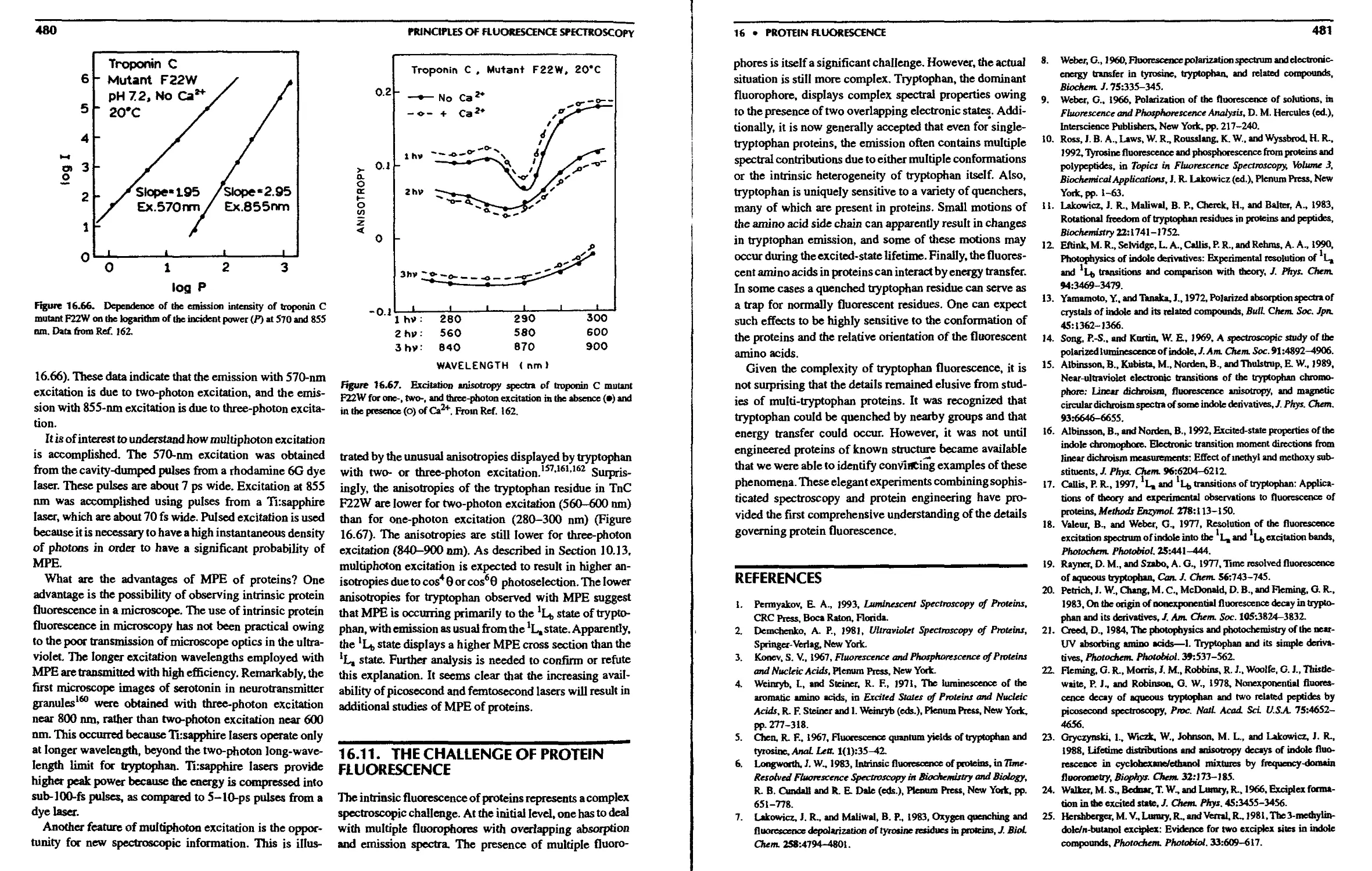
Text
Principles of
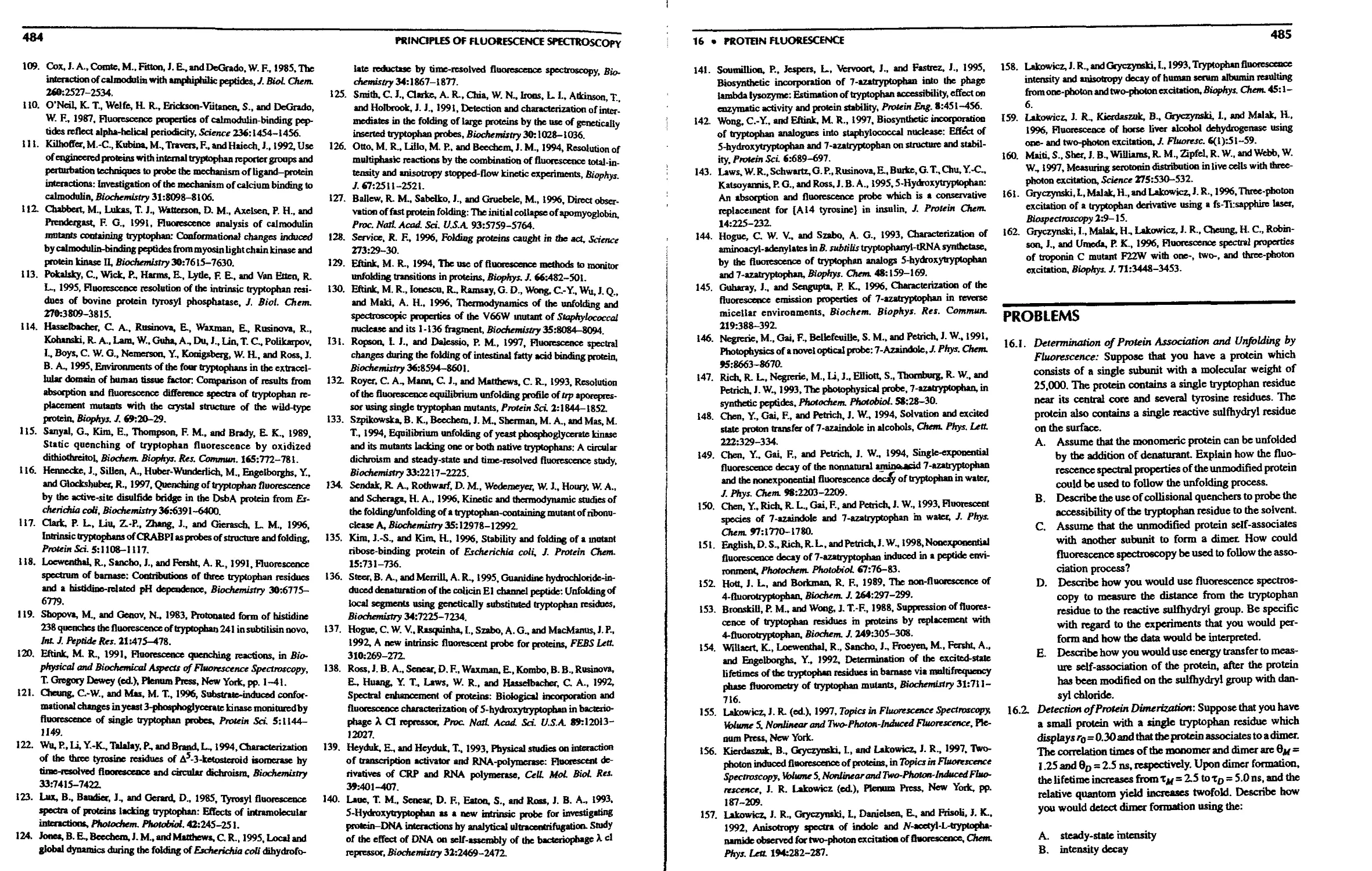
Fluorescence
Spectroscopy
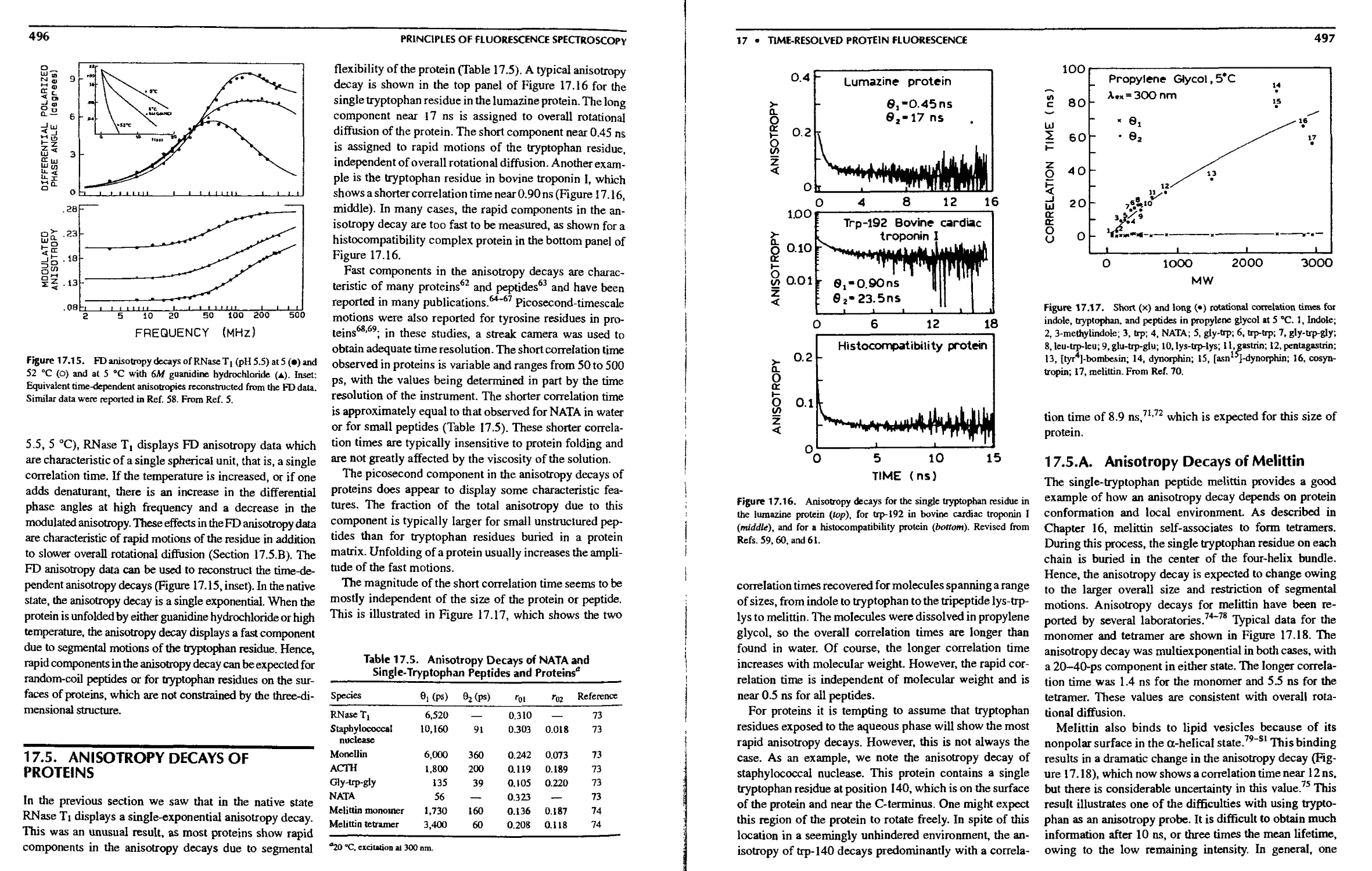
Second Edition
Joseph R. Lakowicz
University of Maryland School of Medicine
Baltimore, Maryland
Kluwer Academic/Plenum Publishers
New York, Boston, Dordrecht, London, Moscow
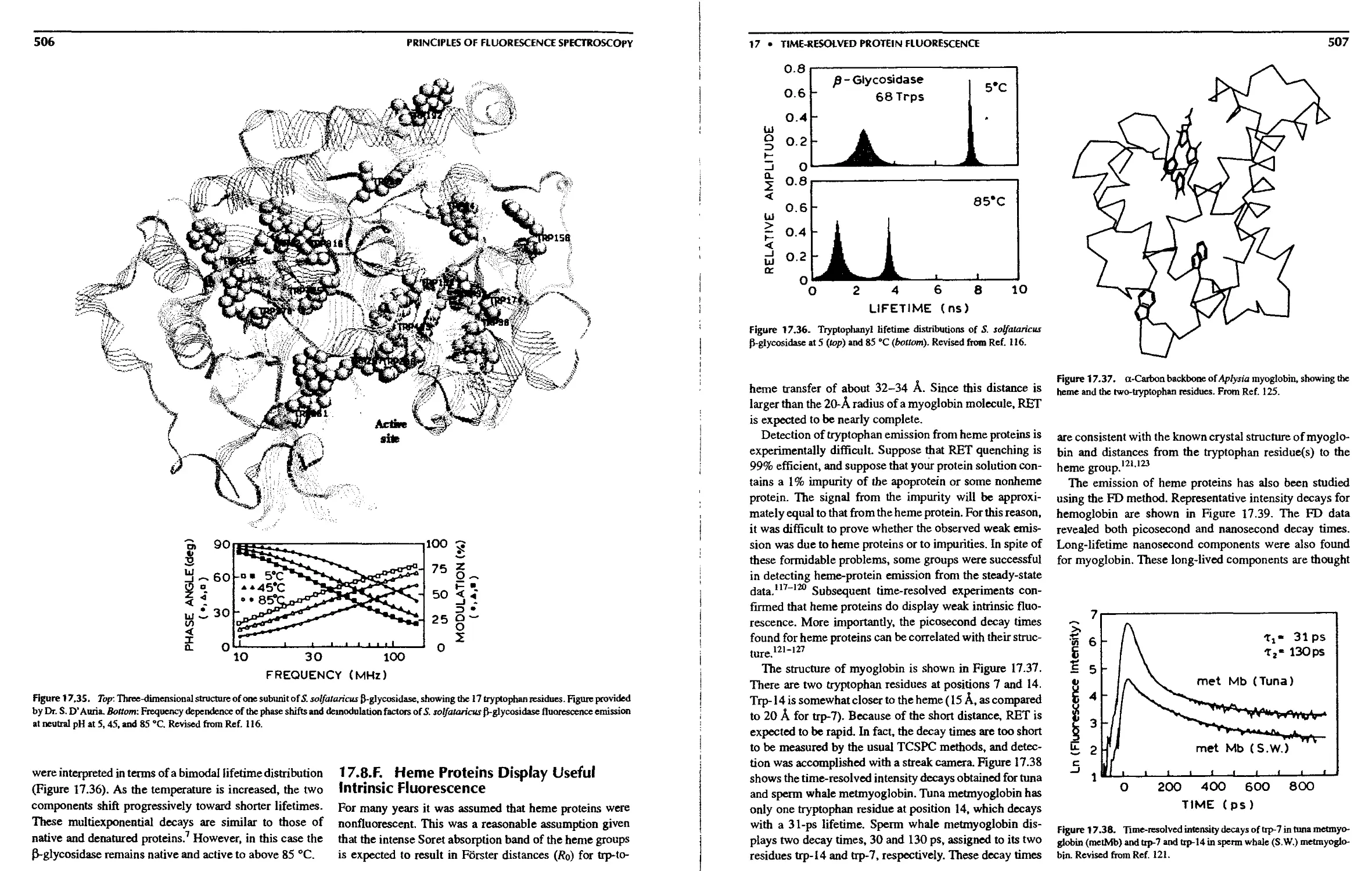
Ltbrary of Congress Catalogfng-ln-PublIcatton Data
.akoHicz, Joseph R.
Princtpies of fluorescence spectroscopy / Joseph R. Ldkow1c2« —w
2nd ей.
p. ел.
ISBN 0-306-46093-9
1. Fluorescence spectroscopy. I. Title.
QD96.F56L34 1999
543'.08584—dc21 99-30047
CIP
ISBN 0-306-46093-9
©1999 Khiwer Academic /Plenum Publishers, New York
233 Spring Street, New York, N.Y. 10013
10 9876543
A C.I.P. record for this book is available from the Library of Congress
All rights reserved
No part of this book may be reproduced, stored in a retrieval system, or transmitted in any form or by any means,
electronic, mechanica], photocopying, microfilming, recording, or otherwise, without written pennission from the
Publisher
Printed in the United States of America
To Professor Aleksander Jabtonski
on the occasion of his 100th birthday
Preface
It has been 15 years since publication of the first edition of
Principles of Fluorescence Spectroscopy. This first vol-
volume grew out of a graduate-level course on fluorescence
taught at the University of Maryland. The first edition was
written during a transition period in the technology and
applications of fluorescence spectroscopy. In 1983, time-
resolved measurements were performed using methods
which are primitive by today's standards. The dominant
light sources for time-resolved fluorescence were the
nanosecond flashlamps, which provided relatively wide
excitaiion pulses. Detection was accomplished with rela-
relatively slow response phoiomultiplier tubes. In the case of
phase-modulation fluorometry, the available instruments
operated at one or two fixed light modulation frequencies
and thus provided limited information on complex time-
resolved decays. Data analysis was also limited because of
the lower information content of the experimental data.
Much has changed since 1983. The dominant lighi
sources are now picosecond dye lasers or femtosecond
Titanium: sapphire lasers. In the case of phase-modulation
fluorometry, frequency-domain instrumentation now op-
operates over a range of light modulation frequencies, allow-
allowing resolution of complex decays. The time resolution in
both the frequency and the time domain has been increased
by the introduction of high-speed microchannel plate
photomultiplier tubes. Data analysis has become increas-
increasingly sophisticated, not only because of the availability of
more powerful computers, but also because of the avail-
availability of additional data and the increased resolution
available using global analysis. These advanced experi-
menial and analysis capabilities have been extended to
provide resolution of complex anisotropy decays, confor-
mational distributions, and complex quenching phenom-
phenomena.
Another important change since 1983 has been the ex-
extensive development of fluorescent probes. Early fluores-
fluorescent probes were those derived from histochemical
staining of cells, a limited number of lipid and conjugat-
able probes, and, of course, intrinsic fluorescence from
proteins. Today the menu of fluorescent probes has ex-
expanded manyfold. A wide variety of lipid and protein
probes have been developed, and probes have become
available with longer excitation and emission wavelengths.
There has been extensive development of cation-sensing
probes for use in cellular imaging. The nanosecond barrier
of dynamic fluorescence information has been broken by
the introduction of long-lifetime probes.
Another example of the rapid expansion of fluorescence
is DNA sequencing technology. Prior to 1985, most DNA
sequencing was performed using radioactive labels. Since
that time, sequencing has been accomplished almost ex-
exclusively with fluorescent probes. The fluorescence tech-
technology for DNA sequencing is advancing rapidly owing to
the goal of sequencing the human genome. Finally, who
would have expected in 1983 that the gene for the green
fluorescent protein could be introduced into cells, with
spontaneous folding and formaiion of the fully fluorescent
protein?
Parts of this book were influenced by a course taughi at
the Center for Fluorescence Spectroscopy, which has been
attended by individuals from throughout the world. How-
However, the most important factor siimulating the second
edition was the positive comments of individuals who
found value in the first edition. Many individuals com-
commented on the value of explaining the basic concepts from
their fundamental origins. Ibis has become increasingly
important as the number of practitioners of fluorescence
spectroscopy has increased, without a significant increase
in the number of courses at the undergraduate or graduate
level.
In this second edition of Principles of Fluorescence
Spectroscopy^ I have attempted to maintain the emphasis
on basics, while updating the examples to include more
recent results from the literature. There is a new chapter
providing an overview of extrinsic fluorophores. The dis-
discussion of time-resolved measurements has been ex-
PRINCIPLES OF FLUORESCENCt SPtCTROSCOPY
panded 10 two chapters. Quenching has also been ex-
expanded to two chapters. Energy transfer and anisotropy
have each been expanded to three chapters. There is also a
new chapter on fluorescence sensing. To enhance the use-
usefulness of this book as a textbook, each chapter is followed
by a set of problems. Sections which describe advanced
topics are indicated as such, to allow these sections to be
skipped in an introductory course. Glossaries of com-
commonly used acronyms and mathematical symbols are pro-
provided. For those wanting additional information, Appendix
III contains a list of recommended books which expand on
various specialized topics.
In closing, I wish to express my appreciation to the many
individuals who have assisted me not only in preparation
of the book but also in the intellectual developments in my
laboratory. My special thanks go to Ms. Mary Rosenfeld
for her careful preparation of the text. Mary has cheerfully
tolerated the copious typing and numerous revisions of all
the chapters. I also thank the many individuals who have
proofread various chapters and provided constructive sug-
suggestions. These individuals include Felix Castellano,
Robert E. Dale, Jonathan Dattelbaum, Maurice Eftink,
John Gilchrist, Zygmunt Gryczynski, Petr Herman, Gabor
Laczko, Li Li, Harriet Lin, Zakir Murtaza, Leah Tolosa,
and Bogumil Zelent. I apologize for any omissions.
I also give my special thanks to Dr. lgnacy Gryczynski
and his wife, Krystyna Gryczynska. When I started to write
this book, lgnacy said "just go and write, don't worry about
the figures." Many of ihe excellent figures in this book
were drawn by Krystyna, with the valuable suggestions of
lgnacy. Without their dedicated efforts, the book could not
have been completed in any reasonable period of time. I
also thank Ms. Suzy Rhinehart for providing a supportive
family environment during preparation of this book. Fi-
Finally, I thank the National Institutes of Health and the
National Science Foundation for support of my labora-
laboratory.
J. R. Lakowicz
Center for Fluorescence Spectrvscopy, Baltimore
Glossary of Acronyms
2,6-ANS 6-Anilinonaphtha!ene-2-sulfonic acid MLCT
ASE Asymptotic standard error MPE
BODIPY Refers to a family of dyes based on 1,3,5,7,8- NADH
pentamethy!pyrTomemene-BF2, or 4,4-di- NATA
fluoro-4-bora-3a,4a-diaza-s-indacene. NATyrA
BODIPY is a trademark of Molecular NBD
Probes, Inc. NIR
СТО Constant fraction discriminator phe
Dansy! 5-Dimethy!aminonaphtha!ene-l-su!fonic PC
acid PMT
DAPI 4',6-Diamidino-2-pheny!indole ЮРОР
DAS Decay-associated spectra PPD
DNS-C1 Dansy! chloride PPO
DPH l,6-Diphenyl-l,3,5-hexatriene Prodan
EB Ethidium bromide PSDF
F Single-letter code for phenylalanine RET
FAD Flavin adenine dinucleotide So
FD Frequency-domain St
FISH Fluorescence in situ hybridization SPQ
FTTC Fluorescein-5-isothiocyanate T[
FMN Flavin mononucleotide TAC
FRET Fluorescence resonance energy transfer TCSPC
GFP Green fluorescent protein TD
HTV Human immunodeficiency virus TICT
HSA Human serum albumin TNS
IAEDANS 5-(((B-iodoacetyl)amino)ethyI)amino)- TRES
naphthalene-l-su!fonic acid TRITC
IAF 5-(Iodoacetamido)fluorescein
ICT Internal charge transfer (state) tip
IRF Instrument response function tyr
LE Locally excited (state) W
MCP MicroChannel plate Y
MLC Metal-ligand complex, usually of a transi-
transition metal (Ru, Rh, or Os)
Metal-ligand charge transfer (state)
Multiphoton excitation
Reduced nicotinamide adenine dinucleotide
N-Acetyl-L-tryptophanamide
N-Acety!-L-tyrosinamide
7-Nitrobenz-2-oxa-1,3-diazo!-4-y!
Near-infrared
Phenylalanine
Phosphatidylcholine
Photomultiplier tube
l,4-BisE-pheny!oxazo!-2-y!)benzene
2,5-Diphenyl-1,3,4-oxadazole
2,5-Diphenyloxazole
6-Propionyl-2-(dimethylamino)naphmalene
Phase-sensitive detection of fluorescence
Resonance energy transfer
Ground electronic state
First excited singlet state
6-Methoxy-N-C-su!fopropy!)quino!ine
First excited triplet state
Time-to-amplitude converter
Time-correlated single-photon counting
Time-domain
Twisted internal charge-transfer state
6-(p-To!uidiny!)naphthalene-2-su!fonicacid
Time-resolved emission spectra
Tetramethylrhodamine 5- (and 6-)isothiocy-
anate
Tryptophan
Tyrosine
Single-letter code for tryptophan
Single-letter code for tyrosine
Glossary of Mathematical
Terms
A Acceptor or absorption r
с Speed of light
Cq Characteristic acceptor concentration in T
resonance energy transfer r@)
C(t) Correlation function for spectral relaxation r(t)
D Donor, diffusion coefficient, or rotational rc
diffusion coefficient
Д| or D± Rate of rotational diffusion around (displac-
(displacing) the symmetry axis of an ellipsoid of /щ or r$g;
revolution
E Efficiency of energy transfer r0
F Steady state intensity or fluorescence
Fx Ratio of 5^ values, used to calculate parame- Го;
ter confidence intervals
F(X) Emission spectrum r«
fi Fractional steady-state intensities in a mul- гш
tiexponential intensity decay Rq
fq Efficiency of collisional quenching CX,-
Correction factor for anisotropy measure-
measurements p
Half-width in a distance or lifetime distribu-
distribution Г
Intensity decay, typically the impulse re- у
sponse function ?
Nonradiative decay rate в
Solvent relaxation rate к
kj Transfer rate in resonance energy transfer
m^j Modulation at a light modulation frequency Л^
со
n Refractive index, when used in consideration X
of solvent effects A^m
N(t^) Number of counts per channel, in time-cor- A^"
related single-photon counting Л^х
Q Quantum yield A^"
P(r) Probability function for a distance (r) distri-
distribution Хпих
рКл Acid dissociation constant, negative loga- \xE
rithm Jic
G
hw
Iff)
к„
k$
Anisotropy (sometimes distance in a dis-
distance distribution)
Average distance in a distance distribution
Time-zero anisotropy
Anisotropy decay
Distance of closest approach between donors
and acceptors in resonance energy transfer,
or fluorophores and quenchers
Fractional amplitudes in a multiexponential
anisotropy decay
Fundamental anisotropy in the absence of
rotational diffusion
Anisotropy amplitudes in a multiexponential
anisotropy decay
Long-time anisotropy in an anisotropy decay
Modulated anisotropy
Forster distance in resonance energy transfer
Preexponential factors in a multiexponential
intensity decay
Angle between absorption and emission
transition moments
Radiative decay rate
Inverse of the decay time: y=\/x
Dielectric constant or extinction coefficient
Rotational correlation time
Orientation factor in resonance energy trans-
transfer
Ratio of the modulated amplitudes of the
polarized components of the emission
Wavelength
Emission wavelength
Maximum emission wavelength
Excitation wavelength
Maximum excitation or absorption wave-
wavelength for the lowest 5 —»Si transition
Emission maximum
Excited-state dipole moment
Ground-state dipole moment
xi
V Wavenumber, in cm
Pcg Emission center of gravity
^f) Time-resolved emission center of gravity, in
cm
X Decay time
% Average lifetime
"fy Apparent lifetime calculated from the phase
angle at a single frequency
To Donor decay time or solvent dielectric re-
relaxation time
%i Solvent longitudinal relaxation time
т„ Apparent lifetime calculated from the modu-
modulation at a single frequency
PRINCIPLES OF FLUORESCENCE SPECTROSCOPY
% Radiative or natural lifetime
%s Solvent relaxation time
До, Differential polarized phase angle, differ-
difference in phase between the parallel and per-
perpendicular components of the emission
фш Phase angle at a light modulation frequency
со
Хд Goodness-of-fit parameter, reduced chi-
squared
X2 Sum of the squared weighted deviations
Ш Light modulation frequency in radians per
second; 2u times the frequency in cycles per
second
Contents
Most sections of this book describe basic aspects of fluorescence spectroscopy, and some sections describe more
advanced topics. These sections are marked "Advanced Topics" and can be omitted in an introductory course on
fluorescence. The advanced chapters on quenching (Chapter 9), anisotropy (Chapter 12), and energy transfer (Chapters
14 and 15) can be skipped in a first reading. Depending on the interest of the reader. Chapters 18 to 22 can also be
skipped.
2. Instrumentation for Fluorescence
1. Introduction to Fluorescence
1.1. Phenomenon of Fluorescence 1
1.2. Jablonski Diagram 4
1.3. Characteristics of Fluorescence Emission . . 6
1.З.А. Stokes'Shift 6
1.З.В. Emission Spectra Are Typically
Independent of the Excitation
Wavelength 7
1.З.С. Exceptions to the Mirror Image Rule 8
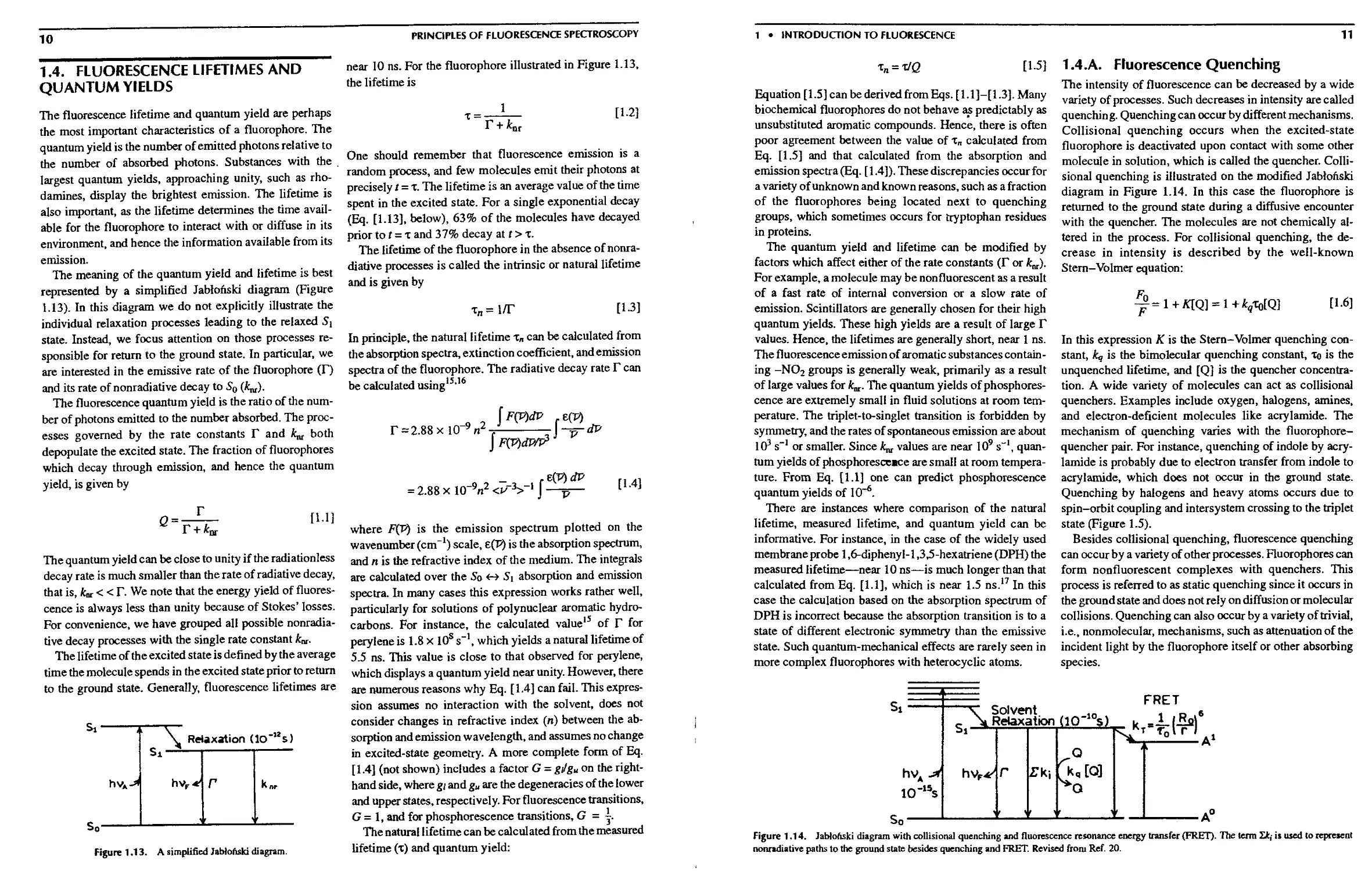
1.4. Fluorescence Lifetimes and Quantum Yields 10
1.4.А. Fluorescence Quenching 11
1.4.В. Time Scale of Molecular Processes in
Solution 12
1.5. Fluorescence Anisotropy 12
1.6. Resonance Energy Transfer 13
1.7. Steady-State and Tune-Resolved Fluorescence 14
1.7 .A. Why Time-Resolved Measurements? 15
1.8. Biochemical Fluorophores 15
1.8.А. Fluorescent Indicators 16
1.9. Molecular Information from Fluorescence . 17
1.9 .A. Emission Spectra and the Stokes' Shift 17
1.9.В. Quenching of Fluorescence 17
1.9.С. Fluorescence Polarization or
Anisotropy 18
I.9.D. Resonance Energy Transfer 19
1.10. Fluorescence Sensing 19
1.11. Summary 20
References 20
Problems 21
2.1. Excitation and Emission Spectra 25
2.1.A. An Ideal Spectrofluorometer 27
2. l.B. Distortions in Excitation and Emission
Spectra 28
2.2. Light Sources 28
2.2.A. Arc and Incandescent Lamps 28
2.2.B. Solid-State Light Sources 31
2.3. Monochromators 32
2.3.A. Wavelength Resolution and Emission
Spectra 33
2.3.B. Polarization Characteristics of
Monochromators 33
2.3.С Stray Light in Monochromators .... 34
2.3.D. Second-Order Transmission in
Monochromators 35
2.3.E. Calibration of Monochromators .... 35
2.4. Optical Filters 36
2.4.A. Bandpass Filters 36
2.4.B. Interference Filters 36
2.4.C. Filter Combinations 38
2.4.D. Neutral Density Filters 38
2.5. Optical Filters and Signal Purity 39
2.5.A. Emission Spectra Taken through Filters 40
2.6. Photomultiplier Tubes 41
2.6.A. Spectral Response 42
2.6.B. PMT Designs and Dynode Chains . . 43
2.6.C. Time Response of Photomultiplier
Tubes 44
xiii
PRINCIPLES OF FLUORESCENCE SPECTROSCOPY
2.6.D. Photon Counting versus Analog
Detection of Fluorescence
2.6.E. Symptoms of PMT Failure
2.6.F. Hybrid Photomultiplier Tubes ....
2.6.G. CCD Detectors
2.7. Polarizers
2.8. Corrected Excitation Spectra
2.8.A. Use of a Quantum Counter to Obtain
Corrected Excitation Spectra ....
2.9. Corrected Emission Spectra
2.9.A. Comparison with Known Emission
Spectra
2.9.B. Correction Factors Obtained by Using
a Standard Lamp
2.9.C. Correction Factors Obtained by Using
a Quantum Counter and Scatterer . .
2.9.D. Conversion between Wavelength and
Wavenumber
2.10. Quantum Yield Standards
2.11. Effects of Sample Geometry
2.12. Common Errors in Sample Preparation . . .
2.13. Absorption of Light and Deviation from the
Beer-Lambert Law
2.13.A. Deviations from Beer's Law ....
2.14. Two-Photon and Multiphoton Excitation . .
2.15. Conclusions
References
Problems
3. Fluorophores
3.1. Intrinsic or Natural Fluorophores
3.1.A. Fluorescent Enzyme Cofactors . . .
З.1.В. Binding of NADH to a Protein . . .
3.2. Extrinsic Fluorophores
3.2.A. Protein-Labeling Reagents
3.2.B. Role of the Stokes' Shift in Protein
Labeling
3.2.C. Solvent-Sensitive Probes
3.2.D. Noncovalent Protein-Labeling Probes
3.2.E. Membrane Probes
3.2.F. Membrane Potential Probes
3.3. Red and Near-Infrared (NIR) Dyes
3.3.A. Measurement of Human Serum
Albumin with Laser Diode Excitation
3.4. DNA Probes
3.4.A. DNA Base Analogs
3.5. Chemical Sensing Probes
3.6. Special Probes
3.6.A. Fluorogenic Probes 78
45 3.6.B. Structural Analogs of Biomolecules . . 81
46 3.6.C. Viscosity Probes 81
47 3.7. Fluorescent Proteins 82
47 3.7.A. Phycobiliproteins 82
47 3.7.B. Green Fluorescent Protein 84
49 3.7.C. Phytofluors—A New Class of
Fluorescent Probes 85
50 3.8. Long-Lifetime Probes 86
51 3.8.A. Lanthanides 87
3.8.B. Transition-Metal-Ligand Complexes 88
51 3.9. Proteins as Sensors 88
3.10. Conclusion 89
51 References 89
Problems 92
51
52
52
53
55
56
57
57
59
59
60
63
63
65
66
67
69
71
71
72
72
74
75
76
77
78
78
4. Time-Domain Lifetime Measurements
4.1. Overview of Time-Domain and
Frequency-Domain Measurements 95
4.1.A. Meaning of the Lifetime or Decay
Time 96
4.1.В. Phase and Modulation Lifetimes ... 97
4.l.C. Examples of Time-Domain and
Frequency-Domain Lifetimes .... 97
4.2. Biopolymers Display Multiexponentia! or
Heterogeneous Decays 98
4.2.A. Resolution of Multiexponential
Decays Is Difficult 100
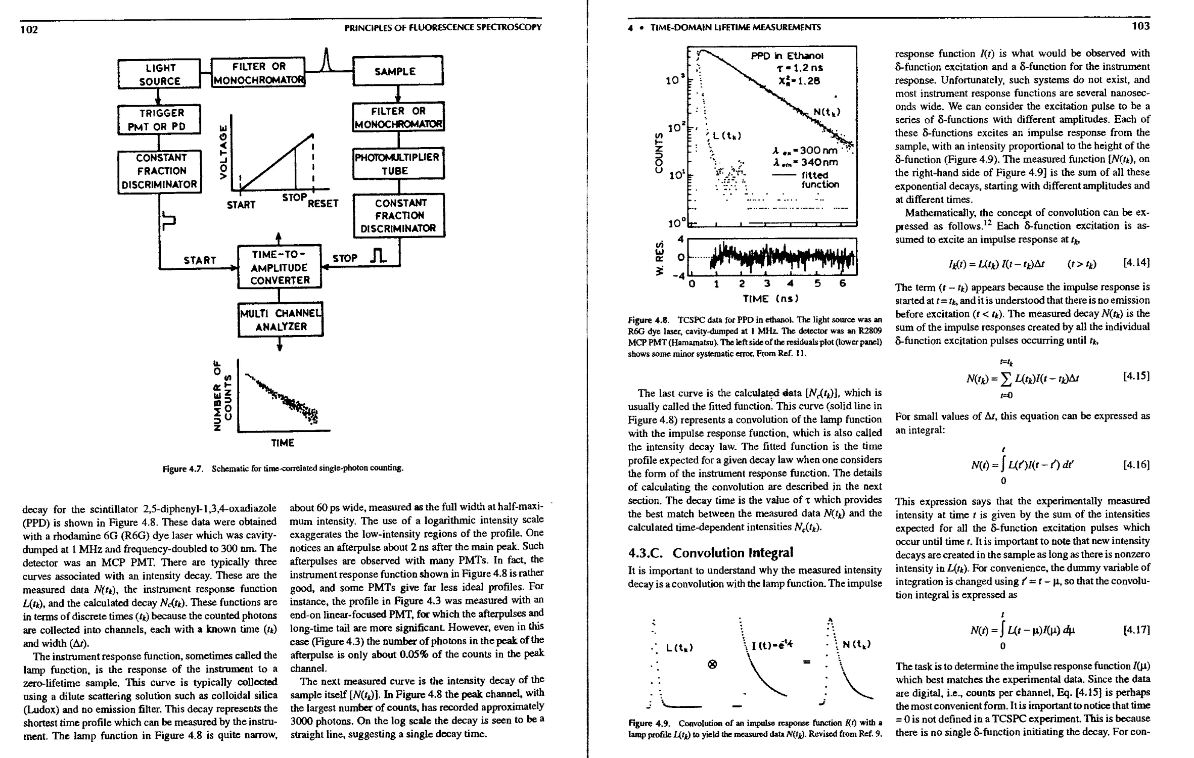
4.3. Time-Correlated Single-Photon Counting . . 101
4.3.A. Principles of TCSPC 101
4.3.B. Example of TCSPC Data 101
4.3.C. Convolution Integral 103
4.4. Light Sources for TCSPC 104
4.4.A. Picosecond Dye Lasers 104
4.4.B. Femtosecond Titanium:Sapphire Lasers 106
4.4.C. Flashlamps 107
4.4.D. Solid-State Lasers 109
4.5. Electronics for TCSPC 109
4.5.A. Constant Fraction Discriminators . . 109
4.5.B. Amplifiers 110
4.5.C. Time-to-Amplitude Converter
(TAC)—Standard and Reversed
Configurations 110
4.5.D. Multichannel Analyzer (MCA) .... 110
4.5.E. Delay Lines 110
4.5.F. PulsePileup Ill
4.6. Detectors for TCSPC Ill
4.6.A. MCPPMTs Ill
CONTENTS
4.6.B. Dynode Chain PMTs 113
4.6.C. Photodiodes as Detectors 114
4.6.D. Color Effects in Detectors 114
4.6.E. Timing Effects of Monochromators . 116
4.7. Alternative Methods for Time-Resolved
Measurements 116
4.7.A. Pulse Sampling or Gated Detection . 116
4.7.B. Streak Cameras 117
4.7.C. Upconversion Methods 118
4.8. Data Analysis 118
4.8.A. Assumptions of Nonlinear
Least-Squares Analysis 119
4.8.B. Overview of Least-Squares Analysis 119
4.8.C. Meaning of the Goodness of Fit, X$ ¦ ¦ 12°
4.8.D. Autocorrelation Function 121
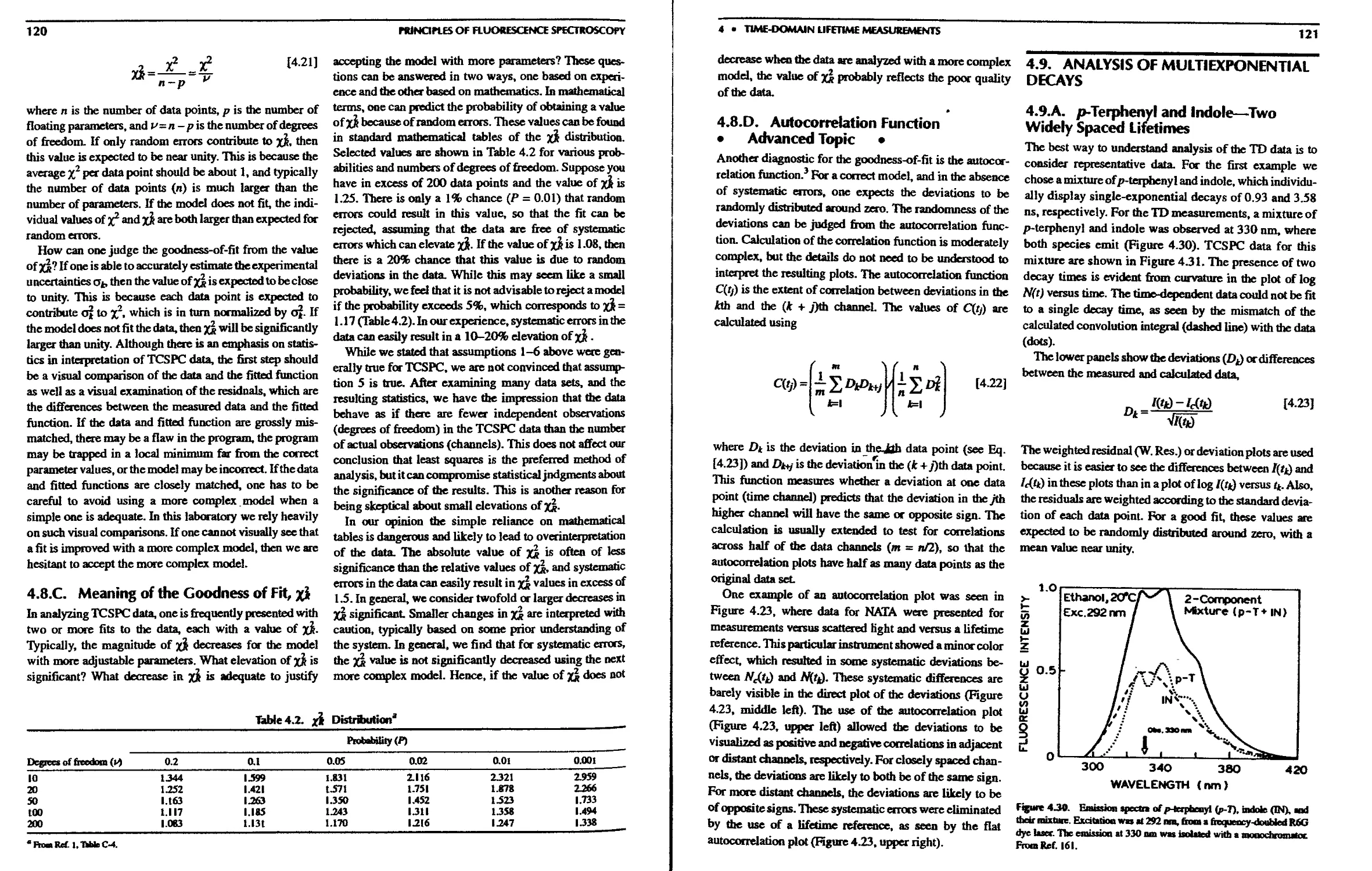
4.9. Analysis of Multiexponential Decays .... 121
4.9.A. p-Terpheny! and Indole—Two Widely
Spaced Lifetimes 121
4.9.B. Comparison of xjj Values—F-Statistic 122
4.9.C. Parameter Uncertainty—Confidence
Intervals 122
4.9.D. Effect of the Number of Photon Counts 124
4.9.E. Anthranffic Acid and 2-Amino-
purine—Two Closely Spaced
Lifetimes 124
4.9.F. Global Analysis—Multiwavelength
Measurements 126
4.9.G. Resolution of Three Closely Spaced
Lifetimes 126
4.10. Intensity Decay Laws 129
4.10.A. Multiexponential Decays 129
4.10.B. Lifetime Distributions 130
4.10.C. Stretched Exponentials 131
4.10.D. Transient Effects 13!
4.11. Global Analysis 132
4.12. Representative Intensity Decays 132
4.12.A. Intensity Decay for a Single-
Tryptophan Protein 132
4.12.B. Green Fluorescent Protein—
Systematic Errors in the Data .... 133
4.12.C. ErythrosinB—A Picosecond Decay
Time 133
4.12.D. Chlorophyll Aggregates in Hexane . 134
4.12.E. Intensity Decay of FAD 134
4.12.F. Microsecond Luminescence Decays 135
4.12.G. Subpicosecond Intensity Decays . . 135
4.13. Closing Comments 136
References 136
Problems 140
5. Frequency-Domain Lifetime
Measurements
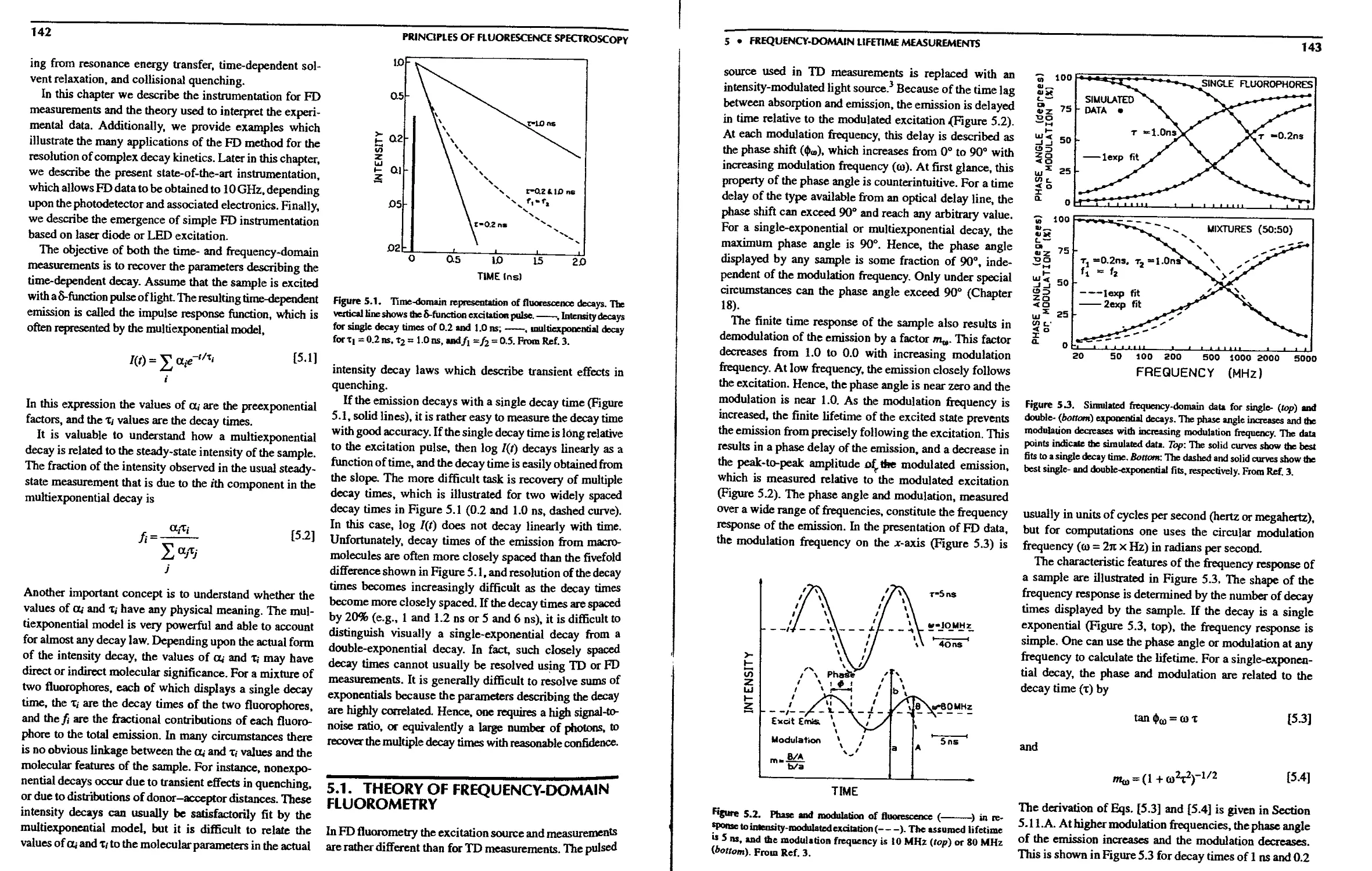
5.1. Theory of Frequency-Domain Fluorometry . . 142
5.LA. Least-Squares Analysis of
Frequency- Domain Intensity Decays 144
5.1.В. Global Analysis of
Frequency-Domain Data 146
5.l.C. Estimation of Parameter Uncertainties 146
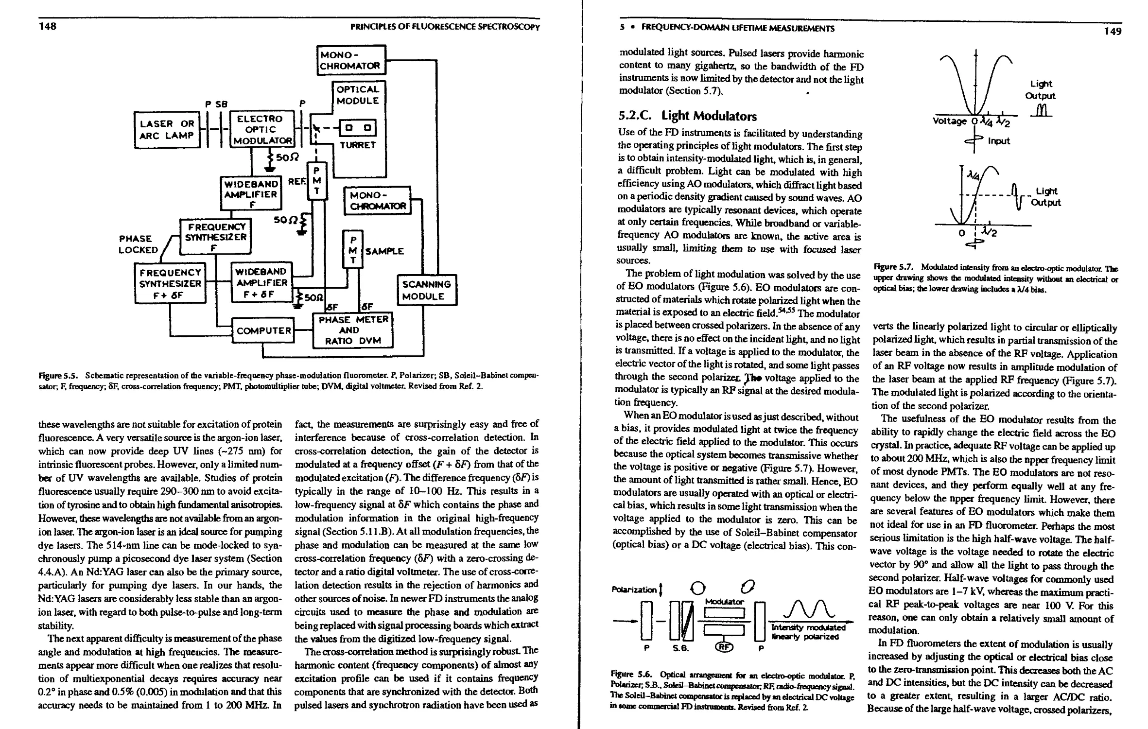
5.2. Frequency-Domain Instrumentation 147
5.2.A. History of Phase-Modulation
Fluorometers 147
5.2.B. The 200-MHz Frequency-Domain
Fluorometer 147
5.2.C. Light Modulators 149
5.2.D. Cross-Correlation Detection 150
5.2.E. Frequency Synthesizers 150
5.2.F. Radio-Frequency Amplifiers 150
5.2.G. Photomultiplier Tubes 150
5.2.H. Principle of Frequency-Domain
Measurements 151
5.3. Color Effects and Background Fluorescence . . 152
5.3.A. Color Effects in Frequency-Domain
Measurements 152
5.3.B. Background Correction in
Frequency-Domain Measurements . . 153
5.4. Representative Frequency-Domain Intensity
Decays 154
5.4.A. Exponential Decays 154
5.4.B. Effect of Scattered Light 154
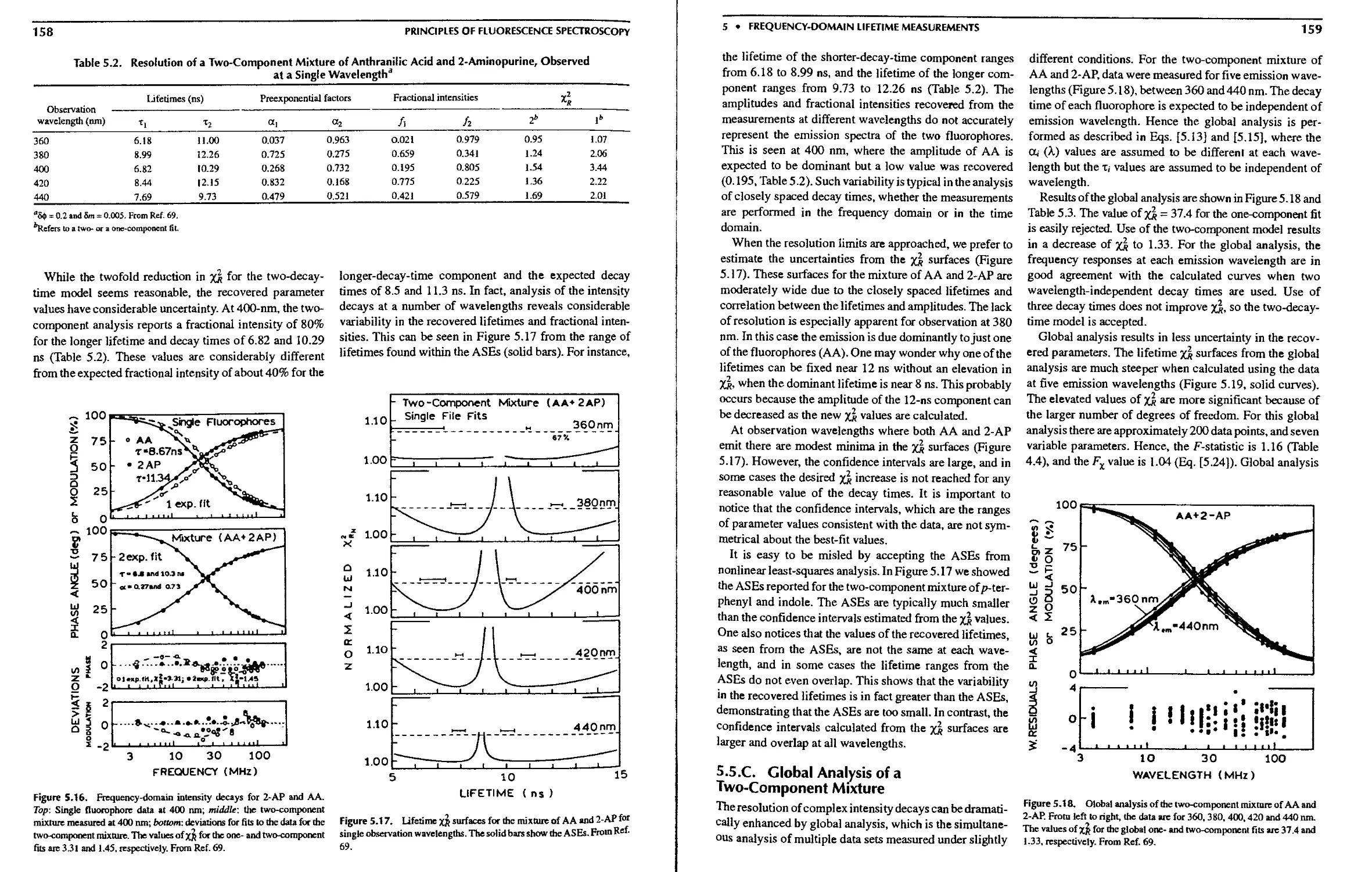
5.5. Analysis of Multiexponential Decays .... 155
5.5.A. Resolution of Two Widely Spaced
Lifetimes 155
5.5.B. Resolution of Two Closely Spaced
Lifetimes 157
5.5.C. Global Analysis of a Two-Component
Mixture 159
5.5.D. Analysis of a Three-Component
Mixture—Limits of Resolution ... 160
5.5.E. Resolution of a Three-Component
Mixture with a 10-Fold Range of
Decay Times 162
5.6. Biochemical Examples of
Frequency-Domain Intensity Decays .... 163
5.6.A. Monellin—A Single-Tryptophan
Protein with Three Decay Times ... 163
5.6.B. Multiexponential Decays of
Staphylococcal Nuclease and Melittin 163
5.6.C. DNA Labeled with DAPI 164
PRINCIPLES OF FLUORESCENCE SPECTROSCOPY
5.6.D. Quin-2—A Lifetime-Based Sensor for
Calcium 165
5.6.E. SPQ—Collisiona! Quenching of a
Chloride Sensor 165
5.6.F. Green Fluorescent Protein—One- and
Two-Photon Excitation 166
5.6.G. Recovery of Lifetime Distributions
from Frequency-Domain Data .... 166
5.6.H. Lifetime Distribution of
Photosynthetic Components 167
5.6.1. Lifetime Distributions of the
Ca2+-ATPase 167
5.6.J. Cross Fitting of Models—Lifetime
Distributions of Melittin 168
5.6.K. Intensity Decay of NADH 169
5.7. Gigahertz Frequency-Domain Fluorometry 169
5.7.A. Gigahertz FD Measurements .... 171
5.7.B. Biochemical Examples of Gigahertz
FDData 172
5.8. Simple Frequency-Domain Instruments . . 173
5.8.A. Laser Diode Excitation 173
5.8.B. LED Excitation 173
5.9. Phase Angle and Modulation Spectra .... 175
5.9.A. Resolution of the Two Emission
Spectra of Tryptophan Using
Phase-Modulation Spectra 176
5.10. Apparent Phase and Modulation Lifetimes 177
5.11. Derivation of the Equations for Phase-
Modulation Fluorescence 178
5.11 .A. Relationship of the Lifetime to the
Phase Angle and Modulation .... 178
5.11.B. Cross-Correlation Detection .... 180
5.12. Perspectives on Frequency-Domain
Fluorometry 180
References 180
Problems 184
6. Solvent Effects on Emission Spectra
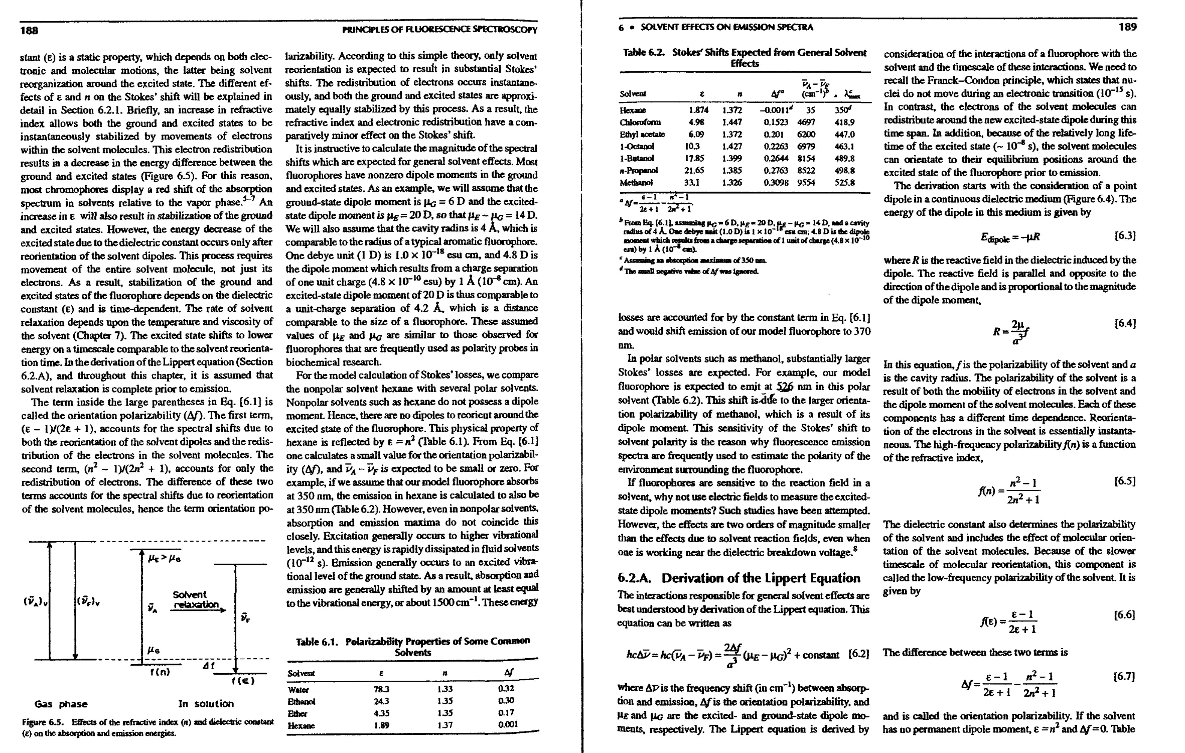
6.1. Overview of Solvent Effects 185
6.1 .A. Polarity Surrounding a Membrane-
Bound Fluorophore 186
6.1.В. Mechanisms for Spectral Shifts . . . 186
6.2. Genera! Solvent Effects—The Lippert
Equation 187
6.2.A. Derivation of the Lippert Equation . . 189
6.2.B. Application of the Lippert Equation . . 191
6.2.C. Polarity Scales 193
6.3. Specific Solvent Effects 194
6.3.A. Specific Solvent Effects and Lippert
Plots 196
6.4. Temperature Effects 198
6.4.A. LE and ICT States of Prodan 200
6.5. Biochemical Examples Using PRODAN . . 201
6.5.A. Phase Transition in Membranes . . . 201
6.5.B. Protein Association 202
6.5.C. Fatty Acid Binding Proteins 202
6.6. Biochemical Examples Using Solvent-
Sensitive Probes 202
6.6.A. Exposure of a Hydrophobic Surface
on Calmodulin 202
6.6.B. Binding to Cyclodextrins Using a
Dansy! Probe 203
6.6.C. Polarity of a Membrane Binding Site . . 203
6.7. Development of Advanced Solvent-Sensitive
Probes 204
6.8. Effects of Solvent Mixtures 206
6.9. Summary of Solvent Effects 207
References 207
Problems 210
7. Dynamics of Solvent and Spectral
Relaxation
7.1. Continuous and Two-State Spectral
Relaxation 212
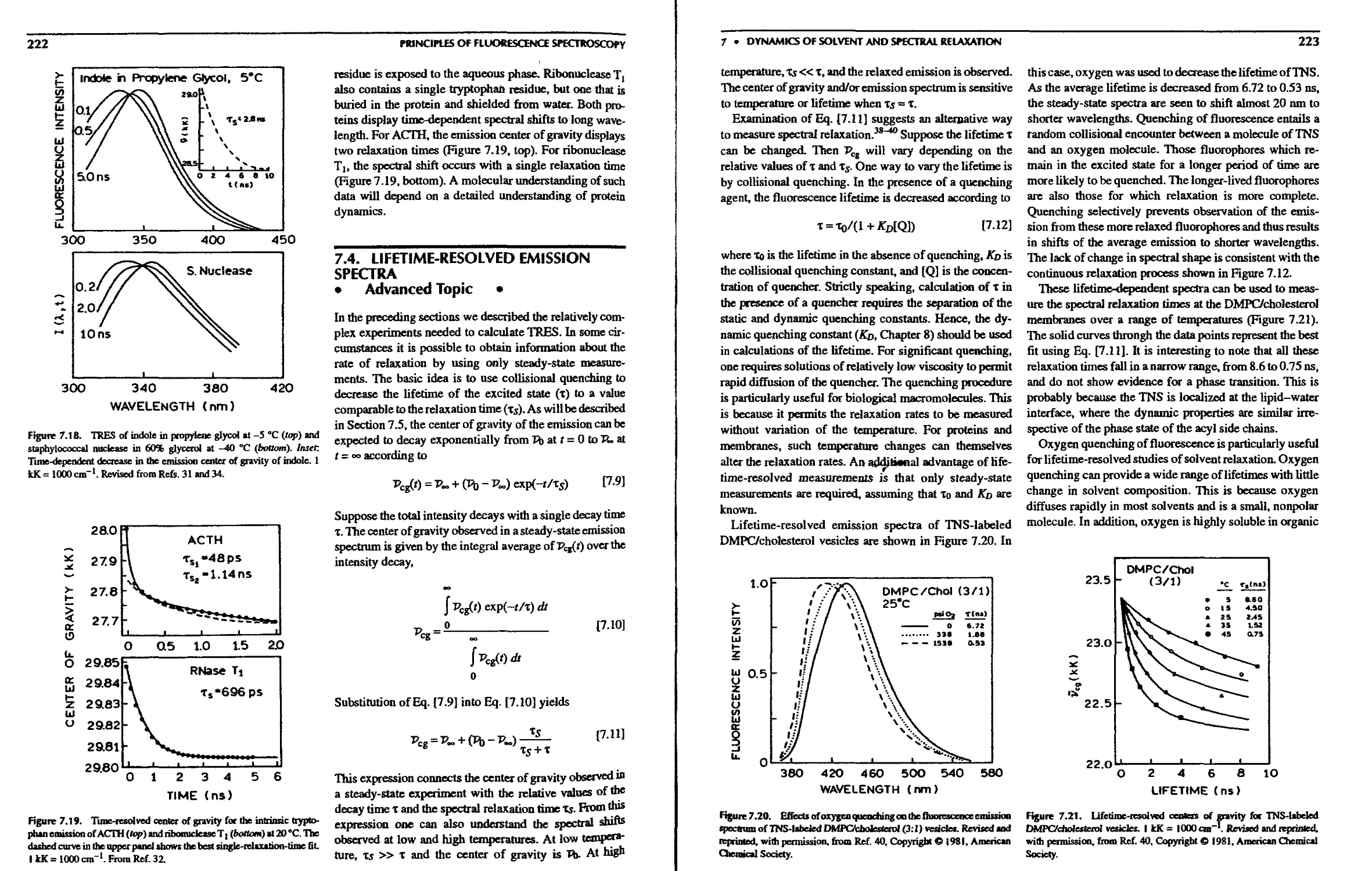
7.2. Measurement of TRES 213
7.2.A. Direct Recording of TRES 213
7.2.B. TRES from Wavelength-Dependent
Decays 213
7.3. Biochemical Examples of TRES 215
7.3.A. Spectral Relaxation in Apomyoglobin 215
7.3.B. TRES of Labeled Membranes .... 217
7.3.C. Analysis of TRES 218
7.3.D. Spectral Relaxation in Proteins .... 220
7.4. Lifetime-Resolved Emission Spectra .... 222
7.5. Picosecond Relaxation in Solvents 224
7.5.A. Theory for Time-Dependent Solvent
Relaxation 224
7.5.B. Multiexponential Relaxation in Water 225
7.6. Comparison of Continuous and Two-State
Relaxation 226
7.6.A. Experimental Distinction between
Continuous and Two-State Relaxation 227
7.6.B. Phase-Modulation Studies of Solvent
Relaxation 227
CONTENTS
xvii
7.6.C. Distinction between Solvent
Relaxation and Formation of
Rotational Isomers 229
7.7. Comparison of TRES and DAS . .* 230
7.8. Red-Edge Excitation Shifts 231
7.9. Perspectives of Solvent Dynamics 233
References 233
Problems 236
8.11. A. Quenching Due to Specific Binding
Interactions 255
8.11.B. Binding of Substrates to Ribozymes 256
8.1 l.C. Association Reactions and Quenching 257
8.12. Intramolecular Quenching 257
8.13. Quenching of Phosphorescence 258
References 259
Problems 264
8. Quenching of Fluorescence
8.1. Quenchers of Fluorescence 238
8.2. Theory of Collisional Quenching 239
8.2.A. Derivation of the Stern-Volmer
Equation 240
8.2.B. Interpretation of the Bimolecular
Quenching Constant 241
8.3. Theory of Static Quenching 242
8.4. Combined Dynamic and Static Quenching . . 243
8.5. Examples of Static and Dynamic Quenching 243
8.6. Deviations from the Stem-Xblmer Equation;
Quenching Sphere of Action 244
8.6.A. Derivation of the Quenching Sphere of
Action 245
8.7. Effects of Steric Shielding and Charge on
Quenching 245
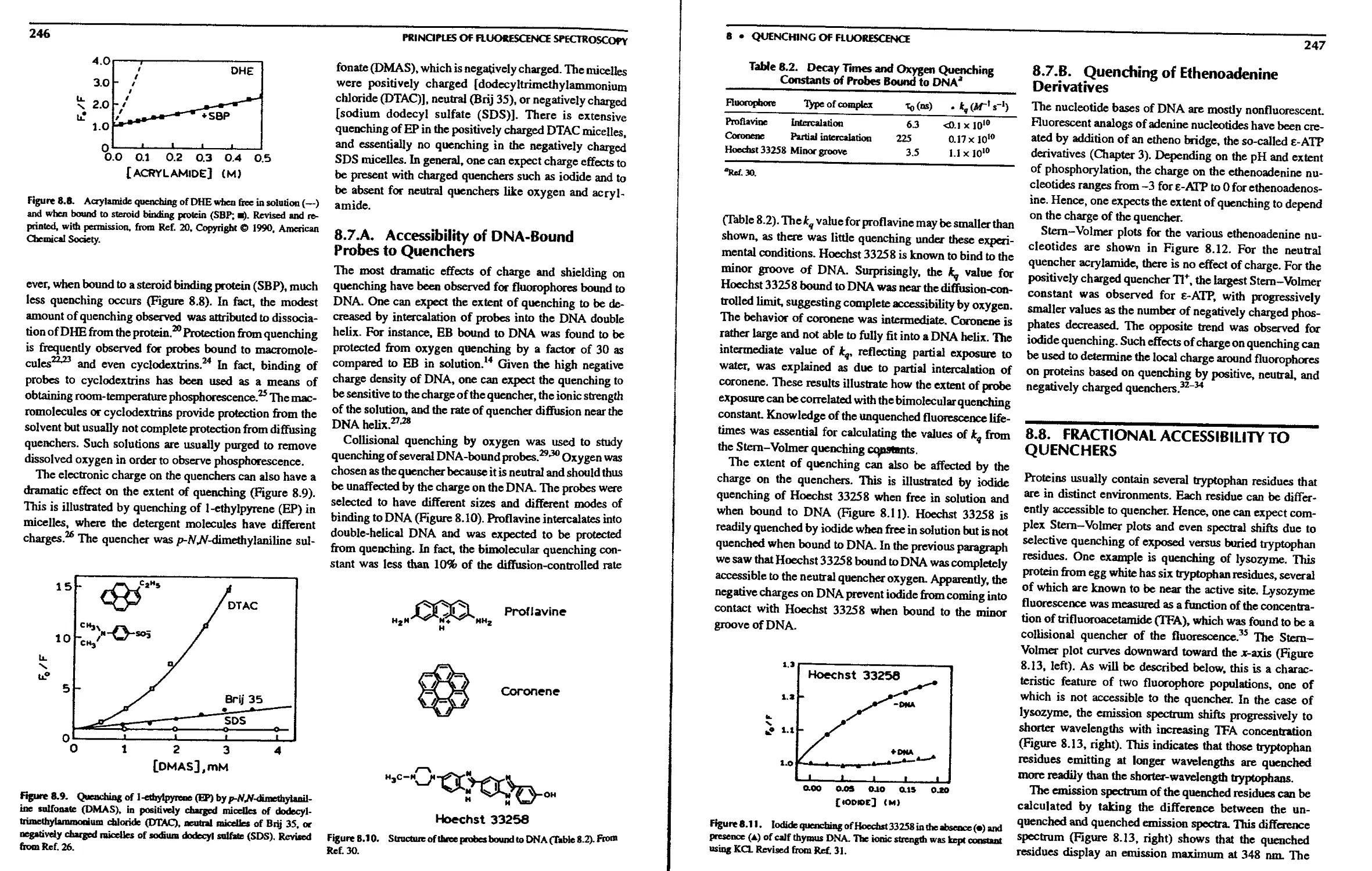
8.7.A. Accessibility of DNA-Bound Probes
to Quenchers 246
8.7.B. Quenching of Ethenoadenine
Derivatives 247
8.8. Fractional Accessibility to Quenchers .... 247
8.8.A. Modified Stem-Volmer Plots .... 248
8.8.B. Experimental Considerations in
Quenching 249
8.9. Applications of Quenching to Proteins . . . 249
8.9.A. Fractional Accessibility of Tryptophan
Residues in Endonuclease Ш .... 249
8.9.B. Effect of Conformational Changes on
Tryptophan Accessibility 250
8.9.C. Quenching of the Multiple Decay
Times of Proteins 250
8.9.D. Effects of Quenchers on Proteins . . 251
8.9.E. Protein Folding of Colicin El .... 251
8.10. Quenching-Resolved Emission Spectra . . . 252
8.10.A. Fluorophore Mixtures 252
8.10.B. Quenching-Resolved Emission
Spectra of the ? сой TetRepressor . . 253
8.11. Quenching and Association Reactions .... 255
9. Advanced Topics in Fluorescence
Quenching
9.1. Quenching in Membranes 267
9.1 .A. Accessibility of Membrane Probes to
Water- and Lipid-Soluble Quenchers 267
9.1.В. Quenching of Membrane Probes
Using Localized Quenchers 270
9.l.C. Parallax Quenching in Membranes . . 272
9.I.D. Boundary Lipid Quenching 273
9.1 .E. Effect of Lipid-Water Partitioning on
Quenching 274
9.2. Diffusion in Membranes 276
9.2.A. Quasi-Three-Dimensional Diffusion
in Membranes 276
9.2.B. Lateral Diffusion in Membranes . . . 278
9.3. Quenching Efficiency 278
9.3.A. Steric Shielding Effects in Quenching 279
9.4. Transient Effects in Quenching 280
9.4.A. Experimental Studies of Transient
Effects 281
9.4.B. Distance-Dependent Quenching in
Proteins 285
References 286
Problems 289
10. Fluorescence Anisotropy
10.1. Definition of Fluorescence Anisotropy .... 291
10.1.A. Origin of the Definitions of
Polarization and Anisotropy 292
10.2. Theory for Anisotropy 293
10.2.A. Excitation Photoselection of
Fluorophores 294
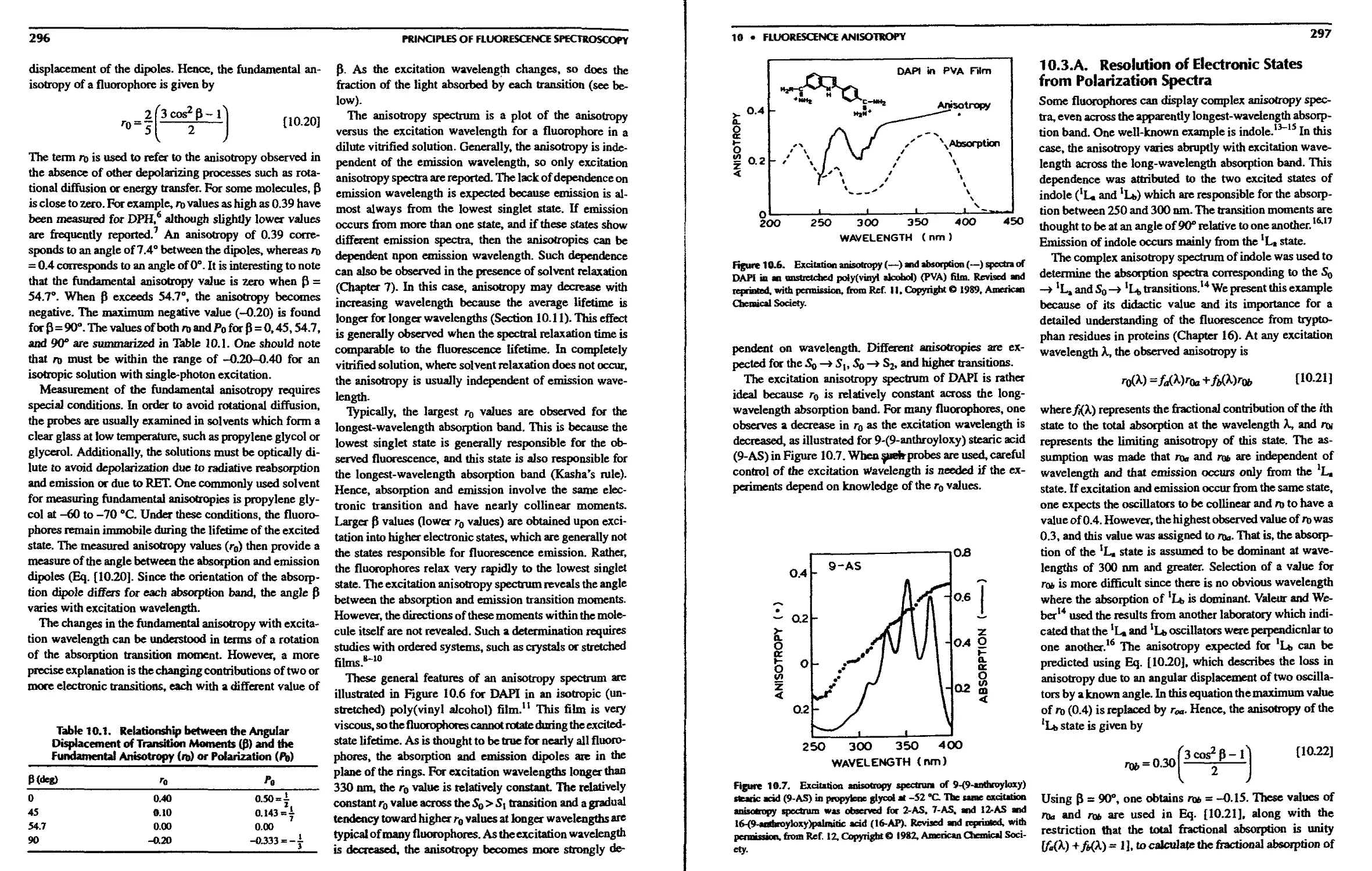
10.3. Excitation Anisotropy Spectra 295
10.3.A. Resolution of Electronic States from
Polarization Spectra 297
10.4. Measurement of Fluorescence Anisotropies . . 298
10.4.A. L-Format or Single-Channel Method 298
PRINCIPLES OF FLUORESCENCE SPECTROSCOPY
10.4.B. T-Fonmt от Two-Channel Anisotropies 299
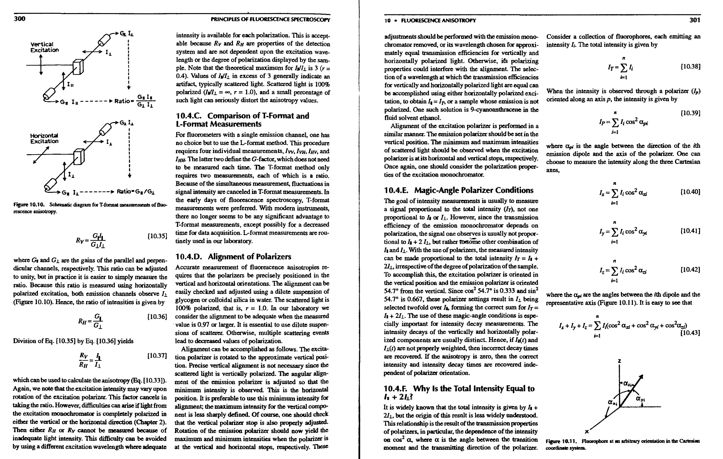
10.4.C. Comparison of T-Format and L-Format
Measurements 300
10.4.D. Alignment of Polarizers 300
10.4.E. Magic-Angle Polarizer Conditions . 301
10.4.F. Why Is the Total Intensity Equal to /,
+ 2/±? 301
10.4.G. Effect of Radiationless Energy
Transfer on the Anisotropy .... 302
10.4.H. Trivial Causes of Depolarization . . 302
10.4.1. Factors Affecting the Anisotropy . . 303
10.5. Effects of Rotational Diffusion on Fluorescence
Anisotropies: The Perrin Equation 303
10.5.A. The Perrin Equation—Rotational
Motions of Proteins 304
10.5.B. Examples of Perrin Plots 306
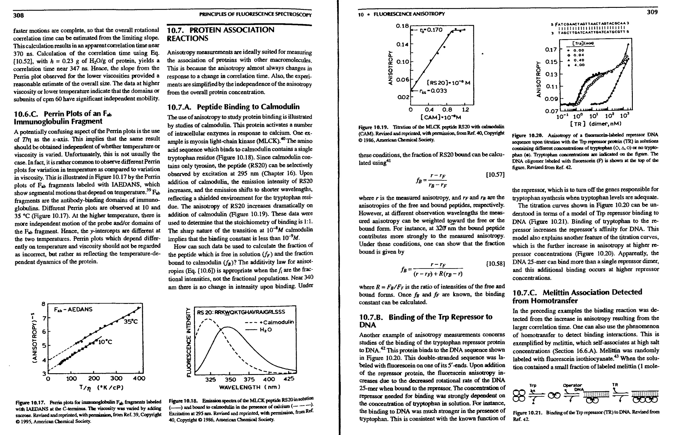
10.6. Perrin Plots of Proteins 307
10.6.A. Binding of tRNA to tRNA Synthetase 307
10.6.B. Molecular Chaperonin cpm 60
(GroEL) 307
10.6.C. Perrin Plots of an F^, Immuno-
globulin Fragment 308
10.7. Protein Association Reactions 308
10.7.A. Peptide Binding to Calmodulin . . 308
10.7.B. Binding of the Trp Repressor to DNA 309
10.7.C. Melittin Association Detected from
Homotransfer 309
10.8. Anisotropy of Membrane-Bound Probes . . 310
10.9. Lifetime-Resolved Anisotropies 310
10.9.A. Effect of Segmenta! Motion on the
Perrin Plots 311
10.10. Soleillet's Rule—Multiplication of
Depolarization Factors 312
10.11. Anisotropies Can Depend on Emission
Wavelength 312
10.12. Transition Moments 313
10.12.A. Anisotropy of Planar Fluorophores
with High Symmetry 314
10.13. Anisotropies with Multiphoton Excitation . . 315
10.13.A. Excitation Photoselection for
Two-Photon Excitation 315
10.13.B. Two-Photon Anisotropy of DPH . . 315
References 316
Problems 318
11. Time-Dependent Anisotropy Decays
11.1. Analysis of Time-Domain Anisotropy Decays 321
11.2. Anisotropy Decay Analysis 325
П.2.А. Time-Domain Anisotropy Data ... 325
11.2.B. Valueofr0 327
11.3. Analysis of Frequency-Domain Anisotropy
Decays 327
11.4. Anisotropy Decay Laws 328
11.4.A. Nonspherical Fluorophores 328
11.4.B. Hindered Rotors 329
11.4.C. Segmental Mobility of a Biopolymer-
BoundFluorophore 329
11.4.D. Correlation Time Distributions .... 330
H.4.E. Associated Anisotropy Decays . . . 331
11.5. Hindered Rotational Diffusion in Membranes 331
11.6. Time-Domain Anisotropy Decays of Proteins 333
11.6. A. Intrinsic Tryptophan Anisotropy Decay
of Liver Alcohol Dehydrogenase . . . 333
11.6.B. PhospholipaseA, 334
11.6.C. Domain Motions of Immunoglobulins 334
11.6.D. Effects of Free Probe on Anisotropy
Decays 335
11.7. Frequency-Domain Anisotropy Decays of
Proteins 335
11.7.A. Apomyoglobin—A Rigid Rotor ... 335
11.7.B. Melittin Self-Association and
Anisotropy Decays 336
11.7.С. Picosecond Rotational Diffusion of
Oxytocin 336
11.8. Microsecond Anisotropy Decays 337
11.8.A. Phosphorescence Anisotropy Decays . 337
11.8.B. Long-Lifetime Metal-Ligand
Complexes 337
11.9. Anisotropy Decays of Nucleic Acids 338
11.9. A. Hydrodynamics of DNA Oligomers . 339
11.9.B. Segmental Mobility of DNA 340
11.10. Characterization of aNew Membrane Probe 341
References 342
Problems 345
12. Advanced Anisotropy Concepts
12.1. Rotational Diffusion of Nonspherical
Molecules—An Overview 347
12.1.A. Anisotropy Decays of Ellipsoids . . 348
12.2. Ellipsoids of Revolution 349
12.2.A. Simplified Ellipsoids of Revolution . . 349
12.2.B. Intuitive Description of an Oblate
Ellipsoid 351
12.2.C. Rotational Correlation Times for
Ellipsoids of Revolution 351
12.2.D. Stick versus Slip Rotational Diffusion 353
CONTENTS
12.3. Complete Theory for Rotational Diffusion of
Ellipsoids 354
12.4. Time-Domain Studies of Anisotropic Rotational
Diffusion 354
12.5. Frequency-Domain Studies of Anisotropic
Rotational Diffusion 355
12.6. Global Anisotropy Decay Analysis with
Multiwavelength Excitation 357
12.7. Global Anisotropy Decay Analysis with
Collisional Quenching 359
12.7.A. Application of Quenching to Protein
Anisotropy Decays 360
12.8. DNA 361
12.9. Associated Anisotropy Decay 362
12.9. A. Theory for Associated Anisotropy
Decays 363
12.9.B. Time-Domain Measurements of
Associated Anisotropy Decays .... 364
12.9.C. Frequency-Domain Measurements of
Associated Anisotropy Decays . . . 364
References 365
Problems 366
13. Energy Transfer
13.1. Theory of Energy Transfer for a
Donor-Acceptor Pair 368
13.1.A. Orientation Factor K2 371
13.1.B. Dependence of the Transfer Rate on
Distance (r), the Overlap Integral (У),
and к2 373
13. l.C. Homotransfer and Heterolransfer . . 373
13.2. Distance Measurements Using RET 374
13.2. A. Distance Measurements in a-Helical
Melittin 374
13.2.B. Effect of к2 on the Possible Range of
Distances 375
13.2.C. Protein Folding Measured by RET . . 376
13.2.D. Orientation of a Protein-Bound Peptide 377
13.3. Use of RET to Measure Macromolecular
Associations 378
13.3. A. Dissociation of the Catalytic and
Regulatory Subunits of a Protein
Kinase 378
13.3.B. RET Calcium Indicators 379
13.3.C. Association Kinetics of DNA
Oligomers 380
13.3.D. Energy Transfer Efficiency from
Enhanced Acceptor Fluorescence . . 381
13.4. Energy Transfer in Membranes 382
13.4.A. Lipid Distributions around Gramicidin 384
13.4.B. Distance of Closest Approach in
Membranes 385
13.4.С Membrane Fusion and Lipid Exchange 386
13.5. Energy Transfer in Solution 386
13.5.A. Diffusion-Enhanced Energy Transfer 387
13.6. Representative Ro Values 388
References 388
Problems 391
14. Time-Resolved Energy Transfer and
Conformational Distributions of
Biopolymers
14.1. Distance Distributions 395
14.2. Distance Distributions in Peptides 398
14.2.A. Comparison for a Rigid and a
Flexible Hexapeptide 398
14.2.B. Cross-fitting Data to Exclude
Alternative Models 399
14.2.C. Donor Decay without RET 400
14.2.D. Effect of Concentration of the D-A
Pairs 401
14.3. Distance Distributions in Proteins 401
14.3.A. Distance Distributions in Melittin . . 401
14.3.B. Distance Distribution Analysis with
Frequency-Domain Data 404
14.3.C. Distance Distributions from
Time-Domain Measurements .... 406
14.3.D. Analysis of Distance Distribution
from Time-Domain Measurements . . 409
14.3.E. Domain Motion in Proteins 409
14.3.F. Distance Distribution Functions . . . 409
14.4. Distance Distributions in a Glycopeptide . . . 410
14.5. Effect of Diffusion for Linked D-A Pairs . . 411
14.5.A. Simulations of RET for a Flexible
D-A Pair 411
14.5.B. Experimental Measurement of D-A
Diffusion for a Linked D-A Pair . . 412
14.5.C. $ Surfaces and Parameter Resolution 413
14.5.D. Diffusion and Apparent Distance
Distributions 415
14.5.E. RET and Diffusive Motions in
Biopolymers 416
14.6. Distance Distributions in Nucleic Acids . . . 416
14.6.A. Double-Helical DNA 416
14.6.B. Four-Way Holliday Junction in DNA 417
14.7. Other Considerations 418
PRINCIPLES OF FlUORtSCENCE SPtCTROSCOPY
14.7 ,A. Acceptor Decays 418
14.7.B. Effects of Incomplete Labeling . . . 418
14.7.C. Effect of the Orientation Factor к2 . 419
14.8. Distance Distributions from Steady-State Data 419
14.8.A. D-A Pairs with Different Ro Values 419
14.8.B. Changing Ro by Quenching .... 420
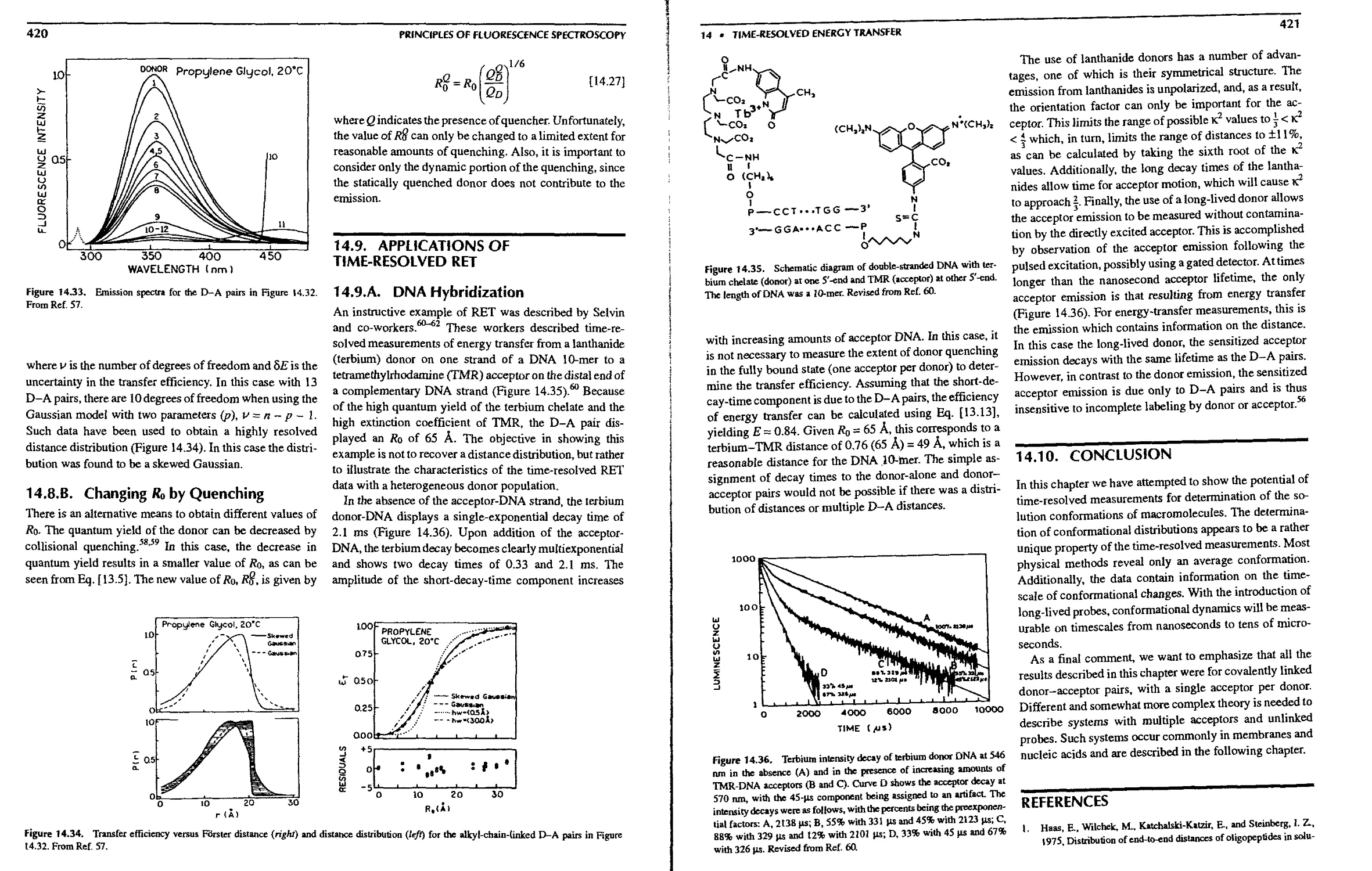
14.9. Applications of Time-Resolved RET .... 420
14.9.A. DNA Hybridization 420
14.10. Conclusion 421
References 421
Problems 423
15. Energy Transfer to Multiple
Acceptors, in One, Two, or Three
Dimensions
15.1. RET in Three Dimensions 426
15.1.A. Effect of Diffusion on RET with
Unlinked Donors and Acceptors . . 428
15.2. Effect of Dimensionality on RET 429
15.2.A. Experimental RET in Two
Dimensions 430
15.2.B. Experimental RET in One Dimension 432
15.3. Energy Transfer in Restricted Geometries . . 434
15.3.A. Effect of an Excluded Area on
Energy Transfer in Two Dimensions 435
15.4. RET in the Rapid-Diffusion Limit 435
15.4.A. Location of an Acceptor in Lipid
Vesicles 437
15.4.B. Location of Retinal in Rhodopsin
Disk Membranes 438
15.4.C. Forster Transfer versus Exchange
Interactions 439
15.5. Conclusions 440
References 440
Problems 442
16. Protein Fluorescence
16.1. Spectral Properties of the Aromatic Amino
Acids 446
16.1 A. Excitation Polarization Spectra of
Tyrosine and Tryptophan 447
16.1.B. Solvent Effects on Tryptophan
Emission Spectra 449
16. l.C. Excited-State Ionization of
Tyrosine 450
16.1.D. Ground-State Complex Formation by
Tyrosine 451
16. I.E. Excimer Formation by Phenylalanine 452
16.2. General Features of Protein Fluorescence . . 452
16.3. Tryptophan Emission in an Apolar Protein
Environment 454
16.3.A. Site-Directed Mutagenesis of a
Single-Tryptophan Azurin 454
16.3.B. Emission Spectra of Azurins with
One or Two Tryptophan Residues . . 455
16.4. Energy Transfer in Proteins 456
16.4.A. Tyrosine-to-Tryptophan Energy
Transfer in Interferon-y 456
16.4.B. Quantitation of RET Efficiencies in
Proteins 457
16.4.C. Energy Transfer Detected by
Decreases in Anisotropy 459
16.4.D. Phenylalanine-to-Tyrosine Energy
Transfer 459
16.5. Quenching of Tryptophan Residues in
Proteins 461
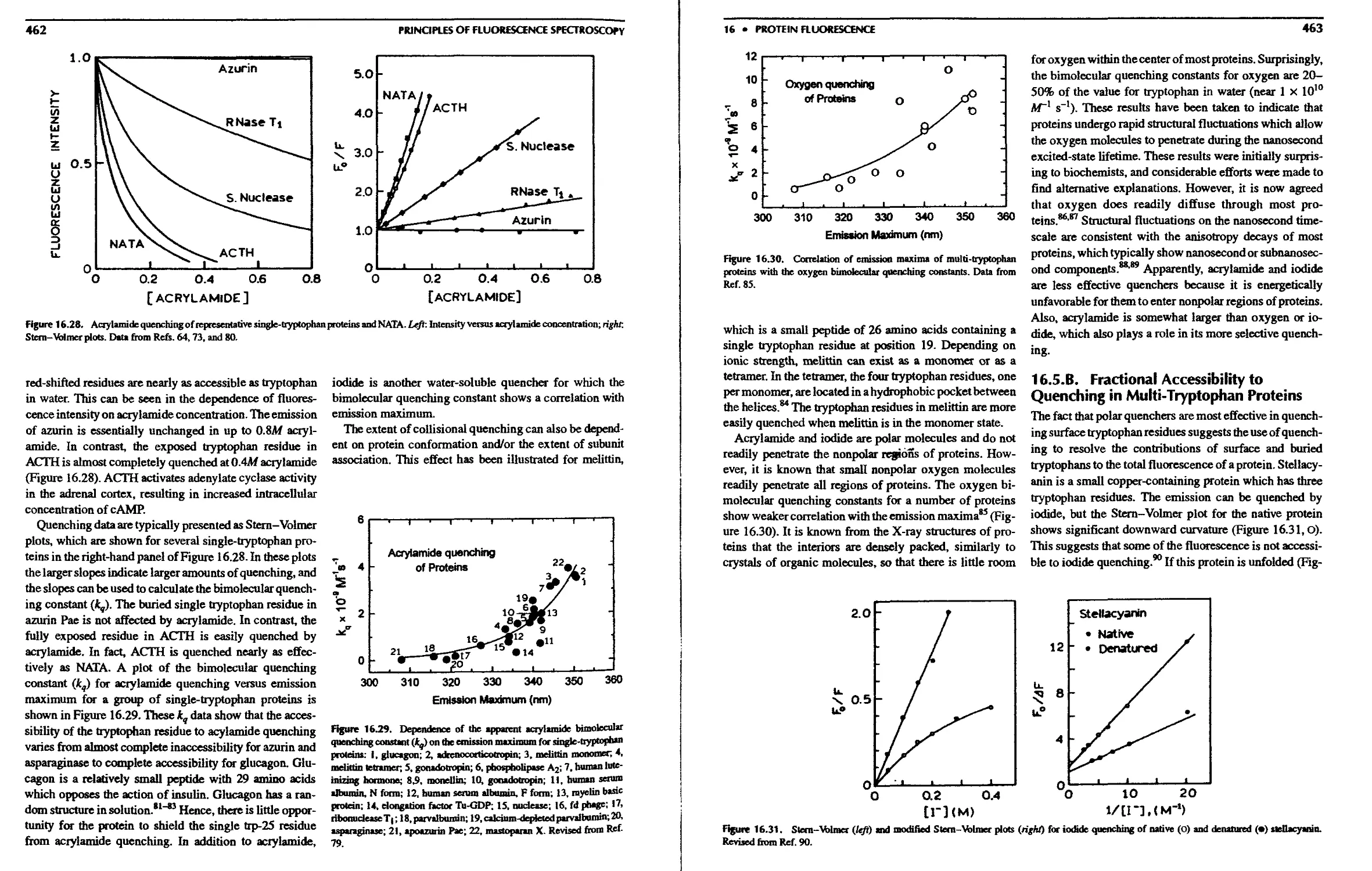
16.5 .A. Effect of Emission Maximum on
Quenching 461
16.5.B. Fractional Accessibility to
Quenching in Multitryptophan
Proteins 463
16.5.C. Resolution of Emission Spectra by
Quenching 464
16.6. Association Reactions of Proteins 465
16.6.A. Self-Association of Melittin and
Binding to Calmodulin 465
16.6.B. Ligand Binding to Proteins 465
16.6.C. Correlation of Emission Maxima,
Anisotropy, and Quenching Constant
for Tryptophan Residues 466
16.6.D. Calmodulin: Resolution of the Four
Calcium Binding Sites Using
Tryptophan-Containing Mutants . . 468
16.7. Spectra! Properties of Genetically Engineered
Proteins 469
16.7.A. Protein Tyrosy! Phosphatase—A
Simple Two-Tryptophan Protein . . 469
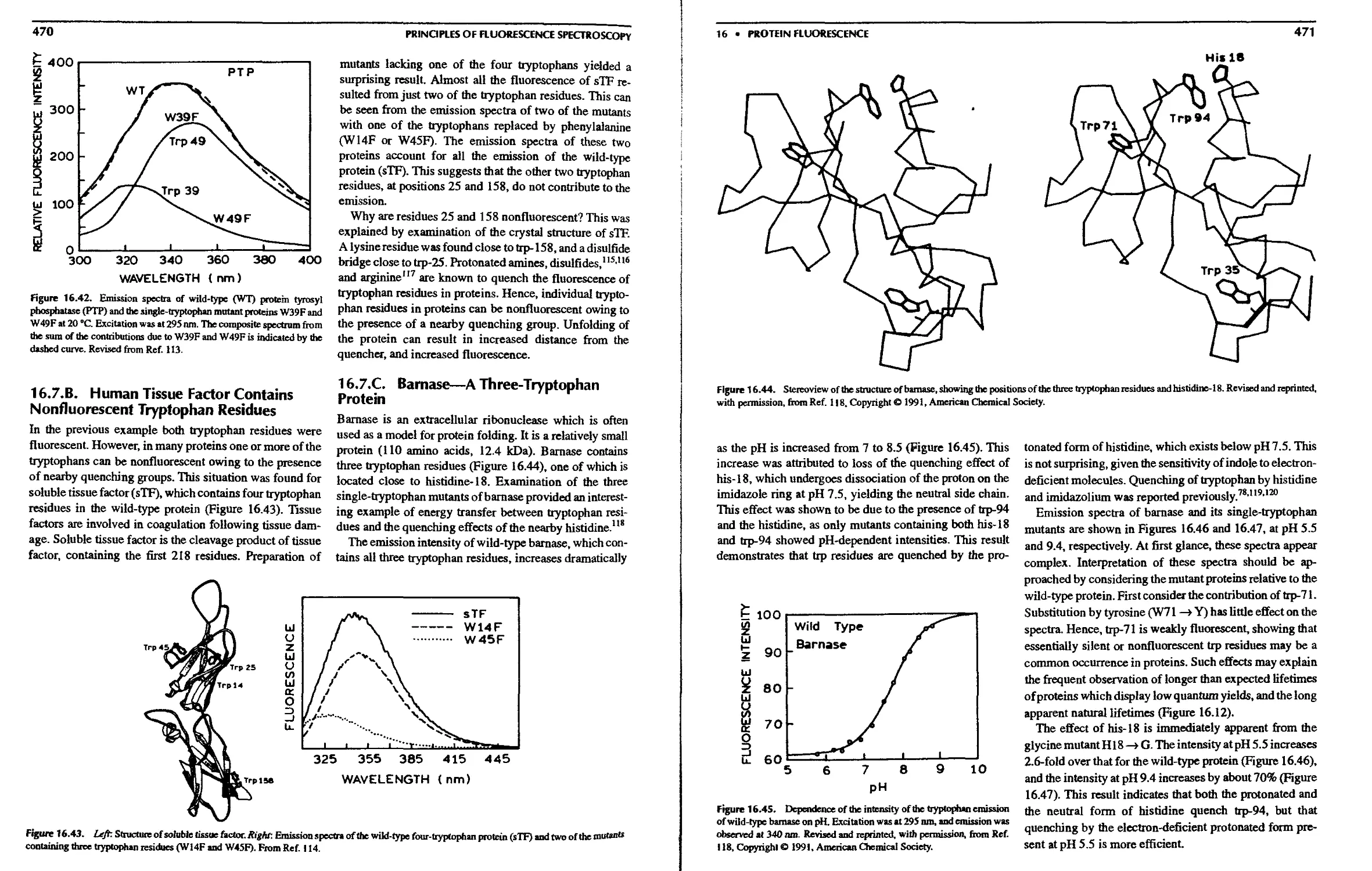
16.7.B. Human Tissue Factor Contains
Nonfluorescent Tryptophan Residues 470
16.7.C. Barnase—A Three-Tryptophan
Protein 470
16.7.D. Substrate Binding and Site-Directed
Mutagenesis 472
16.7.E. Site-Directed Mutagenesis of
Tyrosine Proteins 472
CONTENTS
xxi
16.8. Protein Folding 473
16.8.A. Protein Engineering of Mutant
Ribonuclease for Folding
Experiments 474
16.8.B. Ribose Binding Protein—Insertion
of Tryptophan Residues in Each
Domain 474
16.8.C. Emission Spectra of Native and
Denatured Proteins 475
16.8.D. Folding of Lactate Dehydrogenase 475
16.9. Tryptophan Analogs 476
16.10. Multiphoton Excitation of Proteins 479
16.11. The Challenge of Protein Fluorescence . . 480
References 481
Problems 485
17.8.B. Immunophilin FKBP59—Quenching
of Tryptophan Fluorescence by
Phenylalanine 503
17.8.C. Trp Represser—Resolution of the
Two Interacting Tryptophans by
Site-Directed Mutagenesis 504
17.8.D. Aspartate Transcarbamylase—Two
Noninteracting Tryptophan Residues 504
17.8.E. Thermophilic (J-Glycosidase—
Multi-tryptophan Protein 505
17.8.F. Heme Proteins Display Useful
Intrinsic Fluorescence 506
17.9. Phosphorescence of Proteins 508
17.10. Perspectives on Protein Fluorescence .... 509
References 510
Problems 514
17. Time-Resolved Protein Fluorescence
17.1. Intensity Decays of Tryptophan—The
Rotamer Model 488
17.2. Time-Resolved Intensity Decays of
Tryptophan and Tyrosine 489
17.2.A. Decay-Associated Emission Spectra
ofTryptophan 490
17.2.B. Intensity Decays of Neutral
Tryptophan Derivatives 491
17.2.C. Intensity Decays of Tyrosine and Its
Neutral Derivatives 491
17.3. Intensity Decays of Proteins 492
17.4. Effects of Protein Structure on the Intensity
and Anisotropy Decay of Ribonuclease T] . . 493
17.4.A. Protein Unfolding Exposes the
Tryptophan Residue to Water .... 493
17.4.B. Conformationa! Heterogeneity Can
Result in Complex Intensity and
Anisotropy Decays 494
17.5. Anisotropy Decays of Proteins 496
17.5.A. Anisotropy Decays of Melittin . . . 497
17.5.B. Protein Anisotropy Decays as
Observed in the Frequency Domain 498
17.6. Time-Dependent Spectral Relaxation in
Proteins 498
17.7. Decay-Associated Emission Spectra of
Proteins 499
17.8. Time-Resolved Studies of Representative
Proteins 501
17.8.A. AnnexinV—A Calcium-Sensitive
Single-Tryptophan Protein 501
18. Excited-State Reactions
18.1. Examples of Excited-State Reactions 515
18.1.A. Excited-State Ionization of Naphtho! 516
18.2. Reversible Two-State Model 518
18.2 A. Steady-State Fluorescence of a
Two-State Reaction 518
18.2.B. Tune-Resolved Decays for the
Two-State Mode! 518
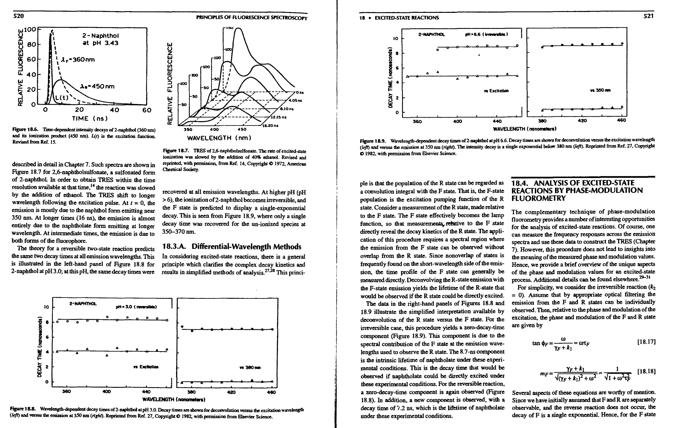
18.3. Time-Domain Studies of Naphthol
Dissociation 519
18.3.A. Differential-Wavelength Methods . . 520
18.4. Analysis of Excited-State Reactions by
Phase-Modulation Fluorometry 521
18.4.A. Effect of an Excited-State Reaction
on the Apparent Phase and
Modulation Lifetimes 523
18.4.B. Wavelength-Dependent Phase and
Modulation Values for an
Excited-State Reaction 524
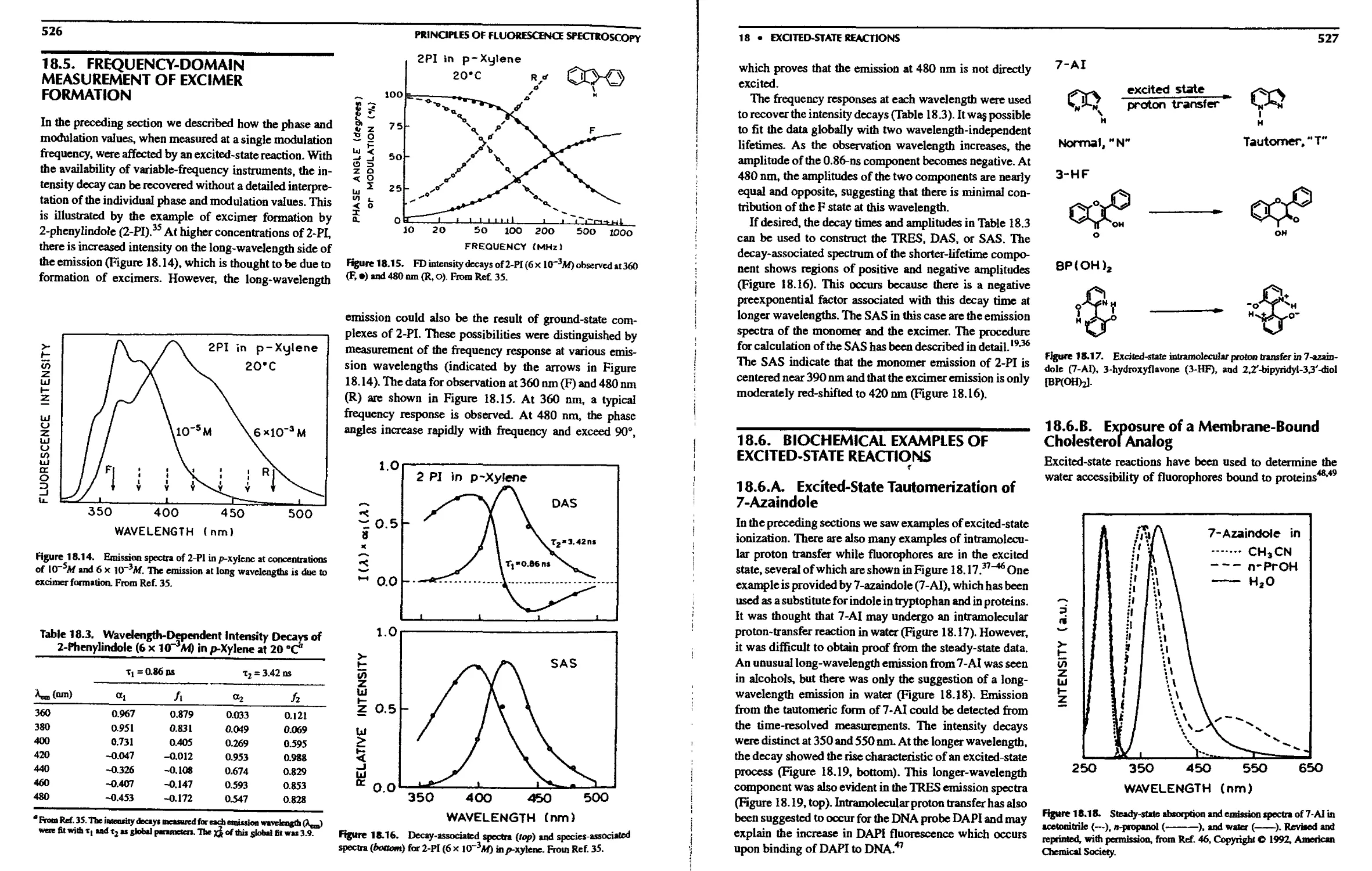
18.5. Frequency-Domain Measurement of Excimer
Formation 526
18.6. Biochemical Examples of Excited-State
Reactions 527
18.6.A. Excited-State Tautomerization of
7-Azaindo!e 527
18.6.B. Exposure of a Membrane-Bound
Cholesterol Analog 527
18.7. Conclusion 528
References 528
Problems 530
PRINCIPLES OF FLUORESCENCE SPECTROSCOPY
19. Fluorescence Sensing
19.1. Optical Clinical Chemistry 531
19.2. Spectral Observables for Fluorescence
Sensing 532
19.2. A. Optical Properties of Tissues .... 534
19.2.B. Lifetime-Based Sensing 534
19.3. Mechanisms of Sensing 535
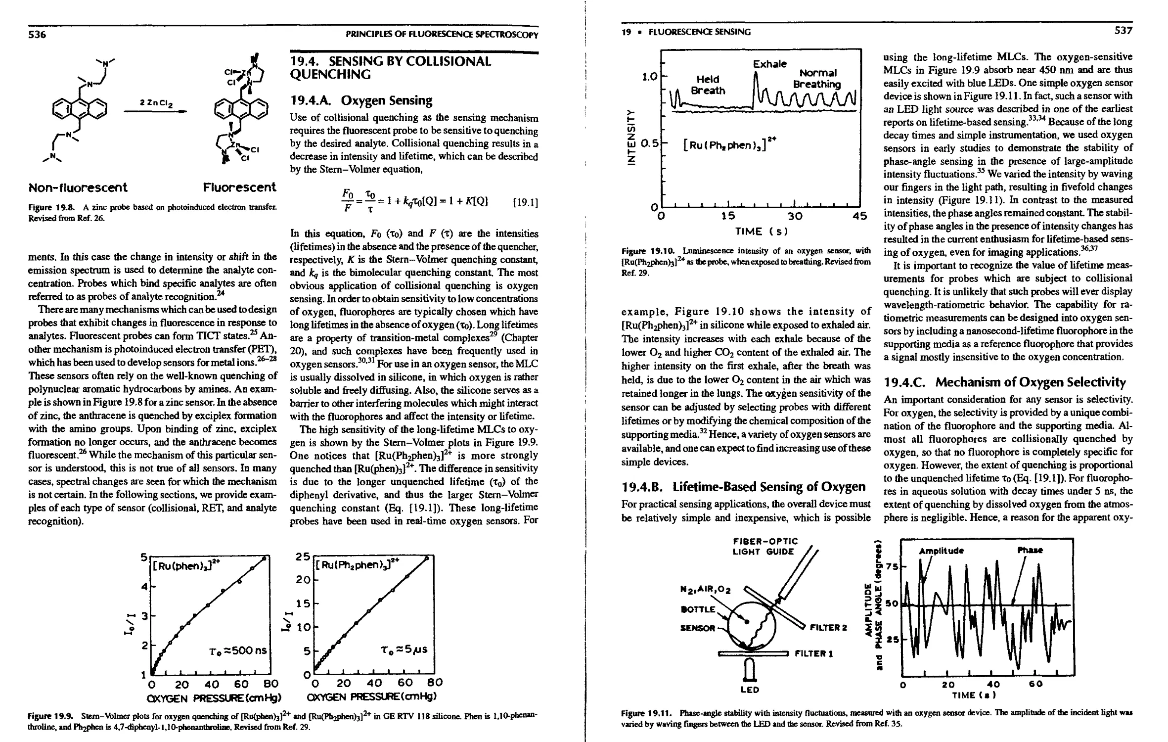
19.4. Sensing by Collisional Quenching 536
19.4.A. Oxygen Sensing 536
19.4.B. Lifetime-Based Sensing of Oxygen 537
19.4.C. Mechanism of Oxygen Selectivity . . 537
19.4.D. Other Oxygen Sensors 538
19.4.E. Chloride Sensors 539
19.4.F. Other Collisional Quenchers .... 541
19.5. Energy-Transfer Sensing 541
19.5.A. pH and pCO2 Sensing by Energy
Transfer 541
19.5.B. Glucose Sensing by Energy Transfer 542
19.5.C. Ion Sensing by Energy Transfer . . 543
19.5.D. Theory for Energy-Transfer Sensing 545
19.6. Two-State pH Sensors 545
19.6.A. Optical Detection of Blood Gases . . 545
19.6.B. pH Sensors 546
19.7. Photoinduced Electron-Transfer (PET)
Probes for Metal Ions and Anion Sensors . . 551
19.8. Probes of Analyte Recognition 552
19.8.A. Specificity of Cation Probes .... 552
19.8.B. Theory of Analyte Recognition
Sensing 553
19.8.C. Sodium and Potassium Probes ... 554
19.8.D. Calcium and Magnesium Probes . . 556
19.8.E. Glucose Probes 559
19.9. Immunoassays 560
19.9.A. Enzyme-Linked Immunosorbent
Assays (ELISA) 560
19.9.B. Time-Resolved Immunoassays . . . 560
19.9.C. Energy-Transfer Immunoassays . . 562
19.9.D. Fluorescence Polarization
Immunoassays 563
19.10.Conclusions 565
References 566
Problems 572
20. Long-Lifetime Metal-Ligand
Complexes
20.1. Introduction to Metal-Ligand Probes .
573
20.1.A. Anisotropy Properties of
Metal-Ligand Complexes 575
20.2. Spectral Properties of Metal-Ligand Probes. . 576
20.2.A. The Energy-Gap Law 577
20.3. Biophysical Applications of Metal-Ligand
Probes 577
20.3.A. DNA Dynamics with Metal-Ligand
Probes 578
20.3.B. Domain-to-Domain Motions in
Proteins 580
20.3.C. MLC Lipid Probes 581
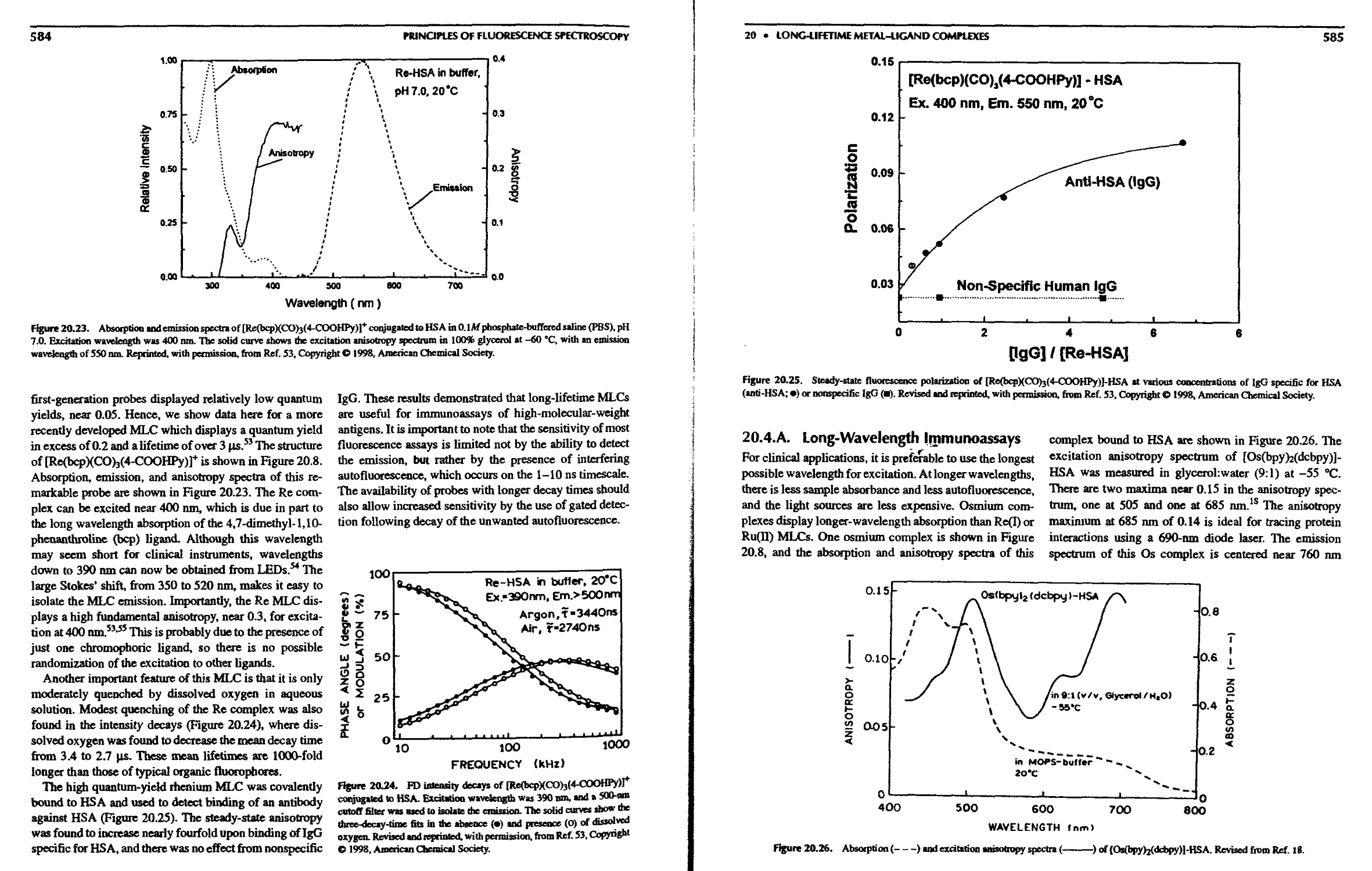
20.4. MLC Immunoassays 582
20.4.A. Long-Wavelength Immunoassays . . 585
20.4.B. Lifetime Immunoassays Based on
RET 586
20.5. Clinical Chemistry with Metal-Ligand
Complexes 587
20.6. Perspective on Metal-Ligand Probes .... 591
References 591
Problems 593
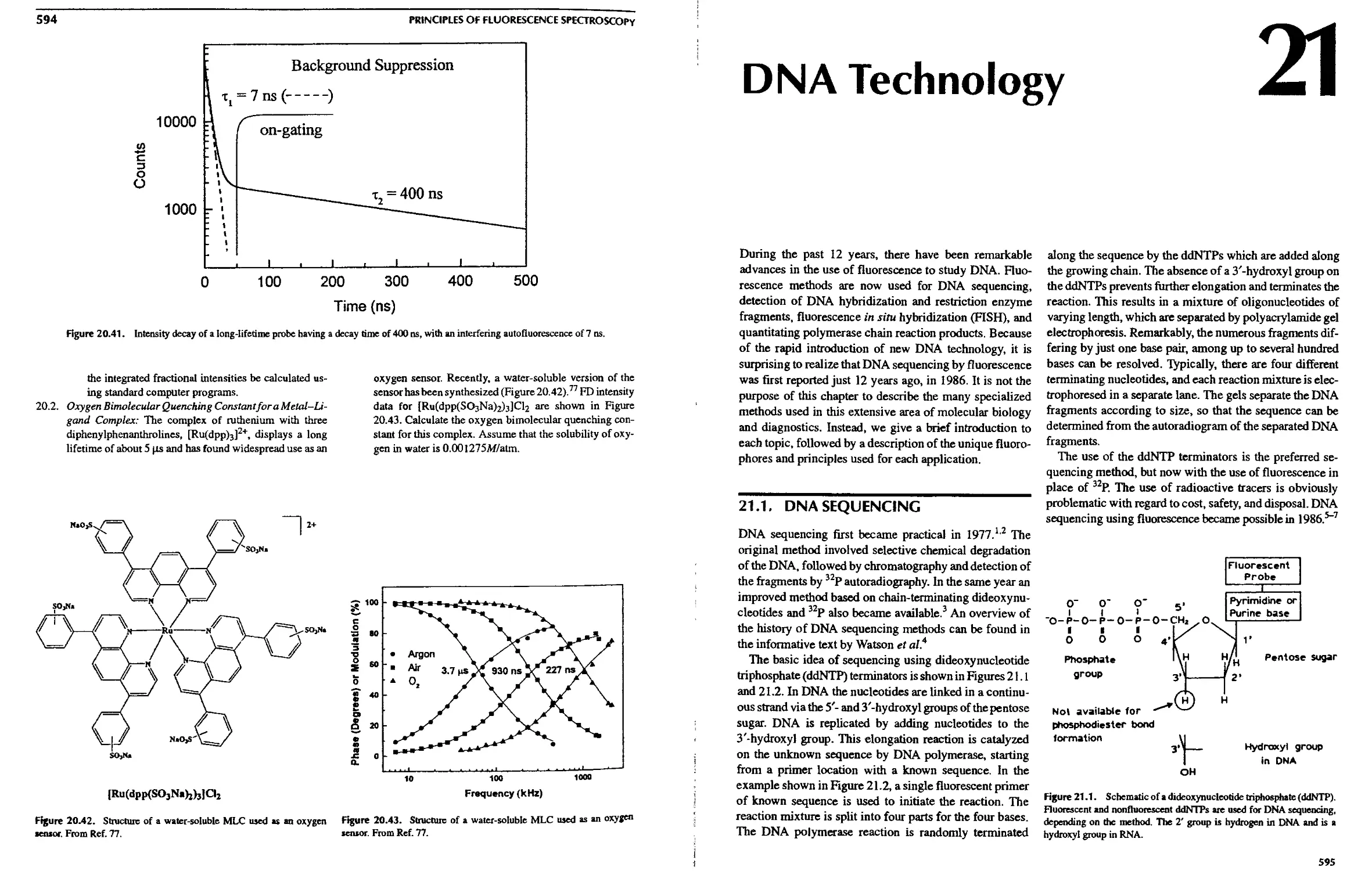
21. DNA Technology
21.1. DNA Sequencing 595
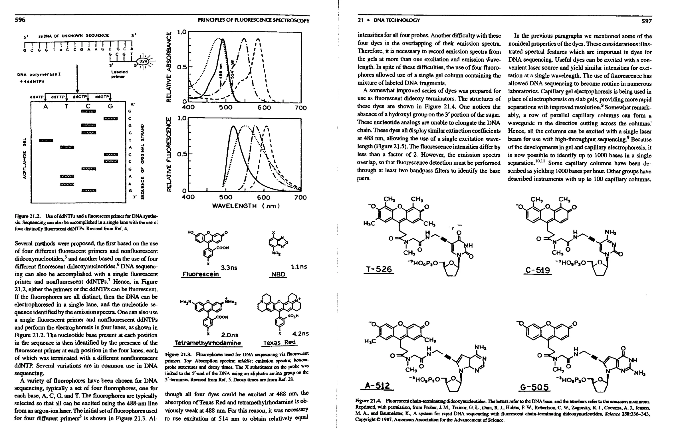
21.1.A. Nucleotide Labeling Methods . ... 598
21.1.B. Energy-Transfer Dyes for DNA
Sequencing 598
21.l.C. DNA Sequencing withNIR Probes. . 601
2I.1.D. DNA Sequencing Based on Lifetimes 604
21.2. High-Sensitivity DNA Stains 604
21.2.A. High-Affinity Bis DNA Stains ... 605
21.2.B. Energy-Transfer DNA Stains .... 606
21.2.C. DNA Fragment Sizing by Flow
Cytometry 607
21.3. DNA Hybridization 607
21.3.A. DNA Hybridization Measured with
One Donor- and Acceptor-Labeled
DNA Probe 608
21.3.B. DNA Hybridization Measured by
Excimer Formation 610
21.3.C. Polarization Hybridization Assays . 610
21.3.D. Polymerase Chain Reaction 612
21.3.E. DNA Imagers 612
21.3.F. Light-Generated DNA Probe Arrays 612
21.4. Fluorescence in sit и Hybridization 613
21.5. Perspectives 614
References 614
Problems 617
22. Phase-Sensitive and Phase-Resolved
Emission Spectra
22.1. Theory of Phase-Sensitive Detection of
Fluorescence 619
22.1 A. Phase-Sensitive Emission Spectra of
a Two-Component Mixture 621
22.1.B. Phase Suppression 623
22. l.C. Examples of PSDF and Phase
Suppression 624
22. l.D. High-Frequency or Low-Frequency
Phase-Sensitive Detection 626
22.2. Phase-Modulation Resolution of Emission
Spectra 627
22.2.A. Resolution Based on Phase or
Modulation Lifetimes 627
22.2.B. Resolution Based on Phase Angles
and Modulations 627
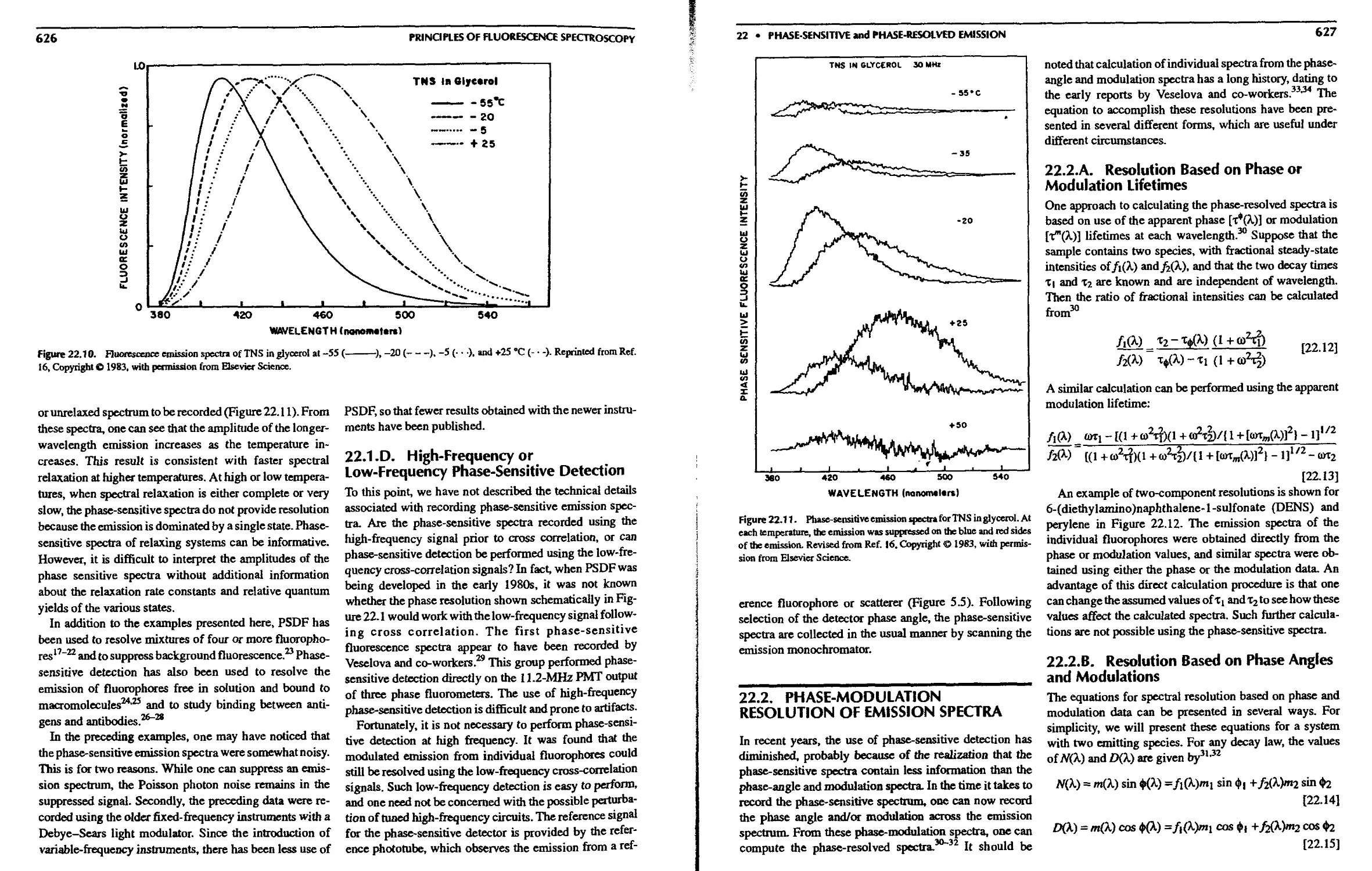
22.2.C. Resolution of Emission Spectra from
Phase and Modulation Spectra . . . 628
22.3. Fluorescence Lifetime Imaging Microscopy 629
22.3.A. Phase-Suppression Imaging .... 631
References 633
Problems 635
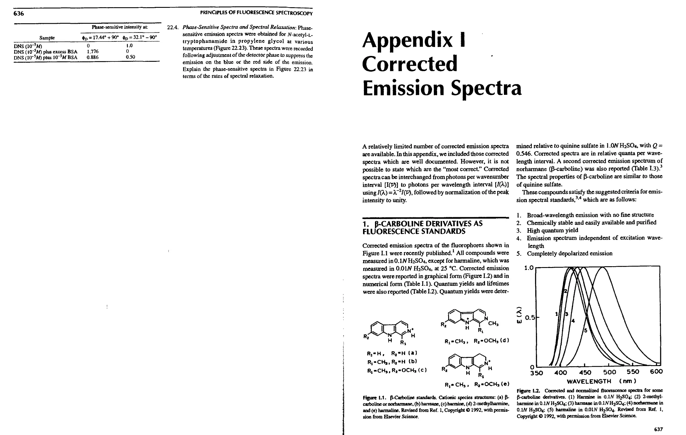
Appendix I. Corrected Emission Spectra
1. Э-Carboline Derivatives as Fluorescence
Standards 637
2. Corrected Emission Spectra of
9,10-Diphenylanthracene, Quinine Sulfate,
and Fluorescein 638
3. Long-Wavelength Standards 639
4. Ultraviolet Standards 639
5. Additional Corrected Emission Spectra . . . 642
References 643
Appendix II. Fluorescent Lifetime
Standards
1. Nanosecond Lifetime Standards 645
2. Picosecond Lifetime Standards 646
3. Representative Frequency-Domain Intensity
Decays 646
4. Time-Domain Lifetime Standards 647
References 650
Appendix III. Additional Reading
1. Lifetime Measurements 653
2. Which Molecules are Fluorescent
Representative Emission Spectra, and
Practical Advice 654
3. Theory of Fluorescence and Photophysics . . 654
4. Principles of Fluorescence Spectroscopy . . . 654
5. Biochemical Fluorescence 654
6. Protein Fluorescence 655
7. Data Analysis and Nonlinear Least Squares . 655
8. Photochemistry 655
9. Flow Cytometry 656
10. Phosphorescence 656
11. Polymer Science 656
12. Fluorescence Sensing 656
13. Immunoassays 656
14. Latest Applications of Fluorescence 656
15. Infrared and NIR Fluorescence 657
16. Lasers 657
17. Fluorescence Microscopy 657
18. Metal-Ligand Complexes and Unusual
Luminophores 657
Answers to Problems 659
Index 679
Principles of
Fluorescence
Spectroscopy
Second Edition
Introduction to
Fluorescence
During the past 15 years there has been a remarkable
growth in the use of fluorescence in the biological sciences.
Just a few years ago, fluorescence spectroscopy and time-
resolved fluorescence were primarily research tools in
biochemistry and biophysics. This situation has changed
so that fluorescence is now used in environmental moni-
monitoring, clinical chemistry, DNA sequencing, and genetic
analysis by fluorescence in situ hybridization (FISH), to
name a few areas of application. Additionally, fluorescence
is used for cell identification and sorting in flow cytometry,
and in cellular imaging to reveal the localization and
movement of intracellular substances by means of fluores-
fluorescence microscopy. Because of the sensitivity of fluores-
fluorescence detection, and the expense and difficulties of
handling radioactive substances, there is a continuing de-
development of medical tests based on the phenomenon of
fluorescence. These tests include the widely used enzyme-
linked immunoassays (ELISA) and fluorescence polariza-
polarization immunoassays.
While there is continued growth in the applications of
fluorescence, and continued development of instrumenta-
instrumentation and fluorescent probe technology, the principles re-
remain the same and need to be understood by the
practitioners. Hence, this volume describes the basic phe-
phenomenon of fluorescence, so that these principles can be
used successfully in basic and applied research. Through-
Throughout the book, we have included examples and applications
that illustrate the principles of fluorescence.
1.1. PHENOMENON OF
FLUORESCENCE
Luminescence is the emission of light from any substance
and occurs from electronically excited states. Lumines-
Luminescence is formally divided into two categories, fluorescence
and phosphorescence, depending on the nature of the
excited state. In excited singlet states, the electron in the
excited orbital is paired (of opposite spin) to the second
electron in the ground-state orbital. Consequently, return
to the ground state is spin-allowed and occurs rapidly by
emission of a photon. The emission rates of fluorescence
are typically 108 s, so that a typical fluorescence lifetime
is near 10 ns A0 x 10~9 s). As will be described in Chapter
4, the lifetime (T) of a fluorophore is the average time
between its excitation and its return to the ground state. It
is valuable to consider a 1-ns lifetime within the context of
the speed of light. Light travels 30 cm or about one foot in
one nanosecond. Many fluorophores display subnanosec-
ond lifetimes. Because of the short timescale of fluores-
fluorescence, measurement of the time-resolved emission
requires sophisticated optics and electronics. In spite of the
experimental difficulties, time-resolved fluorescence is
widely practiced because of the increased information
available from the data, as compared with stationary or
steady-state measurements.
Phosphorescence is emission of light from triplet excited
states, in which the electron in the excited orbital has the
same spin orientation as the ground-state electron. Transi-
Transitions to the ground state are forbidden and the emission
rates are slow A03—10° s), so that phosphorescence
lifetimes are typically milliseconds to seconds. Even
longer lifetimes are possible, as is seen from "glow-in-the-
dark" toys: following exposures to light, the phosphores-
phosphorescent substances glow for several minutes while the excited
phosphors slowly return to the ground state. Phosphores-
Phosphorescence is usually not seen in fluid solutions at room tem-
temperature. This is because there exist many deactivation
processes which compete with emission, such as nonradia-
tive decay and quenching processes. It should be noted that
the distinction between fluorescence and phosphorescence
is not always clear. Transition-metal-ligand complexes
(MLCs), which contain a metal and one or more organic
Iigands, display mixed singlet-triplet states. These MLCs
display intermediate lifetimes of 400 ns to several micro-
microseconds. In this book we will concentrate mainly on the
PRINCIPLES OF FLUORESCENCE SPECTROSCOPY
more rapid phenomenon of fluorescence. However, be-
because of the importance of these new metal—ligand lumi-
nophores, which bridge the gap between fluorescence and
phosphorescence, their properties are described in Chapter
20.
Fluorescence typically occurs from aromatic molecules.
Some typical fluorescent substances (fluorophores) are
shown in Figure 1.1. One widely encountered fluorophore
is quinine, which is present in tonic water. If one observes
a glass of tonic water which is exposed to sunlight, a faint
blue glow is frequently visible at the surface. This glow is
most apparent when the glass is observed at a right angle
relative to the direction of the sunlight and when the
dielectric constant is decreased by adding less polar sol-
solvents like alcohols. The quinine present in the tonic is
excited by the ultraviolet (UV) light from the sun. Upon
return to the ground state, the quinine emits blue light with
a wavelength near 450 nm. The dependence of the bright-
brightness of quinine fluorescence on solvent polarity provides
a noninvasive means of learning more about our neighbors.
The first observation of fluorescence from a quinine solu-
solution in sunlight was reported by Sir John Frederick William
Herschel in 1845.l The following is an excerpt from this
early report.
On a Case of Superficial Colour presented by a homo-
homogeneous liquid internally colourless. By Sir John
Frederick William Herschel, Philosophical Transac-
Transactions of the Royal Society of London A845) 135:143-
145.
Received January 28. 1845, Read February 13, 1845
The sulphate of quinine is well known to be of
extremely sparing solubility in water. It is however
easily and copiously soluble in tartaric acid. Equal
weights of the sulphate and of crystallized lartaric acid,
rubbed up together with addition of a very little water,
dissolve entirely and immediaiely. It is this solution,
largely diluted, which exhibits the optical phenomenon
in question. Though perfectly transparent and colorless
when held between the eye and the light, or a white
objeci, it yet exhibits in certain aspects, and under
certain incidences of the light, an extremely vivid and
beautiful celestial blue colour, which, from the circum-
circumstances of its occurrence, would seem to originate in
those strata which the light first penetrates in entering
the liquid, and which, if not strictly superficial, at least
exert their peculiar power of analyzing the incident
rays and dispersing those which compose the tint in
question, only through a very small depth within the
medium.
To see the colour in question ю advantage, all that is
requisite is to dissolve the two ingredients above men-
mentioned in equal proportions, in about a hundred times
their joint weight of water, and having filtered the
solution, pour it into a tall narrow cylindrical glass
vessel or test tube, which is to be set upright on a dark
colored substance before an open window exposed to
strong daylight or sunshine, but with no cross lights,
or any strong reflected light from behind. If we look
down perpendicularly into the vessel so that the visual
ray shall graze the internal surface of the glass through
a great part of its depth, the whole of that surface of the
liquid on which the light first strikes will appear of a
lively blue, . ..
If the liquid be poured out into another vessel, the
descending stream gleams internally from all iis undu-
undulating inequalities, with the same lively yet delicate
blue colour,... thus clearly demonstrating that contact
with a denser medium has no share in producing this
singular phenomenon.
The thinnest film of the liquid seems quite as effec-
effective in producing this superficial colour as a consider-
considerable thickness. For instance, if in pouring it from one
glass into another,... the end of the funnel be made to
touch the internal surface of the vessel well moistened,
so as to spread the descending stream over an extensive
surface, the intensity of the colour is such that it is
almost impossible to avoid supposing that we have a
highly colored liquid under our view.
As a footnote, Herschel wrote "I write from recollection
of an experiment made nearly twenty years ago, and which
I cannot repeat for want of a specimen of the wood."
It is evident from this early description that Herschel
recognized the presence of an unusual phenomenon which
could not be explained by the scientific knowledge of the
time. To this day, the fluorescence of quinine remains one
of the most used and most beautiful examples of fluores-
fluorescence. However, it is unlikely that Herschel's experiment,
described from memory 20 years later, would be accepted
by the Patent Office. Herschel (Figure 1.2) was from a
distinguished family of scientists who lived in England but
had their roots in Germany.2 For most of his life, Herschel
did research in astronomy, publishing only a few papers on
fluorescence.
It is interesting to notice that the first known fluoro-
fluorophore, quinine, was responsible for stimulating the devel-
development of the first spectrofluorometers, which appeared in
the 1950s. During World War II, the Department of De-
Defense was interested in monitoring antimalaria drugs, in-
including quinine. This early drug assay resulted in a
subsequent program at the National Institutes of Health to
develop the first practical spectrofluorometen3
Many other fluorophores are encountered in daily life.
The green or red-orange glow sometimes seen in antifreeze
is due to trace quantities of fluorescein or rhodamine,
respectively (Figure 1,1). Polynuclear aromatic hydrocar-
1 • INTRODUCTION TO FLUORESCENCE
CH2=CH
H
CH3O
Quinine
POPOP Acridine Orange
Figure 1.1. Structures of typical fluorescent substance:
7-Hydroxy-
cournarin
or Umbelliferone
Figure 1.2. Sir John Frederick William Herschel (March 7,1792-May
П, 1871). Reproduced courtesy of the Library & Information Centre,
Royal Society of Chemistry.
bons, such as anthracene and perylene, are also fluores-
fluorescent, and the emission from such species is used for envi-
environmental monitoring of oil pollution. Some substituted
organic compounds are also fluorescent. For example,
l,4-bisE-phenyloxazol-2-yl)benzene (POPOP) is used in
scintillation counting, and Acridine Orange is often used
as a DNA stain. Coumarins are also highly fluorescent and
are often used as fluorogenic probes in enzyme assays,
such as enzyme-linked immunosorbent assays (ELISA). In
this case the parent molecule is typically umbelliferyl
phosphate, which is nonfluorescent. Hydrolysis of the
7-hydroxyl phosphate by alkaline phosphatase results in a
highly fluorescent product.
Numerous additional examples could be presented. In-
Instead of listing them here, examples will appear throughout
the book, with reference to the useful properties of the
individual fluorophores. In Chapter 3 we summarize the
diversity of fluorophores used for research and fluores-
fluorescence sensing. In contrast to aromatic organic molecules,
atoms are generally nonfluorescent in condensed phases.
One notable exception is the group of elements commonly
known as the lanthanides.4 The fluorescence from euro-
europium and terbium ions results from electronic transitions
between / orbitals. These orbitals are shielded from the
solvent by higher filled orbitals. The lanthanides display
long decay times because of this shielding, and they have
low emission rates because of their small extinction coef-
coefficients.
Fluorescence spectral data are generally presented as
emission spectra. A fluorescence emission spectrum is a
plot of the fluorescence intensity versus wavelength
(nanometers) or wavenumber (cm). Two typical fluores-
fluorescence emission spectra are shown in Figure 1.3. Emission
PRINCIPLES OF FLUORESCENCE SPECTROSCOPY
WAVELENGTH (nm)
37О 390 410 45О 490 930 570
1ваОО 2 6BOO 24ЙОО 2 2S0O 20BO0 16ЯОО
WAVENUMBER (cm)
3SSOO 31S00 275ОО 23SOO 19SOO 155ОО
WAVENUMBER (cm'1)
Figure 1.3. Absorption and fluorescence emission spectra of perylene
and quinine. Emission spectra cannot be correctly presented on both the
wavelength and wavenumber scales. The wavenumber presentation is
correct in this instance. Wavelengths are shown for convenience. See
Chapter 3. Revised from Ref. 5.
spectra vary widely and are dependent upon the chemical
structure of the fluorophore and the solvent in which it is
dissolved. The spectra of some compounds, such as
perylene, show significant structure due to the individual
vibrational energy levels of the ground state and excited
states. Other compounds, such as quinine, show spectra
which are devoid of vibrational structure.
An important feature of fluorescence is high-sensitivity
detection. The sensitivity of fluorescence was used in 1877
to demonstrate that the rivers Danube and Rhine were
connected by underground streams.5 This connection was
demonstrated by placing fluorescein (Figure 1.1) into the
Danube River. Some 60 hours later, its characteristic green
fluorescence appeared in a small river which led to the
Rhine. Today fluorescein is still used as an emergency
marker for locating individuals at sea, as has been seen on
the landing of space capsules in the Atlantic Ocean. Read-
Readers interested in the history of fluorescence are referred to
the excellent summary by Berlman.5
Figure 1.4. Professor Alexander Jablonski A898-1980), circa 1935.
Courtesy of his daughter, Professor Danuta Fraekowiak.
1.2. JABIONSKI DIAGRAM
The processes which occur between the absorption and
emission of light are usually illustrated by a Jablonski
diagram. Jablonski diagrams are often used as the starting
point for discussing light absorption and emission. They
exist in a variety of forms, to illustrate various molecular
processes which can occur in excited states. These dia-
diagrams are named after Professor Alexander Jablonski (Fig-
(Figure 1.4), who is regarded as the father of fluorescence
spectroscopy because of his many accomplishments, in-
including his descriptions of concentration depolarization
and his definition of the term "anisotropy" to describe the
polarized emission from solutions.7'8
Brief History of Alexander jabtohski
Professor ]abtonski was born February 26, 1898, in
Voskresenovka, Ukraine. In 1916 he began his study
of atomic physics at the University of Kharkov. His
study was interrupted by military service first in the
Russian Army and later in the newly organized Polish
Army during World War I. At the end of 1918, when
an independent Poland was recreated after more than
1 • INTRODUCTION TO FLUORESCENCE
120 years of occupation by neighboring powers,
labtonski left Kharkov and arrived in Warsaw, where
he entered the University of Warsaw to continue his
study of physics. His study in Warsaw was again
interrupted in 1920 by his military service during the
Polish-Bolshevik war.
An enthusiastic musician, Jabronski played the first
violin at the Warsaw Opera from 1921 to 1926 parallel
to his studies at the university under Stefan Pienkowski.
He received his doctorate in 1 930 for work "On the
influence of the change of wavelengths of excitation
light on the fluorescence spectra." Although ]abronski
left the Warsaw Opera in 1926 and devoted himself
entirely to scientific work, music remained his great
passion until the last days of his life.
Throughout the 1 920s and 1930s the Department of
Experimental Physics at the University of Warsaw was
an active center for studies on luminescence under
S. Pienkowski. During most of this period, Jabroriski
worked both theoretically and experimentally on fun-
fundamental problems of photoluminescence of liquid
solutions as well as on the effects of pressure on atomic
spectral lines in gases. The problem that intrigued
labronski for many years was the polarization of pho-
photoluminescence of solutions. To explain the experi-
experimental facts, he distinguished the transition moments
in absorption and in emission and analyzed various
factors responsible for the depolarization of lumines-
luminescence.
Jabtoriski's work was interrupted once again by
World War II. From 1 939 to 1945 |abroriski served in
the Polish Army, and he spent time as a prisoner of first
the Germany Army and then the Soviet Army. In 1946
he returned to Poland to chair a new Department of
Physics in the new Nicholas Copernicus University in
Toruri. This beginning occurred in the very difficult
postwar years in a country totally destroyed by World
War II. Despite all these difficulties, labtonski with
great energy organized the Department of Physics,
which became a scientific center for studies in atomic
and molecular physics.
His work continued past his retirement in 1968.
Professor labtonski created a spectroscopic school of
thought which persists even today through his numer-
numerous students who now occupy positions at universities
in Poland and elsewhere. Professor Jabtonski died on
September 9, 1980. More complete accounts of
labtonski's accomplishments are given in Refs. 7 and 8.
A typical Jablonski diagram is shown in Figure 1.5. The
singlet ground, first, and second electronic states are de-
depicted by So, Sit and S2, respectively. At each of these
electronic energy levels the fluorophores can exist in a
number of vibrational energy levels, denoted by 0,1,2, etc.
In this diagram we have excluded a number of interactions
which will be discussed in subsequent chapters, such as
quenching, energy transfer, and solvent interactions. The
transitions between states are depicted as vertical lines to
illustrate the instantaneous nature of light absorption.
Transitions occur in about 10"'s s, a time too short for
significant displacement of nuclei. This is the Franck-
Condon principle.
The energy spacing between the various vibrational
energy levels is illustrated by the emission spectrum of
perylene (Figure 1.3). The individual emission maxima
(and hence vibrational energy levels) are about 1500 cm
apart. At room temperature, thermal energy is not adequate
to significantly populate the excited vibrational states.
Absorption typically occurs from molecules with the low-
lowest vibrational energy. Of course, the larger energy differ-
difference between the So and Si excited states is too large for
thermal population of S,, and it is for this reason we use
light and not heat to induce fluorescence.
Following light absorption, several processes usually
occur. A fluorophore is usually excited to some higher
vibrational level of either S, or S2. With a few rare excep-
Figure1.5. One form of a Jabloftski diagram.
PRINCIPLES OF FLUORESCENCE SPECTROSCOPY
tions, molecules in condensed phases rapidly relax to the
lowest vibrational level of S,. This process is called inter-
internal conversion and generally occurs in 102 s or less. Since
fluorescence lifetimes are typically near 10"8 s, internal
conversion is generally complete prior to emission. Hence,
fluorescence emission generally results from a thermally
equilibrated excited state, that is, the lowest-energy vibra-
vibrational state of St.
Return to the ground state typically occurs to a higher
excited vibrational ground-state level, which then quickly
A(T12 s) reaches thermal equilibrium (Figure 1.5). An
interesting consequence of emission to higher vibrational
ground states is that the emission spectrum is typically a
mirror image of the absorption spectrum of the So ~~> *^i
transition. This similarity occurs because electronic exci-
excitation does not greatly alter the nuclear geometry. Hence,
the spacing of the vibrational energy levels of the excited
states is similar to that of the ground state. As a result, the
vibrational structures seen in the absorption and the emis-
emission spectra are similar.
Molecules in the S, state can also undergo a spin conver-
conversion to the first triplet state, 7\. Emission from 7", is termed
phosphorescence and is generally shifted to longer wave-
wavelengths (lower energy) relative to the fluorescence. Con-
Conversion of S, to Г, is called intersystem crossing. Transition
from Tj to the singlet ground state is forbidden, and, as a
result, rate constants for triplet emission is several orders
of magnitude smaller than those for fluorescence. Mole-
Molecules containing heavy atoms such as bromine and iodine
are frequently phosphorescent. The heavy atoms facilitate
intersystem crossing and thus enhance phosphorescence
quantum yields.
1.3. CHARACTERISTICS OF
FLUORESCENCE EMISSION
The phenomenon of fluorescence displays a number of
general characteristics. Exceptions are known, but these
are infrequent. Generally, if any of the characteristics
described in the following sections are not displayed by a
given fluorophore, one may infer some special behavior
for this compound.
1.3.A. Stokes'Shift
ExaminationoftheJablonskidiagram(Figure 1.5) reveals
that the energy of the emission is typically less than that of
absorption. Hence, fluorescence typically occurs at lower
energies or longer wavelengths. This phenomenon was
first observed by Sir G. G. Stokes in 1852 in Cambridge.9
These early experiments used relatively simple instrumen-
instrumentation (Figure 1.6). The source of UV excitation was pro-
provided by sunlight and a blue glass filter, which was part of
a stained glass window. This filter selectively transmitted
light below 400 nm, which was absorbed by quinine (Fig-
(Figure 1.3). The exciting light was prevented from reaching
the detector (eye) by ayellow glass (of wine) filter. Quinine
fluorescence occurs near 450 nm and is therefore easily
visible.
It is interesting to read Stokes' description of his obser-
observation. The following paragraph is from his report publish-
published in 1852.9
On the Change of Refrangibility of Light. By G. G.
Stokes, M.A., F.R.S., Fellow of Pembroke College, and
Lucasian Professor of Mathematics in the University
ofCambridge. Philosophical Transactions of the Royal
Society of London A852) 142:463-562.
Received May 11, Read May 27, 1852
The following researches originated in a consideration
of the very remarkable phenomenon discovered by Sir
John Herschel in a solution of sulphate of quinine, and
described by him in two papers printed in the Philo-
Philosophical Transactions for 1845, entitled "On a Case of
Superficial Colour presented by a Homogeneous Liq-
Liquid internally colourless," and "On the Epipolic Dis-
Dispersion of Light." The solution of quinine, though it
appears to be perfectly transparent and colourless, like
Emission filter
(yellow-glass of wine)
Transmits » 400 nm
Excitation
filter* 400 nm
(blue-glass from
church window)
G.G. Stokes
Figure 1.6. Experimental schematic for detection of the Stokes' shift.
1 • INTRODUCTION TO FLUORESCENCE
waler, when viewed by transmitted light, exhibits nev-
nevertheless in certain aspects, and under certain inci-
incidences of the light, a beautiful celestial blue colour. It
appears from the experiments of Sir John Herschel that
the blue colour comes only from a stratum of fluid of
small but finite thickness adjacent to the surface by
which the light enters. After passing through this stra-
stratum, the incident light, though not sensibly enfeebled
nor colored, has lost the power of producing the same
effect, and therefore may be considered as in some way
or oiher qualitatively different from the original light.
Careful reading of this paragraph reveals several impor-
important characteristics of fluorescent solutions. The quinine
solution is colorless because it absorbs in the UV, which
we cannot see. The blue color comes only from a region
near the surface. This is because the quinine solution was
relatively concentrated and absorbed all of the UV in the
first several millimeters. Hence, Stokes observed the inner
filter effect. After passing through the solution, the light
was "enfeebled" and no longer capable of causing the blue
glow. This occurred because the UV was removed and the
"enfeebled" light could no longer excite quinine. However,
had Stokes used a second solution of fluorescein, rather
than quinine, it would have still been excited because of
the longer absorption wavelength of fluorescein.
Energy losses between excitation and emission are ob-
observed universally for fluorescent molecules in solution.
One common cause of the Stokes' shift is the rapid decay
to the lowest vibrational level of St. Furthermore, fluoro-
phores generally decay to higher vibrational levels of So
(Figure 1.5), resulting in further loss of excitation energy
by thermalization of the excess vibrational energy. In
addition to these effects, fluorophores can display further
Stokes' shifts due to solvent effects, excited-state reac-
reactions, complex formation, and/or energy transfer.
Brief History of Sir С. С Stokes
Professor Stokes (Figure 1.7) was born in Ireland,
August 3, 1819. He entered Pembroke College, Cam-
Cambridge, in 1837 and was elected as a fellow of Pem-
Pembroke College immediately upon his graduation in
1841. In 1849 Stokes became Lucasian Professor at
Cambridge, a chair once held by Newton. Because of
a poor endowment for the chair, he also worked in the
Government School of Mines.
Stokes was involved with a wide range of scientific
problems, including hydrodynamics, elasticity of sol-
solids, and diffraction of light. The wave theory of light
was already known when he entered Cambridge. In
his classic paper on quinine, he understood that light
of a higher "refrangibility" or frequency was responsi-
responsible for the blue glow of lower refrangibility or fre-
frequency. Thus, invisible UV rays were absorbed to
produce the blue light at the surface. Stokes later
suggested the use of optical properties, such as absorp-
absorption, colored reflection, and fluorescence, to identify
organic substances.
Later in life, Stokes was universally honored with
degrees and medals. He was knighted in 1889 and
became Master of Pembroke College in 1902. After the
1850s, Stokes became involved in administrative mat-
matters, and his scientific productivity decreased. Some
things never change. Professor Stokes died on February
1, 1903.
1.3.B. Emission Spectra Are Typically
Independent of the Excitation Wavelength
Another general property of fluorescence is that the same
fluorescence emission spectrum is generally observed ir-
irrespective of the excitation wavelength. This is known as
Figure 1.7. SirGeorgeGabrielStokesA819-1903).LucasianProfes-
sor at Cambridge. Reproduced courtesy of the Library & Information
Centre, Royal Society of Chemistry.
8
Kasha's rule,1 although Vavilov reported in 1926 that
quantum yields were generally independent of excitation
wavelength. Upon excitation into higher electronic and
vibrational levels, the excess energy is quickly dissipated,
leaving the fluorophore in the lowest vibrational level of
Si. This relaxation occurs in about 10~12 s and is presum-
presumably a result of a strong overlap among numerous states of
nearly equal energy. Because of this rapid relaxation, emis-
emission spectra are usually independent of the excitation
wavelength. Exceptions exist, such as fluorophores which
exist in two ionization states, each of which displays
distinct absorption and emission spectra. Also, some mole-
molecules are known to emit from the 5г level, but such emis-
emission is rare and generally not observed in biological
molecules.
It is interesting to ask why perylene follows the mirror
image rule, but quinine emission exhibits one peak instead
of the two peaks seen in its excitation spectrum at 310 and
335 nm (Figure 1.3). In the case of quinine, the shorter-
wavelength absorption peak is due to excitation to the
second excited state (S2), which relaxes rapidly to 5j.
Hence, emission occurs predominantly from the lowest
singlet state E,). The emission spectrum of quinine is the
mirror image of the So —> Si absorption of quinine, not of
its total absorption spectrum. This is true for most fluoro-
fluorophores: the emission is the mirror image of the So —> 5,
absorption, not of the total absorption spectrum.
The generally symmetric nature of these spectra is a
result of the same transitions being involved in both ab-
absorption and emission and the similarities of the vibra-
vibrational energy levels of So and Si. In many molecules these
energy levels are not significantly altered by the different
electronic distributions of So and S,. According to the
Franck-Condon principle, all electronic transitions are
vertical, that is, they occur without change in the position
of the nuclei. As a result, if a particular transition prob-
PRINCIPLES OF FLUORESCENCE SPECTROSCOPY
»2 O
о-г
. 1 \o-i
V/ V-\o
AbS.y
O-2
O-l/ \
-Off \
^mis.\
DISTANCE WAVELENGTH
Figure 1.8. Mirror image rule and Franck-Condon factors.
ability (Franck—Condon factor) between the zeroth and
second vibrational levels is largest in absorption, the recipro-
reciprocal transition is also most probable in emission (Figure 1.8).
A rigorous test of the mirror image rule requires that the
absorption and emission spectra be presented in appropri-
appropriate units.11 The closest symmetry should exist between the
modified spectra e(P)/P and F(P)/T?, where e(P) is the
extinction coefficient at wavenumber (V) and F(V) is the
relative photon flux over a wavenumber increment ДР.
Agreement between these spectra is generally found for
polynuclear aromatic hydrocarbons.
1.3.C. Exceptions to the Mirror Image
Rule
Although the mirror image rule often holds, many excep-
exceptions to this rule occur. This is illustrated for p-terphenyl
in Figure 1.9. The absorption spectrum of p-terphenyl is
devoid of structure, but the emission spectrum shows vi-
vibrational structure. Such deviations from the mirror image
rule usually indicate a different geometric arrangement of
nuclei in the excited state as compared to the ground state.
Nuclear displacements can occur prior to emission because
of the relatively long lifetime of the Si state, which allows
p-Terphenyl
in Cyclohexane
2O#C
250
300 350
WAVELENGTH (nm)
4O0
Figure 1.9. Absorption (A) and emission (F) spectra of /Merphenyl.
1 • INTRODUCTION TO FLUORESCENCE
360
400 4 40 480 520
WAVELENGTH (nm)
560
Figure 1.10. Emission spectrum of anthracene in toluene containing
0.2Л/ diethylaniline. The dashed curves show the emission spectrum of
anthracene and that of its exciplex with diethylaniline. Revised from
Ref. 13.
time for motion following the instantaneous process of
absorption. In the case of p-terphenyl, it seems likely that
the individual rings become more coplanar in the excited
state.12 As a result, the emission spectrum is more highly
structured than the absorption spectrum. In addition to
being an exception to the mirror image rule, p-terphenyl is
unusual in that its emission spectrum shows more vibra-
vibrational structure than its absorption spectrum. The opposite
is generally observed.
Excited-state reactions other than geometric rearrange-
rearrangements can also result in deviations from the mirror sym-
symmetry rule. One example is shown in Figure 1.10, which
shows the emission spectrum of anthracene in the presence
of diethylaniline.13 The structured emission at shorter
wavelengths is a mirror image of the absorption spectrum
of anthracene. The unstructured emission at longer wave-
wavelengths is due to formation of a charge-transfer complex
between the excited state of anthracene and diethylaniline.
The unstructured emission is from this complex. Many
polynuclear aromatic hydrocarbons, such as pyrene and
perylene, also form charge-transfer complexes with
amines. These excited-state complexes are referred to as
exciplexes.
Some fluorophores can also form complexes with them-
themselves. The best-known example is pyrene. At low concen-
concentration, pyrene displays a highly structured emission
(Figure 1.11). At higher concentrations, the previously
invisible UV emission of pyrene becomes visible at 470
nm. This long-wavelength emission is due to excimer
formation, the term excimer being an abbreviation for an
excited-state dimer.
Other excited-state processes can occur which shift the
emission spectra and may or may not change the spectral
profile. Acridine displays two emission spectra which de-
1.0
n •>
n
" Pyrene
/
Monomer //
w
/NExcimer
л
4OO 45О 5О0 55О
WAVELENGTH (nm)
Figure 1.11. Emission spectra of pyrene and its excimer. The relative
intensity of the excimer peak D70 nm) decreases as the total concentra-
tionofpyrene is decreased from6x I0~3A/((op)to0.9x lO^A/ {bottom).
Reproduced with permission from John Wiley and Sons, Inc., from Ref.
11. Btrks, J. В., Copyright © 1970, Photophysics of Aromatic Molecules,
John Wiley & Sons, New York.
pend on pH (Figure 1.12). The pKa for dissociation of the
proton is 5.45 for acridine in the ground state. However,
emission from the acridinium group can be observed at
higher pH values. This occurs because the pKa of the
excited state of acridine is 10.7, and thus acridine can bind
a proton from the solvent during its excited-state lifetime.14
Changes in pKa in the excited state also occur for bio-
biochemical fluorophores. For example, phenol and tyrosine
each show two emissions, the long-wavelength emission
being favored by ahigh concentration of proton acceptors.
The pKa of the phenolic hydroxyl group decreases from 11
in the ground state to 4 in the excited state. Following
excitation, the phenolic proton is lost to proton acceptors
in the solution. Depending upon the concentration of these
acceptors, either the phenol or the phenolate emission may
dominate the emission spectrum.
4OO 500
WAVELENGTH ( nm )
600
Figure 1.12. Fluorescence emission spectra of the neutral and pro-
tonated forms of acridine (Ac). Revised from Ref. 14.
10
PRINCIPLES OF FLUORESCENCE SPECTROSCOPY
1.4. FLUORESCENCE LIFETIMES AND
QUANTUM YIELDS
The fluorescence lifetime and quantum yield are perhaps
the most important characteristics of a fluorophore. The
quantum yield is the number of emitted photons relative to
the number of absorbed photons. Substances with the .
largest quantum yields, approaching unity, such as rho-
damines, display the brightest emission. The lifetime is
also important, as the lifetime determines the time avail-
available for the fluorophore to interact with or diffuse in its
environment, and hence the information available from its
emission.
The meaning of the quantum yield and lifetime is best
represented by a simplified Jabtonski diagram (Figure
1.13). In this diagram we do not explicitly illustrate the
individual relaxation processes leading to the relaxed St
state. Instead, we focus attention on those processes re-
responsible for return to the ground state. In particular, we
are interested in the emissive rate of the fluorophore (Г)
and its rate of nonradiative decay to So (?„,).
The fluorescence quantum yield is the ratio of the num-
number of photons emitted to the number absorbed. The proc-
processes governed by the rate constants Г and k^ both
depopulate the excited state. The fraction of fluorophores
which decay through emission, and hence the quantum
yield, is given by
near 10 ns. For the fluorophore illustrated in Figure 1.13,
the lifetime is
Q-
The quantum yield can be close to unity if the radiationless
decay rate is much smaller than the rate of radiative decay,
that is, ka < < Г. We note that the energy yield of fluores-
fluorescence is always less than unity because of Stokes' losses.
For convenience, we have grouped all possible nonradia-
nonradiative decay processes with the single rate constant km.
The lifetime of the excited state is defined by the average
time the molecule spends in the excited state prior to return
to the ground state. Generally, fluorescence lifetimes are
^ Relaxation (to"Ks)
[1-2]
One should remember that fluorescence emission is a
random process, and few molecules emit their photons at
precisely i = т. The lifetime is an average value of the time
spent in the excited state. For a single exponential decay
(Eq. [1.13], below), 63% of the molecules have decayed
prior to Г = т and 37% decay at t > т.
The lifetime of the fluorophore in the absence of nonra-
nonradiative processes is called the intrinsic or natural lifetime
and is given by
тл=1/Г
[1.3]
In principle, the natural lifetime х„ can be calculated from
the absorption spectra, extinction coefficient, and emission
spectra of the fluorophore. The radiative decay rate Г can
be calculated using15'16
\F(V)dP
Г=2.88х1(Г9п2
= 2.88 x 10~V <1/>-' j
[1.4]
Figure 1.13. Л simplified Jablonski diagram.
where F(V) is the emission spectrum plotted on the
wavenumber (cm) scale, e(P) is the absorption spectrum,
and n is the refractive index of the medium. The integrals
are calculated over the So <-» Si absorption and emission
spectra. In many cases this expression works rather well,
particularly for solutions of polynuclear aromatic hydro-
hydrocarbons. For instance, the calculated value15 of Г for
perylene is 1.8 x 10s s~\ which yields a natural lifetime of
5.5 ns. This value is close to that observed for perylene,
which displays a quantum yield near unity. However, there
are numerous reasons why Eq. [1.4] can fail. This expres-
expression assumes no interaction with the solvent, does not
consider changes in refractive index (л) between the ab-
absorption and emission wavelength, and assumes no change
in excited-state geometry. A more complete form of Eq.
[1.4] (not shown) includes a factor G = gjga on the right-
hand side, where gi and gu are the degeneracies of the lower
and upper states, respectively. For fluorescence transitions,
G = 1, and for phosphorescence transitions, G = |.
The natural lifetime can be calculated from the measured
lifetime (x) and quantum yield:
1 • INTRODUCTION TO FLUORESCENCE
11
[1.5] 1.4.A. Fluorescence Quenching
Equation [1.5] can be derived from Eqs. [1.1]-[1.3]. Many
biochemical fluorophores do not behave as predictably as
unsubstituted aromatic compounds. Hence, there is often
poor agreement between the value of т„ calculated from
Eq. [1.5] and that calculated from the absorption and
emission spectra (Eq. [1.4]). These discrepancies occur for
a variety of unknown and known reasons, such as a fraction
of the fluorophores being located next to quenching
groups, which sometimes occurs for tryptophan residues
in proteins.
The quantum yield and lifetime can be modified by
factors which affect either of the rate constants (Г or к„).
For example, a molecule may be nonfluorescent as a result
of a fast rate of internal conversion or a slow rate of
emission. Scintillators are generally chosen for their high
quantum yields. These high yields are a result of large Г
values. Hence, the lifetimes are generally short, near 1 ns.
The fluorescence emission of aromatic substances contain-
containing -NO2 groups is generally weak, primarily as a result
of large values for к„. The quantum yields of phosphores-
phosphorescence are extremely small in fluid solutions at room tem-
temperature. The triplet-to-singlet transition is forbidden by
symmetry, and the rates of spontaneous emission are about
103 s or smaller. Since k^ values are near I09 s, quan-
quantum yields of phosphoresce»ce are small at room tempera-
temperature. From Eq. [1.1] one can predict phosphorescence
quantum yields of 1СГ6.
There are instances where comparison of the natural
lifetime, measured lifetime, and quantum yield can be
informative. For instance, in the case of the widely used
membrane probe 1,6-diphenyl-l ,3,5-hexatriene (DPH) the
measured lifetime—near 10 ns—is much longer than that
calculated from Eq. [1.1], which is near 1.5 ns.17 In this
case the calculation based on the absorption spectrum of
DPH is incorrect because the absorption transition is to a
state of different electronic symmetry than the emissive
state. Such quantum-mechanical effects are rarely seen in
more complex fluorophores with heterocyclic atoms.
The intensity of fluorescence can be decreased by a wide
variety of processes. Such decreases in intensity are called
quenching. Quenching can occur by different mechanisms.
Collisional quenching occurs when the excited-state
fluorophore is deactivated upon contact with some other
molecule in solution, which is called the quencher. Colli-
Collisional quenching is illustrated on the modified Jablonski
diagram in Figure 1.14. In this case the fluorophore is
returned to the ground state during a diffusive encounter
with the quencher. The molecules are not chemically al-
altered in the process. For collisional quenching, the de-
decrease in intensity is described by the well-known
Stern-Volmer equation:
[1.6]
In this expression К is the Stern-Volmer quenching con-
constant, kq is the bimolecular quenching constant, To is the
unquenched lifetime, and [Q] is the quencher concentra-
concentration. A wide variety of molecules can act as collisional
quenchers. Examples include oxygen, halogens, amines,
and electron-deficient molecules like acrylamide. The
mechanism of quenching varies with the fluorophore-
quencher pair. For instance, quenching of indole by acry-
acrylamide is probably due to electron transfer from indole to
acrylamide, which does not occur in the ground state.
Quenching by halogens and heavy atoms occurs due to
spin—orbit coupling and intersystem crossing to the triplet
state (Figure 1.5).
Besides collisional quenching, fluorescence quenching
can occur by a variety of other processes. Fluorophores can
form nonfluorescent complexes with quenchers. This
process is referred to as static quenching since it occurs in
the ground state and does not rely on diffusion or molecular
collisions. Quenching can also occur by a variety of trivial,
i.e., nonmolecular, mechanisms, such as attenuation of the
incident light by the fluorophore itself or other absorbing
species.
hvA
v solvent ,„
\ Relaxation (lO''°s)
FRET
кт-4-l"?
Figure 1.14. Jablonski diagram with collisiona] quenching and fluorescence resonance energy transfer (FRET). The term X*j is used to represent
nonradiative paths to the ground state besides quenching and FRET. Revised from Ref. 20.
12
PRINCIPIES OF FLUORESCENCE SPECTROSCOPY
f .4.B. Time Scale of Molecular Processes
in Solution
The phenomenon of quenching provides a valuable context
for understanding the role of the excited-state lifetime in
allowing fluorescence measurements to detect dynamic
processes in solution or in macromolecules. The basic idea
is that absorption is an instantaneous event. According to
the Franck-Condon principle, absorption occurs so fast
that there is no time for molecular motion during the
absorption process. Absorption occurs in the time it takes
a photon to travel the length of a photon, in less than 10
s. Hence, absorption spectroscopy can only yield informa-
information on the average ground state of the molecules which
absorb light Only solvent molecules that are immediately
adjacent to the absorbing species will affect its absorption
spectrum. Absorption spectra are not sensitive to molecu-
molecular dynamics and can only provide information on the
average solvent shell adjacent to the chromophore.
The length of time fluorescent molecules remain in the
excited state provides an opportunity for interactions with
other molecules in solution. CoIIisional quenching of fluo-
fluorescence by molecular oxygen is an excellent example of
the expansion of time and distance provided by the fluo-
fluorescence lifetime. If a fluorophore in the excited state
collides with an oxygen molecule, then the fluorophore
returns to the ground state without emission of a photon.
The diffusion coefficient (D) of oxygen in water at 25 °C
is 2.5 X 10~3 cm2/s. The average distance (Дл2I" an
oxygen molecule can diffuse in IO"8 s or 10 ns is given by
the Einstein equation,
Дд2 = 2?)т [1.7]
The distance is about 70 A, which is comparable to the
thickness of a biological membrane or the diameter of a
protein. Some fluorophores have lifetimes as long as 400
ns, and hence diffusion of oxygen molecules may be
observed over distances of 450 A. In contrast, absorption
measurements are only sensitive to the immediate environ-
environment around the fluorophore, and then only sensitive to the
instantaneously averaged environment.
Other examples of dynamic processes in solution in-
involve fluorophore-solvent interactions and rotational dif-
diffusion. As was observed by Stokes, most fluorophores
display emission at lower energies than their absorption.
Most fluorophores have larger dipole moments in the
excited state than in the ground state. Rotational motions
of small solvent molecules in fluid solution are rapid,
typically occurring on a timescale of 40 ps or less. The
relatively long timescale of fluorescence allows ample
time for the solvent molecules to reorient around the
excited-state dipole, which lowers its energy and shifts
theemissiontolonger wavelengths. This process is called
solvent relaxation and occurs in 100 s in fluid solution.
It is these differences between absorption and emission
that result in the high sensitivity of emission spectra to
solvent polarity, and the smaller spectral changes seen in
absorption spectra. Solvent relaxation can result in sub-
substantial Stokes' shifts. In proteins, tryptophan residues
absorb light at 280 nm, and their fluorescence emission
occurs near 350 nm. Although 10 ns may appear to be a
brief time span, it is in fact quite long relative to the
motions of small molecules in fluid solution. In the follow-
following section we will explain how dynamic rotational diffu-
diffusion can be studied by measuring the polarization or
anisotropy of the emission.
1.5. FLUORESCENCE ANISOTROPY
Anisotropy measurements are commonly used in the bio-
biochemical applications of fluorescence. Anisotropy meas-
measurements provide information on the size and shape of
proteins or the rigidity of various molecular environ-
environments. Anisotropy measurements have been used to
measure protein-protein associations and fluidity of
membranes and for immunoassays of numerous substances.
Anisotropy measurements are based on the principle of
photoselective excitation of fluorophores by polarized
light Fluorophores preferentially absorb photons whose
electric vectors are aligned parallel to the transition mo-
moment of the fluorophore. The transition moment has a
defined orientation with respect to the molecular axes. In
an isotropic solution, the fluorophores are oriented ran-
randomly. Upon excitation with polarized light, one selec-
selectively excites those fluorophore molecules whose
absorption transition dipole is parallel to the electric vector
of the excitation. This selective excitation results in a
partially oriented population of fluorophores (photoselec-
tion) and in partially polarized fluorescence emission.
Emission also occurs with the light polarized along a fixed
axis in the fluorophore. The relative angle between these
moments determines the maximum measured anisotropy
(ro; see Eq. [10.20]). The fluorescence anisotropy (r) and
polarization (P) are defined by
[1.8]
P = -
h - h
[19]
where /¦ and I± are the fluorescence intensities of the
vertically (II) and horizontally A) polarized emission.
1 . INTRODUCTION TO FLUORESCENCE
13
when the sample is excited with vertically polarized light.
Anisotropy and polarization are both expressions for the
same phenomenon, and these values can be interconverted
using Eqs. [10.3] and [10.4].
Several phenomena can decrease the measured anisot-
anisotropy to values lower than the maximum theoretical values.
The most common cause is rotational diffusion. Such
diffusion occurs during the lifetime of the excited state and
displaces the emission dipole of the fluorophore. Measure-
Measurement of this parameter provides information about the
relative angular displacement of the fluorophore between
the times of absorption and emission. In fluid solution,
most fluorophores rotate extensively in 50-100 ps. Hence,
the molecules can rotate many times during the 1 - to 10-ns
excited-state lifetime, and the orientation of the polarized
emission is randomized. For this reason, fluorophores in
aqueous nonviscous solution typically display anisotropies
near zero. Transfer of excitation between fluorophores also
results in decreased anisotropies.
The effects of rotational diffusion can be decreased if the
fluorophore is bound to a macromolecule. For instance, it
is known that the rotational correlation time for the protein
human serum albumin (HSA) is near 50 ns. Suppose HSA
is covalently labeled with a fluorophore whose lifetime is
10 ns. Assuming no other processes result in loss of anisot-
anisotropy, the expected anisotropy is given by the Perrin equa-
equation:
1 + (T/6)
[1.10]
where ro is the anisotropy which would be measured in the
absence of rotational diffusion and в is the rotational
correlation time for the diffusion process. In this case,
binding of the fluorophore to the protein has slowed the
probes' rate of rotational motion. Assuming ro = 0.4, the
anisotropy is expected to be 0.33. Smaller proteins have
shorter correlation times and are expected to yield lower
anisotropies. The anisotropies of larger proteins can also
be low if they are labeled with long-lifetime fluorophores.
The essential point is that the rotational correlation times
for most proteins are comparable to typical fluorescence
lifetimes. As a result, measurements of fluorescence an-
anisotropy will be sensitive to any factor which affects the
rate of rotational diffusion. The rotational rates of fluoro-
fluorophores in cell membranes also occur on the nanosecond
timescale, and the anisotropy values are thus sensitive to
membrane composition. For these reasons, measurements
of fluorescence polarization are widely used to study the
interactions of biological macromolecules.
1.6. RESONANCE ENERGY TRANSFER
Another important process that occurs in the excited state
is resonance energy transfer (RET). This process occurs
whenever the emission spectrum of a fluorophore, called
the donor, overlaps with the absorption spectrum of an-
another molecule, called the acceptor.18 Such overlap is
illustrated in Figure 1.15. The acceptor does not need to be
fluorescent. It is important to understand that RET does
not involve emission of light by the donor. RET is not the
result of emission from the donor being absorbed by the
acceptor. Such reabsorption processes are dependent on
the overall concentration of the acceptor, and on non-
molecular factors such as sample size, and are thus of less
interest. There is no intermediate photon in RET. The
donor and acceptor are coupled by a dipole-dipole inter-
interaction. For these reasons, the term RET is preferred to the
term fluorescence resonance energy transfer (FRET),
which is also in common use.
The extent of energy transfer is determined by the dis-
distance between the donor and acceptor and the extent of
spectral overlap. For convenience, the spectral overlap
(Figure 1.15) is described in terms of the Forster distance
(Ro). The rate of energy transfer kT (r) is given by
[111]
where r is the distance between the donor (D) and the
acceptor (A), and td is the lifetime of the donor in the
absence of energy transfer. The efficiency of energy trans-
transfer for a single donor-acceptor pair at a fixed distance is
[1.12]
2 2
WAVELENGTH
Figure 1.15. Spectral overiap for fluorescence resonance energy trans-
transfer (RET).
14
Hence, the extent of transfer depends on distance (r).
Fortunately, the Forster distances are comparable in size to
biological macromolecules, 30-60 A. For this reason,
energy transfer has been used as a "spectroscopic ruler" for
measurements of distance between sites on proteins.' The
value of ft) for energy transfer should not be confused with
the fundamental anisotropies (r0).
The field of RET is large and complex. The theory is
different for donors and acceptors that are covalently
linked, free in solution, or contained in the restricted
geometries of membranes or DNA. Additionally, depend-
depending on the donor lifetime, diffusion can increase the extent
of energy transfer beyond that predicted by Eq. [1.12].
1.7. STEADY-STATE AND
TIME-RESOLVED FLUORESCENCE
Fluorescence measurements can be broadly classified into
two types of measurements, steady-state and time-resolved.
Steady-state measurements are those performed with con-
constant illumination and observation. This is the most com-
common type of measurement. The sample is illuminated with
a continuous beam of light, and the intensity or emission
spectrum is recorded (Figure 1.16). Because of the
nanosecond timescale of fluorescence, most measure-
measurements are steady-state measurements. When the sample is
first exposed to light, steady state is reached almost imme-
immediately.
The second type of measurements, time-resolved meas-
measurements, is used for measuring intensity decays or anisot-
ropy decays. For these measurements, the sample is
exposed to a pulse of light, where the pulse width is
typically shorter than the decay time of the sample (Figure
1.16). This intensity decay is recorded with a high-speed
detection system that permits the intensity or anisotropy to
be measured on the nanosecond timescale.
It is important to understand that there exists a rattier simple
relationship between steady-state and time-resolved meas-
measurements. The steady-state observation is simply an average
of the time-resolved phenomena over the intensity decay of
the sample. For instance, consider a fluorophore which
displays a single decay time (т) and a single rotational
correlation time F). The intensity and anisotropy decays
are given by
So.2-
Time (minutes)
STEADY STATE: CONSTANT
ILLUMtNATIOH AND C4SERW
Time (ns)
TIME RESOLVED: PULSED
EXCITATION AMD ШвН SPEED
DETECTION
Figure 1.16. Comparison of steady-state and time-resolved fluorescence
spectroscopy.
where h and no are, respectively, the intensities and anisot-
anisotropies at Г = 0, immediately following the excitation pulse.
Equations [ 1.13] and [ 1.14] can be used to illustrate how
the decay time determines what can be observed using
fluorescence. The steady-state anisotropy (r) is given by
the average of rif) weighted by /(r):
lr(t)I(t)dt
о
\l(t)dt
[1.15]
In this equation the denominator is present to normalize
the anisotropy to be independent of total intensity. In the
numerator the anisotropy at any time r contributes to the
steady-state anisotropy according to the intensity at time r.
Substitution of Eqs. [1.13] and [1.14] into Eq. [1.15] yields
the Perrin equation (Eq. [1.10]).
Perhaps a simpler example is how the steady-state inten-
intensity /ss is related to the decay time. The steady-state
intensity is given by
[1.16]
[113] The value of la can be considered to be a parameter which
depends on the fluorophore concentration and a number of
instrumental parameters. Hence, in molecular terms, the
[1.14] steady-state intensity is proportional to the lifetime. This
1 • INTRODUCTION TO FLUORESCENCE
IS
makes sense in consideration of Eqs. [1.1] and [1.2], which
showed that the quantum yield was proportional to the
lifetime.
1.7.A. Why Time-Resolved Measurements?
Whereas steady-state fluorescence measurements are sim-
simple, nanosecond time-resolved measurements typically re-
require complex and expensive instrumentation. Given the
relationship between the steady-state and time-resolved
measurements, what is the value of these more complex
measurements? It turns out that much of the molecular
information available from fluorescence is lost during the
time-averaging process. For example, anisotropy decays
of fluorescent macromolecules are frequently more com-
complex than a single exponential (Eq. [1.14]). The precise
shape of the anisotropy decay contains information about
the shape of the macromolecule and its flexibility. Unfor-
Unfortunately, this shape information is lost during averaging of
the anisotropy over the decay time (Eq. [1.15]). Irrespec-
Irrespective of the form of r(f), Eq. [1.15] yields a single steady-
state anisotropy. In principle, the value of r still reflects the
anisotropy decay and shape of the molecule. In practice,
the information from r alone is not sufficient to reveal the
form of r(t) or the shape of the molecule.
The intensity decays also contain information that is lost
during the averaging process. Frequently, macromolecules
can exist in more than a single conformation, and the decay
time of a bound probe may depend on conformation. The
intensity decay could reveal two decay times, and thus the
presence of more than one conformational state. The
steady-state intensity will only reveal an average intensity
dependent on a weighted average of the two decay times.
There are numerous additional reasons for measuring
time-resolved fluorescence. In the presence of energy
transfer, the intensity decays reveal how acceptors are
distributed in space around the donors. Time-resolved
measurements reveal whether quenching is due to diffu-
diffusion or to complex formation with the ground-state fluoro-
phores. In fluorescence, much of the molecular
information content is available only from time-resolved
measurements.
1.8. BIOCHEMICAL FLUOROPHORES
Fluorophores are divided into two general classes, intrinsic
and extrinsic. Intrinsic fluorophores are those which occur
naturally. Extrinsic fluorophores are those which are added
to a sample that does not display the desired spectral
properties. In proteins, the dominant fluorophore is the
indole group of tryptophan (Figure 1.17). Indole absorbs
near 280 nm and emits near 340 nm. The emission spec-
spectrum of indole is highly sensitive to solvent polarity. The
emission of indole may be blue-shifted if the group is
buried within a native protein (n), and its emission may
shift to longer wavelengths (red shift) when the protein is
unfolded (u).
Membranes typically do not display intrinsic fluores-
fluorescence. For this reason, it is common to label membranes
with probes which spontaneously partition into the nonpo-
Iar side-chain region of the membranes. One of the most
commonly used membrane probes is DPH. Because of its
low solubility and quenched emission in water, DPH emis-
emission is seen only from membrane-bound DPH. Other lipid
probes include fluorophores attached to lipid or fatty acid
chains, as shown forrhodamine В in Figure 1.17.
Although DNA contains nitrogenous bases which look
like fluorophores, DNA is weakly fluorescent or nonfluo-
rescent. However, a wide variety of dyes bind spontane-
spontaneously to DNA such as acridines, ethidium bromide, and
other planar cationic species. For this reason, staining of
cells with dyes that bind to DNA is widely used to visualize
and identify chromosomes. There are a few naturally oc-
occurring fluorescent bases, such as the Y,-base, which oc-
occurs in the anticodon region of a phenylalanine tRNA
(Figure 1.17, bottom).
A wide variety of other substances display significant
fluorescence. Among biological molecules, one can ob-
observe fluorescence from reduced nicotinamide adenine
dinucleotide (NADH), from oxidized flavins (FAD, the
adenine dinucleotide, and FMN, the mononucleotide), and
from pyridoxal phosphate, as well as from chlorophyll.
Occasionally, a species of interest is not fluorescent or is
not fluorescent in a convenient region of the UV-visible
spectrum. A wide variety of extrinsic probes have been
developed for labeling the macromolecules in such cases.
Two of the most widely used probes, dansyl chloride (DNS-CL,
which stands for 5-dimethylamino-l-naphthaIenesulfonyl
chloride) and Suorescein isothiocyanate (FITC), are shown in
Figure 1.18. These probes react with the free amino groups
of proteins, resulting in proteins which fluoresce at blue
(DNS) or green (FITC) wavelengths.
Another approach to obtaining the desired fluorescent
signal from the molecule of interest is to synthesize a
chemical analog that displays both the chemical properties
of the parent molecule and useful fluorescence. For exam-
example, adenosine triphosphate (ATP) is essentially nonfluo-
rescent. However, it is possible to create analogs that are
fluorescent. The etheno-ATP (e-ATP) analog is fluores-
fluorescent21 and might be expected to bind to kinases, but its
base-pairing properties are obviously compromised. The
/ш-benzo-AMP derivative is also fluorescent,22 and one
can expect it to display the same base pairing as adenosine
16
PRINCIPLES OF FLUORESCENCE SPECTROSCOPY
RhB,fatty acid ester
200 300 400 500 600
Yt- Base
300 400 500
WAVELENGTH I nm I
Figure 1.17. Absorption and emission spectra of biomolecules. Top: Tryptophan emission from proteins. Middle: Spectra of extrinsic membrane
probes. Bottom: Spectra of the naturally occurring fluorescent base, Y,-base. DNA itself ( ) displays very weak emission. Reprinted, with
permission from Wiley-VCH, STM, from Ref. 20.
DNS-CI
(PiK-O-CH2
НО-Р-О'
но он J
е- ATP |jn - benzo -AMP
Figure 1.18. Fluorophores for covalent labeling (DNS-CI and FITC)
and fluorescent nucleotide analogs (e-ATP and /in-benzo-AMP).
monophospate (AMP) (Figure 1.18), but it may be too
large to fit into some binding sites or in a DNA helix. It
turns out that /ш-benzo-ATP is an excellent substrate for
some ATPases but is weakly bound by others.23 A useful
fluorescent probe is one that displays a high intensity, is
stable during continued illumination, and does not sub-
substantially perturb the biomolecule or process being studied.
1.8.A. Fluorescent Indicators
Another class of fluorophores consists of the fluorescent
indicators. These are fluorophores whose spectral proper-
properties are sensitive to a substance of interest. One example is
PBFI, which is shown in Figure 1.19. This fluorophore
contains a central azacrown ether, which binds K+. Upon
K+ binding, the emission intensity of PBFI increases,
allowing the amount of K+ to be determined. Fluorescent
1 • INTRODUCTION TO FLUORESCENCE
17
1.0
fe 0.5 -
О
8
Absorption
PBFI
/
\ /
Emission
,' noK* 4^
300
600
400 500
WAVELENGTH (nm)
Figure 1.19. Example of a fluorescent indicator, PBFI, which is sensi-
sensitive to potassium.
indicators are presently available for a wide variety of
substances, including Ca2+, Mg2+, Na2*, СГ, and O2, and
for pH. The application of fluorescence to chemical sens-
sensing is described in Section 1.10.
1.9. MOLECULAR INFORMATION
FROM FLUORESCENCE
1.9.A. Emission Spectra and the Stokes'
Shift
The most dramatic aspect of fluorescence is its occurrence
at wavelengths longer than those at which absorption
occurs. These Stokes' shifts, which are most dramatic for
polar fluorophores in polar solvents, are due to interactions
between the fluorophore and its immediate environment.
The indole group of tryptophan residues in proteins is one
such solvent-sensitive fluorophore, and the emission spec-
spectra of indole can reveal the location of tryptophan residues
in proteins. The emission from an exposed surface residue
will occur at longer wavelengths than that from a tryptophan
residue in the protein's interior. This phenomenon was illus-
illustrated in the top panel of Figure 1.17, which shows a shift in
the spectrum of a tryptophan residue upon unfolding of a
protein and the subsequent exposure of the tryptophan residue
to the aqueous phase. Prior to unfolding, the residue is
shielded from the solvent by the folded protein.
350 400 450 500 550
WAVELENGTH fnml
Figure 1.20. Emission spectra of TNS in water, bound to apomyoglo-
bin, and bound to lipid vesicles [dimyristoyl-L-cc-phosphaudylcholine
(DMPC)]. Reprinted, with permission from Wiley-VCH, STM, from Ref.
20.
Because emission spectra are sensitive to the fluoro-
phore's environment, the spectra of extrinsic probes are
often used to determine a probe's location on a macromole-
cule. For example, one of the widely used probes for such
studies is 6-(p-toluidinyl)naphthalene-2-sulfonic acid
(TNS) (Figure 1.20), which displays the additional favor-
favorable property of being very weakly fluorescent in water.
Weak fluorescence in water and strong fluorescence when
bound to a biomolecule is a convenient property shared by
other widely used probes, including the DNA stain
ethidium bromide. The protein apomyoglobin contains a
hydrophobic pocket which binds the heme group. This
pocket can also bind other nonpolar molecules. Upon the
addition of apomyoglobin to a solution of TNS, there is a
large increase in fluorescence intensity, as well as a shift
of the emission spectrum to shorter wavelengths. This
increase in TNS fluorescence reflects the nonpolar charac-
character of the heme binding site of apomyoglobin. TNS also
binds to membranes (Figure 1.20). The emission spectrum
of TNS bound to model membranes of dimyristoyl-L-a-
phosphatidylcholine (DMPC) is somewhat weaker and at
longer wavelengths compared to that of apomyoglobin.
This indicates that the TNS binding sites on the surface of
the membrane are more polar. From the emission spectrum
it appears that TNS binds to the polar head-group
region of the membranes, rather than to the nonpolar
acyl side-chain region. Hence, the emission spectra of
solvent-sensitive fluorophores provide information
on the location of the binding sites on the macromole-
cules.
1.9.B. Quenching of Fluorescence
As described in Section 1.4.A, a wide variety of small
molecules or ions can act as quenchers of fluorescence;
18
PRINCIPLES OF FLUORESCENCE SPECTROSCOPY
that is, they decrease the intensity of the emission. These
substances include iodide (Г), oxygen, and acrylamide.
The accessibility of fluorophores to such quenchers can be
used to determine the location of probes on macromole-
cules or the porosity of proteins and membranes to quench-
quenchers. This concept is illustrated in Figure 1.21, which shows
the emission intensity of a protein- or membrane-bound
fluorophore in the presence of the water-soluble quencher
iodide, Г. As shown on the right-hand side of the figure,
the emission intensity of a tryptophan on the protein's
surface (W2), or on the surface of a cell membrane (P2),
will be decreased in the presence of a water-soluble
quencher. The intensity of a buried tryptophan residue
(Wi) or of a probe in the membrane interior (Pi) will be
less affected by the dissolved iodide, as seen on the left-
hand side of the figure. Alternatively, one can add lipid-
soluble quenchers, such as brominated fatty acids, to study
the interior acyl side-chain region of membranes through
measurements of the extent of quenching by the lipid-soluble
quencher.
1.9.C. Fluorescence Polarization or
Anisotropy
As described in Section 1.5, fluorophores absorb light
along a particular direction with respect to the molecular
axes. Forexample, DPH absorbs only light polarized along
its long axis (Figure 1.17). The extent to which a fluoro-
fluorophore rotates during the excited-state lifetime determines
its polarization or anisotropy. The phenomenon of fluores-
fluorescence polarization can be used to measure the apparent
volume (or molecular weight) of proteins. This measure-
measurement is possible because larger proteins rotate more
slowly. Hence, if a protein binds to another protein, the
rotational rate decreases, and the anisotropy(s) increases
(Figure 1.22). The rotational rate of a molecule is often
described by its rotational correlation time в, which is
given by
' RT
[1.17]
where r\ is the viscosity, V is the molecular volume, R is
the gas constant, and T is the temperature in Kelvins.
Suppose a protein is labeled with DNS-C1 (Figure 1.22,
middle). If the protein associates with another protein, the
Buried Tryp-tophan
or Probe
Surface Tryptophan
or Probe
E Protein 3
Saturated fatty acids
Aggregate
tQ3
Figure 1.21. Accessibility of fluorophores to the quencher (Q ). Re- Figure 1.22. Fluorescence polarization, protein association, and mem-
printed, with permission from Wiley-VCH, STM, from Ref. 20. brane microviscosity. From Ref. 20.
INTRODUCTION TO FLUORESCENCE
19
volume increases and so does the rotational correlation
time. This causes the anisotropy to increase because of the
relationship between the steady-state anisotropy r and the
rotational correlation time G (Eq. [1.10])".
Fluorescence polarization measurements have also been
used to determine the apparent viscosity of the side-chain
region (center) of membranes. Such measurements of mi-
microviscosity are typically performed using a hydrophobic
probe like DPH (Figure 1.22, bottom), which partitions
into the membrane. The viscosity of membranes is known
to decrease in the presence of unsaturated fatty acid side
chains. Hence, an increase in the amount of unsaturated
fatty acid is expected to decrease the anisotropy. The
apparent microviscosity of the membrane is determined by
comparing the polarization of the probe measured in the
membrane with that observed in solutions of known vis-
viscosity.
Anisotropy measurements are widely used in biochem-
biochemistry and are even used for clinical immunoassays. One
reason for this use is the ease with which these absolute
values can be measured and compared between laborato-
laboratories.
1.9.D. Resonance Energy Transfer
Resonance energy transfer (RET), sometimes called fluo-
fluorescence resonance energy transfer (FRET), provides an
opportunity to measure the distances between sites on
macromolecules. Forster distances are typically in the
range of 15-60 A, which is comparable to the diameter of
many proteins and to the thickness of membranes. Accord-
According to Eq. [1.12], the distance between a donor and ac-
acceptor can be calculated from the transfer efficiency.
The use of RET to measure protein association and
distance is shown in Figure 1.23 for two monomers which
associate to form a dimer. Suppose one monomer contains
a tryptophan {trp) residue, and the other a dansyl group.
The Forster distance is determined by the spectral overlap
of the trp donor emission with the dansyl acceptor absorp-
absorption. Upon association, RET will occur, which decreases
the intensity of the donor emission (Figure 1.23). The
extent of donor quenching can be used to calculate the
donor-to-acceptor distance in the dimer (Eq. [1.12]). It is
also important to notice that RET provides a method to
measure protein association because it occurs whenever
the donor and acceptor are within the Forster distance.
1.10. FLUORESCENCE SENSING
In addition to the use of fluorescence in biochemistry and
biophysics, there is a growing interest in its use for analyti-
analytical and clinical chemistry. The use of fluorescence in
clinical diagnostics is part of the continual shift away from
the use of radioactive tracers. The use of optical methods
eliminates the dangers of handling radioactive materials
and the cost of their proper disposal.
Fluorescence is used for a wide variety of biomedical
purposes. Fluorescence imaging of gels is used to detect
DNA fragments following electrophoretic separation. The
newer DNA stains provide high detection sensitivity and
can mostly replace the use of 32P and autoradiography. The
Donor Acceptor
Dimer
300 400 500
WAVELENGTH (nm }
- 4000
- 2000
600
Figure 1.23. Energy transfer between donor (D) and acceptor (A)-labeled monomers, which associate to form a dimer. In this case the donor is
tryptophan and the acceptor is a dansyl group (DNS).
20
PRINCIPLES OF FLUORESCENCE SPECTROSCOPY
pH
K+
Glucose
pCO,
PO2
Ca*
Filter It
LED
Д Light
Source
Figure 1.24. Fluorescence sensing in clinical chemistry.
expanding use Df DNA sequencing and the Human
Genome Project were made practical by the use of fluores-
fluorescent labels24'25 in place of radioactive tags.
Another area Df active research in the use of fluorescence
is clinical chemistry.26'27 Probes of Ihe type shown in
Figure 1.19 are known for a wide variety of analytes,
including most of the ionic species in blood. Fluorescence
assays have also been described for immunochemical de-
detection of a wide variety of low-molecular-weight drugs
and for higher-molecular-weight antigens. Fluorescence
assays for blood glucose are also known. While these
fluorescence assays exist in numerous formats, the basic
idea is as shown in Figure 1.24. The sample may be whole
blood. The fluorescent sensing chemistry can be contained
within the syringe or capillary tube into which the sample
is drawn, or on the side of the container. The sensor is read
by a low-cost fluorescence instrument, which may use
light-emitting diodes or laser diodes (laser pointers) as the
light source. Within the next decade, one can anticipate the
introduction of numerous point-of-саге fluorescence as-
assays for use at the bedside, in the doctor's office, or for
home health care.
1.11. SUMMARY
The essence of any experiment is the existence of an
observable quantity and the correlation of the value of this
observable with a phenomenon of interest. The time span
between the absorption of light and its subsequent reemis-
sion allows time for several processes, each of which
results in changes of fluorescence spectral observables.
These processes include collisions with quenchers, rota-
rotational and translational diffusion, formation of complexes
with solvents or solutes, and reorientation of the environ-
environment surrounding the altered dipole moment of the excited
state. These dynamic processes can affect the fluorescence
anisotropies, quantum yields, lifetimes, and emission
spectra. In addition, resonance energy transfer provides a
reliable indicator of molecular proximity on the angstrom
sire scale. As aresult, the spectral characteristics of fluoro-
phores can provide a great deal of information on the
solution behavior of macromolecules.
Fluorescence spectroscopy offers the advantages of sen-
sitivity, simplicity, and a wealth of molecular information.
Fluorescence measurements are highly sensitive because
the observations are made against a dark background. The
advantage of a dark background is illustrated by our ability
to see stars at night, but not in the daytime when the sky is
bright. While instrumentation for time-resolved fluores-
fluorescence is often complex, instruments for steady-state fluo-
fluorescence are relatively simple. This is why there is
currently a proliferation of instruments for microscopic
imaging and macroscopic imaging of gels and multiwell
plates. The sensitivity of fluorescence to numerous cations,
anions, or nearby acceptors has resulted in the extensive
development of assays for clinically relevant species.
And, finally, an important feature of fluorescence is that
there is a rather direct connection between the spectral
observables and molecular features of the sample. It is easy
to visualize how the spectral properties are affected by the
local environment, accessibility to quenchers, or the pres-
presence of nearby acceptors. It is this connection between
what the molecules are doing and how this affects the
emitted light which allows the design of experiments that
answer our scientific questions.
REFERENCES
1. Herschel.SirJ.F. W., I845,Onacaseofsuperficialcolourpresented
by a homogeneous liquid internally colourless, Phil. Trans. R. Soc.
London 135:143-145.
2. Gillispie, С. С. (ed.), 1972, "John Frederick William Herschel." in
Dictionary of Scientific Biography, Vol. 6, Charles Scribner's Sons,
New York. pp. 323-328.
3. Undenfriend, S., 1995, Development of thespectrophotofluorometer
and its commercialization, Protein Sci. 4:542-551.
4. Martin, B. R., and Richardson. F., 1979, Lanthanides as probes for
calcium m biological systems, Q. Rev. Biophys. 12:181-203.
5. Berirnan, I. B. 1971, Handbook of Fluorescence Spectra of Aromatic
Molecules, 2nd «L, Academic Press, New York.
6. Jabfonski, A., 1935, Uber den Mechanisms des Photolumineszenz
von Farbstoffphosphoren. Z Phys. 94:38-46.
7. Szudy, I. (ed), 1998, Bom 100 Years Ago: Aleksander JMoriski
A898-1980), Uniwersytet Mikolaja Kopemika, Toran, Poland.
8. Polska Akademia Nauk Instytut Fizyki, 1978, Acta Physica Polo-
mci.Europhys.J.A6SF).
1 . INTRODUCTION TO FLUORESCENCE
21
9. Stokes, G. G.. 1852. On the change of refrangibffity of light, fM
Trans. R. Soc. London 142:463-562.
10. Kasha, M.. 1950, Characterization of electronic transitions in com-
complex molecules, Disc. Faraday Soc. 9:14-19.
11. Birks,J.B., 1970, Photopkysics of Aromatic Molecules. John Wiley
& Sons, New York.
12. Ref. 11, p. 108.
13. Lakowicz, J. R., and Baiter. A., 1982, Analysis of excited state
processes by phase-modulation fluorescence spectroscopy, Biophys.
Chem. 16:117-132.
14. Gafni, A., and Brand, L., 1978, Excited state proton transfer reac-
reactions of acridine studied by nanosecond fluoromctry, Chem. Phys.
Lett. 58:346-350.
15. Birks, J. B, 1973, Organic Molecular Photophysics, John Wiley &
Sons, New York, p. 14.
16. Strickler, S. J.. and Berg. R. A., 1962, Relationship between absorp-
absorption intensity and fluorescence lifetime of molecules, / Chem. Phys.
37:814-822
17. Ref. II. p. 120.
18. Foster. Th.. 1948, Intermolecular energy migration and fluores-
fluorescence, Ann. Phys. (Leipzig) 2:55-75. Translated by R. S. Knox.
19. Stryer, L.. 1978, Fluorescence energy transfer as a spectroscopic
ruler, Anna. Rev. Biochem. 47:819-846.
20. Lakowicz, J. R., 199S, Fluorescence spectroscopy of biomolecules,
in Encyclopedia of Molecular Biology and Molecular Medicine, R.
A. Meyers (ed.), VCH Publishers, New York, pp. 294-306.
21. Secrist, J. A., Barrio, J. R.. and Leonard, N. J., 1972, A fluorescent
modification of adenosine triphosphate with activity in enzyme
synthesis: l^-efhenoadenosine triphosphate, Science 175:646-
647.
22. Scopes, D. I. C, Barrio, J. R., and Leonard, N. J., 1977, Defined
dimensional changes in enzyme cofactors: Fluorescent "stretched-
out" analogues of adenine nucleotides, Science 195:296-298.
23. Grell, E., Lewitzki, E., Bremer, С Kraraer-Schmitt, S., Weber, J.,
and Senior. A. E., 1994, Кл-Boons-ATP and -ADP: Versatile fluo-
fluorescent probes for spectroscopic and biochemical studies, / Fluo-
resc. 4C):247-250.
24. Smith. L. M.. Sanders, J. Z., Kaiser, R. J.. Hughes, P., Dodd, C,
Connell. C. R.. Heiner, C, Kent, S. B. H., and Hood, L. E., 1986,
Fluorescence detection in automated DNA sequence analysis, Na-
Nature 321:674-679.
25. Prober, J. M.. Trainor, G. L., Dam. R. J., Hobbs, F. W., Robertson,
С W., Zagursky, R. J., Cocuzza, A. J., Jensen, M. A., andBaumeister,
K., 1987, A system for rapid DNA sequencing with fluorescent
chain-terminating dideoxynucleotides. Science 238:330-341.
26. Thompson, R. B. (ed.), 1997, Advances in Fluorescence Sensing
Technology III, Proceedings of SPIE, Vol. 2980. SP1E, Bellingham,
Washington.
27. Lakowicz, J. R. (ed.), 1994, Topics in Fluorescence Spectroscopy,
Volume 4, Probe Design and Chemical Sensing. Plenum Press, New
York.
28. Kasha, M., 1960, Paths of molecular excitation, RadiaL Res. 2:243-
27S.
29. Lakowicz,J.R., andWeher.G.W., 1973,Quenchingoffluorescence
by oxygen. A probe for structural fluctuations in macromolecules.
Biochemistry 12:4161-4170.
30. Hagag. N., Bimbaum, E R., and Darnall, D. W., 1983, Resonance
energy transfer between cysteine-34. tryptophan-214, and tyrosine-
411 of human serum albumin. Biochemistry 22:2420-2427.
PROBLEMS
1.1. Estimation of Fluorescence and Phosphorescence Quan-
Quantum Yields: The quantum yield for fluorescence is deter-
determined by the radiative and nonradiative decay rates. The
nonradiative rates arc typically similar for fluorescence
and phosphorescence states, but the emissive rates (Г) vary
greatly. Emission spectra, lifetimes (т), and quantum
yields (9) for eosin and erythrosin В (Er B) are shown in
Figure 1.25.
A. Calculate the natural lifetime (тя) and the radiative
and nonradiative decay rates for eosin and for Er B.
Which rate accounts for the lower quantum yield of
ErB?
B. Phosphorescence lifetimes are typically near 1-10
ms. Assume that the natural lifetime for phosphores-
phosphorescence emission of these compounds is 10ms and that
the nonradiative decay rates of the two compounds
are the same for the triplet state as for the singlet slate.
Estimate the phosphorescence quantum yields of eo-
eosin and Er В at room temperature.
1.2. Estimation of Emission from the S2 State: If excited to the
second singlet state (Sj), fluorophores typically relax to
the first singlet state in 10~13 s.28 Using the radiative decay
rate calculated for eosin (Problem 1.1), estimate the quan-
quantum yield of the S2 state.
1.3. Thermal Population of Vibrational Levels: The emission
spectrum of perylene (Figure 1.3) shows equally spaced
peaks which are due to various vibrational states as illus-
illustrated in Figure 1.5. Use the Boltzmann distribution to
estimate the fraction of the ground-state molecules which
are in the first vibrationally excited state at room tempera-
temperature.
1.4. Anisotmpy of a Labeled Protein: Naphthylamine sulfonic
acids are widely used as extrinsic labels of proteins.
A number of derivatives are available. One little known
but particularly useful derivative is 2-diethylamino-5-
Ethanof, 20"C
Exc.530nm
r(ns) Q
Eosin 3.1 0.65
ErB 0.61 0.12
550 600 650
WAVELENGTH (nm)
Figure 1.25. Emission spectra of eosin and erythrosin В (Er В).
22
PRINCIPLES OF FLUORESCENCE SPECTROSCOPY
2000
1500
I 100O
500
DENS in O.I M
Phosphate Buffer
pH 7.O
1.0
O.5
350
400 450 500
WAVELENGTH (nm)
550
600
Figure 1.26. Absorption and emission spectra of DENS. The quantum yield relative to that of quinine sulfate is 0.84, and its lifetime is near 30 ns.
naphthalenesulfonicacid(DENS),whichdisplays a life-
lifetime near 30 ns,29 longer than that of most analogous
molecules. Absorption and emission spectra of DENS are
shown in Figure 1.26.
A. Suppose the fundamental anisotropy of DENS is 0.30
and that DENS is bound to a protein with a rotational
con-cladon time of 30 ns. What is the anisotropy?
B. Assume now that the protein is bound to an antibody,
with a molecular weight of 160,000 and a rotational
correlation time of 100 ns. What is the anisotropy of
the DENS-labeled protein?
1.5.
Effect of Distance on the Efficiency of FRET: Assume the
presence of a single donor and acceptor and that the
distance between them (r) can be varied.
A. Plot the dependence of the energy transfer efficiency
on the distance between the donor and the acceptor.
B. What is the transfer efficiency when the donor and the
acceptor are separated by 0.5Ло, Rq, and 2Rq1
0.7
0.6
—
0.5
ORBANCE
P P
3 0.2
O.I
- u*^
fl^HSA- Л
Д1 Anthranilate/ (
m \ ' \ ¦
ii \ i \
I I HSA Л \l 1
rtN'1 м \ "
:
:
t
\
t
\
V
. WW\ -
i „i ¦ ^^ ^
260 340 420
WAVELENGTH
nm)
1
1
1
Ш
с
z
Id
FLUORESCI
RELATIVE
Effect of donor-to-acccptor distance on the transfer effi-
Figure 1.28. Absorption and fluorescence spectra of human serum
albumin (HSA) and anthraniloyl-HSA. From Ref. 30.
INTRODUCTION TO FLUORESCENCE
23
1,6. Calculation of a Distance fют FRET Data: The protein
human serum albumin (HSA) has a single tryptophan
residue at position 214. HSA was labeled with an anthra-
niJoyl group placedcovalently on cysteine-34.30 Emission
spectra of the labeled and unlabeled HSA are shown in
Figure 1.28. The Forster distance for trp-to-anthraniloyl
transfer is 30.3 A. Use the emission spectra in Figure 1.28
to calculate the trp-to-anthraniloyl distance.
Instrumentation for
Fluorescence Spectroscopy
The successful application of fluorescence methods re-
requires considerable attention to experimental details and a
good understanding of the instrumentation. There are nu-
numerous potential artifacts which can distort the data. Fluo-
Fluorescence is a highly sensitive method. The gain or
amplification of the instruments can usually be increased
to obtain observable signals, even if the sample is nonfluo-
rescent. These signals seen at high amplification may not
originate with the fluorophore of interest. Instead, one may
observe interference due to background fluorescence from
the solvents, light leaks in the instrumentation, stray light
passing through the optics, light scattered by turbid solu-
solutions, Rayleigh scatter, and/or Raman scatter, to name a
few sources of interference. Furthermore, there is no ideal
spectrofluorometer, and the available instruments do not
yield true excitation or emission spectra. This is because
of the nonuniform spectral output of the light sources and
the wavelength-dependent efficiency of the monochroma-
tors and detectors (photomultiplier tubes). The polariza-
polarization or anisotropy of the emitted light can also affect the
measured fluorescence intensities. To obtain reliable spec-
spectral data, one needs to be aware of and control these
numerous factors. In this chapter we will discuss the prop-
properties of the individual components in a spectrofluorome-
spectrofluorometer and how these properties affect the observed spectral
data.
In our discussion of instrumentation factors, we will
stress their effects on excitation and emission spectra.
However, similar concerns are important in the measure-
measurement of fluorescence lifetimes and anisotropies, which will
be described in Chapters 4, 5, and 10. Additionally, the
optical properties of the samples, such as optical density
and turbidity, can also affect the spectra. Specific examples
are given to clarify these effects and the means to avoid
them.
2.1. EXCITATION AND EMISSION
SPECTRA
Generally, one wishes to record both excitation and emis-
emission spectra. An emission spectrum is the wavelength
distribution of the emission, measured at a single constant
excitation wavelength. Conversely, an excitation spectrum
is the dependence of emission intensity, measured at a
single emission wavelength, upon the excitation wave-
wavelength. Such spectra can be presented on either a wave-
wavelength scale or a wavenumber scale. Light of a given
energy can be described in terms of its wavelength X,
frequency v, or wavenumber V. The usual units for wave-
wavelength are nanometers, and wavenumbers are given in units
of reciprocal centimeters (cm). Wavelengths and
wavenumbers are easily interconverted by taking the recip-
reciprocal of each value. For example, 400 nm corresponds to
D00 X 10 cm) = 25,000 cm. The question of whether
fluorescence spectra are to be presented on the wavelength
or on the wavenumber scale has been the subject of con-
considerable debate. Admittedly, the wavenumber scale is
linear in energy. However, most commercially available
instrumentation yields spectra on the wavelength scale,
and such spectra are more familiar and thus easier to
interpret visually. Since corrected spectra are not needed
on a routine basis, and since accurately corrected spectra
are difficult to obtain, we prefer to use the directly recorded
technical spectra on the wavelength scale.
For an ideal instrument, the directly recorded emission
spectra would represent the photon emission rate or power
emitted at each wavelength, over a wavelength interval
determined by the slit widths and dispersion of the emis-
emission monochromator. Similarly, the excitation spectrum
would represent the relative emission of the fluorophore at
each excitation wavelength. For most fluorophores, the
quantum yields and emission spectra are independent of
excitation wavelength. Hence, the excitation spectrum of
a fluorophore is typically superimposable on its absorption
25
26
PRINCIPLES OF FLUORESCENCE SPECTROSCOPY
spectrum. However, this is rarely observed because the
wavelength responses of almost all spectrofluorometers
are dependent on wavelength. Even under ideal circum-
circumstances, such correspondence requires the presence of only
a single type of fluorophore and the absence of other
complicating factors, such as a nonlinear response result-
resulting from a high optical density of the sample or the
presence of other chromophores in the sample.
Figure 2.1 shows a schematic diagram of a general-purpose
spectrofluorometer. This instrument has a xenon lamp as the
source of exciting light. Such lamps are generally useful
because of their high intensity at all wavelengths ranging
upward from 250 nm. The instrument shown is equipped
with monochromators to select both the excitation and
emission wavelengths. The excitation monochromator in
this schematic contains two gratings, which decreases
stray light (i.e., light of wavelengths different from the
chosen wavelength). In addition, these monochromators
use concave gratings, produced by holographic means,
which further decrease stray light. In subsequent sections
of this chapter we will discuss light sources, detectors, and
the importance of spectral purity to minimize interference
due to stray light. Both monochromators are motorized to
allow automatic scanning of wavelength. The fluorescence
is detected with photomultiplier tubes and quantified with
the appropriate electronic devices. The output is usually
presented in graphical form and is typically stored on the
computer disk.
DUAL GRATING
EXCITATION
MONOCHROMATOR
LIGHT SOURCE
XENON ARC
LAMP
SAMPLE CHAMBER
MONOCHROMATOR
CONTROLLER
DATA ACQUISITION
AND ANALYSIS
DATA OUTPUT
EX EM
Figure 2.1. Schematic diagram of a spectrofluorometer. PMT, Photomultipriei tube. Revised from commercial literature from SLM Instnimenti.
2 • INSTRUMENTATION FOR FLUORESCENCE SPECTROSCOPY
27
The schematic diagram in Figure 2.1 also shows the
components of the optical module which surrounds the
sample holder. Versatile and stable optical components are
indispensable for a research spectrofluorometer. The mod-
module shown in Figure 2.1 contains a number of convenient
features, which should be considered in the design or
selection of such instrumentation. Shutters are provided to
eliminate the exciting light or to close off the emission
channel. A beam splitter is provided in the excitation light
path. This splitter reflects part of the excitation light to a
reference cell, which generally contains a stable reference
fluorophore. The beam splitter consists of a thin piece of
clear quartz, which reflects about 4% of the incident light.
This amount is generally adequate for a reference channel,
since this channel frequently contains a highly fluorescent
quantum counter (Section 2.8). The intensity from the
standard solution is typically isolated with a bandpass filter
and is proportional to the intensity Df the exciting light.
Changes in the intensity of the arc lamp may be corrected
for by division of the intensity from the sample by that
from the reference fluorophore.
Polarizers are present in both the excitation and emission
light paths. Generally, the polarizers are removable so that
they can be inserted only for measurements of fluorescence
anisotropy or when it is necessary to select for particular
polarized components of the emission and/or excitation.
Accurate measurement of fluorescence anisotropies re-
requires accurate angular positioning of the polarizers. For
this reason, the polarizer mounts must be sturdy and accu-
accurately indexed to determine the angular orientation. Fur-
Furthermore, the optical module shown in Figure 2.1 has an
additional optical path on the right side of the sample
holder. This path allows measurement of fluorescence
anisotropy by the T-format method (Chapter 10). There are
many occasions when the additional light path is necessary
or convenient for experiments.
At present, the trend is toward small, compact spec-
spectrofluorometers with all the optical components within a
single enclosure. Such instruments are easy to maintain
because there is little opportunity to alter the configuration.
However, a modular instrument has numerous advantages
in a research laboratory. For instance, if the xenon lamp
and monochromator are removable, a laser source can be
used in place of the arc lamp. On some occasions it is
desirable to bypass the emission monochromator and use
bandpass filters to collect as much of the emission as
possible. Such experiments are only practical if the emis-
emission monochromator is removable. If the monochromator
cannot be removed, it is useful to remember that gratings
act like mirrors at the zero-order diffraction. If the wave-
wavelength is set to zero, the monochromator typically trans-
transmits all wavelengths. One can then use filters to isolate the
desired range of wavelengths.
One should also pay careful attention to the sample
holder. If the research involves anisotropy measurements,
it will often be necessary to measure the fundamental
anisotropy (r0) in the absence of rotational diffusion. This
is accomplished at low temperature, typically -50 °C in
glycerol. Low temperature can only be achieved if the
sample holder is adequately sized for a high rate of coolant
flow, has good thermal contact with the cuvette, and is
insulated from the rest of the instrument. Many cuvette
holders can maintain a temperature near room temperature
but fail if a significantly higher or lower temperature is
needed.
Another useful feature is the ability to place optical
filters into the excitation or emission light path. Filters are
often needed, in addition to a monochromator, to remove
unwanted wavelengths in the excitation beam or remove
scattered light from the emission channel.
2.1 .A. An Ideal Spectrofluorometer
As described above, we wish to record excitation and
emission spectra which represent the relative photon inten-
intensity per wavelength interval. To obtain such "corrected"
emission spectra, the individual components must have the
following characteristics:
1. The light source must yield a constant photon output
at all wavelengths.
2. The monochromator must pass photons of all wave-
wavelengths with equal efficiency.
3. The monochromator efficiency must be independent
of polarization.
4. The detector (photomultiplier tube) must detect pho-
photons of all wavelengths with equal efficiency.
These characteristics for ideal optical components are il-
illustrated in Figure 2.2. Unfortunately, light sources, mono-
monochromators, and photomultiplier tubes with such ideal
characteristics are not available. As a result, one is forced
to compromise on the selection of components and to
correct for the nonideal response of the instrument.
An absorption spectrophotometer contains these same
components, and one may wonder why it is possible to
record correct absorption spectra. In recording an absorp-
absorption spectrum, one generally measures the intensity of light
transmitted by the sample, relative to that transmitted by
the blank. These comparative measurements are performed
with the same components, at the same wavelengths.
Hence, the nonideal behavior of the components cancels
in the comparative measurements. In contrast to absorption
28
PRINCIPLES OF FLUORESCENCE SPECTROSCOPY
ught Source
Monochromator
WAVELENGTH WAVELENGTH WAVELENGTH
Figure 2.2. Properties of ideal components of a spectrofluorotneter.
measurements, fluorescence intensity measurements are
absolute, not relative. That is, comparison of the sample
fluorescence with a blank is not useful because the blank,
in principle, displays no signal. Also, the weak background
signal has an unknown spectral distribution and thus can-
cannot be used for correction of the wavelength dependence
of the optical components. Hence, the opportunity for
internal compensation is limited. As will be described
below, a limited number of standard spectra are available
for correction purposes. Corrected emission spectra are
provided in Appendix I.
2.1 .B. Distortions in Excitation and
Emission Spectra
To record an excitation spectrum, the emission monochro-
mator is set at the desired wavelength, generally the emis-
emission maximum. The excitation monochromator is then
scanned through the absorption bands of the fluorophore.
The observed signal is distorted for several reasons:
1. The light intensity from the excitation source is a
function of wavelength. Even if the intensity of the
exciting light is monitored via the beam splitter shown
in Figure 2.1, and corrected by division as described
earlier in the chapter, the response of the reference
solution or detector may be dependent upon wave-
wavelength.
2. The transmission efficiency of the excitation mono-
chromators is a function of wavelength.
3. The optical density of the sample may exceed the
linear range, which is about 0.1 absorbance units,
depending upon sample geometry.
Emission spectra are recorded by choosing an appropri-
appropriate excitation wavelength and scanning wavelength with
the emission monochromator. In addition to the factors
discussed above, the emission spectrum is further distorted
by the wavelength-dependent efficiency of the emission
monochromator and the photomultiplier tubes. The emis-
emission spectrum can also be distorted by the absorption of
the sample.
2.2. LIGHT SOURCES
We now describe the individual components of a spec-
trofluorometer. The general characteristics of these com-
components are considered, along with the reason for choosing
specific components. Understanding the characteristics of
these components allows one to understand the capabilities
and limitations of spectrofluorometers. We will first con-
consider light sources.
2.2.A. Arc and Incandescent Lamps
Xenon Lamps. At present, the most versatile light
source for a steady-state spectrofluorometer is a high-pres-
high-pressure xenon (Xe) arc lamp. These lamps provide a relatively
continuous light output from 250 to 700 nm (Figure 2.3);
a number of sharp lines occur near 450 nm and above 800
nm. Xenon arc lamps emit a continuum of light as a result
of the recombination of electrons with ionized Xe atoms.
These ions are generated by collisions of Xe atoms with
the electrons which flow across the arc. Complete separa-
separation of the electrons from the atoms yields the continuous
emission. Xe atoms which are in excited states but not
ionized yield lines rather than broad emission bands. The
peaks near 450 nm are due to these excited states. The
output intensity drops rapidly below 280 nm. Furthermore,
many Xe lamps are classified as being ozone-free, meaning
that their operation does not generate ozone in the sur-
surrounding air. The quartz envelope used in such ozone-free
lamps does not transmit light with wavelengths shorter
than 250 nm, and the output of such lamps decreases
rapidly with decreasing wavelength.
The wavelength-dependent output of Xe lamps is a
major reason for distortion of the excitation spectra of
iooowhs
1OOO W Xe
looow qth
400 600 800
WAVELENGTH ( nm)
Figure2.3. Spec(raloulputofhigh-presstirexenon(Xe)andhigh-pres-
sure tnercuiy (Hg) an; lamps. Also shown is the output of a quartz-tung-
quartz-tungsten halogen lamp (QTH). Note that the intensity axis is logarithmic.
Revised from technical literature from Oriel Instruments.1
2 . INSTRUMENTATION FOR FLUORESCENCE SPECTROSCOPY
29
Fluorescein
in0.05N NaOH
460 500 54О
WAVELENGTH (nm)
Figure 2.4. Corrected and uncorrected excitation spectra of fluo-
fluorescein. From Ref. 2.
compounds which absorb in the visible and UV. To illus-
illustrate this effect. Figure 2.4 shows corrected and uncor-
uncorrected excitation spectra of fluorescein. The uncorrected
excitation spectrum displays a number of peaks near 450
nm. These peaks are due to the output of the Xe lamp,
which also displays peaks near 450 nm (Figure 2.3). Also
shown on Figure 2.4 is the excitation spectrum corrected
for the wavelength-dependent output of the Xe arc lamp.
A quantum counter was used in the reference channel to
provide a signal proportional to the lamp intensity, and the
intensity of the sample was divided by this reference
intensity (Section 2.8). The peaks near 450 nm are no
longer apparent in the corrected excitation spectrum, and
this spectrum corresponds more closely with the absorp-
absorption spectrum of fluorescein. The marked difference be-
between the corrected and the uncorrected spectra illustrates
the importance of the spectra! output of the lamp in the
shape of the excitation spectra.
Xenon lamps are usually contained within specially
designed housings. The housing which contains the arc
lamp serves several important functions (Figure 2.5). The
gas in xenon lamps is under high-pressure (about 10 atm),
and thus explosion is always a danger. The housing pro-
protects the user from the lamp and also from its intense
optical output. The housing serves also to direct air over
the lamp and remove excess heat and ozone. Of course, a
xenon lamp which is on should never be observed directly.
The extreme brightness will damage the retina, and the UV
light can damage the cornea.
Another important role of the housing is for collecting
and collimating the lamp output, which can then be fo-
focused into the entrance slit of the monochromator. Some
lamp houses have mirrors behind the lamp to direct addi-
additional energy toward the output. While one's first impulse
is to collect as large an area as possible, most of the light
output originates from the small central region between the
electrodes, and it is this spot which needs to be focused on
the optical entrance slit of the excitation monochromator.
Because of the heat and high intensity of a running xenon
lamp, it is not practical to adjust the position of an uncov-
uncovered lamp. Hence, the lamp housing should have external
Reflector
Adjustment
Condenser
Xenon Arc Lamp
Adjustment
of Lamp
Position
¦
Quartz It
Xenon^
¦
I
Ш
-- + Terminal
у Starter Wire
J-Anode
^Catnode
"~ Molybdenum
Strip
Conductors
i -Terminal
Figure 2.5. Xenon air tamp and a typical hnusing for the lamp. Revised from Ref. 3.
30
PRINCIPLES OF FLUORESCENCE SPECTROSCOPY
provisions for position adjustment and focusing. The use-
useful life of a xenon lamp is about 2000 hours. Safety glasses
should be worn when these lamps are handled. The quartz
envelope should not be touched, and, if touched, it should
be cleaned with a solvent such as ethanol. The fingerprint
residues will char, resulting in hot spots on the quartz
envelope and possibly lamp failure. In disposing of a xenon
lamp, one should wrap the lamp in heavy paper and break
the quartz envelope to protect the next person handling it.
It is important to pay close attention to mounting the lamps
in the proper orientation, which can be different for differ-
different types of lamps.
The power supplies of arc lamps are also extremely
dangerous, generating 25 A at 20 V, for a typical 450-W
lamp. Starting the lamps requires high-voltage pulses of
20^10 kV. This voltage can penetrate the skin, and the
ensuing high current could be lethal. Starting of xenon
lamps is also a frequent cause of damage to nearby elec-
electronics, particularly computers. The high-voltage starting
pulse can destroy sensitive amplifiers or confuse the com-
computers. If possible, it is preferable to start the lamp first and
then turn on other electronic devices.
Xenon arc lamps that have an ellipsoidal reflector as part
of the lamp itself are also available (Figure 2.6). The arc is
positioned at the focal point of the ellipse, and the output
is directed toward the second focal point. Xenon lamps are
also available with parabolic reflectors, which collect a
large solid angle and provide a collimated output.4 In
addition to having improved light collection efficiency,
these lamps are compact, and, as a result, they are found in
commercial spectrofluorometers. It is claimed that the
same light output is obtained from a parabolic xenon lamp
as from a standard lamp housing (Figure 2.5) with twice
the wattage.
When a xenon arc lamp is used, it is important to
remember that these lamps emit a large amount of infrared
radiation, extending beyond the wavelength range of Fig-
Figure 2.3. Because of the infrared output, the lamp output
cannot be passed directly through most optical filters. The
filter will heat and/or crack, and the samples will be heated.
When the lamp output is passed through a monochromator,
the optical components and housing serve as a heat sink.
If the xenon lamp output is to be used directly, one should
use a heat filter, which is made of heat-resistant glass that
absorbs the infrared radiation.
XYZ
LAMP ADJUST
MECHANISM
OPTIMIZED
ELLIPSOIDAL
REFLECTOR
OUTPUT WINOOW
(PYREX OR FUSED SILICA)
Figure 2.6. Left'. Xenon tamp with an ellipsoidal reflector for light collection and focusing. Right: Cross section of the ellipsoidal reflector. Rays
originating at the first focal point, Fj, are focused at F2. From Ref. 1. Xenon lamps with parabolic reflectors and collimated outpots are also available.4
2 . INSTRUMENTATION FOR FLUORESCENCE SPECTROSCOPY
31
10O
200
500 600
Figure 2.7. Spectral lines from a low-pressure Hg lamp, d. Doublet; tr, triplet. Revised from Ref. 5.
300 4O0
WAVELENGTH (nm)
2.2.2. High-Pressure Mercury (Hg) Lamps.
In general, Hg lamps have higher intensities than Xe
lamps, but the intensity is concentrated in lines (Figure
2.3). Usually, one requires the ability to choose the excita-
excitation wavelengths to suit the fluorophore, rather than vice
versa. Hence, these lamps are only useful if the Hg lines
are at suitable wavelengths for excitation.
2.2.3. Mercury-Xenon (Hg-Xe) Arc
Lamps. One can also use high-pressure Hg—Xe lamps.
These have higher intensities in the UV than Xe lamps, and
the presence of Xe tends to broaden the spectral output.
The output of these lamps is dominated by the Hg lines and
is similar to that shown for the Hg lamps in Figure 2.3, but
there is slightly more output between the Hg lines. When
first started, the Hg-Xe lamp output is due mostly to Xe.
As the lamp reaches operating temperature, all the Hg
becomes vaporized, and the Hg output becomes dominant.
2.2.4. Quartz-Tungsten Halogen (QTH)
Lamps. QTH lamps provide continuous output in the
visible and infrared (IR) regions of the spectrum (Figure
2.3). Previously, such lamps were not useful for fluores-
fluorescence because they have low output below 400 nm and are
thus not useful for excitation of UV-absorbing fluoro-
phores. However, there is presently increasing interest
in fluorophores absorbing in the red and near-infrared
(NIR), where the output of a QTH lamp is significant. One
can expect an increased use of such light sources as probes
are developed for use of longer wavelengths.
2.2.5. Low-Pressure Hg Lamps. These lamps
yield very sharp mercury line spectra which are useful
primarily for calibration purposes (Figure 2.7). Details of
this procedure are described in Section 2.3.E.
2.2.6. Time-Resolved Measurements. The
light sources described above are used for steady-state or
continuous illumination. In general, these cannot be in-
intrinsically pulsed or amplitude-modulated fast enough for
use in time-resolved measurements. The arc lamps used
for phase-modulation lifetime measurements use external
light modulators. Flashlamps are available which provide
nanosecond pulses, but the output of these lamps is too
weak for steady-state measurements. Light sources for
lifetime measurements will be discussed in Chapters 4
and 5.
2.2.B. Solid-State Light Sources
In addition to the lamps described in Section 2.2.A, several
other light sources are now being used for fluorescence.
These include light-emitting diodes (LEDs) and laser di-
diodes. LEDs are available which provide output over a wide
range of wavelengths. One LED cannot cover the entire
spectral range, but only a few LEDs are needed to provide
light from 430 to 680 nm (Figure 2.8), and LEDs are rather
inexpensive. LEDs are solid-state devices which require
„ 10O
40O 500 600 700
WAVELENGTH ( nm)
Figure 2.8. Relative spectral output of light-emitting diodes (LEDs).
The dashed curve shows the UV and blue output of a LED when driven
at high current.6
32
PRINCIPLES OF FLUORESCENCE SPECTROSCOPY
little power and generate little heat. LEDs can be placed
close to the samples, and, if needed, the excitation wave-
wavelength can be defined better by the use of an excitation
filter. Unlike a xenon lamp, the LEDs do not generate
significant infrared radiation, so that an additional heat
filter is not needed. Remarkably, blue LEDs have recently
been shown to provide UV output6 near 390 nm (dashed
curve in Figure 2.8). This occurs when a blue LED is driven
at high current. The UV emission can be readily isolated
using optical filters. Hence, LEDs are now practical light
sources for many fluorophores.
Another light source is the laser diode. In contrast to the
LEDs, laser diodes emit monochromatic radiation. At pre-
present, laser diodes are available with wavelengths ranging
from 630 to 1500 nm. It is likely that laser diodes with
shorter wavelengths will soon become available. Laser
diodes are convenient because the output is easily focused
and manipulated.
In contrast to the output of arc lamps or incandescent
lamps, the output of LEDs and laser diodes can be pulsed
or modulated. LEDs can be amplitude-modulated up to
about 100 MHz, and laser diodes can be modulated to
several gigahertz. The use of these light sources for time-
resolved measurements will be described in Chapters 4
and 5.
levels, and therefore higher signal-to-noise ratios. Smaller
slit widths yield higher resolution, but at the expense of
light intensity. However, if the entrance slit of the excita-
excitation monochromator is already wide enough to accept the
focused image of the arc, then the intensity will not be
increased significantly with wider slit widths. If pho-
tobleaching of the sample is a problem, this effect can
sometimes be minimized by the use of decreased light
levels. Gentle stirring of the sample can also minimize
photobleaching. This is because only a fraction of the
sample is illuminated and the bleached portion of the
sample is continuously replaced by fresh solution.
Monochromators may have planar or concave gratings
(Figure 2.9). Planar gratings are usually produced me-
mechanically and may contain imperfections in some of the
grooves. Concave gratings are usually produced by holo-
holographic and photoresist methods, and imperfections are
rare. Imperfections of the gratings are the major source of
stray light transmission by the monochromators and of
ghost images from the grating. Ghost images can some-
sometimes be seen if one observes the dispersed light within an
open monochromator. One may observe diffuse spots of
white light on the inside surfaces. Monochromators some-
sometimes contain light blocks to intercept these ghost images.
2.3. MONOCHROMATORS
Monochromators are used to disperse polychromatic or
white light into the various colors or wavelengths. This
dispersion can be accomplished using prisms or diffraction
gratings. At present, the monochromators used in most
spectrofluorometers employ diffraction gratings rather
than prisms. The performance specifications of a mono-
monochromator include the dispersion, the efficiency, and the
stray light levels. The dispersion is usually given in
nanometers per millimeter, where the slit width is ex-
expressed in millimeters. In selecting a monochromator for
fluorescence spectroscopy, one looks for low stray light
levels to avoid problems due to scattered stray light. By
stray light we mean light transmitted by the monochroma-
monochromator at wavelengths outside of the chosen wavelength and
bandpass. In addition, monochromators are chosen for
high efficiency to maximize the ability to detect low light
levels. Resolution is usually of secondary importance since
emission spectra rarely have peaks with linewidths less
than 5 nm. The slit widths are generally variable, and a
typical monochromator will have both an entrance and an
exit slit. The light intensity which passes through a mono-
monochromator is approximately proportional to the square of
the slit width. Larger slit widths yield increased signal
ENTRANCE SLIT
Plane Grating
Concave Grating
Figure 2.9. Monochromators based on a plane (top) or concave (bot-
(bottom) grating. Revised from Ref. 7.
2 • INSTRUMENTATION FOR FLUORESCENCE SPECTROSCOPY
33
500 1000 1500
WAVELENGTH (nm)
2O00
figure 2.10. Efficiencies of two ruled F00 lines/mm) gratings blazed
for different wavelengths. Redrawn from Ref. 3.
Monochromators based on concave gratings can have
fewer reflecting surfaces and lower stray light and can be
more efficient. A concave grating can serve as both the
diffraction and focusing element, resulting in one instead
of three reflecting surfaces. For these reasons, the holo-
holographic gratings are usually preferable for fluorescence
spectroscopy.
It is important to recognize that the transmission effi-
efficiency of a grating and monochromator is dependent on
wavelength and on the designof the grating. Examples are
shown in Figures 2.10 and 2.11. For a mechanically pro-
produced plane grating, the efficiency at any given wavelength
can be maximized by choice of the blaze angle, which is
determined by the shape and angle of the tool used to
produce the grating. By choice of this angle, one may
obtain maximum diffraction efficiency for a given wave-
100
length region, but the efficiency is less at other wave-
wavelengths. For the examples shown in Figure 2.10, the effi-
efficiency was optimized for 250 or 750 nm. Generally, one
chooses an excitation monochromator with high efficiency
in the UV and an emission monochromator with high
efficiency at visible wavelengths. Because of the different
production methods, holographic gratings are not blazed,
but the shape of the grooves can be varied. In general, their
peak transmission efficiency is less than for a plane grat-
grating, but the efficiency is more widely distributed on the
wavelength scale than that of the planar gratings (Figure
2.11).
2.3.A. Wavelength Resolution and
Emission Spectra
Emission spectra of most fluorophores are rather broad and
devoid of structure. Hence, the observed emission spectra
are typically independent of the spectral resolution. How-
However, for fluorophores which display structured emission,
it is important to maintain adequate wavelength resolution,
which is adjusted by the slit widths on the monochromator.
Emission spectra ofp-terphenyl are shown in Figure 2.12.
The emission spectrum displays vibrational structure when
recorded with a resolution of 0.5 nm. However, this struc-
structure is nearly lost when the resolution is 10 nm. Although
not important for steady-state measurements, it should be
recognized that the transit time through a monochromator
can depend on wavelength (Section 4.6.E).
2.3.B. Polarization Characteristics of
Monochromators
An important characteristic of grating monochromators is
that the transmission efficiency depends upon the polari-
polarization of the light. This is illustrated in Figure 2.11 for a
\v p-Terp*ienyl in
>\ Cyclohexane
400 600 800 1000 1200
WAVELENGTH <nm>
Figure 2.11. Grating efficiency for an 1800-line/mm bolographic grat-
grating, optimized for the UV. The bold curve is the average, and the other
curves are for differently (S and P) polarized light, defined in Figure 2.34.
Redrawn from Ref. 7.
obs. slits
0.5 nm
10 nm
30O
35О 400
WAVELENGTH ( nm )
Figure 2.12. Emission spectra of p-terphenyl collected with a spectral
resolution of 0.5 and 10 nm. From Ref. 8.
34
PRINCIPLES OF FLUORESCENCE SPECTROSCOPY
concave grating. For this reason, the observed fluorescence
intensities can be dependent upon the polarization dis-
displayed by the fluorescence emission. In addition, the emis-
emission spectrum of the sample can be shifted in wavelength
and altered in shape, depending upon the polarization
conditions chosen to record the emission spectrum.
For example, consider an emission spectrum recorded
with the grating shown in Figure 2.11 and through a
polarizer oriented vertically A1) or horizontally (X). As-
Assume that the dotted transmission curve corresponds to
vertically polarized light. The spectrum recorded through
the vertically oriented polarizer would appear shifted to
shorter wavelengths relative to that recorded with the
polarizer in the horizontal position. This is because the
transmission efficiency for vertically polarized light is
higher at shorter wavelengths. This spectral shift would be
observed irrespective of the sample, and irrespective of
whether its emission was polarized or not polarized.
The polarization characteristics of monochromators
have important consequences in the measurement of fluo-
fluorescence anisotropy. Such measurements must be cor-
corrected for the varying efficiencies of each optical
component; this correction is expressed as the G-factor
(Section 10.4). However, the extreme properties of the
concave gratings (Figure 2.11) can cause difficulties in the
measurement of fluorescence polarization. For example,
assume that the polarization is to be measured at an exci-
excitation wavelength of 450 nm. The excitation intensities
will be nearly equal with the excitation polarizers in each
orientation, which makes it easier to compare the relative
emission intensities. If the emission is unpolarized, the
relative intensities of the parallel A1) and perpendicular (X)
excitation will be nearly equal. However, suppose the
excitation is at 340 nm, in which case the intensities of the
polarized excitation will be very different. In this case it is
more difficult to accurately measure the relative emission
intensities because of the larger difference. Measurement
of the G-factor is generally performed using horizontally
polarized light, and the intensity of this component would
be low. Hence, anisotropy measurements can be difficult.
The polarization properties of concave gratings can have
a dramatic effect on the appearance of emission spectra.
This is shown in Figure 2.13 for a probe bound to DNA.
The emission spectrum shows a dramatic decrease near
630 nm when the emission polarizer is in the horizontal
position. This drop is not seen when the emission polarizer
is in the vertical orientation. In addition to this unusual dip
in the spectrum, the emission maximum appears to be
different for each polarizer orientation. These effects are
due to the polarization properties of this particular grating,
which displays a minimum in efficiency at 630 nm for
horizontally polarized light. Such effects are due to the
600 700
WAVELENGTH (nm)
Figure 2.13. Emission spectra of [Ru(bpyJ(dppz)I2+ bound to DNA.
Excitation at 460 nm. Except for intensity, the same spectral distribution
was observed for vertically as for horizontally polarized excitation. Ibis
sample is described in Section 20.3.A. From Ref. 9.
emission monochromators and are independent of the po-
polarization of the excitation beam.
2.3.C. Stray Light in Monochromators
For fluorescence measurements, the stray light level of the
monochromator is perhaps the most critical parameter.
Stray light is defined as any light which passes through the
monochromator besides light of the desired wavelength.
Consider first the excitation monochromator. The entire
output from the light source enters the monochromator.
UV wavelengths are frequently used for excitation, and the
UV intensity may be 100-fold less than the visible output
of the Xe lamp. Stray light at longer wavelengths can be
passed by the excitation monochromator and can easily be
as intense as the fluorescence itself. Fluorescence intensi-
intensities are frequently low, and many biological samples pos-
possess significant turbidity. As a result, the incident stray
light at the emission wavelength can be scattered and can
interfere with measurements of the fluorescence intensity.
For these reasons, double-grating monochromators are
frequently used, especially for excitation. Stray light levels
for such monochromators are frequently lO^-lO'^of the
peak intensities. However, double-grating monochroma-
monochromators are less efficient, and sensitivity must be sacrificed.
It is also important to consider the performance of the
emission monochromator. Generally, only a low percent-
percentage of the exciting light is absorbed by the fluorophores,
and fluorescence quantum yields can be small. It is not
unusual for the fluorescence signal to be 1000-fold less
intense than the exciting light. Now consider a turbid
suspension of membranes, from which we wish to observe
the fluorescence of membrane-bound proteins. The exci-
2 • INSTRUMENTATION FOR FLUORESCENCE SPECTROSCOPY
35
tation and emission wavelengths would be near 280 and
340 nm, respectively. Since the emission monochromator
is imperfect, some of the scattered light at 280 nm can pass
through the emission monochromator set at 640 nm. As-
Assume that the emission monochromator, when set at 340
nm, discriminates against 280 nm by a factor of 10. The
intensity of scattered light at 280 nmcan easily be 103-fold
more intense than the fluorescence at 340 nm. Hence, 10%
of the "fluorescence" may actually be due to scattered
exciting light at 280 nm. It is also important to recognize
that scattered light is highly polarized, typically 100%.
Therefore, stray scattered light can easily invalidate meas-
measurements of fluorescence anisotropy.
The stray light rejection of holographic gratings is supe-
superior to that Df the ruled (i.e., mechanically produced)
gratings. It appears that the passage of stray light depends
upon imperfections in the gratings, resulting in ghost im-
images which can escape from the monochromators. Fewer
such images are present with the holographic gratings
because they are produced optically and have fewer imper-
imperfections. In addition, monochromators with holographic
gratings generally have fewer reflecting surfaces (Figure
2.9). This is because the concave grating can also act as an
imaging device, and thus additional concave mirrors are
not required for focusing. With fewer reflecting surfaces,
there is a decreased probability of Stray light escaping from
the monochromator.
2.3.D. Second-Order Transmission in
Monochromators
Another source of unwanted light is higher-order light
diffraction by the monochromator. Light diffraction at the
grating can occur as a first-, second-, or higher-order
process. These diffraction orders frequently overlap (Fig-
(Figure 2.14). Suppose the excitation monochromator is set at
300 nm. The xenon light source contains output of both
300 and 600 nm. When the monochromator is set at 600
nm, some 300-nm light can be present at the exit slit due
to second-order diffraction (Figure 2.14). Hence, when
recording an emission spectrum from a turbid solution, one
will often observe a peak at twice the excitation wave-
wavelength due to second-order transmission through the exci-
excitation monochromator. For this reason, we often use
bandpass excitation filters to remove unwanted wave-
wavelengths from the excitation beam.
Transmission of the second-order diffraction can also
result in extraneous light passing through the emission
monochromators. Suppose the excitation is at 300 nm, and
the emission monochromator is scanned through 600 nm.
If the sample is strongly scattering, then some of the
scattered light at 300 nm can appear as second-order
diffraction when the emission monochromator is set to 600
nm.
2.3.E. Calibration of Monochromators
The wavelength calibration of monochromators should be
checked periodically, especially on monochromators
where the "calibration" is determined electronically rather
than by direct mechanical coupling. For calibration we use
a mercury penlight. This low-pressure mercury lamp is
shaped like a cylinder, about 5 mm in diameter, and con-
conveniently fits into the cuvette holder. This lamp provides a
number of sharp lines which can be used for calibration
(Figure 2.7). To hold the lamp stationary, we use a block
of metal in which the lamp fits snugly. This holder is the
same size as a cuvette. A pinhole on the side of this holder
allows a small amount of the light to enter the emission
monochromator. A small slit width is used to increase
precision of the wavelength determination and to decrease
the light intensity. It is important to attenuate the light so
that the photomultiplier tube and/or amplifiers are not
damaged. Following these precautions, one locates the
dominant Hg lines using the emission monochromator.
The measured wavelengths are compared with the known
values, which are listed in Table 2.1. Since there are
multiple Hg lines, it is necessary to observe three or more
lines to be certain that the line is assigned the correct
wavelength. If the observed wavelengths differ from the
known values by a constant amount, one recalibrates the
monochromator to obtain coincidence. A more serious
problem is encountered if the wavelength scale is non-
nonlinear, that is, the measured wavelengths differ from those
in Table 2.1 by an amount which is wavelength-dependent.
3OOnm, 1st Order
600nm, i" order
' ЗООпт 2nd Order
Incident
Radiatior
Figure 2.14. First- and second-order diffraction off a diffraction grat-
grating. The region where there is no overlap of the first- and second-order
diffraction is called the free spectral range.
36
PRINCIPLES Of FLUORESCENCE SPECTROSCOPY
Table 2.1. Wavelengths and Relative Intensities
of Mercury Lines"
Wavelength (ran)
253.7
296.5
302.2
312.6
313.2
365.0
365.5
366.3
404.7
435.8
546.1
577.0
579.0
Relative intensity
I00.O
0.6
1.1
O.7
1.1
0.9
0.2
0.1
0.9
1.7
1.2
0.2
0.2
"Pen-Ray lamp from Ultra-Violet Products. San Gabriel, CA. Tbe values of the
relative intensities are only approximate.
In this case the monochromator is generally returned to the
manufacturer for realignment.
After calibration of the emission monochromator, the
excitation monochromator can be calibrated against this
new standard. The slits on both monochromators should
be set to the same small value, consistent with the available
light intensity. A dilute suspension of glycogen is placed
in the cuvette holder to scatter the exciting light. The
emission monochromator is set to some arbitrary wave-
wavelength. If the excitation monochromator is properly cali-
calibrated, then the maximum intensity of the scattered light
is seen when the indicated wavelengths are identical. The
linearity of the wavelength scale can be determined by
setting the emission monochromator at various wave-
wavelengths. One advantage of this procedure is that there is no
need to remove the light source. One could use the mercury
light in place of the xenon lamp to calibrate the excitation
monochromator, but then the xenon lamp must be re-
removed.
2.4. OPTICAL FILTERS
2.4.A. Bandpass Filters
Although spectrofluorometers have monochromators for
wavelength selection, it is often important to use optical
filters in addition to the monochromators. Optical filters
are used to compensate for the less than ideal behavior of
monochromators. Also, when the spectral properties of a
fluorophore are known, maximum sensitivity is often ob-
obtained using filters rather than monochromators. The trans-
transmission curves of some typical glass filters are shown in
Figure 2.15. Filters can be identified which transmit near
the emission maximum of proteins, such as the UG-11 and
BG-3 (Figure 2.15, top). Other filters transmit near 450
nm, such as the BG-14, which is near the450-nm emission
maximum of many extrinsic fluorophores Шее DAPI and
DPH. The performance of such filters is often nonideal.
Many of these bandpass filters also transmit at longer
wavelengths, so that one needs to be cautious in their use
for eliminating second-order transmission through the
monochromator. Long-pass filters, such as those whose
transmission curves are shown in the bottom panel of
Figure 2.15, are often used to reject scattered light and to
transmit the fluorescence.
An important consideration in the use of bandpass filters
is the possibility of emission from the filter itself. Many
filters are luminescent when illuminated with UV light,
which can be scattered from the sample. For this reason, it
is usually preferable to locate the filter farther away from
the sample, rather than directly against the sample. In spite
of the need for these precautions, glass filters of the type
shown in Figure 2.15 are highly versatile, effective, and
inexpensive, and a wide selection is needed in any fluores-
fluorescence laboratory. We typically select and use excitation and
emission filters for all our experiments, even those using
monochromators, to reduce the possibility of undesired
wavelengths corrupting the data. When using off-the-shelf
filters, one has to be content with the available transmis-
transmission curves. Custom filters are also available.
2.4.B. Interference Filters
Ten years ago, the selection of interference filters was
somewhat limited. Interference filters typically transmit
light at a particular wavelength, with a bandpass of 10-20
nm and a peak transmission efficiency of 20%. It is useful
to have a variety of interference filters in any laboratory,
particularly for wavelengths frequently used for excitation
and emission. For intensity or anisotropy decay measure-
measurements, we often find it most convenient to isolate the
desired wavelengths with an interference filter. The use of
an interference filter rather than a bandpass filter for time-
resolved measurements is valuable when the emission
spectra display time-dependent wavelength shifts. An in-
interference filter defines the emission more closely than a
bandpass filter.
At present a much wider variety of interference filters
are available with improved optical properties. This is
illustrated by the three filters shown in Figure 2.16. The
filter on the top was designed for use with the 488-nm line
of an argon-ion laser, and it transmits 80% at the desired
wavelength. There is a companion filter which transmits
2 • INSTRUMENTATION FOR FLUORESCENCE SPECTROSCOPY
37
Z
О
» 400 «00 BOO 10O0
WAVELENGTH (nm)
Figure 2.15. Transmission curves of typical glass filters. From Ref. 10.
from 510 to 560 nm, which was probably designed for use
with fluorescein (Figure 2.16, middle). These two filters
would allow high-sensitivity detection of fluorescein using
an air-cooled argon-ion laser, without the need for addi-
additional monochromators. More complex transmission pro-
profiles are available for specialized applications. This is seen
in the bottom panel of Figure 2.16, which shows the
transmission curve of an interference filter with two trans-
transmission peaks. Interference filters can also be fabricated to
serve as excellent short-pass and long-pass filters. Figure
2.17 shows filters which transmit 90% above or below their
cut-off or cut-on wavelengths. Basically, with current tech-
technology for optical coatings, almost any desired transmis-
transmission profile can be obtained. In practice, one relies on
commonly available filters and uses optimized custom
filters only for dedicated and/or high-volume applications.
It is also possible to design filters which reject light at a
given wavelength and transmit longer and shorter wave-
wavelengths (Figure 2.18). These are known as notch filters, and
can be produced by various means.1" Such filters are
useful for rejecting scattered light at the excitation wave-
wavelength and thus prevent the scattered light from reaching
the detector or passing through an imperfect monochroma-
monochromator.
Another type of filter is a heat filter. Most light sources
and especially arc lamps generate a good deal of infrared
heat Hence, a xenon lamp cannot be used with only an
interference filter to provide monochromatic excitation.
Heat filters are tempered glass filters which absorb the
infrared heat and transmit the shorter visible and UV
wavelengths.
38
100
с 5О
О
100
50
ВР488/10
8Р 510-560
400 500 600 700
WAVELENGTH (nm)
100
50
485/20
Л,
578/12
ОВР
400 500 600
WAVELENGTH (nm)
Figure 2.16. Transmission (T) curves of interference fillers. Revised
tan Ref: 10.
2.4.C. Filter Combinations
While one can obtain almost any desired filter with modern
coating technology, the design of custom filters for each
experiment is usually not practical. If a single filter is not
adequate for a given experiment, it is often possible to
combine two or more bandpass filters to obtain the desired
spectral properties, as illustrated in Figure 2.19. UG-11
and WG 320 filters are often used in this laboratory to
isolate protein fluorescence.12 For probes emitting near
450 nm, we often use a combination of Coming 4-96 and
3-72 filters.13. In the example shown in the lower panel of
Figure 2.19, the filter combination was selected to reject 702
nm, which was the excitation wavelength for two-photon
excitation of Indo-1." This example illustrates an important
aspect in selecting filters. Filters should be selected not only
for their ability to transmit the desired wavelength, but
PRINCIPLES OF FlUORESCENCE SPECTROSCOPY
100
500
600
700
10O
400
500 600 70O
WAVELENGTH (nm)
Figure 2.17. Transmission (T) curves of a 620-nm short-wavelength-
pass filter and a 515-nm long-wavelengih-pass filter. Revised from Ref.
perhaps more importantly for their ability to reject possible
interfering wavelengths.
2.4.D. Neutral Density Filters
Neutral density filters are used to attenuate the light
equally at all wavelengths. They are typically composed of
sheets of glass or quartz coated with a metal to obtain the
desired optical density. Quartz transmits in the UV and is
preferred unless no work will be done using wavelengths
below 360 nm. Neutral density filters are described by their
optical density and can typically be obtained in increments
•
HOUDOAAFHfC
NOTCH FILTER
\ i i i j i .
500 550 600
WAVELENGTH (nm)
Figure2.18. Opticalderrityofa526WHolographicNotchHlter.Note
that the y-axis is optical density. From Ref. 1.
2 • INSTRUMENTATION TOR FLUORESCENCE SPECTROSCOPY
39
1.0
0.5
v>
ш 1.0
О
z
Ш
к
LJ
З0.5
u-
АСТН<1-24)
Exc.295nm
300 350
400
/ \
/+Ca*N
/
/
/ /
/
i
к /NO
\
\
1
\
_ \
Ca" \
\
4-»**Э-72
1
Indo-1
Exc.702nm
\
"Ч..
\-.
\*\
\ \
\\
\\
350
400 450 500 550
WAVELENGTH ( nm)
600
Figure 2.19. Transmission profiles of combinations of Corning and
Schott filters used to isolate protein fluorescence (top) and Indo-1 fluo-
fluorescence (bottom). Data from Refs: 12 and 13.
of 0.1, up to optical densities of 4. It is often necessary to
adjust or match the intensity of two signals, which is
conveniently accomplished using neutral density filters.
2.5. OPTICAL FILTERS AND SIGNAL
PURITY
A major source of errors in all fluorescence measurements
is interference due to scattered light, stray light, or sample
impurities. This problem can be minimized by careful
selection of the emission filter, by the use of optical filters
in addition to the excitation and emission monochroma-
tors, and by control experiments designed to reveal the
presence of unwanted components. The use of optical
filters and control experiments to avoid such artifacts is
best illustrated by specific examples.
The bottom panel in Figure 2.20 shows the emission
spectrum of a dilute solution of tryptophan in aqueous
buffer. The large sharp peak on the left is due to scattered
excitation, the broad peak at 360 nm is the tryptophan
fluorescence, and the small sharp peak at 310 nm is the
Raman scatter. One should be aware of Raman scatter from
the solvents. For water, this peak appears at 3600-cm
lower wavenumber than the exciting light. For excitation
at 280 nm, the Raman peak from water occurs at 311 nm.
For highly fluorescent samples, the emission spectrum
generally overwhelms the Raman peak. However, if the
gain of the instrument is increased to compensate for a
dilute solution or a low quantum yield, the Raman scatter
may become significant and distort the emission spectrum.
Since Raman scatter always occurs at a constant wavenum-
wavenumber difference from the incident light, such scatter can be
identified by changing the excitation wavelength. Also, the
spectral width of the Raman peak will be determined by
the resolution of the monochromators.
Frequently, one wishes to observe the fluorescence with-
without regard for its wavelength distribution. Under these
circumstances, one may remove the emission monochro-
mator from the system and observe the emission through
a filter that removes scattered light. This procedure can
1.0
0.5 -
О
1.0
0.1 M
Ramon
4
JlL
Phosphate Buffer
pH 7.0, 20*C
Exc. Slit :
Obs. Slit :
4 nm
300
350
400
450
2
0.5
Trp in Buffer,
pH7.0,20'C
300 350 400
WAVELENGTH (nm)
450
Figure 2.20. Bottom: Emission spectrum of a O.SuAf solution of tryp-
tryptophan in 0. \M phosphate buffer, pH 7.0. The observation polarizer was
vertically oriented. Top: Emission spectrum of a blank buffer solution
under the same optical conditioris. The emission polarizer was oriented
vertically (H), horizontally A), or at the 54.7" magic-angle (MA) position.
From Ref. 8.
40
result in considerable increases in sensitivity because the
bandpass of the observation is increased and the attenu-
attenuation due to the monochromator is removed. The signal level
can often be 50-fold higher when observed through filters
rather than a monochromator. Also, it is common practice
to perform lifetime measurements using long-pass filters
alone to observe the entire emission. Under these condi-
conditions, it is important to choose an emission filter that elimi-
eliminates both the scattered incident right and the Raman scatter.
In any fluorescence experiment it is essential to examine
blank samples, which are otherwise identical to the sample
but do not contain the fluorophore. These control samples
allow the presence of Rayleigh and Raman scatter to be
assessed and controlled. In addition, such samples can
reveal the presence of fluorescent impurities. An emission
spectrum of the buffer blank for the dilute tryptophan
solution is shown in the top panel of Figure 2.20. These
control spectra are recorded under the same conditions
used to measure the sample, because the only meaningful
consideration is whether the blank contributes to the emis-
emission under the conditions of a given experiment. In this
case the blank spectrum above 320 nm is essentially zero,
showing that the peak at 360 nm (Figure 2.20, bottom) is
in fact due to the sample. While this may seem like a trivial
result, the presence of background fluorescence and/or
scattered light is the most common error in fluorescence
measurements. Examination of the blank sample also al-
allowed identification of the peak at 310 nm as due to the
buffer, and not to the sample.
The most appropriate blank solution is one which is
identical to the sample but does not contain the fluoro-
fluorophore. This can be difficult to accomplish with protein or
membrane solutions,'where the macromolecules them-
themselves are the source of the signal. Such solutions will
typically be more strongly scattering than the buffer
blanks. In these cases it is useful to add glycogen or
colloidal silica (Ludox) to the buffer blank, to mimic the
amount of scattering from the sample. This allows one to
test whether the chosen filters are adequate to reject scat-
scattered light from the sample.
PRINCIPLES OF FLUORESCENCE SPECTROSCOPY
in the top panel of Figure 2.21, the Schott WG 320 filter
rejected both the scattered light and the Raman scatter, as
seen by the zero intensities from280to310nm.Ifone were
concerned about emission from the filter, a similar experi-
experiment could be performed using the buffer blank or an
equivalent scatterer. The use of an equivalent scattering
solution is preferred, as this provides the most rigorous test
of the optical arrangement.
It is important to remember that scattered light is usually
100% polarized (P = r = 1.0). This is the reason the
emission polarizer was vertical in the example shown in
the top panel of Figure 2.21, which is the worse-case
situation. If the emission spectrum was recorded with the
polarizer in the horizontal position, then the scattered light
would be rejected by the polarizer (Figure 2.21, bottom).
If the lifetimes are then measured with a vertical polarizer,
scattered light may be detected. When examining spectra
for the presence of scattered light it is preferable to keep
both polarizers in the vertical position and thereby maxi-
maximize the probability of observing the interfering signal.
Conversely, a horizontal emission polarizer can be used to
Emission Spectra Taken through
1.0
300
350
400
450
z
о
(Л
(Л
2
ы
0.5
2.5.A.
Filters
Suppose one wishes to measure the lifetime of the trypto-
tryptophan sample whose emission spectrum is shown in the
bottom panel of Figure 2.20 (bottom), and the measure-
measurements will be performed using a bandpass filter to isolate
the emission. How can one know mat the scattered light
has been rejected by the emission filter? This control is
performed by collecting an emission spectrum through the
filter used to measure the lifetime. In the example shown
300 350 400
WAVELENGTH (nm)
450
Figure 2.21. Rejection of scattered light from the 8 uM tryptophan
solution m Figure 2.20 using a bandpass filler (top) or • polarizer but no
bandpass filter (bottom). The emission polarizer was oriented vertically
(N) or horizontally A). From Ref. 8.
2 • INSTRUMENTATION FOR FLUORESCENCE SPECTROSCOPY
41
minimize the scattered light if only the emission spectrum
needs to be recorded.
Polarization or anisotropy measurements are frequently
performed using filters rather than monochromators. Scat-
Scattered light is 100% polarized (r = 1.0). Hence, a small
percentage of scatter can result in serious errors. For ex-
example, assume 10% of the observed intensity is due to
Raman scatter. Furthermore, assume that the actual anisot-
anisotropy of a sample, in the absence of scatter, is 0.10. The
observed anisotropy is given by
robs =fsrs +fFrF [2-1 ]
where the/j value represents the fractional contribution of
the scattered light, /f is the fractional contribution of the
fluorescence, rp is the anisotropy of the fluorescence, and
rs is the anisotropy of the scattered lighL Substitution into
Eq. [2.1] yields л*. = 0.19. Hence, a 10% contribution
from scattered light can result in an almost twofold error
in the measured anisotropy. The relative error would be still
larger if tf is smaller. These same considerations apply to
both Raman and Rayleigh scattering.
The emission spectra in the bottom panel of Figure 2.21
also illustrate how the polarization-dependent transmis-
transmission properties of the monochromator can distort the emis-
emission spectra. For these spectra «he excitation was polarized
vertically, and the emission spectra were recorded through
a polarizer oriented vertically (II) or horizontally (±). These
spectra are clearly distinct. The spectrum observed through
the vertically oriented polarizer is blue-shifted relative to
the spectrum observed when the emission polarizer is in
the horizontal orientation. The extra shoulder observed at
390 nm is due only to the transmission properties of the
monochromator. These results illustrate the need for com-
comparing only those spectra that have been recorded under
identical conditions, including the same orientation of the
polarizers.
One way to avoid these difficulties is to use a defined
orientation of the polarizers when recording emission
spectra. One preferred method is to use the so-called
"magic angle" conditions—vertically polarized excitation
and an emission polarizer oriented 54.7" from the vertical.
In effect, the use of these conditions results in a signal
proportional to the total fluorescence intensity (/7), which
is given by /„ + 24, where I, and 4 are the intensities of
vertically and horizontally polarized emission, respec-
respectively. Such precautions are generally taken only when
necessary. If the excitation source is unpolarized, then the
presence of polarizers in both the excitation and the emis-
emission light path results in an approximate fourfold decrease
in the signal level. Also, the emission spectra are still
ЭОО 350 400
WAVELENGTH (nm)
450
Figure 2.22. Emission spectra of tryptophan with a trace impurity of
tyrosine, obtained with excitation at 275 and 295 nm. From Ref. 8.
distorted by the overall diffraction efficiency of the mono-
monochromator.
When measuring tryptophan or protein emission, it is
important to recognize that Raman scatter can be mistaken
for tyrosine emission. This possibility is shown in Figure
2.22, which shows the emission spectrum of a tryptophan
solution that contains a minor amount of tyrosine. Upon
excitation at 275 nm, the tyrosine results in a peak near 300
nm. The fact that this peak is due to tyrosine is shown by
the spectrum obtained for 295-nm excitation, which shows
only the tryptophan emission. If the emission spectrum of
tryptophan alone (Figure 2.20, bottom) was recorded at
lower resolution, one can readily imagine how the broad-
broadened Raman line would become visually similar to tyro-
tyrosine emission (Figure 2.22).
2.6. PHOTOMULTIPLIER TUBES
Almost all fluorometers use photomultiplier tubes (PMTs)
as detectors, and one needs to understand their capabilities
and limitations. A PMT is best regarded as a current source,
the current being proportional to the light intensity. Al-
Although a PMT responds to individual photons, these indi-
individual pulses are generally detected as an average signal.
A PMT vacuum tube consists of a photocathode and a
series of dynodes, which are the amplification stages (Fig-
(Figure 2.23). The photocathode is a thin film of metal on the
inside of the window. Incident photons cause electrons to
be ejected from this surface. The generation efficiency of
photoelectrons is dependent upon the incident wavelength.
The photocathode is held at a high negative potential,
typically -1000 to -2000 V. The dynodes are also held at
42
PRINCIPLES OF FLUORESCENCS SPECTROSCOPY
II
PC Dl 02... D» 0»
С С С
Figure 2.23. Schematic diagram of a PMT and its dynode chain.
negative potentials, but these potentials decrease toward
zero along the dynode chain. The potential difference
between the photocathode and the first dynode is generally
fixed at a constant voltage by a Zener diode, at values
ranging from -50 to -200 V. This potential difference
cause an ejected photoelectron to be accelerated toward the
first dynode. Upon collision with the first dynode, the
photoelectron causes 5-20 additional electrons to be
ejected, depending on the voltage difference to this
dynode. This process continues down the dynode chain
until a current pulse arrives at the anode. The size of this
pulse depends upon the overall voltage applied to the PMT.
Higher voltages result in an increased number of electrons
ejected from each dynode, and hence higher amplification.
The widespread usefulness of PMTs for low-level light
detection is because they are low-noise amplifiers. Little
additional noise is created as the electrons pass through the
PMT Amplification outside of the PMT generally results
in more noise being added to the signal.
For quantitative measurements, the anode current must
be proportional to the light intensity. A nonlinear response
can result from an excessive current being drawn from the
photocathode. Under high-intensity illumination, the elec-
electrical potential of the photocathode can be decreased be-
because of its limited current-carrying capacity. This
decreases the voltage difference between the photocathode
and the first dynode, which also decreases the gain. In
addition, excessive photocurrents can damage the light-
sensitive photocathodes, resulting in loss of gain and ex-
excessive dark currents. The dark current from a PMT is the
current in the absence of incident light.
A linear response also requires that the dynode voltages
remain constant, irrespective of the incident light level and
anode current Dynode chains are designed so that the total
current through the chain is at least 100-fold greater than
the maximum anode current. Consider the 10-stage tube
shown in Figure 2.23. Using 100-k?2 resistors, the dynode
current would be 1.0 mA when the total voltage across the
PMT is 1000 V. Hence, 10 [xA should be the maximum
anode current. Capacitors are often placed between the
higher-numbered dynodes lo provide a source of current
during a single photoelectron pulse or periods of high
illumination. Constant amplification by a PMT requires
careful control of the high voltage. A typical PMT will
yield a three-fold increase in gain for each 100 volts.
Hence, a small change in voltage can result in a significant
change in the signal. The high-voltage supply needs to
provide a constant, ripple-free voltage that is stable for
long periods of time.
PMTs are available in a wide variety of types. They can
be classified in various ways, such as according to the
design of the dynode chain, size and shape, spectral re-
response, or temporal response.
2.6.A. Spectral Response
Prior to discussing the design features of PMTs, it is
valuable to understand their spectral response at various
wavelengths. The spectral response is determined by the
type of transparent material used for the optically sensitive
surface and by the chemical composition of the photo-
photocathode. Only light which enters the PMT can generate
photocurrent. Hence, the input windows must be transpar-
transparent to the desired wavelengths. The transmission curves of
typical window materials are shown in Figure 2.24. UV-
transmitting glass is probably the most commonly used
material, transmitting all wavelengths above 200 nm. For
detection deeper in the UV, one can choose synthetic
quartz. MgF2 windows are only selected for work in the
vacuum UV. Since atmospheric oxygen absorbs strongly
below 200 nm, there is little reason for selecting MgF2
1OO
UV- К
Transmtiinq I Sorosilicote
Glass I Gloss
100
200 300 400 500
WAVELENGTH (nm)
Figure 2.24. Typical transmittance of PMT window materials. Revised
from Ref. 14.
2 • INSTRUMENTATION TOR FLUORESCENCE SPECTROSCOPY
43
unless the apparatus is used in an oxygen-free environ-
environment.
The second important factor is the material used for the
photocathode. Numerous types of photocathodes are avail-
available, and the spectral response curves of just a few are
shown in Figure 2.25. Most photocathode materials are
sensitive at short wavelengths, so this region of the spectral
response is determined by the type of window material.
Also, most photocathodes are sensitive in the UV, blue, and
green C00—500 nm) regions of the spectrum. The differ-
differences in photocathode material are important mostly for
wavelengths above 600 nm. One of the most commonly
used is the bialkali photocathode (Figure 2.25), which
provides high sensitivity and low dark current. One disad-
disadvantage of the bialkali photocathode is the rapid decrease
in sensitivity above 600 nm. Given the current emphasis
on red and NIR fluorescence, the bialkali photocathode is
becoming less useful.
The sensitivity above 500 nm has been increased by the
introduction of multialkali and extended red multialkali
photocathodes, which provide good sensitivity to 700 or
800 nm (Figure 2.25). Red-sensitive PMTs typically have
higher dark current, but with the current generation of
multialkali photocathodes the dark current is not a prob-
problem. Sensitivity to still longer wavelengths can be obtained
using the Ag-O-Cs, or S-l, photocathode. However, its
quantum efficiency is uniformly poor, and it is often diffi-
difficult to detect the signal above the dark current with an S-l
PMT. In fact, these PMTs are rarely used without cooling
to reduce the dark current.
Note that the quantum efficiency is not constant over any
reasonable range of wavelengths. This fact, coupled with
the wavelength-dependent efficiencies of monochroma-
tors, is the origin of the nonideal wavelength response of
spectrofluorometers.
2.6.B. PMT Designs and Dynode Chains
The major types of PMTs and dynode chains used in
fluorescence are shown in Figures 2.26 and 2.27, respec-
respectively. The most commonly used PMT is the side-window
or side-on tube. A large number of variants are available,
and all are descendants of one of the earliest PMTs, the
1P-28. These side-on tubes used a circular cage dynode
chain, sometimes referred to as a squirrel cage (Figure
2.27). The specifications of one such side-on tube are listed
in Table 2.2. Because of the multialkali photocathode, the
spectral response is from 185 to 870 nm. This type of
circular cage PMT has evolved into the subminiature
PMTs (Figure 2.26), which have only recently become
10*F
200
400 600 800
WAVELENGTH ( nm)
1000
Figure 2.25. Spectral response corves of typical photocathodes. E,
Quantum efficiency. From Ref. 14.
, Photo-
Sensitiv
Area
Side-On
Head-On
14 mm
Sub - Miniature
MicroChannel
Plate
Figure 2.26. Types of PMTs. From Ref. 14.
44
PRINCIPLES OF FLUORESCENCE SPECTROSCOPY
Circular cage
Linear Focused
MicroChannel plate
Figure 2.27. Types of PMT dynode chains. From Ref. 14.
available. Because of their compact design, the time re-
response is excellent (Table 2.2). These small PMTs are
available complete with a high-voltage supply and dynode
chain, all in a compact package. These compact high-sensitivity
detectors can be expected to appear in many research and
clinical instruments.
Another type of PMT is the head-on design (Figure
2.26). This design is used with various types of dynode
chains, such as the box and grid, blind, and mesh designs.14
For time-resolved fluorescence, the head-on PMTs are
most often used with a linear-focused dynode chain (Fig-
(Figure 2.27). The purpose of this design is to minimize the
transit time spread and thus improve the time response of
the PMT. The use of a head-on design allows the dynode
chain to be extended as long as desired, so that the highest
amplification is usually available with this type of PMT.
The final type of PMT is the microchannel plate (MCP)
PMT. Examination of this PMT (Figure 2.26) does not
reveal anything about its unique design. In place of a
dynode chain, the MCP PMT has plates which contain
numerous small holes (Figure 2.28). The holes in these
plates are the microchannels, which are lined with the
secondary emissive dynode material. The electrons are
amplified as they drop down the voltage gradient across
the microchannel plate. Because of the short distances for
electron travel, and the restricted range of electron paths,
this type of PMT shows the fastest time response and is
used in the most demanding time-resolved measurements.
MCP PMTs are available with one, two, or three stages of
microchannel plates. The amplification is generally lower
than for PMTs with discrete dynode chains. Also, the
maximum photocurrent is typically 100 nA, as compared
with 10-100 jxA for a dynode PMT.
Time Response of Photomultiplier
2.6.C.
Tubes
For steady-state measurements, the time response of a
PMT is not important. However, some understanding of
the time response of PMTs is essential for an under-
understanding of their use in lifetime measurements. There are
three main timing characteristics of PMTs: the transit time,
the rise time, and the transit time spread (Figure 2.29). The
transit time of a PMT is the time interval between the
arrival of a photon at the cathode and the arrival of the
amplified pulse at the anode. Typical transit times are near
Table 2.2. Characteristics of Typical Photomultiplier Tubes"
Type
Dynode chain
Photocathode
Wavelength
range (nm)
Amplification
Rise time (ns)
Transit time
\ns)
Bandwidth (MHz)
(estimate)
R446
Side window
Circular cage
Multialkali
185-870
SxlO6
2.2
22
200
R2560
Head-on
Linear focused
Bialkali
300-650
6X10⁶
2.2
26
200
R3809
Head-on
MicroChannel Plate
Multialkali S-20
160-185
2x10*
0.15
0.55
2000
R3811
Submimanire
Circular cage
Multialkali
185-850
1.3 x 10s
1.4
15
300
" The numbers refer to types provided by Hamanulsu, lac.14
2 • INSTRUMENTATION FOR FLUORESCENCE SPECTROSCOPY
45
CHANNEL WALL
PRIMARY*
PHOTOELECTRON
|« VOLTAGE *\
Figure 2.28. Electron amplification in an MCP PMT.
20-50 ns (Figure 2.29). The rise time is the time required
for the PMT anode signal to rise from 10% to 90% of its
final level. The rise time is determined primarily by the
transit time variation in the PMT, that is, the scatter around
the average transit time.
The transit time spread is perhaps the most important
determinant of the time resolution available with a given
ы
2
Rise Time
Transit Time
Spread
500
1OOO 2СЮ0
SUPPLY VOLTAGE (V)
3000
Figure 2.29. Time response of a typical PMT. The data are for an
R2059 head-on, 12-stage linear-focused PMT. Revised from Ref. 14.
PMT. These timing variations result from the different
geometric paths that the electrons can take from the pho-
photocathode to the anode. The photoelectrons can originate
from different parts of the photocathode or can have dif-
different trajectories from the same region of the photo-
photocathode. The electrons subsequently ejected from the
dynodes can take slightly different geometric paths
through the PMT. This can be seen in Figure 2.23 from the
various ejection angles of electrons coming off the first
dynode. Transit time spread can be decreased by using
photocathode and dynode geometries which minimize the
number of different trajectories. This can be accomplished
by the use of small illuminated areas or a dynode designed
to direct the flight of the electrons along a defined trajec-
trajectory. Such procedures are generally used where the time
response of the PMT is important, such as in the measure-
measurement of fluorescence lifetimes.
The most dramatic advance in high-speed PMTs has
been the introduction of the MCP PMT. In this case the
photoelectrons are proximity-focused into the MCP (Fig-
(Figure 2.27). Once in the MCP, there is very little variation in
the electron trajectory. For this reason, MCP PMTs have
transit time spreads 10-fold smaller than those of standard
PMTs (Table 2.2).
A second source of the time dependence of a PMT is the
photocathode itself. Typically, the time response of a PMT
is dependent upon the wavelength incident on the photo-
photocathode. This property is called the color effect. Appar-
Apparently, the energy of the ejected electrons is dependent upon
the incident wavelength. Color effects are not important
for steady-state measurements. However, the color effect
can be a significant source of error in the measurement of
fluorescence lifetimes (Chapter 4).
2.6.D. Photon Counting versus Analog
Detection of Fluorescence
A PMT is capable of detecting individual photons. Each
photoelectron results in a burst of 105-106 electrons, which
can be detected as individual pulses at the anode (Figure
2.30). Hence, PMTs can either be operated as photon count-
counters or be used in the analog mode, in which the average
photocurrent is measured. Note that we are considering
steady-state measurements. Time-correlated photon counting
for lifetime measurements will be discussed in Chapter 4.
The use of a PMT in the photon counting mode is shown
in Figure 2.30. In the photon counting mode', the individual
anode pulses due to each photon are detected and counted.
As a result, the detection system is operating at the theo-
theoretical limits of sensitivity. Noise or dark current in the
PMT frequently results in electrons which do not originate
at the photocathode, but from further down the dynode
46
PRINCIPLES Of FLUORESCENCE SPECTROSCOPY
TIME (ns)
Figure 2.30. Photon counting detection using a PMT. Provided by Dr.
R. B. Thompson.
chain. These electron pulses are smaller and can be ignored
by setting the detection threshold high enough to count
only fully amplified primary photoelectrons. Besides in-
increased sensitivity, the stability of the detection system can
be increased. This is a result of the PMT being operated at
a constant high voltage. Small drifts in this voltage do not
result in significant changes in the efficiency with which
each photon is counted. For these reasons, photon counting
detection is frequently used when signal levels are low, and
when it is necessary to average repetitive wavelength scans
to increase the signal-to-noise ratio.
Unfortunately, there are disadvantages of photon count-
counting. The gain of the PMT cannot be varied by changing the
amplified voltage. Another disadvantage of photon count-
counting is the limited range of intensity over which the count
rate is linear. If two pulses arrive at the anode closely
spaced in time, they will be counted as a single pulse.
Anode pulses resulting from a single photon are typically
5 ns wide. This limits the frequency response of the PMT
to 200 MHz, or 2 X 10⁸ Hz, for a periodic signal. For
random events, the count rates need to be about 100-fold
less to avoid the simultaneous arrival of two photons
(Figure 2.30). Hence, count rates are limited to 2 MHz or
less, even in the latest-generation instruments.15 In prac-
practice, the count rates often become sublinear before the
theoretical upper limit is reached (Figure 2.31). Higher
count rates can be obtained with PMTs which show shorter
pulse widths, assuming that the electronic counters are up
to the task. Photon counting detection can be inconvenient
when signal levels are high. To stay within the linear range,
one must adjust the slit widths or the fluorescence intensi-
intensities (using neutral density filters). Additionally, the signal-
to-noise ratio becomes unsatisfactory at count rates below
10,000 photons per second. The linear dynamic range can
be as small as 3 log units.13 This limited intensity range is
a drawback of photon counting detection for steady-state
measurements of fluorescence, unless the highest sensitiv-
sensitivity is required.
In the analog mode the individual pulses are averaged.
Since the current from each pulse contributes to the aver-
average anode current, the simultaneous arrival of pulses is not
a problem. When analog detection is used, the gain of the
detection system can be varied by changing either the
amplifier gain or the voltage on the PMT. As a result, a
wider range of signal levels can be detected without con-
concerns about a nonlinear response. In addition, the precision
of the individual measurements seems higher than for the
photon counting measurements, presumably because of
the higher overall signal levels. However, even the analog
measurements have a limited range because all PMTs
display saturation above a certain light level if one exceeds
the capacity of the photocathode to carry the photocunent
or the ability of the dynode chain to maintain a constant
voltage (Figure 2.31).
2.6.E. Symptoms of PMT Failure
PMTs should be handled with care. Their outer surfaces
should be free of dust and fingerprints, and these surfaces
should not be touched with bare hands. The photocathode
is light-sensitive, and it is best to perform all manipulations
in dim light. It is convenient to know the common signs of
PMT failure. One may observe pulses of current when the
applied voltage is high. At lower voltages, this symptom
may appear as signal instability. For instance, the gain may
change 20% to severalfold over a period of 2-20 seconds.
The origin of this behavior is frequently, but not always, a
leakage of gas into the tube. The tube cannot be fixed and
replacement is necessary. In some instances the tube may
perform satisfactorily at lower voltages.
A second symptom is high dark current. This appears as
an excessive amount of signal when no light is incident on
the PMT. The origin of high dark currents is usually
excessive exposure of the tube to light. Such exposure is
especially damaging if voltage is applied to the tube at the
same time. Again, there is no remedy except replacement
or the use of lower voltages.
Signal levels can be unstable for reasons other than a
failure of the PMT. If unstable signals are observed, one
should determine that there are no light leaks in the instru-
instrument and that the high-voltage supplies and amplifiers are
functioning properly. In addition, the pins and socket con-
connections of the PMT should be checked, cleaned, and
tightened, as necessary. Over a period of years, oxide
accumulation can result in decreased electrical contact.
Furthermore, photobleaching of a sample may give the
appearance of an instrument malfunction. For example, the
fluorescence intensity may show a time-dependent de-
decrease due to bleaching and then an increase in intensity
2 • INSTRUMENTATION FOR FLUORESCENCE SPECTROSCOPY
47
23.45678
LOG FLUORESCENCE INTENSITY ( Photons/second)
Figure 2.31. Dynamic range available with photon counting and analog detection. Provided by Dr. R. B. Thompson.
due to convection currents which replenish the bleached
portion of the sample.
2.6.F. Hybrid Photomujjiplier Tubes
For purposes of ruggedness and simplicity, it is desirable
to replace PMTs by solid-state detectors. Photodiodes
provide a high-speed response and wide spectral sensitiv-
sensitivity. Avalanche photodiodes even provide an internal gain
of about 100-fold. However, the lack of high amplification
and the small active area limit their usefulness for high-
sensitivity detection.
A new type of detector is beginning to appear, the hybrid
photomultiplier tube (HPMT). These devices have a pho-
photocathode like a standard PMT. However, the photoelec-
photoelectrons are amplified in a solid-state structure by an
avalanche process, resulting in an electrical pulse which
can be further amplified for processing. The gain of the
HPMTs is about 2000, with a wide linear response range.
HPMTs should become useful for single-photon counting
applications.
2.6.G. CCD Detectors
We have focused on PMTs as detectors, but we note here
the growing usefulness of charge-coupled devices (CCDs)
in fluorescence spectroscopy. CCDs are imaging detectors
with remarkable sensitivity and linear dynamic range.
CCDs typically contain about 500,000 pixels, but versions
with more than 106 pixels are available. Each pixel acts as
an accumulating detector; that is, charge accumulates in
proportion to the total light exposure. The charge at each
pixel point can be read out when desired, to obtain a
two-dimensional image. CCDs are already in widespread
use in fluorescence microscopy.1617
In the future we can expect increased use of CCDs in
fluorescence spectroscopy. The charge or signal from rows
of pixels can be collected as binned, to improve the signal-
to-noise ratio as a two-dimensional detector.189 The com-
combined use of a CCD detector and a concave diffraction
grating can result in a simple spectrofluorometer. In the
example shown in Figure 2.32, the exit slit of the mono-
chromator was removed. The light of different wave-
wavelengths falls on the CCD at different positions, creating a
fluorescence spectrograph. Using the instrument depicted
in Figure 2.32, it was possible to record an emission
spectrum of 10~9M anthracene in 10 seconds at high sig-
signal-to-noise ratio.19 CCDs also possess good sensitivity
out to 1000 nm. With present CCD technology, the sensi-
sensitivity can be severalfold better than that of a PMT under
low-light conditions.20 The dark counts in a CCD can be
very low. With cooling to -90°C, the dark count can be less
than one electron per pixel per day. While CCDs can be
useful as steady-state detectors, their time response is too
slow for time-resolved measurements.
2.7. POLARIZERS
Prior to discussing polarizers, it is useful to summarize a
few conventional definitions. The laboratory z-axis is typi-
48
PRINCIPIES OF FLUORESCENCE SPECTROSCOPY
X1O3
25
3OO 380
WAVELENGTH (nm)
460
Figure 2.32. Emission spectrum of 10"9M anthracene m ethanol using a CCD spectrograph detector. The peaks и 254 and 274 nm are the elastic
and Raman scatter, respectively. Reprinted, with permission, from Ref. 20, Copyrightc 1989 American Chemical Society.
cally referred to as the vertical axis. Light can be described
as having a direction for its electrical component. Unpo-
larized light, of the type from incandescent or arc lamp
sources, has equal amplitudes of the electric vector normal
to the direction of light propagation. Polarized light has
greater amplitude in one of the directions. Light with its
electric vector directed along the z-axis is said to be verti-
vertically polarized (Fignre 2.33). Light with its electric vector
at right angles to the z-axis is said to be horizontally
polarized.
In the discussion of polarization, the terms "S" and "P"
polarization are often used. These terms are defined rela-
relative to the normal to the plane of incidence of the light on
the optical interface. The plane of incidence is the plane
defined by the light ray and the axis normal to the surface.
If the electric vector is in the plane of incidence, the ray is
said to be "F' polarized (Figure 2.34). If the electric vector
is perpendicular to the plane of incidence, this ray is said
to be "S" polarized.
Polarizers transmit light whose electric vector is aligned
with the polarization axis and block light which is rotated
90°. These principles are shown in Figure 2.35. The inci-
incident light is unpolarized. About 50% of the light is trans-
transmitted by the first polarizer, and this beam is polarized
along the principal axis of the polarizer. If the second
polarizer is oriented in the same direction, then all the light
Figure 2.33. Witically polarized light
Figure 2.34. Definition of "S" and "P" polarization. P-polarized light
has the electric field polarized parallel to the plane of incidence. S-polar-
ized light has the electric field polarized perpendicular to the plane of
iocidence.
2 • INSTRUMENTATION FOR FLUORESCENCE SPECTROSCOPY
49
Principal Axi
Figure 2.35. Transmission of light through polarizers. The incident
beam is unpolarized. Only vertically polarized light passes through the
first polarizer. Transmission through the second polarizer is proportional
to cos2 9.
is transmitted except for reflection losses. If the second
polarizer is rotated through an angle 6, the intensity is
given by
/= Am cos2 9
[2.2]
where /m« corresponds to 6 = 0. Polarizers are frequently
characterized by their extinction ratios. If the first polarizer
is illuminated with linearly polarized light along the prin-
principal axis, the extinction ratio isjhe ratio of intensities for
parallel F = 0") and crossed"pt>larizers F=90°). A slightly
different definition is used if the first polarizer is illumi-
illuminated with unpolarized light. Extinction ratios range from
lf/tolO6.
For general use in fluorescence spectroscopy, a UV-
transmitting Glan-Thompson polarizer has the best all-
around properties (Figure 2.36). This type of polarizer
consists of a calcite prism, which is birefringent, meaning
that the refractive index is different along each optical axis
of the crystal. The angle of the crystal is cut so that one
polarized component undergoes total internal reflection at
the interface, and the other continues along its optical path.
The reflected beam is absorbed by the black material
surrounding the calcite. The purpose of the second prism
is to ensure that the desired beam exits the polarizer in the
same direction as the entering beam. For high-power laser
applications, an exit port is provided to allow the reflected
beam to escape.
Calcite transmits well into the UV, and the transmission
properties of the polarizer are determined by the material
between the two prisms, which can be air or some type of
cement. An air space is usually used for UV transmission.
The polarizers are typically mounted in 1-in.-diameter
cylinders for ease of handling. Glan-Thompson polarizers
provide high extinction coefficients—near 10*—but that
is not the reason why they are used in fluorescence. Glan-
A-Crystal Optical Axis
Figure 2.36. Clan-Thompson polarizer (top) and light paths (bottom).
Thompson polarizers have a high acceptance angle, 10-
15°, allowing them to be used where the beams are not well
collimated. Another advantage is the low UV and visible
absorbance of calcite, providing high transmission effi-
efficiency.
Another type of polarizer used in fluorescence is film
polarizers, the same type as used in Polaroid glasses. These
are thin films of a stretched polymer which transmit the
light polarized in one direction and absorb the light polar-
polarized in another direction (Figure 2.35). Because the light
is absorbed, polarizers of this type are easily damaged by
intense laser beams. They have a wide acceptance angle,
but overall transmission is poor, especially in the UV.
A wide variety of other polarizers are available. Most of
them, such as Wollaston polarizers and Rochon prism
polarizers, split the unpolarized light into two beams which
must then be spatially selected.
2.8. CORRECTED EXCITATION SPECTRA
The development of methods to obtain excitation and
emission spectra corrected for wavelength-dependent ef-
effects has been the subject of numerous investigations.
Overall, none of these methods is completely satisfactory,
especially if the corrected spectra are needed on a regular
basis. Prior to correcting spectra, the researcher should
determine if such corrections are necessary. Frequently,
one only needs to compare emission spectra with other
spectra collected on the same instrument. Such compari-
comparisons are usually made between the technical (or uncor-
so
rected) spectra. Furthermore, the responses of many spec-
trofluorometers are similar because of the similar compo-
components, and comparison with spectra in the literature can
frequently be made. Of course, the spectral distributions
and emission maximum will differ slightly, but rigorous
overlap of spectra obtained in different laboratories is
rarely a necessity. And, finally, modern instruments with
red-sensitive PMTs, with gratings comparable to that
shown in Figure 2.11, can provide spectra which are not
very distorted, particularly in the visible to red region of
the spectrum. However, corrected spectra are needed for
calculation of quantum yields and overlap integrals (Chap-
(Chapter 13), and we will briefly describe the methods we judge
to be most useful.
2.8.A. Use of a Quantum Counter to
Obtain Corrected Excitation Spectra
Excitation spectra are distorted primarily by the wave-
wavelength dependence of the intensity of the exciting light.
This intensity can be converted to a signal proportional to
the number of incident photons by the use of a quantum
counter. Rhodamine В (RhB) in ethylene glycol C g/1) is
the best known quantum counter,21 and to this day, remains
the most generally reliable and convenient quantum
counter. This concentrated solution absorbs virtually all
incident light from 220 to 600 nm. The quantum yield and
emission maximum (-630 nm) of rhodamine В are essen-
essentially independent of excitation wavelength from 220 to
600 nm.
The principle of a quantum counter is illustrated in
Figure 2.37, which shows the ratio of the intensities ob-
observed from the RhB quantum counter and a thermopile.
It is seen that the ratio remains constant with varying
wavelength. Since the emission spectrum of rhodamine В
is independent of excitation wavelength, the quantum
counter circumvents the wavelength-dependent sensitivity
of the reference phototube. Hence, this solution provides
a signal of constant emission wavelength, the intensity of
which is proportional to the photon flux of the exciting
light. Quantum counters can also be made using moder-
moderately concentrated solutions of qninine sulfate or fluo-
rescein. Quinine sulfate D g/1 in IN H2SO4) is useful at
excitation wavelengths ranging from 220 to 340 nm, and
fluorescein B g/1 in 0.1N NaOH) is useful over this same
range but is less reliable from 340 to 360 nm21 where
absorption of fluorescein is weaker.
To record corrected excitation spectra, the quantum
counter is placed in the reference channel of the spec-
trofluorometer (Figure 2.1). However, because of the high
optical density, the reference cell holder is modified so that
the emission is observed from the same surface of the
PRINCIPLES OF RUORESCENCE SPECTROSCOPY
5 1.2
I 0.8
I 0.6
Ratio of the thermopile
to the RhB quantum
counter output.
2OO
300 400 500
WAVELENGTH (nm)
600
Figure2.37. ConiparisonofthethennopileandtheriiodaniineBCRhB)
quantum counter as radiation detectors. Redrawn from Ref. 2t.
quantum counter as is being illuminated. Alternatively,
quantum counters can be used in a transmission mode by
observing the fluorescent light exiting the back surface of
the illuminated cuvette.22 In either case, an optical filter is
placed between the quantum counter and the PMT which
eliminates scattered light but which transmits the fluores-
fluorescence. With a quantum counter in place, a corrected exci-
excitation spectrum may be obtained by scanning the
excitation monochromator and measuring the ratio of the
fluorescence intensity from the sample to that from the
quantum counter. The wavelength-dependent responses of
Table 2.3. Quantum Counters
Range
Solution (nm) Flatness Reference
3 g/1 rhodamine В in ethylene glycol 220-580 15% 21
8 g/1 rhodamine В in ethylene glycol" 250-600 ±4% 22
2g/lfluoresceminO.WNaOH 240-400* ±5% 21
4 g/1 quinine sulfate in WH2SO« 220-340 ±5% 21
Rhodamine in PVA films' 360-600 ±3% 13d
Coumarms in PVA Biros 360-480 +3% 23'
5g/]Ru(bpv)j2*inmethanol 360-540 1.1% 24
Ru(bpyK*inPVAeims 360-530 1% 24'
8 g/1 НТК/in acetonitrile 320-800" ±10% 25
" I» Ref. 22. a hijto cooccnimioa of Aodumoe в is chimed to be preferred for
use in the transmission mode
* Response may be 15* low ia the пир of 340-360 nm.
' PVA. Poly (vinyl alcohol)
'See Ref. 24 for details.
/H1TC. 1, Г, 3,3
* Deviation ир to 20* occmt near 470 nm.
2 • INSTRUMENTATION FC* FLUORESCENCE SPECTROSCOPY
51
the emission monochromator and phototube are not impor-
important because the emission wavelength is unchanged during
a scan of the excitation wavelength. This procedure was
used to record the corrected excitation spectrum of fluo-
fluorescein shown in Figure 2.4. In recording such corrected
excitation spectra, one needs to determine that the detec-
detection system and electronics can record the true ratio over a
wide range of signal intensities.
Other quantum counters have been described and are
summarized in Table 2.3. The long-wavelength dye НГТС
extends the range to 800 nm, but its response is not as flat
as that of RhB. Unfortunately, there is no perfect quantum
counter, and for most applications RhB appears to be the
best choice.
2.9. CORRECTED EMISSION SPECTRA
2.9.A. Comparison with Known Emission
Spectra
To calculate corrected emission spectra, one needs to know
the wavelength-dependent efficiency of the detection sys-
system. It is difficult and time-consuming to measure the
correction factors directly for any given spectrofluorome-
ter. Even after careful corrections are made, the results are
only accurate to ± 10%. For- {JirSTeason, one generally
reports the observed technical spectra. If corrected spectra
are necessary, one simple and reliable method of obtaining
the necessary correction factors is to compare the observed
emission spectrum of a standard substance with the known
corrected spectrum for this same substance. Such spectra
have been published for a variety of readily available
fluorophores including quinine sulfate, jS-naphthol, 3-ami-
nophthalimide, 4-dimethylamino-4'-nitrostilbene, and
MW-dimethylamino-m-nitrobenzene.261 The emission
wavelengths of these compounds cover the range from 300
to 800 nm, and the data are presented in graphical and
numerical form. More recently, corrected spectra have
been published for a series of harmine derivatives, cover-
covering the range from400 to 600 nm.32 For convenience, some
of these corrected spectra are presented in Appendix I.
To obtain correction factors, one records the emission
spectrum of a standard compound and compares these data
with the standard spectrum. By this simple comparative
method, one avoids the difficulties inherent in the more
rigorous procedures described below. fl-Naphthol should
probably not be used as a standard because, under the
conditions described, both naphthol and naphtholate emis-
emission are observed. The dual emission is a result of an
excited-state reaction, the extent of which is difficult to
control. The use of quinine sulfate as a standard has been
questioned, because its intensity decay may not be a single
exponential and its quantum yield may be somewhat de-
dependent on excitation wavelength.33 However, in spite of
these concerns, it seems to be an acceptable standard for
most circumstances. One should remember that quinine
sulfate is collisionally quenched by chloride,34 so solutions
of quinine used as a quantum yield standard should not
contain chloride. A potentially superior standard is
(э-сагЬоНпе, whose spectral characteristics are similar
to those of quinine sulfate and which displays a sin-
single-exponential decay time.35 The emission spectra of
quinine sulfate and р*~сагЬои*пе are similar.
2.9.B. Correction Factors Obtained by
Using a Standard Lamp
The correction factors can also be obtained by observing
the wavelength-dependent output from a calibrated light
source. The wavelength distribution of the light from a
tungsten filament lamp can be approximated by that of a
blackbody of equivalent temperature. Standard lamps of
known color temperature are available from the National
Bureau of Standards and other secondary sources. Gener-
Generally, one uses the spectral output data provided with the
lamp [ДХ)] because the blackbody equation is not strictly
valid for a tungsten lamp. The detection system is then
calibrated as follows:
1. The intensity of the standard lamp versus wavelength,
1(X), is measured using the detection system of the
spectrofluoro meter.
2. The sensitivity of the detection system, S(X), is calcu-
calculated using
~ЦХ)
[23]
where ЦХ) is the known output of the lamp.
3. The corrected spectra are then obtained by dividing the
measured spectra by these sensitivity factors.
It is important to recognize that the operation of a
standard lamp requires precise control of the color tem-
temperature. In addition, the spectral output of the lamp can
vary with the age and usage of the lamp.
2.9.C. Correction Factors Obtained by
Using a Quantum Counter and Scatterer
Another method to obtain the correction factors for the
emission monochromator and PMT is to calibrate the
xenon lamp in the spectrofluorometer for its spectral out-
output.21 The relative photon output [LQC)) can be obtained by
52
placing a quantum counter in the sample compartment.
Once this intensity distribution is known, the xenon lamp
output is directed onto the detector using a magnesium
oxide scatterer. MgO is assumed to scatter all wavelengths
with equal efficiency. Correction factors are obtained as
follows:
1. The excitation wavelength is scanned with the quan-
quantum counter in the sample holder. The output yields
the lamp output ЦХ).
2. The scatterer is placed in the sample compartment, and
the excitation and emission monochromators are
scanned in unison. This procedure yields the product
ЦХ) ¦ S(X), where S(X) is the sensitivity of the detector
system.
3. Division of S(X) ¦ ЦХ) by ЦХ) yields the sensitivity
factors S(\).
The most critical aspect of this procedure is obtaining a
reliable scatterer. The MgO must be freshly prepared and
be free of impurities. Although this procedure seems sim-
simple, it is difficult to obtain reliable correction factors. It is
known that the reflectivity of MgO changes with time and
with exposure to UV light, particularly below 400 nm.36
In addition to changes in reflectivity, it seems probable that
the angular distribution of the scattered light and/or collec-
collection efficiency changes with wavelength, and one should
probably use an integrating sphere at the sample location
to avoid spatial effects. Given the complications and diffi-
difficulties of this procedure, the use of standard spectra is the
preferred method when corrected emission spectra are
needed.
2.9.D. Conversion between Wavelength
and Wavenumber
Occasionally, it is preferable to present spectra on the
wavenumber scale (P) rather than on the wavelength scale
(A.). Wavelengths are easily converted to wavenumbers
simply by taking the reciprocal. However, the bandpass, in
wavenumbers, is not constant when the spectrum are re-
recorded with constant wavelength resolution, as is usual
with grating monochromators. For example, consider a
constant bandpass ДА = Аг - Xi, where Xi and X2 are
wavelengths on either side of the transmission maximum
(Figure 2.38). At 300 nm a bandpass (ДА) of 2 nm is
equivalent to 222 cm. At 600 nm, this same bandpass is
equivalent to a resolution (ДР) of 55 cm. Hence, as the
wavelength is increased, the bandpass, in wavenumbers,
decreases as the square of the exciting wavelength. From
V= \fk, it follows that 1ДИ = 1ДА1/ЯЯ Therefore, if spectra
are obtained in the usual form of intensity per wavelength
PRINCIPLES OF FLUORESCENCE SPECTROSCOPY
Figure 2.38. Relationship between spectral resolution in wavelength
(Л) and in wavenumber (V).
interval, /(Я, Я. + ДА)/Дл, and I(P) = I (P, V+ Щ/&Р, then
conversion to the wavenumber scale requires379 that each
intensity be multiplied by X2:
[2.41
The effect of this wavelength-to-wavenumber conversion
is illustrated in Appendix I. Multiplication by Л2 results in
a selective enhancement of the long-wavelength side of the
emission, and there is a shift in the apparent emission
maximum. It should be noted that even after this correction
is performed, the resolution of the spectrum still varies
with wavenumber.
2.10. QUANTUM YIELD STANDARDS
The easiest way to estimate the quantum yield of a fluoro-
phore is by comparison with standards of known quantum
yield. Some of the most used standards are listed in Table
2.4. The quantum yields of these compounds are mostly
independent of excitation wavelength, so the standards can
be used wherever they display useful absorption.
Determination of the quantum yield is generally accom-
accomplished by comparison of the wavelength-integrated inten-
intensity of the unknown to that of the standard. The optical
density is kept below 0.05 to avoid inner filter effects, or
the optical densities of the sample and reference are
matched at the excitation wavelength. The quantum yield
of the unknown is calculated using
[2.5]
where Q is the quantum yield, / is the integrated intensity,
OD is the optical density, and n is the refractive index. The
subscript R refers to the reference fluorophore of known
quantum yield. In this expression it is assumed that the
sample and reference are excited at the same wavelength,
so that it is not necessary to correct for the different
excitation intensities of different wavelengths.
2 • INSTRUMENTATION FOR FLUORESCENCE SPECTROSCOPY
Table 2.4. Quantum Yield Standards
53
Compound
Quinine sulfale
P-Carboline*
Fluorescein
9,10-DPA*
9,10-DPA
POPOP"
2-Aminopyridine
Tryptophan
Tyrosine
Phenylalanine
Phenol
Rhodamine6G
RhodaminelOl
Cresyl Violet
Solvent
0.1MH2SO4
WH2SO4
O.lMNaOH
Cyclohexane
Cyclohexone
Cyclohexane
0.WH2SO4
Water
Water
Water
Water
Ethanol
Ethsnol
Methanol
(nm)
350
366
350
496
366
285
280
275
260
275
488
450-
465
540-
640
T(»Q
22
25
22
23
23
23
25
22
Q
0.577
0.53 +
0.023
0.60
0.95 ±
0.03
0.95
1.00 +
0.05
0.97
0.60 +
0.05
0.13 +
0.01
0.14 +
0.01
0.024
0.14 +
0.01
0.94
1.0
0.54
References)
43
44
35
45
46
47.48
46
48.49
50
50
50
50
51
52
53
" P-Carboline is 9W-pyrido[3,4-»]im№
* 9.10-DPA, 9.10-DipbenyUnthnKraie.
P, l,4-tnsE-pheiiy!oxuo]-2-rT)lteiueoe.
This expression is mostly intuitive, except for the use of
the ratio of the refractive indices of the sample (n) and
reference (nR). This ratio has its origin in consideration of
the intensity observed from a point source in a medium of
refractive index n, by a detector in a medium of refractive
-C Detector
nterface
Figure 2.39. Refractive index effects in quantum yield measurements.
The point source. S, is in a medium of refractive index n;, and the detector
in a medium of refractive index no, with no < я,-. Reprinted, with
permission, from Ref. 40. Copyright © 1971 American Chemical Society.
index no (Figure 2.39). The observed intensity is modi-
modified40-41 by the ratio (п/л„J. While the derivation was for
a point source, the use of the ratio was found to be valid
for any detector geometry which did not see past the edge
of the beam.42
2.11. EFFECTS OF SAMPLE GEOMETRY
The apparent fluorescence intensity and spectral distribu-
distribution can be dependent upon the optical density of the
sample and the precise geometry of sample illumination.
The most common geometry used for fluorescence is
right-angle observation of the center of a centrally illumi-
illuminated cuvette (Figure 2.40, top left). Other geometric ar-
arrangements include front-face and off-center illumination.
Off-center illumination decreases the path length, which
can also be accomplished by using cuvettes with path
lengths less than 1 cm. These methods are generally used
to decrease the inner filtering effects due to high optical
densities or to sample turbidity.
Frequently, front-face illumination is performed using
either triangular cuvettes or square cuvettes oriented 45°
relative to the incident beam (Figure 2.40). In our opinion,
this 45° positioning should be discouraged. A large amount
of light is reflected directly into the emission monochro-
mator, increasing the chance that stray light will interfere
with the measurements. When front-face illumination is
necessary, we prefer to orient the illuminated surface about
30° from the incident beam. This procedure has two ad-
advantages. First, less reflected light enters the emission
monochromator. Second, the incident light is distributed
over a larger surface area, decreasing the sensitivity of the
measurement to the precise placement of the cuvette within
its holder. One disadvantage of this orientation is a de-
Ш i
Figure 2.40.
rescence.
Various geometric arrangements for observation of fluo-
54
creased sensitivity because a larger fraction of the incident
light is reflected off the surface of the cuvette.
It is important to recognize that fluorescence intensities
are proportional to the concentration over only a limited
range of optical densities. Consider a 1 X 1 cm cuvette
which is illuminated centrally and observed at a right angle
(Figure 2.40, top left). Assume further that the optical
density at the excitation wavelength is 0.1. Using the
definition of optical density (log I<JI = OD), the light
intensity at the center of the cuvette (/) is 0.88/q, where /0
is the intensity of the light incident upon the cuvette. Since
the observed fluorescence intensity is proportional to the
intensity of the exciting light, the apparent quantum yield
will be about 10% less than that observed for an infinitely
dilute solution. This is called an inner filter effect These
effects may decrease the intensity of the excitation at the
point of observation or decrease the observed fluorescence
by absorption of the fluorescence. The relative importance
of each process depends upon the optical densities of the
sample at the excitation and emission wavelengths.
To illustrate the effects of optical density on fluores-
fluorescence intensity, data are presented in Figure 2.41 for qui-
quinine sulfate. The measured intensity is proportional to
optical density only to an optical density of 0.05. The linear
range of the fluorescence intensities could be expanded by
using off-center illumination, which reduces the effective
light path. These intensities can be approximately cor-
corrected for the inner filter effects as follows. Suppose the
sample has a significant optical density at both the excita-
excitation and the emission wavelength, ODe, and OD^,,,, respec-
respectively. These optical densities attenuate the excitation and
emission by lO-500- and 10~°5OD-, respectively. Attenu-
Attenuation due to absorption of the incident light and that due to
absorption of the emitted light are sometimes called the
primary and secondary inner filter effects, respectively.54'55
The corrected fluorescence intensity is approximately
given by
PRINCIPLES OF FLUORESCENCE SPECTROSCOPY
concentration at high optical densities.58'3' Under these
conditions, all the incident light is absorbed near the sur-
surface of the cuvette. Front-face illumination is also useful
for studies of optically dense samples, such as whole
blood, or highly scattering solutions. The intensity is ex-
expected to be proportional to the ratio of the optical density
of the fluorophore to that of the sample.60 When front-face
illumination is used, the total optical density can be very
large B0 or larger), but the signal level remains constant.
However, high fluorophore concentrations can result in
quenching due to a variety of interactions, such as radiative
and nonradiative transfer and excimer formation. Fluoro-
phores like fluorescein that have a small Stokes* shift are
particularly sensitive to concentration quenching.
High optical densities can distort the emission spectra as
well as the apparent intensities. For example, when right-
angle observation is used, the short-wavelength emission
bands of anthracene are selectively attenuated (Figure
2.42). This occurs because these shorter wavelengths are
absorbed by anthracene. Attenuation of the blue edge of
the emission is most pronounced for fluorophores that have
significant overlap of the absorption and emission spectra.
Fluorophores that display a large Stokes' shift are less
sensitive to this phenomenon.
Emission spectra can also be distorted at high concen-
concentrations when front-face illumination is used. For example,
the emission spectrum of 9,10-diphenylanthracene is de-
dependent on excitation wavelength (Figure 2.43). The short-
wavelength portion of the emission is attenuated at 365-nm
+ OD_
[2.6]
The corrected intensities for quinine sulfate are shown on
Figure 2.41, and these calculated values are seen to match
the initial linear portion of the curve. For precise correc-
corrections, it is preferable to prepare calibration curves using
the precise compounds and conditions that will be used for
the actual experimentation. Empirical corrections are typi-
typically used in most procedures to correct for sample absor-
bance.54-57
It is interesting to note that for front-face illumination,
the intensities are expected to become independent of
O.I O.2 D.3 0.4
OPTICAL DENSITY at 346 nm
Figure 2.41. Effects of optical density on the fluorescence intensity of
quinine sulfate. —, Measured intensities', , intensities corrected
according to Eq. [2.6} wilfa ODem - 0. These data were obtained in a
I -cm cuvette which was centralty illuminated.
2 • INSTRUMENTATION TOR FLUORESCENCE SPECTROSCOPY
55
350
400 450
WAVELENGTH (nm)
Figure 2.42. Effects of self-absorption of anthracene on its emission
spectrum. The concentrations were VTSM (—), I0""*M ( ), and
4 x 1<Г*М (— • —) in elhanol. A I-cm2 cuvette wss used with
right-angle observation.
excitation, but not at 265-nm excitation. The optical den-
density is less at 365 nm than at 265 nm. As a result, the
365-nm exciting beam penetrates more deeply into the
sample, and the probability for reabsorption of the emis-
emission is therefore increased. TJjere appears to be no simple
and reliable method to precisely quantify and correct for
these concentration effects. It is best to avoid these prob-
problems by working with dilute solutions.
2.12. COMMON ERRORS IN SAMPLE
PREPARATION
It seems valuable to summarize some of the difficulties
which can be encountered with any given sample (Figure
2.44). The sample can be too concentrated, in which case
all the light is absorbed at the surface facing the light
source. In fact, this is one of the more common errors. With
highly absorbing solutions and right-angle observations,
the signal levels will be very low. Another problem is that
the sample contains a fluorescent impurity, or the detected
light is contaminated by Rayleigh or Raman scatter. Some-
Sometimes one will notice that the signal seems too noisy, given
the signal level. Intensity fluctuations can be due to parti-
particles which drift through the laser beam and fluoresce or
scatter light.
Even if the fluorescence is strong, it is important to
consider the possibility of two or more fluorophores, that
is, an impure sample. Emission spectra are usually inde-
independent of excitation wavelength.62 Hence, it is useful to
determine if the emission spectrum remains the same at
different excitation wavelengths.
1. FLUOROPHORE CONCENTRATION TOO HIGH
Use dilute
solutions
OD «0.05
iof
Ё 0.8
(/>
z 0.6
u
? °-4
Й i
? 0.2
WAVELENGTH (nm)
400 500
1
265
nm
' I/
л/1
f
365
nm
9,10-Diphenyl
\ Anthracene
\
\
1 I ¦ l^>
2C7OO M700 32700 10700 1S7OO
WWENUMBER (cm'1)
Figure 2.43. Effects of excitation wavelength on the self-absorption of
fluorescence by 9,10Hiiphenylanthraceiie. Front-face illumination was
used at the indicated excitation wavelengths. Revised from Ref. 6t.
3. SCATTERED LIGHT
2. CONTAMINATED SOLVENT AND/OR CUVETTE
Always check
background
from solvent
use proper А„с.
filters, polarization,
and concentration
of fluorophore
Filter solution
through proper
size filter
Figure 2.44. Common errors in sample preparation.
4. PARTICLES IN SOLUTION
MOT niTCRCD
56
PRINCIPLES OF FLUORESCENCE SPKTROSCOPY
2 • INSTRUMENTATION FCW FLUORESCENCE SPECTROSCOPY
57
One example of a mixture of fluorophores is shown in
Figure 2.45, which contains the emission spectrum of a
mixture of coumarin 102 (C102) and coumarin 153
(C153). For a pure solution of C102, the same emission
spectrum is observed for excitation at 360 and 420 nm
(upper panel in Figure 2.45). For a mixture of C102 and
C153, one finds an increased intensity above 500 nm for
excitation at 420 nm (dashed curve in the lower panel).
This is due to C153, as can be seen from its emission
spectrum (dotted curve in the lower panel), with an emis-
emission maximum at 520 nm. Whenever the emission spec-
spectrum changes with excitation wavelength, one should
suspect an impurity.
It is interesting to notice the significant difference be-
between the emission spectra of these two coumarin deriva-
derivatives which results from a small change in structure. The
fluorine-substituted coumarin (C153) appears to be more
sensitive to solvent polarity. This effect is probably due to
an increased charge separation in C153, due to movement
of the amino electrons toward the -CF3 group in the
excited state. These effects are described in Chapter 6.
1.0
0.5 -
360nm/
420m /
у
Coumarin
\ С 102 in MeOH
\ Х-Н, С 102
X X-F, С159
ы
О
ы
Ь!
ы
1.0
Mixture
ч С102«С 153
400
500
WAVELENGTH (nm)
600
Figure Z45. Emission spectra of the counuiin derivative С102 (lop)
and a mixture of two coumarin derivatives, CI02 and CI53 (botum),
excited at 360 and 420 nm. From Ref. 63.
2.13. ABSORPTION OF LIGHT AND
DEVIATION FROM THE BEER-LAMBERT
LAW
A fundamental aspect of fluorescence spectroscopy is the
measurement of light absorption. While the theory of light
absorption is well known, a number of factors can result in
misleading measurements of light absorption. We will first
derive the Beer—Lambert law, which allows one to describe
the reasons for deviations from this law.
Consider a thin slab of solution of thickness dx which
contains n light-absorbing molecules per cubic centimeter
(Figure 2.46). Let a be the effective cross section for
absorption, in square centimeters. The light intensity (dt)
absorbed per thickness dx is proportional to the intensity
of the incident light / and to both о and n, where л is the
number of molecules per cubic centimeter:
a = 2.303—
[2.10]
dx"
[2.7]
Rearrangement and integration, subject to the boundary
condition / = /o at x = 0, yield
In -j = <snd
[2.8]
where d is the thickness of the sample. This is the Beer-
Lambert equation, which is generally used in an alternative
form.
log — = ted = optical density
[2.9]
where E is the decadic molar extinction coefficient (in M~'
cm) and с is the concentration in moles per liter. Combi-
Combination of Eqs. [2.8] and [2.9] yields the relationship be-
between the extinction coefficient and the cross section for
light absorption:
Figure 2.46. Light absorption.
Since л = /Ve/103, where N is Avogadro's liumber, we
obtain
3.82xl0le (in cm2)
[2.11]
It is interesting to calculate the absorption cross section
for typical aromatic compounds. The extinction coeffi-
coefficients of anthracene are 160,000 and 6300 AT1 cm at 253
and 375 nm, respectively. These values correspond to cross
sections of 6.1 and 0.24 A2, respectively. Assuming the
molecular cross section of anthracene to be 12 A2, we see
that anthracene absorbs about 50% of the photons it en-
encounters at 253 nm and 2% of the photons at 375 nm.
Occasionally, one encounters the term oscillator
strength. This term represents the strength of an absorption
relative to a completely allowed transition. The oscillator
strength (/) is related to the integrated absorption of a
transition by
4.39 X 10
where n is the refractive index. .M
[2.12]
2.13.A. Deviations from Beer's Law
Beer's law predicts that the optical density is directly
proportional to the concentration of the absorbing species.
Deviations from Beer's law can result from both instru-
instrumental and intrinsic causes. Biological samples are fre-
frequently turbid because of macromolecules or other large
aggregates which scatter light. The optical density result-
resulting from scatter will be proportional to 1Л4 (Rayleigh
scattering), and may thus be easily recognized as a back-
background absorption which increases rapidly with decreasing
wavelength.
If the optical density of the sample is high, and if the
absorbing species is fluorescent, the emitted light can
reach the detector. This process will yield deviations from
Beer's law which are concave toward the concentration
axis. However, the fluorescence is omnidirectional
whereas the incident light is collimated along an axis.
Hence, this effect can be minimized by keeping the detec-
detector distant from the sample, thereby decreasing the effi-
efficiency with which the fluorescence emission is collected.
If the absorbing species is only partially soluble, it may
aggregate in solutions at high concentrations. The absorp-
absorption spectra of the aggregates may be distinct from the
spectrum of the monomers. An example is the common dye
bromophenol blue. At concentrations around 10 mg/ml, it
appears as a red solution, whereas at lower concentrations
it appears blue. Depending upon the wavelength chosen
for observation, the deviations from Beer's law may be
positive or negative.
The factors described above are due to intrinsic proper-
properties of the sample. Instrumental artifacts can also yield
optical densities that are nonlinear with concentration.
This is particularly true at high optical densities. For ex-
example, consider a solution of indole with an optical density
of 5 at 280 nm. In order to measure this optical density
accurately, the spectrophotometer needs to accurately
quantify the intensities of /0 and /, the latter of which is
10 times less intense than the incident light /0. Generally,
the stray light passed by the monochromator, at wave-
wavelengths where the compound does not absorb, is larger than
this value. As a result, one cannot reliably measure such
high optical densities unless considerable precautions are
taken to minimize stray light.
2.14. TWO-PHOTON AND
MULTIPHOTON EXCITATION
• Advanced Topic •
The previous discussion of Beer's law leads naturally to
the emerging topic of multiphoton excitation. In almost all
fluorescence experiments, excitation is due to absorption
of a single photon by each fluorophore. Under these con-
conditions, the excitation spectrum of the fluorophore matches
its absorption spectrum. However, it is also possible for a
fluorophore to absorb two or more long-wavelength pho-
photons to reach the same first singlet excited state.
This process is illustrated by the Jabtonski diagram for
two-photon excitation (Figure 2.47). Two-photon excita-
excitation occurs by the simultaneous absorption of two lower-
energy photons to reach an excited state.
The nature of two-photon excitation is clarified by an
example. Figure 2.48 shows emission spectra of DPH in
the nonpolar solvent triacetin. The sample was excited at
either the usual one-photon wavelength of 358 nm or the
unusual long wavelength of 716 nm. Two photons at 716
nm have the same energy as one photon at 358 nm. Hence,
if the molecule can absorb two photons at 716 run, it can
reach the first singlet state.
Two-photon excitation requires special conditions.
While the possibility of two-photon excitation was pre-
predicted in the 1930s, it was not observed until lasers were
invented. This is because the fluorophore must simultane-
simultaneously absorb two-long wavelength photons. This requires
that the two photons be present at the same instant in
time,65 within 105-10~16 s. This requires high local in-
intensities which can only be obtained from laser sources. In
58
PRINCIPLES OF FLUORESCENCE SPECTROSCOPY
h»j ~ 2hv2
hc/x, /
i У
\Emission
\ he /x,
Figure 2.47. Jabtonski diagram for two-photon excitation.
fact, most two-photon and multiphoton experiments are
performed with picosecond or femtosecond laser sources,
which concentrate the available light into short pulses.
In principle, one-photon and two-photon excitation fol-
follow different selection rules.66 That is, the electronic states
which can be reached by one- and two-photon excitation
are different. This concept is the same as that which applies
to infrared and Raman spectroscopy, where the different
selection rules allow observation of different vibrational
transitions. In principle, the absorption spectra or excita-
excitation spectra are different for one-photon and two-photon
excitation. At this time, there is limited information about
two-photon absorption spectra, as they are difficult to
measure. In some cases, these spectra look like the one-
photon spectra at twice the wavelength, and in other cases
the spectral shapes are different. However, a large number
of emission spectra have been observed with two-photon
and even three-photon excitation. In all spectra measured
to date, the emission spectra have been the same, irrespec-
irrespective of the nature of the excitation process. One example is
DPH, which showed the same emission spectrum for ex-
excitation at 358 or 716 nm (Figure 2.48).
Two-photon excitation results in an apparent violation
of Beer's law. For one-photon excitation, the amount of
light absorbed is proportional to the intensity of the inci-
incident light. This results in the emission intensity being
directly proportional to the intensity of the excitation. Such
behavior is found for DPH for excitation at 358 nm (Figure
2.49). Remarkably different behavior is found for excita-
excitation at 716 nm. In this case the emission intensity depends
on the square of the incident light intensity. This is a
well-known property of two-photon excitation. For three-
photon excitation, the emission intensity depends on the
third power of the incident intensity.
1.0
0.5
DPH in Triacetin,
20*C
one-photon exc.
- two-photon exc.
400 450 500
WAVELENGTH (nm)
550
Figure 2.48. Emission spectra of DPH with one- and two-photon
excitation, at 358 and 716 nm, respectively. Revised from Ref. 64.
The fact that two-photon excitation depends quadrati-
cally on the incident intensity results in an unusual spatial
profile for the excited-state population. For a dilute solu-
solution, with one-photon excitation, the total excited-state
population is uniform across the sample (Figure 2.50). For
two-photon excitation, most of the excitation occurs at the
focal point of the excitation, where the local intensity is
highest.
For one-photon excitation there is no reason to focus the
beam, so collimated excitation beams are usually used. For
two-photon excitation, it is essential to focus the excitation
to obtain a high local intensity. This property of localized
excitation is particularly useful in fluorescence micros-
microscopy, where it is possible to excite fluorophores at the focal
point of the objective, without photobleaching of the
fluorophores above or below the focal plane.
Although multiphoton excitation seems to be an exotic
topic, its use is growing rapidly in spectroscopy and imag-
imaging. This growth is due to the apparent lack of damaging
0 0.2 0.4 Q6 OB 1.0
EXCITATION INTENSITY
Figure 2.49. Dependence of the emission intensity of DFH on the
excitation intensity at 358 (o) and 716 nm (•). The intensities have been
normalized to unity at me highest excitation intensities. The solid lines
represent linear and quadratic curves. From Ref. 64.
2 • INSTRUMENTATION FOR FLUORESCENCE SPECTROSCOPY
59
uv 7 p—
L*tgH BCAM 1 1 —
VISIBLE I \~~-
,A>EH «CAM 1 L—
3»—«S
-1-
AIR SLI1
>~=
-1-
INTENSITY
/\
INTENSITY
One-Photon
•
OISTANCE (/jm)
Two-Photon
Л
DISTANCE (urn)
Figure 2.50. Spatial distribution of excited fluorophores for one-pho-
one-photon (top) and two-photon excitation (bottom).
photochemical processes and the introduction of increas-
increasingly simple femtosecond laser sources.
2.15. CONCLUSIONS
At first glance, it seems easy to perform fluorescence
experiments. However, there are numerous factors which
can compromise the data and invalidate the results. One
needs to be constantly aware of the possibility of sample
contamination or contamination of the signal by scattered
or stray light. Collection of emission spectra, and exami-
examination of blank samples, is essential for all experiments.
One cannot reliably interpret intensity values, anisotropy,
or lifetimes without careful examination of the emission
spectra.
In closing this chapter, it seems useful to acknowledge
the early report by Udenfriend and co-workers, who re-
reported one of the earliest spectrofluorometers that allowed
UV excitation and emission.67 The availability of such
instruments resulted in the remarkable growth of fluores-
fluorescence spectroscopy over the past 45 years.
REFERENCES
1. Technical Literature, Oriel Instruments, 250 Long Beach Blvd., PO
Bex 872, Stratford, CT 06497.
2. Laczko, C, and Lakowicz, J. R., unpublished observations.
3. Light Sources, Monochromators & Spectrographs, Detectors &
Detection Systems, Fiber Optics, Oriel Corporation, 250 Long
Beach Blvd., PO Box 872, Stratford. CT 06497.
4. Cermax Product Specifications for Collimated and Focused Xenon
Lamps, 1LC Technology, Inc., 399 West Joan Drive, Sunnyvale, CA
94089.
5. Analamp Emission Data Sheet, BHK, inc. (Subsidiary of
Hamamatsu Corporation), 1000 S. Magnolia Ave., Monrovia, CA
91016.
6. Sipior, J., Carter, O. M.. Lakowicz, J. R., and Rao, O, 1997, Blue
light-emitting diode demonstrated as an ultraviolet excitation source
for nanosecond phase-modulation fluorescence lifetime measure-
measurements. Rev. Sci. lustrum. 68:2666-2670.
7. 1996 Catalog of Optical Components and Instruments, Optometrics
USA, Inc., Nemco Way, Stony Brook Industrial Park, Ayer, MA
01432.
S. Gryczynski,!., and Lakowicz, J. R., unpublished observations.
9. Castellano, P., and Lakowicz, J. R., unpublished observations.
10. Technical Literature, Spindler & Hoyer, Inc., 459 Fortune Blvd.,
Mil ford, MA 01757.
11. Flaugh,P.L.,O-Donnell,S.E,andAsher,S.A.,l984,Development
of a new optical wavelength rejection filter Demonstration of its
utility in Raman spectroscopy, Appl Spectrosc 386:847-850.
12. Gryczynski,I.,MaIak,H.,Lakowicz,J.R.,Cheung,H.C.,Robinson,
J., and Umeda, P. K., 1996, Fluorescence spectral properties of
troponin С mutant F22W with one-, two- and three-photon excita-
excitation, Biophys. 1. 71:3448-3453.
13. Szmacinski, H, Gryczynski, 1., and Lakowicz, J. R., 1993, Calcium-
dependent fluorescence lifetimes of Indo-1 for one- and two-pboton
excitation of fluorescence, Photochem. Photobiol. 58:341-345.
14. Photomuldplier Tubes, Hamamatsu Photonics K.K., Electron Tube
Center. A994), 314-5, Shimokanzo, Toyooka-village, Iwata-gun,
Shizuoka-ken, 438-01 Japan.
15. Leaback, D. H.. 1997, Extended theory, and improved practice for
the quantitative measurement of fluorescence, 3. Fluoresc.
7A):55S-57S.
16. Hiraoka, Y, Sedat, J. W, and Agard, D. A, 1987, The use of a
charge-coupled device for quantitative optical microscopy of bio-
biological structures. Science 238:36-41.
17. Aikens, R. S., Agard, D. A., and Sedat, J. W, 1989, Solid-state
imagers for microscopy. Methods Cell Biol 29:291-313.
18. Epperson, P.M., and Denton, MB., 1989, Binding spectral images
in a charge-coupled device, Ana/. Chem. 61:1513-1519.
19. Bilhom. R. В., Sweedler, J. V, Epperson, P. M.. and Denton, M. В.,
1987, Charge transfer device detectors for analytical optical spec-
spectroscopy—operation and characteristics, Appl. Spectmsc. 41:1114-
1124.
20. Epperson. P. M.,Jalkaian.R.D., and Denton, M.B, 1989, Molecular
fluorescence measurements with a charge-coupled device detector.
Anal Chem. «1:282-285.
21. Melhuish, W. H., 1962, Calibration of specBofluorometers for meas-
measuring corrected emission spectra, /. Opt. Soc. Am. 52:12S6-1258.
22. Yguerabide, J., 1968, Fast and accurate method for measuring
photon flux in the range 2500-6000 A, Rev. ScL lnstmm. 397:1048-
1052.
23. Mandal, K., Pearson, T.D.L, and Demas,J.N, 1980, Luminescent
quantum counters based on organic dyes in polymer matrices, AnaL
Chem. 52:2184-2189.
24. Mandal, K.. Pearson. T. D. L., and Demas, N. J., 1981, New lumi-
nescenl quantum counter systems based on a transilion-metal com-
complex, burg. Chem. 20:786-789.
25. Nothnagel, E A., 1987, Quantum counter for correcting fluores-
fluorescence excitation spectra at 320- and 800-nm wavelengths, Anal.
Biochem. 163:224-237.
60
26. Iippert, E. Nagelle, W.. Siebold-Blakenstein, 1., Staiger, U.. and
Nfoss, W, I9S9. Messung von fluorescenzspektren nut hilfe von
spektralphotometem und vergleichsstandards, Z Anal Chan. 17:1-
18.
27. Schmillen. A, and Legler, R., 1967, Landolt-Bomstein, VoL 3,
Luminescent Organischer Substanzen, Springer-'Verlag, New York,
pp. 228-229.
28. Argauer. R. J.. and White, С E, 1964, Fluorescent compounds foe
calibration of excitation and emission units of spectrofluorometer.
Anal. Chem. 36:368-371.
29. Melhuish, W. H., 1960, A standard fluorescence spectrum for cali-
calibrating specuofluorometers, /. Phys. Chan. 64:762-764.
30. Parker, С A., 1962, Spectrofluorometer calibration in the ultraviolet
region, Anal Chan. 34:502-505.
31. \%lapoldi, R. A., 1973, Considerations on organic compounds in
solution and inorganic ions in glasses as fluorescent standard refer-
reference materials. Proc Noll Bur. Stand. 378:231 -244.
32. Pardo, A, Reyman, D., Poyato, J. M. L, and Medina, F., 1992, Some
{3-carboline derivatives as fluorescence standards, /. Lumin. 51:269-
274.
33. Chen, R. F., 1967, Some characteristics of the fluorescence of
quinine. Anal Biochem. 19.374-387.
34. Verity, В., and Bigger, S. W.. 1996. The dependence of quinine
fluorescence quenching on ionic strength, Int. J. Chan. Kinet.
2812:919-923.
35. Ohiggino, K. P., Skilton, P. F, and Thistlethwaite, P. J., 1985,
fS-Carboline as a fluorescence standard,/ Photochem. 31:113-121.
36. Middleton, WE. K.. and Sanders, С L, 1951. The absolute spectra]
diffuse reflectance of magnesium oxide, / Opt. Soc. Am. 41F):4I9-
424.
37. Heller, С A., Henry. R. A., McUughlin, B. A., and Bliss, D. E.
1974, Fluorescence spectra and quantum yields: Quinine, uranine,
9,10-diphenylanthracene, and 9,10-bis(phenylethynyl)anthracenes,
J. Chan. Eng. Data 1»C):214-219.
38. Melhuish, W. H.. 1972. Absolute specUofluorometry, J. Res. of the
National Bureau of Standards 7?A:547-560.
39. Tazuke, S., and WinnUc, M. A, 1986, Fluorescence and phosphores-
phosphorescence spectroscopy in polymer systems: A general introduction, in
Photophysical and Photochemical Tools in Polymer Science. M. A.
Winnik (ed.), D. Reidel, Dordrecht, pp. 15-42.
40. Demas, J. N.. and Crosby, O. A., 1971, The measurement of pho-
tolurainescence quantum yields. A review, J. Phys. Chem. 75:991-
1025.
41. Birks, J. В., 1970, Photophysics of Aromatic Molecules, Wiley-In-
terscience. New York, p. 98.
42. Hermans, J. J., and Levinson, S., 1951, Some geometrical factors in
light-scattering apparatus, /. Opt. Soc. Am. 41G):460-465.
43. Eastman, J. W.. 1967, Quantitative spectrofluorimetry—the fluores-
fluorescence quantum yield of quinine sulfate, Photochem. PhotobioL
6:55-72.
44. Adams, M. J. Highficld. J. a. and Kirkbright. G. F., 1977, Deter-
Determination of absolute fluorescence quantum efficiency of quinine
bisulfate in aqueous medium by optoacoustic spectrometry. Anal
C»«n.49:185O-l852.
45. Bramon, J. H, and Magde, D., 1978, Absolute quantum yield
determination by thermal blooming. Fluorescein, J. Phys. Chan.
«2:705-709.
46. Mardelli, M., and Olmsted. J., 1977, Calorimetric determination of
the9,10-diphenyl-antbracene fluorescence quantum yield, J. Photo-
Photochem. 7:277-285.
PRINCIPLES OF FLUORESCENCE SPECTROSCOPY
47. Ware,W.R^andRolhman,W.,1976,Relativefluoresceficequantum
yields using an integrating sphere. The quantum yield of 9,10-
diphenylanthracene in cyclonexane, Chem. Phys. Lett. 39:449-453.
48. Testa, A. C, 1969, Fluorescence quantum yields and standards.
Fluorescence News; Newsletter on Luminescence 4D): 1 -3.
49. Rusakowicz, R., und Testa, A. C, 1968, 2-Aminopyridine as a
standard for low-wavelength specirofluorometry, /. Phys. Chan.
72:2680-2681.
50. Chen, R. F., 1967, Fluorescence quantum yields of tryptophan and
tyrosine, Anal. Lett. 1:35-42.
51. Fischer, M., and Georges, J., 1996, Fluorescence quantum yield of
rhodamine 6G in ethanol as a function of concentration using
thermal lens spectrometry, Chem. Phys. Lett. 260:115-118.
52. Karstens, Т., and Kobe, K., 1980, Rhodamine Band Rhodamine 101
as reference substances for fluorescence quantum yield measure-
measurements, J. Phys. Chem. 84:1871-1872.
53. Magde, D, Brannon, J. H., Crerners, T. L., and Olmsted, J.. 1979,
Absolute luminescence yield of cresyl violet A standard for the red,
J. Phys. Chem. 83:696-699.
54. Kubista, M., Sjoback, R., Eriksson. S,, and Albinsson, В., 1994,
Experimental correction for the inner-filter effect in fluorescence
spectra. Analyst 119:417-419.
55. Yappert, M. C, and Ingle, J. D., 1989, Correction of polychromatic
luminescence signals for inner-filter effects, AppL Spectrosc.
43:759-767.
56. Wiechelman, K. 1, 1986, Empirical correction equation for the
fluorescence inner filter effect. Am. Lab. 18:49-53.
57. Puchalski, M. M.. Morra, M. J.. and von Wandraszka, R., 1991,
Assessment of inner filter effect corrections in fluorimetry, Fresenius
J. AnaL Chem. 340:341-344.
58. Ouilbault, O. O. (ed.), 1990. Practical Fluorescence, Marcel Dek-
ker, New York, p. 31.
59. Eisinger, J., 1969, A variable temperature, U.V. luminescence spec-
trograph for small samples, Photochem Photobiol. 9:247-258.
60. Eisinger, J., and Flores, J., 1979, Front-face fiuorometry of liquid
samples, ЛпЫ. Biochem. 94:15-21.
61. Bcamm.l.b.,\9ll,HandbookofFUu>rescenceSpectraofAromaac
Molecules, 2nd ed.. Academic Press, New York.
62. Kasha. M, 1960,Pathsof molecular excitation, Kodiol. Res. 2:243-
275.
63. Gryczynski, I., unpublished observations.
64. Lakowicz, J. R., Gryczynski, I., Kusba, J., and Danielsen, E, 1992,
Two photon induced fluorescence intensity and anisotropy decays
of dipbenylhexatriene in solvents and lipid bilayers, /. Fluoresc.
2D):247-258.
65. Xu, C, and Webb, W. W., 1997, MuMphoton excitation of molecular
fluorophore and nonlinear laser microscopy, in Topics in Fluores-
Fluorescence Spectroscopy. Volume S. Nonlinear and Tvto-Photon-lnduced
Fluorescence, J. R. Lakowicz (ed.). Plenum Press, New \brk, pp.
471-540.
66. Callis, P. R. 1997, Two-photon induced fluorescence, Алл*. Rev.
Phys. Chem. 48:271-297.
67. Bowman, R. L, Caulfield, P. A., and Udenfriaxl, S., 1955, Spectro-
photofluorometnc assay in the visible and ultraviolet, Science
122:32-33.
PROBLEMS
2.1. Measurement of High Optical Densities: Suppose you
wish to determine the concentration of a lOr^M solution
2 • INSTRUMENTATION FOR RUORESCENCE SPECTROSCOPY
of rhodamine B, which has an ex Line t ion coefficient of 2.2.
about 100,000 M~l cm at 590 nm. The monochromator
in your spectrophotometer is imperfect, and the light
presumed to be at 590 nm is 99.99% 590 nm and 0.01%
longer wavelengths not absorbed by rhodamine B. What
is the true optical density of the solution? What is the
apparent optical density measured with your spectro-
spectrophotometer? Assume that the path length is 1 era.
61
Calculation of Concentrations by Absorbance: Suppose
that a molecule displays an extinction coefficient of
30,000 M~l cm and that you wish to determine its
concentration from the absorbance. You have two solu-
solutions, with actual optical densities of 0.3 and 0.003 in a
1-cm cuvette. What are the concentrations of the two
solutions? Assume the measurement error in percent trans-
transmission is 1%. How does the I %error affect determination
of the concentrations?
Fluorophores
з
Fluorescence probes represent the most important area of
fluorescence spectroscopy. One can spend a great deal of
time describing the instrumentation for fluorescence spec-
spectroscopy, including light sources, monochromators, lasers,
and detectors. However, in the final analysis, the wave-
wavelength and time resolution required of the instruments are
determined by the spectral properties of the fluorophores.
Furthermore, the information available from the experi-
experiments is determined by the properties of the probes. Only
probes with nonzero anisotropies can be used to measure
rotational diffusion, and the lifetime of the fluorophore
must be comparable to the correlation time of interest.
Only probes which are sensitive to pH can be used to
measure pH. And only probes with reasonably long exci-
excitation and emission wavelengths can be used with tissues
which display autofluorescence at short excitation wave-
wavelengths.
Thousands of fluorescent probes are known, and it is not
practical to describe them all. This chapter contains an
overview of the various types of fluorophores, their spec-
spectral properties, and their applications. Fluorophores can be
broadly divided into two main classes, intrinsic and extrin-
extrinsic. Intrinsic fluorophores are those which occur naturally.
These include the aromatic amino acids, NADH, flavins,
and derivatives of pyridoxal and chlorophyll. Extrinsic
fluorophores are added to the sample to provide fluores-
fluorescence when none exists or to change the spectral properties
of the sample. Extrinsic fluorophores include dansyl chlo-
chloride, fluorescein, rhodamine, and numerous other sub-
substances.
residues are the dominant source of UV absorbance and
emission in proteins. Tyrosine has a quantum yield similar
to that of tryptophan (Table 3.1), but its emission spectrum
is more narrowly distributed on the wavelength scale (Fig-
(Figure 3.2). This gives the impression of a higher quantum
yield for tyrosine. In native proteins the emission of tyro-
sine is often quenched, which may be due to its interaction
with the peptide chain or energy transfer to tryptophan.
Denaturation of proteins frequently results in increased
tyrosine emission. As in the case of phenol, the pK, of
tyrosine decreases dramatically upon excitation, and ex-
excited-state ionization can occur. Emission from pheny-
lalanine is observed only when the sample protein lacks
both tyrosine and tryptophan residues, which is a rare
occurrence.
The emission of tryptophan is highly sensitive to its local
environment, and is thus often used as a reporter group for
protein conformational changes. Spectral shifts have been
observed as a result of several phenomena, such as binding
of ligands and protein-protein association. In addition, the
emission maxima of proteins reflect the average exposure
of their tryptophan residues to the aqueous phase. Fluores-
Fluorescence lifetimes of tryptophan residues range from 1 to 6
ns. Tryptophan fluorescence is subject to quenching by
iodide, acrylamide, and nearby disulfide groups. Trypto-
Tryptophan residues also seem to be quenched by nearby electron-
deficient groups like -NH3+, -CO2H, and protonated
histidine residues. The presence of multiple tryptophan
residues in proteins, each in a different environment, is one
reason for the multiexponential intensity decays of pro-
3.1. INTRINSIC OR NATURAL
FLUOROPHORES
Intrinsic protein fluorescence originates with the aromatic
amino acids,1'2 tryptophan (tip), tyrosine (tyr), and phenyl-
alanine (phe) (Figure 3.1). The indole groups of tryptophan
3.1 .A. Fluorescent Enzyme Cofactors
Enzyme cofactors frequently are fluorescent (Figure 3.1).
NADH is highly fluorescent, with absorption and emission
maxima at 340 and 460 nm, respectively (Figure 3.3). The
oxidized form of NADH, NAD*, is nonfluorescent. The
lifetime of NADH in aqueous buffer is near 0.4 ns. The
64
PRINCIPLES OF FLUORESCENCE SPECTROSCOPY
NH2
Tryptophan
Tyrosine
Phenylalanine
н н
н-с-н
¦
н-с-он
н-с-он
I
н-с-он
I
н-с-н
о о
О«р-О-Р-
о о
I
-о-р-он2с
"О
он
сн3
ын2
Pyridoxal
phosphate
н гТ н
но он
NH2
CH2
NADH
FAD
Pyridoxamine
phosphate
Figure 3.1. Intrinsic biochemical fluorophores. In NADH. R is a hydrogen; in NADPH, R is a phosphate group.
fluorescent group is the reduced nicotinamide ring. In
solution its fluorescence is partially quenched by collisions
or stacking with the adenine moiety. Upon binding of
NADH to proteins, the quantum yield of the NADH gen-
generally increases fourfold,3 and the lifetime increases to
about 1.2 ns. However, depending on the protein, NADH
Table 3.1. Fluorescence Parameters of Aromatic Amino
Acids in Water at Neutral pHJ
Species
Phenylalanine
Tyrosine
Tryptophan
afromRef. 1.
*Mean lifetime.
260
275
295
282
304
353
Bandwidth Quantum
i) (nm) yield
34
60
0.02
0.14
0.13
Lifetime
(ns)
6.8
3.6
3.1»
fluorescence can increase or decrease upon protein bind-
binding.3 The increased quantum yield is generally interpreted
as binding of the NADH in an elongated fashion, which
prevents contact between adenine and the fluorescent re-
reduced nicotinamide group. Lifetimes as long as 5 ns have
been reported for NADH bound to horse liver alcohol
dehydrogenase4 and octopine dehydrogenase.5 The life-
lifetimes of protein-bound NADH are typically different in the
presence and absence of bound enzyme substrate.
The cofactor pyridoxal phosphate is also fluorescent63
Its absorption and emission spectra are dependent upon its
chemical structure in the protein, where pyridoxal groups
are often coupled to lysine residues by the aldehyde
groups. The emission spectrum of pyridoxamine is at
shorter wavelengths than that of pyridoxal phosphate (Fig-
(Figure 3.3). The emission spectrum of pyridoxamine is de-
dependent on pH (not shown), and the emission spectrum of
the pyridoxal group depends on its interaction with pro-
65
0
220
240 260 280 300
WAVELENGTH (nm)
320
Ё50
300 350
WAVELENGTH (nm)
400
Figure 3.2. Abaorption (top) and emission spectra (bottom) of Ihe fluorescent araino acids m water of pH 7.0.
teins. When bound to phosphorylase, the emission maxi-
maximum shifts to 535 run, which seems to be the result of
formation of a Schiff base with the enzyme. The spectros-
copy of pyridoxal groups is complex, and it seems that this
cofactor can exist in a variety of forms.
Riboflavin, FMN, and FAD absorb light in the visible
range (at -450 nm) and emit around 525 nm (Figure 3.3).
In contrast to NADH, the ox^dned forms of flavins are
fluorescent, not the reduced forms. Typical lifetimes for
FMN and FAD are 4.7 and 2.3 ns, respectively. As in the
case of NADH, the flavin fluorescence is quenched by the
adenine. This quenching is due to complex formation
between the flavin and the adenine.15 The latter process is
referred to as static quenching. There may also be a dy-
dynamic component to the quenching. In contrast to NADH,
which is highly fluorescent when bound to proteins, flavo-
proteins are generally nonfluorescent, but exceptions exist.
Intensity decays of protein-bound flavins are typically
complex, with multiexponential decay times ranging from
0.1 to 5 ns and mean decay times ranging from 0.3 to 1
ns."
Nucleotides and nucleic acids are generally nonfluores-
cent. However, some exceptions exist. Yeast tRNAPE con-
contains a highly fluorescent base, known as the Y,-base,
which has an emission maximum near 470 nm and a
lifetime of about 6 ns (Figure 1.17). The molecules de-
described above represent the dominant fluorophores in ani-
animal tissues. Many additional naturally occurring
fluorescent substances are known, and these have been
summarized in Ref. 17.
There is presently interest in the use of fluorescence
from tissues,18 either from the intrinsic fluorophores or
from extrinsically added probes. Much of the fluorescence
from cells and tissues is due to NADH and flavins. While
other fluorescent species are seen, their identity is not
always known. The best-characterized fluorescence from
tissues is from the structural proteins collagen and elastin.
When excited below 340 nm, these proteins display emis-
emission near 405 nm (Figure 3.3).14 This fluorescence is
thought to be due to cross-links between oxidized lysine
residues which ultimately result in hydroxypyridinium
groups.18 However, different emission spectra are ob-
observed with longer excitation wavelengths. Intrinsic fluo-
fluorescence from tissues is not completely understood at this
3.1 .B. Binding of NADH to a Protein
The above description of intrinsic fluorophores may seem
abstract, so it seems useful to consider a specific example.
The enzyme 17(}-hydroxysteroid dehydrogenase A7E-
HSD) catalyzes the last step in the biosynthesis of estradiol
from estrogen. The protein consists of two identical
subunits, each containing a single tryptophan residue. It
binds NADPH as a cofactor.
Emission spectra of 17P-HSD and of NADPH are shown
in Figure 3.4. NADPH is identical to NADH (Figure 3.1)
except for a phosphate group on the 2'-position of the
ribose. For excitation at 295 nm, both the protein and
NADPH are excited (Figure 3.4, top). Addition of NADPH
to the protein results in a 30% quenching of protein fluo-
fluorescence and an enhancement of the NADPH fluores-
fluorescence.1' The Forster distance for tip -» NADPH energy
transfer in this system is 23.4 A. Using Eq. [1.12], one can
readily calculate a distance of 26.9 A between the single
tryptophan residue and the NADPH.
66
PRINCIPLES OF RUORESCENCE SPKTROSCOPY
3OO 4OO 500 600 400 500 600
WAVELENGTH ( nm ) WAVELENGTH ( nm )
4OO 5OO 600
WAVELENGTH (nm)
350 400 450 500
WWELENGTH (nm)
Figure 3.3. Top: Absorption and emission spectra of the enzyme cofactors NADH and FAD. Bottom left: Emission spectra of pyndoxamine
phosphate (I), pyridoxal phosphate B), and pyridoxal bound to pbospborylase & as a Scruff base C), revised from Ref. 7. Bottom right. Emission
spectrum of collagen excited at 333 run. Revised from Ref. 14.
Examination of the emission spectra of NADPH re-
revealed that its emission is more intense in the presence of
protein. This can be seen from the increased intensity at
450 nm with 295-nm excitation (Figure 3.4, top). It was
not clear from these data whether the quantum yield of
NADPH has increased on binding or energy transfer
caused the increased NADPH emission. It is possible to
excite NADPH alone, and not the protein, using excitation
at 340 nm (Figure 3.4, bottom). These spectra show that
the emission of NADH is about fourfold higher in the
presence of protein. This point can be understood by
examination of the titration of protein with NADPH (Fig-
(Figure 3.5). In the absence of protein, the emission increases
linearly with NADPH concentration. In the presence of
protein, the intensity initially increases more rapidly and
then increases as in the absence of protein. The initial
increase in the intensity of NADPH is due to binding of
NADPH to 17P-HSD, which occurs with a fourfold in-
increase in the quantum yield of NADPH. Once the binding
sites on 17^-HSD are saturated, the intensity increases in
proportion to the concentration of unbound NADPH.
3.2. EXTRINSIC FLUOROPHORES
There are many instances where the molecule of interest is
nonfluorescent, or where the intrinsic fluorescence is not
adequate for the desired experiment. For instance, DNA
and lipids are essentially devoid of fluorescence (Figure
1.17). In these cases useful fluorescence is obtained by
labeling the molecule with extrinsic probes. In the case of
proteins, it is frequently desirable to label them with chro-
mophores that have longer excitation and emission wave-
wavelengths than the aromatic ami no acids. Then the labeled
protein can be studied in the presence of other unlabeled
proteins.
The number of fluorophores has increased dramatically
during the past decade, and no single source summarizes
the diverse spectral properties. Useful information on a
wide range of fluorophores can be found in the Molecular
Probes catalog,20 and there is a useful summary of fluoro-
fluorophores used for immunoassays.21 Unfortunately, detailed
information on most fluorophores is only available in the
primary literature.
3 • FLUOROPHORES
6
67
330 385 440 495 55О
WAVELENGTH (nm)
400 450 5O0 550
WAVELENGTH (nm)
Figure 3.4. Emission spectra of 17p*-hydroxysteroid dehydrogenase
(I7P-HSD) in the presence and absence of NADPH. Top: 295-nra exci-
excitation; bottom: 340-nm excitation. Revised from Ref. 19.
1.2
0.8
0.4
00
Xex-
AfM"
- S
340 nm
436nm ^^
^^
<Vp -HSD .
^^Bulfer
i i
10 20 30
[NADPH], /JM
40
Figure 3.S. Fluorescence intensity of NADPH titrated into buffer (•)
or a solution of 17fS-HSD (o). Revised from Ref. 19.
3.2.A. Protein-Labeling Reagents
Numerous fluorophores are available for covalent and
noncovalent labeling of proteins. The covalent probes can
have a variety of reactive groups, for coupling with amine,
sulihydryl, or histidine side chains in proteins. Some of the
more widely used probes are shown in Figure 3.6. Dansyl
chloride (DNS-C1) was originally described by Weber,22
and this early report anticipated the numerous advantages
of extrinsic probes in biochemical research. DNS-C1 is
widely used to label proteins, especially where polariza-
polarization measurements are anticipated. This wide use is a result
N(CHjJ
DNS-CI
5-IAF
ПТС
tCH3JN
(CH3>2
,N(CH3J
TRITC
Acrylodan
NBD-CI
Figure 3.6. Reactive probes for conjugation with macromolecules. DNS-CI, Dansyl chloride; 5-IAF, S4iodoacetamida)fluorescein; FITC,
fluorescein 5-Uothiocyanate; TRITC, tetraraethylrhodamtne 5- (and 6-)isothiocyanate; Actylodan, 6-acryloyl-2-<limethylaniinonaphtbaIeiie; NBD-
CI, 7-mtrobenz-2-oxa-1 p3-diazoI-4-yl chloride.
68
300 400 500 600
WAVELENGTH ( nm )
300 400 500 600
WAVELENGTH ( nm )
Figure 3.7. Excitation and emission spectra of FTTC- (lop) and DNS-
Cl-labeled (middle) antibodies. Revised from Ref. 20. Also shown are the
excitation and emission spectra of Cascade Yellow in methanol (bottom).
Revised from Ref. 23.
of its early introduction in the literature and its favorable
lifetime (-10 ns). Dansyl groups can be excited at 350 nm,
where proteins do not absorb. However, since dansyl
groups absorb near 350 nm, they can serve as acceptors of
protein fluorescence. The emission spectrum of the dansyl
moiety is also highly sensitive to solvent polarity, and the
emission maxima are typically near 520 nm (Figure 3.7,
middle).
Brief History of Gregorio Weber
In 1997 the fluorescence community lost its pioneer,
Professor Gregorio Weber (Figure 3.8). The Professor,
as he is referred to by those who knew him, was born
in Buenos Aires, Argentina, in 1916. He received an
M.D. degree from the University of Buenos Aires in
PRINCIPLES OF FLUORESCENCE SPECTROSCOPY
1942 and went on to graduate studies at Cambridge
University. Dr. Weber's extraordinary talents were rec-
recognized by Sir Hans Krebs, who recruited him to the
University of Sheffield in 1953. During his years at
Sheffield, Professor Weber developed the foundations
of modern fluorescence spectroscopy. In 1962, Profes-
Professor Weber joined the University of Illinois at Urbana-
Champaign, remaining active until his death in 1997.
While at Sheffield, the Professor developed the use of
fluorescence polarization for studying macromolecu-
lar dynamics. Dr. Weber's laboratory at the University
of Illinois was responsible for the first widely used
phase-modulation fluorometer, a design that went on
to successful commercialization. Perhaps the most
important area of Professor Weber's research was the
development of probe chemistry and, more impor-
importantly, the recognition that fluorescence spectroscopy
depends on the probes first and instrumentation sec-
second.
While dansyl chloride today seems like a common
fluorophore, its introduction by Professor Weber rep-
represented a fundamental change in the paradigm of
fluorescence spectroscopy. One of Professor Weber's
main contributions was the introduction of molecular
considerations into fluorescence spectroscopy. The
dansyl group is solvent sensitive, and one is thus forced
to consider its interactions with its local environment.
Professor Weber recognized that proteins could be
labeled with fluorophores, which in turn reveal infor-
information about the proteins and their interactions with
other molecules. The probes which the Professor de-
developed are still in widespread use, including dansyl
chloride, ANS, TNS, and Prodan derivatives.
Fluoresceins and rhodamines are also widely used as
extrinsic labels. These dyes have favorably long absorption
maxima near 480 and 560 nm, respectively. In contrast to
the dansyl group, rhodamines and fluoresceins are not
sensitive to solvent polarity. An additional reason for their
widespread use is their high molar extinction coefficients,
near 80,000 ЛГ1 cm {Table 3.2). A wide variety of
reactive derivatives are available, including iodoacetamides,
isothiocyanates, and maleimides. Iodoacetamides and male-
imides are typically used for labeling sulfhydryl groups
whereas isothiocyanates, /V-hydroxysuccinimide, and
sulfonyl chlorides are used for labeling amines.24 Fre-
Frequently, commercial labeling reagents are a mixture of
isomers.
One common use of fluorescein and rhodamine is for
labeling of antibodies. A wide variety of fluorescein- and
rhodamine-labeled immunoglobulins are commercially
available, and these proteins are frequently used in fluores-
FLUOROPHORES
69
Figure 3.8. Professor Gregorio Weber, examining a high-pressure cell used to study proteins, circa 1972.
Table 3.2. Fluorescence Spectral Properties of
Commonly Used Extrinsic Probes*
Fluorophor Absorption
e*
DNS-C1
F1TC
TR1TC
NBD
Lucifer
Yellow
"From Ref. 21
*DNS-C1. D.
(nm)
340-350
492
535-545
470
430
E
(U"' cm"')
4,300
72,000
107,000
12,900
13.000
Emission
(nm)
510-560
516-525
570-580
550
540
Q
0.1-0.3
0.3-0.85
—
—
0.2
x(ns)
10-15
4.5
2-0
3.3
le; TRITC.
tetramelhytrhodamine 5- (and 6-)isothiocyanale; NBD, 7-nitrobenz-2-oxa-1.3-
diazol 4-yl.
cence microscopy and in immunoassays. The reasons for
selecting these probes include high quantum yields and the
long wavelengths of absorption and emission, which mini-
minimize the problems of background fluorescence from bio-
biological samples and eliminate the need for quartz optics.
The lifetimes of these dyes are about 4 ns, and their
emission spectra are not significantly sensitive to solvent
polarity. These dyes are suitable for quantifying the asso-
associations of small labeled molecules with proteins via
changes in fluorescence polarization.
3.2.B. Role of the Stokes' Shift in Protein
Labeling
One problem with fluorescein is its tendency to self-
quench. It is well known that the brightness of fluorescein-
70
labeled proteins does not increase linearly with the extent
of labeling.25 In fact, the intensity can decrease as the
extent of labeling increases. This effect can be understood
by examination of the excitation and emission spectra
(Figure 3.7, top). Fluorescein displays a small Stokes'
shift. When more than a single fluorescein group is bound
to a protein, there can be energy transfer between these
groups. This can be understood by realizing that two
fluorescein groups attached to the same protein are likely
to be within 40 A of each other, which is within the Forster
distance for fluorescein-to-fluorescein transfer. Stated dif-
differently, multiple fluorescein groups attached to a protein
result in a high local fluorescein concentration.
Dyes which display larger Stokes' shifts are thus desir-
desirable for protein labeling. Dansyl chloride is one such probe
(Fignre 3.7, middle). However, its hydrophobicity be-
becomes a problem at higher degrees of labeling, resulting in
protein aggregation. New dyes are being developed which
show both a large Stokes' shift and good water solubility.
One such dye is Cascade Yellow,23 which displays excita-
excitation and emission maximum near 409 and 558 nm, respec-
respectively (Figure 3.7, bottom). The large Stokes' shift
minimizes the tendency for homotransfer, and the charges
on the aromatic rings aid solubility.
It is convenient to have some representative emission
spectra of the commonly used fluorescein and rhodamine
derivatives (Figure 3.9, top). The chemical structures of
some typical rhodamine derivatives are shown in Figure
3.10. Emission maxima can range from 518 to 621 nm. In
the past several years, a new class of dyes has been intro-
introduced, under the trademark BODIPY, as replacements for
fluorescein and rhodamines.23 These dyes are based on an
unusual boron-containing fluorophore (Figure 3.11). De-
Depending on the structure, a wide range of emission wave-
wavelengths can be obtained (Figure 3.9, bottom), from 510 to
675 nm. The BODIPY dyes have the additional advantage
of displaying high quantum yields approaching unity, ex-
extinction coefficients near 80,000 M~l cm, and insensitiv-
ity to solvent polarity and pH. The emission spectra are
HHCHjCNj
•ch,
PRINCIPLES OF FLUORESCENCE SPECTROSCOPY
700
500 550 600 650
WAVELENGTH (nm)
Figure 3.9. Top: Normalized fluorescence emission spectra of goat
anti-mouse IgG conjugates of commonly used dyes: A) fluorescein, B)
rhodamine 6G, C) tetramethylrhodamine, D) lissamtne modamine B,
and E) Texas Red. Bottom: Normalized fluorescence emission spectra of
BODIPY dyes in methanol: A) BODIPY-FL, B) BODIPY-R6G, C)
BODIPY-TMR, D) BODIPY-581/591, and E) BODIPY-Texas Red
Structures are shown in Figures 3.10 and 3.11. From Ref. 23, Molecular
Probes, Inc.
less wide than those of fluorescein and rhodamines, so that
more of the light is emitted at the peak wavelength, possi-
possibly allowing more individual dyes to be resolved. A disad-
disadvantage of the BODIPY dyes is a very small Stokes' shift26
5-carboxyrhodamine 6G,
hydrochioride
lissamine rhodamine В
sulfonyl chloride
Texas Red
sulfonyl chloride
Figure 3.10. Representative structures of rhodamine derivatives. Emission spectra are shown in Figure 3.9. Lissamine and Texas Red are trademarks
of Molecular Probes, Inc.
3 • FLUOROPHORES
71
BODIPY- R6G
BODIPY-581/591
BODIPY- Texas Red
Figure 3.11. Representative structures of BODIPY derivatives. Emis-
Emission spectra are shown in Figure 3.9. BODIPY is a trademark of Molecu-
Molecular Probes, Inc.
As a result, the dyes transfer to each other with a Forster
distance of about 57 A.
3.2.C. Solvent-Sensitive Probes
In contrast to fluorescein, rhodamines, and BODIPYs,
there are fluorophores which display high sensitivity to the
polarity of the local environment. One example is Pro-
dan,27 which is available in the reactive form called aery-
lodan (Figure 3.6). In the excited state, there is a charge
separation from the amino to the carbonyl groups. When
bound to membranes, Prodan and its derivatives display
large spectral shifts at the membrane phase-transition tem-
temperature.29
3.2.D. Noncovalent Protein-Labeling
Probes
There are also a number of dyes which can be used to label
proteins noncovalently. These are typically naphthylamine
sulfonic acids, of which 1-anilinonaphthalene-g-sulfonic
acid (ANS) and 6-(p-toluidinyl)naphthalene-2-sulfonic
acid (TNS) are most commonly used.30 Dyes of this class
are frequently weakly fluorescent or nonfluorescent in
water but fluoresce strongly when bound to proteins
(apomyoglobin) or membranes (DMPC, Figure 1.20). The
100
75
50
25
0
0
8SAA
//о.5о\\
///°5\\\
1- шЩ
2J0O
ANS / \
/t»\
/й
ш/ оло\ш
ГГ^1
NH SO,H
1,8-ANS
300 400 500
WAVELENGTH (nm)
600
Figure 3.12. Fluorescence emission spectra of bovine serum albumin
(BSA) in the presence of increasing concentration of ANS. The numbers
indicate the average number of ANS molecules bound per BSA molecule.
Excitation at 280 nm. Revised from Ref. 31.
use of these dyes can be traced to the early studies of Weber
and co-workers, who examined their binding to bovine
serum albumin (BSA).31 Figure 3.12 shows the emission
spectra of BSA excited at 280 nm as the sample is titrated
with ANS. In the absence of BSA, the emission from the
ANS dissolved in buffer would be insignificant (not
shown). One notices that the tryptophan emission from
BSA is quenched upon addition of ANS and that the ANS
emission increases as the BSA emission decreases. There
is no observable emission from ANS alone, which shows
an emission maximum above 500 nm in water. ANS-type
dyes are amphipathic, so that the nonpolar region prefers
to adsorb onto nonpolar regions of macromolecules. Since
the water-phase dye does not contribute to the emission,
the observed signal is due to the area of interest, the probe
binding site on the macromolecule.
The sensitivity of ANS to its environment was shown by
studies of the ANS lifetimes as BSA was progressively
saturated with more bound ANS molecules. The greatest
enhancements and longest decay times were found for the
first two bound ANS molecules. As more ANS was bound,
the decay time decreased. These results were interpreted
as due to ANS binding to weaker sites which provided a
less favorable environment for ANS. In general, a range of
emission spectra and decay times are found for ANS bound
to different proteins.
Binding of ANS to BSA or human serum albumin (HSA)
is one experiment you can do at home. Prepare aqueous
solutions of ANS (about 10~5 M) and BSA (about 10
mg/ml) and observe them under a UV handlamp. Little
72
emission will be seen from either sample. Any emission
seen from the ANS solution will be weak and greenish.
Then mix the two solutions while illuminating with the UV
handlamp. You will notice an immediate increase in fluo-
fluorescence intensity and a shift of the ANS emission to the
blue. We frequently use this demonstration to illustrate
fluorescence to students.
3.2.E. Membrane Probes
Labeling of membranes is often accomplished by simple
partitioning of water-insoluble probes into the nonpolar
regions of membranes. DPH is one of the most commonly
used membrane probes. Addition of DPH to a membrane
suspension results in complete binding, with no significant
emission from DPH in the aqueous phase. All the emission
from DPH is then due to DPH in the membrane environ-
environment. Within the past few years, the task of labeling
membranes has been made easier by the availability of a
wide variety of lipid probes. A few examples are shown in
figures 3.13 and 3.14. Lipid probes can be attached to the
fatty acid chains or to the phospholipids themselves. The
depth of this probe in the bilayer can be adjusted by the
length of the various chains, as shown for the anthroyl fatty
acid. DPH, which is often used as a partitioning probe, can
be localized near the membrane-water interface by attach-
attachment of a trimethylammonium group to one of the phenyl
rings (TMA-DPH).32 Pyrene has been attached to lipids
(pyrenyl lipid) to estimate diffusive processes in mem-
membranes by the extent of excimer formation. Unsaturated
fatty acids can also be fluorescent if the double bonds are
conjugated as in parinaric acid.33
Membranes can also be labeled with more water-soluble
probes like fluorescein or rhodamine. In such cases the
probes can be forced to localize in the membrane by
attachment to long acyl chains or to the phospholipids
PRINCIPLES Of FLUORESCENCE SPKTROSCOPY
themselves (Figure 3.14). Depending on chemical struc-
structure, the fluorescent group can be positioned either on the
fatty acid side chains (fluorenyl-PC) or at the membrane-
water interface {Texas Red-PE). In the latter case, the
fluorophore Texas Red was selected because of its long-
wavelength absorption and high photostability.
It is interesting to consider the spectral properties of two
membrane probes that sbow unusual behavior. The absorp-
absorption spectrum of a-parinaric acid is highly structured, but
the emission is unstructured (Figure 3.15). The explanation
for this unusual effect is that the emission originates from
a state of different symmetry from that seen in the absorp-
absorption spectrum. Stated differently, the lowest So —» S, tran-
transition is not allowed, so the absorption spectrum reflects
excitation to a higher level.33 Emission still occurs as an S,
—»S0 transition. This unusual effect is also seen for
polyenes like DPH.3*6 It has the favorable consequence
of providing a high extinction coefficient, large Stokes'
shift, and long lifetime (near 10 ns for DPH) due to the
slower S, -> So emission rate. The measured decay times
of polyenes are often longer than the natural lifetime,
because the natural lifetime is calculated from a different
transition.
The pyrenyl-PC probe (Figure 3.14) also displays un-
unusual spectral properties. The emission spectra of pyrenyl-
PC liposomes is highly dependent on temperature (Figure
3.16). Of course, the unstructured emission at higher tem-
temperatures is due to excimer formation between the pyrene
groups.37 If the pyrenyl-PC is diluted into membranes, the
amount of excimer formation can be used to estimate the
rate of lateral diffusion of lipids in the membranes.
3.2.F. Membrane Potential Probes
There are also membrane probes which are sensitive to the
electrical potential across the membrane. Typical mem-
Parinaric acid
hC*C- C*C-C=C-
H H H N H N
Anthroyl fatty acid
Fluorenyl fatty acid
CMj
DPH
Н N Н Н Н
ТМА -DPH
Figure3.13. Membrane probes which partition into lipid bilayers.
3 • FLUOROPHOKES
73
4 i
Uo-P-O-CHj-CHj-MH-C -NH
0" S
Fluorescein - PE
Texas red - PE
O-P-O-CHj-CHj-MHSO,
o-
Pyrenyi - PC
O-P-O-CHj-CHj-M<CH,>,
Fluorenyl - PC
Figure 3.14. Fluorescent phosphoUpid analogs. PC, Phosphatidylcholme; PE, phosphatidytethanolamiDC. Texas Red is a trademaik of Molecular
Probes, Inc.
250 30O 350 400 450 500
WAVELENGTH (iml
Figure 3.15. Absorption (b^?) and emission spectra (n^to) of a-parinaric add in raethanol at 25 °C. Revised from Ref. 33.
74
400 450 500
WAVELENGTH (nm)
Figure 3.16. Fluorescence emission spectra for pyreoyl-PC measured
at 4 and at 30 "C. The lipid probe was disposed in water. From Ref. 37
and reprinted with permission from Springer-Verlag, Inc.
brane potential probes are shown in Figure 3.17. A number
of mechanisms are thought to be responsible, including
partitioning of the dye from the water to the membrane
phase, reorientation of the dyes in the membrane, aggre-
aggregation of dyes in the membrane, and the inherent sensitiv-
sensitivity of the dyes to the electric field. The carbocyanine dyes
typically respond to potential by partitioning and/or aggre-
aggregation in the membranes,38'39 whereas the stryryl dyes
seem to respond directly to the electric field.*3 The
merocyanine dyes probably respond to membrane poten-
potential by both mechanisms.44 This field of membrane poten-
potential probes is extensive and complex.457
:H=CH-CH=CH'
PRINCIPLES OF FLUORESCENCE SPECTROSCOPY
3.3. RED AND NEAR-INFRARED (MR)
DYES
A discussion of available probes would not be complete
without mention of longer-wavelength probes. The cyan-
ine dyes, which were developed for use as membrane
potential probes, evolved into some of the more commonly
used long-wavelength dyes. Long-wavelength probes are
of current interest for several reasons. The sensitivity of
fluorescence detection is often limited by the autofluores-
cence of biological samples. As the excitation wavelength
becomes longer, the autofluorescence decreases, and
hence de'tectability over background increases.48 Long-
wavelength dyes can be excited with simple laser sources,
such as solid-state laser diodes, such as laser pointers.
Long-wavelength dyes are available in the class of cyanine
dyes, such as Cy-3, Cy-5, and Cy-7 in Figure 3.18. Such
dyes have absorption and emission wavelengths above 650
nm.49 The cyanine dyes typically display small Stokes'
shifts, with the absorption maxima blue-shifted about 30
nm from the emission maxima, as shown for Cy-3 in
Figure 3.18. A wide variety of conjugatable cyanine dyes
are available. Charged side chains are used for improved
water solubility or to prevent self-association, which is a
common cause of self-quenching in these dyes.
Additional long-wavelength dyes are shown in Figure
3.19. Some rhodamine derivatives display long-wave-
long-wavelength absorption and emission spectra, as seen for rho-
rhodamine 8O0.50 The oxazine dyes display surprising
long-wavelength absorption and emission maxima, given
their small size.51 Extended conjugated systems result in
Merocyanine 540
CH«CM-CH»CM-CM
diS-C,-E)
V
Naphthyl Styryl
di-5-ASP
Figure 3.17. Membrane potential probes. Napthyl styryl is di-4-ANEPPS or 43-sulfoiwitopropylH-[P-[2[(di-n-batylammo)-«-naphthyllvi-
nyllpyndinium betaine. dis-C3-E) is 3,3'-djpropylthiadic»rbocyanine; and di-5-ASP is 4-(/wlipcMyl eminostyryl)-1 -methylpyridininm.
3 • FLUOROPHOKES
75
? и
I-CHj-C-N,,
chj S
SOJ
Cy-3 Iodo Acetamide
565/590 nm QY=0.07
Cy-5 - N-Hydroxysuccinimid e
648/669 nm QY-0.10
l.O
$05 toj
Cy-7-Isothiocyanate
750/777 nm QY=0.10
Ul
Ы
и
z
Ы
и
Й
ОТ
о
0.5 -
/
/
/
/
1
(
/
/
/
( 1
/ 1
' 1
'-/
/ 1
/ /
/
" . J.
У\суз
\
1 \
1 I
11
, 1
, \
\
t \
I \
• \
I \
I \
\—J
/\cy5
/ \
/ \
1 \
j \
1 \
I \
\
\
1 \ i
/ \
/ \ /
/ V
/ V J
/ ^4
^ л
i Г i* 1
Дсу7
I \
1 1
I 1
j 1
I I
1 1
\
\
1
\
\
\
N^~- 1
450
550 650 750
WAVELENGTH (nm)
850
Figure 3.18. Fluorescence emission spectra of cbemically reactive cyanine dyes. The dashed curve shows the absorption spectrum of Cy-3.
long absorption and emission wavelengths, as shown for
IR-125 and Thiazole Orange. Dyes of this class have been
extensively characterized for use as long-wavelength
probes and in DNA sequencing.52 The dye Thiazole Or-
Orange can be excited at 735 nm and binds strongly to
DNA.53 Dyes of this type are also used for staining DNA
restriction fragments during capillary electrophoresis.
Another class of long-wavelength dyes are the phthalo-
cyanines andnaphthalocyanines (Figure 3.19). At present,
these dyes are less used in biochemistry owing to their
lack of water solubility, their tendency to aggregate, and
the lack of conjugatable forms. The spectral properties
of the NIR dyes have been summarized in Refs. 48, 54,
and 55.
3.3.A. Measurement of Human Serum
Albumin with Laser Diode Excitation
The use of an NIR dye for clinical sensing is illustrated in
Figure 3.20. The dye AB670 displays properties analogous
to those of ANS arid TNS, except at longer wavelengths.
In the absence of HSA, the AB670 emission is weak, but
it increases strongly upon binding to HSA.56 In the pres-
presence of HSA, AB670 is strongly fluorescent. A favorable
feature of this probe is that it can be excited at 670 nm; this
wavelength is readily available from a laser diode. This dye
has been used to develop a clinical assay for HSA. The
assay is claimed to be sensitive to 0.7 mg of HSАЛ and to
provide a low-cost method for measuring HSA.
76
3.4. DNA PROBES
White very weak intrinsic emission has been observed
from unlabeled DNA, this emission is too weak and too
deep in the UV for practical applications. Fortunately,
there are numerous probes which spontaneously bind to
DNA and display enhanced emission.57' Several repre-
representative DNA probes are shown in Figure 3.21. One of
the most widely used dyes is ethidium bromide (ЕВ). ЕВ
is weakly fluorescent in water, and its intensity increases
about 30-fold upon binding to DNA. The lifetime of EB is
about 1.7 ns in water and increases to about 20 ns upon
PRINCIPLES Of FLUORESCENCE SPECTROSCOPY
binding to double-helical DNA. The mode of binding
appears to be due to intercalation of the planar aromatic
ring between the base pairs of double-helical DNA. Many
DNA probes, such as Acridine Orange, also bind by inter-
intercalation. Other types of probes bind into the minor groove
of DNA, such as 4', 6-diamidino-2-phenylindole (DAPI)
and Hoechst 33342 (Figure 3.21). The fluorescence of DAPI
appears to be most enhanced when adjacent to adenine-
thymine (AI>rich regions of DNA.60 Hoechst 33358 binds
with some specificity to certain base-pair sequences.
In recent years, improved DNA dyes which bind to DNA
with high affinity have been developed. Typical high-affin-
Rhodamine 800
6S0/700HKI
CHa-CH,-N
Azure В
вза/ббошп
Nile Blue
(Ctfelr
*MC?t>j
Thiazole Orange
7 35; 765 nm
Al Phthalocyanine
662/68О m
Oxazine 1
643/CMnm
Figure 3.19. Representative NIR dyes.
3 • FLUOROPHORES
77
©
N<CH,L
Т 8.О
4.0 -
О
600
+ HSA
1
/
/
J
_
-HSA ^
/
/
i
/
/
/
\
А
i
i
\\
\ \
\ \ 670nm
\ tLaserDiode
"Л \
\ \
\ \ч
~ ~ -* х^_^
650 700
WAVELENGTH ( nm )
750
Figure3.20. Absorption and emission spectra of the dye AB670 in the
absence (-HSA) and presence (+HSA) of human serum albumin. From
Ref.56.
ity dyes are dimers of known DNA probes, such as the
ethidium homodimer64 and elongated positively charged
dyes like TOTO-165 (Figure 3.21). Such dyes remain
bound to DNA during gel electrophoresis and allow DNA
detection with high sensitivity.
3.4.A. DNA Base Analogs
The native bases of DNA are not useful as fluorescent
probes, and thus the use of extrinsic DNA probes is neces-
necessary. However, DNA can be made fluorescent by the use
of DNA base analogs. 2-Aminopurine B-AP) is an analog
of adenine, and isoxanthopterin (DCP) is an analog of
guanine (Figure 3.22).
In solution, 2-AP has a high quantum yield and a single
exponential decay time near 10 ns. Upon incorporation
into DNA double-strand oligomers, its fluorescence is
partially quenched and its decay becomes complex.66
The sensitivity of 2-AP to its environment makes it a
useful probe for studies of DNA conformation and dy-
dynamics.67
Like 2-AP, DCP is partially quenched when in double-
helical DNA (Figure 3.23) but is more fluorescent when
\ + + '
CCH2K-NH-(CH2>2-HH-CCH2)
N И
Ethidium Bromide
518/605 nm
Ethidium Homodimer
528/617 nm
Acridine Orange
500/526 nm DNA
460/650 nm RNA
Hoechst 33342
350/450 nm
H3C
:-MHa
Figure 3.21. Representative DNA probes. Excitation and emission wavelengths refer to DNA-bound dye.
78
PRINCIPLES OF FLUORESCENCE SPECTROSCOPY
Adenine
2-Aminopurine B-AP)
.,:&> rUX
Guanine
Isoxanthopterin (IX P)
Figure 3.22. DNA purine bases {left) and fluorescent base analogs
{right).
present in a dinucleotide.68 The dependence of the LXP
fluorescence on DNA structure was used for an assay for
the human immunodeficiency virus (HTV) integrase pro-
protein. This protein is responsible for integration of HTV
DNA into the host-cell genome.69-70 The assay was based
on a DNA oligonucleotide which has the sequence specific
for fflV integrase (Figure 3.24). The enzyme mechanism
involves cleavage of a dinucleotide from the З'-end of HTV*
DNA, followed by ligation to the 5'-end of the host DNA.
The LXP nucleotide was positioned near the З'-end of the
synthetic substrate. Incubation with HTV integrase resulted
in release of the dinucleotide, which was detected by an
increase in IXP fluorescence (Figure 3.24).
3.5. CHEMICAL SENSING PROBES
It is often desirable to detect spectroscopically silent sub-
stsnces such as СП, Na+, or Ca +. This is possible using
350 400 450 500 550
WAVELENGTH ( nm)
Figure 3.23. Emission spectra of the isoxanthopterin nucleotide in a
dinucleotide and an oligonucleotide. From Ref. 68.
GTG TGGAAAATC ТС TA3CAET - 3"
CACACCTTTTAGAGATCGTCA -5'
IntegrL-
3'- Processil
¦ase I
ssingN.
FT-31
GTGTGGAAAATCTCTAGCA -3"
CACACCTTTTAGAGATCGTCA -5'
0 900 18ОО 2700 3600
TIME <s)
Figure 3.24. HIV integrase assay based on release of the isoxanthop-
terin-containing nucleotide (F). Revised from Ref. 68, and reprinted with
permission of Oxford University Press.
sensing probes, some of which are shown in Figure 3.25.
The probe N(ethoxycarbonylmethyl>6-methoxyquino-
linium (MQAE) is collisionally quenched by chloride ac-
according to the Stern-Volmer equation (Eq. [1.6]), allowing
the chloride concentration to be estimated from the extent
of quenching.71 Other probes allow measurement of free
Ca2*. Probes such as Fura-2 display Ca2*-dependent spec-
spectral shifts. Such probes are called wavelength-ratiometric
probes because the analyte (Ca2+) concentration can be
determined from a ratio of intensities at different excitation
or emission wavelengths. Other probes such as Calcium
Green display a Ca2*-dependent increase in intensity but
no spectral shift. Wavelength-ratiometric and nonratiomet-
ric probes are known for many species, including Na+, K*,
and Mg2*,724 amines, and phosphate,75 as well as forpH
(Figure 3.25). These dyes typically consist of afluorophore
and a region for analyte recognition, such as an azacrown
ether for Na* or K* or a BAPTA group for Ca2*. Such dyes
are most often used in fluorescence microscopy and cellu-
cellular imaging and are trapped in cells either by hydrolysis of
cell-permeable esters or by microinjection.
3.6. SPECIAL PROBES
3.6.A. Fluorogenic Probes
Another class of probes is the fluorogenic probes.7 '
These are dyes which are weakly flourescent or nonfluo-
rescent until some event occurs, such as enzymatic cleav-
3 • FLUOROPHORES
79
Absorption Emissio
MQAF
300 400 500 600
WAVELENGTH (nm)
Absorption Emission
V+Ca2* !
"\no Ca2*
300 400 500 600
WAVELENGTH (nm)
xox
CALCIUM GREEN
Absorption.
Л
л Emission
f Vca2*
400 500 600 700
WAVELENGTH (nm)
CARBQXY SNARF-6
Absorption л
рн^д
Emission
V\PH60
400 500 600 700
WAVELENGTH (nm)
Figure 3.25. Chemical sensing probes (left) and their spectra (right).
age. Typical fluorogenic probes are shown in Figure 3.26.
7-Umbelliferyl phosphate G-UmP) is nonfluorescent as
the phosphate ester but becomes highly fluorescent upon
hydrolysis. 7-UmP is used to measure the activity of alka-
alkaline phosphatase. This enzyme is often used as the basis of
ELISA assays and is also used in enzyme-amplified DNA
assays.
It is often important to measure f$-galactosidase activity
in cells. This enzyme is often used as agene marker in cells.
Its activity can be detected with the use of a galactoside of
umbelliferone or 7-hydroxycoumarin (Figure 3.26, top
and middle reactions, respectively). The bottom reaction
in Figure 3.26 employs an improved probe. This fiuo-
rescein derivative contains a fatty acid chain which serves
to retain the probe at the site of hydrolysis. This allows the
cells with p*-galactosidase activity to be identified under a
microscope.
Another class of fluorogenic reagents comprises those
which are initially nonfluorescent and become fluorescent
upon reacting with amines (Figure 3.27 and Table 3.3).
While they have been used for labeling proteins, they are
more commonly used in protein sequencing, in the deter-
80
PRINCIPLES OF FLUORESCENCE SPKTROSCOPY
I Alkaline
j^s, Phospho-lnse
7-UraP
/J-goiadosidase
CK3
Figure 3.26. Fluorogenic probes.
Ftuorescamine
mination of protein concentration, or for detection of low-
molecular-weight amines in chromatography.
Fluorogenic probes can also be based on energy trans-
transfer.78"80 One example is shown in Figure 3.28, in which a
peptide is labeled with a donor and an acceptor. The
sequence of amino acids was selected to be specific for a
protease found in HTV. Cleavage of the peptide results in
greater distance between the donor and the acceptor and
increased donor intensity. This concept of a decrease in
energy transfer upon cleavage has also been applied to
Upases which hydrolyze phospholipids. Pyrene-labeled
lipids, similar to that shown in Figure 3.14, have been
synthesized with an additional trinitrophenyl (TNP)
group. li82 The pyrene fluorophore is quenched by reso-
resonance energy transfer to the nonfluorescent TNP group.
Upon cleavage by a lipase, the TNP group is removed and
the pyrene becomes fluorescent
A final type of fluorogenic probe is shown in Rgure
3.29. The probe is soluble and nonfluorescent prior to
CBQCA
Table 3.3. Fluorogenic Amino Reagents'
Compound*
n(nm)
но,
NBD-CI
NOj
Fluorescamine
MDPF
CBQCA
NBD
395
290,390
465
470
6,300
6,400
—
12S0C
480
480
560
550
Figure 3.27. Fluorogenic reagents for amines. See Table 33.
*ftomR*f.2l.p. 127 and Ref. 20 p. 42.
*MDPF, 2-mctboiy-2.4-<lipba>yl-3 BH)-fmmac: CBQCA, 3-<4<arbo*yta>-
zojBquinoiync-2-c«(>ouldd.y<fc; NBD. 7-Nilrobeii2-24ixa-l>diizol-4-yl.
3 • FLUOROPHORES
81
Resonance Energy Transfer
^Arg-Glu-Ser-Gln-Asn-Tyr-Pro-Ile-Val-Gln-Lys-Arg)
HIV
Protease
Cleavage
(Arg-Glu-Ser-Gln-Asn-Tyr^-OH + (pro-Ile-Val-Gln-Lys-Arg)
Figure 3.28. Fluorogenic probes for HIV protease. The fluorescence signal is generated when HIV protease releases the fluorophore (F) from the
quenching effects of the nearby acceptor chromophore (Q). Revised from Ref. 20, from Molecular Probes, Inc.
enzymatic cleavage of the R group. The enzyme can be a
phosphatase or galactosidase. Upon hydrolysis, the probe
precipitates where it is formed.83"85 The precipitates are
highly fluorescent and remain at the site of enzymatic
activity.
3.6.B. Structural Analogs of Biomolecules
Another approach to designing fluorophores is to make the
shape similar to that of the parent biomolecule. This ap-
approach was used to make fluorescent analogs of steroids.
Two examples are shown in Figtire 3.30. Cholesterol is an
essential component of cell membranes, and estradiol is
important for the expression of female sexual charac-
characteristics. Both molecules are nonfluorescent. However,
structurally similar molecules have been synthesized
which display useful fluorescence. Dehydroergosterol is a
fluorescent analog of cholesterol that displays absorption
and emission maxima near 325 and 390 run, respectively.
Dehydroergosterol has been used as a probe for the inter-
interactions of steroids with membranes.86"89
Another type of fluorescent steroid was used as a probe
for the estrogen receptor. This receptor plays a role in the
growth of hormone-responsive breast cancers, and analysis
of receptor levels is an important aspect in the treatment of
breast cancer. Estradiol is not fluorescent, so it cannot be
Water Fluorescent
soluble precipitate
Figure 3.29. A fluorogenic precipitating probe.
used for optical measurement of its receptor. Fluorescent
analogs of estradiol have been developed,90" one example
being the azatetrahydrochrysene in Figure 3.30. Its absorp-
absorption and emission spectra are shown in Figure 3.31. This
estradiol analog is highly sensitive to solvent polarity,
which is an advantage for understanding the local environ-
environment of this probe.
The concept of a ligand analog can be extended to other
systems. In Figure 1.18 we showed the structures of e-ATP
and fin-benzo-AMP, which are fluorescent analogs of ATP
and AMP, respectively. Additional substrate analogs in-
include pyrenebutyryl coenzyme A,92 which is an analog of
fatty acid coenzyme A, and formycin, which is a fluores-
fluorescent analog of adenosine (Figure 3.32).93
3.6.C. Viscosity Probes
Although fluorescent quantum yields are often dependent
on viscosity, there are relatively few fluorophores charac-
characterized as viscosity probes. One such probe is shown in
Figure 3.33. This probe displays charge transfer in the
Cholesterol
Dehydroergosterol
Estradiol
Azatetratiydrochrysene
Figure 3.30. Nonfiuorescent steroids cholesterol and estradiol and
fluorescent analogs dehydroergosterol and l,3-diaza-9-hydroxy-
5,6,11,12-tetrahydrochrvsene. Revised from Ref. 86.
82
PRINCIPLES OF aUORESCENCE SPECTROSCOFY
400 500
WAVELENGTH ( nrn |
Adenosine
Formycin
Figure 3.32. Chemical structure of adenosine and the fluorescent
analog formycin. Reprinted, with permission, from Ref. 93.
200
О 100
Figure 331. Absorption ( ) and emission spectra ( ) of
l,3,-diaza-9-hydroxy-5t6,ll,l2-tetrahydrocnrvsene in various solvents.
Revised from Ref. 91.
excited state, presumably from the amine to the vinyl
group. In a highly viscous environment, the molecule
cannot distort as needed for charge transfer, and the decay
is radiative.94'95 In a less viscous environment, the mole-
molecule displays internal rotation and charge transfer, which
results in radiationless decay. As a result, the quantum
yield depends on solvent viscosity. Probes of this type have
been used to study the viscosities of membranes94 and the
rigidity of binding sites on proteins. These viscosity probes
can be regarded as a subclass of the TICT probes, which
are probes that distort in the excited state to form twisted
intramolecular charge-transfer states. For probes like
DPH, the quantum yield is only weakly dependent on the
viscosity. For DPH the viscosity is determined from the
anisotropy.
3.7. FLUORESCENT PROTEINS
The fluorescence of proteins is usually due to the aromatic
amino acids or to bound prosthetic groups such as NADH,
FAD, or pyridoxal phosphate. However, several classes of
HOCHj
450 500 550
WA/ELENGTH (ran)
2.0
2.0 2.5
Logi) (cP)
Figure 3.33. Fluorescence emission spectra and relative quantum
yields of 9-B4arboxy-2-cyanovinyi)julolidine (CCVJ) in emylene gly-
col/glycol mixtures A-5) of different viscosities (n). Reprinted, with
permission, from Ref. 95, Copyright © 1993, American Chemical Soci-
Society.
proteins display intrinsic fluorescence at longer wave-
wavelengths.
3.7.A. Phycobiliproteins
The phycobiliproteins are intensely fluorescent proteins
from blue-green algae and red algae.9700 These proteins
are contained in phycobilisomes which harvest light that
is not absorbed by chlorophyll. The phycobilisomes absorb
strongly from 470 to 650 run (Figure 3.34), in the gap
between the blue and far-red absorption of chlorophyll. In
intact phycobilisomes the phycobiliproteins are very
weakly fluorescent owing to efficient energy transfer to
photosynthetic reaction centers. However, upon removal
from the phycobilisomes, the phycobiliproteins become
highly fluorescent
The chromophores in the phycobiliproteins are open-
chain tetrapyrolle groups called bilins which are covalently
3 • FLUOROPHORB
Ailophycocyanin
83
R-Phycocyan'm
B-Phycoerythrin
1
1
f
I*7»
1
\
T
b
4OO 5OO 600 700 400- - 500 600 70
WAVELENGTH (nm)
Figure 3.34. Absorption ( ) and fluorescence emission spectra
(—) of four representative phycobiliproteins: Ailophycocyanin from the
filamentous cyanobacterium Anabaena variabilis, R-phycocyanin and
B-phycoerythrin from the unicellular red alga Prophyridium cruentum,
and R-phycoerythrin from the higher red alga Gaslroclonium coulteri.
Revised from Ref. 100, Copyright © 1984, with permission from Elsevier
Science.
bound to the phycobiliprotein subunit (Figure 3.35). Each
phycobiliprotein displays different spectral properties, de-
depending on the type of bound bilins. There are four main
WV- HN-Cy«-CO-W
S HOjC COjH
Phycocyanobilins
VW-HH-Cys-CO-VW
HO2C CO2H
Phycoerythrobilins
VW-HN-Cys-CO-*"»'
Phycourobilins
Figure 3.35. Chemical structures of the peptide-linked bilins in phy-
phycobiliproteins. Revised from Ref. 100, Copyright © 1984, with permis-
permission from Hsevier Science.
types of phycobiliproteins. Representative emission spec-
spectra are shown in Figure 3.34. Each phycobiliprotein is
made up of a number of submits, with molecular weights
ranging from 100,000 to 240,000 daltons (Table 3.4). A
remarkable feature of the phycobiliproteins is the high
density of chromophores. The 34 bilins in phycoerythrin
correspond to a bilin concentration near 80mM. Also, the
large number of chromophores results in high extinction
Table 3.4. Properties of Some Major Phycobiliproteins''
Protein
Subunit Approx.
Composition mol. wt
E(*T'
1,-m-l
Total bilins
per protein
Ailophycocyanin
R-Phycocyanin
B-Phycoerythrin
R-Phycoerythria
(ofta
100,000 700,000
110,000 1,000,000
240,000 2,400,000
240,000
2,200.000
6
9
34
34
650
555,618
543,562
495,536,565
660
642
576
576
" From Ifefs. 98 mil 100. C-Ptiycocysnin F2СЛ42 nm) mil C-phycoerythria E62/576 nm) have a subunit structure (оЭ)„. n = 1-6. with
molecular weight from 36.50010 240.000.
84
coefficients of 2.4 x 10⁶ ЛГ1 cm'1, or about 30 times that
of fluorescein.
These spectral properties of the bilin groups result in
favorable fluorescence properties of the phycobiliprote-
ins.100 They display high quantum yields and are up to
20-fold brighter than fluorescein. They are highly water-
soluble and stable proteins and can be stored for long
periods of time. They are about 10-fold more photostable
than fluorescein.101 They contain a large number of sur-
surface lysine groups and are readily conjugatable to other
proteins.102 The long-wavelength absorption and emis-
emission make them useful where autofluorescence is a
problem. Finally, they display good Stokes' shifts. This
is not evident from Figure 3.34 unless one realizes that
they can be excited at wavelengths below the excitation
maxima.
PRINCIPLES OF FLUORESCENCE SPECTROSCOPY
A minor drawback of the phycobiliproteins is their sen-
sensitivity to illumination. This is not due to photobleaching,
but to the possibility of exciting more than one chromo-
chromophore per protein. This results in annihilation of the excited
state and a decreased quantum yield and lifetime. The
intensity decays are complex, with up to four exponential
components ranging from 10 ps to 1.8 ns.103 In spite of
these problems, the phycobiliproteins have been success-
successfully used for immunoassays,104'105 for marking of cell
surface antigens in flow cytometry,102 and in single-parti-
single-particle detection.106
3.7.B. Green Fluorescent Protein
A recent addition to our armada of probes has been pro-
provided by the green fluorescent protein (GFP) from the
bioluminescent jellyfish Aequorea victoria. The biolumi-
Figure 3.36. Stereo structure of green fluorescent protein. The chromophore is linked to the C-barrel structure by covaknt bonds. Figure provided
by R. Tsien and S. Remington.
3 • FLUOROPHORES
Spontaneous
cyclization and
oxidation
Figure 3.37. Araino acid sequence and chromophore structure in green
fluorescent protein. The dashed lines represent the protein backbone.
Revised from Ref. 108.
nescence of the primary photoprotein aequorin is blue. The
bioluminescence from the jellyfish is green due to aclosely
associated green fluorescent protein. GFP contains a
highly fluorescent group within a highly constrained and
protected region of the protein. The chromophore is con-
Wild Type GFP
400 500
WAVELENGTH (nm)
600
Figure 3.38. Excitation and emission spectra of wild-type GFP (top)
and a T203I GFP mutant (bottom). Revised from Ref. 110, Copyright ©
1995, with permission from Elsevier Science.
85
tained within a barrel of C-sheet protein107 (Figure 3.36).
The remarkable feature of GFP is that the chromophore
forms spontaneously upon folding of the polypeptide
chain,108 without the need for enzymatic synthesis (Figure
3.37). As a result, it is possible to insert the gene for GFP
into cells and obtain proteins which are synthesized with
attached GFP, or even green fluorescent organisms. In fact,
green fluorescent mice were shown in a recent publica-
publication.109
Absorption and emission spectra of GFP are at favorably
long wavelengths (Figure 3.38). The protein displays time-
dependent changes in its excitation spectrum upon illumi-
illumination at 380 nm. but less so for 475 ran.™ Following these
initial changes, GFP is highly photostable. Additionally, it
is possible to obtain mutants with different spectral prop-
properties. Mutants are known which display longer-wave-
longer-wavelength absorption and emission spectra, and which display
less dependence on excitation.11013
GFP is one example of a family of proteins which
modify the emission of bioluminescent organisms. An-
Another example is the lumazine protein,114 which contains a
highly fluorescent ligand, 6,7-dimethyl-8-(r-D-ribityl)lu-
mazine, which is similar to flavin (Figure 3.1) but lacks the
benzyl ring on the left side. In the case of lumazine protein,
the fluorescent group does not form spontaneously as it
does in GFP, so that a source of the fluorophore is needed.
Yellow fluorescent proteins are also known; these appear
to contain flavins as the fluorophore.
3.7.C. Phytofluors—A New Class of
Fluorescent Probes
The latest additions to the family of fluorescent probes are
the so-called "phytofluors." These fluorescent probes are
derived from the phytochromes, which are light-sensitive
proteins that are present in photosynthetic organisms.
These proteins allow the organisms to adjust to external
light conditions and are important in seed germination,
flowering, and regulation of plant growth. Phytochromes
typically contain a nonfluorescent chromophore which
interconverts between two stable forms.
Recently, it was found that some phytochromes sponta-
spontaneously form covalent adducts11517 with phycoerythro-
bilin (Figure 3.35). Absorption and emission spectraof one
phytofluor protein are shown in Figure 3.39. The spectra
are at favorably long wavelengths, and the quantum yield
is near 0.70. A favorable property of these proteins is the
high anisotropy, which occurs because, in contrast to the
phycobiliproteins, there is only a single chromophore.
The phytochrome apoproteins are now becoming avail-
available as recombinant proteins. Since the fluorescent product
is formed spontaneously, these fluorescent phytochromes
86
PRINCIPLES OF FLUORESCENCE SPECTROSCOPY
250
350 450 550 650
WAVELENGTH (nm)
-0.2
Absorption (-
—), emission (- - -), and excitation
Figure 3.39.
polarization (- - ¦) spectra of a phytochrome from the plant Avena saliva,
which contains bound phycoerythrobilin (РЕВ). Revised and reprinted,
with permission, from Ref. 117, Copyright© 1997, Current Biology Ltd.
may become useful as probes for gene expression. How-
However, in contrast to GFP, which spontaneously forms the
pigment, it will be necessary to add the phycoerythrobilin
pigment, which needs to be transported into the cells.
3.8. LONG-LIFETIME PROBES
The probes described above were organic fiuorophores
with a wide variety of spectral properties, reactivities, and
environmental sensitivities. Although there are numerous
organic fiuorophores, almost all display lifetimes between
1 and 10 ns, which limit the dynamic information content
of fluorescence. There are several exceptions to the short
lifetimes of organic fiuorophores. Pyrene (Figure 3.40)
displays a lifetime near 400 ns in degassed organic sol-
solvents. Pyrene has been derivatized by adding fatty acid
chains, which typically results in decay times near 100 ns.
In labeled macromolecules the intensity decays of pyrene
and its derivatives are usually multiexponential. Pyrene
seems to display photochemical changes.
Another long-lived organic fluorophore is coronene,
which displays a lifetime near 200 ns. In membranes the
intensity decay of coronene is multiexponential.118
Figure 3.40
coronene.
Pyrene Coronene
Long-lifetime organic fiuorophores, pyrene and
500 550 600
WAVELENGTH (nm)
650
1000
100
Tb-TTHA-csl24
2.11ms
О 2 4 6 8 10
TIME (ms)
Figure3.41. Emission spectrum and intensity decay of the lanthanide
terbium. TTHA-cs 124 is the conjugate of triemylenetetraamine-
hexaacetic acid (TTHA) and 7-amino-4-niethyl-2( lfl>quinolinone (also
called carbostyril 124 or cs 124). Revised and reprinted from Ref. 123,
Copyright © 1995, American Chemical Society.
ground state
Figure 3.42. Jablonski diagram for excitation of terbium by energy
transfer. Modified and redrawn from Ref. 121, Copyright © 1993. «i*
permission from Elsevier Science.
3 • FLUOROPHORES
Coronene has also been conjugated to lipids.11' Both py-
pyrene and coronene display low initial anisotropies and are
only moderately useful for anisotropy experiments. How-
However, as described in the following sections, there are two
types of organometallic fiuorophores which display long
lifetimes and other unique features which allow new types
of experiments.
3.8.A. Lanthanides
The lanthanides are uniquely fluorescent metals which
display emission in aqueous solution and decay times of
0.5-3 ms.12023 Emission results from transitions involv-
involving 4/orbitals, which are forbidden transitions. As aresult,
the absorption coefficients are very low, less than 10 ЛГ1
cm, and the emissive rates are slow, resulting in long
lifetimes. The lanthanides behave like atoms and display
line spectra120 (Figure 3.41). Because of the weak absorp-
absorption, lanthanides are usually not directly excited but rather
are excited through chelated organic ligands (Figures 3.41
and 3.42). Hence, the excitation spectrum of the complex
shown in Figure 3.41 reflects the absorption spectrum of
the ligand and not that of the lanthanide itself.
Lanthanides possess some favorable properties as bio-
biochemical probes. They can substitute chemically for cal-
calcium in many calcium-dependentproteins.12426 A main
route of nonradiative decay is Ну coupling to vibrations of
water. For both Eu3* and Tb3+, the lifetime in H2O and D2O
can be used to calculate the number of bound water mole-
molecules (л):
[3.1]
where q is a constant different for each metal.121 Hence,
the decay times of the lanthanides when bound to proteins
Ы
о
z
Ы
о
?
Э
Э !
N^-Lonq decay-tint
e emission
\uanthomde che(ates)
Excitation \^
" к.
Background
V
ж
Ш
i
Gated
^Detection
ШШ^—
¦1
TIME ( ms)
Fignre 3.43. Principle of "time-resolved" detection in tanthanide in
munoassays. Revised from Ref. 130.
87
can be used to calculate the number of bound water mole-
molecules in a calcium binding site.
Lanthanides can also be used with proteins which do not
have intrinsic binding sites. Reagents have been developed
which can be coupled to proteins and which chelate lan-
lanthanides.127'128 Because of their sensitivity to water, lan-
lanthanide complexes designed as labels generally have most
sites occupied by the ligand.
Lanthanide Immunoassays. Lanthanides have
found widespread use in high-sensitivity detection, par-
particularly for immunoassays.129130 The basic idea is shown
in Figure 3.43. All biological samples display autofiuores-
cence, which is usually the limiting factor in high-sensitiv-
high-sensitivity detection. The autofiuorescence usually decays on the
nanosecond timescale, as does the fluorescence of most
fiuorophores. Because of their long decay times, the lan-
lanthanides continue to emit following disappearance of the
autofiuorescence. It is technically simple to turn on the
detector after an excitation flash and to integrate the inten-
intensity from the lanthanide. It should be noted that the term
"time-resolved" is somewhat of a misnomer and does not
refer to measurement of the decay time. These time-gated
immunoassays are essentially steady-state intensity meas-
measurements in which the intensity is measured over a period
of time following pulsed excitation.
(bpy), RuS;"
[Ru(bpyb(dppz>]
¦&
~b
[Ru (bpy),(dcsubpy)]
[Ru(bpyJ<dcbpy)]J
(bpy), ru?:;'
*
[Ru (Ьйу)г (mesubpy)]2'
or
[RufbpyMmcbpyl]
[Ru(bpy)j(phen-ITC>]**
or
[RutbpyJjtphen-NH)]1*
Figure 3.44. Representative ruthenium raetal-ligand complexes.
These probes have absorption and emission maxima near 450 and 620
nm, respectively, and decay times near 400 ns. The charges B+) refer to
the charge on the metal, not the overall charge of die complex.
88
PRINCIPLES OF FLUORESCENCE SPECTROSCOPY
10000
4000
Ru(bpy)z(mcbpy) -PE in DPPG
Vesicles
50
100 150
TIME (ns)
200 250
Figure 3.45. Intensity decays of Ru(bpyJ(mcbpy)-PE (PE = phospha-
tidylethanolanime) in dipalmitoyl-L-a-phosphaudyl glycerol (DPPG)
vesicles at 5.20, and 44%. Modified from Ref. 137.
The lanthanides do suffer several limitations- One is the
need to chelate the lanthanide in order to obtain significant
emission. This requirement often results in multistep as-
assays. Another difficulty is the absence of polarized emis-
emission, so that the lanthanides cannot be used for anisotropy
measurements.
3.8.B. Transition-Metal-Ligand Complexes
A final class of probes comprises the long-lifetime transi-
tion-metal-ligand complexes (MLCs). These are typically
complexes of ruthenium [Ru(II)], rhenium [Re(I)], or os-
osmium [OsfJI)] with one or more diimine ligands (Figure
3.44). In contrasl to the lanthanides, these compounds
display molecular fluorescence from a metal-to-ligand
charge-transfer state. The transition is partially forbidden.
Figure 3.46. A zinc-sensitive peptide based on the dansyl fluorophore.
Reprirrt^, with permission, from Ref. 141,Copyright© 1996, American
Chemical Society.
500 550 600 650
Wavelength (nm)
Figure 3.47. Zinc-dependent' emission spectra of the dansyl-Ubeled
zinc linger peptide. From Ref. 141.
so that the decay times are long. These complexes are
highly stable, like covalent compounds, so there is no
significant dissociation of the ligands from the metal.
Some representative structures are shown in Figure 3.44.
MLCs are available for conjugation with biomolecules.13133
There are also intercalating DNA probes (Figure 3.44, top
left) which do not fluoresce in water.134'135 MLCs display
lifetimes ranging from 10 ns to 10 fis.136 For example,
Ru(bpy>2(mcbpy) in Figure 3.45 displayed a decay time
near 400 ns when conjugated to proteins131 and lipids.137
The MLC probes also are highly photostable and display
large Stokes1 shifts, so that probe—probe interactions are
not expected. These molecules are known to display polar-
polarized emission131'132 and are thus useful for measurement
of dynamic processes on the microsecond timescale. The
development of MLC probes is in its infancy, and rapid
progress in their development can be expected. Additional
details can be found in Chapter 20.
3.9. PROTEINS AS SENSORS
The use of fluorescence for chemical sensing requires
highly specific probes. One approach to obtaining the
needed specificity is to rely on proteins which are known
to bind the desired analyte. This approach has been used
to develop sensing proteins for calcium,138 maltose,139 and
zinc.140'141 One sensor for zinc was based on a zinc finger
peptide. Zinc fingers are part of transcription factors. These
proteins bind zinc with high affinity and specificity, the
metal typically being bound to histidine and/or cysteine
residues.
An example of a zinc-sensitive peptide is shown in
Figure 3.46. In this case, the zinc finger amino acid se-
sequence was modified to contain a covalently linked dansyl
group near the middle of the peptide. Emission spectra of
3 • FLUOROPHORES
this dansyl zinc finger are shown in Figure 3.47. Upon
addition of zinc, the emission intensity increases and the
emission maximum shifts to shorter wavelengths. In the
absence of zinc, the peptide is unfolded and the dansyl
group is exposed to the water. In the presence of zinc, the
peptide adopts a folded structure which was anticipated to
result in shielding of the dansyl group from water.
3.10. CONCLUSION
A diversity of molecules display fluorescence, and numer-
numerous interactions and processes can alter the spectral prop-
properties. Fluorophores can be covalently attached to
macromolecules, or they can be designed to interact with
specific ions. Emission can occur from the UV to the NIR,
and probes are available with short (nanosecond) and long
(microsecond to millisecond) lifetimes. The technology of
probe chemistry is rapidly changing, with new probes
allowing previously impossible experiments to be per-
performed. As a result, fluorescence methods are now actively
used not only in biophysics, but in cellular imaging, DNA
sequencing, flow cytometry, and clinical diagnostics.
REFERENCES
1. Demchenko, A. P., 1981, Ultraviolet Spectmscopy of Proteins,
Springer-Verlag, New York.
2. Longworth,J.W., I971,LuminescenccofpoIypeptidesandproteins,
in Excited States of Proteins and Nucleic Acids, R. F. Steiner and I.
Welnryb (eds.). Plenum Press, New York, pp. 319^*84.
3. Velick, S. F, 1958, Fluorescence spectra and polarization of glycer-
aldehyde-3-phosphate and lactic dehydrogenase coenzyme com-
complexes, J. Biol. Chem. 233:1455-1467.
4. Gafni, A., and Brand, L., 1976, Fluorescence decay studies of
reduced nicotinamide ademne dinucleotide in solution and bound to
liver alcohol dehydrogenase. Biochemistry 15:3165-3171.
5. Brochon, J.-C, Wahl, P., Monneuse-Doublet, M.-0., and Gloraucki,
A., 1977, Pulse fluorimetry study of octopine dehydrogenase-re-
dehydrogenase-reduced nicotinamide ademne dinucleotide complexes, Biochemistry
16:4594-4599.
6. Churchich, J. E., 1965, Fluorescence properties of pyridoxamine
5-phosphate, Biochim. Biophys. Acta 102:280-288.
7. Honikel, K. 0., and Madsen, N. В., 1972, Comparison of the
absorbance spectra and fluorescence behavior of phosphorylase b
with that of model pyridoxal phosphate derivatives in various sol-
solvents, / Biol Chem. 247:1057-1064.
8. Vaccari, S., Bend, S., Peracchi. A., and Mozzareffi, A.. 1997, Time-
resolved fluorescence of pyridoxal 5'-phosphate-containing en-
enzymes: Tryptophan synthetase and 0-acetylserine sulfliydrylase, /
Hao/wc. 7:135S-I37S,
9. Kwon, O.-S., Blazquez, Kt, and Churchich, J. E., 1994, Lumines-
Luminescence spectroscopy of pyridoxic acid and pyndoxic acid bound to
proteins, Eur. J. Biochem. 219:807-812.
10. Xiao, G.-S., and Zhou, J.-M, 1996, Conformational changes at the
active site of bovine pancreatic RNase A at low concentrations of
89
guanidine hydrochloride probed by pyridoxal 5'-phosphate, Bio-
chim. Biophys. Acta 1294:1-7.
11. Churchich, J. E., 1986, Fluorescence properties of free and bound
pyridoxal phosphate and derivatives, in Pyridoxal Phosphate:
Chemical, Biochemical and Medical Aspects. Part A, D. Dolphin
(ed.), Wiley, New York, pp. 545-567.
12. Churchich, J. E., 1976, Fluorescent prone studies of binding sites in
proteins and enzymes, in Modem Fluorescence Spectroscopy, Мэ1,
2, E. L. Wehry (ed.), Plenum Press, New York, pp. 217-237.
13. Vaccari, S., Benci, S., Peracchi, A., and Mozzarelli, A., 1996, Time-
resolved fluorescence of tryptophan synthase, Biophys. Chem. 61:9-
22.
14. Personal communication from Dr. Rebecca Richards-Kortum.
15. Visser, A. J. W. G., 1984, Kinetics of stacking interactions in flavin
ademne dinucleotide from time-resolved flavin fluorescence, Pho-
tochem. Photobiol. 40:703-706.
16. Leenders, R., Kooijman, M., van Hoek, A., Veeger, C, and Visser,
A. J. W. G., 1993, Flavin dynamics in reduced flavodoxins, Eur. J.
Biochem. 211:37-45.
17. Wolfbeis, G. S., 1985, The fluorescence of organic natural products,
in Molecular Luminescence Spectroscopy, S. G. Schulman (ed.),
John Wiley & Sons, New York, Part 1, pp. 167-370.
18. Richards-Kortum, R., and Sevick-Muraca, E., 1996, Quantitative
optical spectroscopy for tissue diagnosis, Annu. Rev. Phys. Chem.
47:555-606.
19. Li, В., and Lin, S.-X., 1996, Fluorescence-energy transfer in human
estradiol t7fS-dehydrogenase-NADH complex and studies on the
coenzyme binding, Eur. J. Biochem. 235:180-186.
20. Haugland, R. P., 1996, Handbook of Fluorescent Probes and Re-
Research Chemicals, Molecular Probes, Inc., Eugene, Gregon.
21. Hemmila, I. A., 1991, Applications of Fluorescence in Immunoas-
says, John Wiley & Sons, New York, pp. 107-167.
22. Weber, G., 1951, Polarization of the fluorescence of macromole-
macromolecules, Biochem. J. 51:155-167.
23. BioProbes 25, 1997, New Products and Applications, Molecular
Probes, Inc., Eugene, Oregon.
24. Waggoner, A., 1995, Covalent labeling of proteins and nucleic acids
with fluorophores. Methods Enzymol. 246:362-373.
25. Hemmila I. A., 1991, Applications of Fluorescence in Immunoas-
says, John Wiley & Sons, New York, page 67.
26. Johnson, I. D., Kang, H. C, and Haugland, R. P., 1991, Fluorescent
membrane probes incorporating dipyrrometheneboron difluoride
fluorophores. Anal. Biochem. 198:228-237.
27. Weber. G.T and Farris, F J., 1979, Synthesis and spectral properties
of a hydrophobic fluorescent probe: 6-Propionyl-2-(dimethyl-
amino)naphthalene, Biochemistry 18:3075-3078.
28. Prendergast, F. G., Meyer, M., Carlson, G. L., lida, S_ and Potter, J.
D., 1983, Synthesis, spectral properties, and use of 6-acryloyl-2-di-
methylaminonaphthalene (Acrylodan), J. Biol. Chem. 258:7541-
7544.
29. Rottenberg, H., 1992, Probing the interactions of alcohols with
biological membranes with the fluorescent probe Prodan, Biochem-
Biochemistry 31:9473-9481.
30. Slavik, J., 1982, Anilinonaphthalene sulfonate as a probe of mem-
membrane composition and function, Biochim. Biophys. Acta 694:1-25.
31. Daniel, E., and Weber, G., 1966, Cooperative effects in binding by
bovine serum albumin. 1. The binding of l-anilino-8-naphthalene-
sulfonate. Fluori metric dtrab'ons, in Cooperative Effects in Binding
by Albumin, 5:1893-1900.
32. Prendergast, F. G., Haugland, R. P., and Callahan, P. J., 1981,
l-[4-(Trimethylamino)phenyl]-6-pnenylhexa-I,3,5 triene: Synthe-
90
sis, fluorescence properties, and use as a fluorescence probe of lipkj
bilayecs. Biochemistry 29:7333-7338.
33. Sklar, L. A, Hudson, B. S., Peteisen, M, and Diamond, J., 1977,
Conjugated polyene fatty acids on fluorescent probes: Spectroscopic
characterization. Biochemistry 16:813-818.
34. Iloh, Т., and Kohler, В. Е., 1987, Dual fluorescence of
diphMlylpolyenes, J. Phys. Chem. 91:1760-1764.
35. Alford, P. C. and Palmer, T. R, 1982, Fluorescence of DPH deriva-
derivatives, evidence for emission from S% and 5g excited states, Chem.
Phys, Lett. 86:248-253.
36. CundalLR.В.,Johnson,I.,Jones.MW,Thomas,E.W.andMunro,
I. H., 1979, Photophysical properties of DPH derivatives, Chem.
Phys. Lett. «4:39-42.
37. Kinnurien,P.K.J,Koiv,A.,andMustonen,P., 1993, Pyrene-labeled
lipids as fluorescent probes in studies on biomembranes and mem-
membrane models, in Fluorescence Spectroscopy: New Methods and
Applications, G. S. Wolfbeis (ed.), SpringerAirlag, New York, pp.
159-171.
38. Smiley, S. Т., Reers, M., Mottola-Hartshom, C, Lin, M., Chen, A.,
Smith, T. W, Steele, G. D., and Chen, L. В., 1991. Intracellular
heterogeneity in mitochondrial membrane potentials revealed by a
'-aggregate-forming lipophilic cation JC-1, Proc. Natl Acad. Sci.
U.S.A. 88:3671-3675.
39. Sims, P. J., Waggoner, A. S., Wang, C.-H., and Hoffman, J. F., 1974,
Studies on the mechanism by which cyanine dyes measure mem-
membrane potential in red blood cells and phosphatidylcholine vesicles.
Biochemistry 13:3315-3336.
40. Cross, E., BecUack, R. S., and Loew, L. M., 1994, Dual-wavelength
ratiometric fluorescence measurement of the membrane dipole po-
potential, Biophys. J. «7:208-216.
41. Zhang. J., Davidson, R. M., Wei. M., and Loew, L. M, 1998,
Membrane electric properties by combined patch clamp and fluores-
fluorescence ratio imaging in single neurons, Biophys. J. 74:48-53.
42. Loew, L. M, 1996, Potentiometric dyes: Imaging electrical activity
of cell membranes. Pure AppL Chem. «8:1405-1409.
43. Loew, L. M, 1994, \foltage-sensitive dyes and imaging neuronal
activity, Neuropmtocols 5:72-79.
44. Dragster.. P. R., and Webb. W. W, 1978, Mechanism of the mem-
membrane; potential sensitivity of the fluorescent membrane probe mero-
cyanine 540, Biochemistry 17:5228-5240.
45. Loew, L. M., 1994, Characterization of potentiometric membrane
dyes. Adv. Chem. Ser. 235:151-173.
46. Waggoner, A. S., 1979, Dye indicators of membrane polenaal,/4finii.
Rev. Biophys. Bioeng. 8:47-68.
47. Loew, L. M., 1982, Desigu and characterization of electrochromic
membrane probes, J. Biochem. Biophys. Methods 4:243-260.
48. Thompson, R. В., 1994,Rridandr«ar-infraredfluoroinelry,in7bpicj
in Fluorescence Spectroscopy. Volume 4, Probe Design and Chemi-
Chemical Sensing, J. R. Lakowicz (ed.). Plenum Press, New York, pp.
151-222.
49. Southwick, P. L., Ernst, L. A., TaurieUo, E. W, Parker, S. R.,
Mujumdar, R. B, Mujumdar, S. W, Clever, H. A., and Waggoner, A.
S., 1990, Cyanine dye labeling feagenis-carboxymethyundocyan-
ine succinimidy! esters. Cytometry 11:418-430.
50. Rahavendran, S. V., and Kames, H. Т., 1996, Application of rho-
damine 800 for reversed phase liquid chromatographic detection
using visible diode laser induced fluorescence. Anal Chem.
«8:3763-3768.
51. Rahavendran, S.V., and Kames, H. Т., 1996, An oxazine reagent for
derivatizationof carboxylic acid analyles suitable for liquid chroma-
chromatographic detection using visible diode laser-induced fluorescence,
J. Pharm. Biomed. Anal 15:83-98.
PRINCIPLES OF FLUORESCENCE SPECTROSCOPY
52 Flanagan, J. H., Romero, S. E, Legendre, B.L., Hammer, R. P, and
Sopar, A., 1997, Heavy-atom rundified near-lR fluorescent dyes for
DNA sequencing applications: Synthesis and photophysical charac-
characterization, Proc. SPIE 2980:328-337.
53. Owens, С V., Davidson, Y. Y, Kar, S, and Soper, S. A., 1997,
High-resolution separation of DNA restriction fragments using cap-
capillary electrophoresis with near-IR, diode-based, laser-induced fluo-
fluorescence detection. Anal Chem. 69:1256-1261.
54. Matsuoka, M., 1990, Infrared Absorbing Dyes, Plenum Press, New
York.
55. Leznoff, С. С, and Lever, A. B. P., 1989, Phthalocyanines: Proper-
Properties and Applications, VCH Publishers, New York.
56. Kessler, M. A., and Wolfbeis, G.S, 1992, Laser-induced fluoromet-
ric determination of albumin using longwave absorbing molecular
probes, AnaL Biochem. 200:254-259.
57. Steiner, R. F, and Kubota, Y, 1983, Fluorescent dye-nucleic acid
complexes, in Excited States of Biopolymers, R. F. Steiner (ed.).
Plenum Press, New York, pp. 203-254.
58. Georghiou, S., 1977, Interaction of acridine drags with DNA and
nneleotides, Photochem. Photobiol. 26:59-68.
59. Sun, D., and Chaires, J. В., 1995, Criteria for the mode of binding
of DNA binding agents, Bioorg. Med. Chem. 3:723-728.
60. Eriksson, S., Kim, S. K.. Kubista, M., and Norden, В., 1993, Binding
of 4',6-diamidino-2-phenylindole (DAPI) to AT regions of DNA:
Evidence for an allosteric conformational change. Biochemistry
32:2987-2998.
61. Parkinson, J. A.. Barber, I., Douglas. К. Т, Rosamond, J., and
Sharpies, D., 1990, Minor-groove recognition of the self-comple-
self-complementary duplex d(CGCOAATTCGCGJ by Hoecbst 33258: A high-
field NMR study. Biochemistry 29:10181-10190.
62. Loontiens, F. G., McLaughlin, L. W, Diekmann, S., and Clegg, R.
M., 1991,BindingofHoechst33258and4',6-djamidino-2-f!henylm-
dole to self-complementary decadeoxynucleotides with modified
exocyclic base substitutents. Biochemistry 30:182-189.
63. Haq, I., Ladbury, J. E., Chowdhry, B. Z., Jenkins, Т. C, and Chaires,
J. В., 1997, Specific binding of Hoecbst 33258 to the
d(CGCAAATTTGCGJ duplex: Calorimetric and spectroscopic
studies, J. UoL Biol 271:244-257.
64. Glazer, A. N.. Peck, K., and Matheis, R. A.. 1990, A stable double-
stranded DNA ethidium homodimer complex: Application to pi-
cogram fluorescence detection of DNA in agarose gels, Proc Natl.
Acad. Sci, U.S.A, 87:3851-3855.
65. Rye, H. S., Yue, S, Wemmer, D. E., Quesada, M. A., Haugland, R.
P., Mathies, R. A., and Glazer, A. N.. 1992, Stable fluorescent
complexes of double-stranded DNA with bis-intercalating asymmet-
asymmetric cyanine dyes: Properties and applications. Nucleic Adds Res.
20:2803-2812.
66. Wu, P.. U. H.. Nordlund, T. M., and Rigler. R., 1990. Multistate
modeling of the time and temperature dependence of fluorescence
from 2-aminopurine in a DNA decamer, Proc. SPIE 1204:262-269.
67. Nordlund, T. M., Wu, P., Anderson, S., Nilsson, U Rigler, R-.
Graslund, A., McLaughlin, L. W, and Gildea, В., 1990, Structural
dynamics of DNA sensed by fluorescence from chemically modified
bases, Proc SPIE 1204:344-353.
68. Hawkins, M. E., Pfleiderer, W., Mazumder, A., Pommier, Y G., and
Balis, F M., 1995, Incorporation of a fluorescent guanosine analog
into oligonucleotides and its application to a real time assay for the
HIV-1 integrase З'-processing reaction. Nucleic Acids Res.
23:2872-2880.
69. Kulkosky, J, and Skalka, AM, 1990, HIV DNA integration: Obser-
Observations and inferences, /. Acquir. Immune Defic. Syndr. 3:839-851.
3 • H.UOROPHORES
70. Brown, P. O., 1990, hitegration of retroviral DNA, in Current
Topics in Mictobiobgy and Immunology, voL 157, Springer-\fcr-
lag, Berlin, pp. 19-48.
71. Biwersi,J.,TuUt,В..andVtrkman.A.S., 1994,Long-wavelength
chloride-sensitive fluorescent indicators. Anal. BiochenC 219:139-
143.
72. Valeur, В., 1994, Principles of fluorescent probe design for ion
recognition, in Topics in Fluorescence Spectroscopy, Volume 4,
Probe Design and Chemical Sensing, I. R. Lakowicz (ed.). Plenum
Press, New York. pp. 21-48.
73. Poenie, M., and Chen. C-S., 1993. New fluorescent probes for cell
biology, in Optical Microscopy, B. Herman and J.1. Lemasutn
(eds.). Academic Press, New York, pp. 1-25.
74. SzmacimkLH.,andUkowicz,J.R..1994,LifetinK-basedsensing,
in Topics in Fluorescence Spectroscopy, Volume 4, Probe Design
and Chemical Sensing, J. R. Lakowicz (ed.). Plenum Press, New
York, pp. 295-334.
75. Czamik, A. W., 1994. Fluorescent chemosensors for cations, ani-
ons, and neutral analytes, in Topics in Fluorescence Spectroscopy,
Volume 4. Probe Design and Chemical Sensing, 1. R. Lakowicz
(ed.). Plenum Press, New York, pp. 49-70.
76. Haugland, R. P., and Johnson, I. D., 1993, Detecting enzymes in
living cells nsingfhiorogenicsubstrates,/ FUumsc. 3:119-127.
77. Zhou, M, Upson, R. H, Diwu, Z, and Haugland, R. P., 1996, A
fluorogenic substrate for fj-glncuronidase: Applications in
fluorometric, polyacrylamide gel and histochemical assays, / Bio-
Biochem. Biophys. Methods 33:197-205.
78. Qershkovich, A. A., and Kholodovych. V. V., 1996. Fluorogenic
substrates for proteases based on intramolecular fluorescence en-
energy transfer (IFETS), / Biochem. Biophys. Methods 33:135-162.
79. Geoghegan, K. F, 1996, Improved rauhod for converting an un-
unmodified peptide to an energy-rnmsier substrate for a proteinase,
Bioconjug. Chem. 7:385-391.
80. Matayosbi, E. D., Wang, G. Т., Kraft», G. A., and Erickson, J., 1990,
Novel fluorogenic substrates for assaying retroviral proteases by
resonance energy transfer. Science 247:954-957.
81. Zandonella, G., Haalck, L.. Spener, E, Faber, K.. Paltauf. P., and
Hermeder, A., 1995.rnveniono/lipascstereospe<;ifki(yforfluoro-
genic alkyldiacyl glycerols: Effect of substrate souibilization, Eur.
J. Biochem. 231:50-55.
82. Duque, M., Graupner, M, Sttltz. R, Wiener, L, Zechner, R.,
Paltauf, F, and Hermefler, A., 1996, New fluorogenic triacyl-
glycerol analogs as substrates for the determination and chiral
discrimination of lipase activities, / lipid Res. 37:868-876.
83. Naleway, 1. J., Fox, С M. J., Robinhdd, D.. Terpetschnig, E.,
Olson, N. A., and Haugland, R. P, 1994, Synthesis and use of new
fluorogenic precipitating substrates. Tetrahedron Lett. 35:8569-
8572.
84. Huang, Z., Terpetschnig, E., Yon, W, and Haugland, R. P., 1992,
2-Br-r%0sptoryk>xyplieayl)-4Otf)-quuiazolinone derivatives as
fluorogenic precipitating substrates of phosphatases, AnaL Bio-
c*«n. 207:32-39.
85. Ziomek. С A., Lepire, M. L. and Torres, I.. 1990, A highly
fluorescent simultaneous azo dye technique for demonstration of
nonspecific alkaline phospoatase activity, /. Histochem. Cytochem.
3»:437-442.
86. Hale, J. E., and Schroeder, F, 1982, Asymmetric trambilayer
distribution of sterot across plasma membranes determined by
fluorescence quenching of dehydroergoslerol, Eur. J. Biochem.
122:649-661
87. Fischer, R. Т.. Cowfai, M. S., Dempsey. M. E, and Schroeder, F,
1985, Fluorescence of As-7''A1)'i2-ergostatetra«i-3P-ol in
91
micelles, sterol carrier protein complexes, and plasma membranes,
Biochemistry 24:3322-3331.
88. Schroeder, F, Barenholz, Y, Gratton, E., and Thompson, Т. Е..
1987, A fluorescence study of dehydroergosterol in phosphatidyl-
cholne bilayer vesicles. Biochemistry 26:2441-2448.
89. Loura, L. M S, and Prieto, M., 1997, Aggregation sUte of dehy-
dehydroergosterol in water and in a model system of membranes, /.
Fluoresc. 1:173S-175S.
90. Hwang, K.-J., G'Neil, J. P., and Katzenellenbogen, J. A., 1992,
5,6,11,12-Tetrahydrochrysenes: Synthesis of rigid stilbene systems
designed to be fluorescent ligands for the estrogen receptor, J. Org.
Chem. 57:1262-1271.
91. Bowen, C. M., and Katzenellenbogen, J. A., 1997, Synthesis and
spectroscopic characterization of two aza-tetrahydrochrysenes as
potential fluorescent ligands for the estrogen receptor, / Org.
Chem. «2:7650-7657.
92. Wolkowicz, P. E, Pownali, H. J., and McMillm-WW, J. В., 1982,
A-Pyrenebutyryl)canutine and 1-pyrenebutyry! coeuzyme A:
Fluorescent probes for tipid metabolite studies in artificial and
natural membranes. Biochemistry 21:2990-2996.
93. Rossomando. E. F, Jahngen, J. H. and Ecdeston, J. F., 1981,
Fomrycin 5'-triphosphate, a fluorescent analog of ATP, as a sub-
substrate for adenylate cyclase, Proc Natl Acad Sci. USA 78:2278-
2282.
94. Kung.C. E, and Reed, J. K., 1986, Microviscosity measurements
of phospholipid bilayers using fluorescent dyes that undergo tor-
sionat relaxation. Biochemistry 25:6114-6121. See also Biochem-
Biochemistry 2Я-.661&-Ш6 A989).
95. lwaki.T.,Torigoe,C,Noji,M.,andNakanishi,M., 1993,Antibod-
ies for fluorescent molecular rotors. Biochemistry 32:7589-7592.
96. Rettig, W., and Lapouyade, R-, 1994, Fluorescence probes based
on twisted intramolecular charge transfer (TICT) states and other
adiabatic photoreactions, in Topics in Fluorescence Spectroscopy,
\blume 4, Probe Design and Chemical Sensing. J. R. Lakowicz
(ed.). Plenum Press, New York, pp. 109-149.
97. Teale, F. W. J., and Dale, R. E., 1970, Isolation and spectral
characterization of phycobiliproteins, Biochem. J. 116:161-169.
98. Glazer, A. N., 1985, Light harvesting by phycobilisomes. Anna.
Rev. Biophys. Biophys. Chem. 14:47-77.
99. MacCoU, R., and Guard-Friar, D., 1987, Phycobiliproteins, CRC
Press, Boca Raton, Florida.
100. Glaser. A N, and Stryer, L., 1984, Pbycofluor probes, Trends
Biochem. Sac. 423-427.
101. White, J. C, and Stryer, L., 1987, Pbotostability studies of phyco-
biliprotein fluorescent Ubels, Anal Biochem. 161:442-452.
102. Oi, V. Т.. Glazer, A. N.. and Stryer, L., 1982, Fluorescent phyoo-
biliproteui conjugates for analyses of cells and molecules, J. Cell
Bio/. 93:981-986.
103. Holzwarth, A. R-. Wendler. J., and Suter, O. W, 1987, Studies on
chromophore coupling m isolated phycobuiproleins, Biophys. J.
51:1-12.
104. Kronick, M N.. and Grossman, P. D.. 1983, Immunoassay tech-
techniques with fluorescent phycobtiiprotem conjugates, Clin. Chem.
29:1582-1586.
105. Kronick,MN^ 1986,Theuseofphycobiuproteinsas8ttorescent
labels in immunoassays, X Immun. Methods S2it-I3.
106. Nguyen. D. C. Keller, R. A., fco, J. H., and Martin. J. С 1987,
Detection of single molecules of phycoerythrin in hydrodynami-
cally focused flows by laser induced fluorescence, Anal Chem.
59:2158-2161.
92
107. Ото, М., Cubit!, А. В., Ка11к>, К., Gross, L. А., Тыеп, R. Y, and
Remington, S. J., 1996, Crystal structure of the Aequorea victoria
green fluorescent protein. Science 273:1392-1395.
108. Chalfie, M., Tu, Y, Euskirchen, G., Ward. W. W, and Prasher, D.
C, 1994,Greenfluorescentprotemasamarkerforgerieexpressionl
Science 243:802-805.
109. "Jdlyfish light up mice," Science 277:41.
110. Ehrig, Т., O'Kane, D. J., and Prendergast, F. G, 1995, Green
fluorescent protein mutants with altered fluorescence excitation
spectra, FEBSLett. 367:163-166.
111. Dalagrave, S., Hawtin, R. E, Silva, С M., Yang, M. M., and
Yonvan, D. C, 1995, Red-shifted excitation mutants of the green
fluorescent protein, Bio/Technology 13:151-154.
112. Cabin, А. В., Heim, R., Adams, S. R, Boyd, A. E, Gross, L. A.,
and Tsien, R. Y, 1995, Understanding, improving and nsing green
fluorescent proteins. Trends Biochem. Soc 20:448-455.
113. Heim, R, and Tsien, R Y, 1996, Engineering green fluorescent
protein for improved brightness, longer wavelengths and fluores-
fluorescence resonance energy transfer; Curr. BioL 6:178-182.
114. Petushkov, V N.. Gibson, B. G., and Lee, J, 1995, Properties of
recombinant fluorescent proteins from Photobacterium leiognathi
and their interaction with luciferase intermediates, Biochemistry
34:3300-3309.
115. Li, L., Murphy, J. Т., and Lagarias, J. C, 1995, Continuous fluo-
fluorescence assay of phytochrome assembly in vitro. Biochemistry
34:7923-7930.
116. Murphy, J. T, and Lagarias, J. C, 1997, Purification and charac-
characterization of recombinant affinity peptide-tagged oat phytochrome
A, Photochem PhotobM. 65:750-758.
117. Murphy, J. T, and Lagarias, J. C, 1997, The phytofluors: A new
class of fluorescent protein probes, Сшт BioL 7:870-876.
118. Davenport, l_ and Targowski, P., 1996, Sulrmicrosecond phos-
pholipid dynamics using a long lived fluorescence emission artisot-
ropy probe, Biophys. J. 71:1837-1852.
119. Davenport, L, 1994, Fluorescent phospholipid analogs and fatty
acid derivatives, U.S. patent 5332,794, pp. 1-14.
120. Richardson, F. S, 1982, ТегЬшт(Ш) and europium(UI) ions ss
luminescent probes and stains for hiomolecular systems, Chem.
Rev. 82:541-552.
121. Sabbatini. N.. and Guardigti, M-, 1993, Luminescent lanthanide
complexes as photochemical supramolecular devices, Coord.
Chem Rev. 123:201-228.
122. BaJzani, V, and BaUardim, R., 1990, New trends in the design of
luminescent metal complexes, Photochem. Photobiol. 52:409-
416.
123. U,M.,aKlSelvm,P.R.,I99S,Luniinescentpolyaminocarboxylate
chelates of terbium and europium: The effect of dictate structure,
/.Am. Chem. Sac. 117:8132-8138.
124. Martin, R- В., and Richardson, F. S., 1979, Lanthanides as probes
for calcium in biological systems, Q. Rev. Biophys. 12:181-209.
125. Bruno, J, Horrocks, W. DeW, and Zauhar, R. J., 1992, Euro-
puurKUI) luminescence and tyrosine to terbiuro(lli) energy transfer
studies of invertebrate (octopus) calmodulin. Biochemistry
31:7016-7026.
126. Horrocks. W. DeW., and Sudnick, D. R-, 1981, Lanthanide ion
luminescence probes of the structure of hiological macromole-
cules. Ace Chem Res. 14:384-392.
127. Lumture, J. В., and >№nsel, T. G., 1993, A novel reagent for
labelling macroraoleculcs with intensity luminescent lanthanide
compkxes. Tetrahedron Lett. 34:4141-4144.
PRINCIPLES OF FLUORESCENCE SPECTROSCOPY
128. Lamture. J. В. and Wense], T. G., 1995, Intensely luminescent
imraunoreactive conjngates of proteins and diptcolinate-based
polymeric ТЬAП) chelates, Bioconjug. Chem 6:88-92.
129. Ldvgren, Т., and Pettersson, K., 1990, Time-resolved fluoroimmu-
noassay, advantages and limitations, in Luminescence hnmunoas-
say and Molecular Applications, K. Van Dyke and R. Van Dyke
(eds.), CRC Press, Boca Raton, Florida, pp. 233-253.
130. Hemmila, 1., 1993, Progress in delayed fluorescence imrtrunoassay,
in Fluorescence Spectroscopy, New Methods andAppuctawns, 0.
S. Wolfbeis (ed), Springer-Verlag, New York. pp. 259-266.
131. Terpelschnig, E., Szrnacinski, R, and Lakowicz, J. R., 1997, Long
lifetime metal-ligand complexes as probes in hiophysics and clini-
clinical chemistry. Methods Enzymol. 278:295-321.
132. Szmacimki, H., Terpetschnig, E, and Lakowicz, J. R, 1996, Syn-
Synthesis and evalnation of Ru-complexes as anisotropy probes for
protein hydrodynamics and immunoassays of high molecular-
weight antigens, Biophys. Chem 62:109-120.
133. Guo, X.-Q, Castellano, F. N.. Li, L., and Lakowicz, J. R., 1998.
Use of a long-lifetime Re(I) complex in fluorescence polarization
immunoassays of high-molecular weight analytes. Anal Chem.
70:632-637.
134. Friedman, A. E, СЪалЬгоп, J.C., Sauvage, J.-P, Turro, N. J., and
Barton, J. K., 1990, Molecular light switch for DNA
Ru(bpyJ(dppzJ+, J. Am. Chem Soc. 112:4960-^*962.
135. Haq, I., Lincoln, P., Suh, D., Norden, В., Chowdhry, B. Z, and
Chaires, J. В., 1995, Interaction of Д- and A-{Ru(phenJDPPZ]2+
with DNA: A calorimetric and equilibrium binding study, / Am.
Chem Soc. 117:4788-4796.
136. Demas, 1. N.. and DeOrarf, B. A., 1992, Applications of highly
luminescent transition metal complexes in polymer systems,
Macmmol Chem Macrvmol Syrnp. 59:35-51.
137. Li, L., Szmacinski, H., and Lakowicz, J. R., 1997, Long-lifetime
lipid probe containing a luminescent metal-ligand complex,
Biospectroscopy 3:155-159.
138. Giuliano, K. A, Post, P. L., Hahn, К. М., and Taylor, D. L., 1995,
Fluorescent prolein biosensors: Measurement of molecular dynam-
dynamics in living cells, Amu. Rev. Biophys. BiomoL Struct 24:405-434.
139. Marvin, J.S.,Corcoran,E E., Hattangadi, N. A.,Zhang, J.V.,Oere,
S. A.,andHeUinga,H. W., 1997, The rational design of allosleric
interactions in a monomeric protein and its applications to the
construction of biosensors, Proc. Null. Acad. Sd. USA. S4:4366-
4371.
140. Stewart, J. D, Roberts, V. A., Crowder, M. W., Getzoff, E. D., and
Benkovic, S. J., 1994, Creation of a novel biosensor tor ZnOI), J.
Am. Ckem.Soc llt:415-416.
141. Walkup, G. K, and Imperial!, В.. 1996. Design and evaluation of
a peptidyl fluorescent chemosensor for divalent zinc, / Am Chem.
Soc 118:3053-3054.
142. Ulsley, N. P., and Verkman, A. S,, 1987, Membrane chloride trans-
transport measured using a chloride-sensitive fluorescent probe. Bio-
Biochemistry 26:1215-1219.
143. Kao, ]. P. Y., 1994, Practical aspects of measuring [Ca2+] with
fluorescent indicaton. in Methods in Cell Biology. %Ы. 40, R
Nuccitelh' (ed.), Academic Press. New York, pp. 155-181.
PROBLEMS
3.1. Binding of Proteins to Membranes or Nucleic Acids: Sup-
Suppose you have a protein which displays tryptophan fluo-
fluorescence, and you wish to determine if the protein binds
3 • FLUOROPHORB
93
0.0
400 500
WAVELENGTH (nm)
600
Figure 3.4U. Absorption and emission spectra of 6-methoxyJV-<3-sul-
to DNA or lipid bilayers. Describe how you could use the
tryptophan fluorescence to detect binding. Be specific
regarding the spectral observables and expected results,
including the use of intrinsic fluorescence, anisotropy, and
resonance energy transfer.
3.2. Chloride Quenching of SPQ: Figure 3.4S shows the ab-
absorption and emission spectra of the chloride-sensitive
probe 6-methoxy-JV-C-sulfopropyl)quinolinium (SPQ) in
Ihe presence of increasing amounts of СГ. SPQ is colli-
sionaUy quenched by Or. Th* unquenched lifetime is 26.3
ns.142
A. Use the data in Figure 3.49 to determine the Stem-
Volmer quenching constant for chloride.
B. The average concentration of intracellular chloride in
blood serum is 103mW. What is the lifetime and
relative intensity of SPQ in blood serum?
С Suppose the concentration of СГ decreases to 75mM.
What is the expected lifetime and relative intensity of
SPQ?
D. What factors would complicate interpretation of the
SPQ intensities and lifetimes as a measure of CT" in
blood serum?
Stern- Volmer Plot
Quenching ol SPQ by Q"
K»124 M
10 20 30 40 50 6O
[CHLORIDE] , mM
Stem-\folmer plot for the quenching of SPQ by chloride.
3.3. Calcium Concentrations Using Calcium Green and Fura-
2: The probes Calcium Green and Fura-2 display spectral
changes in the presence of bound Ca2*. Calcium Green
shows changes m fluorescence intensity but not in spectral
shape. Fura-2 displays a large shift in its absorption spec-
spectrum but little change in the shape of its emission spec-
spectrum. Calcium Green and Fura-2 display Ca2+ dissociation
constants (KD) near 200nM.
A. Derive an expression for the fluorescence intensity of
Calcium Green relating its intensity to [Ca2+]. For
your answer, let F™ and Г„„ be the fluorescent
intensities of Calcium Green in the absence and pres-
presence of saturating Ca2+, respectively, and let KD be
the dissociation constant.
B. Derive an expression for the use of Fura-2 as an
excitation wavclength-ratiometric probe of [Ca2+].
This is a somewhat difficult problem to solve, and the
exact form of the answer depends on how one defines
the various terms. Let the subscripts I and 2 represent
the two excitation wavelengths. Let R^, and Л„„ be
the ratio of intensities at the two excitation wave-
wavelengths for the free (f) and the calcium-bound (b) form
of Fura-2, respectively.
Time-Domain Lifetime
Measurements
4
Time-resotved measurements are widely used in fluores-
fluorescence spectroscopy, particularly for studies of biological
macromolecules. This is because time-resolved data fre-
frequently contain more information than is available from
the steady-state data. For instance, consider a protein
which contains two tryptophan residues, each with a dis-
distinct lifetime. Because of spectral overlap of the absorption
and emission, it is not usually possible to resolve the
emission from the two residues. However, the time-resolved
data may reveal two decay times, which can be used to resolve
the emission spectra and relative intensities of the two tryp-
tryptophan residues. Then one can question how each of the
tryptophan residues is affected by the interactions of the
protein with its substrate or other macromolecules. Is one
of the tryptophan residues close to the binding site? Is a
tryptophan residue in a distal domain affected by substrate
binding to another domain? Such questions can be an-
answered if one measures the decay times associated with
each tryptophan residue.
There are many other examples where the time-resolved
data provide information not available from the steady-
state data. One can distinguish static and dynamic quench-
quenching using lifetime measurements. Formation of static
ground-state complexes does not decrease the decay time
of the uncomplexed fluorophores because only the un-
quenched fluorophores are observed in a fluorescence
experiment. Dynamic quenching is a rate process acting on
the entire excited-slate population and thus decreases the
mean decay time of the excited-state population. Reso-
Resonance energy transfer is also best studied using time-re-
time-resolved measurements. Suppose a protein contains a donor
and acceptor, and the steady-state measurements indicate
that the donor is 50% quenched by the acceptor. The
observation of 50% donor quenching can be due to 100%
quenching for one-half of the donors or 50% quenching of
all the donors, or some combination of these two limiting
possibilities. The steady-state data cannot be used to dis-
distinguish between these extreme cases. In contrast, very
different donor intensity decays would be observed for
each case.
One could list many other cases where the time-resolved
data provide more molecular information than steady-state
measurements. Additional examples will be seen through-
throughout this book. In this and the following chapters, we present
an overview of the two dominant methods for time-re-
time-resolved measurements, the time-domain (TD) and fre-
frequency-domain (FD) methods. Since 1983 there have been
remarkable advances in the capabilities of both methods.
The discussion of TD measurements in this chapter and of
FD measurements in Chapter 5 will not start as a historical
survey, but rather with a description of the technology
currently in use. We will then describe some of the earlier
developments and alternative methods, so that one can
understand why specific procedures have been selected. In
this chapter we also discuss the important topic of data
analysis, which allows use_pf the copious data provided by
modern instruments. We also suggest procedures to avoid
misuse of the results by overinterpretation of the data.
4.1. OVERVIEW OF TIME-DOMAIN AND
FREQUENCY-DOMAIN MEASUREMENTS
Two methods of measuring time-resolved fluorescence are
in widespread use, the time-domain and frequency-domain
methods. In time-domain or pulse fluorometry, the sample
is excited with a pulse of light (Figure 4.1). The width of
the pulse is made as short as possible and is preferably
much shorter than the decay time x of the sample. Hie
time-dependent intensity is measured following the exci-
excitation pulse, and the decay time X is calculated from the
slope of a plot of log /(f) versus f, or from the time at which
the intensity decreases to \fe of the value at Г = 0. The
intensity decays are often measured through a polarizer
oriented at 54.7° from the vertical z-axis. Ibis condition is
Pulsed
Excitation
210
?0.5
Emission о
Its:*
0 4 6
TIME (ns)
Figure 4.1. r4tee or unKMjomaui lifetime measiuements.
used to avoid the effects of rotational diffusion and/or
anisotropy on the intensity decay (Chapter 11).
The alternative method of measuring the decay time is
the frequency-domain or phase-modulation method. In
mis case the sample is excited with intensity-modulated
light; typically, sine wave modulation is employed (Figure
4.2). The amplitude-modulated excitation should not be
confused with the electrical component of an electromag-
electromagnetic wave. The intensity of the incident light is varied at
a high frequency @) = 2я times the frequency in hertz)
comparable to the reciprocal of the decay time T. When a
fluorescent sample is excited in mis manner, the emission
is forced to respond at the same modulation frequency.
Owing to the lifetime of the sample, the emission is de-
delayed in time relative to the excitation. This delay is meas-
measured as a phase shift (ф) which can be used to calculate the
decay time. Magic-angle polarizer conditions are also used
in FD measurements.
PRINCIPLES OF FLUORESCENCE SFtCTROSCOPY
Examination of Figure 4.2 reveals another effect of the
lifetime, this being a decrease in the peak-to-peak height
of the emission relative to that of the modulated excitation.
The modulation decreases because some of the fluoro-
fluorophores excited at the peak of the excitation continue to
emit when the excitation is at a minimum. The extent to
which this occurs depends on the decay time and light
modulation frequency. This effect is called demodulation
and can also be used to cal culate the decay time. At present,
pulse and phase-modulation measurements are both in
widespread use.
4.1 Л. Meaning of the Lifetime or Decay
Time
Prior to further discussion of lifetime measurements, it is
important to have a firm understanding of the meaning of
the lifetime t. Suppose a sample containing the fluoro-
fluorophore is excited with an infinitely sharp (o-function) pulse
of light. This results in an initial population (no) of fluoro-
fluorophores in the excited state. The excited-state population
decays with a rate Г + far according to
[4.1]
dt
MODULATED
EXCITATION -f--\-t-
EMISSION -
TIME
Figure4.2. Phase-undulation or frequency-domain lifetime
¦mis. The ratios В1Л and Ыа represent the modulation of the emission
and of the excitation, respectively.
where n(t) is the number of excited molecules at time t
following excitation, Г is the emissive rate, and far is the
nonradiative decay rate. Emission is a random event, and
each excited fluorophore has the same probability of emit-
emitting in a given period of time. This results in an exponential
decay of the excited-state population, n(t) = no exp(-tft).
In a fluorescence experiment we do not observe the
number of excited molecules, but rather a fluorescence
intensity, which is proportional to n(t). Hence, Eq. [4.1]
can also be written in terms of the time-dependent intensity
l(t). Integration of Eq. [4.1] yields the usual expression for
a single exponential decay
/M = /oexpH/T) [«I
where /o is the intensity at time zero. The lifetime т is the
inverse of the total decay rate: т = (Г + far). In general,
the inverse of the lifetime is the sum of the rates which
depopulate the excited state. The fluorescence lifetime can
_u>>8qMHz. be obtained in two ways. This value can be obtained from
the time at which the intensity decreases to lie of its initial
value. More commonly, the lifetime is determined from the
slope of a plot of log l(f) versus t (Figure 4.1).
The lifetime is also the average amount of time a fluoro-
fluorophore remains in the excited state following excitation.
This can be seen by calculating the average time <r>, which
b/a
4 • TIME-DOMAIN LIFETIME MEASUREMENTS
is obtained by averaging t over the intensity decay of the
fluorophore:
тт=— —s—
97
[4.6]
jtl(t)dt
\lWt /ехр(-гЛ)Л
The denominator is equal to t. Following integration by
parts, one finds that the numerator is equal to T2. Hence,
for a single-exponential decay the average time a fluoro-
fluorophore remains in the excited state is equal to the lifetime,
<«) = T [4.4]
It is important to note that Eq. [4.4] is not true for more
complex decay laws, such as multiexponential or nonex-
ponential decays. Using the observed decay law, an aver-
average lifetime can always be calculated using Eq. [4.3.]
However, this average lifetime can be a complex function
of the parameters describing the actual intensity decay. For
this reason, caution is necessary in interpretation of the
average lifetime.
Another important concept is that, the lifetime is a statis-
statistical average, and fluorophores emit randomly throughont
the decay. For a large number of fluorophores, some will
emit quickly following the excitation, and some will emit
at times longer than the lifetime. This time distribution of
emitted photons is the intensity decay.
4.1.B. Phase and Modulation Lifetimes
The FD method will be described in more detail in Chapter
5, but it is valuable to understand the basic equations
relating lifetimes to phase and modulation. The modula-
modulation of the excitation is given by b/a, where a is the average
intensity and b is the modulated amplitude of the incident
light (Figure 4.2). The modulation of the emission is
defined similarly, except using the intensities of the emis-
emission, B/A (Figure 4.2). The modulation of the emission is
measured relative to the modulation of the excitation, m =
(В1АУ(Ыа). Although m is actually a demodulation factor,
it is usually called the modulation. The other experimental
observable is the phase delay, called the phase angle (•»,
which is usually measured from the zero-crossing times of
the modulated components. The phase angle (¦) and the
modulation (nt) can be used to calculate the lifetime from
the following relations:
tan ¦ = шц, Хф = or' tan ф
One can use these expressions to calculate the phase (т*)
and modulation (т„) lifetimes for the curves shown in
[4.3] Figure 4.2 (Problem 4.1).
4.1 .C. Examples of Time-Domain and
Frequency-Domain Lifetimes
It is useful to understand the appearance of the TD and the
FD data. TD and FD data are shown for the tryptophan
derivative /V-acetyl-L-tryptophanamide (NATA) in Figure
4.3. This tryptophan derivative is known to display a
single-exponential decay (Chapter 17). In the time domain
(Figure 4.3, left), the data are presented as log counts
versus time. The data are presented as individual photon
counts because most such measurements are performed by
single-photon counting. The log intensity of NATA is seen
to decay linearly with time, indicating that the decay is a
single exponential. The noisy curve in the lower part of this
panel [Ц0] ^ the instrument response function (IRF),
which shows the shape of the excitation pulse and how this
pulse is detected by the instrument. This IRF is clearly not
a 5-function, and much of the art of lifetime measurements
is in accounting for this nonideal response in analyzing the
data.
Analysis of the time domain is accomplished mostly by
nonlinear least-squares analysis.1 In mis method one finds
the lifetime which results in the best fit between the meas-
measured data and data calculated for the assumed lifetime.
Although not separately visible in the left-hand panel of
Figure 4.3, the calculated intensity decay for t = 5.15 ns
overlaps precisely with the number of photons counted in
each channel. The lower left panel of Figure 4.3 shows the
deviations between the measured and calculated data,
weighted by the standard deviations of the measurements.
For a good fit, the deviations are random, indicating that
the only source of difference is the random error in the data.
FD data for the same NATA sample are shown in the
right-hand panel of Figure 4.3. At present, it is common
practice to measure the phase and modulation over a range
of light modulation frequencies. As the modulation fre-
frequency is increased, the phase angle increases from 0 to
90°, and the modulation decreases from I A00%) to 0
@%). As for the TD data, the FD data are also analyzed by
nonlinear least-squares analysis. The filled circles in the
upper right panel of Figure 4.3 represent the data, and the
solid curves represent the best fit with a single lifetime of
5.09 ns. As for the TD data, the goodness-of-fit is judged
by the differences (deviations) between the data and the
[43] calculated curves. For the FD data there are two observ-
98
PRINCIPLES OF FLUORESCENCE SPECTROSCOPV
__100
^NATA in Propylene
TC
.. , • 4 • *
16
24 32
5 10
50 100
500
TIME (ns}
FREQUENCY (MHz)
Figure 4-3. Comparison of time-domain {left) and frequency-domain {right) decay time measurements of NATA. lit) is the instrument response
function.
ables, phase and modulation, so there are two sets of
deviations (lower panels). The randomness of the devia-
deviations indicates that a single lifetime is adequate to explain
the data.
4.2. B1OPOLYMERS DISPLAY
MULTIEXPONENTIAL OR
HETEROGENEOUS DECAYS
At first glance, the measurement of decay times seems
straightforward (Figure 4.3), so one may question why
these measurements receive so much attention. Interpreta-
Interpretation of the data in Figure 4.3 was relatively simple because
the decays were single exponentials. However, most sam-
samples display more than one decay time. This situation is
illustrated in Figure 4.4 for a protein with two tryptophan
residues. Suppose that the two residues display life-
lifetimes of 5 ns each. Then the decay would be a simple
single-exponential decay. The decay would be simple
to analyze, but one could not distinguish between the two
tryptophan residues. Now suppose that one adds a colli-
sional quencher and that only the residue on the surface of
the protein is accessible to quenching. Assume that the
added quencher reduces the lifetime of the exposed residue
to 1 ns. The intensity decay is now a double exponential,
адr, -t/5.0. л, д-t/l.O [л 71
In this expression the a, values are called the preexponen-
tial factors. A fluorophore usually displays the same radia-
radiative decay rate in different environments. Thus, for the
same fluorophore in different environments, the values of
a, represent the fractional amount of fluorophore in each
environment. Hence, for the protein shown in Figure 4.4,
one expects Oti = ai = 0.5. The presence of twodecay times
results in curvature in the plot of log /(f) versus time,
represented by the dashed line in the upper plot. The goal
of the intensity decay measurements is to recover the decay
times (t,) and amplitudes (a,) from the I(t) measurements.
The presence of two decay times can also be detected
using the FD method. In this case one examines the fre-
frequency response of the sample, which consists of a plot of
phase and modulation on the log frequency axis (Figure
4.4, bottom). The longer-lifetime tryptophan (%i = 5 ns;
solid curve) and the shorter-lifetime tryptophan (т2 = 1 ns;
dotted curve) each display the curves characteristic of a
single decay time. In the presence of both decay times (T[
= 5 ns and x2 = 1 ns; dashed curve), the frequency response
displays a more complex shape which is characteristic of
the heterogeneous or multiexponential intensity decay. As
for the TD measurements, the FD data are used to recover
the individual decay times (T;) and amplitudes (otj) associ-
associated with each decay time, typically using the procedure
of nonlinear least squares.
Examination of Figure 4.4 shows that the /(<) values start
at the same initial value and that the phase and modulation
values do not contain any information about the signal
intensity. For the protein model shown, one expects Ihe
time-zero intensities of each component to be the same, but
in general the time-zero intensities of the components in a
multiexponential decay are not equal. An important point
about lifetime measurements is that the intensity decay, or
phase and modulation values, is typically measured with-
without concern about the actual intensity. Intensity decays are
typically fit to the multiexponential model
4 • TIME-DOMAIN LIFETIME MEASUREMENTS
99
Trp(W2)
0 2 4 6 8
TIME (ns)
100
75
50
25
0
~
. -
i v
- 5
•¦ 1
- 1
-^;
ns
and
1'¦' ¦'
5 ns /V''/::-
< о
* ь 10 30 50 100 200 500 1000
FREQUENCY (MHz)
Figure 4.4. Simulated intensity decays of buried (W,) and exposed (Wj) tryptophan residues in the absence and in the presence of a collisional
quencher. From Ref. 2.
I(t) = ^ a, exp(-r/T,) [4-8] time в is the time at which the initial anisotropy has
,- decayed to l/e of its original value and is longer for larger
proteins. Suppose that the protein monomers associate to
form a tetramer. The rotational correlation time will be-
become longer, and the anisotropy will decay more slowly.
However, one often encounters the more complex case
where the protein is present in both states. In this case the
anisotropy decay will be a double exponential,
Л0 = rafM exp (-r/eM) + ro/г exp (-(/67-) [4.10]
where the^ represent the fraction of the protein present as
monomers and tetramers: fin +fr = 1.0. It is important to
recognize that the fractions appearing in Eq. [4.10] actually
represent the fractional fluorescence arising from each
where Soti is normalized to unity.
A second example of the need for time-resolved meas-
measurements is the complex anisotropy decay displayed by a
protein which self-associates into a tetramer (Figure 4.5).
Rotational motions can be measured from the decays of
anisotropy. For a spherical molecule, one expects a single
decay time for the anisotropy, which is called the rotational
correlation time (в),
r(r) = r0exp(-r/e) [4.9]
In this expression ro is the anisotropy at t = 0, which is
characteristic of the fluorophore. The rotational correlation
100
PRINCIPLES OF FLUORESCENCE SPECTROSCOPY
10 20 30
TIME <ns)
Figure 4.S. Anisotropy decay of a protein monomer (M) that self-as-
self-associates into a tetramcr (T). The dashed line shows the anisotropy decay
expected for partially associated monomers.
to the size of the protein and its interactions with other
macromolecules.
4.2.A. Resolution of Multiexponential
Decays Is Difficult
Why is so much attention given to data analysis and
obtaining a high signal-to-noise ratio in the time-resolved
data? The need for a high signal-to-noise ratio is due to the
inherent difficulty in recovering the amplitudes and life-
lifetimes for a multiexponential process. This difficulty was
well known to mathematicians and was pointed out to
fluorescence spectroscopists in a classic paper by Grinvald
and Steinberg.3 This paper defined the method for analyz-
analyzing time-resolved fluorescence data, and the same basic
approach is still in use today. Another feature of this paper
was to illustrate how apparently different multiexponential
decays can yield similar /(r) values. Consider the following
two double-exponential decays,
species. If the quantum yield changes on going from
monomer to tetramer, then this change would need to be
accounted for in calculating the molecular fraction from
the fractional amplitudes in the anisotropy decay.
Anisotropy decays can be more complex than those
represented by Eqs. [4.9] and [4.10] and are typically
presented as a sum of exponentials
г(Л = Y r*. exnf-r/e.1 I411!
7,@ = 7500 «
2500 e~
W-12]
I2(t) = 2500 e'mi + 7500 e'1 I4-B]
The preexponential factor sum of 10,000 corresponds to
10,000 photons in the highest intensity channel, which is
typical of data for time-correlated single-photon counting
(TCSPC). From examination of these equations, one
would think that the intensity decays would be distinct.
However, a plot of the intensity decays on a linear scale
where the meaning of the amplitudes (n>j) and correlation
times (в;) depends on the chosen molecular model. The
goal of many time-resolved measurements is to determine
the form of a complex anisotropy decay. In general, it is
more difficult to resolve a multiexponential anisotropy
decay (Eq. [4.11]) than a multiexponential intensity decay
(Eq. [4.8]).
Although the intensity decays and anisotropy decays
have similar mathematical forms, there is no direct linkage
between the decay times and rotational correlation times.
The decay times are determined by the spectral properties
of the fluorophore. The rotational correlation times are
determined by the size, shape, and flexibility of the mac-
macromolecules. Both the decay times and the rotational cor-
correlation times are often on the nanosecond timescale.
These conditions result in anisotropies which are sensitive
20 30
TIME (ns)
Figure 4.6. Comparison of two intensity decays, on a linear (left) «nd
logarithmic scale (right). The error bars represent Poisson noise on the
photon counts. The decay functions were described in Ref. 3.
4 . TIME-DOMAIN LIFETIME MEASUREMENTS
101
shows that they are indistinguishable at all times (Figure
4.6). On a logarithmic scale, one notices some minor
differences at 30-50 ns. However, at 50 ns there are only
3-5 photons per time increment (channel), 'so that the
difference between the two decays is just 1—2 photons. In
fact, if one adds the Poisson noise that is inevitably present
in photon counting data, the difference between the curves
is sevenfold less than the uncertainties due to the Poisson
noise. This illustrates that it is difficult to distinguish
between some multiexponential functions or, conversely,
that it is difficult to recover the actual values of a, and T,-
for a multiexponential decay. We note that a similar result
is obtained from simulations of the FD data. The simulated
frequency responses are visually indistinguishable for
these two decay laws.
Why is it difficult to resolve multiexponential decays?
Comparison of /,(r) and /2(() indicates that the lifetimes
and amplitudes are different in each decay law. In fact, this
is the problem. For a multiexponential decay, one can vary
the lifetime to compensate for the amplitude, or vice versa,
and obtain similar intensity decays with different values of
a,- and T,. In mathematical terms, the values of a,- and T,- are
said to be correlated. The problem of correlated parameters
has been described within the framework of general least-
squares fitting.5 The unfortunate result is that the ability
to determine the precise values of a,- and T,- is greatly
hindered by parameter correlation. There is no way to
avoid this problem, except by careful experimentation and
conservative interpretation of data.
4.3. TIME-CORRELATED
SINGLE-PHOTON COUNTING
At present almost all time-domain measurements are per-
performed using TCSPC. Several comprehensive mono-
monographs dealing with TCSPC have appeared .4'80 One book
is completely devoted to TCSPC and provides numerous
valuable details.8 While somewhat dated, the insightful
monograph of Ware10 clearly describes the concept of
TCSPC, and Ware anticipated many of its present applica-
applications. Rather than present a history of the method, we will
start with current state-of-the-art instrumentation. These
instruments use high-repetition-rate picosecond or femto-
femtosecond laser light sources and high-speed MCP PMTs. In
later sections we will describe other light sources and
detectors.
4.3.A. Principles of TCSPC
The principles of TCSPC can be understood by examina- Prior to examining the electronic components in more
tion of an instrument schematic (Figure 4.7). The experi- detail, it is valuable to examine the actual data. An intensity
ment starts with the excitation pulse, which excites the
sample and starts the time measurement clock. TCSPC is a
digital technique, counting photons which are time-correlated
in relation to the excitation pulse. The heart of the method is
a time-to-amplitude converter (TAC), which can be con-
considered to be analogous to a fast stopwatch.
The sample is repetitively excited using a pulse light
source, often from a laser or flashlamp. Each pulse is
optically monitored, by a high-speed photodiode or
photomultiplier, to produce a start signal which is used to
trigger the voltage ramp of the TAC. The voltage ramp is
stopped when the first fluorescence photon from the sam-
sample is detected. The TAC provides an output pulse whose
voltage is proportional to the time between the start and
stop signals. A multichannel analyzer (MCA) converts this
voltage to a time channel using an analog-to-digital con-
converter (ADC). Summing over many pulses, the MCA
builds up a probability histogram of counts versus time
channels. The experiment is continued until one has col-
collected more than 10,000 counts in the peak channel. As will
be described below in more detail, there can be no more
than one photon detected per 100 laser pulses. Under these
conditions, the histogram of photon arrival times repre-
represents the intensity decay of the sample.
There are many subtleties in TCSPC which are not
obvious at first examination. Why is the photon counting
rate limited to one photon per 100 laser pulses? Present
electronics for TCSPC only allow detection of the first
arriving photon. Once the first photon is detected, the dead
time in the electronics prevents detection of another photon
resulting from the same excitation pulse. Recall that emis-
emission is a random event. Following the excitation pulse,
more photons are emitted at early times than at late times.
If all could be measured, then the histogram of arrival times
would represent the intensity decay. However, if many
arrive, and only the first is counted, then the intensity decay
is distorted to shorter times. This effect is described in
more detail in Section 4.5.F.
Another important feature of TCSPC is the use of the
rising edge of the photoelectron pulse for timing. This
allows phototubes with nanosecond pulse widths to pro-
provide subnanosecond resolution. This is possible because
the rising edge of the single photon pulses are usually
steeper than one would expect from the time response of
the PMT Also, the use of a constant fraction discriminator
provides improved time resolution by removing the vari-
variability due to the amplitude of each pulse.
4.3.B. Example of TCSPC Data
102
PRINCIPLES OF FLUORESCENCE SPECTROSCOPY
LIGHT
SOURCE
-
FILTER OR
MONOCHROMATOfi
л
SAMPLE
TRIGGER
PMT OR PD
CONSTANT
FRACTION
DISCRIMINATOR
FILTER OR
MONOCHROMATOR
PHOTOMULTIPLIER
TUBE
START
STOP,
RESET
CONSTANT
FRACTION
DISCRIMINATOR
START
TIME-TO-
AMPLITUDE
CONVERTER
STOP
Jl
MULT1 CHANNEL
ANALYZER
TIME
Figure 4.7. Schematic for time-correlated single-photon counting.
decay for the scintillator 2,5-diphenyl-l,3,4-oxadiazole
(PPD) is shown in Figure 4.8. These data were obtained
with a rhodamine 6G (R6G) dye laser which was cavity-
dumped at 1 MHz and frequency-doubled to 300 nm. The
detector was an MCP PMT. There are typically three
curves associated with an intensity decay. These are the
measured data N(tk), the instrument response function
Ufk), and the calculated decay NAft). These functions are
in terms of discrete times (ft) because the counted photons
are collected into channels, each with a known time (fit)
and width (Дг).
The instrument response function, sometimes called the
lamp function, is the response of the instrument to a
zero-lifetime sample. This curve is typically collected
using a dilute scattering solution such as colloidal silica
(Ludox) and no emission filter. This decay represents the
shortest time profile which can be measured by the instru-
instrument. The lamp function in Figure 4.8 is quite narrow.
about 60 ps wide, measured as the full width at half-maxi-
half-maximum intensity. The use of a logarithmic intensity scale
exaggerates the low-intensity regions of the profile. One
notices an afterpulse about 2 ns after the main peak. Such
afterpulses are observed with many PMTs. In fact, the
instrument response function shown in Figure 4.8 is rather
good, and some PMTs give far less ideal profiles. For
instance, the profile in Figure 4.3 was measured with an
end-on linear-focused PMT, for which the afterpulses and
long-time tail are more significant. However, even in this
case (Figure 4.3) the number of photons in the peak of the
afterpulse is only about 0.05% of the counts in the peak
channel.
The next measured curve is the intensity decay of the
sample itself [ЛВД]. In Figure 4.8 the peak channel, with
the largest number of counts, has recorded approximately
3000 photons. On the log scale the decay is seen to be a
straight line, suggesting a single decay time.
4 • TIME-DOMAIN LIFETIME MEASUREMENTS
103
10'
10'
10"
-4
PPD in Ethanol
T- 1.2 ns
XJS-1.28
', Lit»)
A ., - 300 nm '
A.m-340nm
fitted
(unction
2 3 4
TIME (ns)
Figure 4.8. TCSPC data for PPD in ethanol. The light source was an
R6G dye laser, cavity-dumped at I MHz. The detector was an R28O9
MCP PMT (Hamamatsu). The leftsideoftheresidualsplot (lower panel)
shows some minor systematic error. From Ref. 11.
The last curve is the calculated data ОДОД], which is
usually called the fitted function. This curve (solid line in
Figure 4.8) represents a convolution of the lamp function
with the impulse response function, which is also called
the intensity decay law. The fitted function is the time
profile expected for a given decay law when one considers
the form of the instrument response function. The details
of calculating the convolution are described in the next
section. The decay time is the value of т which provides
the best match between the measured data N(f*) and the
calculated time-dependent intensities Nc(tk).
4.3.C. Convolution Integral
It is important to understand why the measured intensity
decay is a convolution with the lamp function. The impulse
response function /(f) is what would be observed with
8-function excitation and a 8-function for the instrument
response. Unfortunately, such systems do not exist, and
most instrument response functions are several nanosec-
nanoseconds wide. We can consider the excitation pulse to be a
series of 8-functions with different amplitudes. Each of
these 8-functions excites an impulse response from the
sample, with an intensity proportional to the height of the
8-function (Figure 4.9). The measured function [N(ft), on
the right-hand side of Figure 4.9] is the sum of all these
exponential decays, starting with different amplitudes and
at different times.
Mathematically, the concept of convolution can be ex-
expressed as follows.12 Each 8-function excitation is as-
assumed to excite an impulse response at fb
[4.14]
The term (f - ft) appears because the impulse response is
started at t = fit, and it is understood that there is no emission
before excitation (f < ft). The measured decay N(ft) is the
sum of the impulse responses created by all the individual
8-function excitation pulses occurring until ft,
[4.15]
For small values of Дг, this equation can be expressed as
an integral:
t
N(t)=\nf)Kf-f)df
0
[4.16]
This expression says that the experimentally measured
intensity at time t is given by the sum of the intensities
expected for all the 8-function excitation pulses which
occur until time f. It is important to note that new intensity
decays are created in the sample as long as there is nonzero
intensity in L(ft)- For convenience, the dummy variable of
integration is changed using ( = I - |i, so that the convolu-
convolution integral is expressed as
N (tk>
Figure 4.9. Convolution of an impulse response function /(/) with a
tamp profile Цгд)to Ук^ the measured data NA$. Revised from Ref. 9.
[4.17]
The task is to determine the impulse response function /(A)
which best matches the experimental data. Since the data
are digital, i.e., counts per channel, Eq. [4.15] is perhaps
the most convenient form. It is important to notice that time
= 0 is not defined in a TCSPC experiment. This is because
there is no single 8-function initiating the decay. For con-
104
venience, the excitation pulse is positioned close to zero
on the time axis so that one can consider the values of N(ft)
relative to the decay time of the sample.
4.4. LIGHT SOURCES FOR TCSPC
The instrumentation for TCSPC is moderately complex,
and effective use of this method requires understanding of
the various components. Measurement of intensity decays
requires a pulsed light source, which at present is often a
picosecond dye laser. There is a tendency to use pulsed
lasers as "the light source" without developing an appre-
appreciation for the theory of operation. One quickly learns that
the laser source requires frequent day-to-day adjustments,
which are incomprehensible without knowing the operat-
operating principles of mode locking and cavity dumping. Simi-
Similarly, it is not possible to adjust the numerous settings for
the TCSPC electronics without understanding their func-
function.
PRINCIPLES OF FLUORESCENCE SPECTROSCOPY
4.4.A. Picosecond Dye Lasers
Given the current advanced technology for TCSPC, it is
easy to forget that decay time measurements did not be-
become generally available until the early 1980s. At that time
the primary light source for TCSPC was the nanosecond
flash]amp (Section 4.4.C). Since that time the preferred
light source for TCSPC has become the cavity-dumped dye
laser (Figure 4.10). Such lasers provide pulses about 5 ps
wide, and the repetition rate is easily chosen from kilohertz
rates up to 80 MHz.
A dye laser is a passive device which requires an optical
pump source. The primary light source is usually a mode-
locked argon-ion laser. Mode-locked neodyrnium:YAG
(Nd:YAG) lasers are also used as the primary source, but
they are generally less stable than argon (Ar) lasers.
Nd:YAG lasers have their fundamental output at 1064 nm.
This fundamental output is frequency-doubled to 532 nm
or frequency-tripled to 355 nm in order to pump the dye
lasers. The need for frequency doubling is one reason for
MODE
LOCKER
CAVITY
DUMPER
Nd-YAG LASER
FREQUENCY
DOUBLER
1064 nm
¦B
532 nm
OR
MODE
LOCKER
CAVITY
DUMPER
ARGON-ION LASER
514 nm
г
1 П
ГТ1
1
0.1 to 4 MHZ
/>
С
FREOUENCY
DOUBLER
^^
CAVITY DUMPER
285-305 nm
570-610 nm
83 MHz
DYE LASER
С
Figure 4.10. Picosecond light sources for TCSPC. The primary pump can be an argon ion or an Nd: YAG laser.
4 • TIME-DOMAIN LIFETIME MEASUREMENTS
10S
the lower stability of the Nd:YAG lasers, but heating
effects in the Nd:YAG laser rod also contribute to the
instability. The argon-ion laser has an output at 514 nm,
which is used directly for pumping most laser dyes.
It is not practical to provide a complete description of
laser physics, and the reader is referred to the many books
on this topic135 or to a description of laser principles
written for chemists.16 The argon-ion mode-locked laser
provides pulses at 514 nm, about 70 ps wide, with a
repetition rate near 80 MHz. Without active mode locking,
the argon-ion laser would provide a continuous output.
This output is changed to an 80-MHz pulse train by a
mode-locking crystal within the laser cavity. This crystal
is an acousto-optic device which deflects light out of the
cavity based on light diffraction by sound waves in the
crystal.17'18
In order to obtain mode locking, there is a delicate
balance between the length of the argon-ion laser cavity,
the resonance frequency at the acousto-optic (АО) crystal,
and the driving frequency to the АО crystal. The resonance
frequency of the АО crystal and the driving frequency must
be matched in order to obtain stable operation. This can be
difficult because the resonances of the АО crystal are
temperature-dependent. For this reason, the mode-locking
crystal is usually thermostated above room temperature.
Once the АО crystal is at a stable temperature and reso-
resonance, the cavity length of the argon-ion laser must be
adjusted so that the round-trip time for photons (near 12 ns
for a typical large-frame laser) coincides with the nulls in
the АО crystal deflection. Since there are two nulls per
cycle, the АО crystal operates near 40 MHz. The laser
pulses at 80 MHz exit one end of the laser through a
partially transmitting mirror.
The presence of the АО modulator within the laser cavity
causes a loss of energy at times other than the round-trip
time for the photons and the nulls in the АО crystal. If the
cavity length matches the АО crystal frequency, then the
photons accumulate in a single bunch and bounce back and
forth together within the laser cavity. This is the mode-
locked condition.
One may wonder why the argon-ion lasers are usually
mode-locked at 514 nm, and not at 488 nm, which is the
most intense output. Several reasons have been given for
the absence of mode locking at 488 run. It has been stated
that the 488-nm line has more gain, so that one obtains
modulated but not mode-locked output. Also, there appear
to be two closely spaced lines at 488 nm, which cannot be
simultaneously mode-locked. In any event, the 514-nm
output is convenient for pumping an R6G dye laser, which
is perhaps the most stable and easiest to adjust dye laser
for day-to-day use.
Mode-locked argon-ion lasers found use in TCSPC
starting in the late 1970s and early 1980s.194 However,
this light source was not particularly useful for biochem-
biochemistry unless one had a fluorophore which could be excited
at 514 nm. This problem was solved by the introduction of
picosecond dye lasers for TCSPC.259 The mode-locked
argon-ion (or Nd: YAG) laser is used as the pumping source
for a dye laser, typically R6G. The cavity length of the dye
laser is adjusted to be exactly the same as that of the
argon-ion laser, so that the round-trip time for the photon
bunch in the dye laser is the same as in the argon-ion laser.
When the cavity lengths are matched, the incoming 514-
nm pulses reinforce a single bunch of photons which
oscillates at 80 MHz within the dye laser cavity. To con-
conserve space and to have a stable cavity length, the dye laser
cavity is often folded. Because of the wide emission curve
of R6G, this dye laser has intrinsically narrow pulses, so
that a typical pulse width is near 5 ps. This pulse width is
narrower than any available detector response, so that for
all practical purposes the dye lasers provide 8-fimction
excitation. When a picosecond dye laser source is used, the
width of the instrument response function is due primarily
to the detection electronics and PMT.
There are two difficulties with the output of the R6G dye
laser. Its wavelength is too long for excitation of most
fluorophores, and the repetition rate of 80 MHz is too high
for measurement of fluorophores with decay times over 3
ns. At 80 MHz, the pulses occur every 12.5 ns, which is
too soon for most intensity decays. One typically measures
the intensity decay to about four times the mean decay
time, so that decay times longer than 3 ns are too long for
a 80-MHz pulse rate. This problem is solved using a cavity
dumper, which is an acousto-optic device placed within the
dye laser cavity. At the desired time, a burst of radio-frequency
(RF) signal (typically near 400 MHz) is put on the АО crystal.
This causes the laser beam to be deflected by a small angle,
typically 1-3°. The deflected beam is captured by a prism,
which deflects the beam out of the laser cavity (Figure
4.10).
For cavity dumping, the АО crystal is pulsed at the
desired repetition rate. For instance, fora 1-MHz repetition
rate, the RF pulses are sent to the cavity dumping crystal
at 1 MHz. The RF pulse width is narrow enough to extract
a single optical pulse from the dye laser. The arrival times
of the acousto-optic and laser pulses have to be matched.
For this reason, the timing of a cavity dumper is typically
obtained by dividing the frequency of the mode locker by
factors of 2, to obtain progressively lower repetition rates.
A somewhat confusing terminology is the use of continu-
continuous wave (CW) to describe the 80-MHz output of a dye
laser. This term refers to continuous operation of the cavity
106
dumper, resulting in a continuous train of pulses at 80
MHz.
A valuable aspect of cavity dumping is that it does not
typically decrease the average power from the dye laser, at
least within the 1-4 MHz range typical of TCSPC. To be
specific, if the 80-MHz output of the dye laser is 100 mW,
the output at 4 MHz will also be close to 100 mW. When
optical power is not being dumped from the dye laser, the
power builds up within the cavity. The individual cavity-
dumped pulses become more intense, which turns out to be
valuable for frequency-doubling the output of the dye laser.
A final problem with the R6G dye laser output is its long
wavelength, from 570 to 610 nm. While shorter-wave-
shorter-wavelength dyes are available, these will typically require a
shorter-wavelength pump laser. Although argon-ion lasers
have been mode-locked at shorter wavelengths, this is
generally difficult. For instance, there is only one report of
the use of a mode-locked argon-ion laser at 351 nm as an
excitation source for TCSPC.30 Even after this was accom-
accomplished, the wavelength is too long for excitation of protein
fluorescence. Fortunately, there is a relatively easy way to
convert the long-wavelength pulses to shorter-wavelength
pulses, which is frequency doubling or second-harmonic
generation. The cavity-dumped dye laser pulses are quite
intense. When they are focused into an appropriate crystal,
one obtains photons of twice the energy, or half the wave-
wavelength. This process is inefficient, so only a small fraction
of the 600-nm light is converted to 300 nm. Hence, careful
separation of the long-wavelength fundamental and short-
wavelength second harmonic is needed. The important
point is that frequency doubling provides picosecond pulses,
at any desired repetition rate, with output from 285 to 305 nm
when an R6G dye laser is used. These wavelengths are ideal
for excitation of intrinsic protein fluorescence.
A convenient feature of dye lasers is the tunable wave-
wavelength. The range of useful wavelengths is typically near
the emission maximum of the laser dye. Tuning curves of
typical dyes are shown in Figure 4.11. Most of these dye
princim.es of fluorescence spectroscopy
500 700 S
WAVELENGTH (nm)
Figure4.11. Output power of commonly used User dyes.
JH:
Araonlon Laser |
Ti: Sapphire
Laser
720-1000nm
HATE SMOLE WOT TO «0MMI
¦ MO-MO MM
¦ 14С-ЭТО Mm
Figure 4.12. Femtosecond Tlisapphire laser.
lasers are used after frequency doubling. We use R6G for
excitation of intrinsic protein fluorescence, and 4-(Dicy-
anomethylene)-2-methyl-6-D-dimethylaminostyryl)-4tf-
pyran (DCM) and pyridine-2 (Py2) for excitation of extrin-
extrinsic probes. Excitation of tyrosine requires output of shorter
wavelengths than available from R6G. Rhodamine 560 and
rhodamine 575 were found suitable for tyrosine excitation
using an argon-ion or an Nd:YAG laser pump source,
respectively.31
4.4.B. Femtosecond TitaniurruSapphire
Lasers
The newest lasers being used for time-resolved fluores-
fluorescence are the titanium:sapphire lasers (Figure 4.12). These
remarkable devices provide pulse widths near 100 fs, and
special optics are needed to increase the pulse width to
picoseconds. In some ways these lasers are simpler than
picosecond dye lasers. The pump source is a continuous,
not mode-locked, argon-ion laser. In addition to being
simpler, this has the benefit that the continuous output of
an argon-ion laser is typically 10- to 1 S-fold larger than the
mode-locked output. Hence, 15 watts or more are available
from the argon-ion laser for pumping the Ti:sapphire laser.
Typically, Ti:sapphire lasers are pumped with up to 7 W at
514 nm. This allows a Tr.sapphire laser to be pumped with
a small-frame argon-ion laser. More recently, Ti:sapphire
lasers are being pumped with solid-state diode-pumped
lasers, which are similar to Nd:YAG lasers.
A favorable feature of the Ti:sapphire lasers is that they
are self-mode-locking. If one taps a Tr.sapphire laser op-
operating in the continuous mode, it will switch to mode-
locked operation with 100-fs pulses. This phenomenon is
now understood as due to a Kerr lens effect within the
Ti:sapphire crystal. The high-intensity pulses create a tran-
transient refractive index gradient in the Ti:sapphire crystal
which acts like an acousto-optic mode locker. In fact, the
phenomenon is referred to as Kerr lens mode-locking.
Although the laser can operate in this free-running mode-
locked state, an active mode locker can be placed in the
cavity to stabilize the mode-locked frequency and to pro-
provide synchronization for other parts of the apparatus.
An advantage of the Trsapphire laser is that it is a
solid-state device. There are no flowing dyes to be re-
4 • TIME-DOMAIN LIFETIME MEASUREMENTS
107
placed, and the Ti:sapphire crystal seems to have an indefi-
indefinitely long operational life. Self-mode-locking circum-
circumvents the need for matching cavity lengths with the pump
laser. A disadvantage of the Tr.sapphire laser is die funda-
fundamental long-wavelength output, from 720 to 1000 nm.
Even after frequency doubling, the wavelengths from 360
to 500 nm are too long for excitation of many ftuorophores.
This problem can be solved by frequency tripling or third-
hannonic generation. However, this is somewhat more complex
because one has to overlap the second-harmonic and fiinda-
mental beams in a second crystal. The beams need to be
overlapped in time and space, which is difficult with
femtosecond pulses. A minor disadvantage of the Ti:sap-
phire lasers for TCSPC is the use of a pulse picker, instead
of a cavity dumper, to decrease the repetition rate. Because
mode locking occurs within the laser cavity, rather than
being accomplished by synchronous pumping, a cavity
dumper cannot be used with a Ti:sapphire laser. After the
80-MHz pulses exit the laser, the desired pulses are se-
selected with an АО deflector, called a pulse picker. Since
the energy in the other pnlses is discarded, there is no
increase in peak power as occurs with cavity dumping. In
fact, there is a significant decrease in average power when
a pulse picker is used. For these reasons, and for lack of
general availability, picosecond dye lasers are still the most
widely used light source in TCSPC. •
Ti:sapphire lasers are being widely used for two-photon
and multiphoton excitation. In this case, one can use their
intense fundamental output to excite ftuorophores by si-
simultaneous absorption of two or more photons. The use of
multiphoton excitation has been found to be particularly
valuable in microscopy, where localized excitation occurs
only at the focal point of the excitation beam.
Another exotic light source is synchrotron radiation. If
electrons are circulated at relativistic speeds, they radiate
energy over a wide range of wavelengths. These pulses
have clean Gaussian shapes and can be very intense. In-
Instruments for TCSPC have been installed at a number of
synchrotron sites.327 Unfortunately, it is rather inconven-
inconvenient to use these light sources. The experimental apparatus
must be located at the synchrotron site, and one has to use
the beam when it is available. An advantage of the synchro-
synchrotron source is that a wide range of wavelengths is available,
and all wavelengths appear with the same time distribution.
4.4.C. Flashlamps
Prior to the introduction of picosecond lasers, most TCSPC
systems used the coaxial flashlamps. A wide range of
wavelengths is avsilable, depending on the gas within the
flashlamp. These devices typically provide excitation
pulses about 2 ns wide, with much less power than is
available from a laser source. Flashlamp sources became
available in the 1960s,380 but their use in TCSPC did not
become widespread until the mid-1970s.41"*4 Because of
the lower repetition rate and intensity of the flashlamps,
long data acquisition times were necessary. This often
resulted in difficulties when fitting the data because the
time profile of the lamps changed during data acquisi-
acquisition.45'46 While these problems still occur, the lamps are
now more stable, provide higher repetition rates of up to
50 kHz, and can provide pulse widths near 1 ns.479
Figure 4.13 shows a typical coaxial flashlamp. Earlier
flashlamps were free-running, meaning that the spark oc-
occurred whenever the voltage across the electrodes reached
the breakdown value. Almost all presently used lamps are
gated. The electrodes are charged to high voltage. Both
electrodes are charged, as can be seen from the 1-MQ
connecting resistor. At the desired time, the thyratron is
gated on to rapidly discharge the top electrode to ground
potential. A spark discharge occurs across the electrodes,
which results in a flash of light. These pulses are rather
weak, and one frequently has to block the room light to see
the flash with a naked eye.
Compared to laser sources, flashlamps are simple and
inexpensive. Hence, there have been considerable efforts
Gating Pulse
Figure 4.13. Coaxial nanosecond flashlamp. Reprinted with permis-
permission from Ref. 47, Copyright © 1981, American Institute of Physics.
108
PRINCIPLES OF FLUORESCENCE SPECTROSCOPY
10"
103
102;
101
Hydrogen
¦ 50 kHz
• f whm-730 ps
104|
103 r
102
101
—
:
r-
1 Argon-hydrogen
1 fwhm«l to
ft 1.2 ns
1\ чэопт
\V*O> 655 nm
0 2 4 6 8 10 12 14
TIME (ns)
0 10 20 30 40
TIME (ns)
Figure 4.14. Time profiles of coaxial flashlamps. Revised and reprinted froraRefs. 9 and 48, Copyright © 1991, American Institute of Physics.
to obtain the shortest pulse widths and highest repetition
rates. Despite these efforts, the flashes are much wider than
those available with a laser source. One of the shortest time
profiles is shown in the left panel of Figure 4.14, where the
full width at half-maximum (fwhm) is 730 ps. More typical
is the 1.2-ns fwhm for the flashlamp in which the gas is an
100
300 400 500
WAVELENGTH ( nm )
400 500 600 700 800
WAVELENGTH (nm)
Figure 4.1 S. Spectral output of flashlamps. Theoutputof the deuterium
lamp is 100-fold less than that of the nitrogen lamp. It is possible that the
emission below 600 nm for argon is due to impurities. Revised from Refs.
12 and 48.
argon-hydrogen mixture (Figure 4.14, right). Also typical
of flashlamps is the long tail that persists after the initial
pulse.
The spectral output of the pulse lamps depends on the
gas, and the pulse width typically depends on both the type
of gas and the pressure. Hydrogen or deuterium (Figure
4.15) provides a wide range of wavelengths in the UV, but
at low intensity. Nitrogen provides higher intensity at its
peak wavelengths, but little output between these wave-
wavelengths. In recognition of the growing interest in red and
NIR fluorescence, flashlamps have been developed with
red and NIR outputs.48-49 A practical lamp with nanosec-
nanosecond pulse widths was developed using mixtures of argon
and hydrogen, providing output to 750 nm. The difficulties
of developing a flashlamp are hinted at in the right panel
of Figure 4.14, where the temporal lamp output depends
on wavelength. Large pulse widths and long tails were
found for argon alone. Hydrogen was needed to quench the
argon emission and shorten the pulse widths. This is a
trial-and-error process, and the gas pressure and electrode
spacing must be carefully maintained to obtain similar
temporal profiles.
The longer pulse widths obtained using a flashlamp
illustrate the need for deconvolution. TCSPC data for the
laser dye IR-140 show a decay time of 1.2 ns (Figure 4.16).
In this case the width of the excitation pulse is comparable
to that of the intensity decay itself. One can see that the
intensity values track the long tail of the lamp output.
Without the use of deconvolution, these data could not be
analyzed.
TIME-DOMAIN LIFETIME MEASUREMENTS
IR-140 in
acetone
T- 1.20ns
Argon / Hydrogen
lamp, 750nm
0 10 20 30
TIME (ns)
Figure 4.16. Intensity decay of the laser dye IR-140 measured using
an Ar-H2 lamp at 750 nm and an XP-2257B PMT. Uf)k is the lamp
profiie. Revised from Ref. 48.
The most significant drawback of using a flashlamp is
the low repetition rate. The fastest flashlamps have repeti-
repetition rates up to 100 kHz, with 20 kHz being more common.
Recall that one can only collect about one photon per
50-100 light pulses, so that the maximum photon count
rate is near 200 Hz. Hence, a decay curve with 500,000
counts can take up to 40 minutes to accumulate. The data
acquisition timecan be decreased using a higher repetition
rate and a ratio of stop-to-start pulses above 1 %. However,
even with the high sensitivity of single-photon counting,
the low optical output of the flashlamps can limit sensitiv-
sensitivity. For these reasons, the higher optical power and faster voltage t
repetition rates of laser systems make them the preferred
light source for TCSPC.
109
light-emitting diodes will find use as low-cost pulse light
sources, particularly with longer-lived fluorophores.
Hence, one can expect the availability of TCSPC instru-
instruments to increase as the light sources become less expen-
expensive.
4.5. ELECTRONICS FOR TCSPC
• Advanced Material •
Like many technologies in current use, the electronics for
TCSPC appear to have their origins in defense research.
The various components for TCSPC are made to insert into
NIM bins, where NIM stands for nuclear instruments
modules. The NM bin supplies electrical power to mod-
modules designed for use in high-speed timing and/or TCSPC.
In the following sections, we briefly summarize the com-
components most important for TCSPC. Additional details can
be found in the monograph by O'Connor and Phillips.8
4.5.A. Constant Fraction Discriminators
Among the most important parts of the TCSPC electronics
are the constant fraction discriminators (CFDs) (Figure
4.17). The goal is to measure the arrival time of the
photoelectron pulse with the highest possible time resolu-
resolution. This goal is compromised because the pulses have
different amplitudes (Figure 4.17). Hence, if one measures
the arrival of the pulses by the time when the signal exceeds
a threshold, there is a spread Д? in the measured time due
to pulse height variations. Although this effect may seem
minor, it can be the dominant factor in an instrument
LEADING EDGE DISCRIMINATION
4.4.D. Solid-State Lasers
In the future, we can expect the rather expensive picosec-
picosecond dye lasers and Ti:sapphire lasers to be replaced by
simpler and less expensive devices. A diode-pumped
Nd:YAG laser has already been used for time-resolved
detection in capillary zone electrophoresis,50 and one can
purchase a streak camera with a pulsed laser diode excita-
excitation source.51 Laser diodes have also been used as the
excitation source for FD fluorometry.523 The wavelengths
are usually limited to 600-700 nm, but some laser diodes
can be frequency-doubled to 410 nm. It is also likely that
TIME (ps)—-
CONSTANT FRACTION DISCRIMINATION
Figure 4.17. Constant fraction discrimination in TCSPC. Top: Timing
error due to pulse height variations using leading-edge discrimination.
Bottom: Operation of a constant fraction discriminator.
110
response function. Leading-edge discriminators can be
used for pulses which all have the same height, which may
be true for the trigger (start) channel if the laser system is
stable.
The contribution of the pulse height distribution can be
minimized by the use of CFDs.54* The basic idea of a
CFD is to split the signal into two parts, one part of which
is delayed by about half of the pulse width. The other part
of the signal is inverted. When these two parts are recom-
bined, the zero crossing point is mostly independent of the
pulse height The difference between leading-edge and
constant fraction discrimination is remarkable, the timing
jitter being 1 ns and SO ps, respectively.9 It is important to
note that the requirements of а СТО for standard PMTs and
MCP PMTs are different. The shorter pulse width from a
MCP PMT means that the time delay in the CFD needs to
be smaller in order to properly mix the split signals.579
4.5.B. Amplifiers
Amplifiers have been used after the start and stop detectors
in order to obtain adequate signal levels for timing. The
present trend is to avoid such amplifiers, as their use can
result in additional difficulties. In general, the most noise-
free amplification can be obtained within the detector
(PMT or photodiode). The cable connecting the detector
and the amplifier can act as an antenna, resulting in ampli-
amplification of the RF noise. The use of amplifiers was neces-
necessary when MCP PMTs first appeared because the pulses
were too short for the CFDs available at that time. Ampli-
Amplifiers were used to broaden the pulses sent to the CFD.29
This is no longer necessary with newer CFDs. If amplifiers
must be used, they should be positioned as close as possible
to the detector.
4.5.C. Time-to-Amplitude Converter
(TAC)—Standard and Reversed
Configurations
The role of the TAC is to measure the time between the
excitation pulse and the first arriving emitted photon,
which are the start and stop pulses, respectively. This is
accomplished by charging a capacitor during the time
interval between the pulses. Typically, the capacitor is
charged from 0 to 10 V, over a nanosecond to microsecond
time range. For instance, if the chosen range is SO ns, the
capacitor is fully charged at 50 ns. If a stop pulse is received
at 25 ns, the charging is stopped at 5 V. If a stop pulse is
not received, then the TAC is reset to zero.
In general, the TAC is a rate-limiting component in
TCSPC. It takes several microseconds to discharge the
capacitor and reset the TAC. This is not a problem with
flashlamps: a 50-kMz rate results in start pulses every 20
PRINCIPLES Of FLUORESCENCE SPKTROSCOPY
(is. However, with a high-repetition-rate laser source at 1
MHz, the TAC will be overloaded due to continuous start
pulses.
The relatively simple solution to this problem is to
operate the TAC in reverse mode.60-*2 In this mode of
operation, the first photon detected from the sample serves
as the start pulse, and the signal from the excitation pulse
is the stop signal. In this way the TAC is activated only if
the emitted photon is detected. The only minor disadvan-
disadvantage of reverse TAC operation is that the decay curves
appear reversed on the screen of the MCA, but this is easily
corrected by software. The reverse mode of TAC operation
is not needed with flashlamps because of their lower
repetition rates.
An important characteristic of a TAC is its linearity. If
the voltage is not linear with time, then the data will contain
systematic errors, resulting in difficulties with data analy-
analysis. One way to test the linearity of a TAC is to expose the
detector to a low level of room light and still use the pulsed
tight source to trigger the TAC start signal. Since the
photons from the room lights are not correlated with the
start pulses, the stop pulses should be randomly distributed
across the time range, yielding a horizontal line in the
MCA.
4.5.D. Multichannel Analyzer (MCA)
The MCA measures the voltage pulses from the TAC and
sorts them according to counts at each particular voltage
(time). The MCA first performs an analog-to-digital con-
conversion, which typically takes about 5 |ls, during which
time the MCA is unable to accept another voltage pulse
from the TAC. The histogram of the number of counts at
each voltage (time) is displayed on the screen of a cathode-
ray tube (CRT). This histogram represents the measured
intensity decay. MCAs typically have 2048-8192 chan-
channels, which can be subdivided into smaller segments. This
allows several experiments to be stored in the MCA prior
to data transfer and analysis. This ability to store several
histograms is particularly important for measurement of
anisotropy decays, for which one needs to measure the two
polarized intensity decays, as well as one or two lamp
profiles.
4.5.E. Delay Lines
Delay lines are incorporated into all TCSPC instruments.
The need for delay lines is easily understood by recogniz-
recognizing that there are significant time delays in all components
of the instrument. A photoelectron pulse may take 20 ns to
exit a PMT. Electrical signals in a cable travel one foot in
about 1 ns. It would be difficult to match all these delays
in the start and stop detector channels. The need for match-
4 • TIME-DOMAIN LIFETIME MEASUREMENTS
ing is avoided by the use of calibrated delay lines, which
are typically components in the NIM bin. One can also use
lengths of coaxial cable as delay lines, but delay lines in
factory-built NTM bin housing seem to pick up less RF
interference.
Calibrated delay lines are also useful for calibration of
the time axis of the MCA. This is accomplished by provid-
providing the same input signal to the start and the stop channels
of the TAC. The preferred approach is to split an electrical
signal, typically from the start detector, and direct this
signal to both inputs of the TAC. Since the pulses arrive
with a constant time difference, one observes a single peak
in the MCA. One then switches the time delay in the start
or stop channel by a known amount and finds the peak shift
on the MCA display. By repeating this process for several
delay times, the TAC and MCA can be calibrated.
4.5.F. Pulse Pileup
In TCSPC one collects only one photon from the sample
for every 50-100 excitation pulses. What errors occur if
the average number of detected photons is larger? This
question cannot be answered directly because the electron-
electronics limit the experiment to detecting the first arriving
photon. If more than one photon arrives, how does this
affect the measured intensity decay? Simulations are
shown in Figure 4.18 for a single-exponential decay with
larger numbers of arriving photons. The apparent decay
time becomes shorter and the decay becomes nonexponen-
tial as the number of arriving photons increases. The
apparent decay is more rapid because the TAC is stopped
by the first arriving photon. Since emission is a random
event, the first photon arrives at earlier times for a larger
number of arriving photons. Methods to correct for pulse
pileup have been proposed,*3-*1 but the present consensus
is that it is best to avoid pulse pileup by using a low
counting rate.
50 100
TIME (ns)
Figure 4.18. Effect of the pulse coot Me on • smgfc-Mponcntial
decay. The numbeis arc the number of aiming pnoCons per excitation
pulse. For a count rate of 0.01. the curve overiaps the actual decay (curve
labeled 0). From Ref. 4.
Ill
Methods are being developed to circumvent the 1-2%
counting rate typical of TCSPC. One obvious approach is
to use multiple sets of detectors and electronics. However,
this is too complex and expensive, and it would be difficult
to ensure that all components display the same time cali-
calibration and impulse response function. The problem is
being solved to some extent by the introduction of mul-
tianode PMTs and multiplexing methods for detection of
multiple photons. MCP PMTs which function as 8-10
separate detectors are available,65 and devices with up to
96 anodes have been reported.66 Additionally, arrays of 64
or 96 miniature dynode PMTs in a single package are
available, the so-called multichannel PMTs. Each of the
anodes in these array detectors can be used for detection
of the first observed photon following the excitation pulse.
Dedicated electronic circuits are being developed to
allow TCSPC using multianode PMTs. Each detection
channel is associated with an individnal CFD and a sepa-
separate memory segment of the MCA.*72 For a multiplexed
TCSPC instrument with 16 channels, the counting rates
were close to 16-fold higher than possible using a single
channel. With 64 channels it should be possible to measure
photons at up to 38% of the pulse rate, or 380 kHz for a
1-MHz repetition rate. However, one cannot employ a
counting rate exceeding the inverse of the dead time of the
MCA, typically 2-10 (is, for maximum input rates of
500-100 kHz, respectively. The primary advantage of
multiplexed TCSPC seems to be in providing more rapid
data acquisition with low-repetition-rate light sources.
The electronics for TCSPC are also becoming less ex-
expensive and more compact. Most of the components are
now available on PC boards, dispensing with the usual
NTM bin electronics.72 The performance of these systems
is reported to be somewhat less than that of full-sized
systems, but one can expect further improvements based
on application-specific integrated circuits.
4.6. DETECTORS FOR TCSPC
• Advanced Material •
4.6.A. MCP PMTs
Perhaps the most critical component for timing is the
detector. The timing characteristics of various PMTs have
been reviewed in relation to their use in TCSPC. "•73i74 At
present, the detector of choice for TCSPC is the MCP
PMT. An MCP PMT provides a 10-fold shorter pulse width
than any other PMT and displays lower-intensity afterpul-
ses. Also, the effects of wavelength and spatial location of
the light seem to be much smaller with MCP PMTs than
with linear-focused or side-window tubes. Although good
112
PRINCIPLES OP FLUORESCENCE SPECTROSCOPY
4 • TIME-DOMAIN LIFETIME MEASUREMENTS
113
ocusing electrode
photo cathode
Figure 4.19. Comparison between a traditional dynode chain PMT {RCA 8850 or СЗ1000М) (lop) and a proximity-focused MCP PMT (bottom).
FromRef. 16.
time resolution can be obtained with linear-focused and
side-window PMTs. the high-speed performance and ab-
absence of timing artifacts with MCP PMTs make them the
preferred detectors for TCSPC.
Development of MCP PMTs began in the late 1970s,7
with the first useful devices appearing in the early to mid-
1980s,78"82 and their use for TCSPC beginning at the same
time.82"84 The design of an MCP PMT is completely
different from that of a dynode chain PMT (Figure 4.19).
The factor which limits the time response of a PMT is its
transit time spread (TTS), which is the distribution of
transit times through the detector. The overall transit time
of the electrons through a PMT is not important, as this is
just a time delay which is corrected for in the measure-
measurements. However, the distribution of transit times, or TTS,
is important because this spread limits the time resolution
of a PMT. One cannot do timing measurements more
accurately than the uncertainty in the time it takes a signal
to pass through the detector. In a linear-focused PMT, the
TTS is minimized by designing the dynodes so all the
electrons tend to travel along the same path. The TTS of
most phototubes is near 2 ns, and it can be less than 1 ns
with carefully designed PMTs (Table 4.1).
The design of an MCP is completely different because it
does not have dynodes. Instead the photoelectrons are ampli-
amplified along narrow channels lined with the dynode material.
Because these channels are very narrow, typically 4-12 Jim
in diameter, the electrons all travel the same path and hence
have the same transit time. Smaller channels result in less
TTS. There are a few additional features in the MCP PMT
design which provide improved time response. The channels
are angled relative to each other, which prevents feedback
between the channels and broadening of the time re-
response.76'77 Also, the first MCP surface is typically covered
with aluminum, which prevents secondary electrons emitted
from the top of the MCP from entering adjacent channels.
The improvement in time response possible with MCP
PMTs is impressive (Figure 4.20). Although difficult to see
on the figure, the pulse width for the R1564U (about 60
ps) is 10-fold less than that for the СЗ1000M @.5 ns), one
of the fastest dynode PMTs (Table 4.1). MCP PMTs have
been reported to display pulse widths as short as 25 ps (for
Table 4.1. Transit Time Spreads (TTS) of Conventional and MicroChannel Plate (MCP) Photomultiplier Tubes (PMTsK
Manufacturer
Photomultiplier
Configuration
(upper frequency)
TTS (ns)
Dynode
Hamamatsu
RCA
Philips
Hamamatsu
R928
R1450
R1394
R1828
H5O23
C31000M
8852
XP2O2OQ
R1294U
R1564U
R2809U
R3809U
R2566
Side-on C00 MHz)
Side-on
Head-on
Head-on
Head-on A GHz)
Head-on
Head-on
Head-on
Nonproximity MCP-PMT
Proximity focused MCP-PMT,
6 micron A.6-2 GHz)
Proximity MCP-PMT. 6 micron
Proximity MCP-PMT, compact
size. 6 micron
Proximity MCP-PMT with a
end, 6 micron E GHzr*
0.9
0.76
0.65
0.55
0.16
0.49
0.70
0 30
0.14
0.06
0.03'
0.025
—
9 stage
10 stage
10 stage
12 stage
10 stage
12 stage
12 stage
12 stage
2 MCP
2 MCP
2 MCP
2 MCP
"Revised from Ref. 81.
b The numbers in parenti
c From Ref, 140.
d From Ref 65.
e die approximate frequencies where die response is 10% of the
v-frequei
:sponse. The H5O23 has already been used to 1 GHz.
the R3809U). Perhaps the most impressive aspect of the
MCP PMT is the absence of afterpulses, which are always
presenl in dynode PMTs. The origin of these afterpulses is
not always understood.
10 20 30 40 50 60 70
time (ns)
Figure 4.20. Time response of a dynode PMT (RCA C31000M) and
an MCP PMT {Hamamatsu R1564U) at 300 nm, From Ref. 16.
MCP PMTs do have some disadvantages. The photocur-
photocurrent available from an MCP PMT is typically 100 nA
(R29O8), as compared to 0.1 mA (R928) for a dynode
PMT. This means that the MCP PMT responds linearly to
light intensity over a smaller range than a dynode PMT.
The current-carry ing capacity of an MCP PMT is less
because the electrical conductance of the MCPs is low. It
is known that the pulse widths from an MCP PMT can
depend on the count rate,85 presumably because of voltage
changes resulting from the photocurrent. Another disad-
disadvantage of the MCP PMTs is their presumed limited useful
lifetime, which depends on the photocurrent drawn from
the tube. In our hands this has not been a problem, and it
is difficult to know whether an MCP PMT has lost gain
due to the total current drawn or due to the inevitable
overexposure to light which occurs during the lifetime of
a PMT. Of course, MCP PMTs are considerably more
expensive than dynode PMTs. In general, the expense of
an MCP PMT is justified only if it is used with a picosec-
picosecond light source. Dynode PMTs are adequate for use with
flashlamps.
4.6.B. Dynode Chain PMTs
Dynode PMTs cost less than MCP PMTs and are adequate
for many TCSPC experiments, especially if the excitation
source is a flashlamp. Two types of dynode PMTs are used
for TCSPC, the side-window and linear-foe used PMTs.
Their performance is comparable, but there are minor
differences. The side-window tubes are less expensive but
can still provide good time resolution. Pulse widths from
112 to 700 ps have been obtained with side-window
114
tubes,25'86"89 but pulse widths of 1-2 ns are more common.
A disadvantage of a side-window PMT is that the time
response can depend on the region of the photocathode
which is illuminated. Linear-focused PMTs are somewhat
more expensive but provide slightly shorter TTSs (Table
4.1) and are less sensitive to which region of the photo-
photocathode is illuminated. Linear-focused PMTs are probably
still the most widely used detectors in TCSPC, but there is
a continual shift toward the MCP PMTs.
In the near future, one can expect improved time resolu-
resolution at lower costs. Dynode PMTs have been built into
centimeter-sized packages (TO-8). Because of the small
distances, one can expect low TTSs and performance com-
comparable to that of MCP PMTs. These miniature PMTs may
become competitive with MCP PMTs, assuming they are
free of timing artifacts.
4.6.C. Photodiodes as Detectors
Photodiodes (PDs) are inexpensive and can respond faster
than an MCP PMT. Why are phototubes still the detector
of choice? Photodiodes are not usually used for photon
counting because of the lack of gain. However, avalanche
photodiodes (APDs) have adequate gain and can be as fast
as MCP PMTs. The main problem is the small active area.
In a PMT or MCP PMT the area of the photocathode is
typically 1 cm x 1 cm and is frequently larger. Photons
arriving anywhere on the photocathode are detected. In
contrast, the active area of an APD is usually less than 1
mm2, and less than 10 цт х 10 цт for a high-speed APD.
It is therefore difficult to focus the fluorescence onto the
APD, so the sensitivity is too low for most measurements.
Another disadvantage is the relatively long tail following
each pulse, the extent of which depends on wavelength.
The presence of a wavelength-dependent tail can create
problems in data analysis since the instrument response
function will depend on wavelength. Methods have been
developed to actively quench the tail. Values of the fwhm
from 20 to 400 ps have been reported, and APDs have been
successfully used in TCSPC.9*"97 One can expect increased
use of APDs as time-resolved instruments are designed for
specific applications such as DNA sequencing.
Given the low sensitivities of photodiodes, one may
question their use as the start detector in the TCSPC
instrument schematically represented in Figure 4.7. In this
case the light source was a laser, which could be readily
focused onto the small active area of a photodiode. Photo-
Photodiodes are not used as the reference detector with flash-
lamps because of their low sensitivity. When the light
source is a flashlamp, the detector is either a PMT or a wire
which acts as an antenna to detect the RF leakage during
the lamp pulse.
PRINCIPLES OF FLUORESCENCE SPECTROSCOPY
4.6.D. Color Effects in Detectors
When performing lifetime measurements, one generally
compares the response of a fluorescent sample with that of
a гего-decay-time scattering sample. Because of the
Stokes' shift of the sample, the wavelengths are different
when one is measuring the sample and the impulse re-
response function. Unfortunately, the timing characteristics
of a PMT can depend on wavelength, and this effect can
be substantial.9803 The time response of PMTs can also
depend on which region of the photocathode is illumi-
illuminated.
The potential severity of the problem is illustrated in
Figures 4.21 and 4.22 for a high-speed PMT E6 DUVP).
These traces represent the response to essentially 5-func-
5-function excitation. One notices that the shape of the pulse is
dependent on wavelength (Figure 4.21). To show the mag-
magnitude of the color effect more clearly, these responses are
plotted on a linear intensity scale in Figure 4.22. The
electron pulse arrives earlier for shorter wavelengths, pre-
presumably due to a higher velocity of the photoelectrons
ejected from the photocathode. There is also a wider spread
of transit times at shorter-wavelength illumination, prob-
probably due to a range of angles for the ejected electrons and
thus a range of path lengths. Such effects can distort a
measured lifetime or result in poor fits due to systematic
errors. The 56 DUVP is a rather old PMT and is not widely
used at the present time; data are shown for this PMT to
illustrate the effects possible with high-speed detectors.
A variety of methods have been devised to correct for
such color effects. There are two general approaches, one
of which is to use a standard with a very short life-
lifetime.104-105 It is interesting to note that the use of a short-
lifetime standard for phase measurements was introduced
in 1962.106 The standard should emit at the wavelength
used to measure the sample. Because of the short decay
time, one assumes that the measured response is the instru-
1Оа
10'
10>
10"
10"
10°
,4«10*
.' Response 56DUVP
¦/. to detu pulse
¦ j': at A-585nm
': FWHM: 635ps
¦ !
" \ *
1: W^L.
r ;: Response 56 DUVP
; V. to defta pulse
t '¦'¦ at A-292,5r»m
= \/\ FWHM: 1.35 ns
} 4
20 40 60 80 1000
TIME (ns)
20 40 60 80 100
TIME (ns)
Figure 4.21. Response of the 56 DUVP PMT to a delta pulse. AI 585
nm, fwhm = 635 ps. and at 292.5 nm, fwhm = 1.35 us. Revised and
reprinted from Ref. 80. Copyright © 1986, American Institute of Physics.
4 • TIME-DOMAIN LIFETIME MEASUREMENTS
4*1D4
2M04
0
/•
Л-292.5 nm-
i
1
1
. 11
VI
' 1
к
56 DUVP
A»585nnrr
I
I
V97ps/ch*noel
0 12 3 4 5 6
TIME ( ns)
Figure 4.22. Time response of a 56 DUVP PMT on a linear scale.
Revised from Ref. 80.
ment response function. Because the wavelengths are
matched, one assumes that the color effects are eliminated.
The more common method of correcting for color ef-
effects is to use a standard fluorophore which is known to
display a single-exponential decay.10715 One measures
the intensity decay of the sample and the reference fluoro-
fluorophore at the same wavelength. The intensity decays of the
reference fluorophore with the known decay time Tr and
of the sample are analyzed simultaneously. In order to
correct for the reference lifetime, a different functional
form is used for /((),
О 0
§-0.2
Ц 0
S-4.0
10<
S
5
NATA versus
scattered light
5 10 15
TIME (ns)
115
[4.18]
where 6o(?) is the Dirac delta function. In this expression
the values of ex, and tj have their usual meaning (Eq. [4.8]).
This method is best performed when the decay time of the
standard is precisely known. However, some groups vary the
assumed decay time of the standard to obtain the best fit
It is valuable to observe how the measurements can be
improved using a lifetime reference.112 NATA is known to
display a single-exponential decay in water. Its intensity
decay was measured with 295-nm excitation from a cav-
cavity-dumped frequency-doubled R6G dye laser.28 The emis-
emission was detected with a Philips PM 2254 PMT, which is
a linear-focused dynode PMT comparable to the Philips
XP 2020. When NATA was measured relative to scattered
light, the fit was fair. However, there were some nonran-
dom deviations, which are most easily seen in the autocor-
autocorrelation trace (Figure 4.23, top left). Also, the value of the
goodness-of-fit parameter, Xr = 1-2, is somewhat elevated.
The fit was improved when NATA was measured relative
to a standard, p-terphenyl in ethanol, for which xR = 1.06
ns at 20 °C. One can see the contribution of the reference
lifetime to the instrument response function as an increased
intensity from 5 to 15 ns in the instrument response func-
function (Figure 4.23, right). The use of thep-terphenyl refer-
reference resulted in more random deviations and a flatter
autocorrelation plot (Figure 4.23, top right). Also, the value
of уд was decreased to 1.1. Comparison of the two sides
of Figure 4.23 illustrates the difficulties in judging the
quality of the data from any single experiment. It would be
difficult to know if the minor deviations seen on the right
were due to NATA or to the instrument.
|<#Ц"
b io'
2 10'
NATA versus
p-Terphenyl
5 10 15
TIME (ns)
20
Figure 4.23. Intensity decay of NATA as measured versus scattered light {left) and using ap-terphenyl lifetime reference {right). Revised from Ref.
112.
116
At present, the need to correct for the wavelength-dependent
time response of PMTs has decreased. Side-window tubes such
as the R928 show less sensitivity to wavelength than do end-on
tubes.89 Additionally, MCP PMTs are quite insensitive to
wavelength or position of illumination. For the R1564
MCP PMT, the instrument response function was found to
be the same at 273 and 546 nm (not shown).80 Moreover,
some of the earlier reports overestimated the extent of color
effects due to low voltage between the photocathode and first
dynode. At present, most PMTs for TCSPC use the highest
practical voltage between the photocathode and first dynode
to minimize these effects. Also, most programs for analysis
of TCSPC allow for a time shift of the lamp function relative
to the measured decay. This time shift serves to correct for
any residual color effects in the PMT. Although one needs to
be aware of the possibility of color effects, the problem is less
severe with MCP PMTs. In addition to color effects, TCSPC
instruments are prone to systematic errors due to the elec-
electronic and optical components; these sources of error have
been described in detail in Ref. 116.
Prior to performing any TCSPC measurements, it is
desirable to test the performance of the instrument. This is
best accomplished using molecules known to display sin-
single-exponential decays.117118 Assuming the sample is pure
and decays are a single exponential, deviations from the
expected decay can reveal the presence of systematic errors
in the measurements. A number of known single-exponential
lifetimes are summarized in Appendix П.
As described in Chapter 2, it is also important to test for
background fluorescence from blank solutions. Autofluo-
rescence from the sample can result in errors in the inten-
intensity decay, which results in confusion and/or erroneous
conclusions. In fact, we have observed a tendency in many
researchers to collect the time-resolved data prior to meas-
measuring steady-state spectra of the sample and controls. This
is particularly dangerous for time-resolved measurements
because the data are often collected through filters, without
examining the emission spectra. Hence, one can observe
an impure sample and obtain a corrupted data set. Sub-
Subsequent analysis of the data is then unsatisfactory, and one
cannot identify the source of error. In our experience, more
time is wasted by not having the spectra than the time needed
to record blank spectra prior lo time-resolved data collection.
Background correction in TCSPC is straightforward.
One simply coiiects data from the background for the same
time and conditions as used for the sample. The back-
background can then be subtracted from the sample data. Of
course, the source intensity and repetition rate must be the
same. Also, inner filter effects in the samples will attenuate
its signal. If the control samples have a lower optical
density, the measured background can be an overestima-
tion of the actual background. If the number of background
counts is small, there is no need to consider the additional
PRINCIPLES OF FLUORESCENCE SPSCTROSCOPY
Figure 4.24. Path length difference across a monochromator grating.
N is the total number of facets in the grating, and Ax is the path length
difference between adjacent reflections. From Ref. 120.
Poisson noise in the difference data file. However, if the
background level is large, it is necessary to consider the
increased noise level in the difference data file.
4.6.E. Timing Effects of Monochromators
As the time resolution of the instrumentation increases,
one needs to consider the effects of the various optical
components. Monochromators can introduce wavelength-
dependent time delays and/or broaden the light
pulses.1 liu20 This effect is illustrated in Figure 4.24, which
shows the path length difference for an optical grating with
N facets. Monochromators are usually designed in such a
manner that the entire grating is illuminated. The maxi-
maximum time delay is given by121
Nmk
[4.19]
where N is the number of facets, m is the diffraction order
(typically 1), X is the wavelength, and с is the speed of
light. A typical grating may have 1200 lines/mm and be 60
mm across. The maximum time delay at 350 nm is thus 84
ps. While picosecond and femtosecond laser pulses are not
usually passed through a monochromator, doing so can be
expected to broaden the pulse. Alternatively, the apparent
intensity decay of a short-lived fluorophore may be broad-
broadened by the use of a monochromator to isolate the emis-
emission. These effects can be avoided by the use of subtractive
dispersion monochromators.12i123
4.7. ALTERNATIVE METHODS FOR
TIME-RESOLVED MEASUREMENTS
• Advanced Material •
4.7.A. Pulse Sampling or Gated Detection
While TCSPC and FD fluorometry are the dominant meth-
methods used by biochemists, there are alternative methods for
measuring intensity decays. Prior to the introduction of
4 • TIME-DOMAIN LIFETIME MEASUREMENTS
TCSPC, intensity decays were measured using strobo-
scopic or pulse sampling methods. The basic idea is to
sample the intensity decay repetitively following pulsed
excitation (Figure 4.25). The detection gate is dfsplaced
across the intensity decay until the entire decay is meas-
measured. In fact, the first TD lifetime instruments used gated
detection to sample the intensity decay.39
Gated detection can be accomplished in two ways. One
method is to turn on or gate the gain of the detector for a
short period during the intensity decay.124'125 Surprisingly,
this can be accomplished on a timescale adequate for
measurement of nanosecond lifetimes. Alternatively, the
detector can be on during the entire decay, and the electri-
electrical pulse measured with a sampling oscilloscope.126'127
Such devices can sample electrical signals with a resolu-
resolution of tens of picoseconds.
While such methods seem direct, they have been mostly
abandoned owing to difficulties with systematic errors.
The flashlamps generate RF signals which can be picked
up by the detection electronics. This difficulty is avoided
in TCSPC because low-amplitude noise pulses are re-
rejected, and only the higher-amplitude pulses due to pri-
primary photoelectrons are counted. Also, in TCSPC the
standard deviation of each channel can be estimated from
Poisson statistics, whereas there are no methods to directly
estimate the uncertainties with stroboscopic measure-
measurements. Hence, TCSPC became the method of choice owing
to its high sensitivity and low degree of systematic errors,
the latter of which is essential for resolution of complex
intensity decays.
In recent years there has been a reintroduction of gated
detection methods.128 The time resolution can be good but
is not comparable to that of a laser source and an MCP
PMT. Typical instrument response functions are close to 3
117
ns wide, as seen for the intensity decay of perylene in
Figure 4.26. An advantage of this method is that one can
detect many photons per lamp pulse, which should provide
improved statistics. Gated detection can be used with
low-repetition-rate lasers, which are typically less expen-
expensive than cavity-dumped dye lasers. A disadvantage of this
method is the lack of knowledge of the noise level for each
data point, so that one needs to estimate the experimental
uncertainties during data analysis.
4.7.B. Streak Cameras
Streak cameras can provide time resolution of several
picoseconds,12939 and some streak cameras have instru-
instrument response functions of 400 fs, considerably faster than
for TCSPC with an MCP PMT. Streak cameras operate by
dispersing the photoelectrons across an imaging screen.
This can be accomplished at high speed using deflection
plates within the detector (Figure 4.27). In the example
shown, the light is dispersed by wavelength in a line across
the front of the photocathode. Hence, streak cameras can
provide simultaneous measurements of both wavelength
and time-resolved decays. Such data are valuable in the
study of time-dependent spectral relaxation or samples
which contain fluorophores emitting at different wave-
wavelengths.
TIME *4
Figure 4.25. Decay time measurements using gated detection in the
pulse sampling method. Revised from Ref. |0.
10 20 30
TIME ( ns )
Figure 4.26. Intensity decay of perylene in propyiene glycol measured
by the pulse sampling method with a gated PMT. The light source is a
hydrogen flashlamp with a repetition rate near 20 kHz; fwhm = 13 ns.
Excitation, 405 nm; emission, 465 nm. Revised and reprinted from Ref.
128. Copyright © 1992, American Institute of physics.
118
reiNCIflES OF FlUORESCENCT SFECTROSCOFY
Photocathode
SpectrographX
Figure 4.27. Schematic of a streak camera with wavelength resolution.
FromRef. 130.
The time resolution obtainable with a streak camera is
illustrated in Figure 4.28. The instrument response func-
function is superior to that found with the fastest MCP PMTs.
In spite of the high time resolution, streak cameras have
not found wide use in biochemical fluorescence studies.
This is because the dynamic range of measurable intensi-
intensities is low, rarely exceeding 1000. Also, the signal-to-noise
ratio is typically poor compared to that for TCSPC. These
combined factors limit the ability of streak cameras to
resoive complex decays. In the past, synchronization was
a problem, so that signal averaging was not practical.
Modern streak cameras allow averaging with high-repetition-
rate lasers, but resolution of complex decays is still inferior
to that obtainable with TCSPC.
It is interesting to notice from a comparison of the two
MCP PMTs in Figure 4.28 that the performance of MCP
PMTs continues to improve. Both MCP PMTs have 6-^
channels. The R3809U is a compact version of the
R2809U. The electronics have also improved, so the in-
instrument response function with the R3809U is 25 ps
wide.140
ID3
8lO'
10
г
: •
к
¦у
Ч
,
Streakscope
/R3809U
/R2809U
200 400
TIME (ps )
600
800
Figure 4.28. Comparison of the instrument response functions of a
sneak camera and two MCP PMTs (R3809U and R2809U). The 600-nra
dye laser pulse width was 2 ps. Revised from Ref. 137.
Figure 4.29. Schematic for fluorescence tip conversion. B, beamsptit-
ter, С chopper, F, filter to isolate the harmonic from л„ and l^
4.7.C. Upconversion Methods
The ultimate time resolution is provided by methods which
bypass the limited time resolution of the detectors and rely
on the picosecond and femtosecond pulse widths available
with modern lasers.14143 The basic idea is to pass the
fluorescence signal through an upconversion crystal and to
gate the crystal with another picosecond or femtosecond light
pulse (Figure 4.29). One observes the shorter-wavelength
harmonic generated by the combined effects of the laser
pulse and the emission. The intensity decay is sampled by
sweeping the gating pulse with a time delay. The time
resolution is determined by the width of the laser pulse.
The signals are typically weak, so that an optical chopper
and iock-in detector are needed to measure the unconverted
signal in the presence of considerable background. The
time-resolved decay is obtained by measuring the intensity
of the upconverted signal as the delay time is varied.
While upconversion provides impressive time resolu-
resolution, the instrumentation is too complex for most bio-
biochemical experiments. For instance, even a seemingly
minor change of the emission wavelength can require a
major readjustment of the apparatus since the detector uses
an angle-toned crystal. Also, decay times of more than 1-2
ns are difficult to measure owing to the use of a delay line
(-1 ns/ft). Alignment of the delay line can be difficult to
maintain as the time delay is altered.
4.8. DATA ANALYSIS
Time-resolved fluorescence data are moderately complex
and, in general, cannot be analyzed using graphical meth-
4 • TIME-DOMAIN LIFETIME MEASUREMENTS
ods. Since the mid-1970s many methods have been pro-
proposed for analysis of TCSPC data. These include nonlinear
least-squares analysis,3'12'1" die method of moments,1454'
Laplace transformation14*51 and the maximum entropy
method,151153 Prony's method,154 sine transforms,155 and
phase plane156 and analytical methods.157 The method of
moments and the Laplace methods are not widely used at
the current time. The maximum entropy method is newer
and is being used in a number of laboratories. However, we
see no reason to question die early reports which indicated
that nonlinear least-squares analysis is die most general and
reliable method for analysis of time-resolved data.158
4.8.A. Assumptions of Nonlinear
Least-Squares Analysis
Prior to describing the results of least-squares analysis, it
is important to understand its principles, assumptions, and
goals. It is often stated that the goal is to fit the data, which
is not completely true. The goal is to obtain estimates of
parameter values which have die highest probability of
being correct It can be proven mathematically that least-
squares analysis provides the best estimates for parameter
values if the data satisfy a reasonable set of assumptions,
which are as follows159'160:
1. All the experimental uncertainty is in the dependent
variable (y-axis). '
2. The uncertainties in the dependent variable are distrib-
distributed like a Gaussian, centered on the correct value.
3. There are no systematic errors in either die dependent
0>-axis) or independent (x-axis) variables.
4. The assumed fitting function is the correct mathemati-
mathematical description of the system. (Incorrect modeis yield
incorrect parameters.)
5. The data points are all independent observations.
6. There is a sufficient number of data points so that the
parameters are overdetermined.
Since these assumptions generally hold for TCSPC, it
seems that least squares is die preferred method of analysis.
In other fields of science or other areas of biochemistry,
one often encounters data in a form that does not satisfy
these assumptions, in which case ieast squares may not be
the preferred method of analysis. This can occur when the
variables are transformed to yield linear plots, and the error
is no longer a Gaussian and/or no longer only in the y-axis.
4.8.B. Overview of Least-Squares Analysis
The data for TCSPC satisfy the assumptions of least-
squares analysis, so we can now consider its implementa-
implementation. In any least-squares analysis one starts with a model
which is assumed to describe the data. The goal is then to
119
obtain the parameter values which provide the best match
between the data W(»t) and the calculated decay NA_lt) using
assumed parameter values. This is accomplished by mini-
minimizing the goodness-of-fit parameter X2,
[4.20]
In this expression the sum extends over the number (л) of
channels or data points used for a particular analysis, and
at is the standard deviation of each data point.
In TCSPC it is straightforward to assign the standard
deviations (at). From Poisson statistics the standard devia-
deviation is known to be the square root of the number of photon
counts, at = [N(rt)]1/2. Hence, for a channel with 10,000
counts, at = 100, and for 106 counts, at = 1000. The relative
uncertainty in the data decreases as die number of photons
increases. The value of X2 is the sum of the squared
deviations between the measured values ЛСД and the
expected values Nc(ft)> each divided by squared deviations
expected for the number of detected photons.
It is interesting to compare the numerator and denomi-
denominator in Eq. [4.20]. For instance, assume a channel contains
104 counts. Then the expected deviation for this measure-
measurement is 100 counts. If the assumed model accounts for the
data, then die numerator and denominator of Eq. [4.20] are
both A02J, and this data point contributes 1.0 to the value
of X2. In TCSPC, and also for FD measurements, the
number of data points is typically much larger than the
number of parameters. Hence, for random errors and the
correct model, x2 is expected to be approximately equal to
the number of data points (channels).
Suppose the data are being analyzed in terms of die
multiexponential model (Eq. [4.8]). Then the values of a,
and T, are varied until x2 is a minimum, which occurs when
N(t? and Wc(rt) are most closely matched. A variety of
general methods are available for selecting how a,- and X,-
are changed after each iteration. While some procedures work
more efficiently than others, all seem to perform ade-
quately.159-160 These methods include die Gauss-Newton and
modified Gauss-Newton algorithms and die Nelder-Mead
method. This procedure of matching die calculated curves
to die measured data is frequently referred to as deconvo-
lution, which is inaccurate. In reality, an assumed decay
law 1A) is convoluted with Ufk). and die results are com-
compared with /V(<t). This procedure is more correctly called
iterative reconvoiution.
It is not convenient to interpret die values of x2 because
X2 depends on die number of data points.1 For this reason
one uses the value of reduced x2.
120
[4.21]
where n is the number of data points, p is the number of
floating parameters, and e=n -p is the number of degrees
of freedom. If only random errors contribute to xii. then
this value is expected to be near unity. This is because the
average %2 per data point should be about 1, and typically
the number of data points (л) is much larger than the
number of parameters. If die model does not fit, the indi-
individual values of X2 and xii are both larger than expected for
random errors.
How can one judge the goodness-of-fit from the value
of xJ? If one is able to accurately estimate die experimental
uncertainties Of then the value of xl is expected to be close
to unity. This is because each data point is expected to
contribute ojt to X2. which is in turn normalized by oj. If
the model does not fit the data, then xl will be significantly
larger than unity. Although there is an emphasis on statis-
statistics in interpretation of TCSPC data, the first step should
be a visual comparison of die data and the fitted function
as well as a visual examination of the residnals, which are
the differences between the measured data and the fitted
function. If the data and fitted function are grossly mis-
mismatched, there may be a flaw in the program, the program
may be trapped in a local minimum far from die correct
parameter values, or the model may be incorrect. If the data
and fitted functions are closely matched, one has to be
careful to avoid using a more complex model when a
simple one is adequate. In this laboratory we rely heavily
on such visual comparisons. If one cannot visually see that
a fit is improved with a more complex model, then we are
hesitant to accept the more complex model.
4.8.C. Meaning of the Goodness of Fit, $
In analyzing TCSPC data, one is frequently presented with
two or more fits to die data, each with a value of xis-
Typically, the magnitude of xl decreases for die model
with more adjustable parameters. What elevation of x$ is
significant? What decrease in xii is adequate to justify
nUNCirtES OF FLUORESCENCE SPECTROSCOPY
accepting the model with more parameters? These ques-
questions can be answered in two ways, one based on experi-
experience and die other based on mathematics. In mathematical
terms, one can predict the probability of obtaining a value
of xi because of random errors. These values can be found
in standard mathematical tables of the xl distribution.
Selected values are shown in Table 4.2 for various prob-
probabilities and numbers of degrees of freedom. Suppose you
have in excess of 200 data points and the value of xl is
1.25. There is only a 1% chance (P = 0.01) that random
errors could result in this value, so that the fit can be
rejected, assuming that die data are free of systematic
errors which can elevate xl. If die value of xii is 1.08, then
mere is a 20% chance that this value is due to random
deviations in the data. While this may seem like a small
probability, we feel that it is not advisable to reject a model
if me probability exceeds 5%, which corresponds to xii =
1.17 (Table 4.2). In our experience, systematic errors in the
data can easily result in a 10-20% elevation of xii ¦
While we stated that assumptions 1-6 above were gen-
generally true for TCSPC, we are not convinced mat assump-
assumption 5 is true. After examining many data sets, and the
resulting statistics, we have die impression that die data
behave as if diere are fewer independent observations
(degrees of freedom) in the TCSPC data than die number
of actual observations (channels). This does not affect our
conclusion mat least squares is the preferred method of
analysis, but it can compromise statistical judgments about
the significance of die results. This is another reason for
being skeptical about small elevations of xl-
In our opinion die simple reliance on mathematical
tables is dangerous and likely to lead to overinterpretation
of пю data. The absolute value of xl is often of less
significance ttian die relative values of xl, and systematic
errors in the data can easily result in xl values in excess of
1.5. In general, we consider twofold or larger decreases in
Xl significant Smaller changes in xl are interpreted wirn
caution, typically based on some prior understanding of
the system. In general, we find mat for systematic errors,
die xl value is not significantly decreased using die next
more complex model. Hence, if die value of xl does not
ТаЫе4.2. A Distribution*
Degrees of freedom M
10
20
50
too
200
0.2
1344
1.252
I.t63
1.117
1.083
0.1
IJ99
1.421
1.263
1.185
1.131
Protability(P)
0.05
1.831
t.571
1.350
1.243
1.170
0.02
2.116
1.751
1.452
1.311
1.216
0.01
2J21
1.878
1.523
1J58
1.247
0.001
2559
1266
1.733
1.494
IJ38
¦F««Ml,»bC4.
4 • TIME-DOMAIN LIFETIME MEASUREMENTS
decrease when die data are analyzed widi a more complex
model, the value of xl probably reflects the poor quality
of the data.
4.8.D. Autocorrelation Function
• Advanced Topic •
Another diagnostic for die goodness-of-fit is die autocor-
autocorrelation function.3 For a correct model, and in die absence
of systematic errors, one expects the deviations to be
randomly distributed around zero. The randomness of the
deviations can be judged from die autocorrelation func-
function. Calculation of die correlation function is moderately
complex, but the details do not need to be understood to
interpret the resulting plots. The autocorrelation function
C(tj) is the extent of correlation between deviations in die
bh and the (t + j)tti channel. The values of C(rj) are
calculated using
121
where ?>( is the deviation in thejdb data point (see Eq.
[4.23]) and Dt+y is die deviation in the (t+/)th data point.
This function measures whether a deviation at one data
point (time channel) predicts that the deviation in theyth
higher channel will have the same or opposite sign. The
calculation is usually extended to test for correlations
across half of die data channels (m = л/2), so that the
autocorrelation plots have half as many data points as die
original data set
One example of an autocorrelation plot was seen in
Figure 4.23, where data for NATA were presented for
measurements versus scattered light and versus a lifetime
reference. This particular instrument showed a minor color
effect, which resulted in some systematic deviations be-
between N&t) and Afifo). These systematic differences are
barely visible in die direct plot of die deviations (Figure
4.23, middle left). The use of die autocorrelation plot
(Figure 4.23, upper left) allowed die deviations to be
visualized as positive and negative correlations in adjacent
or distant channels, respectively. For closely spaced chan-
channels, die deviations are likely to both be of die same sign.
For more distant channels, die deviations are likely to be
of opposite signs. These systematic errors were eliminated
by die use of a lifetime reference, as seen by the flat
autocorrelation plot (Figure 4.23, upper right).
4.9. ANALYSIS OF MULTIEXPONENTIAL
DECAYS
4.9.A. p-Terphenyl and Indole—Two
Widely Spaced Lifetimes
The best way to understand analysis of die TD data is to
consider representative data. For the first example we
chose a mixture of p-terphenyl and indole, which individu-
individually display single-exponential decays of 0.93 and 3.58
ns, respectively. For die TD measurements, a mixture of
p-terphenyl and indole was observed at 330 nm, where
both species emit (Figure 4.30). TCSPC data for mis
mixture are shown in Figure 4.31. The presence of two
decay times is evident from curvature in the plot of log
N(t) versus time. The time-dependent data could not be fit
to a single decay time, as seen by die mismatch of the
calculated convolution integral (dashed line) with die data
(dots).
The lower panels show die deviations (DJ or differences
between die measured and calculated data,
ЦЯй-Шд 14.23]
The weighted residnal (W. Res.) or deviation plots are used
because it is easier to see the differences between /(ft) and
IAfk) in these plots than in a plot of log /(»») versus tt. Also,
the residuals are weighted according to die standard devia-
deviation of each data point. For a good fit, these values are
expected to be randomly distributed around zero, with a
mean value near unity.
J.VS
z
Ы
z
go.5
i
"*¦ о
Еиипо1,20"еЛ^\
Exc.292nm /
I
1
/ 'v^
И*
f / Ota.»
A / , 1 .
2-Component
Mbrture (p-T+lN)
\
\
4
300 340 380
WAVELENGTH (nm)
420
Figure 430. Emission .peon of p-tapfcoyl (p-T). mdofe (IN), and
Ibeir miitiae Excitation was U 292 nm, bom a frcqueacy-doubfed R6C
dye laser. The emission at 330 ma was isolated with a monochromatec
From R*f. 161.
122
у-
Z
il
z
5
10"
10*
10*
101
in»
Mixture p-T+IN in
Ethanol, 20"C
'¦ A,,'292nm
L pV ACT-330nm
1 lilt
Г \Л li-tMOn.
" ,; * ¦ T2-3.3Qn»
'¦; \. i> JUSiii. ¦.,.., ...
—- - -
1 1 1 1 Г 1 1 1
-23
Figure 4.31. Time-domain intensity decay of a two-component mix-
mixture of indole (IN) and p-terphenyl (p-T). The dashed line shows the
one-decay-time fit, and the solid line the two-decay-time fit. From Ref.
161.
4.9.B. Comparison of %l
Values—F-Statistic
How can one compare the values of XJS for two fits? This
can be done using the /-"-statistic, which is a ratio of %jt
values. In general, this ratio depends on the number of
degrees of freedom (U) for each fit, and this number will
depend on the model. As for xl, the values of the jjt ratios
that are statistically significant at various levels of prob-
probability are available in statistical tables; a few such values
are listed in Table 4.3. In practice, there are usually many
more data points than parameters, so that и is almost the
same for both fits. For this reason, we did not consider the
slightly different numbers of degrees of freedom in the
numerator and denominator.
For the mixture of/bterphenyl and indole, the single-decay-
time fit (Figure 4.31, bottom panel) results in residuals which
oscillate across the time axis; this behavior is characteristic
of an incorrect model. Also, the value of x« = 16.7 is
obviously much greater than unity, and according to Table
4.2. there is a less than 0.1% chance that random error
could result in such an elevated value of Хл. Additionally,
the ratio of Хл f°r this model to that for the two-decay time
model is 17.6, which is much larger than the values of the
PRINCIPLES OF FLUORESCENCE SPECTROSCOPY
Table 4.3. F-Statistic for Comparison of xr2 Values'1
Degrees of
freedom (v)
Probability (/>)
0.32
0.25 0.10 0.05 0.025 0.01
10 1.36 1.55 2.32 2.98 3.96 4.85
15 1.28 1.43 1.97 2.40 2.86 3.52
20 1.24 1.36 1.79 2.12 2.46 2.94
40 1.16 1.24 1.51 1.69 1.88 211
60 1.13 1.19 1.40 1.53 1.67 1.84
120 1.09 1.13 1.26 1.35 1.43 1.53
1.00 1.00 1.00 1.00 1.00 1.00
" From Ref. 189, Table A-4. In general, the F-values are computed for different
degrees of freedom for each Хд value. For TCSPC data and for FD data, the degrees
of freedom are usually similar in the numerator and in the denominator. Hence.
F-values are listed for only one value of V. Additional F-values can be found in
Ref. 1, Tables C-6 and C-7.
/-"-statistic in Table 4.3. Hence, the single-decay-time
model is easily rejected for this data set.
While the use of the /-"-statistic is common in least-
squares analysis, there is a potential problem with the use
of an F-statistic to compare two %| values originating from
different mathematical models and the same data set.162
The use of the /-"-statistic requires that the residuals for each
analysis be independent from each other. This is clearly not
the case in analysis of TCSPC data, where the residuals
result from the same data sets analyzed with different
mathematical models. This is most likely to be a problem
when the xic values are similar.
4.9.C. Parameter
Uncertainty—Confidence Intervals
After the analysis is completed, one has a set of a,- and i,-
values. It is important to recognize that there can be con-
considerable uncertainty in these values, particularly for
closely spaced decay times. Estimation of the uncertainties
in the recovered parameters is an important but often
ignored problem. Unfortunately, with nonlinear least-
squares analysis there are no general methods for estimat-
estimating the range of parameter values which are consistent with
the data. Uncertainties are reported by almost all the data
analysis programs, but these estimates are invariably
smaller than the actual uncertainties. In fact, most of us
have had the experience of not trusting the results to the
degree of precision reported by data analysis programs.
Most software for nonlinear least-squares analysis re-
reports uncertainties which are based on the assumption of
no correlation between parameters. These are called the
asymptotic standard errors (ASEs).15' As shown for a
mixture having more closely spaced lifetimes in Section
4.9.E, the obvious errors in the recovered parameters often
4 • TIME-DOMAIN LIFETIME MEASUREMENTS
exceed the ASEs. The ASEs usually underestimate the
actual uncertainties in the parameter values.
In our opinion the best way to determine the range of
parameters consistent with the data is to examine the xjj
surfaces, which is also called a support plane analysis.160
The basic idea is to change one parameter value from its
value where %R 1S a minimum and then rerun the least-
squares fit, keeping this parameter value constant at the
selected value. By rerunning the fit, the other parameters
can adjust to again minimize xl- If Xr can be reduced to an
acceptable value, then the offset parameter value is said to
be consistent with the data. The parameter value is changed
again by a larger amount until the Хя value exceeds an
acceptable value, as judged by the Fx statistic appropriate
for p and v degrees of freedom (see Eq. [4.24]). This
procedure is then repeated for the other parameter values.
For determination of the range of parameter values
consistent with the data, one typically chooses P = 0.32,
where P is the probability that the value of Fx is due to
random errors in the data. When the value of P exceeds
0.32, there is less than a 32% chance that the parameter
value is consistent with the data. When the value of P is
less than 0.32, there is a 68% chance that the parameter
value is consistent with the data, which is the usual defini-
definition of a standard deviation.
To determine the confidence interval, the value of Хя
with a fixed parameter value, Хя (P1")' is compared with
the minimum value of %д with all parameters variable, Хя
(min).163'164 The range of parameter values is expanded
until Хя (Р31) exceeds the Fx value for the number of
parameters (p) and the degrees of freedom (y) and the
chosen probability, typically P = 0.32:
[4.24]
In this expression, F(p, u, P) is the /-"-statistic with p
parameters and e degrees of freedom with a probability of
P. The /-"-statistics needed to calculate Fx are listed in Table
4.4. It is important to realize that, in general, the uncer-
uncertainty range will not be symmetrical around the best-fit
value of the parameter. For a two-decay-time model (p =
4) and 400 degrees of freedom, the )$ ratio is 1.012 for P
= 0.32. Calculation of the Хя surfaces is a time-consuming
process and has not yet been automated within most data
analysis software. However, these calculations provide a
realistic judgment of what one actually knows from the
data.
We wish to emphasize that there is no general agreement
that the procedure described above represents the correct
method to estimate confidence intervals. This is a topic
123
Table 4.4. F-Statistic for Calculation of
Confidence Intervals'*
Degrees of
Freedom
w
10
30
60
120
»,
10
30
60
120
»,
10
30
60
120
o.
10
30
60
120
»
10
30
60
120
»
10
30
60
120
<„
0.32*
1.09
1.02
1.01
1.00
1.00
1.28
1.18
1.16
1.15
1.14
1.33
1.22
1.19
1.18
1.17
1.35
1.23
1.20
1.19
1.17
1.36
1.22
1.19
1.17
1.16
1.35
1.22
1.18
1.17
1.15
0.25
1.49
1.38
1.35
1.34
1.32
1.60
1.45
1.42
1.40
1.39
1.60
1.44
1.41
1.39
1.37
1.59
1.41
1.37
1.35
1.33
1.56
1.37
1.32
1.30
1.28
1.55
1.35
1.30
1.28
1.25
Probability (P)
0.10
0.05
One parameter
3.29
2.88
2.79
2.75
2.71'
4.96
4.17
4.00
3.92
3.84
Two parameters'7
2.92
2.49
2.39
2.35
2.30
4.10
3.32
3.15
3.07
3.00
Three parameters'7
2.73
2.28
2.18
2.13
2.08
3.71
2.92
2.76
2.68
2.60
Five parameters'7
2.52
2.05
1.95
1.90
1.85
3.33
2.53
2.37
2.29
2.21
Eight parameters'7
2.34
1.88
1.77
1.72
1.67
3.07
2.27
2.10
2.02
1.94
Ten parametersc
2.32
1.82
1.71
1.65
1.59
2.98
2.16
1.99
1.91
1.83
0.025
6.94
5.57
5.29
5.15
5.02
5.46
4.18
3.93
3.80
3.69
4.83
3.59
3.34
3.23
3.12
4.24
3.03
2.79
2.67
2.57
3.85
2.65
2.41
2.30
2.19
3.72
2.51
2.27
2.16
2.05
0.01
10.0
7.56
7.08
6.85
6.63
7.56
5.39
4.98
4.79
4.61
6.55
4.51
4.18
3.95
3.78
5.64
3.70
3.34
3.17
3.02
5.06
3.17
2.82
266
2.51
4.85
2.98
2.63
2.47
2.32
" From Ref. 189.1л the ratio of Хд values, the degrees of freedom refer to that for
the denominator. The degrees of freedom in the numerator are 1. 2, or 3 for one,
two, or three additional parameters.
* The values for 0.32 were calculated with a program (F-sta0 provided by Dr. M.
L. Johnson. University of Virginia.
c These values refer to the degrees of freedom in the numerator (p).
This value appears to be incorrect in Ref. 189 and was taken from Ref. 1.
124
which requires further research. Irrespective of whether the
Fx values accurately define the confidence interval, exami-
examination of the xk surfaces provides valuable insight into the
resolution of parameters provided by a given experiment.
If the x« surfaces do not show well-defined minima, then
the data are not adequate to determine the parameters.
There is some disagreement in the statistics literature
about the proper form of F% for estimating the parameter
uncertainty.162 Some reports166 argue that since one pa-
parameter is being varied, the number of degrees of freedom
[+-F(p,u,P) [4.25]
Since we are varying p parameters to calculate the XJS
surface, we chose to use Eq. [4.24].
An example of a support plane analysis is shown in
Figure 4.32 for the mixture of p-terphenyl and indole. The
confidence intervals (dashed lines) are given by the inter-
intercepts of the xl surfaces (solid curves) with the appropriate
Fx values. For comparison, we have also shown the ASEs
as solid bars. One notices that the ASEs are about twofold
smaller than the confidence intervals. While this is a seri-
serious underestimation, this factor of 2 is in fact small com-
compared to what is found for more closely spaced lifetimes.
Also, in our opinion, the Fx value near 1.005 for about 950
degrees of freedom is an underestimation because the
time-resolved decay does not have completely inde-
1.02
0.69 0.70
AMPLITUDE-1
0.30 0.31
AMPUTUOE-2
Figure 4.32. Confidence intervals for the T,- andec, parameter values
from a support plane analysis for the two-component mixture of indole
andp-terphenyl in Figure 4.31. The solid bars show the ASEs. From Ref.
161.
PRINCIPLES OF FLUORESCENCE SPECTROSCOPY
pendent data points. Suppose the actual number of inde-
independent data points was 200. In this case the F% value
would be near 1.02, which may provide a more realistic
range of the uncertainties. For instance, the confidence
interval for (X2 would become 0.305 ± 0.015 instead of
0.305 ± 0.005. The uncertainty in the latter value appears
to be unrealistically small.
Another way to estimate parameter uncertainty is by
Monte Carlo simulations.167 The basic idea is to simulate
data using the recovered decay law and the known level of
random noise present in a given experiment. Newly gen-
generated random noise is added to each simulated data set,
which is then analyzed as if it were actual data. New
random noise is then added, and the process repeated. This
results in a histogram of parameter values. These parame-
parameter values are examined to ascertain the range which results
from the randomly added noise. It is important that the
simulations use a model that correctly describes the sys-
system. If not, the results are meaningless. This Monte Carlo
method is time-consuming, and thus seldom used. How-
However, with the rapid advances in computer speed, one can
expect Monte Carlo simulations to become more widely
utilized for estimation of confidence intervals.
4.9.D. Effect of the Number of Photon
Counts
For a single-exponential decay, the decay time can usually
be determined with adequate accuracy even for a small
number of observed photons. However, for multiexponen-
tial decays, it is important to measure as many photons as
possible to obtain the highest resolution of the parameter
values. This is illustrated in Figure 4.33 for the same
two-component mixture of p-terphenyl and indole. For
these data the number of counts in the peak channel was
10-fold less than in Figure 4.31,3000 counts versus 30,000
counts. The correct values for the two decay times were
still recovered. However, the relative decrease in Хя for the
two-decay-time model was only 1,9-foId, as compared to
17-fold for the higher number of counts. Also, the %д
surfaces rise more slowly as the lifetimes are varied (Figure
4.33, right), so that the lifetimes are determined with less
precision.
4.9.E. Anthranilic Acid and
2-Aminopurine—Two Closely Spaced
Lifetimes
The resolution of two decay times becomes more difficult
if the decay times are more closely spaced. This is illus-
illustrated by a mixture of anthranilic acid (AA) and 2-amino
purine B-AP), which individually display single-exponential
decays of 8.53 and 11.27 ns, respectively (shown in Figure
4 • TIME-DOMAIN LIFETIME MEASUREMENTS
102F
125
Figure 4.33. Effect of the number of photons counts on the resolution
of the lifetimes for the mixture of p-terphenyl {p-T) and indole (IN) in
Figure 4.31. Left: Two-decay-time fit of the intensity decay measured
with 3000 counts in the peak channel. The corresponding plot for the data
obtained with 30,000 counts in the peak channel is shown in Figure 4.31.
Right: Comparison of the $ surfaces for the data obtained with 3000)
(—) and 30,000 counts (---). From Ref. 161.
4.38 below). Emission spectra for the mixture are shown
in the answer to Problem4.5. The time-dependent data for
the mixture of AA and 2-AP are shown in Figure 4.34. At
380 nm, where both fluorophores emit, it is difficult to
visually detect the presence of two decay times. The sin-
single-decay time model (represented by the dashed line in
Figure 4.34) shows only small differences from the data
(dots). However, the residual plot shows systematic devia-
deviations (Figure 4.34, bottom), which are easier to see on the
linear scale used for the deviations than on the logarithmic
plot. The 4.5-fold decrease in Хя for the two-decay-time
model is adequate to reject the single-decay-time model.
While the data support acceptance of two decay times,
the values of CC^ and T/ are not well determined. This is
illustrated in Figure4.35, which shows that %% surfaces for
the mixture of AA and 2-AP. This mixture was measured
at five emission wavelengths. The data were analyzed
individually at each wavelength. Each of the yfe surfaces
shows distinct minima, which leads one to accept the
recovered lifetimes. However, one should notice that dif-
different lifetimes were recovered at each emission wave-
wavelength. This suggests that the actual uncertainties in the
recovered lifetimes are larger than expected from the
ASEs, and they seem to be even larger than calculated from
the Хд surfaces. Furthermore, the differences in the life-
lifetimes recovered at each emission wavelength seem to be
larger than expected even from the xi surfaces. This illus-
illustrates the difficulties in recovering accurate lifetimes if the
values differ by less than twofold.
Another difficulty is that the recovered amplitudes do
not follow the emission spectra expected for each compo-
10
1O5
10"
103
101
(Л
z
о
.VI-
Ш
Q
10"
A
0
-A
9
0
-s
Mixture AA+2AP in H2O,
2O'C
Obs.380n
90
30 60
TIME (ns)
Figure 4.34. Time-dependent intensity decay of a two-component
mixture of anthranilic acid (AA) and 2-aminopurine BAP). The dashed
line shows the one-decay-time fit, and the solid line the two-decay-time
fit to the data (dots). From Ref. 161.
1.02 -
1.00
7 8 9 10 11
LIFETIME <ns)
Figure 4.35. Lifetime xj? surfaces for the two-component mixture of
AA and 2AP whose intensity decay is shown in Figure 4.34. The data
obtained at each of the five emission wavelengths measured have been
analyzed individually. The horizontal bars show the ASEs. From Ref.
161.
126 PRINCIPLES OF FLUORESCENCE SPECTROSCOPY
Table 4.5. Resolution of a Two-Component Mixture of Anthranilic Acid and 2-Aminopurine, Observed at a Single
Wavelength, Using Time-Domain Data
Observation
wavelength
(run)
Lifetimes (ns)
Preexponential factors
Fractional intensities
Number of decay times
360
380
400
420
440
T,
6.72
7.51
7.22
7.99
8.38
x2
11.58
11.51
11.08
11.22
11.91
«l
0.223
0.404
0.448
0.595
0.763
Щ
0.777
0.596
0.552
0.405
0.237
/l
0.143
0.306
0.347
0.511
0.692
h
0.857
0.694
0.653
0.489
0.308
r
1.01
0.85
0.91
0.93
0.89
1°
2.77
3.81
4.51
2.95
2.72
" Refers to a t\
iponent fit.
nent (Table 4.5 and Problem 4.5). As the lifetimes become
closer together, the parameter values become more highly
correlated, and it is difficult to know the true uncertainties.
This is not intended to be a criticism of the TD measure-
measurements but rather is meant to illustrate the difficulties inher-
inherent in the analysis of multiexponential decays.
4.9.F. Global Analysis—Multiwavelength
Measurements
One way to improve the resolution of closely spaced
lifetimes is to perform measurements at additional wave-
wavelengths and to do a global analysis (Section 4.11). The
concept of global analysis is based on the assumption that
decay times are independent of wavelength. The decay
times are global parameters because they are the same in
all data sets. The amplitudes are nonglobal because they
are different in each data set. Global analysis of the multi-
wavelength data results in much steeper xl surfaces (Fig-
1.10
1.08 -
ure 4.36), and presumably a higher probability of recovery
of the correct lifetimes. The lifetimes are determined with
higher certainty from the global analysis because of the
steeper xJ surfaces and the lower value of Fx with more
degrees of freedom (more data). As shown in Problem 4.5,
the amplitudes (Table 4.6) recovered from the global analy-
analysis more closely reflect the individual emission spectra than
the amplitudes recovered from the single-wavelength data.
4.9.G. Resolution of Three Closely
Spaced Lifetimes
The resolution of multiexponential decays becomes more
difficult as the number of decay times increases. To illus-
illustrate this case, we chose a mixture of indole (IN), AA, and
2-AP (Figure 4.37). Each individual fluorophore displays
a single-exponential decay, with decay times of 4.41,8.53,
1.06 -
1.04 -
1.02 -
1.00 -
(
1
1
1
1
I
I
1
\
I 1
:. \J.
i
4,' v
i i i
SINGLE
FILE
380 nm
GLOBAL
ANALYSIS
1
V v
i t i i i
12
О
Й
6 8 10
TIME (ns)
Figure 4.36. Lifetime j$ surface for the global analysis of the two-
component mixture of AA and 2AP (—). Also shown for comparison is
the $ surface at 380 ran (- - -). The horizontal lines represent the Fx
values. From Rcf. 161.
Three Component Mixture of In, AA and 2-AP
in Water at 2O'C
350 400 450
WAVELENGTH (nm)
500
Figure 4.37. Emission spectra of indole (In), 2-aminopurine BAP),
and anthranilic acid (AA) and of the three-component mixture. From Ref
161.
4 • TIME-DOMAIN LIFETIME MEASUREMENTS
Table 4.6. Global Analysis of a Two Component Mixture
of Anthranilic Acid (M) and 2-Aminopurine B-AP)
Measured at Five Emission Wavelengths: Time-Domain
Data'
127
Observation
Wavelength "
(nm)
360
380
400
420
440
(T.
«l
0.117
0.431
0.604
0.708
0.810
AA"
= 8.35 ns)
/,
0.089
0.357
0.528
0.640
0.758
D
%
0.883
0.569
0.396
0.292
0.190
2-AP
= 12.16 ns)
fl
0.911
0.643
0.472
0.360
0.242
"For the two-component fit, Xr = 0-96; for the one-component fit, j^ = 22.3.
and 11.27 ns, respectively. At 380 nm all three fluoropho-
res emit, and the decay is expected to be a sum of three
exponentials.
TCSPC data for the three individual fluorophores are
shown in Figure 4.38. Excitation was with the frequency-
doubled output of an R6G dye laser, and the emission was
detected with an R28O9 MCP PMT. The excitation was
polarized vertically, and the emission was detected 54.7°
from the vertical to avoid the effects of rotational diffusion
on the measured intensity decays. The points represent the
data /(*?> i.e., the number of counts measured at each time
interval tk. The solid curves are the fitted functions or
calculated data I^t^ using a single decay time. Since
/(fj) and Ic(tk) are well matched, the decays seem to be
single exponentials. As expected for a good fit, the devia-
deviations are randomly distributed around zero and the values
of Xr are near unity.
The data for indole illustrate the need to consider the
convolution integral when using an MCP PMT, even with
a 4.4I-ns decay time. At long times the plot of log I{t%)
versus time becomes nonlinear even though there is only
a single lifetime. This effect is most visible for indole,
which has the shortest lifetime D.41 ns). This long tail on
the intensity decay is due to continued excitation from the
tail of the impulse response function. If one did not con-
consider convolution, and calculated the decay times from
only the slopes, then one would reach the erroneous con-
conclusion that the indole sample displayed a second long
decay time.
Now consider similar data for a mixture of the three
fluorophores. Although the decay times range threefold
from 4 to 12 ns, this is in fact a difficult resolution.
Examination of Figure 4.39 shows that the single-ex-
single-exponential fit (represented by the dashed line) appears
Single Fluorophores
pH-7, 20'C
Ex: ЗООпт; Em:380nm
" Ex: " "'
R6G Dye Laser
Tine/lO4 sec
\Z г
AP
lW(frpT'TpflP
хЦ-0.96 ',
Figure 4.38. TCSPC data for indole (IN), anthranilic acid (AA), and
2-aminopurine (AP). From Ref. 161.
toprovide a reasonable fit to the data. However, the failure
of this model is easily seen in the deviations, which are
much larger than unity and are not randomly distributed on
the time axis (Figure 4.39, bottom panel). The failure of
the single-exponential model can also be seen from the
value of x« = 26.5, which according to Table 4.2 allows the
single-exponential model to be rejected with high cer-
certainty. To be more specific, there is a less than 0.1% chance
(P < 0.001) that this value of xj» could be the result of
random error in the data.
The situation is less clear with the double-exponential
fit. In this case the fitted curve overlaps the data (not
shown), X» = 1.22, and the deviations are nearly random.
According to the xl table (Table 4.2), there is only a 2%
128
PRINCIFUS OF FLUORESCENCE SPECTROSCOPV
>' ..
.••Ex:
• R6G
^Mixture of
\
lexp. fit
3exp.fi*
Dye Laser
Three Fluorophores
IN + AA + AP
рн-7, го'с
Ex.300nm ;
\
Expected
4.41
8.53
11.27
П Нг0
Em:380nm
Recovered
4.29
837 ;
П.53 :
0
8
зт
nmll
IS
24
и
("тт
зг м
Time/lO-"
4В
sec
5Е
All
64
Х2 =
ff
0.93 .
Figure 4.39. TCSPC data for a mixture of indole (IN), anthranilic acid
(AA), and 2-aminopurine (AP). From Ref. 161.
chance that xii = 1.22 could result from statistical uncer-
uncertainties in the data. In practice, such values of x» are often
encountered owing to systematic errors in the data. For
instance, the systematic errors in Figure 4.23 resulted in an
elevation of x« to a similar value. Recall that for an actual
experiment we do not know beforehand if the decay is a
double-, triple-, or nonexponential decay. One should al-
always accept the simplest model that accounts for the data,
so we would be tempted to accept the double-exponential
model because of the weak evidence for the third decay
time.
An improved fit was obtained with the triple-exponential
mode], Xr=0.93, and the deviations are slightly more random
than those for the two-decay-time fit. It is important to
understand that such a result indicates that the data are
consistent with three decay times but does not prove that
the decay is a triple exponential. By least-squares analysis,
one cannot exclude other more complex models and can
only state that a particular modei is adequate to explain the
data. In this case, the data are consistent with the triple-ex-
triple-exponential model, but the analysis does not exclude the
presence of a fourth decay time.
The two- and three-decay-time fits can also be compared
by using the ratio of xi» values. For this mixture the ratio
of Xr values was 1.31. The probability of this ratio occur-
occurring due to random deviations in the data is between 5 and
10% (Table 4.3). Hence, there is a relatively low prob-
probability of finding this reduction in %«A.22 to 0.93) unless
the data actually contain three decay times or are described
by some model other than the two-decay-time model.
Stated alternatively, there is a 90-95% probability that the
two-decay-time model is not an adequate description of the
sample.
One may question why there are two tests for the good-
goodness of fit, one based on X» itself and the other based on
the F-statistic. The values of X» are useful when the experi-
experimental errors can be accurately estimated, which is usually
the case with TCSPC data. In such cases, the value of Xr
provides a test both of the agreement of the measured and
calculated N(t/i values and of whether the only source of
noise is Poisson photon statistics. In contrast to Xr, the
/•"-statistic can be used when the experimental uncertainties
(o> values) are not precisely known. This is usually the case
with stroboscopic, gated detection, and streak camera
measurements, in which photon counting is not used. This
situation also occurs in FD fluorometry, where the uncer-
uncertainties in the phase and modulation values can only be
estimated. The calculated values of x» can be very different
from unity even for a good fit, because the a* values may
not equal the values of [N(t? - N^tt)]2. This is not a
problem as long as the relative values of xi are known. In
these cases one uses the F-statistic, or relative decrease in
Xr, to determine the goodness of fit.
For closely spaced lifetimes, the ASEs will greatly un-
underestimate the uncertainties in the parameters. This un-
underestimation of errors is also illustrated in Table 4.7,
which lists the analysis of the three-component mixture
when measured at various emission wavelengths. It is clear
from these analyses that the recovered lifetimes differ by
amounts considerably larger than the ASEs. This is par-
particularly true for the fractional intensities, for which the
ASEs are +0.001. Similar results can be expected for any
decay with closely spaced lifetimes.
4 • TIME-DOMAIN LIFETIME MEASUREMENTS
129
4.10. INTENSITY DECAY LAWS
So far we have considered methods to measure intensity
decays, but we have not considered the forms which are
possible. Many examples will be seen in the remainder of
this book. A few examples are given here to illustrate the
range of possibilities.
4.10.A. Multiexponential Decays
In the multiexponential model the intensity is assumed to
decay as the sum of individual single-exponential decays:
? a,
[4.26]
In this expression the x,- are the decay times, the (X, represent
the amplitudes of the components at t - 0, and л is the
number of decay times. This is the most commonly used
model, but the meaning of the parameters (a,- and x,)
depends on the system being studied. The most obvious
application is to a mixture of fluorophores, each displaying
one of the decay times x,. In a multi-tryptophan protein the
decay times may be assigned to each of the tryptophan
residues, although in general this is not possible. Many
samples that contain only a sftigle fluorophore display
decays more complex than a single exponential. These data
are usually interpreted in terms of Eq. [4.26], which then
requires explanation of the multiple decay times. If the
probe can exist in two environments, such as exposed to
and shielded from water, then a decay time can be assigned
to each of these states. Hence, single-tryptophan proteins
that exist in multiple conformational states may display a
decay time for each state. Many papers on protein fluores-
fluorescence interpret the multiexponential decays in terms of
conformational distributions.168'169
The meaning of the preexponential factors a,- is different
for a mixture of fluorophores and for one fluorophore
displaying a complex decay. For the latter case, it is gen-
generally safe to assume that the fluorophore has the same
radiative decay rate in each environment. In this case the
a, values represent the fraction of the molecules in each
conformation at t = 0, which corresponds to the ground-
state equilibrium. However, the meaning of the a,- values
is more complex for a mixture of fluorophores. In this case
the relative a, values depend on the quantum yield and
intensity of each fluorophore at the observation wave-
wavelength as well as on its concentration.
Irrespective of whether the multiexponential decay
originates with a single fluorophore or multiple fluoropho-
fluorophores, the values of a, and x,- can be used to determine the
fractional contribution (fj) of each decay time to the steady-
state intensity. These values are given by
fi=-
[4.27]
The terms ow are proportional to the area under the decay
curve for each decay time. In a steady-state measurement,
one measures all the emission irrespective of when the
photon is emitted. This is why the intensity is usually
weaker for a short decay time: the a,X; product is smaller.
For a mixture of fluorophores, the values offi represent the
Table 4.7. Multiexponential Analysis of a Three-Component Mixture of Indole, 2-Aminopurine and Anthranilic Acid
Observation
wavelength
(nm)
360
380
400
420
440
4.79
@.10)»
4.29
@.33)
4.99
@.16)
4.32
@.47)
1.70
@.61)
Lifetimes (ns)
4
7.51
A.66)
8.37
@.05)
9.50
@.13)
8.54
@.25)
7.94
@.24)
11.43
@.02)
11.53
@.02)
13.48
@.25)
11.68
@.09)
11.07
@.06)
Preexponential factors
a,
0.314
0.155
0.180
0.072
0.037
0.004
0.622
0.722
0.658
0.580
0.682
0.223
0.O98
0.270
0.383
Fractional intensities0
/l
0.161
0.079
0.099
0.034
0.007
fl
0.003
@.001)
0.617
@.001)
0.755
@.001)
0.618
@.001)
0.517
@.001)
h
0.836
@.001)
0.304
@.001)
0.146
@.001)
0348
@.001)
0.476
@.001)
Хд Number of exponents
3
1.10
0.93
0.96
0.93
1.02
2
1.10
1.22
0.97
0.34
1.04
1
17.67
26.45
7.88
4.97
4.14
Asymptotic standard «тоге.
130
fractional intensity of each fluorophore at each observation
wavelength (Tables 4.5 and 4.6). However, the recovered
values of fi may not correlate well with the expected
intensities owing to the difficulties of resolving a multiex-
ponential decay.
What are the variable parameters in a muitiexponen-
tial analysis? typically, these are the n lifetimes and the
n or n - 1 amplitudes. In most intensity decay analyses,
the total intensity is not measured, and Xa, is normalized
to unity. Also, Tfi is normalized to unity. Hence, for a
three-decay-time fit, there are typically five independently
variable parameters—three lifetimes and two amplitudes.
However, most programs require that all the amplitudes
remain variable during the fitting procedure, and the a;
values are normalized at the end of the analysis. In these
cases one is fitting to the total intensity, and there are three
variable amplitude parameters.
Finally, it is important to remember that the multiexpo-
nential model (Eq. [4.26]) is perhaps the most powerful
model. Almost any intensity decay, irrespective of its com-
complexity, can be fit using Eq. [4.26]. This means that one can
say that the data are consistent with Eq. [4.26], but the data
can also be consistent with many other decay laws.
When the multiexponential decay law is used, it is often
useful to determine the average lifetime (т). The average
lifetime is given by Eq. [4.3]. For a double-exponential
decay, T is given by
[4.28]
Occasionally, one finds the "average lifetime" given by
«-?«№ [4-291
which is not correct. The value of (т) is proportional to the
area under the decay curve, and for a double-exponential
decay it becomes
reiNCIPUS OF H.UOKESCENCE SPKTROSCOPY
J /(»)* =
[4.30]
This value should perhaps be called a lifetime-weighted
quantum yield. There are occasions where the value of
<T> is useful. For instance, the efficiency of energy transfer
is given by
* D
[4.31]
where /da(O and /Ы0 are the intensity decays of the donor
in the presence and absence of energy transfer, respec-
respectively. The integrals in Eq. [431] are proportioual to the
steady-state intensities in the presence (Fda) and absence
(Fb) of acceptor, which are given by Eq. [4.30]. When one
is using the results of a multiexponential analysis, the
transfer efficiency should be calculated using <r> values,
since these are proportional to the steady-state intensity.
4.10.B. Lifetime Distributions
• Advanced Topic •
There are many situations in which one does not expect a
limited number of discrete decay times, but гашег a distri-
distribution of decay times. Such behavior may be expected for
a fluorophore in a mixture of solveuts, so that a range of
environments exists. One can imagine a fluorophore being
surrounded by one, two, three, or more polar molecules,
each environment resulting in a different intensity decay.
For a single-tryptophan protein, the distribution of decay
times may reflect the distribution of protein conforma-
conformations. 1<we Another possibility is a protein with many
tryptophan residues, so that it is not practical to consider
the individual decay times.
In such cases the intensity decays are typically analyzed
in terms of a lifetime distribution. In this case the сц values
are replaced by distribution functions ос(т). The component
with each individual т value is given by
' [4.32]
However, one cannot observe these individual components
with lifetime t, but only the entire decay. The total decay
law is the sum of the individual decays weighted by the
amplitudes,
/(t)=Jot(T)«"'/T<rc
1=0
[4.33]
where! «x(T)*= 1.0.
Lifetime distributions are usually used without a theo-
theoretical basis for the о(т) distribution. One typically uses
arbitrarily selected Gaussian (G) and Lorentzian (L) life-
lifetime distributions. For these functions the <х(т) values are
4 • TIME-DOMAIN LIFETIME MEASUREMENTS
131
Г/2
[4.34]
[4.35]
where T is the central value of the distribution, о is the
standard deviation of the Gaussian, and Г is the fwhm for
the Lorentzian. For a Gaussian the fwhm is given by
2.345a. For ease of interpretation, we prefer to describe
both distributions by the fwhm. An alternative approach
would be to use <x(t) distributions that are not described by
any particular function. This approach may be superior in
that it makes no assumptions about the shape of the distri-
distribution. However, the use of functional forms for а(т)
minimizes the number of floating parameters in the fitting
algorithms. Without an assumed function form, it may be
necessary to place restraints on the adjacent values of ot(x).
By analogy with the multiexponential model, it is pos-
possible that ouj) is multimodal. Then
[436]
where i refers to the ith ctnarSBent of the distribution
centered at T,\ and gi represents the amplitude of this
component The g, values are amplitude factors and the
а?(т) shape factors describing the distribution. If part
of the distribution exists below т = 0, then the a/x)
values need additional normalization. For any distribu-
distribution, including those cut off at the origin, the amplitude
associated with the ith mode of the distribution is given by
[4.37]
0 i
The fractional contribution of the ith component to the total
emission is given by
[4.38]
In the use of lifetime distributions, each decay time
component is associated with three variables, ah xh and the
half-width (a or Г)- Consequently, one can fit a complex
decay with fewer exponential components. For instance,
data which can be fit to three discrete decay times can
typically be fit to a bimodal distribution model. In general,
it is not possible to distinguish between the discrete mul-
multiexponential model (Eq. [4.26]) and the lifetime distribu-
distribution model (Eq. [4.33]), so the model selection must be
based on one's knowledge of the system.17072
4.10.C. Stretched Exponentials
A function similar to the lifetime distributions is the
stretched exponential
[4.39]
In this expression Э is related to the distribution of decay
times. The function is not used frequently in biophysics,
but it is often found in studies of polymers when one
expects a distribution of relaxation times. In a least-squares
fit, P and т would be the variable parameters.
4.10.D. Transient Effects
In many samples the intensity decay can be nonexponential
due to phenomena which occur immediately following
excitation. This occurs in collisional quenching and in
resonance energy transfer. In the presence of a quencher, a
fluorophore which displays an unquenched single-expo-
single-exponential lifetime will display a decay of the form
J(r) = /oexp[(-»/T)-Bfcf1/2)] [440]
In this expression, b depends on the quencher concentra-
concentration and diffusion coefficient One can fit such decays to
the multiexponential model, but one would men errone-
erroneously conclude that there are two fluorophore populations.
In this case a single fluorophore population gives a nonex-
nonexponential decay owing to rapid quenching of closely
spaced fluorophore-quencher pairs.
Resonance energy transfer (RET) can also result in
decays which have varions powers of time in the exponent
Depending on whemer RET occurs in one, two, or three
dimensions, I can appear with powers of |, A, or ~, respec-
respectively. Hence we see that intensity decays can lake a
number of forms depending on the underlying molecular
phenomenon. In our opinion, it is essential to analyze each
decay with the model which correctly describes the sam-
samples. Use of an incorrect model, such as use of the multiex-
multiexponential model to describe transient effects, results in
apparent parameter values (оц and хЦ which cannot be
132
easily related to the quantities of interest (quencher con-
concentration and diffusion coefficient).
4.11. GLOBAL ANALYSIS
In Section 4.9 we indicated the difficulties of resolving the
decay times and amplitudes in a multiexponential decay.
In general, the parameters in the various decay functions
are correlated and difficult to resolve. The resolution of
correlated parameters can be improved by the use of global
analysis.17378 The basic idea is to combine two or more
experiments in which some of the parameters are the same
in all measurements, and some are different. This can be
illustrated for the emission spectra in Figure 4.37. A non-
globai experiment wouid be to recover the values of (X, and
Xi from the intensity decay collected at 380 nm, where all
three fluorophores emit A global experiment would be to
measure the intensity decays at several wavelengths, say,
360, 380, 400, and 420 run. The multiple intensity decay
curves are then analyzed simultaneously to recover the x,-
values and the a$-) values. The X; values are assumed to
be independent of emission wavelength. In the case of
global analysis, the calculation of %j! extends over several
data sets. The global value of X& is given by
PRINCIPLES OF FLUORESCENCE SPECTROSCOPY
X *=i
[4.41]
where the additional sum extends over the files measured
at each wavelength (X). For the fitted functions, the oc,
values are different at each wavelength [СЦХ)] because of
the different relative contributions of the three fluoropho-
fluorophores. The values of x,- are assumed to be independent of
emission wavelength since each fluorophore is assumed to
display a single-exponential decay.
It is easy to see how global analysis can improve reso-
resolution. Suppose one of the intensity decays was measured
at 320 nm. This decay would be almost completely due to
indole (Figure 4.37), which thus would determine its life-
lifetime without contribution from the other fluorophores.
Since there is only one decay time, there wouid be no
parameter correlation, and x{ would be determined with
good certainty. The data at 320 nm will constrain the
lifetime of indole in data measured at longer wavelengths.
Similarly, even if the choice of wavelengths only partially
selects for a given fluorophore, the data serve to determine
its decay time and reduce the uncertainty in the remaining
parameters.
Global analysis was used to recover the lifetimes across
the emission spectrum of the three-component mixture
Three Component Mixture of
In, 2-AP and AA
Global Fit
4 8 12
LIFETIME <ns)
Figure 4.40. Global lifetime x& surface for the three-component mix-
mixture of IN, AA, and 2AP m Figure 4.39. From Ref. 161.
shown in Figure 4.37, using the decays measured from 360
to 440 nm. The lifetime x» surface for the three decay times
is shown in Figure 4.40. The expected decay time was
recovered for each of the components. However, even with
a multiwavelength global analysis the uncertainties are
significant. For instance, the value of the 4.1-ns lifetime
can range from about 3.2 to 5.5 ns and still be consistent
with the data.
4.12. REPRESENTATIVE INTENSITY
DECAYS
The concepts described in the preceding sections can be
made more understandable by examination of some spe-
specific examples.
4.12.A. Intensity Decay_ for a
Single-Tryptophan Protein
The Tet repressor controls the gene in gram-negative bac-
bacteria that provides resistance to the antibiotic tetracy-
cline. This protein usually contains two tryptophans, but
a mutant protein was engineered which contains a single
tryptophan residue at position 43. Intensity decays are
shown in Figure 4.41. The light source was a frequency-
doubled R6G dye laser at 590 nm, frequency-doubled to
295 nm. The dye laser was cavity-dumped at 80 kHz. The
excitation was vertically polarized, and the emission de-
detected through a polarizer set 54.7° from the vertical. The
use of magic-angle polarization conditions is essential in
this case because the protein can be expected to rotate on
a timescale comparable to the intensity decay. A Schott
WG 320 filter was used in front of the monochromator to
4 • TIME-DOMAIN LIFETIME MEASUREMENTS
prevent scattered light from entering the monochromator,
which was set at 360 nm.
The emission was detected with an XP 2020 PMT. This
PMT shows a wavelength-dependent time response, al-
although less than that shown for a related PMT, the 56
DUVP, in Figures 4.21 and 4.22. To avoid color effects, the
authors used a short-lifetime reference which shifted the
wavelength to the measurement wavelength with minimal
time delay.104 This was accomplished with a solution of
p-terphenyl highly quenched by ССЦ. The fact that the
measurements were performed with a dynode PMT is
evident from the width of the impulse response function,
which appears to be near 500 ps. Some of this width may
be contributed by the short-lifetime standard.
The intensity decay was fit to the single-, double-, and
triple-exponential models, resulting in Xr values of 17,1.6,
and 1.5, respectively. Rejection of the single-exponential
model is clearly justified by the data. However, it is less
clear that three decay times are needed. The ratio of the
Xr values is 1.07, which is attributable to random error with
aprobability of over 20% (Table4.3). In fact, the fractional
amplitude of the third component was less than 1%, and
ю-
1O3
? 10z
8lO'
io°|f
15
О
-15
(Л
< 4
§ °
in -4
ы
cr
* 0
-4
¦i :
:.
- 1 «4>.
¦ t
- 2«p.
_ Э*хр.
-¦«¦•¦ '
Tet
da
Repressor
i.
Trp
4
43
17
1 i
133
the authors accepted the double-exponential fit as descrip-
descriptive of their protein.
4.12.B. Green Fluorescent
Protein—Systematic Errors in the Data
Green fluorescent protein (GFP) spontaneously becomes
fluorescent following synthesis of its amino acid chain.
Hence, it is being widely used as a tag to follow gene
expression. The intensity decay of GFP wasmeasuredwith
365-nm excitation, a 1.25-MHz repetition rate, and magic-
angle polarizer conditions.180 The emission was detected
above 500 nm, using an MCP PMT.
The intensity decay of GFP could be well fit to a single
exponential (Figure 4.42). The value of X» is somewhat
elevated and not consistent with a single-exponential
model. However, the value of Xs was not decreased by
including a second decay time (Xs =1.18). Examination of
the deviations (Figure 4.42, bottom panel) reveals the
presence of a systematic oscillation for which a second
decay time does not improve the fit. The failure of x» to
decrease is typically an indication of systematic error as
the origin of the elevated value of xi-
4.12.C. Erythrosin В—A Picosecond
Decay Time
Even with a picosecond laser light source and an MCP
PMT, the measurement of short decay times remains chal-
challenging. This is illustrated by the intensity decay of
erythrosin В in water, shown in Figure 4.43.181 The width
of the instrument response function is seen to be near 100
100 200
CHANNEL NUMBER
300
Rgure4.41. Intensity decay of tip-43 in the Tet leprcssor protein F75
TetR at 360 nm. The calibration is 108 ps/channel. Revised and reprinted
with permission from Ref. 179. Copyright © 1992. American Chemical
Society.
Figure 4.42. Intensity decay of green fluorescent protein. From Ref.
180.
134
ps. In spite of this fast response, the intensity decay of
erythrosin В is still strongly convoluted with the instru-
instrument response function. This is because its decay time is
only 86 ps. However, the procedure of iterative reconvolu-
tion allows the decay time of erythrosin В to be measured
in spite of the extensive overlap between the data and
instrument response function.
4.12.D. Chlorophyll Aggregates in Hexane
The intensity decay for the tryptophan residues in the Tet
repressor was relatively simple. Intensity decays can be
much more heterogeneous. One example is the intensity
decay of chlorophyll in wet hexane solvents, in which
chlorophyll exists in a variety of aggregated states.182 Data
were obtained using a pyridine dye laser at 760 nm, which
was cavity-dumped at 1 MHz and frequency-doubled to
380 nm. The emission was detected at 715 nm through an
interference filter. The detector was an R28O9 MCP PMT,
with 6-цт channels. Even though the excitation and emis-
emission wavelengths were far apart C80 and 715 nm), color
effect corrections did not seem necessary with this MCP
PMT. Magic-angle polarizer conditions were used.
The intensity decay of chlorophyll was strongly hetero-
heterogeneous (Figure 4.44). The decay could not even be ap-
approximated by a single decay time. The fit with two decay
times was much improved, reducing x2, from 52.3 to 1.49.
A further reduction of 40% in Хя occurred for the three-
decay-time fit. Hence, the two-decay-time model can be
10- г.'
О
-4
-. 1
:•/
It.
1 А„
C~\ Erythrosin В
\ \H
\ \
\ \
\
\
ч
гО
\
\
4
B6!Q2ps
= 365nm
>500nm
in
0.2 0.4
TIME (ns)
0.6
Figure 4.43. Intensity decay of eiythrosin В in water. Excitation was
obtained from a pyridine 1 dye laser. Measurements were performed with
magic-angle polarizer conditions. The solid curve is the best one-decay-
time fit. From Ref. 181.
PRINCIPLES OF FLUORESCENCE SPECTROSCOPY
rejected because the Хя ratio of 1.42 would only occur
between I and 5% of the time due to statistical errors in
the data (Table 4.3). Complex intensity decays with up to
four lifetimes have been reported for photosynthetic sys-
systems.1
, 183.184
4.12.E. Intensity Decay of FAD
FAD is a cofactor in many enzymatic reactions. The fluo-
fluorescent moiety is the flavin, which can be quenched on
contact with the adenine. In solution, FAD can exist in an
open or a stacked configuration. It is known that a signifi-
significant amount of quenching occurs because cleavage of FAD
with phosphodiesterase results in a severalfold increase in
fluorescence intensity.
The nature of the flavin quenching by the adenine was
studied by TCSPC.185 Data were obtained using the output
of a mode-locked argon-ion laser at 457.9 nm. The detector
was an XP 2020 linear-focused PMT, resulting in a rela-
relatively wide instrument response function (Figure 4.45).
The intensity decay of the flavin alone (FMN) was found
to be a single exponential, with a decay time of 4.89 ns.
FAD displayed a double-exponential decay with a compo-
component of 3.38 ns (a! = 0.46) and of 0.12 ns (a2 = 0.54). The
short-decay-time component was assigned to the stacked
forms, allowing calculation of the fractions of FAD present
103
10
<
E
i/i 8
ы
* 0
S -8
I 21
Chiorophyl m
n-Hexane
3 exp. fit
2 exp. fit
XS-1.49
4 8 12
TIME (ns)
16
Figure 4.44. Intensity decay of chlorophyll in wet л-Ьехапе. Revised
from Ref. 182.
4 • TIME-DOMAIN LIFETIME MEASUREMENTS
135
—.
2
>¦
1ST
ш
о
Ш
a
10
8
6
4
2
0
0.4
0
-0.4
0.5
0
-0.5
1 exponential
10 15 20
TIME (ns)
25
Figure 4.4S. Intensity decays of FAD and FMN at pH 7.5, 3 "C. Also
shown is the laser pulse profile. The deviations are for fits to the FAD
intensity decay. Data from Ref. 185.
in the stacked and open conformations. The lifetime of
3.38 ns is thought to be due to dynamic quenching of the
flavin by the adenine moiety.
4.12.F. Microsecond Luminescence
Decays
If the decay times become longer, above several hundred
nanoseconds, the complexity of TCSPC is no longer nec-
necessary. A luminescence intensity decay of a long-lifetime
metal-ligand complex in an SiO2 sol-gel is shown in
Figure 4.46.186 The data were fit to a stretched exponential
(Eq. [4.39]) with г = 1.18 ps and P = 0.843. These data
were obtained by direct digitization of the time-dependent
intensity with a digital oscilloscope. The light source was
a low-repetition-rate N2 laser which pumped a coumarin
460 dye laser. The emission was observed continuously
with an R928 side-window PMT coupled to a monochro-
mator. The width of the instrument response function was
near 14 ns. Because of the long lifetime, relative to the
width of the instrument response function, it was not
necessary to use deconvolution. The intensity values after
the pulse were used for analysis. Because of the high-intensity
multiphoton nature of the signal, an average of 100 responses
was adequate to quantity the intensity decay.
4.12.G. Subpicosecond Intensity Decays
As the intensity decays become shorter, the measurements
become more complex than TCSPC. This may be illus-
illustrated by the intensity decays of Nile Blue in aniline.
TIME
Figure 4.46. Luminescence decay of Ru(bpyK(PF6J in an SiO2 aquo-
gel. Data are fit to a stretched exponential. Revised from Ref. 186.
Dimethylaniline (DMA) quenches Nile Blue by an elec-
electron-transfer process, which in neat DMA occurs on a
picosecond timescale.187'188
Intensity decays were recorded by the upconversion
method (Figure 4.47). The excitation source was a special
R6G dye laser which provided 70-fs pulses near 600 nm.
The width of the instrument response function was less
than 1 ps. Emission was detected by mixing the emission
with a longer-wavelength dye laser pulse and detecting the
harmonics. The intensity decay was obtained by scanning
the time delay of the probe pulse. The intensity decay
contained components from 0.47 to 5.2 ps. Such time
resolution on the subpicosecond timescale is not available
from TCSPC.
Nile Slue (NB)
Ql
0.01
Nile Blue
in Aniline
О 5 10
TIME (ps)
Figure 4.47. Intensity decay of Nile Blue in aniline measured with a
streak camera. The decay has components of 470 fs, l.S ps, and 5.2 ps.
Revised from Ref. 188.
136
4.13. CLOSING COMMENTS
It may not be evident to the reader, but I have attempted to
keep this chapter as brief as possible. There have been
numerous developments in the technology since 1983, and
I felt these needed to be mentioned for a complete overview
of the technology for time-resolved fluorescence. Numer-
Numerous additional details could have, and perhaps should have,
been described. It is hoped that this chapter provides the
basics for understanding me extensive literature on time-
resolved fluorescence.
REFERENCES
1. BevingUm, Г.Я-.19(в. Data Reduction anl Error Anatfsti for the
Physical Sciences. McGraw-Hill. New York.
2.
in Encyclopedia cf Molecular Biology and Biotechnology, R. A.
Meyers (ed.). VCH Publishers, Weinhein, Gammy, pp. 294-306.
3. Grinvald, A, and Steinberg. I. Z-. 1974, On demlysis of fluores-
fluorescence decay kinetics by die metfiod of least-squares, AnaL Biochem.
5*583-593.
4. DcmAi,IN.,\')%S,ExcitalSlate Lifetime Measurements,Katicmc
Press, New York.
5. Johnson, M L, 1985, The analysis of ligand binding data with
ехгяшяспЫ mrrrtainnes m the independent variables, AnaL Bio-
Лет. 148:471-478.
6. Bain, J, 1974, Nonlinear Pammeur Estimation, Academe Press.
New York.
7. Johnson, M. L, 1983, EvaluatioQ and propagation of confidence
intervals in nonlinear, asymmetrical variance spaces: Analysis of
ligand binding data, Biophys. 144:101-106.
8. O'Connor, D. V, and Phillips, D, 1984, Типе-Correlated Single
Photon Coming, Academic Press. New Yorit
9. Bin*. D.I.S., and Imhof, R.E.. 1991, Itae-donum fluorescence
spectroscopy using time-correlated singfe-photon counting, in Top-
Topics m Fluorescence Spectroscope Volume I, Techniques, J. R. Lak-
owicz (ed.). Plenum Press. New York. pp. 1-95.
la Waie.W.R., Wl.TnuiikntUuiuKrancemeasuremen^iriCmj-
nona^Deleaionc^urfiraW.StaK.VW. lA.A.A.Lan>ob(ed.).
Marcel Dekker, New York. pp. 213-302.
11. Malai;H,mDUbUsbed observations.
12. Badea, M. O, and Brand, L. 1971, Tune-resolved fluorescence
measurements. Methods in EnrymoL «1:378-425.
13. Sveko. O., 1998. Principles of Lasers, 4th edition. Translated by
David С Нот». Plenam Press, New YoA.
14. Yariv, A, 1989, Quantum Electronics, 3rd edition. Iota Wiley &
Sons. New Yorit
15. Iga. 1С, 1994. Fundamentals of Laser Optics, Plenum Press. New
Yorit
16. SmalUEW.,1991.UsCTSooccesandmiaod»nDdpUlcdeBctors
foe poise flaorometry, in Topic in Fluorescence Spectroscopy, УЫ-
шк I. Techniques. 1. R. Lakowicz (ed.), Plenum Press. New Yolk,
pp. 97-182.
17. Wilson, 1, and Hawkes, 1. F. B, 1983. Optoeleclronics-An Intro-
Introduction. Prentice-Hail, Englewood difti. New Jeuey.
18. Berg. N. 1, and Lee. 1. N. (cds.), 1983, ЛсоыЯо-Орйс Signal
Processing. Marcel Dekker, New Yorit
FRINCin.ES OF FLUORESCENCE SPECTROSCOPY
19. Visser, A. J. W.O, and Van Hoek, A, 1979, The measurement of
subnanosecond fluorescence decay of flavins using time-correlated
photon counting and a mode-locked Ar Ion laser, J. Biochem. Bio-
Biophys. Methods. 1:195-208.
20. Spears,K.Q.,Cramer,LE,andHofflauLLD, 1978,Subnanosec-
1978,Subnanosecond tune-correlated photon counting with tunable lasers. Rev. Sci.
Instrum. 4*255-262.
21. Lyde. E, and Kelsey, M. S., 1974, Cavity-dumped argon-ion laser
as an excitable source on time-resolved fluorimetry, AnaL Chem.
46:855-860.
22. Wild, U. P., Hotzwarth, A. R, and Good, H. P, 1977, Measurement
and analysts of fluorescence decay curves. Rev. Set. Instrum.
48:1621-1627.
23. Turko, B.T, Nairn, 1. A, and Sauer, K., 1983, Single photon timing
system for picosecond fluorescence lifetime measurements. Rev. ScL
Instrum. 54:118-120.
24. Alfano.A.J.,Fong.F K., and LyUe,FE.. 1983, High repetition rate
subnanosecond gated photon counting, Kev. ScL lustrum. 54:967-
972.
25. Kinoshita, S, Ohta, H, and Kashida, T, 1981. Subnanosecond
fluorescence lifetime measuring system using single photon count-
counting mediod with mode-locked laser excitation. Rev. ScL Instrum.
52:572-575.
26. Koester, V. J, and Dowben, R. M, 1978, Subnanosecond single
photon counting fluorescence spectroscopy using synchronously
pumped tunable dye laser excitation. Rev. Sci Instrum. 4*1186-
1191.
27. Zimmerman, H. E, Perm. J. H, and Carpenter, С W, 1982, Evalu-
ation of single-photon counting measurements of excited-stale life-
lifetimes, Proc NalL Acad. ScL USA. 7*2128-2132.
28. van Hoek, A, \fervoort, J.. and Visser. A. J. W. O-. 1983. A sub-
nanosecond resolving specsrofloorimeter for die analysis of proteul
fluorescence kinetics, J. Biochem. Biophys. Methods 7:243-254.
29. Small, E. W, Libertim, L 1, and lsenberg. L, 1984. Construction
andtunmgofamorMpriotondecayflriororoetcrwithWgh-resdution
capabilities. Rev. ScL Inslrum. 55:879-485.
30. Visser. A. J. W.O, and van Hoek, A, 1981, The fluorescence decay
of reduced ruootinamides in aqueous solution after excitation with a
UV-mode locked Ar Ion laser, Photochem. PhotobioL 33:35-40.
31. Ubertim. LI., and Small, EW., 1987, On die choice of laser dyes
for use in exciting tyrosine fluorescence decays, AnaL Biochem.
163:500-505.
32. Uws.W.R,andS«tfaeriaad.l.C,1986,Thetmie-resolvedphoton-
coonting fluorometer at die national synchrotron light source, Pho-
lochem. Photobiol. 44:343-348.
33. Munro,I.H.,andMaran.M.M.,1991,Tinie-resolvedfhioresccnce
spectroscopy using synchrotron radiation, in Topics m Fluorescence
Spectroscopy, Volume I, Techniques, 1. R. Lakowicz (ed.). Plenum
Press. New York, pp. 261-291.
34. Mimro,I.H.,andSdiwertner.N..1983,r™rcsdv^speclrt)Scopy
using synchrotron radiation, Abet Instrum. Methods 308:819-834.
35. Lopez-Delgado, R, 1978, Comments on die application of synchro-
synchrotron radiation to time-resolved spsctrorluorotnetry, NucL Instrum,
Methods 152:247-253.
36. Reno, V, 1980, Tume-rejrfv^jpttOixcopy in synchrotron radia-
radiation. Abet Instrum. Methods 177:193-205.
37. vanDerOord;C.J.R,Gerritsen.H.C,Romn«rti,FFG..Sliaw,n
c spectm
g a confocal synchrotron radiation «-
aoscoQC, Appl Spectmsc. 4*1469-1473.
38. Mahnberg. J. KL, 1957. Miffiimaosecari duration of light source.
Rev. Sci. Instnmu 2S:1OZ7-IO29.
4 • TIME-DOMAIN UFCT1ME MEASUREMENTS
137
39. Bennett, R. O., I960, lnstruraeM to measure Лоогксепсе lifetimes
in die millimicrosecond regkm. Лек ScL Instrum. 31:1275-1279.
40. Ygnerabide, ]., 1965, Generation and detection of subnanosecond
light pulses: Application to luminescence studies, Kev. ScL Instnm.
3«:I734-I742.
41. Birch, D. I. S, and Imhof, R. E., 1977. A single photon courting
flooresceace decay-time speotromelBr, / Pkys. E: ScL Instrum.
10:1044-1049.
42. Lewis, C, Ware, W. R.. Doemeqy, U J.. and NemzetT. L, 1973,
The measurement of short lived flooresceace decay using the single
photon counting method. Rev. ScL Instrum. 44:107-114.
43. Leskovar, В., Lo. С. С, Harfig. P. R.. and Sauer, K-, 1976, Photon
counting system for subnanosecond fluorescence lifetime measme-
maas,Rey. ScL Instrum. 47:1113-1121.
44. Boffinga;LM.,andThonias,O.rL1961,MeasuRmentofdienme
dependence of scintillatioa intensity by a delayed-coincidence
method. Rev. ScL Instrum. 32:1044-1050.
45. Hazan, G, Griimld. A.. MayuLM., and Steinberg, I. Z.. 1974. Au
improvement of nanosecond flooomctccs lo overcome dbrtft prob-
kms. Rev. ScL Instrum. 45:1602-1604.
46. Dreesbmr4rUSaUmmBer.T,andLaiifer,A.O.a,1989.Tune-
coneuued single-ahoton counting with alteroale recording of exci-
excitation and emission, / Lumm. 44:161-165.
47. Birch, D. 1. S.. and Imhof, R. E, 1981, Coaxial nanosecond flash-
lamp. Kev. ScL ostmrn. 52:1206-1212.
48. BirdtD.J.S,Hungerford.G.,andlmhof.R.E.,1991,Near-inft»red
spark source excitation for fluorescence Hfetiroe measurements, йен
ScL Instrum. 62:2405-2408.
49. Birch, D. 1. S., Hungerford, G., Nadolskj, В., Imhof, R. E, and
Dntch, A., 1988. Time-correlaled single-photon counting fluores-
fluorescence decay studies at 930 пвгяфёЩкк source exci tation, / Phys.
E; ScL Instrum. 21:857-862.'
50. МШег, K.J, and Lyne,FE, 1993, Capillary zone electrophoresis
with time-resolved fluorescence detection using a duxte-pumped
•olid-state laser, / Chmnuuogr. 448:245-250.
51. Picosecond Fluorescence Lifetime Measurement System,
Hamamatsu Uterature. Catalog No. SSCS1O18E02, Nov/91NB.
52. Thompson, R. B, Frisoli, J. K, and Lakowicz, 1. R., 1992, Phase
fluorometry using a contumously modulated laser diode. Anal
Chem. D:2075-2078.
53. Bern*, K. W.. Gryczynski, I, and Lakowicz. 1. R.. 1990, Phase-
modulabon fluorometry using a frequency-douoksd pulsed laser
diooe light source. Rev. ScL Instnm. A:1816-1820.
54. GedckcD. A, and McDonald, W.I, 1967. A constant fraction of
puke height trigger for optimum time resolution, NucL Instrum.
Methods 55:377-380.
55. GedckcD. A, and McDonald, W.I, 1966, Design of the constant
fraction of pube height trigger for optimum time resolution, NucL
Instrum. Methods 58:253-260.
56. ArbeLA-, Klein.I.,andYarom,A.. 1974, Siiap-otTccnstailt fraction
timing discriminators, IEEE Trans. NucL ScL №-21:3-8.
57. Cova. S, Gmoni, M, Zappa, F, and Lacaita, A, 1993, Cosstant-
fraction circuits for pirosfecod photon timing with mkcrochannel
plate photomultiptiers. Rev. ScL Instrum. D:118-124.
58. Cova, S, Ripamonti. O, and Lacaita, A, 1990, New double coo-
stam-fracuon trigger cuenh for locking on User pulse trains «p lo
100 MHz. Rev ScL InsBum. A:1004-1009.
59. Cova, S, and Ripamonti. O, 1990, Improviog the performance of
ultrafast microchannel plate pboeoaaltipUers in nme-correkned
photon counting by puke pn-ihapmg. Rev ScL Instrum. A:1072-
1075.
60. rluigc^G.R.,Waffin,B.W., ami Lyt^F.E. 1979, Optimization
of data-acquisition rates in time-correlated single-photon
fluorimetry. Rev. ScL Instrum. 50:64-72.
61. Bowman, LE.Berglund,K. A, and Nocera,D. G., 1993, A single
photon timing instrument that covers a broad temporal range in die
reversed timing configuration. Rev. ScL Instrum. D338-341.
62. Baumier,W,Schmaizl. A.X.GofSl, G.andPemiofer, A, 1992,
Fluorescence decay studies applying a cw femtosecond dye laser
pumped ungated inverse time-correlaled single photon counting
system, Meas. ScL Technol 3:384-393.
63. Harris, С M. and Seunger, B. K, 1979, Single-photon decay
spectiuscopy. II The pileup problem,/Ы1/ОКЯ. 32:2111-2129.
64. Williamson.]. A, KendaU-Tobias, M. W,BonL M,andSeibert,
M., 1988. Statistical evaluation of dead time effects and puke
pileup in first photon counting. Introdecooa of die sequential
model. AnaL Chem. @:2198-2203.
65. Koyama. K, and Faflowitz. D, 1987, Application of MCP-PMTs
to time correlated single photon counting and related procedures,
Hamamatsu Technical Information. No. EWB, pp. 1-18.
66. Howorth,I.R-, Ferguson, L, andWUcox,D, 1995.Developineuts
inracnKbar»elDlatephotonauttphers,P7Bc.i;W?23«8:356-362.
67. Beechem, 1. M., 1992, Multi-emission wavelength picosecond
time-resolved fluorescence decay data obtained on die millisecond
scale: Application lo protenvDNA interactions and protein folding
reactions. Proa SPIE 1D0:676-680.
68. Birch, D. J. S, Holines, A. S, Irohof, R. E, Nadolski, B. Z-, and
Cooper. 1. C, 1988. Multiplexed time-correlaled single photon
counting, Pmc. SPIE «09:8-14.
69. Birch, D. 1. S, McLoskey. D, Sanderson, A, Suhling. K-, and
Holmes. A. S, 1994, Multiplexed time-correlaled single-photon
counting, J. Fluoresc. 4A)^1-102.
7a McLoskey.D,Birch,D.l.S,Sanderson,A,Suhling,K-,Welch.
E, and tucks. P. 1., 1996, Multiplexed single-photon counting. L
A time-correlaled fluorescence lifetime camera. Rev. ScL Instrum.
•7:2228-2237.
71. Suhling, K-, McLoskey, D, and Birch. D.l.S, 1996, Multiplexed
single-photon counting. H. The statistical theory of time<orrelated
measurements. Rev. ScL Inslrum. 47:2238-2246.
72. Erdmarm. R, Becker, W, Ortmarm. U, and Enderiem, 1, 1995,
Simultaneous detection of time-resolved emission spectra using a
mritianode-PMT and new TCSPC-electromcs with 5 MHz count
rate, Proc SPIE 2ЭвЫЭ0-334.
73. Candy. B. H, 1985. Pnotoraultiolier characKrisocs and practice
relevant lo photon counting. Rev. ScL Instrum. 5t:183-I93.
74. Hungerford, O, and Birch, D. 1. S., 1996, Smgb-photon tuning
detectors for fluorescence lifetime spectroscopy, Meas. ScL Tech-
noL 7:121-135.
75. Leskovar. В., 1977, MicroChannel plates. Phys. Today 1*77:42-49.
76. BoulM, I. P., Delmotte. 1. C, Micoc. J. A, and Sipp, B, 1977,
Impulse response of coned microchannel ptate photomulupliers.
Rev. ScL Instrum. 48:1405-1407.
77. Timothy, 1. Q. and Bybee, R. L, 1977, Prthmmary results with
microchaanel array plates emplovmg carved miciochaanels lo
inhibit ion feedback, Ren Sci Inslrum. 48:292-299.
78. Lo.C.C,andLes|mvai;B,19«l.PerformaDcestudiesofbighgaia
pbotomaltipUer having z-configantion of nucrochaonel pUtea,
IEEE Trans. NucL ScL №-2fc698-704.
79. 1Ш.М, Каме, H, and ОЪа, К, W84, CompBtor analysis of die
timing properties in micro channel plate rtotofntdtipiier tubes,
IEEE Trans. NucL ScL №31:408-412.
80. Bebelaai,D.,19^rmBresponseofyarioustype.ofDhoto<nuln.
pliers and its wavelength dependence in tiiae-correUled single
138
photon counting with an ultimate resolution of 47 pe FWHM, Rev.
So. Instrum. 57:1116-1125.
81. Yamazaki, I, Tamai, N.. Kume, H, Tsuchiya, H., and Oba, K-.
1985, MicroChannel plate photomuMplfer applicability to the time-
correlafcd photon-counting method, Rev. Set Instrum. 56:1187-
1194.
82. UytKnhove.J.Demuvnck.J.. andDeraytor.A, 1978,Application
of a mjcrochannel plate photomultiplier in subnanosecood lifetime
measurements, IEEE Tram. NucL ScL NS-25:566-567.
83. Murao, Т.. Yamazab. I.. Shindo, Y., and Yoshibara, K-, 1982. A
subnanosecond time-resolved spectrophototnelric system by using
synchronously pumped, mode-locked dye laser, /. Spectrosc. Sec
Jptu 1*82.-96-103.
84. Morao.T, Yamaziki, I. and Yoshihaia, K.. 1982, Applicability of
a microchannel pfate pliotomultipuer to me time-correlated photon
courting lechoique.AppI Opt 21:2297-2298.
85. Boens, N.. Tanai. N.. Yamazaki, 1. and Yamazaki, Т., 1990, Pi-
Picosecond single photon timing measurements with a proximity
type microchannel plate photomultiplier and global analysis with
reference convolution, Pkatochem. РНоюЫЫ. 52.-911-917.
86. Beck, G.. 1976, Operation of a 1P28 photomultiplier with sub-
nanosecond response time. Rev. ScL Instrum. 47:537-541.
87.
single photon counting apparatus using a side-on type photomulaplter.
Rev. So. Instrmm. 53:469-472.
88. Canonicz, S., Rorrer, J., and Wild, U. P.. 1985, Improved tuning
resolution using small side-on photomultipliers in single photon
counting, Rev. Sci Inslrum. 56:1754-1758.
89. Ware, W. R., Pratinidhi, M, and Bauer. R. K-, 1983, Performance
characteristics of a small side-window photomultiplier in laser
single-photon fluorescence decay measurements. Rev ScL Instrum
54:1148-1156.
90. Cova, S., Longoni, A., Andreoni, A., and Cubeddu, R-. 1983. A
semiconductor detector for measuring altraweak fluorescence de-
decays with 70ps FWHM resolution. IEEE J. Quantum Electron.
QE-19:63O-634.
91. BuUer. G.S.,Massa,J. S, and Walker, A. C, 1992, AU solid-stale
microscope-based system for picosecond time-resolved photoki-
nunescence RKasureTnents on П-VI semiconductors. Rev. Sci.
«штат. «3:2994-2998.
92. Louis, T. A, Riparnonti, O., and Lacaita, A., 1990, Photolummes-
cenos lifetime microscope spectrometer based on tune-correlated
singte-photon counting with an avalanche diode detector. Rev. Sci.
/nr/ram. «1:11-22.
93. Cova, S., Ripunonti, G, and Lacaita, A., 1987, Avalanche semi-
conductor detector for single optical photons with a time resolution
of 60 ps. Nad. Instrum. Methods Phys. Res. A253:482-487.
94. Cov^S.,Ucaita,A-,GBlord,M.,Ripam<inli,G..andU)ui!,T.A,
19S9,2C-psumirigre»hidoa»ithsiogie-photonivajMicncdiixfcs,
Rev. ScL Instrum, «1:1104-1110.
95. Cova,S,b>ogoni.A..andAndkeoui.A-.1981,lbwardspcosecond
resolution with single-photon avalanche diodes. Rev ScL Instrum,
52:408-412.
96. Louis, Т., Schuz. G. R, Klein-Balling, P.. Holzwarm. A. R.,
Ripamonri, G., and Cova. S.. 1988, Pertormance comparison of a
single-photon avalanche diode with a microchannel plate
photo-multiplier in time-correlated single-photon counting,
Rev. ScL Instnm. 5*1148-1152.
97. Ucaita,A,Cov».S.,andCbora,M.,1988,Foor-bmidredpicoicc-
ond single-photon timing with oommericaHy available avalanche
phondiodes. Ren ScL bum 5* 1115-1121.
PRINCIFIES OF FLUORESCENCE SFECTKOSCOFY
98. Ward. P.. Auchet, 1. С and Donzel. В.. 1974. The wavelength
dependence of me response of a pulse fluorometer using the single
photoelectron counting method, Rev. Sd Instrum. 45:28-32
99. Sipp,B.,Miehe,J. A, and Lopez-Delgado, R.. 1976, Wavelength
dependence of the time resolution of high-speed photomultipliers
used in single-photon timing experiments. Opt Commun. 16:202-
204.
100. Rayner, D. M., McKiimon, A. F. and Szabo, A. O., 1978, Confi-
dence in fluorescence lifetime determinations: A ratio correction
for me photomaltiplier lime response variation with wavelength.
Can. J. diem. 54:3246-3259.
101. Thompson, R. В., and Gratton, E, 1988, Phase fluorometric
method for determination of standard lifetimes, AnaL Chem
6»:670-674.
102. Mei!te,EC,Wild,U. P,Kkm-B61ting,P., andHo4lwarth,A.R,
1988, Time response of small side-on pbotomultipiter tubes in
time-correlated single-photon counting measurements. Rev. Sd.
Instrum. 5*499-501.
103. Bauer, R. K, and Balm, A., 1979, A method of avoiding wave-
wavelength-dependent errors in decay-time measurements. Opt Com-
тип. 2Х.-91-96.
104. Krfbw,Z.S.,ar^Bartfcy,M.D, 1986. Comparison of approaches
to me instrumental response function in fluorescence decay meas-
measurements. Anal Biachem. 152:6-21.
105. Vecer, J., Kowatezyk, A. A., Davenport, U and Dale, R. E, 1993.
Reconvolution analysis in time-resolved fluorescence experi-
experiments—an alternative approach: Reference-to-excitation-to-fliic-
rescence reconvolunon. Rev, Sci Instrum. ?4:3413-3424.
106. Kilin. S. R, 1962. The duration of photo- and radioluminescence
of organic compounds. Opt Spectrosc 12:414-416.
107. Mauzerall,D.,Ho.P.P., and Alfano, R. F, 1985, The use of short
lived fluorescent dyes to correct for artifacts in the measurements
of fluorescence lifetimes, Photockem. PkotobioL 42:183-186.
108. VanDenZcgd.M,Воет.N..Daems.D,andDeScmyver.F.C,
1986, Possibilities and limitations of me tune-correlated single
photon counting technique: A companrtive study of correction
methods for the wavelength dependence of me instrument response
function, Chan. Phys. 101:311-335.
109. lames, D. R., Demmer. D. R. M., Vcrrall. R, E, and Steer. R. P..
1983, Exciution pulse-shape mimic technique for improving pi-
picosecond-laser excited time-correlated single-photon counting de-
convolutions. Rev. Sd. hslrum. 54:1121-1130.
110. Zukcr, M., Szabo.A. G, Braroall, L, Krajcarski, D.T.,andSelin-
ger. В., 1985, Delia function convolution method (DFCM) for
fluorescence decay experiments. Rev. ScL Instrum. 56:14-22.
111. CastellUR, 1985, Determination of correct reference fluorescence
lifetimes by self-consitent internal calibration. Rev. Sci tistrum.
56:538-542.
112. \fas, K-van Hoei, A, and Wiser, A. J.WG, 1987, Appiicatkai of
a reference convolution melhod to tryptophan fluorescence in
proteins, Eur. J. Biochem. 165:55-63.
113. Martmbo, J. M. G, Egan, L S., and Winmk,M. A.. 1987. Analysis
of me scattered light component in distorted fluorescence decay
profiles using a modified delta function convolution method, AnaL
Chem. 5*861-864.
114. RicU)..1981.Evaluaa4ncfnanoaeco^pim^fhioroinetryineas-
urements—no need for the excitation function, Кеч So. hatrum.
52:195-199.
115. Visser, A. J. WG, Kulinski,T. andv»nHoci,A., 198S, Fluores-
cencemetmKnieasnrementscfpseirioazukannsmgricosecond-
resorved single photon counting, / Mat Struct 175:111-116.
4 • TIME-DOMAIN ИППАЯ MEASUREMENTS
139
116. Hottem.O.R.. 1990, Artifacts and diagnostics in fast fmorescence
measurements, Proc SPIE 12*4:2-12.
117. Grinvald,A., 1976,Theuseofstandarasmmear^yshoffhiores-
cence decay data. AnaL Biachem. 75:260-280.
118. Lamport, R. A., Chewier. L A.. PbUlips. D.. O'Connor, D. V,
Roberts, A. 1, and Meech, S. R, 1983. Standards for nanosecond
fluorescence decay time measurements, AnaL Chem. 55:68-73.
119. Schiller, N.H., and Alfano, R.R, 1980, Picosecond characteristics
of a spedrograph measured by a streak camera/video readout
system, Opl. Commm. 35C):45I-4S4.
120. Rubin, В.. and Herman, R. M., 1981. Mooochromators as light
stretchers, Am J. Pkys. «:868-871.
121. Imhof,R.E.,andBirch,D.J.S.,1982,Distortioiiofgaussianfmbes
by a diffraction grating. Opl. Commm. 42B):83-86.
122. Saari. P.. Aaviksoo. J, Freiberg. A, and Tunpmam, K, 1981.
Eaimination of excess pulse broademng at high spectra] resolution
of picosecond duration light emission, Opl. Common. 39(U):94-
98.
123. Bebebar, D., 1986, Compensator for the time dispersion in a
monochromator. Rev. ScL Instrum. 57:1686-1687.
124. Bhanmik. M. U dark. O. L, Sncll. ]., and Ferder, L, 1965,
Stroboscopic tinae-resolved specboscopy. Rev. ScL Instmm,
3«:37-40.
125. Barisas, B. G., and Leulher, M. D., 1980, Grid-gated photomulti-
plior photometer with subnanosecond time response. Rev. ScL
Instrum. 51:74-78.
126. Steingnbcr,O.J..andBertaariI.B..19«,VcrsamelechmqDefor
measuring fluorescence decay times in the nanosecond region. Rev.
ScL Instrum. 34:524-529.
127. Hmidley,UCobmn,T.,Garwm, E, and Strycr.L, 1967, Nanosec-
Nanosecond fluorimetcr. Rev. ScL /|иГга<п^:488-492.
128. Jair^D.R.,Sieimarc2Bk.A7.aMWare.W.R.,1992,SlroboscoDic
optical boxcar technioue for me detemunation of fluorescence
lifetimes. Rev. ScL Instrum. 63:1710-1716.
129. NonOund. T. M., 1991, Streak camera for time-donuin fluores-
fluorescence, in Topics in Fluorescence Spectroscope Volume I, Tech-
Techniques. J. R. Lakowicz (ed.). Plenum Press, New York, pp.
183-260.
130. Schiller, N. H-, 1984, Picosecoad streak camera photonics, in
Semiconductors Probed by Ultrajast Laser Spectroscopy, Vol. II,
Academic Press, pp. 441-458.
131. Camfilto, A. J, and ShafJro.SU 1983, Picosecond streak camera
fmorometry—a review, IEEE J. Quantum Electron. QE-19:585-
603.
132. Knox,W. and Mourou,O., 1981, A ample jitter-free picosecond
streak camera. Opt Cammun. 37C):203-206.
133. Ho, P. P, Kalz. A., Alfano, R. R.. and Schiller, N. H., 1985, Time
respoiwe of ultrafast streak camera system nsmg femtosecond laser
poises. Opl. Сятшп. 54A):57-62.
134. Br»fley,D.J.!*locrney.I.,I)eoou,W.M.,andTaylor,J.R.,l983,
A new synchroscan streak-camera read-out system for use withCW
mode locked lasers. Oft. Commm 44EK57-360.
135. TsucUya,Y4andShmon^Y,1985,RecentoVvdraisei>tsofslreak
cameras, Proa №/?533:110-116.
136. Kmoshita, K-, Ito, M, and SumJri, Y. 1987, Femtosecond streak
шЬе, Rev. ScL Aurrum. 58.-932-938.
137. Watanaoe. M. Koishi, M, and Roehreobeck, P. W, 1993, Devel-
Development and characteristics of a new picosecond fluorescence life-
lifetime system, Proc SPIE 1885:155-164.
138. WicssrietA,ar^Stacrk%H, 1993, Optical design coimdcrations
and performance of a spectro-streak аррапГм for tine-resolved
fluorescence spectroscopy. Rev. ScL InsUvm. D:3430-3439.
139. Graf, U., Buhkr, C, Betz. M., Zuber, H., and Anlfter. M.. 1994,
Optimizrd streak-camera system: Wide exciution range and ex-
extended time scabs for fluorescence lifetime measurement, Proc.
SPIE 2137:204-210.
140. Kume, H., Taguchi. Т., Nakatsugawa, 1С. Ozawa. K-, Suzuki. S..
Samuel, R-. Nishinuira. Y, and Yamazaki. 1, 1992. Compact ultra-
fast microcharmel plate photomultiplier tube, Proc. SPIE
1640:440-447.
141. Porter, G., Reid, E S., and Tredwdl, С J., 1974, Time resolved
fluorescence in me picosecond region, Chem. Pbys. Lett. 29:469-
471
142. Beddard, a S., Doust, Т., and Porter. O., 1981, Picosecoad fluo-
rescence depouuisarion measured by nvoueocy conversion, Chem.
Pkys. 61:17-23.
143. Kahkw,M.A..larzeba.W,DuBruil,T.P.,andBarbara,P.F..1988.
Ultrafast еяпяка speclroscopy in the ultraviolet by time-gated
upconversion. Rev. ScL Instrum. 59:1098-1109.
144. Ware.W. R, Doemeny, L. 1„ and NemzefcT.L., 1973, Deconvo-
lution of flBoresceoce and phosphorescence decay curves. A least-
squares method, J. Phys. Chem. 77:2038-2048.
145. Isenberg, L, Dyson, R. D., and Hanson, R.. 1973. Studies on me
analysis of ffuorescence decay data by me mediod of moments.
Biopkys. J. 13:1090-1115.
146. Small, EW. and Isenberg, L, 1977, On moment index displace-
displacement. / Chem. Phys. 66:3347-3351.
147. Small, EW, 1992. Method of rnota=ots and treatment of nonnm-
doju error, Methods EmymoL 21«:237-279.
148. Gafni, A., Modun,R.L. and Brand, L, 1975, Analysis of fluores-
fluorescence decay curves by means of me Laplace transformanon, Bio-
phys. J. 15:263-280.
149. Almgiai,M.,1973,Arialysisofriulsefluorometi7dataofcomplex
systems, Chem. Sen. 3:145-148.
150. Ametoot, M., 1992, Laplace decoovoloUon of fluorescence decay
surfaces. Methods EnzymoL 210:237-279.
151. Amclom,M..andHendrickx,H.. 1983, Ejtcnsionof the pcrfonn-
ance of laplace osconvolution in me analysts of fluorescence decay
curves, Biophys. J. 44:27-38.
152. U\N«y, A. K.,ar^Brochon,J.C., 1987, Analyzing me distribution
of decay constants in pulse-fluormietry using the maximum en-
entropy method, Biophys. J. 52*93-706.
153. Brochon, J.-C., 1994, Maximum entropy mediod of data analysis
in time-resolved spectroscopy. Methods EnzymoL 249:262-311.
154. Zhang. Z., Oman, K.T.V..HU.Y. Palmer. A. W, and Meggitt.B.
Т., 1996, Prony's mediod for exponential lifetime estimations in
ffuorescence based thermometers. Rev. ScL Instrum. 47:2590-
2594.
155. Lopez, R.1M Gonzalez, F.. and Moreno, F.. 1992, Application of a
sine transform mediod to experiments of single-photon decay
spectroscopy: Single exponential decay signals. Rev. ScL Instrum.
63:3268-3273.
156. Carraway, E. R.. Напевает. B. U, Demas, J. N.. and DcGraff, B.
A, 1985. Luminesccocc lifeoxne roeasoremeots. Elimination of
phototube time shifts with me phase plane method, AnaL Ckem.
57:2304-2308.
157. Bajzer. Z, Zdic, A, and Prendergast. F. a. 1995, Analytical
approach to die recovery of short fluorescence lifetimes from
fluorescence decay curves. Biophys. J. 0:1148-1161.
158. O'Connor, D.V.O, Ware, W.H, and Andre, 1.С.. 1979, Deconvo-
Itttion of ffuorescence decay curves. A critical comparison of
techniques, У. Phys. Ckem. 13:1333-1343.
159. fataison,M.U 1994, Use of icaM-s^iaresBchrua^esm biochem-
biochemistry. Memods EnzymoL 24»: 1-22.
140
160. Straume, M., Frasier-Cadoret, S. G., and Johnson, M. L., 1991,
Least-squares analysis of fluorescence data, in Topics in Fluores-
Fluorescence Spectroscopy, Volume 2. Principles, J. R. Lakowicz (ed.),
Plenum Press, New York, pp. 177-239.
161. Gryczynski, I., unpublished observations.
162. Johnson, M. L., personal communication.
163. Johnson, M. L., and Faunt, L. M., 1992, Parameter estimation by
least-squares methods, Methods Enzymol. 210:1-37.
164. Johnson, M. L., and Frasier, S. G., 1985, Nonlinear least-squares
analysis, Methods Enzymol. 117:301-342.
165. Box, G. E. P., 1960, Fitting empirical data, Ann. N. Y. Acad. Sci.
86:792-816.
166. Bates, D.M., and Watts, D.G., 1988, Nonlinear Regression Analy-
Analysis and Its Applications, John Wiley & Sons, New York.
167. Straume. M., and Johnson, M. L., 1992, Monte Carlo method for
determining complete confidence probability distributions of esti-
estimated model parameters, Methods Enzymol. 210:117-129.
168. Alcala, J. R., 1994, The effect of harmonic conformational trajec-
trajectories on protein fluorescence and lifetime distributions, / Chem.
Phys. 101:4578-4584.
169. Alcala, J. R., Gratton, E., and Prendergast, F. G., 1987, Fluores-
Fluorescence lifetime distributions in proteins, Biophys. J. 51:597-604.
170. James, D. R., and Ware, W. R., 1985, A fallacy in the interpretation
of fluorescence decay parameters, Chem. Phys. Lett. 120:455-459.
171. Vix, A., andLami, H., 1995, Protein fluorescence decay: Discrete
components or distribution of lifetimes? Really no way out of the
dilemma?, Biophys. J. 68:1145-1151.
172. Lakowicz, J. R., Cherek, H., Gryczynski, I., Joshi, N.. and Johnson,
M. L., 1987, Analysis of fluorescence decay kinetics measured in
the frequency-domain using distribution of decay times, Biophys.
Chem. 28:35-50.
173. Beechem, J. M., Knutson, J. R., Ross, J. B. A., Turner, B. W, and
Brand, L., 1983, Global resolution of heterogeneous decay by
phase/modulation fluorometry: Mixtures and proteins, Biochemis-
Biochemistry 22:6054-6058.
174. Beechem,J.M.,Ameloot,M.,andBrand,L., 1985,Globalanalysis
of fluorescence decay surfaces: Excited-state reactions, Chem.
Phys. Lett. 120:466-472.
175. Knutson, J. R., Beechem, J. M., and Brand, L., 1983, Simultaneous
analysis of multiple fluorescence decay curves: A global approach,
Chem. Phys. Lett. 102:501-507.
176. Beechem, J. M., 1989, A second generation global analysis pro-
program for the recovery of complex inhomogeneous fluorescence
decay kinetics, Chem Phys. Upids 50:237-251.
177. Beechem, J. M., Gratton, E., Ameloot. M, Knutson, J. R., and
Brand, L., 1991, The global analysis of fluorescence intensity and
anisotropy decay data: Second-generation theory and programs, in
Topics in Fluorescence Spectroscopy, Volume 2, Principles, J. R.
Lakowicz (ed.). Plenum Press, New York, pp. 241-305.
178. Beechem, J. M., 1992, Global analysis of biochemical and bio-
biophysical data. Methods Enzymol 210:37-55.
179. Chabbert, M., Hillen, W., Hansen, D.. Takahashi, M., and
Bousquet, J.-A., 1992, Structural analysis of the operator binding
domain of TnlO-encoded Tet repressor: A time-resolved fluores-
fluorescence and anisotropy study, Biochemistry 31:1951-1960.
180. Dattelbaum, J. D., and Castellano, F. N.. unpublished observations.
181. Malak, H., and Gryczynski, 1., unpublished observations.
182. Frackowiak, D., Zelent, В., Malak, H., Planner, A., Cegielski, R.,
Munger, G., and Leblanc, R. M., 1994, Fluorescence of aggregated
forms of CHI a in varions media, J. photochem. Photobiol. A:
Chem 78:49-55.
PRINCIPLES OF FLUORESCENCE SPECTROSCOPY
183. Werst, M., Jia, Y, Mets, L., and Fleming, G. R., 1992, Energy
transfer and trapping in the photosystem I core antenna, Biophys.
/61:868-878.
184. Gulotty, R. J., Mets, L., Alberte, R. S., and Fleming, G. R., 1986,
Picosecond fluorescence studies of excitation dynamics in photo-
synthetic light-harvesting arrays, in Applications of Fluorescence
in the Biomedical Sciences^. L. Taylor, A. S. Waggoner, F Lanni,
R. F Murphy, and R. R. Birge (eds.), Alan R. Liss, New York, pp.
91-104.
185. Visser, A. J. W.G., 1984, Kinetics of stacking interactions in flavin
adenine dinucleotide from time-resolved flavin fluorescence, Pho-
Photochem. Photobiol. 40:703-706.
186. Castellano, F. N.. Heimer, T. A., Tandhasetti, M. T, and Meyer, G.
J., 1994, Photophysical properties of ruthenium polypyridyl pho-
photonic SiO2 gels, Chem. Mater. 6:1041-1048.
187. Yoshihara, K., Nagasawa, Y., Yartsev, A., Kumazaki, S., Kandori,
H., Johnson, A. E., and Tominaga, K., 1994, Femtosecond intermo-
lecular electron transfer in condensed systems, J. Photochem.
Photobiol. A: Chem. 80:169-175.
188. Nagasawa, Y., Yartsev, A. P., Tominaga, K., Johnson, A. E., and
Yoshihara, K., 1993, Substituenl effects on intermolecular electron
transfer: Coumarins in electron-donating solvents, J. Am. Chem.
Soc. 115:7922-7923.
189. Montgomery, D. C, and Peck, E. A., 1982, Introduction to Linear
Regression Analysis, John Wiley & Sons, New York, pp. 466-475.
PROBLEMS
4.1. Calculation of Lifetimes: Use the data in Figures 4.1 and
4.2 to estimate the lifetime from the time-domain data and
from the phase and modulation.
4.2. Fractional Intensity of Components in the Tryptophan
Intensity Decay: At pH 7, tryptophan displays a double-
exponential intensity decay. At 320nm the intensity decay
law is /@ = 0.19 exp(-//0.62 ns) + 0.81 ехр(-Г/3.33
ns). What is the fractional contribution of the 0.62-ns
component to the steady-state intensity at 320 nm?
4.3. Stacking Equilibrium in Flavin Adenine Dinucleotide:
Use the lifetimes obtained from the intensity decays in
Figure 4.45 to calculate the collisional rate between the
flavin and adenine groups in FAD.
4.4. Average Lifetime: Suppose that a protein contains two
tryptophan residues with identical lifetimes (Tj = Tj = 5
ns) and preexponential factors (щ = a2 = 0.5). Now
suppose that a quencher is added such that the first tryp-
tryptophan is quenched 10-fold in both lifetime and steady-
state intensity. What is the intensity decay law in the
presence of quencher? What is the average lifetime (t) and
the lifetime-weighted quantum yield (<т>)? Explain the
relative values.
4.5. Decay Associated Spectra: Tables 4.5 and 4.6 list the results of the
multiexponential analysis of the two-component mixture of anthramUc
acid (AA) and 2-aminopurine B-AP). Use these data to construct die
decay-associated spectra (DAS). Explain the results for the DAS
recovered from the nonglobal (Table 4.5) and the global (Table 4.6)
analysis.
Frequency-Domain
Lifetime Measurements
5
In the preceding chapter we described the theory and
instrumentation for measuring fluorescence intensity de-
decays using time-domain measurements. In the present
chapter we continue this discussion, but we now consider
the alternative method called frequency-domain (FD)
fluorometry. In this method the sample is excited with light
which is intensity-modulated at a high frequency compa-
comparable to the reciprocal of the lifetime. When this is done,
the emission is also intensity-modulated at the same fre-
frequency. However, the emission does not precisely follow
the excitation but rather shows time delays and amplitude
changes which are determined by the intensity decay law
of the sample. To be more precise, the time delay is
measured as a phase-angle shift between the excitation and
emission, as was shown in Figure 4.2. The peak-to-peak
height of the modulated emission is decreased relative to
that of the modulated excitation and provides another
independent measure of the lifetime.
The interest in time-resolved measurements, whether
performed in the time domain or in the frequency domain,
originates with the information available from the intensity
decay of the sample. Samples with multiple fluorophores
typically display multiexponential decays. Even samples
with a single fluorophore can display complex intensity
decays due to conformational heterogeneity, resonance
energy transfer, transient effects in diffusive quenching, or
fluorophore-solvent interactions, to name just the most
common origins. The goal of the time-resolved measure-
measurement is to determine the form of the intensity decay law
and to interpret the decay in terms of molecular features of
the sample.
It is informative to consider the difference between
measuring a single mean decay time and measuring the
form of a complex intensity decay. Irrespective of the
complexity of the decay, one can always define a mean or
apparent decay time. For instance, in the time domain this
could be the time when the intensity decays to lie of its
initial value. For a multiexponential decay, the Me time is
typically not equal to any of the decay times. In the
frequency domain the mean or apparent decay time could
be the apparent lifetime (ц) determined from the phase
angle (фш, Eq. [4.5]) or the apparent lifetime (xm) deter-
determined from the modulation (m,, Eq. [4.6]). In both do-
domains the apparent lifetimes are characteristic of the
sample but do not provide a complete description of the
complex intensity decay. The values of Ц and \m need not
be equal, and each value represents a different weighted
average of the decay times displayed by the sample. In
general, the apparent lifetime depends on the method of
measurement. At present, there are relatively few reports
of only the mean decay times. This is because the mean
lifetimes represent complex weighted averages of the mul-
multiexponential decay. Quantitative interpretation of mean
decay times is usually difficult, and the results are often
ambiguous.
Prior to 1983, the status of FD fluorometry was mostly
to allow determination of mean lifetime, but not to resolve
complex intensity decays. This limitation arose because
phase-modulation fluoTometers only operated at one, two,
or three fixed light modulation frequencies. It is well
known that resolution of a complex decay requires meas-
measurements at a number of modulation frequencies which
span the frequency response of the sample. While several
variable-frequency instruments were described prior to
1983, these were not generally useful and were limited by
systematic errors. The first generally useful variable-frequency
instrument was described by Gratton and Limkeman,1 and
shortly thereafter a variable-frequency flourometer was
constructed in our laboratory.2 These instruments allowed
phase and modulation measurements from 1 to 200 MHz.
This design is the basis of currently available instruments.
Since 1983, the use of FD fluorometry has grown rapidly,3"9
and several companies now offer such instruments. FD
fluorometers are now routinely used to study multiexpo-
multiexponential intensity decays and nonexponential decays result-
142
ing from resonance energy transfer, time-dependent sol-
solvent relaxation, and collisional quenching.
In this chapter we describe the instrumentation for FD
measurements and the theory used to interpret the experi-
experimental data. Additionally, we provide examples which
illustrate the many applications of the FD method for the
resolution of complex decay kinetics. Later in this chapter,
we describe the present state-of-the-art instrumentation,
which allows FD data to be obtained to 10 GHz, depending
upon the photodetector and associated electronics. Finally,
we describe the emergence of simple FD instrumentation
based on laser diode or LED excitation.
The objective of both the time- and frequency-domain
measurements is to recover the parameters describing the
time-dependent decay. Assume that the sample is excited
with a 5-function pulse of light. The resulting time-dependent
emission is called the impulse response function, which is
often represented by the multiexponential model,
/Crt = V a^r'^i [5-Ч
In this expression the values of a; are the preexponential
factors, and the X, values are the decay times.
It is valuable to understand how a multiexponential
decay is related to the steady-state intensity of the sample.
The fraction of the intensity observed in the usual steady-
state measurement that is due to the ith component in the
multiexponential decay is
«-_sa_ [5.2]
PRINCIPLES OF FLUORESCENCE SPECTROSCOPY
Another important concept is to understand whether the
values of a, and X; have any physical meaning. The mul-
multiexponential model is very powerful and able to account
for almost any decay law. Depending upon the actual form
of the intensity decay, the values of a,- and X; may have
direct or indirect molecular significance. For a mixture of
two fluorophores, each of which displays a single decay
time, the Xj are the decay times of the two fluorophores,
and the fi are the fractional contributions of each fluoro-
phore to the total emission. In many circumstances there
is no obvious linkage between the ОЦ and T; values and the
molecular features of the sample. For instance, nonexpo-
nential decays occur due to transient effects in quenching,
or due to distributions of donor-acceptor distances. These
intensity decays can usually be satisfactorily fit by the
multiexponential model, but it is difficult to relate the
values of ai and Xi to the molecular parameters in the actual
Figure 5.1. Time-domain representation of fluorescence decays. The
vertical line shows die 5-function excitation pulse. , Intensity decays
for single decay times of 0.2 and 1.0 ns; , umltiexponential decay
for Ti = 0.2 ns. t2 = 1.0 ns, and.fi =/2 = 0.5. From Ref. 3.
intensity decay laws which describe transient effects in
quenching.
If the emission decays with a single decay time (Figure
5.1, solid lines), it is rather easy to measure the decay time
with good accuracy. If the single decay time is long relative
to the excitation pulse, then log I(t) decays linearly as a
function of time, and the decay time is easily obtained from
the slope. The more difficult task is recovery of multiple
decay times, which is illustrated for two widely spaced
decay times in Figure 5.1 @.2 and 1.0 ns, dashed curve).
In this case, log I(t) does not decay linearly with time.
Unfortunately, decay times of the emission from macro-
molecules are often more closely spaced than the fivefold
difference shown in Figure 5.1, and resolution of the decay
times becomes increasingly difficult as the decay times
become more closely spaced. If the decay times are spaced
by 20% (e.g., 1 and 1.2 ns or 5 and 6 ns), it is difficult to
distinguish visually a single-exponential decay from a
double-exponential decay. In fact, such closely spaced
decay times cannot usually be resolved using TD or FD
measurements. It is generally difficult to resolve sums of
exponentials because the parameters describing the decay
are highly correlated. Hence, one requires a high signal-to-
noise ratio, or equivalently a large number of photons, to
recover the multiple decay times with reasonable confidence.
5.1. THEORY OF FREQUENCY-DOMAIN
FLUOROMETRY
In FD fluorometry the excitation source and measurements
are rather different than for TD measurements. The pulsed
5 • FREQUENCY-DOMAIN LIFETIME MEASUREMENTS
source used in TD measurements is replaced with an
intensity-modulated light source.3 Because of the time lag
between absorption and emission, the emission is delayed
in time relative to the modulated excitation {Figure 5.2).
At each modulation frequency, this delay is described as
the phase shift (фш), which increases from 0° to 90° with
increasing modulation frequency (со). At first glance, this
property of the phase angle is counterintuitive. For a time
delay of the type available from an optical delay line, the
phase shift can exceed 90° and reach any arbitrary value.
For a single-exponential or multiexponential decay, the
maximum phase angle is 90°. Hence, the phase angle
displayed by any sample is some fraction of 90°, inde-
independent of the modulation frequency. Only under special
circumstances can the phase angle exceed 90° (Chapter
18).
The finite time response of the sample also results in
demodulation of the emission by a factor «v This factor
decreases from 1.0 to 0.0 with increasing modulation
frequency. At low frequency, the emission closely follows
the excitation. Hence, the phase angle is near zero and the
modulation is near 1.0. As the modulation frequency is
increased, the finite lifetime of the excited state prevents
the emission from precisely following the excitation. This
results in a phase delay of the emission, and a decrease in
the peak-to-peak amplitude of^the modulated emission,
which is measured relative to the modulated excitation
(Figure 5.2). The phase angle and modulation, measured
over a wide range of frequencies, constitute the frequency
response of the emission. In the presentation of FD data,
the modulation frequency on the дг-axis (Figure 5.3) is
143
TIME
2. Phase and modulation of fluorescence ( ) in re-
response tointeasity-modulatedexcitation( ). The assumed lifetime
" 5 ns, and the modulation frequency is 10 MHz (top) or 80 MHz
{bottom). From Ref. 3.
55
53
0
100
SIMULATED4*
• DATA • X
т -J.On^
lexp <&jf
' ' ** ''~~***~»^ ~~ " •*
тл =0.2ns, T, =1.0nsiV
>l - h
lexp fit
2exp fit „^
'¦'¦•¦¦¦ • »
_Vt -0.2ns
UIXTURES E0:50)
100 200 500
FREQUENCY
1000 2000
(MHz)
Figure 5.3. Simulated frequency-domain data for single- (top) and
double- (bottom) exponential decays. The phase angle increases and me
modulation decreases with increasing modulation frequency. The data
points indicate die simulated data. Top: The solid curves show the best
fits to a single decay time. Bottom: The dashed and solid curves show the
best single- and double-exponential fits, respectively. From Ref. 3.
usually in units of cycles per second (hertz or megahertz),
but for computations one uses the circular modulation
frequency (со = 2л X Hz) in radians per second.
The characteristic features of the frequency response of
a sample are illustrated in Figure 5.3. The shape of the
frequency response is determined by the number of decay
times displayed by the sample. If the decay is a single
exponential (Figure 5.3, top), the frequency response is
simple. One can use the phase angle or modulation at any
frequency to calculate the lifetime. For a single-exponen-
single-exponential decay, the phase and modulation are related to the
decay time (x) by
and
tan фш = CO X
(l+uj2x2rI/2
[53]
[5.4]
The derivation of Eqs. [5.3] and [5.4] is given in Section
5.11 .A. At higher modulation frequencies, the phase angle
of the emission increases and the modulation decreases.
This is shown in Figure 5.3 for decay times of 1 ns and 0.2
144
ns. For the 1-ns decay time, the phase shift at 200 MHz is
51.5°, and the emission is demodulated by a factor of 0.62
relative to the excitation. At a modulation frequency of 1
GHz, the phase angle increases to 81 °, and the modulation
decreases to 0.16. Most samples of interest display more
than one decay time. In this case the lifetimes calculated
from the value of фа от mm, measured at a particular
frequency, are only apparent values and are the result of a
complex weighting of various components in the emission
(Section 5.10). For such samples, it is necessary to measure
the phase and modulation values over the widest possible
range of modulation frequencies, with the center frequency
being comparable to the reciprocal of the mean decay time
of the emission.
It is informative to examine the frequency response
expected for a multiexponential decay (Figure 5.3, bot-
bottom). In this simulation the assumed decay times are 0.2
and 1.0 ns. The objective is to recover the multiple decay
times from the experimentally measured frequency re-
response. This is generally accomplished using nonlinear
least-squares procedures.10 The fitting procedure is illus-
illustrated by the solid and dashed curves in Figure 5.3. For the
single-exponential decays shown in the top half of the
figure, it is possible to obtain a good match between the
data (represented by the dots) and the curves calculated
using the single-exponential model. For a double-exponential
decay, as shown in the bottom half of the figure, the data
cannot be matched using a single-decay-time fit, represented
by the dashed curves. However, the complex frequency
response is accounted for by the double-exponential
model, represented by the solid curves, with the expected
decay times @.2 and 1 ns) and fractional intensities (/i =
fi = 0.5) being recovered from the least-squares analysis.
It is valuable to consider the modulation frequencies
needed for various decay times. The useful modulation
frequencies are those for which the phase angle is
frequency-dependent and there is still measurable
modulation (Figure 5.4). Most fluorophores display
lifetimes near 10 ns, so that modulation frequencies are
typically on the order of 2-200 MHz. If the decay time is
near 100 ps, modulation frequencies near 2 GHz are
needed. For longer decay times of 1 -10 ил, the modulation
frequencies can range from 10 kHz to 1 MHz. As the
modulation frequency increases, the modulation of the
emission decreases. Hence, it becomes more difficult to
measure the phase angles as they approach 90°.
5.1 .A. Least-Squares Anajysis of
Frequency-Domain Intensity Decays
We now describe the analysis used to recover the intensity
decay parameters from the frequency response of the emis-
PR1NCIPLES OF RUORESCF.NCE SPfCTROSCOPY
1OO
§ о
j: 1OO
_i
§ 50
1
° О
~ 1OO
50
<
ш
О
100
50
Simulated Data
T-lO^us
т - 1 ,us
т - 10ns
T=100ps
1О"г 10° 10* W
FREQUENCY (MHz)
Figure 5.4. Relationship between die decay time and die useful range
of light modulation frequencies.
sion. For measurement of the intensity decay, it is common
practice to use magic-angle conditions, which are verti-
vertically polarized excitation and observation 54.7° from the
vertical. These conditions eliminate the effects of rota-
rotational diffusion on the intensity decay. At present, the FD
data are usually analyzed by the method of nonlinear least
squares.103 The measured data are compared with val-
values predicted from a model, and the parameters of the
model are varied to yield the minimum deviations from
the data. It is possible to predict the phase and modula-
modulation values for any decay law. The FD data for an
intensity decay can be calculated from the sine and
cosine transforms of /(r).
I(i) sin wt dt
о
\l(t)dt
a
[5.5]
5 • FREQUENCY-DOMAIN LIFETIME MEASUREMENTS
J /(/) cos cor dt
[5.61
where to is the circular modulation frequency Bл times the
modulation frequency in hertz). These expressions are
sometimes written with J = J? /(/) dt, which normalizes the
expression for the total intensity of the sample. Even if the
decay is more complex than a sum of exponentials, it is
generally adequate to approximate the decay by such a
sum. If needed, nonexponential decay laws can be trans-
transformed numerically. For a sum of exponentials the trans-
transforms are1113
[5.7]
Dm = '
[5.8]
For a multiexponential decay, / =*T; at т„ which is propor-
proportional to the steady-state intensity of the sample. Because
of this normalization factor, one can always fix one of the
amplitudes (fU or fi) in the analysis of FD data. The
calculated frequency-dependent values of the phase angle
(фае) and the demodulation (meg) are given by
[5.9]
15.10]
The parameters (a,- and T<) are varied to yield the best fit
between the data and the calculated values, as indicated by
a minimum value for the goodness-of-fit parameters xi.
6m
[5.11]
where V is the number of degrees of freedom. The value of
" is given by the number of measurements, which is
typically twice the number of frequencies minus the num-
number of variable parameters. The snbscript с is used to
indicate calculated values for assnmed values of a. and Tj,
and 5ф and 6m are the uncertainties in the phase and
modulation values, respectively. Unlike the errors in the
145
photon counting experiments (Chapter 4), these errors
cannot be estimated directly from Poisson statistics.
The correctness of a model is judged based on the values
of j$. For an appropriate model and random noise, Xji is
expected to be near unity. If x| is greater than unity, then
one should consider whether the xjl value is adequate to
reject the model. Rejection is judged from the probability
that random noise could be the origin of the value of
Z»-IOJI F°r instance, a typical FD measurement from this
laboratory contains phase and modulation data at 25 fre-
frequencies. A double-exponential model contains three
floating parameters (two Tf and one a,), resulting in 47
degrees of freedom. A value of %| equal to 2 is adequate to
reject the model with a certainty of 99.9% or higher (see
Table 4.2).
In practice, the values of %| change depending upon the
values of the uncertainties Eф and 6m) used in their
calculation. The effects of selecting different values of 5ф
and 6m have been considered in detail.1113 The fortunate
result is that the recovered parameter values (a, and Tf) do
not depend strongly on the chosen values of 5ф and &n.
The parameter values can be expected to be sensitive to 5ф
and 8m if the data are just adequate to determine the
parameter values, that is, at the limits of resolution.
For consistency and ease of day-to-day data interpreta-
interpretation, we use constant values of 6ф = 0.2° and 6m = 0.005.
Although the precise values may vary between experi-
experiments, the x« values calculated in this way indicate to us
the degree of error in a particular data set For instance, if
a particular data set has a poor signal-to-noise ratio, or
systematic errors, the value of xjl is elevated even for the
best fit. The use of fixed values of 6ф and 6m does not
introduce any ambiguity in the analysis, as it is the relative
values of xl which are used in accepting or rejecting a
model. We typically compare J$ for the single-, double-,
and triple-exponential fits. If jQf decreases twofold or more
as the model is incremented, then the data probably justify
inclusion of the additional decay time. According to Table
4.3, a ratio of xj| values of 2 is adequate to reject the simpler
model with a 99% certainty. It should be remembered that
the values of 5ф and 6m might depend upon frequency,
either as a gradual increase in random error with frequency
or as higher-than-average uncertainties at discrete frequen-
frequencies due to interference or other instrumental effects. In
most cases the recovered parameter valnes are independent
of the chosen values of 5ф and 6m. However, caution is
needed as one approaches the resolution limits of the
measurements. In these cases the values of the recovered
parameters might depend upon the values chosen for 5ф
and 5m.
The values of 5ф and 5m can be adjusted as appropriate
for a particular instrument. For instance, the phase data
146
may become more noisy with increasing modulation fre-
frequency because the phase angle is being measured from a
smaller signal. One can use values of оф and 5m that
increase with frequency to account for this effect. In ad-
adjusting the values of оф and 6m, we try to give equal weight
to the phase and modulation data. This is accomplished by
adjusting the relative values of 5ф and 6m so that the sum
of the squared deviations (Eq. [5.11]) are approximately
equal for the phase and modulation data.
Another way to estimate the values of 5ф and 5m is from
the data itself. The phase and modulation values at each
frequency are typically an average of 10-100 individual
measurements. In principle, the values of 6ф and 5m are
given by the standard deviation of the mean of the average
value of the phase and the modulation, respectively. In
practice, we find that the standard deviation of the mean
underestimates the values of 5ф and 5m. This probably
occurs because the individual phase and modulation meas-
measurements are not independent of each other. For simplicity
and consistency, the use of constant values of 5ф and 6m is
recommended.
In discussing the FD data, we have deliberately avoided
the use of phase (т^) or modulation (Tm) lifetimes. These
values are the lifetimes calculated from the measured
phase and modulation values at a given frequency. The use
of phase and modulation lifetimes can be misleading and
is best avoided. The characteristics of x^ and xm are dis-
discussed in Section 5.10.
5.1 .B. Global Analysis of
Frequency-Domain Data
As described in Chapter 4, resolution of closely spaced
parameters can be improved by global analysis. This ap-
applies to the FD data as well as the TD data. The use of
global analysis is easiest to visualize for a mixture of
fluorophores, each displaying a different emission spec-
spectrum. In this case the intensity decay at each wavelength
(X) is given by
[5.12]
where the value of ot,<X) represents the relative contribu-
contribution of the ith fluorophore at wavelength X. The frequency
response is typically measured at several wavelengths,
resulting in wavelength-dependent values of the phase
angle ф«(Л) and the modulation тЛХ). In this case the
values of Ad and ?>i depend on the observation wavelength
and are given by
rmNciites of fluorescence spectroscopy
а,<Х)шт? _,
l + eAf ~
[5.13]
The wavelength-dependent data sets can be used in a
global minimization of xl.
where the sum now extends over the frequencies (to) and
wavelengths (X). Typically, the values of T/ are assumed to
be independent of wavelength and are thus the global
parameters. The values of ai(X) are usually different for
each data set; that is, they are nonglobal parameters. The
data are normalized at each wavelength, allowing one of
the amplitudes at each wavelength to be fixed in the
analysis.
5.1 .C. Estimation of Parameter
Uncertainties
It is important to estimate the range of parameter values
which are consistent with the data. As for TCSPC, the
ASEs recovered from least-squares analysis do not provide
a true estimate of the uncertainty, but provide a significant
underestimation of the range of parameter values which
are consistent with the data. This effect is due to correlation
between the parameters, which is not considered in calcu-
calculation of the ASEs.
Parameter uncertainty can be determined using the
method described in Chapter 4. Algorithms are available
to estimate the upper and lower bounds of a parameter
based on the extent of correlation.146 These estimates are
provided by our own software, but most commercial soft-
software provides only the ASEs. If the analysis is at the limits
of resolution, we prefer to examine the x? surfaces, that is,
to perform a support plane analysis. This is accomplished
just as for the time-domain data. Each parameter value is
varied around its best-fit value, and the value of 3fi <s
minimized by adjustment of the remaining parameters.
The upper and lower limits for a parameter are taken as
those which result in an elevation of the f x to the value
5 • FREQUENCY-DOMAIN LIFETIME MEASUREMENTS
expected for one standard deviation (P = 0.32) and the
number of degrees of freedom (Section 5.5 A).
5.2. FREQUENCY-DOMAIN
INSTRUMENTATION
5.2.A. History of Phase-Modulation
Fluorometers
The use of phase-modulation methods for measurements
of fluorescence lifetimes has a long history.17 The first
lifetime measurements were performed by Gaviola in 1926
using a phase fluorometer.18 The first suggestion that
phase-angle measurements be used for measuring fluores-
fluorescence lifetimes appears to have been made even earlier, by
Wood in 1921.19 The use of phase delays to measure short
time intervals appears to have been suggested even earlier,
in 1899.20 Hence, the use of phase shifts for timing of rapid
processes has been recognized for 100 years. Since the
pioneering measurements by Gaviola,18 a large number of
phase-modulation instruments have been described. These
include an instrument described by Duschinsky in 193321
and an instrument of somewhat more advanced design
described by Szymanowski,22 on which many of
Jabloftski's early measurements were performed. Since
that time, phase fluorometers have been described by many
research groups.230 The first generally useful design
appears to be that of Spencer and Weber in 1969.41 This
instrument used a Debye-Sears ultrasonic modulator42143
to obtain intensity-modulated light from an arc lamp light
source. The Debye-Sears modulator has been replaced by
electro-optic modulators in current FD instruments. How-
However, an important feature of Spencer and Weber's instru-
instrument41 is the use of cross-correlation detection (Section
5.1 l.B). The use of this RF mixing method simplified
measurement of the phase angles and modulation values at
high frequencies and allowed measurement of the phase
angle and modulation with relatively slow timing electron-
electronics.
The primary technical factor limiting the development
of FD fluorometers was the inability to obtain intensity-
modulated light over a range of modulation frequencies.
The Debye-Sears modulators are limited to operating at
the frequency of the crystal, or multiples thereof. Conse-
Consequently, the early phase-modulation fluorometers operated
at only one to three fixed modulation frequencies. The
limited data that they provided were adequate for measur-
measuring mean decay times or for detecting the presence of a
complex decay. However, the data at a limited number of
modulation frequencies were not generally useful for reso-
resolution of the parameters describing multi- or nonexponen-
147
tial decays. Another factor limiting the development of the
FD instruments was the lack of availability of two stable
and closely spaced frequencies, which are needed for cross
correlation. In the early instruments this was accomplished
by a "phase shifter," which added a small frequency to a
higher-megahertz frequency. In present-day instruments
the two closely spaced frequencies are available with mod-
modern frequency synthesizers.
After the introduction of cross correlation by Spencer
and Weber,41 a number of variable-frequency instruments
were described.17'443 These instruments were generally
complex and used a CW laser light source modulated by
an electro-optic device. Most of these instruments did not
use cross-correlation detection and were prone to system-
systematic errors which prevented their use in the analysis of
complex decay kinetics. The use of an electro-optic modu-
modulator allowed the use of a wide range of frequencies. This
feature, combined with cross-correlation detection, re-
resulted in the current generation of variable-frequency in-
instruments.1'2
5.2.B. The 200-MHz Frequency-Domain
Fluorometer
FD fluorometers are now in widespread use. Most designs
are similar to that shown in Figure 5.5, which is in fact not
very different from the design of a standard fluorometer.
The main differences are the laser light source, the light
modulator, and the associated RF electronics. It is difficult
to obtain light modulation over a wide range of frequen-
frequencies. Amplitude modulation of laser sources over a con-
continuous range of frequencies to 200 MHz is now possible
with one of several electro-optic (EO) modulators. Light
can also be modulated with acousto-optic (АО) modula-
modulators. However, АО modulators provide modulation at dis-
discrete resonances over a limited range of frequencies.54'55
Unfortunately, most EO modulators have long, narrow
optical apertures, and EO modulators are not easily used
with arc lamp sources. Initially, only laser sources seemed
practical for use with EO modulators. Surprisingly, it is
now possible to use electro-optic devices to modulate arc
lamps to 200 MHz, and this is done in the commercial FD
instruments. The operational principles of the modulators
and the electronic parts needed to construct such an FD
instrument are discussed below (Section 5.2.C), along with
the rationale for selecting the various components.
The light source for an FD instrument can be almost any
CW light source or a high-repetition-rate pulsed laser. The
choice of the source is based on the needed wavelengths
and power level and the experience and/or budget of the
investigators. The He-Cd laser is a convenient CW source,
providing CW output at 325 and 442 nm. Unfortunately,
148
PRINCIPLES OF FLUORESCENCE SPECTROSCOPY
Figure 5.5. Schematic representation of the variable-frequency phase-modulation fluorometer. P, Polarizer; SB, Soleil-Babinet compen-
compensator, F, frequency; SF, cross-correlation frequency; PMT, photomultiplier tube; DVM, digital voltmeter. Revised from Ref. 2.
these wavelengths are not suitable for excitation of protein
fluorescence. A very versatile source is the argon-ion laser,
which can now provide deep UV lines (-275 nm) for
intrinsic fluorescent probes. However, only a limited num-
number of UV wavelengths are available. Studies of protein
fluorescence usually require 290—300 nm to avoid excita-
excitation of tyrosine and to obtain high fundamental anisotropies.
However, these wavelengths are not available from an argon-
ion laser. The argon-ion laser is an ideal source for pumping
dye lasers. The 514-nm line can be mode-locked to syn-
synchronously pump a picosecond dye laser system (Section
4.4.A). An Nd:YAG laser can also be the primary source,
particularly for pumping dye lasers. In our hands, the
Nd: YAG lasers are considerably less stable than an argon-
ion laser, with regard to both pulse-to-pulse and long-term
stability.
The next apparent difficulty is measurement of the phase
angle and modulation at high frequencies. The measure-
measurements appear more difficult when one realizes that resolu-
resolution of multiexponential decays requires accuracy near
0.2° in phase and 0.5% @.005) in modulation and that this
accuracy needs to be maintained from 1 to 200 MHz. In
fact, the measurements are surprisingly easy and free of
interference because of cross-correlation detection. In
cross-correlation detection, the gain of the detector is
modulated at a frequency offset (f + SF) from that of the
modulated excitation (F). The difference frequency EF) is
typically in the range of 10-100 Hz. This results in a
low-frequency signal at &F which contains the phase and
modulation information in the original high-frequency
signal (Section 5.1 IB). At ail modulation frequencies, the
phase and modulation can be measured at the same low
cross-correlation frequency EF) with a zero-crossing de-
detector and a ratio digital voltmeter. The use of cross-corre-
cross-correlation detection results in the rejection of harmonics and
other sources of noise. In newer FD instruments the analog
circuits used to measure the phase and modulation are
being replaced with signal processing boards which extract
the values from the digitized low-frequency signal.
The cross-correlation method is surprisingly robust. The
harmonic content (frequency components) of almost any
excitation profile can be used if it contains frequency
components that are synchronized with the detector. Both
pulsed lasers and synchrotron radiation have been used as
5 • FREQUENCY-DOMAIN LIFETIME MEASUREMENTS
modulated light sources. Pulsed lasers provide harmonic
content to many gigahertz, so the bandwidth of the FD
instruments is now limited by the detector and not the light
modulator (Section 5.7).
5.2.C. Light Modulators
Use of the FD instruments is facilitated by understanding
the operating principles of light modulators. The first step
is to obtain intensity-modulated light, which is, in general,
a difficult problem. Light can be modulated with high
efficiency using АО modulators, which diffract light based
on a periodic density gradient caused by sound waves. АО
modulators are typically resonant devices, which operate
at only certain frequencies. While broadband or variable-
frequency АО modulators are known, the active area is
usually small, limiting them to use with focused laser
sources.
The problem of light modulation was solved by the use
of EO modulators (Figure 5.6). EO modulators are con-
constructed of materials which rotate polarized light when the
material is exposed to an electric field.54'55 The modulator
is placed between crossed polarizers. In the absence of any
voltage, there is no effect on the incident light, and no light
is transmitted. If a voltage is applied to the modulator, the
electric vector of the light is rotated, and some light passes
through the second polarizer. Th# voltage applied to the
modulator is typically an RF signal at the desired modula-
modulation frequency.
When ал EO modulator is used as just described, without
a bias, it provides modulated light at twice the frequency
of the electric field applied to the modulator. This occurs
because the optical system becomes transmissive whether
the voltage is positive or negative (Figure 5.7). However,
the amount of light transmitted is rather small. Hence, EO
modulators are usually operated with an optical or electri-
electrical bias, which results in some light transmission when the
voltage applied to the modulator is zero. This can be
accomplished by the use of Soleil-Babinet compensator
(optical bias) or a DC voltage (electrical bias). This con-
149
Polarization
Figure 5.6. Optical arrangement for an electro-optic modulator. P.
Figure 5.7. Modulated intensity from an electro-optic modulator. The
upper drawing shows the modulated intensity without an electrical or
optical bias; the lower drawing includes a %J4 bias.
ppy0
The Soleil-Babinet compensator is replaced by an electrical DC voltage
in some commercial FD instruments. Revised from Ref. 2.
verts the linearly polarized light to circular or elliptically
polarized light, which results in partial transmission of the
laser beam in the absence of the RF voltage. Application
of an RF voltage now results in amplitude modulation of
the laser beam at the applied RF frequency (Figure 5.7).
The modulated light is polarized according to the orienta-
orientation of the second polarizer.
The usefulness of the EO modulator results from the
ability to rapidly change the electric field across the EO
crystal. In practice, adequate RF voltage can be applied up
to about 200 MHz, which is also the npper frequency limit
of most dynode PMTs. The EO modulators are not reso-
resonant devices, and they perform equally well at any fre-
frequency below the npper frequency limit. However, there
are several features of EO modulators which make them
not ideal for use in an FD fluorometer. Perhaps the most
serious limitation is the high half-wave voltage. The half-
wave voltage is the voltage needed to rotate the electric
vector by 90° and allow all the light to pass through the
second polarizer. Half-wave voltages for commonly used
EO modulators are 1-7 kV, whereas the maximum practi-
practical RF peak-to-peak voltages are near 100 V. For this
reason, one can only obtain a relatively small amount of
modulation.
In FD fiuorometers the extent of modulation is usually
increased by adjusting the optical or electrical bias close
to the zero-transmission point. This decreases both the AC
and DC intensities, but the DC intensity can be decreased
to a greater extent, resulting in a larger AC/DC ratio.
Because of the large half-wave voltage, crossed polarizers.
150
and a modulator biased near zero transmission, the overall
efficiency of light transmission rarely exceeds 10%.
Another disadvantage of the EO modulators is that they
generally require collimated light. Hence, they work much
better with lasers than with arc lamp sources. It is possible
to obtain useful amounts of modulation with an arc lamp,
but the transmission is typically less than 5%. Unfortu-
Unfortunately, there does not seem to be any general solution to
this problem. As shown in Section 5.7, the limitations of
using a light modulator can be avoided by using intrinsi-
intrinsically modulated light sources. These include pulsed lasers,
laser diodes, and LEDs. However, these sources typically
do not provide the UV wavelengths needed for excitation
of proteins. LEDs are now available with output near 390
шп, which can be used to excite many extrinsic tluorophores.
Longer-wavelength LEDs and laser diodes are widely avail-
available.
Modulators are known which have lower half-wave
voltages and higher frequency limits, above 1 GHz.54
These include the longitudinal-field and traveling-wave
modulators. These devices typically have long, narrow
light paths and are only suitable for use with lasers. Also,
they are sensitive to temperature and RF power. This
instability limits their use in FD instruments.
5.2.D. Cross-Correlation Detection
The use of cross-correlation detection is an essential fea-
feature of the FD measurements. The basic idea is to modulate
the gain of the PMT at a frequency offset (SF) from the
light modulation frequency. The result is a low-frequency
signal from the PMT at frequency SF that contains the
phase and modulation information. The phase shift and
modulation of the low-frequency signal are the same as one
would have observed at high frequency. The phase and
modulation of the low-frequency signal are easily meas-
measured using either analog or digital methods. Some FD
instruments use zero-crossing detectors and a ratio
voltmeter (DVM) to measure these values, as was
done in the early instruments.41 In newer FD instruments,
the low-frequency signal is digitized and analyzed by a fast
Fourier transform.36*5" It seems that the digital data acqui-
acquisition of the low-frequency signal decreases the noise in
the phase and modulation data by about twofold compared
to the analog circuits. The equations describing cross-cor-
cross-correlation detection are provided in Section S.I 1.В.
Cross-correlation detection provides a significant ad-
advantage in addition to allowing low-frequency measure-
measurements. The process of cross correlation suppresses
harmonic or other frequencies, so that the modulation of
the light or PMT gain need not be a pure sine wave. In fact,
the excitation waveform can be almost any repetitive wave-
rfUNCin.ES OF FLUORESCENCE STECTROSCOPY
form, even a laser pulse train. After cross correlation, the
phase and modulation values are the values which would
have been observed if the modulation were perfectly
sinusoidal. This feature of harmonic suppression makes
the FD instruments easy to use. One need not be concerned
about the shape of the modulated signals, as this will be
corrected by cross correlation.
5.2.E. Frequency Synthesizers
The use of cross-correlation detection requires two fre-
frequencies which are synchronized but different by a small
frequency SF. The cross-correlation frequency SF can be
any value and is generally selected to be between 10 and
100 Hz. The synthesizer must provide frequencies to 200
MHz or higher, with 1- or 0.1-Hz resolntion. Fortunately,
this is not difficult with modern electronics. The require-
requirements for frequency resolution in the synthesizer can be
relaxed if one uses higher cross-correlation frequencies,58
and schemes are being developed which use only one
high-stability frequency source.59 It seems clear that the
cost of FD instrumentation will continue to decrease.
5.2.F. Radio-Frequency Amplifiers
The EO modulator requires the highest reasonable voltage,
preferably 1500 V peak-to-peak over a wide frequency
range. Unfortunately, this is not practical. In order to obtain
variable-frequency operation, the circuit is usually termi-
terminated with a 50-Q power resistor. A 25-W amplifier pro-
provides only about 100 V into 50 Q, which is why the overall
light transmission is low. One can usually remove the 50-Q
terminating resistor, which results in a twofold increase in
voltage. The RF amplifier should be protected from re-
reflected power. It is important to avoid standing waves in
the amplifier-to-modulator cable, which should be less
man 30 cm long.
In contrast to the high power required by the light
modulator, relatively little power is needed to modulate the
gain of the PMT. This amplifier is typically near 1 W, and
can be less. In fact, we often directly use the output of the
frequency synthesizer without amplification for gsin
modulation of the PMT.
5.2.G. Photomuitiplier Tubes
The detector of choice for FD measurements is a PMT. The
upper frequency limit of a PMT is determined by its transit
time spread (ITS) so that the same detectors that are useful
in TCSPC are useful in FD fluorometry. There is a slight
difference in that the most important feature for TCSPC is
the rise time of the pulse. For FD measurements, the PMTs
with the highest frequency limits are those with the most
narrow pulses for each photoelectron. While fast rise times
5 • FREQUENCY-DOMAIN LIFETIME MEASUREMENTS
usually imply narrow photoelectron pulse widths, some
detectors can have fast rise tunes with long tails.
The approximate upper frequency limits of commonly
used PMTs are listed in Table 4.1. These values are esti-
estimated based on our experience and product literature. The
upper frequency limit of the side window R928 is near 200
MHz. Much higher frequency measurements are possible
with MCP PMTs (Section 5.7), but special circuits are
needed for cross correlation outside of the PMT.
It is informative to examine the PMT electronics used in
an FD flnorometer (Figure 5.8), in this case for an R928
PMT. The circuit starts with a high negative voltage of the
pnotocathode. There is a Zener diode (Z,) between the
photocathode and the first dynode. This diode maintains
' a constant high 250-V potential. With the use of a constant
high potential, the wavelength-dependent and position-de-
position-dependent time response of the PMT is minimized. The next
dynodes are all linked by simple resistors. This allows the
gain of the PMT to be varied by changes in applied voltage.
Capacitors are included to maintain the voltage difference
during periods of transiently high illumination.
Cross correlation is accomplished by injection of a small
RF signal at dynode 9 (D9). The voltage between Dg and
D9 is held constant by a Zener diode (Zj). The average
voltage between D9 and ground is adjusted by the bias
resistors Ru and R^- A few voturoTRF signal are adequate
to obtain nearly 100% gain modulation of the PMT,
5.2.H. Principle of Frequency-Domain
Measurements
When one is performing FD measurements, it is valuable
to understand what is being measured. One performs a
comparison of the sample emission and scattered light,
similar to the comparison in TCSPC. The FD instruments
typically contain two detectors, one for the sample and one
which serves as a tuning reference (Figure 53). The refer-
reference PMT typically observes reflected light, scattered
light, or the emission from a short-decay-time lifetime
standard. The sample PMT is exposed alternately to the
emission from the sample or to scattered light. The sample
and scattering solutions are usually in a rotating sample
holder (turret) which precisely positions each solution in
the same location. Since everything else in the measure-
measurement remains the same, any change in relative phase or
modulation is due to the intensity decay of the sample.
Because the scanner and sample are not observed at the
same time, the phase difference and relative modulation
cannot be measured at the same time. Instead, all measure-
measurements are performed relative to the reference PMT (Figure
5-9). One first measures the phase shift between the scat-
terer and reference PMT. These signals are shifted by an
151
HV(-4OO-12OOV)
< Anode
Figure 5.8. Dynixte chain fotuiR928photorauHipliernibeused in.
frequency-domain fluoraneter. Revised from Ref. 1 and reprinted with
permission from the Biophysical Society.
arbitrary phase angle (ф|) due to the inevitable time delays
m the cables and electronic circuits. The second measure-
measurement is the phase of the sample relative to the reference
PMT. This phase angle (fe) contains both the arbitrary
phase shift ф i and the value of interest, фа. The actual phase
shift is then calculated from ф» = Ф2 - $t.
The modulation is measured in a similar way, except that
one typically does not measure the modulation of the
reference PMT. The modulation is determined from the AC
and DC components of the sample (BIA) and scatterer
(b/a), as shown in Figure 5.2. For measurement of the
modulation, it does not matter whether one measures the
peak-to-peak or root-mean-square (RMS) voltage of the
modulated signal, as the method of measurement cancels
in the ratio. Although not routinely done, one can use the
modulation at the reference PMT as a correction for modu-
modulation drifts in the instrument- In this case all measured
modulation values are divided by the value at the reference
PMT during each particular measurement. This procedure
is useful if the extent of modulation is changing during the
measurement owing to instabilities in the modulator or
light source.
As described in Chapter 4 for TO measurements, it is
important to consider the effects of rotational diffusion on
the measured intensity decays. Rotational diffusion can
also affect the FD measurements (Chapter 11). The use of
an excitation and/or emission monochromator results in
152
PRINCIPLES OF FLUORESCENCE SPECTROSCOPY
Figure 5.9. р
of 25 Hz. The phase angle is 37.S", and Hie modulation is 0.54.
10 20 30 40 50 60
Time (ms)
a lifetime of 5 ns, and a cross-correlation frequency
either partially polarized excitation or selective observa-
observation of one of the polarized components of the emission.
If the decay rate is comparable to the rate of rotational
diffusion, which is a situation frequently encountered for
fluorophores bound to biological macromolecules, then
the decay of the individual polarized components of the
emission is multiexponential. This effect is unimportant if
the rate of rotational diffusion is either much slower or
much faster than the decay rate. The effects of rotational
diffusion can be canceled by use of vertically polarized
excitation and an emission polarizer oriented at 54.7° to
the vertical.
5.3. COLOR EFFECTS AND
BACKGROUND FLUORESCENCE
5.3.A. Color Effects in Frequency-Domain
Measurements
As described in Section 4.6.D. PMTs can display a wave-
wavelength-dependent time response. These effects can also be
present in the FD measurements.60"*5 In FD measurements
the effects are somewhat more difficult to understand.
There can be systematic errors in the phase or modulation
values, and the direction of the errors is not always intui-
intuitively obvious. Fortunately, the color effects are minor with
presently used side-window dynode PMTs, and they ap-
appear to be negligible with MCP PMTs. Also, systematic
errors due to the wavelength-dependent time response are
easily corrected using lifetime standards.
In order to correct for a wavelength-dependent response,
one uses a lifetime standard in place of the scatterer in the
sample turret (Figure 5.5). The standard should display a
single-exponential decay of known lifetime xB. The life-
lifetime of the standard should be as short as possible, typi-
typically near 1 ns, to avoid demodulation, which results in
decreased precision of the phase-angle measurements. An-
Another advantage of short-lifetime standards is the minimal
effect of dissolved oxygen on the lifetimes. While short
lifetimes can be obtained with collisional quenching, this
is not recommended because such samples display nonex-
ponential decays. Lifetime standards are summarized in
Appendix II. The chosen standard should absorb and emit
at wavelengths comparable to those at which the sample
absorbs and emits, so that the sample and reference can be
observed with the same emission filter and/or monochro-
mator setting. Under these conditions, the PMT observes
essentially the same wavelength for both sample and ref-
reference measurements, so the color effects are eliminated-
The decay time of the reference results in a phase delay
(ф/г) and demodulation (nij) of the reference emission
compared to that which would have been observed using
a scatterer with a zero lifetime. Of course, ф« and m*
depend on the modulation frequency. The measured values
5 • FREQUENCY-DOMAIN LIFETIME MEASUREMENTS
(ф?* and mj*) need to be corrected for this effect. The
corrected values are given by
Фш = ФЙж + Фя • [5.16]
0 =
¦i»j=i
153
If the background is larger, its significance is greater, but
it can also be measured with higher precision.
A data file corrected for background is created by the
following procedure.66 Let
[5.17]
where ФЙ* and тЙ" are the observed values measured
relative to the lifetime standard. These equations can be
understood by noting that the observed phase angle is
smaller than the actual phase angle owing to the phase
angle of the reference (фSj* = ф. - ф/г). Similarly, the ob-
observed modulation is the ratio of the modulation of the
sample to that of the reference (mj?* = пы/mg). While
somewhat different methods have also been proposed,64-65
we have found this simple approach to be adequate for all
samples we have encountered.
5.3.B. Background Correction in
Frequency-Domain Measurements
Correcting for background fluorescence from the sample
is more difficult than correcting for the color effects.66'67
In TD measurements, correction for autofluorescence can
be accomplished by a relatively straightforward subtrac-
subtraction of the data file measured fofthe blank from that
measured for the sample, with error propagation of Poisson
noise if the background level is high. In the frequency
domain it is not possible to perform a simple subtraction
of the background signal. The background may be due to
scattered light with a zero decay tune, to impurities with
finite lifetimes, or to a combination of scattered light and
autofluorescence. One can measure the phase (фшя) and
modulation (т»я) of the background at each light modu-
modulation frequency. However, the measured values фщя and
т^в cannot be subtracted from the sample data unless the
intensities are known and the correction is properly
weighted.
Background correction of the FD data is possible, but
the procedure is somewhat complex and degrades the
resolution of the measurements. Hence, we strive to per-
perform the FD measurements under conditions where back-
background correction is not necessary. If needed, the
correction is performed by measuring the frequency re-
response of the background and its fractional contribution
Vb) to the steady-state intensity of the sample. If the
background level is low, then the values of ф„в and m^g
have large uncertainties due to the weak signals. However,
this is not usually a problem because if the background is
low, its weighted contribution to the sample data is small,
so that minimal additional uncertainty is added to the data.
в ~ ""шВ s
AuS = ""tuS cos Фшя
[5.18]
[5.19]
represent the sine and cosine transforms. In these equations
фшв and ггиав represent the measured values for the phase
and modulation of the background. Alternatively, one can
perform a least-squares fit of the phase and modulation
data for the background and use the parameter values to
calculate фтв and m«s. This latter procedure is useful if the
background file is not measured at the same modulation
frequencies as the sample. In the presence of background,
the observed values of Л/Й* and D%* can be represented by
Лщ* = A ~fa) пЧо sin фш +fBmwB sin фщя [5.20]
= A -/в) "«ш cos фт -tfgnoB sin
[5.21]
In these equations./» is the fraction of the total signal due
to the background, and ф„ and m» are the correct phase and
modulation values in the absence of background. The
corrected values of Na and Д» are given by
[5.22]
[5.23]
I-fa
i-fa
In using these expressions, the values of фщя and т^в are
known from the measured frequency response of the back-
background, and the value of fs is found from the relative
steady-state intensity of the blank measured under the
same instrumental conditions and gain as the sample.
Except for adjusting the gain and/or intensity, me values
of фил and ггиав should be measured under the same con-
conditions as the sample. The corrected values of Na and Da
can be used in Eqs. [5.9] and [5.10] to calculate the
corrected phase and modulation values. An important part
of this procedure is propagation of errors into the corrected
data file. Error propagation is straightforward but complex
to describe in detail.66
154
5.4. REPRESENTATIVE
FREQUENCY-DOMAIN INTENSITY
DECAYS
5.4.A. Exponential Decays
Prior to describing the FD data of biochemical samples,
we consider it useful to examine some simple examples.
FD intensity decays for anthracene (AN) and 9-cyanoan-
thracene (9-CA) are shown in Figure 5.10. The samples
were in equilibrium with atmospheric oxygen. The emis-
emission was observed through a long-pass filter to reject
scattered light. Magic-angle polarizer conditions were
used, but this is unnecessary for such samples where the
emission is completely depolarized. The excitation at 295
nm was obtained from the frequency-doubled output of an
R6G dye laser, cavity-dumped at 3-8 MHz. As described
in Section 5.7, such light provides intrinsically modulated
excitation.
Experimental FD data are represented by the open and
filled circles in the upper panel of Figure 5.10. The increas-
increasing values are the frequency-dependent phase angles (фш),
and the decreasing values are the modulation values (гщ,).
The solid curves are those calculated for the best single-
decay-time fits. In the single-exponential model the decay
time is the only variable parameter. The shape of a single-
decay-time frequency response is always the same, except
that the response is shifted to higher frequencies for shorter
decay times.
s о
CLT*"-»- Cyclohexane, 2O#C
• Xj-1.5
PRINCIPLES Of RUOKESCENCE SPECTROSCOPY
The lower panels show the deviations between the data
and the fitted curves. In this case the deviations are pre-
presented in units of degrees and percent modulation. For
calculation of xl, the standard errors were taken as 5ф =
0.2 and 5m = 0.005. The fact that the values of %J are close
to unity reflects an appropriate choice for the values of 5ф
and 6m. In analysis of the FD data, one cannot rely on the
absolute values of Хл but rather uses the ratio of %| values
for various models. For AN and 9-CA, the values of %J did
not decrease for the two-decay-time model, so the single-
exponential model was accepted.
5.4.B. Effect of Scattered Light
A critical component of any FD or TD experiment should
be collection of emission spectra. One possible artifact is
illustrated in Figure 5.11, which shows the emission spec-
spectrum of 9,10-diphenylanthracene (DPA) in a solution
which also scattered light.66 9,10-DPA was dissolved in
ethanol which contained a small amount of Ludox scat-
terer. When the emission was observed without an emis-
emission filter (solid curve in Figure 5.11), there was a large
peak due to scattered light at the excitation wavelength of
325 nm. The presence of this scattered component would
not be recognized without measurement of the emission
spectrum and would result in an incorrect intensity decay.
Scattered light is typically rejected from the detector by
using emission filters. In this case we used a Corning 3-75
filter, which transmits above 360 nm (dashed curve in
Figure 5.11). As a control measurement, one should always
record the emission spectrum of the blank sample through
the emission filter to ensure that scattered light is rejected.
Alternatively, one can measure the intensity of the blank
through the filter to determine that the blank contribution
is negligible. In such control measuremeuts, it is important
10 20 100 200
FREQUENCY (MHl)
Figures,10. Single-exponential decays of anthracene (AN) and 9-cy-
anoanthracene (9-CA). Samples were equilibrated wim atmospheric
oxygen. o> = 0.2 and 6m = 0.005. From Ref. 68.
. 1.0
/ ¦ DPA+
Scatter
Emission
lilter
Comine3-75
350 400 450 500
WAVELENGTH (nm)
Figure5.11. Emission specuum of DPA in dhanol for Hciulion «13i5
nm from a helium-cadmium laser. Tile, solvent contained a small amount
of Ludox colloidal silica as the scatterer. The dashed carve is me trans-
transmission of me Coming 3-75 filter. Revised from Ref. 66.
5 • FREQUENCY-DOMAIN LIFETIME MEASUREMENTS
that the blank scatters light to the same extent as the
sample. Frequently, buffer blanks do not scatter as strongly
as the sample containing the macromolecules.
It is useful to understand how scattered light can corrupt
the FD data. Frequency responses for the DPA solution are
shown in Figure 5.12. For these measurements the excita-
excitation source was a helium-cadmium (HeCd) laser at 325
nm. The CW output of this laser was modulated with an
EO modulator as shown in Figure 5.6. The effect of scat-
scattered light is visually evident in the FD data. When meas-
measured without an emission filter, the phase angles (open
circles) are considerably smaller than expected for the
single-exponential decay of DPA (filled circles). The
phase-angle error becomes larger at higher frequencies. It
should be noted that the fractional intensity of the back-
background is only 15% (fB = 0.15), so that significant errors in
phase angle are expected for even small amounts of scat-
scattered light.
It is possible to correct for background from the sample.
The filled circles represent the data corrected according to
Eqs. [5.18]-[5.23]. The corrected data can be fit to a single
decay time with T = 6.01 ns. An alternative approach is to
fit the data with scattered light to include a second compo-
component with a lifetime near zero. This also results in a good
fit to the data, with a decay time near zero associated with
fB = 0.15. However, this procedure is only appropriate if
DPA* Scattered
light
• uncorrected
• corrected
scatter
-15
10 30 100
FREQUENCY (MHz)
Fi?ure5.12. Frequericy-araiiatamteiishydecayofDPAmemaiiolwith
a scatterer. The sample was in equilibrium with dissolved oxygen. Data
were measured without an emission filter (o) and then corrected (•) tor
me scattered light using Eqs. [5.1gH5.23]. Bottom panels: Deviations
from me best single exponential fits for die data with (o), and corrected
for (•) scattered light Revised from Ref. 66.
155
the background is only due to scattered light. In general,
autofluorescence will display nonzero lifetimes and
nonzero phase angles.
5.5. ANALYSIS OF MULTIEXPONENTIAL
DECAYS
FD data are often analyzed in terms of the multiexponential
model. As described in Chapter 4, the amplitudes (Oi) and
decay times (t,) are usually strongly correlated, so that
there can be considerable uncertainty in the values of the
recovered parameters. In this section we describe examples
of such analyses, with consideration of correlation be-
between the parameter values.
5.5.A. Resolution of Two Widely Spaced
Lifetimes
To illustrate the principles of multiexponential analysis,
we have chosen the same mixture of />-terphenyl and indole
as was described in Chapter 4. Emission spectra of this
mixture were shown in Figure 4.30. The same 292-nm
excitation and 330-nm emission wavelengths were used
for the FD measurements as for the TD measurements. The
decay times of the individual fluorophores are 0.93 and
3.58 ns for />-terphenyl and indole, respectively. For this
mixture the decay times are spaced 3.8-fold, making this
a moderately easy resolution. FD intensity decay data are
shown in Figure 5.13. The presence of more than a single
decay time is evident from the shape of the frequency
response, which appears to be stretched out along the
frequency axis. The fact that the decay is more complex
than a single exponential is immediately evident from the
attempt to fit the data to a single decay time. The best
single-decay-time fit (dashed curves in the top panel of
Figure 5.13) is very poor, and the deviations are large and
systematic (filled circles, in the lower panels). Also, the
value of xi — 384.6 is easily rejected as being too large.
Use of a two-decay-time model results in a good fit of
the calculated frequency response (solid curves in the top
panel of Figure 5.13) to the measured phase and modula-
modulation values (filled circles in the top panel). Also, the value
of Хл decreases to 1.34. Use of the three-decay-time model
results in a modest reduction of %| to 1.24, so that the
two-decay-time model is accepted. Once a model is ac-
accepted, one examines the recovered parameter values (Ta-
(Table 5.1 ). For this mixture the recovered decay times of 0.91
and 3.51 ns closely match the lifetimes measured for the
individual fluorophores. The recovered amplitudes and
fractional intensities suggest that about 64% of the emis-
156
100
. :•%...«¦••
PRINCIriES OF FLUORESCENCE STECTROSCOPY
ASEs. For this reason we prefer to examine the x| surfaces,
that is, to perform a support plane analysis. The upper and
lower limits of each parameter are determined from the
к], ratio as the parameter value is held fixed around the
optimal value. The least-squares analysis is then run again
to obtain the lowest value of X* consistent with the fixed
parameter value. One then calculates the ratio of x« values,
100 1000
FREQUENCY (MHz)
Figure 5.13. Freopeocy-doiimnmteiBiry decay data of a two-compo-
two-component mixture of p-tcrphenyl (P-T) «ad indole (IN) in rthanoL «t 20 °C.
Magic-angle polarization conditions were used. The sample was in
equilibrium with ait The repetition rate was 1.9 MHz ftora a trequency-
ЛяЬЬ) R»d^la^Emis!OT at 330m w» isolated withamcmxtionB-
tcc Toe dashed curves (юр panel) and filed circles (lower panels) show the
best fit with one decay time; the solid curves (top panel) and open circles
(lower panels) show the best fit with two decay times. From Ret 69.
sion at 330 ran is from the indole, with a decay time of 3.51
ns (Table 5.1).
An important part of data analysis is estimating the
confidence intervals for each parameter. Most computer
programs report the ASEs, which are the uncertainties
calculated under the assumption that the parameters are not
correlated. In reality, the range of possible parameters is
usually 2- to 10-fold larger than that estimated from the
m-p
[5.24]
where xikpar) is the value of X& with a parameter value
held fixed at a value different from that yielding the mini-
minimum value of xfkmin). The upper and lower bounds of
each parameter are selected as those where the xis ratio
matches the Fx value for one standard deviation (/> = 0.32)
and the number of parameters (/>) and degrees of freedom
(v = m — p). It is useful to consider some representative
values for the ratio of xis values. For the two-component
mixture of p-terphenyl and indole, there are 29 frequencies
and 58 data points. The two-decay-time model has three
variable parameters. The F-statistic forp = 3 and m = 60
can be found from Table 4.4 and is 1.19. Hence, the Fx
value used for the confidence interval of each parameter is
1.06. As described in Section 4.9.C, there is some disagree-
disagreement in the statistics literature as to the exact equation for
finding the confidence intervals. We will use Bq. [5.24] but
emphasize that its correctness has not yet been proven.
The Xk surfaces for the two-component mixture are
shown in Figure 5.14. The confidence intervals are deter-
determined from the intercept of the xj surfaces with the %J ratio
appropriate for the number of parameters and degrees of
freedom. Also shown in Figure 5.14, as solid bars, are the
ASEs. One notices that the ASEs are about twofold smaller
than the confidence intervals. We note that the decay times
in this mixture are widely spaced. For more closely spaced
decay times, it becomes even more important to consider
parameter correlation in the calculation of confidence in-
Table 5.1. Multiexponential Analysis of a
Two-Component Mixture of p-Terphenyi and Indole0
Sample
p-Terphenyl
Indole
Mixture
lifetimes (us)
T, Tj
0.93
3.58
0.91 3.51
Preexponential factors
Ot] Щ
1.0
1.0
0.686 0.314
Fraction*
/l
1.0
036
mtfnirftW
h
1.0
0.64
Й Number of decay limes
1.38
1.10
384.6
2*
1.42
1.13
134'
•J» . 03. and Sa . O003. Fram Ref. 69.
*arfMHoaoHS.oratwixoMpciar1«.
Tto vabe ofx$ tor me one-decay-lra St for me mixun •
5 • FREQUENCY-OOMAIN LIFETIME MEASUREMENTS
1.3
1.2
095
3.7
0.9
0.275 0.313 0.350
ALPHA-2
FtgureS.14. ifjp
and indole in Figure 5.13. The horizontal arrows show me ASEs, and me
dashed lines are at the appropriate F% values. From Ret 69.
1.0
.5 -
Mixture of
h Water /
го*с /
\
V
• 11.3-4 ns
• 8.67 ns
К
400
WAVELENGTH (nm)
p S.15. Pmiiskw spBrtnim of a two-component диктате of an-
"Ьпющс acid (AA) and 2-атторшгше B-АР). Also shown are the
amplitudes recovered from the global analysis (Hgnre 5.18). From
Ref. 69.
1S7
tervals, and the ASEs can grossly underestimate the true
confidence intervals.
5.5.B. Resolution of Two Closely Spaced
Lifetimes
The resolution of multiexponential decays becomes more
difficult as the decay times become more closely spaced.
It was previously noted that two decay times spaced by a
factor of 1.4 represents the practical resolution limit for
double-exponential decay.12 It is instructive to examine
data for such a mixture because the analysis illustrates the
difficulties encountered as one reaches the limits of reso-
resolution.
To illustrate a sample with two closely spaced decay
times, we have chosen the mixture of anthranilic acid (AA,
X = 8.5 ns) and 2-arnmopurine B-AP, t = 11.3 ns). While
this may seem to be an easy resolution, it is difficult to
resolve decay times which are less than twofold different
Emission spectra are shown in Figure 5.15.FD data for the
individual fluorophores and for the mixture are shown in
Figure 5.16. Bach of the single fluorophores displays a
frequency response characteristic of a single decay time.
The values of x« for the single-decay-time fits were accept-
acceptably low and were not improved by using a two-decay-time
model. One notices that the 33% difference in decay time
results in only a modest shift on the frequency axis. Also
shown in Figure 5.16 (middle panel) are the FD data for
the two-component mixture of AA and 2-AP. FD data were
measured through a 400-nm interference filter; at this
wavelength, both fluorophores contribute almost equally
to the measured intensities. For these two closely spaced
lifetimes, it is difficult to see a difference between the
calculated curves for the one- and two-decay-time fits. The
deviations plots (Figure 5.16, lower panels) show larger
and systematic deviations for the one-component fit. Also,
X« decreases from 3.31 for the one-decay-time fit to 1.45
for the two-decay-time fit. For these measurements we
have approximately 40 degrees of freedom. The F-value
of 23 is seen to be significant at the 1 % level (Table 43),
and there is less than a 0.1 % probability that random noise
is the origin of the elevated x« value for the one-decay-time
fit (Table 4.2).
In general, we accept the more complex model if x«
decreases by at least 50%, preferably twofold. One often
observes a x« value that is larger than expected but xi does
not decrease for the next more complex model. In these
cases the elevated x* is usually due to systematic errors in
the measurements. It is fortunate mat in many cases sys-
systematic errors cannot be accounted for by another decay
time component in the model.
158
PRINCIPLES OF FLUORESCENCE SPECTROSCOPY
Table 5.2. Resolution of a Two-Component Mixture of Anthranilic Acid and 2-Aminopurine, Observed
at a Single Wavelength3
Lifetimes (ns)
Preexponential factors
Fractional intensities
Observation
wavelength (nm)
360
380
400
420
440
*1
6.18
8.99
6.82
8.44
7.69
> = 0.2 and 6m = 0.005. From Ref. 69.
^Refers to a two- or a
one-component tit.
11.00
12.26
10.29
12.15
9.73
a,
0.037
0.725
0.268
0.832
0.479
<*2
0.963
0.275
0.732
0.168
0.521
/l
O.021
0.659
0.195
0.775
0.421
/2
0.979
0.341
0.805
0.225
0.579
2»
0.95
1.24
1.54
1.36
1.69
1"
1.07
2.06
3.44
2.22
2.01
While the twofold reduction in xj for the two-decay-
time model seems reasonable, the recovered parameter
values have considerable uncertainty. At 400-nm, the two-
component analysis reports a fractional intensity of 80%
for the longer lifetime and decay times of 6.82 and 10.29
ns (Table 5.2). These values are considerably different
from the expected fractional intensity of about 40% for the
le Fluorophores
longer-decay-time component and the expected decay
times of 8.5 and П.З ns. In fact, analysis of the intensity
decays at a number of wavelengths reveals considerable
variability in the recovered lifetimes and fractional inten-
intensities. This can be seen in Figure 5.17 from the range of
lifetimes found within the ASEs (solid bars). For instance.
1.10
10 30 100
FREQUENCY (MHz)
Figure 5.16. Frequency-domain intensity decays for 2-AP and AA.
Top: Single fluorophore data at 400 nm; middle: the two-component
mixture measured at 400 nm; bottom: deviations for fits to the data for the
two-component mixture. The values of x^ for the one- and two-component
fits are 3.31 and 1.45, respectively. From Ref. 69.
Two-Component Mixture (AA+2AP)
10
LIFETIME ( ns )
Figure 5.17. Lifetime xk surfaces for the mixture of AA and 2-AP for
single observation wavelengths. The solid bars show the ASEs. From R=f-
69.
5 . FREQUENCY-DOMAIN LIFETIME MEASUREMENTS
the lifetime of the shorter-decay-time component ranges
from 6.18 to 8.99 ns, and the lifetime of the longer com-
component ranges from 9.73 to 12.26 ns (Table 5.2). The
amplitudes and fractional intensities recovered from the
measurements at different wavelengths do not accurately
represent the emission spectra of the two fluorophores.
This is seen at 400 nm, where the amplitude of AA is
expected to be dominant but a low value was recovered
@.195, Table 5.2). Such variability is typical in the analysis
of closely spaced decay times, whether the measurements
are performed in the frequency domain or in the time
domain.
When the resolution limits are approached, we prefer to
estimate the uncertainties from the %| surfaces (Figure
5.17). These surfaces for the mixture of AA and 2-AP are
moderately wide due to the closely spaced lifetimes and
correlation between the lifetimes and amplitudes. The lack
of resolution is especially apparent for observation at 380
nm. In this case the emission is due dominantly to just one
of the fluorophores (AA). One may wonder why one of the
lifetimes can be fixed near 12 ns without an elevation in
Хд, when the dominant lifetime is near 8 ns. This probably
occurs because the amplitude of the 12-ns component can
be decreased as the new Хд values are calculated.
At observation wavelengths where both AA and 2-AP
emit there are modest minima in the Хя surfaces (Figure
5.17). However, the confidence intervals are large, and in
some cases the desired Хя increase is not reached for any
reasonable value of the decay times. It is important to
notice that the confidence intervals, which are the ranges
of parameter values consistent with the data, are not sym-
symmetrical about the best-fit values.
It is easy to be misled by accepting the ASEs from
nonlinear least-squares analysis. In Figure 5.17 we showed
the ASEs reported for the two-component mixture of p-tex-
phenyl and indole. The ASEs are typically much smaller
than the confidence intervals estimated from the x! values.
One also notices that the values of the recovered lifetimes,
as seen from the ASEs, are not the same at each wave-
wavelength, and in some cases the lifetime ranges from the
ASEs do not even overlap. This shows that the variability
in the recovered lifetimes is in fact greater than the ASEs,
demonstrating that the ASEs are too small. In contrast, the
confidence intervals calculated from the Хя surfaces are
larger and overlap at all wavelengths.
5.5.C. Global Analysis of a
Two-Component Mixture
The resolution of complex intensity decays can be dramati-
dramatically enhanced by global analysis, which is the simultane-
simultaneous analysis of multiple data sets measured under slightly
159
different conditions. For the two-component mixture of
AA and 2-AP, data were measured for five emission wave-
wavelengths (Figure 5.18), between 360 and 440 nm. The decay
time of each fluorophore is expected to be independent of
emission wavelength. Hence the global analysis is per-
performed as described in Eqs. [5.13] and [5.15), where the
<Xi (Л) values are assumed to be differenl at each wave-
wavelength but the T,- values are assumed to be independent of
wavelength.
Results of the global analysis are shown in Figure 5.18 and
Table 5.3. The value of xl = 37.4 for the one-component fit
is easily rejected. Use of the two-component model results
in a decrease of x| to 1.33. For the global analysis, the
frequency responses at each emission wavelength are in
good agreement with the calculated curves when two
wavelength-independent decay times are used. Use of
three decay times does not improve Хя, so the two-decay-
time model is accepted.
Global analysis results in less uncertainty in the recov-
recovered parameters. The lifetime ?s surfaces from the global
analysis are much steeper when calculated using the data
at five emission wavelengths (Figure 5.19, solid curves).
The elevated values of xi are more significant because of
the larger number of degrees of freedom. For this global
analysis there are approximately 200 data points, and seven
variable parameters. Hence, the F-statistic is 1.16 (Table
4.4), and the Fx value is 1.04 (Eq. [5.24)). Global analysis
100
Ц
< 2
i
75h
Oh
-4
""•"""¦«^^ AA+2-AP
JLm-360nrn^^^|^
>^Am-440nm^
i ! MHl|!ii
, , ,,,
. ... i
! !$:•
tiiit
10 30 100
WAVELENGTH (MHz)
Figure 5.18. Olobal analysis of the two-component mixture of AA and
2-AP. From left to right, the data are for 360, 380, 400.420 and 440 nm.
The values of X& for the global one- and two-component fits are 37.4 and
1.33, respectively. From Ref. 69.
160
PRINCIPLES OF FLUORESCENCE SPECTROSCOPY
Table 5.3. Global Analysis of a Two-Component
Mixture of Anthranilic Acid (AA) and 2-Aniinopurine
B-AP) Measured at Five Emission Wavelengths"*
AA
:t, = 8.l9ns)c
2-AP
(X2= 11.18 ns)'
(nm)
360
380
400
420
440
«1
0.117
0.431
0.604
0.708
0.810
Л
0.089
0.357
0.528
0.640
0.758
«2
0.883
0.569
0.396
0.292
0.190
h
0.911
0.643
0.472
0.360
0.242
ф = 0.2 and 6m = 0.005. From Ref. 69.
*For Ac twocomponent fit, J^ = 1.33: for Ac one-component fit, xjj = 37.4.
'Lifetimes assigned to these fluorophores based on measurements of Ac individual
fluorophores (Figure 5.16).
also results in improved estimates of the amplitudes. The
fractional intensities (/j) and decay times (т.,) recovered
from the global analysis closely match those expected from
the spectral properties of the individual fluorophores (Fig-
(Figure 5.15).
5.5.D. Analysis of a Three-Component
Mixture—Limits of Resolution
• Advanced Topic •
In our opinion, a three-component mixture with less than
a threefold range in lifetime represents the practical limit
of resolution for both TD and FD measurements. Analysis
of the data from such a sample illustrates important con-
considerations in data analysis at the limits of resolution. FD
intensity decay data for the mixture of indole D.41 ns),
anthranilic acid (8.53 ns), and 2-aminopurine A1.27 ns)
are shown in Figure 5.20. The data cannot be fit to a single
decay time, resulting in xi = 54.2, so this model is easily
*».
Two-Component Mixture (AA+2AP)
10
LIFETIME ( ns )
Figure 5.19. Lifetime xk surfaces for Ihe mixture of AA and 2-AP. The
67% line refers to the Fx values for global analysis. From Ref. 69.
„ 100
10 30 100
FREQUENCY (MHz)
Figure 5.20. Frequency-domain intensity decay for a three-component
mixture of indole (IN), 2-aminopurine B-AP), and anthranilic acid (AA)
in water, at 20°C, pH 7, observed at 380 nm. The xk values for the one-,
two-, and three-decay-time fits arc 54.2, 1.71, and 1.81, respectively.
From Ref. 69.
rejected. The situation is less clear for the two- and three-
decay-time fits, for which the values of xi are 1.71 and
1.81, respectively. At Erst glance, it seems that xi has
increased for the triple-exponential fit. However, the in-
increase in X* f°r me three-decay-time model is a result of
the larger number of variable parameters and the smaller
number of degrees of freedom. In such cases one should
examine the value of %2, which is the sum of the squared
deviations. The values of %г are 2006, 59.7, and 59.6, for
the one-, two-, and three-decay-time fits, respectively.
Hence, the fit is not worse for the three-decay-time model
but is essentially equivalent to that for the two-decay-time
model.
Samples such as this three-component mixture are diffi-
difficult to analyze. In this case we know that there are three
decay times, and, in fact, the three decay times are correctly
determined by the analysis. However, obtaining the correct
values required that the parameter starting values in the
least-squares analysis be close to the correct values. Oth-
Otherwise, the program stopped at incorrect values, apparently
trapped in local Xx minima. Additionally, the Xx surface is
essentially independent of lifetime, as shown in Figure
5.21 for the data measured at 380 nm (dashed line). Hence,
without prior knowledge of the presence of three decay
times, one would not know whether to accept the two- or
three-decay-time fit.
When one reaches this point in an analysis, there is little
reason for proceeding further. If the information is not
5 . FREQUENCY-DOMAIN LIFETIME MEASUREMENTS
1.08
1.06
1.04
1.02
LOO •
161
Three
-
-
-
4.46ns
V
Component Mixture
Global
- - - Single
8.84 ns
X ;
Fit
File
o( In, AA and 2-AP
380 nm
10.99ns /
8 10
LIFETIME (ns)
12
Figure 5.21. Lifetime -j} surfaces for the three-component mixture in Figure 53). , 38Onm; , global fit at 360, 380,400, 420, and 440 nm.
From Ref. 69.
present in the data, no amount of analysis will create new
information. One can either add new experimental data or
add information by restricting parameters based on sepa-
separate knowledge about the sample. К any of the lifetimes
are known, these can be held constant during the least-
squares fit. Similarly, one of the amplitudes could be fixed.
However, the best approach is to add new data and perform
a global analysis.
100
< 5
25b
"X
-
.
-
1
1
1
IN
¦400ПГПЛ
„!!!
+ AA+2-AP
К
360nm ^
:;i. i: •
4
tilt
*>-
The emission from the three-component mixture was
measured at five wavelengths, 360,380,400,420, and 440
nm. At each wavelength each fluorophore displays the
same decay time but a different fractional amplitude based
on its emission spectrum (Figure 5.22). Because of the
different amplitudes at each wavelength, the frequency
responses are wavelength-dependent (Figure 5.23). One
can understand the relative position of these curves by
recognizing that indole displays the shortest lifetime D.41
ns) and emits toward shorter wavelengths. One expects the
mean lifetime to be largest near 380 nm, which is the
* 10 30 100
FREQUENCY (MHz)
Figure 5.22. Frequency-domain intensity decays of the three-compo-
three-component mixture in Figure 5.20, observed at 360,380,400,420, and 440 nm.
The solid curves are for the best fit to three global decay times and
nonglobal amplitudes. The values of x^ for the one-, two-, and three-de-
three-decay-time fits, arc 109.8, 2.3, and 1.1, respectively. From Ref. 69.
Three Component
in Water at 20*C
/
/
/ 2-AP
/ Ino^^-
Mixture Л In,AAand г=АР
\ Fractional
\ Intensities
\ -In
\ • 2-AP
\ » AA
AA \
350 400 450
WAVELENGTH (nm)
Figure 5.23. Emission spectrum of the three-component mixture from
Figure S.20. Abo shown are the fractional intensities recovered from global
analysis of the FD data. From Ref. 69.
162
PWNCIPLKOF FLUORESCENCE SPECTROSCOPY
Table S.4. Global Analysis of the Frequency-Domain Data for a Three-Component Mixture of Indole, Anthranilic
Acid, and 2-Aminopurine'1-
wavelength (nm)
360
380
400
420
440
«1
0.700
0.434
0.235
0.306
0.219
г, = 4.46 ns
/,
0.468
0.254
0.123
0.169
0.121
13 = 8.1
0.008
0.244
0.429
0.430
0.687
84 ns
A
0.011
0.282
0.444
0.471
0.752
«3
0.292
0.322
0.336
0.264
0.094
. = 10.99 ns
A
0.501
0.464
0.433
0.360
0.127
4 = 0.2 and bm = 0.005. From Krf. 69.
*Й = 1.19,2.30, and 109.8 for the three-, two-, and one-component fits, respectively.
emission maximum of 2-AP A1.27 ns). The mean lifetime
decreases at longer wavelengths as the emission becomes
dominated by AA (8.53 ns).
Figure 5.22 and Table 5.4 show the results of global
analysis of the wavelength-dependent data. The one- and
two-component fits are easily rejected on the basis of the
Xr values of 109.8 and 2.30, respectively, which are both
Q 75
|.O
§25
Ь о
¦ 16
О
<
ш
О
j -16
—T«o rap.fit Jti-5.52 j,
—Three expfit Q26-
3 10 3O 100
FREQUENCY (MHz)
Figure 5.24. Phaseandmodulationdataforathree-coinponentraixQjre
of POPOP, 9-methyUnlhnceiK (Me ANT), and 9-cyanoandiracene (Cy-
ANT) in ethanol it 20 °C, in equilibrium with air. The values shown arc
recovered from the шгее-coinponent fit, and the values in parentheses are
from separate measurements of the individual pore compounds. The
fractional intensities of the three components were equal (ft =fo =/3 =
j). The excitation wavelength was 32S nm, and the emission filter was
Coming 0-52. The measurements were performed relative to a POPOP
reference solution with a reference lifetime of 1.32 ns. 6> = 0.3" and Sm
= 0.003. Revised from Ref. 13 and reprinted with permission from the
Biophysical Society.
significantly larger than xl = 1 ¦ 19 for the three-decay-time
fit. One's knowledge of the parameter values can be tested
by examining xl surfaces (Figure 5.21). For the single-
wavelength data at 380 nm, the value of Хк was insensitive
to fixing of any of the three decay times. When this occurs,
recovery of the correct decay times should be regarded as
a fortunate coincidence rather than evidence for the reso-
resolution obtainable from the data. For the global data, the
Хй surfaces display distinct minima at the correct lifetimes,
providing good estimates of the values and range consis-
consistent with the data. Also, the recovered amplitudes now
closely match those expected from the known emission
spectra of the fluoiophores (Figure 5.22). By performing
additional measurements at different wavelengths and
global analysis, a sample that had been unresolvable be-
became a readily resolvable mixture. It is interesting to notice
that the magnitude of the xl ratio is larger for the more
widely spaced decay times. To be specific, the ratio in-
increases to 1.02 between the 4.46- and 8.84-ns lifetimes,
and to only 1.01 between the 8.84- and 10.99-ns lifetimes.
This effect illustrates why it is more difficult to resolve
more closely spaced lifetimes. Finally, it is interesting to
consider the Fx value appropriate for this analysis. There
are approximately 200 data points and 13 parameters. The
Xr ratio is 1.15, so Fx = 1.08. Hence, the confidence
intervals overlap for the three lifetimes.
5.5.E. Resolution of a Three-Component
Mixture with a 10-Fold Range of Decay
Times
The ability to resolve a three-component mixture increases
rapidly as the decay times become more widely spaced. A
mixture with a 10-fold range of lifetimes is provided by
POPOP A.32 ns), 9-methylanthracene D.44 ns), and
9-cyanoanthracene A2.12 ns). The relative value of X*
decreased 20-fold for the three-decay-time fit relative to
the two-decay-time fit (Figure 5.24). For this mixture the
5 • FREQUENCY-DOMAIN LIFETIME MEASUREMENTS
calculated values for the two-decay-time model (repre-
(represented by the open circles in Figure 5.24) differ systemati-
systematically from the data, whereas the deviations from the
three-decay-time model (filled circles) are randomly dis-
distributed. In this analysis the value of %j* = 0.26 for the
three-decay-time fit seems too small. This is not an error
but indicates that the assumed values of 5ф = 0.3 and 5m =
0.003 are too large and that the actual uncertainties are
smaller. These data were measured with an HeCd laser,
which provides highly stable illumination. From these
results we see that three decay times with a 10-fold range
are easily recovered, whereas, as illustrated by the previous
example, three lifetimes with a threefold range are difficult
to resolve.
5.6. BIOCHEMICAL EXAMPLES OF
FREQUENCY-DOMAIN INTENSITY
DECAYS
5.6.A. Monellin—A Single-Jryptophan
Protein with Three Decay Times
Monellin is a sweet-tasting protein with a single trypto-
phan residue. The FD intensity decay was measured with
300-nm excitation (Figure 5.25) to avoid excitation of
tyrosine residues. The intensity decay is more complex
TitoMc
1.34
3.59
0.37
2.62
T.23
6—
*~*~*~--,^ Monaltln , 2O*
11
.35
.65
.09
.81
.10
xl
2.03
0.74
^•4
_hj— N. ^n*
г о, e .<.*» .
• * >o •
• a ¦ "eo
163
than a single decay-time (not shown). Even the two-decay-
time fit results in xi = 2.83, which is somewhat too large.
The deviations from the two-decay-time fit (open circles
in Figure 5.25) show a nonrandom distribution. Analysis
with three decay times results in more than a threefold
reduction in xi to 0.74 and more randomly distributed
deviations. The three-decay-time model is thus accepted
as describing the sample.
In spite of the improved fit with three decay times, it is
important to remember that the results only indicate that
the data are consistent with three decay times but do not
exclude other models of the same or greater complexity.
The actual decay for monellin could have four decay times
or be due to a distribution of decay times beyond the
resolution limits of the data.
5.6.B. Multiexponential Decays of
Staphylococcal Nuclease and Melittin
Most single-tryptophan proteins display multiexponential
intensity decays. This is illustrated for two proteins in
Figure 5.26.™ The intensity decay of trp-140 in staphylo-
staphylococcal nuclease is at least a double exponential. The inten-
intensity decay of trp-19 in melittin is at least a triple
exponential. Under these experimental conditions i\M
NaCl), melittin is a tetramer, with the monomers each in
the a-helical state. The frequency responses and recovered
lifetimes in Figures 5.25 and 5.26 are typical of many
single- and multitryptophan proteins.
Ш *
о о
1O 30 100 ZOO
FREQUENCY (MHiI
Figure 5.25. Fluorescence intensity decay of the single tryptophan
residue in monellin determined by frequency-domain fiuorometry.
From Ref. 8.
10 20 100 200
FREQUENCY (MHz)
Figure 5.26. Frequency responses of sUphylococcal nuclease and
melittin tetramer. The data arc the solid dots. The best single { ) and
double- or triple-exponentiul fits { ) arc shown. Data from Ref. 70.
164
5.6.C. DNA Labeled with DAPI
The probe DAPI is widely used to study DNA.715 DAPI
binds to the minor groove of DNA and shows preferential
binding to AT-rich regions of DNA. DAPI is only weakly
fluorescent in water (Figure 5.27a) and displays an in-
increase in quantum yield upon binding to DNA.75 The
increase in quantum yield is minimal for binding to poly
(dG-dC). A more significant enhancement in DAPI fluo-
fluorescence is found upon binding to DNA containing both
GC and AT pairs (circular and linear DNA in Figure 5.27).
The largest enhancement of DAPI fluorescence is found
for binding of DAPI to poly (dA)-poly (dT) or to poly
(dA-dT). The dependence of DAPI fluorescence on the
base composition of DNA suggests that DAPI will display
complex decay kinetics when bound to DNA because the
DAPI will be near both AT and GC base pairs.
FD intensity decays of DAPI are shown in Figure 5.28.
Excitation was at 325 nm from an HeCd laser. For the
intensity decay measurements, the entire emission was
observed using an RG370 long-pass filter. Measurements
were performed using POPOP in ethanol as a reference,
with a lifetime of 1.35 ns. The frequency responses are
visually heterogeneous for DAPI bound to poly (dG-dC)
and to linear DNA (Figure 5.28), indicating that DAPI is
bound in more than one environment with different decay
times. The average lifetime is longest when DAPI is bound
to poly (dA)-poly (dT), as seen from the frequency re-
response shifted to the lowest frequencies.
The intensity decays could be fit to the two-decay-time
model (Table 5.5). In the absence of DNA, the intensity is
dominated by a 0.19-ns component. The decay is nearly
unchanged by the presence of poly (dG-dC), except for an
increase in the decay time of the short component to 0.6
ns. Substantial changes in the intensity decay are found
460 56О
WAVELENGTH ( nm )
Figure 5.27. Emission spectra of DAPI in water at pH 7.1 (a) and
complexed with poly(dO-dC) (b), closed circular DNA (c). linear DNA
(d),and poly(dA-dT) (e). Excitation at 340 nm. Revised from Ref. 75.
90
60
a 30
PRINCIPLES OF FLUORESCENCE SPECTROSCOPY
1.0
0.5 g
1 10 100
FREQUENCY (MHz)
Figure 5.28. Frequency-domain intensity decays of DAPI in water at
pH 7.1 (a) and complexed with poly(dG-dC) (b), linear DNA (c), circular
DNA (d), and AT polymers (e). The solid curves correspond to the best
fits obtained using a double-exponential model. Revised from Ref. 75.
upon binding to the other DNAs, where the decays are
dominated by a 3.8-3.9-ns component. Linear and closed
circular (CC) DNA has both AT and GC base pairs. In these
cases the intensity decay is heterogeneous due to the
presence of DAPI bound to both types of base pairs.
Binding of DAPI to a homogeneous DNA, either poly
(dA-dT) or poly (dA)-poly (dT), results in a homogeneous
decay. These results show how the time-resolved decays
can be used to learn about the presence of more than one
type of binding site for a fluorophore.
As discussed in Section 5.10, the lifetimes calculated
from the phase and modulation at a single frequency are
only apparent values. The heterogeneous decay of DAPI
in water illustrates this effect.75 For an observation wave-
wavelength of 470 nm and a modulation frequency of 100 MHz,
Table 5.5. Intensity Decays of DAPI Bound to Various
DNAs"
DNA°
None'
Poly(dO-dC)
CC-DNAJ
Linear DNA
Poly(dA-dT)
Poly(dA)-poly(dT)
T, (ns)
0.19
0.6
0.4
0.5
_
—
T2(ns)
2.80
2.9
3.8
3.8
3.9
3.9
Л
0.73
0.71
0.05
0.20
—
—
h
0.27
0.29
0.95
0.80
1.00
1.00
"From Ref75. The DNA phosphate to DAPI ratio was 60.
*n* measurements with DNA «ere at 24°C. pH7.2in O.lMTris with0.1MN«CI.
rDAPl in water UpH 7.1.
^Closed circular DNA-CoEl plasmid DNA.
FREQUENCY-DOMAIN LIFETIME MEASUREMENTS
165
the apparent phase and modulation lifetimes are ТфРР =
0.47 ns and тЦР = 1-24 ns. The fact that T+ < Tm indicates
0.47 ns and тЦР 1-24 ns. The ft that T+ Tm indicates
that the decay is heterogeneous. In Section 22.2 we show
how the wavelength-dependent values of the phase and
modulation, or Тф and tm, can be used to recover the
emission spectra associated with each decay time.
5.6.D. Quin-2—A Lifetime-Based Sensor
for Calcium
Calcium-sensitive fluorophores are widely used in cell
biology to measure intracellular calcium concentrations.
While most calcium measurements are based on intensity
or wavelength-ratiometric measurements, one can also use
intensity decay measurements. Lifetime measurements of-
offer the advantage of being independent of the total fluores-
fluorescence intensity and can thus be used in fluorescence
microscopy, where quantitative intensity measurements
are difficult
The use of calcium probes as lifetime-based sensors
requires an understanding of how the decay times change
in response to Ca2+. One example is shown in Figure 5.29
for Quin-2.76 The mean decay time of Quin-2 increases
from 1.3 ns in the absence of Ca2* to 11.5 ns in the presence
of Ca2+. Other laboratories have observed similar lifetime
changes for Quin-2.77'78 This increase in lifetime results in
a dramatic shift of the frequency response to lower fre-
frequencies. At intermediate Ca2+ concentrations, where
Quin-2 is partially saturated with Ca2+, one can visually
see that the frequency response is heterogeneous, and one
can discern the contributions of the short and long decay
times of Quin-2.
Data of the type shown in Figure 5.29 are ideal for a
global analysis. The two decay times are expected to be
constant at all Ca2+ concentrations, and the amplitudes are
expected to depend on calcium concentration. An alterna-
i«»;3-72 Corning F«er, 2СГС
10 30 100
FREQUENCY (MHl)
tive approach to improving the resolution is to fix the decay
times. 1л this case the lifetimes in the absence and presence
of saturating Ca2+ can be used as known values. Analysis
of the FD data at one Ca2+ concentration can then be used
to recover the amplitudes with less uncertainty than if the
lifetimes were variable parameters.
5.6.E. SPQ—Collisional Quenching of a
Chloride Sensor
In the previous example the solutions contained two fluo-
fluorescent species, calcium-free and calcium-bound Quin-2.
Each form displayed a different decay time, resulting in a
complex frequency response in the presence of subsaturat-
ing concentrations of Ca2+. Rather different behavior is
observed for other types of sensing fluorophores. The
probe 6-methoxy-iV-C-sulfopropyl)quinoline (SPQ) is
used as a chloride probe.79"sl In contrast to the behavior of
Quin-2 in the presence of Ca2+, the emission of SPQ is
decreased by increasing amounts of chloride.
Absorption and emission spectra of SPQ were shown in
Problem 3.2. Frequency responses of SPQ are shown in
Figure 5.30. The frequency responses shift to higher fre-
frequencies with increasing amounts of chloride, indicating a
decrease in lifetime. One can use the data to calculate the
decay times at each chloride concentration (Problem 5.1).
These lifetimes are 25.5, 11.3, 5.3, and 2.7 ns, for 0, 10,
30, and 70 шМ chloride, respectively.
It is interesting to compare the frequency responses of
Quin-2 and SPQ. Whereas Quin-2 displayed a complex
frequency response, the responses of SPQ appear to be
mostly single exponentials. The decays of SPQ are simpler
than those of Quin-2 because the chloride is quenching the
entire population of SPQ molecules. Hence, the decay is
due to a homogeneous population of fluorophores.
_100
I 80
? во
¦ SPQ
a
- 10
30
70
25.5 ns\° >T><VX^
11.3 ns ^v" V^ Ъ<»\<
5.3 ns m^\ S\ J^\ _*4
2.7 ns S V* ТГ X >
x ЛлА\
10
Frequency (MHz)
Figure 5.29. Frequency response of the calcium indicator Quin-2 in Figure 5.30. Frequency-domain intensity decays of SPQ in the prcs-
thc presence of increasing amounts of calcium. Revised from Ref. 76. ence of 0, 10, 40, and 70mA/ chloride. From Ref. 82.
166
5.6.F. Green Fluorescent Protein—One-
and Two-Photon Excitation
Green fluorescent protein (GFP) is of wide interest because
it can be used to follow gene expression. GFP spontane-
spontaneously forms a highly fluorescent fluorophore after the
amino acid backbone is synthesized. Another area of grow-
growing interest is mnltiphoton excitation.83 In this process a
fluorophore simultaneously absorbs two or more long-
wavelength photons to reach the first singlet excited state.
Two-photon excitation occurs when there is reasonable
probability of two photons being in the same place at the
same time, and thus the power density must be rather high.
In such experiments, one is often concerned that the fluoro-
fluorophore or protein may be perturbed by the intense illumina-
illumination. This possibility was investigated by comparing the
intensity decays of GFP observed with one-photon and
two-photon excitation.
Since GFP is a protein (-28 kDa), the emission is
expected to be polarized. For this reason the intensity
decays were measured with magic-angle polarizer condi-
conditions. Excitation was obtained using femtosecond pulses
from a Ti:sapphire laser.84 A pulse picker was used to
reduce the repetition rate to near 4 MHz. For one-photon
excitation the laser pulses were frequency-doubled to 400
nm. For two-photon excitation the 800-nm output from the
Tirsapphire laser was used directly to excite the sample. It
is essential to select emission filters which reject scattered
light at both 400 and 800 nm. The emission was observed
through a S 10-nm interference filter and a Corning 4-96
filter.
Intensity decays of proteins and labeled macromolecules
are typically dependent on the conformation, and any
perturbation of the structure is expected to alter the decay
times. The intensity decays of GFP were found to be
essentially identical for one- and two-photon excitation
(Figure 5.31). This indicated that GFP was not perturbed
by the intense illumination at 800 nm. The values of Xr are
somewhat high but did not decrease when the two-decay-
time model was used. The single-decay-time model was
thus accepted for GFP, in agreement with one-photon
excitation results from other laboratories.85
5.6.G. Recovery of Lifetime Distributions
from Frequency-Domain Data
In the early days of FD fluorometry, there was skepticism
about its ability to determine nonexponential decays,
which are those not described by a sum of exponential
components. It is now accepted that the FD data, just like
the TD data, can be used to resolve any intensity decay
within the limits of resolution. For a distribution of life-
lifetimes, the intensity decay is given by
PRINCIPLES OF FLUORESCENCE SWCTROSCOPY
.100
Green Fluorescent
Protein
•— Two-photon excitation
10 30 100
FREQUENCY (MHz)
Figure5.31. Frequency~doroaiDintensitydecaydataforGFPiivinO.OS^
phosphate buffo. pH 7, for як-photon excitation at 400 nm and for
two-photon excitation at 800 nm. Rrom Ref. 84.
о
where the lifetime distribution a(t) can be a unimodal or
multimodal distribution,
[5.26)
For a lifetime distribution, the transforms are given by
oo oo
dxsintotdt
'/T dx cos (Mdt t5-28'
г
=J \
where
[5.29]
5 • FREQUENCY-DOMAIN LIFETIME MEASUREMENTS
167
For such decays, one cannot easily write analytical expres-
expressions for the sine and cosine transforms. Hence, the sine
and cosine transforms are calculated numerically. This is
not a problem with modern computers, whicn can rapidly
do the required numerical integrations. Such procedures
have been described in detail for complex decay laws.86 It
is important to recognize that it is difficult to recover all
the parameters of a multimodal lifetime distribution and
that, in general, a lifetime distribution cannot be distin-
distinguished from a multiexponential distribution.8788
5.6.H. Lifetime Distribution of
Photosynthetic Components
Phycobilisomes are large complex assemblies of phyco-
biliproteins designed to collect light and transfer the energy
to the photosynthetic reaction centers of cyanobacteria. Phy-
cobiliproteins and phycobilisomes contain several fluores-
fluorescent species and are known to display complex intensity
decays. While these complex decays can be analyzed in
terms of the multiexponential model, it is equally probable
100
50
Ш
¦л
I
a.
1.0
О
5*0.5
к
-В в-
Photosynthetic system
from Cyanobacterium
100
50
10 100
FREQUENCY (MHZ)
lbar
/ \
/ \
/ \
- / \
/ \
/ \
2.4 kbar
Л
i i
i i
i \
i t
i i
1 V
» \
0.5 1.0 1.5
LIFETIME (ns)
2.0
Figure 5.32. Intensity decay kinetics of pbotosynmetic components
from cvanobacteriuni ЛпаЬаеаа sp. Top: frequency response of tbe
emission observed above 620 nm for excitation at 565 nm. Samples wens
examined at atmospheric pressure (о, ГД) and 2.4 kbar pressure (•, ¦).
Bottom: Lifetime distribution analysis at atmospheric pressure and 2.4
kbar pressure. (I bar = 0.987 aim.) Revised from Ref. 89 and reprinted
with permission fiom me Biophysical Society.
that these structures display a continuous distribution of
decay times.
FD data were used to study the association of phycobi-
phycobilisomes with photosystem II.89 Excitation was at 565 nm,
from an Nd:YAG-pumped R6G dye laser. The frequency
responses were analyzed in terms of a single Lorentzian
distribution (Figure 5.32). The samples were examined at
atmospheric pressure (open symbols in Figure 5.32) and
2.4 kbar pressure (closed symbols). At the higher pressure,
the frequency response shifts to lower frequency (Figure
5.32, top), indicating an increase in the mean lifetime. This
increase in lifetime is seen as a shift in the Lorentzian
distribution to longer lifetimes (Figure 5.32, bottom).
These results were interpreted as due to a pressure-induced
suppression of energy transfer from the phycobilisomes to
photosystem II. Examination of the data at atmospheric
pressure indicates the need for higher modulation frequen-
frequencies to recover the entire intensity decay, and it is possible
that shorter-decay-time components exist at low pressure.
Lifetime measurements are particularly useful in studies
of pressure-dependent phenomena. It is difficult to meas-
measure the intensities using pressure cells. Additionally, an-
isotropy measurements are difficult because the windows
used in these cells typically depolarize the emission. In
contrast, the lifetime measurements are mostly inde-
independent of these effects.
5.6.1. Lifetime Distributions of the
Ca2+-ATPase
Lifetime distributions can also be used to characterize the
complex intensity decays of proteins.90"92 Lifetime distri-
distributions can be particularly useful for multitryptophan pro-
proteins, where there is no practical possibility of resolving
the individual residues. One example is the Ca2+-ATPase.
This enzyme contains 13 tryptophan residues, just one of
which seems to be sensitive to calcium binding.93 The FD
intensity decay is moderately complex (Figure 5.33) and
is consistent with a triple-exponential decay.
Although the decay could be analyzed in terms of the
triple-exponential model, there is no reason to believe that
the decay of a protein with 13 tryptophan residues is
actually a triple exponential. Hence, the FD data were
interpreted in terms of a bimodal Lorentzian distribution
(Figure 5.34). The analysis does snggest that the distribu-
distribution of lifetimes in the presenceof calcium isdifferent from
that in the absence of calcium. The bimodal Lorentzian
model contains the same number of variable parameters
(five) as the three-decay-time model. The fits are essen-
essentially equivalent for these two models, so there is no
statistical reason to select the lifetime distribution model
over the three-decay-time model. While the data demon-
168
?
lexp
3exp
. -
• ¦ ¦•
fit
fit
* ¦ a- •
1 x\ -146.1
•
1.4
a
АТРазе
• •
*
a
«..в * 4 ¦
, 20'С . + Co1*
1
10 20 SO 100 200 500
FREQUENCY (MHz)
Figure 5.33. Frequency response of the tryptophan emission of the
Ca2+-ATPase at 20 "C. The curves are the best single- ( ) and
triple-exponential ( -) fits to the data {•). The lower panels show
the deviations for the best single- (O) and triple-exponential (•) fits.
Revised and reprinted, with permission, from Ref. 93. Copyright © 1989,
American Chemical Society.
strate that Ca2+ causes a change in the intensity decay of
the ATPase, it is difficult to know whether the recovered
distributions actually describe the intensity decay or only
appear to describe the decay owing to the limited resolu-
resolution of the data.
PRINCIPLES OF FLUORESCENCE SPECTROSCOPY
5.6.J. Cross Fitting of Models—Lifetime
Distributions of Melittin
In the previous section we showed lifetime distributions
for the Ca2+-ATPase. When one uses such complex mod-
models, it is difficult to know if the results are unique. In such
cases we suggest cross fitting of models to determine
whether the recovered distributions are statistically differ-
different. This procedure is illustrated by the intensity decay of
melittin. FD data for the single-tryptophan protein melittin
are shown in Figure 5.35. In a mixture of 20% water and
80% methanol, melittin exists as а-helical monomers.The
data could be fit to a bimodal Lorentzian,92 which is shown
in the bottom panel of Figure 5.36. The lifetime distribu-
distributions found for melittin are consistent with the notion that
protein structure is an origin of the complex intensity
decays of proteins. When dissolved in 6M guanidine hy-
drochloride (GuHCl), which eliminates all structure, the
intensity decay becomes equivalent to a double-exponen-
double-exponential decay (Figure 5.36, top). In water, melittin is known to
have a small amount of residual structure. Under these
conditions, one notices that the lifetime distributions be-
become broader (Figure 5.36, middle and bottom panels).
Гаи)
ID
a.
0.4
0.2
0
. +Ca2 +
no Ca»
Phosphate
У \*
i
i
*.p
/*
ATPase
20*C
v
4 6
Таи (ns)
Figure 5.34. Lifetime distributions of the tryptophan emission from
ATPase in the presence of ( ), in the absence of Ca2* ( ), and
in the presence of phosphate ( ). Revised and reprinted, with permis-
permission, from Ref. 93. Copyright © 1969, American Chemical Society.
г2 75
¦oo
33 so
и с.
1°
25
iJ-3
5 о
* -Э
r,-Q26ns
:..:
t > i 111
• •
e о
с
-2.7
......».
• •
о oe
Melittin
20%H20+
•
О о о*
о •
. 20°C
80%Me0H
a
*• •¦ '••4««e^'
e 0
10 20 50 10O 200 500
FREQUENCY (MHz)
Figure 5.35. Phase and modulation data for synthetic melittin in 20%
H2O + 80% MeOH. The solid curves and the filled circles in the lower
panels show the best fit to a bimodal Lorentzian. The dashed curves and
the open circles in the lower panels show the best fit when the widths of
the distribution I*i and Г2 were held constant at the narrow valne of 0.01
ns. From Ref. 92.
5 • FREQUENCY-DOMAIN LIFETIME MEASUREMENTS
169
Ш
as
n
10
O5
n
10
as
0
i
1
MELITTIN ,20*C
H,0-f6HGuHCI I
1
A
2 3
Таи (ns)
Figure 5.36. Lifetime distributions for synthetic melittin in H2O with
fltfGuHCl Ifop), H2O (middle), and a mixture of 20% H2O + 80% MeOH
(bottom). From Ref. 92.
11 75
ш <
й) э 50
58
Я I 25
< ь
I о
¦ 5
in J
>
ш
Q
*O.5
О
-O.5
• One exjx fit
• Two exp. fit
30
too
FREQUENCY (MHz)
Figure 5.37. Frequency response of NADH dissolved in 0.O2M Tris
(pH g), at 25 °C. The excitation wavelength was 32S run from an HeCd
laser, which was modulated with an electro-optic modulator. Tbe emis-
emission filter was a Coming 0-52 filter. For the two-component analysis,/i=
0.57 and/2 - 0 43. Revised and reprinted from Ref. 2, Copyright О 1965,
with permission from Elsevier Science.
While lifetime distributions can be recovered from the
FD data, it is important to ask whether the various distri-
distributions are distinct within the resolution limits of the data
or cannot be distinguished from the data. We answer this
question by fitting the data with some of the fixed parame-
parameter values. In this case we asked whether the data for
melittin in 80% methanol (broad distribution) could be fit
with a narrow Lorentzian half-width (Ti = Г2 = 0.01 ns).
The mean lifetimes and amplitudes of the Lortenzian were
still variable parameters. The forced fit resulted in approxi-
approximately a threefold elevation of xl> indicating that the
intensity decay of melittin in 80% methanol is not consis-
consistent with two lifetimes and narrow distributions. A less
rigorous test would be to cross fit the data with all the
parameters fixed, which results in easier rejection of the
alternate decay law. The cross-fitting procedure is recom-
recommended whenever one is trying to distinguish between two
similar models.
5.6.K. Intensity Decay of NADH
NADH is known to display a subnanosecond decay time
near 0.4 ns. Its intensity decay is complex, with decay
times near 0.3 and 0.8 ns.** FD data for NADH are shown
in Figure 5.37. The presence of more than one lifetime is
immediately evident from the failure of the single expo-
exponential fit (dashed curve) and the systematic deviations
(open circles). Use of the two-decay-time model resulted
in a 50-fold decrease of $. The FD data for NADH
illustrate a limitation of the commercially available instru-
instruments. An upper frequency of 200 MHz is too low to
determine the entire frequency response of NADH or other
subnanosecond intensity decays. For this reason, FD in-
instruments were developed to allow measurements at higher
modulation frequencies.
5.7. GIGAHERTZ FREQUENCY-DOMAIN
FLUOROMETRY
• Advanced Topic •
In FD measurements it is desirable to measure over the
widest possible range of frequencies, so as to examine the
entire frequency response of the sample. Unfortunately,
most FD instruments are limited to an upper frequency
near 200 MHz. This limitation arises from two components.
Fust, it is difficult to obtain light modulation above 200 MHz.
This limitation is due in part to the large half-wave voltages
of most EO modulators. Second, even if light could be
modulated at higher frequencies, most dynode PMTs have
an upper frequency limit near 200 MHz.
170
5ps
FREQUENCY (GHz)
Figure 5.38. Harmonic-content frequency-domain fluorometer. PD,
High-speed photodiode; PS, power splitter; DVM, digital voltmeter;
MCP PMT, microchannel plate photomultiplier tube; BS, beam splitter;
F, pulse repetition rate of (he cavity-dumped dye laser; 5F, cross-correla-
cross-correlation frequency; n, number of the harmonic; S, sample; R, reference or
scatterer. The lower panel shows a laser pulse train and its Fourier
transform. Revised from Ref. 102.
Fortunately, alternative technologies are available to
obtain FD measurements at frequencies above 200 MHz.
The need for a light modulator can be eliminated by using
the harmonic frequency content of a laser pulse train.
Suppose the light source consists of a mode-locked argon-
ion laser and a cavity-dumped picosecond dye laser. This
source provides 5-ps pulses with a repetition rate near 4
MHz. In the frequency domain, this source is intrinsically
modulated to many gigahertz, as shown by the schematic
Fourier transform in the lower panel of Figure 5.38. The
idea of using the harmonic content of a pulse train was
originally proposed for pulsed lasers95 and later for syn-
synchrotron radiation.96"98 Pulse sources provide intrinsically
modulated excitation at each integer multiple of the repetition
rate, up to about the reciprocal of the pulse width.00 For a
picosecond dye laser, the 4-MHz pulse train can be used for
FD measurements at 4,8,12,16 MHz, etc. These harmonics
MCP PMT
PRINCIPLES OF FLUORESCENCE SPECTROSCOPY
extend to many gigahertz—frequencies that are higher
than the upper frequency limit of most detectors.
There are significant advantages in using the pulses from
a picosecond laser. The cavity-dumped output of dye lasers
is rather easy to frequency-double because of the high peak
power. Frequency doubling provides wavelengths for ex-
excitation of proteins and other extrinsic probes absorbing in
the UV. Importantly, when a picosecond dye laser source
is used, it is no longer necessary to use an EO modulator
and nearly crossed polarizers, which result in a significant
attenuation of the incident light. During the past three
years, we have performed numerous measurements with
the harmonics extending to 10 GHz. There is no detectable
increase in noise up to 10 GHz, suggesting that there is no
multiplication of phase noise at the higher harmonics. We
no longer see a need for gigahertz light modulators.
The second obstacle to higher-frequency measurements
was the detector. The PMT in the 200-MHz instrument
(Figure 5.5) was replaced with an MCP PMT. Devices of
this type are 10- to 20-fold faster than a standard PMT, and
hence a multigigahertz bandwidth was expected. As pres-
presently designed, the MCP PMTs do not allow internal cross
correlation, which is essential for an adequate signal-to-
noise ratio. This problem was circumvented by designing
an external mixing circuit,""'102 which allows cross corre-
correlation and preserves both the phase and the modulation
data (Figure 5.39). The basic idea is analogous to that
represented in Figure 5.8, except that mixing with the
low-frequency signal is accomplished after the signal exits
the MCP PMT. External cross correlation was found to
perform well without any noticeable increase in noise.
What range of frequencies can be expected with a pulsed
laser light source and an MCP PMT detector? For
Lorentzian-shaped pulses, the harmonic content decreases
to one-half of the low-frequency intensity at a frequency
uJ = 2 In 2/Дг, where At is the pulse width.100 For 5-ps
pulses, the harmonics extend to 280 GHz, higher than the
upper frequency limit of any available detector. Hence, for
the foreseeable future, the measurements will be limited
by the detector.
AC* DC
To
Photo Moltr
and
Rotio DVM
Figure S.39. External cross correlation of an MCP PMT. From Ref. 101. Reprinted with permission from the American Institute of Physics,
Copyright О 1986.
5 • FREQUENCY-DOMAIN LIFETIME MEASUREMENTS
171
The upper frequency of a detector is limited by the pulse
width due to a single photoelectron, or. equivalently, the
TTS. Hence, one expects the highest modulation frequen-
frequencies to be measurable with MCP PMTs that have the
smallest TTS (Table 4.1). The relative power at various
frequencies can be measured with a spectrum analyzer.
This was done for several PMTs using a picosecond pulse
train with its high harmonic content as the light source.
These results show that the side-window R928 is most useful
below 200 MHz (Figure 5.40) and cannot be used for meas-
measurements much above about 400 MHz. The R1564U, which
is a 6-jim MCP PMT, shows a useful response to 2 GHz. This
PMT was used in the first 2-GHz instrument.101
To obtain frequencies above 2 GHz, it was necessary to
use a specially designed MCP PMT, the R2566. The data
in Figure 5.40 are for the 6-цт version of the R2566, which
provides measurable power to 10 GHz and allowed con-
construction of a 10-GHz FD instrument.102 It is interesting to
understand why the R2566 provides a higher frequency
response. This MCP PMT possesses a grid between the
microchannel plates and the anode, which serves to de-
decrease the width of the photoelectron pulses. In the fre-
frequency domain, the upper limit of the detector is
determined by the reciprocal of the pulse width. In TCSPC
the time resolution is determined by the rise time of the
PMT, and the overall pulse width is less important.
In Figure 5.40 one notices that the photodiode provides
a higher bandwidth than does any of the MCP PMTs. In
fact, photodiode detectors were used in several phase
fluorometers for measurements at high frequencies.10508
Unfortunately, the small active area of photodiodes results
in low sensitivity, so that photodiodes are rarely used for
fluorescence spectroscopy.
The complete 10-GHz instrument is shown in Figure
5.38. This instrument incorporates a picosecond laser as an
intrinsically modulated light source and an MCP PMT as
the detector. A photodiode (PD) is adequate as the refer-
reference detector because the laser beam can be focused on its
small active area. The use of cross correlation allows
measurement over the entire frequency range from 1 MHz
to 10 GHz without any noticeable increase in noise. Cross
correlation allows measurements at any modulation fre-
frequency at the same low cross-correlation frequency and
avoids the need to measure phase angles and modulation
at high frequencies. Another valuable feature of cross
correlation is that all the signal appears at the measured
frequency. Contrary to intuition, one is not selecting one
harmonic component out of many, which would result in
low signal levels. The use of cross correlation provides
absolute phase and modulation values as if the excitation
and detector were both modulated as sine waves. A final
favorable feature of this instrument is that the modulation
can be higher than 1.0, which is the limit for sine wave
modulation. At low frequencies where the detector is fully
responsive, the modulation can be as high as 2.0. To
understand this unusual result, one needs to examine the
Fourier components for a pulse train.
5.7.A. Gigahertz FD Measurements
Several examples of gigahertz FD measurements will il-
illustrate the value of a wide range of frequencies. Short
decay times are needed to utilize the high-frequency capa-
capabilities. Otherwise, the emission is demodulated prior to
reaching the upper frequency limit. A short decay time was
obtained using 4-dimethylamino-4'-bromostilbene (DBS)
in cyclohexane at 75 °C (Figure 5.41). Because of the short
1O1
10°
1СГ1
ior
Frequency Response of MCP-PMTs
Ante! 35 ps PD
10* 107 10* 10* 10"
FREQUENCY (Hz)
10»
Figure 5.40. Measured frequency responses of several PMTs and a fast photodiode (PD). Data arc fioraRefs. 103 and 104 and technical literature
from Hamamatsu, Inc.
172
PRINCIPLES OF FLUORESCENCE SPKTROSCOPY
,1 0
DBS >
ia Crclohexftne
¦ т = eito.2Pi
.....:?.,•:•... г..•.
* * " • V
• •
75*C
••• ¦ •
20 50 1O0 200 500 2000 5000 2000O
FREQUENCY (MHz)
Figure 5.41. Frequency response of 4-dmiethyUi!UDO-4'-bromostil-
bene (DBS) up lo 10 GHz. The verticil dashed lines are at 200 MHz, 2
GHz, and 10 OHz. From Ref. 3.
61-ps lifetime, the phase and modulation data could be
measured to 10 GHz. The intensity decay was found to be
a single exponential.3 The vertical dashed lines in Figure
5.41 illustrate how ouly a fraction of the frequency re-
response could be explored if the upper limit was 200 MHz,
or even 2 GHz. It would be difficult to detect additional
components in the intensity decay if the data stopped at
200 MHz, which would display a maximum phase angle
of 4.4°. An important aspect of these measurements is that
no measurable color effect has been observed in the 10-
GHz measurements.102
If a wide range of frequencies are available, then mix-
mixtures of fluorophores with subnanosecond decay times
can be resolved.109 This is illustrated for a mixture of
4-dimethylammo-4'-fluorostilbene (DFS) and DBS in
toluene (Figure 5.42). The decay times of the individual
fluorophores, 305 and 168 ps, were readily recovered from
the measurements to 5 GHz, resulting in a 10-fold decrease
of Xf. Resolution of these two decay times would be
difficult if data were only available to 200 MHz.
DFS + DBS
t5O:5O)
T(pS)
Expected 305*. 16B
Recovered 303* V*
• 1 exp. fit
•Z - •
>;
Toluene, 25*C
V
v • •
,..y^<-
x\-zoa
^jy
i
3 0
с * -2
го к loo гоо soo гооо loooo
FREQUENCY (MHz)
Figure 5.42. Gigahertz frequency-domain data for a 50:50 mixture of
4-dimetriylammo-4'-bromostilbene (DBS) and 4-dimethylamino-4'-
fluorostilbene (DFS) in toluene at 25 °C. The solid curves show me best
two-component fit to me data, and me dashed curves show me best
single-exponential fit to me data. The lower panels show the deviations
in phase and modulation for double- (•) and single-exponential (o) fits.
From Ref. 109.
5.7.B. Biochemical Examples of
Gigahertz FD Data
While the use of gigahertz measurements may seem exotic,
such data are often needed for studies of routine biochemi-
biochemical samples. One example is NADH. At 200 MHz the data
only sampled part of the frequency response (Figure 5.37).
When data are measured to higher frequencies, one can
more dramatically see the difference between the one- and
two-decay-time fits (Figure 5.43). The decrease in $ for
the two-decay-time model is 400-fold. Although we have
not performed a support plane analysis on these data, the
Oj and т/i values will be more closely determined using the
data extending above 200 MHz.
Another biochemical example is provided by the peptide
hormone vasopressin, which acts as an antidiuretic and a
vasoconstrictor. Vasopressin is a cyclic polypeptide which
contains nine amino acida, including a single tyrosine
residue at position 2. Oxytocin has a similar structure but
has a distinct physiological activity of stimulating smooth-
muscle contraction. Hence, there have been many efforts
to use the tyrosine emission to learn about the solution
conformation of these peptide hormones.
5 • FREQUENCY-DOMAIN LIFETIME MEASUREMENTS
173
mm. яге ""V.
. олаы Trb, fH-e -
Exc 367nm.
Pyricfinc 2 4ys lo»r
т, -0.174iu 1,-417
ra-o.7&4n« с,-.ааз
¦ ? -0.351ns ^t^
.x..\ ...............
yi
It о
.:»,...
/<^'
^.
JCJ-5S2.0 "I
- 1.4
-—
* •¦ у •
50 1O0 200
FflEOUENCY
500 100O
(MHz)
The FD data for vasopressin reveal a complex intensity
decay (Figure 5.44)."° The decay is not even closely
approximated by the single-exponential model, repre-
represented by the dashed curve. Fitting the data requires three
decay times of 0.17, 0.75, and 1.60 ns. These multiple
decay times could probably not be recovered if the data
were limited to 200 MHz.
MCP PMTs are moderately expensive, and their use in
ГО measurements requires special circuits for cross corre-
correlation. However, the advantages of high-frequency FD data
may become available without the use of MCP PMTs.
Examination of Figures 5.42 and 5.43 indicates that con-
considerable data could be obtained if the data were available
to just 1 GHz. This frequency limit can probably be
reached with the new compact PMTs which show short
TTSs (Table 4.1). In fact, a dynode PMT (H5023, Table
4.1) has already been used up to 1 GHz. Unfortunately,
the use of higher frequencies requires a pulsed laser source
to provide the modulated excitation.
Figure 5.43. Frequency-domain intensity decay of NADH measured
up to 2 GHz. From Ref. 3.
?2
33-
Г14
I 0
2 в*»а
"¦•¦• *"-^»^~-- — ^
Vosopresain
1«p. fit
' 3 "
• ¦—-
"• - 829.0
*• •
4
Й
H20, pH-7,
>•
ar« -»# • -•V**O-
.. ." . ...
25* С
^^
t-*.»-
¦ ¦ •
so too гоо аоо юоо гооо
FflEQUENCY (MHz)
FigureS.44. Plase and modalauon data for the vasopressin tyrosine
fluorescence intensity decay. The dashed curves and me open circles in
the lower panels show the best sin^e-eipantarial fit; the solid curves and
the filled circles in me tower panels snow the best МрккхропелгШ fit
From Ref. 110.
5.8. SIMPLE FREQUENCY-DOMAIN
INSTRUMENTS
• Advanced Topic •
In the preceding section we described state-of-the-art FD
instrumentation. There is presently another state-of-the-art
activity focused on simpler, low-cost FD instrumentation.
A large fraction of the cost of an FD instrument derives
from the light source and/or modulation optics. Under
some conditions the light source can be replaced with
simple solid-state sources, including laser diodes,'
and LEDs.~llliFD measurements have also been accom-
accomplished with electroluminescent devices, and even a
modulated deuterium lamp."8
5.8.A. Laser Diode Excitation
It is well known that the output of laser diodes can be
modulated up to several gigahertz. Hence, laser diodes can
be used for FD excitation without the use of a modulator.
Data are shown in Figure 5.45 for two laser dyes, IR-144
and DOTCI, which were excited with 790- and 670-nm
laser diodes, respectively. Frequency-doubled User diodes
have already been used to obtain shorter excitation wave-
wavelengths, near 400 run.111'"
5.8.B. LED Excitation
A disadvantage of laser diodes is that they are presently
available only with red and NIR wavelengths above 630
nm. Green and blue laser diodes are under development
but are not yet available. Fortunately, it is now known that
174
Й6О
PRINCIPLES OF FLUORESCENCE SPECTROSCOPY
13 10 30 10O ЗОО
FREQUENCY, MHz
Figure 5.45. Frequency response for IR-144 in ethanol {open symbols)
and DOTCI in ethanol (filled symbols). Best one-component fits to each
data arc indicated by the curves. IR-144 and DOTCI were excited with
laser diodes at 790 and 670 nm, respectively. Revised and reprinted, with
permission, from Ref. 113, Copyright О 1992, American Chemical
Society.
LEDs can be modulated to above 100 MHz.1'416 Also,
when pulsed at high current, some blue LEDs can provide
UV output at 390 nm. Hence, LEDs are becoming an
alternative to modulated arc lamps.
As shown in Figure 2.8, 390-nm output can be obtained
from a blue LED. The UV output of blue LEDs can be
modulated up to 100 MHz (Figure 5.46), which is adequate
for measurement of decay times over 3 ns. The 390-nm
LED output was used to measure the 3.2-ns decay time of
GFP (not shown) and the 11.8-ns lifetime of 9-cyanoan-
thracene115 (Figure 5.47).
The use of a simple light source such as an LED is likely
to find use in analytical chemistry and clinical chemistry.
This is illustrated in Figure 5.48, which shows the fre-
frequency response of the pH probe SNAFL-2 measured with
10D
LEX) UV OUTPUT
10'
1O 10° 10'
FREQUENCY (MHz)
Figure 5.46. Depth of modulation and output power of a UV-emitting
blue LED when biased with 60 mA DC and modulated with +13 dBra
AC. The -3-dB puint for the modulation is 31 MHz. From Ref. 115.
3 10 30 100
FREQUENCY (MHz)
Figure 5.47. Intensity decay of 9-cyanoanfhracene in ethanol meas-
measured using the 390-nm output of a UV I ED as the excitation source.
Revised from Ref. 115.
a blue LED. The decay time of SNAFL-2 changes from
about 4.6 ns at pH 5.5 to about 1 ns at pH 10. It is
remarkable that such short decay times can be measured
with such a simple light source. The LED measurements
are in good agreement with those obtained using an argon-
ion source, except for a systematic error in the modulation
measurement above 20 MHz. As shown in Section 19.6.B,
pH measurements can be performed using phase or modu-
modulation measurements at a single modulation frequency, and
such measurements can be very stable. The possibility of
measuring nanosecond decay times using modulated
LEDs, and the availability of a wide range of wavelengths
to 390 nm, suggests that these light sources will be used
for low-cost FD instruments in the near future.
Another application of LEDs will be for excitation of the
longer-lived metal-ligand complexes (Chapter 20). The
100
75
50
a.
25
pH 10
- 50mM MES pHS.5
50mM CAPS pHIO
pHIO
3 10 30
FREQUENCY (MHz)
100
Figure5.48. Frequency response of the pH probe SNAFL-2 measured
with a blue LED {•) or with an externally modulated argon-ion laser at
488 nm (+). From Ref. 115. Reprinted with permission from the American
Institute of Physics, Copyright © 1996.
5 • FREQUENCY-DOMAIN LIFETIME MEASUREMENTS
175
Ex. 390 nm
Em. >500 nm
10
100
Frequency (kHz)
Figure 5.49. Frequency-domain intensity decays of [Re(bcpXCO>3D-COOHPy)]+ in methanol. Excitation wavelength was 390 nm from a UV
LED, and a 500-nm cutoff filter was used to isolate the emission. From Ref. 120.
LEDs are ideal because the 450-run output is centered on the
450-nm charge-transfer absorption of the ruthenium com-
complexes. The shorter 390-nm output is suitable for excitation
of the higher-quantum-yield rhenium complexes. In the ex-
example shown in Figure 5.49, the entire frequency response of
Р1е(ЬсрХСОзХ4-СООНРу)Г was measured in the absence
G.25 (is) and in the presence of oxygen E38 ns).120
Given the simplicity of such light sources, one can
imagine the FD fluorometer being contained in a card in a
personal computer (Figure 5.50). The sample may be
placed on a detector on the card, or sampling may be done
remotely using fiber optics. For example, pH can be meas-
measured from lifetime measurements made either in standard
cuvettes121 or through optical fibers.122 LEDs have been
Bus tee
Phase
Flucrometer
? T
Current
Source
Frequency
Synthesizer
w
Frequency
SyrrtfiMaer
U/»4W
Conputer
Figure 5.50. Schematic of an LED-based FD instrument. The current
source, bias tee, and LED replace the light source, 25-W RF power
amplifier, high-voltage bias, Pockels cell, and associated optics found in
a standard phase fluorometer. Revised from Ref. 115.
used in phase fluorometric sensors for oxygen123'124 and
carbon dioxide.125 Phase-modulation lifetimes have been
used in high-performance liquid chromotography (HPLC)
to assist in the identification and quantitation of polynu-
clear aromatic hydrocarbons.12628 Phase-modulation
lifetime measurements have already been used to quantify
a wide variety of clinically important analytes.129 Several
companies are already designing simple phase-modula-
phase-modulation instruments for use in analytical applications. It is
remarkable that the technology of FD fluorometry, once
regarded as an exotic methodology, can now be accom-
accomplished with components no more complex than con-
consumer electronics.
5.9. PHASE ANGLE AND MODULATION
SPECTRA
• Advanced Topic •
In all the preceding sections we emphasized FD measurements
at a single emission wavelength. When phase-modulation
methods are used, it is also possible to record the phase and
modulation data as the emission wavelength is scanned.
Such data can be referred to as phase-angle or modulation
spectra. Given the stability of modern FD instruments, this
procedure is quite reliable. For very short decay times, one
may need to correct for the wavelength-dependent transit
time through the monochromator and/or PMT. For
176
PRINCIPLES OF FLUORESCENCE SPECTROSCOPY
460
580
480 500 520 540 560
WAVELENGTH (nm)
Figure 5.51. Emission spectra and recovered spectra for a mixture
of ACF and AFA in propylene glycol at 20 "C. Emission spectra are
shown for the mixture (л) and the individual components (a, o),
together with the spectra recovered from the phase-modulation spectra
(¦. •). [ACFJ = 5 x кг'л/, [AFAJ = 2 x 10A/. Revised and reprinted,
with permission, from Ref. 130, Copyright © 1990, American Chemical
Society.
nanosecond-timescale measurements, such corrections are
not necessary.
The use of phase-modulation spectra can be illustrated
by the example of a mixture of the fluorophores acriflavine
(ACF, 4.0 ns) and 3-aminofluoranthene (AFA, 11.7 ns)
(Figure 5.51). Phase-angle and modulation spectra were
recorded using the 325-nm output of an HeCd laser modu-
modulated by the Lasermetrics 1024 modulator and detected
through a monochromator with an R928 PMT. Phase and
modulation spectra were collected at various modulation
frequencies. As seen in the top and bottom panels, respec-
respectively, of Figure 5.52, the phase angles increase and the
modulation decreases with wavelength. These effects are
due to the increase in mean lifetime as the relative contri-
contribution of the 11 7-ns decay timeof AFA increases at longer
wavelengths.
The phase-modulation spectra can be used to recover the
emission spectra and lifetime of each component in the
mixture. This is accomplished by a global analysis of the
phase-modulation spectra measured at various frequen-
frequencies. Except for a change in the nature of the data files, the
analysis is performed according to Eqs. [5.12]—[5.15]. The
emission spectra associated with each fluorophore can be
calculated from the recovered values of a,{X) and the
steady-state spectrum of the mixture, /(A.). The fractional
intensity of each fluorophore at wavelength A. is given by
[5.30]
and the emission spectrum of each component is given by
460
500 540
WAVELENGTH (nm)
580
Figure 5.52. Representative phase-angle (top) and modulation spectra
(bottom) for a mixture of ACF and AFA. The complete data set consisted
of spectra at 20 modulation frequencies. Revised and reprinted, with
permission, from Ref. 130, Copyright © 1990, American Chemical
Society.
«A.) =/<*.)/(A.)
[5.31]
The fractional contribution of each fluorophore to the total
intensity of the sample is given by
[5.32]
where N is the number of emission wavelengths. The
emission spectra recovered from the analysis were in good
agreement with those known from the sample preparation
(Figure 5.51). For samples such as ACF and AFA, there is
little advantage in using phase and modulation spectra, as
compared with frequency-swept measurements at a single
wavelength followed by changing the wavelength. How-
However, phase and modulation spectra can be more convenient
if the fluorophores show highly structured emission spec-
spectra. In these cases it may be easier to scan wavelength than
lo measure at discrete wavelengths adequate to determine
the individual emission spectra.
5.9.A. Resolution of the Two Emission
Spectra of Tryptophan Using
Phase-Modulation Spectra
As described in Chapter 17 on time-resolved protein fluo-
fluorescence, tryptophan at pH 7 displays a double-exponential
5 • FREQUENCY-DOMAIN LIFETIME MEASUREMENTS
177
100
Tryptophan
350 400
WAVELENGTH (nm)
Figure 5.S3. Steady-state emission spectrum of tryptophan ( )
and emission spectra associated with the two decay times of tryptophan,
recovered from me phase and modulation spectra (л, •). The dashed curve
shows the emission spectrum of the 0.54-ns component normalized to
that of the 3.44-ns component. {Trp] = 5 x 10A/. Revised from Ref.
131.
decay with decay times of 3.1 and 0.5 ns. The short-lived
component contributes only a small fraction to the total
inlensity and is thought to display an emission spectrum at
shorter wavelengths relative to the total emission of tryp-
tryptophan (Figure 5.53).
Phase and modulation spectra were used to resolve the
emission spectra associated with the two decay times of
tryptophan. These spectra display shorter phase angles on
the short-wavelength side of the emission (Figure 5.54).
For the one-decay-time model, the phase angle and modu-
modulation must be independent of wavelength, so this model
does not fit the wavelength-dependent data (Figure 5.54).
An improved fit was obtained with two decay times, which
allow for the phase and modulation to vary with emission
wavelength.
The /{A.) values recovered from the two-decay-time
analysis were used to calculate the decay-associated spec-
spectra (DAS). The DAS represent the emission spectrum
associated with each lifetime. These spectra (Figure 5.53)
show a weak component centered at 340 nm, which is in
agreement with the results of TCSPC experiments.
5.10. APPARENT PHASE AND
MODULATION LIFETIMES
Prior to the availability of variable-frequency instruments,
most phase-modulation fluorometers Operated at one or a
few fixed modulation frequencies. During this time, it
became standard practice to report the apparent phase and
modulation lifetimes, which are the values calculated from
the data at a single modulation frequency. These values are
given by
(MHi)
5 0.50
и.о. *
34.2 ^"Tt
72.1 .^
117.6^
.212.5-
тРТОРНВД . arc , Xo- 29Snm
350 375
WAVELENGTH (nm)
425
Figure 5.S4. Phase (top) and modulation spectra (bottom) for trypto-
tryptophan at pH 7.0 and 20 °C. The solid lines represent the best two-compo-
two-component fits, and the dashed lines the best one-component fits. From Ref.
131.
ш
[5.33]
[5.34]
where we have dropped the indicator of wavelength for
simplicity.
There are several characteristics of the phase and modu-
modulation lifetimes which are valuable to know.41'132 The ap-
apparent values are equal only if the intensity decay is a single
exponential, for which case
[5.35]
For multiexponential or nonexponential decays, the appar-
apparent phase lifetimes are shorter than the apparent modula-
modulation lifetimes (тУ < •ЙРР). Also, ту1 and tUf generally
decrease at higher modulation frequencies. Hence, their
178
apparent lifetimes depend on the method of measurement
and are not tiue molecular parameters. ы
The relationship of tj* and •tJP is most easily seen by с w.5
consideration of a double-exponential decay. Using Eqs. э
[5.7] and [5.8], one obtains Й
X 80
3.0
12
a
§ 10
g
I.
g
i-
PRINCin.ES OF FLUORESCENCE SPECTROSCOPY
[5-37]
Using Eqs. [5.9] and [5.33], the apparent phase lifetime is
given by
[5.38]
Recall that the average lifetime is given by
[5.39]
508 532
WAVELENGTH (nm)
Figure 5.55. Apparent phase (tip) and modulation lifetimes (bottom)
for a mixture of ACF and AFA. Revised and reprinted, with permission,
from Ref. 130, Copyright О 1990, American Chemical Society.
Comparison of Eqs. [5.38] and [5.39] shows that in т$*
each decay time is weighted by a factor OLfti/(l + ш2!?)
rather than a factor ад; =_/,. For this reason, the components
with shorter decay times are weighted more strongly in т*и>
than in т. Increasing the modulation frequency increases
the relative contribution of the short-lived component and
hence decreases the value of T$PI>. Using similar reasoning
but more complex equations,4' one can demonstrate that
the apparent modulation lifetime is longer than the average
lifetime.
An example of the use of apparent phase and modulation
lifetimes is given in Figure 5.55, for the mixture of ACF
and AFA. This figure shows the phase-angle and modula-
modulation spectra in terms of if and т5*. The fact that
T^4) < xjjf* for a heterogeneous decay is evident by com-
comparison of the upper and lower panels. Also, one immedi-
immediately notices that the apparent lifetime by phase or
modulation depends on modulation frequency and that
higher frequencies result in shorter apparent lifetimes.
Hence, the apparent lifetimes depend on the method of
measurement (phase or modulation) and on the frequency,
and it is difficult to interpret these values in terms of
molecular features of the sample.
It is always possible to interpret the phase and modula-
modulation values in terms of the apparent lifetimes. However, the
use of apparent phase and modulation lifetimes is no longer
recommended. These are ouly apparent values which are
the result of a complex weighting of the individual decay
times and amplitudes, which depend on the experimental
conditions. Also, one does not actually measure apparent
lifetimes. These values are interpretations of the measur-
measurable quantities, which are the phase and modulation values.
5.11. DERIVATION OF THE EQUATIONS
FOR PHASE-MODULATION
FLUORESCENCE
• SUPPLEMENTAL MATERIAL •
5.11 .A. Relationship of the Lifetime to the
Phase Angle and Modulation
The equations relating the phase and modulation values to
the apparent lifetimes (Eqs. [5.3] and [5.4]) are widely
known, but the derivation is rarely given. These expres-
5 • FREQUENCY-DOMAIN LIFETIME MEASUREMENTS
sions have been derived by several routes.41'133'134 The
simplest approach uses the kinetic equations and algebraic
manipulation.41'133 The excitation is assumed to be
sinusoidally modulated light.
Hf) = a + b sin ш
[5.40]
so that bla — mt is the modulation of the incident light The
fluorescence emission is forced to respond with the same
frequency, but the phase shift and modulation will be
different. One can assume that the excited-state population
is given by
)=A + Bsin((of-<|>)
[5.41]
and determine the relationship between fluorescence life-
lifetime and the phase shift (ф) and the demodulation (m).
Suppose the intensity decay following S-function exci-
excitation is a single exponential.
) = /oexp(-r/T)
[5.42]
For a single-exponential decay, the differential equation
describing the time-dependent intensity is
f
Substitution of Eq. [5.41] into Eq. [5.43] yields
(oB cos((Of - ф) = [A + В sin((of - ф)] + a + 6 sin (or
[5.44]
This equation must be valid for all times. The relationship
between the values of a, b. A, and В and the fluorescence
lifetime т can be obtained by expansion of the sine and
cosine functions, followed by equating of the constant
terms and terms in sin (or and cos (at. This yields
а-A/т)А =
шсо5ф-A/тMтф =
[5.45]
[5.46]
5ф = 6/В [5.47]
From Eq. [5.46] one obtains the familiar relationship
5шф [5.48]
— = tan4 = a>T»
ссвф ^
Squaring Eqs. [5.46] and [5.47], followed by addition,
yields
Recalling that A = ax (Eq. [5.45]), one obtains
179
[5.49]
[5.50]
which is the usual relationship between the lifetime and
the demodulation factor.
An alternative derivation is by the convolution inte-
integral.134 The time-dependent intensily /(<) is given by the
convolution of the excitation function (Eq. [5.40]) with the
impulse response function (Eq. [5.42]),
[5.51]
Substitution of Eqs. [5.40] and [5.42] yields
) = /0 j
b cos(a» -
0 [5.52]
This integral can be calculated by recalling the identities
cos(x - y) - cos x cos у + sin x sin у [5.53]
J exp(-fot) sin mx dx = -
[5.54]
fexp(-fa) cos mx dx =^° 2 [5-55]
0 *~~
Using these identities yields
j exp(-/Vx) cos <0(t - О Л'
О
cos (at (Of sin OK | [5.56]
>ll + ffl? 1 Vl + fflV + Vl + rA2
[5.57]
The last equation (Eq. [5.57]) was obtained using
[5.58]
180
and
tanij> =
совф
Hence, the time-dependent intensity is given by
pcos(uM-<t
[5.59]
[5.60]
This expression shows that the emission is demodulated
by a factor A + ш2 T2)" relative to the excitation.
5.11.B. Cross-Correlation Detection
As described in Section 5.2.D, the use of cross-correlation
detection transforms the high-frequency emission to a
low-frequency signal while preserving the meaning of the
phase and modulation values. This can be seen by conaid-
ering the nature of the signals. The high-frequency time-
dependent intensity is given by
ВД = 'o [ 1 + m cos(Cuf + ф)]
[5.61]
This signal is multiplied by the sinusoidal gain modulation
of the detector,133
G(r) = G0[l + mc cosfact + фс)]
[5.62]
where Go is the average value of the function, and ntc, tOc,
and фс are, respectively, the modulation, frequency, and
phase of the cross-correlation signal. Multiplication of
Eqs. [5.61] and [5.62] yields
S(r) = WoGotl + m cos(utf + ф) + mc costay + фс)
+ mmc cos(aM + ф) casiiuc? + oac)] [5.63]
Using trigonometric identities, the last term becomes
—~- [cos(A(of + Дф) + cosia>ct + utf + Дф)]
[5.64]
where Дш = шс - to and Дф = фс - ф. The frequencies uv
and ш typically differ by ouly a small amount. Hence, Eq.
[5.63] contains a constant term plus terms with frequen-
frequencies, to, at, 0)+Шс, and До). The До) term contains the phase
and modulation information. In the electronic filtering
process, the constant term and terms in to. Юс. and a> + tOc
all contribute to average intensity, and the term in До)
determines the phase and amplitude of the low-frequency
modulated emission. The presence of the phase and modu-
modulation information in the low-frequency signal can also be
PRINCIPLES OF FLUORESCENCE SPEOROSCOPV
seen by integration of Eqs. [5.62] and [5.63] over one
measurement cycle.41
5.12. PERSPECTIVES ON
FREQUENCY-DOMAIN FLUOROMETRY
In the 1980s there was considerable debate about the value
of phase-modulation lifetime measurements and about
whether this method could be useful for the resolution of
complex intensity decays. In fact, because of the difficul-
difficulties in using data at just a few modulation Frequencies,
phase-modulation fluorometers were the subject of consid-
considerable criticism. However, since the introduction of the
variable-frequency instruments, phase-modulation
fluorometry has undergone a renaissance, and this method
is now preferred by many laboratories.
What is the limiting factor in developing lower-cost and
simpler variable-frequency instruments? At present, the
main limitation appears to be the light source. It is desirable
to have available a wide range of wavelengths, so that arc
lamps are the preferred light source. However, it is difficult
to amplitude-modulate the output of an arc lamp, and
useful modulation requires a number of expensive compo-
components. Pulsed laser light sources are intrinsically modu-
modulated but are expensive and difficult to maintain.
Development of an improved modulated light source
would allow variable-frequency FD measurements to be-
become simpler and more widely accessible.
REFERENCES
1. Gratton, E, and Limkeman M., 1983, A continuously variable
frequency cross-correlation phase fluoromeler with picosecond
resolution, Biophys. 1.44:315-324.
2. Lakowicz, J. R.. and Maliwa], B. R, 1985, Construction and perform-
performance of a variable-frequency phase-modulation fluorometer. Bio-
Biophys. Chem.lb6\-li.
3. Lakowicz, I. R., and Gryczynski, I., 1991, Frequency-domain fluo-
fluorescence spectroscopy, in Topics in Fluorescence Spectroscopy, Vol-
Volume I, Techniques, J. R. Lakowicz (ed.). Plenum Press, New York,
pp. 293-355.
4. Gratton, E, 1984, The measurement and analysis of heterogeneous
emissions by multifrequency phase and modulation fluorometry,
Appl. Spectmsc Rev. 2O(l):55-106.
5. Gratton, E., Jameson. D. M, and Hall, R. D., 1984, Multrfrequency
phase and modulation fluorometry, Annu. Rev. Biopkys. Bioeng.
13:105-124.
6. Lakowicz, J. R, 1986, Biochemical applications of frequency-do-
frequency-domain fluofnroelry, inApplicattons of Fluorescence in the Biomedical
Sciences, D. Lansing. A. S. Waggoner, F. Laraii, R. F. Murphy, and
R. R. Birge (eds), Alan R. Liss, New York, pp. 225-244.
7. Bright, F. V., Belts, T. A, and Utwiler, K. S, 1990. Advances in
multifrequency phase and modulation fluorescence analysis. Anal
Chem. 21:389-405.
5 • FREQUENCY-DOMAIN LIFETIME MEASUREMENTS
8. Lakowicz, J. R., 1985, Frequency-domain fluorometry for resolution
of time-dependent fluorescence emissioa Spectroscopy 1:28-37.
9. Rabinovich, E M., O'Brien, M., Srinivasan, В., Elliott, S., Long,
X.-C., and Ravinder, K. J., 1998, A compact, LED-based phase
fluorimeter-detection system for chemical and biosensor arrays,
Pmc. SPIE 3258:2-10.
10. Bevington, P. R, 1969, Data Reduction and Error Analysis for the
Physical Sciences. McGraw-Hill New York.
11. Taylor, J. R., 1982, An Introduction to Error Analysis, the Study of
Uncertainties in PhysicalMeasurements, University Science Books,
Mill Valley, California.
12. Lakowicz,!.R.,Laczko,0.,Oierek,H.,Gratton,E,andLimkeman,
M., 1984, Analysis of fluorescence decay kinetics from variable-fre-
variable-frequency phase shift and modulation data, Biophys. J. 46:463-477.
13. Gratton, E, limkeman, M., Lakowicz, J. R., Maliwa]. В., Cherek,
R, and Laczko, G., 1984, Resolution of mixtures of fluoropbores
using variable-frequency phase and modulation data, Biophys, J.
44:479-486.
14. Straume, M., Frasier-Cadoret. S. С and Johnson, M. L, 1991,
Least-squares analysis of fluorescence data, in Topics in Fluores-
Fluorescence Spectroscopy, Volume 2, Principles, J. R. Lakowicz (ed.).
Plenum Press, New York, pp. 177-239.
15. Johnson, M. L., 1994, Use of least-squares techniques in biochem-
biochemistry, Methods EnzymoL 240:1-22.
16. Johnson, M. L., and Faunt. L. M, 1992. Parameter estimation by
least-squares methods. Methods EnzymoL 210:1-37.
17. Klein, U. K. A., 1984, Picosecond fluorescence decay studied by
phase fluorometry and its application to the measurement of rota-
rotational diffusion in liqnids, Arabian J. Sci. Eng. 9D):327-344.
IS. Gaviola, Z., 1926, Ein Fluorometer, apparat zur messtmg von fluo-
reszenzabklingungszeiten, Z Phys. 42:853-861.
19. Wood, R. w., 1921, The time intetafaT'oetween absorption and
emission of light in fluorescence, Proc. R. Soc. London (A} 99:362-
371.
20. Abraham and Lemoine, 1899, С R. Head. Seance Acad Sci.
129:206, as cited in Ref. 23.
21. Duschinsky, V. F, 1933, Der zeitliche intensitatsverlauf von inter-
mimerend angeregter resonanzstrahlung, Z Phys. 81:7-22.
22. Szyroanowsld, W., 1935, \^jessertefluorometermetbodezuriries-
sung der abklingzeiten der fluoreszensatrahlung, Z Phys. 95:440-
449.
23. Tumerman, L. A., 1941, On the law of decay of luminescence of
complex molecules,/. Phys. (USSRL:151-166.
24. Maercks, V. O., 1938, Neuartige fluorometer, Z Phys. 10»:685-699.
25. Hupfeld, V R-R, 1929, Die nachleuchtdauerader l2-. K2, Na2- und
Na-resonanzstrahlung, Z Phys. 54:484-497.
26. Schmillen, A., 1953, Abklingzeitraessungen an flussigen und festen
losungen mit emem neuen fluorometer, Z Phys.. 135:294-308.
27. Galanin, M. D., 1950, Duration of the excited stale of a molecule
and the properties of fluorescent solutions, Tr. Ftz. Inst. Akad. Nauk
SSSR 5:339-386.
28. Buts. J. В., and little, W. A., 1953, Photo-fluorescence decay times
of organic phosphors, Proc. Phys. Soc. A66:421-928.
29. Resewitz, V. E.P.. and lippert, E, 1974. Ein neuartiges phasen-
fluorometer. Bee Bunsenges. Phys. Chan. 78:1227-1229.
30. Labhart, V. R, 1964, Eine experimentelle methode zur wmittlung
ifcrsingulcH-Iriplett-konveniionswahrscheinlichkeitund(krtripl«t-
spektren von gelosten organischeu roolekeln messungen an 1,2-ben-
zantbracen, Fasciculus S 252:2279-2288.
31. Bailey, E. A., and RoUefcon, G. K., 1953. The datermmation of the
fluorescence lifetimes of dissolved substances by a phase shift
method, /. Chem. Phys. 21:1315-1326.
181
32. Bonch-Breuvich, A. M., Kazarin, I. M., Molchanov, V. A., and
Shirokov.l. V., 1959, An experimental model of aphase fluorometer,
Instrum. Exp. Tech. (USSR) 2:231 -236.
33. Bauer. R. K.. and Rozwadawski, M.. 1959, A new type of fluorome-
fluorometer. Measurements of decay periods of fluorescence of acridine
yellow solutions as a function of concentration. Bull. Acad. Poi ScL,
Ser Sci. Math. Astnm. Phys. 8:365-368.
34. Birks,J.B, and Dyson, D.J., 1961,Phaseandmodulationfluorome-
ler, J. Set Instrum. J8:282-285.
35. Muller, A., Lumry, R., and Kokubun, H., 1965, High-performance
phase fluorometer constructed from commercial subunits. Rev. Sci.
Instrum. 36:1214-1226.
36. Michelbacher, E., 1969, Decay time measurements on pseudo-iso-
cyanine by a phase-fluorometer of 200 Mc modulation frequency, Z
Naturforsch. A 24:790-796.
37. Demtroder, W., 1962, Bestimmung von oszillatorenstarken durch
lebensdauermessungen der ersten angeregten niveaus fur die ele-
mente Ga, ЛЦ Mg, Tl und Na, Z Phys.. «2:42-55.
38. Schlag. E. W., and Wessenhoff, H. V., 1969, Direct timing of the
relaxation from selected excited states; beta-naphthylamme, /.
Chem. Phys. 51:2508-2514.
39. Venetta, B. D., 1959, Microscope phase fluorometer for determining
the fluorescence lifetimes of fluorochromes. Rev. Set. Instrum.
30:450-457.
40. Schaefer.V.W., 1956,Bestimmimgderschwingungsrelaxationszeit
in C0/N2-gasgemiscrieu aus der analyse des frequenzganges ernes
ultrarot-gasanalysators, Z Angew. Phys. 19:55-61.
41. Spencer, R. D., and Weber, O., 1969, Measurement of subnansecond
fluorescence lifetimes with a cross-correlation phase fluorometer,
Ann. N.Y.Acad. Sci. 158:361-376.
42. Debye, P., and Sears, F. W., 1932, On the scattering of light by
supersonic waves, Pmc. NatL Acad. Sci. V.S.A. 18:409-414.
43. Lakowicz, J. R., 1983, Principles of Fluorescence Speclmscopy,
Plenum Press, New York, pp. 76-78.
44. Hauser, M., and Heidt, O., 1975, Phase fluorometer with a continu-
continuously variable frequency, Rev. ScL Instrum. 46:470-471.
45. Salmeen, 1., and RimaL L., 1977, A phase-shift fluorometer using a
laser and a transverse electrooptic modulator for subnanosecond
lifetime measurements, Biophys. J. 20:335-342.
46. Menzel. E R., and Popovjc, Z. D., 1978, Picosecond-resolution
fluorescence lifetime measuring system with a cw laser and a radio,
Rn. Sci. Instrum. 49:39-44.
47. Haar, H.-P, and Hauser, M., 1978, Phase fluorometer for measure-
measurement of picosecond processes. Rev. ScL Instrum. 49:632-633.
48. Gugger, H., and Calzafem, G., 1979, Picosecond time resolution by
a continuous wave laser amplitude modulation technique 1: A critical
investigation, /. Photochem. 13:21-33.
49. Gugger, R, and Calzaferri, G., 1980, Picosecond tiroe resolution by
a continuous wave laser amplitude modulation technique 11: Experi-
Experimental basis, / Photochem. 13:295-307.
50. Gugger. H-, and Calzaferri, G., 1981, Picosecond time resolution by
a continuous wave laser amplitude modulation technique Ш: Dual-
beam luminescence experiment, / Photochem. 16:31-41.
51. Baumann, J., and Calzaferri, G., 1983, Development of picosecond
time-resolved techniques by continuous-wave laser amplitude
modulation IV: Systematic errors, / Photochem. 22:297-312.
52. Baumann, J., and Calzaferri, G., 1983,Developmentofpicosecond
time-resolved techniques by continuous-wave V. Elimination of r.f.
interference problems, /. Photochem. 23:387-390.
53. Ide, G.. Engelborghs, Y, and Persoons, A., 1983, Fluorescence
lifetime resolution with phase fluorometry. Rev. Sci. Instrum.
54:841-844.
182
54. Kaminov, L P., 1984, An Introduction to Electro-Optic Devices,
Academic Press, New York.
55. Wilson, I., and Hawkes, J. F. B, 1983, OptoeUctronics: An Intro-
Introduction, Prentice/Hall International, Englewood Cliff, New Jersey,
p. 445.
56. Fedderson, B. A., Piston, D. W., and Gratton, E, 1989, Digital
parallel acquisition m frequency domain fluorimetry, Rev. Sci. In-
Instrum. «0:2929-29».
57. Alcala, I. R., 1991, Comment on "Digital parallel acquisition in
frequency domain fluornmelry,H Rev. ScL Instrum. 62:1672-1673.
58. ВагЫеп, В., De Piccoti. F, and Gratton, E, 1989, Synthesizers'
phase noise in frequency-domain fluorometry. Rev. Sci. Instrum.
0:3201-3206.
59. Levy. R., Guignon, E F., Cobane, S.. St. Louis, E, and Fernandez,
S. M., 1997, Compact, rugged and inexpensive frequency-domain
fluorameter, Proc SPIE 2980:81-89.
60. Lakowicz. J. R., Cherek, H., and Baiter, A.. 1981, Correction of
timing errors in photomultiplier tubes used in phase-modulation
fluorometry. J Biochem. Biophys. Methods 5:131-146.
61. Bern*. K, Dilrr, H, and Palme, D., 1983, Picosecond phase
fluorometry and color delay error. Opt. Commun. 47(S):321-323.
62. Bauminn,J..C»lzafmi, G..Forss, L, andHungentobfcr.Th., 1985,
Wavelength-dependent fluorescence decay: An investigation by
multiple-frequency picosecond phase fluororaetry, / Photochem.
28:457-473.
63. Pouget, J., Mugnier, J., and Valeur, В., 1989, Correction of system-
systematic phase errors in frequency-domain fluorometry, / Phys. ?¦ Sri.
Шиит. 22:855-862.
64. Barrow, D. A., and Lentz, B. R, 1983, The use of isochronal
reference standards in phase and modulation fluorescence lifetime
measurements,/. Biochem. Biophys. Methods7:217-234.
65. Thompson, R.B, and Gratton, E, 1988, Phase fluorometric method
for determination of standard lifetimes, Anal Chem. «6:670-674.
66. Lakowicz, I. R., Jayaweera, R.. Joshi, N.. and Gryczynski, I., 1987,
Correction for contaminant fluorescence in frequency-domain
fluorometry, Anal Biochem. 1@:471-479.
67. ReinhartO.D,Marzola,P,JamesoaD.M, and Gratton, E, 1991,
A method for on-line background subtraction in frequency domain
fluorometry,/ Fluoresc. 1C):153-162.
68. Gryczynsld, L. and Mtlafc H.. unpublished observations.
69. Gryczynski, 1., unpublished observations.
70. Lakowicz, J. R., 1989, Principles of frequency-domain fluorescence
spectroscopy and applications to protein fluorescence, in Cell Struc-
Structure and Function by Microspectrofluorometry, ?. Koheu and J. G.
Hirscfaberg (eds.). Academic Press, New York, pp. 163-184.
71. Manzini,G.,Barcdlona,M.L,AvitabUe,M.,andQuadrifogb'o,F.,
1983, Interaction of ш'агшашо-2-pnesyliadole (DAPI) with natural
and synthetic nucleic acids. Nucleic Adds Res. 11:8861-8876.
72. Cavatorta, P., Masotti, L, and Szabo, A. G., 1985, A tirne-resolved
florescence study of 4^6-d^a^шdilЮ-2-rJетylindofcdшydrochlo^ide
binding to porynudeoudes, Biophys. Chan. 22:11-16.
73. Tanras.E A, \^J.M..BiBiak.H,Ibrmeyer.LS, and Wilson,
W. D., 1992, DAPI №64iainidiw-2-phEiry!iildofe) binds differ-
differently to DNA and RNA: Minor-groove binding at AT sites and
intercalation at All Mites, Biochemistry 31:3103-3112.
74. Barcellona. M. L, and Gratton, E. 1989, Flnorescence lifetime
distributions of DNA^l',6-diamidmo-2-pbaiyUn(lofc complex, Bio-
chim. Biophys. Лею ««3:174-178.
75. BarceUoiu, M. U, and Gratton, E, 1990, The fluorescence proper-
properties of a DNA probe, Eur. Biophys. J. 17:315-323.
PRINCIPLES Of FLUORESCENCE SPECTROSCOPY
76. Uko«icz,J.R.,Szniadnski,H.,Nowaciyk,N., and Johnson, ML,
1992, Fluorescence lifetime imaging of calcium using quin-2. Cell
Calcium 13:131-147.
77. Miyoshi, N.. Han, K, Kimura, S, Nakanishi, K., and Fukuda, M,
1991, A new method of determining intracettiuar free Ca2* concen-
concentration using Quin-2 fluorescence, Photochem. PhotobioL 53:415-
418.
78. HiisnBeld,K.M,Toptygin.D.. Packard, B.S., and Brand, L., 1993.
Dynamic fluorescence measurements of two-state systems: Appli-
Applications to calchun-chelating probes. Anal. Biochem. 209:209-218.
79. Illsky,N.P.,andVerkraan.A.S.. 1987, Membrane chloride transport
measured using a chloride-sensitive fluorescent probe. Biochemistry
24:1215-1219.
80. Vtrkman, A. S., 1990, Development and biological applications of
chloride-sensitive fluorescent indicators. Am. / PhysioL 253K375-
C388.
81. \ferlonan,A.S,Sellers,M.C.,aiao,A.C,l«ung.T.,andKelcliam,
R., 1989. Synthesis and characterization of boriroved chloride-sen-
chloride-sensitive fluorescent indicators for biological applications. Anal Bio-
Biochem. 178:355-361.
82. Szmacinski, H.. and Ukowicz, J. R., unpublished observations.
83. Lakowicz, I. R. (ed.). 1997, Topics in Fluorescence Spectmscopy,
volume 5, Nonlinear and Two-Photon Induced Fluorescence, Ple-
Plenum Press, New York, 544 pp.
84. Dattelbaum, I. D4 Castellano, F. N.. Gryczynski, L, and Lakowicz,
I. R-, 1998. Two-photon spectroscopic properties of a mutant green
fluorescent protein, Biphysical Society Meeting, March, 1998, Kan-
Kansas City, Missouri.
85. Swaminalhan, R., Hoang, C. P., and Verkraan, A. S, 1997, Pho-
tobleaching recovery and anisotropy decay of green fluorescent
protein GFP-S65T in solution and cells: Cytoplasmic viscosity
probed by green fluorescent protein translational and rotational
diffusion, Biophys. J. 72:1900-1907.
86. Kusba,)., and Lakowicz, I. R., 1994, Diffusion-modulated energy
transfer and quenching: Analysis by numerical integration of diffu-
diffusion equation in Laplace space. Methods EnlymoL 240:216-262.
87. LakowicbI.R..C3ierek,R,Gryc2?neliI.,Josb,N,andJobiison,
M. L, 1987, Analysis of fluorescence decay kinetics measured in
the frequency domain using distribution; of decay tunes, Biophys.
Chem. 28:35-50.
88. Alcala,JR.,Gratton.E,andPrendergast.F.G., 1487,ResolvaMity
of fluorescence lifetime distributions using phase fluorometry, Bio-
Biophys. / 51:587-596.
89. FogueL D., Chaloub, R. M., Silva. I. L.. Crofts. A. R-, and Weber,
G., 1992, Pressure and low temperature effects on the fluorescence
f
cyanobacteria, Biochem. J. «3:1613-1622.
90. AlcaU,I.R.,Gratton,E,andPrendergast,F.G., 1987.Fluorescence
lifetime distributions in proteins, Biophys. J. 51:597-604.
91. AlcaU, J.R.. Gratton, E, and Prendergast, F. G., 1987, InterpreonoB
of fluorescence decays in proteins using conunoous lifetime distn-
buoons. Biophys. / S1.-925-936.
92. Lakowicz, J. R, Gryczynski. L, Wiok, W_ and Johnson, M. U
1994, Distributions of flnorescence decay times fcr synthetic meet-
on in waler-melfaatiol mubmss and cwaplffTfd with саивоааип,
troponin С and phospholipids,/ Fluonac 4B):|69-177.
93. Gryc2?neki,L,Wiczk.W,uiesi,O, Squier, Т., and Lakowicz. l»U
1989, Cbaracterization of the tryptophan fluorescence trom sarco-
plasmic reticulimi adenosinetripbosplutase by freojueficy*doffiaui
fluorescence spectroscopy. Biochemistry 21:3490-3498.
5 • FREQUENCY-DOMAIN LIFETIME MEASUREMENTS
94. V"isser,A.J.W.G.,andvanHoek,A, 1981>Tbefluorescencedecay
of reduced mcotinamides in aqueous solution after excitation with
a uv-mode locked Ar ion laser, Photochem. Photohiol. 33:35-40.
95. Merkelo. H. S, Hartman, S. R, Mar, Т.. Singhal, G. S., and
Govindjee, 1969, Mode-locked lasers: Measuremenls'of very fast
radiative decay in fluorescent systems. Science 1«4:3O1-3O3.
96. Gratton. E, and Lopez-Delgado, R., 1980. Measuring fluorescence
decay times by phase-shUt and modulation techniques using the
high harmonic content of pulsed light sources, Nuovo Cimento
856:110-124.
97. Gratton, E, Jameson, D. M., Rosato, N.. and Weber, G., 1984.
Multiirequency cross-correlation phase fluorometer using syn-
synchrotron radiation, Rev Sci Inslrum. 55:486-494.
98. Gi«on,E,andDdgado.R.U,l 974, Use of synchrotron radiation
for the measurement of fluorescence lifetimes with subpicosecond
resohioon, lint Sci. Instrum. 50:789-790.
99. Berndt, 1С, Duerr, H, and Palme, D., 1982, Picosecond phase
fluorometry by mode-locked CW lasers. Opt. Commun. 42:419-
422.
100. Gratton, E, and Barbieri, В., 1986, Multifrequency phase
fluorometry using pulsed sources: Theory and applications, Spec-
Spectroscopy 1F):28-J6.
101. Lakowicz, J. R, Laczko, G., and Gryczynski, I, 1986, 2-GIlz
frequency-domain fluorometer. Rev ScL Instrum. 57:2499-2506.
102. Laczko. G.. Gryczynski. 1, GryraynsM, Z, Wiczfc W, Malak, H.,
and Lakowicz, J.R, 1990, A 10-GHz frequency-domain fluorome-
fluorometer, Rev. ScL Instrum. «1:2331-2337.
103. Lakowicz, I. R., Laczko, G., Gryczynski, I., Szmacinski, H., and
Wiczk, W., 1989, Frequency-donuin fluorescence spectroscopy:
Principles, biochemical applications and future developments, Ber.
Bunsenges. Phys. Chem. 93:31^-327^^,
104. Lakowicz. I. R, Laczko, G., Grycz^nski, I.. Szmacinski, №, and
Wiczk, W.. I9S8, Gigahertz frequency domain fluorometry: Reso-
Resolution of complex decays, picosecond processes and future devel-
developments,/ Photochem. PhotobioL B: Bid. 2:295-311.
105. Bemdt.K.Durr.H, and Palme, D, 1985, Picosecond fluorescence
lifetime detector. Opt. Commun. 55D):271-276.
106. Bemdt,IU 1987, OrA4><tectromc high-frequency cross-correlation
using avaUnchcphotoaiodes,Mmsiire/iKW5<4):159-166.
107. Bemdt, 1С, KJose, E. Schwarz, P., Feller, K.-K, and Fabler, D..
1984, Time resolved fluorescence spectroscopy of cyanine dyes, Z
Phys. Chem. 265:1079-1086.
108. Bemdt, K., Dun. H., and Feller, K.H., 1987. Tune resolved flno-
flnorescence spectroscopy of cyanine dyes, Z Phys. Chem. 268:250-
256.
109. Lakowicz, J. R., Gryczynski, 1., Laczko, G., and Cloyna, D., 1991,
Picosecond fluorescence lifetune standards for frequency- and
time-domain fluorescence, J. FUwresc lB):87-93.
110. Gryczynski, L, Szraacinski. H, Laczko, G, Wkzk, W., Johnson,
M. L, Knsba. J., and Lakowicz, J. R-. 1991, Conformaaonal
diiferences of oxytocm and vasopressin as observed by fluores-
fluorescence anisorropy decays and transient effects in collisional quench-
ingof lyrosmefluorescence,/. Fbutresc. 1C):163-176.
Hi. Nbs, R..Strobbe, R.. andEngetoorghs, Y., 1997, Gigahertz phase
fluorometry using a fast high-gain photomultiplier, /. FUwresc
7AK3S-3SS.
112. Bemdt, K. W. Gryczynski, I., and Lakowicz, J. R., 1990, Phase
modnlatinn fluorometry using a fnauency-doabled рвАясА laser
diode light source. Km ScL Instrum. «1:1816-1820.
113. Thompson, R. В.. Frisoli. J. K, and Lakowicz, J.R., 1992, Phase
fluorometry using a continuously modulated laser diode. Anal
Chem. «4:2075-2078.
183
114. Sipior, J., Carter, G. M.. Lakowicz, J. R, and Rao, G.. 1996, Single
quantum well tight emiuiog diodes demonstrated as excitation
sources for nanosecond phase-modulation fluorescence lifetime
measurements. Rev. ScL Instrum. «7:3795-3798.
115. Sipior, J, Carter, G. M., Lakowicz, J. R., and Rao, G., 1997, Blue
light emitting diode demonstrated as an ultraviolet excitation
source for nanosecond phase-modulation fluorescence tifetune
measurements. Rev. ScL Instrum. «0:2666-2670.
116. Fantini. S., Franceschim, M. A., Fishkin, J. В., Barbieri, В.. and
Gratton, E, 1994, Quantitative determination of the absorption
spectra of chromophores in strongly scattering media: A tight-emit-
tight-emitting diode based technique, AppL Opt 33:5204-5213.
117. Bemdt, K. W.. and Lakowicz, J. R., 1992, Electroluminescent
lamp-based phase fluorometer and oxygen sensor. Anal Biochem.
201dl9-325.
118. Morgan. С G, Hua, Y, Mitchell. A. C, Murray, J. G., and Board-
man, A. D., 1996, A compact frequency domain fluorometer with
a direcliy modulated deuterium light source. Rev. ScL Instrum.
«7:41-47.
119. HoUvanahali, R, Romauld, M, Carter, G. M., Rao. G.. Sipior, J.,
Lakowicz, J. R, andBierlein,). D., 1996, Directly modulated diode
laser frequency doubled in a KTP waveguide as an excitation
source for СОг and Oj phase fluorometric sensors, / Blamed. Opt
1:124-130.
120. Goo, X.-Q.. Castellano, F. N.. Li, L, Szmacinski, H.. and Lak-
Lakowicz, I. R., 1997, A lone-lived, highly luminescent Re(I) metal-
ligand complex as a biomolecular probe, Arud. Biochem.
254:179-186.
121. Szmacinski, H, and Lakowicz, J. R, 1993, Optical measurements
of pH using fluorescence lifetimes and phase-modulation
fluorometry. Anal Chem. «5:1668-1674.
122. Ttompsrn,R.B.larriLafawicz,J.R.,1993,Hber0f*icpHsensar
based on phase flnorescence lifetimes. Anal. Chem. «5:853-856.
123. 0'Keefe,G.,MacCraitn,B.D,McEvoy,A.K,McDonagh.CM..
and McGilp. J. F., 1995, Development of a LED-hased phase
fluorimelric oxygen sensor using evanescent wave excitation of a
sol-gel immobilized gel. Sensors Actual. 29:226-230.
124. Lippitsch, M. E, Pastemofer, J.. Lemer, M. J. P, and Wolfbeis. O.
S., 1988, Fibre-optic oxygen sensor with the fluorescence decay
time as the information carrier. Anal. OunuActa 205:1-6.
125. Sipiot.J.Ilandcrs-Eicrdxin,L.Lakowicz,J.R.,Carter,G.M.and
Rao, G., 1996, Phase fluorometric optical carbon dioxide gas
sensor for fermentation off-gas monitoring, BiotechnoL Prog.
12:266-271.
126. Cobb, W. Т., and McGown, L. В.. 1987. Phase-modulation
fluorometry for on-line Uqnid chromatographic detection and
analysis of mixtures of benzo(jt)fluonuitnene and benzo(b)fliioran-
mene, AppL Spectrosc. 41:1275-1279.
127. Cobb, W. Т., and McGown, L B, 1989, Multifrequency phase-
modulation fluorescence lifetime determinations on-the-fly in
HPLC, AppL Spectrosc. 43:1363-1367.
128. Cobb. W. Т.. Nithipaikom. K.. and McGown. L. В., 1988, Multi-
component detection and determination of porycyclic aromatic
hydrocarbons using HPLC and a phase-modulation spec-
trofluorometer. Special Technical Publication, American Society
for Testing and Materials, Vol. 1009, pp. 12-25.
129. Szmacmsld,H..ar«lLaV»wicz,).R4I994,Ufelime-basedsensing,
mTopics in Fluorescence Spearoscopy. УЫ 4, Probe Design and
Chemical Sensing, i. R. Lakowicz (ed.), Plenom Press, New York,
pp. 295-334.
130. Lakowicz, J. R., Jayaweera, R.. Szmacinski. H. and Wkzk. W.,
1990, Resolution of multicomponent fluorescence emission using
184
frequency-dependent phase angle and modulation spectra, Anal.
Chem. 62:2005-2012.
131. Lakowicz, J. R- Jayaweera, R., Szmacinski, H., and Wiczk, W.,
1989, Resolution of two emission spectra for tryptophan using
frequency-domain phase-modulation spectra, Photochem. Photo-
biol. 50:541-546.
132. Kilin. S. F, 1962, The duration of photo- and radioluminescence
of organic compounds, Opt. Spectrosc. 12:414-416.
133. Jameson, D. M., Gratton, E., and Hall, R. D., 1984, The measure-
measurement and analysis of heterogeneous emissions by multifrequency
phase and modulation fluorometry,-4pp/. Spectrosc. Rev. 20A): 55-
106.
134. Ware, W. R., 1971, Transient luminescence measurements, in Crea-
Creation and Detection of the Excited State, A. A. Lamola (ed.), Marcel
Dekker, New York, pp. 213-302.
PROBLEMS
5.1. Calculation of the Decay Time ofSPQfrom Phase and
Modulation Data: Use the data in Figure 5.30 to calculate
the decay times of SPQ at each chloride concentration. For
convenience, selected phase and modulation values are
listed in Table 5.6. Data can also be read off Figure 5.30.
5.2. Determination of Chloride Concentrations with SPQ:
Chloride quenches the fluorescence of SPQ, and this
intensity can be used to measure chloride concentrations.
Suppose that one is measuring SPQ fluorescence in a
fluorescence microscope and that the SPQ concentration
is not known. Under these conditions, it is difficult to use
the intensity values to measure the chloride concentration.
Suggest how the phase or modulation data of SPQ (Figure
5.30) could be used to measure chloride concentrations.
PRINCIPLES OF FLUORESCENCE SPECTROSCOPY
Table 5.6. Selected Phase and Modulation Values for the
Chloride Probe SPQ"
Chloride
concentration
Frequency
(MHz)
Phase angle
(degrees)
0
lOmM
30mM
ЮтМ
10
lOO
10
100
10
100
10
100
57.4
86.3
35.1
82.2
18.0
73.1
9.4
59.1
0.538
0.060
0.821
0.141
0.954
0.286
0.988
0.505
" The listed values were interpolated using the measured frequency responses
(Figure 5.30).
Assume that the uncertainties in the phase and modulation
values are ±0.2° and ±0.5%, respectively. What is the
expected accuracy in the measured chloride concentra-
concentrations?
5.3. Effect of Heterogeneity on Apparent Phase and Modula-
Modulation Lifetimes: Suppose that you have samples which
display a double-exponential decay law, with lifetimes of
0.5 and 5.0 ns. For one sample the preexponential factors
are equal (Щ = a2 = 0.5), and for the other sample the
fractional intensities are equal (ft =/2 = 0.5). Calculate the
apparent phase and modulation lifetimes for these two
decay laws at modulation frequencies of 50 and 100 MHz.
Explain the relative values of the apparent lifetimes.
Solvent Effects on
Emission Spectra
Solvent polarity and the local environment have profound
effects on the emission spectra of polar fluorophores.
These effects are the origin of lhe Stokes' shift, which is
one of the earliest observations in fluorescence. Emission
spectra are easily measured, and as a result, there are
numerous publications on emission spectra of fluoropho-
fluorophores in different solvents and when bound to proteins,
membranes, and nucleic acids. One common use of sol vent
effects is to determine the polarity of the probe binding site
on the macromolecule. This is accomplished by compari-
comparison of the emission spectra and/or quantum yields of the
fluorophore when it is bound to the macromolecule and
when it is dissolved in solvents of different polarity. How-
However, there are many additional instances where solvent
effects are used. Suppose a fluorescent ligand binds to a
protein. Binding is usually accompanied by a spectral shift
due to the different environment for the bound ligand.
Alternatively, the ligand may induce a spectral shift in the
intrinsic or extrinsic protein fluorescence. Additionally,
fluorophores often display spectral shifts when they bind
to membranes.
The effects of solvent and environment on fluorescence
spectra are complex, and there is no single theory which
accounts for all these effects. Spectral shifts result from the
general effect of solvent polarity whereby the energy of the
excited state decreases with increasing solvent polarity.
This effect can be accounted for by the Lippert equation
(see below). However, spectral shifts also occur due to
specific fluorophore-solvent interactions and due to
charge separation in the excited state. In the following
sections we describe the theory for general solvent effects
and provide examples where the spectral properties indi-
indicate more complex behavior.
6.1. OVERVIEW OF SOLVENT EFFECTS
occurs. This loss of energy is due to a variety of dynamic
processes which occur following light absorption (Figure
6.1). The fluorophore is typically excited to the first singlet
state (Si), usually to an excited vibrational level within Si.
The excess vibrational energy is rapidly lost to the solvent.
If the fluorophore is excited to lhe second singlet state (S2),
it rapidly decays to the Si state in I0~12 s due to internal
conversion. Solvent effects shift the emission to still lower
energy owing to stabilization of the excited state by the
polar solvent molecules. Typically, the fluorophore has a
larger dipole moment in the excited state (ця) than in the
ground state (Hg). Following excitation, the solvent di-
poles can reorient or relax around \xe, which lowers the
energy of the excited state. As the solvent polarity is
increased, this effect becomes larger, resulting in emission
at lower energies or longer wavelengths. In general, only
fluorophores which are themselves polar display a large
sensitivity to solvent polarity. Nonpolar molecules, such as
unsubstituted aromatic hydrocarbons, are much less sensi-
sensitive to solvent polarity.
Fluorescence lifetimes A-10 ns) are usually much
longer than the time required for solvent relaxation. For
fluid solvents at room temperature, solvent relaxation oc-
Internal conversion and
vibrational relaxation
(lO""s)
*
Me
Me
Less polar solvent
Solvent
relaxation
More polar
solvent
Emission from fluorophores generally occurs at wave-
wavelengths Which are longer than those at which absorption Figure6.1. Jabiofeki diagram for fluorescence with solvent relaxation.
186
curs in 10-100 ps. For this reason, the emission spectra of
fluorophores are representative of the solvent relaxed state.
Examination of Figure 6.1 reveals why absorption spectra
are less sensitive to solvent polarity than emission spectra.
Absorption of light occurs in about 10~15 s, a time which
is too short for motion of the fluorophore or solvent.
Absorption spectra are not affected by the decrease in the
excited-state energy which occurs after absorption has
occurred.
6.1 .A. Polarity Surrounding a
Membrane-Bound Fluorophore
Prior to describing the complexities of solvent effects, it is
helpful to see an example. Emission spectra of frani-4-di-
methylamino-4'-<l-oxybutyl)stilbene (DOS) are shown in
Figure 6.2.' The emission spectra are seen to shift dramati-
dramatically to longer wavelengths as the solvent polarity is in-
increased from cyclohexane to butanol. In this case the goal
was to determine the polarity of the DOS binding site on
a model membrane, which was composed of dipalmitoyl-
L-a-phosphatidylcholine (DPPC). The emission spectrum
of DOS bound to DPPC vesicles was found to be similar
to that of DOS in ethyl acetate, which has a dielectric
constant (E) near 5.8. The DOS binding site on DPPC
vesicles is obviously more polar than hexane (e = 1.9) and
less polar than butanol (E = 17.8 at 20 °C). Hence, the
emission spectra of DOS indicate that it is in a rather
nonpolar environment when bound to DPPC vesicles.
Examination of the chemical structure of DOS suggests
a possible mechanism for its high sensitivity to solvent
The dimethylamino group is an electron donor, and the
carbonyl group is strongly electron-withdrawing, resulting
in a significant dipole moment in the ground state. In the
excited state it is likely that this charge separation in-
1.0 -
s
O.5 -
400
500 600
WAVELENGTH (nm)
700
Figure6.2. CorrecKdfluorcsocnceemusionspecttaofDOSmcyclo-
hexane (CH). Bluet* (T). etbyl acetate (ЕЛ), and butanoi (Bu). The
dashed curve shows the emission of DOS from DPPC vesicles. Revised
fiomRef. 1.
PRINCIPLES Of FLUORESCENCE SPECT*OSCOPY
creases, resulting in a larger dipole moment than in the
ground state. Such an increase in dipole moment would
explain the sensitivity of the emission specttum of DOS to
solvent polarity. Note that the important parameter for
solvent effects is the dipole moment, which depends on
charge separation in the fluorophore. The dipole moment
should not be confused with the transition moment, which
is a quantum-mechanical parameter describing the direc-
direction of an electronic transition within the fluorophore.
6.1 .B. Mechanisms for Spectral Shifts
While interpretation of solvent-dependent emission spec-
spectra appears simple, it is a very complex topic. The com-
complexity is due to the variety of interactions which can result
in spectral shifts. At the simplest level, solvent-dependent
emission spectra are interpreted in terms of the Lippert
equation (Eq. [6.1], Section 6.2), which describes the
Stokes' shift in terms of the changes in dipole moment
which occur upon excitation, and the energy of a dipole in
solvents of various dielectric constants (E) or refractive
indices (n).2-3 These general solvent effects occur when-
whenever a fluorophore is dissolved in any solvent and are
independent of the chemical properties of the fluorophore
and the solvent.
Although fluorescence spectral shifts can be interpreted
in terms of general solvent effects, this theory is often
inadequate for explaining the detailed behavior of fluoro-
fluorophores in a variety of environments. This is because fluoro-
fluorophores often display specific interactions with their local
environment, which can shift the spectra by amounts com-
comparable to general solvent effects. For instance, in the
nonpolar solvent cyclohexane, indole displays a structured
emission (see Figure 16.5) that is a mirror image of its
absorption spectrum. Addition of a small amount of etha-
nol A-5%) results in a loss of the structured emission. This
amount of ethanol is too small to change the solvent
polarity significantly and cause a spectral shift due to
general solvent effects. The spectral shift seen in the pres-
presence of small amounts of ethanol is due to hydrogen
bonding of ethanol to the imino nitrogen on the indole ring.
Such specific solvent effects occur for many fluorophores
and should be considered when interpreting the emission
spectra. Hence, the Jabtonski diagram for solvent effects
should also reflect the possibility of specific solvent-
fluorophore interactions which can lower the energy of the
excited state (Figure 6.3). Because of the diversity of
solvent-fluorophore interactions, no single theory can be
used to describe the solvent-dependent spectra.
In addition to specific solvent-fluorophore Interactions,
many fluorophores can form an internal charge-transfer
(ICT) state or a twisted internal charge-transfer (TICT)
6 • SOLVENT EFFECTS ON EMISSION SPECTRA
Iw V
Specific
interactk)
A0"" s)
hv'v
IS
Solvent relaxation
4 [10"*sl
i 4 fCT state
Fluorescence
J(lO-'s)
hvVi
<lO~*s)
Figure 6.3. Effects of solvent on the energy of the excited state,
including specific sorvent-fluorophore interactions, general solvent of-
fects, and formation of internal charge-transfer (ICT) states.
state.4 For instance, suppose that the fluorophore contains
both an electron-donating and an electron-accepting
group. Such groups could be amino and carbonyl groups,
respectively, but numerous other groups are known. Recall
Kasha's rule, which states that emission occurs from the
lowest-energy excited state. Following excitation, there
can be an increase in charge separation within the fluoro-
fluorophore. If the solvent is polar, then a species with charge
separation (the ICT state) may become the lowest energy
state. In a nonpolar solvent the species without charge
separation, the so-called locajfjrexcited (LE) state, may
have the lowest energy. Hence, the role of solvent polarity
is not only to lower the energy of the excited state owing
to general solvent effects, but also to govern which state
has the lowest energy. In some cases, formation of the ICT
state requires rotation of groups on the fluorophore to form
the TICT state. Formation of ICT states occurs in many
fluorophores, and this effect is not contained within the
theory of general solvent effects.
In summary, no single theory can be used for a quanti-
quantitative interpretation of solvent-dependent emission spec-
spectra. The trends observed with solvent polarity follow the
theory for general solvent effects, but there are often addi-
additional shifts due to specific interactions and to the forma-
formation of internal charge-transfer states.
6.2. GENERAL SOLVENT EFFECTS—THE
LIPPERT EQUATION
While the theory of general solvent effects cannot explain
the detailed behavior of many fluorophores, this theory
Provides a valuable framework for consideration of sol-
solvent-dependent spectral shifts. In the description of gen-
general solvent effects, the fluorophore is considered to be a
die in a continuous medium of uniform dielectric con-
187
stant (Figure 6.4). Within this framework, specific sol-
solvent-fluorophore interactions, or formation of ICT states,
can be detected as deviations from the theory. Since this
model is devoid of chemical interactions, one cannot ex-
expect the theory to explain the effects of specific solvent-
fluorophore interactions.
The interactions between the solvent and fluorophore
affect the energy difference between the ground and the
excited state. To a first approximation, this energy differ-
difference (in cm) is a property of the refractive iodex (n) and
dielectric constant (e) of the solvent and is described by
the Lippert equation,2'3
r> tv, 2 (±zL ^-рачг-йсJ
[6.1]
In this equation, Рд and Vf are the wavenumbers (cm) of
the absorption and emission, respectively. A = 6.6256 x
107 erg s is Planck's constant, с = 2.9979 x 1010 cm/s is
the speed of light, and a is the radius of the cavity in which
the fluorophore resides. Although Eq. [6.1] is only an
approximation, there is reasonable correlation between the
observed and calculated energy losses in nonprotic sol-
solvents. By nonprotic solvents we mean those not having
hydroxyl groups or other groups capable of hydrogen
bonding. The Lippert equation is an approximation in
which higher-order terras are neglected. These terms
would account for second-order effects, such as the dipole
moments induced in the solvent molecules by the excited
fluorophore, and vice versa.
It is instructive to examine the opposite effects of E and
n on the Stokes' shift An increase in n will decrease this
energy loss, whereas an increase in E results in a larger
difference between Рд and VF. The refractive index (n)
depends on the motion of electrons within the solvent
molecules, which is essentially instantaneous and can oc-
occur during light absorption. In contrast, the dielectric con-
Figure 6.4. Dipole in «dielectric medium.
188
stant (E) is a static property, which depends on both elec-
electronic and molecular motions, the latter being solvent
reorganization around the excited state. The different ef-
effects of E and n on the Stokes' shift will be explained in
detail in Section 6.2.1. Briefly, an increase in refractive
index allows both the ground and excited states to be
instantaneously stabilized by movements of electrons
within the solvent molecules. This electron redistribution
results in a decrease in the energy difference between the
ground and excited states (Figure 6.5). For this reason,
most chromophores display a red shift of the absorption
spectrum in solvents relative to the vapor phase.5 An
increase in E will also result in stabilization of the ground
and excited states. However, the energy decrease of the
excited state due to the dielectric constant occurs only after
reorientation of the solvent dipoles. This process requires
movement of the entire solvent molecule, not just its
electrons. As a result, stabilization of the ground and
excited states of the fluorophore depends on the dielectric
constant (e) and is time-dependent. The rate of solvent
relaxation depends upon the temperature and viscosity of
the solvent (Chapter 7). The excited state shifts to lower
energy on a timescale comparable to the solvent reorienta-
reorientation time. In the derivation of the Lippert equation (Section
6.2.A), and throughout this chapter, it is assumed that
solvent relaxation is complete prior to emission.
The term inside the large parentheses in Eq. [6.1] is
called the orientation polarizability (&f). The first term,
(E - 1УBе + 1), accounts for the spectral shifts due to
both the reorientation of the solvent dipoles and the redis-
redistribution of the electrons in the solvent molecules. The
second term, (n2 - 1УBл2 + 1), accounts for only the
redistribution of electrons. The difference of these two
terms accounts for the spectral shifts due to reorientation
of the solvent molecules, hence the term orientation po-
PRINCln.ES OF H.UORESCXNCE SPtCTROSCOPY
larizability. According to this simple theory, only solvent
reorientation is expected to result in substantial Stokes'
shifts. The redistribution of electrons occurs instantane-
instantaneously, and both the ground and excited states are approxi-
approximately equally stabilized by this process. As a result, the
refractive index and electronic redistribution have a com-
comparatively minor effect on the Stokes' shift.
It is instructive to calculate the magnitude of the spectral
shifts which are expected for general solvent effects. Most
fluorophores have nonzero dipole moments in the ground
and excited states. As an example, we will assume that the
ground-state dipole moment is Цс = 6 D and the excited-
state dipole moment is fl?=20 D, so that (le - u^ = 14 D.
We will also assume that the cavity radins is 4 A, which is
comparable to the radius of a typical aromatic fluorophore.
One debye unit A D) is 1.0 X 1ГГ18 esu cm, and 4.8 D is
the dipole moment which results from a charge separation
of one unit charge D.8 X 1ГГ10 esu) by 1 A A0"8 cm). An
excited-state dipole moment of 20 D is thus comparable to
a unit-charge separation of 4.2 A, which is a distance
comparable to the size of a fluorophore. These assumed
values of |1? and Цс are similar to those observed for
fluorophores that are frequently used as polarity probes in
biochemical research.
For the model calculation of Stokes' losses, we compare
the nonpolar solvent hexane with several polar solvents.
Nonpolar solvents such as hexane do not possess a dipole
moment. Hence, there are no dipoles to reorient around the
excited state of the fluorophore. This physical property of
hexane is reflected by E =n2 (Table 6.1). From Eq. [6.1]
one calculates a small value for the orientation polarizabil-
polarizability (ДО, and ~vA - Pf is expected to be small or zero. For
example, if we assume that our model fluorophore absorbs
at 350 nm, the emission in hexane is calculated to also be
at 350 nm (Table 6.2). However, even in nonpolar solvents,
absorption and emission maxima do not coincide this
closely. Excitation generally occurs to higher vibralional
levels, and this energy is rapidly dissipated in fluid solvents
A0~12 s). Emission generally occurs to an excited vibra-
rionaj level of the ground state. As a result, absorption and
emission are generally shifted by an amount at least equal
to the vibralional energy, or about 1500 cnT'.These energy
Table 6.1. Polarizability Properties of Some Common
Solvents
Gas phase
Figure 6.5. Efiects of the refractive index (л) and didedric constant
(б) on the absorption and emission energies.
Solvent
Watt
Brhanat
Ether
Hex»e
e
783
24.3
435
1.19
n
133
135
135
U7
Ы
032
0.Э0
0.17
0.001
6 • SOLVENT EFFECTS ON EMISSION SPECTRA
Table 6.2. Stokes' Shifts Expected from General Solvent
Effects
Solvent
Hexane
Chloroform
Erhyl acetate
1-Octanol
1-BoUool
n-Propanol
Median»
e
1.874
4.98
6.09
103
17.85
21.65
33.1
n
IJ72
1.447
1.372
1.427
1.399
1385
1326
Ы"
-0.0011'
0.1523
0.201
0.2263
0.2644
0.2763
0.3098
4,-ир
(enr1?
35
4697
6200
6979
8154
8522
9554
• K-
35ГУ
418.9
447.0
463.1
489.8
498.8
525.8
•v-i
» Fraa E,. [6.11, asawniH Ho - 6 D. |l? . 20 D. lie - Ho - 1* D. a«l« cwity
ndhu of 4 A. Oaedebyc Bait A.0 D) ii 1 x 10 еш сш; 4.В D ii the dipole
аювеа! «Ысв rauki foal >г!шрк|шш> of 1 unit of charge D.B X I(TW
ua)bylAA0~*cn).
' Asamaig u Лащйт auiaaoa of 350 an.
'The aul negative nhas of tfuwa toured.
losses are accounted for by the constant term in Eq. [6.1]
and would shift emission of our model fluorophore to 370
nm.
In polar solvents such as memanol, substantially larger
Stokes' losses are expected. For example, our model
fluorophore is expected to emit at 426 nm in this polar
solvent (Table 6.2). This shift is-dlle to the larger orienta-
orientation polarizability of memanol, which is a result of its
dipole moment This sensitivity of the Stokes' shift to
solvent polarity is the reason why fluorescence emission
spectra are frequently used to estimate the polarity of the
environment surrounding the fluorophore.
If fluorophores are sensitive to the reaction field in a
solvent, why not use electric fields to measure the excited-
state dipole moments? Such studies have been attempted.
However, the effects are two orders of magnitude smaller
than the effects due to solvent reaction fields, even when
one is working near the dielectric breakdown voltage.8
6.2.A, Derivation of the Lippert Equation
The interactions responsible for general solvent effects are
best understood by derivation of the Lippert equation. This
equation can be written as
where Дри the frequency shift (in cm*1) between absorp-
absorption and emission, Afis the orientation polarizability, and
№ and цо are the excited- and ground-state dipole mo-
moments, respectively. The Lippert equation is derived by
189
consideration of the interactions of a fluorophore with the
solvent and the timescale of these interactions. We need to
recall the Franck-Condon principle, which states that nu-
nuclei do not move during an electronic transition AO~1S s).
In contrast, the electrons of the solvent molecules can
redistribute around the new excited-state dipole during mis
time span. In addition, because of the relatively long life-
lifetime of the excited state (- NT8 s), the solvent molecules
can orientate to their equilibrium positions around the
excited state of the fluorophore prior to emission.
The derivation starts with the consideration of a point
dipole in a continuous dielectric medium (Figure 6.4). The
energy of the dipole in mis medium is given by
-u* [6.3]
where R is the reactive field in the dielectric induced by the
dipole. The reactive field is parallel and opposite to the
direction of the dipole and is proportional to the magnitude
of the dipole moment,
„ 2u [6.4]
In this equation,/is the polarizability of the solvent and a
is the cavity radius. The polarizability of the solvent is a
result of both the mobility of electrons in the solvent and
the dipole moment of the solvent molecules. Each of these
components has a different time dependence. Reorienta-
Reorientation of the electrons in the solvent is essentially instanta-
instantaneous. The high-frequency polarizability fin) is a function
of the refractive index,
fin) =
[6-5]
2л2 + 1
The dielectric constant also determines the polarizability
of the solvent and includes the effect of molecular orien-
orientation of the solvent molecules. Because of the slower
timescale of molecular reorientation, this component is
called the low-frequency polarizability of the solvent It is
given by
e-1
[6.6]
The difference between these two terms is
E-1 n2-l [6.7]
ДГ=
2e +1 2я2 +1
and is called the orientation polarizability. If the solvent
has no permanent dipole moment, E = л2 and &f-0. Table
190
6.1 lists representative values of E, n, and bf. From the
magnitudes of A/, one may jndge that spectral shifts (ДР)
will be considerably larger in water than in hexane.
The interactions of a fluorophore with the solvent can be
described in terms of its ground-state (Цс) and excited-
state (ji?) dipole moments and the reactive fields around
these dipoles. These fields may be divided into those due
to electronic motions (K§ and R^ and those due to solvent
reorientation (Л? and й?). Assuming eqnilibrium around
the dipole moments of the ground and excited states, these
reactive field are
PRINCIPLES OF FLUORESCENCE SPECTROSCOPY
Consider figure 6.6, which describes these fields during
the processes of excitation and emission. For light absorp-
absorption, the energies of the ground (?°) and nonequilibrium
excited (?*) states are
^(absorption) = ?*-
^(absorption) = ?? - РсК? -
I6-9!
[6- Щ
where tf and ?? represent the energy levels of the fluoro-
fluorophore in the vapor state, unperturbed by solvent The
absorption transition energy is decreased by the electronic
reaction field induced by the excited-state dipole. This
occurs because the electrons in the solvent can follow the
rapid change in electron distribution within the fluoro-
fluorophore. In contrast, the orientation of the solvent molecules
does not change during the absorption of light. Therefore,
the effect of the orientation polarizability, given by \tcf&
and \IeFSs, contains only the ground-state orientationaj
reaction field. This separation of effects is due to the
Franck-Condon principle. Recalling that energy is related
to the wavenumber by V=ДЕ/Ас, subtraction of Eq. [6.10]
from Eq. [6.9] yields the energy of absorption.
where Ac(PiOv is the energy difference in a vapor where
solvent effects are not present By a similar consideration,
one can obtain the energy of the two electronic levels for
emission. These are
^(emission)
Planck-Condon
State
Relaxed State
ф ф
Franck-Condon
Principle
R? i* unchanged
Ф Ф
Ф Ф
Et-M.R5--M.RJ
Figure 6.6. Effects of me electronic and orientation reaction 6elds on
Ibeenogyofadi|jolemaiiielectricmedium,H?->m3.The sraallci circles
sad the tines tiuoagb mem represent the solvent molecules and tbeir
dipole n
^(emission) = ??-
To derive these expressions, we assumed that the solvent
relaxed qnickly in comparison to the lifetime of the excited
state, so that the initial orientation field (RS,) changed to
i?e prior to emission. The electronic field changed during
emission, but the orientation field remained unchanged.
The energy of the emission is given by
[6.14]
In the absence of environmental effects, one may expect
TJ4 - Vf to be a constant for complex molecules which
undergo vibrational relaxation. Hence, subtracting Eq.
[6.14] from Eq. [6.11] yields
Substitution bom Eq. [6.8] yields the Lippert equation,
—-
hca'
hca'
~ MG)(l»GAf ~ VtW + constant
[6.16]
- MgJ + constant
6 • SOIWNT EFFECTS ON EMISSION SPECTRA
191
It is important to remember that the Uppert equation is
only an approximation and contains many assumptions.
The fluorophore is assumed to be spherical, and there is no
consideration of specific interactions with the solvent
Other more complex equations have been presented, and
the interested reader is referred to extensive publications
on this subject94 In all these treatments, the solvent is
regarded as a continuum in which the fluorophore is con-
contained. In some cases the fluorophore cavity is described
as an ellipse rather than a sphere.9 Also, we have assumed
so far that the ground- and excited-state dipole moments
point in the same direction. If these directions are different,
the Lippert equation is modified to13-14
22 2O 18 16
WWENUMBER UK)
Fipire 6.7. Normalized emission spectra for 6-anilinonaphtha]ene-
2-sulfonic acid (ANS). The solvents are acetonitrile (Ac), ethyiene
glycol (EG), 30% emanol/70% water C0% ЕЮН), and water. 1 ЫС =
1000cm-'. Revised60m Ref. IS.
where
[6.19]
and a is the angle between IIg and Ц?. It seems reasonable
that general solvent effects would depend on the angle
between \Xe and Цс. However, it seems that the directions
of the dipole moments are similar in the ground and the
excited state for many fluorop~nf(reT. Given the fact that the
spectral shifts due to specific solvent effects and formation
of ICT states are often substantial, it seems preferable to
use the simplest form of the Uppert equation to interpret
the spectral data. Deviations bom the predicted behavior
can be used to indicate the presence of additional interac-
6.2.B. Application of the Lippert Equation
The emission spectra of many fluorophores used to label
macromolecules are known to be sensitive to solvent po-
polarity. One of the best known examples is the probe TNS.
This class of probes has become widespread since its
introduction in 1954.'5 TNS and similar molecules are
essentially nonfluorescent when in aqneous solution but
become highly fluorescent in nonpolar solvents or when
bound to proteins and membranes. These probes are highly
sensitive to solvent polarity and can potentially reveal the
polarity of their immediate environments." For example,
the emission maximum of TNS shifts from 416 nm in
acetonitrile to about 500 nm in water17'" (Figure 6.7), and
the positioa of the emission maximum could be used to
estimate the polarity of me binding site of ANS on macro-
molecules.19 Another reason for the widespread use of
these probes is their low fluorescence in water. For exam-
example, the quantum yield of 1,8-ANS is about 0.002 in
aqueous buffer, but near 0.4 when bound to serum albumin.
This 200-fold enhancement of the quantum yield is useful
because the fluorescence of a dye-protein or dye-membrane
mixture results almost exclusively from the dye that is bound
to the biopoTymers, with almost no contribution from the
unbound probe. As a result, the spectral properties of the
bound fraction may be investigated without interference
from free dye.
The solvent sensitivity of a fluorophore can be estimated
from a Lippert plot This is a plot of (pA - Pf ) versus the
orientation polarizability (ДД The most sensitive fluoro-
phores are those with the largest changes in dipole moment
upon excitation. Representative Uppert plots for two
naphthylamine derivatives are shown in figure 6.8. The
0.29 Q3O 0.31 0.32 0.33
л< - g*l n*-l
2E + 1 2rr41
Figure6.8. Uppertplotsfortwonaf4ia4ylammedenvativesiriediailol-
water mixtures. Data are shown for №metfayl-N-pheiiyt-64ini-
non»nhfhalerie-2-»iUfonic acid (o) and 6^ammonapbmalene-2-sulloilic
acid (•). Revised from Ref. 10.
192
/V-phenyl-/V-methyl derivative of 6-aminonaphthalene-2-
sulfonic acid is more sensitive to solveut polarity than the
unsubstituted amino derivatives.10 The linearity of these
plots is often regarded as evidence for the dominant impor-
importance of general solvent effects in the spectral shifts. Spe-
Specific solvent effects lead to nonlinear Lippert plots (Section
6.3). The data in Figure 6.8 are for a limited range of
similar solvents. Specifically, these were ethanol-water
mixtures, so the same specific effects due to hydrogen
bonding were present in all mixtures. In general, the at-
attachment of side chains to the amino group, especially
aromatic groups, enhances the sensitivity to solvent polar-
polarity. This general trend can be seen from Table 6.3, in which
we summarize values of (|i?- Ho) for a variety of naphthy-
lamine derivatives as determined from the Lippert plots.
The aromatic side chains may allow increased charge
separation in the excited state, as compared to that for the
unsubstituted aminonaphthalene derivatives.
While interpretation of the data for the various ami-
nonaphthalenesulfonic acid derivatives seems clear, the
agreement with theory is less satisfactory when the spectral
data are examined over a larger range of solvent polarity.
Typical data are shown in Figure 6.9 for two ANS deriva-
derivatives in dioxane—water mixtures.20 The y-axis is the emis-
emission energy, which parallels the Stokes' shift since the
absorption maxima are relatively insensitive to solvent
polarity. The .v-axis is a different solvent polarity scale
[?jC0)], which is described in Section 6.2.C. One notices
that there are two regions which are distinguished by their
different slopes, suggesting different excited-state dtpole
moments. This behavior has been interpreted as due to the
presence of two different excited states (Figure 6.10).214
Upon excitation, the molecule first reaches an excited state
that is localized on the naphthalene ring, which has been
Table 6.3. Calculated Changes in the Fluorophore
Dipole Moment upon Excitation from Data Obtained
Using Ethanol-VVater Mixtures! 5
Molecule
Onsager
radius (A)
(D)
2-Amioooaphthaleae-6-sulfoitt!?
A4*henyl-2-aminonapbtiufcne
№Cyclohexyt-2-aminonapbttBlei)e-6-solfoaate
N-Phenyl-2-sminona(jJuhale«-6-sulfona<e
sulfooale
№<j>-Toluyi)-2-
3
3
4
5
5
5
5
5
5
9
19
20
23
40
46
49
42
44
'FraoRrf. 10.
PRINCIPLES Of FLUORESCENCE SPECTROSCOPY
85i
0 H
• CH,
In Otoxane-Water
Mixtures
40 50 60 70
ETC0) (kcai/moie)
Figure 6.9. Emission energy of ANS derivatives versus tie solvent
polarity [EjQO)] of {fiaxane-water mixtures. The probes ace rV-merhyWV-
pfaenyl-6-aii]in>-2-tuipbtfaalenesulfonate (R = CH3) and rV-phenyl-6-
апшю-2-naphllialeiiesulfonate (R = H). Revised and reprinted, with
permission, from Ref. 20, Copyright в 1978, American Chemical Soci-
Society.
called the locally excited (LE) or nonpolar (np) state. If the
solvent is nonpolar, the LE state is thelow-energy state and
the emitting species. In more polar solvents, the charge-
transfer state (ct) becomes the low-energy state and emits
at longer wavelengths. Electron transfer (et) also serves as
Si.np
Figure 6.10. Bectronic stales of 1,8-ANS и (he ground and «cited
stales, et. Electron transfer. Emission from the charge-transfer state (ct or
ICT) is at longer wavelength than Out from Ik locally «Kited state (LE).
Radtarjonless decay from Si& is typically rapid, resulting in low quantum
yields. Revised and reprinted from Ref. 21, Copyright в 1983, American
Chemical Society.
6 • SOLVENT EFFECTS ON EMISSION SPECTKA
193
an efficient mechanism for radiationess decay, which ex-
explains the low fluorescence yield of such compounds in
polar solutions.
One may question the difference between the ICT state
of a fluorophore and the charge redistribution which exists
immediately upon light absorption. The LE state forms
immediately upon excitation, without any role of the sol-
solvent. In the LE state the electronic distribution is essen-
essentially the same as found immediately upon excitation. The
ICT state forms in response to solvent polarity and stabi-
stabilization of the ICT state. In the ICT state the electronic
distribution is different from that in the Franck-Condon
state, with a greater charge separation delocalized over
more atoms. This can occur rapidly if the solvent is already
in the proper orientation, or it may occur more slowly if
formation of the ICT state requires the solvent to reorient.
It should be noted that, following formation of the ICT
state, one can expect the solvent to again reorganize around
the newly created ICT configuration.
6.2.C. Polarity Scales
So far, we have described solvent polarity in terms of the
orientation polarizability Л/*. Other polarity scales are also
in use.252 These scales have their origin in physical
organic chemistry, where solvent polarity was defined in
terms of the rate of solvolysis of i-butyl chloride (Figure
6.11). This reaction proceeds by an SnI mechanism requir-
requiring ionization of the r-butyl and chloride groups. These
ionized species are more stable in a polar solvent, so
solvolysis proceeds faster. The Y parameter for solvent
polarity is given by the log of the rate constant, minus the
value in 80% ethanol (Figure 6.11). Given the inconven-
inconvenience of performing a solvolysis reaction, optical indica-
indicators were developed. The first was the iodide salt of an
alkylpyridinium derivative (Figure 6.12). This molecule
already has separated charges in the ground state. In the
excited state the molecule becomes a neutral radical pair,
with a smaller dtpole moment in the excited state than in
the ground state. Since the ground state is stabilized in
polar solvents, the charge-transfer absorption band shifts
to shorter wavelengths with increasing solvent polarity
COOCH,
CH,
CH,-C-CI ¦
CH,
CH,
СНз-С6*.С16'
CH,
Y-log ksowrn" 'O9
Figure 6.11. Solvolysis reaction used to define the solvent polarity
parameter Y. Revised from Ref. 25.
COOCH,
+1
CHj-CH, CHj-CHj
Z-scale
R=H or CHj
ETC0)
Figure 6.12. Charge-transfer absorbers used to define the Kosower
Z-scale or the ?т<30) scale. Revised from Ref. 25.
(Figure 6.13). The absorption maxima are transformed to
the Kosower Z values (kcal/mol) using Z = 2.859 X 10sД,
where Л is the wavelength of the absorption maximum in
angstroms.
Since introduction of the Z-scale, a number of other
molecules displaying charge-transfer absorption have been
proposed as optical indicators of polarity. One of the most
widely used indicators is propidium phenol betaine (Figure
6.12).27'28 The absorption maxima of this indicator are
described as the ?j<30) scale. In general, there is good
>-
л
и
Q
_,
<
О
>-
0.
о
2.0
1.5
1.0
0.5
0
-
-
соосн3
^сн, C(|jOH
i-PrOH
^--*, CH3CN
/* .-¦*Г"Ч cit-ocM-cMCi
V \ ,• Ч--..
250 300 350 400 450 500 550
WAVELENGTH (ml
Figure 6.13. The first charge-transfer hand of l-ethyl-4-car-
tamethoxypyridunuin iodide in methanel, isopropyl alcobol, acetoni-
trile, and cis- U-dichloroetbyleiie. Revised from Ref. 25.
194
PRINCIPLES OF FLUORESCENCE SPECTROSCOPY
correlation between the various polarity scales, but the
numerical values are different for each scale.
While a number of polarity scales are available, it is
important to recognize that there is no such thing as a single
polarity parameter.33 The effects of solvents on fluores-
fluorescence emission spectra are the result of several interactions
which depend not only on ? and n but also on specific
interactions between the solvent and the fluorophore.
6.3. SPECIFIC SOLVENT EFFECTS
In the preceding sections we described the general interac-
interactions between fluorophores and solvents. These interac-
interactions are approximately described by the Lippert equation
and represent the collective influence of the entire set of
surrounding solvent molecules on the fluorophore. These
general effects are determined by the electronic po-
larizability of the solvent (which is described by the refrac-
refractive index n) and the molecular polarizability (which
results from reorientation of solvent dipoles). The latter
property is a function of the static dielectric constant, e. In
contrast, specific interactions are produced by one or a few
neighboring molecules and are determined by the specific
chemical properties of both the fluorophore and the sol-
solvent.35'36 Specific effects can be due to hydrogen bonding,
acid-base chemistry, or charge-transfer interactions, to
name a few of the possible origins. The spectral shifts due
to such specific interactions can be substantial and, if not
recognized, limit the detailed interpretation of fluores-
fluorescence emission spectra.
Specific solvent-fluorophore interactions can often be
identified by examining emission spectra in a variety of
solvents. Typical data for 2-aniljnonaphthalene B-AN) in
cyclohexane are shown in Figure 6.14. Addition of low
concentrations of ethanol, which are too small to alter the
bulk properties of the solvent, result in substantial spectral
shifts.18 Less than 3% ethanol causes a shift in the emission
maximum from 372 to 400 run. Increasing the ethanol
concentration from 3 to 100% ethanol caused an additional
shift to only 430 nm. Thus, a small percentage of ethanol
C%) caused 50% of the total spectral shift. Upon addition
of trace quantities of ethanol, one sees that the intensity of
the initial spectrum is decreased, and a new red-shifted
spectrum appears. The appearance of a new spectral com-
component is characteristic of specific solvent effects. It is
important to recognize that solvent-sensitive fluorophores
can yield misleading information on the polarity of their
environments if specific interactions occur, or if solvent
relaxation is not complete. Because the specific spectral
shift occurs at low ethanol concentrations, we believe that
the effect is due to hydrogen bonding of ethanol to the
400 <5O 500
WAVELENGTH ( nm)
Figure6.14. Huorescenceenu^ionspectraof2-aniUiK}naphthaleuein
cyclohexane to which ethanol was added. The percentages of ethanol in
the solvent were 0% A), 0.2% B), 0.4% C), 0.7% D), 1.7% E), and 2.1%
F). The arrow indicates the emission maximum in 100% ethanol. Revised
and reprinted, with permission, from Ref. 18, Copyright в 1971, Aca-
Academic Press, Inc.
amino groups of 2-AN, rather than stabilization of an ICT
state by a more polar solvent.
Because of the importance of specific solvent-fluorophore
interactions, we present several additional examples. Among
the most studied examples are 2-acetylanthracene B-AA) and
its derivatives.37' Emission spectra of 2-AA in hexane
containing small amounts of methanol are shown in Figure
6.15. These low concentrations of methanol result in a loss
of the structured emission, which is replaced by a longer-
wavelength unstructured emission. As the solvent polarity
is increased further, the emission spectra continue to shift
to longer wavelengths (Figure 6.16). These spectra suggest
that the emission of 2-AA is sensitive to both specific
solvent effects and general solvent effects in more polar
solvents.
WAVELENGTH (nm)
400 500 600
26 24 22 20 18 16
WAVENUMBER (kK)
Figure6.15. Fluorescence spectra of 2'acerylamhracene in methanol-
hexane mixtures ax 20 *C. Concentrations of methanol in mo! dm: 0,
0; 1,0.03; 2.0.05; 3.0.075; 4, 0.12; 5,0.2; 6,034.1 kK = 1000cm.
Revised from Ref. 38.
6 • SOLVENT EFFECTS ON EMISSION SPECTRA
195
n-Hexane
Acetone
Water
25 23 21 19
WAVENUMBER (kK)
17
Figure 6.16. Effect of solvent on emission spectra of 2-acetylan-
2-acetylanthracene. 1 kK = 1000 cm. Revised from Ref. 37.
The presence of specific solvent effects can be seen in
the dependence of the emission maxima on the percentage
of polar solvent (Figure 6.17). In hexane the emission
maximum of 2-AA shifted gradually as the percentage of
dioxane was increased to 100% (Figure 6.17). These shifts
induced by dioxane are probably a result of general solvent
effects. In contrast, most of the shift induced by methanol
was produced by only about 1-2^ methanol. This amount
of alcohol is too small to affect the refractive index or
dielectric constant of the solvent, and hence this shift is a
result of specific solvent effects.
Specific solvent—fluorophore interactions can occur in
either the ground state or the excited state. If the interaction
only occurs in the excited state, then the polar additive
would not affect the absorption spectra. If the interaction
occurs in the ground state, then some change in the absorp-
absorption spectrum is expected. In the case of 2-AA, the absorp-
absorption spectra showed loss of vibrational structure and a red
shift upon addition of methanol to the hexane solvent
(Figure 6.18). This suggests that 2-AA and alcohol are
already hydrogen-bonded in the ground state. An absence
of changes in the absorption spectra would indicate that no
ground-state interaction occurs. Alternatively, weak hy-
hydrogen bonding may occur in the ground state, and the
strength of this interaction may increase following excita-
excitation. If specific effects are present for a fluorophore bound
to a macromolecule, interpretation of the emission spec-
spectrum is complex. For example, a molecule like 2-AA, when
bound in a hydrophobic site on a protein, may display an
emission spectrum comparable to that seen in water if only
a single water molecule is near the carbonyl group.
The presence of specific interactions in the ground state
or only in the excited state determines the timescale of
these interactions. If the fluorophore and polar solvent are
already associated in the ground state, then one expects an
immediate spectral shift upon excitation. If the fluorophore
and polar solvent only associate in the excited state, then
the appearance of the specific solvent effect will depend
on the rates of diffusion of the fluorophore and polar
solvent. In this case, the dependence on the concentration
of polar solvent will be similar to that for quenching
reactions.
Another example of specific solvent effects was found
for 7-nitrobenz-2-oxa-l,3-diazol-4-yl(NBD). This fluoro-
fluorophore is highly sensitive to solvent polarity and has been
conjugated to proteins and lipids in order to probe polarity.
Like 2-AN, NBD derivatives also show specific solvent
effects.40 This can be seen in the shift of the emission
spectra of NBD derivatives in n-hexane upon addition of
~ 2O -
20 40 60 8O
V. POLAR SOLVENT
WAVELENGTH (nm)
300
350 400 450
36 34 32 30 28 26 24 22
WAVENUMBER (kK)
Figure6.18. Absorption spectra of 2-acetylanthracene in pore hexane
(curve 0), a methanol-hexane mixture (curve 1; concentration of raetha-
Hgurc6.17. Effect of solvent composition on the emission maximum nol = 0.2 mol dm), and pure methanol (curve 2). Curve 3 refers to the
of 2-acethylanmracene. lkK = 1000 cm. Revised from Ref. 37. calculated spectrum of the H-bonded complex. Revised from Ref. 38.
196
ethanol (Figure 6.19). The magnitude of the specific effects
varies between JV-alkyl derivatives of NBD, and the effects
are present in most derivatives.
It is interesting to notice in Figure 6.19 that the specific
solvent effects are less dramatic in dioxane than in hexane.
This difference can be understood as the result of the
somewhat higher polarity of dioxane as compared to hex-
hexane. In dioxane, association between ethanol and the
fluorophore is probably weaker, resulting in the need for higher
alcohol concentrations to observe the solvent- dependent shifts.
In tact, the binding in dioxane is so much weaker that the
emission spectra shift according to the overall change in
solvent polarity. These polarity-dependent properties of
NBD have been used to estimate its location in model
membranes. Based on the emission spectra and quantum
yields of NBD-Iabeled lipids. it appears that the NBD
group is usually located at the lipid-water interface, irre-
irrespective of its site of attachment to the lipid.41
6.3 A. Specific Solvent Effects and Lippert
Plots
Evidence for specific solvent-fluorophore interactions can
be seen in the Lippert plots. One example is a long-chain
fatty acid derivative of 2-AA. The probe was synthesized
nilNCIPUS OF FtUORBCENCE SPECTKOSCOPY
18.6
18.4
6.0 -
4.0
Mtthanol a
Ethaiwl О
~O 0.1 0.2 0.3
ORIENTATION POLARIZABILITY ( Л f }
Figure 6.20. SUkes' shifts of methyl 8-B-anrhroyl)octaiioale in or-
organic solvents and water. 1 ЫС = 1000 cm. Revised from Ref. 43.
Copyright © 1991, with permission from Bsevier Sdence.
for use as a membrane probe. * One notices from the
Lippert plot shown in Figure 6.20 that the Stokes' shift is
generally larger in hydrogen-bonding solvents (water,
methanol, and ethanol) than in solvents which less readily
form hydrogen bouds (Figure 6.20). Such behavior is
typical of specific solvent-fluorophore interactions.
Specific solvent effects have also been observed for
other commonly used fluorophores. Examples are shown
in Figures 6.21 and 6.22 for l-aminonaphthalene44 and
9-methyl anthroate,45'4* respectively. In both instances, the
Stokes' shifts are approximately proportional to the orien-
orientation polarizability for some solvents, but other solvents
produced larger spectral shifts. Larger spectral shifts were
found in those solvents capable of forming hydro-
BOOO -
О 02 0.4 0.6 0.8 10
Mote fraction of ethanol
Figure6.19. EffeOsofeo4«nolocNBDdmvalivcsdissolvedia
t (tap) or dunane (bom»). Total shifts have been normalized for Hgure6J1. Ш^Ы^карЫтЧ<я<ЬсSties'МЛЫУ-^
cotiiparisoiLlniii»opylanBno-NBD(P),R,=HanidR2=CH2CM2CH,. naoaphllialene. The filled circles are for «-propanol (.-Pr), fonmami*
In «Betbylamino-NBD (»), R, = R, = CH2CH3. 1UC = 1000 cm. №•>. «nd methaiiol (M«OH), respectively. The other solvents are «on-
Revised from Ref. 40.
protic. Revised from Ref. 44.
6 • SOL VENT EFFECTS ON EMISSION SPECTRA
197
о Aprotic solvents
* Protic solvents
0.30
2t*l
Figure6.22. StokespsUftof9-i»cthyliidhra«icinr«MicandnoriprMic
solvents. The nambers refer to the following solvents: 1, ethyl ether: 2,
benzonitrile; 3, methyl formate: 4, MN-dimMbyiforniumae; 5, acetone;
6, acettnilrile; 7,80% (fioune-20% water, 8, «0% dSoiane-40% water,
9,40* dioxane—60* water, 10,20» dtaune-80% water. The structure
shows the proposed charge distribution in the orated stale. 1 HC = 1000
cm-'. Revised from Ref. 46.
gen bonds. For instance, large Stokes' shifts for 1-ami-
nonaphthalene were observed in n-propanol, for-
mamide, and methanol (Figure 6.21). For 9-methyl
anthroate, excess Stokes' shifts were seen in all the water-
dioxane mixtures, but not intbe oBier solvents. In each case
the excess shifts were explained by hydrogen bouding
between the polar solvent and the polar group on the
flnorophore. For 9-methyl anthroate, the excess shifts were
attributed to the localization of a negative charge on the
oxygen atom of the ester group (Figure 6.22), and the
hydrogen bonding of this group to the protic solvent.
Hence, the emission spectra of fluorophores are dependent
upon both the orientation polarizability of the solvent and
the detailed chemical structures of the fluorophores and the
solvents.
In the case of 9-methyl anthroate, it is not clear whether
to describe the effect as a specific solvent-fluorophore
interaction or as due to formation of a TICT state. In the
ground state the carboxyl group is perpendicular to the
anthracene ring. In the excited state the carboxyl group and
the ring are thought to be coplanar. Hence, 9-methyl an-
anthroate and its derivatives may form a TICT state.470
The sensitivity of fluorophores to specific interactions
with solvents may be regarded as either a problem or a
favorable circumstance. It is problematic because these
effects can prevent a quantitative interpretation of die
emission spectra in terms of die orientation polarizability
of die macromolecule to which die probe is bound. The
situation is favorable because die specific effects of protic
solvents could reveal the accessibility of die macromole-
cule-bound probe to the aqueous phase. Also, specific
solvent effects can cause larger, and hence more easily
observed, spectral shifts.
In view of the importance of specific solvent effects, how
can one reliably use fluorescence spectral data to indicate
the polarity of binding sites? At present, there seems to be
no completely reliable method. However, by careful ex-
examination of the solvent sensitivity of a fluorophore, rea-
reasonable estimates can be made. Consider the following
hypothetical experiment. Assume that 2-AA binds
strongly to lipid bilayers so that essentially all the 2-AA is
bound to the membrane. It seems likely that, irrespective
of the location of 2-AA in the bilayer, adequate water will
be present, either in the ground state or during the excited-
state lifetime, to result in saturation of the specific interac-
interactions shown in Figures 6.15 and 6.17. Under these
conditions, the solvent sensitivity of this fluorophore will
be best represented by that region of Figure 6.17 where the
concentration of the protic solvent is greater than 10-20%.
Note that essentially equivalent slopes are found within
this region for methanol, octanol, and dioxane. These
similar slopes indicate a similar mechanism, which is the
general solvent effect. Apparently, the specific solvent
effects can be saturated or eliminated by an appropriate
choice of solvents, as was suggested by the weaker specific
effects for NBD in dioxane than in hexane (Figure 6.19).
These considerations indicate that a probe will only pro-
provide a useful indication of polarity if one considers the
relative importance of general and specific solvent effects.
An understanding of specific and general solvent effects
can provide a basis for interpreting the emission spectra of
fluorophores which are bound to macromolecules. Con-
Consider the emission spectra of 2-AN bound to membranes
composed of DMPC." The emission spectrum of 2-AN in
DPMC is considerably red-shifted relative to the emission
in cyclohexane, but it is blue-shifted relative to that in
water (Figure 6.23). What is the polarity of the environ-
environment of 2-AN in the membranes? Interpretation of the
emission maxima of these labeled membranes is also com-
complicated by the time-dependent spectral shifts, a complica-
complication that we will ignore for the moment. We noted earlier
(Figure 6.14) that 2-AN is highly sensitive to small con-
concentrations of ethanol. It seems likely that cyclohexane
containing more than 3% ethanol is the preferable refer-
reference solvent for a low-polarity environment This spec-
spectrum is indicated by the dashed line in Figure 6.23. In this
solvent the specific effects are saturated. With this adjust-
adjustment in mind, one may conclude that the environment in
which the 2-AN is localized is mostly nonpotar but that
this site is accessible to water. Without consideration of
specific solvent effects, one might conclude that the 2-AN
is in a more polar environment.
198
400 450 500
WAVELENGTH (nm)
550
Figure 6.23. Normalized fluorescence emission spectra of 2-anili-
nonaphthalene in solvents and bound to vesicles of dimyristoyl-L-a-
phosDhatidylcnoiine (DMPC). The dashed line indicates (he speccrum in
cydohexane containing 3% ethanol. Revised from Ref. Si.
The fact that the hydrogen-bonding interactions of 2-AN
are saturated in membranes is supported by time-resolved
data. The measurement and interpretation of such data will be
described in Chapter 7. figure 6.24 shows the time-dependent
emission maxima of 2-AN bound to DMPC vesicles and in
glycerolandcyclohexane.Even at the shortest observable time
of one nanosecond, the emission maximum of 2-AN-la-
beled membranes is similar to that found in the protic
solvent glycerol. This initial value for the emission maxi-
maximum is also comparable to the completely relaxed value
found for 2-AN in cyclohexane containing 0.1Л/ ethanol.
This final value can be regarded as that expected when the
specific solvent effects are saturated. This result indicates
that in membranes, the specific interactions with water or
PRINCIPLES OF FLUORESCENCE SPECTROSCOPY
other polar hydrogen-bonding groups are saturated. These
interactions may have occurred in the ground state or on a
subnanosecond timescale too rapid to be resolved in this
particular experiment. In either event, it seems clear that
the emission spectra of 2-AN bound to model membranes
can be interpreted more reasonably when compared to
their spectra in reference solvents in which the specific
solvent effects are saturated.
6.4. TEMPERATURE EFFECTS
In the preceding sections we assumed that solvent relaxa-
relaxation was complete prior to emission, which is true for fluid
solvents. At low temperatures the solvent can become more
viscous, and the time for solvent reorientation increases.
This is illustrated schematically in Figure 6.25, which
shows a simplified description of solvent relaxation. Upon
excitation, the fiuorophore is assumed to be initially in the
Franck-Condon state (F). Solvent relaxation proceeds
with a rate ks. If this rate is much slower than the decay
rate (y = 1/T), then one expects to observe the emission
spectrum of the unrelaxed F state. If solvent relaxation is
much faster than the emission rate (ks » y), then emission
from the relaxed state (R) will be observed. At intermediate
temperatures where ks -Y> emission and relaxation will
occur simultaneously. Under these conditions, an interme-
intermediate emission spectrum will be observed. Frequently, this
intermediate spectrum (dashed curve in Figure 6.25) is
broader on the wavelength scale because of contributions
from both the F and R states. Time-dependent spectral
relaxation is described in more detail in Chapter 7.
Figure 6.24. Time-resolved emission maxima of 2-anilinonaphthalene
in DMPC vesicles and in solvents. 1 ИС = 1000 cm. Revised from Ref.
51.
Vt
Vt
Figure 6.25. Jabtortski diagram for solvent relaxation. F, Franck-Con-
Franck-Condon state; R, relaxed state.
6 • SOLVENT EFFECTS ON EMISSION SPECTRA
199
Examples of temperature-dependent emission spectra
are shown in Figure 6.26 for the neutral tryptophan deriva-
derivative NATA in propylene glycoi. Solvents such as propylene
glycoi, ethylene glycoi, and glycerol are frequently used
to study fluorescence at low temperature. These solvents
are chosen because their viscosity increases gradually with
decreasing temperature, and they do not crystallize. In-
Instead, they form a dear highly viscous glass, in which the
fluorophores are immobilized. The presence of hydroxyl
groups and alkyl chains makes these compounds good
solvents for most fluorophores.
As the temperature of NATA in propylene glycoi is
decreased, the emission spectrum shifts to shorter wave-
wavelengths52 (Figure 6.26). This shift occurs because the decay
rate of fluorophores is not very dependent on temperature,
but the relaxation rate is strongly dependent on tempera-
temperature. Hence, at low temperature, emission is observed from
the unrelaxed F state. It is important to notice that the
structured lLb (see section 16.1.1) emission of NATA is not
seen even at the lowest temperature (-68 °C). This is
because the hydrogen-bonding properties of propylene
glycoi persist at low temperature. It is clear that the tem-
temperature-dependent spectral shifts for NATA are due to the
temperature dependence of the orientation polarizability
Another example of temperature-dependent spectra is
provided by Patman (Figure 6.27).53 This fiuorophore is a
lipid-like analog of Prodan, which was developed to be a
probe highly sensitive to solvent polarity.54 The basic idea
is that the amino and carbonyl groups serve as the electron
donor and acceptor, respectively. In the excited state, one
expects a large dipole moment due to charge transfer
(Figure 6.28), and thus a high sensitivity to solvent polar-
polarity. As will be described in the next section, the behavior
of Prodan and its derivatives is actually more complex
owing to formation of an ICT state.
As the temperature of Patman in propylene glycoi is
decreased, the emission spectra shift dramatically to
shorter wavelengths (Figure 6.27). The effects of low
temperature are similar to those of low-polarity solvents.
Because of the decreased rate of solvent motion, emission
occurs from the unrelaxed state at low temperature. At
intermediate temperature (-30 °C), the emission spectra
are broader (Figure 6.27). This is due to emission from
both the F and R states. In fact, a plot of the spectral
half-width versus temperature shows a maximum width
near -30 °C (Figure 6.29). As will be explained in Chapter
7, such behavior indicated a stepwise relaxation process,
rather than a continuous shift due to a multitude of sol-
vent-fluorophore interactions.
0.5 -
//л
" // /
//;
/' /
//;
/I :
а
А' , i
...•¦¦
W •
\\
\\
\ \
\ ч
\
\
\
1
NATA
Propylene
—
Ч
¦,
\ \
in
Glycoi
- -68'С
- -ЗО*С
- +4СГС
"i ~Y—
300 340 380 420
WAVELENGTH (nm)
Figure 6.26. Emission spectra of iV-acetyl-L-tryptophanamide (NATA)
in propylene glycoi. From Ref. 52.
Л-СН2-СН2 N*(CH3J3
о Patman
1.0
Ш 0.5
1-
2
1-0
q 0.5 -
-ere
/ \''
¦ /'
-30*C 2O'C
(MrwUiyHarmaf
\ /
y"
\ ¦ ^
X ч
Patman in
propylene
V glycol
wo* Patman
Ч Mtthanol -Water
400 440 480 520 560
WAVELENGTH (nm)
Figure 6.27. Emission spectra of the Upidlikc Prodan derivative Pat-
Patman at various temperatures in propylene glycoi (top) and in solvents of
different polarities (bottom). Revised and reprinted from Ref. S3, Copy-
Copyright © 1983, American Chemical Society.
200
Figure 6.28. Charge separation in the excited state of Prodan {6-
propionyl-2-(d;methylamino)naphthalene3.
6.4.A. LE and ICT States of Prodan
Since its introduction as a solvent-sensitive probe, Prodan
and its derivatives (Figure 6.30) have become widely used
to label macromolecules.i5S Laurdan and Mana (x, y) are
usually used to label membranes, and Danca has been used
to bind to the hydrophobic regions of proteins. The purpose
of the cyclohexanoic acid group in Danca is to make the
probe bind in a single orientation. Acrylodan is a conjugat-
able form of Prodan that preferentially reacts with sulhy-
dryl groups.
This increased use of Prodan-like probes has resulted in
further studies to understand their dramatic spectral
shifts .59~6i It now appears that the large spectral shift
displayed by Prodan is due to emission from the LE state,
which occurs near 400 nm, as well as from an ICT state
emitting at longer wavelengths. A hint of this behavior was
seen in the top panel of Figure 6.27, where at -30 °C a
shoulder appeared on the short-wavelength side of the
emission. Such changes in spectral shape often indicate the
presence of another state. This new blue-emitting state was
more easily seen in ethanol at low temperatures (Figure
6.31). As the temperature of Laurdan in ethanol was de-
decreased, the emission maximum shifted from about490 nm
to 455 nm. As the temperature was lowered to -190 °C, a
new emission appeared with a maximum near 420 nm.
The unusual temperature-dependent spectra displayed
by Laurdan were explained by the presence of emission
PRINCIPLES OF FLUORESCENCE SPECTROSCOPV
-60 -40 -20 О 20 40
TEMPERATURE (*C)
Figure 6.29. Temperature-dependent emission maximum (•) and half-
width (o) of Patinan in propylene glycol. Revised from Ref. 51.
DANCA
(CHj) ,-COOH
MANA(x.y)
ACRYLODAN
Figure 6.30. Derivatives of Prodan.
from the LE state and from the ICT state. In the LE state,
the excitation is localized on the naphthalene ring, so that
the molecule is not very polar. In this LE state, the dimethyl-
amino and carbonyl groups are not part of the delocalized
electron system. At higher temperature the ICT state forms,
with complete charge transfer from the amino group to the
carbonyl group. This requires twisting of the dimethyl-
amino group to allow the nitrogen electrons to be in
conjugation with the naphthalene ring.64-65 Hence, the
large spectral shift displayed by Prodan-like molecules is
somewhat misleading. Part of the shift from 420 to 455 nm
is due to formation of the TICT state. The remaining shift
from 455 to 490 nm is due to the orientation polarizability
(Д0 of the solvent.
Prodan is just one example of a large number of mole-
molecules which display ICT or TICT emission.663 These
molecules typically include an amino group and a cyano
group. One example is DMANCN (Figure 6.32). As the
temperature is increased, the short-wavelength emission is
replaced by the long-wavelength emission of the TICT
state, in which the methyl groups are rotated above and
below the plane of the naphthalene ring. The long-wavelength
emission is anomalous and is called the A-band. The blue
emission is called the B-band. At present, the possibility of
ICT or TICT emission is being used to design probes with
large Stokes' shifts.668
6 • SOLVENT EFFECTS ON EMISSION SPECTRA
201
12
1
I e
з -
5 о
- / \ снз-(СН2I0-чсД^Д^ СМэ
20*C—Ц1 \^
-4O'C-J7 *\
400
450 500 550 600 400 450 500 550
WAVELENGTH (nm)
Figure 6.31. Left: Emission spectra of Laurdan in eftanol al low temperatures: A) -50, B) -60, C) -70, D) -80, E) -85, F) -90, G) -100, (8),
-110, (9) -190 °C. Right: Emission spectra of Laurdan in ethanol at 20 and -40 °C. Revised from Ref. 59.
4O0 5OO 6OO
NANOMETERS
Figure 6.32. Dual fluorescence of DMANCN in propylene glycol as a
function of temperature. Revised from Ref. 73.
Although solvent relaxation usually proceeds faster at
higher temperatures, high temperature can also prevent the
alignment of solvent dipoles. This effect is seen for Laur-
Laurdan in ethanol at 20 °C (Figure 6.31, right).59 This emission
spectrum is blue-shifted relative to the emission spectrum
in ethanol at -40 °C. High-temperature blue shifts have
been observed for other fluorophores.748 In general, the
most pronounced red shifts occur at temperatures at which
the solvent is fluid enough to reorient prior to fluorescence
emission but thermal energy is not so great as to disrupt
these orientations.
6.5. BIOCHEMICAL EXAMPLES USING
PRODAN
The use of solvent-sensitive probes has a long history in
biochemical research. We now describe a few examples to
illustrate the diversity of applications.
6.5.A. Phase Transition in Membranes
It is well known that model membranes display phase
transitions at temperatures which depend on the chemical
composition of the membranes. Saturated fatty acids dis-
display higher transition temperatures than do unsaturated
fatty acids. For example, dipabnitoyl-L-a-phosphatidyl-
choline (DPPC) displays a transition temperature near 37
°C, whereas dioleoyl-L-ct-phosphatidylcholine (DOPC)
displays a transition below 0 °C.
These phase transitions can be observed with
solvent-sensitive fluorophores. Emission spectra
of DPPC and DOPC labeled with Patman are shown
in Figure 6.33. In DPPC vesicles at 8 °C the emission
of Patman is blue-shifted and representative of the unre-
laxed state. At 46 °C, above theDPPC phase transition, the
\Patrnan-DPPC
8* С
---46*C
Patman-DOPC
- 6'C
4O*C
380
420 460 500 540 580
WAVELENGTH (nm)
Figure 6.33. Temperature-dependent emission spectra of DPPC (top)
and DOPC vesicles (bottom) labeled with Patman. Revised from Ref. 79,
Copyright © 1984, with permission from Elsevier Science.
202
emission of Patman shifts dramatically to longer wave-
wavelengths. In the more fluid DOPC vesicles, the emission of
Patman is red-shifted even at low temperature, indicating
the higher fluidity of the unsaturated Upids. The emission
spectra of Patman-labeled vesicles have been used to study
the effects of anesthetics, hydrostatic pressure, or other
perturbations on the phase states of membranes.
6.5.B. Protein Association
Actin is a protein which is present in almost all eukaryotic
cells and is important in the cytoskeleton and cell motility.
Muscle cells are filled with arrays of actin and myosin
filaments, which produce motion by ATP hydrolysis and
sliding of the filaments. Polymerization of actin (G-actin)
to F-actin is widely studied in cell biology.
Protein association reactions are typically studied using
fluorescence anisotropy. However, anisotropy measure-
measurements are difficult to perform in fluorescence microscopy,
which is often used for viewing actin filaments in cells. In
contrast, wavelength-ratiometric measurements are fre-
frequently used in microscopy. Hence, a method was devel-
developed to study actin polymerization using spectral shifts of
Prodan. More precisely, a cysteine residue of actin was
labeled with acrylodan.80 The emission spectrum was
found to shift to shorter wavelengths upon polymerization
of G-actin to F-actin (Figure 6.34). This shift allows the
extent of polymerization to be measured by the ratio of
fluorescence intensities measured at two emission wave-
wavelengths.
6.5.C. Fatty Acid Binding Proteins
Fatty acids are a significant source of energy. In blood,
fatty acids are usually transported bound to serum albumin.
In cells, fatty acids are transported by fatty acid binding
proteins (FABPs), which are a family of small proteins
PRINCIPLES OF FLUORESCENCE SPECTROSCOPY
1.0
0.5
Acrylodan-labeled
G-actin
F-actin
400
500 600
WAVELENGTH (nm)
Figure 6.34. Emission spectra of Gactin ( ) and F-actin (—)
labeled with acrylodan. Revised and reprinted, with permission, from
Ref. 80, Copyright © 1988, American Chemical Society.
2.0
1.0
0
Acrylodan- labeled
0
/0.1 Л.
FABP
400 450 500 550
WAVELENGTH (nm)
Figure 6.35. Emission spectra of acrylodan-labeled fatty acid binding
protein (FABP). The numbers refer to the concentration (MM) of fatty
acid (oleate) in 0.2 \Ш FABP. Revised from Ref. 81.
(-15 kDa) with a variety of amino acid sequences. Since
fatty acids are spectroscopically silent, their association
with FABPs is not easily measured.
The problem of detecting fatty acid binding was solved
using FABP labeled with acrylodan.81"85 Titration of the
labeled FABP with fatty acid resulted in a progressive red
shift of the emission spectrum (Figure 6.35). Apparently,
bound fatty acid displaces this probe from its hydrophobic
binding site into the aqueous phase. Displacement of acry-
acrylodan from a hydrophobic pocket was supported by a
decrease in anisotropy from 0.32 to 0.15 in the presence of
bound fatty acid. The spectral shifts were also used to
provide a method for the measurement of the concentration
of free fatty acids in clinical samples.86-87
6.6. BIOCHEMICAL EXAMPLES USING
SOLVENT-SENSITIVE PROBES
6.6.A. Exposure of a Hydrophobic
Surface on Calmodulin
Calmodulin is involved in calcium signaling and the acti-
activation of intracellular enzymes. In the presence of calcium,
calmodulin exposes a hydrophobic surface, which can
interact with other proteins. This surface can also bind
hydrophobic probes. Calmodulin was mixed with one of
three different probes, 9-anthroxycholine (9-AC), ANS, or
A/-phenyl-l-naphthylamine (NPN).S8 In aqueous solution,
these probes are all weakly fluorescent in the absence of
protein (Figure 6.36, —). Addition of calmodulin, without
calcium, had only a minor effect on the emission ( )¦
Addition of calcium to calmodulin resulted in a dramatic
increase in the intensity of the three probes ( )¦
Since the effect was seen with neutral (NPN), negatively
charged (ANS), and partially charged (9-AC) probes, the
6 • SOLVENT EFFECTS ON EMISSION SPECTRA
203
loo
400 500 600
WAVELENGTH (nm)
Figure 6.36. Emission spectra of 9-AC, ANS, and NPN ш aqueous
buffer (—), in the presence of calmodulin ( ), and in Ihe presence of
calmodulm plus calcium ( ). Revised and reprinted, with permis-
permission, from Ref. 88, Copyright © 1980, American Chemical Society.
binding was interpreted as due to hydrophobic rather than
electrostatic interactions between the probe and cal-
calmodulin.
6.6.B. Binding to Cyclodextrins Using a
Dansyl Probe
While there are numerous examples of proteins labeled
with fluorescent probes, relatively few studies are available
ОН
[on:
DNSO OH
1HO OHje
CH3
'CH,
DNS
Figure 6.37. Dansyl-labeled cyclndextrin. Abo shown is a schematic
of the effects of 1-adainantanol, represented by the black ball, on the
location of the dansyl (DNS) group. Revised from Ref. 89.
500 600 700
WAVELENGTH (nm)
Figure 6.38. Emission spectra of dansyl-cyclodextrin with increasing
concentrations of 1-adamantanol. Probe concentration = 10uA/; [1-
adamantanol]: 1, 0; 2, 20uJtf; 3, 50uA/; 4, 150uJtf; 5. ЗООцЛ/; 6. lmM.
Revised from Ref. 89.
using labeled carbohydrates.89-90 The solvent sensitivity of
the dansyl probes have been used to study the binding of
organic molecules to cyclodextrins.89 Cyclodextrins are
cyclic sugars. The interior surface of a cyclodextrin is
hydrophobic and can bind appropriately sized molecules.
Carbohydrates are not fluorescent. In order to obtain a
signal, a cyclodextrin was labeled with the dansyl group
(Figure 6.37). The labeled cyclodextrin was titrated with
1-adamantanol, which resulted in a decrease in fluores-
fluorescence intensity and a red shift in the emission spectra
(Figure 6.38). In the absence of 1-adamantanol, the dansyl
group binds in the cyclodextrin cavity, resulting in a blue-
shifted and enhanced emission. Addition of 1-adamantanol,
displaces the dansyl group, resulting in greater exposure to
the aqueous phase and a red shift in the emission spectra.
6.6.C. Polarity of a Membrane Binding
Site
In Section 6.3 we described specific solvent effects and
how these affected 2-AA. This fluorophore was used to
synthesize a labeled phospholipid, anthroyl-PC (Figure
6.39), in which the anthroyl group is expected to be buried
in the bilayer.91 Since 2-AA derivatives are highly sensitive
to solvent, the emission spectra were used to study probe
localization in the bilayer. Emission spectra of anthroyl-PC
in various solvents, and when incorporated into egg PC
vesicles, are shown in Figure 6.40. In egg PC vesicles the
emission is shifted well to the red, to an extent comparable
to that observed in dimethylformamide (DMF) or a
DMF/water mixture. Also, the absorption spectrum of
anthroyl-PC shows the characteristic shape and longer-
wavelength tail seen for hydrogen-bonded anthroyl groups
(compare Figures 6.40 and 6.18), indicating that the an-
204
PRINCIPLES OF FLUORESCENCE SPECTROSCOPY
Hydrophobic
Region
Hydrjted
Inter-facial
Region
Water
Figure 6.39. Chemical structure of anthroyl-PC and its possible location ш a lipid bilayer Revised and reprinted, with permission, from Ref. 91,
Copyright О 1992, American Chemical Society.
throyl group is in contact with polar groups in the ground
state. In spite of its linkage to the acyl side chain of PC, the
probe appears to be in a highly polar region of the mem-
membrane.
Anthroyl-PC
in hexane
\f
in OMF
in DMF/H2O
in egg PC
6.7. DEVELOPMENT OF ADVANCED
SOLVENT-SENSITIVE PROBES
The increased understanding of solvent effects and forma-
formation of ICT states has resulted in the development of a new
class of fluorophores that are highly sensitive to solvent
polarity.92'93 These probes are based on 2^-diphenyloxazole
so2f В
300
400 500
WAVELENGTH (nm)
600
Figure 6.40. Emission spectra of anthroyl-PC in solvents and egg PC
vesicles. The dimethylformamide-water mixture was 3.9/6.1
(moWmolc). 20 °C. Revised and reprinted, with permission, from Ref.
91, Copyright © 1992, American Chemical Society.
M#2M
Figure 6.41. Derivatives of DPO (A) with donor and acceptor groups.
Revised from Ref. 93.
6 • SOLVENT EFFECTS ON EMISSION SPECTRA
205
250
350 450
WAVELENGTH (nm)
Figure 6.42. Absorption spectra of the DPO derivatives shown in
Figure &41. The absorption spectra have been normalized. From Ref. 93.
(DPO), which is a well-known scinu'Uator. DPO is soluble
mostly in organic solvents, where it displays a high quan-
quantum yield. By itself, DPO would not be very sensitive to
solvent polarity. Solvent sensitivity was engineered into
DPO by the addition of electron donor and acceptor
groups. In Figure 6.41, the top compound is DPO; in the
lower structures the DPO is modified to contain an electron
donor group, acceptor group, or both types of groups.
Absorption and emission spectra of these four DPO
derivatives are shown in Figuras.6.42 and 6.43. In metha-
nol, DPO displays structured absorption and emission
spectra, with only a small Stokes' shift Addition of the
sulfonic acid group alone results in a modest red shift A
larger red shift is observed upon addition of the dimethyl-
ami no group. The most dramatic shift is found when both
electron-donating and electron-accepting groups are pre-
present on the DPO. By addition of both groups, the absorp-
absorption maximum is shifted to more convenient wavelengths
near 380 nm, and the emission is shifted to 600 nm.
400 500 600 700
WAVELENGTH (nm)
Figure 6.44. Emission spectra of Dapoxyl SEDA (Daproxyl sulfonyl
ethyienedianune) in solvents of increasing polarity: from left to right,
hexane, chloroform, ethyl acetate, acetone, acetomtrile, dimethyl sulfox-
ide, and acetonitrile-water A:1, vol/vol). From Ref. 93.
Table 6.4. Spectral Properties of Weil-Known
Solvent-Sensitive Probes'1
Probe»
A.abc(nm) A.f(nm) f(
fe (AT1 cm)] inCHO, inMeOH &XF (nm)
Dapoxyl SEDA
DansylEDA
ADMAN
Prodan
1,8-ANS
2,6- ANS
373 B8,000)
335 D,600)
360 A5,000)
361 A6,000)
372 G,800)
319 B7,000)
584
526
499
498
480
422
7-БШохусоитагш 324 A1,000) 399
509
499
440
440
490
410
385
71
27
59
58
-10
12
'Fran Ref. 93.
bDapoiyl SEDA, Daproxyl solfonylethyleaediamiiic; Daosyl EDA. dansy! ecbyle-
Kdiamine; ADMAN, 6-acety!-2-dimethylamino&aphU!alene; Prodan, 6-
ftlhata 1,8-ANS, 8-aniniioiiapbtliatese-l-
d
ppy^p
sulfooic acid; 2.6-ANS, 6-aiulinoiiaptathaleae-2-su]foiiic acid.
400 500 600 700
VWVELENGTH (nm)
Ftgure6.43. Emission spectra of the DPO derivatives shown in Figure
6.41 in methanoi. The spectra have been normalized. From Ref. 93.
The absence of vibronic structure suggests that the long-
wavelength emission is due to an ICT state.
Based on these model compounds, reactive forms of
dyes called Daproxyl probes, have been prepared.*94 These
probes are highly sensitive to solvent polarity (Figure
6.44). A structured emission is seen in hexane, which
disappears in more polar solvents, suggesting that these
dyes form ICT states. These dyes are more sensitive to
solvent than other presently used fluorophores (Table 6.4),
and they also display usefully high extinction coefficients.
Daproxyl is a trademark of Molecular Probes, Inc.
206
In future years one can expect to see increased use of such
dyes designed to display large Stokes' shifts.
6.8. EFFECTS OF SOLVENT MIXTURES
• Advanced Topic •
In Section 6.3 we described the phenomena of specific
solvent effects, in which small amounts of a polar solvent
result in dramatic shifts of the emission spectra. The pres-
presence of such effects suggests the presence of a distribution
of fluorophores, each with a somewhat different solvent
shell. Such a-distribution of environments can result in a
complex intensity decay.'4''5
The effect of a solvent mixture on an intensity decay is
illustrated by Y,-base, which is highly sensitive to solvent
polarity. The emission maximum of Y,-base shifts from
405 nm in benzene to 455 nm in methanol (Figure 6.45).
Addition of only 6% methanol, which does not dramati-
dramatically change the orientation polarizability Д/, results in a
large shift of the emission maximum, to 430 nm. A large
spectral shift for a small change in the composition of the
solvent usually indicates specific solvent effects.
Solvent mixtures provide a natural situation in which
one can expect a complex intensity decay, or a distribution
Si
1.0
0.5
n
/
в/
iIj
6У.М
Л
1 f
Y,-Base
300
400 500
WAVELENGTH (nm)
600
2000
1000
О
¦ <
1 .
о
. A*.
1 I
CHS
H
'">
20
40 60
V. MeOH
80 Ю0
Figure6.45. Гф Emission spectra of Yfbose in benzene (B), benzene
with 6% methanol F% M). and methanol (M). Bottom: Dependence of
the spectral shift on the percent methaool in benzene. From Ref. 96.
r4UNCin.ES Of FtUORESCENCE SreCTROSCOPY
Table 6.5. Muhiexponential Analysis of the Intensity
Decays of YrBase in Benzene-Methanol Mixture/
Percent
Methanol
0
4
6
10
100
of decay
tiroes
1
2
1
2
1
2
I
¦ti(ns)
9.67
8.80
3.67
9.10
8J6
3.50
8.92
7.23
2.99
736
6J5
a,
1.0
1.0
0.061
0.939
1.0
0.113
0887
1.0
0.082
0.918
1.0
ft
1.0
1.0
0.026
0.974
1.0
0.048
0.952
1.0
0.034
0.966
1.0
1.3
32
\2
8.9
1.2
45
1.0
1.9
of lifetimes. The intensity decay of Y,-base in pure benzene
or methanol is mostly a single exponential (Table 6.5).
However, the decay times are different in each solvent, so
that one can expect a more complex decay in benzene-
methanol mixtures. In fact, a more heterogeneous intensity
decay was observed in benzene with 6% methanol than in
either pure solvent. This can be seen by the elevated value
of X* for the single-decay-time fit for the intensity decay
of Yf-base in benzene with 6% methanol (Table 6.5). Use
of the double-exponential model reduces X* from 8.9 to
1.2.
Althongh the intensity decays of Yrbase could be fit
using a two-decay-time model, it seems unlikely that there
would be only two decay times in a solvent mixture. Since
the solvent mixture provides a distribution of environ-
environments for the fluorophores, one expects the intensity decay
to display a distribution of lifetimes. The frequency re-
response of Y,-base in the solvent mixture could not be fit to
a single decay time. However, the data also could be fit to
a distribution of lifetimes (Figure 6.46). In 100% benzene
or 100* methanol the intensity decays were described by
narrow lifetime distributions, which are essentially the
same as a single decay time. In benzene-mcthanol mix-
mixtures, wide lifetime distributions were needed to fit the
intensity decay (Figure 6.47). Lifetime distributions can be
expected for any macromolecnle in which there exists a
distribution of fluorophore environments.
It is interesting to notice that the x* values are the same
for the multiexponential and for the lifetime distribution
fits for Y,-base with 6% methanol. This illustrates the
frequently encountered situation in which different models
6 • SOLVENT EFFECTS ON EMISSION SPECTRA
207
L0RENTZ1AN UNM0DAL
10 20 50 100 200
FREQUENCY (MHz)
Figure 6.46. Frequeocy-doraain intensity decay ofY,-b*se in benzene
with 6% methanoL From Ref. 94.
n
Alph
10
Q5
0
10
0.5
Yt-B3se ""I Д'
in Mixtures 1 / 1
Sannna-MeOH 1 f I
J
L0RENTZ1AN H/
UWM00AL JK
t—-s^n
100 IO
ГЛ
GAUSSIAN N \
-UN1M00AL /A \
vy V
V
OXtteOH
4
6 OX MeOH
4 6 В
Таи (ns)
10 12
Figure 6.47. Lifetime distribution analysis of the шнапсу decay of
Yrbase in pore methanol, benzene witti 10» methanol, benzene with 6%
"ethancj, and pore benzene. From Ref. 94.
yield equivalent fits. In such cases, one must rely on other
information to select the more appropriate model. In this
case the lifetime distribution model seems preferable be-
because there is no reason to expect two unique decay times
in a solvent mixture.
6.9. SUMMARY OF SOLVENT EFFECTS
A quantitative description of the effects of environment on
fluorescence emission spectra is perhaps the most chal-
challenging topic in fluorescence spectroscopy. No single the-
theory or. type of interactions can be used in all circumstances.
There are at least three commonly observed effects:
1. General solvent effects due to the interactions of the
dipole of the fluorophore with its environment
2. Specific solvent effects due to fluorophore-solvent
interactions
3. Formation of ICT or TICT states depending on the
probe structure and the surrounding solvent
Even if only one type of interaction were present, the
effects would still be complex and beyond the limits of
most models. For instance, the Lippert equation is only an
approximation and ignores higher-order terms. Also, this
equation only applies to a spherical dipole in a spherical
cavity. More complex expressions are needed for non-
spherical molecules, but one cannot generally describe the
shape of the fluorophore in adequate detail. With regard to
specific effects, there is no general theory to predict the
shift in emission spectra due to hydrogen-bond formation.
Finally, for fluorophores bound to macromolecules or in
viscous solvents, spectral relaxation can occur during
emission, so that the emission spectrum represents some
weighted average of the unrelaxed and the relaxed emis-
emission.
Given all these complexities, how can one nope to use
the data from solvent-sensitive probes? In our opinion, the
best approach is to consider the molecules rather than to
rely completely on theory. Observed effects should be
considered within the framework of the three interactions
listed above. Unusual behavior may be due to the presence
of more than one type of interaction. Use the theory as an
aid to interpreting plausible molecular interactions, and not
as a substitute for careful consideration of probe structure
and likely chemical interactions.
REFERENCES
1. SafarzadetbAjniri. A., Thompson. M, and Krull.U.1., l989.Ttans-
44fimtthyUmmo-4'-(l-oxobutyl)satbene: A new fluorescent probe
208
/. Photochem. PhotobioL А: Chem.
ofrhebtlayerlipid
«7:299-308.
2. Von Upper!. E, 1957, Speklroskopische bisSmmung des dipolmo-
mentes aromaoscber veroinduogen ira ersten angeregfen singulel-
rzustand, Z Bectrochem. Я.-962-975.
3. Malaga N-,Kaim,Y. and Koizumi. M., 1956, Solvent effects upon
fluorescence spectra and (be dipole moments of excited molecules.
Butt (Лея. Soc Jpa. №465-470.
4. Rettig, W., 1986, Charge separation in excited stales of decoupled
systems—TICT compounds and implications regarding the devel-
development of new laser dyes and the primary processes of vision and
photosynthesis, Angem (Лет. ha. Ed. EngL 25:971-988.
5. Bayliss, N. S., 1950, The effect of me electrostatic polarization of
the solvent on electronic absorption spectra in solution, / (Лет.
Phys. 18:292-296.
6. Bayliss, N. S, and MeRae, E. G, 1954, Solvent effects in organic
spectra: Dipole forces and me Franck-Condon principle, / Phys.
Oitm. 58:1002-1006.
7. McRae, E. G, 1956, Theory of solvent effects of molecular elec-
electronic spectra. Frequency shifts, J. Phys. Chem. 61:562-572.
8. Baumann, W., and Biscoof, H.. 1982. Integral electro optical emis-
emission meastuemeilts. A new method for (be determiaation of dipole
moments of molecules in fluorescent stales, .7. MoL Struct. Я*:Ш-
193.
9. Kawski, A., 1992, Solvent-shift effect of electronic spectra and
excited state dipole moments, m Pivgnss in Photochemistry and
PhoupUysics. I. F. Rabek (ed.). CRC Press, New York, pp. 1-47.
10. Seliskar, С I., and Brand, U. 1971, Bectronk spectra of 2-ami-
nonapnthalene-6-sulfooate and related molecules. И, Effects of sol-
solvent medmm on the absorption and fluorescence spectra, / Am.
(Лет. Soc 9Э-.5414-5420.
11. Suppan, P., 1990, Solvatochromic shifts: The influence of the me-
medium on the energy of electronic states, J. Photochem. PhotobioL A:
Chtm. 5»:293-330.
12. Bakhshiev, N. O., 1961, Universal molecular interactions and their
effect on the position of the electronic spectra of molecules in two
component solutions I. Theory (liquid solutions). Opt. Spectrosc.
10:379-384.
13.
on the position of efadramc spectra of molecules in two-component
soknions. IV. Dependence on the magmtude of the Subs shift m the
solvent luminescence spectrum (liquid solutions). Opt. Spectrosc
12:309-313.
14. Bakhsniev, N. G., 1962, Universal intermolecubr interactions and
their effect on (be position of (be electronic spectra of molecules in
two-component solutions. Opt. Spectrosc. 13:24-29.
15. Weber. G, and Uurence, D. I. R.. 1954, Fluorescent indicalofs of
absorptioii in aqueous solution and on the solid phase, Biochem. J.
56:xxxi.
16. SlavrtJ., 1982, AiuHnonaphtoakne sulfonale as a probe of mem-
membrane composition and function, ВикЫт. Biophys. Ada 6*4:1-25.
17. McCtare, W. G., and Eddmau, G. M, 1954, Huorescent probes for
oonformational slates of proteins. L Mechanism of fluorescence of
2-p-toliadurytaat*aWene-6-sulfonaic, a hydropbobic probe, Bio-
Biochemistry 5:1908-1919.
18. Brand, L, Sdiskar. С J, and Turner. D. C. 1971. The effects of
andFunaion of UacromoleaiUs and Membranes, B. Chance. С Р.
Lee, and J.-K. Blaitie (eds.). Academic Press. Mew York. pp. 17-39.
19. Trnner.D.C,andBrand,U1968,<>muu«ivee«tiinanooofr»olem
binding site polarity. Fluorescence of tf-aryUimnonaphmaleiiesul-
fonalea. Biochemistry 7:3381-3390.
PRINCIPLES Of FLUORESCENCE SPECTROSCOrY
20. Kosower. E. M, and Dodiuk, R. 1978. Intramolecuuu donor-ac-
donor-acceptor systems. 3. A Ibinl type of emitting singlet stale for rV-alkyl-
6-nr-aryiamino-2-naphthalenesulfonates. Solvent modulation of
substituent effects on charge-transfer emissions, J. Am. Chem. Soc.
100:4173-4179.
21. Kosower, E. M, and Kanery, H, 1983. Intramolecular donor-ac-
donor-acceptor systems. 10. Multiple fluorescence from 8-(pbenylamino)-l-
napn&alenesulfbnalcs. J. Am. (Лет. Soc. 1E:6236-6243.
22. Kosower, E. M, and Huppert, D, 1986, Excited state electron and
proton transfers, Atmu. Rev. Phys. Chem. 37:127-156.
23. Wilt, J. W, and Chwang. W. K., 1974, Huorescence of 2-rV-ary-
lammo-6-naphmalenesulfoiiates in giycerol, / Am. Chem. Soc
96:6195-6196.
24. Huppert, D., Imm, V, and Kosower. E. M, 1988. New insights into
Lett. 144:15-22.
25. Kosower, E. M., 1968, A» Introduction to Physical Organic Chem-
Chemistry, toon Wiley 4 Sons, New York, pp. 293-382.
26. Kosower. E. M_ 1958, The eftect of solvent on spectra. LA new
empirical measure of solvent polarity: Z-values, /. Am. (Лет. Soc
вв:3253-32ба
27. Dimrofh.K.fcichardt.C.Si^mann.T, andBohlmann,F, 1963,
Ober pyridiniura-N-phenol-bcUine und ihre verwendung zur
cbaraloerisierung der polaritit von lonngsminem, liebigs Ann.
Chem. 6*1:1-37.
28. Rekhardt, C, and HaAosch-Gomert, E, 1983, Erweiternng. kw-
rektur und neadefinilion der ?r16simgsraittelpolarilarsskala rait
hilfe eines HpophOen peffla-tert-butyl-substiniierteii pyridiraum-rV*-
phenoUt-beUinfaibsloffes, Liebigs Ann. Chem. 5:721-743.
29. Kamlet, M. J., Abboud, J. L, and lift, R. W., 1977, The solvato-
solvatochromic comparison method. 6. The я* scale of solvent polarities,
/ Аи. (Лет. Soc. 9*6027-6038.
30. VonI№cbard^C.,1965,Ernpinscbpanui>etaderlosuiigsniidelp<>-
laritlt, AngewL (Лет. 77J0-40.
31. Buncd, E.. and Rajagopal, S.. 1990, Solvatochromism and solvent
polarity scales. Ace. Chem. Res. 23:226-231.
32. Rekhardt, С 1994, Solvamchromic dyes as solvent polarity indi-
indicators, Chem. Rev. •4:2319-2358.
33. ValcitB., 1993. Huorescent probes for evaliutio. of local physical
and stractunl parameters, in MoUadar luminescence Spectrvs-
copy, Uethods and Applications. Pmi.S.G. Schulman (ed), John
Wiley & Sons, pp. 25-84.
34.
on me posDon of electronic spectra of molecules in Wrwomponeat
solutions. Ope Speamc 12261-264.
35. Perov, A. N.. 1980, Energy of intermediate pair interactions as a
characteristic of their nature. Theory of the solvato (fluoro)
cbromism of three-component solutions. Opt. Spectrosc 49:371-
36. Ner»rcW,B.S,andBakhshiev.N.G..1960,Oniherokofiinivasal
and specific inlermolecular interactkns m the influence of *e
solvent on Ihe electronic spectra of molecules. Opt Spectresc
6:408-413.
37. Cbeiljasov.A.S.,l960.uulaer^ofttiesc>lver*onlr«fliioresccoce
spectra of acetylanmncenes, Akad. Mat SSSR Вий. Phys. Set
24:597-601.
38. Ttanaki,T,1981Thepliolressociaticeofband2-««ylanlhraca»'
with mcthanol. BkU. (Лет. Soc Jpn. 55:1761-1767.
39. Tamaki,T,1980,rblarfltK>rescentstaleofl.and2-acyliiinu»ce»3.
П. The регонЪабоа of protic soivents, В«й От Soc If-
53:577-582.
6 • SOLVENT afFKTS ON EMISSION STECTRA
40. Fery-Forgaes.S.,Fayet.I.-P., and Lopez. A4 1993, Drastic changes
in the fluorescence properties of NBD probes with die polarity of
the medium: Involvement of a T1CT stale,/, Photochem. PhotobioL
A: Chem. 70:229-243.
41. Mazerrs,S.Sdmun,V.,Tocanne,J.-F.,andLopez,A.. 1996,7-Ni-
trobenz-2-ом-13-аицЫе ^l-yl-labeled phospholipids m Hpid mem-
membranes: Differences in fluorescence behavior, Biophys. J.
71327-335.
42. Perochon, E., and Tocanne, J.-F., 1991, Synthesis and phase proper-
properties of phosphatidylcholme labeled with 8-B-anthroyl)-octanoic
acid, a solvatochromic fluorescent probe, (Лет. Phys. Upids 58:7-
17.
43. Perochon, E.. Lopez, A., and Tocanne, J. F, 1991, Fluorescence
properties of methyl S-B-anthroyl) octanoate, a solvatochromic
lipophilic probe, Chen. Phys. Upids 59:17-28.
44. Roseoberg.H.M.,ar^mmiulis,E,l96*.SolveashiftsBielectronic
spectra I Stokes' shift in a series of homologous aromatic «mines,
Spectrodtim. Ada 22:1751 -1757.
45. Werner, Т. С and Hercules, D. M. 1969. The fluorescence of
9-anmrdc acid and its esters. Environmental effects on excited-slate
behavior, /. Phys. (Лет. 73:2005-2011.
46. «feraer, Т. С and Hoffman, R. M.. 1973. Relation between an
excited state geometry change and die solvent dependence of 9-
memyl anmroate fluorescence, / Phys. (Лет. 77:1611-1615.
47. Werner, Т. С Matthews, T, and SoDer. B, 1976, An investigation
of die fluorescence properties of carboxyl sobstimted «nthncencs,
/. Phys. (Лет. 80:533-541.
48. Garrison, M.D., Don, L.M.. Ports, R.G., and Abraham. W.. 1994,
Huorescence spectroscopy of 9-anthroyloxy fatty acids in solvents,
а
уЦр _
49. Berbeian-Santos, M. N.. РпМо,_И/зЛ[, and Siabo. A. G, 1991,
Eidlcd-suue totramolecular relaxation of the lipoohillic probe 12-
(9-amhroyloxy)slearic acid, J. Phys. (Лет. »5:5471-547S.
50. Tbulbom. K. R., and Sawyer, W. H., 1978, Properties and the
locations of a set of fluorescent probes sensitive to the fluidity
gradient of the lipid bUayer, Bwdum. Biophys. Аса 5U:125-140.
51. Bade», M G-. De Toma, R. P.. and Brand. U 1978, Nanosecond
relaxation processes in liposomes, Biophys. J. 24:197-21 г
5Z UlrawicbJ.R.,i™JBaltM,A.,198irarearecord»goftrieinitially
excited and the solvent relaxed fluorescence emission of a trypto-
phan oerivative in viscous solution by phase sensitive detection of
fluorescence, Phouxhem. PhotobioL 36:125-132.
53. Latowicz.J.R-,Bevan,D.R..Maliwil,B. P., СЪегек,Н., and Bailer,
A_ 1983, Synthesis and characterization of a fluorescence probe of
die phase transition and dynamic properties of membranes. Bio-
Biochemistry 22^5714-5722.
54. Weber, G., and Farris, F. J.. 1979, Synthesis and spectral properties
of a hydrophobic fluorescent probe: 6-Ftopionyl-2-(dimetnyl-
•rainojnaphtbatene. Biochemistry 18:3075-3078.
55. Sire. O,Alpert.B.,ar^ Rover, С A., 19%, Probing pH andprcssare
effects of ttieapmyoglobioheine racket wi^ttie2'4Ar.W-<lmietrryl-
ainmo)-6-aar>ldioyl-4-№»>>-qick>hexaimc add floorophore, Bio-
pkys. J. 7*42903-2914.
56. Prendergast.F.G..Meyer,M,Carbon,O.U,Bda,S,andPooer,J.
D.. 1983. Synthesis, spectral properties, and use of 6-acryloyl-2-di-
ncttiylaminrwaphthalene (acrylodan), / ВЫ (Лет. 1Я:7541-
7544.
57. Hendricks«i,H.S.,DuimU.E.^Batcheldei;A.G.,andC>rlsau,
G. U, 1987, Synthesis of Pitdan-paosslutidylcholiae, a new ftao-
resccnt probe, and its interactions with pancreatic and snake venom
phrspholipases A2. Biochemistry 2&Э697-37ОЗ.
209
58. Sandez,M.L,Suarez, A., Rios.M.A^Balo,M. C, Fernandez, F..
andLopez,C, 1996, Sp«roscDpkstudy of K^naorcscentprobes,
Photochem. РпоЮЫЫ. D:486-491.
59. Viard. M, Gallay, I. Vincent, M, Meyer, 0., Robert, B, and
Patemostre, M, 1997, Laurdan solvatochromism: Solvent dielectric
relaxation and intramolecular exdted-state reaction, Biophys. J.
73:2221-2234.
60. Zurawsky, W. P., and Scarlata. S. F, 1992. Preferential solvation of
6-propMyl(N,/V-dMK^ytanuno)naPhthalenc in binary, polar sol-
solvent matures, J. Phys. (Лет. 96:6012-6016.
61. Пкп, P., and Prendcfgast, F. G., 1989. Singlet adiaoanc states of
solvatrd PRODAN: A semiempirical molecular orbital study, J.
Phys. Chem. »3:4441-4447.
62. Catalan, I., Perez, P., Uynez. J.. and Blanco, F. G., 1991. Analysis
of the solvent effect on die photophysics properties of 6-propionyl-
2-(dinKrhylanuno)naphthalenc (PRODAN). /. Fluoresc 1{4):215-
223.
63. ParaseLA..Sciineia>r.F.W4andKonler.G..t997,Anabimtioscudy
on excited and ground stale properties of die organic fluorescence
probe PRODAN. J. МЫ. Struct. (TheoAem) 3*8-39»34l-346.
64. Nowak, W., Sygula, A, Adamczak. P, and Batter, A, 1986, On the
possibility of fluorescence from twisted intramolecular charge trans-
transfer stales of 24imethylamino-6-acylnaphduleDes. A quantum-
chemical study, / MoL Sonet. 1-39:13-23.
65. Balter,A,Nc«ak,W..Pawelriewii:z,W.,andKow«lczytA.,198S,
Some remarks on die interpretation of die spectral properties of
Prodan, (Лет. Phys. Lett. 143:565-570.
66. Rettig, W, and Lapotryade, R, 1994. Huorescence probes based on
twisted intramolecular charge transfer (TICT) states and other adi-
abatic photoreactions. ш Горю in Fluorescence Spectroscopy, Vol-
Volume 4: Probe Design and Chemical Sensing, J. R. Lakowicz (ed).
Plenum Press. New York. pp. 109-149.
67. Qirrielip^C.andReia'g,W.,1994.Uraisualfluorescenceredshifts
inTICT-formingboranes, J. Fluoresc. 4(l):71-74.
68. VbUmer. F, Rettig, W., and Birckner. E., 1994, Photochemical
mechanisms producing large fluorescence Stokes' shifts, J. Fhto-
69. RMtiewicz, K.. GreOmann, K. H., and Grabowski, Z. R, 1973,
Remterpretaa'an of die anomalous fluorescence of р-МгУ-dimethy-
lamino-benzoratrile, Chem. Phys. Lett 19:315-318.
70. Grabowski, Z.R.,Rotkiewicz,K.. and Siemiarczuk. A_ 1979, Dual
fluorescence of donor-acceptor molecules and die twisted intra-
intramolecular charge transfer TICT states, /. Lmm. 18:420-424.
71. Bauetete, M, and Durocher. G.. 1989. Conformaoonal changes
upon excitation of dnnemyuumno pan-substituted 3H-indoles. Vis-
Viscosity and solvent effects, J. Phys. (Лет. И: 1793-1799.
72. Jones, G., Jackson, W. R., Choi, C-Y., and Bergmark. W. R., 1985,
Solvent effects on emission yield and lifetime for coumarin laser
dyes. Requirements for a rotatory decay mechanism, / Phys. Chem.
«9:294-300.
73. Ayuk. A. A, Rettig, W, and Lippert, E., 1981, Temperature and
viscosity effects on an ejtched state equilibrium as revealed from die
dual fluorescence of very dilute solutions of I-diinethyUmmo-4-cy-
апсиагШикяе, Вес tmsenges. Phys. (Лет. 15:553-555.
74. Cherkasov, A. S.. and Dragnev», G. I.. 1961. Inrtaeoce of soivtot
vUcosity on the fluorescence spectra of certain organic coafmmds.
Opt. Spectrosc. M:238-241.
75. Bakhsniev, N. G.. and PUerskaya, I. V., 1965, Universal mofecular
inlerMiomaridlrtieOeacettiedectronksrxsctraofiocJecules
in two-component solutions X. Opt. Spectrosc 19:390-395.
210
76. Macgregor, R. В., and Weber, G., 1981, Fluorophores in polar media.
Spectral effects of the Langevin distribution of electrostatic interac-
interactions, Proc. N.Y.Acad. Sci. 366:140-154.
77. Piterskaya, 1. V., and Bakhshiev, N. G., 1963, Quantitative investi-
investigation of the temperature dependence of the absorption and fluores-
fluorescence spectra of complex molecules. Bull. Acad. Sci. USSR, Phys.
Ser. 27:625-629.
78. Kawski, A., 1997, Thermochromic shifts of electronic spectra and
excited state dipole moments, Asian J. Spectrosc. 1:27-38.
79. Lakowicz, J. R-, Cherek, H., Lazcko, G., and Gratton, E., 1984,
Time-resolved fluorescence emission spectra of labeled phos-
pholipid vesicles. As observed using multi-frequency phase-modu-
phase-modulation fiuorometry, Biochim Biophys. Ada 777:183-193.
80. Marriott, G., Zechel, K., and Jovin, Т. М., 1988, Spectroscopic and
functional characterization of an environmentally sensitive fluores-
fluorescent actin conjugate. Biochemistry 27:6214-6220.
81. Richieri, G. V, Ogata, R. Т., and Kleinfeld, A. M., 1992, A fiuores-
cently labeled intestinal fatty acid binding protein, / Biol. Chem
267:23495-23501.
82. Richieri, G. V, Anel, A., and Kleinfeld, A. M., 1993, Interactions of
long-chain fatty acids and albumin: Determination of free fatty acid
levels using the fluorescent probe AD1FAB, Biochemistry 32:7574-
7580.
83. Richieri, G. V, Ogata, R. Т., and Kleinfeld, A. M., 1996, Kinetics of
fatty acid interactions with fatty acid binding proteins from adipo-
cyte, heart, and intestine,/ Biol. Chem. 271:11291-11300.
84. Richieri, G. V, Ogata, R. Т., and Kleinfeld, A. M., 1996, Thermody-
namic and kinetic properties of fatty acid interactions with rat liver
fatty acid-binding protein, J. Biol. Chem. 271:31068-31074.
85. Richieri,G.V.,Ogata,R.T.,andKleinfeld,A.M., 1994,Equilibrium
constants for the binding of fatty acids with fatty acid-binding
proteins from adipocyte, intestine, heart and liver measured with the
fluorescent probe AD1FAB, J. Biol. Chem. 269:23918-23930.
86. Richieri, G. V, and Kleinfeld, A. M., 1995, Unbound free fatty acid
levels in human serum, J. Lipid Res. 36:229-240.
87. Kleinfeld, A. M., Prothro, D., Brown, D. L., Davis, R. C, Richieri,
G. V, and DeMaria, A-, 1996, Increases in serum unbound free fatty
acid levels following coronary angioplasty. Am. J. Cardiol.
78:1350-1354.
88. LaPorte, D. C, Wierman, B. M., and Storm, D. R., 1980, Calcium-
induced exposure of a hydrophobic surface on calmodulin, Biochem-
istry 19:3814-3819.
89. Wang, Y., lkeda, Т., lkeda, H., Ueno, A., and Toda, R. 1994,
Dansyl-fi-cyclodextrins as fluorescent sensors responsive to or-
organic compounds. Bull. Chem. Soc. Jpn. 67:1598-1607.
90. Nagata, K., Furuike, Т., and Nishimura, S.-l., 1995, Fluorescence-
labeled synthetic glycopolymers: A new type of sugar ligands of
lectins,/. Biochem (Tokyo) 118:278-284.
91. Perochon, E. Lopez, A., and Tocanne, 1. F, 1992, Polarity of lipid
bilayers. A fluorescence investigation, Biochemistry 31 =7672-7682.
92. BioProbes 25, New Products and Applications, Molecular Prohes,
Inc.. Eugene, Oregon, May 1997.
PRINCIPLES OF FLUORESCENCE SPECTROSCOPV
93. Diwu, Z., Lu, Y., Zhang, C, Kalubert, D. H., and Haugland, R. P.,
1997, Fluorescent molecular probes 11. The synthesis, spectral prop-
properties and use of fluorescent solvatochromic Dapoxyl dyes, Pho-
tochem Pholobiol. 66:424-431.
94. Gryczynski, 1., Wiczk, W, Lakowicz, J. R-, and Johnson, M. L,
1989, Decay time distribution analysis of Yt-base in benzene-
methanol mixtures, J. Pholochem Photobiol. B: Biol 4:159-170.
95. Gryczynski. 1., Wiczk, W, Johnson, M. L., and Lakowicz, J. R.,
1988, Lifetime distributions and anisotropy decays of indole fluo-
fluorescence in cyclohexane/ethanol mixtures by frequency-domain
fiuorometry, Biophys. Chem. 32:173-185.
96. Gryczynski, 1., unpublished observations.
PROBLEMS
6.1. Calculation of a Stokes'Shift: Calculate the spectral shift
of a fluorophore in methanol with \\.? - \\& = 14 D and a
cavity radius of 4 A. That is, confirm the values in Table
6.2. Show that the answer is calculated in wavenumbers
(cm). Note: 1 esu = I g1/2 cm3/2 /s and 1 erg = 1 g cm2
/s-2.
6.2. Calculation of the Excited-State Dipole Moment: Use lhe
data in Table 6.6 to calculate the change in dipole moment
(Дц) upon excitation of Prodan. Calculate the change in
dipole moment Дц for both the locally excited (LE) and
the internal charge-transfer (ICT) state. Assume that the
cavity radius is 4.2 A.
Table 6.6. Spectral Properties of Prodan in Various
Solvents
No.
1
2
3
4
5
6
7
8
9
10
11
12
13
Solvent
Cyclohexane
Benzene
Triethylamine
Chiorobenzene
Chloroform
Acetone
Dimethylformamide
Acetonitrile
Ethylene glycol
Propyelene glycol
Ethanol
Methanol
Water
Absorption Emission
maximum maximum
(nm)
342
355
343
354
357
350
355
350
375
370
360
362
364
(run)
401
421
406
430
440
452
461
462
515
510
496
505
531
Stokes'
shift
(cm"')
4302
4416
4523
4992
5284
6448
6477
6926
7249
7419
7616
8206
8646
Д/
0.001
0.002
0.102
0.143
0.185
0.287
0.276
0.304
0.274
0.270
0.298
0.308
0.320
Dynamics of Solvent
and Spectral
Relaxation
7
In the preceding chapter we described the effects of sol-
solvents on emission spectra and considered how the solvent-
dependent data could be interpreted in terms of the local
environment. We assumed that the solvent was in equilib-
equilibrium around the excited-state dipole prior to emission.
Equilibrium around the excited-state dipole is reached in
fluid solution because the solvent relaxation times are
typically less than 100 ps whereas the decay times are
usually 1 ns or longer. However, equilibrium around the
excited-state dipole is not reached in more viscous solvents
and may not be reached for probes bound to proteins or
membranes. In these cases emission occurs during solvent
relaxation, and the emission spectrum represents an aver-
average of the partially relaxed emission. Under these condi-
conditions, the emission spectra display time-dependent changes.
These effects are not observed in the steady-state emission
spectra but can be seen in the time-resolved data or the
intensity decays measured at various emission wavelengths.
As was true for solvent effects, there is no universal
theory which provides a quantitative description of all the
observed phenomena. Time-dependent shifts occur as the
result of general solvent effects, specific solvent—fluoro-
solvent—fluorophore interactions, and formation of ICT states. All these
time-dependent processes affect the time-resolved data.
The effects are often similar and not immediately assign-
assignable to a particular molecular event. Hence, it can be
challenging to select a model for interpretation of the
time-dependent spectra.
Time-dependent spectral shifts are usually studied by
measurement of the time-resolved emission spectra
(TRES). The TRES are the emission spectra which would
be observed if measured at some instant in time following
pulsed excitation. Suppose that the rate of solvent or spec-
spectra! relaxation (ks) is comparable to the intensity decay rate
A/t), as shown in Figure 7.1. In this situation, the solvent
relaxation time (xs = ks') is comparable to the lifetime (т).
At low temperatures in the absence of spectral relaxation,
xs » T, and one observes emission from the initially
excited or Franck-Condon state (F). If relaxation is very
rapid, then xs « T, and emission from the relaxed state (R)
is observed. At intermediate temperatures, emission from
both states will be observed (dashed curve in Figure 7.1).
In general, the decay times of the F(tf) and R(xR) states
can be different. Unless otherwise stated, we will assume
that the decay times are not affected by spectral relaxation
(Tf = T« = T).
A complex situation is encountered if the rate of solvent
relaxation is comparable to the intensity decay rate of the
sample. In this case, the intensity decay becomes complex
and dependent on the observation wavelength (Figure 7.2).
If the emission is observed on the blue side of the emission,
the decay [/f (i)] is more rapid than the decay of the total
emission [/r@1- This is because the short-wavelength
emission is decaying by both emission and relaxation. On
the long-wavelength side of the emission, one selectively
observes those fluorophores which have relaxed prior to
WAVELENGTH *
Figure 7.1. Jablonski diagram for solvent relaxation.
211
212
TIME (ns)
Figure 7.2. Schematic of time-resolved emission spectra. Ij (r) repre-
represents the decay of the total emission, [p (t) and /д@ are the intensity
decays on the Ыие and the red side of the emission spectrum, respectively.
Inset. Emission spectra at t = I,2,or3ns.
emission. Since these fluorophores are relaxed, they are the
longer-lived species. Recall that emission is a random
event proceeding at the radiative decay rate. The fluoro-
fluorophores that emit at earlier times tend to have shorter-wave-
shorter-wavelength emission, and those that emit at later times have
longer-wavelength emission. At time zero, there are no
relaxed fluorophores. For this reason, one typically ob-
observes a rise in the intensity at long wavelengths over a
short interval of time, representing formation of the relaxed
state. The rise time is frequently associated with a negative
preexponential factor in the multiexponential analysis.
Following the rise in intensity, the decay I^t) typically
follows the total emission.
Suppose that emission spectra could be recorded at any
desired instant following the excitation pulse (Figure 7.2).
If the emission spectrum was observed immediately after
excitation (I = 1 ns), then a blue-shifted or unrelaxed
emission would be observed. If the time of observation was
later, then more of the molecules would have relaxed to
longer wavelengths, resulting in a red-shifted emission
spectrum. These emission spectra, representing discrete
times following excitation, are the TRES. It is techni-
technically challenging to determine the TRES. and the mo-
molecular interpretation can be equally difficult. In the first
part of this chapter, we present an overview of TRES,
followed by some biochemical examples. The latter
sections describe molecular mechanisms for time-de-
time-dependent spectral relaxation and show how the wave-
wavelength-dependent data can be used to distinguish
between models for solvent relaxation.
PRINCIPLES OF FLUORESCENCE SPSCTROSCOPY
7.1. CONTINUOUS AND TWO-STATE
SPECTRAL RELAXATION
Prior to describing the details of spectral relaxation, we
will consider two extreme models, which are called the
continuous model and the two-state model. Figure 7.3
shows hypothetical TRES, which have been intensity nor-
normalized for easy comparison. In the continuous model,
shown in the top panel of the figure, the emission spectrum
is assumed to shift progressively to longer wavelengths at
longer times.1 The spectral shape is expected to remain
the same during relaxation. This type of TRES is expected
when there are general solvent effects and/or a multitude
of solvent-fluorophore interactions.
An alternative type of relaxation is represented by the
two-state model (Figure 7.3, bottom). In this case, the
initially excited short-wavelength state (F) is assumed to
change to the longer-wavelength relaxed state (R). The F
and R states are seen at short and long times, respectively.
Each state displays a discrete emission spectrum. This is
the same model used to describe excited-state reactions,
where the fluorophore undergoes a chemical reaction such
as proton loss or excimer formation (Chapter 18). This
two-state model also approximates the behavior of fluoro-
fluorophores which display specific solvent effects, as seen for
2-anilinonaphthalene, or formation of an ICT state, as seen
for Laurdan (Chapter 6).
t-1 2
/XX
/ /\
/ / ' \
/ • ' \
s • ' ^
WAVELENGTH
t-1
/t-2.^--V...
/ ••¦¦ л
/ / ' \
/ / / ^
3 ns
\
\
4 •-.
(nm)
3 ns
\
"\ \
4
\
ч
\
\
\ 4
WWELENGTH (nm)
Figure 73. Normalized time-resolved emission spectn for continuous
relaxation (top) and for a two-state process (bottom).
7 • DYNAMICS OF SOLVENT AND SPECTRA! RELAXATION
Although the continuous and two-state models are only
phenomenological models, they provide a useful frame-
framework for considering the molecular origin of the time-de-
time-dependent shifts.
7.2. MEASUREMENT OF TRES
7.2.A. Direct Recording of TRES
Among the methods employed for the measurement of
TRES, the most easily understood is direct recording using
pulse sampling and time-gated detection (Chapter 4). In
fact, the first reported TRES were obtained using this
method.4 The sample was 4-aminophthalimide in n-
propanol at -70 °C. At this temperature the rate of solvent
relaxation is comparable to the decay time. The sample was
excited with a brief pulse of light, and the detector was
gated on for a brief period (typically <0.5 ns) at various
times following the excitation pulse. The emission spec-
spectrum was then scanned as usual. For short time delays, a
blue-shifted emission was observed (Figure 7.4, top). As
the delay time was increased, the emission spectrum
shifted to longer wavelength. At these longer times, the
solvent has relaxed around the excited-state dipole.
Examination of Figure 7.4 reveals that the shape and/or
width of the emission spectnun is unchanged during spec-
spectral relaxation. This suggests that relaxation of 4-amino-
4-aminophthalimide in n-propanol proceeds as a continuous
process. When the temperature was lowered to -132 °C,
the emission spectra were similar for time delays of 4 and
26 ns (Figure 7.4, bottom). This is because at lower tem-
temperatures the relaxation time of the solvent is longer than
the decay time of 4-aminophthalimide, which is near 10
ns.
One can also imagine direct recording of TRES using
TCSPC. TRES are occasionally obtained by such direct
recording methods. When using TCSPC, one can record
photons which arrive within a short time interval. In this
instance, one selects the output pulses from the TAC to be
within a limited range of voltage values. The range of
accepted voltages determines the time window that is
observed. The emission spectrum is then recorded with a
¦nonochromator. Although intuitively simple, this method
>s rather inefficient and has not been widely utilized.
Direct recording of TRES is easy to understand, but this
Procedure is no longer recommended. The directly re-
recorded TRES do not provide for deconvolution of the
instrument response function. Hence, the recorded TRES
are apparent spectra, which contain distortions due to the
instrument response function. One exception is the use of
213
ш
Z
bJ
z
111
О
ш
400
400 500
WAVELENGTH (nm)
600
Figure 7.4. Time-resolved fluorescence spectra of 4-amino-
phthaliniide in n-propanol at -70 (гор) and -132 "C (bottom) recorded
using the pulse sampling method (Chapter 4). The times between excita-
excitation and gated sampling of the emission intensity are labeled on the figure.
Revised from Ref. 4.
pump-probe or upconversion methods, when the time reso-
resolution is fast compared to the rates of spectral relaxation.
7.2.B. TRES from Wavelength-Dependent
Decays
At present, TRES are usually obtained indirectly. The
procedure starts with measurement of the time-resolved
decays at a number of wavelengths across the emission
spectrum [/(Я, t)].1'9 The intensity decays are wavelength-
dependent, and the emission at short wavelengths decays
more rapidly than that at the longer wavelengths. This
occurs because the emission at short wavelengths is decay-
decaying by both emission and relaxation to longer wavelengths.
In contrast, the emission at long wavelengths requires that
the fluorophores relax prior to emission and is thus delayed
by the relaxation time.
For calculation of the TRES, the intensity decays are
usually analyzed in terms of the multiexponential model.
214
/ (X, 0 = X а,- (л) ехр[-г/т,- (
Г7-
where the а,ф.) are the preexponential factors and the
T,(A.) are the decay times, with 2a.jp.) = 1.0. In this analysis
the decay times can be variables at each wavelength
[t.WL or they can be assumed to be independent of
wavelength (Ti). Wavelength-dependent decay times are
expected for the continuous model, and wavelength-inde-
wavelength-independent lifetimes are expected for the two-state model.
However, because of limited resolution and parameter
correlation, the data can usually be fit with either wave-
wavelength-dependent [Tip.)] or wavelength-independent (т;)
lifetimes, irrespective of whether relaxation is a continu-
continuous or a two-state process. For purposes of calculating the
TRES, the choice does not matter. The goal is to obtain a
parameterized form of the intensity decays, which are then
used to reconstruct the TRES. Typically, no molecular
significance is assigned to the intensity decay parameters.
In order to calculate the TRES, one computes a new set
of intensity decays, which are normalized so that the
time-integrated intensity at each wavelength is equal to the
steady-state intensity at that wavelength. Suppose F(X) is
the steady-state emission spectrum. One calculates a set of
H(X) values using
[7.2]
\l(X,t)dt
which for the multiexponential analysis becomes
[7.3]
Then, the appropriately normalized intensity decay func-
functions are given by
I\X, t) = H(X)l(X, r) =
[7.4]
where aj^X) = ЩХуъ{Х).
The values of F(X, r) can be used to calculate the intensity
at any wavelength and time, and thus the TRES. The TRES
can be shown with the actual intensities, as in Figure 7.2,
or peak normalized, as in Figures 7.3 and 7.4. Assuming
that the intensity decays have been measured at an ade-
adequate number of wavelengths, this procedure (Eqs. [7.1]—
PRINCIPLE OF FLUORESCENCE SPECTROSCOPY
[7.4]) yields the actual TRES independent of the nature of
the relaxation process. The advantage of this procedure is
that the values of f(X, t) are the actual impulse response
functions, corrected for distortions due to convolution with
the instrument response function. The time dependence of
the spectral shifts and the shape of the TRES are then used
to determine the rates of relaxation and the nature of the
relaxation process.
The calculation of TRES from the measured intensity
decays is best understood by considering a specific exam-
example. The data in Figure 7.5 are for the probe 2-anili-
nonaphthalene B-AN) in phospholipid vesicles,9'10 but the
procedure is the same for any sample. The time-resolved
decays are measured at appropriate wavelengths across the
entire emission spectrum. Typical decays at 394,409, and
435 nm are shown in the upper panels. One may interpret
these results as follows. At shorter wavelengths, the inten-
intensity decay is faster. This faster decay is evident in both the
measured decays N^X, t) and the calculated impulse re-
response functions I(X, t). At longer wavelengths, one selec-
selectively observes those fiuorophores which have relaxed, and
hence those which have emitted at later times following
excitation. Thus, the overall decay is slower at longer
wavelengths.
The time-resolved decays are used to derive the impulse
response functions at each emission wavelength, /(X, r). A
multiexponential fit is used, but no physical significance
is attached to the values of a?k) and тД). These are simply
used to obtain an accurate representation for the observed
intensity decays. Note that the *-axis has now been
changed to a time axis. This change was made because
these are the impulse response functions. For the initial
dataAyA., r), the time is not indicated on the^-axis because
the width of the lamp pulse results in an undefined zero
time point.
Examination of the upper right panel in Figure 7.5 shows
a characteristic feature of solvent relaxation, which is arise
in intensity at long wavelengths D35 nm). This rise occurs
because at r = 0 no fiuorophores are in the relaxed state.
The population of the relaxed state increases prior to
decreasing due to the total intensity decay. Observation of
such a term provides proof that an excited-state process has
occurred. If the sample displayed only ground-state het-
heterogeneity, then the decays would be dependent upon
wavelength. However, no rise in intensity would be ob-
observed and all the preexponential factors would be positive
(Chapter 18).
The impulse response functions at each emission wave-
wavelength are now adjusted in magnitude so that the integrated
intensity corresponds to the steady-state intensity at the
same wavelength [T(X, t)\ lower left panel in Figure 7.5].
To obtain the TRES, one uses the family of f (X, f) functions
7 • DYNAMICS OF SOLVENT AND SPECTRAL RELAXATION
215
SO 150 250 350 450
CHANNELS
5 10 15 20
TIME (ns)
370 410 450 490
WAVELENGTH ( nm )
Figure 7.S. Calculation of time-resolved emission spectra. See text for details. Revised from Ref. 9.
5 10 15 20
TIME ( ns)
to plot the emission spectra for the desired times. The TRES
are usually peak normalized to allow easy visualization of the
time-dependent spectral shifts. For 2-AN bound to vesicles,
one notices that the spectra shift to longer wavelengths at
longer times (lower right panel in Figure 7.5).
7.3. BIOCHEMICAL EXAMPLES OF TRES
TRES have been used to study the dynamics of proteins
and membranes. The basic idea is that excitation provides
an instantaneous perturbation because of the increased
dipole moment of the excited state. If the biomolecule is
rigid, there will be no relaxation, as was seen above for
4-aminophthalimide in propanol at -132 °C. If the bio-
molecule is flexible, then the TRES should relax on a
timescale characteristic of the macromolecule. Time-de-
Time-dependent spectral shifts have been observed for probes
bound to proteins117 and membranes.184 Nanosecond
spectral relaxation appears to be typical of labeled bio-
molecules.
7.3 .A. Spectral Relaxation in
Apomyoglobin
One example of TRES of a protein is provided by labeled
myoglobin. Myoglobin is a muscle protein which binds
oxygen from the blood and releases oxygen as needed to
the muscles. Myoglobin thus acts as an oxygen reservoir.
In myoglobin the oxygen molecule is bound to the heme
group, which is near the center of the protein. The heme
group can be removed from the protein, leaving a hydro-
phobic pocket which is known to bind a number of fluoro-
phores.25'26 Myoglobin without the heme group is called
apomyoglobin. The dynamics of myoglobin are of interest
because myoglobin cannot bind and release oxygen with-
without undergoing structural fluctuations to allow diffusion of
oxygen through the protein. If the protein is flexible on the
nanosecond timescale for oxygen penetration, then it
seems likely that the protein can be flexible during the
nanosecond decay times of bound fiuorophores.
In the previous chapter we described Prodan and its
derivatives as being highly sensitive to solvent polarity.
The dynamics of the heme binding site were studied using
216
the Danca probe (Figure 7.6), which is an analog of Pro-
dan. The carboxycyclohexyl side chain serves to increase
the affinity of Danca for apomyoglobin and to ensure that
it binds to the protein in a single orientation. A single mode
of binding simplifies interpretation of the data by provid-
providing a homogeneous probe population. Excitation of Danca
results in the instantaneous creation of a new dipole within
the apomyoglobin molecule. If myoglobin is flexible on
the nanosecond timescale, one expects time-dependent
shifts in its emission spectrum as the protein rearranges
around the new dipole moment.
Intensity decays were measured at various wavelengths
across the emission spectrum (Figure 7.6). The decays are
somewhat faster at shorter emission wavelengths. Impor-
Importantly, there is evidence of a rise time at longer wave-
wavelengths, which is characteristic of an excited-state process.
A rise time can only be observed if the emission is not
directly excited, but rather forms from a previously excited
state. In this case the initially excited state does not con-
contribute to the emission at 496 and 528 nm; the emission at
these wavelengths is due to relaxation of the initially
excited state.
The time-dependent decays were used to construct the
TRES (Figure 7.7). These spectra shift progressively to
longer wavelength at longer times. Even at the earliest
times B0 ps), the TRES are well shifted from the steady-
state spectrum observed at 77 K. At this low temperature,
solvent relaxation does not occur. As was described in
Chapter 6 (Figures 6.28 and 6.31), Prodan-like molecules
can emit from LE and ICT states. The strungly blue-shifted
PRlNCin.ES OF f LUORFSaNCE SMCTROSCOfT
^ 0.0-
4 8 12
TIME (ns)
1.0
S 0.8
fo.6
- 0.4
| 0.2
z 0.0
77-K;' \/T
M«Uc ; /' /
- / li\
- I H
¦ /,'¦'
- ; liJ
•" /''
>Л 298
Гчч.
v* —
\>\ —
\\\-
V \
¦¦¦¦ V
•• Vv
•к
— 2Opi
— In»
\
26 24 22 20 18
WAVENUMBER UK)
16
Figure 7.7. TRES of Danca bound to apomyoglobin. Also shown is die
steady-state spectrum at 77 K. 1 fcK = 1000 cm"'. Revised and reprinted,
with permission, from Ref. IS, Copyright © 1992, American Chemical
Society.
emission at 77 К is probably due to the LE state. Hence,
the emission of Danca-apomyoglobin is from the ICT
state, which has undergone nearly complete charge sepa-
separation.
The TRES can be used to calculate the rates of spectral
relaxation. These data are usually presented as the average
energy of the emission versus time (Figure 7.8). Alterna-
Alternatively, one can calculate the time-dependent change in the
emission maximum. In the case of Danca-apomyoglobin,
the decay of the average energy was highly nonexponen-
tial, with relaxation times ranging from 20 ps to 20 ns.
Spectral relaxation is typically a multi- or nonexponential
process for probes in solvents or when bound to macro-
Figure 7.6. Deconvolved fluorescence decays of Danca-apomyoglo-
bin complex from 400 to 528 ш at 298 K. The area under each trace has
been scaled to the steady-state intensity at mat wavelength. Note that the
intensity decays show a rise tune at longer wavelengths. Revised and
reprinted, with permission, from Ref. 15, Copyright в 1992, American
Chemical Society.
5 10 15
TIME (ns)
Figure 7.8. Decay of the mean energy of the emission (in cm' ) of
Danca-ipomyoglobin at various temperatures in water and glycerol-
water mixtures. Revised and reprinted, with permission, from Ref- "•
Copyright в 1992, American Chemical Society.
7 • DYNAMICS OF SOLVENT AND SPECTRAL RELAXATION
-? 100 -
10 30 100
FREQUENCY (MHz)
Figure 7.9. Frequency-dependent phase and modulation values for
Patman-labeled DPPC vesicles at б {Юр) and 46 "С (bottom). For both
temperatures, data are shown for 400 (&), 450 (o), and 530 nm (•).
Revised from Ref. 21, Copyright в 1984, with pemdssion from Hsevier
Science.
molecules. Methods used to determine the relaxation times
are described in Section 7.3.C. .^
7.3.B. TRES of Labeled Membranes
TRES have been extensively used to study membrane
dynamics.174 While not intuitively obvious, FD data can
also be used to determine TRES. This is shown for Patman-
labeled DPPC vesicles in Figure 7.9. Patman is also a
Prodan derivative, in this case designed to bind to mem-
membranes (Chapter 6, Figure 6.27). As for the TD measure-
measurements, the FD data are measured for various wavelengths
across the emission spectrum. In Figure 7.9, the phase and
217
modulation values are strongly dependent on emission
wavelength. The phase angles become larger and the
modulation becomes smaller at longer emission wave-
wavelengths. These wavelength-dependent changes are charac-
characteristic of an excited-state process. In fact, the data prove
the presence of an excited-state reaction because the phase
angles exceed 90°, which is not possible for a mixture of
directly excited fluorophores27 (Chapter 18). It is interest-
interesting to compare the results for Patman-DPPC at low and
high temperature (Figure 7.9). On the blue side of the
emission, the phase angles are smaller and the modulation
values are higher at the higher temperature. This difference
reflects the shortened decay time on the blue side of the
spectrum due to faster relaxation at the higher temperature.
The data at low temperature F °C) are also characteristic
of an excited-state process, with larger phase angles and
lower modulation values on the long-wavelength side of
the emission. However, the long-wavelength phase angles
do not exceed 90°. The absence of phase angles over 90°
does not prove that relaxation has not occurred, only that
the conditions were not suited to result in very large phase
angles.
The phase and modulation data can be used to derive the
wavelength-dependent impulse response functions. In this
case the data at all wavelengths could be fit to a set of three
wavelength-independent lifetimes (Table 7.1). The three
decay times are similar at both 8 and 46 °C. The main
distinction between the high- and low-temperature data is
the larger contribution of terms with negative preexponen-
tial factors at the higher temperature. Such terms are char-
characteristic of emission which is formed by an excited-state
process; these are the terms which result in phase angles
over 90°. At the longest emission wavelength, these posi-
positive and negative terms are nearly equal in magnitude and
opposite in sign. This is characteristic of emission from a
Table 7.1. Intensity Decays of Patman-Labeled DPPC Vesicles"
Wavdength
400
430
450
470
490
510
530
tX|W
(t,= 0.98 ns)
1.15
0.21
-0.13
-0.40
-0.50
-0.61
-0.74
Intensity decay at 6 *C*
(*2 = 3.74 ns)
0.60
1.02
0.95
0.73
0.57
0.33
0.18
Ojfl.)
(T, = 5.52 ns)
0.25
0.77
0.92
0.87
0.93
1.06
1.08
«lD
(T,= 0.95 ns)
1.84
0.52
-0Л
-0.77
-0.85
-0.71
-0.50
Intensity decay at 46 *C*
•zft)
A2= l.48ns) (t3
—
1.16
0.91
0.45
0.14
-0.20
-0.42
= 3.94 ns)
0.10
0.32
0.53
0.78
1.01
1.09
1.07
"Iran Ref. 21.
*The sura of the absolute values of аД) are set to 2.0 at each wavelength.
218
relaxed state which can be observed without a substantial
contribution from the initially excited state.
The recovered impulse response functions (Table 7.1)
can be used to calculate the TRES (Figure 7.10). To facili-
facilitate comparison of these spectra, we have chosen to display
normalized TRES at 0.2, 2, and 20 ns. For DPPC, below
its transition temperature near 37 °C, there is only a modest
red shift at 20 ns, about 15 nm. At 46 °C, a dramatic spectral
shift is seen to occur between 0.2 and 20 ns, about 50 nm.
These TRES indicate that the extent and/or rate of spectral
relaxation is greater at the higher temperature. At 2 ns and
46 °C, the time-resolved emission spectrum of Patman
appears wider than at 0.2 or 20 ns. This is consistent with
a two-state model for spectral relaxation. Specifically, at
46 °C and 2 ns, emission is observed from both the unre-
laxed and relaxed states of Patman.
7.3.C. Analysis of TRES
The time-dependent spectra] shifts can be characterized by
the time-dependent center of gravity, in wavenumbers or
kilokaysers (kK; 1 kK = 103 cm). The center of gravity
is proportional to the average energy of the emission. The
center of gravity of the emission is defined by
PRINCIPLES OF FLUORESCENCE SPECTROSCOPY
\l'(p,t)VdV
О
\l'(y,t)dv
Г7-5]
where f(P,/) represents the number of photons per
wavenumber interval. These are the intensity decays as
normalized in Eq. [7.4], but on the wavenumber scale. The
data are typically collected for selected wavelengths, and
the center of gravity in kilokaysers is calculated using
Pcg@ = 10,000-
[7.6]
Note that the integral in Eq. [7.5] is over the emission
spectrum (P), and not over time. The TRES at any instant
in time are used to calculate Ptg(O at the chosen time. The
calculated center of gravity is typically an approximation
since the time-resolved data are not collected at all wave-
wavelengths. Also, a rigorous calculation of the center of gravity
requires use of the corrected emission spectra on the
wavenumber scale. Equation [7.6] is simply an expression
380 420 460 500 540 580
WAVELENGTH ( nm)
Figure 7.10. TRESofPatman-labeledDPPCvesiclesat8(/o/>)and46
°C (bottom). Time-resolved spectra are shown at 0.2 (•), 2 (o), and 20 ns
(Д). Revised from Ref. 21, Copyright © 1984, with permission from
Elsevier Science.
which uses the available data [Г(К, t)] to obtain an approxi-
approximate value of Pfcg(f)-
The time-dependent emission centers of gravity for the
Patman-labeled DPPC vesicles considered in the previous
section are shown in Figure 7.11. ft is apparent that the
extent of relaxation is greater at 46 °C than at 8 °C. The
rate of relaxation is somewhat faster at the higher tempera-
temperature. If desired, the values of Pcg(f) versus time can be fit
to multiexponential (Eq. [7.15] below) or other nonexpo-
nential decay laws for Hg@-
The time-dependent spectral half-width ДР(Г) (cm"')can
be used to reveal whether the spectral relaxation is besl
described by a continuous or a two-step model. This half-
width can be defined in various ways. One method is to
use a function comparable to a standard deviation. In this
case Д V{t) can be defined as
[7.7]
P, t)dV
For calculation of ДР(Г). one uses the TRES calculated for
a chosen time I and integrates Eq. [7.7] across the emission
7 . DYNAMICS OF SOLVENT AND SPECTRAL RELAXATION
22
219
l
|g21
20
1.8
I
<
g
1.2
л
Patman-DPPC
1
Patman-DPPC
1 1 1
8*C
46-C
8'C
46*C
4 8 12
TIME (ns)
16
Figure 7.11. Time-resolved emission center of gravity {top) and spec-
spectral half-width (bottom) of Patman-labeled DPPC vesicles at 8 ( )
and 46 °C ( ) 1ИС = 1000 cm. Revised from Ref. 21, Copyright
© 1984, with permission from Elsevier Science.
spectrum. For data collected at various wavelengths, the
value of ДР@ in kilokaysers is given by
[7.8]
Examination of the time-dependent values of AT(t) can
reveal the nature of the relaxation process. For Patman in
DPPC vesicles at 46 °C, there is a dramatic increase in
half-width at intermediate times. This suggests that spec-
spectral relaxation around Patman is best described as a two-
state process. Such behavior is not seen for all probes. For
TNS-labeled vesicles,11'17-21 the half-width remains con-
constant during spectral relaxation (Figure 7.12). This sug-
suggests that relaxation around TNS is best described as a
continuous process in which an emission spectrum of
constant shape slides to longer wavelengths.
The anthroyloxy fatty acids have been extensively used
as membrane probes. One advantage of these probes is that
the fluorophore can be localized at the desired depth in the
membrane by its point of attachment to the fatty acid
(Section 9.1). The localized anthroyloxy groups have been
used to study the dynamics of spectral relaxation at various
depths in membranes. The TRES of these probes are
sensitive to the location of the probe in the membrane.24
This is seen by the larger time-dependent shifts for 2-(9-
22 -
I 4.0
V
-
r-""
°'S TNS-labeled
Egg Lecithin
-—— 7*C
32'C
7-C
32-C
8 12 16
TIME (ns)
20 24
Figure 7.12. Time-resolved emission maxima and spectral half-widths
for TNS-labeled egg lecithin. 1 ИС= 1000 cm"'.Redrawn from Ref. 17.
anthroyloxy)stearic acid B-AS) than for 16-(9-anthroy-
loxy)palmitic acid A6-AP). (Figure 7.13). At first glance,
this difference seems easy to interpret, with larger spectral
shifts for the probe located closer to the polar membrane-
water interface. However, closer inspection reveals that the
emission spectra of 16-AP are more shifted to the red at
early times following excitation. This is evident from the
2—AS
380
420 460 500
WAVELENGTH ( nm)
540
Figure 7.13. TRES of anthroyloxy fatty acids B-AS and 16-AP) m egg
phosphatidylcholine (PC) vesicles. Revised from Ref. 24.
220
PRINCIPLES OF FLUORESCENCE SPECTROSCOPY
7 . DYNAMICS OF SOLVENT AND SPECTRAL RELAXATION
221
460
4b0
440
Anthroyloxy Probes
f-'
-.
in
2-AS
6-AS
9-AS
12-AS
16-AP
8
12
16
20
TIME (ns)
Figure 7.14. Time-dependent emission maxima of anthroyioxy fatty
acids in egg PC vesicles. Revised from Ref. 24.
time-dependent emission maxima (Figure 7.14). One
would expect that the probes located deeper in the bilayer
should display a more blue-shifted emission. The reason
for the larger red shift of 16-AP is not understood at this
time. However, it is thought that the anthroyloxy probes
near the ends of acyl chains can fold back to the Hpid-
water interface. The data in Figure 7-14 are consistent with
the fluorophores in both 12-AS and 16-AP being localized
near the lipid-water interface.
The rates of spectral relaxation for the anthroyloxy
probes also seem to be unusual. The fluidity of lipid
bilayers is thought to increase toward the center of the
bilayer. Examination of the time-dependent emission max-
maxima (Figure 7.14) suggests that the relaxation becomes
slower for probes localized deeper in the membranes. This
is seen more clearly in the correlation functions (Eq. [7.16]
below), which display the relaxation behavior on a normal-
normalized scale (Figure 7.15). The apparent relaxation times
increase from 2.7 to 5.9 ns as the distance between the
point of attachment of the anthroyloxy moiety and the
carboxy group increases. These results can be understood
in terms of the membrane becoming more fluid near the
center, if the 12-AS and 16-AP probes are located near the
surface. Irrespective of the interpretation, the data demon-
demonstrated that membranes relax on the nanosecond timescale,
but the details are not completely understood.
7.3.D. Spectral Relaxation in Proteins
In contrast to the extensive use of labeled membranes,
there are relatively few studies of time-dependent spectral
relaxation around tryptophan residues in proteins. The
possibility of time-dependent shifts was suggested by the
detection of a negative preexponential factor for one pro-
protein28 and by the increase of mean lifetime with emission
wavelength.29 More recently, there have been measure-
measurements of TRES of tryptophan in solvents and in proteins
that provide good evidence that tryptophan residues can
display time-dependent spectral shifts.307
Time-dependent spectral shifts of tryptophan can be
readily observed in solvents at low temperature. Figure
7.16 shows the example of NATA in isobutyl alcohol at
и
:tion
i
1000
800
600
400
200 ¦
Л • 2-AS
¦S\ * 6"AS
- 7\\ ' 9-AS
*\4 * 12-AS
Ts(ns)
2.7
3.0
3.6
4.8
5.9
tett^....
8 12
TIME (ns)
16 20
Figure 7.15. Correlation functions for spectral relaxation of the an-
anthroyloxy fatty acids in egg PC vesicles. Revised from Ref. 24.
NATA in
- Isobutyl Alcohol,
-4O°C
- X,x-280nm
,m- 3O5nm
« О
LIFETIME (ns)
Figure 7.16. Lifetime distributions of NATA in isobutyl alcohol at -~M
"C. Revised and reprinted, with permission, from Ref. 36. Copyright ©
1995, American Chemical Society.
Indole in \y
' Propylene Glycol, ^
-5*C
• 313 nm •''
- • 400nm s^*"
-S. Nuclease ^4
GlyceroM Water
F0:40)
-40*C ^r
Exc.295nm
• 380nm ^**-
100
75 ¦
50
25
0
100
- 75
и
50
25
3 10 30 100
FREQUENCY (MHz)
Figure 7.17. Wavelength-dependent phase and modulation data for
indole in propylene glycol at -5 °C {top) and for staphylococcal nuclease
in glycerol/water F0/40) at -40 °C (bottom). The frequency responses
were measured at the indicated wavelengths on the blue and red sides of
the emission spectra. The solid curves represent the best two-component
fits (Table 7.2). Revised from Refs. 31 and 33.
-40 °C In this case, the intensity decays were analyzed in
terms of lifetime distributions with the use of the maximum
entropy method.36 The presence of an excited-state reac-
reaction is evident from the dependence of the amplitudes on
emission wavelength. On the blue side of the emission C05
nm, top panel in Figure 7.16), the amplitudes are all
positive. On the red side of the emission D00 nm, bottom
panel), there are both positive and negative preexponential
factors, proving the presence of time-dependent spectral
shifts.
Spectral relaxation of indole has also been observed
using the FD method.31 In this case the frequency re-
responses were dependent on the observation wavelength.
The phase angles were larger and the modulations smaller
at longer wavelengths (Figure 7.17, top). It is informative
to examine the parameters recovered from the multiexpo-
multiexponential analysis {Table 7.2). The lifetimes were taken as
global parameters. The intensity decay recovered at 400
nm shows a weak negative preexponential factor (Cti =
-0.15). The negative preexponential factor do not need to
be equal and opposite the positive preexponential factor to
prove that an excited-state reaction is occurring. Spectral
overlap of the F and R states can prevent the amplitudes
from being equal and opposite. The detection of even a
small negative factor proves the existence of an excited-
state process. Negative preexponential factors can be
masked by spectral overlap or heterogeneity in the inten-
intensity decay, so their absence does not exclude an excited-
state process. The wavelength-dependent intensity decays
were used to determine the TRES for indole. In propylene
glycol at -5 °C, one finds time-dependent emission spectra
(Figure 7.18, top). The center of gravity was found to shift
to longer wavelengths with a relaxation time of 2.8 ns.
TRES have also been observed for proteins.324 The
single-tryptophan protein staphylococcal nuclease was ex-
examined in glycerol/water at -40 °C. These conditions were
used to slow the rate of spectral relaxation so that the
frequency responses showed a substantial dependence on
emission wavelength (Figure 7.17, bottom). Such data,
measured across the emission spectrum, were used to
calculate the TRES of staphylococcal nuclease (Figure
7.18, bottom). Under these conditions of low temperature
and high viscosity, the relaxation time is near 1.5 ns. In the
case of staphylococcal nuclease, a negative preexponential
factor was not detected at long wavelength (Table 7.2).
This does not indicate the absence of time-dependent
relaxation but only suggests that the extent of spectral
overlap prevents observation of this component.
Because of the rapid rates of spectral relaxation, it is
more difficult to measure protein TRES in aqueous solu-
solution at room temperature. However, a few measurements
have been performed.32 Adrenocorticotropin (ACTH) is a
small peptide hormone in which the single tryptophan
Table 7.2. Multiexponential Intensity Decay Analysis of Indole and Staphylococcal Nuclease in the
Presence of Spectral Relaxation
Sample
t2 (ns)
Indole m propylene glycol, -5 "C
Staphylococcal Nuclease, 60% glycerol,
-40 °C*
313
360
400
313
340
380
0.61
0.09
-0.15
064
0.31
0.13
0.39
0.91
0.85
0.36
0.69
0.87
5.56
5.89
°R=F.31.
*Rrf.33.
222
indcrfe
/
0.1//
Q5//
7
50 ns
in Propylene
">?N n
Glycol,
LO
L5
\
л
- \ Ts
\
\
\
0 2 4
5*
4
6
С
30
//
02V/
2.o//
10ns
350
' \
S
400 45
Nuclease
300
340 380
WAVELENGTH (nm)
420
Figure 7.18. TRES of indole ui propylene glycol at-5 "C (lop) and
saphylococcal nuclease in 60% glycerol at -40 °C {bottom). Inset.
Time-dependent decrease in Ihe emission center of gravity of indolc. 1
fcK= 1000cm. Revised ftomRefs. 31 and34.
PRINCIPLES OF FLUORESCENCE SKCTROSCOPY
residue is exposed to the aqueous phase. RibonucleaseT,
also contains a single tryptophan residue, but one that is
buried in the protein and shielded from water. Both pro-
proteins display time-dependent spectral shifts to long wave-
wavelength. For ACTH, the emission center of gravity displays
two relaxation times (Figure 7.19, top). For ribonuclease
Ti, the spectral shift occurs with a single relaxation time
(Figure 7.19, bottom). A molecular understanding of such
data will depend on a detailed understanding of protein
dynamics.
7.4. LIFETIME-RESOLVED EMISSION
SPECTRA
• Advanced Topic •
In the preceding sections we described the relatively com-
complex experiments needed to calculate TRES. In some cir-
circumstances it is possible to obtain information about the
rate of relaxation by using only steady-state measure-
measurements. The basic idea is to use collisional quenching to
decrease the lifetime of the excited state (T) to a value
comparable to the relaxation time (ts). As will be described
in Section 7.5, the center of gravity of the emission can be
expected to decay exponentially from Tbatf = OtoR.at
( = w according to
[7.9]
a.
28.0
279
27.8
27.7
1 ACTH
Д TSl-48ps
Л ts,-1.14ns
Q5 1.0 1.5 2jO
RNase T,
Ts-696ps
12 3 4
TIME <ns)
5 6
Figure 7.19. Tune-tesolved cmUct of gravity for Ihe intrinsic trypto-
phan emission of ACTH {top) and ribomiclease T | {bottom) at 20 °C. The
dashed curve in Ihe upper panel shows Ihe best single-relaxanon-tirfie fit
I kK = 1000 спГ1. From Ref. 32.
Suppose the total intensity decays with a single decay time
T. The center of gravity observed in a steady-state emission
spectrum is given by the integral average of Pcj(') over the
intensity decay,
[7.10]
Substitution of Eq. G.9] into Eq. [7.10] yields
G.11]
This expression connects the center of gravity observed in
a steady-state experiment with the relative values of the
decay time T and the spectral relaxation time Xs. From this
expression one can also understand the spectral shifts
observed at low and high temperatures. At low tempera-
temperature, ts » T and the center of gravity is T%. At high
7 • DYNAMICS OF SOLVENT AND SPECTRAL RELAXATION
temperature. Is « T, and the relaxed emission is observed.
The center of gravity and/or emission spectrum is sensitive
to temperature or lifetime when %s - т.
Examination of Eq. [7.11] suggests an alternative way
to measure spectral relaxation.380 Suppose the lifetime T
can be changed. Then ~Pcg will vary depending on the
relative values of т and Ts. One way to vary the lifetime is
by collisional quenching. In the presence of a quenching
agent, the fluorescence lifetime is decreased according to
[7.12]
where To is the lifetime in the absence of quenching, Kd is
the collisional quenching constant, and [Q] is the concen-
concentration of quencher. Strictly speaking, calculation of T in
the presence of a quencher requires the separation of the
static and dynamic quenching constants. Hence, the dy-
dynamic quenching constant (Kb, Chapter 8) should be used
in calculations of the lifetime. For significant quenching,
one requires solutions of relatively low viscosity to permit
rapid diffusion of the quencher. The quenching procedure
is particularly useful for biological macromolecules. This
is because it permits the relaxation rates to be measured
without variation of the temperature. For proteins and
membranes, such temperature changes can themselves
alter the relaxation rates. An addiaenal advantage of life-
lifetime-resolved measurements is that only steady-state
measurements are required, assuming that To and Kd are
known.
Lifetime-resolved emission spectra of TNS-labeled
DMPC/cholesterol vesicles are shown in Figure 7.20. In
1.0
Ш0.5
u
<j
380 420 460 50O 540 580
WAVELENGTH (nm)
Figure 7.20. Effects ofoiygeocficndiirigoD Ihe fluorescence emissioo
specfrum of TNSIabefedDMPGtbofcsMrol C:1) vesicles. Revised and
reprinted, with permission, from Ref. 40, Copyright © 1981, American
Chemical Society.
-
/
1
ii/
I
%
\\
\
\
DMPC/Chol
25*C
31S
151 в
C/1)
T(na)
6.72
1.88
0.53
223
this case, oxygen was used to decrease the lifetime of TNS.
As the average lifetime is decreased from 6.72 to 0.S3 ns,
the steady-state spectra are seen to shift almost 20 nm to
shorter wavelengths. Quenching of fluorescence entails a
random collisional encounter between a molecule of TNS
and an oxygen molecule. Those fluorophores which re-
remain in the excited state for a longer period of time are
more likely to be quenched. The longer-lived fluorophores
are also those for which relaxation is more complete.
Quenching selectively prevents observation of the emis-
emission from these more relaxed fluorophores and thus results
in shifts of the average emission to shorter wavelengths.
The lack of change in spectral shape is consistent with the
continuous relaxation process shown in Figure 7.12.
These lifetime-dependent spectra can be used to meas-
measure the spectral relaxation times at the DMPC/cholesterol
membranes over a range of temperatures (Figure 7.21).
The solid curves throngh the data points represent the best
fit using Eq. [7.11]. It is interesting to note that all these
relaxation times fall in a narrow range, from 8.6 to 0.75 ns,
and do not show evidence for a phase transition. This is
probably because the TNS is localized at the lipid-water
interface, where the dynamic properties are similar irre-
irrespective of the phase state of the асу I side chains.
Oxygen quenching of fluorescence is particularly useful
for lifetime-resolved studies of solvent relaxation. Oxygen
quenching can provide a wide range of lifetimes with little
change in solvent composition. This is because oxygen
diffuses rapidly in most solvents and is a small, nonpolar
molecule. In addition, oxygen is highly soluble in organic
23.5 -
23.О -
22.5 -
10
DMPC/Chol
C/1)
w
•с
• 5
О 15
* 25
A 35
¦//:
r,(n.>
a.60
4.50
2,45
LS2
0.75
—.
О
2 4 6 8
LIFETIME (ns)
Figure 7.21. lifetime-resolved centers of gravity for TNS-labeled
OMPOchotelerol vesicles. I kK= WOOcra-'. Revised and reprinted,
with permission, from Ref. 40, Copyright Q 1981, American Chemical
Society.
224
PRINQPIK OF FLUORESCENCE SPECTROSCOPY
solvents and is an efficient collisional quencher. These
properties result in a large range of accessible lifetimes.
However, oxygen quenching requires specialized pressure
cells,38 and, of course, there are dangers associated with
the use of high pressures and/or organic solvents.
7.5. PICOSECOND RELAXATION IN
SOLVENTS
• Advanced Topic •
In fluid solvents at room temperature, spectral relaxation
is usually complete prior to emission and occurs within
abont 10 ps. This process is too rapid to be resolved with
the usual instrumentation for TD or FD fluorescence.
However, advances in laser technology and methods for
ultrafast spectroscopy have resulted in an increasing inter-
interest in picosecond and femtosecond solvent dynamics.418
Because of the rapid timescale, the data on solvent dynam-
dynamics are usually obtained using fluorescence upconversion.
This method is described in Section 4.7.C. Typical data are
Figure 7.22. Heoiescence upconveoion intensity decays of 7-<<S-
raethylammo)couniarin 4-acetate in water. The solid curve throngb the
points is > muhiciponcnUd fit to Ihe intensity decay at each wavelength.
The peak Bear zero time in Ihe upper panel is Ihe instrument response
function B80-fs fwhm). Revised and reprinted, with pennission. ftom
Ref. 48. Copyright О 1988, American Chemical Society.
17
20 23
WAVENUMBER (kK)
Figure 7.23. TRES of74dSmethyUmmo)coumarin 4-acetate in water
at 0.1 and 5.0 ps alter excitation. 1 kK = 1000 era. Revised and
reprinted, with permission, from Ref. 48. Copyright © 1988, American
Chemical Society.
shown in Figure 7.22 for a coumarin derivative. The inten-
intensity decays very quickly on the blue side of the emission
and displays a rise on the long-wavelength side of the
emission. The total intensity decay of this coumarin deriva-
derivative, with a lifetime of 0.9 ns, is not visible on the picosec-
picosecond timescale of these measurements, as evidenced by the
nearly horizontal line after 1 ps in the lower panel. The
wavelength-dependent upconversion data were used to
reconstruct the TRES, which are shown in Figure 7.23 at
0.1 and S.O ps. By 5 ps, the relaxation is essentially
complete, which is why time-dependent effects are usually
not considered for fluorophores in fluid solution.
7.5.A. Theory for Time-Dependent
Solvent Relaxation
There is no comprehensive theory which can be used to
explain all time-dependent spectral shifts. This is because
the spectral shifts can have their molecular origin in gen-
general solvent effects, specific solvent effects, or other ex-
excited-state processes. However, it is possible to predict the
time dependence of spectral shifts due to general solvent
effects. The basic idea is that the reaction field around the
excited molecule relaxes in a manner that is predictable
from the dielectric relaxation times (td).4*' To be more
precise, the spectral relaxation time (Xs) is expected to be
equal to the longitudinal relaxation time (tt). The value of
Xl is related to the dielectric relaxation time (td) by
G.13]
7 • DYNAMICS OF SOLVENT AND SPECTRAL RELAXATION
225
Table 7.3. Dielectric Properties of Solvents
Solvent
re (*C) Eq
я T/> (ps) Tt (ps) References)
Water 25 78J 5.2 1J3 8J 0.4 56
Methanol 19 31.8 2.0 IJ3 60 8.2 57
Ethanol 19 26.0 1.9 1.36 90 12.4 57
/i-Propanol 19 21.3 1.9 1J8 320 59 57
-20 27 5.6 — 1300 340 58-60
Olycerol 12 46.8 4.0 — 39 61
-70 74 4.2 — 110 59
where e_ is the infinite-frequency dielectric constant, ?o is
the low-frequency dielectric constant, and Ec is the dielec-
dielectric constant of the cavity containing the fluorophore and
is usually set equal to 1. The values of tt are often esti-
estimated using various approximations. The value of E*. is
often taken as л2, where n is the refractive index, and the
value of Eo is taken as the static dielectric constant E.
Expressions used for Xl inclnde525
2n2+ 1
G.14]
Values of xd and Xl for typical solvents are given in Table
7.3. For polar solvents, the special relaxation times are
expected to be 5- to 10-fold smaller than the value of Td.
Hence, the rate of spectral relaxation is expected to be
faster than the rate of dielectric relaxation.
Unfortunately, solvent relaxation even in simple sol-
solvents is expected to be complex. This is because most
solvents are known to display multiple dielectric relaxation
times. For instance, n-propanol is known to display three
dielectric relaxation times. Typical values are listed in
Table 7.4. The largest value (xDt) is too large for overall
rotation of the alcohol molecules and is attributed to rota-
rotation of the alcohol following breakage of a hydrogen bond.
The second dielectric relaxation time Щ is assigned to
Table 7.4. Dielectric Relaxation Times of Alcohols'1
Medunrt
Ethanol
nPropmol
n-Butanol
n-Octanoi
Temperature
CO
20
20
20
40
20
20
40
*Dl(P*)
52
191
430
286
670
1780
668
tra(ps)
13
16
22
17
27
38
29
*ш(Р*)
1.4
1.6
2
2
2.4
3
3
rotational diffusion of the free alcohol molecule. The short-
shortest time ( TD3) is assigned to rotation of the hydroxyl group
around the carbon-oxygen bond. Based on this behavior,
the center of gravity of the emission spectrum of a fluoro-
fluorophore in n-propanol is expected to decay as
> ~ "-) X ft
U-1
where the pi are the amplitudes associated with each re-
relaxation time (т„). Hence, the time-dependent values of
~Pcl(t) can show complex multiexponential decays even in
simple solvents. Complex decays of PcfO) were already
seen for a labeled protein in Figure 7.8.
Spectral relaxation data are frequently presented as the
correlation function
v>-p- p.16j
This expression has the advantage of normalizing the
extent of relaxation to unity, allowing different experi-
experiments to be compared. However, when using Eq. [7.16],
one loses the information on the emission spectra at t = 0
and t = ~. If some portion of the relaxation occurs more
rapidly than the time resolution of the measurement, this
portion of the energy will be missed and possibly not
noticed.
7.5.B. Multiexponential Relaxation in
Water
It is of interest to understand the relaxation times expected
for probes in water. Such experiments have become possi-
possible because of the availability of femtosecond lasers. One
such study examined 7-(dimethylamino)coumarin 4-ace-
tate in water (Figure 7.22).* The excitation source was a
styryl 8 dye laser, with an НГГС1 samrable absorber, which
provided 70-fs pulses at 792 run. These pulses were fre-
frequency-doubled for excitation at 396 nm.
The emission was detected using sum frequency upcon-
upconversion with a potassium dihydrogen phosphate (KDP)
crystal and the residual 792-nm light for gating the crystal.
The instrument response function with an fwhm of 280 fs,
allowed the intensity decay to be directly recorded (Figure
7.22). These decays showed a rapid component on the
short-wavelength side of the emission (top panel), and a
nearly single-exponential decay near the middle of the
emission spectrum (middle panel), and a rise time on the
low-energy side of the emission (bottom panel).
These data allowed construction of the TRES. The time-
dependent shifts all occur within S ps (Figure 7.23). In this
226
PRINCIPLES OF FLUORESCENCE SMCTROSCOFY
TIME (ps)
Figure 7.24. Correlation function for spectral relaxation of 7-(<&-
me%Umino)coumarin 4-acetate m water. Top: Superposirioa of an
experimentally determined 0@ function for the water and a btexponen-
tial function with relaxation times of 0.16 and 1.2 ps. Влит: Residuals
for this fit expanded threefold. Revised and reprinted, with permission,
from Ref. 48, Copyright О 1988, American Chemical Society.
case it was necessary to use two correlation times of 0.16
and 1.2 ps to account for the time-dependent shifts (Figure
7.24). Both values are smaller than the dielectric relaxation
time of water, which is near 8.5 ps (Table 7.3). Similar
results have been observed for other fluorophores in other
solvents. In general, spectral relaxation times are shorter
than the xD values, but one often finds values of xs that are
smaller or larger than the calculated values of iL. This is
illustrated by Y,-base in n-propanol at -20 "C.64 At least
two relaxation times are required to explain the time-de-
time-dependent shifts (Figure 7.25). One can use the correlation
2 4 6
TIME (ns)
Figure 7.25. Time-dependrat emission center of gravity for Yrbasc in
n-propanol at -20 'C. , single-relaxation-time fit; , two-
relaxation-time fit. 1 ЫС = 1000 cm"'. From Ref. 64.
-2O'C
-3
200 400 600
TIME (ps)
800 1000
Figure7.26. ExtentofspectralrelaiationforYr-basetCtl)],compared
to the dielectric (тд> and longitudinal (*i) relaxation times of n-propanol
at -20 *C. Revised from Ref. 64.
functions C(t) to compare the measured and expected
relaxation times (Figure 7.26). For Y,-base in n-propanol,
the decay of C(r) is faster than predicted from the dielectric
relaxation time tD, and slower than predicted from the
longitudinal relaxation time XL. This result is typical of the
findings for many fluorophores in polar solvents.42
7.6. COMPARISON OF CONTINUOUS
AND TWO-STATE RELAXATION
• Advanced Topic •
At the beginning of this chapter, we introduced the con-
continuous and two-state models for spectral relaxation. In
some instances it is possible to experimentally distinguish
these limiting cases. Although this can be accomplished
using the TRES, it is often informative to consider the
decay times at various wavelengths.
The continuous relaxation model was formalized by
Bakhshiev and co-workers.' In this model the center of
gravity of the emission is assumed to decay exponentially
according to Eq. G.9]. The spectral shape of the emission
is assumed to remain constant during the time course of
the emission, as was illustrated in Figure 7.3. The total
emission is assumed to decay exponentially with a lifetime
т.. Hence, at any wavenumber, the time-resolved emission
I(P, f) can be described as a product of an exponential
decay of total fluorescence intensity and a normalized
time-dependent spectral distribution, A(T> I):
7 • DYNAMICS OF SOLVENT AND SKCTKAl RELAXATION
-e'^A(P,f) G.17]
r
The function A(T>, t) describes the time-indepen'dent shape
of the emission spectrum which shifts in time along the V
axis. The time-resolved decays of intensity are functions
of both the emission maximum at time t[Vci(t)] and the
wavenumber that is observed (P). Calculation of the
steady-state spectra for this model is moderately difficult.
Such calculations require integration over all times:
I(P)=jl(P,t)dt
G.18]
The presence of a time-dependent spectral shift requires
numerical procedures. For the continuous model, the
TRES all show the same spectral distribution and half-
width, except for the shifting emission maximum.
An alternative model is the discontinuous two-state
model. This is formally equivalent to the two-state reaction
described in Chapter 18. The emission of the initial state
is assumed to be centered at VF. This state is assumed to
change into a relaxed state with a rate constant ks = 1/%.
Both states are assumed to return to the ground state with
a rate constant T1, but, in general, these rates can be
unequal for the F and R states. Tne emission of the relaxed
state is centered at ~PK.
The instantaneous or time-resolved emission spectra for
the two-state model will be distinctly different from those
for the continuous model, at least for the large spectral
separations illustrated in Figure 7.3. For the two-state
model, the emission spectra of both species will be seen at
all times. At short times immediately following excitation,
the emission from the F state will dominate. At long times,
the emission of the R state will dominate. Unless the decay
times of F and R are very different, the emission of both
species will be seen at all observable times. Generally, the
emission spectra of F and R will be less widely separated
than shown in Figure 7.3. In this case individual emission
maxima may not be observable. However, the occurrence
of relaxation would be revealed by an increase in the
half-width of the emission spectrum at the intermediate
times.
7.6Л. Experimental Distinction between
Continuous and Two-State Relaxation
In principle, the continuous and discontinuous models can
be distinguished by two types of experimental data. These
are TRES and wavelength-dependent lifetimes. We have
already described the TRES and now focus on the wave-
wavelength-dependent intensity decays. The two-state model
227
predicts single, constant decay times on the blue- and
red-sides of the emission spectra, where a single species
(F or R) is being observed. In contrast, the continuous
model predicts that these blue- and red-side lifetimes
change monotonically in these limiting regions. In particu-
particular, the apparent lifetime on the blue edge of the emission
approaches zero, and the apparent lifetime on the red edge
of the emission increases continually with increasing
wavelength. Hence, for continuous relaxation one expects
apparent lifetimes which change continuously with emis-
emission wavelength. For two-state relaxation, one expects
regions of constant lifetime on the blue and red sides of the
emission.
In practice, spectral overlap of the initially excited and
equilibrium emissions can easily prevent a definitive
choice between these models for spectral relaxation. In
addition, sensitivity and background considerations de-
decrease the reliability of data obtained in these spectral
regions. Nonetheless, these limiting cases serve as a con-
convenient framework within which the observed data can be
considered. For instance, a specific solvent effect may
result in an essentially instantaneous spectral shift, which
is followed by a slower decay of the emission maximum
according to the Bakhshiev model. The two-state model
can be used to describe the specific interaction, while the
continuous model can be used to describe the slower
orientational relaxation.
7.6.B. Phase-Modulation Studies of
Solvent Relaxation
Historically, phase measurements preceded the use of
time-domain measurements for studies of time-dependent
spectral shifts. One of the earliest reports appeared in 1965
and described the specific and general solvent effects on
3-arnino-N-methylphthalimide C-AP).65 By a careful
analysis of the phase and modulation data measured at
various wavelengths, the authors were able to distinguish
continuous from two-step relaxation. 3-AP was examined
in hexane containing small quantities of pyridine. In the
nonpolar solvent hexane, the polar additive forms hydro-
hydrogen bonds with the amino group on 3-AP. These specific
solvent effects lead to significant spectral shifts. Figure
7.27 shows the phase angles observed at various emission
wavelengths or wavenumbers. At the time of this study,
data were only available at a single modulation frequency,
so that TRES were not available. The phase angles ob-
observed in pure hexane and in pure pyridine remain rela-
relatively constant with wavenumber. In contrast, the phase
angles of 3-AP were found to be highly dependent upon
wavenumber in hexane solutions containing 0.1 or 0.5%
pydridine. The apparent lifetimes are also shown in Figure
228
PKlNdPlES OF FLUORESCENCE SPECTROSCOPY
- 16.94 „
26 24
22 20 18
v (kK)
Figure 7.27. Phase angles and apparent lifetimes of 3-amino-W-
meihylphthalimide C-AP) in pure hexanc A), hexane containing O.ol%
B), 0.1% C), 0.5% pyridine D), and pure pyridine E). The modulalion
frequency was 11.2 MHz. 1 kK = 1000 cm"'. Revised from Ref. 65.
7.27 (tan ф = tax); one should recall that for an excited-state
process, the apparent lifetimes need to be interpreted using
the more complex expression described in Chapter 22,
assuming that the two-state model is appropriate. In each
of the pure solvents, the lifetimes are expected to be
independent of emission wavelength, which is consistent
with the relatively constant phase angles. In the pyridine-
containing hexane solutions, a substantial dependence of
phase angle on wavenumber was observed, which was
attributed to complex formation between 3-AP and pyri-
pyridine. The decrease in phase angle (or lifetime) on the blue
edge of the spectrum provides strong evidence for an
excited-state process. The form of the data, with regions of
constant phase angle on the blue and red sides of the
emission, is typical of a two-state process.
Contrasting results were obtained for a continuous re-
relaxation process, which was observed for 3-AP in n-bu-
tanol (Figure 7.28). At low or high temperature, where
relaxation either does not occur or is complete, the phase
angle is constant across the emission spectrum. At inter-
intermediate temperatures (-90 and -70 °C), the phase angle
changes continuously on the blue and red sides of the
emission spectrum. These data are typical of a continuous
relaxation process. The data in Figures 7.27 and 7.28
illustrate how one can use phase angles at various wave-
wavelengths to understand the mechanisms of solvent relaxa-
relaxation.
In the discussion of TRES, we noted that negative preex-
ponential factors were proof of an excited-state process.
The presence of a negative preexponential factor results in
some characteristic features in the phase and modulation
data.66- For the product of an excited-state reaction, the
60
50
40
30
20
10
-
-
16
\
а \
1
18 20 22
v (кК)
^183'С
20'С
^ -90'С
У -70#С
24
Figure 7.28. Phase angles of 3-amino-^-methylphthalimide in л-Ьи-
шкЯ at -183, -90, -70, and 20 "C. 1 kK = 1000 cm. Revised from
Ref. 65.
phase angle can exceed 90°; in fact, the upper limit is 180°.
The apparent phase (x*) and modulation (т*) lifetimes also
show unusual behavior. For a multiexponential intensity
decay, with only positive preexponential factors, T* is
always smaller than T™. For an excited state reaction, T* >
T*. This effect is seen in Figure 7.29 for time-dependent
relaxation of Patman. Another characteristic is a positive
ш 6.O
tf 5.0
! 4.0
I 3.O
2.0
1.0
- -20
~ 400 440 480 520
WAVELENGTH (nm)
figure 7.29. Apparent phase (tJ) and modulation (т") lifetimes of
Patman m propylene glycol at -20 and -65 °C. The modulation frequency
was 30 MHz. Also shown arc the values of m/cos ф at-20 °C(«) and-65
•C (o). Revised and reprinted, wim permission, from Ref. 66, Copyright
в 1983, American Chemical Society.
7 • DYNAMICS OF SOLVENT AND SPECTRAL RELAXATION
value of m/cos ф, where m is the measured modulation and
ф is the measured phase angle. For a heterogeneous decay,
m/cos ф < 1.0. Observation of m/cos ф > 1.0 is also proof
of an excited-state process. These relationships are dis-
discussed in more detail in Chapter 18.
7.6.C. Distinction between Solvent
Relaxation and Formation of Rotational
Isomers
The nature of the TRES can yield insights into the molecu-
molecular origin of the time-dependent spectral changes.68 This
concept is illustrated by studies of two closely related
fluorophores, the hemicyanine dyes BABAPH and BABP
(Figure 7.30). These dyes have been used as probes of
membrane potential, but an understanding of their excited-
state properties was not available. These dyes are known
to be solvent dependent, but there was also the possibility
that BABP formed rotational isomers in the excited state.
In order to separate the solvent-dependent spectral shifts
from formation of a polar twisted rotamer, the two closely
related molecules BABP and BABAPH were examined.
The BABAPH derivative contains an ethylene bridge
which prevents rotation of the dibutylamino group in the
ground or excited state.
Time-resolved decays were recorded at single wave-
wavelengths and analyzed in termsr of the multiexponential
model. These decays were then used to calculate the TRES.
The normalized TRES show that BABP displays a larger
time-dependent shift than does the restrained analog
BABAPH (Figure 7.31). Importantly, the shape of the
TRES was time-dependent for BABP but was independent
of time for BABAPH. This result was interpreted in terms
of formation of a polar twisted state for BABP. Formation
of the twisted state also contributed to the rate of deactiva-
tion, resulting in more rapid intensity decays for BABP
than for BABAPH (Figure 7.32, lower panel).
The TRES were also used to determine the time-depend-
time-dependent center of gravity №*(')] a"d the time-dependent half-
BABAPH
C.H,
BABP
СЛ
Figure 7 JO. Hemicyanine dyes 2-<sulfooatobutyt)-7-(<iibutylamii>o>
2-azaphenanthrene (BABAPH) and HsuUonalobutyl)-4-[4'-<dibuly-
lamino)phenyl)pyridine (BABP). Reprinted, wirh permission, from Ref.
68, Copyright © 1996, American Chemical Society.
229
width [АЦ1)]. The procedure used was different from that
described in Section 7.3. In this case the values of the
emission maxima and spectral width (fwhm) were deter-
determined by nonlinear least-squares fitting of the spectral
shape of the TRES. The spectral shape was assumed to
follow a lognormal line shape,
with
G.19]
-In 2
where /o is amplitude, Tw is the wavenumber of the
emission maximum, and the spectral width (fwhm) is
given by
BABAPH/butanol
wavenumber [enr'j
Figure7J1. NormalizedTRESof8ABAPH(wp)andBABP(bonon.)
mbitanol. 25 °C, at time delays of 20(o). SO (П 150 (Д), and 2000 ps
(•) after excitation. The data arc fitted by the lognormal spectral-shape
functions. Reprinted, with permission, from Ref. 68, Copyright © 1996,
American Chemical Society.
230
sinh(b)
[7.20]
The term b is an asymmetry parameter, and Eq. [7.19]
reduces to a Gaussian function for 6 = 0.
The results of least-squares fitting of the TRES line
shapes are shown in Figure 7.32. The dramatic difference
in spectral shape between BABP and BABAPH is seen in
the middle panel. The spectral width of the restrained
analog BABAPH is independent of time, whereas BABP
shows an increase in spectral width with time. The data are
consistent with rotation of the dibutylamino group in
BABP to allow a larger charge separation than in
BABAPH. The larger charge separation results in a new
2*0
Figure 7J2. Fluorescence dynamics of BABAPH (¦) and BABP <?>
in buCmol at 25 "C Tap: Position of spectral maximum. Middlt: Spectral
width (fall width at half-maximum). Boaontr. Integrated intensity normal-
ized to its initial varoe. Reprinted, with permission, from Ref. 68, Copy-
Copyright © 1996, American Chemical Society.
PRINCIPLES OF FLUORESCENCE SPKTROSCOPY
species emitting at longer wavelengths, and thus the in-
increase in spectral half-width of BABAPH. In this case the
TRES provided an explanation for the different spectral
shifts displayed by these similar molecules.
7.7. COMPARISON OF TRES AND DAS
In Chapters 4 and 5 we described the use of time-resolved
data to calculate the decay-associated spectra (DAS). One
may ask how the DAS are related to the TRES. There is no
direct relationship between these two types of calculated
spectra. This can be seen by examination of the TRES and
DAS for a mixture of fluorophores in Figure 7.33. This
mixture contained anthracene (т = 4.1 ns) and 9-cyanoan-
thracene (9-CA, x = 11.7 ns).69 The TRES show contribu-
contributions from anthracene and 9-CA at all times. At shorter
times (approximately 5 ns), the contribution from anthra-
anthracene is larger than in the steady-state spectrum. At longer
times (approximately 20 ns), the relative contribution of
the shorter-lived anthracene becomes smaller.
The DAS for this mixture (Figure 7.33, bottom) have a
completely different meaning. These calculated spectra
>¦
-
in
z
Ш
—
z
u
-
Ы
o:
1.0
0.5
0
1.0
0.5
0
I U
If. \
№
yv/
f/V
Steady
state
=5ns
=20ns
\
\
\
••• 4.1 ns
••• 11.7ns
370 41О 450 490 530
WAVELENGTH (nm>
Figure 733. Top-. Steady-state ( ) and tune-resolved emission
spectra of amixtnrc of anthrarme and 9-cyaaoantfaracene. The TRES aie
shown for an eariy lime window near 5 us and a late time window near
20 ns. Bottom: Decay-aisociatod spectn far the 4.1-ns (•) and 11.7-И
(o) components. Revised and reprinted, with pennisskm, from Ref. 69,
Copyright © 1982, American Chenical Society.
7 • DYNAMICS OF SOLVENT AND SPECTRAL RELAXATION
231
correspond to the emission spectra of the individual com-
components. Also, the DAS are not dependent on time. Inter-
Interpretation of the DAS is straightforward for a mixture of
fluorophores. However, for time-dependent spectral re-
relaxation the DAS can be positive or negative and hence do
not correspond to the emission spectra of any particular
component. It is possible to calculate species-associated
spectra, which reflect the emission spectra of the compo-
components with each decay time (Chapter 18).
7.8. RED-EDGE EXCITATION SHIFTS
• Advanced Material •
In all the preceding discussions we assumed that the emis-
emission spectra were independent of the excitation wave-
wavelength. This is a good assumption for fluorophores in fluid
solvents. However, this assumption is no longer true in
viscous and moderately viscous solvents. For polar fluoro-
fluorophores under conditions where solvent relaxation is not
complete, emission spectra shift to longer wavelengths
when the excitation is on the long-wavelength edge of the
absorptiou spectrum. This effect can be quite substantial,
as is shown for 3-AP in Figure 7.34. This is known as a
red-edge excitation shift and has been observed in a num-
number of laboratories for a variety of fluorophores.7*6
What is the origin of this unusual behavior? The behav-
behavior of polar molecules with red-edge excitation can be
understood by considering a Jablonski diagram which
takes into account spectral relaxation (Figure 735). Sup-
Suppose that the fluorophore is in a frozen solvent and that the
sample is excited in the center of the last absorption band
(Ac) or on the red edge (Лд). For excitation at Ac, the usual
emission from the F state is observed. However, excitation
at A.? selects for those fluorophores which have absorption
1.0 ¦
22 20 18
WAVENUMBER (kK)
Figure 7.34. Emission spectra of 3-anuao-№roemytphmatinude m
isobuunol at -100 *C The sample was excited at 365 nm( ).4O5
nm (• • ¦). and 436 nm ( ). At 20 *C all excitation wavelengths
yielded the same emission spectnim ( —). 1 kK = 1000 cm.
Revised from Ref. 70.
F R
F R
WAVELENGTH
WAVELENGTH
Figure 735. Effects of red-edge excitation on emission spectra. The
tenn \c indicates excitation in the is center of the last absoiption band
of the fluorophore. The tenn Ад indicates excitation on the red edge of
the absoiption band. The solid carves represent the observed spectra. To
allow comparison, the dashed carves represent the emission spectra of
either the F or the R states. The dotted carve (middk panel) represents a
passible consequence of reverse relaxation. Revised and reprinted, with
permission, from Ref. 77, Copyright © 19S4, American Chemical Soci-
Society.
at lower energy. In any population of molecules in frozen
solution, there are some fluorophores which have a solvent
configuration which is equivalent to that of the relaxed
state. These fluorophores are typically more tightly hydro-
hydrogen-bonded to the solvent and thus display a red-shifted
emission. In frozen solution the fluorophore-solvent con-
configuration persists during the intensity decay, so that the
emission is red-shifted.
Knowing the molecular origin of the red-edge shifts, one
can easily understand the effects of increasing temperature.
It is known that the red-edge shifts disappear in fluid
solvents. This is because there is rapid reorientation of the
solvent. Hence, even if red-emitting fluorophores are in-
initially excited, the excited fluorophores reach equilibrium
with the solvent prior to emission. This implies that there
may be some reverse relaxation from the red-shifted emis-
emission to the equilibrium condition, as is shown in the middle
panel of Figure 7.35 for ks=x~l. In fact, relaxation to
higher energies has been observed with red-edge excita-
excita232
PRINCIPLES OF FLUOMSCENCE SPECTROSCOPY
400
450 500 550
WAVELENGTH (nm)
350 370 390 410 430
EXCITATION WAVELENGTH (nm)
Figure 737. Temperature dependence of fluorescence excitation red
shift for 1,8-ANS in l-propanol. Revised from Ref. 74.
1.0
0.5
Figure 7.36. Fluorescence emission spectra of 1,8-ANS in 1-propanol
at 77 К for various excitation wavelengths. The excitation and the
emission bandpass are both 5 run. Revised from Ref. 74.
Red-edge excitation has been applied to biochemically
relevant fluorophoies. The widely used probe 1,8-ANS
displays a substantial red shift (Figure 7.36). As the exci-
excitation wavelength is increased, the emission maxima con-
converge to the value typical of the relaxed emission (Figure
7.37). This suggests that excitation red shifts can be used
to estimate biopolymer dynamics.779 Excitation red
shifts should only be observed if relaxation is not com-
complete. Also, the magnitude of the red shifts will depend on
the rate of spectral relaxation. Excitation red shifts have
been observed for labeled proteins and labeled mem-
membranes79"81 and for the intrinsic tryptophan fluorescence of
proteins.33s2 Examples are shown in Figure 7.38 for TNS-
labeled vesicles and TNS bound to apomyoglobin. In both
cases red-edge shifts are seen, which demonstrate that the
probe is not in equilibrium prior to emission. This implies
that the equilibrium state starting from the completely
red-shifted state cannot be reached during the excited-state
lifetime. Of course, we know this from theTRES, but much
of the work on red-edge shifts was done when TRES were
not readily available.
U
Z
Ш
(J
in
Ш
0.5
TNS in
Hi \\ Apomyogtobin,
4'C
380 420 460 500 540
WAVELENGTH (nm)
Figure 7.38. Emission spectra of TNS-labeled DOPC vesicles (top)
and TNS-labeled apomyoglobin (bottom) for excitation wavelengths of
340 ( ), 390 (¦••), and 400 nm ( ). Revised and reprinted, with
permission, fiora Ref. 77, Copyright © 1984, American Chemical Soci-
Society.
As described above, red-edge excitation is expected to
excite fluorophores that are already in the relaxed state.
Hence, there should be smaller time-dependent spectral
shifts with red-edge excitation than with excitation in the
center-of-gravity absorption band. The time-dependent
shifts have been found to be smaller for red-edge excita-
excitation.83""87 This is shown in Figure 7.39 for 1-phenyl-
naphthylamine A-AN) in glycerol and in Figure 7.40 for
1-AN bound to egg PC vesicles. For excitation at 337 nm,
the TRES display the expected time-dependent shifts. For
red-edge excitation C90 or 416 nm), the emission spectra
400
450 500 400 450
WAVELENGTH (nm)
500
Figure 7.39. TRES of I -AN in glycerol at different excitation wave-
lengths. Left-. 2 us, 3 ns, and 14 ns after excitation; right. 2 ns and 8 ns
after excitation. Revised from Ref. 87.
7 • DYNAMICS OF SOLVENT AND SPECTRAL RELAXATION
233
l.«-337nm >>
Л
l,,-39Onm ч
400 450 500 400 450 500
WAVELENGTH ( nm )
Figure 7.40. TRES of 1-AN in phosphatidylcholine vesicles at differ-
different excitation wavelengths. Left 2 ns, 3 ns, and 14 ns after excitation;
right: 3 ns and 8 ns after excitation. From Ref. 87.
do not shift with time, and the TRES are already red-shifted
at the earliest observation times. Similarly, the extent of
spectral relaxation of staphylococcal nuclease was smaller
with red-edge excitation at 302 nm than with excitation at
295 nm." These results are consistent with the notion that
red-edge excitation results in excitation of prerelaxed
fluorophores.
Red-edge excitation shifts can explain some unusual
observations. There were early reports which suggested the
failure of RET on red-edge excitation.88"90 These studies
also reported a decrease in the rate of rotational diffusion
upon red-edge excitation. Th|s *%ew red-edge effect" was
explained as being due to excitation of an out-of-plane
transition which was not capable of RET. In retrospect,
these data are all understandable in terms of the red-edge
effect shown in Figure 7.35. The decrease in homotransfer
was probably due to the spectral shifts which decreased the
overlap integral for homotransfer. The decrease in the rate
of rotation can be explained as due to increased hydrogen
bonding to the solvenL It is known that the rate of rotational
diffusion decreases with increasing numbers of fluoro-
phore-solvent hydrogen bonds.91 Hence, shifts in the
emission spectra can explain the fsilure of RET with
red-edge excitation.
7.9. PERSPECTIVES OF SOLVENT
DYNAMICS
In biochemical fluorescence there have been relatively few
studies of time-dependent spectral changes. However, it is
clear that the TRES contain considerable molecular infor-
information about macromolecule dynamics. The TRES are
becoming increasingly available from time-resolved in-
instrumentation which simultaneously collects data over a
range of wavelengths. The detailed studies of spectral
relaxation in solvents are providing increased under-
understanding of the molecular basis of spectral relaxation.
Hence, it seems clear that measurements of spectral relaxa-
relaxation will find increased use in studies of biopolymer dy-
dynamics.
REFERENCES
1. Bakhshiev, N. G., Mazurenko, Yu. T. and Piterskaya, I. V, 1966.
Luminescence decay in different portions of the luminescence spec-
spectrum of molecules in viscous solution. Opt. Spectrosc. 21:307-309.
2. Mazurenko, Yu. Т., and Bakshiev, N. K., 1970, Effect of orientation
dipole relaxation on spectral, tune, and polarization characteristics
of the luminescence of solutions. Opt. Spectrosc. 28:490-494.
3. Bakhshiev, N. K, Mazurenko, Yu. Т., and Piterskaya, I. V., 1969,
Relaxation effects m the luminescence characteristics of viscous
solutions, Akad. NaulSSSR, Bull. Phys. Sci. 32:1262-1266.
4. Ware, W. R., Lee, S. K., Brant, О I., and Chow, P. P., 1970,
Nanosecond ume-fesolved emission spectroscopy: Spectral shifts
due to solvent-excited solute relaxation, / Chan. Phys. 54:4729-
4737.
5. Ware, W. R., Chow, P., and Lee, S. K., 1968, Time-resolved nanosec-
nanosecond emission spectroscopy: Spectral shins due to solvent-solute
relaxation, Chem. Phys. Lett. 2:356-358.
6. Chakrabarn, S. K., and Ware, W. R., 1971. Nanosecond time-re-
time-resolved emission spectroscopy of l-anilino-8-naphthalene sutfbnate,
J. Chem Phys. 55:5494-5498.
7. Easter, I. H., DeToma, R. p.. and Brand, l_, 1976, Nanosecond
time-resolved emission spectroscopy of a fluorescence probe ad-
adsorbed to L-a-egg lecithin vesicles, Biophys. 1.16:571-583.
g. O'Connor, D. V, and Phillips. D., 1984, Time-Cormlated SbgU
Photon Counting, Academic Press, New York, pp. 211-251.
9. Badea, M. G.. and Brand, L. 1979, Time-resolved fluorescence
measurements. Methods. Enzymol. 61:378-425.
10. Badea, M. G., De Тоща, R. P., and Brand, L, 1978, Nanosecond
relaxation processes in liposomes, Biophys. J. 24:197-212.
11. Brand, U, and Gohlke, I. R., 1971, Nanosecond time-resolved
fluorescence spectra of a protem-dye complex, / BioL Chem.
2*6:2317-2324.
12. Oafni, A., De Toma, R. P., Manrow, R. E., and Brand, L., 1977,
Nanosecond decay studies of a fluorescence probe bound to
apomyoglobin. Biophys. J. 17:155-168.
13. Lakowicz, I. R., and Cherek, H-. 1981, Proof of nanosecond time-
scale relaxation in apomyoglobin by phase fluorometry, Biochem.
Biophys. Res. Conumm. 99:1173-1178.
14. Ukowicz,l.R.,Gratton,E.,Cherek,a,Maliwal,B.P.,andL»czko,
G., 1984, Determination of rime-resolved fluorescence emission
spectra and anisotropies of a fluorophore-protein complex nsing
frequency-domain phase-modulation fluorometry, J. BioL Chem.
25»:10967-10972.
15. Pierce, D. W, and Boxer, S. G., 1992. Dielectric relaxation in a
protein matrix, J. Phys. Chem. 96:5560-5566.
16. Wang, R, Sun. S., Bekos, E. J., and Bright, F. V, 1995, Dynamics
surrounding Cys-34 in native, chemically denatured, and silica-ad-
silica-adsorbed bovine scnm albumin, Лод? Chem. G:149-159.
17. Demchenko, A. P., Apell, H. -!., Stunner, W.. and Rsddersen, В..
1993, Fluorescence spectroscopic studies on equilibrium dipole-re-
laxational dynamics of Na,K-ATPase. Biophys. Chem. 48:135-147.
234
18. Easier. J. H.,and Brand,!., 1973, Nanosecond time-resolved emis-
emission spectnucopy of a fluorescence probe bound to L-a-egg lecithin
vesicles, Biochem. Biophys. Res. Comma. 52:1086-1092.
19. Easter, I. H.. DeToma, R. P, and Brand, L-, 1978, Fluorescence
measurements of environmental relaxation at the lipid-water inter-
interface region of bilayer membranes, Biochim. Biophys. Ada 508:27-
38.
20. DeToma, R.R, Easier, I. R, and Brand,!., 1976, [tynamic interac-
interactions of Huoresceoce probes with the solvent environment, / Am.
Chem. Soc. 98:5001-5007.
21. Lakowicz, I. R., Cherek, H., Laczko, O., and Gratton, E., 1984,
Tune-resolved fluorescence emission spectra of labeled phos-
pholipid vesicles, as observed using multifrequency phase-modula-
phase-modulation fluorometry, Biodum. Biophys. Ada 777:183-193.
22. Parasassi, Т., Corui, R, and Gratton, E. 1986, Time-resolved fluo-
fluorescence emission spectra of laurdan in phosphotipid vesicles by
mumfrequency phase and modulation fluorometry, Ceti MoL Bid.
32:103-108.
23. Sommer, A, Pakanf, R, and Hennener. A, 1990, Dipolar solvent
relaxation on a nanosecond time scale in efber phosphotipid mem-
membranes as determined by multifrequency phase and modulation
fluorometry, Biochemistry 29:11134-11140.
24. Hutttra.R.,Schreilfcr.F.W,Lamg.H.,andHof,M.,l997,Solvcnt
relaxation behaviour of n-anmroykMcy fatty acids in PC-vesicles and
paraffin oil: A lime-resolved emission spectra study, Biodum. Bio-
Biophys. Ada 1323:195-207.
25. Stryer,L41965,Tteiiiteractionsofanaphmalenea^wimapomyo-
globin and apohemoglobin. A fluorescent probe of non-polar bind-
binding sites, 1. MoL BM. 13:482-495.
26. Murakami, H.. and Kushida, Т., 1994, Huorescence properties of
Zn substituted myoglobin. 1. Lumin. 58:172-175.
27. Lakowkz, J. R., and Bailer, A, 1982, Theory of phase-modulation
fluororaetry for excited state processes, Biophys. Chan. 16:99-115.
28. Gruwald, A. and Steinberg, LZ.. 1974, Fast relaxation processes in
a protein revealed by the decay kinetics of tryptophan fluorescence,
Biochemistry 13:5170-5178.
29. Lakowicz,J.R.,andCherek,H., 1980,Dipolarrelaxationinproteins
on the nanosecond timescale observed by wavelength-resolved
phase fluorometry of tryptophan fluorescence, 1. BioL Chem
255:831-834.
30. Lakowkz,I.R..andBalter,A.,19S2,ResolutionofinitiaUyexcile<l
and relaxed states of tryptophan fluorescence by difterenfial-wave-
length deconvolution of Drue-resolved fluorescence decays, Bio-
Biophys. Chem. I5-J53-360.
31. Lakowicz, J. R, Szmadnski. H., and Gryczynski, L, 1988, Picosec-
Picosecond resolution of indole anisotropy decays and spectral relaxation
by 2 GHz frequency-domain fluorometry, Photochem. Photobiol.
47:31-41.
32. Szmacinski, H., Lakowicz, J. R., and Gryczynski. I, unpublished
33. Demchenko, A. P., Oryczynski, I, Oryczynski, Z, Wiczk, W,
Malafc R, and Fohnum, M., 1993, Intramolecular dynamics in the
environment of the single tryptophan residue in staphylococcal
nuclease, Biophys. Слоя. 48:39^t8.
34. Demchenko, A. R, 1994, Protein fluorescence, dynamics and func-
function: Exploration of analogy between electronically exerted and
btocatatytic transition stales, Biodum. Biophys. Ada 120*149-
164.
35. Vei^D,N.,VincHit,M.imdGaUay,J, 1992. Eicited-Mate lifetime
distribBtions of tryptopban fluorescence in polar solutions. Evidence
for solvent excipiex formation. Chem. Phys. Lett. 1*9:459-464.
PRINCIPLES OF FLUORESCENCE SPECTKOSCOPY
36. Vincent, M., OaUay, J.. and Demchenko, A. P., 1995, Solvent relaxa-
relaxation around the excited stale of inoble: Analysis of fluorescence
lifetime distributions and time-dependence spectral shifts, / Phys.
Chem. №14931-14941.
37. Vincent,M.,OaUay,I.,andDemchenko,A.P.,l997,DipolarreIaxa-
tion around indole as evidenced by fluorescence lifetime distribu-
distributions and time-dependence spectral shifts, / Fluoresc.
7:1O7S-11OS.
38. Weber, G., and Lakowicz, J. R., 1973, SuDMnosecond solvent
relaxation studies by oxygen quenching of fluorescence, Chem.
Phys. Lett. 22:419^123.
39. Rotkiewicz. K, Grabowslri, Z. R., and Jasny, I., 1975, Picosecond
isomerizau'on kinetics of excited o-dimethylaminobenzonitriles
studied by oxygen quenching of fluorescence, Chem. Phys. Lett.
34:55-100.
40. Lakowicz, I. R., and Hogen, D., 1981, Dynamic properties of the
lipid-water interface of model membranes as revealed by lifetime-
resolved fluorescence emission spectra. Biochemistry 20:1366-
1373.
41. Fleming,O. R,andCho,M., 199&Chromophore-solventdynam-
199&Chromophore-solventdynamics, Amu. Rev. Phys. Chem. 47:109-134.
42. Castner, E. W., Maroncelli. M., and Fleming. G. R. 1987, Subpi-
cosecond resolutioii studies of sulvation dynamics in polar aprotic
and alcohol solvents, / Chem. Phys. 84:1090-1097.
43. Su.S.-G. and Simon, J.D.. 1987. Solvstion dynamics uiemanol,/
Phys. Chem. 91:2693-2696.
44. Simon, I. D., t988. Time-resolved studies of solvation in polar
media. Ace. Chem. Res. 21:128-134.
45. OKr«mra.CF.,l«,R.S.,andMarMice!li,M,1995.Measuren*ijts
of the solute dependence of solvation dynamics in l-propanol: The
role of specific hydrogen-bonding interactions, / Phys. Chem.
«9:4811^819.
46. Kahlow. M. A.. Jarzeba, W., King, T. J. and Barbara, P. E. 19S9,
Femtosecond resolved solvation dynamics in polar solvents, /
Chem. Phys. 90:151-158.
47. Maroncelli. M., and Fleming, O. R.. 1987, Picosecond sdvan'on
dynamics of coumarin 153: The importance of molecular aspects of
solvation,/ Chem. Phys. «:6221-«239.
48. Jarzeba, W., Walker, G. C. Johnson, A. E.. Kahlow, M. A., and
Barbara, P. F, 1988, Femtosecond microscopic solvation dynamics
of aqueous solutions,/ Phys. Chem. 92:7039-7041.
49. Bagchi, В., Oxtoby, D. W., and Fleming, G. R., 1984, Theory of the
time development of the Stokes shift in polar media, Chem. Phys.
84:257-267.
50. Castner, E. W., Fleming, G. R., and Bagchi, В., 1988, Influence of
non-Debye relaxation and of molecular shape on the time-depend-
ence of the Stokes shift in polar media, Chem. Phys. Lett. 143:270-
276.
51. Castner, E. W., Bagchi, В., Maroncelli. M., Webb. S. P., Ruggiero,
A. I- and Fleming, O. R., 1988, The dynamics of potar solvanon.
Ber. Bwaenges. Phys. Chem. 92:363-372.
52. Bakhshiev, N. G, 1964, Universal intermolecular interactions and
their effect on the position of the efectromc spectra of molecules in
two-component solutions, Vn. Theory (general case of an isotropic
solution), Opt. Speamsc. 14:446-451.
53.
The dynamics of polar sdvarion: Inho
uum models, J. Chem. Pkys. 89:3519-3534.
54. Piterskaya, I. V, and Bakhshiev. N. G, 1963. Quantitative investi-
galion of the temperature dependence of the absorption and flnores-
flnorescence spectra of complex molecules, Akad. Nauk SSSH Bull Phys.
So. 27:625-629.
7 • DYNAMICS OF SOLVENT AND SPECTRAL RELAXATION
235
55. BushutB. A, andRubinov, A. N,1997, Effect of specific inteimo-
Jecular interactions on the dynamics of fluorescence spectra of dye
solutions. Opt. Spectmsc «2:530-533.
56. Kaatze. U.. and Uhlendorf, V., 1981, The dielectric properties of
water at microwave frequencies, Z Phys. Chem. N. ft 12*: 151-165.
57. Cole, K. S., and Cole, R. H. 1941, Dispersion and absorption in
dielectrics, / Chem. Phys. 9:341-351.
58. Fellner Feldegg, H., 1969, The measurement of dielectrics in the
time domain,/. Phys. Chem. 75Я516-623.
59. Davidson, D. W., and Cole, R. H, 1951. Dielectric relaxation in
glycerol, propylene glycol, and q-propanol, / Chem. Phys.
19:1484-1490.
60. Denny, D.I. and Cole, R.H. 1955, Dietaaric properties of metha-
nol and methanol-l-propanol solimons, / Chem. Phys. 23:1767-
1772.
61. McDuffie. O. E., and Litovitz, T. A., 1962. Diekctric relaxation in
associated liquids, / Chem. Phys. 37:1699-1705.
62. Gard, S. K-. and Smyth, С P.. 1965, Microwave absorption and
molecular structure in liquids 1ХП. The three dielectric dispersion
regions of the normal primary alcohols, / Phys. Chem. 69:1294-
1301.
63. Bamford, С H, and Compton, R. G, 1985, Chemical Klmtics.
FJsevier, New York, 404 pp.
64. Szmacinski, H, Gryczynski, I. and Lakowicz, J. R, 1996, Resolu-
Resolution of mulnexponential spectral relaxation of Y|-base by global
analysis of collisionaUy quenched samples,/ Л«огея:.«:177-185.
65. \feselova,T.V.,Limareva,L.A.,Cherkasov,A.S., and Shirokov, V.
1., 1965, Fluorometric soxry of the effect of solvent on the fluores-
fluorescence spectrum of 3-amino-№roethylpbmalimide, Opt Spectmsc.
19-.39-43.
66. Lakowicz, J.R.,Bevan,D.R,.Miai4jlB. P.. ChcrctH, and Baiter,
A., 1983. Synthesis and characterization of a fluorescence probe of
the phase transition and dynamic properties of membranes, Bio-
Biochemistry 22:5714-5722.
67. Lakowicz, 1. R.. Cherek, H., and Bevan, D. R., 1980. Demonstration
of nanosecond dipolar relaxation in ЫорЫутеп by inversion of
apparent fluorescence phase shift and demodulation lifetimes, /
ВЫ. Chem. 255:4403-4406.
68. Rocker. C, Heilemann, A- and Fromherz. P.. 1996, Time-resolved
fluorescence of a hemicyanine dye: Dynamics of rotamerism and
Ksdvanon, / Phys. Chem. 100:12172-12177.
69. Knutson, I. R., Walbridgc. D. O, and Brand. L., 1982, Decay
associated fluorescence spectra and the heterogeneous emission of
alcohol dehydrogenase, Biochemistry 21:4671-4679.
70. RixlitK.L,andPiknlitLG.,l97l,Effectoftheexcitinglighton
the fluorescence spectra of phthalimioe solutions, Opt Spectmsc.
30:147-148.
71. RuHnov,A.N.,aridTomiii,V.l.,1970,r^r»cb«niclmmnescence
in solutions of organic dyes at low temperatares. Opt. Spectmsc.
2*578-580.
72. Galley,W.C,andPurkey,R.M.,1970,Roleofheterogenatyoflhe
solvation site in electronic spectra in solution, Pmc NasL Acad. Sci.
И5.А «7:1116-1121.
73. ltoh,K^andAгurшДчl973,SЫftof«rmssionoaгldurlCшexdtaDon
at the long wavelength absorption edge, Chem. Phys. Lett. 22:395-
399.
74. Azumi.T. Uoh,K., andShimsbi.H.. 1976, Shift of emission band
upon the excitation at the long wavelength absorption edge. Ш.
Temperature dependence of me shift and carreUuoo with the time
dependent spectral shift. / Chem. Phys. «5:2550-2555.
75. hob. K-, and Azumi. X. 1975. Shift of the emission band upon
excitation at the long wavelength absorption edge. П. Importance of
the solute-solvent interaction and the solvent reorientation relaxa-
relaxation process, / Chem. Phys. «2:3431-3438.
76. Kawski, A., Ston.NL, and lame, 1,1983, On the intensity distribu-
distribution within photolaminescence bands in rigid and liquid solutions,
Z Naturforsch. A 38:322-324.
77. Lakowicz,!. R, and Keating-Nakamoto, S., 1984, Red-edge excita-
excitation of fluorescence and dynamic properties of proteins and mem-
membranes, Biochemistry 23:3013-3021.
78. Demchenlco, A. P., 1982, On the nanosecond mobility in proteins:
Edge excitation fluorescence red shift of protein-bound 2-<>-toluid-
mylnaphmaleneH-sulfonatt, Biophys. Chem. 15:101-109.
79. Shcherbatska, N. V., van Hoek, A., Visser. A. J. W. G.. and Koziol,
I.. 1994, Molecular lelaxauonspectrcsraipyofluraichrome,/ Pho-
Photochem. PhotMoL. A: Chem. 711:241-246.
80. Demchenko, A. P.. and Shcherbalska. N. V., 1985, Nanosecond
dynamics of charged fluorescent probes at the polar interface of a
membrane phospholipid bilayer, Biophys. Chem. 22:131-143.
81. RaudirK>,A.,Oierrera,F.,Asero,A.,andMzza,V.1983,Application
of red-edge effect on the mobility of membrane lipid poUr head
groups, FEBSLett. 159:43-46.
82. DemcrKnko,A.P.,andL^Mdiin.A.S.,1988,Teroperame-depend-
ent shift of fluorescence spectra without confbrman'onal changes in
protein: Studies of dipole relaxation in the melittin molecule, Bio-
Biochim. Biophys. Ada 955:352-360.
83. Conti,C.,andFbcstetbS.,1974,Non-exponeMWdecayoflndole
fluorescence—the red-edge effect, Biochem. Biophys. Res. Com-
Common. 57:1287-1292.
84. Nemkovich, N. A., Rubinov, A. N.. and Toniin, V. I. 1981, Kinetics
of luminescence spectra of rigid dye solutions due to directed
electronic energy transfer, / Lumin. 23:349-361.
85. Milton. I. O., Purkey. R. M, and Galley, W. C, 1978, The kinetics
of solvent reorientation in hydroxylated solvents from the exciting-
wavelenglh dependence of chromopfaore emission spectra, / Chem.
Phys. «8:5396-5403.
86. Morgenmaler, M. I. E, Meech, S. R., and Yoshihara, K-. 1992, The
inhomogeneous broadening of the electronic spectra of dyes in
glycerol solution, Chem. Phys. Lett. 197:537-541.
87. Oakamsky, D. M., Demchenko. A. P., Nemkovich, N. A.. Rubinov,
A. N.. Ibmin, V. I., and Shcherbatska, N. V., 1992, Selective laser
spectroscopy of l-phenylnaphihylanime in phosphotipid mem-
membranes, Biophys. Chem. 42:49-61.
gg. Weber, G-, and Sbmitzky, M.. 1970, Failure of energy transfer
between identical aromatic molecules on excitation at the long wave
edge of the absorption spectrum, Pmc. NatL Acad. Sci. U.SA.
«5:823-830.
89. Valeur, В., and Weber, G., 1977, Anisotropic rotations in 1-naphthy-
lamine, existence of a red-edge transition moment normal to the ring
plane, Chem. Phys. Lett. 45:140-144.
90. Valeur, В.. and Weber, G, 1978, Anew red-edge effect m aromatic
molecules: Anomaly of apparent rotation revealed by fluorescence
polarization, / Phys. Chem. 69:2393-2400.
91. МамЫш, W. W., and Weber, G., 1977, Rotational anisotropy and
solvent-fluorophore bonds: An investigation by differential polar-
ized-phase fluorometry, /. Chem. Phys. «:4092^Ю99.
92. Brand, L., Sdiskar, С J., and Turner. D. C, 1971. The effects of
chemical environment on fluorescence probes, in Pmbes of Struc-
Structure and Function of Macromotecules and Membranes, B.
Chance, С P. Lee. and J. K. Blauie (eds.). Academic Press, New
York, pp. 17-39.
236
PRINCIPLES OF FLUORESCENCE SPECTROSCOPY
PROBLEMS
7.1.
Estimation of the Spectral Relaxation Time; Figure 7.41
shows time-dependent intensity decays of TNS bound to
egg lecithin vesicles. The wavelengths of 390, 435, and
530 nm are in the blue, center, and red regions of the
emission spectrum. Use the data in Figure 7.41 to calculate
the spectral relaxation time for the TNS-labeled residue.
Assume that the emission at 390 nm is dominated by the
initially excited state (F) and that the emission at 435 nm
represents the TNS, unaffected by relaxation.
Interpretation of Wavelength-Dependent Lifetimes: TNS
was dissolved in various solvents or bound to vesicles of
5 10 15
TIME (ns)
Figure 7.41. Fluorescence impulse response functions of TNS-labeled
egg lecithin vesicles. Time-dependent intensities are shown for 390,435,
and 530 nm. From Ref. 92.
dioleoyl-L-ct-phosphatidylcholine (DOPC). Apparent
phase and modulation lifetimes were measured across the
emission spectra of these samples (Figure 7.42). Explain
the data in Figure 7.42.
//Glycerol, 101C \(
Ethanol,10#C
J DOPC,5"C \
"*Ис«апГ25^СЧ|тф
12
8
4
О
10
6
380 460 540 380 460 540
WAVELENGTH (nm)
Figure 7.42. Fluorescence lifetimes and spectra of TNS dissolved in
various solvents and TNS bound to DOPC vesicles. Apparent phase TNS
(o) and modulation (•) lifetimes were measured at 30 MHz. Normalized
emission spectra are shown for TNS in glycerol and bound to DOPC
vesicles ( ) and for TNS in dioxane at 23 °C ( ). From Ref.
20.
Quenching of
Fluorescence
8
Fluorescence quenching refers to any process which de-
decreases the fluorescence intensity of a sample. A variety of
molecular interactions can result in quenching. These in-
include excited-state reactions, molecular rearrangements,
energy transfer, ground-state complex formation, and col-
lisional quenching. In this chapter we will be concerned
primarily with quenching resulting from collisional en-
encounters between the fluorophore and quencher, which is
called collisional or dynamic quenching. Static quenching
is a frequent complicating factor in the analysis of quench-
quenching data, but it can also be a valuable source of information
about binding between the fluorescent sample and the
quencher. In addition to the processes described above,
apparent quenching can occur due to the optical properties
of the sample. For example, high optical densities or
turbidity can result in decreased fluorescence intensities.
This is a trivial type of quenching which contains little
molecular information. Throughout this chapter, we will
assume that such trivial effects are not the cause of the
observed decreases in fluorescence intensity.
Fluorescence quenching has been widely studied both
as a fundamental phenomenon and as a source of informa-
information about biochemical systems. The biochemical applica-
applications of quenching are due to the intrinsic role of molecular
interactions in quenching phenomena. Both static and
dynamic quenching require molecular contact between the
fluorophore and quencher. In the case of collisional
quenching, the quencher must diffuse to the fluorophore
during the lifetime of the excited state. Upon contact, the
fluorophore returns to the ground state, without emission
of a photon. In general, quenching occurs without any
permanent change in the molecules, that is, without a
photochemical reaction. In the case of static quenching, a
complex is formed between the fluorophore and the
quencher, and this complex is nonfluorescent. For either
static or dynamic quenching to occur, the fluorophore and
quencher must be in contact. The requirement of molecular
contact results in the numerous applications of quenching.
For example, quenching measurements can reveal the ac-
accessibility of fluorophores to quenchers. Consider a
fluorophore bound either to a protein or to a membrane. If
the protein or membrane is impermeable to the quencher,
and the fluorophore is located in the interior of the macro-
molecule, then neither collisional nor static quenching can
occur. For this reason, quenching studies can be used to
reveal the localization of fluorophores in proteins and
membranes and the permeabilities of protons and mem-
membranes to quenchers. Additionally, the rate of collisional
quenching can be used to determine the diffusion coeffi-
coefficient of the quencher.
It is important to recognize that the phenomenon of
collisional quenching results in the expansion of the vol-
volume and distance within the solution, which affects the
experimental observables. The root-mean-square distance
[V(Дх2) ] over which a quencher can diffuse during the
lifetime of the excited state (x) is given by
VfAx2) = VBZK), where D is the diffusion coefficient.
Consider an oxygen molecule in water at 25 °C. Its diffu-
diffusion coefficient is 2.5 x 10 cm2/s. During a typical
fluorescence lifetime of 4 ns, the oxygen molecule can
diffuse 44 A. If the lifetime is longer, diffusion over still
larger distances can be observed. For example, for life-
lifetimes of 20 and 100 ns the average distances for oxygen
diffusion are 100 A and 224 A, respectively. With the
introduction of longer-lived probes with microsecond life-
lifetimes (Chapter 20), diffusion over still larger distances can
be observed. Hence, fluorescence quenching can reveal the
diffusion of quenchers over moderately large distances
which are comparable to the sizes of proteins and mem-
membranes. This situation is different from that for solvent
relaxation. Spectral shifts resulting from reorientation of
the solvent molecules are due primarily to the solvent shell
immediately adjacent to the fluorophore.
238
8.1. QUENCHERS OF FLUORESCENCE
A wide variety of substances act as quenchers of fluores-
fluorescence. One of the best-known coliisional quenchers is
molecular oxygen,1 which quenches almost all known
fluorophores. Depending upon the sample under investi-
investigation, it is frequently necessary to remove dissolved
oxygen to obtain reliable measurements of the fluores-
fluorescence yields or lifetimes. The mechanism by which oxygen
quenches fluorescence has been the subject of debate. The
most likely mechanism is that the paramagnetic oxygen
PRINCIPLES OF FLUORESCENCE SPECTROSCOPY
causes the fluorophore to undergo intersystem crossing to
the triplet state. In fluid solutions the long-lived triplets are
completely quenched, so that phosphorescence is not ob-
observed. Aromatic and aliphatic amines are also efficient
quenchers of most unsubstituted aromatic hydrocarbons.
For example, anthracene fluorescence is effectively
quenched by diethylaniline. In this instance the mecha-
mechanism of quenching is the formation of an excited charge-
transfer complex. The excited-state fluorophore accepts an
election from the amine. In nonpolar solvents, fluores-
fluorescence from the excited charge-transfer complex (exciplex)
Table 8.1. Quenchers of Fluorescence
Quenchers)
Acrylamide
Amines
Amines
Amine anesthetics
Bromate
Bromobenzene
Caiboxy groups
Chloride
Chlorinated compounds
Cobalt (Co2*)
Copper (Cu2*)
Diiaetiiylformamde
Disulfides
Ethers
Halogens
Halogen anesthetics
Hydrogen peroxide
linidazole histidine
Iodide
Methylmercoric chloride
Nickel (Ni1*)
Nitromethaae and nitro compounds
Nitroxides
NO (nitric oxide)
Olcfitis
Oxygen
Peroxides
Picoliniura nicotinamide
Pyridine
Quinones
Silver (Ag*)
Si-vHnimH-
Thaliium (Ti*)
Thiocyanate
Trifluoroacetamide
Xenon
Typical пЧюгорЬогф)"
Tryptophan
Anthracene, perylene
Carbazole
Perylene, anlhroyloxy probes
_
Many fluorophores
bdole
Quinolinium, SPQ
Indoles and caibazoles
NBD, PPO, perylene (energy transfer for some probes)
Anthroyloctanoic acid
Indole
Tyrosinc
9-ArylxanthyI cations
Anthracene, naphthalene, carbazole
Pyrene, tryptophan
Tryptophan
Tiyptophan
Antracene
Carbazole, pyrene
Perylene
Polycyclic aromatic hydrocarbons
Naphthalene, Tb3*, anlhroyloxy probes
Naphthalene, pyrene
Cyanonaphlhalene, 23-dunethylnaphthalene, pyiene
Most fluorophores
DimMhylraphthalene
Tryptophan
Carbazole
Aromatic hydrocarbons, chlorophyll
Perylene
Tryptophan
Naphthylaminesulfonic acid
Anthracene, 5,&benzoquinoline
Tryptophan
References)
5-7,79
2,80-85
86
87,88
89
90
91
92-95
96-99
100-105
106
107
108
109
110-125
126,127
128
129
130-133
134,135
136,137
138-144
63,145-148
149-151
152-157
158-166
167
168
169
170,171
172
173,174
175
176,177
35
178
и: NBD. 7-Nitrotejiz-2-ox.-U-diiioM-yl; PPO,
praoyOqiiinoline.
; SPQ, S-nMboxy-W-<J-«u]fo-
8 • QUENCHING OF FLUORESCENCE
239
is frequently observed, and one may regard this process as
an excited-state reaction rather than quenching. In polar
solvents the exciplex emission is often quenched, so that
the fluorophore-amine interaction appears to be that of
simple quenching. While it is now known that mere is a
modest through-space component to almost all quenching
reactions, this component is short-range (< 2 A), so that
molecular contact is a requirement for quenching.
Another type of quenching is due to heavy atoms such
as iodine and bromine. Halogenated compounds such as
trichloroethanol and bromobenzene also act as collisions!
quenchers. Quenching by the larger halogens such as bro-
bromine and iodine may be a result of intersystem crossing to
an excited triplet state, promoted by spin-orbit coupling
of the excited (singlet) fluorophore and the halogen.3 Since
emission from the triplet state is slow, the triplet emission
is highly quenched by other processes. The quenching
mechanism is probably different for chlorine-containing
substances. Indole, carbazole, and their derivatives are
uniquely sensitive to quenching by chlorinated hydrocar-
hydrocarbons and by electron scavengers such as protons, histidine,
cysteine, NOJ, fumarate, Cu2*, Pb2*, Cd2*, and Ma2*.4
Quenching by these substances probably involves dona-
donation of an electron from the fluorophore to the quencher.
Additionally, indole and tryptophan and its derivatives are
quenched by acrylamide, succinimrde, dichloroacetamide,
dimethylformamide, pyridinium hydrochloride, imida-
zolium hydrochloride, methionine, Eu5*, Ag+, and Cs+.
Quenchers of protein fluorescence have been summarized
in several insightful reviews.5 Hence, a variety of
quenchers are available for studies of protein fluorescence,
especially to determine the surface accessibility of trypto-
tryptophan residues and the permeation of proteins by the
quenchers.
Additional quenchers include purines, pyrimidines,
/V-methylnicotinamide, and /V-alkylpyridinium and
-picolinium salts.'¦' For example, the fluorescence of
both FAD and NADH is quenched by the adenine moiety;
flavin fluorescence is quenched by both static and dynamic
processes,10 whereas the quenching of dihydroaico-
tinamide appears to be primarily dynamic. These
aromatic substances appear to quench by formation of
charge-transfer complexes. Depending upon me precise
structure involved, the ground-state complex can be rea-
reasonably stable. As a result, both static and dynamic
quenching are frequently observed. A variety of other
quenchers are known. These are summarized in Table 8.1,
which is intended to be an overview and not a complete
list Known collisional quenchers include hydrogen perox-
peroxide, nitric oxide (NO), nitroxides, BrO4-, and even some
olefins.
Because of the variety of substances which act as
quenchers, one can frequently identify fluorophore-
quencher combinations for a desired purpose. It is impor-
important to note that not all fluorophores are quenched by all
the substances listed above. This fact occasionally allows
selective quenching of a given fluorophore. The occur-
occurrence of quenching depends upon the mechanism, which
in turn depends upon the chemical properties of the indi-
individual molecules. Detailed analysis of the mechanism of
quenching is complex. In this chapter we will be concerned
primarily with the type of quenching, that is, whether
quenching is diffusive or static in nature. Later in this
chapter, we describe biochemical applications of quench-
quenching.
8.2. THEORY OF COLLISIONAL
QUENCHING
Collisional quenching of fluorescence is described by the
Stem-Volmer equation,
=l
In this equation, Fo and F are the fluorescence intensities
in the absence and presence of quencher, respectively, ?,
is the bimolecular quenching constant. To is the lifetime of
the fluorophore in the absence of quencher, and [Q] is the
concentration of quencher. The Stem-Volmer quenching
constant is given by ?,To. If the quenching is known to be
dynamic, the Stern-Volmer constant will be represented
by Ко. Otherwise, this constant will be described as Ksv-
Quenching data are usually presented as plots of Fo IF
versus [Q]. This is because FaIF is expected to be linearly
dependent upon the concentration of quencher. A plot of
FtJF versus [Q] yields an intercept of 1 on the y-axis and
a slope equal to KD (Figure 8.1). Intuitively, it is useful to
note that Kb' >s the quencher concentration at which FJF
= 2, or 50% of the intensity is quenched. A linear Stem-
Volmer plot is generally indicative of a single class of
flnorophores, all equally accessible to quencher. If two
fluorophore populations are present, and one class is not
accessible to quencher, men the Stern-Volmer plots devi-
deviate from linearity toward the лт-axis. This result is fre-
frequently found for the quenching of tryptophan
fluorescence in proteins by polar or charged quenchers.
These molecules do not readily penetrate the hydrophobic
interior of proteins, and only those tryptophan residues on
the surface of the protein are quenched.
It is important to recognize that observation of a linear
Stem-Volmer plot does not prove that collisional quench-
240
Collisional Quenching
Г <F*)
fit)
PRINCIPLES OF FLUORESCENCE SKCTROSCOFY
Static Quenching
F*+ Q = <FQ>*
\ fr>i Jj'^' No emission
F + Q
F-Q
u.
Wgher
/•^^temperature
siope-k, т„-к0
-Slopey^te^rature
[Q] [a]
Figure 8.1. Comparison of dynamic (coUisional) and sUticqucnclung.
ing of fluorescence has occurred. In Section 8.3 we will
see that static quenching also results in linear Stem-
Volmer plots. Static and dynamic quenching can be distin-
distinguished by their differing dependence on temperature and
viscosity, or preferably by lifetime measurements. Higher
temperatures result in faster diffusion and hence larger
amounts of collisional quenching. Higher temperatures
will typically result in the dissociation of weakly bound
complexes, and hence smaller amounts of static quench-
quenching.
8.2.A. Derivation of the Stem-Volmer
Equation
The Stern—Volmer equation can be derived by considera-
consideration of the fluorescence intensities observed in the absence
and presence of quencher. The fluorescence intensity ob-
observed for a fluorophore is proportional to its concentration
in the excited state [F*]. Under continuous illumination, a
constant population of excited fluorophores is established,
and therefore d[F*\ldt - 0. In the absence of quencher, the
differentia] equation describing [F*] is
radiative decay rate and Jt^, is the nonradiative decay rate.
In the presence of quencher, there is an additional decay
rate, fcj[Q]- With continuous excitation, the excited-state
population is constant, so the derivative can be easily
eliminated from these equations. Division of Eq. [8.3] by
Eq. [8.2] yields
[8.4]
which is the Stem-Volmer equation.
This equation may also be obtained by considering the
traction of excited fluorophores, relative to the total, which
decay by emission. This fraction (F/Fo) is given by the ratio
of the decay rate in the absence of quencher (y) to the total
decay rate in the presence of quencher (y + *:,[Q]),
F
[8.5]
at
and in the presence of quencher,
dt
[8-2]
[8.3]
which is again the Stem-Volmer equation. Since colli-
collisional quenching is a rate process which depopulates the
excited state, the lifetimes in the absence (-Го) and presence
(t) of quencher are given by
where/fl) is the constant excitation function, and у = То' is
the decay rate of the fluorophore in the absence of
quencher. In the absence of quenching, the excited-state
population decays with a rate у = (Г + ?>»), where Г is the
and therefore
t8-71
[8.8]
8 • QUENCHINC Of FLUORESCENCE
This equation illustrates an important characteristic of
collisional quenching, which is an equivalent decrease in
fluorescence intensity and in lifetime (Figure 8.1, left); that
is, for collisional quenching,
T-7 [89]
The decrease in lifetime occurs because quenching is an
additional rate process that depopnlates the excited state.
The decrease in yield occurs because quenching depopu-
depopulates the excited state without fluorescence emission.
Static quenching does not decrease the lifetime because
only the fluorescent molecules are observed, and the un-
complexed fluorophores have the unquenched lifetime то.
8.2.B. Interpretation of the Bimolecular
Quenching Constant
A frequently encountered value is the bimolecular quench-
quenching constant (?,), which can reflect the efficiency of
quenching or the accessibility of the fluorophores to the
quencher. As shown below, diffusion-controlled quench-
quenching typically resnlts in values oft, near 1 x 10¹⁰ M s.
Smaller values of kg can resnlt from steric shielding of the
fluorophore, and larger apparent values of kq usually indi-
indicate some type of binding interaction.
The meaning of the bimolecular quenching constant can
be understood in terms of the frequency of collisions
between freely diffusing molecules. The collisional fre-
frequency (Z) of a fluorophore with a quencher is given by
[8.10]
where its is the diffusion-controlled bimolecular rate con-
constant. This constant may be calculated using the
Smoluchowski equation,
where R is the collision radius, D is the nun of the diffusion
coefficients of the fluorophore (D/) and quencher (D,), and
N is Avogadro's number. The collision radius is generally
assumed to be the sum of the molecular radii of the
fluorophore (Rj) and quencher (R,). This equation de-
describes the diffusive flux of a mdecnle with a diffusion
coefficient D through the surface of a sphere of radius R.
The factor of 1000 is necessary to keep the units correct
when the concentration is expressed in terms of molarity.
The term AVI 000 converts molarity to molecules per cubic
centimeter.
241
The collisional frequency is related to the bimolecular
quenching constant by the quenching efficiency/g,
*,=/e*o 18.12]
For example, if/e = O5, then 50% of the collisional en-
encounters are effective in quenching, and one expects kq to
be one-half of ко. Since ко can be estimated with moderate
precision, the observed value of kq can be used to jndge the
efficiency of quenching. Quenchers like oxygen, acryl-
amide, and Г generally have efficiencies near unity, but the
quenching efficiency of succmirnide depends on the sol-
solvent. The efficiency is generally less with the lighter halo-
halogens. The quenching efficiency of amines depends upon
the reduction potential of the fluorophores being
quenched, as may be expected for a charge-transfer reac-
reaction.
The efficiency of quenching can be calculated from the
observed value of k^, if the diffusion coefficients and
molecular radii are known. The radii can be obtained from
molecular models, or from the molecular weights and
densities of the substances in question. Diffusion coeffi-
coefficients may be obtained from the Stokes-Einstein equation,
D = kT/6m]R
[8.13]
where к is the Boltzmann constant, T) is the solvent viscos-
viscosity, and R is the molecular radius. Frequently, the Stokes-
Einstein equation underestimates the diffusion coefficients
of small molecules. For example, quenching efficiencies
of 2-3 were calculated for oxygen quenching of fluoro-
fluorophores dissolved in various alcohols.12 These impossibly
large efficiencies were obtained because the diffusion co-
coefficient of oxygen in organic solvents is severalfokl larger
than predicted by Eq. [8.13]. This equation describes the
diffusion of molecules that are larger than the solvent
molecules, which is clearly not the case for oxygen in
ethanol. As an alternative method, diffusion coefficients
can be obtained from nomograms based upon physical
properties of the system.13 Once the diffusion coefficients
are known, the bimolecular quenching constant (<x/q = 1
can be predicted using the Smoluchowski equation (Eq.
[8.11]).
It is instructive to consider typical values for i, and the
concentrations of quencher required for significant
quenching. For example, consider the quenching of tryp-
tophan by oxygen.14 At 25 °C the diffusion coefficient of
oxygen in water is 25 x 10 cm2/s and that of tryptophan
is 0.66 x 10 cm2/s. Assuming a collision radius of 5 A,
substitution into Eq. [8.11] yields ke = 1.2 x 10¹⁰ ИГ' Г1.
The observed value of the oxygen Stem-Volmer quench-
quenching constant was 32.5 If1. Since the unquenched lifetime
242
of tryptophan is 2.7 ns, i, = 1.2 x 10¹⁰ ЛГ1 s which is in
excellent agreement with the predicted value. This indi-
indicates that essentially every collision of oxygen with tryp-
tryptophan is effective in quenching, that is, /g = 1.0. A
bimolecular quenching constant near 1 x 10¹⁰Af~' s may
be considered as the largest possible value in aqueous
solution. For quenchers other than oxygen, smaller diffu-
diffusion-limited quenching constants are expected because the
diffusion coefficients of the quenchers are smaller. For
example, the efficiency of acrylamide quenching of tryp-
tryptophan fluorescence is also near unity,15 but kg = 5.9 x
10' M~l s. This somewhat smaller value oft, is a result
of the smaller diffusion coefficient of acrylamide relative
to that of oxygen. Frequently, data are obtained for fluorc-
phores which are bound to macromolecules. In this case,
the fluorophore is not diffusing as rapidly. Also, the
quenchers can probably only approach the fluorophores
from a particular direction. In such cases, the maximum
bimolecular quenching constant is expected to be about
50% of the diffusion-controlled value.16
8.3. THEORY OF STATIC QUENCHING
In the previous section we described quenching that re-
resulted from diffusive encounters between the fluorophore
and quencher during the lifetime of the excited state. This
is a time-dependent process. Quenching can also occur as
a result of the formation of a nonfluorescent complex
between the fluorophore and quencher. When this complex
absorbs light, it immediately returns to the ground state
without emission of a photon (Figure 8.1).
The dependence of the fluorescence intensity upon
quencher concentration for static quenching is easily de-
derived by consideration of the association constant for com-
complex formation. This constant is given by
[F-Q]
[8.14]
where [F—Q] is the concentration of the complex, [F] is the
concentration of uncomplexed fluorophore, and [Q] is the
concentration of quencher. If the complexed species is
nonfluorescent, then the fraction of the fluorescence that
remains, FIFa, is given by the fraction of the total fluoro-
fluorophores that are not complexed,/= F/Fo- Recalling that the
total concentration of fluorophore, [FJO, is given by
Э1 [8-15]
PRINCIPLES OF FLUORESCENCE SPECTROSCOPY
[F]p-[F]_ [FqI 1
S [F][Q] [F][Q] [Q] [8.16]
We can substitute fluorescence intensities for the fluoro-
fluorophore concentrations, and rearrangement of Eq. [8.16]
yields
[8.17]
substitution into Eq. [S.14J yields
Note that the dependence of Fo/F on [Q] is linear and is
identical to that observed for dynamic quenching except
that the quenching constant is now the association con-
constant. Unless additional information is provided, fluores-
fluorescence quenching data obtained by intensity measurements
alone can be explained by either a dynamic or a static
process. As will be shown below, the magnitude of Ks can
sometimes be used to demonstrate that dynamic quenching
cannot account for the decrease in intensity. The measure-
measurement of fluorescence lifetimes is the most definitive
method to distinguish static and dynamic quenching. Static
quenching removes a fraction of the fluorophores from
observation. The complexed fluorophores are nonfluores-
nonfluorescent, and the only observed fluorescence is from the un-
uncomplexed fluorophores. The uncomplexed fraction is
unperturbed, and hence the lifetime is to. Therefore, for
static quenching то/т = 1 (Figure 8.1, right). In contrast, for
dynamic quenching, ю/т = Fo/F.
Besides measurement of fluorescence lifetimes, static
and dynamic quenching can often be distinguished on the
basis of other considerations. Dynamic quenching depends
upon diffusion. Since higher temperatures result in larger
diffusion coefficients, the bimolecular quenching con-
constants are expected to increase with increasing temperature
(Figure 8.1). More specifically, kq is expected to be pro-
proportional to Т/ц since diffusion coefficients are propor-
proportional to this ratio (Eq. [8.13]). In contrast, increased
temperature is likely to result in decreased stability of
complexes, and thus lower values of the static quenching
constants.
One additional method to distinguish static and dynamic
quenching is by careful examination of the absorption
spectra of the fluorophore. Collisional quenching only
affects the excited states of the fluorophores, and thus no
changes in the absorption spectra are expected. In contrast,
ground-state complex formation will frequently result in
perturbation of the absorption spectrum of the fluorophore.
In fact, a more complete form of Eq. [8.17] would include
the possibility of different extinction coefficients for the
free and complexed forms of the fluorophore.
8 • QUENCHING OF FLUORESCENCE
8.4. COMBINED DYNAMIC AND STATIC
QUENCHING
In many instances the fluorophore can be quenched both
by collisions and by complex formation with the same
quencher. The characteristic feature of the Stero-Volmer
plots in such circumstances is an upward curvature, con-
concave toward the y-axis (Figure 8.2). Then the fractional
fluorescence remaining (F/Fo) is given by the product of
the fraction not complexed (/) and the fraction not
quenched by collisional encounters. Hence,
¦?-=/ 7~7Г [818]
F0 Y + MQJ
In the previous section we found thatf~* = 1 + Aj[Q].
Inversion of Eq. [8.18] and rearrangement of the last term
on the right yields
fo „
This modified form of the Stem-Volmer equation is sec-
second-order in [Q], which accounts for the upward curvature
observed when both static and dynamic quenching occur
for the same fluorophore.
The dynamic portion of the observed quenching can be
determined by lifetime measurements. That is, Т(/т = 1 +
A'Z)[Q]. If lifetime measurements are not available, then Eq.
[8.19] can be modified to allow a graphical separation of Ks
and Kq. Multiplication of the terms in parentheses yields
y- = 1 + (KD + Ks)[Q] +
= 1 + KW[Q]
[8.20]
[8.21]
MO]
(FQ*>
Nor,
fluorescent
О
Slope-К„К,
CO]
[Q]
where
243
[8.22]
Figure 6.2. Dynamic and static quenching of the same population of
fluorophores.
Hie apparent quenching constant is calculated at each
quencher concentration. A plot of A"app versus [Q] yields a
straight line with an intercept of Kd + Ks and a slope of
KdKs (Figure 8.2). The individual values can be obtained
from the two solutions of the quadratic equation obtained
(see Eq. [8.23]). The dynamic component can generally be
selected to be the solution comparable in magnitude to the
expected diffusion-controlled value. Alternatively, the
temperature or viscosity dependence of the values, or other
available information, may be used as a basis for assigning
the values.
8.5. EXAMPLES OF STATIC AND
DYNAMIC QUENCHING
Before proceeding with additional theories and examples
of quenching, it seems valuable to present some examples
which illustrate both static and dynamic quenching. Data
for oxygen quenching of tryptophan are shown in Figure
8.3.14 The Stern-Volmer plot is linear, which indicates that
only one type of quenching occurs. The proportional de-
decrease in the fluorescence lifetime and yields proves that
the observed quenching is due to a diffusive process. From
the slope of the Stern-Volmer plot, one can calculate that
KD = 32.5 M~l, or that 50% of the fluorescence is quenched
at an oxygen concentration of 0.03 Ш. The value of Kd
and the fluorescence lifetime are adequate to calculate the
bimolecular quenching constant, kg = 1.2 x 10¹⁰ M~' s.
This is the value expected for the diffusion controlled
bimolecular rate constant between oxygen and tryptophan
(Eq. [8.11]), which indicates efficient quenching by mo-
molecular oxygen.
Static quenching is often observed if the fluorophore and
quencher can have a stacking interaction. Such interactions
often occur between purine and pyrimidine nucleotides
and a number of fluorophores. 17~19 One example is
quenching of the coumarin derivative C-120 by the nucleo-
sides uridine (U) and deoxycytidine (dC). The intensity
Stern-Volmer plot for quenching by U shows clear upward
curvature (Figure 8.4). The lifetime Stern-Volmer plot is
linear and shows less quenching than the intensity data. It
is clear that the intensity of C-120 is being decreased by
both complex formation with U as well as collisional
quenching by U. Contrasting data were obtained for
quenching of C-120 by dC. In this case, the Stem-Volmer
plots are linear for both intensities and lifetimes, and Fa IF
244
PRINCIPLES OF FLUORESCENCE SPKTROSCOPY
8 • QUENCHING OF FLUORESCENCE
0.04
0.08
0.12
Figure 8.3. Oxygen quenching of tryptophan as observed from fluo-
fluorescence lifetimes (o) and yields (•). Revised from Ref. 14.
= to ft. Hence, quenching of C-120 by dC is purely dy-
dynamic.
For quenching of C-120 by U, the static and dynamic
quenching constants can be determined from a plot of ЛГцрр
versus [U] (Figure 8.5). The slope (S) and intercept (/)
were found to be 158 ДГ2 and 25.6 M~l, respectively.
Recalling that / = KD + Ks and 5 = KdKs, rearrangement
yields
k}-ksi+s=o
[8.23]
i- 2.0 ^
20 4O 60
[U] or [<JC],mM
Figure 8.4. Quenching ofcounurin C-120 by the nudeosides undine
(Д, FrfF; A, Tr/t) and deoiycvtiduie (O, FrfF; •, Tr/t). The sample was
excited at the isosbestic point at 360 Dm. Revised and reprinted, with
permission, from Ref. 19, Copyright © 1996. American Chemical Soci-
Society.
28 h
26k
и
- . dC
Slope
Кв«К,-158 М~2
KD-15.2 М"'
KS-1O.4M
К-К„-8М-'
0.02 0.04
[U] or CdC]
0.06
Figure 8.5. Separation of the dynamic and static quenching constants
for quenching of C-120 by U or dC.Data from Ref. 19.
The solutions for this quadratic equation are Ks = 15.2 or
10.4 M~'. From the lifetime data, we know that Kd is near
13.5 ЛГ1. The lower value of 10.4 M~l was assigned as the
static quenching constant. At a undine concentration of
96mM, 50% of the ground state C-120 is complexed and
thus nonfluorescent
It is interesting to mention why the interactions of nu-
nudeosides and nucleotides with C-120 were studied. The
goal was to develop a method for DNA sequencing using
a single electrophoretic lane for all four nucleotides. "This
would be possible if coumarin derivatives could be identi-
identified which display different lifetimes when adjacent to
each nucleotide. The DNA sequence could then be deter-
determined from the lifetimes observed for each band on the
sequencing gel. The use of lifetime measurements in fluo-
fluorescence sensing is described in Section 19.2.B, and DNA
sequencing is described in Section 21.1.
8.6. DEVIATIONS FROM THE
STERN-VOLMER EQUATION;
QUENCHING SPHERE OF ACTION
Positive deviations from the Stern-Volmer equation are
frequently observed when the extent of quenching is large.
Two examples of upward-curving Stem—Volmer plots are
shown in Figures 8.6 and 8.7 for acrylamide quenching of
NATA and of the fluorescent steroid dihydroequilenin
(DHE), respectively. The upward-curving Stem-\folroer
plots could be analyzed in terms of the static and dynamic
quenching constants (Eq. [8.19]). This analysis yields Ks
values near 2.8 and 5.2 ДГ1 for acrylamide quenching of
5.0
4.0
• 3.O
2.0
1 П
l.U
NATA Quenching by
о F0/(FeVIM)
у
O.05 0.10
[acrylamide] .
Acrylamide
/
0.15
M
Figure 8.6. Acrylamide quenching of NATA in water. •, FtfF; o,
FtfFWB) h V= 2.0 AT1. Revised Horn Ref. 15.
NATA and DHE, respectively. These values imply that
quencher concentrations near 0.3M are required to quench
one-half of the fluorophores by a static process. Such a
weak association suggests that the fluorophores and
quenchers do not actually form a ground-state complex.
Instead, it seems that the apparent static component is due
to the quencher being adjacent to the fluorophore at the
moment of excitation. These closely spaced fluorophore-
quencher pairs are immediately quenched and thus appear
to be dark complexes.
This type of apparent static quenching is usually inter-
interpreted in terms of a "sphere of action" within which the
probability of quenching is unity. The modified form of the
Stern-Volmer equation which describes this situation is
у = A + KD[Q)) exp([Q]VW/1000) [8.24]
where V is the volume of the sphere.21 The data in Figures
8.6 and 8.7 are consistent with a sphere radius near 10 Л,
which is only slightly larger than the sum of the radii of
DHE Quenching
by Acrylamide
О Ql 0.2 03
[ACRYLAMIDE] (M)
Figure 8.7. Acrylamidc quenching ofdihydroequilenin (DHE) in buff
er containing 10% sucrose at 11 *C •, Fo/F; a, Xr/t: o, *V0*v(<a).
where V = 2.4 AT1. Revised and reprinted, with permission, from Ref.
20, Copyright © t990, American Chemical Society.
245
the fluorophore and quencher. When the fluorophore and
quencher are this close, there exists a high probability that
quenching will occur before these molecules diffuse apart.
As the quencher concentration increases, the probability
increases that a quencher is within the first solvent shell of
the fluorophore at the moment of excitation.
8.6.A. Derivation of the Quenching
Sphere of Action
Assume the existence of a sphere of volume V within
which the probability of immediate quenching is unity.
Intuitively, if a fluorophore is excited when a quencher is
immediately adjacent, then this fluorophore is quenched
and is therefore unobservable. The only observable fluoro-
fluorophores are those for which there are no adjacent quenchers.
The modified form of the Stem-Volmer equation (Eq.
[8.24]) is derived by calculating the fraction of fluoro-
fluorophores which do not contain a quencher within their sur-
surrounding sphere of action.21
The Poisson probability distribution states that the prob-
probability of finding a volume V with n quenchers is
_. . A" j [8.25]
where A is the mean number of quenchers per volume V.
The average concentration of quenchers (in mole-
molecules/cm3) is given by [Q]M1000, and hence the average
number of molecules in the sphere is A = V[Q]AV1000.
Only those fluorophores without nearby quenchers are
fluorescent. The probability that no quenchers are nearby
is
P @) = e- [8.26]
Thus, the existence of the sphere of action reduces the
proportion of observable fluorophores by the factor
exp(-V[Q]/V/1000), which in turn yields Eq. [8.24].
Division of the values of Fo/F by exp(V[Q]W1000)
corrects the steady-state intensities for this effect and
reveals the dynamic portion of the observed quenching
(Figures 8.6 and 8.7). For simplicity, the static term is often
expressed in terms of reciprocal concentration.
8.7. EFFECTS OF STERIC SHIELDING
AND CHARGE ON QUENCHING
The extent of quenching can be affected by the environ-
environment surrounding the fluorophore. One example is the
quenching of the steroid DHE by acrylamide. When free
in solution, DHE is readily quenched by acrylamide. How-
246
0.0 0.1 0.2 0.3 0.4 0.5
[ACRYLAMIDE] (M)
Figure 8.8. Acrylamide quenching of DHE when free in solution (—)
and when bound to steroid binding protein (SBP; ¦). Revised and re-
reprinted, with permission, from Ret. 20, Copyright © 1990, American
Chemical Society.
ever, when bound to a steroid binding protein (SBP), much
less quenching occurs (Figure 8.8). In fact, the modest
amount of quenching observed was attributed to dissocia-
dissociation of DHE from the protein.20 Protection from quenching
is frequently observed for probes bound to macromole-
cules22-23 and even cyclodextrins.24 In fact, binding of
probes to cyclodextrins has been used as a means of
obtaining room-temperature phosphorescence.25 The mac-
romolecules or cyclodextrins provide protection from the
solvent but usually not complete protection from diffusing
quenchers. Such solutions are usually purged to remove
dissolved oxygen in order to observe phosphorescence.
The electronic charge on the quenchers can also have a
dramatic effect on the extent of quenching (Figure 8.9).
This is illustrated by quenching of 1-ethylpyrene (EP) in
micelles, where the detergent molecules have different
charges.26 The quencher was p-AUV-dirnethylaniline sul-
15
10
5
n
/dtac
/
Brij 35
i ¦
PRINCIPLE OF FLUORESCENCE SPECTROSCOW
fonate (DMAS), which is negatively charged. The micelles
were positively charged [dodecyltrimethylammonium
chloride (DTAC)], neutral (Brij 35), or negatively charged
[sodium dodecyl sulfate (SDS)]. There is extensive
quenching of EP in the positively charged DTAC micelles,
and essentially no quenching in the negatively charged
SDS micelles. In general, one can expect charge effects to
be present with charged quenchers such as iodide and to
be absent for neutral quenchers Шее oxygen and aeryl-
amide.
8.7.A. Accessibility of DNA-Bound
Probes to Quenchers
The most dramatic effects of charge and shielding on
quenching have been observed for fluorophores bound to
DNA. One can expect the extent of quenching to be de-
decreased by intercalation of probes into the DNA double
helix. For instance, EB bound to DNA was found to be
protected from oxygen quenching by a factor of 30 as
compared to EB in solution.14 Given the high negative
charge density of DNA, one can expect the quenching to
be sensitive to the charge of the quencher, the ionic strength
of the solution, and the rate of quencher diffusion near the
DNA helix.27'28
Collisions quenching by oxygen was used to study
quenching of several DNA-bound probes.29-30 Oxygen was
chosen as the quencher because it is neutral and should thus
be unaffected by the charge on the DNA. The probes were
selected to have different sizes and different modes of
binding to DNA (Figure 8.10). Proflavine intercalates into
double-helical DNA and was expected to be protected
from quenching. In fact, the bimolecular quenching con-
constant was less than 10% of the diffusion-controlled rate
Proflavine
Coronene
1234
[DMAS],mM
figure 8.9. Quenching of I-ethylnraieCEP) by ^N^4iinie<hyianU-
ine nuTonate (DMAS), in positively charged micelles of dodecyl-
trimethyUmmoaium chloride (DTAC), neutral micelles of Brij 35, or
negatively charged micelles of sodium dodecyl sulfatt (SDS). Revised
fiomRef.26.
Hoechst 33268
Figure 8.10. Structure of three probes bound to DNA (Table 8.2). From
Kef. 30.
8 • QUENCHING OF FLUORESCENCE
Table 8.2. Decay Times and Oxygen Quenching
Constants of Probes Bound to DNAJ
Fluoropbore Type of complex
(as) • t, (Jf~' s)
Proflavine Intercalation
Coronene Partial intercalation
Hoechst 33258 Minor groove
6.3 <0.1 x 10¹⁰
225 0.17 X10¹⁰
3.5 1.1 x 10¹⁰
"fef.30.
(Table 8.2). The kq value for proflavine may be smaller than
shown, as there was little quenching under these experi-
experimental conditions. Hoechst 332S8 is known to bind to the
minor groove of DNA. Surprisingly, the *, value for
Hoechst 3325 8 bound to DNA was near the diffusion-con-
diffusion-controlled limit, suggesting complete accessibility by oxygen.
The behavior of coronene was intermediate. Coronene is
rather large and not able to fully fit into a DNA helix. The
intermediate value of it,, reflecting partial exposure to
water, was explained as due to partial intercalation of
coronene. These results illustrate how the extent of probe
exposure can be correlated with the bimolecular quenching
constant. Knowledge of the unquenched fluorescence life-
lifetimes was essential for calculating the values of k4 from
the Stern-Volmer quenching constants.
The extent of quenching can also be affected by the
charge on the quenchers. This is illustrated by iodide
quenching of Hoechst 33258 when free in solution and
when bound to DNA (Figure 8.11). Hoechst 33258 is
readily quenched by iodide when free in solution but is not
quenched when bound to DNA. In the previous paragraph
we saw that Hoechst 33258 bound to DNA was completely
accessible to the neutral quencher oxygen. Apparently, the
negative charges on DNA prevent iodide from coming into
contact with Hoechst 33258 when bound to the minor
groove of DNA.
aoo oos ало a» o.zo
[IOD»E] IM)
Figuree.1l. Iodide quenching of Hoechst 33258 in the absence (•) and
presence (a) of calf thymus DNA. The ionic strength was kept constant
using Kd Revised from Ret. 31.
247
8.7.B. Quenching of Ethenoadenine
Derivatives
The nucleotide bases of DNA are mostly nonfluorescent.
Fluorescent analogs of adenine nucleou'des have been cre-
created by addition of an etheno bridge, the so-called E-ATP
derivatives (Chapter 3). Depending on the pH and extent
of phosphorylation, the charge on the ethenoadenine nu-
cleotides ranges from -3 for Е-АГР to 0 for ethenoadenos-
ine. Hence, one expects the extent of quenching to depend
on the charge of the quencher.
Stem-Volmer plots for the various ethenoadenine nu-
cleotides are shown in Figure 8.12. For the neutral
quencher acrylamide, there is no effect of charge. For the
positively charged quencher ТГ, the largest Stern-Volmer
constant was observed for E-ATP, with progressively
smaller values as the number of negatively charged phos-
phosphates decreased. The opposite trend was observed for
iodide quenching. Such effects of charge on quenching can
be used to determine the local charge around fluorophores
on proteins based on quenching by positive, neutral, and
negatively charged quenchers.324
8.8. FRACTIONAL ACCESSIBILITY TO
QUENCHERS
Proteins usually contain several tryptophan residues that
are in distinct environments. Each residue can be differ'
entry accessible to quencher. Hence, one can expect com-
complex Stem-Volmer plots and even spectral shifts due to
selective quenching of exposed versus buried tryptophan
residues. One example is quenching of lysozyme. This
protein from egg white has six tryptophan residues, several
of which are known to be near the active site. Lysozyme
fluorescence was measured as a function of the concentra-
concentration of trifluoroacetamide (TFA), which was found to be a
collisional quencher of the fluorescence.35 The Stem-
Volmer plot curves downward toward the лт-axis (Figure
8.13, left). As will be described below, this is a charac-
characteristic feature of two fluorophore populations, one of
which is not accessible to the quencher. In the case of
lysozyme, the emission spectrum shifts progressively to
shorter wavelengths with increasing TFA concentration
(Figure 8.13, right). This indicates that those tryptophan
residues emitting at longer wavelengths are quenched
more readily than the shorter-wavelength tryptophans.
The emission spectrum of the quenched residues can be
calculated by taking the difference between the un-
unquenched and quenched emission spectra. This difference
spectrum (Figure 8.13, right) shows that the quenched
residues display an emission maximum at 348 nm. The
248
PMNCin.ES Of FLUORESCENCE SPECTROSCOPY
2.5
2.0
1.5
0 12
T1CI (mM)
0 2 4
KI (mM)
1.0
0 10 20
ACRYLAMIDE (mM)
figure 8.12. Queoching of (E-ATP (o). e-ADP (Д). c-AMP <P). Bad E-Ad (V) by Tl+ {left), Г (miAUc), Bad aciylamide (right) in lOmM phosphate
buffer, 0.Ш KQ, 20 °C pH 7.0. Revised from Ref. 34.
protected residues display an emission maximum at 333
nm.
8.8.A. Modified Stern-Volmer Plots
The differing accessibilities of tryptophan residues in pro-
proteins have resulted in the frequent use of quenching to
resolve the accessible and inaccessible residues.3* Suppose
that there are two populations of fluorophores, one being
accessible (a) to quenchers and the other being inaccessible
or buried (b). In mis case the Stern-Volmer plot will
display downward curvature (Figure 8.13). The total fluo-
fluorescence in the absence of quencher (Fo) is given by
[8.27]
where the 0 subscript once again refers to the fluorescence
intensity in the absence of quencher. In the presence of
quencher, the intensity of the accessible fraction (/») is
decreased according to the Stern-Volmer equation,
whereas the buried traction is not quenched. Therefore, the
observed intensity is given by
[8.28]
2.0
Л 1-5 ¦
1.0 '
Lysozyme
• A.«t-295nm
Стгл]
L\ 0.05
//\ч V °*77 M
where Ka is the Stem-Volmer quenching constant of the
accessible fraction and [Q] is the concentration of
quencher. Subtraction of Eq. [8.28] from Eq. [8.27] yields
¦ 40]
30 S
- 20 S
- 10 S
Inversion of Eq. [8.29] followed by division into Eq. [8.27]
yields
AF
[8.30]
0.4
0.8 300 350 400 45$
Figure 8.13. Quenching of lysozyme by trifluoroacetaiBide (TFA).
1ф. Slem-Volmer plot Right. Emission spectra with increasing concen-
batkms of TFA. Also shown is the difference spectrum (dirt), 0.0M -
where/i is the fraction of the initial fluorescence which is
accessible to quencher,
Fob + Fa,,
[8.31]
0.77MTFA.RevisedandrepriniedfromRef.35,Copyright© 1984, with T1 modified form of the Stem-Volmer equation allows
permission from EUevier Science. fa and Ka to be determined graphically (Figure 8.14). Aplot
8 • QUENCHING Of FLUORESCENCE
of Fo/AF versus 1/[Q] yields fa as the intercept and
(faKa)~' as the slope. A v-intercept offil may be under-
understood intuitively. The intercept represents the extrapolation
to infinite quencher concentration A/[Q] = O). The value
of Fo/(Fo — F) at this quencher concentration represents the
reciprocal of the fluorescence which was quenched. At
high quencher concentration, only the inaccessible resi-
residues will be fluorescent.
In separation of the accessible and inaccessible fractions
of the total fluorescence, it should be realized that there
may be more than two classes of tryptophan residues. Also,
even the presumed "inaccessible" fraction may be partially
accessible to quencher. This possibility is illustrated by the
dashed curves in Figure 8.14, which show the expected
result if the Stem-Volmer constant for the buried fraction
(Kb) is one-tenth of that for the accessible fraction
(Кь = 0.1 К„). For a limited range of quencher concentra-
concentrations, the modified Stern-Volmer plot can still appear to
be linear. The extrapolated value of/„ would represent an
apparent value somewhat larger than seen with Kb = 0.
Hence, the modified Stern-Volmer plots provide a useful
but arbitrary resolution of two assumed classes of trypto-
tryptophan residues.
8.8.B. Experimental Considerations in
Quenching r -
Although quenching experiments are straightforward,
there are several potential problems. One should always
examine the emission spectra under conditions of maxi-
maximum quenching. As the intensity is decreased, the contri-
contribution from background fluorescence may begin to be
significant Quenchers are often used at high concentra-
concentrations, and the quenchers themselves may contain fluores-
fluorescent impurities. Also, the intensity of the Raman and
Rayleigh scatter peaks is independent of quencher concen-
concentration. Hence, the relative contribution of scattered light
always increases with quenching.
It is also important to consider the absorption spectra of
the quenchers. Iodide and acrylamide absorb light below
290 nm. The inner filter effect due to their absorption can
decrease the apparent fluorescence intensity and thereby
distort the quenching data. Regardless of the quencher
being used, it is important to determine if the inner filter
effects are significant. If inner filter effects are present, the
observed fluorescence intensities must be corrected. The
lifetime measurements are mostly independent of inner
filter effects because these measurements are relatively
independent of total intensity.
When iodide or other ionic quenchers are used, it is
important to maintain a constant ionic strength. This is
usually accomplished by addition of KQ. When iodide is
249
Figure 8.14. Stem-Volmer (top) and modified Stern-Volmer plots
(bottom) for two populations of fiuorophores, one of which is inaccessible
to quencher. The dashed curves show the enect of the "inaccessible''
population being quenched with a K valne one-tenth of that for the
accessible population.
used, it is also necessary to add a reducing agent such as
Na2S2O3. Otherwise, I2 is formed, which is reactive and
can partition into the nonpolar regions of proteins and
membranes.
8.9. APPLICATIONS OF QUENCHING
TO PROTEINS
8.9.A. Fractional Accessibility of
Tryptophan Residues in Endonuclease III
Since the pioneering study of lysozyme quenching,3* there
have been numerous publications on determining the frac-
fraction of protein fluorescence accessible to quenchers.371
In Section 16.5 we show that proteins in the native state
often display a fraction of the emission which is not
accessible to water-soluble quenchers and that denatura-
tion of the proteins usually results in accessibility of all the
tryptophan residues to quenchers. The possibility of buried
and exposed residues in a single protein is illustrated by
endonuclease Ш (endo Ш). Endo Ш is a DNA repair
enzyme which displays both JV-glycosylase and
apurinine/apyrimidinic lyase activities. The structure of
250
Figure 8.15. Structure of cndo 111, showingtheexposedresiduetrp-132
and the buried residue trp-178 near the iron-sulfur cluster. Courtesy of
Dr. Charles P. Scholes.
endo 111 shows two domains, with the DNA binding site in
the cleft region. Endo III contains two tryptophan resi-
residues.* Trp-132 is exposed to the solvent, and trp-178 is
buried in one of the domains (Figure 8.15). Hence, one
expects these residues to be differently accessible to water-
soluble quenchers.
The modified Stem—Volmer plot for quenching of endo
Ш by iodide shows clear evidence for a shielded fraction
(Figure 8.16). Extrapolation to high iodide concentrations
yields an intercept near 2, indicating that only half of the
emission can be quenched by iodide. This suggests that
both trp residues in endo Ш are equally fluorescent and
that only one residue (trp-132) can be quenched by iodide.
Similar results have been obtained for a large number of
proteins, and the extent of quenching is known to depend
on the size and polarity of the quenchers.6*7 Quenching of
solvent-exposed residues in proteins is now a standard tool
in the characterization of proteins.
PRINCIPLES OF FLUORESCENCE SPECTROSCOPY
8.9.B. Effect of Conforrnational Changes
on Tryptophan Accessibility
The conformational state of aprotein can have an influence
on the exposure of its tryptophan residues to solvent. This
is illustrated by the cyclic AMP receptor protein (CRP)
from Escherichia coli.41 This protein regulates the expres-
expression of over 20 genes in E. coli. CRP consists of two
identical polypeptide chains, each containing 209 amino
acids. It contains two nonidentical trp residues at positions
13 and 85.
Stern-Volmer plots for the quenching of CRP by acryl-
amide in the absence and in the presence of bound cyclic
AMP (cAMP) are shown in Figure 8.17. In the absence of
cAMP, the Stern—Volmer plot shows obvious downward
curvature, indicating that one of the trp residues is inacces-
inaccessible or only slightly accessible to acrylamide. Binding of
cAMP results in a dramatic change in the Stera-Volmer
plot, which becomes linear. Apparently, binding of cAMP
to the CRP causes a dramatic conformational change
which results in exposure of the previously shielded trp
residue. Changes in accessibility due to conformational
changes have been reported for other proteins.42 Binding
of substrates to proteins can also result in shielding of
tryptophan, as has been observed for lysozyme36 and for
wheat germ agglutinin.35
8.9.C. Quenching of the Multiple Decay
Times of Proteins
The intensity decays of proteins are typically multiexpc-
nential. Hence, it is natural to follow the individual decay
times as the protein is exposed to increasing concentrations
of quencher. One example is provided by the investigation
of the CRP protein just described.41 FD data for its intrinsic
tryptophan emission yield decay times near 1.5 and 6.8 ns.
12
10
6
4
2
Endonuclease
| |
0 20
Ш
40 eo
1/СП (M)
80
2
cAMP Receptor ,
protein /
0 0.2 O.4 O.
[acrylamide] ,m
Figure 8.16. Modified Stem- \blmer plot foriodidequenchingofendo
111, showing evidence for two types of tryptophan residues. The inacces-
inaccessible fraction is/o = 0.47. Revised from Ref. 40.
Figure 8.17 Stem-"volmer plot for acrylaniide quenching of cAMP
receptor protein in the absence @) and in the presence (•) of cAMP-
Revised from Ref. 41.
8 • QUENCHING OF FLUORESCENCE
Similar decay times were observed in the absence and the
presence of bound cAMP. For the protein without bound
cAMP, the shorter decay time did not change with increas-
increasing iodide concentration (Figure 8.18, top), whereas the
long lifetime decreased. This indicates that the 6.8-ns
component is due to the exposed trp residue. The 1,5-ns
component is not quenched by iodide and is assigned to
the buried trp residue. In the presence of bound cAMP, both
decay times are seen to decrease in the presence of iodide,
indicating that both are quenched (Figure 8.18, bottom).
These results agree with the linear Stern—Volmer plot
found for CRP with bound cAMP (Figure 8.17).
While the results presented in Figure 8.18 show a clear
separation of decay times, caution is needed when inter-
interpreting decay times in the presence of quencher. For many
proteins, the decay times will be closer than 15 and 6.8 ns,
and the decay time for each trp residue can depend on
emission wavelength. Hence, it may not be possible to
assign a unique decay time to each tryptophan residue.
Additionally, collisional quenching results in nonexponen-
tial decays, even if the fluorophore shows a single decay
time in the absence of quencher. This change in the inten-
intensity decay is due to transient effects in quenching, which
are due to the rapid quenching of closely spaced flouro-
phore-quencher pairs, followed by a slower quenching
rate due to quencher diffusion. The presence of transient
effects results in additional nanosecond decay times. The
apparent lifetimes for each residue will be weighted aver-
averages that depend on the method of measurement. The
.roi
~*
CRP-no cAMP
CRP+ cAMP
T0,-6.97n« ^•^•—^^
• T02
O-00 OOZ (MM O.O6 О.Ов O.10
к I Cm]
Figure 8.18. Iodide-dependent decay times of CRP in the absence (top)
and in the presence (bottom) of bound cAMP. Revised from Ref. 41.
251
assignment of decay times to trp residues in the presence
of quenching can be ambiguous. Transient effects in
quenching are described in the following chapter.
8.9.D. Effects of Quenchers on Proteins
When one performs quenching experiments, it is important
to consider whether the quencher has an adverse effect on
the protein. Some quenchers, such as 2,2,2-trichlo-
roethanol, are known to bind to proteins and induce con-
conformational changes.43 For a time it was thought that
acrylamide bound to proteins, but it is now accepted that
such binding does not occur except in several specific
cases.446 However, even the nonperturbing quencher
acrylamide can affect certain proteins, as was found for
glyceraldehyde-3-phosphate dehydrogenase (GAPDH).47
This protein contains three tryptophan residues in each
subunit of the tetrameric enzyme. Quenching of the apoen-
zyme, which lacks NAD+, by acrylamide yields a Stern-
Volmer plot that is highly unusual. The extent of quenching
increases rapidly above 0.4M acrylamide (Figure 8.19).
This effect is not seen for the holoenzyme, which contains
bound NAD+. Acrylamide also caused a slow loss of
activity and reduction in the number of thiol groups. Acryl-
Acrylamide appears to bind to GAPDH, reacting with the protein
and destroying its activity.
8.9.E. Protein Folding of Colicin El
• Advanced Topic •
Colicin El is a 522-residue polypeptide which is lethal to
strains of E. coli that do not contain the resistance plasmid.
Colicin El exerts its toxic effects by forming a channel in
the cytoplasmic membrane which depolarizes and deener-
gizes the cell. The active channel-forming domain consists
1.3
GAPDH
• No NAD*
о + NA0+
О О.1 0.2 0.3 O.4
[ACRYLAMIDE], M
Figure 8.19. Acrylamide quenching of OAPDH in the absence (•) and
in the presence (o) of the cofactor NAD+. Revised from Ref. 47.
252
з.о
2.5
2.0
l.S
in
JANATA
" /
- /
7 /
/
/
/w-443
z
I i
0.0 0.1 0.2 0.3 0.4
C*CRYL*M1DE] (M)
Figure 8.20. Stem-\blmer plots for acrylamide quenching of NATA
(к) and three single-tryptophan mutants of the channel-forming pepu'de
of colicin El. W-355 (•), W-460 (A), and W-443 (¦). Revised from Ref.
48.
340
„ 335
i
S ззо
ж
-< 325
320 -
и 1Л
с
? i.o
0.5
350
W-393
"W-3BS /
I w-эю
-
W-393
W-4O4 W-443
A A
in
W-4.bii V, «^"«„о,
1.24 WC^-
W-460
OW-443
W-4O4 ЙЛ
A-/\
V *^f \
J W-4J4 W-4U* \
PRINCIPLES Of FLUORESCENCE SPECTROSCOPY
of about 200 residues from the, carboxy terminus, which
form 10 a-helices spanning the membrane.
The conformation of the membrane-bound form of the
colicin El channel peptide was studied by aery 1 amide
quenching.48 Twelve single-tryptophan mutants were
formed by site-directed mutagenesis. The tryptophan resi-
residues were mostly conservative replacements, meaning that
the trp residues were placed in positions previously con-
containing phenylalanine or tyrosine. Stem-Volmer plots for
acrylamide quenching of three of these mutant proteins
and of NATA are shown in Figure 8.20. The accessibility
to acrylamide quenching is strongly dependent on the
location of the residue, and all residues are shielded rela-
relative to NATA. Depending on position, the trp residues also
showed different emission maxima (Figure 8.21). The
acrylamide bimolecular quenching constants were found
to closely follow the emission maxima, with lower values
of kq for the shorter-wavelength tryptophans. Such data can
be used to suggest a folding pattern for the channel-form-
channel-forming pepu'de and to reveal conformation^ changes that
occur upon pH activation of colicin El.
8,10. QUENCHING-RESOLVED
EMISSION SPECTRA
• Advanced Topic •
8.10.A. Fluorophore Mixtures
As shown in Section 8.8, the emission spectra of proteins
often shift in the presence of quenching. This effect occurs
because the various trp residues are differently sensitive to
quenching. Stated alternatively, for a mixture of fluoro-
phores, quenching is expected to be dependent on the
observation wavelength. This concept has been extended
to calculation of the underlying emission spectra from the
wavelength-dependent quenching data.4*4 This is ac-
accomplished by measuring a Stem-Volmer plot for each
emission wavelength (A.). For more than one fluorophore,
the wavelength-dependent data can be described by
400 450
RESIDUE NUMBER
500
Figure 8.21. Emission maxima (top) and biniolecular quenching con-
constants (bottom) of 12 single-tryptophan mutants of the channel-forming
peptide of colicin El. Revised and reprinted, with permission, from Ref.
48, Copyright © 1993, American Chemical Society.
HX)
[8.32]
where ДА.) is the fractional contribution of the ith fluoro-
fluorophore to the steady-state intensity at wavelength A, and
ЩК) is the Stern-Wmer quencher constant of the ith
species at A. For a single fluorophore, the quenching
constant is usually independent of emission wavelength,
In order to resolve the individual emission spectra, the
data are analyzed by nonlinear least-squares analysis.
8 • QUENCHING Of FLUORESCENCE
Typically, one performs a global analysis in which the X,
values are global, and the/{A) values are variable at each
wavelength. The result of the analysis is a set of Kt values,
one for each component, and the fractional* intensities
/{A.) at each wavelength, with XftA.) = 1.0. The values of
Х<л) are used to calculate the emission spectrum of each
component,
[8.33]
253
where F(X) is the steady-state emission spectrum of the
sample.
The use of quenching-resolved spectra is illustrated by
a sample containing both DPH and 5-(((B-iodoace-
tyl)amino)ethyl)amino)naphthalene-1 -sulfonic acid
(IAEDANS). These fluorophores were studied in SDS
micelles, where their emission spectra are distinct (Figure
8.22). DPH is not soluble in water, so all the DPH is
expected to be dissolved in the SDS micelles. IAEDANS
is water-soluble and negatively charged, so it is not ex-
expected to bind to the negatively charged SDS micelles.
Hence, IAEDANS is expected to be quenched by the
water-soluble quencher acrylamide, and DPH is not ex-
expected to be accessible to acrylamide quenching.
Stem-Volmer plots for acrylamide quenching of the
DPH-IAEDANS mixture as weljasthe individual fluoro-
fluorophores are shown in Figure 8.23. As predicted from the
solubilities of the probes and acrylamide in water, DPH is
weakly quenched by acrylamide. In contrast, IAEDANS is
strongly quenched. The extent of quenching for the mix-
mixture is intermediate between that observed for each probe
alone. As expected for a mixture of fluorophores, the
DPH
1
I
1
1
1
1
1
A
4»
/
/
/
/
/
SOS
/\
\
\
\
Mkelles
I-AEDANS
\
\
\
\
\
\ \
\ \
\ \
350 400 450 500 550 600
WAVELENGTH (nm)
Figure 8.22. Sttady-sateemissionspec(raofDPH(—) and IAEDANS
(—) in linuV SDS micelles at 23 "C The concentration of DPH was
2uJtf, and that of IAEDANS was П0цМ. The excitation wavelength was
337 nm. Revised from Ref. 49.
1.2
u.
u? 0.4
О
0.03
1 0
: -0.03
SDS
Micelles
IAEDAKSv
MS* DPH
DPH
0.O4 0.08
[ACRYLAMl0E],(M)
0.12
Figure 8.23. Stern-Volmer plots for acrylamide quenching of
IAEDANS (o). DPH (•), and IAEDANS and DPH (Д) in SDS micelles.
For the mixture, the solid line represents the fit with calculated parameters
Ki =9.9 tT1, К2=0ДГ1,/1 =0.69, and/2 = 0.31 at 473 run. The lower
pane] shows the residuals for this fit. Revised from Ref. 49.
Stem-Volmer plot curves downward due to the increasing
fractional contribution of the more weakly quenched spe-
species at higher quencher concentrations.
The curvature in the Stern-Volmer plots was used to
recover the values of K,{X) and/{A.) at each wavelength. In
this case the K,{X) values were not used as global parame-
parameters, so that K\(X) and ОДА.) were obtained for each wave-
wavelength. At all wavelengths, there were two values near
0.5M~' and 9.5M~', representing the quenching constants
of DPH and IAEDANS, respectively. At the shortest wave-
wavelength, below 420 nm, there is only one ДГ,{л) value be-
because only DPH emits. The recovered values of ДА.) were
used to calculate the individual spectra from the spectrum
of the mixture (Figure 8.24). In Chapters 4 and 5 we saw
how the component spectra for heterogeneous samples
could be resolved using the TD or the FD data. The use of
wavelength-dependent quenching provides similar results,
without the use of complex instrumentation. Of course, the
method depends on the probes being differently sensitive
to collisional quenching, which normally occurs if the
decay times are different.
8.10.B. Quenching-Resolved I
Spectra of the E. со//'Tet Repre
I Emission
t Repressor
The Tet repressor from ? colt is a DNA-binding protein
which controls the expression of genes that confer resis-
tance to tetracycline. This protein contains two tryptophan
residues at positions 43 and 75. W43 is thought to be an
exposed residue, and W75 is thought to be buried in the
protein matrix.54 Earlier studies of single-tryptophan mu-
254
PRINCIPLES OF FLUORESCENCE SPECTROSCOPY
430 510 590
WAVELENGTH (nm)
Figure8.24. &»om:EmissionspectnimofthenPH-IAEDANSmix-
ture and quenching-resolved emission spectniof DPH (•) and 1AEDANS
(o). Top: Wavelength dependence of the quenching constants, with aver-
average values of K, = 9.6 M~l and Кг = 0.47 ДГ1. Revised from Ref. 49.
tants of the Tet represser confirmed the accessibility of
W43 to iodide and the shielding of W75 from iodide
quenching.55 Hence, this protein provided an ideal model
protein with which to attempt quenching resolution of the
individual emission spectra of two tryptophan residues in
a protein.
Stero-Volmer plots for iodide quenching of the Tet
represser were measured for various emission wave-
wavelengths54 (Figure 8.2S). A larger amount of quenching was
observed for longer wavelengths. When the quenching
data were analyzed in terms of two components, one of
these components was found to be almost inaccessible to
iodide. For instance, at 324 nm the recovered values are/,
= 0.34, K, = 16.2 ДГ',/2 = 0.66, and K2 = 0. The wave-
wavelength-dependent data were used to calculate the individ-
individual spectra (Figure 8.26). The blue-shifted spectrum with
a maximum at 324 nm corresponds to the inaccessible
fraction, and the red-shifted spectrum with a maximum at
349 nm is the fraction accessible to iodide quenching.
These emission spectra are assigned to W-75 and W-43,
respectively.
The results in the top panel of Figure 8.26 illustrate one
difficulty often encountered in the determination of
quenching-resolved spectra. The quenching constant for a
single species can be dependent on emission wavelength.
In this case the quenching constant of the accessible tryp-
tryptophan changed about twofold across its emission spec-
2.5
2.0
Wild Type Tet Represser
1.5
1.0
370 nm
324 nm
316 nm
О 0.05 0.10 0.15 0.20
[IODIDE] (M)
Figure 8.25. Stem-\blmer iodide {dots for iodide quenching of the
wild-type Tet repressor. The emission wavelengths are indicated on the
figMtThesolidicmcoiUain^lraMsodJiimlhiosutfatetopreventfonna-
Uonof/J.FroraRef. 54.
trum. When this occurs, the values of K,{\) cannot be
treated as global parameters.
The assignments of the quenching-resolved spectra are
consistent with the results obtained using single-trypto-
phan mutants of the Tet repressor55 (Figure 8.27). Little, if
any, quenching was observed for the protein containing
only W-75, and W-43 was readily quenched by iodide.
Iodide quenching of the wild-type protein is intermediate
between that of the two single-tryptophan mutants. While
300 350 400
WAVELENGTH (nm)
ing-Rsohcd spectra <
Figure 8.26. Bottom: Fluorescence .
wild-type Tet repressor, obtained using potassium iodide as the quencher-
Top-. Wavelength-dependent values of AT,. From Ref. 54.
8 • QUENCHING Of FLUORESCENCE
3.0
Tet Represser
50 100
[KI] (mM)
150
Figure8.27. Stem-Vbimerplotsfortheioudeonenchingof?cou'Tel
repressor (wild type, WT) and its mutants (F43 and F75). Revised from
Ref. 55.
the same information is available from the mutant proteins,
the use of quenching provided the resolved spectra with
the use of only the wild-type protein.
It is valuable to notice a difference in the method of data
analysis for the modified Stern—Volmer plots (Section
8.8.A) and for the quenching-re§olve4emission spectra. In
analyzing a modified Stern—Volmer plot, one assumes that
a fraction of the fluorescence is totally inaccessible to
quenchers. This may not be completely true because one
component can be more weakly quenched, but still
quenched to some extent. If possible, it is preferable to
analyze the Stern-Volmer plots by nonlinear least-squares
analysis when the/ and K, values are variable. With this
approach, one allows each component to contribute to the
data according to its fractional accessibility, instead of
forcing one component to be an inaccessible fraction. Of
course, such an analysis is more complex, and the data may
not be adequate to recover the values of/ and Ki at each
wavelength.
8.11. QUENCHING AND ASSOCIATION
REACTIONS
8.11Л. Quenching Due to Specific
Binding Interactions
In the preceding sections we considered quenchers that
were in solution with the macromolecule but did not dis-
display any specific interactions. Such interactions can occur
and can appear to be of static quenching.969 One example
is provided by serum albumin. Serum albumin consists of
255
a single polypeptide chain, with a molecular weight near
65,000. Albumin is present in high concentrations in blood
serum, 35—45 mg/ml, and is important for maintaining
osmotic balance and for transport of hydrophobic species.
Albumins have hydrophobic sites which are known to bind
fatty acids and many fluorescent probes. Human serum
albumin (HSA) has a single tryptophan residue, and bovine
serum albumin (BSA) has two tryptophan residues.
BSA and HSA can bind halogenated anesthetics. This
binding is seen by the effect of chloroform (CHC13) on the
fluorescence intensity of BSA (Figure 8.28). Addition of
CHCI3 is seen to result in a progressive decrease in the
fluorescence intensity of BSA. In the paper in which these
results were reported,58 there was no mention of photo-
photochemical effects, which we found surprising; in our expe-
experience, excitation of tryptophan in the presence of CHCI3
results in the formation of blue fluorescent species.
The dependence of the BSA emission on the CHC13
concentration is shown in Figure 8.29 along with the
effects of CHCI3 on the emission of tryptophan and another
protein, apomyoglobin. The effect of CHCI3 on BSA is
greater than that seen for Up or apomyoglobin, suggesting
a specific interaction with BSA. The fact that there is
hydrophobic binding of CHCI3 to BSA is shown by the
effect of trifluoroethanol (TFE), which disrupts hydropho-
hydrophobic binding. In 50% TFE, CHCI3 no longer quenches BSA
to the extent seen in water.
How can one determine whether the quenching seen for
BSA in water is due to CHCI3 binding or to collisional
quenching? One method is to calculate the apparent bi-
molecular quenching constant (?JPI>). Assume that the de-
decay time of BSA is near 5 ns. The data in Figure 8.29
indicate a Xsv value of 400 ДГ1. The fluorescence is 50%
quenched at 2.5mAf CHCI3. These values correspond to
a bimolecular quenching constant of k^ =
8x lO10^1 s, which is about 10-fold larger than the
maximum value possible for diffusion-limited quenching
320 400 480
WAVELENGTH (nm)
Figure 8.28. Emission spectra of BSA in the presence of various
concentrations of chloroform. Revised from Ref. S8.
256
1.0
О 10 20 30 40
[CHLOROFORM] (mM)
Figure 8.29. Fluorescence intensities of BSA (•), tryptophan (¦), and
apomyoglobin (a) in the presence of various amounts of dissolved
CHC13.0, BSA in 50% trifluoroethanol (TFE), wbich disrupts hydropho-
bic binding to BSA. Revised from Ref. 58.
in water. Hence, there must be some interaction that in-
increases the local concentrations of CHCI3 around the trp
residues in BSA. Since there is no reason to expect ground-
state complex formation between trp and CHCI3, the
quenching may be dynamic. However, the CHCI3 is prob-
probably bound in close proximity to the trp residues, giving
the appearance of a dark complex.
Another example of quenching due to a specific binding
interaction is shown in Figure 8.30 for binding of caffeine
to HSA, an experiment most of us start each morning. The
Stern-Volmer plots show a value of KSy - 7150ЛГ1. This
value is obviously too large to be due to collisional quench-
quenching, especially for a lifetime near 5 ns. The value of k^9 is
1.4 X 10¹² s, over 100-fold larger than the maximum
diffusion-limited rate. Hence, the caffeine must be bound
to the HSA. Caffeine is an electron-deficient molecule and
may form ground-state complexes with indole. This pos-
possibility could be tested by examination of the absorption
spectra of HSA in the absence and presence of caffeine. If
ground-state association with indole occurs, then the trp
absorption spectrum is expected to change. Another indi-
indicator of complex fonnation is the temperature dependence
2.0
20 40 60 80 100
[CAFFEINE] i/UM)
Figure 8.30. Quenching of HSA by caffeine at three temperatures.
Revised from Ref. 59.
PRINCIPLES OF FlUORESCENCf SPECTROSCOPY
of the Stern-Volmer plots. For diffusive quenching, one
expects more quenching at higher temperatures. In the case
of HSA and caffeine, there is less quenching at higher
temperatures (Figure 8.30), which suggests that the com-
complex is less stable at higher temperatures.
8.11 .B. Binding of Substrates to
Ribozymes
The catalytic properties of highly structured RNAs have
been the subject of numerous studies since 1982, when it
was first reported that certain RNAs, termed ribozymes,
could display enzymatic activity. One example is the hair-
hairpin ribozyme, which cleaves single-stranded RNA (Figure
8.31). The early observations of quenching by nucleo-
tides1718 (Section 8.5) provided the opportunity to study
substrate binding to ribozymes. The substrate contained a
fluorescein residue covalently linked at the З'-end. The
hairpin ribozyme contains a guanosine residue at the 5'-
end. Upon binding of substrate nucleotide to the ribozyme,
the fluorescein emission is quenched (Figure 8.32).
Quenching also occurs when the fluorescein-labeled sub-
substrate binds to the substrate-binding strand (SBS) which
contains a 5'-guanosine residue (G-SBS). The guanosine
residue is needed for quenching, and the emission of
fluorescein is unchanged in the presence of the substrate-
binding strand without a 5'-terminal guanosine residue
(not shown in Figure 8.32). This example shows how
Fluorescein
Substrate
Helix 1 I Helix 2
~ ugjj-—j "Hinge"
'iI°A "'
GCGAA-U*.
Helix 3
В
HpRz
C-G>35 i
A-U |
C-G !
30 -G- С
A-U
C-G I
G A
U A
Extended
Helix 4
Figure 8.31. Structure of the hairpin ribozyroe (HpRz) and the fluo-
rescein-labeled substrate. The substrate-binding strand is the region
adjacent to the substrate. Reprinted, with permission, from Ref. 60,
Copyright © 1997, Cambridge University Press.
8 • QUENCHING Of FLUORESCENCE
520 560 600 640
WAVELENGTH (nm)
Figure 8.32. Emission spectra of the fluorescein-labeled substrate
analog (dA_|) in solution and when bound to the hairpin ribozyme
(HpRz) or the guanosine-contatning substrate-binding strand (G-SBS).
From Ref. 60.
fundamental studies of nucleotide quenching have found
useful applications in modern biochemistry.
8.11 .C. Association Reactions and
Quenching
Fluorescence is often used to measure association reac-
reactions. This requires that the fluorescence of one of the
reactants changes upon binding. While this often occurs,
it is not always the case. One example is the binding of
E-ADP to the DnaB helicase hexamer. The fluorescence of
E-ADP displayed only a smaH increase upon binding to the
protein. Collisional quenching was used to induce a larger
change in fluorescence on binding.6' Acrylamide is an
efficient quencher of E-ADP, which should be quenched
more strongly in solution than when bound to the helicase.
Hence, if the binding is studied in a solution which con-
1 -
EADP and
- DnaB Helicase
/
^ИГ* lOOmM
\^ [Acrylanrid* 3
50 mM
^-* •"••
ZSmM
О
» » > • щ
-7
-6
-5
Figure 833. Fluorescence titration of e-ADP, at a constant concentra-
concentration of nucleoude, with the DnaB helicase in buffer containing different
concentrations of acrylamide. Revised and reprinted from Ref. 61, Copy-
Copyright © 1997, with permission from Elsevier Science.
257
tains acrylamide, there should be an increase in e-ADP
fluorescence on binding to the helicase.
Solutions of E-ADP were titrated with the helicase (Fig-
(Figure 8.33). In the absence of acrylamide, there was little
change in the e-ADP fluorescence. The titrations were
performed again, in solutions with increasing amounts of
acrylamide. Under these conditions, E-ADP showed an
increase in fluorescence upon binding. This increase oc-
occurred because the e-ADP became shielded from acryl-
acrylamide upon binding to helicase. The authors also showed
that acrylamide had no effect on the affinity of E-ADP for
helicase." In this system the use of a quencher allowed
measurement of a binding reaction that would otherwise
be difficult to measure.
8.12. INTRAMOLECULAR QUENCHING
Quenching can also occur between covalently linked
fluorophore-quencher pairs.6163 One common example is
the formation of exciplexes by covalently linked aromatic
hydrocarbons and amines.6465 Another example is the
covalent adduct formation by indole and acrylamide. For
example, the lifetime of JV-acetyltryptamine is near 5.1 ns.
When the acetyl group is replaced by an acryloyl group,
the lifetime is reduced to 31 ps (Figure 8.34). Similarly,
covalent attachment of spin labels to a naphthalene deriva-
derivative reduced its lifetime from 33.7 to 1.1 ns.
The concept of intramolecular quenching can be used to
obtain structural information66 as was demonstrated for a
= 31ps
T-l.l ns
r=33.7ns
Figure 8.34. Fluorophore-quencher conjugates wbich display intra-
intramolecular quenching.'2163
258
Figure 8.35. Structure of peptides containing naphtnylaliuiine and
p-bromophenylalanine, separated by 0 (lop), I (middle), or 2 (bottom)
amino acid residues. Revised and reprinted, with permission, from Ref.
66, Copyright © 1993, American Chemical Society.
PRINCIPLES OF FLUORESCENCE SPECTROSCOPY
series of peptides containing a naphthylalanine fluoro-
phore and a p-bromophenylalanine quencher (Figure
8.35). The probe and quencher were separated by 0, 1, or
2 amino acid residues. Emission spectra of these peptides
show minimal quenching except for separation by 2 amino
acid residues (Figure 8.36). In this case the fluorophore
and quencher are adjacent, resulting in over 50% quench-
quenching of the naphthylalanine. These results suggest that, in
solution, this peptide adopts a conformation with the
bromo group near the indole ring.
8.13. QUENCHING OF
PHOSPHORESCENCE
Phosphorescence is not usually observed in fluid solulions
near room temperature. One reason for the absence of
phosphorescence is the long phosphorescence lifetimes
and the presence of dissolved oxygen and other quenchers.
For instance, recent data for tryptophan revealed a phos-
phosphorescence lifetime of 1.2 ms at 20 °C.67 Suppose that the
oxygen bimolecular quenching constant is 1 x 10¹⁰M~' s
and that the aqueous sample is in equilibrium with dis-
dissolved oxygen from the air @.255mA/ Ог). Using Eq. [8.1 ],
the intensity is expected to be quenched 3000-fold. For this
reason, methods have been developed to remove dissolved
oxygen from samples used to study phosphorescence.68'69
In practice, other dissolved quenchers and nonradiative
decay rates result in vanishingly small phosphorescence
quantum yields in room-temperature solutions. Some ex-
exceptions are known, such as when fluorophores are located
in highly protected environments within proteins.7
Phosphorescence has also been observed at room tempera-
temperature for probes bound to cyclodextrins, even in the pres-
320 360 400 440
WAVELENGTH (nm)
Figure 8.36. Emission spectra of the peptides shown in Figure 8.45.
Also shown is the emission spectrum of a control peptide with a pbeny-
lalanine group in place of p-bromophenylalanine. Revised and reprinted,
with permission, from Ref. 66, Copyright © 1993, American Chemical
Society.
0
-1
о
с
-4
Г"~-~~~^^ Alkaline
\
Г\
\7.Ъ/и М Ог
Phosphatase
25*С
sVsT-1.57s
TIME (s)
Figure 8.37. Phosphorescence decay of alkaline phosphatase at 25 °C
in the absence of oxygen and in the presence of 7.8цЛ/ oxygen. Revised
and reprinted, with permission, from Ref. 77, Copyright © 1987, Bio-
Biophysical Society.
8 • QUENCHING OF FLUORESCENCE
259
Subunit Interface
Figure 8.38. Structure of the alkaline phosphatase dimer. showing the phosphorescent residue trp-109. Courtesy of Dr. Ari Gafni, University of
Michigan.
ence of oxygen. However, in general, phosphorescence
is not commonly observed near room temperature.
Protein phosphorescence can be quenched by a number
of small molecules such as amino acids, H2O, and CS2,75'76
in addition to oxygen. An example of the dramatic quench-
quenching of protein phosphorescence by even low concentra-
concentrations of oxygen is shown for alkaline phosphatase
phosphorescence77 in Figure 8.37. It is now known that the
phosphorescence from alkaline phosphatase results from
one of its ihree nonidentjcal tryptophan residues, trp-109.
This residue is located in a highly shielded environment
near the dimer interface (Figure 8.38). In the presence of
1 &\\M oxygen, the phosphorescence lifetime is reduced
from 1.57 s to 0.1 s. Note that an oxygen concentration of
7.8цЛ/ would have an insignificant effect on nanosecond
fluorescence. It is also important to notice that trp-109 in
alkaline phosphatase is one of the most shielded residues
identified to date in a protein. The lifetimes in the absence
and presence of 7.8цЛ/ oxygen can be used to calculate a
value of 1.2 x 10⁶ ЛГ1 s for the bimolecular quenching
constant kg. If the residue were more typical, with a kq value
of 0.1 x Ш9^1 s, one can calculate that the decay time
in 7.8ДЛ/ oxygen would have been reduced to 1.28 ms, and
thus quenched by over 1000-fold for a micromolar
quencher concentration.
REFERENCES
1. Kautsky, H., 1939, Quenching of luminescence by oxygen, Trans.
Faraday Soc. 35:216-219.
2. Knibbe, H., Rehm, D., and Weller, A., 1968, Intermediates and
kinetics of fluorescence quenching by electron transfer, Ben Bun-
senges. Phys. Chem. 72:257-263.
3. Kasha, M., 1952, Collisional perturbation of spin-orbital coupling
and the mechanism of fluorescence quenching. A visual demonstra-
demonstration of the perturbation, J. Chem. Phys. 20:71-74.
4. Sterner, R. F., and Kirby, E P., 1969, The interaction of the ground
and excited states of indole derivatives with electron scavengers, /.
Phys. Chem. 73:4130-4135.
5. Eftink, M.R., and Ghiron,C, 1981, Fluorescence quenching studies
with proteins, Anal. Biochem. 114:199-227.
6. Eftink, M R., 1991, Fluorescence quenching reactions: Probing
biological macromolecular structures, in Biophysical and Biochemi-
Biochemical Aspects of Fluorescence Spectroscopy, T. G, Dewey (ed.). Ple-
Plenum Press, New York, pp. 1 -41.
7. Eftink, M. R., 1991, Fluorescence quenching: Theory and applica-
applications, in Topics in Fluorescence Spectroscopy, Volume 2. Principles,
J. R. Lakowicz (ed.). Plenum Press. New York, pp. 53-126.
260
8. Davis, G. A., 1973, Quenching of aromatic hydrocarbons by al-
tylpyiidmium halides, J. Chtm. Soc, Chem. Common. 1973:728-
729.
9. Shinitzky, M., and Rivnay, В., 1977, Degree of exposure of mem-
membrane proteins determined by fluorescence quenching. Biochemistry
16:982-986.
10. Spencer, R.D., and W*er,G., 1972, Thermodynamics and kinetics
of the intramolecular complex in flavin-adenine dinncieotide, in
Structure and Function of Oxidation Reduction Enzymes, A. Akeson
and A. Ehretiberg (eds.), Pergamon Press, New York, pp. 393-399.
11. Scott, T. G., Spencer, R. D., Leonard, N. J., and Weber, G., 1970,
Emission properties of NAOH. Studies of fluorescence lifetimes and
quantum efficiencies of NADHAcPyADH, and simplified synthetic
models, J. Am. Chan. Soc. «2:687-695.
1Z WarcW.R, 1962, Oxygen quenching of fluorescence in solution:
An experimental study of the diffusion process, J. Phys. Они
66:455-458.
13. Othmer, D. F, and Thakar, M.S., 19S3, Correlating diffusion coef-
coefficients in liquids. Ind. Eng. Chan. 45:589-593.
14. Lakowicz,J.R.,andWdier,G.,l973,Qjiendungofiluarescenceby
oxygen. A probe for structural fluctuations in macromolecules.
Biochemistry 12:4161-4170.
15. Efbnk, M. R.andGhiron, С A., 1976, Fluorescence quenching of
indole and model micelle systems, J. Phys. Chem. W:4S6-493.
16. Johnson. D. A., and Yguerabide, J., 1985. Solute accessibility to
/Y-fluorescein isothiocyanate-lysine-23, cobra a-toxin bound to the
acetylcholine receptor, Biophys. J. 48:949-955.
17. Kubota. Y, Nakamura, H, Morishita, M, and Fujisaki, Y. 1978,
Interaction of 9-aminoacridirie with 7-memyIguanosine and IJ^-
ethenoadenosine monophosphate, Photochem. РкоЮЫЫ. 27:479-
481.
18. Kubota, Y.. Motoda, Y, Shigenwne, Y, and FujisaK, Y, 1979,
Fluorescence quenching of 10-mediylacridinium chloride by nu-
cleotides. Photochem. Photobiol. 29:1099-1106.
19. Seidel, С A. M.. Schulz, A., and Saner, M. H. M., 1996, Nudeo-
base-specific quenching of fluorescent dyes. I. Nucleobase one-
electron redox potentials and tiieir correlation with static and
dynamic quenching efficiencies. / Phys. Chan. 10t-.554l-.5553.
20. Casali, E., Petra. P. H., and Ross, I. B. A, 1990, Fluorescence
investigation of me sex steroid binding protein of rabbit serum:
Steroid binding and submit dissociation. Biochemistry 29:9334-
9343.
21. Frank, tM., and %vilov,S.L, 1931, Ober die mrkungssphare der
ausloschnns-vargange in den flureszierenden flussigHdKn. Z Phys.
«9:100-110.
22. Maniara,G.,Vanoaiooi. J. M.,Bloomgaiden.D. C, andKoloczek,
H., 198g, Phosphorescence from 2-<^Ыш*1гуГ)парпАа1епе-6-5и1-
fonatc and l-amltoonapn&alene-S-sulibnate, coramonly used fluo-
fluorescence probes of biological structures, Photochem. Photobiol.
47:207-208.
23. Kim, H, Crouch, S. R-, and Zabik. M. J.. 1989. Room-temperature
phosphorescence of compounds in mixed organized media: Syn-
Synthetic enzyme model-surfactant system. Anal. Chem. 61:2475-
2478.
24. Enemas, M. V. lissi. Ь A, and Rub, A- M.. 1993, Inclusion and
tnn cavities, Photochem. Photobiol 57:603-608.
25. Turro, N.!., Bolt, J. D.. Kuroda, Y, and Tabust». I., 1982, A study
via time correlated phosphorescence, Photochem. Photobiol
35:69-71
PRINQrUS OF FLUORESCENCE SPECTROSCOFY
26. Waka. Y, Налитою. К., and Malaga. N.. 1980, Heteroexcimer
systems in aqueous micellar solutions, Photochem. Photobiol
32:27-35.
27. Athertoo, S. J., and Beaumont. P. C, 1986, Quenching of the
fluorescence of DNA-intercalated ethidium bromide by some tran-
transition metal ions, J. Phys. Chem. M:2252-2259.
28. Pasteniack, R. F, Сассаш. M. Keogh, B, Slephenson. T. A., WJ-
liams, A.P., arid GibDs.&J., 1991,Lxmg-range fluorescence qtieridi-
ing of ethidium ton by canonic porphyrins in the presence of DNA,
J. Am. Chem. Soc. 113:6835-6340.
29. Poulos, А. Т., Kuzmin, V, and Geacintov, N. E, 1982, Probing the
rrucroenviromnent of benzo[a]pyrene diol epoxide-DNA adducts
by triplet excited stale quenching methods, J. Biochem. Biophys.
Methods f369-2tl.
30. Zinger, D, and Geacmtov, N. R. 1988, Acrylamidc and molecular
oxygen fluorescence quenching as a probe of solvent-accessibility
of aromatic fluoropbines complexed with DNA in relation to their
conformations: Coronene-DNA and other complexes, Photochem.
Photobiol. 47:181-188.
31. SUD.D., and Chaires, J. В., 1995. Criteria for the mode of binding
of DNA binding agents, Bioorgan. Med. Chan. 3:723-728.
32. Ando,T.,andAsai,H., 1980, Charge effects on tte dynamic quench-
quenching of fluorescence of 1/r-ethenoadenosine oligophosptutes by
iodide, thallium (I) and acrylamide. J. Biochem. 80:255-264.
33. Ando, Т.. Fujisab, H., and Asai, H., 1980, Electric potential at
regions near the two specuic thiols of heavy meromyosin determined
by the fluorescence quenching technique, J. Biochem. 88:265-276.
34. Miyata. H.. and Asai, H, 1981, Amphoteric charge distribution at
the enzymatic site of l/r-ethenoadenosine tririhosptiate-binding
heavy raeromyosin determined by dynamic fluorescence quenching,
J. Biochem. »: 133-139.
35. Mitknuc,P, WauUP, AocbetJ.-C.. aodMonsigny.M., 1984. Ruo-
rescence quenching of tryptophan by trifluoroacetamide, Biochim.
Biophys. Ас1аШ:16-25.
36. Lehrer, S.S.. 1971, Solute perturbation of pfottin fluorescence. The
quenching of the tryptophan fluorescence of model compounds and
of lysozyrae by iodide km. Biochemistry 10:3254-3263.
37. Effink, M.R.,andSelvidge, L. A, 1982, Fluorescence quenching of
liver alcohol dehydrogenase by acrylamide. Biochemistry 21:117-
125.
38. Eftink. M, and Hagaman, К. А-, 1986, Fluorescence lifetime and
anisotropy studies with liver alcohol dehydrogenase and its com-
complexes. Biochemistry 25:6631-6637.
39. Son[a6.B..Reboud,A.-M..Diviu.G..DiPietro.A..GuUlot,D..and
Reboud, J.P., 1993, Intrinsic tryptophan fluorescence of rat liver
elongation factor eEF-2 to monitor the interaction wilhguanylic and
aderryuc nuefcotides and related confonuatioml changes, Kodhem-
istry 3b 1976-1980.
40. Xing, D., Dorr, K-, Cnnmnghatn, R. p., and Scholes, С. Р., 1995,
Endonudease Ш паегаейогк with DNA substrates. 2. The DNA
repair enzyme eudomdease Ш hinds differently to intact DNA and
to ariyrimidmic/ainrimc DNA substrates as shown by tryptoprun
fluorescence qnmrhing. Biochemistry 34-.2537-2544.
41. Wasykswski. M.. Malecki. I, and Wasyfcwski. 7-. 1995, Fluores-
Fluorescence study of Escherichia coU cycUc AMP receptor protein, J.
Protein Chan. 14:299-308.
42. Wells. T. A, Nakazawa, M, Manabe, K., and Song, PS, 1994, A
conmnuational change associaled with the phototnueformatian of
Pisum phytochrome A as probed by fluorescence quenching. Bio-
Biochemistry 33:101-712.
8 • QUENCHING OF FLUORESCENCE
43. Efnnk.M.R..Zajicek,J.UandGhiron,CA-,1977,AhyoYor*ooic
quencher of protein fluorescence: 2,2Д-ВДсЫогоетапо1, Biochim.
Biophys. Ada 4M.-473-48I.
44. Blatt, b. Husain, A., and Sawyer, W. Н„ 1986, The association of
acrylwiidewi^rrottiris-The inKrprelatic« of flnorescence quench-
quenching experiments, Biochim. Biophys. Ada 871:6-13.
45. Eftink. M. R., and Chiron, С A.. 1987, Does the fluorescence
quencher acrylamide bind to proteins? Biochim. Biophys. Ada
916:343-349.
46. Punyiczki, M, Norman, J. A., and Rosenberg, A., 1993, Interaction
of acrylamide with proteins in the concentration range used for
fluorescence quenching studies, Biophys. Chan. 47:9-19.
47. Bastyns, K., and Engelborghs, Y. 1992, Acryiamide quenching of
the fluorescence of glyceraldehyde-3-phosphate dehydrogenase:
Reversible and irreversible effects, Photochem. PhatooioL 55:9-16.
48. Merrill. A. R., Palmer. L. R., and Szabo, A. G, 1993. Acrylamide
quenching of the intrinsic fluorescence of tryptophan residues ge-
genetically engineered into the soluble colicin El channel peptide.
Structural characterization of the insertion-corapetent stale. Bio-
Biochemistry 32:6974-6981.
49. Wasylewsti, Z., KaszycU, P, Guz, A., and Stryjewski. W., 1988,
Fluorescence quenching resolved spectra of fluorophores in mix-
mresaridrfikeUarsoiutkMB.fKf:/Brocnem. 178:471-476.
50. Wasylewsld. Z..Kolcia^H. and Wasniowslia.A, 1988, Ruores-
cence quenching resolved spectroscopy of proteins, Eur. J. Biochem.
172:719-724.
51. Laws, W. R, and Shore, I. D., 1978, The mechanism of quenching
of liver alcohol dehydrogenase fluorescence due to ternary complex
formation. J. BioL Chan. 23:8593-8597.
52. Stryjewski, W., and WasylewsU,Z.,1986\ The resolution of hetero-
heterogeneous fluorescence of rrw№iynaaflasra-contairiing proteins stud-
studied by a fluorescence quenching method, Eur. J. Biochem.
158:547-553.
53. Blkharska, Z, and Wasytewski, Z., 1995, Huorescer«x quenching
studies of top represser using single tryptophan mutants, J. Protein
Chen. 14:739-746.
54. WasylewsK, Z., Kaszycki, P.. and Drwiega, M., 1996, A fluores-
fluorescence study of TnlO-encodedlet repressor, J. Protein Chan. 15:45-
55. Hansen. D.. Altschmied, L.. and Hilleu. W, 1987, Engineered let
repressor mutants with single tryptophan residues as fluorescent
probes, J. BioL Chem. 29:14030-14035.
56. Lange. R., АШЕпЬасЬег, P., Mffller, S., Maurin, I_ and Вашу, С.
1994, Interaction of tryptophan residues ofcytochrome P45sccwith
a highly specific fluorescence quencher, a substrate analogue, com-
compared to acrylamide and iodide. Eus. J. Biochem. 22*^63-970.
57. tonar»K^J.S..Ecleri»ff,R-G., and l>itton,L., 1W5. Binding of
nalomane to serum albumin demonstrated using tryptophan fraores-
caxcAnesthesioloty 83:316-324.
to albumin demonstrated using tryptophan fluorescence quenching.
J. BioL Chan. 272:17961-17965.
59. Gorr2ala-Jir»encLJ.,FTirlos.G., and Cayre.L, 1992, Fluorescence
261
62. Eftink. M. R, Jia, Y.-W, Graves. D. E.. Wtczk, W., Gryczynski, L,
and Lakowicz, J. R-, 1989, Intramolecular fluorescence quenching
in covalent acrylamide-indole adducts, Photochem. PhoubM.
49:725-729.
63. GreeaS.A-.Smir>son,D.J,Zhou.a,Ho,P.S,atidBlough,N.V,
1990, Intramolecular quenching of excited singlet states by stable
nitroxyl radicals, J. Am. Chem. Soc. 112:7337-7346.
64. Chiang. T. J., Cox. R. J., and BsentbaL К. В., 1974, Picosecond
studies of the excited charge-transfer interactions in anthracene-
(CH^-rV^-dmiethylanHine systems, / Am. Chem. Soc. 96*828-
6831.
65. Migita, M., Okada, Т., MaUga, N.. Sakata, Y, Misumi. S.,
Nakashima, N.. and Yoshihara, K., 1981, Picosecond laser spectros-
spectroscopy of intramolecular heteroexcimer systems. Time-resolved fluo-
fluorescence studies of
macoL 44:824-826.
60. Walter, N. O., and Burke, I. M., 1997, Real-time monttoring of
hairpin ribozyme kmeacs through base-specific quenching of frao-
rescein-Iabekd Mbstrates, ШИ &Э92-4О4.
61. Jezcwska.M. J,aDdBujalowski.W, 1997. Qnantitanve analysis of
ligaad-macromolecule interactions using differential dynamic
quenching of the Ugand flu
phys. Chem. **i2Si-2&.
systems and 9У-Ыаптгу1,
Bull Chem. Soc Jpn. 54:3304-3311.
66. Basu,G, Anglos. D, and Koki. A, 1993, Fluorescence quenching
in a strongly helical peptide series: The role of noncovalent pathways
in modulating electronic ttiteractions. Biochemistry 32:3067-3076.
67. Stratribini, G. B, and Gormelli. M, 1995, Tryptophan phosphores-
phosphorescence in fluid solution,/. A*v Chan. Soc. 117:7646-7651.
68. Englander, S. W., Calhoun, D. В., and Englander. J. J., 1987, Bin-
chemistry without oxygen. Anal Biochem. 161:300-306.
69. Zhang. H. R, Zhang. J,Wfei.Y.S, Jin, Ь J, and Liu, C.S.. 1997,
Study of new facile deoxygenaDon methods in cydodextrin induced
room temperature phosphorescence. Anal Chim. Ada 357:119-
125.
70. Cioni, P4 Puntora, A-, and Stramoini, G. В., 1993, Tryptophan
phosphorescence as a monitor of the sohrti on structure of phospho-
glycerate kinase from yeast, Biophys. Chan. 46:47-55.
71. GorirKiaM.,andStraniomi,O.B.,1993,fflyceroleffectsonprotein
flexibility: A tryptophan phosphorescence study. Biophys. J.
65:131-137.
72. Strambini, G. В., and Gabeltieri, EL, 1996, Proteins in frozen solu-
solutions: Evidence of ice-induced partial unfolding, Biophys. J.
79:971-976.
73. Vanderkooi. I. M, Calhoun, D. B, and Englander, S. W, 1987, On
the prevalence of room-temperature protein phosphorescence, Sci-
Science 236:568-569.
74. Turro, N. J., Cox, G. S., and U, X-, 1983, Remarkable inhibition of
oxygen quenching of гдйд'Ь'ч'Ч' ^"ce by complexatim with cy-
clodextrins, Photochem. PhoubioL 37:149-153.
75. »>r«ieni,M,atidStranibmi,G.B,l»5,Pbospor*escer«Ufetime
of tryptophan in proteins. Biochemistry 34:13847-13857.
76. Wright,W.W,Owen.CS,atidVara*!l*ooi,J.M,199iPenelnroon
of analogues of H2O and CO2 in proteins studied by room tempera-
temperature phosphraescerice of rryptophan,Biocteir<ij(ry 31:6538-6544.
rescence by O2 and NO, Biophys. J. Я:23-28.
78. Boaz. H.. and Rollebon. О. К-, 1950. The quenching of fluores-
fluorescence. Deviations from the Slcm-Vblmer law, /. Am. Chem. Soc.
72:3425-3443.
residues in proteins. Quantitative determination by fluorescence
quenching studies. Biochemistry 15:072-680.
80. Knzain, M. O, and Gaaeva. L. N, 1969, Donor-acceptor com-
complexes of singlet excited states of aromatic hydrocarbons with ali-
aliphatic amines, Chan. Phys. Lett. 3:71-71
81. RehmD.,arriWclta. A, 1970, Itococs of flmxescer« quenching
hy electron and H-atom transfer. Israel/. Chem. f:259-271.
262
82. ObylmovemayM.E.,Vasileva,LM..ai«ICberkasov,A.S,l986,
Quenching of me fluorescence of anthracene by dimethyliniliiie in
aqueous-micellarsolventandfonnationofluniinescentexciplexes,
Opt Spectmsc 60:169-171.
83. Lewis. F. D.. and Bassani, D. M , 1992, Formation and decay of
styrene-amine exciplexes, J. Photochem. PhotobioL Л; Chem.
6«:43-5Z
84. Schneider S.. Stammler, W., Bieri, R., and Jager, W., 1994, Ultra-
fast pbotoinduced charge separation and recombination in weakly
bound complexes between oxazine dyes and /YA-dunethylaniline,
Chan. Pkys. Utt. 219:433-439.
85. YosMhara,K.,Yartsev,A.,Nagasawa,Y,KanA>ri.H.,Douhal,A..
and Kemnitz, К., 1993, Femtosecond intennokcular electron trans-
transfer between dyes and electron-donating solvents. Pun AppL Chem.
«5:1671-1675.
86. Bisht, P. В., and Tripathi, H. В., 1993, Fluorescence quenching of
carbazole by triefhylaraine: Exciplex formation in polar and non-
polar solvents, I. Lamm. 55:153-158.
87. Sikaris. K. A, and Sawyer, W. H., 1982, The inunction of local
anaesthetics with synthetic phosphoHpid bilayers, Biochem. Phar-
Pharmacol 31:2625-2631.
88. Fernandez. M. S.. and Calderon, R, 1990, The local anaesthetic
temcaine as a quencher of perylene fluorescence in nuceUes, /
Photockem. PhotobioL B: Bid. 7:75-86.
89. Wmklcr.M.H., 1969, A fluorescerc* quenching technique for the
investigstion of the configurations of binding sites for small mole-
molecules. Biochemistry 8:2586-2590.
90. Berimau, I. В., 1973, Empirical study of heavy-atom mllisional
quenching of the fluorescence state of aromatic compounds in
solution, / Pkys. Chem. 77:562-567.
91. James,D.R.,andWare,W.R.,1985,Multkxpoiieritialfluorescence
decay of indole-3-alkanoic acids. J. Pkys. Ckem. 89:5450-5458.
92. IBsley, N. P, and Verkman, A. S., 1987, Membrane chloride trans-
transport measured using a chloride-sensitive fluorescent probe, Bio-
Biochemistry 26:1215-1219.
93. Chao, А. С, Их, J. A.. Sellers. M. C, and Verkman, A. S, 1989,
Fluorescence measurement of chloride transport in monolayer
cultured cells, ««pftvj--Л 5&1О71-1О81.
94. Verkman, A. S.. 1990, Development and biological applications of
chloride-sensitive fluorescent indicators, Am. J. Pkys. 253:C375-
C388.
95. Martin, A., and Narayanaswsmy, R., 1997, Studies on quenching
of fluorescence of reagents in aqueous solution leading to an optical
chloride-ion sensor. Sensors Actuators В 38-39:330-333.
96. Daems, D., Boens, N.. and Schryver, F. C, 1989, Fluorescence
quenching with lindane in small unilameUar Ua-dimyristoylphos-
phalidylcholine vesicles, Eur. Biophys. J. 17:25-36.
97. Nimiii,A..N»kashim»,N.,aDdYosruriara,rC,1979,Fluorcscena
quenching due to the electron transfer. Indole-chlorofaemanes in
rigid ethanol glass. X Chem. Pkys. 71:925-930.
98. Johnson, G. a, 1980, Fluorescence quenching of carbazoles, J.
Pkys. Ckem. 14:2940-2946.
99. Jones, G. T, and Lee, А- С 1985, Interactions of hexachlorocy-
dohexanes with Upid biUyers, Biodum. Biophys. Ada 812:731-
739.
100. Hariharan,C,V1jaysree,V.,andMishn,A-K., 1997. Quenching
of 2^-dipheiiyloxazole (PFO) flaoresceace by metal ions, J. 1л-
min. 75:205-211.
101. Morris, S. J.. Bradley, D, and BhunenmaL R, 1985, The use of
cobalt ions as a cofiisional quencher to probe surface charge and
stability of floorcsccntly labeled bilayer vesicles, Biodiim. Bio-
FRINCln.ES OF FLUORESCENCE SPECTROSCOPY
102. Homan, R, and rSsenberg, M. 1985, A fluorescence quenching
technique for the measurement of paramagnetic ion concentrations
at the membrane/water interface. Intrinsic and X537A-mediated
cobalt fluxes across lipid bilayer membranes, Kockim. Biophys.
Лею 812:485-492.
103. Salthammer, Т.. Dreeskamp, H., Birch, D. J. S., and lrahof, R. E,
1990, Ruorescence quenching of perylene by Co2* ions via energy
transfer in viscous and non-viscous media, J. Photochem. Photo-
Wot. A: Ckem. SSiSi-SZ
104. Holmes, A-S., Birch, D.J.S.,Suhling,K., Imhof, R. a. Saltham-
Salthammer, Т., and Dreeskamp, H.. 1991. Evidence for donor-dooor
energy transfer in Kpid biiayers: Perylene fluorescence quenching
by Co2* ions, Ckem. Pkys. Utt. 186:189-194.
105. Birch. D. I. S., Suhling, K-, Holmes, A. S., Salthammer. Т., and
Irohof, R. a. 1992, Ruorescence energy transfer to metal ions in
lipid biiayers,/W.SP/E 1640:707-718.
106. Paochon,R,andT<)c»nne.J.-E.1991.S)Tidicsisa^Dhasepn)pcnic>
of fhotphaddytcholme labeled with 8-r2-anmroyI)octanoic add, a
solvamchrormc fluarescent probe, Ckem. Pkys. Upids 58:7-17.
107. Fucakxo. A. F.. Burster, L.S., and Campbell. M. K, 1984, Fluo-
Fluorescence quenching of indote by dirnemytfarraamide, Photochem.
108. Swadesh,J.K.,MuLP.W.,andScberaga,H.A., 1987, Thermody-
Thermodynamics of the quenching of tyrosyl fluorescence by ffi'thiotfareitol.
Biochemistry 2«:Я61-Я69.
109. Valentino, M. R., and Boyd, M. K-, 1995. Ether quenching of
singlet excited 9-arylxanthyl cations, / Photochem. PhotobioL
8»:7-lZ
110. Medinger, Т.. and Wilkinson, F.. 1965, Mechanism of fluorescence
quenching in solution I. Quenching of bromobenzene. Turns. Fara-
day Soc 61:620-630.
111. Ahmad, A., and Durocher, G., 1981, How hydrogen bonding of
carbazole to ethanol affects its fluorescence quenching rate by
electron acceptor quencher molecules, Photockem. PhotobioL
34:573-578.
112. Bowen, E.J, andMetcalf.W.S., 1951, Ttequenchingof anthra-
anthracene fluorescence, Рюс. R Soc. London 2MA:437-447.
113. Schmidt. R.. Janssen, VK, and Brauer, H.-D., 1989, Pressure effect
on quenching of perylene fluorescence by halonaphthalenes, /
Pkys. Ckem. 93:466-468.
114. Encuias,M.V..Rubio,M.A.,andLissi, R, 1983, Quenching and
photobleachiiig of excited polycycKc aromatic hydrocarbons by
carbon tetrachloride and chloroform in trdcellar systems, Pkoto-
chem. PhotobioL 37:125-130.
115. Behera, P. K., Mukbetjee, T, and Mishra, A- K., 1995, Quenching
of substituted naphthalenes fluorescence by chloromethanes, /.
Lrnmn. 65:137-142.
116. Behera, P. K.. and Mishra, A. K., 1993, Static and dynamic model
fcr 1-naphthol fluorescence quenching by carbon letncblorkfe in
dtoxane-acetonitrile mixtures. X Photochem. PhotobioL. A: Chem.
71:115-118.
117. Behtra.P. rC,Mukb=rj<x.T, and Mishra, A. K., 1995. Simultane-
ous presence of static and dynamic component in the fluorescence
quenching for substituted гирЫгякде-ССЦ system. X Lumin.
«5:131-136.
118. Zhang, J., Roek. D. P., Chateaimenf, J. a. and Brermecke, 1. F.,
1997. A steady-stale and tune-resolved fluorescence study of
quenching reactions of awhrarmr and lj-benziomracene by
carbon Btnoromidc and broroocthane in supercritical carbon di-
dioxide. / Amer. Ckem. Sec UW980-9991.
119. Tucin;S.A,Cietella.L.E,VMms,R.,Stiect,K.W..Acree,W.E,
and Fetzer, 1. C, 1990, Polycychc aromatic hydrocarbon soMe
probes. Part VI: Effect of dissolved oxygen and halogenaled sol-
S • QUENCHING Of FlUORESaNCE
263
vents on the emission spectra of select probe motecuks, Appl.
Speawsc 44:269-273.
120. Wiczk, W. M., and Latowski, Т.. 1992, The effect of temperature
on me fluorescence quenching of perylene by terracbloromemane
in mixtures with cydobexane and benzene, Z "Naturforsch. A
47:533-535.
121. Wiczk, W. M , and Latowski, Т., 1986, Photophysical and photo-
photochemical stndies of potycydic aromatic hydrocarbons in solutions
containing tetracbioromemane. I. Ruorescence quenching of an-
anthracene by tetrachiorornethaiie and its complexes with benzene,
p-xyfcne and mesitylene, Z Naauforsch. A 41:761-766.
122. Goswami, D., Sarpal, R-S., aod Dogra, S. K., 1991, Fluorescence
quenching of few aromatic amines by chlorinated methanes. Butt.
Ckem. Soc Jpn. «4:3137-3141.
123. Takahashi, Т., Kikuchi.K.. and Kokubun. H., 1980, Quenching of
excited 2,5-diphcnyioiaiole by ССЦ, / Photochem. 14:67-76.
124. Alfonl,P.C.Qiretrin,C.G.,Urnpert,R.A-,andPrdUiiK.D.,1983,
Ruorescence quenching of tertiary amines by halocarbons, Ckem.
Pkys. 76:103-109.
125. Khwaja,H.A.,Semeluk,G. P., and Unger, I.. 1984. Quencbiiig of
the singlet and triplet stale of benzene in condensed phase. Can. J.
Ckem. 62:1487-1491.
126. Washington, K-. Sarasua, M. M.. Keehlet, L. S., Koehler, K. A,
Schultz. J. A-, Pedersen. L. G., and HUkey, R. G, 1984, Utilization
of heavy-atom effect quenching of pyrene fluorescence to deter-
determine the intramembrane distribution of halothanc, Photockem.
Photooiol. 40:693-701.
127. Lopez.M.M..andKosk-Kosicka,D..1998,Spectroscopicanalvsis
of halothane binding to the plasma membrane Ca^-ATPase, Bio-
pkys. J. 74:974-980.
128. Cavatorta, P., Favills, R-. and Majpni, A., 1979, Fluorescence
quenching of tryptophan and felaled compounds hy hydrogen
peroxide, Biodiim. Biophys. Ada 578:541-546.
129. Vos.R.,andEngelborghs,Y.. 1994, A fluorescence study of tryp-
tophan-histidine interactions in the peptide alantio and in solution,
Photochem. PhotobM. 60:24-32.
130. Mae, M. Wach, A-, and Najbar, I., 1991, Solvent effects on the
fluorescence quenching of anthracene by iodide ions, Chem. Pkys.
Utt. 176:167-172.
131. Blan, R.ahiggino,K.R, and Sawyer. W.H., 1982, Fluorescence
depolarization studies of n-(9-anthroyloxy) fatty acids in cetyl-
trimerhylammomum bromide nuceUes, / Pkys. Chem. 86:4461-
4464.
13Z Fraiji, L. K., Hayes, D. M., and Werner, Т. С 1992, Static and
dynamic fluorescence quenching experiments for the physical
chemistry laboratory, /. Chtm. Educ. 6*424-428.
133. Zhu, C, Bright, F. V, and Hicftje, G. M.. 1990, Smudtaneous
determination of Br" and Г with a multiple fiber-optic fluores-
ceoce sensor, AppL Spectrosc. 44^9-64.
134. Lakowicz,J. R., aod Anderson. C. J, 1980, Permeability of lipid
biiayers to lnemytmercuric chloride: Quantification by fluores-
fluorescence quenching of a carbazole-lateW ptiosphoUpid, Chem.BioL
Internet. 30:309-323.
135. Boudon. A.,Dcsmazes.J. P.. andG<»rEescauld,D.. 1982, Fluores-
Fluorescence quenching study of mercury compounds and liposotne inter-
actions: Effect of charged Hpid and pH. EcoKmcoL Embon. So/.
«:379-M7.
136. Holmes. A- S. Suhling. KL. and Birch. D.J.S, 1993, Fluorescence
quenching by metal ions in lipid biiayers, Biophys. Chan. 48:193-
204.
137. Birch. D. J. S.. Suhling, K., Holmes. A- S.. Salthammer. T, and
lrahof. R. R. 1993, Metal ion quenching of perylene fluorescence
in Upid biiayers. Pun AppL Ckem. «5:1687-1691
138. Sawicki, E., Stanley, T. W., and Elbert, W. C. 1964,
Quenchofluorometric analysis for fluoranthenic hydrocarbons m
the presence of other types of aromatic hydrocarbon, Tajanta
11:1433-1441.
139. Dreeskamp, H., Koch, b. and Zander, M, 1975, On the fluores-
fluorescence quenching of polycydic aromatic hydrocarbons by ni-
tromethane, Z Naturforsck. A 30:1311-1314.
140. Pandey, S., Fletcher, К A., Powell. J. R.. McHale, M. E. R.,
Kauppila, AS. M., Acree. W. R, Fetzer, J. С Dai. W, and Harvey.
R. G., 1997, Spectrochemical investigations of fluorescence
quenching agents. Part 5. Effect of surfactants on the ability of
nitromemaue to selectively quench fluorescence emission of alter-
alternant PAHs, Spectrockim. Acta, Part A 53:165-172.
141. Pandey. S.. Acree, W. E.. Cho, B. P., and Fetzer, I. C, 1997,
Spectroscopic properties of polycyclic aromatic compounds. Part
6. The nitromemane selective quenching rule visited in aqueous
пйсеЦаг zwinerionk: surfactant solvent meda, Jaianta 44:413-421.
142. Acree, W. R. Pandey, S., and Tucker, S. A, 1997. Solvent-modu-
Solvent-modulated fluorescence behavior and photophysical properties of poly-
polycydic aromatic hydrocarbons dissolved in fluid solution. Сип: Top.
SouiSonChem. 2:1-27.
143. Tucker, S. A.. AOTC.W.E.Tanga,M.J..Tokita.S.,Hiruu.K., and
Langhals, rt, 1992, Spectroscopic properties of polycyclic aro-
aromatic compounds: Examination of тггогпетаае as a selective
fluorescence quenching agent for alternant polycydic aromatic
nitrogen hetero-atom derivatives, AppL Spectrosc. 46:229-235.
144. Tucker. S. A., Acree. W. a, and Upton, С 1993. Polycyclic
aromatic nitrogen heterocycles. Part V: Fluorescence emission
behavior of select tetraaza- and diazaarenes in nonelectrolyte sol-
solvents, AppL Spectrosc. 47:201 -206.
145. Green, J. A., Singer, L. A., and Parks, I. H., 1973, Ruorescence
quenching by the stable free radical di-t-hutylmtroxide, / Ckem.
Pkys. 58:2690-2695.
146. Bieri, V. G.. and Wallach, D. F. H., 1975. Ruorescence quenching
in lecithin:chotesterol liposomes by paramagnetic lipid analogues:
Introduction of new probe approach, Biochim. Biophys. Ada
389U13-427.
147. Enemas, M. V, Lissi, a A., and Alvarez, J., 1994, Ruorescence
quenching of pyrene derivatives by nitroxides microheterogeneous
systems, Photochem. PhotobioL 59:30-34.
148. Matko,J..Ohkt,K..andEdidin.M., 199iLammescencequench-
199iLammescencequenching by nitroxide spin labels in aqueous somtioii: Studies on the
mechanism of quenching. Biochemistry 31:703-711.
149. Jones,P.F..andSiet^S41971,Qiienchingofnarumalerielumi-
nescenx by oxygen and nitric oxide. /. Chem. Pkys. 54:3360-3366.
150. Harper, J., and Sailor. M. J., 1996. Detection of nitric oxide and
nitrogen dioxide with phototuminesceiit porous silicon, AnaL
Ckem. «8:3713-3717.
151. Denicola, A-, Souza, J. M., Ran'. R, and Lissi, R. 1996, Nitric
oxide diflusion m membranes determined by fluorescence quench-
quenching. Arch. Biochem. Biophys. 328:206-21Z
152. Ware, W. R., Holmes. I. D.. and Arnold. D. R., 1974. Exciplex
photophysics. a Fluorescence quenching of substituted anthra-
anthracenes by substituted l.l-dipbcnyfcdivlenc», J. Am. Chan. Soc.
»«:7861-7864.
153. Ubianca.D. A., Taylor, G.N, and Hammond. G.S.. 1972, Struc-
mre-«acrmty actors in the quenching of fluorescence from naph-
naphthalenes by corrugated dienes, / An CNeis. Siic. M?3679-3683.
154. Enemas, M. V. Guzman, R, and Lissi, a A., 1983, Intramicellar
aromatic hydrocarbon fluorescence quenching by ofefins, / Pkys.
Chem. Ь7:4770-4772.
264
1SS. АЬшл,ЬВ., and Lissi, E A., 1993. Queociimg rate constants in
aqueous solution-, influence of the hydrophone effect, J. Photo-
chem. РЬоиЫЫ. 71:263-267.
136. Chang, S.L. P.. and Schuster. D.I., 1987, Hoonscence qnenching
of ЭЛО-АсуапоашЬпсепс by diems and lUtcncs, ]. Phyi. Chem.
91:3644-3649.
157. Eriksen,J., and Foote. C. S., 1978, Electron-transfer fluorescence
quenching and exdplexes of cyano-substinned anthracenes, J.
Phys. Chem. 12:2659-2662.
158. Hschkoff, S.. and Vandatooi. J. M, 1975, Oxygen diffusion in
biological and artificial membranes determined by the fluoco-
chroroe pyreae. / Gen. Ив*. 65:663-676.
159. Jameson. D. M, GraDoa. E, Weber. G., and Alpert, В.. 1984,
OxyE»dbarib<«kDiiairfmgnnoo«ilhiiMBDESFEandHBDESFE,
Biaphfs.J. 45:795-803.
160. Suoczynski, W. K., Hyde. J. S.. and Kusumi. A, 1989, Oxygen
permeability of pnosphandylcholine-cholcstcrol membranes,
Proc Nad. Acoi &i tt?A 8fc4474-4478.
161. Dm, D., MuBec, S., Gooin. K, Baros, F, Viriot. M.L., and
Stohz, J.-F-, 1997, Membrane muduy and oxygen diflusion in
cholesterol-enriched erythrocyte membrane. Лпк Buxhem. Bio-
phys. 34134-39.
162. Camyshan, S. V.. Gritsan. N. P., Korolev, V. V., and Bazhm, N. M.,
1990, Qoeocbing of me luminescence of organic confounds by
oxygen in glassy matrices, Chem. Phys. 142:59-68.
163. KitaKhi, K., Sato, C. WMaoe, М„ uxda, H, lakahashi, Y, and
Miyashi. Г, 1993, New aspects on fluorescence quenching by
molecular oxygen. J. Am. Chem. Soc 115:5180-5184.
164. Vaughan, W. M, and Weber, G, 1970, Oxygen quenching of
pyrenebutyric acid fluorescence in water. A dynamic probe of the
microenvironment. Biochemistry 9:464-473.
165. Atom. & В., anl lissi. &A^ 1991, Dffiisionaial concentration
of oxygen in microheterogeneous systems. Evaluation from lumi-
luminescence quenching data, Prog. React KuteL 16:1-33.
166. Parasassi. Т., and Gntton, E, 1992, Packing of obospboUpW
vesicles studied by oxygen quenching of launtan fluorescence, J.
Flmrrsc 2:167-174.
167. EiKii^, M. V, aodLisu,bA., 1»83, IntruiiicellarqocDchingof
2>аЪжтушапЫпа1епе fluorescence by peroxides and hydroper-
oxides. fbtndn. PhotobioL 37:251-255.
168. НЫш», UG, and Robr>hK.F.M., 1974, Quenching о/tryptopby]
fluorescence in proteins hy Af-methylnicotiiumidc chloride, Pka-
lochem. PhotobioL №361-366.
169. Martm.M.M, and Wire. W.R, 1978, Fluorescence quenching of
carbazole by pyriome and substituted pyridines. Radiatanless
processes in the carbszoie-amine hydrogen bonded complex, /
Phys. Chem. 82:2770-2776.
170. Secly,O.IUI978,Tkenergoncsofelectron-lnnifarreaclionsof
654.
171. Sd«ncoVr,J., and Wilkinson, F, 1979, Quenching of tripfet states
of aromatic hydrocarbons by qmnooes due to nrvourabie chaige-
transfer interactions. J. dum. Sac, FuvdayTimv. 275:896-904.
172. Dreesbmp. H., Laofer, A., and Zinder, M., 1983. LSschnngder
peryten-ftaoresienz darcb Ag+-iooen, Z Navufonch. A 38^98-
700.
173.
Bmnco» quenching study, Biochm. Bioph} Леи 37W17-528.
174. Efo^M.R..andGbiron.C.A.,19M,IndWefluoretcencequench-
ing studies m proteins and model systems: Use of the inefficient
quencher mmninrioV. Biochemistry 23:3891-3899.
PRINCIPLES OF FlUORESCENCt SPECTKOSCOPY
175. Moore. H.-P. H., and Raflery, M. A., 1980, Direct spectrascopic
studies of cation translocalion by Torpedo acerylcholine receptor
on a time scale of physiological relevance, Proc. NatL Acad. Sci.
U.SJL 77:4509-4513.
176. Mac, M, Najoar. J., PhiBips, D., and Smith, T. A., 1992, Solvent
dukctric relaxation properties and the external heavy atom efiect
in the nme-resotved flwxescence qneachtng of anthracene by
potassium iodide and potassium mtocyanale in methanol and etha-
nol, / Chem. Sac Faraday Trans. «8:3001-3005.
177. Carrigan,S.,Doucet>:,S.,Iones,C,Maraacco,C.J.,aiidHalpem,
A. ML, 1996, The fluorescence quenching of 5,6-benzoquu»line
andits conjugate addbyCr.Br.SCIf-andrions./.raoMcntn.
ПитЫЫ.. A: Chem. П3»-Ъ5.
178. Horrochs.A.R,KearvdI,A..TicUe,K..andWUtimon,F., 1966,
Mechanism of Шюгеасепсе quenching in solution П. Quenchuig
by xenon and intersystem crossing etBciencies, Trans. Faraday
Soc «d393-3399.
PROBLEMS
8.1. Separation of Static and Dynamic Quenching ofAcridonc
by Iodide: The folkwing dataii/etcobtainedforquenching
of acridone in water at 26 "C.™ KNQ2 is used to maintain
a constant ionic strength and does not quench the fluores-
fluorescence of arcidone.
[KIHM)
0.0
0.04
0.10
0.20
0.30
0.50
0.80
[KNOjKAO
1.10
1.06
1.00
0.90
0.80
0.60
0.30
FdF
[10]
4.64
10.59
23.0
37.2
68.6
137
A. Construct a Stem-Volroer plot
B. Determine the dynamic (KD) and static (ОД quench-
quenching constants. Use the quadratic equation to obtain
Ku and K$ from the slope and intercept of a plot of
ДГ.Р,, versus [QJ.
С Calculate the observed rwnolecular quenching con-
constant. The unquenched lifetime tg = 17.6 ns.
D. CalnAMr the diffusion-limited bimolecular quench-
quenching constant and the quenching efficiency. The dtffu-
siou constant of KI in water in 2.065 x 10~s cnrVs for
Ш KI (Handbook of Chemistry and Physics. 55th
ed).
E. Comment on the magnitude of the sphere of action
and the static quenching constant, with regard to the
nature of the complex.
8.2. SepamtionofStaacandDynarmcQuenchiag.TtxfoMam-
ing table lists the fluorescence lifetimes and relative quan-
rum yields of 10-methylacridinium chloride (MAO in the
presence of adenosine monophospbate (AMP)."
в • QUENCHING OF FIUORESCINC?
265
[AMPKmM)
T(ns)
Inteosity
Fluorescence intensity
0
1.75
3.50
5.25
7.00
32.9
26.0
21.9
18.9
17.0
1.0
. 0.714
0.556
0.426
0.333
\. Is the quenching dynamic, static, or both?
0.00
0.01
0.03
0,05
0.10
0.20
0.40
1.0
0.926
0.S28
0.767
0.682
0.611
0.563
С What is the association constant for the MAC-AMP
complex?
D. Comment on the magnitude of the static quenchuig
a Assume mat the AMP-MAC complex is completely
nonfluorescent and that complex formation shifts the
absorption spectrum of MAC. Will the corrected ex-
citation spectrum of MAC, in the presence of nonsatu-
rating amounts of AMP, be comparable to the
absorption spectrum of MAC or mat of the MAC-
AMP complex?
8.3. Effects of Dissolved Oxygen on Fluorescence Intensities
and lifetimes: Oxygen is known to dissolve in aqueous
and organic solutions and is a coUisionai quencher of
fluorescence. Assume mat your measurements are accu-
accurate to 3%. What are the lifetimes above which dissolved
oxygen from the atmosphere will result in changes in the
fluorescence intensities or Итюп that are outside your
accuracy limits? Indicate these lifetimes for both aqueous
and etbanolic solutions. The oxygen solubility in water is
0.001275M for a partial pressure of 1 aim. Oxygen is
fivefold more soluble in emanol than in water. The follow-
following mformatiou is needed to answer this question: t, (in
water) = 1 X 10"> AT1«-'; /r, (in emanol) = 2 x 10¹⁰ AT1
8.4. Intramolecular Complex Formation by Flavin Adenine
Dinucteotide (FAD): PAD fluorescence is quenched both
by static complex formation between the flavin and ade-
adenine rings and by collisions between these two moieties.
Flavin monoaudeoude (FMN) is similar to FAD except
that it lacks the adenine ring. Use the following data for
FAD and FMN to calculate the fraction complexed (f) and
the coUixiooal deactivation rate (*) of the flavin by the
adenine ring. Q is the relative quantum yield. Note that the
deactivanon rate is in units of s~'.
T (FMN) =4.6 пв
T (FAD) = 2.4 ns
G(FMN)= 10 (assumed unity)
C(FAD) = 0.09
8.5. Quenching of Protein Fluorescence; Determination ofthe
Fraction of the Tola! Fluoracence Accessible to Iodide:
Assume mat a protein contains four identical summits,
each containing two tryptophan residues. The following
data are obtained in the presence of iodide.
8.6.
A. What fraction of the total tryptophan fluorescence in
accessible to quenching?
What property of the Stern-Volrncr plots indicates an
inaccessible fraction?
B. Assume mat all the tryptophans have equal quantum
yields and lifetimes E ns). How many tryptophan
residues щ^ accessible to quenching?
С What are the bamole<MlarqiimrJiing constants for the
accessible and inaccessible residues?
D. Assume that you could selectively excite the accessi-
accessible tryptophans by excitation at 300 nm. Draw the
predicted Stern-Volmer and modified Stem-Volmer
plots for the accessible and die inaccessible residues.
Quenching of Endonuclease III: Figure 8.39 shows the
effect of a 19-mer of poly(dA-dT) on the intrinsic trypto-
tryptophan emission of endo nuctease Ш (Endo Ш). Explain the
data in terms of the structure of endo Ш (Figure 8.15). Is
the quenching collisional or static? Assume that the un-
unquenched decay time in 5 ns. The concentration of endo
Ш in
О 10 20
19-mer (dAdTX
Figure S~39. Flnocesceace mteostty of endo Ш with iacreasing coo-
сепЬштю of a 19-mer of pory(dA-dT). Revised from Ref. 40.
Advanced Topics in
Fluorescence
Quenching
9
In the previous chapter we described the basic principles
of quenching. A wide variety of quenchers are known.
Quenching requires molecular contact between the fluoro-
phore and the quencher. This contact can be due to diffu-
diffusive encounters (dynamic quenching), or to complex
formation (static quenching). Because of the close-range
interaction required for quenching, the extent of quenching
is sensitive to molecular factors that affect the rate and
probability of contact, including steric shielding and
charge-charge interactions.
In this chapter we describe more advanced topics in
quenching. Quenching in membranes is described in some
detail because of the numerous applications. These include
localization of membrane-bound probes, estimation of
diffusion coefficients in membranes, and the effect of
quencher partitioning into membranes. We also describe
transient effects in quenching, which result in nonexpo-
nential decays whenever diffusive quenching occurs.
These effects can complicate the interpretation of the Ume-
resolved data, but they also provide additional information
about the diffusion coefficient of the quencher, the inter-
interaction radius, and the mechanism of quenching. For those
interested in an introduction to fluorescence, the reading
of this chapter can be postponed.
9.1. QUENCHING IN MEMBRANES
During the past 15 years, there have been numerous studies
of quenching in membranes. These experiments had a
number of goals, including determination of the accessi-
accessibility of probes to water- and ljpid-soluble quenchers,
determination of quencher partitioning into membranes,
localization of probes in membranes relative to the Upid-
water interface, and measurement of lateral diffusion co-
coefficients. In the following sections we provide examples
of each type of measurement.
9.1 .A. Accessibility of Membrane PrGbes
to Water- and Lipid-Soluble Quenchers
Since the early studies of membranes labeled with fluores-
fluorescent probes, there has been an extensive effort to determine
the location of the probes in the membranes. Early mem-
membrane probes, such as perylene, 9-vinyl anthracene, and
DPH,1 were simple hydrophobic molecules that dis-
dissolved in the hydrophobic regions of micelles or mem-
membranes. Subsequent probes were synthesized and designed
to localize the fluorophore at various depths in the mem-
membrane. Among the earliest of such probes were the anthroyl-
2-AP 6-AS 9-AS 12-AS
Figure 9.1. Chemical structures of the n-(9-anthroyloxy) fatty acids. P
is palmitic acid, and S is stearic acid. Revised and reprinted from Ref. 19,
Copyright © 1985, with permission from Elsevier Science.
267
268
C8A-FL-C4
C6A-FL-C6
C6A-FL-C4
C4A-FL-C4
Figure 9 J. Structures of the tooreflyt bay acids. Revised from Ref. 7.
oxy fatty acids4-* and their Upid analogs (Figure 9.1).
Subsequently, a wide variety of membrane probes were
synthesized, including the fluorenyl fatty acids (Figure
9.2O Other membrane probes include lipids labeled with
anthracene,8-' pyrene,10-" NBD,'2-'4 DPH,15 BODIPY,"
and carbazole.'7
The chemical structures of the lipid probes usually sug-
suggest their location in a membrane. However, this localiza-
localization needed to be experimentally confirmed. In fact, this
PRINCIPLES OF FLUORESCENCE SPKTROSCOPY
turned out to be important because it is now known that
some probes linked to acyl chains can fold back, resulting
in fluorophores localized near the surface of the mem-
membranes rather than near the center of thebilayer. This occurs
with certain membrane probes, but not all probes, and one
can expect this effect to depend on the lipid composition
of the membrane.
The location of probes in membranes can be determined
by fluorescence quenching. One approach is to use
quenchers which are either water-soluble or partition into
the membranes.17^19 The basic idea is illustrated in Figure
9.3. Suppose that the fluorophore is attached to a phos-
pholipid. Information about the location of the fluorophore
can be obtained from the amount of quenching by water-
soluble (Q.,) or membrane-soluble (Q_) quenchers. If the
probe is located deep in the bilayer, one does not expect
quenching by the water-soluble quencher. Quenching is
expected if the quencher dissolves in the lipid phase. The
use of a freely diffusing quencher is illustrated by quench-
quenching of 12-(9-anthroyloxy) stearic acid A2-AS) in egg PC
bilayers by acrylamide.20 In 12-AS the anthroyloxy probe
is located more than halfway down the acyl chain (Figure
9.1), and it is believed that the continuing alkyl chain keeps
12-AS localized deep in the bilayer. Acrylamide is a water-
soluble quencher which is not expected to enter the acyl
side-chain region of membranes. The experiments con-
confirmed this prediction, as there was essentially no quench-
quenching of 12-AS in lipid bilayers by acrylamide (Figure 9.4).
In similar experiments, the carbazole moieties in carba-
zole-labeled lipids were shown to be inaccessible to
111
I
Figure 9.3. Models for quenching of шешЬг
nd fluorophores. Quenching ran be due to freely diffusing quenchers in die water or membra*
pbaae (a) or to quenchers covakndy bound to lipids (b). Comparison of quenching by Hpid-bouDd quenchers at different locations ran be used to
determine probe location in membranes (c). Quenching ran also be analyzed in teniis of bomdary lipid surromidiiu; a pobe or protein (d).
9 • ADVANCED TOPICS IN HOORESCENCE QU€NCHINC
269
1.0
G O.I G.2 0.3 0.4 G.5
[O] (M)
Figure 9.4. Quenching of 12-AS in Kpid bilayers by iodide and acryl-
acrylamide. Revised from Ref. 20.
quenching by the water-soluble quencher JV-methylnicotin-
amide when bound to Upid bilayers.17 However, there is a
need for caution in interpreting quenching data for water-
soluble quenchers, particularly for iodide quenching. Even
though iodide is a water-soluble ion, it readily quenches
12-AS in membranes (Figure 9.4). Iodide quenching of
other probes buried in membranes has been reported.17
This seems to be a characteristic of iodide, which appears
to readily enter hydrophobia regions of membranes.
In an effort to determine the location of each of the
anthroyloxy groups in the series shown in Figure 9.1, these
probes were quenched by ttie water-soluble quencher Cu2*
and the lipid-soluble quencher dimethylaniline (DMA).
For quenching by Cu2+, the apparent quenching constants
were considerably larger than those possible for a diffu-
diffusion-controlled reaction (Figure 9.5, left). This is a result
of the binding of Cu2+ to the lipids and a high local Cu2+
concentration, presumably at the lipid-water interface.
The unquenched lifetimes of these probes are near 10 ns.
The extent of quenching was seen to decrease in the order
2-AP > 6-AS > 9-AS > 12-AS (Figure 9.5, left). These
results indicate that the anthroyloxy moieties are localized
away from the lipid-water interface, in the same order as
predicted from the structures. In these experiments, the
lowest extent of quenching was seen for the uncharged
methyl ester of 9-anthracenecarboxylic acid (M-9A). Al-
Although not a fatty acid derivative, M-9A appears to be
localized at the center of the bilayer, farthest away from
the lipid-water interface.
To obtain additional information on the location of the
anthroyloxy groups, these probes were quenched by DMA,
which partitions into the lipid phase. Those fluorophores
which are predicted from their structure to be most deeply
localized in the membrane (M-9A, 12-AS) showed the
largest degree of quenching by the lipid-soluble quencher
DMA. Again, the apparent bimolecular quenching con-
constants are larger than those possible for a diffusion-control-
diffusion-controlled reaction. The discrepancy arises because the
concentration axis in Figure 9.5 refers to the total concen-
concentration of DMA. This nonpolar compound partitions into
the membranes, resulting in an increased concentration of
quencher in the region surrounding the fluorophore. In
Section 9.1-Е, we describe methods to analyze such data
in terms of the lipid-water partition coefficients of the
quencher. These results illustrate the information obtain-
obtainable using freely diffusing quenchers that are simply added
to the membrane suspension.
Another example of membrane-localized probes is pro-
provided by the series of NBD-labeled lipids shown in Figure
9.6. In order to obtain a surface-localized probe, NBD-
chloride was reacted with phosphatidylethanolamine to
yield NBD-PE. In order to obtain localization at various
depths in the membrane, the NBD group was attached to
6-carbon F-NBD-PA; PA is phospharidic acid) or 12-
carbon A2-NBD-PC) acyl chains. NBD was also attached
to cholesterol.
The location of the NBD group in DOPC vesicles was
studied using quenching by cobalt (Co2+). NBD-choles-
U.
U?
1.3
1.2
1.1
1.0
О 4 8
[Cu**]
12
2.5
2.0
1.5
1.0
О 0.4 0.8 12
[DMA] (mM)
Figure 93. Quenching of the anmroyfcxy probes by a water-soluble quencher, Cu2+, and by a lipid-solnble quencher. dunelhylaniUne (DMA).
Revised and reprinted from Ref. 4, Copyright в 1978, with permission from Elsevier Science.
270
NO2
NBD-Cholesterol
HC-CH —CH-(CH2),2-CH3
HC-MH-C— <CH2>5— HH
сн2он о
HO2
NBD-Ceramide
о
Rl-C-O-CH2
R2-C-O-CH О
II I >
О CH2-O-P-O-CH2-CH2-1
O"
NBD-PE
MO2
о
R,-C-O-CH2
H2C-(CH2L-C-O-CH О
и о снг-о—p-oh
О"
6-NBD-PA
Н2С-(СН2IО-С-О-СН О
о сн2-о-р-о—снг-
I
О"
12-NBD-PC
СНэ
снэ
NO2
Figure 9.6. Chemical structures of NBD-Iabeled lipids. Revised and
reprinted from Ref. 12, Copyright© 1990, with permission from Bsevier
Science.
PRINCIPLES Of FLUORESCENCE SPECTROSCOPY
terol was found to be almost completely inaccessible to
quenching by Co2+, suggesting a deep location in the
bilayer (Figure 9.7; see also Figure 9.12 below). NBD-PE
was readily quenched by Co2+, indicating that the NBD
group is near the lipid-water interface, as would be pre-
predicted from the structure. Surprising results were obtained
for 6-NBD-PC and 12-NBD-PC. The NBD groups in both
probes were equally accessible to Co2* quenching, and
both were more accessible than NBD-cholesterol (Figure
9.7). This result was interpreted as due to folding of the
acyl chains containing the NBD group so that this group
became localized near the lipid-water interface (Figure
9.12 below). While the data for Co2* quenching were
interpreted as due to collisional quenching, cobalt can also
quench NBD emission by RET. The mechanism of
quenching depends on the fluorophore-quencher pair21'22
and can be due to collisional or energy-transfer quenching.
The important point is that the location of the lipid-bound
fluorophores cannot always be predicted from the chemi-
chemical structure.
9.1 .B. Quenching of Membrane Probes
Using Localized Quenchers
The quenchers considered in the previous section diffused
freely in the aqueous or membrane phase. A somewhat
more advanced approach is to use quenchers which are
covalently linked to the phospholipids and thus restricted
to particular depths in the lipid bilayers, as illustrated in
Figure 9.3b. The most widely used lipid quenchers are the
brominated phosphatidylcholines (bromo-PCs) and ni-
troxide-labeled PCs or fatty acids (Figure 9.8). Such
probes have been used to determine the locations of fluoro-
fluorophores in bilayers based on the comparative amounts of
quenching when the probe and quencher are at various
depths in the membrane.235 One example is quenching
2.0
1.5
NBD-PE
I- л 6-NBD-PC
5 10 15
[СоЧ (mM)
Figure 9.7. Cobalt quenching of NBD-lipid probes in DOPC vesicles.
Revised from Ref. 13.
9 • ADVANCED TOPICS IN FLUORESCENCE QUENCHING
271
о
I
X —OH
"ЧГ
Figure 9.8. Structures of a bromo-PC (lop), 9.10-dibromosEaric acid (middle), and a nitroxide labeled fatly acid (bottom), which act as localized
quenchers in membranes.
of the fluorenyl fatty acids when bound to erythrocyte
ghosts. The term ghosts refers to the red blood cell mem-
membranes following removal of the hemoglobin by cell lysis.
The fluorenyl probes (Figure 9.2) were quenched by 9,10-
dibromostearic acid, which partitioned into the membrane.
Since the bromine atoms are rather small, they are expected
to be localized according to their position on the fatty acid
chain. The bromine atoms are located near the center of the
fatty acid (Figure 9.8, middle), so one expects maximal
quenching for those fluorenyl groups which are located as
deep as the bromine atoms. The quenching data reveal
larger amounts of quenching as the fluorenyl groups are
placed more deeply in the bilayer by a longer methylene
О 10 20 30 40
[9.10-DI8R0M0STEARIC ACID] (,uM)
Figure 9,9. Quenching of fluorenyl fatly adds (see Figure 9.2) by
9,10-dibroinostearic acid in erythrocytc ghost membranes. Revised and
reprinted, with permission, from Ref. 7, Copyright О 1992, American
Chemical Society.
chain between the fluorenyl and carboxyl groups (Figure
9.9). Hence, the fluorenyl probes are located as would be
expected from their structures. For these fluorenyl fatty
acids, the continuing acyl chain beyond the fluorenyl
group was important for probe localization.
Another example of the use of localized quenchers is
provided by studies of pyrene-labeled lipids.24 A number
of pyrene-PCs (Руг„РС, where n is the number of
methylene groups between the glycerol backbone and the
pyrene) were used. The variation of the number of
methylene groups localizes the pyrene groups at different
depths in the bilayers (Figure 9.10). Three different bromo-
PCs, in which the bromines were at positions 6 and 7, 9
and 10, or Hand 12, were used as quenchers. The apparent
Stern-Vouner quenching constants were measured for
each pyrene-PC and each quencher (Figure 9.11). The
largest quenching constant was observed for the smallest
number of methylene groups in the pyrene-PC (n) when
the quencher was Br^jPC, in which the bromine atoms are
located just beneath the membrane surface. For large val-
values of n (n > 10), maximum quenching was observed for
ВгцдгРС, in which the bromine atoms are located more
deeply in the membrane. In this case the fluorophores were
localized in the bilayer as would be predicted from their
structures.
Quenching by brominated PCs has been used in a variety
of other experiments. Bromo-PCs are known to quench the
fluorescence of membrane-bound proteins268 and have
272
PRINCIPLES Of FLUORESCENCE SPECTROSCOPY
Г
Bilayer center
Figure 9.10. Schematic representation of the structures of PyrnPC and
Br^j^C species used to study depth-dependent quenching of the pyrene
moiety. Revised and reprinted, with permission, from Ref. 24, Copyright
© 1995, American Chemical Society.
been used to study lateral phase separations in mem-
membranes.29-30
9.1 .C Parallax Quenching in Membranes
• Advanced Topic •
The idea of using localized quenchers in membranes has
been extended to allow calculation of the depth of the
fluorophores from the center of the bilayer.318 The basic
idea is to compare the amount of quenching observed for
quenchers which are located at two different depths in the
bilayer (Figure 9.3c). The distance of the fluorophore from
the center of the bilayer (Zcf) is then calculated from
2 4 6 8 10 12 14 16
n ( Methylene Units)
Figure 9.11. Dependence of Kffi, the apparent Stem-Volmer quench-
quenching constant, on the number of methylene units (л) in the pyrenylacyl
chains of pyrene-PCs in bilayers with different Br^^FC quenchers. The
subscripts x, у indicate the locations of the bromine atoms. The bilayers
cousisted of l-palmitoyl-2-oleoylphosphatidylcholine (POPC) with 50
mo! % cholesterol. Revised and reprinted, with permission, from Ref. 24,
Copyright © 1995, American Chemical Society.
- L2\ }/2Z,2i
[9-11
5
SPIN U8EI
PC
Ю
SPIN LABEL
PC
12
SPIN LABEL
PC
Z.21 is the distance between the shallow and deep quench-
quenchers. The shallow quencher is located at a distance Lei from
the center of the bilayer. These distances are shown in
Figure 9.12. С is the concentration of quenchers in mole-
molecules per unit area. F\ and F2 are the relative intensities of
the fluorophore in the presence of the shallow and the deep
quencher, respectively. This model was derived by assum-
assuming that quenching is complete within a critical distance of
the quencher and that quenching does not occur across the
bilayer. This model also assumes that there is no diffusion
in the membrane.
HBO PC S N80 PC 12 N80 PC
BILAYER CENTER
Figure 9.12. Schematic of a lipid bilayer, showing the structures of various probes and quenchers. The solid horizontal line indicates the center of
the bilayer. Also shown arc the distances used for parallax quenching. Reprinted, with permission, from Ref. 31, Copyright© 1987, American Chemical
Society.
9 • ADVANCED TOPICS IN FLUORESCENCE QUENCHING
This model was tested by examining the quenching of
NBD-labeled lipids by nitroxide-labeled (spin-labeled)
PCs (Figure 9.12). The relative intensity of each probe was
measured as the quencher concentration in the membrane
was increased (Figure 9.13). While the intensity differ-
differences in Figure 9.13 are not dramatic, onecanseethat the
extent of quenching follows expected trends. For instance,
in NBD-PE, the NBD group is attached to the head group
of the lipid and localized near the lipid-water interface.
NBD-PE is quenched most strongly by the most shallow
quencher, 5-SL-PC, and is less quenched by the deeper
quencher 12-SL-PC (Figure 9.13, upper left). However, an
initially confusing aspect of the data was the similar be-
behavior observed for 6-NBD-PC and 12-NBD-PC, in which
the NBD groups were expected to localize deeply in the
bilayer. Contrary to expectations, 6-NBD-PC and 12-
NBD-PC were more quenched by the shallow quencher
5-SL-PC.
These data were used to calculate the distance of the
NBD groups from the center of the bilayer (Figure 9.14).
As expected, NBD-PE is most distant from the center, that
is, closest to the membrane surface. Surprisingly, 6-NBD-
PCandl2-NBD-PCare also rather distant from the bilayer
center. These results were interpreted as due to folding of
the NBD acyl chain so that the NBD moieties are localized
close to the lipid-water interface (Figure 9.12). This result
for 6-NBD-PC and 12-NBD-PC is in agreement with the
quenching of these probes by cobalt (Figure 9.7) and
illustrates the need to determine probe location, rather than
273
О 0.5 1.00 0.5 1O
MOLE FRACTION OF SPIN LABELED LIPID
Figure 9.13. Quenching of NBD-labeled lipids in membranes contain-
containing one of three spin-labeled (SL) PCs. See Figure 9.6 for the probe
structures. From Ref. 31.
Й16
z
Ш
и
К 12
ы
4
<
NBD-PE(»)
¦fe-NBD-PA (•)
12-NBD-PC(»)
NBD-Cholesterol (p)
О O.2 0.4 0.6
MOLE FRACTION OF
SPIN LABEL GROUPS
Figure 9.14. Distance of the probe from the bilayer center
calculated from the data in Figure 9.13. Revised from Ref. 31.
assuming that the location can be predicted from the struc-
structure.
A close examination of Figure 9.13 may cause one to
question how NBD-cholesterol was localized. At low
quencher concentrations, NBD-cholesterol was quenched
most strongly by 12-SL-PC, but this trend did not continue
at high quencher concentrations. For calculation of the
depth in the membrane, only the data below 40 mol %
quencher were used.
The use of spin labels as quenchers requires an under-
understanding of their mechanism of quenching. The mecha-
mechanism is uncertain because the spin labels are paramagnetic
like oxygen but also show visible absorbance suggesting
RET. At present, the consensus is that the nitroxide
quenching is like oxygen quenching, which is thought to
be due to enhanced intersystem crossing caused by the
paramagnetic quenchers. The extent of quenching by ni-
nitroxide does not correlate with the Forster overlap inte-
integrals."
9.1 .D. Boundary Lipid Quenching
• Advanced Topic •
Quenching in membranes can also be used to study bound-
boundary lipids, which are the lipid molecules surrounding a
fluorophore or a membrane-bound protein.406 Suppose
that a protein is surrounded by a discrete number of lipid
molecules and that the tryptophan fluorescence is accessi-
accessible to quenchers in the membrane phase (Figure 9.3d).
Then the number of boundary lipid molecules can be
estimated from
274
L=(l-tQ])"
(9.2]
where Fn is the intensity in the absence of quencher, Fm*
is the intensity when the probe is in pure quencher lipid,
and F is the intensity at a given mole fraction of quencher
lipid.
This model was tested using small probes in membranes,
and for Ca2+-ATPase, which is a large membrane-bound
protein containing 11-13 tryptophan residues. For trypto-
phan octyl ester, the intensity decreased according ton =
6, indicating that each tryptophan was surrounded by six
lipid molecules (Figure 9.15). For the Ca2*-ATPase, the
intensity decreased with я = 2. This does not indicate that
only two lipid molecules surrounded this protein but rather
that only two lipid molecules were in contact with trypto-
tryptophan residues in the Ca2+-ATPase. Similar results of two
boundary lipids were found for Ca2*-ATPase using the
quencher l,2-bis(9,10-dibromooleoyl)phosphatidyl-
choline.42
9.1 .E. Effect of Lipid-Water Partitioning
on Quenching
• Advanced Topic •
In the preceding examples of quenching in membranes, the
quenchers were not soluble in water. Hence, the quencher
~O Q2 Q4 Об 0.8 1.0
MOLE FRACTION G,6) PC
Figure9.15.
(•)hvaspii>-labeledG,D)FCineggPCvesicks. G.6-PC) in « pbospha-
tjdyl cooline m which die spin labd is located oo te eighth cariran кои
chain of the 2-posiaon day acyl group. The stracbire of the irilraxide
spin labd is shown in Figure 9.8. The solid carves are for die indicated
values of n (Eq. (9.21). Revised and leprimed, withperaussioa. firom Ref.
40, Copyright в 1981, American Chemical Socidy.
PRINCIPLES OF FLUORESCENCE SPECTROSCOPY
concentrations in the membrane were known from the
amount of added quencher. However, there are many in-
instances in which the quencher partitions into the mem-
membranes, but some fraction of the quencher remains in the
aqueous phase. Consequently, the quencher concentration
in the membrane is determined not simply by the amount
of quencher added, but also by the total lipid concentration
in the sample. In these cases it is necessary to determine
the lipid-water partition coefficient in order to interpret
the observed quenching.
Consider a quencher which distributes between the
membrane and aqueous phases. At nonsaturating concen-
concentrations of quencher, the concentrations in the water (w)
and membrane (m) phases are related by the partition
coefficient
[9.3]
The total G) concentration of quencher added ([Q]r) par-
partitions between the water and membrane phases according
to
[0]„К„ [9.4]
where Vm and V* represent the volumes of the membrane
and water phases, respectively. By defining
a™ = VM/Vr [9.5]
to be the volume fraction of membrane phase, one ob-
tains47
[9.6]
Substitution of this expression for the membrane concen-
concentration of quencher into the Stem- Volmer equation yields
i. l | WtQir _ l |
T To POm + A - dm) To
where К is the bimolecular quenching constant for the
membrane-bound fluorophore. The apparent quenching
constant is given by
{i-ib}
J
(9.8]
When the fluorophore is present in the membrane phase,
the apparent quenching constant is dependent upon P. a*,
and km. A plot of t^p versus a*, allows P and Ьп to be
determined. Thus, the quenching method allows simulta-
simultaneous quanb'tation of both the extent to which a quencher
9 • ADVANCED TOPICS IN FLUORESCENCE QUENCHING
275
partitions into a bilayer and its diffusion rate (?>,) in this
bilayer. The successful determination of the quencher dif-
diffusion and partition coefficients requires that the range of
lipid concentrations results in a range of fractional parti-
partitioning of the quencher. The fraction of the quencher
partitioned in die membrane (/M) is given by
-NBD-PC
[9.91
To calculate the volume fraction of the lipid, the usual
assumption is equal densities for the water and membrane
phases. In this case, a 10-mg/ml membrane suspension
corresponds to o« = 0.01. The above method of determin-
determining the lipid-water partition coefficient only applies when
the quencher molecules are present in the bilayer at the
moment of excitation. If the diffusional encounters involve
molecules in the aqueous phase that diffuse into the lipid
phase during the lifetime of the excited state, then no
dependence of the apparent quenching on lipid concentra-
concentration is expected. The situation is more complex when the
quenching results from quenchers in both the lipid phase
and the water phase.
A number of publications have appeared on the effect of
partitioning and quenching.472 One example is a study of
quenching of an NBD-laMed lipid by the nitroxide-la-
beled fatty acid 5-daxylstearate (S-NS). In contrast to the
nitroxide-labeled PCs, the fatty acids have a low but sig-
significant solubility in water. When NBD-labeled vesicles
are titrated with S-NS, the Stern-Volmer plots are depend-
dependent on lipid concentration (Figure 9.16). At lower lipid
concentrations, addition of the same total amount of S-NS
results in larger amounts of quenching than observed at
higher lipid concentrations. At low lipid concentrations,
r*a
>
0.8
0.6
0.4
0.2
NBD-DG
•
0 5 10
[5-NSD
15 20
(MM)
0.10
0.14
0.21
0.28
„40'
25
Figure9.16. Quenchingofl-okoyl-24iexanoyt-NBD-glycerol(NBD-
DG) by S-doxyblcante (S-NS). оц. refers to die volume fraction of the
egg PC phase. Revised from Ref. 52, Copyright © 1994, with penusskm
from Ebevier Science.
0.1 Q2 0.3
0' (mg/ml)
Figure 9.17. Dependence of the apparent quenching constant for the
quenching of NBD-DG by S-NS on npid concentration (Ом). Revised
from Ref. 5Z
the added quencher results in a higher quencher concen-
concentration in the membrane. This is because there is less lipid
into which the quencher can partition. It is this dependence
of the apparent quenching constant on lipid concentration
which allows the partition coefficient to be determined.
This is done by plotting K^ versus o« (Figure 9.17). The
data indicate that S-NS partitions almost 10,000-fold into
the lipid phase and that the bimolecular quenching con-
constant is 1.1 X 10⁹ AT1 s. Use of the Smoluchowski
equation yields a mutual diffusion coefficient for the probe
and quencher of about 3 x 1СГ6 cm2/s. This value is larger
than expected for a quencher in a membrane and 100-fold
larger than the diffusion coefficient of lipid in membranes
determined by fluorescence recovery after photobleaching
(FRAP).The interpretation of collisional quenching data in
membranes requires additional development.
In some cases the quencher may partition into the mem-
membrane phase but the extent of quenching is independent of
membrane concentration. This occurs when partitioning is
weak and the amount of added quencher is in excess. One
example is shown in Figure 9.18 for oxygen quenching of
a membrane-bound fluorophore. This figure shows Stern-
Vouner plots for 2-methylanthracene in vesicles of DMPC
and DPPC, which have phase-transition temperatures (Tc)
near 24 and 37 °C, respectively.53 At the experimental
temperature near 31 °C, the DPPC bilayers are below the
phase-transition temperature, and the DMPC bilayers are
above the phase-transition temperatures. Whereas anisot-
ropy measurements on such bilayers suggest a large
change in viscosity at the transition temperature (Chapter
10), the effect on oxygen diffusion is only modest, approxi-
approximately twofold. This rather surprising result has been
confirmed by other fluorescence546 and electron spin
resonance experiments.57 In fact, these experiments sug-
276
11
9
7
> 5
3
1
-2-MA /
. in Lipid vesicles /
30.6'C /
'. DMPCXa43
-
; /
/
DPPC/
lCW1
0.2 0.4 as ae
[oxygen] (m)
to
3.0 -
2.5 -
2.0 -
1.5 -
1.0
" PDA M
'S д O.7J
A 0.65
О 0.35
О 0.19
e Control
Q 2 0.4 0.6 0.8
P(Oi)atm
1.0
Figure 9.19. Oxygen quenching of pyienedodecanoic acid inerythro-
cyte ghost membnnes wim various cholesterDlfrroteui ratios: ¦, 0.19; a,
0.35; л, 0.65; Д, 0.71; •, 0.83. o. Control, no added cholesterol. Revised
fioraRef.56.
PRINCIPLES OF FLUORESCENCE SPECTROSCOPY
the membranes. Unfortunately, precise values are not
known, particularly for membranes with different lipid
compositions. The oxygen solubility in membranes is usu-
usually taken as equal to that in nonpolar solvents, and thus
approximately fourfold larger than in water. Assuming a
lifetime of PDA near 120 ns, one can use the data in Figure
9.19to calculate*, = 0.22x Iff0 AT1 s. The permeability
(P) of a membrane can be approximated by P = kJi/Kx,
where D is the oxygen diffusion coefficient and Ax is the
membrane thickness. Given that the diffusion coefficient
of oxygen is about one-fifth of that in water, and the
lipid-water partition coefficient is near 5, this equation
suggests that biological membranes do not pose a signifi-
significant diffusive barrier to oxygen.
Figure9.18. Oxygenqiienclmigof2-memyIimthracen!B-MA)at30.6
°C in DMPC (Г„ = 24 X) and DPPC (Tc = 37 X) ЬИауеге.
gest that cholesterol, which generally makes membranes
more rigid, results in increased rates of oxygen transport.
This can be seen by quenching of pyrenedodecanoic acid
(PDA) in erythrocyte ghost membranes (Figure 9.19). In
this case, the ghost membranes were modified by addition
of endogenous cholesterol. Except at the highest choles-
cholesterol concentrations, the apparent biomolecular quenching
constant increased with increasing amounts of cholesterol
(Figure 9.19).
In order to calculate the bimolecular quenching con-
constants, it is necessary to know the oxygen concentration in
9.2. DIFFUSION IN MEMBRANES
In the preceding section on localization of probes in mem-
membranes, the models did not consider diffusion of the
quenchers, except for oxygen quenching and quenching of
the NBD-lipid by the nitroxide fatty acid. Diffusion in
membranes is a complex topic, and the appropriate model
depends on the chemical structure of the quencher. For
small, nonpolar quenchers, the membrane can be consid-
considered to be a three-dimensional system, with the quencher
diffusing freely. The situation changes if the quencher is a
lipid, such as the bromo-PCs (Figure 9.10). In this case the
quencher will be limited to lateral diffusion within a plane,
which requires a different theory.
9.2.A. Quasi-Three-Dimensional
Diffusion in Membranes
The concept of quasi-three-dimensional diffusion in mem-
membranes is illustrated by pyrene excimer formation.58 Al-
Although excimer formation is not strictly quenching, the
monomer emission is decreased by diffusive encounters of
excited monomers with ground-atate monomers. Hence,
the quenching of the monomer emission is described by
Stern-Volmer kinetics.
In many instances, it is acceptable to have an observable
which reflects the local viscosity of the membrane. The
excimer-to-monomer ratios have been widely used for this
purpose.59'*0 Emission spectra of pyrene and its excimer
were shown in Figure 1.11. The ratio of excimer to mono-
monomer emission increases with increasing pyrene concentra-
concentration and with increasing rates of diffusion. Typical data are
shown in Figure 9.20 for pyrene in DMPC vesicles. As the
temperature is increased, the excimer-to-monomer ratio
increases. The presence of cholesterol results in a lower
ratio, reflecting slower pyrene diffusion. By comparison of
9 • ADVANCED TOPICS IN FLUORESCENCE QUENCHING
0.5
0.4
0.3
0.2
0.1
24* /
\/
j | 1 L
• 0
/
У5
f / 1O
1
277
In these expressions, [P] is the pyrene concentration, Си
and Ce are constants reflecting the sensitivity of the instru-
instrument at each wavelength, Гц and Ге are the radiative decay
rates of the monomer and the excimer, respectively, and
kt? and &? are the nonradiative decay rates of the monomer
and the excimer, respectively. The rate of excimer forma-
formation is *i[P], and the rate of excimer dissociation is fa. The
last term in Eq. [9-11] is the fraction of the monomers
converted to excimers.
The ratio of the excimer to the monomer emission is
given by
10 20 30
TEMPERATURE CO
40
Figure 9.20. Pyrene exdroer-to-monomer ratios in DMPC vesicles
wilh added cholesterol as a function of temperature. [DMPC] = О.ЗшМ;
0.5% pyrene by weight of phospholipid. Revised and reprinted, with
permission, from Ref. 59, Copyright © 1974, American Chemical Soci-
Society.
these data with those obtained in solvents of known vis-
viscosity, the apparent viscosity of the membrane can be
calculated.60
The factors which determine Jhe relative amounts of
monomer and excimer emission can be understood by
considering the kinetic scheme for pyrene in Figure
g 21 61-66 jfre f^tjons of pyrene molecules emitting from
the monomer and the excimer state are given by the ratio
of the emission rate to the sum of the rates depopulating
each state. Hence, the relative intensities Fu and FE of the
monomer and excimer emission, respectively, are
[9.10]
[9-11]
p + p
Figure 9.21. Kinetic scheme for excimer formation.
[9-12]
where С is an instrumental constant for the relative sensi-
sensitivity at the excimer and monomer wavelengths, and xe is
the excimer lifetime assuming that mis species was directly
excited (Chapter 18). It is usually safe to assume that
excimer formation is irreversible (кг = О), but excimer
dissociatiou is known to occur. The important point is that
the ratio of the excimer to the monomer emission is pro-
proportional to the pyrene concentration and the forward rate
constant ki- This rate constant is analogous to the bi-
bimolecular quenching constant kq and is thus proportional
to the pyrene diffusion coefficient
If lifetime measurements are available, it is not neces-
necessary to use the excimer-to-monomer ratios. This can be
seen by considering the monomer lifetime at low concen-
concentrations, where excimer formation does not occur (том)>
and in the presence of excimer formation (x^).
Division of Eq. [9.13] by Eq. [9.14] yields
[9.13]
[9.И]
[9.15]
Hence, the pyrene monomer lifetime is decreased accord-
according to the Stern—Volmer equation, where the quencher
concentration is replaced by the ground-state pyrene
monomer concentration.
A disadvantage of the use of pyrene is that the extent of
excimer formation depends on the bulk concentration of
pyrene in the membranes. For this reason, several groups
have synthesized covalently linked pyrenes or pyrene-
amine conjugates.672 Examples of such molecules are
278
PRINCIPLES OF FLUORESCENCE SPECTROSCOPY
Pyrenyl- DPPE
10 15 20 25
TIME (ns)
30 35 40
Figure 9.22. Probes which form intramolecular exciiners or exci-
plexes.
shown in Figure 9.22. For such molecules, the extent of
excimer or exciplex formation still depends on pyrenyl-to-
pyrenyl diffusion, but the excimer-to-monomer ratio is
independent of the probe concentration.72
9.2.B. Lateral Diffusion in Membranes
Since these earlier studies of excimer formation, there have
been advances in the theory for diffusion in two dimen-
dimensions. The theory is complex, but analytical expressions
are now available for the time-dependent decays of fluoro-
phores in membranes, with the quenchers constrained to
lateral diffusion in two dimensions. *~™ The expressions
are mathematically complex and are listed below. We first
describe one example of quenching of pyreue-DPPE in
oleic acid monolayers at an air-water interface. The
quencher was a lipid-soluble nitroxide, CAT-16. The py-
rene-DPPE decays in the monolayers are shown in Figure
9.23 for 1 and 3 mole % of CAT-16. The decreased pyrene
lifetime is visible, and the data allowed recovery of the
mutual diffusion coefficient, with a value near 6 x 10~7
cm2/s. The extent of quenching is modest because the
decay time of the pyrene derivative is near 13 ns, not the
200 to 400-ns lifetime normally displayed by pyrene.
Another reason for the modest amount of quenching is that
lateral diffusion is typically slow in two dimensions. There
is usually a rapid component due to quenching of more
closely spaced F-Q pairs, following by a longer-lived
component due to diffusion of more distant quenchers.75
The time-dependent decays expected for Smoluchowski
quenching in two dimensions and for the radiation model
Figure 9.23. Intensity decay of pyrenyl-DPPE [JV-O-pyrenylsul-
fcayl)dipalmitoyl-L-a-phosphatidyleihanolarainel in an oleic acid
monolayer in die presence of the nitroxide quenchex CAT-16 [4-(NJ{-
dimelhyl-JV-hexadecylanunoniuni)-2, 2, 6. 6-tetramelhylpiperidine-l-
oxyliodide] at 20 °C. Revised and reprinted, with permission, from Ref.
76, Copyright © 1993, American Chemical Society.
(Section 9.4) have been reported.736 For the usual as-
assumption of instantaneous quenching on fluorophore-
quencher contact, the intensity decay is given by
[9-16]
where
л [9Л7]
In these expressions, у is the reciprocal of the unquenched
decay time, [Q] is the quencher concentration in molecules
per angstrom squared, R is the interaction radius, and T, =
Я2/Д where D is the mutual diffusion coefficient Jo(x) and
УоОО are zero-order Bessel functions of the first and second
kinds, respectively. Even more complex expressions are
needed for the radiation model. Because of the difficulties
in evaluating Eqs. [9.16] and [9.17], several approximate
analytical expressions have been proposed.74'75
9.3. QUENCHING EFFICIENCY
In many instances, such as for membrane-bound fluoro-
phores and quenchers, one wishes to use the observed
bimolecular quenching constants to calculate the diffusion
9 • ADVANCED TOPICS IN FLUORESCENCE QUENCHING
coefficient of the quencher. This calculation requires that
the quenching efficiency, /q, be known and that this effi-
efficiency be the same in all samples investigated. For exam-
example, the quenching efficiency may be calculated for a given
fluorophore-quencher combination by experiments in a
solvent of known viscosity. Then quenching of this same
fluorophore may be studied when it is bound to a mem-
membrane or a protein. In some instances, changes in the
solvent or viscosity can result in changes in the quenching
efficiency. This dependence of /q on viscosity can be
visualized as follows. Consider the following reaction
scheme:
Q + heat
[9I8]
(F—Q)* designates the excited complex of fluorophore
and quencher which has not yet been deactivated. For an
excited-state reaction, such as exciplex formation with
amines, (F—Q)* could be the exciplex. However, we will
consider only the case where (F—Q)* is nonfluorescent.
If кг is much greater than k\, then the quenching is very
efficient, and the quenching constant is given by ко (Eq.
[8.11]). However, for less efficient quenchers, the disso-
dissociation rate k\ can be comparable to the quenching rate k2.
In this case the quenching constant is
[9.19]
where у = to1, the reciprocal of the unquenched lifetime.
The quenching efficiency is the fraction of the (F—Q)*
complexes which are quenched, instead of dissociating or
emitting.
f<2-
[9.20]
279
interpretation of quenching data for protein- or membrane-
bound fluorophores where the local environment is not
known in detail.
9.3.A. Steric Shielding Effects in
Quenching
The apparent quenching efficiency can also be affected by
the extent of fluorophore exposure to the aqueous phase
(Figure 9.24). One can readily imagine that the quenching
efficiency depends on the solid angle of exposure Fo) and
the radius of the quencher (Rq). The bimolecular quench-
quenching constant also depends on the depth of the fluorophore
in the macromoiecule, and even on the rate of rotational
diffusion because faster rotational diffusion provides more
opportunities for quenching. This theory is moderately
complex and not easily summarized.""86 An important
concept is that the quenching rate for a fluorophore on the
surface of a macromolecule can be reduced by a factor of
2 or more due to immobilization of the fluorophore on the
surface, even without any additional steric shielding.85
This is shown in Figure 9.25, where the apparent quench-
quenching constant quickly decreases to 50% of the original value
as the size of the macromolecule increases. Hence, when
the bimolecular quenching constant of a fluorophore on
the surface of a macromolecule has a value corresponding
to one-half the diffusion-controlled rate, the fluorophore
should be regarded as fully accessible to the aqueous
phase.
О
For this reason, one might expect the quenching efficiency
to increase in more viscous solvents, which slow dissocia-
dissociation of the fluorophore and quencher. The increased dura-
duration of each diffusive encounter increases the probability
of quenching during this encounter.
For most fluorophore-quencher pairs, quenching is
highly efficient, and the quenching efficiency is not known
to depend on solvent or viscosity. However, there is a
known example where the efficiency is less than unity and
dependent on environment, namely, the quenching of in-
dole by succinimide.79'80 In this case the quenching effi-
efficiency is near 0.5 in protic solvents and decreases to less
than 0.05 in pure dioxane. The reason for the changes in
efficiency is not known. Such changes could compromise
О
Protein
Figure9.24. Model for the interaction of a uniformly reactive quencher
(Q) with a protein that is reactive in a surface area described by cone angle
29,). Revised from Ref. 85.
280
50 100 150 200 250
MOLECULAR WEIGHTxlO
Figure 9.25. Ratio of bimotecular quenching constants for a fluoro-
phore on the surface of a roacforootecute ik/^o) and when free in solution
(ifg) as a function of tbe size of tbe macromotecule. Revised and
reprinted, with permission, from Ref. 85, Copyright © 1985, Biophysical
Society.
9.4. TRANSIENT EFFECTS IN
QUENCHING
• Advanced Topic •
In the discussion of collisional quenching, we assumed that
the form of the decay law was not changed by quenching.
That is, if the decay was a single exponential before
quenching, it remained a single exponential in the presence
of quencher, but with a shorter lifetime. In reality, all
intensity decays become nonexponential in the presence of
collisional quenching. By nonexponential, we mean not
described by a sum of exponentials. This effect is due to
the so-called transient effects in quenching. For small
amounts of quenching in fluid solvents, these effects are
barely noticeable. For larger amounts of quenching, espe-
especially in moderately viscous solvents, the intensity decays
become strongly nonexponential.
The theory for transient effects is complex and has been
presented in a monograph on diffusion-controlled reac-
reactions.88 Transient effects were first identified by
Smoluchowski, who considered diffusion-controlled reac-
reactions between particles in solution.89 The rate constant for
reaction between the particles was shown to be time-de-
time-dependent:
k(t)
+ R(nDt)~1/2]
where Л is the interaction radius [sum of the radius of the
fluorophore (F) and that of the quencher (Q)], W = 6.02 x
1020, and D is the sum of the F and Q diffusion coefficients.
The time dependence originates with the random distribu-
distribution of fluorophores and quenchers at the moment of
excitation. Some fluorophore—quencher pairs will be in
PRINCIPLES OF FLUORESCENCE SPECTROSCOPY
close proximity, and others will be more widely spaced.
The fluorophores with a closely located quencher are
extinguished rapidly. With time following excitation, the
ensemble of fluorophores evolves, and the fluorophores
that remain in the excited state longest are those which
were most distant from the closest quencher at the moment
of excitation. The time-dependent rate constant decreases
from an initially high value to the diffusion-limited value
(kg = AnRN'D). The intensity decay in the presence of
collisional quenching can be obtained by integration of the
differential equation describing dl(tydt, which includes
the time-dependent rate constant. This yields
) = /0exp[(-r/T)-2i«l/2]
where т is given by
and
= 4K2WGtDI/2[Q]
[9.22]
[9.23]
[9.24]
While these equations seem complex, the actual situ-
situation is still more complex. The Smoluchowski model
assumes that the fluorophore is instantaneously deacti-
deactivated upon contact with the quencher, which results in an
infinite quencher concentration gradient around the fluoro-
fluorophore. Also, the Smoluchowski model assumes no quench-
quenching in the absence of molecularcontact. These assumptions
have been modified to allow more realistic modeling of the
quenching process.90'91 Two quenching models are shown
schematically in Figure 9.26. The radiation boundary con-
condition (RBC) model assumes that quenching occurs with
a finite rate constant к when F and Q are in contact (Figure
9.26, top). For the Smoluchowski model, к(г) = ¦» when F
and Q are in contact and к(г) = О otherwise.
Another model for quenching, the so-called distance-
dependent quenching (DDQ) model, assumes that the
quenching rate is dependent on the F-Q distance as shown
in the lower half of Figure 9.26. Such an exponential
dependence on distance is well known for electron-trans-
electron-transfer'2 and electron-exchange interactions.93 For distance-
dependent interactions, the rate of quenching at an F-Q
distance r is given by
[9.25]
¦-(—;
k(r)=kt
where rt is the characteristic distance, and fc, is the rate of
reaction at a distance a. Typical values of a, the distance of
9 • ADVANCED TOPICS IN FLUORESCENCE QUENCHING
closest approach, are 5—7 A. These interactions typically
decay quickly with distance, with re values in the range of
1-2 A. The time-dependent rate constant is given by
[9.26]
where Cq(r, t) is the concentration of the quencher mole-
molecules at distance r from the excited fluorophore at time
instant t, and C$ is the bulk quencher concentration.
Unfortunately, the use of these quenching models re-
requires rather complex theory and analysis. For the
Smoluchowski, RBC, or DDQ models, the intensity decay
is given by
/(г) = /о ехр(-г/т0) exp[-[Q] j k(t) dt]
О
I927)
where k(i) is the time-dependent rate constant. For the
RBC model, k(t) is given by94"97
Radiation Boundary Condition
(RBC)
Distance-Dependent Quenching
(DDQ)
Mr)"
Figure 9.26. Comparison of the RBC and DDQ models for collisional
quenching of fluorescence. Revised and reprinted, with permission, from
Ref. 100, Copyright © 1996, American Chemical Society.
*(') =
4%RDN'
1 +(D/kR)\ ' ' D
l+^exp(X2)erfc(X)
281
[9.28]
[9.29]
The function erfc(y) is the complement of the error func-
function,
erfc(y) = —^2 J ехР(-г2) <fe
[9.30]
For the DDQ model, analytical expressions for k(t) are not
yet known, so numerical procedures are used to calculate
the intensity decay /(r).98~102
It is useful to visualize how the quenching constant
depends on time. The values of k(t) are shown in Figure
9.27 for the Smoluchowski model and for the RBC model
with various values of K. For a diffusion coefficient near
10 cm2/s, the transient effects are mostly complete in 10
ps and are no longer present at 1 ns. For these longer times,
the value of k(t) becomes equal to the usual bimolecular
quenching constant (Eq. [8.11 ]). At short times, the values
of kit) are initially larger than the calculated value of kq.
This effect is due to the rapid quenching of closely spaced
F-Q pairs. In the Smoluchowski model, the value of k(t)
diverges to infinity at short times. This difficulty is avoided
in the RBC model, where the maximal rate is limited by
the value of к. As к increases, the RBC model becomes
identical with the Smoluchowski model.
9.4.A. Experimental Studies of Transient
Effects
Rather than focus on the complex theory of transient
effects, we will present several examples. It is important to
recognize that detection of transient effects in quenching
is difficult. This is illustrated for quenching of NATA by
iodide in Figure 9.28. In the absence of iodide, the intensity
decay of NATA is a single exponential. The decay remains
close to a single exponential even in the presence of О.35Л/
iodide. The deviations from the single-exponential model
are difficult to detect even at this highest iodide concentra-
concentration (Figure 9.28). In fluid solutions, transient effects are
often weak and difficult to observe.
It seems that the transient effects are somewhat easier to
observe using the FD data. Y,-base is a naturally fluores-
fluorescent base found near the anticodon region of the E. coli
phenylalanine transfer RNA. In the absence of quenching,
the FD intensity decay reveals a single-exponential decay
(Figure 9.29). In the presence of 0.5Л/ acrylamide, the
282
PRINCIPLES OF FLUORESCENCE SPECTROSCOPY
xio'° 5
~ 2 -
10"
RBC \
x Ccm/s] \
1000 '
¦500
-—^.
00
100
D
a
\
\Smoluchowski
^^
—~^!
-10~6 cm2/s
-7Л
102
1СГ' 10° 10'
TIME (ps)
Figure 9.27. Time-dependent rate constants for the SmoluchowsU and RBC models. From Ref. 103.
decay becomes strongly heterogeneous and cannot even be
approximately fit by a single-exponential decay law
(X« = 413; Table 9.1). This complexity can be accounted
for by using the RBC or DDQ models.105
Transient effects can also be observed for proteins.106'107
The single-tryptophan protein staphylococcal nuclease is
known to display a dominant single-exponential decay, as
о
50
1O0
150 |
2ОО.-Г
О
250 "
300
35О
seen by the overlap with the single-decay-time model
(Figure 9.30). When quenched by oxygen, the intensity
decay is no longer a single exponential (Table 9.1). Oxygen
diffusion is rapid, which minimizes the transient part of the
rate constant (Eq. [9.21]). Larger effects can be expected
С
3
-3
¦ 3
;!
-3
*3
-3
-3
*3
-3
TIME (ns)
1 2 3
A
/S.i „ »|ДЫ
A
hJJUlj
jjw
П т
S о
2О°С,рН-7
One exp. fit OOM
Q5M
X\- I.I
-4H2
0 40 80 120 160 200
CHANNEL NUMBER
Figure 9.28. Weighted residuals for single-decay-time fits of intensity
decays of NATA quenched by indide at concentrations ranging from 50
to 350 raM. pH 7,22 °C. Revised and reprinted from Ref. 104, Copyright
© 1983, with permission from Eisevier Science.
*" 10 20 50 100 200 500 1000
FREQUENCY (MHz)
Figure 9.29. Effect of acrylamide quenching on the intensity decay of
Y,-base. The FD intensity decays in the absence (o) and in the presence
of 0.5W acrylamide are shown. The solid curves represent (he best
single-decay-time fits to the data. The lower panels show the deviations
from thebestsingle-decay-time fits. Revised and reprinted from Ref. 105,
Copyright © 19S8, with permission from Eisevier Science.
9 • ADVANCED TOPICS IN FLUORESCENCE QUENCHING
Table 9.1. Intensity Decays of Yt-Base, N-Acetyltryptophanamide (NATA), and Staphylococcal Nuclease
in the Absence and in the Presence of Quenching
283
Sample
Y,-base"
Yt-base, water, 20 °C
NATA*
NATA, water, 20 °C
Staphylococcal nuclease''
Staphylococcal nuclease, pH 7.5, 20 °C
Quencher
—
0.5W acrylamide
_
0.144W oxygen
—
0.144W oxygen
Single-decay-time fit
¦t(ns)
4.64
0.62
2.87
0.51
5.42
1.70
1.2
413
0.8
175
5.9
26.5
Tj(ns)
0.16
0.91
0.05
0.59
4.89
8.34
0.29
2.08
TWo-decay-time fit
0.56
0.44
0.37
0.63
0.84
0.16
0.36
0.64
fi
0.18
0.82
0.05
0.95
0.76
0.24
0.07
0.93
2.4
1.6
1.1
1.6
"Ref. 105.
*Ref. 106.
if diffusion is slower or if the solution is somewhat viscous.
These transient terms can be accounted for by using the
multiexponential model (Table 9.1). Transient effects in
quenching can result in the appearance of new decay times
and can bias the analysis of a multiexponential decay.
What is the value of analyzing quenching data in terms
of the various transient models? Perhaps the most impor-
important result is that one obtains information on molecular
aspects of the quenching process. This is illustrated in
5 10 20 50 100 200 500 1000
FREQUENCY (MHz)
Figure 9.30. Frequency response of staphylococcal nuclease in the
absence (•) and presence (o) of 0.144W oxygen. The solid curves show
the best single-exponential fits to the data. The lower panels show the
deviations from the single-exponential fits. From Ref. 106.
100
100 1000
FREQUENCY (MHz)
Figure 9.31. FD intensity decays of NATA in propyiene glycol at 20
CC in the presence of increasing (from left to right) concentrations of
acrylamide @,0.5,1.0, and 1.5M). The solid curves in the top panel show
the hest fit to the DDQ model with a = 5 A and re = 0.319 A. The solid
curves in the bottom panel show the hest fit to (he RBC model with a =
5 A. Reprinted, with permission, from Ref. 99, Copyright © 1994,
American Society for Photobiology.
284
PRINCIPLES OF FLUORESCENCE SPECTROSCOPY
0.5 Ш 1.5
[ACRYLAM1DE] , (M)
2J0
Figure 9.32. Stem-\bimer plots for NATA in propylene glycol at 20 °C quenched by acrylamide (o). The solid curves represent die calculated
values of (FtfF - 1) using the parameter values from die DDQ model for a = 7 A and rt = 0.5 A, a = 5 A and rt - 0 j A, a = 5 A and r, - 0.319 A,
and a=3 A and re = 0.39 A. The dashed curve represents the RBC model with a = 5 A. Reprinted, wilh permission, froroRef. 99, Copyright© 1994.
American Society for Photobiology.
Figure 9.31 for qnenching of NATA by acrylamide. The
FD data could not be explained by the RBC model but were
consistent with the DDQ model. This indicates that the
quenching rate displays an exponential dependence on
distance and that quenching is not an all-or-none process
that occurs only at the contact distance.
Another important result from the transient analysis is
an explanation for the upward curvature seen in many
Stern-Volmer plots. The Stern-Volmer plot for quenching
of NATA by acrylamide shows substantial upward curva-
curvature in the moderately viscous solvent propylene glycol
(Figure 9.32). Although the curvature could be explained
by a weak static quenching constant or by a sphere of
action, the upward curvature is a natural consequence of
distance-dependent quenching. This explanation of up-
upward deviations in the Stern—Volmer plots is somewhat
more satisfying because there U a single molecular inter-
interaction, the exponential distance dependence of quenching,
which explains the time-dependent and steady-state data.
The transient model can also explain upward-curving
Stern-Volmer plots obtained for proteins. This is illus-
illustrated by the quenching of staphylococcal nuclease by
acrylamide107 (Figure 9.33). In this case the calculated
curve for the intensity data was obtained using the
Smoluchowski model (Eq. [9-22]). This equation can be
integrated to obtain the Stern-Volmer equation with tran-
transient effects87:
Fpl+KplQ]
F Y
[9.31]
where KD = i,Xo and
S. Nuclease
о Intensity
• Phase lifetime
0.2 0.4 0.6 0.8 l.O
[ACRYLAMIDE] (M)
Figure 9.33. Intensity (o) and phase lifetime (a) Stern-ЛЫгаег plots
for the acrylamide quenching of staphylococcal nuclease A at 20 °C pH
7. Lifetimes were measured at SO MHz. Solid curves are a simultaneous
fit wilh R (fixed) ~ 7 A, Ц, « 4.60 ns. and D=0.058 x 1ГГ5 crAs. Revised
from Ref. 107.
9 • ADVANCED TOPICS IN FLUORESCENCE QUENCHING
285
100
75
50
25
-о- lexp.fit
XJ5-2.15
NATA in
n -60-C
P. 6.
^ 1M Acr.
lexp. fit
Xl-412.2
^-^3exp.fit
N«x;-oe7
^^
1 iii
100
en
LJ
(Л
I
a
0 10 30 ~ 100 300
FREQUENCY (MHz)
Figure 9.34. Frequency response of the NATA intensity decay in
propylene glycol at -60 'C Top: The open circles (o) and solid curve
represent the data and best single-exponential fit in the absence of
acrylamide. The closed circles (o) and solid curve represent the data and
best тиШехролеагШ fit with 1.04Ш acrylamide; the dashed curve
shows the best single-exponential fit to the data. Bottom The data (•) are
for NATA wilh 1 04Ш acrylamide at -60 °C The solid curve represents
the best DDQ fit. The dashed curve shows the RBC fit with D = 0.
Reprinted, with permission, from Ref. 99, Copyright О 1994. American
Society for Photobiology.
r=i —
with
to
[9.32]
[9.33]
and b as defined in Eq. [9.24].
The validity of distance-dependent quenching is sup-
potted by an observation which cannot be explained by
other models. In frozen solution, where diffusion does not
4 8 12
DISTANCE (A)
Figure 9.35. Relationship between the bimolecular quenching con-
constants of single-tryptophaD proteins and distance of the Dyptophan from
the protein surface. Top-. Quenching constants for nitrite (o) and azide (•).
Bottom: Quenching constants for ethanethiol (o) and nicotuumide (•).
From Ref. 108.
occur, one still observes quenching of NATA by acryl-
acrylamide (Figure 9.34). This effect cannot be explained by a
static quenching constant or the RBC model. The data
show a decrease in lifetime even in the absence of diffu-
diffusion. This result is not consistent with a sphere of action
because the fluorophore-quencher pairs within the sphere
are quenched and do not contribute to the intensity decay.
Such data (Figure 9.34) can only be explained by a
through-space interaction.
9.4.B. Distance-Dependent Quenching in
Proteins
The concept of distance-dependent quenching has already
been used in biochemistry. Vanderkooi et ah examined
the quenching of protein phosphorescence by polar mole-
molecules (nitrite and azide) which were not expected to pene-
penetrate the proteins. A number of single-tryptophan proteins
were examined, for which the crystal structures were
known. There was a strong correlation between the
quenching constant and the distance from the tryptophan
to the surface of the protein (Figure 9.35). The quenching
constants were not sensitive to solution viscosity, suggest-
suggesting that the rate of quenching was sensitive to the distance
of closest approach. The exponential dependence of
quenching constants on distance from the surface indicated
that electron transfer or electron exchange governed the
quenching process.
286
REFERENCES
1. Shinilzky, M., Dianoux, A. C, Grder, C, and Weber. O., 1971,
Microviscosity and order ш the hydrocarbon region of micelles and
membranes determined with fluorescence probes I. Synthetic
micelles, Biochemistry 10:2106-2113.
2. Cogen, U., Shinitzky, M, Weber, O, and Nishida, Т., 1973, Micro-
viscosity and order in the hydrocarbon region of phospholipid and
pbospholipid-cbotesterol dispersions determined with fluorescent
probes. Biochemistry 12:521-528.
3. Shinitzky, M., and Barenhdz, Y. 1974. Dynamics of the hydrocar-
hydrocarbon layer in liposomes of lecithin and sphingomyelin containing
mcetytphosphate,/ BioL Chem. 249:2652-2657.
4. Thulbom, K. R., and Sawyer. W. H., 1978, Properties and the
locations of a set of fluorescent probes sensitive to the fluidity
gradient of the lipid Mayer. Uiocnim. Biophys. Aaa 511:125-140.
5. Thulbom, K. R., Tilley. L. M., Sawyer. W. R, and Treloar, F. E,
1979, The use of n-(9-anthroyloxy) fatty adds to determine fluidity
and polarity gradients in phospholipid bilayers, Biochim. Biophy.
Acta 558:166-178.
6. Thulbom, K. R. Treloar, F. E, and Sawyer. W. H. 1978, A micro-
viscosity barrier in the lipid bilayer due to the presence of phos-
pholipids containing unsatnrated acyl chains, Biodvm. Biophys.
Res. Commun. Sl:42-49.
7. Lala, A. K., and Koppala,V., 1992, Floorenyl fatly adds as fluores-
fluorescent probes for depth-dependent analysis of artificial and natural
membranes. Biochemistry 31:5586-5593.
8. de Bony, J., and Tocanne, J. F, 1984, Photo-induced dimerizab'on of
anthracene phospholipids for the study of the lateral distribution of
lipida in membranes, fair J. Biochem. 143:373-379.
9. de Bony, J., >nd Tocanne, J. F, 1983, Synthesis and physical prop-
properties of phosphatidylcholine labelled with 9-B-anmryl)nonanoic
add, a new fluorescent probe, Chem. Phys. Upids 32:105-121.
10. Uu,L.,Cheng.lCK,andSomerharju,P., 1993, Frequency-resolved
intramolecular excimer fluorescence study of lipid bilayer and non-
bilayer phases, Biophys. J. «4:1869-1877.
11. Ollmann, M., Schwarzmann, G, Sandhoff, K., and Oalla, H. I.,
1987, Pyrene-labeled gangliosides: Micelle formation in aqueous
solution, lateral diffusion, and thermotropic behavior in phospha-
udylcbolme bilayers, BwchcmJslr>> 26:5943-5952.
12. Chattopadhysy, A., 1990, Chemistry and biology of N-g-mtmixaz-
2-oxa-I3-diazol-4-yI>labeledlipids: Fluorescent probes ofbiologi-
cal and model membranes, Chem. Phys. Upids 53:1-15.
13. Chattopadhyay, A., and London, E., 1988, Spectroscopic and kjni-
zation properties of AH7-mlrobenz-2-oxa-1.3-dazol-4-yI)-labeIed
lipida in model membranes, BiocUm. Biophys. Aaa 938:24-34.
14. Mazercs, S., Schram, V. Tocanne. J.-E, and Lopez, A, 1996,7-Ni-
trobenz-2-oxa-l^-dtazc4e-4-yl-laoeled phospholipids in lipid mem-
membranes: Differences in fluorescence behavior, Biophys. J.
71:327-335.
15. Kdb,E,Paltauf,F,andrfaineBer.A,1989.Fliio«scencelifetiine
distributions of dSpbenylhexatriene-labekd phosphabdylcholme as
a tool for the study of pbospholipid-cholesterol interactions, Bia-
Biapkys. J. 54:1245-1253.
16. Johnson,l.D..King.H.C.andHiuglanii,R.P., 1991,ИчшекиК
membrane probes mcorporating dipyiromellieneborou difluoride
ВиогорЬоля,Дш>1 Biochem. lW:Z28-237.
17. Lakowic^ J.R., and Hoeen,D.. 1980, Qikmmledhydrocarbon-ceU
membrane interactions studied by the fluorescence quenching of
carbazole-labeled phospholipids: Probe synthesis and charac-
characterization of the quenching methodology, Chem. Phys. Upids И:1-
PRINChHES Of FLUORESCENCE SPECTHQSCOPY
18. Chalpin, О. В., and Beinfeld, A. M., 1983. Interaction of fluores-
fluorescence quenchers with me n-{9-anthroyloxy) fatty acid membrane
probes, Biochim. Biophys. Леш 731:465-474.
19. Blatt, E, and Sawyer, W. H., 1985, Depth-dependent fluorescent
quenching in micelles and membranes, Biochim. Biophys. Acta
122:43-62.
20. More, F, Goni. F. M., and Urbaneja. M. A.. 1993, Fluorescence
quenching at interfaces and me permeation of acrylamide and iodide
across phospholipid bilayers, FEBS Lett. 33»: 129-132.
21. Hariharan,C.,Vijaysree,V..andMishra,A.K., 1997,Quenchmgof
2.5-dipbenyk>xazolc (PPO) fluorescence by metal ions, J. Lumin.
75:205-211.
22. Salthammer, Т., Dreeskamp, H., Birch, D. J. S, and Imhof, R. E.
1990,Fruor
! quenching of perylene by Co ionsviaenergy
transfer in viscous and non-viscous media,/ Photochem. PhatobwL
A: Chem. 55:53-62.
23. Luisetti. J., Mohwald, H. and Galla, H. J., 1977, Paramagnetic
fluorescence quenching m chlorophyll A containing vesicles: Evi-
Evidence for me localization of chlorophyll, Buxhem. Biophys. Res.
Common. 71:754-760.
24. Sassaroh\M..Ruorala,M.,Vinanen,J.,Vauhkoiien,M.,andSonier-
harju, P., 1995, Transversal distribution of acyl-linked pyrene moie-
moieties in liquid-crystalline phosphatidylcholiue bilayers. A
fluorescence quenching study, Biochemistry 34:8843-8851.
25. Ladoktun, A. S., 1997, Distribution analysis of depth-dependent
fluorescence quenching in membranes: A practical guide, Methods
EraymoL 278:462-473.
26. Lakokhin, A., Wang. L., Steggles, A. W, and HoUoway. P. W, 1991.
Fluorescence study of a mutant cytochrome b$ with a single trypto-
phan m me membrane-binding domain. Biochemistry 30:10200-
10206.
27. Everett, I., Zlotnick, A.. Termyson, J., and HoUoway, P. W.. 19B6,
Fluorescence quenching of cytochrome 65 in vesicles with an asym-
asymmetric transbilayer distribution of brominated phosphatidylcholine,
/ BioL Chem. 2*1:6725-6729.
28. Gonzalez-Manas, J. M, Lakey, J. H, and Pamis, F., 1992, Bromi-
Brominated phosphotipids as a tool for monitoring the membrane insernoo
of colidn A, Biochemistry 31:7294-7300.
29. Silvius, I. R_ 1990, Caldura-induced lipid phase separations and
interactions of phospnarjdylchoune/amofiic phospnolipid vesicles.
Fluorescence studies using carbazole-labeled and brominated phos-
phospholipids. Biochemistry 29:2930-2938.
30. SUvius, I. R., 1992, Cholesterol modUalion of UpidinaOTiixing in
phospholipid and giycospbingolipid mixtures. Evalnation using
fluorescent lipid probes and brominated lipid quenchers, Biochem-
tory 31:3398-3403.
31. Chattopadhyay,A.,andlxtidon,E.,1987,Parallaxmethodfordirect
measurement of membrane penetration depth utilizing fluorescence
quenching by spin-labeled phospbolipids. Biochemistry 26:39-45.
32. Abrams, F. S, and London. E., 1992, Calibration of the parallax
fluorescence quenching method for determination of membrane
penetration depth: Refinement and comparison of quennhing by
spin-labeled and brommaled Upids. Biochemistry 31:5312-5322.
33. Abrams. F. S, Chanopaoby«y, A., and London. E., 1992, Detenni-
nation of the location of fluorescent probes attached to fatly adds
using parallax analysis of fluorescence quenching: Effect of car-
boxyl iomzaaan state and environment on depth, Buxhemistry
31:5322-5327.
34. Abrams, F. S., and London, E.. 1993, Extension of the parallax
analysis of membrane penetration depth to the polar region of model
membranes: Use of fluorescence quenching by a spin-label attached
9 • ADVANCED TOPICS IN FLUORESCENCE QUENCHING
287
to me phospholipid polar headgroup. Biochemistry 32:10826-
10831.
35. Asuncion-Punzalan. E, and London, E.. t995, Control of the depth
of molecules within membranes by polar groups: Determination of
rhe location of anthracene-labeled probes in пюаеГтетЬгапеБ by
parallax analysis of nitroxide-labeled phospholipid induced fluores-
fluorescence quenching. Biochemistry 34:11460-11466.
36. Kachel, K., Asimdon-Punzalan, E, and London, E, 1995, Anchor-
Anchoring of tryptopnan and tyrosine analogs at me hydrocarbon-polar
boundary in model membrane vesicles: Parallax analysis of fluores-
fluorescence quenching induced by nitroxide-labeled phospholipids, ?10-
chemistry 34:15475-15479.
37. Ren, J., Lew, S.. Wang, Z.. and London, E., 1997, Transmembrane
orientation of hydrophobic a-helices is regulated both by the rela-
relationship of helix length to bilayer thickness and by the cholesterol
concentration. Biochemistry 3fcl0213-10220.
38. Martm,L,Ruysschaerl,J.-M, Sanders. D, and Giffard, С J, 1996,
interaction of the lamibiotic nisin with membranes revealed by
fluorescence quenching of an introduced tryptopban, Еыг. J. Bio-
chem. 239:156-164.
39. Mad^J.,ONd,IC,andEdidin.M..1992,Lmmnescenceqla3iching
by nitroxide spin labels in aqueous solutian: Studies on the mecha-
mechanism of quenching. Biochemistry 31:703—711.
40. London, E, and Feigenson,O.W., 1981, Fluorescence quenching in
model membranes. 1. Characterization of quenching caused by a
spin-labeled phospholipid. ВмспящЯгу 2*1932-1938.
41. l^odoii,E.,andFeigenson,G.W., 198I,Buorescencequenchingin
model membranes- 2. Determination of the local ripid environment
of the cakium aaenosmetriphosphatase from sarcopUsmic rerictt-
lum. Biochemistry 20:1939-1948.
42. East,J.M., and Lee, A. O., 19*2, Hpd selectivity of the calcium
and magnesium kn dependent adenosinetriphosphatase, studied
with fluorescence quenching by a brominated phospholipid, ото-
отоспали»? 21:4144-4151.
43. Caffrey, M, and Feigenson, O. W., 1981, Fluorescence quenching
in model membranes. 3. Relationship between calcium adenosine-
adenosinetriphosphatase enzyme activity and the affinity of rhe protein for
phosphatidylcholines with different acyl chain characteristics, Bio-
chemstry 20:1949-1961.
44. MarkeUo, Т., Zlotntck, A., Everett, J., Tennyson, J., and HoUoway,
P. W., 1985, Detemunatioii of rhe topography of cytochrome b$ in
lipid vesicles by fluorescence quenching. Biochemistry 24:2895-
2901.
45. Frond, R. I., East, J. M., Rooney, B. YL, and Lee, A. tt, 1986, Binding
of long-chain alkyl derivatives to lipid oUayers and to (Ca^-Mg2*)-
ATPase, Biochemistry 25:7535-7544.
46. Yeager. M. D., and Fdgenson, O. W, 1990, Fluorescence quenching
in model membranes: Pbospholipid acyl chain distributions around
small fluorophores. Biochemistry 29:4380-4392.
47. Ukowicz, J. R., Hogen, D., and Omarm, O., 1977, Diffusion and
partitioning of a pesticide, lindane, into phosphatidylcboline bilay-
bilayers: A new fluorescence quenching method to srady chlorinated
hydrocarbon-membrane interactions, Biochim. Biophys. Acta
«71:401-411.
48. Onumn. O. M. and Gtaser, M, 1985, Dynamic quenchers in fh»
resceBUy labeled membranes, Biophys. J. 47:623-627.
49. Fa», fL, Batnno.M..Esposti, M D., Casteui. G. P.. and Leoaz, G.,
1986, Determination of partition of lateral diffusion coerbcienls of
ubiquinoiaes by fluorescence quenching of H-(9-anmroyloxy>slearic
acids in phospholipid vesicles and muochondrial membranes. Bio-
Biochemistry 25:3378-3390.
5a Wrmeir, M, and Boens. N.. 1992. ParSBoning of (±)-5.6-dihydro-
6-pbenyl-2-n-alkyliniida2o-B.I-6)thiazoks into large unilameOar
liposomes: A steady-stale fluorescence quenching study, Biochim.
Biophys. Асы 1104:63-72.
51. Lakos,Z.,Szarka,A.,andSomogyi,B., l995,Fiuorescencequench-
ing in membrane phase, Biochem. Biophys. Res. Commtm. 208:111-
117.
52. Prieto, M. J. E, Castanho, M., Cootinho, A., Ortiz, A., Anmda, F. J.,
and Oomez-Femandez, J. C, 1994, Fluorescence study of a deriva-
nzed diacylgrycerol incorporated in model membranes, Chem. Phys.
Upids «9:75-85.
53. Lakowicz, J. R., 1980, Fluorescence spectroscopic investigations of
me dynamic properties of proteins, membranes, and nucleic adds,
/ Biochem. Biophys. Methods 2:90-119.
54. Subczynski, W. K., Hyde, J. S., and Kusumi, A., 1989, Oxygen
permeabUity of rjrusrjbAtidylcholine-cbolesteroI membranes, Pnx.
NatL Acad. Sci. U.SA. 8*:4474-4478.
55. Rschkoff, S., and Vanderkooi. J. M, 1975. Oxygen diffusion in
biological and artificial membranes determined by me fluorochrome
pyrene, / Gen. Phys. 45:663-676.
56. Dumas. D..Muller,S.,Gooin,E,Baros,F..Vmot,M.-L.. and Stoltz,
J.-F., 1997, Membrane fluidity and oxygen diffusion in cholcsLerol-
enriched crythrocyte membrane, Arck Biochem. Biophys. 341^4-
39.
57. SubczyrtsktW.IC,Hyde,J.S.,MidKBsmni,A..1991,Efrectofalkyl
chain unsaturation and cholesterol intercalation on oxygen transport
m membranes: A pulse ESR spin labeling study, Biochemistry
30:8578-8590.
58. Vanderkooi.J.M., and Callis.J. В., 1974. Pyrene. A probe of lateral
diffusion in me hydrophobic region of membranes, Biochemistry
13:400XM006.
59. Soutar,A.K.,PownalLRJ.,He,A.S.,andSmith,L.C,1974,Phase
transitions in oilamellar vesicles. Measurements by pyrene excimer
fluorescence and effect on transacyiation by lecithin: Cholesterol
acylrransferase. Biochemistry 13:2828-2836.
60. Pownall.H.J., and Smith, L.C, 1973, Viscosity of the hydrocarbon
region of micelles. Measurement by excimer fluorescence, / Am.
Chem. Soc 95dl36-3140.
61. OaUa. H.-J., Hartmann, W., Thdlen. U., and Sackmann, E, 1979,
On two-dimensional passive random walk in lipid bilayers and fluid
pathways in biomembranes, / Mcmbr. Biol. 48:215-236.
62. Galla, H.J., and Hanmaim, W.. 1980, Excimer forming lipids in
membrane research, Chem. Phys. Upids ZJ: 199-219.
63. Oalla, H.-J., and Sackmann, E., 1974, Lateral diffusion in the hydro-
phobic region of membranes: Use of pyrene excimers as optical
probes. 81'ocnim. Biophys. Aaa 33*103-115.
64. Gelade, E-, Boens. N.. and De Schryver, F. С 1982, Exciplex
formauon in dodecylammonium propionate reversed micellar sys-
systems, J. Am. Chem. Soc lt4:62RS-629Z
65. Anderson. V C. Craig. В. В., and Weiss, R. O., 1982, liqind-
crystaUine solvents as mechanistic probes. 8. Dynamic quenching of
pyrene fluorescence by pyrene in the bqmd-crystalline and isotropic
phases of a ebolesteric solvent, / Am. Chem. Soc 1*4:2972-2977.
66. Hresko,R.C,Sugar.I.P..Barenholz,Y.,andThompson.T.E-,1986,
Biochemistry 25:3813-3823.
67. Nutj»^W,TlMmmel,R.P.andTaggart.A.DH979,liilraraoleco-
lar exdmer-forraing probes of aqueous micellei, J. Am. Chem. Soc
101:771-772.
68. Goldetienj.M..ErBert,J.andMnwetiR. 1978,Inlramolccular
excimer study of rates of conformational transitions. Dependence OS
288
molecular Juncture and the viscosity of die medium, /. Am. Chem.
Soc. 100:7171-7177.
69. Mataga,N..Okada,T.,^uhara,H,Nalcaslmna,N.,Sakata,Y.,and
Misumi, S., 1976, Electronic structure and dynamical behavior of
some intramolecular exciplexes, J. Lumn. 12/13:159-168.
70. Turro, N. J., Obibo, T, and Weed. O. C, 1982, Enhancement of
intramolecular exciroer formation of 1.3-bichromophoric propanes
via applicatioo of high pressure and via complexarian with cydodex-
trins. Protection from oxygen quenching, Photochem. Photobiol.
35:325-329.
71. \buhkonen,M.,Sassardi,M.,Scmerharju.P.,andEUinger,J.,1990,
U|)yrenylphosphaadyicholines as membrane fluidity probes. Rela-
Relationship between intramolecular and intermolecular excinier forma-
formation rates, Biophys. J. 57:291-300.
72. Melnick, R. L.. Haspel. H. C, Goldenherg. M, Greenbaum, L. M.,
and Weinstein, S4 1981, Use of fluorescent probes that form intra-
intramolecular excimers to monitor structural changes in model and
biological membranes, Biophys. J. 34:499-515.
73. Naqti X. R. 1974, Mffuswn-controBed reactions in two-dimen-
two-dimensional fluids: Discussion of measurements of lateral diffusion of
lipids in biological membranes, Chem. Phys. Lett. 28:280-284.
74. Owen. С S4 1975, Two dimensional diffusion theory: Cylindrical
diflusion model applied to fluorescence quenching, J. Chem. Phys.
«2:3204-3207.
75. Medhage, В., and Almgren. M, 1992, Diffusion-influenced fluores-
fluorescence quenching: Dynamics in one to three dimensions,./. Fbtoresc.
2:7-21.
76. Caruso, F., Gricser, E, and ThistlMhwiiB, P. J., 1993, Lateral diffu-
diffusion of amphiphiks in fatty acid monolayers at me air-water inter-
interface: A steady-state and time-resolved fluorescence quenching
study, langmuir 9:3142-3148.
77. Blackwdl, M. R. Gounaris, K., Zara, S. J., and Barber, J., 1987, A
method for estimating lateral diffusion coefficients in membranes
from steady-state fluorescence quenching studies, Biophys. J.
51:735-744.
78. Caruso, R, Gricser, F.. Thisuethwaite, F. J., and Almgren, M., 1993,
Iwo-dtmensional diffusion of amphtphiles in phospnoujNd mono-
layers at the air-water interface, Biophys. J. «5:2493-2503.
79. Eftink, M. R_andGhiron,C. A., 1984,uKk>lefiuoresceocequench-
ing studies on proteins and model systems: Use of the inefficient
quericr»succinuiiiae,Biacnanislry 23:3891-3899.
B0. Eftink, M.R.,Selva,T. I., and Wasyfewski, Z.. 1987, Studies of the
efficiency and mechanism of fluorescence quenching reactions us-
using acrylamide and succinimide as quenchers, Photochem Photo-
Photobiol 46:23-30.
81. Samson. H, and Deutch, J. M.. 1978, Diffusion-controlled reaction
rale to a buried active site. J. Chem. Phys. 68:285-290.
82. Shoup, D, Iipari, O., and Szabo, A., 1981. Diffusion-controlled
birnoiecuhr reaction rates, Biophys. J. 36:697-714.
83. SolcK., and Stockmayer, W. K. 1973, Kinetics of affusion-con-
affusion-controlled reaction between chemically asymmetric molecules. 11. Ap-
Approximate steady state solution. In J. Chem. KmeL 5:733-752.
84. Schmitz, K. S, and Schmr. J. M, 1972. The role of orientation
constraints and rotational diffusion in bunoteculftr solutiofi kinetics,
J. Phys. Chem. 7&534-545.
85. Johnson. D. A., and Ygucrabide. J., 1985. Solute accessibility to
№fluorescein isomtocyanate-lysine-23 cobra a-toxin bound to the
acetykhoune receptor, Biophys. J. 48:949-955.
86. Sontogyt В., and Lakos. Z., 1993, Protein dynamics and fluores-
fluorescence quenching, / Photochem. Photobiol.. B: Biol. 18:3-16.
PRINCIPUS Of FLUORESCENCE SPKTROSCOTY
87. Nemzek, T. L., and Ware, W. R., 1975, Kinetics of diffusion-con-
diffusion-controlled reactions: Transient effects in fluorescence quenching, J.
Chem. Phys. «2:477-489.
88. Bamford, С R, Tipper. С F. H., and Comptou. R- G, 1985,
Chemical Kinetics Elsevier, New York.
89. Smolucbowski, V. M, 1916, Drei vortage uber diffusion, brown-
sche molekularbewegung und koagulation von kolloidteilchen
[Three lectures on diffusion, Brownian molecular motion and
coagulation of colloida], Physik. Z 17:557-571, 585-599. An
English translation is available in: Chandrasekhar. S., Kac. M, and
Smoluchowski, R., 1986, Marian Smobichowstd. His life and
Scientific V/brk, Polish Scientific Publishers, Warsaw.
90. Collins, F. C, and Kimball, О. E, 1949, affusion-controlled
reaction rates, J. Colloid Set. 4:425-437. See also Collins, F. C,
1950. J. Colloid Sci. 5:499-505 for correction.
91. Yguerabide, J.. Dillon, M. A., and Burton. M, 1964, Kinetics of
diffusion-controlled processes in liquids. Theoretical consideration
of luminescent systems: Quenching and excitation transfer in col-
collision, J, Chem Phys. 40:3040-3052.
92. Marcus, R. A., 1993, Electron transfer reactions in chemistry:
Theory and experiment (Nobel lecture), Angew. Chem Int. Ed.
EngL 32:1111-1121.
93. Turro, N. I., 1978, Modem Molecular Photochemistry, Benjamin
Cummings Publishing Co., Meulo Park, California.
94. Ware, W. R., and Novros, J. S., 1966, Kinetics of difhraon-control-
led reactions. An experimental test of theory as applied to fluores-
fluorescence quenching, J. Phys. Chem 70:3246-3253.
95. Ware. W.R., and Andre, J.C., 19B0, The influence of affusion on
fluorescence quenching, in Tune-Resolved Fluorescence Spectms-
copy in Biochemistry and Biology, R. B. Cundall and R. E. Dale
(eds.). Plenum Press, New York, pp. 363-392.
96. Lakowicz, J. R., Johnson. M. L., Gryczynski, I, loshi, N., and
Laczko, C, 1987, Transient effects in fluorescence quenching
measured by 2-GHz frequency-domain fluorometry, / Phys.
Chem. 91:3277-3285.
97. Periasamy, N.. Doraiswamy, S., \№nkataraman. В., and Fleming,
G. R., 1988, Diffusion controlled reactions: Experimental verifica-
verification of the time-dependent rate equation,/ Chem. Phys. «9:4799-
4806.
98. Lakowicz, J. R., KuSoa, J., Szmadnski, H., Johnson. M. U and
Gryczynski, L, 1993, Distance-dependent fluorescence quenching
observed by frequency-domain ftuorometry, Chem. Phys. Lett.
206:455-463.
99. Lalo>wk%J.R..2eIent.B.,Oryczynski,I.,KusDa.J.,and*>liiB<>n,
M. L., 1994, Distance-dependent fluorescence quenching of Iryp-
tophan by acrylamiae, Photochem. Photobiol. «0:205-214.
100. Zetent, В.. Kusoa,J.. Gryczynski, L, Johnson, M.L., and Lakowicz,
J.R., 1996,Distance4leperidentflno<esceiicequericriingorp-bis[2-
E-phenyloxazolylKbenzene by various quenchers, / Phys. Chem
100:18592-18602.
101. Lakowicz, J. R., Zelent, В., Kusba, J.. and Gryczynski, L, 1996,
Distance-aependent quenching of nile blue fluorescence by N/f-
dierhylaruline observed by freqiiency-domain ftuorometry,/ Fhut-
reic.«:187-194.
102. KuSba,J., and Lakowicz, J.R., 1994, Ditmsion-modulated energy
transfer and quenching: Analysis by numerical integration of dif-
diffusion equation in Laplace space, Methods Enzymol. 1АЫ16-262.
103. Kusba, J., 1998, Personal communication.
104. Winjaendts Van ResandXR. W.. 1983, Pfcosecond transient effect
in the fluorescence quenching of tryptophan, Chem Phys. Lett-
»5:2O5-2O8.
9 • ADVANCED TOPICS IN FLUORESCENCE QUENCHING
289
105. Gryraynski. L, Johnson. M. L., and Lakowicz, J. R, 1988, Acryl-
amide quenching of Yfbase fluorescence in aqueous solution,
Biophys. Chem. 31:269-274.
106. Lakowicz, J.R.,Joshi,N. В., Johnson. M. L., Szmacinski, H., and
Gryczynski, L, 1987, Diffusion coefficients of quenchers in pro-
proteins from transient effects in the intensity decays, / BioL Chem.
242:10907-10910,
107. Eftink, M R, 1990, Transient effects in the solute quenching of
tryptophan residues in proteins, Proc. SPIE 1204:406-414.
108. Vanderkooi, I. M , Englander, S. W., Papp, S.. Wright, W. W., and
Owen, C. S., 1990, Long-range electron exchange measured in
proteins by quenching of Iryptophan phosphorescence, Proc. NatL
Acad. Sci. U.S.A. 87:5099-5103.
109. Nelson, G., and Warner, L M., 1990, Fluorescence quenching
studies of cyclodextrin complexes of pyrene and naphthalene in me
presence of alcohols, / Phys. Chem. 94:576-581.
PROBLEMS
9.1. Interpretation of Apparent Bimolecular Quenching Con-
Constants: Calculate the apparent bimolecular quenching con-
constant of 2-(9-anthroyloxy) palmitateB-AP) for quenching
by copper ordimetfaylaniline (Figure 9.5). Assume that the
unquenched lifetime Is 10 ns. Interpret these values with
respect to the maximum value of kq possible in aqueous
solution.
9.2. Oxygen Bimolecular Quenching Constant in a Membrane:
Use the data in Figure 9.36 to ^calculate kq for oxygen
" r
0 100 200 300 400
TIME(ns)
Figure 9.36. Intensity decays of pyrene in DMPC vesicles at 25 °C,
equilibrated with various partial pressures of oxygen. Revised and re-
reprinted, with permission, from Ref. 55, Copyright © 1975, Rockefeller
University Press.
Naphthalene
in Water with
3mM B-CD
5 10
[KI] ImMI
Figure 9.37. Quenching of naphthalene by iodide in me presence of
3mAf Э-cyclodextrin (B-CD). Revised and reprinted, with permission,
from Ref. 109, Copyright Э 1990, American Chemical Society.
quenching of pyrene in dimyristoylphosphatidylcholine
(DMPC) vesicles.
9.3. Quenching in the Presence of Cyclodextrins: Figure 9.37
shows iodide quenching of naphthalene in the presence of
3mA/ p-cyclodextrin (p"-CD). Figure 9.38 shows iodide
quenching of naphthalene in the presence of 1 % (v/v)
benzyl alcohol and increasing amounts of p-CD. Explain
the results. Assume that the unquenched lifetime of naph-
naphthalene is 45 ns.
Figure 9.38. Quenching of naphthalene by iodide in the presence of
benzyl alcohol A% v/v) at various concentrations of p-cyclodextrin
($-CD). Revised and reprinted, with permission, from Ref. 109, Copy-
Copyright © 1990, American Chemical Society.
Fluorescence
Anisotropy
10
Upon excitation with polarized light, the emission from
many samples is also polarized. The extent of polarization
of the emission is described in terms of the anisotropy (r).
Samples exhibiting nonzero anisotropies are said to dis-
display polarized emission. The origin of these phenomena is
based on the existence of transition moments for absorp-
absorption and emission which lie along specific directions
within the fluorophore structure. In homogeneous solution
the ground-state fluorophores are all randomly oriented.
When exposed to polarized light, those fluorophores
which have their absorption transition moments oriented
along the electric vector of the incident light are preferen-
preferentially excited. Hence, the excited-state population is not
randomly oriented. Instead, there is a somewhat larger
number of excited molecules having their transition mo-
moments oriented along the electric vector of the polarized
exciting light.
Depolarization of the emission can be caused by a num-
number of phenomena, the relative importance of which de-
depends upon the sample under investigation. Rotational
diffusion of fluorophores is one common cause of depo-
depolarization. The anisotropy measurements reveal the aver-
average angular displacement of the fluorophore that occurs
between absorption and subsequent emission of a photon.
This angular displacement is dependent upon the rate and
extent of rotational diffusion during the lifetime of the
excited state. These diffusive motions, depend, in turn,
upon the viscosity of lhe solvent and the size and shape of
the rotating molecule. For fluorophores in solution, the
rotational rate of the fluorophore is dependent upon the
viscous drag imposed by the solvent. As a result, a change
in solvent viscosity will result in a change in fluorescence
anisotropy. For small fluorophores in solutions of low
viscosity, the rate of rotational diffusion is typically faster
than the rate of emission. Under these conditions, the
emission is depolarized and the anisotropy is close to zero.
The dependence of fluorescence anisotropy upon rota-
rotational motion has resulted in numerous applications of
fluorescence anisotropy measurements in biochemical re-
research. This is because the timescale of rotational diffusion
of biomolecules is comparable to the decay time of many
fluorophores. For instance, a protein with a molecular
weight of 25 kDa can be expected to have a rotational
correlation time near 10 ns. This is comparable to the
lifetime of many fluorophores when coupled to proteins.
Hence, factors which alter the rotational correlation time
will also alter the anisotropy. As examples, fluorescence
anisotropy measurements have been used to quantify pro-
protein denaturation, protein association with other macro-
molecules, and the internal dynamics of proteins. In
addition, the anisotropies of membrane-bound fluoro-
fluorophores have been used to estimate the internal viscosities
of membranes and the effects of lipid composition upon
the membrane phase-transition temperature.
In this chapter we describe the fundamental theory for
steady-state measurements of fluorescence anisotropy and
present selected biochemical applications. In the next
chapter we will describe the theory and applications of
time-resolved anisotropy measurements.
10.1. DEFINITION OF FLUORESCENCE
ANISOTROPY
The measurement of fluorescence anisotropy is illustrated
in Figure 10.1. The sample is excited with vertically polar-
polarized light. The electric vector of the excitation light is
oriented parallel to the vertical or г-axis. One then meas-
measures the intensity of the emission through a polarizer. When
the emission polarizer is oriented parallel (II) to the direc-
direction of the polarized excitation, the observed intensity is
called /ц. Likewise, when the polarizer is perpendicular (J_)
to the excitation, the intensity is called I±. These values are
used to calculate the anisotropy1:
292
PRINCIPLES OF FLUORESCENCE SPECTROSCOPY
Light
Source
In contrast, the average anisotropy (r) is given by
'II-'
[10.1]
The anisotropy is a dimensionless quantity which is inde-
independent of the total intensity of the sample. This is because
the difference (ft - /j.) is normalized by the total intensity,
which is /j- = /и + 2/j..
In earlier publications one frequently encounters the
term polarization, which is given by
[10.2]
'|| + /J.
The polarization and anisotropy values can be inter-
interchanged using
3r
~2 + r
2P
-P
[Ю.З]
[10.4]
Although there is nothing incorrect about the notion of
polarization, its use should be discouraged. Anisotropy is
preferred because most theoretical expressions are consid-
considerably simpler when expressed in terms of this parameter,
an observation first made by Alexander Jabloftski.1 As an
example of this simplification, consider a mixture of
fluorophores, each with polarization Pi and a fractional
fluorescence intensity fi. The polarization of this mixture
(?) is given by2
fi
Pi 3
[Ю.5]
[Ю.6]
Figure 10.1. Schematic diagram for measurement of fluorescence
anisotropies.
[10.7]
where ro is the anisotropy at t = 0, and 6 is the rotational
correlation time of the sphere. The decay of polarization is
not a single exponential, even for a spherical molecule.
Suppose that the light observed through the emission
polarizer is completely polarized. Then l± = 0, and P = r =
1.0. This value can be observed for scattered light from an
optically dilute scatterer. Completely polarized emission
is never observed for fluorescence from homogeneous
unoriented samples. The measured values of P or r are
smaller due to the angular dependence of photoselection
(Section 10.2). Completely polarized emission can be ob-
observed for oriented samples.
Now suppose that the emission is completely depolar-
depolarized. In this case, /и = /_._ and P =. r — 0. However, it is
important to note that P and r are not equal for intermediate
values. For the moment, we have assumed that these inten-
intensities could be measured without artifacts due to the polar-
polarizing properties of the optical components, especially the
emission monochromator (Section 2.3.B). In Section 10.4
we will describe methods to correct for such interference.
10.1.A. Origin of the Definitions Gf
PGiarizatiGn and AnisGtropy
One may wonder why two widely used measures exist for
the same phenomenon. Both P and r have a rational origin.
Consider partially polarized light traveling along the x-axis
(Figure 10.2), and assume that one measures the intensities
h and /y with the detector and polarizer positioned on the
x-axis. The polarization of this light is defined as the
fraction of the light that is linearly polarized. Specifically,
p + n
[10.8]
where p is the intensity of the polarized componeni, and n
is the intensity of the natural component. The intensity of
the natural component is given by n = 2ly. The remaining
intensity is the polarized component, which is given by p ~
h - Iy. For vertically polarized excitation, /; = h and ly - /i-
10 • FLUORESCENCE ANISOTROPY
Source
Figure 10.2. Polarization of a ray of light.
293
This distribution of radiated intensity is shown in Figure
10.3 for a dipole oriented along the z-axis. The intensity of
the radiated light is proportional to cos ^, where ^ is the
angle above or below the x-y plane. It is for this reason
that, for excitation polarized along the z-axis, the total
intensity is not given by /B + 1L, but rather by 1T = /« + 2
I± (Section 10.4.F). Hence, the anisotropy is the ratio of
the excess intensity that is parallel to the z-axis to the total
intensity. It is interesting to notice that a dipole oriented
along the z-axis does not radiate along this axis and cannot
be observed with a detector on the z-axis.
Substitution into Eq. [10.8] yields Eq. [10.2], which is the
standard definition for polarization.
The anisotropy (r) of a light source is defined as the ratio
of the polarized component to the total intensity (IT),
[Ю.9]
When the excitation is polarized along the г-axis, dipolar
radiation from the fluorophores is also symmetric around
the г-axis. Hence, Ix = Iy. Recalling that ly = l± and I, = /j,
one obtains Eq. [10.1].
The polarization is an appropriate parameter for describ-
describing a light source when a light ray is directed along a
particular axis. In this case, p + n is the total intensity, and
P is the ratio of the excess intensity along the z-axis divided
by the total intensity. In contrast, the radiation emitted by
a fluorophore is symmetrically distributed about the z-axis.
—p\— Dipole orientation
Figure 10.3- Radiating dipole in a coordinate system. The dipole is
oriented along the г-axis, and the intensity /(Q of the emission in any
direction is proportional to cos2 ?, where ? is the angle from the x-y plane.
10.2. THEORY FOR ANISOTROPY
The theory for fluorescence anisotropy can be derived by
consideration of a single molecule.3 Assume for the mo-
moment that the absorption and emission transition moments
are parallel. This is nearly true for the membrane probe
DPH. Assume that this single molecule is oriented with
angles 6 relative to the z-axis and ф relative to the y-axis
(Figure 10.4). Of course, the ground-state DPH molecules
will be randomly oriented in an isotropic solvent. Our goal
is to calculate the anisotropy that would be observed for
this oriented molecule in the absence of rotational diffu-
diffusion. The conditions of parallel dipoles, immobility, and
random ground-state orientation simplify the derivation.
It is known that fluorescing fluorophores behave like
radiating dipoles.4 The intensity of light radiated from a
Figure 10.4. Emission intensities for a single fluorophore in a coordi-
coordinate system.
294
dipole is proportional to the square of its vector projected
onto the axis of observation. One can also reason that the
emission is polarized along the transition moment. The
intensity observed through a polarizer is proportional to
the square of the projection of the electric field of the
radiating dipole onto the transmission axis of the polarizer.
These projections arc given by
/,(9, ф) = cos2 9
[10.10]
/l(e,<t>)=sin2esin2i|> [10.11]
In an actual experiment the solution will contain many
fluorophores with a random distribution. The anisotropy is
calculated by performing the appropriate average based on
excitation photoselection and how the selected molecules
contribute to the measured intensity. First, consider exci-
excitation polarized along the z-axis. Such excitation must
excite all molecules having an angle ф with respect to the
y-axis with equal probability. That is, the population of
excited fluorophores will be symmetrically distributed
around the г-axis. Any experimentally accessible popula-
population of molecules will be oriented with values of ф from 0
to 2л with equal probability. Hence, we can eliminate the
ф dependence in Eq. [10.11]. The average value of sin2 ф
is given by
2л
J sin2 ф <*(i
[
and therefore
[10.13]
PRINCIPLES Of FLUORESCENCE SPECTROSCOPY
/x=7^e)sin2ede|<sin2e> [юле]
where Д6) <Ю is the probability that a fluorophore is
oriented between 9 and 9 + d8, and к is an instrumental
constant Using Eq. [10.11] and the identity sin2 6=1-
cos2 9, one finds that
3<cos2 9) - 1
[10.17]
Hence, the anisotropy is determined by the average value
of cos2 6, where 9 is the angle of the emission dipole
relative to the z-axis. This is because the observed intensi-
intensities h and h are proportional to the square of the projection
of the individual transition moments onto the x- and the
z-axis (Figure 10.4).
It is instructive to consider the relationship between r
and 6. For a single fluorophore oriented along the z-axis,
with collinear transitions, 6 = 0 and r = 1.0. However, it is
not possible to obtain a perfectly oriented excited-state
population with optical excitation of homogeneous solu-
solutions. Hence, the anisotropies are always less than 1.0.
Complete loss of anisotropy is equivalent to 9 = 54.7°. This
does not mean that each fluorophore is oriented at 54.7° or
has rotated through 54.7°. Rather, it means that the average
value of cos2 в is ±, where 9 is the angular displacement
between the excitation and emission moments. Recall that
in the derivation of Eq. [10.17] we assumed that these
dipoles were collinear. A slightly more complex expres-
expression is necessary for almost all fluorophores because the
transition moments are rarely collinear. In addition, we
have not yet considered the effects of photoselection on the
anisotropy values.
Now assume that we are observing a collection of fluoro-
fluorophores which are oriented relative to the г-axis with a
probability fiff). In the following section we will consider
the form offid) expected for excitation photoselection. The
measured fluorescence intensities for this collection of
molecules are
10.2.A. Excitation Photoselection of
Fluorophores
[10.14] Observation of fluorescence requires excitation of the
fluorophores. When a sample is illuminated with polarized
light, those molecules with their absorption transition mo-
moments aligned parallel to the electric vector of the polarized
excitation have the highest probability of absorption. The
electric dipole of a fluorophore need not be precisely
aligned with the z-axis to absorb light polarized along this
axis. The probability of absorption is proportional to cos2
в, where 9 is the angle the absorption dipole makes with
10 • FLUORESCENCE ANISOTROPY
295
the z-axis.3 Hence, excitation with polarized light results
in a population of excited fluorophores that is symmetri-
symmetrically distributed around the z-axis (Figure 10.5). This
phenomenon is called photoselection. Note that the ex-
excited-state population is symmetrical around the z-axis.
Most of the excited fluorophores are aligned close to the
z-axis, and very few fluorophores have their transition
moments oriented in the x-y plane. For the random
ground-state distribution, which must exist in a disordered
solution, the number of molecules at an angle between 9
and 9 + dB is proportional to sin 9 dB. This quantity is
proportional to the surface area on a sphere within the
angles 6 and 6 + dB. Hence, the distribution of molecules
excited by vertically polarized light is given by
Ji/2
Г cos2 9Д9) dB
Д9) dB = cos2 9 sin в <й
[10.18]
The probability distribution given by Eq. [10.18] deter-
determines the maximum photoselection that can be obtained
using one-photon excitation of an isotropic solution. More
highly oriented populations can be obtained using mul-
tiphoton excitation.5 Recall that the anisotropy is a simple
function of (cos2!*) (Eq. [10.17]), so calculation of (cos2
6) allows calculation of the anisotropy.
For collinear absorption and emieeion dipoles, the maxi-
maximum value of (cos29> is given by
<COS29> =
J/(9)d8
0
Excited-state distribution for immobile fluorophorcs with
Substitution of Eq. [10.18] into Eq. [10.19] yields (cos2
9> = }. Recalling Eq. [10.17], one finds a maximum anisot-
anisotropy of 0.4. This is the value which is observed when the
absorption and emission dipoles are collinear, and when
there are no processes which result in depolarization. Un-
Under these conditions, the excited-state population is pref-
preferentially oriented along the z-axis (Figure 105), and the
value of/± is one-third the value of /i (It = 3/j.). We note
that this value (r = 0.4) is considerably smaller than that
possible for a single fluorophore oriented along the z-axis
(r= 1.0).
It is important to remember that there are other possible
origins for polarized light These include reflections and
light scattered by the sample. For a dilute scattering solu-
solution, the anisotropy is close to 1.0. Scattered light can
interfere with anisotropy measurements. If the measured
anisotropy for a randomly oriented sample is greater than
0.4, one can confidently infer the presence of scattered
light in addition to fluorescence. The maximum anisotropy
of 0.4 for collinear absorption and emission dipoles is a
consequence of the cos2 9 probability of light absorption.
Anisotropy values can exceed 0.4 for multiphoton excita-
excitation (Section 10.13).
10.3. EXCITATION ANISOTROPY
SPECTRA
In the preceding discussion we assumed that the absorption
and emission moments were collinear (ro = 0.4). Few
fluorophores display ro = 0.4. For most fluorophores, the
ro values are less than 0.4, and, in general, the anisotropy
values depend on the excitation wavelength. This is ex-
explained in terms of the transition moments being displaced
by an angle C relative to each other. In the previous section
(Eqs. [10.10]-[10.17]), we demonstrated that displace-
displacement of the emission dipole by an angle в from the z-axis
resulted in a decrease in the anisotropy by a factor of
C cos2 8 - l)/2. Similarly, the displacement of the
absorption and emission dipoles by an angle fj results in
a further loss of anisotropy. The observed anisotropy in a
vitrified dilute solution is a product of the loss of anisot-
anisotropy due to photoselection (resulting in a reduction of the
anisotropy by a factor of |) and that due to the angular
296
displacement of the dipoles. Hence, the fundamental an-
isotropy of a fluorophore is given by
[10.20]
The term л> is used to refer to the anisotropy observed in
the absence of other depolarizing processes such as rota-
rotational diffusion or energy transfer. For some molecules, P
is close to zero. For example, л> values as high as 0.39 have
been measured for DPH,6 although slightly lower values
are frequently reported.7 An anisotropy of 0.39 corre-
corresponds to an angle of 7.4° between the dipoles, whereas n>
= 0.4 corresponds to an angle of 0°. It is interesting to note
that the fundamental anisotropy value is zero when P =
54.7°. When p exceeds 54.7°, the anisotropy becomes
negative. The maximum negative value (-0.20) is found
for P=90°. The values of both n> and Po for P = 0,45,54.7,
and 90° are summarized in Table 10.1. One should note
that n must be within the range of -0.20-0.40 for an
isotropic solution with single-photon excitation.
Measurement of the fundamental anisotropy requires
special conditions. In order to avoid rotational diffusion,
the probes are usually examined in solvents which form a
clear glass at low temperature, such as propylene glycol or
glycerol. Additionally, the solutions must be optically di-
dilute to avoid depolarization due to radiative reabsorption
and emission or due to RET. One commonly used solvent
for measuring fundamental anisotropies is propylene gly-
glycol at -60 to -70 °C. Under these conditions, the fluoro-
phores remain immobile during the lifetime of the excited
state. The measured anisotropy values (r0) then provide a
measure of the angle between the absorption and emission
dipoles (Eq. [10.20]. Since the orientation of the absorp-
absorption dipole differs for each absorption band, the angle p
varies with excitation wavelength.
The changes in the fundamental anisotropy with excita-
excitation wavelength can be understood in terms of a rotation
of the absorption transition moment. However, a more
precise explanation is the changing contributions of two or
more electronic transitions, each with a different value of
Table 10.1. Relationship between the Angular
Displacement of Transition Moments ф) and the
Fundamental Anisotropy (m) or Polarization (do)
f>(<feg)
0
45
54.7
90
'о
0.40
0.10
0.00
-0.20
0.50 = j
0.143 = -
0.00
-0.333 «-j
PRINCIPLES OF FLUORESCENCE SPKTROSCOPY
p. As the excitation wavelength changes, so does the
fraction of the light absorbed by each transition (see be-
below).
The anisotropy spectrum is a plot of the anisotropy
versus the excitation wavelength for a fluorophore in a
dilute vitrified solution. Generally, the anisotropy is inde-
independent of the emission wavelength, so only excitation
anisotropy spectra are reported. The lack of dependence on
emission wavelength is expected because emission is al-
almost always from the lowest singlet state. If emission
occurs from more than one state, and if these states show
different emission spectra, then the anisotropies can be
dependent npon emission wavelength. Such dependence
can also be observed in the presence of solvent relaxation
(Chapter 7). In this case, anisotropy may decrease with
increasing wavelength because the average lifetime is
longer for longer wavelengths (Section 10.11). This effect
is generally observed when the spectral relaxation time is
comparable to the fluorescence lifetime. In completely
vitrified solution, where solvent relaxation does not occur,
the anisotropy is usually independent of emission wave-
wavelength.
Typically, the largest r0 values are observed for the
longest-wavelength absorption band. This is because the
lowest singlet state is generally responsible for the ob-
observed fluorescence, and this state is also responsible for
the longest-wavelength absorption band (Kasha's rule).
Hence, absorption and emission involve the same elec-
electronic transition and have nearly collinear moments.
Larger p values (l°wer r0 values) are obtained upon exci-
excitation into higher electronic states, which are generally not
the states responsible for fluorescence emission. Rather,
the fluorophores relax very rapidly to the lowest singlet
state. The excitation anisotropy spectrum reveals the angle
between the absorption and emission transition moments.
However, the directions of these moments within the mole-
molecule itself are not revealed. Such a determination requires
studies with ordered systems, such as crystals or stretched
films.8-10
These general features of an anisotropy spectrum are
illustrated in Figure 10.6 for DAPI in an isotropic (un-
stretched) poly(vinyl alcohol) film." This film is very
viscous, so the fluorophores cannot rotate during the excited-
state lifetime. As is thought to be true for nearly all fluoro-
fluorophores, the absorption and emission dipoles are in the
plane of the rings. For excitation wavelengths longer than
330 run, the r0 value is relatively constant The relatively
constant r0 value across the So > S, transition and a gradual
tendency toward higher r0 values at longer wavelengths are
typical of many fluorophores. As the excitation wavelength
is decreased, the anisotropy becomes more strongly de-
10 • FLUORESCENCE ANISOTKOPY
297
g
I 0.2
DAPI in PVA Film
\ Absorption
250 300 Э5О 400
WAVELENGTH ( nm )
450
Figure 10.6. Excitation anisotropy (—)and absorption (—) spectra of
DAPI m an rmstretched poly(vinyl alcohol) (PVA) film. Revised and
reprinted, with permission, from Ref 11. Copyright О 1989, American
Chemical Society.
pendent on wavelength. Different anisotropies are ex-
expected for the So -» S,, So -» S2, and higher transitions.
The excitation anisotropy spectrum of DAPI is rather
ideal because r0 is relatively constant across the long-
wavelength absorption band. For many fluorophores, one
observes a decrease in r0 as the excitation wavelength is
decreased, as illustrated for 9-(9-anthroyloxy) stearic acid
(9-AS) in Figure 10.7. When sjiefrprobes are used, careful
control of the excitation wavelength is needed if the ex-
experiments depend on knowledge of the r0 values.
0.4 -
10.3.A. Resolution of Electronic States
from Polarization Spectra
Some fluorophores can display complex anisolropy spec-
spectra, even across the apparently longest-wavelength absorp-
absorption band. One well-known example is indole.115 In this
case, the anisotropy varies abruptly with excitation wave-
wavelength across the long-wavelength absorption band. This
dependence was attributed to the two excited states of
indole (!и and ¦!*) which are responsible for the absorp-
absorption between 250 and 300 nm. The transition moments are
thought to be at an angle of 90° relative to one another.16-17
Emission of indole occurs mainly from the 'L, state.
The complex anisolropy spectrum of indole was used to
determine the absorption spectra corresponding to the So
-» !Ь, and So-» 'U, transitions.14 We present this example
because of its didactic value and its importance for a
detailed understanding of the fluorescence from trypto-
phan residues in proteins (Chapter 16). At any excitation
wavelength X, the observed anisotropy is
[10.21]
250 300 350 400
WAVELENGTH (nm)
Figure 10.7. Eldueon anisottopy spectral» of 9-(9-anthroyloxy)
aearic acid (9-AS) in prapyfcne glycol at -52 °C The sane excitation
amsotropy spectrum was observed for 2-AS. 7-AS. and 12-AS and
lH9-«Mbroyloiy)Hnutk: acid A6-AP). Revised and reprinted, with
permission, ftom Ref. 12, Copyright О 1982, American chemical Soci-
ety.
where/j(X) represents the fractional contribution of the ith
state to the total absorption at the wavelength X, and иск
represents the limiting anisolropy of this state. The as-
assumption was made that rrja and гоь are independent of
wavelength and that emission occurs only from the 'L,
state. If excitation and emission occur from the same state,
one expects the oscillators to be collinear and n> to have a
value of 0.4. However, the highest observed value of Л) was
0.3, and this value was assigned to nn- That is, the absorp-
absorption of the 'L. state is assumed to be dominant at wave-
wavelengths of 300 nm and greater. Selection of a value for
rot is more difficult since there is no obvious wavelength
where the absorption of 'I* is dominant Valeur and We-
Weber14 used the results from another laboratory which indi-
indicated that the 'La and 'l* oscillators were perpendicnlar to
one another.16 The anisotropy expected for 'l* can be
predicted using Eq. [10.20], which describes the loss in
anisotropy due to an angular displacement of two oscilla-
oscillators by a known angle. In this equation the maximum value
of ro @.4) is replaced by г„- Hence, the anisotropy of the
'U> state is given by
[10.22]
TO = 0.30
Using P = 90°, one obtains nt = -015. These values of
nu and гоъ are used in Eq. [10.21], along with the
restriction that the total fractional absorption is unity
[«X)+/»(A)= IJ.tocatailatethe fractional absorption of
298
each state as a function of wavelength. Rearrangement of
Eq. [10.21] yields
/1\ /1\ A 1С Г1О.ОЧ1
AW = -
0.45
0.3-r0(X) [Ю.24]
0.45
Finally, the absorption spectrum of each state is given by
[10.26]
where A(X) is the total absorption spectrum. These re-
resolved spectra are shown in Figure 10.8. The *Lb absorp-
absorption is structured, but this absorption is less intense than
the lLi absorption. The peak at 290 nm in the absorption
spectrum of indole is seen to be due to the 'U, state, and
this peak absorption corresponds to a minimum in the д>
value. Above 295 nm, only the 'La state absorbs, and the
anisotropy is relatively constant. This is one reason why
0.3 -
?0.2
О
a
}
0
15
3 Ю ¦
z
Ш
Indole
Г
¦A
230
250 270 290 310
WAVELENGTH (nm)
Figure 10.8. Top: Excitation anisotropy (—) and absorption (—) spec-
spectra of indole in vitrified propylene glycoL Bottom: Calculated absorption
spectra of the 'Lj (O) and 'Ц, (•) states. Revised from Ref. 14.
PRINCIPLES OF FLUORESCENCE SPECTROSCOPY
295—300-nm excitation is used when the intrinsic trypto-
phan emission of proteins is studied. This example illus-
illustrates how polarization spectra reveal the electronic
properties of fluorophores.
10.4. MEASUREMENT OF
FLUORESCENCE ANISOTROPIES
Prior to continuing our discussion of the factors which
result in the depolarization of fluorescence, it is useful to
understand the methods used to measure the anisotropy or
polarization. We now describe steady-state measurements,
but similar considerations apply to time-resolved measure-
measurements of anisotropies. Two methods are commonly used.
These are the L-format method, in which a single emission
channel is used, and the T-format method, in which the
parallel and perpendicular components are observed si-
simultaneously through separate channels. The procedures
described below are intended to correct for the different
efficiencies of the instrumentation for detection of the
various polarized components of the emission (Chapter 2).
10.4.A. L-Format or Single-Channel
Method
The L-format method is used most frequently since most
fluorometers have only a single emission channel. Assume
that the sample is excited with vertically polarized light,
and the emission is observed through a monochromator
(Figure 10.9). The monochromator will usually have a
different transmission efficiency for vertically and hori-
horizontally polarized light. Consequently, rotation of the
emission polarizer changes the measured intensities even
if the sample emits unpolarized light. Hence, the measured
intensities are not the desired parallel and perpendicular
intensities. The objective is to measure these actual inten-
intensities, /n and /x, unbiased by the detection system.
We use two subscripts to indicate the orientation of the
excitation and emission polarizers, respectively. For exam-
example, 1т corresponds to horizontally polarized excitation
and vertically polarized emission. This notation is easy to
recall since the order of the subscripts represents the order
in which the light passes through the two polarizers. Let
Sv and Sff be the sensitivities of the emission channel for
the vertically and horizontally polarized components, re-
respectively. For vertically polarized excitation, the observed
polarized intensities are
[10.27]
[10.28]
= kSHI±
10 • FLUORESCENCE ANISOTROPY
299
Figure 10.9. Schematic diagram for L-foraiat measurements of fluo-
fluorescence anisotropy. MC, Monochromator. The shapes at the ri^it are the
excited-state distributions.
where к is a proportionality factor to account for the
quantum yield of the fluorophore and other instrumental
factors besides the polarization-dependent sensitivity. Di-
Division of Eq. [10.27] by Eq. [10.28] yields
lyy Sy 1\ _ „ /|
[10.30]
For instance, assume G = 2.0. This means that the emission
monochromator passes vertically polarized light, at the
chosen emission wavelength, with twofold greater effi-
efficiency than horizontally polarized light. It is important to
note that the G-factor is dependent upon the emission
wavelength and, to some extent, the bandpass of the mono-
monochromator. Frequently, anisotropy measurements are per-
performed using an emission filter rather than a
monochromator. Filters generally do not have any signifi-
significant polarizing effect, and hence one expects G - 1.0.
Nonetheless, this factor should always be determined since
rotation of the emission polarizer can cause the focused
image of the fluorescence to change position, altering the
effective sensitivity.
The G-factor is easily measured using horizontally po-
polarized excitation. With horizontally polarized excitation,
the excited-state distribution is rotated to lie along the
observation axis. When this is done, both the horizontally
and vertically polarized components are equal and propor-
proportional to /x (Figure 10.9). This is because both polarizer
orientations are perpendicular to the polarization of the
excitation. Hence, any measured difference in /#у and
IHH must be due to the properties of the detection system.
Specifically,
sv
[10.31]
Note that it does not matter if the intensity of the excitation
is changed when the excitation polarizer is rotated to the
horizontal position. This change is a constant factor in the
numerator and denominator of Eq. [10.31], and hence
cancels. When the G-factor is known, the ratio /«//i can be
calculated using
Wv
The anisotropy is given by
Ihv
[10.29]
To calculate the actual intensity ratio (/11//1), we need to
determine the G-factor, which is the ratio of the sensitivi-
sensitivities of the detection system for vertically and horizontally
polarized light.
[ia32]
[Ю.ЗЗ]
V/J. + 2
which is frequently used in the alternative formulation
_
10.4.B. T-Format or Two-Channel
Anisotropies
In the T-format method, one measures the intensities of the
parallel and perpendicular components simultaneously us-
using two separate detection systems (Figure 10.10). The
emission polarizers are left unchanged, and hence meas-
measurement of the relative sensitivity to each polarization is
not necessary. However, one needs to measure the relative
sensitivity of the two detection systems, which is accom-
accomplished using horizontally polarized excitation. The meas-
measurements are performed as follows. The excitation
polarizer is first placed in the vertical orientation, and one
measures the ratio of the parallel and perpendicular signals
(Rv)- This ratio is given by
300
«ill.
Vertical
Excitation
FigureiO.10. Schematic diagram for T-format measurements of fluo-
fluorescence anisotropy.
Ry-
[10.35]
G±I±
where Gi and C± are the gains of the parallel and perpen-
perpendicular channels, respectively. This ratio can be adjusted
to unity, but in practice it is easier to simply measure the
ratio. Because this ratio is measured using horizontally
polarized excitation, both emission channels observe /j.
(Figure 10.10). Hence, the ratio of intensities is given by
" G±
Division of Eq. [10.35] by Eq. [10.36] yields
RH~1±
[10.36]
[10.37]
which can be used to calculate the anisotropy (Eq. [ 10.33]).
Again, we note that the excitation intensity may vary upon
rotation of the excitation polarizer. This factor cancels in
taking the ratio. However, difficulties can arise if light from
the excitation monochromator is completely polarized in
either the vertical or the horizontal direction (Chapter 2).
Then either Rh or Ry cannot be measured because of
inadequate light intensity. This difficulty can be avoided
by using a different excitation wavelength where adequate
PRINCIPLES Of FLUORESCENCE SPECTKOSCOFY
intensity is available for each polarization. This is accept-
acceptable because Rv and Rh are properties of the detection
system and are not dependent upon the excitation wave-
wavelength or the degree of polarization displayed by the sam-
sample. Note that the theoretical maximum for Ы1± is 3 (r =
0.4). Values of It/I± in excess of 3 generally indicate an
artifact, typically scattered light. Scattered light is 100%
polarized (It/Ij. = ~, r = 1.0), and a small percentage of
such light can seriously distort the anisotropy values.
10.4.C. Comparison of T-Format and
L-Format Measurements
For fluorometers with a single emission channel, one has
no choice but to use the L-format method. This procedure
requires four individual measurements, /w, Ivh, Ihv, and
Ihh- The latter two define the G-factor, which does not need
to be measured each time. The T-format method only
requires two measurements, each of which is a ratio.
Because of the simultaneous measurement, fluctuations in
signal intensity are canceled in T-format measurements. In
the early days of fluorescence spectroscopy, T-format
measurements were preferred. With modern instruments,
there no longer seems to be any significant advantage to
T-format measurements, except possibly for a decreased
time for data acquisition. L-format measurements are rou-
routinely used in our laboratory.
10.4.D. Alignment of Polarizers
Accurate measurement of fluorescence anisotropies re-
requires that the polarizers be precisely positioned in the
vertical and horizontal orientations. The alignment can be
easily checked and adjusted using a dilute suspension of
glycogen or colloidal silica in water. The scattered light is
100% polarized, that is, r = 1.0. In our laboratory we
consider the alignment to be adequate when the measured
value is 0.97 or larger. It is essential to use dilute suspen-
suspensions of scatterer. Otherwise, multiple scattering events
lead to decreased values of polarization.
Alignment can be accomplished as follows. The excita-
excitation polarizer is rotated to the approximate vertical posi-
position. Precise vertical alignment is not necessary since the
scattered light is vertically polarized. The angular align-
alignment of the emission polarizer is adjusted so that the
minimum intensity is observed. This is the horizontal
position. It is preferable to use this minimum intensity for
alignment; the maximum intensity for the vertical compo-
component is less sharply defined. Of course, one should check
that the vertical polarizer stop is also properly adjusted.
Rotation of the emission polarizer should now yield the
maximum and minimum intensities when the polarizer is
at the vertical and horizontal stops, respectively. These
10 • FLUORESCENCE ANISOTHOPY
301
adjustments should be performed with the emission mono-
monochromator removed, or its wavelength chosen for approxi-
approximately equal transmission efficiencies for vertically and
horizontally polarized light. Otherwise, ifs polarizing
properties could interfere with the alignment The selec-
selection of a wavelength at which the transmission efficiencies
for vertically and horizontally polarized light are equal can
be accomplished using either horizontally polarized exci-
excitation, to obtain /| = fa or a sample whose emission is not
polarized. One such solution is 9-cyanoanthracene in the
fluid solvent ethanol.
Alignment of the excitation polarizer is performed in a
similar manner. The emission polarizer should be set in the
vertical position. The minimum and maximum intensities
of scattered light should be observed when the excitation
polarizer is at its horizontal and vertical stops, respectively.
Once again, one should consider the polarization proper-
properties of the excitation monochromator.
10.4.E. Magic-Angle Polarizer Conditions
The goal of intensity measurements is usually to measure
a signal proportional to the total intensity (If), not one
proportional to /i or /x. However, since the transmission
efficiency of the emission monochromator depends on
polarization, the signal one observes is visually not propor-
proportional to /i + 21±, but rather torsome other combination of
/¦ and I±. With the use of polarizers, the measured intensity
can be made proportional to the total intensity It = Л +
2/i, irrespective of the degree of polarization of the sample.
To accomplish this, the excitation polarizer is oriented in
the vertical position and the emission polarizer is oriented
54.7° from the vertical. Since cos2 54.7° is 0.333 and sin2
54.7° is 0.667, these polarizer settings result in I± being
selected twofold over It, forming the correct sum for It =
/¦ + 2/i. The use of these magic-angle conditions is espe-
especially important for intensity decay measurements. The
intensity decays of the vertically and horizontally polar-
polarized components are usually distinct. Hence, if/u(() and
/i(<) are not properly weighted, then incorrect decay times
are recovered. If the anisotropy is zero, then the correct
intensity and intensity decay times are recovered inde-
independent of polarizer orientation.
10.4.F. Why Is the Total Intensity Equal to
/. + 2t?
It is widely known that the total intensity is given by /i +
211, but the origin of this resnlt is less widely understood.
This relationship is the result of the transmission properties
of polarizers, in particular, the dependence of the intensity
on cos2 a, where a is the angle between the transition
moment and the transmitting direction of the polarizer.
Consider a collection of fluorophores, each emitting an
intensity U. The total intensity is given by
n
lT=yti [Ю.38]
When the intensity is observed through a polarizer (/•)
oriented along an axis p, the intensity is given by
» [10.39]
where Opi is the angle between the direction of the tth
emission dipole and the axis of the polarizer. One can
choose to measure the intensity along the three Cartesian
/,-cos2 oy
[10.40]
[10.41]
[10.42]
where the Op,i are the angles between the fth dipole and the
representative axis (Figure 10.11). It is easy to see that
lx + ly + lz = У «cos2 aM + cos2 dyi + cos2Oo)
w [10.43]
Figure 10.11. nuorophore at an arbitrary orientation in the Cartesian
coordinate system
302
PRINCIPIES OF FLUORESCENCE SKCTROSCOPY
[10.44] „
Equation [10.44] is correct because
cos2 Оц + cos2 a,,,-+ cos2 ao = 1.0 [10.45]
is always true. Because l, = ly for vertically polarized
excitation, It = Л + 2/x. It is interesting to note that this
relationship would not be correct if the transmission of
polarizers depended on some other function of dpi.
10.4.G. Effect of Radiationless Energy
Transfer on the Anisotropy
In Section 10.3 we discussed an intrinsic cause of depo-
depolarization, namely, the angular displacement between the
absorption and emission moments. The fiuorophores were
assumed to be immobile, and the excited state was assumed
to remain localized on the originally excited fiuorophore.
The anisotropy can also be decreased by extrinsic factors
which act during the lifetime of the excited state.3 These
are rotational diffusion of the fiuorophore and the reso-
resonance energy transfer (RET) of energy among fiuoropho-
fiuorophores (Chapter 13). Both processes result in additional
angular displacement of the emission oscillator and hence
lower anisotropies.
The effects of rotational diffusion and energy transfer
are easily separated by judicious choice of the experimen-
experimental conditions. For example, Brownian rotations cause
negligible depolarization when the rotational rate is much
slower than the rate of fluorescence emission. In contrast,
RET occurs only in concentrated solution where the aver-
average distance between the fiuorophore molecules is compa-
comparable to a characteristic distance So, which is typically near
40 A. One may readily calculate that millimolar concen-
concentrations are required to obtain this average distance (Chap-
(Chapter 13). Hence, since the usual concentrations required for
fluorescence measurements are about lCT'M, RET is eas-
easily avoided by the use of dilute solutions.
The effect of RET on the anisotropy is illustrated by the
excitation anisotropy spectra of fluorescein in dilute and
in concentrated solution18 (Figure 10.12). Fluorescein is
subject to radiative (emission and reabsorption) and radia-
radiationless energy transfer because of the small Stokes' shift.
In these experiments, radiative transfer was avoided by
using thin samples. In dilute solution, fluorescein displays
its characteristic anisotropy spectrum (shown as polariza-
polarization in Figure 10.12), with high anisotropy for excitation
above 380 nm. At high concentration, the anisotropy is
decreased, and this effect is due to RET between fluo-
0.5
0.3
0.2
0.1
0
-0.1
-0.2
¦ "*gr
\ /
Д / 6x10"* M
vSr—f
,'\
I »
1
1
ft—^
*
h
/i -
\ i
Vn.
к
0.3 ~
0.2
0.1 о
о
r ¦ "I1
300 350 400 450 500
WAVELENGTH inm)
Figure 10.12. Excitation polarization spectra of fluorescein in propyl-
ene glycol at -50 °C. Radiative transfer was avoided by using thin
samples, 30-50 |lm thick. Revised and reprinted, with permission, from
Ref. 18.
rescein molecules. In random solution it is known that a
single radiationless transfer step reduces the anisotropy to
4% of the initial value.191 Hence, RET is an effective
mechanism in depolarization. The presence or absence of
RET can usually be predicted from the concentration in the
sample and the spectral properties of the probes.
Examination of Figure 10.12 reveals that the anisotropy
(polarization) of the concentrated sample increases for
excitation wavelengths longer than 460 nm. The anisot-
anisotropy increases because the red-edge excitation results in a
shift of the emission spectrum to longer wavelength, de-
decreased spectral overlap, and less energy transfer (Section
7.8).
10.4.H. Trivial Causes of Depolarization
The measured anisotropies can be lower than the actual
values for several trivial reasons, including light scattering,
reabsorption, and misalignment of the polarizers. While
these are nontrivial experimental problems, they are de-
dependent only on the optical conditions of the experiment
and do not provide useful information on the molecular
properties of the sample.
Biological samples, such as aqueous suspensions of
membranes, are frequently turbid. This turbidity results in
scatter of both the incident light and the emitted photons.
The scattered incident light can result in excitation, and the
emitted photons can be scattered prior to observation. Each
scattering event is thought to decrease the anisotropy of the
scattered photon to 0.7 of the original value,22 and the
observed anisotropy is expected to decrease linearly with
the optical density due to turbidity. The actual proportion-
proportionality constant depends upon the individual sample under
investigation.23 Therefore, it is advisable to investigate the
effect of turbidity for any sample which displays visible
10 • FLUORESCENCE ANISOTROPY
turbidity. This can be accomplished by dilution—either by
actual dilution of the sample or by using a cuvette with
smaller dimensions. If dilution does not result in a change
in anisotropy, then there is unlikely to be significant depo-
depolarization due to scattering.
Perhaps a more serious effect of scattering is the possi-
possibility that scattered light reaches the detector. This is
particularly true for dilute solutions where the intensity is
low and scattering from the optics and sample can be
significant. Since the scattered light will be highly polar-
polarized (r = 1.0), a small percentage of scattered light can
result in significant changes in the anisotropy (Eq. [10.6];
see also Problem 10.2). Hence, the effects of sample tur-
turbidity are complex. If the detector system effectively elimi-
eliminates the scattered light, then the anisotropy will decrease
as compared to that measured with more scattered light. If
scattered light reaches the detector, then the measured
anisotropy is usually increased relative to its true value.
Another trivial cause of depolarization is radiative trans-
transfer, which is the reabsorption of emitted photons. It is more
difficult to eliminate radiative transfer since it can occur at
lower concentrations than RET. In fact, radiative transfer
is a frequent cause of low anisotropy values for fluorescein.
Because of its large spectral overlap, fluorescein solutions
often show the effects of radiative transfer. Surprisingly,
radiative transfer is less effective than RET in depolariza-
depolarization. A single radiative transfer step reduces the anisotropy
to 28% of its initial value,2*125 as compared to 4% in a
single RET step.
Measured anisotropy values can also be too low due to
misalignment or inefficiency of the polarizers. Film polar-
polarizers become less ideal at short wavelengths. One can
always test for such difficulties by examination of a dilute
scattering solution (Section 10.4.D.). Finally, one should
always examine a blank sample which scatters light ap-
approximately equivalently to the sample. Background sig-
signals can be especially problematic for anisotropy
measurements because the unwanted signal may be polar-
polarized if due to scattered light or unpolarized if due to
low-molecular-weight impurities. Hence, background sig-
signals can either increase or decrease the anisotropy. In order
to correct for background, one should measure the four
individual intensities from the blank sample and subtract
them from each respective intensity value in Eq. [10.34].
10.4.I. Factors Affecting the Anisotropy
The various factors which can affect the anisotropy are
summarized in Ref. 3 in an insightful table which outlines
the experimental conditions for various anisotropy meas-
measurements (Table 10.2). The fundamental anisotropy can be
measured in dilute, highly viscous solutions, where rota-
303
Table 10.2. Extrinsic Causes of Depolarization*
Condition
Observable
Molecular property
Dilute viscous solution r0 or cos f} (Eq.
(propylene glycol, [10.20])
-70 °C)
Angle between
absorption and
emission dipole as a
function of
excitation
wavelength
Concentrated viscous 0 < W < 1г„1; anisotropy Distance dependence
solution decreased by energy of radiationless
migration energy transfer
Dilute nonviscoussolu-0< I rl< \ rQ I; Size and shape of
tion (H2O, ЕЮН, anisotropy fluorophore or
room temperature) decreased due to macromolecule
Brownian rotation
"FromRrf.3.
tional diffusion or RET does not occur. Information about
the Forster distance (Ro) for hetero- or homo-RET can be
obtained from studies in concentrated, viscous solutions.
Perhaps the most interesting condition designated in Table
10.2 is that for dilute, nonviscous solutions. In such solu-
solutions, the anisotropy is primarily determined by rotational
motion of the fiuorophore. For labeled proteins, these
motions are dependent upon the size and shape of the
protein and its extent of aggregation, among other factors.
For membranes, the anisotropy depends upon the chemical
composition and phase state of the membranes. As a result,
anisotropy measurements are frequently used to study the
properties and interactions of biological macromolecules.
10.5. EFFECTS OF ROTATIONAL
DIFFUSION ON FLUORESCENCE
ANISOTROPIES: THE PERRIN EQUATION
Rotational diffusion of fiuorophores is a dominant cause
of fluorescence depolarization. This mode of depolariza-
depolarization is described in the simplest case for spherical rotors
by the Perrin equation268
ro , T
—=1+-
e
[10.46]
where т is the fluorescence lifetime, в is the rotational
correlation time, and D is the rotational diffusion coeffi-
coefficient. If the correlation time is much larger than the lifetime
(в » т), then the measured anisotropy (r) is equal to the
fundamental anisotropy (n>). If the correlation time is much
shorter than the lifetime (в « т), then the anisotropy is
zero.
The Perrin equation has been derived from first princi-
principles based on diffusional steps.3-29 Here we present a
304
straightforward derivation based upon the fact that, follow-
following a 5-pulse excitation, the time-resolved decay of anisot-
anisotropy r(() for a spherical molecule is a single exponential,
г{1) = г0еч/в = г0е~6а [10.47]
In this equation the rotational correlation time of the
fluorophore F) is given by
9 = KT [10.48]
where T] is the viscosity, Г is the temperature in kelvins, R
is the gas constant, and Vis the volume of the rotating unit.
The rotational correlation time is related to the rotational
diffusion coefficient by 6 = FД). Only spherical mole-
molecules display a single-exponential anisotropy decay. More
complex expressions are predicted for nonsymmetric spe-
species or molecules (Chapter 12).
The steady-state anisotropy can be calculated from an
average of the anisotropy decay iif) over the intensity
decay /((),
[10.49]
For a single-exponential intensity decay, substitution into
Eq. [10.49] yields
1 + (x/6)
[10.50]
which is a transposed form of the Perrin equation. Using
this equation and Eq. [10.48], one can calculate the aniso-
anisotropy expected for fluorophores ш solvents or for labeled
macromolecules, assuming that the molecules are spheri-
spherical. For example, perylene has a lifetime of 6 ns and n =
0.36. In ethanol, rotational diffusion is expected to de-
decrease the anisotropy to 0.005 (Problem 10.5).
10.5.A. The Perrin Equation—Rotational
Motions of Proteins
Prior to the availability of time-resolved measurements,
the apparent molecular volumes of proteins were measured
using the Perrin equation. This application can be seen by
rearranging Eq. [10.50],
PRINCIPLES OF FLUORESCENCE SPECTKOSCOPY
[10.51]
For globular proteins, the rotational correlation time is
approximately related to the molecular weight (M) of the
protein by
nV
[10.52]
where v is the specific volume of the protein and h is the
hydration, Г is the temperature in kelvins, R = 8.31 x 10⁷
erg К тоГ1, and the viscosity r\ is in poise (P). Values
of v for proteins are typically near 0.73 ml/g, and the
hydration is near 0.23 g of H2O per gram of protein. This
expression predicts that the correlation time of a hydrated
protein is about 30% larger than that expected for an
anhydrous sphere. Generally, the observed values of 6 are
about twice that expected for an anhydrons sphere.30 For
example, for an anhydrous protein sphere with a molecnlar
weight of 50,000, v = 0.73 ml/g, and T] = 0.94 cP, the
calculated rotational correlation time at 25 °C is near 14
ns. The amsotropy decay of an irranunoglobulin F,b frag-
fragment, labeled at the antigen binding site with dansyl-lysine,
yielded a rotational correlation time of 33 ns. This larger
correlation time was consistent with a hydration of 0.32
ml/g and an axial ratio near 2. Such a result is typically
found for proteins (Table 10.3) and is probably due to the
nonspherical shape of most proteins and a larger effective
solvent shell for rotational diffusion than for hydration. For
convenience, we have listed the calculated rotational cor-
correlation times for proteins with different molecular
weights and different amounts of hydration in Table 10.4.
The apparent volume of a protein can be determined by
measuring the anisotropy at various temperatures and/or
Table 10.3. Rotational Correlation Times for Proteins'
Protein
Apomyoglobin
p^Lactoglobulin (monomer)
Trypsin
Chymotrypsui
Carbonic anhydrase
P-Lactoglobulin (dimcr)
ApoperoMdase
Serum albumin
"From Re/. 30.
Molecular
weight
17.000
18,400
25.000
25.000
30,000
36,000
40.000
66.000
Ыдь is the oecerad rotational смтеЬшоа time,
csnesnoadlaa to water at 25 "C. ft^. is tfae rotatk
Observed 9
(ns)
83
8.5
12.9
15.1
11.2
20.3
25.2
41.7
1.9
1.8
2.0
23
1.4
2.1
2.4
2.4
adjuxai u toe «he of ТЩ
aal corrdadori tune calculated
a paitial specific volume of 0.73 ml/f.
10 • FLUORESCENCE ANISOTROPY
305
Table 10.4.
T
2"C
20-C
37-C
Calculated Rotational Correlation Times for
Molecular -
weight (kDa)
10
25
50
100
500
10
25
50
100
500
10
25
50
100
500
Proteins
Correlation time 0" (ns)
A = 0
5.5
13.7
27.4
54.8
274.0
3.1
7.0
15.4
30.8
154.0
2.0
5.0
10.0
20.1
100.5
A = 0.2
6.9
17.3
34.6
69.2
346.0
3.9
9.7
19.5
39.0
195.0
2.5
6.4
12.7
214
127.0
* = 0.4
8.4
21.1
42.0
84.0
420.0
4.7
11.8
23.6
47.2
236.0
3.1
7.7
15.4
30.8
154.0
•СЧаЛясЛ asmt 6 = n*f p> + k)/KT wit» v . 0.75 ml/g aad tie iadkaKd degree
of bydntk» (ft). Tte viscosities an nB "С) . 1.67 cR П B0 XT). 1.00 cP, aad
Э7С е>Р
viscosities. Substitution of Eq. [10.48] into Eq. [10.50]
yields a modified form of the Perrin equation:
11 г ТЙГ
r '0 r0T|V
[10.53]
The use of Eq. [10.53] was one of the earliest biochemical
applications of fluorescence.1313 The general approach
taken is to label the protein covalently with an extrinsic
fluorophore. The fluorophore is chosen primarily on the
basis of its fluorescence lifetime. This lifetime should be
comparable to the expected rotational correlation time of
the protein. In this way the anisotropy will be sensitive to
changes in the correlation time. Generally, the fluores-
fluorescence anisotropies are measured over a range of T/r\
values. Temperature is varied in the usual manner, and
viscosity is generally varied by addition of sucrose or
glycerol. For biochemical samples, only a limited range of
T/r\ values are available. At high temperatures the macro-
molecule may denature, and at low temperatures the sol-
solvent may freeze or the macromolecule may not be soluble.
The apparent volume of the protein is obtained from a plot
of 1/r versus Т/ц (Figure 10.13, upper panel). The inter-
intercept of the y-axis represents extrapolation to a very high
viscosity and should thus be lira, where ro is the funda-
fundamental anisotropy of the fluorophore. In practice, fluoro-
fluorophores bound to protein often display segmental motions,
which are independent of overall rotational diffusion.
These motions are often much faster than rotational diffu-
Denaturatlon ' /
' Seynental
Freedom
Xfi.
T/n
I
Ho.
Т/Г,
Figure 10.13. Perrin plots for determination of protein volume.
sion and rather insensitive to the macroscopic viscosity. As
shown in Section 10.10, such motions can be considered
to be an independent factor which depolarizes the emission
by a constant factor. The effect is to shift the 1/r value to
larger values and shift the apparent ro value to a smaller
value (larger y-intercept). This does not mean that the ro
value is in fact smaller but rather reflects the inability of
the Perrin plot to resolve the faster motion.
What value of r0 should be used to calculate the volume
of the protem? In general, the extrapolated value of fq
(r|P) will yield the best estimate of the volume because
this value accounts for segmental motion of the probe, and
the effects of this motion on the correlation time в are at
least partially cancelled. For example, assume that the
segmental motion of the fluorophore is much more rapid
than the rotational diffusion of the protein. Then, the value
of Гц is effectively reduced to
'1fp = ro| —
s2ct)-l
[10.54]
306
PRINCIPLES OF FLUORESCENCE SPECTROSCOPY
where a is the angle through which the probe undergoes
this segmental motion. The term l/rfjP1' cancels in the
calculation of the molecular volume, and the apparent
volume represents overall rotational diffusion of the pro-
protein. It is important to note that if the short correlation time
for segmental motion Fs) is not much faster than the
overall correlation time Ft), then the apparent volume can
be substantially decreased due to contributions from the
more rapid motions (Section 10.9). One should not ignore
the information available by comparison of the extrapo-
extrapolated and frozen solution values of ro. If rf is much
smaller than ro, one may infer the existence of segmental
motions of the probe on the macromolecule, independent
motions of domains of the protein, or possibly RET in
multiply labeled proteins. Another phenomenon seen in
Perrin plots is a more rapid increase in 1/r at high tempera-
temperatures than at lower temperatures. Such an increase is usu-
usually caused by denaturation of the macromolecule,
resulting in an increase in independent motion of the probe
and a decrease in the anisotropy.
In the older literature, one often encounters a different
version of the Perrin equation:
[10.56]
This equation is equivalent to Eq. [10.53], except for the
use of polarization in place of anisotropy. When using this
equation, one plots A/P-A) versus 77r| to obtain the
molecular volume (Figure 10.13, lower panel). The inter-
intercept yields an apparent value of (l/Pir4' — -), which can be
larger than the true value (\/Po - y) if there is segmental
motion of the probe. The term p is the rotational relaxation
time (p = 36). At present, the use of anisotropy, the rota-
rotational correlation time, and Eq. [10.53] is preferred.
10.5.B. Examples of Perrin Plots
It is instructive to examine some representative Perrin
plots. Figure 10.14 shows Perrin plots for 9-AS in a viscous
paraffin oil, Primol 342.12 The anisotropies were measured
at various excitation wavelengths, corresponding to differ-
different ro values (Figure 10.7). The y-axis intercepts of the
corresponding Perrin plots are different because of the
different n> values. Also, the slopes are larger for shorter
excitation wavelengths because ro, which has a smaller
value at these wavelengths, appears in the denominator of
Eq. [10.53]. In spite of the very different values of 1/r for
1
CL
2
(ANIS
rv
bO
30
1O
9-AS
-
1 \
1O
i
3O
T*
1
—•
1
5O
1—
f
316
„(nml
353
1
7O
Figure 10.14. Peirin plots of 9-anthroxyk>xy stearic acid in Primol
342. The excitation wavelengths were 316 (•), 337 (o), 353 (d) and 381
nm (¦). The lifetime, ranging from 10.S to 9.7 ns, is incorporated into the
x-axis. Revised and reprinted with permission from Ref. 12, Copyright ©
1982, American Chemical Society.
different excitation wavelengths, the data are all consistent
with a correlation time near 15 ns at 25 °C (Table 10.5).
For a spherical molecule, the correlation time is inde-
independent of ro. In Chapter 12 we will see that the correlation
times can depend on the value of n for nonspherical
molecules, an effect which is present to a minor extent for
9-AS.
The y-axis intercepts yield the apparent values of rn
extrapolated to high viscosity, which can be compared with
measured values in a glassy solvent (Table 10.5). One
notices that the extrapolated values are about 25% lower
than the measured r0 values. This is a typical result for
Perrin plots. Fluorophores are often nonspherical, result-
resulting in multiexponential anisotropy decays. In such cases,
the Perrin plots are curved toward the x-axis, resulting in
higher apparent intercepts on the y-axis.
Table 10.5. Fundamental Anisotropy (д>) and
Extrapolated Fundamental Anisotropy (iff4') Values and
Rotational Correlation Times for
9-(9-Anthroxyloxy)stearic Acida
Excitation
wavelength
(nm)
316
337
353
381
"a
0.090
0.175
0.231
0.323
0.075
0.136
0.179
0.242
8(ns)*
13
14
14
18
"FromRef. 12.
10 • FLUORESCENCE ANISOTROPY
307
10.6. PERRIN PLOTS OF PROTEINS
10.6.A. В inding of tRNA to tRNA
Synthetase
Perrin plots of labeled macromolecules have been exten-
extensively used to determine the apparent hydrodynamic vol-
volumes. One example is a study of methionyl-tRNA
(tRNA™") with methionyl-tRNA synthetase (met RS).
The З'-end of the tRNA was labeled with fluorescein (Fl)
by periodate oxidation of the tRNA followed by reaction
with fluorescein thiosemicarbazide.34 In this case the Per-
Perrin plots were obtained at a single temperature with the
viscosity changed by addition of sucrose. As expected,
fluorescein free in solution displays a subnanosecond cor-
correlation time (Figure 10.15). More surprising is the appar-
apparent correlation time for З'-Fl-tRNA, which is 1.7 ns. Based
on the size and shape of tRNA, the rotational correlation
time is expected to be near 25 ns. This result indicates that
the 3'-Fl label displays significant segmental freedom in-
independent of overall rotational diffusion of the tRNA.
Upon binding of З'-Fl-tRNA to the syuthetase, the an-
anisotropy increases dramatically from 0.062 to 0.197. Also,
the small slope of the Perrin plot indicates that the corre-
correlation time is now larger than 30 ns. The synthetase consists
of two identical subunits, 76 kDa each, so that its rotational
correlation time is expected to be 100 ns or longer. Appar-
Apparently, the З'-end of the tRNA interacts with the synthetase,
immobilizing the fluorescein residue.
28
Fluorescein (Fl)
В -0.37 ns
3"-FI-tRNA* met RS
0>3Ons
O.A
1/7)
0.8
(cP
1.2
Figure 10.15. Pemnp)Dtsforfhiorescein(Fl,a)andtRNA(Mcllabeled
at the З'-eod with fluorescein (З'-Fl-tRNA, •). Also shown is the plot for
the labeled t-RNA when bound to methionyl-tKNA synthetase (met RS,
A). The experiments were performed at 20 "C. The viscosity n was varied
by adding sucrose. Excitation was at 480 nm, and emission was measured
at 520 nm. Revised and reprinted, with permission, from Ref. 34, Copy-
Copyright © 1986, American Chemical Society.
The y-intercepts of the Perrin plots yield the apparent Tq
values, which are near 0.2 for these three fluorescein
samples. This value is less than that typical of fluorescein,
which is near 0.35. Hence, there appears to be some
unresolved motion of the fluorescein even when bound to
the synthetase. It is difficult to determine the y-intercept
for fluorescein itself, due to the large extent of depolari-
depolarization.
10.6.B. Molecular Chaperonin cpm 60
(GroEL)
Molecular chaperonins are proteins that assist in protein
folding.35-36 The cpm 60 chaperonin (GroEL) from E. coli
is a large multisubunit oligomer consisting of 14 identical
60-kDa subunits. These subunits are arranged in two
stacked rings, each with 7 subunits. Each subunit consists
of three domains. The entire protein of 840 kDa is a
cylindrical oligomer, 146 A tall, 137 A wide, with a centra]
channel 45 A in diameter.37
The hydrodynamics of cpm 60 were studied using the
pyrene-labeled protein.3s Pyrene was chosen for its long
fluorescence lifetime, which can reach 200 ns. In this case
the pyrenesulfonyl label displayed a lifetime near 45 ns.
The Perrin plot for pyrene-labeled cpm 60 shows signifi-
significant curvature (Figure 10.16). In this case the data were
presented in the older style, using polarization instead of
anisotropy. The chaperonin displays considerable flexibil-
flexibility, as can be seen from the dramatic curvature in the Perrin
plot. Different apparent correlation times can be obtained
for different regions of the curve. At lower viscosities, the
g -1113! 55ns
в -371118ns
»— Р„-»-О.ЗЗ, г**-0.25
0 12 3
Т/^хЮ-1 ("КР)
Figure 10.16. Perrin plot for chaperonin cpm 60 labeled with I-py-
renesulfonyl chloride at 25 °C. Viscosities were varied by adding sucrose.
Two points (• and A) were measured at 0 "C. The pyrene lifetime was
near 45 ns. Revised from Ref. 38.
308
faster motions are complete, so that the overall rotational
correlation time can be estimated from the limiting slope.
This calculation results in an apparentcorrelation time near
370 ns. Calculation of the correlation time using Eq.
[10.52], with h = 0.23 g of H2O/g of protein, yields a
correlation time near 347 ns. Hence, the slope from the
Perrin plot observed for the lower viscosities provided a
reasonable estimate of the overall size. The data at higher
viscosity or lower temperature indicate that the domains or
subunits of cpm 60 have significant independent mobility.
10.6.C. Perrin Plots of an F*
Immunoglobulin Fragment
A potentially confusing aspect of the Perrin plots is the use
of Tlr\ as the x-axis. This implies that the same result
should be obtained independent of whether temperature or
viscosity is varied. Unfortunately, this is not usually the
case. In fact, it is rather common to observe different Perrin
plots for variation in temperature as compared to variation
in viscosity. This is illustrated in Figure 10.17 by the Perrin
plots of Fj, fragments labeled with IAEDANS, which
show segmental motions that depend on temperature.39 F»b
fragments are the antibody-binding domains of immuno-
globulins. Different Perrin plots are observed at 10 and
35 °C (Figure 10.17). At the higher temperature, there is
more independent motion of the probe and/or domains of
the F>b fragment. Hence, the y-intercepts are different at
the two temperatures. Perrin plots which depend differ-
differently on temperature and viscosity should not be regarded
as incorrect, but rather as reflecting the temperature-de-
temperature-dependent dynamics of the protein.
400
Figure 10.17. Perrin plots for immunoglobulin Тл fragments labeled
with IAEDANS at the C-terminus. The viscosity was varied by adding
sucrose. Revised and reprinted, with permission, from Ref. 39, Copyright
6 1995, American Chemical Society.
PRINCIPLES OF FLUORESCENCE SPECTROSCOPY
10.7. PROTEIN ASSOCIATION
REACTIONS
Anisotropy measurements are ideally suited for measuring
the association of proteins with other macromolecules.
This is because the anisotropy almost always changes in
response to a change in correlation time. Also, the experi-
experiments are simplified by the independence of the anisotropy
from the overall protein concentration.
10.7.A. Peptide Binding to Calmodulin
The use of anisotropy to study protein binding is illustrated
by studies of calmodulin. This protein activates a number
of intracellular enzymes in response to calcium. One ex-
example is myosin light-chain kinase (MLCK).40 The amino
acid sequence which binds to calmodulin contains a single
tryptophan residue (Figure 10.18). Since calmodulin con-
contains only tyrosine, the peptide (RS20) can be selectively
observed by excitation at 295 ran (Chapter 16). Upon
addition of calmodulin, the emission intensity of RS20
increases, and the emission shifts to shorter wavelengths,
reflecting a shielded environment for the tryptophan resi-
residue. The anisotropy of RS20 increases dramatically on
addition of calmodulin (Figure 10.19). These data were
used to determine that the stoichiometry of binding is 1:1.
The sharp nature of the transition at 10~*M calmodulin
implies that the binding constant is less than 1СГ9М.
How can such data be used to calculate the fraction of
the peptide which is free in solution (fF) and the fraction
bound to calmodulin {fB)t The additivity law for anisot-
ropies (Eq. [10.6]) is appropriate when the/* are the frac-
fractional intensities, not the fractional populations. Near 340
did there is no change in intensity upon binding. Under
RS 20: HRKWOKTGHAVRAIGRLSSS
,'"\ ¦ Calmodulin
325 350 375 400 425
WAVELENGTH (nm!
Figure 10.18. Emissk>nspeclraoftbeMLCKpeptideRS20insolali«i
(——) and bound to calmodulin in the presence of calcium ( )-
Excitation at 295 tun. Revised and reprinted, with permission, from R*^-
40, Copyright 6 1986, American Chemical Society.
10 • FLUORESCENCE ANISOTROPY
309
0.18
0.14
002
ro-0.170
[RS20>10""M
-0.033
fB'
_ r-rF
rB-rF
where r is the measured anisotropy, and rF and гв are the
anisotropies of the free and bound peptides, respectively.
However, at different observation wavelengths the meas-
measured anisotropy can be weighted toward the free or the
bound form. For instance, at 32Г/ nm the bound peptide
contributes more strongly to the measured anisotropy.
Under these conditions, one can show that the fraction
bound is given by
, r-rF [10.58]
(r-rF) + R(rB-r)
where R = Fb/Ff is the ratio of intensities of the free and
bound forms. Once fy and /f are known, the binding
constant can be calculated.
Binding of the Trp Repressor to
10.7.B.
DNA
Another example of anisotropy measurements concerns
studies of the binding of the tryptophan repressor protein
to DNA.42 This protein binds to the DNA sequence shown
in Figure 10.20. This double-stranded sequence was la-
labeled with fluorescein on one of its 5'-ends. Upon addition
of the repressor protein, the fluorescein anisotropy in-
increases due to the decreased rotational rate of the DNA
25-mer when bound to the repressor. The concentration of
repressor needed for binding was strongly dependent on
the concentration of tryptophan in solution. For instance,
the binding to DNA was much stronger in the presence of
tryptophan. This is consistent with the known function of
5 F*ATCSAACTAUTTAACTAGTAC6CAA3
1 I I 11 I I I II I M 11 111 I I I ) И I
О 0.4 0.8 12
[САМ]-10~аМ
Figure 10.19. Titration of the MLCK peptide RS20 with calraodulin
(CAM). Revised and reprinted, with permission, from Ref. 40, Copyright
ۥ1986, American Chemical Society.
these conditions, the fraction of RS20 bound can be calcu-
calculated using41
[10.57]
0.07
10"' 10° 101 10* 103
[TR] (dimer.nM)
Figure 10.20. Anisotropy of a fluorescem-labeled repressor DNA
sequence upon titration with the Trp repressor protein (TR) in solutions
containing different concentrations of tryptopban (O, A, o) or no trypto-
tryptophan (•). Tryptophan concentrations are indicated on the figure. The
DNA oligomer labeled with fluorescein (F) is shown at the top of the
figure. Revised from Ref. 42.
the repressor, which is to turn off the genes responsible for
tryptophan synthesis when tryptophan levels are adequate.
The titration curves shown in Figure 10.20 can be un-
understood in terms of a model of Trp repressor binding to
DNA (Figure 10.21). Binding of tryptophan to the re-
repressor increases the represser's affinity for DNA. This
model also explains another feature of the titration curves,
which is the further increase in anisotropy at higher re-
repressor concentrations (Figure 10.20). Apparently, the
DNA 25-mer can bind more than a single repressor dimer,
and this additional binding occurs at higher repressor
concentrations.
10.7.C. Melittin Association Detected
from Homotransfer
In the preceding examples the binding reaction was de-
detected from the increase in anisotropy resulting from the
larger correlation time. One can also use the phenomenon
of homotransfer to detect binding interactions. This is
exemplified by melittin, which self-associates at high salt
concentrations (Section 16.6.A). Melittin was randomly
labeled with fluorescein isothiocyanate.43 When the solu-
solution contained a small fraction of labeled melittin A mole-
Figure 10.21. Bir^ngofmeTrprepressor(TR)toDNA.Revisedfrom
Ref. 42.
310
PRINOPIES OF FLUORESCENCE SPECTROSCOf V
0.28
0.24
0.20
0.16
0.12
0 0.5 1.0 1.5
CONCENTRATION OF NaCI (M)
Figure 10.22. Self-association of melittin labeled wim fluorescein in
a 1:24 mixture with iinlabeled melittin @) and of meh'ltin all labeled with
fluorescein (•). Revised and reprinted, wim permission, from Ref. 43,
Copyright в 1995, Biophysical Society.
cule in 24), the anisotropy increased at lit NaCI (Figure
10.22). When all the melittin molecules were labeled, their
anisotropy decreased markedly at high salt concentrations.
This decrease is unexpected because melittin forms a tetra-
mer in high-salt solutions, so its correlation time should
increase fourfold.
The decrease in anisotropy can be understood from the
spectral properties of fluorescein (Figure 3.7). The small
Stokes' shift and large overlap result in a Forster distance
(Xo) of 53 A for homotransfer. Hence, the anisotropy
decrease in Figure 10.22 is due to homotransfer between
fluoresceins in the melittin tetramer.
10.8. ANISOTROPY OF
MEMBRANE-BOUND PROBES
Fluorescence anisotropy measurements have been used
extensively to study biological membranes. These studies
have their origin in the early studies of microviscosity of
micelles and membranes.4*6 The basic idea was to meas-
measure the anisotropy of a fiuorophore in a reference solvent
of known viscosity and then in the membrane. The micro-
viscosity of the membrane was then estimated by compari-
comparison with the viscosity calibration curve.
At present, there is less use of the term "microviscosity"
because it has been shown that fluorophores in membranes
display complex anisotropy decays, which prevents a
straightforward comparison of the solvent and membrane
data (Chapter 11). However, steady-state and time-re-
time-resolved anisotropies are still widely used because of the
dramatic changes which occur at the membrane phase-
0.3
0.2
0.1
n
• .DPH
¦
¦
V.
1 1 1 1
12-AS
—о
1 1 1 ¦
20 30 40 50 20 30 40 50
TEMPERATURE CO
Figure 10.23. Temperature-dependent polarization of DPH and of
12-AS in DPPC vesicles ( ) and in DPPC vesicles with 45 mo] %
cholesterol ( ). Revised and reprinted from Ref. 47, Copyright
& 1982, with permission from Elsevier Science.
transition temperature. This is illustrated by the steady-
state polarization of 12-AS and DPH in DPPC vesicles
(Figure 10.23). For both 12-AS and DPH, the polarization
decreases dramatically at 37 °C, which is where DPPC
undergoes its phase transition. The change is more dra-
dramatic for DPH than for 12-AS, which is one reason why
DPH is so widely used. The polarization values are sensi-
sensitive to the presence of cholesterol, which tends to make the
membranes more rigid and to eliminate the sharp phase
transition. In the following chapters we will see that the
anisotropy values do not accurately reflect the rate of probe
rotation in the membranes, but rather reveal the extent to
which the probe morions are restricted by the anisotropic
membrane environment.
10.9. LIFETIME-RESOLVED
ANISOTROPIES
• Advanced Topic •
In Sections 10.5 and 10.6 we saw how the Perrin equation
could be used to estimate the apparent volume of a macro-
molecule. Examination of Eq. [ 10.51 ] suggests an alterna-
alternative method of estimating the rotational correlation time.
Suppose that the lifetime (т) of the probe could be de-
decreased by collisional quenching. Then a plot of Vr versus
x would have a slope of (гиб) and thus would allow
measurement of the correlation time. These measurements
are called lifetime-resolved anisotropies.482 The first
suggestion of lifetime-resolved anisotropies appeared
early in the literature as a means to study polymers as
well as proteins.55
There are significant advantages to the use of lifetime-
resolved measurements. The lifetime can typically be de-
decreased with only a modest change in solution conditions.
10 • FLUORESCENCE ANISOTROPY
311
r{t) = ro[a exp(-i/6p) + A - a)] ехр(-*/вр) [10.59]
where fe +fy = 1.0. Substitution of Eq. [ 10.59] into Eq.
[10.49] yields
a/b A-а)Л> U0-6O]
S~ + S~T 1+:
Figure 10.24. Lifetime-resolved aaisotropies of human luteiiuzing
hormone (hLH) and its f) subunit (PhLH). The lifetimes were varied by
oxygen quenching and calculated from me dynamic portion of the
observed quenching. Revised and reprinted, wim permission, from Ref.
56, Copyright в 1987, American Chemical Society.
This is particularly true for oxygen quenching, since oxy-
oxygen diffuses rapidly and is an efficient quencher. The use
of oxygen quenching is demonstrated in Figure 10.24,
which shows the anisotropy values of a peptide hormone
when the single tryptophan residue was quenched to vari-
various lifetimes.56 The proteins were human luteinizing hor-
hormone (hLH) and its P subunit (phLH). The intact hormone
has a molecular weight of 28,000, and the f3-subumt, is
14,000. The apparent correlaticuMimes were 6.0 and 4.9
ns, respectively. The calculated correlation times are 10.1
and 5.2 ns, respectively. While the measured and calculated
values are reasonably close, the y-intercepts yield apparent
ro values smaller than the expected value of 0.27. This
result is typical of other reports which suggest segmental
freedom of tryptophan residues in many proteins.481
10.9.A. Effect of Segmental Motion on
the Perrin Plots
The effect of segmental motion on the Perrin plots can be
seen by deriving the Perrin equation for the anisotropy
decay expected in the presence of segmental motions.
While the results are the same whether one measures
anisotropy versus 77r] or versus lifetime, these effects are
somewhat easier to understand in terms of the lifetime-
resolved measurements. In addition, the experiments are
easier to interpret because the temperature and solution con-
conditions are not changed, so mat changes in protein dynamics
and conformation do not complicate the analysis.
Suppose that a fraction a of the total anisotropy is lost
due to the segmental motion, with a fast correlation time
8f, and the remainder decays by overall rotational diffu-
diffusion of the protein (dp). For independent segmental mo-
motions and rotational diffusion, the anisotropy is given as the
product of the depolarization factors (Section 10.10), and
In this expression we have used the notation r{t) as a
reminder that the steady-state anisotropy depends on the
lifetime т. In many cases, the internal motions are more
rapid than overall rotation Ff << Op), simplifying Eq.
[10.60] to
arp
-a)
[10.61]
This expression indicates that a fraction of the anisotropy
(aro) is lost due to the rapid motion, and the remainder
ro(l - a) is lost due to overall rotational diffusion.
The effects of varying degrees of segmental motion are
shown in Figure 10.25. The assumed correlation times
were Op = 20 ns for overall rotational diffusion and ф/т =
1.0 or 0.1 ns for the rapid motion. As the amplitude of the
fast motion increases, the y-intercept increases. This shows
how segmental motions in proteins result in low apparent
r0 values. Perhaps more important is the observation that
the apparent correlation times (9Д), calculated from the
limiting slope of the lifetime Perrin plots, decrease as a
increases. This illustrates how segmental freedom in a
16 ¦
12 •
|.
ro-a26 .
f o.»
r so о
I »,-»¦•¦
Г . e'7°"
2 Э40 1
LIFETIME
2
(ns)
Figure 10.25. Simulated lifetime Perrin plots for a protein wim an
overall correlation time of 0p г= 20 ns and a fast segmearal motion wim
9f= 1.0 (kffior 0.1 ns(n;U). The a values represent Ibe fraction of me
total anisotropy that is lost due to the segmental motion, and me %A values
are the apparent correlation times. Revised and reprinted, with pennis-
skn, from Ref. 48, Copyright в 1983. American Chemical Society.
312
protein can result in apparent correlation times that are
lower than the true values. While these simulated data are
for lifetime-resolved measurements, similar effects can be
seen in simulated Tlr\ Perrin plots.
10.10. SOLEILLET'S
RULE—MULTIPLICATION OF
DEPOLARIZATION FACTORS
• Advanced Topic •
At the beginning of this chapter, we derived the value of no
expected due to photoselection (n> = 0.4), showed how n
was decreased by a factor dependent on the angle P be-
between the absorption and emission transition moments
(Eq. [10.20]), and demonstrated that the anisolropy was
decreased further due to rotational diffusion (Eq. [10.50]).
There is a simple relationship between these different
causes of depolarization, which is known as Soleillet's
rule.579 The anisotropy is given by the product of the
various depolarization factors which occur in a given sam-
pie,
[10.62]
where the di represent the extent to which the anisotropy
is decreased by each depolarization factor. This relation-
relationship can be clarified by a specific example. Suppose that a
fluorophore has an anisotropy less than 0.4 due to a dis-
displacement of the transition moment by an angle p and due
to rotational diffusion. The steady-state anisotropy can be
written as
PRINCIPLES OF FLUORESCENCE SPECTROSCOPY
10.11. ANISOTROPIES CAN DEPEND
ON EMISSION WAVELENGTH
• Advanced Topic •
The anisotropy is generally independent of the emission
wavelength. However, the presence of time-dependent
spectral relaxation (Chapter 7) can result in a substantial
decrease in anisotropy across the emission spectrum.602
A biochemical example is shown in Figure 10.26 for egg
PC vesicles labeled with 12-AS. Because of time-depend-
time-dependent reorientation of the local environment around the ex-
excited state of 12-AS, the emission spectra display a
time-dependent shift to longer wavelengths. While such
relaxation is often analyzed in terms of the TRES, one can
also determine the mean lifetime at various emission wave-
wavelengths (Figure 10.26). The mean lifetime increases with
wavelength because the lifetime at short wavelengths is
decreased by relaxation, and long-wavelength observation
selects for the relaxed species.
Recall that the steady-state anisolropy is determined by
r(t) averaged over/(f) (Eq. [10.49]), resulting in the Perrin
equation (Eq. [10.50]). Because of the longer average
lifetime at long wavelengths, the anisotropy decreases with
increasing wavelength (Figure 10.26). If the fluorophores
2
3(cos2to)-l
[10.63]
In this expression the first depolarization factor (di) is 0.4,
which accounts for excitation photoselection, (cos2 6) (Eq.
[10.17]). The second term (di) accounts for the angle
between the transition moments, (cos2 P> (Eq. [10.20]).
The third term (di) account for the average angular (to)
displacement of the fluorophore during the excited-state
lifetime, (cos2 to). This factor is also given by di = [1 +
(т/В)] (Eq. [10.50]). It is sometimes useful to be aware
of Soleillet's rule when attempting to account for the
overall loss of anisotropy. The extensive review by
Kawski5* summarizes many advanced concepts about
fluorescence anisotropy.
12-AS in Egg PC Vesicles у О'С
375 400 425 450 475 500 525 550
WAVELENGTH (nm)
Figure 10.26. Avmge KfeUme of 12-AS in egg PC vesicles at 0, Л
and40"C(top) and me emission amsoiropy (fawom) as a funrtfooot
emission wavelength. The emission spectrum is shown in me upper paoa-
The avenge lifetime! were determined from foe phase shin at 30 M№-
Revised from Ref. 63.
10 • FLUORESCENCE ANISOTROPY
were in a very fluid or a glassy solvent, the lifetime and
anisotropy would be constant across the emission spec-
spectrum.
10.12. TRANSITION MOMENTS
• Advanced Topic •
Throughout this chapter, we have described the depend-
dependence of anisotropy on the direction of the transition mo-
moments. The existence of a discrete direction often seems
somewhat mysterious because the experiments in isotropic
solution do not reveal this direction in the molecule. The
direction of the transition moment can be determined if the
fluorophores can be oriented. Molecules can be oriented
in crystals, liquid crystals, oriented membranes, or
stretched polymer films. Stretched films provide the easi-
easiest approach to obtaining oriented fluorophores, particu-
particularly if the molecules are elongated along one axis, and if
uniaxial orientation is adequate.647 The basic procedure
is first to dissolve the fluorophore and the polymer in a
solvent. The polymer is typically poly(vinyl alcohol)
(PVA). After removal of the solvent, the polymer is then
stretched about fivefold. For linear molecules like DPH
and DAPI, one can obtain nearly complete orientation
along the stretching axis. Less (symmetric fluorophores
are still aligned, but the orientation function can be more
complex.8
An example of an oriented system is shown in Figure
10.27 for DPH in a stretched PVA film.68 Prior to stretching
of the film, the absorption spectra are independent of the
orientation of the polarizer. After stretching fivefold, the
sample absorbs strongly when the polarizer is oriented
1.0
0.2
' D,
• R,
' /
/
г— i
L
\d,i
~—p-_\
14-
13-
22
34 30 26
WAVENUMBER (kK)
Figure10.27. Absorption spectra of DPH parallel (H) and perpendicu-
perpendicular^) to me direction of stretching in a PVA film. 1 UC= 1000 cm.
Rd = IVDi is me dichfoism ratio. Revised from Ref. 68.
313
along the stretching axis, and the absorption is weak when
the polarizer is perpendicular to this axis. Since the long
axis of DPH orients parallel to the direction of stretching,
these spectra provide an experimental demonstration that
the transition moment of DPH is oriented along its long
axis.
Recall from the theory of anisotropy (Section 10.2) that
the highest anisotropy of 0.4 was a consequence of excita-
excitation photoselection and that a single fluorophore oriented
along the z-axis was predicted to have an anisotropy of 1.0.
This prediction can be confirmed from experiments with
stretched films (Figure 10.28). As the sample is stretched,
the anisotropy of DPH increases well above 0.4, to about
0.82. The value is not 1.0 because the sample is not
perfectly aligned, and the value of P for DPH obtained
from <cos2 P) seems to be about 8". Such data have also
been used to confirm the cosine-squared dependence of
absorption.69
Perylene displays regions of high and low anisotropy
(Figure 10.29). At wavelengths above 360 ran (So -> S,),
the anisotropy is positive and nearly constant. At wave-
wavelengths below 280 nm (Sq —> Sj), the anisotropy is nega-
negative. According to Eq. [10.20], an anisotropy of -0.20
corresponds to an angle of 90° between the absorption and
emission moments. This was demonstrated experimentally
using the polarized absorption spectra of perylene (Figure
10.30).8 In this case the spectra are calculated for light
polarized parallel or perpendicular to the long axis of
perylene. These spectra are calculated from the stretched-
film spectra. The long-wavelength absorption (SQ—tSi) is
thus seen to be oriented along the long axis, and the
short-wavelength absorption is oriented along the short
0.8 -
« 0.6 -
0.4 •
0.2
Figure 10.28. Steady-stale anisotropy of DPH in stretched PVA films
as a function of me stretching ratio (Rs). The solid curves are theoretical
curves for P = 0 and 15". Revised from Ref. 68.
314
PRINCIPLES OF FLUORESCENCE SPECTROSCOPY
0.4
О.З
0.2
O.I
О
-O.I
-0.2
250
300 35О 400 45О
WAVELENGTH ( nm )
5O0
Figure 10.29. Absorption and excitation anisotropy spectra of perylene in piopylene glycol.
axis. We will see in the next chapter how the orientation of
the transition moments affects the correlation times of
nonspherical fluorophores.
As a final example of transition moments, Figure 10.31
shows the polarized absorption spectra of 9-aminoacrid-
inium, again recovered from the experimental spectra for
PVA films. In 9-aminoacridinium, the long-wavelength
transition displays positive anisotropy, which one tends to
associate with transitions along the long axis. However, the
long-wavelength (So —> Sj) transition is polarized along
the short axis of the molecule. This result is counterintui-
counterintuitive because we generally assign the lowest-energy transi-
transition to the longest axis. This result can be understood in
terms of movement of the electronic charge between the
two nitrogen atoms, each with a different electron density.
Absorption spectra in stretched films have been used to
determine the direction of transition moments in a number
of fluorophores of biochemical interest, including ade-
nine,71 2-aminopurine,72Y,-base," and Hoechst 33342.69
10.12.A. Anisotropy of Planar
Fluorophores with High Symmetry
The fundamental anisotropy can be determined in part by
the symmetry of the molecule. This is illustrated by
triphenylene, which has threefold symmetry and for which
n = 0.1 (Figure 1О.32).74 This anisotropy value is found
whenever the transition moments are randomized in a
plane. The anisotropy value of 0.1 can be calculated from
the additivity law of anisotropy (Eq. [10.6]). Following
excitation along one of the axes, the emission is random-
randomized among the three identical axes. Since the axes are
identical, one-third of the emission originates from each
transition, resulting in n = 0.10 (Problem 10.8).
z
PTIO
о:
О
(Л
II
1.4
1.0
0.6
0.2
1
/
/
/
/
220
|
1 *
A, i
зоо
WAVELENGTH
I-
А»/ ' / '
¦ , '
380
( nm}
\
4t
2O 30 40 SO
WAVENUMBER A03 cm)
Figure10.30. Polarized absorption spectra of perylene along the long Figure 10.31. Polarized absorption spectra of 9-aminoacridiniuni ma
(z) and short (y) axis. Revised from Ref. 8. stretched PVA film. Revised from Ref. 70.
10 • FLUORESCENCE ANISOTROPY
Figure 10.32. Structure and symmetry axes of triphenylene.
10.13. ANISOTROPIESWITH
MULTIPHOTON EXCITATION
• Advanced Topic •
In Section 2.14 we introduced the topic of two-photon and
multiphoton excitation. Two-photon excitation occurs
when a fluorophore simultaneously interacts with two
longer-wavelength photons, exciting the fluorophore to the
first singlet state. Since the fluorophores emit from the
same excited state, independent of the mode of excitation,
the same emission spectra have been observed for one-,
two-, or three-photon excitation.75 However, the anisot-
ropies can be very different for two-photon as compared
to one-photon excitation.76~78 There are two reasons for
the different anisotropies. The first reason is because the
excitation photosetection is different depending on the
mode of excitation. More specifically, two-photon excita-
excitation results in a more strongly aligned population because
this process depends on cos4 8 photoselection, rather than
cos2 0 photoselection for one-photon excitation. Secondly,
the anisotropies can be different because the ro values are
fundamentally different for multi-photon as compared to
one-photon excitation.
10.13 A. Excitation Photoselection for
Two-Photon Excitation
As shown in Eq. [10.17], the anisotropy is essentially the
average value of cos2 8. The fundamental anisotropy value
of 0.4 for one-photon excitation is a consequence of cos
8 photoselection (Eq. [10.18]). For two-photon excitation,
the fluorophore interacts simultaneously with two pho-
photons, and each interaction is proportional to cos2 8. Hence,
the photoselection function becomes79
/2(8) = cos4 8 sin 8 dQ
[10.64]
Introduction of this function into the calculation of
(cos2 6) (Eq. [10.19]) allows calculation of the anisotropies
315
Table 10.6. Fundamental Anisotropies for One-, Two-,
and Three-Photon Excitation0
P(deg)
One-photon r01 TAvo-photon r02 Three-photon г
0
4.5
54.7
90
"Data from Ref. 79.
0.40
0.10
0.00
-0.20
0.57
0.41
0.00
-0.29
0.66
0.17
0.00
-0.3
expected for collinear transitions (Table 10.6). For C = 0,
the fundamental anisotropy for two-photon excitation is
0.57, rather than 0.4. For three-photon excitation, the fun-
fundamental anisotropy can be as large as 0.66 (Figure 10.33).
It is important to recognize the meaning of these anisot-
anisotropy values. A value of 0.4 for one-photon excitation and
a value of 0.57 for two-photon excitation both mean that
the absorption and emission transition moments are paral-
parallel. There is no new information in the higher anisotropy
value for two-photon excitation, except for confirming that
the transition moments are still parallel. In some cases the
anisotropies do not follow the predictions based on cos2 8,
cos4 8 photoselection. For example, tryptophan and indole
display lower anisotropies with two-photon excitation
(Section 16.10).
While the preceding description of the muliiphoton an-
anisotropy seems intuitively direct, we emphasize that it is
an oversimplification of the actual situation. An accurate
description of the theory requires a description of the
transition moments and excited-state distributions in terms
of tensors.768
10.13.B. Two-Photon Anisotropy of DPH
It is instructive to see how the anisotropy depends on the
mode of excitation. Figure 10.34 shows the excitation
anisotropy spectra of DPH. For one-photon excitation
Figure 10.33. Excited-state distributions for r
and three-photon excitation.
3hy
03-^3
vith one-, two-.
316
0.6
0.5
0.3
^ DPH in Triacetin, -30'C
two-photon limit
one-photon limit
.340
680
350
700
360
720
370
740
380
760
WAVELENGTH (nm I
Figure 10.34. EidtationnsisotropysptcmofDPHmfroicnsolution
for one-photon and two-photon excitation. From Ret 80.
C40-380 nm), the anisotropy in frozen solution is always
below the one-photon limit of 0.40. For two-photon exci-
excitation, the anisotropy is near 0.5, well above the one-
photon limit. The larger anisotropy for two-photon
excitation is mostly due to cos4 в pbotoselection. Ibis can
be seen from the ratio of the one- and two-photon anisot-
ropies. This ratio is near 1.35, which is close to the pre-
predicted ratio of 1.425 (Table 10.6). These data indicate that
DPH in DMPC
One-photon еж.
TWo-photon exc
'••• No cholesterol --.. JCT
»,» ¦ cholesterol
20 40
TEMPERATURE CO
60
Figure 10.35. Stesdy-stdeanisotropiesofDPHuivcsiclesofDMPC,
with or without cholesterol, for one-photon C58 nm) or two-fhoton G16
nm) excitation. Revised from Ref. «0.
PRlNCin.ES OF FLUORESCENCE SPECIKOSCOFY
the value of P for DPH is nearly the same for one-photon
and two-photon excitation.
Multiphoton excitation requires high local lighl intensi-
intensities, which are obtained from focused laser beams. Hence,
it is natural to ask whether these conditions are compatible
with studies of biological molecules. Remarkably, mul-
multiphoton excitation is possible without significant heating
or damage of many samples. As an example, Figure 10.35
shows the anisotropies of DPH in DMPC vesicles for
one-photon C58 nm) and two-photon excitation G16 nm).
The same membrane phase transition was observed near
24 °C for one-photon or two-photon excitation. This result
indicates that the membranes are not being significantly
heated by the locally intense excitation.
REFERENCES
1. JaoofiskiA419^,Onmenotionofemissionairaotropy,flB/tAcadL
ПЛ Set Set Л *:2S9-264.
2. Weber, G.. 1932, Polarization of the fluoresixnce of macromole-
culcs-LTheory and experutratal method, Biocnein../. 51:145-155.
3. Weber, O, 1966, Polarization of the fluorescence of solutions, in
Fluonscence and Phosphorescence Analysis, D. M. Hercules (edj,
John Wiley ? Sons, New York, pp. 217-240.
4. Selenyi, P., 1939. Wide-angle interferences and the nature of Hie
elementary ligbt sources, Phys. Jfeu 56:477-479.
3. Ukowicz,J.R-,andGryczyn»ki,I., 1997.Mdtiphotonexcilanonof
biochemical flaorophores, in Topics in Fluorescence Spedroseopy,
Volume 5, Nonlinear and TmhPhoton-lnduced Fluorescence, I. R
Lakowicz (ed). Plenum Press. New York. pp. 87-144.
6. Weber. C, 1972, Use of fluorescence in biophysics: Some recent
developments, Anna, Яек Biophys. Bioeng. 1:533-570.
7. Shtataty, M-. and Barenholz. Y, 1974, Dynamics of the hydrocar-
hydrocarbon layer in tiposomes of lecithin and sphingomyetiu сопЬшШ1?
dicetylphosphale. 1. ВЫ Chem 249:2632-2657.
8. Michl. J., and Thulstnip, E W., 1986, Speclmxopy with Polarized
Light, VCH Publishers, New York.
9. Albinsson, В , Kubista, M., Norden, В.. and Thulstnip. E. W, 1989,
Near-ultraviolet electronic transitions of the Iryptophan ctauno-
phore: Linear dichroism, fluorescence anisotropy, and magnetic
circular dichroism spectra of some indole derivatives, 1. Phys. Chem.
93:6646-6655.
10. Albmnon. B-, Eriksson, S, Lyng, R-, and Kubisa. M-. 1991, The
electronically excited states of 2-phenylindole, Chem. Phys.
151:149-157.
11. KuNsta,M.,Akenman,B.,andAn»lss<in,B.,1989,a»acknzaoan
of the electronic structure of <6-u»midiiio-2-pr*«iytoido!e, 3. Am.
Chem. Sac 111:7031-7035.
12. Vincent, M., de Foresta. В., GaUay, J., and Alfcen, A, 1982,
Nanosecond fluorescence aaisotropy decays of а-(9-аптгоу1оху)
fatty acids in dspalmtoylptosplialidyicholine vesicles witb tegard
to isotrooK solvents. Biochemistry 21:708-716.
13. Weber. tt. 1960. Fluorescence-pol
ispectn
г in tyrosine, uyptophan and related com-
compounds, Biochem J. 75:335-345.
10 • FLUORESCENCE ANISOTROPY
14. V.leur. В.. and Weber. C. 1977. Resolution of the fluorescence
exntationspectnimof indoteuuome 'l, and ^excitation bands,
Photochem. РкоиЫЫ. 25:441-444.
15. E№nlc,M.R.,Selvidge,L.A..Calus,P.R..andRehms,A.An1990.
Photophysics of indole derivatives: Experimental resolution of L*
and Ц, transitions and comparison with theory, X Phys. Chem.
Mt3469-3479.
16. Yamamoto, Y, and Tanaka, J., 1972, Polarized absorption spectra of
crystals of indote and its related compounds. Bull Chem. Soc. Jpn.
65:1362-1366.
17. Suwaiyan, A., and Zwarich, R., 1987, Absorption spectra of substi-
tuted indoks in stretched polyethylene fflros, Spectnxhim Ada, Part
Л 4iA:605-609.
18. Weber, C. and Shinitzky, M., 1970, Failure of energy transfer
between identical aromatic motecnles on excitation at me long wave
edge of the absorption spectrum. Proc NatL Acad. Sci U.SA.
«5:823-830.
19. K»wski, A., 1992, R*obminescencja Roawonbv, Wydawmctwo
Naukowe PWN, Warsaw, p. 306.
20. JaoooskAA.. 1970, Anisott^iy of fluorescence of molecules ejeifcd
by excitation transfer, Ada Phys. M. A 38:453-458.
21. BnuBum,]., and payer, M.Dn 1986, Excitation transfer in disor-
dered two4fimensional and anisotropic mree-dimensional systems:
Effects of spatial geometry on time-resolved observables, J. Chem.
Phys. •5:4087-4107.
22. 1eafc,F.W.J, 1969. Fluorescence depolarization by light scattering
in unhid solutions, Photochem РпЫоЫЫ. 10:363-374.
23. Lentz, В R., 1979, Light scattering effects in the measurement of
membrane microviscosity with diphenylbeiatriene, Biophys. J.
2S:489-494.
24. Berberan-Santos, M. N.. Nunes Pereim, E. I., and Martinho, I. M.
С 1995, Stochastic theory of «tatcciltar radiative transport, /
Chem. Phys. 163:3022-3028. '
25. Nunes Pereira, E. J., Berberan-Santos, M. N.. and Mardnho, J. M.
Q. 1996, Molecular radiative transport IL Monte-Carlo simulation.
J. Chan. Phys. 104:8950-8965.
26. Perrin, F.. 1929, Le fluorescence des solutions. Induction пкаеси-
laire. Polarisation et duree demission. Photochiraie, Аля. Phys. Ser.
/012:169-275.
27. Perrin, F_ 1926. Polarisation de la lumiere de fluorescence. Vie
moyeane des molecules dans I'eut ехспе, / Phys. Radium V,Ser.6
7390-W1.
28. Perrin, F., 1931. Fluorescence. DunSe elenvaitaire d'emisskm lu-
raineuse. Conferences d'AcbtaUtis ScUna'fiques et IndustrieUes
ХХП:2-41.
29. Webei; G.. 1953, Rotational Brownian motion and polarization of
the fluorescence of solutions. Adv. Protein Chem $:415-459.
30. Yguerabide. J., Epstein, R R, and Stryer, L. 1970, Segmental
flexibairy in an antibody molecule. / МЫ. ВЫ. 51:573-590.
31. Weber, G, 1952, Polarization of the fluorescence of macromole-
ades. IL Ruoiesocnce conjugates of ovalbumm and bovine serum
albumin. Biochcm. J. 51:155-167.
32. Uurence.D.J.R, 1952.AstudyoftneabsorpnonofIlye.onbovi»e
serum albumin by me method of polarization of fluorescence, Bio-
chtm.J.Sl:\6t-\m
33. Gottlieb.Y.Ya,andWahl,P., 1963,Etudetbeoriquedel»polarisa-
1963,Etudetbeoriquedel»polarisation defhorescence des macromdeculesportant on gronptemeeeur
mobile amour d'ud аи de rotation, / Chun. Phys. 4Ж849-»56.
34. Ferguses, B. Q., and Yang. D. С R, 1986, MetbkmvUKNA syn-
thetase induced 3'-K™inal and delocaterd conforDational iransi-
tion in tRNA™": Steady-state fkuracence of tRNA with a single
flnorophore. Biochemistry 25:529-539.
317
35. Buchner. I, 1996, Supervising the fold: Functional principals of
molecular chaperones, FASEB J. 19:10-19.
36. HUs, R. J., 1996, TheChapemtins, Academic Press, New York.
37. Braig.K.OmUKjwski.Z..Hegde,R..Bolsvert.D.C,joacnimiat,
A., Harwich, A. L., and Sigkx, P. В.. 1994, The crystal structure of
the bacterial cnaperonin GroEL at 2.8 A, Nature 371:578-586.
38. Gorovits. B. M, and Horowitz, P. M. 1995, The molecular
cnaperonin српбО displays local flexibility that is reduced after
binding with an unfolded protein, J. Bid. Chan. 279:13057-13062.
39. Lira, K., Jameson, D. M, Gentry, С A, and Herron, J. N.. 1995.
Molecular dynamics of the antt-ftaoresceia 4-4-20 antigen-bindi&g
fragment 2. Time-resolved fluorescence spectroscopy. Biochemis-
rrv 34:6975-6984.
40. Lukas. T. J., Burgess, W. R, Prendergast, F. G., Lau, W., and
Watttrson. D. M, 1986. Calmodulin binding domains: Charac-
Characterization of a phosphorylanon and cah&odulin binding aite from
myosin light chain kmase, Biochemistry 25:1458-1464.
41. Malencik. D. A., and Anderson, S. R, 1984, Peptide binding by
calmodulin and its proteolytic fragments and by troponin C, Bio-
Biochemistry 23:2420-2428.
42. LeTUly. V., and Royer. С A., 1993, Fluorescence anisotropy assays
implicate protein-protein interactions in regulating trp represser
DNA binding. Biochemistry 32:7753-7758.
43. RmiiKKL.W..andScarlata.S.F,199S.TbeoryandappUcationof
flnorescence homotransfer to meliltin oligomerization, Biophys. J.
69:1569-1583.
44. Shinittky, M-, DUnoux, A. C, Giner, C. and Weber. O., 1971,
Microviscodry and order in me hydrocarbon region of micelles and
membranes determined with fluorescence probes I. Synthetic
micelles. Biochemistry 10:2106-2113.
45. Cogen, U.. ShiniQky. M, Weber, G, and Nishida, Т., 1973, Micro-
viscosity and order in me hydrocarbon region of phospholipid and
phospnolipid-cbolcSerol dispersions determined with fluorescent
probes. Biochemistry 12:521-528.
46. Thulbom, K. R, Tdley. L. M-, Sawyer. W. H., and Treloar, F. E,
1979, The use of л-(9-аптгоу1оху) fatty acids to determine fluidity
and polarity gradients in phospholipid bilayers, Biochim. Biophys.
Ada 558:166-178.
47. Thulbora.K.R.,aiKiBe<Uani,G.S,1982.Theeffeclsofcholesterol
on the time-resolved emission anisotropy of 12-(9-anthroyl-
oxy)stearic acid in dipalmitoylphosobatidylcbolme bilayers, Bio-
Biochim. Biophys. Ada 03:246-252.
48. Lakowicz, ].R., and Weber, G, 1980, Nanosecond segmental mo-
mobilities of Iryptophan residues in proteins observed by lifetime-re-
lifetime-resolved fluorescence anisotropies, Biophys. /32:591-601.
49. Lakowicz, I. R. MaliwaL B. P., Cherek. R. and Bailer, A.. 1983,
Rotational freedom of Iryptophan residues in proteins and pepu'des.
Biochemistry 22:1741-1752.
50. Lakowicz, 1. R, and IkiaUwaL B. P., 1983. Oxygen quenchiag and
flnorescence depolarization of lyrosme residues in proteins, /. ВЫ
Chem 25»:4794-4801.
51. Eftint M-. 1983. Qucnching-resolved enuslion amsotropy studies
with single and niuMn^ptoptian-containing proteins, Biophys. J.
4J:323-334.
52. Lalxs,Z,Szatl^A,Knszolu^UandSomogyLB..199S,QiEnch-
ing-resolved emission amsotropy: A steady state fluorescence
method to smdy protein dynamics, J. PhoUxhem. PhoubioL. B:
ВЫ 27:55-60.
53. BentbJ.P..BeyLP..Bemert,G,arrfWcill.G, 1973,Simultaneotts
raeasuremems of flnorescence polarization and quenching: A spe-
сиШу designed instrument and an application to the micro-Brownian
motion of polymer chains. Bur. Patym. J. 11:711-718.
318
54. Brown, 1С and Sonar, 1., 1974, Fluorescence quenching and polari-
polarization studies of segments! motion in polystyrene, Eur. Potym. J.
10:433-437.
55. Chen, R. E, 1976, Quenching of the fluorescence of proteins by
silver nitrate, An*. Biodum. Biopkys. 168:605-622.
56. Saayal,G..Charieswordi,M.C.. Ryan, R.J., and Prendergast. F. G.,
1987, Tryptophan fluorescence studies of submit inleractiOD and
rotational dynamics of human luteirazing hormone, Biochemistry
26:1860-1866.
57. Soletllet, R, 1929, Sur its parametres caracterisant la polarisation
paraeUe de la huniere dans les phenomenes de fluorescenoe. Ann.
Phys. BiaL Med. 12:23-97.
58. Kawski, Ач 1986, Fluorescence anisotropy as a source of informa-
information about drftereat photophysical processes, in Progress and Trends
in Applied Optical Specuvscopy, D. Fassler, К -H. Fdlcr, and B.
Wilhelrai (eds.), Teubner-Texte zur Physik, Vol. 13, Teubner Ver-
lagsgesellschan. Leipzig, pp. 6-34.
59. KawsU,A41993,nuorescenceanisolropy:1lKoryandapplicatioas
of rotational depolarization. Oil. Rn Anal Ckem. 23:459-529.
60. Ourinovkh, G. R, SarzhevskU. A. M., and Sevchenko, A. N.. 1963,
New data on the dependence of the degree of polarization on the
wavelength of fluorescence. Opt Spectrosc 14:428-432.
61. Mamrento,Y.T,uidBaltahiev,N.G.,1970,Effectoforiratjrioi1
dipole relaxation on spectral, time, and polarization characteristics
of the luminescence of solutions. Opt Spcclrasc 21:490-494.
62. Gakamskii. D. M, Nemkovich, N. A., Ri*uiov, A. N, and Tbmin,
V. 1.. 1988, Light-induced rotation of dye molecules to solution, Oj».
Spectmsc. «4:406-407.
63. Mattyoshi,ED,aiidK]einfeld,A.M., 1981, Emission wavelength-
dependent decay of the 9-anthroyloxy-ratty acid membrane probes,
Biophys. J. 35:215-235.
64. Tbulstrup.E W, and Michl,J, 1988, Polarized absorption spectros-
copy of molecules aligned in stretched polymers, Spectnxnim. Ada,
Pan A 44:767-782.
65. Micbl.J..u«iTbulstnip,EW., 1987, Ultraviolet and infrared linear
dichroism: Polarized light as a probe of molecular and electronic
structure. Асе Слоя. Res. 26:192-199.
66. VanCurp,M..andLevu>e,Y. 1С, 1989. Determination of transitian
moment directions in molecules of low symmetry esmg polarized
fluorescence. LTheory,/ Chem. Phys. 96:4095-4100.
67. Matsuoka. Y., and Yamaoka. K., 1980. Fihu dichroism. V. Linear
dichroism study of acridine dyes in films with emphasis on the
electronic transitions involved in the long-wavelength band of the
absorption spectrum. Bull. Ckem. Soc. Jpn 53:2146-2151.
68. Kawski. A., and Oryczynski, Z., 1986. On the determination of
transition-moment directions from emission anisotropy measure-
measurements, Z №nufondL A 41:1195-1199.
69. Kawski, A., Oryczynski, Z, Dryczynski, 1, Lakowicz. 1. R-, and
PUzczek, С 1996, Photosekction of luminescent molecules in
anisolropic media in the case of two-photon excitation. Part IL
Experimental smfies of Hoechst 33342 in stretched polrfvinyl
alcohol) films, Z Natuiforsch. A 51:1037-1041.
70. Matsuoka, Y, and Norden, В.. 1982, Unear didnism study of
o-cubstiuited acridmes in stretched poly(vinyl alcohol) Sin, Otem.
Phys. Lett. «5:302-306.
71. Dolmen, A., Broo, A.. Albbsson, В., and B. Norden, 1997, Assign-
Assignment of electronic transition moment directions of adenine from
linear dichroism measurements, 1. Am. Ckem Sac. ll*:1224O-
12250.
72. IMmen,A..Narden.B.,andAliinsion,B.. 1997. Electronic transi-
transition moments of 2-amunpurine,/ Am. Onr/nSot 1W-J114-3121.
PRINCIPLES OF FLUORESCENCE SPECTROSCOPY
73. Albinsson. В.. KnbisU, M, Saadras, K., and Nantes. В., 1990,
Electronic linear dichroism spectrum and transition moment direc-
directions of the hypermodified nucleic acid base wye, J. Phys. Oum.
•4:4006-4011.
74. Hall, R. D., Valeur, B, and Weber, G., 1985, Polarization of the
fluorescence of trinhenylene: A planar molecule with three-fold
symmetry, Chan. Phys. Lea. ll«BJ):202-205.
75. Lakowk%J.R.,andOryczyiis>i,L,1997,Multiphotonexcilationof
biochemical fluorophores, in Tbpics in Fluorescence Spectroscope
Voiunx 5, Nonlinear and TWo-Pkoton-lnditced Fluorescence, I. R.
Lakowicz (ed.). Plenum Press. New York, pp. 87-144.
76. CalHs, P. R, 1997, The theory of two-pboton induced Buocesceiice
апвопору, in Tepics ut Fluorescence Spectroscope \Ышпе5:Ыоп-
linear andTwo-Photan-lnductd Fluorescence, 1. R. Lakowicz (ed).
Plenum Press, New York. pp. 1 -42.
77. Johnson. С 1С, and VAui,C 1997, Anisotropy decays induced by
two-photon excitation, in Topics in Fluorescence Spectmscopy, Vbf-
«hkt 5. Nonlinear and ilm-Phoun-lnduced Fluorescence, I. R.
Lakowicz (ed). Plenum Press. New York. pp. 43-85.
78. Callis, P. R., 1997. Iwo-photoo induced fluorescence, Annu. Km
Phys. Cktm. 48:271-297.
79. Lakowicz, J. R., Gryczynski. L, Grvczynski, Z., Danielson, E, and
Wirth. M. I-, 1992, Tune-resolved fluorescence intensity and anisot-
anisotropy decays of 23-dipneiryloxazole by two-fhoton ехсйао'ов and
Dxqgency-doniam fluorometry, J. Phys. Слоя. «:ЗО0О-Э0Об.
80. Lakowicz.J.R,Oryczynski, 1.,Kasba,J.,andDameben,E, 1992.
lv/o pboton-indticed fluorescence inteosiry and amsotzopy decays
of dqdienylhexatnene in solvents and lipid bilayers, J Fluoresc.
2D):247-258.
81. Gryczynski. 1., unpublisbed observations.
PROBLEMS
10.1. Angles ($) between Absorption and Emission Transition
Moments: Figure 10.29 shows the excitation anisotropy
spectrum of peryieae in propytene glycol at -60 °G What
is the angle between the transition moments for excitation
at 430, 320, and 282 run?
10.Z Effect of Scattered Light on the Anisotropy: Suppose that
a rnembrane-bound fiuorophore displays a true anisotropy
of 0.30. However, your emission filter allows 20% of the
signal to be doe to scattered light What is the measured
anisotropy?
10.3. Calculation of an Anuotropy.VsiBg a T-format polariza-
polarization instrument, you obtain the following data for
diphenylhexatriene (DPH) in propylene glycol at -60 °C:
/яу= 0.450;/yy= 1.330. The first and second subscripts
refer to the orientation of the excitation and emission
polarizers, respectively. Calculate r0 and Po for DPH.
What is the angle a between the absorption and emission
oscillators?
10.4. DtrivoUono/l/kr/'erTinajua/ion.-Derive thePerrinequa-
thePerrinequation (Eq. [10.50]) for a single-exponential decay of the
intensity and amsotropy.
10.5. СакиШюп of an Anisotmpy in Fluid Solution: СЛЫ^
the expected anisotropy of pcrylcne in emanol at 20 °C
and in propylcDC glycol at 25 "C The molecular weight
of pcrylcne is 252 g/moL and the density can be taken "
10 • FLUORESCENCE ANISOTROPY
Table 10.7. Polarization Values of DNS
319
[BSA]
(M)
[DNSJ
0
2xlfr5
lxlfr7
lxlfr7
lxlfr7
0.0149
0.2727
0J913
1.35 g/ml. The viscosity of ethanol at 20 °C is 1.194 cP,
and that of propylene glycol at 25 °C is 32 cP. Assume that
the lifetime in 6 ns and r0 = 0.36.
10.6. Binding Reactions by Anisotropy. Derive Eq. [10.58],
which relates the fractional binding to the steady-state
anisotropy and the change in intensity on binding.
10.7. Calculation of a Binding Constant from Anisotropies:
Assume that the probe 54lmieAylaminonaphthalene-i-
suifonic acid (DNS) binds to bovine serum albumin
(BSA). The DNS polarization values are given in Table
10.7. The dissociation constant (K? far the binding is
given by
Kd~ [DNS-BSA]
[10.65]
В
D.
A. Calculate the dissociation constant assuming that the
quantum yield of the probe is not altered upon bind-
binding. ' - r ~-
Now assume mat the quantum yield of DNS increases
twofold upon binding to BSA. What is K/t
How would you determine whether the quantum yield
of DNS changes upon binding to BSA?
Predict the time-resolved anisotropies for each solu-
solution, at 20 °C. Assume that Po = 0.3913 for DNS and
that the rotational correlation tiroes of DNS and BSA
are well approximated by that predicted for an anhy-
anhydrous sphere. The molecular weight of BSA is 64,000
g/mol. The viscosity of water at 25 °C is 0.894 cP (P=
Ig cm'1 s~>). The density of BSA can be taken as 1.2
gfan3.
10.8. Anisotropy of a Planar Oscillator: Calculate the aniso-
anisotropy of tripbenylene assuming that the emission is ran-
randomized among three equivalent axes (Figure 10.32).
10.9. Correlation Times from Lifetime-Resolved Anisotropies:
Figure 10.36 shows lifetime-resolved anisotropies of
melittin. The lifetimes were varied by oxygen quenching.
Calculate the correlation times and rift) values in aqueous
buffer without NaCl and 2 AM NaCl, where melittin exists
as a monomer and a (etramer, respectively. Assume that
the ro values for melittin is 0.26 and that the monomeric
molecular weight is 3250 g/mol.
i г
LIFETIME (ns)
Figure 10.36. Ufetime-resolvcd anisotropy of melittin in aqueous
buffer at 25 °C. ТЪе concentrations of Nad are 0 (o), 0.15 (•). 0J (Д).
0.6 (AX 1.5 dm), and 2AM tp). Revised and reprinted, with permission,
from Ref. 49, Copyright 01983. American Chemical Society.
10.10. Anisotropies of a Styrene Derivative: Figure 10.37 shows
the steady-state anisotropies of 4-Dimethyiamino-ub
diphenylphosphinyl-rraiu-Styrene (DPPS) in n-butanol.
The anisotropies are higher for two-photon excitation than
for one-photon excitation. In both cases the anisotropies
are independent of temperature. Explain both results.
G.5
0.4
C-P-Phj
0.3b
DPPS in n-Butanol
\- -¦- cne-phaton ere. U«i-365nm)
—•— two-photon exc.U«.-73Onm)
20
40 60
TEMPERATURE CO
80
Figure TO.37. Sleady-sone anisotropies of DPPS fer one-photou and
two-photon exdlaiop. Revised from Ref. 81.
Time-Dependent
Anisotropy Decays
11
In the preceding chapter we described the measurement
and interpretation of steady-state fluorescence anisot-
ropies. These values are measured using continuous illu-
illumination and represent an average of the anisotropy decay
over the intensity decay. Measurement of steady-state an-
isotropies is simple, but interpretation of the steady-state
anisotropies usually depends on an assumed form for the
anisotropy decay, which is not directly observed in the
experiment. Additional information is available if one
measures the time-dependent anisotropy, that is, the values
of r(t) following pulsed excitation. The form of the anisot-
anisotropy decay depends on the size, shape, and flexibility of
the labeled molecule, and the data can be compared with
the decays calculated from various molecular models.
Anisotropy decays can be obtained using the TD or the FD
method.
It is valuable to understand the factors which affect the
anisotropy decays. For a spherical molecule, the anisot-
anisotropy is expected to decay with a single rotational correla-
correlation time (8). Perhaps the most frequent interpretation of
the correlation time is in terms of the overall rotational
correlation time of a protein. The measured values of 0 can
compare with the value predicted for a hydrated sphere of
equivalent molecular weight (Eq. [10.52]). However, nu-
numerous factors can result in multiexponential anisotropy
decays. Multiexponential anisotropy decays are expected
for nonspherical fluorophores or proteins. In this case the
correlation times are determined by the rates of rotation
about the various molecular axes. Anisotropy decays can
be used to estimate the shapes of proteins.
In addition to being affected by shape, anisotropy decays
are affected by the segmental flexibility of the macromole-
cule. For instance, tryptophan anisotropy decays of pro-
proteins frequently display correlation times that are too short
to be due to rotational diffusion of the whole macromole-
cule. These short-correlation-time components are often
due to independent motions of the tryptophan residue
within the protein. Measurements of these components
have been widely used to understand the internal dynamics
of proteins. Anisotropy decays can also be affected by RET
between molecules of the same type of fluorophore, that
is, depolarization due to homotransfer.
Anisotropy decays of membrane-bound probes have
been particularly informative. Membrane-bound probes
often display unusual behavior, whereby the anisotropies
do not decay to zero. This behavior occurs because, in
contrast to probes in isotropic solutions, probes in mem-
membranes do not rotate freely. The extent of rotation is often
limited by the anisotropic environment of a membrane.
The nonzero anisotropies at long times have been inter-
interpreted in terms of the order parameters of the membrane.
In this chapter we present examples of simple and complex
anisotropy decays to illustrate the wealth of information
available from measurements of time-dependent anisot-
anisotropies. In the following chapter we describe more ad-
advanced concepts in anisotropy decay analysis.
11.1. ANALYSIS OF TIME-DOMAIN
ANISOTROPY DECAYS
Suppose that a fluorophore is excited with a pulse of
vertically polarized light and that it rotates with a single
correlation time. The anisotropy decay is determined by
measuring the decay of the vertically (II) and horizontally
A) polarized components of the emission. If the absorp-
absorption and emission transition moments are collinear, the
time-zero anisotropy is 0.4. In this case the initial intensity
of the parallel component is threefold larger than that of
the perpendicular component (Figure 11.1, left). Assuming
that the fundamental anisotropy is greater than zero (ro >
0), the vertically polarized excitation pulse results in an
initial population of fluorophores that is enriched in the
parallel orientation. The decay of the difference between
h(t) and /i@. when properly normalized by the total
intensity, is the anisotropy decay (Figure 11.1, right).
322
PRINCIPLES OF FLUORESCENCE SPECTROSCOPV
1.0
0.5
0.1
0.01
Magic Angle
0 4 8 12 16 20 24 28
TIME (ns)
0.01
0 4 8 12 16 20 24 28
TIME (ns)
Figure 11.1. Time-dependent polarized decays (left) and the calculated anisotropy decay (right). From Ref. 1.
Examination of the left panel in Figure 11.1 reveals that
the parallel component initially decays more rapidly than
the horizontal component. This occurs because the verti-
vertically oriented fluorophores are decaying by two processes,
the intensity decay with decay time т and rotation out of
the vertical orientation with a correlation time в. The
horizontal component initially decays more slowly be-
because it is repopulated by rotation from the excess verti-
vertically oriented population.
Interpretation of anisotropy decays is best understood in
terms of the individual components. The decays of the
parallel (II) and perpendicular (X) components of the emis-
emission are given by
Tlt\ — — ИЛП j.0J*\l [11-1J
[11.2]
where r(t) is the time-resolved anisotropy. Generally, r@
can be described as a multiexponential decay.
ables. As shown in the previous chapter, the total intensity
for a sample is given by h = h + IIl- Similarly, the total
(rotation-free) intensity decay is given by
[11.4]
КО = r0 X gj exp(-f/6,)
I»> -3
where ro = "Ejfty is the limiting anisotropy in the absence of
rotational diffusion, the 6/ are the individual correlation
times, and the g, are the associated fractional amplitudes
in the anisotropy decay (Zgj= 1.0). Depending on the
circumstances, ro may be a known parameter, perhaps from
a frozen solution measurement. Alternatively, all the am-
amplitudes (roj) can be considered to be experimental vari-
In the time domain, one measures the time-dependent
decays of the polarized components of the emission (Eqs.
[11.1] and [ 11.2]). The polarized intensity decays are used
to calculate the time-dependent anisotropy,
[11.5]
The time-dependent anisotropy decay is then analyzed to
determine which model is most consistent with the data.
The experimental procedures and the form of the data
are different for FD measurements of the anisotropy de-
decays.2 The sample is excited with amplitude-modulated
light which is vertically polarized (Figure 11.2). As for the
TD measurements, the emission is observed through a
polarizer, which is rotated between the parallel and the
perpendicular orientations. In the frequency domain, there
are two observable quantities which characterize the an-
anisotropy decay. These are the phase shift Д„, at the modu-
modulation frequency 10, between the perpendicular (Ф1) and
parallel (ф|) components of the emission,
дш = ф1-ф| [И.6]
and the ratio of the parallel (mi) and the perpendicular (mi)
components of the modulated emission,
11 . TtME-DEPENDENTANISOTROPY DECAYS
EXCITATION - t- - V - + -
323
Figure 11.2. FD measurements of anisotropy decays. For simplicity,
the average intensity is assumed equal for both polarized components.
From Ref 2.
Лщ — Ши/тп^_ L11.7J
To avoid confusion, we stress that Лщ is the ratio of the
modulated amplitudes of the polarized components, not
the ratio of the modulation of each polarized component.
The ratio Лщ is often presented as the frequency-dependent
anisotropy (rm), which is defined try
Лщ-1
Лщ + 2
[U.8]
The form of the FD anisotropy data is illustrated in
Figure 11.3. Analogously to the TD measurements, one
could measure the phase and modulation of the polarized
component (Figure 11.3, solid curves). One would find
that the phase angle of the parallel component (фи) would
be smaller than the rotation-free phase angle for the total
emission and that the modulation would be larger than the
rotation-free modulation (Figure 11.3). These effects can
be understood as being the result of the shorter mean decay
time of the vertically polarized decay (Figure 11.1). Simi-
Similarly, the phase angle of the perpendicular component is
larger, and the modulation smaller, because this compo-
component is being repopulated by the excess population in the
parallel orientation, resulting in a longer mean decay time
for the perpendicular component. While the concept of a
mean decay time is useful for understanding the relative
behavior of the polarized intensity decays, the use of mean
decay times to describe the decay times of the polarized
components resulted in some confusion in the early litera-
literature.3 For clarity, we note that the modulations shown in
Figure 11.3 (гщ and mjj are the actual modulations of these
75
50
25
0
/^\
T=10ns
e=ions
_ r,=O. 4
\
V\
///
%\
\\
-Ll.l 1,1
III
m',, Л
10 30 100
FREQUENCY(MHz)
300
Figure 11.3. Simulated FD data for an anisotropy decay, with T = 10
ns and в = tO ns, showing the phase and actual modutation
(mf| and mi) of the polarized components of the emission, relative to the
modulated excitation. The dashed curves show the rotation-free phase
and modulation values for the tolat emission. From Ref. 1.
components Щ1) and /j.(')]- For calculation of the anisot-
anisotropy decay, we use the unnormalized amplitudes of the
modulated components of the polarized emission.
While one could measure ф|, ф^, гщ, and m^, to obtain the
anisotropy decay, this is not the preferred method. At present,
almost all FD anisotropy decays are measured by the differ-
differential method. By a simple rotation of the emission polarizer,
the differential polarized phase angle (Д<„) and modulation
ratio (AJ can be directly measured. It is more accurate to
measure the difference and ratio directly, rather than calculat-
calculating these values from two independently measured values.
The form of the FD anisotropy data measured by the
differential method is illustrated in Figure 11.4. The differ-
differential phase angles appear to be approximately Lorentzian
in shape on the log-frequency scale. The modulated anisot-
anisotropy increases monotonically with frequency. One can
notice that the value of гш at low frequency is equal to the
steady-state anisotropy:
1 +
[0
' 2
[11.9]
e
In this case r = O.5ro is a result of x = в for the simulated
curves. At high frequency, r« approaches ro. Longer corre-
correlation times shift the Аш and r» curves to lower modulation
frequencies, and shorter correlation times shift these
curves to higher frequencies.
It is valuable to understand how changes in the anisot-
anisotropy decay affect the TD and the FD data. Suppose that the
correlation time decreases from 10 to 1.0 ns. In the TD data
324
10 30 100 300
FREQUENCY (MHz)
Figure 11.4. Differential phase (Дщ) and modulated (Л^ anisotropy
for т = 10 ns, в = 10 ns, andro = 0.4.fromRef. 1.
the anisotropy decays more rapidly (Figure 11.5). The
changes in the FD data are somewhat more complex. The
differential phase-angle distribution shifts to higher fre-
frequencies with shorter correlation times. Whether the maxi-
maximum differential phase angle increases or decreases
depends on the relative values of T and в. A decrease in
correlation time results in a decrease in the modulated
anisotropy. The limiting value of ra at low frequency is the
steady-state anisotropy, and at high frequency the limit is
still r0.
Suppose that the anisotropy decays with two correlation
times. A typical anisotropy decay for a protein would be
characterized by a 5-ns correlation time for overall rota-
rotational diffusion and a 50-ps correlation time due to seg-
PRINCIPLES OF FLUORESCENCE SPECTROSCOPY
O.40
0.10 •
Z O.O4
Figure 11.6. Simulated TD anisotropy decay for a double-exponential
decay with щ = rO2,9j = 50 ps, and 62 = 5 ns.
mental motion of the tryptophan residue (Figure 11.6). The
TD anisotropy shows a rapid decay due to the 50-ps
component, followed by a slower decay at longer times.
Depending upon the resolution of the TD instrument, the
fast component may or may not be resolved in the meas-
measurements. However, the presence of the fast component can
be identified from a time-zero anisotropy [r{0)] that is
smaller than r0.
The presence of two decay times also has a dramatic
effect on the FD anisotropy data (Figure 11.7). Instead of
showing a single Lorentzian distribution for Д^, the differ-
differential phase angles show two such distributions, one for
each correlation time (dashed curves in Figure 11.7). The
presence of the rapid motion is evident from the shift in
phase-angle distribution to the higher frequencies. If the
amplitude of this rapid motion is increased, the phase
angles become smaller at low frequencies and larger at the
higher frequencies. If the rapid correlation time is very
short, the frequency range of the instrument may not be
adequate to detect the presence of this rapid motion. Also,
the emission may be highly demodulated owing to the
intensity decay, in which case the high-frequency limit of
0.40
10
1OO
FREQUENCY (MHz)
Figure 11.5. Comparison of TD (left) and FD anisolropy decayi (right) with correlation times of 1.0 and 10.0 ns and a lifetime of 10 ns.
11 • TIME-DEPENDENT ANISOTROPY DECAYS
325
О z 0.21
10
100 1000
FREQUENCY (MHz)
Figure 11.7. FD anisotropy data for a double-exponential anisotropy
decay. Revised from Ref. 2.
rm cannot be measured. However, one may notice the
presence of an unresolved motion by a failure of rm to
approach the expected limiting value of rg. This illustrates
the advantage of using both the differential phase (Д„) and
modulation (r,J data in any attempt to resolve a complex
and/or rapid anisotropy decay. A failure of г„ to reach r0 in
the frequency domain is similar to finding r{0) < r0 in the
time domain. As for the intensity decays, the parameters
describing the anisotropy decay are recovered by compari-
comparison of the data with calculated values obtained using
various models.
One may notice that the lifetime is included in the FD
anisotropy simulations (Figure 11.7) but not in the TD
simulations (Figure 11.6). In contrast to the TD anisotropy
decay, the FD data depend on the intensity decay time.
11.2. ANISOTROPY DECAY ANALYSIS
11.2.A. Time-Domain Anisotropy Data
The most direct approach to analyzing the anisotropy data
is to fit the measured r(t) values to an assumed anisotropy
decay law. The measured values are calculated from the
polarized intensity decays,
where Wi(f*) and N±(tk) are the experimental data con-
convolved with the instrument response function. The meas-
measured values rm(tk) are then compared with calculated values
obtained from the convolution integral
nto [«.in
where Hft) is the instrument response function. The instru-
instrument response function is assumed to be independent of
the orientation of the emission polarizer. The anisotropy
decay is then determined by minimizing xii,
y}=iv4-[rJ.,)-r.Ml2 [1Ы2]
In this equation rdti) is the anisotropy calculated using Eq.
[ 11.11 ] and the assumed anisotropy decay law, and eis the
number of degrees of freedom. In using this approach, it is
important to remember that the noise in the measurements
does not decrease in taking the differences of the intensity
values. Instead, the calculated anisotropy values contain all
the noise present in the measured polarized decays, and it
is important to propagate the noise correctly. In this case
the weighting factor is a moderately complex function of
the counts in each channel7'8 and is given by
[11.13]
where
'».(<*) =
[11.10]
[11.16]
While these expressions seem complex, their origin is
simple: it is the propagation of the Poisson noise in each
measured intensity into the anisotropy function. The origin
of Eq. [11.14] can be seen by considering the Poisson noise
in the parallel and perpendicular components, which is
given by [Л(Г*)] and [I±(tt)]ln, respectively. The noise
in the sum is given by the sum of the squares of the Poisson
noise, with appropriate weighting by the G-factor. The
principles of error propagation can be found elsewhere.'
326
Anisotropy decays are sometimes analyzed by separate
analysis of the sum and difference decays (Eq. [11.10]). In
this method, the sum Sm(ft) is analyzed first to obtain the
parameters describing the intensity decay, which are the
a, and T, values when the multiexponential model is used.
For this analysis, Хл is minimized using
R
[11.17]
where ois is given by Eq. [11.15].
The intensity decay also appears in the difference data.
The parameters (a, and т,) recovered from the sum analysis
are held constant during analysis of DJtfi. Once again,
XJj is minimized using80
xk=v ? -4-
[11.18]
where ahk is given by Eq. [11.14]. When this procedure is
used, the values describing D{t) contain both the intensity
decay and the anisotropy decay parameters. This can be
seen by considering a single-exponential decay of the
intensity and the anisotropy. In this case,
Л1
[11.19]
where к is a constant. Hence, the difference D(t) decays
with an apparent decay time that is shorter than the lifetime
(t) and the correlation time F).
Of the two procedures described above, the second one,
using separate analyses of S(r) and D(t), is preferable. This
is because the use of Eq. [ 11.10] to calculate the anisotropy
is not correct, particularly when the correlation times are
close to the width of the instrument response function. The
operations of convolution and division do not commute, so
that the measured values of rjt^) are not a convolution of
the impulse response function r(r) with the lamp function.
For instance, even if the anisotropy decay is a single
exponential, the calculated values of г„(Гц) can display
unusual shapes, particularly near the rising edge of the
curve. Also, the apparent time-zero anisotropies r@) are
often less than the true value of Гц." The use of the
calculated sum [SJt^] and difference [DJt^] curves is
more correct because the operations of addition and sub-
subtraction commute with convolution. However, mis method
still assumes that the lamp function is the same for the
parallel and perpendicular components of the emission.
PRINCIPLES Of FLUORESCENCE SPKTROSCOPV
At present, the preferred method of analysis is to directly
analyze the polarized intensity decays without calculation
of rm(tk) or DM.12'" This is a form of global analysis in
which the parallel and perpendicular components (Eqs.
[11.1] and [11.2]) are analyzed simultaneously to recover
the intensity and anisotropy decay laws. The polarized
decays are used with the instrument response function to
calculate
«*
<=<»
[4-20]
tn-21i
where ?«(li) and L±(Ii) are the instrument response func-
functions for polarized emission. In contrast to the previous
method, this method does not assume that the instrument
response functions are identical, and they can be rather
different without affecting the validity of the procedure.
The calculated polarized intensities are then used to
minimize Хл based on the parameter values in the intensity
(a,- and г,) and anisotropy decays (г& and 6(),
х
[11.22]
Since the polarized intensity decays are used directly, the
weighting factors are given by
[11.23]
[11.24]
and there is no need to propagate the weightin g factors into
the sum and difference data. All the parameters are varied
simultaneously to obtain the best fit, so that the intensity
and anisotropy decay parameters are all optimized to
match the actual data, which are the polarized intensity
decays.
Sometimes it is necessary to correct the polarized inten-
intensity decays for background signals. The counts measured
11 • TIME-DEPENDENT ANISOTROFY DECAYS
for the blank sample with each polarizer position are
subtracted from the measured data for each polarizer posi-
position.
327
Alternatively, the total anisotropy can be a variable
parameter. In this case,
'ЙЛ [11-29]
I11-26]
The weighting factor for the corrected data is given by
the sum of the weighting factors for the sample and for the
background. If the number of background counts is small,
this correction to the weighting factor can be ignored. It is
important to measure the background for both polarized
components, because the background can be different for
each component, particularly if scattered light reaches the
detector.
It is necessary to know the G-factor in order to calculate
the intensity decay. This can be obtained in the usual
manner (Chapter 10), in which the intensities are measured
with horizontally polarized excitation. For this measure-
measurement, one normally measures the polarized intensities for
the same period of time, assuming the excitation is con-
constant. Another method is to measure the steady-state an-
anisotropy of the sample, which is then used to constrain the
total intensities of the polarized dacays. The steady-state
anisotropy can be measured on a different instrument. The
G-factor can be calculated using1012
G = -
l+2r
[11.27]
where the гщ are the fractional anisotropies which decay
with the correlation times 6/. When using this type of
analysis, we will refer to the time-zero anisotropy as riO).
If the anisotropy decay contains fast components which are
not resolved by the instrument, one usually finds that
Ъщ = tip) is less than the fundamental anisotropy ro-
11.3. ANALYSIS OF
FREQUENCY-DOMAIN ANISOTROPY
DECAYS
Analysis of the FD anisotropy data is performed in a
manner similar to the intensity decay analysis (Chapter 5).
However, there is a somewhat more complex relationship
between the data (A» and An) and the transforms. The
expected values of A* (Ac) and A» (An») can be calculated
from the sine and cosine transforms of the individual
polarized decays,3'16-17
[11.30]
where the sums are the total number of counts in the
polarized intensity decays. If the excitation intensity has
changed, or the counting time is different, these values
need to be corrected for the different experimental condi-
conditions.
11.2.B. Value of r.
In the anisotropy decay analysis, the value of ro can be
considered to be a known or an unknown value. If the value
of in is known, the anisotropy decay law can be written as
«,i I"-28!
D* = J/t(f)cos<BrA [11-313
о
where the subscript к indicates the orientation, parallel (II)
or perpendicular A). The calculated values of A» and A»
are given by
Vi-ЛШЛ [П.32]
where the д are the fractional amplitudes which decay with
the correlation times 6;. Since Zg,= 1.0, the use of a known
ro value reduces by one the number of variable parameters.
In mis type of analysis, the time-zero anisotropy is forced
to be equal to ro.
111.33]
where the № and D, are calculated at each frequency. The
parameters describing the anisotropy decay are obtained
by minimizing the squared deviations between measured
and calculated values, using
328
8Д
4z
8Л
[11.34]
where 8Д and 5Л are the uncertainties in the differential
phase and modulation ratio, respectively.
In the FD analysis, the rotation-free intensity decay is
measured in a separate experiment using magic-angle po-
polarizer conditions. The parameter values, typically ос* and
Xf for the multiexponential model, are held constant during
the calculation of xj from Eq. [11.34]. In principle, one
could measure the phase and modulation of the polarized
components and use these data to recover I(t) and tit). This
would be analogous to the method used for TCSPC data.
However, it is believed that the anisotropy decay is better
determined by direct measurement of the difference (Л„)
and ratio (Л») values.
One may wonder why there is no mention of the G-factor
in Eqs. [H.3O]-[11.33]. Use of the G-factor is often un-
unnecessary in analysis of the TD data (Section 11.2). This
is because TD and FD measurements are typically per-
performed using emission filters rather than a monochroma-
tor. The use of an emission monochromator in the
steady-state anisotropy measurements is the dominant rea-
reason for the G-factor being different from unity. For most
time-resolved instruments, especially those using MCP
PMT detectors, the detection efficiency is the same for the
parallel and perpendicular components, and hence G = 1.0.
In the FD measurements, one checks for a sensitivity to
polarization by excitation with horizontally polarized
light. The measured values of the differential polarized
phase angle (Л„) should be zero. Also, the measured value
of the modulation ratio (Д.) should be 1.0. If needed, FD
anisotropy decays can be measured in a T-format to avoid
rotating the emission polarizer."
When the FD anisotropy data are analyzed using Eq.
[1134], the weighting factors are those appropriate for
directly measured phase and modulation values. In our
analyses we find values of &V = 0.2 and 5Л* = 0.004 to
be appropriate for measurements. If one separately meas-
measured the polarized phase (ф, and *i) and modulation ratios
(щ and ml), then it would be necessary to propagate the
uncertainties into the difference and ratio files, as was done
for the TD analyses. A procedure to correct for background
fluorescence has been described for the FD anisotropy
measurements.19 This procedure is somewhat more com-
complex than the direct subtraction used for the TD data.
The values of r0 and гф) are also treated the same way
in the FD analysis as in the TD analysis. The valne of r0
can be a fixed parameter (Eq. [11.28]), or the time-zero
anisotropy (K0)] can be a variable in the analysis (Eq.
PRINCin.ES Of H.UOMSCENCE SreCITOSCOPY
[II.29]). While fixing the value of r0 avoids the problem
of missing a short correlation time present in the sample,
the use of an inappropriately large value of r0 will result in
the appearance of a short correlation time in the calculated
anisotropy decay.
11.4. ANISOTROPY DECAY LAWS
Depending upon the size and shape of the fluorophore, and
its local environment, a wide variety of anisotropy decays
are possible. A spherical molecule displays a single rota-
rotational correlation time. Anisotropy decays can be more
complex if the fluorophore is nonspherical, or if a non-
spherical molecule is located in an anisotropic environ-
environment Another origin of complex anisotropy decays is
internal flexibility of a fluorophore within a larger macro-
molecule.
11.4.A. Nonspherical Fluorophores
One origin of multiple correlation times is a nonspherical
shape. If a molecule is not spherical, one can imagine
different rotational rates around each axis. For instance,
perylene is a disklike molecule, and the in-plane rotations
are expected to be more rapid than the out-of-plane rota-
rotations. The out-of-plane motion requires the displacement
of solvent molecules. The in-plane rotations probably re-
require less displacement of solvent and are thus expected to
be more rapid. Such a molecule is referred to as an anisot-
anisotropic rotor. Generally, macromolecules are nonsymmetric,
and one expects different rotational diffusion rates about
each axis.
The theory for rotational diffusion of anisotropic rotors
is complex. This topic is well understood and is described
in more detail in Chapter 12. Considerable controversy has
surrounded the predicted time-resolved decays for anisot-
anisotropic molecules.2*5 It is now agreed20 that the anisotropy
is expected to decay as a sum of exponentials:
[11.35]
There may be as many as five exponential terms for an
asymmetric body, but in practice only three correlation
times are expected to be distinguishable.23 For ellipsoids
of revolution, which are elongated (prolate) or flattened
(oblate) molecules with two equal axes, the anisotropy
decay can display only three correlation times. The values
of щ and 6,- are complex functions of the rates of rotation
around the molecular axes of the nonsymmetric body and
the orientation of the absorption and emission dipoles
It • TIME-OEPEND?hfTANISOTROPYWCArS
relative to these axes. In practice, one rarely resolves more
than two exponentials, but it is important to recognize that
such anisotropic rotations can result in multiexponential
decays of anisotropy. For small molecules in solution, the
rotational rates around the different axes are rarely differ-
different by more than a factor of 10. The resolution of such
similar rates is difficult but has been accomplished using
TD and FD measurements. The theory of anisotropic rotors
is described in Chapter 12, along with examples of the
resolution of multiple correlation times.
It is important to recognize that the theory for rotation
of nonspherical molecules assumes hydrodynamic behav-
behavior, in which the rates of rotation are determined by the
viscous drag of the solvent. This theory fails for many
small molecules in solution. This failure occurs because
small molecules can slip within the solvent, particularly if
the motion does not displace solvent or if the molecule is
not hydrogen-bonded to the solvent. In these cases one can
recover a multiexponential anisotropy decay, but the val-
values of Гц and 9, may not be understandable using Eq.
[1135] with values or r^ and 6, appropriate for hydrody-
hydrodynamic rotatioual diffusion.
When dealing with nonspherical molecules, it is useful
to have a definition for the mean correlation time. The most
commonly used average is the harmonic mean correlation
time 6H, which is given by .,_
[11.36]
This expression is sometimes used with r{0) in place of ro.
For a nonspherical molecule, the initial slope of the anisot-
anisotropy decay is determined by the harmonic mean correla-
correlation time.
11.4.B. Hindered Rotors
Decays of fluorescence anisotropy can be complex even
for molecules which are isotropic rotors, if these molecules
are contained in an anisotropic environment. For example,
the emission dipole of DPH is oriented approximately
along its long molecular axis. The rotations which displace
this dipole are expected to be isotropic (Chapter 12) be-
because the molecule is nearly symmetrical about this axis.
Rotation about the long axis of the molecule is expected to
be faster than the other rotational rates, but this fast rotation
does not displace the emission dipole and hence does not
depolarize the emission. Hence, only rotation which dis-
displaces the long axis of DPH is expected to depolarize the
emission. In solvents, only a single type of rotational
329
motion displaces the emission dipole of DPH, and its
anisotropy decay is a single exponential.
However, when DPH is in membranes, one usually finds
a complex anisotropy decay.270 The rotational motions
of DPH are hindered, and one finds that the anisotropy does
not decay to zero. By hindered, we mean that the angular
range of the rotational motion is limited. In such cases, a
limiting anisotropy (re) is observed at times that are long
compared to the fluorescence lifetime. The anisotropy
decay is described by
rif) = (ro - r») exp(-r/8) + r«
[11.37]
In this simple approximate model for a hindered rotor, one
assumes that the decay from m to r- still occurs exponen-
exponentially. More complex expressions may be necessary for a
rigorous analysis,313 but the actual data are rarely ade-
adequate to resolve more than one correlation time for a
hindered rotation. The constant term r~ has been inter-
interpreted as resulting from an energy barrier that prevents
rotational diffusion of the fluorophore beyond a certain
angle. Interpretation of the r- values will be discussed in
Section 11J.
11.4.C. Segmental Mobility of a
Biopolymer-Bound Fluorophore
Consider a fluorophore which is bound to a macromole-
cule, and assume that the fluorophore can undergo seg-
segmental motions with a fast correlation time 6f. Let 6j> be
the slow correlation time for overall rotation of the macro-
molecule. A number of theoretical treatments have ap-
appeared.346 These more rigorous treatments lead to
various expressions for r(t). "«^ °f which are well ap-
approximated by the simple expressions presented below.
Assume that the segmental motions of the fluorophore
occur independently of the rotational motion of the mac-
macromolecules. Then the anisotropy at any time r is a product
of the separate factors responsible for depolarization:
This may be regarded as a slightly more complex case of
the hindered rotor in which the anisotropy decays rapidly
to r- = ro A - ot) as a result of the segmental motion.
However, the anisotropy continues to decay to zero as a
result of the overall rotation of the macromolecule. The
effect of segmental fluorophore motion within a macro-
molecule is the appearance of a multiexponential anisot-
anisotropy decay. This can be nnderstood by multiplying the
terms in Eq. [ 1138], resulting in two exponentially decay-
decaying terms. It is interesting to note that the faster motion
must be hindered (a < 1) in order for a mnltiexponential
330
decay of r^t) to be observed. If the segmental motion were
completely free, that is, a = 1, then the anisotropy would
decay with a single apparent correlation time Fл). This
apparent correlation time would be given by 6л =
веве/фг + 6f). The existence of the segmental motion
wonld only be revealed by the small magnitude of вл,
relative to the correlation time expected for the macro-
molecule.
In analyzing time-resolved anisotropy decays, one gen-
generally fits the observed values to a sum of exponential
decays. Hence, a decay of the form shown by Eq. [11.38]
is generally fit to
PRINCIPLES Of FLUORESCENCE SPECTKOSCOPY
possible to measure the maximum values of Д„ due to the
faster motion. In these cases one observes that the value of
Л„ increases up to the highest measured frequency. The
presence of a rapid correlation time also results in complex
behavior for the modulated anisotropy (г„). Depending on
the upper frequency limit of the measurement, the values
of ra may not reach the value of r0.
11.4.D. Correlation Time Distributions
• Advanced Material •
As was seen for intensity decays, anisotropy decays may
also be analyzed in terms of distributions of correlation
= rn(/ce~*/e* + Ле"""'Ч [11.39] times. One approach is to describe the correlation time
spread in terms of a Gaussian, Lorentzian, or other distri-
distribution. The Gaussian (G) and Lorentzian (L) distributions
are given by
where the subscripts S and L refer to the short and long
correlation times. From comparison of Eqs. [11.38] and
[11.39], one can derive the following relationships be-
between the parameters:
~^}
eF
From Eq. [11.41] one sees that it is acceptable to equate
the longer correlation time with that of the overall rota-
rotational motion. However, the shorter observed correlation
time is not strictly eqnal to the correlation time of the
segmental motion. Only when 9f < < Or is 9s = 9f, the
actual correlation time of the fast motion.
The effects of a fast segmental motion on the TD and FD
data were shown in Figures 11.6 and 11.7, respectively.
The presence of a 50-ps correlation time results in a rapid
initial decrease in tif). The amplitude of this rapid compo-
component depends on the amplitude of the motion, which in
Figure 11.6 is assumed to account for half of the total
anisotropy (rol = 0.2). Following the rapid decrease, the
anisotropy decays by the longer correlation time of 5 ns.
This is the basis of estimating the overall correlation time
of a protein from the correlation time observed at longer
limes. When the value of 8f is much less than that of 6j>,
and less than the instrumental resolution, the effect of the
fast motion is to decrease the apparent value of r^ The
remaining anisotropy decays with a correlation time of вг-
The presence of a short correlation time results in a
complex appearance of the FD anisotropy data. The single
bell-shaped Д„ curve is replaced by a more complex curve
(Figure 11.7), which is composed of contributions from the
two correlation times (dashed curves). Depending on the
upper frequency limit of the FD instrument, it may not be
Г/2
я (9 - вJ + (Г72Г
[11.42]
[11.43]
In these expressions 9 is the central value, a is the standard
deviation of the Gaussian, and Г is the full width at
half-maximum of the Lorentzian.
Suppose that the anisotropy decay is described by a
single-modal distribution, with a single mean value (9).
That part of the anisotropy which displays a correlation
time 9 is given by
Hf, 9) = гор(в) expH/9)
[11.44]
where p(9) is the probability of a particular correlation
time 6. However, one cannot selectively observe that frac-
fraction of the anisotropy which decays with 9, but rather must
observe all components. Hence, the observed anisotropy
decay is given by the integral equation
By analogy with a multimodal lifetime distribution, it is
possible to describe the anisotropy decay by a multimodal
correlation time distribution. In this case the amplitude
which decays with a correlation time 6 is given by
[11.46]
11 • TIME-DEPENDENT ANISOTROPY DECArS
331
and the observed anisotropy decay is given by
[u-47]
In this formulation the distribution shape factors are nor-
normalized so that the integrated probability of each mode of
the distribution is equal to unity. Equations [11.45] and
[ 11.47] are properly normalized only if none of the prob-
probability occurs below zero.39 Depending on the values of
9, о, от Г, part of the probability for the Gaussian or
Lorentzian distributions (Eqs. [11.42] and [11.43]) can
occur below aero, even if 9 is larger than zero. The corre-
correlation time distributions can also be obtained using maxi-
maximum entropy methods, typically without using assumed
shapes for the distribution functions.37'38
11.4.E. Associated Anisotropy Decays
Multiexponential anisotropy decay can also occur for a
mixture of independently rotating fluorophores. As an
example, such anisotropy decay can occur for a ftuoro-
phore when some of the flnorophore molecules are bound
to protein and some are free in solution. The anisotropy
from the mixture is an intensity-weighted average of the
contribution from the probe in each environment,
~ r
[11.48]
environment. For single-exponential decays, these frac-
tioual contributions are given by
[11.49]
where r\(t) and n(t) are the anisotropy decays in each
environment The fractional time-dependent intensities for
each fluorophore are determined by the decay times in each
a, exp(-f/T|) + oi2(
Such systems can yield unusual anisotropy decays which
show minima and increases in anisotropies at long
times.40'43 Associated anisotropy decays are described in
more detail in Chapter 12.
11.5. HINDERED ROTATIONAL
DIFFUSION IN MEMBRANES
We now consider examples of anisotropy decays which
have been extensively used to characterize model and real
biological membranes. One of the most widely used probes
is DPH, originally proposed as a probe to estimate the
microviscosity of cell membranes.44 The basic idea was to
compare the anisotropy observed for the membrane-bound
probe with that observed for the probe in solutions of
known viscosity. By comparison, the microviscosity of the
membrane could be calculated. This procedure assumes
that the rotational motions are the same in the reference
solvent and in the membranes.
A frequently used reference solvent for DPH is mineral
oil. This solvent is used because the decay times of DPH
in mineral oil are mostly independent of temperature,
whereas the decay times in propylene glycol are dependent
on temperature. Polarized intensity decays of DPH are
shown in Figure 11.8. In mineral oil the difference between
10'
103
I10'
и
10'
10е
0 2 4 6 8 10
TIME <10-*5)
О 2 4 6 8 10 12
TIME A0"*s)
Figure 11.e. Poiarizrtini™wck«yjofDPHmmincrtloil«20^(/^0«i^bDMK:vesidra«
from seven] laboratories.10'27-31'
332
PRINCIPLES OF FLUORESCENCE SPECTROSCOPY
the polarized intensities decays to zero, indicating that the
anisotropy decays to zero. Contrasting results were found
for DPH in vesicles of DMPC. In this case the polarized
intensities remain different during the entire decay. This
result indicates that the anisotropy does not decay to zero
at long times (Figure 11.9). At higher temperature, above
the membrane phase transition, the long-time anisotropy
becomes closer to zero, as shown for DMPC residues at
37.8 °C (Figure 11.9).
A typical result from these studies is that the presence
of cholesterol in the membranes results in more hindered
rotational diffusion than in the absence of cholesterol. This
can be seen in the experimental anisotropy decays of DPH
in DPPC vesicles, as the mole fraction of cholesterol is
increased (Figure 11.10). Similar behavior has been ob-
observed for DPH in a wide range of phospholipids45"^ and
for other membrane-bound probes.492 Such behavior is
a general feature of the anisotropy decays of labeled mem-
membranes.
Considerable attention has been given to the molecular
interpretation of the limiting anisotropies (r_). The impe-
impetus for the analysis arises from a desire to understand the
properties of the membranes that are responsible for the
hindered rotation. In one analysis,31-53 the rodlike DPH
molecule is assumed to exist in a square-well potential
such that its rotation is unhindered until acertain angle (9C)
is reached. Rotation beyond this angle is assumed to be
0.4
1.0
О 2О 40
TIME (ns)
Figure 11.9. Anisotropy decays of DPH in mineral oil (top) and in
DMPC vesicles (bottom). Redrawn from Refs. 10 and 27.
0.01
DPH in DPPC/Choi, 49.5'C
0 mole %
Cholesterol
20 40
TIME (ns)
60
Figure 11.10. Anisolropy decays of DPH in DPPC vesicles at 49.5 "C,
containing 0, 20, and 50 mol % cholesterol. At 49.5 °C the DPPC
membranes are above their phase-transition temperature, which is near
37 °C. Revised from Ref. 29.
energetically impossible. In this model the limiting anisol-
anisolropy is related to the cone angle 9C by
[П-50]
This ratio is also equal to the square of the order parameter
E). Completely unhindered motion is found for 9c = 90°.
The limiting anisotropies of DPH can be interpreted in
terms of this model. As the cholesterol content of DPPC
vesicles increases, the cone angle decreases (Figure 11.11,
left), with the effect being much smaller at higher tempera-
temperature. If one varies the temperature of the vesicles, the cone
angle of DPH in pure DPPC vesicles increases dramati-
dramatically at the phase-transition temperature near 37 °C, and
the presence of cholesterol prevents free rotation of DPH
at all temperatures (Figure 11.11, right).
While this interpretation of the r_ values is intuitively
pleasing, the values of 9C should be interpreted with cau-
caution. One difficulty of this model is that the calculation of
9C from r*>lr0 depends upon the existence of a square-well
I 60
О 2O 40 6O0 2O 40 60
MOLE Г. CHOLESTEROL TEMPERATURE ("O
Figure 11.11. Cone angle (Eq. [ 11.501) for rotational diffusion of DPH
in DPPC vesicles as a function of cholesterol of the vesicles and tempera-
temperature. Revised from Ref. 29.
DPH in ^ч^
А9.Ъ'С "~*¦
1 i
OPPC *.-*
33mol«V.
11 • TIME-DEPENDENT ANISOTROPV DECAYS
333
2 10 20 100 200
FREQUENCY (MHz)
Figure 11.12. Frequency-dependent values of Дщ for DPH in DPPC
vesicles. The inset shows the recovered anisotropy decay. From Ref. 60.
potential in the membranes. The fact that a nonzero value
of r_ is observed demonstrates the existence of a barrier to
rotation but does not demonstrate that the barrier is as
abrupt as a square-well potential. For this reason, caution
is advised in the interpretation of 9c values derived from
observed values of r«.
Alternatively, it has been shown that r_ is related to the
order parameter describing the equilibrium orientation
distribution of the probe at times much longer than the
rotational correlation time.36-547 Specifically,
3cosz8-l
[11.51]
where the angle brackets indicate an average over all
fluorophores, and в is the angular rotation of DPH in the
membrane. This result is claimed to be independent of any
assumed model except for the assumption of cylindrical
symmetry. In this case, r» = 0 when the average value of в
reaches 54.7°.
The presence of hindered rotations of DPH results in
unusual FD data.580 The effect of a nonzero value of г„
is a uniform decrease in the differential phase angles
(Figure 11.12). Hence, the values of Дщ are much smaller
below the transition temperature of DPPC vesicles and
increase dramatically above the transition temperature,
when the DPH molecules can rotate freely. These data can
be interpreted using Eqs. [11.30]—[11.34] to recover the
time-dependent anisotropy (Figure 11.12, inset).
11.6. TIME-DOMAIN ANISOTROPY
DECAYS OF PROTEINS
During the past 15 years, there have been numerous anisot-
anisotropy decay measurements on proteins, and it is not practi-
practical to even cite the many references. Rather, we choose to
present examples which illustrate the range of behavior
found for proteins.
11.6.A. Intrinsic Tryptophan Anisotropy
Decay of Liver Alcohol Dehydragenase
Liver alcohol dehydrogenase (LADH) is a dimer with two
tryptophan residues in each identical subunit and a total
molecular weight of 80 kDa. One of the residues is exposed
to the solvent (trp-15), and one residue is buried (trp-314).
This buried residue can be selectively excited on the red
edge of the absorption spectrum at 300 nm. '
The anisotropy decay of LADH excited at 300 nm is
shown in Figure 11.13. The decay was found to be a single
exponential with a correlation time of 33 ns.61 This single
correlation time can be compared with that predicted for a
hydrated sphere @.2 g of H2O/g of protein) from Eq.
[10.52]), which is 31 ns at 20 °C. Hence, this tryptophan
residue appears to be rigidly held within the protein matrix.
Even though trp-314 appears to rotate with the protein,
the data still suggest the presence of some segmental
mobility. This is evident from the apparent time-zero an-
anisotropy, r@) = 0.22, which is less than the fundamental
anisotropy of tryptophan at this excitation wavelength. The
motions responsible for this loss of anisotropy may be on
a timescale faster than the resolution of these measure-
measurements. Additionally, the studies have suggested that the
apparent correlation times are different with different ex-
excitation wavelengths.15 This cannot occur for a sphere but
can occur for nonspherical molecules if the orientation of
the transition in the molecule is different for different
excitation wavelengths. LADH is thought to be shaped like
a prolate ellipsoid with semi-axes of 11 and 6 nm and an
axial ratio near 1.8 (Chapter 12).
0.
В.
1
л
z
¦
0.4
0 3
0?
0.1
0
3.2
0
-1 ?
LADH
Xj; 300 nm
, 20-С
1 ¦ 1 1
,,,11,Jl
ШШ
ШШ
Iff
"ill"
5 10 15
TIME (ns)
20
Figure 11.13. Anisotropy decay of liver alcohol dehydrogenase
(LADH) excited at 300 nm. The apparent time-zero anisotropy is K°) =
0.22. Revised from Ref. 61.
334
PRINCIPLES OF FLUORESCENCE SPECTROSCOPY
11.6.B. Phospholipase A2
An anisotropy decay more typical of proteins is shown by
phospholipase A2- This enzyme catalyzes the hydrolysis of
phospholipids and is active mostly when located at a
lipid-water interface. Phospholipase A2 has a single tryp-
tophan residue (trp-3), which serves as the intrinsic probe.
The anisotropy decay is clearly more complex than a single
exponential.62 At long times, the correlation time is 6.5 ns,
consistent with overall rotational diffusion. However, in
comparison with LADH, there is a dramatic decrease in
anisotropy at short times (Figure 1 I.I4). The correlation
time of the fast component is less than 50 ps, and this
motion accounts for one-third of the total anisotropy. In-
Independent tryptophan motions have been observed in a
large number of proteins635 and have been predicted by
molecular dynamics calculations.66 Fast components in the
anisotropy decay are also observed for labeled pro-
proteins.67'68 Hence, segmental motions of intrinsic and ex-
extrinsic fluorophores appear to be a common feature of
proteins.
11.6.C. Domain Motions of
Immunoglobulins
Anisotropy decay measurements have been used to exam-
examine the flexibility of immunoglobulins in solution.693
Early studies of immunoglobulin G (IgG) suggested inde-
independent motions of the Fab fragments, independent of
overall rotational motion. Many immunoglobulins are Y-
shaped proteins. The two tops of the Y are the Fab regions,
which bind to the antigen. In the case of IgE (Figure 11.15),
the bottom of the Y is the Fc fragment, which binds to a
receptor on the plasma membrane.
In order to study IgE dynamics, the antigen dansyl-Iysine
was bound to the antigen binding sites on theFat, regions. The
0.4
wagging
twisting
-0.2
100
300 500 700
CHANNEL NUMBER
Receptor
Figure 11.15. Model of IgG complexed with the plasma membrane
receptor. The arrows suggest modes of segmental motion of the Fafa
fragments. Reprinted, with permission, from Ref. 74, Copyright © 1990,
anisotropy decays are dramatically different when the IgE
is free in solution and when it is bound to the membrane
receptor (Figure 11.16). When it is bound to the receptor,
there is a long correlation time of 438 ns (Table 11.1). This
correlation time is too long for overall rotational diffusion
of the protein and thus reflects the anisotropy decay of the
membrane-bound form of IgE. The actual correlation time
is probably longer, the reported correlation time being the
longest correlation time observable with the 27-ns inten-
intensity decay time of the dansyl-Iysine.
Domain motions within the IgE molecule are evident
from the multiexponential fits to the anisotropy decays
(Table 11.1). When free in solution, IgE displays two
correlation times of 48 and 125 ns. The larger value is due
to overall rotation of IgE, and the shorter value is due to
independent motions of the Fab fragments. Assignment of
the 48-ns correlation time to Fab motion is supported by the
same correlation time being present when the antibody is
0.3
0.2
О 0.1
0.05
Dansyl - Lysine IgE
40 80 120
TIME (ns)
160
Figure 11.16. Anisotropy decay of dansyl-Iysine bound to the antigen
Figure 11.14. Anisotropy decay of trp-3 in phospholipase A2; 30 ps binding sites of IgE in the absence and in the presence of the membrane
per channel. The anisotropy decay parameters are r0l = 0.104, r02 = receptor. Revised and reprinted, with permission, from Ref. 74, Copyright
0.204, 9i < 50 ps, and 82 = 6.5 ns. Revised from Ref. 62.
© 1990, American Chemical Society.
11 • TIME-DEPENDENT ANISOTROPY DECAYS
335
Table 11.1. Anisotropy Decays of Dansyl-Lysine
Bound to Igf7
Sample
IgE in solution
IgE receptor
"From Ref 74.
6,(ns)
0.30
0.32
0.70
0.68
125
438
''The g values represent the fraction of the total anisotropy which decays with the
Table 11.2. Flavin Mononucleotide Intensity
and Anisotropy Decays in the Presence
of Yellow Fluorescent Protein {YFP)a
[YFP]
5.76Ц.И
0.72ЦМ
O.18ulf
a*
0.08
0.34
0.69
(ns)
4.4
4.4
4.4
(ns)
7.6
7.6
7.6
'01
0.02
0.17
0.26
8i
(ns)
0.15
0 15
0.14
0.29
0.19
0.11
(ns)
14.8
14.8
14.8
0.157
0.108
0.071
bound to the receptor. This suggests that IgE interacts with
its receptor through the Fc region and that this interaction
does not inhibit motion of the Fab domains (Figure 11.15).
11.6.D. Effects of Free Probe on
Anisotropy Decays
Anisotropy decays of intrinsic and extrinsic probes fre-
frequently show subnanosecond components, which are usu-
usually due to rapid segmental motions. However, such
components should be interpreted with caution and can be
due to scattered light reaching the detector. Another origin
of rapid anisotropy components is the presence of unbound
probe in a sample thought to contain only the labeled
macro molecule. A free probe will typically display a 50-
100-ps correlation time, which can easily be mistakenly
attributed to segmental motion.
The effect of free probe is illustrated by anisotropy
decays of the yellow fluorescent protein (YFP) from Vibrio
fischeri. This protein is from a bioluminescent bacterium,
and the emitting fluorophore is FMN. The intensity decay
time of FMN is 4.4 ns in solution and 7.6 ns when bound
to YFP. The binding constant of FMN to YFP is only
modest, so that, depending on YFP concentration, some of
the FMN can dissociate.
>-
a.
О
<r
5
z
<
0.4
0.3
0.2
O.I
n
Yellow
,,1 ,
X/
Fluorescent
V3 a"
Щщ
Protein
5.76 /JM
0.72 /jM
0.1 8/JM
LilLJiLi
5 10 15
TIME (ns)
20
Figure 11.17. Amsotropy decays of yellow fluorescent protein at three
concentrations. Revised and reprinted,wiLh permission, from Ref. 75,
Copyright © 1997, American Society for Photobiology.
^Steady-state anisotropy.
Anisotropy decays of YFP are shown in Figure 11.17.
At higher protein concentrations, the decay is predomi-
predominantly due to a 14.8-ns correlation time assigned to overall
protein rotation. This correlation is longer than expected
for a protein with a molecular weight of 22.7 kDa (near 9
ns), which suggests an elongated shape for the protein, so
it appears that the FMN is rigidly bound to YFP. As the
protein is diluted, the anisotropy decay shows a fast com-
component near 0.15 ns, which has been assigned to free FMN
(Table 11.2). The fast correlation time is probably beyond
the time resolution of the measurements, so that the actual
value may be smaller than 0.15 ns. As the protein concen-
concentration is decreased, the amplitude of the short-decay-time
D.4 ns) and fast-correlation-time @.15 ns) component
increases because a larger fraction of FMN is in the free
form. Such data can be used to calculate the dissociation
constant of FMN from the protein.
11.7. FREQUENCY-DOMAIN
ANISOTROPY DECAYS OF PROTEINS
The FD method provides good resolution of the complex
anisotropy decays displayed by proteins.76"81 Several ex-
examples are provided in Chapter 17, so only a few examples
will be presented here.
11.7.A. Apomyoglobin—A Rigid Rotor
Apomyoglobin is known to bind a number of fluorescent
probes in its hydrophobic heme binding site. One example
is TNS, which is essentially n on flu orescent in aqueous
solution and becomes highly fluorescent when bound to
apomyoglobin. Differential polarized phase angles for
TNS-Iabeled apomyoglobin are shown in Figure 11.18.
These values are consistent with a correlation time of 20.5
ns and an r@) value of 0.331. Since the ro value recovered
from the FD data agrees with the frozen solution value
(ro = 0.32), these data indicate that TNS-apomyoglobin
336
PRINCIPLES OF FLUORESCENCE SPKTROSCOPY
но
$
О
ю
TMEIm
-~
Т-,
20
)
¦—-_
г—.
so A-
/
*. V^'^^'^TMS- Р.в, 20#
/аи тю-дро,г* \
FREQUENCE (MHz)
Figure 11.18. FD anisotropy decays of TNS in propylene glycol (PO) and boond to apomyogloobl (Apo). Inset. TD uusoDopy decays. From Ref.
81.
rotates as a rigid body, without significant free rotation of
the TNS group.81
Also shown in Figure 11.18 are FD data for rotational
diffusion of TNS in propylene glycol at 20 °C. At this
temperature the decay time of TNS in propylene glycol is
7.8 ns. The recovered correlation time was 9.5 ns, with
r@) = 0.351. As is typical for polar fluorophores in polar
solvents, TNS appears to rotate like a spherical molecule.
11.7.B. Melittin Self-Association and
Anisotropy Decays
Melittin is a small protein B6 amino acids) which self-as-
self-associates into tetramers. Melittin was labeled with an an-
thraniloyl moiety [/V-methylanthraniloylamide (NMA)] to
serve as an extrinsic probe.78 FD data for the monomeric
and tetrameric forms of melittin are shown in Figure 11.19.
Also shown are the FD data for the free probe (NMA) not
bound to protein. The values of Д» for the free probe are
close to zero for all frequencies below 20 MHz and in-
increase to only several degrees near 150 MHz. Also, the
modulated anisotropies (r») are near zero at all measurable
frequencies. These low values are due to the rapid G3 ps)
correlation time of the free probe.
The shapes of the A* and гл plots are rather different for
the monomeric (M) and tetrameric (T) forms of melittin.
In both cases, the anisotropy decays are complex due to
significant segmental mobility of the probe, with a corre-
correlation time near 0.2 ns. Upon formation of a tetramer, the
shape of the A* curve shows evidence of overall rotational
diffusion with a dominant correlation time near 3.7 ns. In
the monomeric state, overall rotational diffusion is not
visible, but the data contain a substantial component near
1.6 ns, which is due to monomeric melittin. These changes
in the overall rate of rotational diffusion upon tetramer
formation can be easily seen in the values of r^, which are
uniformly large for the tetramer. These dramatic changes
in A,, and ra show that the FD data are highly sensitive to
rotational diffusion and local motions of proteins.
11 -7.C. Picosecond Rotational Diffusion
of Oxytocin
If the correlation times are very short, these fast motions
can be missed in the data. In the time domain, the faster
components are resolved by decreasing the width of the
instrument response function. In the frequency domain, the
resolution of faster components is accomplished by meas-
50 iOO 200
FREQUENCY (MHz)
Figure 11.19. Differential phase angles and modulated anisotrorMS of
N-mcthyUnibmraloyl-raelittin monomer (M) and tetnuner (T). Abo
shown an data foe the ftee probe N-methylMirhraniloylamide (NMA) at
5 °C. Reprinted from Ref. 78, Copyright © t986, with permission (ram
Ekevier Science.
11 • TIME-DEPINDF.NTANISOTllOI'VDECArS
337
l- 12
3O
100 300 1000
FREQUENCY (MHz)
Figure 11.20. FD anisotropy decay of the intrinsic tyrosine fluores-
fluorescence of oxytocin. The dashed curves show the values expected for rni
= 0.208, в! = 29 ps, nn = 0.112. and 82 = 454 ps. Revised and reprinted
from Ref. 80, Copyright © 1986, with permission from Elsevier Science.
uring at higher light modulation frequencies (Section 5.7).
Measurements to 2 GHz wer» u^etTto resolve the picosec-
picosecond anisotropy decay of oxytocin.
Oxytocin is a small cyclic polypeptide which contains
nine amino acida and a single tyrosine residue. The FD
anisotropy decay of the tyrosine flourescence is shown in
Figure 11.20. The FD data to 200 MHz (vertical dotted
line) show only increasing values of Д„ and little change
in the modulated anisotropy. Hence, the data contain in-
incomplete information on the anisotropy decay. This situ-
situation was improved by the use of instrumentation which
allowed measurements to 2 GHz. In this case there is
detectable shape in the values of Д,,,, and one can see that
there are components due to two correlation times, 29 and
454 ps. The 29-ps correlation time is due to segmental
motions of the tyrosyl residues, and the 454-ps correlation
time is due to overall rotation of the peptide.
11.8. MICROSECOND ANISOTROPY
DECAYS
11.8.A. Phosphorescence Anisotropy
Decays
The information available from an anisotropy decay is
limited to times during which emission occurs. For this
100 200 300 -400 500
TIME (/is)
Figure 11.21. Phosphorescence decays of erythrosin-labeled Ca2+-
ATPase m sarcoplasinic reticulum vesicles. Anisotropy decays were
obtained m the absence of meliton (A) and in the presence of acetylated
melittin (B) and native melinin (Q. ERITC is erythrosin-5-isolhiocynate.
Revised and reprinted, with permission, from Ref. 86, Copyright © 1995,
American Chemical Society.
reason, it is usually difficult to obtain reliable data at times
longer than three intensity decay times. Even for probes
having relatively long lifetimes, such as dansyl-Iysine
(Section 11.6.C), the time window is too small to effec-
effectively study membrane-bound proteins.
Rotational motions at longer times can be measured
using phosphorescence anisotropy decays.82"86 These ex-
experiments are illustrated by studies of the sarcoplasmic
reticulum Ca^-ATPase, which is a 110-kDa transmem-
brane protein. Not many phosphorescent probes are avail-
available, and one of the most commonly used is erythrosin,
which in deoxygenated solution displays a phosphores-
phosphorescence decay time near 100 fis.s3 Typical phosphorescence
anisotropy decays are shown in Figure 11.21 for
erythrosin-labeled Ca2+-ATPase. In this case the ATPase
was cross-linked in the membrane by melittin. The extent
of cross-linking was greater for native melittin than for
acetylated melittin, which neutralizes the positive charges
on melittin and decreases its interactions with the Ca2+-AT-
Pase. Because the extent of cross-linking is less for acety-
acetylated melittin, the anisotropy decays more rapidly. There
are several disadvantages to the use of erythrosin, eosin,
and other phosphorescent probes. The signals are usually
weak owing to the low phosphorescence quantum yields;
rigorous exclusion of oxygen is needed to prevent quench-
quenching; and, finally, fundamental anisotropies are usually low,
near 0.1, resulting in decreased resolution of the anisotropy
decays.
11.8.B. Long-Lifetime Metai-Ligand
Complexes
Another approach to measuring long correlation times is
to use luminescent MLCs. These probes, which display
lifetimes ranging from 100 ns to 10 (is, have only recently
become available*7"90 (Chapter 20). They are typically
338
PRINCIPLES OF FLUORESCENCE SPECTROSCOPY
complexes of transition metals with diimine ligands. A
lipid MLC probe was made by covalently linking two
phosphatidylethanolamine (PE) lipids to a ruthenium
MLC which contained two carboxyl groups. The lipid
MLC probe was then incorporated into DPPG vesicles
(Figure 11.22). The maximum in the differential phase
angle (Д») is near 1 MHz, suggesting slow rotational
diffusion. The lifetime of the Ru-РЕг probe was near 680
ns at 2 °C, which allowed resolution of the slow correlation
time.
The FD anisotropy data in Figure 11.22 were used to
resolve a double-exponential anisotropy decay, which
showed correlation times of 133 and 1761 ns. It is useful
to visualize how these correlation times contribute to the
data, which is shown by the dashed lines in Figure 11.23.
The correlation time of 1761 ns is consistent with that
expected for rotational diffusion of phospholipid vesicles
with a diameter of 250 A. At this time the physical origin
of the shorter correlation time is not clear, but presumably
this correlation time is due to restricted motion of the probe
within the membrane.
It is important to notice that the use of a long-lifetime
probe allowed measurement of overall rotation of the
Ru(bpy), (dcbpy)-PEi
Exc. 488nm, Em-> 610 nm
O.O3 0.1 0.3 1.0
FREQUENCY (MHz)
Figure 11.22. FD anisotropy decays ofRu(bpyJ(iicbpy)-PE2 in DPPG
vesicles. Reprinted from Ref. 88, with permission from Academic Press,
Inc.
ы 6.0
(Л
2.0 h
Ни(Ы>г>2<«с»ю
.j. 0
DPPG,
H-CH2C«
ih-chjCh
2"C
o-c
/6-
.--'¦'
5
2-OC(C4 j Jj4 CH j
^1 О
^ \
O.MS " Г.В.-0.ОМ C\
"¦•--
0.01
O.I 0.3 1.0
FREQUENCY (MHz)
Figure 11.23. Differential phase angles of Ru(bpy>2(dcbpy)-P?2 in
DPPG vesicles at 2 °C The resolution of the A^ values is based on the
correlation times (in nanoseconds) and amplitudes shown on the figure.
Data from Ref. 88.
phospholipid vesicles. Earlier in this chapter, we saw that
DPH displayed nonzero r« values at long times. This
occurred because the intensity decay times of DPH are
short relative to the correlation times of the vesicles.
Hence, the use of nanosecond-decay-time fluorophores
provides no information on rotational motions of lipid
vesicles.
The MLCs have several advantages over the phospho-
phosphorescent probes. In contrast to phosphorescence, the lumi-
luminescence from MLCs can be measured in the presence of
dissolved oxygen. The MLCs are only partially quenched
by ambient oxygen, whereas phosphorescence is usually
completely quenched. Additionally, there are relatively
few phosphorescent probes, but there are numerous MLCs
(Chapter 20).
11.9. ANISOTROPY DECAYS OF
NUCLEIC ACIDS
Studies of DNA by fluorescence can be traced to the use
of dyes to stain chromatin for fluorescence microscopy.
The use of time-resolved fluorescence for DNA dynamics
originated with the measurement of anisotropy decays of
EB bound to DNA."~% These early studies showed an
unusual anisotropy decay, similar to that found for DPH in
membranes, in which the anisotropy at long times did not
decay to zero (Figure 11.24). At that time, the results were
interpreted in terms of the angle through which the EB
could rotate within the DNA helix. However, more recent
11 • TIME-DEPENDENT ANISOTROPY DECAYS
339
40 80 120
TIME (ns )
Figure 11.24. Anisotropy decay of EB bound to calf thymus DNA. The
excitation was with unpolarized or natural lighL Revised from Ref. 91-
studies of EB-DNA anisotropy decays show a continued
decrease in anisotropy at longer times, rather than a con-
constant r- value.
One may notice that the anisotropy values in Figure
11.24 are lower than expected for EB. This is because the
experiments were performed with natural or unpolarized
light for the excitation. When the excitation source is
unpolarized, the emission is still polarized. However, the
anisotropy values are one-half of those observed with
polarized excitation.
Since these early studies, there has been considerable
progress in the use of fluorescence to study DNA dynam-
dynamics.97"99 Unfortunately, the theory for DNA dynamics is
rather complex and not easily summarized. The basic result
is that the anisotropy of DNA-bound probes can be depo-
depolarized by fast motions of the probes within the DNA helix
by bending of DNA about the short axis and by torsional
motion of DNA about the long axis. The extent to which
these motions contribute to the anisotropy decay depends
on the orientation of the transition moments within the
DNA helix. The different motions contribute at different
times, and the anisotropy decays are expected to be highly
nonexponential. Additional information on DNA anisot-
anisotropy decays is presented in Chapter 12, but one needs to
examine the primary literature for a complete description
of long-strand DNA dynamics.
11.9.A. Hydrodynamics of DNA
Oligomers
It is easier to understand the anisotropy decays of short
DNA oligomers. These molecules behave like rigid rods,
allowing the data to be interpreted in terms of the rotational
correlation times. One example is the anisotropy decay of
a DNA 29-base-pair duplex labeled with EB (Figure
11.25). 10° In this case the two polarized components of the
anisotropy decay were analyzed separately in terms of Eqs.
[11.1] and [11.2], rather than by calculating ф) from the
convolved decay profiles. Examination of these decays
shows the initially more rapid decay of the parallel com-
component, and the initially slower decay of the perpendicular
component. The anisotropy decays of this and other
double-helical DNA oligomers were found to be single
exponentials, and the correlation times increased linearly
with the number of base pairs (Figure 11.26). Hence, DNA
fragments of this size behave like rigid bodies.
It is now known that DNA can adopt a variety of shapes
besides linear duplexes. One example is formation of bent
helices. In Figure 11.27, the linear structure (АО) is a DNA
50-met The bend in the second structure (A5) is due to the
insertion of five unpaired adenines. This rather modest
change in shape cannot be expected to result in a dramatic
change in the anisotropy decay. However, the different
rotational properties of these two molecules could be seen
in the FD anisotropy data (Figure 11.28). These data were
analyzed in terms of a detailed hydrodynamic model and
о
4
3
2
1
0
In
1
EB-ONA
(t)
•
г '. •
2O 40 6O
TIME ( ns)
8O О
EB-DNA
20 40 60
TIME (ns )
80
Figure 11.25. Polarized intensity decays of EB bound to a double-helical DNA, 29 base pairs long. Revised and reprinted, with permission, from
Ref. 100, Copyright © 1996, American Chemical Society.
340
PRINCIPLES OF FLUORESCENCE SPECTROSCOPY
10 15 20 25 30
Number of Base Pairs
Figure 11.26. Rotational correlation time of EB bound to double-heli-
double-helical DNA oligoraers as a function of the size of the DNA fragment Data
from Ref. 100.
found to be consistent with the known shapes.101 The
different frequency responses can be understood intui-
intuitively by recognizing that the straight DNA molecule can
rotate more rapidly around the long axis than the bent
molecule. This explains the higher frequency of the maxi-
maximum differential phase angle of АО as compared to A5.
Figure 11.27. Structure of a DNA fragment with 50 base pairs (АО,
left) and a bent DNA with five unpaired adenines (A5, right). Reprinted
from Collini, M, Chirico, G., Baldmi, G., and Bianchi, M. E., Confor-
Conformation of short DNA fragments by modulated fluorescence polarization
anisotropy, Biopotymers 36:211-225, Copyright © 1995, by permission
of John Wiley & Sons, Inc.
3 10 30
FREQUENCY (MHz)
Figure 11.28. FD anisotropy decay of the DNA 50-mers shown in
Figure 11.27 (•, А0;И, А5) labeled with EB. In this figure the modulation
data are presented as the ratio of the polarized and modulated intensities,
perpendicular divided by parallel. Reprinted from Collini, M, Chirico,
G., Baldini, G., and Bianchi. M. E., Conformation of short DNA frag-
fragments by modulated fluorescence polarization anisotropy, Biopolymers
36:211-225, Copyright © 1995, by permission of John Wiley & Sons,
Inc.
The remarkable result is the ability to detect this minor
structural difference between the DNA oligomers from the
FD data.
11.9.B. Segmental Mobility of DNA
The anisotropy decay of DNA can reflect local motions of
the DNA in a manner similar to that found for proteins.
However, such motions are more difficult to detect in DNA
because the natural bases are virtually nonfluorescent. This
problem can be circumvented by the use of modified bases
that are fluorescent, one well-known example being
2-aminopurine B-AP).102-103 Figure 11.29 shows the
anisotropy decay of a DNA 7-mer containing 2-AP as a
central residue. The opposite guanine (G) residue does not
base-pair with 2-AP, which is thus thought to be pushed
out of the helix. The 2-AP displays a 83-ps correlation time
which accounts for about 60% of the total anisotropy
(Figure 11.29, lower panel).
Such studies of DNA dynamics are the subject of numer-
numerous recent publications. The anisotropy decays have been
used to detect the effects of ligands on DNA flexibil-
flexibility104-105 and the effects of cations on the hydrodynamic
properties.106 There is also a recent report in which the
intrinsic fluorescence from DNA base pairs was used to
study DNA dynamics.107
11 • TIME-DEPENDENT ANISOTROPY DECAYS
341
0 12 3 4
TIME (ns)
Figure 11.29. Time-resolved anisotropy decay of d[CGG(AP)-CGC]-
d[GCCGCCG] in 50mMTris-HCl, pH 7.4, andO.15Jkf NaCI at4 "C. Top:
Polarized intensity decays. Bottom: Anisotropy decay. Revised and re-
reprinted, with permission, from Ref. 103, Copyright © 1991, American
Chemical Society.
0.1 0.2 0.3 0.4
[O] (M)
Figure 11.31. Stern-\folmer plot for the quenching of f-COPA by the
spin probes 5-NS and 16-NS in unilamellar vesicles of DMPC at 17 °C
(gel phase, g) and 30 °C (fluid phase, 0- The values on the x-axis are the
quencher concentrations in the membrane phase. Revised and reprinted
from Ref. 108, from the Biophysical Society.
11.10. CHARACTERIZATION OF A NEW
MEMBRANE PROBE
The concepts described in the preceding sections allow us
to readily understand the characteristics of newly devel-
developed probes. One recent example is the all-Ггаш isomer of
8,10,12,14,16-octadecapentaenoic acid (r-COPA, Figure
11.30). This probe is essentially insoluble and/or nonfluo-
nonfluorescent in water, so that the only emission is from f-COPA
bound to membranes.108 The absorption spectrum of r-
COPA is centered at 330 nm, making it an effective ac-
acceptor for the intrinsic tryptophan fluorescence of
membrane-bound proteins. The effectiveness of r-COPA
as an acceptor is due in part to its high extinction coeffi-
coefficient, near 105,000/W cm.
Localization of r-COPA in membranes was accom-
accomplished by using the spin-labeled fatty acids as quenchers
(Section 9.1). DMPC has a phase transition near 24 °C, and
quenching is more effective in the fluid phase at 30 °C than
in the gel phase at 17 °C (Figure 11.31). The fact that the
quenching depends on temperature implies that there is a
diffusive component to the quenching, in contrast to the
usual assumption of no diffusion in parallax quenching
(Section 9.1.C). The larger amounts of quenching by 16-
0.4
1.0
0.8
0.6
0.4
0.2
n
C02H
) t-COPA
- | д
" 1 /
л
V
ft
1
250
275 300 325 350
WAVELENGTH (nm)
375
10 20 30
TIME (ns)
Figure 11.32. Time-resolved fluorescence anisotropy of r-COPA in
unilamellar vesicles of DMPC in the gel (t6 °C) and fluid C1 °Q
Figure 11.30. Absorption spectrum of i-COPA, lCr'jkf inethanol at20 phases. Revised and reprinted from Ref. 108, from the Biophysical
°C. Revised and reprinted from Ref. 108, from the Biophysical Society. Society.
342
NS than by 5-NS indicate that the chromophore is buried
deeply in the bilayer, away from the lipid-water interface.
The intensity decay of r-COPA is multiexponential in
solvents and in lipid bilayers. In lipids, the major compo-
component in Ihe intensity decay has a lifetime of about 20 ns.
This means that the anisotropy decay of r-COPA can be
measured to longer times than that of DPH, which has a
lifetime in membranes typically near 9 ns. The time-zero
anisotropy is near O.38S, making r-COPA a useful anisot-
anisotropy probe. The anisotropy decays of r-COPA are multiex-
multiexponential in solvents and in lipid bilayers. In solvents, me
anisotropy decays to zero (not shown). In membranes,
r-COPA behaves like a highly hindered rotor. Below me
phase transition, the anisotropy of r-COPA displays a high
r_ value near 0.31. Above the phase transition, the value
of r_ decreases to 0.07 (Figure 11.32). Because of these
dramatic changes in the properties of r-COPA, one can
expect this fluorophore to become more widely used in
studies of membranes.
REFERENCES
1. Lakowicz,!.R-,ChCTek, R, Kusba.J, Gryczynski,!.,and Johnson.
M. L., 1993, Review of fluorescence anisotropy decay analysis by
frequency-domain fluorescence spectroscopy, J. Fluoresc.
3B): 103-116.
2. Lakowicz, J. R., and Gryczynski, L, 1991, frequency-domain fluo-
fluorescence spectroscopy, in Topics in Fluorescence Spectroscopy,
Volume 1, Techniques, J. R. Lakowicz (ed.). Plenum Press, New
York, pp. 293-355.
3. Srjoicer.R.D,a№jWrsn.G..1970,Iiu1uaraofBroWHianrotaaons
and energy transfer upon the measurement of fluorescence lifetimes,
J. Пет. Pkyi. 52:1654-1663.
4. Szynianowsld,W.,1935,EulflussderRoUtionderMolekuleaufdie
Messungen der Abklingzert des FluoreszenzstrahUing, Z Pkys.
«5:466-473.
5. Kudryashov, P. I.. Sveshnikov, B. Y, and Shirokov, V. 1., 1960, The
kinetics of the concentration depolarization of luminescence and of
the mtermolecular transfer of excitation energy. Opt Spectmsc.
9:177-181.
6. Bauer, R. K-. 1963, Polarization and decay of fluorescence of
solutions, Z Natmforxh. A 18:718-724.
7. Cross, A. J., and Fleming. G. R., 1984, Analysis of time-resolved
fluorescence anisotropy decays, Biophys. J. 44:45-56.
8. Warn, P. 1979, Analysis of fluorescence anisolropy decays by least
square method. Biophys. Chan. 18:91-104
9. Taylor. I. R, 1982, A» Introduction to Error Analysis, University
Science Books, Mill Valley, California, pp. 173-187.
10. Dale,RE, Chen, LA.,andBrand.L. 1977,Rotational relaxation
of the "racroviscosity" probe diphenyllnxatriene in paraffin oil and
egg 1есШп vesicles, / Am. Спет. Soc 252:7500-7510.
11. Papenouijzen, I., and Visser, A. J. W. G, 1983. Simulation of
convabtod and exact emission amsotropy decay profiles, Biophys.
Chem. 17:57-65.
IX Gubot.CW,l9S3.Aveclormi»bodfofnieiic«-linearleastsquarei
recomnlutkn-aad-Smng analysis of polarized fluorescence decay
PRINCIPLES OF FlUORESCENCT SPECTROSCOPY
data, in Tune-Resolved Fluorescence Spectroscopy in Biochemistry
and Biology, R. B. Cundall. and R. E Dale (eds). Plenum Press,
New York, pp. 605-606.
13. Beechem. I. M., and Brand, U, 1986, Global analysis of fluores-
fluorescence decay: Applications to some unusual experimental and theo-
theoretical studies, Photochem. PhotobioL 44:323-329.
14. Crut2en,M.,Aineloot,M.,Boens,N.,Negri,R.M,andDeSchryver,
F. C, 1993, Global analysis of unmatched polarized fluorescence
decay curves,/ Pkys. Chem. 97:8133-8145.
15. Vos, K.. van Hoek, A., and Visser, A. J. W. G., 1987, Application of
a reference convolution method to tryptopban fluorescence in pro-
proteins, Em I. Biochem. 165:55-63.
16. Weber, G., 1971, Theory of fluorescence depolarization by anisot-
ropic Brownian rotations. Discontinuous distribution approach, /
Chem. Pkys. 55:2399-2407.
17. Mcitalo, H., Hammond, J. H.. Hartman, S. R, and Derzko. Z. I,
1970, Measurement of the temperature dependence of depolariza-
depolarization tme of luminescence, У. Lumin. l,2:502-S12.
18. Lakowicz, I. R, Prendergast. F. G. and Hogeu. D.. 1979, Differen-
Differential polarized phase fluorometric investigations of diphenylhexa-
triene in lipid bilayers: QuantiUtion of hindered depolarizing
rotations. Biochemistry 18:508-519.
19. Raiuurt.G.D.,MarzoU,P..Jiraeson,D.M.,«ndGn<tton,E..I99].
A method for on-line background subtraction in frequency domain
finorometry, J. Fluoresc 1C):153-162.
20. Belford, G. G., Belford, R. L, and Weber, G., 1972, Dynamics of
fluorescence polarization in raacromolecules, Proc. Nad. Acad. Set.
USA. «9:1392-1393.
21. Ctuang, T. I., and Eisenthal, К. В., 1972, Theory of fluorescence
depolarization by anisotropic rotational diffusion, J. Chem. Pkys.
57:5094-5097.
22. Ehrenberg. M., and Rigler, R., 1972. Polarized fluorescence and
rotational Brownian diffusion, Chem. Phys. Lett. 14:539-544.
23. Tao, Т., 1969, Time-dependent fluorescence depolarization and
Browuian rotational diffusion of macromolecittes, Biopolymers
8:609-632.
24. Lombard*. J. R.. and Daflom, G. A., 1966. Anisotropic rotational
relaxation in rigid media by polarized pbotoselection, 3. Chem. Pkys.
44-3882-3887.
25. SmaU,EW, and bMnberj, I, ]9T7.Hydnxfynumc properties of a
rigid molecule: Rotational and linear diffusion and fluorescence
anisotropy, Biopolymers 16:1907-1928.
26. Steiner, R. F., 1991, Fluorescence anisotropy: Theory and applica-
applications, in Topics in Fluorescence Spectroscopy, \btume 2. Principles,
J. R. Lakowicz (ed.). Plenum Press, New York, pp. I-Si
27. 'Veatch, W. R., and Stryer. L, 1977, Effect of cholesterol on the
rotational mobility of dipbenylhexatriene in liposomes: A nanosec-
nanosecond fluorescence amsotropy study, J. MoL Biol. 117:1109-1113.
28. Chen, L. A., Dale, R. E, Roth. S., and Brand. L, 1977, Nanosecond
time-dependent fiuonsscence depolarization of diphenylbexatriene
in aunyristoyBecithin vesicles and the deDemunation of "mtcrovis-
cosity." /. Biol Chem. 252:2163-2169.
29. Kjwato.S.^r«>siu.K.,andnLeEarm.A..1978.ErTectofcbokstcrol
on the molecular motion in the hydrocarbon region of lecithin
bilayers studied by nanosecond fluorescence techniques, Biochem-
istry 17:5026-5031.
30. rnUenbrand, K., and Nicolan.C 1979, Nanosecond fluorescence
anisotropy decays of 1,6чОДкпу|-13,5-Ьехагпепе in membranes,
Biochim. Kophys. Ada 553:365-377.
31. Kinosita,K., Kawato, S, and Ikegami, A, t977, A theory of flno-
resceace polarization decay in membranes, Biophys. 3.29:289-305.
11 • TIME-DEPENDENT ANISOTROfY DECAYS
32. Kinosita,IC.,rkegami. A., and Kawato, S., 1982, On the wobbling-
in-cone analysis of fluorescence anisotzopy decay, Biophys. J.
37:461-464.
33. Komura, S.. Otita. Y, and Kawato. S, 1990, A theory of optical
anisotropy decay in membranes, J. Phys. Soc Jpn. 59:2584-2595.
34. Wallacb,D.,t967,Effec»sofintanalrotatiooonangmarcc»rdation
functions, J. Chem. Pkys. 47:5258-5268.
35. Gotdieb,Y.Ya.,andWahl,P, 1963, Etude theorique de la polarisa-
polarisation de fluorescence des macromotecules portant im groupe eroetteur
mobile autour d'un axe de rotation. J. Chin. Pkys. Й-.849-856.
36. Lapari, G, and Szabo, A., t980, Effect of libratknal motion on
fluorescence depolarization and nuclear magnetic resonance relaxa-
relaxation in macromolecules and membranes, Biophys. J. 30:489-506.
37. Vincent. M.. and Gallay, I., 1991, The interactions of horse heart
apocytochrome с with phospholipid vesicles and surfactant micelles:
Tune-resolved fluorescence study of the single tryptophan residue
(Trp-59X Eur. Biophys. J. 20:183-191.
38. Pap, EH. W.TCTHorst,J.J., Van Hoek, A-. and Visser, A. J.W.G..
1994, Fluorescence dynamics of diphenyl-13^bexalriene-labeled
phospnolipids in bUayer membranes, Biophys. Chem. 43:337-351.
39. Gryczynski, I., Johnson. M. L., and Lakowicz, I. R., 1994. Analysis
of anisotropy decays in terms of correlation time distributions,
measured by frequency-domain fhtorometry, Biophys. Chem. 52:1-
13.
40. Ptng.K.,Visscr,A.J.W.G..vjnHix±.A..Vfefts.CJ.A.M,S«ndcrs.
J. C., and Hernmmga.M. A., 199a Analysis of time-resolved fluores-
fluorescence anisotropy in upid-protein systems. L Application to the lipid
probe octadKyirhodaraiiieB in interaction with bacteiophagcMB
coat protein incorporated in phospholipid bilayers, Eur. Biophys. J.
18:277-283.
41. Visser, A. J. W. G, Van Hoek, A., and Van Paridon, P. A.. 1987,
Time-resolved fluorescence dafolarKation studies of parinaroyl
pnosphatidylcboline in Triton X-100 micelles and rat skeletal mus-
muscle membranes, in Membrane Receptors. Dynamics, and Energetics,
K. W. A. Wirtz (ed.), Plennm Press, New York, pp. 353-361.
42. Brand, l_. Knutson, I. R., Davenport, L.. Beechem, I. M., Dale, R.
E., Waibridge, D. G., and Kowalczyk. A. A.. 1985, Time-resolved
fluorescence spectroscopy: Some applications of associative behav-
behaviour to studies of proteins and membranes, in Spectroscopy and the
Dynamics ofkloUcular Biological Systems. P. Bayky and R. E. Dale
(Eds.), Academic Press. London, pp. 259-305.
43. Ruggiero, A., and Hudson, В.. 1989, Analysis of the amsotropy
decay of №mj-parinaric add in lipid bUayers, Biophys. J. 55:1125-
1135.
44. Shuatzky.M, and Barenholz. Y, 1978, Fluidity parameters of lipid
regions determined by fluorescence polarization, Biochim. Biophys.
Леи 515:367-394.
45. Kawato. S., Kinosita, K, and Kegami, A., 1977, Dynamic structure
of lipid mlayers studied by nanosecond fluorescence techniques.
Biochemistry 1*^319-2324.
46. Stuobs. С D., and Williams, B. W.. 1992, Fluorescence in mem-
baaics,ia1bpics in Fluorescence Spectroscopy. УЫитеЗ, Biochemi-
cal Applications, 1. R. Lakowicz (ed.), Plenum Press, New York, pp.
231-271.
47. Stuobs. С D., Kouyanu. Т., Kinosita, K.. and Ikcgami. A-, 1981,
Effect of double bonds on nV dynamic properties of the hydrocarbon
region of lecithin bUayen. Biochemistry 20:4257-4262,
48. Amdoot, M, Hcadrickx, HL, Heneman, W., PoUeL R, Van Can-
welaert, F, and van der Meer, W, 1984. Effect of orientaoonal order
on the decay of fluorescence anisotropy in membrane suspensions,
Biophys. J. «-.525-539.
49. Vincent, №. de Foresta, В.. Gallay, J.. and Alfem, A, 1982,
Nanosecond fluorescence anisotropy decays of iK9-anthroytoxy)
fatty acids in Qipalniitoylphosphalidylcholine vesicles with regard
to isotropic solvents. Biochemistry 21:708-716.
50. Pal, R.,Petri,W. A.. Ben-Yashar, V, Wagner, R.R.. and Barenholz,
Y., 1985, Characterization of the fluorophore 4-heptadecyl-7-hy-
droxycoumarin: A probe for the head-group region of Upid bilayers
and biological membranes. Biochemistry 24:573-581.
51. Wolbet, P. K.. and Hudson, B. S.. 1981, Fluorescence lifetime and
time-resolved polarization anisotropy studies of acyl chain order and
dynamics in Upid bilayers. Biochemistry 20:2800-2810.
52. Davenport, U. and Targowski, P., 1996, Subnucrosecond phos-
phospholipid dynamics using a long-lived fluorescence emission anisot-
anisotropy probe, Biophys. J. 71:1837-1852.
53. Kinosita, K., Kawato. S., and Ikcgami, A.. 1984, Dynamic structure
of biological and model membranes: Analysis by optical anisotropy
decay measurements, Aa\ Biophys. 17:147-203.
54. Jahnig. F, 1979, Structural order of lipids and proteins in mem-
membranes: Evaluation of fluorescence amsotropy data, Proc Nad.
Acad. Sci U.SJL 74:6361-6365.
55. Heyn, M. P, 1979, Determination of Upid order parameters and
rotational correlation times from fiuortscence depolarization experi-
experiments, FEBS Lett. 108:359-364.
56. VanBliBerswijtW. J..VanHoeven.R. P., andVanDerMccr.B.W.,
1981, Lipid structural order parameters (reciprocal of fluidity) in
biomembranes derived from steady-state fluorescence polarization
measurements, Biochim. Biophys. Acta 644:323-332.
57. Best, L, John, E. and Ilhnig, F. 1987, Order and fluidity of lipid
membranes as determined by fluorescence anisotropy decay, Euc
Biophys. J. 15:87-102.
58. Lakowicz, I. R., Cherek, H., Maliwal, B. P, and Gratton, E, 1985.
Tune-resolved fluorescence anisotropKS of dipherrybexatriene and
perylene in solvents and lipid bilayers obtained from mtutifreauency
phase-modulation fluoromea-y. Biochemistry 24376-383.
59. Faucon, J R, and Lakowicz, I. R., 1987, Amsotropy decay of
diphenyrhexatriene in roelittin-phosphoupid complexes by multi-
frequency phase-modulation fluorometry, Arch. Biochem. Biophys.
252:245-258.
60. Latawu^J.R.,1985,Fr«iuer«^-domatafluoromettyf«ieolBlion
of urae-dependent fluorescence emission, Spectroscopy 1:28-37.
61. Ross, I. A.. Schmidt, С I., and Brand, U, 1981, Time-resolved
fluorescence of the two tryptophans in horse liver alcohol dehydro-
dehydrogenise. Biochemistry 20:4369-4377.
6X Vincent, M., Deveer, A.-M. De Haas, G. H.. Verheij, H. M, and
Gallay, I., 1993, Stcreospccificity of the interaction of porcine
pancreatic pbospholipase A2 with miceUar and monomeric mhibi-
tois, EulI Biochem. 215:531-539.
63. Bouhss. A.. Vincent, M., Munier, H.. Gilles, A--M., Takahasni. M.
Barzu, D.. Danchin. A., and Gallay. I, 1996, Conformasonal tran-
transitions within the calmoduun-bindbg site of Bonktella pertussis
adenybte cyclase studied by lime-resolved fluorescence of Trp242
and drcular dichroism, Eur. J. Biochem. 237 .-619-628.
64. Kulmski. Т.. and Visser, A. I.W.G., 1987, Spedroscopic investiga-
investigations of the single tryptophan residue and of riboflavin and 7-oxalu-
mazine bound to lumazine aponrotein from Photobacterimn
leiognathi. Biochemistry 24:540-549.
65. Riscnd, C, Thyberg. P., Rigler, R.. and Poutea, F. M, t996.
Time-resolved fluorescence studies of the molten globule «ale of
армпуоДОш, /. ItoL WoL 257:877-885.
66. AxelmP-H^Graar«.E.,andPKndeigast,F.G.,1991.ExrKriii>ai-
ully verifying moleoOar dynamics «imuUtions through fluores-
344
67. F«,M.,Karolin,J.,Ateshkov.S.,Stnu*ctg,L..Joh«is!oo,LB.-A-,
and Nyt X, 199S, Tune-resolved polarized fluorescence spectros-
copy studies of plasmmogen activator inhibitor type I: Confarma-
tional changes of the reactive center upon interactions with target
proteases, viaxmectin and heparin. Biochemistry 34:13833-13840.
68. Broos, )., Visser. A. I. W. G., Engbersen. F. J.. VUoom, W.. van
Hoefc A., and Reinhoudl, D. N.. 1995, Flexibility of enzymes
suspended in organic solvents probed by time-resolved fluorescence
anisotropy. Evidence that enzyme activity and enantioselectivity are
directly related to enzyme flexibility,/ Am. Chan. Soc. 117:12657-
12663.
69. YgueraKde, I, Epstein, H. F, and Stryer, L, 19m Segmenal
flexibility in an antibody molecule, J. Mol Bid. 51:573-590.
70. HansoT4D.C,YgueraoioV^I.>andSchumaker,V.N.,198l,Seginm-
tal flexibility of immunoglobiilin G antibody moiectdes in solution'.
A new interpretation. Biochemistry 20:6842-6452.
71. Want, P, 1969, Mesnre de la decroissance de U fluorescence po-
larisee de la v-globuIine-l-SQlfoayl-54amettylaAinonapbtaleiie,
Bwchim. Biophys. Ada 175:55-64.
72. WaU,P.,Kasai,M.,andCbaiigiiex,J.-R,l971,Astudyofthemol>oa
of proteins in excitable membrane fragments by nanosecond fluo-
fluorescence polarization spectroscopy, Eur. J. Btochem. 18:332-341.
73. Brochon.J.-C, and WahL P, 1972, Mestires Ora decjms de I'anisot-
ropie de fluorescence de la v-gMxuine et de ses fragments Fab, Fc
et F(ab>2 marques avec la l-su№inyl-5-duneUyl-aniu>oaapbtaleae,
Eur, J. Biochem. 25:20-32.
74. Holowka, D., Weasel, Т.. and Baird, В., 1990, A nanosecond
fluorescence depolarization study on the segmental flexibility of
receptor-bound immimoglobulin E. Biochemistry 29:4607-461Z
75. Visser, A. I. G, van Hoefc A., Visser, N. V, Lee, Y., and Ghisia, S,
1997, Tune-resolved fluorescence study of the dissociation of FMN
from the yellow fluorescence protein from Vibrio fischeri, Phvto-
chem. Pkoubiol. 45:570-575.
76. Lakowicz. J.R,LaczkovG,OryczynskLL, andCherefcHL, 1986,
Measurement of subnanosecond anisotropy decays of protein fluo-
fluorescence using frequency-domain fiuorometry, J. Biol Chem.
2*1:2240-2245.
77. Maliwai, B. P., and Lakowicz, I. R., 1986, Resolution of complex
anisotropy decays by variable frequency phase-modulation
fiuorometry: A simulation study, Biochim. Biophys. Ada 873:161-
17i
78. MauwaLB.P,Hemiett«. A, and Lakowicz, J.R, 1986.Astudyof
protein dynamics from anisotropy decays obtained by variable fre-
frequency phase-modulation fiuorometry: Internal motions of N-
memylanlhraniloyl melimn, Bwchim. Biophys. Ada 873:173-181.
79. Lakowicz, J. R., Laczko, G., and Gryczynski, L, 1987, Picosecond
resolution of tyrosine fluorescence and anisotropy decays by 2-GHz
nrquency-domsun fluorornetry. Biochemistry 26:82-90.
8a Lakowicz. ]. R, Laczko. G, and GryczynskL U 1986. Picosecond
«solution of oxyftxin tyrosyl fiucfescence by 2 GHz Beojuency-domain
пЧюготягу, Biophys. Chem. 24«7-10a
81. Ukowkz.J.R,G™aon,E.CberdcH..Miliwil,B.P,aDd Laczko,
a, 1984. Determination of time-resolved fluorescence emission
spectra and anisotropies of a flnorophore-protein complex using
freattency-domain phase-modulation fiuorometry. / BioL Chem.
25»:10967-10972.
82. MalayoshLE.D.,Sawyer,W.H,andJovin.T.M.. 1991,Rotational
diffusion of band 3 in erylfarocyle membranes. 2. Bmdiagof cyto-
piasnuc enzymes. Biochemistry 30:3538-3543.
83. Fecht,L, Ortega,E. andJovin,T.M.. 1991, Roaiiooaldynamicsof
the Fc receptor on mast cells monitored by specific monodonal
antibodies and IgE. Biochemistry 30:3450-3458.
PRlNCln.ES OF H.UORESCENCE STECTROSCOFY
84. Shi, Y. Karon. B. S., Kntchai. H, and Thomas. D. D., 1996,
PhospholamDan-depcndent effects of C^Eg on calcium transport
and molecular dynamics in canfiac sazcoplasnuc reticulum, Bio-
dkemistry 35:13393-13399.
85. l^ron.B.S.,Geddis.L.M..Kiitchai,H4andThonias.D.D.,1995,
Anesthetics alter the physical and functional properties of the
Ca-ATPase in cardiac sarcoplasmic reticulum. Biophys. J. «8:936-
94S.
86. \fass. J. C, Mahaney, J. E., and Thomas, D. D. 1995, Mechanism
of Ca-ATPase inhibition by melimn in skeletal sarcoplasmic reticu-
reticulum. Biochemistry Э4.-93О-9Э9.
87. Terpetschrag,E.,Sznwinski.H.andLakowicz,J.R.,1997,Loiig-
lifetime metal-ligand complexes as probes in biophysics and clini-
clinical chemistry, Methods EiuymoL 278:295-321.
88. Li, L. Szmacmski. K, and Lakowicz, I. R, 1997, Synthesis and
luminescence spectral characterization of long-lifetime lipuj met-
metal-ligand probes. Anal Bwchtm. 244:80-85.
89. Goo,X.43,Casfcllano,F.N.,UL,Szmacinski,H., Lakowicz. I.
R, and Sipior, J., 1997. A kng-Uved, highly luminescent Reffl)
metal-ligand сопцЛех as a btomotecular probe. Anal Biochem.
254:179-186.
90. DeGraff, B. A., and Demas. I. N.. 1994. Direct measurement of
rotational correlation times of luminescent ruthenium (U) molecu-
molecular probes by differential polarized phase fluoiometiy, J. Phys.
Chem. 98:12478-12480.
91. WahL P, Paokffi, J, and Le Pecq, I.-B, 1970. Decay of fluorcs-
cence emission anisotropy of the ethidiumbromide-DNA complex
evidence for an internal motion in DMA. Proc. Nad. Acad. Set
U.SJL «5:417-421.
92. MiUar.D.P..Robbins,RJ.,andZewaiLA.H..1981.Tnne4<;solved
spectroscopy of macromolecates: Effect of helical structure on the
toreioml dynamics of DNA and RNA. / Chem. Pkys. 74:4200-
4201.
93. AshiJ:awa,l..Kinosita.K..IkcSanu,A,Nithimuri,Y.,Tsuboi.M,
Watanaoe, К. ко, K, and Nakano. Т., 1983, Internal motion of
deoxyribonneleic acid in chromatin. Nanosecond fluorescence
studies of intercalated elhkkiun, Biochemistry 22^018-6026.
94. V«uig, J., Hog«n.M., and Austin, R.H., 1982, DNA motions in the
nudeosome core panicle. Proc. Nad. Acad. ScL U.SJL 79:5896-
5900.
95. Magde, D, Zappala. M, Knox. W. H., and NonDund. Т. М, 1983,
Picosecond fluorescence anisotropy decay in the ethtdiunvDNA
complex, J. Pkys. Chtm. 87:3286-3288.
96. Genest. P.. WahL P., niampagy, M. E M, and Daune, M., 1982,
Fluorescence antsotropy decay of ethidium bromide bound to
nucleosomal core parades, ЯоАЫе 44:419-427.
97. SAurr,I.M,Fujimoto,B.S,Wu.P.,andSong.L.,1992,Fluores-
cence studies of nucleic adds: Dynamics, rigidities, and structures,
in Topics in Fluorescence Sptamscopy, \Ышпе 3, Biochemical
Applications, 1. R. Lakowicz (ed), Pleomn Press, New York. PP
137-229.
98. Thomas, I. C. ADison. S. A.. AppeUof. С ]., and Schurr. I. M.,
1980, Torsion dynamics and depolarization of fluorescence of
linear macroraolecoles. С Fluorescence polarization anisotropy
measurements on a dean viral 29 DNA, Biophys. Chem. 11:177-
188.
99. Barkley, M. D., and Ziram.BR. 1979. Theory of twisting and
bending of chain nuoomolonles; analysis of the fluorescence
depolarization of DNA./ Chem. fhys. 7*2991-3007.
100. Dubamd, J.. Kanyo. J, Dmtcr-GoOJieo, G., and Lu. P.. !?*>¦
Fluorescence emission of ethidium bromide intercalated in defined
11
TIME-DETENDiNT ANISOTROPY DECAYS
345
DNA duplexes: Evaluation of hydrodynamics components. Bio-
Biochemistry 35:16687-16697.
101. СоШт, M, Chirico. G.. Baidini. O.. and Bianchi, M. E, 1995,
Conformation of short DNA fragments by modulated fluorescence
polarization anisotropy, 8wpofj«K/i3<:211-225. ,
102. Wu. P., U H., Nordlund, T. M, and Rigler. R, 1990, Multisule
modeling of the time and temperature dependence of fluorescence
from 2-aminopurine in a DNA decanter, Proc SP1E 1204:262-
269.
103. Guest, С R-. Hochstrasser, R. A., Sowers, L. C, and Millar, D. P.,
1991, Dynamics of mismatched base pairs in DNA, Biochemistry
ЗЛ3271-3279.
104. Cillim,M.,aiirico,a,andBaldii»l,G, 1995. Influence of ligmds
on the fluorescence polarization anisotropy of ethidium bound to
DNA. Biophys. Chem. 53:227-239.
105. Barcellona,M.L.,andGratton,E, 1996, Fluorescence anisotropy
of DNA/DAF1 complex: Torsiooal dynamics and geometry of the
complex. Biophys. J. 70:2341-2351.
106. Fujimoto, B. S., Miller, I. M, Ribeiro, S., and Schurr. I. M., 1994,
Effects of different cations on the hydrodynamic radius of DNA,
Biophys. J. «7:304-308.
107. OeorgMou.S.,Brad«ctT.D,lMiBietls,A.,andBeechem.J.M..
1996. Large-amplitude picosecond anisotropy decay of the intrin-
intrinsic fluorescence of double-aranded DNA, Biophys. J. 70:1909-
1922.
108. Matt», С R., Souto, A. A, Amat-Guem, F, and Acnna, A. U,
1996, New fluorescent octadecapentaenoic acids as probes of lipd
membranes and protein-hpid interactioos, Biophys. J. 71:2177-
2191.
PROBLEMS
11.1. Segmental Freedom in Proteins: Use the data in Figure
11.13 for LADH to calculate the mean angle for the
segmental motions of trp-314. Assume the fundamental
anisotropy r0 = 0.28.
11.2. Binding ConstantcfFMNforrFP: Use the intensity decay
data in Table 11.2 to calculate the dissociation constant
(KD)ofFMNforYFP.
Advanced Anisotropy
Concepts
12
In the preceding two chapters we described steady-state
and time-resolved anisotropy measurements and presented
a number of biochemical examples which illustrated the
types of information available from these measurements.
Throughout these chapters, we stated that anisotropy decay
depends on the size and shape of the rotating species.
However, the theory which relates the form of the anisot-
anisotropy decay to the shape of the molecule is complex and
was not described in detail. In the present chapter we
provide an overview of the rotational properties of non-
spherical molecules, as well as representative examples.
Also in this chapter, as the final anisotropy topic, we
describe associated anisotropy decays. Such decays occur
when the solution contains more than one type of fluoro-
phore or the same fluorophore in different environments.
Such systems can result in complex anisotropy decays,
even if all the individual species each display a single
correlation time.
12.1. ROTATIONAL DIFFUSION OF
NONSPHERICAL MOLECULES—AN
OVERVIEW
Prior to describing the complex equations for this topic,
we present an overview of the results. A rotating fluoro-
fluorophore, or especially a macromolecule, need not be sym-
symmetric about any axis. Such a totally unsymmetric shape
can only be described by the shape itself, but such a
description is not useful for a general theory. Hence, non-
spherical molecules are described as being a general ellip-
ellipsoid or an ellipsoid of revolution (Figure 12.1). An
ellipsoid is a shape whose plane sections are all ellipses or
circles. A general ellipsoid has three unequal semi-axes a
Ф b Ф c, and an ellipsoid of revolution has two equal axes
and one unique axis. The rotational properties of ellipsoids
are described in terms of the rotational rates or rotational
diffusion coefficients around each axis {D\, O2, and D3).
The theory for rotational diffusion of nonspherical mole-
molecules predicts the anisotropy decays for ellipsoids and
ellipsoids of revolution. The rotational correlation times in
the anisotropy decay are functions of the rotational diffu-
diffusion coefficients.
Most experiments cannot reveal the shape of a general
ellipsoid, so that most data are interpreted in terms of the
ellipsoids of revolution. Two cases are possible, the prolate
and oblate ellipsoids of revolution. These shapes are often
referred to as prolate or oblate ellipsoids. In a prolate
ellipsoid, the unique axis is longer than the other two equal
axes (a > b = c). Prolate ellipsoids are elongated along the
symmetry axis. A typical prolate ellipsoid is DPH (Figure
12.2). For an oblate ellipsoid, the unique axis is shorter
than the other two equivalent axes (a < b = c). Oblate
ellipsoids are shaped like flattened spheres. Perylene is an
oblate ellipsoid.
Because of the two equivalent axes in ellipsoids of
revolution, their hydrodynamics can be described with
only two diffusion coefficients (Figure 12-2). Rotation
about the unique axis in either a prolate or an oblate
Figure 12.1. Left: General ellipsoid with three unequal semi-axes с
b*c; right: an ellipsoid of revolution (a # b = c).
348
Prolate
D, - Dn
PRINCIPLES OF FLUORESCENCE SPECTROSCOPY
Oblate
а>ь а<Ь
Figure 12.2. Prolate and oblate ellipsoids of revolution.
ellipsoid is called Dt, and rotation about either of the other
two equivalent axes is referred to as D±. In general, one
can expect D, > DL because rotation about the unique axis
can occur with less displacement of solvent than rotation
about the other two axes. However, small molecules do not
always rotate as hydrodynamic objects, so that prolate- or
oblate-shaped fluorophores may display more than two
correlation times.
12.1 .A. Anisotropy Decays of Ellipsoids
The theory for rotational diffusion of ellipsoids, and meas-
measurements by fluorescence polarization, can be traced to the
classic reports by F. Perrin.1 Since these seminal reports,
the theory has been modified to include a description of
expected anisotropy decays.50 This theory has been sum-
summarized in several reviews.113 For a rigid ellipsoid with
three unequal axes, it is now agreed9 that the anisotropy
decays with five correlation times. The correlation times
depend on the three rotational diffusion coefficients, and
the amplitudes depend on the orientation of the absorption
and emission transition moments within the fluorophore
and/or ellipsoid. While the theory predicts five correlation
times, it is known that two pairs of correlation times will
be very close in magnitude, so that in practice only three
correlation times are expected for a nonspherical mole-
molecule.10
The anisotropy decays of nonspherical molecules are
usually described in terms of prolate and oblate ellipsoids.
The absorption and emission moments can have any arbi-
arbitrary direction relative to the major (a) and minor (ft) axes
of the ellipsoid (Figure 12.3). The anisotropy decay of an
ellipsoid of revolution can display up to three correlation
times, which are functions of the two rotational rates (D,
and Dx). The amplitudes of the anisotropy decay depend
on the orientation of the transition moments. If one of the
transition moments is directed along any of the symmetry
axes of the ellipsoid, then the anisotropy decay becomes a
double exponential. Hence, one can expect double-expo-
double-exponential anisotropy decays for molecules like DPH or
perylene, where the long-wavelength absorption and emis-
emission moments are directed along the long axis of the
molecules.
Figure 12.3. Prolate ellipsoid of revolution. /1 and ? «re Ok directions
of the absorption and emission transition moments, respectively. Revised
and reprinted, with permission, from Ref. t2. Copyright © 1985. Aca-
Academic Press, Inc.
12 • ADVANCED ANISOTROPY CONCEPTS
349
12.2. ELLIPSOIDS OF REVOLUTION
We now describe the theory for the anisotropy decays of
ellipsoids of revolution. It is important to remember that
this theory assumes that the ellipsoid is rigi'd. In the case
of a labeled protein, this assumption implies no inde-
independent motion of the fluorophore within the protein. For
prolate or oblate ellipsoids, the anisotropy decay is ex-
expected to display three correlation times,
lit) = n ехр(-1/в!) + ггехрН/ед + о exp(-</93) [12.1]
The amplitudes decaying with each correlation time de-
depend on the angles that the absorption Фа) and emission
Фе) dipoles make with the symmetry axis. Using the
notation defined in Figure 12.3, these amplitudes are
on its volume and the viscosity. Similarly, one can calculate
D, and D± for ellipsoids of revolution. These values are
given by
[12.11]
P±_3pfBp2-l)S-p]
D 2(p4-l)
[12.12]
Г! = 0.3 sin 2РЛ sin 2 P? cos
[12.2]
where D = F6j) ' is the rotational diffusion coefficient of
a sphere of equivalent volume, and p = alb is the axial ratio.
The value of p is greater than 1 for aprolate ellipsoid; for
an oblate ellipsoid, p < 1.
The value of S depends on the type of ellipsoid:
l)l/2] p>l [12.13]
r-i = 0.3 sin2 рл sin2 P? cos
[12.3] s = (l-p2)-I/2arctan((l-p2I/2/p]
[12.14]
r3 = O.lC cos2 PA- l)Ccos2p?- 1) [12.4]
Occasionally, one finds alternative forms13'14 for r\ and rj,
П = 1.2 sin рл cos ftt sffl p?cos P?cos \ [12.5]
r2 = 0.3sin2pAsin2p?cos25 [12.6]
The fundamental anisotropy is given as usual by
0 = r, + r2 + rs = 0-2C cos2 P-1
[12.7]
where P is the angle between the absorption and emission
transition moments. The three correlation times are deter-
determined by the two different rotational rates:
( = (D, + 5Dj)
,-1
[12.8]
[12.9]
[12.10]
Depending upon the shape of the ellipsoid of rotation and
the orientation of the transition moments, a variety of
complex anisotropy decays can be predicted.12-13
In Chapter 10 we saw that one can calculate the rota-
rotational correlation time for a spherical molecule (Bs) based
These expressions are somewhat complex, but they can be
used to predict a variety of anisotropy decays. It is impor-
important to recognize that one does not directly measure the
rotational diffusion coefficients but rather the correlation
times, which are functions of the rotational rates.
12.2.A. Simplified Ellipsoids of Revolution
It is of interest to consider the anisotropy decays expected
when the absorption and/or emission transitions are di-
directed along one of the axes. In these cases, Eqs. [12.1]-
[12.14] reduce to simpler anisotropy decays, which can
often be understood intuitively. Suppose that the fluoro-
fluorophore is shaped like DPH and that both transition moments
are aligned with the long axis (Figure 12.4, top). In this
case, r, and n are zero (Eqs. [12.2] and [12.3]), and гз =
0.4. Hence, the anisotropy decays as
[12.15]
where the correlation time is 9з = FDj.) '. This result
supports the usual assumption that DPH behaves like an
isotropic rotor. The rotation of DPH around its long axis
(Dt) does not displace the collinear transition moments and
thus does not decrease the anisotropy. Only the rotation
that displaces the transition moments (Di_) results in depo-
depolarization.
The results would be rather different if both transition
moments were perpendicular to the long axis. In this case
the anisotropy decays with two correlation times (Figure
12.4, bottom). The anisotropy decay is more rapid than in
the previous case because the faster rotation about the long
350
r(t)-0.4exp(-6Dit)
+0.1exp(-6Dit)
Figure 12A Anisottopy decays of prolate ellipsoids of revolution.
axis (DJ now displaces the transition moments. This will
result in a rapid randomization about the long axis. At
longer times, the slower rotation (DL) will result in com-
complete depolarization.
One can use similar reasoning to predict the anisotropy
decays of disklike oblate ellipsoids (Figure 12.5). For such
molecules, the transitions are almost always within the
plane of the ring. For collinear transitions, the anisotropy
decay has the same form as just described for the prolate
ellipsoid with transitions normal to the long axis. The
anisotropy decay is initially dominated by the faster in-
plane rotation, and at later times by the slower out-of-plane
rotation.
It is instructive to consider the anisotropy decays of
oblate ellipsoids when the absorption and emission transi-
transition moments are not collinear (P * 0). Nonzero angles
occur in many fluorophores, including indole and
Kt)-0.3exp(-4DBt-2Dit)
+ Qlexp(-6Dit)
r(t)-0.lexp(-6Dit)
rtt)--D.3etp(-4DBt-2Dit)
+0.1 exp (-6Dit)
Figure 12.5. Anisolropy decays of oblate ellipsoids of revolution.
PRINCIPLES OF FLUORESCENCE SPECTROSCOPY
perylene. Suppose that the transition moments are within
the plane and displaced by 90° ф = 90°). To be more
explicit, рд = PE = 90° and P = ^ = 90°. In this case the
anisotropy decay displays positive and negative ampli-
amplitudes,
K«) =
- 2Dxt) + 0.1 exp(-6DXf) [12.16]
From this expression, one can see that the faster in-plane
rotation has a larger absolute amplitude and dominates the
anisotropy decay at early times. In fact, the anisotropy can
become positive prior to decaying to zero. Such behavior
has been observed for perylene.
Now consider excitation when p = 45°, with P, = P? =
90°. In this case the anisotropy decay is given by
= 0.1 exp(-6Dx')
[12.17]
This is the origin of the statement that excitation with ttt =
0.1 results in measurement of the out-of-plane rotation.
When P = 45°, the excitation is randomized in the plane of
the fluorophore, so the in-plane rotation has no further
effects.
Finally, consider excitation with P = 54.7° and r0 = 0.
For this condition, r(t) remains zero at all times if one of
the transitions is aligned with one of the axes. However, if
the transitions make nonzero angles with the axes, then r(t)
can be nonzero at intermediate times, even with ra = 0.
An important aspect of these results (Figures 12.4 and
12.5) is that the correlation times are independent of ra but
the amplitudes (r,, r2, and r3) depend on the excitation
wavelength owing to their dependence on the angles be-
between the transition moments and the axes of the ellipsoid.
This provides the opportunity for global analysis based on
the anisotropy decays measured for multiple excitation
wavelengths. At each excitation wavelength (or r0 value),
one expects different relative contributions of each corre-
correlation time to the anisotropy decay. By global analysis of
the data, with the correlation times constrained to be the
same for all excitation wavelengths, one can expect im-
improved resolution of the multiexponential anisotropy de-
decay.
It is valuable to understand the origin of p values that are
not equal to 0° or 90°. Individuals trained in molecular
photophysics will note that the electronic transitions of
perylene must be directed along the symmetry axes. For
this reason, the only expected values of p for perylene are
0° or 90° for the two in-plane transitions, corresponding to
r0 values of 0.40 and -0.20, respectively. Intermediate
values of r0 probably represent a mixture of the two elec-
electronic transitions, the relative proportion of which depends
on the excitation wavelength. Throughout this book, we
12 • ADVANCED ANISOTROPY CONCEPTS
351
are describing such mixed transitions as due to an apparent
value of P for a single transition.
12.2.B. Intuitive Description of an Oblate
Ellipsoid
The special cases described above can be understood in-
intuitively by considering rotational diffusion of perylene.
Assume that perylene is excited in its long-wavelength
absorption band where no is near 0.4. The excited-state
population will initially be aligned along the vertical or
Z-axis (Figure 12.6). Rotation of perylene about its sym-
symmetry axis (normal to the plane) will displace the transition
moments and result in depolarization. Similarly, one of the
out-of-plane rotations will displace the transition mo-
moments. This agrees with Figure 12.5, which indicates that
for an oblate ellipsoid with n = 0.4 both Di and D±
contribute to the anisotropy decay.
Similarly, consider excitation of perylene with ra=-0.2.
Initially, neither out-of-plane rotation displaces the emis-
emission moment, so the only active depolarizing rotation is the
in-plane rotation. (Recall that the excited-state population
is symmetrical around the z-axis.) Once the molecule has
inactive
Г.-0.4
p-0-
r0 - -Q2
p - 90*
Di inactive
(symmetry)
I
Du Inactive
(symmetry) r<> .q.i
Э-45-
inactive
(symmetry)
Figure 12.6. Rotational motions of an obUle ellipsoid.
undergone in-plane rotation, then the out-of-plane rotation
displaces the emission moment, as seen from Eq. [12.16].
Finally, consider excitation with P = 45° or r0 = 0.10. In
this case, the excited-state population is immediately ran-
randomized around the symmetry axis of the oblate ellipsoid.
Hence, only the out-of-plane rotations can further depolar-
depolarize the emission.
12.2.C. Rotational Correlation Times for
Ellipsoids of Revolution
It is interesting to see how the shape of the ellipsoid affects
the correlation times. Some representative values of the
ratio of the rotational correlation times to that expected for
a sphere of equivalent volume are summarized in Table
12.1.15 The results are quite different for prolate and oblate
ellipsoids. For prolate ellipsoids, the three correlation
times are all different in magnitude and can be much larger
than the correlation time for an equivalent sphere. For the
oblate ellipsoids, the three correlation times are all similar
in magnitude. Hence, it would be difficult to distinguish
an oblate ellipsoid from a sphere, assuming that me oblate
ellipsoid displayed hydrodynamic rotation. However,
small oblate molecules often display slip diffusion, which
results in faster in-plane rotations. For the prolate ellip-
ellipsoids, one correlation time F3) increases dramatically as
the axial ratio increases. This correlation time F3 ~ 6D11) is
determined by the rotation mat displaces the long axis of the
prolate ellipsoid. For a prolate ellipsoid, all three correla-
correlation times can be distinct for large axial ratios. The ability
to detect these correlation times depends on the ampli-
amplitudes, which depend on the angles with respect to the
symmetry axis.
Some fluorophores display r0 values near 0.4, which
indicates that the absorption and emission moments are
collinear. In this case, Eqs. [12.2] and [12.3] can be sim-
simplified further. Using Рл — Ря — Рг э^ \ — 0, one finds
= 0.3sin22pj-
[12.18]
Table 12.1. Rotational Correlation Times for Ellipsoids
of Revolution'
Prolate Oblate
а/в, ays, p-'
вувд
1 1.0 1.0 1.0 1 1.0 1.0 1.0
2 132 0.95 1.50 2 1.17 1.49 1.13
5 X41 0.98 4.64 5 X30 2JI 124
10 3.25 0.99 1337 10 438 4.61 430
20 3.73 0.99 41.82 20 8.60 8.85 8.52
"Fra» Itef. IS. в, . ф, ¦ SDjf1. % • DD, + Иу1. в, - (бО^Г1.
3S2
r2 = 0.3 sin4
[12.19]
[12.20]
where pV is the angle formed by the transition moments
with the symmetry axis of the ellipsoid.
In view of the complexity of the equations relating shape
to the anisotropy decays, it is useful to have some specific
examples. The rotational correlation times for prolate el-
ellipsoids are summarized in Table 12.2. These correlation
times are calculated for proteins with a specific volume of
PRINCIPLES OF FLUORESCENCE STECTKOSCOrY
V = 0.75 ml/g and forahydration of A = 0 or A = 0.2mI/g.
Values are not listed for oblate ellipsoids since most non-
spherical proteins seem to be elongated rather than flat-
flattened. Of course, all the correlation times increase with
increasing molecular weight. Two of the correlation times
(8, and 83) increase dramatically as the axial ratio in-
increases. The other correlation time (82) is relatively inde-
independent of shape.
It is useful to visualize how the three correlation times
depend on the axial ratio. This dependence is shown in
Figure 12.7 for a prolate ellipsoid of revolution. The cho-
Table 12.2. Rotational Correlation Times for Prolate Ellipsoids of Revolution*
e,(ns>
MW= 10,000
1.5
2
3
5
10
1.5
2
3
5
10
1.5
2
3
5
10
1.5
2
3
5
10
1.5
2
3
5
10
3.46
4.05
531
7.40
10.03
8.66
10.11
13.2
18.4
25.1
17.4
20.2
26.7
37.3
50.2
34.7
40.5
53.4
73.0
100.0
173.9
202.4
267.4
373.1
502.5
4.38
5.13
6.72
9.36
12.67
10.96
1X79
16.8
23.4
31.6
21.8
25.5
33.3
46.1
64.1
43.4
50.2
65.3
94.3
128.2
217.9
255.1
3333
460.8
641.0
2.94
2.93
2.97
3.03
3.06
734
7.33
7.43
7.56
7.65
14.7
14.7
15.0
15.2
153
293
29.4
29.9
30.1
30.4
147.1
147.0
149.7
15X0
153.4
3.72
3.71
3.77
3.83
3.88
MW =
931
9.29
9.42
9.60
9.71
MW =
18.5
18.4
18.7
19.0
19.4
MW =
36.7
36.5
37.0
38.1
38.7
MW-
185.2
184.5
1873
190.1
193.8
3.68
4.63
7.18
14.2
41.7
= 25,000
9.21
11.57
17.9
35.4
104.2
: 50,000
18.5
23.1
36.2
7X4
208.3
100,000
37.0
46.3
72.4
138.9
416.7
500,000
185.2
231.5
362.3
724.6
20833
4.66
5.87
9.11
18.0
52.1
11.65
14.62
22.8
45.0
128.2
23.1
29.2
45.0
87.7
277.8
46.3
57.4
87.7
185.2
555.5
231.5
29X4
450.5
877.2
2777.8
3.27
3.59
4.21
5.00
J.69
8.16
8.96
10.54
1X36
14.23
16.3
17.8
21.0
24.8
28.5
3X6
36.9
42.2
49.5
56.6
163.4
177.9
209.6
248.0
285.1
4.14
4.55
J.34
631
7.24
10.37
11.36
13.25
15.96
23.19
20.6
22.4
26.7
31.2
36.2
41.8
44.5
5X1
63.3
7X3
205.S
225.4
267.7
33X0
375.4
, - IP, * 5DjT'. %• 1*0, * IDi)'1. «3 - <6DjT'. DifD torn Eq. 11112) ud D^D torn Eq. [Ill I]. S uom % [1X131 *- 0.75 nllf.
12 . ADVANCED ANISOTROPY CONCEPTS
353
sen parameters (MW = 10,000 v = 0.75 ml/g and A = 0.2
ml/g) were selected to simulate a protein. One of the
correlation times (83) increases progressively as the axial
ratio increases. The other two correlation times (8, and 82)
reach limiting values at large axial ratios. This occurs
because these correlation times contain DB, which stays
relatively constant as p increases. It is interesting to notice
that 62 actually decreases as p increases from 1 to 3. This
effect is due to the initial decrease in Dt and the large
contribution of Z)| to 82.
Also shown in Table 12.2 is the harmonic mean correla-
correlation time (9H). Calculation of 9H is somewhat complicated
because it depends on the value of r0 and the orientation of
the transition moments relative to the ellipsoid axis. The
values in Table 12.2 were calculated using
вн~в,
[12.21]
This definition of 8я is appropriate when the absorption
and emission transition moments are randomly oriented
with respect to the helix axis."
The form of the anisotropy decays depends on the axial
ratio. Figure 12.8 shows anisotropy decays simulated for
various axial ratios using the assumption r0 = 0.4 (Eqs.
[12.18H12.20]). For these s&Biiations, we assumed that
the transition moments made an angle of 20° with the
ы
40
30
20
10 -
4.6
4A
¦ 4
IB
W/
¦//*
//
i г
-
/
/
в,
;,
1234
56789 10
P
Figure 12.7. Correlation times for * prolate ellipsoid of revolution
(MW = 10,000, h = 0.2 mg/g and V= 0.75 mg/g) at various axial ratios
(P). л = I d>, 6, - @, + SDjjr1,62 = DD, + 2DJ-1, % = FDJJ-1.
1.00
D.40
0.01
Ellipsoids of Revolution,
MW-50000, fi-2O',b-O.2
4O 60
TIME (ns)
80 100
Figure 12.8. Simulated anisotropy decays of »pro!dinMW = 50.000)
shaped like a prolate ellipsoid of revolution, for various axial ratios (p).
For these simulations, we assumed v = 0.75 ml/g, h = 0.2 ml/g, and p* =
20°.
symmetry axis of the prolate ellipsoid. The anisotropy
decays become visually different from a single exponential
as the axial ratio exceeds 2. This dependence of the shape
of the anisotropy decay on the axial ratio is the basis for
determining the shapes of proteins from the time-resolved
anisotropies.
12.2.D. Stick versus Slip Rotational
Diffusion
The theory described above for rotation of ellipsoids ap-
applies only to the "stick" boundary condition. The term
"stick" boundary condition refers to rotational difiusion in
which the first solvent layer moves with the rotating spe-
species, so that rotation is governed by the viscosity of the
solvent. Macromolecules and most fluorophores in polar
solvents are well described by the stick diffusion. How-
However, small molecules in nonpolar solvents can often dis-
display slip rotational diffusion. As an example, perylene in
a solvent like hexane can rotate in-plane without signifi-
significant displacement of solvent. When this occurs, the mole-
molecule rotates as if it were in a vacuum, and not affected by
solvent viscosity. The theory of slip rotational diffusion is
rather complex, and the results are often presented numeri-
numerically.16117 The important point is that the possibility of slip
diffusion results in a failure of the theory described above
to predict the correlation times of nonspherical molecules.
Stated alternatively, one can recover multiple correlation
times for small nonspherical molecules, but these values
cannot always be interpreted in terms of the correlation
times predicted from the hydrodynamic theory (Eqs.
354
PRINCIPLES OF FLUORESCENCE SPECTROSCOPY
12.3. COMPLETE THEORY FOR
ROTATIONAL DIFFUSION OF ELLIPSOIDS
In the preceding sections we described the rotational be-
behavior of ellipsoids with transitions directed along one of
the symmetry axes. Although not frequently used, the
complete expression for an ellipsoid with three nonequiva-
lent axes (Figure 12.1, left), derived without restricting one
of the transitions to be on an axis, is useful to have. In this
case the anisotropy decays with five apparent correlation
times911-15:
+ [(F+ G)/4] exp[-FD - 2Д)г]
+ l(F - G)/4] exp[-FD + 2Д)г] [ 12.22]
In this expression, D is the mean rotational diffusion
coefficient,
![12.23J
and
Д = (
J - DtD2 -
[12.24]
The directions of the transition moments with respect to
the axes of the ellipsoid (Figure 12.3) are defined by the
cosine of the angles between the absorption transitions and
the three axes (ai, аг, and аз) and between the emission
transitions and the three axes (E\, 62, and ез). The values of
C,- are given by
Q = ay ak e, ц
[12.25]
with ijk = 123, 231, or 312. This other quantities in Eq.
[12.22] are defined by
e,^CD + 3Dj)"! [12.26]
[12.27]
СД
aj
- D
[12.28]
In the limiting case of spherical symmetry with Di = D2 =
D3 = D, Eq. [12.22] reduces to a single correlation time
with в = FD). For ellipsoids of revolution, these equa-
tionsA2.22to 12.28) reduce to those given in Section 12.2.
12.4. TIME-DOMAIN STUDIES OF
ANISOTROPIC ROTATIONAL DIFFUSION
It is surprisingly difficult to detect the presence of aniso-
tropic rotation. However, a few definitive reports have
appeared.182 In one such report,22 the anisotropy decay
of 9,10-dimethylanthracene (DMA) in a viscous nonpolar
solvent was measured. The sample was excited at 401 nm
using the 0.5-ns pulses available from a synchrotron. The
solvent was glycerol tripropanoate, which at -38.4 °C had
a viscosity of 11 P. Under these conditions, the mean
correlation time was 10 ns. The experimental anisotropy
decay could not be fit to a single correlation time (Figure
12.9), but the data were well fit using two correlation times
(not shown). Although the presence of two correlation
times is consistent with DMA being an ellipsoid of revo-
revolution, the recovered diffusion coefficients did not agree
with those predicted from the hydrodynamic theory for
ellipsoids. This failure was attributed to the presence of
some slip diffusion. The overall behavior of DMA ap-
ш О
а -12
0.3
20 40
TIME (ns)
60
200 300
CHANNEL
400
Figure 12.9. TDanisotropydecayof9,IO-dimethylanthraceneinglyc-
erol tripropanoate (tripropionin) at -38.4 °C. Excitation at 401 tun was
obtained as 0.5-ns pulses from the LURE-ACO synchrotron, Orsay,
France. The solid curve shows the single-correlation-time fit, and the
upper panel shows the residuals for this fit. Revised and reprinted, with
permission, from Ref. 22, Copyright © 1985. American Chemical Soci-
Society.
12 • ADVANCED ANISOTROPY CONCEPTS
355
peared to be intermediate between the slip and stick diffu-
diffusion limits.
Perylene has been widely studied as an anisotropic rotor.
When perylene is excited in its long-wavelength absorp-
absorption band, the anisotropy decay is a double exponential,
but this is difficult to see in the TD data. However, the use
of a shorter excitation wavelength results in a definitive
observation.18 At this wavelength the absorption and emis-
emission transition moments are nearly perpendicular, and the
time-zero anisotropy is -0.14. For a spherical molecule,
the anisotropy is expected to decay from -0.14 to zero with
a single correlation time. However, the anisotropy of
perylene increases to values above zero and then decays to
zero (Figure 12.10). This behavior can be understood in
terms of the different rotational motions of perylene.
An intuitive description of the unusual perylene aniso-
anisotropy decay is shown in Figure 12.11. When perylene is
excited at a wavelength with r0 = —0.2, tht emission
moments are symmetrically distributed in the laboratory
x~у plane, and the horizontal intensity is greater than the
vertical intensity (r0 < 0). Because the in-plane rotation is
more rapid than the out-of-plane rotation, the effect at short
times is to rotate the emission dipoles out of the x-y plane
toward the vertical axis. This results in the transient aniso-
anisotropy values above zero (Figure 12.10). At longer times,
the slower out-of-plane motions also contribute to depo-
depolarization, and the anisotropy decays to zero (Figure
12.11).
-0.2
200 400
CHANNELS
Figure 12.10. Anisotropy decay of perylene in glycerol at 30 °C.
Excitation was at 254 nm, where rn = -0.14. The data were fit as rit) =
0.1 exp(-l/!7 ns) - 0.24 exp(-Z/2.7 ns). Revised and reprinted, with
permission, from Ref. 18, Copyright © 1981, American Institute of
Physics.
slower
E out-of-plane
rotation
Horizontal
Emission
Vertical
Emission
1 so tropic
Emission
r<0
r>0
r = 0
Figure 12.11. Effects of fast in-plane rotation and slower out-of-plane
rotation on the anisotropy decay of perylene with tq ~ -0.2. Revised and
reprinted, with permission, from Ref. 13, Academic Press, Inc.
12.5. FREQUENCY-DOMAIN STUDIES
OF ANISOTROPIC ROTATIONAL
DIFFUSION
Anisotropic rotational diffusion has been more extensively
studied using FD methods. In fact, the earliest reports on
the anisotropic rotation of fluorophores concerned experi-
experiments performed using fixed-frequency phase-modulation
fluorometers.235 At that time the phase-modulation in-
instruments operated at only one or two fixed frequencies.
Hence, it was not possible to recover the anisotropy decay
law. The experiments were performed by measuring the
differential polarized phase angles as the temperature was
varied. It is relatively simple to predict the maximum value
of До, for known values of the lifetime and fundamental
anisotropy. For an isotropic rotor, the predicted value of
Дш is given by
tan Дга = -
B№)anrQ
~mo(l + CuV) + [BZ>t)/3]B + r0) + BZKJ
[12.29]
where /no = A + 2ro) 0 - ro)- The value of tan Дш is a
function of the rotational rate (D), ro, T, and CO. The maxi-
maximum value of tan Дш is given by
3wT.ro
B + r0) + 2[mo(l ¦
[12.30]
356
-20 0 20
TEMPERATURE (*C)
Figure 12.12. Temperature dependence ofdifferential polarized phase
angles of perytene in propylene glycol. The horizontal lines show the
theoretical maximum values of tan Aq, for isotropic rotation. Revised
from Ref. 24.
and is thus seen to be independent of the rotational rate.
We note that these expressions are only valid for an iso-
isotropic rotor with a single fluorescence lifetime. The maxi-
maximum differential tangent depends only on x, гъ, and 0). If
there is more than one rotational rate, the maximum value
of tan A is decreased.23
Anisotropic rotations of perylene were detected by
measurements of the temperature-dependent values of tan
A, measured at a single modulator frequency.24 The values
of tan Д are only nonzero in the temperature range where
rotational diffusion is on a timescale comparable to the
PRINCIPLES OF FLUORESCENCE SPKTROSCOPY
lifetime. At very high or low temperatures, tan Д = 0.
Figure 12.12 shows the temperature-dependent data for
perylene in propylene glycol. The maximum values of tan
Д are significantly smaller than the values predicted using
Eq. [12.30]. Molecules like DPH, which are not spheres
but which display a single rotational rate, display tan
AJJ" values that agree with the calculated values (Figure
12.13). While the data for perylene did not allow determi-
determination of the anisotropy decay parameters, they did pro-
provide evidence for the presence of multiexponential
anisotropy decays. The presence of anisotropic rotation in
perylene was also suggested by early studies with a vari-
variable-frequency instrument which indicated that the corre-
correlation time for perylene was smaller than predicted based
on its size.27 However, multiple correlation times were not
recovered.
At present, the FD measurements provide excellent reso-
resolution of complex anisotropy decays.28 While I do not wish
to start a debate, our experience indicates that resolution
of complex anisotropy decays is a strength of the FD
method. We are not certain why this is so, but one possi-
possibility is the ability to measure the difference between the
polarized components of the decay directly in the fre-
frequency domain. In the time domain, one takes the differ-
difference of two independently measured quantities, /ц(г) and
I±(t). Another possible reason is the use of two experimen-
experimental observables, Дщ, and Л^, which results in better resolu-
resolution than the use of either quantity alone.
-60 -40 -го о го
TEMPERATURE CO
Figure 12.13. Temperature dependence ofdifferential polarized phase angles of DPH in propylene glycoL The solid bars show the maximum values
of tan ^ for isotropic rotation. Reprinted, with permission, from Ref. 26, Copyright © 1979, American Chemical Society.
12 • ADVANCED ANISOTROPY CONCEPTS
a
357
FLUORESCEIN in Propylene elycol
Ю 30
FREQUENCY (MHz)
Ю0
zoo
Figure 12.14. FD anisotropy decays of fiuorescein in propylene glycol at 15 and 25 °C. The solid curves show the best single-correlation-time fits.
The lifetime of fiuorescein was 3.7 ns at 15 and 25 °C. Revised and reprinted, with permission, from Ref. 29, Copyright © 1985, American Chemical
Society.
Resolution of anisotropic rotational diffusion using FD
measurements is illustrated by data for two fluorophores,
fiuorescein and perylene. FD anisotropy data for fiuo-
fiuorescein are shown in Figure 12.14. These data are almost
perfectly fit using a single correlation time, indicating that
fiuorescein behaves like an isotropic rotor. Such behavior
is expected for polar fluorophores in polar solvents. In
general, it seems that hydrogen-bonding interactions de-
decrease slip diffusion and result in more isotropic rotations.
Rather different results were obtained for perylene (Fig-
(Figure 12.15). In this case the FD data could not be fit to a
single correlation time (dashed curve in Figure 12.15), but
these data were well fit using two correlation times.30 The
multiexponential anisotropy decay analysis yielded ampli-
amplitudes of roi = 0.17 and rm = 0.18, with correlation times
of 1.5 and 10.8 ns. This ratio of correlation times is
comparable to that recovered from the TD data." The
80-fold decrease in X* for Ле two-correlation-time as
compared to the one-correlation-time fit suggests that even
more complex anisotropy decays could be recovered from
the FD data.
12.6. GLOBAL ANISOTROPY DECAY
ANALYSIS WITH MULTIWAVELENGTH
EXCITATION
The use of multiple excitation wavelengths provides a
useful method for improving the resolution of closely
spaced correlation times. For a rigid, nonspherical mole-
molecule, different values of n> are expected to yield different
anisotropy amplitudes, but the same correlation times.
Since the contributions of diffusion coefficients are differ-
different for each component in the anisotropy decay (Eqs.
[12.1]—[12-10]), the use of different excitation wave-
wavelengths allows each rotational rate to contribute differently
to the data.313
The concept of using different ra values is illustrated by
the example of perylene (Figure 12.16). A wide range of
r0 values are available with easily available excitation
wavelengths (Figure 10.29). For longer excitation wave-
wavelengths C51 and 442 nm), the fundamental anisotropy of
perylene is near 0.35. For excitation between 292 and 325
nm, the fundamental anisotropy is near 0.07, and for
358
н
Ю 90 Ю0 200
FREQUENCY (MHi)
Figure 12.15. FD inisotropy decay of perylene in glycerol at 35 "C.
The lifetime was 4.8 us. Reprinted ftom Ref. 30, Copyright © 198J, with
pennission from Elsevier Science.
excitation at 281 nm, the anisotropy is slightly below zero.
Inspection of Figure 12.16 reveals that the frequency of the
maximum differential phase angle depends on excitation
wavelength. If there were a single rotational correlation
time, the curves would be proportional to Гц, but the shape
would be unchanged. The shape changes because of the
multiple rotational rates and their different contributions
at each excitation wavelength.
The wavelength-dependent shifts in the differential po-
polarized phase curves can be understood in terms of the
contributions of various rotations to the anisotropy decay.
As reasoned in our discussion of Figures 12.5 and 12.6,
both the in-plane and out-of-plane rotations are expected
to contribute when r0 = 0.4. Hence, the data for 351- and
442-nm excitation represent a weighted average of D, and
Dj.. For r0 values neat -0.2, one expects the in-plane
rotation to be dominant (Figure 12.11). This effect can be
seen in the data for 281-nm excitation, for which the
maximum value of A,, (absolute value) is shifted toward
higher modulation frequencies. Finally, for r0 values near
PRINCIPLES OF FLUORESCENCE SPECTROSCOPY
Peryteoe _»«
in FVoputene Gkjcol Xl~
-5'C Zr
"e^Q96ns
V4II ns
«i-aesns .?
~~***
2—' 'j'" j'o go—1- l&*' l'oo
\
^,
n! 13
31.
II
i5 .07
FREQUENCY (MHz)
Figure 12.16. FD anisotiopy decays of perylene for various excitation
wavelengths. From Ref. 34.
0.1, one expects the out-of-plane rotation to dominate the
anisotropy decay. These slower motions display a maxi-
maximum value of Д„ at lower modulation frequencies.
In performing the global analysis, it is assumed that the
correlation times are independent of excitation wavelength
and that the amplitudes are dependent on wavelength.
Under these assumptions, the value of xi? is calculated
using an expanded form of Eq. [11.34], where the sum
extends over the excitation wavelengths. The changes in
shape of A» provide the opportunity to recover a highly
detailed anisotropy decay using global analysis. In fact, the
data allowed recovery of three rotational correlation times.
The fact that the three correlation times were needed to
14
1.2
Perylene in Propylene Glycol,2°C
and 284nm
0.77ns 3.45ns 7.39ns
4
OXnS)
12
F'njure12.17. The x$ surfaces for the three correlation times foand for
perylene. From Ref. 34.
12 • ADVANCED ANISOTROPY CONCEPTS
3S9
explain the data was demonstrated for the Xj? surfaces
(Figure 12.17). The presence of three correlation times for
perylene is somewhat surprising because the transitions of
perylene are along its long and short axes (Figure 10.30),
and it is shaped like an oblate ellipsoid. Hence, only two
correlation times are expected. Also, the recovered corre-
correlation times and amplitudes do not seem to fit any reason-
reasonable hydrodynamic shape.34 It appears that perylene
displays partial slip diffusion and thus an anisotropy decay
different from that predicted from the hydrodynamic
model.
12.7. GLOBAL ANISOTROPY DECAY
ANALYSIS WITH COLLISIONAL
QUENCHING
As shown in Chapter 10 (Eq. [10.49]), the steady-state
. anisotropy is the average value of the anisotropy decay,
when averaged over the intensity decay of the sample. If
the sample displays several correlation times, Eq. [10.49]
suggests that their contributions to the anisotropy would
be different if the lifetime was changed. It is possible to
change the lifetime using energy transfer or collisional
quenching.357 Consider a sample with a lifetime of 4 ns
and a correlation time of 4.0 or 0.4 ns (Figure 12.18). The
information about the anisotropy decay is contained in the
difference between the parallel (/в) and perpendicular (ij.)
components of the emission (Figure 12.18, left). For the
4-ns correlation time (dashed lines), the difference persists
throughout the duration of the emission, and all the emitted
photons aid in recovering the anisotropy decay. Now sup-
suppose that the correlation time is 0.4 ns (solid lines). Then,
the polarized components are essentially equal after 1 ns,
and the photons detected after this time do not aid in
recovering the anisotropy decay. However, the emitted
photons all contribute to the emission and to the acquisition
time. Because the acquisition times must be finite, and
systematic errors or instrumental drifts are always present,
it is difficult to collect data adequate to determine the
picosecond correlation time.
Now consider the effect of decreasing the decay time to
a subnanosecond value of 0.4 ns by quenching (Figure
12.18, right). Because of the shorter lifetime, a larger
fraction of the emission contains information on the 0.4-ns
correlation time. Hence, information on the faster process
is increased by measurement of the quenched samples.
For rapid single-exponential anisotropy decays, analysis
of data from the most quenched sample is adequate. How-
However, the usual goal is to improve resolution of the entire
anisotropy decay. This can be accomplished by simultane-
simultaneous analysis of data from the unquenched and several
quenched samples. The data from the unquenched sample
contribute most to the determination of the longer correla-
correlation times, and the data from the quenched samples con-
contribute to resolution of the faster motions.
0.6
~ 0.4
о
0.2
5 0.1
.04
ог
4 6
TIMEtnsI
0.4 0.6 0.8
TIME (ns)
1.0
Figure 12.18. Simulated anisotropy decays [or unquenched and quenched decays. Left. Unquenched decay with T = 4nsand6 = 4 (—) or 0.4 ns
(— ). Right-. Quenched decay with т = 0.4 ns and 6 = 0.4 ns. For both decays, rn = 0.4. Reprinted, with permission, from Ref. 39, Copyright ©
1987, Biophysical Society.
360
PRINCIPLES Of f IUORESCENCE SPECTROSCOPY
12.7.A. Application of Quenching to
Protein Amsotropy Decays
While the use of global analysis with quenching is useful
for studies of rigid anisotropic rotors, this method is even
more useful in studies of complex anisotropy decays from
proteins. This is because the correlation times for segmen-
tal motions and overall rotations of a protein are usually
quite different in magnitude, whereas the correlation times
of a rigid rotor are usually similar in magnitude.
The value of quenching can be seen from the simulated
FD data presented in Figure 12.19. The unquenched life-
lifetime was again assumed to be 4 ns, but the correlation times
were assumed to be 10 ns for overall rotation and 0.1 ns
for the segmental motions. To be comparable to the data
found for proteins, the fundamental anisotropy (r0) was
0.30, and the anisotropy amplitude of the segmental mo-
motion was taken as 0.07. Assume that the lifetime is reduced
to 2.0 or to 0.5 ns by quenching. In practice, the decays
become more heterogeneous in the presence of quenching
owing to transient effects in diffusion, but this is not
important for the simulations.
The existence of two rotational motions is easily visible
in the frequency response of the polarized emission. These
SIMULATED DATA
50 100 200 500 1O0O 20OO
FREQUENCY (MHz)
Figure 12.19. Simulated FD anisotropy data. The correlation times
were assumed to be 0.10 and 10.0 ns, with amplitudes of O.07 and 0.23,
respectively. Simulated data are shown for decay times of 4, 2, and 0.5
ns. The solid regions of the curves indicate the measurable frequency
range, where the modulation is 0.2 or larger for the intensity decay. The
dashed curve shows the phase-angle values expected for the 0.1-ns
correlation time, with the smaller amplitude @.07). From Ref. 38.
motions are evident from the two peaks in the plots of
differential phase angle versus frequency; these peaks are
due to the individual motions with correlation times of 10
and 0.1 ns. The assignment of the 0.1-ns motion to the peak
at higher frequencies is demonstrated by the dashed curve
in Figure 12.19, which shows the phase angles for the
0.1-ns component alone, with a maximum near 2 GHz.
There are two features of the data from the quenched
samples which provide increased resolution of the aniso-
anisotropy decay. First, the data can be obtained to higher
frequencies for the samples with shorter decay times. This
is because the emission with the shorter lifetimes is less
demodulated. The solid regions of the curves show the
measurable frequency range where the modulation of the
emission is 20% or larger, relative to the modulation of the
incident light. Based on this criterion, the upper frequency
limit in the absence of quenching (to = 4 ns) is only 100
MHz. If the lifetime is reduced to 0.5 ns, the upper fre-
frequency limit is 2 GHz, which provides more data at fre-
frequencies characteristic of the faster motion.
Quenching also increases the information content of the
modulated anisotropies (Figure 12.19, lower panel). At
low frequencies, the value of the modulated anisotropy is
equal to the steady-state anisotropy, which is increased by
quenching. Once again, the measurable range is extended
to 2 GHz by collisions] quenching. The values of гш for the
unquenched sample increase over the frequency range
from 20 to 100 MHz, which is the portion of ra that
depends upon overall rotation of the protein. For the
quenched sample, the higher-frequency data begin to show
a contribution from the faster motion.
An advantage of measuring a series of progressively
quenched samples is that the data are differently sensitive
to the two motions. The same motions determine the values
of Д,,, and A,» in the quenched and the unquenched samples.
However, the proportions that each motion contributes are
different. As the decay time is decreased by quenching, the
data are shifted toward higher frequencies and the contri-
contribution of overall diffusion is decreased (Figure 12.19).
Hence, we expect increased resolution by simultaneous
analysis of the data from a series of progressively quenched
samples.
The value of global anisotropy analysis using quenched
samples is illustrated for monellin in Figure 12.20. Monel-
lin is a naturally sweet protein which contains a single
tryptophan residue. This residue is rather mobile as seen
from the two peaks near 70 and 500 MHz in the plot of
differential phase angle versus frequency (Figure 12.20).
As the sample was quenched by oxygen, the component
due to overall rotation near 70 MHz decreased in ampli-
amplitude. At the highest amounts of quenching, the FD aniso-
anisotropy data become dominated by the contribution of the
12 • ADVANCEO ANISOTROPY CONCEPTS
361
0
.29
i!
Monelfin, 20#C
fl, - 275ps
$2" 6.0ns /
Oxygen - 0, 250.
-> i i ¦ i i i ¦ i i
600 Л 15
10 20 SO 100 200
FREQUENCY (MHz)
Figure 12.20. FD anisotropy data for monellin with oxygen quenching.
Data arc shown for oxygen pressures of 0,250, 600, and 1500 psi. The
dashed curve shows the phase-angle values expected for a correlation
time of 275 ps, with an amplitude of 0.075. From Ref. 38.
shorter correlation time near 275*ps. Hence, one can visu-
visualize how global analysis of quenched and unquenched
samples provides improved resolution of the two correla-
correlation times.
12.8. DNA
Many fluorophores intercalate into double-helical DNA.
Some fluorophores, like EB, become more highly fluores-
fluorescent when bound to DNA, allowing the emission of the
DNA-bound probes to be easily detected. Consequently,
there have been numerous studies of the anisotropy decays
of DNA-bound probes. At first glance, a DNA-bound
probe seems relatively simple. Suppose that the probe is
located between the DNA base pairs, which is referred to
as being intercalated. The anisotropy decay of such a probe
is determined by its freedom within the DNA helix and by
the diffusive motions of DNA. These motions are charac-
characterized by the torsional motions around the z-axis of DNA
and by bending motions about the^-axis (Figure 12.21).
There have been several theoretical reports on the aniso-
anisotropy decay expected for DNA-bound probes.40"2 Unfor-
Unfortunately, the theory is complex in its complete form. The
contributions of the torsional and bending motions of DNA
depend on the orientation of the probe within the DNA
helix and the value of r0. Also, the depolarization due to
the torsional motions and that due to the bending motions
occur on very different timescales. In fact, the bending
motions do not make a significant contribution to the
anisotropy decay of EB, with its 23-ns lifetime, and lit) is
dominated by torsional motions around the z-axis.
Because of the complexity of the theory, one often
encounters various simplified forms. When the absorption
and emission transition moments are collinear, and perpen-
perpendicular to the helix axis, the anisotropy decay is given by13
0.75 ехр(-Г@] + 0.45 exp(-A(Q + Г(р] + 0.4 exp(-&(r)]
m~ 3+ехр[-Д(г)]
[12.31]
where the twisting decay function is given by
[12.32]
[12.33]
and the bending decay function is
Д(г) = B(t)tu*
In these equations, к is the Boltzmann constant, T is the
temperature, С is the torsional stiffness of DNA, and p is
a frictional coefficient per unit length for rotation about the
helix axis. Bit) is a slowly varying function of time which
is determined by the bending stiffness of DNA. Equations
[12.31]—[12.33] show that the anisotropy decay depends
on tm due to torsional or twisting motions and on t due
to bending motions.
figure 12.21. Torsional and bending motions of DNA. From Ref. 42.
362
PRINCIPLES OF FLUORESCENCE SPKHtOSCOPY
0.3
0.1
50 10O
TIME <ns>
150
exp(-r/8i)l/
with
8, =
[12.34]
[12.35]
where b is the radius of DNA and T| is the viscosity.
While there have been many reports on EB-DNA,437
most of the anisotropy decays are visually similar. The
anisotropy decays rapidly at early tunes and tends toward
a constant value at longer times (Figure 12.22). The early
portion of the anisotropy decay is due to the torsional
motions of DNA, and the constant anisotropy at longer
times is due to the bending motions, which are not signifi-
significant on this timescale.
12.9. ASSOCIATED ANISOTROPY DECAY
In the preceding sections we considered the complex an-
anisotropy decays which result from nonspherical molecules
or long flexible molecules like DNA. However, there is
another possible origin of complex anisotropy decays,
which is a mixture of fluorophores or a single fluorophore
in two different environments. This concept is illustrated
in Figure 12.23, which considers a mixture of tryptophan
and human serum albumin (HSA). Tryptophan has a life-
lifetime near 3 ns and a correlation time near SO ps. The single
Figure 12.22. Fluorescence anisotropy decay curves of intercalated
EB in chromatm DNA. Buffer conditions were imM Tris and 0.2mM
EDTA.pH7.5( ) and50mA/NaCl. ImMTris, and0.2mMEDTA.
pH 7.5 (¦¦•). The temperature was 20 "C. Revised and reprinted, with
permission, from Ref. 47, Copyright ©1983, American Chemical Soci-
Society.
For nanosecond decay times, the bending motions have
little effect on the anisotropy decay. Hence, one often
encounters these equations is a more simplified form435:
T-3ns
9-50ps
Figure 12.23. Model system for an associated anisotropy decay.
tryptophan residue in HSA has a longer lifetime, near 8 ns,
and a correlation time near 40 ns. We have assumed that
the intensity and anisotropy decays are all single exponen-
exponentials.
A mixture of fluorophores with correlation times of 40
ns and SO ps can result in an unusual anisotropy decay. In
Section 11.7 we described how rapid segmental motions
result in an initial rapid decrease in protein anisotropy,
followed by a slower anisotropy decay at longer times due
to overall rotational diffusion. Similar correlation times
from a mixture can result in a different type of anisotropy
decay, in which the anisotropy decreases to a minimum and
then increases at longer times (Figure 12.24).
The origin of the unusual behavior can be understood by
examining the individual intensity and anisotropy decays
0.3
Г
0.15
Associated Anisotropy
Decay
Simulated Data for
T,ns, Ta»8ns
e,-50ps, 62-40ns
ro,-rOf-O.3
5 10
t<ns)
15
Figure 12.24. Simulated associated anisotropy decay for the mixture
of fluorophores in Figure 12.23 (Ti = 3 ns, в] = 50 ps, T2 = 8 re, вг = <0
12 • ADVANCED ANISOTROPY CONCEPTS
363
l.O
I
0.5
0.30
0.15
5 10 15
TIME (ns)
5 10 15
TIME (ns)
Figure 12.25. Intensity (left) and anisotropy decays (right) corresponding to the individual species shown in Figure 12.23.
(Figure 12.25). At any time, the anisotropy is given by the
additivity law
where ft(t) is the fractional intensity of the tryptophan and
/2@ is the fractional intensity of the HSA. One can readily
calculate the fractional intensity of each species using the
intensity decays. At 1 = 0, both species contribute equally.
Because of the shorter lifetime of the tryptophan, its frac-
fractional intensity decreases progressively with time. How-
However, at intermediate times,-tJie^iDw anisotropy of the
tryptophan results in a transient decrease in the measured
value of tit). At longer times, the emission becomes domi-
dominated by HSA with its larger anisotropy, resulting in an
increase in r(r).
Theory for Associated Anisotropy
12.9.A.
Decays
It is useful to compare the equations describing associated
and nonassociated anisotropy decays. For a single fluoro-
fluorophore which displays muhiexponential intensity and an-
anisotropy decays, the parallel and perpendicular
components of the emission are given by
[12.37]
[12.38]
These expressions can be easily expanded in terms of the
components in /(r) and КО.
Щ = \ ? a. «4>H/Ti)[ 1 + 2 ? щ ехрН/в,)]
j [12.39]
) = f S «. exp(-t/x,)[I -
rq, exp(-r/e,)]
[12.40]
For the nonassociated decay, a single intensity decay /(r)
describes the fluorophore population.
For an associated system, each fluorophore population
displays its own intensity and anisotropy decays. The
polarized intensity decays are given by
[12.41]
[12.42]
where m represents each fluorophore population, with an
intensity decay /*(r) and an anisotropy decay rm(t). The
nature of an associated anisotropy decay can be understood
by considering Eqs. [12.41] and [12.42] for a two-compo-
two-component mixture and by assuming that each species displays a
single lifetime (xm) and correlation time Fm). The ampli-
amplitudes at r = 0 can be represented by a». The anisotropy
decay is then given by
? Ои exp(-r/xM)rOm e
[12.43]
The fractional intensity of the mth component at any time
t is given by
[12.44]
364
PRINCIFIES OF FLUORESCENCE SPECTROSCOPY
Hence, the time-dependent anisotropy is given by
[12.45] H
More detailed descriptions of the theory for associated
anisotropy decays can be found elsewhere. '
12.9.B. Time-Domain Measurements of
Associated Anisotropy Decays
Experimental studies of associated anisotropy decays can
be traced to early reports on си- and rraru-parinaric
acid.524 In these studies the anisotropy was observed to
increase at long times. An example is shown in Figure
12.26. In this case the probe was си-parinaric acid which
was covalently linked to the second position on a phospha-
tidylcholine molecule (cij-parinaroyl-PC).SSJ6 The in-
increase in anisotropy at times longer than 10 ns was
explained as the result of a population of fluorophores with
a longer lifetime, which also displayed a larger order
parameter. Associated anisotropy decays have also been
observed for labeled oligonucleotides when bound to pro-
proteins57'58 and for rhodamine and proteins in lipid-protein
systems.59-60
12.9.C. Frequency-Domain
Measurements of Associated Anisotropy
Decays
Associated anisotropy decays also result in unusual FD
data.61'62 This was illustrated by studies of ANS which was
partially bound to apomyoglobin. Each apomyoglobin
molecule binds only one ANS molecule, and the extent of
binding was limited by using low concentrations of
apomyoglobin. FD anisotropy data for the system show
differential phase angles that initially increase with fre-
frequency and then decrease at higher frequencies (Figure
12.27). Surprisingly, the differential phase angles become
Cis-parinaroyl-PC
in Sarcolenvna!
Membranes
r(t)
20 40 60
TIME (ns)
80
Figure 12.26. Intensity and anisotropy decays of cir-parinaroyl-PC in
nt skeletal sarcofcmnul membranes. From Ref. 55.
FREQUENCY (MHz)
Figure 12.27. FD anisotropy data for samples containing apomyoglo-
apomyoglobin- ANS and unbound ANS in molar ratios of 0.0087 (I), 0.0158 B), and
0.079 C). Reprinted from Rof. 61, Copyright © 1987, with permission
from FJsevter Science.
negative even though the time-zero anisotropy is positive.
This behavior is distinct from that observed for ANS when
free in solution or when completely bound to apomyoglo-
apomyoglobin (Figure 12.28). Data of the type shown in Figure 12.27
I I t I I 11
5 10 20
FREQUENCY (MHz)
Figure 12.28. FD anisotropy decays of apomyoglobin-ANS (•) and
ANS alone (о). The correlation times are 13.2 ns for apomyogloDin-ANS
and 97 ps for ANS alone. Reprinted from Ref. 61, Copyright © 1987,
with permission from Bsevier Science.
12 • ADVANCED ANISOTKOPY CONCEPTS
365
can be analyzed to recover the time-zero anisotropies and
correlation times of each fluorophore population.
REFERENCES
1. Perrin, F., 1929, Mouvement brownien d'un ellipsoide @- Disper-
Dispersion dielectrique pour des molecules ellipsoidales, /. Phys. Radium
10:497-511.
2. Perrin,F., l936,Mouvementbrowntend'unellipsoide(li).Rotation
libre et depolarisation des fluorescences. Translation et diffusion de
molecules ellipsoidales, / Phys. Radium 1:1-11.
3. Perrin,F., 1936, Diminution dela polarisation dela fluorescence des
solutions resultant du mouvement brownien de rotation, Acta Phys.
Pot 5:335-345.
4. Perrin, F, 1929, La fluorescence des solutions. Induction moleco-
laire—polarisation et duree d'emission—photochimie, Ann. Phys.
12:169-275.
5. Lombardi, J. R., and Dafforn, G. A., 1966, Anisotropic rotational
relaxation m rigid media by polarized photoselection, J. Chem. Phys.
44:3882-3887.
6. Tao, Т., 1969, Time-dependent fluorescence depolarization and
Brownian rotational diffusion of macroraolecules, Biopotymers
«:609-632
7. Ehrenberg, M., and Rigler, R., 1972, Polarized fluorescence and
rotational Brownian motion, Chem. Phys. Lett. 14:539-544.
8. Chuang, T. ]., and EisenmaL К. В., 1972, Theory of fluorescence
depolarization by anisotropic rotational diffusion, J. Chem. Phys.
57:5094-5097.
9. Belford, G. G, Belford, R. {.«ana* Weber, G., 1972. Dynamics of
fluorescence polarization in macromolecules, Proc. Natl Acad. ScL
USA. «9:1392-1393.
10. Small, E W., and Isenberg, I., 1977, Hydrodynamic properties of a
rigid molecule: Rotational and linear diffusion and fluorescence
anisotropy, Biopotymers 14:1907-1928.
11. Steiner, R. F., 1991, Fluorescence anisotropy: Theory and applica-
applications, in Topics in Fluorescence Spectmscopy, lblume 2, Principles,
I. R. Lakowicz (ed), Plenum Press, New York, pp. 1-52.
12 Brand, U Knutson, I. R., Davenport, L.. Beechem, I. M., Dale, R.
E.. Walbridge, D. G., and Kowakzyk, A. A. 1985. Tune-resolved
fluorescence spectioscopy: Some applications of associative behav-
behaviour to studies of proteins and membranes, in Spectmscopy and the
Dynamics of Molecular Biological Systems, P.BayleyandR.E Dale
(eds.), Academic Press, London, pp. 259-305.
13. Barkley,M.D.,Kowalczyk,A.A.,andBrand.L., 1981,Fluorescence
decay studies of anisotropic rotations: Internal motions in DNA, in
BiomolecularStereodynamics, Vbl. 1, R. H. Sarma(ed). Adenine
Press. New York, pp. 391-403.
14. Beechem.I.M.,Knulson,I.R.,andBrand,L..1986,Glooalanslysis
of multiple dye fluorescence anisotropy experiments on proteins,
Biochem. Soc. Trans. 14:832-*35.
15. Kawski,A., 1993,Hm)Kscenceanisotropy:Theoryandapplicatioris
of rotational depolarization. Crit Rev. Anal Chem. 23F):459-529.
16. Hu, C.-M.. and Zwanzig, R., 1974, Rotational friction coefficients
for spheroids with the slipping boundary condition, /. Chem. Phys.
«0:4354-4357.
17. Youngren, G. K., and Acrivos. A., 1975, Rotational friction coeffi-
coefficients for ellipsoids and chemical molecules with the slip boundary
condition, /. Chem. Phys. «3:3846-3848.
18. Barkl«y,M.D.,KDwdczyk,A.A.,andBrand,Ul981,Fluorescence
decay studies of anisotropic rotations of small molecules, / Chem.
Phys. 75:3581-3593.
19. Brocklehurst, В., and Young, R.N., 1994, Fluorescence anisotropy
decays and viscous behaviour of 2-methyltetrahydrofuran, / Chem.
Soc-, Faraday Trans. 90:271-278.
20. Brocklehurst, В., and Young, R. N.. 1995. Rotation of perylene in
alkanes: Nonhydrodynamic behavior, / Phys. Chem. 99:40-53.
21- Sasaki, Т., Hirota, K., Yamamoto, M., and Y. Nishijima, 1987,
Anisotropic rotation of perylene studied by fluorescence depolari-
depolarization method. Bull Chem. Soc. Jpn. ?0:1165-1167.
22. Viovy, J. L., 1985, Anisotropic rotation of l^-dimemylanrhracene:
A fluorescence anisotropy decay study, /. Phys. Chem. 89:5465-
5472.
23. Weoer,G., l977,Thec>ryofdifferentiaJpluseflwworaetTy:Detection
of anisotropic molecular rotations, J. Chem. Phys. 66:4081-4091.
24. Mantulin, W. W., and Weber, G., 1977, Rotational anisotropy and
solvent-fluoropbore bond: An investigation by differential polarized
phase fluorometry, J. Chem. Phys. 66:4092-4099.
25. Weber, G., and MitcheU, G. W.H976, Demonstration of anisotropic
molecular rotations by differentia, polarized phase fluorometry, in
Excited Suites of Biological Molecules, J. B. Bills (ed.), John Wiley
tc Sons, New York, pp. 72-76.
26. Ukcwicz, J. IL, Prcndecgast, F. G., and Hogen, D., 1979, Differen-
Differential polarized phase fluorometric investigations of dipbenythexa-
triene in liptd btlayers: Quantitalion of hindered depolarizing
rotations. Biochemistry 18:508-519.
27. Klein, U. K. A., and Haas, H. P., 1979, Picosecond rotational
diffusion of perylene, Chem. Phys. Lett. 63:40-42.
28. Lakowicz, J. R., and Gryczynski, L, 1991, Frequency-domain fluo-
fluorescence spectroscopy, in Topics in Fluorescence Spectmscopy. Vol-
Volume I, Techniques, J. R. Lakowicz (ed.), Plenum Press, New York,
pp. 293-355.
29. Ukowicz,J.R.,Cbeick,H..andMa]iwaI,B.P., 1985,Time-resolved
fluorescence anisotropies of diphenylhexatrieae and perylene in
solvents and lipid bilayers obtained from muMfrequency phase-
modulation fluorometry, Biochemistry 24:376-383.
30. Lakowicz, J.R., andMaliwal.B.P.. l985,Consbuctkmandperfomi-
ance of a variable-frequency phase-modulation fluorometec, Bio-
phys. Chem. 21:6|-78.
31. Lakowicz, J. R., Gryczynski. 1., Cherek, H., and Laczko, G.. 1991,
Anisotropy decays of indole, melittin monomer and meltttia tetra-
met by frequency-domain floorometry and multi-wavelength global
analysis, Biophys. Chem. 39:241-251.
32. Gryczynski, I., Cherek, H., Laczko, G., and Lakowicz, J. R, 1987.
Enhanced resolution of amsotropic rotational diffusion by multi-
wavelength frequency-domain fluorometry and global analysis,
Chem. Phys. Lett. 135:193-199.
33. Gryczynski, L, Cherek. H., and Lakowicz, J. R., 1988. Detection of
three rotational correlation times for a rigid asymmetric molecule
using frequency-domain fluorometry, Proc ?PJE 909:285-292.
34. Gryczynski, I., Danielsoa, E., and Lakowicz, J. R., unpublished
observations.
35. Ukowicz,J.R.,GryCyn5ki,I.,andWiczk,W.M41988.Aiiisotropc
rotational diffusion of indole in cyclohexane studied hy 2 GHz
fiequency-domain fluorometry, Chem. Phys. Lett. 149:134-139.
36. Gryczynski, I., Cherek, H.. and Lakowicz, J. R^ 1988. Detection of
three rotational correlation times for a rigid asymmetric molecule
using frequency-domain fluorometry, Biophys. Chem. 30:271-277.
37. Gryczynski, I.. Wiczk, W, Johnson. M. U and Lakowicz. J. R-,
1988, Lifetime distributions and anisotropy decays of indole fluo-
366
PRINCIPLES OF FLUORESCENCE SPECTROSCOpY
rescence in cyclohexane/ethanol mixtures by frequency-domain
fluorometry, Biophys. Chem 32:173-185.
38. Lakowicz. J. R., Gryczynski, I, Szmacinski, R, Cherek, H., and
Joshi, N.. 1991, Anisotropy decays of single tryptophan proteins
measured by GHz frequency-domain fluorometry with coliisional
quenching, Eur. Biophys. J. 19:125-140.
39. Lakowicz, 3. R., Cherek, H., Gryczynski, ]., Joshi, N., and Johnson.
M. L, 1987, Enhanced resolution of fluorescence anisotropy decays
by simultaneous analysis of progressively quenched samples, Bio-
Biophys. J. 51:755-768.
40. Berkley, M. D., and Zimm, В. Н., 1979, Theory of twisting and
bending of chain macro molecules; analysis of the fluorescence
depolarization of DNA, J. Chem. Phys. 70:2991-3007.
41. Thomas, J. C, Allison, S. A., Appellof, C. J., andSchurr, J. M, 1980,
Torsion dynamics and depolarization of fluorescence of linear mac-
romolecules П. Fluorescence polarization anisotropy measurements
on a clean viral 29 DNA, Biophys, Chem. 12:177-188.
42. Schurr, J. M., Fujimoto, B. S., Wu, P., and Song. L., 1992, Fluores-
Fluorescence studies of nucleic acids: Dynamics, rigidities, and structures,
in Topics in Fluorescence Spectroscopy, Volume 3, Biochemical
Applications, J. R. Lakowicz (ed.), Plenum Press, New York, pp.
137-229.
43. Millar,D.P.,Robbins,R.J.,andZewail,A.H., 1981,Time-resolved
spectroscopy of macromolecules: Effect of helical structure on the
torsional dynamics of DNA and RNA, J. Chem. Phys. 74:4200-
4201.
44. Asbikawa, 1., Furuno, Т., Kinosita, K., Ikegami. A., Takahashi, H,,
and Akutsu, H., 1983, Internal motion of DNA in bacteriophages, J.
ВЫ. Chem 259:8338-8344.
45. Ashikawa, 1., Kinosita, K., and Dcegami, A., 1984, Dynamics of
z-form DNA, Biochim, Biophys. Ada 782:87-93.
46. Genest, D., Wahl, P., Erard, M., Champagne, M, and Daune, M.,
1982. Fluorescence anisotropy decay of ethidium bromide bound to
nucleosomal core particles, Biochimie 64:419-427.
47. Ashikawa, I., Kinosita, K., Ikegami. A., Nishimura, Y., Tsuboi, M,
Watanabe, K., Iso, K., and Nakano, Т., 1983, Internal motion of
deoxyribonucleic acid in chromatin. Nanosecond fluorescence stud-
studies of intercalated ethidium. Biochemistry 22:6018-6026.
48. Fisz. J. J., 1996, Polarized fluorescence decay surface for a mixture
of non-interacting species in solution, Chem. Phys. Lett, 259:579-
587.
49. Fisz, J. J., 1996, Polarized fluorescence spectroscopy of two-ground
and two-excited state systems in solutions, Chem Phys. Lett.
262:495-506.
50. Fisz, J. J., 1996, Polarized fluorescence decay surface for many-
ground- and many-excited-state species in solution, Chem. Phys.
Ш. 262:507-518.
51. Bialik, C. N.. Wolf, В., Rachofsky, E. Ц, Ross, J. B. A., and Laws,
W. R.. 1998, Fluorescence anisotropy decay: Finding the correct
physical model, Prvc. SP1E 3526:60-67.
52. Wolber, P. K., and Hudson, B. S., 1981, Fluorescence lifetime and
time-resolved polarization anisotropy studies of acyl chain order and
dynamics in lipid bilayers. Biochemistry 20:2800-2816.
53. Wolber, P. K., and Hudson, B.S., 1982, Bilayer acyl chain dynamics
and lipid-protein interaction, Biophys. J. 37:253-262.
54. Ruggiero, A., and Hudson, В., 1989, Analysis of the anisotropy
decay of trans-pann&nc acid in lipid bilayers, Biophys, J. 55:1125-
1135.
55. van Paridon, P. A., Shute, J. K., Wirtz, K. W. A., and Visser, A. J. W
G., 1988, A fluorescence decay study of parinaroyl-phosphatidyli-
nositol incorporated into artificial and natural membranes, Eur.
Biophys. J. 16:53-63.
56. Visser, A. J. W. G., van Hoek, A., and van Paridon, p. A., 1987,
Time-resolved fluorescence depolarization studies of parinaroyl
phosphatidylcholine in Triton X-100 micelles and rat skeletal mus-
muscle membranes, in Membrane Receptors. Dynamics, and Energetics,
K. W A. Wirtz (ed.), Plenum Press, New York, pp. 353-361.
57. Millar, D. P., Allen, D. J., and Benkovic, S. J., 1990, Structure and
dynamics of a DNA:polymerase complex by time-resolved fluores-
fluorescence spectroscopy, Pmc. SPIE 1204:392-403.
58. Guest, С R., Hochstrasser, R. A., Dupuy, С G., Allen, D. J.,
Benkovic, S. J., and Millar, D. M., 1991, Interaction of DNA with
the KJenow fragment of DNA polymerase I studied by time-resolved
fluorescence spectroscopy, Biochemistry 30:8759-8770.
59. Peng, K., Visser, A. J. W. G., van Hoek, A., Wolfs, С J. A. M.,
Sanders, J, C, and Hemminga, M. A., 1990, Analysis of time-re-
time-resolved fluorescence anisotropy in lipid-protein systems, 1. Applica-
Application to the lipid probe octadecyl rhodamine В in interaction with
bacteriophage M13 coat protein incorporated in phospholipid May-
Mayers, ?«r Biopsy. J, 18:277-283.
60. Peg, K.. Visa, A. J. W G., van Hoe, A., Wolfs, С J. A. M-, and
Hemming, M. A., 1990, Analysis of time-resolved fluorescence an
isotropy in lipid-protein systems, II. Application to tryptophan
fluorescence of bacteriophage M13 coat protein incorporated in
phospholipid bilayers, Eur. Biophys. J. 18:285-293.
6L Szmacinski, R, Jayaweera. R., Cherek, H., and Lakowicz, J. R..
1987, Demonstration of an associated anisotropy decay by frequency-
domain fluorometry, Biophys. Chem 27:233-241.
62. Wang, R., and Bright, F. V, 1993, Rotational reorientation kinetics
of dansylated bovine serum albumin,/ Phys. Chem. 97:4231-4238.
PROBLEMS
12.1. Calculation of an Associated Anisotropy Decay: Use the
intensity and anisotropy decays in Figure 12.25 to calcu-
calculate the anisotropy at t = 0, 1, and 5 ns. Also calculate the
anisotropy values at 0, 1, and 5 ns assuming a nonassoci-
ated anisotropy decay.
Energy Transfer
13
Fluorescence resonance energy transfer (FRET) is transfer
of the excited-state energy from the initially excited donor
(D) to an acceptor (A). The donor molecules typically emit
at shorter wavelengths which overlap with the absorption
spectrum of the acceptor. Energy transfer occurs without
the appearance of a photon and is the result of long-range
dipole-dipole interactions between the donor and ac-
acceptor. The term resonance energy transfer (RET) is pre-
preferred because the process does not involve the appearance
of a photon. The rate of energy transfer depends upon the
extent of spectral overlap of the emission spectrum of the
donor with the absorption spectrum of the acceptor, the
quantum yield of the donor, the relative orientation of the
donor and acceptor transition dipoles, and the distance
between the donor and acceptor molecules. The distance
dependence of RET has resulted in its widespread use to
measure distances between donors and acceptors.
The most common application of RET is to measure the
distances between two sites on a macromolecule. Typi-
Typically, a protein is covalently labeled with a donor and an
acceptor (Figure 13.1). The donor is often a tryptophan
residue, but extrinsic donors are also used. If there is a
single donor and acceptor, and if the D-A distance does
not change during the excited-state lifetime, then the D-A
distance can be determined from the efficiency of energy
transfer. The transfer efficiency can be determined by
steady-state measurements of the extent of donor quench-
quenching due to the acceptor.
Resonance energy transfer is also used to study macro-
molecular systems in which a single D-A distance is not
present, such as assemblies of proteins and membranes or
unfolded proteins where there is a distribution of D-A
distances. The extent of energy transfer can also be influ-
influenced by the presence of donor-to-acceptor diffusion dur-
during the donor lifetime. Although information can be
obtained from the steady-state data, such systems are usu-
usually studied using time-resolved measurements. These
more advanced applications of RET are presented in Chap-
Chapters 14 and 15.
An important characteristic of energy transfer is that it
occurs over distances comparable to the dimensions of
biological macromolecules. The distance at which RET is
50% efficient, called the Forster distance,1 is typically in
the range of 20-60 k. The rale of energy transfer from a
donor to an acceptor (kT) is given by
[13.1]
where Xd is the decay time of the donor in the absence of
acceptor, Ra is the Forster distance, and г is the donor-to-
acceptor (D~A) distance. Hence, the rate of transfer is
equal to the decay rate of the donor in the absence of
acceptor A/xd) when the D-A distance (r) is equal to the
Forster distance (Ro)- When the D-A distance is equal to
the Forster distance (r - Ro), then the transfer efficiency is
50%. At this distance (r = Ro), the donor emission would
be decreased to one-half of its intensity in the absence of
acceptor. The rate of RET depends strongly on distance,
being inversely proportional to r (Eq. [13.1]).
Forster distances ranging from 20 to 90 A are convenient
for studies of biological macromolecules. These distances
are comparable to the diameter of many proteins, the
thickness of biological membranes, and the distance be-
between sites on multisubunit proteins. Any phenomenon
which affects the D-A distance will affect the transfer rate,
allowing the phenomenon to be quantified. Energy-trans-
Energy-transfer measurements have been used to estimate the distances
between sites on macromolecules and the effects of con-
formational changes on these distances. In this type of
application, one uses the extent of energy transfer between
a fixed donor and acceptor to calculate the D-A distance
and thus obtain structural information about the macro-
molecule (Figure 13.1). Such distance measurements have
resulted in the description of RET as a "spectroscopic
ruler.'3 For instance, energy transfer can be used to
368
кт(г)
.-LIB»
ТгЛ Г
. TRANSFER RATE
Figure 13.1. Fluorescence resonance eneigy transferforaproteinwith
a single donor (D) and a single acceptor (A).
measure the distance from a tryptophan residue to a ligand
binding site when the ligand serves as the acceptor.
In the case of multidomain proteins, RET has been used
to measure conformational changes which move the do-
domains closer or further apart. Energy transfer can also be
used to measure the distance between a site on a protein
and a membrane surface, association between protein
subunits, and lateral association of membrane-bound pro-
proteins. In the case of macromolecular association reactions,
one relies less on determination of a precise D-A distance,
and more on the simple fact that energy transfer occurs
whenever the donors and acceptors are in close proximity
comparable to the Fdrster distance.
The use of energy transfer as a proximity indicator
illustrates an important characteristic of energy transfer.
Energy transfer can be reliably assumed to occur whenever
the donors and acceptors are within the characteristic
Fdrster distance, and whenever suitable spectral overlap
occurs. The value of Ro can be reliably predicted from the
spectral properties of the donors and acceptors. Energy
transfer is a through-space interaction which is mostly
independent of the intervening solvent and/or macromole-
cule. In principle, the orientation of the donors and ac-
acceptors can prevent energy transfer between a closely
spaced D-A pair, but such a result is rare, and possibly
nonexistent in biomolecules. Hence, one can assume that
RET will occur if the spectral properties are suitable and
the D-A distance is comparable to Rt>. A wide variety of
biochemical interactions result in changes in distance and
are thus measurable using RET.
RET is a process which does not involve emission and
reabsorption of photons. The theory of energy transfer is
based on the concept of a fluorophore as an oscillating
dipole, which can exchange energy with another dipole
with a similar resonance frequency.4 Hence, RET is similar
PRINCIPLES OF FLUORESCENCE SPECTROSCOPY
to the behavior of coupled oscillators, like two swings on
a common supporting beam. In contrast, radiative energy
transfer is due to emission and reabsorption of photons and
is thus due to inner filter effects. Radiative transfer depends
upon less interesting optical properties of the sample, such
as the size of the sample container, the path length, the
optical densities of the sample at the excitation and emis-
emission wavelengths, and the geometric arrangement of the
excitation and emission light paths. In contrast, nonradia-
tive energy transfer contains a wealth of structural infor-
information concerning the donor-acceptor pair.
RET contains molecular information which is different
from that revealed by solvent relaxation, excited-state re-
reactions, fluorescence quenching, or fluorescence anisot-
ropy. These other fluorescence phenomena depend on
interactions of the fluorophore with other molecules in the
surrounding solvent shell. These nearby interactions are
less important for energy transfer, except for their effects
on the spectral properties of the donor and acceptor. Non-
radiative energy transfer is effective over much longer
distances, and the intervening solvent or macromolecule
has little effect on the efficiency of energy transfer, which
depends primarily on the D-A distance. In this chapter we
will describe the basic theory of nonradiative energy trans-
transfer. This theory is applicable to a D-A pair separated by a
fixed distance, but we also describe examples of RET from
membrane-bound proteins to randomly distributed lipid
acceptors and the use of RET to study association reac-
reactions. More complex formalisms are needed to describe
other commonly encountered situations, such as distance
distributions (Chapter 14) and the presence of multiple
acceptors (Chapter 15).
13.1. THEORY OF ENERGY TRANSFER
FOR A DONOR-ACCEPTOR PAIR
The theory for RET is moderately complex, and similar
equations have been derived from classical and quantum-
mechanical considerations. We will describe only the final
equations. Readers interested in the physical basis of RET
are referred to the excellent review by Clegg.4 RET is best
understood by considering a single donor and acceptor
separated by a distance r. The rate of transfer for a donor
and acceptor separated by a distance r is given by
[13.2]
where Qd is the quantum yield of the donor in the absence
of acceptor; л is the refractive index of the medium, which
13 • ENERGY TRANSFER
369
is typically assumed to be 1.4 for biomolecules in aqueous
solution; Ni& Avogadro's number; Id is the lifetime of the
donor in the absence of acceptor; FofX) is the corrected
fluorescence intensity of the donor in the wavelength range
Л to Л + ДА, with the total intensity (area under the curve)
normalized to unity; 6o(A) is the extinction coefficient of
the acceptor at A, which is typically in units of M~' cm;
1С is a factor describing the relative orientation in space of
the transition dipoles of the donor and acceptor and is
usually assumed to be equal to —, which is appropriate for
dynamic random averaging of the donor and acceptor (see
Section 13.1 .A below). In Eq. [13.2] we wrote the transfer
rate кт as a function of г, кт (г), to emphasize its depend-
dependence on distance.
The overlap integral ДА) expresses the degree of spectral
overlap between the donor emission and the acceptor
tion.
[13.3]
Fd(\) is dimensionless. If Ex(A)js expressed in units of if'
cm and A is in nanometers', then ДА) is in units of A/
cm nm4. If A is in centimeters, then ДА) is in units of AT1
cm3. In calculating ДА,), one should use the corrected
emission spectrum with its area normalized to unity (Eq.
[13.3], middle) or normalize the calculated value of ДА)
by the area (Eq. [13.3], right). The overlap integral has
been defined in several ways, each with different units. In
our experience, we find that it is easy to get confused so
we recommend the units of nanometers or centimeters for
the wavelength and units of M~' cm for the extinction
coefficient.
Because the transfer rate kj (r) depends on r, it is incon-
inconvenient to use this rate constant in the design of biochemi-
biochemical experiments. For this reason, Eq. [13.2] is written in
terms of the Fdrster distance Kn, at which the transfer rate
kT (r) is equal to the decay rate of the donor in the absence
of acceptor (xDl). At this distance, one-half of the donor
molecules decay by energy transfer and one-half decay by
the usual radiative and nonradiative rates. From Eqs. [ 13.1 ]
and[13.2] with kT(r) = xDl, one obtains
This expression allows the Fdrster distance to be calculated
from the spectral properties of the donor and the acceptor
and the donor quantum yield. While Eq. [13.4] looks
complex, many of the terms are simple physical constants.
It is convenient to have simpler expressions for Ro in terms
of the experimentally known values, which is accom-
accomplished by combining the constant terms in Eq. [13.4]. If
the wavelength is expressed in nanometers, then ДА) is in
units of Af~l cm (nmL and the Forster distance, in ang-
angstroms, is given by
and
0 = 0.2UlK?n~*QDJ(k)I*' (in A) [13.5]
SJ = 8.79xl(r5[iArteB-'(*)] (in A6) I13-6!
If the wavelength is expressed in centimeters and ДА) is in
units of ЛГ1 cm3, then the Forster distance is given by
«jj = 8.79 X KT^dcVCc ЛЩ (in cm6) П3.7]
and
(inA) t13-8]
(inA6)
It is important to recognize that the Forster distances are
usually reported for an assumed value of к2, typically к2 =
|. Once the value of A) is known, the rate of energy transfer
can be easily calculated using
[13.10]
One can then readily determine whether the rate of transfer
will be competitive with the decay rate (Tb1) of the donor.
If the transfer rate is much faster than the decay rate, then
energy transfer will be efficient. If the transfer rate is
slower than the decay rate, then little transfer will occur
during the excited-state lifetime, and RET will be ineffi-
inefficient.
The efficiency of energy transfer (?) is the fraction of
photons absorbed by the donor that are transferred to the
acceptor. This fraction is given by
E = -
kT
1Dl + kT
[13.11]
which is the ratio of the transfer rate to the total decay rate
of the donor. Recalling that кт = тЪ'СЫгN, one can easily
rearrange Eq. [13.11] to yield
370
PRINCIPLES OF FLUORESCENCE SPECTROSCOPY
[13.12]
This equation shows that the transfer efficiency is strongly
dependent on distance when the D-A distance is near ft>
(Figure 13.2). The efficiency quickly increases to 1.0 as
the D-A distance decreases below Ro. For instance, if r =
0.1 Ro, one can readily calculate that the transfer efficiency
is 0.999999, so that the donor emission would not be
observable. Conversely, the transfer efficiency quickly de-
decreases to zero if r is greater than Ro. Because E depends
so strongly on distance, measurements of the distance (r)
are only reliable when r is within a factor of 2 of ft> (see
Problem 13.7). If r is twice the Forster distance (r = 2Ro),
then the transfer efficiency is 1.56%.
The transfer efficiency is typically measured using the
relative fluorescence intensity of the donor, in the absence
(FD) and presence (Fm) of acceptor. The transfer effi-
efficiency can also be calculated from the lifetimes under these
respective conditions (TD and тол):
Я=1-~ [13.13]
?=!--
[13.14]
It is important to remember the assumptions involved in
the derivation of these equations. Equations [13.13] and
[13.14] are only applicable to donor-acceptor pairs which
are separated by a fixed distance. This situation is fre-
frequently encountered for labeled proteins. However, a sin-
single fixed donor-acceptor distance is not found for a
Figure 13.2. Dependence of the energy transfer efficiency (?) on
distance. Ro is (he Forsler distance.
mixture of donors and acceptors in solution, nor for donors
and acceptors dispersed randomly in membranes. More
complex expressions are required in these cases, and such
expressions are generally derived by averaging the transfer
rate over the assumed spatial distribution of donor-ac-
donor-acceptor pairs.s
The use of lifetimes in Eq. [13.13] has been a source of
confusion. In Eq. [13.13] we have assumed that the decay
of the donor is a single exponential in the absence (TD) and
presence (тю) of acceptor. Single-exponential decays are
rare in biomolecules. If the intensity decays are multiex-
ponential, then it is important to use average decay times
in Eq. [13.13] which are proportional to the steady-state
intensities. These averages are given by the sum of -the
сцт,- products. Also, even if the donor decay is a single
exponential, the decay rate in the presence of acceptor will
only remain a single exponential if there is a single D-A
distance. The presence of acceptors at more than one
distance can result in more complex decays (Chapter 14).
Assuming that the single-distance model is appropriate,
one sees that the rate of energy transfer is dependent upon
Ro, which in turn depends upon к2, л, gD, and J(X). These
factors must be known in order to calculate the distance.
The refractive index is generally known from the solvent
composition or is estimated for the macromolecule. The
refractive index is often assumed to be close to that of water
(n = 1.33) or small organic molecules (л = 1.39). The
quantum yield of the donor, QD, is determined by compari-
comparison with standard fiuorophores. Since QD is used as the
sixth root in the calculation of Rq, small errors in QD do
not have a large effect on Rq. The overlap integral must be
evaluated for each D-A pair. The greater the overlap of the
emission spectrum of the donor with the absorption spec-
spectrum of the acceptor, the higher is the value of Rq. Ac-
ceptors with larger extinction coefficients result in larger
Яо values. In the equations presented above, it was assumed
that the lifetime of the donor was not altered by binding of
the acceptor, other than by the rate of energy transfer. For
labeled macromolecules, this may not always be the case.
Allosteric interactions between the donor and acceptor
sites could alter the donor lifetime by enhancement of other
decay processes, or by protection from these processes.
Under these circumstances, more complex analysis of the
apparent transfer efficiency is required, typically by a
comparison of the apparent efficiency by donor quenching
and enhanced acceptor emission (Section 13.3.D).
The dependence of /f0 on spectral overlap is illustrated
in Figure 13.3 for RET from structural isomers of dansyl-
labeled phosphatidylethanolamine (DPE) to the eosin-la-
beled lipid (EPE). Each of the dansyl derivatives of DPE
displays a different emission spectrum.5 As the spectra of
the DPE isomers shift to longer wavelengths, the overlap
13 • ENERGY TRANSFER
371
with the absorption spectrum of EPE increases and the
Ra values increase (Table 13.1). One notices that Ло is not
very dependent upon J(X). For instance, for two of the D-A
pairs, a 120-fold change in the overlap integraLresults in a
2.2-fold change in the Forster distance. This is because of
the sixth-root dependence in Eq. f 13.5]. It should also be
noted that the visual impression of overlap is somewhat
misleading because the value of J(X) depends on A.4 (Eq.
[13.3]). Comparison of the spectral overlap for 2,5-DPE
I
z
о
о
X
u
1,5-DPE
RO=48.7A
EPE
300 400 500 600
WAVELENGTH (run)
Figure 133. Excitation (—) and emission (—) spectra of dansyl-la-
beled lipids and an eosin-labeled lipid. The eosin- and dansyl-labeled
compounds are N-derivatives of pbosphatidylelhanolaniine (PE). In the
designations of the dansyl-PE (DPE) derivatives, the numbers refer to the
location of the dimethylamino and sulfbnyl residues on the naphthalene
ring of the dansyl group. The extinction coefficient of eosin-PE (EPE) is
85,000 M~l спГ1 at 527 nm. In the top three panels, the long-wavelength
absorption spectrum of eosin-PE is shown asadotted curve. Revised from
Ref. 5.
and 1,5-DPE suggests a larger Forster distance for 1,5-
DPE, whereas the calculated value is smaller. The larger
Forster distance for 2,5-DPE is due to its larger quantum
yield.
Because of the complexity in calculating overlap inte-
integrals and Forster distances, it is convenient to have several
examples. Values of the overlap integral corresponding to
the spectra in Figure 13.3 are summarized in Table 13.1.
Brief Biographical Sketch of Theodor Forster
The theory for resonance energy transfer was devel-
developed by Professor Theodor Forster (Figure 13.4). He
was born in Frankfurt, Germany, in 1910. He received
a Ph.D. in 1933 for studies of the polarization of
reflected electrons. He then became a research assis-
assistant in Leipzig, Germany, where he studied light ab-
absorption of organic compounds until 1942. In this
phase of his work, he applied the newly developed
principles of quantum mechanics to chemistry. His
most productive period followed World War II. From
1942 to 194S, he held a professorship in Poznan,
Poland, where he did not appear to publish any papers,
but he did get married. In 194S he joined the Max-
Planck Institute for Physical Chemistry in Gottingen,
where he wrote his classic book Fluoreszenz Organis-
cher Verbindungen, which has been described as a
concentrated "house bible" for the German commu-
community of spectroscopists. By 1946 Professor Forster had
written his first paper on energy transfer and pointed
out the importance of energy transfer in photosynthesis
systems. Professor Forster was also among the first
scientists to observe excited-state proton transfer,
which is now described by the Forster cycle. In 19S4
he discovered excimer formation. Professor Forster
died of a heart attack in his car on the way to work in
1974. (For additional biographical information, see
Ref. 6 and the Introduction about Theodor Forster in
Ref. 7.)
13.1 .A. Orientation Factor к2
A final factor in the analysis of the energy-transfer efficien-
efficiencies is the orientation factor к2, which is given by
к2 = (cos Gr- 3 cos вд cos в^J
[13.15]
= (sin eD sin вл cos ф - 2 cos 8C cos вА) [13.16]
In these equations, От is the angle between the emission
transition dipole of the donor and the absorption transition
372
PRINCIPLES OF FLUORESCENCE SPECTROSCOPY
Table 13.1. Calculated Ro Values for RET from Structural Isomers of Dansyi-Labeled Phosphatidylethanolamine {DPE)
to Eosin-Labeled Ethanolamine (EPE) and from 2,6-DPE to 2,5-DPEa
Donor
J (AT 'cm')
M~' cm3{nm)V
1.5-DPE
2,5-DPE
2,6-DPE
2.6-DPE
EPE
EPE
EPE
2,5-DPE
gn-1.4:
г' 1
nd ЛГ1 cm3 n
0.37
0.76
0.71
0.71
4 arises from 1
2.36 X
1.54 x
3.31 x
1.3 x
nm = 10 cm, rai»
ю-"
ю-13
ю-'4
ю-15
'A to The fourth pow
2 36x10"
1.54x10"
3.31 xlO14
1.3 xlO13
er.
48.7
51.2
39.1
22.8
aFrom Ref. 5 tf0 was calculated using
''The factor of lfr* between J{\) in ЛГ
dipole of the acceptor, 0d and 0л are the angles between
these dipoles and the vector joining the donor and the
acceptor, and ф is the angle between the planes (Figure
13.5). Depending upon the relative orientation of donor
and acceptor, к can range from 0 to 4. For collinear and
parallel transition dipoles, к2 = 4, and for parallel dipoles,
K2 = 1. Since the sixth root of к2 is taken in calculating the
distance, variation of K2 from 1 to 4 resulls in only a 26%
change in r. With K2 = |. as is usually assumed, the
calculated distance can be in error by no more than 35%.
However, if the dipoles are oriented perpendicular 10 one
another, K2 = 0, which would result in serious errors in the
calculated distance. This problem has been discussed in
detail.8'10 By measurements of the fluorescence anisot-
ropy of the donor and the acceptor, one can set limits on
K2 and thereby minimize uncertainties in the calculated
distance.9-'1 An example of calculating the range of pos-
possible values of K2 is given in Section 13.2.B. In general,
variation of к seems to have not resulted in major errors
in the calculated distances.12'13 Generally, K2 is assumed
equal to |, which is the value for donors and acceptors that
randomize by rotational diffusion prior to energy transfer.
This value is generally assumed for calculation of Ro.
Alternatively, one may assume that a range of static do-
donor—acceptor orientations are present and that these ori-
orientations do not change during the lifetime of the excited
state. In this case, к2 = 0.476.3 For fluorophores bound to
macromolecules, segmental motions of the donor and ac-
acceptor tend to randomize the orientations. Further, many
Figure 13.4. Professor Theodor Forster, May 15, 1910-May 20, 1974. Figure 13.S. Dependence
Reprinted, with permission, from Ref. 6, Copyright © 1974, Springer- of the emission dipole of t
Veriag. acceptor.
D cos9AJ
-2 cos©D cos©A)
f the orientation factor K2 on the directions
dipole of the donor and the absorption dipole of the
13 • ENERCY TRANSFER
373
donors and acceptors display fundamental anisotropies
less than 0.4 owing to overlapping electronic transitions.
In this case, the range of possible к2 values is more limited,
and errors in distance are likely to be less than0%.14
13.1 .B. Dependence of the Transfer Rate
on Distance (r), the Overlap Integral (/),
and к2
The theory of Forster predicts that кт (r) depends on 1/r6
(Eq. [13.1]) and linearly on the overlap integral (Eq.
[13,2]). Given the complexity and assumptions of RET
theory,4 it was important to demonstrate experimentally
that these dependencies are valid. The predicted 1/r6 de-
dependence on distance was confirmed experimentally.
One demonstration used oligomers of poly-L-proline, la-
labeled on opposite ends with a naphthyl (donor) and a
dansyl (acceptor) group.15'16 Poly-L-proline forms a rigid
helix of known atomic dimensions, providing fixed dis-
distances between the donor and acceptor moieties. By meas-
measuring the transfer efficiency with different numbers of
praline residues, it was possible to demonstrate that the
transfer efficiency in fact decreased as 1/r6. These data are
described in detail in Problem 13.3.
The linear dependence of kT on the overlap integral J has
also been experimentally proven.18 This was accomplished
using a D-A pair linked by a rigid steroid spacer. The
CH,(CI-U)
F (CH2)BCO2H
( nm )
extent of spectral overlap was altered by changing the
solvent, which shifted the indole donor emission spectrum
and the carbonyl acceptor absorption spectrum. The rate
of transfer was found to decrease linearly as the overlap
integral decreased. These data are shown in Problem 13.4.
To date, there has not been experimental confirmation of
the dependence of the transfer rate on к .
Another important characteristic of RET is that the
transfer rate is proportional to the decay rate of the fluoro-
phore(Eq. [13.1]). This means that for a D-A pair spaced
by the Ro value, the rate of transfer will be kT = To whether
the decay time is 10 ns or 10 ms. Hence, long-lived
lanthanides are expected to display RET over distances
comparable to those for the nanosecond-decay-time
fluorophores, as demonstrated by transfer from Tb3+ to
Co2+ in thermolysin." This fortunate result occurs because
the transfer rate is proportional to the emission rate of the
donor. The proportionality to the emissive rate is due to the
term gDAD in Eq. [ 13.2]. It is interesting to speculate what
would happen if the transfer rate were independent of the
decay rate. In this case, a longer-lived donor would allow
more time for energy transfer. Then energy transfer would
occur over longer distances where the smaller rate of
transfer would still be comparable to the donor decay rate.
13.1 .C. Homotransfe r and H eterotransfer
In the preceding sections we considered only energy trans-
transfer between chemically distinct donors and acceptors,
which is called heterotransfer. RET can also occur between
chemically identical molecules. Such transfer, termed ho-
motransfer, typically occurs for fluorophores which dis-
display small Stokes' shifts. One example of homotransfer is
provided by the relatively new class of fluorophores re-
referred to as BODIPY* dyes.20 The absorption and emis-
emission spectra of one BODIPY derivative are shown in
Figure 13.6. Because of the small Stokes' shift and high
extinction coefficient of these probes, the Forster distance
for homotransfer is near 57 A.
At first glance, homotransfer may seem like an unlikely
phenomenon, but its occurrence is rather common. For
example, it is well known that antibodies labeled with
fluorescein do not become more highly fluorescent with
higher degrees of labeling.21 Antibodies are typically
brighlest with about four fluoresceins per antibody, after
which the intensity starts to decrease. This effect is attrib-
attributed to the small Stokes' shift of fluorescence and ho-
homotransfer. In fact, homolransfer among fluorescent
molecules was one of the earliest observations in fluores-
Figure 13.6. Absorption and corrected fluorescence emission {band-
{bandpass 2.5 nm) spectra of the BODIPY derivative C4-BDY-C9 in methanol,
with shaded area representing spectral overlap. Revised and reprinted,
with permission, from Ref. 20, Copyright © 1991. Academic Press, Inc.
* BODIPY, 4,4-difluoro-4-bora-3a,4a-diaza-s-indacene.
BODIPY is a trademark of Molecular Probes, Inc.
374
cence and was detected by a decrease in the anisotropy of
fiuorophores at higher concentrations.22 The possibility of
homotransfer can be readily evaluated by examination of
the absorption and emission spectra. For instance, perylene
would be expected to display homotransfer, but ho-
homotransfer is unlikely for quinine (Figure 1.3).
13.2. DISTANCE MEASUREMENTS
USING RET
13.2.A. Distance Measurements in
a-Helical Melittin
Because RET can be reliably assumed to depend on I/r6,
the transfer efficiency can be used to measure distances
between sites in proteins. This use of energy transfer has
been recently summarized in useful reviews.1123 These
articles contain ft> values for a number of commonly used
D-A pairs and offer practical advice. The use of RET in
structural biochemistry is illustrated in Figure 13.7 for the
peptide melittin.24 This peptide has 26 amino acids. A
single tryptophan residue at position 19 serves as the
donor. A single dansyl acceptor was placed on the N-ter-
minal amino group. The spectral properties of this D-A
pair are shown in Figure 13.8. These spectral properties
result in a Forster distance of 23.6 A (Problem 13.5).
Depending upon the solvent conditions, melittin can
exist in the monomer, tetramer, (X-helix, and/or random-
coil state.257 In the methanol-water mixture specified on
Figure 13.7, melittin is in the rigid a-helical state and exists
as a monomer. There is a single dansyl acceptor adjacent
to each tryptophan donor, and the helical structure ensures
a single D-A distance. Hence, we can use the theory
Й 1.0-
PRINCtPtES OF FLUORESCENCE SPECTROSCOPY
A(Djnsyl)
D(Trp)
20У. H,O+80V.MeOH
Figure 13.7. Structure of meh'nin in the a-helical state. The donor is
tryplophan-19. and the acceptor is an N-teraunal dansyl group. Revised
from Ref. 24.
described above, and in particular Eqs. [13.12] and
[13.14], to calculate the D-A distance.
In order to calculate the D-A distance, it is necessary to
determine the efficiency of energy transfer. This can only
be accomplished by comparing the intensity of the donor
in the presence of acceptor (FM) with the donor intensity
from a control molecule which lacks the acceptor (FD).
From Figure 13.9 one sees that the value of FmIFd is near
0.55, so that the transfer efficiency is less than 50% (? =
0.45). Since E is less than 0.5, we know that the D-A
distance must be larger than the Ro value. Using Eq.
[13.12], and the й„ value of 23.6 A, one can readily
calculate that the tryptophan-to-dansyl distance is 24.4 A.
It is important to notice the assumptions used in calcu-
calculating the distance. We assumed that the orientation factor
K2 was equal to the dynamic average of |. In the case of
melittin, this is a good assumption because both the trp
Trp (DONOR) Dansyl ( ACCEPTOR)
u- 0
300 400 500
WAVELENGTH <nm)
-40O0
-2000
600
Figure 13.8. Overlap integral (shaded area) for energy nnsfer from a tryptophan donor to ¦ dansyl acceptor on melitun. «о ==23.6 A. Data Irom
Ref. 24.
13 • ENERGY TRANSFER
375
donor and dansyl acceptor are fully exposed to the liquid
phase, which is highly fluid. The rotational correlation
times for snch groups are typically near 100 ps, so that the
dipoles can randomize during the excited-sfate lifetime.
Perhaps the most dangerous assumption is that the sample
is 100% labeled with acceptor. If melittin were incom-
incompletely labeled with acceptor, the measured value of FM
would be larger than the true value, and the calculated
distance too large. Suppose that the fractional labeling with
acceptor is given by/,, so that the fractional donor popu-
population lacking acceptor is given by I -fA. In this case, Eq.
[13.14] becomes"
E=\
. FdAi rn]71
1 —— — 113.1/j
FDJfA
For a high degree of RET donor quenching {FoJFd «I),
a small percentage of unlabeled acceptor can result in a
large change in the calculated transfer efficiency (Problem
13.9).
Another assumption in calculating the trp to dansyl
distance in melittin is that a single conformation exists, i.eM
that there is a single D-A distance. This assumption is
probably safe for many proteins in the native state, particu-
particularly for single-domain proteins. For unfolded peptides or
multidomain proteins, a variety of conformations can exist,
resulting in a range of D—Atttstaiices. In this case, calcu-
calculation of a single distance using Eq. [13.12] would result
in an apparent distance, which would be weighted toward
the shorter distances. Such systems are best analyzed in
terms of a distance distribution (Chapter 14).
13.2.6. Effect of к2 on the Possible Range
of Distances
In distance measurements using RET, there is often con-
concern about the effects of the orientation factor K2. At
present, there is no way to measure K2, short of determina-
determination of the X-ray crystal structure, in which case the
distance would be known and thus there would be no
reason to use energy transfer. However, it is possible to set
limits on к2, which in turn sets limits on the range of
possible D-A distances. These limits are determined from
the anisotropies of the donor and acceptor, which reflect
the extent of orientational averaging toward the dynamic
average of к2 = |.
The problem of K2 has been discussed in detail by Dale/|J
and co-workers80 and summarized by Cheung." The
basic idea is that the donor and acceptor move freely within
a cone and that energy transfer is rapidly averaged over all
available D—A orientations. Interpretation of the formal-
formalism described by Dale and co-workers80 is not always
straightforward, and we present the method preferred in
our laboratory.28 Although it is not possible to calculate the
values of к2, it is possible to set upper and lower limits.
These values are given by
[13.18]
[13.19]
where
0.5-
Melittin
Dansyl Melittin
20% H«O ¦ вО'/.МеОН
300
360 420 480
WAVELENGTH (ran)
S40
Figure 13.9. Emission spectra of the melittm donor (D) and acceptor-
labeled mdidin (D-A). Excitation at 282 nra. Revised from Ref. 24.
[13.20]
The value of df represents the depolarization factor due to
segmental motion of the donor (rfc ) or acceptor (rfj ), but
not the depolarization due to overall rotational diffusion of
the protein. Overall rotational diffusion is not important
because it does not change the D-A orientation. The values
of n and ru are often taken as the steady-state and funda-
fundamental anisotropies, respectively, of the donor or acceptor.
If die donor and acceptor do not rotate relative to each other
during the excited-state lifetime, then db = d\ = 1.0, and
kL, = 0 and kLx = 4. If both D and A are independently
and rapidly rotating over all space, kL, = к?»х = |.
There are several ways to obtain the values of d"D and
d\ . The easiest method is to determine the anisotropy
decays of the donor and acceptor, the latter when directly
excited. This calculation of a range of K2 values is illus-
illustrated by the anisotropy decays measured for the trypto-
376
phan donor and dansyl acceptor in cc-helical melittin (Table
13.2). Both the donor and the acceptor display two corre-
correlation times, one near 2 ns due to overall protein rotation,
and a shorter correlation time near 0.3 ns due to segmental
motions of the donor and the acceptor. It is these faster
motions which randomize K2. The values of d'D and d\
are given by the ratio of the long-correlation-time ampli-
amplitude to the total anisotropy. Hence, for melittin,
,1/2
)
[13.22]
Using these values and Eqs. [13.18] and [13.19]. one can
calculate the limits on K2, An = 0.19 and Km,* = 2.66.
Once the limiting values of K2 are known, one may use
these values to calculate the maximum and minimum
values of the distance that are consistent with the data. In
calculating these distances, one must remember that RQ
was calculated with an assumed value of K2 = ^. Hence, the
minimum and maximum distances are given by
2/3
G V
17TJ
4l/6
[13.23]
[13.24]
where r (-) is the distance calculated assuming к2 = -. Using
the limiting values of к2, one finds for the example given
above that the distance can be from 0.81 to 1.26 of r(|),
the distance calculated with the assumed value of к2 = -.
While this range may seem large, it should be remembered
that there is an additional depolarization factor due to the
transfer process itself, which will further randomize K2
Table 13.2. Anisotropy Decays for cc-Helical Melittin'
Huorophore
ф,(ш)
Tryplophan-19*
N-termmai dansyl
0.120
0.174
0.165
0.135
0.23
1.77
0.28
2.18
"From Ref. 24.
^Determined for donor-only melitiin. Similar amplitudes and correlation times
were found for tip-19 in dansyl-meUma.
PRINCIPLES OF FLUORESCENO SPECTROSCOPY
toward |. Equations [13.18]-[13.20] provide a worst-case
estimate, which usually overestimates the effects of к2 on
the calculated distance. For fluorophores with mixed po-
polarization, ro < 0.3, the error in distance is thought to be
below 10%.14
There are two other ways to obtain the depolarization
factors. One method is to construct a Perrin plot in which
the steady-state polarization is measured for various vis-
viscosities. Upon extrapolation to the high-viscosity limit, the
l/ryp intercept (Section 10.5) is typically larger than l/r0
in frozen solution. This difference is usually attributed to
segmental probe motions and can be used to estimate the
depolarization factor, d" = (r jjpp /roI/2. Another method is
to estimate the expected steady-state anisotropy from the
lifetime and correlation time of the protein and to use these
data to estimate dxD andrfj (Problem 13.8).Thebasicidea
is to estimate d\ and tip by correcting for the decrease in
anisotropy resulting from rotational diffusion of the pro-
protein. Any loss in anisotropy, beyond that calculated for
overall rotation, is assumed to be due to segmental motions
of the donor or acceptor.
13.2.C. Protein Folding Measured by RET
Energy transfer has also been widely useful for measure-
measurements of protein folding. One example is for the protein
serine hydroxymethyltransferase. This protein typically
has three tryptophan residues, at positions 16, 183, and
385.29 The acceptor was a pyridoxyl 5'-phosphate (PyP)
residue covalently linked to lysine-229. One expects pro-
protein folding or unfolding to affect the distance from each
of the tryptophan residues to PyP, and thus one expects the
extent of RET to be different for the native and folded
proteins.
The presence of three tryptophan residues results in
emission from three donors, which would be practically
impossible to interpret. For this reason, single-tryptophan
mutants were prepared which each lacked the other two trp
residues. This procedure results in a single trp-PyP pair
for each mutant protein. Emission spectra are shown for
the trp-183 mutant in Figure 13.10. The protein was in-
initially in 8M urea, resulting in a random-coil state; the
initial emission spectrum is shown as the dashed curve in
Figure 13.10. Upon dilution into buffer without urea, the
protein began to refold, as seen by a decrease in the
trp-donor emission and an increase in the PyP-acceptor
emission. The intensity of the PyP emission increases upon
refolding due to increased RET from trp-183. (Enhance-
(Enhancement of acceptor emission is described in more detail in
Section 13.3.D.) The availability of three single-trypto-
single-tryptophan mutants allowed studies of refolding of specific sites
on the protein. The PyP acceptor emission at 380 nm was
13 . ENERGY TRANSFER
377
О
Z
о
to
a.
о
Ы
>
Trp-16
Trp-183
Trp-385
300 350 400
WAVELENGTH (nm)
4 50
Figure 13.10. Emission spectra of trp-183 in PyP-5'-serine hy-
hydroxymethyltransferase during refolding- Excitation at 290 nm. Revised
from Ref. 29.
О
z
ш
о
CO
Ы
ex
о
z>
_l
ex
a «a
\
Lys-229-PyP
Trp-
183
16
пйвплооавйР)
385
200 400
TIME (seconds)
600
Figure 13.П. Time-dependent intensity of PyP at 380 nm in serine
hydroxymethyltransferase during refolding of the single-tryptophan mu-
mutants. Excitation at 290 nm. Revised from Ref. 29.
measured during refolding for each of the mutants (trp-
183, trp-16, and trp-385 in Figure 13.11), providing infor-
information about the folding pathway. For this protein, the
greatest acceptor enhancement is seen for the trp-183
mutant, suggesting that trp-183 is closest to PyP in the
folded protein. Less transfer is seen from the other two
tryptophan residues. The extent of energy transfer from
each tryptophan residue allowed determination of the trp-
to-PyP distances. By such experiments, one can determine
which region of the protein folds first and thus gain an
understanding of the folding pathway. These experiments
on protein folding represent an important class of experi-
experiments based on protein engineering and site-directed mu-
tagenesis. These techniques of molecular biology make it
possible to simplify the spectral signal from multitrypto-
phan proteins to obtain structural information.
13.2.D. Orientation of a Protein-Bound
Peptide
In the presence of calcium, calmodulin is known to interact
with a number of proteins and peptides. One example is
binding of a peptide from myosin light-chain kinase Fi8ure 13-12- structure of spinach calmodulin. The acceptor is
AEDANS on cysteinc-26 of calmodulin. The tryptophan donor is on the
MLCK peptides shown in Figure 13.13. Revised and reprinted, with
(MLCK) to calmodulin. Such peptides areknown to bind
in the cleft between the two domains of calmodulin (Figure permission, from Ref. 30, Copyright С 1992, American Chemical Soci-
13.12). When bound to calmodulin, the MLCK peptide ety.
378
M 5 KRR&KKNFIAVSAANRFG
C24W QILUfRGLNRIQTQIRVVNAFRSS
C24F QILFFRGLNRIQTQIRVVNA^RSS
FP57-Trp OASttfRGHITRKKLKGEK
l.Or
300
350 400 300 350
WAVELENGTH (nm)
400
Figure 13.13. Emission spectra of MLCK peptides when free in solu-
solution and when hound to AEDANS-calmodulin. The upper and lower
spectra in each panel correspond to the peptide emission spectra in the
absence and in the presence of AEDANS-calmodulin, respectively. The
peptide sequences are shown at the top of the figure, and the calculated
distances are shown with the spectra. Excitation was at 295 nm. Revised
and reprinted, with permission, from Ref. 30, Copyright © 1992, Ameri-
American Chemical Society.
was known to adopt an tx-helical conformation. However,
the direction of peptide binding to calmodulin was not
known.
Information on'the direction of binding was obtained by
studying four similar peptides, each of which contained a
single tryptophan residue, which served as the donor (Fig-
(Figure 13.13). Calmodulin typically contains only tyrosine
residues, so an intrinsic acceptor was not available. This
problem was solved by using calmodulin from spinach,
which contains a single cysteine residue at position 26.
This residue was labeled with 1,5-IAEDANS, which con-
contains a thiol-reactive iodoacetyl group. The Forster dis-
distances for trp-to-AEDANS energy transfer ranged from 21
to 24 A.
Emission spectra of the tryptophan-containing peptides
are shown in Figure 13.13. The excitation wavelength was
295 nm to avoid excitation of the tyrosine residues in
calmodulin. Upon binding of AEDANS-calmodulin, the
tryptophan emission of each peptide was quenched. One
PRINCIPLES OF FLUORESCENCE SPECTROSCOPY
of the peptides showed a transfer efficiency of 54%, and
the remaining three peptides showed efficiencies ranging
from 5 to 16%. These results demonstrated that the N-ter-
minal region of the peptides bound closely to the N-termi-
nal domain of calmodulin and illustrate how structural
information can be obtained by comparative studies of
analogous structures.
13.3. USE OF RET TO MEASURE
MACROMOLECULAR ASSOCIATIONS
Energy transfer is widely useful in biochemistry even apart
from its application for the measurement of distances. This
is because energy transfer occurs independently of the
linker joining the donor and acceptor and depends only on
the D-A distance. Hence, any process bringing the donor
and acceptor into close proximity will result in energy
transfer. This includes biochemical association reactions,
as will be illustrated below for protein subunits and DNA
oligomers.
13.3.A. Dissociation of the Catalytic and
Regulatory Subunits of a Protein Kinase
Cyclic 3',5'-adenosine monophosphate (cAMP) is an im-
important second messenger in cellular transduction path-
pathways, and it is thus important to develop optical means to
detect cAMP. Nucleotides are weakly fluorescent or non-
fluorescent, so that it is not practical to use the intrinsic
emission of cAMP. One method to detect cAMP is based
on the effect of cAMP on the cAMP-dependent protein
kinase.3' The basic idea is to label the protein subunits with
donors and acceptors. The presence of cAMP alters the
extent of RET, which can be monitored by the donor or
acceptor emission.
The cAMP-dependent protein kinase (PK) is composed
of four units, two catalytic (Q and two regulatory (R)
subunits. These subunits were thought to dissociate in the
presence of the substrate cAMP and in the presence of
protein kinase inhibitor (PKI). The association of the cata-
catalytic (C) and regulatory (R) subunits was examined by
covalently labeling the subunits with a fluorescein (Fl-C)
and a rhodamine (Rh-R) derivative, respectively.32 The
actual probes used were carboxyfluorescein succinimidyl
ester and Texas Red sulfonyl chloride, which is a rho-
rhodamine derivative. Absorption and emission spectra are
shown in Figure 13.14. The Forster distance for this D-A
pair was 513 A and was thus suited for distance measure-
measurements between protein subunits. For calculation of Ro* thc
quantum yield of the donor was taken as 0Л Кг was
13 • ENERGY TRANSFER
379
45
ы
о
ы
(Г
§ 15
¦
!
i
/
Fl-C
Л А
'i
j'; /
/ V
Rh-R
/ • 1 '
-' , Л.-,
ot
400
500 600
WAVELENGTH (nm)
700
Figure 13.14. Spectral overlap of the fhiorescein-labeled catalytic
subunit (Fl-C) and the Texas Red-labeled regulator snbunit (Rh-R) of a
cAMP-dependent protein kinase. —, Absorption spectrum of Fl-C;
emission spectnim of Fl-C; . absorption spectrum of Rh-R; —,
emission spectram of Rh-R. Revised and reprinted, with permission, from
Ref. 32, Copyright О 1993, American Chemical Society.
assumed equal to |, and the maximum extinction coeffi-
coefficient of the acceptor was set equal to 85,000 Wl cm.
Upon addition of cAMP, the extent of energy transfer
decreased (Figure 13.15), consistent with a 10-A increase
in the D-A distance. This decrease in RET could be
interpreted in terms of a dispfacement of the donor and
acceptor to more distant regions of the protein (Figure
13.16). While the extent of RET allows a distance calcula-
calculation, this is not necessary. The fact that energy transfer still
occurs in the protein kinase with bound cAMP demon-
z
Ul
о
a
о
d. 20
500
550 600 650
WAVELENGTH (nm)
700
Figure 13.15. Effect of cAMP and protein kinase inhibitor (PKI) on
the emission spectrum of a donor-and acceptor-labeled cAMP-dependent
protein kuiase. The emissionspectrum of the boloenzyiiie without cAMP
or PKI (¦•¦) and the emission spectra recorded following addition of cAMP
(—) and PKI ( ) are shown. Revised and reprinted, with permis-
permission, from Ref. 32, Copyright €> 1993, American Chemical Society.
Figure 13,16. Effect of cAMP and protein kuiase inhibitor (PKI) on
the structure and association of cAMP-dependent protein kinase. The
holoenzyme consists of two catalytic and two regulatory subunits. Re-
Revised from Refs. 31 and 32.
strates that the subunits are still associated in the presence
of cAMP. If the subunits were dissociated by cAMP, en-
energy transfer would be eliminated. This is because for
unlinked donors and acceptors, the acceptor concentra-
concentrations need to be in the millimolar range for Forster transfer
to occur (Chapter 15).
The protein kinase was examined further by addition of
PKI, which resulted in elimination of energy transfer (Fig-
(Figure 13.15). While one could argue about changes in D-A
distance versus protein dissociation as the cause of this
effect, the important point from these data is that RET can
be used as a proximity sensor. For dilute biochemical
solutions, energy transfer between nonassociated species
can usually be ignored unless the acceptor concentrations
are very high (millimolar). Binding will bring donor and
acceptor within the Forster distance, resulting in energy
transfer. This example shows how RET can be used to
measure the extent of association even without knowledge
of the Forster distance. Of course, such data could be used
to measure the dissociation constant of cAMP from the
protein (Problem 13.6). Calculation of the distance is not
needed to calculate the dissociation constant. Use of the
donor intensity provides a simple method to monitor the
rates and extents of any association reaction.
It is important to remember the possibility of inner filter
effects, which can distort the measured intensities of the
donors or acceptors.33 For instance, in the previous exam-
example suppose that the fluorescence emission was measured
at 550 nm, where the acceptor extinction coefficient is near
33,000 W1 cm. To maintain the acceptor absorbance
below 0.05, the concentration of the acceptor-labeled pro-
protein must be below l^flM. If higher acceptor concentra-
concentrations are used, the intensity values must be corrected for
the absorption at the excitation and/or emission wave-
wavelength.
13.3.B. RET Calcium Indicators
The dependence of RET on proximity has been used to
develop indicators for calcium. One example used a pep-
380
PRINCIPLES Of H.UORKCENCE SPKTROSCOPY
430
445
460 475 490
Emission X (nm)
505
520
Figure 13.17. An RET calcium indicator composed of calmodulin and two OFP mutants (R and B) linked by the MLCK which hinds to calmodulin.
From Ref. 34.
tide from MLCK to link two mutants of green fluorescent
protein (GFP).34 By modification of the amino acid se-
sequence of GFP, it is possible to create mutant proteins that
emit at shorter or longer wavelengths. Two GFP mutants
which would undergo energy transfer, a red (R) and a blue
(B) GFP, were selected. These GFPs were placed on oppo-
opposite ends of the MLCK peptide. In the presence of calcium,
calmodulin exposes a hydrophobic surface, which can bind
to a number of proteins, including the MLCK peptide.
When calmodulin bound the MLCK peptide, the R and В
GFPs became more widely separated, and the extent of
energy transfer decreased (Figure 13.17). Similar results
were obtained for calmodulin covalently linked to the
MLCK peptide and the GFPs.15 An important aspect of this
work is that the genes for GFP-labeled proteins can be
prepared by molecular biology and expressed in bacteria.
This approach bypasses the usual difficulties associated
with covalent labeling of specific sites on proteins.
13.3.C. Association Kinetics of ONA
Oligomers
The general usefulness of RET in investigations of asso-
association reactions is illustrated by studies of donor- and
acceptor-labeled DNA oligomers that have a complemen-
complementary base sequence. 8 In such studies, one strand is
typically labeled with fluorescein (Fl), and the comple-
complementary DNA strand is labeled with rhodamine (Rh) (Fig-
(Figure 13.18). Upon association, the fluorescein donor is
quenched. The fluorescence of the donor can be used to
measure the rates of association or dissociation of the DNA
oligomers (Figure 13.19). In other studies, the extent of
RET has been used to detect changes in the melting tem-
temperature of DNA oligomers. The melting temperature was
found to be sensitive to even a single base pair mismatch.37
Fl Rh
Figure 13.18. DNA association kinetics observed using oligonu-
cleotides labeled with fiuorescein (Fl) and rhodamine (Rh). Revised from
Ref. 38.
13 • ENERGY TRANSFER
381
40 80 120
TIME (s)
1G0 200
Figure13.19. Asodatkmajiddissociuionkinctksof complementary
donor- and acceptor-Uoeled oUgonudeotides, observed using the donor
(fluorescein) emission intensity. Revised and reprinted, with permission,
from Ref. 38. Copyright С1993. American Chemical Society.
RET has also been used to measure the catalytic activity
of restriction enzymes, which cleave DNA at specific sites
in the sequence. One example of this application is on
investigation of the PaeR7 endormclease." For this restric-
restriction enzyme, the recognition Site consists of a CTCGAG
5
GAG С
f
500 550 GOO
EMISSION WAVELENGTH (nml
Figure 13.20. PrincipleoftheRErendonucleaseassay.Theeniission
spectrum of a 16-mer donor strand (—) is quenched upon addition of its
complementary rhodamme-labeled strand ( ). The fluorescence
spectrum taken after addition of PleR7 endonuclease (¦. ) shows full
recovery of the fluorescein emission intensity of the donor strand, indi-
cating complete cleavage of the DNA duplex substrate. The peak at 580
nm in the emission spectra of duplex samples is due to the rhodamine
acceptor fluorescence. Revised from Ref. 39.
sequence. Fluorescein-donor- and rhodamine-acceptor-la-
beled oligonucleotides served as the substrate (Figure
13.20). Binding of the DNA strands resulted in donor
quenching and acceptor enhancement. Digestion with the
endonuclease resulted in an increase in donor fluorescence
equivalent to that in the donor-only control. When the
donors and acceptors are on separate DNA fragments, the
solution is too dilute for energy transfer.
The concept used in the endonuclease assay was the
elimination of RET by enzymatic breakage of a covalently
linked D-A pair. This concept has been applied in a variety
of other circumstances,40 including assay of an HTV-1
endonuclease,41 which is involved in integrating the HTV
into the host DNA. RET has also been used to measure the
activity of an HIV protease,42 proteolytic cleavage of
linked derivatives of GFP,43 and the activity of ribozymes
in cleaving RNA44 and as the basis of a general assay for
DNA cleavage.45
13.3.D. Energy Transfer Efficiency from
Enhanced Acceptor Fluorescence
In a RET experiment the acceptor must absorb light at
donor emission wavelengths, but the acceptor does not
need to be fluorescent However, fluorescent acceptors are
often used. In these cases, light absorbed by the donor and
transferred to the acceptor appears as enhanced acceptor
emission. This enhanced acceptor emission can be seen in
Figure 13.15 at 620 nm for the Rh-labeled subunits of
protein kinase when bound to the Fl-labeled subunits and
in Figure 13.20 at 580 nm when the donor and acceptor
DNA oligomers are associated. By extrapolating the emis-
emission spectrum of the donor, one can see that its emission
extends to the acceptor wavelengths. Hence, the intensity
measured at the acceptor wavelength typically contains
some contribution from the donor.
Use of the acceptor intensities is complicated by the need
to account for directly excited acceptor emission, which is
almost always present.11'46 In the case of protein kinase,
the acceptor emission without RET (shown as the solid
curve in Figure 13.15) is about 40% of the intensity with
RET. This occurs because the acceptor absorbs at the
excitation wavelength used to excite the donor, resulting
in acceptor emission without RET.
Calculation of the transfer efficiency from the enhanced
acceptor emission requires careful consideration of all the
interrelated intensities. Assuming that the donor does not
emit at the acceptor wavelength, the efficiency of transfer
is given by
382
In this expression, Ед(Ло) and Ed(?3>) are the extinction
coefficients (single D—A pairs) or absorbance (multiple
acceptors) of the acceptor and the donor at the donor
excitation wavelength Q$), and/b is the fractional label-
labeling with the donor. The acceptor intensities are measured
at an acceptor emission wavelength (АД1") in the absence
[Fa(W)] and in the presence [/мо(Хл°)] of donor. This
expression with/b =1.0 can be readily obtained by noting
that /м(Лд°) is proportional to Ед(>#) and Fao(*T) is
proportional to ?д(Л??) + EeoQffi)- The accuracy of the
measured E value is typically less than when using the
donor emission (Eq. [13.14]).
It is also important to remember that it may be necessary
to correct further for the donor emission at Лд, which is not
accounted for in Eq. [13.25]. The possibility of donor
emission at Лд is easily seen from the donor emission
spectra in Figures 13.15 and 13.20. The presence of donor
emission at the acceptor wavelength, if not corrected for in
measuring the acceptor intensities, will result in an appar-
apparent transfer efficiency larger than the actual value (see
Problem 13.11). Equation [13.25] can also be applied
when multiple acceptors are present, that is, in the case of
unlinked donor and acceptor pairs (Chapter 15). In this
case, Eo(Xd ) and 6д(Л") are replaced by the optical densi-
densities of the donor [ODD (X")] and of the acceptor
[ODA(Xo)] at the donor excitation wavelength. The factor
Ufa in Eq. [13.25] is the fractional labeling with the donor.
When measuring the acceptor emission, it is important to
have complete donor labeling,/D = 1.0.
Occasionally, it is difficult to obtain the transfer effi-
efficiency from the sensitized acceptor emission. One diffi-
difficulty is a precise comparison of the donor-alone and
donor-acceptor pair at precisely the same concentration.
The need for two samples at the same concentration can be
avoided if the donor- and acceptor-labeled sample can be
enzymatically digested so as to eliminate energy transfer47
Additionally, methods allowing comparison of the donor-
alone and donor-acceptor spectra without requiring the
concentrations to be the same have been developed. This
is accomplished by relying on the shape of the donor
emission to subtract its contribution from the emission
spectrum of the D-A pair. These methods are best under-
understood by reading the original descriptions.48'49
Finally, one should be aware of the possibility that the
presence of the acceptor affects the donor fluorescence by
a mechanism other than RET. Such effects could occur due
to allosteric interactions between the donor and acceptor
sites. For example, the acceptor may block diffusion of a
quencher to the donor, or it may cause a shift in protein
conformation that exposes the donor to solvent If binding
of the acceptor results in quenching of the donor by some
other mechanism, then the transfer efficiency determined
PRINCIPLES OF f LUORESCENCE SPECTROSCOPY
from the donor will be larger than the true value. In such
cases, the transfer efficiency determined from enhanced
acceptor emission is thought to be the correct value. The
possibility of non-RET donor quenching can be addressed
by comparison of the transfer efficiencies observed from
donor quenching and acceptor sensitization50 (see Problem
13.11).
13.4. ENERGY TRANSFER IN
MEMBRANES
In the examples of RET described so far, there was a single
acceptor attached to each donor molecule. The situation
becomes more complex for unlinked donors and acceptors.
In this case the bulk concentration of acceptors is important
because the acceptor concentration determines the D—A
proximity. Also, one needs to consider the presence of
more than a single acceptor around each donor. In spite of
the complexity, RET has considerable potential for studies
of lateral organization in membranes. For example, con-
consider a membrane which contains regions that are in the
liquid phase and regions that are in the solid phase. If the
donor and acceptor both partition into the same region, one
expects the extent of energy transfer to be increased, rela-
relative to that expected for a random distribution of donors
and acceptors between the phases. Conversely, if donor and
acceptor partition into different phases, the extent of en-
energy transfer will decrease relative to a random distribu-
distribution, an effect which has been observed.51 Alternatively,
consider a membrane-bound protein. If acceptor-labeled
lipids cluster around the protein, then the extent of energy
transfer will be greater than expected for acceptor ran-
randomly dispersed in the membrane. Energy transfer to
membrane-localized acceptors can be used to measure the
distance of closest approach to a donor site on the protein
or the distance from the donor to the membrane surface.
RET in membranes is typically investigated by measur-
measuring the transfer efficiency as the membrane acceptor con-
concentration is increased. Quantitative analysis of such data
requires knowledge of the extent of energy transfer ex-
expected for fluorophores randomly distributed on the sur-
surface of a membrane. This is a complex problem which
requires one to consider the geometric form of the bilayer
(planar or spherical) and transfer between donors and
acceptors which are on the same side of the bilayer as well
as those on opposite sides. A variety of approaches have
been used,5'52"''0 and, in general, numerical simulations
and/or computer analyses are necessary. These theories are
complex and not easily summarized. The complexity of the
problem is illustrated by the fact that an analytical expres-
expression for the donor intensity for energy transfer in two
13 • ENERGY TRANSFER
dimensions only appeared in 196461 and was extended to
allow an excluded volume around the donor in 1979.53
RET to multiple acceptors in one, two, and three dimen-
dimensions is described in more detail in Chapter 15. Several of
these results are presented here to illustrate the general
form of the expected data.
A general description of energy transfer on a two-dimen-
two-dimensional surface has been given by Fung and Stryer.5 Assum-
Assuming no homotransfer between the donors, and no diffusion
during the donor excited-state lifetime, the intensity decay
of the donor is given by
Ш = 1% exp(-f/TD) exp[-crS(f)] [13.26]
where
S(t) = J {1 - expHt/zD)(R0/rf] }2nrdr [13.27]
In these equations exp[-crS(f)] describes that portion of the
donor decay due to RET, a is the surface density of the
acceptor, and rc is the distance of closest approach between
the donor and acceptors. The energy-transfer efficiency
can be calculated by an equation analogous to Eqs. [13.13]
and [13.14], except that the intensities or lifetimes are
calculated from integrals of the donor intensity decay:
E=l- — j
1%
[13.28]
Equations [13.26]-[13.28] are moderately complex to
solve and require use of numerical integration. However,
the approach is quite general and can be applied to a wide
variety of circumstances by using different expressions for
S(f) that correspond to different geometric conditions.
Figure 13.21 shows the calculated transfer efficiencies for
a case in which the donor and acceptors are constrained to
the lipid-water interface region of a bilayer. Several fea-
features of these predicted data are worthy of mention. The
efficiency of transfer increases with Xo and is independent
of the concentration of donor. The absence of energy
transfer between donors is generally a safe assumption
unless the donor displays a small Stokes' shift or the donor
concentration is high, conditions which favor homotrans-
homotransfer. Only small amounts of acceptor, 0.4 mol %, can result
in easily measured quenching. For example, with Ro = 40
A the transfer efficiency is near 50% for just 0.8 mol %
acceptor, or one acceptor per 125 phospholipid molecules.
One may readily visualize how energy quenching data
could be used to detennine whether the distributions of
donor and acceptor are random. Using the calculated value
of Rq, one compares the measured extent of donor quench-
383
ing with the observed efficiency. If the measured quench-
quenching efficiency exceeds the calculated value, then a prefer-
preferential association of donors and acceptors within the
membrane is indicated.62 Less quenching would be ob-
observed if the donor and acceptor are localized in different
regions of the membrane or if the distance of closest
approach is restricted due to steric factors. We note that
these calculated values shown in Figure 13.21 are strictly
true only for transfer between immobilized donor and
acceptor on one side of a planar bilayer. However, this
simple model is claimed to be a good approximation for a
spherical bilayer.5 For smaller values of Rq, transfer across
the bilayer is not significant.
It is also instructive to examine the time-resolved decays
of the donor in the presence of acceptor (Figure 13.22). In
the presence of acceptor, the donor decays become signifi-
significantly nonexponential, especially at higher acceptor con-
concentrations. The origin of this nonexponential decay is the
time-dependent distribution of acceptors around the ex-
excited donors. At short times following excitation, there
exist more donors with nearby acceptors. The donors with
nearby acceptors decay more rapidly because of the dis-
100
0.004 0.012 0.02
ACCEPTOR SURFACE DENSITY (A/P1_)
Figure13.21. Calculated efficiencies of energy transfer foe donor-ac-
donor-acceptor pairs localized in a membrane. The distances labeled on the curves
are (he Xo values for energy transfer, and A/PL is the acceptor-to-pbos-
pholipid molar ratio. The area per phospholipid was assumed to be 70
A2, so the distance of closest approach was 8.4 A. Revised from Ref. 5.
384
PRINCIPLES Of FLUORESCENCE SPECTROSCOPY
There is considerable information in these time-resolved
decays, and methods to recover this information are de-
described in Chapter 15. In the more general case, the dis-
distance between donor and acceptor can vary both as a result
of a range of distances and by diffusion. Both factors affect
the rates of energy transfer and must be considered in any
such analysis.
13.4.A. Lipid Distributions around
Gramicidin
Gramicidin is a linear polypeptide antibiotic containing
r>and L-amino acids and four tryptophan residues. Its
mode of action involves increasing the permeability of
membranes to cations and protons. In membranes, this
peptide forms a dimer (Figure 13.23)" that contains a 4-A
diameter aqueous channel which allows diffusion of cat-
cations. The nonpolar amino acids are present on the outside
of the helix and are thus expected to be exposed to the acyl
side-chain region of the membrane. Hence, gramicidin
provides an ideal model with which to examine energy
transfer from a membrane-bound protein to membrane-
bound acceptors.
It was of interest to determine if membrane-bound
gramicidin was surrounded by specific types of phos-
pholipids. This question was addressed by measurement of
the transfer efficiencies from the tryptophan donor to dan-
syl-labeled phosphatidylcholine (PC), 1-асу1-2-[11-[ЛГ-
[S-(dimethylamino)naphthalene-l-sulfonyl]ami n о ] u n -
decanoyl]phosphatidylcholine. The lipid vesicles were
composed of PC and phosphatidic acid (PA).64 Emission
spectra of gramicidin bound to PC-PA membranes are
Figure 13.22. Calculated time-resolved decays of donor fluorescence
for membrane-bound donors and acceptors. For these calculations До =
40 A. The values labeled on the curves are the acceptor-to-phospbolipid
molar ratios (A/PL). Revised from Ref. 5.
tance dependence of energy transfer. At later times, the
donors with nearby acceptors have decayed, and the emis-
emission results preferentially from donors without nearby
acceptors. The decay time of these donors is longer, owing
to a slower rate of energy transfer to more distant acceptors.
С
HN-Val-Gly-Ala-Leu-Ala-s
Val-Val-Val-Trp-Leu-io
i. 0 1. D L H
Trp-Leu-Trp-Leu-Trp-C
Л-Н
и
CH,
OH
Figure 13.23. Amino acid sequence (left) and structure of the membrane-bound dimer (right) of gramicidin A. In the amino acid sequence, D *nd
L refer to the optical isomer of the araino acid. Revised from Ref. 63.
13 • ENERGY TRANSFER
385
Ё
S
ш
13
9
Ju. 5
¦ i
Gramicidin and
Dansyl-PC in egg
PC/PA vesicles
•
lipid-te-Dan*yl-r>C
ЗЭо:<4
»0:J
33O:2
330 :i
ээо:о
300
400 500
WAVELENGTH (nm)
600
40
rr
UJ
<
rr
rr
UJ
Gramicidin to
Dansyl-PC
Figure 13.24. Dansyl-PC is l-acyl-2-[l l[JV-[5-(dimethyI-
amino)naphthaleae-l-sulfonyl]aminolundecanoyl]phosphatidylcholine.
Emission spectra of gramicidin and dansyl-PC in vesicles composed of
egg PC and egg PA. ^x = 282 nm. The Iipid-to-dansyl-PC ratios are
shown on the figure. Revised and reprinted, with permission, from Ref.
64, Copyright 3 1988, American Chemical Society.
shown in Figure 13.24. The tryptophan emission is pro-
progressively quenched as the dansyl-PC acceptor concentra-
concentration is increased. The fact that the gramicidin emission is
quenched by RET, rather than a collisional process, is sup-
supported by the enhanced emission of the dansyl-PC at 520 nm.
The decreasing intensities of the gramicidin emission
can be used to determine the tryptophan-to-dansyl-PC
transfer efficiencies, as shown in Figure 13.25. The transfer
efficiencies are compared with the calculated efficiencies
for a random acceptor distribution in two dimensions.
These efficiencies were calculated for various values of
Ro using Eqs. [13.26] and [13.28]. The data match the
curve calculated for the known Ro of 24 A, demonstrating
that the distribution of the dansyl-PC acceptors around
gramicidin is random. If a particular lipid (PC, PE, or PA)
was localized around gramicidin, then RET to the dansyl
analog would exceed the calculated values.
13.4.B. Distance of Closest Approach in
Membranes
In addition to determining the randomness of lipid distri-
distributions, it is also possible to determine the distance of
closest approach (rc) between a membrane-bound protein
and an acceptor-labeled lipid. One example is the use of
energy transfer to study skeletal protein 4.1.65 In this case
the protein was labeled, with IAEDANS, a sulfhydryl-se-
lective dansyl derivative. The acceptor was 3,3'-
ditetradecyloxacarbocyanine perchlorate [di-O-Cu-C)],
resulting in an ft> value of 57 A. Emission spectra are
1
1
3 6 9 12 15 18
DANSYL-PC / PHOSPHOLIPID
(mole гатю)x 10
Figure 13.25. Efficiency of energy transfer from gramicidin to dansyl-
PC as a function of dansyl-PC/phospholipid ratio. The experimental
points (•) were calculated from the tryptophan quenching data, and the
solid curves were calculated for a random array of donors and acceptors
in two dimensions with Rq = 22, 23, 24, 25, and 26 A. A value of До =
24 ± I A gave the best fit to the experimental data. Revised and reprinted
with permission from Ref. 64, Copyright © 1988, American Chemical
Society.
shown in the upper panel of Figure 13.26 for the donor-la-
donor-labeled, acceptor-labeled, and doubly labeled samples as
well as the unlabeled sample. The latter spectrum illus-
illustrates the need for recording the emission spectra of control
samples that do not contain the fluorophores. Depending
on the wavelength, the background signal can vary from
20 to nearly 100% of the measured intensity.
In the presence of increasing amounts of acceptor-la-
acceptor-labeled lipid, the donor-labeled protein is quenched (Figure
13.26, bottom). The fact that the shape of the donor emis-
emission spectrum is changing indicates that part of the donor
quenching is due to inner filtering by the acceptor absor-
bance. These data were used to determine the transfer
efficiencies to the lipid-bound cyanine dye(Figure 13.27).
In this case, the predicted transfer efficiencies were ob-
obtained from a simple numerical table54 which provides a
biexponential approximation for various values of rJR0.
Use of this table circumvents the need for numerical inte-
integration of Eqs. [13.26] and [13.28].
The transfer efficiencies are compared with the calcu-
calculated curves for various distances of closest approach. As
the distance of closest approach becomes larger, the calcu-
calculated transfer efficiency decreases. The data indicate that
the acceptor cannot be closer than 77 A from the donor-la-
386
PRINCIPLES OF FLUORESCENCE SPECTROSCOPY
J
л]
о
Ul
CC
О
3
_|
U-
ш
—
<
ш
а.
1.0
0.5
0
1.0
0.5
f\
-
/
400
Donor/ /\>
Alone/ У Ч
У'ооиЫу \
^ Labeled V
-^-v^Acceptor АЮпеЧ
Unlabeled —-iSe^
, i i
s~ Л. [чю-см-(зЯ
///^Ч\ 0.37
///? ^^ О.56
///У^ ^^v 0 93
'lr ^^
Г i i I .. .
450 500 550 6C
WAVELENGTH (nm)
Hgure 13.26. Top: Emission spectra of skeletal protein 4.1 and of
donor-labeled acceptor-labeled, and doubly labeled samples. The donor
is IAEDANS and the acceptor is diO-C]4-C). Bottom: Emission spectra
of IAEDANS-labeled skeletal protein 4.1 in the presence of hpid-bound
diO-Ci4-C) acceptor. The lipid concentration was 55.4uM, and the
acceptor concentrations are shown on the figure. Excitation was at 334
run. Revised from Ref. 65.
1.6
ACCEPTOR SURFACE DENSITY
(acceptors/A2) * 105
bded site and that the donor-labeled site in skeletal protein
4.1 is located deep in the protein. These results suggested
that other domains in the protein prevent closer approach
of the acceptor.65 There have been many other reports on
energy transfer in membranes, only a few of which can be
cited here.669
13.4.C. Membrane Fusion and Lipid
Exchange
Energy transfer has been widely used to study fusion
and/or aggregation of membranes. These experiments are
shown schematically in Figure 13.28. Suppose that a ves-
vesicle contains donor and a surface density of acceptor
adequate to quench the donor. As seen from Figure 13.21,
the acceptor density does not need to be large. Any process
which dilutes the donor and acceptors from the initially
labeled vesicles will result in less energy transfer and
increased donor emission. For example, if the D-A-la-
beled residues fuse with an unlabeled vesicle, the acceptor
becomes more dilute and the donor intensity increases
(Figure 13.28, top). Alternatively, the donor may display a
modest water solubility adequate to allow exchange be-
between vesicles (Figure 13.28, left). Then some of the
donors will migrate to the acceptor-free vesicles, and again
the donor fluorescence will increase. It is also possible to
trap a water-soluble fluorophore-quencher pair inside the
vesicles. Upon fusion, the quencher can be diluted and/or
released. A wide variety of different procedures have been
proposed,704 but most rely on these simple proximity
considerations.
13.5. ENERGY TRANSFER IN SOLUTION
Energy transfer also occurs for donors and acceptors ran-
randomly distributed in three-dimensional solutions. In this
case the theory is relatively simple. Following 5-function
excitation, the intensity decay of the donor is given by
[13.29,
with y = A/Ao, where A is the acceptor concentration. If
Rq is expressed in centimeters, the value of An in moles per
liter is given by
[13.30]
3000
4~2^nNR%
Figure 13.27. RETefficiencyfroralAEDANS-laoeledskeleulproteni
iL^iit^^^t^tSX^cESl ™e relaUve steady-state quantum yield of Ше donor is
according to Ref. 54. Revised from Ref. 65. given by
13 • ENERGY TRANSFER
•-Donor ; o= Acceptor
387
Fusion
Exchange
ш
о
TIME
Figure 13.28. Lipid exchange and membrane fusion assays based on energy transfer. Exchange of the donor or acceptor to unlabeled vesicles or
fusion of D- A-Iabeled vesicles with unlabeled vesicles results m dilution of the D-A pairs and increased donor intensities.
where
[13.31]
[13.32]
These expressions are valid for immobile donors and ac-
acceptors for which the orientation factor is randomized by
rotational diffusion (к2 = |). For randomly distributed
acceptors,3 where rotation is much slower than the donor
decay, K2 = 0.476. Still more complex expressions are
necessary if the donor and acceptor diffuse during the
lifetime of the excited state (Chapters 14 and 15). The
complex decay of donor fluorescence reflects the time-
dependent population of D-A pairs. Those donors with
nearby acceptors decay more rapidly, and donors more
distant from acceptors decay more slowly.
The term Aq is called the critical concentration and
represents the acceptor concentration that results in 76%
energy transfer. This concentration, in moles per liter (M),
can be calculated from Eq. [13.30] or from a simplified
expression,1'
[13.33]
where Xo is in units of angstroms. This reveals an important
feature of energy transfer between unlinked donors and
acceptors, which is that the acceptor concentrations need
to be rather high for RET between unlinked donor and
acceptors. For instance, if Ro = 25 A, then Ao = 0.029Д/ =
29tnM. This is why we usually ignore energy transfer
between donors and acceptors in different linked D-A
pairs. However, it is important to consider inner filter
effects when one is comparing intensity values. The high
acceptor concentrations needed for RET in solution also
make such measurements difficult. The high acceptor con-
concentrations result in high optical densities, requiring front-
face observation and careful correction for inner filter effects.
13.5.A. Diffusion-Enhanced Energy
Transfer
To this point, we have not considered the effects of diffu-
diffusion on the extent of energy transfer. This is a complex
topic, and typically numerical methods are required for
simulations and analysis of these effects. However, one
simple case is that in which the donor decay times are very
long so that diffusive motions of the donors result in their
sampling of the entire available space. This is called the
rapid-diffusion limit.™ With fluorophores displaying
nanosecond decay times, this limit is not obtainable. How-
However, lanthanides are known to display much longer decay
388
PRINCIPLES OF FLUORESCENCE SPECTROSCOPY
times—near 0.6-2.5 ms for terbium and europium,79*80
depending upon the ligands. In relatively fluid solution, the
long donor decay times allow the excited donor molecule
to diffuse through all available space. The rate of transfer
then becomes limited by the distance of closest approach
between donors and acceptors. Suppose that an acceptor is
buried in a protein or a membrane. One can determine the
depth of the acceptor from the extent of energy transfer to
the acceptor from terbium or europium chelates in the
aqueous phase. Another important feature of energy trans-
transfer in the rapid-diffusion limit is that it occurs at much
lower acceptor concentrations.78 For a homogeneous
three-dimensional solution, energy transfer is 50% effi-
efficient at acceptor concentrations near 1 цЛ/, which is 1000-
fold lower than for energy transfer without diffusion.1
This topic is described in detail in Section 15.4.
13.6. REPRESENTATIVE Ro VALUES
It is often convenient to have an estimate of an Ro value
prior to performing the complex calculation of the overlap
integral or labeling of the macromolecule. Unfortunately,
Table 13.3. Representative Forster Distances for Various
Donor-Acceptor Pairs*^
Acceptor
«b (A)
Reference
Naphthalene
Dansyl
Dansyl
E-A
IAF
Pyrene
FITC
IAEDANS
IAEDANS
IAF
BODIPY
BPE
Terbium
Europium
Dansyl
FITC
GDR
NBD
TMR
Coumarin
TMR
FITC
IAF
EIA
BODIPY
Cy5
Rhodamine
Cy5
22
33-41
43
38
37-50
39
49-54
49
46-56
46
57
72
65
70
Europium
12
82
12
12
12
12
12
12
12
12
21
12
23
79
83
'Abbreviation»: Daisyl 5-djmethyluni«t>l-Mphtb»lcne«iilfMiic add: E-A, l-rt*-
«Ьаюаопюйве; IAF, 5Чкхкшяа|Ш|1о)Я1ютат11: FITC, fluocacdn 5-
шхЫосуапаК; IAEDANS. 5-«B-iodo»c«yl)uni?io*thyl)«mi?io) шрЫЫеае-
l-mlfonic add; CF. caiboxyfluorcsceui, succiniimdyl esttr. BOOiFY, 4,4-di'
tluoro-4J>ora-3a.4a*iiaza-s-iiid»ceiie; BPE, B-phytoeythrin; ODR, ooxfccyl-
rhodamine; NBD, 7-Bilrobenz-2-oxa-l,3-diazol-4-Tl; TMR,
tetraniedivlmodainiiie; Е1Л, S-(iodoacetttamido)eosii): TR, Texas Red; Cy5,
cnboxymethyliadocyanine^V^iydfDxysiicdinniidyl ester, APC, allophycocy-
ania.
Table 13.4. Forster Distances for Tryptophan-Acceptor
Pairs*
Acceptor*
Nitrobenzoyi
Dansyl
IAEDANS
Anthroyloxy
TNB
Anthroyl
Tyr-NO2
Pyrene
Herae
NBS
DNBS
DPH
16
21-24
22
24
24
25
26
28
29
30
33
'Чипа are from Rets. 12. 20.23. 79. 82, and 83. which should be consulted for 3.
"From Ref. 12.
^Abbreviations: Dansyl, 5-dimethyIafflioo-l-naphthaleiiesulfonic acid;
IAEDANS. 5-<«2-k«iMi»lyl)amiiKi)Mliyl)amiiKi)n4*liale»M-sulfonic add:
TNB. trinitrophenvr; NBS. nioobemenesulfenyl: DNBS, duutrobeozenesulfonyl:
DPH, 1,6ч>рЬепу1-1,3,5-Ьеха1г«э>е.
there is no general reference for the F6rster distances. A
larger number of Ro values are summarized in a book by
Berlman,81 but most of the listed fluorophores are not used
in biochemistry. A large number of Forster distances have
been summarized in a recent review,12 and useful examples
with spectra are given in a review by Fairclough and
Cantor.82 Some of these Ro values are summarized in Table
13.3 for a variety of D-A pairs and in Table 13.4 for
tryptophan D-A pairs. In the case of lanthanides in envi-
environments where the quantum yield is near unity, and for a
multichromophore acceptor, Ro values as large as 90 A
have been calculated.81 This is the largest Forster distance
reported to this time.
REFERENCES
Forster, Th., 1948, Intermolecular energy migration and fluores-
fluorescence, Ann. Phys. 2:55-75. Translated by R. S. Knox, Department
of Physics and Astronomy, University of Rochester, Rochester, NY
14627.
Stryer, L., 1978, Fluorescence energy transfer as a spectroscopic
ruler, Am*. Rev. Biochem. 47:819-846.
Stemberg,LZ^971,Long-raiu^nonradiativeu-ansferofelectrofflC
excitation energy in proteins and polypeptides, Annu. Rex Biochem.
44:83-114.
Clegg, R. M, 1996, Fluorescence resonance energy transfer, in
Fluorescence Imaging Speclmscopy and Microscopy, X. F. Wang
and B. Herman (eds.), John Wiley & Sons, New York, pp. 179-252.
Fung, B. K. K., and Stryer, L, 1978, Surface density determination
in membranes by fluorescence energy transfer, Biochemistry
17:5241-5248.
13 • ENERGY TRANSFER
389
6. Wcller, A., 1974, Theodor FBrster, Ber. Bunsen-Oes. Phys. Chem.
78:969-971.
7. Gordon, M, and Ware, W R. (eds.), 1975, 77k Exdplex, Academic
Press, New York.
8. Dale, R. E, Eisinger,J., and Blumberg, W. E, 1979, The orienta-
tiortal freedom of molecular probes. The orientation factor in intra-
intramolecular energy transfer, Biophys. J. 26:161-194. Erratum 30:365
<1980).
9. Dale, R. E., and Eisinger, J., 1975, Polarized excitation energy
transfer, in Biochemical Fluorescence. Concepts, \bl. 1. R. F. Chen
and H. Edelhoch (eds.). Marcel Dekker, New York, pp. 115-284.
10. Dale, R. E, and Eisinger, I., 1974, Intramolecular distances deter-
determined by energy transfer. Dependence on orientational freedom of
donor and acceptor, Biopotymers 13:1573-1605.
11. Cheung, H. C, 1991, Resonance energy transfer, in Topics io Fluo-
Fluorescence Spectroscopy, Ш 2. Principles, J. R. Lakowicz (ed.).
Plenum Press, New York, pp. 127-176.
12. Wu, P., and Brand, L., 1994, Review—resonance energy transfer:
Methods and applications. Anal Biochem. 218:1-13.
13. Dos Remedies. С. С, and Moens, P. D. I., 1995, Fluorescence
resonance energy transfer spectroscopy is a reliable "ruler" for
measuring structural changes m proteins, J. Struct Biol. 115:175—
185.
14. Haas, E, Katchalski-Katzir. E, and Steinberg, 1. Z., 1978, Effect of
the orientation of donor and acceptor on the probability of energy
transfer involving electronic transitions of mixed polarizations. Bio-
Biochemistry 17:5064-5070.
15. Latt, S. A., Cheung, H. Т., and Blout, E R., 1965, Energy transfer.
A system with relatively fixed donor-acceptor separation, J. Am.
Chem. Soc. 877:996-1003.
16. Stryer, L., and Haugland, R. P., 1967, Energy transfer A spectro-
spectroscopic ruler, Proc Noll Acad. .Jrt-KAA. 58:719-726.
17. Gabor,G.,l%8,RadiationlessciKrgytninsferthroughapolypepuile
chain, Biopolymers 6:809-816.
18. Haugland, R. P., Yguerabide, I., and Stryer, L, 1969, Dependence
of the kinetics of singlet-singlet energy transfer on spectral overlap,
Proc. NatL Acad. ScL USA. «3:23-30.
19. Horrocks. W. DeW, Holmquist, В., and Vallee, B. L, 1975, Energy
transfer between tetbium(III) and cobalt(II) in thermdysin: A new
class of metal-metal distance probes, Proc. NatL Acad. Set U.SA.
72:4764-4768.
20. Johnson. I. D., Kang. H. C, and Haugland, R. P., 1991, Fluorescent
membrane probes incorporating dipyrrometheneboron difluoride
fluorophores. Anal Biochem. 198:228-237.
21. НетшПа, LA. (ed), 1991, Applications of Fluorescence in Immu-
noassays, John Wiley & Sons, New York. (See p. 113.)
22. Kawski, A., 1983, Excitation energy transfer and its manifestation
in isotropic media, Photochem. PhouMol. 38:487-504.
23. Selvin,P.R., l995,Huorescenceresonanceener8ytransfer,*(«Aodi
EnzymoL 246:300-334.
24. Lakowicz,J.R.Gryczynski,I..Wiczk,W.,Laczko,G.,Prenderga!t,
F. C, and Johnson, M. L., 1990, Conformational distributions of
roelittin in water/methanol mixtures from frequency-domain meas-
measurements of nonradiative energy transfer, Biophys. Chem. 3tK99—
115.
25. Faocon, J. R, Dufourca, J., and Lurson. C, 1979, The self-associa-
Bon of melittin and its binding to lipidj, FEBSUa. 1B:187-190.
26. Goto, Y, and Hagibara,Y, 1992, Mechanism of the conformational
transition of melittin. Biochemistry 31:732-758.
27. Bazzo, R., Tappin, M. U Pastore. A., Harvey, T. S., Carver. J. A., and
Campbell. I. D., 1988, The structure of melittin: A 'Н-NMR stmiy
in methanol, Eur. ]. Biochem, 173:139-146.
28. Lakowicz, J. R., Gryczynski, L, Cheung, H. C, Wang, C.-K.,
Johnson, M. L.. and Joshi, N., 1988, Distance distributions in pro-
proteins recovered by using frequency-domain fluoromelry. Applica-
Applications to troponin I and its complex with troponin C, Biochemistry
27:9149-9160.
29. Cai, K., and Schircht, V., 1996, Structural studies on folding inter-
intermediates of serine hydroxymethyltnuisferase using fluorescence
resonance energy transfer, J. Biol Chem. 271:27311-27320.
30. Chapman, E. R., Alexander, K.. \brherr, T, Carafoli, E., and Storm,
D. R., 1992, Fluorescence energy transfer analysis of calmodutin-
peptide complexes. Biochemistry 31:12819-12825.
31. Adams, S. R., Bacskai, B. J., Taylor, S. S., and Tsien, R. Y, 1993,
Optical probes for cyclic AMP, m Fluorescent and Luminescent
Probes for Biological Activity, W T. Mason (ed.). Academic Press,
New York, pp. 133-149.
32. Johnson, D. A., Leathers, V. L, Martinez, A.-M., Walsh, D. A, and
Fletcher, W.H, 1993,BiomedH:al example: UseofFRETto measure
subunit associations of the regulation (R) and catalytic (C) subunits
of a protein kinase. Biochemistry 32:6402-6410.
33. Guptasarma, P, and Raman, В., 1995, Use of tandem cuvettes to
determine whether radiative (trivial) energy transfer can contami-
contaminate steady-state measurements of fluorescence resonance energy
transfer. Anal Biochem. 230:187-191.
34. Romoser, V. A.. Huikfc. P. M., and Persecluni, A.. 1997, Detection
in living cells of Ca **"-dependent changes m the fluorescence emis-
emission of an indicator composed of two green fluorescent protein
variants linked by a calmodulin-binding sequence, J. BioL Chem.
272:13270-13274.
35. MiyawaB, A., Uopis, J., Heim, R., McCaffery, J. M., Adams, J. A.,
Ikura, M., and Tsien, R. Y., 1997, Fluorescent indicators for Ca2*
based on green fluorescent proteins and calmodulin, Nature
388:882-887.
36. Cardullo, R. A., AgrawaL S., Hores. C, Zamechnik, P. C, and Wolf,
D.E., 1988, Detection of nucleic acid hybridization by nonradiattve
fluorescence resonance energy transfer, Proc. NatL Acad. ScL U.SA.
8S:8790-8794.
37. Parkhurst, K. M., and Parkhurst, L. J., 1996, Detection of point
mutations in DNA by fluorescence energy transfer, J. Biomed. Opt.
1:435-441.
38. Morrison, L. E., and Stols, L. M, 1993, Use of FRET to measure
association of DNA oligomers. Biochemistry 32:3095-3104.
39. Ghosh, S. S, Eis, P. S., Bnimeyer, K., Fearon, K., and Millar, D. P.,
1994, Real time kinetics of restriction endonudease cleavage moni-
monitored by fluorescence resonance energy transfer. Nucleic Acids Res.
22:3155-3159.
40. LeBonniecB.F.Myles, Т., Johnson, T, Knight, C. O., Tapparelli.
C, and Stones, S. R., 1996, Characterization of the J and J
specificities of thrombin using fluorescence-quenched substrates
and mapping of the subsites by mutagenesis, Biochemistry 35:7114-
7122.
41. Lee, S. P, CensuUo, M. L, Kim, H. G., Knutson, J. R, and Han, M.
K., 1995, Characterization of eodonucleolytic activity of HIV-1
mtegrase osing a fluorogenic substrate. Anal Biochem. 227:295-
301.
42. MayayosN.E.D.,Wang,O.T.,Krarrt,O.A.,andErickson,J.. 1990,
Novel fluorogenic substrates for assaying retroviral proteases by
resonance energy transfer, Science 247:954-958.
43. Mitra. R. D, Silva, С M., and Youvan, D. C, 1996, Fluorescence
resonance energy transfer between brae-emitting and red-shifted
excitation derivatives of the green fluorescent protein. Gene 173:13-
17.
390
44. Perkins, T. A, Wolf, D. E., and Ooodchild, J., 1996, Fluorescence
resonance energy transfer analysis of ribozyme kinetics reveals the
mode of action of a facilitator oligonudeotide. Biochemistry
35:16370-16377.
45. Lee, R, and Han, M. K., 1997, Fluorescence assays for DNA
cleavage. Methods Enzymot. 278:343-361.
46. Bilderback, Т., Frjlmer, Т., Manttllin, W. W., and Olaser, M, 1996,
Substrate binding causes movement in the ATP binding domain of
Escherichia coli adenylate kinase, Biochemistry 35:6100-6106.
47. Ере, В., Suinhauser, K. O., and Woolley, P., 1983, Theory of
measurement of Forster-type energy transfer in macromolecules,
Pnx. №11 Head. Set U.SA. 80:2579-2583.
48. Clegg, R. M, 1992, Fluorescence resonance energy transfer and
nucleic acids. Methods Bnzymol. 211:353-388.
49. Clegg, R. M., Murchie, A. 1. H, and Lilley, D. M., 1994, The solution
structure of the four-way DNA junction at low-salt conditions: A
fluorescence resonance energy transfer analysis, Biophys. J. 66:99-
109.
50. Berman, H. A., Yguerabide, J., and Taylor, P., 1980, Fluorescence
energy transfer on acetylcholinesterase: Spatial relationships be-
between peripheral site and active center. Biochemistry 19:2226-2235.
51. Pedersen,S.,Jorgensen,K-,Baekmark,T.R.,andMouritsen.a.a.,
1996, Indirect evidence for lipid-domain formation "m the transition
region of phospholipid bilayers by two-probe fluorescence energy
transfer, Biophys. J. 71:554-560.
52. Estep, T. N.. and Thomson, T. E., 1979, Energy transfer in lipid
hilayers, Biophys. J. 26:195-207.
53. Wolber, P. K., and Hudson, B.S., 1979, An analytical solution to the
FBrster energy transfer problem in two dimensions, Biophys. J.
28:197-210.
54. Dewey, T.C..andHammes,O.a., 1980, Calculation of fluorescence
resonance energy transfer on surfaces, Biophys. J. 32:1023-1035.
55. Shaklai, N.. Yguerabide, I., and Ranney, H. M, 1977, Interaction of
hemoglobin with red blood cell membranes as shown by a fluores-
fluorescent chromophore. Biochemistry 16:5585-5592.
56. Snyder, В., and Freire, E., 1982, Fluorescence energy transfer in two
dimensions, Biophys. J. 48:137-148.
57. Bastiaens, P., de Beus, A., Lacker, M.. Somerharju, P., Vauhkonen,
M., and Eisinger, J., 1990, Resonance energy transfer from a cylin-
cylindrical distribution of donors to a plane of acceptors, Biophys. J.
58:665-675.
58. Yguerabide, J., 1994, Theory for establishing proximity relations in
biological membranes by excitation energy transfer measurements,
Biophys. J. 66:683-693.
59. Dewey, T. G., 1991, Fluorescence energy transfer in membrane
biochemistry, in Biophysical and Biochemical Aspects of Fluores-
Fluorescence Spectmscopy, T. G. Dewey (ed.). Plenum Press, New York,
pp. 197-230.
60. Dobretsov, O. E.. Kurek, N. K., Macbov, V. N.. Syrejshetukova, T.
I.,andYakimenko,M.N., 1989,Detenninationoffruorescentprobes
localization in membranes by nonradiative energy transfer, /. Bio-
chem. Biophys. Methods 19:259-274.
61. Tweet, A. G., Bellamy, W.D., and Gaines.G.L., 1964, Fluorescence
quenching and energy transfer in monomolecular films containing
chlorophyll, /. Chem Pkys. 41:2068-2077.
62. Loura,L.M-S..Fcdotov,A.,aIidPricto,M.,1996.RcsonanceciKrgy
transfer in a model system of membranes: Application to gel and
liquid crystalline phases, Biophys. J. 71:1823-1836.
63. Stryer, L. (ed). 1995, Biochemistry. 4th ed, W. H. Freeman and
Company, New York. (See p. 274.)
64. Wang, S.. Martin, E., Cimino, I., Omann, G., and Qlaser, M. 1938,
Distribution of phospbolipids around gramicidin and D-pMiydroxy-
PRINC1PLES OF FLUORESCENCE SPKTROSCOPY
butyrate dehydrogenase as measured by resonance energy transfer,
Biochemistry 27:2033-2039.
65. Shahrokh, Z., Verkman, A. S., and Shohet, S. В., 1991, Distance
between skeletal protein 4.1 and the erythrocyls membrane bilayer
measured by resonance energy transfer,/ BioL Oiem.266:I2082~
12089.
66. McCaUum, С D., Su, В., Neuenschwander. P. F, Morrissey, J. H.,
and Johnson, A. E., 1997, Tissue factor positions and maintains the
factor Vila active site far above the membrane surface even in the
absence of the factor Vila Ola domain, / Biol. Chem. 272:30160-
30166.
67. Davenport, L., Dale, R. E., Bisby, R. H., and CandsU, R. В., 1985,
Transverse location of the fluorescent probe l,6-diphenyl-l,3,5-
haxatriene in model lipid bilayer membrane systems by resonance
excitation energy transfer. Biochemistry 24:4097-4108.
68. Wolf. D. E, Winiski, A. P., Ting, A. E., Bodaa, К. М., and Pagano,
R. E., 1992, Determination of the transbilayer distribution of fluo-
fluorescent lipid analogues by nonradiative fluorescence resonance en-
energy transfer, Biochemistry 31:2865-2873.
69. Isaacs, B. S , Husten, E. I., Esmon, С. Т., and Johnson, A. E. 1986,
A domain of metnbrane-bound blood coagulation factor Va is located
far from the phospholipid surface. A fluorescence energy transfer
measurement. Biochemistry 25:4958-4969.
70. Ladokhin, A. S., Wiroley, W. C, Hristova, K., and White, S. H., 1997,
Mechanism of leakage of contents of membrane vesicles determined
by fluorescence requenching. Methods EnrymoL 278:474-486.
71. Kok, J. W, and Hoekstra, D., 1993, Fluorescent lipid analogues
applications in cell and membrane biology, Fluorescent and Lumi-
Luminescent Probes for Biological Activity, W. T. Mason (ed.). Academic
Press, New York, pp. 101 -119.
72. Pyror, С Bridge, M., and Loew, L. M., 1985, Aggregation, lipid
exchange, and metastable phases of dimyristoylphosphatidylethano-
lamine vesicles. Biochemistry 24:2203-2209.
73. Duzgunes, N.. and Bentz, J., 1988, in Spectmscopic Membrane
Probes, L. D. Loew (ed.), CRC Press, Boca Raton, Florida, pp.
117-159.
74. Silvins, J. R., and Zuckermann, M. J., 1993, Interbilayer transfer of
phospholipid-anchored macromolecules via monomer diffusion.
Biochemistry 32:3153-3161.
75. Bennett, R. G., 1964, Radiauonless intermolecular energy transfer.
1. Singlet-singlet transfer, / Chem. Phys. 41:3037-3041.
76. EisenmaI,K.B.,andSiegel,S.,1964,mfluenceofresonancetransfer
on luminescence decay, / Chem. Phys. 41:652-655.
77. Birks, J. В., and Georghiou, S., 1968, Energy transfer in organic
systems VII. Effect of diffusion on fluorescence decay, Proc R. Soc.
(J. Phys. B) 1:958-965.
78. Thomas, D. D, Caslsen, W. F, and Stryer, L., 1978, Fluorescence
energy transfer in the rapid diffusion limit, Pnx. Nad. Acad. Sci.
USA. 75:5746-5750.
79. Selvin, P. R, Rana, T. M., and Hearst, J. E.. 1994, Luminescence
resonance energy transfer, J. Am. Chem. Soc. 116:6029-6030.
80. Li, M.,and Selvin, P. R, 1995, Luminescent polyaminocarboxylate
chelates of terbium and europinm: The effects of chelate structure,
/. Am. Chem. Soc. 117:8132-8138.
81. Berlmin, I. B, 1973, Energy Transfer Parameters of Aromatic
Compounds, Academic Press, New York.
82. FaJrck>ugtbR.H.,andCaritor,C.R,I978,Theliseofsingle(energy
transfer to study macromofecular assemblies. Methods EnzymoL
48:347-379.
83. Mathis,G., 1993, Rare earth cryptates and homogeneous fluoroim-
munoassays with human sera, Clin. Chem. 39:1953-1959.
13 • ENERGY TRANSFER
391
84. Lakowicz, J. R., Johnson, M. L, Wiczk, W, Bhat, A., and Steiner.
R.F., 1987,Resolutionofadistribution of distances by fluorescence
energy transfer and frequency-domain fluorometry, Chem Phys.
Lett. 138:587-593.
PROBLEMS
13.1. Calculation of a Distance from the Transfer Efficiency.
Use the emission spectra in figure 13.29 to calculate the
distance from the indole donor to the dansyl acceptor.
Assume that there is a single D-A distance and mat
diffusion does not occur during the donor excited-state
lifetime. The Forster distance Ro = 25.9 A, and the donor-
alone lifetime is 6.8 ns. What is the D-A distance? What
is the donor lifetime in the TUD D-A pair?
13.2. Measurement of RET Efficiencies (E) from Fluorescence
Intensities and Lifetimes: Use Eq. [13.11] to derive the
expressions for E based on intensities (Eq. [13.14]) or
lifetimes (Eq. [13.13]).
13.3. Distance Dependence of Energy Transfer. The theory of
Forster states that the rate of energy transfer depends on
Mr6, where г is the donor-to-acceptor distance. This pre-
prediction was tested experimentally using naphthyl donors
and dansyl acceptors linked by rigid polyprolyl spacers
(Figure 13.30). Figure 13.31 shows the excitation spectra
for this series of D-A pairs. Assume that each polyprolyl
spacer contributes 2.83 Л to the spacing and mat the D-A
distance ranges from 12jt(n=l)to46A(n= 12).
Use the excitation spectra to demonstrate that kT de-
depends on l/r6. Note mat the dansyl acceptor absorbs
maximally at 340 nm and the naphthyl donor has an
absorption maximum at 290 nm. Excitation spectra were
recorded with the emission monochroraator centered on
300
400 500
WAVELENGTH (nm)
600
Figure 13.29. Emission spectra of a donor control (TMA) and a
donor-acceptor pair (TUD) in propylene glycol at 20 "C. DUA is a
dansyl-labeled fatty acid, which is the acceptor-only control sample.
Revised from Ref. 84.
n-1 to 12
Figure 13.30. Structure of dansyHL-prolyOn-a-naphthyl used for de-
tentiining the effects of distance on energy transfer. Revised from Ref.
14.
13.4.
(Л
2
UJ
the dansyl emission near 450 nm. What is Rq for this D-A
pair?
Effect of Spectral Overlap on the Rate of Energy Transfer.
Haugland et ai1B investigated the effect of the magnitude
of the spectral overlap integral an the rate of flnorescence
energy transfer. For mis study, they employed the steroids
shown in Figure 13.32. They measured the fluorescence
lifetimes of compounds 1 and II. The indole moiety is the
donor which transfers energy to the ketone acceptor. Both
the absorption spectrum of the ketone and the emission
i transfer) for
dansyl-L- proh/I-ot-naphthyl
О V. transfer for
dansyl- L- prolyl-hydrazide
400
280 320 360
EXCITATION WAVELENGTH
Figure 13.31. Excitation spectra of dan*yHL-proIyI)fl-a-naphthyl
molecules. Spectra are shown for dansyl-L-prolyl-hydrazide (-), dan-
syi-L-prolyl-a-naphtiiyl (——-), and dansyl-^-prolyt^-a-naphthyl
( ),n = S, 7, 8.10, and 12. Emission was detected at the daosyl
emission maximum near 450 nm. Revised from Ref. 16.
392
PRINCIPLES OF FLUORESCENCE SPECIROSCOPV
Table 13.5. Fluorescence Spectral Properties of
Compounds I and II in a Series of Solvents*
Solvent
Methanol
Ethanol
Dioxane
EAyl acetate
Eftyl ether
Heptane
¦t(ns)
I
5.3
5.6
3.6
3J
2.1
1.1
11
5.6
6.5
5.4
4.7
4.5
2.8
"J
1.331
1.362
1.423
1.372
1.349
1.387
/ (cnrVmmol x
10")
1.5
3.0
13.0
12.8
30.0
60.3
III
Figure 13.32. Structure of the rigid steroid donor-acceptor pair (I), the
steroid containing the donor alone (П), and the steroid containing the
acceptor alone (HI). Indole is the donor and the carbonyl group is the
acceptor. Revised from Ref. 18.
spectrum of the indole are solvent-sensitive. Specifically,
the emission spectrum of the indole shifts to shorter wave-
wavelengths and the absorption spectrum of the ketone shifts
to longer wavelengths as the solvent polarity decreases
(Figure 13.33). These shifts result in increasing spectral
overlap with decreasing solvent polarity.
Use the data in Table 13.5 to demonstrate that kT is
proportional to the first power of the extent of spectral
overlap (J).
13.5. Calculation of a Fdrster Distance: Calculate the Forster
distance for the tryptophan-to-dansyl donor-acceptor pair
shown in Figure 13.8. The quantum yield of the donor is
0.21.
13.6. Optical Assay for cAMP: The effect of cAMP on the
donor- and acceptor-labeled protein kinase (Figure 13.15)
suggests its use for measuring cAMP. Derive an expres-
и
UJ
у
u_
8
40
30
20
10
n
\
"\
¦ \
t
• t
i
i
l
t
l
¦ '
-
I
/
/
/
t /
/
'V ¦
in Me+hanol
yluorescence
\
\
\
\
\
\
\
с
4
/l
л
4
¦ /
I
» /
i
\
\
• 4j
in Hep+ane -
\
\
\F1uorescence
\
\
\
V
- 1
<>
UJ
UJ
3
о
(Л
uj
a.
о
300 340 380 420 300 340
WAVELENGTH ( nm)
380 420
Figure 13.33. Overiapofeinusiaasnettnim of trie iiidofcdoiiorW) with trie absorpfoaspe^
18.
13 • ENERGY TRANSFER
393
100
3.0 3.5 4.0 10 20 30 40 50
In г DISTANCE (A)
Figure 13.34. Distance dependence of the enenjy transfer efficiencies in dansyl (L-propyl),,-a-naptithyl, n = 1-12. Revised from Ref. 16.
sion relating the ratio of donor to acceptor intensities to
the protein kinase-cAMP dissociation constant Assume
that the donor and acceptor quantumyields are unchanged
upon binding of cAMP, except for the change in energy
transfer. Explain any advantages of an assay based on
intensity ratios rather thanrtiirect intensity measurements.
13.7. Characteristics of a Closely Spaced D-A Pair. Assume
that you have isolated a protein which contains a single
tryptophan residue and binds dinitrophenol (DNP) m the
active site. The absorption spectrum of DNP overlaps with
the emission spectrum of the tryptophan residue. Assume
«0 = 50 к and that DNP is not fluorescent The fluores-
fluorescence intensities of the tryptophan residue are 20.5 and 4.1
in the absence and presence of DNP, respectively, after
correction for the inner filter effects due to the DNP
absorption.
A. What is the energy transfer efficiency?
B. Assume that the unquenched lifetime is S ns. What is
the expected lifetime in the presence of DNP?
С What is the energy transfer rate?
D. What is the distance between the tryptophan and the
DNP?
E. Assume that the solution conditions change so that
the distance between the tryptophan and the DNP is
20 A. What is the expected intensity for the trypto-
tryptophan fluorescence?
F. For this same solution (r= 20 A), what would be the
effect on the fluorescence intensity of a 1% impurity
of a second protein which did not bind DNP? Assume
that this second protein has the same lifetime and
quantum yield as the protein under investigation.
G. What lifetime would you expect for the sample which
contains the impurity? Would this lifetime provide
any indication of the presence of an impurity?
13.8. Effect ofK2 on the Range of Possible Distances: Suppose
you have a donor- and acceptor-labeled protein which
displays the following steady-state anisotropies:
-17
SPECTRAL OVERLAP INTEGRAL
J (cm6/mmole)
Figure 13.35. Dependence of the rate of energy transfer on the mag-
aitnde of the overlap integral. Revised from Ref. 18.
394
Fluorophore
T(ns)
Donor-alone control 5
Acceptor 15
0.1
0.05
0.4
0.4
Using an assumed value of к2 = -r, the D-A distance was
calculated to be 25 A. Rq is also equal to 25 A. Assume
that the protein displays a rotational correlation time of 5
ns. Use the data provided to calculate the range of dis-
lances possible for the D-A pair.
13.9. Effect of Acceptor Underlabeting on the Calculated Trans-
Transfer Efficiency: Suppose that you have a presumed D-A
pair. In the absence of acceptor, the donor displays a
steady-state intensity Fp = 1.0, and in the presence of
acceptor, F^a = 0.5. Calculate the transfer efficiency as-
assuming that the fractional labeling with acceptor (fA) is 1.0
or 0.5. How does the change in/ц affect the calculated
distance?
13.10. FRET Efficiency from the Acceptor Intensities: Derive Eq.
[13.25] for the case in which donor labeling is complete;
PRINCIPLES OF FLUORESCENCE SPECTROSCOPY
fry = 1.0. Also derive Eq. [13.25] for the case in which
donor labeling is incomplete (//) < I).
13.11. Correction for Overlapping Donor and Acceptor Emis-
Emission Spectra: Equation [13.25] does not consider the pos-
possible contribution of the donor emission at the wavelength
used to measure acceptor fluorescence (XA). Derive an
expression for the enhanced acceptor fluorescence when
the donor emits at XA. Explain how the apparent transfer
efficiency, calculated without consideration of the donor
contribution, would be related to the true transfer effi-
efficiency.
13 Л2. Effect ofnon-RET quenching: Suppose that you have a
protein with a single tryptophan residue. Assume also that
the protein noncovalently binds a ligand which serves as
a RET acceptor for the tryptophan residue and that the
acceptor site is allosterically linked to the donor site such
that acceptor binding induces an additional rate of donor
quenching, kq, in addition to kT.
What is the apparent transfer efficiency upon acceptor
binding in terms of Tpt к?, and kql Is the apparent value
(Ер) smaller or larger than the true value (?)?
Time-Resolyed
Energy Transfer and
Conformational
Distributions of
Biopolymers
14
In the previous chapter we described the principles of
resonance energy transfer and how the phenomenon could
be used as a "spectroscopic ruler" to measure distances
between donor and acceptor sites on macromolecules.
Energy transfer was described as a through-space interac-
interaction which occurred whenever the emission spectrum of
the donor overlapped with the absorption spectrum of the
acceptor. For a given donor-acceptor (D-A) pair, the
efficiency of energy transfer decreases as r~6, where r is
the D-A distance. Each D-A pair has a characteristic
distance, the Forster distance (fto), at which RET is 50%
efficient. The extent of energy transfer, as seen from the
steady-state data, can be used to measure the distance, to
determine the extent of association based on proximity, or
to determine the distance of closest approach between the
D-A pair.
In this chapter we describe more advanced applications
of RET, particularly those which rely on time-resolved
measurements of covalently linked D-A pairs. For such
pairs, the time-resolved data can be used to recover the
conformational distribution or distance distribution be-
between the donor and acceptor. Donor-to-acceptor motions
also influence the extent of energy transfer, which can be
used to recover the mutual diffusion coefficient. In Chapter
15 we will consider RET to multiple acceptors, in different
geometric conditions, such as those which occur in mem-
membranes and nucleic acids.
While the phenomenon of energy transfer is the same in
all these situations, each application of RET requires a
different formalism to interpret the time-resolved data.
RET depends on the geometry and dynamics of the system
and thus provides a powerful yet complex methodology for
studies of donor-acceptor distributions in any dimension-
dimensionality.
14.1. DISTANCE DISTRIBUTIONS
In the previous chapter we considered energy transfer
between a single donor (D) and a single acceptor (A)
positioned at a unique distance (r). We now consider the
case where a range of D-A distances is possible. This use
of RET was pioneered by Haas, Steinberg and co-workers,
using flexible polypeptides.1 The concept of a distribu-
distribution of D—A distances is shown in Figure 14.1. The protein
is assumed to be labeled at unique sites by a single donor
and a single acceptor. In the native state one expects a
single conformation and a single D-A distance. Thus, for
the native state, the distance is sharply localized at a
particular value of r. This unique distance is expressed as
a probability function P(r) which is narrowly distributed
along the r axis.
Now suppose that the protein is unfolded to the random-
coil state by the addition of denaturant. Since the peptide
is in a random state, there exist a range of D-A distances.
Ibis range of conformations is described by a wide range
of accessible D-A distances, or a wide P{r) distribution
(Figure 14.1). For visual clarity, the P(r) distributions
396
NATIVE
DENATURED
NATIVE
MURED
distance <ai
Figure14.1. Distribution of donor-acceptor distances for a native and
a denatured protein. The probability functions P(r) are peak normalized.
shown in Figure 14.1 are peak normalized, but the actual
area under each curve should be normalized to unity to
correspond to a single acceptor per donor.
The presence of a distribution of distances has a profound
impact on the time-resolved decays of the donor. For the
native protein, the single D-A distance results in a single
PRINCIPLES Of RUORESCTNCE SPECTROSCOPY
transfer rate for all the donors. Hence, the decay time of
the donor is shortened, and the donor intensity decay is
given by
lDA(r,t) = [%exp[(-t/TD)-kTt)] [14.1]
where id is the decay time of the donor in the absence of
acceptor, й is the donor intensity at r=0, and iris the D-A
transfer rate, given by
[14.2]
Since there is only one transfer rate, the donor decay
remains a single exponential (Figure 14.2, top). It is this
assumption of a single distance which allows calculation
of the distance from the relative quantum yield of the donor
(Chapter 13).
Now assume that there is a range of D-A distances. For
these simulated data, we assumed a single-exponential
decay time of 5 ns in the absence of acceptor and Rq = 25
A. Some of the D-A pairs are closely spaced and display
shorter decay times, and other D—A pairs are further apart
and display longer decay times. The range of distances
results in a range of decay times, so that the donor decay
becomes more complex than a single exponential (Figure
0.5
0.2
\\ vs D
:\\ ^
X.
\
V
1 1
Р(г)
I exp.
Ч
ч
ч
ч
\
II 1
Q.
1.0
0.5
0
/ hw \
/ \
(Л
2
0 10 20 30 40
0 2 4 G 8 г (A)
TIME ( ns)
Figure 14.2. Simulated data illustrating the effect of D-A distance distributions of different half-widths (hw) {right) on the TD intensify decay of
the donor {lefty. .Donor intensify decay in the presence of acceptor; .single-exponential fits to the donor intensify decay in the presence
(D-A) and absence (D) of acceptor.
14 • TIME-RESOLVED ENERGY TRANSFER
397
100
В 75
о 50
2 25
* О
j> 100
| 75
ui
g 50
<
ы 25
ters. The most appropriate and commonly used distribution
is a Gaussian,
20 200
FREQUENCY (MHz)
2000
Figure 14.3. Simulated data illustrating the effect of D-A distance
distributions of different half-widths (hw) on the FD intensify decay of
the donor. , Donor intensity decay in the presence of acceptor,
, best single-exponential fit to the simulated data; —, single-expo-
single-exponential fit to the donor intensify decay in the absence of acceptor.
14.2, bottom). Similar results are expected for FD data. If
there is a single D-A distance, the FD intensity decay is
well approximated by the single-exponential fit (Figure
14.3, top), which is shifted to higher frequencies by the
presence of the acceptor. A range of D-A distances results
in a frequency response which is spread out along the
frequency axis, and one which is no longer a single expo-
exponential (Figure 14.3, bottom). The goal of most distance
distribution studies is to recover the D-A probability dis-
distribution from the nonexponential decays of the donor. It
is important to notice the necessity of the time-resolved
data. In the presence of a distance distribution, measure-
measurement of the relative yield of the donor can be used to
calcnlate an apparent distance, as was done in Problem
13.1. However, the steady-state data cannot be used to
determine the distance distribution, and they will not even
reveal the presence of a distribution. For the moment, we
have ignored donor-to-acceptor motions, which will be
discussed in Section 14.S.
Irrespective of whether the donor intensity decays are
measured in the time domain or the frequency domain, the
information content of the time-resolved data is limited. It
is not possible to determine a distance distribution of
arbitrary shape. For this reason, it is common practice to
describe the distribution using alimi ted number of parame-
parameexp --
if?
[14.3]
In this equation, r is the mean of the Gaussian with a
standard deviation of a. Usually, distance distributions are
described by the full width at half-maximum (Figure 14.2,
lower right). This half-width (nm) is given by hw = 2.354a.
Distance distributions have also been expressed as
Lorentzian* and other functions,1-315'6 but the principles
remain the same. With presently available data, distance
distributions can be resolved, but it is difficult to distin-
distinguish the precise shape of the distribution.
What equation describes the intensity decay for a dis-
distance distribution? Unfortunately, the donor decay can
only be described by an integral equation. The intensity
decay for those D-A pairs at a distance r is given by Eq.
[14.1]. However, these D-A pairs with a unique distance
r cannot be individually observed. Rather, one observes a
weighted average determined by P(r). The donor intensity
decay is a summation of the intensity decays for all acces-
accessible distances and is usually written as
dr
[14.4]
Data analysis is perfonned by predicting the values of
/m@ for use with TD or FD measurements and the usual
procedures of nonlinear least squares. Typically, the decay
time of the donor (td) is known from measurements of the
donor in the absence of acceptor. The variable parameters
in the analysis are those describing the distance distribu-
distribution, 7 and hw.
This description of the intensity decay (Eq- [14.4]) illus-
illustrates the value of computer programs written in terms of
molecular features of the sample. The complex donor
decays in the presence of acceptor (Figure 14.2 or 14.3)
could be analyzed in terms of the multieiponential model.
While it would be possible to fit the data, the value of a,
and 1; would only indirectly reflect the distance distribu-
distribution. In contrast, programs based on Eq. [14.4] provide
direct information on P(r).
398
9 9 н
S-(N-CH2- С), -N-CH-CHn
Н l
с=о
С), -N-CH-CHjn
С=0
I
-(pro),- NHj
Figure 14.4. Flexible DNS-(glyN-TrpNH2 "»• rigid DNS-(proN-
TrpNH2 I*-A P»"*- Revised from Ref. 7.
14.2. DISTANCE DISTRIBUTIONS IN
PEPTIDES
14.2.A. Comparison for a Rigid and a
Flexible Hexapeptide
To illustrate the effects of a distance distribution on the
time-resolved decay, we consider two hexapeptides, each
containing a tryptophanamide (TrpNIfc) donor and a dan-
syl (DNS) acceptor (Figure 14.4).7 One of the hexapep-
hexapeptides [DNS-(proN-TrpNH2] consists of six rigid proline
residues separating Tip and DNS by a single distance. In
the other hexapeptide [DNS-(glyN-TrpNH2], the D-A pair
is linked by hexaglycine, which is highly flexible and
expected to result in a range of Тгр-DNS distances. Emis-
Emission spectra of these peptides are shown in Figure 14.5.
PRINCIPLES Of H.UORBCENCE SPKTROSCOPY
The donor is quenched in both D—A pairs, relative to the
donor-alonecontrol, Ac-(glyK-TrpNH2. The donor is more
highly quenched in the flexible (gly>6 peptide relative to
the rigid (рго)б peptide. One could use the relative amounts
of donor quenching to calculate the D-A distances. The
calculated distance would be correct for the rigid peptide
DNS-(proN-TrpNH2, but incorrect for the flexible DNS-
(gtyN-TrpNH2 peptide. For the latter peptide, one must use
time-resolved measurements to interpret the extent of en-
energy transfer.
Information about the distance distribution for flexible
molecules can be recovered from the time-resolved decays
of the donor. FD data for the two D-A peptides and the
donor-alone control molecule are shown in Figure 14.6. In
the absence of acceptor, the donor-alone control molecule
displays a single-exponential decay with XD - 5.27 ns. For
the rigid D-A pair (Figure 14.6, top) energy transfer
decreases the donor decay time, as seen by the shift of the
phase and modulation values to higher frequencies. How-
However, the donor decay remains reasonably close to a single
exponential, as seen by the visual similarity of the single-
and double-exponential fits. As predicted in Figure 14.2, a
single D-A distance results in a single-exponential decay
of the donor. Close inspection of the FD intensity decay
does reveal some heterogeneity, which is due to a narrow
but finite D-A distance distribution.
A remarkably different donor decay is seen for the
flexible D-A pair in DNS-felyVTrpNH* For this case,
the donor decay cannot even be approximated by a single
DNS-(proN-TrpNH2
2 DNS-(glyl6-TrpNH2
Donor Ac-(glyK-TrpNH2
300
400
WAVELENGTH Inml
<- Acceptor
500
GOO
Figure 14.5. Enu»ionфcclr»ofDNS-(pION-TrpNH2(l)шdDNS-(glyN-TфNH2B)rc^a^iтеtolhl;cIшssionspcctnllIlofIhcdonor-aloncconirol
s to an N-acetvl group. Revised from Ref. 7.
14 • TIME-RESOLVED ENERGY TRANSFER
399
13 3
ZQ
<O
21
Ml
<o
a.
100
75
50
25
Propylene
• GlycoJ. 20'C
\
Donor
/
Is
DNS-(pnj)e-trpNH,
JL
8.1
1.0
100
J '
10 20 50 100 200 500 1000
FREQUENCY (MHz)
figure 14.6. FD donor intensity Decays of DNS-tprok-TrpNI^ (<4>. •)¦ ОЫЗ-С^у^-ТгрМНг (bottom), and the donor-alone control Ac-felyb-
TrpNHztto^o).
exponential, as seen from the dashed curve in the lower
panel of Figure 14.6, and %jt = 1254 for the single-decay-
time fit. A 8ingle-decay-time fit is equivalent to fitting the
donor decay to a very narrow distance distribution (Eqs.
[ 14.1 ] and [ 14.2]). For the flexible peptide, the presence of
a range of D-A distances caused the donor decay to
become highly nonexponential.
The FD data can be analyzed to recover the distance
distribution P(r). This is accomplished by using Eq. [ 14.4]
to predict the phase and modulation values for assumed
values of 7 and hw using the general procedures described
in Chapter 4 for TD data or in Chapter 5 for FD data. These
expressions are shown below (Section 14.3Л) for the case
of single- and multieiponential donor decays. Analyses of
the FD data in terms of the distance distribution model for
both peptides are shown in Figure 14.7. These fits reveal
wide and narrow distributions for the flexible and rigid
peptides, respectively (Figure 14.8). This result completes
the analysis. We have used the complexity of the donor
decays to recover the distribution of D-A distances. The
complexity of the donor decay caused by the acceptor
(Figure 14.6) was used to determine the probability distri-
distribution of acceptors around the donor (Figure 14.8).
14.2.B. Cross-fitting Data to Exclude
Alternative Models
In addition to obtaining the average distance 7 and half-
width hw, it is important to consider whether the data
exclude other distance distributions. This can be accom-
accomplished by the procedure of cross-fitting the data. In par-
particular, one uses the parameter values from a second
competing model to see if they are consistent with the data.
If a competing model also fits the data, then we cannot
exclude that model from our consideration without addi-
additional data. For the flexible peptide DNS-(gly)«-TrpNH2,
the alternative model was tested by attempting to fit the
data using the half-width of 4 A found for the rigid peptide.
The value of hw = 4 A was held constant and the least-
squares fit run again to minimize xl using the data for the
flexible peptide. The dashed curves in the left panel of
Figure 14.7 show that the data for DNS-<glyN-TrpNH2 are
not consistent with a narrow distance distribution. Simi-
Similarly, the data for DNS-(proVTrpNH2 could not be fit with
a wide distribution (dashed curves in the right panel of
Figure 14.7). In these cases the attempts to fit the data with
different parameter values resulted in obviously incorrect
400
PRINCIPLES OF FLUORESCENCESPECTROSCOPY
100
VI
75-
O =5
h
50-
25-
»j OS
§ g+40
2; i
Q я О
2-40
Ю.7 1B.1
о »•"'
¦«.-•¦«.•••4
,-r,,|g
4
15
S2S.3
°o
v 0NS-lGlyl6-TrpNH2
V
4
Propylene Glycol,20"C
• ¦••* • мионм» -J * вв" ¦• ¦
,, ,.,
10*
FREQUENCY(MHz)
103
100
75
50
25
0
+8
-8
+20
0
-20
J14 3.9
DNS-lProli-TrpNHj
О О °
:.:.::r::^.a.
Ю1 102 103
FREQUENCY (MHz)
Figure 14.7. Distance distribution fits to the FD donor decays for flexible (left) and rigid (right) peptides. hw. Half-width of the distance distribution;
angular bracked indicate that the value was held constant in the analysis. The lower panels show the residuals with the fixed (o) and variable (•) half
widths.
results. However, for conformational changes of proteins,
one can expect the distance distributions to be more similar
than for these two hexapeptides, so that the ability to reject
similar distributions may be more questionable.
14.2.C. DDnor Decay without RET
An important aspect of the distance distribution analysis is
knowledge of the donor decay time. This is typically
DNS-<oly),-TrpNH,
DNS-<pro)«-TrpNHj
Л
10 20 30 40
Figure 14.8. Distance distribution fits for DNS^glyfe-TrpNHjC )
and ONS-(proN-TrpNH2 ( ). Revised from Ref. 7.
measured using a control molecule which is comparable to
the D-A pair except that it lacks the acceptor (donor-alone
molecule). In the case of the two hexapeptides, the donor
control molecule was Ac-(glyb-TrpNH2, in which the
tryptophan donor was attached to a glycine tripeptide. The
tripepude was acetylated at the N-terminus to be more Шее
the D-A pairs. The selection of a suitably designed donor-
alone control molecule is a critical step in any energy-
transfer experiment. Typically, the donor decay time (or
decay times for a multiexponential decay) is measured
separately. The data (TD or FD) for the D-A pair are then
analyzed with the value of xo held fixed. This is necessary
because the donor intensity decays of the D-A pair only
provide information when compared to the decay that
would be observed without energy transfer.
Depending upon the available software, the data for the
donor-alone and D-A pairs can also be analyzed simulta-
simultaneously. In this case the program needs fo know that the
value of To is determined only by the donor-alone data, as
there is no RET in this data set At first glance, one may
think that this simultaneous analysis is identical to fixing
xD and analyzing the data for the D-A pair. In fact, these
two methods are different, and this second analysis is
preferred. If the presence of the acceptor has no effect on
14 • TIME-RESOLVED ENERGY TRANSFER
401
the donor decay besides that due to RET, both modes of
analysis will yield the same value of xD. However, if the
presence of the acceptor somehow affects xD other than by
RET, then the second mode of analysis could reveal this
effect. Alternatively, since energy transfer decreases the
intensity of the donor, an increased contribution of impu-
impurity fluorescence to the data for the D-A pair could result.
Different values of xD would then be obtained for each
mode of analysis.
14.2.D. Effect of Concentration of the
D-A Pairs
In general, the extent of energy transfer depends on the
concentration of the donors and acceptors. As described in
the following chapter, for unlinked D-A pairs the acceptor
concentration typically needs to be in the millimolar range
for significant energy transfer. This is because millimolar
concentrations are needed in order for one or more ac-
acceptor molecules to be within the Forster distance of the
donor. However, for linked D-A pairs, energy transfer is
usually dominated by the linked acceptor. Hence, in the
preceding sections, we made no mention of the concentra-
concentration of the linked D-A pairs. Knowledge of the concentra-
concentration was unnecessary because each donor sees an effective
constant concentration of the acceptor determined by the
length and flexibility of the linker Ц> Which the acceptor is
attached. However, the concentration of linked D-A pairs
should be low enough to avoid inner filter effects and transfer
between donors and acceptors on unlinked D—A pairs. Under
these conditions, the extent of energy transfer will be inde-
independent of the bulk concentration of the D-A pairs.
14.3. DISTANCE DISTRIBUTIONS IN
PROTEINS
The principles described above have been applied to a wide
variety of proteins. TD measurements have been used to
recover distance distributions in native and unfolded
staphylococcal nuclease,4 ribonuclease,8 troponin C,* and
cardiac troponin I.'° Some of the most elegant reports have
been by Haas and co-workers on bovine pancreatic trypsin
inhibitor (BPTI).5'6"4 This protein was labeled with a
naphthalene donor at the N-terminal ammo group and
selectively labeled with a coumarin acceptor on each of its
four lysine residues. The labeled BPTI was studied during
folding and unfolding to determine the folding path-
pathway.6'""'4 FD measurements have also been used to study
proteins, including the ribonuclease S-peptide," myosin
subfragment-1,16 troponin-C17 and its complexes with tro-
troponin C,18-" and zinc finger peptides.20'21 The use of RET
with proteins has been reviewed by several authors.4>22
14.3.A. Distance Distributions in Melittin
For the purpose of illustrating distance distributions in
proteins, we have chosen to present data for melittin.23'24
Melittin has a single intrinsic tryptophan residue (trp-19)
as the donor and was labeled on the N-terminal amino
group with a dansyl acceptor. This 26-amino-acid peptide
from bee venom was used in Chapter 13 to illustrate
measurements of a single D—A distance; in that case, the
peptide was in the a-helical state. We now consider melit-
melittin in the random-coil state, which folds in a monomeric
a-helical state upon addition of methanol (Figure 14.9).
Hence, this simple peptide is expected to illustrate how a
change in structure affects the D-A distance.
Emission spectra of the donor-alone melittin and dan-
syl-melittin are shown in Figure 14.10. The efficiency of
transfer from tryptophan to the dansyl acceptor can be
determined from these donor-normalized spectra. The
overall efficiency of RET seems to be higher for a-helical
melittin (in 80% methanol) than in aqueous buffer [5rruW
MOPS (morpholinepropanesufonic acid)]. This difference
is seen as a weaker donor emission and stronger acceptor
emission in 80% methanol. If we calculated a single dis-
distance from these data, we would conclude that the trp-to-
Figure 14.9. Duisyl (acceptorHabeled melittin in the random-coil {left) and the a helical state (right). Revised from Ref. 23, Copyright О 1990,
with permission &om Ebeviet Science.
402
0 -MELITTIN
D-A - DANSYL-MELITTIN
5mM MOPS
20%H;O+80%MeOH
360 420 480
WAVELENGTH Irani
540
Figure 14.10. Emission spectra of melittin (D) and dansyl-melittin
(D-A) in the a-fielical ( ) and the random-сои ( ) state. The
donor-alone (melittin) intensities are normalized. Reprinted from Ref. 23,
Copyright 01990, with permission from Hsevier Science.
dansyl distance is shorter in the a-helical state than in the
random coil state. However, the time-resolved data yield a
different result.
FD intensity decays are shown in Figure 14.11 for
random-coil melittin, as the donor-alone control, and for
dansyl-melittin. The presence of the acceptor shortens the
Sz 75
• Melittin
¦ • Danayl-Melittin
: . 8.-«*
5mM
I.....
* • $«
Mops,
20' С
•
* •
pH-7
: *г
I 0
Ol -2
rrg
5 о
5 10 20 50 100 200 500
FREQUENCY (MHz)
Figure 14.11. FD donor deays of melittin (•) and dansyl-melittin (o)
in the random-coil state. The solid lines and residuals (lower panels) are
for the best triple exponential fits. Reprinted from Ref. 23, Copyright
О 1990, with permission from Elsevier Science.
PRINaPtES OF FLUORESCENCE SPECTROSCOPY
donor decay time. However, it is difficult to see increased
heterogeneity in the tryptophan decay due to the presence
of acceptor. The similarity of the donor-alone and donor-
acceptor frequency responses in Figure 14.11 illustrates
the difficulty in determining distance distributions in pro-
proteins. Analysis procedures are needed which not only
provide answers, but which test the data for being consis-
consistent with or not consistent with competing models.
Another difficulty in measuring distance distributions in
proteins is the presence of multiexponential decays even
in the absence of acceptor. The intensity decay of melittin
itself is a multiexponential which requires at least three
decay times for a suitable fit in either solvent (Table 14.1).
Also shown in Table 14.1 are the multiexponential analy-
analyses for dansyl-melittin in aqueous buffer (random coil) and
in 80% methanol (a-helical). The mean decay time (x) of
the tryptophan donor is shortened by the presence of
acceptor. However, it is difficult, if not impossible, to
interpret these values of a,- and т.,- in terms of the melittin
conformation. This is why the data are analyzed in terms
of distance distributions.
The distance distribution analyses are shown in Figure
14.12, and the resulting distributions are presented in the
upper panel of Figure 14.13. In the absence of methanol,
the data are consistent with a wide distribution of trp-to-
dansyl distances, ranging from 0 to 40 A. The mean (r) and
half-width (hw) were 17 and 25 A, respectively. In the
presence of methanol, the distance distribution becomes
quite sharp, with r = 25Aandhw = 3A (Figure 14.13),
which is interpreted as being due to the a-helical structure
shown in Figure 14.9.
Once again, it is important to test the uniqueness of the
result. This was accomplished by cross-fitting the data with
alternate parameter values which yielded the dashed
curves in Figure 14.12. The data for the random-coil state
(Figure 14.12, left) are clearly inconsistent with the a-heli-
a-helical parameters, and the data for the a-helical state (Figure
14.12, right) are clearly inconsistent with the random-coil
parameters. The visual differences seen in the cross-fits
illustrate an important point. If you cannot visually see the
difference, it is probably not there. Trust your eyes, not
your computers.
A trp-to-dansyl distance distribution was also obtained
for melittin when bound to calmodulin24 (Figure 14.13,
lower panel). In this case also, melittin is expected to be in
the a-helical state. It is interesting to notice that the mean
distance is somewhat smaller than for the unbound a-helix.
suggesting that the hydrophobic patch of calmodulin has
imposed some restrictions on the melittin structure. The
distance distribution of melittin seems wider when melittin
is bound to calmodulin than when it is in solution. There
are two possible causes of this result. One is structural
14 • TIME-RESOLVEO ENERGY TRANSFER
403
Table 14.1. Intensity Decays of Melittin and Dansyl-Melittin'
Number of decay tunes
Sample %MeOH T(ns)*
T,(ns)
3.29
Dansyl-melittin 0
Dansyl-melittin 80
0.32
2.49
4.64
0.14
1.12
3.24
0.67
2.96
6.29
0.37
1.73
4.69
0.408
0.401
0.191
0.500
0.287
0.213
0.375
0.434
0.192
0345
0.561
0.094
0.065
0.495
0.400
0.064
0.297
0.639
0.092
0468
0.440
0.083
0.631
0.286
7.7
"From Ref. 23.
*t is die mean decay time calculated using t a/i^ +/2T2 + /3T3.
DANSYL-MEUTTIN in
DANSYL-MEUTTIN
N in 5mM M0PS.pH=7
20"C
FREQUENCY (MHz) FREQUENCY (MHz)
Fipire 14.12. FD&yptophaa decays of dansyl-melittin in the nndom-coil (Jejr) and the a-beli^sUte{n^).ThesoUdanddashedlinesrepresent
the best distance distribntion Sis with the half-widrh variable and fixed, resrrelwely. The lower pajisls show the residaals wiA variable (•) and fixed
(o) half widths. Revised from Ref. 23, Copyright О 1990. with permission from Elsevier Science.
404
HUNCH-US OF FLUORESCENCE SreCTROSCOPY
DISTANCE DISTRIBUTIONS
DANSYL-MEUTTIN
j /(() sin Ш! dt
= 0
«I
\nt)dt
[14.5]
J/(i)cosomA
Л [14.6]
20 30
r (A)
Figure 14.13. Distance distributions of dansyl-melittin m solution and
Using these transforms, the phase and modulation values
can be calculated from
[14.7]
[14.8]
whW bound to cataodulin. The .iashed curve'(-op) shows the distance И the donor decay us a single exponential, then the decay
distribution obtained with consideration of trp-lo-dansyl diffusion; D =
6.5 x КГ6 cm2/s. Revised from Ret 35.
heterogeneity in the bound state. The second is the use of
an incorrect model. In Section 14.5 we describe the effects
of donor-to-acceptor diffusion and, in particular, the nar-
narrowing of the apparent distribution when data are analyzed
without consideration of diffusion (Section 14.5.D), as was
done for melittin. In fact, the distribution shown for a-heli-
cal melittin in Figure 14.13 is narrowed by diffusion, and
consideration of this effect results in a somewhat wider
distribution (dashed curve in Figure 14.13).
14.3.B. Distance Distribution Analysis
with Frequency-Domain Data
We now consider how the time-resolved data for dansyl-
melittin were analyzed to recover the distance distribution.
While the description is for the FD data, the same steps are
taken for analysis of the TD data. The first step in any
distance distribution analysis is determination of the inten-
intensity decay of the donor alone, followed by use of this decay
law in the P(r) analysis. For any form of the decay law, the
phase (фа,) and modulation (m™) at a given frequency can
be calculated (c) from
is given by Eq. [14.4], and the transforms are
dr
A.--H-
dr
where the normalization factor J is given by
[14.9]
[14.10]
in these equations the value of Ida is given by
[14.12]
Hence, Хвл depends on distance r, as can be seen from Eq.
[14.4]. The value of тм corresponds to the lifetime of the
donor for a particular distance r. As was described above,
these specific molecules cannot be observed. Only the
entire population can be measured, hence the integrals over
r in Eqs. [14.9] and [14.10]. Analytical expressions for
14 • TIME-KESOLVED ENERGY TRANSFER
TIME-DOMAIN
405
THEORY
FREQUENCY-DOMAIN
T 0
INSTRUMENTATION
FOSTER TRANSFER RATE
F 0
INSTRUMENTATION
MEASUREMENTS
MODEL
DISTANCE
DISTRIBUTION
observabi.es
counts/channel
"Z
MEASUREMENTS
Io^/ptPlIrAlr.tjdr
OBSERVABLES
CONVOLUTION
INTEGRAL
t
R(t)-J"L tt')F(t-t')dt'
I
FOURIER
TRANSFORMS
tan ф» ш Nu
>м нГы2А
- SQUARES
ANALYSIS
LEAST-SQUARES
ANALYSIS
OUTPUT
hw and T
SIMULATION
OUTPUT
hw and T
Figure 14.14. Flow chart for distance distribution analysis.
Na and Dm are not available, so these values are calculated
numerically. The parameter values describing the distance
distribution are recovered from nonlinear least-squares
analysis by minimization of x$.
N2
5*
6m
[14.13]
In this expression, фа and m» are the experimental values,
V is the number of degrees of freedom, and the subscript с
indicates calculated values for assumed values of 7 and hw.
The values бф and 6m are the experimental uncertainties
in phase and modulation, respectively.
For most proteins or macromolecules, the donor-alone
decays are not single exponentials. Hence, we need to
consider how to recover the distance distribution for mul-
tiexponential-decay donors. In this case the donor-alone
decays are described by
[14.14]
where the OUx are the preexponential factors and the To; are
the decay times for the donor in the absence of any ac-
406
ceptor. At this point we need to make some assumptions.
What are the transfer rates and/or Forster distance from
each component in the donor decay? In Chapter 13 we
showed that the transfer rates were proportional to To for
each fluorophore. Hence, one can assume that the transfer
rate from each decay-time component is given by
[14.15]
and that the distance-dependent donor decay times are
given by
*DAi
П4.16]
Other assumptions are possible,25 but their use does not
seem to alter the results. Assuming that Eq. [14.15] cor-
correctly describes the transfer rate from each component, the
intensity decay of D-A pairs spaced at a distance r is given
by
[14.17]
and the intensity decay of the sample is given by
[14.18]
The sine and cosine transforms are
-dr
[14.20]
where / is given by Eq. [ 14.11 ] using the multiexponential
decay law. It is important to notice that a multiexponential
decay for the donor does not introduce any additional
parameters into the analysis. This is because the intrinsic
decays of the donor are measured in a separate experiment,
using samples without acceptor. The data from the donor
are fit to the multiexponential model, and the parameters
PRINCIPLES OF FLUORESCENCE SPECTROSCOPY
(ct0, and to.) are held constant in Eqs. [14.19] and [14.20]
during the least-squares analysis. It should be remembered
that тол; depends on distance (Eq. [14.16]).
It is apparent from the above description (Eqs. [14.9]-
[14.20]) that the distance distribution analysis is moder-
moderately complex. A flow chart of the analysis (Figure 14.14)
may be easier to understand. The analysis starts with the
model (Forster transfer) and measurements (FD instru-
instrumentation). Measured and calculated values of фш and тш
are compared, and the parameters are varied to minimize
Хя- For an understanding of what values and changes of r
and hw are resolvable, we strongly recommend the analy-
analysis of simulated data. These data should be simulated with
parameter values comparable to those expected for your
experimental system and should contain the level of ran-
random noise found in your data. Analysis of such simulated
data allows one to determine whether one can, in fact,
resolve the parameters. This is particularly important for
similar distributions. We also recommend examination of
the x* surfaces, which reveal the sensitivity of the data to
the described parameters, or the uncertainty range of the
parameter values. The use of yj surfaces is discussed
below in Section 14.5.C. A similar procedure is followed
for analysis of the TD data. The only difference is the use
of the convolution integral (Section 14.3.D) in place of
Eqs. [14.7H14.il].
14.3.C. Distance Distributions from
Time-Domain Measurements
Distance distributions can also be recovered from the TD
data. One example is shown in Figure 14.15. The protein
was a mutant of troponin С from turkey skeletal muscle.9
The structure of troponin С consists of two domains linked
by a helical peptide (Figure 14.15). This protein is involved
in muscle contraction, and its solution structure is sensitive
to calcium.
Troponin С typically lacks tryptophan residues. This is
fortunate because it allows insertion of tryptophan donors
at any desired location by site-directed mutagenesis. In the
mutant shown in Figure 14.15, a single tryptophan residue
was placed at position 22 to serve as the donor. As is typical
in the creation of mutant proteins, the tryptophan (W) was
a conservative replacement for phenylalanine (F). A
uniquely reactive site for the acceptor was provided by
replacing asparagine-52 with a cysteine residue (N52C).
This site was labeled with IAEDANS.
The upper panel in Figure 14.16 shows the time-depend-
time-dependent donor decays of the donor-alone protein and the do-
donor-acceptor protein in the absence of bound calcium.
Without acceptor, the intensity decay of trp-22 is close to
a single exponential. The intensity decay of trp-22 be-
14 • TIME-RESOLVED ENERGY TRANSFER
IAEDANS-52
Figure 14.15. The crystal structure of turkey skeletal 2Ca-troponin С
(left) and the 4Ca-troponin С model (right). The distances hetween
positions 13 and 52, 22 and 52, and 52 and 90 are expected to increase
significantly in the 4Ca model. From Ref. 9.
Troponin С Mutant
F22W/N52C/C1O1L
50
ю4
О
- 1 ^ttl
DA ¦ >"
With Ca2+
V. D
10 20 30
TIME Ins)
50 60
Figure 14.16. Tryptophan-22 intensity decays of troponin С mutant
(F22W/N52C/C101L) without (D) and with (DA) IAEDANS on cyste-
ine-52. Top: Without Ca2+; Bottom: with Ca2+. From Ref. 9.
407
comes strongly heterogeneous in the presence of
IAEDANS acceptor at position 52. This change in the
donor decay was used to recover the trp-to-IAEDANS
distance distribution, which is seen to be centered near 11
A and be about 10 A wide (Figure 14.17). The close D-A
distance and relatively wide distribution is one reason for
the strongly heterogeneous intensity decay. However,
close inspection of Figure 14.16 shows that at longer times
the intensity decay of the D-A pair is the same as that for
the donor-alone protein. This is due to less than 100%
labeling by the acceptor. According to the authors of this
study,' the extent of acceptor labeling is about 95%. Be-
Because the donor is strongly quenched by the nearby ac-
acceptor, even 5% donor-alone protein contributes
significantly to the measured intensity decay. The distance
distribution shown in Figure 14.17 was corrected for ac-
acceptor underlabeling (Section 14.7.B). The data in Figure
14.16 illustrate how the presence of only a small amount
of donor-alone molecules can distort the data. Complete
labeling by acceptor is perhaps the most important step in
measuring a distance distribution.
Binding of calcium to the troponin С mutant results in a
substantial change in the intensity decay (Figure 14.16,
bottom). In this case, the decay of trp-22 appears to be
mostly a single exponential in the absence of acceptor. The
presence of acceptor results in a decrease in the donor
lifetime and some apparent nonexponentiality in the decay.
However, the heterogeneity due to the presence of acceptor
is far less than observed in the absence of Ca2+. Analysis
of the data in terms of a distance distribution yields a
calcium-dependent increase in the D-A distance and a
restriction to a narrow range of distances (Figure 14.17).
It is informative to examine the multiexponential analy-
analyses of the donor decays (Table 14.2). In the absence of
acceptor, the tryptophan decays are close to single expo-
exponentials, especially in the absence of Ca2+. In the presence
of the IAEDANS acceptor, the intensity decay becomes
strongly heterogeneous. The extent of heterogeneity can
be judged from the y], values for the single-decay-time fits.
The wider distribution in the absence of Ca2+ results in a
higher value of xi? (X* = 192) than in the presence of Ca2+
(Xs = 32), where the distribution is narrower. The intensity
decays in the absence and presence of Ca2+ reveal compo-
components with decay times close to that of the donor-alone
protein. The a( values typically represent the fractions of
the molecules which display the respective decay times.
Thus, the values in Table 14.2 suggest that 6-7% of the
troponin С molecules lack a bound acceptor, in agreement
with the known extent of labeling.9
The fractional intensities of each component (/¦ values)
represent the fractional contributions to the steady-state
intensity or the time-integrated intensity decay. The frac-
408
PRINCIPIES OF FLUORESCENCE SrECTKOSCOfY
1.0
~ 0.5
Troponin С (F22W/N52C/CI01 L)
35
Figure 14.17. Trp-22-to-IAEDANS-52 distance distributions in skeletal muscle troponin С mutut (F22W/NS2OCI01L) in the absence ( )
and in the presence ( ) of bound calcium. From Ref. 9.
tional intensity of the component with the donor-alone
decay time is nearly 39% in the absence of Ca2* and 17%
in the presence of Ca2*. The larger fractional contribution
in the' absence of Ca2* is due to the larger extent of energy
transfer and a resulting increased contribution of the do-
donor-alone molecules. This large contribution C9%) of the
donor-alone molecules, when present at a molecular frac-
fraction of 7%, illustrates how the data from strongly quenched
samples are easily corrupted by small impurity contribu-
contributions or underlabeling by the acceptor.
The distance distributions recovered for the troponin С
mutant can be interpreted in terms of what is known about
the structure of troponin С Figure 14.15 shows the crystal
structures of troponin С with two (left) and four (right)
bound calciums. Saturation with calcium results in a dis-
displacement of the peptide loop containing cys-52 On the
mutant protein) away from the rest of the protein. Appar-
Apparently, with less bound Ca2+, the loop has considerable
flexibility in solution and can exist in a variety of confor-
conformations. Saturation with Ca2+ results in a more rigid struc-
Table14.2. Tryplophan Intensity Decays in Troponin С f22W/N52C/C101L'1
0,0/
T2(ns)
T3(ns)
Donor alone
Donor-acceptor
(«„ = 211 A)
Donor alone+ Ca2*
Donor-acceptor + Ca2*
(«„=23.9 A)
lid. 9.
SUnes in parentheses are (he fni
5.74
5.27
1.81
5.60
5.74
4.81
5J9
2J9
4.06
5.16
:ааЫ ion
1.00
0.58
1.0
0.08
0.07
@.39)
1.0
0.59
1.0
0.18
0060
@.17)
bSa calculated fi
6.3
0.76
1.28
3.56
1.59
2.18
0.42
0.92
0.24
@.29)
0.41
0.82
0.57
@.67)
'¦fVr
0.50
0.67
@.32)
0.38
@.16)
1.4
1.6
1923
1.5
1J
2.7
1.1
31.8
1.9
1.2
14 • TIME-RESOLVED ENERGY TRANSFER
ture, in which the D-A distribution is narrow because only
one conformation is allowed.'
These results illustrate the usefulness of time-resolved
measurements for detecting conformatiooal heterogeneity
in proteins. The short decay times of the tryptophan resi-
residues do not allow time for the conformation to be averaged
during the excited-state lifetime, so that the individual
conformations contribute to a complex donor decay. This
is a somewhat unique feature of fluorescence, as most
physical methods reveal an average conformation.
As a filial point, we wish to stress the importance of
time-resolved data for measuring a single distance as well
as for measuring distance distributions. If one measures
only the steady-state intensities, then one cannot detect the
presence of unlabeled or underlabeled molecules. It is easy
to be misled by steady-state data that satisfy preconceived
notions about the system. In contrast, the time-resolved
donor decays contain more information and will often
reveal inconsistencies due to incomplete labeling, multiple
labeling, or impurity fluorescence. For this reason, meas-
measurement of the time-resolved donor decays is recom-
recommended for all distance measurements.
14.3.D. Analysis of Distance Distribution
from Time-Domain Measurements
The procedure for recovery of Ihejiistance distribution
from the TD data is analogous to'mat used for the FD data.
The intensity at any time is described by Eq. [14.4]. This
decay law is used with the convolution integral and the
measured instrument response function, ?(f), to obtain
calculated values of/гм(<) for any given time tj.
[14.21]
Equation [ 14.21 ] can be understood as the intensity at time
tj being the sum of the intensities due to excitation by a
series of 5-functions which, in total, represent the light
pulse ДО-
These calculated values are then compared to the meas-
measured data /здС) to minimize xJ- The experimental /dh(')
data are a convolution of the impulse response function
WO with the instrument function Uf). As for the FD
measurements, a separate measurement of the donor decay
is needed, and this decay law is held constant in die
distance distribution analysis.
Irrespective of the type of measurement, TD or FD, it
should be noted that the limits of the integral (Eqs. [14.9]
and [14.10]) can also be regarded as a variable parameter.
Hence, one can evaluate if there exists a distance of closest
409
D-A approach' (г„ь) or a maximum D-A distance (r^J
that is allowed by the experimental data. If such r^n and
Гти are used- шсп one must be careful to normalize the
P(r) function to unity.
14.3.E. Domain Motion in Proteins
For troponin C, we showed how energy transfer could be
used to measure a conformational distribution within one
domain. RET has also been used to measure the range of
distances between domains. For many enzymes, it is
thought that the substrates cause domains to move relative
to each other. One example is phosphoglycerate kinase,
which consists of two domains (Figure 14.18). Reactive
cysteine residues were introduced at positions 13S and 290
to provide sites for labeling on opposite domains of the
proteins. These sites were labeled with an IAEDANS
donor and a 5-iodoacetamidofluorescein (IAF) acceptor.26
The time-resolved donor decays were used to recover the
distance distribution (Figure 14.18). In the absence of
substrate, a wide D-A distribution was observed. Binding
of 3-phosphoglycerate C-PG) resulted in a displacement
of the D-A distance to larger values. Binding of ATP
resulted in a still larger distance and a more narrow distri-
distribution. This effect is analogous to that observed for
tropinin C, where the more extended structure was con-
constrained to a more uniform distribution of conformations.
The donor decays were also used in an attempt to meas-
measure diffusion motions between the subunits.26 As described
in Section 14.5.E, longer donor decay times are needed to
measure site-to-site domain motions in proteins. Phospho-
Phosphoglycerate kinase has also been used as a model to study
protein folding.27-28 In this case, cysteine residues were
introduced throughout the protein to provide probes at
different sites in order to study the various steps on the
folding pathway.
14.3.F. Distance Distribution Functions
Several different mathematical functions have been used
to describe D-A distributions. The Gaussian distribution
(Eq. [14.3]) has been most commonly used. This distribu-
distribution has been used multiplied by different elements, 2nr
and 4ТЕГ2, presumably to account for different volume
elements available to the acceptor. Inverted parabolas and
other functions have also been used.1*29 These different
functions result in different parameter values, but the over-
overall distant-dependent probabilities look similar.26'30 In gen-
general, there is only enough information to recover an
estimate of the distribution, and finer details are not re-
resolved. For most purposes, the simple Gaussian (Eq.
[ 143]) is adequate and best suited to describe D-A distri-
distributions in macromolecules. In some cases, bimodal Gaus-
410
PRINCIPLES OF FlUORESCENCE SPKTROSCOPY
0.0G
0.00
20
40 60
DISTANCE (A)
Figure 14.18. Distance distributions between domains in phosphogiycerate kinase, without substrate (
(¦ ¦¦), and with bound ATP (- - -). From Ref. 26.
100
), with bound 3-phosphogiyoerate
sians have been used to describe a protein in multiple
conformational states.31
The Lorentzian distribution has also been used,4 but, in
our experience, it results in artificially narrow half-widths.
This is because the amplitude of a Lorentzian decreases
slowly with distance from the r value. As a result, the
half-width is determined more by the ability of the time-
resolved data to exclude these smaller and larger r values
than by the actual width of the distribution. For this reason,
half-widths determined using a Lorentzian model are in-
invariably smaller than those found using a Gaussian model.
t4.4. DISTANCE DISTRIBUTIONS IN A
GLYCOPEPTIDE
Whereas fluorescence is widely used to study proteins and
membranes, there are relatively few studies of polysaccha-
Ala-NH-R
A-Galye(l-4)GlcNAc/S A-2 JManoe A-6}
6' 5' 4' \ /
Man/S(l-4)GlcNAce(l-4)GlcNAc-Asn
6 5 4/3 2 l\
A-Galy8(l-4)GlcNAc^ <l-2)ManoC(l-3) COOH
A-Galy8(l-4)GlcNAc/9(l-4)
8 7
N(CH,),
-CO.-CH,
SO,-NH-(CH,),-NH-
Figure 14.19. Structure of triantennary giycopeptide fluorescence energy-transfer probes. D = naphthyl-2-acetyt; A = dansylethyleeediamine.
GP-A-DanNap glycopepudes all contain D and either A6', A6, or A8. Revised and reprinted, with permission, from Ref. 32. Copyright О 1991.
American Chemical Society.
14 • TIME-RESOLVED ENERGY TRANSFER
rides. This is because it is difficult to obtain polysaccha-
rides with a homogeneous structure, and even more diffi-
difficult to obtain polysaccharides labeled with donor and
acceptor fluorophores. Complex oligosaccharides are
found in many glycoproteins, including antibodies, hor-
hormones, and receptors, yet little is known about their solu-
solution conformation.
The elegant experiments by Rice et a/.32 illustrate the
potential of time-resolved fluorescence to resolve complex
conformational distributions. An oligosaccharide was la-
labeled with a naphthyl-2-acetyl donor and a dansylethyl-
dansylethylenediamine acceptor at one of three locations (Figure
14.19). The authors used both time-resolved and steady-
state measurements of RET. The steady-state data provide
an important control in all energy-transfer measurements.
The transfer efficiency determined from the steady-state
and time-resolved data should be the same. If not, some-
something is wrong with the sample or the analysis. Three
donor- and acceptor-labeled oligosaccharides were stud-
1.0
0.5 ¦
t 0.0
=> '.о
m
m
g 0.5
о.
B-DanNap| A
.L
6-DanNap » С
А Л
б'-DanNapl E
A
61 ^ D
8 >/^П>
\6д.Л,А
,6'A F
A 6' «^TVllX
6 i»X
0.0
5 15 25
DONOR ACCEPTOR
DISTANCE (A)
Figure 14.20. Donor/acceptor population distributions. Lorentzian fits
of the donor decay curves are shown for GP-S-DanNap (A, B), GP-6-
DanNap (C. D), and GF-6'-DanNap (E, F). The plots on the left indicate
the probability of a donor/acceptor population occurring at different
distances in the triantennary glycopeptide. The ratio of populations for
GP-6-DanNap and GP-6*-DanNap were determined to be approximately
60% of the extended conformation and 40% of the folded form. In the
illustrations on the right, tbe double-headed arrows indicate each D-A
distance deterraiaed from the bimodal Lorentzian fit Revised and re-
reprinted, with permission, from Ref. 32, Copyright О 1991, American
Chemical Society.
411
ied, and the data resulted in the remarkable resolution of
the multiple conformations existing in aqueous solution
(Figure 14.20). The Lorentzian model was used to describe
the distance distributions. The distance distributions to two
of the acceptor sites were bimodal, suggesting that the
oligosaccharide branch could fold back toward the donor
site. In contrast, the central branch existed in only one
conformation and was unable to fold back toward the
donor (Figure 14.19). These results represent the most
detailed resolution to date of a conformational distribution
in any type of biopolymer.
14.5. EFFECT OF DIFFUSION FOR
LINKED D-A PAIRS
In all the preceding sections we considered the donors and
acceptors to be static in space and not to move relative to
each other during the excited-state lifetime. However, the
nanosecond timescale of the donor lifetime can allow time
for donor-to-acceptor diffusion, which is defined by the
mutual diffusion coefficient D = Do + At (Figure 14.21).
For the lifetimes of 5-20 ns displayed by most fluoropho-
fluorophores, there is little translation^ displacement during the
lifetime of the donor, so that the data can be analyzed in
terms of a static distance distribution; this was seen in
Section 14.2-A for DNS-(gly>i-TrpNH2. in which the Trp
donor has a lifetime of 5.3 ns. However, in more fluid
solvents, diffusion can influence the extent of energy trans-
transfer. The effects of diffusion are complex to calculate, and
numerical methods are typically used. We will attempt to
illustrate these effects with a minimum of mathematical
detail.
14.5.A. Simulations of RET for a Flexible
D-A Pair
The effects of donor-to-acceptor diffusion on the donor
decay can be seen from the simulated data for a flexible
D-A pair. As described by Haas and co-workers,3-29 the
excited-state population is given by
Figure 14.21. Donor-acceptor pair with diffusion.
412
PRINCIPLES OF FLUORESCENCE SPECTROSCOFY
of the excited acceptor. The time-dependent intensity de-
decay is given by
[14.22]
whereW*(r,») is the distribution of distances for the excited
D-A pairs normalized by the time-zero distribution JVo(r).
At t = 0, the D-A distribution is the equilibrium distribu-
distribution. However, the distribution changes following excita-
excitation owing to more rapid transfer between the more closely
spaced D-A pairs. Equation [14.22] is basically the diffu-
diffusion equation with an added sink term to account for loss
> 0.1 -
0.01 -
0.001
100
^5- Simulated
\
N-io^crnVs
. . , i i i • i . i . t i i
Oats
- - <D>-0
^OO-*""""
10^\
t . . .
8 1С
30 100 300
FREQUENCY (MHz)
1000
figure 14.22. Simulated dcla illustrating the effect of donor-to-ac-
ceptor diffusion in a linked D-A pair as seen in the time domain (top)
and the frequency domain (bottom). The assumed values of die diffusion
coefficient art labeled on die solid curves; the other assumed parameter
values are given in die text The dashed curves show die time-dependent
intensity decay and the frequency response for D = 0. Revised from Ref.
34.
where гш> and Гпах are chosen to span the accessible
distances. Calculation of /ш(') in the presence of diffusion
is moderately complex, and the details can be found else-
elsewhere.3
To understand the expected effects of diffusion, it is
valuable to examine simulated data. Simulated TD and FD
data for an assumed donor decay time of 5 ns are shown in
Figure 14.22. The distribution of distances at time t = 0 was
assumed to be a Gaussian with 7 = 20 A, hw= 15 A, and
a Forster distance of 25 A. If the value of D is 1 (Г7 cm2/s,
there is little time for motion during the excited-state
lifetime. This can be seen from the near overlap of the
simulated data with D = 0 and D = 10~7 cm2/s. The mean
donor-to-acceptor displacement (Д x2) can be calculated
to be B0tDI/2 = 3.2 A. While significant, this distance is
about half the width of a donor or acceptor molecule and
is small compared to the assumed 7 of 20 A. Because of
the range of D-A distances, the FD data are spread out
along the frequency axis, and the intensity decay is com-
complex. As the diffusion coefficient increases, the intensity
decay becomes more rapid, and the frequency response
shifts to higher frequency. Both effects are indicative of an
increasing amount of energy transfer. It is also important
to notice that the intensity decays become more like a
single exponential with increasing rates of diffusion. These
simulated data show that D-A diffusion increases the
extent of energy transfer and alters the shape of the donor
intensity decay. Hence, the FD or TD data can, in principle,
be used to recover the rate of D-A diffusion as well as the
distribution of distances.
14.5.B. Experimental Measurement of
D-A Diffusion for a Linked D-A Pair
Understanding of the role of diffusion in energy transfer is
best understood by an example. Figure 14.23 shows the
emission spectra for a linked indole-dansyl D-A pair
TU2D.34 The donor-alone control molecule is TMA. This
flexible D-A pair was found to have the same distance
distribution in propylene glycol irrespective of tempera-
temperature. However, the donor is quenched to a greater extent at
higher temperatures, which is due to D-A diffusion during
the excited-state lifetime. During the 6-ns donor lifetime,
the expected D-A displacement is BDr) = 11 A if the
diffusion coefficient is near lfT6 em'/s. Hence, there is
TIME-RESOLVED ENERGY TRANSFER
1.0
413
300
4 00 500
WAVELENGTH (nm>
GOO
Figure 14.23. Emission spectra of TMA (donor alone) and TU2D (donor-acceptor pair) in propylene glycol at 20 ( ) and 80 4; ( ).
The emission spectra of TU2D are normalized to Ifae intensity of TMA at each temperature.
time for donor and acceptor to approach each other while
the donor is excited. This results in an increased rate of
energy transfer for each D-A pair, and an overall higher
transfer efficiency. The increased extent of energy transfer
is also seen from the increased acceptor intensity.
FD intensity decays of the donor and the reconstructed
TD decays are shown in Figure 14.24. A more rapid decay
is seen at higher temperature, and the decay is more like a
single exponential. The distance distributions recovered at
each temperature are the same (Table 14.3), so that the
differences in the intensity decays are due to diffusion.
Since the extent of diffusion in propylene glycol is minimal
at 20 °C, the differences in the frequency responses at 20
°C and SO °C can be regarded as the contribution of
diffusion. Clearly, D-A diffusion has a significant effect
on the FD data.
The effect of diffusion on the shape of the frequency
response can be judged by the Хя values. The data were fit
to the model which allows D-A diffusion and to the same
model with the diffusion coefficient set equal to zero (Table
14.3). When D = 0, the values of xj increase at higher
temperatures, indicating that the donor decay has become
more like a single exponential. In fact, the tendency toward
a single exponential can be seen from the recovered values
of the half-width. These apparent hw values become
smaller at higher temperature. As described in Section
14.5.D, the trend in apparent parameter values can yield
useful information about the behavior of complex systems.
Why does D-A diffusion result in increased energy
transfer? A more in-depth understanding of diffusion and
RET can be obtained by examining the distance distribu-
distribution in the excited-state. The excited-state distribution
evolves in time following pulsed excitation. Such distribu-
distributions are shown in Figure 14.25 for the simulated data in
Figure 14.22 with D = 10 cm2/s. The P(r) distributions
are shown at t = 0 and t = 1 ns, in the absence and in the
presence of diffusion. In the absence of diffusion, the
excited-state population shifts to longer distances at t = 1
ns. This occurs because of the distance dependence of kT,
which causes the more closely spaced D-A pairs to trans-
transfer energy more rapidly. For rapid D-A diffusion, the
population of D-A pairs at shorter distances is replenished
by diffusion, resulting in an increase in the closely spaced
D-A population, which displays more rapid energy trans-
transfer. It is this replenishment of the closely spaced D-A pairs
by diffusion which results in increased energy transfer with
increasing rates of diffusion.
14.5.C. /« Surfaces and Parameter
Resolution
The simulations in Figure 14.22 and data for a flexible and
diffusing D-A pair in Figure 14.24 provide a good exam-
example of how the ability to determine a parameter value
depends on the information content of the data. Recall that
parameter values are often correlated, so that the values of
the goodness-of-fit parameter fjt depends on the entire set
of parameters, not just the value of a single parameter.
414
PRINCIPLES OF FLUORESCENCE SPECTROSCOPY
Table 14.3. Distance Distribution and End-to-End Diffusion Analysis for TU2D in Propylene Clycol
4(cP) TD(ns) Я„(А) T(A) hw(A) IogD(cnrVs)
T(X)
20
40
60
80
48.3
16.7
5.8"
2.0°
6.59
6.03
5.38
5.00
25.61
25.16
24.72
24.36
20.0
20.6
20.0
208
20.5
20.9
19.7
20.3
17.2
14.9
16.5
12.9
15.6
8.8
17.5
7.1
-«.95
(—)
-6.67
(—)
-6.32
(—)
-5.75
(—)
1.8
2J
2.4
3.5
2.1
5.7
3.1
10.1
"Obtained bom extrapolation.
More specifically, for highly correlated parameters, a pa-
parameter value can be changed with a minimum effect on
J$ if there is a compensating change in the value of the
correlated parameter. In the case of distance distributions,
10 30 100 300
FREQUENCY(MHz)
Figure 14.24. Bottom: FD donor decays of TU2D in propylene gycol
at 20 ( ) and 80 "C ( ). Tap: Time-dependent decays recon-
reconstructed from the FD data. Reprinted, with penmssioB, from Ref. 34,
Copyright О 1994. American Society for Photobiology.
there is usually strong correlation between the three pa-
parameters 7, hw, and D.
The information content of the data can be judged by
examining the JQt surfaces (Figure 14.26). For the D-A
pair TU2D, these surfaces are constructed by holding the
value of D fixed at various values surrounding the optimal
value. The least-squares analysis is then rerun to again
minimize xi? with different values ofrand hw. These values
of 7 and hw are not shown, but they will typically be
different from the values yielding the minimum of Xx- The
extent to which Хя depends on D indicates the certainty
with which D is known.
For TU2D in propylene glycol at higher temperatures,
diffusion has a significant influence on energy transfer. As
a result, the Xr surface for the diffusion coefficient at SO
°C (Figure 14.26) is a rather steep parabola. At lower
/Co
/ VT()=Q2>
\
=0 \
cmVs
t/rD=a2
TD-5ns
Ro-25A
г -20A
Г"
5 Г(Д) 40
Figure 14.25. Simulated excited-state donor distributions in die ab-
absence and in die presence of diffusion. The assumed parameter values are
shown on the figure. Reprinted, with permission, from Ref. 34, Copyright
О 1994, American Society for Photobiology.
14 • TIME-RESOLVm ENERGY TRANSFER
415
2.5
2.0
1.5
1.0
TU20
0
¦
in Propylene
60
\ /
Glycol
80'C
HI f 1
Y/
AJ--
-8
-7 -6
log 0
-5
Figure 14Л6. xi surfaces for the donor-to-acceptor diffusion coeffi-
coefficient of TU2D. Reprinted, with permission, from Ref. 34, Copyright
© 1994, American Society for Photobiology.
temperatures, D—A diffusion contributes less to energy
transfer in TU2D. Hence, the data contain less information
about the value of the diffusion coefficient D. This can be
seen from the xj surface (Figure 14.26), which is much
flatter in the case of propylene glycol at 20 °C. The broad
Xr surface is a consequence of the short decay time of
indole (zD = 6.0 ns) compared to the, rate of diffusion. If
the decay time of the donor were longer, then diffusion
would have a large influence on RET, D would be better
resolved from the data, and the Хя surface would be
sharper. In Chapter 4 we described how the uncertainty in
a parameter value could be found from the F-statistic,
which is shown as the horizontal dashed line in Figure
14.26.
The Xr surfaces for D also illustrate how the uncertainty
range of a parameter need not be symmetrical about the
optimal value. For the case of TU2D in propylene glycol,
the data exclude larger values of D but are less able to
exclude smaller values of D. At the limit of no diffusion,
energy transfer is not influenced by diffusion and the data
contain no information on the value of D. Hence, Хк w"'
not depend on the value of D below a lower limit. This
effect is seen by the flatness of the Хк surfaces at lower
values of D.
14.5.D. Diffusion and Apparent Distance
Distributions
The limited information content of the time-resolved data
often allows one to obtain satisfactory fits using an incor-
incorrect molecular description of the system. In such cases, the
parameter values are only apparent values because of the
incorrect molecular description. This is illustrated by the
effects of diffusion on the apparent distance distribution
that is obtained when the data are analyzed without con-
consideration of diffusion.^^ In one such example, distance
distributions were recovered for a naphthalene-dansyl
D-A pair, NU2D, in propylene glycol (Figure 14.27). In
this case, the donor lifetime in the absence of acceptor.was
40-65 ns, depending on temperature. This lifetime al-
allowed time for D-A diffusion. The FD data could be well
fit to the Gaussian distance distribution model without
consideration of diffusion (not shown).31 The apparent
D—A distribution appears to become sharper and more
closely spaced at higher temperatures. (An even sharper
apparent distance distribution was found in the less viscous
solvent method.) However, the actual distance distribution
did not change significantly with temperature.31 The dis-
distribution only appears to become sharper and more closely
spaced because diffusion brings the D—A pairs into closer
proximity during the excited-state lifetime of the donor.
This example illustrates several important points. First,
if not accounted for in the analysis, D-A diffusion will
result in apparently sharper and closer D-A distributions.
This explains the tendency toward a more single-exponen-
single-exponential decay seen in Figure 14.22 at higher rates of diffusion.
Second, this example illustrates the importance of consid-
considering the reasonableness of a result before accepting the
answer. In the case of NU2D, the results in Figure 14.27
should raise the question as to why the distribution would
40
Figure 14.27. Apparent distance distributions for a napbthalene-<fan-
syl D-A pair (NU2D) in die presence of diffusion. NMN is die donor-
alone control molecule. Reprinted from Ref. 37, Copyright О 1990, with
permission from Ebevier Science.
416
be closer and sharper at higher temperatures. Since there
was no reason for this to occur, it was important to consider
what factors (i.e., diffusion) had not been accounted for in
the analysis.
14.5.E. RET and Diffusive Motions in
Biopolymers
Time-resolved RET has been proposed as a method to
measure domain motions in proteins26'38 and lateral diffu-
diffusion in membranes. Motions between domains in proteins
are known to occur in many proteins and are thought to be
essential for protein function.39 Unfortunately, measure-
measurements of domain motions in proteins have been largely
unsuccessful owing to the short decay times of the donors,
and diffusion in membranes has only been accomplished
using pyrene derivatives which display decay times of over
100 ns.*41 From the perspective of protein dynamics, the
nanosecond decay times of most fluorophores are too short
for measurement of site-to-site motions. However, a few
measurements have appeared. Ribonuclease A was studied
in a partially unfolded state.4 In this case the carboxy
terminus was labeled with a naphthylalanine donor which
displayed a donor decay time of 25-44 ns. The acceptor
was a coumarin placed on one of three lysine residues. The
TD donor decays yielded site-to-site diffusion coefficients
of 2 A2/ns in the denatured state, but the motions were
mostly undetectable in the native state. Similar results were
found for a zinc finger peptide, where site-to-site diffusion
with D near 10 A2/ns was found in the random state, but D
decreased to immeasurable values in the presence of added
zinc, which induced folding.20'21 Haran el al?6 attempted
to measure domain motions in phosphoglycerate kinase
using RET, but the rate of domain flexing was too slow to
allow estimation of the diffusion coefficient with a 20-ns
donor lifetime.
Fortunately, this limitation in measuring protein dynam-
dynamics can be circumvented by using donors with longer decay
times. If the decay times are increased from 5 ns (Figure
14.22) to 5 us, the measurable diffusion coefficients de-
decrease by a factor of 103, so that the time-resolved RET
becomes sensitive to diffusion coefficients of 10~'°-10~8
cirAs, instead of 10-10 cm'/s (Figure 14.22). Donors
with longer decay times such as the lanthanides europium
and terbium display 0.2- to 0.4-ms lifetimes,43 and the
transition-metal-u'gand complexes display lifetimes from
100 ns to 10 fis.44 These complexes are particularly prom-
promising because they also display polarized emission and can
thus be used to measure rotational motions. The spectral
properties of transition-metal-ligand complexes are de-
described in Chapter 20.
PRINCIPLES OF FLUORESCENCE SPECTROSCOPY
14.6. DISTANCE DISTRIBUTIONS IN '
NUCLEIC ACIDS
14.6.A. Double-Helical DNA
Time-resolved RET measurements have also been applied
to nucleic acids.459 Somewhat surprising results were
obtained from the complementary oligonucleotides 5'-
TGAGGCCTA-3' and 5'-TAGGCCTCA-3'. Each strand
had aminohexylphosphate linkers on the 5'-end (Figure
14.28). One strand was labeled on the 5'-end with fluo-
rescein, and the other with tetramethylrhodamine.45 One
would expect the D-A distance to have a single value,
given the rigidity of double-helical DNA.
Intensity decays of the single-strand donor oligonu-
cleotide and of the donor-acceptor duplex are shown in
Figure 14.29. Quenching of the donor by RET is clearly
seen from the more rapid donor decay in the duplex.
However, the data could not be fit to a single distance, as
seen from the residuals (A in Figure 14.29) and Хя = 4.87.
Fitting the donor decays required a rather wide distance
distribution with a value of 7 near 37 A and a width near
13 A (Figure 14.29). This result was explained as due to
the aminohexyl linker (Figure 14.28) and illustrates the
need for caution in interpreting distance distributions as a
property of the labeled molecule. In this case, the distance
distribution probably has its origin with the probe labeling
procedure. Also, donor-to-acceptor diffusion was not con-
considered in the distance distribution analysis, so it is likely
that the actual D-A distribution is wider than shown in
Figure 14.29.
These time-resolved data illustrate the experimental dif-
difficulty in resolving distance distributions. The fits to a
fixed distance and to the Gaussian distribution are barely
resolvable within the linewidth of the figure (Figure
0-NH(CH2N- TGAGGCCTA - 3'
3'- ACTCCGGAT -!CH2>6NH-A
О ">«-«>-DNA
D: 5-carboxyfluorescein
14 • T1ME-RESOIVED ENERGY TRANSFER
417
A : 5-carboxytrtramettv»rhodamiw
Figure 14-28. Complementary DNA oligoroers labeled with a fluores-
fluorescent donor and a tetramethylrhodamine acceptor. Revised from Ref. 45.
Figure 14.29. Intensity decays of the single-strand donor oligomi-
deotide and of the donor-acceptor duplex shown in Figure 14.28. The
dotted curve shows the intensity decay of the fluorescein donor oligonu-
cleotide alone, and the solid curves show the intensity decay of the donor
when bound to the complementary rhodamine-Iabcled oligonucleotide.
A and В represent the fits with a single distance and a Gaussian distribu-
distribution, respectively. Inset: Recovered distance distribution. Revised from
Ref. 45.
14.29). The distribution is determined by the small number
of counts present in the residuals to the single-distance fit.
14.6.B. Four-Way Hotliday Junction in
DNA
Genetic recombination involves exchange of homologous
strands between two duplex DNA molecules. This process
occurs at a four-way branch point called a Holliday junc-
junction (Figure 14.30). This is a mobile structure which can
propagate along the DNA strands. These sites are ulti-
ultimately removed by cellular enzymes, yielding either the
parental or recombinant DNA product. Time-resolved en-
energy transfer has been used to study one such junction.469
The DNA sequence and sites of labeling (I-IV) are
shown in Figure 1430.47 The same donor and acceptor
chemistry was used as for the duplex DNA in Figure 14.28.
Examination of the oligonucleotide sequence (Figure
14.30, right) suggests a rather symmetrical structure. How-
Ш
Figure 14.30. DNA Holliday junction. Right: Nudeotide sequence;
left, solution structure. The 5' enda of each strand contain an aminohexyl
moiety for covalent attachment of donor and acceptor dyes. Revised and
reprinted, with permission, from Ref. 47, Copyright © 1993, American
Chemical Society.
ever, the time-resolved data reveal different rates of energy
transfer when the donor (F) and acceptor (R) are at sites I
and II or sites I and IV. The data suggest that sites I and II
are further apart than sites I and IV (Figure 14.31). This
expectation is confirmed by the recovered distance distri-
distributions. The time-resolved data also reveal a difference in
the distance distributions between sites I and II and sites I
and IV. There is a narrow distance distribution between one
pair of ends and a wide distribution between the other pair
of ends (Figure 14.31). Results from other laboratories
time ins)
Figure 14.31. Intensity decays and distance distributions in a DNA
Holliday junction. FIR2, Donor at site 1 and acceptor at site Ц; F1R4,
donor at site 1 and acceptor at site IV (see Figure 14.30). Data from Ref.
47.
418
have suggested somewhat different structures.48 Nonethe-
Nonetheless, these data for a complex macromolecular assembly
illustrate how resolution of distance distributions from the
time-resolved energy transfer data has become a widely
used tool in structural biology.
t4.7. OTHER CONSIDERATIONS
t4.7.A. Acceptor Decays
Information about the distance distribution is also con-
contained in the acceptor decays, so that one may ask why we
have stressed measurements of the donor decays. Al-
Although, in principle, either the donor or the acceptor decay
could be used to recover the distance distribution,5051 in
most circumstances there is less information in the ac-
acceptor decay. This can be seen by examining the absorption
spectra of tryptophan (indole) and dansyl (Figure 13.S).
The acceptors typically absorb light at wavelengths used
to excite the donors. As the result of acceptor absorption,
the acceptor is excited by two routes, by direct excitation
and by RET from the donor. Only the latter portion of the
acceptor emission contains information on the distance
distribution. Typically, this is the minor fraction of the
acceptor intensity, so that most of the acceptor emission is
due to the intrinsic decay of the directly excited acceptor.
Because of this fact, any analysis of the acceptor decay
kinetics must consider directly excited acceptor. Depend-
Depending on the donor and acceptor emission spectra, it may also
be necessary to consider contributions of the donor emis-
emission at the wavelength chosen to observe the acceptor.
While, in practice, an analysis correcting for donor emis-
emission and decay of directly excited acceptor can be per-
performed, such a complete analysis of acceptor decay
kinetics has not yet appeared in the literature.
If one can measure the acceptor decay kinetics due only
to RET, they will display the unique properties of an
excited-state reaction. In the time domain, the charac-
characteristics of an excited-state reaction are a rise time in the
decay and a negative precxponential factor in the mnltiex-
ponential analysis. In the frequency domain, the phase
angles of the acceptor can exceed 90°. These characteristic
features are the result of the acceptor being excited by the
donor, rather than directly. These features can be hidden
by spectral overlap of the donor and acceptor emission
spectra and by decay of directly excited acceptor. Excited-
state reactions are described in more detail in Chapter IS.
14.7.B. Effects of Incomplete Labeling
In studies of distance distributions, or in any study of
energy transfer, it is critically important to consider the
PRINCIPLES OF FLUORESCENCE SPECTROSCOfV
extent of labeling, particularly by the acceptors. Most
often, one will measure the donor decay, and paradoxically
this means that it is most important to have complete
labeling at the acceptor site. The importance of complete
acceptor labeling can be understood by considering the
effects of incomplete acceptor labeling. If acceptor label-
labeling is incomplete, the donor decay will contain compo-
components both from the D-A pairs and from the donors that
lack acceptors. The contribution of these donor-alone
molecules to the measured emission is greater than would
be expected on the basis of their mole fraction. For in-
instance, suppose that the donors are quenched 10-fold by
the linked acceptor and that 10% of the donors lack ac-
acceptors. The contribution of each donor-alone molecule to
the measured emission will be 10-fold greater than that of
each D-A pair, so that the donor-alone signal will be equal
to that of the D—A pairs. Hence, a small fraction of under-
labeling by acceptors can result in severe distortion of the
donor decays. This effect was seen in the intensity decay
of donor-and acceptor-labeled troponin С (Figure 14.16).
We have found that the presence of a small fraction of
donor-alone molecules usually results in a failure of the
Gaussian distance distribution analysis to converge. This
is a fortunate occurrence, and preferable to a convergent
analysis which may be accepted as correct. We have less
experience with the properties of the other distribu-
distributions1'4'29 in the presence of a significant donor-alone
population.
Underlabeling by the acceptor can be accounted for in
the least-squares analysis. The donor intensity decay is
given by
'DA®
[14.24]
where /t is the fraction of the molecules labeled with
acceptors.49'52 While it is possible to correct for acceptor
underlabeling, its presence results in decreased informa-
information in the donor decay kinetics and quickly results in loss
of resolution about the distance distribution. There seems
to be strong correlation between/л, 7, and hw during the
least-squares analysis. If the value of f\ is not known, we
regard 5% underlabeling by acceptors as the maximum
consistent with reasonable confidence in the distance dis-
distribution. If/л is known, and not a variable in the analysis,
then a higher level of underlabeling can be tolerated.
j± t(Ro
,4 . TIMEJtESCdVTOENERCY TRANSFER
Surprisingly, the extent of donor underlabeling is not
important in the distance distribution analysis using the
donor emission. If molecules lack the donor (i.e., are
labeled only with acceptor), these molecules do not con-
contribute to the donor decay. The presence of acceptor-only
molecules is not important since the solutions are typically
too dilute for transfer to acceptors not covalently linked to
donors.
14.7.C. Effect of the Orientation Factor к2
As described in the previous chapter, the rate of energy
transfer depends on the relative orientation of the donor
emission dipole and the acceptor absorption dipole. Fortu-
Fortunately for studies of distance distributions, the effect of if
is likely to be small, and use of the dynamic average к* =
2 is reasonable 535 This is because angular displacements
of the donor and acceptor result in a more limited range of
K2 values which tend toward f. For a native protein, one
can expect the donors and acceptors to be relatively immo-
immobile during the excited-state lifetime. This is less likely in
the random-coil state, where the donor and acceptor, aid
the peptide itself, can be expected to rotate and diffuse. For
small molecules the size of fluorophores, the rotational
correlation times are typically near 100 ps in waterorwhen
located on the surface of a macromolecule. The only
mechanism by which к2 could affecttte distance cUstnbu-
tion would be if theaverageD-Aonentation were in some
way correlated with the D-A distance.53'54 Given the mul-
multitude of conformations accessible to random-coil pep-
tides this seems unlikely. In general, rotational probe
motions occur more rapidly than translational diffusion, so
that one can expect rotational averaging even when D-A
translational diffusion is minimal. In general, it seems that
distance distributions should be largely unaffected by к ,
especially when the solution is fluid enough to allow
rotational motions of the probes.
t4 8. DISTANCE DISTRIBUTIONS FROM
STEADY-STATE DATA
14.8.A. D-A Pairs with Different Re Values
Under special circumstances, it is possible to recover dis-
distance distributions without the use of time-resolved data^
The use of steady-state data is possible when several
measurements of the transfer efficiency are available for
different values of Ко. By using different ft, values, the
steady-state energy transfer efficiency samples different
regions of the distance distribution. Small ft, values detect
only the closely spaced D-A pairs, and large ft, values
display transfer for all D-A pairs. Different values of ft
419
can be obtained by synthesis of analogous D-A pairs, as
first suggested by Cantor and Pechukas.56 This is a rather
laborious procedure and has only been accomplished for
simple alkyl-chain-linked D-A pairs.57 These structures
and ft, values are shown in Figure 14.32. The So value is
seen to range from 6.3 to 32.7 A. The steady-state transfer
efficiency is related to the distance distribution by
As seen in Figure 14.33, the donor emission is progres-
progressively quenched as the ft, value of the acceptor increases.
The dependence of E(Ro) on Ro can be compared with a
calculated value & by the usual procedures of non-linear
least squares using
[14.26]
h,—си,—ин
0ONOB
5—(СН,Ц, NH-
LMKER 1
ACCEPTORS, R,
—I—W,lj—I—<Щ
—I—I—а%-ея,
4, 111
2. KM 4, UJS
¦КГ
ъ m
to
10* L,, 26.9
12, 30.1 >* «Г
Figure 14.32. Indole-acceptor pairs with FOnter (^stances ranging
«пял 6.3 to 32.7 A. Prom Ref. 57.
420
PRINCIPLES OF FLUORESCENCE SPECTROSCOPV
14 • TIME-RtSOlVED ENERGY TRANSFER
300
350 400
WAVELENGTH Inml
450
Figure 14.33. Emission spectra for the D-A pairs in Figure 14.32.
From Ref. 57.
where v is the number of degrees of freedom and 5? is the
uncertainty in the transfer efficiency. In this case with 13
D-A pairs, there are 10 degrees of freedom when using the
Gaussian model with two parameters (p), v = n- p - 1.
Such data have been used to obtain a highly resolved
distance distribution (Figure 14.34). In this case the distri-
distribution was found to be a skewed Gaussian.
14.8.B. Changing R« by Quenching
There is an alternative means to obtain different values of
Ro. The quantum yield of the donor can be decreased by
collisional quenching.58'59 In this case, the decrease in
quantum yield results in a smaller value of Ro, as can be
seen from Eq. [ 13.5]. The new value of So, Ro, is given by
Pr-opylene Glycol. 2O"C
Л/6
[14.27]
where Q indicates the presence of quencher. Unfortunately,
the value of R8 can only be changed to a limited extent for
reasonable amounts of quenching. Also, it is important to
consider only the dynamic portion of the quenching, since
the statically quenched donor does not contribute to the
emission.
14.9. APPLICATIONS OF
TIME-RESOLVED RET
t4.9.A. DNA Hybridization
An instructive example of RET was described by Selvin
and co-workers.602 These workers described time-re-
time-resolved measurements of energy transfer from a lanthanide
(terbium) donor on one strand of a DNA 10-mer to a
tetramethylrhodamine (TMR) acceptor on the distal end of
a complementary DNA strand (Figure 14.35).60 Because
of the high quantum yield of the terbium chelate and the
high extinction coefficient of TMR, the D-A pair dis-
displayed an Ro of 65 A. The objective in showing this
example is not to recover a distance distribution, but rather
to illustrate the characteristics of the time-resolved RET
data with a heterogeneous donor population.
In the absence of the acceptor-DNA strand, the terbium
donor-DNA displays a single-exponential decay time of
2.1 ms (Figure 14.36). Upon addition of the acceptor-
DNA, the terbium decay becomes clearly multiexponential
and shows two decay times of 0.33 and 2.1 ms. The
amplitude of the short-decay-time component increases
1.00
075
uT Q50
0.25
0.00
w +5
i °
'PROPYLENE
GLYCOL, 2O'C
a
,0^'
- Skewed Gauesian
- Caucsian
-hw-<OS*>
10 20
Figure 14.34. Transfer efficiency versus Forster distance (right) and distance distribution (left) for the alkyl-chain-(inked D-A pairs in Figure
t4.32. From Ref. 57.
СНЭ
(CH,),N
p CCT-..TGS 3'
3-—SSA'
• ACC —P
O'
N'(CH,>,
Figure 14.3S. Schematic diagram of doubte-stranded DNA with ter-
terbium chelate (donor) at one 5'-end and TMR (acceptor) at other 5'-end.
The length of DNA was a 10-mer. Revised from Ref. 60.
with increasing amounts of acceptor DNA. In this case, it
is not necessary to measure the extent of donor quenching
in the fully bound state (one acceptor per donor) to deter-
determine the transfer efficiency. Assuming that the short-de-
short-decay-time component is due to the D-A pairs, the efficiency
of energy transfer can be calculated using Eq. [13.13],
yielding E = 0.84. Given Ro = 65 A, this corresponds to a
terbium-TMR distance of 0.76 F5 A) = 49 A, which is a
reasonable distance for the DNA .10-mer. The simple as-
assignment of decay times to the donor-alone and donor-
acceptor pairs would not be possible if there was a distri-
distribution of distances or multiple D—A distances.
1000
100
10
4OOO 60OO
TIME t/US>
aooo юооо
Figure 14.36. Terbium intensity decay of terbium donor ONA at 546
nm in the absence (A) and in the presence of increasing amounts of
TMR-DNA acceptors (B and C). Curve D shows the acceptor decay at
570 nm, with the 45-us component being assigned to an artifact The
intensity decays were as follows, with the percents being the ргеехролеп-
tial factors: A, 2t38 us; B, 55% with 331 us and 45% with 2123 us; C,
88% with 329 us and t2% with 2101 us; D, 33% with 45 us and 67%
with 326 us. Revised from Ref. 60.
421
The use of lanthanide donors has a number of advan-
advantages, one of which is their symmetrical structure. The
emission from lanthanides is unpolarized, and, as a result,
the orientation factor can only be important for the ac-
acceptor. This limits the range of possible к2 values to | < к2
< ~ which, in turn, limits the range of distances to ±11%,
as can be calculated by taking the sixth root of the к2
values. Additionally, the long decay times of the lantha-
lanthanides allow time for acceptor motion, which will cause к2
to approach |. Finally, the use of a long-lived donor allows
the acceptor emission to be measured without contamina-
contamination by the directly excited acceptor. This is accomplished
by observation of the acceptor emission following the
pulsed excitation, possibly using a gated detector. Attimes
longer than the nanosecond acceptor lifetime, the only
acceptor emission is that resulting from energy transfer
(Figure 14.36). For energy-transfer measurements, this is
the emission which contains information on the distance.
In this case the long-lived donor, the sensitized acceptor
emission decays with the same lifetime as the D-A pairs.
However, in contrast to the donor emission, the sensitized
acceptor emission is due only to D-A pairs and is thus
insensitive to incomplete labeling by donor or acceptor.56
14.10. CONCLUSION
In this chapter we have attempted to show the potential of
time-resolved measurements for determination of the so-
solution conformations of macromolecules. The determina-
determination of conf ormational distributions appears to be a rather
unique property of the time-resolved measurements. Most
physical methods reveal only an average conformation.
Additionally, the data contain information on the time-
scale of conformational changes. With the introduction of
long-lived probes, conformational dynamics will be meas-
measurable on timescales from nanoseconds to tens of micro-
microseconds.
As a final comment, we want to emphasize that all the
results described in this chapter were for covalently linked
donor—acceptor pairs, with a single acceptor per donor.
Different and somewhat more complex theory is needed to
describe systems with multiple acceptors and unlinked
probes. Such systems occur commonly in membranes and
nucleic acids and are described in the following chapter.
REFERENCES
I. Haas, E., Wilchetc M.. Katchalski-Katzii, E., and Steinberg. 1. Z.,
1975, Distribution of end-to-end distances of oligopeptides in solu-
422
PRINCIPLES OF FLUORESCENCE SPECTROSCOPY
14 - TIME-RESOLVED ENERGY TRANSFER
423
tion as estimated by energy transfer, Proc. NatL Acad. Sci. U.S.A.
72:1807-1811.
2. Grinvald, A., Haas, E., and Steinberg, I. Z., 1972, Evaluation of the
distribution of distances between energy donors and acceptors by
fluorescence decay, Prvc. Nail. Acad. ScL USA. 69:2273-2277.
3. Haas, E., Katchalski-Katzir, E.. and Steinberg, I. Z., 1978, Brownian
motion of the ends of oligopeptide chains in solution as estimated
by energy transfer between chain ends, Biopoh/mers 17:11-31.
4. Wu. P., and Brand, L., 1994, Conformational flexibility in a staphy-
lococcal nuclease mutant K.45C from time-resolved resonance en-
energy transfer measurements. Biochemistry 33:10457-10462.
5. Amir, D., Krausz, S., and Haas, E., 1992, Detection of local struc-
structures in reduced unfolded buvine pancreatic trypsin inhibitor, Pro-
teins 13:162-173.
6. Amir, D., and Haas, E., 1986, Detennination of intramolecular
distance distributions inaglobularproteinby nonradiativeexcitation
energy transfer measurements, Biopofymers 25:235-240.
7. Lakowicz. J. R., Wiczk, W., Gryczynski, 1., and Johnson, M. L..
1990, Influence of oligopeptide flexibility on donor-acceptor dis-
distance distribution by frequency-domain fluorescence spectroscopy,
Prvc. SPIE 1204:192-205.
8. Haas, E., McWherter, С A., and Scheraga, H. A., 1988, Conforma-
tional unfolding in the N-terminal region of riboouclease A detected
by nonradiative energy transfer Distribution of interresidue dis-
distances in the native, denatured, and reduced-denatured states, Biopo-
tymers 27:\-2l.
9. She, M-, Xing, J., Dong. W.-J.. Umeda, P. K., and Cheung, R, 1998,
Calcium binding to the regulatory domain of skeletal muscle tro-
ponin С induces a highly constrained open conformation, J. MoL
Biol. 281:445-452 A998).
10. Dong, W.-J.. Chandra. M.. Xing, J., She, M-, Solaro, R. J., and
Cheung, H. C, 1997, Phosphorylation induced distance change in a
cardiac muscle troponin I mutant, Biochemistry 36:6754-6761.
11. Amir, D., and Haas, E., |987,Estimationofintrarooleculardistance
distributions in bovine pancreatic trypsin inhibitor by site-specific
labeling and nonradiative excitation energy-transfer measurements,
Biochemistry 26:2162-2175.
12. Amir, D., Levy, D. P., Levin, Y, and Haas, E., 1986, Selective
fluorescent labeling of amino groups of bovine pancreatic trypsin
inhibitor by reductive alkytation, Biopofymers 25:1645-1658.
13. Amir, D., Varshavski, L,, and Haas, E., 1985, Selective fluorescent
labeling at the a-amino group of buvine pancreatic trypsin inhibitor,
Biopotymers 24:623-638.
14. Amir, D., and Haas, E., 1988, Reduced bovine pancreatic trypsin
inhibitor has a compact structure. Biochemistry 27:8889-8893.
15. MatiwaL B. P., Lakowicz, J. R., Kupryszewski, G-, and Rekowski.
P., 1993, Fluorescence study of conformational flexibility of RNase
S-peptide: Distance-distributiou, end-to-end diffusion, and anisot-
ropy decays. Biochemistry 32:12337-12345.
16. Cheung, H. С Gryczynski, L, Malak, R, Wiczk, W.. Johnson, M.
L, and Lakowicz. J. R., 1991, Conformational flexibility of the Cys
697-Cys 707 segment of myosin subfragment 1. Distance distribu-
distributions by frequency-domain fluorometry, Biophys. Chem. 40:1-17.
17. Cheung, H. C. Wang. C.-K.. Gryczynski. L. Wiczk, W, Laczko, G.,
Johnson, M. L., and Lakowicz, J. R., 1991, Distance distributions
and anisotropy decays of troponin С and its complex with troponin
L Biochemistry 30:5238-5247.
18. Lakowicz, J. R., Gryczynski. I, Cheung, H. C, Wang, C.-K,
Johnson, M. L., and Joshi, N.. 1988, Distance distributions in pro-
proteins recovered by using frequency-domain fluorometry. Applica-
Applications to troponin I and its complex with troponin C, Biochemistry
27:9149-9160.
19. Zhao, X., Kobayashi, T-, Malak, R, Gryczynski, L, Lakowicz, J. R.,
Wade, R-, and Collins, J. R, 1995, Calchim-induccd troponin flexi-
flexibility revealed by distance distribution measurements between engi-
engineered sites, J. Biol Chem. 270:15507-15514.
20. Eis, P. S., Kusba, J., Johnson, M. L-, and Lakowicz, J. R., 1993,
Distance distributions and dynamics of a zinc finger peptide frora
fluorescence resonance energy transfer measurements, J. Fluoresc.
3(iy.23-31.
21. Eis, P. S., and Lakowicz, J. R., 1993, Time-resolved energy transfer
measurements of donor-acceptor distance distributions and intra-
intramolecular flexibility of a CCHH zinc finger peptide, Biochemistry
32:7981-7993.
22. Cheung, H. C, 1991, Resonanceenergy transfer, in ГорклшЯио-
rescence Spectroscopy, Volume 2, Principles, J. R. Lakowicz (ed.).
Plenum Press, New York, pp. 127-176.
23. Lakowicz, J.R.,Gry«yiis]d, I., Wi<^W..L^zko^
F. C, and Johnson, M. L., 1990, Conformational distributions of
melittin in water/methanol mixtures from frequency-domain meas-
measurements of nonradiative energy transfer, Biophys. Chem. 36:99-
115.
24. Ukowicz,J.R.,GrvczvTOki,I.,UKzko,G..WiC2Jt,W,andJohnson,
M. L., 1994, Distribution of distances between the tryptophan and
the N-termjnal residue of melittin in its complex with calmodulin,
troponin C, and phospbdipids. Protein ScL 3:628-637.
25. Albaugh, S., and Steinet, R. F., 1989, Determination of distance
distribution frora time domain fluorometry, J. Phys. Chem.
93:8013-8016.
26. Haran, G., Haas, E., Szpikowska, B. K_, and Mas, M. Т., 1992,
Domain motions in phosphoglycerate kinase: Determination of in-
terdomain distance distributions by site-specific labeling and time-
resolved fluorescence energy transfer, Prvc. NatL Acad. ScL U.SA.
89:11764-11768.
27. Lilhi, M- P., Szpikowska, B. K., Mas, M. Т., Sutin, J. D., and
Beechem, J. M., 1997, Real-time measurement of multiple intra-
intramolecular distances during protein folding reactions: A multisite
stopped-flow fluorescence energy-transfer study of yeast phospho-
phosphoglycerate kinase. Biochemistry 36:11273-11281.
28. LUlo, M. P., Beechem, J. M., Szpikowska, В. К., Sherman. M. A.,
and Mas, M. Т., 1997, Design and characterization of a multisite
fluorescence energy-transfer system for protein folding studies: A
steady-state and time-resolved study of yeast phosphoglycerate ki-
kinase. Biochemistry 36:11261-11272.
29. Katchalski-Katzir. E., Haas, E.. and Steinberg, I. A.. 1981, Study of
conformation and intramolecular motility of polypeptides in solu-
solution by a novel fluorescence method, Ann. N. Y. Acad. Sci. 36:44-61.
30. Lakowicz, J. R., Johnson, M. L-, Wiczk, W., Bhat, A., and Steiner,
R- F, 1987, Resolution of a distribution of distances by fluorescence
energy transfer and frequency-domain fluorometry, Chem. Phys.
Lett. 138:587-593.
31. Kulinski, Т., Weimerberg, A. B. A., Rigler, R., Provencher. S. W.r
Pooga, M., LangeL U., and Bartfai, Т., 1997, Conformational analy-
analysis of glanin using end to end distance distribution observed by
Forster resonance energy transfer, Ear. Biophys. J. 26:145-154.
32. Rice, K. G., Wu, P., Brand, L-, and Lee, Y C, 1991. intcrterminal
distance and flexibility of a triantennary glycopeptide as measured
by resonance energy transfer. Biochemistry 30:6646-6655.
33. Lakowicz, J. R., Kusba, J, Wiczk, W, Gryczynski, I., and Johnson,
M. L, 1990, End-to-eod dUnuion of a flexible bicfaromopboric
molecule observed by intramolecular energy transfer and frequency
domain fluorometry, Chem. Phys. Lett. 173:319-326.
34. Lakowicz, J. R-, Gryczynski. I., Kusba, J., Wiczk, W, Szmacinski.
H., and Johnson, M. L., 1994, Site-to-site diffusion in proteins as
observed by energy transfer and frequency domain fluorometry,
Photackem. Photobiol. 5*16-29.
35. Kusba, J., and Lakowicz, J- R-, 1994, Diffusion-modulated energy
transfer and quenching: Analysis by numerical integration of diffu-
diffusion equation in Laplace space, Methods EnzymoL 240:216-262.
36. Lakowicz, J. R., Kusba, J., Wiczk. W, Gryczynski, I., Szmacinski,
R, and Johnson, M. L., 1991, Resolution of the conformational
distribution and dynamics of a flexible molecule using frequency
domain fluorometry, Biophys. Chem. 39:79-84.
37. Lakowicz, J. R.. Wiczk, W, Gryczynski, I.. Szmacinski, R, and
Johnson, M. L., 1990, Influence of end-to-end diffusion on intra-
intramolecular energy transfer as observed by frequency-domain
fluorometry, Biophys. Chem. 38:99-109.
38. Somogyi, В.. Matko, J., Papp, S., Hevessy, J., Welch, G. R., and
Damjanovich, S., 1984, ForsCer-type energy transfer as a probe for
changes in local fluctuations of the protein matrix, Biochemistry
23:3404-3411.
39. GcraeirvM..Lcst,A M, and Chothia.C, 1994, Slructural mecha-
mechanisms for domain movements in proteins. Biochemistry 33:6738-
6749.
40. Blackwell, M. F., Gounaris, K., Zara, S. J., and Barber, J., 1987, A
method for estimating lateral diffusion coefficients in membranes
from steady state fluorescence quenching studies, J. Biophys. Soc.
51:735-744.
41. Olmiana,M.,Schwarzmami,G.,Sandboff,K..andGal|a,H-J..19S7.
Pyrene-labeledgangliosides: Micelle formation in aqueous solution,
lateral diffusion, and thermotropic behavior m phosphatidylcholine
bilayers. Biochemistry 26:5943-5952.
42. Buckler, D. R., Haas, E., and Scheraga, R A.. 1995, Analysis of the
structure of riboouclease A in native and partially denatured states
by time-resolved nonradiative dytiatnjc^excitation energy transfer
butween aite-specific extrinsic ftfAes, Biochemistry 34:15965-
15978.
43. Sabbatini, N.. Guardigli, M., and Lehn, J.-M-, 1993, Luminescent
lanmanide complexes as photochemical supramolecular devices,
CoonU. Chem. Rev. 123:201-228.
44. Deraas, J. N.. and DeGraff, B. A., 1992, Applications of highly
luminescent transition metal complexes in polymer systems, Macro-
moL Chem. MacmmoL Symp. 59:35-51.
45. Hochstrasser, R. A., Chen, S.-M., and Millar, D. P., 1992, Distance
distribution in a dye-linked oligonucleotide determined by tune-re-
tune-resolved fluorescence energy transfer, Biophys. Chem. 45:133-141.
46. Yang, M., and Millar, D. P., 1997, Fluorescence resonance energy
transfer as a probe of DNA structure and function, Methods Enzymol.
278:417-444.
47. Eis, P. S., and Millar. D. P., 1993, Conformational distributions of a
four-way DNA junction revealed by time-resolved fluorescence
resonance energy transfer. Biochemistry 32:13852-13860.
48. ac&g,R.M.,Murchic,A.!.H.,andU!lcy,aM.l994,Theso!ution
structure of the four-way DNA junction at low-salt conditions: A
fluorescence resonance energy transfer analysis, Biophys. J. 66:99-
109.
49- Yang, M., and Millar, D. P., 1996, Conformational flexibility of
three-way DNA junctions containing unpaired nucteotides, Bio-
Biochemistry 35:7959-7967.
50. Beecham, J. M., and Haas, E., 1989, Simulations determination of
intramolecular distance distributions and conformational dynamics
by global analysis of energy transfer measurements, Biophys. J.
55:1225-1236.
51. Ohmine, I., Silbcy, R., and Deuteh, J. M., 1997, Eneigy transfer in
labeled polymer chains in semidilute solutions, Macromolecules
10:862-864.
52. Lakowicz. J. R., Gryczynski. I., Wiczk. W, KuSba, J., and Johnson.
M.L., 1991, Correction for incomplete labeling in the measurement
of distance distributions by frequency-domain fluorometry. Anal.
Biochem. 195:243-254.
53. Englert, A., and Leclerc, M., 1978, Intramolecular energy transfer
in molecules with a large number of conformations, Proc. Nail
Acad. Sci. US.A. 75:1050-1051.
54. Wu, P., and Brand, L., 1992, Orientation factor in steady state and
time-resolved resonance energy transfer measurements, Biochemis-
Biochemistry 31:7939-1947.
55. Dos Remedios, C. G., and Moens, P. D. J., 1995, Fluorescence
resonance energy transfer spectroscopy is a reliable "ruler" for
measuring structural changes in proteins, J. Struct. Biol 115:175-
185.
56. Cantor, С R., and Pechukas, P., 1971, Detennination of distance
distribution functions by singlet-singlet energy transfer, Proc. Natl.
Acad. ScL USA. 68:2099-2101.
57. Wizk, W, Eis, P. S., fishroan, M. N.. Johnson, M. L., and Lakowicz,
J. R., 1991, Distance distributions recovered from steady-state fluo-
fluorescence measurements on thirteen donor-acceptor pairs with dif-
different Forster distances, J. Fluoresc. lD):273-286.
58. Gryczynski, I., Wiczk, W, Johnson, M. U and Lakowicz, J. R.,
1988, End-to-end distance distributions of flexible molecules from
steady state fluorescence energy transfer and quenching induced
changes in the Forster distance, Chem. Phys. Lett. 145:439-446.
59- Gryczynski, L, Wiczk, W, Johnson, M. L, Cheung, H. C, Wang, C,
and Lakowicz, J. R., 1988, Resolution of the end-to-end distance
distribution of flexible molecules using quenching-induced vari-
variations of the Forster distance for fluorescence energy transfer, Bio-
Biophys. J. 54:577-586.
60. Selvin,P.R., and Hearst, J. E., 1994, Luminescence energy transfer
using a terbium chelate: Improvements on fluorescence energy
transfer, Proc. NatL Acad. Sci. U.S.A. 91:10024-10028.
61. Selvin, P. R-, Rana, T. M., and Hearst, J. E., 1994, Luminescence
resonance energy transfer, J. Am. Chem. Soc. 116:6029-6030.
62. Sctvin,P.R.J995,Ruorescenceresonanceenergytnmsfer,Afe(fto^
EnzymoL 246:301-334.
PROBLEMS
14.1. Intensity Decays for \farious Donor-Acceptor Pairs; As-
Assume that you have three different solutions. All contain
donors which display the same quantum yield, a single-
exponential decay time of 5 ns in the absence of acceptor,
and the same Forster distance of 20 Л. One sample (A)
consists of a protein with a single donor and three ac-
acceptors at distances /^ = 15 A, r2 = 20 A, and r$ = 25 A
(Figure 14.37). The second sample (B) contains an equi-
molar mixture of three proteins, each with a single donor
and a single acceptor. However, in each protein there is a
different D-A distance, 15,20, or 25 A. The third sample
(C) is a protein with a single acceptor but with three
donors. Each donor displays the same donor-alone life-
lifetime (xD - 5 ns) but is at a different distance A5,20, or 25
A) from the acceptor.
A. Describe the intensity decays of samples A, B, and С
Which samples display a single-exponential decay
law?
424
PRINCIPLES OF FLUORESCENCE SPECTROSCOPY
Figure 14.37. Schematic drawings of a protein with one donor and three acceptors (A), three proteins, each with a single donor and acceptor (B),
and a protein with three donors and one acceptor (C). The distances are q = 15 A, r2 = 20 A, and rj = 25 A. The Forster distance is 20 A.
B. Describe the intensity decay law of sample B, includ-
including the decay times, preexponentiul factors (a,), and
fractionul intensity (/?) vulues.
C. For the Ihree-acceptor protein (sample A), could you
detect the presence of three acceptors from the inten-
intensity decay?
D. For the three-acceptor protein, what is the apparent
D-A distance if you assume the presence of a single
acceptor?
14.2. Acceptor Concentration for RET for Unlinked D-A Pairs:
A. Suppose that you have a donor and acceptor which
are not covalently linked and lhat the Forster distance
is 30 A. Calculate the acceptor concentration needed
to place, on average, one acceptor within a 60-A cube
containing a donor at the center- To a first approxima-
approximation, this concentration is comparable to that for 50%
energy transfer. Compare this acceptor concentration
with that calculated using Eq. [13.33].
B. Consider a D-A pair covulently linked by a 30-A
linker. Calculate the effective concentration of ac-
acceptors around the donor.
Energy Transfer to
Multiple Acceptors,
in One, Two, or
Three Dimensions
15
In the previous two chapters on energy transfer, we con-
considered primarily covalently linked donor-acceptor pairs,
or situations in which there was a single acceptor near each
donor. However, there are numerous situations in which
there exist multiple acceptors, such as the obvious case of
donors and acceptors dissolved in homogeneous solutions.
More interesting examples of the multiple-acceptor case
occur in membranes and nucleic acids. Suppose that one
has a lipid bilayer which contains both donors and ac-
acceptors (Figure 15.1, middle). Each donor will be sur-
surrounded by acceptors in two dimensions. Since the
acceptor distribution is random, each donor sees a different
acceptor population. Hence, the intensity decay is an en-
ensemble average and is typically nonexponential. A similar
situation exists for donors and acceptors which are inter-
intercalated into double-helical DNA (Figure 15.1, right), ex-
except thai in this case the acceptors are distributed in one
dimension along the DNA helix.
The theory for these multiple-acceptor cases is complex,
even in three dimensions. For a completely homogeneous
and random solution, with no excluded volume, the form
of the donor intensity decay and donor quantum yield was
described by Forster.1>2 However, consider a protein with
a buried fluorophore which serves as the donor. The exact
form of the intensity decay will depend on the acceptor
concentration and on the distance of closest approach (rc)
between the donor and acceptor, which could be approxi-
approximated by the radius of the protein (Figure 15.1, left). The
concept of a minimum D-A distance becomes particularly
important for membrane-bound proteins, where rc may
reflect the size of the protein, the presence of boundary
lipid which excludes the acceptor, or the distance of the
donor above the membrane surface. Unfortunately, the
theory for RET under these conditions is complex. The
theory becomes still more complex if we consider D-A
diffusion. Hence, we cannot present a complete description
of energy transfer for these diverse conditions. Instead, we
will present the best understood cases, with reference to
the more complex cases.
figure 15.1. RET between unlinked donors (D) and acceptors (A) in a protein (left), a lipid bilayer (middle), and double-helical DNA (right).
425
426
15.1. RET IN THREE DIMENSIONS
Consider a homogeneous solution of donors and acceptors,
without D-A diffusion. If the concentration of donor is
adequately low so that there is no homotransfer between
donors, the intensity decay is well known1 and is given by
[15Л]
where Tn is the donor decay in the absence of acceptors.
The term with the tm time dependence is given by
1 =
ГA/2) С
2 C0
[15.2]
In this expression, ГA/2) = л/я = 1.7724539 ... is the
complete gamma function, С is the acceptor concentration,
and Co is a characteristic acceptor concentration in mole-
molecules per cubic centimeter. This concentration is related to
the F6rster distance by
Co = (U
[15.3]
The ratio C/Cb is thus seen to be the number of acceptor
molecules in a sphere of volume | я KJS.
For randomly distributed acceptors in three dimensions,
the steady-state intensity of the donor is given by
[15.4]
where the error function erf(y) was defined in Eq. [13.32].
In contrast to the situation when we were dealing with
linked D—A pairs, we have analytical expressions like Eqs.
[15.1] and [15.4] for energy transfer between donors and
acceptors dissolved in solution. An important consequence
of unlinking the donors and acceptors is that the extent of
transfer depends on acceptor concentration and that the
acceptor concentrations must be quite high for significant
energy transfer. The acceptor concentration is often de-
described in terms of Co, which is the acceptor concentration
needed for 72% transfer. The values of Co can be calculated
from So and are typically in the range of 2-50mM. Co is
the concentration of acceptors needed to statistically place
an acceptor within a distance Яо of the donor. The defini-
definition of Co is slightly different from that of До in Eq. [ 13.30],
and Co = 05 пшАо. Both Co and Ao are in common use.
The orientation factor к2 is not shown explicitly in Eqs.
[15.11—[15.4], as a value of | is usually assumed in the
calculation of the Forster distance R& In general, fluoro-
phores rotate faster than they undergo translational diffu-
PRINCIPLES Of FLUORESCENCE SPECTROSCOPY
sion. As a result, it is often possible to find conditions in
which rotational motions result in dynamic averaging of
K2 to 1. However, if the solution is completely frozen so
that rotational motions are slower than the donor decay,3
then for a random three-dimensional solution, K2 = 0.476.
Hence, energy transfer is somewhat slower in rotationally
frozen solutions compared to that under conditions in
which the fluorophores can rotate during the excited-state
lifetime. To obtain the same energy transfer as with к2 =
j the acceptor concentration needs to be 1.18-fold larger.5
There have been numerous studies of energy transfer in
three-dimensional solutions. It is generally accepted that
Eqs. [15.1]-[15.4] provide an accurate description for
randomly distributed donors and acceptors.6 To illustrate
energy transfer in homogeneous solution, we have chosen
data for indole as the donor and dansylamide as the ac-
acceptor.7 The donor and acceptor were dissolved in metha-
methanol, which is highly fluid, so that diffusion can be expected
to increase the extent of energy transfer. In order to obtain
significant energy transfer, the dansylamide concentration
was 5mAf. The high acceptor concentrations needed for
RET in solution between unlinked D-A pairs make it
difficult to measure the donor emission. This is seen from
Figure 15.2, where the acceptor emission is much more
intense than the donor emission. Of course, the acceptor is
excited both by energy transfer and by direct absorption.
Careful optical filtering is needed to eliminate the acceptor
emission, which is essential for measurement of the donor
decay kinetics. Additionally, it is often necessary to use
higher than usual concentrations of donor to obtain detect-
detectable donor emission in the presence of high acceptor
concentrations and high optical densities. For these rea-
inoole Methanol, 20"C
DANSYLAMIDE
300 360 420 480 540 600
WAVELENGTH(nm)
Figure 15.2. Emission spec» of an unlinked indole donor and 5mM
dansylunide acceptor in methanol at 20 "C Reprinted, with penaisston.
from Ret 7, Copyright С 1990, American Chemical Society.
ENERGY TRANSFER TO MULTIPLE ACCEPTORS
100
Propylene Glycol, 20*C
300
FREQUENCY (MHz)
Figure15.3. FD intensity decays of indole with l2mAf dansylamide in
propylene glycol at 20 "C The fits to the experimental data (•) arc shown
for three models. Reprinted, with permission, from Ref. 7, Copyright
О 1990, American Chemical Society.
sons, energy-transfer measurements in homogeneous so-
solutions are frequently performed using front-face observa-
observation. Even with front-face observation, correction of the
donor intensities for the large inner filter effect is difficult
and error-prone. For this reason, it is usually more conven-
convenient to use time-resolved measurewreiBs of the donor, since
the intensity decay is independent of the total intensity.
Equation [15.1] predicts that the donor intensity decay
becomes nonexponential in the presence of dissolved ac-
acceptors. At the moment of excitation, the solution contains
donors which, on average, are surrounded by a constant
427
concentration of acceptors at all distances. Some of the
donors are located closer to acceptors than other donors.
Following pulsed excitation, energy transfer between these
more closely spaced D—A pairs occurs rapidly, leading to
a rapid component in the intensity decay, which is the tm
term in Eq. [15.1]. At longer times, the decay becomes
dominated by the longer-lived donors, which are, on aver-
average, more distant from the acceptors.
In a fluid solvent like methanol, the intensity decay of
indole is influenced by translational diffusion, which in-
increases the extent of energy transfer. To understand the
effects of diffusion, it is useful to first consider the decay
of indole in therelatively viscous solvent propylene glycol,
where little diffusion is expected during the 4.23-ns ex-
excited-state lifetime of indole. The form of the indole decay
was examined using FD measurements (Figure 15.3). In
the absence of acceptor, the indole decay was a single
exponential (Table 15.1). Because diffusion does not in-
increase the transfer efficiency in this solvent, it was neces-
necessary to increase the acceptor concentration to 12mW. In the
presence of acceptor A2mA/ dansylamide), the decay of
indole can no longer be fit to a single decay time (dotted
curve in Figure 15.3; X* = 92.8). The donor intensity decay
can be fit using Eq. [15.1], resulting in a much improved
value of x« = 4.1 (dashed curve in Figure 15.3). The
variable parameter in this fit is Co or й<>. In fact, such
measurements are a reliable means of experimentally de-
determining Ro, assuming the acceptor concentration is
known. A still better fit of the indole decay was obtained
using a model which accounts for D-A diffusion (solid
curve in Figure 15.3), because a small amount of D-A
diffusion occurs in this solvent.
ТаЫе 15.1. Indole Decay Times and Donor-to-Acceptor Diffusion Coefficients in Propylene Glycol and Methanol at
20 "C
Solvent
[A]
Equation no.
«o(A)
10«D(cin2/s)
Propylene glycol
Methanol
ь
15.1
15.1
15.8
15.8
-*
ь
15.1
15.1
15.8
15.8
4.23
2.57
<4.23>'
<4.23>
<4.23>
<4J3>
4.09
2.03
<4.09>
<4.0S>
<4.0S>
<4.0S>
24.9
<24J>
23.9
<24J>
37.1
<26.1>
27.8
<26.1>
1.03
0.62
26.4
34.0
1.4
92.8
4.1
10.6
0.9
1.3
2.4
30.7
95.g
1152.1
1.8
3.1
"From Ref. 7. The acceptor (A) was dauylamide.
'Toe data were lit to a atefbvexpoaemial decay law.
'Angular bracken iadfcaB «at Ac parameter was held find darinf It» aaalyste.
428
PRINCIPIES OF FLUORESCENCE SPECTROSCOf Y
15 • ENERGY TRANSfER TO MULTIPLE ACCEPTORS
429
15.1 .A. Effect of Diffusion on RET with
Unlinked Donors and Acceptors
In Chapter 14 we described how D-A diffusion increases
the efficiency of energy transfer between covalently linked
D-A pairs. A similar effect occurs for unlinked D-A pairs
in homogeneous solution. However, the theory for energy
transfer for unlinked donors and acceptors becomes more
complex in the presence of diffusion.819 In fact, the theory
has not been solved to yield exact analytical expressions
to describe the intensity decay. Numerical solutions have
been described8'10; however, for purposes of least-squares
data analysis, it is usually more convenient to use approxi-
approximate expressions which are available in a closed form.
Several approximations are available. For unlinked donors
and acceptors in homogeneous solution, the donor decay
can be described by"
[15.5]
[15.6]
The parameter В is given by
1O.87JC+15.5*2
1 + 8.743*
where
[157]
A comparable expression is also available12 where
B =
1 + 5.47* + 4.00c2
1 + 3.34*
,3/4
[15.8]
It is claimed that this latter approximation is better for
longer times.121'3 If D = 0, these expressions become
equivalent to Eq. [15.1]. These expressions are thought to
be valid for a wide range of diffusion coefficients and
acceptor concentrations.6 The important point is that it is
complex to calculate the intensity decay exactly in the
presence of D—A diffusion, but the intensity decay can be
predicted with good accuracy using the approximate ex-
expressions.
The approximate expression for /zm(') can be used to
predict the donor intensity at any time, and thus it can be
used for analysis of FD and TD data. Figure 1S.4 shows
FD data for the indole-dansylamide D-A pairs in metha-
nol, which is less viscous than propylene glycol and allows
significant diffusion during the donor's excited-state life-
lifetime. In this case, the Forster equation (Eq. [15.1]) does
not fit the data (dashed curve in Figure 15.4) because
FREQUENCY (MHz)
Ftgure15.4, FD intensity decays of indole with 5mAf dansylamide in
methanol «t 20 °C The fits to the experimental data (•) an: shown for
three models. Reprinted, with permission, from Ref. 7, Copyright в 1990,
American Chemical Society.
diffusion changes the shape of the intensity decay. Diffu-
Diffusion results in a donor decay which is more like a single
exponential, as can be seen by the deviation of the data
from the F6rster equation toward the single-exponential
model (dotted curve in Figure 15.4). The data were well fit
by the approximate intensity decay described by Eq.
[15.8]. The value of 3$ = 95.8 obtained using the Forster
model is artificially low because the fitting procedure
increases До to account for diffusion-enhanced energy
transfer. If the Forster distance is held constant at the
known value of 26.1 A, then x* = 1152 (Table 15.1). This
highly elevated xl value indicates the significant influence
of diffusion in this system. When the correct model is used
(Eq. [15.8]), the variable parameters in the analysis are До
and the mutual diffusion coefficient D. Least-squares
analysis yielded До = 27.8 A and D = 2.64 X 1ГГ5 cm2/s
(Table 15.1), which are reasonably close to the expected
values in this solvent
If the acceptor concentration is known, then the time-re-
time-resolved data can be used to determine the F&ster distance.
For the indole-dansylamide D-A pair in propylene glycol,
the recovered value of 24.9 A is in good agreement with
the calculated value of 24.3 A. For the D-A pair in metha-
methanol, it is interesting to consider the value of До obtained if
diffusion is neglected, which is accomplished by setting D
= 0 during the least-squares analysis. In this case the
apparent value of До is larger, 37.1 A. This result provides
a useful hint. If the time-resolved data yield a larger than
expected До value, the cause could be diffusion during the
donor excited-state lifetime. It should be noted that we
have assumed that the distance of closest approach (rc) is
0.01
0.001
D: Indole
А: Oansylamide
4 6
TIME Ins)
10
Figure 15.5. Reconstructed TD intensity decays of indole in methano)
( ) and in propylene glycol ( ) without accepter (D), with 5mAf
dansylamide in mettunol (DA; ), and with 12mAf dansyUmide in
propylene glycol (DA; ).
zero. If re is a significant fraction of An, then Eqs. [15.1]-
[15.8] are not appropriate.
The effect of diffusion on the donor intensity decay can
be seen in the TD data. The impulse response functions for
the indole-dansylamide mixtures are shown in Figure
15.5. It is visually evident that the presence of the dansy-
dansylamide acceptor results in a nonexponential indole decay
in propylene glycol. In methanol the decay is still hetero-
heterogeneous but is closer to a single exponential. This trend
toward a single exponential donor decay in the presence of
diffusion is well known in the literature,14 and the donor
decay becomes a single exponential in the rapid-diffusion
limit (Section 15.4).
15.2.
RET
EFFECT OF DIMENSIONALITY ON
In the previous section we saw that a random distribution
of acceptor molecules around a donor resulted in a charac-
characteristic donor decay. For randomly distributed acceptors,
the form of the donor decay depends on the dimensionality
of the acceptor distribution. Different donor decays are
expected for acceptor distributions in a volume, in a plane,
or along a line. Planar distributions are expected for donors
and acceptors in membranes, and linear distributions are
expected for dyes intercalated into double-helical DNA
(Figure 15.1). Assuming no diffusion, no excluded vol-
volume, and a random distribution of donors and acceptors in
two dimensions or one dimension, the intensity decays are
known in analytical form. For a random two-dimensional
distribution,151'6
1 20 [— I I [15.9]
where
and
? 1X2/3)- 1.354177...[15
[15.11]
Hence, C/CoUme number of acceptormolecules in an area
equal to лДо\ that of a circle with diameter До. For a
one-dimensional distribution of acceptors, the donor inten-
intensity decay is given by
where
and
^1.128787... [15.13]
1
~2R0
[15.14]
In this case, the ratio C/Co is the number of acceptor
molecules within a linear distance До of the donor. For
one-, two-, and three-dimensional distributions of ac-
acceptors, there exist components which decay as t, tm,
and r, respectively. Values of the gamma function can be
found from standard mathematical tables using Г(а + 1) =
аГ(а). One may be interested in obtaining the relative
quantum yields of the donor. Although such expressions
are available in one and two dimensions, these are infinite-
series and not closed-form expressions. With presently
available computers and software, it is equally easy to
perform numerical integration of Eqs. [15.1], [15.9], and
[15.12] to obtain the donor transfer efficiency. For С = Co,
that is, Y = P = 8 = 1.0, the energy transfer efficiencies are
72,66, and 63% in three, two, and one dimensions, respec-
respectively. A graph of the relative donor quantum yields is
given in Problem 15.3.
Prior to examining experimental data, it is of interest to
examine the forms of the donor decays. The effects of
dimensionality on RET are shown using simulated data in
Figure 15.6. For these simulations, the acceptor concentra-
concentrations were taken as equal to the values of Co, which allows
430
f
100 1000
Frequency (MHz)
Figure 15.6. Eflect of RET in one, two, and three dimensions on the
donor intensity decays. Revised from Ref. 17.
the forms of the intensity decays to be compared. As the
dimensionality is reduced, the TD intensity decays show
an increase in the contribution of the short-time compo-
components, which decay faster in one dimension than in three
dimensions. The differences in the intensity decays can
also be seen in the FD simulations. These simulations
suggest that the time-resolved decays can be used to deter-
determine the dimensionality of the system. In fact, analysis of
the simulated FD data showed that the decay for one-di-
one-dimensional RET could not be analyzed in terms of RET in
two or in three dimensions, and vice versa.17'18 That is, the
form of the intensity decay is unique in each dimension. In
such studies, the geometry of the system is often described
as a combination of one, two, and three dimensions. Sev-
Several groups have described the use of RET to determine the
fractal dimensions of molecular surfaces."'21
PRINCIPLES OF FLUORESCENCE SPECTROSCOPY
15.2.A. Experimental RET in Two
Dimensions
In spite of the considerable interest in membrane organi-
organization, there have been relatively few time-resolved studies
of RET in two dimensions. We will now describe two
reports, one which confirmed the expected decay in two
dimensions22 (Eq. [15.9]) and one which found more com-
complex behavior.23
Energy transfer in two dimensions was examined using
octadecylrhodamine В (ORB) as the donor and a mem-
membrane-bound cyanine dye, DiIC,G) as the acceptor (Figure
15.7). These dyes were dispersed in large unilamellar
vesicles of DPPC. The intensity decay of ORB became
more rapid in vesicles containing increasing concentra-
concentrations of the acceptor (Figure 15.7). When the temperature
was above the lipid phase-transition temperature (-37 °C),
the data were adequately fit to the two-dimensioual inten-
intensity decay law. The data for temperatures both above and
below the phase-transition temperature were fit to a gen-
general expression.
[15.15]
where time-independent с is a constant21 and rfdepends on
dimensionality. The constant с is related to the surface
density of the acceptors and the dimensionality of the
system.24-25
The time-resolved ORB donor decays (Figure 15.7)
were used to recover the value ofrfinEq. [15.15]. This was
accomplished by least-squares analysis and examination
of the x| surfaces. For DPPC vesicles at 50 °C, above the
phase-transition temperature near 37 °C, the value of rfwas
near 2 and the donor decays were consistent with energy
transfer in two dimensions (r dependence). At 25 °C,
below the phase transition of the lipids, the time-resolved
data were no longer consistent with two-dimensional RET.
In this case, the value of d was found to be 0.83-1.0, which
is expected for energy transfer in one dimension (r1*
dependence). This effect was explained in terms of co-lo-
co-localization of the donor and acceptor along defect lines in
the bilayers. While one may argue with the exact interpre-
interpretation of the results, it is clear that RET depends on the
spatial distribution of donors and acceptors in the lipids.
One can use the time-resolved decays to determine din Eq-
[ 15.15], and thus the fractal dimension of the system. This
has been accomplished for lipid bilayers26 and for dyes
adsorbed to silica surfaces27-29 and to latex spheres.30
Returning to ORB adsorbed to DPPC vesicles, an im-
important aspect of the analysis was measurements of the
steady-state donor intensities, in addition to the time-
15 • ENERGY TRANSFER TO MULTIPLE ACCEPTORS
431
z
о
10000
1000
100
j\ ¦
| \ 4
1 \ Iм
1 Mo
1 . \?"
1^
/Vxinantatii />
Л J
•00 700
WAVCLEN9TH tiwn)
LMlCiG>
Vtbtortrttan
\
\
BOO
0 12 3
TIME (ns)
Figure 15.7. TDintensitydecayrfp*etaDPPCat50'CwithDaC1C7)-to-DPPCratiosof0(l), 1 to900B),450C),245D),and 160E).Лия:
ORB emission specbum and OiIGiG) absorption spectrum. Revised from Ref. 22.
resolved decays. For the fluid-phase vesicles, the intensi-
intensities were well fit by theoretical data based on Monte Carlo
simulations (Section 15.3). In contrast, for the gel-phase
vesicles at 25 °C, the extent of donor quenching was
greater than predicted for a random two-dimensional dis-
distribution (Figure 15.8). The direction of the deviations was
toward the prediction for a one-dimensional system. This
is what led the authors22 to conclude that the donors and
acceptors were co-localized aronnd defect lines for the
gel-phase lipid. The important point of this comparison is
о
1.0
0.8
0.6
0.4
0.2
0
N. ORB in DPPC, 50*C
- ^S. R.-46.BX
•
1 1 1 t
1 1
0 Q05 0.1 015 02 025
ACCEPTOR MOLECUIES/IR,*1*I
0.005 0.01
DiIC,G):DPPC
Figure 15.8. ORB*mortalensltieswifciiicnajtagco«OTtranonsofDi^^
is for a two-dunensKnal model43 with fy = 46.8 А. Ф is the donor quantum yield. Right. The solid and dashed cvrves m die theoretical predictions
for RET in two and one dimensions, respectively, with «b = 512 A.44 Rom Ref. 22.
432
PRINCIPLES OF FLUORESCENCE SPECTROSCOPV
that one can gain important insight by comparison of the
steady-state and the time-resolved data. Such a comparison
is a form of global analysis, that is, inclusion of multiple
types of data for comparison with a given molecular model.
For membrane-bound probes, it is not always clear
whether energy transfer is occurring in two or in three
dimensions. Energy transfer to surface-localized fluoro-
phores on the side of the membrane is likely to be two-di-
two-dimensional. However, RET may display a different
dimensionality for donors on the surface transferring to
acceptors dispersed in the acyl side-chain region. Also,
acceptors on the opposite surface from the donor may
contribute a three-dimensional component to the donor
decay. While such systems can be interpreted in terms of
fractal dimensions, the concept of fractal dimensions is
rather abstract and does not always lead to physical in-
insights. In these cases, it is useful to consider a combination
of energy transfer in two and three dimensions.
Energy transfer with a mixed dimensionality was found
for Ihe time-resolved donor decays from rhodamine 6G to
Malachite Green, when both were adsorbed to vesicles of
dihexadecyl phosphate (DHP).23 The donor decays are
shown in Figure 15.9. In this case it was necessary to fit
the data to a sum of Eqs. [15.1] and [15.9]. Neither Eq.
[15.1] norEq. [15.9] alone provided a good fit to these data.
While the authors interpreted this effect in terms of a
nonrandom acceptor distribution, energy transfer across
the bilayer could also have provided a component which
appeared to be three-dimensional. Once again, comparison
of the steady-state data with predicted donor intensities
was essential for selecting between distinct models.23
z
r)
о
15.2.B. Experimental RET in One
Dimension
While there have been numerous studies of the time-
resolved fluorescence of dyes bound toDNA,31 there have
been relatively few studies of RET for dyes intercalated
into DNA.18'32 In Figure 15.6 we showed simulations
which indicated a rapidly decaying t116 component for
donors and acceptors in one dimension. Such a time-
dependent decay has been observed with dyes intercalated
into poly d(A-T).32 The donor was dimefhyldiazaperopy-
renium (DMPP) and the acceptor was efhidium bromide
(EB). Upon binding of the EB acceptor to the poly d(A-T),
the DMPP emission was quenched, and the EB emission
was enhanced (Figure 15.10). The TD data clearly show a
fast component with increasing amplitude as the acceptor
concentration is increased (Figure 15.11). Owing to lack
of software, the TD data were not analyzed in terms of Eq.
[15.12], but the shape of the decays is visually similar to
the simulated data for RET in one dimension (Figure 15.6).
As found for energy transfer in membranes, useful in-
information was obtained by examination of the steady-state
data. For the D-A pair, the observed transfer efficiency
(Figure 15.10, inset) was found to be smaller than that
predicted from Monte Carlo simulations. This result was
explained in terms of distortion of the DNA by binding of
DMPP, which prevented EB from binding to nearby sites.
Energy transfer in one dimension was also studied using
the FD method.18 In this case the donor was Acridine
Orange (АО) and the acceptor was a weakly fluorescent
dye, Nile Blue (NB). Binding of NB to AO-DNA at a low
dye/base-pair ratio resulted in significant quenching of the
Figure 15.9. Donor decays for energy transfer hetween donors and
acceptors adsorbed to dihexadecyl phosphate vesicles. The donor was
rhodamine 6G, and the acceptor was Malachite Green. Concentration of
Malachite Green: A) 0; B) 3.32 X 10"**f; C) 4.40 X W^M; D) 5.27 X
МУ^М. Revised and reprinted, with permission, from Ref. 23, Copyright
О 1987, American Chemical Society.
480
520 560 600 640
WAVELENGTH ( nm)
680
Figure 15.10. Emission spectra of DMPP buund to poly (dA-dD with
different concentrations of EB. The numbers on the spectra are the
micromolar concentrations of EB. Inset: Comparison of the measured (•)
and predicted (o) transfer efficiencies. Revised from Ref. 32.
15 • ENERGY TRANSFER TO MULTIPLE ACCEPTORS
433
10000
1000-
x
и
о:
LJ
100-
10-
^4 [Ethidium Bromide]
¦%
\\. ч.
.¦ 4X
1 |
Vs.
8
TIME
12 16
(lCT8s)
20
Figure 15.11. Intensity decays of DMPP bound to double-stranded
poly (d A-dT) with different concentrations of eshidium bromide. Revised
from Ref. 32.
АО emission (Figure 15.12). The FD intensity decay data
are best fit by the equation for RET in one dimension
(Figure 15.13), indicating that energy transfer occurs in
one dimension in this system.
While the values of %? support the one-dimensional (ID)
model, there are only minor visual differences between the
fitted functions for ID, 2D, and 3D RET. However, analy -
sis of the data should also include consideration of the
parameter values and the reasonableness of these values.
For Eqs. [15.1], [15.9], and [15.12], once Ro is known, the
concentration is the only variable parameter. The concen -
trations recovered for NB from the analysis in Figure 15.13
are 0.058 acceptors/base pair, 9.9 x 10" molecules/cm2,
and 1.32mM for the ID, 2D, and 3D models, respectively.
Based on one's understanding of the sample preparation,
it should be readily possible to exclude the concentration
of 1.32mA/ recovered from the 3D model. This is the
concentration of acceptors in a 3D solution that would
result in energy transfer comparable to that observed for
AO-DNA. The essential point is that one should always
examine the desired parameters for reasonableness based
on one's chemical knowledge of the system. In our expe -
Ex
;
-
-
470nr
J
n
nb/o \
/ аозз \
/ /Л \
/ /o.O43v \
Ш
Donor
Acceptor
A0
NB
500 550 600
WAVELENGTH Inm)
Figure 15.12. Emission spectra of Acridine Orange (АО) bound to
DNA with different concentrations of Nile Blue (NB) acceptor per DNA
base pair. From Ref. 18, Maliwal, B. P.. Ku&ba. I., and Lakowicz, I. R.,
Fluorescence energy transfer in one dimension: Frequency-domain fluo-
fluorescence study of DNA-fluoropnore complexes, Biopolymers 35:245-
255, Copyright © 1994. Reprinted with permission from John Wiley and
Sons, Inc.
rience, we have found that the failure of parameter values
to follow expected trends is often a sensitive indicator of
the lack of validity of the model, often more sensitive than
the values of J$ themselves.
m*
+ 11
-11
+ 6
-6
¦» « H«!! »•!•::¦: :::..
10
l±L.
30 100 300
FREQUENCY(MHz)
Figure 15.13. FD intensity decay of AO-DNA with 0.058 NB/base
pair. The lower panels show the residuals for the fits of the experimental
data using the equations for RKT in one (•), two (o), and three dimensions
(д). From Ref. 18. Maliwal, B. P., Kusba. J., and Lakowicz, J. R.,
Fluorescence energy transfer in one dimension: Frequency-domain fluo-
fluorescence study of DNA-fluorophore complexes. Biopolymers 35:245-
255, Copyright© 1994. Reprinted, with permission, from John Wiley and
Sons, Inc.
434
15.3. ENERGY TRANSFER IN
RESTRICTED GEOMETRIES
For the systems described above, a random distribution of
acceptots, in one, two, or three dimensions, was assumed.
One can imagine other situations in which the acceptor
distribution is nonrandom. For instance, consider a donor-
labeled protein which is bound to a membrane. Depending
on the size of the protein, the acceptors may be excluded
from a region directly around the donor. In this case the
acceptor distribution would be random in two dimensions,
but with a minimum distance between the donor and the
nearest acceptor (Figure 15.14, inset). Many other nonran-
nonrandom distributions can be imagined, such as DNA dyes with
preferred binding to particular base sequences and distri-
distributions of charged acceptors around charged donors.
There have been many attempts to provide analytical
expressions for a variety of geometric conditions. These
attempts have resulted in complex expressions, which typi-
typically are valid under a limited range of conditions. For
instance, an analytical solution for 2D RET was given, but
this solution only applies when the distance of closest
approach (rc) is much less than R0.33 Another approximate
1.0
1.5
Figure 15.14. Relative donor yields for a random distribution of ac-
acceptors in two dimensions. The numbers on the curves are the ratios of
the distance of closest approach of the donor and acceptor (rc) to the
Rirster distance («о). The curves were calculated according to Ref. 33
(Table 15.2).
PRINCIPLES OF FLUORESCENCE SPECTROSCOPV
solution was presented for the case where rJR0 > O.7.34
Other solutions have been given,35^3 and even these com-
complex formulas do not include D-A diffusion. Given the
complexity of the equations and the range of possible
conditions, there is merit in directly calculating the data
for the desired geometry and D-A distribution. This can
be accomplished by Monte Carlo simulations44 or by use
of the general expressions.45
Monte Carlo simulations provide a rather ideal way to
simulate the data for complex systems. The basic idea is to
simulate data for one assumed configuration of the system,
such as for a given number of acceptor molecules at given
distances from the donor. This process is repeated many
times, for random configurations generated for the as-
assumed model. As stated in Ref. 44, such simulations can
be performed for systems of arbitrary complexity, and to
any desired precision. Another positive feature is that one
does not need to derive an equation for the donor decay or
donor intensity but instead simply writes the differential
equation describing the donor. This is clearly an advantage
for any but the most mathematically inclined. However, the
necessary simulations can be time-consuming even with
modern computers, particularly if the Monte Carlo simu-
simulations must be done withm least-squares fits.
Fortunately, there exists a general solution which can be
used for systems of almost any complexity, in the absence
of diffusion.45 The basic idea is to use an integral equation
to predict the intensity decay. In two dimensions, the
equation is
/D(r) = 1% exp(-r/TD) e
[15.16]
where
S{t) = \ {1 - e
г dr
[15.17]
The term exp[-aS(i)] describes that portion of the donor
decay due to energy transfer, a is the surface density of the
acceptor, and rc is the distance of closest approach between
the donors and acceptors. The expressions appropriate to
one or three dimensions can be written by substituting the
surface element 2nr with 2.0 or 4ПГ2 for a line or sphere,
respectively. The donor intensity at time I can be calculated
for any assumed probability distribution by numerical
integration of the appropriate equation. The efficiency of
transfer can be calculated from
15 . ENERGY TRANSFER TO MULTIPLE ACCEPTORS
435
?=l-;
\lD{t)dt
[15.18]
lating the relative quantum yield of the donor using simple
numerical equations. These data show that an excluded
area results in a significant decrease in the transfer effi-
efficiency as soon as rc exceeds O.5Ro. One can use the
calculated values in Figure 15.14 for comparison with
experimental data to estimate r^.
While the use of these equations will be moderately com-
complex, the approach is general and can be applied to most
circumstances. For instance, the existence of an excluded
volume around the donor is readily tested by changing the
lower limits on the integral over distance. Example calcu-
calculations using Eqs. [15.16] and [15.17] were shown in
Figures 13.21 and 13.22. The transfer efficiency predicted
using Eqs. [15.16]—[15.18] can be used as evidence for
nonrandom distributions of donors and acceptors in mem-
membranes.468 The basic idea is to compare the efficiency of
energy transfer (Eq. [15.18]) with that calculated for a
random distribution. Larger or smaller transfer efficiencies
are taken to indicate co-localization or exclusion of the
probes from areas containing the donor. It should be noted
that the intensity decays of membrane-bound donors do
not always agree with the model for RET in two dimen-
15.3.A. Effect of an Excluded Area on
Energy Transfer in Two Dimensions
Energy transfer from a donor to acceptor is twodimensions
in a frequently encountered model in membrane biophys-
biophysics. Hence, it is valuable to visualize how the donor inten-
intensities depend on the surface density of the acceptor and the
distance of closest approach (rc). These values can be
obtained from approximation to the exact theory (Table
15.2).33 The data in Table 15.2 provide a means of calcu-
15.4. RET IN THE RAPID-DIFFUSION
LIMIT
The theory for energy transfer in restricted geometries is
obviously complex. Hence, one may question how we can
consider the further complications of combining restricted
geometries with D-A diffusion. In fact, such theory has
not yet appeared in the literature. However, if the donor
decay time is very long, then one reaches the rapid-diffu-
rapid-diffusion limit,49'50 where the theory once again becomes rela-
relatively simple.
The basic idea of energy transfer in the rapid-diffusion
limit is to use a donor lifetime (T,c) and acceptor concen-
concentration such that the diffusion distance of the donor during
Xp is greater than the mean distance(s) between the donor
and acceptor molecules. The rapid-diffusion limit is
reached when Dx^/s2 > > 1, where D = DD + DA is the
mutual diffusion coefficient and s is the mean distance
between D and Л. There are several valuable consequences
of being in the rapid-diffusion limit.49 The concentration
of acceptors needed for RET can be 1000-fold less than in
the static limit (От^А2 < < 1), that is, micromolar is, rather
than millimolar concentrations (Section 15.1). The donor
intensity decays are single exponentials because the ac-
acceptor distribution is averaged by diffusion, so that all
donors see the same distribution. Finally, the extent of
transfer becomes limited by the distance of closest ap-
Table 15.2. Numerical Parameters to Calculate the Relative Donor Quantum Yields in Membranes"
o.o
0.25
0.5
0.7
0.8
0.9
1.0
1.1
1.3
0.6463
0.6290
0.6162
0.6322
0.6344
0.6336
0.6414
0.6327
0.6461
4.7497
4.5752
4.0026
3.1871
2.7239
2.2144
1.74O0
1.3686
0.4899
0.3537
0.3710
0.3838
0.3678
0.3656
0.3664
0.3586
0.3673
0.3539
2.0618
1.9955
1.4430
0.7515
0.4706
0.2909
0.1285
0.04654*
0.005633*
"From Reference 33. The relative quantum yields ere given by F^FD = *\ exp("-*!O + ^2 cxt^-kjC) where С is concentration of acceptor per Rg. The calculated
values ere accurate to better than 1 * for 0 ? 0.5.
*These values seem to be incorrect in Ref. 33. We decreased the published k2 values by ¦ factor of 10 and 100. for rc/«n =1.1 and 1.3. respectively. B. Hudson and P.
Wolber confirmed that t2 =. 0.04654 at r^/R,,. 1.1.
436
PRINCIPLES OF FLUORESCENCE SPSCTROSCOPY
proach of the donor and acceptor and can thus provide
structural information about the investigated system.
What donor decay times are needed to reach the rapid-
diffusion limit? This question was addressed by numerical
solution of the differential equations describing energy
transfer in three dimensions.8'4' Figure 15.15 shows the
calculated transfer efficiencies for donors with various
lifetimes when the acceptor concentration is 0.1mA/.50 If
the decay time is 1 ns. there is little effect of diffusion on
energy transfer, even for the highest possible diffusion
coefficient of 10 cnAs in aqueous solution at room
temperature. This is why D-A diffusion is often neglected
in measurements of D—A distances and why RET with
nanosecond-lifetime donors has not been used to measure
domain dynamics in proteins.
If the donor lifetime is near 1 до, then the transfer
efficiency becomes sensitive to diffusion. Such decay
times are available using transition-metal—ligand com-
complexes, as described in Chapter 20. As the donor lifetime
becomes longer, 1 rns-1 s, the transfer efficiency reaches
an upper limit. This is the rapid-diffusion limit, which can
be reached for diffusion coefficients exceeding 10~7 cm2/s
if the donor lifetimes are on the millisecond timescale.
Such decay times are found in the lanthanides such as
europium and terbium, which display lifetimes near 2 ms.
Examination of Figure 15.15 reveals that the transfer
efficiency reaches a limiting value of less than 100% for
high diffusion coefficients. This rapid-diffusion limit is
sensitive to the distance of closest approach of the donor
to the acceptors. The transfer efficiency is given by
10"'
DIFFUSION COEFFICIENT lcmz/s>
Figure 15.15. Ctbdafcddqxadeo» of the transfer efficiency oil the
diffusion coefficient in three dimensioiis for donor lifetimes Xp of 1 ns,
1 us, 1 ms, and 1 s. D is the sum of the diffusion coefficients of the donor
and the acceptor. In this calculation, Rp - 50 A, rc & 5 A, and the acceptor
concentration ts O.lmAY. Revised and reprinted, with permissfoa, from
Ref. 50. Copyright С 1982, Annual Review, Inc.
? = -
[1519]
where кт is the sum of the transfer rates to all available
acceptors. The transfer rate кт can be calculated from the
decay times measured in the absence (td) and presence of
acceptors (tat),
b.=_L__L [15.201
Because of diffusive averaging, it is relatively simple to
calculate predicted values of кт- The precise form of кт
depends on the geometric model. Many such models have
been described in detail.4'3 For spherical donors and
acceptors, the diffusion-limited value of кт is given by49
rc \
[15.21]
where рд is the density of acceptors (molecules/A3) and
rc is the distance of closest approach. Equation [15.21] can
be understood as the sum of all transfer rates to acceptors
randomly distributed in three dimensions starting at rv> The
diffusion-limited transfer rate is thus dependent on rf and
the acceptor concentration, as shown in the top panel of
Figure 15.16 for various acceptor concentrations. For n
values less than 10 A, the transfer efficiencies can exceed
50% for an acceptor concentration of 10цЛт\ considerably
lower than in the absence of diffusion (Section 15.1). This
model can be employed to measure the distance at which
an acceptor is buried in a protein, with the use of a long-
lived donor. One such study measured transfer from ter-
terbium to the iron binding sites in the protein transfernn.
From the transfer rates, the iron binding sites were deter-
determined to be deeply buried in the protein, 17 A below the
surface.
Suppose that one had a long-lived lipid derivative which
served as the donor and that the membrane also contained
acceptors. In two dimensions, the diffusion-limited rate
constant is given by
15 • ENERGY TRANSFER TO М1Л.Т1ПЕ ACCEPTORS
437
1 tfr\
kT=— J ГгГ ол2лгА- =
[15.22]
*r=
О 20 40 60 80
DISTANCE OF CLOSEST APPROACH (Д)
Figure 15.16. Effect of the distance of closest approach (rc) between
the donor and the acceptor on the transfer efficiency in the rapid-diffusion
limit, «o a 50 A in this calculation. Top-. Solution of donors and acceptors.
The acceptor concentrations are 1.0,0.1, and O.OlmW. Bouonr. Solution
of donors (rapped in the inner aqueons space of a membrane vesicle
containing a spherical shell of acceptors at radius Ь = 150 A. The surface
densities of acceptor are 0.02,0.002, and 0.0002 per phospholipid (ac-
(acceptors per 70 A2). Revised from Ref. 49.
:ЦBЬ-гсГ2-г?]
where Ол is in units of acceptors/A2. Hence, in two dimen-
dimensions the transfer efficiency is proportional to rj*, whereas
in three dimensions it is proportional to /v3- Given the
simplicity of calculating кт, these expressions have been
obtained for a variety of geometric models.50
15.4.A. Location of an Acceptor in Lipid
Vesicles
Diffusion-limited energy transfer has also been applied to
membrane-bound fluorophores, but to a case different
from lateral diffusion (Eq. [15.22]). One example, shown
in the bottom panel of Kgure 15.16, is for donors trapped
within a vesicle of radius b. The acceptors are at a known
surface density (ал in molecules/A2) located at a distance
rc below the surface. The diffusion-limited transfer rate is
given by
+ | К3-B6-^)^
[15.23]
These values are shown in the bottom panel of Figure 15.16
for various surface densities of the acceptor. Energy trans-
transfer can be 50% efficient with only 1 acceptor per 5000
phospholipids, if the distance of closest approach is 10 A.
This model was applied to egg PC vesicles labeled with
eosin-PE as the acceptor. The donor was Tb(DPA),, where
DPA is dipicolinic acid. The donor was trapped in the
internal aqueous volume of the vesicles. Energy transfer
from the ТЬAЭРА)з to the eosin acceptor was about 50%
efficient at just 1 acceptor per 1000 phospholipid mole-
molecules (Figure 15.17). The distance of closest approach of
Tb(DPAK to eosin was determined by comparison with
curves calculated using Eq. [15.23]. The overall diameter
of the vesicles was estimated by electron microscopy,
allowing b to be fixed at 150 A. The extent of energy
transfer was consistent with a distance of closest approach
of 10 A (Figure 15.17), suggesting that the eosin was
localized just under the surface of the membrane. It was
not necessary to consider eosin in the outer bilayer since
the distance of closest approach determined the transfer
efficiency.
О
10
10~4 10 1O'1 10"
ACCEPTORS PER PHOSPHOLIPID
Figure 15.17. Diffusion-limited energy transfer from Tb(DPA>j
trapped in the inner volume of egg PC vesicles labeled with eosin-PE as
the acceptor. The solid curves were calculated from Eq. [15.231 assuming
«0 = 45.6 A,»= 150 A, and assuming an area of 70A2perphospbolipid.
Revised from Ref. 49.
438
15.4.B. Location of Retinal in Rhodopsin
Disk Membranes
The model of a long-lived donor trapped in vesicles was
applied to rhodopsin, the photoreceptor protein in retinal
rods. This membrane-bound protein contains a retinal
chromophore, which serves as the acceptor (Figure
15.18).sir54 It was possible to prepare vesicles containing
rhodopsin which had the same sidedness as native disk
membranes.
The absorption spectrum of the acceptor is shown in the
bottom panel of Figure 15.19. A favorable aspect of retinal
is that it can be photobleached, thus decreasing the ac-
acceptor concentration in the disk membranes. Prior to pho-
tobleaching, the absorption spectrum of retinal overlaps
with that of the Tb3+ donor. The emission spectrum of
terbium is typical of the lanthanides. The emission is from
/orbitals of the atom, and the emission spectra are typically
highly structured line spectra. Also, it is common to use
lanthanide chelates, rather than lanthanides alone. This is
because the lanthanides are extremely weak absorbers,
with extinction coefficients near 0.1 M~x cm. Fortu-
Fortunately, lanthanides can be chelated with aromatic absorb-
absorbers such as dipicolinate (Figure 15.19). Light absorbed by
the ligand is efficiently transferred to the lanthanide, re-
resulting in effective absorption coefficients orders of mag-
magnitude larger than those of the uncomplexed lanthanides.
In order to localize the retinal in membranes, Tb3* was
added to the inside or the outside of vesicles. Intensity
decays for Tb3* trapped inside the disk vesicles are shown
in Figure 15.20. The intensity decay is a single exponential
in the absence and in the presence of rhodopsin, as pre-
predicted for diffusive averaging. The Tb3+ decays as a single
exponential in the presence of acceptors because all of the
PRINCIPLES Of FLUORESCENCE SPECTROSCOPY
Figure 15.18. Schematic diagram of rhodopsin in a membrane. The
single retinal moiety is placed midway hetween the membrane surfaces,
roughly consistent with the energy-transfer data. Reprinted, with permis-
permission, from Ref. 51, Copyright 01982, Academic Press, Inc.
1.0
0.8
0.6
0.4
- ТЬ l-n-f*S*tf^f*n-
Л .
RETINAL
400 450 500 550 600 650
WAVELENGTH (nm)
Figure 15.19. Top: Emission spectrum of the donor terbium dipicoli-
dipicolinate. Bottom'. Absorption spectrum of the retinal acceptor, before ( )
and after ( ) photobleaching. Reprinted, with permission, from Ref.
51, Copyright e 1982, Academic Press, Inc.
300F
NTEN
«ICE II
Ul
и
Ul
or
о
100
30
10
I
-
1
Not
¦-(A.-),
^^W^Bleached
BleachecfV ^ja
0 12 3 4
TIME Ims)
Figure 15.20. Emission kinetics of terbium dipicolinate trapped inside
disk membrane vesicles. The fluorescence intensity ({jotted on a loga-
logarithmic scale) is shown *s л function of time after a 1-jis exciting light
pulse, o. Unbleached membranes (fastest decay); д, partially bleached;
a, completely bleached. Revised from Ref. 51.
15 • ENERGY TRANSFER TO MULTIPLE ACCEPTORS
1.0
439
10 20 30 40
DISTANCE OF CLOSEST
APPROACH, rc (A)
50
10 20 30 40
DISTANCE OF CLOSEST
APPROACH , rc ( A )
50
Figure 15.21. F>lenninationofthedistaiK%ofclosestapproachoft^umd4r»colinatefromttM
surface {right) to 11-cu-retinal in rhodopsin. The observed transfer efficiencies for different degrees ofbleaching are shown as rectangles. The curves
show the calculated dependence of the transfer efficiency on rc for different densities of acceptors (corresponding to different degrees of bleaching).
For external donors (right), the rhodopsin concentration was 0.4niA/. The sizes of the rectangles indicate estimated uncertainties in E and r,. Revised
from Ref. 51.
Tb3* donors experience the same diffusion-limited rate of
transfer. Photobleaching of the retinal decreases its effec-
effective concentration, and the Tb3* lifetime increases.
The decay times found for Tb3* within the vesicles can
be used to determine the transfer efficiency. Since the
intensity decays are single exponentials, the efficiency can
be calculated from
?=1--
[15.24]
where т/м and id are the Tb3* decay times in the presence
and in the absence of energy transfer. The transfer effi-
efficiency is then compared with that predicted using Eq.
[15.23] to determine the distance of retinal below the inner
membrane surface (Figure 15.21, left). The distance of
retinal from the inner membrane surface was estimated to
be about 22 A.
Diffusion-limited RET was also used to determine the
distance of the retinal from the outer disk membrane. In
this case the diffusion-limited transfer rate is given by
[15.25]
where рл is the concentration of acceptor in units of
molecules/A3. In this case the transfer rate depended on the
bulk concentration of the rhodopsin. By comparison of the
measured efficiency for a given bulk concentration with
the corresponding theoretical curve (Figure 15.21, right).
it was possible to localize retinal from the outer disk
surface. From these combined experiments, it was con-
concluded that the retinal chromophore was located about 28
A from the outer surface.
15.4.C. Forster Transfer versus Exchange
Interactions
While the interpretation of diffusion-enhanced energy
transfer seems straightforward, there are some complica-
complications. In these examples the distances of closest approach
were typically greater than 15 A. However, there have been
difficulties in interpreting the transfer rate constants for
smaller molecules in solution where rc was less than 15
KPis At short distances, energy transfer can occur by the
exchange mechanism. This mechanism becomes dominant
at shorter distances (Figure 15.22) but becomes less im-
important at distances beyond 12 A. For this reason, diffu-
diffusion-limited energy transfer cannot be used to calculate
distances of closest approach if these distances are within
the range of the exchange interaction. The presence of an
exchange interaction is typically ascertained from transfer
rates that are larger than calculated for Forster transfer.
For comparison of the observed and calculated transfer
rates, it is useful to write kT in terms of a bimolecular (b)
rate constant. For spherical donors and acceptors, the rate
is given by53
2.5234
[15.26]
440
PRINCIPLES OF FLUORESCENCE SPECTROSCOPY
10
10
10
<
a.
ос
ui
u_
сл
<
y-
10
8 .
6 .
10"-
10'
^v ~оос-нгс
r.J*
DIPOLAR—-O^SUM
v1-^—.
EXCHANGE4.
coJ*
- -coc-HjC сиг-соо-
N-CHj-CHj-M
"OOC-HjC7 ^j-COO-
Co3*- EDTA
4
I 1
G 8 10 12 14
DONOR-ACCEPTOR DISTANCE (A)
Figure 15.22. Contributions of dipole-dipole interaction and ex-
exchange interaction to the rate of energy transfer from To**-HED3A to
Co -EDTA as a function of donor-acceptor distance. The terbium
complex has a zero net charge. Revised from Ref. 51.
Ibis bimolecular rate constant has the usual units of AT1
s~' when all distances are in nanometers and time is in
seconds. As an example, suppose the lifetime is 2 ms, the
Forster distance is 30 A = 3.0 run, and rc = 12 A = 1.2 run.
Then the maximum value of кт consistent with Forster
transfer is 5.3 X 10s AT1 s. Measured values of *r larger
than the calculated value indicate the presence of an ex-
exchange contribution to the transfer rate and/or a distance
of closest approach less than 12 A.
For those familiar with collisional quenching and inter-
interpretation of the bimolecular rate constants for quenching
(kg), Eq. [15.26] can be confusing. Why are the calculated
values of tf-on the order of lf/AT1 s~', whereas diffusion-
limited quenching results in kq values on the order of 10w
Af~' s. The difference is due to the unique dependence of
energy transfer on the emissive rate of the donor, which
appears as the factor to in Eq. [15.26]. The rate of energy
transfer depends on the decay time of the donor, whereas
the rates of collisional quenching are typically independent
of the decay time of the fluorophore.
One may question why the exchange interaction is im-
important in quenching of lanthanides, but not in energy
transfer from more usual fluorophores with nanosecond
lifetimes. For nanosecond-lifetime fluorophores, the rates
of transfer are much faster due to the dependence on tg.
Hence, energy transfer occurs as soon as the donors and
acceptors are within the Forster distance. The longer life-
lifetimes of the lanthanides result in slower transfer rates and
thus the opportunity for the donors and acceptors to ap-
approach closely without Forster transfer.
15.5. CONCLUSIONS
The phenomenon of Forster transfer is simultaneously
simple and complex. While the theory describing the
mechanism of dipolar transfer is complex, the result is
dependable and robust Forster distances can be predicted
with good accuracy from the spectral properties of the
donor and acceptor. There are no known exceptions to
Forster transfer, so that RET can be reliably assumed to
occur whenever the donors and acceptors are in close
proximity. Hence, RET is a reliable method for the study
of the proximity and geometric distributions of donor-ac-
donor-acceptor pairs.
The complexity of energy transfer arises from the occur-
occurrence of distance distributions, nonrandom distributions,
and donor-to-acceptor diffusion. These phenomena result
in complex theory, not because of Forster transfer, but
because of the need to average the distance dependence
over various geometries and timescales.
REFERENCES
1. Forster, V. Т., 1949, Experimentelle und theoretische Untersuchung
des zwischeruiiolekularen Ubergangs von Elektronenanreguiigsen-
ergie, Z Naiurforsck. A 4:321-327.
2. Forster. Th., 19S9, 10th Spiers Memorial Lecture, Transfer mecha-
mechanisms of electronic excitation. Due. Faraday Soc. 27:7-17.
3. Bojarski, C-. and Sienkki, K.. 1990, Energy transfer and migration
in fluorescent solutions, in Photochemistry and Photopkysics, ^Ы.
i. J. F. Rabet (nd), CRC Press, Boca Raton, Florida, pp. 1-57.
4. Galamn, M. D., 1955, The influence of concentration on lumines-
luminescence in solutions. Sm. Phys. JETP 1:317-325.
5. Maksiraov. M. A., and Rozman, 1. M., 1962, On the energy transfer
in rigid solutions. Opt Spectrosc. 12:337-338.
6. Millar, D. P., Roobins, R J., and Zewail, A. H., 1981, Flcosecond
dynamics of electronic energy transfer in condensed phases, /
Chem Phys. 75:3649-3659.
7. Lakowicz, I. R, Szmactaski, H.. Gryczynski, I.. Wfczk, W., and
Johnson, M. L, 1990, Influence of diffusion on excitation energy
transfer in sohmons by gigahertz harmonic content frequency-do-
frequency-domain fluoromelTY, J. Pkys. Chan. 94:8413-8416.
8. Steinberg, I. ?, and Katchalski, E, 1968, Theoretical analysis of the
role of diffusion in chemical reactions, fluorescence quenching, and
nonramatrre energy transfer, / Chan. Phyi. 41:2404-2410.
9. Elbm. Y..Feitebon,J. and Katchalski, a. 1968, Eflcct of diffusion
on transfer of electronic excitation energy,/. Chan. Pkys. 48:2399-
2404.
10. Kusba, J., 1987, Long-range energy transfer in me case of material
diffusion. J. Umm. 37:287-291.
11. Yokott,M., and Tammato, O., 1967, Effects of diffusion on energy
transfer by resonance, J. Phys. Soc. Jpn. 22:779-784.
15 • ENERGY TRANSFER TO MULTIPLE ACCEPTORS
441
12. G«sele,U,Ha4ser,M.,Klein,U.K.A,andFrey,R., 1975,Diffusion
and long-range energy transfer, Chem Pkys. Lot. 34:519-522.
13. Faulkner, I_ R., 1976, Effects of diffusion on resonance energy
transfer. Comparisons of theory and experiment, Chem. Pkys. Lett.
43:552-556.
14. Birks, I. В., and Georghiou, S., 1968, Energy transfer in organic
systems VII. Effect of diffusion on fluorescence decay, J. Pkys. В
1:958-965.
15. Tweet, A. O., Bellamy, W. D., and Gains, O. 1_, 1964, Fluorescence
quenching and energy transfer in monomolecular films containing
chlorophyll J. Chem. Phys. 41:2068-2077.
16. Koppel, D. E, Fleming, P. J.. and Strittmatter, P., 1979, Intramem-
brane positions of membrane-bound chroroophores determined by
excitation energy transfer. Biochemistry 24:5450-5457.
17. Szmacinski, H., 1998, personal communication.
18. Maliwal. B. P., Kusba. J., and Lakowicz, J. R.. 1994, Fluorescence
energy transfer in one dimension: Frequency-domain fluorescence
study of DNA-fluorophore complexes, Biopotymers 35:245-255.
19. Drake, J. М.,Юапв, J., and Levitz,»., 1991, Chemical and biologi-
biological microstnictures as probed by dynamic processes. Science
251:1574-1579.
20. Dewey,T.C.,1991.ExdutionenergytranspminfractaIaggregates,
Chem Pkys. 150:445-451.
21. Uanos, P, and Duportaii. G., 1993, Time-resolved fluorescence
fractal analysis in lipid aggregates, Biophys. Chem. 48:293-299.
22. Loura, L. M. M., Fedorov, A., and Prieto, M., 1996, Resonance
energy transfer in a model system of membranes: Applications to gel
and liquid crystalline phases, Biophys. J. 71:1823-1836.
23. TanMi,N,Yanmaki,T.,Yamazaki,l,MBuma,A.,andMiitaga,N.,
1987, Excitation energy transfer between dye molecules adsorbed
on a vesicle surface, J. Phys. Chcmf МЙ5ОЗ-Э5О8.
24. Levitt. P., Drake, I. M., and Klaftcr, J., 1988, Critical evaluation of
the application of direct energy transfer in probing the morphology
of porous solids, J. Ckem. Phys. 89:5224-5236.
25. Drake,J.M.,Levitz,P..Sinha,S.K.,andKlane,J.. 19g8,Relaxation
of excitations in porous silica gels, Chem. Phys. 128:199-207.
26. Dewey, T. G., and Datta, M. M, 1989, Determination of the fractal
dimension of membrane protein aggregates using fluorescence en-
energy transfer. Biophys. J. 56:415-420.
27. Drake, J.M., and Kafter,J., 1990, Dynamics of conflned molecular
systems, Phys. Today 199» (May) 46-55.
28. Pines, D.. and Huppert, D., 1987, Time-resolved fluorescence depo-
depolarization measurements in mesoporous silicas. The fractal ap-
approach, / Pkys. Chem. 91:6569-6572.
29. Pines.D, Huppert, D, and Avnir.D, 1988, The tract»! nature of the
surfaces of porous silicas as revealed in electronic energy transfer
between adsorbates: Comparison of three donor/acceptor pairs, J.
Chem. Pkys. 89:1177-1180.
30. Nakashima,K..[)uhamel,J.,andWinnik,M. A, 1993,Pho<oohysi
cal processes on a latex surface: Electronic energy transfer from
rhodamme dyes to malachite green, J. Pkyi. Chem. 97:10702-
10707.
31. Schurr, J. M, Fujimoto, B. S., Wu, P., and Song, I_ 1992, Fluores-
Fluorescence studies of nucleic adds: Dynamics, rigidities and structures,
in Topics in Fluorescence Spectroscope Volume 3. Biochemical
Applications, J. R. Lakowicz fed.). Plenum Press, New York. pp.
137-229.
32. Mergny, J.-U Slama-Schwok, A., Montenay-Garesuer, Т., Rougee,
M., and Helen, C, 1991, Fluorescence energy transfer between
dimethylduzaperopyrenium dication and emidium intercalated in
poly d(A-T), Photochem. Photobiol. 53:555-558.
33. Wolber, P. K., and Hudson, B. S., 1979, An analytic solution to me
problem of Forster energy transfer problem in two dimensions,
Biophys. J. 28:197-210.
34. Dewey,T.G..andHammes,O.G.,1980,Calculationoffluorescence
resonance energy transfer on surfaces, Biophys. J. 32:1023-1036.
35. Hauser, M., Klein, U. K. A., and Gosele, U., 1976, Extension of
F5rster's theory for long range energy transfer to donor-acceptor
pairs in systems of molecular dimensions, Z Phys. Chem. 101:255-
266.
36. Estep, T. N.. and Thompson, T. E., 1979, Energy transfer in lipid
bUayers, Biopkja. J. 24:195-208.
37. Dobretsov, G. E, Kurek, N. K., Machov, V. N.. Syrejshchikova, T.
l.andYakiraenko.M.N, 1989,DetermirMtionoffluorescent probes
localization in membranes by ronradiative energy transfer, /. Bio-
chem. Biophys. Methods 19:259-274.
38. Blumen, A., Batter, J., and Zumofen, G., 1986, Influence of re-
restricted geometries on die direct energy transfer, / Chem. Pkys.
«4:1307-1401.
39. Kellerer, H, and Blumen, A.. 1984, Anisotropic excitation transfer
to acceptors randomly distributed on surfaces, Biophys. J. 46:1-8.
4tt Yguera№de,Y.,1994,TheoryofestahlishmgproxmiityreUQonslups
in biological membranes by excitation energy transfer measure-
measurements, Biophys. J. 66:683-693.
41. Bastiaem,P,deBeun,A,Ijickea,M,Sornerharja,P.,Vauhkonier,
M, and Eisinger, J., 1990, Resonance energy transfer from a cylin-
cylindrical distribution of donors to a plane of acceptors; location of
apo-B100 protein on the human low-density lipoprotein particle,
Biophys. J. 58:665-675.
42. Baumam, J., and Fayer, M. D., 1986, Excitation transfer in disor-
disordered two-dimensional and anisotropic three-dimensional systems:
Effects of spatial geometry on time-resolved observables, / Chem.
Phys. 85:4087-4107.
43. Zimet, D. В., Thevenin, B. J.-M., \ferkman, A. S., Shonet, S. В., and
Abney, J. R., 1995, Calculation of resonance energy transfer in
crowded biological membranes, Biophys. J. «8:1592-1603.
44. Snyder, B, and Frieri, E., 1982, Fluorescence energy transfer in two
dimensions, Biophys. J. 40:137-148.
45. Fung, B, and Stryer, U, 1978, Surface density measurements in
membranes by fluorescence resonance energy transfer, Biochemistry
17:5241-52«.
46. Pedersen,S..Iorgensen,K.,Baekmark,T. R., and Mouritsra, O. G..
1996, Indirect evidence for lipid-domain formation in the transition
region of phospbdipid bilayers by two-probe fluorescence energy
transfer. Biophys. J. 71:554-560.
47. Wolf,D.E,Winisld,A.P,Tmg,A.E.,Bocian,K.M.,andPagario,
R. E., 1992, Determination of the transbilayer distribution of fluo-
fluorescent lipid analogues by noamnative fluorescence resonance en-
energy transfer. Biochemistry 31:2865-2873.
48. Sbaklai,N.,Yguerabide. J., and Rarmey, H.M., 1977, Interaction of
hemoglobin with red blood cell membranes as shown by a fluores-
fluorescent chromophore. Biochemistry 16:5585-5592.
49. Thomas, D. D, Caslsen, W. F., and Stryer, L, 1978, Fluorescence
energy transfer in the rapid diffusion limit, Proc. NatL Acad. Sci.
V.S.A. 75:5746-5750.
50. Stryer, I_, Thomas, D. D., and Means, с F., 1982, Diffuskm-
enhanced fluorescence energy transfer, Annu. Rev. Biophys. Bioeng.
11:203-222.
51. Thomas, D. D, and Stryer, L, 1982. Transverse location of me
retinal chromophore of rhodopsin in rod onter segment disc mem-
membranes, / MoL Ш. 154:145-157.
442
52. Yen, S. M., and Meares, С E, 1980, Characterization of transferrin
metal-binding sites by diffusion-enhanced energy transfer. Biochem-
Biochemistry 19:5057-5062.
53. Wensel, T. G-, Chang, С-H.. and Meares, С F. 1985. Diffusion-
enhanced lanthanide energy-transfer study of DNA-bound со-
balt(HI) bleomycins: Comparisons of accessibility and electrostatic
potential with DNA complexes of ethidium and acridine orange,
Biochemistry 24:3060-3069.
54. Stryer, L., Thomas, D. D., and Carlsen, W. F., 1982, Fluorescence
energy transfer measurements of distances in rhodopsin and the
purple membrane protein. Methods Enzymol. 81:668-678.
55. Cronce, D. Т., and Horrocks, W. DeW., 1992, Probing the metal-
binding sites of cod paravalbumin using europium(III) ion lumines-
luminescence and diffusion-enhanced energy transfer, Biochemistry
31:7963-7969.
56. Duportail,G.,Merola,F.,andUanos,P., 1995,F!uorescenceenergy
transfer m lipid vesicles. A time-resolved analysis using stretched
exponentials, J. Photochem. Photobioi, A: Chem. 89:135-140.
PROBLEMS
PR1NCIPIES OF FLUORESCENCE SPECTROSCOPY
sulfonyl)-phosphatidylethanolamine (Rh-PE).56 Emis-
Emission spectra are shown in Figure 15.23.
Estimate the distance of closest approach of NBD-PE
and Rh-PE. Assume that a phospholipid molecule (PE)
occupies 70 A and that the Forster distance is 50 A.
15.2. Calculation of the Maximum Transfer Rate for Diffusion-
Limited Quenching: Wensel et al. examined quenching
of a positively charged terbium chelate (ТЬВЕОгА4) by
ethidium bromide (EB) bound to double-helical DNA. In
the presence of DNA alone, the decay time was 0.844 ms,
and in the presence of DNA-EB, the decay time was 0.334
ms (Figure 15.24).
For a donor in an infinite cylinder like DNA, the diffu-
diffusion-limited transfer rate is given by a modified form of
Eq. [15.26],
15.1.
Estimation of the Distance of Closest Approach (rc) for
Donor andAcceptor lApids in Vesicles: Egg yolk phospha-
tidylcthanolamine (PE) vesicles were prepared containing
donors and acceptors. The donor was <V-G-nitrobenz-2-
oxa-l,3-diazol-4-yl)-phosphatidylethanolamine (NBD-
PE). The acceptor was W-(lissaminerhodamine-P-
(inAr-ls-l) [15.27]
Calculate the observed value of $ and compare it with the
maximum theoretical value, assuming Rq = 30.2 A = 3.02
nmandrc= I.I nm due to the combined radii of the donor
and DNA. Explain the difference between the measured
and theoretical values of ?$-.
15.3. Acceptor Concentration for 50% Energy Transfer in One,
Two, and Three Dimensions: The equations describing the
intensity decays in one, two, and three dimensions (Eqs.
1.0
0.0
NH-PE
500
650
550 600
WAVELENGTH ( nm)
Figure 15.23. Emission spectra of egg yolk PE vesicles containing I mol % NBD-PE and the indicated mol percent of Rh-PE. Excitation wavelength
was 455 ran. Revised from Ref. 56.
IS • ENERGY TRANSFER TO MULTIPLE ACCEPTORS
443
r-
<n
Ш
H
z
105
104
103
102
is.
\
DNA + Eb\
/
"OOC-HjC
v
DNA ^
ь г;'0в4,4п
n коал»
m-ch,-ch,-<
CM-COO-
асогА
(No DNA
012345678
TIME ( ms)
Figure 1 S.24. Intensity decays of TDBED2A+ in the presence of DNA or of DNA with EB. The concentration of EB was 2.77uM. Revised from
[15.1], [15.9], and [15.12]) were numerically integrated
over time to obtain the relative donor quantum yields
versus normalized concentrations (C/Cq). The graph ob-
obtained is presented in Figure 15.25. Using this graph,
calculate the acceptor concentration corresponding to
50% transfer for a homogeneous solution (mM), a mem-
membrane (acceptor per phospholipid), and DNA (acceptor per
base pair). For the membrane, assume 70 A2 per phos-
phospholipid, and for DNA, ajsume 3.4 A per base pair. Use
Rq ~ 50 A. Are the acceptor concentrations practical for
proteins, membranes, or nucleic acids?
0.0 b
C/Co
Figure 15.25. Relative donor quantum yield versus CICq in one (ID),
two BD), and three CD) dimensions. From Ref. 17.
Protein
Fluorescence
Discussions of biochemical fluorescence frequently start
with the subject of protein fluorescence. This is because,
among biopolymers, proteins are unique in displaying
useful intrinsic fluorescence. Lipids, membranes, and sac-
charides are essentially nonfiuorescent, and the intrinsic
fluorescence of DNA is too weak to be useful. In proteins,
the three aromatic amino acids—phenylalanine, tyrosine,
and tryptophan—are all fluorescent. A favorable feature of
protein structure is that these three amino acids are rela-
relatively rare in proteins. Tryptophan, which is the dominant
intrinsic fluorophore, is generally present at about 1 mol
% in proteins. A protein may possess just one or a few
tryptophan residues, which facilitates interpretation of the
spectral data. If all 20 amino acids were fluorescent, it is
probable that protein emission would be too complex to
interpret.
A valuable feature of intrinsic protein fluorescence is the
high sensitivity of tryptophan to its local environment. One
can frequently observe changes in emission spectra of
tryptophan in response to protein conformational transi-
transitions, subunit association, substrate binding, or denatura-
tion, all of which can affect the local environment
surrounding the indole ring. Anisotropy measurements are
also informative because tyrosine and tryptophan display
high anisotropy, the extent of which is sensitive to protein
conformation and the extent of motion during the excited-
state lifetime. Also, tryptophan appears to be uniquely
sensitive to collisional quenching, apparently due to a
tendency of indole to donate electrons while in the excited
state. Tryptophan can be quenched by externally added
quenchers or by nearby groups in the protein. Hence, one
finds numerous reports on the emission spectra, anisot-
anisotropy, and quenching of tryptophan residues in proteins.
A complicating factor in the interpretation of protein
fluorescence is the presence of multiple fluorescent amino
acids in most proteins. Since the environment of each
residue is distinct, the spectral properties of each residue
are generally different. The emission spectra of tryptophan
residues in proteins overlap at most usable wavelengths,
and one cannot easily separate the spectral contributions
of each tryptophan in a multi-tryptophan protein. In addi-
addition, complex time-resolved intensity decays are found
even for tryptophan itself, as well as for proteins which
contain a single tryptophan residue. Most single-trypto-
single-tryptophan proteins display multiexponential intensity decays.
For this reason, one cannot simply interpret a multiexpo-
multiexponential time-resolved decay in terms of the individual
tryptophan residues in a protein.
As a further complicating factor, tryptophan displays
complex spectral properties due to the presence of two
nearly isoenergetic excited states, 'La and iLb. The elec-
electronic transitions display distinct absorption, emission, and
anisotropy spectra and are differently sensitive to solvent
polarity. The complexity of indole photophysics has stimu-
stimulated detailed studies of protein fluorescence but has also
inhibited interpretation of the data.
While the preceding paragraphs present a pessimistic
viewpoint of the complexity of protein fluorescence, con-
considerable progress has been made in the past decade. The
origin of the multiexponential decay of tryptophan in water
is now largely understood as due to the presence of rota-
rotational conformational isomers (rotamers). Charac-
Characterization of single-tryptophan proteins has provided a
basis for interpreting the spectral properties of tryptophan
in unique environments. Importantly, the introduction of
site-directed mutagenesis has allowed creation of mutants
which contain one instead of several tryptophan residues,
insertion of tryptophan at desired locations in a protein, or
modification of the environment around a tryptophan resi-
residue. Examination of single-tryptophan proteins and engi-
engineered proteins has provided a more detailed
understanding of how the local environment determines
the spectral properties of tryptophan. It is also possible to
insert tryptophan analogs into proteins. These analogs
display unique spectral features and are observable in the
presence of other tryptophan residues.
446
In summary, a detailed understanding of indole photo-
physics, together with the ability to place the tryptophan
residues at desired locations, has resulted in an increased
ability to use protein fluorescence for a detailed under-
understanding of protein function.
16.1. SPECTRAL PROPERTIES OF THE
AROMATIC AMINO ACIDS
Proteins contain three amino acid residues that contribute
to their ultraviolet fluorescence: tyrosine (tyr, Y), trypto-
tryptophan (trp, W), and phenylalanine (phe, F). Several useful
reviews and monographs have summarized their spectral
properties.1*4 Absorption and emission spectra of these
PRINCIPLES OF FLUORESCENCE SPECTROSCOPY
amino acids are shown in Figure 16.1. The emission of
proteins is dominated by tryptophan, which absoibs at the
longest wavelength and displays the largest extinction
coefficient Also, because of its long wavelength, energy
absorbed by phenylalanine and tyrosine residues is often
transferred to the tryptophan residues in the same protein.
Phenylalanine displays the shortest absorption and emis-
emission wavelengths. It displays a structured emission with a
maximum near 282 nm. The emission of tyrosine in water
occurs at 303 nm and is relatively insensitive to solvent
polarity. The emission maximum of tryptophan in water
occurs near 350 nm and is highly dependent upon polarity
and/or local environment. As will be described below
(Section 16.1 B). tryptophan is sensitive to general solvent
effects and also displays a substantial spectral shift upon
250 300 350
WAVELENGTH (nm)
Figure 16.1. Abtocptio<i(A)and«ius»ioii(F)spc«r»ofthc»romuic:»mii>o«ci<isuipH7
400
solution-1. Gryezyiuki,unpubU»l«^obKrv.tkin!
16 . PROTEIN FLUORESCENCE
formation of a hydrogen bond to the imino nitrogen, which
can be regarded as a specific solvent effect (Section 6.3).
As a result, the emission of each tryptophan residue in a
protein depends on the details of its surrounding environ-
environment
Protein fluorescence is generally excited at the absorp-
absorption maximum near 280 nm or at longer wavelengths.
Consequently, phenylalanine is not excited in most experi-
experiments. Furthermore, the quantum yield of phenylalanine
in proteins is small, typically near O.O3,1-5 so emission from
phenylalanine residues in proteins is rarely observed. The
absorption of proteins at 280 nm is due to both tyrosine
and tryptophan residues. At 23 °C in neutral aqueous
solution, the quantum yields of tyrosine and tryptophan are
near 0.14 and 0.13, respectively, with the reported values
being somewhat variable.1 At wavelengths longer than
295 nm, the absorption is due primarily to tryptophan.
Tryptophan fluorescence can be selectively excited at
295-305 run. Thus, many papers report the use of 295-nm
excitation, which is selected to avoid excitation of tyrosine.
An especially comprehensive review of protein fluores-
fluorescence was published by Longworth.6 This review describes
the spectral properties of the aromatic amino acids, single-
tryptophan proteins, and multi-tryptophan proteins.
Tyrosine is often regarded as a rather simple fluoro-
phore. However, under some circumstances, tyrosine can
also display complex spectral properties. Tyrosine can
undergo an excited-state ionization, resulting in the loss of
the proton on the aromatic hydroxyl group. In the ground
state, the pjfo of this hydroxyl is about 10. In the excited
state, the pKa decreases to about 4. In neutral solution, the
hydroxyl group can dissociate during the lifetime of the
excited state, leading to quenching of the tyrosine fluores-
fluorescence. Tyrosinate is weakly fluorescent at 350 nm, and its
emission can be mistaken for tryptophan fluorescence.
Although tyrosinate emission is observable in some pro-
proteins, it is now thought that excited-state ionization is not
a major decay pathway for tyrosine in proteins.
Because of their spectral properties, RET can occur from
phenylalanine to tyrosine to tryptophan. Also, blue-shifted
tryptophan residues can transfer the excitation to longer-
wavelength tryptophan residues, fa fact, energy transfer
has been repeatedly observed in proteins and is one reason
for the minor contribution of phenylalanine and tyrosine
to the emission of most proteins. The anisotropy displayed
by tyrosine and tryptophan is sensitive to both overall
rotational diffusion of proteins and the extent of segmental
motion during the excited-state lifetimes. Hence, the in-
intrinsic fluorescence of proteins can provide considerable
information about protein structure and dynamics and is
often used to study protein folding and association reac-
reactions. In this chapter, we present examples of protein
447
fluorescence which illustrate the factors governing the
intrinsic fluorescence of proteins. In the next chapter, we
describe time-resolved studies of protein fluorescence.
16.1 .A. Excitation Polarization Spectra of
Tyrosine and Tryptophan
Tryptophan emission is highly sensitive to the local envi-
environment, but tyrosine emission is rather insensitive. What
is the reason for this distinct behavior? Fluorophores that
are sensitive to solvent polarity are typically those that
display a large charge separation in the excited state.
Although indole is uniquely sensitive to solvent polarity,
its spectral properties cannot be completely explained by
the change in dipole moment in the excited state. The
complex spectral properties of tryptophan and indole are
due to the presence of two overlapping transitions in the
long-wavelength absorption band, transitions to the "L,
and !U states of indole. For most fluorophores, the long-
wavelength absorption represents a single electronic tran-
transition to the first singlet state (Si), which appears to be the
case for tyrosine. In the case of tryptophan, indole, and
their derivatives, the long-wavelength absorption B40-
300 nm) consists of two overlapping transitions to the 'L,
and 'U excited states. These states have similar energies,
and, depending on the environment, either state can have
the lower energy. Emission occurs from the lowest-energy
state, in accordance with Kasha's rule. The 'L, and lU,
transitions have differentdirections in the molecule, so that
the anisotropy of indole is complex, Each state has a
different dipole moment, so that each state responds dif-
differently to solvent polarity.
One way to resolve overlapping electronic transitions is
by the use of excitation anisotropy spectra. The anisotropy
spectrum is usually measured in frozen solution to prevent
rotational diffusion during the excited-state lifetime. For a
single electronic transition, the anisotropy is expected to
be constant across the absorption band. In the case of
tyrosine (Figure 16.2), the anisotropy is relatively constant
across the long-wavelength absorption band B60-290
nm). As seen for tyrosine, most fluorophores display some
increase in anisotropy as the excitation wavelength in-
increases across the 5o -» S, transition B60-290 nm), but
such a monotonic increase is usually regarded as the result
of a single transition. It is interesting to note that the data
shown in Figure 16.2 are for W-acetyl-uyrosuMrnide
(NATyrA) instead of tyrosine. Neutral derivatives of the
aromatic amino acids are frequently used because the
structures of these derivatives more closely resemble those
of the residues found in proteins. Also, it is known that the
quantum yield and lifetimes can be affected by the ioniza-
ionization state of the amino and carboxyl groups in tyrosine and
448
?120
i so
PR1NC1PIES Of FLUORESCENCE SPtCTROSCOn
Excitation
NATyrA,
Emission -62*C
260 280 300 320 340
WAVELENGTH Inm)
Figure 16.2. Excitation, emission, and excitation anisotropy spectra of
rV-acetyl-L-tyrosuumide (NATyrA). Toe fluorescence anisotropies (o)
weie measured in a mixture of 70% propylene ^ycol with 30% buffer at
-61 °C. The emission was observed at 302 run. D«u from Refs. 7-9.
tryptophan. These effects can be avoided by use of the
neutral analogs.
The lowest electronic transition of tyrosine, with absorp-
absorption from 260 to 290 nm, is thought to be due to the 'Ц,
transition oriented across the phenyl ring10 (Figure 16.3).
The 'L, transition is the origin of the more intense absorp-
absorption below 250 nm. The anisotropy of tyrosine decreases
for shorter-wavelength excitation (Figure 16.2) and be-
becomes negative below 240 nm (not shown). This indicates
that the transition moment for the 'L, absorption is nearly
perpendicular to that for the emission from the 'Ц, state.
For longer-wavelength excitation, above 260 nm, the an-
anisotropy is positive, indicating that the absorption transi-
transition moment is nearly parallel to the transition moment for
the emission from the lhk state. Hence, the electronic
properties of tyrosine for excitation above 260 nm are
relatively simple, with absorption and emission occurring
from the same 'Lt, state.
Л very different anisotropy spectrum is characteristic of
tryptophan, indole, and many of their derivatives. In con-
contrast to tyrosine, tryptophan does not show a constant
polarization across the long-wavelength absorption band
(Figure 16.4)."-12 The high r0 values at 300-nm excitation
indicate nearly collinear absorption and emission dipoles.
The anisotropy decreases to a minimum at 290-nm excita-
excitation and increases at excitation wavelengths from 280 to
250 nm. This complex behavior is attributed to the pres-
presence of two electronic transitions to the 'L, and 'Ц, states
in the last absorption band (Figure 16.3). The transition
dipoles for these transitions are oriented nearly perpen-
perpendicular to each other, 13~" so that the fundamental aniso-
anisotropy (ro) is strongly dependent on the fractional
contributions of each state to the absorption transition. For
instance, the minimum in the anisotropy spectrum near 290
u'U
Figure 16.3. Electronic absorption fransitions in tyrosine and trypto-
tryptophan. Data from Refs. 10-11.
nm is due to a maximum in the absorption of the 'Ц, state.
The emission of tryptophan in solution and of most pro-
proteins is unstructured and due to the 'L, state. Since the
emission is from a state ('LJ which is rotated 90° from the
absorbing state ('Ц,), the anisotropy is low with 290-nm
excitation. This is another reason why protein fluorescence
is often excited at 295-300 nm. For these excitation wave-
wavelengths, only the 'L, state absorbs and the anisotropy is
high.
The excitation anisotropy spectra can be used to resolve
the absorption spectra of the 'L, and 'Ц states (Figure
16.4)." This procedure was described in Chapter 10 and
is based on the additivity of anisotropies (Section 10.1).
For this resolution, one assumes that the maximal aniso-
anisotropy is characteristic of absorption to and emission from
the same 'L, state. A further assumption is that the transi-
transitions to the 'L, and 'Ц, states are oriented at 90°. Using
these assumptions, the 'L, transition is found to be unstruc-
unstructured and to extend to longer wavelengths than the struc-
structured 'Lt, transition (Figure 16.4). The dominance of the
'L, absorption at 300 nm, and emission from the same 'L,
state, is why proteins display high anisotropy with long-
wavelength excitation.
It is well known that the intensity decay of tryptophan
at pH 7 is a double exponential, with decay times near 0.5
and 3.1 ns. Time-resulved protein fluorescence will be
16 • PROTEIN FLUORESCENCE
449
0.4 -
240
260 280 300
WAVELENGTH (nm)
320
Figure 16.4. Eimssionandexciuticff aiusotroftyspectraoftryptophan
in propylene elycol at -50 °C. Also shown are the anisotropy^esolved
spectra of the'U( - Oand'l^ ) transitions. Data from Ref. 12.
discussed in more detail in the following chapter. At first,
it was thought that the two decay times were due to
emission from the 'L, and 'Lj, states." However, it is now
agreed221 that the two decay times have their origin in the
rotamer populations (Chapter 17) and that tryptophan
emits only from the 'L, state unless the local environment
is completely nonpolar. It should, b»«oted that an early
report of 2.1 and 5.4 ns for the two decay times of trypto-
tryptophan22 was in error owing to photodecomposition of the
sample.
16.1 .B. Solvent Effects on Tryptophan
Emission Spectra
In order to understand protein fluorescence, it is important
to understand how each state of indole is affected by the
local environment. Valuable hints can be obtained from the
solvent-dependent spectra of indole, which can be under-
understood in terms of the 'U and 'Ц, transitions. Emission
spectra of indole in cyclohexane are sensitive to trace
quantities of hydrogen-bonding solvent (Figure 16.5).
These spectra show the presence of specific and general
solvent effects.23 In pure cyclohexane, in the absence of
hydrogen bonding, the emission is structured and seems to
be a mirror image of the absorption spectrum of the 'Ьь
transition (compare Figures 16.4 and 16.5). In the presence
of the hydrogen-bonding solvent ethanol, the structured
emission is lost and the emission mirrors the 'U transition.
Similar results were described in a number of early re-
reports.249 These structured and unstructured emission
spectra indicate dual emission from the 'U and 'Ц, states,
with the 'U transition being more solvent-sensitive than
the 'U, transition, and a shifting of the 'U transition to
INTENSITY
5
У 0.5
.set
ос
§ n
0 ! J
-
J
1У/Л
///\
5100%EtOH
ЛД INDOLE in
\ \ Cuclohcxene-
\ \\ Ethenol
\ \ \ Mixtures
\ \\ 20°C
300
350
400
WAVELENGTH(nm)
Figure 16.5. Emission spectra of indole in cyclohexane, ethanol, and
their mixtures at 20 eC. From Ref. 23.
lower energies in polar solvents. A greater solvent sensi-
sensitivity for the 'U state seems reasonable since the 'L,
transition more directly involves the polar nitrogen atom
of indole (Figure 16.3). It is also known that the excited-
state dipole moment is near 6 D for the 'U state but is much
smaller for the 'Ц, state.30 In a completely nonpolar envi-
environment, the 'Ц, state can have lower energy and dominate
the emission. The electrical field due to the protein, or the
solvent reaction field, may also influence the emission
spectrum of indole.3'
The different solvent sensitivities of the 'L, and 'Ц,
states of indole can also be seen in the absorption spectra
of indole in the same cyclohexane-ethanol mixtures (Fig-
(Figure 16.6). As the ethanol concentration is increased, one
observes a decrease in the vibrational peak at 288 nm.
Similar results have been observed for indole derivatives
under a variety of similar conditions.2*'3133 These spectral
changes can be understood in terms of a red shift of the 'L,
absorption spectrum due to a decrease in energy of the
'L, state upon interaction with the polar solvent This
energy shift is due to a hydrogen-bonding interaction with
the indole nitrogen. The 'Ц, state is less sensitive to sol-
solvent, and its absorption is less affected by polar solvent,
The presence of the 'L, and 'Ц, states allows one to
understand the complex emission spectra displayed by
indole (Figure 16.5). In a completely nonpolar solvent, the
'Ц, state can be the lowest-energy state, resulting in a
structured emission. The presence of polar solvent de-
decreases the energy level of the 'L, state, so that its unstruc-
unstructured emission dominates, and the structured emission is
not observed. At higher ethanol concentrations, these spe-
specific solvent interactions are saturated, and indole displays
450
PRINCIPLES OF FLUORESCENCE STECTROSCOPY
2.0
1.5
1.0
0.5
Indole in
Cyclohexane-Ethanol Mixture
20*C
100% EtOH
220 240 260 280 300 320
WAVELENGTH ( nm )
Figure 16.6. Absorption spectra of indole in cyclohexane with increasing amounts of ethanol. Data courtesy of Dr. lgnacy Oryczynski.
a polarity-dependent red shift consistent with general sol-
solvent effects.
16.1 .C. Excited-State lonization of
Tyrosine
Although tyrosine is usually a simple fluorophore, it is
important to recognize the potential for excited-state ioni-
zation. Such ionization is expected because the pK, of the
phenolic hydroxyl group decreases from 10.3 in the
ground state to about 4 in the excited state. Hence, ioniza-
ionization can occur even at neutral pH. Tyrosinate emission can
be most easily observed at high pH, where the phenolic
OH group is ionized in the ground state (Figure 16.7). In
0.0 Ш NaOH the emission of tyrosine is centered near 34S
run'0-34 and can be mistaken for tryptophan emission. The
decay time of tyrosinate at pH 11 has been reported to be
30 ps.35
It is important to recognize that tyrosinate emission can
also be observed at neutral pH, particularly in the presence
of a base which can interact with the excited state. One
example is presented in Figure 16.8, which shows the
emission spectra of tyrosine at the same pH but with
increasing concentrations of acetate buffer. The emission
intensity decreases with increasing acetate concentration.
This decrease occurs because the weakly basic acetate
group can remove the phenolic proton, which has а рК<, of
ENSITY
z
pH7
Д
r.
pH12
Л
\
275 325 375 425
WWELENGTH (nm)
Figure 16.7. Emission spectra of tyrosine at pH 7 and in 0.01 M NaOH
(pH 12). The emission spectra are approximately normalized. Modified
from Ref. tO.
16 • PROTEIN FLUORESCENCE
451
>
—
Ill
z
Ш
J
z
5!
0
u_
Ш
>
0.009 M
f\ "э"'сн-сн -О-ои
/ \ ~°'C'
1 \
/o.09m\
/ /^\ \
/ / \ \
// \ \
// \ \
// 0.3 M \ \
/// \ \\
¦ // / \ \ \
/// O9M \ \\
280
300 320 340
WAVELENGTH (nm)
360
Figure 16.8. Corrected fluorescence emission spectra of tyrosine in
acetate/acetic acid buffer solutions of differing ionic strength, pH 6.05.
Revised from Ref. 36.
4.2-5.3 in the first singlet stage.347 The acetate behaves
like a colusional quencher, arid the extent of excited-state
ionization and quenching depends on the acetate concen-
concentration.
Close examination of the emission spectra of tyrosine at
high acetate concentrations reveals a spectral shift. This is
seen more easily in the peak-normalized emission spectra
(Figure 16.9). In 2.0M acetate, tyrosine displays additional
intensity at 340 nm; this is most clearly seen in the differ-
difference emission spectrum (dashed curve in Figure 16.9),
which displays a maximum near 34S nm. The essential
point is that the phenolic group of tyrosine can ionize even
at neutral pH, and the extent to which this occurs depends
on the base concentration and exposure of tyrosine to the
aqueous phase. However, the extent of excited-state ioni-
ionization is limited by the short decay time of tyrosine34 and
is slight under most conditions.
16.1 -D. Ground-State Complex
Formation by Tyrosine
In the example shown above, tyrosinate was formed in the
excited state, following excitation of un-ionized tyrosine.
More complex behavior is also possible, in which tyrosine
forms ground-state complexes.3SJ9 In these complexes, the
hydroxyl group is not ionized but is prepared to ionize
immediately upon excitation. One example is provided by
300 340 380
WAVELENGTH (nm)
Figure 16.9. Corrected fluorescence emission spectra of tyrosine in
О.О0ОД and 1M acetate solutions at pH 6.05. The dashed curve shows the
difference spectrum due to tyrosinate. Revised from Ref. 36.
the effects of phosphate on the emission spectrum of
tyrosine (Figure 16.10, right).3* Increasing the phosphate
concentration results in a progressive decrease in the tyro-
tyrosine emission at 30S nm. Concurrently, a new emission is
observed at 34S nm, which is due to emission from tyros-
tyrosinate or tyrosine that is complexed with phosphate. The
static mechanism of complex formation between tyrosine
and phosphate is seen from a shift of the absorption spec-
spectrum to longer wavelengths with increasing phosphate
concentration (Figure 16.10, left). If there were no ground-
state interaction between tyrosine and phosphate, the ab-
absorption spectra would be unchanged. Recall that
excitation at 290-300 nm is frequently used to achieve
selective excitation of tryptophan residues. From the red-
shifted absorption spectrum of the complex (Figure 16.10),
one may predict that the 345-nm emission of tyrosinate
could be selectively excited at longer wavelengths.
Quenching of tyrosine by phosphate and other bases can
proceed by both static complex formation and by a colli-
sional Stern-Volmer process.40'41
Generally, tyrosinate emission is weak owing to its low
quantum yield and, hence, is minor relative to the trypto-
tryptophan emission. However, the possibility of this emission
should be considered in any detailed analysis of the emis-
emission spectra and/or fluorescence lifetimes of proteins. In
fact, tyrosinate-like emission has been reported for a num-
number of proteins.426 However, it is difficult to be sure
whether the proteins in fact displayed tyrosinate emission
or the samples were contaminated with tryptophan-con-
452
PRINCIPLES OF FLUORESCENCE SPECTROSCOPY
0.5h
О
t-
Q_
a.
s
ш
<
260 270 280 29О
WAVELENGTH (nm)
300 350 400
WAVELENGTH (nm)
Figure 16.10. Dependence of the absorption and emission spectra of tyrosine on phosphate concentration. The numbers refer to the concentration
of K2HPO4. The pH was 7.5. Revised from Ref. 38.
tajning proteins. Hydrogen-bonding interactions of tyro-
tyrosine are probably one reason for the low tyrosine emission
observed for most native proteins.
16.1.E. Excimer Formation by
Phenylalanine
Compared to studies of tyrosine and tryptophan, the num-
number of studies of phenylalanine fluorescence that have been
reported is much fewer. One detailed report47 showed that
the quantum yield of phenylalanine in water decreases
from 0.04 to 0.01 over the range 0-70 °C, with a value near
0.03 at 20 °C. Over this same temperature range, the decay
time decreases from 10 to 2 ns, with a value of 6.8 ns at 20
°C. Like benzene, phenylalanine can also display excimer
emission. At concentrations nearO. lA/in aqueous solution,
phenylalanine displays weak unstructured emission on the
long-wavelength side of the emission. This emission, cen-
centered near 320 nm, is thought to be due to excimers.
Excimer emission from phenylalanine residues in proteins
has not yet been reported.
16.2. GENERAL FEATURES OF PROTEIN
FLUORESCENCE
A number of reviews have summarized the fluorescence
spectral properties of proteins.482 Reviews of protein
fluorescence frequently begin with the spectral properties
of multi-tryptophan proteins, which have been studied
since the 1950s. The emission maximum and quantum
yield of tryptophan residues in proteins can vary greatly,
and these variations are due to the three-dimensional struc-
structure of the proteins. Denaturation of proteins results in
rather similar emission spectra and quantum yields for the
unfolded proteins and an increase in tyrosine emission. l
There have been attempts to divide proteins into classes
based on their emission spectra.50 The basic idea is that the
tryptophan emission spectrum should reflect the average
environment of the tryptophan. For tryptophan in a com-
completely apolar environment, one expects a blue-shifted
structured emission characteristic of indole in cyclohex-
ane. As the tryptophan residue moves toward hydrogen-
bonding groups and/or becomes exposed to water, the
emission shifts to longer wavelengths (Figure 16.11). In
fact, individual proteins are known which display this wide
range of emission spectra. For example, later in this chap-
chapter we will see that azurin displays an emission spectrum
characteristic of a completely shielded tryptophan residue.
The emission from adrenocorticotropin hormone (ACTH)
is characteristic of a fully exposed tryptophan residue.
One might expect that proteins which display a blue-
shifted emission spectrum would have higher quantum
yields (Q) or lifetimes (X). Such behavior is expected on
the basis of the usual increase in quantum yield when a
fluorophore is placed in a less polar solvent For instance,
the lifetime of indole increases from 4.1 ns in ethanol to
7.7 ns in cyclohexane.23 However, when one examines the
values of Q and X for a number of single-tryptophan
proteins, one finds that there is no clear correlation be-
between quantum yield and lifetime (Figure 16.12). Appar-
16 • PROTEIN FLUORESCENCE
453
300 350
WAVELENGTH (nm)
400
2-
Figure 16.11, Effect of tryptophan environment on the emission spectra of proteins: A) apoazurin Pfl, B) ribonuclease Ti, C) staphylococca)
nudease, D) glucagon. Revised from Refs. 52 and 53.
ently, the complexity of the protein environment can over-
override the general effects of polarity on the lifetime of tryp-
tryptophan.
As described in Chapter 1, the natural lifetime (Xjy) of a
fluorophore is the reciprocal of the radiative decay rate,
which is typically independent of the fluorophore environ-
environment. The value of Xjy is calculated from the measured
lifetime (X) and quantum yield @, % = ilQ. Surprisingly,
the apparent values of TN also vary considerably among
various proteins (Figure 16.12).
Why should the natural lifetimes of proteins be so vari-
variable? One explanation is that some tryptophan residues are
completely quenched in a multi-tryptophan protein and
thus do not contribute to the measured lifetime and the
emission maximum. For instance, indole is known to be
partially quenched by benzene.54 Hence, one might expect
indole to be quenched by nearby phenylalanine residues in
proteins. The nonfluorescent residues still absorb light,
and this results in highly variable quantum yields for the
different proteins. The lack of correlation between emis-
emission spectra and lifetimes of proteins is probably due to the
effects of specific protein environments which quench
particular tryptophan residues. In the case of single-tryp-
single-tryptophan proteins, one can imagine slightly different confor-
conformations which bring the residue closer to or farther from
a quenching group. Under these conditions, only a fraction
of the protein population would be fluorescent, and this
fraction would display a longer lifetime than expected
from the quantum yield. As will be seen in Chapter 17,
there are known examples where particular tryptophan
residues are quenched (Section 17.S.B) and examples
where normally fluorescent tryptophan residues transfer
energy to nonfluorescent tryptophan residues (Section
17.8.C).
•
• •
•
•p • 1 1
•
¦ • i-
. • ••
.'• V
Q
* •
• • *
f
. •
— •
*l 1
It) U
_120
in
- 80
X
W
40
n
•
•
•
•
•
• V:
300 320 340 360
EMISSION MAXIMUM (nm)
Figure 16.12. Relationship of the emission maximum of proteins to
the quantum yield Q {top), mean lifetime? (midtfk), and natural lifetime
Tjv (bottom). Courtesy of Dr. Maurice Eftinlc University of Mississippi.
454
16.3. TRYPTOPHAN EMISSION IN AN
APOLAR PROTEIN ENVIRONMENT
Inteipretation of protein fluorescence has been hindered
by the presence of multiple tryptophan residues in most
proteins. Hence, there have been continuous efforts to
identify and characterize singie-tryptophan proteins. Fluo-
Fluorescence studies of azurins have been uniquely informa-
informative. Azurins are small copper-containing proteins with
molecular weights near 15,000. These proteins are in-
involved in the electron-transfer system of denitrifying bac-
bacteria. A number of azurins have been characterized, and
some contain a single tryptophan residue. A unique feature
of the azurins is that some display the most blue-shifted
emission observed for a tryptophan residue in proteins.
Emission spectra of the singie-tryptophan azurin Pfl
from Pseudomonas fluorescens is shown in Figure 16.13.
In contrast to the emission from most proteins, the emis-
emission spectrum shows structure characteristic of the 'Ц,
state.557 In fact, as seen in Figure 16.13, the emission
spectrum is nearly identical with that of the tryptophan
analog 3-methylindole in the nonpolar solvent methylcy-
clohexane. This suggests that the indole residue is located
in a completely nonpolar region of the protein, most prob-
probably without a single polar group for a hydrogen bond.
100
75 -
50 ¦
Ы
U
(Л
25 -
Native
¦
1
Denatured
/\6M GuHCl, A.,
/У
-292nm
•275nm
300
350
400
450
WAVELENGTH (nm)
Figure 16.13. Emission spectra of Pxudamcnas fiuomcais (КЮС-
13525-2) azurin Pfl. The solid curves show emission spectra for native
@.0l*fcacodylalt.pH5.3)anddcnaturedFMgiujiidmchydrochloride)
azurin Pfl for X^ = 292 run. Also shown is the emission spectrum of
denatured azurio excited at 275 nm. •, Emission spectrum of 3-methylin-
3-methylindole in methylcyclonexane. Data from Ref. 57.
PRINCIPLES OF FLUORESCENCE SPECTROSCOPY
These results agree with X-ray studies, which show that
the indole group is located in the hydrophobic core of the
to en
protein. "
The fact that the structured indole emission of azurin is
due to shielding by the protein matrix is shown by denatu-
ration of azurin Pfl. In the presence of 6M guanidine
hydrochloride, the tryptophan emission loses its structure
and shifts to 3S1 nm, characteristic of a fully exposed
tryptophan residue. The emission spectra of denatured
azurin (Figure 16.13) illustrate another typical spectral
property of proteins. The emission spectra are different for
excitation at 275 and 292 nm. For 275-nm excitation, a
peak is observed near 300 nm, which is due to the tyrosine
residue(s). The occurrence of tyrosine emission indicates
that RET from tyrosine to tryptophan is not complete in
denatured azurin. Excitation at a wavelength of 292 nm or
longer results in excitation of only the tryptophan residue.
These spectra demonstrate the wide range of tryptophan
spectral properties that can be observed for proteins and
suggest that changes in the emission spectra can be used
to follow protein unfolding.
16.3. A. Site-Directed Mutagenesis of a
Single-Tryptophan Azurin
The tools of molecular biology have provided a powerful
means for unraveling the complexities of protein fluores-
fluorescence. Site-directed mutagenesis and expression of mutant
proteins allow the amino acid sequences of proteins to be
altered as desired.60'6' Site-directed mutagenesis was used
to determine the effect of amino acid substitutions on the
emission spectra of the single tryptophan at position 48 in
azurin Рае from Pseudomonas aeruginosa.62 The three-di-
three-dimensional structure of the protein is known and consists
of an a-helix plus eight C-strands which form a hydropho-
hydrophobic core, the so-called P-barrel (Figure 16.14). The single
tryptophan residue (W48) is located in the hydrophobic
region. The wild-type protein, with no changes in the
amino acid sequence, displays the structured emission
characteristic of indole in a hydrophobic solvent (Figure
16.15).
It is interesting to observe how small changes in the
sequence can affect the structured emission. Can a single
amino acid substitution shift the emission spectrum? How
many changes are needed to eliminate the structured emis-
emission spectrum of tryptophan? This question was answered
by mutating two amino acid residues known to be located
close to the indole ring in the native protein. In one of these
mutant proteins, the nonpolar amino acid isoleucine file)
in position 7 was replaced with serine (ser). This mutant
protein is referred to as Ile7Ser. The amino acid serine
contains a hydroxyl group, which might be expected to
16 • PROTEIN FLUORESCENCE
455
Figure 16.14. a-Carbon backbone of wild-type azurin bamPseudomxmasaerug inosa. The environment around toe single tryptophan residue (W48)
was varied by mutating isoleucine A7) or phenylalanine (Fl 10). The shaded sphere is the copper ion. Reprinted, with permission, from Ref. 62,
Copyright © 1994, American Chemical Society.
hydrogen bond to indole and thus mimic ethanol in cyclo-
hexane (Figure 16.5). In fact, this single amino acid sub-
substitution, Ile7Ser, resulted in a complete loss of the
structured emission (Figure 16.15)».The emission maxi-
maximum is still rather blue-shifted (K,^ = 313 nm), reflecting
the predominantly nonpolar character of the indole envi-
environment. The emission of tryptophan-48 was also found to
be sensitive to substitution of the phenylalanine residue at
position 110 by serine (PhellOSer, Figure 16.15). These
studies demonstrate that just a single hydrogen bond can
eliminate the structured emission of indole and that the
emission spectra of indole are sensitive to small changes
in the local environment.
16.3.B. Emission Spectra of Azurins with
One or Two Tryptophan Residues
The azurins also provide examples of singie-tryptophan
proteins with the tryptophan residues located in different
100
80
Azurin Рае
WT
\ He 7 Ser
\ PhellOSer
280
320
360
400
WAVELENGTH (nm)
Figure 16.15. Corrected steady-state fluorescence spectra of
holoazurin Рае: , wild type (WT); • ¦ ¦, Ue7Ser (I7S); ,
PhellOSer (F110S). Data were collected at 298 К in 20mM HEPES
buffer at pH 8.0. The excitation wavelength was 285 nm. Revised from
Ref. 62.
1.0
-
й
z
J
b 0.5
z
и
Ы
re
§
n
ч '>'
- у л
1 ' ¦•¦¦•
- 1 '
//
Is
\ У t i ¦ , 1
u
\л
\
\
\
\
\
\
\
35000
30000
ENERGY ( cm"
25000
4
Figure 16.16. Fluorescence spectra of apoazurin Рае (¦ ¦ ), «poiziirin
Ade ( ), and apoazurin Afe ( ). The fluorescence spectra
of the holoproteins only differ from those of the apoproteins in having a
reduced intensity. Data from Ref. 63.
456
regions of the protein.63 Azurins isolated from different
microorganisms have somewhat different sequences. As
described above, azurin Рае has a single buried tryptophan
residue at position 48. Azurin Afe has a single tryptophan
on the surface at position 118, and azurin Ade has trypto-
tryptophan residues at both positions 48 and 118. Each of these
azurins displays a distinct emission spectrum (Figure
16.16). The emission of the buried residue W48 is blue-
shifted, and the exposed residue W118 displays a red-
shifted, featureless spectrum. The emission spectrum of
azurin Ade, with both residues, is wider and shows emis-
emission from each type of tryptophan residue. Hence, a wide
range of environments can exist within a single type of
protein.
16.4. ENERGY TRANSFER IN PROTEINS
We now consider the possibility of RET between the
aromatic amino acids in proteins. Such transfer is likely to
occur because of spectral overlap of the absorption and
emission spectra of phe, tyr, and tip (Figure 16.1). Further-
Furthermore, the local concentrations of these residues in proteins
can be quite large. For instance, consider a typical globular
protein with a molecular weight near 50,000. Such a pro-
protein contains approximately 4S0 amino acid residues
(about 110 daltons per amino acid residue), about 10 of
which will be one of the aromatic amino acids. Using a
typical density of proteins of 1.4 g/ml, one can calculate a
radius of about 24 Л and a concentration of aromatic amino
acids of about 0.28M = 280mM.
Typical Forster distances (Ru) and characteristic concen-
concentration values (Co) for energy transfer between the aro-
aromatic amino acids are listed in Table 16.1. These values are
only meant to illustrate the range of distances and concen-
concentrations typical of RET between the fluorescent amino
acids. For any given donor-acceptor pair, the actual dis-
distances will depend on the quantum yield and emission
spectrum of the donor, which can vary greatly for the same
residue in different protein environments. Absorption
Table 16.1. Forster Distances (Ro) and Critical
Concentrations (До) for RET in Proteins
Acceptor
References
Phe Tyr 11.5-13.5 0.29-0.18 69-71
Tyr Tyr 9-16 0.61-0.11 8,9,121
Tyr Tip 9-18 0.61-0.08 8,67,71-75
Tip Tip 4-16 7.0-0.11 8,64,76.154
* The critical concentration (Aq> in moka/Oa en be calculated from Aq =
447/«J. when «o u in angstroms. See Chapm 13.
PRINCIPLES OF FLUORESCENCE SPECTROSCOPY
spectra are typically less sensitive to the environment, so
the emission spectrum and quantum yield of the donor are
the dominant origin of the range ofR0 values. From these
values (Table 16.1), it is evident that RET can be expected
between the aromatic amino acids in proteins.
It should be noted that the Forster distance for trypto-
phan-to-tryptophan homotransfer is particularly variable.
This is because the extent of spectral overlap is strongly
dependent on solvent polarity. In polar solvents the emis-
emission spectrum of tryptophan is shifted away from the
absorption spectrum, and the Forster distances are smaller.
For instance, for the fully exposed tryptophan residues in
melittin, the Forster distance was estimated to be just 4
A.64'65 At low temperature in a viscous solvent, where the
Stokes' shift was smaller, the Ко value for tryptophan
homotransfer8 was found to be as large as 16 A. Hence,
trp-to-trp transfer can be expected in proteins, particularly
if some of the residues display a blue-shifted emission.
16.4.A. Tyrosine-to-Tryptophan Energy
Transfer in Interferon-Y
The most commonly observed RET in proteins is from
tyrosine to tryptophan. This is because most proteins con-
contain both of these amino acids, and both are readily excited
at 275 nm. One typical example is human interferon-Y,
whose emission spectrum depends on the extent of self-as-
self-association. Interferon-Y is produced by activated lympho-
lymphocytes and displays antiviral and immunoregulator
activities. Its activity depends on the extent of association
to dimers. The intrinsic fluorescence of interferon-Y was
used to study its dissociation into monomers.
Interferon-Y is usually a dimer of two identical 17-kDa
polypeptides, each containing one tryptophan residue at
position 36 and four tyrosine residues (Figure 16.17).66
The emission spectrum of the interferon-y dimer (Figure
16.18, top) displays emission from both tyrosine and tryp-
tryptophan when excited at 270 nm, and from only tryptophan
for 295-nm excitation. A difference emission spectrum
was obtained by normalizing the spectra at long wave-
wavelengths, where only tryptophan emits, followed by subtrac-
subtraction. This difference spectrum is seen to be that expected
for tyrosine (dotted curve in the upper panel of Figure
Figure 16.17, Schematic of the interferon-Y (timer. Each monomer
contains one tryptophan and four tyrosines.
16 • PROTEIN FLUORESCENCE
150
- 100
ы
о
z
U)
о
1Л
111
rr
О
150
100
hrlFN-J
Dimer
Monomer
300 340 380 420
WAVELENGTH (nm)
Figure 16.18. Emission spectra of human recombinant interferon-Y
(hrlFN Jy) dimer (lop) and monomer (bottom) in 1 OmM Tris buffer at pH
7.7. , Excitation at 295 nm; , excitation at 270 urn; •¦•,
difference spectrum. Revised from Ref. 66.
16.18). When incubated under the appropriate conditions,
interferon-Y dissociates into monomers. One notices that
the relative contribution of the tyrosine increases in the
monomeric state (Figure 16.18, lower panel). This increase
in tyrosine fluorescence occurs because in the monomeric
state the four tyrosines are more distant from the trypto-
tryptophan acceptors, one of which is on the dissociated subunit.
This result also demonstrates that RET can occur between
the subunits; otherwise, the extent of tyr-to-trp energy
transfer would be independent of association.
16.4.B. Quantitation of RET Efficiencies
in Proteins
In the previous section we explained the emission spectra
of interferon-Y in terms of energy transfer, but we did not
consider the effect of dimer dissociation on the fluores-
fluorescence intensity of the tryptophan residue. How could we
kndw that the tryptophan quantum yield did not decrease
on dissociation of interferon-Y into monomers? In fact, the
tryptophan emission intensity decreases approximately
twofold on dissociation.** Fortunately, there is a means to
measure the efficiency of tyr-to-trp energy transfer which
is independent of the tryptophan quantum yield.
The efficiency of RET in proteins can be measured by
considering the relative absorbance of the aromatic amino
457
acids at various wavelengths67 (Figure 16.19). These
curves can be calculated from the absorption spectra in
Figure 16.1. For an equimolar mixture of the three amino
acids, tryptophan is the dominant absorber at all wave-
wavelengths between 260 and 300 nm. Above 295 nm, only
tryptophan absorbs. As the wavelength is decreased, the
fractional absorbance of tryptophan decreases, as the frac-
fractional absorbance of tyrosine increases. At higher relative
concentrations of tyrosine, its fractional absorbance is
larger. The extent of tyr-to-trp energy transfer can be found
by measuring the relative tryptophan quantum yields for
various excitation wavelengths. If energy transfer is 100%
efficient, then the tryptophan emits irrespective of whether
tyrosine or tryptophan is excited. In this case the relative
quantum yield [QU-)] is independent of excitation wave-
wavelength. If there is no tyr-to-trp energy transfer, then the
relative tryptophan quantum yield decreases at shorter
wavelengths. This decrease occurs because light absorbed
by the tyrosine does not result in emission from the tryp-
tryptophan.
This concept of excitation-dependent quantum yields is
shown in Figure 16.19 for an equimolar mixture and a
2:1:1 mixture of tyrosine, tryptophan, and phenylalanine.
The upper curves represent the fraction of the total light
absorbed by tryptophan. The fractional absorbance due to
tryptophan is given by
[16.1]
260 280
WAVELENGTH
300
( nm)
Figure 16,19. Fractional absorbances of tyrosine, tryptophan, and
pbenylaUnine in 1:1:1 ( ) and 11:1 ( ) mixtures of the
three amino acids. Revised from Ref. 67.
458
where the а,<л) are the absorbances of the individual
residues at wavelength \. For simplicity, we have deleted
from this expression the minor term due to absorption by
phenylalanine. From Figure 16.19, one sees that only
tryptophan absorbs at wavelengths longer than 295 nm.
This is the basis for using this wavelength to selectively
excite tryptophan fluorescence. The relative quantum yield
at 295-nm excitation is taken as a reference point at which
all the light is absorbed by tryptophan. The fluorescence is
monitored at 350 nm or longer to avoid the tyrosine emis-
emission. The relative quantum yield at any excitation wave-
wavelength is given by
<№ =
[16.2]
where E is the efficiency of energy transfer. Typically, the
relative quantum yield is normalized to unity for long-
wavelength excitation. If E is 100%, then the relative
quantum yield of tryptophan fluorescence is independent
of excitation wavelength. If ? is zero, then the relative
quantum yield is given by the fractional absorbance due to
tryptophan.
Representative data for a dipeptide, tyr-trp, and an equi-
molar mixture of tyrosine and tryptophan are shown in
Figure 16.20. In the dipeptide, the donor and acceptor are
well within the Forster distance, and the transfer efficiency
is expected to be near 100%. This prediction is confirmed
by the independence of the tryptophan quantum yield from
the excitation wavelength. All the energy absorbed by the
a
_i
ш
E
^E
¦
-1.
Тгр-Тут
Тгр+Туг
0
0 о
-0,5 У
-0
4
1
-/
О/
i
Mixture
7
1
2
| 0.9
О
> 0,8
°'7 260 270 280 290 300
WAVELENGTH (nm)
Figure 16.20. Excitation wavelength dependence of the relative quan-
quantum yields of the dipeptide nyptopnaayttyrosine (d) and an equunolar
mixture of tyrosina and tryptophan (o). The curves correspond to energy
transfer efficiencies of 0,50, and 100%. Revised from Ref. 67.
PRINCIPLES OF FLUORESCENCE SPECTROSCOPY
solution, irrespective of whether the light is absorbed by
tyrosine or tryptophan, appears as tryptophan fluores-
fluorescence. For the mixture of unlinked tyrosine and trypto-
tryptophan, the relative quantum yield closely follows the
fractional absorbance due to tryptophan (E=0), indicating
the absence of significant energy transfer.
From the examination of comparable data for proteins,
one can estimate the efficiency of tyr-to-trp energy transfer.
The excitation-wavelength-dependent tryptophan quan-
quantum yields are shown for interferon-Y in Figure 16.21.
These values are measured relative to the quantum yield at
29S nm, where only tryptophan absorbs. In both the
monomeric and dimeric states, the relative quantum yield
decreases with shorter excitation wavelengths. The
quenching efficiency (?) is estimated by comparison with
curves calculated for various transfer efficiencies. Using
this approach, the transfer efficiency is estimated to be
20% and 60% in the monomer and dimer. respectively. The
decrease in relative quantum yield is less in the dimeric
state, indicating a greater efficiency of tyr-to-trp energy
transfer in the dimer. This implies that the tyrosine residues
in one subunit transfer energy to the tryptophan residue in
the other subunit. The smaller decrease in relative quantum
yield for the dimer at 270 nm can be understood as due to
the higher transfer efficiency, so that more of the photons
absorbed by tyrosine appear as tryptophan emission.
hrIFN-7
DIME»
MONOMER
V
1 1
E-l
c-o.2.
-*/'
I
о
7
/с • o.o
1
1
О 0.9
a
У 0.8
| 0.7
260 280 300
WAVELENGTH (nm)
Figure 16.21. Wavelength dependence of the relative quantum yield
(XX) of luMhuman recombuiant interferon-tfbrlFN-y) in the monomer
(*) and dimer (•) states. The solid curves are theoretical curves obtained
according to Eisinger67 for different values of the energy transfer effi-
efficiency E. All theoretical and experimental data were normalized to the
absorbance at 295 nm. Revised from Ref. 66.
16 • PROTEIN FLUORESCENCE
16.4.C. Energy Transfer Detected by
Decreases in Anisotropy
Another effect of RET is a decrease in anisotropy. This
effect is seen in the excitation anisotropy spectrum of a
trp-trp dipeptide shown in Figure 16.22. Compared to
tryptophan itself, the dipeptide shows lower anisotroptes.
This decrease is attributed to RET and the loss of orienta-
orientation during the transfer process. Although decreases in
anisotropy can be used to detect energy transfer, it is
difficult to use the data in a quantitative manner. This is
because one does not know the extent of depolarization
that occurs during transfer. For instance, for randomly
distributed donors and acceptors, a single energy-transfer
step is expected to decrease the anisotropy to 4% of the
initial value. However, the decrease in anisotropy may be
less for donors and acceptors that are in partial alignment
due to a covalent linkage. Even if the extent of depolariza-
depolarization were known for model compounds, the effect could
be different in a protein, dependent on protein conforma-
conformation, and/or dependent on the relative orientation of the
tryptophan residues in the protein.
16.4.D. Phenylalanine-to-Tyrosine Energy
Transfer
RET can also occur from phenylalanine to tyrosine. This
was found in an unusual histoifelike protein, HTa, from a
thermophilic archaebacterium Thermoplasma acidophi-
lum.69 HTa associates strongly with DNA to protect it from
459
thermal degradation. This highly unusual protein is a tetra-
mer, with five phenylalanine residues and one tyrosine
residue in each monomer, and no tryptophan residues
(Figure 16.23). In this class of organisms, the more ther-
thermophilic organisms have higher phenylalanine contents in
their histonelike proteins. An experimentally useful prop-
property of this protein is the ability to remove the tyrosine
residues, located at the third position from the carboxy
terminus, by digestion with carboxypeptidase A. The di-
digested protein can be used to study the spectral properties
of proteins containing only phenylalanines.
Emission spectra of HTa excited at 252 nm are shown in
Figure 16.23. The emission appears to be similar to that of
tyrosine, with an emission maximum near 300 run. How-
However, the spectrum also shows a shoulder at 280 nm, which
is too blue-shifted to be due to tyrosine. The origin of the
dual emission was determined by a comparison with the
emission from tyrosine and phenylalanine at equivalent
concentrations (Figure 16.23). These spectra suggest that
the emission spectrum of HTa is due to the individual
contributions of the phe and tyr residues. Assignment of
the 280-nm emission to phenylalanine was also accom-
accomplished by removal of the tyrosine residue by digestion
with carboxypeptidase A, which yielded a spectrum iden-
identical to that found for phenylalanine (Figure 16.23, lower
panel). Thus, the emission at 280 nm was clearly identified
as due to phenylalanine.
5
</>
z
<
0.3
0.2
0.1
Propylene Glycol,-6O*C
280
310
290 300
WAVELENGTH ( nm )
Figure 16.22. Excitation anisotropy spectra of tryptophan (a) and tryptophanyltryptopmm (o). From Ref. 68-
460
1.0 -
о
1.0
260
У,-
V
-^п !.• 1 1
/ 1 1 1 1
X НТа
' А
1 ^ Г 1
300 340
WAVELENGTH (nm)
Figure 16.23. Top: Emission spectra of archaebacteria] histonelike
protein (HTa) excited at 252 nm ( ) and of equivalent concentra-
concentrations of phenylaianine ( ) and tyrosine (¦ ¦ ¦). Bottom: Emission
spectrum of HTa following removal of the tyrosine by carboxypeptidase
A digestion. Revised from Ref. 69.
The presence of phe-to-tyr energy transfer in HTa was
detected from the excitation spectra. The reasoning is
analogous to that employed in the interpretation of the
results in Figure 16.20 for tyr-to-trp transfer. These results
0.16
ы
и
z
tr.
О
0.08 -
i |
i 1
i 1
i '
1
i
-. i
: t
i
". \
•• >"
у
'л
1
Ч
iA
НТа
230 250 270 290
WAVELENGTH (nm)
310
Figure 16.24. Ultraviolet absorption spectra of the histonelike protein
HTa. (A) Native protein HTa (80цЛ/); (В) mixture of aromatic amino
acids equivalent to that in the protein (80uAf tyrosine plus 400uJW
phenylalanine); (C) HTa (80uM) that has been digested with carboxypep-
carboxypeptidase in order to remove the tyrosine residue. Revised from Ref. 69.
PRINCIPLES OF FLUORESCENCE SPECTROSCOPY
are best understood by first examining the absorption
spectra (Figure 16.24). The native protein shows the char-
characteristic structured absorption of phenylalanine, as well
as absorption at 280 nm (Figure 16.24A). Removal of the
tyrosine residues by carboxypeptidase digestion results in
loss of absorbance at 280 nm and a structured absorption
centered at 260 nm (Figure 16.24C). The excitation spec-
spectrum of HTa is shown in Figure 16.25. These data are
superimposed on the absorption spectra of tyrosine alone
and of a 5:1 mixture of phenylalanine and tyrosine. The
excitation spectrum of HTa lies midway between these
absorption spectra, indicating a phe-to-tyr transfer effi-
efficiency of near 50%. If the transfer efficiency were zero or
100%, the excitation spectrum would be superimposed on
the absorption spectrum of tyrosine or of the phe-tyr
mixture, respectively. Given Ro = 13.5 A for phe-to-tyr
energy transfer,69 and the diameter expected for a protein
with a molecular weight of 9934, which is near 28A, it is
not surprising that phenylalanine fluorescence is quenched
in HTa. While most proteins are larger, they may also
contain multiple phenylalanine and tyrosine residues.
Hence phenylalanine-to-tyrosine energy transfer is a com-
common feature of proteins.
Characteristics of Phenylalanine Emission
in Proteins. Removal of tyrosine from HTa provides
a protein without tyrosine or tryptophan. In this case, the
lifetime of phenylalanine was near 22 ns, which is consid-
considerably longer than the values of 2-5 ns typical of tyrosine
and tryptophan. In the presence of the tyrosine residue, the
phenylalanine lifetime is decreased to near 12 ns. This
value is consistent with 50% energy transfer from phenyl-
phenylalanine to tyrosine. It is interesting to notice that the 12-ns
decay time is observed at all emission wavelengths, even
those where only tyrosine is expected to emit.69 Such long
decay times are unlikely to be due to tyrosine itself. In this
0.16
24О
260
280
300
WAVELENGTH ( nm )
Figure 16.25. Corrected fluorescence excitation spectrum of HTa (o)
superimposed upon the ultraviolet absorption spectra of a mixture of
tyrosine plus phenylalanine ( ) and of tyrosine alone ( )¦
Fluorescence emission was measured at 330 nm. Revised from Ref. 69.
16 • PROTEIN FLUORESCENCE
461
Trp(W2)
Buried Tryptophan
Surface Trtflatophan
Figure 16.26. Collisionai quenching of surface-accessible (Wi) and
buried (W2) tryptophan residues in proteins.
protein the excited phenylalanines continue to transfer
energy to tyrosine during their decay, resulting in an ap-
apparent 12-ns tyrosine lifetime. This phenomenon will be
described more fully in Chapter 18 on excited-state reac-
reactions.
16.5. QUENCHING OF TRYPTOPHAN
RESIDUES IN PROTEINS
CoUisional quenching of proteins has been extensively
utilized to determine the extent of tryptophan exposure to
the aqueous phase.77"80 The basic idea is shown in Figure
16.26, which depicts quenching by a water-soluble
quencher which does not easily penetrate the protein ma-
matrix. Recall that coUisional quenching is essentially a con-
contact phenomenon, so that the fluorophore and quencher
need to be in molecular contact for quenching to occur.
Consequently, if the tryptophan residue is buried inside the
protein (Wi), quenching is not expected to occur. If the
tryptophan residue is on the protein surface (W2), then
quenching is expected.
Apoazurin Ade
0.0 M KI
300 340 360
WAVELENGTH ( nm )
Figure 16.27. Fluorescence emission spectra of apoazurin Ade from
Akaligenes denitrificam in the absence (top curve) and presence (bottom
curve) of 0.45M Kl. The dashed curve is the difference spectrum and is
due to the easily quenched emission (presumably from Trp-} 18). The
buffer was 0.05Msodium acetate, pH 5.0. Revised from Ref. 79.
One example of selective quenching is provided by
apoazurin, th at is, an azurin lacking copper. Apoazurin Ade
has two tryptophan residues, one surface residue and one
buried residue.63 The emission spectrum of this protein,
along with those of its single-tryptophan relatives, was
shown in Figure 16.16. For our present purposes, the
properties of the protein with or without (apo) copper are
the same.
Emission spectra were recorded in the absence and
presence of 0.45M iodide, which is a collisionai quencher
(Figure 16.27). The intensity decreases in the presence of
iodide. More important is the change in the emission
spectrum: in the presence of iodide, the spectrum resem-
resembles the structured emission seen from the single-trypto-
single-tryptophan azurin Рае. The spectrum of the quenched tryptophan
residue can be seen from the difference spectrum (dashed
curve in Figure 16.27) and is characteristic of an exposed
residue in a partially hydrophobic environment. In this
favorable case, one residue is quenched and the other is
not, providing immediate resolution of the two emission
spectra.
16.5.A. Effect of Emission Maximum on
Quenching
For water-soluble quenchers, which do not readily pene-
penetrate the hydrophobic regions of proteins, there is a strong
correlation between the emission maximum and quench-
quenching constant.79 Blue-shifted tryptophan residues are essen-
essentially inaccessible to quenching by acrylamide, and
462
PRINCIPLES OF FLUORESCENCE SPECTROSCOPY
1.0
5.0
4.0
3.0
2.0
1.0
NATA/
7
i
/ ACTH
*—'—
1 I
/
V^Nudease
Azurin
0.2 0.4 0?
[ACRYL AMIDE]
0.8
0.2 0.4 0.6
[ACRYLAMIDE]
0.8
Figure 16.28. Acxylamide quenching of representative single-tryptophan proteins and NATA. Lefi: Intensity versus acrylamide concentration; right.
Stem-\blmer plots. Data from Refs. 64,73, and 80.
red-shifted residues are nearly as accessible as tryptophan
in water. This can be seen in the dependence of fluores-
fluorescence intensity on acrylamide concentration. The emission
of azurin is essentially unchanged in up to 0.8Л/ acryl-
acrylamide. In contrast, the exposed tryptophan residue in
ACTH is almost completely quenched at 0AM acrylamide
(Figure 16.28). ACTH activates adenylate cyclase activity
in the adrenal cortex, resulting in increased intracellular
concentration of cAMP.
Quenching data are typically presented as Stem-Volmer
plots, which are shown for several single-tryptophan pro-
proteins in the right-hand panel of Figure 16.28. In these plots
the larger slopes indicate larger amounts of quenching, and
the slopes can be used to calculate the bimolecular quench-
quenching constant (it,). The buried single tryptophan residue in
azurin Рае is not affected by acrylamide. In contrast, the
fully exposed residue in ACTH is easily quenched by
acrylamide. In fact, ACTH is quenched nearly as effec-
effectively as NATA. A plot of the bimolecular quenching
constant 0y for acrylamide quenching versus emission
maximum for a group of single-tryptophan proteins is
shown in Figure 16.29. These kq data show that the acces-
accessibility of the tryptophan residue to acylamide quenching
varies from almost complete inaccessibility for azurin and
asparaginase to complete accessibility for glucagon. Glu-
cagon is a relatively small peptide with 29 amino acids
which opposes the action of insulin. Glucagon has a ran-
random structure in solution.81"83 Hence, there is little oppor-
opportunity for the protein to shield the single trp-25 residue
from acrylamide quenching. In addition to acrylamide.
iodide is another water-soluble quencher for which the
bimolecular quenching constant shows a correlation with
emission maximum.
The extent of collisional quenching can also be depend-
dependent on protein conformation and/or the extent of subunit
association. This effect has been illustrated for melittin,
Acrylamide quenching
of Proteins
300 310 320 330 340 350 360
Emission Maximum (nm)
Figure 16.29. Dependence of the apparent acrylamide bimolecular
quenching constant (kq) on the emission maximum for single-tryptopbtn
proteins: I, glucagon; 2. «drcnocorticotropm; 3, melittin monomer; *.
roehain temmer. 5, gonadotropin; 6, pbospbolipase A2; 7. human lufc-
inizmg hormone; 8,9, monellm; 10, gonadotropin; II, human serum
albumin, N form; 12, human serum albumin, F form; 13, myelin basic
protein; U. elongation factor Tu-GDP; 15, nudease; 16, fd phage; 17,
!; 18,parv«]bumin; 19,calcinm-depletedparvalbamin;20,
>; 21, apoazurin Рае; 22, mastoparan X. Revised from Ref-
79.
16 • PROTEIN FLUORESCENCE
463
300 310 320 330 340 350
Emission Maximum (nm)
360
Figure 16.30. Correlation of emission maxima of mutti-tryptophan
proteins with the oxygen bimolecular quenching constants. Data from
Ref. 85.
which is a small peptide of 26 amino acids containing a
single tryptophan residue at position 19. Depending on
ionic strength, melittin can exist as a monomer or as a
tetramer. In the tetramer, the four tryptophan residues, one
per monomer, are located in a hydrophobic pocket between
the helices.84 The tryptophan residues in melittin are more
easily quenched when melittin is in the monomer state.
Acrylamide and iodide are polar molecules and do not
readily penetrate the nonpolar regions of proteins. How-
However, it is known that small nonpolar oxygen molecules
readily penetrate all regions of proteins. The oxygen bi-
bimolecular quenching constants for a number of proteins
show weaker correlation with the emission maxima85 (Fig-
(Figure 16.30). It is known from the X-ray structures of pro-
proteins that the interiors are densely packed, similarly to
crystals of organic molecules, so that there is little room
for oxygen within the center of most proteins. Surprisingly,
the bimolecular quenching constants for oxygen are 20-
50% of the value for tryptophan in water (near 1 X 10¹⁰
AT1 s~'). These results have been taken to indicate that
proteins undergo rapid structural fluctuations which allow
the oxygen molecules to penetrate during the nanosecond
excited-state lifetime. These results were initially surpris-
surprising to biochemists, and considerable efforts were made to
find alternative explanations. However, it is now agreed
that oxygen does readily diffuse through most pro-
proteins.86187 Structural fluctuations on the nanosecond time-
scale are consistent with the anisotropy decays of most
proteins, which typically show nanosecond or subnanosec-
ond components.88'89 Apparently, acrylamide and iodide
are less effective quenchers because it is energetically
unfavorable for them to enter nonpolar regions of proteins.
Also, acrylamide is somewhat larger than oxygen or io-
iodide, which also plays a role in its more selective quench-
quenching.
16.5.B. Fractional Accessibility to
Quenching in Multi-Tryptophan Proteins
The fact that polar quenchers are most effective in quench-
quenching surface tryptophan residues suggests the use of quench-
quenching to resolve the contributions of surface and buried
tryptophans to the total fluorescence of a protein. Stellacy-
anin is a small copper-containing protein which has three
tryptophan residues. The emission can be quenched by
iodide, but the Stern-Volmer plot for the native protein
shows significant downward curvature (Figure 16.31,0).
This suggests that some of the fluorescence is not accessi-
accessible to iodide quenching.90 If this protein is unfolded (Fig-
2.0 -
0.5 -
SteHacyanin
• Native
0.2 O.4
tr](M)
Figure 16.31. Stem-Vbuner (kft) and modified Stem-Vblmer plots (right) for iodide quenching of native (o) and denatured (•) «ellacymo.
Revised ftom Ref. 90.
10 20
l/1Г1 AM'1)
464
иге 16.31, •), the extent of quenching increases and the
Stern-Volmer plot becomes linear.
As described in Section 8.8, the fraction of accessible
fluorescence (/„) can be obtained from a modified Stern-
Volmer plot, in which F0/AF is plotted versus reciprocal
quencher concentration. The y-intercept represents ex-
extrapolation to infinite quencher concentration. Complete
quenching is expected for an accessible fluorophore, so
F0/&F is unity. If a portion of the fluorescence is not
accessible, AF is smaller than Fo. and the intercept (/;') is
greater than unity.
For denatured stellacyanin, the intercept is unity (Figure
16.31, right), so all three tryptophans are accessible to
iodide quenching. For native stellacyanin, fa = 0.66, sug-
suggesting that two of the three tryptophans are accessible and
on the surface of the protein. While a value of/, = 0.66 was
easy to interpret for a protein containing three tryptophan
residues, it should be recalled that each tryptophan residue
need not contribute equally to the total emission. The
values of/o refer to the fraction of fluorescence accessible
to quenching, which need not be the same as the fraction
of tryptophan residues that is accessible to quenching.
16.5.C. Resolution of Emission Spectra by
Quenching
Selective quenching of tryptophan residues in proteins has
been extended to allow resolution of the emission spectra
of the quenched and unquenched components. The idea is
similar to that shown for apoazurin Ade in Figure 16.27.
However, for apoazurin Ade, one of the residues was
completely inaccessible to quenching. A more general
procedure has been developed which can be used to resolve
the emission spectra even when both residues are partially
accessible to quenching.""'3 The basic idea is to perform
a least-squares fit of the quenching date to recover the
quenching constant and fractional intensity at each wave-
wavelength (X),
PRINCIPLES OF FLUORESCENCE SPECTROSCOPY
Uy.
/X*)
[16.3]
In this expression the values of ДЯ) represent the fraction
of the total emission quenchable with a quenching constant
АГД) (Section 8.10).
This procedure was applied to a metalloprotease from
Staphylococcus aureus which contains two tryptophan
residues.94 At any given emission wavelength, the Stern-
Volmer plot is curved owing to the different accessibilities
of each residue (Figure 16.32). The data were fit by least-
squares methods to obtain the values of ЛГД) and/{Д.).
Similar data were collected for a range of emission wave-
1
1
0
5
0
5
0
0.03
nr
о
IT
Metalloprotease ^_^_^-"
'II 1
1 1 I
D.25 O.5 0.75
ACRYLAMIDE, Г.М]
Figure 16.32. Stem-Volmer plot for acrylamide quenching of 5.
aureus metalloprotease. Excitation wavelength was 297 run, and emis-
emission was observed at 336 nm. The solid curve shows the least-squares fit
to the data (o) with parameters ЛГ, = 14.1 M~l, K2 = 0.51 IT1,/, =0.52.
and/2 = 0.47. The lower panel shows the residuals. Revised from Ref.
94.
lengths. These data can be used to calculate the emission
spectrum of each component,
[16.4]
where FtfX) is the unquenched emission spectrum. For the
metalloprotease, this procedure yielded two well-resolved
emission spectra (Figure 16.33).
320
360
400
WAVELENGTH (nm)
Figure 16.33. Resolution emission spectrum of the two-tryptophan
metalloprotease ftom X aurtiu: 0, component with ЛГ1 = 0.513 ЛГ1; A
component withK2 = 14.13 AT1 ;•, steady-state spectrum. Revised from
16 • PROTEIN FLUORESCENCE
465
It should be noted that the use of quenching-resolved
spectra may not always be successful. One possible reason
for failure would be that one of the tryptophan residues is
not in a unique environment In this case, eacn tryptophan
residue may display more than one emission spectrum,
each of which would be quenched to a different extent In
fact, quenching-resolved spectra have already been re-
reported for proteins which contain a single tryptophan
residue.93'5 These results have been interpreted in terms
of the protein being present in more than a single confor-
mational state. Also, since a single tryptophan residue can
display a multiexponential decay, there is no a priori
reason to assume that the residue is quenched with the
same quenching constant at all emission wavelengths.
16.6. ASSOCIATION REACTIONS OF
PROTEINS
16.6.A. Self-Association of Melittin and
Binding to Calmodulin
A valuable use of fluorescence is to study the association
of proteins with other proteins, lipids, or nucleic acids.
Such studies take advantage of the high sensitivity of
fluorescence for measurements in. dilute solutions. Also,
the sensitivity of tryptophan emission to the local environ-
environment typically results in spectral changes upon association.
Among examples of protein self-association, one of the
most studied by fluorescence is the association of melittin
monomers to tetramers. When self-association occurs, the
random-coil monomers adopt an a-helical conformation.
In the a-helical state, one side of the helix is covered with
nonpolar amino acid side chains. These nonpolar surfaces
come together to form the center of the melittin tetramer.
The single tryptophan residue of each monomer is local-
localized in the center of the tetramer, partially shielded from
solvent. This results in a blue shift of the emission spec-
spectrum (Figure 16.34). Changes in the emission maximum
and anisotropy of melittin have allowed a detailed study of
solution conditions which favor tetramer formation.97'9*
Melittin is positively charged, and charge repulsion pre-
prevents tetramer formation. Increased ionic strength shields
these charges and allows the monomers to associate.
The intrinsic tryptophan fluorescence of melittin has
also been used to study its binding to calmodulin.99'100
Calmodulin does not contain tryptophan, so the single
tryptophan residue of melittin serves as the intrinsic probe.
In the presence of Ca2+, calmodulin undergoes a confor-
mational change and exposes a hydrophobic surface. This
surface can interact with the hydrophobic side of the
melittin a-helix. In the a-helical state, one side of melittin
300
400
350
WAVELENGTH ( nm)
figure 16.34. Emission spectra of melittin monomer and tetramer.96
Excitation was at 295 nm. In the schematic structure, the tryptophans are
located in the center between the four helices.
is covered with nonpolar amino acids. This side of melittin
also contains the tryptophan residue. Binding of melittin
to calmodulin results in a blue shift of the melittin emission
and an increase in intensity (Figure 16.35). The association
of melittin and calmodulin also results in an increase in the
anisotropy. From such data, one can determine the binding
constants and the stoichiometry of the association. It ap-
appears that the increase in anisotropy saturates at a cal-
modulin/melittin ratio of 1, indicating a 1:1 complex.
16.6.B. Ligand Binding to Proteins
Intrinsic protein fluorescence has also been widely utilized
to study binding of ligands to proteins. In many cases the
ligands are also fluorescent and their fluorescence
0.25
0.15
0.05
Melittin
ЭОО 3K 4OO
WAVCLENeTHtflflll
0.4 0.8
ССаМЗ /СМЕШТНЧЭ
1.2
Figure 16.35. Effect of meuttui-caunodulul association on the anisot-
anisotropy of melittin. Inset. Emission spectra of melittin in the presence and
absence of calmodulin (CaM). Modified from Ref. 100.
466
changes when they are bound to the protein. For instance,
the increased fluorescence of ANS and TNS has been
widely used to study their binding to hydrophobic sites on
PRINCIPLES OF FLUORESCENCE SPECTROSCOPY
proteins.
101,102
which binds a molecule of TNS in the tetrameric state, but
not in the monomeric state.103 In aqueous solution TNS is
essentially nonfluorescent, and adding TNS to melittin
monomer does not result in an enhanced TNS emission. In
contrast, adding TNS to tetrameric melittin results in
strong emission at 430 nm and quenching of the melittin
emission due to RET (Figure 16.36). Apparently, TNS
binds to tetrameric melittin because of the formation of a
hydrophobic pocket between the four helices. Such data
can be used to determine the affinities and stoichiometry
of the binding reaction. A similar idea has been widely
used to study binding of the coenzyme NADH to dehydro-
genases. In this case the increased intensity of the NADH
upon binding can be used to determine the extent of
binding.104'105 Alternatively, one can use the quenching of
protein fluorescence due to RET to detect coenzyme bind-
binding to proteins.1
It is important to recognize that ligand binding to pro-
proteins can often be detected even if the ligand is spectro-
scopically silent. This possibility is illustrated by the
maltose receptor protein fromE. colt.'07 Such receptors are
important in bacterial chemotaxis, in which they appar-
apparently undergo a ligand-induced conformational change.
The sensitivity of protein fluorescence to ligand binding is
illustrated by the 21 % increase in intensity and 6-nm red
shift of the emission of the maltose receptor in the presence
350
400
450
WAVELENGTH (nm)
Figure 16.36. Effect of addition of TNS on the emission spectra of
tetrameric metittui. The concentration of TNS ranged from 0 (a) to 2 x
10~5Af (k). Melimn does not have any tyrosine residues, allowing exci-
excitation at 280 nm. Data from Ref. 103.
This idea has also been applied to melittin,
E.Coli Maltose
Receptor
20/jM
Maltose
300
340 380
WAVELENGTH ( nm)
420
Figure 16.37. Fluorescence emission spectra (uncorrected) of the E
coli maltose receptor in the presence and absence of maltose. Excitation
was at 288 nm. Revised from Ref. 107.
of maltose (Figure 16.37). This spectral change was spe-
specific for maltose and did not occur with similar amounts
of glucose. Maltose is a water-soluble compound whose
polarity is not very different from that of water itself, so
that one does not expect maltose to have a direct effect on
tryptophan fluorescence. The occurrence of the spectral
shift suggests that the protein conformation is altered by
ligand binding. This result illustrates that binding of almost
any ligand to a protein can result in a detectable change in
the intrinsic protein fluorescence. However, determination
of the binding stoichiometries can be difficult, particularly
for weak binding.
16.6.C. Correlation of Emission Maxima,
Anisotropy, and Quenching Constant for
Tryptophan Residues
In the preceding sections we saw how the emission max-
maxima, anisotropy, and accessibility to quenching were all
dependent on protein structure and/or ligand binding.
These ideas were unified in a single experiment intended
to determine the conformation of small peptides bound to
calmodulin. Calmodulin is involved in regulation of the
activity of intracellular enzymes. This activity is the result
of a hydrophobic surface which is expressed in the pres-
presence of calcium. This surface interacts with amphipathic
a-helices. In fact, calmodulin binds melittin and other
16 • PROTEIN FLUORESCENCE
467
a-helical peptides.108109 One such peptide is from myosin
light-chain kinase (MLCK), which is involved in post-
translational phosphorylation of proteins. It was of interest
to determine whether peptides bound to calmodulin were
in the a-helical form. This could not be determined by
circular dichroism (CD) because binding of the peptide
changed the conformation of calmodulin, so that changes
in the CD spectra were due to both changes in MLCK
peptide and calmodulin conformation.
Calmodulin does not contain any tryptophan residues,
allowing observation of tryptophan-containing peptides in
the presence of calmodulin. Seventeen MLCK-like pep-
peptides were synthesized in which a single tryptophan resi-
residue was moved along the sequence.110 If these peptides
were bound to calmodulin in the a-helical state, then one
expects the single tryptophan residue to be buried between
the peptide and calmodulin in some of the peptides, and to
be exposed to water in other peptides (Figure 16.38). This
dependence is expected to repeat with the periodicity of an
a-helix.
The calmodulin-bound state of the peptides was studied
by recording the emission spectra, steady-state aniso-
tropies, and acrylamide quenching constants. A periodic
behavior was found for all three observables, which oscil-
oscillated at a rate of about once per 3.4 amino acid residues
(Figure 16.39). This period is the same as the number of
amino acid residues per turn of an a-helix. The parameter
values changed in a manner consistent with periodic expo-
exposure and shielding of the tryptophan residue. For instance,
at position 3 the emission maximum is at the shortest
wavelength. At the same position, the steady-state aniso-
anisotropy is at its maximum and the acrylamide quenching
constant is at a minimum. All three effects are consistent
with a shielded tryptophan residue at position 3. At posi-
position 8, the emission is at the longest wavelength, the
anisotropy is at a minimum, and the tryptophan residue is
accessible to quenching. In total, these results demon-
demonstrated that the bound peptide was in the a-helical state.
Figure 16.38. Schematic of the interactions of the a-helical MLCK
peptide with calmodulin. The position of the single tryptophan residue is
moved along the helix in 16 synthetic peptides. Reprinted, with permis-
permission, from O'Nral, К. Т.. Wolfe, H. R-, Erickson-Viiunen, S., and
DeGrado, W. F-, Fluorescence properties of calmodulin-binding peptides
reflect alpha-helical periodicity, Science 236:1454-1456, Copyright ©
1987, American Association for the Advancement of Science.
340
- 330
•< 320
310
6.0
3.0
0
0.18
0.14
0.10
0.06
"\ Л Л
Wl
; Y
.,
_B
:\лМ
¦ ¦ i i i i i i
.c
- | i ii ii ii
4 8 12
Trp position
16
Figure 16.39, Dependence of the emission maxima (A), acrylamide
quenching constants (B), and steady-state anisotropies (C) of the MLCK
peptides bound to calmodulin on the position of the tryptophan residue.
Reprinted, with permission, from O'Neil, К. Т., Wolfe. H. R-, Erickson-
Viitanen, S., and DeGrado, W. E, Fluorescence properties of calmodulin-
binding peptides reflect alpha-helical periodicity. Science
23S;I454-1456, Copyright © 1987, American Association for the Ad-
Advancement of Science.
468
16.6.D. Calmodulin: Resolution of the
Four Calcium Binding Sites Using
Tryptophan-Containing Mutants
An important tool for modern protein fluorescence is the
use of mutant proteins containing single tryptophan resi-
residues at desired locations in the protein. This idea was
applied to calmodulin and resulted in the ability to detect
binding of calcium to each of the four binding sites.
PRINCIPLES OF FLUORESCENCE SPECTROSCOPY
Calmodulin is a single polypeptide chain with 145 ammo
acid residues, with two domains connected by an rx-helical
linker (Figure 16.40). While calmodulin contains several
tyrosine residues, it does not contain tryptophan. This
allowed the insertion of tryptophan residues into the se-
sequence to probe various regions of the protein. Calmodulin
was known to bind four calcium residues, but little was
known about the sequence of binding and possibility of
NH2
140 \
Figure 16.40. Amino icid sequence of calmodulin and rive single-ttyptophan mutants. Reprinted, «ith pennission, from Ref. Ill, Copyright в
1992. American Chemical Society
16 • PROTEIN FLUORESCENCE
469
Mol of calcium per mol Сам
Figure 16.41. Relative changes in the fluorescence intensity of trp-99
(o), trp-135 (a), trp-26 (л), and trp-62 (¦) in single-trvptophan mutants
of calmodulin (CAM) with changes in the amount of bound calcium.
Reprinted, with pennission, from Ref. 111, Copyright® 1992, American
Chemical Society.
cooperativity between the four binding sites. Extensive
studies of calcium binding were not adequate to distin-
distinguish between various models for Ca2+ binding. Of course,
bulk measurements of binding can reveal only the total
amount of bound calcium and do not indicate the sequence
of calcium binding. This problem was solved by the crea-
creation of single-tryptophan mutants.1" The tryptophan resi-
residues were inserted near each of the four Ca2+ binding sites,
one trp residue per mutant, and in the fifth mutant a trp
residue was placed on the a-helical linker.
The authors of the study presented extensive data on the
effects of Ca2+ on the spectral properties of each single-
tryptophan mutant. Their summary results (Figure 16.41)
show the intensity changes for each of the four trp bind-
binding-site mutants in the presence of various amounts of
bound calcium. These measurements yielded the sequence
of calcium binding to calmodulin and revealed interactions
between the various binding sites. These elegant studies
represent the state of the art in combining protein design
and fluorescence spectroscopy to provide detailed infor-
information on the solution behavior of a protein. Similar
tryptophan-containing calmodulin mutants were used to
study binding of peptides to calmodulin.112
16.7. SPECTRAL PROPERTIES OF
GENETICALLY ENGINEERED PROTEINS
The use of molecular biology and site-directed mutagene-
sis provides an ideal way to gain an understanding of the
spectral properties of multi-tryptophan proteins. Suppose
that the protein of interest contains two tryptophan resi-
residues in the wild-type sequence. Typically, it will be of
interest to resolve the contributions of each tryptophan to
the total emission. Then, further studies in the presence of
substrate or other macromolecules may reveal which re-
region of the protein is involved with its activity. One can
attempt to use quenching or time-resolved methods to
resolve the emission spectra of the two residues. However,
a common result is that the tryptophan residues may inter-
interact, so that the wild-type emission is not a simple sum of
the contributions of the two residues. In fact, such interac-
interactions are difficult to detect using only data from the wild-
type two-tryptophan protein.
A powerful approach to resolving the contributions of
each tryptophan, and investigating their interactions, is by
examination of the two single-tryptophan mutants. Each
tryptophan residue is replaced in turn by a similar residue,
typically phenylalanine. If the wild-type protein contains
three tryptophans, then the three single-tryptophan mu-
mutants, each with two tryptophan replacements, are usually
created. This approach to resolving protein fluorescence
has been used in many laboratories, and it is not practical
to summarize all these results in this chapter. Rather, we
have attempted to describe a few representative cases
which show simple noninteractive tryptophans as well as
several more complex cases in which there is trp-to-trp
energy transfer.
16.7.A. Protein Tyrosyl Phosphatase—A
Simple Two-Tryptophan Protein
A relatively simple example of the use of protein engineer-
engineering is provided by protein tyrosyl phosphatase (FTP).
Tyrosine phosphorylation and dephosphorylation are ex-
extensively involved in the regulation of cell growth and
transformation. FTP is an 18-kDa single-subunit protein
which is involved in the dephosphorylation pathway. The
bovine wild-type protein contains two tryptophan residues
at positions 39 and 49.
Single-tryptophan mutants of PTP were constructed. In
W39F, tryptophan-39 is replaced by phenylalanine (F). In
W49F, tryptophan-49 is replaced by phenylalanine. The
emission spectra for the two single-tryptophan mutants
sum to match the emission spectrum of the wild-type
protein (Figure 16.42). Tryptophan-39 is seen to emit at
320 nm (W49F), and tryptophan-49 is seen to be the
dominant fluorophore emitting at 350 nm (W39F). The
finding that the sum of these two spectra matches the
wild-type spectrum indicates that the two tryptophans
behave independently and probably do not undergo energy
transfer. The use of the two single-tryptophan mutants
allowed an unambiguous assignment of the emission spec-
spectra to each tryptophan residue.
300 ¦
200 -
100 ¦
300
WTy
W39F
«<Ггр39
I
PTP
.W49F
i Г ¦
320 340 360
WAVELENGTH { nm)
380 400
Figure 16.42. Emission spectra of wild-type (WT) protein tyrosyl
phosphatase (PTP) and the single-tryptophan mutant proteins W39F and
W49F at 20 °C. Excitation was at 295 nm. The composite spectrum from
the sum of the contributions due to W39F and W49F is indicated by the
dashed curve. Revised from Ref. 113.
16.7.B. Human Tissue Factor Contains
Nonfluorescent Tryptophan Residues
In the previous example both tryptophan residues were
fluorescent. However, in many proteins one or more of the
tryptophans can be nonfluorescent owing to the presence
of nearby quenching groups. This situation was found for
soluble tissue factor (sTF), which contains four tryptophan
residues in the wild-type protein (Figure 16.43). Tissue
factors are involved in coagulation following tissue dam-
damage. Soluble tissue factor is the cleavage product of tissue
factor, containing the first 218 residues. Preparation of
PRINCIPLES OF FLUORESCENCE SPECTROSCOPY
mutants lacking one of the four tryptophans yielded a
surprising result. Almost all the fluorescence of sTF re-
resulted from just two of the tryptophan residues. This can
be seen from the emission spectra of two of the mutants
with one of the tryptophans replaced by phenylalanine
(WMF or W45F). The emission spectra of these two
proteins account for all the emission of the wild-type
protein (sTF). This suggests that the other two tryptophan
residues, at positions 25 and 158, do not contribute to the
emission.
Why are residues 25 and 158 nonfluorescent? This was
explained by examination of the crystal structure of sTF.
A lysine residue was found close to trp-158, and a disulfide
bridge close to trp-25. Protonated amines, disulfides,1151"
and arginine are known to quench the fluorescence of
tryptophan residues in proteins. Hence, individual trypto-
tryptophan residues in proteins can be nonfluorescent owing to
the presence of a nearby quenching group. Unfolding of
the protein can result in increased distance from the
quencher, and increased fluorescence.
16.7.C. Barnase—A Three-Tryptophan
Protein
Barnase is an extracellular ribonuclease which is often
used as a model for protein folding. It is a relatively small
protein A10 amino acids, 12.4 kDa). Barnase contains
three tryptophan residues (Figure 16.44), one of which is
located close to histidine-18. Examination of the three
single-tryptophan mutants of barnase provided an interest-
interesting example of energy transfer between tryptophan resi-
residues and the quenching effects of the nearby histidine.118
The emission intensity of wild-type barnase, which con-
contains all three tryptophan residues, increases dramatically
16 • PROTEIN FLUORESCENCE
471
Ш
и
и
и
1Л
ы
LUORI
и.
Г
1
1 1
1 1
IL....
л.
\
\
\
><ч \
V \
V
- sTF
- W14F
• W45F
325 355 385 415 445
WAVELENGTH ( nm)
Figure 16.43. Uft Structure of soluble lissae factor. Right. Emission spectra of the wild type four-trypfophan protein (sTF) and two of the пшил»
containing three tryptophan residues (WMF and W45F). Prom Ref. 114.
His IS
Figure 16.44. Stereoview of the structure of barnase, showing the positions of the three tryptophan residues and histidine-18. Revised and reprinted,
with permission, &om Ref. 118, Copyright © 1991, American Chemical Society.
as the pH is increased from 7 to 8.5 (Figure 16.45). This
increase was attributed to loss of the quenching effect of
his-18, which undergoes dissociation of the proton on the
imidazole ring at pH 7.5, yielding the neutral side chain.
This effect was shown to be due to the presence of trp-94
and the histidine, as only mutants containing both his-18
and trp-94 showed pH-dependent intensities. This result
demonstrates that trp residues are quenched by the pro-
Figure 16.45. Dependence of the intensity of the tryptophan emission
of wild-type barnase on pH. Excitation was at 29S nm, and emission was
observed at 340 am. Revised and reprinted, with permission, &om Ref.
118. Copyright в 1991, American Chemical Society.
tonated form of histidine, which exists below pH 7.5. This
is not surprising, given the sensitivity of indole to electron-
deficient molecules. Quenching of tryptophan by histidine
and imidazolium was reported previously.78"9'120
Emission spectra of barnase and its single-tryptophan
mutants are shown in Figures 16.46 and 16.47, at pH 5.5
and 9.4, respectively. At first glance, these spectra appear
complex. Interpretation of these spectra should be ap-
approached by considering the mutant proteins relative to the
wild-type protein. First consider the contribution of trp-71.
Substitution by tyrosine (W71 -» Y) has little effect on the
spectra. Hence, trp-71 is weakly fluorescent, showing that
essentially silent or nonfluorescent trp residues may be a
common occurrence in proteins. Such effects may explain
the frequent observation of longer than expected lifetimes
of proteins which display low quantum yields, and the long
apparent natural lifetimes (Figure 16.12).
The effect of his-18 is immediately apparent from the
glycine mutant H18 -» G. The intensity at pH 5.5 increases
2.6-fold over that for the wild-type protein (Figure 16.46),
and the intensity at pH 9.4 increases by about 70% (Figure
16.47). This result indicates that both the protonated and
the neutral form of histidine quench trp-94, but that
quenching by the electron-deficient protonated form pre-
present at pH 5.5 is more efficient
472
300
Barnase
330 360 390 420
WAVELENGTH (nm)
Figure 16.46. Fluorescence emission spectra of wild-type (W.T.) bar-
barnase and its three single-tryptophan mutants in buffer at pH 5.5, where
histidine-18 (H18) is protonated, and of the H18 -> G mutant Revised
and reprinted, with permission, from Ref. 118, Copyright © 199I, Ameri-
American Chemical Society.
Rather remarkable results were found when trp-94 was
replaced with leucine (W94 -> L). The intensity of the
protein emission increased even though the number of
tryptophan residues decreased. Other studies showed that
these effects were not due to a structural change in the
protein.118 The increase in intensity upon removal of trp-94
can be understood as due to energy transfer from the other
trp residues to trp-94. Trp-94 serves as an energy trap for
the other trp residues. The emission of trp-94 is red-shifted
300
330 360 390 420
WAVELENGTH (nm)
Figure 16.47. Fluorescence emission spectra of wild-type (W.T.) bar-
barnase and the barnase mutants in Tris buffer at pH 9.4, where histidine-1S
is neutral. From Ref. 118.
PRINCIPLES OF FLUORESCENCE SPECTROSCOPY
relative to that of trp-35 and trp-71, as seen in the H18-»G
mutants. When trp-94 is removed (W94 —> L), the blue-
shifted emission from the other residues increases since
they no longer transfer energy to the quenched residue
trp-94. Examination of the structure (Figure 16.44) sug-
suggests that trp-94 is located on the surface of bamase,
whereas trp-71 and trp-35 appear to be buried. Trp-94 is
red-shifted and serves as an acceptor for the other two
tryptophan residues. Trp-94 is also quenched by the pres-
presence of a nearby histidine residue. Hence, the overall
quantum yield of bamase is strongly influenced by just one
tryptophan residue. These results for barnase provide an
elegant example of the complex spectral properties of
multi-tryptophan proteins and how their behavior can be
understood by site-directed mutagenesis.
16.7.D. Substrate Binding and
Site-Directed Mutagenesis
Site-directed mutagenesis and insertion of single trypto-
tryptophan residues have also been valuable in studies of sub-
substrate binding and substrate-induced conformational
changes. One example is provided by phosphoglycerate
kinase (Figure 16.48), which binds both 3-phosphoglycer-
ate C-PG) and ATP. The binding sites for the two ligands
are in opposite domains of the protein. In this case a series
of mutant proteins, each containing a single tryptophan
residue, were prepared (Figure 16.48). Binding of ligand
C-PG or ATP) to either domain resulted in changes in the
emission from tryptophan residues in the hinge region and
on the inner surface of both domains.121 Emission from
W122 and W308, which are distant from the hinge region,
were not affected by substrate binding. These results illus-
illustrate how the regions of ligand contact and/or conforma-
tional change can be mapped by the design of
singie-tryptophan mutant proteins.
16.7.E. Site-Directed Mutagenesis of
Tyrosine Proteins
The concept of engineered proteins has also been applied
to tyrosine-only proteins. One example is A5-3-ketosteroid
isomerase (Kl), which catalyzes the isomerization of ster-
steroids. The protein is a dimer, and each subunit contains
three tyrosine residues (tyr-14, tyr-55, and tyr-88). The
three double-tyrosine deletion mutants were prepared by
substitution with phenylalanine.122 One of the residues
(tyr-14) displayed a normal tyrosine emission (Figure
16.49) and a good quantum yield @.16). The other two
mutants (tyr-55 and tyr-88) displayed lower quantum
yields @.06 and 0.03, respectively) and long-wavelength
tails on the tyrosine emission. These spectra were inter-
interpreted in terms of quenching due to hydrogen-bonding
16 . PROTEIN FLUORESCENCE
473
48
Figure 16.48. Yeast PGK-ATP complex. Numbers indicate positions of single tryptophans used as intrinsic fluorescent probes to detect
substrate-induced conformational changes. Three helices situated in the hinge region, V, Xffl, and XIV, are shown in black. Reprinted, with permission,
from Ref. 121, Copyright e 1996, Cambridge University Press.
interactions with nearby groups, an effect which has also
been observed in other proteins.123 In this protein, the
emission is dominated by one of the tyrosine residues.
Tyr-14
Tyr-55
Tyr-88
300 350 40O
WAVELENGTH (nm)
450
Figure 16.49. Emission spectra of the single-tyrosine mutants of Д5-
3-ketosteroid isomerase. The wild-type enzyme has three tyrosine resi-
residues per subunit. The mutants are Y55F/Y88F (Tyr-14, ),
Y14F/Y88F (Tyr-55, ), and Y14F/Y55F (Tyr-88, - • ). Revised
from Ref. 122.
16.8. PROTEIN FOLDING
The intrinsic tryptophan emission of proteins has proven
to be particularly valuable in studies of protein fold-
folding.12433 It is widely recognized that proteins must fold
by a particular pathway, as the process is too fast to be
explained by a random conformational search. The sensi-
sensitivity of tryptophan to its local environment usually results
in changes in intensity or anisotropy during the folding
process. One example is provided by kinetic studies of the
refolding of apomyoglobin.127-128 In this case one of the
tryptophan residues was quenched as two helices of myo-
globin came into contact. This quenching occurred due to
contact of tryptophan-14 on one helix with methionine-
131 on another helix. Methionine is known to quench
tryptophan fluorescence.120
Another example is shown in Figure 16.50 for a mutant
nuclease from 5. aureus. The nuclease contains a single
tryptophan residue at position 140 near the carboxy termi-
terminus. This residue is mostly on the surface of the protein,
but its intensity and anisotropy are sensitive to protein
folding. Folding and unfolding reactions were initiated by
jumps in pH from 3.2 to 7.0 and from 7.0 to 3.0, respec-
respectively. For a pH jump to 7.0, the intensity increased over
474
PRINCIPLES OF FLUORESCENCE SPECTROSCOPY
и
ш
ERVABL
(Л
ш
0
1.0
0.8
0.6
0.4
0.2
0
11
и
I Refolding
1 pH 3.2—70
I
— , 1 1
200 400 600
TIME ( s )
800
Figure 16.50. Time-dependent intensity (I) and anisotropy (r) of the
single tiyptophan in staphytococcal nuclease following a pH jump from
3.2 to 7.0 (lap) or 7.0 to 3.2 (bottom). Revised from Ref. 126.
several minutes, indicating that the intensity is larger in the
folded state. A time-dependent decrease was observed for
unfolding following a pH jump from 7.0 to 3.2.
Protein folding can be followed using fluorescence in-
intensities, anisotropies, or lifetimes. It is important to rec-
recognize that the unfolding transitions may not be accurately
represented by the lifetimes or anisotropies.129 For in-
instance, suppose that the intensity and anisotropy both
decrease when the protein is unfolded by denaturant. Then
the anisotropy data will be more sensitive to the folded
state (Figure 16.51). When the intensity decrease indicates
that unfolding is one-half complete, the anisotropy change
is less than 50% because of the larger contribution of the
folded state to the steady-state anisotropy. This is why the
folding transition observed from the anisotropy data pre-
precedes that observed from the intensities (Figure 16.50,
top). When one performs measurements of protein folding,
it is important to remember that the aniso-tropy and mean
lifetime are intensity-weighted parameters. This means
that the measured value depends on the relative fluores-
0.2O
~ Z. 0.15r
O.5 l.O 1.5 2.0 2.5
Guanidine-HCI , M
Figure 16.51. Unfolding of staphylococcai nuclease in the presence of
various concentrations of denaturant (guanidine hydrochloride) as ob-
observed from the steady-state intensity (•) or anisotropy (o). From Ref.
129.
cence intensity of each state, as well as the fraction of the
protein present in each state.
16.8.A. Protein Engineering of Mutant
Ribonuclease for Folding Experiments
Since the classic refolding experiments of Christian Anfin-
sen on ribonuclease A (RNase A), this protein has been a
favorite model for studies of protein folding. RNase A
normally contains only tyrosine residues. In order to create
a unique probe to study folding, a single tryptophan residue
was inserted at position 92.134 This position was chosen
because, in the wild-type protein, the tyrosine residue at
position 92 is hydrogen-bonded to aspartate-38. This sug-
suggested the possibility that a tryptophan residue inserted at
position 92 would be quenched by the nearby carboxyl
group in the folded state.
Emission spectra of RNase A with the trp-92 insertion
are shown in Figure 16.52. The excitation wavelength was
280 nm, so that both tyrosine and tryptophan are excited.
The surprising feature of these spectra is that the tyrosine
contribution is highest in the native protein. This is the
opposite of what is observed for most proteins. The reason
for this unusual result is quenching, in the folded state, of
trp-92 by the nearby aspartate residue. Hence, trp-92 in this
engineered protein provides a sensitive probe of protein
folding, and its intensity increases nearly 100-fold when
RNase A is unfolded.
16.8.B. Ribose Binding Protein—Insertion
of Tryptophan Residues in Each Domain
Many proteins with a single polypeptide chain have two or
more domains in the folded state. The ribose binding
protein (RBP) from E. coli is one such protein (Figure
16.53). It is of interest to study the folding-unfolding
16 • PROTEIN FLUORESCENCE
10 H
0.8 h
a.
О 0.6
0.4
475
Ы
or
0.2
- y/
]l \Native
RNase A with
. trp-92
^Denatured
300
420
transition of each domain independently. This can be ac-
accomplished by placing a tryptophan residue in each do-
domain.13 For the RBP, a single tryptophan residue was
placed in either the carboxy-terminal (C) domain at posi-
Figure 16.53. The X-ray crystallographic structure of the wild-type
ribose binding protein from E. coli, showing the locations of trp substi-
substitutions for the threonine (Ihr) residue at position 3 or the phenytalanine
(phe) residue at position 187. From Ref. 135.
SITY
N11
2
и
1Л
ш
a:
О
KLU
/и
60
50
40
30
20
10
0
- native RiboSe Bindin9
^-^ ^ ^ Protein
-/ \ 4\ Trp-187
/ /\ \ Trp-3
" ''' \ ^
'/denatured x;-^"-^
340 380
WAVELENGTH ( nm )
Figure 16.52. Emission spectra of the trp-92 mutant of RNase A, in the
native and in the denatured state at pH 5. Excitation was at 280 nm.
Revised from Ref. 134.
320 360 400 440
WAVELENGTH ( nm)
Figure 16.54. Emission spectra of mutants of ribose hinding protein in
the native and in the denatured state. Revised from Ref. 135.
tion 187 or in the amino-terminal (N) domain at position
3. It was found that the emission of trp-187 was blue-
shifted (Figure 16.54), indicating that this residue was
shielded from the solvent, whereas trp-3 was exposed to
the aqueous phase. Upon unfolding of the protein, both
residues displayed the same emission spectrum and quan-
quantum yield, demonstrating that the emission of each residue
was sensitive to protein structure. In the present case, both
the N and С domains displayed similar stability, so both
trp-187 and trp-3 showed similar transitions.
16.8.C. Emission Spectra of Native and
Denatured Proteins
In the previous example of the ribose binding protein, we
saw that each tryptophan residue displayed a distinct emis-
emission spectrum and that the spectra became nearly identical
upon protein unfolding. In fact, this is a general feature of
protein fluorescence, which is nicely illustrated by the
retinal binding protein CRABPI. This protein has three
tryptophan residues at positions 7, 87, and 109 (Figure
16.55). In the native state, the emission spectra are strongly
dependent on the excitation wavelength (Figure 16.56,
left). This occurs because each of the tryptophan residues
is in a different environment, and the absorption and emis-
emission spectra of the residues depend on the local environ-
environment. When the protein is denatured, the emission spectra
become independent of the excitation wavelength (Figure
16.56, right) because the three tryptophan residues are all
in a similar environment.
16.8.D. Folding of Lactate Dehydrogenase
In order to determine the folding pathway, it is important
to examine multiple positions in a protein.l25'136 This has
476
PRINCIPLES OF FLUORESCENCE SPECTROSCOPY
Figure 16.55. Ribbon structure of the native form of the cellular retinal binding protein 1 (CRABPI). Reprinted, with permission, from Ref. 117,
Copyright О 1996, Cambridge University Press.
become feasible as the result of protein engineering. One
elegant example is a study of the folding-unfolding tran-
transition of lactate dehydrogenase from Bacillus steamther-
mophilus}75 This protein typically contains three
tryptophans (at positions 80, 150, and 203). These were
replaced by tyrosines, and nine single-tryptophan mutants
were produced, with the trp residues dispersed throughout
the protein matrix (Figure 16.57). These mutant proteins
were studied in the presence of increasing concentrations
of guanidine hydrochloride. Just three of the nine unfold-
unfolding curves are shown in Figure 16.58. The unfolding
transitions occur at different denaturant concentrations for
each of the three residues. For instance, the structure
surrounding trp-248 persists to higher denaturant concen-
concentrations than the structure around residues 279 and 285.
From such data, it is possible to elucidate which regions of
the protein are more stable and which are first disrupted
during protein unfolding.
16.9. TRYPTOPHAN ANALOGS
• Advanced Topic •
For calmodulin and other tyrosine-only proteins, a geneti-
genetically inserted tryptophan residue can serve as a useful
probe. However, most proteins contain tryptophan, and in
Native
CRABPI
Denatured CRABH
310
340 370 310
WAVE LENGTH
340
( nm )
370
Figure 1636. Emission spectra of CRABPI, in the native (left) and in the denatured state {right), for various excitation wavelengths. Revised from
Ref. 117.
16 • PROTEIN FLUORESCENCE
Figure 16.57. Positions of tryptophan probes in die lactate dehydro-
dehydrogenase subunit from B. steamthermophilus. The backbone of the protein
is shown as a ribbon, and die positions of each single change of tyrosine
to tryptophan are indicated by the residue number. Reprinted, with
permission, from Ref. 125, Copyright © 1991, American Chemical
Society.
6000
>- 4O00
2
2000
S 0
LJ
Ш 4000
U
? 2000 -
" ¦
: V4..
- ,
•
TRP248
•
•
\
TRP279
¦ i i
TRP285
0
4000
2000 -
0 2 4
GUANIDINE HCI [M]
Figure 16.58. Equilibrium unfolding of three single-tryptophan mu-
mutants of tactate dehydrogenase monitored by tryptophan fluorescence
intensity. Tryptophan fluorescence was excited at 295 nm and measured
at 345 nm. Revised from Ref. 125.
HCX
со;
477
CO7
-NH
5HW 7AW
Figure 16.59. Chemical structures of 5HW and 7AW.
order to study these, or to study a particular protein in the
presence of other tryptophan-containing proteins, it would
be useful to have tryptophan analogs which could be
selectively observed in the presence of tryptophan-con-
tryptophan-containing proteins. This can be accomplished using trypto-
tryptophan analogs that absorb at longer wavelengths than
tryptophan. Two of the most widely used tryptophan ana-
analogs are 5-hydroxytryptophan EHW) and7-azatryptophan
GAW) (Figure 16.59).13741 Both of these analogs display
absorption to 320 nm, which is beyond the longest-wave-
longest-wavelength absorption of tryptophan (Figure 16.60). These
tryptophan analogs are structurally similar to tryptophan
and can be incorporated into proteins grown in bacteria that
Ы
О
Ы
и
(Л
ы
240
80
60
40
20
n
-
-
_
-
/
1
i
I
1
t
i
' /
1/
270 300
\
\
\
¦ — >~—
330
Trp
5HW
7AW
300
350 400
WAVELENGTH (nm )
460
Figure 16.60. Top: Absorption spectra of tryptophan ( ), 5HW
( ), and 7AW (—). The spectra have been normalized to have the
same maximum absorbance. Bottom: Fluorescence spectra of tryptophan,
5HW, and 7AW. (Aqueous buffer, pH 7.3, room temperature; excitation
at 295 nm.) Revised and reprinted, with permission, from Ref. 142,
Copyright © 1997, Cambridge University Press.
478
cannot synthesize their own tryptophan, which are called
tryptophan auxotrophs. The resulting proteins are called
alloproteins.
5HW and 7AW differ from each other, and from trypto-
tryptophan, in their spectral properties.142 In water, 5HW dis-
displays a higher quantum yield than tryptophan @.275
versus 0.14). It is less sensitive to solvent polarity than
tryptophan and displays an emission maximum near 339
nm (Figure 16.60). 7AW is highly sensitive to solvent
polarity. In water, its quantum yield is low, near 0.017, with
an emission maximum near 403 nm.
These two tryptophan analogs have been incorporated
into a number of proteins.13744 One example is substitu-
substitution of 5HW and 7 AW for the single tryptophan residue in
staphylococcal nuclease (Figure 16.61). In this case the
emission maxima of tryptophan and 5HW are similar, and
the quantum yield of 5HW is lower than that of tryptophan.
It is interesting to notice that the emission of 7AW is more
intense when located in the protein than in water. This is
because the quantum yield of 7AW is highly dependent on
solvent polarity and decreases upon contact with water.145
In fact, this property of 7AW is somewhat problematic. The
use of 7 AW as an alternative to tryptophan was originally
PRINCIPLES Of FLUORESCENCE SPECTROSCOn
340
340
380
420
WAVELENGTH (nm)
Figure 16.61. Top: Absorption spectra of saphyiococca] nnclease con-
containing Bvptophan (—). 5HW ( ), and 7AW (—). Bottom-. Fluo-
Fluorescence emission spectra of staphylococcal nuclease containing
tryptophan (—), 5HW ( ), and 7AW (—). (Aqueous buffer. pH
7 J, 20 *C; excitation at 295 run.) Revised and reprinted, with permission,
from Ref. 142, Copyright О 1997, Cambridge University Press.
270 300 330
WAVELENGTH (nm)
figure 16.62. Low-temperature excitation atusotropy spectra of tryp-
tryptophan (o), 5HW (V), and 7AW (d) in 50% glycerol-phosphate buffer,
77 K. Revised and reprinted, with permission, from Ref. 142, Copyright
© 1997, Cambridge University Press.
proposed because 7AW displays a simple single-exponen-
single-exponential decay.146'147 Unfortunately, it is now known that 7AW
and azaindole display complex decay kinetics owing to the
presence of several solvated states.14850 A nonexponen-
tial decay has also been observed for an octapeptide con-
containing a 7AW residue.151 7AW is a useful tryptophan
analog, but it is not a simple fluorophore.
The advantages of 5HW and 7AW can be seen by their
use in studies of more complex biochemical mixtures.
5HW was used to replace the tyrosine residue in insulin.
This allowed the fluorescence of 5HW-insulin to be used
to study its binding to the insulin receptor.143 Such studies
would not be possible using the tyrosine fluorescence of
250
300 350 400 450
WAVELENGTH (nm)
Figure 16.63. Relative fluorescence intensities in aqueous solution of
tryptophan ( )and4FW( ) at 25 "C and 285-nm excita-
excitation. Revised from Ref. 151
16 • PROTEIN FLUORESCENCE
4|
479
Ribosomal protein
Normal
4FW
300
350 400
WAVELENGTH (nm)
Figure 16.64. Emission spectra of ribosonul protein containing tryp-
tryptophan ( ) or 4FW ( ). Excitation was at 280 nm. Revised
from Ref. 153.
insulin because this emission is masked by the tryptophan
emission of the insulin receptor protein.
These tryptophan analogs are also likely to be useful in
studies of protein association reactions, which are often
studied using anisotropy measurements. For these pur-
purposes, it is valuable to know trie excitation anisotropy
spectra. It is perhaps unfortunate that the anisotropy of
both analogs is lower than that of tryptophan itself (Figure
16.62). The low anisotropy of 7AW is another indication
of its complex electronic properties. 5HW has proven
valuable in measuring an antigen-antibody association.137
In this work, 5HW was incorporated into oncomodulin.
Binding of this protein to antibodies could be detected even
though the antibody possessed numerous tryptophan resi-
residues.
Another useful tryptophan analog is 4-fluorotryptophan
DFW). This analog is useful because it is similar in size
and shape to tryptophan but is almost nonfluorescent (Fig-
(Figure 16.63).l52 It has been incorporated into ribosomal
proteins, resulting in suppression of their fluorescence
(Fignre 16.64). In these modified proteins the dominant
emission is due to the tyrosine residues.
16.10. MULTIPHOTON EXCITATION OF
PROTEINS
• Advanced Topic •
During the past several years, there has been an increasing
number of reports on muMphoton excitation (MPE).I5S
Multiphoton excitation refers to the simultaneous absorp-
0.50 -
0.25 -
300
350
WAVELENGTH ( nm1
Figure 16.65. Emission spectra of a single-tryptophan mutant of tro-
ponin С P22W, for excitation at 285 (—X 570 ( ), and 855 nm
(—). The emission spectra are normalized prior to twofold attenuation of
the incideut light From Ref. 162.
tion of two or more long-wavelength photons to excite a
fluorophore to the first singlet excited state. MPE is typi-
typically accomplished using photons of the same wavelength
from the same focused laser beam. As may be expected,
tryptophan and proteins have already been examined by
MPE.156-159
MPE of proteins is illustrated in Figure 16.65 for a
mutant of troponin С (TnC). This protein from muscle
typically contains only tyrosine residues. This TnC mutant
contains a single tryptophan residue replacing a phenyl-
alanine residue at position 22 (F22W). Emission spectra
are shown for excitation at 285 nm and at the unusual
wavelengths of 570 and 855 nm. Remarkably, the same
emission spectra were observed for all three excitation
wavelengths. Since 570 and 855 nm are much longer than
the last absorption band of tryptophan, the emission ob-
observed with these excitation wavelengths cannot be due to
the usual process of one-photon excitation.
The nature of the excitation process is revealed by the
effects of attenuating the intensity of the incident light At
285 nm a twofold decrease in the incident light results in
a twofold decrease in the emission intensity, which is the
usual result for one-photon excitation, for which the inten-
intensity of the emitted light is directly proportional to the
excitation intensity. For excitation at 570 nm, twofold
attenuation of the incident light results in a fourfold de-
decrease in emission intensity. At 855 nm the same twofold
decrease in incident intensity results in an eightfold de-
decrease in emission intensity. In fact, the emission intensity
depends on the sqnare of the incident intensity at 570 nm,
and on the cube of the incident intensity at 855 nm (Figure
480
PR1NCIPIES Of ftOORESCENd SPKTROSCOPY
6
5
4
•¦4
oi 3
э
2
1
n
Troponin С
- Mutant F22W
pH 7.2, No Ca**
" 20*C /
/
/
. /Slope-195
/ Ex.570nm/
/ /
/
/
/
/
/Slope-2.95
Ex.855nm
i \
0.2
0 12 3
log P
Figure 16.66. Dependence of the emission intensity of troponin С
mutant F22W on the logarithm of the incident power (Л at 570 and 855
tun. Data from Ref. 162.
16.66). These data indicate that the emission with 570-nm
excitation is due to two-photon excitation, and the emis-
emission with 855-nm excitation is due to three-photon excita-
excitation.
It is of interest to understand how multiphoton excitation
is accomplished. The 570-nm excitation was obtained
from the cavity-dumped pulses from a rhodamine 6G dye
laser. These pulses are about 7 ps wide. Excitation at 855
nm was accomplished using pulses from a Ti:sapphire
laser, which are about 70 fs wide. Pulsed excitation is used
because it is necessary to have a high instantaneous density
of photons in order to have a significant probability of
MPE.
What are the advantages of MPE of proteins? One
advantage is the possibility of observing intrinsic protein
fluorescence in a microscope. The use of intrinsic protein
fluorescence in microscopy has not been practical owing
to the poor transmission of microscope optics in the ultra-
ultraviolet. The longer excitation wavelengths employed with
MPE are transmitted with high efficiency. Remarkably, the
first microscope images of serotonin in neurotransmitter
granules160 were obtained with three-photon excitation
near 800 nm, rather than two-photon excitation near 600
nm. This occurred because Tbapphire lasers operate only
at longer wavelength, beyond the two-photon long-wave-
long-wavelength limit for tryptophan. Ti:sapphire lasers provide
higher peak power because the energy is compressed into
sub-10O-fs pulses, as compared to S-10-ps pulses from a
dye laser.
Another feature of multiphoton excitation is the oppor-
opportunity for new spectroscopic information. This is illus-
Troponin С , Mutant F22W, 20*C
—•— No Ca **
1
1 hv:
2hl>:
3hv
I I
280
560
S40
WAVELENGTH
i i
2Э0
580
870
< nm)
t
300
Б00
900
Figure 16.67. Excitation anisotropy spectra of troponin С mutant
F22W for one-, two-, and Ihree-photon excitation in the absence (•) and
in the presence (o) of Ca2*. From Ref. 162.
trated by the unusual anisotropies displayed by tryptophan
with two- or three-photon excitation.157'161162 Surpris-
Surprisingly, the anisotropies of the tryptophan residue in TnC
F22W are lower for two-photon excitation E60-600 nm)
than for one-photon excitation B80-300 nm) (Figure
16.67). The anisotropies are still lower for three-photon
excitation (840-900 nm). As described in Section 10.13,
multiphoton excitation is expected to result in higher an-
anisotropies due to cos4 6 or cos69 photoselection. The lower
anisotropies for tryptophan observed with MPE suggest
that MPE is occurring primarily to the 'Ц state of trypto-
tryptophan, with emission as usual from the 'L, state. Apparently,
the 'Ц state displays a higher MPE cross section than the
'L, state. Further analysis is needed to confirm or refute
this explanation. It seems clear that the increasing avail-
availability of picosecond and femtosecond lasers will result in
additional studies of MPE of proteins.
16.11. THE CHALLENGE OF PROTEIN
FLUORESCENCE
The intrinsic fluorescence of proteins represents a complex
spectroscopic challenge. At the initial level, one has to deal
with multiple fluorophores with overlapping absorption
and emission spectra. The presence of multiple fluoro-
16 • PROTEIN FLUORESCENCE
481
phores is itself a significant challenge. However, the actual
situation is still more complex. Tryptophan, the dominant
fluorophore, displays complex spectral properties owing
to the presence of two overlapping electronic states. Addi-
Additionally, it is now generally accepted that even for single-
tryptophan proteins, the emission often contains multiple
spectral contributions due to either multiple conformations
or the intrinsic heterogeneity of tryptophan itself. Also,
tryptophan is uniquely sensitive to a variety of quenchers,
many of which are present in proteins. Small motions of
the ami no acid side chain can apparently result in changes
in tryptophan emission, and some of these motions may
occur during the excited-state lifetime. Finally, the fluores-
fluorescent amino acids in proteins can interact by energy transfer.
In some cases a quenched tryptophan residue can serve as
a trap for normally fluorescent residues. One can expect
such effects to be highly sensitive to the conformation of
the proteins and the relative orientation of the fluorescent
amino acids.
Given the complexity of tryptophan fluorescence, it is
not surprising that the details remained elusive from stud-
studies of multi-tryptophan proteins. It was recognized that
tryptophan could be quenched by nearby groups and that
energy transfer could occur. However, it was not until
engineered proteins of known structure became available
that we were able to identify convincing examples of these
phenomena. These elegant experiments combining sophis-
sophisticated spectroscopy and protein engineering have pro-
provided the first comprehensive understanding of the details
governing protein fluorescence.
REFERENCES
1. Permyakov, E. A., 1993, Luminescent Spectroscopy of Proteins,
CRC Press, Boca Raton, Florida.
2. Demchenko, A. P., 1981, Ultraviolet Spectroscopy of Proteins,
Springer- Verlag, New York.
3. Konev, S. V., 1967, Fluorescence and Phosphorescence qfPmteins
and Nucleic Acids, Plenum Press, New York.
4. Weinryb. L, and Sterner. R. F., 1971, The luminescence of the
aromatic amino acids, in Excited States of Proteins and Nucleic
Acids, R. F. Steiner and 1. Wcinryb (eds.), Plenum Press, New York,
pp. 277-318.
5. Chen, R. F., 1967, Fluorescence quantum yields of tryptophan and
tyrosine, ЛжЛ Lett. I(l):35-t2.
6. Longworth, J. W, 1983, Intrinsic fluorescence of proteins, in Time-
Resolved Fluorescence Spectroscopy in Biochemistry and Biology,
R. B. Cundall and R. Ь Dale (eds.). Plenum Press, New York. pp.
651-778.
7. Lakowicz, J. R, and MaUwal, B. P., 1983, Oxygen quenching and
fluorescence depolarization of tyrosine residues in proteins,/ BioL
Chem. 258:4794-4801.
8. Weber, G., 1960,Fluorescencepolarizationspectrumandelectronic.
energy transfer in tyrosine, tryptophan, and related compounds,
BiochemJ. 75:335-345.
9. Weber, С 1966, Polarization of the fluorescence of solutions, in
Fluorescence and Phosphorescence Analysis, D. M. Hercules (ed.),
Interscience Publishers, New York, pp. 217-240.
10. Ross,J.B.A,Laws,W.R.,Rousslang,K.W..andtt^ssorod,H.R.,
1992, Tyrosine fluorescence and phosphorescence from proteins and
polypeptides, in Topics in Fluorescence Spectroscopy, Volume 3,
Biochemical Applications, 1. R. Lakowicz (ed.). Plenum Press, New
York, pp. 1-63.
11. Lakowicz. J. R., Maliwal, В. Р., СЬегек, Н, and Baiter, A., 1983,
Rotational freedom of tryptophan residues in proteins and peptides,
Biochemistry 22:1741-1752.
12. Effink, M. R., Selvidge, L. A., Callis, P. R., and Rebus. A. A., 1990,
Photophysics of indole derivatives: Experimental resolution of Ц
and ^ transitions and comparison with theory, J. Phys. Chem.
»4:3469-3479.
13. Yamamoto,Y.andlanaka,J.,1972,Polarizedabsorptionspectraof
crystals of indole and its related compounds. Bull Chem. Soc. Jpn.
45:1362-1366.
14. Song, P.-S., and Kurttn, W. E, 1969, A spectroscopic study of the
polarized luminescence of indole,/.Affl. Chem Soc. 91:4892-4906.
15. Albinsson, В., Kubista, M., Norden, В., and Thulstrup, E. W, 1989,
Near-ultraviolet electronic transitions of the tryptophan chromo-
phore: linear dichroisnl, fluorescence anisotropy, and magnetic
circular dichroism spectra of some indole derivatives, J.Phys. Chem.
93*646-6655.
16. Albinsson, В., and Norden, В., 1992, Excited-state properties of the
indole chromophore. Electronic transition moment directions from
linear dichroism measurements: Effect of methyl and methoxy sub-
stituents. J. Phys. Chem. 96:6204-6212.
17. Callis, P. R., 1997, *L, and 1Lb transitions of tryptophan: Applica-
Applications of theory and experimental observations to fluorescence of
proteins. Methods EnzymoL 278:113-150.
18. Valeur, В., and Weber, С 1977, Resolution of the fluorescence
excitation spectrum of indole into the L, and ^excitation bands,
Photochem. Photobiol. 25:441-444.
19. Rayner, D.M., and Szabo, A. G., 1977, Time resolved fluorescence
of aqueous tryptophan. Can. J. Chem. 56:743-745.
20. Petrich, 1. W, Chang, M. C. McDonald, D. В., and Fleming, G. R,
1983, On the origin of nonexponential fluorescence decay in trypto-
tryptophan and its derivatives, J. Am. Chem. Soc. 105:3824-3832.
21. Creed, D., 1984, The photophysics and photochemistry of the near-
UV absorbing amino acids—1. Tryptophan and its simple deriva-
derivatives, Photochem. Photobiol. 39:537-562.
22. Fleming, G. R., Morris, I. M., Roboim, R. I., Woolfe, G. ]., Ttode-
waite, P. ]., and Robinson, G. W, 1978, Nonexponential fluores-
fluorescence decay of aqueous tryptophan and two related peptides by
picosecond spectroscopy, Pnx. NalL Acad. ScL USA. 75:4652-
4656.
23. Gryczynski, 1., Wiczk. W., Johnson. M. L., and Lakowicz. J. R,
1988, Lifetime distributions and anisotropy decays of indole fluo-
fluorescence in cydohexane/ethanot mixtures by frequency-domain
Ruocomcuy, Biophys. Chem 32:173-185.
24. Walker, M.S.,Bednar.T.W, and Lurary.R, 1966. Exdplex forma-
formation in the excited state, J. Chem. Phys. 45:3455-3456.
25. rfcrshbergei,M.V.,Liimry.R..MKiVcrral,R..1981,Thc3-mMhylm-
dole/n-butano! exciptex: Evidence for two exciplex sites in indole
compounds, Photochem. Photobiol. 33:609-617.
482
26. Strickland, E. H., Horwitz. 1., and Billups, C, 1970, Near-ultraviolet
absorption bands of tryptophan. Studies using indole and 3-
methylindole as models. Biochemistry 9:4914-4920.
27. Lasser, N-, Feitelson, ]., and Lurary, R-, 1977, Exciplex formation
between indole derivatives and polar solutes, Isr. J. Chem. 16:330-
334.
28. Sun, M., and Song, P.-S., 1977, Solvent effects on the fluorescent
states of indole derivatives—dipole moments, Photochem. Photo-
Photobiol. 25:3-9.
29. Lami, H., and Glasser, N.. 1986, indole's solvatochromism revisited,
J. Chem. Phys. 84:597-604.
30. Pierce, D. W., and Boxer. S. O., 1995, Stark effect spectroscopy of
tryptophan, Biophys. / 68:1583-1591.
31. CaHis, P. R-, and Burgess. B. K, 1997, Tryptophan fluorescence
shifts in proteins frora hybrid simulations: An electrostatic approach,
J. Phys. Chem. B. 101:9429-9432.
32. Strickland, E. H., BiUups, C, and Kay, E., 1972, Effects of hydrogen
bonding and solvents upon the tryptophanyl L, absorption band.
Studies using 2,3-dimethylindole, Biochemistry 11:3657-3662.
33. VanDmuen,B.U1961,Solventeffectsintl)enuorescenceofinitole
and substituted inddes, J. Org. Chem. 24:2954-2960.
34. VvilIis,K.].,andSzabQ,A.G41991,Fluorescencedecaykineticsof
tyrosinate and tyrosine hydrogen-bonded complexes, / Phys. Chem.
95:1585-1589.
35. Willis, K. J., Szabo, A. G.. and Krajcarsld, D. Т., 1990, The use of
Stokes Raman scattering in time correlated single photon counting:
Application to the fluorescence lifetime of tyrosinate, Photochem.
Photobiol. 51:375-377.
36. Rayner, D. M, Krajcarski, D. Т., and Szabo, A. G, 1978, Excited-
stale acid-base equilibrium of tyrosine, Can. J. Chem. 56:1238-
1245.
37. Pal, H., Palit, D. K.. Mukherjee, Т., and Mittal, J. P., 1990, Some
aspects of steady state and time-resolved fluorescence of tyrosine
and related compounds, J. Photochem. PhotobioL, A: Chem.
52:391-409.
38. Shimizu, 0., and Imakuvo, ft, 1977, New emission band of tyrosine
induced by interaction with phosphate ion, Photochem. Photobiol.
24:541-543.
39. Ketze, E. C, Wang, R. W., Lu, A. Y. H., and Atkins, W. M, 1996,
Ligand effects on the fluorescence properties of tyrosine-9 in alpha
1-1 gluuthione S-transferase, Biochemistry 35:6745-6753.
40. Behmaarai, T. A., Toulme, J. J., and Heiene. C, 1979, Quenching of
tyrosine fluorescence hy phosphate ions. A model study for protein-
nucleic add complexes, Photochem. Photobiol. 30:533-539.
41. Schnarr, M., and Heiene, C, 1982, Effects of excited-state proton
transfer on the phosphorescence of tyrosine-phosphate complexes,
Photochem. Photobiol. 36:91-93.
42. Szabo, A, Lynn. K. R., Krajcarski, D. Т., and Rayner, D. M., 1978,
lyrosinate fluorescence maxima at 345 nm in proteins lacking
tryptophan at pH 7, FEBS Lett. 94:249-251
43. Libertim, L. ]., and Small, E. W, 1985, The intrinsic tyrosine
fluorescence of histone HI, Biophys. / 47:765-772.
44. Jordano, ]., Barbero, ]. L. Montero, E, and Franco, L, 1983,
Fluorescence of histories HI, / ВЫ Chem. 258:315-320.
45. Prenderjast, F. O., Hampton, P. D. and Jones, В., 1984, Charac-
teristks of tyrosinate fluorescence emission m a- and в-pu/othion-
ins. Biochemistry 23:6690-6697.
46. Piindak, S., and Rocbe,R.S., 1984, Tyrosine and tyrosinate fluores-
fluorescence of bovine testes calraodutin: Calcium and pH dependence.
Biochemistry 23:1549-1555.
PRINCIPLES OF FLUORESCENCE SPECTKOSCOPY
47. Leroy, E., Lami, H, and Laustriat, G., 1971, Fluorescence lifetime
and quantum yield of phenylalamne aqueous solutions. Temperature
and concentration effects, Photochem. Photobiol. 13:411-421.
48. Longworth,J.W., 1971,Luminescenceofpolypeptidesandprotems,
in Excited States of Proteins and Nucleic Adas, R. F. Steiner and 1.
Weinryb (eds.). Plenum Press, New York, pp. 319-484.
49. Teak, F. W. J., 1960, The ultraviolet fluorescence of proteins in
neutral solution, Biochem. J. 76:381-388.
50. Burstein, E.A, Vedenkina, N.S., and Ivkova,M.N., 1974, Fluores-
Fluorescence and the location of txyptophan residues in protein molecules,
Photochem. Photobiol. 18:263-279.
51. Kronman, M. J., and Holmes, L. G., 1971, The fluorescence of
native, denatured and reduced denatured proteins, Photochem. Pho-
Photobiol. 14:113-134.
52. Eftink, M. R., 1990, Fluorescence techniques for studying protein
structure. Methods Biochem Anal 35:117-129.
53. Burstein, E. A., 1976, Luminescence of protein chromophores, in
Model Studies. Science and Technology Results, Volume 6, Biophys-
Biophysics, VuNTTI, Moscow.
54. Smvaiyaa, A., and Klein, U. K. A., 1989, Picosecond study of
solute-solvent interaction of the excited state of indole, Chem Phys.
Lett. 159:244-250.
55. Finazzi-Agro, A., Rotilio, G., Avigliano, L., Guerrieri, P., Boffi, V.,
and Mondovi, В., 1970, Environment of copper in Pseudomonas
fluorescens azurin: Fluorometric approach, Biochemistry 9:2009-
2014.
56. Burstein. E.A., Permyakov. E. A, Yashin, V. A., Burkhanov, S. A,
andAgro, A. F., 1977, The fine structure of luminescence spectra of
azurin, Biochim. Biophys. Acta 491:155-159.
57. Szabo, A. G., Stepamk, T. M, Wayner, D. M, and Young, N. M..
1983, Conformational heterogeneity of the copper binding site in
azurin, Biophys. / 41:233-244.
58. AdrruB,ET,Stenkamp,R.E.,Sieker,L.C,andJensen,L.R,1978,
A crystallographic model for azurin at 3 A resolution, / Mol ВЫ.
123:35-47.
59. Adman, R Т., and Jensen, L.H., 1981, Structural features of szurin
at 2.7 A resolution, Isr. / Chem 21:8-12.
60. Aueuhd, F. M., Brent, R., Kingston, R. E, Moore, D. D.. Seidman,
J. G,, Smith, J. A, and Strahl, K. (eds.), 1987, Current Pmtocols in
Molecular Biology, John Wiley & Sons, New York, Chapter 8.
61. Sambrook. J., Fritsch, E. F., and Mamatis, T, 1989, Molecular
Cloning, Cold Spring Harbor Laboratory Press, Plamview, New
York, USA, Chapter 15.
62. Gilardi, G, Mei. G.. Rosato, N., Canters, G. W, and Finazzi-Agro,
A^ 1994, Unique environment ofTrp48 in Pseudomonas aeruginosa
azurin as probed by site-directed inutagenesis and dynamic fluores-
fluorescence anisotropy. Biochemistry 33:1425-1432.
63. Pe01ch,J.W.,Longworth,J.W., and Fleming, G.R, 1987, Internal
motion and electron transfer in proteins: A picosecond fluorescence
study of three homologous azurins. Biochemistry 26:2711-2722.
64. Lakowicz. J.R.,Cherek,H., Gryczynski, I., Joshi,N, and Johnson,
M.L,1987,Enhanced resolution of fluorescence anisotropy decays
by simultaneous analysis of progressively quenched samples. Buy
pkys.J. 51:755-768.
65. Gcorghjoo, S, Thompson, M., and Mukhopadhyay. A. K., 1982,
MeUttm-phospholrpid interaction studied by employing the single
tryptophan residue as an intrinsic fluorescent probe, Biochim. Bio-
pkys. Acta (88:441-452.
66. BoBva, R, Zlateva, Т., Dorovska-Taran, V, Visser, A. J. W. a.
Tsanev, R, and Salvato, В.. 1996. Dissociation equilibrium of
human recombinant interferon y. Biochemistry 35:14825-14830.
16 • PROTEIN FLUORESCENCE
67. Eismger, J., 1969, Intramolecular energy transfer in adrenocottico-
tropin, Biochemistry 8:3902-3908.
68. Gryczynski, 1., unpublished observations.
69. Searcy,D.G.,Montenay Garestier,T.,andHelene,C., 1989,Phenyl-
alanine-to-tyrosine singlet energy transfer in the archaebacterial
histone-like protein HTa, Biochemistry 28:9058-9065.
70. Kupryszewska, M., Gryczynski, I., and Kawski, A., 1982, Intra-
Intramolecular donor-acceptor separations in methionine- and leudne-
enkephalin estimated by long-range radiationless transfer of singlet
excitation energy, Photochem Photobiol. 36:499-502.
71. Gryczynski. I., Kawski, A., Darlak, K., and Grzonka, Z., 1985.
Intramolecular electronic excitation energy transfer in dermorphine
and its analogues, J. Photochem. 30:371-377.
72. СЫи, H. C, and Bersohn, R., 1977. Electronic energy transfer
between tyrosine and tryptophan in the peptides Trp-(Pro)R-Tyr,
Biopolymers 16:277-288.
73. Moreno, M. I., and Prieto, M., 1993, Interaction of the peptide
hormone adrenocofticotropin, ACTH(l-24), with a membrane
model system: A fluorescence study, Photochem. Photobiol.
57:431-437.
74. Pearce, S. F., and Hawrot, E.. 1990. Intrinsic fluorescence of bind-
binding-site fragments of the nicotinic acetylcboline receptof: Perturba-
tions produced upon binding ct-bungarotoxin, Biochemistry
29:10649-10659.
75. Schiller, P. W, 1983, Fluorescence study on the conformation of a
cyclic enkephalin analog in aqueous solution, Biochem. Biophys.
Res. Commun. 114:268-274.
76. Alfimova, E. Ya., and Likhtenstein. G. L, 1976, Fluorescence study
of energy transfer as method of study of protein structure, Moi Bioi
<Mosam)S(Z)-AZ]-l,9.
77. Eftink, M R., and Ghiron, C. A.. 1977,-fixposure of txyptophanyl
residues and protein dynamics. Biochemistry 16:5546-5551.
78. Eftink, M. R., and Ghiron, С A., 1981. Fluorescence quenching
studies with proteins, Anal Biochem 114:199-227.
79. Eftink, M. R-, 1991, Fluorescence quenching: Theory and applica-
applications, in Topics in Fluorescence Spectroscopy, Ifohime 2, Principles,
1. R. Ukowicz (ed). Plenum Press, New York, pp. 53-126.
80. Eftink, M. R., and Ghiron, С A., 1976, Exposure of tryptophanyl
residues in proteins. Quantitative determination by fluorescence
quenching studies, Biochemistry 15:672-680.
81. Wu, C.-S. C, and Yang, 1. Т., 1980, Helical conformation of glu-
cagon in surfactant solutions. Biochemistry 19:2117-2122.
82. Boesch. C, Bundi. A., Oppliger, M., and Wtthrich, K., 1978, *H
nudear-raagnetic-resonance studies of the molecuiar conformation
of monomeric glucagon in aqueous solution, Eur. J. Biochem.
91:209-214.
83. Edelhoch, H., and Uppoldt, R. E., 1969, Structural studies on
polypeptide hormones. J. BioL Chem 244:3876-3883.
84. TerwiUiger.TC..andEisenbcrg,D.,1982,TlKStnictureofmelit(in,
J. ВЫ. Chem. 257.-6016-6021
85. LakowicztJ.R.,and?feber,G., 1973,Quenchragofproteinfluores-
cence by oxygen. Detection of structural fluctuations in proteins on
the nanosecond timescale. Biochemistry 12:4171-4179.
86. Caftoun, D. В., VandeAoot. ]. M., and Englander, S. W, 1983.
Penetration of small molecules into proteins studied by quenching
of phosphorescence and fluorescence. Biochemistry 22:1533-1539.
87. Calhoun,D. В.. Englander, S. W, Wright, W.W, and -Vanderkooi, J.
M., 1988, Quenching of room teniferatme protein pbospoorescence
by added small molecules, Biochemistry 27:8466-8474.
88. Kooyama, L, Kinosita, K., and Ikegami. A, 1989. Correlation be-
between internal motion and emission kinetics of tryptophan residues
in proteins, Eur. J. Biochem. 182:517-521.
483
89. Lakowicz, J. R, Gryczynski, L, Cherek. I., Szmacinski, H.. and
Joshi, N.. 1991, Anisotropy decays of single tryptophan proteins
measured by GHz rreqoency-domain fluorometry with collisional
quenching, Eur. Biophys. J. 19:125-140.
90. Avigliano, 1^, Fmazzi-Agro, A., and Mondovi, В., 1974, Perturba-
Perturbation studies on some Ыое proteins, FEBS Lett. 38:205-208.
91. Wasylewski, Z., Kaszycki, P., Guz, A., and Stryjewski, W, 1988,
Fluorescence quenching resolved spectra of floorophores in mix-
mixtures and micellar solutions, Eur. J. Biochem. 178:471-476.
92. Stryjewski, W., and Wasylewski, Z., 1986, The resolution of het-
heterogeneous fluorescence of multitryptophan-containing proteins
studied by a fluorescence-quenching method, Eur. J. Biochem.
158:547-553.
93. Wasylewski, Z., Kaszycki, P., and Drwiega. M, 1996, A fluores-
fluorescence study of TnlO-eocoded tet repressor, / Protein Chem
15:45-52.
94. Wasylewski.Z,Koloczrt,H.,andWasmowska.A. 1988,Huorcs-
cence quenching resolved spectroscopy of proteins, Eur. J. Bio-
Biochem. 172:719-724.
95. BUcharska,Z,»nd Wasylewski, Z., 1995. Fluorescence quenching
studies ofT^repressOTUSmgsingte-tryptophan mutants,/ Protein
Chem. 14:739-746.
96. Gryczynski, I., and Lakowicz, J. R., unpublished observations.
97. Taloot, J. C, Dufourcq, ]., de Bony, J., Faucon, J. F., and Lussan,
C, 1979, Conformational change and self association of
monomeric melittin, FEBS Lett. 102:191-193.
98. Georghiou, S., Thompson, M., and Mukhopandhyay, A. K.. 1981,
Melittin-phospholipid interaction. Evidence for melittin aggrega-
aggregation, Biochim. Biophys. Acta «42:429-432.
99. Steiner, R.F., Marshall. l_, and Needleman, D., 1986, The interac-
interaction of melittin with calmodulin and its tryptic fragments. Arch.
Biochem Biophys. 246:286-300.
100. Lakowicz, I. R., Gryczynski, I., Laczko. G., Wiczk, W. and
Johnson, M. L., 1994, Distribtition of distances between the tryp-
tryptophan and the N-termuul residue of melittin in its complex with
calmodulin, troponin C, and phospholipids, Protein Sci. 3:628-
637.
101. Daniel, E., and Weber,G., 1966, Cooperative effects in binding by
bovine serum albumin, L The binding of 1-anilino-S-naphthalene-
sdfonate. Biochemistry 5:1893-1900.
102. Anderson, D. R4 and Weber, G., 1969, Fluorescence polarization
of the compleKes of l-amlino-8-naphthalenesulfonate with bovine
serum albumin. Evidence for preferential orientation of the ligand.
Biochemistry 8:371-377.
103. Condie, с. С and Quay, S. С 1983, Conformational studies of
aqueous melittin, J. BioL Chem. 258:8231-8234.
104. Ross, J.B.A..Subramanian.S., and Brand, L, 1982, Spectroscopic
studies of the pyrimne oacleotide coenzymes and their complexes
with dehvdrogenases, in The Pyridine Nucleotide Coenzymes,Aca-
demic Press, New York. pp. 19-49.
105. Anderson, S. R, and Weber, G.. 1965, Multiplicity of binding hy
lactate dehydrogenase. Biochemistry 4:1948-1957.
106. Velick,S.F.J958,noorescencespectraan<ipoliriz«tionofglycer-
aldehyde-3-phosphate and lactic dehydrogenase coenzyme com-
complexes./. BioL Chem. 233:1455-1467.
107. Zukin, R. S., 1979, Evidence for a conformational change in the
Escherichia coii maltose receptor by excited stale fluorescence
lifetime data, Biochemistry 18:2139-2145.
108. Malendk. D. A., and Anderson, S. R.. 1984. Peptide binding hy
calmodulin and its proteolvtic fragments and by troponin C, Bio-
Biochemistry 23:2420-2428.
484
109. Cox, J.A.,Comte.M..Fitton, J.E,andDeGrado,W.F.. 1985, The
interaction of calmodulm with amphiphilic peptides, J. Biol Chem.
2*0:2527-2534.
110. O'NeU, К. Т., Welfe, a R, Erickson-Viitanen, S., and DeGrado,
W. F., 1987, Fluorescence properties of caimodulin-trinding pep-
tides reflect alpha-helical periodicity. Science 236:1454-1456.
111. KiUK>ffer,M.-C,Kubma,M.,TYavers,F,andHaiech.J., 1992,Use
of engineered proteins with internal tryptophan reporter groups and
perturbation techmques to probe the mechanism of ligand-protein
interactions: Investigation of the mechanism of calcium binding to
calmodulin. Biochemistry 31:8098-8106.
1IX Chabbert, M., Lukas, T. ]., Watterson, D. M., Axelsen. P. H.. and
Prendergast, F. O., 1991, Fluorescence analysis of calmodulin
mutants containing tryptophan: Canformational changes induced
by calmodulin-binding peptides from myosin light chain kirtase and
protein kiruse II, Biochemistry 30:7615-7630.
113. Pokalsky, C, Wick. P, Harms, E, Lytle, F. E-, and Van Eden, R.
l~, 1995, Fluorescence resolution of the intrinsic tryptophan resi-
residues of bovine protein ryrosyl phosphatase, J. Biol. Chem.
276:3809-3815.
114. Hasselbacher, С A., Rusmova, E-, Waxmari, E, Rusinova, R.,
Kohanski, R. A.. Lam, W., Guha, A, Du, J., lin, T. C, Polikarpov.
I., Boys, С W. G.. Neraerson, У. Komgsberg, W. R, and Ross, J.
B. A., 1995, Environments of the four tryptophans in the extracel-
extracellular domain of human tissue factor Comparison of results from
absorption and fluorescence difference spectra of tryptophan re-
replacement mutants with the crystal structure of the wild-type
protein, Biophys. J. №20-29.
1 IS. Sanyal, G, Kim, E., Thompson, F. M., and Brady, E. K.. 1989,
Static quenching of tryptophan fluorescence by oxidized
dithiothreitol, Biochem. Biophys. Res. Commun. 165:772-781.
116. Hermecke, J., Silien, A., Huber-Wunderlich, M., Engelborghs, Y.,
and Glocksbubex, R., 1997, Quenching of tryptophan fluorescence
by the active-site disulfide bridge in the DsbA protein from &-
chtnehia coli, Biochemistry 36:6391-6400.
117. Clark, P. L, liu, IP, Zhang, J., and Gierasch, L. M., 1996,
Intrinsic Iryptophans of CRABPI as probes of structure and folding,
ProteinSci. 5:1108-1117.
118. Loewenlhal, R., Sancho, ]., and Fersht, A. R., 1991, Fluorescence
spectrum of bamase: Contributions of three tryptophan residues
and a histidine-related pH dependenoe, Biochemistry 30:6775-
6779.
119. Shopova, M., and Genov, N.. 1983, Protonated form of histidine
238 quenches the fluorescence of tryptophao 241 in subtilisin novo.
Int. J. Peptide Res. 11:475-478.
120. Eftink, M. R., 1991, FluorescetKe quenching reactions, in Bio-
Biophysical and Biochemical Aspects of Fluorescence Spectmscopy,
T. Gregory Dewey (ed). Plenum Press, New York, pp. 1-41.
121. Cheung. C.-W., and Mas, M. Т., 1996, Substrate-induced confor-
mational changes in yeast 3-phosphoglycerate kinase monitured by
fluorescence of single tryptophan probes. Protein Sci. 5:1144-
1149.
122. Wu,P.UY.-K,T«laI»y,P,andBnmd,L, 1994,Ch«ractm2aUon
of the three tyrosine residues of As-3-ketosteroid isomerase hy
time-resolved fluorescence and circular drchroism, Biodiemistry
33:7415-7422.
123. Lux, В., Baodier, J.. and Gerard. D., 198S, Tyrosyl fluorescence
spectra of proteins lacking tryptophan: Effects of intramolecular
interactions, Photodtem. Photobwt. 42:245-251.
124. Jonei,B.E,Beecbem.J.M.,«n<iMitthews,C.R., 1995, Local and
global dynamics during the folding of Escherichia coli dinydrofo-
PRINCIPUS Of FLUORESCENCE SreCTROSCOPY
late reductase by time-resolved fluorescence spedroscopy. Bio-
Biochemistry 3*:1Ш-ИП.
125. Smth. С J., Clarke. A. R., Chia, W. К, Irons, L. I., Atkinson, T,
and Holbrook, J. J., 1991, Detection and characterization of inter-
intermediates in the folding of large proteins by the use of genetically
inserted tryptophan probes, Biochemistry 30:1028-1036.
126. Otto, M. R., LiUo, M. P., and Beechem, 1. M., 1994, Resolution of
multiphask reactions by the combination of fluorescence total-in-
total-intensity and anisotropy stopped-flow kinetic experiments, Biophys.
J. «7:2511-2521.
127. Ballew, R. M.. Sabetto, ]., and Gruebele, M., 1996, Direct obser-
observation of fast protein folding: The initial collapseof apomyoglobin,
Proc. NatLAcad. Sci. V.SA. 93:5759-5764.
128. Service, R. E, 1996, Folding proteins caught in tbe act. Science
273:29-30.
129. Eftink, M. R., 1994, The use of fluorescence methods to monitor
unfolding transitions in proteins, Biophys. J. 66:482-501.
130. Eftink, M. R., lonescu, R, Ramsay, G. D., Wong, C-Y, Wu, J. Q.,
and Maki, A. H., 1996, Thermodynamics of the unfokting and
spectroscopic properties of the V66W ulutant of Staphylococcal
nucleus and its 1-136 fragment. Biochemistry 35:8084-8094.
131. Ropson, I. ]., and Dakssio, p. M.. 1997, Fluorescence spectral
changes during the folding of intestinal fatty acid binding protein,
Biochemistry 36:8594-8601.
132. Royer. С A, Mam, С J., and Matthews. С R., 1993. Resolution
of the fluorescence equilibrium unfolding profile of up aporepres-
sor using single tryptophan mutants, Protein Sci 2:1844-1852.
133. Szpikowsta,B. K., Beechem, J.M.. Sherman, M. A., and Mas, M.
Т., 1994, Equilibrium unfolding of yeast phosphoglycerate kinase
and its mutants lacking one or both native tryptophans: A circular
dichroism and steady-state and time-resolved fluorescence study.
Biochemistry 33:2217-2225.
134. Sendak, R. A, Rothwarf, D. M., Wedemeyer, W. J., Houry. W. A.,
and Scheraga, H. A., 1996, Kinetic and thermodynamic studies of
the folding/unfolding of a tryptophan-containing mutant of ribonn-
clease A, Biochemistry 35:12978-12992.
135. Kim, J.-S, and Kim, H.. 1996, Stability and folding of a mount
ribose-binding protein of Escherichia coli, J. Protein Chem.
15:731-736.
136. Sttef.B. A, and Merrill, A. R., 1995. Guinidinehydrochlonde-in-
duced denaturation of the colicin El channel peptide: Unfolding of
local segments using genetically substituted tryptophan residues,
Biochemistry 34:7225-7234.
137. Hogue, С W. V. Rasquinha, I., Szabo, A. G.. and MacManus, J. P,
1992, A new intrinsic fluorescent probe for proteins, FEBS Lett.
310:269-271
138. Ross, 1. B. A., Senear, D. F, Waxman, E., Kombo, В. В., Rusinova,
E, Huang, Y. Т.. Laws. W. R.. and Hasselbacher, С A., 1992,
Spectral enhancement of proteins: Biological incorporation and
fluorescence characterization of 5-hydroxvtryptophan in bacterio-
phage Л Q repressor, Proc NatL Acad Sci. U.S.A. 89:12013-
12027.
139. Heyduk. R, and Heyduk, Т.. 1993, Physical studies on interaction
of transcription activator and RNA-polymerase: Fluorescent de-
derivatives of CRP and RNA polymerise, Cell MoL Biol. Res
3»:401-407.
140. Lane, T. M., Senear, D. F, Eaton. S., and Ross, 1. B. A., 1993.
5-Hydroxytryptophan as a new intrinsic probe for investigating
protein-DNA interactions hy analytical ultracentrifugation. Study
of the effect of DNA on self-assembly of the baderiopnage X cl
repressor, Biochemistry 32:2469-2472.
16 • PROTEIN FLUORESCENCE
141. Souimllion, P.. Jespers, L., Vfervoort, ]., and Fastrez, J., 1995,
Biosynthetic incorporation of 7-azatryptophan into the phage
lambda lysozyme: Estimation of tryptophan accessibility, effect on
enzymatic activity and protein stability, Protein Eng. 8:451-456.
142. Wong, C.-Y, and Eftink, M. R., 1997. Biosynthetic incorporation
of tryptophan analogues into staphylococcal nudease: Effect of
5-hydroxytryptophan and 7-azatryptophan on structure and stabil-
stability, Pmtein Sci. 6:689-697.
143. Laws, W. R., Schwartz, O. P., Rusinova, H, Burke, а Т., Chu, Y-C,
Katsoyarmis, P. G., and Ross, J. B. A., 1995,5-Hydroxytryptophan:
An absorption and fluorescence probe which is a conservative
replacement for [A14 tyrosine) in insulin. J. Protein Chem.
14:225-231
144. Hogue, С W. V, and Szabo, A. G.. 1993, Characterization of
aminoacyl-adenylates in B. subtiUs tryptophanyl-tRNA synthetase.
by the fluorescence of tryptophan analogs 5-hydroxytryptophan
and 7-azatryptophan, Biophys. Chem. 48:159-169.
145. Guharay, J.. and Sengupta, P. K, 1996, Characterization of the
fluorescence emission properties of 7-azatryptophan in reverse
micellar environments, Biochem. Biophys. Res. Commun.
219:388-392.
146. Negrcrie, M., Gai. F, Bellefeuille, S. M., and Petrich, J. W., 1991,
Photophysics of a novel optical probe: 7-Azamdole, J. Phys. Chem.
•5:8663-8670.
147. Ricti.R.UNegrerK,M.,U,J..Eniott,S.,Tnornburg.R.W,and
Petrich, I. W., 1993, The photophysical probe, 7-azatryptophan, in
synthetic peptides. Photocnem. Photobiol. 58:28-30.
148. Chen, Y, Gai, F, and Petrich, J. W., 1994, Solvation and excited
state proton transfer of 7-azaindole in alcohols, Chan. Phys. Lett.
222:329-334.
149. Chen, Y. Gai, F, and Petrich. ]. W.. 1994, Single-exponential
fluorescence decay of the nonnatural amioMcid 7-azatryptophan
and the nonexponential fluorescence decay of tryptophan in water,
/ Phys. Chem. 98:2203-2209.
150. Chen. Y,Rich.R.L.. Gai, F, and Petrich. J.W., 1993. Fluorescent
species of 7-azaindole and 7-azatryptophan in water, J. Phys.
Chem. 97:1770-1780.
151. EiujUsh.D.S..Rich,R.L,andPetrich.J.W,1998,Nonexponential
fluorescence decay of 7-azatryptophan induced in a peptide envi-
environment, Photochem. Phototn'oL 67:76-83.
152. Hott, ]. L, and Borkman, R. F, 1989, The non-fluorescence of
4-fluorotryptophan, Biochem. J. 264:297-299.
153. BronskiU, P. M., and Wong, J. T.-F, 1988, Suppression of fluores-
fluorescence of tryptophan residues in proteins by replacement with
4-auorotryptophan, Biochem. J. 249:305-308.
154. Willaert, K., Loewenthal, R., Sancho, J, Proeyen, M,, Fersht, A.,
and Engetborghs, Y4 1992, Determination of the excited-state
lifetimes of the tryptophan residues m bamase via multifrequency
phase rruorometry of tryptophan mutants, Biochemistry 31:711-
716.
155. Lakowkz, J. R. (ed.), 1997, Topics in Fluorescence Spectmscopy.
Volume 5. Nonlinear and Two-Photon-Induced Fluorescence, Ple-
Plenum Press, New York.
156. Kierdaszuk, В., Gryczynski. I., and Lakowicz, 1. R, 1997, Two-
photon induced floorescence of protems, in Topics in Fluorescence
Spectmscopy, Volume 5. Nonlinear and Two-Photon-Induced Fhto-
rescence, 1. R. Lakowicz (ed), Plenum Press, New York, pp.
187-209.
157. Lakowicz. 1. R., Gryczynski, L, Danidsen, E.. and FrisoU, I. K.,
1992, Anisotropy spectra of indole and /V-acetyl-L-tryptopha-
namide observed for two-photon excitation of fluorescence, Chem.
Phys. Lea. 19*282-287.
485
158. I^akowicz,J.R.,aridGryczyrB^I.,1993,Tryr^prianfluorescertce
intensity and anisotropy decay of human serum albumin resulting
from one-photon and two-photon excitation, Biophys. Chem. 45:1-
6.
159. Lakowicz, J. R, Kierdaszuk, В.. Oryczynski, I., and Mai at H.
1996, Fluorescence of horse liver alcohol dehydrogenase using
one- and two-photon excitation, J. Fluoresc. 6A)^1-59.
160. Main,S..Sher,J. B.WiUiams.R.M, Zpfel.R.W, and Webb, W.
W, 1997, Measuring serotonin distribution in live cells with three-
photon excitation. Science 275:530-532.
161. Gryczynski, L,Malak.H, and Lakowicz, J.R., 1996, Three-photon
excitation of a tryptophan derivative using a fs-Ti:sapphire User,
Biospectroscopy 2:9-15.
162. Gryczynski, I, Malak, H, Lakowicz, J. R., Cheung, H. C, Robin-
Robinson, J., and Umeda, P. K., 1996, Fluorescence spectral properties
of troponin С mutant F22W with one-, two-, and three-photon
excitation, Biophys. J. 71:3448-3453.
PROBLEMS
16.1. Determination of Protein Association and Unfolding by
Fluorescence; Suppose that you have a proton which
consists of a single subunit with a molecular weight of
25,000. The protein contains a single tryptophan residue
near its central core and several tyrosine residues. The
protein also contains a single reactive sulfhydryl residue
on the surface.
A. Assume that the monomeric protein can be unfolded
by the addition of denaturant Explain how the fluo-
fluorescence spectral properties of the unmodified protein
could be used to follow the unfolding process.
B. Describe the use of collisional quenchers to probe the
accessibility of the tryptophan residue to the solvent,
C. Assume that the unmodified protein self-associates
with another subunit to form a dimer. How could
fluorescence spectroscopy be used to follow the asso-
association process?
D. Describe how you would use fluorescence spectros-
spectroscopy to measure the distance from the tryptophan
residue to the reactive sulfhydryl group. Be specific
with regard to the experiments that you would per-
perform and how the data would be interpreted.
E. Describe how you would use energy transfer to meas-
measure self-association of the protein, after the protein
has been modified on the sulfhydryl group with dan-
syl chloride.
16.2. Detection of Protein Dimerization: Suppose that you have
a small protein with a single tryptophan residue which
displays гд=0.30 and that the protein associates to a dimer.
The correlation times of me monomer and dimer are 0W=
1.25 and QD к 2.5 ns, respectively. Upon dimer formation,
the lifetime increases from Tw=2.5 to %D ~ 5.0 ns, and the
relative quantom yield increases twofold. Describe how
you would detect dimer formation using the:
A. steady-state intensity
B. intensity decay
486
C. steady-state anisotropy, or the
D. anisotropy decay.
E. What fraction of the emission is due to the monomers
and dimers when 50% of the monomers have formed
PRINCIPLES OF FLUORESCENCE SPECTROSCOPY
dimers? What is the steady-state anisotropy? What are
the intensity and anisotropy decays?
Time-Resolved
Protein Fluorescence
17
In the previous chapter we presented an overview of pro-
protein fluorescence. We described the spectral properties of
the aromatic amino acids and how these properties depend
on protein structure. We now extend this discussion to
include time-resolved measurements of intrinsic protein
fluorescence. Prior to 1983, most measurements of time-
resolved fluorescence were performed using TCSPC. The
instruments employed for these measurements typically
used a flashlamp excitation source and a standard dynode-
chain-type PMT. Such instruments provided instrument
response functions with a half-width near 2 ns, which is
comparable to the decay time of most proteins. The limited
repetition rate of the flashlamps, near 20 kHz, resulted in
data of modest statistical accuracy, unless the acquisition
times were excessively long. Given the complexity of
protein intensity and anisotropy decays, and the inherent
difficulty of resolving multiexponential processes, il was
difficult to obtain definitive information on the decay
kinetics of proteins.
During the past decade, the instrumentation for time-re-
time-resolved fluorescence of proteins has advanced dramatically.
The flashlamp light sources have been replaced by high-
repetition-rate (MHz) picosecond dye lasers, which pro-
provide both higher excitation intensities and more rapid data
acquisition.1'2 The dynode-chain PMTs have been re-
replaced by MCP detectors, which provide much shorter
single-photoelectron pulse widths than a dynode chain
PMT. In combination, the new light sources and detectors
provide instrument response functions with half-widths
near 100 ps, so that picosecond resolution can now be
obtained.
Advances in the instrumentation for FD fluorometry
have also occurred. Prior to 1983, only fixed-frequency
phase-modulation instruments were available. The first
generally useful variable-frequency instruments were in-
introduced in the mid-1980s,3 resulting in instruments
capable of measurements to 10 GHz.6 These instruments
use the same picosecond dye lasers and MCP PMT detec-
detectors as employed for TCSPC, but one measures the phase
and modulation of the emission, rather than the arrival time
of the individual photons. These instruments provide ex-
excellent resolution of the complex intensity and anisotropy
decays displayed by proteins. In the past several years,
there has been an increased availability of Ti:sapphire
lasers, which are more convenient than picosecond dye
lasers and which provide femtosecond pulses. However,
the Trsapphire lasers operate between 700 and 1000 nm
and have not been widely used to excite intrinsic protein
fluorescence owing to the lack of suitable excitation wave-
wavelengths, even after frequency doubling.
The study of time-resolved fluorescence of proteins is
challenging because the intensity decays are typically
complex owing to the presence of a number of emitting
species and the possibility of interactions between the
fluorophores. Instruments with high time-resolution and
signal-to-noise characteristics are essential for resolving
the complex intensity decays from proteins. Once the
multiexponential intensity decays were resolved, it was
tempting to assign the various components to the individ-
individual tryptophan residues in multi-tryptophan proteins.
However, it is known that even proteins with a single
tryptophan residue typically display two or more decay
times.7's Hence, there is no reason to believe that the
individual decay times represent individual trp residues,
until this fact is experimentally demonstrated. In some
cases where the decay times are very different, il has been
possible to assign decay times to individual tryptophan
residues. However, this is usually difficult unless single-
tryptophan mutants are available to support the analysis.
An additional complication is that tryptophan itself in
solution at neutral pH displays a multiexponential or non-
exponential decay. The heterogeneity is moderately weak,
and most of the emission occurs with a decay time near 3.1
ns. It is now accepted that a second component exists with
a decay time near 0.5 ns. For some time, the origin of this
component was unknown. It is now generally agreed that
488
the heterogeneity of the decay is due to the presence of
conformational isomers, called rotamers, which display
distinct decay times.
Additional factors can also contribute to the complex
intensity decays of proteins. Energy transfer can occur
from tyrosine to tryptophan, or between tryptophan resi-
residues themselves. Following excitation, the tryptophan
emission can display time-dependent spectral relaxation.
Another source of complexity is the possibility of transient
effects in collisional quenching, due to either added
quenchers or the presence of nearby quenching groups in
the protein. In principle, all these phenomena can be stud-
studied using time-resolved measurements. In practice, it is
difficult to determine the contributions of each phenome-
phenomenon to the intensity decay. The use of engineered proteins
is critical to resolving these complex interactions.
While the preceding comments are somewhat pessimis-
pessimistic, time-resolved fluorescence offers numerous opportu-
opportunities for a more detailed understanding of protein
structure and function. In favorable cases, it is possible to
resolve the emission spectra of individual tryptophan resi-
residues based on the time-dependent decays measured at
various emission wavelengths. Many time-resolved decays
have been interpreted in terms of the location of the tryp-
tryptophan residues in proteins and the interactions of these
residues with nearby amino acid residues in the protein.
Conformational changes in proteins often result in changes
in the intensity decay due to altered interactions with
nearby groups. The time-dependent anisotropy decays are
invariably informative about the extent of local protein
flexibility and the interactions of a protein with other
macromolecules. Also, fluorescence quenching is best
studied by time-resolved measurements, which can distin-
distinguish between static and dynamic processes. Finally, it is
now known that proteins can be phosphorescent at room
temperature. The phosphorescence decay times are sensi-
sensitive to exposure to the aqueous phase as well as the
presence of nearby quenchers. In this chapter we present
an overview of time-resolved protein fluorescence, with
examples which illustrate the range of behavior seen in
proteins.
17.1. INTENSITY DECAYS OF
TRYPTOPHAN—THE ROTAMER MODEL
One difficulty in interpreting the time-resolved intensity
decays of proteins has been a lack of understanding of the
intensity decay of tryptophan itself. In neutral aqueous
solution, the intensity decay of tryptophan is known to be
a double exponential, with decay times near 3.1 and 0.5 ns
(Table 17.1).*6 To avoid confusion in an already complex
PRINCIPLES OF FLUORESCeNCe SPECTROSCOPY
Table 17.1. Intensity Decays of the Aromatic Amino
Acids and Related Compounds at 20 °C, pH 7°
17 • T1ME-RESOIVED PROTEIN HUORESCENCE
489
Compound
Indole
Tryptophan
NATA
Phenol
Tyrosine*
NAlyrA
•t,(ns)
4.4
3.1
3.0
3.16
3.27
1.66
t2(ns)
—
0.53
—
_
_
Oil
a, a,
1.0 —
0.67 0.33
1.0 —
1.0 —
1.0 —
0.65 0.35
Х„„(пга)
350
330
330
300
300
300
Reference^)
107
10
10
34,36
34,36
34,36
"See Rfifs. 30 and 36 for the intensity decays of dyptophan and tyrasine deriva-
derivative,.
*pH6.
topic, we note that incorrect tryptophan decay times have
been reported and retracted. One could write many pages
describing the numerous results on tryptophan intensity
decays. Rather than providing an extensive review, we will
describe the final result. The most likely origin of a biex-
ponential decay of tryptophan is the presence of rotational
isomers (Figure 17.1). In solution, the side chain of tryp-
tryptophan can adopt various conformational states, which
appear to interchange slowly, on the nanosecond timescale.
Hence, a tryptophan solution can be regarded as a mixture
of these rotational isomers, called rotamers.
In neutral aqueous solution, tryptophan is present in a
neutral but zwitterionic form in which the amino group is
protonated (-NBJ) and the carboxy group is ionized
(-СОЭ- Recall that indole was found to be uniquely sen-
sensitive to quenching, particularly by electron-deficient spe-
species. Reported quenchers of indole include acrylamide,
imidazolium, ammonium, methionine, tyrosine, disul-
fides, peptide bonds, trifluoroethanol, and electron scav-
scavengers.188 In solution, the emission of tryptophan can be
self-quenched by an intramolecular process involving the
indole ring and the positively charged ammonium group.
Evidence for such a process is found in the well-known
dependence of the tryptophan quantum yield on pH (Fig-
(Figure 17.2). As the pH is increased from 8 to 10, the pro-
protonated amino group undergoes dissociation to the neutral
Figure 17.1. Rotationalisoniers(rottmers)oftiyptophan.Therotamer
on the left is thought to be responsible for the 0.5-ns decay time. Revised
fromRef. 16.
5 6
Ш
Tryptophan
• LIFETIME
. INTENSITY
90 ?
60
12
pH
Tyrosine (Туг)
Л-СН2-СН
NATyrA
О
S-c-c
Figure 17.2. Relative fluorescence intensity (o) and mean lifetime (•)
of tryptophan as a function of pH. Excitation was at 280 nm, and emission
was observed through a Coming 0-52 filler. Mean lifetimes were meas-
measured from the phase angle at 10 MHz. Revised from Ref. 29.
form, and the quantum yield and mean lifetime increase
approximately threefold.11-29 The quenching effect of a
protonated amino group on tryptophan is quite general and
occurs for a number of tryptophan-containing peptides as
well as tryptophan itself.30 Furthermore, tryptophan ana-
analogs lacking the amino group, such as 3-methyIindoIe,16 or
constrained tryptophan derivatives in which contact of the
amino group with the indole ring is rjrevented,15 do not
show the pH-dependent increase in quantum yield between
pH 8 and 10. Complexation of the amino groups to acrown
ether, which prevents contact between the charged amino
groups and the indole ring, results in a severalfold increase
in fluorescence intensity.31 Examination of the pH-de-
pendent intensities of tryptophan indicates that the in-
intensity decreases further below pH 3 and above pH 11. The
decrease in intensity below pH 3 is due to intramolecular
quenching of indole by the neutral carboxy group, which
serves as an electron acceptor, and provides strong support
for the notion of intramolecular quenching of indole by the
side chains of aspartate and glutamate residues in proteins.
At high pH, indole is quenched by hydroxyl groups, which
may be due to collisional quenching by OH" or excited-
state deprotonation of the proton on the indole nitrogen
group.
How does quenching by the amino group explain the
biexponential decay of tryptophan at pH 7? The basic idea
is that this quenching process is most efficient in one of the
rotamers and that this species (Figure 17.1, left) displays
the shorter 0.5-ns decay time. The complete explanation is
probably somewhat more complex. For instance, more
than three rotamers are possible, when one also considers
the possible orientations of the indole ring.15 Also, it is
known that quenching is usually accompanied by transient
effects which appear as short components in the intensity
Tryptophan (Trp)
NATA
Figure 17.3. Structures of tyrosine and tryptophan and their neutral
analogs, W-acetyl-L-tyrosinaraide (NATyrA) and W-acetyl-L-tryptopha-
namide (NATA).
decay.16 For our purposes, the presence of ground-state
rotamers is the dominant origin of the nonexponential
decay of tryptophan. Because of the complexity introduced
by the amino and carboxyl groups, experiments are fre-
frequently performed on uncharged tryptophan analogs (Fig-
(Figure 17.3). In the neutral tryptophan analog NATA, the
amino group is acetylated and the carboxyl group is con-
converted to an amide. Uncharged tyrosine derivatives are also
used. These forms of the amino acids mimic the structures
found when these amino acids are contained in a polypep-
tide chain.
17.2. TIME-RESOLVED INTENSITY
DECAYS OF TRYPTOPHAN AND
TYROSINE
Controversy regarding the intensity decay of tryptophan
persisted for many years, and one may wonder why the
problem took so long to solve. One difficulty was that the
measurements pushed the limits of the available instru-
instrumentation and methods of data analysis. Many of the early
time-resolved decays of tryptophan were measured with
flashlamps having nanosecond pulse widths. The low in-
intensities and repetition rates of the flashlamps resulted in
data adequate to detect the short-decay-time component,
but not to reliably resolve its decay time and amplitude.
Also, the emission spectrum of the short-decay-time com-
component is now known to be different from the dominant
tryptophan emission, which compromised some of the
earlier measurements in which only the long-wavelength
emission above 350 nm was observed.
490
PRINCIPLES Of FLUOMSCtNCe SPECTROSCOPY
17 • TIME-RESOLVED PROTBN FLUORESCENCE
491
The difficulty in resolving the two intensity decay com-
components is illustrated by the intensity decay of tryptophan
at pH 7 (Figure 17.4). The light source was a cavity-
dumped rhodamine 6G dye laser, which was frequency-
doubled to 295 nm and provided pulses about 7 ps wide.
The detector was an MCP PMT detector.32 This configu-
configuration of high-speed components represents the state of the
art for TCSPC measurements. The data were fit to the
single- and double-exponential models,
Ю) = X a" expC-'//) [17.1]
where the <Xi are the amplitudes of the components with
decay times Xi. The fitted curves for both models are
superimposable on the measured data. Deviations of the
data from the single-exponential fit are barely visible in the
deviations (Figure 17.4, lower panels), and the decrease in
%ii is only from 2.62 for the single-exponential fit to 1.23
z
О
О
101
10°
4
О
-4
О
-12
Trp in 25 mM Tris
PH7,2O*C
T-0.33 and 3.15ns
a=0.16 and 0.84
XJI-2.62
4 8
TIME (ns)
12
16
figure17.4. TO intensity decay of tryptophan at pH 7. Excitation was
at 295 nm, and the emission was observed through a Corning WG 320
filter. The deviations are for the single-exponential ( xr = 2.62) and the
donble-exponential (х? = 1.23) fits. From Ref. 32.
for the double-exponential fit. Hence, even with modern
TCSPC instrumentation, it remains difficult to resolve the
two decay times of tryptophan. We note that a larger
number of counts in the peak channel would have resulted
in a larger change in the relative values of x«-
The multiexponential decay of tryptophan has also been
observed using the FD method (Figure 17.5). The data
were obtained using the same dye-laser light source and an
MCP PMT detector. While we do not wish to initiate a
debate about which method is superior, it seems that the
0.6-ns component is easier to detect in the FD data. Visible
deviations are seen between the single- and double-expo-
double-exponential fits from 100 to 200 MHz, and the deviations from
the single-exponential model are clearly nonrandom (Fig-
(Figure 17.5, lower panels). The 50-fold decrease in xj? from
58.9 for the single-exponential fit to 0.9 for the double-ex-
double-exponential fit is convincing evidence for the non-single-ex-
non-single-exponential decay of tryptophan. However, the deviations
from a single-exponential decay are modest, so that reso-
resolution of the two decay times for tryptophan requires
careful experimentation and analysis.
17.2.A. Decay-Associated Emission
Spectra of Tryptophan
Another difficulty in recovering the two decay times of
tryptophan was the lack of knowledge that the emission
spectra were distinct for the 0.5- and 3.1-ns components.
100
[
. 75
i
ii
z
I о
--- л
T,
¦*•
- al
at
1—
¦¦¦¦¦*
—-—к
-0.62n.
-З.ЗЗп.
-0.1»
-0.B1
«ex
2
.......
..
L-Tryi*o|>hon in 25mtl Tri.
>. pH-7, 20*C
Em. WG320 Coraine '
pm J^-5a9i-»-i 1
• - Q9 I — )
• • • • "
• • • • •••» ^
5 io го so loo aoo
FREQUENCY (MHz)
Figure 17.5. FD intensity decay of tryptophan in H2O at 20 °C and pH
7. Excitation was at 295 nm, and the emission was collected through »
long-pass Coming WG 320 filter. From Ref. 5.
It is now known that the 0.5-ns component displays an
emission maximum near 320 nm and does not contribute
to the emission above 380 run.9'10 For this reason, some of
the early experiments did not detect the short-decay-time
component owing to selection of only the longer-wave-
longer-wavelength emission of tryptophan. Long-wavelength filters
were often used to avoid possible observation of the *Lb
emission, which was thought to occur at shorter wave-
wavelengths.
Wavelength-dependent data, comparable to those shown
in Figure 17.4, were used to reconstruct the emission
spectra associated with each decay time.9'10 To calculate
the decay-associated spectra, one has to recall that the
fractional contribution (/)) of each species to the steady-
state intensity is proportional to the product од. Hence,
the contribution of the short-decay-time component is
lower than the relative amplitude (a,) of this component.
Following this procedure, one finds that the short decay-
time-component contributes only about 4% to the total
emission of tryptophan at neutral pH (Figure 17.6). Emis-
Emission from the short decay-time-component occurs at
slightly shorter wavelengths than for the overall emission
and is centered near 335 nm. This blue shift of the emission
is consistent with the expected effect of a positive charge
on the polar 'La state of indole. Little contribution from the
'Ц state is expected as conversion of 'Ц to 'L, occurs in
less than 2 ps.33
"^ 1.0
3OO
350 400
WAVELENGTH (nm )
17.2.B. Intensity Decays of Neutral
Tryptophan Derivatives
In proteins, the amino and carboxyl groups of tryptophan
are converted into neutral groups by the formation of
peptide bonds. Hence, one expects the dominant effect of
the —NH3 group to be eliminated. In fact, it is known that
neutral tryptophan analogs display simpler decay kinetics.
The most commonly used analogs is NATA, which has
essentially the same structure as a tryptophan residue in
proteins (Figure 17.3). The intensity decay of NATA (Fig-
(Figure 17.7) is essentially a single exponential.1016'35 Compa-
Comparable FD data for NATA also revealed a dominant
single-exponential decay (Figure 17.8). There is some
decrease in %ii for the double-exponential fit, so that the
decay of NATA may display a weak second component.
However, for all practical purposes, we can consider NATA
to display a single decay time (Table 17.1).
17.2.C. Intensity Decays of Tyrosine and
Its Neutral Derivatives
Tyrosine can also display complex decay kinetics, but its
properties appear to be opposite to those of tryptophan. FD
intensity decays of tyrosine and its neutral analog N-
acetyl-L-tyrosinamide (NATyrA) are shown in Figure 17.9.
z
о
о
10'
10*
101
10°
4
0
-4
r
г
г
Л
V^N-Acetyl -L-Tryptopnan
^^ч_^ Amide in Water
• T - 3.17 ns
* v Xj-1.08
4 6 8
TIME (ns)
10 12
Figure 17.6. Spectral resolution of the 0.5- and 3.2-ns decay compo-
components of tryptophan. Revised from Ref. 10.
Figure 17.7. TD intensity decay of jV-acetyl-L-tryptophanamide
(NATA) at pH 7. The solid curve and weighted residuals are for the
single-decay-time fit From Ref. 32.
492
lexp.
3.20ns
2.4
•
КАТА In НгО. pH-7, 2O'C
AMe~295nm V.
A absB3e0nm ^^-—.
' . v л .•
••*.-. *• ~ .¦ •*.
га so loo гоо
FREQUENCY (MHz)
Figure 17.8. FD intensity decay of NATA at pH 7. 20 X. The solid
curves and deviations ale for the single-exponential fit (T=3.20 ns, x| =
2.4). The double-exponential fit yielded Tj = 1.04 us, x2 = 3 .28 ns, щ =
0.05, and ot2 = 0.95, with xl = 13. From Ref. 32.
Tyrosine itself displays a single-exponential decay,369
whereas NATyrA displays a biexponential decay (Table
17.1). While the molecular origin of the double-exponen-
double-exponential decay of NATyrA js not clear, this phenomenon is
accepted to be also due to the presence of ground-state
rotamers.379
PRINCIPLES OF FLUORESCENCE SPECTROSCOPY
Considerably less information is available on the inten-
intensity decays of phenylalanine. Some limited decay time
information is available,40*41 but pH-dependent lifetimes
have not been reported.
17.3. INTENSITY DECAYS OF PROTEINS
Having a reasonable understanding of the intensity decays
of tryptophan, we can now ask how the decays depend on
protein structure. Since NATA displays a single decay
time, we naturally expect single-tryptophan proteins to
display single-exponential decays. However, this is not the
case. In a survey of eight single-tryptophan proteins, only
one protein (apoazurin) was found to display a single decay
time.7 Most single-tryptophan proteins display double- or
triple-exponential decays (Table 17.2), and, of course,
mnlti-tryptophan proteins invariably display multiexpo-
nential decays (Table 17.3).7'8
What are the general features of protein intensity de-
decays? In general, the variability of the intensity decays
seems to be a result of protein structure. The intensity
decays and mean decay times' seem to be more variable for
native proteins than for denatured proteins. The decay
times for denatured proteins can be grouped into two
classes, with decay times near 1.5 and 4.0 ns, with the latter
displaying a longer emission wavelength.7 This tendency
is enhanced in native proteins, and many show lifetimes as
long as 7 ns, typically on the red side of the emission.
Surprisingly, buried tryptophan residues seem to display
shorter lifetimes. There is little correlation between the
mean lifetime and emission maximum of proteins (see
Figure 16.12). In proteins which contain chromophoric
т
•
•a 27ns
>
1 . 1
• •
1 • >
Tyrosine
Ч рН6.0^^-"
• • а • • ¦! ¦ ¦ .
а . 1 . а .1 . , .
NATyrA
10 30 1OO 300
FREQUENCY (MHz)
30 100 300 1000
FREQUENCY (MHz)
Figure 17.9. FD intensity decay» of tyrosine and NATyrA. The solid curves and weighted residuals are for the single-exponential fit for tyrosinc
and the double-exponential fit for NATyr A. The single-exponential fit for NATyrA is represented hy the dashed curve. Dau from Ref. 34.
17 • TIME-RESOLVED PROTEIN FLUORESCENCE
493
Table 17.2. Intensity Decays of Single-Tryptophan
Proteins"
Protein
(ns) t2 (ns) t3 (ns) Reference
Azurin 4.8 0.18
Apoazurin 4.9 —
Staphylococcal nuclease 5.7 2.0
RNaseT,(pH5.5) 3.87 —
RNaseT,(pH7.5) 3.57 0.98
ducagon 3.6 1.1
Human serum albumin 7.8 3.3
PhospholipaseA; 7.2 2.9
Sublilisin 3.82 0.83
0.96
0.17
157
" Additional intensity decays of singfe-lrypcophaji protein can be found in Ref. 158.
groups (ferredoxin and myoglobin), the tryptophan resi-
residues are often quenched by RET, resulting in subnanosec-
ond decay times (Table 17.3).
Multiexponential decays are not surprising for multi-
tryptophan proteins. However, the origin of multiexponen-
multiexponential decays in single-tryptophan proteins is less clear. Given
that NATA displays a single decay time, it seems that a
single tryptophan residue in a single unique protein envi-
environment should result in a singfadecay time. One obvious
origin of multiexponential decays is the existence of mul-
multiple protein conformations. Since nearby amino acid resi-
residues can act as quenchers, it seems logical that slightly
different conformations can result in different decay times
for native proteins. However, multiexponential decays can
be observed even when the proteins are thought to exist in
a single conformation.42143 As shown in the following
section, unfolding of a protein can change a single-expo-
single-exponential decay into a multiexponential decay, which seems
to be consistent with the presence of multiple conforma-
conformations for a random-coil peptide. It appears that multiexpo-
multiexponential decays of single-tryptophan proteins can also be the
Table 17.3. Intensity Decays of Multi-tryptophan
Proteins"
No. of top
Protein residues T, (ns) T2 (ns) T3 (ns)
Bovine serum albumin 2 7.1 2.7 —
liver alcohol dehydrogenase 2 7.0 3.8 —
Ferredoxin 2 6.9 0.5 —
Sperm whale myoglobin 2 2.7 0.1 0.01
Papain 5 7.1 3.7 1.1
Lactale dehydrogenase 6 8.0 4.0 1.0
"From Ref. 8.
result of static conformational states of proteins and dy-
dynamic processes occurring during the excited-state life-
lifetime.445 These dynamic processes can include nearby
motion of quenchers, spectral relaxation, and/or RET.
17.4. EFFECTS OF PROTEIN STRUCTURE
ON THE INTENSITY AND ANISOTROPY
DECAY OF RIBONUCLEASE T,
In the previous section we saw that most single-tryptophan
proteins display multiexponential decays. However, there
are two known exceptions, apoazurin and ribonuclease Ti
(RNase Ti) from Aspergillus oryzae. Most ribonucleases
do not contain tryptophan. RNase Ti is unusual in that it
contains a single tryptophan residue and, under some
conditions, displays a single-exponential decay. RNase Ti
consists of a single polypeptide chain of 104 amino acids.
It has four phenylalanines, nine tyrosines, and a single
tryptophan residue at position 59. This tryptophan residue
is near the active site. The emission maximum is near 323
nm, suggesting that this residue is buried in the protein
matrix and not exposed to the aqueous phase. Quenching
studies have confirmed that this residue is not easily acces-
accessible to quenchers in the aqueous phase.46"9 RNase Ti is
also unusual in that its intensity decay is a single exponen-
exponential at pH 5.5.5O~53 The decay becomes a double exponen-
exponential at pH 7. A single-exponential decay is convenient
because changes in the protein structure can be expected
to result in more complex decay kinetics. Hence, we will
use RNase Ti as a model to illustrate how the emission
spectrum, intensity decay, and anisotropy decay depend on
protein structure.
17.4.A. Protein Unfolding Exposes the
Tryptophan Residue to Water
Emission spectra of RNase Ti are shown in Figure 17.10.
An excitation wavelength of 295 nm was chosen to avoid
excitation of the tyrosine residues. The emission maximum
is at 323 nm, which indicates that the indole group is in a
nonpolar environment. Although not evident in Figure
17.10, the presence of weak vibrational structure in the
emission spectrum has been reported,50 as also seen for
indole in cyclohexane and for azurin. The indole ring of
trp-59 is known to be located between the a-helix and
fj-sheet regions of the protein (Figure 17.11). In this loca-
location, the indole ring is expected to be held rigidly by the
protein.
Proteins can be unfolded at high temperature or by the
addition of denaturants such as urea or guanidine hydro-
chloride. These conditions result in a dramatic shift of the
494
PRINClPLeS OF FLUOReSCENCe SPECTROSCOPY
CO
Ш
or
О
/ \ RNase
/ \ >
1 \ 2
1 -~д \ з
/ / \ \ 4
m
-20°C
-50°C
-65°C
- 5°C
- 5°C
T,,pH = 5.5
+ 4.5M GuHCI
+ 7.0M GuHCI
300
350 400
WAVELENGTH (nm)
4 50
Figure 17.10. Emission spectra of RNase Tb X
Guanidine hydrochloride. From Ref. 54.
x = 295 nm. GuHCJ,
emission spectrum of RNase T[ to longer wavelengths. In
the presence of 7.0M guanidine hydrochloride, or at 65 °C,
the emission spectrum of RNase T[ becomes characteristic
of a tryptophan residue which is fully exposed to water
(Figure 17.10). These results show that protein structure
determines the emission maxima of proteins or, con-
conversely, that protein folding can be studied by changes in
the fluorescence intensities or emission spectra of proteins.
17.4.B. Conformational Heterogeneity
Can Result in Complex Intensity and
Anisotropy Decays
If a tryptophan residue exists in a single, unique environ-
environment, one expects a single decay time. A single decay time
has been observed for RNase Ti at pH 5.5, as can be seen
from the TD (Figure 17.12) or the FD data (Figure 17.13).
This is an unusual result, as many singie-tryptophan pro-
proteins do not display single decay times (Table 17.2). In fact,
RNase Ti only displays a single-exponential decay at pH
5.5. At pH 7.5, the decay becomes more heterogeneous and
can be fit to a two-decay-time model.52
Another remarkable feature of RNase T, is that the
anisotropy decay is described by a single correlation time
(Figure 17.14), without significant segmental mobility of
the tryptophan residue.5057'58 This is an unusual result as
most tryptophan residues in proteins display significant
segmental mobility in addition to overall rotational diffu-
diffusion of the protein. The correlation time of 9.6 ns at 15.4
°C (Table 17.4) is consistent with the overall rotational
diffusion coefficient of the protein. One can use the data in
Table 17.4 to show that the rotational rate follows the
,©
Figure 17.11. Structure of RNase Ti in the presence of 2'-GMPB'-GMP removed). Тф-59 is located between the a-helix and fj-shcet structure.
From Ref. 55.
17 . TIME-RESOLVED PROTeiN FLUOReSCENCE
49S
RNase Ti
3.87ns
CS=0.92
0 8 16 24 32
i
TIME (ns)
Figure 17.12. Fluorescence decay of RNaseTj analyzed by using a
single-exponential model. The points represent experimental data, and
the soJid curve represents the best singJe-decay-time fit RES and AC are
the residuals and the autocorrelation function, respectively, for the fit.
Excitation was at 295 nm, and emission was monitored at 350 nm. The
sample was in 0.05M acetate buffer, pH 5.5, ionic strength 0.5M, 25 °C.
Redrawn from Ref. 50.
expected Airhenius dependence, except at the higher tem-
temperatures, where the correlation time is smaller than ex-
expected (Problem 17.1). These data50-57 suggest the absence
of segmental motions of the trp residue in the native state
о
¦5+20
I 0
P о
• 5'C
•57'C
One т fit
" = 2082.0
S 10 20 50 100 200 500
FREQUENCY (MHz)
Figure 17.13. Frequency response of RNase T[ at 5 (•) and 57 eC (o).
The solid and dashed curves show the best single-component fits to the
data at 5 and 57 "C, respectively. The lower panels show the deviations
between the data and the best single-component fits. From Ref. 51.
TIME (ns)
Figure 17.14. Time-resolved fluorescence anisotropy decay of RNase
Ti in buffered aqueous solution at -1.5 °C, pH 5.5. Excitation was at 295
n/n. RES and AC are the residuals and the autocorrelation function,
respectively, for the single-component fit. Redrawn from Ref. 50.
of RNase Tr However, the time-zero anisotropies are less
than 0.2 (Table 17.4) and are thus considerably smaller
than the expected value of close to 0.3 for excitation at 295
nm. This suggests the presence of some rapid loss of
anisotropy which could not be resolved from the data.56
Since other groups have reported r@) values near 0.3 for
RNase Ti,51J8 the cause of the low values in Figure 17.14
is not clear.
What is the effect of protein unfolding on the time-re-
time-resolved decays of RNase T[? One example is presented in
Figure 17.13, which shows the FD intensity decay at 57
°C. In this case the data cannot be even roughly approxi-
approximated by the single-decay-time fit. Hence, one origin of
the multiexponential decays shown by proteins is the con-
conformation al heterogeneity that exists in unfolded proteins.
The effects of protein unfolding are also evident in the
anisotropy decays (Figure 17.15). In the native state (pH
Table 17.4. Rotational Correlation Times F) and
Time-Zero Anisotropies [r(@] for RNase Ti at Various
Temperatures'
цГПх lO
kgm-'s
Г CO K) T(ns) КО) в(гв)
4.50 0.183+0.007 20.9 + 1.1
4.45 0.176 ±0.003 15.6 + 0.8
4.19 0.18410.004 9.6 + 0.6
3.83 0.187 + 0.004 6.0±0.4
3.33 0.197 ±0.003 3.7+0.2
"Also listed arc the calculated values of n/T. where n is the solution viscosity. From
Ref. 50
-1.5
1.5
15.4
29.9
44.4
6.63
6.18
3.92
2.63
1.89
496
a 5 io го so "loo aoo soo
FREQUENCY (MHz)
Figure 17.15. FD anisotropy decays of RNase Tj (pH 5.5) at 5 (•) and
52 "C (o) and al 5 "C with 6M guanidine hydrochloride (л). Inset:
Equivalent time-dependent anisotropies reconstructed from the FD data.
Similar data were reported in Ref. 58. From Ref. 5.
5.5, 5 °C), RNase T, displays FD anisotropy data which
are characteristic of a single spherical unit, that is, a single
correlation time. If the temperature is increased, or if one
adds denaturant, there is an increase in the differential
phase angles at high frequency and a decrease in the
modulated anisotropy. These effects in the FD anisotropy data
are characteristic of rapid motions of the residue in addition
to slower overall rotational diffusion (Section 17.5.B). The
FD anisotropy data can be used to reconstruct the time-de-
time-dependent anisotropy decays (Figure 17.15, inset). In the native
state, the anisotropy decay is a single exponential. When the
protein is unfolded by either guanidine hydrochloride or high
temperature, the anisotropy decay displays a fast component
due to segmental motions of the tryptophan residue. Hence,
rapid components in the anisotropy decay can be expected for
random-coil peptides or for tryptophan residues on the sur-
surfaces of proteins, which are not constrained by the three-di-
three-dimensional structure.
17.5. ANISOTROPY DECAYS OF
PROTEINS
In the previous section we saw that in the native state
RNase Ti displays a single-exponential anisotropy decay.
This was an unusual result, as most proteins show rapid
components in the anisotropy decays due to segmental
PRINCIPLES OF FLUOReSCeNCe SPECTROSCOPY
flexibility of the protein (Table 17.5). A typical anisotropy
decay is shown in the top panel of Figure 17.16 for the
single tryptophan residue in the lumazine protein. The long
component near 17 ns is assigned to overall rotational
diffusion of the protein. The short component near 0.45 ns
is assigned to rapid motions of the tryptophan residue,
independent of overall rotational diffusion. Another exam-
example is the tryptophan residue in bovine troponin I, which
shows a shorter correlation time near 0.90 ns (Figure 17.16,
middle). In many cases, the rapid components in the an-
anisotropy decay are too fast to be measured, as shown for a
histocompatibility complex protein in the bottom panel of
Figure 17.16.
Fast components in the anisotropy decays are charac-
characteristic of many proteins62 and peptides63 and have been
reported in many publications.647 Picosecond-timescale
motions were also reported for tyrosine residues in pro-
proteins68'69; in these studies, a streak camera was used to
obtain adequate time resolution. The short correlation time
observed in proteins is variable and ranges from 50 to 500
ps, with the values being determined in part by the time
resolution of the instrument. The shorter correlation time
is approximately equal to that observed for NATA in water
or for small peptides (Table 17.5). These shorter correla-
correlation times are typically insensitive to protein folding and
are not greatly affected by the viscosity of the solution.
The picosecond component in the anisotropy decays of
proteins does appear to display some characteristic fea-
features. The fraction of the total anisotropy due to this
component is typically larger for small unstructured pep-
peptides than for tryptophan residues buried in a protein
matrix. Unfolding of a protein usually increases the ampli-
amplitude of the fast motions.
The magnitude of the short correlation time seems to be
mostly independent of the size of the protein or peptide.
This is illustrated in Figure 17.17, which shows the two
Table 17.5. Anisotropy Decays of NATA and
Single-Tryptophan Peptides and Proteins"
Species
RNase T,
Staphylococca!
nuclease
Monellin
ACTH
Gly-trp-giy
NATA
Melittin monomer
Melittin tetramer
в, (ps)
6,520
10,160
6,000
1,800
135
56
1,730
3,400
0,A»)
_
91
360
200
39
_
160
60
0.310
0.303
0.242
0.119
0.105
0.323
0.136
0.208
—
0.018
0.073
0.189
0.220
_
0.187
0.118
Reference
73
73
73
73
73
73
74
74
°20"C.excittlional300i.:
17 • TIME-RESOLVeD PROTEIN FLUOReSCeNCE
497
0.4
0.2
0
* Lumazine
в,
в,
\
'¦ytJ. i ||)Jj
protein
-0.45 ns
-17 ns
i,. i Li.
1.00
0.10
i O.O1
O.2
Ol
12
16
Trp-192 Bovine cardiac
troponin I
Histocompatibility protein
0 5 10 15
TIME (ns)
Figure 17.16. Anisotropy decays for the single tryptophan residue in
the lumazine protein {top), for trp-192 in bovine cardiac troponin I
{middle), and for a histocompatibility protein {bottom). Revised from
Refs. 59, 60. and 61.
correlation times recovered for molecules spanning a range
of sizes, from indole to tryptophan to the tripeptide lys-trp-
lys to melittin. The molecules were dissolved in propylene
glycol, so the overall correlation times are longer than
found in water. Of course, the longer correlation time
increases with molecular weight. However, the rapid cor-
correlation time is independent of molecular weight and is
near 0.5 ns for all peptides.
For proteins it is tempting to assume that tryptophan
residues exposed to the aqueous phase will show the most
rapid anisotropy decays. However, this is not always the
case. As an example, we note the anisotropy decay of
staphylococcal nuclease. This protein contains a single
tryptophan residue at position 140, which is on the surface
of the protein and near the C-terminus. One might expect
this region of the protein to rotate freely. In spite of this
location in a seemingly unhindered environment, the an-
anisotropy of trp-140 decays predominantly with a correla-
in
с
Ш
TIM
О
ELAT!
о
о
юо
80
60
40
20
0
Propylene Glycol,5*С
- л"ж30°пт
¦ • e.
- • e2
: y<
- *v^'
1 1 1
14
IS
1
1O00
2000
3000
MW
Figure 17.17. Short (X) and long (•) rotational correlation times for
indole, tryptophan, and peptides in propylene glycol at 5 °C. 1, Indole;
2, 3-methylindole; 3, trp; 4, NATA; 5, giy-trp; 6, trp-trp; 7, gly-trp-gly;
8,leu-trp-leu; 9,glu-trp-giu; 10,lys-trp-lys; ll.gastrin; 12,pentagastrin;
13, [tyr4l-bombesin; 14, dynorphin; 15, [asnI5]-dynorphin; 16, cosyn-
tropin; 17, melittin. From Ref. 70.
tion time of 8.9 ns,71-72 which is expected for this size of
protein.
17.5.A. Anisotropy Decays of Melittin
The single-tryptophan peptide melittin provides a good
example of how an anisotropy decay depends on protein
conformation and local environment. As described in
Chapter 16, melittin self-associates to form tetramers.
During this process, the single tryptophan residue on each
chain is buried in the center of the four-helix bundle.
Hence, the anisotropy decay is expected to change owing
to the larger overall size and restriction of segmental
motions. Anisotropy decays for melittin have been re-
reported by several laboratories.748 Typical data for the
monomer and tetramer are shown in Figure 17.18. The
anisotropy decay was multiexponential in both cases, with
a 20-40-ps component in either state. The longer correla-
correlation time was 1.4 ns for the monomer and 5.5 ns for the
tetramer. These values are consistent with overall rota-
rotational diffusion.
Melittin also binds to lipid vesicles because of its
nonpolar surface in the a-helical state.79"sl This binding
results in a dramatic change in the anisotropy decay (Fig-
(Figure 17.18), which now shows a correlation time near 12 ns.
but there is considerable uncertainty in this value.75 This
result illustrates one of the difficulties with using trypto-
tryptophan as an anisotropy probe. It is difficult to obtain much
information after 10 ns, or three times the mean lifetime,
owing to the low remaining intensity. In general, one
498
0.2
| 01
и о
-0.1
PRINCIPLES Of FLUORESCENCE SPKTROSCOPY
-
\ 0M NaCl
-
N^2M NaCI
0 5 10
TIME (ns)
0 5 10
TIME (ns)
figure 17.18. Amsotropy decays of raonomeric and tetnmericinelit.
tin, in water and 2M Nad, respectively, and roelittin bound to DMPC
lipid vesicles. Excitation was at 300 nm. Data from Ref. 75.
should attempt to select probes whose decay times are
longer than the timescale of the process being measured.
The data in Figure 17.18 illustrate another problem
encountered when one is measuring protein anisotropy
decays. Examination of the data reveals that the measured
time-zero anisotropy f/@)] is less than the fundamental
anisotropy (r0=0.3) for the 300-nm excitation wavelength.
This frequently occurs owing to the limited time resolution
of the instrumentation. If the correlation time is too short,
the anisotropy decays within the instrument response func-
function, and the apparent time-zero anisotropy is less than the
actual value.82
17.5.B. Protein Anisotropy Decays as
Observed in the Frequency Domain
Anisotropy decays of proteins are often measured using
the FD method. Hence, it is valuable to understand how
the nature of the anisotropy decay affects the appearance
of the FD data. Representative data for three single-tryp-
tophan proteins are shown in Figure 17.19. In one of these
proteins, the single tryptophan residue is rigid in the pro-
protein (RNaseTi), and in another it is highly mobile (ACTH).
The intermediate case of monellin is also shown, in which
about 25% of the anisotropy decays by a subnanosecond
process (Table 17.5). For the rigid tryptophan residue in
RNase Ti, the differential phase angles (Аи) are distributed
approximately as a Lorentzian on the log frequency axis
(Figure 17.19). As the extent of segmental flexibility of the
10 30 100 300 1000
FREQUENCY (MHz)
Figure 17.19. FD anisotropy decays of three single-tryptophan pro-
proteins: a, RNaseTi; *• monellin; л, adrenocorticotropin (ACTH A-24».
Data from Ref. 73.
proteins increases, the differential phase angles increase at
higher frequencies. This effect is characteristic of a sub-
nanosecond component in the anisotropy decay.
The extent of segmental mobility also affects the modu-
modulated anisotropy (rB) data. The values of rB at low modu-
modulation frequency reflect the steady-state anisotropy and are
thus lower for the proteins with higher segmental flexibil-
flexibility. The transition of rB toward the high-frequency value
of r0 occurs at higher frequency for proteins with greater
flexibility. It is apparent from these data that the FD
anisotropy data are highly sensitive to the form of the
anisotropy decay and/or the dynamic properties of the
proteins.
17.6. TIME-DEPENDENT SPECTRAL
RELAXATION IN PROTEINS
Although there have been extensive studies of protein
dynamics using the anisotropy decays, less attention has
been given to the possibility of time-dependent spectral
relaxation in proteins. The occurrence of spectral relaxa-
relaxation seems probable for the solvent-sensitive indole group
buried in a semirigid protein matrix. In fact, nanosecond-
timescale relaxation of proteins around probes other than
tryptophan has been reported by several laboratories.83
17 • TIME-RESOLVED PROTEIN FLUORESCENCE
499
Evidence for time-dependent relaxation of tryptophan resi-
residues is pervasive but not specific. One characteristic of
spectral relaxation is an increase of the mean decay time
with increasing observation wavelength. Since there seems
to be no correlation between the emission maxima of
proteins and their mean lifetimes (see Figure 16.12), it can
be concluded that, in the absence of spectral relaxation,
there should be equal numbers of proteins which display
increases or decreases in lifetime with increasing wave-
wavelength. However, for almost all proteins, the mean life-
lifetime increases with increasing emission wavelength.
Even single-tryptophan proteins display lifetimes which
increase with increasing wavelength.85'86 An unambigu-
unambiguous characteristic of an excited-state process is a negative
preexponential factor in the intensity decay. Such compo-
components have only been rarely observed in proteins, one
example being chicken pepsinogen.87 The absence of
negative preexponential does not prove the absence of
spectral relaxation because these terms are easily elimi-
eliminated by spectral overlap.
Why is spectral relaxation rarely observed in proteins?
One partial answer is because this effect is usually not
considered and the heterogeneity of protein decays is
interpreted in terms of conformational states. Also, the
time-dependent shifts are small and somewhat difficult to
observe. Finally, spectral relation probably occurs
mostly on a subnanosecond timescale, so that this process
is mostly complete prior to emission.
In spite of the difficulties, a limited number of time-re-
time-resolved emission spectra have been reported for single-tryp-
single-tryptophan proteins88"90 and for model compounds,"''2 and
several reviews have appeared.'3"95 The TRES of melittin
bound to lipid vesicles were found to display a modest shift
at 5 ns following the excitation pulse (Figure 17.20). In
°330 350 370 390 410
WAVELENGTH (nm)
Figure 17.20. TRES for mclilrin bound to egg PC vesicles. Similar
results were found for roelittin tetranwt Revised from Ref. 88.
2935.
2925'
29051
„+O0E
I
i 0
-ooe
S.NUCLEASE,20*C
Ml.xp O»25 0-Я5 192
2 4 6
TlME(ns)
Figure 17.21. Emission center of gravity of staphylococcal nudease.
1 kK = 1000 era. From Ref. 90.
those cases where detailed information is available, the
emission center of gravity decays by a multiexponential
process, as seen for staphylococcal nuclease (Figure
17.21). One of the spectral relaxation times is typically less
than 1 ns,90'95 so that relaxation may be almost complete
prior to emission in most proteins with lifetimes of 2 ns or
longer. Nonetheless, it seems that time-dependent spectral
shifts contribute to the multiexponential intensity decays
of most proteins.
17.7. DECAY-ASSOCIATED EMISSION
SPECTRA OF PROTEINS
An obvious application of time-resolved protein fluores-
fluorescence is to resolve the contributions of individual trypto-
tryptophan residues in multi-tryptophan proteins. This is
accomplished by measuring the intensity decay across the
emission spectrum of the protein, resulting in wavelength-
dependent data,
/(Л,*) =
[П.2]
As implied by this equation, a typical, but not necessarily
correct, assumption is that the decay times are independent
of wavelength. The wavelength-dependent values <X/(A) are
then used to construct the emission spectra [/,<X)] associ-
associated with each species.
500
PRINCIPLES OF FLUORESCENCE SPECTROSCOPY
[17.3]
In this expression, /(A.) is the steady-state emission spec-
spectrum. These spectra IrfX) are called decay-associated spec-
spectra (DAS)96 because /i(X) represents the emission spectrum
of the component emitting with lifetime T,\
DAS have been determined for a number of proteins,
with an emphasis on proteins which contain two trypto-
phan residues. In these cases one hopes that each trypto-
phan will display a single decay time, so that the DAS
represent the emission spectra of the individual residues.
One example is provided by a study of yeast 3-phospho-
glycerate kinase C-PGK), which has two tryptophan resi-
residues. From a number of pH- and wavelength-dependent
measurements, the 0.6-ns component in the decay was
associated with one residue, and the 3.1- and 7.0-ns com-
components were associated with the second tryptophan resi-
residue.*7 The wavelength-dependent intensity decays were
then used to resolve the contributions of each residue to
the total spectrum of 3-PGK (Figure 17.22). The shorter-
lived residue was found to emit at 322 nm, and the longer-
lived residue at 338 nm. Similar resolutions have been
performed on a number of proteins with two tryptophan
residues, including the E. coli lac represser98 and horse
liver alcohol dehydrogenase.102
A serious difficulty with the DAS is that each tryptophan
residue may not display a unique lifetime. This problem
was already noted for 3-PGK, which displayed two decay
times for one of its tryptophan residues (Figure 17.22).
Another difficulty is that even single-tryptophan proteins
often display two or more decay times. These decay times
can be used to construct the DAS for a single-tryptophan
protein. One example is provided by a study of the single-
tryptophan phosphofructokinase from Bacillus steamlher-
mophilus.100 The intensity decay was found to be a double
exponential at all emission wavelengths, with lifetimes of
1.6 and 4.4 ns. Since the protein contains a single trypto-
tryptophan residue, one naturally questions the meaning of the
1.0
(Л
z
ш 0.5
i-
z
Id
(J
Z О
Id
(J
1Л
Id
o:
О
Э
3-P6K at pH 3.9
Two Trps
1.0
0.5
320 340 360 360
Bs-PFK
pne Trp
Ij(A) for T«4.4ns
320 360 400 440
О
315
1.0
0.5
О
330 345 360 310
WAVELENGTH (nm)
355 400
WAVELENGTH (nm)
Figure 17.22. DAS of proteins: 3-pbospboglycerate kinase P-PGK)," human parathyroid honnone (hPTH)99 phosphofhMokinase (Bs-PFK),100
and terminal deoxynucleolide transferase (TDT).101
17 • TIME-RESOLVED PROTEIN FLUORESCENCE
501
1.0
,0.5
NATA in 90V. Glycerol
310 330 350 370 390
WAVELENGTH (nm)
Figure 17.23. DAS of NATA in 90% glycerol. The solid carve without
symbols is the steady-state emission spectrum. Revised from Ref. 107.
DAS. In this case the DAS were interpreted as representing
the equilibrium between two ground-state conformations
of the protein. DAS have also been reported for a number
of single-tryptophan proteins and are usually interpreted
in terms of multiple conformations.99-103-104 While the
authors of these studies may be correct, it seems surprising
that all proteins exist in multiple conformations in solution.
Also, DAS based on three decay times imply three confor-
conformations. When one examines the DAS for a number of
proteins, with one, two, or more_tryptophan residues,105
one finds that the short-lived OAS are almost always at
shorter emission wavelengths, and the longer-lived DAS
are usually at longer wavelengths. This suggests a common
origin for the DAS, which may be time-dependent spectral
relaxation. In fact, the DAS often look similar to the DAS
spectra of NATA in a viscous solvent (Figure 17.23).10608
It seems that DAS can be calculated for almost any protein,
whether the protein contains just one or several tryptophan
residues. One should exercise caution in assigning physi-
physical reality to the DAS until they are supported by additional
information beyond the time-dependent decays.
17.8. TIME-RESOLVED STUDIES OF
REPRESENTATIVE PROTEINS
In the previous chapter we illustrated the general features
of protein fluorescence by a description of specific exam-
examples. We now do the same using time-resolved data. Use of
the time-resolved data provides considerable information
about protein structure and function. For example, the time-
resolved intensity decays of proteins can be sensitive to bound
ligands, which can displace tryptophan residues to new loca-
locations inproteins. The emission from multitryptophan proteins
can be resolved through studies of the single-tryptophan
mutants. The intensity decays of proteins can be altered by
the presence of bound chromophores which serve as RET
acceptors. The sensitivity of protein intensity decays to a
variety of phenomena has resulted in increased under-
understanding of the functional behavior of proteins.
17.8.A. Annexin V—A Calcium-Sensitive
Single-Tryptophan Protein
Annexins are a class of homologous proteins which bind
to cell membranes in a calcium-dependent manner. An-
Annexin V possesses a single tryptophan residue, which was
found to be highly sensitive to calcium.109 Addition of
calcium results in a shift of the emission maximum from
324 to 348 nm (Figure 17.24). The calcium-dependent
shift to long wavelength is accompanied by an increase in
the mean decay time (Figure 17.25). A longer lifetime for
the solvent-exposed tryptophan is consistent with the ear-
earlier observations of long decay times for proteins emitting
at longer wavelengths.7 As expected for a surface-exposed
residue, the anisotropy decay also becomes more rapid in
the presence of calcium (Figure 17.26). The anisotropy
decay was recovered as a distribution of correlation times
using the maximum entropy method (MEM) (Figure
17.27). In this case the plot of the correlation time distri-
0.0
300
320
340
360
380
emission wavelength (nm)
Figure 17.24. Fluorescence emission spectra of trp-lS7 in anoexinV:
o, calcium-free protein; •>, calcium-bound protein Inset. Dependence of
toe emission maximum of annexin V on the catcium-to^rotein molar
ratio. Revised and reprinted, with permission, from Ref. 109, Copyright
01994, American Chemical Society.
502
PRINCIPLES OF FLUORESCENCE SPECTROSCOPY
0.10
°- 0.05 -
О
a.
•- 0
О 0.10
0.05 -
0.1 1 10
CORRELATION TIME(ns)
Figure 17.27. MEM-reconstituted correlation time distributions of
trp-187 in annexin V in the absence (top) and presence (bottom) of Ca2+.
Revised and reprinted, with permission, from Ref. 109, Copyright ©
1994, American Chemical Society.
Annexin Y
-
-
i
No Ca2*
tea24
i
400 800 1200 1600 2000
channal @.012 ns/cl)
Figure 17.25. Fluorescence intensity decays of trp-187 in annexin V
in the absence and in the presence of calcium. Revised and reprinted, with
permission, from Ref. 109, Copyright © 1994, American Chemical
Society.
0.30r
0.20
2
8
I
No Ca
0.10
o.oo
0 100 200 300 400 500
Channel @.012 ns/cl)
Figure 17.26. Time-resolved anisotropy decays of annexin V in the
absence and in the presence of calcium. Data from Ref. 109; figure
provided by Dr. Jacques Gallay.
Figure 17.28. Structure of annexin V in the absence (top) and presence
(bottom) of Ca2+. Revised and reprinted, with permission, from Ref. 109,
Copyright © 1994, American Chemical Society.
T7 • TIME-RESOLVED PROTEIN FLUORESCENCE
503
bution is useful for understanding the form of the anisotropy
decay. In the absence of Ca2+, annexin V displays a dominant
correlation time near 10 ns. In the presence of Ca2+, the
anisotropy decay becomes a triple exponential, with corre-
correlation times near 70 ps, 1 ns, and 10 ns (Figure 17.27).
Taken together, these results are consistent with the known
structural change induced by Ca2*, which results in dis-
displacement of trp-187 from a buried environment to one in
which the side chain extends into the aqueous phase (Fig-
(Figure 17.28). It is apparent that the time-resolved intensity
and anisotropy decays of proteins are highly sensitive to
their solution conformation.
17.8.B. Immunophilin
FKBP59—Quenching of Tryptophan
Fluorescence by Phenylalanine
Immunophilins are receptors for immunosuppressant
drugs such as cyclosporine.11 The immunophilin domain
FKBP59-I contains two tryptophan residues at positions
59 and 89 (Figure 17.29). In general, it would be difficult
to separate the contributions of the two tryptophan residues
using data for just FKBP59-I. In this case an analogous
protein, FKBP12, was available which contained just trp-
89. The intensity decays of these two proteins are markedly
different, with FKBP12 showing a much lower quantum
500 1000 1500
CHANNELS (O.O24ps/cl)
FKBP59-I
Trp 59 and 89
FKBP12
Trp 89
Figure 17.29. Location of the two tryptophan residues in FKBP59-I.
FKBP12 has only trp-89. Reprinted, with permission, from Ref. 110,
Copyright© 1997, American Chemical Society.
Ш
О
3
DL
2
0.1 1 10
LIFETIME (ns)
Figure 17.30. Top: Time-resolved intensity decays of FKBP59-I and
FKBP12. Bottom: Lifetime distributions recovered using the maximum
entropy method. Excitation at 295 nra; emission at 340 run; 20 °C.
Reprinted, with permission, from Ref. 110, Copyright © 1997, American
Chemical Society.
yield @.025 versus 0.19 for FKBP59) and a more rapid
intensity decay (Figure 17.30). For the protein with two
tryptophan residues, one of which is highly fluorescent, the
lifetime distribution analysis shows a dominant decay time
near 6.26 ns. For the single-tryptophan protein, the inten-
intensity decay is dominated by the more weakly emitting
residue, which displays a more heterogeneous intensity
decay with a dominant decay time near 0.21 ns (Figure
17.30, lower panels). These results revealed an unexpected
origin for quenching of trp-89. Apparently, this tryptophan
residue is quenched due to a nearby phenylalanine residue.
Benzene is known to decrease the decay times of indole.''l
Although not reported, one would expect denaturation of
the protein to decrease the extent of quenching and nor-
normalize the fluorescence of trp-89.
Another example of tryptophan quenching by nearby
amino acid residues is in mutants of HSA.112 This 64-kDa
single-chain protein contains a single tryptophan residue
504
at position 214. There are many genetic varieties of the
HS A amino acid sequence, most of which seem to have no
physiological significance. However, one mutant displays
a high binding affinity for thyroxine (T4), resulting in
elevated levels of serum thyroxine. This mutant HSA has
a histidine residue in place of arginine at position 218. The
histidine residue quenches trp-214, shortening its mean
decay time from 5.6 to 4.2 ns.'12 It is likely that quenching
of tryptophan by nearby amino acid residues is a common
occurrence in folded proteins.
17.8.C. Trp Represser—Resolution of the
Two Interacting Tryptophans by
Site-Directed Mutagenesis
In Section 17.7 we saw the possibility of resolving the
emission spectra of individual tryptophan residues using
DAS. An alternative and more powerful method is to use
site-directed mutagenesis to create mutant proteins, each
with a single tryptophan residue. For example, this method
has been applied in studies of the Trp represser from E.
coli.1'3 The wild-type protein contains two tryptophans
at positions 19 and 99. One mutant, W99F, contains only
trp-19, and the other mutant, W19F, contains only trp-99.
Emission spectra of the three proteins show that the mutant
with trp-19 has a higher quantum yield than the mutant
with trp-99, or even the wild-type protein with two trypto-
tryptophan residues (Figure 17.31).
FD intensity decays of the three repressor proteins show
that each displays a distinct average lifetime (Figure
17.32). The longest decay time is shown by the mutant with
trp-19, as can be judged by the larger phase angles at lower
frequencies. The mean decay time of this protein is even
longer than that of the wild-type protein. These results
indicate that trp-99 acts as a quencher in the wild-type
protein, presumably by RET from trp-19 to trp-99.
The difficulties in calculating the DAS are illustrated by
the intensity decays (Table 17.6). Both the wild-type pro-
PRINCIPLES OF FLUORESCENCE SPECTROSCOPY
300 325 350 375 400
WAVELENGTH (nm)
Figure 17.31. Emission spectra of the wild-type E. coli Trp repressor
(WT) and its two singie-tryptophan mutants. Revised from Ref. 113.
_ 90
60
30
Trp Repressor
1O0.
5
50
i
о
1 10 100
FREQUENCY (MHz)
Figure 17.32. FD intensity decays of tbe wild-type Trp repressor (WT)
and its two single-uyptophan mutants. Revised from Ref. 113.
tein and the singie-tryptophan mutants display double-ex-
double-exponential decays. Additionally, the decay times overlap for
all three proteins. It is difficult to imagine how the emission
of the two tryptophan residues could be resolved using data
from only the wild-type protein. Also, the interactions
between the tryptophan residues imply that the intensity
decay of the wild-type protein is not the sum of the inten-
intensity decays of the two singie-tryptophan mutants.
17.8.D. Aspartate
Transcarbamylase—Two Noninteracting
Tryptophan Residues
Aspartate transcarbamylase (ATCase) is a multisubunit
protein with six catalytic (c) and six regulatory (r) subunits
and exists as a dodecamer [(сэ)г(Г2)э]. Each catalytic
subunit contains two tryptophan residues at positions 209
and 284, and the regulatory subunit has no tryptophan
residues. The intensity decay of the wild-type protein is
intermediate between that of the two singie-tryptophan
mutants (Figure 17.33).115 This suggests that in ATCase
the tryptophans are not interacting. The intensity decays
were analyzed in terms of lifetime distributions. Although
the results of such an analysis are not always unique, they
do allow one to easily visualize the nature of the intensity
Table 17.6. Intensity Decays of the Trp Repressor and
Its Single Tryptophan Mutants"
Protein
Wild type
(trp-19 and trp-99)
W19F (trp-99)
W99F(trp-19)
"From Ref. 113.
^Calculated rating 4=
t,- (ns)
0.57
3.36
0.58
3.14
0.40
3.94
a,-
0.70
OJO
0.83
0.17
0.28
0.72
/1
0.28
0.72
0.47
0.53
0.04
0.96
T(ns)b
1.41
1.01
2.95
17 • TIME-RESOLVED PROTEIN FLUORESCENCE
505
I
rluoresci
i<r-
10s-
10'-
10s-;
10s -=
10'"!
10*-
|FLASH|
AV. .[w§mf]
1 ^^>C |W209F|
\ X^v |Wf]
\ ^^
\
ATCase
0 200 «0 BOO BOO
TIME (Channel)
Figure 17.33. Intensity decays of wild-type (WT) aspartate transcarbamylase (ATCase) and its two single-uyptophan mutants. Revised from Ref.
115.
decay. For ATCase, the lifetime distribution of the wild-
type protein seems to be a sum of the distributions obtained
from each singie-tryptophan mutant (Figure 17.34). If the
tryptophans interacted by RET, as occurred for the Trp
repressor, this simple sum would not occur, as the trp-trp
interactions would create new decay-time components in
the wild-type protein.
17.8.E. Thermophilic P-Glycosidase—
Multi-Tryptophan Protein
In the preceding sections we saw that considerable effort
was devoted to obtaining proteins with a limited number
of tryptophan residues, each in a known environment As
the number of tryptophan residues increases, it becomes
impractical to resolve the individual residues. This is one
instance where it is valuable to use lifetime distributions
to characterize the intensity decays.
Sulfolobus solfataricus is an extreme thermophile grow-
growing at 87 °C. Its P-glycosidase is a 240-kDa tetramer which
contains 68 tryptophan residues, 17 per subunit. The high
density of tryptophan residues is evident from the three-di-
three-dimensional structure of one subunit of the protein (Figure
17.35, top). It is obviously impractical to attempt to resolve
the individual emission spectra, and equally impractical to
prepare singie-tryptophan mutants. One can nonetheless
characterize the intensity decays of the protein, which in
this case were measured using the FD method (Figure
17.35, bottom). The decays are highly heterogeneous and
100 -
ao-
ao -
И-
e-
100 -
э ao -
О M-
SS 40-
«Ю -
M -
40-
10-
ATCase щ
11.
li»»!
LIFETIME (ns)
Figure 17.34. Lifetime distributions of wild-type ATCase (WT) and its
two single-tryptophan mutants. Revised and reprinted, with permission,
from Ref. 115, Copyright © 1992, American Chemical Society.
506
PRINCIPLES OF FLUORESCENCE SPECTROSCOPY
!
ш
•
90
60
30
0
-О ¦
А *
о •
10
45'С "*S^|
30
FREQUENCY
100
(MHz)
100
75
50
25
0
z
I)
о
Figure 17.35. Top: Three-dimensional structure of one subunit of S. solfataricus P-glycosidase, showing the 17 tryptophan residues. Figure provided
by Dr. S. D' Auria. Bottom: Frequency dependence of the phase shifts and demodulation factors of S. solfataricus fi-glycosidase fluorescence emission
at neutral pH at 5,45, and 85 "C. Revised from Ref. 116.
were interpreted in terms of a bimodal lifetime distribution
(Figure 17.36). As the temperature is increased, the two
components shift progressively toward shorter lifetimes.
These multiexponential decays are similar to those of
native and denatured proteins.7 However, in this case the
f}-glycosidase remains native and active to above 85 °C.
17.8.F. Heme Proteins Display Useful
Intrinsic Fluorescence
For many years it was assumed that heme proteins were
nonfluorescent. This was a reasonable assumption given
that the intense Soret absorption band of the heme groups
is expected to result in Forster distances (Ro) for trp-to-
17 • TIME-RESOLVED PROTEIN FLUORESCENCE
507
2 4 6 8 10
LIFETIME (ns)
Figure 17.36. Tryptophanyl lifetime distributions of S. solfataricus
fi-glycosidase at 5 (top) and 85 °C (bottom). Revised from Ref. 116.
heme transfer of about 32-34 A. Since this distance is
larger than the 20-A radius of a myoglobin molecule, RET
is expected to be nearly complete.
Detection of tryptophan emission from heme proteins is
experimentally difficult. Suppose that RET quenching is
99% efficient, and suppose that your protein solution con-
contains a 1% impurity of the apoprotein or some nonheme
protein. The signal from the impurity will be approxi-
approximately equal to that from the heme protein. For this reason,
it was difficult to prove whether the observed weak emis-
emission was due to heme proteins or to impurities. In spite of
these formidable problems, some groups were successful
in detecting heme-protein emission from the steady-state
data.11720 Subsequent time-resolved experiments con-
confirmed that heme proteins do display weak intrinsic fluo-
fluorescence. More importantly, the picosecond decay times
found for heme proteins can be correlated with their struc-
structure.12127
The structure of myoglobin is shown in Figure 17.37.
There are two tryptophan residues at positions 7 and 14.
Trp-14 is somewhat closer to the heme A5 A, as compared
to 20 A for trp-7). Because of the short distance, RET is
expected to be rapid. In fact, the decay times are too short
to be measured by the usual TCSPC methods, and detec-
detection was accomplished with a streak camera. Figure 17.38
shows the time-resolved intensity decays obtained for tuna
and sperm whale metmyoglobin. Tuna metmyoglobin has
only one tryptophan residue at position 14, which decays
with a 31-ps lifetime. Sperm whale metmyoglobin dis-
displays two decay times, 30 and 130 ps, assigned to its two
residues trp-14 and trp-7, respectively. These decay times
Figure 17.37. ос-Carbon backbone of Aplysia myoglobin, showing the
heme and the rwo-tryptophan residues. From Ref. 125.
are consistent with the known crystal structure of myoglo-
myoglobin and distances from the tryptophan residue(s) to the
heme group.121123
The emission of heme proteins has also been studied
using the FD method. Representative intensity decays for
hemoglobin are shown in Figure 17.39. The FD data
revealed both picosecond and nanosecond decay times.
Long-lifetime nanosecond components were also found
for myoglobin. These long-lived components are thought
T,- 31 ps
T2- 13Ops
ж i i IV ъ a*iv \ Wi TV./
О 200 400 600 800
TIME (ps)
Figure 17.38. Time-resolved intensity decays of trp-7 in tuna metmyo-
globin (metMb) and trp-7 and trp-14 in sperm whale (S.W.) metmyoglo-
bin. Revised from Ref. 121.
508
PRINCIPLES OF FLUORESCENCE SPECTROSCOPY
я
is.
а
s§
UjS
il
я t.
r
100
75
50
25
0
- • OEOXYHEMOGLOBtM ^^
> CARSOXYHEMOGLOBIN
T'6,35 and 1100 pe
«=Q725, 0272 and 0-003
¦is
20 50 100 200 500 2O00 5000 2O000
FREQUENCY (MHz)
Figure 17.39. FD intensity decays of the intrinsic tryptophan fluores-
fluorescence from deoxyhemoglobin (•) and carboxyhemoglobin (i). From Ref.
127.
to be due to conformational isomers of the proteins in
which the heme and the tryptophan residue are positioned
so that energy transfer cannot occur. The important con-
conclusion from these studies of heme proteins is that the
time-resolved data can provide unambiguous information
under conditions where the steady-state data are ambigu-
17.9. PHOSPHORESCENCE OF
PROTEINS
For the weakly fluorescent heme proteins, the application
of time-resolved measurements allowed clarification of
less definitive steady-state data. A similar situation oc-
occurred with protein phosphorescence. In this case, there
were reports of phosphorescence from proteins at room
temperature. However, the signals were weak and variable,
so that there was uncertainty as to the existence of the
phenomenon and its quantitative interpretation. The use of
lifetime measurements allowed a more quantitative inter-
interpretation of protein phosphorescence in terms of exposure
of the tryptophan residues to the aqueous phase.
Phosphorescence is typically observed at low tempera-
temperatures in rigid solutions.12e~130 Low temperatures are
needed to decrease the possibility of quenching by even
very low concentrations of oxygen and other species and
to slow the nonradiative decay pathways. It is important to
minimize ail nonradiative decay pathways because the
radiative rates are slow, as the unquenched phosphores-
phosphorescence lifetime of tryptophan is 5.5 s.130131 Phosphores-
Phosphorescence of tryptophan is structured and occurs at longer
wavelengths than fluorescence, as seen at 77 К in a frozen
glass (Figure 17.40, right). The sharp peak near 400 nm is
the 0-0 vibronic transition. The shoulder below 400 nm in
LADH
A.x-290nm
400 500
WAVELENGTH
400
(nm)
500
Figure 17.40. Phosphorescence spectra of horse liver alcohol dehydro-
genase (LADH; lefi) and tryptophan methyl ester {right) m 1:1 ethylene
glycoi-buffer glasses at 77 K. Revised and reprinted, with permission,
from Ref. t29. Copyright © 1970, American Chemical Society.
the phosphorescence spectrum of horse liver alcohol dehy-
drogenase (LADH; Figure 17.40, left) is due to tyrosine
residues. A somewhat surprising result is the presence of
two peaks near 400 nm in the phosphorescence spectrum
of LADH, which contains two tryptophan residues, as
compared to one peak in the spectrum of the tryptophan
derivative. Recall the Trp represser, in which trp-19 is
buried and trp-99 is more exposed to the aqueous phase.113
The phosphorescence spectra of the wild-type protein and
the two single-tryptophan mutants are shown in Figure
17.41. Each of the single-tryptophan mutants shows a
single 0-0 transition, whereas the wild-type protein shows
two 0-0 peaks. The presence of two 400-nm peaks has
been observed in the phosphorescence spectra of other
two-tryptophan proteins.13237 It should be noted that the
V)
z
uJ
350
400 450 500 550
WAVELENGTH (nm)
Frgurei7.41. Phosphorescence spectra of the wild-type Trp represser
(WT) and its two singie-tryptophan mutants at liquid-nitrogen tempera-
temperature. The spectra are offset for visualization. Revised from Ref. 113.
17 • TIME-RESOLVED PROTEIN FLUORESCENCE
509
maximum in the phosphorescence spectrum is expected to
be at shorter wavelength for exposed tryptophan resi-
residues,13335 that is, the opposite trend to that for fluores-
fluorescence. However, this is not the case for the Trp repressor,
where trp-99 is thought to be the more exposed residue.
The correlation between solvent exposure and phosphores-
phosphorescence emission maximum is unclear at the present time. It
should be recalled that many phosphorescence spectra are
recorded at low temperature, where solvent relaxation may
not occur. Under these conditions, the exposed residues
may display a blue-shifted emission, which could shift to
longer wavelengths as the temperature increases.
Gradually, reports appeared about the observation of phos-
phosphorescence from proteins at room temperature.13840
Room-temperature phosphorescence of LADH was reported
even in the presence of oxygen.141 However, it turned out
that the intense illumination of the protein needed to detect
the weak phosphorescence apparently caused depletion of
oxygen.142 In spite of the initial confusion, these results
pointed toward the possibility of room-temperature phos-
phosphorescence from proteins.
Room-temperature protein phosphorescence is now an
accepted phenomenon and has been summarized in several
reviews.14346 Confidence in the observation of room-
temperature protein phosphorescence was increased by the
use of the phosphorescence decay-times, which could be
measured more reliably than the intensities. Quantitation
of the phosphorescence lifetime required development of
a method to continuously remove all traces of dissolved
oxygen. Room-temperature phosphorescence decay times
were measured for a number of single-tryptophan pro-
proteins.147 The decay times varied with exposure to the
aqueous phase (Table 17.7). The longest phosphorescence
lifetime found was for azurin, and melittin exhibited one
of the shortest lifetimes. The phosphorescence lifetime of
parvalbumin increased in the presence of calcium, which
results in shielding of its tryptophan residues from water.
Subtilisin and staphylococcal nuclease, two proteins with
exposed tryptophan residues, were initially reported to be
nonphosphorescent.148 However, a later report indicated
that these proteins were phosphorescent, but with phos-
phosphorescence lifetimes of less than 1 ms. This value is even
less than the 1.2-ms lifetime of tryptophan in water at
20 °C,149 suggesting some specific quenching interaction.
While this is still an active area of research, it is now
accepted that protein phosphorescence is highly sensitive
to protein structure. Initially, it was thought that the phos-
phosphorescence decays of single-tryptophan proteins were
single-exponential decays. It now appears that multiexpo-
nential phosphorescence decays are common among many
single-tryptophan proteins.15054 It is thought that the
multiexponential decays reflect the presence of multiple
Table 17.7. Correlation of Fluorescence Emission
Maximum and Phosphorescence Lifetime in
Single Tryptophan Proteins"
Protein
Azurin
Parvalbumin (calcium
рте sent)
Ribonuclease Tj
Mellitin
Monellin
Parvalbumin (no calcium)
Fluorescence
maximum (nm)
305
320
325
340
345
350
Phosphorescence
lifetime (ms)
400
5
14
<0.5
<0.5
<0.5
"From Ref. 147.
protein conformations that exchange only slowly in solu-
solution. A number of amino acids acts as quenchers, including
histidine, tyrosine, cysteine, and cystine.155 The presence
of nearby amino acid residues is thus likely to have a
dramatic effect on the phosphorescence quantum yield and
decay times of the tryptophan residues in proteins. A
potentially convenient property of protein phosphores-
phosphorescence is that several of the tryptophan residues may be
completely quenched at room temperature, so that the
phosphorescence is due to just one or two shielded resi-
residues.156
At first glance, it appears that our understanding of
protein phosphorescence is progressing faster than past
developments in protein fluorescence. However, this is the
result of the past efforts which clarified many aspects of
protein fluorescence and have provided model proteins
with previously characterized tryptophan residues.
17.10. PERSPECTIVES ON PROTEIN
FLUORESCENCE
The technology for time-resolved fluorescence now pro-
provides picosecond time resolution with excellent signal-to-
noise ratio, and one can readily obtain numerous intensity
and anisotropy decays. Perhaps the most important goal is
to avoid overinterpretation of the data. Subnanosecond
motions can be detected in almost all proteins, but that does
not demonstrate that the motions are significant for protein
function. One should strive for the design of experiments
that allow changes in protein dynamics to be linked to
structure or function.
Resolution of multiexponential decays is now common,
and the data can be readily used to obtain DAS. In most
such cases, it is not clear that the assumption of wave-
wavelength-independent lifetimes is valid. Also, the apparent
DAS do not necessarily correspond to discrete molecular
species.
510
REFERENCES
1. Birch, D. J. S-, and Imhof, R. E, 1991, Time-domain fluorescence
spectroscopy using time-coirelated single-photon counting, hi Top-
Topics in Fluorescence Spectroscopy. Volume 1. Techniques, J. R. Lak-
owicz (ed.). Plenum Press, New York, pp. 1-95.
2. Small, EW., 1991, Laser sources airi microcbarmel plate detectors
for pulse fluorometry, in Topics in Fluorescence Spectroscopy, Vol-
Volume 1, Techniques, J. R. Lakowicz (ed.), Plenum Press, New York,
pp. 97-182.
3. Gratton, a, and Limkeman, M, 1983, A continuously variable
frequency cross-correlation phase fluorometer with picosecond
resolution, Biophys. J. 44:315-324.
4. Lakowicz, J.R., and Maliwal,B. P., 1985, Construction and perform-
performance of a variable-frequency phase-modulation fluorometer, Bio-
Biophys. Chem. 21:61-78.
5. Lakowicz, J. R., and Gryczynski, L. 1991, Frequency-domain fluo-
fluorescence spectroscopy, in Topics in Fluorescence Spectroscopy. Vol-
Volume I, Techniques, J. R. Lakowicz (ed), Plenum Press, New York,
pp. 293-355.
6. Laczko, G, Gryczynski, 1., Gryczynski, Z, Wiczk, W, Malak, M.,
and Lakowicz, I. R., 1990, A lOGflz faquency-domain fluotorneler.
Rev. Sci. Instrum. 61:2331-2337.
7. Grinvald. A., and Steinberg, 1. Z., 1916, The fluorescence decay of
tryptophan residues in native and denatured proteins, Biochim. Bio-
phys. Acta 427:663-678.
8. Beechem, J. M., and Brand, L., 1985, Tlrne-resolved fluorescence
of proteins, Amu. Rev. Biochem. 54:43 -71.
9. Rayner, D. M., and Szabo, A. G., 1978, Time resolved fluorescence
of aqueous tryptophan, Cm /. Chan. 56:743-745.
10. Szabo, A. G., and Rayner, D. M, 1980, Fluorescence decay of
tryptophan conformers in aqueous solution, J. Am. Chem. Soc.
102:554-563.
11. Gudgin,E,Lopez-Delgado,R, and Ware, W.R., 1981, The trypto-
tryptophan fluorescence lifetime puzzle. A study of decay times in aqueous
solution as a function of pH and buffer composition, Can. J. Chem.
5»:1037-1044.
12. McLaughttn, M. L., and Barkley, M. D., 1997. Time-resolved fluo-
fluorescence of constrained tryptophan derivatives: Implications for
protein fluorescence. Methods EnzymoL 278:190-202.
13. Scroller, P. W., 1985, Application of fluorescence techniques in
studies of peptide conformations and interactions, Peptides 7:115-
164.
14. Robbins, R. J., Fleming. G. R., Beddard, G. S, Robinson, G. W.,
Trosuethwaite, P. J., and Woolfe. G. J., 1980, Photophysics of
aqueous tryptophan: pH and temperature effects, J. Am. Chem. Soc.
102:6271-«280.
15. Eftink, MR.,Jia,Y.,Hu,D, and Ghiron, С. А„ 1995, Fluorescence
studies with tryptophan analogues: Excited state interactions involv-
involving the side chain amino group, /. Phys. Chem. 99:5713-5723.
16. Pctrich,J.W.,Chang,M. C..McDociild,D. B..andFkming,G. R-.
1983, On the origin of nooexponentia! fluorescence decay in trypto-
phan and its derivatives. J. Am. Chem. Soc. 1050824-3832.
17. Fleming. G. R, Morris. I. M.. Robbins, R. J., Wootfe, G. J., Thisde-
waile, P. J, and Robinson, G. W., 1978, Nonexponential fluores-
fluorescence decay of aqueous tryptophan and two related peptides by
picosecond spectroscopy, froc. Nad. Ami Sci. USA. 75:4652-
4656.
18. Oien, Y.Iiu, В., Yu,H.-T, and Barkley, M.D, 1996, The peptide
bond quenches indolc fluorescence, /. Am. Chem. Soc. 118:9271-
9278.
PRINCIPLES OF FLUORESCENCE SPECTROSCOPY
19. Chen, Y, Uu, B, and Barkley, M. D., 1995, Trifluoroethanol
quenches indole fluorescence by excited-state proton transfer. J. Am.
Chem. Soc. 117:5608-5609.
20. Steiner, R. F., and Kirby, E P., 1969, The interaction of the ground
and excited states of indole derivatives with electron scavengers, J.
Phys. Chem. 15:4130-4135.
21. Froehlich,P.M.,Gantt,D.,andParamasigamani, V, 1977, Fluores-
Fluorescence quenching of indoles by A^N-dimethylformamide, Photo-
chem. Photobiol. 26:639-641
22. Ricci, R. W., and Nesta, J. M., 1976, Inter- and intramolecular
quenching of indole fluorescence by carbonyl compounds, J. Phys.
Chem. 80:974-980.
23. Shopova,M.,andGenov,N., 1983,Prolonatedformofhistidine238
quenches the fluorescence of tryptophan 241 in subtilisin novo, Int.
J. Peptide Protein Res. 21:475-478.
24. Shimtzky, ML, and Rivnay, В., 1977, Degree of exposure of mem-
membrane proteins determined by fluorescence quenching. Biochemistry
16:982-986.
25. Prutz, W. A., Siebert, F., Butler, J., Land, E J-. Menez, A, and
Montenay-Garestier, Т., 1982, Intramolecular radical transforma-
transformations involving methtonme, tryptophan and tyrosine, Biochim. Bio-
phys. Ada 705:139-149.
26. Sanyd,G.,10ro,E, Thompson, F.M., and Brady, EK., 1989,Stauc
quenching of tryptophan fluorescence by oxidized dithiothreitol,
Biochem. Biophys. Res. Commun. 165:772-781.
27. Butler, J., Land, E J., Prutz, W. A., and Swallow, A. J, 1982, Charge
transfer between tryptophan and tyrosine in proteins, Biochim. Bio-
Biophys. Acta 705:150-162.
28. Eftink, M. R., 1991,Fluorescencequenchingreactions,inft'4>A)OT'-
cal and Biochemical Aspects of Fluorescence Spectroscopy, T. G.
Dewey (ed.), Plenum Press, New York, pp. 1-41.
29. Jameson, D.M, and V**er,G., 1981,ResolutionofthepH-depend-
ent heterogeneous fluorescence decay of tryptophan by phase and
modulation measurements, /. Phys. Chem. 85:953-958.
30. Chen, R. F., Knutson, J. R., Ziffer, H., and Porter, D, 1991, Fluores-
Fluorescence of tryptophan dipeptides: Correlations with the retainer
model. Biochemistry 30:5184-5195.
31. Shizuka. H, Serizawa, M, Shimo, Т., Saito, I., and Matsuura, T,
1988, Fluorescence-quenching mechanism of tryptophan. Remark-
ablyefficient internal proton-induced quenching and charge-transfer
quenching, /. Am. Chem. Soc. 110:1930-1934.
32. Malak, H, Gryczynski, I., and Lakowicz, 1. R., unpublished obser-
observations.
33. Ruggiero, A. J, Todd, D. C, and Fleming, G.R., 1990, Subpicosec-
ond fluorescence ardsofropy studies of tryptophan in water, /. Am.
Chem. Soc. 112:1003-1014.
34. Lakowicz, I. R., Laczko, G., and Gryczynski, I, 1987, Picosecond
resolution of tyrosine fluorescence and anisolropy decays by 2-GHz
frequency-domain fluorometry, Biochemistry 26:82-90.
35. Doting. К.. Konermann. L.. Surrey, T, and JUmig, F., 1995, A long
lifetime component in the tryptophan fluorescence of some proteins,
Eur Biophys. J. 23:423-432.
36. Ross, J. B. A., Laws, W. R.. Rousslang, K. W., and Wyssbrod, H. R,
1992, Tyrosine fluorescence and phosphorescence from proteins and
porypeptides, in Topics in Fluorescence Spectroscopy, Щите 3,
Biochemical Applications, 1. it Lakowicz (ed), Plenum Press. New
York, pp. 1-63.
37. Ljrws,W.R.,Ross.J.B.A,Wvssbrod,H.R..Beechem,J.M,Brand.
L, and Sutherland, J.C., 1986, Time-resolved fluorescence and H
NMR studies of tyrosine and tyrosine analogues: Correlation of
NMR-determined rotamer populations and fluorescence kinetics,
Biochemistry 25:599-607.
17 • TIME-RESOLVED PROTEIN FLUORESCENCE
511
38. Ross, J. B. A, Laws,W. R., Sutherland,J. C, Buku, A.. Katsoyannis,
P. G., Schwartz, I. L, and Wyssbrod, H. R., 1986, Linked-function
analysis of fluorescence decay functions: Resolution of side-chain
retainer populations of a single aromatic amino acid in small
polypeptides, Photochem. Photobiol. 44:365-370. *
39. Contino, p. B, and Laws, W R., 1991, Rotamer-specinc fluores-
fluorescence quenching in tyrosinamide: Dynamic and static interactions,
/. Fluoresc. 1A):5-13.
40. Leroy, E., Lami, H, and Lauslriat, G., 1971, Fluorescence lifetime
and quantum yield of phenylalanine aqueous solutions, temperature
and concentration effects, Photochem. Photobiol. 13:411-421.
41. Sudhakar, K, Wright, W. W, Williams, S. A., Phillips, С. М„ and
Vanderkooi, J. ML, 1993, PhenyUlanine fluorescence and phospho-
phosphorescence used as a probe of conformation for cod parvalbumin, J.
Fluoresc. 3B):57-64.
42. Eftink, M. R., Ghiron, С A., Kautz, R. A., and Fox, R. O., 1989,
Fluorescence lifetime studies with staphylococcat nudease and its
site-directed mutant: Test of the hypothesis that proline isomerism
is the basis for nonexponential decays, Biophys. J. 55:575-579.
43. Dahms, Т. E. S., Willis, K. J., and Szabo, A. G, 1995, Conforma-
tional heterogeneity of tryptophan in a protein crystal, J. Am. Chem.
Soc. 117:2321-2326.
44. Tanaka. F, and Malaga, N.. 19S7, Fluorescence queiKhing dynamics
of tryptophan in proteins, Biopnys. /. 51:487-»95.
45. Alcala, J. R., 1994, The effect of harmonic conformational trajecto-
trajectories on protein fluorescence and lifetime distributions, J. Chem.
Phys. 10l:4578-t584.
46. Eftink, M.R., and Chiron, C. A.. 1975. Djnamics of a protein matrix
as revealed by fluorescence quenching. Pine. Nail. Acad. Sci. U.SA.
72:3290-3294.
47. Eftink, M. R, and Ghiron, C. A.rl?77rExposure of tryptophanyl
residues and protein dynamics. Biochemistry 16:5546-5551.
48. Eftink, MR., and Hagaman,K. A., 1986, The viscosity dependence
of the acrylaroide quenching of the buried tryptophan residue in
parvalbumin and ribonuclease Tj, Biophys. Chem. 25:277-282.
49. Longworth, J. W, 1968, Excited state interactions in macromole-
cules, Photochem. Photobiol. 7:587-594.
50. James, D. R., Demrner, D. R., Steer, R. P., and \ferrall, R. E, 1985,
Fluorescence lifetime quenching and anisotropy studies of ribonu-
ribonuclease Tl, Biochemistry 24:5517-5526.
51. OryczyrBki,I.,Ertink,M^andLakc>wicz,J.R., 1988, Conformation
heterogeneity in proteins as an origin of heterogeneous fluorescence
decays, illustrated by native and denatured ribonuclease Tlt Bio-
Biochim. Biophys. Acta «54:244-252.
52. Eftink, M.R., and Ghiron, С A., 1987, Frequency domain measure-
measurements of the fluorescence lifetime of ribonuclease T], Biophys. J.
52:467-t73.
53. Chen, L. X.-Q., Longworth, J. W, and Fleming, G. R.. 1987,
Picosecond time-resolved fluorescence of ribonuclease T}, Biaphys.
/.51:865-873.
54. Gryczymki, I., and Lakowicz, J. R., unpublished observations.
55. Heiiwmann, U., and Saenger, W., 1982, Specific profcin-nuclek
acid recognition in ribonuclease Tj-2'-guanylic acid complex: An
X-ray study, NaBire 79ЮП-31.
56. MacKereO, A. D., Nilsson. L, Rigler, R, Heinemann. U., and
Saenger. W., 1989.Molecnlar dynamics «imulations of ribonuclease
T|: Comparison of the free enzyme and the 2' GMP-enzyme com-
complex, Proteins; Structure. Function and Genetics 6:20-31.
57. MacKcreU. A. D.Rigkr.R, Nilsson, UHahruU, and Saenger. W.,
1987, A time-resolved fluorescence, energetic and molecular dy-
dynamics study of ribonuclease TitBiophys. Chem. 26:247-261.
58. Johnson, J. L. and Raushel, F. N1, 1996, Influence of primary
sequence transpositions on the folding pathways of ribonuclease Ti,
Biochemistry 35:10223-10233.
59. Dats courtesy of Dr. John Lee, University of Georgia.
60. Liao, R., Wang, C.-K, and Cheung, a C, 1992, Time-resolved
tryptophan emissionstudy of cardiac troponin I, Biophys. J. 63:986-
995.
61. Dittes, K-, Gakamsky, D. M. Haran, G., Haas, E., Ojdus. D. M.,
Kourilsky, P., and Pecht, I., 1994, Picosecond fluorescence spectros-
spectroscopy of a single-chain class I major MstocompatibUity complex
encoded protein in its peptide loaded and unloaded states, Immunol.
Lett. 40:125-132.
62. Kouyama, I., Kinosita, K., and Ikegami, A., 1989, Correlation be-
between internal motion and emission kinetics of tryptophan residues
in proteins, Eur. J. Biochem. 182:517-521.
63. Chen, L. X.-Q, Petrich, J. W., Fleming, G. R, andPerico, A., 1987,
Picosecond fluorescence studies of polypeptide dynamics: Fluores-
Fluorescence anisotropies and lifetimes, Chem. Phys. Lett. 139:55-61.
64. Rischel, C. Thyberg, P.. Rigler, R., and Poulsen, F. M., 1996,
Trme-resolved fluorescence studies of the molten globule state of
apomyoglobin, /. Wot ВЫ. 257:877-885.
65. Gakamsky, D.M., Haas, E, Robbins, P., Strominger, J. L.. and Pecht,
L, 1995, Selective steady-state and time-resolved fluorescence spec-
spectroscopy of an HLA-A2-peptide complex, Immunol Lett. 44:195-
201.
66. Hansen, J. E., Rosenthal, S. J., and Fleming, G. R., 1992, Subpi
cosecond fluorescence depolarization studies of tryptophan and
tryptophanyl residues of proteins, /. Phys. Chem. 96:3034-3040.
67. Ross, J.B. A., Rousslang, K.W., and Brand, L., 1981. Tune-resolved
fluorescence and anisotropy decay of the tryptophan in adrenocorti-
cotropin-(l-24), Biochemistry 20:4361-4369.
68. Nordlund,T.M.,andPodolski,D.A.,1983,Sireakcamerameasure-
ment of tryptophan and rhodamme motions with picosecond time
resolution, Photochem. Photobiol. 38:665-669.
69. Nordlund.T.M..Uu.X.Y.,andSommer.J.H. 1986,Fluorescence
polarization decay of tyrosine in lima bean trypsin inhibitor, Proc.
Noll Acad. Sci. U.SA. 83:8977-8981.
70. Gryczynski, 1., and Lakowicz, J. R., unpublished observations.
71. Brochon, J-C.,Waol,P, and Auchet,J-C, 1974, Fluorescence time-
resolved spectroscopy and fluorescence anisotropy decay of the
Staphylococcus aureus endonnclease, Eur. J. Biochem. 41:577-583.
12. Efo'nk,M.R., Gryczynski, 1., Wiczk, W, Laczko, G., and Lakowicz,
J.R., 1991, Effects of temperature on the fluorescence intensity and
anisotropy decays of staphyiococcal nudease and the less stable
nuclease-ConA-SG28 mutant. Biochemistry 30:8945-8953.
73. Lakowicz, J. R., Gryczynski, I.. SzmadnsW, H., Cherek, H, and
Joshi, N., 1991, Anisotropy decays of single tryptophan proteins
measured by GHz frequency-domain fluorometry with coUisional
quenching, Eur. Biophys. J. 19:125-140.
74. Lakowicz, J. R, Cherek. H, Gryczynski. L, Joshi, N.. and Johnson,
M. L., 1987, Enhanced resolution of fluorescence anisotropy decays
by simultaneous analysis of progressively quenched samples. Bio-
phys. J. 51:755-768.
75. John, E., and Jahnig, F., 1988, Dynamics of melirtin in water and
membranes as determined by fluorescence anisotropy decay, Bio-
Biophys. J. 54:817-827.
76. Tran, С D., and Beddard, G. S., 1985, Studies of the fluorescence
from tryptophan in raelitan, Eur. Biophys. J. 13:59-64.
77. Lakowicz, J. R.. GtyczynsU, L, Cherek. H., and Laczko. G., 1991.
Anisotropy decays of indole, mdittin monomer and melim'n tetra-
mer by frequency-domain fluorometry and multi-wavelength global
analysis, Biophys. Chem. 39:241-251.
512
78. Georghiou, S.. Thompson, M., and Mukhopadhyay, А. К, 1981,
Melittin-phospholipid interaction. Evidence for melittin aggrega-
aggregation, Biochim. Biopkys. Acta 642:429^432.
79. Dufoiircq. J. and Faucon, J.F., 1977, Intrinsic fluorescence study
of lipid-protein interactions in membrane models, Biochim. Bio-
phys. Acta *SI:\-\\.
80. Faucon, J. F., Dufourcq, J., and Lussan, C, 1979, The self-associa-
self-association of mclitnn and its binding to lipids, f EfiS iett 102:187-190.
81. Kaszycki, P., and WasylewsM, Z., 1990, Fluorescence-quenching-
resolved speclra of melitlin in Iipid bilayers, Biochim. Biophys. Acta
1040:337-345.
82. Papenhuijzen, J., and Visser, A. J. W. O., 1983, Simulation of
convoluted and exact emission anisotropy decay profiles, Biopkys.
Chan. 17:57-45.
83. UdcowJcz,J.R.,andOierebH.,1981,Piix>fofrianosecordlimescale
relaxation in apomyoglobui by phase fluorometry, Biochem. Biophys.
Res. Common. 99:1173-1178.
84. Pierce, D. W., and Boxer, S. G., 1992, Dielectric relaxation in a
protein matrix, /. Pkyi. Chan. 96:5560-5566.
85. Lakowicz, J. R, and Cherek, H . 1980, Nanosecond dipolar relaxa-
relaxation in proteins observed by wavelength-resolved lifetimes of tryp-
lophan fluorescence, /. Bid. Chem- 255:831-834.
86. Demcbenko, A. P, Gryczynski, 1., Gryczynski, Z., Wiczk, W.,
Matak. H., and Fishman, M., 1993, Intramolecular dynamics in the
environment of tbe single tryptophan residue in staphylococcal
nuclease, Biophys. Chem. 48:39-48.
87. Grinvaki, A., and Steinberg, I.Z., 1974, Fast relaxation process in a
protein revealed by me decay kinetics of tryptophan fluorescence.
Biochemistry 25:5170-5178.
88. Georghiou, S., Thompson, ML, and Mukhopadhyay, Л. К. 1982,
Meh'Bin-phospholipid interaction studied by employing the single
tryptophan residue as an intrinsic fluorescent probe, Biochim. Bio-
Biophys. Acta 688:441-452.
89. Kamalov, V. F., Ladokhin, A. S., and Toleutaev, B. N.. 1987,
Nanosecond intramolecular dynamics of melittin, Translated from
DoU. АШ. NaukSSSR2MO):ltO-lSl.
90. SzmadmVi, a, Lakowicz, J. R.. and Johnson, M, 1988, Time-re-
Time-resolved emission spectra of tryptophan and proteins from frequency-
domain fluorescence spectroscopy, Proc SPIE 909:293-298.
91. Lakowicz, J. R., Szmacinski, R, and Gryczynski, 1., 1988, Picosec-
Picosecond resolution of indole anisotropy decays and spectral relaxation
by 2 GHz frequency-domain fluorometry, Photochem. Photobiol.
47:31—11.
92. Vincent, M, and Gallay, J., 1995, Solvent relaxation around the
excited state of indole: Analysis of fluorescence lifetime distribu-
distributions and tune-dependence spectral shifts, /. Phys. Chem.»: 14931 -
14941.
93. Demchenko, A. P, 1992, Fluorescence and dynamics in proteins, in
Topics in Fluorescence Spectroscopy. Volume 3. Biochemical Appli-
caHoas, I. R. Lakowicz (ed.), Plenum Press, New York, pp. 65-111.
94. Demcbenko, A. P, 1994, Protein fluorescence, dynamics and func-
function: Exploration of analogy between electronically excited and
biocalalytic transition states, Biochim. Biophys. Acta 12*9:149-
164.
95. Demcbenko, A. P., ApeU, H.-J., Stunner, W., and Feddenon. В.,
1993, Fluorescence spectroscopic studies on equilibrium diode-re-
diode-relaxation dynamics of NaJC-ATPase, ftq>*yj. Oiem 48:135-147.
96. Knutson, J. R., Walbridge, D. G., and Bond, L, 1982, Decay-asso-
Decay-associated fluorescence spectra and the heterogeneous emission of alco-
alcohol dehydrogenase, Biochrmistr) 21:4671-4679.
PRINCIPLES Of FLUORESCENCE SPECTROSCOPY
97. Privat, J.-P, Ward, P, Auchet, J.-C. and Pain, R. H., 1980, Tune
resolved spectroscopy of tryptophyi fluorescence of yeast 3-phos-
phoglyceratekinase, Biophys. Chem. 11:239-248.
98. Brochon,J.C, Wahl, P., CharBer, M, Matmzot, J. C, and Hekne,
C, 1977, Time resolved spectroscopy of tbe tryptophyi fluores-
fluorescence of tbe ? coti lac repressor, Biochem. Biophys. Res. Common.
79:1261-1271.
99. Willis, K. I., and Szabo, A. G.. 1992, Conformation of parathyroid
hormone: Time-resolved fluorescence studies. Biochemistry
31:8924-8931.
100. Kim, S.J., Chowdhury, F. N, StryjewsK, W., Younathan, E. S.,
Russo,P.S,andBarkley,M.D4 1993, Tune-resolved fluorescence
of tbe single tryptophan of Bacillus steamthermophilus phos-
phofructotmaae, Biopkys. J. 65:215-226.
101. Roobins, D. J., Deibd. M. R., and Barkley, M. D., 1985, Trypto-
Tryptophan fluorescence of terminal deoxynucleotidyl transferase: Ef-
Effects of quenchers on time-resolved emission spectra, Biochemistry
24:7250-7257.
102. Ross, J. A., Schmidt, С J., and Brand, L., 1981, Time-resolved
fluorescence of tbe two tryptophans in horse liver alcohol dehydro-
dehydrogenase. Biochemistry 20:4369-4377.
103. She, M., Dong. W.-J., Uroeda, P. K., and Cheung, H. C, 1997,
Time-resolved fluorescence study of tbe single tryptophans of
engineered skeletal muscle troponin C, Biophys. J. 73:1042-1055.
104. Merrill, A. R, Steer, B. A., Prentice, G. A, Welter, M.J., and Szabo,
A. G., 1997, Identification of a chameleon-like pll-sensilive seg-
segment within tbe coticin El channel domain that may serve as the
pH-acu'vated trigger for membrane bilayer association, Biochems-
try 36:6874-6884.
105. Hof, M., Fleming, G. R., and Fidler. V.. 1996, Time-resolved
fluorescence study of a calcium-induced conformational change in
prothrombin fragment 1, Proteins: Structure. Function and Genet-
ics 24:485-494.
106. Lakowicz. J.R., and Baiter, A, 1982, Resolution of initially excited
and relaxed states of tryptophan fluorescence by differential wave-
wavelength deconvolution of time-resolved fluorescence decays, Bio-
Biophys. Chem. 15:353-360.
107. \ferkshin, N, Vincent, ML, and Gallay, J., 1992, Excited-state
lifetime distributions of tryptophan fluorescence in polar solutions.
Evidence for solvent exdplex formation, Chem. Phys. Lett.
199:459-464.
108. Vincent, M, Gallay, J., and Demchenko, A. P., 1997, Dipolar
relaxation around indole as evidenced by fluorescence lifetime
distributions and time-dependence spectral shifts, J. Fluoresc.
7A):1O7S-11OS.
109. Sopkova, J., Gallay, J., Vincent, M, Pancoska, P., and Lewil-Ben-
dey.A., 1994, The dynamic behavior of armexinV as a function of
calcium ion binding: A circular dichroism, UV absorption, and
steady state and time-resolved fluorescence study, Biochemistry
33:4490-4499.
110. Rouviere, N.. Vincent, M, Craescu, С. Т., and Gallay, I, 1997.
Imraunosuppressor binding to tbe iromunophilin FKBP59 affects
tbe tool structural dynamics of a surface B-strand: Time-resolved
fluorescence study, Biochemistry 36:7339-7352.
111. Suwaliyan, A., and Klein, U. К. А-, 1989, Picosecond study of
solute-solvent interaction of tbe excited state of indole, Chem.
Phys. Lett. 15*244-250.
112. Helms, M. K., Petersen, С. E, Bhagavan, N. V., and Jameson, D.
M, 1997, Time-resolved fluorescence studies on site-directed mu-
tants of human serum albumin, FEBS Lett. 408:67-70.
113. EftintM. R_, Ramsay, G.D, Bums. L.Maki, AH, Mum, С.J,
Matthews, C. R., and Ghiron. С A., 1993, Laminescence йкВя
17 • TIME-RESOIVED PROTEIN FLUORESCENCE
513
of trp repressor and its single-tryptophan mutants. Biochemistry
32Й189-9198.
114. Royer,C. A., 1992, Investigation of tte structural detorminants of
tbe intrinsic fluorescence emisston of tbe trp represser using single
tryptophan mutants, Biophys. J. 63:741-750.
115. Fetter, L, Tauc, P, Herve, G., Ladjimi, ML ML, and Brochon, J.-C.,
1992, The tryptophan residues of aspartate transcarbamyiase: Site-
directed rautagenesis and time-fesolved fluorescence spectroscopy.
Biochemistry 31:12504-12513.
116. Bismuto, E, trace, G., D'Auria, S.,Rossi, M., and Nucci, R., 1997,
Mula'tryptophan-fluorescence emission decay of p^glycosidase
from the extremely thermoprulic archaeon Sulfblobus solfataricus,
Eur. J. Biochem. 244:53-58.
117. Hirsch, R. E, and Nagel, R. L, 1981, Conformational studies of
hemoglobins using intrinsic fluorescence measurements, / Biol.
Chem. 256:1080-1083.
118. Hirsch, R. E, and Peisach,J., 1986, A comparison of the intrinsic
fluorescence of sed kangaroo, horse and sperm whale metmyoglo-
bins, Biochim. Biophys. Acta 872:147-153.
119. Hirsch, R.E, and Noble, R.W., 1987, Intrinsic fluorescence of carp
hemoglobin: A study of tbe R -^ T transition, Biochim. Biophys.
Аяв»14:213-219.
120. Sebban,P,Copf«:y, M,Alpert, В., Undqvist,L., and Jameson, D.
M., 1980, Fluorescence properties of porphyrin-globin from human
hemoglobin, Photochem. Photobiol. 32:727-731.
121. Hochstrasser, R. M., and Negus, D. К. 1984, Picosecond fluores-
fluorescence decay of tryptophans in myogbbui, Proc. NatL Acad. Set
U.SA. 8Ы399-4403.
122. Bismuto, E, Irace, G., and Gralton, E, 1989, Multiple conforma-
conformational states in myoglobin revealed by frequency domain
fluorometry, Biochemistry №.\S0^tSl2.
123. WiUis,K.J.,Szabo,A.G.,Zuker.M.,Ridgeway,I.M.,andAlpeit,
В., 1990, Fluorescence decay kinetics of tbe tryptophyi residuesof
myoglobin: Effect of heme Hgation and evidence for discrete
lifetime components. Biochemistry 29:5270-5275.
124. Gryczynski, Z., Lubkowski. J., and Bucci. E, 1995, Heme-protein
interactions in horse heart myoglobm at neutral pH and exposed to
acid investigated by time-resolved fluorescence in tbe pico- to
nanosecond time range, / Biol Chem. 270:19232-19237.
125. Janes,S. M.HolloirtG, Asccnzi,P.,Bnmdri,M.,andHoctistns-
ser, R. ML, 1987, Fluorescence and energy transfer of tryptophans
in Aplysia myoglobin, Biophys. J. 51:653-660.
126. Szabo, A. G., Krajcarski, D., Zuker, M, and Arpert, В., 1984,
Conformarional heterogeneity in hemoglobin as determined by
picosecond fluorescence decay measurements of the tryptophan
residues, Chem. Phys. Lett. 108:145-149.
127. Bucci, E., Gryczynski, Z., Frormcdli, C, Gryczynski, L, and
Lakowicz, J. R., 1992, Fluorescence intensity and amsotropy de-
decays of tbe intrinsic tryptophan emission of hemoglobin measured
with a HHjHz fhtorometer using front-face geometry on a tree
liquid surface, J. Fluoresc. 2(l):29-36.
128. Sleiner, R. K. and Kolinski, R., 1968, The phosphorescence of
oligopeptides containing tryptophan and tyrosine, Biochemistry
7:1014-1018.
129. Purkey, R. M, and Galley, W. C, 1970, Phosphorescence studies
of environmental heterogeneity for tryptophyi residues in proteins.
Biochemistry ?3569-3575.
130. Strambini. G. В., and GormeJJl M., 1985, The indole nucleus
triplet-state lifetime and its dependence on solvent raicroviscosity,
Chem. Phys. Lett. 115:196-200.
131. Permyakov, E A., 1993, Luminescent Spectroscopy of Proteins.
CRC Press, Boca Raton, Florida.
132. Strambini, G. В., and Gonnelli, M., 1990, Tryptophan lumines-
luminescence from river alcohol dehydrogenase in its complexes with
coenzyme. A comparative study of protein conformation in solu-
solution. Biochemistry 2*196-203.
133. Snambini, G. В., and Oabellieri, E., 1989, Phosphorescence prop-
properties and protein structure surrounding tryptophan residues in
yeast, pig, and rabbit glyceraldehyde-3-phosphate dehydrogenase.
Biochemistry 28:160-166.
134. Cioni, P., Puntoni. A., and Strambini. G. В., 1993, Tryptophan
phosphorescence as a monitor of the solution structure of phospho-
grycerate kinase from yeast, Biophys. Chem- 46:47-55.
135. Bums, L. E, MaU, A. H., Spotts, R, and Matthews, K. S, 1993,
Characterization of tbe two tryptophan residues of tbe lactose
repressor from Escherichia colt by phosphorescence and optical
detection of magnetic resonance. Biochemistry 32:12821-12829.
136. GabcmejiE,Rahud-Clcraont,S.,Branlant.G.,an<iStramDmi,G.
В., 1996, Effects of NAD+ binding on the luminescence of trypto-
tryptophans 84 and 310 of glyceraldehyde-3-phosphate dehydrogenase
from Bacillus stearothermophihis. Biochemistry 35:12549-12559.
137. Strambini, G. В.. Qoni, P, and Cook, P. F, 1996, Tryptophan
luminescence ss a probe of enzyme conformation along me O-ace-
tylserine sulfhydryiase reaction pathway. Biochemistry 35:8392-
8400.
138. Kai, Y., and Imakubo, K., 1979, Temperature dependence of the
phosphorescence lifetimes of heterogeneous tryptophan residues in
globular proteins between 293 and 77 K, Photochem. Photobiol.
2*261-265.
139. Dori^us,J.,Strambirii,G.B,andGalley,W.C,1980,Heteroge-
neity in tbe thermally-induced quenching of tbe phosphorescence
of multi-tryptophan proteins, Photochem. Photobiol. 31:15-21.
140. Barboy, N.. and Feitelson, J., 1985, Quenching of tryptophan
phosphorescence in alcohol dehydrogenase from horse liver and its
temperature dependence, Photochem. PhotobioL 41:9-13.
141. Saviotti, M. L, and Galley, W. C, 1974, Room temperature phos-
phosphorescence and tbe dynamic aspects of protein structure, Proc.
NatL Acad. Set U.SA. 71:4154-4158.
142. Strambird, G. В., 1983, Singular oxygen effects on the room-tem-
room-temperature phosphorescence of alcohol dehydrogenase from horse
Uver, Biopkys. J. 43:127-130.
143. Papp, S., and Vanderkooi, I. M., 1989, Tryptophan phosphores-
phosphorescence at room temperature as a tool to study protein structure and
dynamics, Photochem. Photobiol 4»:775-784.
144. Vanderkooi, J. M., and Berger, 1. W, 1989, Excited triplet states
used to study biological macromolecules at room temperature,
Biochim. Biophys. Acta 976:1-27.
145. Subramaiuani,V., Garni, A., and Steel, D.G., 1996, Time-resolved
tryptophan phosphorescence spectroscopy: A sensitive probe of
protein folding and structure, 1EEEJ. 2:1107-1114.
146. Schauerte, J. A., Steel, D. G., and Garni, A., 1997, Time-resolved
room temperature tryptophan phosphorescence in proteins, Mem-
odsEraymolZn:49-71.
147. Vandcjkooi,I.M,Calhomi,D.B,andEnglander,S.W., 1987. On
tbe prevalence of room-temperature protein phosphorescence. Sci-
Science 230:568-569.
148. Strambmi. G. В., and GabeUieri, E, 1990, Temperature depend-
dependence of tryptophan phosphorescence in proteins, Photochem. Pho-
PhotobioL 51:643-648.
149. Strambmi, G. В., and ОоппеШ.М., 1945, Tryptophw phosphores-
phosphorescence in fluid sotation, /. Am. Chan. Soc 117:7646-7651.
150. Gonnelli. М„РшКош, A., and Strambim.G. В., 1992, Tryptophan
DhosprioiescenceofribonucleaseTi as a probe of protein flexibil-
flexibility. /. Fluoresc. 2СЗУ.157-165.
514
151. Cioni, P., Gabeffieri, E., GonneUi, M., and Strambini, G. В., 1994.
Heterogeneity of protein conformation in solution from the lifetime
of tryptophan phosphorescence, Biophys. Chem. 52:25-34.
152. Schlyer, B. D., Schauerte, J. A., Steel, D. G., andGafhi, A., 1994,
Time-resolved room temperature protein phosphorescence: Non-
exponential decay from single emitting tryptophans, Siophys. J.
67:1192-1202.
153. Hansen, J. E, Steel, D. G., and Garni, A., 1996, Detection of a
pH-dependent conformational change in azurin by time-resolved
phosphorescence, Biophys. J. 71:2138-2143.
154. Subramaniam, V., Bergenhem, N. С. Н., Gafhi, A., and Steel, D.
G., 1995, Phosphorescence reveals a continued slow annealing of
the protein core following reactivation of Escherichia coli alkaline
phosphatase. Biochemistry 34:1133-1136.
155. Gonnelli, M., and Strambini, О. В., 1995, Phosphorescence life-
lifetime of tryptophan in proteins, Biochemistry 34:13847-13857.
156. Strambini, G. В., Cioni, P., and Felicioli, R. A., 1987. Charac-
Characterization of tryptophan environments in glutamate dehydro-
genases from temperature-dependent phosphorescence.
Biochemistry 26:4968-4975.
157. Tanaka, E, Tamai, N.. Malaga, N.. Tonomura, В., and Hiromi, K.,
1994, Analysis of internal motion of single tryptophan in Strep-
tomyces subtilmn inhibitor from its picosecond time-resolved fluo-
fluorescence, Biophys. J. 67:874-880.
158. Tanaka, F., and Mataga, N.. 1992, Non-exponential decay of fluo-
fluorescence of tryptophan and its motion in proteins, in Dynamics and
Mechanisms of Ptiotoinduced Electron Transfer and Related Phe-
Phenomena, N. Malaga, T Okada, and H. Masuhara (eds.), North-Hol-
North-Holland, Amsterdam, pp. 501-512.
159. Eisenberg, D., and Crothers, D., 1979, Physical Chemistry with
Applications to the Life Sciences, see p. 240.
PROBLEMS
17.1. Rotational Diffusion of Proteins: Use the data in Table 17.4
10 calculate the activation energy for rotational diffusion
of RNase Tx in aqueous solution. Indicate how the data
PRINCIPLES OF FLUORESCENCE SPECTROSCOPY
reveal the presence of protein dynamics at higher tempera-
temperature. Also, predict the steady-state anisotropy of RNaseT1!
at each temperature from the time-resolved data.
17.2. Rotational Freedom of Tryptophan Residues in Proteins:
Use the data in Table 17-5 to calculate the cone angle for
tryptophan motion, independent of overall roiational dif-
diffusion. Assume that the fundamental anisotropy is 0.31
Perform the calculation for RNase Т[, staphylococcal
nuclease, monellin, melitlin monomer, and melittin tetra-
mer.
17.3. Apparent Time-Zero Anisotwpies of Proteins: The time-
zero anisotropies for RNase Tj are different in Tables 174
and 17.5. Describe possible reasons for these differences.
17.4. Calculation of Decay-Associated Spectra: The lac re-
pressor from E. coli is a tetrarneric protein with two
tryptophan residues per subunit The intensity decays and
emission spectra are shown in Figure 17.42, and the inten-
intensity decays are given in Table 17.8.
A. Interpret the intensity decays (Figure 17.42, left) in
terms of the mean lifetime at each wavelength.
B. Calculate the DAS and interpret the results.
С How could you confirm the assignment of the DAS
to each tryptophan residue?
Table 17.8. Intensity Decays of the E. coli lac repressor"
*™(nm)
315
320
330
340
350
360
370
380
[t, = 3.8 ns)
0.72
0.64
0.48
0.35
0.28
0.18
0.08
—
a2(t2 = 9.8 ns)
0.28
0.36
0.52
0.65
0.72
0.82
0.92
1.00
10s
10"
1O1
10s
1O1
¦ I \
1
) 20
TIME
,390nm
Хзбо
5^320
s ^
\IRF
40 60
(ns)
80
60
^40
20
0
E.coli lac
f\ Repressor
/ \
- / \
300 350 400 450
WAVELENGTH (nm)
Figure 17.42. Intensity decays at the indicated emission wavelengths (left) and emission spectrum {right) of the С coli be repressor IRF, Instrument
response function. Revised from Ref. 98.
Excited-State
Reactions
18
In the preceding chapters we saw many examples of ex-
excited-state reactions. By an excited-state reaction we mean
a molecular process which changes the structure of the
excited-state fluorophore, and which occurs subsequent to
excitation. Such reactions occur because light absorption
frequently changes the electron distribution within a
fluorophore, which in turn changes its chemical or physical
properties. The best-known example of an excited-state
reaction is that of phenol, which in neutral solution can lose
the phenolic proton in the excited state. Deprotonation
occurs more readily in the excited state because the elec-
electrons on the phenolic hydroxyl groups are shifted into the
phenol ring, making this hydroxyl group more acidic.
Excited-state reactions are not restricted to ionization.
Many dynamic processes that affect fluorescence can be
interpreted in terms of excited-state reactions. These proc-
processes include spectral relaxation, resonance energy trans-
transfer, and excimer formation (Table 18.1). Excited-state
reactions occur in biochemical systems, such as the energy
transfer between fluorophores in phycobiliproteins and
during photosynthesis. In spite of the diversity of phenom-
phenomena, excited-state processes display characteristic time-
dependent decays which can be unambiguously assigned
to the presence of an excited-state process. In this chapter
Table 18.1. Phenomena That Display the Characteristics
of an Excited-State Reaction
Phenomenon
Examples
Proton loss
Proton gain
Proton tautomerization
Resonance energy transfer
Solvent relaxation
T1CT and ICT states
Excimer formation
Exciplex formation
Phenols, naphthols
Acridine
7-Azaindole, 3-hydroxyflavone
Tryptophan-to-dansyl energy transfer
ANS and TNS in viscous solvents
r<-Dimethylanunobenzonitrile
Pyrene, 2-phenylindole
Anthracene, dimethylaniline
we provide an overview of the spectral characteristics of
excited-state reactions.
18.1. EXAMPLES OF EXCITED-STATE
REACTIONS
While a variety of phenomena can be described as excited-
state reactions, in this chapter we will emphasize chemical
reactions. Perhaps the predominant type of excited-state
reaction is the loss or gain of protons (Table 18.2).1
Whether a fluorophore loses or gains a proton in the
excited-state reaction is determined by the direction of the
change in pKa in the excited state. If the pKa decreases
(pfd, < pKa, where the asterisk denotes the excited state),
then the fluorophore will tend to lose a proton in the excited
state. If the pKa increases (рЛЗ > рКо), then the fluoro-
fluorophore may pick up a proton in the excited state. The
best-known examples are phenols and acridities. In gen-
Table 18.2. Examples of Excited-State Ionization
Reactions
Reaction
ROH^RO+H*
RNH2^ RNH+H*
rnh; ^ rnh2+h*
ArN + H* ^ ArNH*
RCO; + H* ?± RCOjH
Compound
Phenol
1-Naphthol
2-Naphthol
HPTSb
2-Naphthylaraine
2-Naphthylamine
(protonated)
Acridine
Benzoicacid
1-Naphthoic acid
Anthracene-9-
carboxylic acid
рк.
10.0
9.2
9.5
7.3
7.14
4.1
5.1
4.2
3.7
3.7
pJC
4.1
2.0
28
1.0
12.2
-1.5
10.6
9.5
7.7
6.9
Dor
P"
D
D
D
D
D
D
P
P
P
P
"Deprotonalion (D) or pnxotution (P).
*HFFS, 8-HydroJcypvrene-l,3,6,8,10-trisulfonate.
516
era), phenols undergo excited-state deprotonation, and ac-
ridines undergo excited-state protonation. Electron donors
such as -OH, -SH, and -NH2 have a lone pair of electrons,
and these electrons tend to become more conjugated to the
aromatic ring system in the excited state, resulting in
рй < pKa. Electron acceptors such as -CO2 and CO2H
have vacant л orbitals into which electrons can be trans-
transferred in the excited state. This increased electron density
results in weaker dissociation in the excited state, pt& >
pKa. Representative ground-state and excited-state ptCs
are given in Table 18.2.
Other examples of excited-state processes include en-
energy transfer, solvent relaxation, and formation of excited-
state complexes (Table 18.1). The shared characteristic of
all these phenomena is the involvement of an excited-state
species which is not excited directly but is formed from the
initially excited species. Depending on the magnitude of
the spectral shift due to the excited-state process, it may or
may not be possible to observe the reaction product with-
without a spectral contribution from the initially excited spe-
species.
18.1.A. Excited-State lonization of
Naphthol
Perhaps the most widely studied excited-state reaction is
the ionization of aromatic alcohols.7"" In the case of
2-naphthol, the pKa decreases from 9.5 in the ground state
to 2.8 in the excited state.18 In acid solution, the emission
is from naphthol, with an emission maximum of 357 run
(Figure 18.1). In basic solution, the emission is from the
PRINCIPLES OF FLUORESCENCE SFECTROSCOPY
naphtholate anion and is centered near 409 run. At inter-
intermediate pH values, emission from both species is ob-
observed, as shown by the dashed curve in Figure 18.1. The
excited-state dissociation of 2-naphthol can be either re-
reversible or irreversible, depending on pH. At pH values
near 3 the reaction is reversible, but at pH values above 6
the reaction is irreversible.14'15 Hence, this system illus-
illustrates the characteristics of both reversible and irreversible
excited-state reactions.
The spectra shown in Figure 18.1 illustrate another
feature of an excited-state process, namely, the appearance
of the reaction product under conditions where no product
is present in the ground state. At low or high pH, the
ground-state fluorophore is present in only one ionization
state, and only the emission from this state is observed. The
absorption spectra of these low- and high-pH solutions are
characteristic of naphthol and naphtholate, respectively
(Figure 18.2). However, at pH 3, about 50% of the total
emission is from each species. Because the ground state
рК„ of 2-naphthol is 9.2, only the un-ionized form is
present at pH 3, and the absorption spectrum is that of
un-ionized naphthol. Whereas only un-ionized naphthol is
present in the ground state at pH 3, the emission spectrum
at pH 3 shows emission from both naphthol and naphtho-
naphtholate. At pH 3 the naphtholate emission results from mole-
molecules which have undergone dissociation during the
duration of the excited state. The invariance of the absorp-
absorption spectrum under conditions where the emission spec-
spectrum of a reacted state is observed is a characteristic feature
of an excited-state reaction.
1.0
as
0
/aiMHCi i
/
/
I / 0.09 M NaOH >
Y-J-4
2-NAPrrrH0L
\
\
\
V \
\\
340 3B0 420 460
WAVELENGTH ( MMMMttn)
Figure 18.1. Steady-stale emission speclraof 2-naphlhol at 24 •Cin0.1MHC1,0.05MNaOR and water at pH 3.0 ( ). Reprinted from Ref-
27, Copyright 01982, with permission from Elsevier Science.
EXCITED-STATE REACTIONS
S17
NaOHUOSM
pH 3
на 0.1 м
300
325 350 375
WAVELENGTH (nm)
400
Figure 18.2. Absorption spectra of 2-naphthol in 0AM HC3 ( ),
0.05M NaOH ( ), and water at pH 3 (-¦¦). From Rof. 20.
extent of ionization will increase with increasing buffer
concentration owing to reaction of excited 2-naphthol with
the weak-base form of the buffer.
The spectral shifts that occur upon dissociation in the
excited state can be used to calculate the change in pKa that
occurs upon excitation. This is known as the Forster cy-
cycle214 (Figure 18.4). The energies of the ground and
excited states depend on ionization. Because the dissocia-
dissociation constants are small, the dissociated form of the fluoro-
fluorophore is shown at higher energy. If the pKa value is lower
in the excited state (рЛ? < рКД then there is a smaller
increase in energy upon dissociation of the excited state
(ДЯ* < ДН). If one assumes that the entropy change for
dissociation is the same for the ground and excited states,
then the difference in energy between the ground and
excited states of AH and A~ can be related to the change in
pKa values by
This characteristic of an excited-state reaction is shown
in Figure 18.3. Suppose that one measured the fraction of
the signal, absorption or emission, from un-ionized 2-
naphthol. The absorption measurement would show a de-
decrease in this fraction at pH 9.2, which is near the
ground-state pKa. The fluorescence measurements would
show a change near pH 2, near «hf ptfj value of the excited
state. The difference is due to ionization that occurs during
the excited-state lifetime. Depending on the fluorophore
and solvent, the excited-state reaction can be complete or
only partially complete during the excited-state lifetime. It
is also important to note that the extent of dissociation
depends on the buffer concentration. For instance, suppose
that 2-naphthol is dissolved in buffer solutions of the same
pH but with increasing concentrations of the buffer. The
[18-1]
where R is the gas constant and T is the temperature in
kelvins. The energies of the protonated form (?ha) and of
the dissociated form (Ел~) are usually estimated from the
average of the absorption (Pa) and emission (Pf) maxima
of each species.
VA+VF
[18.2]
where Рд and Vp are in wavenumbers, A is the Planck
constant, N is Avogadro's number, and с is the speed of
light.
While the Forster cycle calculation is useful for under-
understanding the excited-state ionization of fluorophores, the
calculated values of ApK, should be used with caution.
This is because at 300 nm an error of 4 nm corresponds to
a shift of one pKa unit. Hence, the Forster cycle is useful
1.0
Ruorescence \
Absorption1
1
pK,-9.2 1
4 6
oH
1O
Figure 18.3. Comparison of ground-stale ( ) and excited-stale
( ) ionization of 2-naphthol.
(AHJ1*-
E»-
•A-4H*
AH —
Figure 18.4. Electronic energy levels of an acid AH and its conjngaie
base A~ in the ground and excited stales (the FSrster cycle). Reprinted,
with permission, from the Journal of Chemical Education, \bl. 69, No.
3,1992, pp. 247-249; Copyright О 1992, Division of Chemical Educa-
Education, Inc.
518
for determining the direction of the change in pKa but is
less reliable in estimating the precise value of рЛ?.
18.2. REVERSIBLE TWO-STATE MODEL
The features of an excited-state reaction are illustrated by
the Jabtonski diagram for the reversible two-state model
(Figure 18.5). The terms and subscripts F and R refer to
the initially excited and the reacted states, respectively. The
decay rates of these species are given by
YF = r> + *i+*?andv« = r« + fa + *&, where l>andr>
are the radiative decay rates and &? and k§, are the rates of
nonradiative decay. The rate of the forward reaction is
given by ki, and the rate of the reverse reaction by кг. For
simplicity, we have not included the rates of intersystem
crossing to the triplet state, nor the rates of solvent relaxa-
relaxation. Depending upon the specific process under consid-
consideration, k\ and кг can each be more complex than a simple
rate constant. For example, in the case of a reversible loss
of a proton, the reverse rate would be кг = ?г[Н*]. In the
case of exciplex formation, the forward rate would include
the concentration of the species (Q) forming the exciplex,
*i= *i[Q]. If the reaction is irreversible, кг = 0. It is simpler
to interpret the decay kinetics for irreversible reactions
than for reversible reactions.
18.2.A. Steady-State Fluorescence of a
Two-State Reaction
Prior to discussing the analysis of excited-state reactions
by TD and FD fiuorometry, it is useful to describe the
spectral properties observed using steady-state methods.
Assume that unique wavelengths can be selected where
emission occurs only from the unreacted (F) or the reacted
Hi)
1
¦
\\
hvp
ki
R
'r
PRINCIPLES OF FLUORESCENCE SPECTROSCOPY
(R) state, and assume initially that the reaction is irre-
irreversible, that is, кг = 0 (Figure 18.5). The relative quantum
yield of the F state is given by the ratio of the emissive rate
to the total rate of depopulation of the F state. Thus,
?) [18.3]
[18.4]
where Fo and F are the fluorescence intensities observed
in the absence and in the presence of the reaction, respec-
respectively. Division of Eq. [18.4] by Eq. [18.3] yields
1
[185]
where tof = Yf1 = (Tf + Jfc?) ' is the lifetime of the F state
in the absence of the reaction. Recall that for a biomolecu-
lar rate process kt would be replaced by ii [Q], where Q is
the species reacting with the fluorophore. Hence, under
some circumstances, the initially excited state can be
quenched in accordance with a Stern-Volmer dependence.
The yield of the reaction product R is the fraction of F
molecules which have reacted. This yield is given by
Fo 1
[18.6]
Figure 18.5. Jabtonsii diagram for a rcremble Hlched^lale racoon.
ДО й the excitation function, which can he a pulsed or amplitude-modu-
amplitude-modulated light beam.
where R and So are the intensities of the reacted species
when the reaction is incomplete and complete, respec-
respectively. In the case of excimer formation, ЛЬ would be
observed at high concentrations of the monomer. It is
important to note the distinctly different dependences of
the F- and R-state intensities on the extent of the reaction.
The intensity of the F state decreases monotonically to zero
as the reaction rate becomes greater than the reciprocal
lifetime. In contrast, the intensity of the R state is zero
when the forward rate constant is much less than the decay
rate of the F state, h < v? or ki%№ < < 1. The intensity of
the R state increases to a constant value when kiTor > > 1 •
The reason for this limiting behavior is that essentially all
the F state is converted to the R state. In practice, the
fluorescence of the reacted species may not reach a limit-
limiting value but may rather decrease as the rate of the forward
reaction is increased. This can occur because the condi-
conditions needed to drive the reaction to completion may result
in other interactions which quench the R state.
18.2.B. Time-Resolved Decays for the
Two-State Model
The model presented in Figure 18.5 is described by the
following kinetic equations:
18 • EXCITED-STATE REACTIONS
519
dt
[18.7]
[18.8]
where [F] and [R] are the concentrations of these states and
Uf) is the time profile of the excitation. The solution to
these kinetic equations, subject to the boundary conditions
[F] = [Fo] and [R] = 0 at t = 0, has been described
previously.14'15'2526 Following 5-pulse excitation, the
fluorescence decays of the F and R states are given by
expressions of the form
If(') = "l «pHfiO + a2expeyy) [ 18.9]
Р, exp(-iri»)- Pi
[18.10]
where the a,-, Pi, andt/ values are moderately complex
functions of the various rate constants. The values of
Yi = tT1 and Y2 = тг1 are given by
[18.11]
where the same two decay times will be present at all
wavelengths. In this case one can perform a global analysis
with two wavelength-independent lifetimes. The meaning
of the Oj(X) values is complex and has been described in
detail.15'1' As the observation wavelength is increased, one
observes an increasing fraction of the R state. The aKX)
values thus shift from those characteristic of the F state
(Eq. [18.9]) to those characteristic of the R state (Eq.
[18.10]). On the long-wavelength side of the emission, one
expects to observe a negative preexponential factor, unless
the spectral shift is small so that the F and R states overlap
at all wavelengths. The values of <Xj(X) can be used to
calculate decay-associated spectra (DAS), which show
positive and negative amplitudes. The DAS do not corre-
correspond to the emission spectrum of either species. The 1(X,
1) data can also be used to calculate the species-associated
spectra (SAS), which are the spectra of each of the states
(Section 18.5).
The theory for an excited-state reaction is considerably
simplified if the reaction is irreversible (кг=О). In this case,
Eq. [ 18.11 ] yields Yi = Yf + ki and Y2 = Y* Also.one oi me
preexpodential factors in Eq. [18.9] becomes zero so that
[18.15]
where
/«(')
- Pi exp(-T>') I1816!
The important point from these equations is that both
species display the same decay times and that the decay of
both states is a double-exponential decay. Hence, one
consequence of a reversible excited-state reaction is that
the F and R states both display a double-exponential decay
and that the decay times are the same for both species.
Another important characteristic of an excited-state re-
reaction is seen from the preexponential factors for the R
state. If only the R state is observed, then the preexponen-
preexponential factors for the two lifetimes are expected to be equal
and opposite (P| inEq. [18.10]). The negative preexponen-
preexponential factor results in a rise in intensity, which is charac-
characteristic of excited-state reactions.
For many molecules that display excited-state reactions,
there is spectral overlap of the F and R states. If one
measures the wavelength-dependent intensity decays, this
will be described by
/(X, t) = оц(л) expt-r/tO + a2(X)exp(-f/T2) [1814]
Hence, the decay of the initially excited state becomes a
single exponential. This prediction has been verified in
experimental studies of reversible and irreversible reac-
reactions. We note that the negative preexponential factor may
be associated with either of the decay times (ti or t2),
depending on the values of the kinetic constants. The
negative preexponential factor is always associated with
the shorter decay time.1'
18.3. TIME-DOMAIN STUDIES OF
NAPHTHOL DISSOCIATION
The properties of excited-state reactions can be effectively
studied using TD methods. Typical data for the excited-
state ionization of 2-naphthol are shown in Figure 18.6.
The time-dependent data were collected at either 360 or
450 nm. At 360 nm one observes the un-ionized form of
2-naphthol. At 450 nm the emission is due to naphtholate.
As predicted by the theory, the naphtholate emission starts
at zero and shows a rise time, during which the ionized
species is formed.
Time-resolved data collected across the emission spectra
can be used to calculate the TRES. These procedures were
riUNCin.ES Of FLUORESCENCE SPECTHOSCOPY
20 40
TIME (ns)
Figure 18.6. Tunc-dcpen<fcnt intensity decays of 2-naptithol C60 nm)
and Hs ionizatkm product D50 nm). L(t) is the excitation function.
Revised from Ref. 15.
described in detail in Chapter 7. Such spectra are shown in
Figure 18.7 for 2,6-naphtholsulfonate, a sulfonated form
of 2-naphthol. In order to obtain TRES within the time
resolution available at that time,14 the reaction was slowed
by the addition of ethanol. The TRES shift to longer
wavelength following the excitation pulse. At / = 0, the
emission is mostly due to the naphthol form emitting near
350 nm. At longer times A6 ns), the emission is almost
entirely due to the naphtholate form emitting at longer
wavelength. At intermediate times, the emission is due to
both forms of the fluorophore.
The theory for a reversible two-state reaction predicts
the same two decay times at all emission wavelengths. This
is illustrated in the left-hand panel of figure 18.8 for
2-naphthol at pH 3.0; at this pH, the same decay times were
ш
Z
ш
о
1Л
ш
S
э
IVE
-I
ш
о:
-100
гЮО
-5О
¦юо
-50
¦юо
-5О
/ \
I \
-J V
I" 1 \ / ^Ч X.
Ji / V\ \\
/!' /X \ X
/ !' / X \
IT a
^' \/ А 1-й.
''^^" -1* -' ¦•' >JQ Л*
350 400 450
WAVELENGTH (nm)
Figure 18.7. TRES of 2,6-naphtholsulfonate. The rate of exdled-state
ionization was alowed by me addition of 40% ethanol. Revised and
reprinted, with permission, from Ref. 14, Copyright С 1972, American
Chemical Society.
recovered at all emission wavelengths. At higher pH (pH
> 6), the ionization of 2-naphthol becomes irreversible, and
the F state is predicted to display a single-exponential
decay. This is seen from Figure 18.9, where only a single
decay time was recovered for the un-ionized species at
350-370 nm.
18.3.A. Differential-Wavelength Methods
In considering excited-state reactions, there is a general
principle which clarifies the complex decay kinetics and
results in simplified methods of analysis.28 This princi-
10
a
6
4
0
*-«aphthol fH.U(mnMI
* л " " ° " ii
.oooue о n vo
n E«clkrtloB
пзеою
Г * fa * i Л
" 7 * . " .
360 400 «О 380 420 «О
WAVELENGTH (aommtan)
Figure 18.8. Wavelengfh-der«xlent decay times of2-napridWatpH 3.0. Decay times a» shown for decon^unonveraus me exdtauon wavelength
(left) and versus me emission at 350 nm (right). Reprinted from Ref. 27, Copyright © 1982, wim permission from Bsevier Science.
IS • EXCITED-STATE REACTIONS
521
0
8
6
2
0
г-NAPHIMOL «И-6.6 <«ia»«H)H)
о u "
¦ а * * a i а * ¦
у» Encnoni»
¦ ¦ ' 1 '
Л. X * А *
560 400 440 380 420 460
WAVELENGTH (mnomfert)
Figure 18.9. Wavelength-dependent decay times of 2-naphthol atpH 6.6. Decay times are shown for deconvomtion versus me excitation wavelengm
(left) and versus me emission at 350 nm (right). The intensity decay is a single exponential below 380 nm (left). Reprinted from Ref. 27, Copyright
О 1982, with permission from Ekevier Science.
pie is that the population of the R state can be regarded as
a convolution integral with the F state. That is, the F-state
population is the excitation pumping function of the R
state. Consider a measurement of the R state, made relative
to the F state. The F state effectively becomes the lamp
function, so that measurements,- relative to the F state
directly reveal the decay kinetics of the R state. The appli-
application of this procedure requires a spectral region where
the emission from the F state can be observed without
overlap from the R state. Since nonoverlap of states is
frequently found on the short-wavelength side of the emis-
emission, the time profile of the F state can generally be
measured directly. Deconvolving the R-state emission with
the F-state emission yields the lifetime of the R-state that
would be observed if the R state could be directly excited.
The data in the right-hand panels of Figures 18.8 and
18.9 illustrate the simplified interpretation available by
deconvolution of the R state versus the F state. For the
irreversible case, this procedure yields a zero-decay-time
component (Figure 18.9). This component is due to the
spectral contribution of the F state at the emission wave-
wavelengths used to observe the R state. The 8.7-ns component
is the intrinsic lifetime of naphtholate under these experi-
experimental conditions. This is the decay time that would be
observed if naphtholate could be directly excited under
these experimental conditions. For the reversible reaction,
a zero-decay-time component is again observed (Figure
18.8). In addition, a new component is observed, with a
decay time of 7.2 ns, which is the lifetime of naphtholate
under these experimental conditions.
18.4. ANALYSIS OF EXCITED-STATE
REACTIONS BY PHASE-MODULATION
FLUOROMETRY
The complementary technique of phase-modulation
fluorometry provides a number of interesting opportunities
for the analysis of excited-state reactions. Of course, one
can measure the frequency responses across the emission
spectra and use these data to construct the TRES (Chapter
7). However, this procedure does not lead to insights into
the meaning of the measured phase and modulation values.
Hence, we provide a brief overview of the unique aspects
of the phase and modulation values for an excited-state
process. Additional details can be found elsewhere.2*1
For simplicity, we consider the irreversible reaction fe
= 0). Assume that by appropriate optical filtering the
emission from the F and R states can be individually
observed. Then, relative to the phase and modulation of the
excitation, the phase and modulation of the F and R state
are given by
coxf [18.17]
mF=-
Ч1+а>Ч
[18.18]
Several aspects of these equations are worthy of mention.
Since we have initially assumed that F and R are separately
observable, and the reverse reaction does not occur, the
decay of F is a single exponential. Hence, for the F state
YR
522
we find the usual expressions for calculation of lifetimes
from phase and modulation data. In the absence of any
reaction (*i = 0), the lifetime is Zof = "$¦ In the presence
of a reaction, the lifetime of F is shortened to
*f = (Yf + k{fl. Thus, for an inreversible reaction, the ob-
observed values of фг and mrcan be used to calculate the true
lifetime of the unreacted state.
The phase and modulation of the R state, when measured
relative to the excitation, are complex functions of the
various kinetic constants. These values are given by
[18.19]
A8.20)
In contrast to the values for the F state, the measured values
for the R state cannot be directly used to calculate the
fluorescence lifetime of the R state. The complexity of the
measured values (фваш1тя) illustrates why use of the
apparent phase (x*) and modulation (T™) lifetimes of the
relaxed state is not advisable.
Closer examination ofEqs. [18.17]-[18.20] reveals im-
important relationships between the phase and modulation
values of the F and R states. For an excited-state process,
the phase angles of the F and R states are additive, and the
modulations multiply. Once this is understood, the com-
complex expressions (Eqs. [18.19] and [18.20]) become easier
to understand. Let фщ, be the phase angle of the R state that
would be observed if this state could be excited directly.
Of course, this is related to the lifetime of the directly
excited R state by tan фщ, = вПок- Using Eq. [18.19], the
law for the tangent of a sum, and tan (iff + фол) = 1апфл,
one finds
[18.21]
nUNaPLG Of FLUORESCENCE SPECIROSCOPY
Hence, the phase angle of the reacted state, measured
relative to the excitation, is the sum of the phase angle of
the unreacted state (фг) and the phase angle of the reacted
state that would be observed if this state could be directly
excited (фок). This relationship, represented in Figure
18.10, may be understood intuitively by recognizing that
the F state is populating the R state. Of course, these are
the same considerations used to describe differential-
wavelength deconvolution. For the irreversible reaction,
measurement of Дф = фя-фрз=фм reveals directly the
intrinsic lifetime of the reacted fluorophore, unaffected by
its population through the F state.
FREQUENCY
Figure 18.10. Relationship between the phase angles of theF and R
states.
The demodulation factors of the two states display simi-
similar properties. From Eq. [18.20], one finds that the de-
demodulation of the relaxed state (m«) is the product of the
demodulation of the unrelaxed state (mF) and that demodu-
demodulation due to the intrinsic decay of the R state alone (mag).
That is,
A8.22)
A further interesting aspect of the phase difference or the
demodulation between F and R is the potential of measur-
measuring the reverse reaction rate k2. This reverse rate can be
obtained from the phase-angle difference between the R
and F states, or from the modulation of the R state relative
to the F state. For a reversible reaction, these expressions
[18.23]
[18.24]
These expressions are similar to the usual expressions for
the dependence of phase shift and demodulation on the
decay rates of an excited state, except that the decay rate
is that of the reacted species (vjf + кг). The initially excited
state populates the relaxed state, and the reverse reaction
repopulates the F state. Nonetheless, the kinetic constants
of the F state do not affect the measurement of
- фу) от rmt/mf. Measurement of either the phase
IS • EXCrTED-STATE REACTIONS
523
or modulation of the reacted state, relative to that of the
unrelaxed state, yields a lifetime of the reacted state. This
lifetime is decreased by the reverse reaction rate in a
manner analogous to the decrease in the lifetime'of the F
state by k\. If the decay rate (y«) is known, кг may be
calculated. If the emission results from a single species
which displays one lifetime, and ф and m are constant
across the emission, then ф« - фр = 0 and mttlmr = 1.
Returning to the irreversible model, we note an interest-
interesting feature of фх (Eq. [ 18.19]). This phase angle can exceed
90°. Specifically, if Ш2 exceeds Y«(Yf + *i). tnen
1апфя<0 от фя>90°. In contrast, the phase angle of
directly excited species, or the phase angles resulting from
a heterogeneous population of fluorophores, cannot ex-
exceed 90°. Therefore, observation of a phase angle in excess
of 90° constitutes proof of an excited-state reaction.
18.4.A. Effect of an Excited-State
Reaction on the Apparent Phase and
Modulation Lifetimes
The multiplicative property of the demodulation factors
and the additive property oftheindividnalphaseanglesare
the origin of a reversed frequency dependence of the
apparent phase-shift and demodulation lifetimes and the
inversion of apparent phase andmorfuTSUon lifetimes when
compared to those of a heterogeneous sample. The appar-
apparent phase lifetime (tii) calculated from the measured phase
(фк) of the relaxed state is
П825]
Recalling Eq. [18.20], one obtains
П8.28]
Again, increasing Щ yields an increased apparent modula-
modulation lifetime. This frequency dependence is also opposite
to that expected from a heterogeneous sample and is useful
in proving that emission results from an excited-state
process. In practice, however, the dependence of TJJ upon
modulation frequency is less dramatic than that of xl We
again stress that the calculated lifetimes are apparent val-
values and not true lifetimes.
The information derived from phase-modulation
fluorometry is best presented in terms of the observed
quantities ф and m. For a single-exponential decay, and for
the unrelaxed state if relaxation is irreversible,
mF = cos fjB. Also mng = cos фоД, irrespective of the revers-
reversibility of the reaction. A convenient indicator of an excited-
state process is the ratio m/cos ф, where m and ф are the
experimentally measured demodulation factor and phase
angle, respectively. This ratio is unity for a single-expo-
single-exponential decay and is <1 for a heterogeneous emission. In
contrast, m/cos ф > 1 if the emitting species forms sub-
subsequent to excitation." Using Eqs. [18.21] and [18.22],
and the law for the cosine of a sum, we obtain
mR cos фпк cos фу
[18.29]
cos фая cos фf
Recalling the law for the tangent of a sum, one obtains
[18.26]
Because of the term (Лргоя, an increase in the modulation
frequency can result in an increase in the apparent phase
lifetime. This result is opposite to that found for a hetero-
heterogeneous emitting population where the individual species
are excited directly. For a heterogeneous sample, an in-
increase in modulation frequency yields a decrease in the
apparent phase Шейте.32 Therefore, the frequency de-
dependence of the apparent phase lifetimes can be used to
differentiate a heterogeneous sample from a sample which
undergoes an excited-state reactions. Similarly, the appar-
apparent modulation lifetime is given by
cos фои cos ф(с — sin фок sin фр
-1/2
[18.27]
Dividing the numerator and the denominator by
cos фо« cos фр, we obtain
mR 1 _ 1 [18.30]
ссвфя 1-1апфок1апфР 1-cAofftf
If relaxation is much slower than emission, significant
relaxation does not occur. The R state cannot be observed,
and Eq. [18.30] cannot be applied. If relaxation is much
faster than emission, фг=0аЫт«/со5фя= 1. Impor-
Importantly, if relaxation and emission occur on comparable
timescales, the ratio mg/cos фв exceeds unity. Observation
of m/cos ф > 1 proves the occurrence of an excited-state
reaction. However, failure to observe m/cos ф > 1 does not
prove that a reaction has not occurred. Heterogeneity,
spectral overlap, or the reverse reaction can prevent obser-
observation of m/cos ф> 1.
18.4.B. Wavelength-Dependent Phase
and Modulation Values for an
Excited-State Reaction
The general features of phase-shift and demodulation data
for a sample which undergoes an irreversible excited-state
reaction are illustrated by the excited-state protonation of
acridine by ammonium ion.30 In basic solution, an emis-
emission maximum of 430 nm is observed (Figure 18.11).
Upon acidification of the solution, this spectrum is re-
replaced by a red-shifted spectrum with an emission maxi-
maximum of 475 nm. The former spectrum is due to neutral
acridine (Ac) and the latter is due to the acridinium cation
(AcH*). Since the ground state p/C of acridine is 5.45, only
the neutral species is present at pH 8.3. Nonetheless,
increasing concentrations of ammonium ion, at pH 8.3,
yield a progressive quenching of the short-wavelength
emission, with a concomitant appearance of the emission
from the acridinium ion (Figure 18.11). These spectral
shifts are the result of protonation of the excited neutral
acridine molecules by ammonium ions. In the excited state.
fRINCin.ES Of FLUORESCENCE SPECTHOSCOPY
WAVELENGTH
Figure 18.11. Fluorescence emission spectra of me neutral and pro-
toiuKd form of acridine (lop) and of acridine at pH 83 witb various
concenmtiora of ammonium ion (bottom). Reprinted from Ref. 30,
Copyright О 1982, with permission from Bsevier Science.
the рЛГ„ of neutral acridine increases from the ground-state
value of 5.45 to 10.7.
This excited-state reaction illustrates the phase-modula-
phase-modulation theory just described. It is a two-state process that is
essentially irreversible. Time-resolved studies demon-
demonstrated that at 410 nm the decay is a single exponential.6
At 560 nm, tbe fluorescence decay can be described with
two lifetimes, one of which is the same as the decay time
observed at 410 run. The two lifetimes were independent
of emission wavelength, but the preexponential factors
were dependent upon emission wavelength. These data
imply that the lifetime of each species (Ac and AcH*) is
constant across its emission spectrum and that the irre-
irreversible two-state theory is appropriate to describe this
excited-state process. Examination of the emission spectra
(Figure 18.11) reveals a region where only the neutral
species emits C90-410 run), a region of strong overlap
D40-500 nm), and a region of moderate overlap where the
spectrum is dominated by the AcH* emission (> 500 nm).
The apparent phase lifetimes (x*) for acridine in Q.05N
NaOH, 0. WH2SO4, and Ш NH4NO3 are shown in Figure
18.12. In acidic or basic solution, one species is present in
both the ground and excited states, and the lifetimes (or
phase angles) are independent of emission wavelength. In
contrast, the lifetimes in 1M NH4NO3 are highly dependent
upon wavelength because of protonation of acridine sub-
subsequent to excitation. At short wavelengths D10 nm)
where neutral acridine emits, the lifetime is decreased in
the presence of ammonium ions. A decreased phase angle
(or lifetime) of the initially excited state is a characteristic
feature of an excited-state reaction. At longer wavelengths,
the apparent lifetime increases with the emission wave-
wavelength until a nearly constant value is reached for wave-
lengths longer than 500 nm. In this wavelength range, the
emission is dominated by the acridinium ion. The constant
lifetime, or more correctly phase angle, on the red and blue
sides of the emission may be regarded as evidence for the
two-state model. If the overall emission were shifting to
longer wavelengths according to the continuous Bakhshiev
model,34 such regions of constant phase angle would not
be expected (Section 7.6). Overall, the phase data for
acridine may be regarded as typical for a two-state reaction
with moderate spectral overlap. These characteristics in-
clnde a decrease in lifetime on the blue side of the emis-
emission, an increase in apparent lifetime with emission
wavelength, and nearly constant lifetimes on the blue and
red sides of the emission.
An interesting potential of phase fiuorometry is the
ability to measure directly the intrinsic lifetime of the
reacted species. By "intrinsic" we mean the lifetime that
would be observed if this species were formed by direct
excitation, rather than by an excited-state reaction. The
IS • EXCITED-STATE REACTIONS
525
O.O5 N H«OH
4OO 600 SOO
WAVELENGTH (nanometers)
Figure 18.12. Apparent phase lifetimes of acridine in 0.1N H2SO4 (A), 0.05JV NaOH «. and Ш NH4NO3 (o). The axis at the right-hand side of
me plot indicates me phase angles relative to the exciting light The phase-angle difference between the red (фх = 54.6") and blue (фг=3.1") regions
of me emission in 2M NH4NO3 reveals me lifetime of me acridinium cation that would be observed if this species could be directly excited. The
phase angles of acridintam, relative to the exciting light, do not yield true lifetimes for tbe directly excited acridiniuin cation. Reprinted from Ref.
30, Copyright С 1982, with permission from Bsevier Science.
intrinsic lifetime of the reacted species is revealed by the
phase difference (Дф) between the blue and red sides of the
emission (Дф = фв - фг). Considerjhe phase difference
between 400 nm and 560 nm shown on Figure 18.12. This
phase angle difference (Дф = 51.5°) yields the lifetime of
the acridine cation [T(AcH*)] according to
wavelengths, t* > 1" and m/cos ф > 1. These last results
are impossible for a multiexponential decay with any
degree of heterogeneity. This observation proves that the
emission at these longer wavelengths is not a result of
direct excitation, but rather is the result of an excited-state
reaction.
tan Д ф =
[18.31]
The lifetime is found to be 20 ns in 2M NH1NO3. Recall
that the origin of this simple result is that the excited
neutral acridine population is the pumping function for the
excited-state acridinium molecules.
Phase measurements alone, at a single modulation fre-
frequency, cannot be used to distinguish between ground-
state heterogeneity and an excited-state reaction. The
increase in phase angle shown in Figure 18.12 could also
be attributed to a second directly excited flnorophore with
a longer lifetime. Of course, the decrease in the phase
lifetime at short wavelengths indicates a quenching proc-
process. A rigorous proof of the presence of an excited-state
process is obtainable by comparison of the phase shift and
demodulation data from the same sample. Figure 18.13
shows apparent phase and modulation lifetimes and the
ratio m/cos ф for acridine in 0.2M NH4NO3. On the blue
edge, t*=t™ and m/cos ф = 1, indicative of a single-expo-
single-exponential decay and therefore an irreversible reaction. In the
central overlap region, 1* < t" and m/cos ф < 1, which is
indicative of emission from more than one state. At longer
400 900
WAVELENGTH (parameters)
Figure 18.13. Apparent phase (o) and modulation (?) lifetimes of
acridine in 0.1M NHtNOj, pH 8.3. Also shown is the wavelength
dependence of m/cos ф (л). Reprinted from Ref. 30, Copyright С 1982,
with permission from Qsevier Science.
526
18.5. FREQUENCY-DOMAIN
MEASUREMENT OF EXCIMER
FORMATION
In the preceding section we described how the phase and
modulation values, when measured at a single modulation
frequency, were affected by an excited-state reaction. With
the availability of variable-frequency instruments, the in-
intensity decay can be recovered without a detailed interpre-
interpretation of the individual phase and modulation values. This
is illustrated by the example of excimer formation by
2-phenyiindole B-PI).35 At higher concentrations of 2-PI,
there is increased intensity on the long-wavelength side of
the emission (Figure 18.14), which is thought to be due to
formation of excimers. However, the long-wavelength
PRINCIPLES OF FLUORESCENCE SFECTKOSCOPY
2PI in p-Xylene
20*C
SO 1OO 200
FREQUENCY (MHll
500 1000
Figure 18.15. FD intensity decays of 2-PI F x 1(Г3Л<) observed at 360
(F, •) and 480 nm (R, o). From Ref. 35.
:nsity
INT!
Ш
о
2
set
o:
э
u_
[VK
Jr\
f / \io-5m
// V
I in p-Xylene
20'C
\
\бхЮМ
emission could also be the result of ground-state com-
complexes of 2-PI. These possibilities were distinguished by
measurement of the frequency response at various emis-
emission wavelengths (indicated by the arrows in Figure
18.14). The data for observation at 360 nm (F) and 480 nm
(R) are shown in Figure 18.15. At 360 nm, a typical
frequency response is observed. At 480 nm, the phase
angles increase rapidly with frequency and exceed 90°,
350 400 450
WAVELENGTH (nm)
500
1.0
- 0.5
8
Figure 18.14. Emission spectra of 2-PI in p-xylene at concentrations C<
of IO~5M and 6 x 10~3M. The emission at long wavelengths is due to ~
excimer formation. From Ref. 35. *"* 0.0
Table 18.3. Wavelength-Dependent Intensity Decays of
2-Phenylindole F x 1СГМ) in p-Xylene at 20 °C
1.0
A»(nm)
360
380
400
420
440
460
480
0.967
0.951
0.731
-0.047
-0.326
-0.407
-0.453
= 0.86 ns
/l
0.879
0.831
0.405
-0.012
-0.108
-0.147
-0.172
4-
<h
0.033
0.049
0.269
0.953
0.674
0.593
0347
= 3.42 ns
h
0.121
0.069
0.595
0.988
0.829
0.853
0.828
0.5
Ы
g
0.0
2 PI in p-Xylene
DAS
SAS
350 400 450 500
WAVELENGTH (nm)
TlKinttosilydcciy.incMiireilfciradiOTUsioBWiwtoigttKi^
w~64withT,iirft2uglobalpinu»Meri-n»a(Of*i.sb>>»l»wu3.9.
Figure 18.16. Decay-associated spectra (top) and species-associated
spectra (boom) for 2-PI F x 10~3Л<) in/vxylene. Froin Ref. 35.
18 • EXCITED-STATE REACTIONS
which proves that the emission at 480 nm is not directly
excited.
The frequency responses at each wavelength were used
to recover the intensity decays (Table 18.3). It was possible
to fit the data globally with two wavelength-independent
lifetimes. As the observation wavelength increases, the
amplitude of the 0.86-ns component becomes negative. At
480 nm, the amplitudes of the two components are nearly
equal and opposite, suggesting that there is minimal con-
contribution of the F state at this wavelength.
If desired, the decay times and amplitudes in Table 18.3
can be used to construct the TRES, DAS, or SAS. The
decay-associated spectrum of the shorter-lifetime compo-
component shows regions of positive and negative amplitudes
(Figure 18.16). This occurs because there is a negative
preexponential factor associated with this decay time at
longer wavelengths. The SAS in this case are the emission
spectra of the monomer and the excimer. The procedure
for calculation of the SAS has been described in detail. "-36
The SAS indicate that the monomer emission of 2-PI is
centered near 390 nm and that the excimer emission is only
moderately red-shifted to 420 nm (Figure 18.16).
18.6. BIOCHEMICAL EXAMPLES OF
EXCITED-STATE REACTIONS
18.6.A. Excited-State Tautomerization of
7-Azaindole
In the preceding sections we saw examples of excited-state
ionization. There are also many examples of intramolecu-
intramolecular proton transfer while fluorophores are in the excited
state, several of which are shown in Figure 18. 17.37"*6 One
example is provided by 7-azaindole G-AI), which has been
used as a substitute for indole in tryptophan and in proteins.
It was thought that 7-AI may undergo an intramolecular
proton-transfer reaction in water (Figure 18.17). However,
it was difficult to obtain proof from the steady-state data.
An unusual long-wavelength emission from 7-AI was seen
in alcohols, but there was only the suggestion of a long-
wavelength emission in water (Figure 18.18). Emission
from the tautomeric form of 7-AI could be detected from
the time-resolved measurements. The intensity decays
were distinct at 350 and 550 nm. At the longer wavelength,
the decay showed the rise characteristic of an excited-state
process (Figure 18.19, bottom). This longer-wavelength
component was also evident in the TRES emission spectra
(Figure 18.19, top). Intramolecular proton transfer has also
been suggested to occur for the DNA probe DAPI and may
explain the increase in DAPI fluorescence which occurs
upon binding of DAPI to DNA.47
527
7-AI
exerted state .
•n proton transfer
TautomeT,"T"
Figure 18.17. Excited-state intramolecular proton transfer in 7-azain-
7-azaindole G-AI), 3-hydroxvflavone C-HF), and 2.2/-bipvridvl-3,3/-diol
18.6.B. Exposure of a Membrane-Bound
Cholesterol Analog
Excited-state reactions have been used to determine the
water accessibility of fluorophores bound to proteins
48'49
z
Ш
25О 350 45О 55О
WAVELENGTH (nm)
65О
FtgureiS.IS. Steady-state absorption and emission spectra of 7-AI in
acetordtrile (—), n-propanol ( ), and water ( ). Reviled and
reprinted, with permission, from Ref. 46, Copyright С 1992, American
Chemical Society.
528
13
17 21 25 29
WAVENUMBER dO'cm)
33
1ООО 2000
TIME (DS)
3000
Figure 18.19. Top-. TRES of 7-AI in water, at < = 0 (o), 500 (d), and
3000 ps (a). Bottom: Intensity decays of 7-A1 in water at 390 and 550
am. The solid lines are the experimental data, and the dished lines ait
the best flt using an excited state reaction model. Revised and reprinted,
with permission, from Ref. 46, Copyright С 1992, American Chemical
Society.
50 400 450 350 400 450
WAVELENGTH (nm>
WAVELENGTH (nm)
Figure 18.2a ro/>:btitcd-stattiMiizanonofD!ffi.Borrum:Ernission
spectra of DHE bound to DMPC vesicles (left) or DMPC vesicles
containing 10 mol % cholesterol (right). Revised and reprinted, with
penniasion, from Ret 19, CopyrightC 1986, American Chemical Soci-
«У-
PRINCIPLES Of FLUORESCENCE SPECIKOSCOPY
or membranes.7 This is illustrated by the example of the
cholesterol analog DHE, which can lose a proton in the
excited state (Figure 18.20). The emission spectra of DHE
bound to DMPC vesicles without or with 10 mol% choles-
cholesterol were examined (Figure 18.20). The long-wavelength
emission from the ionized DHE was more intense for the
vesicles that also contained cholesterol. This result indi-
indicates that cholesterol displaces DHE toward the surface of
the bilayers, allowing deprotonation and thus resulting in
a more intense long-wavelength emission. The concept of
an excited-state reaction was also used to study diffusion
of lipids in membranes. Similarly, pyrene-labeled lipids
were used to determine the extent to which excimer emis-
emission was formed by diffusion or due to preexisting ground-
state complexes.50
18.7. CONCLUSION
There is an extensive literature on the theoretical and
experimental aspects of excited-state reactions. It is known
that some coumarins display emission from three states,
resulting in more complex data and analysis.514 Also,
there have been detailed reports describing methods of
identifying excited-state reactions and determining the
kinetic parameters.55""*0 In this chapter we could only
present a summary to serve as an introduction to this topic.
REFERENCES
1. Ireland, J. E, and Wyatt, P. A. H, 1976, Acid-base properties of
electronically excited states of organic molecules, in Advances in
Physical Organic Chemistry, V. Oold and D. Bethell (eds.). Aca-
Academic Press, New York, pp. 132-215.
2. Wan, P.. and Shukla, D., 1993, Utility of acid-base behavior of
excited states of organic molecules, Chem. Rev. 93:571-584.
3. Martynov, 1. Y., Demyashkevich, А. В., Uzhinov, В. М., and
Kuz'min, M. G., 1977, Proton transfer reactions in the excited
electronic states of aromatic molecules, Usp. Шт. {Russian Chemi-
Chemical Physics) 46:3-31.
4. Slriruka, R, 1985, Excited state proton-transfer reactions and pro-
proton-induced quenching of aromatic compounds. Ace. Chem. Res.
18:141-147.
5. Schulman, S. G., 1976, Acid-base chemistry of excited singlet
states, in Modem Fluorescence Speamscopy. E L. Wfehry (ed.),
Plenum Press, New York, pp. 239-275.
6. Gafhi, A., and Brand, L., 1978, Excited state proton transfer reac-
reactions of acridine studied by nanosecond ftnorometry, Chen Phys.
Lett. 5*346-350.
7. Ofcan, M, and Feitelson. J., 1973. Time dependence of dissociation
in the excited state of fl-naphthol, Chem. Phys. Lett. 19:427-431.
8. Tsutsumi, Ю, and Shizuka, H, 1980, Proton transfer and acidity
constant in the excited stale of naphrhob by dynamic analyses, Z
Phys. Chan. N. F. 122:129-142.
18 • EXCITED-STATE REACTIONS
529
9. Harris, С M., and Selinger, В. Ю, 1980, Proton-induced fluores-
fluorescence quenching of 2-naphthol, J. Phys. Chem. 84:891-898.
10. Harris, С M., and Sellinger, B. K., 1980, Acid-base properties of
1-naphthol. Proton-induced fluorescence quenching, J. Phys. Chem.
84:1366-1371.
11. Webb, S. P., Yeh, S. W., Philips, L. A., Tdbert, M. A., and dark, J.
H., 1984, Ultrafast excited-state proton transfer in 1-naphthol, J.Am.
Chem. Soc. 106:7286-7288.
12. Boyer, R.. Deckey, G., Marzzacco, C, Mulvaney, M., Schwab, C,
and Halpem, A. M., 1985, The photophysical properties of 2-
naphthol, J. Chem. Educ. 62:630-632.
13. Bardez, E., Monnier, E, and Valeur, В., 1985, Dynamics of excited-
state reactions in reversed micelles. 2. Proton transfer involving
various fluorescent probes according to their sites of solubilization,
J. Phys. Chem. 89:5031-5036.
14. Loken, M. R., Hayes, J. W., Gohlke, J. R., and Brand, L, 1972.
Excited-state proton transfer as a biological probe. Determination of
rate constants by means of nanosecond fluorometry. Biochemistry
11:4779-4786.
15. Laws.W. R.,andBrand,L., 1979,Analysisoftwo-stateexcited-state
reactions. The fluorescence decay of 2-naphthol, J. Phys. Chem.
83:795-802.
16. Htun, M. T, Suwaiyan, A., and Klein, U. K. A, 1995, Time-resolved
spectroscopy of 4-hydroxy-l-narAmalenesulphonate in alcohol-
water mixtures, Chem. Phys. Lett. 243:506-511.
17. Laws, W. R., Posner, G. H., and Brand, L., 1979, A covalent
fluorescence probe based on excited state proton transfer. Arch.
Biochem. Biophys. 193:88-100.
18. Marciniak, В., Kozubek, H., and Paszyc, S., 1992, Estimation of
pKa in the first excited single slate, J. Chem. Educ 69:247-249.
19. Davenport, L., Knutson, J. R., and Brand, L, 1986, Excited-state
proton transfer of equilenin and dihydfoequilenin: Interaction with
hilayer vesicles, Biochemistry 25:1186-1195.
20. Lin, H., and Gryczynski, I., unpublished observations.
21. Forster, Th., 1950, Die pH-abhangigkeit der fluoreszenz von
naphrhaunderivaten, Z Eleclmchem. 54:531-553.
П. Grabowski, Z. R., and Grabowska, A., 1976, The Forster cycle
reconsidered, Z Phys. Chem. N. F. 104:197-208.
23. Grabowski, Z. R., 1981, Generalized Forster cycle applied to coor-
coordination compounds, J. Lumin. 24/25:559-562.
24. Grabowski, Z. R., and Rubaszewska, W., 1977, Generalised Forster
cycle,/ Chem. Soc., FaradayTrans. /73:11-28.
25. Birks, J. В., 1970, Photophysics of Aromatic Molecules, Wiley-
Inlerscience, New York.
26. Brand, L, and Laws, W. R., 1983, Excited-state proton transfer, in
Time-Resolved Fluorescence Spectroscopy in Biochemistry and Bi-
Biology, R. D. Cundall and F. E Dale (eds.), Plenum Press, New York,
pp. 319-340.
27. Lakowicz, I. R., and Baiter. A., 1982, Differential wavelength de-
convoluuon of time-resolved fluorescence intensities: Anew method
for the analysis of excited state processes, Biophys. Chem. 16:223-
240.
28. Rumbles, G., Smith, T. A., Brown, A. J., Carey. M., and Soutar, I.,
1997, Autoreconvolution—an extension to the "reference convolu-
convolution" procedure for the simultaneous analysis of two fluorescence
decays from one sample, /. Ftuoresc. 7C):217-229.
29. Lakowicz, J. R., and Baiter, A, 1982, Theory of phase-modulation
fluorescence spectroscopy for excited state processes, Biophys.
Cfem. 16:99-115.
30. Lakowicz, J. R., and Baiter, A., 1982, Analysis of excited state
processes by phase-modulation fluorescence spectroscopy, Biophys.
Chem. lti\ 17-132.
31. Lakowicz, J. R., and Baiter, A., 1982,Detectionofthereversibility
of an excited state reaction by phase modulation fluorometry, Chem.
Phys. Leu. 92:117-121.
32. Spencer, R. D., and Weber, G., 1969, Measurement of subnanosec-
ond fluorescence lifetimes with a cross-correlation phase fluorome-
ter, Ann. N.Y.Acad. So. 158:361-376.
33. Veselova,T.V.,Limareva,LA.,Cherkasov,A.S,andShirokov,V.
1., 1965, Fluorometric study of the effect of solvent on the fluores-
fluorescence spectrum of 3-amino-jV-methytphthalunide, Opt. Spectmsc.
19:39-43.
34. Bakhshiev, N. G.. Mazurenko, Yu. Т., and Piterskaya, 1. V.. 1966,
Luminescence decay in different portions of the luminescence spec-
spectrum of molecules in viscous solutions. Opt. Spectmsc. 21:3O7-3O9.
35. Gryczynski, 1., unpublished observations.
36. Lorroth.J-E, 1985,Recentdevelopmentsinrheanalysisoffluores-
cence intensity and anisotropy data, in Analytical Instrumentation,
A. J. W. G. Visser (ed.). Marcel Dekker, New York, pp. 403-431.
37. Boh, M.. Tokumura, Ю, Tanimoto. Y, Okada, Y. Takeuchi, H., Obi,
K., and Tanaka, 1., 1982, Time-resolved and steady-state fluores-
cence studies of the excited state proton transfer in 3-hydroxyfiavone
and 3-hydroxychromone, J. Am. Chem. Soc. 104:4146-4150.
38. McMorrow, D., and Kasha, M., 1984, intramolecular exdted-state
proton transfer in 3-hydroxyflavone. Hydrogen-bonding solvent per-
perturbations, J. Phys. Chan. 88:2235-2243.
39. Bulska, H., 1983, Intramolecular cooperative double proton transfer
in [2,2Wpyridyl]-33-diol, Chem. Phys. Lett. 98:398-402.
40. Borowicz, P., Grabowska, A., Wortmann. R., and Liptay, W., 1992,
Tautomerization in fluorescent states of bipyridyt-diols: A direct
confirmation of the intramolecular double proton transfer by elec-
electro-optical emission measurements, J. Lumin. 52:265-273.
41. Klopffer, W., 1977, Intramolecular proton transfer in electronically
excited molecules, in Advances in Photochemistry, J. N. Pitts, G. S.
Hammond, and K. Gollnick (eds.), John Wiley & Sons, New York,
pp. 311-358.
42. Waluk. J., Bulska, H, Pakula, В., and Sepiol, J., 1981, Red edge
excitation study of cooperative double proton transfer in 7-azain-
dole, J. Lumin. 24/25:519-522.
43. Kim, Y. Т., Yardley, J. T, and Hochstrasser, R. M.. 1989, Solvent
effects on intramolecular proton transfer, Chem. Phys. 136:311-
319.
44. Sytmk, A., Gormin. D., and Kasha, M., 1994, Interplay between
excited state intramolecular proton transfer and charge transfer in
flavonols and their use as protein-binding site fluorescence probes,
Proc. Nail. Acad. So. USA. 91:11968-11972.
45. Sekikawa, Т., Kobayashi, Т., and Inabe. Т.. 1997, Femtosecond
fluorescence study of proton-transfer process in thermochromic
crystalline salicylideneanilines, J. Phys. Chem. В 101:10645-
10652.
46. Chapman. С F. and Maroncelli. M., 1992, Excited state tautomeri-
tautomerization of 7-azaindole in water, / Priyj. Chem. 96:8430-8441.
47. Szabo, A. G., Krajcarski, D. Т., Cavatorta, P., Masotti, 1^, and
Barcellona, M. L., 1986, Excited state pKa behaviour of DAPI. A
rationalization of the fluorescence enhancement of DAPI in DAP1-
nucleic acid complexes, Photochem. PhotobioL 44:143-150.
48. Gutman, M., Huppert, D., and NachlielE, 1982, Kinetic studies of
proton transfer in the nucroenvironment of a binding site, Eut J.
Biochem. 121:637-642.
49. Gutman, M., Nachliel, E, and Huppert, D-, 1982, Direct measure-
measurement of proton transfer as a probing reaction for the microenvnon-
ment of the apomyoglobin heme-hinding sita, Eur. J. Biodiem.
125:175-181.
530
50. Hresko,R.C.,Su8ar,I.P.,BarenhoIz,Y.,andThompson,T.E., 1986,
Lateral distribution of a pyrenc-labcled phosphatidylcholine in phos-
phatidyicholine bilayers: Fluorescence phase and modulation study.
Biochemistry 25:3813-3823.
51. Bauer, R. K-, Kowalczyk, A., and Baiter, A., 1977, Phase fluorometer
study of the excited state reactions of 4-methyIumbeItiferone, Z
Naturforsch. A 32:560-564.
52. Nemkovich, N. A., Matseiko, V. 1., Rubinov, A. N.. andTomin, V. 1.,
1979, Kinetics of the spontaneous luminescence of p-methylumbel-
liferone solutions in the nanosecond region. Opt. Spectrosc. 47:490-
493.
53. Baiter, A., and Rolinski, O., 1984, Excited state reactions of 4-
methytumbetliferone studied by nanosecond fluorometry, Z Natur-
Naturforsch. A 39:1035-1040.
54. de Melo, J. S., and Macanita, A. L~, 1993, Three interconverting
excited species: Experimental study and solution of the general
photokinetic triangle by time-resolved fluorescence, Chem. Phys.
Lett. 204:556-562.
55. Beechem, J. M., Ameloot, M., and Brand, L., 1985, Global analysis
of fluorescence decay surfaces: Excited-state reactions, Chem. Phys.
Lett. 120:466-47Z
56. Araeloot, M, Boens, N.. Andiiessen, R., Vkn den Bergh, V, and De
Schryver, F. C., 1991, Non a priori analysis of fluorescence decay
surfaces of excited state processes. 1. Theory, J. Phys. Chem.
95:2041-2047.
57. Andriessen, R-, Boens, N.. Aroeloot, M., and De Schryver, F, C,
1991, Non a priori analysis of fluorescence decay surfaces of ex-
excited-state processes. 2. Interroolecular excimer formation of py-
rene, J. Phys. Chem, 95:2047-2058.
58. Boens, N.. Andriessen, R., Ameloot, M., Vui Donuneten, L., and De
Schryver, F. C, 1992, Kinetics and identifiabUity of intramolecular
two-state excited state processes. Global compartmental analysis of
the fluorescence decay surface, J. Phys. Chem. 96:6331-6342.
59. Van Dommelen, L~, Boens, N.. Ameloot, M., De Schryver, F. C, and
Kowalczyk, A., 1993, Species-associated spectra and upper and
lower bounds on the rate constants of reversible intramolecular
two-state excited state processes with added quencher. Global com-
compartmental analysis of tho fluorescence decay surface, J. Phys.
Chem. 97:11738-11753.
60. Van Dommelen, L-, Boens, N.. De Schryver, F. C, and Ameloot, M.,
1995, Distinction between different competing kinetic models of
irreversible intramolecular two-state excited-state processes with
added quencher. Global compartmental analysis of the fluorescence
decay surface, J. phys. Chem. 99:8959-8971.
PRINCIPLES OF FLUORESCENCE SPECTROSCOPY
PROBLEMS
18.1. Lifetime of the R State: Use the data in Figure 18.15 to
calculate the decay time of the 2-PI excimer emission,
assuming that this state could be excited directly.
18.2. Interpretation of Tune-Resolved Decays of Acridine: The
excited-state protonation of acridine was examined by
time-resolved measurements of the fluorescence de-
decays.27 Neutral acridine is protonated in the excited state
by ammonium ions. The impulse response functions for
acridine in 0.2Л/ NH4NO3, pH 8.3 (Figure 18.11), are
listed in Table 18.4.
A. If the absorption spectra of acridine in 0.05Л/ NaOH,
0.05Л/ H2SO4. and Q.2M NH4NO3 were available,
how would you use them to distinguish between
ground-state and excited-state protonation of acrid-
acridine?
B. What characteristics of these data most clearly illus-
illustrate that an excited-state reaction is present? Do these
data indicate a two-state reaction от some more com-
complex process? Is the reaction reversible or irre-
irreversible?
Table 18.4. Time-Resolved Decays of Acridine in 0.2M
NH4 N03**
X(nm)
400
410
420
450
500
540
550
560
«i
0.503
0.220
0.491
0.067
-O.O10
-0.036
-0.036
-0.029
Ti(ns)
3.94
4.00
3.88
3.90
4.91
3.76
3.56
3.86
Щ
-0.001
0.O02
0.028
0.082
0.064
0.058
0.046
T2(ns)
33.96
—
25.20
30.05
29.13
29.83
29.94
29.90
"Ref. 27.
ТЪе la/ijl products are normalized to the steady-state
wavelength.
intensity « each
Fluorescence
Sensing
19
Fluorescence sensing of chemical and biochemical ana-
lytes is an active area of research.1 This research is being
driven by the desire to eliminate radioactive tracers, which
are costly to use and dispose of. Additionally, there is a
need for rapid and low-cost testing methods for a wide
range of clinical, bioprocess, and environmental applica-
applications. During the past decade, we have witnessed the
introduction of numerous methods based on high-sensitiv-
high-sensitivity fluorescence detection, including DNA sequencing,
DNA fragment analysis, fluorescence staining of gels fol-
following electrophoretic separation, and a variety of fluores-
fluorescence immunoassays. Historically, one can trace many of
these analytical applications to the classic reports by Un-
denfriend and co-workers,8'9 which anticipated many of
today's applications of fluorescence. More recent mono-
monographs have summarized the numerous analytical applica-
applications of fluorescence.104
Why do we use fluorescence rather than absorption for
high-sensitivity detection? The answer lies in the different
ways of measuring absorbance and fluorescence. Light
absorbance is measured as the difference in intensity be-
between light passing through the reference and the sample
which contains the absorbers. In fluorescence, the intensity
is measured directly, without comparison with a reference
beam. Consider a 100M solution of a substance with a
molar extinction coefficient of lt^Af cm. The absor-
absorbance will be 10 per centimeter, which is equivalent to a
percentage transmission of 99.9977%. Even with excep-
exceptional optics and electronics, it will be very difficult to
detect the small percentage of absorbed light, 0.0023%.
Even if the electronics allow measurement of such a low
optical density, the cuvettes will show some variability,
which will probably lead to an intensity difference exceed-
exceeding that due to an absorbance of Ю. In contrast, fluores-
fluorescence detection at 10"'°Л/ is readily accomplished with
most fluorometers. This advantage is due to measurement
of the fluorescence relative to a dark background, as com-
compared to the bright reference beam in an absorbance meas-
measurement. In fact, it is relatively easy to detect low levels of
light, and the electronic impulses due to single photons are
measurable with most PMTs.
In this chapter we describe the various mechanisms of
fluorescence sensing, which include essentially all the
phenomena discussed in previous chapters. Fluorescence
sensing is described mostly within the framework of its
medical applications, but it is clear that fluorescence de-
detection is also widely used in biochemical, chemical, and
environmental analysis.
19.1. OPTICAL CLINICAL CHEMISTRY
The value of fluorescence as an analytical method can be
seen by imagining future devices which will be used in the
doctor's office, at the patient's bedside, or for home health
care. Assume that the appropriate fluorescent sensors were
available to detect clinically relevant electrolytes (Figure
19.1). Then, a blood sample could be withdrawn directly
into the sensing device, which could be a syringe, capillary
tube, or self-filling cartridge. The sensor would then be
placed into an instrument which would determine the
analyte concentration. It is expected that such point-of-
care instruments would use solid-state light sources and
perform sensing based on fluorescence intensity, polariza-
polarization, or lifetime. The goal of optical clinical chemistry is
to provide information in real time, without handling of
blood and without the need to send samples to a central
laboratory. While the drawings in Figure 19.1 may seem
like science fiction, a capillary sensor for electrolytes has
already been reported, and this sensor uses lifetimes to
determine the analyte concentrations.15
While the devices shown schematically in Figure 19.1
seem simple, one can imagine even simpler devices. For
instance, photolithographic methods have been used to
create arrays with a different DNA sequence at each posi-
position on the array16'17 and to create patterns of proteins on
532
PRINCIPLE OF FLUORESCENCE SPECIROSCOPY
LIFETIME-BASED SEMSMO
IMTEMSITY, POLARIZATION, «ATIO
\ OR LIFETIME SENSING
Figure 19.1. Optical clinical chemistry. The sensing fluorophores may be placed oo the walls of a syringe or in a self-filling cartridge or capillary
tube. HCG, Human chorionic gonadotropin.
two-dimensional surfaces.I819 One can imagine these pho-
photochemical methods being applied for localization of sens-
sensing fluorophores on a two-dimensional sensor (Figure
19.2). Such portable devices would find widespread use-
usefulness, especially in emergency situations. The sensor
array could be exposed to blood, and the results would be
immediately available. It is this concept of rapid point-of-
care clinical chemistry which is driving the rapid develop-
development of numerous fluorescence sensing devices. In the
following sections, we describe the principles of fluores-
fluorescence sensing and illustrate how such sensing devices
provide analytical data.
19.2. SPECTRAL OBSERVABLES FOR
FLUORESCENCE SENSING
In Chapter 1, we described how fluorescein was used to
detect an underground connection between two rivers. In
this case, sensing was accomplished by detection of the
fluorescein in the second river, following its addition to the
first river. In the present chapter, sensing is understood in
a different context. The goal is to measure the amount of
some analyte, not the amount of probe. For example, in the
case of blood gas measurements, the analytes are pH,
рСОг, and pCh. Blood electrolytes—Na+, K+, Ca2+, Mg2*,
Figure 19.2. Second-generation fluorescence sensor for point-of-care testing. TnC, Troponin C; Mb, myoglobin.
19 • FLUORESCENCE SENSING
533
and СП—and many additional analytes are also measured
in the clinical laboratory.20 Fluorescence sensing requires
that a fluorescence property change in response to the
analyte. Changes can occur in the intensity, excitation
spectrum, emission spectrum, anisotropy, or lifetime of the
sensing probe. These modes of sensing are shown sche-
schematically in Figure 19.3.
The most direct sensing method is based on the fluores-
fluorescence intensity of the probe changing in response to the
analyte. Such changes often occur for fluorophores that are
subject to collisional quenching by a relevant species, such
as oxygen. While conceptually simple, collisional quench-
quenching is only useful with a few clinically relevant analytes.
Also, it is often inconvenient or unreliable to use intensity
changes, which can occur for a wide variety of reasons. For
instance, the use of fiber optics is desirable as a means of
locating the sensor at the site of interest and having the
light source and detector remotely located.7 However, it is
difficult to perform quantitative intensity measurements
through fibers. Intensity measurements are also difficult in
fluorescence microscopy. One cannot control the fluoro-
phore concentration at each location in the cell, and the
local probe concentration changes continually due to dif-
diffusion and/or photobleaching. For this reason, it is impor-
important to use measurements that are independent of fluoro
phore concentration. This has been accomplished using
wavelength-ratiometric probes (Figure 19.3), which dis-
display shifts in their absorption or emission spectra upon
binding of the analyte. The analyte concentration can then
be determined from the ratio of fluorescence intensities
measured at two excitation or two emission wavelengths.
The use of wavelength-ratiometric probes is desirable be-
because these ratios are independent of the probe concentra-
concentration.
Another ratiometric method is based on the measure-
measurement of fluorescence polarization or anisotropy. In this
case the analyte causes a change in the polarization of the
label. Anisotropy measurements are frequently used in
competitive immunoassays, in which the actual analyte
displaces labeled analyte that is bound to specific antibody.
This results in a decrease in the anisotropy. Anisotropy
values are calculated using the ratio of polarized intensity
measurements. The use of an intensity ratio makes the
anisotropy measurements independent of fluorophore con-
concentration as long as the measurements are not distorted
by autofluorescence or poor signal-to-noise ratio. Polari-
Polarization immunoassays are discussed in Section 19.9.D.
Sample
Phase-Modulation
WAVELENGTH
WAVELENGTH
WAVELENGTH
TIME
TIME
[analyte]
[analyte]
[analyte]
[analyte]
Am
[analyte]
Figure 19.3. Spectral observables for fluorescence sensing. From left to right; Intensity, intensity ratio, anisotropy, tune-domain lifetime, and
phase-modulation lifetime.
534
One can also use fluorescence lifetimes for sensing
(Figure 19.3). The lifetimes can be measured using either
TD or FD methods. A few years ago, lifetime measure-
measurements were regarded as too complex for sensing applica-
applications. However, advances in electro-optics technology now
make it feasible to perform nanosecond-decay-time meas-
measurements with small inexpensive instruments. In fact, the
use of lifetimes for sensing is presently seen as the next
step in making sensors that display the long-term stability
needed in real-world applications.12-21
19.2.A. Optical Properties of Tissues
The design of fluorescence probes for clinical applications
is determined in part by the optical properties of water and
tissues. In general, the autofluorescence from tissues or
any biological sample is lower for longer excitation wave-
wavelengths. Longer wavelengths also allow one to avoid light
absorption by hemoglobin and melanin (Figure 19.4).
While longer is better, there seem to be few fluorophores
that emit at wavelengths longer than 900 nm. This is just
as well because water absorption increases above 1000 nm.
The region of low absorption from 600 to 1000 nm is
sometimes called the therapeutic range.22 Fortunately, a
variety of lasers and solid-state lasers are available for
excitation in this range of wavelengths.
19.2.B. Lifetime-Based Sensing
Prior to describing the various mechanisms of sensing, we
consider it useful to expand on the use of decay-time
measurements for sensing. The advantages of lifetime-
based sensing are illustrated in Figure 19.5. In the research
laboratory, where clean cuvettes and optical surfaces are
0
200 1000 2000
WAVELENGTH ( nm)
Figure 19.4. Optical absorbance of tissues and water. Hb, Hemoglobin.
Revised and reprinted, with permission, from Ref. 22, Copyright 01996,
Annual Reviews.
PRINCIPLES OF FLUORESCENCE SPECTROSCOPY
easy to maintain, intensity measurements can be accurate
and reproducible (top panel in Figure 19.5). However,
suppose that the sample is blood, which is contained in a
translucent syringe. The intensity will be decreased by the
absorbance of the blood and by the scattering properties of
the syringe, and it may be difficult to obtain a reliable
intensity-based calibration. Now suppose one measures
the lifetime instead of the intensity (middle panel in Figure
19.5). Assuming that the intensity is large enough to meas-
measure, the intensity decay is independent of attenuation of the
signal. Similarly, if the lifetime is measured by phase or
modulation (bottom panel in Figure 19.5), the values are
expected to be independent of intensity.
19 • FLUORESCENCE SENSING
S3S
Figure19.5. Intensity, time-domain, and frequency-domain sensing, as
applied in the research laboratory (a cuvette) and in a clinical setting (a
blood sample in a syringe). In the top panel, Д/с is the intensity change
obtained from cuvette measurements, and Д/g is thet obtained from
measurements on blood in a syringe.
Figure 19.6. Modified Jablonski diagram for the processes of absorption and fluorescence emission (left), dynamic quenching (middle), and RET
(right).
Lifetime-based sensing is presently an active area of
research and seems likely to become widely used as a
means to avoid the difficulties of quantitative intensity
measurements.112' For instance, consider a sensing fluoro-
phore placed on the end of an optical fiber which is used
for oceanographic studies. The fiber will be flexing while
being towed by the ship, resulting in intensity fluctuations.
Additionally, the probe may be leaking from the tip, result-
resulting in decreases in intensity. Quantitative intensity meas-
measurements would clearly be difficult under these conditions.
Lifetime measurements have already been used for an
oceanographic fiber-optic oxygen sensor.23
19.3. MECHANISMS OF SENSING
Any phenomenon which results in a change of fluores-
fluorescence intensity, wavelength, anisotropy, or lifetime can be
used for sensing. The simplest mechanism to understand
is collisional quenching (Figure 19.6, middle). In this case,
one identifies a fluorophore which is quenched by the
analyte. Collisional quenching results in a decrease in the
intensity or lifetime of the fluorophore, either of which can
be used to determine the analyte concentration.
RET is perhaps the most general and valuable phenome-
phenomenon for fluorescence sensing (Figure 19.6, right). Any
FREE FORM
process which brings the donor and acceptor into closer
proximity will result in a decrease in the donor intensity
and/or decay time. Since energy transfer acts over macro-
molecular distances, it can be used to detect association of
proteins, as occurs in immunoassays. However, the appli-
applications of RET are not limited to detection of protein
association. RET has also been used as the basis for pH
and cation sensors. Sensors have been developed which
contain acceptors whose absorption spectra are dependent
on pH. A change in pH results in a change in absorbance
of the acceptor, which in turn alters the donor intensity.
Another mechanism for sensing is available when the
fluorophore can exist in two states, depending on the
analyte concentration (Figure 19.7). Typically, there is an
equilibrium between the fluorophore free in solution and
the fluorophore bound to analyte. One form can be non-
fluorescent, in which case emission is only seen in the
absence or presence of analyte, depending on which form
is fluorescent. Probes which act in this manner are not
wavelength-ratiometric or lifetime probes. Alternatively,
both forms may be fluorescent but differ in quantum yield
or emission spectra. This type of behavior is often seen for
pH probes, where ionization of the probe results in distinct
absorption and/or emission spectra. Spectral shifts are also
seen for probes which bind specific cations such as cal-
calcium. Such probes allow wavelength-ratiometric measure-
BOUND FORM
с
к?
Figure 19.7. Jablonski diagram for tbe free (F) and bound (B) forms of a sensing probe. From Ref. 12.
536
Non-fluorescent
Fluorescent
Figure 19.8. A zinc probe based on photoinduced electron transfer.
Revised trom Ref. 26.
merits. In this case the change in intensity or shift in the
emission spectrum is used to determine the analyte con-
concentration. Probes which bind specific analytes are often
referred to as probes of analyte recognition.24
There are many mechanisms which can be used to design
probes that exhibit changes in fluorescence in response to
analytes. Fluorescent probes can form TICT states.23 An-
Another mechanism is photoinduced electron transfer (PET),
which has been used to develop sensors for metal ions.2*8
These sensors often rely on the well-known quenching of
polynuclear aromatic hydrocarbons by amines. An exam-
example is shown in Figure 19.8 for a zinc sensor. In the absence
of zinc, the anthracene is quenched by exciplex formation
with the amino groups. Upon binding of zinc, exciplex
formation no longer occurs, and the anthracene becomes
fluorescent.26 While the mechanism of this particular sen-
sensor is understood, this is not true of all sensors. In many
cases, spectral changes are seen for which the mechanism
is not certain. In the following sections, we provide exam-
examples of each type of sensor (collisional, RET, and analyte
recognition).
PRINCIPLES OF FLUORESCENCE SKCTROSCOPY
19.4. SENSING BY COLLISIONAL "
QUENCHING
19.4.A. Oxygen Sensing
Use of collisional quenching as the sensing mechanism
requires the fluorescent probe to be sensitive to quenching
by the desired analyte. Collisional quenching results in a
decrease in intensity and lifetime, which can be described
by the Stern-Volmer equation,
[19.1]
In this equation, Fo (to) and F (T) are the intensities
(lifetimes) in the absence and the presence of the quencher,
respectively, К is the Stern-Volmer quenching constant,
and k, is the bimolecular quenching constant. The most
obvious application of collisional quenching is oxygen
sensing. In order to obtain sensitivity to low concentrations
of oxygen, fluorophores are typically chosen which have
long lifetimes in the absence of oxygen (to). Long lifetimes
are a property of transition-metal complexes29 (Chapter
20), and such complexes have been frequently used in
oxygen sensors.30'31 For use in an oxygen sensor, the MLC
is usually dissolved in silicone, in which oxygen is rather
soluble and freely diffusing. Also, the silicone serves as a
barrier to other interfering molecules which might interact
with the fluorophores and affect the intensity or lifetime.
The high sensitivity of the long-lifetime MLCs to oxy-
oxygen is shown by the Stern-Volmer plots in Figure 19.9.
One notices that [Ru(Ph2phenK]2+ is more strongly
quenched than [Ru(phenK]2*. The difference in sensitivity
is due to the longer unquenched lifetime (To) of the
diphenyl derivative, and thus the larger Stern-Volmer
quenching constant (Eq. [19.1]). These long-lifetime
probes have been used in real-time oxygen sensors. For
О 20 40 60 BO
CKYGEN PRESSURE(emHg)
0 20 40 60 80
OXYGEN PRESSURE(cmHg)
Figure 19.9. Slwn-Volmer plots for oxygen quenching of ГДо(рЬеп)з]2+ and ГДи(РЬ2рпеп)з]2+ in GE RTV 118 silicone. Phen is 1,10-phenan-
throlinc. and Fhjphen is 4,7-?pbenyl-l,10-phenanthroline. Revised from Ref. 29.
19 • FLUORESCENCE SENSING
S37
1.0
(Л
ш 0.5
Exhale
[RulPrbphen),]"*
15 30
TIME (s)
45
Figure 19.10. Luminescence intensity of an oxygen sensor, with
[Ru(Ph2phenK]2'f as tbe probe, when exposed to brearhing. Revised trom
Ref. 29.
example. Figure 19.10 shows the intensity of
[Ru(Ph2phenK]2+ in silicone while exposed to exhaled air.
The intensity increases with each exhale because of the
lower O2 and higher CO2 content of the exhaled air. The
higher intensity on the first exhale, after the breath was
held, is due to the lower O2 content in the air which was
retained longer in the lungs. The oxygen sensitivity of the
sensor can be adjusted by selecting probes with different
lifetimes or by modifying the chemical composition of the
supporting media.32 Hence, a variety of oxygen sensors are
available, and one can expect to find increasing use of these
simple devices.
19.4.B. Lifetime-Based Sensing of Oxygen
For practical sensing applications, the overall device must
be relatively simple and inexpensive, which is possible
FIBER-OPTIC
LIGHT GUIDE
using the long-lifetime MLCs. The oxygen-sensitive
MLCs in Figure 19.9 absorb near 450 nm and are thus
easily excited with blue LEDs. One simple oxygen sensor
device is shown in Figure 19.11. In fact, such a sensor with
an LED light source was described in one of the earliest
reports on lifetime-based sensing.33'34 Because of the long
decay times and simple instrumentation, we used oxygen
sensors in early studies to demonstrate the stability of
phase-angle sensing in the presence of large-amplitude
intensity fluctuations.35 We varied the intensity by waving
our fingers in the light path, resulting in fivefold changes
in intensity (Figure 19.11). In contrast to the measured
intensities, the phase angles remained constant The stabil-
stability of phase angles in the presence of intensity changes has
resulted in the current enthusiasm for lifetime-based sens-
sensing of oxygen, even for imaging applications.3437
It is important to recognize the value of lifetime meas-
measurements for probes which are subject to collisional
quenching. It is unlikely that such probes will ever display
wavelength-ratiometric behavior. The capability for ra-
tiometric measurements can be designed into oxygen sen-
sensors by including a nanosecond-lifetime fluorophore in the
supporting media as a reference fluorophore that provides
a signal mostly insensitive to the oxygen concentration.
19.4.C. Mechanism of Oxygen Selectivity
An important consideration for any sensor is selectivity.
For oxygen, the selectivity is provided by a unique combi-
combination of the fluorophore and the supporting media. Al-
Almost all fluorophores are collisionally quenched by
oxygen, so that no fluorophore is completely specific for
oxygen. However, the extent of quenching is proportional
to the unquenched lifetime To (Eq. [19.1]). For fluoropho-
fluorophores in aqueous solution with decay times under 5 ns, the
extent of quenching by dissolved oxygen from the atmos-
atmosphere is negligible. Hence, a reason for the apparent oxy-
n
20 40
TIME (¦)
Figure 19.11. Phase-angle stability with intensity fluctuations, measured with an oxygen
varied by waving fingers between the LED and the sensor. Revised from Ref. 35.
device. The amplitude of the incident light was
538
PRINCIPLES Of FLUORESCENCE SPECTROSCOPY
gen selectivity of [Ru(Ph2phenK]2+ is its long lifetime,
near 5 us, which results in extensive quenching by atmos-
atmospheric oxygen.
Selectivity of the MLC oxygen sensor is also due to the
silicone support. Silicone is impermeable to most polar
species, so most possible interferants cannot penetrate the
silicone to interact with the probe. Fortunately, oxygen
dissolves readily in silicone, so that the support is uniquely
permeable to the desired analyte. Finally, there are no other
substances in air which act as collisional quenchers. NO is
also a quencher but is not usually found in the air. Hence,
the sensor is selective for O2 because of a combination of
the long lifetime of the MLC probe and the exclusion of
potential interferants from the nonpolar silicone support.
19.4.D. Other Oxygen Sensors
While [Ru(Ph2phenK]2+ is the most commonly used
fluorophorc in oxygen sensors, other probes are available.
Almost any long-lived fluorophorc can be used in an
oxygen sensor, particularly when dissolved in an organic
solvent38 Because of the long decay times, phosphores-
phosphorescence has also been frequently used to detect oxygen. One
example is presented in Figure 19.12, which shows the
excitation and emission spectra of camphorquinone in
poly(vinyl chloride) (PVC). The oxygen concentration
could be determined from the change of intensity (Figure
19.12) or of the phosphorescence decay times (Figure
19.13). In the case of camphorquinone, the signal was
unstable due to photochemical reactions which were oc-
occurring in the triplet state. Hence, oxygen measurements
based on the intensities were not reliable. However, the
s о
400 500 600
WAVELENGTH (nm)
7OO
Ffgure19.12. Nonnau'zedexcitationandeim^ion&pectraofcamphor-
quinone in po!y( vinyl chloride), illustrating the effect of oxygen concen-
concentration on phosphorescence intensity. Revised and reprinted from Ref. 39,
CopyrigbtO 1994, with permission from Elsevier Science.
s23
I»
(Л
gO.5
В /i x
&. ,72s °
ш (c>» :
|lv :
0
0.52
118
G.OS
9.S3
15.45
fetii
0.5 1.0 1.5
TIME (ms)
2.O
Figure 19.13. Phosphorescence lifetime measurements for camphor-
camphorquinone in poly(inethyl methacrylale) (PMMA), illustrating the influ-
influence of oxygen concentration on the triplet decay. The polymeric supports
are different in Figures 19.12 and 19.13. Revised and reprinted from Ref.
39, Copyright & 1994, with permission from Elsevier Science.
decay times consistently yielded the true oxygen concen-
concentrations.
For many applications, such as oxygen sensing in blood
or through skin, it is useful to have probes which can be
excited with red or NIR wavelengths. Several porphyrin
derivatives have recently been described which display
oxygen-sensitive phosphorescence.* One example is
platinum(II) octaethylporphyrin ketone (Figure 19.14),
which can be excited at 600 nm. This molecule shows a
surprisingly large Stokes' shift, with the emission maxi-
maximum at 758 run. The lifetime of 61.4 us results in oxygen-
sensitive emission even when the probe is embedded in
polystyrene.
Another long-wavelength oxygen probe is
[Os(Ph2phenK]2+. In contrast to ruthenium MLCs, the
osmium MLCs absorb at wavelengths longer than 600 nm.
These MLCs can be excited with laser diodes up to 670 nm
(Figure 19.15).41 The unquenched lifetime is near 300 ns,
making the Os complex less sensitive than
[Ru(Ph2phenK]2+ but still adequately sensitive for some
applications (Figure 19.16). Such long-wavelength-excit-
long-wavelength-excitable Os complexes have been used to measure oxygen
through skin.42 Examination of the Stern-Volmer plots for
quenching of [Os(Ph2phenK]2+ by oxygen reveals that
drastically different results were found for the same probe
in two different silicones (Figure 19.16). This illustrates an
important aspect of sensing: the supporting media is often
as important as the probe in determining the re-
sponse.3-43-44
19 • FLUORESCENCE SENSING
1.0
539
Absorption
Emission
э50 650 76О 850 950
WAVELENGTH ( nm)
Figure 19.14. Absorption and emission spectra of a phosphorescent porphyrin ketone derivative. Revised from Ref. 40.
19.4.E. Chloride Sensors
It is well known that heavy atoms like bromine and iodine
act as collisional quenchers. For sensing applications,
chloride is more important because it is prevalent in bio-
biological systems. However, chloride is a less effective
quencher, and relatively few fluorophores are quenched by
chloride. A hint for developing chloride-sensitive probes
was available from the knowledge that quinine is quenched
by chloride. Quinine contains a quinolinium ring, and
other compounds containing this ring were subsequently
used to make a variety of chlorfde-sensitive probes.4
Representative structures are shown in Figure 19.17. It is
1.0
E I / \ S \ -\o.e |
I
0.6 Z
I
0.4 &
0.2^
400 500 600 700 800
WAVELENGTH (nm)
Figure 19.15. Absorption ( ) and corrected emission ( )
spectra of [Os(Ph2phenK]Ci2 ш СН^г- Revised and reprinted, with
permission, from Ref. 41, Copyright О 1996, American Chemical Soci-
Society.
20
lo
0
Д Os(Ph,phenKCi, i
/ ^Л in СН,С1г ,'
/ \ '
/ 1 '
" / \ '
/ 1 '
/ \ '
¦ / \ 1
/ \ 1
/ \ '
\
\
I
1
1
I
>-
1
\
-
-
5.0 -
4.0 "
0 Q 2 0.4 0.6 OB 1.0
OXYGEN PRESSURE (atm)
Figure 19.16. Stern-Volmer plots for quenching of
[Os(Ph2PhenK]a2 by oxygen in PS368.5 and Op-103 silicone. Data
from Ref. 41.
H,co
SPQ
SPA
Lucigenin
MACA
MAMC
Figure 19.17. Representative chloride probes. These probes are colli-
sionally quenched by chloride (see Table 19.1). Revised and reprinted,
with permission, from Ref. 49, Copyright С 1994, Academic Press, Inc.
540
lucigeninf
И--о о о--
1 1
^.tt'
— ¦а— ¦
t
¦^MAMQ
' SPQ
PRINCIPLES OF FLUORESCENCE SPECTROSCOPY
Table 19.1. Spectral Properties of Representative
Chloride Probes'
Compound*
SPQ*
SPA
Lucigemn
MACA
MAMC
*ль.(пт)
318/345
—
368»55
364/422
366/424
*«,(nm)
450
—
506
500
517
Quantum
yield
0.69
—
0.67
0.64
0.24
К(ЛГ')
US'
5
390
225
160
10 15 20
[СГ],(тМ>
25
Figure 19.18. Stern-ЛЫтет plots for chloride quenching of SPQ,
SPA. lucigenin, MACA, and MAMC. See Table 19.1. Revised and
teprinted, with permission, from Ref. 49, Copyright © 1994, Academic
Press, Inc.
evident from the Stern-Volmei plots in Figure 19.18 that
all the quinolmes are not equally sensitive to chloride and
that the quenching constant depends on the chemical struc-
structure (Table 19.1).
These chloride-sensitive probes can be used to measure
chloride transport across cell membranes (Figure 19.19).
Erythrocyte ghosts are the membranes from red blood cells
following removal of the intracellular contents. The ghosts
were loaded with SPQ and lOOmM chloride. The ghosts
were then diluted into a solution of 66mAf K2SO4. Sulfate
°Ref.49.
Abbreviations: SPQ, 6-metboxy./V-C-sulfoproxyl)quioolinuiin; SPA. N-
salfopropyUcridiniuin; lucigenis, AyV-ifiniethyl-9,9'-bisacridiiiiU!n nitrate-
МЛСЛ. »m«b>laciidiiiiiiin-9-c»ib.>jamdes, MAMC, N-meltiylamdiniuiit-9.
melhylcaiboxylate.
"Тис imquenched Main* of SPQ is 26 us.
r constant in cells is 13 4Г1 (Rrf. 51).
does not quench SPQ. When the ghosts were diluted into
sulfate-containing buffer, the intensity of SPQ increased
owing to efflux of the chloride. This transport is due to an
anion-exchange pathway. Chloride transport could be
blocked by dihydro-4,4'-diisothiocyanostilbene-2,2'-
disulfonic acid (H2DIDS), which is an inhibitor of anion
transport. Hence, the chloride probes can be used for
physiological studies of ion transport
The chloride probes are subject to interference. They are
quenched by bromide, iodide, and thiocyanate.50 Perhaps
more importantly, SPQ is quenched by free amines, which
can distort measurements in amine-containing buffers. In
fact, the Stern-Volmer quenching constant of SPQ in
to
8
6
SPQ in
Erythrocyte
- Ghosts
75
100
Figure 19.19. Fluorescence uuensily of SF4}m erythrocyte ghosts as a fraction of u^
The two curves are for SPQ-conlaining erythrocyte ghosts debited into sulfate-containing buffer in the absence and in the presence of an anion-trantport
inhibitor (H2DIDS). Revised and reprinted, with permission, from Ref. 46, Copyright © 1987, American Chemical Society.
19 • FLUORESCENCE SENSING
aqueous solution is 118 M~', whereas in cells the quench-
quenching constant is near 13 M~l. This decrease has been attrib-
attributed to quenching of SPQ by nonchloride anions and
proteins in cells.51 Quenching of SPQ by amines was
turned into an opportunity, by using the quenching caused
by the ami ne buffers as an indicator of the pH.50 As the pH
increases, more of the buffer is in the free arrune form,
resulting in a decrease in the intensity of SPQ. Another
disadvantage of the chloride probes is that they are not
ratiometric probes. Some of the probes leak out of cells,
causing the intensity to decrease and preventing accurate
measurements of the chloride concentration.
19.4.F. Other Collisional Quenchers
A wide variety of molecules can act as quenchers (Chapter
8), and they permit development of sensors based on
collisional quenching. Benzo[b]fluoroanthene was found
to be highly sensitive to sulfur dioxide.52 Oxygen inter-
interfered with the measurements but was 26-fold less efficient
as a quencher than SO?. Halogenated anesthetics are
known to quench protein fluorescence and can be detected
by collisional quenching of anthracene and perylene.53
Carbazole is quenched by a wide variety of chlorinated
hydrocarbons.54 NO, which serves as a signal for blood
vessel dilation, is also a collisional quencher.55156
19.5. ENERGY-TRANSFER SENSING
RET offers many opportunities and advantages for fluo-
fluorescence sensing. Energy transfer occurs whenever the
donor and acceptor are within the Forster distance.
Changes in energy transfer can occur due to changes in
analyte proximity or due to analyte-dependent changes in
the absorption spectrum of the acceptor (Figure 19.20). A
significant advantage of RET-based sensing is that it sim-
simplifies the design of the fluorophore. For collisional
quenching, or analyte recognition probes (Section 19.8),
the probe must be uniquely sensitive to the analyte. It is
frequently difficult to obtain the desired sensitivity and
fluorescence spectral properties in the same molecule.
Energy transfer
-* A
Donor chosen
for use with
simple
light sources,
desired spectra
and lifetime.
Acceptor displays
changes in its
absorption spectrum
in response to analyte.
541
However, if RET is used, the donor and acceptor can be
separate molecules (Figure 19.20). The donor can be se-
selected for use with the desired light source and need not be
intrinsically sensitive to the analyte. The acceptor can be
chosen to display a change in absorption in response to the
analyte. Alternatively, the sensor can be based on a chang-
changing concentration of acceptor around the donor.
19.5.A. pH and рСОг Sensing by Energy
Transfer
A wide variety of pH indicators are available from analyti-
analytical chemistry. Since indicators are intended for visual
observation, they display pH-dependent absorption spec-
spectra, with absorption at visible wavelengths. These indica-
indicators have formed the basis for a number of RET рН/рСОг
sensors. One of the earliest reports used eosin as the donor
and Phenol Red as the acceptor.51 Phenol Red was selected
because it displays a pKa near 7, and the basic form absorbs
at 546 nm, where eosin emits. Consequently, the eosin
intensity decreased as the pH increased. In the case of this
particular sensor, it was not certain whether the decreased
intensity was due to RET or to an inner filter effect, but it
is clear that RET is a useful mechanism as a basis for
designing sensors.
This same basic idea was used to create lifetime-based
sensors for pH, pCO2,5Sl59 and ammonia.60 Spectra for a
representative sensor are shown in Figure 19.21. The donor
was sulforhodamine 101 (SR 101), whose emission over-
overlapped with the absorption of the acceptor Thymol Blue
(ТВ).59 The acceptor displayed a pH-dependent change in
absorption, which was expected to result in an increase in
the extent of energy transfer with an increase in pH. The
average lifetime of SR 101 in the sensor was measured by
ТВ Absorbance
400
450 SOO 550 600
WAVELENGTH <nm>
650
Figure 19.20. Principle of energy-transfer sensing.
Figure 19.21. Spectral characteristics of the donor and acceptor em-
employed in an RFT pCOj sensor. The solid curves show the absorption
spectra of the Thymol Blue (ТВ) acceptor at different pH values (labeled
on the corves), demonstrating overlap with the emission spectrum of the
SRlol donor ( ). From Ref. 59.
542
О 120 240 360 480 600
TIME (s )
Figure 19.22. Response ofan RET рСОг sensor employing SR 101 ss
donor and ТВ ss acceptor to changes in the percentage of CO2 between
0 and 2%. The phase-angle measurements weie made at a light modula-
modulation frequency of 138.14 MHz. From Ref. 59.
the FD method. The phase angle was found to be sensitive
to the percentage of C02 (Figure 19.22). The use of life-
lifetimes confirmed that the change of intensity is due to
energy transfer, since inner filter effects are not expected
to alter the lifetime. The CO2 sensor responded in seconds
and was highly reproducible. Although not shown in Fig-
Figure 19.22, the phase angles were demonstrated to be inde-
independent of intensity oscillations in the HeCd laser
source.59
A critical point in sensor design is the support containing
the probes. For the рСОг sensor, the support consisted of
an ethyl cellulose (EC) film coated on a glass slide. The
EC contained tetraoctylammonium hydroxide (TOAH),
which served as a phase-transfer agent for the CO2. These
PRINCIPLES OF FLUORESCENCE SPECTROSCOPY
details are mentioned to stress the fact that careful consid-
consideration of the support and actual use of the sensor is needed
to produce a useful device. Depending on the support and
analyte, it may be necessary to use phase-transfer agents
to facilitate uptake of the analyte into the supporting me-
media." Another important technique for fabricating sensors
is the use of sol gels. The basic idea is to hydrolyze
tetraethylorthosilicate [TEOS; Si(OC2H5L] in a mixture of
water and ethanol. As TEOS is hydrolyzed, it forms silica
(Sid). Monoliths and glass films of silica can be formed
at low temperatures under mild conditions. The porosity
of the sol gels can be controlled, and fluorophores or even
enzymes can be trapped within the sol gel matrix.62-63 The
result is a solid sensor which contains the trapped mole-
molecules.
19.5.B. Glucose Sensing by Energy
Transfer
Control of blood glucose is crucial for the long-term health
of diabetics. Present methods of measuring glucose require
fresh blood, which is obtained by a finger stick. This
procedure is painful and inconvenient, making it difficult
to determine the blood glucose as frequently as is needed.
Erratic blood glucose levels due to diabetes are responsible
for adverse long-term problems of blindness and heart
disease. These effects are thought to be due to glycosyla-
tion of protein in blood vessels.
Because of the medical need, there have been numerous
efforts to develop a noninvasive means to measure blood
glucose. Unfortunately, such a method is not presently
available. There have been continued efforts to develop
S Cgluco»»
ICt)
•0*
(«псом] *<"•) [Glu
Figure 19.23. Glucose sensing based on RET. Revised ftom Ref. 64.
19 • FLUORESCENCE SENSING
543
fluorescence methods to detect glucose. These have often
been based on the glucose binding protein concanavalin A
(Con A) and a polysaccharide, typically dextran, which
serves as a competitive ligand for glucose (Figure 19.23).6*
Typically, the Con A is labeled with a donor (D) and the
dextran with an acceptor (A), but the labels can be re-
reversed. Binding of D-Con A to A-dextran results in a
decrease in donor intensity or lifetime. The glucose in the
sample competes for the glucose binding sites on D-Con
A, releasing D-Con A from the acceptor. The intensity
decay time and phase angles of the donor are thus expected
to increase with increasing glucose concentration.
These principles were used in the first reports of glucose
sensing based on fluorescence intensities.65"'67 Several de-
designs were presented. The first glucose sensor (Figure
19.24, top) used dextran labeled with FITC as the probe
and no acceptor. Con A was immobilized on the sides of
the sensor. The FITC-dextran bound to Con A on the sides
of the sensor was outside of the light path. Hence, in the
absence of glucose, the FITC-dextran intensity was low.
Optical fiber
Immob№zed Con A
ПТС-Dextran
icose
520 nm
550 л m
1
.«.-,.—490 мп
I
•¦
*
f
' ' t
t **¦ i
w
>
yGlucose
Rh-Con A
FITC-Dextran
Figure 19.24. RET sensors for glucose. Revised ftom Ref. 66.
w 1.0
о ш
g * 0.8
> Ш
о о
' Energy transfer glucose
¦ ¦ t i i
sensor
A ~-
1
0123456789
GLUCOSE CONCENTRATION (mg/ml)
Figure 19.25. Recovery of FTTC fluorescence during glucose titration
for Rh-Con A/FFTC-dextnm ratios of 217 (A) and 870 w/w (a). Revised
from Ref. 67.
Addition of glucose released the FITC-dextran to the cen-
central region of the sensor, where it could be observed. The
sensor design was then changed to a homogeneous format
(Figure 19.24, bottom), with FITC-labeled dextran and
rhodamine-labeled Con A (Rh-Con A) as the acceptor. The
acceptor could be directly excited as a control measure-
measurement to determine the amount of Rh-Con A.
The response of this glucose sensor is shown in Figure
19.2S. The donor and acceptor were placed on the dextran
and Con A, respectively. It is important to notice that the
donor fluorescence was not completely recovered at high
concentrations of glucose. This lack of complete revers-
reversibility is a problem which plagues Con A-based glucose
sensors to the present day. It is hoped that these problems
can be solved using alternative glucose binding proteins,
especially those which have a single glucose binding site
and may be less prone to irreversible associations. It seems
probable that site-directed mutagenesis will be used to
modify the glucose binding proteins to obtain the desired
glucose affinity and specificity.
As might be expected, lifetime-based sensing has been
applied to glucose. It has been accomplished using
nanosecond probes,68 long-lifetime probes,69 and laser-di-
laser-diode-excitable probes.70 The problem of reversibility has
been addressed by using sugar-labeled proteins, in an
attempt to minimize cross-linking and aggregation of the
multivalent Con A. Such glucose sensors are occasionally
fully reversible,70 but there is reluctance to depend on a
system in which reversibility is difficult to obtain.
19.5.C. Ion Sensing by Energy Transfer
While wavelength-ratiometric probes are available for
Ca2+ and Mg2*, the performance of similar probes for Na*
and K* is inadequate (Section 19.8.C). Also, it is difficult
to design probes for K* and Na* with the desired binding
constant and selectivity. These difficulties can be under-
understood by considering a sensor for K+. In blood, the concen-
544
PRINCIPLES OF FLUORESCENCE SPECTROSCOPY
CONHCnH,7
KFU 111
°°400 500 600 700
WAVELENGTH (nm)
Hgure 19.26. Absoiption spectra of 44B\4'-dinitrophenYl)azo)-2-
((oaadecylamtao)carbonyl)-l-naphlnol (KFU 111) in a plastidzed PVC
membrane containing potassium tctraldsD-cblorophenyl)borate (PTCB)
and valinomycin, in contact with a lOOraAf aqueous solution of КО at
pH 7.41 or wim potassium-nee buffer at pH7.41. Revised from Ref. 71.
trations of K+ and Na* are near 4.5mM and 120mAf,
respectively. A probe for K* must be able to bind K*
selectively and not be saturated by a 25-fold excess of Na+.
Given the similar chemical properties of Na+ and K+, such
selectivity is difficult to achieve. These problems can be
alleviated to some extent by making use of ionophores like
valinomycin which display high selectivity for K+. Vali-
Valinomycin is a cyclic molecule which unfortunately does not
contain any useful chromophoric groups. Consequently,
one has to develop a sensor which transduces the binding
of K* to result in a fluorescence spectral change.
One method that has been employed to develop a K*
sensor is to use a dye which displays a change in its
absorption spectrum on ionization." The sensor was fab-
fabricated using pvc and valinomycin, plus fluorescent beads
(FluoSphere™).* The acceptor, 4-(B',4'-dimtrophenyl)-
azo)-2-((octadecylamino)carbonyl)-l-naphtho(KFU
111), is shown in Figure 19.26. When K* enters the mem-
membrane, KFU 111 loses a proton, resulting in an increase in
absorbance at 650 nm. This absorbance overlaps with the
*FluoSphere is a trademark of Molecular Probes, Inc., Eugene,
Oregon.
Emission
500 550 600 650
WAVELENGTH ( nm)
700
Figure 19.27. Excitation and emission spectra of FtuoSphere1* parti-
particles contained in a plasticized PVC membrane containing potassium
tetrakisD-chkxopnenyl)- borafc(FTCB), valinomycin, and KFU III, in
contact wimaMOmMKCI solution at pH5.22( ) or with plain buffer
ofpH5.22( ). The emission spectrum of the FluoSpnere particles
in the presence of K* is distorted owing to the inner filler effect caused
by the blue form of the absorber dye. Revised and reprinted, with
permission, from Ref. 71, Copyright О 1993, American Chemical Soci-
Society.
emission spectrum of the FluoSphere™ particles, resulting
in a decreased intensity (Figure 19.27). As the K+ concen-
concentration is increased, the FluoSphere intensity is progres-
progressively decreased (Figure 19.28).
Examination of Figure 19.27 reveals that the emission
spectrum is distorted at higher concentrations of K*. This
indicates that the mechanism of K+ sensing is not energy
transfer but is an inner filter effect due to KFU 111, as was
clearly stated by the authors.71 In this particular sensor,
there was no opportunity for the fluorophore and absorp-
absorption dye to interact, as the fluorophores were in the beads,
and thus distant from the absorber. The important point is
that spectral overlap does not imply that the mechanism is
energy transfer. Potassium sensors using valinomycin but
other donors such as rhodamine and cyanine dyes have also
been reported.72173 For the cyanine donor 1,1 '-dioctadecyl-
3,3,3',3'-tetramethylindodicarbocyanine perchlorate
[ШС,«E)], lifetime measurements demonstrated that
RET was the dominant mechanism for K+ sensing.73
One difficulty with RET sensing is that the extent of
energy transfer depends strongly on acceptor concentra-
concentration, so that the sensors require frequent calibration. This
problem can potentially be circumvented by using cova-
lently linked donors and acceptors. Few such sensors have
been reported, primarily owing to the synthetic difficulties.
19 • FLUORESCENCE SENSING
l.Oi
4 0 80 120
TIME (min)
160
Figure 19.28. Response time, [dative signal change, and reversibility
of the potassium sensor m the presence of dye KFU 111 in the membrane;
pH S.82; excitation/emission wavelengths set to 56u№05 ran. The con-
concentrations of K* are indicated on the figure. The sensor did not respond
to K+ without the presence of KFU HI in the membrane. Revised and
reprinted, with permission, from Ref. 71, Copyright О 1993, American
Chemical Society.
19.5.D. Theory for Energy-Transfer
Sensing
The theory for sensing based on energy transfer is complex
and depends on the nature of the sensor. There are two
limiting cases: A) unlinked donors and acceptors distrib-
distributed randomly in space and B) covalently linked donor-
acceptor pairs. Suppose that the donor-acceptor pair is not
linked and that the acceptor can exist in two forms with
different absorption spectra and Forster distances (Й01 and
Й02). The intensity decay is given by
рГ—*—
= /оехрГ—*
[19.2]
where Tc is the donor decay time and Yi andy2 are functions
of the acceptor concentration and are related to Л01 and Rm
as described in Chapter 15 (Eqs. [15.2] and [15.3]). Alter-
Alternatively, the donor and acceptor may be covalently linked.
In this case, the intensity decay is given by
Kl-Sl) j P(r)exp\—-)*•
0 I™2)
[19.3]
S45
where
[19.4]
P(r) is the distance distribution, and gi and A-gi) are the
fractional intensities of each form at I = 0. The transfer
efficiency (?) can be calculated as
= 1 -J
[19.5]
where 1Ы.0 is the intensity decay of the donor in the
absence of acceptor, and Fo and Fda are the relative inten-
intensities of the donor in the absence and in the presence of
acceptor, respectively. These general expressions can be
used to simulate the expected performance of an energy-
transfer sensor using known or estimated parameter val-
19.6. TWO-STATE pH SENSORS
19.6.A. Optical Detection of Blood Gases
Prior to considering the spectral properties of fluorescent
pH probes, it is useful to understand the clinical need for
optical measurements of pH. The phrase "blood gases"
refers to the measurement of pH, рСОг, and pOj in arterial
blood. Optical detection of blood gases is one of the Holy
Grails of optical sensing. Blood gas measurements are
frequently performed on patients in the intensive care unit,
premature infants, and trauma victims. Since the status of
such patients changes rapidly, it is important to obtain the
blood gas results as quickly as possible. While the status
of optical detection of blood gases is evolving rapidly,
many of the currently used methods do not satisfy the
needs of intensive care and emergency health care situ-
situations. In these unfortunate cases, the blood gases change
on the timescale of minutes in response to the patient's
physiological status.74'75
Determination of blood gases is difficult, time-consum-
time-consuming, and expensive. Measuring a blood gas requires taking
a sample of arterial blood, placing it on ice, and transport-
transporting it to a central laboratory. At the central laboratory, the
pH is measured using an electrode, and O2 and CO2 are
measured by the Clark and Severinghaus electrodes, re-
respectively. Even for a stat request, it is difficult to obtain
the blood gas report in less than 30 minutes, by which time
the patient's status is often quite different Additionally,
handling of blood by health care workers is undesirable
546
PRINCIPLES OF FLUORESCENCE SPECTROSCOPY
with regard to the risk of acquired immunodeficiency
syndrome (AIDS) and other infectious diseases. At pre-
present, determination of blood gases is estimated to cost at
least $400,000,000 per year in the United States.
How can optical sensing of blood gases improve on this
situation? One currently available device is shown in Fig-
Figure 19.29.75 The basic idea is to place the sensor chemistry
in a cassette, which is attached to an arterial line. When
needed, blood is drawn into the cassette, and the blood
gases are determined by appropriate fluorescent sensors.
Oxygen is typically determined using [Ru(Ph2phenK]2+,
and pH is usually measured using HPTS (see Section
19.6.2).76 The ability to measure pH also allows pCO2 to
be measured using the bicarbonate couple.77 This is ac-
accomplished by measuring the pH of a bicarbonate solution
which is exposed to the CO2. The concentration of dis-
dissolved CO2 alters the extent of bicarbonate dissociation
and hence the pH. With the use of such a device, the blood
gas measurements can be made without loss or handling
of blood, and the results can be available immediately.
Such instruments are currently in use,7879 but their per-
performance is sometimes less than desired, and there is a
continuing effort to develop simpler and more stable de-
devices. This idea of clinical chemistry using fiber optics
originates with the early work of D. W. Lubbers and
colleagues.80
Although optical detection of blood gases is not routine
at present, one can expect point-of-care blood gas meas-
measurements to be used more frequently as the technology is
To Blood
Gas Monitor
and Display
perfected. This is because the blood gas data are needed
immediately, a fact which may override the efficiencies
available in the central clinical laboratory. Catheter-type
devices similar to that shown in Figure 19.29 are now
specified to provide blood gas measurements for several
days. Also, one can imagine blood gas devices similar to
that shown in Figure 19.2 being used in ambulances and
emergency rooms.
19.6.B. pH Sensors
Fluoresceins. Having shown the need for optical pH
measurements, we now describe the pH-sensitive probe
fluorescein, which was used in one of the earliest pH
sensors.ailS2 Fluorescein and other pH-sensitive probes
have also been used to measure pCO2 by the bicarbonate
couple.8384 One early use of fluorescein was to determine
intracellularpH values. However, fluorescein leaks rapidly
from cells, so highly charged derivatives are often used,
such as 5F)-carboxyfluorescein or 2',7'-bisB-car-
boxyethyl)-5F)-carboxyfluorescein (BCECF) (Figure
19.30). Fluorescein displays a complex pH-dependent
equilibrium and emission from the various ionic forms85'86
(Figure 19.31). The lactone form is usually found in or-
organic solvents and is not formed in aqueous solutions
above pH 5. Only the two high-pH anionic forms are
fluorescent (Figure 19.31).
Fluorescein is a moderately useful excitation wave-
length-ratiometric probe. The absorption spectrum shifts
to higher wavelengths with a pKa near 6.5 (Figure 19.32).
These absorption and emission spectral changes represent
the equilibrium between the two fluorescent forms of
fluorescein, the monoanion and dianion forms (Figure
19.31). These spectral changes allow wavelength-ra-
tiometric pH measurements with two excitation wave-
wavelengths, near 450 and 495 run. The intensity ratio increases
with increasing pH (Figure 19.33). The data in Figure
pK. =6.5
FluorMcu'n or
SF)-Carboxy
fluorescein
pK,= 7.0
BCECF
Figure 19.29. Arterial blood gas sensor. Revised from Ref. 75.
Figure 19.30. Fluorescein-type pH probes.
19 • FLUORESCENCE SENSING
547
monoanion dianion
Fluorescent Fluorescent
lactone
Figure 1931. Tbe pH-dependent ionizatiofl of fluorescein. Only the monoanion and dianion forms of fluorescein are fluorescent
19.33 are for fluorescein linked to dextran, which was used
to prevent the fluorescein from leaking out of the cells.
One disadvantage of fluorescein is that its рК„ is near
6.5, whereas the cytosolic pH of cells is in the range of
6.8-7.4. Hence, it is desirable to have a higher pKa for
accurate pH measurement. BCECF (Figure 19.30) was
ANCE.
ABSORB
Fluorescein
PH 9.0—^
i
300
4OO
5OO
500 55О 600 65О
WAVELENGTH (nm)
Figure 19.32. Absorption {lop) and emission spectra (bottom) of fluo-
rescein at various pH values. Revised from Ref. 86.
developed87 to have spectral properties similar to those of
fluorescein but to have a higher pKa, near 7.0 (Table 19.2).
This illustrates an important aspect of all sensing probes:
the pifa value or the analyte dissociation constant must be
comparable to the concentration of the analyte to be meas-
measured. However, it can be difficult to adjust a pKa value or
dissociation constant Additionally, the affinities observed
in solution may be quite different from the values needed
in a sensor, where the sample may be diluted prior to the
measurements or the polymeric support may affect the
binding constant. For these reasons, significant develop-
development is often needed from the point of identifying a sensor
to its use in a clinical application.
Figure 19.33. Wavelength-ratiometric pH calibration for fluorescein
linked to dextran. Revised from Ref. 81.
548
PRINCIPLES OF FLUORESCENCE SPECTROSCOPY
Table 19.2. Spectral and Lifetime Properties of pH Probes"
Probe*
s)
BCECF
SNAFL-1
Carboxy SNAFL-1
Carboxy SNAFL-2
Carboxy SNARF-I
Carboxy SNARF-2
Carboxy SNARF-6
Carboxy SNARF-X
Resoru&n
HPTS
[RufdeabpyXbpyfe]2*
Oregon-Green
DM-Nerf
d-Ncrf
503D84)
539E10)
540E08)
547E14)
576 E49)
579 E52)
557 E24)
575 E70)
571 D84)
454D03)
450D52)
489E06)
497 E10)
504E14)
528E14)
616E42)
623 E43)
623E45)
638 E85)
633 E83)
635 E59)
630F00)
528E14)
511
615 F50)
526
527E36)
540
4.49C.17)
0.093 @.33)
0.075 @.32)
0.054 @.43)
0.091 @.047)
0.110@.022)
0.053 @.42)
0.160@.07)
NA'
NA
NA
0.65 @.22)
0.88@.37)
0.78@.19)
1.19C.74)
1.11C.67)
0.94 D.60)
1.51@.52)
1.55@.33)
1.03 D.51)
2.59A.79)
2.92 @.45)
NA
380B35)
4.37 B.47)
3.98B30)
4.00A.71)
7.7
7.8
7.7
7.5
7.7
7.6
7.9
-5.7
7.3
7.5
1.8
1.6
2.3
"tA and TB refer lo the mean lifetimes of the add and base forms, respectively.
'Abbreviations-. BCECF, Г,Г-ЬиB-аг1юхумпу1>5F><я^1уПюгагавд HPTS, S-hydraxypytelie-l,3.6-tmiufoin№ deabpy. 4,4'^iialiyUmit*>methyl-2,r-bipynd-
ЬгГЫ
O.5
'MA, n« applicable.
HPTS, a Wavelength-Ratiometric pH Sensor.
A disadvantage of the use of fluorescein in sensors is that
fluorescein is difficult to employ as a wavelength-ratiomet-
ric probe. This is because the absorption and emission
intensity are low for 450-nm excitation (Figure 19.32). The
pH probe 8-hydroxypyrene-l,3,6,8-trisulfonate
(HPTS)88"91 displays more favorable properties as a wave-
length-ratiometric probe. In HPTS (Figure 19.34), the
sulfonate groups provide solubility in water, and the hy-
droxyl group provides sensitivity to pH.
Excitation and emission spectra of HPTS show a strong
dependence on pH (Figure 19.34). As the pH is increased,
HPTS shows an increase in absorbance at 450 ran, and a
decrease in absorbance below 420 run. These changes are
due to the pH-dependent ionization of the hydroxyl group.
The emission spectrum is independent of pH, suggesting
that emission occurs only from the ionized form of HPTS.
Conveniently, the apparent рК„ of HPTS is near 7.5, mak-
making it useful for clinical measurements, which need to be
most accurate between pH 7.3 and pH 7.5 (see Table 19.3).
HPTS has also been used as a CO2 sensor when dissolved
in the appropriate bicarbonate solution.92
One possible disadvantage of HPTS is that it undergoes
ionization in the excited state, rather than a ground-state
equilibrium. The fact that HPTS undergoes an excited-
state reaction can be recognized by noting that the excita-
excitation spectra are comparable to the absorption spectra of the
350 400 450 500
EXCITATION WAVELENGTH (ml
HPTS
500 550 600
WAVELENGTH (nm)
Figure 19.34. Top: Excitation spectra of the pH probe 1-hydroxypy-
rene-3,6,S-trisiiifonate (HPTS) in 0.07Mphosphate buffer at various pHs-
Bottom: Emission spectra of HPTS when excited at 454 nm. Revised ftoni
Ref. 89.
19 • FLUORESCENCE SENSING
549
phenol and phenolate forms but that there is only a single
long-wavelength emission spectrum (Figure 19.34). The
phenol form emits at shorter wavelengths and is only seen
in highly acidic media. The presence of excited-state ioni-
ionization is also indicated by a higher apparent pKa in pure
water than in buffers.89 It is known that the pK^ values of
the hydroxyl group for the ground- and excited-state HPTS
are 7.3 and 1.4, respectively,90 so that HPTS molecules in
the protonated state will tend to undergo ionization upon
excitation. It seems that any excited-state process will be
dependent on the details of the local probe environment
Under most conditions, excited-state ionization of HPTS
is complete prior to emission, so that only the phenolate
emission is observed. Nonetheless, for sensing purposes
we prefer probes that display a ground-state pKa near 7.5.
Another disadvantage of HPTS has been the relatively
short excitation wavelength, particularly for the acid form,
as it has been difficult to obtain wavelengths below 450 nm
Carboxy SNAFL-2
Carboxy SNARF-6
CNF
Figure 19.35. Wavelength-ntiomelricpH sensors. Carboxy SNAFL-2
is a temuiaphthonuoiescein, carboxy SNARF-6 is a seminaphthorho-
dafluor, and CNF is 5-(and 6-)carboxynaphthofluorescem.
without the use of complex light sources. However, the
recent discovery of UV emission from blue LEDs (Chapter
2) may result in the increased use of HPTS.
SNAFL and SNARF pH Probes. A family of im-
improved pH probes became available in 1991.93 These dyes
are referred to as seminaphthofluoresceins (SNAFLs) or
seminaphthorhodafluors (SNARFs). Representative struc-
structures are shown in Figure 19.35. A favorable feature of
these probes is that they display shifts in both their absorp-
absorption and emission spectra with ap&, from 7.6 to 7.9 (Figure
19.36). Also, the absorption and emission wavelengths are
reasonably long, so that both forms of the probes can be
excited with visible wavelengths near 540 nm (Table 19.2).
The spectral shifts (Figure 19.36) allow the SNAFLs and
SNARFs to be used as either excitation or emission wave-
length-ratiometric probes.
The fact that both the acid and base forms of these probes
are fluorescent suggests their use as lifetime probes. If only
one form was fluorescent, then the lifetime would not
O.2O
650
500
550 600 650
WAVELENGTH ( nm)
700
Figure 19.36. pH-dependent absorption (top) and emission spectra
(bottom) of carboxy SNARF-6. The dashed line shows the transmission
cutoff of the long-pass filler used for the phase and modulation measure-
measurements. Revised from Ref. 94.
550
PRINCIPLES OF FLUORESCENCE SMCTROSCOPY
40
30
го
10
0
_ Carboxy
135 MHz
-
-
1 1 1
SNARF-6 j<*~
f
V /
\ f Modulation
A^
i i i
8 10
PH
Figure 19.37. pH-dependent phase and modulation of carboxy
SNARF-6 when excited it 543 m with a green HeNe laser. The phase
values are relative to the value at high pH, фо = 4Г. The modulation
values are relative to the value at low pH, mo = 0.25. Revised and
reprinted, with permission, from Ref. 94, Copyright © 1993, American
Chemical Society.
change with pH. The pH-dependent phase and modulation
data for carboxy SNARF-6 show a strong dependence on
pH (Figure 19.37). Apparently, the decay time of the base
form is less than that of the acid form. A detailed study
I 60
: 40
-ij-5.3-
Carboxy SNARF-6
102.465 MHz
-6.6-
-7.0-
-7.5-
-7.9-
0 4 8 12 16 20 24
TIME(davs)
Figure 19.38. Tune stability of pH phase-angle sensing by carboxy
SNARF-6. The stability was monitored at room temperature, which
varied by several degrees Celsius during the monitoring period. Excita-
Excitation was at 563 run from an R6G dye User, and emission was measured
at 580 run using an interference filter. Revised and reprinted, with
permission, fiom Ref. 94, Copyright © 1993, American Chemical Soci-
Society.
revealed the decay tiroes at pH 4.9 and 9.3 to be 4.51 and
0.95 ns, respectively.94 Lifetime-based pH sensing can
provide stable measurements for extended periods of time.
The phase angles of carboxy SNARF-6 were found to be
constant for a month (Figure 19.38). However, it is impor-
important to recognize that lifetime measurements, like intensity
ratio measurements, can be affected by interactions of the
probes with biological macromolecules. In particular, the
intensity decays of carboxy SNARF-1 were found to be
sensitive to the presence of serum albumin or intracellular
proteins.95
For clinical applications, longer wavelengths are usually
preferable. This was accomplished with the SNAFL probes
by the introduction of an additional benzyl ring into the
parent structure (Figure 19.35). This carboxynaphthofluo-
rescein (CNF)96 also shows shifts in its absorption and
emission spectra with pH (Figure 19.39). CNF displays the
longest-wavelength absorption and emission available to
date in a pH probe, and its pKa value is near 7.5. A pH probe
0.4
Ш
yo.3
kBSORBAI
p
to
0.1
" CNF
-
1
1 \Base Form
/ \
/ \
\Acid Form \
500 550 600 650 700
520 580 640 700
WAVELENGTH ( nm)
760
Figure 19.39. Absorption (top) and emission spectra (bottom) of the
acid and base forms of carboxynaphthofluorescein (CNF). Revised from
Ref. 96.
19 • FLUORESCENCE SENSING
551
hv.
Fluor
/ 4
/ \
Spacer
v e" .
Cation
Receptor
Nonfluorescent
hv,
/ V
Fluorescent
Figure19.40. Chemical sensing based on photoinduced electron trans-
transfer. Revised from Ref. 102.
excitable at 795 nm has been described.97'98 This carboxy
carbocyanine dye shows a decrease in intensity near pH
8.5 but does not display spectral shifts, except at short
wavelengths near 435 nm. UV-eKcitable pH probes with
multiple pjfo values from 1.7 to 9.0 have also been de-
described.99 For clinical applications with simple instru-
instruments, it can be valuable to have long-lifetime pH probes.
A pH-sensitive ruthenium MLC with a decay time near 300
ns and а рАГ„ value near 7.5 has been reported.100 A pH-de-
pendent lanthanide has also been reported.101 Given the
continuing need for pH measurements in analytical and
clinical chemistry, one can anticipate additional advances
in practical pH sensors.
з.о
12.0
Figure Г 9.41. pH-dependentfluorescenceof9-chloro-IO-<diemylami-
nomethyl) anthracene. Revised from Ref. 102.
19.7. PHOTOINDUCED
ELECTRON-TRANSFER (PET) PROBES FOR
METAL IONS AND ANION SENSORS
In die previous section we saw how probes could be
designed based on reversible ionization of a group in
conjugation with an aromatic ring. Another mechanism for
sensing is the quenching interaction of a linked side chain
with die fluorophore. The origin of this type of probe can
be traced to the early studies of exciplex formation of
amines with aromatic hydrocarbons. This phenomenon
has been exploited to develop sensors based on quenching
of polynuclear aromatic hydrocarbons by amines,1021103 as
illustrated in Figure 19.40. The basic idea is mat quenching
by amines requires the lone pair of electrons localized on
the nitrogen. If mis electron pair is bound to a proton, then
electron transfer is inhibited, and the fluorophore is not
quenched. Such probes are said to undergo photoinduced
Low fluorescence
High fluorescence
Nonfluorescent
Figure 19.42. Phosphate sensing with an alkylaminoanthracene derivative. Revised from Ref. 107.
552
PRINCIPLES OF FLUORESCENCE SPECTROSCOPY
400 420 4 40 460
WAVELENGTH <nm)
electron transfer (PET), which is the light-induced transfer
of electrons from the nitrogen into the aromatic ring. A
simple example of a PET probe is the alkylaminoan-
thracene derivative shown in Figure 19.41. At low pH, the
amino group is protonated and does not quench the anthra-
anthracene. As the pH is increased, the amino group becomes
unprotonated, and the fluorescence decreases due to PET.
This idea of PET has been extended to create sensors for
metal ions10406 and for nonmetal anions.261107 As an
example, Figure 19.42 shows an anthracene derivative
with an aminoalkyl side chain which binds phosphate.
Hydrogen bonding of phosphate to the amino group results
in increased anthracene fluorescence. A similar approach
was used to create an anthracene derivative which displays
increased fluorescence when bound to citrate (Figure
19.43). The structures of these phosphate and citrate
probes illustrate the rational design of fluorophores based
on known principles. Unfortunately, the PET mechanism
may not be extendable to long-wavelength probes because
quenching by amines becomes inefficient at long wave-
wavelengths.
19.8. PROBES OF ANALYTE
RECOGNITION
The phosphate and citrate probes shown above suggest the
design of fluorophores to bind specific analytes. In fact,
extensive efforts have been directed toward the design and
synthesis of fluorescent probes for cations—Na*, K*,
Mg2*, and especially Ca2+. These efforts can be traced to
the discovery of crown ethers and their ability to form
complexes with metal ions107" and subsequent work to
create more complex structures to bind a variety of small
Table 19.3. Typical Analyte Concentrations in Blood
Serum and in Resting Cells
Analyte
In blood serum (mM) In resting cells (mM)
480 500
Figure 19.43. Emission spectra ofanalkylaminoanthracene derivative
in the presence of various amounts of citrate at pH 6. From bottom to top,
[citralel = 0,0.ImM, lmM, lOmM, 0.Ш, and 0.2M. Revised from Ref.
107.
H*
(pH)
Na'
K*
u+
Mg*
Ca2*
cr
hco;
COj
°2
0.034-0.045
G.35-7.46)
135-148
3.5-5.3
0-2
4.5-5.5
95-110
23-30
4-7 (% atm)
8-16 (%atm)
0.01-1
F-9)
4-10
100-140
0.5-2
0.05-0.2
5-100
_
—
—
molecules.111 The greatest effort has been expended in
synthesis of probes for calcium, and entire books have been
devoted to calcium probes.112 Much of this work can be
(raced to the development of intracellular cation probes by
Tsien and colleagues.11315 Since these initial publica-
publications, many additional cation probes have been devel-
developed.116 It is not possible to completely describe this
extensive area of research. Instead, we describe the most
commonly used cation sensors and the strengths and weak-
weaknesses of existing probes.
19.8.A. Specificity of Cation Probes
A survey of the literature reveals that a large number of
diverse structures can chelate cations. However, a domi-
dominant use of cation probes is imaging of intrecellular cat-
cations. In this case the indicators have to be sensitive to the
intracellular concentrations of cations or unions (Table
19.3). These concentrations define the affinity needed by
the dictators for the cation and the degree of discrimination
required against other cations. Also, it is desirable to have
Г"»
Na*
Mg1
Ca
Figure 19.44. Chclating groups for Na*. K*. Mg2* and Ca2*.
19 • FLUORESCENCE SENSING
553
a means of trapping the probes within cells. Alternatively,
when used to measure the concentrations of electrolytes in
blood, the probes must have affinity constants comparable
to the ion concentrations in blood, which are summarized
in Table 19.3. The specificity of these probes must be
adequate to discriminate against the other ions present in
blood. Once these criteria are taken into account, one
arrives at a group of chelators that are useful for intracel-
intracellular probes. The azacrown ethers have suitable affinity
constants for Na* and K*, APTRA is a chelator for Mg2*,
and BAPTA is a suitable chelator for Ca2* (Figure 19.44).
These are the dominant chelation groups used in intracel-
intracellular cation probes.
19.8.B. Theory of Analyte Recognition
Sensing
Suppose that the probe can exist in two states, free (Pf) and
bound (P«) to the analyte (A). If the binding stoichiometry
is 1:1, the dissociation reaction is given by
[19.6]
and the dissociation constant is defined as
The relative concentrations of the free and bound forms of
the probe are given by
[P]
[19.8]
1.0
5 0.8
0.6
8 0.4
0.2
ш
о: О
0.01
100
Figure 19.45. Relations between analyteconcentration ([A]), dissocia-
dissociation constant (Kp) of the analy te-probe complex, and relative concentra-
concentrations of the free (PF) and bound (PB) forms of the probe. From Ref. 12.
observed signal. In the use of fluorescence sensing probes,
and Eqs. [19.6]-[19.9], we are assuming that the analyte
is present in much greater concentration than the probe.
Otherwise, the probe itself becomes a buffer for the analyte
and distorts the analyte concentration.
Intensity-Based Sensing. There are a number of
probes which display changes in intensity but do not
display spectral shifts. Such probes include the calcium
probes Calcium Green™, Fluo-3, and Rhod-2. In these
cases, the analyte concentration can be obtained from
[19.10]
[APB1
[P]
[19.9]
where [P] is the total concentrations of indicator ([P] = [Pf]
+ [APe)).
These equations can be used to calculate the relative
amounts of free and bound probes as the analyte concen-
concentration is increased (Figure 19.45). The analyte concentra-
concentrations that can be measured are those for which there exist
significant amounts of each form of the probe. Thus, the
analyte concentration range over which a probe can be
used is determined by the dissociation constant, KD (Figure
19.45). This is a critical factor in using probes which bind
specific analytes. The binding constant of the probe must
be comparable to analyte concentration. The useful range
of analyte concentrations is typically restricted to
0.1ATD<[A]<10>vD. Concentrations lower than 0.1>vD
and higher than 10ATD will produce little change in the
where Fmm is the fluorescence intensity when the indicator
is in the free form, Fmn is the intensity when the indicator
is totally complexed, and F is the intensity when the
indicator is partially complexed by analyte. Changes in the
fluorescence intensity are typically due to different quan-
quantum yields of the free and complexed forms, rather than
differences in the absorption spectrum. The changes in
quantum yield have been explained as due to formation of
TICT states. Binding of the cation raises the energy of the
TICT state, so that it is no longer available as a route of
radiationless decay.117
In order to determine the analyte concentration using Eq.
[19.10], all intensities must be determined with the same
instrumental configuration, the same optical path length,
and the same probe concentration. These requirements are
often hard to satisfy, especially in microscopy when ob-
observing cells. Measurement of F,^, and F^ requires
554
PRINCIPLES OF FLUORESCENCE SPECTROSCOPY
lysing the cells and titrating the released indicator or using
ionophores to saturate the indicator. However, such cali-
calibration methods do not compensate for dye loss due to
photobleaching or leakage during the experiment and can
also alter the spatial distribution of the probe. For this
reason, it is desirable to have methods that are independent
of probe concentration. This is possible using wavelength-
ratiometric probes or lifetime-based sensing.
Wavelength-Ratiometric Probes. Many probes
display spectral shifts in their absorption or emission spec-
spectra upon binding analytes. In these cases, the analyte
concentrations can be determined from a ratio of intensi-
intensities, independent of the overall probe concentration. For
excitation wavelength-ratiometric probes, the analyte con-
concentration can be determined as
[19.111
where R = F(hyF(k2) is the ratio of intensities for the two
excitation wavelengths X\ and As, and Rtaa and Raw, are the
ratios for the free and the complexed probe, respectively. For
an excitation wavelength-ratiometric probe, the values of
SfQ.i) and Se(A2)arerelaled to the extinction coefficients (e)
and quantum yields (Ф) of the probe excited at A2:
*8
[19.12]
For an emission wavelength-ratiometric probe, one can use
Eq. 19.11 with the values of Sf{A.2) and SbQ-z); these values
are related to the relative intensities of the free and bound
forms of the probe:
[19.13]
Use of wavelength-ratiometric probes and Eq. [19.11]
makes the measurements independent of the probe concen-
concentration, unlike intensity-based measurements.
19.8.C. Sodium and Potassium Probes
typical Na* and K+ probes are shown in Figure 19.46. All
of these contain azacrown groups or a closely related
structure. The first reported probes113 were sodium-bind-
sodium-binding benzofuran isophthalate (SBFI) for Na* and potas-
potassium-binding benzofuran isophthalate (PBFI) for K*
(Table 19.4). While designed to be excitation wavelength-
ratiometric probes, these probes suffer several disadvan-
disadvantages. They require UV excitation, which results in
substantial amounts of autofluorescence from cells. The
excitation spectra show only minor changes in shape upon
SBFI.Na*
PBFI.K*
Sodium Green, Na*
S
CD 222.K*
Figure 19.46. Representative Na+ and K+ probes. Sodium Green U a trademark of Molecular Probes, Inc.
19 • FLUORESCENCE SENSING 555
Table 19.4. Spectral and Lifetime Properties of Mg2*, Na*, and K* Probes"
Excitation
Emission
Probe*
Mag-Quin-I
Mag-Quin-2
Mag-Fura-2
Mag-Fura-5
Mag-Indo-1
Mag-Fura-Red
Mg Green
Mg Orange
№i* probes
SBFI
SBFO
Na Green
K*pmbes
PBFI
CD 222
Xf(Xj,)(nm)
348C35)
353C37)
369C30)
369 C32)
349C30)
483D27)
506
550
348C35)
354C43)
506
336C38)
396C63)
V (*»)(¦"")
499D90)
487D93)
511D91)
505D82)
480D17)
659F31)
532
575
499D90)
515E00)
535
557E07)
480D67)
*F and В refer to die free and calioiHxxjad forms of die probes, respectively.
СИСа)
0.0015@.009)
0.003 @.07)
0.24@.30)
NA'
0.36 @.59)
0.012@.007)
0.04@.42)
0.13@.34)
0.045 @.083)
0.14@.44)
d
0.24 @.72)
3.7-fold
'Abbreviations: SBFI. sodium-binding benzofuran isophlhahte SBFO, sodium-binding benzofuran cnazole: PBFI, p
Tf(T,)(ns)
0.57A0.3)
0.84(8.16)
1.64A.72)
2.52B.39)
1.71 A.90)
0.38 @.35)
0.98C.63)
1.06B.15)
0.27 @.47)
1.45B.09)
1.14B.38)
0.47 @.72)
0.17@.71)
ATD(mM)
6.7
0.8
1.9
2.3
2.7
2.5
1.0
3.9
3.8
31.0
6.0
5.1
0.9
ofassium-biildiag benzofuran isophcbalate.
*NA: Not applicable.
binding of Na* and JC+ to these probes (Figure 19.47).
Apparently, the charge densities<T)fthese singly charged
cations are not sufficient to result in substantial spectral
shifts. In support of this hypothesis, one notices that PBFI,
which binds the larger K* ion, shows a smaller spectral
shift than seen for binding of Na* to SBFI.
Recently, a coumarin-based probe for K*, CD 222, was
reported. This probe has a more complex chelating group
(Figure 19.46) which is directly connected to the coumarin
fluorophore.118 This probe can be excited at longer wave-
wavelengths than SBFI and PBFI and displays larger spectral
shifts (Figure 19.47). Given the limited number of probes
for K+, we can expect to see increased use of CD 222.
Because the dissociation constant for K+ binding to CD
222 is near lmM (Table 19.4), this probe is useful for
measurements of extracellular 1С; the binding is too strong
for measurements of intracellular К* (Table 19.3). How-
However, recent studies have shown that the apparent KD of CD
222 for 1С is increased in the presence of Na+. As a result,
CD 222 may be useful for measurements of extracellular
K+ in blood in the concentration range of 3-6mAf.1"
Several other probes with a coumarin fluorophore and a
chelator for K* have been described.120-121 Given the avail-
availability of blue and UVLEDs, these probes11*21 may soon
find use in simple clinical devices.
In an effort to avoid cellular autofluorescence, several
Na* and 1С probes have been developed for longer excita-
excitation wavelengths. One of these probes is Sodium Green ,
which is a sodium-specific azacrown conjugated on both
nitrogens to dichlorofluorescein (Figure 19.46). Sodium
Green can be excited at 488 nm and diaplays increasing
intensity in the presence of increasing concentrations of
Na+ (Figure 19.47). Unfortunately, Sodium Green does not
display any spectral shifts, so that wavelength-ratiometric
measurements are not possible. Furthermore, the analo-
gous probe for potassium has not been reported, so that K*
probes are limited in number.
The inability to develop wavelength-ratiometric probes
for Na* and K*, particularly with long excitation and
emission wavelengths, illustrates an advantage of lifetime-
based sensing. Sodium Green was found to display a
multiexponential decay, with lifetimes of 1.1 and 2.4 ns in
the absence and the presence of Na*, respectively.122 The
phase and modulation values (Figure 19.48) are inde-
independent of total intensity, allowing the concentration of
Na* to be determined even if the probe concentration is
unknown. Cation-dependent decay times of SBFI and
PBFI have been reported. Unfortunately, SBFI, PBFI, and
similar probes display only modest changes in life-
lifetime, 123-125 so that these probes do not seem suitable for
lifetime- based sensing of Na* or K*. However, CD 222 was
found to display useful changes in lifetime in response to
K+, even in the presence of large amounts of Na*. In this
case, lifetime-based sensing of K* at the concentration
556
PRINCIPLES OF FLUORESCENCE SPECTKOSCOPY
Ш
U
Z
Ш
и
u)
ш
к
О
ION
s
EXCI
SBFI
135ШМ
Em-SOSnm
-1» им
300
ION
В
EXCI
PBFI
mMlt*m
// 41^v
t ¦
Em>SOSnm
-13» him
35О
400 300
Z
О
1ISSI
ш
Sodium
Green
/
1
13S
A
17 \
AN
14 \
О
e«-4Unm
-135 mM
475 525 575 625
WAVELENGTH (nm)
350 400
300 350 400 450
WAVELENGTH (nm)
Figure 19.47. Excitation (SBFI, PBFI, and CD 222) and emission (Sodium Green) spectra of Na+ and K+ probes in the presence of various
concentrations of the ion. Sodium Green is a trademark of Molecular Probes, Inc. Revised from Ref. 116.
present in blood appears to be possible using CD 222. In
contrast, CD 222 does not allow wavelength-ratiometric
measurements of K+ in the presence of lOOmM sodium."9
19.8.D. Calcium and Magnesium Probes
Calcium probes (Figure 19.49) are perhaps the most
widely used intracellular indicators. All these indicators
«j60
t
2 50
ш
aj
Z40
/>
I 30
L
Sodium Green
^J[Na]*0035mM
-
151.8 MHz
70
5
60 С
<
50 О
О
2
40
1 10 100
[Na+J <mM)
1000
Figure 19.48. Dependence of phase angle Щ) and modulation (m) of
Sodium Green on Na* concentration. Excitation was at 514 nm, and
emission above 530 nm was observed. Data from Ref. 122.
are based on the BAPTA chelator, which binds Ca2+ with
affinities near 100 xM (Table 19.5). Hence, these probes
are suitable for measurements of intracellular Ca2+ but
bind Ca2+ too tightly for measurement of Ca2+ in blood or
serum, in which the Ca2+ concentration is near 5mM (Table
19.3). These probes are used most often in fluorescence
microscopy, where the local probe concentration is un-
unknown. The salt forms of these dyes (Figure 19.49) do not
diffuse across cell membranes, so that the cells need to be
labeled by microinjection or electrophoration. BAPTA-
based probes are also available with esterified carboxy
groups, the so-called acetoxymethyl esters (AM esters).
Indo-1 is shown in Figure 19.49 as the AM ester. In this
form, the dyes are less polar and passively diffuse across
cell membranes. Once inside the cell, the AM esters are
cleaved by intracellular esterases, and the negatively
charged probe is trapped in the cells.
Fura-2 and Indo-1 are both wavelength-ratiometric
probes. Fura-2 displays a large shift in its absorption
spectrum upon binding Ca2* and is thus used with two
excitation wavelengths (Figure 19.50).126 Indo-1 displays
a shift in its emission spectrum upon binding Ca2+. Indo-1
can be used with two emission wavelengths and a single
excitation wavelength. Thus, Indo-1 is preferred when
laser excitation sources are used, such as in a laser scanning
19 • FLUORESCENCE SENSING
557
ICCHjCO-lj
OCH,CH,O
IICHjCR);
Fura-2, Ca2+
CH,
И»-ОСН2-0-С-СНэ
о
Indo-1, AM ester, Ca**
N(CH2CO-J
N<CHfCO~J
Calcium Green-1, Ca** Magnesium Orange, Mg*
figure 19.49. Representative Ca2+ and Mg2* probes.
Table 19.5. Spectral and Lifetime Properties of Ca2+ Probes''
Probe
Quta-2
Fura-2
lndo-1
FuraRed
BTC
Ruo-3
Rhod-2
Ca Green
Ca Orange
Ca Crimson
CaGreen-2
CaOreen-5N
CaOrange-5N
Oregon Green
BAPTA-1
BAPTA-2
BAPTA-5N
Excitation
356C36)
362C35)
349C31)
472D36)
464D01)
504
550
506
555
S88
505
506
549
494
494
494
Emission
*,(»*> О»»)
500E03)
518 E10)
482C98)
657 F37)
531
526
S81
534
576
611
536
536
582
523
523
521
aF and В refer to die Ca2*-ftee and Ca2+-boUBd forms of the probes, respectively.
*Low quantum yield.
CVTC. coumaria beozotfaiazc
ile-based indicak»
Qf(Qb>
0.03 @.14)
0.23 @.49)
0.38@.56)
—*
NA"
40-fold
100-fold
0.06@.75)
0.11@33)
0.18@.53)
-lOO-fold"
-30-fold
-5-fold
-14-fold
-35-fold
NA
1.35A1.6)
1.09A.68)
1.40A.66)
0.12@.11)
0.71 A.38)
0.04A.28)
NA
0.92 C.60)
1.20B.31)
2.55D.11)
NA
NA
NA
0.73 D.0)
NA
NA
«„(nM)
60.0
145.0
230.0
140.0
390
570
190
18S
18S
550
14,000
20,000
170
580
20,000
'NA: Not applicable.
The term X-fold refers to tbe relative increase in fluoreseace upon cation binding.
558
PRINCIPLES OF FLUORESCENCE SPECTROSCOPY
ION
ш
39.8^
0.23^
w
Fura-2
Em.sSiOnm
250
Indo-l
350
450
400
500
600
Magnesium
Orange
500
550 600 550 600 650
WAVELENGTH tnm) WAVELENGTH (nm)
Figure 19.50. Excitation (Fura-2) and emission spectra (Indo-l, Calcium Green-1, and Magnesium Orange) of Ca2+ and Mg2* probes in the
presence of varions concentrations of the ion. Revised from Refs. 114 and 116.
microscope, as it is difficult to get two different excitation
wavelengths.
Like the Na+ and K+ probes, Fura-2 and Indo-l absorb
in the UV. This is disadvantageous because, in addition to
problems of cellular autofluorescence, it is difficult to obtain
microscope optics with high UV transmission. Hence, it is
desirable to develop calcium probes with longer excitation
and emission wavelengths. Coumarin-127 and styryl-based128
calcium probes have been developed but have not yet been
widely used. Excitation spectra of one such probe are shown
in Figure 1951. These probes allow excitation up to 520
nm, but wavelength-ratiometric measurements require a
second excitation wavelength below 430 nm.
Calcium probes based on fluoresceins and rhodamines
are also available.129130 These probes typically have a
BAPTA group linked to the fluorophore, rather than being
part of the fluorophore. We refer to such probes as conju-
conjugate probes. One example is Calcium Green-1™ (Figure
19.49), which shows approximately an eight-fold increase
in fluorescence upon binding calcium (Figure 19.50). Cal-
Calcium Green-1 is just one member of a series of conjugate
probes for Ca2+ which display a range of emission wave-
wavelengths.130 Because Calcium Green-1 does not display a
spectral shift, it cannot be used for wavelength-radiometric
measurements. However, the lifetimes of the Calcium
Green series all increase on Ca2+ binding, allowing the
calcium concentration to be determined from the life-
lifetimes.131132 One of the first calcium probes, Quin-2, also
displays a 10-fold increase in lifetime when bound to
<HOOCCH2>2N
о^Г BTC
У
Emission 540 nm
V
CH3
*0^ IOO^jM ^^4
400 440 480 520
EXCITATION WAVELENGTH (nm)
Figure 19.51. Excitation spectra of the coumarin benzothiazole-based
indicator (BTC) lithium salt in Ca2* solutions with concentrations rang-
ranging from 1.3 to 100цЛ/СаС12. Revised from Ref. 127.
19 • FLUORESCENCE SENSING
559
сн2—соон hooc—сн2
1NDO-1 Mag-lNDO-l
Figure 19.52. Chemical structures of the calcium probe Indo-l and the
magnesium probe Mag-Indo-1. Revised from Ref. 152.
calcium.133134 However, Quin-2 requires UV excitation
and displays a low quantum yield, so that it is now used
less frequently. Recently, Ca2+ probes based on squaraines
have been reported, allowing excitation wavelengths as
long as 635 nm,135136 but these probes have not yet been
used for intracellular Ca2+ measurements.
Although the use of the calcium probes seems straight-
straightforward, calibration is difficult when such probes are lo-
located within cells.13740 Reference 141 should be
consulted for a detailed description of the calibration pro-
procedures. When used as intracellular indicators, the calcium
probes are typically calibrated in the presence of other
intracellular ions at their expected concentrations.142 Also,
it is difficult to maintain nanomolar Ca2+ concentrations,
and the probes themselves can alter the overall Ca + con-
concentration. For this reason, calcium buffers have been
developed and are commercially available. Finally, the
probe may interact with intracellular macromolecules, or
by phototransformation during illumination in the micro-
microscope, resulting in altered behavior compared to the cali-
calibration data.137-143
For completeness, we note that Ca2+ probes have also
been developed using azacrown ethers as the chelator,
rather than BAPTA.13514*48 However, these probes have
been studied mostly in organic solvents and used to study
the effects of Ca2+ on electron transfer. Such probes have
not found use in cell physiology. Magnesium-sensitive
probes are also available (Table 19.4),14752 and some
have been characterized as lifetime probes.153 These probes
typically have the APTRA chelator, rather than BAPTA, as
can be seen for the calcium probe Indo-1 and the analogous
magnesium probe Mag-Indo-1 (Figure 19.52).
19.8.E. Glucose Probes
How can the principles of analyte recognition be used to
develop a fluorophore which is sensitive to glucose? An
intrinsic glucose probe would be simpler and more stable
than a sensor based on the use of concanavalin A (Section
19.5.B). One approach is to use boronic acid as part of the
fluorophore (Figure 19.53).154 Boron is known to complex
»2HaO
OH
OH
HO OH
-2H2O
+ 2H2O
HO
HO'
H
-2H2O
Fluortsctnt Nonfluor*Sctnt
Figure19.53. Glucose sensor based on photoinduced electron transfer. Revised from Ref. 1S4.
S60
PRINCIPLES Of FLUORESCENCE SPECTROSCOPY
-1
loa [total saccharide]
Figure 19.54. Top. Glucose-specific probe (R isomer). The lines on Die
central oxygens and (he amino groups represent methyl groups. Bottom:
Response of (he probe to D-glucose (•) and L-glucose (o). Revised from
Ref. 136.
diols, and this has been used for decades for oxidation of
sugars. Complexation of sugars to boron-containing
fluorophores can result in a change in the emission inten-
intensity.
154,155
Apparently, sugar complexation to the boron
influences the extent of photoinduced electron transfer
from the amino group. Depending on pH and sugar con-
concentration, the anthracene group is either fluorescent or
nonfluorescent.
A probe reasonably specific for D-glucose has already
been reported.|И In this probe, the boron atoms are located
to interact stereospecifically with D-glucose (Figure
19.54). Unfortunately, this glucose probe requires excita-
excitation at 289 run and emits at 358 run, which is a rather short
wavelength for clinical applications. However, given the
need for glucose sensors, it seems probable that longer-
wavelength glucose probes will be developed.
19.9. IMMUNOASSAYS
Immunoassays constitute a large and diverse family of
assays, some of which are based on the principles de-
described above, whereas others are based on unique princi-
principles not yet discussed. The basic idea is to couple the
association of antibody (Ab) with antigen (Ag) to some
other event that yields an observable spectral change.
Various mechanisms are possible, including energy trans-
transfer, anisotropy, lanthanide trapping and release, or the use
of enzymes to amplify the signal from a limited number of
antigens. Several reviews are available.15762 The use of
antibodies as analytical tools can be traced to the develop-
development of radioimmunoassays by Berson and Yalow,163
which resulted in a Nobel Prize. Since then, immunoassays
have been widely used, but they are now based maiuly on
fluorescence detection.
19.9.A. Enzyme-Linked Immunosorbent
Assays (ELISA)
The ELISA method is perhaps the most commonly used
inununoassay format owing to its high sensitivity and
applicability to a wide range of antigens. This method
relies on the specific interaction between antigen and an-
antibody. The basic idea is to coat a surface with an antibody
specific for the antigen of interest The sample is incubated
with the surface-bound antibody to allow the antibody to
capture the antigen (Figure 19.55). The sample is then
exposed to a second antibody that is covalently bound to
an enzyme, typically alkaline phosphatase (AP), horserad-
horseradish peroxidase, or [3-galactosidase. Hence, the antigen
must have more than a single antigenic site, and the second
antibody must be different from the first antibody. Follow-
Following adequate time for binding, the surface is washed to
remove unbound enzyme-labeled antibody and the en-
enzyme substrate is added. In the case shown in Figure 19.55,
the enzyme alkaline phosphatase cleaves nonfluorescent
umbelliferyl phosphate (UmP), yielding the highly fluo-
fluorescent umbel liferone. A signal is observed only when the
antigen is present.
ELISA assays exist in a number of formats. In some
cases the reaction product absorbs light, and in other cases
the product is strongly fluorescent. The second antibody is
not always labeled with enzyme but rather is sometimes
detected with yet another antibody that contains the bound
enzyme. This procedure eliminates the need to attach
probe or enzyme to a specific antibody which may be in
short supply.
19.9.B. Time-Resolved Immunoassays
A variant of the ELISA method is the so-called "time-
resolved immunoassay.6*68 This type of assay also uses
a polymeric support containing the capture antibody. The
second labeled antibody has a covalently bound dictating
group which contains a lanthanide such as europium (Fig-
(Figure 19.56). Detection is accomplished by addition of a
19 • FLUORESCENCE SENSING
561
Umbelliferone
Fluorescent
umP
Nonfluorescent
Figure 19.55. Sctematic ofan enzyme-linked immum>irarbenl assay (ELISA). AP is albUre
phosphate.
И
Ей**
w
J^Eu"
Figure 19.56. Tune-resolved unraunoassay based on the long-lived emission of europium.
so-called enhancer solution, which chelates the Eu3* and
has the necessary chromophore for excitation of the lan-
lanthanide by energy transfer (Figure 19.57). The enhancer
solution is needed because the lanthanides absorb light
very weakly and are rarely excited directly. With the en-
enhancer solution, light is absorbed by chelators, which then
transfer their excitation to the lanthanide. The chelating
group is typically an EDTA derivative which strongly
binds the Eu3*. The Eu3* can be released from the chelator
atlowpH. f -
The "time-resolved immunoassays" can be performed
by direct detection or in a competitive format Direct
detection is usually used for proteins which contain mul-
multiple antigenic sites. One example of direct detection is
presented in Figure 19.58, which shows an increase in
intensity with increasing amounts of human thyrotropin or
thyroid-stimulating hormone (TSH). TSH stimulates syn-
synthesis and release of thyroxine (T4) and triiodothyronine
(T3) from the thyroid. In this case larger amounts of TSH
result in larger amounts of bound antibody which is labeled
with Eu3*. After washing, the surface-bound Eu3* is re-
released by the enhancer solution, resulting in higher fluo-
fluorescence at higher TSH concentrations. Competitive
assays are also possible and are typically used for low-mo-
low-molecular-weight species. Figure 19.59 shows one such assay
for T4, where the intensity decreases due to release of
ОО25 0.25 2.5 25
hTSH (juIU/ml)
Figure 19.57. Europium in a fluorescent stale following addition of Figure 19ЛШ. Tune-resolved direct immunoasny of human thy-
er*mcersorotion. Reprinted, with permission, from Ref. 166, Copyright rotropn, (hTSH). The dashed line is the linear response after the b**-
C 1990, CRC Press. ground is subtracted. Revised from Ref. I6«.
562
PRINCIPLES OF FLUORESCENCE SPECTROSCOPY
t-VAb-Eu'* +T, -*|-Х,+АЬ-Еиэ
xlO».
О
Donor-Acceptor
Complex
Acceptor
CY5-AT4XgG
0 1 10 100 1000
THYROXINE (pM)
Figure 19.59. Competitive time-resolved immunoassay of thyroxine
(T4). Revised from Ref. 166.
Eu2*-Ab from the surface with increasing concentrations
ofT4.
These assays are called "time-resolved" because the
sample is excited with a pulse of light, and the detector is
gated-on following decay of the prompt autofluorescence.
Because the lanthanides display millisecond lifetimes,
they continue to emit long after the nanosecond interfer-
interferences have decayed. The signal is integrated for a period
of time, and the assay is based on measurement of inte-
integrated intensity, not a decay time. Hence, the phrase "time-
resolved" should not be confused with a lifetime
measurement A similar approach was used with pyrene
derivatives as long-lifetime donors to phycobiHproteins.1"
ELISA and time-resolved immunoassays are both de-
described as heterogeneous assays, because the antibodies
are bound to a surface and separation steps are required.
To minimize sample handling, it is useful to have assays
that do not require separation steps. As described in the
following sections, such homogeneous assays are possible
based on energy transfer or anisotropy.
19.9.C. Energy-Transfer Immunoassays
RET provides an obvious approach to measuring antigen-
antibody association and was suggested as a basis for
immunoassays in 1976.170 Such an assay would typically
be performed in a competitive format and can be homoge-
Figure 19.60. Homogeneous energy-transferimmunoassay for thyrox-
ine (T4). The donor, B-phycoerythrin (BPE), is labeled with T4, and
anti-T4 antibody (AT4lgG) is labeled with (he cyanine dye Cy5, which
serves as the acceptor. Revised from Ref. 171.
neous. Suppose that the antigen is thyroxine (T4). Thryox-
ine is an iodinated hormone produced by the thyroid gland
which stimulates metabolism in most tissues. One configu-
configuration for such an assay would be for the donor to be
labeled with T4. In the assay shown in Figure 19.60, the
donor is a phycobiliprotein, B-phycoerythrin (BPE).'71
The antibody was labeled with the cyanine dye Cy5, which
serves as the acceptor (Figure 19.61). In the absence of T4
from the sample, one expects maximum quenching of the
donor. As the T4 concentration is increased, T4 competes
for binding sites on the antibody, and the donor intensity
increases.
To date, the use of energy transfer for immunoassays has
been limited. This may be because of the difficulties in
measuring intensities. However, energy-transfer immu-
immunoassays can be performed using the donor decay
times.171172 Representative data are shown in Figure
19.62. The decay time of the donor, BPE, is decreased on
binding by Cy5-labeled antibody specific for T4 (C5-
AT4IgG). Addition of free T4 results in a return to the
frequency response seen in the absence of T4. These phase-
angle measurements can be used to quantify T4 in a homo-
homogeneous format (Figure 19.63). We note that phase-angle
measurements are preferred to the so-called "phase-re-
550
600 650
WAVELENGTH (nm)
700
Figure 19.61. EmissionspectnmioftheflaorescentdonorBPE-T4aBd
absorption spectrum of the acceptor Cy5- ATjIgG for the energy-transfer
immunoassay in Figure 19.60. From Ref. 171.
19 • FLUORESCENCE SENSING
563
50 100 200
FREQUENCY IMHzl
500
Figure 19.62. Frequencjtresponseof4nWBPE-T4,D(»),with50n«
Cy5-AT4IgG, D + А (л), and in the presence of a near saturating amount
ofT4(*). From Ref. 171.
solved" immunoassays.173 The measurements of phase-
sensitive intensities in the latter type of assays are still
intensity-based measurements.
19.9.D. Fluorescence Polarization
Immunoassays
The final type of immunoassay is the fluorescence polari-
polarization immunoassay (FPI). Assays of this type are based
on anisotropy measurements of labeled antigens.174'175The
use of the term polarization instead a?aoisotropy is histori-
historical, and now entrenched in the literature. The anisotropy
of a mixture (r) is determined by the anisotropies of the
free (F) and bound (B) species (rj? and rB) and their relative
fluorescence intensities (fe and/s),
fB [19.14]
Г1 Fl
Y
+ Д
cortisol
Д-П
Cor-FI
Y
Figure 19.64. Homogeneous fluorescence polarization immonoassay
for cortisol (Cor). И, Fluorescent.
hormone cortisol (Cor).176 The assay mixture would con-
contain labeled cortisol, typically labeled with fluorescein
(Fl), and antibody specific for cortisol (Figure 19.64). Prior
to addition of cortisol from the sample, the anisotropy will
be the highest owing to binding of antibody to Cor-FI. Free
cortisol from the sample will displace Cor-FI from the
antibody. The Cor-FI is now free to rotate, and the anisot-
anisotropy decreases.
Typical data for a cortisol FPI are shown in figures 19.65
and 19.66. Cor-FI was prepared by reaction of cortisol-21-
amine with FITC.176 Upon mixing anti-Cor antibody (Ab)
with Cor-FI, the polarization increased (Figure 19.65),
which was presumed to be due to specific binding of Ab to
Cor-FI. The specificity of the reaction was confirmed by
adding unlabeled cortisol, which resulted in a decrease in
polarization, and also by the absence of a change in polari-
polarization due to nonspecific antibody.
400 -
An FPI is a competitive assay, which can be performed in "
a homogeneous format. Suppose that the antigen is the о 30° \~
200 -
100 -
5 10 15 20 25
T4 CONCENTRATION (/ig per dL)
Figure 19.63. Phase fluorescence T4 immunoassay dose-lesponse
curves at selected frequencies: m. 49.5 MHz; A, 64.8 MHz; t>, 99.1 MHz.
ExperimenUwerecondiictedwith2nMBPE-T4, 10nMCy5-AT4IgG,and
0.76mMfurosemkie. From Ref. 171.
120
'""•О 15 30 60 90
INCUBATION TIME (min)
Figure 19.65. Time-dependent changes in polarization upon mixing of
antibody to cortisol or nonspecific antibody (Д) and fluoresceut-labeled
cortisol and upon addition, at 60 minutes, of 100 ng of unlabeled cortisol.
The antibody is more dilute from Юр 0> bottom- Revised from Ref. 176.
564
PRINCIPLES OF FLUORESCENCE SPECTROSCOPY
To perform the cortisol assay, one uses a mixture of Ab
and Сог-Fl, to which is added the serum sample. As the
concentration of serum cortisol is increased, the polariza-
polarization decreases (Figure 19.66). The polarization values are
used to determine the cortisol concentration. Similar FPIs
have been developed for a wide range of low-molecular-
weight analytes, including antibiotics,'77178 cocaine meta-
metabolites,179-180 therapeutic drugs,18184 the immuno-
suppressant cyclosporine,185186 and environmental con-
contaminants,187188 to name just a few. Numerous FPIs are
routinely performed on automatic clinical analyzers.189
With an understanding of the basis of an FP1 (Eq.
[19.14]), ways to modify the assay for the desired purposes
can be envisaged. Suppose that the goal was of the cortisol
FPI described above to detect the minimum amount of the
antigen. The antibody could be labeled with an energy-
transfer acceptor to result in partial quenching of Cor-Fl,
decreasing its fractional contribution (fg). Addition of a
small amount of antigen (Cor) would result in release of
Cor-Fl, which would display an increase in intensity as
well as a lower anisotropy. In this way, one could increase
the sensitivity of the assay for release of the labeled anti-
antigen.
FPIs have advantages and disadvantages. FPIs do not
require multiple antigenic sites, as is needed with hetero-
heterogeneous capture immunoassays, as detected in sec-
tionl9.9.A. FPIs can be performed in a homogeneous
format and may not require separation steps. However,
0.25
210
200
190
180
170
160
150
140
r~f>—•
\
\
Cortisol \
Polarization \.
Immunoassay \
\
\
U \ \ ' ' II?
1.56 6.25 25 100
CORTISOL CONCENTRATION (,ug/dl)
Figure 19.66. Cortisol fluorescence polarization immunoassay. Re-
Redrawn from Ref. 176.
0.17b
Cardiac Marker
Polarization
Immunoassay
2 4 8 12
CK-BB (,ug)
Figure 19.67. Fluorescence polarization immunoassay of creatine Id-
nase BB. Revised from Ref. 192.
because FPIs are usually performed with fluorescein, they
are generally limited to low-molecular-weight analytes.
This is because the emission must be depolarized in the
unbound state, which would not occur for higher-molecu-
higher-molecular-weight fluorescein-labeled proteins.
The limitation of FPIs to low-molecular-weight analytes
is illustrated by the FPI for creatine kinase BB. Creatine
kinase (CK) is a dimer, and the subunits can be from
muscle (M) or brain (В). СК-МВ is used as a marker for
cardiac damage, and the presence of CK-BB in the blood
may reflect a number of disease states, including brain
trauma.190- Figure 19.67 shows an FPI for CK-BB.
In this case the protein was labeled with dansylaziridine
(DANZA), instead of fluorescein. The immunoassay was
also performed with other probes (Table 19.6). One notices
that the polarization changes are smaller when the fluo-
fluorescein derivative IAF or the coumarin derivative CPM is
used as the probe. This is because the lifetimes of these
Table 19.6. Fluorescence Polarization Immunoassay of
Creatine Kinase (CK) BB"
Fluorophore-CK*
CPM-CK
IAF-CK
DNS-CK
DANZA-CK
T(ns)
-5
-5
-15
-15
Polarization
No antibody With antibody
0337 0.342
0.333 0.339
0.181 0-224
0.170 0.242
*Ref. 192.
'Abbreviations: CPM. 3-<4-m»tomj<ii>j*eiiyl>7-diMhyL»mir><>J-m«h>to><in>«-
rin; IAF. 5-(iodoKCtamido)fluorescein; DNS, duuyl chloride: DANZA. dansyl-
aziridine.
19 . FLUORESCENCE SENSING
565
probes are near 5 ns, whereas the lifetime of DANZA is
near 16 ns.192 The longer lifetime of the dansyl labels (DNS
or DANZA) allows more time for the protein to undergo
rotational diffusion. This limitation of FPIs to low-molecu-
lar-weight substances can be overcome by the use of
long-lifetime MLC probes, which is described in the fol-
following chapter.
19.10. CONCLUSIONS
Fluorescence sensing is a diverse and rapidly changing
field of research. It is not practical to provide a complete
description of the numerous results in a single chapter. For
example, we have not discussed enzyme-based sensors,
which allow determination of a wide range of analytes
based on enzymatic activities. One example of such a
sensor allows determination of urea based on pH changes
induced by urease.193 Another example of a newly devel-
developed probe is the dye Albumin Blue 580, which does not
fluoresce in aqueous solution and which becomes highly
fluorescent upon binding to albumin.194 The development
of such specific probes and the use of enzyme-coupled
sensors suggest that fluorescence-based sensors can be
developed for a wide range of clinically relevant analytes.
Another important development is the recent introduc-
introduction of engineered proteins for use in sensors. This type of
sensor is illustrated by the use of a glucose binding protein
MBP-Open
MBP-Closed
S377C
>- 80
MBP-IAN
'500 525 550 575 600
EMISSION WAVELENGTH (nm)
Figure 19.66. Top: Binding of maltose to the mutant (S337C) maltose
binding protein (MBP) labeled at cysteine-337 with IANBD. Bottom:
Emission spectra in the presence of various concentrations of maltose.
Excitation was at 480 nm. Revised and reprinted, with permission, from
Ref. 197, Copyright © 1994, American Chemical Society.
37О OP 440 nm
440 or 480 nm
?y\ 1^13^ GFP
OR
YFP
2+
510 or 535 nm
Figure 19.69. Calcium-sensing protein based on RET between two mutant GFPs at opposite ends of caunodulin (CaM). Revised and reprinted,
with permission, from Ref. 199. Copyright в 1997. Macmillan Magazines Limited.
566
in glucose sensors.195 The amino acid sequence of the
glucose-galactose binding protein from E. colt was modi-
modified to allow labeling by the environmentally sensitive
probe Prodan. The emission spectrum of the labeled
protein was found to be sensitive to glucose binding.
Another example is the maltose binding protein (MBP)
from gram-negative bacteria. A mutant MBP which con-
contained a cysteine residue in the binding cleft was pre-
prepared,1961*7 (S377C; Figure 19.68). The sulfhydryl group
was labeled with a derivative of NBD (IANBD), which is
a polarity-sensitive fluorophore. The emission of the la-
labeled protein was found to be highly sensitive to binding
of maltose. As a control, the wild-type protein was labeled
randomly with IANBD, presumably at methionine resi-
residues. The emission of the labeled wild-type protein was
not sensitive to binding of maltose. This result illustrates
the importance of using the known protein structure and
the tools of molecular biology to obtain protein sensors
which display useful spectral changes.
The idea of genetically engineered proteins has been
extended to create calcium-sensing proteins.1981" This
has been accomplished by placing mutants of GFP onto
each end of calmodulin (Figure 19.69). Mutants of GFP
are available which display a range of absorption and
emission maxima. Some of these mutants can function as
donors and acceptors for RET. A calcium-sensing protein
was constructed using molecular biology to contain a
donor cyan fluorescent protein (CFP) and an acceptor
yellow fluorescent protein (YFP) on each end of cal-
calmodulin. This engineered protein also contains a segment
of the M13 peptide which binds to calmodulin in the
presence of calcium. The presence of this peptide results
in a change in energy transfer between the CFP and the
YFP upon binding of calcium to calmodulin. Hence, the
CFP donor emission is quenched and the YFP acceptor
emission is enhanced in the presence of calcium (Figure
19.70). Another example of a calcium-sensing protein was
described in Section 13.3.B. Given the specificity of pro-
proteins and the power of molecular biology, one can expect
to see a wide range of proteins engineered for sensing in
the near future.
Finally, we note that GFP can be used as a tag to allow
easy detection of gene expression. In these cases the de-
desired genes are linked to the gene for GFP. Protein synthe-
synthesis can be readily monitored from the amount of GFP
formed in the incubator flask.200'201 Fluorescence sensing is
an area of active research, with new developments appearing
at a rapid pace. In the present chapter, we have attempted to
provide examples of each type of sensing and to illustrate the
various principles used in fluorescence sensing. The latest
information on fluorescence sensing will continue to be
PRINCIPLES OF FLUORESCENCE SPECTROSCOPY
Calcium Sensor
Protein
-Ca
44О 480 520 560
WAVELENGTH (nm)
Figure 19.70. Emission spectra, in the presence and in the absence of
Ca2*, of a calcium-sensing protein composed of cyan fluorescent protein
(CFP), yellow fluorescent protein (YFP). calmodulin, and the M13
peptide. Excitation was at 432 nm. Reprinted, with permission, from Ref.
199. Copyright © 1997, Macmillan Magazines Limited.
available in monographs and conference proceedings fo-
focused on the applications of fluorescence.
REFERENCES
1. Miller, J. N.. and Birch, D. J. S. (eds.), 1997, 4th International
Conference on Methods and Applications of Fluorescence Spectro-
scopy, J. Fluoresc. 7(I):IS-246S.
2. Wolfbeis, G. S. (ed.), 1993. Proceedings of the 1st European Con-
Conference on Optical Chemical Sensors and Biosensors, Europt(R)ode
I, Sensors Actuators В 11.565 pp.
3. Baldini, F. (ей.), 1995, Proceedings of the 2nd European Conference
on Optical Chemical Sensors and Biosensors, Europt(R)ode II,
Sensors Actuators в 29. 439 pp.
4. Kunz,R.E(e<L), 1997, Pwceedingsofthe3rdEuwpemConfetence
on Optical Chemical Sensors and Biosensors, Part I—Plenary and
Parallel Sessions: Part II—Poster Sessions, Europt(R)ode III, Sen-
Sensors Actuators В 38. 1-188 and 189-468.
5. Thompson, R. B. (ed.), 1997, Advances in Fluorescence Sensing
Technology III, Pmc SPIE 298».
6. Lakowicz, J. R. (ed.), 1995, Advances in Fluorescence Sensing
Technology II, Pmc. SPIE 2388.
7. Wolfbeis. G. S. (ed.), 1991. Biomedical applications of воет optic
chemical sensors, in Fiber Optic Chemical Sensors and Biosensors,
\Ы. II, О. S. Wolfbeis (ed.), CRC Press, Boca Raton, Florida, pp.
267-300.
8. Undenfriend, S., 1969, Fluorescence Assay in Biology and Medi-
Medicine. МЫ. П, Academic Press, New York. See also\Ы. 1.1962.
9. Duggan. D. E, Bowman. R. L., Brodie, В., and Undenfriend, S.,
1957, A spectrophotofluorometric study of compounds ofbiological
interest. Arch. Biochem. Biophys. 68:1-14.
19 • FLUORESCENCE SENSING
567
10. Ichinose, N, Schwedt, G., Schnepd, F. M., and Adachi, K., 1987,
FluowmetricAnaiysis in Biomedical Chemistry, John Wiley & Sons,
New York.
11. Lakowicz, J. R. (ed.), 1994, Topics in Fluorescence Spectroscopy,
Volume 4, Probe Design and Chemical Sensing, Plenum Press, New
York.
12. Szmatinski.H., and Lakowicz, JR., 1994, Lifetime-based sensing,
in Topics in Fluorescence Spectroscopy, Volume 4, Probe Design and
Chemical Sensing, J. R. Lakowicz (ed.), Plenum Press. New York,
pp. 295-334.
13. Schnlinan,S.G.(ed), IVn.MolecularLuminescenceSpeclmscopy,
fart III. Methods and Applications, John Wiley & Sons, New York.
See also Part П, 1988, and Part L. 1985.
14. Czaraik, A. W. (ed.), 1993, Fluorescent Chemosensors for Ion and
Molecule Recognition, American Chemical Society, Washington,
D.C
15. Kieslinger,D.,Draxler,S,Trznadel,K, and Lippitsch, M. E, 1997,
Lifetime-based capillary waveguide sensorinstnimentation,&rLr0ra
Actuators В 38-39:300-304.
16. Pease, А. С Solas, D., Sullivan, E J, Cronin. M. Т., Holmes, С Р.,
and Fodor, S. P. A., 1994, Light-generated oligonucleolide arrays for
rapid DNA sequence analysis, Proc. Nail. Acad. Sci. U.SA.
91:5022-5026.
17. Lipsnutz,R.J.,Morris,D.,Chee,M.,Hvibbdl,E,Ko2al,M.J,Shah,
N., Shen, N.. Yang, R., and Fodor, S. P. A., 1995, Using oligonu-
cleonde probe arrays to access genetic diversity, BioTechniques
l»C):442-447.
18. Mooney, J. F., Hunt, A. J., Mclntosh, J. R, Liberko, С A., Wafta,
D. M., and Rogers, С. Т., 1996, Patterning of functional antibodies
and other proteins by photolithography of silane monojayers, Proc
NatL Acad. Sci. VS.A. 93:I2287-I2»I "*
19. Bhatia, S. K, Teixeira, J. L., Anderson, M., Schriver-Lake, L. C,
Calvert, J. M., Georger, J. H, Hickman, J. J., Dukey, С S., Schoen,
R E, and Ligler, F. S., 1993, Fabrication of surfaces resistant to
protein adsorption and application to two-dimensional protein pat-
patterning. Anal Biochem. 208:197-205.
20. Kricka, L. J., Skogerboe, K. J, Hage. D. A., Schoeft L., Wang, J.,
Sokol, L. J., Chan, D. W., Ward, K. M., and Davis, K. A, 1997,
Clinical chemistry, AnaL Chem. 6»:I65R-229R.
21. Lippitsch, M. E, Drajder, S., and Kieslinger, D., 1997, Lumines-
Luminescence lifetime-based sensing: New materials, new devices. Sensors
Actuators 838-39:96-102.
22. Richards-Kortum, R, and Sevick-Murao, E, 1996, Quantitative
optical spectroscopy for tissue diagnosis, Annu. Rev. Phys. Chem.
47:555-606.
23. Oouin,J.F.,Baros,F,Birot,D., and Andre, J.C., 1997, A fibre-optic
oxygen sensor for oceanography. Sensors Actuators В 38-39:401-
406.
24. Valeur, B, 1994, Principles of fluorescent probe design for ion
recognition, in Topics in Fluorescence Spectroscopy, Volume 4,
Probe Design and Chemical Sensing, J. R. Lakowicz (ed), Plenum
Press, New York, pp. 21-48.
25. Rettig. W, and Lapouyade, R., 1994, Fluorescence probes based on
twisted intramolecular charge transfer (ЛСТ) states and other adi-
•batic photoreactions, in Topics in Fluorescence Spectroscope Vol-
Volume 4, Probe Design and Chemical Sensing, J. R. Lakowicz (ed.).
Plenum Press, New York, pp. 109-149.
26. Czaraik, A. W, 1994, Principles of fluorescent probe design for ion
recognition, in Topics in Fluorescence Spectroscope Volume 4:
Probe Design and Chemical Sensing, J. R. Lakowicz (ed.), Plenum
Press. New York, pp. 49-70.
27. Fabbrizzi, L., and Poggi. A, 1995, Sensors and switches from
supramolecular chemistry, Chem. Soc. Rev. 24:197-202.
28. Bryan, A. J.. Prasanna de Silva, A, de Silva, S. A., Dayasiri Rupas-
inghe, A. D., and Samankumara Sandanayake, K. R. A., 1989,
Photo-induced electron transfer as a general design logic for fluo-
fluorescent molecular sensors for cations, Biosensors 4:169-179.
29. Demas, IN., and DeGraff,B. A., 1994, Design and applications of
highly luminescent transition metal complexes, in Topics in Fluores-
Fluorescence Spectroscopy, Volume 4, Probe Design and Chemical Sensing,
J. R. Lakowicz (ed.), Plenum Press, New York, pp. 71-107.
30. Bacon, J. R., and Demas, J. N., 1987, Determination of oxygen
concentrations by luminescence quenching of a polymer immobi-
immobilized transition metal complex, AnaL Chem. 59:2780-2785.
31. Wolfbeis, O. S., 1991, Oxygen sensors, in Fiber Optic Chemical
Sensors and Biosensors, \bl. П, G. S. Wolfbeis (ed.), CRC Press,
Boca Raton, Florida, pp. 19-53.
32. Mills, A., and Williams, F. C, 1997, Chemical influences on the
luminescence of ruthenium diimine complexes and its response to
oxygen. Thin Solid Films 3Ot:l63-no.
33. Lippitsch, M. E, Pusterhofer, J, Leuier, M. J. P, and Wolfbeis, O.
S., 1988, Fibre-optic oxygen sensor with the fluorescence decay time
as the information carrier, AnaL Chun. Ada 205:1-6.
34. Draxler, S, Uppitsch, M. E.. KHmant. I, Kraus, H.. and Wolfbeis,
C. S., 1995, Effects of polymer matrices on the time-resolved
luminescence ofaruthenium complex quenched by oxygen,/. Phys.
Chem. 99:3162-3167.
35. Lakowicz, J. R., Johnson, M. L., Lederer, W. J., Szmacmski, H.,
Nowaczyk, K., Malak. H, and Berndt, K. W., 1992, Fluorescence
lifetime sensing generates cellular images. Laser Focus World
28E):6O-8O.
36. Hoist. G.,Glud,R.N.,Kuhl,M., and Klimant, L, 1997, A microop-
tode array for fine-scale measurement of oxygen distribution, Sen-
sors Actuators В 38-39:122-129.
37. Hartmann, P., Ziegler, W., Hoist, G., and Lubbers, D. W, 1997,
Oxygen flux fluorescence lifetime imaging, Sensors Actuators В
38-39:110-115.
38. Cox, M. E, and Dunn, В., 1985, Detection of oxygen by fluores-
fluorescence quenching, AppL Opt 24:2114-2120.
39. Chariesworth, J. M.. 1994, Optical sensing of oxygen using phos-
phosphorescence quenching. Sensors Actuators В 22:1-5.
40. Papkovsky, D. В., Ponomarev, G. V., Trettnak, W., and O'Leary, P.,
1995, Phosphorescent complexes of porphyrin ketones: Optical
properties and applications to oxygen sensing, Anal. Chem.
67:4112-4117.
41. Xu, W., Kneas, K. A.. Demas, J. N.. and DeOraff, B. A., 1996.
Oxygen sensors based on luminescence quenching of metal com-
complexes: Osmium complexes suitable for laser diode excitation, AnaL
Chem. 68:2605-2609.
42. Barabot, S. В., Rao, G., Romaold, M., Carter, G. M., Sipior, J.,
Terpctschnig.E., and Lakowicz, J.R., 1995, Sensing oxygen through
skin using a red diode User and fluorescence lifetimes, Biosensors
Bioelectwn. 10:643-652.
43. Xn, W., McDonough, R. C, Langsdorf, В., Demas, J. N.. and
DeGraff, B. A., 1994, Oxygen sensors based on luminescence
quenching. Interactions of metal complexes with the polymer sup-
supports, AnaL Chem. «.-4133-4141.
44. Hartmann, P., and Leiner. M. J. P., 1995, Luminescence quenching
behavior of an oxygen sensor based on a Rufll) complex dissolved
in polystyrene, AnaL Chem. 6:g?-93.
45. Wolfbeis, 0. S., and Urbano, E, 1983, Eine fluorimelriscbe, schwer-
metallfreie memode zur analyse von chlor, broin and iod in organ-
ischen malerialien, Fresemusl AnaL Chem. 314:577-581.
568
46. IUsley, N. P., and Verkman, A. S.,19S7,Manbnmc chloride transport
measured osing a chloride-sensitive fluorescent probe, Biochem
26:1215-1219.
47. Vericman, A. S, 1990. Development and biological applications of
chloride-sensitive fluorescent indicators, Am 1. Physiol 253:075-
ait.
48. Vferkman, A. S, Selleis, M. C, Chao, A. C, Leung, Т., and Ketcham,
R., 1989, Synthesis and characterization of improved chloride-sen-
chloride-sensitive fluorescent indicators for biological applications, AnaL Bio-
Biochem 17»:355-36I.
49. Biwersi, J, Tulk. В., and \ferkman. A. S., 1994, Long-wavelength
chloride-sensitive fluorescent indicators, AnaL Biochem. 219:139-
143.
50. Orosz, D. &, and Carlid, K. D., 1992, A sensitive new fluorescence
assay for measuring proton transport across liposonul membranes,
AnaL Вис*™. 219:7-15.
51. Chao, A. C, Dix, J. A., Sellers, M. C, and Vfekmaa, A. S., 1989,
Fluorescence measurement of chloride transport in monoUyer cul-
cultured cells. Mechanisms of chloride transport in fibroblasts, Biophys.
7.56:1071-1081.
52. Wolfbeis,O. S., and Sharma, A., 1988, Fibre-optic fluorosensor for
sulphur dioxide. Anal. Опт. Асш 208:53-58.
53. Sharma, A., Draxler, S., and Lippitsch, M. E, 1992. Time-resolved
spectroscopy of the fluorescerice quenching of a donor-acceptor
pairbyhalothane,App/. Phys. 554:309-312.
54. Omann,G.M..arKlLalmwiczlJ.R.,1982,Interacdomofchlorinatt<i
hydrocarbon insecticides with membranes, Biochim. Biophys. Асш
«8*83-95.
55. Vanderkooi, J. M, Wright, W. W., and Erednska, M., 1994, Nitric
oxide diffusion coefficients in solutions, proteins and membranes
determined by phosphorescence, Biochim. Biophys. Ada 1297:249-
254.
56. Demcola,A.,Souza,J.M,Riidi,R.,andLissi,E., 1996, Nitric oxide
diffusion in membranes determined by fluorescence quenching,
Arch. Biochem. Biophys. 328:208-212.
57. Jordan,D.M,Walt,D.R.,andMiIanovich,F.P., 1987,Physiolegical
pH fiber-optic chemical sensor based on energy transfer, AnaL
Chtm. 59:437-439.
58. Lakowicz, J. R-, Szmactnski, H., and Karakeue. M., 1993, Optical
sensing of pH and p(X>2 using phase-modulation fluorimelry and
resonance energy transfer, AnaL Chim Acta 272:179-186.
59. Sipior. J., Bambot, S.. Romsuld, M., Carter, G. M., Lakowicz, J. R,
and Rao, C, 1995, Л lifetime-based optical CO2 gas sensor with
blue or red excitation and Stokes or anti-Stokes detection. AnaL
Biochem. 227:309-318.
60. Chang, Q..Sipior,J,Ukowicz,J.R, and Rao, G, I995.Alifctime-
based fluorescence resonance energy transfer sensor for ammonia,
Anal. Biochem. 232:92-97.
61. Mills,A.,Chang.Q,andMcMurray.N, 1992.EquilibriumstudBea
on cokvimetrk plastic film sensors for carbon dioxide. AnaL Chem.
«4:1383-1389.
62. Wolfbeis, G. S, Reisfeld, R., and Oehme, I., 1996, Sol-gels and
chemical sensors. Struct Bonding 85:5 1 -98.
63. Avoir. D., Braun, S., and Onofengni. M., 1992, A review of novel
photoactive, optical, sensing andbioactive materials. A review. ACS
Symp. Sir. 4*9:384-404.
64. Lakowicz, J. R,, 1994, Emerging bjomcdical applications of time-
resoived fluorescence spectroscopy, in Topics in Fluorescence Spec-
uascopy. Volume 4, Probe Design and Chemical Sensing, J. R.
Lakowicz (ed). Plenum Press, New York, pp. I -9.
65. Schultz, J. S., and Sims, G., 1979, Affinity sensors for individual
metabolites, BCoudmol. Biacng. Symp. *65-71.
PRINCIPLES OF FLUORESCENCE SPECTROSCOPY
66. Schultz, J.. Mansouri, S, and Goldstein, I. J., 1982, Affinity sensor
A new technique for developing implantable sensors for glucose and
other metabolites. Diabetes Care 5<3):245-253.
67. Meadows, D., and Schultz, J. S, 1988, Fiber-optic biosensors based
on fluorescence energy transfer, Talanta 35B): 145-150.
68. Lakowicz, JR., and Maliwal,B. P., 1993. Optical sensing of glucose
using phase-modulation fluorometry, AnaL Chim. Acta 271:155-
164.
69. Toloss, L, Szmacinski, H., Rao, G., and Lakowicz, J. R., 1997,
lifetime-based sensing of glucose using energy transfer with a long
lifetime donor, AnaL Biochem. 250:102-108.
70. Tolosa, L., Malak. H, Rao, G, and Lakowicz, J. R., 1997, Optical
assay for glucose based on the luminescence decay time of the long
wavelength dye Cy5 , Sensors Actuators 45:93-99.
71. He, H., Li, H., Mohr, G., Kovacs. В., Werner, Т., and Wolfbeis, G.
S., 1993, Novel type of ion-selective flnorosensor based on the inner
filter effect An optrode for potassium, AnaL Chem. 65:123-127.
72. Roe,J.N..Szoka,F.C.,and\takman,A.S, I989,Opticalmeasure-
ment of aqueous potassium concentration by a hydrophobic indica-
indicator in lipid vesicles, Biophys. Chem 33: 295-302.
73. Roe,J.N.,Szolr*F.C.,ardVbtaian,A.S,1990,Rbreopticserisor
for the detection of potassium rising fluorescence energy transfer,
Analyst 115:353-368.
74. Mahutte, С. К., 1994, Continuous intra-arterial blood gas monitor-
monitoring. Intensive Care Med. 20:85-86.
75. Shapiro.B.A.,Mahutte,C.K,Cane,R.D.,andOilmour,I.J., 1993,
Clinical performance of a blood gas monitor A prospective, mul-
ticenter trial, Crit Care Med. 21D):487-494.
76. Yafuso, M.. Arick, S. A., Hansmann, D, Holody, M., Miller. W W,
Yan, С F., and Mahutte, K., 1989, Optical pH measurements in
blood, Proc SPIE 1067:37-43.
77. Vurek, G. G.. Feustel, P. J., and Severinghaus, J. W. 1983. A fiber
optic pCO2 sensor, Ann. Biomed. Eng. 11:499-510.
78. Mahutte, С. К, Holody, M., Maxwell, T. P., Chen, P. A., and Sasse,
S. A., 1994, Development of a patient-dedicated, on-demand, blood
gas monitor, Am. J. Respir. Crit. Care Med. 149:852-859.
79. Mahutte, С. К., Sasse, S. A., Chen, P. A., and Holody, M, 1994,
Performance of a patient-dedicated, on-demand blood gas monitor
in medical |CU patients, Am. J. Respir. Crit. Care Med. 150:865-
869.
80. Gpitz, N.. and Lubbers, D. W, 1987, Theory and development of
fluorescence-based optochemical oxygen sensors: Oxygen optodes,
Int. AneslhesioL Clin. 2SC):I77-I97.
81. Ohkuraa, S., and Poole.B., 1978, Fluorescence probe measurement
of the intralysosomal pH in living cells and the perturbation of pH
by various agents, Proc. NatL Acad. ScL USA. 5:3327-3331.
82. Ttomas,J.A.,Buchsbaum,R.N.,Zimniak.A.,andRacker,E, 1979.
Intracellular pH measurements in Ehrlich ascites tumor cells utiliz-
utilizing spectroscopic probes generated in situ. Biochemistry 18:2210-
2218.
83. Munkhota.C, Walt, D.R.. and Milanovich,F.P, 19B8, A fiber-optic
sensor for CO? measurement, Talanta 35B): 109-112.
84. Kawabata, Y, Kamichika, Т.. Imasaka, Т., and Ishibashi. N.. 1989,
Fiber-optic sensor for carbon dioxide with a pH indicator dispersed
in a poly(ethyleneglycol) membrane, AnaL Chim. Acta 219:223-
229.
85. Yguerabide,J,Talavera,E.. Alvarez. J.M., and Quintero.B.. 1994.
Steady-state fluorescence method for evaluating excited-state proton
reactions: Applicatiou to fluorescein. Photochem. Photobioi.
«0:435-441.
19 • FLUORESCENCE SENSING
569
86. Haugland. R. R, 1996, Chapter 23, in Handbook oj Fluorescent
Probes andResearch Chemicals, Molecular Probes, Eugene, Ore-
Oregon, pp. 551-561.
87. Rink, T. J., Tsien, R. Y, and Pozzan, Т., 1982, Cytoplasmic pH and
free Mg2* in lymphocytes, J. CeUBioL 95:189-196.
88. Clement,N.R,andGould,I.M.,1981.Pyranine(8-hydroxy-I.3.6-
pyrenetrisulfonate) as a probe of internal aqueous hydrogen ion
concentration in phospholipid vesicles, Biochemistry 20:1534-
1538.
89. WoIrbeis,O.S,Fttrlinger,E,KroneU.H,andMarsoner,H., 1983,
Fluorimetric analysis. 1. A study on fluorescent indicators for
measuring near neutral ("physiological") pH-values, Fresenius'Z
Anal. Chem. 314:119-124.
90. Schulman, S. G., Chen. S., Bai. F., Leiner, M. J. P., Vteis. L.. and
Wolfbeu, O. S., 1995, Dependence of the fluorescence of immobi-
immobilized l-hydroxvpyrene-3,6,8-trisulfonateonsodiumpH: Extension
of the range of applicability of a pH fluorosensor, AnaL Chim. Acta
304:165-170.
91. Zhujun, H., and Seta, W. R., 1984, A fluorescence sensor for
quantifying pH in the range from 6.5 to 8.5. And Chim. Acta
168:47-55.
92. Uttamlal, M.. and Walt, D. R.. 1995, A fiber-optic carbon dioxide
sensor for fermentation monitoring, BioTechnology 13:597-601.
93. Whitaker. J. E.. Haugland, R. P., and Prendergast, F. G.. 1991,
Spectral andphotophysical studies of benzofejxanthene dyes: Dual
emission pH sensors, AnaL Biochem. 194:330-344.
94. Szmacioski.H.andLajLou-icz,J. R, 1993,Optical measurements
of pH using fluorescence lifetimes and phase-modulation
fluorometry, AnaL Chem. 65:1668-1674.
95. Srivastava, A., and Krishnamoorthy, G., 1997, Time-resolved fluo-
fluorescence microscopy could corrector pnbe bindiug while estimat-
estimating intracellular pa Anal. Biochem. 249:140-146.
96. WolfbeU, 0. S., Rodriguez, N. V, and Werner, Т„ 1992, LED-com-
patible fluorosensor for measurement of near-neutral pH values,
Mikrochim. Acta 108:133-141.
97. Zeri,J-M.,aridPatonay,G.,1991,Ne8r-infraredfluorescenceprobe
for pH determination, Anal. Chem. «3:2934-2938.
98. Boyer, A. E., Devanathan, S. Hamilton, D., and Patonay, G, 1992,
Spectroscopic studies of a near-infrared absorbing pH sensitive
carbocyanine dye, Talanta 3»E):505-5I0.
99. WolfbeU, G.S., and Marhold,H., 1987, A new group of fluorescent
pH-mdicators for an extended pH-range, AnaL Chem. 327:347-
350.
100. Murtaza.Z., Chang, Q., Rao, G.,Un.H, and Lakowicz, J.R., 1997,
Long-lifetime metal-Iigand pH probes, AnaL Biochem. 247:2t6-
222.
101. de Silva, A. P., Nimal Gunaratne, H. Q.. and Rice. T. E, 1996.
Proton-controlled switching of luminescence in lanthanide com-
complexes in aqueous sulntion: pH sensors based on long-lived emis-
emission, Angrw. Chem. Int. Ed. Eng!. 35:2116-2118.
102. Bryan, A. J., de Silva, P., de Silva, S. A., Rupasinghe, R. A. D. D.,
and Sandanayake, K. R. A. S., 1989, Photo-induced electron trans-
transfer as a general design logic for fluorescent molecular sensors for
cations. Biosensors 4:169-179.
103. de Silva, A. P, Gunaratne. H. Q. N.. НаЫЬ-fiwan, J.-L, McCoy, С
P, Rice, T. E, and Soumiilion, J.-P. 1995. New fluorescent modul
compounds for the study of photoinduced electron transfer The
influence of a molecular electric field in the excited state, Angew.
Chem. Int. Ed. Engl 34:1728-1731.
104. Akkaya, E U., Huston, M. E, and Czanuk, A. W, 1990, Chela-
tion-enhanced fluorescence of anthrylazamacrocycle conjngate
probes in aqueous solution,/ Am Chem. Soc. 112:3590-3593.
105. Fages, F.. Desvergne, J. P, Bouas-Laurent. H., Marsau, P., Lehn,
J.-M., Kotzyba-Hibert, E, Albrecht-Gary, A.-M., and Al-Joubbeh,
M., 1989, Anthraceno-cryptands: A new dass of catiou-complex-
ing macrobicyclic fluorophores, /. Am. Chem. Soc. 111:8672-
8680.
106. de Silva, A. P., and de Silva, S. A.. 1986, Fluorescent signalling
crowu ethers; 'switching on' of fluorescence by alkali metal ion
recognition and binding in situ, / Chem. Soc., Chem. Commun.
1986:1709-1710.
107. Huston, M. E., Akkaya, E. U., and Czarnik, A. W, 1989, Chelation
enhanced fluorescence detection of non-metal ions, 1. Am Chem.
Soc. 111:8735-8737.
108. Pederson, С J., 1967, Cyclic polyethers and their complexes with
metal salts, / Am Chem. Soc. 89:7017-7036.
109. Cram,D.J., 1988,TnedesignofmolecuIarhost5,guests,andtheir
complexes. Science 240:760-767.
110. Pederson, С J., 1988, The discovery of crown emers, Science
241:536-540.
111. Ookel, G. W., 1991, Спят Ethers and Cryptands, The Royal
Society of Chemistry, Cambridge.
112. Nuccitelli. R. (ed), 1994, Methods in Cell Biology. Ш 40: A
Practical Guide to the Study of Calcium in Living Cells, Academic
Press, New York.
113. Minta,A.,andTsien.R.Y, 1989,Fluorescentmdicatorsforcytoso-
h'c sodium, J. Bid Chem. 264:19449-19457.
114. Grynkiewicz, G., Poenie, M., and Tsien, R. Y, 1985, A new
generation of Ca2+ indicators with greatly improved fluorescence
properties, /. Biol. Chem. 260:3440-3450.
115. Tsien, R. Y, 1989, Fluorescent indicators of ion concentrations,
Methods CeUBioL 30:127-156.
116. Haugland, R. P, 1996, Handbook of Fluorescent Pmbes and Re-
Research Chemicals, 6th ed.. Molecular Probes, Eugene, Oregon, pp.
503-584.
117. Reuig, W., and Lapouyade, R., 1994. Fluorescence probes based
on twisted intramolecular charge transfer (TICT) states and other
adiabatic photoreactions, in Topics in Fluorescence Spectroscopy,
Volume 4, Probe Design and Chemical Sensing, J. R. Lakowicz
(ed), Plenum Press, New York, pp. 109-149.
118. Crossley, R.. Goolamali, Z., and Samroes, P. G., 1994, Synthesis
and properties of a potential extracellular fluorescent probe for
potassium, /. Chem. Soc., Perhn Trans. 1*94:1615-1623.
119. Szmacinski, H., and Lakowicz, J. R., 1998, Potassium and sodium
measurements in blood using phase-modulation fluorometry, sub-
submitted.
120. Qossley,R.,Gc>oUmali,Z..Gosper.J.J.,andSammes.P.0,1994,
Synthesis and spectral properties of new fluorescent probes for
potassium, /. Chem Soc. Perkin Trans. 21*94:513-520.
121. Golchini.K..M.ckovic-Bisk.M.Gharib,S. A.,Masilamam,D.,
Lucas, M. E, and Kurtz, I., 1990, Synthesis and characterization
of a new fluorescent probe for measuring potassium. Am. J. Physiol.
ZSHRenal Fluid Electrolyte Physiol. 27):F438-F443.
122. Szmacinsld, H . and Lakowicz, J. R, 1997. Sodium Green as a
probe for inCracellular sodium imaging based on fluorescence
lifetime, AnaL Biochem. 259:131-138.
123. Lakowicz. J. R., and Szmacinski. H., 1992. Fluorescence Bfetinie-
based sensing of pH. Ci2*. K* and glucose. Sensors Actuators В
11:133-143.
124. Maiwis,K,Boens.N..DeSchryver.F.C.,GaUay.J,andVinceiil,
M-, 1995, Photophysics of the fluorescent K* indicator PBFI,
Biophys. 1. 68:2469-2473.
125. Valeur, В.. Bourson. J., and Pouget, J, 1993, Ion recognition
detected by changes in photoinduced charge or energy transfer, in
570
Fluorescent Ckemosensorsjor Ion and Molecule Recognition, A.
W. Czarnik (ed.), ACS Symposium Series 538, pp. 23-44.
126. Tsien. R. Y, Rink. T. I, and Poenie, M., 1985, Measurement of
cytosofic free Ca2* in individual small ceils using fluorescence
microscopy with dual excitation wavelengths, Cell Calcium
«:t45-I57.
127. Iatridou,H,Foukafaki,R.Kuhn,M.A.,Marcus,E. M, Haugland,
R. P., and Katerinopoulos, H. E., 1994, The development of a new
family of intracelliilar calcium probes. Cell Calcium 15:190-198.
128. Akkaya,ED,andLakowicz,J.R, 1993,Styryl-basedwavelength
ratiometric probes: A new class of fluorescent calcium probes with
long wavelength emission andalarge Stokes'shift,Anoi Biochem.
213:285-289.
129. Minta,A.,Kao,J.P. Y, and Tsien, R. Y, 1989, Fluorescent indica-
indicators for cytosolic cakium based on rhodamine and fluorescein
chromophores, J. Bio/. Chem. 244:8171-8178.
130. Eberhard,M, and Erne, P., 1991, Calcium binding to fluorescent
calcium indicators: Calcium green, calcium orange and calcium
crimson. Biochem. Biophy. Res. Comm. 180:209-215.
131. Lakowicz, I. R., Szmacinsld, H , and Johnson. M. L., 1992. Cal-
cium concentration imaging using fluorescence lifetimes and tortg-
wavelength probes, / Fluoresc. 2(I):47-62.
132. MrslifiekLK.M,Toptygm,D..Packard,B.S,andBrand,L,l993,
Dynamic fluorescence measurements of two-stale systems: Appli-
cations to cakaum-chelating probes. Anal Biochem. 209:209-218.
133. Miyoshi,N.,Hara,K., Итога, S., Nakanishi, К., and Fukuda,M.,
1991. A new method of determining intracelliilar tree Ca2+ con-
concentration using Quin-2 fluorescence, Photochem. Photobiol.
53:415-418.
134. Lakowicz, J. R.. Szmarinski, H . Nowaczyk, K.. and Johnson. M.
L., 1992. Fluorescence lifetime imaging of calcium using Quin-2,
СеЯСЫсткт 13:131-147.
135. Oguz,U.,andAkkaya,EU.,I997,One-potsynthesisofared-fluo-
rescentchemosensorfromanazacrown,phloroglucinolandsquaric
acid: A simple in-solution construction of a functional molecular
device. Tetrahedron Lett. 38:4509-4512.
136. Akkays, E. U., and Turkyilmaz, S., 1997, A squaraine-based near
IR fluorescent chemosensor for calcium. Tetrahedron Lett.
38:4513-4516.
137. WahL M, Ucherini, M. J., and Groenstein, E, 1990, Inttacellular
Ca2+ measurement with Indo-1 in substrate-attached calls: Advan-
Advantages and special considerations, CeU Calcium 11:487-500.
138. Groden.D. L.,Guan,Z-, and Stokes, В. Т.. 1991, Determination of
Fura-2 dissociation constants following adjustment of the apparent
Ca-EGTA association constant for temperature and ionic strength,
CeU Calcium 12:279-287.
139. Duvid-Dufflho,M.,Moota»y-Garestier,T., and Devynck, M.-A,
1989, Fluorescence measurements of free Ca2+ concentration in
human erythrocytes using the Ca2* indicator Fura-2, CeU Calcium
*I67-I79.
14a HirstufcUK.M.,1bptygin,D.,C*andbige,G.,Kiiii,H., Packard,
B.Z., and Brand, 1_ 1996, Steady-stale and time-resolved fluores-
ceace measurements for studying molecular interactions: Interac-
Interaction of a calcnnn-buidirig probe with proteins, Biophys. Chem.
«2:25-38.
141. Kao, J. P. Y, 1994, Practical aspects of measuring [Ca2*] with
fluorescent indicator». Methods CeU BM. 40:155-181.
142. M<)T№S.J,WiegilliM^T.B.,VWlir*L.W,anda1ronwall,B.
M., 1994. Rapid simultaneous estimation of imtacelralar calcium
and pa Methods CeU «tot 40:183-220.
PRINCIPUS OF FLUORESCENCE SPECTROSCOPY
143. Scanlon, M., Williams, D. A., and Fay, F. S., 1987, A Ca2*-insen-
sitive form of fura-2 associated with polymorphonuclear leuko-
cyles, /. Biol Chem. 2*2:6308-6312.
144. Bourson, J , Pouget, J., and VaJeur, В., 1993, Ion-responsive fluo-
fluorescent compounds. 4. Effect of cation bonding on the photophysi-
cal properties of a coumarin linked to inonoaza- and diaza-crown
ethers,/. Pkys. Chem. 97:4552-4557.
145. Duinon, P., Jonusauskas, G., Dupuy, F, Pee, P., Rulliere, C, Letard,
J. F., and Lapouyade, R., 1994, Picosecond dynamics of cation-
macrocycle interactions in the excited state of an intrinsic fluores-
ceuce probe: The calcium complex of 4-(rV-monoaza-I5-
crown-5)-4'-pnenylsfflbene,/. Pkys. Chem. 98:10391-10396.
146. Letard, J.-F., Lapouyade, R-, and Rertig, W., 1993, Chemical engi-
engineering of fluorescence dyes. Wot Cryst Liq. Cryst. 236:41-46.
147. Rurack, K., Bricks, J. L, KachkovskJ, A., and Resch, U., 1997,
Cornplexing fluorescence probes consisting of various fiuoropho-
res linked to I-aza-15-crown-5, / Fluoresc. 7A):63S-66S.
148. Lohr, H.-G., and Fogde, F, 1985, Chrome- and fluoroionophores.
A new class of dye reagents. Ace. Chem. Res. 18:65-72.
149. de Silva, A. P., Nimal Qonarame, H. Q., and Maguire, G. E M.,
1994, Off-on fluorescent sensors for physiological levels of mag-
magnesium ions based on photomduced electron transfer (PET), which
also behave as photoionic OR logic gates, /. Chem. Soc, Chem.
Commun. 1994:1213-1214.
150. Rajn, В., Murphy, E., Levy, L. A., Hall, R. D, and London, R. E,
1989, A fluorescent indicator for measuring cytosolic free magne-
magnesium, Am. J. PhysioL 25«:C54O-C548.
151. Diner, H., McOuigan. J. A. S, and Uthi, D., 1992. Evaluation of
mag-fura-5, the new fluorescent indicator for free magnesium
measurements, Eur. 1. PhysioL, 422:179-184.
152. Morelk, В., Salmon, J.-M, Vigo, J., and Viallet, P., 1993, Proton.
Mg2* and protein as competing ligands for the fluorescent probe,
mag-indo-1: A first step to the quantification of intracelliilar Mg2*
concentration. Photochem. PhotobioL 58:795-802.
153. Szmacinski, H., and Lakowicz, J. R., 1996, Fluorescence lifetime
characterization of magnesium probes: Improvement of Mg^
dynamic range and sensitivity using phase-modulation
fluorometry./. Fluoresc. SB):83-95.
154. James, T. D., Sandanayake, K. R. A. S., and Shinkai, S, 1994,
Novel photoinduced electron-transfer sensor for saccharides based
on the interaction ofboronic acid and amine,/. Chem. Soc, Chem.
Commun. 1994:477-478.
155. Yoon, J., and Czarnik, A. W., 1992. Fluorescent cbemosensors of
carbohydrates. A means of chemically communicating the binding
of рЫуок in water based on chelatioii-enhanced quenching, /. Am.
Ckem. Soc. 114:5874-5875.
156. James, T. D.. Sandanayake, K. R. A. S., and Shinkai, S., 199S.
Chiral discrimination of monosaccharides using a fluorescent mo-
molecular sensor. Nature 74:345-347.
157. Hemmila, I. A, 1992, Applications of Fluorescence in bnmunoas-
says, John Wiley & Sons, New York.
158. Van Dyke. K., and Van Dyke, R. (eds.), 1990, Luminescence
Immunoassay and Molecular Applications, CRC Press, Boca Ra-
tofiFlorida.
159. Ozirckas, A. J, 1994, Principles of fluorescence immunoassay, in
Topics in Fluorescence Spectroscopy, Volume 4. Probe Design and
Chemical Sensing, I. R. Lakowicz (ed), Plenum Press, New York,
pp. 449-496.
160. Gosling. J. P., 1990, A decade of development in inunmoassay
methodology, Clin. Chem. 3«:140S-I427.
19 . FLUORESCENCE SENSING
571
161. Davidson, R. S., and Hilchenbach, M. M., 1990, The use of
fluorescent probes in inummocbeinislry, Photochem. Photobiol.
52:431-438.
162. Vo-Dinh. Т.. Sepaniak. M. J., Griffin, G. D., and Alarij, J. P, 1993,
Immunosensors: Principles and applications, Unmunomethods
3:85-91
163. Berson,S.,andYalow,R., 1959, Quantitative aspects of the reaction
between insulin and insulin-binding antibody, /. Clin. Invest.
38:1996-2016.
164. Lovgren. T, Hemmila, I.. Pettersson, K., and Halonen, p., 1985.
Time-resolved fruoromerry in immunoassay, in Alternative hnmu-
noassays, W. P. Collins (ed.), John Wiley & Sons, New York, pp.
203-217.
165. Diamandis, E P, 1988, Immunoassays with time-resolved fluores-
fluorescence spectroscopy: Principles and applications, Clin. Kochem.
21:139-150.
166. LSvgren, T, and Pettersson, K., 1990, Time-resolved fluoroimrnu-
noassay, advantages and limitations, in Luminescence Immunoas-
Immunoassay and Molecular AppUcations, K. Van Dyke and R. Van Dyke
(eds.), CRC Press, Boca Raton, Ftoride, pp. 234-250.
167. Khosravi, M., and Diamandis, E. P., 1987, Immunofluoromeny of
choriogonadotropin by time-resolved floorescence spectroscopy, a
new europium cbelate as label, Cut Chem. 33:1994-1999.
168. Soini, E., 1984. Pulsed light, time-resolved Buorometric immu-
immunoassay, in Monoclonal Antibodies and New Trends m Immunoas-
Immunoassays, С A. Bizollon (ed). Elsevier Science Publishers, New York,
pp. 197-208.
169. Morrison. L. E, 1988, Time-resolved detection of energy transfer:
Theory and application to immunoassays. Anal Biochem.
174:101-120. -_
170. iniman. E F. Schwarzberg. M., and Rubenstein. K. E, 1976,
Fluorescent excitation transfer immunoassay: Ageneral method for
determination of antigens, / BioL Chem. 251:4172-4178.
171. Ozinskas, A. J., Malak, H., Joshi, J., Szmacinski, H.. Britz, J.,
Thompson, R. В., Koen, P. A., and Lakowicz, J. R., 1993, Homo-
Homogeneous model immunoassay of thyroxine by phase-modulation
floorescence speclroscopy. Anal Biochem. 213:264-270.
172. Lakowicz, J. R., Mallwal, В., Ozinskas, A., and Thompson, R. В.,
1993, Fluorescence lifetime energy-transfer immunoassay quanti-
quantified by phase-modulation fluorometry, Sensors Actuators ? 12:65-
70.
173. Bright,F. V, and McGown,L. В., 1985, Homogeneous immunoas-
immunoassay of phenobarbital by phase-resolved fluorescence spectroscopy,
174. Dandliker, W. В., and de Saussure, V. A., 1970, Fluorescence
polarization in immunochemistry, Immunochemistry 7:799-828.
175. Spencer,R.D.,Tole<lo,F.B.,Wmiams,B.T.,andYoss,K.L.,I973,
Design, construction, and two applications for an automated flow-
cell polarization fluorometer with digital read out: Enzyme-inhibi-
Enzyme-inhibitor (antitrypsin) assay and antigen-antibody (insulin-insulin
armserom) assay. Clin. Chem. 19:838-844.
176. Kobayashi, Y., Amitani, K., Watanabe, F, and Miyai, K., 1979,
Fluorescence polarization immunoassay for oortisoL Can. Chim.
Лси»2:24|-247.
177. Cox, H, Whitby, M, Nimmu, G., and Williams, G., 1993, Evalu-
ation of a novel fluorescence polarization immunoassay for teico-
phmn,Antimicmb.AgenlsChemother.J7:l924-№6.
178. Mascn.S.H,BiKk,R.L,andMueggler,P.A., l993,Perfoanance
of a fluorescence polarization immunoassay for teicoplanin in
serum. Kagn. MicwbioL Infect. Dis. 14:17-24.
179. Ирг*, M.G.,Goldberger.B. A., Caplaii,Y.H., Butter, M.G, and
Schwartz, S.. 1992, Detection of cocaine and its metabolites in
human amniotic fluid, / Anal. VmcoL 14:328-331.
180. de Kanel, J., Dunlan, L., and Hall, T. D., 1989. Extending the
detection limit of the TDx fluorescence polarization immunoassay
for benzoyiecgonine in urine, Clin. Chem. 35:2110-2112.
181. Uber-Bucek, E, Hamon, M., Huy, С P., and Dadoun, R, 1992,
Determination of mevetiu В in serum by fluorescence polarization
immunoassay, J. Pharm. Biomed. AnaL 10F):4I3-419.
182. U,P.K.,Lee,J.T.,Conboy,K.A..andEUis.EF., I986,Huores-
cence polarization immunoassay for theophylline modified for use
with dried blood spots on filter paper, Can. Chem. 32:552-555.
183. Haver, V. M., Audino, N.. Burns, S., and Nelsnol. M, 1989, Four
fluorescence polarization immunoassays for therapeutic drug
monitoring evaluated, Clin. Chem. 35:138-140.
184. Ktein, C, Batz, H.-G., Draeger, B, Guder, H.-J., Hemnann, R.,
Josel, H.-P, Nagele, U., Schenk, R, and Bogt, В., 1993, Fluores-
Fluorescence polarization immunoassay, in Fluorescence Spectroscopy:
New Methods ати!Applications, G. S. Wolfbeis (ed), Springer- Ver-
Ug, Berlin, pp. 245-25E.
185. Wang, P. P, Simpson. E. Mencci, V, Morrison. M., Lunetta, S.,
Zajac, M, and Boeckx, R., 1991, Cyctosporine monitoring by
fluorescence polarization immunoassay, Clin. Biochem. 24:55-58.
186. Winkler, M., Schumann, G., Petersen, D., OeUerich, M., and
Wonigeit, K., 1992, Monoclonal fluorescence polarization immu-
immunoassay evaluated for monitoring cydosporine in whole blood after
kidney, heart, and liver traiisplantation. Can. Chem. 38:123-126.
187. Lukens, H. R, Williams, С В., Levison, S. A., Dandliker, W. В.,
Murayama, D., and Baron, R. L., 1977, Fluorescence immunoassay
technique for detecting organic environmental contaminants, ?>ivi-
ron. Sd. TechnoL 11:292-297.
188. Eremin, S. A., 1995, Polarization fluoroimmunoassay for rapid,
specific detection of pesticides, in Immunoanatysis ofAgrochemi-
cals, J. G. Nelson, A. E Kara, and R. B. Wong (eds.), American
Chemical Society. Washington, D.C. pp. 223-234.
189. Fiore,M., Mitchell, J.,Doan, Т., Nelson. R., Winter, G, Grandone,
C, Zeng, K., Haraden, R., Smith, J., Harris, K., Leszczynsld, J.,
Berry, D., Saflbrd. S., Barnes, G., Scholnick. A, and Ludington,
K., 1988. The Abbott IMj™ automated benchtop immnnocheinis-
try analyzer system. Ом. Chem. 34:1726-1732.
190. Lang, R, and Wurzburg, U., 1982, Crealme kinase, an enzyme of
many forms, Clin. Chem. 28:1439-1447.
191. Brayne.C. E.G.,CaIloway,S. P. and Dow. L, 1982, Blood creatine
kinase isoenzymes BB in buxen. Lancet 11:1308-1309.
192. Grossman, S. H , 1984, Fluorescence polarization immunoassay
applied to macromolecules: Creatine tinase-BB, / Clin. Immunol
7Й6-100.
193. Koncki, R., Mohr, G. J., and Wolfbeis, 0. S., 199S, Enzyme
biosensor for urea based on a novel pH bulk optode membrane.
Biosensors Bioelectron. 18:653-659.
194. Kesster,M.A.,Meinitzer,A,andWolfbm,O.S., 1997,Aloumui
Ыие 580 fluorescence assay for albumin. Anal Biochem. 248:180-
182.
195. Marvin, J. S., and HeUinga. R W, 1998, Engineering biosensors
by introducing fluorescent aUosteric signal transducers: Construc-
Construction of a novel glucose sensor, / Am. Chem. Soc 120:7-11.
196. Gilardi, CMei, G., Rosato, N, Agro, A. E, and Сам, А. Е. G.,
1997, Specooscopic properties of an engineered maltose binding
protein. Protein Eng. №479-486.
197. Gilardi, G., Zhou, L. Q., ШЬЬеп, L, and Cast, A. E. G.. 1994,
Engineering the maltose binding protein for reagendess fluores-
fluorescence sensing. Anal Chem. 64:3840-3847.
572
198. Romoser, V. A., ffinklc, P. M., and Persechini, A., 1997, Detection
m living cells of Ca depcodcnt changes in the fluorescence
emission of an indicator composed of two green fluorescent protein
variants linked by a calmodulin-binding sequence, A new class of
fluorescent indicators J. BioL Chem. 272:13270-13274.
199. Miyawaki, A., Llopis, J., Heim, R.. McCaffery, J. M., Adams, J. A.,
Dcura, M., and Tsien, R. Y., 1997, Fluorescent indicators for Ca2+
based on green fluorescent proteins and calmodulin, Nature
388:882-887.
200. Albano, C. R-, Randers-Eichhom, L., Bentley, W. E., and Rao, G.,
1998, Green fluorescent protein as a real time quantitative reporter
of heterogeneous protein production, Biotechnol. Prvg. 14:351-
554.
201. Randers-Richhorn, L, Albano, С R., Sipior, J., Bentley, W. E., and
Rao, G.. 1997, On-line green fluorescent protein sensor with LED
excitation, Biotechnol Bioeng. 55:921-926.
PROBLEMS
19.1. Oxygen Diffusion in a Polymer. Use the data in Figure
19.13 to calculate the oxygen bimolecular quenching con-
constant of camphorquinone. Compare this value with that
expected for a fluorophore in water, which is near I x 1010
M"^ s~', Also calculate the diffusion coefficient of oxygen
in poly(methyl methacrylate) (PMMA). How does this
compare with the value in water, 2.5 x 10~5 cm2/s? Assume
PRINCIPLES OF FLUORESCENCE SPECTROSCOPY
that the solubility of oxygen in PMMA is the same as in
water, 0.00l275Af/atm.
19.2. Lifetimes and Oxygen Quenching: In Section I9.4.B, we
stated that a short-lifetime probe can serve as an intensity
reference in an oxygen sensor. Assume that the lifetime of
the [Ru(Ph2phenKJ2+ oxygen sensor is 5 \is and that the
lifetime of the reference fluorophore is 5 ns. Describe the
relative extents of quenching for each probe.
19.3. Fluorescence Polarization Immunoassays and Effects of
Resonance Energy Transfer: Suppose that you are per-
performing a fluorescence polarization immunoassay for a
small molecule with a rotational correlation time (8) of 1
ns and that this peptide (P) is labeled with fluorescin (Fl),
for which т = 4 ns and r0 = 0.40.
A. What is the range of possible anisotropy values?
Assume that the antibody (Ab) specific for the peptide
has a rotational correlation time of 100 ns.
B. Assume that your starting assay contains Fl-P bound
to Ab and that upon mixing with the sample, 10% of
the Fl-P is displaced. What is the anisotropy?
С Now assume that the antibody is labeled with rho-
daraine (Rh) so that Fl-P is 90% quenched by RET.
What is the anisotropy when 10% of the Fl-P is
displaced?
Long-Lifetime Metal-
Ligand Complexes
20
Throughout the previous chapters, we described fluoro-
phores with decay times ranging from 1 to 20 ns. While
this timescale is useful for many biophysical measure-
measurements, there are numerous instances where longer decay
times are desirable. For instance, one may wish to measure
rotational motions of large proteins or membrane-bound
proteins. In such cases the overall rotational correlation
times can easily be longer than 200 ns, and they can exceed
1 I-Ls for larger macromolecular assemblies. Rotational
motions on this timescale are not measurable using fluoro-
phores which display nanosecond lifetimes. Processes on
the microsecond or even the millisecond timescale have
occasionally been measured using phosphorescence.1
However, relatively few probes display useful phosphores-
phosphorescence in room-temperature aqueous solutions. Also, it is
usually necessary to perform phosphorescence measure-
measurements in the complete absence of oxygen. Hence, there is
a clear need for probes which display microsecond life-
lifetimes. In this chapter we describe a family of metal-ligand
probes which display decay times ranging from 100 ns to
10 \ls. The long lifetimes of the metal-ligand probes allow
the use of gated detection, which can be employed to
suppress interfering autofluorescence from biological
samples and can thus provide increased sensitivity.5 Fi-
Finally, the metal-ligand probes display high chemical and
photochemical stability. Because of these favorable prop-
properties, we expect metal-ligand probes to have numerous
uses in biophysical chemistry, clinical chemistry, and DNA
diagnostics.
20.1. INTRODUCTION TO
METAL-LIGAND PROBES
We use the term metal-ligand complex (MLC) to refer to
transition-metal complexes containing one or more di-
imine ligands. This class of probes is typified by
[Ru(bpyK]2+, where bpy is 2,2'-bipyridine (Figure 20.1,
left). This class of compounds was originally developed
for use in solar-energy conversion. Upon absorption of
light, [Ru(bpyK]2+ becomes a metal-to-ligand charge-
transfer species, in which one of the bpy ligands is reduced
and ruthenium is oxidized:
[Run(bpy),]2+ X [Rum(bpyJ(bpy-)]2+ [20.1]
Ru™ is a strong oxidant, and bpy" is a strong reductant. It
was hoped that this charge separation could be used to split
water to hydrogen and oxygen. Although solar-energy
conversion based on such MLCs is not in commercial use,
there have been extensive studies of the photophysical
properties of the MLCs. A wide variety of luminescent
MLCs are now known, some of which are strongly lumi-
luminescent, and some of which display little or no emission.
An extensive review of their spectral properties is avail-
available.6
Prior to examining the spectral properties of the MLCs,
it is useful to have an understanding of their unique elec-
Figure 20.1. Chemical structure of [Яи(Ьру)з]2+ aud of
|Ru(bpy>2(dcbpy)]2+. The latter compound is conjugatable and displays
strongly polarized emission.
574
PRINCIPLES Of FLUORESCENCE SPKTROSCOPY
tronic states. The я orbitals are associated with the organic
ligands, and the d orbitals are associated with the metal.
All the transition-metal complexes that we will discuss
have six d electrons. The presence of ligands splits the
d-orbital energy levels into three lower (t) and two higher
(e) orbitals (Figure 20.2). The extent of splitting is deter-
determined by the crystal-field strength Д. The three lower-
energy d orbitals are filled by the six d electrons. Transi-
Transitions between the orbitals (t -» e) are formally forbidden.
Hence, even if d-d absorption occur, the radiative rate is
low and, like phosphorescence, the emission is quenched.
Additionally, electrons in the e orbitals are antibonding
with respect to the metal-ligand bonds, so excited d-d
states are usually unstable.
The appropriate combination of metal and ligand results
in a new transition involving charge transfer between the
metal and ligands (Figure 20.3). For the complexes de-
described in this chapter, the electrons are promoted bom the
metal to the ligand, the so-called metal-to-ligand charge-
transfer (MLCT) transition. The MLCT transition is the
origin of the intense absorbance of the ruthenium MLCs
near 450 nm. Emission from these states is formally phos-
phosphorescence. However, these states are somewhat shorter-
lived (microseconds) than normal phosphorescent states
and thus can emit prior to quenching. The luminescence of
MLCs is thought to be short-lived due to spin-orbit cou-
coupling with the heavy metal atom, which increases the
allowedness of the normally forbidden transition to the
ground state.
A Jabtonski diagram for the MLCs is shown in Figure
20.4. Following absorption, the complex undergoes in-
tersystem crossing to the triplet MLCT state. This occurs
rapidly,9 in less than 300 fs, and with high efficiency. Once
in the MLCT state, the excited-state complex decays by
the usual radiative and nonradiative decay pathways. In
3=
d—.; &
ORBITALS
e.'IRu)
STATES
[Ru(IIHbpy),]" + hv» — [RufllD (bpy), (bpy")]•**
Figure 20.3. Metal-to-ligand charge-transfer (MLCT) transition in
P- From Ref. 8.
general, the nonradiative decay rates (*„) are larger than
the radiative decay rates (Г), and the decay times are
determined mostly by the nonradiative decay rates.
For an MLC to be luminescent, several criteria must be
satisfied. The crystal field must be strong enough to raise
the d-d state above the MLCT state (Figure 205). Hence,
iron MLCs (FeLf*) are nonluminescent owing to the low-
lying d-d state. In contrast, RuL|+ is luminescent because
the d-d states are above the MLCT state and do not serve
as a major route of radiationless decay. One notices that
OsLi+has still higher d-d energies. Because the d-d levels
are not accessible, osmium complexes are highly photo-
stable. However, osmium MLCs are usually weakly lumi-
luminescent. This is a result of the energy-gap law (Section
20.2): as the energy of the excited state becomes closer to
the ground state, the rate of radiationless decay increases.
Osmium MLCs typically have long-wavelength emission,
a low-energy MLCT state, and a rapid rate of radiationless
decay.
The relative levels of MLCT and d-d states determine
the sensitivity of the MLC decay times to temperature. If
the d-d levels are close to the MLCT level, then the d-d
states are thermally accessible. In such cases, increasing
temperature results in decreased lifetimes owing to thermal
'MLCT-
Figure 20.2. Olbital and electronic stales of metal-tigmd complexes.
Mte^Ii*
vIrrtersystem Crossing
(Q-1.0)
'MLCT Г
T=4OOns
-» hvF
y
with the Ugiuids. Revised from Ret 7.
___i«. For
Figure 20.4. JtbMski diagrun for . marf-hgud «mptex. «•
P, the deay lime U near 400ns.
20 • LONC-UFETIMEMETAL-UGAND COMPLEXES
575
! ThMiMl DtKttvs№Ni Plfliway
'MLCT
Increasing Crystal Field Strength (Л)
Figure 20.5. Lowest-energy triplet states for metal-ligand complexes
with increasing crystal-field strength. Revised from Ref. 10.
population of the d—d states, followed by rapid radiation-
radiationless decay. Osmium complexes with thermally inaccessi-
inaccessible d-d levels are less sensitive to temperature. The
spectroscopy of MLCs is described in detail in Refs. 7 and
10-12.
20.1.A. Anisotropy Properties of
Metal-Ligand Complexes __
The interest in MLCs as biophysical probes was stimulated
by the observation that particular MLCs display strongly
polarized emission. The structure of ГДи(Ьру)э]2+ is highly
symmetrical, with three identical ligands. Hence, one does
not expect the excited state to be localized on any particular
ligand, and the emission is expected to display low or zero
anisotropy. This expectation of low anisotropy was sup-
supported by the spectra] properties of lanthanides, in which
the electrons are in a rather symmetrical environment. To
the best of our knowledge, the lanthanides have not been
shown to display polarized emission. However, it was
found that Ru MLCs that contained nonidentical diimine
ligands displayed high anisotropy. The first such com-
compound studied13 was the dicarboxy derivative
[Ru(bpy)j(dcbpy)f*, where debpy is 4,4'-dicarboxy-2,2'-
bipyridyl (Figure 20.1, right). The excitation anisotropy
spectrum of this MLC is shown in Figure 20.6, along with
those of [ВДЬруЬ]2* and two other MLCs. In this case the
dicarboxy ligand was conjugated to human serum albumin
(HSA) via the carboxy groups. Much higher fundamental
anisotropies (rn) were observed for the dicarboxy deriva-
derivative than for [Ru(bpyK]2+. Also, usefully high anisotropies
have been observed for a number of other MLCs (Figures
20.6 and 20.7), most of which have been prepared in a form
conjugatable with macromolecules.14~16 It is important to
0.20
0.15
0.10
0.05
0.00
' IRufljpy^LJ-HSA
[Ru(bpy),]1*
400 450 500
Excitation Wavelength (nm)
Figure 20.6. Excitation anisotropy spectra of [RlKbpyhLJ-HSA and
[RufljpyK]2+. The anisotropy spectra of [Ru<bpyJ(dcbpy)]2+,
[RuOwhCmcbpy)!2*, «x№u(I>pyh(pben-ITC)J2+, conjugated to HSA.
in 6:4 (v/v) glycenrtwater, T = -55 °C, aie shown. —. Anisotropy
spectrum of [RuOjpy^j2* in 9:1 (v/v) glycerol:water, Г = -55 °C
notice that the anisotropy depends strongly on excitation
wavelength, which must be carefully selected if one wishes
to have the highest value of rn.
The potential of the MLCs as biophysical probes is
illustrated by the range of decay times and quantum yields
available with this diverse class of compounds. The chemi-
[RutbpyWmcsubpy)]* [Ru(bpyMphen-lA)]*
or
[Ruiopybtrncbpy)]*
[Ru(bpy).(phen-mi)][Pfi], [RiHbpyMphen-ITC)]*1
or
Figure 20.7. Conjugatable пкЫ-Iigand complexes.
576
PRINCIPLES Of FLUORESCENCE SFECTROSCOPY
Figure 20.8. Chemical structures of гаИкшшпЩ), оипшт(П), and
ifaeniuiii(I) MLCs. Intensity decays are shown in Figure 20.9.
cal structures of useful ruthenium (Ru), osmium (Os), and
rhenium (Re) complexes are shown in Figure 20.8. When
conjugated to HSA, the rhenium MLC displays lifetimes
as long as 2.7 us in oxygenated aqueous solution at room
temperature (Figure 20.9), and up to 4 us in the absence of
oxygen." The osmium complex displays a much shorter
lifetime and lower quantum yield" but can be excited at
680 run, which is available from a red laser diode. The
10000-
«..
,00-
-——
\
\
\
PaflWl^dcbpy)]
i» 17.5 та
a < 0.005
-_
[Re<l>C|
(Ru(bpvUdcbp
\ Q» 0.035
a
/a*
0у«ООНРу1НвА~-
2.7 м»
-0.20
IS*
s.
u
1
12 3 4 5
Time (us)
Figure 20.9. Decay times and quantum yields of the Re, Ru, and Os
MLCs shown in Figure 20.8 when covaientfy linked to HSA. The actual
intensity decays an umMexponential. The single-exponential intensity
decays are shown to illustrate the range of decay times available with
MLCs.
possibility of long-wavelength excitation and long decay
times made us realize that the MLCs had significant po-
potential as biophysical probes," as has been pointed out by
others.7'20
20.2. SPECTRAL PROPERTIES OF
METAL-LIGAND PROBES
In addition to long decay times and polarized emission, the
MLCs have favorable absorption and emission spectra.
Absorption and emission spectra of three conjugatable Ru
MLCs are shown in Figure 20.10. The long-wavelength
absorption of the Ru MLCs is not due to absorption by the
metal alone or the ligand alone. Ligand absorption, re-
referred to as ligand-centered (LC) absorption, occurs at
shorter wavelengths, near 300 nm. Absorption by the metal
via d-d transitions is forbidden, and the extinction coeffi-
coefficients are very low A-200 iTl cm). The broad absorp-
absorption band at 450 nm is due to the MLCT transition (Eq.
[20.1]). The MLCT transitions display extinction coeffi-
coefficients of 10,000-30,000 ЛГ1 cm'1.7 Although these values
are not as large as those of fluorescein or cyanine dyes,
these extinction coefficients are comparable to those found
for many fluorophores and are thns adequate for most
applications.
The emission of the MLCs is also dominated by the
MLCT transition, which is centered near 650 nm for *e
RvUTI) complexes (Figure 20.10). The important point is
20 • LONG-LIFETIME METAL-LIGAND COMPLEXES
577
<
400
450
500
550
600
ui
550 600 650 700
WAVELENGTH Inml
750
Figure 20.10. Absorption (lop) and етшк spectra (bottom) of
[RuCwWdcbpy)]2* [Ru(bpyJ(mcbpy)r|r, and [Ru(bpyJ(phen-
ШЭ]1*- conjngated to HSA. Excitation wavelength, 440 nm; T= 20 "C.
Structures are shown in Figures 20.1 and 20.7. Revised from Ref. 14,
Copyright © 1996, with permission, from Bsevier Science.
that the MLCs behave like a single chromophoric unit. In
the case of the MLCs, in contrast to the lanthanides, the
absorption and emission are not due to the atom but rather
to the entire complex. Also, the metal-ligand bonds are
covalent bonds, and the ligands do not dissociate from the
metal under any conditions which are remotely physiologi-
physiological.
Examination of Figure 20.10 reveals another favorable
spectral property of the MLCs, namely, a large Stokes'
shift, which makes it relatively easy to separate the excita-
excitation and emission. This large shift results in minimal
probe-probe interaction. In contrast to fluorescein, which
has a small Stokes' shift, the MLCs do not appear to
self-quench when multiple MLCs are attached to a protein
molecule.
For the ruthenium complexes, comparison of Figures
20.10 and 20.6 reveals that the MLCs with the longest
emission wavelengths display the highest anisotropy. This
behavior seems to correlate with the electron-withdrawing
properties of the ligand, which are highest for debpy and
lowest for phenanthroline isothiocyanate (phen-ITC). In
general, it seems that having one ligand to preferentially
accept the electron in the MLCT transition results in high
fundamental anisotropies. This suggests that MLCs with a
single chromophoric ligand will have high anisotropies, as
has been observed for Re(I) complexes.17
20.2.A. The Energy-Cap Law
Another factor which determines the decay times of the
MLCs is the energy-gap law. This law states that the
nonradiative decay rate of an MLC increases exponentially
as the energy gap or emission energy decreases.217 One
example of the energy-gap law is shown in Figure 20.11
for Re(I) complexes. In this case the emission maximum
is sensitive to the structure of the nonchromophoric ligand.
The radiative decay rates (Г) are relatively independent of
the ligand, but the nonradiative decay rate (km) is strongly
dependent on the ligand and the emission maximum. The
dependence of km on emission energy for a larger number
of Re(I) complexes is shown in Figure 20.12. One sees that
Anr increases as the emission energy decreases. Because fc,
is much larger than Г, the decay times of these complexes
are determined mostly by the value of km.
Another example of the energy-gap law is shown in
Figure 20.13 for osmium complexes. In this case the
shortest-wavelength (highest-energy) emission was found
for the osmium complex with two phosphine (dppene)
ligands. When the dppene ligands are replaced with phen-
phenanthroline (phen) ligands, the emission maximum occurs
at longer wavelengths. When this occurs, the quantum
yield (Q) and the lifetime decrease, again illustrating the
dependence of the nonradiative decay rate on the energy
gap-
Although the energy-gap law is useful in understanding
how the quantum yield and lifetime are related to the
emission maximum, it cannot be used to compare different
types of complexes. That is, the energy-gap law works well
within a homologous series of complexes but is less useful
when comparing different types of complexes.
20.3. BIOPHYSICAL APPLICATIONS OF
METAL-LIGAND PROBES
There are numerous biophysical applications for long-life-
long-lifetime anisotropy probes. These include studies of all types
of macromolecular assemblies. The use of long-lifetime
probes in biochemistry is just beginning. We have chosen
to show just three representative applications: studies of
DNA dynamics, measurement of domain-to-domain mo-
578
PRINCIPLES Of FLUORESCENCE SPECTROSCOPY
ОС-
ОС
fec-Re(bpy)(COfeL
L-CM-NHjPy.Py.CHjCN
Cl"
4-NH, Py
РУ
CH,CN
622
597
558
536
0.005
0.052
0.16
0.41
51
129
669
1201
9.79 x 10*
4.06x10*
2.36 x 10'
3.43 x 10*
1.95x10'
7.34 x 10*
1.26 x 10*
4.90x10*
Figure 20.11. Effectof emission maximum on the nonradiative decay rates of Re(I) complexes. The nonradiative decay rate increases exponentially
with decreasing emission energy, which is the energy-gap law. Dau iroin Ref. 21.
tions in proteins, and examples of metal-ligand lipid
probes.
20.3.A. DNA Dynamics with
Metal-Ligand Probes
A spherical molecule will display a single correlation time,
and, in general, globular proteins display closely spaced
correlation times due to overall rotational diffusion. In
15 16 17 18 19 20
EMISSION MAXIMUM UK)
Ffeure 20.12. Dependence of the nonradiative decay rale of Re(r)
complexes on the emission maximum. I UC=1000cin . Revised from
Ref. 21.
contrast, DNA is highly elongated and is expected to
display motions on a wide range of timescales, from
nanoseconds to microseconds2*129 (Section 12.8). Most
experimental studies of DNA dynamics have been per-
performed using ethidium bromide (EB), which displays a
decay time for the DNA-bound state of about 30 ns, or
acridine derivatives, which display shorter decay times.302
The short decay times of most DNA-bound dyes are a
serious limitation because DNA is expected to display a
wide range of relaxation times, and only the nanosecond
motions will affect the anisotropy of nanosecond-lifetime
probes. In fact, most studies of DNA dynamics report only
the torsional motions of DNA, which are detectable on the
nanosecond timescale. The slower bending motions of
DNA are often ignored when nanosecond-lifetime probes
are employed. It seems likely that these slower bending
motions are important for packaging of DNA into chromo-
chromosomes.
A MLC probe which intercalates into double-helical
DNA, (RufbpyWdppz)]2*, where dppz is dipyrido-
[3,2a:2,'3'-c]phenazioe shown in Figure 20.14. This probe
is quenched in water and is highly luminescent when
bound to DNA. The emission spectrum of
[Ru(bpyJ(dppz)]2+ bound to calf thymus DNA is shown
20 • LONG-LIFETIME METAL-UGAND COMPLEXES
579
I
X - 26в DS
Q-0.016
t = 1830 ns
Q-1.138
Q-0.518
Figure 20-13. Effect of Kgands on the emission maximum, quantum yield, and lifetime of osmium MLCs. Data from Ref. 22.
Figure 20.14. Chemical structure of a DNA anisotropy probe,
(RB(bpyh(dpre>l2+.
in Figure 20.15. In aqueous solution, the probe lumines-
luminescence is nearly undetectable. In the presence of DNA, the
luminescence of [Ru(bpy>2dppz]2+ is remarkably en-
enhanced,335 an effect attributed to intercalation of the dppz
ligand into double-helical DNA. This MLC is highly lumi-
luminescent in aprotic solvents but is dynamically quenched by
water or alcohols.36-37 The increase in fluorescence upon
binding to DNA is due to shielding of the nitrogens on the
dppz ligand from the solvent This enhancement of emis-
emission upon binding to DNA means that the probe emission
is observed from only the DNA-bound forms, without
contributions from free probe in solution. In this respect,
[Ru(bpy>;(dppz)]2+ is analogous to EB, which also dis-
displays significant emission from only the DNA-bound
form.
In order to be useful for anisotropy measurements, a
probe must display a large fundamental anisotropy (r0).
580
PRINCIPLES OF FLUORESCENCE SPECTROSCOPY
SOmM NaCI.
5mM Tris,
pH 7,
20-c
о
300
400 500 600
WAVELENGTH ( nm I
Figure 20.15. Absorption and emission ( ) and excitation anisotropy spectra (— ¦ ) of [Ru(bpyJ(dppz)]2+ bound to the calf thymus
DNA. The excitation anisotropy spectrum is for a solution in 100% glycerol at -60 °C. From Ref. 38.
The excitation anisotropy spectrum of [Ru(bpyJ(dppz)]2+
in vitrified solution (glycerol, —60 °C) displays maxima at
365 and 490 nm3839 (Figure 20.15). The high value of the
anisotropy indicates that the excitation is localized on one
of the organic ligands, and not randomized among these
ligands. It seems reasonable to conclude that the excitation
is localized on the dppz ligand because shielding of the
dppz ligand results in an increased quantum yield. The
time-resolved intensity decay of [Ru(bpyJ(dppz)]2+
bound to calf thymus DNA is shown in Figure 20.16. The
intensity decay is best fit by atriple-exponential decay with
a mean decay time near 110 ns. Anisotropy decay can
typically be measured to about three times the lifetime,
suggesting that [Ru^py^dppz]2* can be used to study
DNA dynamics to 300 ns or longer.
The time-resolved anisotropy decay of DNA-bound
[Ru(bpyJ(dppz)]2+ is shown in Figure 20.17. The anisot-
anisotropy decay could be observed to 250 ns, severalfold longer
than possible with EB. The anisotropy decay appears to be
a triple exponential, with apparent correlation times as
long as 189.9 ns. Future intercalative MLC probes may
display longer decay times. Studies of DNA-bound MLC
probes offer the opportunity to increase the information
content of the time-resolved measurements of nucleic ac-
acids by extending the observations to the microsecond
timescale.
20.3.B. Domain-to-Domain Motions in
Proteins
There is presently considerable interest in measuring the
rates of domain flexing in multidomain proteins.110 Domain
motions occur in signaling proteins such as calmodulin and
sugar receptors. Domain motions are thought to occur in
proteins such as hexokinase,41 creatine kinase,42>43 protein
kinase C, phosphoglycerate kinase,44 calcium-binding
proteins, and immunoglobulins.45'46 As described in Sec-
Section 14.5, such motions can be detected by the effects of
donor-to-acceptor diffusion on the extent of RET. In spite
of this potential, such measurements have not been suc-
>
u
о
о
\-
(Л
10"
103
ю2
101
10°
0
-fi
DNA Labeled with
CRulbpyljfdppzlJ2*
50mM NaCI,
5mM Tris,
pH 7,
20'C
1 1 1 , . 1
150 300
TIME (nsl
450
Figure 20.16. Tune-dependent intensity decays of DNA labeled with
(RuCbpy^dppz)]2*. The data are shown as dots. The solid line и*1
deviations Cower panel) are for the best three-decay-ome fit, with decay
times of 12.4,46.6, and 126 ns. From Ref. 38.
20 • LONG-LIFETIME METAL-LIGAND COMPLEXES
S81
>
o.
о
<x
о
V)
0.12
0.08
0.04
DNA Labeled with
CRulbpy^ldppzO2*
50mM NaCI,
5mM Tris,
7,
20"C
4
-4
100
TIME (nsl
200
Figure 20.17. Time-dependent anisotropy decay of DNA labeled with
(Ru(bpyJ(dppz)i2+. The data are shown as dots. The solid line and
deviations (lower panel) are for the best fhree-correlation-time fit with
correlation times of 3.1,22.2, and 189.9 ns. From Ref. 38.
cessful to date, primarily because the decay times of most
fluorophores are too short for significant motion to occur
during the excited-state lifetime.44 This fact is illustrated
in Figure 20.18, which considers the effect of donor-to-ac-
donor-to-acceptor diffusion on the donor decay, as measured in the
frequency domain. For dDmain-to-domain motions, the
mutual diffusion coefficients are expected to be 10 em'/s,
or smaller. If the donor decay time is 5 ns, then diffusion
has essentially no effect on the extent of RET (Figure
20.18, top). For this reason, the donor decay contains no
information on the diffusion coefficient and cannot be used
to recover the diffusion coefficient. Suppose now that the
donor decay time is increased lo 200 ns. Then a diffusion
coefficient of 10~7 cm2/s has a significant effect on the
extent of RET, as shown by the shaded area in the bottom
panel of Figure 20.18.
To date, RET with MLCs has not been used to measure
domain flexing in proteins. However, the potential seems
clear, especially in light of the long decay times possible
with rhenium MLCs. Decay times as long as 4 us have been
found in aqueous solution,17 suggesting that domain flex-
flexing will be measurable with D values smaller than 10""8
cnAs.
0.3 1.0 3.0 10.0 30.0
FREQUENCY (MHz)
Figure 20.18. Simulated data illustrating the effect of donor lifetime
on the contribution of mterdomain diffusion to the FD donor decays. For
the simulations, we assumed a D-A distance distribution with Rq = Г =
30 A and hw =20 A, diffusion coefficients of 0 (—) and 10~7 cm2 /s
( ), and donor decay times of 5 (lop) and 200 ns (bottom). Inset:
Schematic representation of donor- (D) and acceptor- (A) labeled do-
domains for calroodulin.
20.3.C. MLC Lipid Probes
Long-lifetime probes are expected to be especially valu-
valuable in membrane biophysics. The interest in long-lifetime
lipid probes is evident from recent publications on
coronene in membranes (т. •= 200 nsL7 and on a 20-ns
component from tryptophan in a membrane-bound pro-
protein.48 Long-lifetime MLC probes could be used to study
rotational motions of entire lipid vesicles, or to measure
diffusion by its effect on RET. Several MLC lipid probes
have been described (Figure 20.19), all of which show
polarized emission.17-4'150 The Ru MLC lipid probes dis-
display lifetimes near 400 ns, and the Re MLC lipid probe
displays a lifetime near 4 us in dipalmitoyl-L-a-phospha-
tidylglycerol (DPPG) vesicles, in the presence of dissolved
oxygen. Such long-lifetime probes can be used to measure
microsecond correlation times in membranes, or even the
rotational correlation times of lipid vesicles (Section
11.8.B).
582
PRINCIPLES OF FLUORESCENCE SPECTKOSCOPY
CH-OC(CH21,4CH,
о—сн2 о
CHjCHjP
Ru (bpyJ( mcbpy)-PE-lipid
О O-CHj
CNH-CH2CHjP
CH-OC(CH2)MCH,
i—CH2 О
C«-Og(CH,)MCHj
о-сн2 о
cnh-сн2снг p m °
o-
Ru (bpyJ(dcbpy)-PE-lipid
CH2-OC(CH2>,4C
C
CH-OC(CH2),4CH3
Re (Ь ср) (СО)э(руССХ)Н )-PE-lipid
Figure 20.19. MLC lipid probes.
20.4. MLC IMMUNOASSAYS
Fluorescence polarization immunoassays (FPIs) are
widely used to measure the amounts of drugs (D) and small
molecules in clinical samples (Chapter 19). FPIs are based
on the changes in polarization (or anisotropy) which occur
when a labeled drug analog (F-D) binds to an antibody
specific for that drug (Figure 20.20). The anisotropy of the
labeled drug can be estimated from the Perrin equation,
r0 [20.2]
where nj is the anisotropy observed in the absence of
rotational diffusion and в is the rotational correlation time.
Suppose that the fluorophore is fluorescein (Fl), with a
lifetime near 4 ns, and the analyte (A) is a small molecule
with a rotational correlation time near 100 ps (Figure
20.20, top). The assay is performed using a covalent adduct
Fl-A Fl-A
Unubeled
analyte(A)
Figure 20.20. Schematic of a fluorescence polarization inununoassay.
of fluorescein and the analyte (Fl-A). When Fl-A is free in
solution, its anisotropy is expected to be near zero. How-
However, the correlation time of an antibody is near 100 ns.
Hence, when Fl-A is bound to immunoglobulin G (IgG),
the anisotropy of the Fl-A-IgG complex is expected to be
near n. FPIs are typically performed in a competitive
format. The sample is incubated with a solution containing
the labeled drug (Fl-A) and antibody (Figure 20.20, bot-
bottom). The larger the amount of uulabeled drug, the more
Fl-A is displaced from the antibody, and the lower the
polarization. For an FPI to be useful, there needs to be a
substantial difference in anisotropy between the free and
bound forms of the labeled drug.
The usefulness of MLCs in clinical FPIs is illustrated by
consideration of an FPI for a higher-molecular-weight
species (Figure 20.21). Suppose that the antigen is HSA,
with a molecular weight near 64,000 and a rotational
correlation time near SO ns. This correlation time is already
much longer than the lifetime of fluorescein, so that the
anisotropy is expected to be near г„. For this reason, FPIs
are typically used to measure only low-molecular-weight
substances.
The use of MLC probes can circumvent this limitation
of FPIs to low-molecular-weight antigens. The depend-
dependence of the anisotropy on the probe lifetime and the mo-
molecular weight of the antigen is shown in Figure 20.22. For
typical probes with lifetimes near 4 ns (fluorescein or
rhodamine), the anisotropy of low-molecular-weight anti-
antigens (MW < 1000) can be estimated from Figure 20.22 to
be in the vicinity of 0.05. An antibody has a molecular
20 • LONC-UFETIMEMETAl-UGANDCOMPUXES
583
[RuL]
[RuL]
[RuL]
S=5Ons
Figure 20.21. Fluorescence polarization inununoassay of a high-molecular-weight species using a R»(II) MLC.
weight near 160,000, resulting in an anisotropy near 0.29
for the antigen—antibody complex. Hence, a large change
in anisotropy is found upon binding of low-molecular-
weight species to larger proteins or antibodies. However,
if the molecular weight of the antigen is larger, above
20,000, then the anisotropy of the probe changes only
slightly upon binding of the labeled antigen to a larger
protein. For example, consider an association reaction
which changes the molecular weight from 65,000 to 1
million. Snch a change could occur for an immunoassay
of HSA using polydonal antihodree, for which the effec-
effective molecular weight of the immune complexes could be
1 million or higher. In mis case, the anisotropy of a 4-ns
probe would change from 0.278 to 0.298, which is too
small a change for quantitative purposes. In contrast, with
the use of a 400-ns probe, which is near the value found
for our MLC, the anisotropy value of the labeled protein
with a molecular weight of 65,000 is expected to increase
from 0.033 to 0.198 when the molecular weight is in-
increased from 65,000 to 1 million (Figure 20.22).
FPIs of the high-molecular-weight antigen HSA have
been performed using the Ru MLC probes.51J2 These
10* 10* 10* 10T
Molecular Weight (Daltons)
10*
Figure 20.22. Mok*ular-wcight-<fcpeodeot inisotropics for probe lifedrocs from 4 ns lo 4 (is. ТТк curvra are bas^ ш Е4 J20.2], Miuming F + A
= 1.9 mVg for ite proteins and r& = 030, in aqueous solution *t 20 "C with 1 viscosity of 1 cP.
584
PRINCIItES OF FLUORESCENCE STCCTROSCOPY
/: Absorption
; / Anisotropy ;
v I
ft , /
Re-HSA m buffer.
\ pH 7.0,20°C
MO 400 500 600 700
Wavelength (nm)
Figure 20.23. Absorption and emission spectra of [Re(bcp)(COKD-COOHPy)l+ conjugated to HS A in 0. Ш phosphate-buffered saline (PBS), pH
7.0. Excitation waveleagth was 400 nm. ТЪе solid curve shows the excitation anisotropy spectrum in 100% glycerol at -60 aC, with an emission
wavelength of 550 nm. Reprinted, with permission, from Ref. 53, Copyright © 1998, American Chemical Society.
first-generation probes displayed relatively low quantum
yields, near 0.0S. Hence, we show data here for a more
recently developed MLC which displays a quantum yield
in excess of 0.2 and a lifetime of over 3 (is.53 The structure
of [Re(bcpXCOKD-COOHPy)]+ is shown in Figure 20.8.
Absorption, emission, and anisotropy spectra of this re-
remarkable probe are shown in Figure 20.23. The Re com-
complex can be excited near 400 nm, which is due in part to
the long wavelength absorption of the 4,7-dimethyl-l,10-
phenanthroline (bcp) ligand. Although this wavelength
may seem short for clinical instruments, wavelengths
down to 390 nm can now be obtained from LEDs.5* The
large Stokes' shift, from 350 to 520 nm, makes it easy to
isolate the MLC emission. Importantly, the Re MLC dis-
displays a high fundamental anisotropy, near 0.3, for excita-
excitation at 400 nm.S3J5 This is probably due to the presence of
just one chromophoric ligand, so there is no possible
randomization of the excitation to other ligands.
Another important feature of this MLC is that it is only
moderately quenched by dissolved oxygen in aqueous
solution. Modest quenching of the Re complex was also
found in the intensity decays (Figure 20.24), where dis-
dissolved oxygen was found to decrease the mean decay time
from 3.4 to 2.7 |is. These mean lifetimes are 1000-fold
longer than those of typical organic fluorophores.
The high quantum-yield rhenium MLC was covalently
bound to HS A and used to detect binding of an antibody
against HSA (Figure 20.25). The steady-state anisotropy
was found to increase nearly fourfold upon binding of IgG
specific for HSA, and there was no effect from nonspecific
IgG. These results demonstrated that long-lifetime MLCs
are useful for immunoassays of high-molecular-weight
antigens. It is important to note that the sensitivity of most
fluorescence assays is limited not by the ability to detect
the emission, but rather by the presence of interfering
autofluorescence, which occurs on the 1-10 ns timescale.
The availability of probes with longer decay times should
also allow increased sensitivity by the use of gated detec-
detection following decay of the unwanted autofluorescence.
100
75
ы] 50
25
Re-HSA in butler, 20*C
Ex.-390nm, Em.>500nm
Argon,?-3440ns
Air, ?-2740ns
10
1000
100
FREQUENCY (kHz)
Figure 20J4. FD intensity decays of [Re(bcpXCOKD-COOHPy)f
conjugated to HSA. Excksoon wavelength was 390 nm, and a 500-om
cutoff filter was ased to isolate the emission. The solid curves show the
mree-decay-time fits in the absence (•) and presence (o) of dissolved
oxygen. Revised and reprinted, with permission, from Ref. 53, Copyright
О 1998, American Chemical Society.
20 • LONG-LIFETIME METAl-UGAND COMPLEXES
0.15,
585
0.12
0.03
^у] - HSA
Ex. 400 nm, Em. 550 nm, 20 "C
Non-Specific Human IgG
0 2 4 6 6
PgG] / [Re-HSA]
Figure 20.25. Steady-state fluorescence polarization of [Re(bcpXCOKD-COOHPy)]-HSA at various concentrations of lgG specific for HSA
(ano'-HS A; •) or nonspecific IgO (¦). Revised and reprinted, with permission, from Ref. 53, Copyright в 1998, American Chemical Society.
20.4.A. Long-Wavelength Immunoassays
For clinical applications, it is preferable to use the longest
possible wavelength for excitation. At longer wavelengths,
there is less sample absorbance and less autofluorescence,
and the light sources are less expensive. Osmium com-
complexes display longer-wavelength absorption than Re(I) or
Ru(II) MLCs. One osmium complex is shown in Figure
20.8, and the absorption and anisotropy spectra of this
complex bound to HSA are shown in Figure 20.26. The
excitation anisotropy spectrum of [Os(bpyJ(dcbpy)]-
HSA was measured in glycerol:water (9:1) at -55 °C.
There are two maxima near 0.15 in the anisotropy spec-
spectrum, one at 505 and one at 685 nm.ls The anisotropy
maximum at 685 nm of 0.14 is ideal for tracing protein
interactions using a 690-run diode laser. The emission
spectrum of this Os complex is centered near 760 nm
0.15
Os(bpyl2 (debpy I-HSA
in «:1 (v/v, Glycirol /H,o)
-S5-C
in MOPS-buffer ¦"-.._
го*с
0.8
0.6
HO-4
-|о.г
400
—JO
800
500 600 700
WAVELENGTH fnm)
Figure 20.26. Absorpn'on( ) and excitation Musottopy spectra ( )of (Os(bpy>2<dcbpy)l-HS A. Revised from Ref. 18.
586
PRINCIPLES OF FLUORESCENCE SPECTROSCOPY
0.5 -
CRu{bpy)({dcbpyK
°55O 600 650 700 750 800 850
WAVELENGTH (nml
Figure 20.27. Emission spectra of [RvKbpy^dcbpy)] and [OsOwhfdcbpy)]. Fran Ref. 18.
(Figure 20.27). Hence the emission can be expected to
escape from tissues or even whole blood. The Os MLC was
used in the same HSA immunoassay as described above.
Though the lifetime of the Os complex is short A4 ns), we
observed a nearly twofold increase in steady-state anisot-
ropy upon binding of the antibody (Figure 20.28).
0.15
0.13
012
0.11
[Os (Ьру!г (dcbpy 8-HSA
3.6 jig/ml
0.10 т
• monoclonal Ab(enti-HSAI
• polyclonal Ablanti-HSAI
100 200
fenti-HSA] jig/ml
300
Figure 20.28. Fluorescence polarization immunoassay with
[Os(bpy>2(dcbpy)J2+ bound to HSA for excitation near 680 ran using
monoclonal (o) and potydonal (•» antibodies. Data from Ref. 18.
It is presently a challenge to obtain Iong-wavelength-ex-
citableMLCs which display long lifetimes and high quan-
quantum yields. However, some progress has been made. It is
known that the decay times of Os MLCs can be increased
by the use of tridentate ligands in place of bidentate li-
gands.56 Several such compounds have been synthesized57
(Figure 20.29). These Os complexes display long-wave-
long-wavelength absorption and decay times longer than 100 ns.
Another approach to increasing the quantum yield and
decay times of Os MLCs is by the use of arsine and
phosphine ligands.22 Typical structures are shown in Fig-
Figure 20.29. Using this approach, it is possible to obtain high
quantum yields. Unfortunately, the absorption spectra shift
to shorter wavelengths, and the 450-nm absorption is
weak. Nonetheless, work is in progress to improve the
spectral properties of the Os MLCs.
20.4.B. Lifetime Immunoassays Based on
RET
In Chapter 19, on fluorescence sensing, we described the
advantages of lifetime-based sensing. Lifetimes can be
mostly independent of the total fluorescence intensity,
suggesting that lifetime-based immunoassays can be used
in a homogeneous format. Hence, it was of interest to
determine if RET could be used to transduce antigen-an-
antigen-antibody binding. The donor-acceptor pair used in this study
is shown in figure 20.30. Reactive Blue 4 (RB4) is non-
fluorescent, and its absorption spectrum is centered on the
emission spectrum of the Ru probe (Figure 2031). Binding
of Ru-labeled HSA to anti-HSA labeled with RB4 resulted
in quenching of the Ru emission (Figure 20.32). Binding
20 • LONG-LIFETIME METAL-UGAND COMPLEXES
587
HjC-
[Os(tpyK<lcbpy)(py)](PFeJ
= 550 nm, X „ = 640 nm, т = 130 ns
СИ,
\
60
[Os(ttpyJ](PF6J
Хаь, « 600 nm, X ащ = 735 nm, t * 220 ns
could be detected by a decrease in intensity or lifetime.
Addition of unlabeled HSA resulted in increased intensi-
intensities and lifetimes, due to displacement of Ru-HSA from
the acceptor-labeled antibody. As described in Chapter 19,
lifetime measurements can be performed when the inten-
intensities cannot be accurately measured. Also, a lifetime assay
of the type shown in Figure 20.32 could potentially be
performed in homogeneous solution, without separation
Xab, = 470 nm, X ащ = 710 nm, т = 230 ns
Figure20.29. Long-wavelength,longlifetime osmium(II)complexes.
20.5. CLINICAL CHEMISTRY WITH
METAL-UGAND COMPLEXES
Another area of interest is the use of MLCs in ion sensing
for application in either blood chemistry or cellular imag-
imaging. At present, ion-sensitive MLCs are just starting to
become available. One example is the pH-sensitive MLC
[Ru(bpyJ(deabpy)]2+, where deabpy is 4,4'-diethylami-
nomethyl-2,2'-bipyridine (Figure 20.33).58 Emission
spectra of [Ru(bpyJ(deabpy)]2+ at pH values from 2.23 to
11.75 are shown in Figure 20.34. The emission intensity
increases about threefold as the pH increases from 2.52 to
11.75. The pH-dependent intensity changes show a pAi
value near 7.5. This pAT« value is ideally suited for meas-
measurements of blood pH, for which the clinically relevant
range is from 7.35 to 7.46, with a central value near 7.40.
In addition, much cell culture work is performed near pH
7.0-7.2. The changes in emission with changes in pH are
believed to be due to deprontonation of the amino groups
of[Ru(bpyJ(deabpy)]2+.
The emission spectrum of the MLC pH probe shifts to
longer wavelengths as the amino groups are protonated at
low pH (Figure 20.34). This suggests the use of
[Ru(bpyJ(deabpy)]2t as a wavelength-ratiometric probe.
The emission spectra at various pH values were used to
obtain a wavelength-ratiometric calibration curve (Figure
ci
Reactive Blue 4 (RB4)
Donor Acc«ptor
Figure 20.30. Ruthenium MLC donor (Itfl) and Reactive Blue 4 acceptor (right) used in an energy-transfer immunoassav.
588
PRINCIPLES OF FLUORESCENCE SPECTROSCOr-y
' (A.U.»
-
z
INTE
'ION Oft
r-
Q.
ОС
«
ID
<
1.0
0.8
0.6
0-4
0.2
[
\
\
\
\
\.
~ \
ч
Ru-HSA
\ ABSORPTION
\
\
—л
V
RB4-AHA v
ABSORPTION''
у
/
/ /
/ /
/ /
/
/ Ru:
/--ivEMlSSIC»!
/ \\
/ \
V
CRu(bpyJ (pr«n-ITC>3J*vOv
400
450
650
700
750
Figure 20.31. Absorption spectra of Ru-HSA (
Ru-HSA. Prom Ref. 52.
500 550 600
WAVELENGTH (nm)
) and acceptor labeled with anti-HSA (RB4-AHA; ) and emission spectrum of
20.35). Such ratiometric probes are already in widespread
use for measurement of Ca2+ and pH (Chapter 19), but
these are not MLC probes and they display nanosecond
decay times. (Rufjipy^deabpy)]2* is the fiist MLC probe
suitable for use as a ratiometric probe.
The emission shift to longer wavelengths at low pH
(Figure 20.34) seems to be generally understandable in
terms of the electronic properties of the excited MLCs. The
o\
- д\
0.9
OB
CHSAj/tSu-HSA]
2 4 6
8
A
long-wavelength emission is from an MLCT state in which
an electron is transferred from Ru to the ligand. The
protonated form of deabpy is probably a better electron
acceptor; this lowers the energy of the MLCT state, shift-
shifting the emission to longer wavelengths and thereby de-
decreasing the lifetime. These results suggest a general
approach to designing wavelength-ratiometric MLC
probes based on cation-dependent changes in the electron
affinity of the ligand. Changes in the emission spectra can
be expected to cause changes in lifetime in accordance
with the energy-gap law (Section 20.2).
The emission spectra (Figure 20.34) reveal that the
probe is luminescent in both the protonated and the unpro-
tonated form. This suggests that it can be useful as a
lifetime probe because each form is luminescent and may
display distinct decay times. TD or FD measurements
could be used to recover the multiexponential decay ex-
<J
о 0.8 b
>-
i-
Й
5
•I 0.71-
0 12 5 4 5 6
CRB4-AHA]/CRu-HSA)
Hpm20J2. Effect of binding of inti-HSA labeled with RB4(RB4-
AHA) to Ru-HSA on the relative intensity (o) and lifetime (л) of
RuHSA./Tuer.CompctiuveirranunoisnyotHSA. «hawing the increase
offlo<»cjcenceintensity(»)orUfe<inle(A)nithepreaerKeofunlabeled Figure 20.33. Structure of [Ru(bpy>2(de«bpy)]2+, a
HSA. From Ref. 52. MLC pH probe. From Ref. 58.
Ru(bpy)a(deabpyJ( PF»J
20 • LONG-LIFETIME METAL-LIGAND COMPLEXES
500
750
550 600 650 700
Wavelength (nm)
Figure 20.34. pH-dependent emission spec» of [RnTbpy^deabpyXPFeb Excitation was at 414 nm. Revised from Ref. 58.
pected in the presence of two or more emitting species.
However, this is not necessary for sensing applications,
where measurements of the mean lifetime or at a single
frequency can be used to recover the analyte concentra-
concentration.59 The pH-dependent phase and modulation values of
[Ru(bpyJ(deabpy)]2t' are shown in Figure 20.36. As the
pH is increased, the phase angles increase from 45 to 57°,
and the modulation decreases from 0.69 to 0.52. Similar
data were obtained using the blue LED excitation source
amplitude-modulated at 823 kHz. Conveniently, these
changes occur over the pH range from 6 to 8. With present
instrumentation, one can expect the phase angles and
modulation to be accurate to 0.1 ° and 0.005 in modulation.
Figure 20J5. Wivdengtti-ratiomctnc measurements of pH using the Figure 20.36. pH-dependent phase angles and modulation of
emission intensities of (Ru(bpy>2<deabpy)]2+ at 620 and 650 nm. From [Ru(bpy>2<deabpy)l2+ with a modulation frequency of 700 kHz. From
Ref. 58. Ref. 58.
590
PRINCIPLES Of FLUORESCENCE SPECTROSCOPY
.CM3
R-different chelators
о
K
Ca2+Chelator
Na+Cheiator
K* Chelator
Figure 20.37. Possible structures of cation-sensitive metal-ligand probes.
Hence, the pH can be measured to about 1 part in 50, or
±0.04 from pH 6 to 8. Such resolution is acceptable by
medical standards60; however, one can expect improved
phase and modulation accuracies with dedicated instru-
instrumentation and/or the use of multiple light modulation
frequencies.
In addition to pH, a variety of other cations and anions
are of medical interest Hence, it seems probable that
metal-ligand probes for a wide variety of analytes will be
developed.61'62 For instance, it is now known that nanosec-
nanosecond-lifetime probes with ion-chelating groups display
changes in lifetime upon chelation. Such nanosecond-life-
nanosecond-lifetime probes are known for Ca2+, Mg2*, Na+, K+, and СГ.
It seems probable that coupling of the appropriate chelat-
ing groups, such as BAPTA or an azacrown ether, to an
MLC will result in metal-ligand probes which display
ion-sensitive lifetimes (Figure 20.37). One example of
such a sensing probe is shown in Figure 20.38 for a Re(I)
complex. In this case the emission intensity of the complex
is increased upon binding of Pb2t to the covalently attached
crown ether. A variety of other cation-sensitive MLCs have
been reported,637 as well as a number of pH-sensitive
complexes.683 However, in most cases additional devel-
development will be needed to obtain complexes which have
suitable binding constants, specificity, and solubility for
use in cellular or clinical applications.
Once such long-lifetime cation probes are available, one
can imagine many applications with simple instrumenta-
instrumentation. Because of the long decay time, the light modulation
frequencies can be near 1 MHz or lower. Hence, the light
source can be an amplitude-modulated LED. The optical
output of an LED is easily modulated at kilohertz to low
megahertz frequencies.746 If necessary, signal detection
can be performed with electronic off-gating of the detector
to suppress the nanosecond components due to autofluo-
rescence from the samples. Such probes and simple instru-
instrumentation may allow sensing in blood serum or whole
blood (Figure 20.39). Immunoassays based on RET with
MLCs have already been reported.52 Hence, the develop-
500 600 700
WAVELENGTH Iran)
Figure 20.3U. Effect of Pb2* on the emission spectrum of a Re<I)
complex used as an ion-sensing probe, [Re(S-aza-ie-crown-6-l,10-
phenXCOj)ia. ТЪе Pb2* concentration is indicaled as multiples of U»
Re(I) complex concentration of 1.4 x 10⁻⁴M in MeOH. Reprinted, with
permission, from Ref. 61, Copyright © 1995, American Chemical Soci-
Society.
20 • LONG-LIFETIME METAL-UGAND COMPLEXES
S91
CLINICAL CHEMISTRY WITH LEOs
pH, pCO,, O,,
Ca", Mg**, N2*,
К'.СГ, GLUCOSE
POLARIZATION
IMMUNOASSAY
LIFETIME-FRET
ASSAYS
Figure 20.39. Clinical chemistry based on metat-ligand probes with
an LED light source.
ment of MLCs can enable the use of simple instrumenta-
instrumentation for point-of-care clinical chemistry.
Finally, we wish to point out the high photostability of
the MLCs. When [Ru(bpyJ(dcbpy)J5+ and fluorescein
were illuminated with the 488-nm output of an argon-ion
laser, the MLC was stable for extended periods of time,
under conditions where fluorescein was rapidly bleached
(Figure 20.40). The initial decrease in the MLC intensity
is thought to be due to heating. TKe long-term photo-
stability of MLCs should make them useful for high-
sensitivity detection in fluorescence microscopy, fluores-
fluorescence in situ hybridization, and similar applications.
0.8
0.5 1 " 2 4 6 8 10
TIME I minutes I
Figure 20.40. Photostability of [Ru(bpyJ(acbpy)l21'and fluorescein.
20.6. PERSPECTIVE ON METAL-LIGAND
PROBES
In a textbook one expects to find information only on fully
matured fields, not on new areas of recent interest Hence,
one may question why there is a chapter on MLCs. This
author believes that it is fortunate that fluorescence occurs
on the nanosecond timescale, but that applications of fluo-
fluorescence have also been trapped on this timescale. The
development of microsecond MLC probes has resulted in
a fundamental change in what is experimentally accessi-
accessible, particularly detection of processes that are on a times-
timescale slower than nanoseconds. The synthetic and spectral
versatility of the MLC probes suggests that they will
become a permanent part of the tools used by spectros-
copists and biochemists.
REFERENCES
1. Vanderkooi,J.M., 1993,Tryptophanphosphorescencefromproteins
at room temperature, in Topics in Fluorescence Spectroscopy. Vol-
Volume 3, Biochemical Applications, 3. R. Lakowicz (ed.). Plenum
Press, New York, pp. 113-136.
2. Hurtubise, R. J.. 1990, Phosphorimetry: Theory. Instrumentation,
and Applications, VCH Publishers, New York.
3. Barrhold, M-. Ban-antes. F. J., and Jovin, Т. М.. 1981, Rotational
molecular dynamics of the membrane-bound acetylcholine receptor
revealed by phosphorescence spectroscopy, Eur. J. Biochem.
120:389-397.
4. О». A., and Cherry. R.J., 1995. Loss of rotauona) mobility of band
3 proteins in human erythrocyte membranes induced by antibodies
to glycophorin A, Biophys. J. 68:1881-1887.
5. Haugen, G. R., and Lyue, F. E, 1981, Quantitation of fluorophores
in solution by pulsed laser excitation and tune-filtered detection.
Anal Chem. 53:1554-1559.
6. Juris, A., Balzani, V., Barigelletti, F, Campagna, S., Belser. P-. and
%n Zetewsky, A, 1988, Ru(Il) polypyridine complexes: Photo-
physics, photochemistry, electrochemistry and cnemiluminesceace,
Coord. Chem. Rev. «4:85-277.
7. Demas, I. N.. and DeOraff, B. A., 1994, Design and applications of
highly luminescent transition metal complexes, in Topics in FluoreS'
cence Spectroscopy, Volume 4, Probe Design and Chemical Sensing,
I. R. Lakowicz (ed.). Plenum Press, New York. pp. 71-107.
8. F. N. Caslellano. personal communication.
9. Damrauer,N.H.,Ceruao,O.,Yeh,A.,Boussi(!,T.R.,Shamk,C.V.,
and McCusker, J. 1С 1997, Femtosecond dynamics of excited state
evolution in [RuCbpy^l2*, Science 275:54-57.
10. Demas, J. N.. and DeGraff, B. A., 1991, Design and applications of
highly luminescent transition metal complexes. Anal. Chem.
«3:829A-837A.
11. Kalayanasundaram, K, 1992, Photochemistry of РЫуруп&пе and
Porphyrin Complexes, Academic Press, New York.
12. Demas.J.N., and DeCraH,B. A., 1997, Applications of luminescent
transition metal complexes to sensor technology and molecular
probes, J. Chem. Educ 74:690-695.
592
13. Terpetscbnig, E., Szmacinski, H., Malik., H., and Lakowicz, J. R.,
199S, Mettl-ligand complexes as a new class of long-lived fluoro-
phores for protein hydrodynamics, Biophys. J. 68:342-350.
14. Szmacinski, H., Terpetschnig, E, and Lakowicz, J.R., 1996, Synthe-
Synthesis and evaluation of Ru-complexes as anisotropy probes for protein
hydrodynamics and immunoassays of high-molecular-weight anti-
antigens, Biophys. Chem. «2:109-120.
15. Castellano, P. N.. Dettelbaum, ). D., and Lakowicz, I. R.. 1998,
Long-lifetinie Ru(Il) complexes as labeling reagents for sulfhydryl
groups. AnaL Biochem. 255:165-170.
16. Terpetscrmg, R, DatJe&Mim, 3. D., Szmacmski, H., and Lakowicz,
J. R., 1997, Synthesis and spectral characterization of a thiol-reactive
long-lifetime Ru(II) complex, AnaL Biochem. 251:241-245.
17. Guo X., Li, L., Castellano, P. N.. Szmacinski, H, and Lakowicz,).
R., 1997, Along-lived, highly lnminescentrheiiium (I) metal-ligand
complex as a bimolecalar probe, AnalBiochem 254:179-186.
18. Terpetschmg, E, Szmacinski, H., and Lakowicz. J. R-. 1996, Fluo-
Fluorescence polarization immunoassay of a high molecular weight
antigen using a long wavelength absorbing and laser diode-excitable
metal-ligand complex, AnaL Biochem. 240:54-59.
19. Lakowicz, I. R., Terpetschnig, E, Murtaza, Z., and Szmacinski, H..
1997, Development of long-lifetime metal-ligand probes for bio-
biophysics and cellular imaging, J. Fluoresc 7(l):17-25.
20. Demas, I. N.. and DeGrafT, B. A., 1992, Applications of highly
luminescent transition metal complexes in polymer systems, Mok-
romol Clam., MacmmoL Symp. 59:35-51.
21. Caspar, I., and Meyer, T. I., 1983, Application of the energy gap law
to nonradiative, excited-state decay, / Phys. Chem «7:952-957.
22. Kober, E. M., Marshall, J. L., Dressick, W. J., Sullivan, B. P., Caspar,
I. V., and Meyer, T. I., 1985, Synthetic control of excited states.
Nonchromophoric ligand variations in polypyridyl complexes of
osmium(H), Inorg. Chan. 24:2755-2763.
23. Kober, E M, Sullivan, B. P., Dressick, W. J., Caspar, I. V, and
Meyer, T. I., 1980, Highly luminescent polypyridyl complexes of
osmium(U). J. Am. Chan. Soc. 102:1383-1385.
24. Caipar,I.V.,andMeyer,T.I.,1983,Photocr«!mistryofRu(bpyKt'—
solvent effect, J. Am. Chan. Soc. 165:5583-5590.
25. Caspar,). V., Kober, E M., Sullivan. B. P., and Meyer, T. J., 1982,
Application of the energy gap law to the decay of charge-transfer
excited states, / Am. Chan. Soc. 104:630-632.
26. Bixon, M., and Jortner, J., 1968, Intramoiecularradiationless transi-
transitions, J. Chem. Phys. 48:715-726.
27. Freed. К F, and Jortner, )., 1970, Mulophonon processes in the
nonradiative decay of large molecules, / Chem. Phys. 52:6272-
6291.
28. Barkley, M. D., and Zimm. В. Н., 1979, Theory of twisting and
bending of chain macromolecules: Analysis of me fluorescence
depoUrization of DNA, J. Chan. Phys. 70:2991-3007.
29. Schurr, I. M., Fujimoto. B. S., Wu, P., and Song, L, 1992, Fluores-
Fluorescence studies of nucleic adds: Dynamics, rigidities and structures,
in Topics in Fluorescence Spectroscope Volume 3, Biochemical
Applications, I. R Lakowicz (ed), Plenum Press, New York, pp.
137-229.
30. Genest, D, Ward, P.. Erard, M.. Champagne, M, and Daune, M.,
1982, Fluorescence anisotropy decay of ethidiura bromide bound to
nucleosomal cons particles, BiochimU «4:419-427.
31. Millar, D. P., Robbins, R. J.. and Zcwul. A. H, 1980, Direct
observation of me tonional dynamics of DNA and RNA by picosec-
picosecond «pectroscopy, Proc. NatL Acad Sci U.SA. 77:5593-5597.
32. Millar, D. P., Robbins, R. I., and ZewaU, A. Н„ 1982, Tonional and
bending of nucleic adds studied by subnanosecond time-resolved
PRINCIPLES Of FLUORESCENCE SPECTROSCOPY
fluorescence depolarization of intercalated dyes, / Chan. Phys.
74:2080-2094.
33. Friedman, A. E, Chambron, I.-C, Sauvage, J.P., Turro, N. J., and
Barton, J. K., 1990, Molecular light switch for DNA
Rurtjpy^dppzJ*, J. Am Chan. Soc. 112:4960-4962.
34. Jenkins, Y. Friedman, A. E., Turro, N. J, and Barton, J. K, 1992,
Characterization of dipyridophenazine complexes of ruthenium(il):
The light switch effect as a function of nucleic acid sequence and
conformation. Biochemistry 31:10809-10816.
35. Holmlin, R. E., Stemp, E. D. A., and Barton. J. K., 199s,
Ru(phenJappz luminescence: Dependence on DNA sequences
and groove-binding agents, Inorg. Chem. 37:29-34.
36. Chang, Q., Murtaza, Z., Lakowicz, J. R., and Rao, G., 1997, A
fluorescence lifetinie-based solid sensor for water. Anal. ChimActa
350:97-104.
37. Guo. X-Q., CasteUano, F. N., Li, L., and Lakowicz, J. R., 1998, A
long-lifetime Ru(ll) metal-ligand complex as a membrane probe,
Biophys. Chem 71:51-62.
38. Lakowicz, J. R.. Malak, H., Gryczynski, I. Castellano, F. N.. and
Meyer, G. J., 1995, DNA dynamics observed with long lifetime
metal-ligand complexes, Biospectwscopy 1:163-168.
39. Malak, H, Gryczynski, I, Lakowicz, J. R., Meyer, G. J, and
Castellano, F. N.. 1997, Long-lifetime metal-ligand complexes as
luminescent probes for DNA, / Fluoresc. 7B):1O7-112.
40. Gerslein.M. Lest, AM, and Chothia.C. 1994, Structural mecha-
nisms for domain movements in proteins. Biochemistry 33:6739-
6749.
41. Anderson,СM.,Zucker.F.H,andSteitz,T.A., 1979,Space-filling
models of kinase clefts and conformation changes, Science
2*4:375-380.
42. Grossnnm,S.K1990,ResonarKeenergytransrerbetweenlheactive
sites of creatine kinase from rabbit brain, Biochim. Biophys. Ada
1*40:276-280.
43. GnMsman,S.H. 1989,Resonanceenergytransferbetweenlheactive
sites of rabbit muscle creatine kinase: Analysis by steady-state and
time-resolved fluorescence, Biochemistry 28:5902-5908.
44. Haran, G.. Haas, E, Szpikowska, B. K, and Mas, M. Т., 1992,
Domain motions in phospbogrycerate kinase: Determination of in-
terdomain distance-distributions by site-specific labeling and time-
resolved fluorescence energy transfer, Pmc Natl Acad. Sci. U.SA.
89:11764-11768.
45. Holowka, D., Wensel, Т., and Baud, В., 1990, A nanosecond fluo-
fluorescence depolarization study on me segmental flexibility of recep-
receptor-bound immunogloouun E. Biochemistry 29:4607-4612.
46. Zb»g.Y.,Shopes,B.,Holowka,D,andBiard,B.,1991,Coriforma-
tions of IgE bound to its receptor Pc epsilon RI and in solution.
Biochemistry 30:9125-9132.
47. Davenport, L, and Targowski, P., 1996, Submicrosecond phos-
pboUpid dynamics using a long-lived fluorescence emission anisot-
anisotropy probe, Biophys. J. 71:1837-1852.
48. Donng,K.,Beck,W..KorKirnann,L.,andJahrug,F.,1997,Theiise
of a long-lifetime component of tryptophan (o detect slow orienta-
rional fluctuations of proteins, Biophys. J. 72:326-334.
49. Ц L., Szmacinski, H., and Lakowicz, J. R., 1997, Long-lifetime
lipid probe containing a luminescent metal-ligand complex.
Btarpmjc4y3B):15519.
50. UL, Szmacinski, H., and Lakowicz, J.R., 1997, Synthesis and
luminescence spectral characterization of long-lifetime lipid metal-
ligand probes, Anal Biochem 244:80-85.
51. Tcrpeuchnig. E, Szmacinski, H.. and Lakowicz, J. R. 1995, Fluo-
Fluorescence polarization immunoassay of a high molecular weight
20 • LONG-LIFETIME METAL-LrGAND COMPLEXES
antigen based on a long-lifetime Ru-ligand complex. Anal. Bio-
chem. 227:140-147.
52. Youn, H. J, Terpetschnig. E, Szmacmski, H, and Lakowicz, J.R.,
1995, Fluorescence energy transfer immunoassay based on a long-
lifetime luminescence metal-ligand complex. Anal. Biochem.
232:24-30.
53. Guo, X-Q., Castellano, F. N.. Ц L., and Lakowicz, J. R., 1998, Use
of a long-lifetime Re(T) complex in fluorescence polarization immu-
immunoassays of high-molecular weight analyKs, AnaL Chem. 70:632-
637.
54. Sipior, J., Carter, G. M., Lakowicz, J. R., and Rao, G., 1997, A blue
light-emitting diode demonstrated as an ultraviolet excitation source
for nanosecond phase-modulation fluorescence lifetime measure-
measurements, Rev. Sci. Instnim. «8:2666-2670.
55. Lakowicz, J.R., Murtaza, Z., Jones, W.E., Kim. K., and Szmacinski,
H., 1996, Polarized emission from a rhenium metal-ligand complex,
J. Fbumsc. SD):245-249.
56. Brewer, R. G_ Jensen, G. E, and Brewer. K. J., 1994, Long-lived
osmium A1) chromophores containing 2,3,5,6-tetrakisB-
pyridyUpyrazine, Inorg. Chem. 33:124-129.
57. Murtaza, Z, and Lakowicz, J. R., 1999, Long-lifetime and long-
wavelength osmium(TI) metal compounds containing polypyridme
ligands. Excellent red fluorescent dyes for biophysics and sensors,
SPfE 3602, in press.
58. Murtaza, Z., Chang, Q., Rao, G., Lin, H., and Lakowicz, J.R., 1997,
Long-lifetime metal-ligand pH probe. Anal. Biochem. 247:216-
222.
59. Szmacinski, H., and Lakowicz, J. R, 1994, Lifetime-based sensing,
in Topics in Fluorescence Spectwscopy. Volume 4, Probe Design and
Chemical Sensing, J. R. Lakowicz (ed.). Plenum Press, New York,
pp. 295-334.
60. Medicare, Mecficaid and CUA programs; Regulations implement-
implementing the clinical laboratory improvement amendments of 1988 (CUA
'88). 1992, Federal Register 57:7002-7018.
61. Snen, Y, and Sullivan, B. P., 1995, A versatile preparative route to
5-substituted-l,10-phenanrhroline ligands via 1,10-pbenanthroline
5,6-epoxide, Inorg. Chem. 34:6235-6236.
62. SrKn,Y.,andSuUivan,B.P.,1997,Lmninesoencesensorsforcarions
based on designed transition metal complexes, 1. Chem Educ.
74:685-689.
63. Fujilz,E..Mildcr.S.J.. and Brunschwig.B.S, 1992, Photoptiysical
properties of covalently attached Ru(bpyK* and Mcyclun (M =
Ni, Щ complexes, Inorg. Chem 31:2079-2085.
64. Beer, P. D, Kocian. 0, Mortimer, R. J.. and Ridgway, C, 1991,
Syntheses, coordination, spectroscopy and eledropolynierisation
studies of new alkynyl and vinyl linked benzo- and aza-crown
emer-bipyridyl nitheniumdJ) complexes. Spectrochemical recogni-
recognition of grooplA/UA metal cations, / Chem. Soc.. Chem. Commun.
1991:1460-1463.
65. Yoon, D. I., Berg-Brennan, С A., Lu, H., and Hupp, J. Т., 1992,
Synthesis and preliminary photophysical studies of intramolecular
electron transfer m crown-linked donor-(chromopbore-) acceptor
complexes, Inorg. Chan. 31:3192-3194.
66. MacQtieen, D. В., and Schanze, K. S., 1991. Cation-controlled
photophysics in a Re(I) fluoroionopriove, J. Am. Chem. Soc.
113:6108-6110.
67. Rawle. S. С Moore, P, and Alcock, N. W, 1992, Synthesis and
coordination chemistry of l-f^2"-birryridyl-5'-yl-n>emyl)-
1,4,8,11-tetnuzacydotetradecane L . Quenching of fmorescence
from [Ru(bipyJ(L1)]1* by coordination of Ni" or Си2* in the
cydam cavity, / Chem Soc., Chem Соттю. 1992.-684-687.
S93
68. Smi,H.,artdHofrman,M.Z,1993,Protonationoflheexcitedstates
of ruthenium (II) complexes containing 2,2'-bipyridine, 2,2'-
bipyrazine and 2^'-bipyrimidine ligands in aqueous solution, /
Phys. Chem. 97ЛН4-5018.
69. Park, J. W., Ann, J., and Lee, С 1995. Dependence of the photo-
physical and photochemical properties of the photosensitizer
trisD,4'-dcarboxy-2^'-oipyridine)rutheniuru (II) on pH, / Photo-
chem. Photobiol, A: Chem 86:89-95.
70. de SUva, A. P, Gunaratne, H. Q. N.. and Lynch, P. L. M., 1995,
Luminescence and charge transfer. Part 4. "On-off* fluorescent PET
(photoinduced electron transfer) sensors with pyridine receptors:
l,3-diaryl-5-pyridyI-4^-dihydrcpyrazoles, / Chan. Soc., Реткт
Tims. 2 1995:685-690.
71. Walsh, M., Ryan, E M., O'Kemedy, R, and Vos, J. G, 1996, The
pH dependence of the emitting properties of ruthenium polypyridyl
complexes bound to poly-L-lysine, / Inorg. Biochem «3:215-221.
72. Giordano,P.J4Bock,C.R.,andWrighton,M.S.,1978.Excitedstate
proton transfer of rutheniumCIT) complexes of 4.7-dihydroxy-l,10-
phenanthroline. Increased acidity in the excited state, /. Am Chem.
Soc. lW:6960-6965.
73. Grigg, R., and Norbert, W. D. J. A, 1992, Luminescent pH sensors
based on diB^'-bipyridyl) E^'-<Saininomethyl-t2'-bipyridyl)-ru-
thenium(ll)complexes,/ Chem Soc, Chem Commun. 1992:1300-
1302.
74. Fantini, S, Franceschini, M. A., Fishkin, J. В., Barbieri, В., and
Gratton, E., 1994, Quantitative determination of the absorption
spectra of chromophores in strongly scattering media: A light-emit-
light-emitting diode based technique, AppL Opt. 33:5204-5213.
75. Lippitsch, M. E, and Wolfbeis, 0. S., 1988, Fiber-optics oxygen
sensor with the fluorescence decay time as the information carrier,
AnaL Chim Ada 205:1-6.
76. Sipior, J., Carter, G. M., Lakowicz, J. R., and Rao, G., 1996, Single
quantum well light emitting diodes demonstrated as excitation
sources for nanosecond phase-modulation fluorescence lifetime
measurements, Rev. Sci. Instnim. «7:3795-3798.
77. CasteUano, F. N.. and Lakowicz, J. R., 1998, A water-soluble lumi-
luminescence oxygen sensor, Photochem. Photobiol. «7:179-183.
PROBLEMS
20.1. Effect of Off-gating on the Background Level- Figure
20.41 shows the intensity decay of a long-lifetime sensing
probe (T2) with an interfering antofluorescence of Ti = 7
ns.
A. The decay time of the long-lifetime component is 400
ns. Confirm this by your own calculations.
B. What are the values of a,- in the intensity decay law?
That is, describe /(') in terms of a|f"*/*i + a2e"*/t2.
С What arc the fractional intensities (fi) of the two
components in the steady-state intensity measure-
measurements?
D. Suppose that the detector was gated on at SO ns and
that the turn-on time is essentially instantaneous in
Figure 20.41. Assume that the intensities arc inte-
integrated to 5 }is, much longer than T2- What are the
fractional intensities of each component? Explain the
significance of this result for clinical and environ-
environmental sensing applications. It is recommended that
S94
PRINCIPLES OF FLUORESCENCE SPECTROSCOPY
и
о
О
10000
1000
¦V
1
- 1
: i
i
t
i
Background Suppression
= 7ns(- )
on-gating
___ x^ - 400 ns
100
200 300
Time (ns)
400
500
Figure 20.41. Intensity decay of a long-lifetime probe having a decay lime of 400 ns, with an interfering autofluorescence of 7 ns.
the integrated fractional intensities be calculated us-
using standard computer programs.
20.2. Oxygen Bimolecular Quenching Constant fora Metal-Li-
gand Complex: The complex of ruthenium with three
diphenylphenanthrolines, [Ru(dpp>3J2+, displays a long
lifetime of about 5 \is and has found widespread use as an
oxygen sensor. Recently, a water-soluble version of the
sensor has been synthesized (Figure 20.42).77 FD intensity
data for [Ru(dpp(SO3NaJK]Cl2 are shown in Figure
20.43. Calculate the oxygen bimolecular quenching con-
constant for this complex. Assume that the solubility of oxy-
oxygen in water is 0.00l275M/atm.
{Ru(dpp<SO3N«)jblCI2
100
Frequency (kHz)
Figure 20.42. Structure of a water-soluble MLC used as an oxygen Figure 20.43. Structure of a water-soluble MLC used as an oxygen
эг. From Ref. 77. sensor. From Ref. 77.
DNA Technology
Zl
During the past 12 years, there have been remarkable
advances in the use of fluorescence to study DNA. Fluo-
Fluorescence methods are now used for DNA sequencing,
detection of DNA hybridization and restriction enzyme
fragments, fluorescence in situ hybridization (FISH), and
quantitating polymerase chain reaction products. Because
of the rapid introduction of new DNA technology, it is
surprising to realize that DNA sequencing by fluorescence
was first reported just 12 years ago, in 1986. It is not the
purpose of this chapter to describe the many specialized
methods used in this extensive area of molecular biology
and diagnostics. Instead, we give a brief introduction to
each topic, followed by a description of the unique fluoro-
phores and principles used for each application.
21.1, DNA SEQUENCING
DNA sequencing first became practical in 1977.12 The
original method involved selective chemical degradation
of the DNA, followed by chromatography and detection of
the fragments by 32P autoradiography. In the same year an
improved method based on chain-terminating dideoxynu-
cleotides and 32P also became available.3 An overview of
the history of DNA sequencing methods can be found in
the informative text by Watson et al*
The basic idea of sequencing using dideoxynucleotide
triphosphate (ddNTP) terminators is shown in Figures 21.1
and 21.2. In DNA the nucleotides are linked in a continu-
continuous strand via the 5'- and З'-hydroxyl groups of thepentose
sugar. DNA is replicated by adding nucleotides to the
З'-hydroxyl group. This elongation reaction is catalyzed
on the unknown sequence by DNA polymerase, starting
from a primer location with a known sequence. In the
example shown in Figure 21.2, a single fluorescent primer
of known sequence is used to initiate the reaction. The
reaction mixture is split into four parts for the four bases.
The DNA polymerase reaction is randomly terminated
along the sequence by the ddNTPs which are added along
the growing chain. The absence of a З'-hydroxyl group on
the ddNTPs prevents further elongation and terminates the
reaction. This results in a mixture of oligonucleotides of
varying length, which are separated by polyacrylamide gel
electrophoresis. Remarkably, the numerous fragments dif-
differing by just one base pair, among up to several hundred
bases can be resolved. Typically, there are four different
terminating nucleotides, and each reaction mixture is elec-
trophoresed in a separate lane. The gels separate the DNA
fragments according to size, so that the sequence can be
determined from the autoradiogram of the separated DNA
fragments.
The use of the ddNTP terminators is the preferred se-
sequencing method, but now with the use of fluorescence in
place of 32P. The use of radioactive tracers is obviously
problematic with regard to cost, safety, and disposal. DNA
sequencing using fluorescence became possible in 1986.5
5'
O" O" i
"O-P-0-P-O-P-O-CH,
О О О „•
Phosphate
group
Not available for **
phosphodiest«r bond
formation
¦г-
OH
Pentose sugar
Hydroxyl group
in DNA
Figure 21.1. Schematic of a dideoxynucleotide triphosphate (ddNTP).
Fluorescent and nonfluorescent ddNTPs are used for DNA sequencing,
depending on the method. The 2' group is hydrogen in DNA and is a
hydroxyl group in RNA.
595
596
PRINCIPLES OF FLUORESCENCE SPECTROSCOPY
21 • DNA TECHNOLOGY
597
6> •¦ОНА OF UNKNOWN SEOUEHCE 3'
| 1 I I I I I I I I I I I I I I
(SCGGTACCGAAGC6CA
G С G T
DNA polym#ras«I
+4ddNTPs
Figure 21.2. Use of ddNTPs and a fluorescent primer for DNA synthe-
synthesis. Sequencing can also be accomplished in a single lane with me ше of
four distinctly fluorescent ddNTPs. Revised from Ref. 4.
Several methods were proposed, the first based on the use
of four different fluorescent primers and nonfluorescent
dideoxynucleotides,5 and another based on the use of four
different flnorescent dideoxynucleotides.6 DNA sequenc-
sequencing can also be accomplished with a single fluorescent
primer and nonfluorescent ddNTPs.7 Hence, in Figure
21.2, either the primers or the ddNTPs can be fluorescent.
If the fluorophores are all distinct, then the DNA can be
electrophoresed in a single lane, and the nucleotide se-
sequence identified by the emission spectra. One can also use
a single fluorescent primer and nonfluorescent ddNTPs
and perform the electrophoresis in four lanes, as shown in
Figure 21.2. The nucleotide base present at each position
in the sequence is then identified by the presence of the
fluorescent primer at each position in the four lanes, each
of which was terminated with a different nonfluorescent
ddNTP. Several variations are in common use in DNA
sequencing.
A variety of fluorophores have been chosen for DNA
sequencing, typically a set of four fluorophores, one for
each base, A, C, G, and T. The fluorophores are typically
selected so that all can be excited using the 488-nm line
from an argon-ion laser. The initial set of fluorophores used
for four different primers5 is shown in Figure 21.3. Al-
400
1.0
0.5 -
500
600
700
/A
: // \
/<¦ l
! j
1 J <Л
4
i
i
К
\
t
s
\ л
¦Л' \
%\
i \ i
1 4
( ^^
400
500 600
WAVELENGTH (nm)
700
Fluorescein
3.3ns
1.1ns
NBD
* 2.0ns
Tetramethylrhodaming
S03H
4.2ns
Texas Red
Figure 21Л. Fluorophores nsed for DNA sequencing via fluorescent
primers. Top-. Absorption spectra; middle: emission spectra; bottom:
probe structures and decay times. The X subsntuent on the probe was
linked to me У-end of me DNA using an aliphatic amino group on me
5'-teraunus. Revised from Ref. 5. Decay times are from Ref. 28.
though all four dyes could be excited at 488 run, the
absorption of Texas Red and tetramethylrhodamine is ob-
obviously weak at 488 nm. For this reason, it was necessary
to use excitation at 514 nm to obtain relatively equal
intensities for all four probes. Another difficulty with these
four dyes is the overlapping of their emission spectra.
Therefore, it is necessary to record emission spectra from
the gels at more than one excitation and emission wave-
wavelength. In spite of these difficulties, the use of four fluoro-
fluorophores allowed use of a single gel column containing the
mixture of labeled DNA fragments.
A somewhat improved series of dyes was prepared for
use as fluorescent dideoxy terminators. The structures of
these dyes are shown in Figure 21.4. One notices the
absence of a hydroxyl group on the 3' portion of the sugar.
These nucleotide analogs are unable to elongate the DNA
chain. These dyes all display similar extinction coefficients
at 488 nm, allowing the use of a single excitation wave-
wavelength (Figure 21.5). The fluorescence intensities differ by
less than a factor of 2. However, the emission spectra
overlap, so that fluorescence detection must be performed
through at least two bandpass filters to identify the base
pairs.
H,C
T-526
NH2
In the previous paragraphs we mentioned some of the
nonideal properties of the dyes. These considerations illns-
trated spectral features which are important in dyes for
DNA sequencing. Useful dyes can be excited with a con-
convenient laser source and yield similar intensities for exci-
excitation at a single wavelength. The use of fluorescence has
allowed DNA sequencing to become routine in numerous
laboratories. Capillary gel electrophoresis is being used in
place of electrophoresis on slab gels, providing more rapid
separations with improved resolution.5 Somewhat remark-
remarkably, a row of parallel capillary columns can form a
waveguide in the direction cutting across the columns'
Hence, all the columns can be excited with a single laser
beam for use with high-throughput sequencing.9 Because
of the developments in gel and capillary electrophoresis, it
is now possible to identify up to 1000 bases in a single
separation.10'11 Some capillary columns have been de-
described as yielding 1000 bases per hour. Other groups have
described instruments with up to 100 capillary columns.
G-505
Ftgure21.4. Huorescentchain^enimiatingdideoxynucleotiaes. The tetters refer to meDNA base, and me rrtunbers refer to me emission nuximmn.
Reprinted, with permission, from Prooer, J. M., Trainor, O. U, Dam, R. J, Hobbs, F. W, Robertson, С W, Zagnrsky, R. J., Cocuzza, A.J., Jensen,
M. A., and Вштеивг. К., A system for rapid DNA sequencing with fluorescent chain-terminating dideoiynucleotides. Science 238:336-343,
Copyright© 1987, American Association for me Advancement of Science.
598
PRINCIPLES OF FLUORESCENCE SPECTROSCOPY
WAVELENGTH llM
Figure 21.5. Absorption (top) and emission spectra (bottom) of the
fluorescent chain-terminating dideoxynucleolides m Figure 21.4. The
absorption spectra are of the succinylfluorescein (SF) dyes, prior to
coupling to the amine-reactive ddNTPs. Reprinted, wirhpermUsioii, from
Prober, J. M., Trainor, O. U, Dam, R. J, Hobos, F. W, Robertson, С W.,
Zagursky, R. I., Cocuzza, A. I., Jensen, M. A, and Baumeister, К., А
system for rapid DNA sequencing with fluorescent chain-termmating
dMeoxynucleotides, Science 238:336-343, Copyrigbt 01987, American
Association for the Advancement of Science.
Hence, it seems clear that sequencing technology is poised
for further improvements.
21.1 .A. Nucleotide Labeling Methods
A wide variety of chemical structures have been used to
covalently label DNA.12'13 One typical linkage was seen in
Figure 21.4, which showed acetylene linkages between the
flourophores and the nucleotide bases. Other typical struc-
structures are shown in Figure 21.6. Probes can be attached to
the S'-end of DNA via a sulfhydryl group linked to the
terminal phosphate. Amino groups can also be placed on
the terminal phosphate. Alternatively, fluorophores have
been linked to the bases themselves, typically opposite to
the base-recognition hydrogen-bonding side of the base.
The S'-phosphate can be made reactive with ic-
doacetamide probes by attaching a terminal -PO3S resi-
"ч^*^—o-jU>»'-
OLI0O«UCl?GT@C
-op)
о о о
О- Р—О—г*—О—Р—
i 1 1 «V
0-P-O-P-o—P—°~UoJ
o- 0- o- T~^
-йА^^^К
>.-"»-dye
0
P
0
dye-«H-C-CH,-S-P-O5-0LieOMUCLEOTlDE
0-
Figure 21.6. Methods 10 label DNA. In the top structure, DNA is
labeled with a fluorescent primer. The two structures in the middle show
labeling of DNA using labeled nucleotide triphosphates. In the bottom
structure, DNA is labeled on the S'-end via a thiophosphate linkage.
Revised from Refs. 12 and 13.
due. This type of attachment is used to label the internal
DNA bases.
21.1 .B. Energy-Transfer Dyes for DNA
Sequencing
For DNA sequencing, it is desirable to have dyes that
display distinct emission spectra and similar intensities
with a single excitation wavelength. This is difficult to
accomplish using a single fluorophore. Hence, donor-
acceptor pairs have been used to accomplish these require-
requirements. One set of donor-acceptor pairs for sequencing was
constructed using the fluorophores shown in Figure 21.7.
The emission spectra of these four probes are moderately
distinct (Figure 21.8), suggesting that they would allow
sequencing in a single lane. However, the intensities were
found to be rather unequal when excited at a single wave-
wavelength of 488 nm. For this reason, the donors and acceptors
were covalently linked within the Forster distance (ft>)
using reactive oligonucleotides (Figure 21.9, top) orDNA-
like sugar polymers without the nucleotide bases (Figure
21.9, bottom).
21 • ONA TECHNOLOGY
HO
599
Cl
c=o
NH
495/525 run
FAM or F
5 - carboxyf luorescein
525/555 nm
JOE or J
2',7'-dimethoxy - 4\ 5'-
dichloro- 6-carboxy-
fluorescein
(CH,),N
575/602 n»
TAMRA or T
N.N.N'.N- tetramethyl- 6-
carboxyrhodamine
ROX or R
5-carboxy-X-
rhodamine
Figure 21.7. Fluorophores used as energy-transfer DNA sequencing probes. The two wavelengths are the excitation and emission maxima. Revised
from Ref. 14.
20 5
500 550 600 650
WAVELENGTH (nm)
Figure 21.8. Emission spectra of the four probes used for construction of energy-transfer primers. Reprinted, with perraiasion, from Ref. 16,
Cupyright О 1994. American Chemical Society.
600
PRINCIPLES Of RUORBONCE SPECTROSCOPY
Excitation Emission
488 nm 525 nm
F10F 5'-GTTTTCCCAGT»CACGACG-3"
?N?R«Y TRANSFER
555 nm
F10J 5-GTTTTCCCAGT»CACGACG-3'
ENERGY TRANSFER
580nm
iFAMl I ТАМ I
F1OT 5'-6ТТТТСССА61*САСвАа5-3'
ENER6V TRANSFER
605 nm
| FAMl IROXl
F1 OR 5'-GTTTTCCCAGT» CACGACG -3'
I Donor | [Acceptor |
5'-|SSSSSST*|CAGGAAACAGCTATGACC|-3'
t
Desired Primer Sequence
Figure 21.9. Energy-ffamfer primers used for DNA sequencing. F10F,
F10I, Fl ОТ, and F10R are energy-transfer primers in which the donor and
acceptor (see Figure 21.7 for the structures of F, J, T, and R) have been
and the eraissioa wavelengths are indicated on the right-hand side of the
Ggure. As shown at the bottom of the figure, donor-acceptor pairs can
also be placed on sugar polymers (-SSS-) prior to the primer sequence.
Revised from Rets. 14 and 15.
The usefulness of energy transfer for equalization of the
intensities is shown in Figure 21.10. All four probes show
similar absorbance at 488 nm, and the emission intensities
are relatively equal. These probes show emission spectra
which are moderately well separated, as is easier to see in
0.06
0,03
„ aoe
1 0.03
о
LJ
о :
2 0.10
Abs.
ao5
о
0.10
0.05
F3R
400
500 600 700
WAVELENGTH (nm)
Figure 21.10. Absorption and emission spectra of four energy-transfer
primers, showing the relative Qourescence intensity for excitation at 488
nm. See Figure 21.8 for the structures of F, J, T, and R. The emission
spectrum for each primer pair was determined in solutions having the
same absorbance at 260 nm. From Ref. 14.
и
4
u
i
1
о
F10J F3R
F10F F3T
A ^ Л л
/ V / V *
/ л I1 1
/ * \ / * '\
// V v\
! M\
\
у
\
\
\
500 S50 600 650
WAVELENGTH (nm)
7O0
Figure 21.11. Normalized emission spectra of the energy-transfer
DNA probes in Figure 21.10. From Ref. 14.
21 • DNA TECHNOLOGY
601
Table 21.1.
Comparison of a laser Diode and an
Argon-Ion Laser"
Wavelength
Life span
Optical power output
Power consumption
Replacement cost
"torn Ref. 19.
Laser diode
785 nm
100,000+ hr
20 mW
0.I50W
$150
Argon-ion laser
488 nm*
3000 hr
20 mW
1800W
<S5000
the normalized emission spectra (Figure 21.11). The bases
can be readily identified by measurement at the four emis-
emission wavelengths16 and allow DNA sequencing with cap-
capillary electrophoresis using a single 488-nm excitation
wavelength.17 However, close examination of Kgure21.11
shows that the emission spectra overlap and that residual
emission from the donors contributes to the intensities at
shorter wavelengths. Hence, there is still a need for im-
improved dyes for DNA sequencing. Another set of energy-
transfer primers has been reported based on the BODIPY
fluorophore.18 These primers are claimed to show more
distinct emission spectra than shown in Figure 21.11.
Given the interest in sequencing, one can expect continued
development of probes for use with argon-ion laser exci-
excitation.
21. t .C. DNA Sequencing with NIR Probes
To satisfy the demands of the human genome project, it is
necessary to sequence DNA as rapidly and inexpensively
ABS.-7B5 nm
EM. -810 nm
FUNCTIONAL GROUP
|W\
о
n
O-P-O-GTAAAACGACGGCCAGT
PRIMER SEQUENCE
1.0 "
0.0 -
-0.0
900
700 800
WAVELENGTH ( nm )
figure 21.12. SoiKOm: and ibsoiptton and emission spcctri of an N!R DNA primer. Revised from Ref. 20.
602
PRINCIPLES OF FLUORESCENCE SPECTROSCOPY
as possible. One method to decrease the cost is to use
semiconductor laser diodes, which are now available from
630 nm to longer wavelengths. The advantages of a semi-
semiconductor laser over a relatively simple air-cooled argon-
ion laser are summarized in Table 21.1. These lasers
consume little power and can operate for up to 100,000
hours between failures.19 An additional advantage of red and
NIR excitation is the lower autofluorescence from biological
samples, gels, solvents, and optical components.
The advantages of NIR wavelengths for DNA sequenc-
sequencing are obvious, and several groups have described NIR
dyes for DNA sequencing.204 One such DNA primer is
shown in Figure 21.12. Excitation can be accomplished in
the NIR at 785 nm, and emission occurs at 810 nm. Such
dyes often display small Stokes' shifts,24 which can result
in difficulties in rejecting scattered excitation. The Stokes'
shift can be increased using donor-acceptor pairs, as was
shown in Section 21.1.B. The quantum yield of the NIR
probe shown in Figure 21.12 is low @.07), and consider-
considerably less than that of fluorescein @.90). Nonetheless, the
detection limit was 40-fold lower for this NIR probe,
primarily because of the decreased background signal.20
In the past, most sequencing instruments have been
designed around the spectral properties of available
probes. However, there are significant advantages in de-
designing the probes prior to the instrumentation. For in-
instance, the probes shown in Figure 21.3 require an argon
ion laser at 488 and 5143 nm for excitation. This was the
r-LASER DtODE
r-THERMOELECTRIC COOLER
FOCUSING LENS
FRONT
GLASS PLATEJ
GEL-
REAR
GLASS PLATE—'
¦FOCUSING LENS
AVALANCHE PHOTODIODE
IERMOELECTRIC COOLER
FILTER STACK
и и и и
¦в- -s. .з- -о-
Figure 21.13. NIR DNA sequencer. Redrawn with permission from LiCor, Inc.
21 • DNA TECHNOLOGY
603
philosophy in designing the NIR DNA primer (Figure
21.12), which in turn allowed design of a sensitive and
reliable sequencer (Figure 21.13). The long-wavelength
absorption maximum allowed use of a 780-nm laser diode
as the excitation source.20 The long-wavelength emission
could be efficiently detected with an avalanche photo-
diode. The excitation beam is incident on the glass plate at
the Brewster angle to minimize scattered light. This se-
sequencer illustrates the effectiveness of including probe
design as an integral part of the instrument design process.
At present, a set of four NIR probes for single-lane DNA
sequencing does not seem to be available, but the spectral
н3с
CH2
cooh MR200-1
JA51-DS
10000 г
1OOO
z
Ш
о
О
1OO f
10
IRF
MR 200-1
JA51-DS
MR 116
JA105
r(ns)
3.62
2.16
1.29
0.71
¦ Jk ¦¦¦- X
. >•"»••
5O
100
150
200 250
Figure 21.14. Structures and intensity decays of dyes for lifetime-based sequencing. Excitation was with a pulsed laser diode at 636 nm. IRF.
Instrument response function. Revised from Ref. 29.
604
properties of many NIR dyes are known.23 Most NIR
probes are used as primers with nonfluorescent dideoxy
terminators. It is difficult and challenging to develop
probes for use in DNA sequencing. Hie dyes must display
similar intensities at a single excitation wavelength and
must not alter too greatly the electrophoretic mobility of
the labeled DNA fragments. Although it seems possible to
have four red-NTR dyes for DNA sequencing, each with a
distinct emission spectrum, this has not yet been accom-
accomplished.
21.1 .D. DNA Sequencing Based on
Lifetimes
It is difficult to obtain four dyes with similar absorption
spectra and different emission spectra. Such dyes would
allow determination of all four bases on a single gel
column, which is highly desirable for more rapid sequenc-
sequencing. The use of decay times, instead of emission maxima,
offers an alternative method of identifying the bases. An
additional advantage of lifetime-based sequencing is that
the decay times are mostly independent of intensity. If
decay times are used to identify the bases, flourophores
with overlapping emission spectra can be employed, pos-
possibly making it easier to identify suitable fluorophores.
Several groups have made progress toward lifetime-
based sequencing.269 The decay times for the initially
proposed DNA sequencing dyes (Figure 21.3) have been
measured in polyacrylamide gels under sequencing condi-
conditions.28 These decay times are listed on Figure 21.3. Al-
Although the decay time is different for each dye, pulsed light
sources at 488 and 514 nm are not practical for sequencing.
The source would need to be an argon-ion laser, which is
pulsed or modulated by an internal (mode-locker) or ex-
external (light modulator) device.
A set of lifetime DNA dyes excitable at 636 nm has been
proposed (FigureH .14).29 The decay times range from 3.6
to 0.7 ns. However, some of these dyes are quenched when
bound to oligonucleotides. Nonetheless, the possibility of
obtaining different lifetimes suggests that continued re-
research will lead to progress in lifetime-based sequencing.
In fact, methods have been described for "on-the-fly"
lifetime measurements of labeled DNA primers in capil-
capillary electrophoresis.30131 Lifetime measurements during
capillary electrophoresis are likely to be used in lifetime-
based sequencing.
21.2. HIGH-SENSITIVITY DNA STAINS
There are numerous applications which require detection
of DNA and DNA fragments. One example is analysis of
PRINCIPLES OF FLUORESCENCE SPKTKOSCOPY
DNA fragments following digestion with restriction en-
enzymes. Frequently, one wishes to know whether a DNA
sample is from a particular individual. This does not re-
require determination of the entire sequence and can be
accomplished by examination of the DNA fragments
formed by enzymatic degradation of DNA by restriction
enzymes. A large number of restriction enzymes are
known, each of which is specific for a particular base
sequence, but they sometimes recognize more than one
sequence. Generally, the enzymes are specific for rela-
relatively long sequences of four to nine base pairs, so that a
relatively small number of DNA fragments are formed.
The basic idea of a restriction fragment analysis is shown
in Figure 21.15. The normal DNA has three restriction
enzyme sites, and the mutant is missing one of these sites.
Following digestion and electrophoresis, the mutant DNA
shows one larger DNA fragment, whereas the normal DNA
shows two smaller DNA fragments.
Typically, samples of DNA are examined using one or
more restriction enzymes. The fragments are different for
each individual owing to the sequence polymorphism that
occurrs in the population. These different-size fragments
are referred to as restriction fragment length polymor-
polymorphisms (RFLPs). RFLPs do not represent mutations but
rather the usual diversity in the gene pool. Following
Normal
t t
Mutant
•M
I
Restriction digest of ONA
1
electrophoresis
I
M N
21 • ONA TECHNOLOGY
enzymatic digestion, the fragments are separated on
agarose gels. Originally, the DNA was detected using 32P
and autoradiography. Today, detection is accomplished
mostly by fluorescence.
Detection of DNA using stains has a long history, start-
starting with staining of chromatin with acridine dyes. The
situation was improved by the introduction of dyes such as
ethidium bromide (EB) and propidium iodide, which fluo-
resce weakly in water and more strongly when bound to
DNA.32 DNA on gels has been detected by exposing the
gels to EB; the gel typically contains micromDlar concen-
concentrations of EB to ensure that the DNA contains significant
amounts of EB. Although such dyes are useful for locating
the DNA fragments, sensitivity can be low owing to the
background from the free dyes.
60S
21-2Л. High-Affinity Bis DNA Stains
During the past several years, a number of greatly im-
improved dyes have appeared which have high affinity for
DNA and exhibit almost no fluorescence in water. Many
of these dyes are dimers of acridine or EB.33J4 The
ethidium dimer was found to bind DNA I03—10* times
more strongly than the monomer.34 Perhaps the most sur-
surprising observation was that the homodimer of EB (EthD
in Figure 21.16) remained bound to DNA during electro-
electrophoresis.35 This result is surprising because one would
expect the positively charged dye to migrate in the opposite
direction from the DNA. It was explained as due to slow
dissociation of the dyes, such that they do not dissociate
on the timescale of electrophoresis. The DNA fragments
can thus be stained prior to electrophoresis. As a result, the
EttlO
<tf
JS.
<CH,l,-«-ciVHICH,-«i
сн, „,c
TOTO
4OO 440 4S0 520 SCO «OO
WAVELENGTH (.vn)
400 455 510 565 «0
WWELCN6THIMI)
f
Of, HjC
YOYO
figure 21.15. Analysis of DNA restriction ftagments. The «trows
indicate three de»v«ge sites in norm»] DNA (N), one of which is missing
in the mutant DNA (M).
figure 21.16. Chemical structures of high-affinity DNA dyes, absMptjon spectra of the ueedyes in water( ), and absorption (— . _) and
emission spectra (...) of the dyes bound to DNA. TterelaliwrailiaiicraiienBofthefloiircsceiiceofthedyesoniAiduMj^
35.18.900.1100.700, and 3200. Revised and reprinted, with pemussion, from Rrf. 36, Copyright С 1992. Oxfbnl Umvemty Press.
606
PRINCIPLES Of fLUORBCENCf. SPECTROSCOTY
21 • DNA TECHNOLOGY
607
gels display little background fluorescence, and the DNA
fragments can be detected with high sensitivity.
Realization of the usefulness of the EB homodimer
resulted in the continued development of DNA dyes with
high affinity for DNA.368 Several such structures are
shown in Figure 21.16. These dyes are typically positively
charged and display large enhancements in fluorescence
upon binding to DNA. For example, the EB homodimer
displays a 35-fold enhancement, whereas TOTO-1 dis-
displays a 1100-fold enhancement. The name ТОГО is used
to describe thiazole homodimers. The use of such dyes to
prestain DNA fragments results in a 500-fold increase in
sensitivity as compared to that obtained with gels stained
with EB after electrophoresis.36 These dyes are now widely
used as DNA stains, and analogs with slightly longer
excitation and emission wavelengths are also available.
Additionally, different DNA samples can be stained with
different dyes prior to electrophoresis. The dyes do not
exchange between the DNA strands, allowing the samples
to be identified from the spectral properties. This allows
molecular weight standards to be electrophoresed in one
lane of the gel with the unknown sample.
21.2.B. Energy-Transfer DNA Stains
While the bis dyes shown in Figure 21.16 display favorable
properties, it would be desirable to have dyes excitable at
488 nm that exhibit large Stokes' shifts. Such dyes were
created using donor—acceptor pairs.39'40 One such dye is
shown in Figure 21.17. The thiazole dye on the left (TO)
serves as the donor for the thiazole-indolenine acceptor
(TIN) in TOTIN on the right. Like the previous DNA
stains, TOTIN remains bound to DNA during electropho-
electrophoresis. The half-time for dissociation is 317 min.40 TOTIN
z
о
1-
0.
<r
о
1Л
о
JO.
Abs
. Em.
1
TOTIN
. TOTIN-ds DNA л .•-..
ТЛТ1М- НчПМЛ 1 * • -
TIN-ds DNA /
Л /
/ \ /
I У
i /
\ /
\ /
1 • "
UI
о
to
Ы
<r
s
400 500 600
WAVELENGTH (nm)
700
figure 21.17. ?<^SlrocUraofThiazoteOrai^(TO)uid1beTUazoteOiange-thia^
f<*«ttiiiiIigofDNA.a««om:Abson>tion( )andeir«sHon(-) spectra of TOTIN Mid emission spectrum of TIN ( ),thestractoieoiithe
right side of T0T1N, bound to double-stranded DNA. Breitarion was at 488 am. Reprinted, with remission, nra Ret 40. CopvrightC1995,AMdemic
Press, Inc.
can be excited at 488 nm and displays emission from the
TIN moiety near 670 nm (dotted curve in Figure 21.17).
For excitation at 488 nm, the emission from TIN alone is
much weaker (dashed curve in Figure 21.17). ТОТГМ also
allows red excitation at 630 nm with laser diode or HeNe
21.2.C. DNA Fragment Sizing by Flow
Cytometry
The development of high-affinity DNA stains allows a new
method of DNA fragment sizing. At present, DNA frag-
fragment analysis is performed almost exclusively on slab or
capillary gels. These methods are typically limited to frag-
fragment sizes up to SO kilobases (kb) in length, and the size
resolution is highly nonlinear.
Flow cytometry is a method in which cells flow one-by-
one through an area illuminated by a laser beam. Informa-
Information about the cells is obtained using fluorescent labels.
The development of high-affinity DNA stains allows DNA
fragment sizing using flow technology. The basic idea is
that the amount of dye bound by the DNA fragments is
2000 4000
BURST SIZE (pe)
6000
10 20 30 40 50X103
FRAGMENT LENGTH (bo)
figure21.18. 7op:HislDgnmofpbotonbunnsize>ofTOTO-l-slaiiied
DNA from > Hindm digest of *. DNA. Bottom-- ConxMkn of the photon
burst size with DNA fragment length. Buautkjn was at 514 nm from an
argon-ion laser, and emission was observed through ж S50-nra interfer-
interference filter. Modified From Ref 42.
proportional to the fragment length. Thus, longer DNA
fragments bind more dye. The DNA fragments are ana-
analyzed in a flow cytometer modified for use with DNA.413
This approach allows measurement of the size and number
of DNA fragments, without physical separation of the
fragments by chromatography or electrophoresis.
An example of DNA fragment sizing by flow cytometry
is shown in Figure 21.18. In this case the DNA was from
bacteriophage X, which was digested with the HindlU
restriction enzyme.42 The DNA was stained with ТОГО-1
and excited by an argon-ion laser at 514 nm. As the
TOTO-1-stained DNA passes through the laser beam, the
instrument records a histogram based on the size of the
photon bursts (Figure 21.18, top). For this DNA-enzyme
combination, the size of the DNA fragments was known.
The photon burst size correlated precisely with fragment
size (Figure 21.18, bottom). In other work, the photon burst
size was found to be linear with fragment size up to 167
kb.43 Given the expense and complexity of DNA gels, it
seems probable that DNA analysis by flow cytometry will
become more widely used in the near future.
21.3. DNA HYBRIDIZATION
Detection of DNA hybridization is widely useful in mo-
molecular biology, genetics, and forensics. Hybridization is
the basis of the polymerase chain reaction (PCR) and
fluorescence in situ hybridization. A variety of methods
have been used to detect DNA hybridization by fluores-
fluorescence. Most rely on energy transfer between donor- and
acceptor-labeled DNA. Several possible methods are
shown schematically in Figure 21.19. The presence of
complementary DNA sequences can be detected by in-
increased energy transfer when these sequences are brought
into proximity by hybridization.446 This can occur if the
complementary strands are labeled with donors and ac-
acceptors (Figure21.19a), as was shown in Figures 13.15 and
13.16. Energy transfer can also occur if the donor- and
acceptor-labeled oligonucleotides bind to adjacent regions
of a longer DNA sequence (Figure 21.19b). Hybridization
can also be detected if a donor intercalates into the double-
helical DNA and transfers energy to an acceptor-labeled
oligonucleotide (Figure 21.19c). The use of an intercalat-
intercalating dye has been extended to include covalently attached
intercalators, whose fluorescence increases in the presence
of double-stranded DNA (Figure 21.19d).47-" One can
also have competitive hybridization,50 in which the pres-
presence of increased amounts of target DNA competes with
formation of donor-acceptor pairs (Figure 21.19e). The
acceptor can be fluorescent, or it can be nonfluorescent, in
which case the donor appears to be quenched.
608
*
• I I 1 1 I I
PRINCIPLES Of FLUOMSCENCISPECTROSCOPY
—> I I HI I I
9)
Figure 21.19. Methods to detect ONA hybridization by energy transfer. O, Donor, A, acceptor or quencher, I, intercalating dye. (a)-(e) See Section
21.3; @ see Section 21.ЗА; (g) see Section 21.5. From Refs. 20,45, and 48.
Examples of the various types of hybridization assays
can be found throughout the literature. A competitive assay
(Figure 21.19e) was performed with complementary DNA
strands in which the opposite strands were labeled with
fluorcscein and rhodamine.50 Hybridization of the strands
resulted in quenching of the donor fluorescence. Increas-
Increasing amounts of unlabeled DNA, complementary to one of
the labeled strands, resulted in displacement of the ac-
acceptor and increased donor fluorescence. Such assays can
be useful in amplification reactions in which the DNA is
thermally denatured during each cycle.
Intercalating DNA dyes have also been used to detect
hybridization. One example is shown in Figure 21.20, in
which the acridine dye is covalently linked to the 3'-phos-
phate of an oligothymidylate.47-48 Upon binding to a com-
complementary adenine oligonucleotide, the acridine
fluorescence increases about twofold (Figure 21.20). It
seems clear that this method can be extended to dyes which
show greater enhancements upon hybridization.
350 400 450 500 550
WAVELENGTH (nm)
Fifure 21.20. ONA hybridization detected with a covakndy bound
intercalating probe. , Flourescence intensity of the probe, an
21.3.A. DNA Hybridization Measured
with One Donor- and Acceptor-Labeled
DNA Probe
• •, Hou
e intensity of the probe upon binding to a complementary
ougonadeottde. From Ref. 49.
Most DNA hybridization methods (Figure 21.19) require
two probe DNA molecules, one labeled with donor and the
21 • ONA TECHNOLOGY
609
X-RHOOAMINE
FLUORESCEIN
CO
Ul
Ul
О
Ы
Ul
?E
500
540
580
620
WAVELENGTH (nm )
Figure 21.21. Detection of DNA hybridization with a single-donor and acceptor-labeled ougonncleotide. The increase in donor emission and
decrease in acceptor emission upon binding of the oligonucleotide to its complementary strand is shown. From Ref. 51.
other with acceptor. It is possible to develop an assay based
on a single donor- and acceptor-labeled probe DNA.51 One
example is shown in Figures 21.19f and 21.21, in which
single-stranded DNA was labeled on opposite ends with a
donor and an acceptor, respectively. In the absence of the
complementary strand, the single-stranded probe DNA is
flexible. This allows the donor- and acceptor-labeled ends
to approach each other closely, resulting in a high RET
efficiency. Upon binding of the single-stranded probe
DNA to its complementary strand, the donor and acceptor
become more distant owing to the greater rigidity of the
double-stranded DNA. Hence, hybridization can be de-
detected by an increase in donor emission and a decrease in
acceptor emission. One can imagine many circumstances
in which a RET assay would be simplified by the use of
only a single probe molecule. The donor and acceptor
610
PRINCIPLES OF FLUORESCENCE SPECTROSCOTY
concentrations are forced to remain the same, independent
of sample manipulations, because the donor and acceptor
are covalently linked. This allows the extent of hybridiza-
hybridization to be determined using wavelength-ratiometric meas-
measurements.
21.3.B. DNA Hybridization Measured by
Excimer Formation
In addition to energy transfer, pyrene excimer formation
has also been used to detect DNA hybridization.52 In this
case DNA probes were synthesized with pyrene attached
to the 5' and 3' ends (Figure 21.22). It is well known that
one excited pyrene molecule can form an excited-state
complex with another ground-state pyrene. This complex
is called an excimer and displays an unstructured emission
near 500 nm as compared to the structured emission of
pyrene monomer near 400 nm.
The principle of the excimer-forming DNA hybridiza-
hybridization assay is shown in Figure 21.23. The assay requires two
DNA probes which bind to adjacent sequences on the
target DNA. In this case the correct target DNA is a 32-mer
oligonucleotide. If both the 5'- and З'-pyrene probes bind
to target DNA, the pyrene monomers are expected to be in
close proximity, resulting in excimer emission. Emission
spectra of a mixture of the 3'- and 5'-pyrene probes are
shown in Figure 21.24. In the absence of target DNA, the
emission is near 400 nm and characteristic of pyrene
5'
Target 32-mer
I I I I I I I I I I I I I I I
|3*
З'-РгоЬе
Figure 21.22. Pyrenc-labeled oligonudeotide probes. Modified from
Ref. 52.
5 - Probe
3'- Probe
y| I I I I I I I ry
Pyrene
Hybridization
5'
31
I I I I I I I I I I I I I I I |
3,l I I I I I I I I I I I I I I I 5,
Й5
Excimer Emission
Figure 21.23. Principle of the exciraer-forming ONA hybridization
assay. Modified from Ret 52.
monomer. Titration with increasing amounts of target
DNA results in increasing emission from the excimer near
500 nm.
This excimer hybridization assay is remarkably sensitive
to precise matching of the target sequence with the probe
sequence. Just one extra thymine residue in the target
DNA, between the pyrene sites on the probe DNA, elimi-
eliminates most of the excimer emission. This property of the
assay distinguishes it from a hybridization assay based on
RET. In the case of RET, the donor-acceptor interaction
occurs over long distances, so that the additional distance
of one base would not abolish RET. In contrast, excimer
formation is a short-range interaction which requires mo-
molecular contact between the pyrene monomers. For this
reason, it is sensitive to small changes in the pyrene-to-
pyrene distance.
21.3.C. Polarization Hybridization Assays
DNA hybridization has also been detected using fluores-
fluorescence anisotropy. The basic idea is to measure the increase
in anisotropy when labeled DNA binds to its complemen-
complementary strand.535 These assays are analogous to the fluores-
fluorescence polarization immunoassays. Polarization or
anisotropy measurements have the favorable property of
being independent of the intensity of the signal and de-
dependent on the molecular weight of the labeled molecnle.
21 • DNA TECHNOLOGY
40
611
increasing amounts
of target DNA-32mer
400 450 500 550 600
WAVELENGTH ( nm)
400 450 500 550 600
WAVELENGTH ( nm)
Figure 21.24. Effect of target ONA C2-mer) and mismatched target DNA C3-mer and 34-mer) on the emission from ONA probes labeled with
pyiene at the 3' and 5' ends. The target ONA 32-mei and the mismatched target DNA have the sequence S'-AGAGGGCACG-
GATACC*GCGAGGTGGAGCGAAT-3', where the asterisk designates the location of one or two extra thymine tesidues in the 33-mer and 34-mer,
respectively. Modified from Ref. 52.
Also, polarization measurements do not require separation
steps.
DNA hybridization assays based on polarization have
been reported using the usual fhiorescein probes,54'55 as
well as a more novel NIR dye.53 The structure of the dye,
La Jolla Blue™, is shown in Figure 21.25. The central
chromophore is a phthalocyanine, which displays the fa-
favorable property of absorbing in the NIR and in this case
was excited by a pulsed laser diode at 685 nm. The phtha-
locyanines are poorly soluble in water, and hence the
central silicon atom was conjugated to polar groups to
increase the water solubility and prevent aggregation.
Polarization values of the La Jolla Blue oligonucleotide
are shown in Figure 21.26. The dye-DNA probe was mixed
with either complementary or noncomplementary DNA.
The polarization increased upon mixing with the comple-
complementary strand, but not with the control samples. This
110
La Jolla Blue-DNA
сн,
Figure 21.25. Structure of the La Jolla Blue™ oligonucleotide. One
mP is equivalent to 0.0001 polarization units. Revised and reprinted, with
permission, from Ref. S3, Copyright © 1993, American Association for
Clinical Chemistry.
Э 2 4 6 8
TIME (min)
Figure 21.26. Fluorescence polarization DNA hybridization assay.
The probe DNA was mixed with complementary (•) or оопсотрктеп-
tary ONA (a, ¦). The excitation source was a pulsed laser diode at 685
run. The emission at 70S nm was detected after the excitation pulse.
Modified from Ref. 53.
612
result suggests that polarization measurements can be used
to monitor the production of complementary DNA by PCR
and related amplification methods. A unique aspect of the
data in Figure 21.26 is the use of pulsed excitation and
gated detection after the excitation pulse. This was done to
avoid detection of scattered light and/or background fluo-
fluorescence from the sample.
21.3.D. Polymerase Chain Reaction
Donor- and acceptor-labeled oligonucleotides, such as that
shown in Figure 21.21, have been used to assay the polym-
polymerase chain reaction. One such assay is shown in Figure
21.27. The sample initially contains a donor- and acceptor-
labeled oligonucleotide, in which the donor fluorescence
is quenched.56'57 During the PCR reaction, this D-A strand
is displaced and cleaved by DNA polymerase, which dis-
displays some nuclease activity. Upon cleavage of the D—A
pair, the donor becomes distant from the acceptor and thus
more fluorescent. PCR assays based on fluorogenic D-A
pairs are presently used in commercial instruments. The
oligonucleotide sequence in the D-A pair is complemen-
complementary to a portion of the DNA to be amplified. This type of
assay can be regarded as an extension of the work on
fluorogenic probes described in Chapter 3, wherein the
molecule becomes more fluorescent as the result of enzy-
enzymatic cleavage. Since oligonucleotides are available with
POLYMERIZATION
FORWARD
, PHIMER
STRAND DISPLACEMENT
Хрз-
CLEAVAGE
POLYMERIZATION COMPLETED
E)
:D (A)
_ 1 Jpr
Figure 21.27. Release of donor quenching during polymerase chain
reaction. From Ref. 56.
PRINCIPLES OF FLUORESCENCE SPECTROSCOPY
NIR dyes excitable at 770 nm,58 one can expect to see the
concept of fluorogenic PCR substrates extended to longer
excitation and emission wavelengths. PCR can also be
quantified by dyes which bind to double-stranded DNA
and by RET.59
21.3.E. DNAImagers
The high-sensitivity detection provided by the current
generation of DNA stains has resulted in development of
a new class of instruments dedicated to imaging the gels
containing stained DNA. A schematic of a typical imaging
fluorometer is shown in Figure 21.28. A typical imager
uses an argon-ion laser operating at 488 or 514 nm. The
excitation source and detector are scanned across the gel.
The emission is recorded through an emission filter. With
the increasing availability of NIR DNA probes,2058 one
can expect future DNA imagers to be based on laser diode
excitation sources.
21.3.F. Light-Generated DNA Probe
Arrays
As a final example of DNA hybridization, it is important
to mention the new possibility of DNA arrays created by a
combination of photochemistry and photolithography. It is
now possible to develop DNA "chips" which contain up to
15,000 different DNA sequences.602 This possibility is
illustrated in Figure 21.29, which is a schematic of the
synthesis of tetranucleotides by photolithographic meth-
methods. The surface can be activated by exposure to light,
allowing the desired nucleotide to be synthesized at each
position on the array. These chips can be incubated with
the test DNA which has been labeled with fluorescent
Figure 21.28. Imaging fluorometer for quantitation of stained gels.
Redrawn with permission from Molecular Dynamics.
21 • DNA TECHNOLOGY
TC
TCG
TCGA
Round 1
Round 2
Round 3
I
TCGA
TCGA
J
I
TCGA
TCGA
I
TCGA
TTTT
.i, .
A* tetranucleotides
Figure 21.29. Light-generated array of oligonucleotides. The surface is light-activated to react with the added nucleotides, allowing a unique
sequence to the synthesized at each position in the array. From Ref. 60.
probes. The presence of certain sequences can be corre-
correlated with disease states. For instance, the gene for
Duchenne muscular dystrophy is very large, over 250
kilobases long, and more than 500 mutations are known.61
Hence, it is not practical to sequence the genes or search
for each of the possible mutations. Using a DNA chip, one
can potentially scan for numerous mutations in a single
test. The desired regions of DNA would be amplified by
PCR using fluorescent oligonucleotides. Then, if a se-
sequence that is complementary to a sequence on the DNA
chip occurs, a bright spot on the array would be detected.
These chips could be read with either scanning optics or
CCD cameras.
21.4. FLUORESCENCE IN SITU
HYBRIDIZATION
Fluorescence in situ hybridization (FISH) has become
widely used in the medical sciences. The basic idea is
shown in Figure 21.30. The DNA to be tested, typically
metaphase chromosomes, is exposed to probe DNA. The
exposure conditions result in denaturation of the chromo-
chromosomes and hybridization of the chromosomes with the
probe DNA. The probe DNA has a base sequence directed
toward one or more chromosomes. The probe DNA can be
specific for the centromeric or telomeric region of chromo-
chromosomes, or it can be directed toward the entire chromosome.
DNA probes can also be specific for small regions of DNA
representing one or several genes.
In situ hybridization has been detected using radioactive
tracers and autoradiography. A more complete description
can be found in many texts (see, e.g., Ref. 63). For fluo-
fluorescence in situ hybridization, the probe DNA is made as
fluorescent as possible by labeling with fluorophores that
do not interfere with hybridization. One commonly used
fluorescent base is shown in Figure 21.31. The reactive
ammo group attached to the base can be coupled to any of
a wide variety of fluorescent probes. The highest sensitiv-
sensitivity has typically been found using the rhodamine dyes.64
This is because detection of a particular gene sequence
requires high-sensitivity detection, and rhodamines are
usually more photostable than fluoresceins. DNA oligom-
ers can also be labeled by any of the methods shown in
Figure 21.6. A remarkable aspect of the FISH technology
is that fluorophores can be incorporated into DNA without
disruption of the base pairing. DNA can be synthesized
with relatively high levels of fluorescent nucleotides.
The power of FISH is illustrated by its ability to identify
all 24 human chromosomes.65'66 It is possible to develop
DNA probes which impart a unique color to each of the
human chromosomes. Chromosome-painting probes are
developed by PCR amplification of DNA fragmenis from
metaphase chromosomes
//Г /Г/Г
DNA PROBE
HYBRIDIZATION
/Y /Y/
Fluorescence
Detection
Figure 21.30. Schematic of fluorescence in situ hybridization (FISH)-
614
FL
350
450 550 650
WAVELENGTH (nm)
Figure 2131. Emission spectra of fluorescent deoxynucleotides for
incorporation into DNA FISH probes. The fluorophore can be fluorescein
(FL) {top) or one of a variety of other fluorophores, such as tetramethyl-
rhodamine (TMR), lens Red (TR), or Cascade Blue (CB). From Mo-
Molecular Probes literature.
chromosomes that have been previously sorted by flow
cytometry. Nonspecific binding is prevented by adding
additional DNA which binds to the most common se-
sequences. However, the potential of FISH for chromosome
screening can only be realized if all the chromosomes can
be simultaneously visualized. Unfortunately, 24 turnover-
lapping fluorophores are not available.
A variety of methods have been developed for identify-
identifying the chromosomes, two of which are multiplex FISH
(M-FISH) and spectral karyotyping (SKY). Most methods
include the use of multiple DNA probes, each containing
a different fluorophore.67"" Differences in the chromo-
chromosomes are revealed by the different colors or ratio of probes
bound to each region of the chromosome. The most spec-
spectacular advances in FISH have resnlted from charac-
characterization of the emission spectra,'7'68 using either an
interferometric method67 or interference filters.6* By using
combinations of just five colors for the chromosome
paints, it was possible to identify each of the 24 chromo-
PRINCin.ES OF FLUORESCENCE SPECTROSCOW
somes. These were then assigned easily recognized pseudo
colors. These advanced FISH methods promise to provide
a means of detecting chromosome abnormalities and chro-
chromosome rearrangements and of monitoring bone marrow
cells following transplantation and cancer chemother-
ару.71»5
FISH has many other important applications besides
identifying chromosomes. With the use of appropriate
DNA sequences, FISH can be used to detect the human
papillomavirus, considered to be responsible for cervical
cancer,76 and to determine fetal sex from amniotic fluid.77
The applications of FISH rely on methods for labeling
DNA, computerized imaging, and high-sensitivity CCD
detection. FISH technology represents a combination of
modern optics, molecular biology, and fluorescence spec-
troscopy and promises to become a central tool in molecu-
molecular medicine.
21.5. PERSPECTIVES
The use of fluorescence methods in DNA analysis is per-
perhaps the most rapidly growing area of fluorescence spec-
troscopy. New methods for sequencing, fragment analysis,
PCR, and FISH are appearing at a remarkable pace. Also,
many additional methods not mentioned in this chapter
have been used to amplify, label, and detect DNA.™1 As
just one example, we note the introduction of "molecular
beacons." These "beacons" are nonfluorescent until bound
to the complementary strand of DNA.82lS3 Donor quench-
quenching occurs by RET to a nonfluorescent acceptor. Prior to
annealing with target DNA, the donor and acceptor are
closely spaced due to their location on complementary
arms of the hairpin stem (Figure 21.19g). Upon binding to
the complementary strand of DNA, the donor and acceptor
become widely spaced, and the donor fluorescence in-
increases. This type of DNA probe, with either fluorescein
or rhodamine donors, is now being used for genotyping of
human alleles. No one chapter could summarize these
extensive applications, and no chapter on DNA technology
can remain up-to-date for long. We have attempted to
provide an overview of DNA technology from the view-
viewpoint of the spectroscopist
REFERENCES
1. Maxam,A. M. and Gilbert. W. 1977, A ikw method for SKjuoiciiig
DNA, Proc. NatL Acad. Set. VJS.A. 74:560-564.
2. Maxam, A. M.,andGabert, W, 1980, Sequencing end-labeled DMA
with base-specific cheniol cleavage, *fefto*&zvmo<. «5:499-560.
21 • DNA TECHNOLOGY
3. Sanger,F..№cklen,S.,andCoulson,A.R, 1977. DNA sequencing
with crab-terminating inhibitors, Proc. NatL Acad. ScL V.SA.
74:5463-5467.
4. Watson, J. D, Oilman, M., Wirkowski, J, and Zollcr, ML, 1992,
Recombinanl DNA, 2nd ed.. Scientific American Books, N«w York.
5. Smith, L. M., Sanders, J. Z,, Kaiser, R. J., Hughes, R, Dodd, C,
Cornell, С R, Heiner, C, Kent. S. B. H., and Hood, L. E., 1986,
Fluorescence detection in automated 0NA sequence analysis, Na-
Nature 321:674-679.
6. Prober, J. M., Trainor, G. L, Dam, R. J., Hobbs, F. W, Robertson,
С W., Zagursky, R. I., Cocuzza, A. J., Jensen, M. A., andBaumeister,
K., 1987, A system for rapid DNA sequencing with fluorescent
chain-terminating dideoxynucleotides, Science 238:336-343.
7. Ansorge, W., Sproat, B. S., Stegemann, J., and Schwager. C, 1986,
A non-radioactive automated method for DNA sequence determina-
determination, /. Biochem. Biophys. Methods 13:315-323.
8. Flick, P. K., 1995, DNA sequencing by nonisotopic methods, m
Nonisotopic Probing, Blotting, and Sequencing, J. J. Kricka (ed.).
Academic Press. New York, pp. 475-492.
9. Dhadwal, H. S., Quesada, M. A., and Studier. F. W.. 1997, DNA
sequencing by multiple capillaries that form a waveguide, Pmc.
SP1E 2890:149-162.
10. HunkapiUer, Т.. Kaiser, R. J., Koop, B. F., and Hood, I.. 1991,
Large-scale and automated DNA sequence determination. Science
254:59-67.
11. Zminienriarin,J.,VVieinaim,S.,\bss,H.,Schwager,C.,andAnsorge,
W., 1994, Improved fluorescent cycle sequencing protocol allows
reading nearly 1000 bases, Biolechniques 17B):3O2-3O7.
12. Ansorge, W., Sproal, В., Stegermann, J., Schwager, C, and Zenke,
M., 1987, Automated DNA sequencing: Ultrasensitive detection of
fluorescent bands during electrophoresis, Nucleic Acids Res.
15:4593^1602. , '"
13. Brumbaugh, J. A., Middendorf, L. R., Grone, D. L., and Ruth, J.L.,
1988, Continuous on-line DNA sequencing using oligodeoxynu-
cleotide primers with multiple fluorophores, Proc. Noll Acad Set
V.S.A. 85:5610-5614.
14. Ju, J., Ruan, C, Fuller, С W., Glazer, A. N.. and Mamies, R. A.,
1995, Fluorescence energy transfer dye-labeled primers for DNA
sequencing and analysis, Proc. Nail. Acad. ScL USA 92:4347-
4351.
15. Ju, J., Glazer, A. N.. and Mathies, R. A.. 1996, Energy transfer
primers: A new fluorescence labeling paradigm for DNA sequencing
and analysis, Nat. Med 2<2):246-249.
16. Takahashi, S.. Murakami, K., Anazawa, Т.. and Kambara,H., 1994,
Multiple sheath-flow gel capillary-array electrophoresis for multi-
multicolor fluorescent DNA detection, AndL Chan. 6C:1021-1026.
17. Ju, J., Kheterpal, 1., Scherer, J. R., Ruan, C, Fuller. С W, Glazer,
A. N.. and Mathies, R. A.. 1995, Design and synthesis of fluores-
fluorescence energy transfer dye-labeled primers and their application for
DNA sequencing and analysis. Anal Biochem. 231:131-140.
18. Melzker, M. L, Lu, J., and Oibbs, R. A., 1996, BcdrophoreHcalry
uniform fluorescent dyes for automated DNA sequencing, Science
271:1420-1422.
19. Middendorf. L. R., Bruce, J. C, Brace, R. C, Eckles. R. D., Roemer,
S. С, and Slooker, G. D.. 1993, A versatile infrared laser scan-
1 ner/electrophoresis apparatus, Pwc. SME 1*85:423-434.
1 20. Soper,S.A.,Ran.gan,I. H,Ugendre.B.L..WUliams,O.C.and
Hammer, R. P.. 1996, Near-infrared, laser-induced fluorescence
detection for DNA sequencing applications, IEEEJ. SeL Top. Qttan-
tomBectmn.H4y.l-ll.
21. Shealy,D.B.,Upowska.M.,Upowski,J.,Narayanan,N.,Sutler,S.,
Strekowsb, L., and Patonay, G.. 1995, Synthesis, chromatographic
61S
separation, and characterization of near-infrared labeled DNA oli-
gomers for use in DNA sequencing. Anal Спет. 67:247-251.
22. Williams, D. C, and Soper, S. A., 1995, Ultrasensitive near-K
fluorescence detection for capillary gel electrophoresis and DNA
sequencing applications, Anal Chem. 67:3427 -3432.
23. Middendorf, L., Amen, J., Bruce, В., Draney, D., DeGraff, D.,
Gewecke, /., Grone, D., Humphrey, P., LMe, G., Lugade, A., Naray-
Narayanan, N., Oommen, A., Osterman, H., Peterson, R., Rada, J.,
Raghavachari, R., and Roemer, S., 1998, Near-infrared fluorescence
instrumentation for DNA analysis, S. Daehne et al. (eds), Near-In-
Near-Infrared Dyes for High Technology Applications, 21-54. С 1998
Kluwer Academic Publishers. Printed in the Netherlands.
24. Middendorf, L. R.. Bruce, J. C, Brace, R. C, Eckles, R. D., Grone,
D. L., Roemer, S. C, Sloniker, G. D., Stenens, D. L., Sutter. S. L.,
Brumbaugh, J. A., and Patonay. G., 1992, Continuous, on-line DNA
sequencing using a versatile infrared laser scanner/electrophoresis
apparatus, Bectrophoresis 13:487-494.
25. Middendorf, U Bruce, R.. Brumbaugh, J., Grone, D., Jang, G.,
Richlerich, P., Holtke, H. J., Williams, R. J., and Peralta, J. M, 1995,
A two-dimensional infrared fluorescence scanner used for DNA
analysis, Proc. SPIE 2388:44-54.
26. Han, K.-T, Sauer, M., Schulz, A., Seeger,S., andWolfrum, J.. 1993,
Tune-resolved fluorescence studies of labelled nucleosides, Ber.
Bunsenges. Phys. Chem. 97:1728-1730.
27. Legendre, B. L., Williams, D. C, Soper, S. A., Erdmann, R., Ort-
mann, U, and Enderiein, 1., 1996, An all solid-state near-infrared
time-correlated single photon counting instrument for dynamic life-
tune measurements in DNA sequencing applications, Rev. ScL In-
strum. 67:3984-3989.
28. Chang, K., and Force, R. K., 1993. Time-resolved laser-induced
fluorescence study on dyes used in DNA sequencing, AppL Spec-
trosc. 47:24-29.
29. Sauer, M., Han, K.-T., Ebert, V., MUUer, R. Schulz, A., Seeger, S.,
and Wolfrum, J., 1994, Design of multiplex dyes for the detection of
different biomolecules, Proc. SPIE 2137:762-774.
30. U L.-C, He, H.. Nunnally, B. K., and McOown, L. В., 1997,
On-tne-fly fluorescence lifetime detection of labeled DNA primers,
/. Chromatogr. 695:85-92.
31. Li, L.-C., and McGown, L. В., 1996, On-the-fly frequency-domain
fluorescence lifetime detection in capillary electropboresis, AnaL
Chem. *8:2737-2743.
32. Le Pecq, J.-B., and Paoletti, C, 1967, A fluorescent complex be-
between ethidium bromide and nucleic acids, J. MoL Biol. 27:87-106.
33. Le Pecq, J.-B., Le Bret, M., Barbet, J, and Roques, В., 1975, DNA
poryintercalarirtg drugs: DNA binding of diacridine derivatives,
Proc. Noll Acad. ScL U.SA. 72:2915-2919.
34. Markovits, J., Roques, B. P., and Le Pecq, IB-, 1979, Ethidium
dimer. A new reagent for the flnoriraetric deterroination of nucleic
acids. Ami: Biochem. 94:259-264.
35. Glazer, A. N.. Peck, K., and Mamies, R. A., 1990. A stable double-
stranded DNA ethidium homodimer complex: Application to pi-
cogram fluorescence detection of DNA in agarose gels, Proc Nad.
Acad. ScL V.SA. 17:3851-3855.
36. Rye, H. S., Улк, S., Wemmer, D. E., Quesada. M. A., Haugland, R.
P., Mathies. R. A., and Glazer, A. N, 1992, Stable fluorescent
complexes of doubfe-atranded DNA wilhbis-intercaiating asymmet-
asymmetric cyanine dyes: Properties and applications, Nucleic Adds Res.
20:2803-2812.
37. Abramo, K. H., Pitner, J. В., and McGown, I. В., 1997, Spectro-
scopic studies of single-stranded DNA ligands and oxazole yellow
dyes, Biospectroscopy 4:27-35.
616
PRINCIPLES OF FLUORESCENCE SPECTROSCOrY
38. Nygren, J., Svanvik. N, «nd Kubista, M., 1998, The interactions
between the fluorescent dye rhiazole orange and DNA, Biopolymers
46:39-51.
39. Benson, S. C, Mamies, R. A., and Glazer, Л. N.. 1993, HcBrodi-
meric DNA-binding dyes designed for energy transfer: Stability and
applications of the DNA complexes, Nucleic Acids Res. 21:5720-
5726.
40. Benson, S. C, Zeng, Z., and Glazer, A. N., 1995, Fluorescence
energy-transfer cyamne beterodimers with high affinity for douhle-
stranded DNA, Anal. Biochem. 231:247-255.
41. Goodwin, P. M., Johnson, M. E, Martin, J. C, Ambrose, W. P,
Marrone, B. U Jett, J. H.. and Keller, R. A., 1993, Rapid sizing of
individual fluorescent)? stained DNA fragments by flow cytometry.
Nucleic Acids Res. 21:803-806.
42. Petty,J.T,Johnson,HE,Goodwin,P.M..Martin,J.C,Jett,J.tt,
and Kelter, R. A., 1995, Characterization of DNA size determination
of small fragments by Bow cytomctry, Anal Chem. «7:1755-1761.
43. Huang, Z., Petty, J. Т., O'Quinn. В., Longmire, J. L, Brown, N. C,
Jett, J. H.. and Kelter, R. A., 1996, Large ONA fragment sizing by
flow cytometiy: Application to the characterization of PI artificial
chromosome (РАС) clones. Nucleic Acids Res. 24:4202-4209.
44. CirduUo,R.A,AgrawaLS.,Hores,a,Zainecmk,P.C,andWolf,
O. E., 1988, Detection of nucleic acid hybridization by nonradiative
fluorescence resonance energy transfer, Pmc. rVatL Acad. Sci U.SA.
85:8790-8794.
45. Morrison, L. E., and Slob, L. M., 1993, Sensitive fluorescence-based
thermodynanuc and kinetic measurements of DNA hybridization in
solution. Biochemistry 32:3095-3104.
46. Morrison, L. E, 1995,Detectionofenergytransferandfluorescence
quenching, in Nonisotopic Probing, Blotting, and Sequencing, L. J.
Kricka (ed.). Academic Press, New York, pp. 429-471.
47. AsseHne, U., Ibulme, F., Thuong, N. Т., Delarue, M., Montemy-
Gareslier, Т., and Некое, С, 1984, Oligodeoxynudeotides cova-
lently linked to intercalating dyes as base sequence-specific ligands.
Influence of dye attachment site, EMBO J. 3:795-800.
48. Asseline, U.. Delarue. M., Lancelot, G, Toulme, R, Thuong, N. X,
Montenay-Garestier, Т., and Некпе, С, 1984, Nucleic acid-binding
molecules with high affinity and base sequence specificity: Interca-
Intercalating agents covatenu у linked to otigodeoxynudeotides, Proc NatL
Acad. Sci UJA. «1:3297-3301.
49. Heltae, C, Montenay-Garestier, Т., Saison, Т.. Takasugi, M..
Toiurnc, AsseHne, U., Lancelot, G., Maurizot, J. C, Tolume, R, and
Thuong, N. Т., 1985, Oligodeoxynucleotides covaiendy linked to
intercalating agents: A Dew class of gene regulatory substances,
Biochime 67:777-783.
50. Morrison.l~E.,rU*ta.T.C,andStoU,LM.,1989,Solution-phase
detection of polynudeotides using interacting fluorescent labels and
competitive hybridization. Anal Biochem. 188:231-244.
51. Parkhurst, K. M., and Parkhurst, L. ]., 1996, Detection of point
imitations in DNA by fluorescence energy transfer, J. Biomed Opt
1:435-441.
52. FAata,K,Masuko,M,OhtanLH,andKasHwasake-Jibu,M., 1995,
Nucleic acid hybridization accompanied with excimer formation
from two pyreoc-Ubcled probes, Photochem. PhotobioL «2:836-
839.
53. DevUn.R.,Studholii«,R.M.,DindIiker,W.B..F»hy,E:.Bluroever,
K.. and Ghosh. S. S., 1993, Homogeneous detection of nucleic acids
by transient state polarized fluorescence, Clin. Chem. 39:1939-
1943.
54. Murabmii,A.,Nakaura,M..Nalatsuji,Y,Nagahara,S.,Tran-Cong,
0, and Makino, K., 1991, Fluorescent-labeled oligonudeotide
probes: Detection of hybrid formation in solution by fluorescence
polarization spectroscopy. Nucleic Acids Res. 19:4097-4102.
55. Kumke, M. U., Shu, L, McGown, L. В., Walker, G. T, Pimer, J. В.,
and Linn, С P.. 1997, Temperature and quenching studies of fluo-
fluorescence polarization detection of DNA hybridization. Anal Chem.
«9:500-506.
56. Livak, K. J.. Hood, S. J. A., Marmaro, J.. Giusti, W, and Deetz, K.,
1995, Oligonucleotides with fluorescent dyes at opposite ends pro-
vide a quenched probe system useful for delecting PCR product and
nucleic acid hybridization, PCR Methods AppU. 4:357-362.
57. Gibson, U. E. M., Heid, С A., and Williams, P. M., 1996, A novel
method for real time quantitative RT-PCR, Genome Res. 6:995-
1001.
58. Steffens, D. L., Jang, G. Y, Sutler, S. U Brumbaugh, I. A.. Midden-
dorf, L R, Muhtegger, K., Mardis, E. R.. Weinstock. L. A., and
Wilson, R. K., 1995, An infrared fluorescent dATP for labeling DNA.
Genome Res. S:393-399.
59. Wittwer, С Т., Herrmann, M. G., Moss, A. A, and Rasmussen, R.
P., 1997, Continuous fluorescence moaiiDring of rapid cycle DNA
amplification, BtoTechniqiies 22A): 1Э0-13Й.
60. Pease, A. C, Solas, D.. Sullivan, E. J., Cronin. M. X, Holmes, С. Р.,
and Fodor, S. P. A., 1994, light-generated oligonudeotide arrays for
rapid DNA sequence analysis, Proc. NatL Acad. Sci. U.SA.
И:5О22-5026.
61. Iipshutz,R.J., Morris, D.,ChecM.,HubbeU.E..Kozal,M.J, Shah,
N., Shen, N.. Yang, R., and Poder, S. P. A., 1995, Using oligonu-
cleon'de probe arrays to access genetic diversity, BioTechmques
1*442-447.
62. Cronin, M. Т., Fucini, R. V, Kim. S. M., Masino, R. S., Wespi, R.
M, and Miyada, C.G., 1996, Cystic fibrosis mutation detection by
hybridization to light-generated DNA probe arrays. Hum. MutaL
7:244-255.
63. РЫак, J. M., and McGee, J. O'D, 1990, In Situ Hybridization,
Principles and Practice, Oxford University Press, New York.
64. Wiegant, J., Wiesmeijer, С. С, Hoovers, J. M. N.. Schuuring, E.,
d'Ano, A., Vrolijk, J, Tanke, H. J, and Raap, A. K., 1993, Multiple
and sensitive fluorescence in situ hybridization with rhodamine-,
fluorescent-, and coumarin-labeled DNAs, CytogeneL Cell Genet.
«3:73-76.
65. Schrock, E.duMaaoir. S.. Vddman,T.. Schoell. B,Wicnberg, I..
Ferguson-Smith. M. A.. Ning, Y, Ledbener, D. H., Bar-Am, 1.,
Soenksen. D., Garini. Y, and Reid, X, 1996, Molticolor spectral
karyotyping of human chromosomes. Science 273:494-497.
66. Spercher, M. R, Ballard, S. G., and Ward, D. C» 1996, Karyotyping
human chromosomes by combinatorial multi-fluor FISH, Nat.
Genet 12:368-378.
67. Nederlof, P. M., van der Flier, S.. Wiegant, J., Raap, A. K., Tanke,
H. J., Ploem, J. S., and van der Ploej. M., 1990, Multiple fluores-
fluorescence m situ hybridization, Cytometry 11:126-131.
68. Kallionicmi. A.. Kalliomemi, D. P.. Sudar, O., Rutovitz, D., Gray. I.
W., WaMman, F, and Pmkel, D., 1992, Comparative genomic hy-
hybridization for molecular cytogeneuc analysis of solid tumors, За-
Заело 258:818-821.
69. Lewis,R, 1996, Chromosome charting takes a giant step, Photonics
Spectra 1»М(Лше):48-49.
70. Le Bean, M.M., 1996, One FISH, two FISH, red FISH, blue FISH,
Nat Genet. 12:341-344.
71. Speicbn;M.R.,andWard,D.C,1996,Thecok>ringofcytogenetics,
Mil Med. 2:1046-1048.
72. Bentz,M,Do1iner,H,Cabot,G..andUchler,P..1994,Huorescence
in sini hybridization in kukemias: The FISH are spawning, Leuke-
mio 8:1447-1452.
21 • DNA TECHNOLOGY
73. Fox,J.L.,Hsu,P.-H,Legator.M.S.,Morrison,L.E,andSeelig.S.
A.. 1995, Fluorescence in situ hybridization: Powerful molecular
tool for cancer prognosis, СШ. Chem. 41:1554-1559.
74. Popescu, N. C. and Zimonjic, D. В., 1997, Molecular cytogenetic
characterization of cancer cell alterations. Cancer GeneL Cytogenet.
93:10-21.
75. Swiger, R.R., and Tucker, J.D., 1996, Fluorescence in situ hybridi-
hybridization, Environ. UoL Mutagenesis 27:245-254.
76. Siadat-Pajouh, M., Periasamy. A, Ayscue, A. H.. Moscicki, А. В.,
Palefsky, J. M., Walton, U, DeMars, L. R., Power, J. D., Herman,
B, and Lockett, S. J., 1994, Detection of human papillomavinis type
16/18 DNA in cervicovaginal cells by fluorescence based in situ
hybridization and automated image cytometry, Cytometry 15:245-
257.
77. Pandya, P. P., Cardy, D. L. N.. Jauniaux, E.. CampbeU, S., and
Nicolaides.K. H., 1994,Rapiddeteimmationoffetalsexincoelomic
and amniotic fluid by fluorescence in situ hybridization, Fetal Di-
agn. Ther. 10:66-70.
78. Matlhews,J.A.,andKricka,L.J,1988,AnalyecalsIrategiesforthe
use of DNA probes, Anal Biochem. l«»:l-25.
79. Nazarenko, I. A., Bhatnagar, S. K., and Hohroan, R. J.. 1997, A
closed tube format for amplification and detection of DNA based on
energy transfer. Nucleic Adds Res. 25:2516-2521.
617
80. Uiehtsen,ICR..Mair.L.UvajiclerKnaap,E.,andCumDerledge,
S., 1997, Analysis of differential display RT-PCR products using
fluorescent primers and GENESCANTM software, BioTechmques
22:168-174.
81. Alexandra, I., Zammatteo. N.. Moris, P., Brancart, F., and Remade.
J., 1997, Comparison of three lummescent assays combined with a
sandwich hybridization for the measurement of PCR-amplified hu-
human cytomegalovirus DNA, /. KmL MethodsЧ-.Ю-т.
82. Kostrikis, L. G., Tyagi, S., Mhlanga, M. M., Ho, D. D, and Kramer,
F. R., 1998, Spectral genotyping of human alleles, Science
279:1228-1229.
83. Tyagi, S., Bratu, D. P., and Kramer, E R., 1998, Malucolormoleaibr
beacons for alkie discrimmation, Nat BiotechnoL 16:49-52.
PROBLEMS
21.1. Spectral Observable* Use/ul for DNA Sequencing: Ыеа-
sity, intensity ratio, and lifetime measurements have been
used for DNA sequencing. Suggest reasons why anisot-
ropy and collisions] quenching have not been used for
DNA sequencing.
Phase-Sensitive and
Phase-Resolved
Emission Spectra
22
In Chapter 5 we described the use of the FD method to
measure lifetimes and to iesolve complex intensity decays.
In FD fluorometers, the sample is excited with intensity-
modulated light, and one measures the phase shift and
modulation of the emission, both relative to the excitation.
The FD method also allows several other types of meas-
measurement which can be useful in special circumstances. One
method is measurement of phase-sensitive intensities
and/or emission spectra. Another method is to use the
measured phase and modulation values to resolve the
components of species in a mixture based on known decay
times.
In phase-sensitive detection of fluorescence (PSDF), the
measurements are somewhat different than in FD
fluorometers. In PSDF, the emission from the sample is
analyzed with a phase-sensitive detector, typically a Iock-
in amplifier. This measurement procedure selectively at-
attenuates the signal from individual fluorophores on the
basis of their fluorescence lifetimes or, more precisely,
their phase angles relative to the phase of the detector.
PSDF allows the emission from any one species, or, more
precisely, the emission with any desired angle, to be sup-
suppressed. Phase suppression is accomplished when the
phase of the detector is shifted 90° from the phase angle of
the emission. Then, the resulting phase-sensitive emission
spectrum represents only the emission from the remaining
fluorophores. For a two-component mixture, suppression
of the emission from one component allows the emission
spectrum of the second component to be directly recorded.
This procedure is experimentally simple and can be used
to record the emission spectra of fluorophores with closely
spaced lifetimes.
The second technique is calculation of phase-resolved
(PR) emission spectra. In this case one measures the wave-
wavelength-dependent phase and/or modulation of the emis-
emission. If the lifetimes of the components in the mixture are
known, the phase and/or modulation can be used to calcu-
calculate the emission spectrum of each component in the
mixture. The equations for phase-resolved emission spec-
spectra have been presented in several equivalent forms, which
are summarized in this chapter. These expressions are
useful to understand because they clarify one's under-
understanding of what is actually measured in a phase-modula-
phase-modulation instrument, and which values are interpretations of the
measured values. Also, there are numerous potential appli-
applications for these methods, including resolution of hetero-
heterogeneous fluorescence from proteins and membranes,
quantification of macromolecular binding reactions, and
analysis of excited-state reactions and solvent dipolar re-
relaxation. All these phenomena are frequently encountere
in the application of fluorescence methods to biochemk <d
research. PSDF and PR fluorescence can be profitably
used to study these phenomena. Finally, we show how the
concept of phase-sensitive detection in fluorescence mi-
microscopy has allowed the creation of lifetime images.
22.1. THEORY OF PHASE-SENSITIVE
DETECTION OF FLUORESCENCE
In a phase-modulation fluorometer, the sample is illumi-
illuminated with sinusoidally modulated light which is intensity-
modulated with a circular modulation frequency o> (Figure
22.1, upper left). It is known that, irrespective of the
complexity of the emission (i.e., single-, multi-, or nonex-
ponential), the emission will also be sinusoidal but will be
shifted by a phase angle ф and demodulated by a factor m
relative to the excitation (Figure 22.1, upper left). For a
620
PHASE SUPPRESSION
схатАлон
i(t)-l-t» eeu.l
АД,
I-kl.cos ^,-
/
PRINCIPLES OF FLUORESCENCE SPECTROSCOPY
A phase fluorometer, when coupled with phase-sensitive
detection of fluorescence, can be used in a simple manner
to resolve heterogeneous fluorescence. Consider a sample
containing a single fluorescent species with a lifetime x.
When excited with sinusoidally modulated light, the emis-
emission is given by
F\t) = 1 + тцп sin((or - ф)
[22.3]
where Bii is the modulation of the exciting light. In this
equation, m and ф are related to the lifetime by Eqs. [22.1]
and [22.2]. Because phase-sensitive spectra are typically
measured at a single modulation frequency, the subscript
(u has been dropped for simplicity. If the sample contains
more than one fluorophore, then the modulated emission
at each wavelength (X) is given by
[22.4]
«USE SENSITIVE FLUORESCENCE SPECTRA
¦.•*. ¦«" t «Vr.-»'
/
Figure 22.1. Intuitive description of phase-sensitive detection of fluo-
rescence. Reprinted from Ref 1, Copyright О1981, with permission from
Elsevier Science.
single-exponential decay, as is expected for pure fluoro-
phores in a fluid homogeneous environment, the phase
shift and demodulation can be used to calculate the fluo-
fluorescence lifetime (x). These relations are
tan фщ = (a x
[22.Ц
[22.21
However, if the sample consists of a mixture of two fluoro-
fluorophores, or a single fluorophore that displays two decay
times, then the fluorescence decay is doubly exponential.
Multiexponential decays are frequently encountered in
biochemical fluorescence, and still more complex decays
are found for collisional quenching or in the presence of
spectral relaxation. Phase angles and demodulation factors
may still be measured, but these values, when interpreted
according to Eqs. [22.1] and [22.2], yield only apparent,
and not actual, lifetimes.
In this expression, the !$•) are the individual emission
spectra; the/ are the fractional contributions to the total
steady-state intensity, 2/y = 1.0; and m, is the modulation
of the ith component and ф; is its phase angle. Depending
upon the needs of the experiment, the steady-state spec-
spectrum of each species, I,{X), can be replaced by the steady-
state spectrum of the sample, I(X), and the
wavelength-dependent fractional intensities:
F(X, r) =
i,sin(Otf-*i) [22.5]
In Eqs. [22.4] and [22.S] we have assumed that the sample
contains discrete lifetimes characterized by m, and <J>f,
rather than a nonexponential decay or a lifetime distribu-
distribution.
Phase-sensitive detection is accomplished by multiply-
multiplying the emission F(\, t) by a square wave and integrating
the result over time to yield a steady-state intensity.1"' The
square wave is usually regarded as having a value of 0 or
1 depending on the angle within a single period of 2n
(Figure 22.2),
fromO to Фс
[22.6]
from ф/) + 71 to фо + 2п
Typically, the phase angle of the detector (фо) is varied to
integrate the emission over various portions of the 0 to 2n
cycle.
The phase-sensitive detector yields a direct current sig-
signal proportional to the modulated amplitude and to the
22 • PHASE-SENSITIVE and PHASE-RESOLVED EMISSION
621
*o"O
P(t)
1 * ч
\y
Фо-Ф +90*
I | 1
is' ^Щ
P(t)
FU.t)
Фвbetween фапаФ+90'
P(t)
ГA П
i) [22.7]
where F(X) is the steady-state emission spectrum, X is the
wavelength, and к is a constant which contains the usual
sample and instrumental factors and the constant factor
mi. From Eq. [22.7] one can predict the appearance of the
phase-sensitive spectrum of a single-component solution
at various detector phase angles. One expects the intensity
of the spectra to vary as сс«(фо - ф), and the spectral
distribution to remain unchanged.
The principle and usefulness of phase-sensitive detec-
detection are best understood by considering a mixture of two
fluorophores, A and B, whose lifetimes (хл and xs) are each
independent of emission wavelength (Figure 22.1). Tb
resolve the spectra of A and В by PSDF, the phase angles
(фл and фя) or lifetimes must be different. We will assume
Т.д < is- The time-dependent emission is given by
Fs{X)mB sin(a» - ф„)
[22.8]
where Fn(X) and Fg(X) are the intensities of components
A and В at wavelength X in the steady-state spectrum. An
important characteristic of the modulated emission is that
it is a superimposition of sine waves of the same frequency
but differing phases, each resulting from one of the fluoro-
fluorophores (Figure 22.1). The modulated emission can be
conveniently examined with a phase-sensitive detector or
lock-in amplifier. The resulting unmodulated signal is
given by
F(X Фс) = FA(X)mA
- ф„)
Figure 22.2. Phase-sensitive detection of fluorescence. The detector
phase (фо) can be in-phase with the emission (ф0=ф) (top), oot-of-phase
with the emission (ф0 = ф + 90°) (middle), or at some intermediate value
(bottom). Revised from Ref. S.
cosine of the phase difference between the detector phase
фо and the phase of the sample. If an emission spectrum of
a sample containing a single fluorflphore (lifetime) is
scanned using phase-sensitive detection, one observes a
steady-state spectrum whose amplitude depends on the
detector phase angle ф0 and the phase angle of the fluoro-
fluorophore 4t:
[22.9]
For a mixture of two fluorophores, one expects the phase-
sensitive spectra to contain contributions from both fluoro-
fluorophores, with fractional contributions dependent on the
relative intensities [F;(A)], the modulations (mi), and, most
important, the values of фо - ф|. The relative contribution
of each fluorophore to the phase-sensitive intensity de-
depends on the value of со5(фо - ф(). By selection of фо - ф/
= 90°, the detector can be out-of-phase with one compo-
component in the sample. Then, the phase-sensitive spectrum
represents the emission spectrum of the other component.
22.1 .A. Phase-Sensitive Emission Spectra
of a Two-Component Mixture
To illustrate the characteristics of phase-sensitive spectra,
it is instructive to consider a mixture of TNS (x = 12 ns)
and Prodan (x = 4 ns). The emission spectra of TNS and
Prodan overlap, but each spectrum can still be visually
recognized. TNS dominates the emission up to 440 nm,
and TNS and Prodan both contribute to the emission at
longer wavelengths (Figure 22.3). The modulated emis-
emission of the TNS-Prodan mixture consists of two sine
waves, each with a characteristic phase and modulation.
When examined with a phase-sensitive detector, the rela-
relative intensity of each fluorophore depends on the phase
angle of the detector (Figure 22.4). The shape of the
phase-sensitive spectra varies with detector phase angle
and wavelength. Such changes in shape would not be
observed for a single fluorophore or single decay time, and
thus they indicate the presence of a heterogeneous decay.
As the detector phase angle is increased, the long-wave-
long-wavelength portion of the spectrum decreases more rapidly than
the short-wavelength region and crosses zero at smaller
phase angles. This is because the phase angle and lifetime
of Prodan are smaller than those of TNS. Inspection of the
phase-sensitive spectra shows that the emission of Prodan
is almost completely suppressed at фо near 105°, and that
of TNS is suppressed at фо near 125°.
622
1.0
PRINCIPLES OF FLUORESCENCE SrECTROSCOPY
ETHAN0L,20>C
400
440 480
WAVELENGTH (nonom.t.rt)
520
560
Figure 22.3. Steady-stale fluorescence emission spectra of TNS, Prodan, and a mixture of TNS and Prodan. The excitation wavelength was 340
nra. Solutions were purged with inert gas to remove dissolved oxygen. Reprinted from Ref. 1, Copyright О 1981, with permission from Elsevier
Science.
It is important to recognize that PSDF, at a single modu-
modulation frequency, cannot be used to determine both the
spectrum and the lifetime of each component in a two-
component mixture. The complete resolution of such a
TNS *M MODAM
ETIMNOL. M'C
440
WvCLCMCTH t
Figure 22.4. Phase-sensitive fluorescence spectra of the TNS-Prodan
mixture in Figure 223. The detector phase angles are idative to me phase
of the excitation, which is considered to be 0°. Reprinted from Ref. 1,
Copyright О 1981, with permission from Hsevier Science.
mixture requires that either one of the emission spectra or
one of the lifetimes be known from an independent meas-
measurement. In spite of this limitation, PSDF can be useful in
determining whether the emission from a given sample is
heterogeneous, even when the individual spectra or life-
lifetimes are not known and are not resolved. This may be
accomplished by observing the phase-sensitive spectra at
various phase angles. Generally, the lifetime of each
fluorophore is independent of emission wavelength. Of
course, exceptions occur in viscous solvents, for excited-
state reactions and even for pure compounds. For fluoro-
phores which display a single wavelength-independent
lifetime, the phase-sensitive emission spectra are inde-
independent of the detector phase angle, except for the vari-
variation of intensity according to cos(<|>D - ф,). This
independence from фо is expected because the emission at
each wavelength has the same phase angle, and therefore
the entire emission spectrum varies with ф0 according to
Eq. [22.7]. In contrast, the phase-sensitive spectra are
dependent upon the detector phase angles when a mixture
is present.
The dependence of the phase-sensitive intensities on the
detector phase angle can be used to determine the phase
angle of the emission at each wavelength. The phase-sen-
phase-sensitive intensities at 410 and 510 run for the TNS-Prodan
mixture are shown in Figure 22.5. These phase-sensitive
intensities clearly follow the expected dependencies on
сс*(фо - Фй- The modulated amplitude at 410 nm is smaller
PHASE-SENSITIVE ant) PHASE-RESOLVED EMISSION
623
1+10
TNS-PRODAN MIXTURE
ETHANOL, 20"C, 30MHz
90") =
[22.10]
270
DETECTOR PHASE (degrees)
360
Figure 22.5. Dependence of phase-sensitive fluorescence intensity of
the TNS-Prodan mixture in Figure 22.3 on detector phase angle at a
modulation frequency of 30 MHz. The 410-nm component is phase-de-
phase-delayed relative to the 510-nm component because of the longer lifetime of
TNS A2 ns) relative to that of Prodan D us). The detector phase angles
at which the phase-sensitive intensities are zero are in good agreement
with those expected from the fluorescence lifetimes, recalling that the
spectra overlap at 510 nm. Reprinted from Ref. 1, Copyright 01981, with
permission from Elsevier Science.
than at 510 nm as a result of the longetljfetrme of TNS and
the smaller value of the modulation of TNS. The zero
crossing point occurs at a larger phase angle at 410 nm than
at 510 nm, which is due to the longer decay times of TNS
as compared to Prodan. It is interesting to notice that
measurement of intensity versus phase angle has become
used in fluorescence microscopy and is the basis of fluo-
fluorescence lifetime imaging (Section 22.3).
22.1.B. Phase Suppression
Examination of Figures 22.4 and 22.5 revealed that at
certain phase angles the phase-sensitive intensities of TNS
or Prodan were near zero. In fact, one can always select a
detector phase angle to be out-of-phase with any given
component, |фо - фA = 90°. Then, the phase-sensitive
emission spectrum contains contributions from only the
remaining fluorophores. In the case of a sample which
contains two fluorophores, the emission from either com-
component can be suppressed. Then the phase-sensitive emis-
emission spectrum reveals the steady-state spectrum of the
unsuppressed component. This technique is called phase
suppression. For instance, consider species A in Figure
22.1. If фо = фл + 90°, then species A does not contribute
to the phase-sensitive spectrum. At this detector phase
angle, the phase-sensitive spectrum is given by
Scanning the wavelength then yields Fg(X), the steady-
state spectrum of species B. Conversely, if фо = ф« - 90°,
then
[22.11J
The emission from species В is suppressed, and a scan of
the emission wavelength yields the steady-state spectrum
of species A, F^(X).
Several aspects of the phase-suppressed spectra are wor-
worthy of mention. For a two-component mixture, suppression
of one component results in the attenuation of the emission
from the other component Specifically, these spectra are
each attenuated to 5т(фа - ф,,) of the original modulated
intensity. Hence, the resolution of components by this
method depends on the phase-angle difference between the
two emissions, and not on the absolute phase angles or
lifetimes. Phase resolution of spectra can be expected to
become increasingly difficult as the phase angles or life-
lifetimes of the components become similar. Obviously, if фя
= фл, suppression of either component results in simulta-
simultaneous suppression of the other component One should
also recognize that the spectrum of each component is
further attenuated by a factor тл or ms, where these
modulation factors are related to the lifetimes of compo-
components A and В by Eq. [22.2]. This indicates that the phase-
sensitive intensity from the species with the longer lifetime
will be smaller than that from the component with the
shorter lifetime. If one wishes to use the phase-sensitive
intensities to quantify the amount of each component
present in the mixture, these demodulation factors must be
considered.
Importantly, for a mixture of fluorophores, the phase
angles used for suppression can be used to calculate the
lifetime of each species in the mixture. If the steady-state
spectrum of one of the species is known, then фс can be
adjusted so that the phase-sensitive spectrum superim-
superimposes on this steady-state spectrum. For example, if ГЛ(Х)
is known, фо can be chosen to yield a phase-sensitive
spectrum which overlaps with Fn(X). The chosen phase
angle will be 90° out-of-phase with the emission from
species В and may be used to calculate its lifetime. Of
course, this procedure can be reversed to yield the lifetime
of species A. For a twe-component mixture, phase-sensi-
phase-sensitive detection of fluorescence allows the lifetimes of both
components to be determined for the mixture, if the steady-
state spectrum of one component is known. This minimal
requirement is satisfied in many experimental situations.
The use of phase suppression is illustrated by recording
the individual emission spectra of TNS and Prodan from
624
the mixture. It was possible to identify detector phase
angles at which the phase-sensitive emission spectra from
the mixture overlapped with the emission spectrum of TNS
or Prodan (Figure 22.6). When the detector phase angle
was фо = 12.8° + 90°, the phase-sensitive emission spec-
spectrum resembled the emission spectrum of TNS. The detec-
detector phase angle of 12.8° is out-of-phase with the 3.6-ns
lifetime of Prodan. Hence, Prodan does not contribute to
the phase-sensitive spectrum. Similarly, at a detector phase
angle of <iD = 36.5° - 90°, the phase-sensitive spectrum
matched the emission spectrum of Prodan. This result is
due to the detector being out-of-phase with the 11.6-ns
lifetime of TNS. In contrast to steady-state spectra, phase-
sensitive spectra can be positive or negative. Suppression
of the shorter-lifetime component (Prodan) and a positive
phase-sensitive signal required a +90° phase shift. Sup-
Suppression of the longer-lived species (TNS) and a positive
phase-sensitive signal required a -90° phase shift.
22.1.С Examples of PSDF and Phase
Suppression
Since the initial reports on PSDF, this method has been
applied to a variety of samples. These applications are
illustrated by two examples, suppression of scattered light
and resolution of an excited-state reaction.
Scattered light has a zero lifetime and is thus always
out-of-phase to some extent with the emission. Several
laboratories have suggested the use of phase-sensitive detec-
detection to suppress Raman or Rayleigh scattered light6'103 This
PRINCIPLES OF FLUORESCENCE SPECTROSCOPY
SIT
z
ш
INT
ш
j
z
Ш
ESC
<r
%
lA.
Quinine sulfate
\ Steady state
\
\
/ \
J 'Phase \
\S' sensitive S^
300
400 500
WAVELENGTH (nm)
600
Figure 22.7. Steady state emission spectrum of quinine sulfate ( )
and the phase-sensitive spectrum with nuliing of the scattered light (—).
Revised from Ref. 6.
application is illustrated in Figure 22.7 for a dilute solution
of quinine sulfate excited at 355 nm. There is a large peak
due to Rayleigh scatter below 370 nm, and a Raman scatter
peak at 410 nm. The scattered light could be suppressed by
phase-sensitive detection, allowing the emission spectrum
of quinine sulfate to be directly recorded.
PSDF can be used to record the emission spectra of
proteins.2'3 This is illustrated in Figure 22.8 for a mixture
of the neutral analogs of tryptophan and tyrosine. At a
detector phase angle of 103°, the tyrosine emission is
TNS and PRODAN
440 480
WAVLENGTH (noitomtars)
520
Figure 22.6. Direct recording of the emission spectra of TNS and Prodan from the mixture. When the detector phase angle is out-of-phase with a
11.6-ns component (TNS), only Prodan fluorescence is detected When the detector phase angle is out-of phase with a 3.6-ns component (Prodan),
only TNS fluorescence is detected. Revised from Ref. 1.
PHASE-SENSITIVE and PHASE-RESOLVED EMISSION
625
- If* TOLUENE
- 0.2M METHYLANIUNE
310 350 390
WAVELENGTH (nanometers) .
Figure 22.8. Steady-state (top) and phase-sensitive emission spectra
(bottom) of a mixture of N-acetly-L-tyrosinamide (NATrA) and N-acetyl-
L-tryptophanamide (NATpA). Excitation was at 280 nm, and modulation
frequency was 30 MHz. From Ref. 2.
nearly suppressed. At a detector phase angle of 123°, the
tryptophan emission is nearly suppressed, in this case
resulting in a negative phase-sensitive spectrum. The life-
lifetimes of NATrA and NATpA are 1.8 and 2.9 ns, respec-
respectively, showing that PSDF is useful for resolving spectra
with closely spaced lifetimes.
As a final example of PSDF, we show that it can be used
to study excited-state reactions, as well as ground-state
multiexponential decays.1'146 This application is illus-
illustrated in Figure 22.9 for exciplex formation between an-
anthracene and diethylaniline. In this case, the
long-wavelength emission forms subsequent to excitation
of anthracene and displays the features of an excited-state
reaction. In PSDF it does not matter whether the preexpo-
nential factors are positive or negative, or if the phase angle
exceeds 90°. Adjustment of the detector phase angle to be
out-of-phase with either anthracene or its exciplex allows
the emission spectrum of the other species to be recorded
(Figure 22.9, lower panel).
420 460 500
W1VFI FNf.TH /noJiometers)
Figure 22.9. Emission spectra of anthracene and its exciplex with
diethylaniline. Top: Normalized steady-state spectra of anthracene in
toluene ( ) and 0.2M diethylaniline ( ); bottom: phase-sensi-
phase-sensitive fluorescence spectra of anthracene in the presence of diethylaniline.
The excitation wavelength was 357 nm, and the excitation and emission
band passes were 8 nm. The solutions were not purged with inert gas.
Reprinted from Ref. 1,Copyright© 1981, with permission from Hsevier
Science.
The concept of phase suppression can also be applied
when the decay is not a sum of exponentials and when the
lifetimes of the individual species are not known. This
possibility is illustrated by the example of TNS in glycerol.
The emission spectrum depends on temperature owing to
time-dependent spectral relaxation (Figure 22.10). At in-
intermediate temperatures near -10 °C, the mean lifetime is
comparable to the rate of spectral relaxation, and the mean
lifetime is expected to increase with increasing observation
wavelength.
One can examine such samples using phase-sensitive
spectra. The basic idea is to consider the short-wavelength
side of the emission as representing the initially excited
state, and the red side of the emission as representing the
solvent-relaxed state. Suppression of the emission on each
side of the emission spectrum allows the apparent relaxed
626
PRINCIPLES OF aUORESCENCt SPECTROSCOPY
420 460 500
WAVELENGTH (mmoiMHr.)
540
Figure 22.10. Иоопммиа: emission spectra of TNS in glycerol at -55 ( ), -20 ( ). -5 (¦ • ¦), and +25 "C (- • -). Reprinted from Ref.
16, Copyright О 1983, with permission from Hsevier Science.
or unrelated spectrum to be recorded (Figure 22.11). From
these spectra, one can see that the amplitude of the longer-
wavelength emission increases as the temperature in-
increases. This result is consistent with faster spectral
relaxation at higher temperatures. At high or low tempera-
temperatures, when spectral relaxation is either complete or very
slow, the phase-sensitive spectra do not provide resolution
because the emission is dominated by a single state. Phase-
sensitive spectra of relaxing systems can be informative.
However, it is difficult to interpret the amplitudes of the
phase sensitive spectra without additional information
about the relaxation rate constants and relative quantum
yields of the various states.
In addition to the examples presented here, PSDF has
been used to resolve mixtures of four or more fluoropho-
fluorophores172 and to suppress background fluorescence.23 Phase-
sensitive detection has also been used to resolve the
emission of fluorophores free in solution and bound to
macromolecules24125 and to study binding between anti-
antigens and antibodies.268
In the preceding examples, one may have noticed that
the phase-sensitive emission spectra were somewhat noisy.
This is for two reasons. While one can suppress an emis-
emission spectrum, the Poisson photon noise remains in the
suppressed signal. Secondly, the preceding data were re-
recorded using the older fixed-frequency instruments with a
Debye-Sears light modulator. Since the introduction of
variable-frequency instruments, there has been less use of
PSDF, so that fewer results obtained with the newer instru-
instruments have been published.
22.1.D. High-Frequency or
Low-Frequency Phase-Sensitive Detection
To this point, we have not described the technical details
associated with recording phase-sensitive emission spec-
spectra. Are the phase-sensitive spectra recorded using the
high-frequency signal prior to cross correlation, or can
phase-sensitive detection be performed using the low-fre-
low-frequency cross-correlation signals? In fact, when PSDF was
being developed in the early 1980s, it was not known
whether the phase resolution shown schematically in Fig-
Figure 22.1 would work with the low-frequency signal follow-
ing cross correlation. The first phase-sensitive
fluorescence spectra appear to have been recorded by
Veselova and co-workers.29 This group performed phase-
sensitive detection directly on the 11.2-MHz PMT output
of three phase fluorometers. The use of high-frequency
phase-sensitive detection is difficult and prone to artifacts.
Fortunately, it is not necessary to perform phase-sensi-
phase-sensitive detection at high frequency. It was found that the
modulated emission from individual fluorophores could
still be resolved using the low-frequency cross-correlation
signals. Such low-frequency detection is easy to perform,
and one need not be concerned with the possible perturba-
perturbation of tuned high-frequency circuits. The reference signal
for the phase-sensitive detector is provided by the refer-
reference phototube, which observes the emission from a ref-
22 • PHASE-SENSITIVE and PHASE-RESOLVED EMISSION
627
TNS IN GLYCCROL 30 MHz
380 420 4*0 500 540
WAVELENGTH (nonomtlars)
Figure 22.11 • Phase-sensitive emission spectra for TNS inglycerol. At
each temperature, the emission was suppressed on the blue and ted sides
of the emission. Revised from Ref. \6. Copyright © 1983, with permis-
permission from Elsevier Science.
erence fluorophore or scatterer (Figure 5.5). Following
selection of the detector phase angle, the phase-sensitive
spectra are collected in the usual manner by scanning the
emission monochromator.
22.2. PHASE-MODULATION
RESOLUTION OF EMISSION SPECTRA
In recent years, the use of phase-sensitive detection has
diminished, probably because of the realization that the
phase-sensitive spectra contain less information than the
phase-angle and modulation spectra. In the time it takes to
record the phase-sensitive spectrum, one can now record
the phase angle and/or modulation across the emission
spectrum. From these phase-modulation spectra, one can
compute die phase-resolved spectra.302 It should be
noted that calculation of individual spectra from the phase-
angle and modulation spectra has a long history, dating to
the early reports by Veselova and co-workers.33134 The
equation to accomplish these resolutions have been pre-
presented in several different forms, which are useful under
different circumstances.
22.2.A. Resolution Based on Phase or
Modulation Lifetimes
One approach to calculating the phase-resolved spectra is
based on use of die apparent phase [т*(Л.)] or modulation
[т^)] lifetimes at each wavelengdi.30 Suppose that the
sample contains two species, with fractional steady-state
intensities of/i(X) and/2(X), and that the two decay times
X| and T2 are known and are independent of wavelength.
Then the ratio of fractional intensities can be calculated
from30
[22.12]
_
MX) тф(Х)-Т1 (l+co2^)
A similar calculation can be performed using the apparent
modulation lifetime:
i - [(I
[A
) - l]1/2-on2
[22.13]
An example of two-component resolutions is shown for
6-(diethylamino)naphthalene-l-su]fonate (DENS) and
perylene in Figure 22.12. The emission spectra of the
individual fluorophores were obtained directly from the
phase or modulation values, and similar spectra were ob-
obtained using either the phase or the modulation data. An
advantage of this direct calculation procedure is that one
can change the assumed values oft, and x2 to see how these
values affect the calculated spectra. Such further calcula-
calculations are not possible using the phase-sensitive spectra.
22.2.B. Resolution Based on Phase Angles
and Modulations
The equations for spectral resolution based on phase and
modulation data can be presented in several ways. For
simplicity, we will present these equations for a system
with two emitting species. For any decay law, the values
of N(X) and D(X) are given by31-32
N[X) = m(X) sin <KX) =fi(K)mx sin ф, +/г(Х)т2 sin (fc
[22.14]
DQ.)
=f,(X)mi cos
[22.15]
628
400 45О 500
WAVELENGTH (run)
Figure 22.12. Steady-state emission spectrum for a mixture of DENS
and perylene in ethanol (• • •) and the emission spectra calculated from
the phase-angle or modulation spectra ( ), superimposed on the
emission speclra of the individual species. The modulation frequency was
20 MHz. The decay times of perylcnc and DENS were 4.3 and 12.0 ns,
respectively. Revised and reprinted, with permission, from Ref. 23,
Copyright © 1984, American Chemical Society.
It is important to understand the meaning of the terms in
Eqs. [22.14] and [22.15]. The values of m(X) and ф(л) are
the experimentally determined data; mi and ф,- are constant
terms whose values will somehow be known or separately
measured. If the intensity decay is due to a mixture of
fluorophores each of which displays a single-exponential
decay, then m\ = cos ф] and m% - cos fyi and
Щ) =Л(Х) sin ф! cos Ф1 +f2(X) sin ф2 cos ф2 [22.16]
Дл) =MX) cos2 ф1 +/2(л) cos2 Ф2
[22.17]
However, if the decay is nonexponential, then mi * cos ф,\
Application of Cramer's rule to Eqs. [22.14] and [22.15],
followed by application of the law for the sine of a differ-
difference between two angles, yields
[22.18]
[22.19]
These expressions were first used by Veselova et al. to
calculate the emission spectra of relaxed and unrelaxed
fluorophores during spectral relaxation. Alternative forms
of Eqs. [22.1S] and [22.19] can be found by noting that
PRINCIPLES OF FLUORESCENCE SPECTROSCOPY
m(X) cos ф(Х.) - Ш2 cos Ф2
m\ cos Ф1 - mi cos Ф2
[22.20]
т2со5ф2-т1со5ф1
Use of either form of these equations requires knowledge
of фь ф2, mi, and mz, or, for a mixture of fluorophores, ti
and t2.
22.2.C. Resolution of Emission Spectra
from Phase and Modulation Spectra
Resolution of emission spectra from the phase and modu-
modulation data will be illustrated with the data in Figure 22.13.
The dashed curve shows the emission spectrum of anthra-
anthracene in the presence of diethylaniline (DEA). The struc-
structured emission is due to anthracene, and the broad
long-wavelength emission is due to the exciplex formed
with DEA. The presence of DEA results in a decrease in
the phase angle of anthracene seen near 400 nm and
increased phase angles at long wavelengths where the
exciplex emits. The modulation decreases at wavelengths
where the exciplex emission contributes to the intensity.
At long and short wavelengths, the phase and modula-
modulation values are constant, allowing assignment of фь фг, ть
and m2. The constant phase angles and modulations indi-
indicate that the excited-state reaction in a two-state process,
wo «0iio
WAVELENGTH IranomMn)
Figure 22.1S. Emission spectrum (---), phase angles (•), and demodu-
demodulation factors (t) for anthracene and its exciplex with djetbyuMUine
(DEA). Anthracene was dissolved m toluene, and the concentration ot
DEA was 0.2M. The excitation was at 357 nm. The solution was not
purged with inert gas. o. Phase angles of anthracene in the •bsw?*'"
DEA. Reprinted from Ref. 32, Copyright О 1982, with permission troro
Elsevier Science.
22 • PHASE-SENSITIVE and PHASE-RESOLVED EMISSION
629
DAPI in H2O
420
470 520 570
WAVELENGTH (nm)
400 440 4«0 520
WAVELENGTH (nonomtttrt)
Figure 22.14. Resolution of the monomer and exciplex emission of
anthracene. The spectra were calculated nsing Eqs. [22.20] and [22.21]
and the data shown in Figure 22.13. Reprinted from Ref. 32, Copyright
О 1982, with permission from Elsevier Science.
rather than a continuous process. In the case of an excited-
state reaction, it may not be possible to use Eqs. [22.12]
and [22.13] because the phase angles can exceed 90° and
the value of the modulation is not due to a single modula-
modulation lifetime. One can use Eqs. [22.20] and [22.21] to
calculate the fractional intensities attach wavelength. By
multiplying the steady-state spectrum by the/<X) values,
one can calculate the emission spectra of anthracene and
its exciplex (Figure 22.14).
This procedure can also be used when the phase and
modulation values do not display constant values on the
blue and red sides of the emission. In this case one obtains
apparent spectra, whose molecular significance can only
be understood with additional information about the sam-
sample.32
Another example of the resolution of spectra from the
phase-angle and modulation spectra is shown in Figure
22.15 for the DNA probe DAPI dissolved in water at pH
7.1. As described in Section 5.6.C, DAPI displays a mul-
tiexponential decay in water with decay times of 0.15 and
2.50 ns.35 The fractional contribution of each decay time
Figure 22.15. Phase anrl modulation resolved spectra of DAPI at pH
7.1. Excitation was at 325 nm; the modulation frequency was 100 MHz.
The spectra for the 0.15- and 2.50-ns components are shown. Revised
from Ref. 35 and reprinted with permission from SpringerAferlag.
depends on emission wavelength, so that the mean decay
time is wavelength-dependent.
The emission spectra associated with each decay time
were resolved using the apparent phase lifetimes and Eq.
[22.12]. Representative phase and modulation lifetimes are
listed in Table 22.1. One notices that x+ < Т„ at all wave-
wavelengths, which is indicative of a multiexponential decay. If
DAPI displayed an excited-state reaction, then one expects
Тф > xm on the long-wavelength side of the emission. The
DAS of DAPI (Figure 22.15) show that the shorter-decay-
time component displays a longer-wavelength emission.
22.3. FLUORESCENCE LIFETIME
IMAGING MICROSCOPY
While phase-sensitive detection of fluorescence is some-
somewhat outdated for the resolution of multicomponent mix-
mixtures, this method has found use in fluorescence lifetime
imaging microscopy (FLIM).364 The concept of FLIM is
illustrated in Figure 22.16. Suppose that the sample con-
contains two regions in which the fluorophore displays differ-
different lifetimes, Ti and Тг- The intensity from both regions
may be the same, so that the difference in probe environ-
environment is not visible in the steady-state image. If the lifetimes
Table 22.1.
Emiasion wavelength (nm)
420
450
500
550
Apparent Phase and Modulation Lifetimes of DAPI in Water, pH 7.1 "*
ту(ю>
0.71
0.63
0.38
031
тУЧгаО
1.91
1.61
0.92
0.78
Л
0.50
0.45
0.24
0.16
"Ref.35.
'Modulation frequency. 100 MHz.
630
PRINCIPLES OF FLUORESCENCE SPECTROSCOFY
Intensity Image
Lire-time Image
Figure22.16. fotmtivepeseiitationoffeconceptoffliKXKcenceUfeumeim^
the same fluorescence intensity (/} = /2) but different decay times, T2 > Tj. From Rcf. 37.
were measured in each region of the cell, one would
observe regions with the two decay times. These regions
can be revealed by color, gray-scale, or contour plots.
The usefulness of FLIM is a result of the difficulties of
quantifying fluorescence intensities in fluorescence mi-
microscopy. The steady-state fluorescence images can be
difficult to interpret and quantify because there is no prac-
practical way to determine local concentrations of the probes
in various regions of the sample. Moreover, most fluoro-
phores photobleach rapidly, which further complicates the
ability to use the intensity images quantitatively. As a result
of these difficulties, there have been extensive efforts to
develop probes and imaging methods that are independent
of the local intensity, such as the wavelength-ratiometric
22 • PHASE-SENSITIVE and PHASE-RESOLVED EMISSION
probes for Ca2*. Lifetime imaging is advantageous because
the lifetimes are mostly independent of local probe con-
concentration and photobleaching. Also, lifetime probes are
now known for a variety of cations and anions.
Measuring decay times at even a single point in a cuvette
can be challenging, and one may wonder how an array of
lifetimes, adequate for good spatial resolution, could be
obtained. Phase-sensitive detection was found to provide
a straightforward means of lifetime imaging.36'37 The basic
idea is to excite the sample with modulated light and to
observe the image with an image intensifier. The gain of
the image intensifier is modulated at the same frequency
as the light modulation (Figure 22.17). Each spot in the
image intensifier acts like a phase-sensitive detector, ex-
except that the intensities cannot be negative. By varying the
phase angle of the image intensifier, one obtains data
analogous to those in figure 22.5, except that one obtains
a phase-sensitive image rather than a phase-sensitive inten-
intensity.
The principle of FLIM is easier to explain with macro-
macroscopic objects than with cellular images. Figure 22.18
shows the phase-sensitive images recorded for a line of
four cuvettes, each of which contained a fluorophore with
a different lifetime. As the lifetime becomes longer, the
phase angles are larger relative to the «KcTtation. Also, the
modulation becomes smaller. The phase-sensitive intensi-
631
ties at each detector phase angle can be used to determine
the phase angle and modulation at each point in an image.
The results of a calcium-imaging FLTM experiment are
shown in Figure 22.19. Kidney cells from a monkey (COS
cells) were labeled with the calcium probe Quin-2. The
lifetime of Quin-2 increases severalfold in the presence of
calcium (Figure 5.29). The intensity of Quin-2 varies dra-
dramatically in different regions of the cell (Figure 22.19,
left). Without additional information, one does not know
whether these variations are due to different probe concen-
concentrations or different lifetimes and quantum yields of Quin-
2. The phase-angle or calcium concentration images of the
Quin-2-labeled cells show a constant phase angle, which
indicates that the calcium concentration is the same in all
regions of the cell (Figure 22.19, right). FLIM can now be
used to image a wide variety of ions, and its use in cell
physiology can be expected to increase.
22.3.A. Phase-Suppression Imaging
The concept of phase suppression has also been applied to
FLIM. As for PSDF, one can always collect a phase-sensi-
phase-sensitive image that is out-of-phase with one decay time,
thereby suppressing this component in the image. How-
However, the concept of phase suppression can be generalized.
Suppose that phase-sensitive images are obtained at two
detector phase angles, фо and фо + Д, where Д is the
phase-angle difference used in recording the two images.
IMAGE
INTENSIFER CCD
CAMERA
PHASE-SENSITIVE
(MAGES
DMSS
POPOP PERYLENE
9-CA
GREY SCALE or
COLOR DISPLAY
Figure 22.17. Schematic diagram ofaFUM experiment. The "object" consisuof >row of fom-cnivcncsandhuregiora with dulerent decay times.
T,-t4. This object is illuminated with intensity-modulated light The emission is detect with a r*ase-sentiSve unage intensifier and imaged onto
a CCD camera. The laser system is a cavity-dumped dye laser, which is synchronously pumped by a mode-locked and frequency-doubled NdrYAG
laser. From Ref. 37.
LASER BEAM
355 nm
2760
-500
FLUORESCENCE STANDARDS
49.53 MHz
O-fdeg) rrw
О 242.0 1.029
fi 256.7 1.023
• 289.6 0.820
319.0 0.394
0 60 120 180 240 300 3S0
DETECTOR PHASE 6*. (dog)
Figure 22.18. Phase-sensitive intensities of standard fluorophores at various detector phase angles. The decay times are 0.04 (o), 1 10 (Д) 3 75
(e), and 9.90 ns (i). The modulation frequency was 49.53 MHz. From Ref. 37.
632
PRINCIPLES OF FLUORESCENCE SPECTROSCOPY
Figure 22.19. Intensity (left) and calcium images (right) of Quin-2 fluorescence in COS cells. The calcium concentrations were calculated using
the calcium-dependent phase angles of Quin-2. Reprinted, with permission, from Ref. 42, Copyright © 1996, John Wiley & Sons, Inc.
One then subtracts the two phase-sensitive images. By a
series of trigonometric rearrangements, one can show that
the intensity in the difference image is zero for components
which display a phase angle of tys,
80° [22.22]
where n is an integer. The lifetime of the suppressed
component is given by
'tan6s
[22.23]
The concept of phase suppression is shown schematically
in Figure 22.20, where the detector phase-angle difference
between two phase-sensitive images is 180°. The sup-
suppressed component (Ts) has equal phase-sensitive intensi-
intensities at 6d and QD + 180°. If the lifetime (T2) is longer than
is, then this component displays negative intensity in the
difference images. If the lifetime (ti) is shorter than is,
then this component displays a positive phase-sensitive
intensity.
The principle of phase suppression in FLIM can be
illustrated by images of NADH in cuvettes. Figure 22.21
0.0
e.
ке,
ч
\
\
f180)-
7
/ ¦
у 180
120 240
DETECTOR PHASE ANGLE (deg)
ЗБО
figure 22.20. Intuitive description of phase suppression. In a differ-
difference image with Д/ = /(вд + 180°) - /(вд), a component with t = zs is
completely suppressed (Д/$ = 0). Components with longer lifetimes (tj)
appear as negative values (Д/2 < 0), and those with shorter lifetimes (?L)
appear to be positive (AI\ > 0). From Ref. 38.
>-
LJ
Z
u
.A!h
ы
<r
1.0
0.5
0
-
-
t
Л
POPOP( '
T-1.07nil '
л \\l
Wi
¦///
1 / //
Ч-У //
, J(
400
/74 x
v\
(¦ T#«0,94n
450
WAVELENGTH
•. HADH(HC)
\ r'"°'S"
n\\
m« 0.7* nt ^ >v
500 550
(nm)
Figure 22.21. Emission spectra of NADH solutions used for phass-
suppression imaging. The dashed curve is the emission spectrum of
POPOP, which served as a lifetime standard. The concentrations of
NADH were 10цМ (LC) and 20цМ (НС) in the absence of malate
dehydrogenase (MDH) and 10|Ш in the presence of 20цМ MDH.
Revised from Ref. 36.
22 . PHASE-SENSITIVE and PHASE-RESOLVED EMISSION
633
F, P-B F,
Tp(nsec) 0.4 0.7 0.4 <1.1>
Figure 22.22. Phase-suppressed images of free and protein-bound NADH. (A) Phase-sensitive intensity image of samples (Fi and F2, free NADH;
P-B, NADH bound to protein; POPOP, standard fluorophore used for lifetime calculation). (B) Difference image with a suppressed lifetime of 0.37
ns. (C) Difference image with a suppressed lifetime of 0.47 ns. From Ref. 39.
shows the emission spectra of NADH free in solution, with
a phase lifetime near 0.37 ns, and bound to malate dehy-
dehydrogenase, with a phase lifetime near 0.94 ns. There are
two protein-free samples, each with a different concentra-
concentration of NADH. Also included is a lifetime standard of
POPOP with тя= 1.07 ns.
Phase-sensitive images and difference images of these
NADH solutions are shown in Figure 22.22. In the
nonprocessed image, all the samples display a positive
nonzero intensity. Phase-suppressed images are shown in
the middle and lower panels, where the suppressed life-
lifetimes are 0.37 and 0.47 ns, respectively. Also shown are
the gray-scale images, in which only the positive regions
are nonzero. When the suppressed lifetime is 0.37 ns, the
emission from both cuvettes with free NADH is sup-
suppressed. When the suppressed lifetime is longer @.47 ns),
emission from protein-bound NADH is suppressed, and
the difference images show positive signals for the free
NADH samples.
REFERENCES
1. Lakowicz, J. R., andCherek, H., 1981, Phase-sensitive fluorescence
spectroscopy. A new method to resolve fluorescence lifetimes or
634
PRINCIPLES Of FLUORESCENCE SKCTROSCOPY
emission spectra of components in a mixture of fluoropbores, /.
Biochem. Biophys. Mahals 5:19-35.
2. Lakowicz,).R., and CberetH. 1981, Resolution of hcBrogcaieous
fluorescence from proteins and aromatic amino acids by phase-sen-
phase-sensitive detection of fluorescence, J. Biol. Chan. 25«:6348-6353.
3. Lakowicz, J.R.. and Cherek,H., 1982, Resolution of heterogeneous
fluorescence by phase-sensitive fluorescence spectroscopy. Biophys.
J. 37:148-150.
4. Jameson, D. M., Gratton, E. and Hall, R. D., 1984, The measurement
and analysis of heterogeneous emissions by multirrequency phase
and modulation fluorometry, Appl Spectmsc. Rev. 20(l):55-106.
5. McGown, L., and Bright, P.. 1984, Phase-resolved fluorescence
spectroscopy. Anal Chan. 56:1400-1415.
6. Fugale,R.D, Bartlett, J.D., and Mattheis, J. R, 1984, Phase-reso-
Phase-resolution in spectrofluorometric measurements: Applications to bio-
biochemical systems, BioTechniques 1984 (Majr/Jane):174-180.
7. McGown, L. В., 1985, Determination of fluorescence lifetimes and
heterogeneity analysis using time-independent phase-resolved in-
intensity measurements, Anal Instrum. 14C44):251-265.
8. McGown, L. В., and Nithipatikom, K., 1991, Muracomponent de-
determinations of polycyctic aromatic hydrocarbons using synchro-
synchronous excitation phase-resolved fluorometry, in Advances in
Multidimensional Luminescence, Vol. 1, I. M. Warner and L. B.
McGown (eds.), JA1 Press, Greenwich, Connecticut, pp. 97-109.
9. McGo»n,L.B.,an<iBrighr.F.V.. 1987,Phase-rcsolvi;dfluofescencc
m chemical analysis, Anal Chan. 18:245-298.
10. Demas,J.N., and Keller. R. A.>1985,Enhancementofluminescence
and Raman spectroscopy by phase-resolved background suppres-
suppression. Anal Chan. 57:538-545.
11. Nithipatikom, K., and McGown, L. В.. 1987, Phase-resolved sup-
suppression of scattered light in total luminescence spectra, Appl.
Spectrosc. 41:1080-1082.
12. Wirth, M. J., and Chou, S.-H., 1988, Comparison of time and
frequency domain methods for rejecting fluorescence from Raman
spectra, AnaL Chan. №1882-1886.
13. Nithipatikom, K., and McGown, L. В., 1986, Elimination of scatter
background in synchronous excitation spectrofluorometry by the use
of phase-resolved fluorescence spectroscopy, AnaL Chan. 58:3145-
3147.
14. Lakowicz, I. R., and Baiter, A., 1982,Directrecorduigoftheinitially
excited and the solvent relaxed fluorescence emission spectra of
tryptophan by phase sensitive detection of fluorescence, Photochan.
ПюиЫЫ. 34:125-132.
15. Lakowicz, J. R.. and Baiter, A., 1982, Detection of the reversibility
of an excited-state reaction by phase-modulation fluorometry, Chan.
Phys.Lett.nB):m-\2l.
16. Lakowicz, J. R., Thompson, R. В., and Cherek, H., 1983, Phase
fluorometric studies of spectral relaxation at the lipid-water inter-
interface of phospooOpid vesicles, Biochim. Biophys. Acta 734:295-308.
17. Nilhipatikom, K., and McGown, L. В., 1987, Rve- and six-compo-
six-component determinations using phase-resolved fluorescence spectros-
spectroscopy and synchronous excitation, Appl Spectrosc. 41:395-398.
18. Bright, F. V, and McGown, L. В.. 1986, Three-component determi-
determinations using fluorescence anisotropy measurements and wave-
wavelength selectivity, AnaL Chan. 58:1424-1427.
19. Bright, F. V., and McGown, L. B, 1985, Phase-resolved fluorometric
determinatiotis of four-component systems using two modulation
frequencies. Anal Chan. 57:2877-2880.
20. Bright, F. V, and McGown, L. В., 1985, Four-component determi-
determinations using phase-resolved fluorescence spectroscopy. Anal
Chan. 57:55-59.
21. Vitense, K. R., and McGown, L. В., 1987. Simultaneous determina-
determination of metals in two-component mixtures with 5-sulfo-8-qutnolinol
by using phase-resolved fluorirnetry, Anal. Chim. Acta 193:119—
125.
22. Nithipatikom, K., and McGown, L. В., 1986. Multidimensional data
formats for phase-resolved fluorometric multicomponent determi-
determinations using synchronous excitation and emission spectra, AnaL
Ckem. 58:2469-2473.
23. Bright, F. V., and McGown, L. В., 1984, Elimination of bilirubin
interference in fluorometric determination of fluorescein by phase-
resolved fluorescence spectrometry, Anal. Chim. Acta 162:275-283.
24. Lakowicz, J. R., and Keating, S., 1983, Binding of an indole deriva-
derivative to micelles as quantified by phase-sensitive detection of fluores-
fluorescence,/ «tot Chan. 258:5519-5524.
25. McGown, L. В., 1984, Phase-resolved fluoroirnetric determination
of two albumin-bound fluorescein species. Anal. Chim. Acta
157:327-332.
26. Nithipatikom, K., and McGown, L. В., 1989, Studies of the homo-
homogeneous imraunochemical determination of insulin by using a fluo-
fluorescent label, Talanta 36(l/2):305-309.
27. Nithipatikom, K., and McGown, L. В., 1987, Homogeneous inunu-
nochemical technique for determination of human lactoferrin using
excitation transfer and phase-resolved fluorometry, Anal Chem.
59:423^27.
28. Tshboub, Y. R., and McGown, L. B. 1986, Phase-resolved fluoroim-
munoassay of human serum albumin, AnaL Chim. Acta 182:185-
191.
29. Veselova, T. V, Cherkasov, A. S., and Shirokov, V. I., 1970,
Fluorometric method for individual recording of spectra in systems
containing two types of luminescent centers. Opt. Spectrosc.
29:617-618.
30. Gratton, E, and Jameson, D. M., 1985, New approach to phase and
modulation resolved spectra, Anal Chem. 57:1694-1697.
31. Lakowicz, J. R., and Baiter, A, 1982, Theory of phase-modulation
fluorescence spectroscopy for excited state processes, Biophys.
32. Lakowicz, J. R., and Baiter, A., 1982, Analysis of excited-state
processes by phase-modulation fluorescence spectroscopy, Biophys.
СТЮВ.1Ы17-132.
33. Veselova, T. V. Umareva, L. A., Cherkasov, A. S., and Shirokov, V.
I., 1965, Fluorometric study of the effect of solvent on the fluores-
fluorescence spectrum of 3-ararno-№methytrihthaumide, Opt Spectrosc.
19:39-43.
34. Limareva, L. A., Cherkasov, A. S., and Shirokov, V. I, 1968, Evi-
Evidence of the radiating-centers inhomogeneity of crystalline anthra-
anthracene in fluorometric phase spectra, Opt. Spectrosc. 25:132-134.
35. Barcelona, M. L., and Gratton, E. 1990, The fluorescence proper-
properties of a DNA probe. Ear. Biophys. /17:315-323.
36. Lakowicz, J.R.,Szmacinski,H..Nowaczyk,K., and Johnson, M.L.,
1992, Fluorescence lifetime imaging of free and protein-bound
NADH, froc NatL Acad. Sci. USA. 89:1271-1275.
37. ljutowicz,J.R.,SziTBcmski,H.,Nowaczyk,K,Berndt,B.W.,arid
Johnson, M. L., 1992, Fluorescence lifetime imaging, Anal Bio-
Biochem. 202:316-330.
38. Lakowira,J.R.,Sznadr«*i,H.,Nowaczyk,K.. and Johnson. ML.,
1992, Fluorescence lifetime imaging of calcium using quin-2. Cell
Calcium 13:131-147.
39. Szr«acuijb,H,ljkwicz,J.lt,«wfJohiisc^M.UI994.r4uores-
cence lifetime imaging microscopy: Homodyne technique using
high-speed gated image mtensifier. Methods Enzymd. 240:723-
748.
22 • PHASE-SENSITIVE and PHASE-RESOLVED EMISSION
635
40. Draaijer, A.. Sanders. R., and Gerritsen, H. C. 1995, Fluorescence
lifetime imaging, a new toot in confocal microscopy, in Handbook
of Biological Confocal Microscopy, J. B. Pawley (ed.). Plenum
Press. New York, pp. 491-505.
41. French, Т., Gratton, E, and Maier, J, 1992, Frequency domain
imaging of thick tissues using a CCD.ftoc. SHE 1640:254^261.
42. Lakowicz, J. R., and Szmacinski, H., 19%, Imaging applications of
time-resolved fluorescence spectroscopy, in Fluorescence Imaging
Spectroscopy and Microscopy, X. F. Wang and B. Herman (eds.),
John Wiley & Sons, New York, pp. 273-311.
43. Wang, X. F, Periasamy, A., Wodnicki, R, Gordon, G. W., and
Herman, В., 1996, Time-resolved fluorescence lifetime imaging
microscopy: Instrumentation and bioniedical applications, in Fluo-
Fluorescence Imaging Spectroscopy and Microscopy, X. F Wang and B.
Herman (eds.), John Wiley & Sons. New York, pp. 313-350.
44. Gerritsen, H., and Draaijer, A., 1997, Second International Lifetime
Imaging Meeting, Utrecht. The Netherlands. June 14, 1996, /
Fhioresc. 7(l):l-98.
45. Herman, В.. Wodnicki, P., Kwon, S., Periasamy, A., Gordon. G. W,
Mahajan, N.. and Wang, X. F, 1997, Recent developments in moni-
monitoring calcium and protein interactions ш cells using fluorescence
lifetime microscopy, /. Fhioresc. 7A):85-91.
46. Wagnieres, G., Mizeret, J., Smdanski, A, and van den Bergh, H.,
1997, Frequency-domain fluorescence lifetime imaging for en-
doscopic clinical cancer photodelection: Apparatus design and pre-
preliminary results, /. Fluoresc. 7(l):75-83.
47. Hartraann. P., and Ziegler, W. 1996, lifetime imaging of lumines-
luminescent oxygen sensors based on all-solid-state technology, AnaL Chem.
58:4512-^514.
48. Cubeddu,R.,Canti,G.,Pifferi,A.,Taroni,P.,andValentim,G, 1997,
Fluorescence lifetime imaging of experimental tumors in he-
matoporphyrin derivative-sensitized mice, Pbetochem. Photobiol.
66:229-236. '
49. Morgan, С G., and Mitchell, A. C, 1996, Fluorescence lifetime
imaging: An emerging technique m fluorescence microscopy. Chro-
Chromosome Res. 4:261-263.
50. Schneider, P. C, and Ckgg, R. M., 1997, Rapid acquisition, analysis,
and display of fluorescence lifetime-resolved images for real-time
applications, Rev. Sci. Instnm. (8:4107-4119.
51. Dowling, K, Hyde. S. С W. Dainty, J. C, French, P. M. W., and
Hares, J. D., 1997, 2-D fluorescence lifetime imaging using a
time-gated image intensifier, Opt. Common. 135:27-31.
52. Gaddla, T. W. J., van Hoek, A., and Visser, A. J. W. G.. 1997,
Construction and characterization of a frequency-domain fluores-
fluorescence lifetime imaging microscopy system,/ Лногмс.7A):35-43.
53. vandeVen. M., and Gratton, E, 1993, Tune-resolved fluorescence
lifetime imaging, in Optical Microscopy: Emerging Methods and
Applications, B. Herman and J. J. Lemasters (eds.). Academic Press,
New York, pp. 373-402.
54. Lakowicz, J. R., Szmacinski. R, Nowaczyk, K., Lederer, W. J.,
Kirby, M. S.. and Johnson, M. L, 1994, Fluorescence lifetime
imaging of intracellular calcium in COS celts using Quin-2, Cell
Calcium 15:7-27.
PROBLEMS
22.1. Detenninmwn of the Excitation Waveleng A: The sieady-
statc emission spectrum of quinine suifate shows a Raman
scatter peak at 410 am (Figure 22.7). What is the excitation
wavelength?
/A \\
//¦Л v
//¦•¦ \ V-
" //•¦¦ \
//¦¦
DETECTOR PHASE
ANCLE (?„>:
131'
4Юа« /~/V ^
123*
I i i
MATA ntmOPYLEMECUrCOL
STEADY STATE
SO"C
JCfC
+io*c
4 ¦.
\".
J — ii-.... 1
30UHI
-60*C
^ЗЮа» SUPPRESSION
+ 40*C
I i
340 380 420
WAVELENGTH (nonomtiers)
Figure 22.23. Resolution of the initially excited and relaxed slates of
W-aretyl-L-ttyptophanamide by phase-sensitive detection of fluores-
fluorescence. Excitation was at 280 nm. Emission was observed through a
monochromator with a bandpass of 8 nm. Reprinted from Ref. 32,
Copyright О 1982, with permission from Elsevier Science.
22.2. Attenuation of Phase-Sensitive Spectra: Assume that the
lifetime of quinine suifate is 20 ns and that the phase-sen-
phase-sensitive spectrum in Figure 22.7 was obtained with a light
modulation frequency of 10 MHz. What detector phase
angle was used to suppress the scattered light? What
detector phase angle would yield the highest signal for
quinine suifate? What are the relative values of the quinine
suifate intensity for the maximum intensity and when the
light is suppressed?
22.3. Assume that the flourescent probe 5-dimethyIami-
nonaphthalene-l-sulfonic acid (DNS) binds to bovine se-
serum albumin (BSA). Assume further that the yield of DNS
increases twofold upon binding and mat the lifetime of the
free and bound forms are 5 and 10 ns, respectively. Use
the following data to calculate the percentage of DNS free
in solution and the percentage bound to BSA in the solu-
solution containing equimolar concentrations of DNS and
В S A. The modulation frequency is 10 MHz. Abo, explain
the intensity changes between the first two solutions.
636
Sample
DNS A<Г5М)
DNS (IO*O plus «cess BSA
DNS (IO-'М) plus 1<Г5М BSA
Phase-sensitive intensity at:
ф„= 17.44°+ 90°
0
1.776
0.886
Фо = 32.1°-90"
1.0
0
0.5O
PRINQPIES OF FLUORESCENCE SPECTROSCOPY
22.4. Phase-Sensitive Spectra and Spectral Relaxation: Phase-
sensitive emission spectra were obtained for N-acetyl-L-
tryptophanamide in propylene glycol at various
temperatures (Figure 22.23). These spectra were recorded
following adjustment of the detector phase to suppress the
emission on the blue or the red side of the emission.
Explain the phase-sensitive spectra in Figure 22.23 in
terms of the rates of spectral relaxation.
Appendix I
Corrected
Emission Spectra
A relatively limited number of corrected emission spectra
are available. In this appendix, we included those corrected
spectra which are well documented. However, it is not
possible to state which are the "most correct" Corrected
spectra can be interchanged from photons per wavenumber
interval [1И] to photons per wavelength interval [/(X)]
using I(,X)=Х~г1(Р), followed by normalization of the peak
intensity to unity.
1. P-CARBOLINE DERIVATIVES AS
FLUORESCENCE STANDARDS
Corrected emission spectra of the fluorophores shown in
Figure I.I were recently published.1 All compounds were
measured in 0.INH2SO4, except for harmaline, which was
measured in 0.01ЛГ H2SO4, at 25 °C. Corrected emission
spectra were reported in graphical form (Figure 1.2) and in
numerical form (Table I.I). Quantum yields and lifetimes
were also reported (Table 1.2). Quantum yields were deter-
R,-H, R,-H (a)
R,-CHj,R2-H (b)
R,-CH,,R,-OCH,(C)
> R2-OCH3(e)
Figure 1.1. fKtaboline standards. Cationic species structures: (a) P-
carbolme or norhannane, (b) harmane, (с) harmine, (d) 2-merhylharraine,
and (e) harmaline. Revised from Ref. 1, Copyright 01992, with permis-
permission from Elsevier Science.
mined relative to quinine sulfate in 1 .ON H2SO4, with Q =
0.546. Corrected spectra are in relative quanta per wave-
wavelength interval. A second corrected emission spectrum of
norhannane (P-carboline) was also reported (Table I.3).3
The spectral properties of p-carboline are similar to those
of quinine sulfate.
These compounds satisfy the suggested criteria for emis-
emission spectral standards,3'4 which are as follows:
1. Broad-wavelength emission with no fine structure
2. Chemically stable and easily available and purified
3. High quantum yield
4. Emission spectrum independent of excitation wave-
wavelength
5. Completely depolarized emission
350
400 450 500 550
WAVELENGTH (nra)
600
Figure 1.2. Corrected and normalized fluorescence spectra for some
P-carboline derivatives. A) Harmine in O.LV H2SO4; B) 2-methyl-
2-methylhannine in 0.IN H2SO4; C) harmane in O.LV H2SO4; D) norharmiine in
O.IN H2SO4; E) harmaline in 0.0W H2SO4. Revised from Ref. 1,
Copyright О 1992, with permission from Elsevier Science.
637
638
PRINCIPLES OF FLUORESCENCE SPECTROSCOTY
Table 1.1. Normalized and Corrected Fluorescence
Spectra for Norharmane, Harmane, Harmine,
2-Methylharmine, and Harmaline in H2SO4 Aqueous
Solutions"
Table 1.3. Corrected Emission Intensities for
Norharmane ф-Carboline) in 1.0NH2SO4at 25 °Cb
Wave-
Wavelength
(nm)
p-carboline* Harmane* Harmine*
2-Methyl-
harmine* Harraaline*
400
405
410
415
420
425
430
433
435
440
445
450
454
455
460
465
470
475
480
485
490
495
498
500
505
510
515
520
525
530
535
540
550
560
0.63
0.76
0.87
0.56 0.93
0.70 0.98
0.54 0.81 1.O0
0.67 0.90 0.99
0.79
0.90
0.9S
0.99
1.00
0.99
0.98
0.96
053
0.87
0.83
0.78
0.73
0.67
0.61
0.54
0.97 0.94
1.00 О.97*1
0.98 0.80
0.94 0.73
0.88 0.64
0.82 0.54
0.76 0.48
0.69
0.61
0.56
0.50
0.53
0.68
0.78
0.89
0.95
0.98
1.00
0.99
0.97
0.90
0.84
0.76
0.66
0.58
0.52
0.44
0.48
0.59
0.69
0.78
0.86
0.92
0.96
0.98
1.O0
0.99
0.97
0.96
0.92
0.89
0.83
0.77
0.74
0.71
0.59
0.49
"Fromltef. 1.
Ia.H24.
^Пш number is ш qaesaon.
Table 1.2. Quantum Yields and Lifetimes of the
P-Carboline Standards*'''
Compound
Norbarmane
Harmane
Harmine
2-Metbylhamiffle
Harmafine
"From Ret 1.
"s.™ conditions и
Quantum yield
0.58 ±0.02
0.83 ±0.03
0.45 ±0.03
0.45 ±0.03
0.32 ±0.02
in Table Ы.
Lifetime (¦»)
212
20.0 ±0.5
6.6 ±0.2
6.5 ±0.2
5.3 ±0.2
Wavelength (nm)
Collected
intensity
Wavelength (nm)
Collected
intensity
380
390
400
410
420
430
440
450
460
470
480
490
500
0.O01
0.010
0.068
0.243
0.509
0.795
0.971
1.000
0.977
0.912
0.810
0.687
0.540
510
520
530
540
550
560
570
580
590
600
610
«20
630
0.417
0.327
0.255
0.193
0.143
0.107
0.082
0.059
0.044
0.034
0.025
0.019
0.011
"From Ref 3.
^Excitation it 360 ш».
While the polarization of the fS-earboline standards was
not measured, these values are likely to be near zero, given
that the lifetimes are near 20 ns (Table 1.2).
2. CORRECTED EMISSION SPECTRA OF
9,10-DIPHENYLANTHRACENE, QUININE
SULFATE, AND FLUORESCEIN
Corrected spectra in quanta per wavelength interval [/(A.)]
were published for 9,10-diphenylanthracene, quinine sul-
fate, and fluorescein5 (Figure 1.3 and Table 1.4). The emis-
emission spectrum for quinine sulfate was found to be at
somewhat shorter wavelengths than that published by Mel-
huish.6
400 500 600
WAVELENGTH ( nm )
Figure 1.3. Corrected emission spectra, in relative photon! per wave-
lellgthuЛr^ralда)^for9.IOЧliphenylaIahшмle(DPA),qaiшne sulfate
(OS), and fluorescein. From Ref. 5.
APFENDIXI • CORRECTED EMISSION SPECTRA
639
Table 1.4. Corrected Emission Spectra, in Relative
Quanta per Wavelength Interval, for Quinine Sulfate,
Fluorescein, and 9,10-Piphenylanthracene (DPA)"
Quinine sulfate» Fluorescein' DPA'
X(nm)
/(X) X(nm)
X(nm) ЦХ)
310
350
380
400
410
420
430
440
445
450
455
457.2
400
465
470
475
480
490
500
520
550
600
650
700
0
4
18
151
316
538
735
888
935
965
990
1000
998
979
951
916
871
733
616
408
171
19
3
0
470
480
490
495
500
505
510
512
515
520
525
530
540
550
560
570
580
600
620
640
650
670
0
7
151
360
567
795
950
1000
985
933
833
733
533
417
333
233
167
83
42
17
8
0
ч "*
380
390
400
412
422
432
440
450
460
470
480
490
500
550
600
0
39
423
993
914
1000
882
607
489
346
222
150
103
4
0
"From Ref. 5.
*I» I-OWHjSO,; «citation at 346.5 n
% 0.1A'N«OH, «citation at 322 nm.
'la benzene; excitation at 385 nm.
500 600
WAVELENGTH ( nm I
700
Figure 1.4. Corrected emission spectra, in relative quanta per wave-
wavelength interval [/(X)], for quinine sulfate (QS) in O.LVH2S04.3-ишпо-
pnthalimide C-AP) in 0.LV H2SO4, and WMiroethylamhci-
m-mtrobenzene (N.N-DMANB) in 30% benzene/70% л-hexane. Modi-
Modified from Ref. 4.
range to 940 nm. These spectra are plotted on the
wavenumber scale in Figure 1.5. For convenience, the data
are transformed to the wavelength scale in Figure 1.6 and
Table 1.6. In summarizing these corrected spectra, we
omitted E-naphthol, whose emission spectrum depends on
pH and buffer concentration. Because these factors change
its spectral shape, E-naphthol is not a good standard.
4. ULTRAVIOLET STANDARDS
2-Aminopyridine has been suggested as a standard from
315 to 480 шп,'10 which covers most, but not all, of the
wavelengths needed for tryptophan fluorescence (Table 1.7
3. LONG-WAVELENGTH STANDARDS
Corrected emission spectra in relative quanta per wave-
wavelength interval were reported in Ref. 4 for quinine sulfate
(QS), 3-aminophthalimide C-AP), and AUV-dimethyl-
amino-m-nitrobenzene (N.N-DMANB). These standards
are useful because they extend the wavelength range to 750
nm (Figure 1.4). The data were not reported in numerical
form. These corrected emission spectra [/(л)] were in
agreement with those reported earlier7 in relative quanta
per wavenumber \KP)\, following the appropriate transfor-
transformation.
A more complete set of corrected spectra,7*8 in relative
quanta per wavenumber interval, are presented in Figure
15 and summarized numerically in Table 1.5. These data
contain an additional standard, 4-dimethylamino-4'-ni-
trostilbene D,4'-DMANS), which extends the wavelength
•Г 10 "
20000 15OO0
WAVENUMBER (cm)
10000
Figurel.5. Corrected emission spectra, in relative quanta per wavenum-
ber interval [JOT], for quinine sulfate (QS), 3-aimnophtbalimide C-AP),
N^-<«raethylanimo-m-nitrobeiizene (N.N'-DMANB), and 4-diraethyl-
amino-4'-mtiostilbene D,4' DMANS). See ТаЫе 1.5 for additional de-
details. Data from Refe. 7 and 8.
640
PRINCIPLES OF FLUORESCENCE SPECTKOSCOPY
Table 1.5. Corrected Emission Spectra, in Relative Quanta per Wavenumber Interval,' for Quinine SuKate,
3-Aminophthalimide C-AP), N,N-Dimethylamino-m-nitrobenzene (N,N'-DMANB), and
4-Dimethybmino-4'-nitros«lb«ie D,4'-DMANS)
J>(cnr')
15.0
15.25
15.5
15.75
16.0
16.25
16.5
16.75
17.0
17.25
17.5
17.75
18.0
18.25
18.5
18.75
19.0
19.25
19.5
19.75
20.0
20.25
20.5
20.75
21.0
21.25
21.5
21.75
210
22.25
22.5
2175
23.0
23.25
23.5
23.75
24.0
24.25
24.5
24.75
25.0
25.25
25.5
25.75
26.0
Max.
21.6
Quinine sulfate*
m
0
1.5
3.0
4.5
6.0
7.5
9.5
Hi
14.0
16.0
18.0
20.5
24.0
28.5
34.5
40.5
46.0
525
58.5
65.0
71.5
78.5
84.5
90.0
95.0
98.5
100.0
99.5
98.0
94.5
89.0
815
74.0
65.5
55.5
46.0
37.5
29.5
21.0
15.0
10.5
6.5
4.0
15
1.0
100.0
3-A1*
J>(cm-')
14.0
14.25
14.5
14.75
15.0
15.25
15.5
15.75
16.0
16.25
16.5
16.75
17.0
17.25
17.5
17.75
18.0
18.25
18.5
18.75
19.0
19.25
19.5
19.75
20.0
20.25
20.5
20.75
21.0
21.25
21.5
21.75
22.0
2125
215
22.75
23.0
Max.
19.5
KP)
1.5
3.0
5.0
7.5
10.0
13.0
16.0
19.0
210
25.5
29.5
33.5
38.5
44.0
50.0
56.5
65.0
73.0
815
90.0
95.0
98.5
100.0
98.5
94.5
87.5
77.5
66.0
53.0
39.5
28.0
17.5
11.0
6.0
3.0
1.5
1.0
100.0
N.N'-DMANB'
12.0
12.25
115
12.75
13.0
13.25
13.5
13.75
14.0
14.25
14.5
14.75
15.0
15.25
15.5
15.75
16.0
16.25
16.5
16.75
17.0
17.25
17 5
17.75
18.0
18.25
18.5
18.75
19.0
19.25
19.5
19.75
20.0
20.25
20.5
20.75
21.0
21.25
21.5
21.75
210
2125
22.5
Max.
18.4
m
2.0
4.0
6.0
8.5
11.0
13.5
17.0
20.0
23.5
27.5
31.0
35.5
40.5
45.0
50.0
55.5
61.5
68.0
73.0
78.0
815
87.0
91.5
95.0
97.5
99.5
99.5
97.5
93.5
87.0
80.0
71.5
61.0
51.0
41.5
315
23.5
16.0
10.5
6.0
3.0
2.0
IS
100.0
4,4'DMANS'
14cm-1)
10.5
10.75
11.0
11.25
Hi
11.75
110
1125
12.5
1175
13.0
13.25
13.5
13.75
14.0
14.25
14.5
14.75
15.0
15.25
15.5
15.75
16.0
16.25
16.5
16.75
17.0
17.25
17.5
17.75
18.0
Max.
13.5
m
12.5
18.5
24.5
32.5
41.5
50.5
60.0
70.5
80.5
89.0
95.0
98.5
100.0
98.0
94.0
88.0
81.0
72.0
61.5
51.0
41.0
32.0
24.0
17.5
13.0
9.0
6.0
4.0
15
10
1.5
100.0
'AD Вятр an ш 101 an; U- 13 S it 13АЮ an"'.
*10~3l»hl O.lNHjSO,, 20 *C.
C5x 1<Г4Иш0.|ЛГНгЯ>4, J0t
*МГ*Ы m 30» Ъааа*П0% i-hin. 20 -С.
'In о-асЫосоЬеши*. 20 "С.
APPENDIX I • CORRECTED EMISSION SPECTRA
641
Table 1.6. Corrected Emission Spectra, in Relative Quanta per Wavelength Interval,' for Quinine SuKate,
3-Ajninophthalimide C-AP), N.N'-Dimethylamino-m-nitrobenzene (N,N-DMANB), and
4-Dimethylamino-4'-nitrostilbene D,4'-DMANS)
X(nm)
384.6
388.3
3912
396.0
400.0
404.0
408.2
4114
416.7
421.1
425.5
430.1
434.8
439.6
444.4
449.4
454.5
459.8
465.1
470.6
476.2
481.9
487.8
493.8
500.0
506.3
5118
519.5
526.3
533.3
540.5
547.9
555.6
563.4
571.4
379.7
588.2
597.0
606.1
615.4
625.0
634.9
645.2
655.7
666.7
Quinine sulftte*
/(X)
1.4
3.5
5.5
8.7
13.8
19.*
26.6
36.6
45.5
54.7
64.6
74.6
815
90.0
95.0
98.6
100.0
99.2
97.5
93.8
88.3
81.7
74.9
67.9
60.3
53.4
46.9
41.0
35.0
30.0
24.9
20.0
16.4
13.6
11.6
10.0
8.5
6.8
5.5
4.2
3.2
2.4
1.5
0.7
0.0
X(nra)
434.8
439.6
444.4
449.4
454.5
459.8
465.1
470.6
476.2
481.9
487.8
493.8
500.0
506.3
512.8
519.5
526.3
533.3
540.5
547.9
555.6
563.4
571.4
579.Г
588.2
597.0
606.1
615.4
625.0
634.9
645.2
655.7
666.7
678.0
689.7
701.8
714.3
3-A1*
«Л)
1.4
2.0
4.0
7.7
13.9
21.5
33.7
46.4
60.8
74.0
84.8
93.4
98.4
100.0
99.0
95.0
89.2
813
73.5
63.3
54.8
46.3
39.9
34.1
29.0
24.5
20.9
17.5
14.7
113
10.0
7.9
5.9
4.2
17
1.6
0.8
N.N-DMANB'
X(nm)
444.4
449.4
454.5
459.8
465.1
470.6
476.2
481.9
487.8
493.8
500.0
506.3
5118
519.5
526.3
533.3
540.5
547.9
555.6
563.4
571.4
579.7
588.2
597.0
606.1
615.4
625.0
634.9
645.2
655.7
666.7
678.0
689.7
701.8
714.3
727.3
740.7
754.7
769.2
784.3
800.0
816.3
8333
/(X)
12
2.9
4.2
8.3
14.2
21.1
30.2
40.8
50.9
61.0
71.2
81.4
88.7
94.1
98.5
100.0
99.3
96.7
92.2
87.3
81.8
75.5
69.6
63.8
5S.0
52.4
45.9
40.2
35.0
30.5
26.6
22.5
19.0
16.3
13.4
11.0
9.0
6.9
5.4
4.0
17
1.8
0.8
4,4'-DMANS>
X(nra)
555.6
563.4
571.4
579.7
588.2
597.0
606.1
615.4
625.0
6345
645.2
655.7
666.7
678.0
689.7
701.8
7143
727.3
740.7
754.7
769.2
784.3
800.0
816.3
833.3
851.1
869.6
88B.9
909.1
930.2
9514
/(X)
16
3.4
4.1
6.4
9.4
13.6
19.1
24.9
33.2
418
53.2
64.0
74.7
84.5
91.9
96.4
99.4
100.0
98.4
93.3
86.7
78.1
67.9
57.1
46.6
37.6
29.6
22.2
16.0
11.5
7.4
i4,
'5 x UrV ш aWHjSO^ JO -С.
'l(T* U in 30» Ьаиас 70» iHaeiaoe. 20 -С.
642
PRINCIPLES OF FLUORESCENCE SPECTROSCOPY
400
500 600 700 800
WAVELENGTH (nm)
900
Figure US. Corrected emission spectra, m relative quantum per wave-
wavelength interval [/(X)], for quinine sullate (QS), 3-aminophthaliimdc C-
AP). «Л-imMhylaraino-m nitrobenzene (N.N'-DMANB), and
4Hfimemyl>mno^'-nitrosfflbene D,4' DMANS). See ТаЫе 1.6 for addi-
additional details. Data from Refs. 7 and 8.
and Figure 1.7). Corrected emission spectra have been
reported1' for phenol and the aromatic amino acids, pheny-
lalanine, tyrosine, and tryptophan (Figure 1.8).
5. ADDITIONAL CORRECTED EMISSION
SPECTRA
Corrected spectra, as I(P) versus P, can be found in the
compendium by Berlman. Included in this volume are a
33 333
1.0
0.8
0.6
- 0.4
0.2
¦
300
WAVENUMBER (cm"')
25000
>"V 2-Aminopyridine
/ \ КЛ)
f \ — II.)
/ \
/ \
350 400 450
WAVELENGTH (nm)
20000
-
-
-
1.0
0.8
0.6 -
>>
0.4 "
0.2
50»
Figure 1.7. Corrected emission spectra of 2-anunopyridinel in relative
quanta per wavenumber interval [KPfl and per wavelength interval [ ДХ)].
See Table 1.7 for additional details. From Refs. 9 and 10.
number of UV-emitting species, including indole and phe-
phenol, which can be used to obtain corrected emission spectra
of proteins. For convenience, Berlman's spectra for phenol
and indole are provided in Figure 1.9. Cresyl violet in
methanol has been proposed as a quantum yield and emis-
emission spectral standard for red wavelengths.13 In methanol
at 22 °C, the quantum yield of cresyl violet is reported to
be 0.S4, with an emission maximum near 614 nm. The use
of quinine as a standard has occasionally been ques-
questioned-147 Additional discussion about corrected emis-
emission spectra can be found in Refs. 18 and 19.
Table 1.7. Corrected Emission Spectrum
of 2-Aminopyridine
J>(cm-')
20,800
21,500
22,200
23,000
23,800
24,700
25,600
26,600
27.200
27.800
28,900
30,150
31,000
"From lush. 9 and 10.
0.010
0.038
0.073
0.133
0.264
0.450
0.745
0.960
1.00
0.939
0.587
0.121
0.033
X(nm)
480.8
465.1
450.5
434.8
420.2
404.9
390.6
375.9
367.7
359.7
346.0
T*1 7
a \.i
322.6
0.006
0.024
0.049
0.095
0.202
0.371
0.660
0.918
1.00
0.981
0.663
0.149
0.049
2U
>-
w 15
z
UI
r-
Z.
ш 10
и
z
ш
о
¦л
ш 5
g
d
U-
Л
Ik
250
A. \ —— phenyialarine
NU -л- phenol
// \\ —»— tyrosine
// \\ ^>- tryptophan
I \\
// \\ J^\.
II \\/ \
// W \
11 Ж V
TV /W V
/V/ \\. \.
300 350 400 450
WAVELENGTH ( nm)
•IQW1 followed by noraalizmtioo of Ibe muimmi в
Figure I.S. Corrected emission spectra №)] for pharylalanine (•),
phenol (д), tyrosine (i), and tryptophan (o). The areas underneath the
curves are proportional to the quantum yields. Data from Ref. 11.
APPENDIX I • CORRECTED EMISSION SPECTRA
643
WAVENUMBER (cm'1)
40000 33333 25000 22 222
250 300 35О 400
WAVELENGTH (nm)
Figurel.9. Omectederoissionsfjectraofpheoolinmemanolanduidole
in ethanoL From Ref. 12.
REFERENCES
1. Pardo, A., Reyman,D,Poyato,J.M.UarKl Medina, F, 1992, Some
p^caiboluie derivatives as fluorescence standards, /. Lumin. 51:269-
274.
2. Mdhuish, W. H., 1972, Absolute spectrofluorometry, / Res. Nad.
Bur. Stand. Sea. Л А76:547-560.
3. Ohiggino. K. P., Skilton, P. F, and Thistletfawaite, P. J., 1985,
P-Caiboline ss a fluorescence standard,/ Photochem. 31:113-121.
4. \felapoldi, R. A., 1972, Considerations on organic compounds in
solution and inorganic ions in glasses asflyohtSUnt standard refer-
reference materials, Nad. Bur Stand. Spec. РиЫ. 371:231-244.
5. Heller, С A., Henry, R. A., Mclaughlin, B. A., and Bliss, D. E.,
1974, Fluorescence spectra and quantum yields: Quinine, uranine,
9,10-diphenylanthracene, and 9.10-bis(phcnykthyny1)anamcencs.
/ Chan. Eng. Data 19C):214-219.
6. Me&tuish, W. H., I960, A standard fluorescence spectrum for cali-
calibrating spectrofluorophotometers, J. Phys. Chem. 64:762-764.
7. Lippert, E, NSgele. W., Seibold-Blankenstein, I., Staiger, W, and
Tfoss, W, 1959. Messung von fluorescenzspektren rait hilfe von
spektralphotometern und vergleichsstandards, Z Anal Chem.
170:1-18.
8. SchmiBen, A, and Legler, R, 1967. Landdt-Bdmsuin, Volume 3,
Lumineszenz Organischer Substanzen, Springer-\brlag, New York,
pp. 228-229.
9. Testa, A. C, 1969, Fluorescence quantum yields and standards,
American Instrument Co., Newsletter on Luminescence 4D): 1 -3.
10. Rusakowicz, R., and Testa, A. C, 1968, 2-Aminopyridine as a
standard for low-wavelength spectrofluorimetry, J. Phys. Chem.
72:2680-2681.
11. Chen, R. F-, 1967, Fluorescence quantum yields of tryptophan and
tyrosine. Anal Lett. 1:35-42.
12. Berbnan,I.В., \91\,HandbookcfFtuorescenceSpectmofAromatic
Molecules, 2nd ci, Academic Press, New York.
13. Magde, D. Brannon, I. H, Cremers, T. L-. and Olmsled, J.. 1979,
Absolute luminescence yield of cresyl violet A standard for the red,
J. Phys. Chem. 83:696-699.
14. Chen, R. F, 1967, Some characteristics of the fluorescence of
quinine. Anal Biochem. 19:374-387.
15. Fletcher, A. N., 1968, Fluorescence emission band shift with wave-
wavelength of excitation, /. Phys. Chem. 72:2742-2749.
16. ltoh,K.,andAzumi,T.,1973,Shirtofeimsskinbandurjonexcitation
at the long wavelength absorption edge. A preliminary survey for
quinine and related compounds, Chem. Phys. Lett. 22:395-399.
17. GiH, J. E., 1969, The fluorescence excitation spectrum of quinine
bisulfate, Photachem. fhotohiol. ?313-322.
18. Melhuish, W. H., 1972, Absolute spectrofluorometry, J. Res. Natl.
Bur. Stand., Sea. A 76:547-560.
19. Credi, A., and Prodi, L., 1996, Correction of luminescence intensity
measurements in solution: A simple method to standardize spec-
troftuorimelers, EPA Newsletter 58:50-59.
Appendix II
Fluorescent Lifetime
Standards
It is valuable to have fluorophores of known lifetimes for
use as lifetime standards in time-domain or frequency-do-
frequency-domain measurements. Perhaps more important than the
actual lifetime is knowledge that the fluorophore displays
single-exponential decays. Such fluorophores are useful
for testing the time-resolved instruments for systematic
errors. We have summarized the results on lifetime
standards from several laboratories. There is no attempt
to compare the values or to evaluate which values are
more reliable. Much of the data is from our laboratory
because it was readily available with all the experimen-
experimental details.
Table 11.1. Nanosecond Lifetime Reference Fluorophores
Compound0
p-Teiphenyl
PPD
PPO
POPOP
(MefePOPOP
Emission wavelength
range (nm)
310-412
310-440
330-480
370-540
390-560
T(ns)*
1.05
1.20
1.40
1.35
1.45
"Abbreviations: PPD, 2^-diphenyl-I,3,4-oMdiazole; PPO, W-dipbenyloxazole;
РОТОР, 1.4-bisE-phcnyloxazoI-2-yI)]bcnzeDe;(MeJpOroP. l,4-bisD-methyl-
5-pheoyIoxazol-2-yl)benzcne.
iThese values are judged to be accurate to ±0.2 ns at 10 and 30 MHz. From Ref.
1. NANOSECOND LIFETIME
STANDARDS
A series of scintillator fluorophores were characterized as
standards for correcting timing errors in photomultiplier
tubes. Although the decay times were only measured at
one or two frequencies, these compounds are thought to
display single-exponential decays in ethanol. The decay
times were measured for ethanol solutions in equilibrium
with air and are not significantly sensitive to temperature
(Table П. 1). The excitation wavelengths range from 280 to
360 nm, and the emission wavelengths range from 300 to
500 nm (Figure П.1).
One of our most carefully characterized intensity de-
decays is for 2,5-diphenyl-l,3,4-oxadiazole (PPD) in etha-
ethanol at 20 °C, in equilibrium with air.2 The frequency
response was measured with a gigahertz frequency-do-
frequency-domain instrument. No deviations from a single-exponen-
single-exponential decay were detected over the entire range of
frequencies (Figure II.2).
490
WAVELENGTH (имоям1«п|
Figure 11.1, Emission spectra of nanosecond lifetime reference fluoro-
fluorophores. Reprinted from Ref. I .Copyright © 1981, with permission from
Efeevier Science.
645
646
PRINCIPLES OF FLUORESCENCE SPECTROSCOPY
2 -3
1000 10000
FREQUENCY (MHz!
Figure 11.2. PPD in ethanol as a single-decay-time standard. The frequency response was raessured in ethanol in equilibrium with air. Reprinted,
with permission, from Ref. 2, Copyright © 1990, American Institute of Physics.
2. PICOSECOND LIFETIME STANDARDS
Derivatives of dimethylaminostilbene were characterized
as lifetime standards with subnanosecond lifetimes3 (Fig-
(Figure П.З). Excitation wavelengths range up to 420 run, and
emission wavelengths from 340 to over 500 nm (Figure
П.4). Representative frequency responses show that the
intensity decays are all single exponentials (Figure П.5).
The solutions were all in equilibrium with air. The decay
times range from 57 to 921 ps (Table П.2 and Figure П.6).
Rose Bengal can serve as a picosecond lifetime standard
at longer wavelengths (Figure П.7). Rose Bengal can also
be used as a standard for a short rotational correlation time
(Figure П.8).
3. REPRESENTATIVE
FREQUENCY-DOMAIN INTENSITY
DECAYS
It can be useful to have access to the actual lifetime data.
Representative frequency-domain data for single-expo-
single-exponential decays are shown in Figure П.9. All samples were
in equilibrium with air.5 Additional frequency-domain data
on single-decay-time fluorophores are available in the
literature,60 and a cooperative report between several
laboratories on lifetime standards is in preparation."
DMS
DFS
DBS
DCS
X
0CH3
F
Br
CN
Figure 11.3. Picosecond lifetime standard fluorophores: DMS, 4-di-
mcthylamino-C-meAoxystilbcne; DFS, 44limerhylanuno-4'-l1iiorostil-
bene; DBS, 4-dimetliylamino-4'-bromostilbene; DCS,
4^UniemylarnjiK>-4'-cyanostiIbene. From Ref. 3.
APPENDIX II • FLUORESCENT LIFETIME STANDARDS
647
' \ DMS, E5"C
1.0
ш
о
z
Ы
о
0.5 E3
8
300
350
400
450
500
1.0
t 0.5
<r
о
из
ю
<
X'\ -,'Л\ Cyctohexane, E5*C
OFS
T»32Bps
DBS
r«176ps
1.0
ш
о
z
UJ
<J
0.5 Й
rr
о
300
350
400
450
1.0
05
OCS. E5"C
Cydohexane /i
f-66ps /-
Toluene
T.llSps//
' 300
350 400 450
WAVELENGTH (nm)
500
Figure 11.4, Top: Absorption and fluorescence spectra of DMS in cydohexane ( ) and rV,r/-dimethylforraamide ( ) at 25 °C. UiddU:
Absorption and fluorescence spectra of DFS ( ) and DBS ( ) in cydohexane at 25 °C Bottom: Absorption and fluorescence spectra of
DCS in cyclohexane ( ) and toluene ( ) at 25 °C Revised from Ref. 3.
4. TIME-DOMAIN LIFETIME STANDARDS
The need for lifetime standards for time-domain measure-
measurements has been recognized for some time.12 A number of
laboratories have suggested samples as single-decay-time
standards.137 The data are typically reported ouly in
tables (Tables П.З-П.5), so representative figures are not
available. The use of collisional quenching to obtain dif-
different lifetimes'7'18 is no longer recommended for lifetime
standards, owing to the possibility of transient effects and
nonexponential decays. Quinine is not recommended as a
lifetime standard owing to the presence of a multiexponen-
tial decay."-20
648
й«.
1°
о
I о
и!
TipsN
• DMS 880
•DFS 328
¦ -DBS 176
•DCS 66*
.. а л». м|;.^ 4
•
a*^feV
100 200 500
FREQUENCY
2000
(MHz)
Figure 11.5. Representative frequency responses of the picosecond
lifetime standards in Figure 113. From Ref. Э.
PRINCIPLES OF FLUORESCENCE SPECTROSCOPY
1000
800 -
U)
Q_
600 -
Ld
400 -
гоо -
" 1
-——— г
б
-
-
-
1
10
—~— 7
8
Aexc65nm
14
mmU "
12
I
IS
17
15
16
OMS OFS DBS
STANDARDS
ocs
Figure 11.6. lifetimes of the picosecond lifetime standards in Figure
П.З in various solvents *t various temperatures. See Table П.2 for the
identification of the measurement conditions for 1-18. From Ref. 3.
Table 11.2. Picosecond Lifetime Standards'
Compound* No/ Solvent1'
TfQ T(ps)
DMS 1
2
3
4
5
6
DFS 7
8
9
10
DBS 11
12
13
14
DCS 15
16^
17^
18
"Rom Ref. 3. ibeseieoiRt
С
С
T
Т
DMF
ЕА
С
С
Т
Т
С
С
Т
Т
С
С
Т
Т
0.59
—
0J2
—
0.27
0.15
_
—
0.16
_
0.11
—
0.12
_
0.06
_
0.06
—
25
37
25
5
25
25
25
37
25
5
25
37
25
5
25
37
25
5
11» «ckattoa wavelength «as 365 am.
880
771
740
921
572
429
328
252
305
433
176
133
168
248
66
57
115
186
авшюЧ'-ааомИЬеае; DBS, «чЬлаЬуишшо^-ЬгопоайЬгпе: DCS. 4*S-
охЛуЬпшо^'-стшомЦЬ™.
'Numbers Kfer to Biure ПА
¦fc, СуеЫаяаве;Т, «Янек DMF. oWmylfocmainide: ЕЛ, ediyl
'Qummyiddi.
S 100 ¦
Sg
-ЙОЙЕ
T—в
Тм> -
„—•—
¦""""¦
- *-
ют
fw .
91»
tL lit MEDN
ЕХСВ7ЯГШ
• •
•>
>
. .. *. •
¦••¦¦¦•¦.¦•¦¦>•*"•'
• •• .
• • •.
• • • •
1 • • ¦ t 1
*•
Ф
¦s *г
1
Si
o? -г
По +2
го so loo гоо soo 1000 2000
FREQUENCY (MHz)
Figure 11.7. Rose Bengal as a long-wavelength picosecond lifetime
standard. For additional lifetime data on Rose Bengal, see Ref. 4.
APPENDIX il • FLUORESCENT LIFETIME STANDARDS
649
20
SO 100 200"
FREQUENCY (MHz)
Figure 11.8. Rose Bengal as a picosecond correlation- time standard. For additional data on Rose Bengal, see Ref. 4.
ТаЫе 11.3. Time-Domain Single-lifetime Standards' Table 11.4. Single-Exponential Lifetime Standards"
Compound
Solvent*
t(ns)
Sample*
T(ns)
YKf
Anthracene
Cyclonexane
(degassed)
Cyclobexane
(undegsssed)
Cyclohexane
(degassed)
Cydohexane
(undegassed)
l-Cyartonaphthalene Hexane (degassed)
I-Methylindole Cyclohexane
(degassed)
3-Methyliridole Cyclohexane
(degassed)
Ethanol (degassed)
l^-Dimethylindole Ethanol (degassed)
440
440
405
405
345
330
330
330
5.23
4.10
18.23
6.24
4.36
8.17
5.71
Anthracene
VtV
TOTOP1
9-Cyanoanthracene
380
400
400
440
5.47
1.60
1.38
14.76
" From Ref. 13. The results were obtained vsing time<ODrreiated suigkvphotoa
"From Ref. 14. The lifetimes were measured by timeHxrrelated single-pbotoa
counting. Tfae paper is unclear on purging, but the values seem consistent with
degassed samples.
* AU samples in ethanoL
'РГО, 2^-Dipbenykuuzole.
'POPOP, 1.4-Bis(S-phenyloiazol-Z-y»benzene.
ТаЫе 11.5. Single Exponential Standards"
Fluorophore г (ns)
POPOP* in cyclohexane
POPOP in ЕЮН
POPOP in aqueous BOH
Anthracene in BOH
9-Cyanoantfaracene in BOH
1.14 ±0.01
1.32 ±0.01
0.87 + 0.01
4.21 ± 0.02
11.85 ±0.03
"Rom Ref. 17Allrneasnrementswereal23*C,ineqmlib-
rium with aa; by олвмяоеЬ&х! aiogle^ttoton coamuuj.
*
650
PRINCIPLES OF FLUORESCENCE SPECTROSCOFY
"К
«м
—"
-J J
ANG
<. a
I
Щ
00
75
50
25
0
ГГКОЗШЕ i
ph - ». г
xjj- o.g
Г
- /4
Л«ы>300пт "^—
.....:..,...;v,..:..\v.
10 20 50 100 200 500
FREQUENCY (MHz)
5 »г
I о
in!
о'-г
Ю го so too гоо
FREQUENCY (MHz)
•g
f
I 0
ari
is H2O
2°
kl«
5 10 20 SO 100 200
FREQUENCY (MHz)
75
50
CO
p
I 0
-г
t - a.e7n»
At oe
Л 1 1—1—t-J-Ц.
•
ANTHRANIIiC ACID in
N. pH - 7. 20"C
X
А..с=гвошп ^
-¦¦•¦•.-•¦¦••^-;-
H20
-LJ 1.
*»-4
5 to го so too гоо
FREQUENCY (MHz)
Figure 11.9. Representative frequency-domain intensity decays. From Ref. S.
REFERENCES
1. Lakowicz, I. R-, Chaek, H., and Baiter, A, 1981, Conectfon of
timing «топ in photomultifriicr tubes, used in pfuue-moduluion
Яоопиаену, /. Biochem. Btopkys. Methods 5:131-146.
1 Laczko, G, Gryraynski, I, Giyraynda, Z., Wiak, W., Mai Jc, H.,
and Ulowicz, J. R., 1990, A 10-GHz Егечиспсу-Лотят fluoromc-
Ih; R« &i Inanm- A:2331-2337.
3. Ukowicz, J.R.,Gryczynski, I.,Laczko,G.,andGtoyna,D. 1991.
Picosecond fluorescence lifetime standards for frequency-and time-
domain fluorescence, / Ftuorrsc lB):87-93.
4. Lakowicz, J. R., and Gryczynski. L, unpublished observations. For
additional lifetime and anisotropy data on Rose Bengal, see; Lak-
owicz, J. R, Laczko, G., and Gryczynski, 1., 1986,2-GHz frequency-
domain fluoromeler, Rev. Set Instmm. 57:2499-2306.
i. Gryczynski. L, unpublished dau.
6. Lakowicz, J. R. «nd Gryczynski, 1., 1993, Characterization of
p-bis(O-methylstyryl)benzene as a lifetime and anisotropy decay
standard for two-photon induced fluorescence. Шорку!. Clum.
47:1-7.
7. \fos, R., Strobbe, R., and Engelborghs, Y., 1997, Gigahertz pease
fluorometry using a fast high-gain photomultiplier, / Fluofsc.
7A):33S-35S.
APPENDIX II • FLUORESCENT LIFETIME STANDARDS
651
8. Thompson,R.B.,andGratton,E., 1988,Phasefmorometricmethod
for detamination of standard lifetimes. Anal Chem. 60:670-674.
9. Pouget, J., Mugnier, J, and Valeur, В., 1989, Correction of system-
systematic phase errors in frequency-domain fluorometry, J. Pkys. ?: Sci.
Instrum. 22:835-862.
10. Barrow, D. A., and Lentz, B. R., 1983, The use of isochronal
reference standards in phase and modulation fluorescence lifetime
measurements, /. Biochtm. Biophys. Methods 7:217-234.
11. Boens, N.. Hofkens, J, De Schryver, F. C, Ameloot, M.. Valeur, В.,
Pouget, J., Gratton, J., Vandeven, M., Silva, N.. Engelborghs, Y,
WUlaert, K., Rumbles, G., PhUUps, D., Visser, A. J. W. G., Van Hock,
A., LaJcowicz, J. R., Malak, H, Gryczynski, I., Szabo. A. G., and
Krajcarski, D. Т., 1998, Fluorescence lifetime standards for time and
frequency domain fluorescence spectroscopy, in preparation.
12. Grinvald, A., 1976, The use of standards in the analysis of fluores-
fluorescence decay data, AnaL Biochtm. 75:260-280.
13. Lampert, R. A., Chewier, L. A., PhUUps, D, O'Connor, D. V,
Roberts, A. J., and Meech, S. R., 1983, Standards for nanosecond
fluorescence decay time measurements, AnaL Chem. 55:68-73.
14. Zuker,M., Szabo, A. G.,BramalLL, KrajcarsM. D. Т., and Selinger,
В., 1985. Delta ranction convolution method <DFCM) for fluores-
fluorescence decay experiments. Rev. Sci. Inanm. Si: 14-22.
15. Riyner,D.M..McKinnon,A.E.,andSzabo,A.G,1977,Cotrcction
of instrumental time response variation with wavelength in fluores-
fluorescence lifetime determinations in the ultraviolet region, Rev. Sci.
Inslnm. 48:1050-1054.
16. Castelli, F., 1985, Determination of correct reference fluorescence
lifetimes by self-consistent internal calibration, fcu Sri. Instrum.
56:538-542.
17. Rolber, Z. S., and Barkley, M. D., 1986, Comparison of approaches
to the instrumental response function in fluorescence decay meas-
measurements, AnaL Biochem. 152:6-21.
18. Chen,R. F, 1974, Fluorescence lifetime reference standards for the
range 0.189 to 115 nanoseconds, AnaL Biochem. 57:593-604.
19. O'Connor. D. V, Meech, S. R., and Phillips, D.. 1982, Complex
fluorescence decay of quinine bisulphate in aqueous sulphuric acid
solution, Chem. Phys. Lett. 88:22-26.
20. Pant, D., Tripathi, H. В., and Pant, D. D., 1992, Time resolved
fluorescence spectroscopy of quinine sulphate, quinidine and 6-
methoxyquinolme: pH dependence, / Lurnin. 51:223-230.
Appendix III
Additional Reading
In the preceding chapters we presented an overview of the
expanding field of fluorescence spectroscopy and its ap-
applications. It is not possible in a single volume to com-
completely describe the molecular photophysics, underlying
fluorescence phenomena and the application of these prin-
principles to the chemical and biological sciences. The follow-
following books are recommended for additional details on
specialized topics. This listing is not intended to be inclu-
inclusive, and the author apologizes for absence of important
citations.
1. LIFETIME MEASUREMENTS
Fleming, G. R., 1986, Chemical Applications of Ultrafast
Spectroscopy, Oxford University Press, New York, 262
pp.
Demas, J. N.. 1983, Excited State Lifetime Measurements,
Academic Press, New York, 267 pp.
O'Connor, D. V, and Phillips, D., 1984, Time-Correlated
Single Photon Counting, Academic Press, New York,
288 pp.
Lakowicz, J. R. (ed.), 1991, Topics in Fluorescence Spec-
tmscopy. Volume 1, Techniques, Plenum Press, New
York, 453 pp.
These books provide detailed information on measure-
measurements of fluorescence lifetimes. Time-domain methods are
described in detail by Demas A983) and by O'Connor and
Phillips A984). Demas A983) describes a variety of life-
lifetime methods, and the book by O'Connor and Phillips
stresses time-correlated single-photon counting. While the
technology for time-resolved fluorescence has advanced
rapidly, the principles have remained the same, so these
books remain valuable. A more recent summary of time-
resolved methods is given in Volume 1 of Topics in Fluo-
Fluorescence Spectroscopy A991). Ultrafast spectroscopy
using pump-probe methods has been summarized by
Fleming A986).
2. WHICH MOLECULES ARE
FLUORESCENT, REPRESENTATIVE
EMISSION SPECTRA, AND PRACTICAL
ADVICE
Berlman, I. B., 1973, Energy Transfer Parameters of Aro-
Aromatic Compounds, Academic Press, New York, 379 pp.
Berlman, I. B., 1971, Handbook of Fluorescence Spectra
of Aromatic Molecules, 2nd ed., Academic Press, New
York, 473 pp.
Haugland, R. P., 1996, Handbook of Fluorescent Probes
and Research Chemicals, 6th ed., M. T. Z. Spence
(ed.), Molecular Probes, Inc., Eugene, Oregon, 697 pp.
Landolt-Bornstein, Zahlenwerte und Funktionen aus
Naturwissenschaften und Technik, neue Serie, 1967,
Springer-Verlag, Berlin, 416 pp.
Schulman, S. G. (ed.), 1985, Molecular Luminescence
Spectroscopy, Methods and Applications: Part 1, John
Wiley & Sons, New York, 826 pp.
Schulman, S. G. (ed.), 1988, Molecular Luminescence
Spectroscopy, Methods and Applications: Part 2, John
Wiley & Sons, New York, 526 pp.
Schulman, S. G. (ed.), 1993, Molecular Luminescence
Spectroscopy, Methods and Applications: Part 3, John
Wiley & Sons, New York, 467 pp.
Krasovitskii, B. M., and Bolotin, В. М. 1984, Organic
Luminescent Materials (translated by V. G. Vopian),
VCH Publishers, Wemheim, Germany, 340 pp.
Parker, С A., 1968, Photoluminescence of Solutions, El-
sevier, New York, 554 pp.
Guilbault, G. G. (ed.), 1990, Practical Fluorescence, 2nd
ed., Marcel Dekker, New York, 812 pp.
Prior to experimentation, it is often useful to know which
molecules are fluorescent and what is known about their
spectral properties. Such information has been gathered in a
systematic manner in Part 1 of Molecular Luminescence
Spectmscopy (Schulman, 1985). Subsequent volumes of this
useful series contain information on specialized topics such
654
PRINCIPLES OF FLUORESCENCE SPECTROSCOPY
as luminescence from surfaces, sensors, lanthanides, and
SpoTskri' spectroscopy (Schulman, 1988) and chemilumi-
nescence, NIR fluorescence, and biological probes (Shulman,
1993). Useful experimental details are provided in the second
edition of Practical Fluorescence (Guilbault, 1990), includ-
including instrumentation, examples of organic and biochemical
fluorophores, environmental analysis, and enzymology.
The book by Krasovitskii and Bolotin A984) systemati-
systematically lists classes of organic compounds and their spectral
properties, including representative absorption and emis-
emission spectra. Examples of absorption and corrected emis-
emission spectra of organic molecules can be obtained in the
valuable book by Berlman A971), which unfortunately is
no longer in print Berlman A973) has also summarized
Forster distances for numerous donor-acceptor pairs.
Many emission spectra and some corrected standard spec-
spectra can be found in Landolt-Bornstein A967). Data on
newly available fluorophores are available in the useful
catalogs from Molecular Probes, Inc., and from the Mo-
Molecular Probes web site, http://www.probes.com.
3. THEORY OF FLUORESCENCE AND
PHOTOPHYSICS
Birks, J. В., 1970, Photophysics of Aromatic Molecules,
Wiley Interscience, New York, 704 pp.
Birks, J. B. (ed), 1973, Organic Molecular Photophysics,
Vol. 1, John Wiley & Sons, New York, 600 pp.
Birks, J. B. (ed.), 1975, Organic Molecular Photophysics,
Vol. 2, John Wiley & Sons, New York, 453 pp.
Kawski, A., 1992, Fotoluminescencja Roztworow, Wy-
dawnictwo Naukowe PWN, Warsaw, 369 pp.
As the field of fluorescence spectroscopy is migrating
toward applications, the basic principles are described less
frequently. The book by Birks A970) and the two volumes
edited by Birks A973 and 1975) are classic works which
summarized organic photophysics. These books start by
describing fluorescence from a quantum-mechanical per-
perspective and also contain valuable detailed tables and
figures which summarize the spectral properties and pho-
tophysical parameters. Unfortunately, these books are no
longer in print, but they may be found in libraries.
Lakowicz, J. R. (ed.), 1991, Topics in Fluorescence Spec-
Spectroscopy, Volume 2, Principles, Plenum Press, New
York, 428 pp.
Lakowicz, J. R. (ed.), 1992, Topics in Fluorescence Spec-
Spectroscopy, Volume 3, Biochemical Applications, Plenum
Press, New York, 390 pp.
Hercules, D. M. (ed.), 1966, Fluorescence and Phospho-
Phosphorescence Analysis, Interscience Publishers, New York,
258 pp.
Michl, J., and Thulstrup, E. W, 1986, Spectmscopy with
Polarized Ught. VCH Publishers, New York, 573 pp.
Detailed information on specialized areas of fluores-
fluorescence can be found in the book series Topics in Fluores-
Fluorescence Spectroscopy. Each volume emphasizes a different
aspect of fluorescence spectroscopy, in which the experts
have provided chapters on their specialties. Volume 1
describes instrumentation for time-domain and frequency-
domain fluorescence, detectors, streak cameras, correla-
correlation methods, microscopy, and flow cytometry. Volume 2
provides information on the biochemical applications of
anisotropy, quenching, energy transfer, least-squares
analysis, and oriented systems. There are also chapters on
solvent interactions and fiber-optic sensors. Volume 3 de-
describes the spectra properties of intrinsic biological fluoro-
fluorophores and labeled macromolecules. There are chapters on
proteins, membranes, and nucleic acids, as well as chapters
on total internal reflectance fluorescence and microparticle
fluorescence.
4. PRINCIPLES OF FLUORESCENCE
SPECTROSCOPY
Lakowicz, J. R. (ed.), 1991, Topics in Fluorescence Spec-
troscopy. Volume I, Techniques, A991), Plenum Press,
New York, 453 pp.
5. BIOCHEMICAL FLUORESCENCE
Kohen, E., and Hirschberg, J. G. (eds.), 1996, Analytical
Use of Fluorescent Probes in Oncology, Plenum Press,
New York, 448 pp.
Taylor, D. L., Waggoner, A. S., Murphy, R. E, Lanni, E,
and Birge, R. R. (eds.), 1986, Applications of Fluores-
Fluorescence in the Biomedical Sciences, Alan R. Liss, Inc.,
New York, 639 pp.
Chen, R. E, and Edelhoch, H. (eds.), 1975, Biochemical
Fluorescence: Concepts, Vol. 1, Marcel Dekker, New
York, 408 pp.
Chen, R. F., and Edelhoch, H. (eds.), 1976, Biochemical
Fluorescence: Concepts, Vol. 2, Marcel Dekker, New
York, pp. 410-944.
Dewey, T. G. (ed.), 1991, Biophysical and Biochemical
Aspects of Fluorescence Spectroscopy, Plenum Press,
New York, 294 pp.
Bach, P. H., Reynolds, С H., Clark, J. M., Mottley, J., and
Poole, P. L. (eds.), 1993, Biotechnology Applications
APPENDIX III • ADDITIONAL READING
655
of Microinjection, Microscopic Imaging, and Fluores-
Fluorescence, Plenum Press, New York, 255 pp.
Steiner, R. F. (ed.), 1983, Excited States of Biopolymers,
Plenum Press, New York, 258 pp.
Steiner, R. E, and Weinryb, I. (eds.), 1971, Excited States
of Proteins and Nucleic Acids, Plenum Press, New
York, 487 pp.
Mason, W. Т., 1993, Fluorescent and Luminescent Probes
for Biological Activity, Academic Press, New York,
433 pp.
Jameson, D. M., and Reinhart, G. D. (eds.), 1981, Fluores-
Fluorescent Biomolecules, Plenum Press, New York, 461 pp.
Ichinose, N., Schwedt, G., Schnepel, F. M., and Adachi,
K., 1987, Fluorometric Analysis in Biomedical Chem-
Chemistry, John Wiley & Sons, New York, 225 pp.
Brand, L., and Johnson, M. L. (eds.), 1997, Fluorescence
Spectroscopy, Academic Press, New York, 628 pp.
Loew, L. M. (ed.), 1988, Spectroscopic Membrane
Probes, Vol. I, CRC Press, Boca Raton, Florida, 227
pp.
Loew, L. M. (ed.), 1988, Spectroscopic Membrane
Probes, Vol. П, CRC Press, Boca Raton, Florida, 206
PP-
Loew, L. M. (ed.), 1988, Spectmscopic Membrane
Probes, Vol. Ш, CRC Press, Boca Raton, Florida, 278
pp.
6. PROTEIN FLUORESCENCE
Konev, S.V., 1967, Fluorescence and Phosphorescence of
Proteins and Nucleic Acids (translated by S. Uden-
friend). Plenum Press, New York, 204 pp.
Longworth, J. W, 1971, Luminescence of polypeptides
and proteins, in Excited States of Proteins and Nucleic
Acids, R. F. Steiner and I. Weinryb (eds.), Plenum
Press, New York, pp. 319^*84.
Permyakov, E. A., 1993, Luminescent Spectroscopy of
Proteins, CRC Press, Boca Raton, Florida, 164 pp.
Demchenko, A. P., 1981, Ultraviolet Spectroscopy of Pro-
Proteins, Springer-Verlag, New York, 317 pp.
There are numerous publications on intrinsic protein
fluorescence, but there are relatively few volumes dedi-
dedicated to this topic. The book by Demchenko A981) con-
contains extensive information about the optical spectroscopy
of proteins, as does the older but more difficult to find book
by Konev A967). A comprehensive review was presented
by Longworth A971). The more recent book by Per-
Permyakov A993) gives a less detailed overview of protein
fluorescence.
7. DATA ANALYSIS AND NONLINEAR
LEAST SQUARES
Bevington, P. R. 1969, Data Reduction andEnor Analysis
for the Physical Sciences, McGraw-Hill, New York,
336 pp.
Johnson, M. L., 1983, Evaluation and propagation of con-
confidence intervals in nonlinear, asymmetrical variance
spaces: Analysis of ligand binding data, Biophys. J.
44:101-106.
Taylor, J. R., 1982, An Introduction to Error Analysis, Uni-
University Science Books, Mill Valley, California, 270 pp.
Johnson, M. L., and Brand, L. (eds.), 1994, Methods in
Enzymology, Volume 240: Numerical Computer Meth-
Methods, Academic Press, New York, 857 pp.
Brand, L., and Johnson, M. L. (eds.), 1992, Methods in
Enzymology, Volume 210: Numerical Computer Meth-
Methods, Academic Press, New York, 718 pp.
Mark, H., and Workman, J. 1991, Statistics in Spectros-
Spectroscopy, Academic Press, New York, 313 pp.
Magar, M. E., 1972, Data Analysis in Biochemistry and
Biophysics, Academic Press, New York, 497 pp.
The use of nonlinear least-squares analysis is ubiquitous
in the analysis of fluorescence data, particularly time-do-
time-domain and frequency-domain data. A useful introduction to
the principles of least-squares analysis is found in the
compact but informative book by Bevington A969). The
applications of these concepts to diverse types of fluores-
fluorescence data can be found in edited volumes (Brand and
Johnson, 1992; Johnson and Brand, 1994). For more basic
information about statistics and spectroscopy, one can
examine several introductory texts (Taylor, 1982; Mark
and Workman, 1991).
8. PHOTOCHEMISTRY
Gilbert, A., and Baggott, J. 1991, Essentials of Molecular
Photochemistry, CRC Press, Boca Raton, Florida, 538
PP-
Kavarnos, G. J., 1993, Fundamentals of Photoinduced
Electron Transfer, VCH Publishers, New York, 359 pp.
Turro, N. J. 1978, Modem Molecular Photochemistry,
Benjamin/Cummings Publishing Co., Menlo Park,
California, 678 pp.
Rabek, J.F., 1990, PhotochemistryandPhotophysics,Vo\.
I, CRC Press, Boca Raton, Florida, 183 pp.
Rabek, J. E, 1990, Photochemistry and Photophysics, Vol.
IL CRC Press, Boca Raton, Florida, 200 pp.
Rabek, J. F., 199], Photochemistry and Photophysics,Vo\.
Ш, CRC Press, Boca Raton, Florida, 202 pp.
656
PRINCIPLES OF FLUORESCENCE SKCTROSCOTY
Wayne, R. P., 1988, Principles and Applications ofPhoto-
ofPhotochemistry, Oxford University Press, New York, 268 pp.
For most applications of fluorescence, photochemical
effects are to be avoided. However, it can be valuable to
understand the chemical reactions that occur in the excited
state.
9. FLOW CYTOMETRY
Givan, A. L., 1992, Flow Cytometry, Wiley-Liss, New
York, 202 pp.
Shapiro, H. M., 1988, Practical Flow Cytometry, 2nd ed.,
Alan R. Liss, New York, 353 pp.
Flow cytometry provides a method for measuring the
emission from single cells as they pass through a laser
beam. Flow cytometry can be used with DNA stains to
measure the DNA content of cells, with antibodies to detect
cell-surface antigens, or with sensing probes to measure
intracellular concentrations of ions.
10. PHOSPHORESCENCE
Hurtubise, R. J., 1990, Phosphorimetry: Theory, Instru-
Instrumentation, and Applications, VCH Publishers, New
York, 370 pp.
11. POLYMER SCIENCE
Winnik, M. A. (ed.), 1986, Photophysical and Photo-
Photochemical Tools in Polymer Science: Conformation,
Dynamics, Morphology, D. Reidel, Boston, 647 pp.
12. FLUORESCENCE SENSING
Wolfbeis, O. S. (ed.), 1991, Fiber Optic Chemical Sen-
Sensors and Biosensors, Vol. I, CRC Press, Boca Raton,
Florida, 413 pp.
Wolfbeis, O. S. (ed.), 1991, FiberOptic Chemical Sensors
and Biosensors, Vol. П, CRC Press, Boca Raton, Flor-
Florida, 3S8 pp.
Kunz, R. E. (ed.), 1996, Proceedings of 3rd European
Conference on Optical Chemical Sensors and Biosen-
Biosensors, Europt(R)ode III, Vol B39. Sensors Actuators В
1996. Part I: Plenary and Parallel Sessions; Part II:
Poster Sessions.
Lakowicz, J. R. (ed.), 1994, Topics in Fluorescence Spec-
tmscopy. Volume 4, Probe Design and Chemical Sens-
Sensing, Plenum Press, New York, 501 pp.
Lakowicz, J. R. (ed.), 1995, Advances in Fluorescence
Sensing Technology II, Proc. SP1E, Vol. 2388,598 pp.
Thompson, R. B. (ed.), 1997, Advances in Fluorescence
Sensing Technology III, Proc. SP1E, Vol. 2980,582 pp.
Spichiger-Keller, U. E. 1998, Chemical Sensors and
Biosensors for Medical and Biological Applications,
Wiley-VCH, New York, 413 pp.
Fraser, D. M. (ed.), 1997, Biosensors in the Body—Continu-
Body—Continuous in Vivo Monitoring, Biomaterials Science and Engi-
Engineering Series, John Wiley & Sons, New York, 268 pp.
Fluorescence spectroscopy is rapidly changing to in-
include analytical and clinical applications. There is also a
rapid expansion of the use of fluorescence in DNA analysis
and molecular diagnostics. These books describe the de-
design principles of sensing probes, NIR probes, and life-
lifetime-based sensing.
13. IMMUNOASSAYS
Hemmila, I. A. 1991, Applications of Fluorescence in
Immunoassays, John Wiley & Sons, New York, 343 pp.
Van Dyke, K., and Van Dyke, R., 1990, Luminescence
Immunoassay and Molecular Applications, CRC
Press, Boca Raton, Florida, 341 pp.
14. LATEST APPLICATIONS OF
FLUORESCENCE
Kohen, E., and Hirschberg, J. G. (eds.), 1996, Applications
of Optical Engineering to the Study of Cellular Pathol-
Pathology, Research Signpost, India 182 pp.
Czarnik, A. W. (ed.), 1992, Fluorescent Chemosensorsfor
Ion and Molecule Recognition, ACS Symposium Se-
Series, Vol. 538,235 pp.
Slavik, J., 1994, Fluorescent Probes in Cellular and Molecu-
Molecular Biology, CRC Press, Boca Raton, Honda, 295 pp.
Slavik, J.(ed.), 1996, Fluorescence Microscopy and Fluo-
Fluorescent Probes, Plenum Press, New York, 306 pp.
Slavik, J.(ed.), 1998, Fluorescence Microscopy and Fluo-
Fluorescent Probes, Volume 2. Plenum Press, New York,
272 pp.*
Wolfbeis, O. S. (ed.), 1993, Fluorescence Spectroscopy,
Springer-Verlag, New York, 309 pp.
Baldini, F. (ed.), 1994, Sensors and Actuators B, Vol.
B29(l-3),439pp.
Lakowicz, J. R. (ed.), 1994, Time-Resolved Spectroscopy
in Biochemistry IV, Pmc. SPIE, Vol. 2137, 806 pp.
•Dr. Jan Slavik passed away unexpectedly in January 1999.
APPENDIX III • ADDITIONAL READING
657
Lakowicz, J. R., and Ross, J. B. A., (eds.), 1998, Advances
in Optical Biophysics, Proc. SPIE, Vol. 3256, 280 pp.
Lakowicz, J. R. (ed.), 1997, Topics in Fluorescence Spec-
Spectroscopy, Volume 5, Non-Linear and Two-Photon-ln-
duced Fluorescence, Plenum Press, New York, 544pp.
Kwiatkowski, J. S., and Prochorow, J. (eds.), 1999, Pro-
Proceedings of the Jabtonski Centennial Conference on
Luminescence and Photophysic, Ada Physica Polo-
nica A, Vol. 95( 1), Warsaw, Poland, 196 pp.
Lakowicz, J. R., Soper, S.A., and Thompson, R. B. (eds.),
1999, Advances in Fluorescence Sensing Technology
IV, SPIE Proceedings, 3602A.
15. INFRARED AND NIR FLUORESCENCE
Matsuoka, M. (ed.), 1990, Infrared Absorbing Dyes, Ple-
Plenum Press, New York, 224 pp.
Leznoff, С. С, and Lever, A. B. P. (eds.), 1989, Phthalo-
cyanines: Properties and Applications, VCH Publish-
Publishers, New York, 436 pp.
All biological samples display interfering autofluores-
cence, which decreases at longer excitation wavelengths.
Because NIR fluorescence can be detected with high sen-
sensitivity and inexpensive instrumentation, there is increas-
increasing interest in this topic.
rescent Analogs, Labeling Cells, and Basic Micros-
Microscopy, Academic Press, New York, 503 pp.
Taylor, D. L., and Wang, Y.-L. (eds.), 1989, Fluorescence
Microscopy of Living Cells in Culture. Part B: Quan-
Quantitative Fluorescence Microscopy—Imaging and Spec-
Spectroscopy, Academic Press, New York, 503 pp.
Pawley, J. B. (ed.), 1995, Handbook ofConfocal Micros-
Microscopy, 2nd ed., Plenum Press, New York, 632 pp. See
also the First Edition, 1990.
Matsumoto, B. (ed.), 1993, Methods in Cell Biology. Vol-
Volume 38: Cell Biological Applications ofConfocal Mi-
Microscopy, Academic Press, New York, 380 pp.
Nuccitelli, R. (ed.), 1994, Methods in Cell Biology, Volume
40: A Practical Guide to the Study of Calcium in Living
Cells, Academic Press, New York, 368 pp.
Herman, В., and Lemasters, J. J., 1993, Optical Micros-
Microscopy, Emerging Methods and Applications, Academic
Press, New York, 441 pp.
Herman, В., and Jacobson, K. (eds.), 1990, Optical Mi-
Microscopy for Biology, Wiley-Liss, New York, 658 pp.
A renaissance has occurred in optical microscopy as the
result of the availability of cation probes, confocal meth-
methods, CCD technology, and multiphoton excitation. These
advances have been summarized in numerous recent edited
volumes.
16. LASERS
Meyers, R. A., 1991, Encyclopedia of Lasers and Optical
Technology, Academic Press, New York, 764 pp.
Iga, K., 1994, Fundamentals of Laser Optics, R. B. Miles,
Tech. Ed., Plenum Press, New York, 285 pp.
Svelto, O. 1998, Principles of Lasers, 4th ed., (D. С
Hanna, Editor and Translator), Plenum Press, New
York, 594 pp.
Laser technology is evolving rapidly, and most texts are
quickly out-of-date. The latest information is typically
available at focused meetings and from manufacturers'
brochures. The above texts provide relatively simple de-
descriptions of the principles of lasers.
17. FLUORESCENCE MICROSCOPY
Wang, X. E, and Herman, B. 1996, Fluorescence Imaging
Spectroscopy and Microscopy, John Wiley & Sons,
New York, 483 pp.
Wang, Y.-L., and Taylor, D. L. (eds.), 1989, Fluorescence
Microscopy of Living Cells in Culture. Part A: Fluo-
18. METAL-LICAND COMPLEXES AND
UNUSUAL LUMINOPHORES
Meyer, G. J. (ed.), 1997, Molecular Level Artificial Pho-
tosynthetic Materials, John Wiley & Sons, New York,
421pp.
Kalyanasundaram, K., 1992, Photochemistry of Polypyrid-
ine and Porphyrin Complexes, Academic Press, New
York, 626 pp.
Juris, A., Balzani, V, Barigelletti, F., Campagna, S., Belser
P., and Von Zelewsky, A., 1988, Ru(H) polypyridine
complexes: Photophysics, photochemistry, electro-
electrochemistry, and chemiluminescence. Coord. Chetn. Rev.
84:85-277.
The introduction of metal-ligand complexes of the
[Ru(bpyK]2* class has extended the time range of fluores-
fluorescence from nanoseconds to microseconds. Most of this
information is widely dispersed in the chemical literature,
without concern for the biochemical applications. Much of
the biochemically relevant information is summarized in
Chapter 20. An extensive summary of the spectral proper-
properties can be found in the review by Juris etal A988).
Answers to Problems
CHAPTER 1
I.I.
A. The natural lifetimes and radiative decay rates can be
calculated from the quantum yields and experimental life-
lifetimes:
T^eosin) = ^ = -^~ = 4.77 ns
.12
5.08 ns
[1-18]
[1.19]
Hence, eosin and erythrosin В have similar natural life-
lifetimes and radiative decay rates (Eq. [1.3]). This is because
the two molecules have similar absorption and emission
wavelengths and extinction coefficients (Eq. [1.4]).
The nonradiative decay rates can be calculated from Eq.
[ 1.2], which can be rearranged to
[1.20]
ZN
1.2.
For eosin and erythrosin B, the nonradiative decay rates
are 1.1 x 10⁸ s and 1.44 x 10⁹ s-14 respectively. The
larger nonradiative decay rate of erythrosin В is the reason
why it has a shorter lifetime and a lower quantum yield
than eosin.
B. The phosphorescence quantum yield (Qp) can be
estimated from an expression analogous to Eq. [1,1]:
[1-21]
Using the assumed natural lifetime for phosphorescence
emission of 10 ras and k^^ I x 108 s~;, Q_ = 10~6. If k^
is larger, Qp is still smaller, so that Qp - 10" for erythrosin
B. This explains why it is difficult to observe phosphores-
phosphorescence at room temperature—most of the molecules that
undergo intersystem crossing return to the ground state by
nonradiative paths prior to emission.
The quantum yield (Q2) of S2 can be estimated from
1.3.
1.4.
1.5.
Q2--
[1.22]
The value of k^ is given by the rate of internal conversion
toSj, lO^s^.UsingT^Zlx 108 (fromProblem 1.1),
one can estimate Q2 = 2x 10~5. Observation of emission
from ?2 is unlikely because the molecules relax to 5j prior
to emission from S^-
The energy spacing between the various vibrational en-
energy levels is revealed by the emission spectrum of
perylene (Figure 1.3). The individual emission maxima
(and hence vibrational energy levels) are about 1500 cm
apart. The Boltzmann distribution describes the relative
number of perylene molecules in the 0 and 1 vibrational
states. The ratio {R) of the number of molecules in the first
vibrationally excited state to that in the ground state is
given by
? _ -&E/kT
[1-23]
where Д? is the energy difference between the two states,
к is the Boltzmann constant, and T is the temperature in
kelvins (K). Assuming a room temperature of 300 K, this
ratio is about 0.001. Hence, most molecules will be present
in the lowest vibrational state, and light absorption results
mainly from molecules in this energy level. Because of the
larger energy difference between Sq and 5j, essentially no
fluorophores can populate 5 j as a resnlt of thermal energy.
A. The anisotropy of the DENS-labeled protein is given
by Eq. [1.10]. Using x = 6, the steady-state anisotropy is
expected to be 0.15.
B. If the protein binds to the larger antibody, its rota-
rotational correlation time will increase to 100 ns or longer.
Hence, the anisotropy will be 0.23 or higher. Such in-
increases in anisotropy upon antigen-antibody binding are
the basis of the fluorescence polarization immunoassays,
which are used to detect drugs, peptides, and small pro-
proteins in clinical samples.
The dependence of transfer efficiency (?) on distance (r)
between a donor and an acceptor can be calculated using
659
660
PRINCIPLES Of FLUORESCENCE SPECTKOSCOPY
ANSWERS TO PROBLEMS
661
Eq. [U2] (Figure 1.27). At r=Ra, the efficiency is 50%;
at r = 0.5Rfc ? = 0.98; and at r = 2Ro, ?=0.02.
1.6. The distance can be calculated for the relative quantum
yield of the donor in the presence and absence of the
acceptor. The data in Figure 1.28 reveal a relative trypto-
phan intensity of 0.25, assuming that the anthraniloyl
group does not contribute to the emission at 340 nm. A
transfer efficiency of 75% corresponds (Eq. [1.12]) to a
distance of О.83Ло = 25.2 A.
In reality, the actual calculation is more complex, and
the tryptophan intensity needs to be corrected for anthra-
anthraniloyl emission.30 When this is done, the transfer effi-
efficiency is found to be about 63%, and the distance about
31.9 A.
CHAPTER 2
2.1. The true optical density is 10. Because of stray light, the
lowest percent transmission that you can measure is
0.01%. The percent transmission of the rhodamine solu-
solution is much less than 0.01%. In fact, ///0 = 10-10, and %
T= 10~*%. Hence, your instrument will report an optical
density of 4.0. The calculated concentration of rhodamine
В would be 4 x 1 (TSM, 2.5-fold less man the true concen-
concentration.
2.2. TheconcentrationsofthesolutionsarelO-"%andlOM,
respectively. A 1% error in percent transmission means
that the OD can be
OD=^T=^oirOTlo«a49 l2l3]
Hence, the calculated concentration can be from 0.97 x
1(Г5ЛГи> 1.03 xl(T5Af.
For the more dilute solution, the 1% error results in a
large eiror in the concentration:
OD^og^log^orlog^ [2.14]
The measured OD ranges from 0 to 0.009, so the calcu-
calculated concentration ranges from 0 to 2.9 x 1(Г7М. This
shows that it is difficult to determine the concentration
from low optical densities. In contrast, it is easy to obtain
emission spectra with optical densities near 0.003.
CHAPTER 3
3.1. Binding of the protein to membranes or nucleic acids
could be detected by several types of measurements. The
most obvious experiment would be to look for changes is
the intrinsic tryptophan fluorescence upon mixing with
lipid Mayers or nucleic acids. In the case of lipid Mayers,
one might expect the tryptophan emission to shift to
3.2
shorter wavelengths due to shielding of the indole moiety
from water. The blue shift of the emission is also likely to
be accompanied by an increase in the tryptophan emission
intensity. In the case of nucleic acids, tryptophan residues
are typically quenched when bound to DNA, so that a
decrease in the emission intensity is expected.
Anisotropy measurements of the tryptophan emission
could also be used to detect binding. In this case ii is
difficult to predict the direction of the changes. In general,
one expects binding to result in a longer correlation time
and higher anisotropy (Eq. [110]), and an increase of the
tryptophan anisotropy is likely upon binding to proteins.
However, the anisotropy increase upon binding to mem-
membranes may be smaller than expected if the tryptophan
lifetime increases on binding to the membranes (Eq.
[1103).
In the case of protein binding to nucleic acids, it is
difficult to predict the anisotropy change. The tryptophan
residues would now be in two states, free (F) and bound
(B), and the anisotropy would be given by
г-гф+пА [3.21
where/jr and ./ft represent the fraction of the total fluores-
fluorescence from the protein in each state. If the protein is
completely quenched on binding to DNA, then the aniso-
anisotropy will not change because fB = 0. If the protein is
partially quenched, the anisotropy will probably increase,
but less man expected owing to the small contribution of
the DNA-bound protein to the total fluorescence.
Energy transfer can also be used to detect protein bind-
binding. Neither DNA nor model membranes possess chromo-
phores which can serve as acceptors for the tryptophan
fluorescence. Hence, it is necessary to add extrinsic
probes. Suitable acceptors would be probes which absorb
near 350 nm, the emission maximum of most proteins.
Numerous membranes and nucleic acid probes absorb
near 350 nm. The membranes could be labeled with DPH
(Figure 3.13), which absorbs near 350 nm. If the protein
bound to DPH-labeled membranes, its emission would be
quenched by resonance energy transfer to DPH. Similarly,
DNA could be labeled with DAPI (Figure 3.21). An ad-
advantage of using RET is that the through-space quenching
occurs irrespective of the details of the binding interac-
interactions. Even if there were no change in the intrinsic trypto-
tryptophan emission upon binding to lipids or nucleic adds, one
still expects quenching of the tryptophan when bound to
acceptor-labeled membranes or nucleic acids.
A. The data in Figure 3.48 can be used to determine the
value of Ft/F at each chloride concentration, where Fo =
1.0 is the SPQ fluorescence intensity in the absence of СГ,
and F is the intensity at each Cl~ concentration. These
values are plotted in Figure 3.49. Using the Stem-'volnwr
equation (Eq. [1.6]), one obtains AT= 124 ЛГ1, which isin
good agreement with the literature value of 118 ЛГ (Ref.
142 in Chapter 3).
B. The values of FrfF and tolx for 0.103M СГ" can be
found from Eq. [1.6]. Using JC= 118 ЛГ1, one obtains F(/F
= T</t = 1315. Hence, the intensity of SPQ is F= 0.076,
relative to the intensity in the absence of СГ, Fo = 1.0. The
lifetime is expected to be t = 26.3/13.15 = 2.0 ns.
С At [СП = 0.О75М, F=0.102 and t = 2.67.
D. The Stern-'Volmer quenching constant of SPQ was
determined in the absence of macromolecules. It is possi-
possible that SPQ binds to proteins or membranes in blood
serum. This could change the Stem-Volmer quenching
constant by protecting SPQ from coUisional quenching.
Also, binding to macromolecules could alter to, the un-
quenched lifetime. Hence, it is necessary to determine
whether the quenching constant of SPQ is the same in
blood serum as in protein-free solutions.
3.3. A. The dissociation reaction of the probe (P) and analyte
(A) is given by
VB^A + VF [3.3]
where В and F tefer to the free and bound forms of the
probe, respectivley. The ratio of free to bound probe is
related to the dissociation constant by
KD=7^rW I3-4!
For the nonratiometric probe Calcium Green, the fluores-
fluorescence intensity is given by .„
~ r
[3.5]
where the qt are the relative quantum yields, f, is the
molecular fraction in each form, aDdfy+fg = 1.0. The
fluorescence intensity when all the probe is free is F^ =
kqft when all the probe is bound, the flourescence inten-
intensity is Fmu = kqg, where к is an instrumental constant and
С is the concentration of the probe.
Equation [3.5] can be used to derive expressions for/g
and/jr in terms of the relative intensities:
A'
fF'
F-Fm
Fm«-J
C3.6]
[3.7]
The fractions fg and/jr can be substituted for the probe
concentration in Eq. [3.4], yielding
„ F-Fntn [3.8]
sities and the molecular fractions (fF and/B) of the free
and the bound forms at each excitation wavelength:
[3.91
[3.101
The terms Sp and Sh- depend on the absorption coefficients
and relative quantum yields of the free and bound forms
of Fura-2 at each wavelength.
Let R = F\IFt be the ratio of intensities at the two
excitation wavelengths. In the absence of Ca2+,
and in the presence of saturating Ca2+,
Using the definition of the dissociation constant.
one obtains
"mm"" t
[ЗЛ31
[3.14]
B. The fluorescence intensity (Ft or Fj) observed with
each excitation wavelength A or 2) depends on the inten-
Hence, one can measure [Ca2+] from the ratio of the
emission intensities at two excitation wavelengths. How-
However, one needs control measurements, which are the ratio
of intensities of the free and bound forms measured at one
excitation wavelength as well as measurements of Rvi^
and «„,, (see Ref. 143 in Chapter 3).
CHAPTER 4
4.1. Calculation of the lifetime from the intensity decay is
straightforward. The initial intensity decreases to 0.37 (=
lie) of the initial value at r = 5 ns. Hence, the lifetime is 5
ns.
From Figure 4.2 the phase angle is seen to be about 60°.
Using 0) = 2it • 80 MHz and t^ = О) tan ¦, one finds t =
3.4 ns. The modulation of the emission relative to the
excitation is near 0.37. Using Eq. [4.6], one finds т„ = 5.0
ns. Since the phase and modulation lifetimes are not equal,
and since TB > Тф, the intensity decay is heterogeneous. Of
course, it is difficult to read precise values from Figure 4.2.
4.2. The fractional intensity of the 0.62-ns component can be
calculated using Eq. [4.27] and is found to be 0.042 or 4%.
4.3. The short lifetime was assigned to the stacked conforma-
conformation of FAD (see Section 4.12.E). For the open form, the
lifetime of the flavin is reduced from to = 4.89 ns to T =
662
1.0
Mixture of
2-AP«AAh Water
20*C
12.16 ns
8.35 ns
300 400 500
WAVELENGTH (nm)
Figure 4.48. Emissioa spectra of a two-component mixture of anthra-
шНс acid (AA) Mid 2-anunopurine B-АР). The data show the fractional
altitudes associited with each decay time recovered from the global
analysis. From Ref. 161.
3.38 ns due to collisions with the adenine. The collision
frequency is given by к = X~l - Tg1 = 9 X 10⁷ s.
4.4. In the presence of quencher, the intensity decay is given
by
/(r) = 0.5 exp(-r/0.5) + 0.5 exp(-r/5) [4.42]
Toe a, and Oz values remain the same. The fact that the
first tryptophan is quenched 10-fold is accounted for by
the 0,1,- products, (XiTi = 0.25 and а&г = 2.5. Using Eqs.
[4.28] and [4.29], one can calculate T=4.59 ns and <r> =
2.75. The average lifetime is close to the imquenched value
because the quenched residue (ti = 0.5 ns) contributes
ouly/i = 0.091 to the steady-state or integrated intensity.
If the sample contained two tryptophan residues with
equal steady-state intensities and lifetimes of 5.0 and 0.5
ns, then t = 0.5-t! + O.5T2 = 2-75 ns. The fact that <c>
reflects the relative quantum yield can be seen by noting
that <ofto = 2.75/5.0 = 0.55, which is the quantum yield
of the quenched sample relative to that of the unquenched
sample.
4.5. The DAS can be calculated by multiplying the fractional
intensities [/) (A.)] by the steady-state intensity at each
wavelength [/(X)]. For the global analysis, these values
(Figure 4.48) match the emission spectra of the individual
components. However, for the single-wavelength data, the
DAS ate poorly matched to the individual spectra. This is
because the ct,<X) values are not well determined by the
data at a single wavelength.
CHAPTER 5
5.1. The decay times can be calculated from either the phase
or modulation data at any frequency, using Eqs. [5.3] and
PRINCIPLES OF FLUORESCENCE SPtCTROSCOPY
Table 5.7. Apparent Phase and Modulation Lifetimes for
the Chloride Probe SPQ
Chloride
concentration
Frequency
(MHz)
Apparent phase
lifetime (T^)
Apparent
modulation
liifctime
(Tj(ns)
30 mU
10
100
10
100
10
100
10
100
24.90
24.62
11.19
11.62
5.17
5.24
2.64
2.66
24.94
26.49
11.07
11.18
5.00
5.36
2.49
2.72
[5.4]. These values are listed in Table 5.7. Since the decay
times are approximately equal from phase and modula-
modulation, the decay is nearly asingle exponential. One expects
the decay to become nonexponential at high chloride
concentrations due to transient effects in quenching. This
effect is not yet visible in the IFP data for SPQ.
SPQ
0 20 40 80
Chloride Concentration (mM)
Figure 5.56. Dependence of the phase and modulation of SPQ <
chloride concentration.
ANSWERS TO PROBLEMS
ТаЫе5.8. Apparent Phase and Modulation Lifetimes for
a Double-Exponential Decay
Frequency Decay
(MHz) law*
663
50
100
A
В
A
В
50.5
25.6
60.1
29.8
0.552
0.702
0.444
0.578
"For decay law A. c»i = Oj.; for decay law B,/t =/2. ь bolb cases, the lifetimes ire
0.3 lad 5.0 ns.
5.2. Chloride concentrations can be determined from the phase
or modulation values of SPQ at any frequency where these
values are sensitive to chloride concentration. Examina-
Examination of Figure 5.30 indicates that this is arather wide range,
from5to 100 MHz. One can prepare calibration curves of
phase or modulation of SPQ versus chloride, as shown in
Figure 5.56. An uncertainty of ±0.2" in phase or ±0.5% in
modulation results in chloride concentrations accurate to
approximately ±0.2 and +0.3mM respectively, from 0 to
25 mM.
5.3. Alistofthephaseandmodulationvaluesforthetwodecay
laws, as well as the apparent phase and modulation life-
lifetimes, is given in Table 5.8. As expected, ту < тЦР". Both
values decrease with higher modulation frequency. The
phase angles are smaller, and the modulation is higher,
when/! =/2 than when at = 02- Wbb>$ aft, the a,- values
are (Xi = 0.909 and 02=0.091. The fractionsl contribution
of the short-lifetime component is larger when/i =/2.
CHAPTER 6
6.1. The Stokes' shift in wavenumbers can be calculated
from the Lippert equation (Eq. [6.17]). Because it is
easy to confuse the units, this calculation is shown
explicitly:
2@.3098) A4X1O~");
F.6256X 10"nX2.9979x 1010) D.0x W*K
[6.20]
The emission maximum in the absence of solvent effects
is assumed to be 350 nm, which is 28,571 cm. The
orientation polarizability of methanol is expected to de-
decrease the excited-state energy by 9554 cm, to 19,017
cm, which corresponds to 525.8 nm.
The units for Рд-P^ are as follows:
(esucmJ
[621]
(erg
Recalling that 1 erg = 1 g cm2 s and 1 eju - 1 gm
cm3'2/*, ooe obtains P^-Pf in wavenumbers (cm).
iCT state
0.1
0.2 аз
Figure 6.48. Lippm plot of the Stokes' shift of PRODAN. Data from
Ref. 54.
6.2. The change in dipole moment can be estimated from the
Lippert plot (Figure 6.48). This plot shows Diphasic be-
behavior. In low-polarity solvents the emission is probably
due to the LE state, and in higher-polarity solvents the
emission is due to the ICT state. The slopes for each region
of the Lippert plot are
slope (LE) = 7000 cm
slope (ICT) = 33,000cm
The slope is equsl to 2(p.? - ilcIlhca>. Assuming a radius
of 4.2 A used previously,54 one obtains for the LE state
= ^Tp F.6256 x 107X2-9979 x 1010)
D.2X 10~8K = 5.15x 1O5
The units of (jlE - ЦсI are (cm) (erg s) (cm/s) (cm3).
Using 1 erg = 1 g cm2 s, one obtains the units
g cmVs2 cm2. Taking the square root yields
J'21/2 [6.23J
Since 1 csu = 1 g1/2 enr г'1, the result (цЕ - Mg) is in
esu cm. This yields (ц?-(!<;) = 7.1 x 10~lee*acin = 7.1
D. The dipole moment of Prodan is estimated to change
by 7.1 debye units upon excitation. An electron separated
from a unit positive charge by 1 A has a dipole moment of
4.S D. Hence, there is only partial charge separation in the
LEstate. It should be noted that this value is smaller than
664
initially repotted54 due to a trivial error during the calcu-
calculations.*5
For the 1СГ state, a similar calculation yields (jlE - UcJ
= 2.42 X КГ34 and Дц = 15.5 X 1(Г17 esu cm = 15.6 D.
This change in dipole moment is equivalent to separation
of a unit charge by 3.2 A, which suggests nearly complete
charge separation in the 1СГ state of Prodan.
CHAPTER 7
7.1. Assume that the decay is a single exponential. Then, the
time at which the intensity has decayed to 37% of its
original intensity is the fluorescence lifetime. These values
arc XF = 1 ns at 390 nm and T = 5 ns at 435 nm. The decay
time of 5 ns at 435 nm is the decay time that the F state
would display in the absence of relaxation. The lifetime of
the F state at 390 nm is given by lhF = lft + lftj. This is
equivalent to stating that the decay time of the F state (Yf)
is equal to the sum of the rates which depopulate the F
state,Yf = lH + ks. Hence,xs= 1.25 ns.
7.2. In the fluid solvents ethanol and dioxane, the apparent
lifetimes of TNS are independent of wavelength, indicat-
indicating that spectral relaxation is complete in these solvents.
In glyceroi or DOPC vesicles, the apparent lifetimes in-
increase with wavelength, suggesting time-dependent spec-
spectral relaxation. The observation of T* > Xй1 at long
wavelength is equivalent to observing a negative preexpo-
nential factor and proves that relaxation is occurring at a
rate comparable to the intensity decay rate.
CHAPTER 8
8.1. Figure 8.40 shows a plot of F</F versus [Г]. From the
upward curvature of this plot it is apparent that both static
and dynamic quenching occur for the same population of
fhiorophorcs. The dynamic (Kp) and static (Ks) quenching
constants can be obtained bom a plot of the apparent
quenching constant (Afapp) versus the concentration of
Q2 0.4 0.6 0.8
[IOCXDE] (M)
Figure 8.40. Iodide quenching of Kridone. Data fiom Ref. 80.
PRINCIPLES OF FLUORESCENCE SPECTROSCOPY
2OO1 1
Q2 0.4 0.6
[IODIDE] (M)
0.8
Figure8.41. Staacanddynamicquenchingcoastantsofacridone.Data
fiom Ref. 80.
quencher [Г]. The apparent quenching constant is given
b(FyFVm «
[K](A0
0
0.04
0.10
0.20
0.30
0.50
0.80
91
96
110
121
135
170
These results are plotted in Figure 8.41. In the plot the
y-intercept is Kp + Ks = 89 hfl, and the slope is KgKs =
101 At~2. The quadratic equation can be solved to find
Kp and Ks. Assuming that the larger value is Kp, we obtain
Kp = 87.8 M and Ks = 1.15 M. The bimolecular
quenching constant is given by ЛГд/То = кч = 4.99 x ltr
M~ * s~l. The collisional frequency can be calculated inde-
independently from the Smoluchowski equation. Assuming a
collision radius of 4 A, and the diffusion of the quencher
to be dominant, one obtains
4* D x КГ* СШХ2.065 x Iff cmVsX6.O2 x 10*23 тоГ1)
= 6.25X10" AT's
I8341
This value describes the quenching constant expected if
100% of the collisional encounters are effective in quench-
quenching. Hence, the quenching efficiency Y = V*o = 08°-
The radius of the sphere of action can be calculated
using any of the FrfF values for which there is excess
quenching. The expected values of FrfF due to dynamic
quenching only are indicated bythedashedlineon Figure
8.40. At 0.8M iodide,
^1 =1+87.8@.8) =
[8.351
The observed value is 137. Using
ANSWERS TO PROBLEMS
^F= A + KDIQD exp([QJWv/1000)
[8.36]
we obtain exp ([QJAWIOOO) = 1.92 or [Q]/Vv/1000 =
0.654. From these results, one can calculate that the vol-
volume of the sphere of action is v= 1.37 x 10lcm3. Using
v = yiu3, where r is the radius, one finds r = 6.9 A.
According to this calculation, whenever an iodide ion is
within 6.9 A of an excited acridone molecule, the prob-
probability of quenching is unity.
The static quenching constant is quite small, as is the
radius of the sphere of action. It seems that no actual
complex is formed in this case. Rather, the static compo-
component is due simply to the probability that a fluorophore is
adjacent to a quencher at the moment of excitation.
8.2. Using the data in Problem 8.2, one may calculate the
following:
[AMP](mM)
0.0
1.75
3.50
5.25
7.0
1.0
1.265
1.502
1.741
1.935
FJF
1.0
1.40
1.80
235
3.00
(Vry(Xort)
1.0
1.11
1.20
1.35
1.55
The collisioual or dynamic quenching constant can be
obtained from a plot of t</i versus [AMP] (Figure 8.42,
left). The dynamic quenching constant is 136 M~l. Using
the lifetime in the absence of quencher, one finds k^ -
KolXo = 4.1 X 10' A/ s, wbi^h * typical for a
diffusion-controlled reaction which occurs with high
efficiency.
In the previous problem, we obtained Ks and Kp from
a plot of the apparent quenching constant versus quencher
concentration (Figure 8.41). In this case both the lifetime
and yield data are given, and a simpler procedure is
2.2
1.8
1.4
1.0
665
possible. We calculated the quantity (F(/F)/(i^z). From
Eqs. [8.8], [8.17], and [8.19], this quantity is seen to reflect
only the static component of the quenching,
Fp/F
xq/t
= 1+^5 [AMP]
[8.37]
A plot of (FyF^n/t) versus [AMP] yields the association
constant as the slope (Figure 8.42, right).
In contrast to the apparent association constant for the
"acridone-iodide complex," this value G2.9 M) is much
larger. An actual ground-state complex is likely in this
case. This was demonstrated experimentally by examina-
examination of the absorption spectrum of MAC, which was found
to be changed in the presence of AMP. If the MAC-AMP
complex is nonfluorescent, then the only emission ob-
observed is that from the uncomplexed MAC. Since these
molecules are not complexed, the excitation spectrum of
MAC in the presence of AMP will be that of MAC alone.
8.3. The susceptibility of a fluorophore to quenching is pro-
proportional to its fluorescence lifetime. Fiuorophores with
longer lifetimes are more susceptible to quenching. To
decide on the upper limit of lifetimes, above which oxygen
quenching is significant, we need to consider dissolved
oxygen from the air. Based on the assumed accuracy of
3%, we can use FyF = Vt = 1.03. Since the atmosphere
is 20% oxygen, the oxygen concentrations due to atmos-
atmospheric oxygen are one-fifth the total solubility. For aque-
aqueous solutions,
5i = 3Ul.03 = l+*,1o[O2] l838l
Using the information provided for aqueous solutions.
1.6
KB-136 м ^
ttq-4.1x10 М-*» if
>14
u 1.2
1.0
KJ-72.9M"
2 4 6 8
[AMP] (mM)
Figure 8.42. Quenching of methyl-acridiraom chloride by AMP. From Ref. 18.
О 2 4 6 В
[AMP] (DIM)
666
PRINCIPLES OF FLUORESCENCE SPECTROSCOPY
0.03
0.03E)
A x 10**)@.001275)
= 11.8 ns
FJF
[8.39]
For the ethanol solution,
0.03E)
BxlO10)(OO01275)E)
= 1.2 ns [8.40]
If the unquenched lifetimes are longer than 1.2 ns in
ethanol, or 11.8 ns in water, then dissolved oxygen from
the air can result in significant quenching (greater than
3%). If desired, this quenching can be minimized by
purging with an inert gas, such as nitrogen or argon.
8.4. The rate of collisional deactivaoon can be calculated from
the decrease in lifetime due to collisions with the adenine
ring. The lifetimes in the absence (To) and presence (т) of
the adenine moiety are To=Y"'andt=(Y+t). Therefore,
* = I--U2.oxio8rl I»-"]
t to
The quantum yield of FAD is decreased by both static and
dynamic quenching,
[8.42]
where/is the fraction not complexed. Hence,
FAD)
т ?>(FMN)~
= 0.17
[8.43]
Thus, 83% of the FAD exists as a nonfluorescent complex.
8.5. Using the data provided, one can calculate the following
quantities needed for the Stem-Afolmer plots.
0.0
0.01
0.03
0.03
0.10
0.20
0.40
1.000
1.080
1.208
1.304
1.466
1.637
1.776
0
0.074
0.172
0.233
0.318
0.389
0.437
—
13.51
3.814
4.292
3.145
2.571
2.288
100
33.3
20.0
10.0
5.0
2.5
The Stem-Voliner and modified Stem—Volmer plots are
shown in Figure 8.43. The downward curvature of the
Stem-Volmer plot indicates an inaccessible fraction.
From the intercept on the modified Stem-Volmer plot, one
finds Д = 0.5. Hence, one tryptophan residue per subunit
is accessible to iodide quenching. The slope on the modi-
modified Stem-Volmer plot is equal to ОУС). Thus К = 17.4
M~l. By assumption, the quenching constant of the inac-
inaccessible fraction is zero. Using these results, one can
calculate the following quantities in order to predict the
quenching plots for each tryptophan residue.
in wo
0.0
0.01
0.03
0.05
0.10
0.20
0.40
ПТ1
(«-')
0
100
33.3
20.0
10.0
5.0
2.5
wa
1.0
1.0
1.0
1.0
1.0
1.0
1.0
(fo/^e W?
1.0
1.174 -
1.522 ~
1.870
2.740
4.480
7.960
\Р)„ (F0/&F%
,
6.747
2.916
2.149
1.575
1.287
1.144
from FtfF - 1 + Jt[Q] - 1 + 17.4(Г).
For the accessible fraction, the Stem-Volmer plot is
linear and the apparent value of/„ is 1 (Figure 8.44).
Hence, if the quenching data were obtained using 300-nm
1.0
15
10
0.1 O.2 0.3 0.4 0 25 50
[I-],(M) 1 /[I"], (M
Figure 8.43. Stem-Volmer and modified Stem-Volmer plots for iodide quenching.
75
1OO
Accessible Fraction
K-I7.4 M
667
0.2 O.3
[!"]>( M)
Figure 8.44. Predicted Stem—Vobner plots for the accessible and inaccessible tryptophan residues.
100
excitation, where only the accessible residue was excited,
all the fluorescence would appear to be accessible. Since
the inaccessible fraction is not quenched, Fq[F= 1 for mis
fraction. One cannot construct a modified Stem-Volmer
plot since AF = 0 for this fraction. The bimolecular
quenching constant can be calculated using К = 17.4 M-1
and t = ns, yielding a bimolecular quenching constant k,
= 0.35 xI0loM-'sec
8.6. Quenching ofendoIII by poly(dA-dT) displays saturation
near20flMpo]y(dA-dT), which indicates specific binding
of poly(dA-dT) to endo Ш. Assume that the quenching is
dynamic. Then KD is near 105 M~l .^smiting in an appar-
apparent value of *,=2x 10¹³M~' s-'.This is much larger than
the diffusion-controlled limit, so there must be some spe-
specific binding.
About 50% of the fluorescence is quenched. In Section
8.9.A we saw that both top residues in Endo Ш were
equally fluorescent Hence, the titralion data (Figure 8.39)
suggest that one residue, probably trp-132. is completely
quenched when poly(dA-dT) binds to endo Ш.
CHAPTER 9
9.1. The apparent bimolecular quenching constant for Cu2+
can be found by noting that FrfF -1.10 at 2 X IG^MCu2*.
Hence, К « 50,000 M~x and kq = 5 X Ю12 AT1 s.
Similarly, F</F= 1.7 at O-OOIWDMA, yielding K= 700
htl and Jfc, = 7 x 10¹⁰ AT1 s. Both values are larger than
the maximum value possible for diffusive quenching in
water, -1 X 10i0 iV1 s. This implies some binding or
localization of the quenchers near the fluorophores.
9.2. The data in Figure 9-36 can be used to calculate the
lifetimes of pyrene, which are 200,119, and 56 ns in the
presence of Nj, air, and O2, respectively.55 Assuming that
the oxygen solubility in DMPC vesicles is five-fold larger
than in water @.00l275Af/atm in water), the oxygen bi-
bimolecular quenching constant is kq = 0.2 x 10⁹ M~x e.
This value is about 20% of the value expected for a
fluorophore dissolved in water.
9.3. The data in the absence of benzyl alcobol (Figure 9-37)
can be used to calculate a bimolecular quenching constant
of 0.6 x 10⁹ M~l s~l. This indicates that the naphthalene
is mostly accessible to iodide and probably not bound to
the cyclodextrin. This conclusion is supported by the data
in the presence of benzyl alcohol. In the presence of benzyl
alcohol, the Stem-\blmer plots curve downward in the
presence of increasing concentrations of &-CD. This sug-
suggests the presence of two naphthalene populations, one of
which is less accessible to iodide quenching. In the pres-
presence of benzyl alcohol and 5.1mM &-CD, the Stem-
Volmer plot is still curved, and the apparent value of kq
decreases, which indicates shielding from iodide quench-
quenching. Under these conditions, it seems that naphthalene
binds to fi-CD only in the presence of benzyl alcohol.
CHAPTER 10
10.1. At 430, 320, and 282 nm, the r0 values of perylene are
0.35,0.10, and 0.0, respectively. The angle p between the
absorption and emission moments can be calculated using
Eq. [10.20]. These calculations yield p = 16.8°, 45°, and
54.7°, respectively.
10.2. If the sample is weakly scattering, the scattered compo-
component will be completely polarized (r = 1.0). The measured
anisotropy can be obtained using Eq. [10.6]:
/obs =0.30@.80) + 1.0@.20) = 0.44 [10.66]
An anisotropy value greater than 0.40 should be an imme-
immediate warning that the measured value was not due only to
fluorescence.
10.3. The corrected ratio,/yv/Z/^v, is given by 1.33/0.45 = 2.95.
Therefore, r0 = 0.394 and Po = 0.494. The angle between
the absorption and emission dipoles can be calculated
668
PRINCIPLES OF FLUORESCENCE SPtCIROSCOpY
using Eq. [10.20]. Substitution of r0 = 0.394 yields 3
5.7°.
10.4. The denominator in Eq. [10.49] is given by
[10.67]
0 0
The uumerator in Eq. [10.49] is given by
J /((MO* » J exp \-t{- + ill dt
0 0 L lT ejj
0 0 L lT ejj [10.68]
Division of Eq. [10.68] by Eq. [10.67] yields Eq. [10.50].
10.5. The rotational correlation time of peryiene in ethanol at
20°C can be calculated using Eq. [10.52]:
0 r\V @.01194PX252g/mol)@.74ml/g) [10.69]
RT B93KX8.314 x 107 erg/mol K)
= 91 ps [10.70]
The anisotropy can be calculated using Eq. [10.50]:
0.36
1+F/0.091)
= 0.005
[10.71]
Л similar calculation for propylenc glycol at 25 °C yields
0 = 2.4nsandr=O.lO3.
10.6. Equation [10.58] can be derived by deducing an expres-
expression for the average anisotropy. Suppose that the quantum
yields of the free and bound forms are qF and qB, respec-
respectively. Then the measured anisotropy is
fF4frF+fB4BrB
fFVF+fMB
[10.72]
The correctness of this expression can be seen by noting
that the numerator is simply a revised form of the additiv-
ity law for anisotropies and that the products ffqF and
fgqg represent the intensities of each form of the probe.
The denominator normalizes these values to fractional
fluorescence intensities. Equation [10.72] can be rear-
rearranged to Eq. [10.58] by noting that/f +/„ = 1.0 and R =
10.7. The observed polarization may be converted into anisot-
anisotropies using r= 2/7C - P). The latter are more convenient
since
[10.73]
where the subscripts F and В represent the free and bound
forms of the fluorophore, respectively, and/- is the fraction
of fluorescence due to each form of the probe. When
[BSA] = 0, one observes rF, and when [BSA] > > Kd, one
observes rg. These considerations are summarized below:
[BSA] Observable ',
0
2 x 10M
0.010
0.200
0.300
Using Eq. [10.73], one obtains
0.200 =/f@.010) + A -/FX0.300) [10.74]
and hence/f = 0.345 and/g = 0.655. Since the concentra-
concentration of DNS is much less than that of BSA, we can assume
that the concentration of unliganded BSA is not depleted
by the binding of DNS. The ratio of free to bound DNS is
given by 0.345/0.655. Hence, from Eq. [10.65],
[Ю.75]
B. In the use of Eq. [10.73], we assumed that the calculated
fractional intensity of each species represented the frac-
fraction of the DNS which was bound or free. However, if the
relative quantum yield of the bou nd probe is twofold larger
than that of the free probe, then clearly the concentration
of the bound form is twofold lower. Therefore,
[Ш6]
C. A change in quantum yield could be readily detected
by comparing the intensities of DNS solutions with and
without added BSA. Provided that the DNS concentra-
concentrations are identical, the relative intensities represent the
relative quantum yields.
D. Using the data provided, the calculated rotationsl cor-
correlation time of BSA is 20 ns. The anisotropy of free DNS
will decay too rapidly for measurement with most cur-
currently available instruments. For the solution containing a
concentration of BSA adequate to bind all the DNS, one
expects
= 0.20e"'
For the 2 x 10""% solution,
[10.77]
[10.78]
10.8. The anisotropy can be calculated using Eqs. [10.6] and
[10.20]. The anisotropy from the three transitions can be
ANSWERS TO PROBLEMS
669
calculated using fi = 0° and P = ±120°. Hence, г =
0.33@.40) + O.33(-O.O5) + O.33(-O.O5) =0.10.
10.9. The apparent rt.0) values ofmehttin are near 0.16, which
is considerably less than r0 = 0.26. This indicates that the
tryptophan residue in melittin displays fast motions that
are not resolved with the available range of lifetimes
@.6-2.4 ns).
The apparent correlation times from ineiittin can be
calculated from the slopes in Figure 10.36. For example,
in the absence of NaCI the slope is near 5.8 x 10', which
is eqnal to [гЩвУ1. Hence, the apparent correlation time
is 1.07 ns.
10.10. The anisotropy of DPPS is higher for two-photon excita-
excitation because of cos*e photoselection. The ratio of the
two-photon to one-photon anisotropies is near 1.39, which
is close to the predicted values for parallel transitions,
1.425 (Section 10.13).
The anisotropy is independent of temperature because
the lifetime decreases with increasing temperature. The
decrease in lifetime offsets the decrease in correlation
time, resulting in a constant anisotropy.
CHAPTER 11
11.1. The angle can be calculated using Eq. [11.51]. Using the
apparent time-zero anisotropy of 0.22 as rw one finds
<cos2 6> = 0.924 and 9 = 16°.
11.2. The most direct approach is to use fte amplitudes from the
intensity decay. The radiative rate of a fluorophore is
usually not affected by its environment. Hence, the relative
values of Щ and Otj represent the fraction of the FMN free
or bound to YFP. The dissociation constant is given by
Table 12.3. Associated Anisotropy Decay
Sb
r(«s> MO
0 0.5
1 0.45
5 0.25
CHAPTER 12
hV>
0.5
0.55
0.75
г,@
0.3
0.0
0.0
r2(<>
0.3
0.29
0.27
КО
030
0.16
0.20
12.1. The anisotropy at any time can be calculated using Eq.
[12.36]. The values obtained are listed in Table 12.3. The
anisotropy values for the nonassociated decay can be
calculated using
K<) =1>[0.5 exp(-f/0.05) +0.5 exp(-t/40)] [12.46]
For I = 0, 1, and 5 ns, these values are 0.30, 0.146, and
0.132, respectively.
CHAPTER 13
13.1. The D-A distance can be calculated using Eq. [13.12].
The transfer efficiency is 90%. Hence, the D-A distance
is r = @.1 )'*«o = О.68Ло = 17.6 A. The donor lifetime in
the D-A pair can be calculated from Eq. [13.13], which
can be rearranged to Хрд = A - ?)T/> = 0.68 ns.
13.2. The equations relating the donor intensity to the transfer
efficiency can be derived by recalling the expressions for
relative quantum yields and lifetimes. The relative inten-
intensities and lifetimes are given by
Гр
Tp =
[13.34]
This equation can be rewritten in terms of the total YFP
concentration and the fraction of FMN bound ifB),
[И.53]
rP
where {YFP]r= [YFP] + [FMN • YFP] is the total concen-
concentration of YFP. This expression can be understood by
noticing that the concentrations of free YFP and FMN are
both given by [YFP]r(l -fB) and that the concentration
of [FMN- YFP] isgivenby [YFPlifc. At [YFP] =0.18uAf,
the fraction bound is given by
= 031
[1134]
[13.35]
where Г/> is the emission rate of the donor and к„ is the
nonradiative decay rate. The ratio of intensities is given by
[13.36]
Hence,
Hence, KD = 0.28 X
[1337]
670
PRINCIPLES OF FLUORESCENCE SPECTROSCOPY
One can derive a similar expression for the transfer effi-
efficiency ? based on lifetimes using the right-hand side of
Eqs. [13.34] and [13.35].
It should be noted that kT was assumed to be a single
value, which is equivalent to assuming a single distance.
We also assumed that the donor population was homoge-
homogeneous, so that each donor had a nearby acceptor, mat is,
labeling by acceptor is 100%.
13.3. The excitation spectra reveal the efficiency of energy
transfer by showing the extent to which the excitation of
the naphthyl donor at 290 nm results in dansyl emission.
The transfer efficiency can be calculated from the emis-
emission intensity at 450 nm for 290-nm excitation, which
reflects acceptor emission due to excitation of the donor
and direct excitation of the acceptor. Dansyl-L-prolyl-hy-
drazide does not contain a donor, and hence this excitation
spectrum defines that expected for 0% transfer. For dan-
syl-L-prolyl-a-naphthyl, in which the donor and acceptor
are closely spaced, energy transfer is 100% efficient For
this D-A pair, the greatest sensitivity of the excitation
spectrum to energy transfer is seen near 290 nm, the
absorption maximum of the naphthyi donor. For the other
derivatives, the intensity is intermediate and dependent
upon the length of the spacer. For 290-nm excitation, the
transfer efficiency can be calculated from the relative
intensity between 0% and 100% transfer. The efficiency
of energy transfer decreases as the length of the spacer is
increased.
The object of these experiments was to determine the
distance dependence of radiationless energy transfer.
Hence, we assume that the efficiency of energy transfer
depends on distance according to
kT = CJ
[13.40]
? = -
[13.38]
where Rq and r have their usual meanings and у is an
exponent to be determined from the observed dependence
of ? on r. Rearrangement of Eq. [13.38] yields
Iog(?-1-l)=ylogr-;log«o
Hence, a plot of \og(E~l - 1) versus tog r has a slope of
j. These data are shown in Figure 13.34. The slope was
found to be 5.9 ± O.3.'6 From mis agreement with the
predicted value of/=6, the authors of this study concluded
that energy transfer followed the predictions of FSrster.
See Ref. 16 for additional details.
The value of Rq can be fouod from the distance at which
the transfer efficiency is 50%. From the right-hand side of
Figure 13.34, the value of Ro is seen to be near 33 A.
13.4. The lifetime of compound I is tM, and the lifetime of
compound П is Tq. Compound П serves as a control for
the effect of solvent on the lifetime of the indole moiety,
in the absence of energy transfer. The rate of energy
transfer is given by kT= tjj» -1[}, and
where С is a constant. Hence, a plot of kT versus 7 should
be linear. The plot of kj versus У is shown in Figure 13.35.
The slope is 1.10. These data confirm the expected de-
dependence of kj on the overlap integral. See Ref. 16 for
additional details.
13.5. If the wavelength (X) is expressed in nanometers, the
overlap integral for Figure 13.8 can be cslculated using
Eq. [13.3] and is found to be 4.4 x 10¹³ M cm nm4.
Using Eq. [13.5], with n = 1.33 and QD = 0.21, one finds
Rq = 23.6 A. If X is expressed in centimeters, than 7(X) =
4.4 x 1(T15 ЛГ1 cm3, and Eq. [13.8] yields Ro = 23.6 A.
13.6. The dissociation reaction of cAMP from protein kinase
(PK) is described by
PKcAMP^PK + cAMP
[13.41]
where В represents PK with bound cAMP, F represents
the PK without bound с AMP, and A represents cAMP. The
dissociation constant for cAMP is defined by
.JEMl
[13.42]
Using conservation of mass, [F] + [B] = [T], the total
protein kinase concentration, one can show that the free
and bound fractions of PK are given by
m
, JQ
JF m
[13.43]
Let RB and RF represent the ratio of donor to acceptor
intensities for each species. At any given cAMP concen-
concentration, the observed ratio R is
[13.44]
[13.45]
Assuming that/g +fF = 1.0, one obtains
[A] = [cAMP] = KD
A ratio of intensities is independent of the total PK con-
concentration and independent of sample-to-sample vari-
variations in PK concentration. Hence, intensity ratiometric
measurements are convenient and accurate. See Ref. 31
for additional details.
13.7. A. The efficiency of energy transfer can be calculated
from Eq. [13.14].
E- l-
[13.46]
ANSWERS TO PROBLEMS
67t
B. The expected lifetime in the presence of DNP can be
calculated using Eq. [13.13] with to = 5.0 ns and ?=0.8:
тдд =Tp(l -?) = 1 ns [13.47]
С The rate of energy transfer (tj) can be calculated
using Eq. [13.11] with ?=0.8 and TD = 5 ns:
tr = -^-=8xl08s [13-48]
D. The distance can be calculated using Eq. [13.12].
Substitution and rearrangement yields r* = 0.25Jtjj, and
therefore r= 39.7 A.
E. The efficiency can be calculated using Eq. [13.12]
with r= 20 A. Theefficiency is 0.9959. Once the efficiency
is known, the intensity can be calculated using Eq. [13.14].
The fluorescence intensity (FM) is expected to be
0.0041Fo =0.084.
F. The 1% impurity would contribute 1% of 20.5, or
0.205, to the total intensity. The contribution from this
minor component would be @.205/0.084) = 2.5 times
more intense than the signal from the DNP-binding pro-
protein and would invalidate any interpretation of the inten-
intensity in the presence of DNP.
G. The lifetime of the sample would be dominated by
the impurity and thus would be near 5 ns. Such a result is
indicative of an impurity. Specifically, the quantum yield
is decreased to 0.0041 of the original vdae";flut the lifetime
is relatively unchanged. When this result is found, one
should consider the possibility of the presence of a fluo-
fluorescent impurity.
13.8. In order to calculate the possible effects of к2 on distance,
we need to determine the depolarization factors due to
segmental motion of the donor and the acceptor. Knowl-
Knowledge of the rotational correlation time of the protein F)
allows us to factor out this component in the steady-state
anisotropy. The depolarization factors due to overall rota-
rotation (dpi) can be calculated from the Perrin equation. For
the donor (t0 = 5 ns) and acceptor (Тд = 15 ns), these
factors are
- = 0.5
= 0.25
[13.49]
[13.50]
rD
ч1/2
rgdpD
=0.71
A-
sl/2
= 0.71
[13.51]
[13.52]
Hence, the maximum and minimum values of K2 calcu-
calculated from Eqs. [13.18] and [13.19] are 0.19 and 2.61.
Using Eqs. [13.23] and [13.24], the D-A distance can
range from O.81«o to 1.26*o. or from 20J to 31.5 A.
13.9. If fA = 1.0, then the transfer efficiency is given by Eq.
[13.14],
Recall that the overall depolarization is given by Sohelkt's
rule (Section 10.10), г^-гр^ь when <4,is the factor due
to segmental motions of the donor or the acceptor. Hence,
we can use the steady-state anisotropies to calculate the
depolarization factors due to rapid segmental probe mo-
motions:
?=.-?|=0,
[13.53]
and the D-A distance is thus equal to Rq- lffA = 0.5, the
transfer efficiency is given by Eq. [13.17],
[13.54]
If fA =0.5, then the transfer efficiency for the actual D-A
pair is 100%, and thus the D-A distance is less than 0.5%
The presence of acceptor underlabeling results in a higher
intensity of the donor emission and an ovcrestiraation of
the true D-A distance.
13.10. Equation [13.25] can be easily daived by writing expres-
expressions for the acceptor intensity in the absence (FA) and in
the presence of donor (,FAD). These intensities are given
by
[13.56]
where excitation is at XD, intensities are measured at Хд,
and ? is the transfer efficiency. Сд(Хд"°) is a constant
relating the intensity at Хд to the acceptor concentration.
Dividing Eq. [13.55] by Eq. [13.56], followed by rear-
rearrangement, yields Eq. [13.25].
If the extent of donor labeling is less than 1.0, then the
acceptor intensities are given by
[13.57]
[13J8]
where fD is the fractional labeling with the donor. These
expressions can be understood by recognizing that the
directly excited acceptor intensity is independent of/n, but
672
the acceptor intensity due to energy transfer depends on
/D. Rearrangement of Eqs. [13.57] and f 13.58] yields Eq.
[13.25].
13.11. Let CA(kA) and Cj^Xj be the constants relating the inten-
intensities at XA to the acceptor and donor concentrations,
respectively, when both are excited at A-p. Since the donor
is assumed to emit at \A, Eqs. [13.55] and [13 J6] become
[13.59]
[13.60]
In Eq. [13.60] we have considered the contribution of the
donor in the D-A pair to the intensity at \A. In general,
CM(XA) will be smaller than Со(А.л) due to RET quench-
quenching of the donor. However, Crf(\A) can be measured with
the donor-alone sample. CpA(KA) can be estimated using
the shape of the donor emission to estimate the donor
contribution to the emission at kA in the doubly labeled
sample. Equations [13.59] and [13.60] can be rearranged
to
[13.61]
The transfer efficiency as seen from the acceptor emission
is given by Eq. 13.25, which assumes that the donor does
not emit at the acceptor wavelength. Hence the acceptor
emission increases the apparent efficiency to
[13.62]
' CA(XA)
and would thus be larger than the actual efficiency. If the
donor does not contribute to the emission at Хд, then
0>л(Хд) - 0 and Ядрр becomes the true efficiency. See
Ref. 82 for additioual details.
13.12. The true transfer efficiency is defined by the proportion of
donors which transfer energy to the acceptor and is given
by
E =
4}
[13.63]
The apparent efficiency seen for the donor fluorescence is
given by
[13.64]
The apparent efficiency (?p) is larger than the true effi-
efficiency (?) because the additional quenching pathway
decreases the donor emission more than would have oc-
occurred by RET alone. See Ref. 50 for additional details.
PRINCIPLES Of FLUORESCENCE SPECTROSCOPY
CHAPTER 14
14.1. A. The intensity decay of A would be a single exponen-
exponential, but the intensity decays of В and С would be triple
exponentials. For sample A, the donors are at a unique
distance from acceptors at 15,20, and 25 A. The transfer
rate is given by
Calculation of the transfer rate yields кт= Тд!F.88).
Hence, the decay of sample A is given by Eq. [14.1] and
is a single exponential with
[14.29]
The intensity decay of sample В would be a triple
exponential. There would be three different decay times,
which can be calculated from the three transfer rates in Eq.
[14.28]. The decay times are 0.76 ns, 2,5 ns, and 3.96 ns.
B. Since the unquenched lifetime and quantum yields of
the three proteins in sample В are the same, the radiative
decay rates are the same, and the relative amplitudes of the
three proteins would be the same. Hence, the intensity
decay would be given by
ВД = Ха*-'/1с [14.30]
with (*! = a2 = a3 = 0.33 and t, = 0.76, T2 = 2.5, and T3 =
3.96 ns.
In contrast to the a, values, the fractional intensities will
be very different for each protein in sample B. These
vslnes are given by
fi =
а,т,-
[14.31]
Hence, the fractional intensities of the three proteins are
0.105,0.346, and 0.549. The intensity decay of sample С
would be the same as sample B, except the a, values are
for the three tryptophan residues.
С Thepresenceofthreeacceptorscouldnotbedetected
in sample A. This is because the only observable would he
the decreased donor quantum yield or lifetime. The only
way the three acceptors could be detected is from the
absorption spectrum, assuming one knows the extinction
coefficient for a single acceptor.
D. The apparent distance for an assumed single acceptor
can be found from Eq. [14.28]. Numerically, we found
*r= Td'F.88), which can be equated to an apparent dis-
distance.
ANSWERS TO PROBLEMS
673
^¦T^-^lTrl П4.32]
Solving for Ro'r.pp yields RoVipp = 1-38, so ;-,„,= 145 A.
The extent of energy transfer is thus seen to be dominated
by the closest acceptor, at 15 A. The presence of two more
acceptors at 20 and 25 A ouly decreases the apparent
distance by 0.5 A.
14.2. A. One acceptor per 60-A cube corresponds to an ac-
acceptor concentration of 8mM. Use of Eq. [13.33] with Ко
= 30 A yields a critical concentration of 17mM.
B. A covalently linked acceptor is somewhat equivslent
to one acceptor per sphere of 30-A radius, or 8.84 x 10"
acceptors/cm3. This is equivalent to an acceptor concen-
concentration of 15mM. Covalent attachment of an acceptor
results in a high effective acceptor concentration.
CHAPTER 15
15.1. UsingthedataprovidedinRgurel5.23,onecancalculate
the following vslues:
Mol%Rh-PE Rh-PE/A2 Rh-PBRj
0.0
0.2
0.4
0.8
1.2
0.0 0.0
2.8x10"* 0.071
5.7 X10 -U143
11.4X10-' Г 0.286
17.1 x lO-5 0.429
1.0
0.62
0.40
0.21
0.15
The distance of closest approach can be estimated by
plotting the last two columns on Figure 15.14. The ob-
observed energy-transfer quenching is greater than predicted
for no excluded area, so rc is zero or much less than Rq.
This suggests that the donors and acceptors are fully
accessible or that perhaps they are somewhat clustered in
the PE vesicles. The Rq value was not reported in Ref. 56.
15.2. TnedecaytimescanbeusedwithEq.[15.20]toobtainthe
transfer rate, kT = 1.85 x 10³ s~l. Dividing by the EB
concentration B.77|iM) yields *$¦= 6.7 x 10⁸ M s.
Using Eq. [15.27] and the values of Rq and r^, one finds
a maximal bimolecular rate constant of 1.1 X 10⁶ AT1 s.
The measured values could be larger than the theoretical
vslues for two reasons. The positively charged donors may
localize around the negatively charged DNA. This would
result in a larger apparent concentration of EB. Given the
small value of ra we cannot exclude the possibility of an
exchange contribution to Jfc?.
15.3. To a first approximation, the donor intensity is about 50%
quenched when C/Co=0J. This value of C7C« can be used
to calculate the acceptor concentration in any desired
units, as listed hi Table 15.3.
Acceptor concentrations near 2mAf are needed in ho-
homogeneous solution. This is generally not practical for
Table 15.3. Approximate Concentrations for 50%
Quenching in One, Two, and Three Dimensions
Concentration for 50% energy
Equation transfer
9.55 x 10" acceptors/cm' =
1.59mM
6.4 x 10!' acceptoB/cm2 = 4.5 x
10~3 acceptors/lipid
5x 10⁵ acceptors/cm = 1.7 xlO
acceptors/base pair
proteins because the absorbance due to the acceptor would
not allow excitation of the protein. Also, such high con-
concentrations of acceptors are likely to perturb the protein
structure.
The situation is much better in iipids and nucleic acids.
In this case the acceptors need only to he about 1 per 225
tipids or 1 per 59 base pairs.This favorable situation is the
result of a locally high concentration of acceptors due to
their localization in the lipid or nucleic acid. The bulk
concentration of acceptors can be low and is determined
by the bulk concentration of membrane or nucleic acid.
CHAPTER 16
16.1. A. Without experimentation, it is not possible to predict
how the fluorescence properties of the protein will vary
when it is unfolded. In general, one can expect the extent
of tyrosine fluorescence to increase when the protein is
unfolded This could be detected by excitation at 280 nm.
The tyrosine emission would appear near 308 nm. It is also
probable that the fluorescence intensity or the emission
maximum of the single tryptophan residue would change
asthepixHeinisnnfolcW.Onccthespcct^cJiaracteristics
of the native and unfolded states are determined, the data
can be used to quantify the unfolding process. It is impor-
important to remember that anisotropy or lifetime measurements
may not accurately reflect the fractional populations of the
folded and unfolded states. This is particularly true if the
quantum yields of the fluorescent residues in the protein
change upon unfolding.
B. The extent of exposure to the aqueous phase could be
studied by measuring the Stem-Volmcr bimolecular
quenching constant (kq) and comparing the measured
values with those observed for N ATA in the same solvent
One should choose the neutral tryptophan analog to avoid
electrostatic effects on the quenching process. The extent
of exposure to the aqueous phase can be estimated by
comparing the measured quenching constant for the pro-
protein with the values found for model compounds.
674
C. If the protein associates to form a dimer.it is possible
that the tryptophan residue becomes shielded from the
aqueous phase. In this case one can expect a change in the
intensity or emission maximum of the protein. If the
tryptophan residue remains exposed to the aqueous phase
upon dimcr formation, than it is probable that the emission
spectrum and intensity will remain the same, in this case
the extent of the association should still be detectable from
changes in the steady-state anisotropy.
D. In order to measure the distance of the tryptophan to
the reactive group, it is necessary to select an appropriate
acceptor and to covalently label the protein at the reactive
site. It is critical that the protein be completely labeled with
acceptor, because any unlabeled fraction will contribute a
large amount to the measured intensity, resulting in an
underestimation of the distance. Following calculation of
the Forster distance Rq from the spectral properties of the
donor and acceptor, the distance can be measured from the
decrease in the donor quantum yield due to the presence
of acceptor.
E. While not immediately obvious, the extent of energy
transfer from a tryptophan donor to an acceptor is expected
to change upon association of the acceptor-labeled mono-
monomers. This is because, upon dimerization, each tryptophan
residue will be brought into proximity of the acceptor on
the other subunit Hence, each tryptophan will transfer to
two acceptors, resulting in a higher amount of energy
transfer and a lower donor quantum yield in the dimeric
state.
16.2. A. Dimerization could be detected from the steady-state
intensity or the intensity decay. Upon (timer formation,
one will observe a twofold increase in the relative quantum
yield. If the dimerization occurs due to a change in protein
concentration, then it is necessary to normalize the meas-
measured intensities to the same protein concentration. If di-
dimerization occurs as a result of a change in solution
conditions, then the intensity change may be observed at
a constant protein concentration.
B. Dimer formation could be detected by an increase in
the mean lifetime. When dimerization is partially com-
complete, one expects the decay to be a doable exponential.
C. Dimerization could not be detected from the steady-
state anisotropy. The anisotropy (r) of the monomer and
dimer can be calculated using the Perrin equation,
1 + (т/В)
[16.5]
where t is the lifetime and в is the rotational correlation
time. The steady-state anisotropy of the monomer (rM) and
that of the duner (ro) are both 0.10.
D. Dimerization could be detected by measuring the
anisotropy decay, which will display a longer mean corre-
correlation time as dimers are formed.
E. When 50% of the monomers have formed dimers,
these dimers contribute twice as much as the monomers
PR-NCIPIES Of FLUORESCENCE SPECTROSCOPY
to the steady-state intensity. Hence, the fractional intensi-
intensities ж fa = 0.33 and fD = 0.66. The steady-state anisot-
anisotropy is given by
г = 0.33гм+0.66ло = 0.1
[16.6]
and is unchanged during dimerization.
For the intensity decay, we need to calculate the values
of au and aD. The relative values are given by au =
0.33/2.5 = 0.13 and ao = 0.66/5.0 = 0.13. Hence, the
intensity decay is given by
lit) = 0.5 expH/tM) +0.5 exp(-r/TD) [16.71
Toe a,-values are equivalent because we assumed that the
intensities and lifetimes both increased by the same
amount, meaning that the radiative decay rate stayed the
same.
For a mixture of monomers and dimers, the anisotropy
decay follows the associated mode], where each decay
time is associated with one of the correlation times. At any
time Г, the fractional intensity of the monomer or dimer is
given by
/M@ =
0.5«Г'/т"
ад
/d@=-
ад
[16.81
[16.9]
where /(() is given by Eq. [16.7]. The anisotropy decay is
given by
Hence, this mixture of monomers and dimers displays an
associated anisotropy decay.
CHAPTER 17
17.1. The activation energy for any process can be calculated by
plotting the logarithm of the rate constant (*) versos the
inverse of the temperature in kelvias. For an anisotropy
decay, me rotational rate (R) is related to the rotationsl
correlation time (9) by в = FRT1. The plot of lnFR)
versus A00OT) is shown in Figure 17.43. The activation
energy (?д) can be calculated from the Arrhenins equa-
don,15»
tu* = lnFR) =——+ InA [17.4]
where A is a constant, and R, is the gas constant This
equation is simply an expression of the principle that the
ANSWERS TO PROBLEMS
675
rate of a process depends on a frequency factor and the
energy needed to pass over an energy barrier,
к=Ас-Ел'ВТ [17.5]
From this analysis (Figure 17.43), one finds EA = 6.18
kcal/mol, which is typical for rotational diffusion of pro-
proteins in water. Also, this value is comparable to the activa-
activation energy for the temperature-dependent viscosity of
water, Ел = 4.13 kcal/mol.
The right-hand side of Figure 17.43 represents higher
temperatures. At these temperatures, one notices that the
rotationsl rate increases faster than expected from the
Arrhenius equation. This is because the protein is begin-
beginning to unfold, so that the correlation time is shortened by
the additional process of segmental mobility of this tryp-
tryptophan residue.
The steady-state anisotropy for RNase T, at each tem-
temperature can be calculated from the Perrin equation,
[17.6]
Hence, the values are expected to be 0.151,0.137,0.128,
0.114, and 0.104, in order of increasing temperature from
-1.5 to 44.4 °C in Table 17.4.
17.2. The cone angle for tryptophan rotational freedom can be
calculated from the ratio of the anisotropy amplitude
associated with the long correlation time to the total an-
anisotropy. The fractional contribution of the long correla-
correlation time (Гг) is given by
Sl-
r01
'01 +102
[17.7]
This fraction can be related to the displacement of the
transition dipole according to the definition of anisotropy:
COS2P
2ft,+ 1
3
[17.8]
Alternatively, this fraction can be related to the angle @c)
through which the tryptophan rotates before striking an
energy barrier
>H?
[17.9]
Application of these expressions to the data in Table 17,5
yields the results presented in Table 17.9.
17.3. Tb? time-zero anisotropies [K0)] for RNase Tt in Table
17.4 are from TD data and are lower than those from other
reports. One possible origin of the difference is the shorter
excitation wavelength B95 nm) for the TD data and the
possibility of a small error in the reported excitation
wavelength. Another difference is that r@) was a variable
parameter in the TD measurements, whereas r{0) was
RNase Tj
Ед-6.17в kcalmoJ"
~a5
3.1 3.2 3.3 3.4 3.5 3.6 3.7
ХШ (-к)
Figure 17.43. Anhcnius plot for the rotational correlation tiroes of
RNase T,. Data from Ref. SO.
fixed during analysis of the FD data. It is possible that a
short component in the anisotropy decay was missed in
the TD data, as suggested by molecular dynamics simula-
simulations for RNase TV57
17.4. A. The intensity decays more slowly at longer emission
wavelengths. This indicates that the mean decay rime is
increasing. In this case the effect is due to an increasing
fractional contribution of the long-lived component (9.8
ns).
B. The DAS are calculated using the data in Table 17.8
and Eq. [17.3], resulting in the DAS shown in Figure
17.44. In order to interpret the DAS, one has to assume
that each decay time C.8 or 9.8 ns) is associated with one
of the tryptophan residues. Using mis assumption, the
3.8-ns decay time is associated with a blue-shifted emis-
emission and a lower quantum yield than the red-shifted 9.8-ns
residue.
С The most rigorous way to confirm assignment of the
DAS is to create the single-tryptophan mutants. Each
Table 17.9. Angular Freedom of NATA and Tryptophan
Residues in Single-Tryptophan Peptides and Proteins"
Species
RNase T,
Staphylococcsl nuclease
МожШп
ACffl
dy-ttp-jdy
NATA
Melton monomer
Melton temmer
0.310
0.321
0.315
0.308
0325
0.323
0.323
0.326
A
1.00
0.944
0.768
0.386
0.323
0.00
0.421
0.638
Ptfcg)
0.0
11.1
23.1
39.8
42.2
54.7
38.4
29.4
e,(dcg)
0.0
11.2
23.8
43.8
47.3
90.0
41.9
30.8
676
300 350 400 450
WAVELENGTH (nm)
Figure 17.44. Decay-associated spectra calculated from Table 17.8.
mutant should display one of the calculated DAS. One
could slso use quenching by iodide or acrylamide with the
lwo-tryptophan wild-type protein. In this case one expects
the 9.8-ns emission to be more sensitive to quenching,
given its longer lifetime and higher exposure to the aque-
aqueous phase. The emission spectra could also be resolved by
the quenching-resolved method (Section 16.5.C).
CHAPTER 18
18.1. The lifetime of the R state (tOR) can be calculated from
the phase-angle difference Дф= фя - ф^. At 100 MHz this
difference is 58°, which corresponds to a lifetime of 16 ns.
18.2. A. Acridine and acridmium may be reasonably expected
to display distinct absorption spectra. The emission spec-
spectrum in 0.2M NKiNOj (Figure 18.11) shows evidence for
emission from both acridine and acridinium. Hence, if
both species were present in the ground state, the absorp-
absorption spectrum in OJM NH4NO3 should be a composite of
the absorption spectra in 0.0.W H2SO4 and in 0.05M
NaOH. In contrast, if the acridinium is formed only in the
excited state, then the absorption spectrum in 0.2M
NH4NO3 should be almost identical to that of neutral
acridine.
B. Examination of the data in Table 18.4 reveals two
decay times which are independent of emission wave-
wavelength. This indicates that there are two emitting species
and that their decay rates are independent of emission
wavelength. On the short-wavelength side of the emission,
the decay is a single exponential. This indicates that the
reaction is irreversible and that the measured decay times
at other wavelengths contain contributions from both ac-
acridine and acridinium. Proof of an excited-state reaction
is provided by observation of negative prcexponentisl
factors. As the observation wavelength is increased, the
term having a negative preexponential factor becomes
more predominant At the longest observation wave-
wavelengths, one finds that the preexponential factors are
PRINCIPLES OF IIUOMSCENCE SPKTROSCOPY
nearly equal in magnitude and opposite in sigu. This near
equality of the preexponential factors indicates that at 560
nm the emission is predominantly from the reacted spe-
species. The fact that the magnitude of 02 is slightly larger
than that of ai indicates that there is still some emission
from neutral acridine at 560 nm.
CHAPTER 19
19.1. The data in Figure 19.13 can be used to determine the
lifetimes of camphorquinone in PMMA at various partial
pressures of oxygen. These values can be used to construct
a lifetime Stem-Volmer plot (Figure 19.71). The oxygen
bimolecular quenching constant is near 2.8 x 10* M s,
which is nearly 104 smaller than that for oxygen in water.
This suggests a low diffusion coefficient of oxygen in
PMMA of about 7x IO"9 cm2/s. Of course, the accuracy
of these values depends on the assumed oxygen solubility
in PMMA.
200 x10-
Figu re 19.71. Stem- Vblmer plot for oxygen quenching of camphor-
quinone m PMMA. Data from Ref. 39.
19.2. Examination of Figure 19.9 rev
is quenched 10 fold at 30 torr oxygen. The Stern-Volmer
quenching constant is proportional to the lifetime, which
is near 5 us- Hence, for the 5-ns probe, FrfF = 1.009 at
this same oxygen pressure. At the highest oxygen pressure
of 80 torr, the abort-lifetime probe will be quenched less
than 3%. This extent of quenching is negligible, so the 5-ns
probe can serve as an intensity reference.
19.3. A. The range of anisotropies can be calculated from the
Perrin equation,
1 + (T/6)
[19.151
ANSWERS TO PROBLEMS
677
The anisotropy of the free peptide will be 0.080, and the
anisotropy of АЬ-Fl-P will be 0.385.
B. The anisotropies are additive (Eq. [19.14]). Hence,
the anisotropy with 10% free R-P is given by
r = O.10(O.08)+O.9O(O.385) = O.364 ' [19.16]
С Displacement of R-P from Rh-Ab will result in a
10-fold increase in the intensity of R-P, due to the elimi-
elimination of RET. For such cases, the fractional intensities of
the free and bound forms are given by
fa-
[19.17]
[19.18]
where the m, are the molecular fractions in the free or
bound state, and the qt are the quantum yields. If
qF=l0qB, then
/F =
lOmjr +
[19.19]
For a molecular fraction of 10%, fF = 0.53. Hence, ,10%
displacement of R-P results in over 50% of the emission
from the free peptide. The anisotnjpy is
r
r = 0.53@.08) + 0.47@.40) = 0.230 [19.20]
and is seen to decrease more rapidly with displacement of
Fl-P. We used 0.40 for the anisotropy of the bound form
because RET will decrease the lifetime of the fluorescein
to 0.40 ns.
CHAPTER 20
20.1. A. The decay time can be calculated from the slope of
the long-lifetime component using any two points. For
instance, extrapolating the long decay to zero the intensi-
intensities of the long delay time component at I= 0 and t = 500
nsinRgure 20.41 are near2000and 600, respectively. For
a single-exponential decay, the intensities at two points in
time are related by In '(<i) - hi /(Щ = -iirt + tjft. Insertion
of the values at I = 0 and ) = 500 ns yields T = 415 ns.
B. a! = 0.096, 0t2 = 0.04. These values are from Figure
20.41, following normalization to cti + <*2 = 1.0.
C. /!=0.296,/2 = 0.704.
D. /1 = 0.0004, /2 = 0.9996. This result shows that
off-gating essentially eliminates the short-lived compo-
component, decreasing its fractional contribution from 0.296 to
0.0004. These values were obtained by computer integra-
integration of the delay law.
20.2. The oxygen bimolecular quenching constant can be cal-
calculated using the decay times in the absence and in the
presence of 100% oxygen. The value of Tn./T = 16.3 = 1 +
*,To [OJ. Using [СЫ = 0.001275M and To = 3.8 us, one
obtains jfc, = 3.16 x 10* AT1 s. This value is reasonably
close to the diffusion-controlled limit and indicates that
the quenching by oxygen is highly efficient.
CHAPTER 21
21.1. In order to answer this question, we need to desigu the
quenching or anisotropy measurements which could po-
tenu'slly be used for sequencing. One can imagine se-
sequencing with four fluorescent ddNTPs. The
Stem-Volmer quenching constants could be different due
to either different lifetimes or different accessibilities to
the collisional quencher. Then, the sequence could be
determined by the quenching constant for each fluorescent
band on the gel. Determination of the quenching constant
requires a minimum of two intensity measurements, in the
absence of quencher and in the presence of a known
concentration of quencher. Although such measurements
are possible, the use of two samples to measure a single
base is. too complicated for large-scale sequencing of
DNA.
Suppose that the sequencing reaction is performed with
a single fluorescent primer. Because anisotropy measure-
measurements depend on molecular weight, in principle each
oligonucleotide will display a differenl anisotropy. In
practice, the anisotropies for DNA oligomers differing by
a single base pair are likely to be too similar in magnitude
for useful distinction between oligomers. If the adjacent
base pair changes the lifetime of the labeled oligomer, then
the anisotropy measurements may be able to identify the
base.
One can also imagine the use of four fluorescent
ddNTPs, each with a different lifetime. In this case the
anisotropy would be different for each base pair, and the
anisotropy measurement could be used to identify the
base. This approach is more likely to succeed for longer
oligomers, for which the anisotropy will become mostly
independent of molecular weight. For shorter oligomers,
the anisotropy will depend on the fragment length.
CHAPTER 22
22.1. ThewavelengthoftheRamanpeakD10nm)isequivalent
to 24,390 cm. The Raman peak of water is typically
shifted 3600 cm. Hence, the excitation wavelength is at
27,990 cm, or 357 nm.
22.2. The scattered light has an effective lifetime of zero. Hence,
the scattered light can be suppressed with фо = 90°. The
phase angle of quinine solfate at 10 MHz can be calculated
from ф = atan(Ott) = 51.5°. The maximum phase-sensitive
678
PRINCIPLES OF FLUORESCENCE SPECTROSCOPY
intensity for quinine sulfate would be observed with фо =
51.5°. The scattered light is suppressed with фо = 90°. At
this phase angle, the phase-sensitive intensity is attenuated
by a factor of cos(<|>D - ф) = cos(90 - 51.5) = 0.78 relative
to the phase-sensitive intensity with фо = 51.5°.
22.3. The detector phases of 17.4" + W and 32.1° - 90° are
out-of-phase with DNS and DNS-BS A, respectively. This
is known because at фд = 32.1° - 90°, only free DNS is
detected. In the equiraolar mixture of DNS and В S A, the
phase-sensitive intensity of DNS is decreased by 50%.
Hence, 50% of the DNS is bound to BSA. Similarly, at фп
= 17.4° + 90°, where only the fluorescence of the DNS-
BSA complex is detected, the intensity is 50% of that for
the second solution, in which DNS is completely bound.
Hence, 50% of the DNS is bound.
The phase-sensitive intensities of the first two solutions
may be rationalized as follows. Upon addition of a satu-
saturating amount of BSA, all the DNS is bound. Therefore,
its contribution to the signal at фр = 32.1° - 90° is
eliminated. The intensity increases twofold and now is
observed with фо = 17.4° + 90*. However, a twofold
increase in intensity is not observed because the signal
from the bound DNS is more demodulated than that of the
free DNS. Specifically, these values are 0.954 and 0.847
for 5 and 10 ns, respectively. Hence, the expected twofold
increase in fluorescence intensity is decreased by a factor
of 0.847/0.954 = 0.888.
22.4. The viscosity of propylene glycol changes dramatically
with temperature, which affects the rate of solvent relaxa-
relaxation. At an intermediate temperature of-10 °C, the relaxa-
relaxation time is comparable to the lifetime. Under these
conditions, the emission spectrum contains components
of the unrelaxed initially excited state (F) and the relaxed
excited stale (R). Suppression on the red side of the
emission D10 nm) results in recording of the emission
spectrum of the F state. Suppression of the blue side of the
emission C10 nm) results in recording of the emission
spectrum of the R stale. Of course, these are only the
approximate spectra of these states, but the phase-sensitive
spectra appear to show the positions of the unrelaxed and
relaxed emission spectra.
At very low temperature (-60 °Q, all the emission is
from the unrelaxed stale, and at high temperature D0 °C)
all the emission is from the relaxed state. Since there is
ouly one lifetime across the emission spectra, suppression
on either side of the emission suppresses the entire emis-
emission spectrum.
Index
9-AC (9-anthroxycholine), 202, 203
Acetate quenching, 451
Acetoxymethyl esters (AM esters), 556, 557
2-Acctylanthracene, 194,195
W-Acctyl-t^tyrosinamide, see NAIyrA
Acousto-optic (АО) crystal, 105
Acousto-optic (АО) deflector, laser, 107
Acousto-optic (АО) modulators, 149
Acridine
DNA technology, 605, 608
emission spectrum, 9
excited-state reactions, 515, 525
Acridine orange, 3, 77,432-433
Acriflavine, 176,178
Acrylamide quenching, 238, 239, 244-246,
250, 251, 252
absorption spectra, 249
bimolecular quenching constants, 252
covalent adduct formation, 257
intensity decays, 282, 283
NATA, 285
proteins, 463
ethenoadenine-DNA-B helicase hex-
amer,257
metalloprotease, 464-465
singkHrp, 462
tryptophan position and, 467
quenching efficiency, 241
transient effects, 281-282
Acrylodan, 67,200
Aetin, 201-202
1-Adamanatol, 203
Adduct formation, intramolecular quenching,
257-258
Adenine and derivatives, 15, 239, 247, 248,
257, 388
Adenosine, fluorescent analogs, 81
Adenosine monophosphate, 15
ADMAN. 205
Adrenocorticotropin (ACTH), 221-222, 452,
462,496.498
Albumin Blue 574.565
Alcohol dehydrogenase, 333, 508
Alcohols, dielectric relaxation times, 225
Alkaline phosphatase, 259
Alkylaminoanthracene derivatives, phosphate
sensors, 551, 552
N-Alkylpyridinum, 239
Allophycocyanin, 83, 392
Alpha helices, 466-467
Aluminum phthalocyanine, 76
Amines
fluorogenic probes, 80
quenchingby.238,541
Araino acids, phosphorescence quenching, 259
9-Aminoacridinium, 314
3-Aminofluoranthren? (AFA), 176,178
I-Aminonaphthalene, 196
2-Aminonaphthalenc, 197,198
3-Ainino-W-methylphthalimidc, 231
3-Arainophthaiiniide, 639,640,641,642
2-Aminopurinc, 77, 78, 650
frequency-domain lifetime measurements,
157-162
mixture lifetime resolution, 126-128
time-domain lifetime measurements, 124-
126
Aminopbthalamide, 53,639, 642
Aminopyiidine, 642
1-AN (phenylnaphthylarnine), 232-233
2-AN B-anilinonaphthalenc), 194,195, 215
Analog-to-digital converter (ADC), 102
Analyte recognition probes, 552-560; see also
specific elements
calcium and magnesium, 556-559
cation probe specificity, 552-553
glucose, 542-543, 559-560
sodium and potassium, 554-556
theory of, 553-554
2-Anilmonaphthalene B-AN), 194,195, 215
l-AniUnonaphthalene-8-sulfonic acid (ANS).
see ANS
6-Anilinonaphthalene-2-sulfonic acid (ANS),
205
Anion indicators, 16
Anion sensors, 551-552; see also Chloride
probes
chloride, 539-541
oxygen, 536-538,539
Anisotropy, 12,291-316
Anisotropy (cont.)
definition, 291-293
emission wavelength and, 312
energy transfer and, 373-374
excitation anisotropy spectra, 295-298,
447-449
electronic state resolution from polarization
spectra, 297-298
excitation photoselection of fluorophores,
294-295
instrumentation, 34-35
lifetime-resolved, 310-311
measurement, 298-303
comparison of methods, 300
depolarization, trivial causes, 302-303
factors affecting anisotropy, 303
L-format or single-channel method, 298-
300
magic-angle polarizer conditions, 301
polarizer alignment, 300-301
radiationless energy transfer effects, 302
T-format or two-channel method, 299-
300
total intensity, 301-302
membrane-bound probes. 310
irtetal-ligand complexes, 575-576
with multiphoton excitation, 315-316
Perrin equation, rotational diffusion effects,
303-306
examples of Perrin plots, 306
rotational motions of proteins, 304-306
Perrin plots
segmental motion effects, 311
of proteins, 306-308
photoselection, 294-295
polarization, molecular information from
fluorescence, 18-19
principles, 12-13
proteins
association reactions, 308-310
folding and, 473,474
Perrin plots, 306-308
tryptophan position and, 467
rotational motion, 98-99
segmented motions, 311
679
680
PRINCIPLES OF FLUORESCENCE SPECTROSCOPY
Anisotropy (соях.)
SoleiUet's rule, depolarizatioa factor multi-
multiplication, 311-312
theory, 293-295
transition moments, 312-314
for tryptophan, 466-467
Anisotropy, advanced concepts, 347-365
associated anisotropy decay, 362-365
frequency-domain measurements, 364-
365
theory, 363
time-domain measurements, 364
DNA, 361-362
ellipsoids, anisotropy decay, 348
ellipsoids of revolution, 349-353
oblate, intuitive description of, 351
rotational correction times, 253-255
simplified, 349-351
stick versus slip rotational diffusion, 353
global anisotropy decay analysis
with collisions quenching, 359-361
with multiwavelengm excitation, 358-
359
quenching application to protein anisotropy
decays, 360-361
rotational diffusion
of ellipsoids, theory, 354
frequency-domain studies of, 355-357,
358
of uoospherical molecules, 347-348
time-domain studies of, 354-355
Anisotropy decay laws, 328-331
associated decays, 331
condition time distributions, 330-331
hindered rotors, 329
nonspharical fluorophores, 328-329
segments] mobility of biopolymer-bound
fluorophore, 329-330
Anisotropy decays, 15, 98-99,100, 359-361,
362-365
energy transfer, 375-376
in frequency domain, 498
melittin, 497^198
proteins, 496-498
ribonudease Ti, 493-496
rotational motion measurement, 98-99
Anisotropy decays, tune-dependent, 321 -342
analysis, 321-328
frequency-domain decays. 327-328
revalue, 327
rune-domain decays, 321-325
laws governing, 328-331
associated decays, 331
correlation time distributions, 330-331
hindered rotors, 329
nompherical fluorophores, 328-329
segmental mobility of biopolymer-bound
fluorophore, 329-330
membrane probe, characterization of, 341-
342
membranes, hindered rotational diffusion in,
331-333
Anisotropy decays, time-dependent (conl.)
microsecond, 337-338
tang-lifetime roetal-ligand complexes,
337-338
phosphorescence, 337
nucleic acids, 338-341
DNA oligomer hydrodynamics, 339-340
DNA segmental mobility, 340-341
proteins, frequency-domain decays of, 335-
337
apomyoglobin, rigid rotor, 334-336
meh'ltin, 336
oxytocin, picosecond rotational diffusion,
336-337
proteins, time-domain decays of, 333-335
alcohol dehydrogenase, 333
domain motions of immunoglobulins,
334-335
free probe, effects of, 335
phospnoIipaseAi, 334
Anisotropy polarization, mulecular informa-
information from fluorescence, 18-19
Anisotropy spectra, excitation, 295-298,447-
449
Armexin V, 501-503
ANS (l-anUinonaphthalene-8-sulfonic acid),
71,202,203,205
anisotropy decay, 364-365
excited-state reactions, 515
protein studies, 466
red-edge excitation, 232
solvent effects, 191
ANS F-anilinonaphthalene-2-sulfonic acid),
205
Forster distances, 388
ANS derivatives, solvent effects, 192
Anthracene, 3, Ml, 649
emission spectrum, 9
excited-state reactions, 515
membrane probes, 268
phase-sensitive detection, 625,628-629
quenchers of, 238
TRES and DAS comparison, 230-231
Anthracene-o-carboxylic acid, 515
Anthranilic add, 650
frequency-domain lifetime measurements,
1ЭТ-162
mixture lifetime resolution, 126-128
time domain lifetime measurements, 124-
126
9-Anmroxychohno <?-AQ, 202, 203
Anthroyloxy fatty acids, 238,239,388
accessibility, 267-269
9-AS,306
12-AS.3I2
solvent relaxation, 227-228
TOES, 219-220
Anthroyl fatty acid, 72
Anmroyrxanthyl cations, quenchers of, 238
APC (allopbyococyanin), 388
Apoazurin, 453,462.493
Apomyoglobin, 255.304.364-365
anisotropy decay, 334-336
time-resolved emission spectra (TRES)
215-217
Apoperoxjdase, 304
Apparent distance distribution, 415-416
Apparent phase and modulation lifetimes, 177-
178,523
APTRA.559
Archaebacterial histone-like protein (HTl),
459^161
Arc lamps, 26,51
Argon-hydrogea flashlamps, 108,109
Argon-ion lasers, 37,104-105,601,602
Aromatic amino acids, see also Phenylalanine;
Tryptophan; Tyrosine
intensity decays, 488
quantum yield standards, 53
spectral properties, 445-452
9-Aryixanthjrl cations, 238
9- AS,306
I2-AS.3I2
Asparaginase, 462
Aspartate transcarbamylase, noninteractmg
tryptophan, 504-505
Associated anisotropy decays, 362-365
Association reactions, 465-469
anisotropy, 308-310,449
roelittin association detected from ho-
rootransfer, 309-310
peptide-calmodulin binding, 308-309
Tip repressor-DNA binding, 309
calmodnlio, tryptophan mutants, calcium
binding site resolution, 468-469
Prodan effects on emission spectra, 202
orientation of bound peptide, 377-378
quenching, 255-257
specific binding reactions, 255-256
substrate binding to ribozymes, 256-257
Asymptotic standard errors (ASEs), 122-124
Azacrown ethers, 559
7-Azaindole, 515,527,528
Azatetrahydrochrysene, gl, 82
7-Azattyptopban, 477^179
Azide, 285
Azure B, 76
Azurin, 461,462,493,509
emission spectra of molecules with one or
two tryptophan, 455-456
site-directed nmtagenesis of single-ttypto-
phan, 454-455
BABAPH, 229-230
BABP, 229-230
Bandpass filters. 36
BAPTA.78,590
BAPTA-based probes, 556-559
Bamase, 470-472
BCECF. pH sensors. 546-547.548
Beer-Lambert law, deviation from, 56-57
Beer's law, deviation from, Я
Benzene, quenching of indole, 453
INDEX
681
Benzofluoranthene, Ml
Benzoic acid, 515
5,6-BenzoquinoIine, 238
Bimoleoilar quenching, 252.258
Binding, see Association reactions
Biomolecules
literature references, 654
energy transfer, see Energy transfer
excited-state reactions, 527-528
7-azaindole tautomerization, 527
membrane-bound cholesterol exposure,
527-528
fluorophores,principles, 15-16, n;seealso
Fluorophores
frequency-domain lifetime measurements,
163-169.172
Ca2+-ATPase lifetime distributions, 167-
168
DNA, DAPl-labeled, 164-165
gigahertz data, 172-173
green fluorescent protein, one- and two-
photon excitation, 166
melittin lifetinie distributions, cross fit-
fitting of models, 168-169
moneliin, single tryptophan protein with
three decay times, 163
NADH inteanity decay, 169
Quin-2.165
recovery of lifetinie distributions from
data, 166-167
SPQ, coUisional quenching, 165
staphylococcal nudease and roelrrbji,*
multiexponential decay, 163
quenching
DN A-bound probe accessibility, 246-247
effects of quenchers on proteins, 251
ethenoadenine derivatives, 247
substrate binding to ribozymes, 256-257
Tet repressor, 253-255
solvent effects on emission spectra
calmodulin, hydrophobic surface expo-
exposure, 202-203
cyclodextrin binding using dansyl probe,
203
membrane binding site polarity, 203-205
with Prodan, 201-202
with soivent-sensilive probes, 202-205
structural analogs as fluorophores, 81,82
tirae-domain lifetinie measurements
chlorphyll, 134
erythrosynB. 133-134
FAD intensity decay, 134-135
multiexponential or heterogeneous de-
decays of, 98-101
single-tryptophan protein, 132-133
time-resolved emission spectra (TRES).
215-222
analysis, 218-220
apomyoglobin, 215-217
labeled membranes, 217-219
proteins, spectral relaxation in, 220-222
Biophysical applications
metal-ligand complexes, 577-582
DNA dynamics, 578-580
lipid probes, 581-582
proteins, domaio-to-domain motions in,
580-581
Biopolymers
bound fluorophore segmental mobility, 329-
330
diffusive motions in, 416
2^-Bipyridjrl-33-diol [BrXOHd, 527
Bis DNA stains, 605-606
Blood gas sensors
energy-transfer mechanisms, M1-M2
two-state, optical detection of, M5-546
Blue shifted spectra, 452.456
BODIPY.70,76
DNA technology. 601
Fdrster distances, 388
homotransfer, 373
membrane probes, 268
Bombesin,497
Boron-containing fluorophores, 559-560
Boundary lipid, membranes, 273-274
Bound fluorophore segmental mobility, 329-
330
Bovine cardiac troponin 1,497
Bovine serum albumin, 71-72.255,256,493
BPE (B-phycoerythrin), 388
Bromate, quenching by, 238,239
Bromide, 239,540
., Bromobenzene, 238,239
p-Bromophenylalanine, 258
Bromo-phospnaudylcholines, 270,271-271
ButanoL Stokes' shift, 189
Ca -ATPase
anisotropy decays, 337
boundary lipid quenching, 274
FD lifetime measurements, 167-168
lifetime distributions, 167-168
Cadmium, 239
Caffeine. 256
Calcium-binding proteins, 580
Calcium Green, 78,79,553,557,558
Calcium sensors, 16,78, M3.556-559
delators, 552,553
green fluorescent protein mutant-based,
379-380,565.566
QUIN-2, fluorescence lifetime imaging mi-
microscopy, 63I,632
Calibration of monochromators, 35-36
Calmodulin, 466-467
energy transfer
calcium indicators, 379-380
MLCK binding and, 377-378
melittin binding, 465
peptide binding anisotropy. 308-309
solvent effects on emission spectra, 202-203
Cuuphorqoinones, 538
Capillary zone ekctrophoresis, 109
Carbazole, 541
membrane probes, 268
quenchers of, 238,239
P-Carboline, 53.637-638
Carbon dioxide
blood gas measurement, M5-546
energy-transfer mechanisms, 541-542
Carbon disulfide. 259
Carbonic anhydrase, 304
5-Carboxyfluorescein, 599.600
Carboxyhemoglobin, 508
Carboxyl groups, quenching by, 238
5-Carboxyrhodamine. 599.600
Carboxy SNARF-6,78,79
Cardiac troponin 1,497
Cascade Bine, 614
CAT-16,278
CBQCA.80
CCD detectors, 47-48
CD 220.5M, 555-556
Ceramide, NBD-labded, 270
Cesium, 239
Chaperonin cpm 60 (GroEL), 307
Charge effects, quenching, 245-247
Charge transfer
quenching, 238-239
solvent effects, 186-187
Charge-transfer complex formation, 9
Chelators, 552,590
Chemical sensing probes, see Analyte recogni-
recognition probes; specific ions
Chicken pepsinogen, 499
Chloride, quenching by, 238
Chk>ride-NERF,548
Chloride probes, 16,78.539-MI
Chlorinated compounds, quenching by, 238,
239
Chlorinated hydrocarbons. Ml
Chloroform
quenching, 255
Stokes'shift, 189
Chlorophyll, 134. 238
Cholesterol, 270,273
analogs. 81,527-538
membrane bound, exposure of, 527-528
Chymotrypsin, 304
Clinical chemistry, 20,21
metal-ligand complexes, 587-591
sensors, 531-532
Coaxial flashlamps, 107,108
Cobalt
energy transfer, 373
quenching by, 238,269-210,273
Cofactors, 15
intrinsic fluorescence, 63-65
protein binding of NADH, 65-66
quenching by adenme moiety, 239
time-domain lifetinie measurement, 134-
135
ColidnEI folding. 251-252
CoUisional frequency, fluoropbore-queacher,
241
682
PRlNdriES OF FLUORESCENCE SPECTROSCOPY
Collision*! quenching. 11,238,239
amsotropy decay, time-dependent, 359-361
combined with static quenching, 243
etnenoadenine-DNA-B hdicase hexamer,
257
examples, 243-244
and excited state lifetime, 222-224
FD lifetime measurements, 165
proteins, 360-361,462
as sensor mechanisms, 536-541
chloride, 539-541
oxygen, 536-538,539
sensors, 541
simulated intensity decay, 99
theory of, 239-242
bimolecular quenching constant, inter-
interpretation of, 241-242
Stern-Nfolmer equation, derivation of,
240-241
Color effects, frequency-domain Hfetime meas-
measurements, 152-153
Combination filters, 38-39
Concanavalin A. 542,543,559
Confidence intervals
ГО lifetime measurements, 156-157
TD lifetime measurements, 122-124
Conformation, 376,473^O4
changes of. 250,251-252
heterogeneity
ribonuclease T,, 493-496
rotational, see Rotamers
and quenching, 462
Conformational distance, see Energy transfer,
time-resolved
Constant fraction discriminators, 109-110
Continuous spectral relaxation, 212-213,226-
230
Continuous wave output, laser, 105
Convolution integral, 103,179,409
СОРА, 341-342
Copper, 238, 239,269
Coronene, 86,87.247,248
Corrected emissions spectra, 51,637
Correlation time distributions, 330-331
Correlation times, 304-306
Cortisol, 563-564
Cosyntropin, 497
Coumarin,388
Coumarin-based potassium probe, 554, 555-
556
Couraarin derivatives
quenching, 243,244
solvent relaxation, 224
Covalent adduct formation, intramolecular
quenching, 257-258
CPM-CK.564
CRABPI (retinal binding protein), 475,476
Creatine kinase, 580
Cresyl violet, 52
Cross-correlation method, 148,150.151,152,
180
Crown ethers, 16,552,559.590
Cy5 (carboxynieftylindocyanine-JV-bydroxy-
sucdnimidyl ester). 388
Cyan fluorescent protein (CFP), 566
Cyanine dyes, 74-75,430
immunoassays, 562-563
potassium sensors, 544
9-Cyanoanthracene, 174,230-231,649
Cyanonaphthalene, 238,649
Cyclic AMP-dependent protein kinase, 378-
379
Cyclic AMP receptor protein (CRP), 250-251
Cydodextrins
phosphorescence of bound probes, 258-259
and quenching. 246
solvent effects, 203
Cysteine, 239,565
Danca, 200,215-217
Dansyl groups. 15.67,68.69,205,627,628
acceptor decay, 416
creatine kinase immunoassay, 564-565
energy transfer, 372,374,375,384
excited-state reactions, 515
Raster distances, 388
sulvent effects, 203
Dansyl chloride
DANZA, S64-565
DAPI, 76,77,164-165,629
Dapoxyl SEDA, 206
Daproxyl probes, 205
DAS, see Decay-associated spectra
Data analysis. 97,98
distance distribution, 399-400
roelimn lifetime distributions, 168-169
frequency-domain lifetime measurements,
144-147
literature references, 655
recovery of lifetime distributions, 166-167
trrae-domain lifetime measurements, 118-
121
DBS D-dimethylaroino-4-bromostilbene),
171-172,646-648
DCM.I06
DCS D-Dimethylamino-4-cyanostilbene),
646-648
Decay, 154-155,169; see also Intensity decay
Decay-associated spectra (DAS), 177, 499-
501
frequency-domain data for calculation of,
527
TOES and DAS comparison, 230-231
two-state model, 519
Decay tiroe, see Lifetime
Delay lines, 110-111
6 function, 103
Denatured proteins, emission spectra for, 475,
476
DENS, 21,627,628; see also Dansyl groups
Deoxycyndine quenching, 243,244
Deoxyhemoglobin. 501
Depolarization, trivial causes, 302-303
Depolarization factor multiplication, 311-3I2
Deprotonation.515
Detectors
CCD, 47-48
higher-frequency measurements, 170-171
time-correlated single-photon counting,
tt 1—116
color effects in. 114-116
dynode chain PMTs, 113-114
MCPPMTs. 111—113
photodiodes as, 114
timing effects on monochromators, 116
Deuterium pulse lamps, 107-108
Dextran.543
DPS D-dimethylammo-4-fluorostiIbene), 172,
646-«48
DHE, excited stale tantomerization, 527-528
Di-ASP, 74
l,2,-bis(9,10-Dibromooleyl)phosphaadyI
cholmc, 274
Mchloroacetaaide, 239
4-(Dicyanomethylene)-2-methyI-644-di-
methylaiainostyryi)-4tf-pyran, 106
Dielectric constant, 187,188
Dielectric properties of solverds, 225
Dielectric relaxation times, 225-226
Diethylaniline, 238,625,628-629
Differential-wavelength methods, excited-stale
reactions, 520-521
Diffusion, rotational, see Rotational diffusion
Diffusion coefficients, 427
Diffusion effects
anisotropy decay, nonspherical molecules,
347-348
for linked D-A pairs, 411-416
apparent distance distribution, 415-416
experimental measurement, 412-413
goodness of fit surfaces and parameter
resolution, 413^115
RET and diffusive motions in hiopoly-
mers,416
simalations of RET for flexible pair,411-
412
oxytodn, 336-337
RET in rapid-diffusion limit, 435-440
acceptor location in lipid vesicles, 437
Roster transfer versus exchange interac-
interactions, 439-440
retinal location in rhodopsin disc mem-
membranes, 438^K9
RET with unlinked donors und acceptors,
428^129
Diffusion-enhanced energy transfer in solution,
387-388
Difiusion in membranes, 276-278
lateral. 278
quasMhree dimensional, 276-278
rotational, 331-333; see also Rotational dif-
diffusion
Diflnsion-limited quenching, 255-256
Diffusive motions m biopolymers, 416
INDEX
Dihydro-4,4-diisothiocyanostilbene-2,2-disul-
fonic add (ЩЭПИ), 540
Dihydroequilenin (DHE). 244,245-246
DilCi,430
Dimensionality effect, experimental RET, 429-
434
in one dimension, 432-433
in two dimensions, 430-432
f)inietr«xyA5-<Bcliloro-6-carboxvflucHescein,
599.600
p-Dimerhylaminobenzonitrile, 515
4-Dimethylamino-4-bromostilbene (DBS),
171-172,646-648
7-(Diraethylamino)coumarin-4-acetate, 224,
226
4-Diraethylamino-4-cyanostilbene (DCS),
646-648
Dimethylamino-4-cyanostabtne (DMS), 652,
653,654
5-Kmethylamino-l-naphmaleriesulfonic acid
(Dansyl), see Dansyl groups
A^-Dimethylanuno-m-nitrobenzene (N,N-
DMANB), 639-642
4-Dimethylamin6-4-mtrosOIbene (DMANS),
639-642
(raiM-4-DimerhyIamino-4-(I -oxybutyl)-
stilbene(DOS). 186
Dimethylaminostilbene, 646
Dimethylanilme (DMA), 135,269, 515
MM-Dimethylaniline sutfonate (DMAS), 246
9,10-Dimethylanmracene, 354-355
Dimethyldiazaperopyreriium (DMPP), 432-
433
Dimethylformamide, 238,239
Diroethylindole, 649
Dimethyl-POPOP,645
Dimyristoyl-HX-phosphatidylcholine, see
DMPC
Dimtrobenzenesulfenyl (DNBS), 388
Dioleolyl-l-a-rAosphatidylcholine, see DOPC
Kpeptides, 458
2,5-Diphenyl-l,3,4-oxadiazoIe (PPD), 102,
645.646
2,5-Diphenyloxazole (DPO), 205
Dipnenylanthncene (DPA), 52,155,637,638
I,6-DiphenyI-l,3,5-hexatriene, see DPH
Dipicounate,435
Dipole interactions, energy transfer rates, 439
Direct recording, TKES, 213
Distance-dependent quenching (DDQ) model,
280-284
Distance distribution functions, 409-410
Distance distributions, 395-397; see also En-
Energy transfer, time-resolved
in glycopeptide, 410-411
in nucleic adds, 416-418
DNA, dotsbfe-behcal, 416-418
DNA, four-way Holliday junction in,
417-418
in peptides, 397-401
concentration of D-A pairs and, 401
Distance distributions (cent.)
ш peptides (conr.)
cross-fitting data to exclude alternative
models, 399-tOO
donor decay without RET, 400-401
rigid versus flexible hexapeptide, 397-
399
in proteins, 401-410
analysis with frequency domain data,
404-406
distance distribution functions, 409-410
domain motion in, 409
meh'ttin, 401-404
from time-domain measurements, 409
from steady-state data, 419-420
Distance measurements, resonance energy
transfer, 374-378
meUttin, alpha helkal, 374-375
orientation factor effects on possible range
of distances, 375-376
orientation of protein-bound peptide, 377-
378
protein folding measured by RET, 376
Disulfides, quenching by, 238
DMANCN, 200,201
DMANS D-DimethyIamino-4-nitrostilbene),
639-642
DM-Nerf, 548
DMPC (diniyristoyl -l-a-phosphatidyl-
cholme),I97
hilayers. 275
r cholesterol membranes, 223-224
vesicles
DPH anisotiopies in, 316
quasi-lhree-diroensional diffusion, 276-
278
DMPP (dimetliyldiazaperopyremum), 432-
433
DMS (diroethylamino-4-methoxystilbene),
646-648
DNA
anisotropy decay, time-dependent, 361-362
oligomer hydrodynamics, 339-340
segmental mobility, 340,341
distance distributions
double-heUcal, 416-417
four-way Holliday junction in, 417-418
energy transfer, 425
energy transfer in one dimension, 432-433
Ft) Hfetime measurements, 164-165
metal-ligand complex dynamics, 578-580
Trp represser bindtng amsotropy, 309
DNA base analogs, 77-78
DNA-BheUcase.257
DNA-bound probe accessibility, quenching,
246-247
DNA oligomer association kinetics, 380-381
DNA probes, 76-78,87,88
DNA sequencing, 595-604
DNAsOiiu, 3
683
DNA technology, 595-UI4
hybridization, 607-612
exdmer formation, 610
imagers, 612
in situ, 613-614
light-generated probe arrays, 612-613
one donor- and acceptor-labeled probe,
608-610
PCR.6I2
polarization assays, 610-612
RET applications, 416-418,420-421
sequencing. 595-604
energy-transfer dyes, 598-601
lifetime-based, 604
NIR probes, 601-604
mideotide labeling methods, 598
stains, high-sensitivity, 604-607
his DNA stains, 605-606
energy-transfer stains, 606-607
fragment sizing by flow cytometry, 607
DNBS (dinitrooenzenesulfenyl), 388
Domain motion. 334-335,409
Donor-acceptor pairs, see also Energy transfer
acceptor decays, 418
und distance distribution in peptides, 401
distance distribetions from steady-state data
with different Ro values. 419-420
quenching, changing Ro by, 420
DNA hybridization, one donor- und ac-
acceptor-labeled probe, 380,608-610
energy transfer mechanisms, 19
Forster distances, 388
linked, diffusion effects, 411—416
apparent distance distribution, 415-416
experimental measurement, 412-413
goodness of fit surfaces und parameter
resolution, 413-415
R?T and diffusive motions in biopolym-
ers,4I6
simulations of RET for flexible pair, 411-
412
Donor decay without RET in peptides. 400-
401
DOPC (dioleolyl+a-phosphandylchdine),
201
quenching. 269-270
red-edge excitation. 232
DOS (rraiu-4-dinieniylamino-4-(l-oxyburyl)-
snlbene, 186
DOTd, 173
5-Doxjrlstearate E-NS). 275
DPA (diphenybnthracene). 52,155
DPH (I,64Bphaiyl-U,5-hexatriene), 15,72
anisotropic rotational diffusion, 356-357
amsotropy decays, time-dependent, 329,
331,332
in film, 313
Forster distances, 388
membrane probes, 268
quenchmg-resolved spectra, 253,254
DPO B^-diphenyloxszole), 205
684
PRINCIPLES OF FLUORESCENCE SKCTROSCOPY
DPFC (dipalmitolyl+a-phosphalklylcholiBc)
systems. 201,275
energy transfer in two dimensions, 430-432
Parman-laoebd, TRES. 217-218,219
DPPG vesicles, 581,582
DTAC micelles, 246
Dye lasers, 104-107,480
Dyes, 2, 3; see also specific dyes
energy-transfer, 598-601,606-607
red and near-», 74-75
solvent relaxation, 229
Dynamic quenching, see Collisional quench-
quenching-. Quenching
Dynamics of relaxation, see Relaxation dynam-
dynamics
Dynode chains, 43-44
Dynocphin.497
Efficiency, quenching, 241
E1A [E4iodoacetaraido)«>sui], 388
Electronics
frequency-domain fluorometers, 147, 149-
150
ptatomultiplier tube, 41
time-coirelated single-photon counting,
109-111
Electronic state icsohitioD from polarizatioD
spectra, 297-298
Electronic states, 5-6
Electron scavengers, quenching by, 239
Electron transfer, photoinduced (PET), 536,
551-552
Electro-optic modulator, 149-150
Electrophoresis, 109
ELBA, 3,560
Elongation factor (Ta-GDP), 462
Emission spectra, 3-4,5-6
decay-associaied, 490-491,499-501
instrumentation, 25-28
distortions in, 28
ideal spectrofluorometer, 28-32
molecular information from fluorescence,
17
through optical fillers, 40-41
representative, Hterature references, 653-
654
tryptophan decay -associated, 490-491
two-component mixture, 621-623
Emission spectra, corrected, 637-649
additional spectra, 642,643
P-carbolenc derivatives as fluorescence
standards, 637-638
9,10-oiphenyianthracene, quinine sulfate,
and fluoiescein, 637,638
instrumentation. 51-52
comparison with known emission spec-
spectra, 51
conversion between wavelength and
wavenmnber, 52
correction factors obtained with standard
lamp, 51-52
quantum counter and scatlerer use, 52
Emission spectra, corrected (conl.)
long-wavelength standards, 639, 640, 641,
642
ultraviolet standards, 639,642
Emission spectra, qutncrring-resoTved, 252-
255
fluorophore mixtures, 252-253,254
let repressor, 253-255
Emission wavelength, and anisotropy, 312
Endonucleases, 249-250,381
Energy-gap law, 577-579,588
Energy transfer
acceptor emission, 381
data analysis, 405
diffusion-enhanced, 387
distance measurements using RET, 13,374-
378
meUttin, a helical. 374-375
orientation factor effects on possible
range of distances, 375-376
orientation of protein-buund peptide,
377-378
protein folding measured by RET, 376
DNA hybridization, one donor- and ac-
acceptor-labeled probe, 380,608-610
FSrster distances, 388
homotransfer, 373
excited-state reactions, 515
macromolecular associations, RET for
measurement of, 378-382
calcium indicators, 379-380
DNA oligomer association kinetics, 380-
381
energy transfer efficiency from enhanced
acceptor fluorescence, 381-382
protein kinase subunit dissociation, 378-
379
in membranes, 382-386
distance of closest approach in, 385-386
kipid distributions around Gramicidin,
384-385
membrane fusion and lipid exchange, 386
orientation factor, 371
proteins, 374-377.456-461
anisotropy decreases-, detection of ET by,
459
interferon-y, tyrosine-to-tryptophan en-
energy transfer in, 456-457
phenylalaoine-to-tyrosme, 459-461
RET efficiency quanutation, 457-458
raaiationless, anisotropy measurement, 302
representative Jib values, 388
sensor mechanisms, 541 -545
glucose, 542-543
ion, 543-544,545
pHandpCOb541-542
theory for, 545
in solution, 386-388
theory of, 368-374
homotransfer und heterotransfer, 373-
374
orientation factor (K2), 371-373
Energy transfer (com)
theory of (сом.)
transfer rate dependence on distance,
overlap integral, and orientation
factor, 373
Energy transfer, time-resolved, 395-421
acceptor decays, 418
applications of RET, 420-421
diffusion effects for linked D-A pairs, 411-
416
apparent distance distribution, 415-416
experimental measurement, 412-413
goodness of fit surfaces and parameter
resolution, 4I3-jtI5
RET and diffusive motions in ЫорЫут-
ers.416
simulations of RET for flexible pair, 411-
412
distance distributions, 395-397
distance distributions from steady-state data,
419-420
D-A pairs with different Jib values,4I9-
420
quenching, changing ft> by, 420
distance distributions in glycopeptide, 410-
411
distance distributions in nucleic acids, 416-
418
DNA, double-helical, 416-417
DNA, four-way Holliday junction in,
417-418
distance distributions in peptioes, 397-401
concentration of D-A pairs and, 401
cross-fitting data to exclude alternative
models, 399-400
donor decay without RET, 400-401
rigid versus flexible hexapepUde, 397-
399
distance distributions in proteins, 401-410
analysis with frequency domain data,
404-^06
distance distribution functions, 409-410
domain motion in, 409
melittin, 401-404
from tune-domain measurements, 409
DNA hybridization, 420-421
incomplete labeling effects, 418-419
orientation factor effects, 419
terbium, 420-421,438
Energy transfer efficiency from enhanced ac-
acceptor fluorescence, 381-382
Energy-transfer immunoassavs, 562-563
Energy transfer to multiple accentors in one,
two, or three dimensions, 425-440
dimensionality effect on RET. 429-434
one dimension, 432-433
two dimensions, 430-432
restricted geometries, 434-435
RET in rapid-diflasjon limit, 435-440
acceptor location in lipid vesicles, 437
FSrster transfer versus exchange interac-
interactions, 439-440
INDEX
685
Energy transfer to multiple acceptors in one,
two, or three dimensions (cont.)
RET in rapid-diffusion limit (cent.)
retinal location in rhodopsin disk mem-
membranes, 438-439
three dimensions, 425-429
diffusion effects on RET with unlinked
donors and acceptors, 428-429
Energy-transfer stains and dyes, DNA, 598-
601,606-607
Enzyme cofactors, 15
intrinsic fluorescence, 63-65
time-domain lifetime measurement, 134-
135
Eosiu.20
Eosin-labeled emanolamine, 372
EWTC (erythrosyn-5-isothincyanate), 337
ErythrosinB, 20,133-134
Escherichia coti lac repressor, 514
Escherickia coli maltose receptor protein, 466
Escherickia coli ribose binding protein, 474-
475
ЕтапетМ, 285
Ertanol
indole emission spectra in cyclohexane-
ethanol mixtures, 449-450
indole lifetime in, 452
porarizabUity properties, 188
rotational diffusion in, 304
tryptophan amsotropy spectra in, 449
Erhanolamine, 372
Emenoadenine and derivatives, 15, 239, 247f
248,256,388
Ethers, 188,238
Ethidium bromide, 76,77,246
amsotropy decay, 361-362
DNA technology, 605
energy transfer in one dimension, 432,433
Ethidium homodimer, 77,605
Ethoxycoumarin, 205
l-Ethyl-4-carbometaoxypyridinium iodide,
193
Ethyl acetate, 189
Етукяетатше, dansylated, 206
1-Ethylpyraie, 246
Europium
energy transfer studies, 416
FSrster distances, 388
immunoassavs, 561
quenching by. 239
Europium probes, 87
Excimers, 9,515
DNA hybridization, 610
pbenylalaninc452
quari-three-duneimofml diffusion in mem-
membranes, 276-278
Exdplex formation, 9,238-239,515
Excitation anisotropy, two-photon and raul-
tiphoton, 315-316
Excitation amsotropy spectra. 295-298, 447-
449
Excitation pbotoselection of fluorophores,
294-295
Excitation spectra
anisotropy, 295-298,447-449
instrumentation, 25—28
corrected spectra. 50-51
distortions in, 28
ideal spectrofluorometer, 27-28
polarization, tyrosine and lryptophan, 447-
449
Excitation wavelength independence of fluo-
fluorescence, 7-8
Excited charge-transfer complex (exciptex),
238-239.515
Excited-state distribution, one. two, and three
photon excitation, 315
Excited-state reactions, 515-528
analysis by pbase-modulation fluorometry,
521-526
apparent phase and modulation lifetimes,
effects on, 523
wavelength-dependent phase and modu-
modulation values, 524-525
biochemical examples, 527-528
7-azaindole tautomerization, 527
membrane-bound cholesterol exposure,
527-528
differential-wavelength methods, 520-521
examples, 515-519
frequency-domain measurement of excimer
formation, 526-527
'"** naphmoi dissociation, time-domain studies
of, 519-521
naphmoi iordzation, 516-518
phase modulation, 521
reversible two-state model, 518-519
steady-state fluorescence of, 518
time-resolved decays for, 518-519
Exponential decays, frequency-domain life-
lifetime measurements, 154
Extrinsic fluorophores, 15,66
FAD (flavin adenine dtnudeotide), 66
quenching by adenine moiety, 239
time-domain lifetime measurement, 134-
135
FAM,599,600
Fatty add binding proteins, 202
Fatty acid coenzyme A, 81
Fatty acids, see also specific fatty acids
fluorenyl, 267-269
membrane probes, 72
Femtosecond titamum:sappuire lasers, 106-
107
Ferrcdoxin,493
Rims, 312-313
Filters, see Optical filters
FISH, 613
FJTC see Fmorescein isomiocyanate
FKBP59,503-504
Flashiamps, time-correlated single-photon
counting, 107-108,109
Flavin adenine mnuclcotidc. see FAD
Ravine monormcleotide. 15
Flexible D-A pairs. 411-412
Flexible hexapeptide, distance distributions,
397-399
How cytometry, 85
DNA fragment sizing by, 607
literature references, 655-656
Huo-3,553
Fluorenyl fatty acids, 72,73,267-269,271
Huorescaraine, 80
Huorescein, 2,4,591
anisotropic rotational diffusion, 357
corrected emission spectra. 637,638
DNA energy transfer reactions, 381
DNA technology, 596,608,614
filters, 37
melittin labeled with, 309-310
memionyltRNA synthetase labeled with,
306-307
quantum yield standards, 53
quenching, 256-257
Huorescein isomiocyanate (ТТГС), 15.16,67,
69
FTrC-dextran.543
ForsUr distances, 388
Fluorescem-PE. 72-73
Fluorescence amsotropy, see Anisotropy
Fluorescence in situ hybridization, 613
Fluorescence lifetime imaging microscopy,
629-633
Huorescence microscopy literature, 657
Huorescence polarization, see Polarization
Fluorescence polarization immunoassays,
563-565,582-584,585,586
Huorescence quenching, see Quenching
Fluorescence recovery after photobteacbing
(FRAP),275
Fluorescence resonance energy transfer
(FRET), 367; see also Energy transfer
Huorescence standards, see Standards
Hnorogenic probes, 79-81
Huororoetry, frequency-domain lifetime meas-
measurements, 169-173
Fluorophores, 3-4,63-89
amsotropy decay, time-dependent, 328-329
anisotropy of planar fluorophores with high
symmetry, 314
chemical sensing probes, 78,79
DNA probes, 76-78
excitation photoselection of, 294-295
extrinsic, 66-74
membrane potential probes, 73-74
membrane probes, 72-73
protein labeling, role of Stokes' shift in,
70-71
protein-labeling probes, noncovalent,
71-72
proteta-Ubelmg reagents, 67-70
solvent-sensitive probes, 71
686
PRINCIPLES Of FLUORESCENCE SraCIKOSCOPY
Fluorophores (cent)
fluorescent proteins, 82-86
green fluorescent protein, 85-86, 565-
566
phycobUiproteins, 82-85,562
phytofluors, 86
intrinsic or natural, 63—66
enzyme cofactots, 63-65
protein binding of NADH. 65-66
long-lifetime probes, 86-88
lanthanides. 86-87
txansition-metal-ligand complexes, 87,
88
mixtures, quenching-resolved emission
speed», 252-253,254
proleira as sensors, 88-89
quenchers of, 238,239
red and near-tR dyes, 74-75
special probes, 79-82
fmorogenic 79-81
stroctural analogs of biomoleciiles, 81,82
viscosity probes, 82
HuoSpherc, 544, Я5
Formycm, 81
Forster, Theodor, 372
Forster cycle, 517
Forster distance (So), 13,367
amsotropy decay, tiroe-dependent, 327
determination from time-resolved data, 428
distance distributions from steady-state data,
419-420
donor-acceptor pairs, 388
homotnnsfer, 373
indole acceptor pairs, 419
proteins, 456
representative, 388
RET in three dimensions, 426
Forster transfer, versus exchange interactions,
439-440
Fractional accessibility, 247-249
Franck-Condon principle, 5,12
Franck-Condon state, 211
Frequency-domain decays
amsotropy, time-dependent, 327-328
representative, 646,650
Frequency-domain lifetime measurements,
141-180
apparent phase and modulation lifetime,
177-178
background correction, 153
biochemical examples, 163-169
Ca^-ATPase lifetime distributions, 167-
168
DNA, DAPl-labeled, 164-165
green fluorescent protein, one- and two-
photon excitation, 166
mclimn lifetime distributions, cross fit-
fitting of models, 168-169
mooellin, single Hyptophan protein with
three decay times, 163
NADH intensity decay, 169
Quin-2,165
Freqnency-domain lifetime measurements
(cow.)
biochemical examples (conl)
recovery of lifetime distributions from
data, 166-167
SFQ, collision*] quenching, 165
staphylococcal nuclease and roelittin,
multiexponennal decay, 163
color effects, 152-153
gigahertz fluorometry, 169-173
biochemical examples, 172
measurements, 171-172
instrumentation, 147-152
cross-correlation detection, 150
frequency synthesizers, 150
history, 147
light modulators, 149-150
photomultipuer tubes, 150-151
principles of measurement, 151-152
radio-frequency amplifiers, 150
200-MHz fluorometers, 147-149
multiexponential decay analysis, 155-163
global analysis of two-component mix-
mixture, 159-160
three-component mixture, resolution lim-
limits, 160-162
three-component mixture, resolution
with 10-fold range of decay times,
162-163
two closely spaced lifetimes, 157-159
two widely spaced lifetimes, 155-157
perspectives on, 180
phase angle and modulation spectra, 175,
176-177
phase modulation fluorescence equations,
derivation of, 178-180
cross-correlation detection, 180
lifetime relationship to phase angle and
modulation, 178-180
representative decays, 154-155
exponential, 154
scattered light, 154-155
simple ГО instruments, 173-175
laser diode excitation, 173,174
LED excitation, 173-175
theory, 142-147
estimation of parameter uncertainties,
146-147
global analysis of dsta, 146
least squares analysis of intensity decays,
144-146
Frequency-domain measurements
amsotropy decay, 355-357,358,364-365
exdmer formation, 526-527
protein distance distributions from, 404-406
time-domain lifetime measurements, 95-98
examples of time-domaiii and foequency-
domain lifetimes, 97-98
lifetime or decaytime, meaning ot 96-97
phase modulation lifetimes, 97
frequency synthesizers, 150
FRET, see Energy transfer
F-stanstic, 122,123
Fumarate, 239
Fura-2,78, 79,557,558
Gastrin.497
Gated detection, 116-117
Gaussian distributions, correlation time, 330
Gauss-Newton algorithms, 119
Genetically engineered proteins
azurins, 454-455
for ribonuclease protein folding studies, 474
in sensors, 565-566
spectral properties, 469-473
bamase, 470-472
human tissue factor, 470
protein tyrosyl transferee, 469,470
tyrosine proteins, 472-473
C-factor, 34,300,328
Gigahertz fluorometry, 169-173
Global analysis
anisotropy decay
with collisional quenching, 359-361
with multiwavekngth excitation, 357-359
frequency-domain lifetime measurements,
146,159-160
time-domain lifetime measurements, 126,
132
CHucagon, 453.462,493
Glucose sensors
analyte recognition probes, 559-560
energy-transfer mechanisms, 542-543
Glyceraldehyde-3-phospnate dehydrogenase,
251
Glycerol, 225
Glycopeptides, 410-411
fWilycosidase, 505-506,507
gly-trp-gly,496
Gonadotropin, 462
Goodness of fit 0$). 123-124,125
diffusion of D-A pairs, linked, 413-415
frequency-domain lifetime measurements,
157-161
three-decay time model, 155
time-domain lifetime measurements, 120-
121,122
Gramicidin, 384-385
Green fluorescent protein, 84, 565-566
fluorophores, 85-86
frequency-domain lifetime measurements,
166
time-domain lifetime measurement, 133
GroEL (molecular спарегоша cpm 60), 307
Ground-state complex
quenching mechanisms, 239
tyrosine, 451-452
Guanosine-containtng substrate-binding strand
(G-SBS), 257
Halides, 17
Halogenated anesthetics. 541
Halogens, 17,238,239
Harmane/Harmaline/Harmme, 637-638
INDEX
Heat filters, 38
Helicase, 257
Helium-cadmium laser, 155,176
Heme proteins
Forster distances, 388
intrinsic fluorescence, 506-508
solvent relaxation, 215-216
Hemicyanine dyes, 229
Herschet,J.F.W.,2,3
Heterogeneous decays, TD lifetime measure-
measurements, 98-101
Heterolransfer, 373-374
Hexane
pdarizability properties, 188
Stokes-shift, 189
Hexane-pyridme, solvent relaxation, 227-228
Hexokinase, 580
Hindered rotational diffusion, membranes,
331-333
Hindered rotors, 329
Hisudine quenching, 238,239
Histocompatibility protein, 497
HITC,5I
HTV protease, 81
Hoechst 33258,247.248
Hoechst33342,76,77
Hoechst 33358,76
Holliday junction in.417-418
Holographic gratings, 35
Homotransfer, 373-374
HPLC, 175
HPTS(8-hydroxypvrene-I^,6-trisulfonate) „
blood gas measurement, 546
excited-state reactions, 515
pH sensors, 548-549
HTa (histone-like protein), 459-461
Human immunodeficiency virus integrase, 78
Human inununodefictency virus protease, 80-
81,381
Human luteinizing hormone, 462
Human serum albumin, 13,72,255,256,462
anisotropy decay, 362-363
intensity decay of, 493
laser diode excitation, measurement with, 75
tryptophan quenching by nearby amino acid
residues, 503-504
Human tissue factor, 470
Hybrid photomultipuer tubes, 47,48
Hydrogen bonding, tyrosine, 452
Hydrogen peroxide, 238,239
Hydrogen pulse lamps, 107-108
Hyorophobic surface, calmodulin, 202-203
7-Hydroxycoumarin (umbeUifcrone). 3,79
3-HvdroxyflaYone. 515.527
8-Hydroxypyrene-l ,3,6,8-trisulfonate, see
HPTS
np-Hydroiysteroid dehydrogenise. 67
5-HydroxyOvptophan EHW), 477-479
IAEDANS
caunoduun trp energy transfer, 378
distance distributions. 406-409
IAEDANS (com.)
Forster distances, 388
immunoglobulin fragment labeled with,
307-308
quenching-resolved spectra, 253,254
1AF [5-aodoacetamido)fluoresce'm], 67
domain motion, 409
Forster distances, 388
1AF-CK.564
1ANBD.566
1СГ (internal charge transfer), 186-187. 199,
200-201,205,515
Imagers, DNA hybridization, 612
Imidazole and imidazoliutn, quenching by, 238,
239
Immunoassays, 21,560-565
EUSA.560
energy-transfer, 562-563
fluorescence polarization, 563-565
literanire references, 656
inetal-ugand complexes, 582-587
lifetime assays based on RET. 586-587
long-wavelength, 585-586
time-resolved, 560-562
Immunoglobulin
anisotropy decay, 334-335
domain-to-domain motions in, 580
fragment, Perrin plots, 307-308
rotational correlation time, 304
lmmunophilin FKBP59,503-504
Incomplete labeling effects, energy transfer
studies, 413-419
Indicators, principles. 16.17
Indo-1,556,557,558,559
Indole, 650
corrected emission spectra. 643
covatent adduct formation. 257
decay times, 427
Forster distances, acceptor pairs, 419
frequency-domain lifetime measurements,
156,160-162
intensity decays, 488
mixture lifetime resolution, 126-128
quenching, 238,239.453
rotational correlation times, 497
solvent effects, 449-450
spectral relaxation. 221-222
TD lifetime, multiexponential decays, 121-
122
Infrared and NIR fluorescence
dyes. 74-75
light sources, 30
literature references, 657
Infrared filters, 38
Inner filter effects. 52-54
In situ DNA hybridization. 613-614
Instrumentation, 25-59
corrected emission spectra. 51-52
comparison with known emission spectra.
51,637
conversion between wavelength and
wavenumber, 52
687
Instrumentation (cant.)
corrected «mission spectra {ami.)
correction factors obtained with standard
lamp, 51-52
quantum counter and scanner use, 52
corrected «citation spectra, 50-51
excitation and emission spectra, 25-28
distortions in, 28
ideal spectrofluorometer, 27-28
frequency-domain lifetime measurements,
147-152,173,174
cross-correlation detection, I SO
frequency synthesizers, 150
history, 147
laser diode excitation, 173,174
LED excitation, 173-175
light modulators, 149-150
photomultiplier tubes, 150-151
principles of measurement, 151 -152
radio-frequency amplifiers, 150
simple FD instruments, 173-175
200-MHz fluorometers, 147-149
light absorption and deviation from Beer-
Lambert law, 56-57
light sources, 28-32
arc and incandescent lamps, 28-30
solid-state, 31-32
monochromators, 32-36
calibration of, 35-36
polarization characteristics of, 33-34
second-order transmission in, 35
wavelength resolution and emission spec-
spectra, 33
optical filters, 36-39
bandpass, 36
combination, 38-39
interference, 36-38
neutral density, 39
and signal purity. 39^1
photomoltipKcr tubes, 41 -48
CCD detectors, 47-48
failure of, symptoms, 47
hybrid, 47,48
photon counting versus analog detection
of fluorescence, 46,48
PMT designs and dynode chains, 43-44
spectral response, 42-43
time response of, 44-46
polarizers, 48-49
quantum counters, 50-51
quantum yield standards, 52-53
sample geometry effects, 53-55
sample preparation, common errors in, 55—
56
time-conelated single-photon 1-mnniHng. see
Tune-correlated single-photon counting
two-photon and multiphoton excitation, 57-
59
Instrument response function, 409
Intensity decay, 492^93
least-squares analysis, 144-146
melbexponentia] model, 98
688
PRINCIPLES OF FLUORESCENCE SPECTROSCOPY
Intensity decay (cont.)
ribonudease Ti, structure effects, 493
time-domain lifetime measurements, 132-
136
chlorphyll aggregates in hexane, 134
erythrosyn B, picosecond decay time,
133-134
FAD, 134-135
green fluorescent protein, systematic data
errors, 133
microsecond luminescence decays, 135
single-tryptophan protein, 132-133
subpicosecond intensity decays, 135-136
tryptophan
decay-associated emiasion spectra, 490-
491
neutral tryptophan derivatives, 491-492
rotamer model, 488-489
Intensity decay laws, 129-132
lifetime distributions, 130-131
luultiexponenual decay, 129-130
stretched exponentials, 131
transient effects, 131
Interference filters. 36-38
Internal charge transfer ОСТ), 186-187, 199,
200-201,205,515
Intramolecular quenching, 257-258
Intrinsic/natural fluorescence, 15,63-66
enzyme cofactors, 63-66
of proteins, 480-481
Iodide, 17
absorption spectra, 249
quenching by, 18,240,241,256
chloride probe, 540
proteins, 463
Ionic quenchers, 251; see also specific ions
Ion indicators/probes/sensors, 16,78,379-380,
543,565-566; see also specific elements/
ions
analyte recognition probes, 552-559
calcium and magnesium, 556-559
cation probe specificity, 552-553
sodium and potassium, 554-556
chloride, 539-541
energy-transfer mechanisms, 543-544,545
oxygen, 536-538,539
photoindnced electron-transfer (PET)
probes, 551-552
Ionization
naphftol, 516-518
tyrosine, 450-451
IR-I25,74.75,76
1R-I44,173,174
bomers, rotational, 239-230,445,488-489
lsoxanthopterin. 77,78
Jabtonski, Alexander, 4-5
Jabtonski diagram, 4-6
coUisional quenching and
transfer, 11
lanthanide probe, 86
red-edge excitation, 231
Jabfcnski diagram (cont)
solvent effects, 198
solvent relaxation, 185,211
JOE. 599,600
Kasha's rule, 187,447
A9-3-Ketosteroid isomerase, 472,473
KFUIII.544, 545
KosowerZ-scale, 193
Labeling, incomplete, energy transfer studies,
418-419
Lactate dehydrogenase, 475-476,477,493
Lactogtooulin, 304
La folia Blue, 611
Lanmanide MLCs, 86, 87
long-lifetime probes, 86,87
quenching, 440
retinal energy transfer study, 435
Laser diodes, 21
DNA technology. 601,602
frequency-domain lifetime measurements,
173,174
human serum albumen measurement with,
75
instrumentation, 31,32
Lasers
DNA technology, 601,602
frequency-domain lifetime measurements,
155
literature references, 657
monochromators, 37
mulaphoton excitation, 480
solvent effects on emission spectra, Prodan,
200-201
tirae-carrelated single-photon counting
picosecond dye devices, 104-106
solid-state devices, 109
Lateral diffusion in membranes, 278
Uurdan.200,201
Lead, 239,590
Least-squares analysis. 97,98,159,419
frequency-domain hfenme measurements,
159
intensity decays, 144-146
literature references, 655
Stem-Volroer plots, 255
time-domain lifetime measurements, 119-
120
TOES, 230
LED, see light-emitting diodes
Lcthicin vesicles, 232-233
L-format amsotropy measurement or single-
channel method, 298-299,300
Lifetime (decay time) (T), 5-6
coUisional quenching and, 222-224
examples of, 97-98
frequency-domain, see Frequency-domain
literature references, 653
meaning of, 96-97
Lifetime (decay time) (x) (conl.)
phase-modulation, 523
apparent lifetimes, 177-178
phase angle and modulation, 178-180
principles, 10-12
quenching, 11
time scale of molecular processes in solu-
solution, 11-12
protein folding and, 474
quantum yield and, 452
steady state intensity and, 14
time-domain, see Time-domain lifetime
measurements
lifetime, natural, 10,453
lifetime-based probes and sensing, 534-535
DNA sequencing, 604
metal-ligand complexes, 86-8; see also
Metal-ligand complexes
oxygen, 537
Lifetime distributions, time-domain lifetime
measurements, 130-131
lifetime imaging, 629
lifetime iromunoassays based on RET, 586-
587
Lifetime reference, 115
Lifetime-resolved atusotropy, 310-311
lifetime-resolved emission spectra, relaxation
dynamics, 222-224
lifetime standards, 645-649
frequency-domain intensity decays, repre-
representative. 646,650
nanosecond, 645
picosecond, 646-649
time-domain, 647,649
Iigand analogs, 81
ligand binding, proteins, 465-466
light absorption and deviation from Beer-
Lambert law, 56-57
Light-emitting diodes, 31
FD lifetime measurements, 173-175
instrumentation, 31-32
light-generated probe arrays, DNA hybridiza-
hybridization, 612-613
light modulators
frequency-domain lifetime measurements,
149-150
monochromators, 32-36
light sources, 26
instrumentation, 28-32
time-correlated single-photon counting,
103-109
femtosecond txtaniumrsapphire lasers,
106-107
flasbUmps, 107-108, 109
picosecond dye lasers, 104-106
solid-state lasers, 109
lipids
membrane, see Membranes
metal-ligand complex probes, 581,5g2
pyrenc-labeted, 80,271.272
pyrenyl-DPPE. 278
pyrenyl-PC 72-73
INDEX
689
lipids, membrane
boundary, 273-274
distributions around Gramicidin, 384-385
energy transfer, 425,437
exchange of, 386
lipid-water partitioning effects, 274-276
lippert equation, 187-194
application of, 191-193
derivation of, 187-191
polarity scales, 193-194
Lippert plots, solvent effects, 196-198
liquid crystals, 312-313
lissamine rhodamine B, 70
Literature, 653-657
liver alcohol dehydrogenase, 493. 508
Localized quenchers, membranes, 270-272
Longitudinal relaxation times, 224
Long-hfeame probes, 86-88
Long-wavelength standards, 639-642
Lorentzian distribution, correlation time, 330
Lucifer yellow, 69
Ludgenin, 539-541
Lumazine,497
Luminescence, defined, 1
Luminescence decays, 135
Lysozyme, 246-247
MACA (№roethylacridinium-9-carboxamide),
539-541
Macromolecular associations, RET for meas-
measurement of, 378-382
calcium indicators, 379-380 * <
DNA oligomer association kinetics, 380-
381
energy transfer efficiency from enhanced ac-
acceptor fluorescence, 381-382
protein kinasesubunitdissociation, 378-379
Magic angle conditions, 39,41.299-300
Mag-INDO-1,559
Magnesium indicators/probes/sensors, 16,543,
552,556-559
Magnesium Orange, 557,558
Maltose binding protein, 567,568
Maltose receptor protein, 466
MAMC (JV-methylacridinium-9-methylcar-
boxylate), 539-541
Mana.200
Manganese, 239
MastoparanX.462
MDPF [9-methoxy-2,4-diohenyl-3 BH>fura-
none],80
Melittin, 462-463,466-467
amsotropy decays, 336,496,497-498
association reactions
detection from bomotransfer, 309-310
self-association and calmodulin binding
of, 465
distance distributions, 401-404
frequency-domain lifetime measurements,
163,168-169
protein studies, 466
RET distance measurements, 374-375
Melittin (cow.)
rotational correlation time, 497
TRES.499
phosphorescence, 509
Membrane binding she polarity, solvent effects
on emission spectra, 203-205
Membrane-bound cholesterol exposure, 529-
530
Membrane-bound fluorophore
amsotropy, 310
solvent effects on emission spectra, 186,
203-205
Membrane fusion and lipid exchange, 386
Membrane potential probes, 73-74
Membrane probes, 72-73
absorption and emission spectra, 16
amsotropy decay, time-dependent, 341-342
Membranes, 34,382-386
amsotropy decay, hindered rotational diffu-
diffusion in, 331-333
diffusion in, 276-278
lateral, 278
quasi-three dimensional, 276-278
energy transfer, 385-386
lipid distributions around Gramicidin,
384-385
membrane fusion and lipid exchange, 386
relative donor quantum yields, 435
quenching, 18,267-279
boundary lipid, 273-274
lipid-water partitioning effects, 274-276
"¦" localized quenchers, 270-272
parallax quenching in, 272-273
probe accessibility to water- and tipid-sol-
uble quenchers, 267-270
RET in rapid-diffusion limit
acceptor location in lipid vesicles. 437
retinal location in rhodopsin disc mem-
membranes, 438-439
TNS spectrum, 17
TRES, 217-218,219
Membranes, polymer films, 312-314
Mercury lamps, 31
Merocyamne,74,540
Metal Urn and anton sensors, 551-552
Metal-Ugand complexes (MIX), 87-88,573-
591
amsotropy properties, 575-576
biophysical applications, 577,581,582
DNA dynamics, 578-580
lipid probes, 581,582
proteins, domam-to-domain motions in,
580-581
clinical chemistry, 587-591
energy-gap law, 577,578,579
energy transfer studies, 416
frequency-doraaui lifetime measurements,
174
general prindpka, 573-576
iramunoassaya, S82-587
lifetime assays based on RET. 586-587
long-wavelength, 585-586
Metal-ligand complexes (MLCI (com.)
LED, 591
literature references, 657
long-lifetime probes. 87.88
microsecond amsotropy decay, 337-338
oxygen sensors, 536-538
perspective on, 591
pnotostahility, 591
spectral properties, 576-578,579
MetaUoprotease. 464-465
Metals, quenching by, 238, 239
Methanol
dielectric properties, 225
diffusion coefficients in, 427
Stokes'shift, 189
Methioninc, 239,473
Methionyl-tRNA syntheUse, 306-307
2-MethyIanthracene. 276
9-MethyIanthoate, 197
Methyl 842-anthroyl)ocBnoate, 196
2-MethyIharmine, 637-638
Methylindole,497. 649
Methylmercuric chloride, 238
JV-Methylnicotimmide. 239.268-269
Micelles, 246
Microscopy
fluorescence lifetime imaging, 629-633
literature references, 657
Microsecond anisotropy decays, 337-338
long-lifetime metal-ligand complexes,
337-338
phosphorescence, 337
Microsecond luminescence decays, time-do-
time-domain lifetime measurements, 135
Mirror image rote, exceptions to, 8-9
Mixtures
phase-sensitive detection, 621-623
quenching-resolved emissioa spectra, 253-
255
sample preparation errors, 55-56
solvent, emission spectra effects, 206-208
TRES and DAS comparison, 230-231
MIX, see Metal-ligand complexes
Mode locking, laser, 105
Modulation lifetimes
apparent, 177-178
phase-modulation fluororoerry, 523
Modulation spectra, 175,176-177
Molecular chaperonin cpm 60 (GroEL), 307
Molecular information from fluorescence, 17-
19
emission spectra and Stokes' shift, 17
fluorescence polarization of anisotropy, 18-
19
quenching. 17
resonance energy transfer, 19
MoneBin,462
amsotropy decay, 496,498
frequency-domain lifetime, 163
phosphorescence, 509
690
PRINCIPLES Of RUOMSCENCE SreCTROSCOPY
Mooochromators, 26,32
instrumentation
calibration of, 35-56
polarization characteristics of, 33-34
second-order transmission in, 35
time-correlated single-photon counting, 116
Monte Carlo simulations, energy transfer, 434
MQAE [W-(emyoxycaroonylmethyl)-6-melb-
oxyquinolinium], 78,79
Multichannel analyzer (MCA), 110
Multiexponential decay
apparent phase lifetimes, 177
emission center of gravity, 499
frequency-domain lifetime roeasuremenls,
155-163
global analysis of two-component mix-
mixture, 159-160
roetittin, 163
three-component mixture, resolution lim-
limits, 160-162
three-component mixture, resolution
wim 10-fold range of decay times,
162-163
two closely spaced lifetimes, 157-159
two widely spaced lifetimes, 155-157
phase-sensitive detection, 620
solvent effects, 206-207
time-domain lifetime measurements, 121-
129
anthranilic acid and 2-aminopurine, 124-
126
global analyais, mulliwavelength meas-
measurements, 126
goodness of fit comparison, f-statistic,
122
intensity decay laws, 129-130
multiexponential or heterogeneous de-
decays of, 98-101
number of photon counts, effect of, 124
parameter uncertainty-confidence inter-
intervals, 122-124
p-terphenyl andindole, 121-122
resolution, 100
resolution of Ihree closely spaced life-
tiroes, 126-128
Multiexponential phosphorescence, 509
Mulo'exponential relaxation in water, 225-226
MuMphoton excitation
instrumentation, 57-59
protein fluorescence, 479-480
Maliiphoton excitation anisotropy, 315-316
Multiple decay time quenching, 250-251
Multipfcx FISH. 614
Mulliwavelength excitation, time-dependent
anisotropy decay, 357-359
Myelin basic protein, 462
Myoglobin.493.507
Myosin light-chain kinase (MLCK), 308,377-
378,467
NADH. 15,63-65
binding studies, 466
NADH (сол/.)
frequency-domain lifetime measurements,
169,172,173
protein binding, 65-66
quenching by adenine moiety, 239
Nanosecond flashlamp, 107-108
Nanosecond fluorophores, energy transfer
rates, 444
Nanosecond lifetime standards, 645
Naphthalene. 388
Naphthalocyanmes, 75
1-Naphthoic acid, 515
Naphthol
dissociation tirae-domainstudiesof,519-521
excited-state reactions, 515
ionizanon. 516-518
Naphmylalanine, 258
Naphthylamines and sulfonic acids, 71, 515;
set alsoAUS-.TNS
excited-state reactions, 515
quenchers of, 238
Naphthylstyryl.74
NATA (N-acelyl btryptophanamide). 199,285,
462
anisotropy decay of, 496
decay-associated spectra, 501
intensity decay, 488,491.492
lifetime distributions, 220-221
lifetime reference, 115
quenching, 244-245,252
rotational correlation times, 497
single-decay time, 282,283.284
structure, 489
NATpA.625
NATrA.625
Natural fluorescence of proteins, 480-481
Natural lifetime, 10.453
NATyrA (W-acetyl-L-tyrosinamids), 447,448
intensity decay of, 488,491-492
structure, 489
NBD G-nitrobenz-2-oxa-l ,3-diazole), 69
DNA technology, 596
glucose sensors, 566
membrane probes, 268
quenchers of, 238
solvent effects, 195-196,197
NBD derivatives
chloride. 67,68
Forster distances, 388
hpids, 273
quenching. 269-270,274,275
solvent effects, 196
NBS (mtrobenzenesulfenyl, 388
Nd:YAG lasers, 104,105,109
Near-IR, see Light-emitting diodes
Near-m probes, DNA sequencing, 601-604
Ndder-Mead method, 119
Neutral density filters, 39
Nickel, 238
Nicotinamide, 285
Nicotinamkle adenine duiudeotide, set NADH
Nile Bine, 76,135,432-^t33
Nitrite, 285
Nilrobenz-2-oxa-l ,3-diaxol-4-yL see NBD
Nitrous oxide. Ml
Nitroxide-labeled S-doxylstearate, 275
Nitroxide quenching, 238,239,273,278
Nonlinear least-squares analysis, see Least-
squares analysis
Nonspherical fluorophores, 328-329
Norharmane, 53,637-638
Notch filters, 38
NPN (W-phenyl-1-naphthylamineX 202-203
NU2D, 415-416
Nuclease, 462
Nucleic acids, 15,16
anisotropy decay, time-dependent, 338-340,
341
DNA oligomer hydrodynamics, 339-340
DNA segmcntal mobility, 340,341
labeling methods, 598
quenching, 243,244
Oblate ellipsoids of revolution, 351
Octadecapenaenoic acid, 341-342
OcttdecylAodamine В (ORB), 430-432
Ccuulecylrhodamine (ODR), 388
Octanol, 189
О1еЯм,238.239
Oligonucleotides
anisotropy decay, 364
distance distributions, 416
energy transfer in one dimension, 432-433
Optical filters
bandpass, 36
combination, 38-39
interference, 36-38
neutral density, 39
and aignal purity, 39-41
Optical properties of tissues, 534
Oregon-Green, 548
Orientation factor (к2), 371-373
energy transfer, 419
on possible range of distances, 375-376
Orientation factor, RET in Ihree dimensions,
426
Oriented ftuorophores, transition moments,
312-313
Osmium MLCs
electronic stales, 575
immunoassays, 585,586,587
ligand effects, 579
oxygen sensors, 538,539
Overlap integral. 373,393
Oxazmedyes.74,76
Oxygen probes/sensors, 16,175
blood gas measurement, 545-546
camphormtinone, 538
coUisionalqiieaching mechanism, 536-538,
539
lifetime-based, 537
mechanism of oxygen selectivity, 537-538
osmium MLCs, 538,539
INDEX
691
Oxygen quenching, 238,239
DMPC/cholesterol vesicles, 223-224
DNA-bound probes, 246
intensity decays, 282,283
membrane lipids, 276
of phosphorescence, 258,259
of proteins, 463
quenching efficiency, 241
rhenium MLC, 584
transient effects, 282
of tryptophan, 241 -242
Oxylorin, 172-173,336-337
PaeR7 endonuclease, 381
Papain,493
Parallax quenching in membranes, 272-273
Parameter resolution, diffusion of linked D-A
pairs, 413-415
Parameter uncertainty, time-domain lifetime
measurements, 122-124
Parathyroid hormone, 500
Parinaric acid, 72,73.364
Parvalhumin, 462,509
Patman, 199,201-202
membrane TRES, 217-218,219
phase and modulation lifetimes, 228
PBF1 (potassium-bindtng benzofuran
isophthalate), 16,17,554,555,556
Penlagasirin, 497
Pepainogen, chicken, 499
Peptides
calmodulin binding, 308-309 .. r -
distance distributions, 397-401
concentration of D-A pairs and, 401
cross-fining data to exclude alternative
models, 399-400
donor decay without RET. 400-401
rigid versus flexible hexapeptide. 397-
399
protein-bound, RET measurement, 377-378
Peroxides, quenching by, 238
Perrin equation, 14,303-306
Perrin plots, 306-308
unraunoglobulm fragment, 307-308
molecular chaperomn cpm 60 (GroEL), 307
segmental motion effects, 311
tRNA binding to tRNA synthdase, 306-307
Perytene.3,4,9,541
ardsoeopy, 355-356,357.358
inproDyteneglycoL313,314
rotational diffusion and, 304
emission spectrum, 5
energy transfer, 374
phase-sensitive detection, 627,628
quenchers of, 238
pH, iixacators/probesftensors, 16,175
energy-transfer mechanisms, 541 -542
fluorescein, 546-547
HPTS, 548-549
MLCs, 587-588,589
SNAFL and SNARF, 548,549-551
pH, indicators/probes/sensors (conf.)
two-state, 545-551
blood gases, optical detection of, 545-
546
pH sensors, 546-551
Phase angles* 141
excited-state reactions, 522-523,524.525
frequency-domain anisotropy decays, 327,
328
frequency-domain lifetime measurements,
175,176-177
lifetime relationship to, 178-180
MLCs, pH-dependent, 589
solvent relaxation, 228
pH. and tryptophan decay, 487.488,489
Phase lifetimes, apparent, 177-178
Phase modulation, lifetime relationship to,
178-180
Phase-modulation fluorescence equations,
derivation of, 178-180
Phase-modulation fluorometry, 521-526
apparent phase and modulation lifetimes, ef-
effects on, 523
wavelength-dependent phase and modula-
modulation values. 524-525
Phase-modulation lifetimes
HPLC.175
light sources, 31
time-domain lifetime measurements, 97
Phase-modulation spectra
frequency-domain lifetime measurements,
175,177
' solvent relaxation, 227-229
two-emission spectra of Trp, resolution with,
176-177
Phase-resolved immunoassays, 562-563
Phase-sensitive and phase-resolved emission
spectra, 619-633
fluorescence lifetime imaging microscopy,
629-433
phase-modulation resolution of emission
spectra, 627-629
from phase and modulation spectra, 628-
629
phase angle and modulation-based, 627-
628
phase or modulation lifetime-based, 627
phase suppression imaging, 631 -633
theory of phase-sensitive detection, 619-
627
emission spectra of two-component mix-
mixture, 621-623
examples of PSDF and phase suppres-
suppression, 624-626
high-frequency or tow-frequency, 626-
627
phase suppression, 623-624
Phase suppression imaging, 631-633
Phase transition in membranes, 201-202
Phenol
corrected emission spectra, 642,643
excited-state reactions, 515
Phenol (ami.)
intensity decays, 488
quantum yield standards, 53
Phenylalanine, 64
corrected emission spectra. 642
excimer formation by, 452
quantum yield standards, 53
quenching of indole, 453
resonance energy transfer in proteins, 456,
457
spectral properties, 446,447
tryptophan flnorescence quenching of, 503-
504
2-Phenylindole, 515,526-527
I-Phenylnaphmylamine (I-AN). 232-233
JV-Phenyl-1-naphftylamme (NPN). 202-203
Phosphate, tyrosine absorption and emission,
452
Phosphate sensors, 551,5S2
Phosphatidic acid, energy transfer, 384
PhosphatidylchoUne
brominated, 270,271
dansyl, energy transfer; 384
NBD-Iabetd, 270
parinaroyl, 364
red-edge excitation, 232-233
Phosphatidylethanolamine
energy transfer, 372
NBD-Iabeled, 270
ruthenium MLC, 338
Phosphofructokinase, 500
Phosphogiycerate kinase, 409, 410, 416. 472,
473, 500,580
Phospnolipase Кг, 334,462,493
Phosphorescence
defined, I
literature references, 656
microsecond anisotropy decays, 337
protein, 508-509
quenching, 258-259
Photobkaching, 275,439
Photochemistry literature, 655-656
Photodiodes (PD)
amplification, 110
fast, 171
time-correlated aingle-photon counting, 114
Photoinduced electron-transfer (PET) probes,
536,551-552
Photomultipher tubes (PMT), 41-47
amplification, 110
constant fraction discriminators. 109-110
frequency-domain lifetime measurements,
150-151
instrumentation, 41-48
CCD detectors, 47-48
designs and dynode chains, 43-44
failure of, symptoms, 47
hybrid, 47,48
photon counting versos analog detection
of fluorescence, 46,48
spectral response, 42-43
time response of, 44-46
692
PRINCIPLES OF FLUORESCENCE SPECTROSCOPY
Fhotomultiplier tubes (FMT) (con.)
pulse pileup, 111
time-correlated single-photon counting
dynode chain. 113—114
MCP, III-II3
Photophysics literature, 654
Photoselection, 294
Photostability, ruthenium MLCs, 591
pH sensors, see pH, indicatore/probes/sensors
Phtrialncyanines, 75
PhycobiliprotHns, 82-85,86,562
Phycobilisomes, 167
Phytofluots, 86
Picolinium salts, quenching by, 238,239
Picosecond dye lasers, time-correlated single-
photon counting, 104-106
Picosecond lifetime
standards, 646,647,648.649
time-domain lifetime measurements, 133-
134
Picosecond relaxation in solvents, 224-226
multtexponential relaxation in water, 225-
226
theory of time-dependent solvent relaxation,
224-225
Picosecond rotational diffusion, oxytocin,
336-337
Planar fluorophores with high symmetry, an-
isolropy, 314
Polarity
protein, 452-453
solvent effects on emission spectra. 188
calmodulin hydrophobic surface expo-
exposure, 202-203
Lippert equation, 193-194
membrane binding site, 203-205
membrane-bound fluorophore, 186
Polarity scales, 193-194
Polarization, 12; see also Ardsotropy
anisotropy measurement, 18-19,300-301
fluorescence polarization immunoassays,
563-565,582-584,585,586
instrumentation, 34.40-41,48-19
monochromator characteristics, 33-34
transition metal-tigand complexes, 416
Polarization assays
DNA hybridization, 610-612
immunoassays, 563-565
Polarization spectra
electronic state resolution from, 297-298
tyrosine and tryptophan, 447-449
Polarizers, 47-49
Polycycfic aromatic hydrocarbons, 2-3, 175,
238; see also specific PAHs
Polymerase chain reaction (PCR). 612
Polymer Blms, 312-314
Porymer science literature, 656
Poly+proline, 373
POPOP, 3,52,645,649
Porphyrin ketone derivative, 539
Potassium-binding benzofuran bophthalate
(PBFI). 16, И, 554, 555.556
Potassium chloride, 249
Potassium dihydrogen phosphate (KDP), 225
Potassium probes, 78,543-544,545,552,554-
556
PPD B,5-diphenyl-l,3,4-oxadiazole), 102,
645,646
PPO, 238.645,649
Primol306,338
Principles of fluorescence, 1-21
anisotropy, fluorescence, 12-13
biochemical fluorophores, 15-16,17
emission characteristics, 6-9
excitation wavelength independence, 7-8
mirror image rule, exceptions to, 8-9
Stokes shift, 6-7
fluorescence sensing, 19-21
Jablonski diagram, 4-6
lifetimes and quantum yields, 10-12
molecular information from fluorescence,
17-19
emission spectra and Stokes shift, 17
fluorescence polarization of anisotropy,
18-19
quenching, 17
resonance energy transfer, 19
phenomenon, 1-4
resonance energy transfer, 13—I4
steady-state and time-resolved fluorescence,
14-15
Probes, see Fluorophores
Prodan,71,205
apomyoglobin spectra] relaxation, 215-216
phase-sensitive detection, 621-624
solvent effects, 208
fatty acid binding proteins, 202
LE and ICT states, 200-201
phase transition in membranes, 201 -202
protein association, 202
Prodan derivatives, 199
Proflavine, 247, 248
Propanol, 189,225
Propjmum iodide. 605
Propyiene glycot
anisotropic rotational diffusion, 357,358
diffusion coefficients in, 427
perylene anisotropy spectra in, 313,314
rotational correlation times in, 497
tryptophan anisotropy spectra in, 449
Protein binding and association reactions, see
Association reactions
Protein fluorescence, 445-481
aromatic amino acids, spectral properties,
445^*52
phenylalanine, excimer formation by, 452
tryptophan, solvent effects on emission,
449-450
tyrosine, excited-state ionizalion of, 450-
451
tyrosine, ground-state complex formation
by, 451-452
tyrosine and tip, exciution polarization
spectra, 447-449
Protein fluorescence (cant.)
association reactions, 465-469
calmodulin, tryptophan mutants, calcium
binding site resolution, 468-469
emission maxima, anisotropy, and
quenching constant for tip, 466-
467
ligand binding, 465-466
melittin, self-association and calmodulin
binding of, 465
Protein fluorescence
challenge of, 480-481
energy transfer, 456-461
anisotropy decreases, detection of ET by,
459
interferon-Y, tyrosine-to-tryptophan en-
energy transfer in, 456-457
phenylalamne-to-tyrosinc, 459-461
RET efficiency quantitation, 457-458
general features, 452-453
genetically engineered proteins, spectral
properties, 469-473
bamase, 470-472
human tissue factor, 470
protein tyrosyl transferase, 469,470
tyrosine proteins, 472-473
indc4e,449
literature references, 654
multiphoton excitation, 479-480
phenylalanine, 460
protein folding, 473-П4
lactate dehydrogenase, 475-476,477
native and denatured, emission spectra
for, 485,476
ribonuclease mutants for, 474
ribose binding protein, 474-475
quenching, 239.464
tryptophan analogs, 476-479
tryptophan emission in apolar environment,
454-456
azurins, emission spectra of molecules
with one or two tryptophan, 455-
456
azurins, site-directed mutagenesis of sin-
gle-tryptophan, 454-455
tryptophan quenching, 461 -465
emission maxima, effects of, 461 -463
emission spectra resolution by, 464—465
fractional accessibility in multi-trypto-
phan proteins, 463-464
tyrosine, 450
Protein fluorescence, time-resolved
anisotropy decays, 496-498
in frequency domain, 498
melittin, 497-498
decay-associated emission spectra.499-501
intensity decays, 492-493
perspectives, 509-510
phosphorescence, 508-509
representative proteins, 501-508
inV, 501-503
INDEX
693
Protein fluorescence, ante-resolved (cent)
representative proteins (cont.)
aspartate transcarbamylase, noninteract-
ing tryptophan, 504-505
berne proteins, intrinsic fluorescence,
506-508
immunophilin FKBP59. phenylalanine
quenching of tryptophan fluores-
fluorescence, 503-504
tbermophilic 0-glycosidase, 505-506,
507
tryptophan represser, site-directed mu-
mutagenesis, 504
spectral relaxation in, 498-499
structure, effects in intensity and anisotropy
decay of ribonuclease Ti, 493^)96
conformau'onal heterogeneity, 494-496
protein unfolding, 493-194
tryptophao, intensity decays - rotaroer model,
488-489
tryptophan and tyrosine, intensity decays,
489-491
decay-associated tryptophan emission
spectra, 490-491
neutral tryptophan derivatives, intensity
decays, 491-492
Protein fulding, 251-252,376,473-174
Protein kinaseC, 580
Protein kinase submit dissociation, 378-379
Proteins, see also Fluorophores
anisotropy. Pen-in plots, 306-308
conformation, see Conformation
distance distributions, 401-tIO
analysis with freqnency domain data,
404-406
distance distribution functions, 409-410
domain motion in, 409
melittin, 401-404
from time-domain measurements, 409
energy transfer, 425
labeling
probes, ooncovalent, 71-72
reagents, 67-70
Stokes'shift in, 70-71
metal-ligand complexes, domain-to-do-
main motions in, 580-581
quenching
distance-dependent, 285
radiation boundary model, 280-281
specific binding reactions, 255-256
substrate binding to ribozymes, 256-
257
queaefdng applications to, 249-257
cotton El folding, 251-252
conformational changes and tryptophan
accessibility, 250
effects of quenchers on proteins, 251
endonadease Ш, 249-250
multiple decay time quenching. 250-251
as sensors, 88-89
' e
Proteins (con*.)
time-resolved emission spectra (TRES)
apomyoglobtdin, 215-217
membranes, 217-218,219
spectral relaxation in, 220-222
Proteins, anisotropy decay
collisional quenching, analysis with. 360-361
frequency-domain, 335-337
apomyoglobin. rigid rotor, 334-336
melittin, 336
oxytodn, picosecund rotational diffusion,
336-337
tune-domain, 333-335
alcohol dehydrogenas, 333
domain motions of immunoglobulins,
334-335
free probe, effects of, 335
phospholipaseA2,334
Proteins, fluorescent, 82-86
green fluorescent protein, 85-86
phycobUiprotdns. 82-85,562
phytofiuors, 86
Protein tyrosyl transferase, 473,474
Proujoation, 515
Protons, quenching by, 239
Pulse pileup, 111
Pulse sampling or gated detection, time-re-
time-resolved measurements, 116-117
Purincs, 239,243,244
Pyrene,86
DNA technology, 610
emission spectrum, 9
excited-state reactions, 276,515
Forster distances, 388
lipids labeled with, 80-81,271,272
pyrenyl-DPPE, 278
pyrenyl-PC, 72-73
quasi-rhree-<limensional diffusion in mem-
membranes, 276-278
quenchers of, 238
Pyrenedodecanoic acid (PDA), 276
1-Pyrensulfonyl chloride, 307
Pyridinc, 238
Pyridine-2,106
Pyridinium hydrochloride, 239
Pyridoxal 5-phosphate, 64,376-377
Pyrimidines, 239.243,244
Quantum counters
corrected spectra. 52
instrumentation, 50-51
Quantum yields, 10,34
and lifetime. 452
principles, 10-12
quenching, 11
time scale of molecular processes in solu-
solution, 11-12
resonance energy transfer in proteins, 457,
458
Quantum yield standards, 52-53
Quartz-tungsten halogen (QTH) lamps, 31
Quenchers, 238; see also specific agents
Quenching, II, 15,18,237-289.359-361
and association reactions, 255-257
specific binding reactions, 255-256
substrate binding to ribozymes, 256-257
bimokcular quenching constant, 241
chloride probes, 540
collisional, theory of, 239-242
bimolecular quenching constant, inter-
interpretation of, 241-242
Stern-\folmer equation, derivation of,
240-241
energy transfer, /to changes from, 420
fractional accessibility, 247-249
experimental considerations, 249
Stem-Volmer plots, modified, 248-249
intramolecular, 257-258
oflantfianides, 440
molecular information from fluorescence,
17
of phosphorescence, 258-259
proteins
anisotropy decays, 360-361
tryptophan position and, 467
proteins, applications to, 249-257
cohan El folding, 251-252
conformational changes and tryptophan
accessibility, 250
effects of quenchers on proteins, 251
endonudease III, 249-250
multiple decay time qnenching, 250-251
quenchers, 238-239
quenching-resolved emission spectra, 252-
255
fluorophore mixtures, 252-253,254
let represser, 253-255
simulated intensity decay, 99
sphere of action, 244-245
static, theory of, 242
static and dynamic, examples of, 243-244
steric shielding and charge effects, 245-247
DNA-bound probe accessibility, 246-247
ethenoadenine derivatives, 247
Stern-\folmer equation, deviations from,
244-245,248-249
tryptophan fluorescence, by phenylalanine,
503-504
Quenching, advanced topics, 267-285
membranes, 267-279
boundary lipid, 273-274
excimer, 276-278
lipid-water partitioning effects, 274-276
localized quenchers, 270-272
partitioning, 274-276
parallax quenching in, 272-273
probe accessibility to water- and lipid-wl-
иЫе quenchers, 267-270
membranes, diffusion in, 276-278
lateral, 278
quasi-three dimensional, 276-278
quenching efficiency, 278-280
transient effects, 280-285
experimental studies, 281-2E
694
PRINCIPLES OF FLUORESCENCE SPECTROSCOPY
Quenching, advanced topics (conl)
transient effects (cont)
proteins, distance-dependent quenching
in, 285
Quenching constants, 466-467
Quenching efficiency, 241,278-280
Qirin-2,165,557,558,559
Quinidine, 4
Quinine, 2
chloride sensors, 539
energy transfer, 374
quantum yield standards, 53
Quinine sulfale, 52,637,638,639,640,641,642
Quinoltaium, 238
Quinones, 238,538
Ro, see Forster distance
R6GUsei, 105,106
Radiation boundary condition (RBC) model,
280-284
Radiationless energy transfer effects, 302
Radiative decay rale, 453
Radio-frequency amplifiers, frequency-domain
lifetime measurements, 150
Radiontetric probes, MLCs, 587-588,589
Ranum scatter, 39-40,41,249
Rayleigh scatter, 40,41,249
Reactive Blue 4,586,587, 588
Red-edge excitation shifts, 231-233
Red and near-IR dyes. 74-75
Red shift, solvent effects, 449^M0
Retractive index, 53,187, 188
Relaxation, 12
Relaxation dynamics, 212-233
continuous and two-state spectral relaxation,
212-213
continuous versus two-state, 226-230
experimental distinction, 227
phase modulation studies of solvent re-
relaxation, 227-229
solvent relaxation versus rotational iso-
mer formation, 229-230
lifetime-resolved emission spectra. 222-224
perspectives of solvent dynamics, 233
picosecond relaxation in solvents, 224-226
multiexponential relaxation in water,
225-226
theory of tune-dependent solvent relaxa-
relaxation, 224-225
red-edge excitation shifts, 231-233
time-resolved emission spectra (IKES), bio-
biochemical examples, 215-222
analysis, 218-220
apomyoglobin, 215-217
labeled membranes. 217-218,219
proteins, spectral relaxation in, 220-222
time-resolved emission spectra AHES)
measurement, 213-215
direct recording, 213
frum wavelength-dependent decays,
213-215
TRES versus DAS, 230-231
Resonance energy transfer (RET), 11,367,409,
515; see also Energy transfer
applications, 420-421
and diffusive motions in biopolymers, 416
molecular information from fluorescence, 19
principles, 13-14
Resorufin, 548
Restricted geometries, energy transfer, 434-435
Restriction fragments, 604
RET, see Resonance energy transfer
Retinal, 438-439
Reversible two-state model, 518-519
steady-state fluorescence of, 518
time-resolved decays for, 518-519
Rhenium MLCs, 578,584,585,590
Rhod-2,553
Rhodamine, 2
anisotropy decay, 364
DNA energy transfer reactions, 381
DNA technology, 608
glucose sensor, 543
quantum yield standards, 52
Rhodamine B, 3,16,50,51
Rhodamine derivatives, 74
Forster distances, 388
structures of, 70-72
Rhodamine 800,76
Rhodamine 6O dye laser, 480
Rbodopsin disk membranes, retinal in, 438-
439
RibonudeaseA,4I6
Rjbonuclease Ti, 453,462,493^196
amsotropy decays, FD, 498
spectral relaxation, 221-222
Ribose binding protein (RBP), 474-475
Ribozyme substrate binding, 256-257
Rigid rotor, 334-336
Rigid versus flexible hexapeptide, distance dis-
tribotions, 397-399
Room-temperature phosphorescence of pro-
proteins, 509
Rose Bengal, 646,648,649
Rotamers (rotational isomers), 229-230, 445,
488-489
Rotational correction times, ellipsoids, 253-
255
Rotational correlation time, 98-99,100,304
Rotational diffusion, 12-13,151-152
amsotropy decay
ellipsoids, theory, 354
frequency-domain studies of, 355-357,
358
nonspberical molecules, 347-348
stick versus sup rotational diffusion, 353
time-domain studies of, 354-355
membranes, hindered, 331-333
oxytorin, 336-337
Perrin equation, 303-306
examples of Perrin plots, 306
rotational motions of proteins, 304-306
Rotational isomer formation, 229-230, 445,
488-489
Rotational correction times, ellipsoids, 253-
255
Rotational motion
measurement of, 98
transition metal-Hgand complexes, 416
Rotors
hindered, 329
rigid, 334-336
ROX, 599,600
Ruthenium MLCs, 34, 87,88; see also Metal-
ligand complexes
anisotropy properties, 338,575-576
blood gas measurement, 546
electronic states, 573-575
frequency-domain lifetime measurements,
175
oxygen sensors, 536-538
pH probes, 548
Sample geometry effects, 53-55
Sample preparation, common errors in, 55-56
SBFI (sodium-binding benzofuran isophma-
late), 555,556
Scattered light effect, frequency-domain life-
lifetime measurements, 154-155
Scattering, quenching considerations, 249
Second-order transmission, monochroraator,
35
Segmental mobility
biopdymer-bound fluorophore, 329-330
DNA, 340,341
Seminaphthofluoresceins (SNAFLS), 548,
549-551
Seminaphthorhodofluors (SNARFS), 548,
549-551
Sensing and sensors, 79, 531-565
analyte recognition probes, 552-560
calcium and magnesium, 556-559,565
cardiac markers, 564
cation probe specificity, 552-553
chloride, 539
glucose, 559-560
sodium and potassium. 554-556
theory of, 553-554
clinical chemistry, S3I-532
by colliaional quenching, 536-541
chloride, 539-541
nmcellaiieous, 541
oxygen, 536-538, 539
energy-transfer, 541-545
glucose, 542-54J
ion, 543-544.545
pH and pCCh, 541-542
theory for. MS
immunoaisays, 560-565
EUSA.56O
energy-transfer, 562-563
fluorescence polarization, 563-565
Brae-resolved, 560-562
Ummamde, 560
literature references, 656
of sensing, 535-536
INDEX
695
Sensing and sensors (ami.)
metal-h'gand complexes, sec Metal-ligand
complexes
molecular information from fluorescence,
19-21
pH, two-state sensors, 545-551
blood gases, optical detection of, 545-
546
pH sensors, 546-551
phosphorescence, 538
photoinduced electron-transfer (PET)
probes for metal ions and anions, 551 -
552
probes, 78,79
proteins as sensors, 88-89
spectral observablcs for, 532-535
lifetime-based sensing, 534-535
optical properties of tissues, 534
Serotonin, 480
Serum albumin, 13, 71-72,75, 255, 256,462,
503-504
anisotropy decay, 362-363
intensity decay of, 493
rotational correlation time, 304
Silicone, oxygen sensor support materials, 536,
537,538
SUver, 238,239
Simulated intensity decay, 99
Single-channel anisotropy measurement
method, 298-299,300
Single-exponential decay, 619-620
spherical molecules, 304
time-dependent intensity, 179 , "
Single-exponential decay law, 282
Single-exponential fit, FD intensity decay ap-
approximation, 396,397
Single-particle detection, 85
Single-photon counting, 100; see also Tiroe-
correlated aingle-pboton counting
Single-photon excitation, green fluorescent
protein, 166
Site-directed mutagenesis, azurins, 454-455;
see also Genetically engineered proteins
Skeletal muscle troponin C, 407-409
Skeletal protein 4.1, 386
Smoluchowski model, 241,280-281,282,284
SNAFL, 174,548,549-551
SNARF, 548, 549-551
Sodium analyte recognition probes, 554-556
Sodium-binding benzofuran isophthalate
(SBFI), 554
Sodium Green, 555.556
Sodium metabisulfite, 249
Sodium probes, 16,78,543,544,552,554-556
Soual-Babinet compensator, 149
Soleillet's rule, depobrizatkm factor multipli-
multiplication, 311-312
Solvent effects on emission spectra, 185-208,
233,452,501
biochemical examples
calmodulin, hydrophobic surface expo-
exposure, 202-203
Solvent effects on emission spectra (ami)
biochemical examples (aw.)
cydodextrin binding using dansyl pcobe,
203
membrane binding site polarity, 203-205
with Prodan, 201 -202
with solvent-sensitive probes, 202-205
development of advances solvent-sensitive
probes, 205-206
Uppert equation, 187-194
application of, 191-193
derivation of, 187-191
polarity scaks, 193-194
Lippat plots, specific solvent effects, 196-
198
mixtures, effects of, 206-208
overview, 185-187
polarity surrounding membrane-bound
fluorophore, 186
Prodan
fatty acid binding proteins, 202
LE and 1CT states, 200-201
phase transition in membranes, 201-202
protein association, 202
specific, 194-198
spectral shift mechanisms, 186-187
summary of, 208
temperature effects, 198-201
Solvent relaxation, 12; see also Solvent effects on
emission spectra; Relaxation dynamics
excited-state reactions, 515
versus rotational isomer formation, 229-230
Solvent-sensitive probes, 71, 202-205
SPA (Msmfopropylacridmium), 539-541
Species-associated spectra (SAS). 519,527
Spectral fcaryotvping, 614
Species-associated spectra (SAS), 519,527
Spectral observables, sensors, 532-535
Spectral overlap, two-state model, 519
Spectral properties, metal-ligand complexes,
576-578
Spectral relaxation, 498-499; see also Relaxa-
Relaxation dynamics
Spectral response, PMTs, 42-43
Spectral shift mechanisms, solvent effects on
emission spectra, 186-187
SpecfrDfhioromefer, 26
Spectrofluorometet, ideal, 28-32
Spectroscopy
general principles, see Principles of fluores-
fluorescence
literature references, 654
Sperm whale myoglobin, 493
Sphere of action, 244-245
Spin labeled naphthalene derivative, 257
Spin-labeled PC, 273
Spin-orbit coupling, quenching, 239
SPQ ib-TueXhoxy-N-il-salfopropyiyquino-
limum]
chloride sensors, 539, 540,541
quenching, 165,238
Stains, DNA, 604-607
Bis DNA stains, 605-606
energy-transfer stains, 606-607
fragment sizing by flow cytometry, 607
Standard lamp, correction factors obtained
with, 51-52
Standards
fj-carboh'ne derivatives, 637-638
corrected emission spectra, 51
emission spectra correction, 51
lifetime, 645-649
long-wavelength, 639,640,641,642
quantum yield, 52-53
ultraviolet, 639,642
Stapkylococcus aureus metalloprotease, 464-
465
Staphylococcal nuclease, 163. 221, 282. 283.
453,462,473^174
anisotropy decay of, 496
emission center of gravity, 499
intensity decay of, 493
phosphofcscence, 509
Static quenching, 240; see also Quenching
combined with dynamic quenching, 243
examples of. 243-244
theory of, 242
Steady-state and time-resolved fluorescence
principles, 14-15
Steady-?tate amsotropy
calculation of, 304
DPH in DPMC vesicles, 316
proteins, tryptophan position and, 467
Steady-state data, distance distributions from,
419^120
Steady-state intensity, 14
Steady-state measurements
continuous relaxation model, 227
light sources, 28-31
relaxation rate information, 222
SteUacyanin, 463-464
Steric shielding, quenching. 245-247,279,280
Stem-Winer equation, 239,243
Stem-Mdroer equation, deviations from, 244-
245
Stem-\fclmer plots, 463-464
Stem-'volmer plots, modified, 248-249
StenvAfclmer quenching, 11
Stem-\blmer quenching constant, 239
Steroid analogs, 81
Steroid binding protein (SBP). 246
Steroids, quenching. 244.245-246
Stroboscopic sampling. 116-117
Stokes, G. G., 7
Stokes1 shift, 6,114.189
advanced solvent-sensitive probes, 205,206
dielectric constant and refractive index ef-
effects. 187,188
solvent effects. 189,196-197,200
Stray light, 34-35
Streak cameras, 117-118
Stretched exponentials, time-domain lifetime
696
PRINCIPLES OF FLUORESCENCE SKCTKOSCOPY
Structural analogs of biomolecules, 81,82
Structure
protein, see Conformation; Protein folding
steric shielding and quenching, 245-247
Subpicosecond intensity decays, 135-136
Substrate binding to ribozymes, 256-257
SubtiUsin,493,509
Succimmide, 238,239,241
Sulforhodamine 101 (SR 101), 541-542
Sulfur dioxide. Ml
Support materials, oxygen sensors, 537,538
TAMRA.599,600
T, see Lifetime
Temperature effects
excited stale lifetiine, 222-223
LE and 1СГ states of Prodan, 200-201
room-temperature phosphorescence of pro-
leins, 509
rotational motion of proteins, 305
solvent relaxation, 198-201
Terbium
DNA hybridization. 420-421
energy transfer, 373,416,435
Fbrsfcr distances, 388
quenchers of, 238
Terbium probes, 86,87
Terminal deoxynucleotide tnmsferase, 500
p-TerphenyL. 115,121-122,156,645
TetraethylorthosiUcalc, 542
Tetramethyi-6-carboxyTbodainine, 599,600
Tetramemylrhodamine, 596,614
Tetramethylrhodamine isothiocyanates
CTRiTC),67,69
TetrarMthyuhodamine (TMR), 420-421
Tetraooylammonium hydroxide (TOAH), 542
Tet repressor, 134,253-255
Texas Red, 70,71,596,614
TexasRed-PE,72,73
T-format anisotropy measurement, 299-300
Thallium, 238
Theory, 368-374
anisotropy, 293-295
anisotropy decay, 363
energy transfer
homotransfer and heterotransfer, 373-
374
orientation factor (к2), 371 -373
transfer rate dependence on distance,
overlap integral, and orientation
factor, 373
frequency-domain lifetime measurements,
142-147
estimation of parameter uncertainties,
146-147
global analysis of data, 146
least squares analysis of intensity decays,
144-146
literature references, 654
phase-sensjtive detection, 619-627
emission spectra of two-component mix-
mixture, 621-623
Theory (conr.)
phase-sensitive detection (conL)
examples of PSDF and phase suppres-
suppression. 624-626
high-frequency or low-frequency, 626-
637
phase suppression, 623-624
quenching, 239-242
relaxation dynamics, time-dependent, 224-
225
Thermolystn, 373
ThermophUic p-glycosidase, 505-506,507
Thiazole dyes, DNA technology, 605,606
Thiazote orange, 75,76
Thincyanate, 238,540
ТЬгеечЬзсау time model, 155
Thymol blue, 541-542
Thyrotropm, 561
Thyroxine, 563
TICT (twisted internal charge transfer), 186-
187,197,200,515,536
Time-correlated single-photon counting
(TCSPC), 100,101-103
convolution integral, 103
detectors, 111-116
color effects in, 114-116
dynode chain PMTs, 113-114
MCPPMTs, 111-113
photodiodesas.114
timing effects of monoenromators, 116
electronics, 109-111
constant fraction discriminators, 109-
110
delay lines, 110-111
multichannel analyzer (MCA), 110
pulsepilcup. 111
time-to-amplitude converter (TAC),
standard and reversed, 110
examples of data, 102-103
Ught sources, 103-109
femtosecond titaitium:sapphire lasers,
106-107
nashlamps, 107-108,109
picosecond dye lasers, 104-106
solid-state lasers, 109
principles, 101-102
Tune-dependent anisotropy decays, see Anisot-
Anisotropy decays, time-dependent
Tune-dependent solvent relaxation, theory of,
224-225
Time-domain lifetime measurements, 95-136
alternative methods for time-resolved meas-
measurements, 116-118
pulse sampling or gated detection, 116-
117
streak cameras. 117-118
upconversioo methods, 118
biopolymers, nwltiexponenti*l or heteroge-
heterogeneous decays of, 98-101
dau analysis, 118-121
assumptions of nonlinear least-squares
method, 119
Time-domain lifetinie measurements (cool.)
data analysis (conr.)
autocorrelation function. 121
goodness of fit (xl), 120-121
least-squares analysis. 119-120
frequency-domain measurements, 95-98
examples of time-domain and frequency-
domain lifetimes, 97-98
lifetime or decay time, meaning of, 96-97
phase modulation lifetimes, 97
global analysis, 132
intensity decay laws, 129-132
lifetime distributions, 130-131
multiexponential decay, 129-130
stretched exponentials, 131
transient effects, 131
multiexponential decays, analysis of, 121-
129
anthnnilic acid and 2-aminopurine, 124-
126
global analysis, multiwavelength meas-
measurements, 126
goodness of fit comparison, f-statistic,
122
number of photon counts, effect of, 124
parameter uncertainty-confidence inter-
intervals, 122-124
jMerphenyl and indole, 121-122
resolution of three closely spaced tire-
times, 126-128
representative intensity decays, 132-136
chlorphyll aggregates in hexane, 134
erythrosyn B, picosecond decay time,
133-134
FAD intensity decay, 134-135
green fluorescent protein, systematic dsta
errors, 133
microsecond luminescence decays, 135,
573
single-trvptophan protein, 132-133
subpicosecond intensity decays, 135-136
time-correlated single-photon counting
(TCSPC), 101-103
convolution integral, 103
examples of data, 102-103
principles, 101-102
time-correlated single-photon counting
(TCSPC)detectors, III-II6
color effects in, 114-116
dynode chain PMTs, 113-114
MCPPMTs, 111-113
pbotodiodesas, 114
timing effects on monochromators, 116
time-correlated single-photon counting
(TCSPC) electronics, 109-111
constant fraction discriminators, 109-
110
delay lines, 110-111
multichannel analyzer (MCA), 110
pulsepileup. Ill
time-to-amplitude converter (TAC),
standard and reversed. 110
INDEX
697
Time-domain lifetiine measurements icont.)
time-correlated single-photon counting
(TCSPC) light sources, 103-109
femtosecond titaniumisapphire lasers,
106-107
ftashlamps, 107-108,109
picosecood dye lasers, 104-106
sobd-state lasers, 109
Time-domain lifetime standards, 647,649
Time-domain measurements
anisotropy decay, 304,354-355,364
protein distance distributions from, 409
Time-resolved emission spectra (TRES), see
also Relaxation dynamics
biochemical examples, 215-222
analysis, 218-220
apomyoglobin, 215-217
labeled membranes, 217-218,219
proteins, spectral relaxation in, 220-222
versus DAS, 230-231
frequency-domain data for calculation of,
527
measurement, 213-215
Tiroe-resolvod energy transfer, see Energy
transfer, time-resolved
Time-resolved fluorescence
anisotropy decay, 99,304
Forster distance determination, 428
light sources, 31
principles, 14-15
protein, see Protein fluorescence, time-re-
time-resolved
reasons for, 15
reversible two-state model, 518-519
Time-resolved imraunoassays, 560-562
Time-to-amplitude converter (TAC), 102Л*»
TIN, 606,607
Tissue factor, 470
Titanium:sapphire lasers, 106-107,480
TMA,4I2-tI5
TMA-DPR72
TMR (tetnunethyhbodamine), 388
TNB (trinitrophenyl), 388
TNS [6-0-tolindinyl)naphlhakne-2-sulfonic
acid], 17,71
excited-state reactions, 219,515
phase-sensitive detection, 621-624, 625,
626
protein studies, 466
red-edge excitation, 232
solvent effects, 191
vesicles, TRES, 219
TO, 605,606
6-(p-Tolnidinyl)naphthalene-2-snlfoinc acid
(TNS), л* TNS
TOTTN. 606-607
ТОГО, 77,605,607
Transient effects, time-domain lifetime meas-
measurements, 131
Transition metal-ligand complexes, set Metal-
tigand complexes; specific elements
Transition metals, quenching by, 238,239
Transition moments, anisotropy, 312-314
Transit time spreads (TTS), 111 -113
TRES, see Time-resolved emission spectra
Trichloroethanol (TCE), 239,251
Trifluoroacetamide (TFA), 238,247-248
TriOuoroethanol (TFE), 255-256
Triphenylene, 314
Tripropionm, 354
TR1TC ^tetramethylrhodamine isothiocy-
isothiocyanates), 67,69
tRNA binding to tRNA syntheUse, 306-307
Troponin С 407-409,479-480
Troponin 1,497
Tip repressor-DNA binding anisotropy, 309
Trypsin,304
Tryptophan, 12,15,64
absorption and emission spectra, 16
acceptor decay, 416
aspartate transcarbamylase, 504-505
confofmational changes and accessibility,
250
corrected emission spectra, 642
emission in apolar environment, 454-456
energy transfer, 374,375
excitation polarization spectra, 447-449
frequency-domain lifetime measurements,
176-177
intensity decays, 489-491
pH and, 487,489
quantum yield standards, 52
resonance energy transfer m proteins, 456,
457,458
rotamers, 488
rotational correlation times, 497
simulated intensity decay, 99
solvent effects on emission spectra, 449-4 50
spectral properties, 446,447
structure, 489
TRES, 220
Tryptophan analogs, protein fluorescence,
476-479
Tryptophan quenching, 238, 239. 244, 461-
465; see also specific proteins
accessibility of quencher, 18,250,463-464
emission maxima, effects of, 461 -463,466-
467
emission spectra resolution by, 464-465
quenching constant, 241-242,466-467
by phenylalanine, 503-504
Tryptophan repressor, site-directed mutagene-
sis,504
TU2D, 412-415
Twisted internal charge-transfer state (TICT),
186-187,197,200,515,536
Two-channel method of anisotropy measure-
measurement, 299-300
Two-component mixture, phase-sensitive de-
detection, 621-623
Two-emission spectra of Tip, 176-177
200-MHz fluorometers, 147-149
Two-photon excitation, instrumentation, 57-59
Two-photon excitation anisotropy, 315-316
Two-state pH sensors. 545-551
Two-state relaxation, 212-213,226-230
Tyr-NOb 388
Tyrosinate-like emissions, 451
Tyrosine, 64,650
corrected emission spectra, 642
dipcptides.458
excitation polarization spectra, 447-449
excited-state ionization of, 450-451
ground-state complex formation by, 451-
452
intensity decays, 488,489-^91
quantum yield standards, 52
quenchers of, 238
resonance energy transfer in proteins, 456,
457,458
spectral properties, 446,447
structure, 489
vasopressin, 173
Tyrosine proteins, genetically engineered, 472-
473
Tyrosyl transfers», 469,470
Tyr-Trp,458
Ultraviolet flashlamps, 107-108
Ultraviolet standards, 639.642
Umbelh'ferone G-hydroxycoumarin). 3,79
Urabelliferyl phosphate, 3,79
Underlabeling, 416-417
Upoonversion methods, time-resolved meas-
measurements, 118
Uriduie quenching, 243,244
Valinomycin, S44
Vasopressin, 172-173
Vesicles
Patmui-Iabeled, TRES, 217-218,219
Prodan, 201
red-edge excitation. 232-233
RET in rapid-diffusion limit. 437
TNS-labeted, TRES, 219
Vibrational structure of fluorophores, 4
Viscosity
and decay-associated spectra, 501
excited-state reactions, 515
and rotational diffusion, 304
rotational motion of proteins, 305
Viscosity probes, 82
Water
DAPI phase and modulation lifetimes in, 629
dielectric properties, 225
multiexponential relaxation in, 225-226
phosphorescence quenching, 259
polarizabutty properties, 188
Wavelength
dye lasers, 106
emission spectrum, 3
excitation, emission characteristics, 7-8
Wavelength-dependent decays, TRES meas-
measurement from, 213-215
Wavelenglh-to-wavemimber conversion, 52
698 raiNarLBOfRUORESCBJCESPKTKOSCOnf
W*er,Oiegorio,68,69 YO/YOYO.605 Z (collisional freqnency. fluorophore-
Yrbase, 206-208 quencher), 241
Xenon, 238 absorption and emission spectra, 16 Zener diode, 151
Xenon lamp, 26,38 solvent rdaMtion, 226 Zinc-finger peptide, 88-89.416
transient effects. 281-282,283 Z-scale, 193
Yellow fluorescent protein (YFP), S66