/


Text
STATISTICAL
MODELS IN
John VI. Chambers Irevor J. Hastie
STATISTICAL MODELS IN
EDITED BY
John M. Chambers Trevor J. Hastie
AT&T Bell Laboratories
CHAPMAN & HALL
London Weinheim New York Tokyo - Melbourne • Madras
Published in Great Britain by
Chapman & Hall
2-6 Boundary Row
London SEI 8HN
Reprinted 1996, 1997
© 1993 AT&T Bell Laboratories
Printed in Great Britain by St Edmundsbury Press Ltd, Bury St Edmunds, Suffolk
All rights reserved. No part of this book may be reprinted or reproduced or utilized in any form or by any electronic, mechanical or other means, now known or hereafter invented, including photocopying and recording, or by an information storage or retrieval system, without permission in writing from the publishers.
Library of Congress Cataloging-in-Publication Data
Statistical models in S / edited by John M. Chambers, Trevor J. Hastie. p. cm.
Includes bibliographical references and index.
ISBN 0-412-05291-l(hb) ISBN 0-412-05301-2 (pb)
1. Mathematical statistics—Data processing. 2. Linear models (Statistics)
3. S (Computer program language) I. Chambers, John M., 1941-
П. Hastie, Trevor J., 1953-
QA276.4.S65 1991
519.5'0285’5133—dc20 91-17646
CIP
British Library Cataloguing in Publication Data also available.
This book was typeset by the authors using a PostScript-based phototypesetter (Linotronic 200P). Figures were generated in PostScript by S and directly incorporated into the typeset document The text was formatted using the LATEX document preparation system (Leslie Lamport, Addison-Wesley, 1986).
UNIX is a registered trademark of AT&T in the USA.and other countries. PostScript is a trademark of Adobe Systems Incorporated.
The automobile frequency-of-repair data is copyrighted 1990 by Consumers Union of United States Inc., Yonkers, NY 10703. Reprinted by permission from CONSUMER REPORTS, April 1990.
Preface
Scientific models — simplified descriptions, frequently mathematical — are central to studying natural or human phenomena. Advances in computing over the last quarter-century have vastly increased the scope of models in statistics. Models can be applied to datasets that, in the past, were too large even to analyze, and whole classes of models have arisen using intensive, iterative calculations that would previously have been out of the question. Modern computing can make an even more important contribution by providing a flexible, natural way to express models and to compute with them. Conceptually simple, “standard” operations in fitting and analyzing models should be simple to state. Creating nonstandard computations for special applications or for research should require a modest effort based on natural extensions of the standard software.
This book presents software extending the S language to fit and analyze a variety of statistical models: linear models, analysis of variance, generalized linear models, additive models, local regression, tree-based models, and nonlinear models. Models of all types are organized around a few key concepts:
• data frame objects to hold the data;
• formula objects to represent the structure of models.
The unity such concepts provide over the whole range of models lets us reuse ideas and much of the software.
Fitted models are objects, created by expressions such as:
mymodel <- tree(Reliability cars)
In this expression, cars is a dataset containing the variable Reliability and other variables. Calling the function tree() says to fit a tree-based model and the formula
Reliability
says to fit Reliability to all the other variables. The resulting object mymodel has all the information about the fit. Giving it to functions such as plotO or summary() produces descriptions, including various diagnostics. Giving it to update(), along
v
VI
PREFA СЕ
with changes to the formula, data, or anything else about the fit produces a new fitted model. The goal is to let the data analyst think about the content of the model, not about the details of the computation.
Many users will want to go on to develop ideas of their own, by using and modifying the underlying software. Making such extensions easy was one of the main goals of our software design and of the book’s organization. The functions provided should be a base on which to build to suit your own interests. The material covered here is far from the whole story. We hope to see many new ideas worked out: improvements in efficiency and generality of the existing functions; specialization of the software to applications areas; extensions to new statistical techniques; and different user interfaces building on this software. In writing the book and distributing the software, we hope many of you will become involved in these exciting projects.
Reading the Book
The book is designed to accommodate different interests and needs. Each chapter covers a topic from beginning to a fair degree of depth. If your interests center on one topic, you can read right through that chapter, referring back to other chapters occasionally if you need to. If your interests are more general, you will be better off . reading the beginning of several chapters (the first section to get the general ideas, or the first two if you want to do some computing). Skip the later sections of the chapters at first; they are likely to seem a bit heavy.
The book begins with three chapters of general and introductory material, including a first chapter that informally shows off the style by presenting a sizable example. However you plan to read the rest of the book, we strongly recommend reading this chapter first, to make later motivation clear. If you aren’t sure whether the book is for you or not, the first chapter should help there also. The heart of the book, Chapters 4 through 10, deals with the statistical models, from linear models to tree-based models. Finally, the material in the appendices gives computational details related to all the previous techniques. In particular, Appendix A presents the computational core of our approach, a new system of object-oriented programming in S.
The chapters on specific kinds of models are organized into four sections, treating the topic of the chapter in successively greater detail. The first section introduces the statistical concepts, the terminology, and the range of techniques we intend to cover in the chapter. The intent is to let readers acquainted with the statistical topic match their understanding to the terminology and context we will be treating in later sections. Reading just the first section of each such chapter will give an overview of the contents of the book. The second section of each chapter introduces the basic S software with examples. Reading the first two sections of a chapter should allow you to start applying the ideas to your own data.
The third and fourth sections of the chapters introduce more advanced use of
PREFA СЕ
*
Vll
the software and explain some of the computational and statistical ideas behind the software. One or both of these sections will be recommended if you plan to extend the software or to use it in nonstandard ways, but you should probably wait to read them until you are familiar with the basic ideas.
As ideas from previous chapters come up, some back-referencing may be needed. However, once you have a grasp of the basic ideas about models and data, the individual chapters should be largely self-contained.
For purposes of learning the statistical methods—for example, in a course - this book should be combined with one or more texts treating the kinds of model being discussed. Bibliographic notes at the end of each chapter suggest some possibilities. For purposes of learning about statistical computing, the later sections of the chapters introduce numerical and other computational techniques, again with references for further reading.
The Plots
Although graphics is not an explicit topic of this book, good plotting is essential to our approach. We believe that examining the data and the models graphically contributes more than any single technique to using the models well. Skimming through the book anywhere between Chapter 5 and Chapter 9 should suggest the importance of the plots. We emphasize simple graphics expressions; for example,
plot(object)
should produce something helpful, for all sorts of objects. The plots in the book can all be done in S; we show them in PostScript output, but the software is deviceindependent. Several of the chapters feature new graphical techniques, such as a conditioning plot to show gradual changes in patterns. There are also plots with mouse-based interactive control, including a flexible plotting toolbox for additive models and interactive plotting for tree-based models.
The New Software
The software for statistical models to be described in this book is part of the 1991 version of the S language. The 1991 version is a major revision that incorporates, in addition to the statistical models software itself:
• A mechanismTor object-oriented programming, using classes and methods. This new programming style pervades all the modeling software. It makes possible a simpler approach for ordinary computation, with a few generic functions applicable to all the kinds of model. Extensions of the software are easier and cleaner through the use of classes and methods. Appendix A describes the use of classes and methods in S.
PREFA СЕ
Vlll
• Extensions to the treatment of S objects in databases. There are a number of these extensions, the most important for the modeling software being the ability to attach S objects as databases. This capability allows formulas in models to be interpreted in terms of the variables in a single data object. The database extensions are described in Section 3.3.2.
• A new facility for interactive help. This you should find useful right away. The character "?" invokes interactive help about a particular object or expression:
?lm would give you help about the lm() function;
?myfit for some object myfit gives help concerning that class of objects;
?plot (myfit) gives you information in advance about using the function plot О on myfit.
Typing ? alone gives help on the on-line help facility itself.
• A new set of debugging tools. These are chiefly new versions of the functions trace() and browser().
• A “split-screen” graphics system that allows flexible arrangements of multiple plots on a single frame.
• A large number of extensions to numerical methods, graphics, functions for statistical distributions, and other areas.
Relevant new features will be described as they arise throughout the book.
Some basic familiarity with simple use of S will be needed for this book, but you should be able to learn what you need either as you read the book or by spending a little while learning S beforehand. S is a large, interactive language for data analysis, graphics, and scientific computing. Other than the material in the present book, S is described in The New S Language, (Becker, Chambers, and Wilks, 1988). We will refer to this book by the symbol [sj, usually followed by a page or section number. The first two chapters of |sj will be,enough to get you started.
Detailed Documentation
Appendix В contains detailed documentation for a selected subset of the functions, methods and classes of objects. Online documentation is available for these, and for all the other functions discussed in the book, by using the “?” operator.
Obtaining the Software
The S software is licensed by AT&T. Information on ordering S can be obtained by calling 1-800-462-8146. S is available either in source form or in compiled (binary)
PREFAСЕ
ix
form. There is one version only of the source, while the binary comes compiled for a particular computer. For most use, we recommend a binary version, with support. Several independent companies provide S in this form; call the phone number above for more information. If you want S in source form, you can order it directly from AT&T.
The software you get must be the 1991 version or later. The version date should be shown when you receive the software, or you can check it before running S, by typing
S VERSION
The response should be a date. If the command isn’t there or the date is earlier than 1991, you won’t be able to run the software in this book. Check with the supplier of the software about getting an updated version.
The statistical modeling software is available as a library of S functions, plus some c and fortran code. Depending on the local installation, you may get the statistics material automatically or may need to use a special command. In S, type the expression
> library(help=statistics)
to get the local documentation about the library.
As you read through the book, we recommend pausing frequently to play with the software, either on your own data or on the examples in the text. The majority of the datasets used in the book have been collected in the S library data:
> library(data)
will make them available. The figures in the book were produced using a PostScript device driver in S; the same S commands will produce plots on your own graphics device, though device details may cause some of them to look different.
Acknowledgements
This book represents the results of research in both the computational and statistical aspects of modeling data. Ten authors have been involved in writing the book. All are in the statistics research departments at AT&T Bell Laboratories, with the exceptions of Douglas Bates of the University of Wisconsin, Madison, and Richard Heiberger of Temple University, Philadelphia. The project has been exciting and challenging.
The authors have greatly benefited from the experience and suggestions of the users of preliminary versions of this material. All of our colleagues in the statistics research departments at AT&T Bell Laboratories have been helpful and remarkably patient. The various beta test sites for S software, both inside and outside
X
PREFACE
AT&T, have provided essential assistance in uncovering and fixing bugs, as well as in suggesting general improvements.
Special thanks are due to Rick Becker and Allan Wilks for their detailed review of both the text and the underlying S functions. Comments from many other readers and users have helped greatly: special mention should be made of Pat Burns, Bill Dunlap, Abbe Herzig, Diane Lambert, David Lubinsky, Ritei Shibata, Terry Therneau, Rob Tibshirani, Scott Vander Wiel, and Alan Zaslavsky. In addition to the authors, several people made valuable contributions to the software: Marilyn Becker for the analysis of variance and the tree-based models; David James for the multifigure graphics; Mike Riley for the algorithms underlying the tree-based models; and Irma Terpening for the local regression models. Lorinda Cherry and Rich Dreschler provided valuable software and advice in the production of the book.
Thanks also to those who helped supply the data used in the examples. For the wave-sold ering experiments, we are indebted to Don Rudy and his AT&T colleagues for the data, and to Anne Freeny and Diane Lambert for help in organizing the data and for the models used. Thanks to Consumers Union for permission to use the automobile data published in the April, 1990 issue of Consumer Reports. Thanks to James Watson of AT&T for providing the long-distance marketing data and to Colin Mallows for the table tennis data.
It has been a pleasure to work with the editorial staff at Wadsworth/Brooks Cole on the preparation of the book; special thanks to Carol Dondrea, John Kimmel, and Kay Mikel for their efforts.
JMC & TJH
Contents
1 An Appetizer 1
John M. Chambers, Trevor J. Hastie 1.1 A Manufacturing Experiment.................................... 1
1.2 Models for the Experimental Results........................... 4
1.3 A Second Experiment........................................... 7
1.4 Summary...................................................... 11
2 Statistical Models 13
John M. Chambers, Trevor J. Hastie 2.1 Thinking about Models ....................................... 15
2.1.1 Models and Data........................................ 15
2.1.2 Creating Statistical Models........................... 16
2.2 Model Formulas in S.......................................... 18
2.2.1 Data of Different Types in Formulas.................... 20
2.2.2 Interactions........................................... 22
2.2.3 Combining Data and Formula............................. 23
2.3 More on Models .............................................. 24
2.3.1 Formulas in Detail..................................... 24
2.3.2 Coding Factors by Contrasts............................ 32
2.4 Internal Organization of Models.............................. 37
2.4.1 Rules for Coding Expanded Formulas..................... 37
2.4.2 Formulas and Terms..................................... 40
2.4.3 Terms and the Model Matrix............................. 42
Bibliographic Notes .............................................. 44
3 Data for Models 45
John M. Chambers
3.1 Examples of Data Frames ..................................... 45
3.1.1 Example: Automobile Data............................... 40
3.1.2 Example: A Manufacturing Experiment.................... 47
xi
хи
CONTENTS
ЗД.З Example: A Marketing Study................................ 49
3.2 Computations on Data Frames.................................... 51
3.2.1 Variables in Data Frames; Factors........................ 52
3.2.2 Creating Data Frames..................................... 54
3.2.3 Using and Modifying Data Frames.......................... 64
3.2.4 Summaries and Plots...................................... 69
3.3 Advanced Computations on Data.................................. 85
3.3.1 Methods for Data Frames.................................. 85
3.3.2 Data Frames as Databases or Evaluation Frames............ 87
3.3.3 Model Frames and Model Matrices.......................... 90
3.3.4 Parametrized Data Frames ................................ 93
4 Linear Models 95
John M. Chambers
4.1 Linear Models in Statistics ................................... 96
4.2 S Functions and Objects........................................ 99
4.2.1 Fitting the Model .......................................100
4.2.2 Basic Summaries..........................................104
4.2.3 Prediction...............................................106
4.2.4 Options in Fitting.......................................109
4.2.5 Updating Models..........................................116
4.3 Specializing and Extending the Computations ...................117
4.3.1 Repeated Fitting of Similar Models.......................118
4.3.2 Adding and Dropping Terms................................124
4.3.3 Influence of Individual Observations.....................129
4.4 Numerical and Statistical Methods..............................131
4.4.1 Mathematical and Statistical Results.....................132
4.4.2 Numerical Methods .......................................135
4.4.3 Overdetermined and Ill-determined Models.................138
5 Analysis of Variance; Designed Experiments 145
John M. Chambers, Anne E. Freeny, Richard M. Heiberger
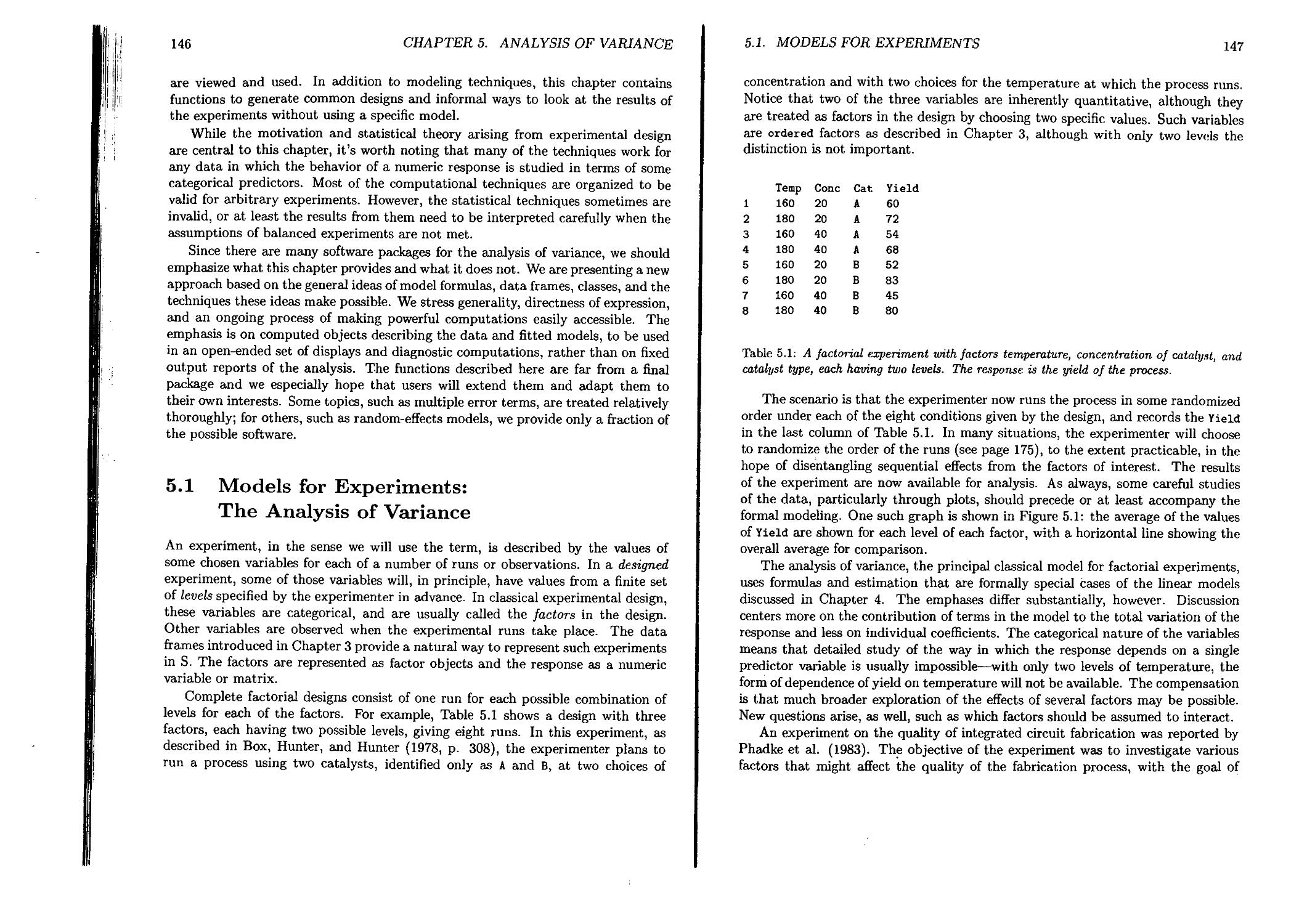
5.1 Models for Experiments: The Analysis of Variance...............146
5.2 S Functions and Objects........................................150
5.2.1 Analysis of Variance Models..............................150
5.2.2 Graphical Methods and Diagnostics........................163
5.2.3 Generating Designs.......................................169
5.3 The S Functions: Advanced Use .................................176
5.3.1 Parametrization; Contrasts...............................176
5.3.2 More on Aliasing ........................................178
5.3.3 Anova Models as Projections .............................181
5.4 Computational Techniques.......................................184
CONTENTS xiii
5.4.1 Basic Computational Theory.................................Ig5
5.4.2 Aliasing; Rank-deficiency................................. ^g?
5.4.3 Error Terms...................................................
5.4.4 Computations for Projection.................................
6 Generalized Linear Models 195
Trevor J. Hastie, Daryl Pregibon
6.1 Statistical Methods.................................................
6.2 S Functions and Objects.............................................
6.2.1 Fitting the Model ............................................
6.2.2 Specifying the Link and Variance Functions.................206
к2.3 Updating Models............................................209
6.2.4 Analysis of Deviance Tables................................210
6.2.5 Chi-squared Analyses ......................................213
6.2.6 Plotting...................................................216
6.3 Specializing and Extending the Computations.......................221
6.3.1 Other Arguments to glm() ............-......................221
6.3.2 Coding Factors for GLMs....................................223
6.3.3 More on Families...........................................225
6.3.4 Diagnostics................................................230
6.3.5 Stepwise Model Selection...................................233
6.3.6 Prediction.................................................238
6.4 Statistical and Numerical Methods................................241
6.4.1 Likelihood Inference.......................................242
6.4.2 Quadratic Approximations ..................................244
6.4.3 Algorithms.................................................245
6.4.4 Initial Values.............................................246
7 Generalized Additive Models 249
Trevor J. Hastie
7.1 Statistical Methods..............................................250
7.1.1 Data Analysis and Additive Models .........................251
7.1.2 Fitting Generalized Additive Models........................252
7.2 S Functions and Objects..........................................253
7.2.1 Fitting the Models.........................................253
7.2.2 Plotting the Fitted Models.................................264
7.2.3 Further Details on gamO . ... '................ 268
7.2.4 Parametric Additive Models: bs О and ns () ................270
7.2.5 An Example in Detail.......................................273
7.3 Specializing and Extending the Computations......................280
7.3.1 Stepwise Model Selection...................................280
7.3.2 Missing Data...............................................286
xiv
CONTENTS
7.3.3 Prediction....................................................
7.3.4
7.3.5
Smoothers in gam()
More on Plotting.............................................
Numerical and Computational Details.............................
7.4.1 Scatterplot Smoothing.....................................
7.4.2 Fitting Simple Additive Models............................
7.4.3 Fitting Generalized Additive Models.......................
7.4.4 Standard Errors and Degrees of Freedom ...................
7.4.5 Implementation Details....................................
288
293
295
298
298
300
302
303
304
8 Local Regression Models 309
William S. Cleveland, Eric Grosse, William M. Shyu
8.1 Statistical Models and Fitting................................ 312
8.1.1 Definition of Local Regression Models.....................312
8.1.2 Loess: Fitting Local Regression Models....................314
8.2 S Functions and Objects.........................................316
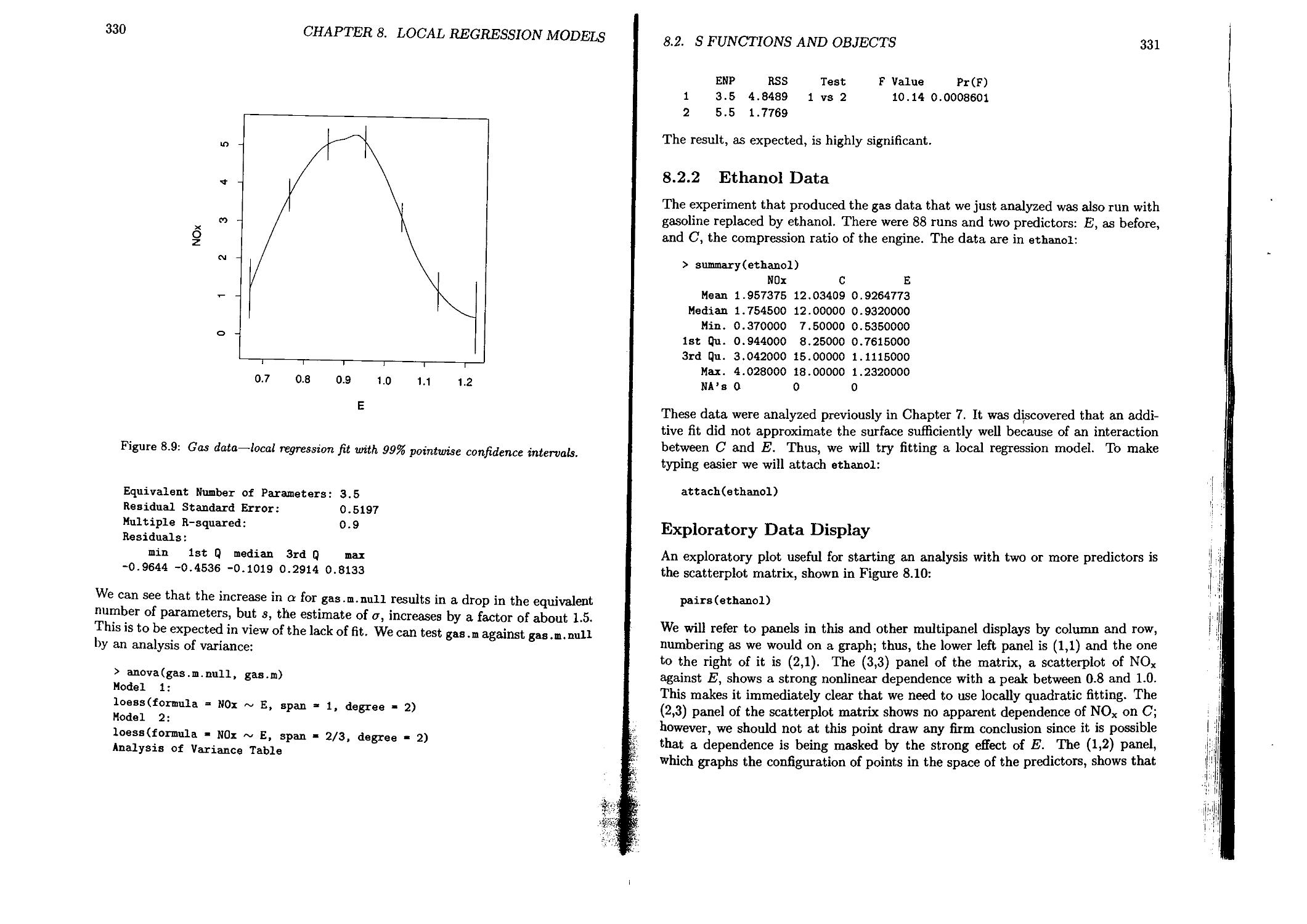
8.2.1 Gas Data..................................................322
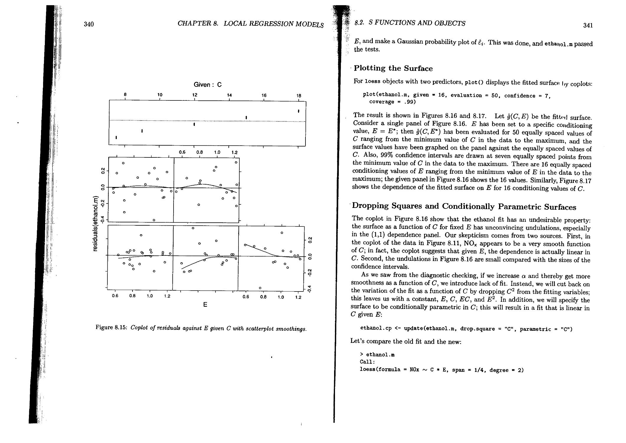
8.2.2 Ethanol Data..............................................331
8.2.3 Air Data .................................................348
8.2.4 Galaxy Velocities.........................................352
8.2.5 Fuel Comparison Data......................................359
8.3 Specializing and Extending the Computations.....................366
8.3.1 Computation............................................. 366
8.3.2 Inference ................................................367
8.3.3 Graphics .................................................368
8.4 Statistical and Computational Methods...........................368
8.4.1 Statistical Inference.....................................368
8.4.2 Computational Methods.....................................373
9 Tree-Based Models 377
Linda A. Clark, Daryl Pregibon
9.1 Tree-Based Models in Statistics.................................377
9.1.1 Numeric Response and a Single Numeric Predictor ...... 378
9.1.2 Factor Response and Numeric Predictors ...................380
9.1.3 Factor Response and Mixed Predictor Variables.............382
9.2 S Functions and Objects.........................................382
9.2.1 Growing a Tree............................................382
9.2.2 Functions for Diagnosis................................. 395
9.2.3 Examining Subtrees........................................396
9.2.4 Examining Nodes...........................................398
9.2.5 Examining Splits..........................................402
9.2.6 Examining Leaves..........................................405
CONTENTS
xv
9.3 Specializing the Computations ................................406
9.4 Numerical and Statistical Methods.............................412
9.4.1 Handling Missing Values................................415
9.4.2 Some Computational Issues..............................417
9.4.3 Extending the Computations.............................417
10 Nonlinear Models 421
Douglas M. Bates, John M. Chambers
10.1 Statistical Methods...........................................422
10.2 S Functions...................................................427
10.2.1 Fitting the Models.....................................428
10.2.2 Summaries..............................................432
10.2.3 Derivatives............................................433
10.2.4 Profiling the Objective Function.......................438
10.2.5 Partially Linear Models................................440
10.3 Some Details..................................................444
10.3.1 Controlling the Fitting................................444
10.3.2 Examining the Model....................................446
10.3.3 Weighted Nonlinear Regression..........................450
10.4 Programming Details...........................................452
10.4.1 Optimization Algorithm.................................452
10.4.2 Nonlinear Least-Squares Algorithm......................453
A Classes and Methods: Object-oriented Programming in S 455
John M. Chambers
A.l Motivation ......................................... > 456
A.2 Background....................................................457
A.3 The Mechanism.................................................460
A.4 An Example of Designing a Class...............................461
A.5 Inheritance.................................................. 463
A.6 The Frames for Methods........................................467
A.7 Group Methods; Methods for Operators..........................471
A.8 Replacement Methods...........................................475
A.9 Assignment Methods............................................477
A. 10 Generic Functions ...........................................478
A.ll Comment.......................................................479
В S Functions and Classes 481
References 589
Index
595
Chapter 1
An Appetizer
John M. Chambers
Trevor J, Hastie
This book is about data and statistical models that try to explain data. It is an enormous topic, and we will discuss many aspects of it. Before getting down to details, however, we present an appetizer to give the flavor of the large meal to come. The rest of this chapter presents an example of models used in the analysis of some data. The data are “real,” the analysis provided insight, and the results were relevant to the application. We think the story is interesting. Besides that, it should give you a feeling for the style of the book, for our approach to statistical models, and for how you can use the software we axe presenting. Don’t be concerned if details are not explained here; all should become clear later on.
1.1 A Manufacturing Experiment
In 1988 an experiment was designed and implemented at one of AT&T’s factories to investigate alternatives in the “wave-soldering” procedure for mounting electronic components on printed circuit boards. The experiment varied a number of factors relevant to the engineering of wave-soldering. The response, measured by eye, is a count of the number of visible solder skips for a board soldered under a particular choice of levels for the experimental factors. The S object containing the design, solder.balance, consists of 720 measurements of the response skips in a balanced subset of all the experimental runs, with the corresponding values for five experimental factors. Here is a sample of 10 runs from the total of 720.
2
CHAPTER 1. AN APPETIZER
> sample.runs <- sample(seq(720),10) > solder.balance[sample.runs,]
Opening Solder Mask PadType Panel skips 162 S Thin Al.5 D6 3 6
75 S Thick Al.5 L6 3 1
653 L Thin B3 L8 2 4
117 L Thin Al.5 W9 3 0
40 M Thick Al.5 D6 1 0
569 L Thick B3 L9 2 0
229 M Thick A3 L7 1 0
788 S Thick B6 L4 2 30
655 L Thin B3 W9 1 0
129 M Thin Al.5 L4 3 1
We can also summarize each of the factors and the response:
> summary(solder.balance)
Opening Solder Mask PadType Panel
S:240 Thin :360 Al.5:180 L9 : 72 1:240
M:240 Thick:360 A3 ;180 W9 : 72 2:240
L;240 B3 :180 L8 : 72 3:240
B6 :180 L7 : 72
D7 : 72
L6 : 72
(Other):288
skips
Min. : 0.000
1st Qu. Median Mean 3rd Qu. Max.
0.000
2.000
4.965
6.000
48.000
The physical and statistical background to these experiments is fascinating, but a bit beyond our scope. The paper by Comizzoli, Landwehr, and Sinclair (1990) gives a readable, general discussion. Here is a brief description of the factors:
Opening: amount of clearance around the mounting pad;
>,ТЯ'Г I C-yttJ*1
Solder: amount of solder;
Mask: type and thickness of the material used for the solder mask;
PadType: the geometry and size of the mounting pad; and
Panel: each board was divided into three panels, with three runs on a board.
Much useful information about the experiment can be seen without any formal modeling, particularly using plots. Figure 1.1, produced by the expression
plot(solder.balance)
is a graphical summary of the relationship between the response and the factors, showing the mean value of the response at each level of each factor. It is immediately obvious that the factor Opening has a very strong effect on the response: for levels
1.1. A MANUFACTURING EXPERIMENT
co
<N
St
B6t
L4t
Thin
D4
2т
Thick x
A3-
D6
3
M
A1.5-1-
W9X
Opening Solder Mask PadType Panel
Factors
Figure 1.1: A plot of the mean of skips at each of the levels of the factors in the sold experiment. The plot is produced by the expression plot (solder, balance).
M and L, only about two skips were seen on average, while level S produced abo six times as many. If you guessed that the levels stand for small, medium, a: large openings, you were right, and the obvious conclusion that the chosen sm opening was too small (produced too many skips) was an important result of t experiment.
A more detailed preliminary plot can be obtained by attaching the solder.bala data and plotting skips against the factors, using boxplots:
plot(skips Opening + Mask)
We have selected two of the factors for this plot, shown in Figure 1.2, and they b< exhibit the same behavior: the variance of the response increases with the me The response values are counts, and therefore are likely to exhibit such behavi since counts are often well described by a Poisson distribution.
4
CHAPTER 1. AN APPETIZER
S M L-
Opening
Mask
Figure 1.2: A factor plot gives a separate boxplot о/skips at each of the levels of the factors in the solder experiment. The left panel shows how the distribution of skips varies with the levels of Opening, and the right shows similarly how it varies with levels oj mask.
(J-
1.2 Models for the Experimental Results
Now let’s start the process of modeling the data. We can, and will, represent the Poisson behavior mentioned above. To begin, however, we will use as a response sqrt(skips), since square roots often produce a good approximation to an additive model with normal errors when applied to counts. Since the data form a balanced design, the classical analysis of variance model is attractive. As a first attempt, we fit all the factors, main effects only. This model is described by the formula
sqrt(skips)
where the saves us writing out all the factor names. We read ” as “is modeled as”; it separates the response from the predictors. The fit is computed by
> fitl <- aov(sqrt(skips) ~ , data = solder.balance)
The object fitl represents the fitted model. As with any S object, typing its name invokes a method for printing it:
> fitl
Call:
aov(formula = sqrt(skips) ~ Opening + Solder + Mask + PadType +
1.2. MODELS FOR THE EXPERIMENTAL RESULTS
5
Panel, data = solder.balance)
Terms: Opening Solder Mask PadType Panel Residuals
Sum of Squares 593.97 233.31 359.63 113.44 14.56 493.05
Deg. of Freedom 213 92 702
Residual standard error: 0.83806 Estimated effects are balanced
fitted (f it 1)
-2 0 2 4 6 8
fitted(fit2)
Figure 1.3: The left panel shows the observed values for the square root of skips, plotted against the fitted values from the main-effects model. The dotted line represents a perfect fit. The fit seems poor in the upper range. The right panel is the same plot for the model having main effects and all second-order interactions. The fit appears acceptable.
Once again, plots give more information. The expression
plot(fitted(fit 1), sqrt(skips))
shown on the left in Figure 1.3, plots the observed skips against the fitted values, both on the square-root scale. The square-root transformation has apparently done a fair job of stabilizing the variance. However, the main-effects model consistently underestimates the large values of skips. With 702 degrees of freedom for residuals, we can afford to try a more extensive model. The formula
sqrt(skips) ~ . л2
6
CHAPTER 1. AN APPETIZER
ИснспЬсн a model that includes all main effects and all second-order interactions. We fit this model next:
fit2 <- dov(oqrt(skips) ~ .л2, solder.balance)
Instead of printing the fitted object, we produce a statistical summary of the model using standard statistical assumptions, in this case an analysis of variance table as Hliown in I’ablc 1.1, with mean squares and F-statistic values.
> summary (f j t,2)
Df Sum
Opening 2
Solder 1
Mask 3
PadType 9
Panel 2
Opening:So]der 2
Opening;Mauk 6
Opening:PadType 18
Opening:Panel 4
Solder:Hank 3
Solder:PadType 9
Solder:Panel 2
Mask:PadType 27
Mask:Panel 6
PadType:Panel 18
Residualo 607
of Sq Mean Sq F Value Pr(F)
594 297 766 0.00
233 233 602 0.00
360 120 309 0.00
113 13 33 0.00
15 7 19 0.00
42 21 54 0,00
89 15 38 0.00
34 2 5 0.00
10 1 0.66
20 7 17 0.00
20 2 6 0.00
7 4 9 0.00
28 1 3 0.00
914 0.00
10 1 1 0.14
235 0
able 1.1: An analysis of variance table for the model fit2, including all main effects and second-order interactions. The columns give degrees of freedom, sums of squares, mean squares, b statistics, and their tail probabilities, nearly all zero here because of the very argc number of observations.
The function summaryO is generic, in that it automatically behaves differently, according to the class of its argument. In this case fit2 has class "aov" and so a particular method for summarizing aov objects is automatically used. The earlier use of summary () produced a result appropriate for data, frame objects. The modeling software abounds with generic functions; besides summaryO, others include plot(), predictQ, print(), and updateO.
The fitted values are plotted in the right panel of Figure 1.3, and the improvement is clear. Of course, we really expect an improvement; including all the pairwise interactions costs us 95 degrees of freedom! We can see from the table that the F statistic column varies greatly for the second-order terms in the model. The three
1.3. A SECOND EXPERIMENT
7
largest values, interestingly, are the interactions of three of the factors, Opening, Solder, and Mask. So an interesting intermediate model could be formed from just these interactions:
sqrt(skips) ~ . + (Opening + Solder + Mask)A2
This time we gave three factors, explicitly, for which we wanted interactions:
> fit3
Call:
aov(formula » sqrt(skips) ~ Opening + Solder + Mask + PadType
+ Panel + (Opening + Solder + Mask)A2, data - solder.balance)
Terms:
Opening Solder Mask PadType Panel Opening-.Solder
Sum of Squares 593.97 233.31 359.63 113.44 14.56 41.62
Deg. of Freedom 2 1 3 9 2 2
Opening:Mask Solder:Mask Residuals
Rum of Squares 88.66 19.86 342.90
Deg. of Freedom 6 3 691
Residual standard error: 0.70445
Estimated effects are balanced
The left panel of Figure 1.4 shows the observed/fit ted values for this second-orde submodel, which is comparable to the right plot of Figure 1.3. It uses far fewer de grees of freedom, achieves almost as good a fit, and also accounts for the departure missed by the main-effects model.
1.3 A Second Experiment
The results from the first experiment were valuable in the application, and subs< quently a similar experiment was run at another AT&T factory. The results a; recorded in the design object solder2. In part, the intention was to apply some < the lessons learned in the first experiment. The design was nearly the same as the first experiment, and we can use summaryO and plot() as before:
> >
CHAPTER 1. AN APPETIZER
-2 0 2
4 6 8
fitted (fit3)
fitted(fit3.2)
?igure 1.4: The left panel is a plot of the square root о/skips from the first AT&T solder xperiment against the fitted values for the second-order submodel The right panel is the ame plot using the data from the second solder experiment.
summary(solder2)
Opening Solder
S:300 Thin :450
M:300 Thick:450
L:300
Mask PadType
Al.5:180 L9 : 90
A3 :270 W9 : 90
A6 : 90 L8 : 90
B3 : 180 L7 : 90
B6 :180 D7 : 90
L6 : 90
(Other):360
Panel skips
1:300 Min. : 0.0
2:300 1st Qu.: 0.0
3:300 Median : 0.0
Mean : 1.2
3rd Qu.: 0.0
Max. :32.0
NA’s : 150
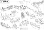
The summaries show some striking differences, especially that there are far fewer kips overall in this experiment. Only 17% of the runs from the second experiment iad skips, compared to 66% from the first. Figure 1.5 shows a plot of the design, reated by the expression plot(solder2). The plot suggests that in this case, factor iask appears to have the largest effect. At first it may appear that the two experiments are almost unrelated—a little discouraging for the statistician, although the ngineer is likely to be happy that the overall performance is substantially improved. Is for modeling, if we start with the last model considered for the first experiment,
> fit3.2 <- update(fit3, data = solder2, na ® na.omit)
nd plot its fit in the right panel of Figure 1.4, the model does not appear to fit hese data well at all. Notice the use of the na.action® argument in the call to
1.3. A SECOND EXPERIMENT
9
J I I I
Opening Solder Mask PadType Panel
Factors
Figure 1.5: A plot of the mean of skips at each of the levels of the factors in the second wave-soldering experiment. Compare with Figure 1.1.
update(); in any model-fitting computation, this causes the 150 cases with skips missing to be omitted. Since we can’t handle these missing values in any of our models, we have assigned solder2 as na.omit(solder2) in the remaining examples.
Interestingly, more careful analysis shows that the two experiments are not as unrelated as they initially appear to be. We must keep in mind that we can no longer use the square-root transformation with so many zero responses. More fundamentally, the statistical model should reflect more closely the way engineers would likely view the process. When (as one would certainly prefer) solder skips are a rare event, it is natural to imagine that the solder process has two states: a “perfect” state where no skips will be observed, and an “imperfect” state in which skips may or may not occur. From the view of the application, one is particularly interested in factors that relate to keeping the process in the perfect state.
10
CHAPTER!. AN APPETIZER
When this more complicated but more plausible model is worked out in detail, it shows patterns in the second experiment that are largely consistent with those in the first. To see these results in detail, you will have to read on in the book. Some of the ideas, however, we can sketch here as a final appetizer.
Suppose we are only concerned with whether there are any skips, as measured by the logical variable
skips > 0
Although this variable is very different from the quantitative variable sqrt(skips) that we have studied so far, models for it can be handled in a very similar style. Specifically, a generalized linear model (glm) using the binomial distribution is a natural way to treat such TRUE, FALSE or equivalently 1, 0 variables:
fit3.binary <- glm( skips > 0 ~ . + (Opening + Solder + Мазк)л2, data = solder2, family = binomial)
What has changed here? The function glm() has replaced aov() to do the fitting, the response is now a logical expression, and a new argument
family = binomial
has been added. As you can imagine, glm() fits generalized linear models, and the new argument tells it that the fit should use the binomial family within the glm models. Otherwise, the specification of model and data remain the same. Also, the object returned can be treated similarly to those we computed before using aov(), applying the various generic functions to summarize the model and study how well it works.
Another idea, somewhat complementary to using a binomial model, is to treat the response directly as counts, rather than using the square-root transformation. As we said early on in our discussion, the Poisson distribution is a natural model for counts, and usually works better than the transformation when the typical number of counts is small. The same generalized linear models allow us to model the mean of a Poisson distribution by the structural formula we used earlier. Let’s apply this to the data from both experiments to compare the results:
> expl.pois <- glm(skips ~ . + (Opening + Solder + Mask)A2, data = solder.balance, family = poisson )
> exp2.pois <- update(expl.pois, data = solder2 )
We display the fits in Figure 1.6, using the square-root scale as before to compare these fits with those in Figure 1.4. The Poisson model appears to be an improvement over those in Figure 1.4, especially for the second experiment; the systematic bias for large counts is gone.
This is still not the end of the story. There are more zero values in the data from the second experiment than the Poisson model predicts. The binomial model
1.4. SUMMARY
11
0 2 4 6 8
sqrt(fitted(exp1 pois)
0 2 4 6 8
sqrtff itted (exp2 .pois)
Figure 1.6: The second-order model of Figure 1.4, treating the response skips as Poisson
and using a log-linear link. The data are plotted on the square-root scale for comparison
with Figure 1.4- The plot on the left corresponds to the first experiment, the right the
second.
handles this aspect, but we clearly can’t just apply both binomial and Poisson models since they imply two incompatible explanations. An answer is to use a mixture of the two models, as the idea of perfect and imperfect states for the process suggests. Some runs are in the perfect state, and the binomial model lets us treat the probability of this; others are in the imperfect state, and for those the Poisson model can be applied. This model, called the Zero-Inflated Poisson, cannot be described as a single linear or generalized linear model. A full statistical discussion by the inventor of the technique is in the reference Lambert (1991). One version is described in Section 10.3, as an example of a general nonlinear model.
1.4 Summary
This has been a large plate of appetizers, and we will finish here. All the same, we have touched on only a few of the kinds of models that appear in the book, mainly the analysis of variance and generalized linear models. The book discusses models that fit smooth curves and surfaces, generalized additive models, models that fit tree structures by successive splitting, and models fit by arbitrary nonlinear regression or optimization. We also showed only a small sample of the diagnostic summaries and plots appearing in the rest of the book.
12
CHAPTER 1. AN APPETIZER
However, the general style to be followed throughout has been illustrated by the examples:
• The structural form of models is defined by simple, general formulas.
• Many kinds of data for use in model-fitting can be organized by data frames and related classes of objects.
• Different kinds of models can be fitted by similar calls, typically specifying the formula and data.
• The objects containing the fits can then be used by generic functions for printing, summaries, plotting, and other computations, including fitting updated mo dels .
• The computations are designed to be very flexible, and users are encouraged to adapt our software to their own needs and interests.
In presenting our appetizer, we did not emphasize the last point heavily, but it is central to the philosophy behind this book. Even though a large number of functions and methods are presented, we intend these to be a starting point for the computations you want, rather than some rigid prescription of how to use statistical models.
Chapter 2
Statistical Models
John M. Chambers
Trevor J. Hastie
This is a book about statistical models — how to think about them, specify them, fit them, and analyze them. Statistical models are simplified descriptions of data, us uallyr const rue ted from some mathematically or numerically defined relationships. Modern data analysis provides an extremely rich choice of modeling techniques; later chapters will introduce many of these, along with S functions and classes of S objects to implement them. All these techniques benefit from some general ideas about data and models that allow us to express what data should be used in the model and what relationships the model postulates among the data. You should read this chapter (at least the first two sections) for a general notion of how models are represented. You can do this either before you start to work with specific kinds of models or after you have experimented a little. Getting some hands-on experience first is probably a good idea—for example, by looking at the first two sections of Chapter 4 on linear models, or by experimenting with whatever kind of model interests you most.
The first two sections of this chapter introduce our way of representing models, and are likely to be all you need for direct use of the software in later chapters. When and if you come to modify our software to suit your own ideas, as we hope many users will do, then you should eventually read further into Sections 2.3 and 2.4.
Throughout the book, we will be expressing statistical models in three parts:
• a formula that defines the structural part of the model—that is, what data are being modeled and by what other data, in what form;
13
14
CHAPTER 2. STATISTICAL MODELS
• data to which the modeling should be applied;
• the stochastic part of the model—that is, how to regard the discrepancy or residuals between the data and the fit.
This chapter and the next concentrate on the first two of these. They discuss how formulas are represented, what objects hold the data, and how the two are brought together. The rest of the book then brings together the three parts in the context of different kinds of models.
Formulas are S expressions that state the structural form of a model in terms of the variables involved. For example, the formula
Fuel ~ Power + Weight
reads “Fuel is modeled as Power plus Weight.” More precisely, it tells us that the response, Fuel, is to be represented by an additive model in the two predictors, Power and Weight. There is no information about what method should be used to fit the model. Formulas of this general style are capable of representing a very wide range of structural model information; for example,
100/Mileage ~ poly(Weight, 3) + sqrt(Power)
says to fit the derived variable 100/Mileage to a third-order polynomial in Weight plus the square-root of the Power variable. Transformations are used directly in the formula, and the basis for the polynomial regression in Weight is generated automatically from the formula. Here is a formula to fit separate B-spline regression curves within the two levels of Power obtained by cutting Power at its midrange:
Fuel ~ cut(Power, 2) / bs(Weight,df=5)
In the next example, nonparametric smooth curves will be used to model the transformed Fuel additively in Weight and Power, using 5 degrees of freedom for each term:
sqrt(Fuel-min(Fuel)) ~ s(Weight, df=5) + s(Power, df=5)
The details of these formulas will be explained later in the chapter.
The models above imply the presence of some data on Fuel, Power and Weight; in fact, reasonable models are inspired by data, since models without data are hard to think about. These data actually do exist, and form part of a large collection of data on automobiles described in Chapter 3 and used throughout the book; the present model relates fuel consumption to two vehicle characteristics. Part of the model-building process is collecting and organizing the relevant dataset, and looking at it in many different ways. Some of the useful views are simple, such as summaries and plots. The next chapter is about tools for organizing data into objects that are convenient both for studying the data directly and as input for more sophisticated procedures. For the moment we assume that such data organization has already taken place, and that all the variables referred to in formulas are available.
2.1. THINKING ABOUT MODELS
15
2.1 Thinking about Models
Models are objects that imitate the properties of other, “real” oli)(4-ts ju a simpler or more convenient form. We make inferences from the an(j npply them to the real objects, for which the same inferences would be iтроян!bh* <’r inconvenient. The differences between model and reality, the residitnis often arc the key to reaching for a deeper understanding and perhaps a better model.
2.1.1 Models and Data
A road map models part of the earth’s surface, attempting to imitate the relative position of towns, roads, and other features. We use the map to make inferences about where real features are and how to get to them. Architects use both paper drawings and small-scale physical models to imitate the properties of a building. The appearance and some of the practical characteristics of the actual building can be inferred from the models. Chemists use “wire frame” models of molecules (by either constructing them or displaying them through computer graphics) to imitate theoretical properties of the molecules that, in turn, can be used to predict the behavior of the real objects.
A good model reproduces as accurately as possible the relevant properties of the real object, while being convenient to use. Good road maps draw roads in the correct geographical position, in a representation that suggests to the driver the important curves and intersections. Good road maps must also be easy to read. Any good model must facilitate both accurate and convenient inferences. A large diorama or physical model of a town could provide more information than a road map, and more accurate information, but since it can be used only by traveling to the site of the model, its practical value is limited. The cost of creating or using the model also limits us in some cases, as this example illustrates: building dioramas corresponding to every desirable road map is unlikely to be practical. Finally, a model may be attractive because of aesthetic features — because it is in some sense beautiful to its users. Aesthetic appeal may make a model attractive beyond its accuracy and convenience (although these often go along with aesthetic appeal).
Statistical models allow inferences to be made about an object, or activity, or process, by modeling some associated observable data. A model that represents gasoline mileage as a linear function of the weight and engine displacement of various automobiles,
Mileage ~ Weight + Disp.
is directly modeling some observed data on these three variables. Indirectly, though, it represents our attempt to understand better the physical process of fuel consumption. The accuracy of the model will be measured in terms of its ability to imitate the data, but the relevant accuracy is actually that of inferences made about the
16
CHAPTER 2. STATISTICAL MODELS
real object or process. In most applications the goal is also to use the model to understand or predict beyond the context of the current data. (For these reasons, useful statistical modeling cannot be separated from questions of the design of the experiment, survey, or other data-collection activity that produces the data.) The test data we have on fuel consumption do not cover all the automobiles of interest; perhaps we can use the model to predict mileage for other automobiles.
The convenience of statistical models depends, of course, on the application and on the kinds of inference the users need to make. Generally applied criteria include simplicity; for example, a model is simpler if it requires fewer parameters or explanatory variables. A model that used many variables in addition to weight and displacement would have to pay us back with substantially more accurate predictions. especially if the additional variables were harder to measure.
Less quantifiable but extremely important is that the model should correspond as well as possible to concepts or theories that the user has about the real object, such as physical theories that the user may expect to be applicable to some observed process- Instead of modeling mileage, we could model its inverse, say the fuel consumption in gallons per 100 miles driven:
100/Mileage ~ Weight + Disp.
This may or may not be a better fit to the data, but most people who have studied physics are likely to feel that fuel consumption is more natural than mileage as a variable to relate linearly to weight.
2.1.2 Creating Statistical Models
Statistical modeling is a multistage process that involves (often repeated use of) the following steps:
• obtaining data suitable for representing the process to be modeled;
• choosing a candidate model that, for the moment, will be used to describe some relation in the data;
• fitting the model, usually by estimating some parameters;
• summarizing the model to see what it says about the data;
• using diagnostics to see in what relevant ways the model fails to fit as well as it should.
The summaries and diagnostics can involve tables, verbal descriptions, and graphical displays. These may suggest that the model fails to predict all the relevant properties of the data, or we may want to consider a simpler model that may be
2.1. THINKING ABOUT MODELS
17
nearly as good a fit. In either case, the model will be modified, and the fitting and analysis carried out again.
If we started out with a model for mileage as a linear function of weight and displacement, we would then want to look at some diagnostics to examine how well the model worked. The left panel of Figure 2.1 shows Mileage plotted against the values predicted by the model. The model is not doing very well for cars with high
co
fair
о co
о CM
J0 О о
OOxO OD
O'OO ®0
О /fooo
CD' О О 00 о
IO
co
CM
О 0/ ✓ О / ' о ✓6 о oo ozti OD z о oo op* о OO О
О (ГО
OO (OD ojm о о oo
Off oo
✓
О '
20 25 30 35
20 25 30 35
Fitted: Weight + Disp.
Fitted: Weight + Disp. + Type
Figure 2.1: Mileage for 60 automobiles plotted against the values predicted by a linear model in weight and displacement (the left panel) or weight, displacement and type of automobile (the right panel).
mileage: they all fall above the line. The change to 100/Mileage helps some (there is a plot on page 104). If we add in a coefficient for each type of car (compact, large, sporty, van, etc.) the fit improves further. In practice, we would continue to study diagnostics and try alternative models, seeking a better understanding of the underlying process. This model is our most commonly used simple example, and will recur many times, to introduce various techniques.
Research in statistics has led to a wide range of possible models. Later chapters in this book deal with specific classes of models: traditional models such as linear regression; recent innovations, such as models involving nonparametric smooth curves or tree structures; important specializations such as models for designed experiments, and general computational techniques such as minimization, which can be used to fit models not belonging to any of the standard classes. This rich choice of possible models is of real benefit in analyzing data. Whenever we can specify
18
CHAPTER 2. STATISTICAL MODELS
a model that is close to our intuitive understanding or is able to respond to some observed failure of a standard model, chances are we will more easily discover what is really going on. A limited computational or statistical framework that requires us to distort or approximate the model we would like to fit makes such discovery more difficult. It can also hide from us some important information about the data. The methods presented in this book and the functions that implement the methods are designed to give the widest possible scope in creating and examining statistical models.
Of course, all this rich variety will only be helpful if we can use it easily enough. We must be able to carry out the steps in specifying the models without too much effort on our part. The fitting must be accurate and efficient enough to be used in practical problems. There must be appropriate summaries and diagnostics so that we can assess the adequacy of the models. In later chapters, each of these questions will be considered for the various classes of models.
Fortunately, many different classes of models share a substantial common structure. The steps we listed above apply to many models, and important summaries and diagnostics can be shared directly or, at worst, adapted straightforwardly from one class of models to another. The organization of the S computations for the various classes of models is designed to take advantage of this common structure.
This chapter describes a way to express the structural formula for the model. What about the data? For the moment we can assume the data are around in our global environment, and simply refer to variables by name. In Chapter 3 we describe data frames, a more systematic way of organizing and providing the data for a model. Depending on the class of models, formulas and data frames may be all we need to specify; for example, if we are using linear least-squares fitting, there is not much more to say in step 3. Other kinds of models may require some further specifications; generalized linear models, for example, require choosing link and variance functions. The choice of the kind of model and the provision of these additional specifications fix the stochastic part of the model to be fit.
2.2 Model Formulas in S
The modeling formula defines the structural form of the model, and is used by the model-fitting functions to carry out the actual fitting. Most readers will already be familiar with conventional modeling formulas, such as those used in textbooks or research papers to describe statistical models, as in (2.1) below. The formulas used in this book have evolved from mathematical formulas as a simpler and in some ways more flexible approach to be used when computing with models.
A formula in S is a symbolic expression. For example,
Fuel ~ Weight + Disp.
2.2. MODEL FORMULAS IN S
19
just stands for the structural part of a model. If you evaluate the formula, you will just get the formula. In particular, use of a formula such as the one above does not depend on the values of the named variables; indeed, the variables need not even exist! The expression to the left of the is the response, sometimes called the dependent variable. In this case the response is simply the name Fuel. The right side is the expression used to fit the response, made up in an additive model of terms separated by “+”. The variables appearing in the terms are called the predictors. Experienced S users are by now probably very curious, so this comment is for their benefit: is an S function that does nothing but save the
formula as an unevaluated S expression, a formula object.
The formula above expresses most of the ingredients of a statistical model of the form
Fuel = a + Weighty + Disp.fa + £ (2.1)
fl
For most of the models in this book, the formula does not specifically refer to the parameters f3j in the linear model. These can be inferred and so we save typing them. In a sense, we also avoid mental clutter, in that the names of the parameters are not relevant to the model itself. When we come to general nonlinear models in Chapter 10, however, the formula will have to be completely explicit, since it is no longer additive.
The formula makes no reference to the errors e either. These, of course, are the stochastic part of the model specification. When formulas are used in a call, say to the linear regression model-fitting function
lm(Fuel ~ Weight + Disp.)
we complete the rest of the modeling specification; lm() assumes the mean of Fuel is being modeled by the linear predictor, and uses least squares to compute the fit. Expressions such as the one above were encountered in Chapter 1; in fact all the model-fitting functions take a formula as their first argument, and in most cases the same formula can be used interchangeably among them (hopefully with different consequences!).
The formula above is equivalent to
Fuel 1 + Weight + Disp.
where the 1 indicates that an intercept a is present in the model. Since we usually want an intercept, it is included by default; on the other hand, we can explicitly exclude an intercept by using -1 in the formula
Fuel ~ -1 + Weight + Disp.
In using formulas it is important to keep in mind that we are writing a shorthand for the complete model expression. In particular, there is no operation going on that adds Weight and Disp-.; the operator “+” is being used in a special sense, to
20
CHAPTER 2. STATISTICAL MODELS
separate items in a list of terms to be included in the model. The formula expression is, in fact, used to generate such a list, from which the terms and the order in which they appear in the model will be inferred. This inference poses no problem for most models, but with complicated formulas, some care may be needed to understand the model implied. The remainder of this section gives enough information for most uses of model formulas; Section 2.3.1 provides a complete description.
2.2.1 Data of Different Types in Formulas
The terms in a formula are not restricted to names: they can be any S expression that, when evaluated, can be interpreted as a variable. For example, if we wanted to model the logarithm of Fuel rather than Fuel itself, we could simply use that transformation in the formula
log(Fuel) ~ Weight + Disp.
A variable may be a factor, rather than numeric. A factor is an object that represents values from some specified set of possible levels. For example, a factor Sex might represent one of two values, "Male" or "Female". Readers familiar with S might wonder what happened to the category, which is also an object with levels. Factors have all the features of categories, with some added class distinctions; in particular there is a distinction between factors and ordered factors. Factors can be created in a number of ways, as will be discussed in Section 3.2. For the moment the distinction between factors and categories is not important, and we will simply refer to them as factors.
Factors enter the formula in the same way as numeric variables, but the interpretation of the corresponding term in the model is different. In a linear model, one fits a set of coefficients corresponding to a factor. Consider the model
Salary ~ Age + Sex
where Salary and Age are numeric vectors and Sex is a two-level factor. This is now shorthand for a model of the form
Salaryi = p + AgeiP +
Otp
if Sexi is Male
if Sexi is Female
(2.2)
where a? and ам are two parameters representing the two levels of Sex. The coding of factors proceeds from observing that this model is equivalent to one in which the factor is replaced by one “dummy” variable for each level—namely, a numeric variable taking value 1 wherever the factor takes on that level, and 0 for all other observations. In this case, for example, suppose XMale is a dummy variable set to 1 for all Male observations and XFemale is set to 1 for all Female observations. The original model is then equivalent to
2.2. MODEL FORMULAS IN S
21
Salary ~ Age + XMale +XFemale
Often in models such as this not all of the coefficients can be determined numerically; for example, in (2.2) we could replace /z by /z + <5, and then compensate by replacing of and ад/ by ap — 6 and ам — 8. Numerically such indeterminacies can be detected by collinearities in the variables used to represent the terms (Xmale and Xf emale add to a vector of ones, which is also used to represent the constant /z), and will be handled automatically during the model-fitting. Occasionally, you may want to control the parametrization of a term explicitly; Section 2.3.2 will show how.
Other non-numeric variables enter into the models by being interpreted as factors. A logical variable is a factor with levels "TRUE" and "FALSE". A character vector is interpreted as a factor with levels equal to the set of distinct character strings. A category object in S will be treated as a factor in the modeling software. Section 3.2.1 deals with these issues in more detail.
A term in a formula can also refer to a matrix. Each of the variables represented by the columns of the matrix will appear linearly in the model with its own coefficient. However, the entire matrix is interpreted as a single term.
To sum up so far, the following S data types can appear as a term in a formula:
1. a numeric vector, implying a single coefficient;
2. a factor or ordered factor, implying one coefficient for each level;
3. a matrix, implying a coefficient for each column.
Transformations increase the flexibility greatly, since the final element in this list is
4. any S expression that evaluates to a variable corresponding to one of the three types above.
To appreciate this last item, consider these examples of valid expressions that can appear as terms within a formula:
• (Age > 40), which evaluates to a logical variable; ж
• cut (Age, 3), which evaluates to a three-level category;
• poly(Age,3), which evaluates to a three-column matrix of orthogonal polynomials in Age.
The classical computational model for regression is an X matrix and a coefficient vector p. The rich syntax of our modeling language allows us instead to think of each of the terms as an entity, even though they eventually will be expanded into one or more columns of a model matrix X in most of the models discussed. But the formulas and the modeling language put no restrictions on the form of a term
22
CHAPTER 2. STATISTICAL MODELS
or on the interpretation given to the term by a particular model-fitting function. The contribution of a term to the fit can often be thought of as a function of the underlying predictor; factors produce step functions, and terms based on functions like polyO produce smooth functions. See Section 2.3.1 and Chapter 6. For other models, like local regression and tree-based models, the contribution of the terms is interpreted differently. In particular, the contribution of a term to a tree-based model is invariant under monotone transformations of the variable.
2.2.2 Interact ions
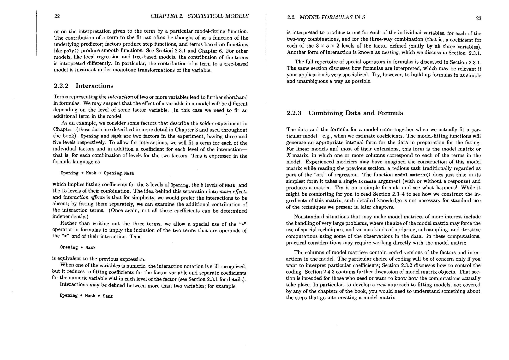
Terms representing the interaction of two or more variables lead to further shorthand in formulas. We may suspect that the effect of a variable in a model will be different depending on the level of some factor variable. In this case we need to fit an additional term in the model.
As an example, we consider some factors that describe the solder experiment in Chapter 1 (these data are described in more detail in Chapter 3 and used throughout the book). Opening and Mask are two factors in the experiment, having three and five levels respectively. To allow for interactions, we will fit a term for each of the individual factors and in addition a coefficient for each level of the interaction— that is, for each combination of levels for the two factors. This is expressed in the formula language as
Opening + Mask + Opening:Mask
which implies fitting coefficients for the 3 levels of Opening, the 5 levels of Mask, and the 15 levels of their combination. The idea behind this separation into main effects and interaction effects is that for simplicity, we would prefer the interactions to be absent; by fitting them separately, we can examine the additional contribution of the interaction terms. (Once again, not all these coefficients can be determined independently.)
Rather than writing out the three terms, we allow a special use of the operator in formulas to imply the inclusion of the two terms that are operands of the and of their interaction. Thus
Opening * Mask
is equivalent to the previous expression.
When one of the variables is numeric, the interaction notation is still recognized, but it reduces to fitting coefficients for the factor variable and separate coefficients for the numeric variable within each level of the factor (see Section 2.3.1 for details).
Interactions may be defined between more than two variables; for example,
Opening * Mask * Samt
2.2. MODEL FORMULAS IN S
23
is interpreted to produce terms for each of the individual variables, for each of the two-way combinations, and for the three-way combination (that is, a coefficient for each of the 3x5x2 levels of the factor defined jointly by all three variables). Another form of interaction is known as nesting, which we discuss in Section 2.3.1.
The full repertoire of special operators in formulas is discussed in Section 2.3.1. The same section discusses how formulas are interpreted, which may be relevant if your application is very specialized. Try, however, to build up formulas in as simple and unambiguous a way as possible.
2.2.3 Combining Data and Formula
The data and the formula for a model come together when we actually fit a particular model—e.g., when we estimate coefficients. The model-fitting functions will generate an appropriate internal form for the data in preparation for the fitting. For linear models and most of their extensions, this form is the model matrix or X matrix, in which one or more columns correspond to each of the terms in the model. Experienced modelers may have imagined the construction of this model matrix while reading the previous section, a tedious task traditionally regarded as part of the “art” of regression. The function model, matrix О does just this; in its simplest form it takes a single formula argument (with or without a response) and produces a matrix. Try it on a simple formula and see what happens! While it might be comforting for you to read Section 2.3-4 to see how we construct the ingredients of this matrix, such detailed knowledge is not necessary for standard use of the techniques we present in later chapters.
Nonstandard situations that may make model matrices of more interest include the handling of very large problems, where the size of the model matrix may force the use of special techniques, and various kinds of updating, subsampling, and iterative computations using some of the observations in the data. In these computations, practical considerations may require working directly with the model matrix.
The columns of model matrices contain coded versions of the factors and interactions in the model. The particular choice of coding will be of concern only if you want to interpret particular coefficients; Section 2.3.2 discusses how to control the coding. Section 2.4.3 contains further discussion of model matrix objects. That section is intended for those who need or want to know how the computations actually take place. In particular, to develop a new approach to fitting models, not covered by any of the chapters of the book, you would need to understand something about the steps that go into creating a model matrix.
24
CHAPTER 2. STATISTICAL MODELS
> I
I
2.3 More on Models
The third section of each chapter in this book expands on the S functions and !
objects provided in the chapter. Here we discuss the options and extended versions 1
available that add new capabilities to the basic ideas. The material in section 3 should usually be looked at after you have tried out the essentials presented in ! section 2 on a few examples. Experience shows that, after trying out the ideas for a while, you will have a better feeling for how to make use of the functions, and will begin to think “This would be a bit better if only ....” Section 3 is intended to handle most of the “if-only.” When the extra feature needed is not here, and there is no obvious way to create it by writing some function yourself, the next step is to look at section 4, which reveals how it all works. There you can learn what would be involved in modifying the basics. However, you should not take that step before thoroughly understanding what can be done more directly.
2.3.1 Formulas in Detail
In Section 2.2 we introduced model formulas and gave some examples of typical S expressions that can be used to give a compact description of the structural form of a model. Simple model-fitting situations can often be handled by the simple formulas shown there, but the full scope of model formulas allows much more detailed control. In this section, we give the full syntax available and explain how it is interpreted to generate the terms in the resulting model. Unless otherwise stated, we will always be talking about linear or additive models, in which the coefficients to be fitted do not have to appear explicitly in the formula. Formulas as discussed here follow generally the style introduced by Wilkinson and Rogers (1973), and subsequently i adopted in many statistical programs such as GLIM and genstat. While originally | introduced in the context of the analysis of variance, the notation is in fact just a shorthand for expressing the set of terms defined separately and jointly by a number of variables, typically factors. Its application is therefore much more general; for (
example, it works for tree-based models (Chapter 9), where there is no direct link I
to linear models. Two additional extensions appear in our use of formulas: I
• a “variable” can in fact be an arbitrary S expression, and ।
• the response in the model is included in the formula. i
Of course the “any expression” in the first item had better evaluate to one of the permissible data types: numeric vector, factor (including categories and logicals), or matrices. The discussion here focuses on special operators for the predictors, and so, in the examples below, we will omit the response expressions. I
A model formula defines a list of terms to appear in a model. Each term identifies j some S expression involving the data. This expression, in a linear model, generates |
4
•J 1 4
J
2.3. MORE ON MODELS
25
one or more columns in a model matrix. These columns, each multiplied by the appropriate coefficient, are the contribution of this term to the fit. For other types of models, the contribution of the term may be computed in a slightly different way, but in any case the expanded definition of the model corresponds to this list of terms. A corresponding expanded formula has one expression for each term, separated by + operators. You will hardly ever write fully expanded formulas, but any formula you do write will first be expanded (and simplified) before being evaluated. In this section we proceed by first discussing the meaning of expanded formulas. Then we give the complete rules by which arbitrary formulas are expanded.
Interaction and Nesting
Expanding a formula reverses the process shown in Section 2.2 of choosing a shorthand for a formula. For example, the formula
Opening * Mask
says that we want a model which fits coefficients for Opening, for Mask, and for the interaction of the two. When Opening and Mask are factors, this means a coefficient for each level of the factor; if either is a numeric variable or a numeric matrix, there will instead be one coefficient for the variable or for each column of the matrix. (We will discuss the meaning of interaction in this case later in this section.) In the more customary textbook notation,
• a factor: factor interaction represents a term of the form which is a set of IJ constants for each cell in the two-way table obtained by crossing the two factors (assuming the factors have I and J levels, respectively);
• a factor: numeric interaction represents a term of the form ffjX, or a varying slope model, in which the coefficient of the numeric variable x is different for each of the J levels of the factor;
• a numeric:numeric interaction represents a term pxz, where xz is simply the pointwise product of the variable x with the variable z. This is probably the least meaningful form of interaction, but of course the syntax allows far more meaningful terms to be created in cases such as this. For example, poly(x,z,2) will specify a bivariate quadratic surface in the two numeric variables x and z.
The formula Opening * Mask in expanded form is then
1 + Opening + Mask + Opening:Mask
The formula above brings in factors in a crossed model; that is, the model says that the individual factors should be included and, in addition, that the contribution of one factor to the fit may change depending on the level of the other factors.
26
CHAPTER 2. STATISTICAL MODELS
Nested terms in a model, on the other hand, arise when the levels of one factor are only meaningful within a particular level for some other factor or combination of factors. For example, suppose we have some geographic data in which the variable state defines the state for each location and the factor county indexes counties within each state. Clearly, county was generated by coding whatever county names appeared for each state, so that level 1 of county means something different in different states. In this context, a main effect for county is meaningless, and a typical model will fit a main effect for state and then look at the coefficients for county within each level of state. In expanded form this could be written
1 + state + county:state
However, to emphasize that the last term is thought of as a nested term, not an interaction, we allow (and encourage) writing the model as
1 + state + county %in*X state
The formula written above in expanded form has the shorthand notation
state / county
meaning “state and then county within state.” Notice that while factors joined by * can be permuted without changing the meaning (except for the order of the expanded terms), factors joined by / can never be meaningfully permuted: if county is nested in state, then state cannot be nested in county.
While the model implies a coefficient for each level of each term, in practice the coefficients have built-in dependencies. When a model matrix is created that represents a particular model, columns coding each term are included for all the coefficients that can be estimated; this is the condition for a valid coding of the model. One would like the individual coefficients to be meaningful in terms of the overall model and to avoid too many redundant coefficients that will have to be removed in the fitting. In Section 2.4.1, the general rules for coding will be outlined, but for practical purposes you need not worry about the coding unless you want to understand or control the specific choice of coefficients.
The coding of factors depends on the overall model. In the two-factor crossed model, main effects are included for both of the factors in the interaction term. All the possible coefficients for the interaction term can be estimated by representing each factor by contrasts among the levels of the individual factors. The contrasts will be chosen by default in a standard way, but the coding can be controlled, as shown in the next section. Unordered factors are coded as successive differences using the Helmert contrasts (Section 2.3.2), and ordered factors are coded to give a polynomial fit to a hypothetical underlying numeric variable. In the nested model, there is no main effect for county, so that the coding of county 7.in% state proceeds differently: state is coded by dummy variables and county by contrasts. This produces the
2.3. MORE ON MODELS
27
computational equivalent of “county within state” and also guarantees that the model will fit as many coefficients as can be meaningfully defined. The details of coding affect only the meaning of the individual coefficients estimated. Any valid representation will give the same contribution to the overall fit in the model for each of the terms. If you don’t care about the individual coefficients, leave the default coding in place; if you do care, look at page 32 to see how to change it.
When one of the variables in an interaction is numeric, the term will be computed formally the same way, but some extra remarks are needed on how crossed and nested interactions are interpreted. A numeric factor is always “coded” as itself. In
interactions, the numeric factor will be multiplied by either the dummy variables or the contrasts for a factor. Consider a simple example using the automobile data:
suppose Weight is numeric and Foreign is a logical variable, which will be turned
into a factor with two levels corresponding to FALSE and TRUE. Both the crossed
formula
Foreign * Weight and the nested one
Foreign / Weight
make sense, but they mean something different. Consider the nested version. As before, this expands into the main effects for Foreign followed by Weight within each level of Foreign. In terms of the actual coefficients, one coefficient will be fitted for Weight using only data from level 1 of Foreign and one using data for level 2. There will only be one coefficient for Foreign, estimating the contrast between the two levels. This is equivalent to fitting a model to observations for which Foreign is TRUE as
g + ap + 0\ X Weight
and another model to observations for which Foreign is FALSE as
g — ap + 02 X Weight
There are four coefficients: the intercept g, the contrast ap for Foreign, and coefficients 0i for Weight within each level of Foreign. This formula therefore corresponds to the concept of fitting “separate slopes” to the different levels of the factor.
The crossed formula fits main effects for both Foreign and Weight, and then fits the product of Weight with the coded contrasts of levels for the factor. In terms of specific coefficients this is
g + dtp + 0 X Weight + 7 X Weight
when Foreign is TRUE and
g — ap + 0 X Weight — 7 X Weight
28
CHAPTER 2. STATISTICAL MODELS
when Foreign is FALSE. Again there are four coefficients, but this time there is an overall slope (3 for Weight and a contrast 7 estimating the interaction of Foreign and Weight. This is an appropriate way to code the model if we want to look at an overall fit to Weight and then to examine whether something substantial would be added to the model by allowing the regression to depend on the level of the factor. The distinction between the crossed and nested versions is not so strong here as when both predictors are factors, because a numeric factor is always just itself, but the treatment is entirely analogous. (Section 2.4.1, where we discuss how the coding works, will show why the computations can be the same.)
When both factors in an interaction are numeric, the formula expands as usual; now the pure interaction x:z amounts to fitting an ordinary product. In this case, however, you may really have wanted to use ♦ or / in its ordinary S sense, in which case you ought to have protected the expression with the identity function I(), as we will show when we go into details about general formulas next.
Syntax of Formulas
We now give the full rules for writing model formulas. A model formula is created by separating a response term from the predictor terms by the operator the response can be absent. Expressions appearing in a model formula are interpreted as ordinary S expressions, except for the following operators:
7.in7. л
The operator - is used to delete terms; for example,
Padtype ♦ Opening * Mask - Padtype'.Opening:Mask
deletes the third-order interaction term that was implied by the expansion of the * operator, so that the formula expands to
Padtype + Opening + Mask + Padtype: Opening + Padtype .‘Mask + Opening: Mask
As in this example, the - operator is useful for compactly dropping a few interactions, when we are prepared to assume these particular terms are negligible. A simple use of - is to exclude the intercept from a model:
Yield ~ Mass - 1
In Chapter 1 we describe the update () function for changing fitted models, typically by altering the formula. The operator plays a special role there as well (illustrated again in the first example in the list below).
The use of to denote interaction is a break from the traditional Wilkinson and Rogers syntax, where is used instead. A is a valid part of a name in S, as in wind.speed, so it could not serve as an interaction operator. A single
2.3. MORE ON MODELS
29
does have a special meaning though; it serves as the default left or right side of a formula wherever that makes sense. We made use of in some of the examples in Chapter 1. Other examples are
• update(Imob, ~ . Age) is used to update the fitted linear-model object imob by modifying its formula and then refitting it. The on the left of ~ implies that the response is the same as in Imob, while the on the right of ~ gets replaced by whatever was on the right in the formula used to fit imob.
• lm(Mileage ~ ., data = car.test.frame); here the is interpreted relative to the data frame car.test.frame, which is a dataset to be used in fitting the linear model. Data frames are described in Chapter 3. The here means that all the variables in car.test.frame, except Mileage, are to be used additively, which is equivalent to the explicit formula
Mileage ~ Price + Country + Reliability + Type + Weight + Disp. + HP
• Im (skips ~ . л2, data = solder .balance); similar to the previous item, except all the main effects and second-order interactions of the variables in solder .balance are to be used.
The following table summarizes the special meanings of the operators in formulas:
Expression
Fa : Fb or Fb ’/.in*/. Fa F*m
Meaning______________________________
T is modeled as F
Include both Fa and Fb
Include all Fa except what is in Fb
Fa + Fb + Fa : Fb
Fa + Fb 7.in7. (Fa)
The factor jointly indexed by Fa and
Fb
All the terms in F crossed to order m
The expression T is a term (with no special operators included), but F, Fa, and Fb can be arbitrary formulas, not just single terms. The operators in the table are special in their semantics (that is, in the way that S interprets them) but they otherwise act as they would in ordinary expressions, with the same precedence and association they would normally have (see [sj, Section 3.2.6). Parentheses can be used to change the grouping implied by precedence rules—for example, to force a combination of terms to act like one term. The formula
Panel / (Opening * Mask)
says to fit all the terms in Opening * Mask, within each level of Panel. Slightly more subtle is
30
CHAPTER 2. STATISTICAL MODELS
(Panel + Mask)/ Opening
which expands to
1 + Panel + Mask + Opening %in% (Panel + Mask)
The parentheses around Panel + Mask here do not get expanded further, and the last term is equivalent to
Opening:Panel:Mask
The last item in the table is a shorthand for creating interactions. For example
(Opening + Mask + Panel)л2
expands to the same formula constructed from using :
Padtype + Opening + Mask + Padtype:Opening + Padtype:Mask + Opening:Mask
Composite Terms in Formulas
The special meaning of the operators applies only at the top level in the formula expressions, and only on the right of the If the operators appear as the arguments to other functions, they behave as they always do in S. As the user certainly intended, the term
atan( Length / Width )
fits a single coefficient to the ordinary value of the S expression, and does not treat / as a nesting operator. Similarly,
sqrt (x - min(x))
does not treat - specially. It is also possible to force the operators to be treated in an ordinary way, by using the identity function, I(). This function returns its argument and exists only to protect special operators. For example, to fit as a single term the product of Length and Width, use
I( Length * Width )
to prevent the operator * from getting its special interpretation.
As emphasized before, any variables in the formula (either the response or the factors in the terms) can be arbitrary S expressions, so long as they evaluate to objects having a valid data type, namely: numeric variables or matrices, factors including ordered factors, and non-numeric variables which will be converted into factors.
Matrices that appear in the formula are treated as a single factor. This is how special curves can most easily be generated, and functions are provided that generate suitable matrices for common kinds of curves. The following are some examples:
2.3. MORE ON MODELS
31
• The expression poly(x, degree) returns a matrix whose columns are an orthogonal basis for fitting a polynomial of degree degree in the numeric variable x. Similarly poly(x,y, degree) returns the matrix of bivariate polynomial terms of degree no more than degree, and so on.
• The expression bs(x, df) returns a matrix which is a B-spline basis for piecewise-cubic regression on x. The parameter df is the degrees of freedom, which determines the number of interior knots. These knots are automatically placed by the function; otherwise, the knots argument can be used to place them explicitly.
See Chapters 6 and 7 for a general discussion of composite terms such as these.
Functions can be used that produce factors and categories as well; for example, ordered(x,breaks) will return an ordered factor cutting the numeric variable x at the breakpoints breaks. This is similar to the S function cutO, which produces a category. Expressions that produce factors or categories can be used in conjunction with the special operators, so that
cut(Weight,5) * Country
creates a five-level category from the numeric variable Weight and then uses it in a crossed model with the factor Country. Similarly
( Age < 45 ) * Cholesterol *
creates different linear trends in Cholesterol for people under and over 45. The function codes 0 produces numbers to represent the levels in a factor or ordered factor; so if Opening is an ordered factor with levels Large, Medium, and Small, then the expression
codes(Opening)
implies a term linear in the numbers 1, 2, and 3, coding the three levels.
As always in S, you can write any functions of your own to create other suitable variables. The expressions can be more complicated than function calls as well:
group * (if(all(x)>0)log(x) else log(x-min(x)+.01))
Exotic expressions like this are perfectly legal but hard to read and not good programming style. A better approach is to define a function, say
plus.log <- function(x)
if(all(x)>0)log(x) else log(x-min(x)+.01)
and then write the formula as group*plus.log(x).
32 CHAPTER 2. STATISTICAL MODELS
2.3.2 Coding Factors by Contrasts |
On page 21 we noted that factors entering a model normally produce more coef- I ficients than can be estimated. This is true regardless of the data being used; for | example, the sum of all the dummy variables for any factor is a vector of all ones. |
This is identical to the variable used implicitly to fit an intercept term. This is |
functional overparametrization, as opposed to data-dependent overparametrization | in which the number of observations is not large enough to estimate coefficients or in J which some of the variables turn out to be linearly related. The functional problem ; is removed in most cases before any model-fitting occurs, by replacing the dummy variables by a set of functionally independent linear combination of those variables, which is arranged to be independent also of the sum of the dummy variables. For a factor with к levels, к — 1 such linear combinations are possible. We call a particular choice of these linear combinations a set of contrasts, using the terminology of the analysis of variance. Computationally, the contrasts are represented as a к by к — 1 matrix.
Any choice of contrasts for factors alters the specific individual coefficients in a model but does not change the overall contribution of the term to the fit. All the model-fitting functions choose contrasts automatically, but users can also specify the contrasts desired, either in the formula for the model or in the factor variable itself. By default, contrasts are chosen as follows:
• unordered factors are coded by what are known as the Helmert contrasts, which effectively contrast the second level with the first, then the third with the average of the first and second, and so on;
• ordered factors are coded so that individual coefficients represent orthogonal j polynomials if the levels of the factor were actually equally spaced numeric values. ?
If this choice of contrasts is adequate, no user action is needed.
The simplest way to alter the choice of contrasts is to use the function c() , J
with usage C(factor, contrast) in the formula. The first argument is a factor, the |
second a choice of contrast. It returns factor with the appropriate contrast matrix § attached as an attribute. The choice can be made in three ways:
L
• By giving the name of a built-in choice for contrasts: helmert, poly, sum, or | treatment. For example, C(Opening, sum) uses the function contr.sumO to generate the appropriate sized contrast matrix. We will explain the meaning of these choices below.
• By giving a function, which when called with either a factor or the number of levels of the factor as its argument, returns the к by к — 1 matrix of constraints: C(0pening, myfun) calls my fun (Opening) to generate the contrast matrix (if myfun exists as a function). J
2.3. MORE ON MODELS
33
• By giving the contrast matrix or some columns for the contrast matrix. C(Opening, mymat) uses the matrix mymat as the contrast matrix.
The function CO tests for each of these cases to determine how it has been called.
The four standard choices correspond to four functions to generate particular flavors of contrasts. The polynomial contrasts are the result of the function contr.polyO:
> contr.poly(4) L
[1,1 -0.6708204
[2,] -0.2236068
[3,] 0.2236068
[4,] 0.6708204
Q C
0.5 -0.2236068 -0.5 0.6708204 -0.5 -0.6708204 0.5 0.2236068
The coefficients produced by this transformation of the dummy variables correspond • to linear, quadratic, and cubic terms in a hypothetical underlying numeric variable that takes on equally spaced values for the four levels of the factor. In general, contr.poly produces k — 1 orthogonal contrasts representing polynomials of degree 1 to k — 1.
Similarly, the function contr.helmert() returns the Helmert parametrization. The first linear combination is the difference between the second and first levels, the second is the difference between the third level and the average of the first and second, and the jth linear combination is the difference between the level j + 1 and the average of the first j—for example,
> contr.helmert(4)
[,1] [,2] [,3]
1 -1 -1 -1
2 1-1-1
3 0 2 -1
4 0 0 3
These two are the default choices.
The sum choice and the corresponding function contr.sumO produce contrasts between each of the first к — 1 levels and level к.
> contr.sum(4)
[,1] [,2] [,3] 110 0
2 0 10
3 0 0 1
4 -1 -1 -1
This corresponds to a parametrization got by applying the constraint that the sum of the coefficients be zero.
34
CHAPTER 2. STATISTICAL MODELS
The treatment form of coding is commonly used in models for which the first level of all the factors is considered to be the standard or control case, and in which one is interested in differences between any of the nonstandard or treatment situations. As constraints on the coefficients, this is usually expressed as saying that any coefficient in which any of the factors appears at its first level is set to 0. The equivalent coding uses the dummy variables for levels 2 through k. The function contr.treatmentO gives this coding:
> contr.treatment(4)
2 3 4
10 0 0
2 10 0
3 0 10
4 0 0 1
This is a legitimate coding, in that it captures all the coefficients. However, it is not a set of contrasts, in that the columns do not sum to zero and so are not orthogonal to the vector of ones. For applications to linear models in designed experiments, the coefficients will not be statistically independent for balanced experiments. This complicates the interpretation of techniques such as the analysis of variance, so that the control-treatment coding should generally not be used in this context. For some other models, such as the GLM models in Chapter 6, the lack of orthogonality is less obviously a defect, since the assumptions of the models do not produce statistical independence of the estimated coefficients anyway. Probably for this reason, the control-treatment coding is popular among"GLM modelers, since what it lacks in orthogonality it gains in simplicity.
Any of these can be selected in a formula to override the default. You can also implement any function you like, perhaps by modifying one of the four standard functions, to produce a different set of contrasts. The matrix must be of the right dimension and the columns must be linearly independent of each other and of the vector of all ones. If this fails, model-fitting with complete data will produce singular models. An easy way to test this condition is to bind a column of 1 to the matrix and pass the result to the qr() function. The value of this function has a component rank that is the computed numerical rank of the matrix. For a set of contrasts on к levels, the rank should be к—for example
> qr(cbind(1,contr.treatment(4)))$rank
[1] 4
A function to generate contrasts must also, by convention, take either the levels of the factor or the number of levels as its argument. See any of the four standard functions for code to copy.
The third way to specify contrasts is directly by numeric data. You can start from the value of one of the functions, but a more typical situation in practice is that
2.3. MORE ON MODELS
35
you want to estimate one or more specific contrasts, but will take anything suitable for the remainder of the k — 1 columns. Suppose quality is a factor (unordered) with four levels:
> levels(quality)
[1] "tested-low" "low" “high" "tested-high"
Suppose that we want the first contrast of quality to measure the difference between tested and nontested—that is, levels 1 and 4 versus levels 2 and 3—and we don’t care about the other contrasts. Then we can give the factor in the formula as
C(quality, c(l, -1, -1, 1))
Two additional contrasts will be chosen to be orthogonal to the specified contrast. If we had wanted the second contrast to be between the two low and the two high levels, we would have supplied CO with the matrix
fl,] [2J [3J [4,]
LU 1 -1
1
1,2]
1
-1
-1
and one further column would be supplied.
One additional detail is sometimes needed. Sometimes the user is willing to assert that only some specified contrasts in the levels of a factor can be important; the others should be regarded as known to be zero and omitted from the model. This is risky, of course, but is done in some experiments where the number of runs is limited and the user has considerable prior knowledge about the response. The specification can be done by giving CO a third argument, the number of contrasts to fit. For example, suppose we are fitting polynomial contrasts to an ordered factor, Reliability, and assert that no more than quadratic effects are important. The corresponding expression in the model would be
C(Reliability, poly, 2)
Since the zth contrast generated by contr. poly О corresponds to an orthogonal polynomial of degree г, this term retains only linear and quadratic effects.
The function CO combines a factor and a specification for the contrasts wanted, and returns a factor with those contrasts explicitly assigned as an attribute. The companion function contrasts () extracts the contrasts from a factor, and returns them as a matrix. The contrasts may have been explicitly assigned as an attribute or may be the appropriate default, according to whether the factor is ordered or not. If you want to set the contrasts for a particular factor whenever it appears, the function contrasts О on the left of an assignment does this. In the example of one specific contrast,
36
CHAPTER 2. STATISTICAL MODELS
> contrasts(quality) <- c(l, -1» -1, 1)
> contrasts(quality)
[,1] [>2] [,3]
tested-low 1 -0.1 -0.7
low -1-0.7 0.1
high -1 0.7 -0.1
tested-high 1 0.1 0.7
.*
J
two additional linear combinations have been added to give a full contrast specification. Now, quality will have this parametrization by default in any formula, with the opportunity still available to use the C() function to override. As with c(), the function contrasts 0 on the left of an assignment takes an optional additional argument, how.many, that says to assign fewer than the maximum number of contrasts to the factor.
You can also change the default choice of contrasts for all factors using the options() command in S, once you know a little more about how coding is done.
> options()$contrasts
factor ordered
"contr.helmert" "contr.poly"
shows us what the defaults are. These options are the names of functions that provide contrasts for unordered and ordered contrasts, respectively. To reset the defaults, use:
options(contrasts=c("contr.treatment","contr.poly"))
Redefining one or both of the elements changes the default choice of contrasts. The effect of using options() to change the default contrast functions lasts as long as the S session; each time S is started up, the permanent default is assumed. If you really want to have your own private default coding every time you run S, you can invoke options() automatically via the .First() function ([s|, Section 3.4.9). Notice that >
explicit choices for individual factors can still be used to override the new default k
coding by assigning the contrasts as before.
Strictly speaking, the term contrast implies that all the linear combinations are contrasts of levels. In this case, the sum of the numbers in any column of the j;
matrix should be zero. Orthogonal contrasts have the additional property that the •
inner products of any two columns of the contrast matrix is also zero. The Helmert and polynomial contrasts have both these properties. The contrast and orthogonal contrast properties are particularly important for linear models in designed experiments. Otherwise, the choice of contrasts can introduce artificial correlations between coefficient estimates, even if the design is balanced. Additional details on the implications of contrasts for fitted models appear in Section 5.3.1 in the context of analysis of variance, and in Section 6.3.2 in the context of glms. J
2.4. INTERNAL ORGANIZATION OF MODELS
37
2.4 Internal Organization of Models
In this section, as in the fourth section of later chapters, we will reveal how things work: the internal structure of the objects that have appeared earlier in the chapter and the computational techniques used in the functions. This section is not required reading if you only want to use the functions described so far. It will be useful, however, for those who want to extend the capabilities and/or to specialize them in a serious way for particular applications. Extensions and modification of the software we provide is not only allowed but is one of the goals of our approach to statistical software in this book. Rather than trying to provide a complete approach to the topics we cover (probably an impossible task anyway), we present functions and objects that form a kernel containing the essential computations. The functions include what we see as the natural approach to common, general use of the statistical methods. The classes of objects organize the key information involved, with the goal of making subsequent use of the information as easy and general as possible.
Users with special needs, and researchers who want to extend the statistical techniques themselves, will want to go beyond what we provide. Understanding the material in this section will likely help.
2.4.1 Rules for Coding Expanded Formulas
This section gives the rules underlying the coding of factors in the expanded formulas of Section 2.3.1. To produce a model matrix for use in linear models, factors and their interactions are represented by columns of numeric data, either dummy variables or contrasts. To be valid, the representation must estimate the full linear model. Since such models are generally overparametrized, there will be many different valid representations in this sense. The goal of a particular representation is to be meaningful and reasonably parsimonious. The actual coefficients estimated should mean something in the application of the model. For example, a coefficient value significantly different from zero should say something useful about the data. A parsimonious parametrization is desirable numerically, since the size of the model matrix can in some cases be much larger than necessary. The mathematical discussion that follows provides the basis for understanding how the representation can be chosen for various models.
Each term in an expanded formula can be written using only one special operator, Suppose we have an expanded formula with p factors:
Fi, F2, •, Fp
and m terms:
T!+T2 + --.+
771
The Fj need not be simple variables, but can be essentially arbitrary S expressions. The expanded term 7} can always be written as an interaction of 0, 1, or more of
38
CHAPTER 2. STATISTICAL MODELS
the Fj', say, p. .p. . .... p. . гг2 . . гго_
where 1 < ij < p. The value of 0{ is the order of Ti—that is, the number of factors. We will assume that the expanded formula is sorted by the order of the terms, so that all terms of order 1 appear first, then all terms of order 2, and so on.1 The intercept term is the only term of order 0, and is written as 1. If it is present, it comes first.
As discussed in Section 2.2, a factor corresponding to Fj can be represented in the model by a matrix whose columns are the dummy variables corresponding to each level of Fj. The interaction of and Fj2 is represented by the matrix containing all possible products of pairs of columns from the matrices representing the main effects. A three-way interaction is represented by all products of columns of this matrix and columns of the matrix representing Fj3, and so on. For details, see the function column, prods О, which carries out just this computation.
If all factors were represented by dummy variables, there would be nothing more to the interpretation of expanded formulas. However, both numerical and statistical arguments require more careful coding of factors. Usually, coefficients cannot be estimated for all the levels of the factor. For example, the sum of all the dummy variables for any main effect is the constant 1, and so is functionally equivalent to the intercept. Coding all levels by dummy variables would produce a model matrix with more columns than necessary (in some cases many more), and the model matrix would nearly always be singular, so that numerical solutions would not produce estimates for all the requested coefficients. These are the numerical reasons for choosing a good coding for the terms, but the statistical reason is more important—namely, to allow a meaningful choice of coefficients for the particular model. The functional dependencies among the dummy variables in the terms imply that only certain linear combinations of the coefficients for the dummy variables are estimable. The goal is to represent those linear combinations so that the individual computed coefficients are useful for the particular model. Section 2.3.2 showed how this coding could be controlled.
The following rule specifies which factors should be coded by dummy variables and which should be coded by contrasts in producing the columns of the model matrix:
Suppose Fj is any factor included in term Ti. Let denote the margin of Ti for factor Fj—that is, the term obtained by dropping Fj from 7}.
We say that T^ has appeared in the formula if there is some term T^ for if < i such that 7}/ contains all the factors appearing in T^. The usual case is that T^ itself is one of the preceding terms. Then Fj is
*The only ordering that we actually need is-that any term Ti appear in the formula after its margins. It does not make sense for a factor to appear in the formula after some interaction including that same factor.
2.4. INTERNAL ORGANIZATION OF MODELS
39
coded by contrasts if T^ has appeared in the formula and by dummy variables if it has not.
In interpreting this rule, the empty term is taken to be the intercept.
The application of this rule corresponds to generating a matrix—the model matrix—with n rows and some number of columns, to represent the whole model. This matrix comes from binding together the columns of the matrices produced by the rule for each term. We can compare this matrix with the overspecified but valid coding we would get if we used dummy variables for all the factors. Our rule is valid if the dummy variables, say X*, introduced for term Ti in this overspecified coding, can be represented as a linear combination of columns from the matrices produced by our rule for terms up to and including Tj, for all i.
Here is an informal proof that the rule is valid. Start with an inductive assumption: suppose that the rule is valid for terms of order less than the order of T,; specifically, for any such term, assume that its dummy matrix can be written as a linear combination of the matrices given by our rule for that term and those of its margins that are in the formula. Suppose Fj is one of the factors for which the rule says we can use contrasts. Let Xj be the n by kj — 1 matrix of contrast variables for Fj, and Xj the corresponding n by kj matrix of dummy variables. We will need to refer to the Zth columns of these matrices; let’s call them Xj:i and Xja. Any column of X* can be written as the product of one column from each of the dummy matrices, X}, for factors J in Ti, so in particular it can be written as:
*
( 11.
Note that this is ordinary multiplication of the n-vectors, not matrix product. Now look at the two parts of the above expression separately, the left part in parentheses and the single vector on the right.
1. By the inductive assumption, the left part is a linear combination of our matrices for T^ and its margins.
2. From the definition of a valid coding of the individual factors, the right part is a linear combination of 1 and the XjZT
If we were to expand these two linear combinations, the result would be a linear combination of column products from our coding for T< and for its various margins. Therefore, the inductive assumption holds for Ti as well. By looking directly at the cases of the empty term and terms of order 1, the inductive assumption holds for these cases, and so is believable in general. This is not quite precise; in particular, extra arguing needs to be added for the (somewhat strange) case that T^j) is not in the model, but is contained in some other preceding term of order equal that of Тг.
10 CHAPTER 2, STATISTICAL MODELS
The argument above should nevertheless be sufficiently convincing for our purposes iere.
The rule does not always produce a minimal coding; that is, in some cases there nay be functional dependencies between columns of the matrix representing TJ and hose representing earlier 7^. In particular, this will be the case again when there s no Ti' that is exactly equal to Tz<jy However, models of that form are usually piestionable; for most sensible model formulas, the rule above produces a minimal md meaningful coding of the terms.
Numeric variables appear in the computations as themselves, uncoded. There-bre, the rule does not do anything special for them, and it remains valid, in a trivial ;ense, whenever any of the Fj is numeric rather than categorical.
2.4.2 Formulas and Terms
?ormula objects pass through an intermediate stage before being combined with he data. This stage produces objects of class "terms", which contain the formula ifter it is processed to have, in a convenient form, all the information needed to :reate the model. Users of model-fitting functions will not see this intermediate ;tage, but those of you who want to modify model-fitting techniques or to create a lew class of models may find it helpful to know what information the terms objects :ontain. A terms object is an object of mode "expression" with extra attributes. Phe elements of the expression are the individual terms in the expanded right side )f the formula:
> forml <- skips ~ Panel * Opening
> termsl <- terms(forml)
> as.vector(termsl)
expression(skips, Panel, Opening, Panel:Opening)
'low let’s consider the attributes: > names(attributes(termsl)) >
[1] "formula" "factors" "order" "variables" |
[5] "term.labels" "intercept" "response" "class" ?
Che meaning of the attributes is as follows: |
formula": the actual formula used to construct terms, in this case the contents of ? forml:
> attr(termsl,"formula") skips ~ Panel * Opening
There is a generic function formula() for extracting formulas from a variety of objects; in this case, formula(termsl) would extract the formula from the terms object.
2.4. INTERNAL ORGANIZATION OF MODELS
41
"factors": a matrix with factors along the rows and terms along the columns. The jth column says what factors appear in the jth term and also whether they are coded as contrasts or dummy variables. Values in the column are 1 for contrasts, 2 for dummy variables, and 0 if the factor does not appear in the term:
> attr(termsl,"factors")
Panel Opening Panel:Opening
skips 00 0
Panel 10 1
Opening 01 1
The coding is specified according to the general rule in the previous section.
"order": a vector giving the order of each term: 1 for main effects, 2 for second-order interactions, and so on:
> attr(termsl,"order") [1] 1 1 2
"variables": an expression whose elements are the expressions for each of the variables, including the response (remember that these need not simply be names):
> attr(terms 1, "variables")
expression(skips, Panel, Opening)
"term.labels": the character form of the terms, only included to save repeated deparsing later:
> attr(termsl,"term.labels")
[1] "Panel" "Opening" "Panel:Opening"
which can also be extracted using the labels () generic function.
"intercept": a logical variable that will be THUE unless the term -1 appears in the formula. Notice that the intercept term does not appear in the expression vector itself nor in the term labels. The label "(Intercept)" is used to label coefficients, etc. corresponding to the intercept.
"response": which variable in the "variables" attribute is the response (0 if there is no response specified).
Since all the model-fitting functions include the terms object for a particular model in the object that represents the fitted model, you can use the information above to conveniently get at information about pieces of the model when designing new summary functions or modifying the model-fitting. Section 7.4 describes some additional arguments in the call to terms that add to its flexibility.
42
CHAPTER 2. STATISTICAL MODELS
2.4.3 Terms and the Model Matrix
The process of putting together data and formula to construct a model matrix involves three basic steps:
1. Convert the formula into a terms object, in which all the interactions and nested terms have been expanded, and any simplifications resulting from subtractions, parentheses, dots, and powers have been applied.
2. Compute a model frame from the terms and the data, containing variables corresponding to the expressions needed to compute the terms defined in step 2.
3. Generate the model matrix itself from the model frame.
A model frame is a special type of data frame, described in the next chapter. For the moment, simply think of it as a list of the response variable and variables corresponding to all the terms in the formula. The function model.frameO uses the terms object, specifically its attribute variables, to determine which expressions will be used in generating the model matrix. It returns a special data frame containing those variables. Notice that there is no restriction on the expressions appearing in the formula for the terms. The names of the variables will not necessarily be syntactic names in S; if one of the terms is log (Fuel) then the corresponding variable will have name "log(Fuel)". Two other, optional computations take place during the evaluation of the model frame. If a subset argument is supplied, the corresponding subset will be extracted from each computed variable before it is inserted into the model frame. Similarly, if a na.action function is supplied either as an argument or as an attribute to the data frame, this function will be applied to the model frame. See Section 3.3.3 for further details.
Once the model frame has been computed, it is used to generate a model matrix, with columns corresponding to each of the terms in the model formula. A model matrix is a numeric matrix of suitably coded dummy variables, contrasts, or numeric variables, plus some attributes related to the model.
We don’t have to worry about the steps described above; the fitting functions such as lm() do the work for us, and will return both the model frame and model matrix if requested. On the other hand, we can create a model matrix from some data directly from the model.matrix() function. To illustrate the structure in model matrices, we will compute a model matrix from a market study data frame described in the next chapter. The model chosen will use the numeric variable usage along with a complete model (main effects and interaction) for two factors, nonpub and education:
2.4. INTERNAL ORGANIZATION OF MODELS
43
> modell <- model.matrix(~ usage + nonpub * education) > print(modell[l:5,], abbreviate ж T)
(Intrc)
1
2
7
8
10
usage 9 2
nonpub educationl education educations education4
2
educations nnp:edcl nnp:edc2 nnp:edc3 nnp:edc4
1 -11-1 -1 -1
nnp:edc5
2 -11-1 -1 -1 -1
7 -1 1.1 1 1 1
8 -1-11111
10 -111111
> dim(modell)
[1] 1000 13
Notice we used no response in the formula; had one been there it would have been ignored. The model matrix has as many columns as are required by the coding of the expanded formula. The abbreviate= argument to the printing method for matrix objects abbreviates the column labels. The unabbreviated column labels are
> dimnames(modell) [[2]]
[1] "(Intercept)" "usage" "nonpub"
[4] "educationl" "education2" "educations"
[7] "educat ion4" "educat ion5" "nonpub:educat ion1"
[10] "nonpub:education2" "nonpub:educations" "nonpub:education4"
[13] "nonpub:educations"
Model matrices have additional attributes:
> names(attributes(modell))
[1] "dim" "formula"
[6] "assign" "dimnames"
"class"
"order"
"term.labels"
The class attribute has value c("model.matrix", "matrix"), which means that model matrices inherit from the more general class "matrix". The formula, order and term.labels attributes are retained from the terms object. The assign attribute is a list, with length equal to the number of terms. The elements of assign define which columns of the matrix belong to the corresponding terms:
> attr(modell,"assign")
$"(Intercept)":
[1] 1
J
44
CHAPTER 2. STATISTICAL MODELS
I г %
$usage:
[1] 2 |
$nonpub: |
[1] 3 I
$education: <
1 2 3 4 5
4 5 6 7 8
$"nonpub:education”:
1 2 3 4 5
9 10 11 12 13
The model.matrix function produces the matrix of predictors for linear and generalized linear regression and anova model-fitting routines; other model-fitting functions, such as those that build trees, require other constructions. These are discussed further in the relevant chapters, as well as in Section 3.3.3. There we also expand on the sequence of steps needed to create model frames and model matrices, to allow facilities for weights, missing data, and subsets.
T
r
Bibliographic Notes J
The formula language described in this chapter was inspired by the the Wilkinson and Rogers (1973) formula language used in the package glim. Several of the |
enhancements introduced here, such as poly О, for example, were mentioned in the j
Wilkinson and Rogers paper, but not fully implemented in glim. *
i,
r
C,
Chapter 3
Data for Models
John M. Chambers
This chapter describes the general structure for data that will be used throughout the book. In particular, it introduces the data frame, a class of objects to represent the data typically encountered in fitting models.
Section 3.1 presents some datasets that recur as examples throughout the book. S functions to create, manipulate, modify, and study data frames are described in Section 3.2. Section 3.3 discusses the computations on data frames and related classes of objects at a detailed level, suitable if you want to modify functions dealing with these objects.
As with Chapter 2, the ideas in this chapter underlie all the computations for various models in the following chapters. To get a general view of our approach to data, you should read some of this chapter before going on to specific models. Sections 3.1 and 3.2 should be plenty. Your data analysis will benefit from studying graphical and other summaries of the data before any commitment to a particular model. This chapter describes a number of such summaries and also shows how to apply S functions generally to the data in data frames. Therefore, we recommend reading through the first two sections of the chapter before fitting particular models.
3.1 Examples of Data Frames
The statistical models discussed in this book nearly always think of the underlying observational data as being organized by variables—statistical abstractions for different things that can be observed. Values on these variables can be recorded for a
46
CHAPTERS. DATA FOR MODELS
number of observations—points in time or space, for example. A data frame is an object that represents a sequence of observations on some chosen variables. In later sections of the chapter we will describe functions to create, modify, and use these objects. Here, we are only concerned with the concepts involved, not the specific functions.
Data frames clearly have the flavor of matrices; in particular, in thinking and in computing both, the variables can be treated as columns and the observations as rows of a matrix-like structure. Data frames can also act as frames in S; that is, the variables can be thought of as separate objects, named by the corresponding variable name in the data frame. In particular, model formulas as discussed in Chapter 2 use variable names in just this way. Data frames are more general than matrices in the sense that matrices in S assume all the elements to be of the same mode—all numeric, all logical, all character string, etc. In contrast, the variables in a data frame can be anything at all, so long as each variable is indexed by the same observations. The variables can even be matrices; in fact, matrix variables in data frames are very useful in mo del-fit ting.
The essential concept to keep in mind throughout the book is that data frames support matrix-like computations, with variables as columns and observations as rows, and that, in addition, they allow computations in which the variables act like separate objects, referred to by name.
Time now for some examples. Statistical software for models, as for any other data analysis, can only be fully appreciated when it is seen working on substantial applications. In this book, we present both examples that are as realistic as practicable as well as the usual small examples that illustrate specific points conveniently. In the next three subsections, three fairly substantial sets of data are introduced. Later in the chapter, we will present some details of the procedures that get the data into the data frame as well as techniques for computing with the data. These datasets will be made available in S if you execute the expression
library(data)
which attaches a library of datasets for use in computations. Attaching this library will let you experiment with the examples in this book.
3.1.1 Example: Automobile Data
Our first example is a somewhat recreational one, acknowledging the lasting passion for the automobile, in the United States and elsewhere. Suppose we are interested in understanding the properties of different automobiles, such as their fuel consumption or their reliability. Are expensive cars more reliable, or less fuel-e/Iicient? What about differences due to country of manufacture?
A wealth of data related to these questions is published by the magazine Consumer Reports, with one monthly issue per year devoted to automobiles, in addition
3.1. EXAMPLES OF DATA FRAMES
47
to detailed test reports throughout the year, all providing testimony to the automobile’s central role in our society. The annual issue contains several tables of data, of which we will use three: overall summaries, dimensions, and specifications. The reader of Consumer Reports with an interest in data analysis could record some of this information in the computer and organize it suitably for analysis. We will now illustrate how this might be done. Let’s consider the three tables individually, showing objects in S corresponding to each. In Section 3.2.2 we show how S objects are generated from such data.
These tables are naturally represented as data frames, with rows corresponding to automobile models. The summary section of the issue, for instance, records five variables for price, country of origin, overall reliability, fuel mileage per gallon, and type of car. The S object cu. summary is a data frame containing the data. There are 117 models; let’s look at a sample of 10. We will generate a sample from the row names of the data frame, sorting them alphabetically to make it easy to refer back to the printed table. Data frames always have row names, in this case the model names as they appeared in Consumer Reports. These names can be used to extract the corresponding rows of the data frame:
> summarylO <- sample(row.names(cu.summary), 10) > summarylO <- sort(summarylO)
> cu.summary[summarylO,] Price
Acura Integra 4 11950 Audi 100 5 26900 BMW 325i 6 24650 Chevrolet Lumina 4 12140 Ford Festiva 4 6319 Mazda 929 V6 23300 Mazda MX-5 Miata 13800
Nissan 300ZX V6 27900 Oldsmobile Calais 4 9995 Toyota Cressida 6 21498
Country Rel. Mileage
Japan 5 NA
Germany NA NA
Germany 4 NA
USA NA NA
Korea 4 37
Japan 5 21
Japan NA NA
Japan NA NA
USA 2 23
Japan 3 23
Type
Small Medium Compact Medium
Small Medium Sporty Sporty Compact Medium
Other data frames, cu.dimensions and cu.specs, represent the dimensions and specifications data. The set of rows (automobile models) changes from one table to another, so it will be natural to start with separate data frames and consider merging them when the data analysis demands it. In Section 3.2 we illustrate a variety of computations on data frames.
3.1.2 Example: A Manufacturing Experiment
Designed experiments to improve quality are important tools in modern manufacturing. In such experiments, a number of variables are chosen as factors to vary in the experiment. Several levels (typically two or three) are chosen for each factor.
48
CHAPTER 3. DATA FOR MODELS
The levels may be values of some numeric variable, such as the quantity of some |
ingredient or the diameter of an opening on a machine. They may also simply be r
alternatives, such as the choice of an ingredient in a recipe. The experiment is planned as a number of runs, on each of which all the factors are supposed to be set < at predetermined levels. After each run, one or more response variables is recorded.
An observer may examine the output of the run and record statistics, or some test of the output may be carried out and recorded. f
A designed experiment will be represented in our work by a design object—a I
special class of objects that inherit all the properties of data frames. The variables in the data include design factors as above, plus some number of observed responses, plus perhaps other uncontrolled variables. The values of the factors are, in principle, prechosen according to the design selected by the statisticians and engineers to best achieve the goals of the study given any prior information available about the process and the constraints imposed by cost and other practical considerations. The factors may be ordered or unordered, according to whether we believe they represent some underlying, perhaps unobservable, numeric quantity. The entire design will usually be selected from some statistical definition (as we discuss in Chapter 5). Using this design, the experiment is run. To the design object are then added the responses and other observed variables to produce a data frame describing the experiment.
You have already seen designs if you have read Chapter 1. There we discussed experiments to study alternatives in the wave-soldering procedure for mounting electronic components on boards. Two experiments performed on the wave-soldering 4 process were shown there. Let’s return to that example and consider it more closely. Factors in both of the experiments were:
• opening: the amount of clearance around the mounting pad allowed in the \ solder mask; ?
• solder amount; >
• mask: a composite factor coding the type and thickness of the material used j for the solder mask; |
• pad type: the geometry and size of the pad on which the component was to 1 be soldered; |
• panel: each board was divided into three panels at the beginning, middle, and | end of the board (allowing three different experimental units to be defined in each board).
Such experiments are difficult and important exercises in pursuing quality in man- i ufacturing, so our general goal of providing precise and flexible computational fa-cilities is needed to get the most information from the experiment. As we saw j
in Chapter 1, these? experiments also provided some interesting challenges in data I
3.1. EXAMPLES OF DATA FRAMES
49
analysis. An article by Comizzoli, Landwehr, and Sinclair (1990) discusses the background to this and similar experiments. It is an interesting example of the interaction between materials science and statistics, and well worth reading.
The design object solder contains all the data from the experiment at the first site:
> sampleruns <- sample( row.names(solder), 10) > solder[ sampleruns,]
Opening Solder Mask PadType Panel skips
865 M Thin B6 W9 1 3
844 M Thin B6 D4 1 5
40 M Thick Al.5 D6 1 0
689 M Thin B3 L9 2 0
636 L Thin B3 D4 3 5
836 L Thin B6 W9 2 0
757 M Thick B6 L4 1 5
493 M Thin A6 L6 1 2
440 s Thick A3 L7 2 7
834 L Thin B6 L8 3 9
The variable skips is the response: a count of the number of visible soldering skips on the particular run. The other variables are the factors described in the experiment; for example, Solder is solder amount, and Mask is a combined factor for solder mask type and thickness (combined to economize on the size of the design). The row names are just the run numbers in the experiment.
The dataset solder.balance shown in Chapter 1 was extracted from solder. The design object solder2 contains the data from the second wave-soldering experiment.
3.1,3 Example: A Marketing Study
For the third example, we look at data used in a marketing study at AT&T. A survey of 1000 households was carried out to characterize customers’ choice of a long-distance company.1 Although relatively recent (1986), the study may already be regarded as historic, in the sense that it took place during the aftermath of the divestiture of the local telephone companies in the United States from the Bell System. As part of the divestiture process, each telephone subscriber was asked to pick a primary long-distance telephone company.
Data in the study we will examine were obtained from three sources: a telephone interview survey of selected households; telephone data based on service and billing databases; and demographic data, taken from a separate marketing database. The study hoped to develop a model to predict the household’s tendency to pick AT&T. The model would help the marketing group target their efforts more effectively.
Variables from the survey included in our version of the data are:
JThis example was kindly provided for us by James W. Watson.
50
CHAPTER 3. DATA FOR MODELS
• the income level of the household;
• the number of times the household had moved in the last five years;
• the age, education level, and employment category of the respondent.
Variables from the telephone records are:
• whether the household picked AT&T;
• the average monthly telephone usage of the household;
• whether the household had an unpublished telephone number;
• whether the household participated in some special AT&T plans or calling card service (before the choice of long-distance company).
Demographic variables included are:
• measures of affluence, such as mean income per household, average number of cars per household, and median housing value;
• household size (average number of people per household);
• the racial patterns, in particular the percent black population;
• the employment profile, in terms of percent professional, percent college graduate, and percent management;
• a clustering, presumably based on more extensive demographic data, that assigns a cluster number to each census block group.
Substantially more than this already large amount of data could have been included; many demographic variables were dropped when they appeared to add little to the predictions.
This example illustrates many of the features that make analysis of business data interesting but challenging. The data are highly “ragged”: although we will treat all the variables as observations on the 1000 respondents to the survey, there are many missing values. The demographic data are unavailable for about 30% of the observations, and in any case are not observed on the individual households but rather on demographic entities determined by their addresses. The telephone data were derived (no doubt with considerable difficulty) from databases not originally intended to support data analysis at all. Nearly all the data, bpt particularly the survey data, can be expected to be based at least partly on subjective opinion, open to questions about meaning, and prone to errors.
The ten variables in the survey data are in data frame market. survey and the complete data, including nine additional demographic variables, are in market.frame. Both data frames have 1000 rows. Instead of sampling the data as we did in previous examples, let’s make some graphical summaries of entire variables:
3,2. COMPUTATIONS ON DATA FRAMES
51
attach(market.frame) plot(age) plot(nonpub,usage)
age
N Y NA
nonpub
Figure 3.1: Two graphical summaries of the marketing data, market.frame. The left panel shows the number of observations for each level of the ordered factor age. The right panel plots the distribution of usage (monthly telephone usage) separately for the two levels of nonpub.
The style of attaching a data frame and exploring the variables through a variety of interactive graphics and other computations is a rewarding one, and we recommend it as a preliminary before doing any formal modeling.
3.2 Computations on Data Frames
We proceed now to show how computations on data frames can be carried out in S. As you use the modeling software described in this book, you will find yourself carrying out the following general computations involving data frames:
• setting up some data as a data frame;
• extracting, inserting, or modifying variables and/or rows of the data frame;
• plotting and summarizing the variables;
• creating a fitted model with a model formula involving the variables in the data frame;
52
CHAPTERS. DATA FOR MODELS
• examining the fitted model using the data; for example, by plotting residuals in various ways against variables in the data frame.
Section 3.2.2 presents functions to create data frames. Section 3.2.3 provides methods to use and modify data frames. Some general summary functions for data frames are described in Section 3.2.4. Additional plots and summaries using any of the features of S can be carried out by attaching the data frame, as described in Section 3.2.3.
Throughout, the appropriate computations are more intuitively obvious if we keep in mind the two ways to think of data frames. First, a data frame can be regarded as a matrix with the variables being the columns and the observations the rows, but with the variables not restricted to any particular mode or class of object. Second, a data frame can be used as a frame within which the variable names define separate objects.
3.2.1 Variables in Data Frames; Factors
Variables in data frames can be anything that is indexed by the set of rows. However, variables that can be used for statistical models in this book are of three forms:
1. numeric vectors;
2. factors and ordered factors;
3. numeric matrices.
In each case, the variable is implicitly indexed by the rows of the data frame—the observations. That is, numeric and factor variables must have length equal to the number of observations, and matrix variables must have the same number of rows as there are observations.
Numeric vectors and matrices should be familiar to any S user. We use the term “numeric variable” throughout this book to distinguish this type of variable from a factor. This replaces the terminology “quantitative variable” or “continuous variable” for such variables. Factors are not described in |s|, and are introduced in Section 2.2.1. A factor is an object that represents repeated values from some set. The set is the levels attribute of the factor and is represented by a character vector. For example, suppose sex is a factor of length 10 with levels "Male" and "Female".
> sex
[1] Male Male Male Female Female Male Female Male Male
[10] Male
When operating on factors, think of them as containing character strings, but with only strings from the levels allowed. Factors can contain missing values, while
3.2. COMPUTATIONS ON DATA FRAMES
53
character vectors can not. On the other hand, factors are not numeric objects Most basic functions behave as if they were operating on character data:
> sex === "Male”
[1] TTTFFTFTTT > sex+1
Error in call to : Non-numeric first operand
This is the key difference from categories, in which the numeric coding used in the implementation is not transparent to the user. Occasionally, one needs to replace a category by some corresponding numeric codes; in this case, use the function codes():
> codes(sex)
[1] 2221121222
Some care is taken to make factors be well defined by the levels as a set; for example, neither the comparison nor the call to codes () depends on the ordering of the elements of levels (sex). That is, whether the first element in levels (sex) is "Male” or "Female" should make no difference to any calculation involving sex. The levels of a factor form a set.
Users who became familiar with categories as described in (s| can think of factors as reimplementing categories as a class. Compared to categories, factors behave more strictly according to the model that says they are repeated values from some set of possible values.
An extension of factors is the class of ordered factors. Conceptually, these differ from factors in that the levels are taken to be ordered; now, the levels are not a set but a vector with elements in increasing order. A factor or a vector can be turned into an ordered factor by the function ordered О:
> osex <- ordered(sex, cC'Male", "Female")) > osex
[1] Male Male Male Female Female Male Female Male Male
[10] Male
Male < Female
The second argument is the levels in their desired order. Ordered factors can be created with any number of levels. For modeling, an ordered factor with only two levels behaves identically to an unordered factor. With three or more levels, the choice of contrasts in a linear model will be different for an ordered factor (see Section 2.3.2). Models that use different fitting methods from those in linear models may treat ordered factors differently; see, for example, Section 9.4 for tree-based models.
The function ordered() can also be used on the left of an assignment, with the same effect. For example;
54
CHAPTER 3. DATA FOR MODELS
> osex <- sex
> ordered(osex) <- cC’Male", "Female")
would have the same effect as the previous computation to create osex.
Variables in data frames can contain missing values. The computations described in this chapter to create and manipulate data frames allow missing values and do nothing to remove them. The model-fitting methods, on the other hand, mostly do not allow missing values, so that some computations need to be done to the data before fitting the model. By default, most of the fitting functions will generate an error if the missing values are still there when the model frame is computed (see Section 3.3.3).
The functions in Section 3.2.2 to create data frames convert character or logical vectors to factors, since the modeling software interprets non-numeric variables as factors. If necessary, one can prevent this conversion; indeed, as we said, variables can be anything at all, so long as indexing them by the rows makes sense. All that is needed to ensure that a variable to be created in a data frame does not get converted is to make the expression that defines it an argument to the I() function. Thus, while the character vector state.abb would be converted to a factor, the expression I (state, abb) would stay a character vector. Section 3.3.1 goes into the implications of nonstandard variables in data frames. However, the three forms listed on page 52 are the most commonly useful, particularly since most statistical models are incapable of handling more general variables directly.
3.2.2
Creating Data Frames
New data frames can be created in a number of ways: by reading in data from an external file; by binding together objects of various kinds; by replacements or additions to existing data frames; and by other specialized methods. We begin by discussing how to read in an external table-like file, using the function read, table(). Starting on page 59, we discuss the function data.frame(), which combines other objects into a data frame. On page 62 we introduce a more specialized function, expand.grid(), to create a data frame over a regular grid of values. In addition to these specific functions, a list object can be coerced to be a data frame; see page 63.
Reading Tables of Data
Data frames are naturally analogous to printed tables, with the columns of the table as variables, the column labels as variable names, and the row labels as row names. Data from such a table should start as a text file outside of S and be made into a data frame by calling the function read.table().
Consider the automobile data on page 46. The original data (from the viewpoint of a reader of Consumer Reports) consist of a number of tables along with verbal
3.2. COMPUTATIONS ON DATA FRAMES
summaries that implicitly define additional tables. Specifically cu.summary is a dat?’ frame containing information selected from the summary descriptions in the maga zine. This table is a good example of data entry starting from a non-computerizeo source. To enter such data, you should begin by deciding what data you want, and by then having the data recorded as a text file. Often, you may have received data in this form, or close to it. Tables produced from other software (for example, spreadsheet software) often resemble printed tables, perhaps after cleaning up special control information.
The function read.tableO is designed to read files that look like printed two-way tables. Let’s begin with a simple example, a file that is essentially like the printout on page 47:
Price Country Reliability Mileage Type
Acura.Integra.4 11950 Japan 5 NA Small
Audi.100.5 26900 Germany NA NA Medium
BMW.3251.6 24650 Germany 4 NA Compact
Chevrolet.Lumina.4 12140 USA NA NA Medium
Ford.Festiva.4 6319 Korea
Mazda.929.V6 23300 Japan
Mazda.MX.5.Miata 13800 Japan
Nissan.300ZX.V6 27900 Japan
Oldsmobile.Calais.4 9995 USA
Toyota.Cressida.6 21498 Japan
4 37 Small
5 21 Medium
NA NA Sporty
NA NA Sporty
2 23 Compact
3 23 Medium
If this is on a file named "autol" it can be read in and turned into a data frame by a simple call to read.tableO.
> somedata <- read.table("autol")
> dim(somedata)
[1] 10 5
> dimnames(somedata)
[fl]]:
[1] "Acura.Integra.4" "Audi.100.5" "BMW.325i.6"
[4] "Chevrolet.Lumina.4" "Ford.Festiva.4" "Mazda.929.V6"
[7] "Mazda.MX.5.Miata" "Nissan.300ZX.V6" "Oldsmobile.Calais.4"
[10] "Toyota.Cressida.6"
[[2]]:
[1] "Price" "Country" "Reliability" "Mileage" "Type"
Let’s look at this example in a little more detail to see what is going on. The file contained fields separated by “white space”, one or more blanks or tabs. The first line of the file contained five fields, meant to be the names for the variables; the remaining lines had six fields, the first being the row label and the rest the data for this observation. Some of the fields are numeric; others are character strings. The character strings will be turned into factor variables, as we can see by the following:
56
CHAPTER 3. DATA FOR MODELS
> sapply(somedata, data.class)
Price Country Reliability Mileage Type "numeric" "factor" "numeric" "numeric" "factor"
(The function data.classO returns the class of an object, but for objects without a class it tries a little harder to figure out what the object might be.) Notice that the numeric fields could have NA values in the input.
This is a good general form for a file to input with read.tableO. You don’t need to have either the variable names or the row labels; if they are missing, you can construct them later on. For example, suppose file "auto2" contained:
11950 Japan
26900 Germany
24650 Germany
12140 USA
6319 Korea
23300 Japan
13800 Japan
27900 Japan
9995 USA
21498 Japan
5 NA
4 NA
4
5 NA NA
2
3
NA Small NA Medium NA Compact NA Medium 37 Small 21 Medium NA Sporty NA Sporty 23 Compact 23 Medium
The expression read.table("auto2") turns this into a data frame.
The following options control the behavior of read.table():
• Character strings by default cannot contain internal white space, hence the characters used in the row labels. You can allow white space by quoting the strings, by using an explicit default field separator character, or by organizing the data in fixed-format fields. In the example, we could quote all the model names used as row labels:
"Acura Integra 4" 11950 Japan 5 NA Small
The field separator is the argument sep= to read.tableO; to use a non-blank as a separator, say ":", we would need to replace all nonsignificant blanks by this character:
Acura Integra 4:11950:Japan:5:NA:Small
Notice that we edited out all extra blanks; when an explicit separator is used, blanks are significant in character fields.
• An optional argument row.names= to read.tableO allows the call to specify where the row names come from, either giving explicit labels or specifying one of the fields to be used as row names instead of a variable. By default, the first field will be used for row names, if it is a non-numeric field with no
3.2. COMPUTATIONS ON DATA FRAMES
57
duplicates. If all else fails, the row names are just the row numbers. They are never null and must be unique.
• Names for the variables can be supplied as the argument col.names=. By default, variable names will be read from the header line, if any; otherwise, the defaults are "VI", etc. Explicit col.names override the default, but read.tableO will still try to read over a header line so that unwanted column labels can be ignored. Names can also be changed after creating the object by using the function names () to assign new variable names to the data frame.
• The header line can be explicitly forced in by the argument header=T. This is needed if there is a column label for every column, as would be the case if the first line of the file "autol" were
Model Price Country Reliability Mileage Type
since in this case the first line has the same number of fields as the remaining lines, not one fewer.
Sometimes input data come in “fixed-format” fields; that is, it is known that each field starts in the same column on each line. In this case, the appearance of a particular separator character won’t indicate a new field. The printed version of the automobile data on page 47 would make such a file. With a little tedious counting, we can find the starting columns of the fields. Providing this to read.tableO reads in the data:
> columns <- c(l, 21, 27, 35, 47, 55)
> somedata <- read.table("auto",sep=columns, header - T)
With the explicit columns used to put in separators, the first line now looks just like the remaining lines, so read.tableO can’t tell automatically that there is a header line; instead, we used the explicit header= argument.
If you are not too sure about the column positions, it may be wise to create a new file with separators included, using the function make.fieldsO. Type ?make.fields to see the detailed documentation for this function.
If you have been involved in many data-acquisition projects, your reaction to any list of possibilities such as the above may well be that serious projects tend to fall in the “none-of-the-above” category. If so, ad-hoc work will be needed, inside or outside S, to convert the data into a suitable form. Work outside S can involve any tools operating on text files; text editors (especially if they are reasonably programmable) and special languages like awk are helpful. Within S, two functions that may be useful are count.fields() and scanO. These functions count the number of fields in each line of a file and read data from a file. As an example of using them, consider the following sort of data. On each line of a file, we have recorded two variables, say X and Y, and then an arbitrary number of values of
58 CHAPTER 3. DATA FOR MODELS
a third variable Z, corresponding to events measured under conditions given by X and Y. This is a common form of data; for example, imagine that the data record locations in the sky and the observed magnitude of all the stars within a certain radius of that location. The problem with such data is that there are a variable number of observations associated with each row. Putting aside the analysis for the moment, what is a convenient way to read the data in?
Here is one technique, broken into three steps. First, we get the number of fields on each line. Second, we read in all the data, ignoring lines. Third, the number of fields per line is used to extract X, Y, and Z. The following might be the data, on a file "sky.data":
10 30 5.9 10.9 8.2
20 40 13.8
30 50 10.7 8.8
40 60 9.8 11.0
50 30 13.4 11.9
60 40 9.2
70 50 9.4
80 60 13.4 7.2
Here are the first two steps:
> f <- count.fields("sky.data")
> f
[1] 53444334
> data <- scan("sky.data")
Now the problem is to split the data into the three variables. Doing this with a loop over the lines is fairly simple, and I will leave that as an exercise. The following technique is more typical of the advanced S user. It’s not needed for understanding data frames, but you might find it interesting and helpful. We compute the positions of the X and Y values in the vector data, extract these values, remove them from data, and finally form Z by splitting what is left according to the original line.
> nline <- length(f)
> Xpos <- c(l, 1 + cumsum(f[-nline]))
> X <- data[Xpos]
> Y <- data[Xpos+l]
> data <- data[-c(Xpos, Xpos+1)]
> Z <- split(data, rep(linline,f-2))
The S function cumsumO gives the cumulative sum of its argument. Convince yourself that the expression above gives the indices in the data of all the X values. The call to split О splits the data according to the values of its second argument: all the values corresponding to a 1 into the first element, and so on. The call to rep()
3.2. COMPUTATIONS ON DATA FRAMES
59
returns as many Is as there are Z fields on the first line, followed by as many 2s as there are z fields on the second line, etc.
Having formed the three variables, one can combine them into a data frame using the data.frame() function to be described in the next section:
> sky.data <- data.frame(X, Y, Z=I(Z))
The function I() is used to keep Z as a single variable of mode "list". The standard use of the model-fitting functions cannot treat such variables directly, so some additional calculations will be needed. For example, linear models to fit Z as a function of X and Y could use
> Zmean <- sapply(Z,mean)
> W <- sapply(Z,length)
to get a response Zmean and weights W, assuming all the individual observations were independent. Two possibilities for more direct use of this sort of data would be as a response in a general linear model in Chapter 6 (with a special family definition) or in a nonlinear model as in Chapter 10.
Combining Variables into a Data Frame
If the variables to be included in a data frame already exist in one or more S objects, the function data.frameO is the usual way to combine those objects into a data frame. For example,
> state <- data.frame(state.abb, state.center, state.x77)
takes data in the three arguments and creates a data frame combining all of them.
The arguments to data.frameO are an arbitrary number of objects, each of which will contribute one or more variables in the data frame returned. These arguments can be more general than items 1-3 on page 52, including the following kinds of objects:
1. Numeric vectors, factors and ordered factors: these each contribute a single variable.
2. Character or logical vectors: these are converted into factors. The levels will be the set of distinct values in the vector. The factor will not be ordered; the function orderedO will convert the data into an ordered factor.
3. Matrices: each column creates a separate variable in the data frame. Column names of the matrix, if any, are used for variable names.
4. Lists: like matrices, these contribute one variable for each component of the list, according to the rules we are outlining here, applied recursively. (For example, a character vector that is a component of a matrix is turned into a factor.)
60
CHAPTER 3. DATA FOR MODELS
5. Data frames: the variables in the data frame become variables in the result, essentially without processing.
If any argument to data.frameO is of the form I(x), then x will be inserted as is into the data frame as a single variable. In particular, logical vectors, character vectors, matrices, lists, and data frames will not be converted as described above if protected by I(). Needless to say, if you put something in that makes no sense, later calculations with the data frame are likely to run into trouble. Basically, though, you can put anything you like into a data frame and compute away with it, as we illustrated in creating sky.data above.
As data.frameO proceeds through its arguments, it attempts to compute variable names and row names. For row names, the function takes the first reasonable candidate that comes along: a names attribute for a vector argument, row labels for a matrix, or row names for a data frame. This can all be overridden by supplying the argument row.names=. The value of this argument can be one of the variables in the resulting data frame, specified either by number or by name, in which case that variable becomes the row names attribute and is deleted as a variable. Alternatively, the row names argument to data.frameO can supply a specific vector of names. Wherever they come from, row names must be unique.
Variable names can be specified by naming the actual argument to data.frameO. For matrix, data frame, or list arguments, the appropriate column labels, variable names, or names attribute will be used (with an actual argument name pasted on if supplied). A rule is enforced that variable names in a data frame must be syntactically S names, made up of letters, numbers and and not starting with a number. Variable names must also be unique. The function make, names О is used to ensure both these conditions; see its documentation for details of the algorithm used. You can get any variable names you want, simply by assigning the names О attribute of the data frame after creating it. Remember, though, that when data frames are attached or used with formulas in models, life will be much simpler if the variable names are really names that can appear in S expressions.
To illustrate, let’s generate a data frame in which the rows correspond to the states of the United States. The standard S database contains several objects with related data (|sj, page 658): state.name and state.abb are character vectors with the name and its official abbreviation, state.center is a list whose components are the x and у co-ordinates for plotting on maps, state.region and state.division are factors for regions and divisions, and state.x77 is a matrix with some demographic data. These are just the sort of data for which a data frame is a convenient structure, with the states corresponding to rows, and the variables containing different kinds of information about the states.
> state <- data.frame(state.center, state.x77,
+ rov.names = state.abb)
> state[1:5,]
3.2. COMPUTATIONS ON DATA FRAMES
61
x у Population
AL -86.7509 32.5901 3615
AK -127.2500 49.2500 365
AZ -111.6250 34.2192 2212
AR -92.2992 34.7336 2110
CA -119.7730 36.5341 21198
Income Illiteracy Life.Exp
3624 2.1 69.05
6315 1.5 69.31
4530 1.8 70.55
3378 1.9 70.66
5114 1.1 71.71
Murder HS.Grad Frost Area AL 15.1 41.3 20 50708 AK 11.3 66.7 152 566432 AZ 7.8 58.1 15 113417 AR 10.1 39.9 65 51945 CA 10.3 62.6 20 156361
The first argument was a list. Its two components, x and y, became separate variables. The second argument was a 50 by 7 matrix, providing seven more variables. The column labels of state.x77 were:
> dimnames(state.x77)[[2]]
[1] "Population" "Income" "Illiteracy" "Life Exp"
[5] "Murder" "HS Grad" "Frost" "Area"
Notice that these were automatically converted to legal names (by changing blanks to dots). The optional row.names= argument forced the row names to be the abbreviations in state.abb.
Now we will put in some additional information, and use argument names to data.frameO to control the variable names.
> state <- data.frame(state.center, state.x77,
+ name=state.name, region=state.region, row.names - state.abb)
> state[1:5,]
x у Population Income Illiteracy Life.Exp
AL -86.7509 32.5901 3615 3624 2.1 69.05
AK -127.2500 49.2500 365 6315 1.5 69.31
AZ -111.6250 34.2192 2212 4530 1.8 70.55
AR -92.2992 34.7336 2110 3378 1.9 70.66
CA -119.7730 36.5341 21198 5114 1.1 71.71
Murder HS.Grad Frost Area
AL 15.1 41.3 20 50708
AK 11.3 66.7 152 566432
AZ 7.8 58.1 15 113417
AR 10.1 39.9 65 51945
CA 10.3 62.6 20 156361
name region Alabama South Alaska West Arizona West Arkansas South California West
The last two arguments would have produced variables state.name and state .region; we supplied shorter names. If we had named either the second or third arguments,
62
CHAPTER 3. DATA FOR MODELS
that name would have been pasted together with the individual component or column names. Using center=state. center, for example, would give:
center.x center.у Population Income Illiteracy Life.Exp AL -86.7509 32.5901 3615 3624 2.1 69.05 AK -127.2500 49.2500 365 6315 1-5 69.31 AZ -111.6250 34.2192 2212 4530 1.8 70.55 AR -92.2992 34.7336 2110 3378 1-9 70.66 CA -119.7730 36.5341 21198 5114 1.1 71.71
The state names were converted to a factor by the general rule given above. Occasionally, you may want to retain them as a character vector, if they should never be used as a factor in modeling. The function l() can again be used for this purpose:
> state <- data.frame(name = I(state.name), state.center, state.x77)
by using the IO function as mentioned before.
Data Frames from Regular Grids
For some applications, one wants to generate pseudo-observations that form a grid over some specified variables. When such data are to be given to a function that expects a data frame as its argument, the grid needs to be used to generate the corresponding data frame. The predictO methods, in particular, expect new data to be a data frame. They return the values that the fitted model would predict to correspond to the observations in this data frame. Suppose Weight and Disp. from cu.specs were used as predictors in some model. To look at predictions from the model over the range of the two variables, we might ask for all the pairs of values from the two vectors:
> pretty(Weight)
[1] 1500 2000 2500 3000 3500 4000
> pretty(Disp.)
[1] 50 100 150 200 250 300 350
There are 6x7 = 42 pairs of values. Since prediction and other similar computations usually want their input as a data frame, the function expand.grid() takes marginal specifications of the values and creates a data frame with all the combinations:
> WDgrid <- expand.grid(Weight = pretty(Weight), Disp. = pretty(Disp.)) > dim(WDgrid) [1] 42 2
> WDgrid[l:5,J Weight Disp.
1 1500 50
2 2000 50
3.2.
COMPUTATIONS ON DATA THAMES
63
3 2500 50
4 3000 50
5 3500 50
The call to expand.gridO should provide the names for the variables in the new frame, along with the marginal values. To make it easy to alter the specifications of the grid, the entire set of arguments can be replaced by a single list argument:
spec <- list(Weight = pretty(Weight), Disp. = pretty(Disp.)) WDgrid <- expand.grid(spec)
The grid variables can also be factors; the analogue to a range of values for г numeric variable is the levels for a factor. If the argument to expand.gridO b such a character vector (or any character vector), the corresponding variable in the result will be a factor with each level appearing the same number of times:
> WDgrid2 <- expand.grid(Type = levels(Type), > WDgrid2 Type
1 Compact
2 Large
3 Medium
4 Small
5 Sporty
6 Van
Weight = range(Weight))
Weight 1845 1845 1845 1845 1845 1845
7 Compact 3855
8 Large 3855
9 Medium 3855
10 Small 3855
11 Sporty 3855
12 Van 3855
Keep in mind that the total size of the grid can grow very quickly, since the numbe of rows is the product of the length of all the arguments!
The rows of the data frame produced by expand.gridO are ordered in “standard order for a multiway array defined by the arguments to expand.gridO. So, fo example, any vector whose elements correspond to the rows of Wgrid2 could b made into a 6 by 2 matrix. This is, in fact, what some of the prediction method arrange to do (see, for example, Section 8.2.4). The same operation can be don in general by giving the corresponding vector, along with the data frame, to th function make.gridO. Another example of expand.gridO is given on page 81, i illustrating its use with the coplot О function.
Coercing to a Data Frame
Since a data frame has characteristics both of a matrix and of a list, it is reasonab) that either of these structures could be turned into a data frame. So they can, b
64
CHAPTER 3. DATA FOR MODELS
calling as. data, frame (object). This is the preferred way to create a data frame if the variables are naturally built up in an ordinary matrix or in a list. Any matrix can be turned into a data frame, but the operation is only likely to be useful if you plan subsequently to add new variables of a different class to the matrix or if the matrix contains character data that you want to treat as factors. If the data are all numeric, the data frame has no more information than the matrix.
Lists to be turned into data frames should have all elements of the same length and should have non-null, unique names.
Using and Modifying Data Frames
Two approaches to working with data frames are useful, either using matrix-like computations or attaching the data frame and using the variables as separate objects. The matrix view is most often useful when working with more than one data frame at a time and when extracting or replacing rows within a single data frame. To introduce new variables, to revise individual variables, or to study the variables interactively, the best approach is to attach the data. Some examples are given starting on page 67.
Data Frames as Matrices
Data frames can be treated as matrices in calls to most of the basic functions treating arrays: subsets and elements, dim(), dimnames(), and functions based on those. If x is a data frame, then
did ; x[,j] ; x[i,j]
dim(x) ; dinmames(x)
nrow(x); ncol(x)
produce results corresponding intuitively to their behavior on matrices. For example, x[i,] produces a new data frame by using i to index the rows of x. The indexing by i can use numeric, logical, or character values. Similarly, x[,j] indexes on the columns (the variables) and x[i, j] on both. When a single column is selected, the result is by default the variable, not a data frame containing one variable. This action can be suppressed by including the argument drop=F, following the rules applied to arrays (page 128). For example, if stats was some statistic computed for each of the variables in market .frame, the expression
market.frame[, stats > cutoff , drop=F]
ensures that the extracted object is still a data frame, even if it has only one column. A single row by default remains a data frame—there is no generally useful object corresponding to rows of a data frame. If you really want to, however, you can cause the single row to be dropped to a list by including the argument drop=T.
3.2. COMPUTATIONS ON DATA FRAMES
65
Variable names and row names may be abbreviated in selecting subsets, so long as the character strings given match the beginning of one unique name. In the state data, stateE/'P"] would select the Population variable, but State[,"l"] would fail because it would partially match both Income and Illiteracy. Names given in replacement expressions must match exactly in order to replace rows or variables. These are just the standard S rules for partial matching, extended to data frames. Row and column replacements can specify positions not currently in the data. The result will be to extend the data frame as necessary. The example on page 66 uses this to combine data frames.
The dimO attribute is just what one would expect: a numeric vector of length 2 containing the number of observations and the number of variables. The list returned by dimnamesO contains the row names and the variable names as its two elements. Notice that by the construction of data frames, both of these should contain a set of unique names, in contrast to a matrix in which dimnamesO or either of its elements could be empty. These two attributes can also be replaced or modified by putting the expression on the left of an assignment.
Computations that want to use data frames as ordinary matrices can convert them. The standard coercing function, as. matrix О, has a method for coercing data frames. The technique used by
as.matrix(x)
is to find the ordinary S mode required to represent the data. The most typical case, if any of the variables in x is not numeric, is that the matrix will be of mode "character". It is also possible for the resulting matrix to have dimension different from that of x, if any of the variables in x was itself a matrix (see the discussion in Section 3.2.2).
A second kind of conversion to an ordinary matrix is provided by the function data.matrixO. This function tries its best to interpret the variables in the frame as numeric data. In particular, it converts any factors or ordered factors to numbers representing the levels, by calling the function codes О for each of them. In order not to lose information, the factor levels are kept in a list, as attribute "column.levels" of the resulting matrix. Like as.matrix(), data.matrixO will expand any matrix variables in the data frame.
Another relation between data frames and matrices arises dinring the fitting of models. Most of the models discussed in this book proceed by creating a numeric matrix that describes all the terms included in the model. These objects belong to the "model.matrix" class, and can be generated by calling model.matrixO- These matrices encode appropriately all terms in a model, to produce a numeric matrix suitable for fitting. We describe them in Section 2.4.3, in discussing how variables of various kinds can be coded numerically. In particular, factors and ordered factors are converted to numeric variables derived from the “dummy” variables that code the presence of each level of each factor.
66
CHAPTER 3. DATA FOR MODELS
The three functions each produce different results, if any variable in the data frame is a factor or an ordered factor. Which result is right depends on the circumstances. Models in Chapters 4-7 use model.matrix(), models in Chapter 8 use a special function loess.matrixO, the tree-based models in (Chapter 9) use data.matrix(), and printing methods tend to use as.matrixO or a similar calculation.
An Example: Combining Data
To illustrate data frames as matrices, we will combine some of the data in the three data frames of automobile data we discuss in Section 3.1.1 to form a single data frame. The goal is to match corresponding model names in the three data frames, and create a single data frame. Since the model names in the three original data frames are not quite consistent, we will use the S function pmatchO and some handediting to match rows. This sort of preliminary data cleaning is typical of most data analyses. All the details would take too much space to show, but we can convey the style of the computations. You can skip to the frames discussion on page 67 if you are not interested in the example.
We first try to match row names in the three data frames as well as possible. The practical problem is that the three data frames use slightly different ways to refer to the automobile models. Of the three original frames, cu.dimensions seems to have the cleanest set of row names; sorting them and editing a little by hand produces our 111 target row names, saved in common.names. The row names in the other data frames tend to have extra characters after some of the model names.
The function pmatchO finds row names in the data frames that contain exactly the common names, or a unique match with extra characters after the common names:
match.summary <- pmatch(common.names, row.names(cu.summary)) match.specs <- pmatch(common.names, row.names(cu.specs))
These two vectors contain row numbers in cu.summary and cu.specs that we can match to names in common.names. We will use these matches to bind together rows from all three data frames. There will be NA’s in the vectors where names didn’t match uniquely. The next step is to try to match those names by hand. Editing of the matching vectors and perhaps of common.names will occur.
Once we are satisfied with the matches, the new data can be set up by
> car.all <- cu.dimensions[match.dims, ]
> car.all[, names(cu.summary)] <- ch.summary[match.summary, ]
> car.all[, names(cu.specs)] <- cu.specs[match.specs, ]
> row.names(car.all) <- common.names
Notice that we appended the new columns to car.all using the names for the columns in the original frames. Although we started with the rows of cu.dimensions,
3.2. COMPUTATIONS ON DATA FRAMES
67
we end up with a match.dims as well, after editing and sorting. It was essential to check before the above calculation that the variable names were unique:
> any(duplicated(c(names(cu.summary), names(cu.dimensions),
+ names(cu.specs))))
[1] F
Once uniqueness is assured, the computations above create a data frame with all the data, carrying over the individual variable names, and using common.names to name the rows.
As another example, done similarly, we construct a data frame with just the automobiles for which Consumers Union test data are available. Since the Mileage variable in the cu.summary data frame is missing unless the model was tested, we begin by selecting rows from cu.summary:
> ok <- •is.na(car.all[,"Mileage"])
> car.test.frame <- cu.summary[ok,]
From a process of matching row names from cu. specs, we then added some variables from cu.specs. Both car.test .frame and car.all will appear in examples in this and later chapters.
Data Frames as Frames or Databases
A frame in S is a mapping of names to objects for the purpose of evaluating S expressions using the names. The S evaluator maintains a frame to hold the arguments in a call to an S function, plus any local assignments, during the evaluation of the call. A database is a directory, S object, or other permanent construction that is attached via the attach () function to define a similar mapping of names to objects. The files in the directory, the components of the object, or whatever mapping the database implies make objects available by name to subsequent S expressions.
A data frame can be attached as a database and can be used as a frame for evaluation. In either case, each of the variables in the data frame becomes available, by name, as a separate object. The model-fitting functions to be described in later chapters all take a data frame as an optional data argument.
fuel.fit <- lm( Fuel ~ Weight + Disp., fuel.frame)
The variables in the data frame fuel.frame include all the names appearing in the formula. These variables will be automatically made available by name during the computation of the fit. Section 3.3.3 will discuss the details of what happens when data frames are used in mod el-fit ting.
To do interactive computations with the variables in a data frame, you should attach it; for example,
68
CHAPTER 3. DATA FOR MODELS
> attach(cu.specs, 1)
> h <- Weight/Disp.
This is the recommended way to revise a data frame, whether changing existing variables or creating new ones. Notice the second argument to attachO: the data frame is attached in position 1, as the working data. As a result, ordinary assignments, such as that for h above, take place in the attached database. A secondary benefit is that variables in the data frame will not be hidden by objects in the previous working database (typically the local .Data directory).
Any calculations used to create or modify objects in the attached database do not modify the original data frame. In the example, h is created in the working data, an object internal to the S evaluator. The call to attachO initialized that object as a copy of the data frame cu.specs. From then on, assignments only changed the internal object. You can save a copy of this object at any time. The easiest, and the recommended, way to save it is at the time the attached database is detached; for example,
detach(l, save = "new.specs")
will save the revised data frame as the object new.specs, in the database in second place on the search list before detaching. This is typically the local .Data directory.
This sequence of steps is the recommended way to revise data frames:
• Attach a data frame as in position 1.
• Carry out any computations to revise or create variables.
• Detach and save the database in position 1.
For most purposes, you do not need to know any further details, but we provide a few here anyway, in case they may be relevant.
While the data frame is attached, its class is ignored in assignments. The objects created will not generally be valid variables in the data frame. For example, here is a natural way to take logs of a variable known to have zero, but not negative, values:
> attach(market.frame, 1)
> uu <- .0001*max(usage)
> logU <- log(usage + uu)
The object logU is a new variable, but uu is just a single number. Although the class of the attached database has not been lost, the internal object is not itself a valid data frame at this point. To turn it into such an object, the evaluator looks for a method for the generic function dbdetach(). There is such a method for data frames; specifically, it deletes all objects in the database that are not the right size
3.2. COMPUTATIONS ON DATA FRAMES
69
to become variables. Only objects that have length or number of rows equal to the row.names attribute of the database are retained. Another class of objects can be used if you do want to retain these objects of arbitrary length along with the variables—see Section 3.3.4.
Attaching a data frame is also a good way to examine the results of a fit. Each kind of model provides methods for overall summaries and diagnostics. After looking at these, you will often want to examine the fit further, plotting variables from the data frame in a variety of ways along with components of the fit. Attaching the data frame makes such computations simple.
As always in S, the data frame attached or included as an argument can be any expression that evaluates to a data frame, not just the name of an object:
attach( car.all[l:50,] )
attaches a data frame from the first 50 rows of car.all.
3.2.4 Summaries and Plots
Plots and numerical summaries play a critical role in statistical modeling. Numerical summaries provide an incisive, although quite limited, quantification of aspects of the data such as the variation of measurements of a single variable or the degree of correlation between measurements of two variables. Plots have two roles: exploratory analysis before embarking on a first model, and diagnostic checking of fitted models. For a thorough, interactive analysis, the best approach is to attach the data frame to the search list and use as wide a range of appropriate computations in S as possible. In this section, we show the behavior of some generic functions that can be applied to entire data frames:
• summary(): print summaries;
• plot(): plot variables;
• pairs(): plot a scatterplot matrix;
• coplot(): plot, conditioning on other variables.
These functions are generic; that is, they have suitable methods for a wide range of objects. In the examples of this section, we will use the generic functions either with complete data frames
summary(car.al1)
or with formulas
plot(Mileage ~ Weight, car.test.frame)
70
CHAPTER 3. DATA FOR MODELS
used to select or transform variables from the data frame. Of course, we can use other S functions to plot and summarize, by giving rows or columns of a data frame as arguments. For example, one function, scatter. smoothO, which we will also show here, makes a scatterplot and adds a smooth curve.
The summary and plot functions are designed to give you an overall look at the data. They try to do something reasonable in choosing information to print or plot about the data variables and their interrelationships. Use them for an initial view, to be followed by detailed study of interesting details. Generally, graphical summaries are better for seeing unexpected features of the data than are printed summaries. When there are many variables, there may simply be too many plots or too much printed output, even for initial study. In that case, one approach is to look at smaller subsets of variables. For example, from the car.test.frame constructed above, we select the Weight, Disp. and Mileage variables for some simple analysis of fuel economy:
> fuel.frame <- car.test.frame[,c(**W”,”D“,*‘M")]
We will produce some plots of this data frame, and will use it in later model-fitting examples.
Plots and summaries can be produced by using the generic plot() and summary () functions with various classes of objects: data frames, individual variables, and formulas. Giving a formula to a summary or plot implies that the response, if any, and all the predictors in the formula should be displayed. As some examples will show, this is a flexible and convenient way to produce summaries and plots.
Summaries
Calling summary () produces a printed summary of the variables:
> summary(car.test.frame)
Price Country
Min. : 5866 USA :26
1st Qu.: 9870 Japan :19
Median :12220 Japan/USA: 7
Mean :12620 Korea : 3
3rd Qu.:14940 Germany : 2
Max. :24760 Sweden : 1
(Other) : 2
Weight Min. :1845 1st Qu.:2568 Median :2885 Mean :2901
Reliability
1 : 7
2 : 7
3 :12
4 : 6
5 :17
NAJs:11
Mileage
Min. :18.00 1st Qu.:21.00 Median Mean 3rd Qu Max.
:23.00
:24.58
:27.00
-.37.00
Type
Compact:15
Large : 3
Medium :13
Small :13
Disp.
Min. : 73.0 1st Qu.:113.5 Median :144.5 Mean :152.1
HP
Min. : 63.0 1st Qu.:101.0 Median :111.5 Mean :122.3
3.2. COMPUTATIONS ON DATA FRAMES
71
Sporty : 9 3rd Qu.:3243 3rd Qu.:180.0 3rd Qu.:143.5
Van : 7 Max. :3855 Max. :305.0 Max. :225.0
The summary for numerical variables, like Price, gives mean, median, smallest and largest values and first and third quartiles. For factors or ordered factors, like Type or Reliability, a table of counts is produced. For all forms, if there are missing values, the number of these will be printed.
Distribution Plots
A plotO method for the variables of a data frame generates plots summarizing the distribution of the variables. For numeric variables, quantile plots are shown; that is, if the data are in x, sort(x) is graphed against ppoints(x). For factors, plotO graphs the counts for each level.
The method can be invoked by giving plotO a data frame. Where only some of the variables in the data frame are to be plotted, you can select a subset of the columns. This is illustrated in Figure 3.2:
plot(~ Country + HP, car.test.frame)
Country
Brazil England France Germany Japan Japan/USA Korea Mexico Sweden USA
о
о
о
о
о
о
о
о
о
о
Г " I----1----1----Г---1-
HP
0 5 10 15 20 25
Count
Figure 3.2: Two distribution plots of data from car.test.frame.
A flexible alternative is to use the model formulas to specify which variables to plot. A plotting method for formulas will produce scatter plots of the response (the left side of the operator) against each of the terms (the expressions separated by ”+" on the right side of the operator). If the left side is omitted, however, distribution
72
CHAPTERS. DATA FOR MODELS
plots will be produced of each of the terms. The plots in Figure 3.2 could have been made by:
> plot(~ Country + HP, car.test.frame)
This form is more flexible, in that any transformation or combination of variables could have been specified in the formula. For a third option, the data frame could have been attached, after which the formula can be given without a second argument:
> attach(car.test.frame)
> plot(~ Country + HP)
See Section 2.3.1 for further discussion of formulas.
Scatterplots, Scatterplot Matrices, and Smoothing
Let us focus now on three variables from car. test .frame: Mileage, Disp., and Weight. Our purpose is to study the dependence of fuel consumption on weight and displacement. The scatterplot matrix is a useful graphical method for a first look at the data to show inter-relationships among the variables:
> attach(car.test.frame)
> pairs(~ Mileage + Disp. + Weight)
The result is shown in Figure 3.3. To produce just the scatterplots of mileage against weight and displacement, give a formula object to plot():
plot(Mileage ~ Disp. + Weight)
Given a formula with a left side (a response), the plot method makes scatterplots of the response against each of the terms on the right side. The result is shown in Figure 3.4. The last two plots show that the variables are strongly associated, and there is some suggestion of nonlinearities. In particular, the dependence of Mileage on Weight appears to be somewhat curved. Let us add a smooth curve to the scatterplot of Mileage against Weight to study the dependence more incisively:
> scatter.smooth(Mileage ~ Weight, span = 2/3)
The result is shown in the left panel of Figure 3.5. We have added the smooth curve using a nonparametric regression procedure that is described in Chapter 8; the argument span controls the amount of smoothness. The curve confirms the nonlinear pattern. Since gallons per mile are as sensible for measuring gets consumption as miles per gallon, it makes sense to attempt a straightening of the relationship by an inverse transformation:
> scatter.smooth(100/Mileage Weight, span в 2/3)
3.2. COMPUTATIONS ON DATA FRAMES
73
Mileage
100 150 200 250 300
1 -I_____I_________I______L
о
о о о о
о о оо Ф о оо о о о о О ООО ООО о о о
CD ОО ® о о о о о
о
о
<п> о
о о
о
о о о оо о о о
о о о о CD CD CD О ОО о о о о <и> О ООО 000 о оо о О CD О О О ООО о о
О CD о оо о
100 150 200 250 300
си
3500
20
30
25
2000
3000
Figure 3.3: Scatterplot matrix of measurements of three variables from car.test.frame.
74
CHAPTER 3. DATA FOR MODELS
100 150 200 250 300
uo
CM
о
CM
о oo о о о
о о о о 00 Ф
00 о оо о о о
о ©
О 0D о о о ООО о о
О 00 о оо о 1-------1-------1-------1-----
2000 2500 3000 3500
Disp.
Weight
Figure 3.4: Response against predictors.
2000 2500 3000 3500
о оо о
Г-------1-------1-------r
2000 2500 3000 3500
Weight
Weight
Figure 3.5: Scatterplots of mileage and the inverse of mileage against weight with smooth curves added.
I
3.2. COMPUTATIONS ON DATA FRAMES
75
The result is shown in the right panel of Figure 3.5. Now the dependence is nearly linear.
Since we have been having so much fun with cars, we will study the variables in the data frame ethanol, which are from an experiment with a single-cylinder automobile test engine (Brinkman, 1981). The data are graphed in Figures 3.6 and 3.7:
> plot(ethanol); pairs(ethanol)
The dependent variable, NOX, is the concentration of nitric oxide, NO, plus the concentration of nitrogen dioxide, NO2, in the engine exhaust. Concentration is normalized by the amount of work done by the engine, and the units are p,g of NOX per joule. One predictor is the compression ratio, C, of the engine. A second predictor is the equivalence ratio, E, at which the engine was run; E is a measure of the richness of the air and fuel mixture. There were 88 runs of the experiment, and as the name of the data frame suggests, ethanol was the fuel.
Coplots
A conditioning plot, or coplot, is a graphical method for seeing how a response depends on a predictor given other predictors. The technique is described in the second edition of the book The Elements of Graphing Data, (Cleveland, to appear). The function coplot () implements this graphical method for one or two given predictors. Coplots are used extensively in plotting with the local regression models in Chapter 8; look at the examples and discussion in that chapter for further motivation and details. The graphical technique is useful generally, however, so we introduce it here.
Figure 3.8 is a coplot of the ethanol data. The dependence panels are the 3x3 array of square panels and the given panel is at the top. On each dependence panel, NOX is graphed against C for those observations whose values of E lie in an interval; thus, on the panel, we are seeing how NOX depends on C for E held fixed to the interval. The intervals are shown on the given panel. As we move from left to right through the intervals in the given panel, we move from left to right and then bottom to top through the dependence panels. Figure 3.9 is a coplot of NOX against E given C. Since C takes on five values, we have simply conditioned on each of these five values.
Figures 3.8 and 3.9 show us much about the ethanol data. For low values of E, NOX increases with C, and for medium and high values of E, NOX is constant as a function of C. Thus there is an interaction between C and E. Second, over the range of values of E and C in the dataset, NOX undergoes more rapid change as a function of E for C held fixed than as a function of C for E held fixed. Finally, the plots show that the amount of scatter about the underlying pattern is small compared with the effect due to E and is moderate compared with the effect due to a
Order Statistics
igure 3.6: Distribution plots for variables in ethanol.
Order Statistics
Order Statistics
S 10 12 14 16 18
CHAPTER 3. DATA FOR MODELS I 3-2- COMPUTATIONS ON DATA FRAMES
12 3 4
i
CHAPTERS. DATA FOR MODELS
Given: E
Figure 3.8: Coplot of NOX against C given E.
3.2. COMPUTATIONS ON DATA FRAMES
79
NOx
Given : C
E
Figure 3.9: Coplot of NOX against E given C.
80
CHAPTER 3. DATA FOR MODELS
Let us now see how we produced the two coplots, starting with Figure 3.8. First, the conditioning intervals were computed by the function co.intervals().
> attach(ethanol)
> E.intervals <- co.intervals(E, number = 9, overlap = 1/4)
The result is a 9 x 2 matrix that gives the left endpoints of the intervals in the left column and the right endpoints in the right column:
> E.intervals
[,1J f,2] [1,] 0.535 0.686 [2,] 0.655 0.761 [3,] 0.733 0.811 [4,] 0.808 0.899 [5,] 0.892 1.002 [6,] 0.990 1.045 [7,] 1.042 1.125 [8,] 1.115 1.189 [9,] 1.175 1.232
The intervals have the following properties: they contain approximately the same number of values of E, and the fraction of values shared by two successive intervals is approximately equal to overlap. Now we call coplot():
> coplot(NOx ~ С I E, given.values = E.intervals, panel =
+ function(x.y) panel.smooth(x, y, degree = 1, span = 1))
The first argument is a formula that specifies the response, the predictor to plot against, and the given predictor; in our example we are graphing NOx against C given E. This is a special kind of formula, which uses the operator " I" to separate the predictor(s) from the conditioning variable. This operator is interpreted in formulas as “given”, following its typical use in mathematics. With this interpretation, we read the formula as
“Model NOx by C, given E”
In the plotting functions, we extend “modeled” in a natural way to imply the informal process of looking at one variable as a function of another.
The argument given.values to coplot() specifies the conditioning values. For a numeric given predictor the values can be a two-column matrix as in the example, or can be a vector, in which case each element is both the left and right endpoint of an interval, so the intervals have length 0. We can also condition on the levels of a factor; in this case the argument is a character vector.
The argument panel takes a function of x and у that determines the method of plotting on each dependence panel; x refers to the abscissas of points on a panel and у
3.2. COMPUTATIONS ON DATA FRAMES
81
refers to the ordinates. The default function is points!). In the above expression we have used the function panel. smooth to smooth the scatterplots. Notice a paradigm that is frequently useful in S: giving an in-line function definition to specify both a function and some optional arguments. In the example, we want panel.smooth!) to be called with two specific values for optional arguments. This defines a new function, but instead of assigning it somewhere, we just include the definition inline:
function!*, y) panel.smooth!*, y, degree = 1, span = 1)
The value of this expression is an S function, just what we need as the panel argument.
As with scatter.smooth!), the argument span to panel.smooth!) controls the amount of smoothness. Also, the argument degree is specified. It controls the degree of the locally-fitted polynomials that are the basis of the smoothing method, and can take the values 1 or 2. Figure 3.9 was produced by the following expressions:
> C.points <- sort!unique!C))
> coplot!N0* ~ E|C, given.values = C.points, column.row = c!3,2),
+ panel = function!*,y) panel.smooth!*, y, degree = 2, span = 2/3))
In this case, given.values is a vector. The argument column.row has been used to specify the dependence panels to be arranged in an array with three columns and two rows.
Coplots of Fitted Functions
A coplot can also be used to display a surface fitted to a response as a function of two or three predictors. The points at which to do the plot will in this case be chosen by us, typically over a regular grid of values. The function expand.grid!) will be used to generate a data frame corresponding to the grid. Let us look at one example. The data in data frame air are from an environmental study to determine the dependence of the air pollutant ozone on solar radiation, wind speed, and temperature:
> summary!air) ozone
Min. :1.000 1st Qu.:2.621 Median :3.141
Mean :3.248 3rd Qu.:3.968
Ma*. -.5.518
radiation
Min. : 7.0 1st Qu.:112.8 Median :207.0 Mean :184.8 3rd Qu.:255.8 Max. :334.0
temperature Min. :57.00 1st Qu.:71.00 Median :79.00 Mean :77.79 3rd Qu.:84.75 Max. :97.00
wind
Min. : 2.300 1st Qu.: 7.400 Median : 9.700 Mean : 9.939 3rd Qu. :U.5OO Max. :20.700
Figure 3.10 is a scatterplot matrix of the data:
82
CHAPTER 3.
DATA FOR MODELS
0 50 150 250 5 10 15 20
12 3 4 5 60 70 80 90
Figure 3.10: Scatterplot matrix of air
3.2. COMPUTATIONS ON DATA FRAMES
83
> pairs(air)
In an analysis described in Chapter 8, a surface was fitted to ozone as a function of the three predictors. Suppose we want to make a coplot of the fitted surface against radiation, given wind and temperature. Denote the surface by s(r, t,w). We want to condition on values of t and w and graph against r; that is, we graph s(r, against r for various values of t* and w*. To do this, the surface was evaluated on a 50 x 5 x 5 three-dimensional grid in the space of the predictors—50 values of radiation, 5 values of temperature, and 5 values of wind speed. Specifically, suppose object air.marginal is a list with three components: radiation, containing 50 equally spaced values of radiation from 125 to 250; temperature, containing 5 values of temperature from 70 to 85; and wind, containing 5 values of wind from 7.5 to 11.5 (a call to seq() will generate each of these). For plotting, we need a data frame with all the 1250 combinations of these values. The function expand, gr id 0, defined on page 62, turns the marginal values into a data frame:
> air.grid <- expand.grid(air.marginal)
air.grid is a data frame with 3 columns and 1250 = 50 x 5 x 5 rows; the row values are the coordinates of the grid points:
> names(air.grid)
[1] "radiation" "temperature" "wind"
The surface values corresponding to this grid are an array, air.fit, with one dimension for each predictor:
> dim(air.fit)
[1] 50 5 5
> names(dimnames(air.fit))
[1] "radiation" "temperature" "wind"
(How we construct these values is discussed in Chapter 8.) Now we add to the data frame air.grid to form a new data frame that has both the coordinates and the surface values: a
> air.gridf, "fit"] <- as.vector(air.fit)
The as.vectorO is just to be certain that the fitted values enter as a vector; the definition of expand.grid() ensures that the rows of air.grid come in the same order cis the values of the three-way array for air.fit. Finally, we can make the coplot:
> coplot(fit ~ radiation I temperature * wind, data = air.grid,
+ given.values = air.marginal[c("temperature", "wind")], type = "1")
84
CHAPTER 3. DATA FOR MODELS
Given: temperature
70 75 BO 85
Figure 3.11: Coplot of surface fitted to air.
Given : wind
3.3. ADVANCED COMPUTATIONS ON DATA
85
The result is shown in Figure 3.11. The dependence panels — that is, the graphs of the surface against radiation given wind speed and temperature — are the 5x5 array of square panels. The given panels, one for each conditioning predictor, are to the right and top. As we move up a column of dependence panels, the given values of wind speed increase, and as we move from left to right across a row of dependence panels, the given values of temperature increase. For example, the curve on the panel second from the bottom and third in from the left shows the surface given the second marginal grid value of temperature and the third marginal grid value of wind speed. Further study of the surface would construct two more coplots — ozone against temperature given radiation and wind, and ozone against wind given radiation and temperature.
3.3 Advanced Computations on Data
The discussion in the previous section should be adequate for using data frames in basic fitting and analyzing of models, as well as in other data analysis. We discuss next some topics that may be needed for more advanced use of models, and for adapting the functions to special applications. Section 3.3.1 explains in more detail how computations with data frames work. Section 3.3.2 discusses some new facilities for databases in S as they may be useful for model-fitting. Section 3.3.3 describes the intermediate model frame and model matrix objects. Finally, Section 3.3.4 introduces the parametrized data frame.
3.3.1 Methods for Data Frames
First, here is a look at how data frames work (the “private” view, in the terminology of Appendix A). The various methods for data frames use only a small number of internal quantities and assertions:
• The attribute row.names must be defined and must have length n, equal to the number of rows in the data frame.
• If x is a data frame, then unclass(x) should be a list with a non-null names attribute with unique names. The elements of this list are the variables (columns) in the data frame.
• The variables of the data frame must be interpretable as either a vector of length n or as a matrix with n rows.
Computations using a data frame as a frame require only that the names of the variables be unique, since any variable with a duplicate name will be inaccessible when the frame is attached. Variable names that are not syntactically names are
86
CHAPTER 3. DATA FOR MODELS
inconvenient, since the only way to refer to a variable named "Rev per mile", for example, is by
get("Rev per mile")
For this reason, read.table() and data.frameO convert all names to make them syntactically legal. The function make.names() can be used directly if you need to convert other strings to legal names.
Computations using a data frame as a matrix require that the variables behave either as vectors or cis matrices defined over the n observations. They do not, however, otherwise constrain what is in the variables. For example, a vector of length n and mode "list" or "character" will work fine. Functions "["(), "[["(), dimO, and dimnamesO all have methods that treat data frames as if they were matrices. Assignment methods also exist for each of these. The methods for dim О and dimnamesO are fairly obvious, just using the row.names attribute to define the row dimensions and the row labels, and the length and names attribute of the unclassed list object for columns and column labels.
The method for '* [" replicates the behavior of the default subsetting for matrices (pages 127-129). Specifically, it treats expressions of the form
x[i, jl
where either i or j may be omitted, but not the comma (the expression x[i] is ambiguous since it has different matrix-like and frame-like interpretations). It also obeys the optional drop= argument. Either subscript can be numeric (positive or negative), logical, or character. Character subscripts are matched against the row names for i and the names for j. Matching is partial (via pmatchO) on extraction and strict on replacement, as with matrices. The semantics of subscripting can be summarized briefly as follows. The method creates a data matrix with one variable (column) for each variable extracted according to j. It then loops over the selected variables, selecting from each of those according to i. If the selected variable is a matrix, the rows implied by i are extracted; otherwise, the vector subset. It’s worth noting that the method is rather deliberately simple at this stage: if xj is some selected variable, then the extraction is done directly by
xj [i]
xj [i, J
in the two cases. The key point here is a reliance on methods for the variables; for example, a method factor"() will ensure that extracted factors retain their factor-ness. If new classes of objects, including matrix-like classes, are to be used as variables in data frames, it is essential that methods be defined for them to make " [" 0 work right.
Computations that apply as.matrixO to a data frame will also work, using a method for data frames. One difference from ordinary coercing to a matrix is
3.3. ADVANCED COMPUTATIONS ON DATA
87
important: if any of the variables in the data frame is itself a matrix or matrixlike, then the number of columns of the resulting matrix will not generally be the same as the number of variables. The method works as follows. It loops over the variables in the data frame, determining a common mode to represent the result. If all variables are numeric, so is the result. If some are non-numeric but none is recursive (list-like), then the result is a character matrix. Otherwise, the result is a matrix of mode "list”. In particular, factors are converted into character vectors, each element containing the corresponding level of the factor. If the factor originated as character data, this will be the obvious result, but remember that logical data are also converted to a factor and will not be automatically converted back to logical (not that this is likely to be a major problem in practical situations). The result of the method is a member of the class "matrix”, primarily to ensure it inherits a printing method capable of treating mode "list”.
As noted several times in earlier discussion, variables in a data frame can be considerably more general than the original description in Section 3.2.1. Once you try to use the data frame in any of the model-fitting in later chapters, however, you cannot expect variables other than those listed on page 52 to be interpreted sensibly when included in model formulas. Numeric vectors and numeric matrices are used as is. Factors and ordered factors are converted into coded numeric form, as is described in Section 2.4.3. Anything else will almost certainly cause an error. Other, future work on models could well make sense of more general variables, but the models discussed in this book do not.
3.3.2 Data Frames as Databases or Evaluation Frames
The version of S used in this book has a number of new features added since the publication of [§|. Appendix A discusses one key addition, the use of object-oriented programming. Another addition is an extension and formalization of S databases— that is, of the things that can be attached and detached in order to access objects by name in S expressions. In |s|, databases were always directories in the file system, and the objects were files, accessed by the name of the file. The current version allows databases to be list-like S objects, as well as compiled databases and user-defined classes of database objects. In addition, the object names can be arbitrary (nonempty) character strings, regardless of file system limitations.
Of these extensions, the ability to attach S objects as databases is used extensively in the book. The use of arbitrary object names is also important, implicitly, in permitting unrestricted naming of methods and other functions. The other extensions are not used. The whole topic of S databases in the current form is much too large to cover here, but in this section we outline some of the functions that deal with relevant aspects of databases.
First, a definition of the search list. At any time during an S session, this special object, internal to the S evaluator, defines the databases currently accessible by
88
CHAPTER 3. DATA FOR MODELS
name in S expressions (see [sj, Section 5.4). In [sj, this object was in fact a character vector, although called a list. In the current version of S, it actually is a list. The elements of the list are the attached databases, which can be character strings (e.g., if they specify a directory), lists or other list-like S objects, or objects of special database classes. We refer to the object in element i as the database in position i of the search list.
When a name is used in an S expression, the evaluator matches that name to an object by looking successively in:
• the local frame of the currently evaluating function;
• frame 1, associated with the top-level expression;
• a session database, called database 0;
• each of the databases on the search list, in order.
This is essentially equivalent to |s|, page 118. What is new is the way the search is carried out, as well as the generality of the search list.
Each database in the search list can be examined by appropriate S expressions. Of course, the fundamental functions for this purpose are getO, existsO, assignO, and remove О. These get, test, and change the contents of the attached database. They behave consistently independent of whether the database was a directory, an object, or something else. In addition, objects() returns the names of all the objects known by name in the database, possibly restricted to those matching a regular expression in the sense of the grep command.
A few additional functions give useful information about the currently attached databases:
• database.object(i) returns the object that was attached as the database in position i.
• database.typed) returns a character string giving the type of the database in position i. The possible types are "directory", "object", "compiled", and "user". Only the first two types are used in this book.
• database.attr(which,i) returns the value of the attribute which for the database object in position i.
The third function is particularly useful for the applications in this book. Data frames and classes inheriting from them have useful attributes in addition to the variables, "row.names" being an example. When the data frames are attached to the search list, it may be important to have access to these attributes. The function database.attr() handles this. For example, if we have attached the data frame cu. specs, as on page 68, we can obtain the row names by
3.3. ADVANCED COMPUTATIONS ON DATA
89
database. attr ("row. names")
Notice that we omitted the second argument giving the position of the database. In this case the function will search through the databases in order, returning the first non-null instance of the requested attribute, or NULL. Direct use of the function will be safer if an explicit position is included, but functions that suspect a data frame to have been attached but do not know the position, will ask database. attrO to search. This is the case, for example, with the model.frameО function. There is also an assignment function for database attributes, which can be used to modify attributes in the attached database while leaving the original data frame alone.
While the S evaluator is evaluating an expression, it creates temporary evaluation frames. Calls to S functions are evaluated in such frames, which are list-like objects whose components correspond to the arguments and to locally assigned objects. Each evaluation frame disappears when the evaluation of the function call is complete. An S function can create such a frame explicitly from a list or a data frame; for example,
> n <- new.frame(fuel.frame)
creates an evaluation frame and returns the index of the new frame in the vector of evaluation frames. The new frame initially contains copies of all the variables in the data frame fuel.frame. The returned index can be used as an argument to the function eval():
eval(expr, n)
causes expr to be evaluated in the frame created by the call to new. frameO.
This is not something to be used directly in user-written expressions, but it provides an efficient mechanism for evaluating several expressions in the context of a particular data frame or other list-like object. In particular, it is used by the modelfitting functions for that purpose. Frames created by new.frameО disappear when the function calling new.frameO returns. A second useful mechanism, however, overrides this:
move.frame(n, to)
causes frame n to be handed over to frame to. This is an efficient mechanism for moving around intermediate results. See the documentation for new.frameO and move.frameO for further details.
Some of the other functionality described above for databases is available as well for temporary frames created by the evaluator:
• sys.frame(i) returns the ith frame in the evaluator.
• f rame. attr (which, i) returns the value of the attribute which for the ith frame in the evaluator.
11 90 CHAPTER 3. DATA FOR MODELS
II i i ;
‘ The concept of database.type() does not have an analogue for frames, since all
i frames are conceptually lists. There are a number of other functions that return
i quantities associated with the evaluator, but that are not meaningful for databases;
J, | for example, sys. callO and sys. function() give the call and the function definition.
• I ) '! '
3.3.3 Model Frames and Model Matrices d И
All the models in Chapters 4 through 7 prepare for fitting the model by essentially the same steps. Beginning with a formula, an optional data frame, and possibly other arguments such as subset or weights, they compute two intermediate forms of data:
I I
1. a model frame, a data frame containing just the data needed to fit the model;
2. a model matrix, response variable, and possibly other information needed to carry out the fit.
• I I I
• The development of these objects from the formula, particularly emphasizing the
terms object, is discussed in Section 2.4.3. We now continue that discussion, emphasizing the properties of the two intermediate data objects. Although the models discussed in Chapters 8 and 9 do not use model matrices, they do use model frames. From the model frame, they construct a different form of matrix suited to their own fitting methods, as described in those chapters.
The function model, frame О computes the model frame corresponding to a formula, using the terms object computed from such a formula. The variables in the model frame are the expressions for the terms of order 1 (the variables that appear as terms or as one of the arguments to '7", or in an interaction). The response is also included. Optional weights and other special variables will be included in the model frame too, but under special names: ” (weights)" for the weights, and so on. Enclosing the names in parentheses is intended to reduce the chance that they accidentally conflict with an actual variable name.
Let’s develop an example to examine the contents of the model frame and model matrix. Suppose we decide to fit the model formula
100/Mileage ~ Weight + bs(Disp.) + Type
to the car. test .frame data. This will fit the transform of Mileage to a linear term in Weight plus a В-Spline fit in Disp. plus a term in the factor Type. At the moment, however, it is not the fitted model that is of interest, but the objects common to all fitted models, specifically the model frame. Suppose we include the optional argument weights=HP, where HP is the horsepower variable in the same frame (don’t ask for this to make statistical sense!). Finally, suppose the fit is only to be on the subset of the data for which Weight<3500. The actual call would be:
3,3. ADVANCED COMPUTATIONS ON DATA
91
lm( 100/Mileage ~ Weight + bs(Disp.) + Type,
car.test.frame, weights *= HP, subset « Weight < 3500)
We’re not interested in the fit, but in the model frame. Suppose we compute the model frame and store it in mframe. This can be done by giving lm() the argument
method = "model.frame"
Some representative rows of the model frame are as follows:
> mframe[sample.mframe, ]
100/Mileage Weight
Chevrolet Beretta 4 3.846154 2655
Chrysler New Yorker V6 4.545455 3450
Ford Mustang V8 5.263158 3310
Ford Probe 3.333333 2695
Hyundai Sonata 4
Mercury Tracer 4
Mitsubishi Wagon 4
Nissan 240SX 4
Toyota Corolla 4
4.347826 2885
3.846154 2285
5.000000 3415
4.166667 2775
3.448276 2390
bstDisp.).1 0.4264473738 0.3287921649 0.0004951483 0.4264473738 0.4413522746 0.2494567223 0.4413522746 0.4433782744 0.2494567223
bs(Disp.).2 0.1487607118 0.4117882453 0.0377963202 0.1487607118 0.1907077730 0.0287834680 0.1907077730 0.2035636103 0.0287834680
Chevrolet Beretta 4
Chrysler New Yorker V6
Ford Mustang V8 Ford Probe
Hyundai Sonata 4
Mercury Tracer 4
Mitsubishi Wagon 4
Nissan 240SX 4
Toyota Corolla 4
bs(Disp.).3 Type (weights)
0.0172977572 Compact 95
0.1719115976 Medium 147
0.9617063693 Sporty 225
0.0172977572 Sporty 110
0.0274681978 Medium 110
0.0011070565 Small 82
0.0274681978 Van 107
0.0311533408 Sporty 140
0.0011070565 Small 102
In this model frame, there are four variables, one for each of the three terms in the model and one for the weights. The first term is an ordinary numeric variable, the second is a matrix returned by the B-spline function, and the third term is a factor. The matrix prints out as three columns, but the whole matrix is one variable in the model frame.
The model frame and model matrix are not usually intended for direct user interaction, but for use by other functions. Both objects have extra attributes that link them to the model. The model frame, in particular, contains as an attribute the terms object discussed in Section 2.4.3. The terms object contains information such as the identification of variable 1 in the model frame as the response.
A few of points of detail are worth noting. Since the model frame is not intended for human use, its variable names are left exactly as in the formula. In the example,
92
CHAPTER 3. DATA FOR MODELS
the second variable is itself a matrix, corresponding to the two orthogonal polynomials in Weight; this contributes two columns to the printout. The model frame contains only the rows of the original data corresponding to the subset argument.
One further option affecting the model frame has not been shown. The na.action argument to one of the model-fitting functions specifies a function that carries out some action to detect missing values. The value returned by the na.action function must be a data frame without missing values. Any missing values left in the model frame cause an error in the model-fitting functions. Supplying the argument as na.omit causes all rows containing any missing values to be dropped from the analysis. Other strategies may be specified for particular kinds of models or the user may supply a special function. Whatever is supplied as na.action must be a function that takes a data frame as argument and returns another data frame as result, with the same variables and containing no missing values.
The function model.matrixO takes a terms object and a model frame as arguments. It returns the matrix of linear predictors used in fitting linear models and in models that derive from linear models, such as those of Chapters 6-7. The construction of the model matrix from the terms was discussed in Section 2.4.3. Here we add a few points about the object itself.
The model matrix is a valid numeric matrix. It contains, in addition, attributes that define its role in the model. The most important is "assign". This is a list with as many elements as there are terms. The elements of the list say which columns of the matrix estimate coefficients to the corresponding term. For example, if mm is a model matrix, the following computations would extract a matrix containing the columns corresponding to the third term:
asgn <- attr(mm,"assign")
x3 <- mmf, asgn[[3]], drop=F] -
This information is kept correct during the fitting of linear and related models, is returned as an "assign" component of the fit, and is then used by the corresponding summary methods. If mm is the model matrix corresponding to mframe above, the assignment information is:
> attr(mm, "assign")
$"(Intercept)":
fl] 1
$Weight:
[1] 2
$"bs(Disp.)":
[1] 3 4 5
3.3. ADVANCED COMPUTATIONS ON DATA
93
$Type:
[1] 6 7 8 9 10
Both the spline term, bs(Disp-), and the factor Type contribute multiple columns to the model matrix.
The importance of the model matrix comes in large part because key numerical results (for example, the coefficients in fitting a linear model) are indexed the same way as the columns of the model matrix. Numerical fitting methods that work from the model matrix are expected to keep the assign attribute consistent with any changes they make. An important example is our standard fitting algorithm for linear models, Im.fit.qrO. If a linear model is over-determined, this method removes the aliased columns of the model matrix (by pivoting them to the right end of the matrix). At the same time, it modifies the assign attribute to show that these columns no longer contribute to the corresponding term. Whatever is done to the assign attribute of this nature should not change the number, order, or names of the list. These are used to match the terms for future calculations. Thus the "assign" component of a linear model can be used to select the coefficients corresponding to a particular term. The assign attribute is also kept correct by subsetting methods for model matrices.
3.3.4 Parametrized Data Frames
The matrix nature of data frames requires that each variable can be indexed by the rows of the data frame, either as a vector of n elements or a matrix with n rows. This restriction is reasonable enough in that it agrees with the intuitive view of data frames as corresponding observations on a number of variables. Occasionally, however, it would be convenient to have additional information accessible from the data frame that does not correspond to variables in this sense. For example, suppose we are analyzing the solder data and have decided to model the data in terms of a chosen power transformation of the skips variable. The chosen power might be kept as an object, say power. For clarity, it would be nice to write formulas in a style like
skipsApower
In this way of thinking, we are regarding the chosen power as fixed (at least for the moment). It is then not a coefficient in the model, but neither can it be a variable in the data frame. We could just keep it separately, say in the working data, but this is also not very attractive, since it belongs with the solder data.
To handle such situations, we provide an extension to data frames called parametrized data frames, or pframe’s. The class of a pframe object is
c("pframe", "data.frame")
94
CHAPTER 3. DATA FOR MODELS
In addition to variables, pframe objects have parameters. These are accessed and set by special functions operating on the pframe object, but when the object has been attached for evaluation, they are accessible by name in the same way as variables. Parameters, however, are not assumed to be indexed by the rows of the data frame. The function paramO can be used to extract or set a given parameter, while parametersO does the same for the complete list of all the parameters. These functions are analogous to attr() and at tributes () for handling attributes (e.g., |sj, pp. 143-146). For example,
param(solder, "power") <- .5
would set the parameter "power" and make expressions like skipsApower work in any formula using solder.
Parametrized data frames can be attached in position 1 to create new or revised data, as we showed on page 68 for ordinary data frames. When they are detached, however, objects that are not variables will be retained as parameters rather than being dropped. Only a few special objects generated by the S evaluator (e.g., .Last.value) will be deleted. A convenient way to work with pframe objects is: first, assign any parameter so as to convert a data frame to a pframe; second, attach the object in position 1 and create or modify whatever parameters and/or variables you want; finally, detach and save the revised data frame.
Parametrized data frames come into their own in nonlinear models, where the coefficients must be explicitly included in the model formulas. In Chapter 10, parametrized data frames are used extensively to achieve effects such as holding some parameters constant at pre-specified values.
Chapter 4
Linear Models
John M. Chambers
This chapter presents S functions and objects for classical linear methods in statistics, in which a numerical response variable is predicted by linear combinations of other numeric or categorical variables. S functions and classes of objects described in this chapter fit linear models by least squares, and analyze the models by a variety of techniques. By modifying and extending the functions provided, you can specialize the modeling to your own applications or develop new statistical techniques for linear models.
The statistical, computational, and mathematical ground covered in this chapter deserve to be called “classic” in any sense. The statistical use of linear models goes back to Laplace and Gauss early in the nineteenth century and continues to underlie much of statistical modeling. The numerical techniques, also, are exceptionally reliable and well developed, representing some of the most successful results of numerical analysis. Many of the computational tools can be applied in other situations as well; in particular, many computations in later chapters will use linear least-squares computations as building blocks. The mathematical analysis of this topic, particularly the fundamental results of linear algebra and vector geometry, also serve as the basis for many other results.
If you expect to use linear models in your work, then you should read this chapter. The computational details described in Section 4.4 will likely be a useful reference for advanced work on other models as well, particularly those in Chapters 5-7. This chapter follows a style and organization of computations, around classes of objects and the functions that create and use them, that provides a perspective on linear models different from traditional treatments. The data analyst has greater
95
96
CHAPTER 4. LINEAR MODELS
freedom: summaries and displays are not restricted to a few predetermined printouts or tests. Instead, there is an essentially unlimited scope for getting the relevant analysis for particular problems. The theme is that one function, lm(), creates an object describing a fitted model, and other functions use this object to analyze or modify the fit. Optional arguments to imO specialize the fitting. Fitted models can be updated in a simple and general way.
The functions and objects in this chapter provide a number of statistical techniques directly. Equally important in their design, however, is the goal of providing a powerful basis for nonstandard computations or for the implementation of new ideas. Even such a well-developed area of statistics as linear models provides many challenges and opportunities. New functions, new user interfaces, and new algorithms can all be built on the basis provided here.
4.1 Linear Models in Statistics
This chapter describes S functions and objects for linear models that use leastsquares as a fitting criterion. Some of the discussion will also be relevant to other situations, either because the techniques do not depend specifically on the fitting criterion or because the least-squares computations form an essential basis for other techniques. The first section of the chapter outlines the statistical concepts we will use in discussing linear models. The goal is to set the background for the computational discussions that follow in the rest of the chapter. We don’t aim to teach the statistics of linear models; for that, you should look at one of the many good books on the subject (some are mentioned on page 144), either in advance or while you are reading this chapter.
Linear regression models a numeric response variable, г/, by a linear combination of predictor variables x?, for j = 1,... ,p. Each of the variables was observed on the same n observations. The fitted values are the sum of coefficients pj multiplying each of the Xj plus (usually) an intercept p$. Using our operator to mean “is modeled as”, the linear model is:
У ~ Po + Pixi H-----h PPXp (4.1)
Linear least-squares models estimate the coefficients to minimize the squared sum of residuals. If the response and predictors corresponding to the ith of n observations are yiyхц , , Xip, then the fitting criterion chooses the pj to minimize
J2 (yi - {Po + 22/^^o))2 (4.2)
г—1 j=l
The standard statistical theory of linear models makes (4.1) more explicit by writing
4.1. LINEAR MODELS IN STATISTICS
97
the model for the ith observation as:
p
Vi = 00 + + £i (4.3)
j=i
and by making the following assumptions:
i. the are independently and identically distributed;
ii. the Ej have mean zero and (finite) variance a2;
iii. the Ei are distributed according to the normal distribution.
Coefficients that minimize (4.2) define a fitted linear model, represented by what we will call a linear-model object. The object contains the estimated coefficients the fitted values
and the residuals yi — yit The statistical assumptions define the distribution of various components of the fitted model. The residuals will be normally distributed with zero mean, and the estimated coefficient pj will be normally distributed with mean pj. The linear-model object also contains a set of effects, which we define formally in Section 4.4.1 on page 133. Under the statistical assumptions, they are independently and normally distributed, with variance a2. The elements of the squared effects are the contribution from fitting the corresponding coefficient to the standard analysis of variance breakdown. The effects are used extensively when linear models are applied in the context of the analysis of variance in Chapter 5.
The standard error a can be estimated from the residuals. Estimated variances and covariances for the coefficients, fitted values, and residuals are known functions of the Xj multiplied by the estimate of cr.
These statistical characterizations lead to a variety of summaries and diagnostics, including plots. As with all models, both the structural form of the regression and its probabilistic characterization are at best simplifications that help us understand the data. Fortunately, linear models can use a particularly well-supplied box of tools to help assess and improve the model.
The model (4.1) is additive, representing у as the sum of p terms. In this view, PjXj is the contribution of the Xj term to the fit. Statistically, such a view needs to be taken cautiously since the contributions are not independent, but the view °f (4.1) as an additive model is a useful one that carries over to generalizations such as those discussed in Chapters 6 and 7. The symbols pj in (4.1) are not needed to convey the model. Just specifying the terms as Xj defines the structural form. Computer systems for additive models have evolved a notation in which the coefficients (including the intercept) are omitted. Our formula objects take
CHAPTER 4. LINEAR MODELS
that evolution further by including the response, adding some new notation, and allowing more general expressions for terms. For computational purposes we will write (4.1) as: V
у ~ Xi + • • • 4- xp (4.4)
As we will see, this form is very convenient and extends well to related models in later chapters. It is important to remember, however, that some additional statistical specification is always involved before (4.4) fully defines a model that can be used in practice.
The variables in (4.4) were said to be numerical, but they can be more general than that. If Xj is a factor or an ordered factor, its presence in the formula stands for fitting a coefficient in the additive model for each level of the factor. Terms that are factors can therefore contribute more than one coefficient (that is, more than 1 degree of freedom) to the fit; still, it makes sense to regard the entire contribution as a single term. If Xj is a numeric matrix, the intention is to regard all the coefficients contributed by Xj as a single term in the model. As an example, choosing to fit a polynomial of degree d in one or more predictor variables usually means that the contributions of different basis vectors for the polynomials should be regarded as forming a single term. Similar comments apply to splines or other parametrized family of curves.
The response in a linear model cannot be a factor. Generalized linear models in Chapter 6 treat factors with two levels as response variables, and tree-based models in Chapter 9 will allow arbitrary factors. The response in a linear model can however be a numeric matrix, a generality that will not extend to some of the other models. The reason is that the solution to (4.2) is characterized essentially in terms of the matrix formed from the Xj. In particular the solution can be characterized by linear operators that are applied to у to generate coefficients, fitted values, residuals, and effects. If у is a matrix, the same linear operators apply, generating matrices instead of vectors.
The fitting functions in this chapter mostly use one particular numerical algorithm for linear least squares. The algorithm has been chosen for high accuracy and good reliability, and is based on the widely used unpack algorithm library. However, a recurring theme of this and some later chapters will be that it is the objects representing the fitted models that are key, not a particular algorithm that computes them. Modifications of our chosen algorithm or the use of an entirely different algorithm are perfectly acceptable, so long as the computations produce objects containing the necessary information in a form that the various summary and diagnostic methods can handle. Section 4.4.2 reviews some of the underlying theory behind linear least-squares models, to explain how the computations work and how you can alter them.
One extension of the standard model that will be discussed is that of weighted least squares, in which each of the squared residuals in equation (4.2) is given some
4.2. S FUNCTIONS AND OBJECTS
99
specified weight, say wt > 0. This generalization arises both directly (see page 111) and as a computational technique for implementing other models in terms of linear least squares. If it is known or suspected that the variance of the errors is not the same for all observations, then the standard fitting shown so far is not appropriate. Treatments for this situation include looking for a transformation of the data that makes the variance constant or using a model, such as one of those in Chapter 6, which incorporates the changing variance in the model itself. If, however, the variance is known (up to a constant), ordinary linear least-squares fitting can proceed by weighting the squared residuals proportionally to the inverse of the variance. For example, if each value of the response represents the average of observations on some known but varying number of replications for fixed values of the predictors, the variance will be inversely proportional to the number of replications, so that the number of observations can be used as weights in the fit. The statistical theory of linear models carries over essentially unchanged, by considering the model in terms of variables w?y and w^Xj. For this to be valid, the weights (and the Xj as well) are assumed to be fixed and in particular not to involve y.
In addition to providing the basic fitting of the model (4.4), functions in this chapter address some other important aspects of using linear models:
• diagnostics, especially graphical, that look for aspects of the data that are not well explained by the model, often by looking at the residuals;
• examining the structural form of the model, to see the result of adding, dropping, or changing terms;
• summaries showing the inherent variability in the coefficients, fitted values, or predictions;
• summaries using the effects and other information to study the importance of individual terms in explaining the response.
Section 4.2.2 describes S functions to compute a number of analytical summaries and diagnostic plots. Variations on these and many other analytical results can be computed from the information in the objects, as described in Section 4.3.
4.2 S Functions and Objects
This section presents S functions for typical fitting and analysis of linear models. The function lm() returns an S object that we will call a fitted linear least-squares mode/object, or an Im object for short. Section 4.2.1 shows the fitting itself; Section 4.2.2, some summary functions; Section 4.2.3, some functions to compute predictions. The last sections, 4.2.4 and 4.2.5, present some useful options for doing the fitting and a powerful general technique for updating the fit.
100
CHAPTER 4. LINEAR MODELS
4.2.1 Fitting the Model
The S function lm() creates a least-squares fit: lm(formula, data)
where formula is the structural formula that specifies the model and data is the data frame in which the model is to be computed. Let’s look at an example using data introduced in Chapter 3. On page 70, we created a data frame fuel.frame, including variables Fuel, Weight, and Disp.. A linear model that fits Fuel to Weight and Disp. is specified by the formula
Fuel ~ Weight + Disp.
which is read “Fuel is modeled as a linear combination of Weight and Disp.”. The names occurring in the formula are interpreted in the frame fuel.frame. The fit,
fuel.fit <- lm(Fuel ~ Weight + Disp., fuel.frame)
does not produce printed tables or other summaries of the model. Instead, the Im object created represents the fit, and contains all the essential information, such as coefficients, residuals, fitted.values, and some other less obvious things. The Im object can be given to functions to produce summaries, or to functions with the names above (coefficients(), etc.) to get at the specific information in the model. Short forms of the commonly used extracting function names are provided to save typing: coef (), residO, and fittedO.
> coef(fuel.fit)
(Intercept) Weight Disp.
0.4789733 0.001241421 0.0008543589
Notice that the coefficients are printed with names, constructed automatically from the data and the formula. It is important to use the functions like coef(), rather than prying open the inner contents of the Im object, at least while you’re getting used to the model-fitting. The functions can use all the information in the object to return a sensible result. Particularly with models that are derived from linear models, such as glm models, the raw components may be misleading.
The Im object itself can be printed, like any S object, by just giving its name:
> fuel.fit
Call:
lm(formula = Fuel Weight + Disp., data ~ fuel.frame)
Coefficients:
(Intercept) Weight Disp.
0.4789733 0.001241421 0.0008543589
Degrees of freedom: 60 total; 57 residual Residual standard error: 0.3900812
4.2. S FUNCTIONS AND OBJECTS
101
The style of the printing method for this and for other models is to show the simple information in the model that seems most likely to be relevant. The printing method tends to give you just what is in the fitted model, with little statistical embellishment. Another function, summaryO, gives a more technical, statistical description of the model, using the statistical assumptions mentioned on page 97. We discuss this function on page 104.
Formulas are discussed extensively in Chapter 2 and will come up again repeatedly, but here are a few points to keep in mind. The individual terms in the formula can be any S expressions that evaluate to something that can be a predictor: numeric vectors, factors, ordered factors, or numeric matrices. Several coefficients in the model may correspond to one factor or matrix term. The special name may be used on the right of the operator, to stand for all the variables in a data frame other than the response. Assuming that Fuel, Weight, and Disp. were the only variables in fuel.frame, the expression
fuel.fit <- lm(Fuel ~ , fuel.frame)
would produce the same fit as before.
Terms in formulas are separated by therefore, if we want to have a single term equal to the sum of Weight and Disp., the “+” sign must be protected. This is done by enclosing the term in the “identity” function, I():
Fuel ~ I (Weight + Disp.)
The operators “л”, and are also special on the right side of
formulas. Terms that use these operators in their usual arithmetic sense should be protected by the I() function. The operators are special only as predictors, not in expressions for the response.
The terms for predictors can evaluate to numeric vectors, numeric matrices or factors. Logical or character vectors will be turned into factors. The response can be a numeric vector or a matrix. In the case of a matrix response, the coefficients, residuals, and effects will also be matrices, with the same number of columns as the response.
Models that include factors are discussed in great detail in Chapter 5, in the context of the analysis of variance. The model-fitting functions fit factors by, in principle, replacing them with the corresponding set of “dummy variables,” variables that take the value 1 for observations with a particular level for the factor and 0 for all other observations. The details can be left for Chapter 5; for now, it’s sufficient to know that factors can be included in models with the fitted values and residuals coming out correctly. With our Fuel example, it might be interesting to include the type of automobile as a predictor:
102
CHAPTER 4. LINEAR MODELS
> fu.el.fit2 <- lm(Fuel ~ Weight + Disp. + Type, fuel.frame)
> fuel.fit2
Call:
lm(formula « Fuel ~ Weight + Disp. + Type, data = fuel.frame)
Coefficients:
(Intercept) Weight Disp. Typel Type2 ТуреЗ Type4
2.9606 4.164e-05 0.0075941 -0.14528 0.098084 -0.12409 -0.04358
Type5 0.19151
Degrees of freedom: 60 total; 52 residual Residual standard error: 0.31392
By the way, using the function update () would have been simpler than rewriting the whole call to lm():
fuel.fit2 <- update (fuel, fit, . ~ . + Type)
This very handy generic function allows nearly all common changes in a model to be created from the original model and the changed arguments; in addition, it uses the notation as shorthand for the previous left or right side of the formula. Section 4.2.5 will describe updateO.
The factor Type has 6 levels,
> levels(Type)
[1] "Compact" "Large" "Medium" "Small" "Sporty" "Van"
which produce five coefficients, or contrasts. The individual coefficients are usually less important for factors than the overall contribution of the term to the fit. If you do want to know more about the choice of contrasts, see Sections 2.3.2 and 5.3.1. Another example with factors as terms will be shown on page 111.
It is worth emphasizing that a response or predictor in a formula is not restricted to being a name, but can be any S expression that evaluates to an object that can be used as that response or predictor. The variable Fuel was defined as 100/Mileage, so we could have fit the same model by:
> fuel.fit2 <- Im(100/Mileage ~ Weight + Disp. + Type, car.test.frame)
The operator “/” is special in predictor terms, but not in the expression for the response, so there was no need to protect it. As with the response, the predictors on the right of the can be anything that evaluates to numeric vector, matrix, or factor. Of course, the variables should all be defined on the same set of observations in order to be meaningful in the model.
4.2. S FUNCTIONS AND OBJECTS
103
Most analysis of linear models will benefit from organizing the data into a data frame, encouraging the kind of preliminary analysis discussed in Chapter 3. It is possible, however, to omit the data argument from the call to lm(), in which case the names in the formula will be evaluated in the usual way for arguments, meaning they typically will be the names of permanent S objects. As an example, suppose we want to reproduce the analysis of the “stack loss” data, a classic set of data in which the loss of ammonia in an industrial process (an indirect measure of the yield of the process) is fitted to three measures of conditions in the process. The response variable and the matrix of three predictors are supplied with S as the vector stack.loss and the matrix stack.x (|sj, page 657). The fit can be produced directly from these objects:
> stack.fit <- lm(stack.loss ~ stack.x)
> coef(stack.fit)
(Intercept) stack.x.Air Flow stack.x.Water Temp stack.x.Acid Cone.
-39.92 0.71564 1.2953 -0.15212
Notice that the formula referred only to the whole matrix of predictors, but the coefficients are labeled using the dimnames from the matrix. Nevertheless, expressing the formula in terms of stack.x means that the whole matrix should be regarded as a single term. More natural and more flexible would be to form a data frame and use the notation:
> stack <- data.frame(loss-stack.loss, stack.x)
> stack.fit <- lm(loss
• 9 stack)
> coef(stack.fit)
(Intercept) Air.Flow Water.Temp Acid.Cone.
-39.91967 0.7156402 1.295286 -0.1521225
The terms in this case are separate vectors rather than one matrix.
Formulas may be kept as objects to save the effort of retyping them:
> fuel.f <- formula(Fuel ~ Weight+Disp.)
> fuel.f
Fuel Weight + Disp.
This assigns the formula expression as an unevaluated S object. The formula function will also extract a formula from objects representing a fitted model; an equivalent way to get at the formula from the fitted model fuel.fit on page 106 would be
> fuel.f <- formula(fuel.fit)
Formula objects can be edited like other objects using S editor functions such as vi(). Usually, however, the update() function makes direct editing of formulas unnecessary, as in Section 4.2.5.
04
CHAPTER 4. LINEAR MODELS
1.2.2 Basic Summaries
к wide range of plots and summaries can be applied to linear models. We will lescribe several of them, but you are definitely encouraged to design your own as veil.
A plot method for Im objects makes two plots against the fitted values, one of he response and another of the absolute residuals.
plot(fuel.fit)
jroduces the plot in Figure 4.1. The left panel shows the general pattern of the
3.0 3.5 4.0 4.5 5.0 5.5
Fitted: Weight + Disp.
Fitted: Weight + Disp.
Figure 4.1: Plot method for an Im object, applied to fuel. fit. The left panel shows response against fitted values, the right panel plots absolute values of residuals against fitted values.
*it by plotting the response against the fitted values, with the у = x line super-(inposed. The right panel tries to point out patterns in the residuals by plotting .heir absolute values against the fitted values. Figure 4.1 shows, for example, one residual considerably larger than the rest. To find out which observation it is we :an use identifyO or look directly in the row names of the data frame. The high 'esidual is the only residual with an absolute value greater than .9:
> row.names(fuel.frame) [ abs(resid(fuel.fit)) > .9 ] [1] "Chevrolet Lumina APV V6"
The generic function summary () produces summary objects for fitted models intended to give more “statistical” information than comes from just printing the
4.2. S FUNCTIONS AND OBJECTS
105
object. For a linear model, the summary contains estimated standard errors, correlations, and t-statistics for the individual coefficients, correlations for the coefficients, and summaries of the residuals:
> summary (fuel. fit)
Call: lm(formula = Fuel ~ Weight + Disp., data » fuel.frame) Residuals:
Min IQ Median 3Q Max
-0.81 -0.26 0.02 0.27 0.98
Coefficients:
Value Std. Error t value
(Intercept) 0.47897 0.34179 1.40
Weight 0.00124 0.00017 7.22
Disp. 0.00085 0.00157 0.54
Residual standard error: 0.39 on 57 degrees of freedom
Multiple R-Squared: 0.74
Correlation of Coefficients: (Intercept) Weight
Weight -0.90
Disp. 0.47 -0.80
The Coefficients table gives the coefficients and their estimated standard error. The third column is the ratio of the estimated coefficients to the corresponding standard-error estimate, which could be compared to a Student’s t distribution. The residual standard error is the sum of squared residuals, divided by the number of degrees of freedom for residuals (usually the number of observations less the number of coefficients). Multiple R-squared is the term for a quantity usually defined as the fraction of the total variation in the response accounted for by the variation in the fitted values. It can be a useful measure of the success in explaining the response by the current model, although it ignores the number of coefficients and so invites over-fitting. The table of correlations are those of the estimated coefficients; only the lower triangle is printed. Remember that these correlations are for the coefficients, not for the original variables.
The summary () function is normally used to produce printed output. However, the value of the function is an S object of class "summary. Im”, containing all the information printed. Computations needing the information printed above can extract it from the object. The printing is produced by a special method for summary.Im objects. Let’s look at the components of the summary.Im object:
106
CHAPTER 4. LINEAR MODELS
> fuel.summary <- summary(fuel.fit)
> names(fuel.summary)
[1] "call" "terms" "residuals"
[5] "sigma" "df" "r.squared"
[9] "correlation"
"coefficients" "cov.unsealed"
The meaning of most of these will be obvious from the printed version of the summary. The cov.unsealed and df components are not reflected directly in the printing. The latter gives the degrees of freedom for each term. The discussion in Section 4.4.1 clarifies the use of the unsealed covariance, cov.unsealed.
The qqnormO function ([sj, pp. 70-71) plots a vector of numbers, sorted, against corresponding expected values from a standard normal distribution. If the vector behaves like a sample from a normal distribution, the plot should look roughly linear. Since the standard statistical assumptions for linear models say that the residuals from the model are distributed as a normal sample, the plot is a useful way to look for patterns indicating that the candidate model needs to be modified. The residuals from the fitted model don’t exactly follow this distribution, but the plot is still a reasonable way to look for problems. Figure 4.2 shows the result. The pattern looks reasonably linear in this example.
> qqnorm(residuals(fuel.fit))
-2-1012
Quantiles of Standard Normal
Figure 4.2: Normal probability plot of residuals, for the fit о/Fuel ~ Weight + Disp.
4.2.3 Prediction
After fitting a model to some data, we would often like to know the predicted response from the model for some different values of the predictor variables. This
4.2. S FUNCTIONS AND OBJECTS
107
is provided by the generic function
predi ct(f it,newdata)
where newdata contains the data for which we want a predicted response. Following our general approach, newdata is a data frame including all the variables used in fitting the model. The response variable is ignored in newdata and need not be present.
The fuel.fit model was fitted to the automobile data for which the Mileage variable was present. One reason for fitting the model might well be to predict the fuel consumption for automobiles not road-tested by Consumers Union, for which Mileage would be NA. To obtain predicted values for a sample of those automobiles, we need to construct a data frame containing the Weight and Disp. variables. The data frame car. all contains all the variables for the automobile data. For prediction we want Mileage to be missing but Weight and Disp. to be present:
> attach(car.all)
> ok.for.predict <- is.na(Mileage) & ’(is.na(Weight) I is.na(Disp.))
> sum(ok.for.predict)
[1] 55
> predict.rows <- row.names(car.all)[ok.for.predict]
Let’s sample 10 of the possible rows for prediction:
> sample.rows <- sample(predict.rows,10)
> new.cars <- car.all[sample.rows,c("Weight", "Disp.")]
The data frame new.cars is now suitable as an argument to predict():
> new.cars
Weight
Volkswagen Golf 2215
Volkswagen GTI 2270
BMW 325i 2895
Pontiac Bonneville 3360
Mitsubishi Precis 2185
Hyundai Excel 2345
Sterling 827 3295
Lincoln Continental 3695
GEO Storm 2455
Dodge Spirit 2940
Disp. 109 109 152 231
90 90
163 232
97 181
> pred.fuel <- predict(fuel.fit,new.cars)
The predicted values have the same structure as the original response, either a numeric vector or a matrix. In our example:
108
CHAPTER 4. LINEAR MODELS
> pred.fuel
Volkswagen Golf Volkswagen GTI BMW 325i Pontiac Bonneville
3.3218 3.3901 4.2027 4.8475
Mitsubishi Precis Hyundai Excel Sterling 827 Lincoln Continental 3.2684 3.467 4.7087 5.2642
GEO Storm Dodge Spirit
3.6095 4.2834
Notice that the row names from new. cars have been retained as the names attribute of the predicted values. As for how well the model predicts, at least the names associated with low and high fuel consumption seem plausible.
The predict() function has a number of useful options. The option se.fit=T causes the prediction to include pointwise standard errors for the predicted values. The argument type=”terms" causes the predictions to be broken down into the contributions from each term, returning a matrix whose columns correspond to the individual terms in the model. For examples of these options, see Section 7.3.3.
Prediction from a fitted model is usually straightforward, with one important exception. A problem arises whenever the expression for one of the predictors uses some overall summary of a variable. For example, consider the following two expressions:
x/3; x/sqrt(var(x))
The first expression is fine for prediction; the second is not. The problem is that while we could compute a subset of values for the first expression just from knowing the corresponding subset of x, the same is not true of the second expression. Ordinary prediction is precisely that: we try to compute values for the new data using only the formula and new values for the predictor variables. The functions to watch out for include:
poly(x) #orthogonal polynomials
bs(x) #spline curves
and any function that uses overall summaries, such as range (), mean О, or quantile (). These are all fine expressions for linear models, but if you use them and want to do prediction, look ahead to Section 7.3 for a safe method.
Just in case you don’t believe there is a problem, you can try a simple experiment. Fit the two models
fuel.fitq <- lm(Fuel ~ Weight + I(WeightA2) + Disp., fuel.frame)
fuel.fitq2 <- lm(Fuel ~ poly(Weight, 2) + Disp., fuel.frame)
4.2. S FUNCTIONS AND OBJECTS
109
These both fit a quadratic polynomial in Weight to the Fuel data. The coefficients will be different but the fitted values are equivalent; they represent different parametrizations of the same model. Now compute predicted values for the two models. The fitted values for fuel.fitq are not very different from those for fuel.fit; for example, the low and high values are:
Mitsubishi Precis Lincoln Continental
3.209793 5.187772
which can be compared to 3.27 and 5.27 before. But for the fit using poly(), the corresponding values are
Mitsubishi Precis Lincoln Continental
2.364744 6.642079
which have changed more than is plausible from the small contribution of the quadratic term.
4.2.4
Options in Fittin
Additional, optional arguments to the Im О function and special features of the formula language give a great deal of flexibility in fitting the model. Among other things, it is possible to select subsets of observations, provide weights for fitting, deal with missing values, fit parallel regressions, handle over-specified models, and update models to produce new models.
Fitting to Subsets of Observations
The subset argument allows the call to specify a rule for selecting a subset of the rows in the data to be included in the fit. For example, the data frame car.test .frame includes a factor, Type, that specifies one of six types of car:
> attach(car.test.frame)
> levels(Type)
[1] "Compact” "Large" "Medium" "Small" "Sporty" "Van"
Suppose we decide that cars of type "Van" should be excluded (perhaps because they tend to be big fuel guzzlers and we’re really only interested in standard cars). Evaluating the expression
Type != "Van"
identifies the non-Van observations in factor Type. Including this expression as the subset argument causes lm() to fit the model only for this subset of the observations. Let’s assume we added Type to fuel.frame, and fit the restricted model:
110
CHAPTER 4. LINEAR MODELS
> fuel.not.van <- lm(Fuel ~ Weight + Disp., fuel.frame, + subset = (Type != "Van") ) > fuel.not.van
Call:
lm(formula = Fuel ~ Weight + Disp., data ~ fuel.frame, subset = (Type ! = "Van"))
Coefficients:
(Intercept) Weight Disp.
1.1528 0.00084507 0.0035165
Degrees of freedom: 53 total; 50 residual Residual standard error: 0.36717
The original fit included seven cars of type van. We can see that the coefficients have changed somewhat and the residual standard error is reduced by about 10%. As an aside, suppose we want to ask also whether dropping out those seven vans from the data changed the pattern of the residuals. We can compare our two sets of residuals using qqplot, as in Figure 4.3. This function plots the quantiles of two sets of data and will give a roughly linear pattern if the two sets have the same distribution. In this case, the distribution of the residuals has changed very little,
> qqplot(residuals(fuel.fit), + residuals(fuel.not.van))
> abline(0,l)
-0.5 0.0 0.5 1.0
residuals(fuel.fit)
Figure 4.3: Empirical quantile plot of residuals, the у-axis showing the fit with seven "Van" models excluded. The у — x line is included. О
despite the difference. in the coefficients. The most discrepant point is the large residual in fuel.fit that appears also in Figure 4.1 on page 104.
4.2. S FUNCTIONS AND OBJECTS
111
Weighted Regression
A vector of non-negative weights can be supplied with the fit for applications where the contributions of the observations to the fitting criterion are not equal. The optional argument weight= to Im О allows weights to be supplied as an expression to be evaluated along with the formula. Note that the weights are defined to be the weights appearing in the sum of squared residuals; some discussions of regression use the square root of these instead.
Some data to illustrate this situation were reported by Baxter, Coutts, and Ross (1980). The data consist of the average cost of automobile insurance claims, along with the age of the policyholder, the age of the car, and the type of car, these predictors being recorded as factors with 8, 4, and 4 levels. The number of claims in each cell was also recorded. The data are in the data frame claims, as variables cost, age, car.age, type, and number. The model used in the published reference fits cost to the sum of terms in the age, the car’s age and the type of car. Because the response is average cost, the rows should be weighted in the fitting by the number of claims. Also, there were five missing values in the reported cost data; we will explain how those were handled just a few paragraphs below.
> claims.fit <- lm(cost ~ age + type + car.age, claims,
+ weights = number, na.action - na.omit)
> coef(claims.!it)
(Intercept) age.L age.Q age.C age л 4 age л 5 age л 6 age л 7
250.64 -58.261 30.195 5.9625 -34.107 -33.5 -7.1807 18.667
typel type2 type3 car.age.L car.age.Q car.age.C
2.6612 9.4708 24.269 -78.918 -54.769 -49.47
This model includes factors among the predictors, as discussed on page 20. The factor age has 8 levels, meaning there will be 7 linearly independent coefficients; similarly, for the factor type with 4 levels there will be 3 coefficients. Chapter 5 discusses appropriate summaries for linear models in this context in detail. In particular, the summary method used there groups together all the effects for a particular term. While we did not fit this example explicitly by the function aov(), as we would have in Chapter 5, the summary methods are compatible. By using the name of the method explicitly, we can produce the same summary information for the lm() fit:
> summary.aov(claims.fit)
Df Sum of Sq Mean Sq F age 7 5618930 802704.3 2.18
type 3 12110810 4036936.6 10.99
car.age 3 6987861 2329287.1 6.34
Residuals 109 40056968 367495.1 1.00
112
CHAPTER 4. LINEAR MODELS
The summary suggests that the type variable contributed the most to the fit, since it has the largest F-statistic value.
The use of the summary.aov() method on an Im object is worth remarking on. It illustrates a general principle throughout the book that the classes of model objects are linked as closely as makes sense, so that software for each kind of model takes advantage of work on other kinds of models. In particular, more advanced models are often designed to inherit from linear models. Many nice features of the computations result from this approach. Generalized linear models and additive models make particularly strong use of the style.
The lm() function allows weights to be exactly zero (but not negative). Zero weights are rather ambiguous, however, and discouraged: the problem is to decide whether they just happened as part of some numeric computation, or whether they really imply that the corresponding rows should be omitted from the computations. We assume the latter; for example, summaryO does not count zero-weighted observations toward residual degrees of freedom. Expect to see a few warning messages if you use zero weights; on the whole, it’s safer to use the subset argument to omit observations. In fact, the example just shown could have involved us in zero weights, since several observations had no recorded claims:
> sum(claims[, "number"] == 0)
[1] 5
One way of avoiding zero weights would be to supply as a subset argument the expression number>0.
Missing Values
The lm() function, like most other model-fitting functions in the book, cannot deal with NA values in either response or predictor; instead, it takes an argument na.action that allows the user to specify what technique should be used to remove the missing values. By default, lm() generates an error if there are any NA’s in the predictors, response, or weights. You can specify a method for removing missing values in a particular application, by giving an S function as an na.action, either in an argument to lm() or as an attribute of the data frame. The attribute is used if you want the na.action to apply to all models constructed from this data frame. This would be a reasonable approach in the example above: in the claims data, the average claim was, as it should have been, recorded as NA whenever there were no claims, A reasonable attitude would then be that any model that needs an na.action should omit such observations. This would be achieved by:
attr(cInLms>"na.action") <- na.omit
This function drops any row of the data frame for which any of the variables has a missing value. The function is applied to the data to be used in the actual fit;
4.2. S FUNCTIONS AND OBJECTS
113
missing values elsewhere in the data will be ignored. Giving an na.action attribute to a data frame automatically sets up the strategy for all models generated from that frame. If an action is supplied directly to lm() as the na.action argument, it will override the attribute, if any, of the data frame. Notice that since the na. action is a function, you can write your own function to take any action that is suitable for a specific application.
Section 3.3 discusses na.action functions in general. We have not tried to provide a sophisticated facility for imputing values for NA’s; the function na.omitO is the only really general one. The problem is difficult and to some extent depends on the kind of model as well, of course, as the assumptions that can be made about the missing values. Tree-based models deal rather better than linear models with missing values; Section 9.2 discusses a nice method for replacing missing values in tree models. Otherwise, we encourage users to write na.action functions appropriate to their own data: the essential requirement is that the function take a data frame as an argument and return one in which there are no missing values.
Another approach to removing the missing values is to work interactively to estimate them on a case-by-case basis, and then to work with the revised data frame. Keep in mind that only missing values in the observations and variables included in the fit will matter. Missing values anywhere else are irrelevant.
Fits Through the Origin; Parallel Regression
In (4.2) a constant or intercept term was included by default, as is usual. The coefficient for the intercept is labeled as (Intercept) in the fitted model. You can force a fit “through the origin”—that is, without an intercept—by including the term -1 in the model formula:
Fuel ~ Weight + Disp. - 1
Used with a factor as the first predictor, this produces “parallel regressions,” models in which a different intercept is included for each level of the factor but the coefficients of subsequent terms are estimated on all the observations. The following example produces a parallel regression of Fuel on Weight for each Type of automobile:
> lm(Fuel ~ Type - 1 + Weight, fuel.frame)
Call:
lm(formula = Fuel ~ Type - 1 + Weight, data = fuel.frame)
Coefficients:
Type.Compact Type.Large Type.Medium Type.Small Type.Sporty Type.Van
1.6721 1.7153 1.7743 1.2761 1.4816 2.2019
Weight 0.00088464
114
CHAPTER 4. LINEAR MODELS
Degrees of freedom: 60 total; 53 residual
Residual standard error: 0.3634
Compare this with the use of Type with an intercept on page 102. In the parallel regression, there are 6 coefficients associated with each of the levels of Type. With an intercept there are 5 coefficients associated with the contrasts and not with individual levels.
Parallel regression can be used with any number of other terms in the model. If we want the slopes to be defined within each level of Type as well as for the intercept, then we are dealing with a nested model, as discussed in Section 5.2.1:
lm(Fuel ~ Type/Weight - 1, fuel.frame)
The separate slopes and intercepts will fit 12 coefficients; without the -1 the model would fit contrasts for Type and then a coefficient for Weight within each level of Type-
Overdetermined Models
By default, lm() requires that the data be sufficient to estimate uniquely all the coefficients in the model. In numerical terms, the model matrix used in the fitting must be nonsingular. If the matrix is singular, the model is overdetermined' that is, there are (infinitely) many coefficient values that provide the same least-squares fit. In this case, computations using the coefficients may be meaningless. Our default approach is to treat overdetermined models as an error.
The application, the data, or the purpose of the analysis can suggest that overdetermined models should be allowed, or at least checked for by some nonstandard computations. Some designed experiments buy a smaller number of runs by arranging that not all the effects in the model will be estimable. A very different perspective comes from retrospective studies with predictor variables that can be highly correlated and at the same time not measured exactly. The statistical and numerical questions are subtle, and discussion of them is deferred to Section 4.4.3. Here we will just describe how to allow singularities and how to check for badly-determined models.
Fitted values and residuals will be well defined if the model is exactly singular. Such would be the case, for example, if the same predictor was effectively included twice in the model:
у ~ xl + x2 + poly(xl,2)
The linear predictor in xl appears twice in this formula. There was no need to have the first xl term, but except for the coefficients, everything about the model should be well defined.
4.2. S FUNCTIONS AND OBJECTS
115
If the application suggests that such exact singularities are possible and not a problem, you can allow them by using the singular.ok argument to lm():
1
> lm( Fuel ~ Weight + Disp. + poly (Weight, 2), fuel, frame,
+ singular.ok = TRUE)
Call:
lm(formula = Fuel ~ Weight + Disp. + poly(Weight, 2), data = fuel.frame, singular.ok = T)
Coefficients: (1 not defined because of singularities) (Intercept) Weight Disp. poly(Weight, 2)2
0.50447 0.0012196 0.0011032 -0.45364
Degrees of freedom: 60 total; 56 residual
Residual standard error: 0.38894 a
As the printing warns, not all the coefficients will be defined. The value of coef (fit) will give only the estimated coefficients; those not printed are stored as NA. The full story is that many coefficients will give the same fit. In this case, the linear part of the third term is completely aliased with the first term, and a one-dimensional linear family of coefficients will give the same fit. Chapter 5 deals extensively with overde ter mined linear models and presents techniques for studying the pattern of aliasing.
A somewhat different issue is that of models that are nearly singular, in that some small change to the data could make the model singular. Again, this is a complicated question, that we deal with in Section 4.4.3. The function kappa () returns an estimate of the condition number of the model matrix, large values of which indicate that the model is close to singularity. The argument to kappa () can be a fitted model or a matrix. A single number is returned; if it is large, there is a possibility that the numerical results of the fit are not well defined. For example, for the model on page 100,
> kappa(fuel.fit)
[1] 15494.84
> kappa(diag(5))
[1] 1
How large is large? The condition number of any orthogonal matrix is 1. Values that are approaching e-*1, where e is the relative precision of the computations are cause for numerical concern. On the machine we are using, e is small enough that the condition estimate for fuel.fit is not troubling from a computational view:
> .Machine$double.eps
[1] 2.220446e-16
> .Machine$double.eps * kappa(fuel.fit)
[1] 3.440546e-12
116
CHAPTER 4. LINEAR MODELS
However, if the data in the problem are subject to sizable error of measurement you ought perhaps to be concerned long before numerical inaccuracy is a problem. Section 4.4.3 gives some suggestions.
4.2.5 Updating Models
Developing statistical models nearly always involves modifying an existing model when something is seen to be wrong with it. The structural formula may not be right or some other aspect of the fit may need to be adjusted. The function update() allows a new model to be created from an old one by providing only those arguments that have to be changed. This function works on all the kinds of models to be fit in this book, taking advantage of some common structure in the fitted objects and, again, of the ability of methods to be inherited from one class of objects to another.
As an example, the model fuel.not.van that we computed above differed from the model fuel.fit only in the subset argument. Therefore, an equivalent but somewhat simpler way to generate it would have been:
fuel.not.van <- update(fuel.fit, subset = (Type = "Van"))
Updating also allows the formula to be updated so as to add, drop or change pieces of it while keeping the rest constant. For example, to add the variable Type to the fuel.fit model, as on page 102, we could update the formula:
fuel.fit2 <- update(fuel.fit, . ~ . + Type)
In giving the formula, we used both on the left and the right of the to stand for “whatever was here before”. On the left it stands for the old response, Fuel, and on the right for the old right side, Weight + Disp.. The same shorthand works for dropping terms. We could have gone back from fuel.fit2 to the original model by:
fuel.fit.old <- update(fuel.fit2, - Type)
A different response can be fit to the same predictors. If we wanted to fit sqrt (Fuel), sqrt.fit <- update(fuel.fit2, sqrt(.) ~ . )
will substitute for the original response from fuel.fit2:
> formula(sqrt.fit)
sqrt(Fuel) ~ Weight + Disp. + Type
The computations in update () attempt to simplify the new formula, so that adding and then dropping terms will work reasonably well:
> formula(fuel.fit.old)
Fuel ~ Weight + Disp.
4.3. SPECIALIZING AND EXTENDING THE COMPUTATIONS
117
The expressions to be simplified must match as expressions, not just numerically; for example, Weightл2 and Weight * Weight are different.
Any arguments in the original call can be deleted from the new call by giving them as empty arguments to update(). To go from the fit with a subset= argument to one without:
> fuel.no.sub <- update(fuel.not.van,subset=) > fuel.no.sub
Call :
lm(formula = Fuel ~ Weight + Disp., data = fuel.frame)
* к Ш
Finally, you can change from one kind of model to another by giving the class= argument to update 0. The value of the argument is the name of the fitting function to be used, instead of that called to produce the current fit. To refit a model using glm() instead of lm(), call update () with
class = "glm"
along with whatever other new arguments and changes in the formula are needed.
The update() function’s only assumptions about the fitting function are that it has formula as its first argument, and that the call that produced the old fit can be extracted from a "call" component in the fit. The new fit must be computable from the reconstructed call; in particular, the data must be available. If all the relevant data are in a data frame given as an argument, there should be no trouble. If the data frame is omitted or if we mix in variables from several sources, updating can fail—for example, because the search list or the contents of the working data have changed since the original fit was computed.
4.3 Specializing and Extending the Computations
The techniques illustrated up to this point don’t require knowing what lm() does internally. Most statistical use of the linear model software should be at this level: the analyst wants to concentrate on asking the relevant and interesting questions rather than being diverted into computational details. One’s perspective begins to change when the modeling software starts to be used to develop further techniques (for example, when a number of related linear models are to be produced at once). Since most of the computing time taken by lm() is in analyzing and setting up the proposed model and only a small part in the actual numerical fitting, repeated fitting can be made faster by iterating at a lower level than lm() itself.
Section 4.3.1 illustrates this in the context of general fitting of related models, and Section 4.3.2 discusses the special case of adding and dropping terms from the current model. Section 4.3.3 provides a framework for a variety of statistical techniques assessing the influence of observations.
118
CHAPTER 4. LINEAR MODELS
Repeated Fitting of Similar Models
When fitting a single linear model, the natural way to proceed is as shown in subsection 4.2.1. The model and data are provided as a formula and a data frame; all the details from that point on are worked out by the lm() function. In some applications, however, you may want to fit related linear models, varying some aspect each time but otherwise reusing the previous model.
There are several ways to do this. Generally, they amount to a tradeoff between saving computing time and getting deeper into the computations. The use of update() as described in Section 4.2.5. is by far the easiest and most flexible approach. Anything can be changed (the new model doesn’t even have to use ImO), and shorthand notation is provided for the common case of making changes in the formula. You pay for the generality in that update() just constructs a new call to lm() or to a similar function and then recomputes the fit from scratch. In order to save the computer some of this work, a human will have to work harder. If similar problems arise repeatedly, the investment will usually be worthwhile. The first requirement is to understand a bit more about how lm() and its cousins work. The main stages are as follows:
• From the formula, the data, and the optional arguments weights, subset, and na. action, lm() constructs an intermediate data frame, called the model .frame, containing just the data needed in the model. This includes the variables that appear in the formula, taking account of any subset selection, NA action, etc. The model frame has an attribute, terms, that summarizes in detail the terms of the model defined by the formula. See Section 3.3.3 for details.
• From the model frame, lm() constructs the response as a numeric vector or matrix, and the predictors as the model.matrix, a numerical matrix with some additional information about the model. See Section 2.4.3.
• The model matrix and the response are the arguments to lm.fit(x, y), which does the numeric fitting.
• The basic fitted model returned by Im.fitO is augmented with components describing the terms, the call to lm(), and the response and/or model matrix, if the call asked for those.
A look at the definition of lm() will show how this works. The special techniques for repeated fitting proceed by doing the first step or the first two steps once only, and then repeating the rest of the calculations as needed.
Repeatedly modifying and using the model frame mainly saves manipulating the large data frame from which the (perhaps much smaller) model frame was constructed for this specific model. This technique is very general, using no special features of linear models. Therefore, it is a useful paradigm for repeated fitting
4.3. SPECIALIZING AND EXTENDING THE COMPUTATIONS
119
of any models. Repeating the fitting using the model matrix, rather than the model frame, saves much more of the preparation and so is important for large-scale computations, such as simulation studies.
The other main question in repeated fitting is how to organize the results. Here too there is a tradeoff, this time between a simple list of ordinary Im objects and some more specialized organization. The list of fits has the advantages that the elements of the list are ordinary Im objects: all the usual summaries can be applied. Also, building the list needs no special knowledge of how Im objects are organized internally. Special structures can save on some space and can sometimes make later computations simpler. We will show one special organization, as a matrix of repeated fits by components of the fit. This simplifies, access by component (for example, getting the residuals from all the models at once) and can also save some space by not including components of the fit that stay the same or that are not needed in the result.
Simple Repeated Fitting
As an example, suppose we want to include a power of one or more predictor variables, and would like to investigate the fit for a sequence of possible powers. In particular, suppose we want to fit a model of the form
Fuel ~ I(WeightAk) + Disp.
where к is to be chosen. This is not a linear model with к as a parameter, but rather than drag in a more powerful algorithm, we can refit with a sequence of values for к and compare the fits. We choose to study different powers of a predictor, rather than the more common case of powers of the response, because the latter can be done in a single call to lm(); however, for models in later chapters such as those fit by glm(), powers of a response would need to be handled as in the example to follow.
Let’s begin with a purely lazy approach. Suppose k. values is a vector of values we want to try for k:
> fits <- listO
> for(k in k.values)
+ fits[[as.character(k)]] <-
+ lm( Fuel ~ I(WeightAk) + Disp., fuel.frame)
Notice that we assigned the elements of fits by name, not by position. This trick is recommended for many computations that create lists, because it creates named lists directly and avoids the confusion that can happen when a NULL value is assigned, deleting a component of the list. In this example, we called lm() each time, since the formula and data expressions were constant, with only the value of к changing.
120
CHAPTER 4. LINEAR MODELS
If there are changes in the call other than values for data, the updateO function can be used to construct the new call each time.
Once the list of models is created, we can pluck off specific results to study the fits. Several functions in S help, one of the most useful being sapplyO- This applies a function to each element of a list and then attempts to simplify the result to a vector or matrix. The function supplied to sapplyO can be any function suitable to be applied to the elements of the list. In this case, each element will be an Im object, and we can apply any of the summarizing functions in Section 4.2.1.
The “function” supplied to sapplyO really is an S function object, even though the argument is usually just a name. As a result, if the precise function you want doesn’t exist, you can simply define it in-line. For example, suppose we want to compare the variance of the residuals of the fits. All that is needed is to supply sapplyO with the function definition
function(x) var(residuals(x))
This function will be called for each of the Im objects in fits:
sapply(fits, function(x)var(residuals(x)))
0.5 1 1.5 2
0.1445124 0.1470052 0.1514131 0.1574302
The four values of k, c(.5, 1, 1.5, 2), appear as the names of the vector of variances. It seems that the square-root is the best choice, but there is not much difference over the chosen range. To look more closely, let’s draw boxplots of the sets of residuals. The argument to the boxplot () function is a list with each set of residuals as one element. The expression
sapply(fits, residuals)
would simplify its result to a matrix since each set of residuals is of the same length. Using the function lapplyO or giving the argument simplify=FALSE to sapplyO, suppresses the simplification, so the resulting list can be passed to boxplot () directly:
> boxplot(sapply(fits, residuals, simplify = F))
Fitting from the Model Matrix
Even though updateO makes no effort to save on space or time, the simplicity of this approach makes it the one to start with. But if the computations are to be done many times, a lower-level version is useful. As noted, lm() eventually calls a function lm.fit(x,y) or, for weighted fitting, a function Im.wfit(x,y,w), where x and у are the model matrix and the response. In order to do more efficient fitting, we can construct these arguments and call the appropriate fitting routine directly.
4.3. SPECIALIZING AND EXTENDING THE COMPUTATIONS 121
The Im О function computes the model matrix and response, but by default does not return them as components of the Im object. If arguments x=T or y=T are supplied to im(), it will return the corresponding component in its value.
Suppose we wanted to resample the data in a model with nrows observations, picking rows with replacement each time, to generate a new fitted model (a “bootstrap” resampling of the predictor and response). We can generate the model matrix and response for the resample by sampling with replacement from the observations of the original model. To begin, we create the original model, including the model matrix and response:
> fitl <- lm(Fuel ~ Weight + Disp., fuel.frame, x=T, y=T) > x <- fitl$x; у <- fitl$y
The resampling of rows can be applied to the model matrix x and the response vector y, and a new fit produced by Im.fitO:
> rows <- sample(nrows, nrows, replace=T)
> fit2 <- Im.fit(x[rows, ], у[rows])
We can repeat the calls to sample() and Im.fitO to resample as many times as desired. For a substantial number of resamples, much less computation will be needed than when using updateO or Im О each time. In this case, the computationally simpler form is simple for the human as well, once the necessary details of Im О are understood.
The real payoff, of course, comes from writing an S function to encapsulate the details. Let’s write bootstrap.ImO to carry out the bootstrap sampling given a single initial fit, z, and the number of resamples wanted:
bootstrap.1m <- function(z, nsample) { x <- z$x; у <- z$y nrows <- dim(x)[1] value <- list() for(i in seq(nsample)){
rows <- sample(nrows, nrows, T)
value[[i]] <- Im.fit(x[rows, ], у[rows]) } value
A user-friendly version of bootstrap. ImO should be a bit more careful than this; for example, if the original fit was missing the x or у component, bootstrap.Im() could use updateO to redo the fit.
One caveat about proceeding at this lower level of numerical fitting is that not all of the information in the full Im object will have been generated by Im.fitO. A fairly simple modification of the function above would retain all the information available in the Im objects. Replace the line
122
CHAPTER 4. LINEAR MODELS
I
value[[ill <~ Im.fit(x[rowsJ, у[rows])
with the lines
z$x <- xx <- x[rows,]; z$y <- yy <- у[rows] vi <- lm.fit(xx, yy) z[names(vi)] <- vi value[[i]] <- z
The technique here, which is quite general, arranges for each element of the list to have the following components:
• all the components returned by Im.fitO on the ith call;
• anything in the original fit not returned by Im.fitO;
• the data x and у used in the ith fit (these are not required and could be omitted if there was a large amount of data).
For large examples, the replication of identical information in the elements of the list may waste a serious amount of space. An organization of the results in an object of a special class (see, for example, page 124) avoids this wasted space at the cost of more effort in organizing the results. Either approach only works on the assumption that the information other than the components returned by Im.fitO stays the same from one fit to the next. This is often correct, but needs to be checked for each application. For example, bootstrap.lm() as written does not handle the case that the sampled model is overdetermined (singular), as it could well be. A possible approach is to use the argument singular.ok=T to Im.fitO, but comparing a singular model with a nonsingular one is a bit ambiguous. Let’s pass over these details, however, and discuss an alternative organization of the results.
Matrix Organization for Repeated Fits
Organizing the results of repeated fitting as a list of fits is undoubtedly the best way to start, and is probably the best choice in any case unless one expects to apply some extensive calculations repeatedly across the different fits. However, notice that it was necessary to use the function sapplyO to get at all the residuals. This does rather a lot of computing and efficiency might again be a consideration. In some specialized applications, it may be important to make indexing symmetric and efficient, either across the models or across the components of the models.
What kind of data organization in S makes subscripting in two different ways easy? Obviously, a matrix. It is designed exactly for this purpose, and we should consider organizing the fits as a matrix, indexed by the components of an 1m object along one dimension, and by the different circumstances giving rise to the model along the other. This may sound a little strange at first since you are more likely
4.3. SPECIALIZING AND EXTENDING THE COMPUTATIONS
123
to encounter matrices of numerical data or of character strings than matrices of mode "list", as this one will be. However, nothing bizarre or specially constructed is necessary, and the technique will prove extremely useful. Therefore, let’s pause to review a few things about matrices in S, to clarify what we are going to do. Sections 5.5.1 and 5.5.2 of [Ц (pages 126-135) are also useful reading. A matrix, or generally a multiway array, is any S object that has an attribute dim. This attribute gives the dimensions of the array; a matrix is just the special case in which the dim attribute is of length 2. S takes care to keep the dimension information meaningful and consistent with the length of the object, but otherwise it imposes no constraints on a matrix. In particular, the mode can be anything at all.
The meaning and the importance of matrices reside largely in the functions that understand how to deal with them. In this case, it is the [ and [[ operators that will be essential. These both understand how to subscript matrices (|sj, p. 127), and they also are written so that matrices can have any mode at all. You will not have used [[ much with matrices, but when the mode of the matrix is "list", there is an important distinction. The result of [ is always an object of the same mode as the original object; however, if you want to get a particular single element of a list, rather than the list of length 1 that contains that element, the [[ operator is the one to use ((sj, p. 111). Arrays can also have a dimnames attribute that gives names to the rows and/or the columns, which can be used with the [ or [[ operators.
With this brief review in mind, let’s turn the value of bootstrap.lm() into a matrix, whose rows correspond to the components returned by Im.fitO and whose columns correspond to the different samples. The calculations are identical, except that just before returning value:
rnames <- names(value[[1]])
value <- unlist(value, recursive = F)
dim(value) <- c(length(value)/nsample, nsample)
dimnames(value) <- list(rnames, paste("Sample",1insample))) class(value) <- "matrix"
The call to unlist () makes a single vector from the components of all the nsample fits. Both the dim and dimnames rely on the assumption that Im.fitO returns the same components each time; other than that, the paradigm used above applies to essentially any similar sequence of refitting. The dimnames attribute is computed from the component names of the object returned by Im.fitO. Setting the class to "matrix" will bring in some matrix methods, the most important being a special printing method for matrices of mode "list" (see page 126).
This same organization could have been used in the computation of the fits with different powers of the Weight variable on page 119.
fits <- array(fits, c(length(fit1),length(k.values)), list(names(fitl), k.values))
124
CHAPTER 4. LINEAR MODELS
The boxplot function used on page 129 to produce Figure 4.5 expects as its argument a list of the data vectors to be plotted. With the matrix organization this does not require sapplyO:
boxplot(fits["residuals”, ])
Other functions might want, for example, a matrix whose columns are the residuals from the different fits. This is obtained by the expression
matrix(unlist(fitsp’resid",]), ncol = ncol(fits))
Remember also that the [ [ operator works for matrices of any mode. For example, a normal probability plot of the residuals for k=. 5 is produced by:
qqnonn(fits[["resid”, ".5"]])
If you get unexpected error messages about trying to use non-atomic or non-numeric data, chances are you meant to use [[, but used [ instead.
The matrix form makes extractions simpler to write and computationally faster, but the extra programming involved in computing the object is not worthwhile for “one-off” analyses. For substantial new software efforts, where the objects created may themselves be used for further computing, the matrix form can be useful. The approach could be taken further by designing a class of objects for the matrix version of bootstrap.lm(), for example, so that methods could smooth over the details of the implementation. This would allow us to return complete 1m objects when columns are selected, without replicating all the components in each fit, as we did previously. The extra information would be copied once as an attribute of the object, and a method for the "["() function would insert these in the value when a column subset was computed. The details would make an interesting, fairly advanced exercise. See Appendix A on how such classes and methods are designed, and the function "[.data.frame"() for an example.
If you have read Chapter 3 on data, all this discussion of lists versus matrices might suggest that data frames are likely to pop up. Indeed they do, in somewhat different uses of refitting. One example is shown in Section 4.3.2, in which new models will be formed by systematically adding or dropping one term from the current model. This example is sufficiently important that it rates a generic function and methods, but it is also interesting as another version of the general refitting techniques.
4.3.2 Adding and Dropping Terms
The analytic techniques to be considered next focus on individual terms that are candidates for inclusion in a linear model. The questions to consider include “Does this term appear to add a useful structural relationship to the model?”, “What
4.3. SPECIALIZING AND EXTENDING THE COMPUTATIONS
125
structural form seems to represent the relationship best?”, and “Is the relationship strongly influenced by a few observations?”. These questions hark back to the displays and summaries in Chapter 3, where we were studying the relationships between variables in the data frame. The focus now is sharper and narrower. We have chosen a response and are looking for a good linear model. A candidate, initial model has been fitted. We want to study some possible new models.
Computationally and statistically, two different situations arise. In one case, we begin with a model and ask what would happen if we dropped a term. In the other, we begin with a model and an additional set of candidate terms, and ask what would happen if we added one of those terms. The analytic techniques are essentially the same, but the context is different, and different computations are used to provide an efficient answer.
For the most part, we will talk about terms in this discussion, rather than coefficients. A distinction arises when the term being considered corresponds to a factor or a matrix, so that more than one coefficient is involved. Dropping single coefficients rather than terms is an option, but dropping some of the coefficients used to fit a categorical variable means quite a different thing from dropping the term, and is not always a meaningful operation. For example, if we coded an ordered factor by polynomial contrasts—linear, quadratic, cubic, etc.—then dropping the highest power would make sense, but dropping a lower power usually would not. So the discussions here will be of adding and dropping terms:
dropl(fit)
will return all the fits obtained from dropping one of the terms in fit and
addl(fit, scope)
will return all the fits from adding one term to fit from the possibilities in scope. These are generic functions. They find more frequent application in generalized linear models (Chapter 6), where adding and dropping terms involves somewhat more computations. The glm objects inherit from linear-model objects, however, and in this case the methods used for glm’s are applicable to any linear model.
As an example, suppose we consider the two terms in the original fuel.fit, and form an object representing this model and the two models that can be formed from dropping either Weight or Disp.:
fuel.dropl <- dropl(fuel.fit)
The object fuel.fit is the fitted model computed on page 100. The anova object fuel.dropl is a summary of the changes resulting from dropping each of the terms:
> fuel.dropl
Single term deletions
126
CHAPTER 4. LINEAR MODELS
Model: Fuel ~ Weight + Disp.
Df Sum of Sq RSS Cp <none> 8.67 9.59
Weight 1 7.931 16.60 17.21
Disp. 1 0.045 8.72 9.33
The printing method shows the initial model, and then a table with rows corresponding to the original and each of the deletions. The columns give the number of degrees of freedom in the deleted term, the sum-of-squares due to the deleted term, the residual sum-of-squares for the reduced model, and the Cp statistic for the subset of terms in the reduced model. For a discussion of the Cp statistic in this context, see page 233 in Chapter 7.
The object returned by droplO or addlO summarizes the fits by the quantities Df, etc., as shown in the printing above. In contrast to the examples in the previous section, the object is not a list of the individual fits. Additional information for each of the models will be returned if you supply the argument keep=T to the droplO function:
> fuel.keep <- dropl(fuel.fit, keep=T)
When printed out, this object will list some additional statistics kept for future computations:
> fuel.keep
$anova:
Single term deletions
Model: Fuel ~ Weight + Disp.
Df Sum of Sq RSS Cp
<none> 8.67 9.59
Weight 1 7.931 16.60 17.21
Disp. 1 0.045 8.72 9.33
$keep: coefficients fitted residuals
Weight numeric, 2 numeric, 60 numeric, 60
Disp. numeric, 2 numeric, 60 numeric, 60
x.residuals effects R
Weight numeric, 60 numeric, 60 numeric, 4
Disp. numeric, 60 numeric, 60 numeric, 4
In this version, the object returned is a list whose anova component is the table seen before. The other component, keep, is a matrix of mode "list", whose columns are
4.3. SPECIALIZING AND EXTENDING THE COMPUTATIONS
127
indexed by different statistics and whose rows correspond to the dropped terms, here "Weight" and "Disp.". The printout "numeric, 2" means that the corresponding element of the matrix is a numeric vector of length 2.
The keep component is similar to the organization in Section 4.3.1, where repeated fits are represented as matrices. Elements of the matrix give single components for particular models:
fuel.keep$keep[[ "Weight", "residuals"]]
gives the residuals from the model in which Weight was dropped. The column "x.residuals" gives the residuals of the corresponding predictor when it is regressed against all the other predictors in the original model. This statistic arises in a number of plots and summaries used for studying added and dropped terms. The other columns should be self-explanatory. Since the individual elements are whole objects, not numbers or character strings, the printing method for class "matrix" just prints a brief summary of each element.
As an example of using the additional statistics from keep=T, suppose we want to look at the residuals of the model with Weight omitted. One useful plot shows the residuals of Fuel from this model plotted against residuals of Weight fitted against the same terms—in this case, regressed against Disp.. If the configuration of points in this plot shows a noticeable linear trend, this is evidence that Weight should be included; in particular, the simple linear regression of the points in this plot gives the same coefficient for Weight as in the full model Imf. For the statistical background, see Belsley, Kuh, and Welsch (1980, p. 30), Cook and Weisberg (1982, p. 44), and Chambers et al. (1983, pp. 268-277). All three references give a different name to the plot; we will call it the added variable plot, following the second reference, but with the caution that there are other reasonable plots for looking at added variables.
Figure 4.4 shows the plot for our example, along with a similar plot when Displacement is dropped. There is a clear linear pattern for Weight, indicating that it deserves to be in the model, but a much less obvious pattern for Displacement, reinforcing the message given from the two printed summaries. To produce these plots we extract the corresponding components from each of the two columns:
keepstuff <- fuel.keep$keep
for(x in dimnames(keepstuff)[[1]])
plot(keepstuff[[x,"x.resid"]],keepstuff[[x,"resid"]], xlab= paste("Residuals of",x,"from rest"), ylab=paste("Residuals without",x))
Note the use of double square-brackets: we want the vector in the corresponding element of the list, not a sublist (see (sj, p- 111, if this is an unfamiliar distinction). It should also be obvious that we could write an “added variables plot” function that did little more than the above, to produce this sort of plot for any drop-1 linear
128
CHAPTER 4. LINEAR MODELS
-500 0 500
Residuals of Weight from rest
d.
b
о
5
CO cu
p w Ф CC
Residuals of Disp. from rest
Figure 4.4: Plots of the “drop-1” fits from the fit о/Fuel on Weight + Displacement
model summary. As in the previous subsection, the goal of functions like droplO is to produce an object from which a wide variety of specific diagnostics can be generated easily.
The opposite approach starts from a model and adds on one term from each of a possible choice of terms; for example,
> fitO <- lm(Fuel ~ 1, fuel.frame)
> fuel.addl <- addl(fit0, . ~ Weight + Disp. + Type)
The first statement creates an empty model, fitting only the intercept. The second then investigates all the one-variable fits by adding each of them to the empty model. The resulting object has the same structure as for droplO, but this time the individual models in the rows will all have one more term than the original model.
> fuel.addl
Single term additions
Model: Fuel 1
Df Sum of Sq RSS Cp
<none> 33.86 35.00
Weight 1 25.14 8.72 11.01
Disp. 1 17.25 16.60 18.90
4.3. SPECIALIZING AND EXTENDING THE COMPUTATIONS
129
Type 5 24.24 9.62 16.50
The keep=T option is again available, with the same statistics. The x.residuals statistic contains the residuals from fitting each of the new terms against the same, original model. If we had computed fuel.addl with keep=T, boxplots of the three sets of residuals could be produced easily. Figure 4.5 shows that the spread of the
> boxplot(fuel.addl$keep[, "residuals"])
Weight Disp. Type
Figure 4.5: Boxplots of residuals, fitting Fuel to three variables in the automobile data using the addlO function
residuals is much less when fitting Weight or Type than Disp. (the comparison is not entirely fair, since Type uses 5 degrees of freedom and the numeric variables only 1).
4.3.3 Influence of Individual Observations
A weakness of least-squares models, in theory and sometimes in practice, is that individual observations can exert a large influence on the fitted model. If those observations were in some sense inconsistent with the bulk of the data, the conclusions drawn from the model could be misleading. A wide variety of statistical techniques have been proposed to detect and analyze such situations: the books by Belsley, Kuh, and Welsch (1980) and by Cook and Weisberg(1982) present a variety of techniques, some of which we will illustrate. The questions that we will consider center around what influence individual observations have on the fit. In particular, what would happen to various aspects of the fitted model if individual observations were omitted? Computing all the n models arising if one of the n observations were omitted would be impractical for large datasets. Fortunately, numerical techniques for linear least-squares models allow many relevant summaries of such models to be
130
CHAPTER 4. LINEAR MODELS
computed all at once. (If this were not the case, the subject would have received much less attention than it has!)
The function lm. influenced takes an initial linear model and returns an object whose components contain various summaries of the n models obtained by omitting one observation. These summaries tend to be either vectors of length n or matrices with n rows, corresponding to the omitted observation. Specifically, Im. influence() returns a list with components coefficients, sigma, and hat. The first is a matrix whose rows are the coefficients for the model with the corresponding observation omitted, and sigma is a vector of the estimates for the residual standard error in the corresponding model. The definition of hat is a little more technical, and has to anticipate just a little the theoretical discussion of Section 4.4. The fitted values for the response, say y, can always be written as the product of an n by n matrix times y:
У = Н-у
The component hat is the vector of the n diagonal elements of H; large values of this vector indicate observations with a large influence on the fit. The matrix H depends only on the predictors, not on y. The utility of hat arises from its ability to summarize what is often called the leverage of the individual observations—that is, the effect on the fit arising from the corresponding row of the model matrix.
The components of the Im. influence object, or at least coefficients and sigma, are directly interpretable and of some interest. The real point in their design, however, is that they can be combined with some of the components of the Im object describing the original fit to compute a very wide variety of diagnostics. A number of these are summarized in Table 4.1. The S expressions in the second column of the table compute the specified diagnostics, using objects assumed to have been extracted from an 1m object, say Imf, and from corresponding summaries and influence objects as follows:
1ms <- summary(Imf)
Imi <- Im.influence(lmf)
e <- residuals(Imf)
s <- lms$sigma; xxi <~ diag(lms$cov.unsealed)
si <- lmi$sigma; h <- lmi$hat
bi <- t(coef(Imf) - t(coef(Imi)))
A typical use of this information-would be to construct S functions that produce the particular statistics you want, using whichever of the quantities in the table are needed; for example,
dfbetas <- function(fit, 1ms ® summary(f it) , Imi = Im.influence(fit)) { xxi <- diag(lms$cov.unsealed) si <- lmi$sigma
bi <- t(coef(fit) - t(coef(Imi)))
4.4. NUMERICAL AND STATISTICAL METHODS
131
Quantity
Standardized
Residuals
Studentized
Resid uals DFBETAS
Expression
e/(s»(l-h)A.5)
bi/(si 7,0% xxiA.5)
Meaning
Residuals with equal variance
Use si as standard error
The change in the coefficients, scaled by the standard error for
Reference
BKW(20)
BKW(21),
CW(18)
BKW(13), CW(125)
e/(si*(l-h) .5)
the coefficients
DFFIT
h*e/(l-h)
DFFITS
hA.5*e/(si*(l-h))
The change in the fitted value when that observation is dropped Change in fitted values, standardized to variance 1
BKW(15)
BKW(15),
CW(124)
Table 4.1: Computation of some diagnostic summaries for influential observations from the components of lm() and lm.influence(). References are to page numbers in Belsley, Kuh, and Welsch (1980) and Cook and Weisberg (1982).
bi/(si %o% xxiA0.5)
}
X
The use of the outer product operator, %o%, produces a 60 by 3 matrix (observations by coefficients), matching the dimension of bi.
Similar functions could be created for the other statistics in Table 4.1, as well as for many other related quantities. The computations done by summary.imO and Im.influence() provide the building blocks.
4.4 Numerical and Statistical Methods
This section discusses details of fitting linear models that underlie the functions in the previous sections. You should read the material if you want to understand why things work the way they do, or if you want to make them work in a seriously different way. You’re welcome to read it anyway, if you’re just curious. Section 4.4.1 gives a more formal discussion of the statistical regression model as we have used it in the chapter. Section 4.4.2 presents similar elaboration on the numerical methods used. Section 4.4.3 goes into some detail about the difficulties associated with over- or ill-determined models.
132
CHAPTER 4. LINEAR MODELS
4.4.1 Mathematical and Statistical Results
Mathematical, computational, and statistical results on linear models are covered in many books and articles. We give some references for further reading at the end of the chapter. In this section, the main results will be given briefly, along with some special considerations for statistical modeling not discussed in the numerical-analysis literature. The mathematical and computational discussion of linear leastsquares fitting rests on a few fundamental results. To express these compactly, we need to use matrix notation. Let X be the model matrix whose columns, х}, are the predictors in the model, including a first column whose elements are all 1, if the intercept is included. Let /3 be the vector of coefficients, again including the intercept if one is fitted. Let p be the length of /3. The least-squares estimate of the coefficients will be denoted (3.
The vector of n fitted values from the linear model can be written in matrix form, for any coefficients /?, as
X-/3
where denotes matrix multiplication. As in equation (4.3) on page 97, the residuals are:
£ = y-X /3
The least-squares fit chooses /3 = f3 to minimize the sum of squares of the residuals (4.2). Two characterizations of a least-squares fit arise most frequently. One can be stated in terms of an orthogonal transformation that takes X into an upper-triangular matrix. Suppose Q is an orthogonal n by n matrix; that is,
where QT is the transpose of Q, and I is the identity matrix. For the orthogonal decomposition, Q is chosen so that
QT - X =
(4-5)
where R is a p by p upper-triangular matrix; that is,
Rij — 0, i > j
and О is a matrix of all zeros. If Q\ is the first p columns of Q, then
X = Qi • R
In geometric terms, Qx is a set of orthogonal vectors in n-space that span the columns of X; i.e., any linear combination of columns of X can be written as a linear combination of the columns of Qp
4.4. NUMERICAL AND STATISTICAL METHODS
133
We now define the effects to be the vector c such that:
i;
Cl
(4.6)
where Ci is of length p and is of length n — p. Any (3 that satisfies the equations
I
• i i
can be shown to produce a least-squares fit. Equation (4.7) is the basis for practical numerical methods for least-squares solutions. The computations performed by lm() use the Householder decomposition for computing Q; this produces a complete and accurate definition of the transformation. Choosing R upper-triangular provides efficient, accurate solutions for (4.7). Mathematically, we have not used the upper-triangular property, and all we need is the ability to compute an orthogonal basis of X and then solve for /3. More about this when we come to discuss the singular-value decomposition. We are assuming in this section that the linear model is of full rank. The characterizations of the results in terms of an orthogonal decomposition carry over to the case that the model is over-determined, but the notation becomes more cumbersome, so we prefer to postpone this generalization to Section 4.4.3.
A second characterization of the least-squares fit begins from the cross-products and can be derived from (4.5) - (4.7). Any /3 satisfying the normal equations; namely,
Г •
! i i
I
i I
I I
(XT • X) -fi = X1 у (4.8)
gives a least-squares fit. The normal equations follow directly by substitution; in particular,
RT • R = XT • X
RT-C1 = XT-y (4.9)
which provides a basis for the computations using the computed cross-products. The first equation of (4.9) is implemented by computing the Choleski decomposition of XT • X. The second equation is then used to solve for ci; this is the solution of another triangular system of equations, and therefore can be computed quickly and accurately. Given ci and Я, /3 is computed as before from (4.7).
The solution to (4.7) can be written as a linear transformation of ci, say
/3 _ R -ci
If all the columns of X are linearly independent, as we are assuming in this section, then R~ is the inverse of R, is upper-triangular, and is uniquely defined. Substituting ci from (4.7), we can write /3 as
/3 — X~ у (4-Ю)
I
134 CHAPTER 4. LINEAR MODELS
where X~ = R~ • Qf. The relevance of (4.10) is not that one computes X~, but that writing /? in this way shows that it is a linear transformation of y. So also are the least-squares residuals and fitted values. The fitted values are
У = X-0
= X • X~ • у
= Qi'QT - у
The last line follows from the definition of X and the fact that
R • Я' = I
The n by n matrix
H = Qi - Ql
projects у into its fitted values y. The diagonal elements of у are used in Section 4.3.3 as a measure of the leverage the individual observations have on the fitted values. The residuals are also a linear transformation of y,
e = y-y = (I-H)-y
Much of the formal neatness of linear least-squares results from the estimated coefficients, the fitted values, and the residuals all being linear functions of the response.
Statistical characterizations follow from making assumptions about the process that generated the data. In the usual treatment, the values of X are taken as fixed and the model assumes that
у-X-P + e
where the elements Ei of e satisfy the assumptions of independence, constant variance, and (usually) normal distribution on page 97. The combination of these assumptions with the algebraic characterizations given before leads to relatively precise theoretical results on the distribution of estimates from the fitted model.
In particular, because coefficients, fitted values, and residuals are linear transformations of j/, the assumptions determine normal distributions for these quantities as well. Linear combinations of normally distributed quantities are also normally distributed. If z has a multivariate normal distribution with mean у and variance matrix S, then any linear transformation of z, say A z, has a normal distribution with mean A • у and variance
V(A =
From the characterization of (4.10), 0 is normally distributed with mean fi and variance
v(4) =
X--X-T-V(y)
R~ • x a2
1
4.4. NUMERICAL AND STATISTICAL METHODS
135
The variances and covariances of the coefficients are estimated by replacing a2 by an estimate of the residual standard error, typically s2, the sum of squared residuals divided by the number of degrees of freedom for residuals (n — p if X is nonsingular). Notice that whatever estimate of a2 is used, it just multiplies the unsealed covariance, R~ • R~T. This is one reason why the unsealed covariance is included as a component of the summary object returned by summary. lm() (see page 106). In particular, the correlation matrix of /3 in the model is the corresponding cross-product when the rows of R~ are rescaled to have unit sum-of-squares.
Given some new predictor data, say x, the model predicts the corresponding response values to be x • /?. Since this is a linear transformation of /J, the variance of the vector of the prediction is given by the formula for the variance of /?:
V(x • (3) — x V(j3) xT — x * x T x a2
where x~ = x • R~; that is, x~ satisfies
R • x~ = x
Notice also that the prediction itself can be written as я- • cj.
Let’s summarize by noting what information from the fit we need in order to define various summaries. R and Ci are essential: they are used to get the coefficients and, with an estimate of a, are enough to estimate distributional properties, such as variances and correlations, for the coefficients and for predictions corresponding to new data. Some additional information is needed to answer similar questions about the n fitted values or residuals. This information comes from the orthogonal basis, Qi, or through the projection matrix H defined from it.
4.4.2 Numerical Methods
One argument to lm() not discussed so far is method. This argument can specify a function to use for the numerical fitting. The method of estimation remains least squares; the motivation is to provide a more efficient or desirable numerical algorithm for special applications. Three methods are supplied, implementing the algorithms discussed in the previous section: "qr" implements the QR decomposition (in particular, the Householder method); "chol", the Choleski decomposition method; and "svd", the singular-value method. The default is "qr".
> fuel, chol <- update (fuel, fit, method=,,chol")
> fuel.chol
Call:
Im(formula = Fuel ~ Weight + Disp., data - fuel.frame, method = "chol")
Coefficients:
136
CHAPTER 4. LINEAR MODELS
(Intercept) Weight Disp.
0.47897 0.0012414 0.00085436
Degrees of freedom: 60 total; 57 residual
Residual standard error: 0.39008
> effects(fuel.chol)
(Intercept) Weight Disp.
32.611 5.0139 0.21169
Different methods will produce slightly different numeric results, as we will discuss, but only in situations where their particular numerical properties are relevant is this likely to matter to the user. For example, the Choleski method may be important in situations where computations using the cross-products are simpler or faster than those using the QR decomposition. The "svd" method may be important in some studies of ill-conditioned problems.
Other than these numerical issues, the different methods should produce essentially equivalent objects, in that the summary methods and other functions using the lm objects can function regardless of the method. This goal is largely, but not completely, achieved with the current methods. If the summary methods are themselves built around generic functions that do not depend on the particular numerical method, the results will be transparent. However, the information available is slightly different, even between "qr" and "chol", which refer to the same underlying decomposition. As the example shows, one difference with the Choleski method is that the solution from the normal equations only determines the first p elements of the vector of effects. For most purposes, such as calling summary(), this makes no difference. Occasionally, you may encounter a diagnostic function that assumes all n elements of the effects have been computed, such as when doing plots of effects; for such diagnostics, the "chol" method will not be adequate.
The most commonly used numerical methods for finding an orthogonal basis, in the sense of equation (4.5) on page 132, are the orthogonal-triangular decomposition methods, usually just called orthogonal decompositions, and in particular the Householder decomposition. Solving linear equations in R is done by the efficient, accurate process of back-substitution. When the computations proceed from the normal equations rather than by decomposing X, this choice of R comes from the Choleski decomposition of XT • X. Either method works fine for most practical examples. The main argument in favor of the normal equations is usually speed, but it is necessary to understand, first of all, that in most applications the computer time taken in the numerical phase of solving linear least-squares problems is a small fraction of the total time spent preparing the model, displaying the results, and carrying out other tasks. A more likely reason for using the method might be that the cross-products can be accumulated or derived from some other computation, but that the corresponding full data are not easily produced. Historically, methods using cross-products came from a background of accessing data sequentially by rows,
4.4. NUMERICAL AND STATISTICAL METHODS
137
with the assumption that the full model matrix would take too much space.
The time taken by the numerical solution of least-squares problems can be estimated by counting “flops,” floating-point operations. The counts can be expressed in terms of p and q, where
a = n/p
is the ratio of observations to coefficients (hopefully a > 1). The Householder solution takes 2p3(a — 1/3) operations, the solution from the normal equations, p3(o + 1/3). This means that if a is large, the normal equations solution approaches half the operation count of the Householder method, whereas when a — 1 the counts are equal. If you think such considerations might be important to your applications, you should study a careful account of the numerical methods, such as found in Golub and van Loan(1989), and also be prepared in most cases to do some detailed programming in fortran or c. Just to make the situation more complicated (but also more interesting), if you do really need to worry about speed, you should probably consider the option of special hardware dedicated to the numerical processing. For example, parallel computation is a practical alternative that can alter the relevant time estimates in a fundamental way. The book by Golub and van Loan is again a good place to start studying such questions. In using lm() to fit linear models, more time goes into computing the terms, model frame, and model matrix objects than into solving the estimation numerically. Therefore, techniques to re-use the model matrix and response, as discussed on page 120, should be the first step in saving on computations. After that, considerations of the algorithm used may become relevant.
The other side of the comparison between normal equations and orthogonal decompositions concerns accuracy. To oversimplify a complicated topic, if the numerical rank of X is well-defined computationally, either method will produce accurate solutions to the least-squares problems, but as X becomes ill-conditioned computationally, two things happen. First, the solution itself becomes unstable, in the sense that small changes in X will substantially alter the least-squares coefficients and, perhaps, the fitted values or residuals. Second, the numerical accuracy of a solution using the normal equations will tend to degrade faster than that from an orthogonal decomposition. It is in this sense that the orthogonal decomposition can be said to be more accurate. But the question of non-unique or ill-conditioned solutions to the computation must be considered in the context of the statistical nature of the model, a context that usually dominates strictly numerical questions. We will say a little about this in the next section.
One last topic in comparing the two approaches is important, but subjective. It can be argued that orthogonal decomposition starting from the model matrix is a more informative and more elegant solution than computations based on normal equations. A basis for this statement is that, particularly with the Householder method, one obtains a simple geometric characterization of the solution, consid-
138
CHAPTER 4. LINEAR MODELS
ered as the definition of a subspace spanned by the columns of X, within the n-dimensional space of possible response values. The Householder QR method defines this subspace by p reflections. Stored in the form of these reflections, the corresponding transformation can be applied to project vectors onto this subspace, or onto its orthogonal complement. S has a variety of functions related to the QR decomposition that implement the various computations in a simple manner, using for example the qr component that can optionally be returned from a call to lm(). For someone familiar with a little of the underlying mathematics, the computations made possible by this form of the decomposition may simplify programming new computations related to linear models.
The third method provided for solving linear least-squares problems corresponds to choosing R in (4.5) of the form
R = D- V
where D is a diagonal matrix and V is a p by p orthogonal matrix. Solving equations in R is again easy, divide by the diagonal elements of D (assuming these are positive), and multiply by VT. These methods correspond to forming the singular value decomposition of X. In using the singular values, it is important to carry out the computations appropriately for least-squares problems: in particular, one can avoid the portion of the decomposition requiring an n by p orthogonal matrix. See again the comments in the next section, and the reference by Golub and van Loan.
The different numerical methods are integrated into the Im object by the component R. This component must exist, and there must be methods for each new class of R objects to allow the functions treating Im objects to work with the new numerical method. As far as the generic functions described in this book are concerned, the only critical method is for solving (back-solving in the case of upper-tri angular R), as required by summary. Im ().
4.4.3 Overdetermined and Ill-determined Models
There is no guarantee that the formula and data in a model will define the leastsquares fit precisely, or even be numerically unique. Two situations need to be considered, both arising quite frequently. First, if some column of X is exactly equal to a linear combination of the preceding columns, then the coefficients (3 are determined only up to a one-dimensional family. However, the fitted values from the estimated model are unique: any least-squares coefficients are equivalent, geometrically, to fitting у to the p - 1 linearly independent columns of X. This sort of linear dependency arises all the time in models, such as those in Chapter 5, that include factors. In this case, it is quite natural that some variables will be functionally equivalent to other variables; in particular, fitting such a factor always generates columns in the model matrix that are linearly dependent on the vector of ones representing the intercept term.
4.4. NUMERICAL AND STATISTICAL METHODS
139
A somewhat different situation arises when some numeric terms are not exactly known, perhaps because of observation error. In this case, a column of X may be approximately equal to a linear combination of previous columns. The issue here is that a model may be statistically meaningless and substantively misleading because some linear combinations of variables are just noise. Hard decisions about which model to choose may not be possible in this situation; it may be necessary to look at several possible solutions. To make matters worse, in this case the fitted values may be affected by the choice as well as the coefficients. If we choose to include a questionable term in the model, the corresponding column of X will not be an exact linear combination of the preceding columns. Therefore, there is no guarantee what effect this inclusion will have on the fit. It could range from entirely negligible to being the only important effect in the model.
Clearly, the proper treatment of these questions involves both statistical and numerical questions. The two situations above correspond numerically to singular and ill-determined models, in numerical terminology. The distinction between these is clearly important statistically, but is not always made clearly in numerical discussions.
Attitudes to the Problem
To set the discussion in a realistic context, let’s take the viewpoint of a user who needs to decide what precautions, if any, to take about these potential problems. Four plausible attitudes that one might have in presenting a linear model for fitting are:
1. “This model is not singular or ill-determined, and I don’t want to waste time checking.”
2. “This model shouldn’t be singular or ill-determined, and if it is, treat that as an error. Errors in the predictor variables are not important.”
3. “This model may well be singular, because the particular design makes it impossible to fit all the coefficients I’d like; if it is, just fit the nonsingular part and note the family of coefficients. The model should not be ill-determined once we take account of these design limitations.”
4. “This model may be ill-determined; in particular, I realize that the predictor data are both correlated and not known precisely. Solve it in such a way that I can take account of these considerations.”
These alternatives do not exhaust all the possible situations, but they do cover the majority of practical situations. Number 3 is the typical situation in designed experiments that are not “complete”; Chapter 5 will discuss this situation. Number 4, on the other hand, is a common situation in data where all the variables, response
140
CHAPTER 4. LINEAR MODELS
and predictors, are measured numeric quantities. Data in the social sciences particularly tend to be both subject to measurement error and strongly correlated.
Alternative number 2 is the default assumption made by the lm() function, so let’s begin by considering that situation. The approach only protects against numerical singularity, the important, but very difficult, question of errors in the predictors is not considered. Numerical methods for solving least-squares problems allow us to compute a solution, given the number of linearly independent columns of X, and then examine that solution to see whether the problem seems to be nearly singular. If singularity or ill-conditioning is to be an error condition, we proceed to compute the numerical solution assuming that all the columns of X are linearly independent (this will generate an error if the algorithm being used concludes that X is singular). If not, the standard lm() computation returns the result, without further checking. If ill-determined models are a statistical concern, however, some additional checking should be done. Theoretical results about numerical linear least-squares solutions offer some useful help.
Estimating Numerical Sensitivity
The condition number k(X) of a matrix X is defined as the ratio of the largest to the smallest nonzero singular value. The essential qualitative property is that к(Х) will turn out to measure how well linear models using X are determined. Small condition numbers mean well-determined models, while large condition numbers mean that either the coefficients or the residuals may be poorly determined. This statement can be made more meaningful in terms of the sensitivity of the fitted model to changes in the data (that is, to X or у or both). Suppose we let 6 — 6(X,y) stand for a small relative change in the data, and let 6e and <5^ be corresponding relative changes in the residuals and the coefficients of the fitted models. The fundamental sensitivity results are then
8e < Ck(X)6
< (Cl к(Х) + C2(e) k(X)2)5 (4.11)
Here C and Ci are constants, and C^e) depends on the residuals; specifically, it is small if the residuals are small relative to у but becomes arbitrarily large if the residuals are nearly equal to y. Equation (4.11) is the key theoretical result on computational sensitivity in linear models. Both the residuals and the coefficients can be ill-determined if the condition number of X is large. The coefficients, however, are more sensitive than the residuals in that they can be ill-determined even for moderate condition numbers if the residuals are large relative to ?/, indicating that the model is not doing a good job of fitting y. In addition, the sensitivity of the coefficients grows with the square of the condition number rather than the condition number itself, even if the model gives a moderately good fit.
4.4. NUMERICAL AND STATISTICAL METHODS
141
Although we have left a few notions unspecified in setting out (4.11), the definitions can all be made precise. The important practical message is that one should estimate the condition number of the model matrix. This and the size of the residuals relative to the response will give guidance as to the degree of ill-determinacy possible in the problem. We could compute &(X) from the singular-value decomposition, but this takes substantially more calculation than the default method for the least-squares computations themselves. An adequate approximation is available, as the function kappaO, using the triangular factor, Я, from an orthogonal or Choleski decomposition of X. This requires only on the order of p2 floating-point operations. The resulting estimate of the condition number is not guaranteed as to accuracy, but experience with it has been that it gives reliable order-of-magnitude estimates. The underlying algorithm comes from the unpack library; the method is described in Golub and van Loan (1989, page 128). Let’s examine the estimate on the model fitted to the Fuel data. Consider the Im object fuel.fit:
> kappa(fuel.fit) [1] 15494.84
Roughly speaking, if the condition number times the relative precision of the computations is small compared to 1, then linear algebra calculations using the matrix should be numerically well-defined (which of course does not say they are statistically meaningful). In this case, computations are being done with a precision of around 10“17. The product of this with к is then around 2 x 10-12, which seems quite small.
We can compare the estimated condition number with the actual value computed from the svd function applied to the matrix R. The condition number is the ratio of the largest to the smallest singular value:
> xx <- svd(fuel.fit$R)$d
> XX
[1] 22822.766404 280.651689
> xx[l]/xx[3]
[1] 19997.27
1.141294
So the cheap estimate from kappaO has underestimated «(K), but not very seriously.
An estimate of k(X) produces an estimate of the two kinds of sensitivity in the fitted model, via equation (4.11). The function Im.sensitivity takes an Im object and returns two numbers: the estimated sensitivities for the residuals and for the coefficients. In the example previously shown:
> Im.sensitivity(fuel.fit) residuals coefficients
1766469 21546499
Despite the numerical accuracy implied by the value of /с, these numbers would be cause for worry, particularly about the values of the coefficients. To interpret the
142
CHAPTER 4. LINEAR MODELS
value 2 x IO7 for coefficients, think of it as estimating how much the relative change in the coefficients might be as a multiple of some small relative change in the data. The term “relative change” is defined as follows: if we change some vector x to я+ &r, the relative change is ||&е||/||я||, with “||” standing for the Euclidean norm, that is, the square root of the sum-of-squares. Clearly, the estimated coefficients in this model are very sensitive, or can be, to changes in the data.
The definition of relative change in residuals is a little different: it is taken to be the ratio of the norm of the change in the residuals over the norm of y. Here again, the fit is clearly sensitive to changes in the data, although not quite so much so.
Using the Estimated Sensitivity
The sensitivity numbers are upper bounds, if the condition number is known exactly. If the inexpensive estimate is used, this tends to underestimate the condition somewhat, but usually by less than a factor of two. In any case, the bound from the condition number is likely to be much larger than the actual change in the fit due to a small change in the data. Nevertheless, the bounds are useful in that they point out models in which there is potential for the results to be influenced by such small changes. Very large values, such as those in the example above, should be cause to interpret the model cautiously, and to experiment statistically with changes in the data or the model.
The use of such diagnostics following a fit that is numerically nonsingular is recommended as a careful approach to situation 2 in our list. This is also a reasonable approach to situation 4; in this case, however, some explicit account should, if possible, be taken of the uncertainties in the predictors. A thorough treatment of this problem is far. beyond the scope of this section, but the following procedure is one approach. Suppose we are willing to assume that the uncertainty or measurement error in the values of X can be adequately represented by a model in which the observed value Xij has an error, say £?, with the errors being independently distributed with mean 0 and standard deviation aj. Furthermore, assume we have an estimate, say, Sj of aj. The prescription is then:
• Divide the jth column of X by Sj. If your model includes an intercept term, first subtract means from у and from each column of X.
• Use the singular-value decomposition of X to compute the regression. Examine the singular values. If any of them are substantially smaller than y/n, the suggestion is that these linear combinations of columns of X are essentially noise, under the assumptions made about errors in X. Therefore, you should not use these columns in computing a meaningful regression.
• From the examination of singular values above, select one or more possible ranks for the regression and compute corresponding fitted values and resid-
4.4. NUMERICAL AND STATISTICAL METHODS
143
ual. Since assumptions about errors in X are usually not very accurate, it is strongly recommended that you try several models if the singular values are at all ambiguous.
Our alternative 3 on page 139, in which one expects to find some exact singularities, can also be accommodated by using a standard method (say, an orthogonal decomposition) with an included test for strong linear dependence of a column on preceding columns of X. Both Householder and Choleski methods are oiusily adapted to this test; roughly, either allows one to compute the norm of the residual of the Jth column of X from a regression on the preceding j — 1 columns. If this number is small, we treat the new column as a linear combination of preceding columns, and pivot it out. The result, in the case of an orthogonal decomposition, is that we will end up with a decomposition that can be represented as follows:
XP = QR (4.12)
where Q is orthogonal as before, R is triangular with a special form that we will examine shortly, and P is a permutation matrix—that is, X • P is a permutation of the columns of X. In practice, of course, P is not kept as a matrix but rather as a vector, pivot, such that x[,pivot] is the permutation. The pivot is chosen so that the first r columns of R represent the full-rank portion of X:
In this form, Bn is an r by r matrix giving the full-rank decomposition, Pj2 is an г by p — r matrix giving the “aliasing” pattern (the computed dependencies of the dependent part on the first r columns), and Rq is treated as being zero.
Detailed discussion of how this information can be used to understand what coefficients can be estimated in the model, and methods to present singular models informatively are given in Chapter 5. The first point to note here is that we can use Ян exactly as we would use R in the full-rank case to compute fitted values, residuals, and one valid set of coefficients. In particular, the various standard summaries and diagnostics are generally designed to use the full-rank portion of the decomposition. Because Im.sensitivity() works from the computed Я, the sensitivity estimates apply directly to the full-rank portion of the model. This gives us an essentially complete treatment of models, in the sense that we can compute the apparent rank of X and then get a sense of how well this rank is defined by looking at the sensitivity of the corresponding model. For experiments using standard, balanced designs, the rank should be easy to compute and the reduced-rank model well-conditioned.
If singular models are allowed, by supplying singular.ok=T as an argument to im(), then pivot and rank components are returned in the 1m object to define the
144
CHAPTER 4. LINEAR MODELS
full-rank part of the model. The coefficients are retained in unpivoted form, with NA’s corresponding to effects that cannot be estimated. Some additional components are included in the 1m object to help later computations allow for the singularities. See the methods summary.aov() and print.aov() for examples. In manipulating this extended version of the Im object, it is important that any calculations using the R component should treat the data in the permuted form. Chapter 5 discusses aliasing and its relation to the full set of coefficients.
Bibliographic Notes
Both the statistical and the computational literature on linear least-squares regression are substantial. Further statistical discussion should ideally be oriented to the applications you are interested in. Books exist that discuss regression models in many applications (economics, engineering, social sciences, biology, and many more). Draper and Smith (1981) and Weisberg(1980) give general discussions of linear models in applications; Searle (1971) emphasizes the connections with the analysis of variance.
For numerical issues, Golub and van Loan (1989) is the best general referent > as background to all the discussions of matrix methods in this book. Additional discussions of linear least squares may be found in Lawson and Hansen (1974). The user guide to the unpack subroutine library (Dongarra et al., 1979) is also recommended as a reference, since our numerical methods derive from that library.
Chapter 5
Analysis of Variance;
Designed Experiments
John M. Chambers
Anne E. Freeny
Richard M. Heiberger
This chapter provides for the modeling of numeric variables by factors, variables that take on one of a specified set of levels. Such data are often the result of a designed experiment, in which observations of one or more responses are made for changing values of several factors. The variation in the response is then studied, in the hope of understanding how it depends on the underlying phenomena that the levels of the factors represent. One of the most important contributions in the history of statistics was R. Д. Fisher’s notion that choosing the factors according to a suitable experimental design could provide more information on such dependencies than varying only a single factor at a time. Techniques for choosing such designs and for analyzing the results, particularly the analysis of variance, have become an important part of scientific studies in agriculture, biology, social sciences and, increasingly, in manufacturing and other applications of engineering and the physical sciences.
Our goal is a general computing capability for such data. This chapter draws on the ideas of Chapter 3 to represent the experiments, and on those of Chapters 2 and 4 to represent and fit the models. The classical models for designed experiments are very closely related to the linear models of Chapter 4; in fact, many of the modeling techniques are the same, but with important differences in how the models
146
CHAPTER 5. ANALYSIS OF VARIANCE
are viewed and used. In addition to modeling techniques, this chapter contains functions to generate common designs and informal ways to look at the results of the experiments without using a specific model.
While the motivation and statistical theory arising from experimental design are central to this chapter, it’s worth noting that many of the techniques work for any data in which the behavior of a numeric response is studied in terms of some categorical predictors. Most of the computational techniques are organized to be valid for arbitrary experiments. However, the statistical techniques sometimes are invalid, or at least the results from them need to be interpreted carefully when the assumptions of balanced experiments are not met.
Since there are many software packages for the analysis of variance, we should emphasize what this chapter provides and what it does not. We are presenting a new approach based on the general ideas of model formulas, data frames, classes, and the techniques these ideas make possible. We stress generality, directness of expression, and an ongoing process of making powerful computations easily accessible. The emphasis is on computed objects describing the data and fitted models, to be used in an open-ended set of displays and diagnostic computations, rather than on fixed output reports of the analysis. The functions described here are far from a final package and we especially hope that users will extend them and adapt them to their own interests. Some topics, such as multiple error terms, are treated relatively thoroughly; for others, such as random-effects models, we provide only a fraction of the possible software.
5.1 Models for Experiments:
The Analysis of Variance
An experiment, in the sense we will use the term, is described by the values of some chosen variables for each of a number of runs or observations. In a designed experiment, some of those variables will, in principle, have values from a finite set of levels specified by the experimenter in advance. In classical experimental design, these variables are categorical, and are usually called the factors in the design. Other variables are observed when the experimental runs take place. The data frames introduced in Chapter 3 provide a natural way to represent such experiments in S. The factors are represented as factor objects and the response as a numeric variable or matrix.
Complete factorial designs consist of one run for each possible combination of levels for each of the factors. For example, Table 5.1 shows a design with three factors, each having two possible levels, giving eight runs. In this experiment, as described in Box, Hunter, and Hunter (1978, p. 308), the experimenter plans to run a process using two catalysts, identified only as A and B, at two choices of
5.1. MODELS FOR EXPERIMENTS
147
concentration and with two choices for the temperature at which the process runs. Notice that two of the three variables are inherently quantitative, although they are treated as factors in the design by choosing two specific values. Such variables are ordered factors as described in Chapter 3, although with only two levels the distinction is not important.
Temp Cone Cat Yield
1 160 20 A 60
2 180 20 A 72
3 160 40 A 54
4 180 40 A 68
5 160 20 В 52
6 180 20 В 83
7 160 40 В 45
8 180 40 В 80
Table 5.1; A factorial experiment with factors temperature, concentration of catalyst, and catalyst type, each having two levels. The response is the yield of the process.
The scenario is that the experimenter now runs the process in some randomized order under each of the eight conditions given by the design, and records the Yield in the last column of Table 5.1. In many situations, the experimenter will choose to randomize the order of the runs (see page 175), to the extent practicable, in the hope of disentangling sequential effects from the factors of interest. The results of the experiment are now available for analysis. As always, some careful studies of the data, particularly through plots, should precede or at least accompany the formal modeling. One such graph is shown in Figure 5.1: the average of the values of Yield are shown for each level of each factor, with a horizontal line showing the overall average for comparison.
The analysis of variance, the principal classical model for factorial experiments, uses formulas and estimation that are formally special cases of the linear models discussed in Chapter 4. The emphases differ substantially, however. Discussion centers more on the contribution of terms in the model to the total variation of the
response and less on individual coefficients. The categorical nature of the variables
и
eans that detailed study of the way in which the response depends on a single
predictor variable is usually impossible—with only two levels of temperature, the form of dependence of yield on temperature will not be available. The compensation is that much broader exploration of the effects of several factors may be possible.
New questions arise, as well, such as which factors should be assumed to interact.
An experiment on the quality of integrated circuit fabrication was reported by Phadke et al. (1983). The objective of the experiment was to investigate various factors that might affect the quality of the fabrication process, with the goal of
148
CHAPTER 5. ANALYSIS OF VARIANCE
Temp
Cone
Cat
Factors
Figure 5.1: Yield from the experiment in Table 5.1, averaged for each level of the factors. Vertical position shows the mean yield for the corresponding level; for example, the position labeled 180 is the mean of the observations with Temp at level 180.
controlling both the average level and the variability of the quality. The experimental design had 18 runs, varying 8 factors based on an orthogonal-array design (p. 171). In principle, two wafers with 5 measurements each should have been manufactured for each run, but three wafers were broken. Two measures of quality are the pre-etch line width and post-etch line width. The line widths are numeric
responses, measured five times on each wafer. The published analysis uses the mean and standard deviation for each experimental run for pre- and post-etch line width
as responses, the goal of the experiment being to control both the average quality
and the variability in quality. Table 5.2 shows a sample of 6 runs to suggest the for
П
of the data. This experiment will be used severed times in the chapter to illustrate
some interesting techniques of analysis. See the reference for more discussion of the experiment and additional analysis.
5.1. MODELS FOR EXPERIMENTS
149
maskdim visc.tem spinsp baketime aperture exptime devtime etchtime
2 204,90 normal
30
2 normal 45 13.2
5 2 206,90 normal 30
10 2.5 204,90 low 40
14 2.5 206,90 normal 40
15 2.5 206,90 high 20
18 2.5 204,105 high 30
3 -207. 30 14.5
3 normal 45 14.5
1 normal 30 15.8
2 -207. 45 14.5
1 normal 60 14.5
2
pre.mean pre.dev post.mean post.dev N
2 2.684 0.1196
5 1.870 0.1168
10 2.660 0.1912
14 2.308 0.0964
15 2.464 0.0385
3.14 0.063 10
1.72 0.400 5
3.31 0.350 10
3.14 0.160 10
2.55 0.210 5
18 3.494 0.0473 4.34 0.078 5
Table 5.2: Part of an experiment (6 of 18 runs) on wafer fabrication: 8 factors, 4 responses (the mean and standard deviation for pre- and post-etch line width), and the number N of measurements per run.
Models for experiments may differ from other linear models also in the emphasis they give to structure among factors and in the error assumptions. Factors may be dependent on other factors, in that levels of the one factor are meaningful only within each level of the other factors, giving rise to nested or hierarchical models. The experimented situation may also imply that the errors of observation depend on the levels of some of the factors, giving rise to an error model. In our approach this situation can be expressed by including the error model as an additional term in the formula. The analysis of variance will then reflect the multiple sources of error, so that estimated effects are compared to the appropriate error estimates. These aspects of factorial experiments will be handled in this chapter by extensions to the basic computational techniques developed in earlier chapters, while keeping the organization built around formula, data, and fitted model.
The experiment in Table 5.1 is small and complete. Such experiments tend perhaps to appear mostly in textbooks. In practice, a large number of factors, more factor levels, unbalanced or incomplete designs, and other practicalities are likely to arise. The experiment in Table 5.2 is somewhat larger and, in its complexity and slight irregularity, more typical of practice. We will also deal with the wafer solder experiment introduced in Chapter 1. This, with its large size (900 observations) as well as its irregular features, is indeed a serious application. In choosing examples for this chapter, we will mix small examples for ease of illustration with these more realistic ones to emphasize the issues such experiments raise.
I
150 CHAPTERS. ANALYSIS OF VARIANCE
r J,
5.2 S Functions and Objects
This section describes the basic use of S functions to do analysis of variance, to display the results of experiments graphically, and to generate designs.
The modeling techniques of the analysis of variance apply the ideas of formulas and data from previous chapters, expanding on the range of formulas and introducing some summaries of particular relevance for designed experiments. Subsection 5.2.2 presents some summary and diagnostic techniques, chiefly graphical. These are particularly valuable, and we encourage you to use the plots as preliminary views of the data and as communication tools. Subsection 5.2.3 presents functions for generating some standard designs and running experiments. This subsection will not be relevant if you are only analyzing data after collection. The first two subsections, however, should be read by anyone interested in analyzing designed experiments.
5.2.1 Analysis of Variance Models
The basic expression for fitting an analysis of variance is
aov(formula, data)
where formula is a model formula, relating the response to appropriate factors, and data is an optional design object containing the data from the experiment. The object returned by the aov() function has class "aov". It is very similar to a linear-model object, and inherits the use of functions fitted, residuals, coef, and effects to return the named components of the aov object.
Suppose the catalyst experiment in Table 5.1 is contained in design object catalyst. To fit a simple additive model in all the factors,
> aovcat <- aov(Yield ~ , catalyst)
Notice that we used the shorthand “. ” to refer to all the variables in the data frame except for the response on the left of the formula. As with all fitted models, there are methods for printing and for a slightly more statistical summary:
> aovcat
Call:
aov(formula = Yield ~ Temp + Cone + Cat, data « catalyst)
Terms:
Temp Cone
Sum of Squares 1058.0 50.0
Deg. of Freedom 1 1
Cat Residuals
4.5 205.0
1 4
Residual standard error: 7.1589
5.2. S FUNCTIONS AND OBJECTS
151
Estimated effects are balanced
> summary(aovcat)
Df Sum of Sq Mean Sq F Value Pr(F)
Temp 1 1058 1058 20.64 0.0105
Cone 1 50 50 0.98 0.3782
Cat 1 5 5 0.09 0.7791
Residuals 4 205 51
The printing and summary methods for analysis of variance objects reflect the different approach to what is essentially the same information as returned by im(). While a printed linear-model object shows individual coefficients, printed aov objects show terms, which may correspond to several coefficients. In this, and in other ways we will demonstrate, the focus will shift somewhat in this chapter. Nothing has been lost, however, because methods for linear models can always be applied explicitly to aov objects, such as those for the coefficients or residuals:
> coef(aovcat)
(Intercept) Temp Cone Cat 64.25 11.5 -2.5 0.75
> resid(aovcat)
1 2 3 4 5 6 7 8
5.5 -5.5 4.5 -4.5 -44-66
We could also have previously attached the design object:
at tach(catalyst)
to allow us to refer to the individual variables (Temp, etc.) in arbitrary S expressions. In this case, the second argument to aovO can be omitted, but at a price: without the data argument there is no context to define the meaning of so the formula would have to be given in full.
Crossed and Nested Terms
In models involving factors as predictors, interactions among the factors are often important. When possible, good data analysis suggests that one should ask whether the effect of one factor depends on the levels of one or more other terms. This leads us to a richer use of formulas than is typical of Chapter 4.
The expression A ♦ в in a model formula puts into the model the terms for A, B, and the interaction of A and В (represented as А:в). The notation can be used in any general way that makes sense: the operands of * can be any expression that evaluates to a factor, and crossed terms can be combined with other operators, and parenthesized to indicate grouping. This is needed to permit covariates to be crossed and nested. With a small factorial experiment, we may want to fit the full
152
CHAPTER 5. ANALYSIS OF VARIANCE
model including all possible effects. This model is specified by combining all the terms with ♦ (an alternative specification avoids writing an explicit formula at all, as we show on page 153). In our previous example:
> aovall <- aov(Yield ~ Temp ♦ Cone ♦ Cat, catalyst) > aovall
Call:
aov(formula = Yield ~ Temp * Cone ♦ Cat, data = catalyst)
Terms:
Temp Cone Cat Temp:Cone Temp:Cat Cone:Cat
Sum of Squares 1058.0 50.0 4.5 4.5 200.0 0.0
Deg. of Freedom 111 1 1 1
Temp:Cone:Cat
Sum of Squares 0.5
Deg. of Freedom 1
Estimated effects are balanced
The specified model fits three main effects, three two-way interactions and one three-way interaction. Notice that the term "Residuals" did not appear, nor the residual standard error. When all interactions in this experiment are included in the model, no degrees of freedom are left for residuals. Intermediate models can be specified, including whatever set of interactions make sense. Some short forms simplify writing common instances of such models, as we will illustrate shortly.
When the levels of factor В are meaningful only given the level of some other factor A, В is said to be nested in A. The notation in a formula is A / B, saying to fit first A and then the effects of В in each level of A. Main effects for в are not meaningful in this case. As with ♦, the operands to / can be arbitrary expressions.
An experiment on methods for firing naval guns was reported by Hicks (1973, page 194). Two methods were tested by gunners corresponding to three different physiques (slight, average, and heavy). Nine gunners of each physique were divided into three teams, and each team tested the two loading methods twice, for a total of 36 runs. The response was the number of rounds fired per minute. The data are in design object gun; a sample of six runs is as follows:
Method Physique Team Rounds 3 Ml A TI 22.0
4 М2 A TI 14.1
14 М2 S T3 12.5
25 Ml S T2 26.9
29 Ml H T2 23.7
34 М2 A T3 16.0
5.2. S FUNCTIONS AND OBJECTS
153
I
For this experiment, the Team factor is only meaningful within each physique, so one possible model is:
Rounds ~ Method + Physique/Team
which will fit effects for Method, Physique and Team within Physique, as follows:
> gunaov <- aov(Rounds ~ Method + Physique/Team, gun)
> summary(gunaov)
Df Sum of Sq Mean Sq F Value Pr(F)
Method 1 652.0 652.0 316.8 0.0000
Physique 2 16.1 8.0 3.9 0.0330
Team ZinZ Physique 6 39.3 6.5 3.2 0.0178
Residuals 26 53.5 2.1 1.0 0.5000
Short Forms for Formulas
When an experiment involves a substantial number of factors, writing a formula to contain them all is tedious. An alternative is to generate a model specification including all the possible terms, up to a specified order of interaction. The convention introduced in Section 2.3 is a shorthand way of referring to all the variables, as an additive model. We used it to specify the main-effects model, but in fact it can appear anywhere. It is replaced by all the variables in the data frame, with the exception of those used in the expression for the response. In analysis of variance models, the notation is often conveniently combined with the “л” operator. This operator specifies all the main effects and interactions in the operand on its left, up to the limit defined by the “power” on its right. So:
aov(Yield ~ ,л 2 , catalyst)
says to fit the main effects and the two-way interactions of all the factors in the data.
If you plan to work for some time on a subset of the variables in a design, it may be worthwhile to create a new data frame containing only this subset, so that will have the desired meaning. The data from Table 5.2 are in the data frame wafer. It contains 8 factors, 4 responses, and the auxiliary variable N. To study pre.mean, the first response, we can create a new data frame, wpm:
> wpm <- waferf, c(l:9)J
> waovl <- aov( pre.mean ~ , wpm )
> summary(waovl)
Df Sum of Sq Mean Sq F Value Pr(F) maskdim 1 0.652 0.6521 107.4 0.0092
visc.tem 2 1.343 0.6717 110.6 0.0090
spinsp 2 0.765 0.3827 63.0 0.0156
baketime 2 0.002 0.0012 0.2 0.8380
154
CHAPTERS. ANALYSIS OF VARIANCE
aperture 2 0.032 0.0158 2.6 0.2771
exptime 2 0.545 0.2724 44.9 0.0218
devtime 2 0.280 0.1401 23.1 0.0415
etchtime 2 0.103 0.0517 8.5 0.1052
Residuals 2 0.012 0.0061
Model updating, discussed in Section 4.2.4, can also be used to refine the specification, by adding or dropping individual terms. For example, we can pool the contribution of the factor baketime into the estimate of the residual mean square:
> summary(update(waovl, . ~ . - baketime ))
Df Sum of Sq
maskdim 1 0.652
visc.tem 2 1.343
spinsp 2 0.765
aperture 2 0.032
exptime 2 0.545
devtime 2 0.280
etchtime 2 0.103
Residuals 4 0.014
Mean Sq F Value Pr(F)
0.6521 180.0 0.00018
0.6717 185.4 0.00011
0.3827 105.6 0.00035
0.0158 4.4 0.09848
0.2724 75.2 0.00067
0.1401 38.7 0.00242
0.0517 14.3 0.01513
0.0036
In the formula given to update(), the notation can be used on both sides of the referring to the response on the left and to all the terms in the original model on the right. See Section 4.2.4.
Multiple-Response Models
The examples described so far have dealt with single response variables. It is also possible to supply a numeric matrix as the response variable. Columns of the matrix are interpreted as the individual responses. The fit carries through as before, with the distinctions that the object now inherits from class "maov" and that the effects, coefficients, residuals, and fitted values will be matrices having as талу columns as the response. These models should not be confused with the “manova” analysis, which studies the dependence of the covariance structure among the responses on one or more factors. Each response is modeled separately in our analysis.
Multi-response models can be described in the same way as single-response models. To illustrate this and also a useful way to organize multiple-response data, let’s construct a new data frame from the wafer data with all four responses stored as a single matrix-valued response. While we’re at it, we take logarithms of the standard deviations, which should be analyzed on the log scale:
> waferm <- wafer!, 1:8]
> attach("wafer")
> waferm!, "Line"] <- cbind(pre.mean, log(pre.dev), post.mean,
+ log(post.dev))
5.2. S FUNCTIONS AND OBJECTS
155
We first select the 8 factors, then insert in this data frame a single new variable, Line, set to all the columns of wafer containing responses. With a single column on the left of the assignment and a matrix on the right, the replacement method for data frames inserts the entire matrix as one variable. Now we can fit the multivariate anova simply:
> wmaov <- aov(Line , waferm)
Summaries for multi-response models repeat the univariate summary for each re-
sponse:
> summary(wmaov) Response: pre.mean
Df Sum of Sq Mean Sq F Value
maskdim 1 vise.tern 2
spinsp 2 baketime 2 aperture 2
expt ime 2 devtime 2
etchtime 2
Residuals 2
0.652 0.6521
1.343 0.6717
0.765 0.3827
0.002 0.0012
0.032 0.0158
0.545 0.2724
0.280 0.1401
0.103 0.0517
0.012 0.0061
Pr(F)
107.4 0.0092
110.6 0.0090
63.0 0.0156
0.2 0.8403
2.6 0.2770
44.9 0.0218
23.1 0.0415
8.5 0.1052
Response: log(pre.dev)
Df Sum of Sq Mean Sq F Value Pr(F)
maskdim 1 vise.tern 2
spinsp 2 baketime 2
aperture 2
expt ime 2 devtime 2
etchtime 2
Residuals 2
0.661 0.6606
0.165 0.0826
0.191 0.0956
0.492 0.2460 1.114 0.5570 0.651 0.3255 0.015 0.0074 0.313 0.1566 0.328 0.1638
4.03 0.1825
0.50 0.6667
0.58 0.6329
1.50 0.4000
3.40 0.2273
1.99 0.3344
0.05 0.9524
0.96 0.5102
Etc.
Summaries for multi-response models (and also for models with Error strata) are lists of the summaries for the individual responses or error strata. If we wanted to print only the summary for one response, we could just select the corresponding element of the summary object for the whole model.
Aliasing; Over-specified Models
The specification of a model for the analysis of variance may include more terms than can actually be estimated from the design. In this case the fit goes through,
156
CHAPTER 5. ANALYSIS OF VARIANCE
but some of the terms or coefficients specified in the formula may not appear in the fit. A table of aliasing information can summarize the relation between effects that can be estimated and those that cannot. Let’s consider a small example. Suppose that instead of the complete eight observations in the catalyst data shown in Table 5.1 on page 147, we could only afford four observations. By taking the half-replicate consisting of rows 2, 3, 5, 8, and assuming the yields were the same as in Table 5.1, we would obtain the following data, in design object catalyst2, say:
> catalyst2
Temp Cone Cat Yield
2 180 20 A 72
3 160 40 A 54
5 160 20 В 52
8 180 40 В 80
What happens if we fit the complete model in the three factors?
> half.aov <- aov(Yield ~ Temp*Conc*Cat, catalyst2) > half.aov
Call:
aov(formula = Yield ~ Temp ♦ Cone ♦ Cat, data = catalyst2)
Terms:
Temp Cone Cat
Sum of Squares 529 25 9
Deg. of Freedom 111
4 out of 8 effects not estimable
Estimated effects are balanced
The printing method warns us that some of the effects in the model formula can’t be estimated in the data. The fit includes three terms plus the intercept, using up all 4 degrees of freedom available.
The function alias () defines the relation between the effects that could not be estimated (the rows) find the effects that were estimated (the columns). Looking at the alias pattern gives information about what happened to the interaction terms:
> alias(half.aov)
Complete
Temp:Cone Temp:Cat Cone:Cat
(Intercept) Temp Cone Cat
1
Temp:Cone:Cat 1
For example, the first row shows that the estimate for the Temp:Cone interaction was completely aliased to the Cat main effect, already included. Statistically, the
5.2. S FUNCTIONS AND OBJECTS 157
i
1
implication is that the design cannot distinguish these two terms. Only if one is willing a priori to treat the Temp:Cone interaction as known to be zero can the sum-of-squares assigned to Cat be attributed unambiguously to that term. The last row shows that the Temp: Cone: Cat interaction is aliased with the intercept. j In the terminology of fac.designO, this says that the interaction is the defining I
contrast for the fractional design represented by the four rows of catalyst2. For !
more discussion of aliasing, see page 178.
Incomplete balanced, or fractional factorial, designs are widely used and useful when experiments are expensive to run or when many factors need to be studied simultaneously. It’s perhaps preferable in these cases to understand beforehand what can be estimated, and to phrase the model to make the assumptions plain. In this case, for example, if we had specified only the main effects, as in the initial example on page 150, we would have got the same fit, but without aliasing. On the other hand, if you are unsure just what can be estimated from a particular balanced design, specifying a complete model and then examining the alias pattern is one way to find out. The aliasing depends only on the design and the structural form of the model, not on the response itself. Therefore, the aliasing can be studied before running the experiment; for example, if half design were the half-replicate design in catalyst2:
alias(halfdesign, ~ .л3)
would show the same alias pattern as above. If the formula is omitted, ~.л2 is assumed. See Section 5.3.2 for more discussion of aliasing.
Error Terms
The analysis of experiments with multiple factors departs from standard linear models in an important way when the model includes multiple error terms. An example, described in Federer (1955, page 274), will suggest the idea. In an experiment on eight varieties of guayule (a Mexican plant yielding rubber), four different treatments were applied to the seeds. The question of interest was the effect of the treatments on the rate of seed germination. The experimenter reasoned that plants grown on different greenhouse flats were likely to have differences due to the flats. These differences are not of particular interest and can be modeled as a random quantity depending on the individual flat.
In order to gain the most information on the seed treatments, the experimenter divided each flat (plot in the classic terminology) into subplots and assigned all treatments to each subplot so as to allow estimation of the treatment effects orthogonal to flat effects and subject only to within-flat variability. Specifically, each flat was planted with seeds of one variety and each subplot contained 100 seeds treated with one of the four treatments. Each seed variety was planted in three
158
CHAPTER 5. ANALYSIS OF VARIANCE
flats, for a total of 24 flats. The response in this example consisted of 96 observations of the number of plants germinating per 100 seeds planted in each subplot. The first two treatments in eight of the flats are shown below:
> guayule[1:16, ] variety treatment
1 VI TI
2 V2 TI
3 V3 TI
4 V4 TI
5 V5 TI
6 V6 TI
7 V7 TI
8 V8 TI
9 VI T2
10 V2 T2
11 V3 T2
12 V4 T2
13 V5 T2
14 V6 T2
15 V7 T2
16 V8 T2
reps plants flats
1 66 1.V1
1 77 1.V2
1 51 1.V3
1 52 1.V4
1 45 1.V5
1 59 1.V6
1 56 1.V7
1 49 1.V8
1 12 1.V1
1 26 1.V2
1 8 1.V3
1 4 1.V4
1 20 1.V5
1 8 1.V6
1 12 1.V7
1 14 1.V8
In the analysis of variance, we want to specify an error term corresponding to the levels of flats, which we do by including the expression Error (flats) in the model formula:
> attach(guayule)
> gaov <- aov(plants ~ variety * treatment + Error (flats))
This model will produce a separate fit for the portion of the data corresponding to the effects of the variable flats and for the residuals from these effects—in classical anova terminology, the whole plot and subplot error strata.
As you might expect, since there is a separate fit for each error stratum, the overall fit is represented as a list of aov objects. Its class is aovlist, and methods exist for the usual functions such as print() and summary():
> summary(gaov) Error: flats
Df Sum of Sq Mean Sq F Value Pr(F)
variety 7 763 109.0 1.232 0.3421
Residuals 16 1416 88.5
Error: Within
Df Sum of Sq Mean Sq F Value Pr(F)
treatment 3 30774 10258 423.4 0.000e+00
I
5.2. S FUNCTIONS AND OBJECTS
159
variety:treatment 21 2620 125
Residuals 48 1163 24
5.2 1.327e-06
Notice that the experimenter chose a design such that treatment effects, which the experiment was particularly anxious to estimate accurately, were entirely orthogonal to flats. They do not appear in the first (less accurate) stratum at all. The experimenter’s assumption of substantial flat-to~flat variation is supported by the residual mean square in the flats stratum being over three times that of the Within stratum.
The error model specified can include more than one term; the argument to Error 0 can be anything that would go on the right side of a formula. For example, depending on how the experiment was run, the experimenter might have wanted to reflect a situation in which flats within one replication would tend to be more alike than those in different replications. This reasoning suggests having two error terms: reps and flats. The formula
plants variety ♦ treatment + Error(reps + flats)
produces an analysis divided into three strata: reps, flats after removing reps, and residuals from both. In this case, flats are actually defined within reps, but nothing in the computations requires this. The model is as follows:
> gaov2 <- aov(plants ~ variety ♦ treatment + Error(reps + flats))
> summary(gaov2)
Error: reps
Df Sum of Sq Mean Sq F Value Pr(F)
Residuals 2 38.58 19.29
Error: flats
Df Sum of Sq Mean Sq F Value Pr(F)
variety 7 763 109.0 1.108 0.41
Residuals 14 1377 98.4
Error: Within
Df Sum of Sq Mean Sq F Value Pr(F)
treatment 3 30774 10258 423.4 0.000e+00
variety:treatment 21 2620 125 5.2 1.327e-06
Residuals 48 1163 24
This experiment was designed so that treatments, varieties, and their interaction were balanced within each replication. As a result, there are no effects from varieties+treatment at all in the reps stratum.
Random-Effects Models
Some factors in experiments have the property that the levels chosen are not so much interesting in themselves but instead are examples of “typical” values for the
160
CHAPTER 5. ANALYSIS OF VARIANCE
underlying variable. Samples of counties within a state, households on a block, or animal or human subjects for testing may have been chosen in the hope that conclusions made from the experiment can be generalized to the overall population from which the samples are chosen. The random-effects model applied to such factors looks at the variability in the effects for a particular term, not the individual effects themselves. The standard distributional assumption is that the coefficients for individual levels are distributed with zero mean and some unknown standard deviation. Large or small standard deviation then indicates important or unimportant terms.
We have included only a special case of this model, implementing the completely random model for the balanced case, as described by Searle (1971, page 393). The software tests for balance, by computing the number of replications for each of the terms involved. To obtain a fitted analysis of variance including random-effects information on all the factors, use
raov(formula, data)
instead of aovO. Let’s do an example. Box, Hunter and Hunter (1978, page 572) report an experiment in which 15 batches of a pigment were each sampled analytically twice find two repeated analyses were performed from each sample, to measure the moisture content. Given this experiment, in a design object, pigment, we can compute the random-effects analysis of variance as follows:
> pigment
Batch Sample Test Moisture 1 Bl SI T1 40
2 B2 SI T1 26
3 B3 SI T1 29
4 B4 SI T1 30
5 B5 SI T1 19
6 B6 SI T1 33
7 B7 SI T1 23
8 B8 SI T1 34
9 B9 SI T1 27
> praov <- raov(Moisture ~ Batch/Sample, pigment) > summary(praov)
Df Sum of Sq Mean Sq Est. Var.
Batch 14 1210.933 86.49524 7.12798
Sample 7.in7. Batch 15 869.750 57.98333 28.53333
Residuals 30 27.500 0.91667 0.91667
See the references cited for further discussion of the analysis.
5.2. S ^UNCTIONS AND OBJECTS
161
Analysis of Unbalanced Experiments
The term balance describes a relation between a pair of factors in which every level of one factor appears with every level of the other factor the same number of times. If all the pairs of factors are balanced in this sense, the variables in the model matrix will be orthogonal, and interpreting the analysis will be more straightforward. On the other hand, data from an unbalanced experiment must often be analyzed. The nature of the unbalance can be studied, and alternatives to the usual summaries help with the interpretation. It should be emphasized that there is no problem in fitting the model, regardless of balance; the issues arise in summarizing and interpreting the fitted model.
The function replications() presents the relevant information about balance as part of a more general result. The arguments to replications О are a model formula and an optional data frame. The value returned has as many elements as there are terms in the model. Each element describes the pattern of replications for all the levels associated with the corresponding term. In general, these elements will each be a table of the number of replications of the levels (a one-way table for main effects, a two-way table for two-factor interactions, and so on). If the term is balanced in the design, all the numbers in this table will be equal. In this case replications() replaces the table by this single number. If all terms are balanced, replications() replaces the list by a numeric vector containing for each term the number of replications. The response in the formula given to replications() is not used in computing the replications, but may be helpful if we want to use in the formula (the response will then not be included incorrectly in the definition of
An example of repli cat ions 0 on the solder data is
> replications(skips , solder.balance)
Opening Solder Mask PadType Panel
240 360 180 72 240
We stated that this subset of the data was balanced, and indeed it is. It came from a larger set of data from an experiment originally designed to be balanced, but not balanced as actually run. The result of replications() for the full set of data is
> rep,all <- replications( skips ~ , solder)
The test for balance is
> is.numeric(rep.all)
[1] F
Given that there is some unbalance, a simple computation to find the unbalanced terms is
> supply(rep.all, function(x)length(x)>l) Opening Solder Mask PadType Panel
162
CHAPTER 5. ANALYSIS OF VARIANCE
This calculation applies a function to each element of the list, in this case the in-line function
function(x)length(x)>l
which returns TRUE wherever the replications did not reduce to a single number. The result shows us that one term, that for Mask, caused the unbalance. We can look at the replication pattern for that term:
> rep.all$Mask Al.5 АЗ A6 ВЗ B6 180 270 90 180 180
Level A6 of the Mask factor is found in the full experiment, but not in solder .balance. You might be able to guess what happened from this printout. Level A6 was originally intended to be used on 180 runs, just like the other levels. In the actual experiment, however, half of those runs were done with level A3 instead. Level A6 turned out not to be a good one to pursue, but as a result, the full experiment left the data analyst with the dilemma of choosing between a larger, unbalanced experiment and a smaller, balanced one. With a properly randomized experiment, the balanced subset is still a legitimate one to study, but it does represent a loss of information.
Chapter 1 shows an analysis of sqrt (skips) over the balanced subset. For comparison, we now fit the main effects over the complete set of data. Since aov() is based on a linear model estimation, there is no problem with the fit, but the interpretation of the results is different. First, we fit and use the standard summary.
> aov.solder.all <- aov(sqrt(skips) ~ , solder)
> summary(aov.solder.all)
Df Sum of Sq Mean Sq F Value Pr(F)
Opening 2 740.8 370.4 527.7 0.000e+00
Solder 1 295.1 295.1 420.4 0.000e+00
Mask 4 548.7 137.2 195.4 0.000e+00
PadType 9 161.3 17.9 25.5 0.000e+00
Panel 2 22.7 11.3 16.2 1.272e-07
Residuals 881 618.4 0.7
With 881 degrees of freedom for residuals, and the F probabilities nearly all off-scale, the formeil statistical analysis is not perhaps too relevant. However, if we were worried about its validity, we should take account of the unbalance. That is to say, the standard table above is to be interpreted sequentially. The contribution of each row must be interpreted as adding that term to the model containing the previous terms. A different analysis is obtained by the function droplO, introduced in Section 4.3.2 for linear models. This function produces a table showing the effect of dropping each term from the complete model, and therefore is interpret able without the sequential considerations required for the standard summary.
5.2. S FUNCTIONS AND OBJECTS
163
> dropl(aov.solder.all) Single term deletions
Model: sqrt(skips) ~ Opening + Solder + Mask + PadType + Panel Df Sum of Sq RSS F Value Pr(F)
<none> 618
Opening 2 684.3 1303 487.5 0.000e+00
Solder 1 226.0 844 322.0 0.000e+00
Mask 4 548.7 1167 195.4 0.000e+00
PadType 9 161.3 780 25.5 0.000e+00
Panel 2 22.7 641 16.2 1.272e-07
The summary here has sums of squares and F-statistics, but replaces the meansquare column with RSS, the residual sum-of-squares for the reduced model. This is useful in that it gives a direct comparison of the terms, showing that dropping Opening or Mask has the largest effect on RSS. The function droplO is further discussed in the context of generalized linear models in Chapter 6.
Another way to investigate the lack of balance is with the function alias(). An example of this is given in Section 5.3.2. The aliasing information is derived from the numerical fit, not from the factors. In cases like the example here, where the unbalance is systematic, repiicationsO generally gives more interpretable results. But if a few runs at random were omitted, no terms would be balanced. In this case, alias() gives direct numerical information about the pattern of unbalance.
5.2.2 Graphical Methods and Diagnostics
There are a number of useful graphical methods for displaying data that includes multiple factors. The plots shown in Figure 1.1 in Chapter 1 and Figure 5.1 in this chapter are examples. Figure 5.1 is produced by the default plotting method for designs:
plot(catalyst)
which shows a plot of the means at each level of each factor for the data given in Table 5.1. Similarly, Figure 1.1 was produced from the balanced subset of data from the experiment on wave soldering. The experiment, in design object solder .balance, has factors Opening, Solder, Mask, PadType, replication factor Panel, and response skips. So
plot(solder.balance)
plots the response, skips, showing its mean value for each level of each of the factors.
When the plotting method gets only one argument, as in the above examples, it looks for a numeric variable in the design to use as the response. If there are several such variables, separate plots will be produced for each of them. A second argument
164
CHAPTER 5. ANALYSIS OF VARIANCE
can be provided to define the variables to be plotted. Typically, this argument is a formula, to be interpreted in terms of the variables in the design; for example, to plot the square root of the skips in solder.balance against all the factors:
> plot(solder.balance,sqrt(skips) ~ .)
The plotting method for designs can use summary statistics other than means. In this case, a third argument is used to specify the function. Figure 5.2 shows the median skips for each level of each factor in the design, obtained by
plot(solder.balance, fun = median, ylim = c(0, 10))
Opening Solder Mask PadType Panel
Factors
Figure 5.2. Median number of solder skips at each level of each factor in the solder, balance data.
Graphical parameters can be supplied in the call to the plot methods; in this case, the limits on the у-axis have been specified to include 0. The supplied function may be anything returning a single numeric value. Slightly more complicated cases—for
5.2. S FUNCTIONS AND OBJECTS 165
example, when the function needs another argument—can be handled by providing an in-line function definition. See the example on page 167.
Two other specialized plotting functions are also available for use with designs:
• plot.factor() shows the distribution of a response for each level of one or more factors;
• interaction, plot О shows the interaction of two factors on some summary of the response.
The distribution of the response for different levels of one or more factors can be summarized using boxplots, shaded bar plots, and other plots, from plot.factor(). Figure 5.3 shows the first four of five boxplots produced by the expression:
plot.factor(solder.balance)
As its name implies, plot.factor() is a method for plotting factors or ordered factors. For example, the two cedis
plot(Mask); plot(Mask, sqrt(skips))
would make a barplot of the factor Mask and a boxplot of sqrt (skips) for each level of Mask. Since the function is often called with a design or data frame rather than a factor as its first argument, we are emphasizing its direct use by calling plot.factor() as well as its automatic use as a plotting method for factors.
The arguments to plot, f actor 0, like those to the plot method for designs, can be a design plus an optional formula or response. If the second argument is omitted, as in this case, all the numeric variables in the design object will be plotted, split up by levels of each of the factors. One plot is produced for each combination of factor and response.
As another example of plot .factor (), suppose we want to produce a plot of the data in solder.balance by boards. The interaction of the factors Opening, Solder, and Mask uniquely identifies a board. We could plot boxes for each board, but let’s try instead a character plot and identify the Panel within each board by plotting characters:
> attach(solder.balance)
> Boards <- interaction(Solder, Mask, Opening)
> plot(Boards, skips, character = Panel)
The function interact ion () produces a new factor indexed by all combinations of levels of the arguments to interactionO. By giving the argument character we tell the plotting method for factors to produce a character plot, using the levels of the factor Panel to label individual points. Figure 5.4 shows the result.
The function interaction, plot О summarizes graphically how pairs of factors interact in influencing the response. The function takes three arguments, the first two being factors and the third the response:
CHAPTER 5. ANALYSIS OF VARIANCE
S M L
Opening
c/> a.
U)
A1.5 A3
Thin Thick
Solder
W4D4 L4 D6 L6 D7 L7 L8W9L9
Mask
г
PadType
Figure 5.3: Box plots of solder skips by factors for the so Ider, balance data. Each box pattern shows the distribution of the response skips for one level of a factor.
I
5.2. S FUNCTIONS AND OBJECTS
167
Figure 5.4: Character plot of solder skips by boards, showing the levels of factor Panel as the characters 1, 2, and 3. The prevalence of 2 and 3 in higher values suggests that the second and third panels had more skips. Board Thin.B6.S tended to have the most skips overall.
> interaction.plot(Opening, Solder, skips)
The left panel of Figure 5.5 is the result. The horizontal axis of the plot shows levels of the first factor. For each level of the second factor, connected lines are drawn through the mean of the response for the corresponding level of Opening:Solder. The style of the plots are related to the matpiotO function (|s|, page 67). Like plot.designO, interact ion. plotO uses a summary function, again the mean by default. Interesting plots for datasets with many factors may be suggested by looking at an analysis of variance table that includes two-factor interactions, or by previous knowledge of the factors. The right panel of Figure 5.5 shows the 95th-percent-point plot for Mask by Opening, produced by the expression:
> interaction.plot(Mask, Opening, skips,
+ fun = function(x) quantile(x, probs = .95) )
This example again shows the use of an in-line function definition to increase the flexibility of the plots. We wanted to give quantile() a second argument. Rather than assign a special object to be the new function, we can supply the expression
168
CHAPTER 5. ANALYSIS OF VARIANCE
S M L
Opening
A1.5 АЗ ВЗ B6
Mask
Figure 5.5: Interaction plots of solder skips.
The
nel plots mean skips at each
combined level о/Opening and Solder, and connects the points with the same level о/Solder.
The right panel does the same for Mask and Opening, using the 95th percentile rather than the mean.
function(x) quantile(x, probs = .95)
The value of this expression is an S function object. The function takes one argument and returns the corresponding value from quantileO.
All of these plot functions take plotting parameters and can, as noted, sometimes take either factors or designs. In addition, plot.design and plot.factor can take formulas to specify the desired plot. See the on-line documentation for details.
Normal Quantile-Quantile Plots of Effects
Under the standard assumptions for linear models (independently normal errors with constant variance), the effects computed in fitting the model are also independently normal. If the true value of the coefficient for a particular contrast were zero, the corresponding effect would have mean zero. Thus, large values on a normal quantile-quantile plot of the effects suggest important effects. Since the signs of the effects are of secondary interest, the absolute values are traditionally plotted (a half-normal” plot). A method for the S function qqnorm() for aov objects produces
5.2. S FUNCTIONS AND OBJECTS
169
this plot. Effects corresponding to residuals or to factors having no contribution to the response should form a roughly linear pattern in the lower left of the half-normal plot; the slope of this pattern estimates the residual standard error in the fit. More importantly, points that lie well above this pattern suggest important contributions to the fit. Separate plots will be produced for each response in a multiple-response model and for each error term in a multiple-strata analysis of variance. Optional arguments can control the labeling of points on the normal or half-normal quantilequantile plot of effects. If label is provided as a positive integer, the largest in absolute value label effects will be identified; if the option identify=T is included, the function prompts for interactive identification (e.g., with a mouse) of interesting points on the plot. In either case, the corresponding effect labels will be plotted.
As an example, we show in Figure 5.6 the half-normal plot of effects from the analysis of pre-etch mean in the wafer data discussed in the previous subsection, with the six largest effects identified:
qqnorm(waovl, label=6)
The effect names are abbreviated on the plot; typing effects(waovl) gives the full labels. For example, vsl is visc.teml, the first effect for visc.tem, and exp.L is the linear contrast for the factor exptime.
5.2.3
Generating Designs
Design objects inherit from data frames, and thus any manipulations that can be done on data frames should also be appropriate for design objects. Designs can be created either by using some special functions or by taking any data frame and coercing it to be a design.
Two functions, fac.designO and oa.designO, are provided to generate commonly used experimental designs—namely, factorial designs (complete or fractional), and orthogonal array designs. In the simplest call, these functions take an argument levels, giving the number of levels for each of the factors to be included in the design:
fac.design(levels)
oa.design(levels)
A call to fac.designO produces a factorial design, with a row of the design object for each possible combination of the factors in the design. To generate a 23 design, as in Table 5.1 at the beginning of the chapter, we ask for a design with three factors, each at two levels:
> fac.design(c(2,2,2))
ABC
1 Al Bl Cl
170
CHAPTER 5. ANALYSIS OF VARIANCE
Figure 5.6: Half-normal plot of pre-etch mean effects in the wafer experiment. The six largest points are labeled: "vsl" is the first effect for factor vise .tern; "sp.L" is the linear effect for ordered factor spinsp, etc.
2 A2 Bl Cl
3 Al B2 Cl
4 A2 B2 Cl
5 Al Bl C2
6 A2 Bl C2
7 Al B2 C2
8 A2 B2 C2
A call to oa.designO produces an orthogonal array design. These designs aim to study a large number of factors in as few runs as possible. The designs returned by oa.designO select as small a design as possible from a given set of such designs,
5.2. S FUNCTIONS AND OBJECTS
171
on the assumption that only main effects need to be included in the model, and allowing for an optional request to provide a specified number of degrees of freedom for residuals. The wafer experiment in Table 5.2 is an example of such a design. The underlying design had nine factors, three with two levels and six with three levels. Two of the two-level factors were combined in a special way to define a three-level factor, creating an experiment with one two-level factor and seven three-level factors.
> wafer.design <- oa.design(c(2,rep(3,7)))
> wafer.design
ABCDEGHI
1 Al Bl Cl DI El G1 Hl II
2 Al Bl C2 D2 E2 G2 H2 12
3 Al Bl C3 D3 E3 G3 H3 13
4 Al B2 Cl DI E2 G2 H3 13
5 Al B2 C2 D2 E3 G3 Hl II
6 Al B2 C3 D3 El G1 H2 12
Etc.
Orthogonal array design with 2 residual df.
Using columns 1, 2, 3, 4, 5, 6, 7, 8 from design oa.18.2plx3p7
> replications(wafer.design)
ABCDEGHI
96666666
The printing method for the design shows the number of degrees of freedom for residuals (the default minimum requested is 3). If this is less than 10% of the size of the design, a warning is given. The call to replications shows that we have a balanced design with 18 runs.
The oa.designO function uses a table of known designs of which the largest contains 36 runs to handle a limited range of requests for factors with two or three levels. Outside of that range, it gives up:
> oa.design(rep(2,100))
Error in oa.design(rep(2, 100)): Don’t have an all 2 levels oa for > 32 runs, use fac.design
Other factors can sometimes be accommodated by adjusting the design; for example, a four-level factor can be formed out of two two-level factors, provided the interaction of those factors is estimable.
By default, fac.designO and oa.designO generate standard names for factors and for the levels of the factors. These names may be provided by the fact or. names argument. If supplied, factor.names can either be a character vector or a list; in either case, it should have length equal to the number of factors. A character vector provides names for the factors. The names for the levels are then constructed from an abbreviated form of the factor names:
172
CHAPTER 5. ANALYSIS OF VARIANCE
> fac.design(c(2,2,2), factor.names = c("Temp","Cone","Cat")) Temp Cone Cat
1 T1 Col Cal
2 T2 Col Cal
3 T1 Co2 Cal
4 T2 Co2 Cal
5 T1 Col Ca2
6 T2 Col Ca2
7 T1 Co2 Ca2
8 T2 Co2 Ca2
If factor .names is a list, its elements provide names for the levels of the corresponding factors, and the names attribute of the list gives the factor names:
> nlist <- list(Temp = c(160, 180), Cone = c(20, 40), Cat = LETTERS[1:2])
> fac.design(c(2,2,2), factor.names = nlist)
Temp Cone Cat
1 160 20 A
2 180 20 A
3 160 40 A
4 180 40 A
5 160 20 В
6 180 20 В
7 160 r 40 В
8 180 40 В
The expression factor, names (design) returns a similar list giving the factor and level names of design. Factor names can be assigned to an existing design by using f act or. names () on the left of an assignment. The same interpretation is given to the object on the right of the assignment as was outlined for the factor.names argument:
> cdesign <- fac.design(c(2,2,2))
> factor.names(cdesign) <- nlist
This produces the same design as in the previous example. A factor.names argument can be used in calling oa.designO as well, with the same interpretation.
The function fac.designO also takes an optional argument row.names to provide names for the rows of the resulting design object:
> cdesign <- fac.design(c(2,2,2), names = nlist,
+ row.names paste("Run",1:8))
The row names are the attribute "row.names" of the resulting data frame, and can be extracted or assigned as this attribute. For oa.design, and by default for fac.design, the values of row.names are the sequence numbers of the rows. As with the factor names, the row names can be assigned after creating the design:
5.2. S FUNCTIONS AND OBJECTS
173
> cdesign <- fac.design(c(2,2,2))
> row.names(cdesign) <- pasteC’Run”,1:nrow(cdesign))
For designs created by oa.designO this will generally be necessary, since the number of runs is not known in advance.
Factorial designs can be generated with multiple replications of each combination of factor levels by setting the optional replications argument to the number of replicates wanted. Fractional factorial designs can also be generated from fac.designO, but only for 2k designs. The argument fraction defines what fraction of a design is wanted. The argument can be a numeric fraction:
> fac.design(rep(2,5),fraction=l/4) ABODE
1 Al B2 Cl DI El
2 A2 Bl C2 DI El
3 A2 B2 Cl D2 El
4 Al Bl C2 D2 El
5 A2 Bl Cl DI E2
6 Al B2 C2 DI E2
7 Al Bl Cl D2 E2
8 A2 B2 C2 D2 E2
Fraction: у ~ A:B:D + B:C:E
In this case, the function provides a one-quarter replicate of a 25 design, using some standard choices to pick the fraction. For more control over how the fractionation is done, fraction can be one or more defining contrasts. In terms of our model formulas, a defining contrast is an interaction of factors, such as A:B:C. In a two-level design, each such interaction defines one contrast with two possible values. Therefore, each such contrast implicitly divides the design into two halves, one of which will be chosen in forming the fractional design. If one contrast is supplied, a half-replicate is produced; if two contrasts are supplied, a quarter-replicate, and so on. The half chosen is specified by the sign of the corresponding term in the formula. The following creates a specific quarter-replicate of a 25 design:
> fac.design(rep(2,5), fraction s ~ A:B:C - B:D:E)
А В C D E
1 A2 Bl Cl DI El
2 Al Bl C2 DI El
3 Al B2 Cl D2 El
4 A2 B2 C2 D2 El
5 Al B2 Cl DI E2
6 A2 B2 C2 DI E2
7 A2 Bl Cl D2 E2
8 Al Bl C2 D2 E2
I
174
CHAPTER 5. ANALYSIS OF VARIANCE
5.2. ADVANCED USE
175
Fraction: ~ A:B:C - B:D:E
It’s important that we used not in defining the contrasts. We wanted only the three-factor interactions, not the expanded model with all the main effects, etc. The latter will produce a design, but not one we want. The printing method for designs will show the defining contrasts, whether chosen automatically or specified in the call.
Design objects are essentially just data frames in which the design itself is represented by the factor variables. The function designO can be used to make a design object from one or more arguments (data frames, matrices, etc.), each variable or column being coerced to be a factor. In particular, designs are sometimes printed as tables, with numbers 1,2, ..., in each column to stand for the levels of the factors. For instance, the first five rows of the orthogonal array design on page 171 in this form and without row labels would look like:
11222222
11333333
12112233
12223311
The function read.tableO will read in such a file and convert it to a data frame. Suppose the complete design was read in this form, as waf erd. Then design(waferd) will convert the data frame waf erd to a design object.
Once a design object has been created, the factor names can be assigned from a list. For example, we could make up the names for the factors in the wafer.design design as follows:
> fn <- list()
> fn$maskdim <- c(2, 2.5)
> fn$visc.tem <- c("204,90", "206,90", "204,105")
> fn$spinsp <- c("low", "normal", "high")
> fn$baketime <~ c(20, 30, 40)
> factor.names(wafer.design) <- fn
Alternatively, fn could have been given to designO as the factor.names= argument. In some designs, we want to indicate that some factors are ordered. Either single factors or selected factors in a design can be designated as ordered by using the function orderedO on the left of an assignment. The right side can give for each factor either a TRUE/FALSE value or the vector of levels in the order desired. With a
logical value, the current levels are assumed to be in increasing order. For example, in wafer.design, all the factors except the second and fifth are ordered:
> ord <- rep(T, 8)
> ord[c(2,5)J <- F > ordered(wafer) <- ord
Further control over the parametrization can be obtained by specifying contrasts for the factors. See Section 5.3.1.
Randomization
In carrying out an experiment, one may want to randomize the order in which the runs are to take place. A randomized order could be generated by
mydes ign[ sample(1:nrow(mydes ign)), ]
which permutes the rows of the design in a random order. Unfortunately, things may not be quite so simple. In practice, some factors may be difficult to vary. We want to restrict randomization to leave these factors alone, so they can be varied as infrequently as possible. The function randomize() takes a design and the names of some factors to be restricted, and returns an ordering, first by levels of the restricted factors, and then randomized within those levels. Running the experiment in the order given by this permutation would provide the restricted randomization requested. For example, suppose we wanted to randomize the design in Table 5.1, but not over the Cat factor:
> perm <- randomize(catalyst, restrict = "Cat") > perm
[1] 1 3 4 2 8 6 5 7
> catalyst[perm,]
Temp Cone Cat Yield
1 160 20 A 60
3 160 40 A 54
4 180 40 A 68
2 180 20 A 72
8 180 40 В 80
6 180 20 В 83
5 160 20 В 52
7 160 40 В 45
The result is to do all the A catalyst runs first, then all the в catalyst runs, while randomly permuting within each level of the catalyst factor. The restrict argument is essentially a subscript argument on the factors and can have any form suitable for such a subscript: character, numeric, or logical.
176
CHAPTER 5. ANALYSIS OF VARIANCE
5.3 The S Functions: Advanced Use
In this section, we present some more advanced techniques for using S functions to parametrize contrasts in more customized ways, to investigate aliasing, and to compute projections.
5.3.1 Parametrization; Contrasts
If we think of the anova model as implying coefficients for each level of each factor or interaction, then the model is inherently over-parametrized. The sum of all the coefficients for a main effect is trying to estimate the same thing as the intercept term, and the sum of the coefficients over one factor in a two-factor interaction is estimating the same thing as a single level of the other factor. No matter how many observations we take, these parameters are functionally aliased. In addition, if the experiment does not include all the possible combinations of levels for the factors in the model, even parameters that are not functionally aliased may be aliased in the design.
The resolution of these ambiguities is done in two steps. First, a parametrization of the model is constructed according to a choice of contrasts for each factor appearing in the model, to eliminate functional aliasing. Second, the numerical fitting of the model checks for and identifies any further design-dependent aliasing.
The need to parametrize factors to fit linear models is common to all models in Chapters 4 to 7, although the details may vary a little depending on the emphasis in the modeling. For most analysis of variance, the default choice of contrasts is adequate: unordered factors use the Helmert contrasts, and ordered factors use orthogonal polynomials. In particular applications, you may want to set the contrasts or study the fit in terms of particular contrasts. In doing any of these computations, two tools are particularly useful:
• The function CO takes a factor and a chosen set of contrasts, and returns a factor with those contrasts inserted. You typically use CO directly in the formula of a fit, to set the contrasts for that fit.
• The function contrasts О returns or sets the contrasts of a factor. If you want to modify the contrasts, you can start by getting the current contrast matrix and then make any changes you want to that matrix. The matrix can then be used with CO in a formula or assigned as the contrasts of the factor.
Chapter 2 presents the techniques for defining and modifying contrasts in Section 2.3.2 with the rules examined in detail in Section 2.4.1. In addition to CO and contrasts О, a number of other techniques in this chapter are handy when studying contrasts. For example, the projections of the fit for individual terms are useful as
5.3. ADVANCED USE
177
responses in fits designed to study the effects of different contrasts for the corresponding factors. The remainder of this section illustrates some of these techniques.
It is possible to choose fewer than к — 1 contrasts for a factor with к levels, if the remaining contrasts are of no particular interest. There are two distinct ways to do this:
contrasts(x) <- value
contrasts(x, how.many) <- value
The first version value and fills it out to give a complete parametrization. The second version assigns only how.many contrasts, allowing a partial term in the analysis, in the sense that at most how.many degrees of freedom will be given to this term.
Suppose we wanted to make sure the first effect for a four-level factor contrasted the average of the first and third against the average of the second and fourth levels:
> attach(state, 1)
> contrasts(region) <- c(l,-l,l,-l)
> contrasts(region)
[,1] [,2] [,3]
Northeast 1 -0.7 -0.1
South -1 0.1 -0.7
North Central 1 0.7 0.1
West -1 -0.1 0.7
The assignment function for contrasts has appended two additional, orthogonal columns to the supplied contrast. The rows of the contrast matrix, as always, are labeled by the levels of the factor.
For an example of omitting degrees of freedom from a term, we look again at the wafer data in Table 5.2. The factor called visc.tem was a three-level factor concocted from three of the four possible levels constructed by combining two levels each for viscosity (204 and 206) and baking temperature (90 and 105). In analyzing this factor, one needs to choose contrasts specially. If one chose to assume that the temperature factor had no effect, then the quadratic effect from three-level orthogonal polynomial contrasts turns out to be equivalent to the single contrast for viscosity. One way to install this assumption in the anova fitting would then be:
> attach(wafer, 1)
> contrasts(visc.tem,1) <- contr.poly(levels(vise.tem))[, 2]
> contrasts(vise.tem)
LU
204,90 0.40825
206,90 -0.81650
204,105 0.40825
> detach(l, save » "wpml")
r
178
CHAPTER 5. ANALYSIS OF VARIANCE
This is a fairly typical computation; let’s examine it a step at a time. We want to create a new data frame with the modified contrasts for vise.tern; to start this off, we attach wafer as the working data. Now we generate the quadratic contrast for visc.tem (since it is not an ordered factor, its default contrasts would not use contr.polyО). Because we assigned this with how.many«1, only one degree of freedom will be used for this term. Detaching and saving gives us our new data, in wpml. Now we fit the pre.mean response to the new data:
> wvaov <- aov(pre.mean ~ , wpml)
> summary(wvaov)
Df Sum of Sq Mean Sq F Value
maskdim 1 visc.tem 1
spinsp 2 baketime 2 aperture 2 exptime 2 devtime 2 etchtime 2 Residuals 3
0.652 0.652
1.326 1.326
0.765 0.383
0.002 0.001
0.032 0.016
0.545 0.272
0.280 0.140
0.103 0.052
0.029 0.010
Pr(F)
67.1 0.0038
136.4 0.0013
39.4 0.0070 0.1 0.8904 1.6 0.3318
28.0 0.0115
14.4 0.0289
5.3 0.1033
Only one degree of freedom goes to visc.tem, the other being included in the residuals. The same technique could have been used in a formula, replacing visc.tem by
C(visc.tem, contr.poly(levels(vise.tern))[, 2], 1)
The third argument to C() is again how.many, with the same interpretation as when setting contrasts. In this example, permanently setting the contrasts seems more straightforward than having to include such a complicated expression in formulas.
More on Aliasing
The term aliasing is used in the analysis of variance to refer to the inability in some circumstances to talk about the estimate of an effect in the model without reference to other effects, either;
• complete or full aliasing, in which the estimate is identical to (completely aliased with) some previously estimated effect or linear combination of effects; or,
• partial aliasing, in which all the effects can be estimated but with correlation between estimates of the coefficients.
There are many ways to phrase the definition of aliasing, and other terminology is sometimes used (the term confounding is used in some cases for partial aliasing,
5.3. ADVANCED USE
179
particularly between block and treatment factors). The wording we use reflects our linking of analysis of variance with linear models. In fact, complete aliasing corresponds to singularity of the model matrix and partial aliasing to non-orthogonality of the columns of that matrix.
Complete aliasing will happen in fractional factorial designs, and may be deliberate if the design has been chosen to alias some higher-order interactions in the hope that not all of these will be important. Numerically, an effect or coefficient that would have been estimated is found to be equal to some linear combination of previously estimated parts of the model. That is, a column in the model matrix representing a contrast for one of the terms is found to be linearly dependent on previous columns of that matrix.
Complete aliasing is represented by a matrix of dependencies, with rows for inestimable effects and columns for estimated effects. Each row equates an inestimable effect to a linear combination of previously included effects. The expression alias (fit) returns the aliasing pattern appropriate to the object fit: for a linear model or an anova with a single error stratum the result is a matrix or NULL; for a model with multiple error strata the result is a list of the non-null alias matrices for the strata. The alias pattern in the fractional factorial analyzed on page 156 is:
> alias(half.aov)
Complete
(Intercept) Temp Cone Cat
Temp:Cone 1
Temp:Cat 1
Cone:Cat 1
Temp:Cone:Cat 1
In this example the interpretation of the pattern is very simple, since each inestimable contrast is exactly aliased with one earlier contrast. For example, one can say that the two-factor interaction Temp:Cone is aliased with the main effect Cat. When several nonzero coefficients appear in single rows of the alias matrix, interpretation may be more difficult.
Partial aliasing is used to refer to the situation when two contrasts are correlated but not exactly linearly dependent. Where complete aliasing relates inestimable effects to estimable ones, partial aliasing is a relationship among the estimable effects. The measure we use is the correlation matrix of the coefficient estimates, with the diagonal terms set to zero.
As an example of partial aliasing, we return to the wafer-pro cessing example in Table 5.2 on page 149. The analysis in the referenced paper, and our own analysis so far, have ignored the fact that 3 of the 18 runs were done on one wafer, meaning that they had 5 instead of 10 repeated observations from which to compute the mean and standard deviation of the line widths. Under these circumstances, linear model computations should weight the observations proportionally to the number
180
CHAPTER 5. ANALYSIS OF VARIANCE
of repeated observations, since the variance of the mean line width is inversely proportional to this number. The weighting is easy to do with the aov() function. Arguments to aov() can include optional arguments to lm(), such as weight= to provide weights to be used in the fitting.
wvaov <- aov( post.mean ~ maskdim + visc.tem + spinsp + baketime + aperture + exptime + devtime + etchtime, data = wafer, weight = N)
The weighted linear model is not balanced, and we can examine the alias pattern:
> alias(wwaov) Partial
(I) (Intercept) maskdim vise.teml visc.tem2 spinsp.L spinsp.Q baketime.L baketime.Q aperture1 aperture2 expt ime.L exptime.Q devtime.L devtime.Q etchtime.L etchtime.Q
m vl v2 sL sQ bL bQ al a2 eL eQ dL dQ eL2 eQ2 3 6-1 6 1-4-5 1-1-6 1-1 -1 -9
466-31-1-6 -46-3 -4
-5 4 -3 -4 -2 4 3-7 5 -4 -3 -8
242-3-6-45-764 1
4-4-3 1 -4 -4 -2 4 -2 -8
-2 3-1-7 3-4 6 -3 -1
-2 -4 2 4 -2 1 4 5
5-323-1-6 6
1 -4 6 -4 -6 -1
-3 4 -6 3 1
-5 4 3 8
-6 -4 -1
1 1
1
Notes:
$"Max. Abs. Corr.": [1] 0.184
Most effects are partially aliased with most other effects. The object returned to represent partial aliasing is a table simplified by coding the substantially nonzero correlations from -9 to +9 relative to the maximum absolute correlation, which is added as a note to the table. In addition, since the table is symmetric, only the upper triangle is shown, with the column labels abbreviated since they are the same as the row labels. There are many other ways to try to simplify this sort of pattern. The function patternO is used to produce the simplified form:
alias(wwaov, pattern = F)
suppresses the call
to pattern () and returns just the numerical alias pattern. So
nested designs tend to produce less global partial aliasing patterns.
5.3. ADVANCED USE
181
In the examples shown, we either had complete aliasing (half.aov) or partial aliasing (wwaov). It’s possible, of course, to have both, in which case alias() returns both as elements of a list. Arguments Complete=F or Partial=F will suppress one part of the report if it is not of interest.
So far, we have shown alias О as applied to a fitted model. You might well want to study the aliasing properties of a proposed design before fitting the model. In particular, studying the alias pattern of a proposed design and model may be a useful step in selecting a design. For this reason, alias О has a method for design objects:
alias(mydesign)
This method returns the aliasing pattern of the design, with respect to a model that fits all possible main effects and second-order interactions. Generally, the numerical aliasing pattern is determined by the design and the structural form of the model (but not by the response data). For this reason, an optional model formula can be added to the above call (a response is not needed). The default model is equivalent to
alias(mydesign, 2)
5.3.3 Anova Models as Projections
The description of a model formula as the sum of terms suggests an analogous way of looking at the fitted model. The model formula for the gun example on page 152 is
Rounds ~ Method + Physique/Team
which expands to
Rounds ~ Method + Physique + Team 7,in*/, Physique
This additive model can usefully be related to the sum of five vectors, one for each of the terms in the model (including the intercept) and one for the residuals. These vectors identically sum to the response:
Rounds = 2/1 4-2/2 4- Уз + 2/4 + 2/5
where is the projection of the response on the intercept, 3/2 is the projection on the Method term, and so on. These projections are useful diagnostics and summaries of the fit. They can be computed, either during the fit or later. The projections are represented as a matrix. If computed during the fit (the most efficient approach) < they are returned as the projections component of the fit. In the gun example, the computations would be as follows: 4 4
182
CHAPTERS. ANALYSIS OF VARIANCE
> gunaovp <- aov(Rounds ~ Method + Physique/Team, gun,
+ projections TRUE)
> gunproj <- proj(gunaovp)
> dim(gunproj)
[1] 36 5
> dimnames(gunproj) [[2]]
[1] "(Intercept)'* "Method" "Physique"
[4] "Team Xin7, Physique" "Residuals"
The argument projections^! to aov() causes projections to be computed. If we had previously computed a fit and just wanted to produce the projections, this can be done by
> gunproj <- proj(gunaov)
This usually does as much work as the previous version, since projO must refit the
model unless a qr component was requested in the original fit.
The projection has one column for each term and one for the residuals. The
linear equation above corresponds to asserting that the sum of the columns of the projection is equal to the response (up to rounding error):
> sum. of .projections <- gunproj *Z*7« rep(l,5)
> all. equal, numeric (sum. of .projections, gun $ Rounds)
[1] T
Since the columns of the projections are defined by the corresponding factor (main effect or interaction), all the elements of the column that correspond to the same level of the factor are equal. Thus, for all rows with the same level for Method, the values of gunproj[."Method"] are the same. For example, with Method=e"Ml", the common value is 4.256. The same is true for the Physique effect. For the "Team •/.in’/. Physique" nesting, all cells indexed by each unique combination of Team and Physique have a common value.
The sums of squares of each of the columns of gunproj are the sums of squares listed in the anova table (with, as usual, the sum of squares for the "(Intercept)" suppressed from the anova table).
> apply( gunprojл2, 2, sum)
(Intercept) Method Physique Team 7.in7, Physique Residuals
13456 651.95 16.052 39.258 53.499
Compare this with the summary on page 152.
Indeed, the anova table is a systematic way of recording the quadratic equation that expresses the total sum-of-squares as the sum of the five values above. This quadratic equation is often called Cochran’s theorem in the statistics litera-
ture. It is a multidimensional analogue of Pythagoras’s theorem. The degrees of
freedom associated with the su:
iii
s of squares are kept in the computed projection,
5Л ADVANCED USE
183
as attr(gunproj,"df"). The sums of squares for si ngle-degree-of-freedom projections are effects(gunaov)л2. We could store the sums of squares as an attribute of gunproj, but have chosen not to do so. Recording the degrees of freedom in gunproj is necessary. The row sums of the linear equation recover the response variable Rounds. The sum of the sums of squares equals the sum-of-squares of Rounds, and the sum of the sums of squares excluding "(Intercept)" is the corrected total sum of squares often seen in anova tables.
Each column of gunproj is the projection of the response variable into the linear space spanned by the columns of the model matrix corresponding to that term of the model. The standard notation for the model expansion
Rounds ~ Method + Physique + Team 7,in7, Physique
gives the linear equation*.
R = R + Rm + Rp + /?T%in%p + €
= 1Pq 4- Xr/3r -f- Хм^м + -Xr%in%p/?T%in%p + e
where the Rterm columns are projections of R onto the linear space of the model terms, the Xterm matrices are subsets of the columns of the model matrix, and the fterm coefficients are subsets of gunaov.qrScoef. In this notation Cochran’s equation is:
RfR= R*R+ + RpRp + Rr%in%P^T%in%P + e*e
Projections of the vector gun[, "Rounds"] onto each of the single-degree-of-freedom i
columns of the model matrix are also possible:
> gunproj1 <- proj(gunaov, onedf = T)
> dim(gunprojl)
[1] 36 11
> dimnames(gunproj1)[[2]]
[1] "(Intercept)" "Method"
[3] "Physique.L" "Physique.Q"
[5] "PhysiqueSTeaml" "PhysiqueATeaml"
[7] "PhysiqueHTeaml" "PhysiqueSTeam2"
[9] ,,PhysiqueATeam2" "PhysiqueHTeam2"
[11] "Residuals"
The sums of squares of the columns of gunproj 1 are the single-degree-of-freedom sums of squares. They are identical to the squared effects, effects(gunaov)л2.
Projections with Multiple Sources of Variation
Projections in the multiple-stratum models form a list whose elements are the projections for each of the Error() terms. They are created by the same generic proj () function. We illustrate using the guayule example:
184
CHAPTER 5. ANALYSIS OF VARIANCE
> gaov.proj <- proj(gaov)
Refitting model to allov projection
> names(gaov.proj)
[1] "(Intercept)" "flats" "Within"
Each element of the list of projections is the projection matrix for the corresponding error term. The number of columns is the number of non-empty terms in the analysis for that error term:
> sapply(gaov.proj, dim)
(Intercept) flats Within
[1,] 96 96 96
[2,] 123
In the analysis on page 158 that produced gaov, there are two terms for the flats strata, with two corresponding columns of gaov.proj$flats:
> dimnames(gaov.proj$flats)[[2]]
[11 variety Residuals
Each of the projection matrices has its own df attribute, recording the degrees of freedom for the projections:
> attr(gaov.proj$flats,"df") variety Residuals 7 16
The projections in a multi-stratum model represent two steps of projection. First, the response is decomposed into projections onto each term of the error model. Then, each of these projections is decomposed into projections onto each term of the treatment model.
As with the single-stratum projections, we could use design. tableO to examine each of the projection matrices in the multiple-stratum case. The value of each projection is constant within each level of the interaction factor corresponding to that term.
Single-degree-of-freedom projections are again available, with the same interpretation.
5.4 Computational Techniques
This section presents some background on the computations shown in previous sections, including numeric and statistical results to justify the computations. The purpose is to make clearer the computations available and how they might be further extended. The topic is a rich one and our discussion here is necessarily brief and incomplete. However, it should help to clarify what is going on and why. Section
5.4. COMPUTATIONAL TECHNIQUES
185
5.4.1 relates the effects and coefficients to the underlying linear model. Section 5.4.2 discusses what happens when aliasing prevents estimating all the effects in the model. Section 5.4.3 adds the results needed when the model has an ErrorO model. Computations for projections are discussed in Section 5.4.4.
5.4.1 Basic Computational Theory
This section states some results that link the computations for aov models to the results for linear models. Specifically, we state the algorithm for generating the model matrix and give the essential properties of the effects. A thorough treatment would require a fairly extensive excursion into linear algebra or geometry. Fortunately, the numerical algorithms themselves provide a natural way to motivate these results in an informal way, extending the corresponding results from Section 4.4.
We start by rephrasing the linear model appropriately for this chapter. Suppose there are m terms in the formula, with expressions involving * or / expanded, the result simplified to eliminate duplicate terms, and with the intercept, if any, included as the first term. The n observations on the response у can be written:
2/ = Т1 + Т2 + --- + Ттп + б (5.1)
where each Tj represents the expected contribution from the Jth term and e is the error, conventionally assumed independently normal with zero mean and variance a2, as outlined in Chapter 4, page 97. In this chapter, the emphasis is on terms and on single-degree-of-freedom effects. The algorithms used to fit the models, however, work by finding a model matrix, X, that is equivalent to (5.1). The term Tj corresponds to Xj, a submatrix of X. The columns of Xj are generated from contrast definitions for all the factors appearing in the term Tj. These contrasts are chosen so as to represent all the linear combinations of the dummy variables for the factors that are not redundant (in the sense of being functionally dependent on previous terms).
The rules for constructing the columns of Xj were given in Section 2.4.1, where a recursive rule was given. For a factor, F, appearing in Tj, the computation generates a matrix with n rows and either к or k — 1 columns, where к is the number of levels of F. If Tj is an interaction of two or more factors, then Xj is formed by taking all possible products of columns from the matrices generated for each of these factors. Section 2.4.1 has an informal proof that this is a valid coding of the model.
We can write the model matrix as:
X = [X1X2---XJt]
(5-2)
and let Xj have dj columns. Then dj is the maximum number of degrees of freedom for Tj, as determined from the form of the model (5.1). If the design is complete °r the model is chosen so that all terms are estimable, then X will be of full rank.
186
CHAPTER 5. ANALYSIS OF VARIANCE
Otherwise, the number of degrees of freedom for some Tj will be less than dj. Since the notation is a bit simpler, let us assume to begin with that X has full rank, d = J^dj, and then consider the general case in Section 5.4.2.
Given a valid coding of the model in the form (5.2), we can use the orthogonal decomposition discussed in Section 4.4 to state the properties of the effects. The decomposition expresses X in terms of an n by n orthogonal matrix Q and an n by d upper-triangular matrix R such that
— [C1 ^2 * ’ * Cm Cm+l]
(5.3)
where Cj is the set of effects associated with term 7} (dj of them by the assumption of full rank), and Cm+i is the set of residual effects, if any. These effects are the key computational tool for standard anova summaries. Their essential properties follow directly from the construction of the orthogonal decomposition:
1. The elements of c are all uncorrelated, both within and between terms, regardless of whether the design is balanced or not.
2. The distribution of Cj is unaffected by any of the preceding terms Tj», j' < j; in particular, Tj» contributes nothing to the expected value of Cj. Again, this is true regardless of balance.
3. In addition, if a following term 7)/, j* > j, is balanced with respect to T5, the same is true of it; that is, the distribution of Cj is unaffected by Tj».
By “unaffected” in properties 2 and 3 we mean that the mean of Cj does not involve the coefficients from term Tj». These three properties justify the use of standard summaries, such as the anova tables and the association of effects in probability plots with the corresponding terms.
To complete this section, we outline how the three properties can be derived from the linear model. Equation (5.3) and the model assumptions imply the first property, since the elements of у are independent and c is an orthogonal transformation of y. To see the other properties, we write Q in columns corresponding to the terms,
Q — [Qi Q2 • • • Qk Qfc+i]
! In the Householder algorithm, Q is not stored explicitly as an n by n matrix, but
the matrix form is nevertheless fully defined. We also write out the linear model for у in terms of coefficients corresponding to the chosen contrasts,
1
У = Xi/31 4- X2P2 + • • • + Xk0k + £ (5.4)
COMPUTATIONAL TECHNIQUES
187
г
and partition the upper-triangular matrix R into rows and columns corresponding
X to the terms; that is, Нц is the first di rows and columns, Я21 next d% rows
* of the same columns, and so on. Since R is upper-triangular,
In addition, if the j'th term is balanced with respect to the Jth term,
Pjj' — 0» j > J
b
as well. The second and third properties then follow from writing out cf.
Q} (Xifa + X2p2 + • • + Xkpk + e)
= Rjj • fljA-------h Rjk * 0k + Qj ' £
(5.5)
and Cj = Rjj • 0j, if all the terms are balanced.
As in the linear model, all the basic results extend directly to the case of a multivariate response—that is, to the case that у is an n by q matrix. Then c, c;, (3 and 0j all become matrices with q columns.
5.4.2 Aliasing; Rank-deficiency
This section derives the matrix returned by the alias () function to represent aliasing in an over-determined model. When the computed rank r of X is less than d = 52 , the decomposition pivots columns so that the first r columns are linearly independent. In this case, the numerical decomposition is written:
Q* • X P =
(5-6)
Here P is a permutation matrix, representing the permutation of columns described by the component pivot returned from the decomposition, and R+ is an r by r upper-triangular, nonsingular matrix. The computation has decided that the diagonal elements in the triangular matrix corresponding to the pivoted columns are all effectively zero.
The matrix Ra contains the aliasing information. To see this, let Xq be the columns of X found to be linearly dependent, the last d — r columns of X • P in
188
CHAPTER 5. ANALYSIS OF VARIANCE
(5.6). Similarly, let X+ be the first r columns of X-P, and Qq, Q+ the corresponding columns of Q. Then
Q+ • *0 = Ла
By analogy with (5.3), Ra contains the effects from fitting Xo to X+. In the sense developed in Section 4.4, the elements in Ra define the contribution of the contrasts in X+ to predicting the contrasts in Xq. But since the fit is exact, the effects actually define Xo in terms of X+. The alias() method returns R*a as the definition of complete aliasing as illustrated in Section 5.3.2.
This discussion of aliasing shows clearly the extension to partial aliasing. When complete aliasing occurs, the contrasts in Xo are regressed on X+ with effectively zero residuals. However, when the jth contrast is not fully aliased, we can still consider fitting it to the preceding j — 1 columns of X, and it remains true that the jth column of R represents the effects of this fit. If the first j — 1 elements of this column are effectively zero, then the jth column is orthogonal to (unaliased with) the preceding columns. Otherwise, partial aliasing exists, and can be summarized in various ways. The result returned by alias() uses the above-diagonal elements of the correlation matrix of the coefficients. This is a relatively easy summary to interpret. However, there is no single definitive numerical summary. In terms of theory, the matrix R itself is attractive. It clearly has all the information and connects fairly smoothly between complete and partial aliasing. It is not scaleindependent, on the other hand, and probably is not as easy to explain intuitively.
5.4.3 Error Terms
This section explains the computations used with an explicit error model, supplied as an Error () expression in the formula. The method is nicely simple and general, and uses the basic linear model computations in a neat, recursive way. The general problem is to fit an analysis of variance model when the error is assumed to be the sum of errors due to the levels of certain factors occurring in the error model, as w<4) as a common residual error.
To begin, we need to write such a model explicitly. Let’s submerge the specifics of the terms and just let p, stand for the sum of all the terms in (5.1) on page 185, except for the Error () expression. This is often called the treatment model. Suppose the error model has s terms. Then (5.1) can be rewritten for observation i:
3
yi = Mi 4" (5-7)
when* the notation /(г,у) just means that the jth error term is at level for the zl,h observation.
The key to the computations is to write the element-wise model (5.7) in terms of the equivalent model matrix, Xg, for all the terms in the Error () expression. In
5.4. COMPUTATIONAL TECHNIQUES
189
matrix form:
У = M + Xe • £e + £
But now we can compute an orthogonal matrix Qe from the decomposition of Xe. As in (5.3), Qe applied to у produces s + 1 sets of orthogonal effects, which we write y*:
( * ♦ * * \ = (У1У2 -"УзУз+0
= M* + Ле • + Qe • e (5.8)
where y^ are the effects for error term j, and
M* = Qe • M
Since Qe is orthogonal, Q*E •£ has the same distribution as e under the normal error assumptions. The analogy with (5.3) extends to equation (5.5). In particular, the /th error term contributes nothing to the variance of ?/*, for / < j. Statistically, this says that the jth term of the error model produces a set of effects, say bj of them, constituting the components of у affected by the jth error term (but not by previous error terms), and a set of n — 52 bj components affected only by the Within (intra-block) errors. The appropriate analysis then applies the treatment model separately to these sets of effects, producing analyses for each that can be related to the corresponding error estimates.
Computationally, this works out quite simply. The quantity we have written as у is really the sum of the components from each of the terms in the treatment part of the model (5.1) and can be written in terms of the model matrix (5.2):
V = X-/3
Therefore
where X* — Q*E - X. Equation (5.8) fits y$ to the first bi rows of X*, у 2 to the next 62 rows, and so on. Each fit may produce estimates for any of the terms in the treatment model, which are to be compared to the relevant error estimates for that fit, assuming there are degrees of freedom left for residuals in that fit. It is these separate fits that correspond to the error strata.
To summarize the computations:
1. Compute the orthogonal transformation, Qe> for the error model.
2. Apply this to the response and to the model matrix for the treatment model, producing y* and X*.
fe’-
I
X
I I
190 CHAPTER 5. ANALYSIS OF VARIANCE
3. For each term in the error model, fit the elements of y* assigned to that term to the corresponding rows of X*.
4. The object representing the complete analysis of variance is the list of these models.
5.4.4 Computations for Projection
Section 5.4.1 extends the QR calculations for linear models to handle the singlestratum analysis of variance. In essence, we partitioned the response variable у in equation (5.4):
У = Xfi + E — X\P\ + X202 + • • + XkPk + £
The columns of the Xj components are not necessarily orthogonal, neither within nor between Xj. The projections are a reparametrization of the same equations with the substitution X = Q • R. In terms of computed quantities:
у « Xfi + e = QR0 4- e = 4- Q272 + • • ’ + Qkik + e (5.9)
where ~ means equal up to computational error, the 7j are the elements of the product 7 = R-/3 and e is the computed residuals. Each term Qffj in equation (5.9) is one column of the n by m projection matrix returned by the generic function proj О. For ordinary linear models, and so for anova models without an ErrorO model, the result follows directly from the QR method of fitting. If single-degree-of-freedom projections are not wanted, all the columns associated with each term of the model formula are summed into one column. By supplying the argument onedf=T, this summation is suppressed. The column of residuals is appended to the projection matrix, so the columns sum to the response.
The multiple-stratum projections are more interesting. They begin with the objects constructed as described in Section 5.4.3. The fit in stratum j bj, generally much smaller than n. Specifically, the computations solved the linear model:
Уз = Xj@i
where Ej is the part of Qee associated with the jth term in the ErrorO model. The projection computations in this case begin by producing the projections of columnlength bj for the zth error term. They then reconstruct the n-row projection matrix for each error term by embedding the length bj projection into an n-row matrix of zeros and premultiplying by Qe-
To make this concrete, consider again the guayule example. Recall that the ErrorO model forms a stratum from the flats factor, specifically,
plants ~ variety * treatment + Error(flats)
5.4. COMPUTATIONAL TECHNIQUES
191
The assign component of gaov.qr assigns 1 degree of freedom to the Intercept stratum, 23 degrees of freedom to the flats stratum, and the remaining 72 degrees of freedom to the Within stratum. Suppose Qe is the orthogonal transformation defined by the QR decomposition of the ErrorO model. For any (n = 96)-vector x, Q*e 'x projects the first element onto the Intercept stratum, the next 23 to the flats stratum, and the remaining 72 to the Within stratum. In phrticular, if M is the treatments model matrix, Q*E • M projects each column of M in this way. This is the key step in computing the analysis of variance (and the piojections) with multiple error strata.
The anova for the flats stratum is computed by fitting elements 2 through 24 of Q*e ' У to ^e corresponding rows of Q* - M, and the anova for the Within stratum fits elements 25 through 96 to rows 25 through 96. The computational efficiency is realized because each of these steps has computational cost proportional to t/3, where и is the number of degrees of freedom in the stratum. For example, и — 23 in the flats stratum. The projection process reverses the subsetting process. The column-length 23 projection in the flats stratum is embedded into rows 2 through 24 of an otherwise 0-valued 96x23 matrix, which we will call P. The column-length 96 projection returned in the component gaov.projSflats is calculated as Qe • P-
As we noted, there is no need to specify separate treatment models for the different strata; with a balanced design the balance will cause the columns of the transformed model matrix to be zero (within computational accuracy) in strata where the corresponding terms drop out of the analysis. For example, the flats in this experiment are orthogonal to the treatment factor, so that the corresponding treatment columns of QlE • M will be zero in rows 2 through 24.
The computations are designed to be general. An error structure with more than two strata would correspond to additional factors in the ErrorO model. Also, there is no computational requirement for balance, either in the error strata or between the error factors and the treatment factors. Of course, statistical use and interpretation of analysis of variance models fitted to unbalanced data are adversely affected and need to be much more carefully stated.
Generalized Yates Algorithm for Direct Projection
We derive here an algorithm for fitting the models of this chapter from projections, without explicitly using linear model calculations. The function aov.genyatesO implements this algorithm. The relevance is that for some large, balanced designs the calculations may be much more efficient than those based on linear models. In addition, the method illustrates a more general notion; namely, that our approach to these models can be adapted to any algorithm capable of producing the essential information used for computing summaries and derived quantities. While we do not discuss them, methods- exist that solve a wider range of models without using linear model calculations. These too could, in principle, be used to generate aov
192
CHAPTER 5. ANALYSIS OF VARIANCE
objects.
The generalized Yates algorithm is based on knowing that the columns of the X matrix in the regression setting are orthogonal. Hence the fundamental mathematical specification for the projections,
is numerically simplified because XlX is diagonal. By starting with an orthogonal X matrix we are able to avoid the cross-product and inversion in the cross-product algorithm, or the orthogonalization process in the QR algorithm:
xx <- apply(X*X,2,sum);
xy <- crossprod(X,Y)
coef <- xy/xx
From this we can calculate the projections directly:
# element by element multiplication
proj <- X * matrix(coef,nrow(X),ncol(X),byrow=T)
Yhat <- apply(proj,1,sum)
# alternatively:
Yhat <- X 7.*7. coef
residual <- Y - Yhat
We collect in function aov.genyatesO the direct calculation of the single-degree-of-freedom projection information from the model formula and the data frame. The result is an aov object with an added proj component.
This process gives us projections onto single-degree-of-freedom contrasts that correspond to the columns of the specific contrast matrix used in the construction of the model matrix. Often we care about the projection into the subspace, but not onto the arbitrary individual degrees of freedom. We therefore collect them by summation of all the columns of the projection that have been assigned (with the assign attribute) to the same model term. Since the columns are orthogonal, their sums by the assign groups retain the orthogonality.
Generalized Yates Algorithm with Multiple Error Strata
The error strata correspond to a model matrix similar to that used for treatments. The calculations for the multiple-strata designs are also similar to those for the simpler one-stratum designs. We describe them in terms of the direct projection algorithm.
First, the response variable Y is partitioned via aov.genyatesO into a set of projections onto the terms of the Error() model formula. For the gun example,
5.4. COMPUTATIONAL TECHNIQUES
193
there are the "(Intercept)", flats, and Within terms. Each carries the entire sum of squares and degrees of freedom of what will become its stratum.
Second, each column of the projection onto the error space and its residual is partitioned, by recursive use of the aov.genyatesO function, into columns corresponding to the terms of the treatment model. Treatment terms whose model matrix columns are orthogonal to the columns of the error model matrix that define a stratum have projections with 0 sum-of-squares and 0 degrees of freedom. Should a stratum be entirely orthogonal to the treatment model, the entire sum-of-squares for the stratum appears in the stratum residual. To avoid redundancy in terminology, the stratum to which the residuals from the fit to the Error() model are assigned is called the Within stratum.
The direct projection algorithm is efficient but not immediately generalizable to situations where the error and treatment models do not define orthogonal model matrices. Common designs such as partially confounded designs are therefore excluded. In addition, designs for which there are missing values on some observations are excluded.
We can partially compensate for the lack of generality by including an optional argument in the multiple-stratum function. When it is known that the error and treatment model matrices are not orthogonal, setting the argument causes the treatment model matrix to be projected onto the space of the error model matrix before the recursive anova of the current partition of the response variable.
Bibliographic Notes
There are many good introductions to the analysis of variance. Box, Hunter, and Hunter (1978) is widely used in industrial applications. Searle (1971) gives a somewhat less applied approach, connecting the methods to linear models as we have done here. Computational methods for the analysis of variance are presented in detail in Heiberger (1989).
I
Chapter 6
Generalized Linear Models
Trevor J. Hastie Daryl Pregibon
Linear models and analysis of variance are popular. Many phenomena behave linearly (at least over small ranges) and have errors that are Gaussian. Often even nonlinear phenomena can be modeled linearly by transforming or “bending” the response. This simplifies the computations, but it can lead to interpreting the model in unnatural scales.
This chapter is devoted to a class of models that is as tractable as classical linear models but does not force the data into unnatural scales. Instead, separate functions are introduced to allow for nonlinearity and heterogeneous variances. Generalized linear models are closer to a reparametrization of the model than to a reexpression of the response.
Take, for example, binary response data, where the outcome variable takes one of two values, say “success” or “failure.” If the response is coded 1 for success and 0 for failure, the mean is the probability of success and is a natural candidate foi modeling. We might want to investigate the effect of the predictor variables on this probability. Is the linear regression model still appropriate for binary response data? Probably not, unless we are willing to constrain the fitted values to be in [0,1]. Furthermore, the variance of a binary response depends on the mean, which we are modeling as a function of the predictors, so we should account for that as well. The logistic regression model, described in this chapter, is a generalized linear model (glm) that is specially designed for modeling binary and more generally binomial data.
The family of generalizations includes log-linear models for contingency tables
195
196
CHAPTER 6. GENERALIZED LINEAR MODELS
and count data, models for multinomial responses, gamma models for positive data with long-tailed error distributions, and many more. These models share several features:
• They can be described concisely in terms of a link function, which describes the relationship between the mean and the linear predictor, and a variance function, which relates the variance to the mean.
• They can be fitted by iteratively-reweighted least squares. Apart from the computational convenience, the accompanying quadratic approximation to the log-likelihood makes for simple approximate inferences.
• The fitted nonlinear models can be summarized by statistics, tables, and plots that are all natural generalizations of their linear model counterparts.
S is a natural environment for exploring generalized linear models and for creating suitable data structures for their representation and fitting. For example, the link and variance functions are packaged up in the family argument to the glm() function, and are themselves S functions; typically they are very simple, and as such they can be easily modified and new link and variance functions can be created.
6.1 Statistical Methods
The classical linear model
у — [3Tx 4- £-
(6.1)
postulates that e is (normally) distributed with zero mean and constant variance. This model serves a large variety of data situations very nicely, and it has seen a lot of use. In some situations, (6.1) is not appropriate for one or more reasons:
• If у assumes values over a limited range, the model E(y) = p = /3*х for the mean does not incorporate this restriction.
• For many types of data a change in the mean of у is accompanied by a change in its variance.
For example, binary response data have their mean p € [0,1] and a variance p(l ~p) that changes with the mean. The problem seems to be that a mean linear in the parameters/predictors is not restricted to [0,1] without additional assumptions, and that a constant variance is not always realistic.
Generalized linear models deal with these issues in a natural way by using reparametrization to induce linearity and by allowing a nonconstant variance to be directly incorporated into the analysis. Specifically, a generalized linear model requires two functions:
6.1. STATISTICAL METHODS
197
• a link function that describes how the mean depends on linear predictors, p(g) = 0Tx, and
• a variance function that captures how the variance of у depends upon the mean, var(y) = 0V(/i), with ф constant.
Link functions are monotone increasing, and hence invertible; the inverse link f = p-1 is an equivalent and often a more convenient function for relating p to the predictors:
P = /(/3Tx).
For convenience, it is clistomary to denote the linear predictor by 77 = (3Tx. For example if the response is binary, the so-called logit link
or
e*
1 +e^
guarantees that p is in the interval [0,1], which is appropriate since p is a proportion in this case. The logit link, together with the binomial variance function V(/z) = /1(1 — /i) defines the popular logistic regression model.
Although binary data problems are an important application, the following table summarizes other commonly used generalized linear models, along with their default link and variance functions:
Distribution Link Function Variance Function
Gaussian Bernoulli Binomial Poisson Gamma Inverse Gaussian Quasi M log{^/(l - m)} log{/x/(l - /x)} log(/x) 1//X i/м2 p(m) m(1 - m) m(i -M /X2 M3 V(m)
Apart from the last entry, all the distributions in the table belong to the one parameter exponential family of distributions. The last entry in the table refers to the quasi-likelihood model. While all the other entries are generated by a specific distribution or likelihood, this need not be the case for quasi-likelihood models; they are specified entirely by the mean and variance functions. A thorough account of quasi-likelihood inference would be out of place here; McCullagh and Nelder (1989) is a good reference for all the material in the chapter.
198
CHAPTER 6. GENERALIZED LINEAR MODELS
Generalized linear models are an alternative to response transformation models of the form
ф(у) = /Зт x + e (6.2)
which are also used for enhancing linearity and homogeneity of variance. In fact, certain choices of g and V above lead to analyses very similar to the class of responsevariable reexpression models, but in fact they are more general due to their flexibility in allowing separate functions to specify linearity and variance relationships.
Reexpressions, although very useful at times, suffer from several defects:
• Familiarity of the measured response variable is sacrificed in the analysis of
• A single reexpression ip(y) must simultaneously enhance both linearity and homogeneity of variance.
• Often the preferred transformations are not defined on the boundaries of the sample space; e.g., the logit transformation is not defined for observed proportions exactly equal to zero or one.
Generalized linear models finesse both these problems.
The next question is how to estimate the model. We use maximum-likelihood estimation. For the class of response models we consider here, maximum-likelihood estimation has a particularly convenient structure. An iteratively reweighted leastsquares (IRLS) algorithm is used to compute the model parameter estimates, and weighted least-squares plays a central role in the asymptotic inference. We give an outline of the methodology in Section 6.4.1. Readers not familiar with this area might even read that section first, because we draw on the concepts throughout the chapter.
Another popular arena for GLMs is the analysis of cross-classified count data, or contingency tables. The margins of a table are indexed by factors, and the cell counts are very similar to the response in a balanced, multiway, designed experiment. For example, an entry in a three-way table is the number of individuals at level i of factor I, level j of factor J and level к of factor К. The most popular models are linear in the logarithm of the expected cell count = Enijk- For example, the main-effects model has the form
log Mijfc = a + 0{ + /?/ + 0*
where the superscript refers to the factor and the subscript to the level of the factor. Alternatively, we can write the log-linear model as a multiplicative model for the expected cell count
P'ij к ~ M P'j P’k
6.2. S FUNCTIONS AND OBJECTS
199
which is the complete independence model for the table. All the models for various forms of independence, such as conditional independence and marginal independence, have a log-linear representation. Although the multinomial distribution is usually appropriate as the sampling model for the cell proportions, appropriate Poisson models for the cell counts produce identical estimates and inference. Despite the similarity with a fully-balanced designed experiment, the estimated effects are not independent because of the nonlinearity of the mean and the changing error variance. Nevertheless, the analysis is similar, and an analysis of deviance table is used to compare nested sequences of models. We return to this member of the glm family in Section 6.2.5, where we fit a log-linear model to the wave-soldering data of Chapters 3 and 5.
In the next section we describe S functions for fitting glms. Since weighted least squares is used iteratively to fit the models, the final fit is also a weighted least-squares fit. Indeed, we have made sure that objects produced by the glm() functions inherit as many of the properties of the lm and aov objects as possible. This means that summaries and diagnostics described in Chapters 4 and 5 can also be used here, typically with minor modifications.
Section 6.3 describes the functions in more detail, and examines more advanced functions for model selection, diagnostics, and creating private families. Section 6.4 gives details on the statistical concepts associated with maximum-likelihood inference, as well as algorithmic details.
6.2 S Functions and Objects
Here we describe some S functions for fitting generalized linear models, and for printing, summarizing, and working with the fitted glm objects. Many of the functions here resemble those encountered in Chapter 4; indeed, the glm object inherits all the properties of an Im object. Readers familiar with the earlier chapters will not have to learn too many new names here; functions such as summary О, plotO, and so on work as before, with suitably modified effect. We show in the examples how this inheritance can also be exploited to provide additional views of a fitted generalized linear model.
We encourage you to read Chapter 4 on linear models before reading this chapter in order to become acquainted with the basic functions associated with linear models. Although this chapter is self-contained, the pace is quicker than in Chapter 4.
6.2.1 Fitting the Model
A call to the S function glm() in its simplest form looks like
glm(formula, family)
200
CHAPTER 6. GENERALIZED LINEAR MODELS
Ф
O)
Kyphosis
Kyphosis
Kyphosis
Figure 6.1: Boxplots of the kyphosis data
The argument family captures all the relevant information about the link and variance functions. Without the family argument, the glm() function is equivalent to lm(), modulo some additional returned components.
Let us explore glm() using some binary data. The data frame kyphosis consists of measurements on 81 children following corrective spinal surgery. The first few observations are
> kyphosis[1:13,]
Age Number Kyphosis Start
1 71 3 absent 5
2 158 3 absent 14
3 128 4 present 5
4 25 absent 1
5 14 absent 15
6 12 absent 16
7 61 2 absent 17
8 37 3 absent 16
9 113 2 absent 16
10 59 6 present 12
11 82 5 present 14
12 148 3 absent 16
13 18 5 absent 2
where the binary outcome variable Kyphosis indicates the presence or absence of a postoperative deformity (called Kyphosis). The other three variables are Age of the child in months, Number of vertebrae involved in the operation, and Start, the beginning of the range of vertebrae involved.
1
6.2. S FUNCTIONS AND OBJECTS
201
The questions are: how do the latter three variables relate to the response, and can they be used to screen the patients prior to the operation? In 17 of the 81 children Kyphosis is present. Figure 6.1 summarizes the data. We start with a simple linear logistic model involving all the predictors
kyph.glml <- glm(Kyphosis ~ Age + Start + Number,
family = binomial, data = kyphosis)
The formula reads “Kyphosis is modeled as a linear function in Age, Start, and Number.” The family= argument is given as binomial, which means that the link function defaults to logit and the variance to the binomial variance. The response is coerced to a 0-1 variable with 1 indicating the presence of Kyphosis. So what the formula really means is “The logit of the mean of Kyphosis, given the predictors, is linear ... .” Symbolically, the model is
logit (/z) = a + PiXi + /32x2 + /З3Х3
where p is the probability of Kyphosis. Although we have named the family^ argument, this is unnecessary since it is the second argument to glm(); we could simply have entered the word “binomial” in this second position. We return to the family^ argument in Sections 6.2.2 and 6.3.3. Data can either be explicitly provided as a data frame via the data= argument, as is done here, or else the variables named in the call to glm() are expected to be found in one of the directories attached during the session. Of course, the data frame kyphosis7 itself can be attached once and for all at the beginning of the session using at tach (kyphosis).
The glm() function fits the coefficients of the linear logistic model using maximum likelihood in the binomial family. When we print the fitted glm object, it resembles an Im object, but with slightly different naming conventions:
> kyph.glml
Call:
glm(formula = Kyphosis ~ Age + Start + Number, family = binomial, data = kyphosis)
Coefficients: (Intercept) Age Start Number -2.035 0.01092 -0.2064 0.4103
Degrees of Freedom: 81 Total; 77 Residual
Residual Deviance: 61.38
To print kyph.glml, we simply typed the name of the fitted object. The print() function uses the class of kyph.glml and invokes the print method print.glm(). A brief summary is produced by printing an object, while a more detailed one is produced by the summary() function. The call component of kyph.glml gives
202
CHAPTER 6. GENERALIZED LINEAR MODELS
a succinct record of how it was created, and is useful for distinguishing different fitted objects. Instead of the residual standard error reported for an Im object, the deviance of the fitted model is printed, which is a more meaningful measure in this context. The deviance, described in Section 6.4, is similar to the residual sum-of-squares, and is a useful quantity for comparing models. The residual degrees of freedom are needed to calibrate the deviance. The signs of the coefficients match the information we get from the boxplots, but that is about all we can say from the analysis so far.
Our call to glm() above has explicit arguments. Several shortcuts are available in these calls, some pertaining only to this case:
• As always, if we had attached the data frame kyphosis, we would not need the data^kyphosis argument.
• Since we are using all the variables in the data frame as predictors in a simple additive model, we could use the “dot” facility in formulas
glm(Kyphosis ~ ., binomial, kyphosis)
For “dot” to be interpretable, the data argument has to be present.
• Since Kyphosis is the first column of the data frame kyphosis,
glmfkyphosis, binomial)
will also work, since the formulaO method for data frames assumes that the first column is the response.
• We simply give the response as Kyphosis, leaving glm() to coerce into the form of a 0-1 variable. Here Kyphosis is a two-level factor, with levels "absent" and "present", and the rule is that the first level is the 0 and the rest are Is (Section 6.3.3). An alternate, more explicit specification would be
glm(Kyphosis == "present" ~ .)
All the above would produce the same result.
The components of kyph.glml include all the components of an Im object:
> names(kyph.glml)
[1] "coefficients" "residuals"
[4] "effects" "R"
[7] "assign" "df.residual"
[10] "linear.predictors" "deviance"
[13] "call" "iter"
[16] "terms" "family"
"fitted.values"
11 rs^pk11
"weights"
"null.deviance"
Пу ••
"formula"
with some added extras. A glm object inherits from the class "1m":
6.2. S FUNCTIONS AND OBJECTS
203
> class(kyph.glml)
[1] "glm" "Im"
This means that we could have printed kyph.glml using print. im() instead, although the merit of doing this is not obvious at this stage.
There are several functions for extracting single components from the fitted objects, which we list here and explain as we go along:
• residualsO or its abbreviation resid(): produces residuals, with an argument specifying the type of residual;
• fittedO or fitted.values(): extracts the vector of fitted values;
• predict (): has several arguments, and by default extracts the linear predictor vector;
• coef () or coeff icientsO: extracts the coefficient vector;
• deviance(): extracts the deviance of the fit;
• effects (): returns the vector of labeled 1 degree-of-freedom effects;
• formulaO: extracts the model formula that defines the object;
• familyO: returns the family object used or implicitly used in producing the ob j ect.
All of these functions are generic, which means they should produce sensible results for a number of different classes of models, provided specific methods exist.
The details of a glm object are described in the documentation section of the appendix, under glm.object, and can also be obtained online using the expression help(glm.object). Among the components are both
fitted.values
linear.predictors.
The former is on the scale of the mean, while the latter is the linear parametrization obtained from the fitted values via the link function. A simple way to extract these is to use the functions fittedO and predict(). For example, the first three values of the linear predictor for kyph. glml are
> predict(kyph.glml) [1:3]
12 3
-1.061 -1.969 -0.02822
while the first three fitted values are
204
CHAPTER 6. GENERALIZED LINEAR MODELS
> fitted(kyph.glml) [1:3] 12 3
0.2571 0.1225 0.4929
which lie in [0,1] as expected. These are obtained in this case by applying the inverse logit transformation
> TT <- exp(predict(kyph.glml)[1:3])
> TT/(1+TT) 12 3
0.2571 0.1225 0.4929
The summary () function gives a more detailed description of the fitted model:
> summary(kyph.glml)
Call: glm(formula = Kyphosis ~ Age + Start + Number, family = binomial, data = kyphosis)
Deviance Residuals:
Min IQ Median 3Q Max
-2.398 -0.5702 -0.3726 -0.1697 2.197
Coefficients: Value Std. Error t value
(Intercept) -2.03491 1.432240 -1.421
Age 0.01092 0.006353 1.719
Start -0.20642 0.067061 -3.078
Number 0.41027 0.221579 1.852
(Dispersion Parameter for Binomial family taken to be 1 )
Null Deviance: 83.23 on 80 degrees of
freedom
Residual Deviance: 61.38 on 77 degrees of freedom
• 4
Number of Fisher Scoring Iterations: 4
'V J F л
Correlation of Coefficients: $
(Intercept) Age Start
Age -0.4552
Start -0.3949 -0.2755
Number -0.8456 0.2205 0.1236
iu'4 л
Residuals for GLMs can be defined in several different ways. The summary() method produces deviance residuals, and prints a five-number summary of them. These О are different from the residuals component of a glm object, which are the so-called S
a
nWUL Д ’W?
6.2. S FUNCTIONS AND OBJECTS
205
working residuals from the final IRLS fit. The residuals() method has a type= argument, with four choices:
• "deviance" (the default): Deviance residuals are defined
rf = sign (у, -
(6-3)
where di is the contribution of the ith observation to the deviance. The deviance itself is then D = 52i(rf>)2- These are presumably reasonable residuals for use in detecting observations with unduly large influence in the fitting process, since they reflect the same criterion as used in the fitting.
• "working": We name these working residuals because they are the difference between the working response and the linear predictor at the final iteration of the IRLS algorithm. They are defined
(6-4)
They are an example of why it is safer to use the extractor functions such as residuals О rather than accessing the components of a glm object directly;
re s i duals(kyph.glml)
would produce the deviance residuals, while
kyph.glmlSresiduals
would give the working residuals. Working residuals are used to construct partial residual plots; we give an example in Section 6.2.6.
• "pearson": Pearson residuals are defined by
Vi ~ Pi y/vfa)
(6-5)
and their sum-of-squares
is the chi-squared statistic. Pearson residuals are a rescaled version of the working residuals, when proper account is taken of the associated weights:
"response": These are simply yi — pi-
206
CHAPTER 6. GENERALIZED LINEAR MODELS
For Gaussian models these definitions coincide.
The summaryO function is generic; the method summary.glm() is used for glm objects. One can assign the result of summaryO rather than printing it, in which case it produces a summary.glm object. The summary object includes the entire deviance residual vector and the asymptotic covariance matrix, which are often useful for further analysis.
Along with the estimated coefficients, the summaryO method produces standarderror estimates and t values. The standard errors are square roots of the diagonal elements of the asymptotic covariance matrix of the coefficient estimates. More simply stated, they are the standard errors appropriate for weighted least-squares estimates, if the weights are inversely proportional to the variance of the observations. We discuss the quadratic approximation that leads to these estimates in Section 6.4. The t values are the estimated coefficients divided by their asymptotic standard errors and can be used to test whether the coefficients are zero.
The printed summary reports the value for the dispersion parameter ф. For the binomial and Poisson families, the dispersion parameter is identically 1, and is not estimated in these cases. For other families, such as the Gamma or Gaussian, ф is estimated by X2jv, the Pearson chi-squared statistic scaled by the residual degrees of freedom. Of course, for the Gaussian-error model, this is the usual procedure. The dispersion parameter is used in the computation of the reported standard errors and i values for the individual coefficients. These defaults can be explicitly overridden by specifying the value for the dispersion parameter using the dispersion= argument to the summaryO method; dispersion=0 will result in the Pearson estimate, irrespective of the family of the object.
6.2.2 Specifying the Link and Variance Functions
The family argument is the main difference between calls to glmО and calls to lm(). The family argument expects a family object, which is a list of functions and expressions that are needed to define the IRLS algorithm and calculate the deviance. In our example above we used f amily=binomial.
Actually, binomial () is itself not a family object but a family generator function that evaluates to a family object. It can have arguments of its own, as we see later.
Let’s explore a binomial family object:
> faml <- binomialO
> names(faml)
[1] "family" "names" "link" "inverse" "deriv"
[6] "initialize" "variance" "deviance" "weight"
The family component is simply a vector of names used for printing, and is used by the print () method for families
J 6.2. S FUNCTIONS AND OBJECTS 207
Я > faml
.1 Binomial family
I link function: Logit: log(mu/(1 - mu))
I variance function: Binomial: mu(l-mu)
I Three components of faml are S functions for computing the link function, its in-
I verse, and its derivative:
I (link:
I function(mu)
I log(mu/(1 - mu))
I (inverse:
I function(eta)
I 1 / (l+exp(-eta))
I (deriv:
I function(mu)
I l/(mu * (1 - mu))
I Similarly, the remaining components are also S functions and expressions that enable
I the IRLS algorithm to fit the logistic regression model.
I For the binomial model, link functions other than the logit are also possible.
I For bioassay problems, the probit link, defined by = Ф“1(^), where Ф is the
I Gaussian distribution function, is popular. To invoke the probit link, use
I binomial(link = probit)
I or, in a call to glm(),
I glm(formula, binomial(link - probit))
I Some of the components of the binomial family object are changed:
(link:
I function(mu)
I qnorm(mu)
I (inverse:
I function(eta)
I pnorm(eta)
I (deriv:
I function(mu)
I 1/dnorm(qnorm(mu))
208
CHAPTER 6. GENERALIZED LINEAR MODELS
eta
> eta <- seq(from = -5, to = 5, length = 200)
> plot(range(eta), c(0,l), xlab = "eta", ylab = "mu", type = "n")
> lines(eta, binomial(link = logit)Sinverse(eta))
> lines(eta, binomial(link = probit)$inverse(eta), Ity = 2)
> lines(eta, binomial(link = cloglog)Sinverse(eta), Ity = 4)
Figure 6.2: A plot of three commonly used (inverse) link functions for the binomial family. The functions are the logit (solid line), the probit (dotted line) and the complementary log-log (broken line).
Figure 6.2 displays the inverse logit, probit, and complementary log-log link functions, three commonly used links for binomial data. The expressions used to create the plot are also displayed, if only to convince the reader that these components of the .. family objects are legitimate functions.
Other family generator functions are gaussianO (the default), poissonO, GammaO,
inverse.gaussianO, and quasi() (we use uppercase Gamma to distinguish this family function from the S probability-distribution function gammaO). All but the last are special families implied by an error model with the same name. Since the error model determines the variance function, these generator functions do not have a variance- argument. The quasi() function has both a link= and variance-argument, and is used for constructing arbitrary link/variance combinations. In
6.2. S FUNCTIONS AND OBJECTS
4
209
Section 6.3.3, we give some more details on families. We show how to construct special-purpose families and modify existing ones. A great deal of flexibility can be achieved through the family argument to glm(). Two examples described later are
• the power () link function, which allows the link to be parametrized;
• the function robust(), which converts a family into a robust version of itself.
Updating Models
We seldom know in advance what model will be appropriate, so we typically fit a number of different models and explore various combinations of predictors. Usually, the new model will differ from the preceding one in a simple way:
• one additional predictor is included in the model formula;
• the response in the model formula is transformed; ft
• a subset of the data is used in the fit;
• a slightly different family is used in fitting the model, and often all the other arguments to the original call are held fixed.
It is convenient in situations such as these to have a function for updating a model. Suppose we want to drop the term Age from our fitted model kyph.glml. The call
kyph.glm2 <- update(kyph.glml, ~ . - Age)
results in
> kyph.glm2
Call:
glm(formula = Kyphosis ~ Start + Number, family = binomial, data = kyphosis)
Coefficients:
(Int.) Start Number
- 1.029 -0.1849 0.3574
Degrees of freedom: 81 total; 78 residual
Residual Deviance: 64.54
Apparently Age is not a very important predictor (if modeled linearly), since the deviance increased by only 3.16 when Age was dropped.
The first argument to update () is a model object, and the second an updating formula. A (on either side of is replaced by the corresponding left or right
6.2. S FUNCTIONS AND OBJECTS
211
210 CHAPTER 6. GENERALIZED LINEAR MODELS
formula of the model object. In this case, the response is thesame, and the linear predictor has the term Age removed. For convenience, the “. ” on the left of ~ can be omitted. Any additional named arguments to update () are used to replace the corresponding arguments of the object being updated. For example,
update(kyph.glml, subset = -79)
simply augments the existing call with a subset argument to repeat the fit, with observation 79 deleted.
Arguments can also be removed from the call. For example, suppose kyph. subset was created using a subset=-79 argument; then
update(kyph.glml, subset =)
will remove the subset argument, and fit the same model to all the data.
Updating is also described in some detail in Section 4.2.5, and is used several times in Chapter 1. Although we emphasize its simple uses, some more exotic applications include:
• The class= argument can be used to change the fitting mechanism from, say, glm() to lm(), or even to treeO or loessO.
• By supplying a data= argument to update О, we can refit the model to an entirely new dataset (as long as the variables named in the formula and other arguments in the call are to be found in the new data).
• Using evaluate=F causes update to return the call corresponding to the new model, without actually evaluating (fitting) the model. This can be useful if the original attempt at updating an object caused an error of some kind.
6.2,4 Analysis of Deviance Tables
More often than not, we fit more than one glm model. It is convenient to summarize a series of fitted models in an analysis of deviance table. An analysis of deviance table is simply the analogue of an analysis of variance table, such as that produced by summary.aov().
There are many ways to arrange a series of models into such a table, and more importantly, there are many ways of generating an appropriate series of models. In this and subsequent sections we describe several functions that produce anova tables, or more precisely objects of class "anova":
• anova(...) takes an arbitrary number of fitted models as arguments, and makes sequential pairwise comparisons in the order the fitted models are listed.
• anova(object): given a single object, anovaO fits a sequence of module by successively dropping each of the terms (from last to first), and product^ a table to summarize the changes.
• dropK) and addl() produce tables by making a series of single term deleti.,ns or additions. These functions are also encountered in Chapters 4, 5 and 7 and we describe them in some detail in the next section.
• stepO is a stepwise model selection function that builds a model by sequc(l tially adding or dropping terms (Sections 6.3.5 and 7.3.1).
Let’s look at a simple example of the use of the anovaO function:
> anova(kyph.glml, kyph.glm2, Analysis of Deviance Table
kyph.glm3)
Response: Kyphosis
Terms Resid.
1 Age + Start + Number
2 Start + Number
3 Start
Df Resid. Dev Test Df Deviance
77 61.38
78 64.54 -Age -1 -3.157
79 68.07 -Number -1 -3.536
If adjacent models are nested with respect, to the terms in the linear predictor, as is the case here, then the terms comprising the difference are named in the Test column. Either way, the column labeled Deviance reports the difference in deviances between each model and the one above it, and Df is the difference in degrees of freedom.
The output of anovaO is an S object with class "anova" that inherits from the class "data.frame". There are several advantages to arranging the output in this form. As a data frame, the numbers in the individual columns can be accessed, and columns can be subscripted out. For example, for large models the Terms column can be rather wide, so we might choose to omit it when printing the table. The table could then be printed in pieces, with the row numbers used for cross-referencing.
> kyph.anodev <- anova(kyph.glml, > kyph.anodev[,-l] Analysis of Deviance Table
kyph.glm2t kyph.glm3)
Response: Kyphosis
Resid. Df Resid. Dev 1 77 61.38 2 78 64.54 3 79 68.07
Test Df Deviance
-Age -1 -3.157
-Number -1 -3.536
212
CHAPTER 6. GENERALIZED LINEAR MODELS
Similarly, if we want to use the numbers in the "Deviance" column, we can simply extract them:
> kyph.anodev$Deviance
[1] NA -3.157 -3.536
When given a single model as an argument, anovaO behaves a bit differently:
> anova(kyph.glml)
Analysis of Deviance Table
Binomial model
Response: Kyphosis
Terms added sequentially (first to last) Df Deviance Resid. Df Resid. Dev
NULL 80 83.23
Age 1 1.30 79 81.93
Start 1 16.63 78 65.30
Number 1 3.92 77 61.38
Notice the table header is different, as are the row labels and columns in the table. The table reports the effect of sequentially including each of the terms in the original model, starting from the NULL model. The NULL model is a constant, and is the mean of the response if an intercept is present in the model, as is the case here; if there is no intercept, the NULL model has a linear predictor that is all zeros. The same table is obtained if we drop terms sequentially from the full model, from right to left in the formula. The formula in our example is rather simple; for more complicated formulas with interaction terms, the formula is first expanded and then terms are dropped while honoring the model’s hierarchy. This version of anovaO mimics the table produced by summary.aov() when applied to an aov or Im object. In fact, the anovaO method for these two classes is summary.aovО. The distinction is worth noting, however. For a balanced aov model, the table is the same no matter what the order of the terms. For an unbalanced aov or Im model, the order is relevant, as it is for glm models. For large models, anova.glm(object) might take a while to compute, since it has to fit each of the submodels of object iteratively; for Im models no refitting is needed.
It is apparent that the contents of an anova object are rather general; any data frame can be transformed into one by attaching a character vector header attribute. There is a print method for anova objects, and all it does is print the header and hand it over to the printer for data frames. Typically each row corresponds to a term in a model, and there will be columns labeled “Deviance” or “Sum of Sq” and “Df ”.
6.2. S FUNCTIONS AND OBJECTS
213
The anovaO methods all have a test= argument. The default is "none" for anova.glm(), and other choices are "Chisq", "F", and "Cp". For a binomial model, the changes in deviances between nested models are typically treated as chi-squared variables, so test="Chi" is appropriate here (notice abbreviations are allowed):
> anova(kyph.glml, test = "Chi") Analysis of Deviance Table
Binomial model
Response: Kyphosis
Terms added sequentially (first to last
Df Deviance Resid. Df Resid. Dev Pr(Chi)
NULL 80 83.23
Age 1 1.30 79 81.93 0.2539
Start 1 16.63 78 65.30 0.0000
Number 1 3.92 77 61.38 0.0477
The additional column labeled “Pr(Chi)” gives the tail probability (p-value) of the chi-squared distribution corresponding to the values in the “Df” and “Deviance” columns. The test="F" option is suitable for Gaussian GLMs, Gamma models with a dispersion parameter, and perhaps for overdispersed binomial and Poisson models. The choice test="Cp" is discussed in Section 6.3.5.
One can directly augment an anova object with one or more test columns using the function stat.anovaO. For example, the sequence
> anoval <- anova(kyph.glml)
> stat.anova(anoval, test = "Chisq")
produces the same table as above. This function is useful in situations where the original table is expensive to compute.
6.2.5 Chi-squared Analyses
A glm object looks very similar to a fitted Im object, as it should. We say that it inherits the properties of an Im object. The fitting algorithm uses iteratively reweighted least squares, which means that the final iteration is a weighted leastsquares fit. This linearization is not only a coincidence of the numerical algorithm, but is the same linear approximation that drives the first-order asymptotic inference for generalized linear models. So, for example, the usual covariance matrix from this linear fit is the same as the inverse of the expected Fisher information matrix for the maximum-likelihood estimates. This is precisely what is used as the asymptotic covariance matrix of the coefficients and is what is usually reported along with the fit. Section 6.4 has more details.
214 CHAPTER 6. GENERALIZED LINEAR MODELS
Apart from simplifying the algorithms for fitting these models, this linearization allows us to use many of the tools intended for linear models and models for designed experiments. To illustrate this, we return to the wave-soldering data introduced in Chapter 1 and revisited in subsequent chapters. Recall that in this experiment the response is the number of defects or skips, an integer count taking on values 0,1,.... In some of the earlier analyses we reexpressed the response using the square-root transformation, and modeled the transformed data using aov() as though the errors were Gaussian. An alternate and perhaps more justifiable approach is to model the response directly as a Poisson process. The natural link for the Poisson family is the logarithm of the expected counts. The effect of the log link is similar to that of the square-root transformation, but in addition it guarantees that the fitted means are positive.
The call looks similar to the aov О call:
paov <- glm(skips ~ ., family - poisson, data s solder .balance)
Once again we can print and produce summaries of the fitted object using either the methods appropriate for glm objects or else, in this case, those appropriate for aov or Im objects:
> summary (paov)
Call: glm(formula = skips ~ Opening + Solder + Mask + PadType + Panel, family = poisson, data = solder.balance)
Deviance Residuals:
Min IQ Median 3Q Max
•3.661 -1.089 -0.4411 0.6143 3.946
Coefficients:
(Intercept) Opening.L Opening.Q Solder Mask.1 Mask.2 Mask.3
PadType.1 PadType.2 PadType.3 PadType.4 PadType.5 PadType.6 PadType.7 PadType.8
Value 0.735680 -1.338898 0.561940 -0.777627 0.214097 0.329383 0.330751 0.055000 0.105788 -0.104860 -0.122877 0.013085 -0.046620 -0.007584 -0.135502
Std. Error t value
0.029481 0.037898 0.042005 0.027310 0.037719 0.016528 0.008946 0.033193 0.017333 0.015163 0.013605 0.008853 0.008838 0.006976 0.010598
24.955 -35.329
13.378 -28.474
5.676 19.929 36.970
1.657 6.103 -6.916 -9.032
1.478 -5.275 -1.087
-12.786
$,2. S FUNCTIONS AND OBJECTS
215
PadType.9 -0.028288 0.006564 -4.310
Panel.1 0.166761 0.021028 7.931
Panel.2 0.029214 0.011744 2.488
(Dispersion Parameter for Poisson family taken to be 1 )
Null Deviance: 6856 on 719 degrees of freedom
Residual Deviance: 1130 on 702 degrees of freedom
Number of Fisher Scoring Iterations: 4
Correlation of Coefficients: (Intercept) Opening.L Opening.Q Solder Mask.l
Opening.L 0.4472
Opening.Q -0.1082 0.3844
Solder 0.3277 0.0000 0.0000
Mask.l -0.1350 0.0000 0.0000 0.0000
Mask.2 -0.3095 0.0000 0.0000 0.0000 0.1605
Mask.3 -0.4050 0.0000 0.0000 0.0000 0.1483
plus many more correlations which we omit. Using summary. aov() instead we get
> summary.aov(paov)
Df Sum of Sq Mean Sq F Value
Opening 2 2101
Solder 1 811
Mask 3 1429
PadType 9 473
Panel 2 66
Residuals 702 1045
Pr(F) 1050 706 0.006+00
811 545 0.00e+00
476 320 0.00e+00
53 35 0.00e+00
33 22 4.89e-10
1
The default summary method for glm objects concentrates on the individual parameters, while summary. aov () concentrates on the fitted terms. The F values and their tail probabilities are only valid under some special assumptions, in particular that the Poisson model is over- or underdispersed. In this case, the scaled chi-squared estimate of ф is 1.49, which is somewhat larger than 1 and does indicate overdispersion. Of course, the default summaryO for a Poisson GLM makes the even stronger assumption that ф = 1, which justifies the use of chi-squared rather than F-statistics. In practice, it seems that this often is not the case, the above example being a case in point.
It is interesting to note that the asymptotic correlations (and hence covariances) between the parameter estimates are zero in the same places as they are for the balanced analysis of variance model. This is a special feature of the main-effects Poisson model, a result of the multiplicative structure of the fitted values (they create weights that are similar to those arising from a proportionally balanced design).
216
CHAPTER 6. GENERALIZED LINEAR MODELS
The sums of squares in the analysis of variance table are appropriately weighted versions of the usual sums of squares.
If paov is summarized by summary .lm(), the residuals reported are the Pearson residuals
Min IQ Median 3Q Max
-3.382 -0.852 -0.402 0.664 5.259
and what is reported as the residual standard error estimate is y/X2 jv, the square root of the scaled Pearson chi-squared statistic.
The “balance” property referred to above also means that the weighted sums of squares decompose orthogonally. This is not the case in general for other GLMs, where orthogonality is rare. For example, we can use summary.aov() on the kyphosis model
> summary. aov (kyph. glml)
Df Sum of Sq Mean Sq F Value Pr(F)
Age 1 0.1 0.1 0.1 0.738
Start 1 11.1 11.1 12.5 0.001
Number 1 3.4 3.4 3.9 0.053
Residuals 77 68.5 0.9
but the components here are not as meaningful. The entries would differ depending on the order of the variables, which is the case for any “unbalanced design.” The last effect, Number in this case, approximates the change in deviance resulting from dropping this variable from the model formula. The approximation in effect takes one step toward the solution, and as such is similar to Rao’s score test. The functions addl() and droplO are also based on score tests, and are described in Section 6.3.5.
6.2.6
Plottin
We have already seen some plots of fitted GLMs in Figure 1.6, where we plot the observed versus fitted values (on the square-root scale) for the wave-soldering data. Many plots are possible for GLMs, so our selection for a plot method is bound to be subjective and not please all. Figure 6.3 shows the result of plot(paov), a plot of our Poisson model. The left panel graphs the response variable against their fitted values, while the right panel graphs the absolute deviance residuals against the linear predictor values. This is similar in spirit to the plotO method for Im objects introduced in Chapter 4. In fact, plot.lm() can be used on glm objects to produce a variation of the two plots in Figure 6.3. In that case, the axis labeled response would actually be the working response, and the fitted values would be the linear predictor.
By using the extractor functions fittedO, predict(), and residualsO, we can easily produce a large variety of plots. For the wave-soldering data, we plot response residuals against the fitted values in Figure 6.4:
6.2. S FUNCTIONS AND OBJECTS
217
fitted(paov)
Figure 6.3: A plot of the glm object paov. The left panel shows the response plotted against its fitted values; the broken line is at ^5 degrees. The right panel shows the absolute deviance residuals plotted against the linear predictor. The discrete nature of the response introduces strange striations in the residuals.
-2 0
predict(paov)
> attach(solder.balance)
> plot(sqrt(fitted(paov)), skips - fitted(paov))
> abline(h=0)
We could have used the residuals() function with type="response" to extract the residuals, although our usage here produces more informative plot labels. We actually plot against the square root of the fitted values to expand the horizontal scale.
The mean of the residuals is approximately zero, with the most striking feature being the increase of variability with the mean. This is, of course, expected for Poisson data, since the variance is supposed to increase linearly with the mean. The plot on the left uses the main-effects model, and we see some large negative residuals for high values of the fitted values. This indicates lack of fit for some regions of factor space, and we need to fit some interaction terms. The plot on the right is the residual plot for the model
paov2 <- glm(formula « skips ~ . + (Opening + Solder + Mask)A2, family= poisson, data e solder.balance) •l.
; which is the same model selected in the analysis in Chapter 1. The large neg-
r b F ъ I1
t
• A
218
CHAPTER 6. GENERALIZED LINEAR MODELS
£2. S FUNCTIONS AND OBJECTS
219
in fact, the expression
Main Effects
0 2 4 6 8
sqrt(fitted(paov))
CM
Interactions
0 2 4 6 8
sqrt(fitted(paov2))
predict(kyph.glml, type "terms”) + kyph.glml$residuals
will produce a matrix of partial residuals, one column for each term. The expression takes advantage of the fact that matrix addition recycles the values in the vectorvalued residuals term (fortunately columnwise).
Curvature in the pattern of these residuals (plotted against Xj) can suggest nonlinear transformations of the variables, which might improve the fit. A smooth curve fitted to these partial residuals enhances this display and allows one to detect the nonlinearities more easily. Figure 6.5 shows such plots for the kyphosis model.
Figure 6.4. The residuals for two Poisson models fitted to the wave-soldering data, plotted against the square root of the fitted values. The residuals on the left correspond to the main-effects model, while those on the right are from a model that includes some interactions.
ative residuals are not as pronounced as for the main-effects model. Both plots exhibit rather strange curved bands due to the constrained and discrete nature of the response and fitted values. This behavior is far more extreme for binary data, rendering plots of this kind almost useless in that case.
Other plots such as the half-normal plot of Figure 5.6 can also be generated for a glm object, although one should exercise caution in making interpretations not necessarily valid in the nonlinear context.
Partial residual plots are useful for detecting nonlinearities and for identifying the possible cause of unduly large residuals. The partial residuals for variable Xj are defined to be
ri = xijfy + (yi - Рг)дтц1д1Л. (6.6)
The term to the right of the plus sign in (6.6) is simply the working residual, while the term on the left is the J th fitted term. As mentioned earlier, the working residual is available using the type="working" argument in a call to residuals 0, and is in fact the •’residuals" component of a fitted glm object. The individual fitted terms are available from the predict() method, with the argument type="terms". A matrix of values is returned, with a column for every term in the model. We remind the reader that a term is often composite, involving several coefficients. So,
Age
2 4 6 8 10
Number
Figure 6.5: Partial residual plots for the kyphosis data. In each plot the residuals are summarized by a loess() smooth curve, which suggests nonlinear transformations. One large negative residual seems to have a strong local effect on the curve for Number.
After some exploration with these partial residual plots, and experimenting with various nonlinearities, we eventually arrived at the model
Kyphosis ~ poly (Age, 2) + I ((Start > 12) * (Start - 12))
which has a quadratic effect for Age, and a piecewise-linear effect for Start. The functions polyO and IO are both special, and are described in Chapter 2. For convenience, we describe them again here.
• polyO is an S function that takes one or more vector arguments (or a matrix argument), as well as a degree^ argument, and generates a basis for polynomial regression. Since this is itself a matrix, it is a valid object for inclusion in a formula. The more common application uses a single, vector argument (or an
220
CHAPTER 6. GENERALIZED LINEAR MODELS
expression that evaluates to 1), as is the case here, and the resulting columns of the basis are orthonormal. For more than one argument or a matrix argument, the bases are no longer orthonormal. In either case, the polynomials defining the columns have maximum degree given by the degree= argument.
• I () is the identity function, and protects its argument from the formula parser. Such protection is clearly needed here since its argument uses the and operators, which have a different interpretation in a formula. In this case, the expression evaluates to the truncated linear function (Start — 12)+, where the ()+ notation refers to the positive part.
If the positive part function were to be used frequently, it would make sense to write a special function, say pos.partO, for future inclusion in formulas. Any function with arbitrary arguments can be used in a formula, as long as it evaluates to a numeric vector, a matrix, or a factor. The use of compound expressions such as polyO and I() in formulas is discussed in some detail in Chapter 2, as well as in Chapter 7. We saved the fitted model in kyph.glm4:
> kyph.glm4
Call:
glm(formula = Kyphosis ~ poly (Age, 2) + I ((Start > 12) * (Start - 12)), family = binomial, data = kyphosis)
Coefficients:
(Intercept) poly(Age, 2)1 poly(Age, 2)2 I((Start > 12) * (Start - 12))
-0.684961 5.77193 -10.3248 -1.35101
Degrees of Freedom: 81 Total; 77 Residual
Residual Deviance: 51.9533
We can plot the fitted terms by separating out the relevant columns and multiplying by their fitted coefficients. If we want to see pointwise standard-error curves, we need to do a similar partitioning of the covariance matrix of the parameter estimates. Both these operations can be performed by the predict () method; the expression
predict(paov, type = "terms", se = T)
will return a list with two components, "fit" and "se.fit". Both of these will be matrices, the former having as columns the fitted terms, the latter, the pointwise standard errors for each term. Section 6.3.6 has more details.
There is an even easier way out. Chapter 7 focuses on the fitted terms in additive models, and the plot. gam() method produces exactly the type of plot outlined above. The pair of plots in Figure 6.6 were created by the call
plot.gam(kyph.glm4, se « T, residuals « T)
6.3. SPECIALIZING AND EXTENDING THE COMPUTATIONS
221
Figure 6.6: The fitted polynomial and step function for kyph.glm4, constructed using plot.gamQ. The broken lines are pointwise 2 x standard-error curves, and the points are the partial residuals.
Start
It can also be useful to plot factor terms and even linear terms in a similar fashion, especially if the factors are ordered. Figure 6.7 displays such a plot, created by the expressions
> preplot.paov <- preplot.gam(paov, terms = c("Mask", "PadType")) > plot(preplot.paov, se = T, rug = F, scale =2.1)
If all the plots are on the same scale (achieved by using the scale argument), the fitted effects or slopes can be easily compared visually. Detailed discussion of plot.gamO and preplot.gam() is given in Section 7.3.5.
6.3 Specializing and Extending the Computations
Other Arguments to glm()
In addition to the formula and data argument, glm() shares other arguments with lm() and aov(). These include the subset» and weights» arguments. The latter allows one to specify prior weights for the observations. A common situation requiring prior weights is when the responses are themselves averages over homogeneous groups of independent responses. The weights would then be the number
222
CHAPTER 6. GENERALIZED LINEAR MODELS
f1
CM о
co о
CM « о
03
S
CO О
Mask
s? 0
PadType
Figure 6.7: The fitted effects for two of the factors in the main-effects model for the wavesoldering data. The broken bars indicate two standard errors.
in each average. Binomial proportions have this form, in which case the nt- or numbers of trials corresponding to each proportion can be passed as weights. Binomial responses can also be presented as a two-column matrix; we discuss this in Section 6.3.3.
A commonly used device in GLM models is the offset, a component of the linear predictor that is known and requires no coefficient. An offset is redundant for standard Gaussian linear models, since one can simply work with the residuals. An offset allows a form of “residual” analysis for GLMs; we can evaluate the contribution of additional terms while holding fixed those already fit. In some stratified sampling situations, offsets are required to correct the sampling imbalance. An offset term is specified directly in the model formula by including it as the argument to the offset() function, as in
у ~ dose + age + offset(prior.fit)
There will be no coefficient fit for the offset term; it is added as is into the linear predictor.
The start= argument allows initial values for the linear predictor different from the default given in the "initialize" component of the family object. The control-argument sets algorithmic constants, and expects a named list. The default values are given by the expression
6.3. SPECIALIZING AND EXTENDING THE COMPUTATIONS
223
> glm.controlO
$epsilon:
[1] 0.0001
$maxit:
[1] 10
Strace:
[1] F
and glm.controlO can be used to adjust any of the values as well:
• epsilon= gives the convergence threshold, described Section 4.
• maxit= sets the maximum number of IRLS iterations.
• If trace=T, then iteration information is printed during the execution of glm().
Any of the three arguments to glm.controlO can optionally be given directly as named arguments in the call to glm().
We list on page 202 some shortcuts in constructing the call to glm(). The main candidate for shortcuts is the formula= argument. The function formulaO, which has methods for a variety of object classes, is used inside glmО (and other modeling functions) to extract a formula from the given argument, in the event that it is not an explicit formula. In particular, there is a formulaO method for data frames, and a slightly different method for design matrices (as described in Chapter 5). The expression formula (data, frame) assumes the first column of data, frame is the response, the remaining columns are predictors, and constructs a simple linear model formula. A consequence of this is that glm(data, frame) will fit a Gaussian GLM (and implicitly use the argument datasdata.frame as well). The expression formula(design.matrix), on the Other hand, uses the first numeric (nonfactor) column as the response, discards all the remaining numeric columns, and constructs a formula additive in all the factors.
6.3.2 Coding Factors for glms
In Sections 2.3.2 and 5.3.1, we describe how factors are coded in forming the model matrix. By default, unordered factors are coded using Helmert contrasts, and ordered factors by orthogonal polynomials. Both these choices lead to uncorrelated parameter estimates for balanced designs, both within and between factors. A lot of this appeal disappears for GLMs, where balanced designs rarely lead to uncorrelated parameter estimates, except in special cases. The easiest way to see this is through the information matrix
X1 WX
224
CHAPTER 6. GENERALIZED LINEAR MODELS
which will typically be full due to the presence of the diagonal weight matrix W.
Two other popular coding schemes are described in Section 5.3.1, each accompanied by a contrast function to generate them. Suppose a factor f has к levels:
• contr, sum() produces к — 1 contrasts, which compare each level of the factor to the last level. This is equivalent to constraining the k original coefficients corresponding to each level of the factor to sum to zero.
• contr.treatment() simply produces the к — 1 dummy variables corresponding to all but the first level of the factor. GLMs are frequently used for analyzing medical data, where it is common to compare a number of new procedures, drugs, or, more generally, treatments. Usually there is a control treatment that can be considered the baseline for comparison, which we assume to be at the first level of the factor. Each coefficient then measures the difference between a treatment and the control.
One can explicitly attach a contrast attribute to a factor using the CO function, if a one-time special coding is desired. For example,
C(f, treatment)
creates a new version of f, with the appropriate contrast matrix attached. A more convenient and permanent approach is to reset the default using the options() function; for example,
options(contrasts = c("contr.treatment”, "contr.poly"))
makes contr. treatment О instead of contr. helmert () the default for factors. The effect remains for the duration of the session.
Let’s look at a simple example using contr.treatment() as the default:
> f <- factor(rep(l:3, 3)) > x <- -4:4
> model .matrix(~ f * x)
(In) f.2 f.3 x f:x.2 f:x,3 1 1 0 0 -4 0 0
2 110-3 -3 0
3 10 1-2 0 -2
4 10 0-1 0 0
5 1 1 0 0 0 0
6 10 11 0 1
7 1 0 0 2 0 0
8 1 1 0 3 3 0
9 10 14 0 4
Using contr.helmert0 as the default we get:
6.3. SPECIALIZING AND EXTENDING THE COMPUTATIONS
225
(In) f.l f.2 1 1-1-1
2 11-1
3 10 2
4 1-1-1
5 11-1
6 10 2
7 1-1-1
8 11-1
9 10 2
Setting the default to "contr.sum", on the other hand, produces:
(In) f.l f.2 x f:x.l f:x.2
1
2
3
4
5
6
7
8
9
In examples like this, where we have a quantitative predictor as well as a factor, we may well prefer one of the alternative codings. For instance, it is harder to interpret a contrast of slopes than a contrast of simple mean effects.
6.3.3 More on Families
In Section 6.2.2, we introduce the family= argument of glm(), and looked at some of the components of the binomial family in detail. In this section we explore their flexibility and power in extending the capabilities of the GLM functions.
The initialize component of a family object is an expression that sets up internal variables before the iterations begin. At face value it simply assigns initial values for the linear predictor, on which everything else depends. The potential is far greater, however. Since it is simply an expression involving variables local to the main frame of glm(), it allows an opportunity to insert additional code in the glm() function at the point at which it is evaluated. The binomial family illustrates some of this potential:
> binomial()$initialize expression({
if(is.matrix(y)) { if(dim(y)[2] > 2)
226
CHAPTER 6. GENERALIZED LINEAR MODELS
stop(
"only binomial response matrices (2 columns)" )
n <- as. vector (у 7» *7. c(l, 1))
У <- y[> 1]
else {
if(is.category(y))
у <- у != levels(y)[l]
else у <- as.vector(у) n <- rep(l, length(y))
}
у <- y/n
w <- w * n
mu <- у + (0.5 - y)/n
In the above example, the local variables that are used in the body of glm() are y, v, and mu.
If the response is a matrix with two columns, say mi and m2, they are assumed to be of the form mu successes and тпц failures. The initialize expression converts to уг = mu /(mi i 4- m2i) and incorporates the mu + ^2 г into the weight vector. If the response is a category, factor or ordered factor, the first level is assigned the value 0, and all other levels are 1.
In general, the initialize expression allows an arbitrary amount of user-defined preprocessing of the data. Although expressions such as this are more flexible than functions in that no arguments need to be specified, they are more dangerous since careless use of them can disturb local variables unintentionally.
The variance and deviance functions form a logical group in that a variance function implies a deviance function [see (6.7)]. Let’s look at the Poisson family:
> poissonO [c("variance","deviance")]
$variance:
function(mu)
mu
$deviance:
function(mu, y, w, residuals = F)
{
nz <- у > 0
devi <- - (y - mu)
devifnz] <- devifnz] + y[nz] * log(y[nz]/mu[nz]) if(residuals)
sign(y - mu) * sqrt(2 * w * devi)
6.3. SPECIALIZING AND EXTENDING THE COMPUTATIONS
227
else 2 * sum(v * devi) }
The variance function gives the variance of y, as a function of the mean while the deviance function computes the residual deviance. Notice that the deviance function has a residuals= argument that is convenient for computing the deviance residuals; it is mainly there for the residuals() function. Although variances and deviances usually arise from a likelihood corresponding to a particular error model, quasi-likelihood models are more general. They allow any variance function V(g) to determine a corresponding deviance element:
D(y, M) = 2
у — и
du.
(6-7)
There are two auxiliary lists for families: glm.links and glm.variances. Their separate presence is indicative of the disjoint contributions of link and variance functions to a family. Each of them is stored as a matrix of mode "list”, and their diinnames are instructive:
> dimnames(glm.links) [fl]]:
[1] "name" "link"
"inverse” "deriv"
"initialize"
[[2]]:
[1] "identity" "logit” "cloglog" "probit" "log"
[7] ,,l/muA2" "sqrt"
"inverse"
> dimnames(glm.variances)
[[!]]:
[1] "name" "variance" "deviance"
[[2]]:
[1] "constant" "mu(l-mu)" "mu" "muA2" ”muA3"
We see that each column of glm.links is a link subfamily with five elements, and each column of glm.variances is a variance subfamily with three elements. The family generator functions, such as binomial() and poissonO, protect the user against bad choices; for example, only logit, probit, and cloglog are permissible links when constructing a binomial family.
There are several ways to modify the families and construct private ones:
• The quasi () function can be used to build a family from the supplied links and variances whose names appear in the two lists above.
• Users can build their own link or variance subfamilies (by mimicking any ol the supplied ones). These can then be used to construct a family, either using quasi() or the function make.familyO.
228
CHAPTER 6. GENERALIZED LINEAR MODELS
• An entire family object can simply be constructed from scratch.
• Functions such as robust () can be used to modify existing families.
The second approach is probably safer than the third. The function make. family() (type ?make.family to see detailed documentation) forces the user to include the appropriate components together with suitable naming information, and builds an object with class "family". This new object would then be passed via the family» argument to glm(). Of course, it is the responsibility of the creator to ensure that all the components behave as they should.
As a start to creating a family object, it might seem reasonable to simply type poisson to see an example; the Poisson family generator function would be printed out! Typing poissonO is not much better; this evaluates to the poisson family, but there is a print О method for families that simply prints the names of the family, link, and variance (we give an example on page 206). This feature was built in partly to protect the user from unwittingly having to see all the family function definitions. One can avoid the print() method for family objects (and more generally for objects of any class), by using either of the following expressions:
print.default(binomial())
unclass(binomial())
The link and variance subfamilies do not have print () methods that need to be side-stepped, so
glm. links [, ”logit"]
would extract the logit link subfamily and print out the list of functions.
A slightly more advanced modification in family construction is to parametrize the link and/or the variance subfamilies. We provide a function power (lambda) that creates a link subfamily with components link, inverse, deriv, and initialize, each of which depends on the value of lambda. A call to glm() might have the form
> glm(formula, family = quasi(link = power(0.5)))
where the first few components of quasi (link = power (0.5)) are
> quasi(link = power(0.5))fc("link","inverse","deriv")] Slink:
function(mu)
muA0.5
Sinverse:
function(eta)
etaA(l/0.5)
6.3. SPECIALIZING AND EXTENDING THE COMPUTATIONS 229
$deriv:
function(mu)
0.5 * тил(0.5 - 1)
A much more advanced modification of a family is the robust () wrapper function. It takes a family as an argument, and returns a new family that has been robustified. Its definition begins
robust <-function(familyt scale, к = 1.345, maxit = 10){
This allows for a rather elegant modification to the call to glm(), which now may have the form
> glm(formula, family = robust(binomial, scale =1))
Instead of minimizing the usual sum of deviance contributions
n
О — 2
t=l
p-
the robust minimum-deviance estimate uses the tapered criterion
1 f
I i 1 ' ! < « '
where cut dampens contributions larger than k2
Шк® ~ {tkjt-k2
for t < k2\
for t > k2.
The dispersion parameter ф is either supplied or else estimated if it is missing. Two aspects of the IRLS iterations need to be modified to handle robust families:
• The iterative weights get multiplied by an additional weight factor wr, which is 1 for suitably small deviance contributions, and decreasingly small for increasingly large contributions. The parameter k determines the point at which the weights get smaller than 1.
I
;' i
1
• The deviance function needs to be replaced by a tapered version.
The function robust () achieves these changes by modifying the weight and deviance components of its family argument. The details of how it does this are rather technical but interesting, since it involves augmenting the weight expression and deviance function with additional code, some of which depends on the arguments to robust (). We encourage readers to explore the details by reading the code of the robust () function.
I
I-
I
11
I
I
I
230
CHAPTER 6. GENERALIZED LINEAR MODELS
6,3. SPECIALIZING AND EXTENDING THE COMPUTATIONS 231
Diagnostics
In Chapter 4, we describe some tools for generating diagnostic statistics for linear models. The function Im.influence() (page 129) takes a linear-model object and generates a list of three basic diagnostic elements that, together with the output of summary.lm(), can be used to construct all the currently popular diagnostic measures. The three diagnostics are the delete-one coefficient matrix, the delete-one standard-error estimate, and the diagonals of the hat matrix. The exact computation of a delete-one statistic, say a coefficient, is quite expensive for a nonlinear model. Essentially, each observation has to be removed one at a time and the fitting algorithm iterated until convergence. A cheaper but effective approximation is to remove the observation, and perform only one iteration of the IRLS algorithm toward the new solution, starting from the model fit to the complete data. It turns out that Im.influence() achieves exactly that when given a fitted glm object as its argument! This pattern is becoming familiar, and is once again a consequence of the fact that a glm is fitted by iter at ively-re weighted least squares, and the least-squares fit at the final iteration is part of the glm object.
We demonstrate these diagnostics on the glm object kyph.glm4, which is displayed in Figure 6.6. The Cook’s distance diagnostic
0
20 40 60 80
observation
(P-P^TXTWX(P-P(i)) рф
(6.8)
_ _ Л
measures the effect of the ith observation on the coefficient vector. Writing f] — X/3 and leads to
Figure 6.8: An index plot of the Cook’s distances for kyph.glm4. The numbers in the figure identify the observations with large distances.
piecewise linear terms in kyph.glm4. The expression
2
W
(6-9)
(6.10)
showing that it also measures an overall difference in the linear predictor when the observation is removed, suitably standardized. The W that subscripts the norm Ц-Hjy reminds us that the squared norm is in fact a weighted sum-of-squares, or in other words we are computing the norm in the chi-squared metric. The term in the denominator is usefully viewed as the average variance of the fitted values, where once again we mean weighted average. Figure 6.8 is a plot of these distances against the sequence number for the fitted model kyph.glm4. There are three observations with large values for the distance—namely 11, 25, and 77. Possibly a more useful diagnostic in this scenario is the version of Cook’s distances confined to a subset of the parameters, in particular those belonging to an individual term in the model. Figure 6.9 shows index plots of the Cook’s distance for both the quadratic and
where fj ~ Xj[3^ denotes the subset of the model matrix and coefficient vector for the yth term in the model, and similarly fj(t) = Xj/S^ is an approximation to the Jth term fit with the ith observation removed. It now becomes apparent why some of the observations have large Cook’s distances. In each case, the observation
is a 1 in a region of nearly pure 0s. In logistic regression with binary response data, such points are highly influential. In a sense they are the most important observations in regions where the probability of a 1 is small. It is also clear that if we were to remove them, the fitted functions and hence coefficients could change quite dramatically, and in some cases diverge.
The overall Cook’s distance in (6.8) can be computed most efficiently using the
232
CHAPTER 6. GENERALIZED LINEAR MODELS
0 50 100 150 200
Age
w
tn
CM
U)
Age
CD
CD
CM
Л
CM
I
Start
Figure 6.9: Cook’s distances for the individual functions, plotted against the respective variables. The lower figures reproduce the fitted functions in Figure 6.6 and identify the partial residuals corresponding to the points with largest distances.
6.3. SPECIALIZING AND EXTENDING THE COMPUTATIONS
233
equivalent formula
p? h. • C- — ' i
рф(1- h«)2
where the ha are the diagonal “hat” elements of the weighted least-squares projection matrix used in the final IRLS iteration. The are the standardized residuals from this final regression, and ф is the scaled chi-squared statistic. These are immediately available from the output of Im.influenceO and summary.lm() applied to kyph.glm4.
For the distances for the different terms, it is more convenient to use the delete-one coefficients themselves rather than a hat element equivalent. As an illustration of working with glm objects, we end this example by showing a function written to derive the Cook’s distances for each of the terms in a glm or Im object:
Cook.terms <- function(fit)
{
fit.s <- summary.lm(fit) fit.infl <- Im.influence(fit) R <- fit$R
I <- t(R) 7.*7, R linv <- fits$cov.unsealed ass <- fit$assign
D <- matrix(0, length(fit$residuals), length(ass)) dimnames(D) <- list(names(fit$residuals), names(ass)) Dcoef <- scale(fit.infl$coefficients, center = fit$coefficients, scale= F) for(subname in names(ass)) { sub <- ass[[subname]]
Dcoefi <- Dcoef[, sub, drop = F] 7«*7. t(R[, sub, drop - F]) denom <- I [sub, sub, drop - F] 7»* % linv[sub, sub, drop = F] denom <- sum(diag(denom)) * fit.s$dispersion
D[, subname] <- apply(DcoefiA2, 1, sum)/denom
D
6.3.5 Stepwise Model Selection
A typical glm analysis proceeds in a stepwise fashion. We build models by adding Ш new terms and seeing how much they improve the fit, and by dropping terms that don’t degrade the fit by a “significant” amount. This is usually a tedious task if performed manually, since many different models need to be tried, and the bookkeeping alone qan get voluminous. Since each candidate model is fit iteratively, the computations can be time-consuming as well. Here we describe some ways to
234
CHAPTER 6. GENERALIZED LINEAR MODELS
finesse these operations, and provide a function step.glmO for conducting a stepwise selection procedure. We illustrate the functions on the wave-soldering data.
The function step.glmO operates as follows:
1. It starts with an arbitrary glm object.
2. It takes a step by adding or removing that term from the current model that reduces the AIC selection criterion the most.
3. It stops when it hits a specified model boundary or when no step will decrease the criterion.
The second step is clearly the most work and would be quite time-consuming if carried out exactly. It assumes there is a current model from which to work. The AIC statistic
AIC = D + 2p<j>
is used by step.glmOto evaluate different models, where D is the deviance, p the degrees of freedom in the fit, and ф an estimate of the dispersion parameter. AIC is the likelihood version of the Cp statistic, and like Cp> changes in AIC due to augmenting or subsetting a model by a given term reflects both the change in deviance caused by the step, as well as the dimension of the term being changed (often terms involve more than 1 degree of freedom).
The idea is to fit all the models obtainable by deleting a single term from the current model, and computing the AIC statistic for each. Similarly, all models obtainable by adding a single term to the current model are fit, and the AIC statistic is computed. A step is taken toward the model having the smallest value for the AICstatistic; if none are smaller than the original model, the procedure terminates.
There is an inherent vagueness in the previous paragraph that is cleared up by the scope= argument to step.glmO. Although it may seem obvious what terms can be dropped at any stage, the terms available for inclusion have to be specified in some way. This information is supplied in the form of a list with two components, "upper" and "lower". Each is a formula (for which only the right side is of relevance). Only those models are considered that include the terms in scope$lower and whose terms are included in scope$upper. Since the lower limit is often the null model, the scopes argument can be given simply as a formula, in which case it is interpreted as the upper formula, and the lower is taken to be the null model. Our example starts with the model paov fit to the wave-soldering data.
> formula(paov)
skips ~ Opening + Samt + Stype.th + PadType + Panel > paov.step <- step(paov, scope « ~ . л3)
This will potentially step through all models ranging from the full third-order interaction model down to the null model.
и • 6.3. SPECIALIZING AND EXTENDING THE COMPUTATIONS 235
At each step, not all single terms in scope$upper are eligible for inclusion; sim-’Я ilarly, not all terms in the current model (less those in scopeSlower) are available
I 1 for exclusion). The reason is that the model hierarchy has to be honored; for ex-I . ample, main-effect terms must be added before their interactions. The function I add.scope() is useful for seeing what terms can be added in a hierarchical fashion:
> forml <- formula(paov)
> add.scope(forml, update(forml, 3)
[1] "Opening:Solder" "Opening:Mask" "Opening:PadType"
[4] "Opening:Panel" "Solder:Mask" "Solder:PadType"
[7] "Solder:Panel" "Mask:PadType" "Mask:Panel"
[10] "PadType:Panel"
So even though the upper formula included third-order interactions, only the second-order interactions could be added at this stage. Similarly drop.scope() determines what terms can be dropped at any stage:
> drop.scope(forml)
[1] "Opening" "Solder" "Mask" "PadType" "Panel"
Both these functions are used before each step taken by step.glmO, and thus repeatedly throughout its execution.
Suppose step.glmO is considering as current model the initial model, paov. It has ten separate terms to consider for inclusion and five for deletion. A maximumlikelihood fit of each of these models requires iteration and would be time-consuming. We expect the fit of each of these subset or augmented models to be reasonably close to the parent model. This suggests that the quadratic approximation to the deviance can be used rather than the deviance itself in computing the selection criterion, and more importantly that we can use the one-step approach of the score test in computing all the subset fits. We use the Pearson chi-squared version of AIC, which is the Cp statistic for the local quadratic model, defined by Cp = X2 + 2рф.
The consequence of all this is that we can simply hand the glm object corresponding to the current model to dropl.lmO and addl.lmO, which compute all the subset and augmented models efficiently. This is another example of where we can exploit the inheritance properties of classes of models in a very natural way. We then select for deletion or addition the term corresponding to the smallest value of Cp, and complete the IRLS iterations for that model. The AIC statistic is then computed for this selected model; if it is lower than the AIC for the previous model, the new model becomes the current model, and the stepping continues, otherwise step.glmO terminates by returning the previous model.
Before we examine the output of step.glmO, let us make a slight diversion and take a closer look at addlO and droplO:
236
CHAPTER 6. GENERALIZED LINEAR MODELS
6.3. SPECIALIZING AND EXTENDING THE COMPUTATIONS 237
> addl(paov, ~ . 2)
Single Term Additions
Model: skips
Opening + Solder + Df
Sum
<none> Opening:Solder
Opening:Mask Opening:PadType Opening:Panel
Solder:Mask Solder:PadType
Solder:Panel
Mask:PadType Mask:Panel PadType:Panel
2
18
27
18
23.07
68.02
46.26
10.93
48.74
43.82
6.48
57.12
21.48
14.63
RSS 1045 1022
977 999 1034
996 1001 1039
988 1024 1031
Mask + PadType + Panel Cp
1099 1082 1049 1106 1100 1059 1082 1098 1122 1095 1138
> paov.step <- step(paov, ~.л3)
> paov.step$anova
Stepwise Model Path
Analysis of Deviance Table
Start:
skips ~ Opening + Solder + Mask + PadType + Panel
Final: skips ~ Opening + Solder + Mask + PadType + Panel + Opening:Mask + Solder:Mask + Solder:PadType + Opening:Solder + Opening:PadType + Opening:Solder:Mask
Single Term Deletions
1
2
3
4
5
6
7
Step Df Deviance Resid. Df Resid. Dev AIC
702 1130 1166
+ Opening:Mask -6 -71.0
+ Solder:Mask -3 -55.0
+ Solder:PadType -9 -43.3
+ Opening:Solder -2 -32.2
+ Opening:Solder:Mask -6 -52.7
+ Opening:PadType -18 -47.7
696
693
684
682
676
658
1059 1107
1004 1058
961 1033
929 1005
876 964
828 952
Model: skips ~ Opening + RSS 1045 3146 1856 2474 1518 1111
Df Sum
<none> Opening Solder
Mask PadType Panel
2
2
2101 811
1429
473
66
Solder +
Cp 1099 3194 1907 2518 1545 1159
Mask + PadType + Panel
Although these are generic functions, the dropl.lmO and addl.lmO methods are what actually get invoked since no particular methods exist for glm objects, which inherit from the class "Im". They both return anova objects, and have arguments scope- and scale=. The scale= argument is also used in stepO, and allows the user to specify the dispersion constant ф to be used in computing the Cp or AlC statistic. If scale is missing, addl() and droplO use the residual variance of the original model. By default, stepO uses the dispersion parameter for the original glm object, which is 1 for binomial and Poisson models, and the scaled Pearson chi-squared statistic in all other cases. Both these functions are described in some detail in Section 4.3.2, where additional arguments such as keep- are described. See also their detailed documentation for a precise description.
Typically, one calls stepO using the trace=T argument, which then displays all the dropl and addl anova tables along the way. For large models, such as the wavesoldering example, the function can take a while to run so it is encouraging to see the intermediate results:
4
fr,-.
The result of step.glmO is a glm object corresponding to the final model selected. The object includes an anova object, printed above, which shows the path taken to the final model. No terms were deleted in this case, only added, including one third-order interaction.
There are other arguments to stepO, namely keep-, direction-, scale-, and steps-; these are described in the detailed documentation, and also in some detail in Section 7.3.1.
As is pointed out in Chapter 4, we do not always want to drop or include entire terms. For example, we might wish to try different orders of a polynomial fit for one of the variables. It would be simple, for example, to modify dropl.lmO (and make it less smart) so that it dropped columns of the model matrix rather than subsets of the columns corresponding to terms. But this would not be sufficient, because we do not really want to drop these columns in any order.
In Chapter 7, a more general stepwise method step.gamO is described for additive models and can be used with GLMS and LMs as well. It allows a regimen of subterms to be specified for each term in the model, and performs stepwise backward and forward selection on subsets defined by these. For example, a particular regimen for polynomial regression may be
+ Age + poly(Age, 2) + poly(Age, 3)
There is an ordering in this sequence of subterms, ranging from no term at all to a third-degree polynomial. The price to be paid for this greater generality is speed, since each of the candidate models has to be fitted separately. Although
238
CHAPTER 6. GENERALIZED LINEAR MODELS
this stepwise model works for both glm and Im objects as well, we postpone its full description until Chapter 7.
6.3.6 Prediction
Often we wish to evaluate the fitted model at some new values of the predictors, either for predictive purposes, or for validation. The method predict.glm() is used to make such evaluations. The expressions
predict(glmob)
fitted(glmob)
are simple ways of extracting the linear predictor and the fitted values from glmob. More generally, the syntax for predict () is
predict(glmob, newdata)
where newdata is a data frame consisting of the new data. This will once again produce values for the linear predictor evaluated at the new data. If the newdata argument is missing, predictions are made using the same data that were used to fit the model. Unless some of the options below are selected, the predictions in this case already exist on the fitted glm object, so no additional work is required.
Prediction for glms is not much different than that for lms, which is discussed in Section 4.2.3. Our discussion here is meant to complement that section, as well as describe any features specific to glms. The type= argument allows a choice of either "link", "response", or "terms"; thus
fitted(glmob)
predict.glm(glmob, type = "response")
produce identical results. Choosing type="terms" results in a matrix of predictions, with a column for each term in the model. The construction of these columns is quite straightforward. Recall that a component of a glm or Im object is the "assign" list; it has an element for each term, and each element is a vector of numbers. For example,
> kyph.glm4$assign
$"(Intercept)":
[1] 1
$"poly(Age, 2)":
$"I((Start > 12) * (Start - 12))": [1] 4
6.3. SPECIALIZING AND EXTENDING THE COMPUTATIONS
239
tells us that the columns 2 and 3 of the model matrix correspond to the quadratic term "poly(Age, 2)", and similarly elements 2 and 3 of the coefficients vector. The relevant components are extracted and multiplied together to form a single fitted term, and the same is done for all terms:
> predict(kyph.glm4, type *= "terms") [1:5,J poly(Age, 2) I((Start > 12) * (Start - 12))
1 1.06519 2.2648
2 0.06911 -0.4133
3 1.07005 2.2648
4 -2.28338 2.2648
5 -2.35883 -1.7523
These fitted terms are centered such that, when computed for the original data, they average zero. Fitted terms are typically used in plots—i.e., plotting a fitted polynomial term against its predictor(s). The terms are centered because the interesting features in such plots are typically the slope and shape, while the level is of no importance. The matrix of predicted terms returned has an attribute "constant", which is a single number; the sum of the terms plus this constant is then identical to the linear predictor. The centering is simply achieved by subtracting from each column of the model matrix the (weighted) mean of the corresponding column of the model matrix for the original data.
Standard errors can optionally be computed using the se.fit= argument in a call to predict(). The object returned is then a list with four components:
• fit: the usual output that would have been returned if se.fit=F; either a vector or a matrix if terms=T;
• se.fit: the standard errors of each element in the fit component, and therefore having the same shape as fit;
• residual.scale: the scale estimate used in constructing the standard errors;
• df: the degrees of freedom used in estimating the scale estimate.
The last two components are provided in case alternative scaling is required, and for computing pointwise confidence intervals.
When the type="terms" option is used, the "assign" component is once again used to extract the relevant sub-block of the estimated covariance matrix of the parameter estimates. Assume we have available the model matrix X, which has been centered in the fashion described above. Suppose we are constructing the fit and standard errors for the jth term, and we have extracted the relevant subset of the model matrix Xj, the coefficients flj, and the covariance submatrix Sjj. Then the fitted term and its pointwise standard errors are given by
240
CHAPTER 6. GENERALIZED LINEAR MODELS
var(T)j)
— diag(Jf jUjjXj )
Centering is even more important when standard errors are computed» once again in the context of plotting fitted terms. Since plots of this kind are produced by the plotO method for additive models, we defer further discussion of the centering issue until Section 7.3.5 (page 296).
When the type=” re spouse" option is used in combination with se.fit=T, the delta-method standard errors are computed:
var(/z) «
dp dr]
2
diag(XrXT)
(6-11)
Let’s look at an example. The mean of the binary response Pick in the market survey data has a strong dependence on Usage, as we see in Chapters 7 and 9. We fit the simple model
survey.fit <- glm(pick ~ log(Usage + 2), binomial)
The sample is rather large (759 observations), and our model is simple; rather than plot all the fitted values, we choose to represent them over a grid of 50 evenly spaced values of Usage. The following computations produce the required fitted values and standard errors:
Usage.grid = seq(from = min(Usage), to = max(Usage), length = 50) survey.pred <- pr2dict(survey.fit, list(Usage = Usage.grid), type = "resp", se = T)
Notice that even though we have only one predictor, the newdata= argument of predict expects a data frame or a list. In fact, a matrix is acceptable as well, as long the number of columns coincides with the number of coefficients. Since an intercept is included in this model, we would have to provide a two-column matrix, so
predict(survey.fit, cbind(l, Usage.grid), type ~ "resp", se = T)
would give the same predictions as the previous expression. In general, it is at least as simple to provide a list or data frame of new data, and far safer when factors might be involved. Figure 6.10 shows the fitted proportions at the selected points, as well as line segments joining the twice-upper and -lower pointwise standard errors. The fitted values are not too extreme, and the delta method seems to have worked well. Had the fitted values been around zero or one, it is quite likely that the standaiderror bands could have gone outside [0,1], which is not acceptable for binomial data. An alternative approach in situations such as this is to instead compute the bands on the scale of the linear predictor and then invert the upper and lower bands using the inverse logit transform. We give an example in Section 7.3.3 (page 291).
6.4. STATISTICAL AND NUMERICAL METHODS
241
Figure 6.10: The central curve is the fitted proportion for the binary response Pick, modeled linearly in the logarithm of Usage for the market survey data. The curve was evaluated at 50 points over the range о/Usage using predict О, as were the pointwise standard errors. The vertical bars join the upper and lower twice-standard-error points, meant to represent approximate 95% confidence intervals for the mean response.
GLMs also inherit from lms the pitfalls in prediction arising from the general expressions allowed in model formulas, as described in Section 4.2.3. For example, ~ log(x - min(x) + 1) is a perfectly valid formula expression; any coefficient for this term is likely to be meaningless when the same expression is applied to new data. The predict.gam() method is designed to avoid these pitfalls at a slight loss in computational efficiency; we defer discussion of this safer form of prediction to Section 7.3.3.
6.4 Statistical and Numerical Methods
Here we give a brief overview of the estimation of generalized linear models by maximum likelihood, and the associated iteratively-re weighted least-squares algorithm. We describe the inference tools available for this model of analysis, which are similar ь to those for linear models. 4*-
£? In Section 6.4.3, we give some additional algorithmic details about glmO, and discuss starting values in Section 6.4.4.
Г.
L
E'
I
5.
242
CHAPTER 6. GENERALIZED LINEAR MODELS
6.4. STATISTICAL AND NUMERICAL METHODS
6.4.1 Likelihood Inference
If f(y,p) is the density or probability mass function for the observation у given д, then the log-likelihood, considered as a function of д, is simply
where д* maximizes the log-likelihood over д unconstrained. Often it is the case that д* = y, as it is in the exponential family models that we discuss here. For the Gaussian distribution, the deviance is
Д) ~ 52^i(yi ~ Mi)2
г
Large values of Z(/z; y) correspond to more likely values of the parameter p, for a given value of y. Now suppose we have a sample of n independent observations yi,. • • ,yn with Eyi = дг; then the log-likelihood for the entire sample is
/(у»; Mt)-
i
(6.12)
If <?(мг) = XT0, then the parameters /3 can be estimated by maximizing (6.12). For example, for independent binary response data the log-likelihood of the sample is
and is simply the residual sum-of-squares. Since the first term in (6.15) does not depend on the parameters, maximum-likelihood estimation i§ identical to minimumdeviance estimation, with the latter being more natural since it has the interpretation of a distance.
To compute the maximum-likelihood estimates, we solve the score equations dl(J3\ y)/dfl = 0. These score equations are nonlinear in /3, so iteration is required to solve them. The IRLS algorithm for exponential-family models consists of the following steps:
• Compute a working response with typical value
Km; ») = log(Mt) + (1 - y.) iog(i - mJ} г
If we use the logit link, then the log-likelihood can be written as
(6.13)
The Bernoulli distribution is a member of the exponential family of distributions, whose members have densities of the form
9, ф) = exp{ (y0 - Ь(0))/а(ф) + c(y, ф)}
(6-14)
Other familiar members are the binomial, Poisson, gamma, and Gaussian distributions. For our purposes, а{фг) — ф/wi, where ф is referred to as the dispersion parameter, and the are prior weights. If the dispersion parameter is known, then the distributions are one-parameter members; the binomial, Bernoulli, and Poisson all have а(ф) = 1, while for the Gaussian distribution ф = a2, the variance parameter. The parameter в is known as the natural parameter; the links in the table on page 197 are the corresponding natural links that transform the mean of a family to the natural parameter. For this class of link functions, the regression parameters enter the log-likelihood as linear combinations
The deviance function is linearly related to the log-likelihood, and is often used as a goodness-of-fit criterion. The deviance D(y\p,) is defined by
D(w: u}
= 2l(p*; y) - 2l(p; y) (6.15)
zo = Vo + (y - до) I — ) \ир/о
where r; = g(p) is the linear predictor, and the subscript 0 denotes evaluation at the current value of the parameters /3Q.
• Compute weights
Regress zq on the predictors ,..., Xj with weights Wq to obtain an updated
These steps are iterated until the relative change in the coefficients is below some small threshold. For the binary response example, the working response and weights are
zo
Wq
(y ~ Mo)
+ W,(l - Mo)
= Мо(1~Мо)
The IRLS algorithm can be justified in a variety of ways. When the natural link function is used, it is equivalent to the Newton-Raphson algorithm for iteratively solving the score equations. For other link functions it is equivalent to the Fisher-scoring algorithm, a close relative to the Newton-Raphson algorithm. The maximum-likelihood score equations can be written as
diifty^Wj = J2 г
(yi - fb) дтц
Vt dmXij
(6.16)
244
CHAPTER 6. GENERALIZED LINEAR MODELS
for each predictor Xj. These equations represent a form of orthogonality between the residual (y — jT) and the linearized version of the model at the solution, in the metric of where V is the variance of the residual; in this sense they are the analogues of the usual least-squares normal equations.
Although these estimating equations are formally derived from maximum-likelihood principles, one could simply write them down knowing the link and variance functions. We may not know or be willing to postulate the distribution of a response, but may be happy to pin down its mean-variance relationship. These estimating equations behave like score equations in several important respects, and provide a basis for estimation in this case. This is known as quasi-likelihood estimation, and extends the class of generalized linear models considerably.
We have seen that fitting a generalized linear model is not much harder than fitting a linear model. The interpretation generalizes in a similar way. The steps in comparing two models are very similar to those for comparing two Gaussian-error linear models. The difference in deviance between two nested models measures the contribution of the parameters by which they differ, just as does the numerator of the F-test statistic. The distribution theory is asymptotic; under appropriate assumptions and the null hypothesis that the smaller model jii is correct, the difference in deviance
Д2) =
has an asymptotic фх2 distribution with degrees of freedom v = щ — V2 equal to the difference in the dimension of the linear spaces implicit in fa and д2- These approximations can be poor in small sample situations, but the difference in deviance between two models can still be useful as a screening device.
Also of interest is the distribution of the parameter estimates Д. Under the same asymptotics and a correct model, the distribution of /3 approaches that of a N[/3^XTWX)~1(f)) distribution, where X is the model matrix and W, the diagonal matrix of weights. This approximation is often used to perform hypothesis tests on subsets of the parameters. The form of the asymptotic-covariance matrix alerts us to a possible additional difference between these models and the usual linear models: even if the predictors are orthogonal, the nonlinearity of the model can induce correlations in their associated parameter estimates.
6.4.2 Quadratic Approximations
Each step of the IRLS algorithm minimizes the weighted least-squares criterion
n
2
(6.17)
6.4. STATISTICAL AND NUMERICAL METHODS
245
where zt = a:f/30 + (yi - (drji / d and Wi 1 = Ц, and each of
Hi, r)i and Vi are evaluated at /30. At convergence, /30 = j3, which means that the criterion (6.17) reduces to the Pearson chi-squared statistic
(6.18)
By a simple Taylor series expansion, (6.18) can be seen to be a quadratic approximation to the deviance D(y\ д) = 2 yi) - l(pi,yi)} at the minimum.
All the first-order asymptotic theory for maximum-likelihood estimates is based on this approximation. A simple way of viewing this theory is through the working response, evaluated at the MLE p. The asymptotics can be derived by assuming that the Zi are asymptotically independent with mean щ and variance / \2
[дтк/дщ j where rji and Vj now depend on the true mean
As an example, consider the asymptotic covariance matrix of the parameter estimates:
var/3 = (ХтУУХ)~гф (6.19)
where W is a diagonal matrix with elements IVj. This is exactly the covariance matrix that would be obtained from the weighted linear regression of Zi on with weights Wi. The weights Wi are estimated, based on the fitted values. The dispersion parameter is either assumed known (as is often assumed in the case of binomial or Poisson regression), or else is estimated by X2/и, where и is the residual degrees of freedom. Both these quantities are computed automatically by the summary.lm() function when handed a weighted least-squares fit object; a glm object inherits from the class "lm", and so has all the components of weighted least-squares object.
It is also clear that all the other functions designed for lm objects will work when handed glm objects. These include print.ImO, lm.influence(), dropl.lmO, and addl.lmO. They will produce appropriate weighted least-squares output, and so can be interpreted as the Pearson chi-squared equivalent of the usual output. In each case we need to be careful about interpreting the results. For example, the results of dropl.lmO and addl.lmO are conditioned on the weights and the working response of the current fit when computing the subset or augmented fits. This is equivalent to taking one IRLS step toward the new solution, and is the same philosophy that motivates Rao’s score test.
6.4.3 Algorithms
The IRLS computations in glmO are performed by the function glm. f it О, which uses repeated QR decompositions. The only nonstandard aspect of glm.fit() is
246 CHAPTER 6. GENERALIZED LINEAR MODELS
its family= argument, which is the same as in glm(), and the generality of the response y. Otherwise, it receives an X matrix and optional prior weights, offset and starting values, as well as some iteration constants. The implications of this are that the fitting mechanism of glm() could be replaced without much knowledge of the workings of glm(). The only constraints on such a replacement function would be:
• the family argument would have to be used in much the same way as it is by glm.fitO;
• the object returned should include the essential components of a glm object.
There are several reasons why one might embark on such a venture:
• For standard families, all the computations could be performed in c or FORTRAN. This would be faster than the current setup, where the iteration updates are computed in S, and only the weighted least-squares fit is computed in FORTRAN. Whether or not a family is standard could be identified by the family component of a family object, which is an identification tag.
• This modularity allows dramatic functionality changes to be made with relative ease. For example, one could create a function to fit the Cox’s proportional hazards model with relative ease, perhaps by using a cox family. The initialize expression of the family object would be responsible for untangling the death times and censoring information, and glm.fit.coxO would fit the model using the usual Newton-Raphson algorithm for minimizing the partial likelihood.
Currently such modifications to glmO can be implemented via the method= argument, which defaults to "glm.fit". Using the Cox model as an example, a typical calling sequence would look like:
glm(Times Dose + Age, family = "cox", method = "glm.fit.cox")
Alternatively, users could write their own version of glm.fitO that identified what algorithm to use by examining the family object. Such a (more permanent) modification could simultaneously deal with both the generalizations suggested above.
6.4.4 Initial Values
As is always the case, the Newton-Raphson iterations are not guaranteed to converge unless step-length optimization is used. No such step-length calculations are performed in glm(), simply because they add to the computational burden and are rarely needed.
6.4. STATISTICAL AND NUMERICAL METHODS 247
There is an art, however, in selecting starting values for the iterations. It might seem that an obvious starting point should be the sample mean for the fitted values. This causes problems, however, when the response is binary and the sample mean is too small or large. Similarly, it might seem even more natural to start the iterations of the stepwise algorithms from the previous fit, or even better, from the fit produced by the single step taken by dropK) or addl(). This strategy, too, is dangerous; while it may save one or perhaps two iterations most of the time, these starting values cause convergence problems far more often than those we describe below. It is also worthwhile to note that selection of a model is computationally far more intensive than iterating the selected model to convergence.
We use the data themselves as starting values for the fitted response. These need to be corrected in some cases. For binomial data, we use п 4- (0.5 - п)/п£, where n is the proportion of Is, and щ is the number of trials for the ith response. This shrinks the response toward 0.5 to avoid a proportion of 0 or 1; for binary data the shrinking is dramatic (all initial values are 0.5). For Poisson counts and gamma data, a zero response is replaced by 1/6.
There is a start argument to glm(), so in the rare situations when convergence problems are encountered, alternative starting values for the fitted response can be tried.
Bibliographic Notes
GLMS have become popular over the last 10 years, partly due to the computer package GLIM (Generalized Linear Interactive Modeling; Baker and Nelder, 1978). GLIM is a FORTRAN-based interactive environment that features a formula language for describing the components of the linear predictor, and easy specification of the different components of a GLM. Apart from the formula language, the core of GLIM is the iteratively-re weighted least-squares (IRLS) algorithm; the remainder is an environment for setting up the data structures and summarizing and plotting the fitted models. Our formula language, described in Chapter 2 and used throughout this book, was inspired by the the Wilkinson and Rogers (1973) formula language used in GLIM, and features many enhancements. Several recent books have appeared on the practice of using GLIM and on the GLM mode of modeling (Healy, 1988; Aitkin et al., 1989).
McCullagh and Nelder’s (1989) research monograph is a comprehensive text about the theory of generalized linear models. They study many examples covering a wide spectrum of applications, and give an excellent overview of the recent advances in the field. They discuss in some detail the asymptotic results referred to in this chapter, and also summarize the recent work that has been done to improve them.
The robust () function follows the conventions for resistant GLMs established by Pregibon (1982), and described in Hastie and Tibshirani (1990).
Chapter 7
Generalized Additive
Models
Trevor J. Hastie
In the previous chapters we introduced a number of new functions for fitting linear models. In particular, glm() fits linear models in a variety of settings such as ordinary regression or logistic regression for binary data. The data and formula arguments provide a flexible language for specifying the variables and their form in a model, and the family argument supplies information on the error structure and the link function. The output of glm() can be fed into a number of auxiliary functions for summarizing the estimated coefficients and evaluating and examining the fits. In particular, residual and partial residual plots are used to identify discrepant observations and to identify nonlinearities. This chapter describes some tools for identifying nonlinearities in a more direct way by incorporating them into the model. This practice is not new, of course, if by nonlinearities we mean polynomial terms and parametric transformations. We use a more adaptive approach; the techniques described here allow us to model the terms nonparametrically using a scatterplot smoother, and in so doing let the data suggest the nonlinearities. The gam functions share many of the features of glm() and lm(), with some added flexibility. The output of gam(), being graphical in nature, tends to complement rather than overlap with glm().
249
CHAPTER 7. GENERALIZED ADDITIVE MODELS
2t>0
7.1 Statistical Methods
An additive regression model has the general form
T)(x) = a + /1(X1) + f2(x2) + + fp(xp)
(7-1)
where each of the Xi are predictors and the fi are functions of the predictors or terms. The name additive refers to the multivariate assumption underlying the model, namely that the p-predictor function ту has a low-dimensional additive structure. Such models are attractive if they fit the data, since they are far easier to interpret than a p-dimensional multivariate surface.
So far we have entertained additive models in which each of the terms is a parametric function of the predictor—in fact, a function linear in its parameters. Examples are simple transformations such as logarithm, polynomials, and sinusoids, as well as step functions introduced by transforming numeric variables into ordered factors. More elaborate functions can be used to generate piecewise linear or polynomial functions with breakpoints at specified values of the predictors.
The innovations in this chapter are additional flexible methods for modeling an individual term in an additive model. This relieves the user of the burden of fishing around for the correct transformation for each variable. The functions are fitted using scatterplot smoothers, nonparametric techniques for fitting a regression function in a flexible data-defined manner. Several smooth terms are fitted simultaneously in an additive model by using the scatterplot smoothers iteratively. Of course, nothing comes for free; for the nonparametric techniques to be successful and remain parsimonious, the underlying functions need to be reasonably smooth.
The additive predictor q can be used in all the situations where the linear predictor was used for generalized linear models. Lets look at a few examples:
• A univariate smoother estimates the unknown function in the simple additive model у — f (rr) + e, having only one term.
• A semiparametric model у = xl/3 + f(z) + e is an additive model, where only one term is modeled nonparametrically. Of course, the purely linear model is additive as well! These semiparametric models have received attention in the analysis of agricultural field trials; the linear terms usually correspond to design effects and the nonlinear function models spatial ordering of the plots.
• The additive model у = /3*х + + /2(^2) + • • • + fq&q) + £ is also semi-
parametric, but more complicated. There are several linear and several nonparametric terms.
• The nonparametric logistic regression model has the form
logit P(x)
=log(l^))=
7.1. STATISTICAL METHODS
251
Once again the additive predictor can be a single term, a semiparametric term, a full additive model as in (7.1), or a mixture.
Often the nature of the variables determines to a certain extent how we model them. For example, if a variable Xj is a factor, we would most likely fit it as a set of constants corresponding to each level, and so it would appear in the linear part of the semiparametric predictor. If a variable is quantitative, we can choose whether we want to model it in a parametric or nonparametric fashion—often we want to try both.
The examples above may give the impression that each of the terms is univariate. On the contrary, they may be parametric compound variables, or even multivariate nonparametric terms, which might be fitted using a surface smoother.
We have presented these models from a rather formal statistical point of view. In fact, each of the items above represents somewhat independent and rather large sections of the statistical modeling literature. The next step is to define algorithms for fitting these models, subject to suitable constraints on the nonparametric functions. The methods we use unify this large literature, and in fact allow us to discuss all these different models under the description generalized additive models. One approach is based on penalized likelihood and smoothing splines. Others are based on the idea of local estimation. Section 7.1.2 gives a brief overview of the steps involved; a more detailed account is given in Section 7.4.
7.1.1 Data Analysis and Additive Models
New and adventurous techniques abound in the applied statistics literature. In order for these new techniques to be used and become popular, they must blend with the existing technology. Additive models and the associated methodology naturally blend well, and the software described in this chapter emphasizes this.
For example, the formula
ozone wind + s(temp)
specifies an additive model in which wind is to appear linearly and temp is to be modeled by a nonparametric smooth term. This model looks very similar to the model
ozone ~ wind + poly (temp, 3)
except that smoothers allow the term in temp to be modeled in a more flexible way. Readers familiar with smoothing will wonder about the amount of smoothing or smoothing parameters implicit in the term s(temp). Using the concept of the equivalent degrees of freedom of a smoother, we are able to prespecify the value of the smoothing parameter. So in the example above, s(temp) implies a smooth term fit using a smoothing spline with df=5 (the default), while the general form would be
252
CHAPTER 7. GENERALIZED ADDITIVE MODELS
s(temp, df). Similarly, the term lo(temp) implies a smooth term using the loess() smoother, with a default amount of smoothing.
The fitted model is therefore very similar to a parametric model, and similar analyses are possible. For example, we can perform tests (albeit crude) for whether terms should be linear or simply smooth, by fitting the two separate models and analyzing the change in deviance relative to the change in df. Similarly, we can use stepwise model-building algorithms for automatically selecting terms. We can compute pointwise standard-error bands for the curves, and make predictions at new observations. The fitted functions have strong graphical appeal, and are almost always plotted.
Some analysts may not be comfortable with the more confirmatory type of analysis proposed above. Additive models can also be used in a diagnostic mode as a tool for suggesting parametric transformations or alternative forms for terms in the model. Once the transformations have been discovered, subsequent fitting and testing can then be based on these parametric transformations.
7.1.2 Fitting Generalized Additive Models
This section briefly outlines how we fit additive models, leaving the details to Section 7.4. A general and efficient algorithm for fitting a generalized additive model (gam) consists of a hierarchy of three modules:
• Scatterplot smoothers, which are used to fit individual functions, can be thought of as a general regression tool for fitting a functional relationship between a response and, in our case, a one- (or typically low-) dimensional predictor variable. So locally weighted polynomials (loess() in Chapter 8), smoothing splines, kernel and near-neighbor smoothers fall into this category. So do linear parametric regression fitters such as simple and polynomial regression.
• The backfitting algorithm cycles through the individual terms in the additive model and updates each using an appropriate smoother. It does this by smoothing suitably defined partial residuals. Known as the Gauss-Seidel algorithm in numerical analysis, the cycles continue until none of the functions change from one iteration to the next. Typically, three or four smooths per variable are required.
• The local-scoring algorithm is similar to the Fisher-scoring algorithm or IRLS used to fit generalized linear models. Each iteration produces a new working response and weights, which are handed to a weighted backfitting algorithm, which produces a new additive predictor.
These three steps are a rather natural and intuitive generalization of the usual linear model algorithms, and that is how they were originally conceived. The al-
7.2. S FUNCTIONS AND OBJECTS 25."
4
gorithm can be placed on firmer theoretical ground if we are willing to commit ourselves to particular classes of smoothers. For example, if all the smooth term: in the additive model are polynomial smoothing splines, then the local scoring algo rithm solves an appropriately penalized likelihood problem.
7.2 S Functions and Objects
This section presents the S functions for fitting and understanding generalized ad ditive models (gams). Readers who visit Chapters 4 and 6 will soon discover tha' the tools are the same, and most of the new functions introduced here can be uset with Im and glm objects as well.
7.2.1 Fitting the Models
Readers familiar with S may have used lowessO, an example of a scatterplo smoother. Figure 7.1 (left panel) shows the lowess smooth of Mileage against Weigh
gam(Mileage - lo(Weight))
2000 2500 3000 3500
Weight
gam(Mileage - s(HP))
100 150 200
HP
Figure 7.1: Scatterplot smoothers summarize the relationship between the variable Mileaf as a response and Weight and HP as predictors in the automobile data. The first panel usi the loess() smoother, while the second panel uses a smoothing spline. They can also i viewed as nonparametric estimates of the regression function for a simple additive modt The straight line in each case is the least-squares linear fit.
254
CHAPTER 7. GENERALIZED ADDITIVE MODELS
for the automobile data, using the default smoothing parameter and no iterative reweighting. We can also view this smooth as an estimate of the regression function / in the simple additive model у = f(x) where у is Mileage, x is Weight, and the e represents iid errors. We can go further, and estimate that there are 4.5 equivalent degrees of freedom (df) used in the smooth fit, versus 2 df for the linear fit. Comparing the residual sum-of-squares (RSS ) for the two models, we can perform an approximate F-test for the hypothesis that the regression is linear:
F __ (380.8 - 317.3)/(4.5 - 2) _
317.3/(60 - 4.5)
and compute the corresponding percentage point of the F distribution
> 1 - pf(4.45, 4.5-2, 60 - 4.5)
[1] 0.01063
which is significant. So it seems that, although visually undramatic, the nonlinearity exhibited by the smooth is real. This model was actually fit by the expression
gam(Mileage ~ lo(Weight))
This is a call to gam() with a model formula that specifies a single smooth term in Weight, using the smoother lo(), which is an abbreviation for loess() (the newer version of the S function lowessO, described in Chapter 8). The amount of smoothing is set to the default (span=l/2); Otherwise this parameter could be passed as well, as in the expression
gam(Hileage ~ lo(Weight, span = 1/3))
The span= argument gives the fraction of data to be used in computing the local polynomial fit at each point in the range of the predictor. Since this model only involves a single term rather than a sum of terms, it could also have been fit using the loess О function described in Chapter 8.
The plot on the right in Figure 7.1 also displays a scatterplot smooth, using a different predictor HP (horsepower) and a different smoother. It was created by the call
gam(Mileage ~ s(HP))
where s(Mileage) requests a smooth term to be computed using a smoothing spline. The smoothing parameter is also set to the default, which in the case of s() is df=4 for the smooth term, or 5 in all for the overall fit. The df= argument stands for degrees of freedom, and is a useful way of calibrating a smoother. Smoothing splines are discussed in a bit more detail in Section 7.4.1; there we mention the stand-alone smoothing-spline function smooth. splineO, which could also have been used to produce the spline curve in Figure 7.1.
7.2. S FUNCTIONS AND OBJECTS
255
2000 2500 3000 3500
Weight
Figure 7.2: An additive model relates Mileage to Weight and HP. Each plot is the contribution of a term to the additive predictor, and has as “y” label the expression used to specify it in the model formula. Each curve has been centered to have average 0. The effect of HP in this joint fit is greatly reduced from that in Figure 7.1.
What smoother to use is a matter of taste, and the very question has given rise to a large research literature; visually the performance of the two used here seems comparable. In practice, both have complementary advantages and disadvantages. For example, it is almost as easy to fit two- or higher- dimensional surfaces with loess () as it is to fit one-dimensional curves; the computational complexity of smoothing splines increases dramatically as we move from curves to surfaces. Smoothing splines, on the other hand, minimize a data-defined convex criterion, while the loess () method is based on sensible heuristics; one consequence is that both the theoretical and numerical behavior of smoothing splines is cleaner than for loess(). We discuss the use of different smoothers in additive models in more detail in Section 7.3.4.
The variables Mileage, Weight, and HP in the data frame car .test, frame are available by name, because we attached the data frame for use in the entire session:
attach(car.test.frame)
This is a useful alternative to supplying the data= argument each time we fit a model.
We can model Mileage additively in Weight and HP:
256
CHAPTER 7. GENERALIZED ADDITIVE MODELS
usage
Figure 7.3: A scatterplot smooth for binary data (jittered to break ties). The smooth estimates the proportion of ATT subscribers (Is) as a function о/usage.
auto.add <- gam(Mileage ~ s(Weight) + s(HP))
and plot the fitted model
plot(auto.add, residuale=T)
Figure 7.2 shows the result, which seems to indicate that the effect of HP is dramatically reduced in the presence of Weight. The curves in the plot are produced by the plot О method for gam objects, which joins up the fitted values for each term by straight line segments.
We can get a numerical summary of the fit by simply printing the gam object:
> auto.add
Call:
gam (formula = Mileage ~ s(Weight) + s(HP))
Degrees of Freedom: 60 total; 51 Residual
Residual Deviance: 306.4
Similarly the model fit to Weight alone prints as
7.Z S FUNCTIONS AND OBJECTS
257
> gam(Mileage ~ s(Weight))
Call:
gam(formula «= Mileage ~ в (Weight))
Degrees of Freedom: 60 total; 55 Residual Residual Deviance: 313.6
and we see that the residual deviance (or residual sum-of-squares in this case) has not increased much (relative to the average residual deviance of the bigger model). We should not be too surprised by this particular result; heavier cars tend to have higher horsepower, so on its own HP acts as a surrogate for the more important predictor Weight.
The overall predictor-response relationships are evident in Figure 7.1 without the smooth fits, although the finer details are not. Often the structure of interest is not at all evident for bivariate data. Figure 7.3 shows a plot of a binary variable
1.0
н 0.5 и
£
0.0
1 2 3 4 5
log(usage + 2)
0 50 100 200 300
usage
Figure 7.4: The left figure smooths pick against the transformed log(usage+2). The right figure plots the same fit against the untransformed usage.
pick against a numeric variable usage, two variables from the frame market.survey. The response pick indicates whether a household chose ATT or OCC (Other Common Carrier) as their long-distance carrier. These data are described in some detail in Chapter 3. Of interest in this particular plot is the proportion of ATT subscribers
258
CHAPTER 7. GENERALIZED ADDITIVE MODELS
as a function of usage. Although we have randomly perturbed (jittered) usage to break ties, it is still difficult to detect the trend from the data alone. The scatterplot smooth is really needed here; it shows an initial increase which then flattens off. Although we could simply have smoothed the 0-1 data directly, that was not done here. The curve in Figure 7.3 was flt on the logit scale, which guarantees that the fitted proportions (which is what is plotted) lie in [0,1] (scatterplot smoothers do not in general guarantee this). Our fitting mechanism also takes the changing binomial variance into account. This model was fit by the call
gam(pick «= "ATT" ~ s(usage), family » binomial)
which should look familiar to those readers who are reading this book serially. Notice the form of the response in the formula. The variable pick is a factor with levels "OCC" and "ATT", and we want to make sure that we are modeling the proportion of AT&T subscribers. We can express that preference directly in the formula, by creating the binary (logical) variable pick=="ATT". The fit in the right tail of usage appears to track the data rather closely. This is not surprising, since the data are very sparse in this region. Smoothers such as smoothing splines and loess give high leverage to outlying points such as these, and as a consequence the variance of the fit is high. In situations such as this, it is useful to transform the predictor prior to smoothing to bring in the long tails. In this case, the log transformation seems appropriate (a histogram of log(usage+2) appears symmetric with short tails). The transformation can be applied directly in the model formula, as in
mkt.fitl <- gam(pick == "ATT" ~ s(log(usage +2)), family = binomial)
The fitted values are shown in Figure 7.4, plotted against both log(usage+2) and usage. The fitted values are easily obtained using fitted(mkt.fitl), which produces the fitted mean of the response—in this case the fitted proportion of AT&T subscribers. So, for example, the right plot in Figure 7.4 was produced by the sequence of expressions
> plot(usage, pick == "ATT", type = "n", ylim = c(-.l, 1.1), yaxt = "n")
> axis(2, at = c(0, 1))
> points(jitter(usage), pick == "ATT", pch = "I")
> о <- order(usage)
> lines(usage[o], fitted(mkt.fitl) [o])
Along with fittedO, other generic functions such as residualsO, summaryO, predict(), family(), deviance(), formulaO produce appropriate results when applied to gam objects. Printing the fitted gam object
7.2. S FUNCTIONS AND OBJECTS
259
> mkt.fitl
Call :
gam(formula = pick == "ATT" ~ s(log(usage + 2)), family = binomial)
Degrees of Freedom: 1000 total; 995.01 Residual
Residual Deviance: 1326.9
we notice that the residual degrees of freedom is not an integral quantity. As we will see, the df of a nonparametric term is an intuitively defined quantity, and can take on fractional values. Our smoothing spline was requested to produce a fit with 4 df (the default), and it returned one with 3.99, which is certainly close enough for our purposes. One might compare such a fit to a parametric fit with four parameters, such as a quartic polynomial; only here the functional form is not nearly as rigid.
We now move on to some data used in Chapter 6 on spinal bending in children.
Figure 7.5 shows the fitted functions for the additive logistic regression model:
logitP (Kyphosis) = a + fAge(Age) 4- fdumber (Number) + fstart (Start)
relating the prevalence of Kyphosis, a spinal deformity in young children, to three possible predictors: Age, Number, and Start. The response indicates the presence or absence of this deformity, a forward flexion of the spine, after an operation to correct it. The last two predictors refer to the number of vertebrae involved in the operation, and the position of the first. These data are also used in Chapter 6 and are described there. The plot is produced by the call
plot(kyph.garni, residuals = T, rug = F)
Each of the functions represented in the plot is the contribution of that variable to the fitted additive predictor, the analogue of the linear predictor in glms. The curves are drawn by connecting the points in plots of the fitted values for each function against its predictor. The vertical level of these plots is of no importance since there is an intercept in the model; the fitted values for each function are adjusted to average zero. We have included the partial residuals, which automatically put all the figures on the same scale. Notice that for Age and Start there are regions where the residuals are all below the fitted curve. These correspond to pure regions in the predictor space where only zeros occur in the sample, and tend to dramatize the fitted curves in those regions.
This model was fit by the call:
kyph.garni <- gam(Kyphosis ~ s(Age) + s(Number) + s(Start), family = binomial, data = kyphosis)
The summary function produces
260
CHAPTER 7. GENERALIZED ADDITIVE MODELS
Number
Start
Figure 7.5: A graphical description of the generalized additive model fit of the binary response Kyphosis to three predictors. The figures are plotted on the logit scale, and each plot represents the contribution of that variable to the fitted logit. Included in each of the plots are partial residuals for that variable.
7.2. S FUNCTIONS AND OBJECTS
261
2 4 6 8 10
number of levels
Figure 7.6: A scatterplot matrix of the three predictors in the Kyphosis data. The presence (solid dots) and absence (hollow circles) of Kyphosis is indicated in the plots.
262
CHAPTER 7. GENERALIZED ADDITIVE MODELS
> summary(kyph..garni)
Call: gam(formula = Kyphosis ~ s(Age) + s(Number) + s(Start), family = binomial, data = kyphosis)
Deviance Residuals:
Min IQ Median 3Q Max
-1.3603 -0.45752 -0.16406 -0.009855 2.0945
(Dispersion Parameter for Binomial family taken to be 1 )
Null Deviance: 83.234 on 80 degrees of freedom
Residual Deviance: 40.53 on 68.086 degrees of freedom
Number of Local Scoring Iterations: 7
DF for Terms and Chi-squares for Nonparametric Effects
Df Npar Df Npar Chisq P(Chi) (Intercept) 1
s(Age) 1 2.9 5.743 0.1162
s(Number) 1 3.0 5.777 0.1263
s(Start) 1 3.0 5.838 0.1181
The last part of the summary gives a crude breakdown of the degrees of freedom between terms, and separates the parametric and nonparametric contributions within terms. This is represented in an anova table, which is a component of the output of summary. gam(). The column labeled “Npar Chisq” represents a type of score test to evaluate the nonlinear contribution of the nonparametric terms. In this case it seems to indicate that none of the nonlinear components are significant. Further details can be found in Section 7.4.5.
Figure 7.6 is a scatterplot matrix of the three predictors, with the response encoded. We see that Start and Number are negatively associated, and so it is possible that the fit would not suffer much by removing one of them. Let’s remove the term in Number using the update() function:
> kyph.gam2 <- update(kyph.garni, ~ . - s(Number))
> summary(kyph.gam2)
Call: gam(formula = Kyphosis ~ s(Age) + s(Start), family = binomial, data = kyphosis)
Deviance Residuals:
Min IQ Median 3Q Max
-1.6917 -0.44878 -0.20098 -0.030184 2.0857
7.2. S FUNCTIONS AND OBJECTS
263
(Dispersion Parameter for Binomial family taken to be 1 )
Null Deviance: 83.234 on 80 degrees of freedom
Residual Deviance: 48.615 on 72.24 degrees of freedom
Number of Local Scoring Iterations: 6
DF for Terms and Chi-squares for Nonparametric Effects
Df Npar Df Npar Chisq P(Chi)
(Intercept) 1
s(Age) 1 2.9 6.122 0.1016
s(Start) 1 2.8 7.639 0.0469
Age
Start
Figure 7.7: The additive logistic fit of Kyphosis to Age and Start. The dashed curves are pointwise 2 x standard-error bands.
We see that the term s (Start) has apparently gained in importance. The fitted functions for s(Start) look much the same for the two models, and are displayed in Figure 7.7. They were produced by the expression
plot(kyph.gam2, se = T)
We can use the anovaO function to make the comparison of the two models for us:
264
CHAPTER 7. GENERALIZED ADDITIVE MODELS
> anova(kyph.garni, kyph.gam2, test = “Chi") Analysis of Deviance Table
Response: Kyphosis
Terms Resid. Df Resid. Dev
Test
1 s(Age) + s(Number) + s(Start) 68.09 40.53
2 s(Age) + s(Start) 72.24 48.61 -s(Number)
Df Deviance Pr(Chi)
1
2 -4.154 -8.085 0.097
and find that the omitted term is not quite significant. These nonparametric curves suggested a quadratic term in Age and perhaps a low-order spline in Start; they led to the final parametric model selected for these data, as displayed in Figure 6.6 on page 221.
7.2.2 Plotting the Fitted Models
Since gam() fits an additive model consisting of a sum of flexible components, the emphasis in many of the functions in this chapter is on the individual terms in the formula. The plot() method for gam objects tries to produce a sensible plot for each term. To illustrate, suppose we fit the two-term model mkt.fit2 to the market share data:
> summary(mkt.fit2)
Call: gam(formula = pick ~= "ATT" ~ s(log(usage + 2)) + income, family ~ binomial, data = market.survey, na.action = na.omit, trace = T)
Deviance Residuals:
Min IQ Median 3Q Max -1.6625 -1.1008 0.79345 1.1373 1.4811
(Dispersion Parameter for Binomial family taken to be 1 )
Null Deviance: 1086.9 on 784 degrees of freedom
Residual Deviance: 1038.7 on 774.02 degrees of freedom
Number of Local Scoring Iterations: 2
DF for Terms and Chi-squares for Nonparametric Effects
7.2. S FUNCTIONS AND OBJECTS
265
Df Npar Df Npar Chisq P(Chi)
(Intercept) 1
s(log(usage + 2)) 1 3 6.194 0.1014
income 6
where income is a five-level factor. Notice that we have used the na RCtion= argil ment in creating mkt.fit2, since there are missing observations for i.|ie predictor income. The na.omitO action removes all observations missing any values in the model frame derived from market.survey. Section 7.3.2 gives more details on tin* use of na.actions(). The pair of plots in the top row of Figure 7.8 wh« created by the expression
plot(mkt.fit2, se = T, scale = 3)
A plot was produced for each term in the model, and since the se=T option was set, each includes upper and lower pointwise 2 x standard-error bands. Some features to notice in the pair of plots:
• The curve for s(log(usage + 2)) is plotted against usage itself rather than against log(usage+2). The rugplot at the base of the plot indicates the locations of the observed values of usage, randomly perturbed or jittered to break ties. The rugplot offers an explanation for the wide standard-error bands, since the observations are sparse in the right region of the plot.
• The variable income is an ordered factor with seven levels, and so an appropriate step function is produced. The jittering at the base of this plot results in solid bars because there are so many observations; the width of the bars is proportional to the level membership for the factor.
The plotO method is set up to produce a variety of different plots, depending on the nature of the term and the predictors involved. It will plot a curve for any term that can usefully be represented as a curve, a step function for a factor term, and two-dimensional surfaces for terms that are functions of two variables. In Section 7.3.5, we outline how users can add their own plot functions to the list.
For example, plot.gamO is used in Figure 6.6 in Chapter 6 to plot a polynomial term. The coefficients of polynomial terms and other similar terms that result in a curve, such as the B-splines produced by terms that are expressions in bs(), are kept together and the composed polynomial or spline is plotted as a function of the argument, Age in that case. Even straight line fits are usefully plotted in this fashion, for visual comparison with other terms in the model. The details and options given in this section are therefore pertinent for plotting fitted lm, glm, and even some aov models as well.
In Figure 7.8 we give an argument scale=4 in the call to plot.gamO. The scale argument is a lower bound for the range of each vertical axis, in this case large
266
CHAPTER 7. GENERALIZED ADDITIVE MODELS
CM
СП
co
CD
co
50
100
150
200
income
usage
ь»
usage
Figure 7.8: Representations of some additive fits to the market share data. The top row was created by the expression plot(mkt.fit2, se = T, scale » 3). The x-axis in each plot is labeled according to the “inner” predictor in the term, such as usage in the term s(log(usage+2)); the у-axis is labeled by the term label itself. The bottom row is a plot of the GLM model glm(piскза"ATT" ~ log(usage+2) + income, binomial), using a similar call to the function plot.gamO.
7.2, S FUNCTIONS AND OBJECTS
267
enough to ensure that both the plots are on the same vertical scale. This allows us to make visual judgments of how important different functions are relative to each other. Setting a common scale is essential when plotting purely linear terms; otherwise the lines would all be plotted as 45-degree diagonals.
The argument se=F is a logical flag, and is a request for pointwise standard-error curves. These are constructed at each of the fitted values by adding and subtracting two (pointwise) standard errors, resulting in an upper and lower curve that define an envelope around the fitted term. Under additional assumptions of no bias, these can be viewed as approximate 95% pointwise confidence intervals for the “true” curve.
The rug=T flag causes a frequency plot of the x-values to be represented at the base of the plot. Ties are broken by randomly jittering the values, and each value is represented by a vertical bar. Usually this information is available if residuals are included in the plot, which is also an option. In some cases, especially for generalized linear or additive models, adding residuals to a plot is unhelpful because they can distort the scale dramatically. Any interesting features in the functions get lost because of a few large residuals, even though they may carry a very small weight. In cases such as these, where residuals are omitted, the rugplot is useful since it warns us about influential predictor values. For example, in the top left panel in Figure 7.8, we see that three values of usage occupy about half its range! No wonder the standard-error bands are so wide in that region.
The residuals= argument can either be a logical flag, or a residual vector. If residuals®?, the plot for each term includes partial deviance residuals; these are simply the fitted term plus the deviance residuals. The residuals® argument can also be supplied with a residual vector rather than a logical flag, thus allowing the user to choose what partial residuals to use in the plots. For example
> plot(gamob, residuals = residuals(gamob, type = "working"))
would construct partial residuals by adding the working residuals to the fitted values for each term. The points resulting from this choice have the property that if the term in question is refit to the points using the final iterative weights, in a univariate fashion, then the same fitted term values would be obtained. We use the deviance residuals as the default because they have the variance information built in.
We have seen that a variety of choices have to be made in plotting the terms of an additive model. Not all terms are suitable for plotting; for example, plots are not available for interaction terms. Other choices have to be made for each plot, regarding standard-error curves, partial residuals, the rugplot, and the scale. For these reasons, plot.gamO has an interactive mode, initiated by the plotting parameter ask®?. When used, a menu is displayed on the screen: *
> plot(mkt.fit2, ask = T)
Make a plotter selection:
268
CHAPTER 7. GENERALIZED ADDITIVE MODELS
1: plot: s(log(usage + 2))
2: plot: income
3: plot all terms
4: residuals on
5: rug off
6: se on
7: scale (0)
8: browser
9: exit
Selection:
Some of the menu options, such as “se on” in item 6, are flags that can be switched on or off; for example, the display “se on” means that currently the standard-error flag is off, but choosing this item will flip the switch. Subsequent plots would include standard-error bands.
Options 4, 5, 6, and 8 in this example are similar flags. The “browser” option allows the user access to a local frame within the function call, and therefore access to all the variables, the fitted values and the component functions. This is useful for augmenting the standard plots, or creating a new plot. It is up to the user to define the plotting region before invoking plot(). By using the “browser” option, users can reset the plotting parameters, or even change devices without leaving plot.gamO.
When the “scale” item (7 above) is selected, the user is prompted to enter a new vertical scale; thereafter, each plot will be produced using the new scale. After each plot is completed, the scale actually used is printed on the screen; this helps in selecting an appropriate scale for all the plots. We give further details of the plot function in Section 7.3.5.
Getting back to the examples, it is interesting to note that on page 264 the summary() function flags the nonlinear part of the nonparametric term for usage in mkt.fit2 as nonsignificant. This claim is supported by fitting the model
pick "ATT" log(usage + 2) + income
So although we are using logarithms to improve the behavior of the smoother, it appears that the nonparametric term is well approximated by a term linear in log(usage + 2). The bottom row of Figure 7.8 displays this model. The standarderror bands for the log-linear term are much narrower for large values of usage since three less parameters are being used in the fit.
Further Details on gam()
The functions for fitting additive models look very similar to those for fitting linear and generalized linear models; the only change is in the formula= argument. To fit the functions in Figure 7.5 on page 260, we used the formula
Kyphosis ~ s(Age) + s(Number) + s(Start)
7.2. S FUNCTIONS AND OBJECTS
269
The s() function indicates that a smooth term is to |,e fitted as a function of its argument, using a smoothing spline as the smoother ftUci tfie default amount of smoothing. We are able to mix smooth terms with linear terms or factors as in *
pick ~ s(usage) + income
and mix smoothers within an additive model
Kyphosis ~ poly(Age, 2) + lo(Number) + s(Start)
All the other possibilities available for glms and lms can be mixed in with smooth terms; so, for example, both
ozone ~ log(ibt) + poly(dpg, 3) + s(ibh)
ozone ibt*ibh + s(dpg)
are also accommodated. The former indicates a linear term in the log of ibt, a cubic polynomial in dpg, and a smoothing spline term in ibh. The latter indicates an interaction term between the quantitative predictors ibt and ibh, consisting of main effects and tensor product interaction, and a smoothing spline term in dpg.
The function s() can have more than one argument. A second argument is df=, which determines how much smoothing is done (default df=4). The units are in degrees of freedom, a convenient but approximate way of calibrating a nonparametric smoother. A third possible argument is the more customary but less intuitive smoothing parameter that we call spar. These parameters are described in more detail in Section 7.4.
The term lo() can be used to specify functions of more than one variable, using the loess() smoother. For example, lo(wind, rad, 1/2) implies a smooth nonparametric loess surface as a function of wind and rad, using a span or neighborhood size of 50%. There is an optional degree= argument to lo() that can be 1 (default) or 2 for local quadratic fits.
To avoid any possible confusion, it is probably worth noting up front an important detail about the implementation of gam(), which is described at greater length in Sections 7.3.4 and 7.4.5. A term using lo() or s(), such as s(Age), does not itself evaluate to a smooth term. It evaluates to an object that conveniently packages up the information needed for gam() to jointly model that term with the others in the model. In the case of s(Age), the evaluation results in Age itself, with some attributes containing the other arguments to s() and more. This behavior is consistent with a linear parametric term such as poly (Age, 3), which does not evaluate to a cubic polynomial itself, but rather to a basis for polynomial regression.
The software does not currently fully accommodate interaction terms of the sort a:s(b) or a:lo(b) (anything interacting with smooth term), although in principle this is possible. Even more plausible would be terms of the type a/s(b), or separate nonparametric curves within each level of the factor a. We say “not fully”, since
270
CHAPTER Z. GENERALIZED ADDITIVE MODELS
using such terms is not illegal; they simply result in the usual linear interaction between a and the term that results from the evaluation of s(b) or lo(b). Of course, parametric versions of these interactions could be used instead; this issue is resumed in the next two sections.
In principle, any number of different smoothers can be used; see Section 7.3.4 for details on adding personalized smoothers to the list.
The object returned by gam() has the following components:
> names(kyph.garni)
[1] "coefficients" ,
[4] "R"
[7] "nl.df”
[10] "assign"
[13] "formula"
[16] "y"
[19] "additive.predictors"
"residuals"
"rank"
"df.residual"
"terms"
"family" "weights" "deviance"
"fitted.values"
"smooth"
" var"
"call"
"nl.chisq"
"iter"
"null.deviance"
A gam object inherits from class "glm":
> class(kyph.garni)
[1] "gam" "glm" "Im"
and has a few additional components:
• $smooth is a matrix of fitted smooth functions with as many columns as there are s() or lo() terms in the formula;
• $var is a matrix, like $smooth, of pointwise variances;
• $nl.df is a vector of the effective degrees of freedom for the nonlinear part of each smooth term; and
• $nl. chisq is a vector of chi-squared statistics that approximate the effect of replacing each nonparametric curve by its parametric component.
Once again functions like residuals(), fitted, and predict () are useful for extracting particular components from the fitted object.
7.2.4 Parametric Additive Models: bs() and ns()
The 1is of this chapter is on flexible methods for fitting terms in an additive model. The greatest flexibility for any single term is achieved by using a non-param*i.ric regression smoother, with user control over the smoothing parameter. In нош* applications we might prefer an intermediate level of control. Flexible parwnc.l.ric methods exist that fill this gap. These typically construct the fit for a term uahig a parametric fit to a set of basis functions. Some simple examples that
7.2, S FUNCTIONS AND OBJECTS
271
we have already seen include step functions—e.g., cut (Age, 4)—and polynomial terms—e.g., poly (Age, 3). Although somewhat less flexible than the nonparametric techniques, these models (albeit large at times), are fitted using weighted least squares rather than the iterative algorithms required to fit nonparametric gams. Although this implies a slightly faster fitting method, the more important consequence is that the fit is a least-squares projection, while the nonparametric fits are not. Consequently, issues such as degrees of freedom, standard-error bands, and tests of significance are straightforward, while for nonparametric GAMs we rely on approximations and heuristics.
A special class of parametric linear functions with a flexibility approaching that of smoothing splines and loess () are the piecewise polynomials and splines as specified by bs() (B-splines) and nsO (natural splines). We give a very brief description here, and refer the reader to the literature for more details.
A piecewise polynomial requires the placement of interior knots or breakpoints at prechosen places in the range of the predictor. These knots separate disjoint regions in the data, and the regression function is modeled as a separate polynomial piece in each region. It is common to require the pieces to join smoothly; a polynomial spline requires that the d — 1th derivatives be continuous at the knots when the pieces are dth-degree polynomials. Cubic splines are very popular. The space of functions that are cubic splines with a given set of к interior knots is a linear space of dimension к + 4, and so к + 4 basis functions are needed to represent them:
where d = 3 for cubic splines. B-splines are one particular class of basis functions that represent piecewise polynomials, popular in the numerical analysis literature. The function bs() computes the values of the к + d B-spline basis functions at the n values of its argument, and returns the n x (fc + d) matrix of evaluations. So, for example, a cubic spline term in Start with one interior knot at 12 can be specified by bs(Start, knots = 12), and will result in a term with 4 df.
Other arguments to bs() besides the variable itself are
• knots=: a vector of (interior) knot locations. The degree of continuity at a given knot can be dropped by duplicating the knot. So j copies of a knot for a d-degree spline results in continuity of order d — j — 1.
• df=: rather than specify knots, one can simply give the degrees of freedom, and have bs place df — d knots uniformly along the range of the predictor.
• degree=: the degree d of the spline, with a default of 3 for cubic splines.
• intercepts by default, intercept=F and bs() evaluates to a matrix whose columns are all orthogonal to the column of Is.
272
CHAPTER 7. GENERALIZED ADDITIVE MODELS
0.6 0.8 1.0 1.2
0.6 0.8 1.0 1.2
E
Figure 7.9: A demonstration of В-spline functions using bs(). The у-labels show the term used in a call to lm(); the functions were plotted using plot. gam(). The dotted vertical lines are included to show the placement of the single knot.
Figure 7.9 shows two splines fitted to the scatterplot of NOx versus E, two variables from the ethanol data frame. The response NOx is a measure of nitric oxide concentration in exhaust emissions from automobiles, and the predictor E is the equivalence ratio, a measure of fuel/air mixture. These data are described in more detail in Chapter 8. The function on the left, a cubic spline with a single interior knot at 0.93, was created by a call to lm():
gas.bsl <- lm(N0x^ bs(E, knots = 0.93))
and then plotted using plot.gamO. The function on the right was created by the expression
gas.bs2 <- lm(N0x~ bs(E, knots = 0.93, degree = 1))
The function ns() is similar to bs(); it produces a basis for a natural cubic spline function in its first argument. A natural cubic spline is a cubic spline with the additional constraint that the function is linear beyond the boundary knots, which we take to be the endpoints of the data. Natural cubic splines tend to have better behaved tails than cubic splines, and the 2 degrees of freedom saved by the endpoint constraints can be spent on additional knots in the interior. As an
illustration, we refit the
К
lodel above using ns() rather than bs ():
^^НРгС***** р.- '
I " 7.2- S FUNCTIONS AND OBJECTS 273
| gas.ns <- lm(NOx~ ns(E, knots = c(0.7, 0.93, 1.1)))
I Here we used two additional interior knots, and end up with the same degrees of
I freedom as gas.bsl:
I > anova(gas.ns, gas.bsl, gas.bs2)
Analysis of Variance Table
Response: NOx
2
ns(E, knots = c(0.7, 0.93, bs(E, knots =
Terms Resid. Df 1-D) 0.93)
83
83
RSS Test Df 9.09 9.83 1 vs. 2 0
3 bs(E, knots = 0.93, degree = 1)
85 12.98 2 vs. 3 -2
Sum of Sq F Value Pr(F) 1
2 -0.743
3 -3.149 14.38 4.343e-06
Notice that the anova table does not report F values for model 1 versus 2 since they have the same degrees of freedom; the difference is still large though, relative to the residual variance of about 0.1. Figure 7.10 graphs the fitted natural spline, showing the knot placement as well as pointwise twice standard-error curves. Although these models were all fit by lm(), the plots were all produced by plot.gamO.
Further details can be found in the detailed documentation of bs() and ns().
7.2.5 An Example in Detail
The example in the previous section is based on one of the two predictors in the ethanol data frame. In this section, we explore the ethanol data further using additive models; these data also receive considerable attention in Chapter 8. We
perform many fits, summaries, and plots, and in so doing demonstrate the ease with which quite complex analyses can be simply performed using the hierarchy of
additive modeling software.
Figure 7.11 (top row) shows NOx plotted against both E and С. C stands for
compression ratio, and the other two variables are described in the previous section.
The right plot seems to suggest that an additive model would be ideal for modeling
these data; in fact C does not see:
II
to play a role. Indeed, we fit the model
> attach(ethanol)
> ethl <- gam(N0x ~ C + lo(E, degree ~ 2)) > ethl
Call:
gam(formula = NOx ~ C + lo(E, degree = 2))
274
CHAPTER 7. GENERALIZED ADDITIVE MODELS
Figure 7.10: A demonstration of a natural cubic B-spline using ns(). The vertical lines indicate the placement of knots. The upper and lower curves are pointwise twice standarderror bands.
Degrees of Freedom: 88 total; 80.118 Residual
Residual Deviance: 5.1675
and show the plotted functions in the bottom row of Figure 7.11. We have included the partial residuals and the pointwise twice standard-error curves. The fit seems acceptable at face value. The figure suggests that perhaps the linear term in C is not needed; we can check this by simply dropping it:
> eth2 <- update(ethl, ~ - C)
> eth2
Call:
gam(formula - NOx ~ lo(E, degree = 2))
Degrees of Freedom: 88 total; 81.118 Residual
Residual Deviance: 9.1378
and we see that the residual deviance has increased dramatically relative to the error variance estimate 5.2/80.2»0.06 for 1 df.
7.2. S FUNCTIONS AND OBJECTS
275
CM
10
16
18
C
0.6 0.8 1.0 1.2
0.6 0.8 1.0 1.2
Figure 7.11: The top row shows NOx plotted against C, the combustion level, and E, the equivalence ratio for the ethanol data. The bottom row shows an additive model fit, where C is modeled linearly and E is modeled by a locally quadratic smooth term, specified by lo(Et degree “ 2).
276
CHAPTER 7. GENERALIZED ADDITIVE MODELS
The next question is whether an additive surface is sufficient. We fit a two-dimensional smooth surface, again using loess ():
> eth3 <- gam(NOx ~ lo(C, E, 1/4, degree = 2)) > eth3
Call:
gam(formula e NOx ~ lo(C, E, 1/4, degree = 2))
Degrees of Freedom: 88 total; 62.19 Residual
Residual Deviance: 1.74
We use a span of 1/4, the square of the span used for the loess curve in the additive model fit. This ensures (approximately) that the marginal span for E is the same for both fits, and as a consequence that the models are approximately nested. The anovaO function can be used to compare the models:
> aovl<- anova(eth2, ethl, eth3, test = *'F") > aovl
Analysis of Deviance Table
Response: NOx
C + lo(C, E
lo(E lo(E 1/4
degree degree degree
Terms Resid. Df
= 2)
= 2)
= 2)
81.12
80.12
62.19
Resid. Dev 9.138 5.168 1.740
Test
Df
2
vs. 3
1.00
17.92
Deviance F Value Pr(F) 1 2 3.970 141.9 0.000e+00
3 3.427 6.8 5.143e-09
and the effect looks rather small. However, the residual deviance is also s
the F-test shows that the interaction surface is strongly significant.
If
iall, and
Figure 7.12 is a perspective plot of the the bivariate smooth term in eth3, produced by the expression plot (eth3). The surface in fact looks additive, and a similar plot of the additive surface defined by eth2 shows no perceptible difference. Perspective plots have their limitations; in this particular case, the structure is dominated
by the strong quadratic effect of E, and departures from additivity are not evident. There is a noticeable roughness in the perspective plot, an artifact due to the
technique used to construct it. The default style for plotting gam objects is to plot the fitted values for each term against the corresponding predictors, using the data that were used to fit the object. In the case of surfaces such as the one here,
these fitted values occur at irregularly placed (E, C) pairs in the plane. The S
function interpO is used within
gplot.matrixO (Section 7.3.5) to approxi
II
iate the
12.
S FUNCTIONS AND OBJECTS
277
Figure 7.12: A perspective plot of the bivariate surface smooth term in the model eth3, produced by the plotO method for gam objects.
fitted values on a grid, the required form of input for perspO. The interpolation algorithm used by interp() introduces the roughness evident in the surface. A more sophisticated method for extracting fitted curves and surfaces on a grid of values, described in Section 7.3.3, does not produce these anomalies.
Next we use the condition plot routine coplot () described in Chapter 8 to show
the interaction structure remaining in the residuals from the additive model fit. The
separate least-squares fits in each plot show that the slope of C changes with the
level of E. Such behavior cannot be
II
lodeled simply using an additive model. The
following sequence of expressions produces the coplot displayed in Figure 7.13:
> to.do <- function(x, y){ points(x, y) abline(1stit(x, y))
278
CHAPTER 7. GENERALIZED ADDITIVE MODELS
Given: E
Figure 7.13: A coplot () shows the residuals from the additive model fit plotted against C, given three different overlapping intervals of the values of E. The interaction structure is evident.
> E.int <- co.intervals(E, number « 3, overlap « 0.1)
> coplot(residuals(ethl) ~ ClE, given » E.int, panel « to.do)
These data are pursued in more detail in Chapter 8, where a conditionally parametric model seems to fit the bill. The coplot() function is described there as well.
Finally, to wrap up this example for the moment, let’s proceed along more conventional lines. The following anovaO display compares two parametric linear models which address the interaction question:
7.2. S FUNCTIONS AND OBJECTS
279
CM
0.6 0.8 1.0 1.2
8 10 12 14 16 18
о
C
Figure 7.14: A plot of the terms in the parametric model glm(N0x ~ C + cut(E, 7)), with pointwise twice standard-error bands and partial residuals. The plot.gamO method represents a categorical transformation of a quantitative predictor as a piecewise constant function.
I
> anova(eth4, eth5, test = "F") Analysis of Variance Table
Response: NOx
I
Terms Resid.
1 C + cut(E, 7)
2 C ♦ cut(E, 7)
Df RSS 80 12.68
Test Df Sum of Sq
74 8.21 +C:cut(E, 7) 6 4.472
F Value Pr(F) 1
2 6.717 1.046e-05
Here we have approximated the quadratic shape for the E effect by making seven cuts along the range of E. Once again the F-test rejects the no-interaction hypothesis, but we had to sacrifice a good deal of fit in the process. It is interesting to plot the additive fit eth4:
> plot.gam(eth4, residuals и T, scale a 4, se T, rug я F)
280
CHAPTER 7. GENERALIZED ADDITIVE MODELS
The results are shown in Figure 7.14, and we see the piecewise constant approximation to the quadratic curve.
A better approximation could have been achieved using piecewise linear or cubic functions rather than piecewise constant:
> eth6 <- gam (formula *= NOx ~ C * bs(E, df = 6)) > eth6
Call:
gam(formula = NOx ~ C * bs(E, df = 6))
Degrees of Freedom: 88 total; 74 Residual
Residual Deviance: 2.3963
Here we used the same degrees of freedom as in the model eth5 above, but achieved a much better fit. These last two models, eth5 and eth6, can be viewed as conditionally linear models; they serve as parametric counterparts for the nonparametric conditionally linear model proposed for these data in Chapter 8. Notice that we used gam() to fit the model eth6, although it is entirely parametric. No extra cost is incurred in doing this, and it facilitates making comparisons with the two preceding models:
> anova(eth3,eth6,eth5,test="Cp")
Analysis of Deviance Table
Response: NOx
Terms Resid. Df Resid. Dev Test Df Deviance
1 lo(C, E, 1/4, degree =2) 62.2 1.74
2 C * bs(E, df = 6) 74.0 2.40 1 vs. 2 -11.8 -0.66
3 C * cut(E, 7) 74.0 8.21 2 vs. 3 0.0 -5.81
Cp 1 3.18 2 3.18 3 8.99
We compare the models using the Cp statistic since they are not nested. The first two models are roughly equivalent in terms of Cp; the better fit of the nonparametric model is offset by the extra degrees of freedom required to fit it.
7.3 Specializing and Extending the Computations
7.3.1 Stepwise Model Selection
In Section 6.3.5, we describe an efficient stepwise model selection method step.glmO for selecting a glm model. Here we describe a much more general but less сотри-
7.3. SPECIALIZING AND EXTENDING THE COMPUTATIONS
281
tationally efficient version that will also work on glm and 1m objects.
The function step.gamO allows one to step through arbitrary models along a prespecified path. The syntax of the function is
step.gamCobject, scope, scale, direction, keep, steps, ...)
The argument scope= is a list, with each element corresponding to a term in the model. This is different from the scope= argument of step.glmO. Each of the elements of this list is a formula object that specifies ah ordered regimen of candidate forms for the term. Each candidate model is constructed by pasting together a formula consisting of a single element from each term formula, in conjunction with the formula used in the initial model object. Here are some examples of term formulas, the elements of the scope list:
• + income: selecting the 1 for this term is the natural way for step.gamO
to remove a term in income from the model. Otherwise income enters linearly or as a factor, depending on its class.
• + log(usage + 2) + s(log(usage + 2)): this allows the choice between no
term, a log-linear term, or a smooth term in usage.
• ~1 + age + poly (age, 2) + s(age) + s(age, 7): select the form of the nonlinear effect from a class ordered in richness.
• + education + income-.education: this makes most sense if income is in the
model by default. It checks whether education should enter, enter additively, or as an interaction with income.
Suppose the four examples above were actually the four elements of the scope argument to a call to stepO; then an example of a valid formula within the scope of stepO is
. ~ 1 + log(usage + 2) + s(age) + education
where the first term is represented by the 1 (and is effectively left out), the second term by log(usage + 2), and so on. The gets replaced by the response in object.
We restrict the term formulas in scope to be ordered; this means that step.gamO will only look ahead or back one step each time from the current version of a term. If there are p terms with к choices each, this reduces the number of models that need to be tried for each term change from (k — l)p to at most 2p. The function ensures that it never visits a model more than once.
The first argument object to stepO is a gam object, which the function uses as its starting model. Each of the formulas in the scope argument must be represented in the formula of object; otherwise an error is reported.
282
CHAPTER 7. GENERALIZED ADDITIVE MODELS
Starting with object as the current model, a series of models is constructed and fitted by successively moving each term up or down in its scope formula. The argument direction® to step.gamO determines whether steps are made in a "backward*' or "forward" direction, or in the default direction, which is "both". Thus, if the example above was the starting model and direction="both", the first few trial models considered by stepO would have formulas
. ~ income + log(usage + 2) + s(age) + education
. ~ 1 + s(log(usage + 2)) + s(age) + education
. ~ 1 + 1 + s(age) + education
. ~ income + log(usage + 2) + s(age) + education
. ~ 1 + log(usage + 2) + s(age, 7) + education
and so on.
The model that results in the biggest decrease in AIC:
AIC = D + 2df<t>
is then selected as the current model, and the updating is repeated. Here df is the effective degrees of freedom used in fitting object, and ф is the dispersion parameter. The argument scale® to step.gamO is the cost (divided by 2) per df incurred by adding or dropping a term. It defaults to the dispersion parameter for the initial model, which is 1 for binomial or Poisson models, else the scaled Pearson chi-squared statistic. If all the modified models cause AIC to increase, the function stops and returns the gam object of the best-fitting model visited (in the AIC sense).
The object returned by stepO has two additional components:
• $anova is an anova object that summarizes the models selected along the path to the final model;
• $keep is a list of the items created by the keepO function, an optional argument to step.gamO. This list is constructed by applying keepO to every model visited during the model search, and then repacking the results in a convenient form. By default nothing is kept.
We illustrate the stepO method on the marketing data described in Sections 2.1.3 and 8.2.1. There are missing observations in these data, so we use the 759 observations in market.clean for which complete data are available:
> market.clean <- na.omit(market.survey)
We deliberately do not use any of the alternative missing data strategies, since with model selection going on, it seems important to fit all the models to the same data. The response is the binary pick (ATT or OCC), and all the predictors are either factors or ordered factors, with the exception of usage, which is quantitative (Section 7.2.1).
Our initial model is simply additive in all the factors, with a linear term in usage:
7.3. SPECIALIZING AND EXTENDING THE COMPUTATIONS
283
> mkt. start <- gam (pick ~ ., data = market. clean, + family = binomial) > mkt.start
Call:
gam (pick ~ ., data = market. clean, family « binomial)
Degrees of freedom: 759 total; 723 residual
Residual Deviance: 942.2
We need to construct the scope argument. For this example, we will simply allow each of the factors to be in or out, and allow the term in usage to be in, out, or a smooth term s(usage). Although this could easily be done manually, it seems such a useful default scope argument that we provide the function gam.scope() for producing it as a default:
> mkt.scope <- gam.scope(market.clean)
> mkt.scope
$ income:
~ 1 + income
$moves:
I ~ 1 + moves
{age:
~ 1 + age
{education: :
~ 1 + education !
{employment: .
~ 1 + employment ;
{usage:
~ 1 + usage + s (usage) pji
{nonpub: ;
1 + nonpub J J
{reach, out: И;!
~ 1 + reach, out
{card: j:
1 + card ='
We also write a function mkt.keepO to save particular components of the models visited:
> mkt.keep <- function(object, AIC)
+ list(df.resid = object{df.resid, deviance = object{deviance,
+ term = as.character(object{formula)[3], AIC = AIC)
The component "term" is a character version of the right side of the formula. We now execute step.gamO (and probably go for a cup of coffee; 50 models are visited in this example!)
I I
I
284
CHAPTER 7. GENERALIZED ADDITIVE MODELS
7.3. SPECIALIZING AND EXTENDING THE COMPUTATIONS
> mkt.step <- step(mkt.start, mkt.scope, keep в mkt.keep)
> mkt.step
Call:
gam (formula e pick ~ moves + s (usage) + nonpub + reach, out + card, family s binomial, data market.clean)
pick ~ income + moves + age + education + employment + usage + nonpub + reach.out + card
Final Model: pick ~ moves + s(usage) + nonpub + reach.out + card
Degrees of Freedom: 759 total; 742.06 Residual
Residual Deviance: 954.32
The final model consists of five of the nine predictors, with the smooth term for usage selected. The deviance has increased by about 12 for an increase of 19 residual degrees of freedom.
Scale: 1
From To
1
2 income 6.000
3 employment 6.000
4 age 5.000
5 usage s(usage) -2.941
6 education 5.001
Df Deviance Resid. Df Resid. Dev AIC 723.0 942.2 1014
5.45 729.0 947.6 1008
6.53 735.0 954.2 1002
4.58 740.0 958.8 997
-10.32 737.1 948.4 992
5.88 742.1 954.3 988
720 725 730 735 740 745 750
Residual Degrees of Freedom
Figure 7.15: An AIC plot of the models visited during the stepwise search by st ep. gam () for the (stepwise) optimal mkt.step. The best-fitting model is plotted using a black dot.
The anova component of mkt. step summarizes the path taken to the final model:
> mkt.step$anova
Stepwise Model Path
Analysis of Deviance Table
Initial Model:
Starting from the initial model, the table reports the changes in the order that they occurred.
The keep component of mkt.step is a list with elements
> names(mkt.step$keep)
[1] "df.resid" "deviance" "term"
"AIC"
Each is a vector of length 50, the number of models visited by step.gamO. Figure 7.15 plots the AIC statistic against the residual deviance for each of the models visited, with the final model indicated. One might also use an S function such as identifyO in conjunction with this plot to see what models are close to the best model.
We end this section with a brief discussion of further differences between the model selection methods for glms and gams. The method step.glmO is based on the primitives droplO and addlO, which in turn are based on a quadratic approximation to the likelihood for glm models. With the more flexible scope= argument to step.gamO, droplO and addlO are no longer applicable, because terms get changed rather than added or dropped. There are in fact no droplO and addlO methods for gam objects, but since gam objects inherit from class "Im", these functions would produce results. We have deliberately not blocked this usage since the results can be interpreted with caution. Parametric terms in the model can be dropped or added, with the effect of freezing the nonlinear components of any nonparametric terms present. The results provided for the nonparametric terms should be ignored. However, the summaryO method for gam objects fills the gap, and gives approximate “drop” information about the nonlinear parts of the nonparametric terms; Section 7.4.5 has more details.
286
CHAPTER 7. GENERALIZED ADDITIVE MODELS
7.3.2 Missing Data
All the modeling functions have an na.action= argument. An na.actionO is a filter function that takes a data frame as input and returns a “clean” data frame. For example, in Section 7.2.2 we pass the function na.omitO as the na.action= argument in creating mkt.fit2. The action of na.omitO is to omit all rows from the data frame missing values on any of the variables. There are two ways of using na.omitO:
• When na.omitO is passed as an argument to the fitting function, it gets applied to the model frame. This is the data frame created internally that consists of only those observations required to compute the fit. Consequently, only those variables will be checked for missing observations; in some cases, as in the construction of mkt. sm for Figure 7.4, no observations are omitted. In the case of mkt.fit2, 215 observations were omitted.
• One can create a new data frame at the onset by applying na.omitO to the original data frame. For example, in Section 7.3.1 we create the new frame
market.clean <- na.omit(market.survey)
which we then use as the data in the stepwise model selection procedure. This is important in such applications, since one would like model comparisons to be based on the same sample sizes.
The gam() function has a way of dealing with missing data in a reasonably natural way in conjunction with replacement na. act ion 0 functions. A replacement na.actionO is one that replaces missing observations rather then removing them. The simplest of these treat each of the variables in a data frame separately, and apply some replacement rule depending on the class of the variable. More complicated methods would treat the data frame as a whole in order to impute values for the missing data. Which particular methods are best, if any, is an ongoing debatable subject, and consequently we have not recommended any particular na.replaceO function for general use with this software. Rather we outline a particular example, na.gam.replace(), that blends nicely with additive models; another, similar choice suitable for tree-based models, na. tree .replace(), is described in Chapter 9.
The function na.gam.replace() operates on each of the variables in its argument frame separately, and replaces them in the following fashion:
• Quantitative predictors have their missing observations replaced by the mean of the nonmissing observations.
• Quantitative matrices are treated similarly, where a row is regarded as missing if any observation in any of the columns is missing for that row.
7.3. SPECIALIZING AND EXTENDING THE COMPUTATIONS 287
• Factors or ordered factors get endowed with a new level, labeled NA, that records all the missing observations.
• If the data frame is a model frame, and in particular if the response can be identified, then all rows having missing response values are removed.
So na.gam.replace() returns a clean data or model frame. This na.actionO is not specific to gams, and can be used in any other context, such as with GLMs or lms in particular.
Let’s understand what happens when a linear model is fit to the variables in this filtered data frame. Factors have an extra effect estimated that isolates the missing data. The coefficient of a term linear in a quantitative predictor with missing observations is not directly influenced by them since they have all been replaced by the mean of the nonmissing values for that predictor. With a constant in the model, we can regard the predictors as centered (zero mean), in which case those recorded at exactly the mean have zero leverage. The fitted term values for those observations that are missing data for that particular term are therefore zero.
The backfitting algorithm in gam() cycles around the smooth terms, updating them in an iterative fashion. At each stage the fitting operation involves a single term. The natural thing to do in gam(), when missing predictor values are encountered, is mimic the behavior described above for linear models:
• ignore the missing predictor values when computing the smooth term for a particular predictor, and
• return zero as the fitted smooth values corresponding to the missing observations for that term.
This makes sense since fitted nonparametric terms in an additive model are centered to have average value zero, so the missing predictors get assigned the mean value of the curve.
This all works because gam() and its associated functions are set up to anticipate the missing data. During the construction of the model frame, the functions lo() and s() always detect missing observations, and if present, attach an "na" attribute to their output, recording the rows that are missing. After replacement functions such as na.gam.replace() have made their changes, these "na" attributes remain on the “smooth” terms, even though the values of the terms have been modified. The consequence of this is that the model matrix can be constructed on the replaced data frame, just as it would be for linear models; the model matrix is used to compute the parametric component of the fit. These "na" attributes are picked up again when gam() comes to compute a particular term for the nonparametric component; the missing observations are omitted from the smooth, and their fitted values are returned as zero.
288
CHAPTER 7. GENERALIZED ADDITIVE MODELS
This strategy will work for any replacement na.actionO, as long as it does not inadvertently strip off the "na" attribute of the variables during its replacement operation. If it were to do that, the function would still produce results, but they would not be as interpretable.
7.3.3 Prediction
Often we wish to evaluate the fitted model at some new values of the predictors: for predictive purposes, for plotting, or for validation. There is a predict () method for gam objects, just as there is for other classes of objects. However, we will see that the method predict, gam О also serves as the “safe” method for predicting from new data for both glm and Im model objects.
Just as for glm objects, the expression predict (gamob) is a simple but clean way of extracting the additive predictor from gamob—in other words, making predictions at the same predictor values that were used to fit gamob. Similarly, fitted(gamob) extracts the fitted values. Once again
predict.gam(gamob, type = "response”)
is identical to
fitted(gamob)
The other choice is type="terms", in which case a matrix of fitted terms is returned. The argument terms= is used in conjunction with the choice type="terms", and specifies a character vector of term labels for which predictions are desired; by default, all terms are predicted. The se .f it=T argument causes a list to be returned that contains both fitted values and standard errors. All these arguments are exactly the same as for predict.glmO, and are discussed in some detail in Section 6.3.6. The difference occurs when the new.data= argument is used.
In Sections 4.2.3 and 6.3.6 we draw attention to problems that can occur in using coefficients from a fitted Im or glm object on new data. Both predict.lm() and predict .glm() compute a model matrix using the new data, which is then multiplied by the coefficients extracted from the original object. This will work as long as the expressions defining the terms in the formula do not depend on the entire data vector for their evaluation. The functions poly() and lo(), for example, normalize their arguments to have length 1, an operation that depends on the entire vector of values. A term like bs(E, df - 5) is an elegant way of specifying a B-spline with 5 degrees of freedom (excluding the intercept). This corresponds to 2 interior knots, which bs() places at the 1/3 and 2/3 quantiles of E. This is a highly data-dependent operation, and as a consequence bs(E, df = 5) applied to a new version of E will result in different knots, and hence different basis functions. Any coefficients estimated for the former will make no sense when applied to the latter. In situations such as these and many others, the predictions are incoherent. Since
7.3. SPECIALIZING AND EXTENDING THE COMPUTATIONS 289
GAM objects tend to be made up of either nonparametric smooth terms or often somewhat complicated parametric terms, they are likely to face these prediction problems more frequently.
As a consequence, the function predict.gam() operates quite differently from the other predict() methods, when presented with new data. On the negative side, it is slower since essentially it has to refit the model. On the brighter side, it is a “safe” method of prediction that overcomes the problems described above. It can also handle glm and 1m objects (with less work than gam objects), and so is the safe method of prediction for them as well.
Here follows a brief outline of the steps that are taken in the execution of predict(gamob, new.data, ...):
1. A new data frame, both.data, is constructed by combining the data used to fit gamob, say, old.data with the data in new.data, retaining only the relevant predictor variables.
2. The model frame and model matrix are constructed from the combined data frame both.data. The model matrix is then separated into the two pieces X° and Xn corresponding to the old and new data.
3. The parametric part of the object gamob is refit using X°. In most situations, the fitted values should be identical to those in gamob. In some, such as in the case of bs() above, the fit will not be identical; the percentage difference between the old fit and the new fit is reported as a warning in cases such as this.
4. The coefficients from this new fit are then applied to Xn to obtain the new predictions.
5. For gam objects with both parametric and nonparametric components, an additional step is taken to evaluate the fitted nonlinear functions at the new data values. In principle, most smoothers produce a fitted function that can be evaluated anywhere (at least in the domain of the original data).
Details of steps 3 and 5 are discussed in Section 7.4.
To illustrate the use of predict(), let’s first return to the model eth3 fitted to the ethanol data:
> formula(eth3)
NOx ~ lo(C, Е» 1/4, degree = 2)
The perspective plot in Figure 7.12 on page 277 has some irregularities, introduced by the function interpO. We can predict the values of the surface exactly on a grid:
290
CHAPTER 7. GENERALIZED ADDITIVE MODELS
> attach(ethanol)
> new.eth <- expand.grid(
+ C = seq(from = min(C),
+ E = seq(from = min(E),
+ )
> eth.grid <- predict(eth3,
to = max(C), len a 40),
to = max(E), len = 40)
nev.eth)
The function expand.grid() produces a data frame of points from a grid, with marginal values supplied as arguments. So new.eth has 1600 rows and two columns. Figure 7.16 shows the fitted surface, which is much smoother than that of Fig-
Figure 7.16: The fitted surface corresponding to eth3, evaluated on a 40 x 40 grid of values of C and E using predict (). Compare with Figure 7.12.
ure 7.12. A slight additional difference between the two is that Figure 7.12 is a display of the fitted term (excluding the intercept), while Figure 7.16 includes the intercept. Of course, we could have removed the intercept here as well. The model eth3 is not really additive, even though we are able to accommodate it within the
J
I I
7.3. SPECIALIZING AND EXTENDING THE COMPUTATIONS 291 '*
GAM framework. Rather, it is an example of a general multivariate smooth surface, and models Buch as this are covered in much more detail in Chapter 8. In particular, a variety of plotting methods are described there for displaying such surfaces.
Our next example is particular to additive models. By the nature of additive models, we need only evaluate the individual terms on a reasonable grid of predictor values to be able to reconstruct the entire multivariate additive surface everywhere. So suppose we construct a data frame new.data, where each component has 40 evenly spaced observations over a suitable range. Then
predict.gam(gamob, new.data, type = "terms")
will return a 40xiength(terms) matrix of fitted terms, from which we can construct the additive surface.
We return to the kyphosis example to illustrate this feature, in particular to the model kyph.gam2:
> formula(kyph.gam2)
Kyphosis ~ s(Age) + s(Start)
> attach(kyphosis)
> kyph.margin <- data.frame(
Age ~ seq(from = min(Age), to = max(Age), len = 40), Start = seq(from = min(Start), to = max(Start), len = 40) )
> margin.fit <- predict(kyph.gam2, kyph.margin, type = "terms")
The matrix margin, fit has two columns labeled “s(Age)” and “s(Start).” If we were to plot these two columns of margin. f it against the two columns of kyph. margin, we would see exactly the same function as in Figure 7.7 on page 263, except the abscissae would be at 40 evenly spaced values.
The following sequence of expressions constructs the additive surface on a bivariate grid defined by the margins in kyph.margin:
> kyph.surf <- outer(margin.fit[, 1], margin.fitf, 2], "+") > kyph.surf <- kyph.surf + attr(margin.fit, "constant") > kyph.surf <- binomial()$inverse(kyph.surf)
The first line computes an outer sum, adding together the additive components at each of the 1600 elements of the 40 x 40 grid. The second line adds in the "constant" attribute of margin, fit, since the terms produced by predict () are centered to have weighted mean zero (Section 6.3.6). The third line converts the surface from the logit scale to the probability scale using the inverse link function. Of course, for a two predictor problem such as this, we could have simply produced the data frame with the 1600 points on the grid, as in the previous example, and predicted the fitted probabilities directly using type="response". Often there are more terms, and then a procedure like the one described above is far more efficient for constructing the additive surface.
292
CHAPTER 7. GENERALIZED ADDITIVE MODELS
Age
Figure 7.17: A contour plot of the fitted probability surface derived from the fitted additive model kyph.gam2. The black dots indicate cases with Kyphosis present, the circles, absent.
Finally, in Figure 7.17 we produce a contour plot from the fitted prevalence surface:
> plot(Age, Start, type = "n")
> points(Age[Kyphosis ~~ "absent"], Start[Kyphosis =« "absent"])
> points(Age[Kyphosis == "present"], Start[Kyphosis == "present"],
+ pch = 183) # for postscript() device-driver
> contour(kyph.margin$Age, kyph.margin$Start, kyph.surf,
+ add=T, v= c(0.1, 0.3, 0.5))
The contours appear to enclose the cases reasonably well (black dots), and the plot is a confirmation of the fit.
7.5. SPECIALIZING AND EXTENDING THE COMPUTATIONS
293
7.3.4 Smoothers in gam()
In all of our examples so far we have specified a smooth term in a formula using оце of two smoothers:
• s(): as in s(Age, df - 5). This implies that a smoothing spline will be used in the backfitting algorithm for fitting that term in the model, using 5 df as the smoothing parameter.
• lo(): as in lo(Age, f « 0.5), which uses the loessO smoother described in Chapter 8. The lo() smoother additionally allows smooth surface to be included in the model, as in lo(wind, temp, 0.4).
Remember that the functions s() and lo() do not actually smooth the data, but rather set things up for the backfitting algorithm used by gam() to fit the model. These are both shrinking smoothers, in that their operation is not a projection but rather a shrunken fit onto a rich basis set.
In this section, we outline the steps needed to add a smoother to the existing set, and in so doing give an idea how it all works.
Adding a new smoother to gam() is extremely simple if it is of the projection type, such as regression splines or polynomials. All that is required is that functions such as bs() or polyO be written that create a basis matrix for representing the projection space. These can then be used by any of the regression fitters, not only gam().
Suppose someone wishes to fit additive models using their own favorite shrinking smoother rather than using smoothing splines or locally weighted regression (prejudices do exist in the smoothing field!). They would need an S function (typically interfaced with FORTRAN or c) that computes the smooth. Let’s suppose their smoother is called kernel(). Three simple steps need to be taken in order to incorporate kernel() as a smoother to be used in fitting additive models in gam():
• An interface function to kernel О is needed that takes as input arguments x, y, and weights (the names are not important), as well as any parameters that control the amount and type of smoothing. The function should return a residual vector called residuals, and optionally a vector of point wise variances called var, and the nonlinear degrees of freedom called nl.df. We discuss these latter two items in more detail in Section 7.4. Let’s assume that kernelO itself has all these features. The function gam.s(), for example, is the interface function for the smoothing spline s().
• A shorter named function such as k() is needed for use in the model formula. Typically, k(x) will return its argument x, along with one or more attributes. One of the attributes is named "call", and gives the expression needed in the backfitting algorithm to update the residuals by smoothing against x. In the
294
CHAPTER 7. GENERALIZED ADDITIVE MODELS
case of both lo() and s(), the data returned are exactly what is required for the parametric part of the fit. For example, the expression lo(x, degree » 2) evaluates to a two-column matrix consisting of basis vectors for quadratic regression. This would be incorporated into the model matrix. The "call” attribute, on the other hand, would reference the first column as the smoothing variable.
• The character vector gam.slist should be augmented with the character "k". This is used as an argument to the terms() function, which identifies all the special smooth terms in the formula.
To illustrate, let’s look at the output of s():
> pred <- 1:4
> s(pred)
[1] 12 3 4
attr(f "spar"):
[1] 0
attr(, "df"):
[1] 4
attr(f "call"):
gam.s(data[["s(pred)"]], z, w, spar = 0, df = 4)
attr(, "class"):
[1] "smooth"
The "call" component is an S expression (of mode "call"); it gets evaluated repeatedly inside the backfitting algorithm all.warn0 when fitting the terms in the model. The name “warn” stands for weighted additive models while “all” refers to the fact that it can mix in smoothers of all types. This is in contrast to s.wamO, which is a specialized backfitting algorithm only used if all the smooth terms are splines; similarly, lo.wamO is used if all the smooth terms are to be fitted using loess(). So the only knowledge all.warn() has of the smoother to be used for a particular term is this call it is given to evaluate. The arguments z, data, and w in the call are local to al 1. warn О, and in fact dataf["s(pred)"]] refers to exactly that component of the model.frame created by the expression s(pred). The other attributes of s(pred) are needed for the more efficient backfitting algorithm s.wamO described in Section 7.4.
Apart from allowing other regression smoothers, this modularity opens the door to other interesting generalizations. For example, included in this software is a function randomO that is aimed at fitting a random effect factor term in an additive model. All it does is fit each level by a constant, but then shrinks all the constants toward the overall mean—another shrinking smoother. The function randomO is used in the formula, and evaluates to its argument, which is a factor. It might be instructive for the reader to print the definition of randomO or look at the detailed
7.3. SPECIALIZING AND EXTENDING THE COMPUTATIONS
295
documentation (?random), as well as its workhorse gam. random (), for further illustration. Ridge regression can be accommodated similarly; one could write a simple function ridge () that would perform a similar shrinking.
In Section 7.4, we show how users can provide their own backfitting algorithms for efficiency. This opens the door to even more adventurous generalizations.
More on Plot tin
The plot.gamO method has a modular construction, and consequently users can tailor-make their own plotting functions very straightforwardly. Before we describe the method plot.gamO itself, we first describe the preplot0 method for gam objects.
In order to produce a plot, a certain amount of computation is required. Typically, there are many different choices to be made in representing a function or surface; in the case of GAMs, these choices involve rugplots, standard-error bands, residuals, vertical scales, and which terms to plot. With not much loss in efficiency, all the extra “data” needed to produce these plots can be computed once and for all, and stored away for future plotting. This is the idea behind the preplot() functions.
In its standard usage,
preplot(gamob)
produces a list with class "preplot.gam", with an element for each term in the model. Each of these elements is named according to the particular term label. Let’s examine the contents of one of these term elements in the context of a specific example, say the term "s(Age)" in kyph.gam2. The expression
kyph.preplot <- preplot(kyph.gam2)
evaluates to a two-element list, with names "sCAge)” and "s(Start)", and we shall dissect the first of these. It has components:
• $x, the values of the inner variable in the expression s(Age), in this case Age itself, to be used as abscissa in the plot. Had the expression been sdog(Age)), the x component would still have been Age. The values in Age are exactly those used to fit the model.
• $xlab, which is the character name "Age" in this case.
• $y, the fitted term to be used as the ordinate in the plot. It is exactly the term returned by predict (object, type » "terms").
• $ylab, which is simply "s(Age)".
• $se. у is the vector of pointwise standard errors corresponding to the term, as returned when the se«T option is used with predict ().
296
CHAPTER 7. GENERALIZED ADDITIVE MODELS
It should be clear that a major part of this work is done by predict.gam() in producing the fitted terms and their standard errors. This element "s(Age)" of kyph.preplot is also an object of class "preplot.gam", and it might seem to be ready for plotting as it is. Although true in this case, in general the x component can be more complex. It may be a factor or a category, or it may be a list of two or more variables. The preplot () method goes to some effort to identify these inner predictor(s), and different plotting methods are appropriate depending on their data class.
The function that actually performs the plot is named gplotO, and it currently has four methods, corresponding to the data classes numeric, category, matrix, and list. The last of these can deal only with two-element lists, which it reshapes into a matrix and then calls gplot.matrixO.
The expression plot(kyph.preplot) produces two plots, one after the other, for each of the two terms in kyph.preplot. One can use plotO on either the entire preplot.gam object, or else on any of the elements separately. Ultimately, the appropriate gplotO method is invoked.
Some readers may wonder why we bothered to invent the generic gplotO instead of simply using plotO. The reason is that we did not wish to claim the name plot.matrix, for example, for the very specific type of plots we have in mind here.
The gplotO methods are quite straightforward, and produce the style of plots we have seen in this chapter and the last. It would be easy for users to create their own gplotO functions, either to modify the styles we have chosen, or else to accommodate other classes. Currently we do not provide plots for interaction terms, or for terms involving more than two variables. There will also be data classes for which we have no methods. Related to this, and as a caveat, we note that the concept of extracting the x variable is somewhat fragile. Although most of the time it should produce the desired results, there is no guarantee that what is extracted as x will be suitable as an abscissa for plotting. Indeed, it may not even have the correct length, or correspond in any way to an abscissa. Expressions in formulas are governed only by rules dictating the data class of the object they evaluate to, and can be built up in general from objects of any size, shape, etc.
The plotO method for gam objects is built up in a straightforward way from the plot method for preplot.gam objects. In its simplest usage, it computes the preplot.gam object and plots it! If its x argument has a preplot component, it uses it instead. This suggests a convenient place to stash preplot objects, and in fact the usage
kyph.gam2$preplot <- preplot(kyph.gam2)
is quite standard.
Further details on plot.gamO can be found in the detailed documentation in the appendix, as well as online (?plot.gam.)
i
7.5. SPECIALIZING AND EXTENDING THE COMPUTATIONS 297
Figure 7.18: The plot on the left shows the centered, fitted term for C in the model eth7, together with pointwise twice standard-error bands. The plot on the right is the uncentered version.
We end this section with an explanation of why centering is important when computing fitted terms and their standard errors, as is done by the predict () methods (Section 6.3.6, page 239). We require the fitted terms most often for plotting purposes, and wish to represent the composed polynomial, B-spline, smooth term, etc. as a function of their argument. The slope and shape of each term is important for this kind of examination, and not the level; rather, an overall level in the
model is usually only interpret able if the nonconstant terms average zero. These are not compelling reasons, however, to go to the extra expense of centering since we could simply ignore the level when examining the plots. Centering becomes essential when we compute pointwise standard errors. We illustrate on the simplest of
terms, namely a linear term involving a single coefficient, why this is the case. The
point wise standard errors for such a term, if it is centered, are given by the expres-
sion \xj these are zero at Xj and increase linearly for values away from
Xj. If the term is not centered, the pointwise standard errors are simply |a?j| &jj.
To illustrate the difference, consider the linear
li
LOdel
> eth7 <- lm(N0x ~ C + ns(E, 5), data = ethanol)
Figure 7.18 shows the centered and uncentered versions of a plot for the fitted linear term in C, together with pointwise twice standard-error terms. The centered plot
298
CHAPTER 7. GENERALIZED ADDITIVE MODELS
is informative, since it shows us both the range of the effect of C, as well as an approximate 95% t interval for the variation in the slope (in units of this effect). The uncentered plot also shows us the same range of effect, but there is no such interpretation for the standard-error bands.
7.4 Numerical and Computational Details
This section gives some background to additive models, and further insight into this particular implementation of the algorithms needed to fit them. Generalized additive models are a fairly recent innovation, and the methodology will likely be unfamiliar. Fortunately, the way smooth terms appear additively in formulas is quite intuitive, and the fitted models look and feel just like GLM models, only more flexible. All we can hope to do in the following few pages is shed some insight into the technical background that supports the algorithms we use, and guide the reader to the references for a more detailed explanation.
7.4.1 Scatterplot Smoothing
A basic element of our additive model routines is the scatterplot smoother. We have favored two approaches to smoothing in constructing the gam software:
• lo: short for loess or locally weighted regression, is a direct method of smoothing, and extends naturally to dimensions higher than 1.
• s: short for smoothing splines, is an indirect methods of smoothing, driven by penalized least squares. Although smoothing splines are also defined in higher dimensions, the computational complexity increases dramatically.
There are other types of smoothers, such as kernel smoothers, nonlinear smoothers (for example running medians), and trigonometric series smoothers, to name a few. All of these, and in fact any smoother, can be used as a building block for
fitting additive models.
For our purposes, it is easiest to motivate a smoother in terms of the simple model yi = f(xi) 4- e,, where f is some unknown and arbitrary function of the predictor x and the £i represent zero mean independently distributed errors. Since E(yt | Xi) = /(x,), any estimate of f can be viewed as an estimate of this condi
tional expectation. For simplicity, we assume x is univariate. However, we seldom
have more than one observation at any given point Xi, so we have to relax the
definition in order to get a reasonable estimate. The typical assumption that is
made toward this end is to assume that f is smooth in some sense, and then exploit
this smoothness in defining the esti
II
tate. Smoothers differ chiefly in the way they
exploit the smoothness assumption.
7.4. NUMERICAL AND COMPUTATIONAL DETAILS
299
A locally weighted regression smoother estimates f(t) at an arbitrary point t by computing a weighted average of all those values yj in the sample that have predictors Xj close to t, and the weights depend smoothly on this closeness.
We can represent it analytically as
n
/(0 = xj)yj>
J=1
(7-2)
where {sy, j/j}, j = 1,... ,n is the series of n data points, t is the target point, and S> is a weight function parametrized by Л. The n x n matrix {S>(xi, is often
called the smoother matrix. All linear smoothers can be represented in the form (7.2); they differ chiefly in the construction of the weights:
• The loess () smoother imposes a tricube weight function on the A = span nearest neighbors in x to the target point i, and then computes the fit at t by a weighted linear (or optionally quadratic) regression. The span controls how much smoothing is performed: a large span results in smoother but less local fitted functions whereas a small span results in rougher (higher variance), more local fits. Locally weighted regression smoothers are discussed in depth in Chapter 8, so we do not dwell further on them here.
• Smoothing splines exploit the smoothness from a different more explicit angle. A cubic smoothing spline fit to our data is that function f that minimizes
n г
PRSS = £(y4 - + X I
i=l
(7-3)
over all functions with continuous first and integrable second derivatives. The solution is a function; it is a natural cubic spline with interior and boundary
knots at the unique values of the Xi.
The smoothing parameter A controls
the tradeoff between fidelity to the data and s
II
loothness. S
II
oothing splines
are also linear s
II
oothers, and so can be represented as in (7.2). The function
smooth.splineО, which is the workhorse underlying s.wam() and gam.sO, fits
a smoothing spline; see the detailed documentation for a description of its arguments (?smooth. spline.)
Both smoothing methods have a smoothing parameter that needs to be specified. In practice, it is common to use automatic techniques such as cross-validation for selecting the smoothing parameters. We prefer using fixed or user-specified smoothing parameters, since concepts such as cross-validation are very expensive j to implement for generalized additive models.
;; The span for loess () is rather intuitive and can be selected subjectively, while : the A parameter for smoothing splines is not easy to prespecify. Another parameter
Iе • r
I"
I [
7.4. NUMERICAL AND COMPUTATIONAL DETAILS
301
300 CHAPTER 7. GENERALIZED ADDITIVE MODELS
useful for calibrating a smooth is the equivalent degrees of freedom, related, of course, to the span or Л. The simplest definition is df = tr(S), where S is the smoother matrix that produces the fit у = Sy at each of the n data points Xi. For smoothing splines, a convenient smoothing parameter is df = tr(S) itself, which implies a value of Л.
> gam(ozone ~ s(radiation) + s(wind) + s(temperature), trace=T)
WAH iter rss/n term
7.4.2 Fitting Simple Additive Models
1 0.251 Parametric — Im.wfit
1 0.242 Nonparametric — s(radiation)
1 0.208 Nonparametric — s(vind)
1 0.183 Nonparametric — s(temperature)
Relative change in functions: 0.089
We now use the scatterplot smoother as a building block for fitting simple nonparametric additive models of the form yi = 52>=i Consider the system of
p (vector) equations:
(7.4)
where the dots in the equation are placeholders showing the term that is missing in each row. Here a vector of the form fj represents the function fj evaluated at the n observed values of Xj in the sample; Sj represents the smoother operator matrix for smoothing against predictor Xj. The jth equation is reasonable for fitting fj if we pretend we know all the other functions appearing on the right side; since we don’t, we plan to solve all the equations simultaneously. There are several more rigorous motivations for these equations than that just given. For example, if all the smoothers are smoothing splines, then this system solves the penalized least-squares problem
PRSS = - 52л(®£))2 + f (Ji'Wfdt (7.5)
t=l j=l j=l J
The Sj can represent any smoother; in particular, the choice Sj = Hj, the leastsquares projection matrix, produces a linear fit for the term Xj. If all the smoothers are projections, system (7.4) reduces to the usual normal equations for least squares.
One method for solving (7.4) uses the Gauss-Seidel iterative method, also known as backfilling. The algorithm cycles through the equations, each time substituting the most current versions of the functions in the right side. Let’s look at the algorithm applied to some air-pollution data contained in the frame air. The response is ozone, and there are three predictors: radiation, wind speed, and temperature. We fit the model
2 0.181 Parametric — Im.wfit
2 0.18 Nonparametric — s(radiation)
2 0.181 Nonparametric — s(wind)
2 0.18 Nonparametric — s(temperature)
Relative change in functions: 0.015
3 0.18 Parametric — Im.wfit
3 0.18 Nonparametric — s(radiation)
3 0.18 Nonparametric — s(wind)
3 0.18 Nonparametric — s(temperature)
Relative change in functions: 0.003
4 0.18 Parametric — Im.wfit
4 0.18 Nonparametric — s(radiation)
4 0.18 Nonparametric — s(wind)
4 0.18 Nonparametric — s(temperature)
Relative change in functions: 0.001
GAM all.warn loop 1:
deviance = 19.944
Figure 7.19 shows the additive model fitted above. Included in the figure are the univariate scatterplot smooths of ozone against each of the predictors separately. Due to correlations in the three predictors, we can see how backfitting had to adjust the smooth terms to achieve a joint fit.
Although backfitting is an efficient method for solving (7.4), convergence can be slow if variables are correlated, as in this example. By arranging the iterations sensibly, we can eliminate most of the problems. Two important strategies are:
• All the linear terms in a semiparametric fit are lumped together and treated as one term in the iterations.
• Even the terms to be smoothed are separated into a parametric and nonparametric part: fj(xj) = fijXj + g(xj). The linear coefficient is fitted together with the linear parts of all other terms in the model.
302
CHAPTER 7. GENERALIZED ADDITIVE MODELS
0 50 150 250 5 10 15 20 60 70 80 90
radiation
wind
temperature
Figure 7.19: The solid curves represent the additive model fit to ozone using three atmospheric variables. The points in the figures represent the partial residuals (fitted function + overall residuals). The broken curves show the functions obtained by smoothing the variables separately against ozone.
The reason for this latter strategy is simple; a smoothing spline fit, for example, can be exactly decomposed into a component that is a projection onto the space of fits linear in its predictor, and a nonprojection component. The effect is that all the terms have one or more linear components, fitted jointly by least squares; some also have a nonparametric component. Splitting nonparametric terms up in this fashion avoids extended iterations in situations such as that above, where the overall slope of a function can change when fitted jointly. This strategy is generalized when fitting locally quadratic fits specified by lo(); both the linear and quadratic part is a projection component and is fit parametrically. Similarly, generalizations occur for surfaces.
7.4,3 Fitting Generalized Additive Models
The algorithm for fitting a GAM is exactly analogous to the algorithm for GLMs. For simplicity, we use the binary logistic regression model as an example.
Suppose the current estimate of the additive predictor is and, via the inverse
of the logit link, we get p.°ld = exp(^fZd)/(l + exp(^fld)). Then we
• compute the working response:
= rf,d 4
(yi -4 /
7.4. NUMERICAL AND COMPUTATIONAL DETAILS
303
• compute weights wz =
• obtain rffew by fitting a weighted additive model to This simply means that the smoothers in the backfitting algorithm incorporate the additional weights, and weighted least squares is used for the linear parts.
These steps are repeated until the relative change in the fitted coefficients and functions is below a tolerance threshold (say 0.001).
Apart from having intuitive appeal, this algorithm can also be justified on more rigorous grounds. For example, if an appropriate additive penalized likelihood is used as the criterion, the Newton-Raphson step for updating all the unknown functions simultaneously requires a system identical to 7.4 to be solved, with z instead of j/, and weighted cubic spline smoothers for the Sj. For other error models and link functions, all that changes is the formula for constructing the working response and the weights, just as in the GLM case.
For additive and generalized additive models we can also compute approximate dfj for each of the terms, and hence perform crude likelihood-ratio tests in an informal way. Alternatively, we can use the fitted functions to suggest parametric transformations, and then use the linear model for inferences.
Standard Errors and Degrees of Freedom
An entirely parametric GLM is computed by weighted least squares, and the usual weighted least-squares covariance matrix is the inverse of the estimated Fisher information matrix for glms. This is readily available from the output of summary. glm(). The standard-error curves for composite functions are constructed in the obvious way, since they are linear combinations of fitted coefficients that have a covariance matrix. Even for glms that have no scale parameter, we use the scaled chi-squared statistic to estimate a scale parameter and use it in the calculations. This gives protection against overdispersion, and typically results in conservative standard errors.
When smooth terms are present in the model, the procedure is far more complicated. An exact analysis requires the computation of an operator matrix Gj for each smooth term such that Sj = GjZ. Here z is the working response from the last IRLS fit, which one can argue has an asymptotic Gaussian distribution. Then the covariance matrix of the fitted term is given by GJcov(z)Gt1, and is estimated by ^>GjW~1Gtj where W is diagonal in the final IRLS weights. Since all of this is extremely expensive to obtain in general, and is asymptotic anyway, we have resorted to some even cruder approximations.
First, we approximate (frGjW^Gj by 4>GjW~x. This is exact for weighted projections, is usually conservative for nonprojection smoothers in that it is larger, and
304
CHAPTER 7. GENERALIZED ADDITIVE MODELS
can also be justified on Bayesian grounds for smoothing splines. One can orthogonally decompose Gj further into Gj = Hj + Nj, where Hj produces the parametric part of sy, and Nj the nonparametric part. Although we do have we do not have the latter, and so approximate it by Sp, the operator for the nonprojection part of the smoother itself. The diagonal of Sj is all we need to compute the diagonal of S”, and the former is usually available as part of the output of the smoothing operation.
Thus, in summary, our standard-error curves for nonparametric curve estimates are derived from the sum of 2 variance curves. The variance curve for the parametric part of the function reflects the joint covariance behavior, whereas the variance for the nonparametric part reflects only marginal information.
The procedure outlined above is admittedly ad hoc. Exact methods for computing the operators Gj exist, but the least expensive version we know takes O(n2) operations (with a large constant) to compute. The approximations described here have shown empirical success on a number of examples, as long as the pairwise correlations among the predictors are not too high. In practice one can always approximate the nonparametric term parametrically (and even conservatively) using functions such as bs() or ns(), and use the inexpensive parametric standard-error curves.
The dfj in the case of nonparametric terms are computed as tr(S^) — 1; see the references for more details.
7.4.5 Implementation Details
In this section, we describe some of the implementational details. The style will tend to be somewhat narrative since the details can get complicated, and interested programmers will want to have a listing of some of the examples alongside.
First a general overview. The beginning of gam О is almost identical to that of glm() or even lm(). A slight difference is that when the termsO function is invoked, the vector gam.slist is passed as a specials® argument. At present, gam.slist consists of the three character strings "s", *'lo", and "random", and all that happens is that termsO makes a note of which terms are special in this way.
As we have seen, terms in s() and lo() evaluate to vectors or matrices in the model frame, with certain attributes. In fact, whatever they evaluate to is included in the model matrix. So smoothing splines evaluate to their argument vector since this will comprise its projection part. A locally quadratic bivariate term specified by lo(C, E, 1/4, degree = 2), on the other hand, will evaluate to a five-column matrix consisting of terms of degree 2 or less. This is its projection part. All in all, a model matrix is constructed that one way or another represents all the terms in the model. The backfitting algorithms then cycle around, performing one large least-squares projection step, then one smooth for each of the nonparametric terms (to update the nonprojection parts). This is repeated until the relative change in
7А. NUMERICAL AND COMPUTATIONAL DETAILS
305
the functions is below the threshold bf.eps su|,|llied by de{ault by the function gam.control().
The most general backfitting function is called »и.иааО It performs the itera-tions described above, and computes each smooth >ry simply evaiuating the "call" attribute of the corresponding term in the model hnme. Recall the example from Section 7.3.4:
gam.s(data[[”s(pred)”]], z, w, spar = 0, df 4)
This works because data is the local name in all. wan О for the model frame and z is the local name for the partial residual to be smoothed, and so on. By inKi8ting that the result of the evaluation of this call have a component labeled reaiduai, ^he term can be updated. In addition, the smoothers return a component called var is optional; if users provide their own smoothers without var, they will «imply see less accurate standard-error curves. As described earlier, var is approximated by diag(S”W’"1), where Sf is the (weighted) smoother operator with the (weighted) projection part removed. The component nl.df is the approximate degrees of free_ dom used in computing this nonprojection part of the smoother; nl. df is given by
This general backfitter all. warn О is quite modular but computationally rather inefficient. Part of the reason why is that the smoothers gam.sO and gam.loO are both S functions (interfaced to FORTRAN), and in order to retain their simplicity and modularity we cannot take advantage of the fact that all that is changing during backfitting is the response.
If all the smooth terms in the model use the same smoother, say s(), a vector gam.wlist is consulted (currently the same as gam.slist). Since "s" is present, the implication is that a specialized, more efficient backfitter s. warn О exists and should be used. Some of the speed ups are achieved in this case by:
precomputing all the information needed for sorting and condensing the predictors prior to smoothing;
performing the least-squares part and all the smoothing iterations within one FORTRAN subroutine
In fact, little of the work done by s.wamO is done in S! Users wishing to hard wire their own backfitting algorithms in this fashion will have to print out s.wamO or lo.wamO for further details.
In addition to the (inner) backfitting iterations, gamO performs the (outer) local scoring iterations; the backfitter is thus called repeatedly.
The local-scoring update step and test for convergence is organized in a single expression that is evaluated at each iteration. This expression can even be evaluated from within the FORTRAN subroutine itself, so in fact s.wamO and lo.wamO are
306
CHAPTER 7. GENERALIZED ADDITIVE MODELS
invoked only once, but initiate a back-chat to gam() to get their updated response and weights.
The anova table at the end of the summary produced by summary.gam() reports a type of score test for the effect of each nonparametric function. For each nonparametric term in the model, the nonlinear component is set to zero and the parametric part of the model is refit by weighted least squares, holding the other nonlinear components fixed. There are two levels of approximation here:
• To refit the model completely, one should also adjust the nonlinear components of the other smooth terms; we only adjust their linear components, and hold the nonlinear parts fixed.
• For generalized additive models, we are making the typical score test approximation by using the weights and working response from the final local scoring iteration.
The change in the Pearson chi-squared statistic is recorded for each term so dropped. These computations can be done simultaneously for all the smooth terms in an efficient way, using the QR decomposition of the final IRLS iteration. Readers interested in further details can print out the short function gam.nlchisqO to see the details.
Finally, a few additional comments on predict.gamC). In order to produce fitted values at new observations, predict.gam() needs to produce both the parametric components and the nonparametric components of the predictions. For the parametric components, it simply needs to refit the coefficients using the derived model matrix and the final IRLS information in the fitted gam object, as outlined in Section 7.3.3. Rather than using the working response derivable from the gam object, the values in the linear predictor are used instead. For gam objects, this is the additive predictor less the nonparametric smooth terms. For 1m objects the linear predictor is the vector of fitted values. When the model is refit to this response (using the final working weights), the residuals are expected to be zero. The situations where this is not the case are a subset of the cases where “safe” prediction is necessary, and a warning message is issued reporting the percentage difference.
To get the nonparametric components, a bit of trickery is used. We modify the "call” attribute of each smooth term in the model frame to include the argument "xeval=xnew". The smoothers gam.loO and gam.sO both respond differently if they have an xeval argument; instead of performing the smooth, and returning the residuals, variances, etc., they return the fit evaluated at the new predictor points xnev. The predict() method simply cycles through each smooth term and sets up the local variables appropriately.
7.4. NUMERICAL AND COMPUTATIONAL DETAILS
307
Bibliographic Notes
The topic of nonparametric smoothing and additive models has a long history, although most of the material treated here has appeared in the last 15 years. Two popular smoothers are implemented in this chapter. One is the locally weighted polynomial smoother of Cleveland (1979) and Cleveland and Devlin (1988). This is the loessO smoother of Chapter 8, referred to as lo() in gam formulas. The lowessO smoother in [sj is the one-dimensional predecessor of loessO. The other smoother implemented here is the cubic smoothing spline, first introduced by Whittaker (1923). The monograph by Wahba (1990) is a comprehensive account of the theory and applications of smoothing splines. The s() function in gam formulas refers to a cubic smoothing spline term, and the stand-alone function smooth.spline() is also provided. Our underlying FORTRAN code is a modified version of the subroutine BART written by Finbarr O’Sullivan, known to some as the S function bartO-
The ACE algorithm of Breiman and Friedman (1985) was the first fully nonparametric proposal for fitting additive models, allowing a nonparametric transformation of the response as well as the predictors. The backfitting algorithm was proposed by Friedman and Stuetzle (1981) in the context of projection pursuit regression, and its convergence properties were studied by Breiman and Friedman (1985) and Buja et al. (1989).
A full historic account of generalized additive models with ample references can be found in the research monograph by Hastie and Tibshirani (1990). The style of working with additive models as an extension of linear models, fixing smoothing parameters via degrees of freedom, and using approximate chi-squared tests to evaluate smooth terms was developed in this last reference.
fr
4 4
Chapter 8
Local Regression Models
William S. Cleveland
Eric Grosse
William M. Shyu
Local regression models provide methods for fitting regression functions, or regression surfaces, to data. Two examples are shown in Figures 8.1 and 8.2 In the first figure, there is one predictor, and the fitted function is the curve. In the second figure, there are two predictors, and the fitted surface is shown by a contour plot. These two examples will be explained in detail later.
Consider any point x in the space of the predictors. One basic specification in a local regression model is that there is a neighborhood containing x in which the regression surface is well approximated by a function from a specific parametric class; for the S implementation described in this chapter, there will be two classes— polynomials of degree 1 or 2. The specifications of local regression models lead to methods of fitting that consist of smoothing the response as a function of the predictors; thus the fitting methods are nonparametric regression procedures.
Recall that in Chapters 4 to 6, responses are modeled as parametric functions of the predictors. Then, in Chapter 7, generalized additive models are introduced that lead to an element of nonparametric fitting. For such an additive model, a regression surface of two or more predictors is specified to be well approximated by additive functions of the predictors. In other words, the specification rules out certain interactions or rules out interactions altogether. But for local regression models, there is no explicit specification that rules out interactions. If a regression surface is additive, then the methods of Chapter 7 are appropriate since, in such a
309
310
CHAPTER 8. LOCAL REGRESSION MODELS
Figure 8.1: Local regression model with one predictor—fitted curve.
case, they provide more parsimonious descriptions of the surface and have better estimation properties. However, if additive fits are unlikely to result in a good approximation of the surface, the methods in this chapter are appropriate; the surface in Figure 8.2 is one example.
In Section 8.1.1, local regression models are defined; that is, the various specifications are described. The specifications of a particular model determine the details of the method used to fit the model; the fitting method, which is called loess, is described in Section 8.1.2.
In Section 8.2, we discuss the S functions and objects for local regression models by working through a number of examples. Our goal is to show how the data are analyzed in practice using S. This means we must discuss diagnostic methods. The specifications of a local regression model are impositions on the data, and these impositions need to be thoroughly checked if we are to have estimates and inferences with a demonstrated validity. Thus, diagnostic checking is an essential part of the practice of fitting local regression models, and, as with all model building, omitting it results in demonstrated validity being replaced simply by hope.
J
I к
I
311
-40 -20 О 20 40
EW
Figure 8.2: Local regression model with two predictors—contours of fitted surface.
312 CHAPTER 8. LOCAL REGRESSION MODELS
8.1 Statistical Models and Fitting
8.1.1 Definition of Local Regression Models
Suppose, for each i from 1 to n, that j/, is a measurement of the response and Xi is a corresponding vector of measurements of p predictors. In a local regression model the response and predictors are related by
Уг = +
where g is the regression surface and the Ei are random errors. If x is any point in the space of the predictors, g(x) is the value of the surface at x\ for example, g(xi) is the expected value of yi. In the fitting of local regression models we specify properties of the regression surface and the errors; that is, we make assumptions about them. We will now discuss the specifications that are allowable using the S functions and objects that are described in Section 8.2.
Specification of the Errors
In all cases, we suppose that the Ei are independent random variables with mean 0. One of two families of probability distributions can be specified. The first is the Gaussian. The second is symmetric distributions, which allow for the common situation where the errors have a distribution with tails that are stretched out compared with the normal (leptokurtosis), and which lead us to robust methods of estimation.
We can specify properties of the variances of the Ei in one of two ways. The first is simply that they are a constant, a2. The second is that diEi has constant variance a2, where the a priori weights, a,i, are positive and known.
Specification of the Surface
Suppose, first, that all predictors are numeric; that is, none are factor variables. For each x in the space of the predictors, we suppose that in a certain neighborhood of x, the regression surface is well approximated by a function from a parametric class. The overall sizes of the neighborhoods are specified by a parameter, a, that is defined in Section 8.1.2. Size, of course, implies a metric, and we will use Euclidean distance. For two or more numeric predictors, the shapes of the neighborhoods are specified by deciding whether to normalize the scales of the numeric predictors. We will elaborate on this later.
We will allow the specification of one of two general classes of parametric functions: linear and quadratic polynomials. For example, suppose there are two predictors, и and v. If we specify linear, the class consists of three monomials: a constant, u, and v. If we specify quadratic, the class is made up of five monomials:
8.1. STATISTICAL MODELS AND FITTING 313
a constant, u, v, uv, u2, and v2. We will let Л be a parameter that describes the specification; if A = 1, the specification is linear, and if A = 2, the specification is quadratic.
Suppose A = 2 and there are two or more numeric predictors. We can specify that any of the monomials that is a square be dropped from the class. For example, suppose again that the predictors аге и and v. If we drop the square for u, then the class has four monomials: a constant, u, u, uv, and v2.
If there are two or more numeric predictors we can specify that the surface be conditionally parametric in any proper subset of the numeric predictors; this means that given the values of the predictors not in the subset, the surface is a member of a parametric class as a function of the subset. If we change the conditioning, or given values, the surface is still a function in the same class, although the parameters might change. For example, suppose the predictors аге и and v. Suppose A = 1, and we specify the surface to be conditionally parametric in u. Then given v, the surface is linear in u; this means the general form of the surface is + ^(v)u. Suppose A = 2, and we specify the surface to be conditionally parametric in u. Then given v, the surface is quadratic in u; the general form of the surface in this case is Po(v) + /?i(v)u + /?2(^)u2- It makes sense to specify a regression surface to be conditionally parametric in one or more numeric variables if exploration of the data or a priori information suggests that the surface is globally a very smooth function of the variables. Making such a specification when it is valid can result in a more parsimonious description of the surface.
Suppose now that there are factor predictors. A combined factor is formed by taking all combinations of levels of the predictors. For example, suppose there are two factor predictors with levels male and female for the first and black and white for the second. Then the combined factor has four levels: black female, black male, white female, and white male. In such a case, the above specifications for numeric predictors apply separately for each level of the combined factor; that is, we divide the data up into subsets according to the levels of the combined factor, and the specifications of the surface as a function of the numeric variables hold separately for each subset.
Summary of the Choices
Thus, the fitting of local regression models involves making the following choices about the specification of properties of the errors and the regression surface:
• Gaussian or symmetric distribution;
• constant variance or a priori weights;
• locally linear or locally quadratic in numeric predictors;
• neighborhood size;
314
CHAPTER 8. LOCAL REGRESSION MODELS
• normalization of the scales;
• dropping squares;
• conditionally parametric subset.
Loess: Fitting Local Regression Models
The method we will use to fit local regression models is called loess, which is short for local regression, and was chosen as the name since a loess is a deposit of fine clay or silt along a river valley, and thus is a surface of sorts. The word comes from the German loss, and is pronounced lois.
Identically Distributed, Gaussian Errors: One Numeric Predictor
Let’s begin with the classical case of Gaussian errors with constant variance a2. Suppose there is just one numeric predictor. Let x be any value along the scale of measurement of the variable. The loess fitting procedure is a numerical algorithm that prescribes how g(x), the estimate of g at a specific value of x, is computed.
Let Дг(х) = — Xj|, let Д^)(х) be the values of these distances ordered from
smallest to largest, and let
T(«; t) = | q1 (и^3'
for 0 < и for и > t
t
be the tricube weight function.
The smoothness of the loess fit depends on the specification of the neighborhood parameter, a > 0. As a increases, g becomes smoother. Suppose a < 1. Let q be equal to an truncated to an integer. We define a weight for (xi, yf) by
Wj(x) T(Д^(x), Д(g)(x)).
For a > 1, the Wi(x) are defined in the same manner, but Д(9)(ж) is replaced by Д(п)(ж)а. The Wi(x), which we will call the neighborhood weights, decrease or stay constant as x, increases in distance from x.
If we have specified the surface to be locally well approximated by a linear polynomial—that is, if Л is 1— then a linear polynomial is fitted to y. using weighted least squares with the weights w,(z); the value of this fitted polynomial at x is g($)-If Л is 2, a quadratic is fitted. Note that as a —+ oo, g(x) tends to a linear surface for locally linear fitting or a quadratic surface for locally quadratic fitting.
8.1. STATISTICAL MODELS AND FITTING
315
Identically Distributed, Gaussian Errors: Two or More Numeric Predictors
We continue to suppose the errors are identically distributed and Gaussian. The one additional issue that needs to be addressed for p numeric predictors with p > 1 is the notion of distance in the space of the predictors. Suppose a; is a value in the space. To define neighborhood weights we need to define the distance, Дг(х), from x to Xi, the ith observation of the predictors. We will use Euclidean distance, but the Xi do not have to be the raw measurements. Typically, it makes sense to take Xi to be the raw measurements normalized in some way. We will normalize the predictors by dividing them by their 10% trimmed sample standard deviation, and call this the standard normalization. There are, however, situations where we might choose not to normalize—for example, if the predictors represent position in space.
Armed with the Дг(х), the loess fitting method for p > 1 is just an obvious generalization of the one-predictor method. For a < 1, neighborhood weights, Wi(x), are defined using the same formulas used for one predictor; thus, if Л = 1, we fit a linear polynomial in the predictors using weighted least squares, or, if Л — 2, we fit a quadratic. For a > 1, the Wi(x) are defined by the same formula except that Д(9)(х) is replaced by Д(п)(ж)а1^р.
Dropping Squares and Conditionally Parametric Fitting for
Two or More Predictors
Suppose A has been specified to be 2. Suppose, in addition, that we have specified the squares of certain predictors to be dropped. Then those monomials are not used in the local fitting.
Suppose a proper subset of the predictors has been specified to be conditionally parametric. Then we simply ignore these predictors in computing the Euclidean distances that are used in the definition of the neighborhood weights, Wi(x). It is an easy exercise to show that this results in a conditionally parametric fit.
Symmetric Errors and Robust Fitting
Suppose the Ei have been specified to have a symmetric distribution. Then we modify the loess fitting procedures to produce a robust estimate; the estimate is not adversely affected if the errors have a long-tailed distribution, but it has high efficiency in the Gaussian case.
The loess robust estimate begins with the Gaussian-error estimate, g(x). Then the residuals
ёг = yi -д(ъ)
I
11
316
CHAPTER 8. LOCAL REGRESSION MODELS
are computed. Let
be the bisquare weight function. Let
m = median(| e, |)
be the median absolute residual. The robustness weights are
г, = B(£j;6m).
An updated estimate, р(ж), is computed using the local fitting method, but with the neighborhood weights, Wj(x), replaced by riWi(x)', thus, points (xi,yi) with large residuals receive reduced weight. Then new residuals are computed and the procedure is repeated. The final robust estimate is the result of updating the initial estimate several times.
Factor Predictors
We can include one or more factor predictors in the fitting by dividing the data into subsets, one for each combination of levels of the factor predictors, and then fitting loess surfaces to yi as a function of the numeric predictors for each subset. This allows for very general interactions between the numeric and factor predictors but, of course, requires that there be a sufficient number of measurements of the numeric predictors for each combination of the levels of the factor predictors. If we have specified the errors to be Gaussian, the fits for the subsets are not related in any way; for example, neighborhoods are determined separately for each subset. However, if the error distribution has been specified to be symmetric, the various fits are pooled in forming the median absolute residual, m.
Errors with Unequal Scales
Suppose we specify that aiEt have constant variance a2. Then, for the Gaussian-error estimate, the neighborhood weight, Wj(x), is replaced by ajWi(rc), and for the robust estimate, the weight riWi(x) is replaced by airiW^x).
8.2 S Functions and Objects
This section describes the S functions for local regression modeling. In each subsection we analyze a dataset, illustrating how S functions are used to explore the data, fit models, and then carry out graphical diagnostics to check the specifications of
8,2. S FUNCTIONS AND OBJECTS
317
the fitted models. Our goal is to show how the data are analyzed in practice using S, and how each dataset presents a different challenge. We begin, however, by rapidly running through the S functions for fitting and inference to give an overview; the reader need not understand details at this point.
The basic modeling function is loessO, which returns an object of class "loess". Let’s apply it to some concocted data in the data frame madeup, which has two numeric predictors:
> names(madeup)
[1] "response1* "one" "two"
> attach(madeup)
We will fit a Gaussian model with the smoothing parameter, a, equal to 0.8 and the degree, Л, of the locally-fit ted polynomial equal to 1:
> madeup.m <- loess (response ~ one * two, span = 0.5, degree = 2)
> madeup.m
Call:
loess (formula = response ~ one * two, span = 0.5, degree = 2)
Number of Observations: 100
Equivalent Number of Parameters: 14.9 Residual Standard Error: Multiple R-squared: Residuals: min 1st Q median 3rd Q
-2.289 -0.5064 0.1243 0.7359
0.9693 0.76
max
2.357
Notice that the printing shows the equivalent number of parameters, g; this measure of the amount of smoothing, which is defined in Section 8.4, is analogous to the number of parameters in a parametric fit. Also shown is an estimate of a, the standard error of the residuals. Let’s update the fit by dropping the square of the first predictor and making it conditionally parametric:
> madeup.new <- update(madeup.m, drop.square = "one",
+ parametric = "one")
> madeup.new
Call:
loess (formula = response ~ one * two, span = 0.8, degree = 2, parametric = "one", drop.square - "one")
Number of Observations: 100
Equivalent Number of Parameters: 6.9
Residual Standard Error: 1.48
Multiple R-squared: 0.34
Residuals:
318
CHAPTER 8. LOCAL REGRESSION MODELS
min 1st Q median 3rd Q mar -4.758 -0.6449 0.03682 0.9094 2.589
Until now we have been fitting Gaussian models because the argument that controls this, family, defaults to "gaussian". Now let us fit a model with the error distribution specified to be symmetric:
> made up. new <- update(madeup.new, family « "symmetric'’)
> madeup.new
Call:
loess (formula - response ~ one * two, span = 0.8, degree = 2, parametric = "one", drop.square = ’’one", family ~ ”symmetric”)
Number of Observations: 100
Equivalent Number of Parameters: 6.9 Residual Scale Estimate: 1.089
Residuals: min 1st Q median 3rd Q mar
-7.472 -0.726 -0.1287 0.6342 2.594
Also, we have been using the standard normalization to normalize the scales of the two predictors; this is controlled by the argument normalize, whose default is TRUE. Let’s now remove the normalization:
> madeup.new <- update(madeup.new, normalize = FALSE)
The function specs shows all of the aspects of the fit, both the specifications of the local regression model and the computational options:
> specs(madeup.m)
DATA
formula: model: ERRORS
family: weights: SURFACE
span: degree: normalize: parametric: drop.square: enp:
COMPUTING surface: statistics:
response ~ one * two FALSE
gaussian
0.8 2 TRUE
9.7
interpolate approrimate
8.2. S FUNCTIONS AND OBJECTS
319
cell: 0.2
iterations: 4 method: loess
In the above S expressions, we utilized the generic functions print() and updated. The generic function predict() can be used to evaluate a fitted surface at a set of points in the space of the predictors:
> range(one)
[1] -2.809549 3.451000
> range(two)
[1] -1.885139 1.859246
> newdata <- data.frame(one = c(-2.5, 0, 2.5,), two = rep(0, 3)) > newdata
one two
1 -2.5 0
2 0.0 0
3 2.5 0
> predict(madeup.m, newdata)
[1] 8.15678 14.49359 14.85414
In this case, the second argument is a data frame, each of whose rows is a point in the space of the predictors, and the result is a vector of length equal to the number of rows. Its zth element is the evaluation at the ?th row of newdata. Suppose, however, that the points over which we want to do the evaluation form a rectangular grid in the space of the predictors. For example, let us create the following:
> marginal.grid <- list(one = c(-2.5, 0, 2.5), two = c(-1.5, 0, 1.5))
> newdata <- expand.grid(marginal.grid) > newdata
one two
1 -2.5 -1.5
2 0.0 -1.5
3 2.5 -1.5
4 -2.5 0.0
5 0.0 0.0
6 2.5 0.0
7 -2.5 1.5
8 0.0 1.5
9 2.5 1.5
The two components of marginal. grid are marginal grid points. The function eipand. grid() expands this marginal information into a data frame whose rows the coordinates of the grid points. Let’s see what happens when this data frame
*8 given to predict ():
320 CHAPTERS. LOCAL REGRESSION MODELS $
; Ll > predict(madeup.m, newdata) two=-1.5 twos 0.0 two= 1.5 /;
one=-2.5 5.072129 8.15678 -1.207997 '
one* 0.0 14.111210 14.49359 14.112857
one= 2.5 1.951178 14.85414 3.042429
Thus, in this case, predictO produces an array shaped according to the marginal grid values.
The function predictO can also be used to compute information about standard errors:
> newdata <- data.frame(one = c(-.5, .5), two = rep(0,2)) > newdata
one two
1 -0.5 0
2 0.5 0
> madeup.se <- predict(madeup.m, newdata, se.fit « TRUE)
> madeup.se
$f it:
[1] 14.49181 14.38973
$se.fit:
[1] 0.2767463 0.2780086
Sresidual.scale:
[1] 0.9693021
$df:
[1] 81.23189
The components are fit, the evaluated surface at newdata; residual.scale, the estimate of the residual scale; df, the degrees of freedom of the t distribution upon which the confidence intervals are based; and se.fit, estimates of the standard errors of the fit. Now we can use pointwise () to compute upper and lower confidence intervals:
> madeup.ci <- pointwise(madeup.se, coverage ~ .99)
> madeup.ci
Supper:
[1] 15.22179 15.12303
Sfit:
[1] 14.49181 14.38973
Slower:
[1] 13.76183 13.65642
I
8.2. S FUNCTIONS AND OBJECTS
321
The computations of predictO that produce the coefficients in the component se.fit are much more costly than those that produce fit, so the number <i| points at which standard errors are computed should be modest compared to ( Ионе at which we do evaluations; this is not a limitation for the practice of local шнн'ннюп
it
odeling since it makes statistical and graphical
sense to
compute interviiIh at a
limited set of points.
In our first model, madeup.m, we took span to be 1/2. Can we increase it and still get a good fit? The best way to check is to use graphical diagnostics, but the analysis of variance can also provide some guidance:
> anova(update(madeup.m, span = .75), madeup.m)
Model 1:
loess (formula ® response ~ one * two, span = 0.75, degree « 2)
Model 2:
loess (formula ~ response ~ one * two, span = 0.5, degree = 2)
Analysis of Variance Table ENP RSS Test F Value Pr(F)
1 10.1 93.219 1 vs 2 2.86 0.012145
2 14.9 74.583
The results suggest that the increase in span has led to a distortion.
The equivalent number of parameters, g, is related, albeit somewhat roughly, to the smoothing parameter, a, by the following formula:
a ~ 1.2r/g
where r is the number of monomials used in the local fitting. (If factors are present in the model, then we must multiply the right side of the above approximation by the number of levels of the combined factor.) The function loess has an argument enp that can be used to specify a target value for g. Then a is computed from this approximation. The actual equivalent number of parameters, which is what appears in the printing, will typically be somewhat different, as the following example shows:
> loess (response one * two, enp.target = 15, degree = 2)
Call:
loess (formula = response ~ one * two, enp. target = 15, degree = 2)
Number of Observations:
100
Equivalent Number of Parameters: 15.4 Residual Standard Error: 0.968
Multiple R-squared: 0.76
Residuals:
min
1st
median 3rd
max
-2.292 -0.512 0.09987 0.7253 2.355
322
CHAPTER 8. LOCAL REGRESSION MODELS
For exploratory data analysis and diagnostic checking, we will employ S graphics functions extensively, including pairsO, panel.smoothO, scatter.smoothO, and coplot(), which are discussed in Chapter 3. In addition, the generic function plotO takes loess objects and displays the fitted curve or surface. For the remainder of this chapter, we will set a graphics parameter and stick with it until we exit from the chapter:
par(ptу= "s”)
8.2.1 Gas Data
The data frame gas has 22 observations of two variables from an industrial experiment that studied exhaust from an experimental one-cylinder engine (Brinkman, 1981). The dependent variable, which will be denoted by NOX, is the concentration of nitric oxide, NO, plus the concentration of nitrogen dioxide, NO2, normalized by the amount of work of the engine. The units are (лд of NOX per joule. The predictor is the equivalence ratio, E, at which the engine was run. E is a measure of the richness of the air and fuel mixture. Here is a summary:
> summary(gas) NOx E
Mean 3.546591 0.9249545
Median 3.899500 0.9490000
Min. 0.537000 0.6650000 1st Qu. 2.118000 0.8070000 3rd Qu. 4.937000 1.0210000
Max. 5.344000 1.2240000
NA’s 0 0
Data Exploration
We begin our analysis with an exploration of the data by the scatterplot of NOX against E in Figure 8.3:
attach(gas)
plot(E, NOx)
The plot shows that there is substantial curvature as a function of E and that the errors have a small variance compared with the change in the level of NOX.
Fitting a First Model
Because of the substantial curvature in the overall pattern of the data, we will fit a local regression model using locally quadratic fitting. A reasonable starting point for the smoothing parameter is a = 2/3. Also, because variation about the overall
8.2. S FUNCTIONS AND OBJECTS
323
Figure 8.3: Gas data—NOX against E.
pattern shows no unusual behavior, we begin with the hope that an assumption of Gaussian errors is reasonable:
> gas.m <- loess(NOx ~ E, span = 2/3, degree = 2)
> gas.m
Call:
loess (formula = NOx ~ E, span = 2/3, degree = 2)
Number of Observations: 22
Equivalent Number of Parameters: 5.5 Residual Standard Error: 0.3404
Multiple R-squared: 0.96
Residuals: min 1st Q median 3rd Q max -0.5604 -0.213 -0.02511 0.1271 0.6234
The equivalent number of parameters of the fit is 5.5. The estimate of the residual variance is 0.3404, but we should not take this estimate seriously before carrying
324
CHAPTER 8. LOCAL REGRESSION MODELS
out the diagnostic procedures to come.
Evaluation and Plotting the Curve
Having fitted a model to gas, we can compute g(x) at values of the predictor, E:
> gas.fit.x <- c(min(E), median(E), max(E))
> gas.f it.x
[1] 1.1964144 5.0687470 0.5236823
> predict(gas.m, gas.fit.x)
[1] 1.1964144 5.0687470 0.5236823
We could compute the fitted values, yi = g(xi), by:
predict(gas.m, E)
However they, as well as the residuals, yi — y^ are stored on the loess object and can be accessed by the expressions:
fitted(gas.m)
residuals(gas.m)
If our goal is to evaluate the curve just to plot it, we can use plotO to both evaluate and graph: .
plot(gas.m)
The result is shown in Figure 8.4. For one predictor, the plot() method for "loess" objects carries out an evaluation at equally spaced points from the minimum to the maximum value of the predictor, and makes the plot. An argument, evaluation, specifies the number of points at which the evaluation is carried out; the default is 50, so in Figure 8.4 the curve is evaluated at 50 equally spaced points and graphed by connecting successive plotting locations by line segments.
Diagnostic Checking
We turn now to diagnostic checking to accept or reject the specifications of the model we have fitted. To check the properties of g(x) that are specified by the choice of a = 2/3 and Л = 2, we plot the residuals, against E to look for lack of fit:
scatter.smooth(E, residuals(gas.m), span = 1, degree = 1)
abline(h=0)
The result is shown in Figure 8.5. The function scatter.smoothO makes a scatterplot and adds a smooth curve using loess fitting. No effect appears to be present in the diagnostic plot, so a = 2/3 appears to have introduced no lack of fit. But is there surplus of fit, that is, can we get away with a larger a? To check this, we fit a new loess model with a = 1:
I
8.2. S FUNCTIONS AND OBJECTS
325
lb
E
Figure 8.4: Gas data—local regression fit.
gas.m.null <- update(gas.m, span = 1)
The residual plot is shown in Figure 8.6. There is a strong signal in the residuals—a dependence of the level of the on E, so a = 1 is too large, which suggests that a = 2/3 is about as large as we can get away with. Thus, we have verified our specification of the form of g(x) since there appears to be no surplus or lack of fit.
Next, we check the distributional specifications for the error terms. To see if the scale of the residuals depends on the level of the surface, we plot | against the fitted values, fa. Taking the square root tends to symmetrize the distribution of the absolute residuals. For our current example, with its small sample size of 22, we would not expect this method to reliably detect anything but a radical change in scale, but for illustrative purposes we show the plot in Figure 8.7:
scatter.smooth(fitted(gas.m) , sqrt(abs(residuals(gas.m))), span = 1, degree =1)
The graph does not show any convincing dependence. To check for dependence of the scale on E, a similar graph was made—but against E instead of the fitted
326
CHAPTER 8. LOCAL REGRESSION MODELS
E
Figure 8.5: Residuals against E with a scatterplot smoothing—first fit to gas.
values—and, again, no convincing dependence was found. To check the assumption of a Gaussian distribution of the errors, we will make a Gaussian probability plot of the residuals. In order to judge the straightness of the points on such plots, we will write a little function that draws a line through the lower and upper quartiles:
> qqline function(x)
data.quartiles <- quantile(x, c(0.25, 0.75))
norm.quartiles <- qnorm(c(0.25, 0.75))
b <- (data.quartiles[2] - data.quartiles[l])/
(norm.quartiles[2] - norm.quartiles[1])
a <- data.quartiles[1] - norm.quartiles[1] * b abline(a, b)
}
Now we make the plot:
qqnorm(residuals(gas.m))
8.2. S FUNCTIONS AND OBJECTS
327
Figure 8.6: Residuals against E with a scatterplot smoothing—second fit to gas.
qqline(residuals(gas.m))
The result, shown in Figure 8.8, suggests that the Gaussian specification is justified.
Inference
gas.m has passed the diagnostic tests, which allows us to carry out statistical inferences with an assurance of validity. First, we compute 99% point wise confidence intervals for д(х) at seven values of E:
> gas.limits.x <- seq(min(E), max(E), length « 7)
> gas.se <- predict(gas.m, gas.limits.x, se.fit TRUE)
> pointvise(gas.se)
$upper:
[1] 1.985621 4.109807 5.480230 5.566510 3.527610 1.710617
[7] 1.472049
328 CHAPTER 8. LOCAL REGRESSION MODELS
8.2. S FUNCTIONS AND OBJECTS
1 2 3 4 5
fitted (gas.m)
Figure 8.7: Square-root absolute residuals against fitted values with a scatterplot smoothing.
$fit:
[1] 1.1964144 3.6794968 5.0557086 5.1352603 3.1436568 1.1969317
[7] 0.5236823
Slower:
[1] 0.4072080 3.2491865 4.6311876 4.7040105 2.7597037 0.6832464
[7] -0.4246841
The function plotO, which was earlier used to plot the curve, will compute and add confidence limits to the plot, as shown in Figure 8.9:
plot(gas.m, confidence ® 7)
The limits are added at confidence equally spaced points from the minimum to the maximum of the values of the predictor. Thus, the limits that are plotted in Figure 8.9 are the same as those we just computed.
We know from the diagnostic checking that gas.m.null does not fit the data. But for purposes of illustration we will carry out a statistical comparison of the two models:
Number of Observations:
Quantiles of Standard Normal
329
Figure 8.8: Gaussian quantile plot of residuals with line passing through lower and upper quartiles.
Call:
loess (formula = NOx ~ E, span ~ 2/3, degree = 2)
Number of Observations: 22
Equivalent Number of Parameters: 5.5 Residual Standard Error: Multiple R-squared: Residuals: min 1st Q
-0.5604 -0.213 > gas.m.null Call: loess(formula e
median -0.02511
NOx ~ E,
0.3404
0.96
3rd Q 0.1271 0.6234
max
span = 1, degree = 2)
22
330
CHAPTER 8. LOCAL REGRESSION MODELS
E
Figure 8.9: Gas data—local regression fit with 99% pointwise confidence intervals.
Equivalent Number of Parameters: 3.5
Residual Standard Error: 0.5197
Multiple R-squared: 0.9
Residuals:
min 1st Q median 3rd Q max
-0.9644 -0.4536 -0.1019 0.2914 0.8133
We can see that the increase in a for gas.m.null results in a drop in the equivalent number of parameters, but s, the estimate of ст, increases by a factor of about 1.5. This is to be expected in view of the lack of fit. We can test gas .m against gas .m. null by an analysis of variance:
as.m.null, gas.m)
Model 1:
loess (formula = NOx ~ E, span я 1, degree * 2)
Model 2:
loess (formula NOx E, span « 2/3, degree “ 2) Analysis of Variance Table
8.2. S FUNCTIONS AND OBJECTS
331
ENP RSS Test F Value Pr(F) 1 3.5 4.8489 1 vs 2 10.14 0.0008601 2 5.5 1.7769
The result, as expected, is highly significant.
8.2.2 Ethanol Data
The experiment that produced the gas data that we just analyzed was also run with gasoline replaced by ethanol. There were 88 runs and two predictors: E, as before, and C, the compression ratio of the engine. The data are in ethanol:
> summary(ethanol) NOx С E
Mean 1.957375 12.03409 0.9264773
Median 1.754500 12.00000 0.9320000
Min. 0.370000 7.50000 0.5350000 1st Qu. 0.944000 8.25000 0.7615000 3rd Qu. 3.042000 15.00000 1.1115000
Max. 4.028000 18.00000 1.2320000
NA’s 000
These data were analyzed previously in Chapter 7. It was discovered that an additive fit did not approximate the surface sufficiently well because of an interaction between C and E. Thus, we will try fitting a local regression model. To make typing easier we will attach ethanol:
attach(ethanol)
Exploratory Data Display
An exploratory plot useful for starting an analysis with two or more predictors is the scatterplot matrix, shown in Figure 8.10:
pairs(ethanol)
We will refer to panels in this and other multipanel displays by column and row, numbering as we would on a graph; thus, the lower left panel is (1,1) and the one to the right of it is (2,1). The (3,3) panel of the matrix, a scatterplot of NOX against E, shows a strong nonlinear dependence with a peak between 0.8 and 1.0. This makes it immediately clear that we need to use locally quadratic fitting. The (2,3) panel of the scatterplot matrix shows no apparent dependence of NOX on C; however, we should not at this point draw any firm conclusion since it is possible that a dependence is being masked by the strong effect of E. The (1,2) panel, which graphs the configuration of points in the space of the predictors, shows that
332
CHAPTER 8. LOCAL REGRESSION MODELS
4
<М-
1
оо о о
ОО ®ООФООО
ODD О
18
16
14
10
1
1
1
NOx
- <M
о о
(М
<$> о go
о ЯОсР
о о
о
8
о
о
0.8
Figure 8.10: Ethanol data—scatterplot matrix o/NOx, and E
о о оо
О ООО
О О 00 О ООО о® о оо О ФО
о
о
о
о
о
8
о
6
о &
□о оо о оо®
ODOO О О ОО
ОО Ф О ООО
8.2. S FUNCTIONS AND OBJECTS
333
the values of the two variables are nearly uncorrelated and that C takes on one of five values.
Coplots, introduced in Chapter 3, are an essential tool in fitting local regression models. Figure 8.11 is a coplot of the ethanol data. Thus, the dependence panels are the 3x3 array, and the given panel is at the top. On each dependence panel, NOX is graphed against C for those observations whose values of E lie in an interval; on the panel, we are seeing how N0x depends on C for E held fixed to the interval. The intervals are shown on the given panel; as we move from left to right through these intervals, we move from left to right and then bottom to top through the dependence panels.
To produce Figure 8.11, we begin by selecting the intervals:
E.intervals <- co.intervals(E, number = 9, overlap = 1/4)
The result is a 9 x 2 matrix that gives the left endpoints of the intervals in the left column and the right endpoints in the right column:
> E.intervals
f,l] f,2]
[1,] 0.535 0.686
[2J 0.655 0.761
[3,] 0.733 0.811
[4,] 0.808 0.899
[5,] 0.892 1.002
[6,] 0.990 1.045
[7,1 1.042 1.125
[8,] 1.115 1.189
[9,] 1.175 1.232
The intervals produced by co.intervals have two properties: approximately the same number of observations lie in each interval and approximately the same number of observations lie in two successive intervals. The shared number is specified by the argument overlap as the fraction of points shared by the successive intervals. For example, if there are approximately 20 points in each interval and overlap is 1/2, then successive intervals share about 10 points. Now we make the coplot:
coplot(NOx ~ С I E, given.values = E.intervals,
panel = function(x, y) panel.smooth(x, y, degree = 1, span ® 1))
The first argument specifies the response, the predictor, and the given variable by a formula; in the above expression, the formula is read, “Plot NOX against C, given E.” The argument given.values specifies the conditioning values. For a numeric given predictor, the values can be a two-column matrix as in the example, or they can be a vector, in which case each element is both the left and right endpoint of an interval, so the intervals have length 0. We can also condition on the levels of a
334
CHAPTER 8. LOCAL REGRESSION MODELS
Given : E
NOx
0.6 0.8 1.0 1.2
8
10 12 14 16 18
10 12 14 16 18
Figure 8.11: Ethanol data—coplot of NOX against C given E with scatterplot smoothings-
8.2. S FUNCTIONS AND OBJECTS
335
factor; in this case the argument is a character vector. The argument panel takes a function with two arguments x and у that determine the method of plotting on each dependence panel; x refers to the abscissae on a panel and у refers to the ordinates. The default function is points(). In the above expression, the method of plotting is to create a scatterplot of the data for each panel and a scatterplot smoothing of the points. To do this, we used the function panel. smooth, which adds curves using loess smoothing. We defined a function on the fly that involves panel. smooth; this trick allows us to pass the arguments span and degree into coplot().
Figure 8.12 is a coplot of N0x against E given C. Since C takes on five values, we have simply conditioned on each of these five values:
> C.points <- sort(unique(C))
> coplot(NOx ~ E I C, given.values = C.points, columns = 3, rows = 2, + panel = function(x,y) panel.smooth(x, y, degree = 2, span ~ 2/3))
The arguments columns and rows have been used to specify the dependence panels to be arranged in an array with three columns and two rows.
What have we learned from these coplots? First, NOX does in fact depend on C; for low values of E, N0x increases with C, and for medium and high values of E, N0x is constant as a function of C. Thus, there is an interaction between C and E. Second, over the range of values of E and C in the dataset, N0x undergoes more rapid change as a function of E for C held fixed than as a function of C for E held fixed. Finally, the plots show that the amount of noise—that is, the variance, ст2, of the Ei—is small compared with the effect due to E, and is moderate compared with the effect due to C.
Modeling the Ethanol Data
It is quite clear from the exploratory plots that we must specify a locally-quadratic surface—that is, take A to be 2—because of the substantial curvature as a function of E. Also, we will specify a = 0.5 for the first fit:
> ethanol.first <- loess(NOx ~ C * E, span = 1/2, degree = 2)
> ethanol.first
Call:
loess (formula = NOx ~ C * E, span - 1/2, degree = 2)
Number of Observations: 88
Equivalent Number of Parameters: 13
Residual Standard Error: 0.2599
Multiple R-squared: 0.96
Residuals:
min 1st Q median 3rd Q max
-0.5017 -0.253 -0.06219 0.1333 0.43
336
CHAPTER 8. LOCAL REGRESSION MODELS
Given: C
NOx
E
Figure 8.12 : Ethanol data—coplot o/NOx against E given C with scatterplot smoothings.
8.2. S FUNCTIONS AND OBJECTS
337
•ч
!Г-Ь
We begin a search for lack of fit by plotting the residuals against each of the predictors:
> scatter.smoothfC, residuals(ethanol.first), span = 1, degree • 2,
+ ylab s "Residuals", main = "First Fit")
> abline(h = 0)
> scatter.smooth(E, residuals(ethanol,first), span = 1, degree s 2,
+ ylab ~ "Residuals", main = "First Fit")
> abline(h = 0)
The result is shown in the top two panels of Figure 8.13. Clearly there is lack of fit in the right panel. Thus, we drop span to 1/4:
> ethanol.m <- update(ethanol.first, span = 1/4)
> ethanol.m
Call:
loess (formula = NOx ~ C * E, span = 1/4, degree « 2)
Number of Observations: 88
Equivalent Number of Parameters: 21.6 Residual Standard Error: 0.1761
Multiple R-squared: 0.98
Residuals: min 1st Q median 3rd Q max -0.3975 -0.09133 0.00862 0.06417 0.3382
The residual plots, shown in the bottom two panels of Figure 8.13, look much better. To enhance the comparison of the two sets of residual plots, the values of the arguments span and degree of scatter .smoothO are the same for all four panels, as are the vertical scales.
But we must check further; these marginal residual plots can, of course, hide local lack of fit in the (С, E) plane. We check this by the coplots in Figures 8.14 and 8.15:
> coplot(residuals(ethanol.m) С I E, given.values = E.intervals,
+ panel = function(x, y)
+ panel.smooth(x, y, degree = 1, span = 1, zero.line = TRUE))
> coplot(residuals(ethanol.m) E I C, given.values = C.points,
+ panel = function(x, y)
+ panel.smooth(x, y, columns = 3, rows = 2, degree = 1, span = 1,
+ zero.line - TRUE))
There is some suspicious behavior on the (1,2) and (2,2) dependence panels of Figure 8.14; almost all of the residuals are positive. The detected effect is, however, quite minor, so we will ignore it.
We can check the specifications of the error distribution by the same diagnostic methods used for the gas data—graph \/|eJ against graph against C and
338
CHAPTER 8. LOCAL REGRESSION MODELS
Residuals Residuals
8 10 12 14 16 18
(Л Г0 D P
Ф
□r
0.6 0.8 1.0 1.2
10 12 14 16 18
0.6 0.8 1.0 1-2
C
E
Figure 8.13 : Residuals against E and C with scatterplot smoothings. The top row of p№ corresponds to the first fit, the bottom row to the second fit.
8.2. S FUNCTIONS AND OBJECTS
339
Given : E
residuals(ethanol.m)
0.6
0.8
1.0
8 10 12 14 16 18
-0.4 -0.2
Figure 8.14 : Coplot of residuals against C given E with scatterplot smoothings.
340
CHAPTER 8. LOCAL REGRESSION MODELS
Given : C
residuals(ethanol.m)
-0.4 -0.2
0.6 0.8 1.0 1.2
0.6 0.8 1.0 1.2
-0.4 -0.2
Figure 8.15 : Coplot of residuals against E given C with scatterplot smoothings.
8.2. S FUNCTIONS AND OBJECTS 341
E, and make a Gaussian probability plot of This was done, and ethanol.m passed the tests.
Plotting the Surface
For loess objects with two predictors, plot() displays the fitted surface |,y coplots:
plot(ethanol.m, given « 16, evaluation ~ 50, confidence = 7, coverage « .99)
The result is shown in Figures 8.16 and 8.17. Let g(C, E) be the fitted surface. Consider a single panel of Figure 8.16. E has been set to a specific conditioning value, E = E*; then g(C,E*) has been evaluated for 50 equally spaced values of C ranging from the minimum value of C in the data to the maximum, and the surface values have been graphed on the panel against the equally spaced values of C. Also, 99% confidence intervals are drawn at seven equally spaced points from the minimum value of C in the data to the maximum. There are 16 equally spaced conditioning values of E ranging from the minimum value of E in the data to the maximum; the given panel in Figure 8.16 shows the 16 values. Similarly, Figure 8.17 shows the dependence of the fitted surface on E for 16 conditioning values of C.
Dropping Squares and Conditionally Parametric Surfaces
The coplot in Figure 8.16 show that the ethanol fit has an undesirable property: the surface as a function of C for fixed E has unconvincing undulations, especially in the (1,1) dependence panel. Our skepticism comes from two sources. First, in the coplot of the data in Figure 8.11, NOX appears to be a very smooth function of C; in fact, the coplot suggests that given E, the dependence is actually linear in C. Second, the undulations in Figure 8.16 are small compared with the sizes of the confidence intervals.
As we saw from the diagnostic checking, if we increase a and thereby get more smoothness as a function of C, we introduce lack of fit. Instead, we will cut back on the variation of the fit as a function of C by dropping C2 from the fitting variables; this leaves us with a constant, E, C, EC, and E2. In addition, we will specify the surface to be conditionally parametric in C; this will result in a fit that is linear in C given E:
ethanol.cp <- update(ethanol.m, drop.square = "C", parametric = "C")
Let’s compare the old fit and the new:
> ethanol.m
Call:
loess (formula = NOx ~ C * E, span « 1/4, degree = 2)
342
CHAPTER 8. LOCAL REGRESSION MODELS
Given : E
Ox
0.8
c
Figure 8.16 : Ethanol data—coplot of the local regression fit with pointwise 99% confidence intervals.
8.2. S FUNCTIONS AND OBJECTS
343
Given: C
8 10 12 14 16 18
E
Figure 8.17 : Ethanol data—coplot of the local regression fit with pointwise 99% confidence intervals.
344
CHAPTER 8. LOCAL REGRESSION MODELS
1
Number of Observations: 88
Equivalent Number of Parameters: 21.6 Residual Standard Error: 0.1761
Multiple R-squared: 0.98
Residuals:
min 1st Q median 3rd Q max -0.3975 -0.09133 0.00862 0.06417 0.3382 > ethanol.cp Call:
loess (formula = NOx ~ C * E, span = 1/4, degree = 2, parametric = "C", drop.square = "C")
Number of Observations: 88
Equivalent Number of Parameters: 18.2 Residual Standard Error: 0.1808
Multiple R-squared: 0.98
Residuals: min 1st Q median 3rd Q max -0.4388 -0.07436 -0.009093 0.06651 0.5485
The equivalent number of parameters has dropped by about 15%, the residual standard error has increased insignificantly, and diagnostic plots, not shown here, indicated no lack of fit. But the big gain is that we can now increase span to 1/2 without introducing lack of fit:
> ethanol.cp <- update(ethanol.cp, span = 1/2)
> ethanol.cp
Call:
loess (formula = NOx ~ C * E, span = 1/2, degree = 2, parametric = "C", drop.square s "C")
Number of Observations: 88
Equivalent Number of Parameters: 9.2 Residual Standard Error: 0.1842
Multiple R-squared: 0.98
Residuals: min 1st Q median 3rd Q max
-0.5236 -0.0973 0.01386 0.07345 0.5584
In so doing we have driven the equivalent number of parameters to less than half of what it was originally and kept the residual standard error about the same. The coplots in Figures 8.18 and 8.19 show the resulting fitted surface:
plot(ethanol.cp, given = 16, evaluation = 50, confidence - 7, coverage = 0.99)
8.2.
S FUNCTIONS AND OBJECTS
345
Given : E
NOx
0.6
1.0
0.8
Figure 8.18 : Ethanol data—coplot of conditionally parametric local-regression fit with pointwise 99% confidence intervals.
346
CHAPTER 8. LOCAL REGRESSION MODELS
Given : C
12
14
16
18
E
Figure 8.19 : Ethanol data—coplot of conditionally parametric local-regression fit with pointwise 99% confidence intervals.
8.2. S FUNCTIONS AND OBJECTS
347
I
Computing the Fitted Surface and Confidence Intervals
We turn now to a further discussion of how predict () is used to evaluate a fitted surface and to compute information for confidence intervals. As we saw at the beginning of this section, for two or more predictors there are two data structures that can be given to the second argument, newdata, which specifies the points in the space of the predictors at which the evaluation takes place. The first data structure is a plain old data frame:
> newdata
С E 1 7.5 0.6 2 9.0 0.8 3 12.0 1.0 4 15.0 0.8 5 18.0 0.6
The following evaluates the ethanol surface at points in the space of the predictors given by the rows of newdata:
> predict(ethanol.m, newdata)
[1] 0.2815825 2.5971411 3.0667178 3.2555778 1.0637788
The result is a vector whose length is equal to the number of rows of the data structure. This is similar to our use of predict () for one predictor, but there is now one difference: the function must be able to match each column of newdata with a predictor specified by the formula of the loess object. The matching is done by looking at the column names of newdata and the names of the predictors in formula. In our example, the columns of newdata are C and E.
A second data structure can be used when the evaluation points form a grid. For example, to show the curves in Figure 8.18, the function plotO used predict0 to evaluate the ethanol surface on a 50 x 16 grid of 800 points in the (Cf E) plane. We refer to the 800 points as the grid points and the equally spaced values of C and E that define the grid as the marginal grid points. Let’s see how this evaluation is carried out. First we compute the marginal grid points and put them in a list:
C.marginal <- seq(min(C), max(C), length = 50)
E.marginal <- seq(min(E), max(E), length = 16)
CE.marginal <- list(C = C.marginal, E = E.marginal)
Then we use the function expand.gridO:
CE.grid <- expand.grid(CE.marginal)
This creates a data frame whose rows are the coordinates of the grid; attributes of the data frame provide the information that the data structure describes a grid. Now we do the evaluation:
348
CHAPTER 8. LOCAL REGRESSION MODELS
8.2. S FUNCTIONS AND OBJECTS
349
ethanol.fit <- predict(ethanol.cp, CE.grid)
Matching is done in the same way as for the first data structure. The evaluation is carried out at the grid values, and the result is a numeric array whose dimension is equal to the number of predictors:
> dim(ethanol.fit)
[1] 50 16
> names(dinmames(ethanol.fit))
[1] "C" "E"
The (i,y)th element of the array ethanol.fit is the evaluation at the zth marginal grid point of C and the jth marginal grid point of E.
As with one predictor, confidence-interval information can be computed at each point of newdata by setting se.fit=TRUE, but again we point out that this increases the computational intensity substantially. To get the intervals shown in Figure 8.19, we do the following:
C.marginal <- seq(min(C), max(C), length = 7)
E.marginal <- seq(min(E), max(E), length - 16)
CE.marginal <- list(C = C.marginal, E = E.marginal)
CE.grid <- expand.grid(CE.marginal)
ethanol.se <- predict(ethanol.cp, CE.grid)
ethanol.ci <- pointwise(ethanol.se, coverage = .99)
8.2.3 Air Data
We turn now to an application with three predictors. The data frame air, which is used as an example in Chapter 7, contains four variables:
> names(air)
[1] "ozone" "radiation" "temperature" "wind"
> dim(air)
[1] 111 4
These data are from an environmental study that analyzed how the air pollutant ozone depends on three meteorological variables: radiation, wind speed, and temperature. The data are daily measurements of the four variables for 111 days.
For three or more predictors, carrying out fitting and inference for local regression models in S is no more complicated than for two. What gets harder, of course, is graphing the data to explore and diagnose. The function coplot () can be used for three predictors since it allows plotting against one predictor, conditioning on two others. Thus, for three predictors, we can make three coplots, graphing against each predictor conditional on the other two. Figure 8.20 shows one of the three coplots for the air data:
attach(air)
w.given <- co.intervals(wind, 4, 0.5)
t.given <- co.intervals(temperature, 4, 0.5)
coplot(ozone ~ radiation f temperature * wind,
given = list(temperature = t.given, wind = w.given),
panel = function(x,y) panel.smooth(x, y, span = 1, degree = 1))
We have conditioned on wind and temperature. The dependence panels are the 4x4 matrix of panels. The given panels, one for each conditioning predictor, are to the right and top. As we move up a column of dependence panels, the intervals of wind speed increase, and as we move from left to right across a row of dependence panels, the intervals of temperature increase. For example, the points on the (2,3) panel of the coplot are observations for which the temperature measurements are in the second interval and the wind speed measurements are in the third interval. We omit the two remaining coplots, but in the analysis of these data they were carefully studied.
Let’s fit a local regression model to the data:
> air.m <- loess(ozone ~ radiation * temperature * wind, span = .8, + degree = 2) > air.m
Call:
loess(formula = ozone ~ radiation * temperature * wind, span = 0.8, degree = 2)
Number of Observations: 111
Equivalent Number of Parameters: 15.7
Residual Standard Error: 0.4331
Multiple R-squared: 0.81
Residuals: min 1st Q median 3rd Q max
-1.158 -0.2906 -0.05033 0.2229 0.8758
Diagnostic plots revealed that the specifications of air.m were reasonable assumptions. Let’s now display the fitted surface:
> air.ranges <- list(radiation = quantile(radiation, c(l/4, 3/4)),
+ temperature = quantile(temperature, c(l/4, 3/4)), wind =
+ quantile(wind, c(l/4, 3/4)))
> plot(air.m, given = 5, confidence = 7, which.plots = "radiation",
+ ranges = air.ranges)
The argument which.plots has selected just one of the three possible coplots to be graphed. The argument ranges has been used to specify the ranges of the evaluation points and given values to be the lower and upper quartiles of the predictor observations rather than the default, which is the minima and the maxima. The result is shown in Figure 8.21.
350
CHAPTER 8. LOCAL REGRESSION MODELS
Given : temperature
0 100 200 300 0 100 200 300
0 100 200 300 0 100 200 300
Given : wind
radiation
Figure 8.20: Air data—coplot of ozone against solar radiation given wind speed and temperature with scatterplot smoothings.
8.2. S FUNCTIONS AND OBJECTS
351
Given : temperature
ozone
Given : wind
radiation
Figure 8.21: Air data—local regression fit with pointwise 99% confidence intervals.
352
CHAPTER 8. LOCAL REGRESSION MODELS
8.2, S FUNCTIONS AND OBJECTS
353
I
8.2.4 Galaxy Velocities
NGC7531 is a spiral galaxy in the Southern Hemisphere with a very bright inner ring. When looked at from the earth, the galaxy takes up a small area on the celestial sphere. Figure 8.22 shows measurements of the radial velocity of the galaxy at 323 locations in this area (Buta, 1987). The positions have been jittered slightly to reduce overplotting. The horizontal scale of the graph is the east-west coordinate
©
-20
20
40
ew. jittered
к.
Figure 8.22: Galaxy data—locations of velocity measurements.
and the vertical scale is the north-south coordinate. Note that north is up and east is to the left because we are looking at the celestial sphere from the inside. Each measurement lies along one of seven slits that nearly intersect at a single point near the origin, (0,0).
The data are stored in a data frame galaxy:
> names(galaxy)
[1] "east.west" "north.south" "angle"
[3] "radial.position" "velocity"
> dim(galaxy)
[1] 323 5
The first column contains the east-west positions of the tueasureihentH and the second contains the north-south positions. For each observe'юп, angle
is the angle with the horizontal of the slit on which the obqf«rva^on the units are degrees of counterclockwise rotation from horizontal: 1
> attach(galaxy)
> sort(unique(angle))
[1] 12.5 43.0 63.5 92.5 102.5 111.0 133.0
radial.position contains signed distances from the origin to the measurement locations; a distance is multiplied by -1 if the east-west coordinate is negative and by 1 if it is positive:
> range(radial.position)
[1] -52.4 55.7
Finally, velocity, whose units are km/sec, contains the velocity measurements:
> summary(velocity)
Min IQ Median 3Q Max
[1,] 1409 1522 1586 1669 1775
Data Exploration
Figure 8.22 was made by the following:
attach(galaxy)
ew.jittered <- jitter(east.west, factor = 1/2)
ns.jittered <- jitter(north.south, factor e 1/2) lim <- range(ew.jittered, ns.jittered)
plot(ew.jittered, ns.jittered, xlim = lim, ylim = lim)
f
xlim and ylim were specified in plot О to keep the number of units per cm the
e on the vertical and horizontal scales. Figure 8.23 uses coplot () to explore the
velocities by graphing velocity against radial position for each slit:
coplot(velocity ~ radial.position t angle, given.values * sort(unique(angle)), panel ж function(x, y) panel.smooth(x, y, span" 1/2, degree"2))
The figure shows that it is sensible to approach modeling velocity dependence by an overall smooth pattern with random variation superimposed.
Modeling
The goal in the analysis of these data is to understand how galaxy velocity varies over the measurement region. Thus, velocity is a dependent variable and there are
354
CHAPTER 8. LOCAL REGRESSION MODELS
Given : angle
60 80 100
120
40
20
velocity
Figure 8.23: Galaxy data—coplot of velocity against radial position given slit angle.
v
Ж
• 4* fl
J
8.2. S FUNCTIONS AND OBJECTS
355
two predictors: east-west position and south-north position. In Figure 8.23 the curvature of the underlying pattern is substantial; thus we will specify a locally-quadratic surface. Since many points appear to deviate substantially from the overall pattern compared to the deviations of the majority of points, it seems prudent to specify symmetric errors. Finally, it makes sense to preserve the spatial metric of the predictors and not normalize the variation in their measurements:
> galaxy.m <-loess(velocity ~ east.west * north.south, degree ~ 2,
+ span = 0.35, normalize = F, family = "symmetric")
> galaxy.m
Call:
loess(formula = velocity ~ east.west * north.south, span = 0.35, degree = 2, normalize = F, family ~ "symmetric")
к
Number of Observations: 323
Equivalent Number of Parameters: 19.6
Residual Scale Estimate: 12.3
Residuals: min 1st Q median 3rd Q max -57.23 -5.898 0.2501 9.417 53-52
Let’s evaluate the surface on a grid and then make a contour plot:
> galaxy.marginal <- list(east.west = seq(-29,29),
+ north.south = seq(-49,49))
> galaxy.fit <- predict(galaxy.m, expand.grid(galaxy.marginal))
> contour(galaxy.marginal$east.west, galaxy.marginal$north.south, + galaxy.fit, v = seq(1435, 1755, by = 40), xlim » c(-50, 50), + xlab = "EW", ylab « "NS")
> contour(galaxy.marginal$east.west, galaxy.marginal$north.south, + galaxy.fit, v ~ seq(1435, 1755, by = 20), labex=0, add=T)
The result is shown in Figure 8.24. Recall that we studied the fits to ethanol and air by coplots, but in this application it makes sense to use a contour plot since we want to see the surface as a whole entity—finding peaks, troughs, ridges, steep terrain, and so forth—and are not interested in conditional dependence.
Diagnostic Checking
Of course, we must carry out diagnostic checking to make sure we have not plotted nonsense in Figure 8.24. First, in Figure 8.25, we make a coplot of the residuals, displaying them as we did the original data:
coplot(residuals(galaxy.m) ~ radial.position I angle, given = sort(unique(angle)), panel s function(x, y) panel.smooth(x, y, span - 1, degree = 2, zero.line = TRUE))
356
CHAPTER 8.
LOCAL REGRESSION MODELS
EW
Figure 8.24: Galaxy data—contour plot of local regression fit.
8.2
S FUNCTIONS AND OBJECTS
357
Given: angle
60 80
20
40
100
120
residuals(galaxy.m)
Figure 8.25: Coplot of residuals with scatterplot smoothings.
358
CHAPTER 8. LOCAL REGRESSION MODELS
The (1,2) dependence panel shows some clear lack of fit. At the left extreme, the distortion is as large as 40 km/sec, which is more than we would like. But since the fraction of observations that are affected is small we push on, but noting that our results are somewhat tainted. Figure 8.26 is a normal probability plot of the residuals:
qquorm(residuals (galaxy. m) ) qqline(residuals(galaxy.m))
Quantiles of Standard Normal
Figure 8.26: Gaussian quantile plot of residuals.
The distribution of the residuals is symmetric and strikingly leptokurtic. The robust estimation is clearly justified, and we should feel quite smug at having guessed correctly from the exploratory coplot.
Confidence Intervals
Figure 8.24 shows that the velocity surface has a backbone of sorts. Consider the lii»v in the plane of the predictors that goes through the origin and through
8.2. S FUNCTIONS AND OBJECTS
359
the position, (10, -37), where the maximum of the surface occurs. The surface is roughly symmetric in directions perpendicular to the line. Also, the line passes close to the minimum of the surface. Let’s evaluate the surface along this line and compute confidence intervals at selected positions:
ns <- seq(-49, 49, length « 100)
ew <- ns/(-3.7)
fit.newdata <- data.frame(east.west = ew, north.south = ns)
spine.fit <- predict(galaxy.m, fit.newdata)
ns <- seq(-49, 49, length = 15)
ew <- ew/(-3.7)
limits.newdata <- data.frame(east.west = ew, north.south ~ ns)
spine.se <- predict(galaxy.m, limits.newdata, se.fit = TRUE)
spine.limits <- pointwise(spine.se, coverage = .99)
Figure 8.27 plots the fit against north-south position, and shows the 99% confidence intervals:
ylim <- range(spine.fit, spine.limits$upper, spine.limits$lower)
plot(fit.newdata$east.west, spine.fit, xlab = "North-South Coordinate", ylab « "Velocity", ylim = ylim, type = "1")
segments(limits.newdata$east.west, spine.limits$lower, limits.newdata$east.west, spine.limitsSupper)
8.2.5 Fuel Comparison Data
For the gas data in Section 8.2.1, the fuel used in the engine experiment was gas, and for the ethanol data Section 8.2.2, the fuel was ethanol. In the first case, the compression ratio, C, was equal to 7.5, and in the second case, C took on five values, one of which was 7.5. To compare the two fuels we form a new data frame, fc, which consists of the 22 ethanol observations for which C = 7.5 and the 22 gas observations:
su
r(IH
iary(fc)
> summary(fc)
NOx
Min. :0.54 1st Qu.:1.60 Median :2.70 Mean :2.80 3rd Qu.:3.90 Max. :5.30
E Min. :0.63
1st Qu.:0.78 Median :0.90 Mean :0.91 3rd Qu.:1.00
Max. :1.20
Fuel ethanol:22 gas :22
Thus, the two predictors are E, which is numeric, and Fuel, which is a factor.
360
CHAPTER 8. LOCAL REGRESSION MODELS
Figure 8.27: Galaxy data—local regression fit along the backbone with pointwise 99% confidence intervals.
Exploratory Data Display
The plotting function coplot () allows a given variable to be a factor, so we can use it to graph the fc data:
coplot(N0x ~ E I Fuel, given.values = unique(Fuel), columns = 2, rows = 1, data = fc)
The result is shown in Figure 8.28.
Modeling
As with the gas data, we fit a locally-quadratic model with span equal to 2/3:
> attach(fc)
> fc.m <- loess(NOx ~ E * Fuel, span = 2/3, degree = 2) > fc.m
Call:
8.2. S FUNCTIONS AND OBJECTS
361
Given : Fuel
ethanol
0.8 0.9 1.0
0.8 0.9
Figure 8.28: Fuel comparison data—coplot of NOX against E given fuel type.
362
CHAPTER 8. LOCAL REGRESSION MODELS
loess (formula - NOx ~ E * Fuel, span = 2/3, degree = 2)
Number of Observations: 44
Equivalent Number of Parameters: 11.1
Residual Standard Error: 0.2691
Multiple R-squared: 0.98
Residuals:
min 1st Q median 3rd Q max
-0.5604 -0.1283 -0.01978 0.06869 0.6234
Diagnostic Checking
Figure 8.29 is a coplot of the residuals:
coplot(residuals(fc.m) ~ E I Fuel, given.values s unique(Fuel), panel = function(x, y) panel.smooth(x, y, span = 1, degree = 1), zero.line = TRUE, columns = 2, rows « 1)
No lack of fit appears, but one serious problem does stand out glaringly in the figure; the gas residuals have a wider spread. That is, the specification of a constant variance, a2, appears incorrect. The estimate of <t, which is pooled over both levels of Fuel, is s = 0.27. The estimate from the observations, where Fuel is equal to "ethanol", is shown by the following: r" a
> fc.ethanol.m
Call:
loess(formula = NOx ~ E * Fuel, subset = Fuel “ '’ethanol'*,
span - 2/3, degree = 2)
Number of Observations: 22
Equivalent Number of Parameters: 5.6 Residual Standard Error: 0.1696
Multiple R-squared: 0.98
Residuals:
min 1st Q median 3rd Q max
-0.2487 -0.1022 -0.0126 0.05354 0.3094
The estimate with Fuel equal to "gas" is shown by the following:
> fc.gas.m
Call:
loess (formula * NOx — E ♦ Fuel, subset ~ Fuel s= "gas", span ~ 2/3,
degree - 2)
Number of Observations: 22
Equivalent Number of Parameters: 5.5
8.2. S FUNCTIONS AND OBJECTS
363
Given: Fuel
ethanol 9as
0.7 0.8 0.9 1.0 1.1 1.2
0.7 0.8 0.9 1.0 1.1 1.2
Figure 8.29: Coplot of residuals with scatterplot smoothings.
I
364
CHAPTER 8. LOCAL REGRESSION MODELS
Residual Standard Error:
Multiple R-squared:
0.$404 0.96
Residuals:
min 1st Q median 3rd Q max -0.5604 -0.213 -0.02511 0.1271 0.6234
Thus, the estimate of a for "gas" is about double that for "ethanol". We clearly need to rethink the model.
A New Model
One action we can take is to analyze the gas data and the ethanol data separately. (We have already fitted a satisfactory model, gas.m, to the gas data in Section 8.2.1.) Instead, let’s cheat a bit. Suppose that a2 for "gas" is four times that for "ethanol", and that we knew this a priori. We will fit a model using a priori weights that gives weight 4 to the ethanol observations and weight 1 to the gas observations:
> fc.weights <- c(l,4)[match(Fuel, c("gas","ethanol"))]
> fc.new.m <- update(fc.m, weights = fc.weights)
> fc.new.m
Call:
loess (formula = NOx ~ E * Fuel, weights = fc. weights, span = 2/3, degree = 2)
Number of Observations: 44
*
Equivalent Number of Parameters: 11.1
Residual Standard Error: 0.3398
Residuals:
min 1st Q median 3rd Q max -0.5604 -0.1283 -0.01978 0.06869 0.6234
Notice that the estimate of a is close to that obtained for the fit using just the gas data. The reason is that in our new weighted analysis we have defined the a priori weights to be 1 for "gas", so the error standard deviation for these runs is a. Figure 8.30 shows the fitted curves and 99% confidence intervals:
plot(fc.new.m, confidence = 7, columns = 2, rows = 1)
Notice that the intervals for ethanol are smaller than those for gas; the reason, of course, is the larger error variance for gas.
Diagnostic Checking
Consider carrying out diagnostics for fc.new.m. First, the fit is the same as for fc.m because in the multiple-fit procedure for factors, curves are fitted separately and
' 8.2. S FUNCTIONS AND OBJECTS
365
Given : Fuel
ethanol
Figure 8.30: Fuel comparison data—coplot of local regression fit with 99% confidence intervals.
CHAPTER 8. LOCAL REGRESSION MODELS
366
independently to the ethanol runs and to the gas runs. (N.B. This would not be true if we used a robust loess estimate, because m, the residual absolute deviation used in the robustness iterations, is based on all of the residuals.) Thus, Figure 8.29 is also the diagnostic residual plot for fc.new.m. As we have already concluded, the fit appears satisfactory. To investigate the distributional assumptions, we use the standardized residuals, £*, which are computed by:
residuals(f c.new.m)*sqrt(fc.weights)
A normal probability plot of £* justified the assumption of normality, and a plot of ^/|f* | against & revealed no dependence of scale on the fitted values. Thus, all is well with fc.new.m, but in our elation we must not forget that the analysis is tainted by having used an estimated variance ratio as given a priori.
8.3 Specializing and Extending the Computations
8.3.1 Computation
In the examples of Section 8.2, the function predict() did not use the loess fitting method to compute surfaces directly at every evaluation point. Rather, to get very fast computation, a default algorithm was used that employs interpolation. In this algorithm, a set of points, typically small in number, is selected for direct computation using the loess fitting method, and a surface is evaluated using an interpolation method that is based on blending functions. The space of the predictors is divided into rectangular cells using an algorithm based on k-d trees. The loess fit is evaluated at the cell vertices, and then blending functions do the interpolation. The loess objects contain data structures that store the k-d trees and the fits at the vertices. This information is used by predict () to carry out the interpolation. Of course, the resulting interpolated surface is not exactly the same as that of a surface computed directly, but the agreement is typically excellent. Even when it is not, the interpolation method is a perfectly logical smoothing method that has a number of desirable properties. This approach is what allows us, for example, to rapidly compute the surface of the galaxy data at a grid of 5841 values. Doing a direct loess evaluation at all of these points would be expensive. The interpolation method, however, results in one restriction: the surface cannot be evaluated outside the range of the data; that is, the value of each numeric variable for an evaluation point must lie within the range of the observations of that variable in the data. This is not the case for the direct computation method, so evaluation can be done anywhere.
The local regression functions produce quantities that express in various ways information about degrees of freedom, loess () returns the equivalent number of parameters, predict () returns the degrees of freedom of ^-intervals, and anova returns
8.3. SPECIALIZING AND EXTENDING THE COMPUTATIONS
367
the numerator and denominator degrees of freedom of an F-test. In the examples of Section 8.2, these quantities, which are defined in Section 8.4, are computed by an approximation method that is described in Section 8.4. A supercomputer environment (or a user with a great deal of patience) would be needed to routinely compute these statistical quantities exactly.
Most users will not want to use direct computation of surfaces or exact computation of the statistical quantities. However, those who want to explore the computational and statistical methods of loess fitting can change the computational methods using the argument control of loessO. The argument is specified by the output of the function loess.control():
my.control <- loess.control(surface = "direct”, statistics = "exact") gas.slower <- loess(NOx ~ E, data = gas, control = my.control)
In these expressions we have used the argument surface to switch the computation of the surface from "interpolate" to "direct", and the computation of the statistical quantities from "approximate" to "exact".
The function loess.control() can also be used to control two other computational matters. When interpolation is used, an argument cell controls the cell size of the k-d tree. The maximum fraction of points allowed inside a cell is cell*span; in the algorithm, a cell is divided if the maximum is exceeded. Also, the argument iterations specifies the number of iterations of the loess robust estimate.
8.3.2 Inference
We stressed in Section 8.2 that it is critical to carry out diagnostic methods to study, among other things, surplus and lack of fit. In some applications, however, a clearly identifiable lack of fit might be acceptable if the identified magnitude of the distortion is judged to be small for the purpose to which the fit is put. For example, we might want a distorted surface if it made communication simpler and the distortion did not interfere with the judgment of salient features. But one problem is that an estimate, s, of a based on a distorted fit would be biased, and thus a confidence interval based on this estimate would not have the stated coverage. There is a remedy. Suppose we have two loess fits, fit .biased and fit .unbiased, the first distorted and the second not. We can use the value of s from the undistorted fit to form confidence intervals for the distorted fit. We do this by changing fit. biased:
fit.biased$inference <- fit.unbiased$inference
Now giving fit.biased to predict() gives correct confidence intervals. It should be appreciated that the intervals are not for the true surface, but rather for the expected value of the distorted estimate.
368 CHAPTER 8. LOCAL REGRESSION MODELS
8.3.3 Graphics
In some cases, enough evaluation is done by plot() for loess objects that we want to save the fit and confidence intervals for future renderings of the graph. This can be done using the function preplot(), which saves the computations for future plotting by piot():
ethanol.plot <- preplot(ethanol.cp, confidence = 7)
plot(ethanol.plot)
8.4 Statistical and Computational Methods
In this section we discuss computational and statistical methods in the fitting of local regression models. In Section 8.4.1, we discuss the methods of inference that arise from the loess fitting method. In Section 8.4.2, we discuss computational methods that underlie loess fitting, and numerical problems that can arise. To keep the discussion from being cumbersome, we suppose that the predictors are all numeric. Extending the results to the case where factors are present is quite obvious.
8.4.1 Statistical Inference
Initially, we will suppose that the errors have been specified to be Gaussian and the variances have been specified to be constant.
One important property of a Gaussian-error loess estimate, p(x), is that it is linear in yi—that is, n з(ж) = y^li(x)yi
where the l{(x) do not depend on the y^. This linearity results in distribution properties of the estimate that are very similar to those for classical parametric fitting.
Suppose that the diagnostic methods have been applied and have revealed no lack of fit in g(x)\ we will take this to mean that Eg(x) — g(x) is small. Suppose further that diagnostic checking has verified the specifications of the error terms in the model.
Estimation of a
Since g(x) is linear in yiz the fitted value at Xi can be written
71
Уг = 'jj&ijyj.
j=l
8.4. STATISTICAL AND COMPUTATIONAL METHODS 369
Let L be the matrix whose (i, j)th element is lj(Xi) and let
L = I-L
where I is the n x n identity matrix. For k = 1 and 2, let
6k = tr(L'L)k.
We estimate a by the scale estimate
Confidence Intervals for g(x)
Since
n
g(x) = y^Ji(x)yi,
the standard deviation of g(x) is
i— 1
We estimate a(x) by
Let
The distribution of
g(x) - g(x) s(x)
is well approximated by a t distribution with p degrees of freedom; we can use this result to form confidence intervals for g(x) based on g(x). Notice that the value <S by which we divide the sum-of-squares of residuals is not the same as the value p used for the degrees of freedom of the t distribution. For classical parametric fitting, these two values are equal. For loess, they are typically close but not close enough to ignore the difference. We will refer to p as the look-up degrees of freedom since it is the degrees of freedom of the distribution that we look up to get the confidence interval.
370
CHAPTER 8. LOCAL REGRESSION MODELS
Analysis of Variance for Nested Models
We can use the analysis of variance to test a null local regression model against an alternative one. Let the parameters of the null model be A<n\ and Let the parameters of the alternative model be а, A, and Z>2- For the test to make sense, the null model should be nested in the alternative; we will define this concept shortly. Let rss be the residual sum-of-squares of the alternative model, and let rss^ be the residual sum-of-squares of the null model.
The test statistic, which is analogous to that for the analysis of variance in the parametric case, is
(rs5(n) - rss)/((5in> -
F=-----------------------------
F has a distribution that is well approximated by an F distribution with denominator look-up degrees of freedom defined earlier, and numerator look-up degrees of freedom
^2
The concept of a null model being nested in the alternative expresses the idea that the alternative is capable of capturing any effect that the null can capture, but the definition is more precisely a specification of when it makes sense to use the analysis of variance to compare two models. The null is nested in the alternative if the following conditions hold:
(1) > a.
(2) A<n> < A.
(3) If the square of a numeric predictor is dropped from the alternative model, I then it must not be present in the null model; the converse need not be true. 1
(4) The models must have the same numeric predictors with the following ex- В ?•
ception: a conditionally parametric predictor in the alternative need not be present in the null; if present, though, it must also be conditionally parametric. »\
Conditions (2) to (4) can be expressed in a different way. To explain, we need to differentiate neighborhood variables—the predictors used to determine the neigh- » borhoods in the loess fitting—and fitting variables—the predictors that are fitted К locally by weighted least squares. Let’s take a specific example. Suppose there are B three numeric predictors: u, v, and w. Suppose A = 2, и is taken to be conditionally Ж,
parametric, and the square of w is dropped. The neighborhood variables are v and Ж
w. The fitting variables are a constant, u, u2, v, v2, w, uvy and vw. Now we can reexpress (2) to (4) by the following:
8.4. STATISTICAL AND COMPUTATIONAL METHODS
371
(2) The null and alternative models have the same neighborhood variables.
(3) The fitting variables of the null model are a subset of the fitting variables of the alternative model.
The Equivalent Number of Parameters
Let
p = tr(L L).
If the yi are the fitted values, then
_ E?=i Variance^) a*
We will call p the equivalent number of parameters since if the yi were the fitted values for a linear model, the right side of the last equation would be the number of estimated parameters, p is greater than or equal to t, the number of fitting variables, and approaches r as a tends to infinity. The equivalent number of parameters is one measure of the amount of smoothing. (Chapter 7 has another.) Strictly speaking, p depends on a, on the values of the predictors, and on the choices of the neighborhood and fitting variables. However, having selected all of these factors except a, we can get, approximately, a desired value p by taking a to be 1.2т/р, where r is the number of fitting variables.
Symmetric Errors
When the error distribution is specified to be symmetric, inferences are based on pseudo-values. Let the robustness weights and the median absolute residual used in the final update of the fit, g(x), be ri an<I respectively, and let b) = uB(u; b). The pseudo-values are
yi = Уг + CFi€i
where fa are the fitted values, e, are the residuals, and
Inferences are carried out by applying the inference procedures of the Gaussian case but replacing the observations of the response yi by the pseudo-values fa. For example, suppose we want to compute a confidence interval for g(x) about the robust estimate, g(x). Using the pseudo-values as the response, we compute a Gaussian-error estimate, p, and s(x) as described above. The confidence interval for g(x) is i the g(x) plus and minus s(s) times a t value with p degrees of freedom. The true < coverage using this procedure is well approximated by the nominal coverage. For
ъ. i b
F r-
f
I
372
CHAPTER 8. LOCAL REGRESSION MODELS
the analysis of variance, we proceed in a similar fashion using the pseudo-values from the alternative model and carrying out the Gaussian-error procedures. For small samples, the approximation is not as good as for confidence intervals and produces optimistic results, but work is under way to find methods for adjusting degrees of freedom that will improve the approximations.
Errors with Unequal Scales
Suppose we have specified that the random errors €i in the model have the property that did are identically distributed where the a priori weights, di, are positive and known. Then various modifications are made to the methods of inference.
For the Gaussian-error estimate, the operator matrix L is, of course, different from that in the equal-variance case, but <5i and <52 are defined in terms of L as before. The estimate of a becomes
and the estimate of the standard deviation of g(x) becomes
s(z) = s
For the analysis of variance, all residual sum-of-squares are modified by adding the terms di, as done above for s.
For the robust estimate, the median absolute residual is defined using the standardized residuals
That is,
m = median(|^|).
Similarly, the robustness weights are
The pseudo-values are
Уг = Уг + CTiEi
where c is now
8.4. STATISTICAL AND COMPUTATIONAL METHODS
373
8.4.2 Computational Methods
Interpolation by k-d Trees and Blending
The k-d tree is a particular data structure for partitioning space by recursively cutting cells in half by a hyperplane orthogonal to one of the coordinate axes (Bentley, 1975). For our application, the к in the name refers to the number of neighborhood variables, those predictors that are used to define the neighborhoods.
Here is how the k-d tree is formed. Start with a rectangular cell just containing the values of the neighborhood variables. Pick the predictor whose spread is the greatest and divide the cell in half at the median along the axis of that predictor. Recursively apply the same division procedure to each subcell. If a cell contains fewer than ftn points, where ft is a small fraction, do not refine it. Figure 8.31 shows a k-d tree for two predictors, n — 500, and ft — 0.05.
Once the k-d tree is built, g(x) is directly computed at the vertices. By “vertex,” we just mean a corner of a cell; “vertex” seems a better term than “corner” because a vertex of one cell typically lies in the middle of a side of an adjacent cell. In addition to computing g(x) at a vertex, a derivative of g at the vertex is approximated by the derivative of the locally-fitted surface. This derivative is a natural by-product of the least-squares computation and costs nothing extra to obtain.
Typically, the number of vertices, v, will be much smaller than n. This is at least true asymptotically, because the number of cells needed to achieve a certain accuracy of approximation depends on the smoothness of g(x), not n. In Figure 8.31 there are 66 vertices, so we solve 66 least-squares problems instead of one problem per evaluation of g(x). (Recall that for the galaxy surface we carried out 5841 evaluations to make a contour plot.) The amount of work in general to construct the k-d tree, including vertex coefficients, is O(v((1.5 + ar)n + r3)). After building the tree, each interpolation costs O(logv). Since т is fixed and v is asymptotically bounded, the total running time is linear in the size of the input and output.
Let’s turn now to the scheme used to build a piecewise polynomial approximation to g. To simplify the discussion, we will suppose that there are two neighborhood variables. For our k-d tree, the boundary of each rectangular cell is cut into segments by vertices. (There are four sides, some of which will likely contain internal vertices, breaking them into more segments.) On each segment, the surface is interpolated using the unique cubic polynomial determined by the fits and derivatives at the vertices. To interpolate in the interior of the cell, we apply blending functions, also known as transfinite interpolants (Cavendish, 1975). This technique, well known in computer-aided design, takes a certain combination of univariate interpolants in each variable separately to build a surface. In effect, each cell is subdivided and on each piece a cubic polynomial in two variables is constructed although the computation is not actually done this way.
For one and two neighborhood variables, the interpolation function is C1, but
374
CHAPTER 8. LOCAL REGRESSION MODELS
Second Predictor
First Predictor
Figure 8.31: A k-d tree.
8.4. STATISTICAL AND COMPUTATIONAL METHODS
375
for more variables, the present code does not use enough vertices to guarantee a consistent approximation across cell facets. Hence the overall approximation may not be C1 or even 0°. This defect will be removed in a future implementation.
Computing Si
Three statistical quantities are described in Section 8.4.1 that provide information about degrees of freedom—/г, /?, and v. These three quantities are functions of 6i, <52, and n. Straightforward computation of the 6i is horrendously expensive, so we have developed methods of approximation. First, we generated a large number of datasets, each with a response and one or more predictors, and computed the <5; for each. We discovered, through substantial graphical analysis, that the 6i could be predicted to within a few percent by the following predictors: Л, n, t, and
The model that was fitted is semiparametric, involving both parametric functions and a local regression model.
Error Messages from the Bowels of Loess
Although loess fitting is based on sound numerical methods, some delicate situations can arise that require the judgment of the user. When problems are detected by the loess FORTRAN routines, messages are transmitted up to the S user.
One class of messages involves the smoothing parameter a. In order for the least-squares problem in a direct computation of g(x) to be well posed, a must be large enough that there are as many data points in the neighborhood as fitting variables, r, in the local regression. Moreover, since neighborhood weights drop to 0 at the boundary, at least r of these points must be strictly inside the neighborhood. If a is too small, the fix is to increase it or reduce r by lowering A or dropping squares.
The sample points must be sufficiently well distributed as well as sufficiently numerous. For example, consider locally quadratic fitting in one predictor. If, because of multiplicities, there are only two distinct sample locations inside a neighborhood, then a quadratic polynomial is not uniquely determined.
When numerical problems arise because of poor conditioning of the design matrix of the local regression, small eigenvalues are set to zero and a pseudo-inverse message is sent. None of this means the fit has a problem, but a pseudo-inverse message is a caution that extra alertness must be used in examining the diagnostic displays.
£ Mathematically, tr(L) is greater than or equal to r, the number of fitting vari-ables. Numerically, however, if eigenvalues are set to zero, tr(L) can drop below r, *1. T# L л" .
I i’
f -
376 CHAPTER 8. LOCAL REGRESSION MODELS 9
which causes the method of computing approximately to abort. If this indicator Я of an eigenvalue meltdown occurs, the coded message “Chernobyl” is sent up to the Я S user.
Finally, when the interpolation method is used, the fortran code must allocate ’W space based on a prediction from the number of observations, the number of numeric ? predictors, and the specification of the surface and errors. If this allocated space is too small, the k-d tree division is truncated and a warning message sent up. In some cases the problem is extreme enough that the fit is not carried out; this necessitates increasing the value of a.
Bibliographic Notes
Local regression models are treated in detail in a new book by Cleveland and Grosse (forthcoming). But methods of local fitting date back at least to the 1920s. Initial applications were to smooth a time series (Macauley, 1931). An early use of local fitting for the general regression problem was investigated by Watson (1964). The method amounted to fitting a constant locally—in other words, taking the polynomial degree A to be zero. This came to be known as kernel smoothing. It leads to very interesting theoretical work but is not of use in practice since it is hard to coax the method into following the patterns in most datasets. More serious attempts at local fitting were suggested by McLain (1974), who fitted quadratic polynomials, and Stone (1977), who fitted linear polynomials. The method of fitting used here was described by Cleveland (1979) for one predictor, and is the basis of the S function lowess, which has now been upgraded to the function scatter.smoothO. Cleveland and Devlin (1988) extended the method to two or more predictors and investigated the sampling properties in the Gaussian case. (Sampling properties in the symmetric case are still under development.) The computational methods described in Sections 8.3 and 8.4, which are crucial to local regression being useful in practice, are due to Cleveland and Grosse (1991).
TTvf
Chapter 9
Tree-Based Models
Linda A. Clark
Daryl Pregibon
This chapter describes S functions for tree-based modeling. Tree-based models provide an alternative to linear and additive models for regression problems and to linear logistic and additive logistic models for classification problems. The models are fitted by binary recursive partitioning whereby a dataset is successively split into increasingly homogeneous subsets until it is infeasible to continue. The implementation described in this chapter consists of a number of functions for growing, displaying, and interacting with tree-based models. This approach to tree-based models is consistent with the data-analytic approach to other models, and consists primarily of fits, residual analyses, and interactive graphical inspection.
9.1 Tree-Based Models in Statistics
Tree-based modeling is an exploratory technique for uncovering structure in data. Specifically, the technique is useful for classification and regression problems where one has a set of classification or predictor variables (x) and a single-response variable (y). When у is a factor, decision or classification rules are determined from the data—for example,
if (si < 2.3) and (x3 € {A,B})
then у is most likely to be in level 5.
When у is numeric, regression rules for description or prediction are of the form if (%2 < 413) and (x$ e {C,D, F}) and (x5 < 3.5)
then the predicted value of у is 4.75.
377
I
378
CHAPTER 9. TREE-BASED MODELS
A classification or regression tree is the collection of many such rules determined by a procedure known as recursive partitioning, which is discussed in detail in Section 9.4. This form of classification or prediction rule is very different from that given by more classical models, such as logistic and linear regression analyses, where linear combinations are the primary mode of expressing relationships between variables. Indeed, this difference is both the strength of the method and also its weakness.
Statistical inference for tree-based models is in its infancy and far behind that for logistic and linear regression analyses. This is partly because a particular type of variable selection underlies tree-based models (e.g., each rule contains only a subset of the available classification or predictor variables, and some may not be used at all). Despite the lack of formal procedures for inference, the method is gaining widespread popularity as a means of devising prediction rules for rapid and repeated evaluation, as a screening method for variables, as a diagnostic technique to assess the adequacy of linear models, and simply for summarizing large multivariate datasets. Some possible reasons for its recent popularity are that:
• in certain applications, especially where the set of predictors contains a mix of numeric variables and factors, tree-based models are sometimes easier to interpret and discuss than linear models;
• tree-based models are invariant to monotone reexpressions of predictor variables so that the precise form in which these appear in a model formula is irrelevant;
• the treatment of missing values (NAs) is more satisfactory for tree-based models than for linear models; and
a
• tree-based models are more adept at capturing nonadditive behavior; the standard linear model does not allow interactions between variables unless they are prespecified and of a particular multiplicative form.
Among the other models covered in this book, tree-based models provide the only means of analysis for factor response variables at more than two levels.
Tree-based models are so-called because the primary method of displaying the fit is in the form of a binary tree. We now provide several examples to motivate the range of application of the methods. The examples are organized according to the type (numeric or factor) of the response variable (y) and the classification or predictor variables (sr) involved.
9 .1.1 Numeric Response and a Single Numeric Predictor
Figure 9.1 displays two views of a tree-based model relating mileage to weight of automobiles in the car. test .frame data frame. The left panel of the figure is the
9.1. TREE-BASED MODELS IN STATISTICS
379
2000 2500 3000 3500
Weight
Figure 9.1: Displays of a tree-based model relating mileage to automobile weight. The plot in the left panel shows how a tree is typically displayed, whereby successive partitions of the data into homogeneous subsets are shown with the rule labeling each split. The overplotting of labels is a common occurrence with this type of display. The plot in the right panel shows a function plot of the same tree together with the actual data values. This representation is only practical for at most two predictor variables.
standard method of displaying a tree-based model. The idea is that in order to predict mileage from weight, one follows the path from the top node of the tree, called the root, to a terminal node, called a leaf, according to the rules, called splits, at the interior nodes. Automobiles are first split depending on whether they weigh less than 2567.5 pounds. If so, they are again split according to weight being less than 2280 pounds, with the lighter cars having predicted mileage of 34 miles/gallon and the heavier cars having slightly lower mileage of 28.9 miles/gallon. For those automobiles weighing more than 2567.5 pounds, six weight classes are ultimately formed, with predicted mileage varying from 25.6 miles/gallon to a gas-guzzling low of 18.7 miles/gallon. The relationship between mileage and weight seems to behave according to intuition, with heavier cars having poorer mileage than the lighter cars. It appears that doubling the weight of an automobile roughly halves its mileage.
The right panel displays the tree-based model in a more specialized form and one that is more conventional for data of this sort. Here the data themselves and the fitted model are displayed together. As a function of automobile weight, the
' I I
380 CHAPTERS. TREE-BASED MODELS i
Л |M
fitted model is a step function. The height of each step corresponds to the average 1 mileage for automobiles in the weight range under that step. There are a total of 1 eight steps, one for each of the terminal nodes in the tree in the left panel.
9.1.2 Factor Response and Numeric Predictors
The data in this section are from the kyphosis data frame introduced in Chapter 6 and analyzed further in Chapter 7. Recall that in those chapters linear and additive logistic models predict the probability of developing Kyphosis from the variables Age, Start, and Number. The resulting prediction equations are smooth functions of the first two predictors. By contrast, we now demonstrate tree-based prediction equations that are not smooth but share the essential features of these more traditional analyses.
absent present absent present absent present
kyphosis
kyphosis
kyphosis
Figure 9.2: Boxplots of the three numeric predictor variables in the kyphosis data frame. For each variable, the distribution of individuals with and without Kyphosis are displayed side by side. The predictor start exhibits the greatest difference in these distributions since the lower quartile of those without Kyphosis is just below the upper quartile of those with Kyphosis.
The distributions of the predictor variables are plotted as a function of Kyphosis in Figure 9.2. Of the three predictors, start appears to be the best single predictor since there is a much greater propensity of Kyphosis for individuals having st art < 12 than those with Start> 12. The algorithm underlying tree-based prediction determines this cutoff more objectively (by optimization) as 12.5. Moreover, the method then applies the same principle separately to individuals with Start< 12.5 and those with Start> 12.5—namely, comparing the distributions of the predictors as functions of Kyphosis. The result of repeated application of this idea leads to the tree displayed in Table 9.1. This semigraphical representation is different from those used in Figure 9.1. It is most useful when the details of the fitting procedure are of interest.
£1. TREE-BASED MODELS IN STATISTICS 381
node)» split, n, deviance, yval, (yprob) * denotes terminal node
1) root 81 83.234001 absent (0.790 0.2100)
2) Start<12.5 35 47.804001 absent (0.571 0.4290)
4) Age<34.5 10 6.5019999 absent (0.900 0.1000) *
5) Age>34.5 25 34.296001 present (0.440 0.5600)
10) Number<4.5 12 16.301001 absent (0.583 0.4170)
20) Age<127.5 7 8.3760004 absent (0.714 0.2860) *
21) Age>127.5 5 6.73 present (0.400 0.6000) *
11) Number>4.5 13 16.048 present (0.308 0.6920)
22) Start<8.5 8 6.0279999 present (0.125 0.8750) *
23) Start>8.5 5 6.73 absent (0.600 0.4000) *
3) Start>12.5 46 16.454 absent (0.957 0.0435)
6) Start<14.5 17 12.315 absent (0.882 0.1180)
12) Age<59 5 0 absent (1.000 0.0000) *
13) Age>59 12 10.813 absent (0.833 0.1670)
26) Age<157.5 7 8.3760004 absent (0.714 0.2860) *
27) Age>157.5 5 0 absent (1.000 0.0000) *
7) Start>14.*5 29 0 absent (1.000 0.0000) *
Table 9.1: A tree-based model for predicting Kyphosis. The first number after the split is the number of observations. The second number is the deviance, which is the measure of node heterogeneity used in the tree-growing algorithm. A deviance of zero corresponds to a perfectly homogeneous node. This term is defined more precisely in Section 9.4-
The split on Start partitions the 81 observations into groups of 35 and 46 individuals (nodes 2 and 3), with probability of Kyphosis of 0.429 and 0.0435, respectively. This first group is then partitioned into groups of 10 and 25 individuals (nodes 4 and 5), depending on whether Age is less than 34.5 years or not. The former group, with probability of Kyphosis of 0.10, is not subdivided further. The latter group is subdivided into groups of 12 and 13 individuals (nodes 10 and 11), depending on whether or not Number is less than 4.5. The respective probabilities for these groups are 0.417 and 0.692. This procedure continues, yielding nine distinct probabilities of Kyphosis ranging from 0.0 to 0.875. Clearly, as the partitioning continues, our trust in the individual estimated probabilities decreases as they are based on less and less data. Many of the tools discussed in Section 9.2 are aimed at assessing the degree of over- or underfitting of a tree-based model.
382
CHAPTER 9. TREE-BASED MODELS
9.1.3 Factor Response and Mixed Predictor Variables
The data are from the market.survey data frame introduced in Chapter 3 and subsequently analyzed in Chapters 6 and 7. Here we briefly review the available data, which were obtained from a survey of 1000 people; for now, we concentrate on the 759 individuals for whom complete data were obtained. The aim of the survey was to identify segments of the residential long-distance market, where AT&T should concentrate its marketing efforts. The variables collected include household income (income), number of household moves in the past five years (moves), age of respondent (age), education level (education), employment category (employment), average monthly usage (usage), whether the respondent has a nonpublished phone number (nonpub), whether the respondent participates in the Reach Out America Plan (reach.out), whether the respondent holds a calling card (card), and the respondent’s chosen long-distance carrier (pick).
The tree in Figure 9.3 provides a particularly simple prediction rule for longdistance carrier. For average usage of more than $12.50 per month, the preferred choice is AT&T. For average usage of less than $12.50 per month, the choice depends on whether the respondent has a nonpublished directory listing. If so, then AT&T is again the preferred choice, but if the directory listing is published, then an “other common carrier” (OCC) is preferred. (Evidently the OCC folks did some telemarketing themselves!)
9.2 S Functions and Objects
Our approach is not to have a single function for tree-based modeling, but rather a collection of functions, which, together with existing S functions, form a basis for building and assessing this new class of models. Our implementation centers around the idea of a tree object. This object provides commonality among functions to grow, manipulate, and display trees.
9.2.1 Growing a Tree
There is a single function to grow a tree, named tree О - The expression
> z.auto <- tree(Mileage ~ Weight* car.test.frame)
grows a regression tree using the variables Mileage and Weight from the data frame car.test.frame and gives the name z.auto to the resulting tree object. Similarly, the expression
> z.kyph <- tree(Kyphosis ~ Age + Number + Start, kyphosis)
9.2. S FUNCTIONS AND OBJECTS
383
OCC ATT
136/355 40/109
Figure 9.3: A display of a tree fitted to the long-distance marketing data. This form of tree display is primarily for presentation purposes as it conceals the details of the tree-growing process. The edges connecting the nodes are labeled by the left and right splits. Interior nodes are denoted by ellipses and terminal nodes by rectangles, with the predicted value of the response variable centered in the node. The number under each terminal node is the misclassification error rate; for example, in the rightmost node, which is labeled ATT, 95 out of the 295 respondents in the node actually picked OCC.
grows a classification tree using the variables from the data frame kyphosis and gives the name z.kyph to the resulting tree object. The function tree() automatically distinguishes between regression and classification trees according to whether the response variable is numeric or a factor. It implements a binary recursive partitioning algorithm described in Section 9.4. The only detail relevant to the present discussion is that the algorithm adds nodes until they are homogeneous or contain too few observations (< 5, by default).
The function tree() takes two arguments, a formula object and a data.frame, either of which can be missing. As with all modeling functions, a missing data.frame argument simply means that the functions expect the variables named in formula to be in the search list. If formula is missing, then it is constructed automatically from
I
384
CHAPTER 9. TREE-BASED MODELS
the data.frame using the first variable as the response. For example, an equivalent expression defining z.kyph is tree (kyphosis). Valid formulas for trees allow all standard manipulations of variables such as cut(), log(), I(), etc. These are seldom used on the right side of a formula since trees are invariant to monotone reexpressions of individual predictor variables. The only meaningful operator in a formula for trees is “ + indicating which variables are to be included as predictors. This is so because trees capture interactions without explicit specification. Given these points, it may seem that formulas for trees are a gross overkill as a means of specifying the terms used in the model. Nonetheless, they provide a convenient means to specify reexpressions of the response variable and, more importantly, to facilitate applying quite different models to the same data.
tree object contains infor
lation regarding the partitioning of the predictor
variables into homogeneous regions that is required by subsequent functions for manipulating and displaying trees. Predictably, a tree object has class "tree".
Generic functions such as summary(), print(), plot(), residuals(), and predictO
work as expected for objects of class "tree". A summary of a fitted tree-based model is available by the summaryO function:
> summary(z.auto)
Regression tree:
tree(formula = Mileage Weight । car. test. frame )
Number of terminal nodes: 8
Residual mean deviance: 4.208 = 218.819 / 52 Distribution of residuals:
Min. 1st Qu. Median Mean 3rd Qu. Max.
-3.889 -1.111 0.000 0.000 1.167 4.375
> summary(z.kyph)
Classification tree:
tree(formula = Kyphosis ~ Age + Number + Start, kyphosis)
Number of terminal nodes: 9
Residual mean deviance: 0.594 = 42.742 / 72
Misclassification error rate: 0.123 =10/81
Notice that there is some difference in the summary depending on whether the tree is a classification or a regression tree.
A tree prints using indentation as a key to the underlying structure. Since
print () is invoked upon typing the name of an object, a tree can be printed si
я»
ply by typing its name. The example given in Table 9.1 was constructed with the
expression z.kyph.
The amount of infor
ation displayed by print () relative to
A
П
и
summaryO might seem disproportionate for objects of class "tree", but the philosophy that print() should provide a quick look at the object is maintained, as it does
t •
g,2. S FUNCTIONS AND OBJECTS
385
little more than format the contents of a tree object. The summaryO function on the other hand does involve computation that can result in less than instantaneous response.
Subtrees
A subtree of a tree object can be selected or deleted in a natural way through subscripting; for example, a positive subscript corresponds to selecting a subtree and a negative subscript corresponds to deleting a subtree. This implies that there is an ordering or index to tree objects that permits identification by number. Indeed, nodes of a tree object are numbered to succinctly capture the tree topology and to provide quick reference. An example of the numbering scheme is that given in Table 9.1 for the tree grown to the kyphosis data. Descendants of node number 3 can be removed, or a new subtree can be rooted at node 3, as follows:
> z.kyph[-3]
node), split, n, deviance, yval, (yprob) * denotes terminal node
1) root 81 83.234 absent (0.790 0.2100)
2) Start<12.5 35 47.804 absent (0.571 0.4290)
4) Age<34.5 10 6.502 absent (0.900 0.1000) *
5) Age>34.5 25 34.296 present (0.440 0.5600)
10) Number<4.5 12 16.301 absent (0.583 0.4170)
20) Age<127.5 7 8.376 absent (0.714 0.2860) *
21) Age>127.5 5 6.73 present (0.400 0.6000) *
11) Number>4.5 13 16.048 present (0.308 0.6920)
22) Start<8.5 8 6.028 present (0.125 0.8750) *
23) Start>8.5 5 6.73 absent (0.600 0.4000) *
3) Start>12«5 46 16.454 absent (0.957 0.0435) *
> z.kyph[3]
node), split, n, deviance, yval, (yprob) * denotes terminal node
3) Start>12.5 46 16.454 absent (0.957 0.0435)
6) Start<14.5 17 12.315 absent (0.882 0.1180)
12) Age<59 5 0 absent (1.000 0.0000) *
13) Age>59 12 10.813 absent (0.833 0.1670)
26) Age<157.5 7 8.376 absent (0.714 0.2860) *
27) Age>157.5 5 0 absent (1.000 0.0000) *
7) Start>14.5 29 0 absent (1.000 0.0000) *
Implicit in our discussion above is that a subtree of a tree object is itself a tree object. This allows a subtree to be printed with the same ease as the original tree.
386
CHAPTER 9. TREE-BASED MODELS
The importance of tree subscripting becomes apparent as tree size gets larger. For example, consider growing a tree to the long-distance marketing data:
> z.survey <- tree(market.survey, na.action = na.omit)
The tree displayed earlier in Figure 9.3 is a particularly terse summary of this tree obtained with the expression z.survey[-c(4,5,3)J. The complete tree, z.survey, is displayed using the plot() function in Figure 9.4. The function displays a tree as an unlabeled dendrogram, rooted at the top of the figure. The plot.tree() method takes an optional argument, type=, which controls node placement. The default is nonuniform spacing whereby the vertical position of a node pair is a function of the importance of the parent split. It is particularly appropriate during analysis where the primary consideration is often one of tree simplification. The alternate (type="u") behavior uses node depth to guide vertical placement of nodes. This results in a uniform layout that is useful for subsequent labeling. The tree displayed in the left panel of Figure 9.4 was obtained with the default node spacing, e.g., plot(z.survey), while that in the right panel was obtained by plot(z.survey, type = "u"). In the former plot, the importance of the first few splits is readily apparent. This insight is at the expense of reduced resolution at the leaves of the tree, where detail is arguably of lesser importance. '
Labeling a tree is distinct from plotting a tree. The size of the tree displayed in Figure 9.4 demonstrates why two separate functions are required; once the tree is plotted, labeling may or may not follow depending on its topology. The textO method for trees provides a means to label the dendrogram displayed by plot(). The user has control over what components of the tree object are used as labels at interior or leaf nodes. The tree displayed in the left panel of Figure 9.1 was labeled with text(z.auto).
Tree-based modeling is similar in many ways to that discussed in previous chapters. An important similarity is the degree to which tools to diagnose model adequacy are applied. Figure 9.5 displays two commonly used plots for regression models as applied to the automobile mileage example—namely, a scatterplot of residuals versus fitted values and a normal probability plot of residuals. The fitted values are obtained with the expression predict(z.auto). The residuals, observed—fitted, are obtained by subtracting the fitted values from the response variable, or directly with the expression residuals(z.auto). The normal probability plot does not suggest any unusual patterns, but the plot of residuals versus fitted values demonstrates het-eroscedasticity. This pattern, together with the moderate curvature demonstrated in Figure 9.1, suggests that a reexpression of the response variable, say from miles per gallon to gallons per mile, might be more appropriate.
• -f.1 rL: Z'1 *4 »
9.2. S FUNCTIONS AND OBJECTS
387
Figure 9.4: Dendrograms of the tree z.survey grown to the long-distance marketing data. The dendrogram on the left uses the change in deviance to guide the vertical positioning of each pair of nodes. Resolution at the leaves of the tree is sacrificed to provide a visual cue of split importance. The dendrogram on the right uses node depth to guide the placement of each node. (The root has depth 0.)
Pruning and Shrinking
Another aspect of assessing a fitted tree-based model is the extent to which it can be simplified without sacrificing goodness-of-fit. This is also an important consideration for prediction. Since tree size is intentionally not limited in the growing process, a certain degree of overfitting has occurred. There are two ways to address this problem; the one to choose depends upon whether the primary concern is parsimonious description or accurate prediction.
Figure 9.6 displays three variations of z.kyph, the classification tree grown to the kyphosis data. The first panel is the dendrogram for the full tree with nine terminal nodes. The second panel is a pruned version with three terminal nodes. The third panel is a shrunken version with nine actual terminal nodes and about three effective terminal nodes. Note that the pruned tree shares the same estimated probabilities 88 the full tree but that apart from the root node, those of the shrunken tree are completely different. Summaries of the pruned and shrunken trees are*.
388
CHAPTER 9. TREE-BASED MODELS
см
0°
V) Л
см
20
25
30
-2-10 1 2
Л
О
О
О
О
о
о
о
о
о
о
о
о
о
т
е
о
о
о
о
о
о
о
о
о
о
о
о
о
т
а
е
о
о
о
о
т
predict(z.auto)
Quantiles of Standard Normal
Figure 9.5: Two standard diagnostic plots for regression data as applied to the fit described by z.auto. The plot in the left panel is that of residuals versus fitted values. The plot in the right panel is a normal probability plot of residuals. These plots suggest that there are no apparent outliers but that the variance seems to increase with level.
> summary(zp.kyph)
Classification tree:
prune.tree(tree = z.kyph, к = 5)
Variables actually used in tree construction:
[1] "Age" "Start" Number of terminal nodes: 3
Residual mean deviance: 0.734 = 57.252 / 78 Misclassification error rate: 0.173 =14/81
> summary(zs.kyph)
Classification tree:
shrink.tree(tree = z.kyph, к = 0.25)
Number of terminal nodes: 9
Effective number of terminal nodes: 2.8 Residual mean deviance: 0.739 = 57.754 / 78.2 Misclassification error rate: 0.136 =11/81
Which tree is better? In one sense, the pruned tree, since it provides a much more
1 9.2. S FUNCTIONS AND OBJECTS
389
Three variations
of the
grown to the kyphosis data.
All plots are on a
Figure 9.6:
common scale, and nonuniform (vertical) spacing of nodes is used. The nodes are labeled with the estimated probability that Kyphosis==absent. The node labels have been rotated to improve readability. The first panel is the full tree z.kyph; it is a graphical representation of the tabular version presented in Table 9.1. The second panel is a pruned version of z.kyph, whereby the least important splits have been pruned off. Note that the estimated probabilities and node heights match those of the full tree. The third panel is a shrunken version of z.kyph, whereby the estimated probabilities have been pulled back or shrunken toward the root. Apart from the root, neither the estimated probabilities nor the node heights match those of the full tree. The squashing of the dendrogram at the bottom indicates that these nodes have been shrunk completely to their parents.
tree
succinct description of the data (note that only two out of the three predictors remain). In another sense, the shrunken tree, since its misclassification error rate is lower than that of the pruned tree. Thus, there is no hard and fast rule on which is better; the choice depends on where your priorities lie (simplicity versus accuracy). We now proceed to describe these methods in more detail.
The function prune.tree() takes a tree object as a required argument. If no additional arguments are supplied, it determines a nested sequence of subtrees of the supplied tree by recursively snipping off the least important splits. Importance is captured by the cost-complexity measure:
Da(Tf) = D(T') + asize(Tf)
390
CHAPTER 9. TREE-BASED MODELS
where D(T') is the deviance of the subtree T', size(Tf) is the number of terminal nodes of T', and a is the cost-complexity parameter. For any specified o, costcomplexity pruning determines the subtree T' that minimizes Da(T') over all subtrees of T. The optimal subtree for a given a is obtained by supplying prune.tree() with the argument k=a. For example, the tree displayed in the second panel of Figure 9.6 was obtained by prune.tree(z.kyph, 5). If k=o is a vector, the sequence of subtrees that minimize the cost-complexity measure is returned rather than a tree object.
The function shrink, tree() takes a tree object as a required argument. If no additional arguments are supplied, it determines a sequence of trees of the supplied tree that differ in their fitted values. A particular tree in the sequence is indexed by a, which defines shrunken fitted values according to the recursion:
у (node) = ay (node) + (1 — a)y(parent)
where y(node) is the usual fitted value for a node, and y(parent) is the shrunken fitted value for the node’s parent—that is, it was obtained by applying the same recursion. The function shrink, tree() uses a particular parametrization of a that optimally shrinks children nodes to their parent based on the magnitude of the difference between у (node) and у (parent). The sequence is anchored between the full tree (a = 1) and the root node tree (a = 0). A heuristic argument allows one to map a into the number of effective terminal nodes, thereby facilitating comparison with pruning. The tree for a given a is obtained by supplying shrink, tree() with the argument k=a. For example, the tree displayed in the third panel of Figure 9.6 was obtained by shrink.tree(z.kyph, .25). If k=a is a vector, the sequence of trees that are determined by these shrinkage parameters is returned rather than a tree object.
Figure 9.7 displays the sequences for pruning and shrinking z.survey. These are obtained by omitting the k= argument and plotting the resulting object. These objects have class "tree.sequence" for which a plot() method exists. Each panel displays the deviance versus size (the number of terminal nodes or the number of effective terminal nodes) for each tree in the sequence. An additional (upper) axis shows the mapping between size and к for each method. By construction, the deviance decreases as tree size increases, a common phenomenon in modelfitting (i.e., the fit improves as parameters are added to the model). This limits the usefulness of the plot except in those situations where a dramatic change in deviance occurs at a particular value of k.
It should not be surprising that the sequences produced by these methods provide little guidance on what size tree is adequate. The same data that were used to grow the tree are being asked to provide this additional information. But since the tree was optimized for the supplied data, the tree sequences have no possible alternative but to behave as observed. There are two ways out of this dilemma»
9.2. S FUNCTIONS AND OBJECTS
391
Figure 9.7: Plots of deviance versus size (number of terminal nodes) for sequences of subtrees of z. survey. The left panel is based on optimal shrinking while the right panel is based on cost-complexity pruning. The former is plotted as a continuous function to reinforce its continuous behavior. The latter is plotted as a step function because optimal subtrees remain constant between adjacent values of k. Each panel has an additional axis along the top indicating the values of к that correspond to the different sized subtrees in the sequence.
one is to use new (independent) data to guide the selection of the right size tree, and the other is to reuse the existing data by the method of cross-validation. In either case, the issue of tree-based prediction of new data arises. Let’s pursue this diversion before returning and concluding our discussion of choosing the right size tree.
Prediction
An important use of tree-based models is predicting the value of a response variable for a known set of predictor variables. By prediction we mean to evaluate the splits describing a tree-based model for a set of predictor variables and defining the yval
at the deepest node reached as the prediction. Normally this corresponds to a leaf
node of the tree, but we adopt the convention that a prediction
iay
reside in a
nonterminal node if, in following along the path defined by the set of predictor variables for a new observation, a value of a predictor is encountered that has
392
CHAPTER 9. TREE-BASED MODELS
9.2. S FUNCTIONS AND OBJECTS
393
never been seen at that node in the tree-growing process. The classic case of this is encountering a missing value (NA) when only complete observations were used to grow the tree. More generally and more subtly, this condition occurs for factor predictors whenever a split is encountered where the value goes neither left nor right (e.g., if x = В and the left and right splits at a node are, respectively, x € {4,0} and x € {P, E}).
Figure 9.8: Tree representation of prediction from the classification tree zs.survey. The node labels are the predicted values о/pick. The numbers displayed under each node represent the misclassification error rate for the new data na.market .survey. The overall misclassification error rate is quite high (0.41). Four of the respondents remain at the root node due to missing values in the predictor usage.
We return to the long-distance marketing example where we illustrate prediction
using an additional 241 survey respondents. These respondents were part of the
initial survey but were
omitted from the preli
inary analysis because of missing
values in the variables. The data are collected in the data frame na.market.survey.
Predictions from the tree in Figure 9.3 are displayed in Figure 9.8. The figure shows the disposition of the 241 observations along the prediction paths of the tree. Of the 241 observations, 161 are directed to the left (OCC), 76 to the right (ATT), and
ij
4 remain at the root node (due to missing values for usage). Of the 1^1 132 are directed to the left (OCC) and 29 to the right (ATT). The misclassifi*.!)t*on error rate associated with these predictions is quite high (41%). This error ^ate varies from leaf node to leaf node, from 33% (leftmost leaf), to 66% (middle to 42% (rightmost leaf).
The tree displayed in Figure 9.8 was obtained with the expression:
zd.survey <- predict(zs.survey, na.market.survey, type = "tree"j
The predict () method takes a tree object and a data frame. The tree objc. j is likel у to be a simplified version of that provided by tree(). The names of the variable in the data frame must include the predictors in the formula used to construct the tree. The function returns the values predicted by the tree for the d«i.n jn the data frame, either as a vector (the default) or as a tree object, type="tJnQ". if a data frame is not supplied, predict () returns the fitted values for the data used to construct the tree; we used this feature in our earlier discussion of residual plots.
Cross-validation
We now return to the topic of choosing the right size tree based on data not used to grow the tree. Test data can be supplied to the functions prune.tree() and shrink.treeO with the newdata= argument. The functions return an object of class
"tree.sequence" containing the sequence evaluated on the test data. Figure 9.9 illustrates this functionality for the market survey data, where the new data consist of those held back due to missing values. These plots span a wide range of tree sizes, but the most promising are those with fewer than a dozen nodes. The range can be restricted by suitable specification of the argument k. Panel 1 of Figure 9.10
de
ni
onstrates such a restriction for к in the range 0.05 to 0.20 for the optimal
shrinking sequence. Evidently, either a very small tree is called for or the data with
NAs are not drawn from the same population as those without.
The function cv.treeO can be used to address this ambiguity by applying a procedure described in Section 9.3 called cross-validation. The basic idea is to
divide the original data into mutually exclusive sets. For each set, a tree is grown to the remaining sets and a subtree sequence obtained; the set held out is then used
to evaluate the sequence. Deviances from each set are accumulated (as a function of k) and returned as an object of class "tree.sequence". A plot of the cross-validated deviance versus tree size is seldom monotone decreasing since data used to evaluate
the sequences were not used to construct them. А сопи
fairly flat minimu
II
II
on feature of the plot is a
and trees in this region are candidates for further consideration.
The result of tenfold cross-validation of the tree z.survey is displayed in the right panel of Figure 9.10. The plot was obtained by the expressions
I
394
CHAPTER 9. TREE-BASED MODELS
Figure 9.9: Plots of deviance versus size for sequences of subtrees of z. survey evaluated on new data. The new data are from the data frame market. survey but were omitted from the
fit due to missing values in some of the predictors. The na.tree.replace() function was used to replace NAs with an additional factor level. Since the original tree was constructed from data without missing values, this in effect means that when the new level "NA" is encountered, the deviance at that node is used. The left panel is based on optimal shrinking
while the right
nel is based on cost-complexity pruning.
Comparison with Figure 9.7
highlights the differences in these sequences when based on training and independent test data. This figure suggests that either a very simple tree (at most three nodes) be used to summarize these data, or that the two datasets, those with and those without NAs, are
qualitatively different.
> к <- seq(.05, .20, length « 10)
> cv.survey <- cv.tree(z.survey, r.survey, к я к)
> plot(cv.survey, type я "b”)
The dataset r. survey contains a random permutation of the integers 1 to 10, of length length(pick), denoting the assignment of the observations into 10 mutually exclusive sets. The function cv.treeO will determine a permutation by default, but it is often useful to specify one, especially if comparison with another sequencing method is desired. The final argument, FUN», specifies which sequencing function is to be used; the default is shrink. tree.
9.2. S FUNCTIONS AND OBJECTS
395
size
Figure 9.10: Plots of deviance versus size for sequences of shrunken trees of z. survey. The range of trees considered was restricted to values of к between 0.05 and 0.20, corresponding to trees with effective size from 1 to 12. The left panel is based on evaluating the sequence on new data while the right panel is based on cross-validation. The left panel provides sharp discrimination in tree size, strongly suggesting a three-node tree. The right panel is not so sharp and is typical of sequences computed by cross-validation. Even so, a modest seven-node tree is suggested.
0.085 0.160 0.190
2 4 6 8 10 12
size
9.2.2 Functions for Diagnosis
Residual analysis is important and not peculiar to a single class of models. In the case of trees, it is natural to exploit the very representation that is used to
capture and describe the fitted
П
odel—namely, the dendrogram—as the primary
means of diagnosis. We now introduce functions that utilize the tree
etaphor to
П
facilitate and guide diagnosis. The functions divide themselves along the natural
components of a tree-based model—namely, subtrees, nodes, splits, and leaves. Most of the methods involve interacting with trees, and by this we usually mean graphical interaction. We note parenthetically, and sometimes explicitly below, that all the functions can be used noninteractively (by including a list of node numbers as an argument), but their usefulness seems to be significantly enhanced when used interactively.
In certain of the figures in this section, a (new) general mechanism to obtain
multiple figures within the S graphics
if
odel is used. The split-screen mode is an
396
CHAPTER 9. TREE-BASED MODELS
alternative to par(mfrow) that allows arbitrary rectangular regions (called screens) to be specified for graphics input and output. We use this mechanism rather than the standard multifigure format not only to attain a more flexible layout style, but also because the order in which screens are accessed is under user control. It is able, for example, to arbitrarily receive graphics input from one screen and send graphics output to another. We have attempted to restrict our use of the split-screen mode to minimize the introduction of too much ancillary material. A single function tree. screensO, called without arguments, will set up a generic partition of the figure region used by the tree-specific functions that we provide. See the detailed documentation of split .screenO for further information.
9.2.3 Examining Subtrees
The function snip.treeO allows the analyst to snip off branches of a tree either through a specified list of nodes, or interactively by graphic input. For the former, the subset method for tree objects described earlier, w[.tree"(), is a convenient shorthand. For example, the expression z.auto[-2] is equivalent to the expression snip.tree(z.auto, 2). This usage requires knowing the number of the node or nodes in question; the interactive approach obviates this need. It is most convenient when working at a high-resolution graphics terminal and provides a type of what-if analysis on the displayed tree. The graphical interface is such that a single click of the graphics input device (e.g., a mouse) informs the user of the change in tree deviance that would result if the subtree rooted at the selected node is snipped off; a second click on the same node actually does the snipping. By snipping, we mean that the tree object is modified to reflect the deleted subtree and also that the portion of the plotted dendrogram corresponding to the subtree rooted at the selected node is “erased.” The process can be continued, and, on exit, what remains of the original tree is returned as a tree object. An example of the textual information displayed during this process is as follows:
> zsnip.survey <- snip.tree(z.survey) node number: 4
tree deviance = 562.518
subtree deviance « 741.663
node number: 10
tree deviance = 741.663
subtree deviance = 786.214
node number: 7
tree deviance = 786.214
subtree deviance = 962.767
Here we first selected and then reselected nodes 4, 10, and 7 of the tree z.survey. Note how the subtree deviance at one stage becomes the tree deviance at the next stage. The graphical result of this process is displayed in Figure 9.11. The second
u
<12.5
397
nonpub :N employ rpent:S,U
ATT ATT
4mploymert:F,R.S.H
occ Fl
ATT ATT
Figure 9.11: An illustration of interactive snipping of subtrees. The full tree z.survey is plotted in the first panel. Upon selection of a node, the change in deviance that would result
by snipping off the subtree rooted at that node is displayed. If it is reselected, the subtree
is snipped off, which has the side effect of erasing the subtree from the dendrogram. The second panel shows what remains of the tree after the subtrees rooted at nodes 4, 10, and 7 are snipped off. The final panel replots and labels the snipped tree.
panel shows the result of snipping off the subtrees rooted at nodes 4, 10, and 7. The final panel rep lots the snipped tree zsnip. survey and labels it. This points out one reason for snipping—gaining resolution at the top of the tree so that it can be usefully labeled. The node numbers of the branches that were snipped off are collected together and pasted into the call component of the tree object to inform the user that the result was obtained by snipping nodes so-and-so from tree such-and-such. For example, the call component of zsnip.survey is
> zsnip.survey$call
snip.tree(tree = z.survey, nodes = c(4, 10, 7))
The function select.tree() is the dual of snip.treeO. It allows individual subtrees of a specified tree to be selected and assigned. For each node number supplied, the function returns a tree object rooted at that node. If no nodes are
supplied, the function expects them to be selected by graphical interaction. When more than one node is specified or selected, the subtrees are organized as a list,
with the node number naming the individual ele
II
ents. One might reasonably call
398
CHAPTER 9. TREE-BASED MODELS
stand.survey[['4']]
stand. survey[[’7’]]
Figure 9.12: An illustration of a stand of trees. The three panels contain the subtrees of z.survey that were snipped off in Figure 9.11. Each tree in the stand is amenable to all methods for tree objects, including plot methods. The panels in the figure were obtained by applying the plot() method to the stand stand.survey.
such a list a stand (of trees). An interesting feature of stands results from the fact that the trees it contains are bona fide tree objects. Thus, they are amenable to any and all display and analysis functions for trees. A useful way to peruse a stand is by applying a function to it using apply(). For example, Figure 9.12 is obtained by the expression
> stand.survey <- select.tree(z.survey, nodes = c(4, 10, 7))
> sapply(stand.survey, plot)
Like snip.treeO, the subset method for tree objects, "[.tree"O, is a convenient shorthand for select.treeO. For example, z.survey[c(4, 10, 7)] is equivalent to the expression given above for stand.survey. Also like snip.treeO, the call component of a selected subtree is constructed to inform the user that the result was obtained by selecting subtree so-and-so from tree such-and-such.
9.2.4 Examining Nodes
Much information concerning a fitted tree resides in the nodes. It is important
that this information be
readily available, and yet, there is too much infor
II
at ion to
9.2. S FUNCTIONS AND OBJECTS
399
usefully label a dendrogram with. We now introduce some tree-specific functions to encourage users to browse the nodes of a fitted tree-based model. Let’s introduce a new example based on the data frame cu. summary described in Section 3.1.1. The data are summarized as follows:
summary (cu. summary)
Price
Min. : 5866 1st Qu.:10090 Median :13150 Mean :15740 3rd Qu.:19160 Max. :41990
Country
Reliability
USA :49
Japan
:31
Germany :11
Japan/USA: 9
Sweden : 5
Korea : 5
(Other) : 7
Much worse :18 worse :12 average :26 better : 8 Much better:21
NAs :32
Mileage
Min. :18.00 1st Qu.:21.00 Median :23.00
Mean :24.58 3rd Qu.:27.00 Max. .-37.00
NAs :57
Type Compact:22 Large : 7 Medium :30 Small .* 22 Sporty :26 Van :10
The model we entertain addresses the relationship of automobile characteristics to automobile reliability. The fitted tree-based model is obtained by the expression
> f.cu <- formula (Reliability ~ Price + Country + Mileage + Type)
> z.cu <- tree(f.cu, cu.summary, na.action = na.trее.replace)
and is plotted in Figure 9.13. Since this is a classification tree with a five-level response variable, much information has been suppressed in the labeled dendrogram. Node contents may be inspected with the browserO method for trees, which takes a tree object as a required argument and an optional list of nodes. If the latter is omitted, the function waits for the user to select nodes with the graphics input device. For example, clicking on the left-child of the root node of the tree z.cu yields:
> browser(z.cu)
node number .* 2
split: Country:Japan,Japan/USA n: 27
dev: 36.9219
yval: Much better
Much worse worse average better Much better 0 0 0.1111111 0.1111111 0.7777778
400
CHAPTER 9. TREE-BASED MODELS
5
Country Japan Japan/US A
Country :Germany, Korea,Mexico,Sweden, USA
Priced 2197 / Price>12l97
uch better
uch better
T ype:Compact, Small Typa:Large,Medium, Sporty .Van
( worse
Type:Compact,Spory Country :Germany, Mexico I Type:Medium,Van Country:Korea,Sweden,USA
better
h|uchbett|r
average ( worse ) Much wo
Mileage 23+ thru 27,27+ thru 37 Type: Medium Mileage2l + thru 23,NA /
Type:Sporty
Type:Large, Medium, Van
Type: Large. Van
better
worse
(average
average
Mileages 7+ thru 21,21+ thru 23
/ MileaoezNA
Priced 5770 \
/ Price>15770
worse
average
average
average 1/6
Figure 9.13: A display of a tree fitted to the automobile reliability data. The response variable hets levels Much Worse, worse, average, better, Much Better. The predicted value of the response variable is centered in the node. The number under each terminal node is the misclassification error rate. The split at the root node suggests that Japanese cars, whether manufactured here or abroad, have much better perceived reliability than cars of other nationalities.
9.2. S FUNCTIONS AND OBJECTS
401
The identify() method also takes a tree object as a required argument and an optional list of nodes. If the latter is omitted, the function waits for the user to select nodes from the dendrogram. The function returns a list, with one component for each node selected, containing the names of the observations falling in the node. For example, clicking on the leftmost node of the tree z. cu yields:
> identify(z.cu) node number: 4 Acura Integra 4 GEO Prizm 4 Honda Civic 4 Mazda Protege 4 Nissan Sentra 4 Subaru Loyale 4 Toyota Corolla 4 Toyota Tercel 4 Honda Civic CRX Si 4 Honda Accord 4 Nissan Stanza 4 Subaru Legacy 4 Toyota Camry 4
The “4” following each automobile name is actually part of the name (these are all four-cylinder cars) and has nothing to do with the fact that node 4 was selected. If the result of identify () is assigned, these names can then be used as subscripts to examine data specific to individual nodes. The following expressions demonstrate how the predictor Price varies for observations in nodes 2 and 3:
> node2.3 <- identify(z.cu, 2:3)
> quantile(Price[node2.3[["2"]J])
[1] 6488.00 9730-50 12145.00 17145.25 24760.00
> quantile(Price[node2.3[[,’3,’]J])
[1] 5899.0 9995.0 13072.5 20225.0 39950.0
Nodes 2 and 3 are the left and right children, respectively, of the root node. Given that the more reliable cars follow the left path rather than the right, apart from the least expensive automobiles, it appears that you pay more for more troublesome cars!
The function path, tree() allows the user to obtain the path (sequence of splits) from the root to any node of a tree. It takes a tree object as a required argument and an optional list of nodes. If the latter is omitted, the function waits for the user to select nodes from the dendrogram. The function returns a list, with one component for each node specified or selected. The component contains the sequence of splits leading to that node. In interactive mode, the individual paths are (optionally) printed out as nodes are selected. The function is useful in those cases where tree
402
CHAPTER 9. TREE-BASED MODELS
size or label lengths are such that severe overplotting results if the tree is labeled indiscriminately. For example, selecting one of the deep nodes of the tree z.cu yields:
> path.tree(z.cu)
node number: 26
root
Country:Germany,Korea,Mexico,Sweden,USA
Type:Compact,Small
Country:Korea,Sweden,USA
Mileage:23+ thru 27,27+ thru 37
By examining the path, we can see that the automobiles in this node consist of those manufactured in Korea, Sweden, and USA, which are compact or small, and for which the reported mileage is between 23 and 37 mpg.
9.2.5 Examining Splits
The tree grown to the automobile reliability data suggests that Japanese cars, whether manufactured here or abroad, are more reliable than cars of other nationalities. Should we believe this? The answer in general is no; the recursive partitioning algorithm underlying the treeO function is just that: an algorithm. There may well be other variables, or even other partitions of the variable Country, that discriminate reliable from unreliable cars, but these just miss out being the “best” split among all possible. The function burl.treeO allows the user to select nodes and observe the competition for the best split at that node. For numeric predictors, a high density plot is used to show the goodness-of-split at each possible cut-point split. For factor predictors, a scatterplot plot displays goodness-of-split versus a decimal equivalent of the binary representation of each possible subset split; the plotting character is a string labeling the left split. Figure 9.14 provides an example for the tree z.cu. The plots under the dendrogram show a clear preference for splits involving the variable Country. Figure 9-15 is an enlargement of the scatterplot for Country. We see that the candidate splits divide into two groups, one of which (top) discriminates better than the other (bottom). Among those in the top portion, that labeled ef=Japan, Japan/USA is the best; moreover, it is the common intersection of all the candidate splits in the top portion. Given this information, we are more likely to believe that this split is meaningful.
The function hist.treeO also focuses on splits at specified or interactively selected nodes by displaying side-by-side histograms of supplied variables. Specifically, the histogram on the left displays the distribution of the observations on that variable following the left split, while the histogram on the right displays the distribution of the observations following the right split. It is similar to burl.treeO in J. that it displays a variable’s discriminating ability, but is different in that it allows у
9.2. S FUNCTIONS AND OBJECTS
403
Price* 12197
Much better
Country Japa^n, Japan/USA
Type:Compact,Small
Type:Compact,Sporty Country:Ger(nany, Mexico
Type:gporty
better Much better average
Mileage:23+ thrp 27,27+ thru 37
Much worse
Type Medium
Mileage: 17+ thrfr 21,21 + thru 23Pnce< 15770
better worse
worse average average average
Price
Country
Type
Figure 9.14: An illustration of burling a tree-based model. The top panel displays the labeled dendrogram of z.cu; initially, the lower portion is empty. Upon selection of the root node, the plots in the lower four panels are displayed. These show, for each predictor in the model formula, the goodness-of-split criterion for each possible split. The goodness-of-split criterion is the difference in deviance between the parent (in this case the root node) and its children (defined by the tentative split); large deviance differences correspond to important splits. For numeric predictors, a high-density plot conveys the importance of each possible cut-point split. For factor predictors, an arbitrary ordering is used along the abscissa (x-cxis) to separate different subset splits; the left split is used as a plotting character. The ordinate (у-axis) of all plots is identical. These plots show that, at the root node, Country w the best discriminator of automobile reliability. It also shows that there are many good subset splits on Country, the “best” being the one labeled ef in the upper left. Upon selection of another node in the dendrogram, the lower portion of the screen is erased and refreshed with four new panels displaying the splits relevant at that node.
404
CHAPTER 9. TREE-BASED MODELS
О <0
о CM
efh
def defh .
efg efgh e,hi e
defg defgh defhi efghi ef9' defi
defghi defgi
e eh
de f deh ehi ei
eg egh fh
fg deadegh dehl e9hl е9' dei
df 09 fgfilfh fhi. <%Mdegi fti
dfg dfgh dK)hi dj
1----------1----------1---------1----------1----------1---------r
a Brazil b England c France d Germany e Japan f Japan/USA g Korea h Mexico i Sweden jUSA
0 10 20 30 40 50 60
Decimal equivalent of binary subset split
Figure 9.15: A scatterplot of the competing subset splits on Country at the root node of the tree z.cu. The plotted character strings are the left splits; none contain j since it is the last level of Country and, by construction, resides in right splits only. No subsets contain abc since automobiles from these countries were omitted due to missing values of the response variable Reliability; this occurred silently by na.tree.replaceO when z.cu was grown. There are no singleton splits for d, g, h, or i since these countries have fewer than five automobiles in the model frame and the algorithm has a minimum subset size of five. The splits seem to divide into two groups: those having good discriminating power (upper portion), and those having mediocre to poor power (lower portion). The former all contain ef, supporting its selection as the best discriminating subset.
variables other than predictors to be displayed. Figure 9.16 provides an example for the tree z.cu fitted to the automobile reliability data. This example resulted from the expression:
> hist.tree(z.cu, Reliability, Price, Mileage, nodes = 1)
At a glance we see the complete distribution of the response variable Reliability for nodes 2 and 3 (the children nodes of the root). It is interesting that not a single Much Better car follows the right split. The second panel (Price) graphically conveys what our earlier analysis using identifyO suggested: that the most reliable cars are not the most expensive ones. It appears that status and reliability are incompatible in these data.
9.2. S FUNCTIONS AND OBJECTS
405
Price<12197
Country:Japcyi,Japan/USA
Type :Compact,Small
T ype:Compact,Spo6puntry:Ger(nany, Mexico
Much better I
Type:$porty
M leaqe.23+ thijj 27,27+ thru $7 better Much betteaverage
Type:hjledium
Much worse
Mileage:! 7+ thr(j 21 21+ thnPg&e< 15770
better worse
Reliability
Price
worse average average average Mileage
Figure 9.16: A illustration of the function hist.treeO at the root node of the automobile reliability tree z.cu. The upper portion of the plot contains the labeled dendrogram. The lower portion displays a side-by-side histogram for each of the variables Reliability,
Price, and Mileage. The left-side histogram summarizes the observations following the left
split, and similarly for the right. The figure shows that Japanese cars manufactured here
or abroad tend to be more reliable, less expensive, and more fuel efficient than others.
9.2.6 Examining Leaves
Often it is useful to observe the distribution of a variable over the leaves of a tree. Two related (noninteractive) functions encourage this functionality. They are noninteractive since they do not depend on user selection of a particular node; their intended effect is across all terminal nodes. The function tile.tree() augments the bottom of a dendrogram with a plot that shows the distribution of a specified factor for observations in each leaf. These distributions are encoded into the widths of tiles that are lined up with each leaf. If numeric variables are supplied, they are automatically quantized. One use of this function is for displaying class probabilities across the leaves of a tree. An example is displayed in Figure 9.17. A related function rug.tree() augments the bottom of a dendrogram with a (high-density) plot that shows the average value of the specified variable for observations in each leaf. These averages are encoded into lengths of line segments that are lined up with each leaf. The function takes an optional argument, FUN=, so that summaries other than simple averages (e.g., trimmed means) can be obtained. Figure 9.18 displays
406
CHAPTER 9. TREE-BASED MODELS
Figure 9.17: The dendrogram of the automobile reliability tree z.cu enhanced with a tiling of the variable Reliability. The distribution of Reliability over the leaves of the tree is readily discerned. Successive calls to tile.tree() with other variables is encouraged by not replotting the dendrogram—only the new tiling is plotted after the bottom screen is “erased”.
the distribution of the variable usage for the tree grown to the market survey data. Recalling that the split at the root node was usage < 12.5, the general shape of the rug is as expected: lower on the left and higher on the right. Somewhat unexpected is the fact that the heavier users are, by and large, much heavier users.
9.3 Specializing the Computations
As described in the preceding section, the tree object is a repository for a number of by-products of the tree-growing algorithm. The named components of a tree object are
> names(z.survey)
[1] "frame” "where"
"terms" "call"
The frame component is a data frame, one row for each node in the tree. The row labels, row. names (frame), are node numbers defining the topology of the tree. Nodes of a (full) binary tree are laid out in a regular pattern:
9.3. SPECIALIZING THE COMPUTATIONS
407
Figure 9.18: The dendrogram of the long-distance marketing tree z.survey enhanced with a rug of the variable usage. The distribution of this variable over the leaves of the tree is readily discerned. Successive calls to rug.tree() with other variables is encouraged by not replotting the dendrogram—only the new rug is plotted after the bottom screen is erased.
3
4
5 6 7
More generally, nodes at depth d are integers n, 2d < n < 2d+1. Of course, any specific tree is not full and consists of a subset of all possible nodes. The ordering of the nodes in the frame corresponds to a depth-first traversal of the tree according to this numbering scheme.
The elements (columns) of frame contain the following node-specific information:
• the variable used in the split at that node (var)
• the number of observations in the node (n)
• a measure of node heterogeneity (dev)
• the fitted value of the node (yval)
• the matrix of left and right split values (splits).
Routine application of the functions in this chapter does not require users to manipulate this object directly, but for concreteness we display the 21 row z.cu$frame here:
408 CHAPTER 9. TREE-BASED MODELS
var n
1 Country 85
2 Price 27
4 <leaf> 14
5 Type 13
10 <leaf> 8
11 <leaf> 5
3 Type 58
6 Country 22
12 <leaf> 5
13 Mileage 17
26 <leaf> 7
27 <leaf> 10
7 Type 36
14 <leaf> 9
15 Type 27
30 Mileage 16
60 <leaf> 7
61 <leaf> 9
31 Price 11
62 <leaf> 5
63 <leaf> 6
dev yval splits.left
260.997544 average
36.921901 Much better 0.000000 Much better 26.262594 Much better 17.315128 better 5.004024 Much better
splits.right : ef •* dghi j <12197 >12197
:ae :cf
146.993133 59.455690
6.730117 42.603572 15.105891 19.005411 68.976020
9.534712 50.919255 33.271065 14.059395 16.863990 12.890958
6.730117
5.406735
average worse
average worse better worse
average Much worse
average average worse
average average average average
: ad :dh
: cd
: e
: c
:ab
<15770
: beef v A
•glj
:be
:bcf
:bf
:e
>15770
This example illustrates a labeling convention specific to trees whereby levels of factor predictors are assigned successive lower-case letters. Thus, the first right split, :dghij (on Country), is shorthand for :Germany,Korea,Mexico,Sweden,USA. Such a convention is necessary in order to provide meaningful information about splits in a limited amount of space. The problem is particularly acute for labeling plotted dendrograms but is also important in tabular displays such as that resulting from print (). The labels() method for trees allows full control over which style of labels is desired; it is usually invoked by printing and plotting functions rather than called directly by the user.
In the case of classification trees, an additional component of the frame object is the matrix (yprob) containing the class probability vectors of the nodes labeled by the levels of the response variable. We omitted this in the above display of z.cu$frame in order to conserve space.
The where component of a tree object is a vector containing the row number (in frame) of the terminal node that each observation falls into. It has a names attribute that corresponds to the row.names of the model frame used to grow or otherwise define the tree. Like the frame component, it is heavily used in many of the functions that manipulate trees. For example, the vector of fitted values is obtained as z$frame[z$where, "yval"]. The remaining components, "terms" and "call", are identical to those described in previous chapters.
Жg.3. SPECIALIZING THE COMPUTATIONS 409
fl We emphasize that for the most part you will not have to look directly at the J values of these components. However, in order to modify the behavior of any of the supplied functions, or to construct new ones, you should first feel comfortable manipulating these components. For example, consider the following function (provided in the library):
meanvar .treeO <- function(tree, xlab = "ave(y)", ylab = "ave(deviance)", ...) { if(!inherits(tree, "tree"))
stop("Not legitimate tree") if(!is.null(attr(tree, "ylevels"))) stop("Plot not useful for probability trees") frame <- tree$frame frame <- frame[frame$var == "<leaf>", ] x <- frame$yval у <- frame$dev/frame$n label <- row.names(frame)
plot(x, y, xlab = xlab, ylab = ylab, type = "n", ...)
text(x, y, label)
invisible(list(x = x, у = у, label = label))
}
This function uses only the frame component to produce a plot of the within-node variance (dev/n) versus the within-node average (yval) for numeric responses. The node number is used as the plotting character. This plot is useful for assessing the assumption of constant variability throughout predictor space. If trend is apparent in the plot, a reexpression of the response variable у is recommended for proper trees to be grown.
The functions we provide are intended to make the task of modeling data with binary trees more pleasant and at the same time more powerful. The examples in the previous sections showed how the user might directly use these functions during an analysis. Of course, the functions can also be called by other functions and thus form the building blocks for more specialized functions or even more complicated manipulations of tree-based models.
The single best example illustrating the power of using the functions as primitives in a more complicated function is given by the technique known as cross-validation. Specifically, consider the problem of selecting the optimal tree in a pruning or shrinking sequence. The general idea is that the deviances, used as a measure of predictive ability, for any of the trees in the sequence are far too optimistic—that is, too small—as they are based on the same data used to construct the tree. It would be better—that is, less biased—to use an independent sample with which to assess the predictive ability of any specific tree. Cross-validation is an attempt to do just this where the original dataset is carved into К mutually exclusive subsets, each of which will serve as an independent test set for trees grown
I
410
CHAPTER 9. TREE-BASED MODELS
on learning sets composed of the union of the К — 1 remaining subsets. For each of the learning sets, a tree must be grown and a pruning or shrinking sequence determined. The corresponding test set must then be dropped down the trees in the sequence and some measure of goodness computed (e.g., misclassification error rate or deviance—we use the latter). These are then summed over the induced replications and displayed. An implementation is as follows:
cv.tree <- function(tree, rand, FUN = shrink.tree, ...)
{
if(!inherits(object, "tree")) stop("Not legitimate tree") m <- model.frame(object) p <- FUN(object, ...) if(missing(rand))
rand <- sample(10, length(m[[1]]), replace = T)
which <- unique(rand)
cvdev <- 0
for(i in which) {
tlearn <- tree(model = mfrand != i, ])
plearn <- FUN(tlearn, newdata = m[rand == i, ], p$k, ...) cvdev <- cvdev + plearn$dev
}
p$dev <- cvdev
p
}
Apart from some initialization steps, the function first sequences the original tree and assigns the result to p. In the for loop, we use two different high-level tree manipulation functions. We first use treed to grow a tree to the learning model, mfrand != i, ]. This is followed by a call to the sequencing function, shrink.tree0 by default, to produce the sequence for the learning tree and to evaluate the sequence for the model containing the test data, mfrand == i, ]. Finally, the deviances are summed across samples and returned for subsequent plotting.
Other functions for tree-based modeling are included in the library that have not been explicitly mentioned in the text. Some are low-level utility functions that are called by the high-level functions accessed directly by the user. Others are high-level functions that are specialized for certain numerical or graphical purposes. The function basis, treed is an example of the former whereby an orthogonal basis for a fitted tree is computed. There is one basis vector for each split and one for the root (the unit vector). A linear model fitted to this basis yields fitted values identical to those from the tree. This linear model representation of a fitted tree-based model is sometimes useful for suggesting new methods for understanding trees (e.g., shrinkage estimation.) The functions post.treed and partition.treed are examples of special purpose graphics functions. The function post.treed does not require
9.3. SPECIALIZING THE COMPUTATIONS
411
Figure 9.19: A display o/z.kyph[-c(5, 6)3, a subtree о/z.kyph depending on the variables Age and Start. The plot was obtained with the expression partition.tree(z.kyph[-c(5, 6)], label = "absent1')- The data values appear on the plot as the plotting characters and These were added with the expression textCAge, Start, if else (Kyphosis
== "absent", , "+")). Three of the four regions are quite homogeneous; no apparent structure is discernible in the remaining one.
activation of a graphics device, but rather that the user has access to a printer compatible with the PostScript page-descript ion language. The trees displayed in Figures 9.3, 9.8, and 9.13 were produced by post.treeO. This “pretty printed” display of a tree uses uniform vertical spacing of nodes and is more appropriate for presentation than for diagnosis.
The function partition.treeO is peculiar to trees that depend on at most two predictor variables. For a single predictor, partition. treeO displays the tree as a step function, each step corresponding to a terminal node of the tree. This display sacrifices the information in the tree object concerning the sequence of splits leading to the leaf nodes, but gains familiarity of expression when one regards у
412
CHAPTER 9. TREE-BASED MODELS
as a function of x. The example in the right panel of Figure 9.1 was created with partition. tree(). For two predictors, partition, tree() displays the partition of the plane into homogeneous regions, each rectangular region corresponding to a terminal node of the tree. In certain cases it is possible to reconstruct the sequence of splits giving rise to the partition from the display, although this is not the primary intended purpose. An optional argument, label, allows the user to specify the labels associated with the partition, the default being the fitted value yvai. For classification trees, a specific level of the response factor can be specified. Figure 9.19 demonstrates a two-variable example based on the subtree z.kyph[-c(5, 6)].
Certain enhancements to the display functions are desirable so that more information can be displayed subject to the constraint of minimal overplotting. For example, the text О method for trees introduced in Section 9.2 allows an argument, FUN=, to encourage users to explore interactive labeling. Suppose a user had a function, say brushO, which allowed one to paint on labels (say with button 1) as well as erase them (say with button 2). By paint we mean that buttons are depressed and held rather than simply clicked. Then one could selectively label a plotted dendrogram in those cases where unrestricted labeling would conceal the dendrogram itself.
A somewhat different specific proposal that we considered was displaying a histogram or a boxplot of the distribution of у at each node of the tree. This would allow comparison of scale and shape changes as nodes are split in addition to location differences, as is currently done. A function zoom.tree() might then be written so that selecting a node might zoom in or otherwise provide an enlargement of the histogram. This would necessitate some device-specific graphics functions, which we have attempted to avoid. %
9.4 Numerical and Statistical Methods
Tree-based models are defined most precisely by the algorithm used to fit them. The algorithm attempts to partition the space of predictor variables (X) into homogeneous regions, such that within each region the conditional distribution of у given ж, f(y\x), does not depend on x. We first present the algorithm and then discuss the three essential components as regards our implementation.
Initialize: current node = root = {уг ,i — 1,... ,n}
stack = NULL
Recurse: for current node / NULL
Loop: for each Xj partition x into two sets X^eft and XRjght f(y\XLEFr) and f(y\XR[GHT) are most different
such that
9.4. NUMERICAL AND STATISTICAL METHODS
413
Split node: split current node into Yle ft and YRJGHT according to the Xj and the associated split that is best among all z’s
Test: if ok to split Уя/ght
push YRiGht onto stack
if ok to split Yle ft
current node = Yle ft
else pop stack
Partitioning the Predictors
Predictor variables appropriate for tree-based models can be of several types: factors, ordered factors, and numeric. Partitions are governed solely by variable type and therefore do not require explicit specification by the user.
If z is a factor, with say к levels, then the class of splits consists of all possible ways to assign the к levels into two subsets. In general, there are 2k~1 — 1 possibilities (order is unimportant and the empty set is not allowed). So, for example, if x has three levels (a, &, c), the possible splits consist of a|6c, a6|c, and 6|ac.
If x is an ordered factor with к ordered levels, or if x is numeric with к distinct values, then the class of splits consists of the к — 1 ways to divide the levels/values into two contiguous, nonoverlapping sets. These splits can be indexed by the midpoints of adjacent levels/values, which we call cutpoints. By convention, we implicitly extend the range beyond the observed data, so that at the left-most cutpoint, cl defines the split —oo < x < c^, and similarly for the right-most cutpoint. Note that the values of a numeric predictor are not used in defining splits, only their ranks. Indeed, it is this aspect of tree-based models for numeric predictors that render them invariant under monotone transformations of x.
Comparing Distributions at a Node
We depart slightly from most previous authors on recursive partitioning methods in that our view is more closely akin to classical models and methods for regression and classification data. Our view is that we are estimating a step function r(z) that is simply related to a primary parameter in the conditional distribution of j/l®. The likelihood function provides the basis for choosing partitions. Specifically, we use the deviance (likelihood ratio statistic) to determine which partition of a node is “most likely” given the data. The implementation is such that the type of the response variable is the sole determinant of whether a classification tree (factor response y) or a regression tree (numeric y) is grown. The current implementation ignores any possible ordering of an ordered factor response variable; arguably, this should be exploited in the fitting.
414
CHAPTER 9. TREE-BASED MODELS
The model we use for classification is based on the multinomial distribution where we use the notation, for example,
у = (0,0,1,0)
to denote the response у falling into the third level out of four possible. The vector p = {PiiPziP'SiPaL such that = 1, denotes the probability that у falls into each of the possible levels. In the terminology of Chapter 6, the model consists of the stochastic component,
I = 1, . . . ,N
and the structural component
The deviance function for an observation is defined as minus twice the log-likelihood,
к
D{in\yi) = -2^yik log(pifc).
t=i
The model we use for regression is based on the normal (Gaussian) distribution, consisting of the stochastic component,
г/^Х(^,<т2), i = 1,... ,N
and the structural component
Pi = ?"(®i)'
The deviance function for an observation is defined as
= (j/i - Дг)2
which is minus twice the log-likelihood scaled by cr2, which is assumed constant for all i.
At a given node, the mean parameter p is constant for all observations. The maximum-likelihood estimate of p, or equivalently the minimum-deviance estimate, is given by the node proportions (classification) or the node average (regression).
The deviance of a node is defined as the sum of the deviances of all observations in the node D(p\ y) = J2 Р(Д; yf). The deviance is identically zero if all the p’s are the same (i.e., the node is pure), and increases as the p’s deviate from this ideal. Splitting proceeds by comparing this deviance to that of candidate children nodes that allow for separate means in the left and right splits,
О(Ад,Дя;?/) = 52D(/7z,;yi) + ^2 Р(Дя;&) l я
The split that maximizes the change in deviance (goodness-of-split)
ДО = D(jr,y) - О(Дл,Дя;^)
is the split chosen at a given node.
9.4. NUMERICAL AND STATISTICAL METHODS
415
Limiting Node Expansion
The above discussion implies that nodes become more and more pure as splitting progresses. In the limit a tree can have as many terminal nodes as there are observations. In practice this is far too many, and some reasonable constraints should be applied to reduce the number. We use two different criteria for deciding if a node is suitable for splitting. Do not split:
• if the node deviance is less than some small fraction of the root node deviance (say 1%); and
• if the node is smaller than some absolute minimum size (say 10).
These limits are implemented through the arguments mindev and minsize, respectively, in the function tree.control(). The current defaults are given above in parentheses.
The default is quite liberal and will still result in an overly large tree with roughly N/10 terminal nodes. This is intentional and mimics “best current practice” in recursive partitioning methods. Indeed, the major problem of early tree-building algorithms was deciding when to stop expanding nodes. It was indeed critical as the tree was built in a forward stepwise manner, and once the final node was expanded, modeling was complete. The approach we adopt is not to limit node expansion in the tree-growing process. Instead, an overly large tree is grown, and one must decide which branches to prune off or find some other way account for overfitting (e.g., recursive shrinking). The difference in the approaches is similar to that between forward and backward stepwise selection of variables in linear models. Forward methods can be fooled when the best early split does not meet the criterion of splitting and tree growth is halted—when in fact this split is necessary to clear the field for very important succeeding splits. The example of looking for interactions in linear model residuals provides an illustration.
The design of our functions had this concept in mind from its inception, providing a simple interface to growing a large tree, while providing a collection of interactive functions to inspect nodes, identify observations, snip branches, select subtrees, etc. Our recommended approach to tree building is far less automatic than that provided by other software for the same purpose, as the unbundling of procedures for growing, displaying, and challenging trees requires user initiation in all phases. We now turn to another issue that also requires the user to get involved in the modeling process.
9.4.1 Handling Missing Values
Tree-based models are well suited to handling missing values and several possibilities exist for building trees and predicting from them in the face of NAs. For tree
416
CHAPTER 9. TREE-BASED MODELS
9.4. NUMERICAL AND STATISTICAL METHODS
417
I
1
building itself, the current implementation of treeO only permits NAs in predictors i and only if requested by the special na.actionO for trees, na. tree, repl ace (). The effect of this function is to add a new level named "NA" to any predictor with missing values; numeric predictors are first quantized. The net effect of using na.tree.replaceO is that the new variable is treated like any other factor as regards determination of the optimal split. If x has three levels (a, b, c), the candidate splits accommodating missing values are NA\abc, NAa\bc, NAab\c, NAb\ac, AAc|a6 NAbc\a, and NAac\b. Other possible ways to adapt treeO to allow missing values in ordinal and numeric variables would likely require changes in the underlying algorithm.
As described earlier on page 392, the approach we adopt for prediction is that once an NA is detected while dropping a (new) observation down a fitted tree, the observation “stops” at that point where the missing value is required to continue the path down the tree. This is equivalent to sending the observation down both sides of any split requiring the missing value and taking the weighted average of the vector of predictions in the resulting set of terminal nodes. We chose this method over that based on so-called surrogate splits because we believe it to be less affected by nonresponse bias. A surrogate split at a given node is a split on a variable other than the optimal one that best predicts the optimal split. If a new observation is being predicted that has a missing value on the split-defining variable, then prediction continues down the tree so long as there is data on the variable given by the surrogate split.
We note in passing another function concerned with missing values.; The function na.pattern() enumerates the distinct pattern of missing values in a data frame, together with the number of occurrences. For example,
> na. pattern (market, survey) 0000000000
759
0000000011
16
0000000100
0000100000
0001000000 0010000000
0100000000
168
0100000011
0100010000
0100100000
5
0100110000 0101000000
4 10
0101100000
0101110000
0110000000
2
0110100000
0111110000
12
indicates that all but 241 observations were complete, and of these 168 had information missing on the second variable (income!) alone. The remaining 73 observations have a variety of patterns of missing values; of these, all but 26 have income among the missing fields.
g.4.2 Some Computational Issues
? It should be clear that a fair amount of computation is required to select the best Ц split at a given node. The algorithm underlying tree-based models is computationally intensive. Although it is possible to implement it entirely in the S language, we chose instead to write several of the underlying routines in c. Most have to do with the actual tree-growing process (grow.c, splitvar.c, and vspiit.c), others are for sequencing (prune.c and shrink.c), another for efficient prediction (pred.c), and, finally, others for character manipulation (btoa.c) and printing labels (prlab.c). Most users will not have to deal with this underlying code, but there are cases where it is unavoidable and even desirable to modify code at this level for some desired effect. Ultimately, such changes need to be compiled and loaded into S.
Our implementation is efficient in the sense that excessive computation is avoided by updating, whereby the assessment of split optimality (AD) is done incrementally after it has been done once for a particular split. FYirther computational improvement is possible for splits of factor predictors (where it is needed most!) provided that у is numeric or has at most two levels. If this is the case, then the average value of у in each level of the factor can be used to order the levels so that the best split is among the k — 1 contiguous splits after reordering. This fails for factor responses with more than two levels since it is unclear how a reordering is to be effected.
9.4.3 Extending the Computations
Tree-based models can be extended to response variables from the exponential family of distributions f(y\p) described in Chapter 6. This results in the class of generalized tree-based models (gtms), whereby the stochastic component of a response is assumed to be an exponential family member and the structural component is described by a tree structure. Thus, for exponential family distributions, there is a logical progression of models of the structural component afforded by linear predictors (glms, Chapter 6), additive predictors (gams, Chapter 7), and tree-based predictors (gtms). In principle, the extension is quite straightforward as the only change to the existing software is in the form of the deviance function. Note in particular that specification of a link function is not necessary since the estimate of д in each node is the within-node average for all exponential family distributions. However, link specification would be necessary in the event that an offset is used. More importantly, an offset induces iteration in the calculation of the within-node fitted value. For computational efficiency, one would determine splitting rules using an approximation to the deviance, say the score function, and only iterate to convergence once a candidate variable and splitting rule have been determined. This would increase the amount of computation by only a trivial amount relative to the current implementation for classification and regression.
418
CHAPTER 9. TREE-BASED MODELS
Another possible generalization is the enlargement of the class of splitting rules allowed by our tree-growing algorithm. Specific possibilities include linear combination splits for selected sets of numeric predictors, as well as boolean combinations whereby splits on individual factor predictors are ANDed and O7?ed to form a single split at a node. A convenient user interface is obtained by allowing a matrix data type in the formula expression supplied to tree(), such that columns of the matrix represent the individual variables to be combined: a matrix of numeric variables for linear combination splits, and a logical matrix for boolean combination splits. Thus, splits for these variable types are defined implicitly just as they are for numeric predictors and factors. The computational complexity of such splitting is unwieldy, and only suboptimal selections using heuristics are likely to be feasible.
Another interesting possibility is to consider hierarchical or conditional variables that are typical of surveys. For example, depending on whether or not a person is head of household, certain sections of a survey are not completed by the respondent. For others, the values for the entries in these sections are missing, not at random, but because of the structure of the instrument. Tree-based models are particularly adept at capturing these types of data since by decomposing the sample into homogeneous subgroups, the responses to the conditional part of these questions are appropriate once the primary variable has been used in a split. It would seem that a useful way to implement such variables is through an activation bit, which is on for all primary variables, but gets turned on for the secondary ones only when their primary variable is used in a split.
Bibliographic Notes
The introduction of tree-based models in statistics, particularly statistics for the social sciences, is due to Sonquist and Morgan (1964). An implementation of their ideas was realized in the computer program aid (Automatic Interaction Detection), which served to stimulate much subsequent research, such as th A ID (Morgan and Messenger, 1973) and chaid (Kass, 1980). These methods differed primarily in the stopping rules used to halt tree growth.
The inclusion of a chapter on tree-based modeling in this book is due to the influence of the work on classification and regression trees by Breiman et al. (1984). Besides masterfully presenting the material to the mainstream statistical audience, they are responsible for several important pioneering ideas that have redefined the state-of-the-art of tree-based methods. The primary innovation was not to limit node expansion in the tree-growing process. They recommended growing an overly large tree and spending one’s effort deciding which branches to prune off. Their method of determining a pruning sequence, based on the concept of minimal cost complexity, forms the basis for the function prune.tree(). Subsequent work by Chou et al. (1989) generalizes this concept to other tree functionals besides tree
9.4. NUMERICAL AND STATISTICAL METHODS
419
size. Their other important innovation was the introduction of surrogate splits to provide a mechanism to grow trees and make predictions in the presence of NAs and also to provide a measure of variable importance.
Our methodology parallels that of Ciampi et al. (1987) in the use of the likelihood function as the basis for choosing partitions. This is a departure from that of Breiman et al. who use a variety of measures for tree growing and subsequent pruning. The precise definition of the shrinkage scheme discussed in Section 9.2 is also based on the likelihood (deviance) function. Recursive shrinking of tree-based models is a relatively new application of shrinkage estimators due to Hastie and Pregibon (1990). It has not been used as extensively as cost-complexity pruning nor have extensive comparisons been performed with it.
The computational shortcut for enumerating subset splits for factors and numeric responses dates back to Fisher (1958). This shortcut extends to binary responses but not to factor responses with more than two levels. Chou (1988) suggests a heuristic that restricts search to a (possibly) nonoptimal set of partitions. The split produced by the heuristic gets closer to the optimal split as the number of the levels of the factor increase—exactly the case where exhaustive search is infeasible. The current implementation of tree О does not incorporate this heuristic.
.5,
Chapter 10
Nonlinear Models
Douglas M. Bates John M. Chambers
This chapter discusses the analysis of data using nonlinear models such as nonlinear regression, general likelihood models, or Bayesian estimation.
Throughout this book, statistical models have been defined by a three-part paradigm:
• a formula that specified the structural form of the models;
• data that corresponded to the variables in the formula;
• further specifications, such as probabilistic assumptions, that completed the definition of the model sufficiently to allow fitting.
We first introduced the paradigm in Chapter 2, in a specialized form. For linear models, the formula could use a shorthand that omitted explicit mention of the parameters to be estimated and used special interpretations of some S operators to allow compact specification of commonly occurring models. The formula represented an additive prediction from one or more terms. Further, the expressions for the terms, when evaluated using the data supplied, always produced vectors or matrices with elements or rows corresponding to the same set of observations. Use of data frame objects went along with this specialization of models. Subsequent chapters dealt with a variety of models more general than ordinary linear models, but which could still use the specialized version of the paradigm, along with some additional specifications.
421
422
CHAPTER 10. NONLINEAR MODELS
We now must use a more general interpretation of formulas, to deal with the more general models considered in this chapter. These model formulas contain the parameters of the model explicitly, no restrictions are put on the data, and the criteria for fitting the models are essentially unlimited. However, model formulas are often quite similar to the special cases, and data frames can still be used, often in an extended form.
This generality does mean that the user needs to supply more information. In many examples, the computations will also be more difficult, and successful numerical solution to the estimation problem will not be guaranteed. So nonlinear models come with a cautionary warning that getting answers out may not be as easy as before. What one buys with the extra difficulty is a completely unrestricted range of models. While models of specialized types might be more convenient or numerically easier, if they conflict either with the data or with the subject-matter understanding of the problem, you should try to fit a model you believe to be more appropriate. Here are the techniques that may make that possible.
The estimation techniques for nonlinear models differ from those in many other chapters in that the techniques to determine parameter estimates are explicitly iterative. The desired parameter estimates are required to optimize some objective function, such as the sum of squared residuals or the likelihood function. The advantage of using S for nonlinear model applications is that expressions and functions can be described easily in S. The basic paradigm remains: model formulas are S expressions, data are organized into data frames, and the functions of this chapter organize the information to set up and carry out the iterative fitting required.
The primary S functions described in this chapter provide an interface to nonlinear optimization routines and to nonlinear regression. We describe the use of these functions for some common types of nonlinear models, summaries of these models, and methods for studying the variability in the estimates. Some special cases, such as partially linear models, will be discussed. As in earlier chapters, the S functions and underlying software can be used for more advanced or specialized applications. The statistical summaries and diagnostics in this chapter are more rudimentary than in most earlier chapters, partly because the range of nonlinear models is so large that little statistical theory can be assumed. Applications with a more limited range of models may be able to design specialized summaries based on more specific assumptions.
10.1 Statistical Methods
The statistical models to be considered use various general fitting criteria. In practice, two kinds of criteria occur most frequently: minimizing sums of contributions from observations, and the specialization of this to the case of nonlinear regression by least squares. There are plenty of other criteria, and the numerical techniques
10.1. STATISTICAL METHODS
423
of the chapter can be adapted to them, but these two organize the statistical information from the model in a form that facilitates summaries and diagnostics. They also retain many of the concepts developed in earlier chapters, in extended or approximate form.
Typical minimum-sum fitting criteria arise from probability models, in which parameters are estimated by maximizing the likelihood or by some other computationally similar criterion. A model in which n independent observations are distributed with probability densities Pi(0) for some vector of parameters 0 leads to maximum-likelihood estimation framed in terms of minimizing the negative loglikelihood: n
€(0) = E(~l°g(PiW))
i-l
The individual probabilities generally depend, of course, on the data.
As an example, consider some data on the results of table tennis matches. The United States Table Tennis Association assigns each of its members a numerical rating, based on the member’s performance in tournaments. Winning a match boosts the winner’s rating and lowers the loser’s rating by some number of points, depending on their current ratings. The intuitive notion is that players with a higher rating should tend to win over players with a lower rating, and the greater the difference in rating, the more likely the higher-rated player is to win. Colin Mallows fitted a probability model to the results of 3017 matches to study the relation between rating and chance of winning. The model assumes a logistic distribution in which log(p/(l — p)) was proportional to the difference in rating between the winner and loser:
J
I I i
J ri
* = пда (101>
where — Li, the difference between the ratings of the winner and loser of
the zth match. This is about the simplest nontrivial model. It has one parameter, q, representing the effect of a unit difference in the ratings. The point of main interest was whether in fact this effect was the same for all levels of play, whatever the average rating of the two players. We can add this into the model with a second parameter. Letting Ri — .5(Wj -I- Li),
eDia+Ri(3
Pi 1 +eDia+RiP
To fit the model, we minimize the negative log-likelihood,
= 52 -Di° + M1 + е°‘“) (10-2>
in the case of one parameter. This model is, in fact, treatable as a generalized linear model, as in Chapter 6. However, it is a very simple model presented as is, and will help to illustrate a number of techniques.
424
CHAPTER 10. NONLINEAR MODELS
As a second example, consider the data presented in Chapter 1 on visible skips in an industrial experiment on wave soldering. We have already analyzed these data by a variety of models, but in fact only in this chapter can we tackle directly models that fully reflect the physical intuition and the observed behavior of the data, as we hinted at the end of Chapter 1.
Physical theory and intuition suggest a model in which the process is in either a “perfect” or “imperfect” state. In the perfect state, no defects will occur. In the imperfect state, there may or may not be defects, manifesting themselves as skips in the soldering. Both the probability of being in the imperfect state and the distribution of skips in that state depend on the factors in the experiment. One form of the model can be described by postulating that some “stress” depending on the factor levels induces the process to be in the imperfect state and also increases the tendency to generate skips when in the imperfect state.
For the ith experimental run, the corresponding factor levels determine a stress, say Si. The stress is itself a parametric function of the levels of the factors chosen for inclusion in the model, exactly as in Chapter 5. The stress is a linear function,
p
where fi is the vector of parameters resulting from some suitable coding of qualitative factors (and possibly their interactions). The probability of being in the imperfect state is monotonically related to the stress by a logistic distribution:
As the stress increases, this probability approaches 1. Given that the process is in the imperfect state, the probability of ki skips is modeled by the Poisson distribution with mean, say Л^:
\ fc*
-A,
For yi = 0, the probability that у — yi is the probability of the perfect state plus the probability of being in the imperfect state and having 0 skips. For yi > 0, it is the probability of being in the imperfect state and having yi skips:
Prob(j/ = уi) =
if Vi = 0
if Vi > 0
The mean skips in the imperfect state is always positive and modeled in terms of the stress by
A — eSi At — c
10.1. STATISTICAL METHODS
425
Since the stress is an arbitrarily-scaled linear function, we only need one scale parameter, r, which we can apply to either the logistic or the Poisson part of the model. We can now proceed to estimate /3 and т by maximizing the likelihood, or equivalently by minimizing the negative log-likelihood. As in the previous example, we can write a formula for this in terms of the data and the parameters, from the probability specified above. The zth element of the negative log-likelihood can be written
£i(P,T) = log(l + e~TSi)—
if Vi = 0
if Vi > 0
(10.3)
omitting expressions that do not involve the parameters of the model. This model does not reduce to any of the techniques of earlier chapters. Fitting it with sizable quantities of data is a challenging task. We will study it in the following sections; for a full discussion, see Lambert (1991).
As a third example, consider a nonlinear regression model. Data from a biochemical experiment where the initial velocity of a reaction was measured for different concentrations of the substrate are given in the data frame Puromycin. The data came from two runs, one on cells treated with the drug Puromycin and one on cells without the drug. The three variables in the data frame are the concentration of the substrate, the initial velocity of the reaction, and an indicator of treated or untreated. The experimenters expected a Michaelis-Menten relationship between the reaction velocity and the concentration, modeled by |Г
V = + e (10.4)
К + c
where V is the velocity, c is the enzyme concentration, Утах is a parameter representing the asymptotic velocity as c —> оо, К is the Michaelis parameter and e is experimental error. Furthermore, they expected that the treatment with the drug would change Утах but would not change К appreciably.
By plotting velocity against concentration separately for the two levels of treatment, we can see the general pattern directly (Figure 10.1). The plot can be made as follows:
> attach(Puromycin)
> plot(cone, vel, type="n")
> text(cone, vel, ifelse(state == "treated", "T", "U"))
There does indeed seem to be a change in the asymptotic velocity for the two different runs. It is a little more difficult to tell about the Michaelis parameter, К, since it determines the shape of the curve. This parameter is the concentration at which the velocity becomes half the asymptotic velocity.
426
CHAPTER 10. NONLINEAR MODELS
0.0 0.2 0.4 0.6 0.8 1.0
cone
Figure 10.1: Initial velocity of the enzymatic reaction versus the concentration of the substrate. Treated and untreated runs are plotted as "T" and "U".
By analogy with the linear model (Chapter 4), the parameter estimates Umax and К can be chosen to minimize the sum-of-squares of the residuals:
b
S(Vmax,K) = V (Vi -
' \ К + Ci J
The parameter К enters the expression for the fit nonlinearly. The sum-of-squares criterion can be derived as a special case of a sum of contributions to the negative log-likelihood if we assume e in (10.4) is Gaussian with constant variance. Since the plot indicates that the variability for replicate observations is reasonably constant across the range of the data, the use of nonlinear least squares appears warranted. As with a linear model, nonlinear least squares estimates are often useful even when the error term is not assumed to be Gaussian with constant variance.
Unlike the linear model, nonlinear regression needs starting estimates for the parameters. These can be obtained from the plot which suggests that Утах is near 200 for the treated cells and near 160 for the untreated cells. Since the value of К is the concentration at which V reaches Цпах/2, we expect this to be near 0.1 for both runs.
10.2. S FUNCTIONS
427
Examples such as these lead us to formulate models to be estimated either by minimizing a function (typically the negative log-likelihood) or by formulating a nonlinear least-squares criterion. As with linear models, maximum likelihood and nonlinear regression produce estimates for the parameter. In addition, the computations lead to a description of the objective function or the model surface in the neighborhood of the parameter estimates. Such descriptions can sometimes be used to give approximations to quantities such as the standard errors or correlations of the parameter estimates, as in earlier chapters. The theory supporting these approximations is weaker than for ordinary linear models, however. The approximation used in nonlinear regression is to replace the nonlinear model by its linear Taylor series approximation at the parameter estimates and to use methods for linear statistical models on the approximation. These results are called the linear approximation results. For likelihood models, the distributional results are asymptotic; namely, maximum-likelihood estimates tend, for large samples, toward a normal distribution with mean equal to the true parameter and variance matrix given by the inverse of the information matrix, the negative of the matrix of second derivatives of the log-likelihood, given suitable regularity assumptions about the model. It is not possible to make any precise distributional statement in general about finite-sample distributions in either case. Statistical assumptions underlying any model need always to be questioned and tested; for nonlinear models, extra caution is called for.
Nonlinear regression models are obviously special cases of the general minimumsum fitting criteria, so one might think of them as redundant. The specialization is worthwhile, however, both because the numerical fitting in this case is often more efficient and because the direct use of the linearized approximation helps in summarizing the model.
10.2 S Functions
Now we proceed to describe and illustrate the software for fitting and summarizing nonlinear models. Section 10.2.1 presents the functions that fit the models; this section needs some careful reading, even if you are familiar with earlier chapters, because of the more general form of nonlinear models. Section 10.2.2 covers the summary and diagnostic functions. Section 10.2.3 discusses a topic specific to this chapter: the computation of derivatives for nonlinear models. Section 10.2.4 extends the summary techniques to profiling, refitting the model with some parameters held fixed, to show the variability of the parameter estimates more directly. Finally, Section 10.2.5 covers an important special case of nonlinear regression, in which some of the parameters enter linearly.
428
CHAPTER 10. NONLINEAR MODELS
10.2.1 Fitting the Models
This chapter has two fitting functions, one for general minimization models and one for nonlinear regression. In typical use, they both have three arguments, specifying the model, the data, and starting estimates for the parameters.
ms(formula, data, start)
nls(formula, data, start)
As usual, these functions return objects describing the fitted model. The formula argument gives the structural form of the model. If provided, data is a frame containing the data referenced in the model. The optional argument start specifies starting values for the parameters to be estimated. The object returned has class "me" or "nls". Each of the three arguments involves some new ideas, so let’s consider them in turn.
Formula
The formula in nonlinear models is an expression in S, involving data, parameters in the model, and any other relevant quantities. As in earlier chapters, the operator ~ marks off the prediction and, for nonlinear regression, the response. For instance, the nonlinear regression model (10.4) on page 425 can be written:
vel ~ Vm*conc/(K + cone)
As usual, we read this as: “Model vel as ..Also as usual, the left and right sides of the ~ represent response and predictor. The key difference, however, is that the expression on the right includes all the parameters as well as the data. The formula contains both variables like vel and cone, and parameters like Vm and K. This must be so since we no longer assume a linear or additive model that would define the coefficients implicitly. When operators like + or / appear in nonlinear formulas, they mean just what they mean in ordinary S expressions; they do not imply the special shorthand used in formulas in earlier chapters.
Minimization models have no explicit response. Instead, the formula is written with the ~ symbol at the left. In the table tennis example, equation (10.2) on page 423 corresponds to a model formula
~ - D * alpha + log( 1 + exp( D * alpha) )
where D is a variable in the data and alpha is the parameter to fit. This can be read the same way as the previous formula: “Model as -D ♦ alpha ...”.
What specifically do these formulas compute? The nonlinear least-squares formula defines the response as the left operand of ~ and the prediction as the right operand. These must evaluate to numeric objects of the same length. The nls() function tries to estimate parameters to minimize the sum of squared differences
10.2. S FUNCTIONS
429
between response and prediction. The function nls() can also handle formulas where only the right side of the ~ operator is supplied. In this case the formula is interpreted as the residual vector. See Section 10.3.3 for an example.
The minimization formula computes some numeric vector, and ms О estimates parameters to minimize the sum of this vector. The concept here is linked to maximum-likelihood models, with the formula defined to compute the vector of elements of the negative log-likelihood, as the examples will illustrate. The computational form, however, does not depend on this concept. The elements can be anything and there need not be more than one of them, so that any optimization problem can be presented to ms(). The advantage of having individual elements is only that they may be convenient for purposes of summaries and diagnostics, if they help to point out the contribution of individual observations.
The evaluated model formulas can include derivatives with respect to the parameters. The derivatives are supplied as attributes to the vector that results when the right operand of ~ is evaluated. The derivative values are used by the fitting algorithms. When explicit derivatives are not supplied, the algorithms will use numeric approximations. These approximations usually increase the amount of computation needed and sometimes may introduce numeric problems. Accurate derivatives are sometimes crucial to success in numerical estimation for nonlinear models. However, expressions for derivatives are often difficult to get right. If you can try out some initial examples without computing derivatives, you will get a feeling for nonlinear models more easily. Section 10.2.3 explains how to supply derivatives and provides some tools to help construct the necessary expressions.
Data; Parametrized Data Frames
In most nonlinear modeling, the relevant data include not only variables similar to those encountered earlier, but also other quantities such as initial estimates for parameters or fixed values occurring in the model formula. These should usually go along with the data but they are not columns of the data frame. For this purpose parametrized data frames are convenient. These were introduced in Section 3.3.4. The function parameters() can be used to extract or to set the parameter attributes of a data frame to any list of named values. Setting parameters automatically promotes the data frame to be a pframe object. Attaching such an object automatically makes the parameters, as well as the variables, available for computation by name.
Parameters of a data frame can appear anywhere in a model formula. Unlike variables, however, parameters can have any length or mode, and no checking or coercion is done. For example, the table tennis model needed to estimate alpha and p. If some computations have produced aO and pO as initial values that we would like to carry along with the pingpong data frame, they will be set as follows:
> parameters(pingpong) <- list(alpha = aO, p = pO)
430
CHAPTER 10. NONLINEAR MODELS
This assignment turns pingpong into a pframe object. Another, perhaps more typical, approach to introducing starting estimates as parameters is shown on page 431. Throughout this chapter, when we refer to a data frame we expect that in fact this will be a parametrized data frame.
Starting Values; Identifying Parameters
The fitting functions nls() and ms() have to know which names in the formula correspond to parameters to be estimated. Starting values must be supplied for these parameters. The functions apply the following two rules:
1. If the argument start is supplied, its names are the names of the parameters to be estimated, and the values are the corresponding starting estimates. The object can be either numeric or a list; in the latter case, more than one value can be associated with each name.
2. If start is missing, the parameters attribute of the data argument defines the parameter names and values.
We recommend using an explicit start argument to name and initialize parameters, for most applications. You can easily see what starting values were supplied and, as we will show, you can arrange to keep particular parameters constant when that makes sense. Keeping the starting values with the data frame is sometimes convenient and acceptable as an alternative.
Examples
A nonlinear regression corresponding to (10.4) can be fitted to the treated data in the Puromycin frame as follows:
> Treated <- Puromycin[Puromycin$state == "treated*1, ]
> Purfiti <- nls(vel ~ Vm*conc/(K + cone), Treated,
+ list(Vm = 200, К = 0.1))
Treated is a new data frame with only the treated observations from Puromycin, and the start argument is a list with two elements for the two parameters to be estimated.
Let’s look at a second example, and illustrate typical calculations to come up with starting estimates. To fit the model for the table tennis data, we need an initial estimate for alpha. A very crude estimate would come from replacing all the differences in ratings by ±d, where d is the mean difference, say. Then for each match, the probability from the model that the winner had a higher rating always satisfies
d*a = log(p/(l -p))
10.2. S FUNCTIONS
431
We can solve this for an initial estimate of a if we replace p by the observed frequency with which the player with the higher rating wins.
The difference in the ratings, say D, will be required every time we evaluate the likelihood, so it pays to precompute it and save it in the data frame. Initially, the frame contains only the ratings of the winner and loser, along with a category identifying the matches. The following calculations turn it into a parametrized data frame with an additional variable and two parameters.
> param(pingpong, "p") <- 0
> attach(pingpong, 1)
> D <- winner - loser
> p <- sum(winner>loser)/length(winner)
> P
[1] 0.8223401
> alpha <- log(p/(l-p))/mean(D)
> alpha
[1] 0.007660995
> detach(l, save ~ "pingpong")
The first assignment just converts the data frame into a pframe, if it wasn’t before. Now we attach it as the working data and do some calculations to create D, alpha, and p to provide the new variable and the initial values for the fitting. Detaching and saving will convert the latter two to parameters, since they are of the wrong length to be variables. Saving back on top of the original data frame is rather bold, and we don’t recommend it as a general practice. We can now proceed to fitting with ms(), omitting the start argument, since we arranged for the parameters to be in the data frame.
Where a nonlinear model is at all complicated, you should organize it as a simple expression involving one or more S functions that do all the hard work. Even in this simple example, a little preliminary work will be worthwhile. Notice that the expression D * alpha appears twice in the formula on page 428. We can write a general function for the log-likelihood in any similar model in terms of this quantity.
Iprob <- function(Ip)log(1 + exp(Ip)) - Ip
If you have read the chapter on generalized linear models, you may recognize D * alpha as the linear predictor. If we added more terms and more parameters to our model, the argument to Iprob 0 would be expanded accordingly, but iprob () would not change.
Isolating the nontrivial computations in a separate function is slightly more efficient in most cases, but more importantly it lets us concentrate on those computations and see where some care needs to be taken. Even in this model, some care is indeed needed, as we will note later. For the moment, however, we can plunge in:
> fit.alpha <- ms( ~ Iprob(D * alpha), pingpong)
432
CHAPTER 10. NONLINEAR MODELS
> fit.alpha
value: 1127.635
parameters *.
alpha
0.0111425
formula: ~ lprob(D * alpha)
3017 observations
call: ms(formula = ~ lprob(D * alpha), data = pingpong)
We will come back to look in more detail at this fit in Section 10.2.3.
10.2.2 Summaries
As with fitted model objects in previous chapters, there is a special printing method for ms and nls objects that prints out the information in the object suitable for looking at directly. The output from printing the fit was illustrated above. There are also summaryO methods for both classes of objects.
Fitting the treated data from the Puromycin data frame produced the model Purfitl. Suppose Purfit2 is the result of fitting the same model to the untreated data from the same source. The two summaries for these models are:
> summary(Purfitl)
Formula: vel ~ (Vm * conc)/(K + cone)
Parameters:
Value Std. Error t value
Vm 212.6830000 6.94709000 30.61460
К 0.0641194 0.00828075 7.74319
Residual standard error: 10.9337 on 10 degrees of freedom
Correlation of Parameter Estimates:
Vm
К 0.765
> summary(Purfit2)
Formula: vel (Vm * conc)/(K + cone)
Parameters:
Value Std. Error t value
Vm 160.2770000 6.48000000 24.73400
К 0.0477027 0.00778116 6.13054
Residual standard error: 9.773 on 9 degrees of freedom
Correlation of Parameter Estimates:
Vm
К 0.777
> (0.0641194 - 0.0477027)/sqrt(0.00828075A2 + 0.00778116л2)
[1] 1.444753
The last calculation shows that the difference in the fitted values of К is about 1.5 times its standard error, so the experimenters’ feeling that treatment with the drug
10,2. S FUNCTIONS
433
should not change К may be warranted. We should check this by actually fitting data from both runs using a common К, as follows:
> Purboth <- nls(vel ~ (Vm + delV*(state=="treated'*)) *conc/
+ (K + cone), Puromycin, list(Vm=160, delV=40, K=0.05))
> summary(Purboth)
Formula: vel ~ ((Vm + delV*(state==,’treated'1))*conc)/(K + cone)
Parameters:
Value Std. Error t value
Vm 166.6030000 5.80737000 28.68820 delV 42.0254000 6.27209000 6.70038 К 0.0579696 0.00590999 9.80875 Residual standard error: 10.5851 on 20 degrees of freedom Correlation of Parameter Estimates:
Vm delV delV -0.5410
К 0.6110 0.0644
> combinedSS <- sum(Purfitl$resA2) + sum(Purfit2$reeA2)
> Fval <- (sum(Purboth$resA2) - combinedSS)/(combinedSS/19) > l-pf(Fval, 1, 19) [1] 0.2055524
A detailed explanation of the statistical evaluation of whether the Jfs could be equal is beyond the scope of this book. Briefly, we can say that the last three calculations are to determine the p value for an F-test of identical Ks versus different Ks. Since the p value is 20%, the identical Ks appear reasonable.
Further study of nonlinear models often involves calculations specific to the particular model. General statistical techniques such as Monte-Carlo sampling, resampling, and cross-validation are particularly valuable for nonlinear models. The technique of profiling—refitting holding all but one of the parameters constant—is another important mechanism. Its application to nonlinear regression is described in Section 10.2.4. These techniques differ from the asymptotic summaries in the important sense that they can provide some direct, although approximate, information about the behavior of the model in finite samples. The price is that these techniques nearly always require much more computation.
10.2.3 Derivatives
Numerical methods for fitting nonlinear models typically can make use of the derivatives of the objective function (in optimization) or of the predictor (in nonlinear least-squares) with respect to the parameters to be estimated. While the algorithms can proceed by using numerical estimates of these derivatives instead, these numerical estimates typically require more computation. Particularly in the case of models with many parameters, figuring out the derivatives analytically often speeds
434
CHAPTER 10. NONLINEAR MODELS
up the computation. Even if efficiency is not a concern, numerical accuracy may still suffer when the derivatives are estimated numerically. Some examples fail to converge numerically if the derivatives are not computed analytically. So providing analytical derivatives may be necessary: it is also a frequent source of aggravation and human error. Fortunately, some computing tools are available that make the work somewhat easier and the errors somewhat less likely.
Let’s go back to the negative log-likelihood for the table tennis example, in its simplest form:
log(l 4- eDiOi) — Di&
The corresponding S formula was
~ log( 1 + exp( D * alpha) ) - D * alpha
Differentiating with respect to a and simplifying a little gives
and the corresponding S expression would be:
-D / ( 1 + exp( D * alpha) )
This model has only one parameter; usually, there would be derivatives for each of the parameters in the model. Keep in mind that evaluating the' formula in a data frame with n observations produces the vector of n values, whose sum is the negative log-likelihood. Similarly, evaluating the derivative expression gives n values for each parameter. The gradient expression for a model with p parameters should evaluate to an n by p matrix. This is the same shape as a matrix corresponding to p numeric x variables in a linear model. In fact, the gradient matrix in a nonlinear model plays the role of a “local” linear model in many respects, as we will see.
The gradient is supplied to the nonlinear fitting functions as an attribute. The attribute can be attached directly to the formula; for example,
> fg.alpha <- ~ log( 1 + exp( D * alpha) ) - D * alpha
> attr(fg.alpha, "gradient") <- ~ -D / ( 1 + exp( D * alpha) ) > fg.alpha
~ log(l + exp(D * alpha)) - D ♦ alpha
Gradient: ~ -D/(l + exp(D * alpha))
The object fg.alpha has class "formula" and can be supplied to ms() as the formula in fitting our table tennis model. The presence of the gradient attribute tells ms() to use derivatives.
Most models are too complicated to write out the expression for the values and the gradient explicitly. In this case, as we illustrated before, one writes a function that captures the computations for the model, often in a more general form so the
10.2, S FUNCTIONS
435
same computations can be used in other, similar models. Gradients follow along in this case in just the same way: the function should return a value for the model as before, but attach to it an attribute containing the gradient matrix. Consider our function IprobO on page 431. We can arrange for it to compute the derivative with respect to alpha as well. By observing the expression for the gradient, we note that it can be computed from the quantities used in the previous version, plus the same quantity that appeared as the multiplier of alpha. This leads to the following function:
lprob2 <- functiondp, X){ elp <- exp(lp) z <- 1 + elp value <- log(z)-lp attr(value, "gradient") <- -X/z value
}
Here Ip is again the linear predictor and X is, in general, the data in that linear predictor. In our one-parameter example, it reduces to D. Notice that z was used for both the value and the gradient. Such gains in efficiency are common, and are one reason to prefer computing derivatives where possible. With the gradient computations carried out inside lprob2(), we will not be giving a separate gradient expression in the explicit formula. Instead, the model-fitting functions will look at the evaluated model for a gradient attribute and behave appropriately. Given p parameters and n observations, the gradient needs to be an n by p matrix—not a problem in this case, since the corresponding X will be a matrix of that dimension. Generally, gradient computations need to take some care to get dimensionality correct.
The fitting algorithm for minimization can use second derivatives of the model as well. The procedure is entirely analogous: in this case, an attribute "hessian" is provided as well as the "gradient" argument. The hessian expression should produce an n by p by p array of computed second derivatives. Here’s how it works:
lprob3 <- function(Ip, X){ elp <- exp(lp) z <- 1 + elp
value <- log(z) - Ip
attr(value, "gradient") <- -X/z
if(length(dx <- dim(X))==2) {
n <- dx[l); p <-dx[2]
else { n <- length(X); p <- 1 }
xx <- array(x, c(n, p, p))
attr(value, "hessian") <- xx * aperm(xx, c(l, 3, 2)) * elp/zA2 value
436
CHAPTER 10. NONLINEAR MODELS
Need we add that all the cautions about checking the computations apply to computing second derivatives as well, only more so?
The mathematics required to compute the gradient in most models encountered in practice will be a good deal harder than it was in these examples. Computing tools should be used to assist in this chore, even though they cannot take over completely. Two kinds of assistance are available: symbolic differentiation of S expressions and routines to approximate derivatives numerically. Symbolic differentiation does not work on all expressions and the results nearly always need to be examined to see potentially faster computations, but it can be a useful starting point that saves human error. Comparing numerical approximations to the evaluated versions of the exact gradient expression will catch most remaining errors.
A symbolic differentiation function, D(), was defined in an example in |s) (page 298). It returns an expression representing the derivative of its first argument with respect to the name or names specified in its second argument. Let’s see what it can do with our formula:
> D( substitute(log(l+exp(D*alpha)) - D*alpha), "alpha”)
(exp(D * alpha) * D)/(l + exp(D * alpha)) - D
Not too bad, but as is typical, this is the expression without “simplifying a little”.
For nonlinear models, we provide a somewhat more sophisticated version of symbolic differentiation via the function deriv(). This does some of the elimination of common expressions in the formula and its gradient. It also produces an expression in the form expected for nonlinear models.
> formulal <- ~ log(l+exp(D*alpha))-D*alpha
> deriv(fonnulal, "alpha") expression({
.exprl <- D * alpha
.expr2 <- exp(.exprl)
.ехргЗ <- 1 + .expr2
.value <- (log(.ехргЗ)) - .exprl
.grad <- array(O, c(length(.value), 1), list(NULL, "alpha")) .gradf, "alpha"] <- ((.expr2 * D)/.ехргЗ) - D
attr(.value, "gradient") <- .grad .value
}
)
The value of derivO is an S expression object. Evaluating this expression will produce both the formula value and its gradient, with most of the common subexpressions evaluated only once. Alternatively, derivO will create a function object that, when called, produces the appropriate values and gradients. To do this, give
10.2. S FUNCTIONS
437
derivO a third argument that identifies the names of the arguments to the function you want to create. In our example, let’s produce a function IprobgO, with arguments D and alpha, to evaluate formal al and its derivative:
> Iprobg <- deriv( formulal, "alpha", c("D", "alpha")) > Iprobg
function(D, alpha) {
.exprl <- D * alpha
.expr2 <- exp(.exprl)
.ехргЗ <- 1 + ,expr2
.value <- (log(.ехргЗ)) - .exprl
.grad <- array(0,
c(length(.value),
1), list(NULL,
"alpha"))
.grad[, "alpha"] <- ((.expr2 * D)/.ехргЗ) - D attr(.value, "gradient") <- .grad
.value
The third argument could also have been a function definition. This acts as a dummy version of the function to be returned, and is useful if we want to give default values to the arguments. For example,
deriv(formulal, "alpha", function(D=l, alpha=0)NULL)
will produce a function with the default values as shown. The body of the function in the argument is irrelevant. Comparing IprobgO to lprob2() above shows that, in this example, the mechanical derivatives do nearly as well as the hand-coded ones (and without the errors humans tend to produce). The expressions generated by derivO use names beginning with to avoid conflicting with names chosen by the user. For more complicated problems, it is sometimes possible to do a better job of coding the derivatives “by hand” but the expressions from derivO provide a good starting point for determining the derivatives yourself.
The second argument to derivO can be a vector of parameter names:
> deriv(vel ~ Vm * (conc/(K + cone)), c("Vm","K")) expression({
.exprl <- К + cone
.expr2 <- cone/.exprl
.value <- Vm * .expr2
.grad <- array(0, c(length(.value), 2), list(NULL, c("Vm", "K")))
.grad[, "Vm"] <- .expr2
.gradf, "K"] <- - (Vm * (сопс/(.ехрг1л2))) attr(.value, "gradient") <- .grad .value
})
438
CHAPTER 10. NONLINEAR MODELS
The symbolic differentiation interprets each parameter name as a scalar. Functions such as lprob2() on page 435 cannot be produced directly from derivO; the generalization from a scalar to a vector parameter must be done by hand.
Use of parentheses can help derivO to isolate relevant subexpressions. This is desirable if you know that the subexpression will appear as part of the gradient. In our example, we put a redundant set of parentheses around conc/(K + cone), forcing this to be a single expression, since this expression is the derivative with respect to Vm.
10.2.4 Profiling the Objective Function
The methods presented in Section 10.2.2 for assessing the uncertainty in the parameter estimates were based on a local quadratic approximation to the log-likelihood, or a local linear approximation to the nonlinear least-squares predictor. In both these cases, the approximation results in a local quadratic approximation to the objective function, which is either the negative log-likelihood or the residual sum-of-squares.
A more accurate picture of the uncertainty in the parameter estimates can be obtained by examining the objective function directly. When there are only two parameters, contours of the objective function can be plotted by generating a grid of values and using the contour function in S. When there are more than two parameters, direct examination of the objective function becomes much more difficult. Fixing.all but two of the parameters at their estimated value and creating a grid of the objective function by varying the remaining two gives a “slice” through the higher-dimensional contour. However, this is not the appropriate computation. When assessing the uncertainty in the parameter estimates we usually want to see the projections of the higher-dimensional contour instead of such slices.
Although getting two-dimensional or three-dimensional projections of the objective function contours would often be too time consuming, in most cases it is feasible to look at one-dimensional projections or profiles of the objective function. These can be used to reconstruct some of the important features of the two-or three-dimensional projections; in particular, the extent of the cqntours can be determined.
To profile the objective function, we choose a parameter, say delV in the last example of Section 10.2.2, and fix it at a value different from the estimate, say 40 instead of 42.025. We then optimize the objective with respect to the remaining parameters:
> Pur.pro Puromycin
> paramett3fn(pur pro) <_ list(delV = 40)
> Pur.40 < nls(vel ~ (Vm +delV*(state=="treated”))*conc/(K + cone),
+ Pur.pro, list(Vm = 160, К = 0.05))
> sum(Pur.40$resA2)
[1] 2252.ББ1
10.2. S FUNCTIONS
439
The minimum residual sum-of-squares with delV = 40 is greater than at the leastsquares estimate, as it should be:
> sum(Purboth$resA2)
[1] 2240.891
By repeating the procedure of fixing delV at a value and minimizing the objective function with respect to the other parameters, we could build up the table
delV
profile.SS
El,] [2,] [3J
E4,] [5,1 [6j
36.00000
38.00000
40.00000
42.02542
44.00000
46.00000
2344.253
2286.983
2252.551
2240.891
2251.934
2285.585
Plotting these values shows that the profile sum-of-squares is very close to quadratic over this range.
Since it is easier to evaluate deviations from straight line behavior than to evaluate deviations from quadratic behavior, the profiled objective function is converted to the “signed square-root” scale. If we write the profiled objective as S and the parameter as 0, the converted profile is
sign(0 — 0) у/ S — S
(10.5)
When the objective is quadratic in the parameters, this quantity will be linear in 0.
For the special case of the linear regression model, scaling (10.5) by 1/s produces the t statistic for the parameter 0. By analogy, when S is the residual sum-of-squares, we use
sign(0 ~~ 0)\/S ~~ S ] /s
as the nonlinear t statistic. If S is the negative log-likelihood, then
c = sign(0 - 0)iJs-S
would be the analogue of the z statistic for 0. Even if neither of these statistical interpretations holds, (10.5) provides a way of visually assessing the validity of the quadratic approximation. In addition, it provides an empirical transformation of 0, say by fitting a spline to the (0, £) pairs, under which the objective function is much closer to being quadratic. This can be useful for Monte-Carlo techniques such as importance sampling.
The function profile is used to automate the process of creating the profiles. The arguments are:
440
CHAPTER 10. NONLINEAR MODELS
• the object returned by ms() or nls();
• the index of the parameter or parameters to be profiled;
• a vector of initial step sizes;
• a cut-off value on the scale of £ for an ms object or r for an nls object to indicate the magnitude at which the profiling should be terminated.
This function returns a list of data frames corresponding to the parameters being profiled. Each data frame contains a variable for the C (or r) values and a matrix variable containing the parameter values. The values of the parameters being optimized are called the profile traces. These provide additional valuable information about the behavior of the objective function and can be used to reconstruct two-dimensional projections of contours of the objective (Bates and Watts, 1988, Appendix 6).
When the object from the nonlinear fit contains enough information to construct a quadratic approximation to the objective function, defaults are available for the step sizes and the cutoff. The indices always default to selecting all the parameters. The default profile for the Purboth fit is as follows:
> Pur.pro <- profile(Purboth)
> names(Pur.pro)
[1] "Vm" "delV" "K"
> plot(Pur.pro)
The plot produced by the plotting method for profiles is shown in Figure 10.2. For each parameter being profiled, the method plots the r or £ value for each fit against the corresponding parameter value, using a smooth curve through the fitted points.
10.2.5 Partially Linear Models
We have said that all the parameters in a model must be given initial estimates, either through the start argument or within the data frame. This is not always the case in nonlinear least squares. There is an alternate form of the nls() function for partially linear regression models where some of the parameters appear linearly in the predictor. When values for the other parameters are chosen, the conditional least squares estimates for these linear parameters can be easily calculated using linear least squares. This is done automatically for the starting values and at every other stage in the iterations.
The Michaelis-Menten model is an example of a partially linear model since the parameter Vmax behaves as a linear parameter. We can refit the model to the treated enzyme data as shown on page 430:
2. S FUNCTIONS
441
.s ’ V
150 170 190 20 40 60 0.04 0.06 0.08
Vm
Vm
Figure 10.2: The profile of the three-parameter fit Purboth shown on page 433. Each of the three panels shows the fit, on the square-root scale (r), when the parameter on the х-axis ranges over the values shown, and the other two parameters are optimized. Over this range, the model appears linear in delV, nearly so in Vm, and slightly less so in K. The cross (+) shows the global fit.
> Treated <- Puromycin[Puromycin$state == "treated", ] > Purfit.pl <- nls(vel ~ conc/(K + cone), Treated, + list(K = 0.1), alg - "plinear") > Purfit.pl
Residual sum-of-squares : 1195.449 parameters: К .linl 0.06411777 212.6815
formula: vel ~ conc/(K + cone) 12 observations
Although it appears that К is the only parameter being varied, the current optimal value of Vmax is being used at each iteration and is available after convergence. Since this parameter is an implicit parameter, it is given the name .linl. More details on the actual algorithm are given in Section 10.4.
The formula is interpreted slightly differently for partially linear models. The expression on the right of the ~ must evaluate to a vector or a matrix. If it is a vector, it is implicitly converted to a matrix with as many rows as the length of the response on the left.
Another example may make this clearer. The data frame Lubricant contains the logarithm of the viscosity of a lubricant at various temperatures and pressures (Bates and Watts, 1988, Appendix Al.8), as shown in Figure 10.3:
> attach(Lubricant)
> unique(tempC)
442
CHAPTER 10. NONLINEAR MODELS
[1] 0.00000 25.00000 37.77778 98.88889
> plot(pressure, viscos, type = ”n")
> text(pressure, viscos, match(tempC, unique(tempC)))
0 2000 4000 6000
pressure
Figure 10.3: Logarithm of the viscosity of a lubricant versus pressure for different temper atures.
The experimenters proposed a model of
v
+ 0tf> + 04p2 + Osp3 + (06 + #7p2)pexp
where v is the log viscosity, p is the pressure, and T is the temperature (Celsius). Six of the parameters (#i, 0з,#4, - -. ,0?) behave linearly. Since the expression for the model is more complicated than we would want to type in a call to nls(), we define a function that returns a vector of the multipliers of these parameters:
tub.mod <- function(temp, press, t2, t8, t9)
{
efac <- press * exp(( - temp)/(t8 + t9 * pressA2))
c(l/(t2 + temp), press, pressA2, pressA3, efac, efac * pressA2)
10.2. S FUNCTIONS
443
There are 53 observations of the viscosity. The value returned by this function has length 318 = 53 x 6, giving a 53 by 6 model matrix for the 6 linear parameters.
To fit this model we only need initial estimates for the nonlinear parameters 02, 08, and 09. Even guessing just these three could be difficult, however, and we have to make some coarse approximations. Roughly we could say that 02 must be of the same order of magnitude as the temperature to have any effect. Very small values of 02 will be dominated by T in 02 + T. Very large values of 02 will dominate T and change the model to a different form. Using this reasoning, we could start 02 at 100. Similar reasoning would give a value around 100 for 08. Turning to 09, it is not even clear if this parameter should be positive or negative. We may start it out at 0 and see what happens. Adding these as parameters to the data frame, we can try to fit the model:
> parameters(Lubricant) <- list(t2 = 100, t8 s 100, t9 = 0)
> Lubfit <- nls(viscos ~ Lub.mod(tempC,pressure,t2,t8,t9),
+ Lubricant, alg = "plinear")
Error in call to "nls": singular gradient matrix
Dumped
This failed to converge. If we repeat the call to nls with tracing enabled (see Section 10.3.1), we find that even though the sum-of-squares is being reduced, the parameter t8 is taking on unreasonable values. Eventually, the gradient matrix becomes singular.
Our coarse starting estimates are inadequate and must be refined. We can use nls() to help up do this by keeping some of the parameters fixed while refining the values of the others. For example, we could see if 100 is actually a good estimate for 02 in the lubricant data when 0g = 100 and 09 = 0. Since the parameters listed in the start argument override the parameters in the data frame, we do not need to modify the data frame; we simply list the parameters that we want to be varied in the start argument. The others will retain their values from the data frame. For example,
> Lubfit <- nls(viscos ~ Lub.mod(tempC,pressure,t2,t8,t9),
+ Lubricant, list(t2 = 100), alg = "plinear")
> Lubfit$parameters
t2 ...
218.979 ...
It appears that the value of 02 should be closer to 200 than to 100. Next we optimize over both 02 and 0g, then finally over all three nonlinear parameters:
> Lubfit <- nls(viscos ~ Lub.mod(tempC,pressure,t2,t8,t9), + Lubricant, list(t2=219, t8«10O), alg ® "plinear")
> Lubfit$parameters
t2 t8 . . .
444
CHAPTER 10. NONLINEAR MODELS
209.514 47.7296 ...
> Lubfit <- nls(viscos ~ Lub.mod(tempC,pressure,t2,t8,t9), + Lubricant, list(t2=210, t8=48, t9=0), alg = "plinear")
> Lubfit
Residual sum-of-squares : 0.08702405 parameters:
t2 t8 t9 .linl .Iin2
206.5461 57.40411 -4.766996e-07 1054.542 0.001460311
.lin3 .lin4 .lin5 .lin6
-2.596517e-07 2.257323e-ll 0.0004013854 3.528393e-ll formula: viscos ~ Lub.mod(tempC, pressure, t2, t8, t9) 53 observations
Now we have estimates for all nine parameters in the model.
The general approach of building from simpler models to more complex models, as in this example, is very useful in fitting nonlinear models. The ability to keep some parameters fixed while optimizing over others can be used to simplify the model temporarily.
10.3 Some Details
This section covers some additional details and special cases in nonlinear fitting. Section 10.3.1 summarizes some of the special settings that can be used to control the iterative fitting. Section 10.3.2 looks at an example of the detailed numerical examination sometimes needed in nonlinear models. Section 10.3.3 considers the use of weighted nonlinear least-squares fitting.
10.3.1 Controlling the Fitting
Both ms О and nls() use several values to control characteristics of their optimization algorithms. The argument control is used to specify a list of control values to these functions. Any control parameters not specified are computed at default values by the fitting function. So, for example, to set the maximum number of iterations to 10 but leave all other control values at their defaults, we use:
myfit <- nls(myformula, control = list(maxiter=10))
The same mechanism works for either nls() or ms О.
To see all the possible controls, do ?nls.control or ?ms.control. Here are the three most common controls; they are supplied the same way for both fitting functions:
maxi ter: the maximum number of steps in the iteration (default 50);
10.3. SOME DETAILS 445
tolerance: the tolerance for convergence of the iteration (the default depends on the function);
trace: control of trace printing during the iteration (default FALSE).
Either a logical value or a function can be given for trace. The trace, if done, is also stored in the component trace of the output structure. When trace is false, no summary of the iterations is printed or saved. Advanced users can define their own function to generate the trace in the form they wish to see it—the function trace.ms() illustrates how a trace function is called.
By default, the maximum number of iterations is 50. This limit is not often reached since the algorithm convergences quickly or reaches a point where the iterations cannot proceed. On rare occasions, the iterations may still appear to be progressing toward an optimum slowly but steadily when the limit is reached. You can try to restart the optimization with this limit increased. You can also decrease this limit if you believe the estimates must be reached sooner, or if you just can’t afford 50 iterations.
Convergence is declared when the convergence criterion becomes less than the tolerance level. The default value is based on the relative precision of computations and is about 0.001 on typical current machines. Smaller values will require more iterations while larger values will result in convergence being declared earlier. The form of the convergence criterion differs between the two fitting functions. The nls() uses a relative offset criterion (Bates and Watts, 1988, Section 2.2) that measures the numerical imprecision in the parameter estimates compared to the statistical variability. The ms О algorithm will exit when any of several measures of progress in the optimization drop below chosen values. The tolerance value is used to set each of these to comparable values. You can also set the tolerances individually—see the detailed documentation for ms.control(). It would be advisable to leave these tolerances at their default settings until you see some undesirable behavior.
One more control variable, minscale, is common to both ms() and nls(). As described in Section 10.4, both a step size and a step direction are determined at each iteration. Since the approximation used to determine this step may not be valid over the entire extent of the step, a minimum step size is incorporated. Having determined a direction in which to look for an optimum, the algorithms try to make some improvement by taking a step in that direction. If the initial step does not produce a reduction in the fitting criterion, the algorithm reduces the scale of the step and tries again.
If the scale of the step becomes very small without the objective function decreasing, the model is probably incorrectly defined or poorly behaved. Typically, either the derivatives are not correct, with the result that the computed direction is not really pointing downhill, or there are some discontinuities in the function or its derivatives in this region. The algorithms will stop if the minimum scale factor is reached, and will indicate an error condition. The default value of the minimum
146
icale factor is 0.001.
1
CHAPTER 10. NONLINEAR MODELS
10.3.2 Examining the Model
Svery chapter of this book has emphasized the importance of looking at the data ind at the fitted model. The advice applies with special emphasis for nonlinear no dels. In earlier chapters, we supplied the data portion of the model, but the explicit combination of data with parameters was handled by the fitting software. We could reasonably hope that the evaluation of the model would produce correct results.
Now, however, the scope of models is much greater. The formula we supply :s explicitly the computation to be used to combine parameters and data. Some careful examination of that formula often prevents frustrating problems during the atting. Both empirical examination, often using plots, and mathematical thinking may be needed. Some questions to ask are:
• Can the model be expressed in terms of some intermediate functions that will make its behavior clearer?
• What will happen to the computations as particular elements take on extreme values (e.g., tending to ±oo)?
• Should the computations be reexpressed to avoid numerical problems or to speed up the computations?
In thinking about these questions, the origin of the model often helps. For example, many general nonlinear models arise when we need to generalize a model that could be handled by simpler methods (e.g., a linear model). The quantities arising in the simpler model are often important in understanding the generalized one.
Our first example was so simple that we might not expect any problems to arise. No such luck: the naive expression for the model can easily cause problems. We can begin by noting again that the likelihood only depends on the parameters through a linear predictor, via a function that we define on page 431:
Iprob <- function(lp)log(l + exp(lp)) - lp
where lp was D * alpha in our example. The computations depend on the trivial-looking univariate function whose graph is shown in Figure 10.4. Some of its mathematical properties are:
log(l + ex) x + /(-x)
x as x —> oo
0 as x —> —oo
10.3. SOME DETAILS
447
Figure 10.4: Behavior of the function log(l + ex), which determines the log-likelihood in our table tennis example.
This apparently mild-mannered function can easily cause problems if we compute it directly from its definition. With finite precision arithmetic, ex will overflow while f(x) is still moderate for positive x. The alternative form, x + f(-x), allow us to restrict the exponential computations to the range x < 0. A second problem arises when x becomes large and negative: finite-precision computation of 1 + ex will be exactly 1 when ex is less than the relative precision of computations. The computed value for f(x) will be zero before it should. Notice that the limit as x -oo is more precisely stated as
f(x)/ex -> 1
so that f(x) should behave like ex for large negative x.
What is needed to avoid these problems is an explicit function to compute log(l + ex) accurately, by mapping all positive arguments onto negative ones, and by using an asymptotic computation in terms of ex for large negative x. First, here is an S function to compute log(l + ехр(я)) for x < 0:
logexp.neg <- function(x) { у <- exp(x)
small <- у < 4 * .MachineSdouble.eps
fc
XjFJftWrffiT
448
CHAPTER 10. NONLINEAR MODELS
у[small] <- у[small] * (1 - 0.5 * у[small]) у['small] <- log(l + y[!small])
У }
Where exp(x) is at or near the relative precision of the machine, we used two terms from an expansion of log(14-t/) for small y. Using logexp.neg(), we can now handle any arguments:
logexp <- function(x) { у <- X pos <- x > 0
у[pos] <- x[pos] + logexp.neg( -x[pos]) y[!pos] <- logexp.neg(x[!pos])
У }
We have not tried to be particularly efficient about this calculation; in practice, one might implement this as an algorithm in C or fortran. The model on page 431 can now use the function
Iprob <- function(x)logexp(x) - x
for safer computations.
When derivatives of models involving logexp are required, they typically enter in terms of the linear predictor; that is, the argument to logexp(x) comes from matrix iriultiplication of, say, X by a vector of parameters, beta. If X is supplied as an argument, the corresponding matrix of gradients can be returned. The derivative of log(l + ехр(я)) is
e7(l + ex) = 1/(1 + e-x)
with the left expression preferable for negative x and the right for positive x. This can be turned into an S function for the linear predictor:
glogexp <- function(x, X) {
neg <- x < 0; pos <- !neg x <- exp( ifelse(neg, x, -x) ) x[neg] <- x[neg]/(1+x[neg]) x[pos] <- 1/(1 + x[pos]) x*X }
Notice that we arranged that the argument to exp() would always be negative, to avoid possible overflow. Now we can provide gradients for our table tennis example:
Iprob <- functiondp, X){
value <- logexp(lp) - Ip
10.3. SOME DETAILS
449
attr(value, "gradient") <- glogexp(lp,X) - X value
The analogous changes to computing second derivatives we leave as an exercise.
To see similar reasoning in a more realistically complicated situation, we return to the model (10.3) on page 425 for the soldering experiment. The contribution to the negative log-likelihood for observations with yi = 0 included a term
log(e
This can be rewritten as
-eSi + log(l + exp(e5i - rSi))
With this substitution, equation (10.3) can be rewritten in a computationally more convenient form:
£i(0,r) = logexp(-TSi) +
eSi — logexp(eSi — т<5г) yiSi - eSi
if Vi = 0
if Vi > 0
using the logexp function defined above. The second use of this function particularly needs numerical care, since the argument to our favorite function now itself contains an exponentiation. We can rewrite the above as an S function:
zip <- function(у, X, beta, tau) {
S <- X 7.*7. beta tS <- tau * S eS <- exp(S) zero <- у < 0.5; pos <- !zero Ikh <- logexp(-tS)
Ikh[pos] <- Ikh[pos] + у[pos] * S[pos] -es[pos]
Ikh[zero] <- Ikh[zero] + es[zero] - logexp(es[zero] - tS[zero]) Ikh
}
In terms of this function, the model formula given to ms() is
~ zip(defects, X, beta, tau)
assuming that the appropriate matrix of predictor variables is in X and that defects is the vector of defect counts.
Next, consider calculating derivatives as well. With a little bit of effort, you can verify that the derivatives of £$ with respect to the elements of /? satisfy
(^/^)/xy = -rgt-rSi) +1 -s^eSi - rSi^eSi - Vi; °
Уг c 11 Уг v
450
CHAPTER 10. NONLINEAR MODELS
where g stands for the derivative of the logexp function. The derivatives with respect to r can be written:
dii/dr = -Stgi-rSi) +1 ^eS' rSi>> Jf jj* > J
Remember that, as always, the gradient computation should return a matrix with n rows and one column for each parameter. A function to compute both the likelihood and the gradient starts off just like zip above, and then implements the gradient calculations. Here is one implementation:
zip2 <- function(у, X, beta, tau) {
S <- X 7.*7. beta tS <- tau * S eS <- exp(S) zero <- у < 0.5; роз <- 'zero lkh <- logexp(-tS) lkhEpos] <- lkh[роз] + у Epos] * SEpos] -esEpos] lkhEzero] <- lkhEzero] + esEzero] - logexp(esEzero] - tSEzero]) # now the gradients. First the derivatives for beta
g <- X #make g the right size
gEpos,] <- у Epos] - esEpos]
gO <- glogexp(esEzero] - tSEzero])
gEzero,] <- esEzero] - gO
g <“ (g + tau * glogexp(-tS)) * X
# now derivatives for tau
gtau <- - S * glogexp(tS)
gtauEzero] <- gtauEzero] + SEzero] * gO
# bind them together, as an attribute to lkh attr(lkh, "gradient") <- cbind(g,gtau) lkh
}
Similar work will produce expressions for the second derivatives.
10.3.3 Weighted Nonlinear Regression
As in linear regression, the sum-of-squares criterion in nonlinear regression can include weights. In linear regression, an optional argument supplies the weights. There is no need for a separate argument for nonlinear weighted regression because the form of the model is sufficiently general to include the weights. This generality is necessary if, as often occurs, the weights depend on the values of the parameters or the value of the predictor.
To use weights, the model is written without a response and with the “predictor” being the square root of the contribution to the weighted sum-of-squares. Suppose
10Л SOME DETAILS
451
we wanted estimates for the Michaelis-Menten model applied to the treated enzyme data, with weights inversely proportional to the prediction. We could construct a function weighted.MM and use it as
> weighted.MM function(resp, cone, Vm, K)
pred <- (Vm * conc)/(K + cone) (resp - pred)/sqrt(pred)
> Pur.wt <- nls(~ weighted.MM(vel, cone, Vm, K), Treated, + list(Vm = 200, К = 0.05)) > Pur.wt Residual sum-of-squares : 14.5969 parameters:
Vm К
206.8338 0.05461018 formulaI weighted.MM(vel, cone, Vm, K) 12 observations
We have used numerical derivatives here. Obtaining analytic derivatives would be delicate, even for this simple example.
As described in Carroll and Ruppert (1988), a weighted nonlinear regression with the weights given by a power of the predictor is very similar to taking a power transformation of both the predictor and the response. This “transform both sides” approach uses the Box-Cox form of power transformations
(A) Г (yx - 1)/A if A # 0
1 log у if A = 0
and is implemented in the function TBS. For example, to fit the logarithm of the velocity to the logarithm of the predictor for the treated enzyme data we would use
> Pur.TBS <- nls(~ TBS(vel, Vm*conc/(K+conc), 0), Treated, + list(Vm=200, K=0.05)) > Pur.TBS
Residual sum-of-squares : 0.1676924 parameters:
Vm К
203.5726 0.05284299 formula: ~ TBS(vel, (Vm * conc)/(K + cone), 0) 12 observations
As can be seen, this produces results very similar to those from the weighted regression.
452
CHAPTER 10. NONLINEAR MODELS
One advantage of the “transform both sides” approach is that the log-likelihood for the transformation parameter Л can be evaluated and used to choose the transformation. See Carroll and Ruppert (1988) for details.
10.4 Programming Details
Numerical methods for general optimization and for nonlinear least-squares have been the subject of much research. As we have been saying throughout the chapter, the problems are harder and more likely to produce numerical difficulties than those in any other chapter of the book. The numerical algorithms used here are, we believe, representative of the current state of the art. In this section, we give some information that may help users to get the most from the methods. As is the general philosophy in the book, informed users are encouraged to go beyond what we provide, to extend or replace the methods by others that may be more suited to their particular needs. In the case of nonlinear models, a warning label needs to be shown, however. These are indeed difficult numerical problems, and fiddling with the underlying algorithms is not recommended if you are not sure of what you are doing. If other numerical algorithms are to be used, they need to produce objects containing the information used by the summary and printing methods.
10.4.1 Optimization Algorithm
Like most methods for general optimization, the algorithm used here is based on a quadratic approximation to the objective function. When the model formula provides both first and second derivatives, this approximation is a local one using these derivatives (i.e., the algorithm is a version of Newton’s method). When no derivatives or only first derivatives are supplied, the algorithm approximates the second derivative information, but in a method designed specifically for minimization, since the quadratic approximation is not a goal in itself. There are many such methods, the one used here being taken from the PORT subroutine library, and evolved from the published algorithm by Gay (1983).
Two distinctive numerical features of the algorithm are the particular method used to develop a quadratic approximation when second derivatives are absent and a “trust region,” a running estimate of the size of the region around the current estimate in which a quadratic approximation to the objective function is likely to be trustworthy. These are discussed in the reference above and in the PORT library documentation, but are unlikely to affect S users.
The algorithm is capable of working with user models that return 0, 1, or 2 orders of derivatives. As discussed in Section 10.2.3, improvements in numerical accuracy and in efficiency often come when users supply analytical derivatives.
10.4. PROGRAMMING DETAILS
453
10.4.2 Nonlinear Least-Squares Algorithm
There are many algorithms for the problem of nonlinear least squares, even though it is clearly more specialized than general optimization. The nlsO function uses a relatively simple approach—the Gauss-Newton algorithm with a step factor to ensure that the sum of squares decreases at each iteration. In this algorithm the residuals and the gradient are calculated at the current parameter values then a linear least-squares fit of the residual on the gradient gives the parameter increment. If applying the full parameter increment increases the sum-of-squares rather than decreasing it, the length of the increment is halved. The step factor is retained between iterations and started at twice the value that was successful on the last iteration except that it is not allowed to become greater than unity. In other words, if the last iteration required the increment to be reduced to one quarter of its original length before the sum of squares decreased, the next iteration starts at one half of the calculated increment.
If the gradient is not returned with the value of the formula, it is calculated using finite differences with forward differencing.
For partially linear models, the increment is calculated using the Golub-Pereyra method (Golub and Pereyra, 1973) as implemented by Bates and Lindstrom (1986).
The convergence criterion for both algorithms is the relative offset criterion described in Section 10.3.1.
Bibliographic Notes
The books by Bates and Watts (1988) and by Seber and Wild (1989) discuss nonlinear regression, including nonlinear least squares but also with some general treatment of likelihood and Bayesian inference. Both books give a discussion of computing algorithms; the method described in Bates and Watts (1988) is the basis for that used by nls().
For statistical theory for general nonlinear modeling, we are unaware of any single comprehensive treatment. What is needed is a set of general results relating the statistical model, based on likelihood function, Bayesian inference, or other models, to the data-based results that can be computed by an algorithm such as that used by ms(). The basic statistical results, due to Fisher and others, are classical, but applying them in practice and with due regard for issues of curvature, small-sample behavior, and many other questions, is decidedly difficult. With the much greater accessibility of computational methods, a good general statistical treatment would be a major contribution to the community. Meanwhile, books on general statistical inference provide some basic results; for example, Chapters 9-11 of Kalbfleisch (1979) or various results in Cox and Hinkley (1974), Lehmann (1986), or various other classic references. Unfortunately, these discussions are not usually
454
CHAPTER 10. NONLINEAR MODELS
from the viewpoint of actually fitting a model to data. The books on nonlinear regression, and even McCullagh and Nelder (1989) on generalized linear models, will have some relevant results, if the reader can make the necessary generalizations from the special cases discussed.
Computational issues for nonlinear models are discussed from a statistical viewpoint in Chapter 6 of Chambers (1977). More detail regarding optimization is given by a number of authors; for example, see Dennis and Schnabel (1983).
Appendix A
Classes and Methods: Object-oriented Programming in S
John M. Chambers
The version of S used in this book extends that described in [sj in several ways, the most important being the use of methods. Throughout this book a phrase such as “the summary method for objects of class "Im"” means that, if fuel.fit is an object of this class, typing
> summary(fuel.fit)
invokes a function specially designed to carry out the computations of summary 0 on Im objects. You didn’t call that function explicitly or give summary() an argument
to tell it that fuel.fit was an Im object. Instead, a mechanism in the S evaluator
figured out which method for sui
Hill
ary() should be applied to fuel.fit, and arranged
to call that method. This mechanism causes S evaluation to be data driven (another
way of describing object-oriented programming).
From the view of the user who is taking the functions as they stand, the method mechanism should be invisible. Functions, operators, and assignments should adapt to the classes of objects introduced in this book, without explicit user action. If you don’t expect to do much programming to specialize the functions we provide, then you don’t need to read any further in this appendix. However, if you want to redesign some of the methods or to design new classes of objects for new applications,
455
456
APPENDIX A. CLASSES AND METHODS
you will need to know something about the mechanism. This appendix will describe how methods are organized, how classes of objects and their associated methods can be designed, and how the S evaluator arranges for data-driven computations to work. The description is far from the whole story but is intended to give enough information so that you can use classes and methods effectively in extending the modeling software.
A.l Motivation
The scope of a programming language can be viewed at a fundamental level in terms of the computations that can be performed and the kinds of data on which they can act—in S terminology, the functions available and the classes of objects to which the functions can be applied. A language that hopes to grow and adapt to new applications faces the fundamental challenge of helping the designer to create the new software while preserving a simple view of the language for the user. The class/method mechanism is the core of our response to that challenge in S.
The challenge can be seen more clearly if we begin with the “primitive” view of the language, in terms of the functions and data classes that map directly onto the underlying implementation. For example, primitive objects in S are essentially atomic vectors of a few prescribed modes (numeric, logical, complex, and character string), plus recursive (list-like) objects made up from other objects used as elements and attributes. Most of the functions in ЦЦ are defined for such objects. The concern addressed by the class/method mechanism is to allow the language to deal with new classes of objects (and new functions as well) while preserving a simple and natural view of the language for ordinary users.
Even as simple a data structure as the category (|g|, page 136) illustrates the challenge. Conceptually, categories represent repeated values, each of which comes from a finite set of levels—for example, "Male" and "Female", or "Low", "Medium", and "High". While the values could be represented as character strings, it is essential that there is some known set of possible levels, so representing the category as a character vector would be misleading. Categories in S code the values as integers, and retain the levels as an attribute. This implementation does not correspond to the concept as well as it should. Numeric operations are meaningless conceptually for categories, but numeric expressions involving categories in S will produce a result. Sometimes, as in the second example, we would like to include the notion that the levels are ordered, but not explicitly numeric, while continuing to inherit the other properties of categories. Working with just the primitive objects, there is no simple way to add the concept of ordered categories to the software.
In this book we talk about factor objects, rather than categories. Factors are a class of objects that implement the same notion as categories, only often in a better way, because of the class/method mechanism. Section 3.2.1 discusses factors
А.2. BACKGROUND
457
and outlines their properties. We will use factors as an example throughout this appendix.
Our goal is to incorporate new classes of objects into the language in a seamless way, with functions such as printing, plotting, and subsetting behaving “correctly” on the new objects, without any explicit action on the user’s part. At the same time, the job of the applications programmer should be made as simple as possible when designing new classes of objects and providing software to use them. Object-oriented programming systems pursue this goal by allowing programmers to define methods that replace generic functions when the argument to the function belongs to a particular class of objects. This is the kind of mechanism presented here: designers of new classes of objects will implement methods for some of the generic functions in S to handle the new class. Users will continue to see only the generic functions, so their view of the language will not be made more complicated. At the same time, the designer does not need to rewrite the generic functions or to worry about ensuring that the new methods will be invoked. In addition, the notion of inheritance—that new classes can automatically inherit methods written for existing classes—further reduces the amount of programming for the designer.
A. 2 Background
This section is addressed to those interested in programming languages in general or to those familiar with S who would like to see a general defense of adding methods and classes to the language. Others can skip ahead to Section A.3.
The mechanism for classes and methods in S has much in common with other object-oriented languages, but differs in a number of respects related to the nature of S. The S language follows, in an informal way, three main programming paradigms:
1. object-oriented programming;
2. functional languages;
3. interfaces.
The first of these paradigms is the topic of this appendix, but a few words about the other two will clarify the context.
Functional programming languages use a model in which the central activity is the evaluation of a function call (to use S terminology—“expansion” rather than evaluation is the common term). The language operates by reading the user’s function calls and evaluating them. The result of the evaluation is to present the user with some computations (printed, or often in the case of S, plotted). Languages based on this paradigm aim for a simplicity and clarity that makes programming in them more straightforward and less error-prone than with “conventional” languages such as fortran or c.
458
APPENDIX A. CLASSES AND METHODS
The paradigm of interfaces appears less frequently and less explicitly in computer science, but it is key to S and is also part of the background philosophy of many approaches to modern computing systems. A language like S wants to make use of a wide variety of computational techniques (numerical methods, text processing, symbolic computations, etc.). Good implementations of all of these within the language itself would be prohibitively difficult. Instead, we try wherever possible to define an interface to some other language or system in order to incorporate some of that system’s abilities into S. An interface, as used in S, is a communication model that defines some simplified version of what the other system can do and a mapping from S expressions and objects into that model. For example, most text manipulation in S is handled by an interface to the UNIX shell. The model and the mapping in this case are based on the model that UNIX commands only read and write streams of bytes, possibly broken up into lines by newline characters.
These two paradigms influence the class/method mechanism in S. The functional language paradigm focuses our attention on generic functions and on the evaluation process as the center of the mechanism. The use of interfaces provided a strong incentive to adopt the class/method mechanism and continues to test out the strength of the mechanism.
Object-oriented programming replaces the idea of executing a program, in the traditional sense of a single set of machine instructions, with actions that take place as the result of passing messages between objects. The messages can be thought of as requests to the object—for example, that the object print itself. The action occurring in response to the message typically depends on the class to which an object belongs. The definition of the class determines for which messages the object has a method. A method implements, in some programming language, the definition of what should happen in response to the message. S shares an emphasis on general objects, and allows users to define classes of objects. Classes as discussed h* Is), Chapter 8, are informal. A convention on the essential data structure for the class (in terms of what components or attributes are expected) is shared among a collection of functions written to create and use objects from the class.
While this informal approach was adequate for many applications, it has some dirtju| vantages. The user had to be conscious of the class structure in order to call the specific functions for that class. For example, to print a summary of an object of < 1анн "Isfit" one called a function for that class, Is. summaryO. For a different chtHNt there would be a different function. The only alternative was to write a single function that understood all the relevant classes of objects. This happened to some extent with the function print(), but no general summaryO function existed.
bi the class/method paradigm, there is a generic summaryO function, which will be called by the user regardless of what class of object is to be summarized. The generic function, however, does hardly anything itself. Instead, it invokes a mechanlHrn that:
А.2. BACKGROUND
459
• finds the class, if any, of the relevant argument to summaryO;
• finds a special summary method for that class, if one exists;
• evaluates the method in place of the call to the generic.
The user need only remember how the generic function is called. Applying the function to different classes of objects will produce the results designed for those objects, automatically.
This is the mechanism provided now in S. Some of the features are:
• Users of generic functions can expect the functions to adapt to new classes of objects without any action on the user’s part.
• Designers of new classes of objects can redefine generic functions by writing a method: a new function with the same arguments as the generic function.
• Classes and methods can use a general form of inheritance, the ability of one class of objects to inherit methods from one or more other classes. The designer of a new class supplies only methods that need to be different from those inherited.
• Methods can invoke inherited methods in a simple, general way, simplifying the modification of methods to new classes.
• Groups of generic S functions (e.g., operators like arithmetic) often map into an interface to one C routine. If all these functions adapt in essentially the same way to a new class of objects, a single group method can be written for all of them.
• Methods for operators are invoked when either or both of the operands unambiguously identify a method.
• Methods can be written for some key operations in the language that are not precisely functions (e.g., replacement and permanent assignment).
• Methods in S are functions that can be called explicitly. In particular, a user can override the standard method for an object and force it to be treated as an object from another class.
The use of methods allows programming in S to have
it
uch more of the style
of
object-oriented programming systems. However, methods in S differ from such sys
tems in some interesting ways, partly from the influence of the other two paradigms. The last feature above is an example. Because all functions in S are objects and because function calls are the central, essentially the only, activity in an S session, methods are not restricted to automatic invocation, but can be used like any other function.
п
460 APPENDIX A. CLASSES AND METHODS
A.3 The Mechanism
Two conventions define the mechanism for methods in S. First, objects in S can have a special attribute, "class". The class of an object can be extracted or set by the function class О:
> class(myobject) <- "factor"
> class(myobject)
[1] "factor"
For the moment, we think of the class as either a single character string or NULL; this will be extended when we talk about classes that inherit methods from other classes.
Second, a mechanism in the S evaluator will automatically find an appropriate method and evaluate a call to it. The special function UseMethodO invokes this mechanism:
UseMethod("print", x)
with the following effect. The evaluator looks for an S function object to act as a method for the generic function print() for the object x. If x has class "factor", a function named print.factor will be used as the method. The function call currently being evaluated is replaced by the corresponding call to print.factor(). The second argument to UseMethodO is normally omitted, in which case it is taken to be the first argument in the definition of the current function. More detail of how this mechanism works is covered in Section A.6.
The class/method mechanism in S is uniform and general, but not obligatory. Functions that look for methods are called generic, in the sense that they define only generically what their effect should be, leaving further specifications to be done by methods. Generic functions perform some standard computation, which we expect to be adapted to different classes of objects by other functions, the methods. The body of a standard generic function typically consists of a call to UseMethodO:
print <- function(x, ...)
UseMethod("print")
The first argument to print () is the object that determines the method. The “.. argument is there so that methods may have additional arguments, specific to the particular method. Generics are perfectly free to have other arguments as well. It might make sense to do so if we asserted that any method for this generic must deal with the argument. In practice, nearly all generic functions look like the above.
In the case of basic S functions, for which we want to make the default computations particularly efficient, the interface to the method mechanism will be invoked directly from c code, and the body of the generic function will be a call to the .InternalО interface. Although these functions do not call UseMethodO, they
Ж A.4. AN EXAMPLE OF DESIGNING A CLASS 461
mostly make use of the same mechanism. The main exceptions are the operators (arithmetic, comparison, or logical), which allow either or both operands to define the method, provided they do so consistently (see Section A.7).
Я;. There is a second special function, NextMethodO, which uses the method mech-1' anism to simplify handling inherited methods. Section A.5 describes inheritance. Я We will discuss some important special cases, such as operators, subsets, and as-I signments, in Sections A.7 and A.8. Section A. 10 lists those internal functions that I take methods.
Ш All objects implicitly inherit from class "default". Corresponding to the generic 1 function print() will be a default method, print.default(). Objects without a I specific class or with a class inheriting no other print method will be printed us- ing print.default(). For generic functions invoking methods via the .Internal() interface, the default method is also contained in the internal code.
A.4 An Example of Designing a Class
The essential programming exercise involving the method mechanism is to design or refine the behavior of a class of objects. How should users think about the objects in the class? How should generic functions behave for them?
As an example, we will consider the implementation of the class "factor". The class/method mechanism allows a more consistent and natural implementation of such objects. What would otherwise be a very substantial job of reprogramming many S functions can be done quite simply by writing some appropriate methods so factors behave sensibly when used with common generic functions.
Designers of a class of objects need to consider the internal or private structure for the objects that will best implement the conceptual or public view. In the case of factors, we give the object an attribute, levels, that represents the set of possible values. The object itself then consists of a vector of integer values between 1 and length(levels(x)). We also allow elements of the object to be missing (na). This implementation defines the private view of factors. As designers of the class, and implemented of the most basic methods for them, we work with this view. General users, however, should see only the public view—the view of factors as repeated values from the set of levels. Even designers of new methods later on may be able to work entirely or largely with the public view. In any case, methods must be written with a clear understanding of which view is being used. We will illustrate the important practical consequences of the public/private distinction later on.
Besides methods, a generator function must exist to generate objects from the new class. The function factorO will do this:
factor <- function(x, levels = sort(unique(x)), labels = as.character(levels)) {
у <- match(x, levels)
462
APPENDIX A. CLASSES AND METHODS
names(y) <- names(x) levels(y) <- labels class(y) <- "factor"
У
In |^, Section 8.1, a convention was set out that each class should also have functions to test membership in the class and to coerce to that class. For factors, these functions would be is. fact or () and as. fact or О. Such functions are still useful, but the method mechanism makes them less important. Methods are designed to produce suitable results without explicitly coercing objects to a particular class, and the inheritance mechanism to be described later generalizes the notion of testing membership. The function inherits() replaces the testing functions for all classes in most applications.
inherits(x, "factor")
returns TRUE if the class of x includes "factor".
For our first method, let’s arrange to print the object. The method will be a function object named print.factor. Its first argument will be the object to be printed.
What should a printing method for factors do? We want users to think of the data as values from the levels set, and a natural way to do that is to print the vector computed as
levels(x)[x]
This is a vector whose elements are the levels of the corresponding elements of x. It is a character vector, but to emphasize the levels as a set, we will print it without quotes, using the quote=F argument to print (). One more detail: We allow NA in the data, so before printing we should turn any NA’s into an additional level. Adding some code to achieve this, we get our method:
print.factor <- function(x, ...) {
class(x) <- NULL
1 <- levels(x)
if(any(is.na(x))) {
1 <- c(l, "NA") x[is.na(x)] <- length(l)
x <- l[x]
print(x, quote F)
invisible(x)
А.5. INHERITANCE
463
The class of the object was set to NULL at the beginning of the method because this is a private method. The print.factorO definition depends on the implementation of factors. When it applies functions such as levelsO and "["() to x, these are intended to be the default methods, regardless of whether the object x might have inherited some method for those functions. In contrast, public code in a method expects most of the computations to be done by another method, with just a little pre- or post-processing. The other method may be for the same class or for an inherited class, but the public method does not take explicit control of which method is used.
We’ll improve print.factorO a little in later discussion, but the above is quite respectable. As an example of its use,
> sex <- factor( sample(c("Male","Female"), 25, T)) > sex
[1] Male Female Female Male Female Female Female Female Male
[10] Male Female Male Female Male Female Male Female Male
[19] Female Male Male Female Female Female Male
In later sections, we will show methods for other generic functions, but first we look at a new class, ordered factors, as an example of inheritance.
A. 5 Inheritance
A powerful tool in object-oriented programming is the ability of objects to inherit methods from one or more other classes. This greatly simplifies defining new classes that are adapted from existing classes. Only methods related to the new features need be written. In S, inheritance is easily incorporated. The class attribute of an object can be of any length. When it is of length greater than 1, the object can inherit methods from any of the classes included. For example,
> class(x)
[1] "ordered" "factor"
says that methods for either class "ordered” or class "factor" can be used for object x. The search for methods will proceed sequentially through all the elements of the class attribute. In this sense, "ordered" can be thought of as the principal class of x, and often we will speak of such an object as belonging to class "ordered" even though it inherits from other classes as well. All classes implicitly inherit from the class "default", which need not appear in the class attribute.
Let’s define the class of ordered factors to be just like factors, except that the levels are now assumed to be ordered increasingly as given. A function to generate objects from this class could be as follows:
464
APPENDIX A. CLASSES AND METHODS
ordered <- function(x, levels = sort(unique(x)), labels « as.character(levels)){
x <- factor(x, levels, labels)
class(x) <- c("ordered", class(x))
| A.5. INHERITANCE f u-
I Our previous example now prints as follows:
465
> ratings
[1] Medium High
[11] Medium High
Low
High
High Medium Medium High Low Low High
High Medium Low High Low High Low
Low < Medium < High
Generic functions applied to ordered factors will look first for methods for class "ordered", then for class "factor”, and finally for "default".
As an example, consider a character vector, say rating.text, containing character strings "Low", "Medium", and "High”, which we will convert to an ordered factor:
> rating.text
[1] "Medium" "High" "Low" "High" "Medium" "Medium" "High" "Low"
[9] "Low" "High" "Medium" "High" "High" "High" "Medium" "Low"
[17] "High" "Low" "High" "Low"
> ratings <- ordered(rating.text, levels = c("Low","Medium","High"))
> ratings
[1] Medium High Low High Medium Medium High Low Low High
[11] Medium High High High Medium Low High Low High Low
The levels argument is needed in the call to orderedO to establish the correct ordering. Because of inheritance, print (ratings) uses the method print. factorO if the method print.orderedO is not found.
The function NextMethodO, which exploits inheritance, is a key tool in writing methods. The call
NextMethod("print")
looks for an inherited method for the generic function "print"; that is, it searches for a function whose name is "print." concatenated with one of the classes following the current class, "ordered", in the class attribute of the object. It calls this function and returns the value as the value of NextMethodO. All classes implicitly inherit from the class "default", so that NextMethodO invokes the default method if no other inherited method is found. Section A.6 gives a more precise definition of the inheritance mechanism.
Suppose we decided to show the ordering of the levels after printing the data for our new class. The essential printing is done by the inherited method, after which print.orderedO adds a line at the end to show the levels:
print.ordered<- function(x, ...) {
NextMethod( "print '*)
cat("\n", pasteQevels(x) ,collapse=" < "), "\n")
invisible(x)
The function NextMethodO is useful even in cases not involving inheritance as a way of invoking the default method for the generic function. For example/we should write a method for extracting subsets from factor objects, to ensure that the extracted object continues to belong to class "factor". The Generic function named " [" extracts subsets. Its definition is
"[*' <- function(x, ..., drop = T)
.Internal(x[..., drop = drop], "S_extract", T, 1)
If there were no method "[.factor"(), the behavior would be as follows:
> sex[1:5] [1] 2 1 1 2 1 attr(, "levels"):
[1] "Female" "Male"
The internal calculations remove the class of the object. Clearly we need a method, although only a simple one:
"[.factor" <- function(x, i){ у <- NextMethodC [") class(y) <- class(x)
У
Now subsets of factors retain their class nature;
> sex[1:5]
[1] Male Female Female Male Female
The style of "[.factor"() is a common way of writing methods: use the inherited method and then set some attributes of the result (here just the class), before returning it. The use of NextMethodO is crucial. Recursive use of the generic function directly can cause an infinite loop—the object in question is still a factor, so the generic function will invoke the method once again, and so on, until S complains when the maximum level of nesting of expressions is reached. In more complicated computations, the method may need to construct a new object, rather than counting on the inherited method for the current object (the method Ops.factorO on page 473 is an example).
466
APPENDIX A. CLASSES AND METHODS
The definition of "[.factor"О illustrates one other point: the argument lists for methods. When UseMethodO has found a method, it re-matches the actual call to the generic with the definition of the method. Similarly, NextMethodO matches arguments with the same order and names as the call to the generic. Methods do not need to have the same arguments as the generic. In most examples, the method should allow optional, named arguments to be passed down, if it plans to call NextMethodO. This means that most such methods should have as an argument. In the case of "[.factor"О, however, we took the opposite approach. We decided that only one subscript argument made sense for factors, although other objects might meaningfully have more arguments. The definition here then produces a clean error message if an extra argument is included:
> sex[l,5]
Error in call to [.factorO: Argument number 3 in call not matched whereas, if the second argument were “...” rather than “i”, the message is:
> sex[lt5]
Error in x[..l, ..2]: No dim attribute for array subset
which is less helpful. This is a tradeoff between allowing more general use of the method and providing informative error messages; the relative importance of each should be examined case-by-case.
The object determining the choice of method is not modified when the methods are invoked, either directly or through inheritance. When print.factorO is called in printing ratings, for example, the class of x will be c( "ordered", "factor"). This is why " [.factor"() sets the class by
class(y) <- class(x)
rather than just setting it to "factor". The distinction is essential if other classes are to inherit the method "[.factor"О and retain their own class attribute. Special objects introduced into the frame provide full information on the actual methods and classes used—see Section A.6.
A related point applies to the design of classes. Asserting that one class inherits from another asserts that an inherited method will work; for example, the objects of class "ordered" must have all the information used to print objects of class "factor" if the NextMethodO call is to work in the definition of print, ordered О. So while S does not enforce any rules about which classes can inherit from which other classes, the designer needs to ensure that inheriting classes really do make sense when viewed by the inherited methods as objects of another class.
The distinction between public and private views of classes applies to these examples: print.factorO was a private method, depending on the levels attribute; print.orderedO was a public method, just invoking the inherited method and modifying its value. Similarly, "[.factor"О is a public method: its only assertion is
A. 6. THE FRAMES FOR METHODS
467
that a subset of the factor object should still be considered a factor. Public methods have the advantage of being less dependent on implementation details, and are usually simpler to understand. Private methods tend to be more efficient, if carefully designed; in any case, some private methods will be necessary. Private methods should set the class of the object to NULL, as we did in print.factorO, to prevent accidental infinite loops and, more generally, to ensure that computations are done by the default methods.
The distinction is sometimes subtle and not always clear-cut. For example, another possible implementation of "[.factor*'О would be:
"[.factor" <- function(x, i){ oldclass <- class(x) class(x) <- NULL у <- x[i] class(y) <- oldclass
У
This is somewhere between a public and private view. It does not use any explicit attributes of the factor object, but notice that, since it sets the class to NULL, the default method will always be used for x[i]. Therefore, this implementation would prevent anyone from defining a class from which factor inherits, with a method for " ["(). Generally, the previous implementation is more flexible, although for factors the distinction makes little practical difference.
A.6 The Frames for Methods
Methods invoked through UseMethodO or through a .InternalО interface behave as if the call to the generic had, instead, been a call to the method. When an inherited method is invoked by a call to NextMethodO, it behaves as if called from the previous method, with that method’s arguments. The specific way this works will be described below. The evaluator also arranges for some special objects to be inserted in the frame of the method; these define precisely the class, method, etc., being used. See page 470.
Arguments to Methods
When UseMethodO is called, the frame in the evaluator for the call to the generic function becomes the frame for the call to the method:
• The arguments in the call to the generic are re-matched to the formal arguments of the method, using the standard S rules for argument matching (|s|, page 354). The method will see argument matches as it would if the user’s call had been directly to the method.
468
APPENDIX A. CLASSES AND METHODS
• Any other objects in the frame remain the same. In particular, the first argument, which defined the choice of method, will have been evaluated.
• The special objects defined on page 470 will be in the frame.
Most generic functions will have only two arguments, the object itself and “... ” as illustrated on page 460. Methods can have other arguments to control aspects of the computation peculiar to them. As an example, consider the print method for data frames. Basically, the method just turns the data frame into a matrix and prints the result. Here is a slightly simplified version:
print.data.frame <- function(x, ...» quote = F, right = T) {
print(as.matrix(x), ...» quote = quote, right = right) invisible(x)
The method has arguments quote= and right= not found in the generic. These control whether quotes should be put around strings and whether character columns should be right-justified. They are also arguments to the print, default О method, which will eventually do the actual printing of the matrix. Having the arguments in this method allows their default values to be set differently from the defaults in other print methods, while still allowing the user to set the arguments explicitly:
> print(catalyst, quote=T) Temp Cone Cat Yield
1 "160" "20" "A" "60"
2 "180" "20" "A" "72"
3 "160" "40" "A" "54"
4 "180" "40" "A" "68"
5 "160" "20" "B" "52"
6 "180" "20" "B" "83"
"160" "40" "B"
"45"
8 "180" "40" "B" "80"
The existence of in the generic and in the methods means that other arguments can be passed down that may be meaningful to later, inherited methods. For example, the argument digits^ is meaningful to print.defaultO and other methods, but not to print.data.frame(). Constructing the methods as above will allow users to pass this argument down to the methods that understand it. The extra arguments to the method above came after the forcing the arguments to be named in the call. This is a reasonable strategy; the natural order of such arguments is unclear, given that the user may combine optional arguments from more than one method.
Turning now to methods invoked as a result of a call to NextMethodO, these behave as if they had been called from the previous method with a special call. The
A. 6. THE FRAMES FOR METHODS 469
arguments in the call to the inherited method are the same in number, order, and actual argument names as those in the call to the current method (and, therefore, in the call to the generic). The expressions for the arguments, however, are the names of the corresponding formal arguments of the current method. Suppose, for example, that the expression print (ratings) has invoked the method print .orderedO. When this method invokes NextMethodO, this is equivalent to a call to print.factorO of the form
print.factor(x)
where x is here the x in the frame of print. orderedO. If several arguments match the formal argument those arguments are represented in the call to the inherited method by special names “. .1”, “..2”, etc. The evaluator recognizes these names and treats them appropriately (see page 476 for an example).
This rather subtle definition exists to ensure that the semantics of function calls in S carry over as cleanly as possible to the use of methods (compare |s|, page 354). In particular:
• Arguments are passed down from the current method to the inherited method with their current values at the time NextMethodO is called.
• Lazy evaluation continues in effect; unevaluated arguments stay unevaluated.
• Missing arguments remain missing in the inherited method.
• Arguments passed through the formal argument arrive with the correct argument name.
• Objects in the frame that do not correspond to actual arguments in the call will not be passed to the inherited method.
The inheritance process is essentially transparent so far as the arguments go.
If the object driving the choice of method, x in the case of print(), has been modified, the modified version is the one seen by inherited methods. However, modifying this object does not alter the choice of which method is invoked next. The object .Class always determines the choice of method. If the method wants to change x and use the class of the new version to control inheritance, it should invoke the generic function, just as print.data.frameO did in the above example. It is possible to make changes to .Class instead, but this is not recommended unless you understand the inheritance mechanism thoroughly.
The rules above describe how NextMethodO constructs the new call, by default. If the current method wants to alter this call, the changes are provided as additional arguments to NextMethodO. Consider print.factorO again. It called print () rather than NextMethodO in order to change the default value of the quote= argument. Another approach would be to insert the argument into a call to NextMethodO:
470
APPENDIX A. CLASSES AND METHODS
NextMethod("print", quote = quote)
replacing the call to print(). In this case there is no particular difference, but if x still retained its original class, the call to print() would have caused an infinite loop. Any arguments can be given in this way, including the object itself. Named arguments override any correspondingly named arguments in the inherited call, and unnamed arguments are inserted at the beginning of the call. Generally, unnamed arguments should be used only to replace the object itself, but remember that doing so does not affect the choice of the next method.
Special Objects in the Frame
The method mechanism adds to the evaluation frame a complete picture of the current situation, in four special objects:
.Class: The class attribute corresponding to the current method. NextMethodO adds the current .Class to the inheriting .Class as the attribute previous. See the example below.
.Generic: The name of the generic function.
.Method: The name of the method being used, as a character vector. This object has a special form when methods are defined for operators: see the discussion in Section A.7 below.
.Group: The name of the group, in the case that the interface to methods comes through one of the internal interfaces in Table A.l on page 472.
These objects are maintained and used by the S evaluator, but they can be used also in writing methods. To illustrate, suppose we trace print.factorO with the browser:
> trace(print.factor,browser) > sex
browser: print.factor(sex) b> ?
1: .Class
2: .Method
3: .Generic
4: .Group 5: x b> .Class [1] "factor" b> .Method [1] "print.factor" b> .Generic
A.7. GROUP METHODS; METHODS FOR OPERATORS
471
[1] "print" b> .Group [1]
Similarly, suppose we also trace print.orderedO, and then print ratings:
> trace(print.ordered,browser) > ratings
browser: print.ordered(rat ings) b> .Class [1] "ordered" "factor" b> .Method [1] "print.ordered" b> 0 browser: print.factor(x) b> .Class [1] "factor" attr(, "previous"): [1] "ordered" "factor"
Typing 0 returns from the browser() trace in print.orderedO. NextMethodO is then called. It constructs a call to print.factorO, which we are also tracing. We print Class again. The class is "factor", as when we were printing sex, but now with an attribute "previous", containing the same object that was in .Class in the previous method, print. orderedO.
Each time NextMethodO moves down through the inheritance pattern, it shifts the .Class along to the inherited class, and attaches the previous value as the "previous" attribute of the new one. This extra information in .Class provides a mechanism for working back through the entire network of methods involved in the current computation, should we want to do so.
A.7 Group Methods; Methods for Operators
Functions using the . Internal 0 interface generate calls to C routines; for example,
> exp
function(x)
.Internal(exp(x), "do.math", T, 108)
calls the C routine dojnath. Usually one routine handles a number of related S functions; for example, there is one internal interface for all the usual operators (arithmetic, comparison, logical), either in binary or unary form, and one for all the “mathematical” functions that transform objects element by element, including functions such as exp(), as well as less obviously mathematical functions, such as rouud(). Table A.l shows the functions in this group and in various other groups
472
Group
Math
At'lr'ttl.NDLA A. GLAdd£/O AIVjL/ ivininujj^
_________________Functions______________ atan(x, y); cumsum(x); abs(x); acos(x); acosh(x); asin(x); asinh(x); atanh(x); ceiling(x); cos(x); cosh(x); exp(x); floor(x); log(x); loglO(x);
round(x, digits); signif(x, digits); sin(x); sinh(x); tan(x); tanh(x);
Summary
gamma(x);
Igamma(x);
trunc(x)
all(x); any(x); max(x); min(x);
prod(x);
Ops
range(x); sum(x)____________________________
el + e2; el-e2; el*e2; el/e2; elAe2;
el<e2; el>e2; el<=e2; el>=e2; el ! = e2; el==e2; el7.7.e2; el7./7.e2; el&e2;
Table A.l: The groups of functions for which methods can be written
of functions. Methods often will be identical, or nearly so, for all the functions in a group. One can take advantage of this by writing one group method, rather than a separate method for each function in the group. All the functions in the group will obey the method for objects from the new class, with only one piece of code to be written, saving substantially on work and clutter when implementing a method for all the 26 functions in the Math group, for example. The catch, of course, is that the new method must work correctly for all the functions in the group. The NextMethodO function and the .Generic object are the key tools in writing such methods.
Group methods are functions whose name consists of the group name, not the name of the individual function, followed by followed by the name of the class. The function Math.factorO, then, provides the method for all the functions in the Math group applied to factors. Since we want to discourage the user from thinking of the levels as numbers, the definition of this method is simple:
Math.factor <~ function(x,...)
stop("A factor is not a numeric object")
Trivial? Yes, but it prevents returning a meaningless (indeed, wrong) answer that would have resulted if the generic definition had been used. •
It is possible to have methods for individual functions included in the group as well. The individual method is always chosen in preference to the group method. Group methods that can treat all the included generic functions the same way are the most convenient, but the method is free to do something special depending on the particular function. The value of the special object ".Generic" gives the name
J
А.7. GHOUP METHODS; METHODS FOR OPERATORS
473
of the generic function. This could be an argument to the switchO function to enumerate special cases.
Methods for the Math group and the Summary group tend to be simple, if they are needed at all. The generic functions are meaningful only for numeric or, occasionally, logical data. If a method is needed at all, it will typically just produce an error message or do some simple conversion of the object to the appropriate mode. Writing methods for the Ops group tends to be more challenging. This group includes all the arithmetic, comparison, and logical operators. One is fairly likely to want a method for this group, so that operators will work when the operands are one object from a special class and one plain object, or when the two operands are compatible objects from the same special class.
Notice that S already supplies methods, implicitly, for arrays and time-series. A matrix and a vector can be operands to an operator, with the result being a matrix. Two matrices can be operands if their dimensions match. Similar but more liberal definitions apply to time series (|§J, page 296). New classes of objects ought to have similar methods where they make sense.
An interesting feature here is that the traditional object-oriented view is rather clumsy, because the two operands ought to be treated equally in deciding what should happen. Taken literally this suggests having to define a new class of objects for each pair of original classes. Then a method would be defined for the various operator “messages” for each class pair, either explicitly or by inheritance. Implementing such a scheme, however, would be very clumsy and in practice a symmetric, pure approach seems never to be taken. The focus in S on the function as the primary arbiter of what method to be used seems in this situation to be natural.
For the Ops group of functions in Table A.l, the internal interface invokes a special method if the two operands, taken together, suggest a single method— specifically, if one operand corresponds to a method that dominates that of the other operand, or if they both correspond to the same method. Otherwise, the default definition of the operator is used. Either a group definition or an individual definition of a method dominates if the other operand has no corresponding method, and an individual definition dominates a group definition.
With the factor class of objects, if a group method, Ops.factorO has been defined (we will define one below), then any operation involving two factors will be handed over to this method. So will any operation in which either the left or the right operand is a factor, and the other operand either has no class attribute or else is a class for which no special method is defined. Notice that the special method is responsible for doing some further analysis to determine which operand is the factor and to check that two factor operands are compatible:
Ops.factor <- function(el, e2) {
ok <- switch(.Generic, "==*'=, "!=" = T( F) if(!ok) stop(pasteGeneric,
474
APPENDIX A. CLASSES AND METHODS
not meaningful for factors*, sep="")) nas <- is.na(el) I is.na(e2)
if (ncharG Method [1])) {
11 <- levels(el) el <- ll[el]
}
if(nchar(.Method[2])) {
12 <- levels(e2) e2 <- 12[e2]
}
if(all(ncharGMethod)) && (length(ll) != length(12) II !all(sort(12) == sort(ll))))
stop("Level sets of factors are different") value <- NextMethodG Generic)
value[nas] <- NA value
}
This method works by converting each factor operand to the corresponding character vector, as defined by the levels. The call to switchO at the beginning of the method checks that the operator is meaningful, by examining .Generic. Only equality comparisons are allowed. If this check was omitted, arithmetic operators would be caught automatically, but comparisons, such as >, would be interpreted on the levels as character strings. This does not make sense—the levels set is explicitly unordered—so we catch it here.
The Method object (page 470) shows which operands are factors. The first and second elements of .Method will be non-empty strings if the corresponding operand inherited from class "factor". In the case that both operands inherited, we implement a check that the two objects are compatible, in the sense that they use the same level set. The particular test there ignores, as it should, the order of appearance of the levels in the level set. When Ops. fact or () is called on one factor operand and one character vector, the factor operand is converted to a character vector. Comparisons will be in this form:
> ratings=="Low"
[1] FFTFFFFTTFFFFFFTFTFT
Without the special method, this would have ended up comparing the numbers used to code the levels with the string "Low".
Note the use of .Generic in the call to NextMethodO to avoid explicit mention of the individual function. If it was necessary to invoke the generic function directly, the simplest approach would be:
get(.Generic, mode = "function")(el, e2)
А.8. REPLACEMENT METHODS
475
An example of this is the method Ops.orderedO. It does not want to invoke the next method, which would be Ops.factor(), since that method is incompatible. Instead, it constructs some objects without any class and explicitly invokes the generic function on those.
Factors, unlike character vectors, can contain missing values, so the definition of Ops.factor() allows for them according to the standard S rule that an element of the result is NA wherever either operand is NA. The missing values are computed at the beginning of the function by the expression
nas <- is.na(el) I is.na(e2)
and inserted into the result at the end by
value[nas] <- NA
Print Ops.ordered, the corresponding method for ordered factors, to see a similar general style, using the numeric code, however, rather than the levels. This method implements operations that are meaningful for ordered, but non-numeric, values.
A.8 Replacement Methods
Many S functions can appear on the left side of an assignment arrow, indicating replacement of some subset or attribute of the object that is the first argument of the function. These too are good candidates for special methods. S already provides a mechanism by which users can write their own replacement functions ((sj, page 217). Replacements of the form
f(x) <- value
are evaluated by S as the expression
x <- "f<-"(x, value)
I
so that the user need only define the function "f<-"(). This mechanism combined with our mechanism for methods allows methods to be generated for replacement operations. To create a replacement method for function f () for objects inheriting, say, from class "factor", we write a method function "f<-.factor"(). Parenthetically, the S evaluator actually intercepts replacements using "["(), "[["(), "$"(), dim(), dinmamesO, levelsO, and tsp() without calling a function. Nevertheless, replacement methods can be written for these, just as if a replacement function were being called, and definitions for "[<-”(), etc. are provided for reference.
To show an example of replacement methods, and a somewhat more ambitious example of methods, we consider a method for replacements using [] for data frames. We can write a replacement method for data frames, by defining a function data.frame" (). The goal is to replace data as if the object were a matrix:
J
I
476
APPENDIX A. CLASSES AND METHODS
4
i mydata[6, 1:2] <- 0
sets the first two variables of the sixth observation to 0. Here is a simplified version, ignoring NA’s, matrix-like variables, character subscripts, and various possible errors. It illustrates some useful points, nevertheless:
"[<-.data.frame"<-function(x, ...» value)
cl <- class(x); class(x) <- NULL rows <- attr(x, "row.names")
has.l <- !missing(..1); has.2 <- !missing(..2)
nrows <- length(rows) if(length(value) < nrows)
value <- value[rep(l:length(value), length = nrows)] if(has.2)
x[..2] <- list(value) else x[] <- list(value) class(x) <- cl retum(x)
iseq <- seq(along = rows)[..l] if(has.2) jseq <- seq(along = x)[..2] else
if (m
jseq <- seq(along = x)
length(iseq); p <- length(jseq) length(value)
< p) value <- value[rep(l:m, length = p)]
x[[j j]] [iseq] <- value[[j]]
class(x) <- cl
The first if О disposes of the special case that only columns are being replaced, since this reduces to an ordinary replacement in a list. The remainder of the code goes through all the columns selected, replacing the appropriate elements or rows. The for loop applies the replacement to each variable in turn. Finally, the class attribute is replaced and the entire data frame returned as the value of the function call. Any replacement method, like any user-defined replacement function, should return the new value for the entire object.
A.9. ASSIGNMENT METHODS
477
A.9 Assignment Methods
One other piece of S evaluation, in addition to function calls, may be relevant in designing new classes of data. The process of assignment associates a name with an S object, either in one of the frames active during the S session or as a permanent S object. Currently, methods are accepted for permanent assignment, by writing a method for the generic function ”<<-”(). Methods for temporary assignments could have been allowed as well, but our feeling is that the overhead would be excessive.
To redefine permanent assignment, create a function followed by the
name of the class. This method will be called just before a permanent assignment is committed (|^, page 121). The arguments to the method are x (the name) and value (the S object to be assigned that name). As an example, we consider briefly a class of objects designed to support large amounts of data. Suppose we had defined a class "extern” to allow S to refer indirectly to objects, perhaps stored in a different format. The public view of external objects hides this indirect reference. Methods allow access to the data and other operations on it without reading the entire object into memory, as would happen for ordinary S objects. The private view of the object is defined by two attributes: the class attribute, with value "extern", and the where attribute, whose value is a character string identifying the external data, say as a file name.
We will not try to describe how external objects would be handled in detail, but will use them to illustrate assignment methods. This class needs a method for assignment because the appropriate permanent file must be created when the assignment of an external object is to be committed. The other methods defined for extern objects will create new objects as the result of functions such as arithmetic operators. These objects will have special where names, referring to files that will be removed automatically at the end of the expression. Suppose permanent files for extern objects reside in the . Ext subdirectory of the working directory, in which they have the same name as the extern object that refers to them. The method for permanent assignment sets up the appropriate file and returns an extern object for assignment with the correct where attribute:
"«-.extern" <- function(x, value) {
perm.file <- paste(searchO [1] , ".Ext”, x, sep="Z”) cur.file <- attr(value, "where”)
if(is.pennCcur.file)) {
if(cur.file !« perm.file)
unix( pasteC'cp", cur.file, perm.file))
} else unix( paste("mv”, cur.file, perm.file)
attr(value, "where") <- perm.file
NextMethodO
}
The
И
ethod essentially does two things: it puts the where file in the right place,
47b
APPENDIX A. CLASSES AND METHODS
by using either the mv or cp command; and it sets the where attribute in the object to the correct file name. Calling NextMethodO completes the standard assignment with the modified object.
External objects are related to a nu:
iber of interesting applications of the
u
classes/methods mechanism, including interfaces between S and database manage
ment software and the definition of classes of S databases. These applications are
outside the scope of the present book, however, and we will not pursue them any further here.
A. 10 Generic Functions
Generic functions that call UseMethodO are easy to recognize, of course, and new generic functions can be written in this form at any time. A new generic function, say pre ci s(), usually looks like this:
precis <- function(x, ...)
UseMethod("precis")
The inclusion of the name of the generic in the call to UseMethodO ensures that the generic function will be self-defining, so that the function object can be used anywhere in S without losing the identity of the related class.
For most generic functions, a default method will also be written:
precis.default <- function(x, ...) {
if(is.null(class(x))) cat("Mode:", mode(x), "Length:", length(x), "\n")
else cat("Class:", class(x),"Xn")
It is not obligatory that the body of the generic consist only of the call to UseMethodO, although the keep-it-simple motto encourages it. The effect of UseMethodO is to replace the body of the generic function with the body of the method, after rematching the arguments. See page 460.
The inclusion of in the generic is recommended so methods can include optional arguments not meaningful to the generic. When UseMethodO invokes the method, the actual arguments to the generic are re-matched to the arguments of the method.
Generic functions working through the .Internal interface can’t be recognized by looking at the definition of the generic. Table A.2 lists all the functions using the . Internal () interface for which methods can be written. There must not be a default, method for these functions. The default is provided by the internal code. The list in Table A.2 is larger than that in Table A.l because group methods are not allowed in all cases. The decision, somewhat arbitrary, was that some internal
A.ll. COMMENT
479
x [.. ., drop] el 7./Z e2 el I e2 el «== e2 el fcft e2 -el abs(x) any(x) as inh (x) attributes(x) cumsum(x) floor(x) levels(x) min(x) range(x) sinh(x) tanh(x)
x[[..., drop]] el * e2 el ле2 el > e2 el I e2 !x acos(x) as. any thing (T) atan(x,y) ceiling(x) dim(x) gamma(x) log(x) mode(x) roundfx, digits) storage.mode(x) trunc(x)
x$name el + e2 el < e2 el >= e2 el |I e2
acosh(x) as.vector(x, mode) atanh(x) cos(x) dimnames(x) Igamma(x) match(x) names(x) signif(x, digits) sum(x) tsp(x)
el Г/. e2
el - e2
el <® e2
el ft e2 «1!«e2
all(x) asin(x) attr(x, which) cosh(x)
exp(x) length(x) max(x) prod(x) sin(x) tan(x)
Table A.2: Functions in S for which internal code will detect special methods.
| interface routines handled a group of functions too diverse or too unlikely to be [candidates for methods to justify the extra overhead in checking each time for a group method.
fc
A.ll Comment
Methods provide a powerful tool for extending S to handle novel classes of objects.
We have concentrated here on illustrating the technique and have kept the methods i as simple as possible. In practical applications, designing the methods should be the j- most carefully thought-out part of the project. The best strategy to make methods
| correspond to the meaning of a class of objects in serious applications can be chal-
I lenging and not entirely unambiguous. These strategic questions, although requiring care and sometimes introducing subtle issues, are not disadvantages. Rather, they t illustrate the substantive needs that can be addressed directly with a rich software 1 environment.
|| Having now persevered to the end, you may be interested to look back at some l| of the methods that have arisen throughout the book. They should illustrate the 1 concepts behind the design of the various classes of objects, and in particular how I those classes are interconnected to form our overall approach to statistical models.
1
480 APPENDIX A. CLASSES AND METHODS
Bibliographic Notes
There is an enormous literature on programming languages, and a very large one even on the subtopic of object-oriented programming. None of it is directly needed to use the facilities described here, since the approach in S is not directly derived from any one other approach. The styles of Lisp-based object-oriented programming and that of C++ represent two divergent approaches, described respectively in the books by Keene (1989) and Stroustrup (1986). Our approach is closer in some respects to the former, although, as noted, the other properties of S tend to produce a different use of methods and classes. A statistical system built directly on Lisp and having its own approach to object-oriented programming is lisp-stat, described in Tierney (1990).
Functional programming is also widely discussed. A thorough treatment is given by Reade (1989). The book by Gelernter and Jagannathan (1990) discusses a wide range of programming languages, including both object-oriented and functional, attempting to model them all in a consistent way.
У'-.
•n
4ч s
Appendix В
S Functions and Classes
This appendix contains detailed documentation for a selected subset of the functions, methods and classes of objects used in the book. Online documentation is available for these, and for all the other functions discussed in the book, by using the “?” operator. Where a generic function implies most of the information needed (e.g., deviance), documentation for the methods is omitted here. Conversely, if one method dominates the use in all models (e.g., addl.lm, alias.Im), only that method is included here. Finally, several methods are included if they are important and substantially different (e.g, plot.factor, plot.gam, and others for plot). If you want online documentation, you should not have to worry about such distinctions. Typing
?plot(myfit)
for example, shows you the methods for plot О applicable to the object my fit. To see all the plotO methods for any object whatever, do
?methods(plot)
The online documentation will be up to date with your version of S; therefore, it may reflect changes since this book was published.
481
1
482 ?
APPENDIX В
On-line Information on Functions, Objects, and Calls
7
?name
?object
?name(object, ...)
?methods(name)
ARGUMENTS
name: a name or a character string giving the name of a function or operator. If omitted, documentation on ? is given (this documentation).
object: the name of an S object. Documentation will be offered on all the classes of objects from which the object inherits.
name(object, ...): a proposed call, typically to a generic function, with the first
argument being some (existing) S object. Documentation will be offered on the function name itself and on all methods for name that might be used when the call is actually evaluated. However, the call is not evaluated: this use of ? is usually to decide what would happen if some proposed * computation were done.
methods (name): all possible methods for function name will be presented, based on the functions available on the current search list.
In the cases where documentation is offered on all classes or methods, the options are presented to the user via the menu() function. All the possibilities (as a character vector) are returned (invisibly) as the value of ?. Not all the proposed documentation need exist: ? does not check for the existence of the documentation when it constructs the menu.
SEE ALSO
help, menu
EXAMPLE
?plot
# help on plot function
?myfit # documentation for all the classes of object myfit ?"+" # addition (and other arithmetic) Note the need for quotes
?plot(myfit)
?">"(obj, 0)
H tell me about the plot methods for myfit # tell me about the ">” methods for obj
S FUNCTIONS AND CLASSES
addl.Im 483
addl.lm(object, scope, scale, keep, x)
ARGUMENTS
object: an 1m object, or any object that inherits from class 1m. In particular, a glm object is also appropriate for a chi-squared analysis based on the score-test.
scope: a formula object describing the terms to be added. This argument is required, and is parsed to produce a set of terms that may be added to the model on their own without breaking the hierarchy rules. The scope can also be a character vector of term labels. Any in scope is interpreted relative to the formula implied by the object argument.
scale: the multiplier of the df term in the Cp statistic. If not supplied, scale is estimated by the residual variance of object, or else in the case of a glm object the dispersion parameter.
keep: a character vector of names of components that should be saved for each augmented model. Only names from the set coefficients, fitted.values, residuals, x.residuals, effects, R are allowed. keep=T implies the complete set. x.residuals for a given term is the X matrix corresponding to that term, adjusted for all the terms in the model object. The other components are as in object. The default behavior is not to keep anything.
x: a model matrix that includes all the terms in object as well as all those to be added. This is an optional argument, used, for example, by step.glmO, and saves recomputing the model matrix every time.
VALUE
Using the "R" component of object, as well as the corresponding qr object, each of the superset models corresponding to object plus a term as specified in scope are fitted. An anova object is constructed, consisting of the term labels, the degrees of freedom, the residual sum of squares, and the Cp statistic for each superset model. If keep is missing, this is what is returned. If keep is present, a list with components "anova" and "keep" is returned. In this case, the "keep" component is a matrix of mode "list", with a column for each superset model, and a row for each component kept.
484 alias-lm
APPENDIX В
S FUNCTIONS AND CLASSES
anova 485
addlO handles weighted Im objects, in particular glm objects. The weighted residual sum of squares is a Pearson chi-square statistic based on the weights of the model object, and a one-step iteration towards the superset model. This results in a score test for the inclusion of each term. The function addlO is used as a primitive in step.glmO.
This function is a method for the generic function addlO for class "1m". It can be invoked by calling addl (x) for an object x of the appropriate class, or directly by calling addl.lmO, regardless of the class of the object.
SEE ALSO
dropl, anova, step, step.glm, step.gam
EXAMPLE
addl(Im.object, ~ -л2)
# consider all interactions of terms in Im.object for inclusion
addl(glm.ob, ~ . -Age + poly(Agef2) + log(Age) + sqrt(Age))
# try some candidate transformations for Age.
alias.Im(object, complete=T, partial=T, pattern=T, ...)
ARGUMENTS
object: a fitted model, inheriting from Im.
complete:
partial: flags indicating whether information for complete and partial aliasing should be included in the result.
pattern: should the resulting alias matrices be simplified by calling the patternO function.
VALUE
a list potentially containing components for complete aliasing and for partial aliasing; each is included only if both requested and found to exist in the model. The component for complete aliasing is a matrix with columns corresponding to effects that are linearly dependent on the rows (i.e., effects that are completely aliased with the estimable effects). Partial aliasing is essentially the correlation of the estimable effects, with the diagonal elements set to zero.
This function is a method for the generic function alias() for class "Im". It can be invoked by calling alias(x) for an object x of the appropriate class, or directly by calling alias. lm(), regardless of the class of the object.
anova(object, ..., test = "none") anova(object)
ARGUMENTS
object: a model object, such as those produced by lm(), glm(), aov(), loess() etc. ’
...: optional additional model objects; anovaO will behave differently if additional models are provided.
test: the type of test statistic to be included in the table. The default is "none", and other choices depend on the method. Typical choices are "F", "Chi", or "Cp". ’ ’
VALUE
an anova object. This class of objects inherits from the class "data -frame", and consequently suitable methods exist for printing, subsetting, etc. An additional "heading" attribute is a character vector that is printed at the top of the table.
If called with a single object as an argument, anova produces a table with rows corresponding to each of the terms in the object, plus an additional row for the residuals. The method for aov objects is similar to summary (). When two or more objects are used in the call, a similar table is produced showing the effects of the pairwise differences between the models, considered sequentially from first to last.
SEE ALSO
anova.Im, anova.glm, anova.gam, anova.aov, anova.loess
EXAMPLE
> anova(glm.object)
Analysis of Deviance Table
Binomial model
Response: Kyphosis
Terms added sequentially (first to last)
486 aov
APPENDIX В
Df Deviance Resid. Df Resid. Dev NULL 80 83.23
bs(Start, 5) 5 23.49 75 59.75
Number 1 1.73 74 58.02
anova(gas.null, gas.alternative) Model 1: loess(formula = NOx ~ E, span = 1) Model 2: loess (formula = NOx ~ E, span = 2/3) Analysis of Variance Table Model Enp RSS Test F Value Pr(F)
1 3.5 0.5197 1 vs. 2 10.14 0.0009
2 5.5 0.3404
aov Fit an Analysis of Variance Model aov
• " • . • • * ' r '
aov(formula, data, projections = F, ...)
ARGUMENTS
formula: the formula for the model.
data: if supplied, a data frame in which the variables named in the formula are to be found. If data is omitted, the current search list is used; for example, a data frame may have been attached or variables may be objects in the working database.
projections: if TRUE, the fitted model will include a matrix of the projections onto the terms in the model. This matrix will be the component ‘'projections" of the returned fit, or of the fits for the error strata in the case of multiple error strata. See projO for the description of the projections. This adds substantially to the size of the returned object (the matrix has as many rows as observations and as many columns as terms), but if you plan to use the projections, it is more efficient to compute them during the fit rather than by calling projO later.
...: other arguments can be supplied that are meaningful to lm(). In particular, weights, subsetting of the data frame and treatment of missing values can be supplied. See Im.
VALUE
an object describing the fit. There are two cases: if there is no Error term in the model, the object is of class "aov". This class inherits from the class of linear models (class "Im"). See aov.object and Im.object. The formula may optionally specify special blocking or error structure if it includes a term that calls the special function Error(). For example,
S FUNCTIONS AND CLASSES
aov.genyates 487
aov(response ~ time * concentration + Error(blocks)
specifies that factor blocks defines an error stratum. The resulting model will include two error strata, blocks and Within. In the case of multiple error strata, aov fits a separate model for each stratum. Specifically, the response is projected onto each term in the error model, and these projections are then used to fit separate models. The object returned by aov has class aovlist and is a list of aov objects of the form above, one for each stratum. In addition, the "aov.list" object has an attribute "call" containing the call.
EXAMPLE
gunaov <- aov(Rounds ~ Method + Physique/Team, gun)
aov.genyates Anova for Balanced Designs
aov.genyates
aov.genyates(formula, data, onedf=F)
ARGUMENTS
formula: the formula for the model. The formula must not include an Error term.
data: if supplied, a data frame in which the objects named in the formula are to be found. If data is omitted, the current search list is used; frequently, a data frame will have been attached.
onedf: logical expression of length 1. When onedf==T, the function returns single degree of freedom projections in component proj. When onedf==F (the default), the function collapses the single degree of freedom projections into multi-degree of freedom projections. Each column of the collapsed result represents one term of the analysis of variance table. The sum of squares of each column is the sum of squares for the corresponding term in the model.
VALUE
an object describing the fit. It will be of class aov. In addition, the fit contains the projection matrix:
proj: an orthogonal matrix, identical to the result of the proj. Im function applied to the aov structure. Thus the two expressions:
proj.lm(aov(formula, data, qrsT, onedf=F)) aov.genyates(formula, data, onedf=F)$proj
488 as.factor
APPENDIX В
yield the same result.
SEE ALSO
proj, proj .Im, aov
EXAMPLE
> aov.genyates(Yield ~ Temp * Cone * Cat, catalyst)
aov.object Analysis of Variance (aov) Object aov.object
This class of objects is returned from aov() and other functions to represent an analysis of variance. Class aov inherits from class 1m. With a matrix response, the object inherits from cC'maov", "aov") so that methods can use the matrix nature of the response, fitted values, etc. Objects of this class have methods for the functions print(), summaryO, and predict () functions, among others. In addition, any function that can be used on an Im object can be used on an aov object. The components of a legitimate aov object are those of an Im object. See Im. object for the list. The residuals, fitted values, coefficients, and effects should be extracted by the generic functions of the same name, rather than by the “$” operator. For a multivariate response, the coefficients, effects, fitted values and residuals are all matrices whose columns correspond to the response variables. If the model formula contained an Error specification for fitting in strata, the object is of class aovlist, and each component of the list is an aov object. The first component of the list is for the degenerate “intercept” stratum. The object in this case also has attributes describing the overall model; in particular, the call and the terms object correspond to the components of the same name in an Im object.
aovlist.object See aov.object'ОС--.
' / . '7: . < <. /-/ ' a; ; .
' J ' I • . I ’ ь • • г ‘ ' • “b '• * '• • 4 ' • ' i S * 1
S FUNCTIONS AND CLASSES
binomial 489
binomial
ie family
browser
Browse Interactively On Objects
browser
ARGUMENTS
object: Some S object.
VALUE
typically the value in a return 0 expression typed to the browser.
The methods for this function are used for the interaction provided in looking at S objects. Nearly always, the objects will be list-like or in some sense composed of components that are themselves useful to be examined. The various methods amount, generally, to constructing a suitable list object which then becomes the argument to browser.defaultO.
This is a generic function. Functions with names beginning in "browser." will be methods for this function.
SEE ALSO
trace, restart, debugger, traceback
EXAMPLE
browser(treeobject) #examine a tree-based fitted model browser0 * examine the current evaluation frame
490 browser.default
APPENDIX В
browser.default(frame=, catch=TRUE, parent=, message=, prompt="b> ", readonly=F)
ARGUMENTS
frame: either a list or a number, the latter meaning the corresponding frame in the evaluator. This is particularly useful when using the browser interactively: tracebackO returns the active frame numbers, and one of these can be given to browser to examine data in another frame. By default the frame of the function calling browser is used. Therefore in its usual use, adding the expression browser () to a function allows you to see what the function has done so far. If frame is a list, ‘new.frame() is called to make an evaluation-frame copy of it.
catch: logical; should errors and interrupts be caught in the browser? If TRUE, then the browser will be restarted after such errors, but see the quit signal comment below. If FALSE, any errors will return to the S prompt level.
parent: optional frame to be used as the parent frame of frame. Defaults to sys. parent (2) if frame is missing and to sys.parent(l) if frame is specified.
message: optional text to be printed instead of the standard browser message.
prompt: character string to be printed to prompt for input. This allows changing the prompt to distinguish between several versions of browser that may be in effect at the same time. If frame is specified numerically, the default prompt includes the frame number, e.g. "b(5)> ".
readonly: optional flag. If FALSE, and if frame is missing or numeric, assignments will cause changes in the corresponding evaluation frame that persist after the return from browserO.
VALUE
the value returned in a return expression typed by the user; if you return by giving a response 0 to the prompt, the value is NULL.
When the browser is invoked, you will be prompted for input. The input can be any expression; this will be evaluated in the frame. Three kinds of expressions are special. The response ? will get you a list of menu-selectable items (the elements of the frame). A numeric response is taken to be such a selection. A return expression returns from the browser
S FUNCTIONS AND CLASSES
bs 491
with this value. The expression substitute(x) is useful to see the actual argument that was given, corresponding to the formal argument x.
The quit signal (usually the character control-backslash) will exit from the browser, and from the whole expression that generated the call to the browser, returning to the S prompt level. (Don’t type two controlbackslash characters, or one if catch=FALSE; either action will terminate your session with S!)
This function is a method for the generic function browserO for class "default". It can be invoked by calling brows er (x) for an object x of the appropriate class, or directly by calling browser, default О, regardless of the class of the object.
SEE ALSO
trace, restart, debugger, traceback I
EXAMPLE
trace(foo, browser) #call browser on entering foo() options(interrupt=browser) #invoke browser upon interrupts myfun <- function(x, y) {
# lots of computing
browserO #now check things just before the moment of truth
. CC'myroutine", x, y, w)
bs(x, df, knots, degreee3, intercept=FALSE)
ARGUMENTS
x: the predictor variable.
df: degrees of freedom; one can specify df rather than knots; bsO then chooses df-degree-1 knots at suitable quantiles of x.
knots: the internal breakpoints that define the spline; the range of the data provide the boundary knots. The default is NULL, which results in a basis for ordinary polynomial regression. Typical values are the mean or median for one knot, quantiles for more knots.
degree: degree of the piecewise polynomial—default is 3 for cubic splines.
intercept: if TRUE, an intercept is included in the basis; default is FALSE.
492 burl.tree
APPENDIX В
S FUNCTIONS AND CLASSES
burl.tree 493
VALUE
a matrix of dimension length(x) * df, where either df was supplied or if knots were supplied, df «= length(knots) + 3 + intercept.
bs() is based on the function spline.des() written by Douglas Bates. It generates a basis matrix for representing the family of piecewise polynomials with the specified interior knots and degree, evaluated at the values of x. A primary use is in modeling formulas to directly specify a piecewise polynomial term in a model.
SEE ALSO
ns, poly, lo, s, smooth. spline
EXAMPLE
lm(y ~ bs(age, 4) + bs(income, 4)) # an additive model
burl.tree
View all Splits for Nodes of a TYee Object burl.tree
A
burl.tree(tree, nodes, ...)
ARGUMENTS
tree: fitted model object of class tree. This is assumed to be the result of some function that produces an object with the same named components as that returned by the treeO function.
nodes: an integer vector containing indices (node numbers) of all nodes to be examined. If missing, users select nodes as described below.
VALUE
the primary purpose of burl. treeO is its graphical side effect: for each node selected or specified, a plot of the change in deviance at each possible split, on each available predictor. For continuous predictors, a high density plot displays the change in deviance for each cut-point. For factor predictors, a scatterplot displays the change in deviance against an encoding of the subset split; the plotting symbol is the left-hand split. For the last node specified or selected, burl.treeO returns a named (by predictor variable) list containing the following details of the competition for the best split at that node.
ARGUMENTS
x: vector of cutpoints or sequence numbers (subset splits).
у: vector of deviance change if node is split at x.
cut left: character vector of left-hand splits.
cutright: character vector of right-hand splits.
numl: the number of observations in the left-hand split at each x.
GRAPHICAL INTERACTION
This function checks that the user is in split-screen mode. A dendrogram ol tree is expected to be visible on the current screen, and a graphics input, device (e.g., a mouse) is required. Clicking (the selection button) on a node results in the additional screens being filled with the information described above. This process may be repeated any number of times. Warnings result from selecting leaf nodes. Clicking the exit button will stop the burling process and return the list described above for the last node selected. See .Device and split.screen for specific details on graphic input and split-screen mode.
Graphical parameters (see par()) may also be supplied as arguments to this function. In addition, the high-level graphics control arguments described under plot.defaultO and the arguments to titleO may be supplied to this function.
EXAMPLE
z <- tree(Mileage~Weight + Type)
tree.sereens()
plot(z)
burl.tree(z)
494 С
APPENDIX В
Factor with Chosen Contrasts
C(object, contr, how.many)
ARGUMENTS
object: a factor or ordered factor.
contr: what contrasts to use. May be one of four standard names (helmert, poly, treatment, or sum), a function, or a matrix with as many rows as there are levels to the factor.
how.many: optionally, the number of contrasts to be assigned to the factor, if fewer than k-1, where к is the number of levels. Note that setting this in a model formula is an assertion that the coefficients for the remaining factors are either known to be negligible or else should be aliased with other coefficients.
VALUE
a factor, with the contrasts attribute set as above. May be used inline in a model formula or to create a new factor.
EXAMPLE
# use treatment contrasts for factor Cat
aov(Yield ~ Cont* C(Cat, treatment), catalyst)
# only fit linear and quadratic effects
aovCDefects ~ C(Reliability, poly, 2) * Type * Plant)
S FUNCTIONS AND CLASSES
coefficients 495
coefficients Extractcoefficients,etc. from a Mode! rnafflrlant.
' ' ’ ’ s • . ' ' ‘ l ’ . • ' ' ' •• • ' ь г . - ; •" . * j". ' t
coefficients(object) residuals(object) fitted.values(object)
ARGUMENTS
object: any object representing a fitted model, or, by default any object with a component named by the name of the extractor function.
VALUE
the coefficients, residuals, or fitted values defined by the model in object. While for some models this will be identical to the component of the object with the same name, you are encouraged to use the extractor functions, since these will call the appropriate method for this class of object. For example, residuals from generalized linear models come in four flavors, and the typically most useful one is not the component.
NOTE
As a special inducement to use the extractor function rather than the component, three abbreviated versions of these functions exist; namely, coef (), residO, and fittedO.
SEE ALSO
predict, effects
EXAMPLE
re s iduals(kyph..fit)
496 coplot
appendix в
S FUNCTIONS AND CLASSES
coplot 497
contrasts The Contrast Matrix for a Factor contrasts
contrasts(x)
ARGUMENTS
x: a factor or ordered factor.
VALUE
a matrix, with as many rows as there are levels for x, say k, and at most k-1 columns. When x is used in a model, such as through ImO or aov(), the portion of the model matrix assigned to x will be the result of matrix-multiplying the dummy matrix for the levels of x by contrasts (x). If x has an attribute "contrasts", this is the value of contrasts(x); otherwise, the standard contrasts are computed and returned. These are given by calling one of two functions, as named by options("contrast"). The first function is the default for factor objects and the second the default for ordered factor objects.
EXAMPLE
contrasts(f) <- contrasts(f)E,l:3] #only the first 3 contrasts
coplot(formula, data, given.values, panel = points, rovs, columns, show.given я TRUE, add = FALSE, xlab, ylab, xlim, ylim, ...)
ARGUMENTS
formula: formula defining the response and the predictors involved in the plotting. This is an S expression of the form:
у ~ x I gl
or
у ~ x | gl * g2
where у is the response, x is the predictor against which у is plotted on the dependence panels, and gl and g2 are given predictors. These variables may specify numeric vectors or factors. The formula may be given literally, or it may be an expression that evaluates to a formula.
data: data frame in which the formula will be evaluated. If missing, evaluation will take place as if the formula were evaluated in t he frame of the function calling coplot.
given.values: a numeric vector, character vector, or two-column matrix that specifies the given values when there is one given predictor, or a list of two such objects when there are two. If missing, reasonable things happen.
panel: a user-supplied function of x and у that determines the method of plotting on the dependence panels.
rows: for the case of one given predictor, the number of rows of the matrix of dependence panels. If missing, the following is the default: let к be the number of given values; if columns is missing, then
rows <- ceiling(sqrt(k))
else
rows <- ceiling(k/columns)
This argument is not used if there are two given predictors.
columns: for the case of one given predictor, the number of columns of the matrix of dependence panels. If missing, the following is the default: let к be the number of given values; if rows is missing,
columns <- ceiling(k/ceiling(sqrt(k)))
else
columns <- ceiling(k/rows)
This argument is not used if there are two given predictors, show.given: if FALSE, given panels are not included.
add: if TRUE, add to the current plot.
Graphical parameters (see parO) may also be supplied as arguments to this function. Graphical parameters (see par) may also be supplied as arguments to this function. The arguments xlab and ylab are as for other graphics functions, except that the former is a character vector of labels for predictors. If the elements have names, they are matched to the names in formula; if not, the elements are assigned, in order, according to the order in which they appear in formula. If missing, the names of the predictors in formula are used. The arguments xlim and ylim are axis limits as in other graphics functions.
For an example of the output of coplot О, see Figure 3.8 on page 78.
498 data.frame
APPENDIX В
SEE ALSO
co.intervals, panel.smooth
EXAMPLE
# the following makes a coplot of NOx against C given E
# with smoothings of the scatterplots on the dependence panels: E.intervals <- co.intervals(ethanol$E, 16, 0.25)
coplot(NOx ~ С I E, given.values = E.intervals, data = ethanol, panel « function(x, y) panel.smooth(x, y, span = 1, degree = 1))
data.frame( ..., row.names, check.rows = F, check.names = T) as.data.frame(object)
ARGUMENTS
...: objects to be included in the data frame. These can be vectors (numeric, character, or logical), factors, numeric matrices, lists, or other data frames. Matrices, lists, and data frames provide as many variables to the new data frame as they have columns, elements, or variables, respectively. Numeric vectors and factors are included as is, and non-numeric vectors are coerced to be factors, whose levels are the unique values appearing in the vector. Making any of the above the argument in a call to the function I () prevents the expansion or conversion.
row.names: optional argument to provide the row.names attribute. If included, can either provide an explicit set of row names or indicate that one of the variables should be used as the row names. In the latter case, row.names can either be a numeric index for the variable or the name that the variable would have in the data frame. The indicated variable will be dropped as a variable and used for the row names. By default, data.frame tries to construct the row names from the dimnames attribute of a matrix argument, from the row.names argument of a previous data frame, or, if none of these produces row names, by using the row numbers. However the row names are constructed, they are required to be unique. Note that arguments row.names, check.rows, and check.names, if supplied, must be given by name.
check. rows: flag; if TRUE, the rows are checked for consistency. If several arguments imply row names, the function will check that these names are consistent.
S FUNCTIONS AND CLASSES
data.frame.object 499
Generally only useful in computations that claim to have selected the same rows from several parallel sources of data.
check.names: flag; if TRUE, the variable names will be made into legal S object names, by replacing illegal characters, like blanks, parentheses, or commas by (type ?make.name for details). « 4
object: an object to be coerced to be a data frame. If not a data frame already, this object is likely to be a matrix or a list.
VALUE
a data frame, consisting of all the variables supplied in the arguments. The variables are required to have the same number of observations. All the variables should have names; in the case of list arguments this is required, and in other cases data.frame will construct default names but issue a warning. The elements of the data frame are the variables. In addition, the data frame will always have an attribute "row.names" containing the row names.
EXAMPLE
# two lists, taking one component as row names
data.frame(car.specs, car.report[-1], row.names = "Model")
Data frames are objects that combine the behavior of data, in the sense that they can be addressed by rows (meaning observations) and columns (meaning variables), with the behavior of lists or frames in S, in the sense that the variables can be used like individual objects—for example, by attaching the object to the search list, by setting it up as a frame in the evaluator or the browser, or by passing it to a model-fitting function along with a formula using the variable names in the data frame.
Many matrix-like computations are defined as methods for data frames, notably, subsets and the dim and dimnames attributes. However, data frames are not matrices; most importantly, any object can become a variable in the data frame, so long as it is addressable by the observations. In practice, this means that the variables should be one of vectors, matrices, or some other class of objects that can itself be treated as either a vector or matrix (in particular, can be subset like a vector or matrix). If the variable is vector-like, it should have length equal to the number of rows; if matrix-like, it should have the same number of rows as the data frame.
500 data.matrix
APPENDIX В
The definition of the dimension and the dimnames of a data frame is done differently from that of a matrix. Every data frame is required to have an attribute "row.names" whose length is, by definition, the number of rows of the data frame. The number of columns is by definition the number of variables; that is, the length of the data frame as a list. The dimnames list is equivalent to
list(rov.names(x), names(x))
Both the row names and the names are required to be there and to have no duplicate values.
ATTRIBUTES
The following attributes must be included and behave as follows.
row. names: a vector of length equal to the number of observations (and therefore equal to either the length or the number of rows of every variable). There must be no duplicate values. Where no explicit row names are supplied in creating the data frame, l:nrows(x) will be used.
names; the names must exist, be of full length, and be unique.
SEE ALSO
data.frame, design, design.object, pframe.object
data.matrix(frame)
ARGUMENTS
frame: a data frame, or else a frame that inherits from class "data.frame" (design or model frame).
VALUE
a numeric matrix containing the numeric information in frame. The matrix has a column for each numeric vector, a set of columns for each matrix, and a column for each factor in frame. Factors are first transformed to numeric values using codes(). If factors are present in frame, the matrix returned has an attribute called "column.levels", a list with an element for each column of the matrix. The elements of this list are either NULL or else contain the levels of the factors prior to conversion by codes().
SEE ALSO
codes, as.matrix, model.matrix
1
S FUNCTIONS AND CLASSES
deriv 501
deriv Symbolic Partial Derivatives of Expressions
deriv
deriv(expr, namevec, function.arg, tag=".expr")
ARGUMENTS
expr: expression to be differentiated, typically a formula, in which case the expression returned computes the right side of the ~ and its derivatives.
namevec: character vector of names of parameters.
function.arg: optional argument vector or prototype for a function. If present, the returned value is in the form of a function instead of a multiple statement expression. When function.arg is given as a function prototype, the function arguments can have defaults.
tag: base of the names to be given to intermediate results. Default ".expr".
VALUE
a multiple-statement expression or a function definition. When evaluated, these statements return the value of the original expression along with an attribute called "gradient". This is the gradient matrix of the expression value with respect to the named parameters.
If function.arg is a character vector, the result is a function with the arguments named in function.arg. If function.arg is a function, the result is a function with the same arguments and default values.
While generating this sequence of expressions, the function attempts to eliminate repeated calculation of common subexpressions. Sometimes user assistance is needed, as in the example below. To improve readability, expressions that are used only once are folded back into the expression where they are used. Since parentheses are always added when such expressions are folded in, there may be redundant parentheses in the final expressions.
The symbolic differentiation and the simplification of the result are highly recursive. Even for relatively simple expressions, S can reach its limit on the number of nested expressions and give an error message. The remedy is to increase the value of the option expressions when this happens.
502 deriv
APPENDIX В
EXAMPLE
# value and gradient of the Michaelis-Menten model > deriv(~ Vm*conc/(K+conc),c("Vm","K")) expression({
.exprl <- Vm * cone
.expr2 <- К + cone
.value <- .exprl/.expr2
.grad <- array(0, c(length(.value), 2), list(NULL, c("Vm", "K")))
.grad[, "Vm"] <- conc/.expr2
.grad[, "K"] <- - (.exprl/(.ехрг2л2))
attr(.value, "gradient") <- .grad .value
# to obtain a function as the result
> deriv(^ Vm*conc/(K+conc),c("Vm","K"), + function(Vm, K, cone = 1:10) NULL) function(Vm, K, cone = 1:10)
.exprl <- Vm * cone
.expr2 <~ К + cone
.value <- .exprl/.expr2
.grad <- array(0, c(length(.value), 2), list(NULL, c("Vm", "K")))
.grad[, "Vm"] <- conc/.expr2
.grad[, "K"] <- - (.exprl/(.ехрг2л2)) attr(.value, "gradient") <- .grad
.value
i
S FUNCTIONS AND CLASSES
design 503
designG.., factor.names)
ARGUMENTS
...: objects that can be interpreted as factors in a design: vectors» data frames,
matrices, or factors themselves. Each object or column of a data frame or matrix will be considered as a template for a factor. Numeric vectors and
matrices will be converted to factors, with the unique values of the vector or the column of the matrix defining the levels.
factor.names: optional vector of names for the factors. If omitted, names will be
constructed. In the case that the argument(s) are matrices with dimnames for the columns, these dimnames will be used. Otherwise, the standard factor names are used.
VALUE
an object of class design, inheriting from the class data.frame. This function should be compared and contrasted with data.jtrameO, which does not force all variables to be factors, and with data.matrix(), which in a sense performs the inverse operation to designO, by converting factors to numeric variables.
SEE ALSO
fac.design, oa.design
EXAMPLE
# dmat is a numeric matrix with appropriate levels in the
# rows; myfac is a factor defined on the same observations, mydesign <- design(dmat, myfac)
504 design.table
APPENDIX В
deeign.object • ''0bj<ecte ' ; design.object
Designs inherit from data frames. By virtue of having class "design", they are treated differently by some generic functions, notably plot(). The assumption is that a design object starts life as a data frame, all of whose variables are factors. Then, one or more quantitative variables are added. Unless told otherwise, methods for designs tend to assume that the first quantitative variable found in the design should be the response.
ATTRIBUTES
Designs need have no attributes other than those for data frames. They may have special information indicating that they were produced as fractional factorial designs or as orthogonal array designs (see fac.designO or oa.designO). The important function factor.names() returns or sets the names for the factors and for their levels. It does not use an explicit attribute of this name, however. Instead, it uses the names of the design object and the levels of each factor variable.
SEE ALSO
data.frame.object, data.frame, design, fac.design, oa.design
design.table Arrange Response as a Multiway Array design.table
• • • ’ • . • Г % , \ « - r *4 \ . -• J
J ' _*_ _ * * ь _ _ > _ 1 * _ > г _ *_b_ _ 2 * * - 1 - - __-1______
design.table(design, response)
ARGUMENTS
design: a data frame representing a design, perhaps with a response included.
response: a response variable. If omitted, the first non-factor included in the design
is used.
VALUE
a multiway array, whose elements are formed from the response. Suppose d is a numeric vector whose elements are the number of levels in each of the factors in the design. Then the dimension attribute of the array is d if there are no replicated values in the design, or c(nrep, d) otherwise, where nrep is the maximum number of replications. The dimnames attribute of the array is the factor names of design, with an initial element of l:nrep if there are replications.
S FUNCTIONS AND CLASSES
deviance 505
Note that rearranging the response as a multiway array makes more sense for complete designs. The function will work fine for fractional designs, but the resulting array will be mostly NAs, and hard to look at. Such designs are usually easier to look at just by printing them, but if you have some functions that work on multiway arrays with NAs, the value of design.table can be used whether the design is complete or not.
deviance Extract the Deviance from a Fitted Model Object deviance
deviance(object)
ARGUMENTS
object: a fitted model object, typically of class glm or gam, although others are possible.
VALUE
the deviance of the fitted model is returned. For glm, gam, and tree models, the "deviance" is a component of object, in which case deviance() is a simple extractor function. For other models, the gaussian family is assumed and the weighted residual sum of squares is returned.
dropl(object, scope, scale, keep)
ARGUMENTS
object: an Im object, or any object that inherits from class Im. In particular, a glm object is also appropriate for a chi-squared analysis based on the score test.
scope: an optional formula object describing the terms to be dropped. Typically this argument is omitted, in which case all possible terms are dropped (without breaking hierarchy rules). The scope can also be a character vector of term labels. If the argument is supplied as a formula, any is interpreted relative to the formula implied by the object argument.
scale: the multiplier of the df term in the Cp statistic. If not supplied, scale is estimated by the residual variance of object, or else in the case of a glm object the dispersion parameter.
506 dropl.lm
APPENDIX В
keep: a character vector of names of components that should be saved for each subset model. Only names from the set coefficients, fitted.values, residuals, x.residuals, effects, R are allowed. keep=T implies the complete set. x.residuals for a given term is the X matrix corresponding to that term, adjusted for all the other terms in the model object. The other components are as in object. The default behavior is not to keep anything.
VALUE
using the "R" component of object, each of the subset models corresponding to the terms specified in scope is computed. An anova object is constructed, consisting of the term labels, the degrees of freedom, the residual sum of squares, and the Cp statistic for each subset model. If keep is missing, this is what is returned. If keep is present, a list with components "anova” and "keep" is returned. In this case, the "keep" component is a matrix of mode "list", with a column for each subset model, and a row for each component kept.
droplO handles weighted Im objects, including glm objects. The weighted residual sum of squares is a Pearson chi-square statistic based on the weights of the full model, and a one-step iteration towards the subset model. This results in a score test for the removal of each term. The function droplO is used as a primitive in step.glmО.
This function is a method for the generic function droplO for class "Im". It can be invoked by calling dropl(x) for an object x of the appropriate class, or directly by calling dropl. lm(), regardless of the class of the object.
SEE ALSO
addl, step, step.glm, step.gam
EXAMPLE
dropl(Im.ob)
dropl(Im.ob, ~ . - Age) # drop all terms except Age
dropl(Im.ob, keep=T)
S FUNCTIONS AND CLASSES
fac.design 507
fac.design(levels, factor.names, replications = 1, row.names, fraction)
ARGUMENTS
levels: vector of the number of levels for each factor in the design.
factor.names: optional factor names attribute. This may be a character vector, giving the names of the factors, or a list. If it is a list, the names attribute of the list is the names of the factors, and the elements of the list (which need not be of mode character) give the levels of the corresponding factor. If factor names are not given, they default to std. factor .names (length (levels)); namely, "A", "B", etc. If a factor’s levels are not named, the levels are set to the factor name (possibly abbreviated) followed by level numbers.
replications: the number of times the complete design should be replicated.
row.names: optional names to use for the rows of the design. Defaults to l:nrows. л
fraction: optional definition for the fraction desired in a fractional factorial design. This may either be a numerical fraction (e.g, 1/4 for a quarter replicate), or a model formula giving one or more defining contrasts, as in the example below. See fractionate () for details. Fractional factorials are provided only for two-level factors.
VALUE
a design corresponding to the factors specified. The design object is a data frame, with variables in the frame corresponding to each of the factors requested in the design.
SEE ALSO
design, oa.design, fractionate.
EXAMPLE
a 1/4 replicate of а 2Л5 design,
fac.design(rep(2,5), names ~ fnames, fraction “ ~ A:C:D + A:B:E ) react acidcon acidamt reactim reactem
1
2
4mod
dil
2 low
5mol dil 2.5mol 2 low
I
508 factor
APPENDIX В
S FUNCTIONS AND CLASSES
factor.names 509
3 5m о 1 con 2mol 4 low
4 4mod con 2.5mol 4 low
5 5mol con 2mol 2
6 4mod con 2.5mо1 2
7 4mod dil 2mо1 4
8 5mol dil 2.5mol
high high high high
Fraction: y. ~A:B:C+B:D:E
• г
factor Create Factor Object factor
factor(x, levels, labels) is.factor(x)
as.factor(x)
ARGUMENTS
x: data, to be thought of as taking values on a finite set (the levels). Missing values (NAs) are allowed.
levels: optional vector of levels for the factor. Any data value that does not match a value in levels will be NA in the factor.
labels: optional vector of values to use as labels for the levels of the factor, in place of the levels set.
VALUE
object of class "factor", representing values taken from the finite set given by levels(). It is important that this object is not numeric; in particular, comparisons and other operations behave as if they operated on values from the levels set, which is always of mode character. NA can appear, indicating that the corresponding value is undefined. The expression na.include(f) returns a factor like f, but with NAs made into a level.
is.factor returns TRUE if x is a factor object, FALSE otherwise.
as.factor returns x, if x is a factor, factor(x) otherwise.
SEE ALSO
ordered, na.include.
EXAMPLE
factor(occupation) # "doctor", "lawyer", etc.
# make readable labels
occ <- factor(occupation,level=c("d","1"), label=c("Doctor","Lawyer"))
# turn factor into character vector
as.vector(factor)
colors <- f actor (color, c("red",,,green",,,blue"))
table(colors) ttable counting occurrences of colors
factor.names(design)
factor.names(design) <- values
ARGUMENTS
design: a design, typically to be used with the analysis of variance and/or other functions for designed experiments.
values: either a list, similar to the returned value of factor.namesO, or a vector, to be used as the names of the factors. In the second case, the factor levels will default as below.
VALUE
factor.namesO returns a list, whose names attribute contains the names of the factors in the design, and whose elements are the levels for the corresponding factors. Defaults will be produced wherever necessary: the factor names default to "A", l”B”, etc., and the levels to abbreviated factor names, with "1", etc. pasted on.
When used on the left side of an assignment, factor.names takes values and coerces them to the form just described, using the default rules.
EXAMPLE
> factor.names(design.1)
$Temperature:
[1] 160 180
$Concentration:
[1] 20 40
$Catalyst:
[1] "cat A" "cat В
> factor.names(design2) <- cC'Glass","Phosphor")
510 family
APPENDIX В
> factor.names(design2) $Glass:
[1] "Gl" "G2" "G3"
SPhosphor:
"Pl"
P2
[11
II
family(object)
binomial(link = logit)
gaussian()
Gamma(link = inverse)
inverse.gaussian ()
poisson(link = log)
quasi(link = identity, variance ~ constant)
ARGUMENTS
link: the choices of link functions are logit, probit, cloglog, identity, inverse, log, "l/muA2,,J and sqrt. Not all links are suitable for all families. The following table summarizes the suitable pairings:
binomial gaussian Gamma inverse.gaussian poisson quasi logit * *
probit * *
cloglog * *
identity * * * *
inverse * *
log * * *
l/muA2 * *
sqrt * *
The function power () can also be used to generate a power link function object for use with quasi(); power() takes an argument lambda.
variance: the choices of variance functions are constant, mu(l-mu), mu, muA2, and muA3. This argument may be used only with quasi(); each of the other families implies a variance function.
object: any object from which a family object can be extracted. Typically a fitted model object, with a default of gaussian.
S FUNCTIONS AND CLASSES
family 511
VALUE
a family object, which is a list of functions and expressions used by glm() and gam() in their iteratively reweighted least-squares algorithms. Each of the names, except for quasi and the family extractor function family(), are associated with a member of the exponential family of distributions. As such, they have a fixed variance function. There is typically a choice of link functions, with the default corresponding to the canonical link for that family. The quasi name represents Quasi-likelihood and need not correspond to any particular distribution; rather quasi() can be used to combine any available link and variance function.
Users can construct their own families, as long as they have compatible components having the same names as those, for example, of binomial(). The easiest way is to use quasi0 with home-made link and variance objects; otherwise make.familyO can be used, or else direct construction of the family object. When passed as an argument to glm() or gam() with the default link, the empty parentheses () can be omitted. There is a print method for the class "family".
SEE ALSO
family.object, glm, gam, robust, power
EXAMPLE
binomial(link = probit) # generate binomial family with probit link glm(formula, family ~ binomial)
robust(gaussian) # create a robust version of the binomial family gam(formula, family s robust(quasi(link = power(2)))) # the works!
512 family.object
APPENDIX В
This class of objects is returned by one of the family functions. See family for the choices. It is a list of functions and expressions that define the IRLS iterations for fitting glm and gam models. These family objects allow a great deal of flexibility in the use of glm() and gam(). In particular, they allow construction of robust fitting algorithms and composite link functions. There is a print() method for family objects, that produces a simple summary without any details; use unclass (family, object) to see the contents.
COMPONENTS
The following components, with a corresponding functionality, are required for a family object.
family: a character vector giving the family name, and the names of the link and variance functions.
link: a function with argument mu that transforms from the scale of the mean to the scale of the linear or additive predictor eta.
inverse: a function with argument eta, the inverse of the link.
deriv: a function with argument mu, the derivative of the link function.
initialize: an expression to initialize the values of the fitted values mu in the body of glm() or gam(). Other values can also be initialized, such as the prior weights w, or the maximum number of iterations maxit, to name two. Modifying these expressions should be done with some care, and is only recommended for experienced users. Other variables local to glm() or gam() can be initialized as well; see binomial()$initialize for an example. The initialize expression can also be used to transform a response variable having specialized structure into the required vector response y. Once again the binomial serves as an example.
variance: a function with argument mu, the variance function.
deviance: the deviance function has four arguments:
deviance(mu, y, w, residuals ~ F)
and returns the deviance, a quantity similar to the residual sum of squares for a Gaussian least squares model. If residuals=T, deviance () returns a
S FUNCTIONS AND CLASSES
fitted.values 513
vector of deviance residuals, whose weighted sum of squares is the deviance.
weight: an expression for updating the iterative weights. For the binomial family, this expression is w*mu*(l - mu), for the gaussian it is w, where w are the prior weights.
fiU0d.yalue^
See coefficients \ A? A .-.-.A A?
fitted.values
s
formula(object)
4
ARGUMENTS
object: either a formula expression (a call to the ~ operator), or an object that defines such an expression, such as a fitted model or a terms object.
VALUE
an object of class "formula", essentially just the call to
This is a generic function. Functions with names beginning in "formula." will be methods for this function.
SEE ALSO
formula.object
EXAMPLE
sqrt(skips) ~ . for, equivalently formula(sqrt (skips) ~ .)
formula(fuel.fit) # find the formula
514 fractionate
APPENDIX В
This class of objects represents the structural models in all model-fit ting functions, and is used also in a number of other functions, particularly for plots. Formulas are their own value; that is, they represent an expression calling the operator but evaluating this expression just returns the expression itself. The purpose of formula objects is to supply the essential information to fit models, produce plots, etc., in a readable form that can be passed around, stored in other objects, and manipulated to determine the terms and response of a model. Names in the formula will eventually be interpreted as objects, often as variables in a data frame. This interpretation, however, only takes place when the related subexpressions have been removed from the formula object.
Useful generic functions for formulas include: terms(), updateO, and plotO.
fractionate(design, fraction)
ARGUMENTS
design: a design object; that is, a data frame containing factors.
fraction: the fraction desired. This is either a numeric fraction (e.g., 1/2, 1/4), or a formula containing the terms to be used as defining contrasts. If numeric, fractionate () will choose a fraction according to a set of defining contrasts representing an attempt to allow estimation of as many low-order effects as possible. (The fractions are in the object dimdc.list if you want to look at them.) If a formula is supplied, its terms should generally be simple high-order interactions—that is, factor names linked by Each such term defines one interaction (combination of factors). The design will be divided in half according to whether the corresponding contrast variable has value +1 or -1. The term can appear in the formula with sign either or and the positive or negative half will be chosen accordingly. Notice that negative and positive terms do not cancel in this use of formulas.
S FUNCTIONS AND CLASSES
gam 515
VALUE
a new design object, containing the rows of the original design specified by fraction. The function only works for 2лк designs. Defining fractions for factors with three or more levels is more complicated, and we have not attempted to do so. The design has an attribute "fraction" containing the defining contrast(s).
EXAMPLE
* a 1/4 replicate from the full 2Л5 design in full.design
# specifying the -1 fraction for the first contrast
> davies.design <- fractionate(full.design,
+ fraction = ~ -A:C:D + A:B:E)
gam(formula, family = gaussian, data, weights, subset, na.action, start, control, trace=F, model=F, x=F, y=T, ...)
ARGUMENTS
л
formula: a formula expression as for other regression models, of the form response ~ predictors. See the documentation of lm() and formula for details. Nonparametric smoothing terms are indicated by s() for smoothing splines or lo() for loess smooth terms. See the documentation for s and lo for their arguments. Additional smoothers can be added by creating the appropriate interface. Interactions with nonparametric smooth terms are not fully supported, but will not produce errors; they will simply produce the usual parametric interaction.
family: a family object—a list of functions and expressions for defining the link and variance functions, initialization, and iterative weights. Families supported are gaussian, binomial, poisson, Gamma, inverse.gaussian and quasi. Functions such as binomialO produce a family object, but can be given without the parentheses. Family functions can take arguments, as in binomial(link=probit).
data: an optional data frame in which to interpret the variables occurring in the formula.
weights, subset, na.action: the optional weights for the fitting criterion, subset of the observations to be used in the fit, and function to be used to handle any NAs in the data. These are interpreted as in the ImO function.
516 gam
APPENDIX В
start: an optional vector of initial values on the scale of. the additive predictor.
control: a list of iteration and algorithmic constants. See gam.controlO for their names and default values. These can also be set as arguments to gam() itself.
...: all the optional arguments to lm() can be given to gam(), including weights, subset and na.action.
VALUE
an object of class gam is returned, which inherits from both glm and Im. Can be examined by print 0, summaryO, plot О, and anovaO. Components can be extracted using extractor functions predict0, fittedO, residuals(), deviance(), formulaO, and familyO. Can be modified using updateO. It has all the components of a glm object, with a few more. Other generic functions that have methods for gam objects are stepO and preplot О. Use gam.object for more details.
The model is fit using the local scoring algorithm, which iteratively fits weighted additive models by backfitting. The backfitting algorithm is a Gauss-Seidel method for fitting additive models, by iteratively smoothing partial residuals. The algorithm separates the parametric from the nonparametric part of the fit, and fits the parametric part using weighted linear least squares within the backfitting algorithm. Although nonparametric smooth terms lo() and s() can be mixed in a formula, it is more efficient computationally to use a single smoothing method for all the smooth terms in an additive model. In this case the entire local scoring algorithm is performed in FORTRAN.
SEE ALSO
gam.object,
glm, family
EXAMPLE
gam(kyphosis ~ s(age,4) + Number, family = binomial)
gam(ozoneA(1/3) ~ lo(rad) + lo(wind, temp))
gam(kyphosis rv poly(Age,2) + s(Start), data=kyph.data, subset = Number>10)
'W'
• S FUNCTIONS AND CLASSES gam.object 517
ч
Л ___________________________________________________________________
II
•object Generalized Additive Model Object gam.object
This class of objects is returned by the gam() function to represent a fitted generalized additive model. Class gam inherits from class glm, since the parametric part a gam.object is fit by weighted least-squares; the object returned has all the components of a glm. Objects of this class have methods for the functions printO, plotO, summaryO, anovaO, predictO, fittedO, and stepO, among others.
COMPONENTS
The following components must be included in a legitimate gam object. The residuals, fitted values, coefficients and effects should be extracted by the generic functions of the same name, rather than by the operator. The familyO function returns the entire family object used in the fitting, and deviance () can be used to extract the deviance of the fit.
coefficients: the coefficients of the parametric part of the additive.predictors, which multiply the columns of the model matrix. The names of the coefficients are the names of the single-degree-of-freedom effects (the columns of the model matrix). If the model is overdetermined there will be missing values in the coefficients corresponding to inestimable coefficients, и
additive.predictors: the additive fit, given by the product of the model matrix and the coefficients, plus the columns of the "smooth" component.
fitted.values: the fitted mean values, obtained by transforming the component additive.predictors using the inverse link function.
smooth, nl.df, nl.chisq, var: these four characterize the nonparametric aspect of the fit. smooth is a matrix of smooth terms, with a column corresponding to each smooth term in the model; if no smooth terms are in the gam model, all these components will be missing. Each column corresponds to the strictly nonparametric part of the term, while the parametric part is obtained from the model matrix, nl.df is a vector giving the approximate degrees of freedom for each column of smooth. For smoothing splines specified by s(x), the approximate df will be the trace of the implicit smoother matrix minus 2. nl.chisq is a vector containing a type of score test for the removal of each of the columns of smooth, var is a matrix like smooth, containing the approximate pointwise variances for the columns of smooth.
J
518 glm
APPENDIX В
residuals: the residuals from the final weighted additive fit; also known as working residuals, these are typically not interpret able without rescaling by the weights.
deviance: up to a constant, minus twice the maximized log-likelihood. Similar to the residual sum of squares.
null.deviance: the deviance corresponding to the model with no predictors.
iter: the number of local scoring iterations used to compute the estimates.
family: a three-element character vector giving the name of the family, the link, and the variance function; mainly for printing purposes.
weights: the iterative weights from the final IRLS fit
The object will also have the components of an Im object: coefficients, residuals, fit ted. values, call, terms and some others involving the numerical fit. See Im.object.
glm(formula, family = gaussian, data, weights, subset, na.action, start, control, trace=F, model=F, x=F, y=T, ...)
ARGUMENTS
formula: a formula expression as for other regression models, of the form response ~ predictors. See the documentation of lm() and formula for details.
family: a family object—a list of functions and expressions for defining the link and variance functions, initialization, and iterative weights. Families supported are gaussian, binomial, poisson, Gamma, inverse.gaussian, and quasi. Functions such as binomial() produce a family object, but can be given without the parentheses. Family functions can take arguments, as in binomial(link-probit). See family.
S FUNCTIONS AND CLASSES
glm 519
data: an optional data frame in which to interpret the variables occurring in the formula.
weights, subset, na.action: the optional weights for the fitting criterion, subset of the observations to be used in the fit, and function to be used to handle any NAs in the data. These are interpreted as in the lm() function.
start: a vector of initial values on the scale of the linear predictor.
control: a list of iteration and algorithmic constants. See glm.control() for their names and default values. These can also be set as arguments to glmО itself.
trace: if TRUE, details of the iterations are printed. Can also be set in the control argument.
model: if TRUE, the model. frame is returned. If this argument is itself a model. frame, then the formula and data arguments are ignored, and model is used to define the model.
x: if TRUE, the model.matrix is returned.
y: if TRUE, the response variable is returned (default is TRUE).
qr: if TRUE, the QR decomposition of the model.matrix is returned.
...: all the optional arguments to ImO can be provided to glmO, including weights, subset, and na.action. Note that weights refers to original prior weights, not the iterative weights used in fitting. See Im for documentation of these arguments.
VALUE
an object of class glm is returned, which inherits from Im. Can be examined by print 0, summary (), plot О, and anova(). Components can be extracted using predictO, fittedO, residualsO, devianceO, formulaO, and familyO- Can be modified using updateO. It has all the components of an Im object, with a few more. Other generic functions that have methods for glm objects are droplO, addlO, stepO, and preplot О. See glm.object for further details.
The model is fit using iterative reweighted least squares (IRLS). The working response and iterative weights are computed using the functions contained in the family object, glm models can also be fit using the function gamO. The workhorse of glm() is the function glm.fitO, which expects an x and у argument rather than a formula.
SEE ALSO
glm.object, gam, family, glm.fit
520 glm.object
APPENDIX В
EXAMPLE
glm(Count ~ , data * solder, family = poisson)
glm(Kyphosis ~ poly(Age, 2) + (number > 10)*Start, family = binomial)
glm(ozoneA(1/3) ~ bs(rad, 5) + poly(wind, temp, degree « 2))
This class of objects is returned by the glm() function to represent a fitted generalized linear model. Class glm inherits from class Im, since it is fit by iterative reweighted least squares; the object returned has all the components of a weighted least squares object. The class of gam objects, on the other hand, inherit from class glm. Objects of class glm have methods for the functions print(), plotO, summaryO, anovaO, predict(), fittedO, droplO, addl(), and step(), among others.
COMPONENTS
The following components must be included in a legitimate glm object. The residuals, fitted values, coefficients and effects should be extracted by the generic functions of the same name, rather than by the operator. The family() function returns the entire family object used in the fitting, and deviance() can be used to extract the deviance of the fit.
coefficients: the coefficients of the linear .predictors, which multiply the columns of the model matrix. The names of the coefficients are the names of the single-degree-of-freedom effects (the columns of the model matrix). If the model is overdetermined, there will be missing values in the coefficients corresponding to inestimable coefficients.
linear.predictors: the linear fit, given by the product of the model matrix and the coefficients; also the fitted.values from the final weighted least-squares fit.
f itted. values: the fitted mean values, obtained by transforming linear. predictors using the inverse link function.
residuals: the residuals from the final weighted least-squares fit; also known as working residuals, these are typically not interpretable without rescaling by the weights.
deviance: up to a constant, minus twice the maximized log-likelihood. Similar to the residual sum of squares.
S FUNCTIONS AND CLASSES
inherits 521
null.deviance: the deviance corresponding to the model with no predictors.
*
iterz the number of IRLS iterations used to compute the estimates.
family: a three-element character vector giving the name of the family, the link, and the variance function; mainly for printing purposes.
weights: the iterative weights from the final IRLS fit.
The object will also have the components of an Im object: coefficients, residuals, fitted.values, call, terms, and some others involving the numerical fit. See Im.object.
inherits(x, what, which=F)
ARGUMENTS
x: any object, possibly but not necessarily having a class attribute.
what: a character vector of possible classes.
which: option; if TRUE, the returned value specifies which classes matched the object; otherwise, the value is a single logical, suitable for use in an if expression test.
VALUE
THUE if any of the classes in the class attribute of x match (exactly) any of the strings in what.
EXAMPLE
# the definition of as.factorО
function(x) if(inherits(x,"factor")) x else factor(x)
522 interaction
APPENDIX В
interaction(design, drop » F) interaction(..., drop = F)
ARGUMENTS
design:
...: the arguments to interaction can be either a data frame containing all the factors to be used or all the individual factors. It will not understand a combination of factors and designs as arguments; you have to pick one form or the other.
drop: if true the levels of the new factor not represented in the data are dropped.
VALUE
a new factor, whose levels are all possible combinations of the factors supplied as arguments. If drop = T, only the levels represented in the new factor are retained.
EXAMPLE
> attach(catalyst)
> Temp
[1] 160 180 160 180 160 180 160 180
> Cone
[13 20 20 40 40 20 20 40 40
> interaction(Temp, Cone)
[1] 160.20 180.20 160.40 180.40 160.20 180.20 160.40 180.40
S FUNCTIONS AND CLASSES
interaction.plot 523
interaction.plot(x.factor, trace.factor, response, ...» fun = mean, trace.label = deparse(substitute(trace.factor)))
ARGUMENTS
x.factor: factor to be plotted on the з-axis It may be a factor in a design object.
trace.factor: factor whose levels will be separate traces. It may be a factor in a design object.
response: vector containing the response. It may be contained in a data frame.
...: optional specification of graphical parameters, including parameters for matplot, to be applied before doing the plot (and reset after the plot is finished).
fun: a function or the name of a function. It should be a summary function returning one number on each call.
trace. label: heading given to factor plotted as traces.
VALUE
a plot will be created showing the requested function of responses for each level of the x.factor at each level of the trace.factor. By default, lines for each value of the trace.factor are drawn in different styles so that they may be more easily distinguished. Note: Ignore warning messages: missing values generated coercing to double.
For an example of the output of interaction.plotO, see Figure 5.5 on page 168.
EXAMPLE
> attach(catalyst)
> interaction.plot(x.factor = Cone, trace.factor e Cat, Yield)
> detach. ()
524 Im
APPENDIX В
lm(formula, data, weights, subset,
na.action, method=,,qr" , modelsF, x=F, y=F, ...)
ARGUMENTS
formula: a formula object, with the response on the left of a ~ operator, and the terms, separated by “+” operators, on the right. This argument is passed around unevaluated; that is, the variables mentioned in the formula will be defined when the model frame is computed, not when lm() is initially called. In particular, if data is given, all these names should generally be defined as variables in that data frame.
data: an optional data.frame in which to interpret the variables named in the formula, or in the subset and the weights argument.
weights: optional weights; if supplied, the algorithm fits to minimize the sum of the weights multiplied into the squared residuals. The weights must be nonnegative and it is strongly recommended that they be strictly positive, since zero weights are ambiguous, compared to use of the subset argument.
subset: optional expression saying that only a subset of the rows of the data should be used in the fit. This argument, like the terms in formula, is evaluated in the context of the data frame, if present. The specific action of the argument is as follows: the model frame, including weights and subset, is computed on all the rows, and then the appropriate subset is extracted. A variety of special cases make such an interpretation desirable (e.g., the use of lag О or other functions that may need more than the data used in the fit to be fully defined). On the other hand, if you meant the subset to avoid computing undefined values or to escape warning messages, you may be surprised. For example,
lm(y ~ log(x), mydata, subset = x > 0)
will still generate warnings from log(). If this is a problem, do the subsetting on the data frame directly:
lm(y ~ log(x), mydata[,mydata$x > 0])
na.action: a missing-data filter function, applied to the model.frame, after any subset argument has been used.
S FUNCTIONS AND CLASSES
Im 525
method: the least-squares fitting method to be used; the default is "qr". The method "model.frame" simply returns the model frame.
model, X, у, qr: flags to control what is returned. If these are true, then the model frame, the model matrix, the response, and/or the QR decomposition will be returned as components of the fitted model, with the same names as the flag arguments.
...: additional arguments for the fitting routines. The most likely one is singular .ok=T, which instructs the fitting to continue in the presence of over-determined models (the default method recognizes this, but if new fitting methods are written, they don’t have to do so).
VALUE
an object representing the fit. Generic functions such as print О and summaryO have methods to show the results of the fit. See 1m.object for the components of the fit, but the functions residuals(), coefficientsO, and effects() should be used rather than extracting the components directly, since these functions take correct account of special circumstances, such as over determined models. The response may be a single numeric variable or a matrix. In the latter case, coefficients, residuals, and effects will also be matrices, with columns corresponding to the response variables. In either case, the object inherits from class "Im". For multivariate response, the first element of the class is "mlm".
EXAMPLE
Im (Fuel , fuel.frame)
526 Im.object
APPENDIX В
This class of objects is returned from the 1mО function to represent a fitted linear model. Class Im is also inherited by other fitted models, when the fitting computation is based eventually on linear least-squares. Examples include aov, glm, and gam objects. If the response variable is a matrix, the class of the object is cC’mlm", "Im") so that methods can use the matrix nature of the response, fitted values, etc. Objects of this class have methods for the functions print(), plotO, summaryO, and predict(), among others. In addition, the function kappaO can be used to estimate how ill-determined the model was, and the function qqnormO applied to the residuals is a good test of the distributional assumptions.
COMPONENTS
The following components must be included in a legitimate 1m object. The residuals, fitted values, coefficients, and effects should be extracted by the generic functions of the same name, rather than by the operator. For pure 1m objects this is less critical than for some of the inheritor classes.
coefficients: the coefficients of the least-squares fit of the response to the columns of the model matrix. The names of the coefficients are the names of the single-degree-of-freedom effects (the columns of the model matrix). If the model was о ver determined and singular, ok was true, there will be missing values in the coefficients corresponding to inestimable coefficients.
residuals, fitted.values: the residuals and fitted values from the fit.
effects: orthogonal, single-degree-of-freedom effects. Using the "qr" method, there will be as many of these as observations. The first rank of them correspond to degrees of freedom in the model and are named accordingly.
R: the triangular factor of the decomposition. For method=qr, this is determined by the orthogonal decomposition of the model matrix. For other methods, it may be computed by other calculations, but note that summary methods for Im objects assume the existence of this component. If it is not computed, the methods will fail.
rank: the computed rank (number of linearly independent columns in the model matrix). If the rank is less than the dimension of R, columns of R will have been pivoted, and missing values inserted in the coefficients. The upperleft rank rows and columns of R are the nonsingular part of the fit, and
S FUNCTIONS AND CLASSES
Im.object 527
the remaining columns of the first rank rows give the aliasing information (see alias O).
assign: the list of assignments of coefficients (and effects) to the terms in the model. The names of this list are the names of the terms. The ith element of the list is the vector saying which coefficients correspond to the ith term. It may be of length 0 if there were no estimable effects for the term.
terms: an object of mode expression and class term summarizing the formula. Used by various methods, but typically not of direct relevance to users.
call: an image of the call that produced the object, but with the arguments all named and with the actual formula included as the formula argument.
df .residual: the number of degrees of freedom for residuals.
qr: optionally, the qr decomposition object. See qr for its structure. Depends on using method "qr".
model: optionally the model frame, if model®!.
x: optionally the model matrix, if x=T.
y: optionally the response, if y=T.
For a multivariate response, the object returned has class "mlm", and the coefficients, effects, fitted values, and residuals are all matrices whose columns correspond to the response variables.
528 lo
APPENDIX В
lo(..., span«0.5, degree®!)
ARGUMENTS
...: the unspecified ... can be a comma-separated list of numeric vectors, numeric matrix, or expressions that evaluate to either of these. If it is a list of vectors, they must all have the same length.
span: the number of observations in a neighborhood. This is the smoothing parameter for a loess fit.
degree: the degree of local polynomial to be fit; can be 1 or 2.
VALUE
a numeric matrix is returned. The simplest case is when there is a single argument to loO and degree®!; a one-column matrix is returned, consisting of a normalized version of the vector. If degree®2 in this case, a two-column matrix is returned, consisting of a 2d-degree orthogonal-polynomial basis. Similarly, if there are two arguments, or the single argument is a two-column matrix, either a two-column matrix is returned if degree® 1, or a five-column matrix consisting of powers and products up to degree 2. Any dimensional argument is allowed, but typically one or two vectors are used in practice. The matrix is endowed with a number of attributes; the matrix itself is used in the construction of the model matrix, while the attributes are needed for the backfitting algorithms all.warn() or lo.wamO (weighted additive model). Local-linear curve or surface fits reproduce linear responses, while local-quadratic fits reproduce quadratic curves or surfaces. These parts of the loessO fit are computed exactly together with the other parametric linear parts of the model.
Note that lo() itself does no smoothing; it simply sets things up for gam О.
SEE ALSO
s, bs, ns, poly, loess
EXAMPLE
у ~ Age + lo(Start, span®.5)
«fit Start using a loess smooth with a span of 0.5.
у ~ lo(Age) + lo(Start, Number)
у ~ lo(Age, 0.5) # the argument name for span is not needed.
S FUNCTIONS AND CLASSES
loess 529
' у S ' * , ' , • . , ' ' ,• '» * • I II • ,i i •b ' • ’ 4 ,,
loess Fit a Local Regression Model loess
loess(formula, data, subset, na.action, model •- FALSE, weights, family « c("gaussian", "symmetric"), normalize « TRUE, span = 3/4, enp.target, degree = 2, drop.nquare, parametric, control = loess.control(), ...)
ARGUMENTS
formula: a formula object, with the response on the left of a operator, and the terms, separated by operators, on the right. This argument is passed around unevaluated , that is, the variab1^ mentioned in the formula will be defined when the model frame is .*puU \ not when loessO is initially called. In particular, if data is given, all these names should generally be defined as variables in that data frame, and in no case should you expect that names of local variables in the function calling loessO can appear in the formula and be matched to those local variables.
data: an optional data.frame in which to interpret the variables named in the formula, the subset and the weights argument.
subset: optional expression saying that only a subset of the rows of the data should be used in the fit. This argument, like the terms in formula, is evaluated in the context of the data frame, and should typically only involve variables in that frame. The specific action of the argument is as follows: the model frame, including weights and subset, is computed on all the rows, and then the appropriate subset is extracted. There are a variety of special cases that make such an interpretation desirable (e.g, the use of lag() or other functions that may need more than the data used in the fit to be fully defined). On the other hand, if you meant the subset to avoid computing undefined values or to escape warning messages, you may be surprised. For example,
loess(y ~ log(x), mydata, subset = x > 0)
will still generate warnings from log(). If this is a problem, do the subsetting on the data frame directly:
loess(y ~ log(x), mydata[,mydata$x >0])
na.action: a missing-data filter function, applied to the model.frame, after any subset argument has been used.
model: if TRUE, the model frame is returned.
530 loess
APPENDIX В
weights: optional expression for weights to be given to individual observations in the sum of squared residuals that forms the local fitting criterion. By default, an unweighted fit is carried out. If supplied, weights is treated as an expression to be evaluated in the same data frame as the model formula. It should evaluate to a non-negative numeric vector. If the different observations have nonequal variances, weights should be inversely proportional to the variances.
family: the assumed distribution of the errors. The values are "gaussian" or "symmetric". The first value is the default. If the second value is specified, a robust fitting procedure is used.
normalize: logical that determines if numeric predictors should be normalized. If TRUE, the standard normalization is used. If FALSE, no normalization is carried out.
span: smoothing parameter.
enp. target: another way to specify the amount of smoothing. An approximation is used to compute a value of span that will yield approximately enp.target equivalent number of parameters.
degree: overall degree of locally-fitted polynomial. 1 is local-linear fitting and 2 is local-quadratic fitting.
drop. square: for cases with degree equal to 2 and with two or more numeric predictors, this argument specifies those numeric predictors whose squares should be dropped from the set of fitting variables. The argument can be a character vector of the predictor names given in formula, or a numeric vector of indices that gives positions as determined by the order of specification of the predictor names in formula, or a logical vector of length equal to the number of predictor names in formula.
parametric: for two or more numeric predictors, this argument specifies those variables that should be conditionally parametric. The method of specification is the same as for drop.square.
control: a list that controls the methods of computation in the loess fitting. The list can be created by the function loess. controlO, whose documentation describes the computational options.
...: arguments of the function loess.controlO can also be specified directly in the call to loess without using the argument control.
S FUNCTIONS AND CLASSES
loess.object 531
VALUE
an object of class "loess" representing the fitted model. See the documentation for loess.object for more information on the components.
SEE ALSO
specs.loess, pointwise, loess.control.
EXAMPLE
> attach(ethanol)
> loess(NOx ~ C * E, span = 1/2, degree = 2, parametric = "C",
+ drop.square = "C")
Call:
loess (formula = NOx ~ C * E, span = 1/2, degree - 2, parametric = "C", drop.square = "C")
Number of Observations: 88
Equivalent Number of Parameters: 9.2
Residual Standard Error: 0.1842
Multiple R-squared: 0.98
Residuals: min 1st Q median 3rd Q max
-0.5236 -0.0973 0.01386 0.07345 0.5584
This class of objects is returned from the loess() function to represent a fitted local regression model. Objects of this class have methods for the functions print(), plot(), preplot(), predict(), and anova() functions, among others.
COMPONENTS
fitted, values: surface evaluated at the observed values of the predictors.
residuals: response minus fitted values.
terms: an object of mode expression and class term summarizing the formula. Used by various methods, but typically not of direct relevance to users.
call: an image of the call that produced the object, but with the arguments all named and with the actual formula included as the formula argument.
532 model.frame
APPENDIX В
model: the model frame, which is present only if the argument model is true. The model frame contains the data—after transformation, subsetting, and treating missing values—to which the local regression model is fitted.
The remaining components of the loess object are lists: surface, errors, control, inference, and predictors. The first two contain all of the information about the specification of the local regression model, apart from the selection of the data used in the fit. The third contains the computational options. The contents of these three components can be inspected by using specs.loess. The component inference contains information that is used by other local regression functions to carry out inferences. The component predictors contains information about the predictors.
SEE ALSO
loess, predict.loess, plot.loess, pointwise, anova.loess, specs.loess, preplot.loess,loess.control
model.frame(formula, data, ...)
ARGUMENTS
formula: the formula or other object defining what terms should be included in the model frame. Besides being a formula object, this can be a fitted model of various kinds, in which case the formula used in fitting the model defines the terms.
data: optional data frame from which the model frame is to be constructed.
...: other arguments to the model fitting functions, such as weights=, subset=, na.action= are passed on to ‘model. frame().
Typically, model, frame О is called less often by users than by functions that are either fitting a model or summarizing one. The default method for model.frame() constructs the model frame from the terms (usually
S FUNCTIONS AND CLASSES
model.frame 533
inferred from the formula), the data if any, and any special expressions such as subsets, weights, or whatever I4le particular fitting method needs.
VALUE
a data frame representing all the termH in the model (precisely, all those terms of order 1; i.e., main effects), plus the response if any, and any special extra variables (such as weight arguments to fitting functions). One such argument is handled specially—namely, subset*. If this argument is present, it is used to compute a subset of the rows of the data. It is this subset that is returned. The returned data frame has an attribute terms containing the terms object defined by the formula. The response and any extra variables other than subset are stored in the data frame. They should be retrieved from the frame by using
model.extract(fr, response) # for response
model.extract(fr, weights) # for weights=
and so on for whatever names were used in the arguments to model. frame (). Other than subset, the names of such extras are arbitrary; they only need to evaluate to a legitimate variable for the data frame (e.g., a numeric vector, matrix, or factor). The names of such variables are specially coded in the model frame so as not to conflict with variable names occurring in the terms. You should always use model.extract(), which shares the knowledge of the coded names with model. frameO, rather than assuming a specific coding.
NOTE
Model frames are more typically produced as a side-effect of fitting a model rather than directly by calling model.frameO. Functions like lm() take an option model=T, that produces the model frame as a component of the fit.
EXAMPLE
model.frame(fuel.fit)
model.frame(sqrt(skips) ~ ., solder)
534 ms
APPENDIX В
ms(formula, data, start, control, trace)
ARGUMENTS
formula: the nonlinear model formula. There will be no left side to the ~ expression. Unlike formulas for linear models, nonlinear formulas include the parameters to be estimated. The right side of the formula is essentially an arbitrary S expression. When evaluated, it should return values to be minimized.
data: a data frame in which to do the computations. In addition to the usual data variables, the data frame may contain parameters (set, typically, by using the paramO assignment for objects of class "pframe") that establish initial values for the fit, or are used for any other purpose.
start: optional starting values for the iteration. If start is omitted, the modelfitting will look for starting values as ordinary objects with the names of the parameters. Note that whenever the names of the par гопе ters are not supplied explicitly, the assumption is that any names occurring in formula that are not variables in the data frame are parameters.
If start is supplied, it can be either a list or a numeric vector. The list is the most general and is recommended for unambiguous specification of the parameters. In either case, names (start) gives the names of the parameters. Notice that the list form allows the individual parameter names to refer to subsets of the parameters of arbitrary length. If a numeric starting vector is supplied the named parameters must each be of length 1.
control: optional list of control values to be used in the iteration. See ms. control () for the possible control parameters and their default settings.
trace: should a trace function be called after each step of the iteration? Default FALSE. Otherwise, trace can be either TRUE or the name of a function to use as a tracer. The standard tracer function is trace.ms(). Also available, by trace= "browser.ms", is an invocation of the interactive browser, in a frame containing all the fitting information. See the definition of these functions for the calling sequence to any do-it-yourself tracer function. The use of special trace functions with ms() should be distinguished from the standard S tracing. The latter is simpler and usually the best way to
S FUNCTIONS AND CLASSES
ms.object 535
track the modeling. Tracing through ms О allows access in S to the internal flags of the FORTRAN minimization algorithm. If you don’t need to look at that information, you can usually trace a function you have written to compute the model information. Often tracing on exit, for example,
trace(mymodel, exit = browser)
is a good way to look at your function mymodel() just before it returns the next model values.
VALUE
an object of class "ms" with the the final parameters, function and derivative values, and some internal information about the fit. See ms.object.
SEE ALSO
ms.control, nls
EXAMPLE
fit.alpha <- ms( ~ lprob(D * alpha), pingpong)
This object is returned by the function ms() to represent the result of fitting a nonlinear model by general minimization.
COMPONENTS
The object contains the final parameter values, corresponding function and gradient values, and final values for the flags generated internally in the minimization algorithm. If the model was defined in terms of n contributions from n observations, as in the case of minimizing the negative log-likelihood, the function value and derivatives will also be returned on a per-observation form for use in plots, etc.
parameters: the final values of the parameters in the estimation.
formula: the formula used for the estimation.
call: an image of the call to ms(), but with all the arguments explicitly named, so that the data component of the call will always give the data argument, and so on.
536 nls
APPENDIX В
pieces, slopes, curves: these are the contributions of the N observations to, respectively, the value, the gradients and the hessian of the objective function. The first is a vector of length N, the other two are matrices with n rows. The slopes component is only returned if derivatives are computed and the curves component only if second derivatives are computed.
scale: the scaling vector used by the optimization algorithm.
opt.parameters, flags: these are the floating point and integer parameters used and generated by the underlying FORTRAN algorithm. You hope you don’t need to know about them, but if you do, see the documentation for the algorithm dnmf in the Port library.
SEE ALSO
nls.object
nls Nonlinear Least Squares nls
nls(formula, data, start, control, algorithm)
ARGUMENTS
formula: the nonlinear regression model as a formula.
data: a data frame in which to do the computations. In addition to the usual data variables, the data frame may contain parameters (set, typically, by using the paramO assignment for objects of class "pframe") that establish initial values for the fit, or are used for any other purpose.
start: optional starting values for the iteration. If start is omitted, the modelfitting will look for starting values as ordinary objects with the names of the parameters. Note that whenever the names of the parameters are not supplied explicitly, the assumption is that any names occurring in formula that are not variables in the data frame are parameters. On the whole, setting up the parameters in the data frame is often simpler, particularly if you want to experiment interactively with different starting values.
If start is supplied, it can be either a list or a numeric vector. The list is the most general and is recommended for unambiguous specification of the parameters. In either case, names (start) gives the names of the parameters. Notice that the list form allows the individual parameter names to refer to subsets of the parameters of arbitrary length. If a numeric starting vector is supplied the named parameters must each be of length 1.
S FUNCTIONS AND CLASSES
nls 537
control: optional list of control values to be used in the iteration, including the maximum number of iterations, tolerance for convergence, possible tracing, and scaling factors. For the complete list of the available control options and their default settings, see the documentation for ni я. control.
algorithm: which algorithm to use. The default algorithm is a Gauss-Newton algorithm. If algorithm is "plinear" the Golub-Pereyra algorithm for partially linear least-squares models is used.
For the default algorithm the left side of formula is the response to be fitted. The right side should evaluate to a numeric vector of the same length as the response. If the value of the right side has an attribute called "gradient" this should be a matrix with the number of rows equal to the length of the response and one column for each of the parameters. The skelton of functions to provide this can be formed using nl.deriv. When there are linear parameters in the model as well as nonlinear parameters, the "plinear" algorithm can be used. The right side of the formula should evaluate to the derivative matrix for the linear parameters, conditional on the nonlinear parameters. This matrix can be given instead as a vector whose length is a multiple of the length of the left side. If the "gradient" attribute is included, it should be an array of dimension the number of observations by number of linear parameters by number of nonlinear parameters.
VALUE
an object inheriting from class "nls", containing the parameters, residuals, fitted values, and derivatives of the model at the end of the iteration.
EXAMPLE
1 # fitting Michaelis and Menten’s original data
I > cone <- c(0.3330, 0.1670, 0.0833, 0.0416,
| + 0.0208, 0.0104, 0.0052)
> vel <- c(3.636, 3.636, 3.236, 2.666, 2.114, 1.466, 0.866) > Micmen <- data.frame(conc=conc, vel=vel)
| > param(Micmen,"K") <- 0.02; param(Micmen,"Vm") <- 3.7
> fit <- nls (vel^Vm+conc/(K+conc) , Micmen)
1
,|| Л ЯМЩ|
538 ns
APPENDIX В
This is an object inheriting from class "nls" with the following components:
parameters:
the final value of the
para
leters in the estimation.
II
formula: the formula used for the estimation.
call: an image of the call to nls(), but with all the arguments explicitly named, so that the data component of the call will always give the data argument, and so on.
pnames: parameter names
residuals: the final value of the residuals.
fitted.values: the final value of the right side of formula.
data: a copy of the data argument with the final value of the parameters.
R: the upper-triangular R matrix from a QR decomposition of the gradient matrix at the final value of the parameters.
ns(x, df, knots, intercept=F)
ARGUMENTS
x: the predictor variable.
df: degrees of freedom. One can supply df rather than knots; ns О then chooses df~l-intercept knots at suitably chosen quantiles of x.
knots: breakpoints that define the spline. The default is no knots; together with the natural boundary conditions this results in a basis for linear regression on x. Typical values are the mean or median for one knot, quantiles for more knots.
intercept: if TRUE, an intercept is included in the basis; default is FALSE.
S FUNCTIONS AND CLASSES
oa.design 539
VALUE
a matrix of dimension length(x) * df where either df was supplied or if knots were supplied, df = length(knots) + 1 + intercept.
bs() is based on the function spline.des() written by Douglas Bates. It generates a basis matrix for representing the family of piecewise-cubic splines with the specified sequence of interior knots, and the natural boundary conditions. These enforce the constraint that the function is linear beyond the boundary knots, which are taken to be at the extremes of the data. A primary use is in modeling formula to directly specify a natural spline term in a model.
SEE ALSO
bs, poly, lo, s
EXAMPLE
Isfit(ns(x,5),y)
lm(y ~ ns(age, 4) + ns(income, 4)) # an additive model
oa.design(levels, factor.names, min.resid.df=0)
ARGUMENTS
levels: vector of the number of levels for each factor in the desired design. Currently only two or three levels are allowed.
fact or. names: optional factor names attribute. This may be a character vector, giving the names of the factors, or a list. If it is a list, the names attribute of the list is the names of the factors, and the elements of the list (which need not be of mode character) give the levels of the corresponding factor. If factor names are not given, they default to std.factor.names(length(levels))—namely, "A", ,fB", etc. If a factor’s levels are not named, the levels are set to the factor name (possibly abbreviated) followed by level numbers.
min.resid.df: minimum residual degrees of freedom requested for a main-effects-only model.
VALUE
a design for the factors specified, generated by selecting some of the columns from one of a stored catalog of orthogonal array designs. The
540 ordered
APPENDIX В
design object is a data frame, with variables in the frame corresponding to each of the factors requested in the design. Three additional attributes are special to orthogonal array designs: "generating.oa" gives the name of the object that contains the complete orthogonal array design from which the result was generated; "selected.columns" says which columns of this object were used to produce the result; "residual.df" gives the number of residual degrees of freedom in the design, when only the main effects are fitted (you may want to check this value to see how many more residual degrees of freedom than are needed in your application are available), oa.design may not be able to find a design as requested. If so, an error stop is made.
SEE ALSO
fac.design, design, fractionate.
EXAMPLE
oa <- oa.design(c(2,3,3,3,3,3))
«produces an 18 run design with 6 degrees of freedom «for error assuming only main effects are fit.
orderedfx, levels, labels)
ordered(x) <- levels
ARGUMENTS
x: data to be made into an ordered factor.
levels: optional vector of levels for the factor. Any data value that does not match a value in levels is coded in the output vector as NA. The levels will be assumed ordered (low to high) in the order given. If omitted, the sorted unique values of x will be used.
labels: optional vector of values to use as labels for the levels of the factor.
VALUE
an ordered factor, i.e., an object of class c("ordered", "factor").
When orderedO is used on the left of an assignment, the levels of x will be taken to be ordered according to the argument on the right side of the assignment. Typically, levels in this case will consist of some permutation
S FUNCTIONS AND CLASSES
pairs 541
of the current levels of x. If values in levels(x) are missing from levels, any corresponding data values in x will become NA.
The assignment can also be applied to a data frame, in which case the right side is taken to apply to each of the variables in the data frame. The right side should be either a logical vector of length equal to the number of variables, or else a list of the same length. In the case of a list, each element acts like the right side of an assignment of the ordered attribute of the corresponding variable.
SEE ALSO
factor, design, data.frame
EXAMPLE
ratings <- ordered( ratings.text, c("Low","Med”,"High") ) # reverse the ordering
ordered(ratings) <- c("High","Med","Low")
pairs(x, labels = names(x) , panel = points, ...)
ARGUMENTS
x: matrix-like object; pairs of columns will be plotted.
labels: optional character vector for labeling the variables in the plots. The strings labels[1], labels[2], etc. are the labels for the 1st, 2nd, etc., panel in the diagonal panels. If supplied, the label vector must have length equal to ncol(x).
panel: a user-supplied function of x and у that determines the method of plotting on the panels.
Graphical parameters (see parO) may also be supplied as arguments to this function.
This is a generic function. Functions with names beginning in "pairs." will be methods for this function.
For an example of the output of pairs 0, see Figure 3.7 on page 77.
EXAMPLE
pairs(ethanol)
542 panel.smooth
APPENDIX В
panel.smooth(x, y, span = 2/3, degree = 1, family = cC'symmetric", "gaussian"), zero.line = FALSE, evaluation = 50, ...)
ARGUMENTS
x: refers to abscissas of points on a panel.
y: refers to ordinates of points on a panel.
span: smoothing parameter.
degree: overall degree of locally fitted polynomial. 1 is locally linear fitting and 2 is locally quadratic fitting.
family: the values are "gaussian" or "symmetric". In the first case, local fitting methods are used. In the second case, the default, local fitting is used together with a robustness feature that guards against distortion by outliers.
zero.line: if TRUE, the line у = 0 is drawn on the panel.
evaluation: number of values at which the loess curve is evaluated.
This function adds smooth curves to the scatterplots on multipanel displays made by graphical functions such as pairs() and coplot(). The smoothing method used is loess(). The fit is evaluated at evaluation equally spaced points from min(x) to max(x) and then graphed by connecting the successive plotting locations by line segments.
Graphical parameters (see par()) may also be supplied as arguments to this function.
SEE ALSO
coplot, loess
EXAMPLE
E.intervals <- co.intervals(E, 16, 0.25)
coplot(NOx ~ С I E, given = E.intervals, data = ethanol, panel = function(x, y) panel.smooth(x, y, span = 1, degree = 1))
S FUNCTIONS AND CLASSES
parameters 543
parameters(x)
parameters(x) <- value
param(x, what)
param(x, what) <- value
ARGUMENTS
x: a data frame, specifically one inheriting from class "pframe".
what: character string, the name of the parameter. Parameters must be addressed by name, like attributes, which they very much resemble.
value: the value for the assignment. If assigning all the parameters, this should be a list.
VALUE
parameters () returns or sets all the parameters. paramO returns or sets the specific parameter named in what. The parameters are arbitrary named quantities. When a pframe object is attached or is the data argument to a model-fitting function, the parameters become available for computations just like the variables (i.e., the components) of the data frame. However, they are otherwise unrestricted; in particular, they do not need to correspond to the set of observations (the rows) of the data frame. The names of the parameters must be unique and must not conflict with the names of the variables in the data frame.
EXAMPLE
, "lambda") <- 1.5
544 pframe.object
APPENDIX В
partit ion.t гее
Plot alxJW-DimensionalTree Object partition.tree
partition.tree(tree, label, add = F)
ARGUMENTS
tree: fitted model object of class tree. This is assumed to be the result of some function that produces an object with the same named components as that returned by the tree() function.
label: a column name of tree$frame that defines how each partition will be labeled.
add: logical; if TRUE, the partition or step function is added to the current plot.
VALUE
this function is used for its graphical side effect, a plot of the relationship у = f(x) (one-variable tree) or у = f(xl, x2) (two-variable tree). The function stops if tree consists of more than two predictors or if the predictors are factors. For a single predictor, y=f(x) is a step function. For two predictors, the prediction space is carved into partitions, displaying the fitted values in each.
Parametrized frames ("pframe" objects) inherit from data frames. Their essential difference is that they contain special parameters , which are just a list of arbitrary named objects, kept separate from the variables in the data frame specifically so they will not be subject to the constraints that all variables apply to the same set of observations. When a pframe is attached to the search list, the constraint is dropped and the parameters become accessible by name, just as the variables are.
ATTRIBUTES
In addition to the attributes of data frames:
parameters: the parameter objects as a list. The list must be named, and the names must be unique.
SEE ALSO
data, frame .object, data, frame.
S FUNCTIONS AND CLASSES
plot 545
plot Plot an Object plot
plot(x, ...)
plot(x, y, . . .)
ARGUMENTS
x: an S object. The plot will either display the data defined by x alone, or will plot data supplied in x (usually on the horizontal axis) versus data supplied by a second argument, у (usually on the vertical axis).
Graphical parameters (see parO) may also be supplied as arguments to this function. In addition, the high-level graphics control arguments described under plot.defaultO and the arguments to titleO may be supplied to this function.
This is a generic function. Functions with names beginning in "plot." will be methods for this function.
plot.data.frame(object, labels = dimnames(data)[[2]], ...)
ARGUMENTS
object: data frame to be plotted.
labels: character vector of labels for the variables. If the elements have names, they are matched to the names of the variables of the data frame; if not, the elements are assumed to be in the same order as the columns of the data frame.
This function makes plots of the sample distributions of the variables of a data frame. The observations of numeric predictors are graphed by a quantile plot; that is, if x is a numeric variable, sort(x) is graphed against ppoints(x). For a factor, counts of occurrences of levels are graphed.
Graphical parameters (see parO) may also be supplied as arguments to this function.
This function is a method for the generic function plot() for objects of class "data, frame". It can be invoked by calling plot(x) for an object x of
546 plot.design
APPENDIX В
the appropriate class, or directly by calling plot.data.frame(), regardless of the class of the object.
For an example of the output of plot .data. frameO, see Figure 3.6 on page 76.
EXAMPLE
plot(ethanol) # ethanol is a data frame
x <- data.frame(weight - rawdata[, 1], sex = rawdata[, 2]) plot(x, labels = c("Weights of Mongooses", "Sex of Mongooses"))
plot.design(x, y, fun = mean,
ARGUMENTS
x: either a data frame containing the design factors and, optionally, the response, or a formula.
y: the response, if not given in x.
This function is a method for the generic function plotO for class "design". It can be invoked by calling plot(x) for an object x of the appropriate class, or directly by calling plot.designO, regardless of the class of the object. There are two basic styles for calling this method. If x is a design or data frame, then у can select a response variable from the design or, if у is a formula, it can define both terms and response, relative to the given design. Conversely, if x is not a design, it is assumed to be a formula or terms object, or something else from which a model frame can be computed. Then the design factors and response are determined from that model frame.
fun: a function or the name of a function. It should be a summary function returning one number on each call. The plot shows this function of the response for each level of each factor.
The supplied function will be called once for each level of each factor in the design. A plot will show these summary values. The levels for a particular factor are shown along a vertical line, and the overall value of fun() for the response is drawn as a horizontal line.
Graphical parameters (see parO) may also be supplied as arguments to this function.
S FUNCTIONS AND CLASSES
plot.factor 547
This function is a method for the generic function plot() for class "design". It can be invoked by calling plot(x) for an object x of the appropriate class, or directly by calling plot.designO, regardless of the class of the object.
For an example of the output of plot.designO, see Figure 5.2 on page 164.
EXAMPLE
# draw trimmed means
plot.design(catalyst, fun = function(x)
mean(x, trim = .05),
col = 2)
#choose which factors to include in the plot
plot,design(Yield ~ Cone + Cat, data = catalyst)
plot.factor(x, y, style="box", rotate, boxmeans, character)
ARGUMENTS
x, y: the first argument gives either factor(s) or a formula. In the former case x can be a single factor or a design, and у is expected to be the response. In the latter case, both the response and the factors are determined by x; if у is given, it is a data frame in which to evaluate the formula.
style: character string indicating style of plot. Possible values are "box" (default), "fraction nonO", "shaded bar", and "character". The names can be abbreviated (one character is enough). The four styles produce: boxplots; bar-plots of the fraction of observations not equal to 0; shaded bars with each shaded area representing the number of observations having a particular value; characters plotted at the values of y, the characters given by argument character». Supplying argument character» implies the style.
rotate: if TRUE, 3>axis labels will be rotated.
boxmeans: TRUE if you want the mean of the boxplots to be indicated. Applicable for style="box" only.
character: name of factor whose levels will be used as plotting characters.
Produces a set of plots, one for each factor. Levels of the factor are arranged along the 2>axis. Depending on the value of style, a box, bar, shaded bar, or characters will be plotted at each level.
548 plot.gam
APPENDIX В
Graphical parameters (see par()) may also be supplied as arguments to this function.
This function is a method for the generic function plotO for class "factor". It can be invoked by calling plot(x) for an object x of the appropriate class, or directly by calling plot.factorO, regardless of the class of the object.
For an example of the output of plot.factorO, see Figure 5.3 on page 166.
EXAMPLE
# do box plots of all factors.
> plot.factor(Yield ~ catalyst, character = catalyst$Temp, main = "Yield, points identified by levels of Temp")
# do character plot of interaction
> attach("solder.balance")
> Boards <- interaction(Solder, Mask, Opening)
> plot.factor(Boards, skips, character = Panel, rotate = T)
> detachO
plot.gam(x, residuals, rug, se, scale, ask = F)
ARGUMENTS
x: a gam object, or a preplot.gam object. The first thing plot.gamO does is check if x has a component called preplot; if not, it computes one using preplot.gamO. Either way, it is this preplot.gam object that is required for plotting a gam object.
residuals: if TRUE, partial deviance residuals are plotted along with the fitted terms—default is FALSE. If residuals is a vector with the same length as each fitted term in x, then these are taken to be the overall residuals to be used for constructing the partial residuals.
rug: if TRUE (the default), a univariate histogram or rugplot is displayed along the base of each plot, showing the occurrence of each rvalue; ties are broken by jittering.
se: if TRUE, upper and lower pointwise twice-standard-error curves are included for each plot. The default is FALSE.
S FUNCTIONS AND CLASSES
plot.gam 549
scale: a lower limit for the number of units covered by the limits on the у-axis for each plot. The default is scale=0, in which case each plot uses the range of the functions being plotted to create their ylim. By setting scale to be the maximum value of diff(ylim) for all the plots, then all subsequent plots will produced in the same vertical units. This is essential for comparing the importance of fitted terms in additive models.
ask: if TRUE, plot.gamO operates in interactive mode.
VALUE
a plot is produced for each of the terms in the object x. The function currently knows how to plot all main-effect functions of one or two predictors. So in particular, interactions are not plotted. An appropriate x-y plot is produced to display each of the terms, adorned with residuals, standard-error curves, and a rugplot, depending on the choice of options. The form of the plot is different, depending on whether the rr-value for each plot is numeric, a factor, or a matrix.
When ask=T, rather than produce each plot sequentially, plot.gamO displays a menu listing all the terms that can be plotted, as well as switches for all the options. An additional switch called browser allows users to temporarily regain control, and is useful for setting par() options, or for adding additional information to the current plot.
A preplot.gam object is a list of precomputed terms. Each such term (also a preplot.gam object) is a list with components x, у and others—the basic ingredients needed for each term plot. These are in turn handed to the specialized plotting function gplotO, which has methods for different classes of the leading x argument. In particular, a different plot is produced if x is numeric, a category or factor, a matrix, or a list. Experienced users can extend this range by creating more gplotO methods for other classes.
Graphical parameters (see parO) may also be supplied as arguments to this function.
This function is a method for the generic function plotO for class "gam". It can be invoked by calling plot(x) for an object x of the appropriate class, or directly by calling plot.gamO, regardless of the class of the object.
For an example of the output of plot.gamO, see Figure 7.7 on page 263.
SEE ALSO
preplot, predict.gam, gplot
550 plot.loess
APPENDIX В
[
i
EXAMPLE
plot(gamob, ask=T) # interactive version plot(gamob, residuals=T, se=T, rug=F) gamob$preplot <- preplot(gamob) plot(gamob)
plot.loess(object, given = 6, evaluation = 50, confidence = 0, coverage = 0.99, ranges « NULL, which.plots = NULL, xlab, ylab, rows, columns, show.given = TRUE, ...)
plot.preplot.loess(object, xlab = object$xlab, ylab = object$ylab, which.plots = object$which.plots, rows, columnя, show.given = TRUE, ...)
ARGUMENTS
object: a loess object or a preplot.loess object. The latter is created by the function preplot .loess() when the user wishes to save the evaluations of the surface that are carried out to make the coplot.
given: number of conditioning values for a numeric given variable.
evaluation: number of points at which the curve on each dependence panel is computed.
confidence: number of points at which the confidence intervals on each dependence panel are displayed.
coverage: the level of the confidence intervals expressed as a fraction.
ranges: the ranges of evaluations of numeric variables. If there are к numeric predictors, ranges should either be a list of minimum and maximum pairs of length k, or a 2 by к matrix. Matching is done the same way as for xlab. If missing, the range for a numeric predictor is the range of the predictor observations.
which.plots: a character vector of names of predictors that determines the coplots that are made. If missing, all coplots are made.
xlab: character vector of labels for predictors. If the elements have names, they are matched to the names in formula; if not, the elements are assigned, in order, according to the order in which the predictors appear in formula. If missing, names are taken from terms.
Mr
S FUNCTIONS AND CLASSES
plot.loess 551
ylab: a label for the response. If missing, the name is taken from terms.
rows: for the case of one given predictor, the number of rows of the matrix of dependence panels. If missing, the following is the default: let к be the number of given values; if columns is missing, then
rows <- ceiling(sqrt(k))
else
rows <- ceiling(k/columns)
This argument is not used if there are two given predictors.
columns: for the case of one given predictor, the number of columns of the matrix of dependence panels. If missing, the following is the default: let к be the number of given values; if rows is missing,
columns <- ceiling(k/ceiling(sqrt(k)))
else
columns <- ceiling(k/rows)
This argument is not used if there are two given predictors.
show.given: if FALSE, given panels are not included.
Graphical parameters (see par()) may also be supplied as arguments to this function.
These functions graph the fitted surface of a local regression model for one, two or three predictors. For one predictor, a curve is graphed against the predictor. For two or three predictors, a coplot is made against each predictor, conditional on the others. Each dependence panel of a coplot shows a curve that is a slice through the surface and is based on an evaluation for evaluaton equally spaced values of the predictor ranging between values specified by ranges; in addition, confidence intervals at confidence equally spaced values over the same range are shown. Normally, the user will want to make all coplots, but coplots against just certain predictors can be made by using the argument which.plots.
Graphical parameters (see parO) may also be supplied as arguments to this function.
This function is a method for the generic function plot() for class "loess". It can be invoked by calling plot(x) for an object x of the appropriate class, or directly by calling plot .loess(), regardless of the class of the object.
For an example of the output of plot.loess(), see Figure 8.18 on page 345.
552 plot.tree
APPENDIX В
SEE ALSO
loess, predict.loess, pointwise, anova.loess, specs.loess, preplot.loess loess.control.
EXAMPLE
ethanol .model <- loess(N0x ~ C * E, data = ethanol* span = 1/2, drop.square = "C", parametric = "C")
plot(ethanol.model, confidence = 7, which.plots = "C",
coverage = .95)
plot.tree(x, type = ...)
ARGUMENTS
x: fitted model object of class tree. This is assumed to be the result of some function that produces an object with the same named components as that returned by the treeO function.
type: if "u", uniform spacing of nodes is used; default is nonuniform spacing based on change of deviance of parent and children nodes. The mkh graphical parameter is changed so that functions that require node coordinates, such as textO and identifyO, can query it.
VALUE
this function is used for its graphical side effect, an unlabeled dendrogram of the tree object x. If assigned, the coordinates of the nodes in x are returned as a list with components x and y.
Graphical parameters (see parO) may also be supplied as arguments to this function.
This function is a method for the generic function plotO for class ’’tree". It can be invoked by calling plot(x) for an object x of the appropriate class, or directly by calling plot.treeO, regardless of the class of the object.
For an example of the output of plot. treeO, see Figure 9.13 on page 400.
EXAMPLE
zauto <- tree(Mileage ~ Weight + Displacement) plot(zauto)
text(zauto) # put some labels on the plot identify(zauto) # find out what car is where
S FUNCTIONS AND CLASSES
poisson 553
poly(x, 3) poly(x, y, 2) poly (...)
ARGUMENTS
...: the arguments to poly can be a comma-separated list of numeric vectors or matrices. If the final argument is atomic, positive, and integer-valued, it is taken to be the degree of the polynomial.
VALUE
a matrix of orthonormal polynomials is returned.
For a single vector argument and a trailing degree argument (first case above), a matrix of orthonormal polynomials of given degree is returned (the constant column is excluded). The orthogonality is with respect to the data.
For several arguments (vector, matrix, or both), each of the column vectors is used to generate orthogonal polynomials of the required degree. The columns will be a subset of the tensor product of the the orthogonal polynomials of given degree of each of the individual variables. The matrix has an attribute degree that is a vector giving the degree of each column.
SEE ALSO
bs, ns, formula
1
EXAMPLE
glm(Kyphosis ~ poly(Age, 3) + Start, family = binomial) lm(N0x poly(C, E, 4)
554 post.tree
APPENDIX В
post-tree(tree, pretty ~ 0, file, ...)
ARGUMENTS
tree: fitted model object of class tree. This is assumed to be the result of some function that produces an object with the same named components as that returned by the treeO function.
pretty: an integer denoting the extent to which factor levels in split labels will be abbreviated. The default (0) signifies no abbreviation. A NULL signifies using elements of letters to represent the different factor levels.
file: ASCII file (tree.ps by default) to contain the output.
...: additional graphical arguments to control title and pointsize.
VALUE
this function is used for its graphical side effect, a plot of tree in the PostScript page description language. The plot is different from the dendrogram produced by plotO and is intended for presentation. The edges connecting uniformly spaced nodes are labeled by left and right splits. Nodes are represented by ellipses (interior nodes) and rectangles (leaves) and labeled by yval. Under each node, either the within-node deviance is printed (regression trees) or the misclassification error rate (classification trees). The function is independent of the current graphics device. It creates a file which can be sent directly to a PostScript printer.
1
S FUNCTIONS AND CLASSES
predict 555
r
predict Make Predictions from a Fitted Model Object predict
predict(object, newdata, type, se.fit = F)
ARGUMENTS
object: a fitted model object, such as those produced by lm(), glm(), loessO, etc.
newdata: a data frame containing the values at which predictions are required. This argument can be missing, in which case predictions are made at the same values used to compute the object. Only those predictors, referred to in the right side of the formula in object, need be present by name in newdata. Some methods allow additional flexibility in the newdata argument; all allow a list rather than a data frame, and some, such as predict.lm(), allow an appropriate model.matrix.
type: type of predictions. The defaults differ for different methods, and for some only one type is sensible: predictions of the response. For objects with distinct terms, such as Im, glm, and gam objects, type = "terms" produces a matrix of predictions with a column for each term. For "glm" and "gam" models, the default is type = "link", in which case predictions are on the scale of the linear or additive predictor, respectively.
se.fit: if TRUE, pointwise standard errors are computed along with the predictions.
VALUE
a vector or array of predictions, or a list consisting of the predictions and their standard errors if se.fit = T. A standard use of predict() is to simply extract the fitted values from a fit object, or in the case of generalized models, to extract the linear or additive predictor.
When standard errors are requested, the output of predict (> is a list that includes components "fit", "se.fit", "residual.scale", and "df". The "se.fit" component consists of pointwise standard errors, and consequently has the same shape as the "fit" component. Although the computations of these standard errors differ for the different classes of models, they all have a similar flavor. The fitted values are linear either in the response or in some derived pseudo-response; the raw standard errors are the norm of these linear weights. The "residual.scale" component is the scale estimate used by predictO to scale the raw standard errors in computing the "se.fit" component; "df" is the degrees of freedom of this scale estimate. This allows rescaling of the "se.fit" component by other scale factors.
556 predict.gam
APPENDIX В
This is a generic function. Functions with names beginning in "predict." will be methods for this function.
WARNING
predict() can produce incorrect predictions when the newdata argument is used if the formula in object involves data-dependent transformations, such as poly (Age, 3) or sqrt (Age - min(Age)). The predict .gam () method overcomes this for the gam, glm, and Im classes. In other cases, this can be overcome by explicitly supplying the derived matrix for predictions, rather than a data frame.
SEE ALSO
fitted, expand.grid
EXAMPLE
#extract the fitted linear predictor from a glm object predict(glmob)
predict(gamob, newdata, type=,,terms,,)
predict.gam(object, newdata, type, se.fit = F, terms)
ARGUMENTS
object: a fitted gam object, or one of its inheritants, such as a glm or Im object.
newdata: a data frame containing the values at which predictions are required. This argument can be missing, in which case predictions are made at the same values used to compute the object. Only those predictors, referred to in the right side of the formula in object need be present by name in newdata.
type: type of predictions, with choices "link" (the default), "response", or "terms". The default produces predictions on the scale of the additive predictors, and with newdata missing, predict () is simply an extractor function for this component of a gam object. If "response" is selected, the predictions are on the scale of the response, and are monotone transformations of the additive predictors, using the inverse link function. If type="terms" is selected, a matrix of predictions is produced, one column for each term in the model.
se.fit: if TRUE, pointwise standard errors are computed along with the predictions.
S FUNCTIONS AND CLASSES
P’pfHct.gam 557
terms: if type="terms", the terms= argument can be used to which terms should be included; the default is labels (object).
J VALUE
I a vector or matrix of predictions, or a list consisting of ц1е predictions
| and their standard errors if se.fit = T. If type== "terms", и matrix of fitted
J terms is produced, with one column for each term in the model (or subset
!i of these if the terms= argument is used). There is no column for the
£ intercept, if present in the model, and each of the terniM is centered so
s that their average over the original data is zero. The matrix of fitted
I terms has a "constant" attribute which, when added to the sum of these
centered terms, gives the additive predictor. See the documentation of predict() for more details on the components returned.
This is a safe method of prediction for the classes gam, glm, and Im. Naive use of the generic predict() can produce incorrect predictions when the newdata argument is used, if the formula in object involves data-dependent £ transformations, such as poly(Age, 3) or sqrt(Age - min(Age)). These
i problems are overcome by predict.gam() by taking the following steps. A
I combined data frame is constructed containing the predictors in object,
I using both the data used in fitting object, as well as newdata. From this,
I a combined model frame and model matrix is constructed, and object is
• refitted using the top portion of both of these (belonging to the fitting
j set). The gam iterations are not repeated; rather one final IRLS step is
* performed, using the working weights and response from the final iteration
; in the creation of the original object. In this way, it is guaranteed that
i any coefficients that are estimated can be applied to both the fitting or
< prediction portions of the model matrix.
'< This function is a method for the generic function predict () for class
j "gam". It can be invoked by calling predict(x) for an object x of the
• appropriate class, or directly by calling predict.gam(), regardless of the
class of the object.
SEE ALSO
i fitted, expand.grid
,1
i EXAMPLE
J
J л 4
predict(gamob) # extract the additive predictors
predict(gamob, newdata, type="terms")
predict.gam(Imobjet, newdata) # safe prediction for Im object •
558 predict .loess
APPENDIX В
pr^lict.loess • • . , Evaluation ofpredictUoess
й'г i -K : ? . ' ' : ?' - г ;. V 4;л". : .- - '' > ;
predict.loess(object, newdata, se.fit = FALSE)
ARGUMENTS
object: a loess object.
newdata: a data frame specifying the values of the predictors at which the evaluation is to be carried out. The default is to predict at the data used to fit object.
se.fit: if TRUE, estimates of the standard errors of the surface values and other statistical information are returned along with the surface values.
VALUE
if se.fit=FALSE, a vector or array of surface values evaluated at newdata. The evaluation is on the scale of the expression given on the left side of formula; for example, if the expression is log(temperature), then the evaluation is on the log scale. If se.fit=THUE, then a list is returned, with the following components.
fit: the evaluated loess surface at newdata.
se.fit: estimates of the standard errors of the surface values.
residual.scale: estimate of the scale of the residuals.
df: the degrees of freedom of the ^-distribution used to compute pointwise confidence intervals for the evaluated surface. The function pointwise () can be used to compute such intervals.
For one predictor, newdata can be a vector rather than a data frame. For two or more predictors, the names of newdata must include the names of predictors used in formula as they appear on the database from which they come. For example, if the right side of formula is log(E)*C, then there must be names C and E in newdata. Note that the specification of E in this example is not on the transformed but rather on the original scale. For two or more predictors, there are two data structures that can be given to newdata. The first is a plain old data frame; the result is a vector whose length is equal to the number of rows of newdata, and the element of the vector in position i is the evaluation of the surface at row i of newdata. A second data structure can be used when the evaluation points form a grid. In this case, newdata is the result of the function expand. grid().
S FUNCTIONS AND CLASSES
predict.loess 559
If se.fit=FALSE, the result of predict.loess() is a numeric array whose dimension is equal to the number of predictors; if se.fit=TRUE, then the components fit and se.fit are both such arrays.
The computations of predict. loess О that produce the component se.fit are much more costly than those that produce fit, so the number of points at which standard errors are computed should be modest compared to those at which we do evaluations. Often this means calling predict.loess() twice, once at a large number of points with se.fit equal to FALSE to get a thorough description of the surface, and once at a small number of points to get standard-error information.
Suppose the computation method for loess surfaces is interpolate, the default for the argument surface. Then the evaluation values of a numeric predictor must lie within the range of the values of the predictor used in the fit. The evaluation values for a predictor that is a factor must be one of the levels of the factor. For any evaluation point for which these conditions are not met, an NA is returned.
This function is a method for the generic function predict О for class "loess". It can be invoked by calling predict(x) for an object x of the appropriate class, or directly by calling predict.loess(), regardless of the class of the object.
SEE ALSO loess, plot.loess, pointwise, anova.loess, specs.loess, preplot.loess, loess.control.
EXAMPLE
# Example 1 - evaluation at the 5 values of C and E in newdata
> ethanol.cp$call
loess (formula = NOx ~ C * E, span = 1/2, degree = 2, parametric - "C", drop.square = "C")
> predict(ethanol.cp, newdata)
[1] 0.2815825 2.5971411 3.0667178 3.2555778 1.0637788
# Example 2 - evaluation at 9 grid points
> C.marginal <- seq(min(C), max(C), length = 3)
> E.margined. <- seq(min(E), max(E), length = 3)
> CE.grid <- expand.grid(list(C = C.marginal, E = E.marginal))
> predict(ethanol.cp, CE.grid)
E=0.5350 E=0.8835 E=1.2320
C= 7.50 -0.1039991 3.399360 0.6823181
C=12.75 0.2057837 3.850801 0.6481270
C=18.00 0.5155665 4.302243 0.6139359
# Example 3 - evaluate and compute estimates of standard errors > gas.m$call
560 predict .tree
APPENDIX В
loess (formula « NOx ~ E, span = 2/3, degree = 2)
> predict(gas.m, newdata = seq(min(E), max(E),length = 5),
+ se.fit = T)$se.fit
[1] 0.2694392 0.1536510 0.1489403 0.1665470 0.3237732
predict.tree Predictions from a Fitted Tkee Object predict .tree
predict.tree(object, newdata, type = c("vector", "tree"))
ARGUMENTS
object: fitted model object of class tree. This is assumed to be the result of some function that produces an object with the same named components as that returned by the treeO function.
newdata: data frame containing the values at which predictions are required. The predictors referred to in the right side of formula (object) must be present by name in newdata. If missing, fitted values are returned.
type: character string denoting whether the predictions are returned as a vector (default) or as a tree object. If "tree", a tree object is returned with new values for frame$n and frame$yval/yprob.
VALUE
vector of predicted responses obtained by dropping newdata down tree. For factor predictors, if an observation contains a level not used to grow the tree, it is left at the deepest possible node and frame$yval at that node is the prediction.
This function is a method for the generic function predict () for class "tree". It can be invoked by calling predict (x) for an object x of the appropriate class, or directly by calling predict.treeO, regardless of the class of the object.
S FUNCTIONS AND CLASSES
preplot 561
preplot Precompute a Plotting Object preplot
preplot(object, newdata)
ARGUMENTS
object:
a fitted model object, such as those produced by
;am() and loess().
J newdata: a data frame containing the values at which evaluations are required. This j is often missing, in which case evaluations are made at the same values
| used to compute the object. Only those predictors referred to in the right
j side of the formula in object need be present by name in newdata.
j VALUE
? an object set up for plotting to describe the fit, optionally at the location
c specified in newdata. The purpose of calling preplot() is to precompute
| information to be used in the plot, without necessarily doing the plot at
s the same time. The object returned differs depending on the kind of fit
’ (that is, on which method is being used), but in all cases can be given
directly to the plotO function. This implies that a suitable plot method has been written for whatever class of object preplot О returns.
4 ' This is a generic function. Functions with names beginning in "preplot."
will be methods for this function.
SEE ALSO
predict
EXAMPLE
preob <- preplot(gam.object, newdata) plot(preob, resid=T, se=T)
562 proj
APPENDIX В
proj Projection Matrix proj
proj(object, onedf=T)
ARGUMENTS
object: any object of class Im or any object that inherits from class Im. It will run faster if the object contains either a qr component or a proj component.
onedf: logical flag. When TRUE (the default for objects of class Im), the function returns a matrix of single-degree-of-freedom projections of the response variable onto the columns of the predictor matrix. The default method does not use this argument. When FALSE, an option available in proj.lm and the default for objects of class aov, the function collapses the single degree of freedom projections into multi-degree-of-freedom projections. Each column of the collapsed result represents one term of the analysis of variance table. The sum of squares of each column is the sum of squares for the corresponding term in the model formula, with degrees of freedom given by the df attribute of the result. The formula itself is returned in the formula attribute.
7 VALUE
matrix of orthogonal columns, one column for each column in an orthogonalized model matrix. In the default method, each column in the result is the projection of the response variable onto a column in the Q matrix from the QR decomposition of the model matrix. The sum across the columns gives the column of predicted values. The sum of the squared values in each column is the single-degree-of-freedom sum of squares for the corresponding column of the model matrix. The onedf attribute returns the value of the onedf argument. The method for lm objects appends a column of residuals. The method for aovlist objects returns a list of projection matrices, one for each stratum in the design.
This is a generic function. Functions with names beginning in "proj." will be methods for this function.
EXAMPLE
> lm.object <- lm(cost ~ age + type + car.age, claims)
> tmp <- proj(lm.object)
> gunaov.qr <- aov(Rounds ~ Method + Physique/Теam, gun, qr « T)
> gunaov.proj <- proj(gunaov.qr)
S FUNCTIONS AND CLASSES
prune.tree 563
prune.tree(tree, к, newdata)
ARGUMENTS
tree: fitted model object of class tree. This is assumed to be the result of some function that produces an object with the same named components as that returned by the treeO function.
k: cost-complexity parameter defining either a specific subtree of tree (k a scalar) or the sequence of subtrees minimizing the cost-complexity measure (k a vector). If missing, к is determined algorithmically.
newdata: a data frame containing the values at which predictions are required.
The sequence of cost-complexity subtrees is evaluated on these data. If missing, the data used to grow the tree are used. The response as well as the predictors referred to in the right side of the formula in tree must be present by name in newdata. These data are dropped down each tree in the cost-complexity sequence and deviances calculated by comparing the supplied response to the prediction. л
VALUE
if к is supplied and is a scalar, a tree object is returned that minimizes ' the cost-complexity measure for that k. Otherwise, an object of class tree.sequence is returned. A plot() method exists for objects of this
class. It displays the value of the deviance for each subtree in the cost- ! complexity sequence. An additional axis displays the values of the costcomplexity parameter at each subtree. The object contains the following components:
size: number of terminal nodes in each tree in the cost-complexity pruning sequence.
deviance: total deviance of each tree in the cost-complexity pruning sequence. I
k: the value of the cost-complexity pruning parameter of each tree in the sequence.
nodes: vector indicating the pruning order of the nodes that define the subtrees in the sequence. The first element of nodes is 0, indicating the full tree; the next element is the number of the node that is the root of the next subtree to be pruned, etc.
564 qqnorm.aov
APPENDIX В
qqline(x)
ARGUMENTS
x: typically a residual vector
This function fits and plots a line through the first and third quartile of the data, and the corresponding quantiles of the standard normal distribution.
EXAMPLE
# to check Gaussian distribution of the errors : qqnorm(galaxy.m$residuals) qqline(galaxy.m$res iduals)
qqnorm(x, full=F, label, omit=NULL, ...)
ARGUMENTS
x: the result of fitting an analysis ^of variance model, including the cases of multivariate response and multiple-error strata.
full: TRUE for a full normal probability plot of the effects, FALSE for a half-normal plot of the absolute values of the effects.
label: should some of the points be labeled? Can be set to TRUE, in which case the user will be prompted to identify the points to label, or to a single number, n, in which case the n largest effects (in absolute value) will be labeled.
omit: those effects that should be omitted from the plot. By default, the first effect (assumed to be the intercept) is omitted. Either numeric or character data can be given. Character data are matched against the effect labels. The intercept is always omitted: if you really want to see it, set its name explicitly to anything other than "(Intercept)"—e.g.,
names(x$effects)[1] <- "*1*"
Graphical parameters (see parO) may also be supplied as arguments to this function.
J S FUNCTIONS AND CLASSES quasi 565
r 7 . I
j VALUE
| the points plotted, suitable to use as an argument to identifyO to label
interesting points after the fact. In the case of multiple responses or error strata, the points from the last plot are returned, s
A quantile-quantile plot is produced, either of the effects component from the fit or of its absolute value, plotted against the appropriate quantiles of the normal distribution. In the case of multiple response or multiple strata, one plot will be produced for each separate set of effects. Subtitle labels will be composed in this case identifying the response and/or the stratum. 4
This function is a method for the generic function qqnorm 0 for class "aov". It can be invoked by calling qqnorm(x) for an object x of the appropriate class, or directly by calling qqnorm.aov(), regardless of the class of the object.
For an example of the output of qqnorm. aov(), see Figure 5.6 on page 170.
randomize(design, restrict)
ARGUMENTS
design: a design; that is, a data frame representing factors for an experimental design.
restrict: an optional vector specifying some factors (either numerically or by name) in the design matrix. If restrict is supplied, randomization will occur only within levels of the combination of the restricted factors. The runs (rows) of the design will be ordered by the restricted factors, and then randomly within this order.
VALUE
a permutation of the rows of the design, randomized in the sense above.
566 raov
APPENDIX В
EXAMPLE
# а Зл2 factorial, randomized within levels of the first factor
> mydesign <- fac.design(rep(3,2))
> perm <- randomize(mydesign,"A")
> perm
[1] 741285963
raov(formula, data, . ..)
ARGUMENTS
formula: formula and optional data frame for analysis of variance model, or a previously computed analysis of variance fit. These arguments are interpreted in the standard form for analysis of variance. The usual optional arguments for aov() and Im О can be supplied to raov() also.
VALUE
a fitted anova model, similar to that returned by aovO, and containing in addition two components used for computing the estimated randomeffects. The difference from standard anova models appears when the summary method is called: this method will compute and print the estimated variances for the random-effects model. Specifically, the ordinary mean-squares and the component ems.coef from the fitted anova model are used to estimate the variances for the usual random effects model for each relevant main factor or interaction in the model.
The analysis produced by raovO is valid only for the fully random model on a balanced design, with one error stratum. The function will check for balance, by calling replications().
EXAMPLE
# in the design pigment, Batch and Sample have
# attribute "random" set to TRUE
> praov <- raov(Moisture ~ Batch/Sample, pigment)
> summary(praov)
Df Sum of Sq Mean Sq
Batch 14 1210.9 86.495
Sample 7.in7. Batch 15 869.8 57.983
Residuals 30 27.5 0.917
Random Effects — estimated variances:
Batch Sample 7.in7» Batch Residuals
7.128 28.533 0.917
i
S FUNCTIONS AND CLASSES
read.table 567
read.tabledile, header=F, sep, row.names, col.names)
ARGUMENTS
file: the name of the text file for the data. The file should contain one line per row of the table, with fields separated by the character in sep.
header: should the first line of the file be used as a header, specifying the names of the variables in the data frame?
sep: the field separator. If missing, any amount of white space can separate items.
row.names: optional specification of the row names for the data frame. If provided, it can give the actual row names, as a vector of length equal to the number of rows, or it can be a single number or character string. In the latter case, the argument indicates which variable in the data frame to use as row names (the variable will then be dropped from the frame). If row.names is missing, the function will use the first nonnumeric field with no duplicates as the row names. If no such field exists, the row names are l:nrow(x). Row names, wherever they come from, must be unique.
col.names: optional names for the variables. If missing, the header information, if any, is used; if all else fails, "V" and the field number are be pasted together. Variable names, wherever they come from, must be unique. Variable names will be converted to syntactic names before assignment, but not if they came from an explicit col.names argument.
as.is: control over conversions to factor objects. By default, non-numeric fields are turned into factors, except if they are used as row names. If some or all fields should be left as is (typically producing character variables), set the corresponding element of as.is to TRUE. The argument will be replicated as needed to be of length equal to the number of fields; thus, as. is=TRUE leaves all fields unconverted.
VALUE
a data frame with as many rows as the file has lines (or one less if header==T) and as many variables as the file has fields (or one less if one variable was used for row names). Fields are initially read in as character data. If all the items in a field are numeric, the corresponding variable is numeric. Otherwise, it is a factor (unordered), except as controlled by the
568 replications
APPENDIX В
as.is argument. All lines must have the same number of fields (except the header, which can have one less if the first field is to be used for row names).
This function should be compared to scanO; read.table() tries much harder to interpret the input data automatically, figuring out the number of variables and whether fields are numeric. It also produces a more structured object as output. The price for this, aside from read.tableO being somewhat slower, is that the input data must themselves be more regular and that read.tableO decides what to do with each field, except for the use of the as.is argument. With scanO, input lines do not need to correspond to one complete set of fields, and the user decides what mode each field should have. Overall, read.tableO will usually be the easy way to construct data frames from tables. If it doesn’t do what you want, consider the functions scanO, make, fields (), or count, fields О, as well as text-editing tools and languages outside S.
replications(formula, data)
ARGUMENTS
formula: a formula, terms object, or design. If a design, then data need not be given, and the formula ." is implied.
data: a design or data frame.
VALUE
if the design is balanced—that is, for each term in the formula all levels are replicated the same number of times—then replications returns a vector of length equal to the number of terms, containing the number of replications for each term. Otherwise, the object returned is a list, with one element for each term. If the individual term is balanced, the corresponding element of the list will be a single number, the number of replications. Otherwise, the element will give the pattern of replications for the levels of the corresponding term. If the term is a main effect, the element will be a vector of length equal to the number of levels. If the term is a two-way interaction, the element will be a two-way array, and so on. The names or dimnames of the elements will identify the corresponding levels of the factor(s) in the term. See the example below. The value of replicationsO provides an easy test for overall balance or for balance of individual terms:
S FUNCTIONS AND CLASSES
residuals 569
is.numeric(replications(formula, data) sapply(replications(formula, data), funct ion (x) length (x)Ml )
respectively test for complete or term-by-term balance. The second test is sensible only if the first one fails.
EXAMPLE
> reps <- replications(Yield ~ . л2, catalyst[-1, ])
> reps$"Conc:Cat"
A В
20 1 2
40 2 2
robust(family = gaussian, scale=0, k=1.345, maxit=10)
ARGUMENTS
family: a family object, as produced by gaussianO, binomial(), poissonO, etc.
scale: a scale parameter can be supplied. If omitted, a robust scale is estimated based on a scale of 1 and the fit of the first glm() or gam() iteration.
k: a threshold used in the computation of the robustness weights.
maxit: the maximum number of iterations.
VALUE
a new family object, with its component functions suitably modified to perform a robust version of the glm() or gam() fit.
SEE ALSO
glm, gam, family, quasi, family.object.
EXAMPLE
# Fit a linear model robustly
glm(formula, family=robust)
# Fit a generalized additive model robustly
gam(formula, family=robust(binomial))
570 s
APPENDIX В
spar=O)
ARGUMENTS
x: the univariate predictor, or expression, that evaluates to a numeric vector.
df: the target equivalent degrees of freedom, used as a smoothing parameter. The real smoothing parameter (spar below) is found such that df=tr(S)-l, where S is the implicit smoother matrix. Values for df should be greater than 1, with 1 implying a linear fit.
spar: can be used as smoothing parameter, with values larger than 0.
VALUE
the vector x is returned, endowed with a number of attributes. The vector itself is used in the construction of the model matrix, while the attributes are needed for the backfitting algorithms all. warn О or s.wamO (weighted additive model). Since smoothing splines reproduces linear fits, the linear part will be efficiently computed with the other parametric linear parts of the model.
Note that s() itself does no smoothing; it simply sets things up for gam().
SEE ALSO
lo, smooth. spline, bs, ns, poly
EXAMPLE
# fit Start using a smoothing spline with 4 df.
у ~ Age + s(Start, 4)
# fit log(Start) using a smoothing spline with 5 df.
у ~ Age + s(log(Start), df=5)
S FUNCTIONS AND CLASSES
scatter.smooth 571
scattensmooth - ScatterplotwithaSmoothCurvetfiinooth
scatter.smooth(x, y, span ~ 2/3, degree = 1, family = c("symmetric", "gaussian"), evaluation = 50, ...)
ARGUMENTS
x: abscissas of points on scatterplot.
y: ordinates of points on scatterplot.
span: smoothing parameter.
degree: overall degree of locally-fitted polynomial. 1 is locally-linear fitting and 2 is locally-quadratic fitting.
family: the values are "gaussian" or "symmetric". In the first case, local-fitting methods are used. In the second case, the default, local fitting is used together with a robustness feature that guards against distortion by outliers.
evaluation: number of values at which the loess curve is evaluated.
This function makes a scatterplot and adds a smooth curve using the loess fitting method. The fit is evaluated at evaluation equally spaced points from min(x) to max(x) and then graphed by connecting the successive plotting locations by line segments. This function replaces the use of the function lowessO for scatterplot smoothing.
Graphical parameters (see parO) may also be supplied as arguments to this function.
For an example of the output of scatter. smoothO, see Figure 8.5 on page 326.
SEE ALSO
loess, panel.smooth
EXAMPLE
scatter.smooth(x, y, span = 1, degree = 1, xlab = "predictor")
572 select.tree
APPENDIX В
select.tree(tree, nodes, drop = T)
ARGUMENTS
tree: fitted model object of class tree. This is assumed to be the result of some function that produces an object with the same named components as that returned by the treeO function.
nodes: an integer vector containing indices (node numbers) of all subtrees to be selected. If missing, user selects nodes as described below.
drop: if TRUE, and only one subtree was specified or selected, returns a tree object, not a list.
VALUE
returns a list (sometimes called a stand) of subtrees rooted at nodes. For noninteractive use, select.tree(obj, nodes) is longhand for the leftsquare-bracket method for trees obj [nodes].
GRAPHICAL INTERACTION
A dendrogram of tree is expected to be visible on the graphics device, and a graphics input device (e.g., a mouse) is required. Clicking (the selection button) on a node selects the subtree rooted at that node. This process may be repeated any number of times. Warnings result from selecting the root or leaf nodes. Clicking the exit button will stop the selection process and return the resulting stand of tree objects.
See the documentation for the specific graphics device for details on graphical input techniques.
For an example of the output of select.treeO, see Figure 9.12 on page 398.
S FUNCTIONS AND CLASSES
shrink.tree 573
shrink.tree(tree, k, newdata)
ARGUMENTS
tree: fitted model object of class tree. This is assumed to be the result of some function that produces an object with the same named components as that returned by the treeO function.
k: shrinkage parameter (0<k<l) defining either a specific shrunken version of tree or, if length(k)>i, the sequence of shrunken trees obtained by optimal shrinking for each value of k. By default the sequence (1:10)/(20:11) (roughly .05 to .91) is used.
1 *
newdata: a data frame containing the values at which predictions are required. The sequence of optimally shrunken trees is evaluated on newdata. If missing, the data used to grow the tree are used. If supplied, the sequence is evaluated on newdata, The response as well as the predictors referred to in the right side of the formula in tree must be present by name in newdata. These data are dropped down each shrunken tree in the sequence and deviances calculated by comparing the supplied response to the prediction.
VALUE
if к is supplied and is a scalar, a tree object is returned that has the same topology as the supplied tree but new values for the yval/yprob, dev, and n components of tree$frame. Otherwise, an object of class tree.sequence is returned. A plot() method exists for objects of this class. It displays the value of the deviance for each shrunken tree in the sequence. An additional axis displays the values of the shrinkage parameter for each tree. The object contains the following components:
size: number of (effective) terminal nodes in each tree in the optimal shrinkage sequence.
deviance: total deviance of each tree in the optimal shrinkage sequence.
k: the value of the shrinkage parameter of each tree in the sequence.
For an example of the output of shrink.treeO, see Figure 9.12 on page j 398.
i
*
ъ
574 smooth.spline
APPENDIX В
4
I
1 a
smooth.spline(x, y, w, df, spar, cv, all.knots, df.offset, penalty) i
ARGUMENTS
x: values of the predictor variable. There should be at least ten distinct x values.
y: response variable, of the same length as x.
x and у can be supplied in a variety of different forms, along the lines of the function plot(); e.g., a list with components x and y, a two-column matrix, or simply a single vector, taken to be a time series.
w: optional vector of weights for weighted smoothing, of the same length as x and y. If measurements at different values of x have different variances, w should be inversely proportional to the variances.
df: one can supply the degrees of freedom = trace(S) rather than a smoothing parameter. Here S is the implicit smoother matrix. If both df and spar are supplied, spar is used unless it is 0, in which case df is used. 4
spar: the usual smoothing parameter for smoothing splines, which is the coefficient of the integrated second squared derivative penalty function. If spar is 0 or missing and df is missing, cross-validation is used to automatically select spar. If a value of spar greater than zero is supplied, it is used as the smoothing parameter.
cv: the ordinary or generalized cross validation score (cv or Gcv) is computed according to whether cv is TRUE or FALSE. Default is FALSE.
all.knots: if FALSE, a suitable fine grid of knots is chosen, usually less in number than the number of unique values of x. If TRUE, the unique values of x are used as knots.
df .offset: allows an offset to be added to the df term used in the calculation of the GCV criterion: df=tr(S) + df .offset. Default is 0.
penalty: allows the df quantity used in Gcv to be charged a cost = penalty per degree of freedom.
The last two arguments are experimental and typically will not be used. If used, the GCV criterion is RSS/(n - (penalty*(trace(S)-l) + df .offset +1)).
S FUNCTIONS AND CLASSES
smooth.spline 575
VALUE
an object of class smooth.spline is returned, consisting of the fitted smoothing spline evaluated at the supplied data, some fitting criteria and constants, and a structure that contains the essential information for computing the spline and its derivatives for any values of x.
x: ordered distinct x values
у: smoothing spline fits corresponding to x
w: weights used in the fit. This has the same length as x, and in the case of ties, will consist of the accumulated weights at each unique value of x.
yin: y-values used at the unique x values (weighted averages of input y)
lev: leverage values, which are the diagonal elements of the smoother matrix S.
cv.crit: cross validation score (either gcv or cv)
pen. exit: penalized criterion
df: degrees of freedom of the fit estimated by the sum of lev. If df was supplied as the smoothing parameter, then the prescribed and resultant values of df should match within 0.1 percent of the supplied df
spar: smoothing parameter used in the fit (useful if df was used to specify the amount of smoothing)
fit: list containing details of the fits (knot locations, coefficients, etc.) to be used by predict .smooth.spline().
call: the call that produced the fit
SEE ALSO
predict.smooth.spline, print.smooth.spline
COMMENTS
A cubic B-spline is fit with care taken to insure that the algorithm runs linear in the number of data points. For small data vectors (n<50), a knot is placed at every distinct data point, and the regression is fit by penalized least squares. For larger data sets the number of knots is chosen judiciously in order to keep the computation time manageable (if all.knots=F). The penalty spar can be chosen automatically by cross-validation (if spar=0), can be supplied explicitly, or supplied implicitly via the more intuitive df number.
576 snip.tree
APPENDIX В
The fortran code supporting smooth.spline() was supplied by Finbarr O’Sullivan, whose original function bartO is known to some S users. Subsequent modifications allowing for user supplied df and other small changes were made by Trevor Has tie.
EXAMPLE
# smoothing spline fit and approximate 957. fit <- smooth.spline(x, y) res <- (y - fit$y)/(l-fit$lev) sigma <- sqrt(var(res))
upper <- fit$y + 2.0*sigma*sqrt(fit$lev)
lower <- fit$y - 2.0*sigma*sqrt(fit$lev) matplot(fit$x, cbind(upper, fit$y, lower).
"confidence" intervals # smooth.spline fit # jackknife residuals # estimated sd
# upper 957. conf. band # lower 95% conf, band type="plp", pch=".")
snip.tree(tree, nodes)
ARGUMENTS
tree: fitted model object of class tree. This is assumed to be the result of some function that produces an object with the same named components as that returned by the treeO function.
nodes: an integer vector containing indices (node numbers) of all subtrees to be snipped off. If missing, user selects branches to snip off as described below.
VALUE
a tree object containing the nodes that remain after specified or selected subtrees have been snipped off. For noninteractive use, snip.tree(obj. nodes) is longhand for the left-square-bracket method for trees obj [-nodes].
GRAPHICAL INTERACTION
A dendrogram of tree is expected to be visible on the graphics device, and a graphics input device (e.g., a mouse) is required. Clicking (the selection button) on a node displays the total tree deviance and what the total tree deviance would be if the subtree rooted at the node were removed. Clicking a second time on the same node snips that subtree off and visually erases the subtree. This process may be repeated any number of times. Warnings result from selecting the root or leaf nodes. Clicking the exit button will stop the snipping process and return the resulting tree object.
S FUNCTIONS AND CLASSES
split-screen 577
See the documentation for the specific graphics device for details on graphical input techniques.
For an example of the output of snip.treeO, see Figure 9.11 on page 397.
split-screen Split the Graphics Display into Multiple Screens split .screen
split.screen(figs, screen, erase = T)
screen(n, new = T )
erase.screen(n, eject = F)
close.screen(n, all - F)
prompt.screen(delta = 1/8, draw ~ T)
ARGUMENTS
figs: a multiple-figure vector like mfrow or mfcol—e.g, c(n,m)—or an N by 4 matrix where N is the number of screens and each row specifies the position of a screen on the display. The first two columns specify the left and right coordinates (in the 0, 1, 0, 1 plane) for the screens, and the third and fourth columns the bottom and top coordinates. Use prompt.screen() to create this matrix interactively.
screen: screen to split up. By default it carves up the current screen, which initially is the entire display (denoted as screen 0).
erase: should the screen being split be cleared? Default is TRUE.
n: screen to activate for screenO, screen to erase for erase.screenO, or the vector of screens to close for close.screenO (the active screen cannot be closed). For screenO and erase.screenO the default is the currently active screen.
new: should screen be cleared? Default is TRUE.
eject: should current page be ejected? On noninteractive devices like PostScript printers, this will advance to a new page. On exit, the first valid screen is left active.
all: should all screens be closed? Set all = TRUE to exit the split-screen mode.
delta: spacing, in inches, used to snap or line up adjacent screens; if corners of a newly created screen are less than delta inches from a neighboring screen, screen borders are made to coincide.
draw: should display be cleared and screen borders be drawn? Default is TRUE.
578 split.screen
APPENDIX В
VALUE
these functions provide a means of dividing up the graphics display into multiple screens or figures of various sizes. The split-screen mode is an alternative to the usual multiple-figure mode obtained by par(mfrow), and it is useful for interacting with individual figures and for producing nonmatrix arrangements; however, the two modes are not compatible—i.e., you cannot mix calls to split. screenO and par(mfrow).
Graphics input and output is directed to and from screens by calling screenO. As part of the initialization, split.screen(figs) activates the first screen in figs.
SIDE EFFECTS
If any screen in figs is smaller than half of the horizontal or vertical dimensions of the graphics display, the character expansion parameter cex is set to 0.5 in all screens in figs. Outer margins are not defined in split-screen mode, thus the graphical parameters oma and omi should not be used.
For an example of the output of split .screenO, see Figure 9.14 on page 403.
EXAMPLE
split.screen(c(2,l)) # split display into to screens
[1] 1 2
split.screen(c(l,3)» screen = 2) # now split the bottom half into 3
[1] 345
screenO) # prepare screen 3 for output
plot(x, y)
close.screen(all = T) # exit split-screen mode
S FUNCTIONS AND CLASSES
step 579
Build a Model in a Stepwise Fashion
step(object, scope, scale, direction, trace = T, keep, steps)
ARGUMENTS
object: a glm or gam object, or an object that inherits from either of these. This is used as the initial model in the stepwise search.
scope: defines the range of models examined in the stepwise search. This argument has a different form for step.gamO and step.glmO; see their detailed documentation.
scale: an optional argument used in the definition of the AIC statistic for selecting the models. By default, the scaled chi-squared statistic for the initial model is used, but if forward selection is to be performed, this is not necessarily a sound choice.
direction: the mode of stepwise search, can be one of "both", "backward", or "forward", with a default of "both". If the scopes argument is missing, the default for direction is "backward".
trace: if TRUE, information is printed during the running of step(). This is a good choice in general, since stepO can take some time for large models.
keep: a filter function whose input is a fitted glm or gam object and the associated AIC statistic, and whose output is arbitrary. Typically keepO will select a subset of the components of the object and return them. The default is not to keep anything.
steps: the maximum number of steps to be considered. The default is 1000 (essentially as many as required). It is typically used to stop the process early.
VALUE
the stepwise-selected mode! is returned, with up to two additional components. There is an "anova" component corresponding to the steps taken in the search, as well as a "keep" component if the keep= argument was supplied in the call.
A series of models is generated sequentially, where each model differs from its neighbors by a single term. The stepO methods differ in the way they construct this sequence*, both in the way the set of candidates are generated for each step, and in the way the candidates are evaluated for selection.
580 summary
APPENDIX В
SEE ALSO
step.glm, step.gam,glm, gam, dropl, addl
EXAMPLE
step(glm.object)
step(glm.object, list(upper = ~.л2, lower = ~ Age) step(gam.object, scope=list(
"Age" = ~ 1 + Age + log (Age),
"BP" = ~ 1 + BP + poly(BP, 2) + s(BP),
"Choi" = ~ s(Chol, df = 4) + s(Chol, df = 7)
summary Summarize an Object summary
• - к - " j j r , • • • ' 4 "* <
summary(object, ...)
ARGUMENTS
object: any object, including a fitted model object of various kinds, a data frame, or a factor.
VALUE
a summary object is returned—usually a list-like object whose elements ; describe the contents of the argument to summaryO. For example, the method for lm objects produces an object of class "summary .lm" with components "residuals", "correlation", "cov.unsealed", "r.squared", and more. There is a printO method corresponding to each "summary." class, so typing summary(object) will not save the summary, but rather produce a nicely formatted table of a selection of the components in the summary object. Simpler summary methods may get away without a special class; e.g., the summary for factors is the value of a call to table().
This is a generic function. Functions with names beginning in "summary." will be methods for this function.
EXAMPLE
> summary(stackfit)
Call: lm(formula = stack.loss ~ stack.x)
Residuals:
Min IQ Median 3Q Max
-7.237713 -1.763111 -0.455093 2.430138 5.697774 Coefficients: •
Value Std. Error t value
S FUNCTIONS AND CLASSES terms.object 581
(Int.) -39.9197 11.8960 -З.ЗЬЬУ
Air Flow 0.7156 0.1349 5.306u
Water Temp 1.2953 0.3680 3.5196
Acid Cone. -0.1521 0.1563 -0.9733
Residual standard error: 3.243364 on 17 degrees of freedom Multiple R-Squared: 0.8346228 Correlation of Coefficients:
(Int.) Air Flow Water Temp Air Flow 0.1793
Water Temp -0.1489 -0.7356 Acid Cone. -0.9016 -0.3389 0.0002
terms.object
Class of Objects for Terms in a Model terms.object
An object representing the information about a structural model, as specified by a formula. This object drives all the model-fitting and is returned as a component of the fitted object by the fitting functions lm(), etc. The object itself is of mode "expression”, with one element for each of the terms, after expansion and possible simplification, and not including the intercept. The object also has a number of attributes:
formula: the formula, with abbreviations expanded.
variables: a vector of mode "expression", whose elements include those in the terms.object itself, as well as the response variable.
factors: a matrix of variables by terms, showing which variables occur in which terms. The entries are 0 if the variable does not occur, 1 if it appears and should be coded by contrasts, and 2 if it appears and should be coded by dummy variables for all levels.
order: the order of the terms (1 for main effects, 2 for two-way interactions, etc.) term.labels: a character version of the terms expression, just to save converting later on.
intercept: 1 if there is an intercept, 0 otherwise.
response: the variable number corresponding to the response (the expression on the left side of the formula).
specials: if any of the specials actually appeared in the formula, this is a list with one component for each of the specials found. The value of this ! component says which of the terms was one of the specials. (See the
। "Error" component in the example below.)
582 trace
APPENDIX В
EXAMPLE
> terms(Y^T+Co+Error (blocks) , specials="Error") expression(T, Co, Error(blocks), T:Co) attr(, ''formula"): Y ~ T * Co + Error(blocks) attr(, "factors"):
T Co Error(blocks) T:Co
Y 0 0 0 0
T 1 0 0 1
Co 0 1 0 1
Error(blocks) 00 10
attr(, "order"): [1] 1 1 1 2 attr(, "variables"): expression(Y, T, Co, Error(blocks)) attr(, "term.labels"):
[1] "T" "Co" "Error(blocks)" "T:Co"
attr(, "intercept"): [1] 1 attr(, "response"): [1] 1 attr(, "specials"): attr(, "specials")$Error: [1] 3 attr(, "class"): [1] "terms"
trace(what, tracer=, exit=, at=)
untrace(what)
ARGUMENTS
what: either the name of a function, or a character vector giving the names of several functions: trace (what) adds tracing to the functions and untrace (what) removes it. Called with no arguments, untrace () removes tracing from all functions.
tracer: a function, the name of a function, or a logical value, tracer will be called on entry to the function what. If TRUE, a standard tracing function is used, which prints the call to the traced function. Omitting all arguments except what is equivalent to tracer=TRUE.
S FUNCTIONS AND CLASSES
trace 583
exit: trace the function on exit, either instead of or in addition to trace on entry. If supplied, this can either be TRUE, in which case a standard tracer is used, or it can be a function to use for tracing.
at: a number or character string describing a location inside the body of the traced function at which the tracing is to be inserted. The function body must consist of a braced expression; the call to the tracing function is inserted just before the expression identified by at.
Tracing is accomplished by putting a revised version of the functions into the session database; untrace removes those versions. There is no permanent effect on the functions themselves. Each call to trace for a given function replaces any previous tracing for that function.
WARNING
Because tracing inserts a modified version of the traced function in the session database, it is dangerous to attempt to edit the traced function while tracing is in effect. Use untrace before attempting to modify a traced function.
SEE ALSO
trace.on, sys.trace, std.trace, std.xtrace, browser
SIDE EFFECTS
Two session datasets are created or updated: .Tracelist is a character vector giving the names of the functions currently being traced. .Traceon is a logical value telling whether tracing is on or off.
EXAMPLE
trace(stem, exit=T) # display when stem exits trace(eval) # display all explicit calls to eval trace(Im, exit=browser) ttinsert interactive browser on exit trace(c("sin","cos”),browser)
584 tree
APPENDIX В
tree Fit a Ttee-Based Model tree
tree(formula, data, weights, subset, na.action, control, model = F, x = F, у = F, ...)
ARGUMENTS
formula: a formula expression as for other regression models, of the form response predictors. See Im and formula for details.
data: an optional data.frame in which to interpret the variables named in the formula, subset, and weights arguments.
weights: optional prior observation weights; can have zeros, although the subset argument is preferred for deleting observations.
subset: an expression to be used to subset the rows of the model.frame prior to fitting.
na.action: a missing data filter function, which gets applied to the model.frame.
control: a list of iteration and algorithmic constants. See tree.control for their names and default values. These can also be set as arguments to treeO itself.
model: if TRUE, the model. frame is returned. If this argument is itself a model. frame, then the formula and data arguments are ignored, and model is used to define the model.
x: if TRUE, the model.matrix is returned.
y: if TRUE, the response variable is returned.
. ..: additional arguments for the fitting routines such as tree, control О; typically not used.
VALUE
an object of class tree is returned. The model is fit using binary recursive partitioning, whereby the data are successively split along coordinate axes of the predictor variables so that at any node, the split which maximally distinguishes the response variable in the left and the right branches is selected. Splitting continues until nodes are pure or data are too sparse; terminal nodes are called leaves, while the initial node is called the root. If the response variable is a factor, the tree is called
S FUNCTIONS AND CLASSES
tree.object 585
a classification tree; otherwise, it is called a regression tree. Can be examined by printO, summaryO, and plotO. Contents can be extracted using predict(), residuals(), deviance0, and formulaO. Can be modified using update(). Other generic functions that have methods for tree objects are text О, identify О, inspect (), and [.treeO. Use tree.object for further details.
EXAMPLE
# fit regression tree to all variables
z. solder <- tree (Count ~ . , data = solder)
# fit classification tree to data in kyphosis data frame z.kyphosis <- tree(kyphosis)
tree «object
Tree-Based Model Object
tree.object
This class of objects is returned from the treeO function to represent a classification or regression tree. Objects of this class have methods for the summary functions printO, summaryO, and plotO; for the extractor functions predict(), residualsO, and devianceO; and for miscellaneous diagnostic functions [.(), inspectO, identifyO, textO, and labelsO.
COMPONENTS
The following components must be included in a legitimate tree object. Of these, only the where component has the same length as the data used to fit the tree object.
frame: data frame with one row for each node in the tree. The row.names of frame contain the (unique) node numbers that follow a binary ordering indexed by node depth. Elements of frame include var, the variable used in the split at each node (leaf nodes are denoted by the string <leaf>); n, the size of each node; dev, the deviance of each node; yval, the fitted value of the response at each node; splits, a two-column matrix of left and right split labels for each node. Classification trees have an additional element yprob, the matrix containing the class probabilities for each node.
where: vector, the same length as the number of observations in the root node, containing the row number of frame corresponding to the leaf node that each observation falls into.
terms: an object of mode expression and class term summarizing the formula. Used by various methods, but typically not of direct relevance to users.
586 update
APPENDIX В
call: an image of the call that produced the object, but with the arguments all named and with the actual formula included as the formula argument. To reevaluate the call, say update (tree).
: ’ ’ ;/ /: ’.. \ ,, . : '' ’v. 7 \ 7 ;/ ?; у '"'- ••. * -.V . ' . - ?
update Update a Fitted. Model Object update
updatefobject, formula, ..., evaluate=T, class)
ARGUMENTS
object: any object-with a component named call, which is the expression used to create itself.
formula: a modeling formula, such as у ~ a + b. A single dot “.” on either side of the ~ gets replaced by the left or right side of the formula in object. The dot on the left can be omitted. By default, it refits object using the same formula as in object.
...: any other arguments that are appropriate for the particular call. These must all be named, and may be abbreviated, in the same manner they could be as arguments to the fitting function itself. Arguments in the previous fit; that is, in object$call, can be removed by putting nothing on the right side of the =. For example, the argument x=, in a call to update() causes the x argument, if present in object$call, to be removed.
evaluate: if TRUE (the default), the new call is evaluated; otherwise, the call is returned as an unevaluated expression.
class: the fitting class to be used for the new object; that is, the basic fitting function, such as lm(), aov(), glm(), etc. This argument allows the model to be switched from one kind to another, assuming the formula and other arguments make sense for the new model. Although suggestive, class is a slight misnomer since the object may already inherit from this new class.
VALUE
either a new updated object, or else an unevaluated expression for creating such an object.
This is a generic function. Functions with names beginning in "update." will be methods for this function.
S FUNCTIONS AND CLASSES
update 587
EXAMPLE
# refit, unchanged update(glmob)
# refit, adding term
update(glmob, + Age)
# transform response to log scale; drop intercept updatedmob, log(.) ~ . -1)
# use all the 2nd order interactions of previous fit update(lmob,~ .л2)
ttremove the model argument, supply a subset update(gamob, mod=, subset = Age>25)
589
References
Aitkin, M.A., Anderson, D.A., Francis, B.J., and Hinde, J.P. (1989) Statistical Mod-eling in GLIM. Oxford University Press, Oxford.
Akaike, H. (1973) Information Theory and an Extension of the Maximum Likelihood Principle, in Second International Symposium on Information Theory (eds. B.N. Petrov and F. Csaki). Akademia Kiado, Budapest, 267-281.
Baker, R.J. and Nelder, J. A. (1978) The glim System, Release 3, Generalized Linear Interactive Modeling. Numerical Algorithms Group, Oxford.
Bates, D.M. and Lindstrom, M.J. (1986) Nonlinear Least-squares with Conditionally Linear Parameters. Proceedings, Statistical Computing Section, American Statistical Association. I I I
Bates, D.M. and Watts, D.G. (1988) Nonlinear Regression Analysis and its Applications. J. Wiley & Sons, New York.
Baxter, L.A., Coutts, S.M., and Ross, G.A.F. (1980) Applications of Linear Models in Motor Insurance. Proceedings of the 21st International Congress of Actuaries. Zurich, 11-29.
Becker, R.A., Chambers, J.M., and Wilks, A.R. (1988) The New S Language. Wadsworth, Pacific Grove, California.
Belsley, D.A., Kuh, E., and Welsch, R.E. (1980) Regression Diagnostics. J. Wiley & Sons, New York.
Bentley, J.L. (1975) Multidimensional Binary Search Trees Used for Associative Searching. Comm. Assoc. Comp. Mach. 18, 509-517.
Box, G.E., Hunter, W.G., and Hunter, S. (1978) Statistics for Experimenters. J. Wiley & Sons, New York.
Breiman, L. and Friedman, J.H. (1985) Estimating Optimal Transformations for Multiple Regression and Correlation (with discussion). J. Am. Statist. Assoc. 80, 580-619.
Breiman, L., Friedman, J.H., Olshen, R., and Stone, C.J. (1984) Classification and Regression Trees. Wadsworth International Group, Belmont, California.
I
Brinkman, N.D. (1981) Ethanol Fuel—A Single-cylinder Engine Study of Efficiency and Exhaust Emissions. SAE Transactions 90, No. 810345, 1410-1424.
| Buja, A., Hastie, T., and Tibshirani, R. (1989) Linear Smoothers and Additive Mod-i els (with discussion). Annals of Statist. 17, 453-555.
590
REFERENCES
But a, R. (1987) The Structure and Dynamics of Ringed Galaxies, III: Surface Photometry and Kinematics of the Ringed Nonbarred Spiral NG C7531. The Astrophysical J. Supplement Ser. 64, 1-37.
Carroll, R.J. and Ruppert, D. (1988) Transformations and Weighting in Regression. J. Wiley & Sons, New York.
Cavendish, J.C. (1975) Local Mesh Refinement Using Rectangular Blended Finite Elements. J. Comp. Physics 19, 211-228.
Chambers, J.M. (1977) Computational Methods for Data Analysis. J. Wiley & Sons, New York.
Chambers, J.M., Cleveland. W.S., Kleiner, B., and Tukey, P.A. (1983) Graphical Methods for Data Analysis. Wadsworth, Pacific Grove, California.
Chou, P.A. (1988) Applications of Information Theory to Pattern Recognition and the Design of Decision Trees and Trellises. Ph.D. Thesis, Computer Science Department, Stanford University.
Chou, P.A., Lookabough, T., and Gray, R.M. (1989) Optimal Pruning with Applications to Tree-structured Source Coding and Modeling. IEEE Trans. Inf Theory 35, 299-315.
Ciampi, A., Chang, С-H., Hogg, S., and McKinney, S. (1987) Recursive Partitioning: a Versatile Method for Exploratory Data Analysis in Biostatistics, in Biostatistics (eds. LB. MacNeil and G.J. Umphrey). D. Reidel Publishing, New York.
Cleveland, W.S. (1979) Robust Locally-weighted Regression and Smoothing Scatterplots. J. Am. Statist, Assoc. 74, 829-836.
Cleveland, W.S. The Elements of Graphing Data, 2d edition (forthcoming). Wadsworth, Pacific Grove, California.
Cleveland, W.S. and Devlin, S.J. (1988) Locally-weighted Regression: An Approach to Regression Analysis by Local Fitting. J. Am. Statist. Assoc. 83, 596-610.
Cleveland, W.S. and Grosse, E. (1991) Computational Methods for Local Regression. Statistics and Computing, 1.
Cleveland, W.S. and Grosse, E. (forthcoming) Fitting Curves and Surfaces to Data. Wadsworth, Pacific Grove, California.
Collomb, G. (1981) Estimation Non-parametrique de la Regression: Revue Bibli-ographique. International Statistical Review 49, 75-93.
REFERENCES
591
Comizzoli, R. B., Landwehr, J. M., and Sinclair, J. D. (1990) Robust Materials and Processes: Key to Reliability. AT&T Technical Journal 69 (No. 6), 113-128.
Cook, R.D. and Weisberg, S. (1982) Residuals and Influence in Regression. Chapman and Hall, New York.
Cox, D.R. and Hinkley, D.V. (1974) Theoretical Statistics. Chapman and Hall, London.
Dennis, J.E., Jr. and Schnabel, R.B. (1983) Numerical Methods for Unconstrained Optimization and Nonlinear Equations. Prentice-Hall, Englewood Cliffs, New Jersey.
Dongarra, J.J., Bunch, J.R., Moler, C.B., and Stewart, G.W. (1979) unpack User's Guide SIAM, Philadelphia.
Draper, N.D. and Smith, H. (1981) Applied Regression Analysis, 2d edition. J. Wiley & Sons, New York.
Federer, W.T. (1955) Experimental Design Theory and Applications. The Macmillan Company, New York.
Fisher, W.D. (1958) On Grouping for Maximum Homogeneity. J, Am. Statist. Assoc. 53, 789-98.
Friedman, J.H. and Stuetzle, W. (1981) Projection Pursuit Regression. J. Am. Statist. Assoc. 76, 817-823.
Gay, D.M. (1983) Algorithm 611: Subroutines for Unconstrained Minimization Using a Model/Trust-Region Approach. ACM Trans. Math. Software 9, 503-524.
Gelernter, D. and Jagannathan, S. (1990) Programming Linguistics. The MIT Press, Cambridge, Massachusetts.
Golub, G.H. and Pereyra, V. (1973) The Differentiation of Pseudo-inverses and Nonlinear Least-squares Problems Whose Variables Separate. Journal of SIAM 10, 413-432.
Golub, G.H. and van Loan, C.F. (1989) Matrix Computations, 2d edition. Johns Hopkins University Press, Baltimore.
Hastie, T. and Pregibon, D. (1990) Shrinking Trees. AT&T Bell Laboratories Tech. Report.
Hastie, T. and Tibshirani, R. (1990) Generalized Additive Models. Chapman and Hall, London.
592
REFERENCES
Healy, M.J.R. (1988) glim: An Introduction. Clarendon Press, Oxford.
Heiberger, R.M. (1989) Computation for the Analysis of Designed Experiments. J. Wiley & Sons, New York.
Hicks, C.R. (1973) Fundamental Concepts in the Design of Experiments. Holt, Rinehart and Wilson, New York.
Kalbfleisch, J.G. (1979) Probability and Statistical Inference: Vol. 2: Statistical Inference. Springer-Ver lag, New York.
Kass, G.V. (1980), An Exploratory Technique for Investigating Large Quantities of Categorical Data. Applied Statistics 29, 119-127.
Keene, S.E. (1989) Object-Oriented Programming in COMMON LISP: A Programmer’s Guide to CLOS. Addison-Wesley, Reading, Massachusetts.
Lambert, D. (1991) Zero Inflated Poisson Regression, with an Application to Defects in Manufacturing. Technometries (forthcoming).
Lawson, C.L. and Hansen, R.J. (1974) Solving Least-Squares Problems. Prentice-Hall, Englewood Cliffs, New Jersey.
Lehmann, E. L. (1986) Testing Statistical Hypotheses. J. Wiley & Sons, New York.
Macauley, F.R. (1931) The Smoothing of Time Series. New York: National Bureau of Economic Research.
Mallows, C.L. (1973) Some Comments on Cp. Technometrics 15, 661-667.
McCullagh, P. and Nelder, J.A. (1989) Generalized Linear Models, 2d edition. Chapman and Hall, London.
McLain, D.H. (1974) Drawing Contours from Arbitrary Data Points. Computer J. 17, 318-324.
Morgan, J.N. and Messenger, R.C. (1973) TH AID—A Sequential Analysis Program for the Analysis of Nominal Scale Dependent Variables. Survey Research Center, Institute for Social Research, University of Michigan.
Phadke, M.S., Kackar, R.N., Speeney, D.V., and Grieco, M.J. (1983) Off-line Quality Control in Integrated Circuit Fabrication Using Experimental Design. Bell System Technical Journal 62, 1273-309.
Pregibon, D. (1982) Resistant Fits for Some Commonly Used Logistic Models with Medical Applications. Biometrics 38, 485-498.
' REFERENCES 593
i f
I Reade, C. (1989) Elements of Functional Programming. Addison Wesley, Woking-
ham, England.
j Searle, S.R. (1971) Linear Models. J. Wiley & Sons, New York.
* Seber, G. A. F. and C. J. Wild (1989) Nonlinear Regression. John Wiley & Sons,
New York.
Sonquist, J.N. and Morgan, J.N. (1964) The Detection of Interaction Effects. Monograph 35, Survey Research Center, Institute for Social Research, University of Michigan.
Stone, C.J. (1977) Consistent Nonparametric Regression. Ann. of Stat. 5, 595-620.
Stroustrup, B. (1986) The C++ Programming Language. Addison-Wesley, Reading, Massachusetts.
Tierney, L. (1990) LISP-STAT: An Object-Oriented Environment for Statistical Com-t puting and Dynamic Graphics. J. Wiley & Sons, New York.
*
Wahba, G. (1990) Spline Functions for Observational Data. CBMS-NSF Regional Conference series. SIAM, Philadelphia.
! Watson, G.S. (1964) Smooth Regression Analysis. Sankhya A 26, 359-372.
Weisberg, S. (1980) Applied Linear Regression. J. Wiley & Sons, New York.
Whittaker, E. (1923) On a New Method of Graduation. Proceedings of the Edinburgh Mathematics Society 41, 63-75.
Wilkinson, G.N. and Rogers, C.E. (1973) Symbolic Description of Factorial Models for Analysis of Variance. Applied Statistics 22, 392-399.
Index
The index is arranged according to topics as well as distinctive words and phrases. Most chapters have at least two topic headings; e.g., Linear models and Linear model functions. The former lists some key topics in the linear models chapter and augments the table-of-contents information; the latter lists all those functions commonly used in fitting and examining that class of models.
A complete list of individual functions referenced in the book can be found under the index heading Functions. Page numbers in bold font refer to the detailed documentation in Appendix B. Documentation for all functions can be obtained online using ?; see the Documentation entry below.
Added variable plot, 127 Additive, logistic model, 259 model, 146, 249 predictor, 250, 258, 288 surface, 274-276, 291 Air-pollution data, see Data objects Aitkin, M.A., 247, 586
Akaike, H., 589
Aliasing, see Analysis of variance models Analysis-of-deviance table, 210-213 Analysis-of-variance model functions,
aliasO, 179, 181, 484
anovaO, 210, 485, see also summary() below
aov(), 150, 486 aov.genyatesO, 192, 487 CO, see Coding factors contrasts (), see Coding factors contr .helmertO, see Coding factors contr.poly(), see Coding factors contr.sumO, see Coding factors contr. treatment (), see Coding factors effects(), 169, 203
Error(),157-159
fittedO, 203, 513 interaction(), 165, 522 int er act ion. plot (), see Design functions
plot(), 169, 545
plot .design(), see Design functions plot .factor (), see Design functions print (), 150
projO, 182, 561
qqnonn. aov ( ), 168-169, 564 raov(), 160, 566 residualsO, 203, 569 summaryO, 151, 580
A nalysis-of-variance models, 145-193, aliasing in, 155, 163, 178 anova table, 151-154, 210 background, 146, 193 classes, 154-160, 488, 532 computational theory, 185-193 contrasts, 32-36, 176, 185 design, 150-152, 169-175 effects, 150-160, 169 error model, 157-159, 188-191 examples, 1, 7, 146, 149 factors in, 20, 32, 147
595
596
INDEX
fitting, aov(), 4, 150, 486 formulas in, 24, 150-154 interactions in, 22, 151 multiple error strata, see error model multiple responses, 154 nesting in, 151 object, 150, plotting, 163-169 projections, 181 random effects, 159
Anderson, D.A., 247, 589
Anova table, see Analysis-of-variance models Approximate F-test, 213, 215-216, 254, 273, 321, 331, 369-371
Approximate degrees of freedom, see Degrees of freedom
Arguments, common, control=, 222, 367 data3, 100, 201 family3, 201, 206-209 formula3, 18, 100 method3, 135 na.action3, 113, 286-287, 415-416 subset3, 116, 221 weights3, 111, 221
Assessing model adequacy, 5, 104-106, 219, 232, 292, 324
Asymptotic, approximations, 245, 433 covariance matrix, 205-206, 213-215, 245
Attached data frames, see Data frames Automobile data, see Data objects
B-spline basis functions, see Smoothing Backfitting algorithm, 252, 300 convergence, 300-302 specialized, 302
Baker, R.J., 247, 589
Balanced designs, see Factorial designs, Bates, D.M., ix, 421, 440-441, 445, 453, 589 Baxter, L.A., 111, 589 Becker, M.H., x
Becker, R.A., viii, x, 589
Belsley, D.A., 127, 131, 129, 589
Bentley, J.L., 372, 589
Binary response, 195-196, 226, 240, 242-243
Binary tree, see Tree-based models Binomial, family, 10, 201 family object, 206-207 model, 207
response, 202, 226 variance, 201, 225, 258
Bisquare weight function, 316, see also Local regression models
Bivariate smooth term, 276
Blending functions, 366, 423
Bootstrap sampling, 121
Boundary knots, 270-273, see also Smoothing
Box, G.E., 146, 160, 193, 451, 589
Breiman, L., 307, 418-419, 589
Brinkman, N.D., 72, 321, 589
Buja, A., 307, 589
Bunch, J.R., 144, 591
Buta, R., 349, 589
C routines, 137, 246, 417 Category, see Factor Cavendish, J.C., 373, 590 Chambers, J.M., viii, 1, 13, 45, 95, 127, 145, 421, 454, 589-590
Chang, C-H., 419, 590
Cherry, L.R., x
Chi-squared statistic, 210-216, see also Pearson
Choleski decomposition, 133, 135-136, 140, 143
Chou, P.A., 418-419, 590
Ciampi, A., 419, 590
Clark, L.A., 377
Class/method mechanism, 456-461 Classification tree, see Tree-based models Cleveland, W.S., 75, 127, 307, 309, 376, 590 Coded variables, see Factors Coding factors, 32-39
CO, 32, 176, 224, 494
contr .helmertO, 32-33, 223-225 contr.polyO, 32-33, 177, 223 contr.sumO, 32-33, 224-225 contr.treatment0, 34, 224 contrasts(), 35-36, 176, 496 default, 36, 176-178, 224
Comizzoli, R.B., 2, 48, 590
Comparing models, see Model selection Computational, accuracy, 191 complexity, 255, 298 efficiency, 125, 117-118, 191, 240 methods, 135, 185, 245, 298, 373, 412, 452-453
Conditional dependence, 341, see also Local regression models
INDEX
597 :
J I
Conditionally parametric models, 341
Conditioning plot, coplot!),78-85, 333, 496 Conditioning values, see Conditioning plot Consumer Reports data, see Data objects Continuous, see Numeric predictor
Contour plot, 291, 309, 355, 423
Contrast,
attribute, 34, 176-177
definitions, 33
matrix, 32-37
see also Coding factors
Cook, R.D., 127, 129, 131, 230-231, 233, 590
Coutts, S.M., 111, 589
Cox, D.R., 246, 451, 453, 591
Cross-validation, 393-394
Crossed,
models, 27
terms, 151 see also Nested
Cubic,
polynomial, poly(), 21, 553 (smoothing) spline, see Smoothing
Data entry, 54-59, count.fields(), 58 fixed format, 57
read, table 0, 54-57, 567
scanO, 58
Data frame functions, 54-59
attach(), 67-68
coplot (), 75, 79-85, 495
data.frame!), 59-62, 498
data.matrix!), as.matrix!), 65, 500
dim!), dimnames!), 64-65, 86
expand.grid!), 62-63
formula!), 29, 202, 513
names!), 57
pairs!), 69, 72-73, 541
plot!), 71, 75, 545
print!), 61
row.names!), 67, 173
summary!), 70, 580
Data frames, 45-94,
adding variables, 67
adding observations, 85-87
as.matrix!), 65
attaching, 67-68
combining, 66-67
constructing, data.frame!), 54-59, 498
data.matrix!), 65, 5
ill
default formulas, 29, 202
detaching, 68
editing, 67-68 factors in, 52-53 grids to define, 62 matrices in, 52, 60-62 matrices, relation to 64-67, 90
methods for, 85, 476 i
missing data in, 91-92, 113, 286-288 ;•
model frame, 90-93
na.actions, 91-92
numeric vectors in, 52
parametrized, pframe, 93-94, 429
plotting, 71-85
preliminary cleaning, 51
printing, 49 }
reading data, format, 54
row names, 60 |
subsetting, 61, 64, 109-110 :
Data objects,
air, New York ozone concentration, 81,
300, 348
car.all, Consumers Union, 67
car.test.frame, Consumers Union, 67,
109
catalyst, 147, 150-152
claims, 111-112
cu. dimensions, Consumers Union, 67
cu.specs, Consumers Union, 67
cu.summary, Consumers Union, 46-47,
- 67, 399
ethanol, fuel experiment, 75, 272-280, 331
fuel.frame, automobile data, 70, 100
galaxy, 352
gas, 222
guayule, 157
gun, 152
kyphosis, spinal disease in children, 200, 380
market. survey, AT&T tele-marketing, 382
pigment, 160
pingpong, 423
Puromycin, 425
solder .balance, AT&T solder experi-
ment, 1
solder2, AT&T solder experiment, 7
solder, AT&T solder experiment, 47
wafer, AT&T wafer experiment, 147
Default,
coding, contrasts, 36
link, 197
method, 461
598
INDEX
na.action, 113
permanent, 36
smoothing parameter, 254
variance, 197
Defining contrast, 157, 173-174
Defining new classes, 461-463
Degrees of freedom,
approximate, effective, nonintegral, 303,
369
equivalent number of parameters, 317,
369
for generalized additive models, 251,
303
for linear models, 100
for loess models, 317, 369
for tree models, 390
Dennis, J.E., 454, 591
Dependent variable, see Response
Design functions,
designO, 174, 503
design.table(), 184, 504
fac.designO, 169, 507
fractionate 0, 514
interaction(), 165, 522
interaction.plot(), 167, 523
oa.designO, 171, 539
plot.designO, 164, 546
plot.factor0, 165, 547
randomize О, 175, 565
replications0, 161, 568
Design, 48-49, 172,
class, 504
creating, designO, 169-175, 503, 507,
539
default formula, 153
fractionating, 156, 173, 514
object, 504
plotting, 163-169, 546-547, 523
randomization, 175
replicating, 161, 173
Designed experiment, 1, 47-49,114, 145-149
Deviance residuals, see Residuals
Devlin, S.J., 307, 376, 590
Diagnostic,
checking, 69, 310, 324
displays, 163-168, 230, 337-339
procedures, 230
tests, 324-327
Direct computation, see Local regression models
Dispersion parameter, 204, 206, 213, 215, 229, 234, 236, 242, 245
Documentation,
online, ?, viii, 482
S functions, 481-582, also |sj, 367-
661
Dongarra, J.J., 144, 591
Draper, N.D., 144, 591
Drechsler, R.L., x
Dropping squares, see loess ()
Dropping terms, see Model selection
Dummy variable, 20, 26-27, 33, 37-40, 42,
101, 185, 224
Editing data frames, 64-69
Effective degrees of freedom, see Degrees of freedom
Equivalent coding, 32, see also Coding factors
Equivalent degrees of freedom, see Degrees of freedom
Equivalent number of parameters, see Degrees of freedom
Error model, 158, see also Analysis-of- Variance models
Error strata, 157, see also Analysis-of- Variance models
Estimating equations, 244, 300
Evaluated surface, 320
Expanded formula, see Model formulas
Expected Fisher information matrix, 213
Experimental design, see Design
Explanatory variables, see Predictors
Exploratory plots, 331, 335
Exponential family, 242, see also General-
ized
Extractor functions, 100, 203, 495
coef (), 100, 495
class(), 270, 459
devianceO, 505
effects 0 , 203, 169
familyO, 203, 510
fitted. valuesO, 100, 495
fonnulaO, 40, 103, 116, 513
model.frame(), 90, 532
predictO, 203-204, 555
residualsO, 205, 495
Factor, 20
category, 21, 53
class, 461-467
extracting numeric, codes(), 53
creating, factorO, 463, 508
labels of, 411
INDEX
599
levels of, 462
methods for, 461-475
object, 563
ordered, ordered.factorO, 53, 540
plotting, 165—168, 523, 547
printing, 462
Factorial designs, 169, see also Balanced designs
Family, 197, 206-209, 225-229, 510
binomial 0, 206, 510
construction, 227-229
GammaO, 208, 510
gaussianO, 208, 510
generator, 206
inverse.gaussianO, 208, 510
object, 207, 512
poissonO, 10, 214, 510
private, 227-229, 246
quasi О, quasi-likelihood, 97, 108, 227, 510
robust О, robustified, 229, 569
Federer, W.T., 157, 591
Final iteration, 205, 213, 229
Final iterative weights, 267
Final robust estimate, see Local regression models
Fisher, R.A., 145, 453
Fisher, W.D., 419, 591
Fisher-scoring algorithm, 243, 252
Fitted,
additive predictor, 288
coefficients, 100
curve, functions, 100, 221, 239, 324
effects, 150
model, e.g., 100, 526
probabilities, 238-240
surface, 291, 347
terms, 151, 239
tree, 382-384
values, 5-7, 96-99, 100, 203
Fitting methods,
aov(), anova models, 150, 486
gam(), generalized additive models, 253, 515
glm(), generalized linear models, 199, 518
ImO, linear models, 100, 524
loess(), local regression models, 316, 529
ms О, general minimization models, 428, 534
nlsO, nonlinear least squares, 428, 536
tree(), tree based models, 382, 584 Formula language, see Model formulas and
Model operators
FORTRAN routines, 137, 246, 304-306, 375-376
Fractional factorial designs, see Designs Francis, B.J., 247, 589
Freeny, A.E., x, 145
Friedman, J.H., 307, 418-419, 589, 591 Functional programming, 457, 480 Functions, 481-582, add.scope(), 235 addlO (generic), 125, 211, 483 alias () (generic), 179-181, 156, 484 all.wamO, 294, 305 anovaO (generic), 151, 210-211, 264, 321, 485
aovO, 150, 486
aov.genyates 0, 192, 487
as.data.frameО, 63-64, 488 as.matrix0, 65 attach.data.frameO (method), 67-68 basis.treeO, 410 binomialO, 201, 206-207, 510 browserO (generic), viii, 399, 489 bsO, 270-273, 491 burl.tree(), 402, 492 C(), 32, 176, 494 classf), 270, 459 co.intervals 0, 333 codes О, 53 coef(), coefficients О (generic, extractor), 100, 151, 495
column.prods0, 38 contr.helmertO, 32-33 contr.poly0, 32-33 contr.sumO, 32-33 contr.treatment(), 34 contrasts(), 35-36, 496 coplot0 , 79-85, 333, 496 count.fields(), 58 cv.treeO, 390-391, 410 D(), 436 data.classO, 56 data.frame(), 54-59, 498 data, matrix 0 , 65, 500 database.attr(), 88 database.object0, 88 database.type0, 88 derivO, 436, 501 designO, 174, 503 design.tableO, 184, 504
600
INDEX
Functions (continued),
deviance О (generic, extractor), 505
drop.scopeO, 235
droplO (generic), 125, 505
effects () (generic), 169, 203
Error(), 158
expand.gridO, 62—63, 290, 319
fac.designO, 169-175, 507
factorO, 463, 508
factor.names(), 171-174, 509
familyO (generic, extractor), 203, 510 fittedO, fitted, values О (generic, extractor), 100, 203, 288, 495
formulaO (generic, extractor), 103, 116
513
fractionate 0, 514
frame.attrO, 89
gamO, 254, 515
gam.controlO, 305
gam.loO, 306
gam.nlchisqO, 306
gam.randomO, 294-295
gam.sO, 293, 306
gam.scopeO, 283
Gamma(), 208, 510
gaussianO, 208, 510
glmO, 199, 518
glm.ControlO, 223
glm.fitO, 246
gplotO (generic), 296
hist.treeO, 404
IO, 30, 101
identify.treeO (method), 401
inherits 0 , 462, 521
interactionO, 165, 522
interaction.plotO, 167, 523
inverse.gaussianO, 208, 510
jitter0, 353
kappa(), 115
labels() (generic), 41, 408
lm(), 100, 524
Im.fitO, 118
Im.fit.chol(), 135
Im.fit.qrO, 135
Im.influenceO, 130, 233
Im.sensitivityO, 141
Im-wfitO, 120
loO, 254, 528
lo.wamO, 294
loessO, 317, 529
loess.controlO, 367
loess.matrixO, 66
make.familyO, 227
make.f ieldsO, 57
make.grid(), 63
make.namesO, 60
meanvar.tree0, 409
model.frameO (generic, extractor), 90, 532
model.matrixO, 43, 92, 224
move.frameO, 89
msO, 428, 534
ms.controlO, 444
na.gam.replace0 , 286-288
na.omitO, 113
na.patternO, 416
na.tree.replaceO, 416
new.frameO, 89
NextMethodO, 461
nls 0 , 428, 536
nls.controlO, 444
ns 0, 270-273, 538
oa.designO, 171, 539
offsetO, 222
Ops.factorO, 465
orderedO, 53, 540
pairsO, 72, 541
panel, smooth 0 , 335, 542
paramO, 431, 543
parametersO, 429, 543
partition.treeO, 410-412, 544
path.treeO, 401
patternO, 180
plot О (generic), 71, 163, 217, 256, 328,
386, 545
pointwiseO, 320
poissonO, 208, 510
polyO, 31, 108, 219-220, 553
post.treeO, 410, 554
power(), 228
predict О (generic, extractor), 107, 203
238-241, 288-292, 320, 393, 555
preplot О (generic), 295, 368, 561
printO (generic), 100
profileO, 440
projO, 182, 562
prune.treeO, 389, 563
qqlineO, 326, 564
qqnormО (generic), 168-169, 564
quasi(), 197, 208, 510
randomO, 294-295
randomize 0, 175, 565
raovO, 160, 566
read.tableO, 55, 567
INDEX
601
Functions (continued), replications(), 161, 568 resid(), residualsO (generic, extractor), 203-205, 495
robustO, 229, 569
row.names 0, 67, 173
rug О (generic), 405
s(), 254, 570
smooth.splineО, 254, 299, 574
s.wam(), 294
scatter.smooth(), 324, 571
select.treeO, 398, 572
shrink.tree(), 390, 573
snip.treeO, 396, 576
specsO, 318
split.screenO, 396, 577
stat.anovaО (method), 213
stepO (generic), 234-237, 281, 579
summary О (generic, extractor), 70, 105, 204, 262, 322, 388, 432, 580
terms(), 460
text.treeO (method), 386
tile.treeO, 405
trace() (generic), 405, 445, 470-471, 582
treeO, 382, 584
tree.controlO, 415
tree.screens(), 396
unclassO, 85, 228
updateO (generic), 102, 116-117, 209-
210, 317, 586
UseMethodO, 460
zoom.treeO (method), 412
.InternalO, 461
"["() (generic), 86, 385, 465
Galaxy velocity, see Data objects
GAM, see Generalized additive models
Gamma models, see Family,
Gas data, see Data objects
Gauss-Seidel iterative method, see Backfit-ting
Gaussian error model, 196-198, 254, 312,
426
Gay, D.M., 452, 591
Gelernter, D., 480, 591
General likelihood models, see Nonlinear models
General minimization models, see Nonlinear models
Generalized additive model functions,
all.wamO, 294, 305
anovaO, 264, 485
deviance 0, 505 garnC), 254, 259, 515 gam.controlO, 305 gam.scopeO, 283 lo 0, 254, 273-276, 428, 528 lo.wam(), 294 plot 0, 256-259, 295-298, 545, 548 predict О, 288-292, 555 preplotO, 295-296, 561 print 0, 256 residualsO, 205, 495 s(), 254, 570 s .wam(), 294 stepO, 280-285, 579 summaryO, 262, 580 updateO, 262, 586
Generalized additive models, 249-307, algorithms for, 252, 300-303 backfitting algorithm, 300-302 background, 250-251 class of, 270, 517 comparing, 279-280 degrees of freedom for, 259, 303 displaying, 259 estimation of, 300-303 examples, 257, 259-264, 273-280 fitting, gam(), 254, 515 formulas in, 251, 259, 270 missing data, 286-288 model selection for, 276-285 parametric versions, 270-272 prediction, 288-292 scatterplot smoothers, 254-255, 298-300 standard errors for, 263, 303-304
Generalized linear model functions, addlO, 211, 234-238, 483 anovaO, 211, 485 binomial(), 206, 510 devianceO, 505 droplO, 211, 234-238, 505 familyO, 203, 510 fittedO, 203, 495 GammaO, 208, 510 gaussianO, 208, 510 glm(), 199-202, 518 glm.controlO, 223 inverse.gaussianO, 208, 510 plotO, 216-218, 220-221, 545 poissonO, 208, 510 power0, 228 predictO, 238-241, 288-292, 555-556
602
INDEX
printO, 201 quasi О, 208, 227, 510 residualsO, resid(), 205, 495 robust 0 , 229, 569 stepO, 233-238, 280-285, 579 summaryO, 204, 580 updateO, 209-210, 586
Generalized linear models, 195-247, anova tables, 211, 233-238 background, 195-199 class of, 203, 520 coding factors for, 223-225 deviance, 242-243 diagnostics for, 230-233 examples, 10, 200, 214 families, 197, 206-209, 225, 510 fitting, glm(), 199, 242-243, 510 formulas in, 202 initialization, 222, 225-226, 246-247 likelihood inference, 242-243 link functions, 197 methods for, 203 model selection, 233-238 prediction, 238-241 prediction (safe), 288-292 quadratic approximation, 244-245 quasi-likelihood, 197 residuals for, 205 variance functions, 197 weighted least squares, 213-216, 245
Generic functions, 460, 478 addlO, 125, 211, 483 aliasO, 179-181, 156, 484 anova(), 151, 210-211, 264, 321, 485 browser(), viii, 399, 489 coef (), coeff icientsO (extractor), 100, 151, 495 devianceO (extractor), 505 droplO, 125, 505 effects0, 169, 203 familyO (extractor), 203, 510 fittedO, fitted.valuesO (extractor), 100, 288, 495
formulaO (extractor), 103, 116, 513 labels0, 41, 408 inodel.frame() (extractor), 90, 532 PlotO, 71, 163, 217, 256, 328, 386, 545
Predict О (extractor), 107, 203, 238-241, 288-292, 320, 393, 555 breplotO, 295, 368, 561 FrintO, 100
qqnormO, 168-169, 564
residO, residualsO (extractor), 203-
205, 495
rugO, 405
stepO, 234-237, 281, 579
summaryO (extractor), 70, 105, 204, 262,
322, 388, 432, 580
traceO, 405, 445, 470-471, 582
updateO, 102, 116-117, 209-210, 317, 586
-["(), 86, 385
GLIM, 24, 44, 247
GLM, see Generalized linear models
Golub, G.H., 137-138, 140, 144, 453, 591
Goodness-of-split, 402, 414
Gradient matrix, 434, 443
Graphical, diagnostics, 170, 231, 316, 321 interaction, 268, 398-406 summaries, 50-51, 69-85
Gray, R.M., 418, 590
Grieco, M.J., 147, 592
Grosse, E., 309, 376, 590
Group method, 459, 471-475, 478
Half-normal plot, 168-169
Hanson, R.J.,
Hastie, T., 1, 13, 195, 247, 249, 307, 419, 589, 591
Healy, M.J.R., 247, 591
Heiberger, R.M., ix, 145, 193, 591
Herzig, A., x
Hicks, C.R., 152, 591
Hierarchical models, 149, 234-236
Hinde, J.P., 247, 589
Hinkley, D.V., 453, 591
Hogg, S., 419, 590
Householder decomposition, 133, 136
Hunter, S., 146, 160, 193, 589
Hunter, W.G., 146, 160, 193, 589
Identifying nonlinearities, 249
Identity function, I (), 30, 101
Ill-determined models, 138-144
Independence model, 198-199, 215
Inestimable contrast, 178-181
Information matrix, 223, 245, 303, 427
Inherited,
class, 462, 471
method, 459, 461
frame, 467
Initial estimate, values, 222, 225-229, 246-
247, 316, 429-430
INDEX
603
Interactions, creating, 22-28 term, 25 two-factor, 22 higher-order, 22, 28-30 plots, 167-168
Intercept term, see Model formulas
Interior knots, 270-273, see also Smoothing
Inverse link function, 288, 291, 240
Inverse logit transformation, 204
Iterative algorithms, fitting, 243-244, 300-303, 316, 452-453
Jagannathan, S., 480, 591
James, D., x, 49
Kackar, R.N., 147, 592
Kalbfleisch, J.G., 453, 592
Kass, G.V., 418, 592
Keene, S.E., 479, 592
Kernel smoothing, 293
Kleiner, B., 127, 590
Kuh, E., 127, 131, 129, 589
Lambert, D., x, 425, 592
Landwehr, J.M., 2, 48, 590
Lawson, C.L., 144, 592
Leaf nodes, see Tree-based models, Least-squares fitting, see Linear models
Legitimate coding, 34
Lehmann, E.L., 453, 592
Leverage, 130
Likelihood estimation, see Maximum-likelihood estimation
Likelihood function, 242, 423
Likelihood-ratio statistic, see Deviance
Lindstrom, M.J., 453, 589
Linear model functions,
addlO, 124-129, 245, 483
anova(), 126, 485
coefficientsО, coef(), 100, 495
droplO, 124-129, 245, 483
fittedO, 100, 495
kappa(), 115
lm(), 100, 524
Im.fitO, 118
Im.fit.cholO, 135
Im.fit.qrO, 135
Im. influence(), 130, 233, 245
Im.sensitivityO, 141
Im.wfitO, 120
plotO, Ю4, 545
predict 0, 106-109, 555-556 residualsO, residO, 100, 495 summaryO, 105, 580 updateO, 116-117, 586
Linear models, 95-144 background, 95-99 class of, 526 diagnostics for, 129-131 examples, 100, 103 fitting, lm(), 100, 524 formulas in, 18-31, 100 methods for, 100, 203 model selection, 124-129 numerical methods for, 135-138 options for, 109-117 predictions, 106-109, 238-241 predictions (safe), 288-292 updating, 116-117
Linear predictor, 195-197, 203, 205 Linear smoothers, 299
Link functions, 197 complementary log-log, 208 identity, 256 log, log(ji), 10, 214 logit, log(p/(l - ^)), 207 power, /iQ, 209, 228 probit, Ф-1(^), 207
LINPACK subroutine library, 144
Local approximation, 312-314, see also Local regression models
Local regression model functions, anovaO, 321, 485 coplot (), 333, 496 co.intervalsО, 333 fittedO, 324, 495 loessO, 317, 529 loess.control(), 367 panel.smoothO, 333, 542 plotO, 328, 550 pointwiseO, 320 predict 0, 320, 555 preplot(), 368, 561 printO, 317 residualsO, 324, 495 scatter.smoothO, 324, 571 specsO, 318 summaryO, see printO
Local regression models, 309-376 algorithm, 312-315 approximate computation, 373-375 background, 309-311 choices in fitting, 313-316
604
INDEX
class of, 531
conditionally parametric, 341 confidence intervals, 347, 358 diagnostic checking, 324, 362, 364 direct computation, 366-367 displaying, 333, 341
equivalent numbers of parameters, 317, 370-371
error models, 314-315
examples, 321, 331, 348, 352, 359 fitting, loess (), 317, 529 inference, 327-331, 370-371 local linear fit, 312-313, 341 local quadratic fit, 312-313 robust estimation, 315-316, 355 scale normalization, 315, 318 tricube weight function, 314
Local scoring algorithm, 252 Loess, see Local regression models Log likelihood, 242
Log link, see Link functions Log-linear model, 195, 197-198 Logical variable, 10, 21, 27 Logit link, see Link functions Long-tailed distribution, 315 Lookabough, T., 590 Lowess, see Local regression models Lubinsky, D., x
Macauley, F.R., 376, 592
Main-effects model, 5-7, 29, 153, 198 Mallows, C.L., 423, 592 Marginal grid values, 319-320 Matrix of predictors, see Model matrix Matrix variable, 46, 52, 65 Maximum likelihood,
estimation, 242-245, 302-303, 423-425 inference, 241-245, 438-440
models, 250, 422-427
score equations, 431-438 see also Nonlinear models McCullagh, P., 197, 247, 453, 592 McKinney, S., 419, 590 McLain, D.H., 376, 592 Mean/variance relationship, 196-197 Messenger, R.C., 418, 592 Methods,
arguments to, 467
assignment, 477
group, 471 invoking, 460-461
NextMethodO, 464-466, 469, 471
objects to identify, 470 private vs public, 461 replacement, 475 writing, 461 see also Object-oriented programming
Minimal cost complexity, 387-391
Minimum-deviance estimation, see Maximumlikelihood estimation
Missing data, 8, 56, 91, 112-113 missing response, 286-288 na.action, 8, 91, 112-113 na.faiK) (default), 112 na.gam.replace(), 286-288 na.omitO, 91-92, 113, 282 na.tree.replaceO, 416 strategies, 112-113, 286-288, 416
Model building, see Model selection Model formulas, 13-44
1, intercept in, 19
-1, intercept out, 19, 37-40, 113 bs(), 270-273, 491
CO, 32, 494 complicated, 28-31 creating, 18 dot, 29 Error0, 158 expanded, 28 expressions, 30-31 IO, 30, 101 implicit, 29, 202 interactions, 25 language, 37-40 *
loO, 254, 528 logical variables in, 21, 258 matrices, 21 methods for, 40, 103, 116-117 nesting, 25-28 ns(), 270-273, 538 numeric variables, 20-21 offset 0, 222 operators, see Model operators poly 0, 31, 108, 219-220, 553 response, 18-21, 24, 29 sO, 254, 570 terms, 40, 41 updating, 210, 116-117 see also Model operators Model frame, as data, 90-93 constructing, model, frame0, 901, 532 data.matrixO, 65, 500 model.matrixO, 90
INDEX
605
terms of, 42
Model matrix, 21, 23-24,
assign list, 43-44, 70-92
attributes of, 43
coding in, 32-36
creating, model. matrixO, 43
factors in, 32
interactions in, 43
logical vectors in, 21
matrices in, 21
numeric vectors in, 21
subsetting, 121
see also Model formulas Model operators and notation, 29
: , 28, 101
(), 30
/, 26, 30
л, 30
- , 19, 37-40, 113
+ , 18, 29
* , 22
19
1, 19
-1, 19 Model selection,
adding/dropping terms, 124-129, 234-
238
AIC, 234-235, 282
Cp, 235
criteria, 234, 282
step-wise, 233-238, 280-285
Moler, C.B., 144, 591
Morgan, J.N., 418, 592-593
Multinomial distribution, 198
Multiple-error strata, see Analysis of variance models
Multiple-response model, 154, 169
Natural cubic spline, see Smoothing
Natural link, 242-243
Natural parameter, 242
Neighborhood weights, 314
Nelder, J.A., 197, 247, 453, 589, 592
Nested,
models, 27
terms, 151
see also Crossed
Nesting operator, 25-27, 30
Newton-Raphson algorithm, 243
Nonlinear least-squares, see Nonlinear models
Nonlinear model functions,
derivO, 436, 501
ms(), 428, 534 ms. control (), 444 nls(), 428, 536 nls.controlO, 444 paramO, 431, 543 parameters(), 429, 543 print(), 432 sunmaryO, 432, 580
Nonlinear models, 421-454 algorithms, 452-453 background, 421-427, 453 examples, 430-433, 440-444 fitting, ms(), 428, 431, 534 fitting, nls(), 428, 430, 536 formulas in, 428-429 gradient, 434-438 initial values, 430 maximum likelihood, 423, 434-438 nonlinear least-squares, 425, 428, 430, 438, 450 object, 535, 538 parametrized data frames, 429-431 parti ally-linear models, 440-444 profiling, 438 starting values, 430, 536, 538 summaries, 432-433 tracing, 445, 536 zero-inflated Poisson, 424-425
Nonlinear transformations, 219 N onparametric, components, 289, 303-306 estimates, 252-254, 298-299 functions, 255, 290, 325 models, 250, 312-314 terms, 262, 270 transformations, 306
Normal equations, 133, 136-137, 243, 300
Normal probability plot, 106, 124, 358, 366
Normal quantile-quantile plot, 168
Null deviance, 204
Numeric variable, 21
Numerical accuracy, 137, 141, 434, 452
Numerical methods, 131-144, 184-193, 241-247, 298-306, 373-376, 412-419, 452-453
Numerical rank, 114
Object-oriented programming, 455-480 classes, 460-463, 466 creating classes, 461-463 examples, 461-463, 468 generic functions, 478
иии
inheritance, 463-467
in S, 455, 459
languages, 456-459
methods, 467, 471
methods, assignment, 477
methods, group 471
methods, replacement, 475
see also Methods
Offset, see Model formulas
Olshen, R., 418-419, 589
Online documentation, see Documentation
Operator matrix, 299, 303, 368-375
Ordered factor, see Factor Orthogonal,
array design, see oa.design()
basis, model matrices, see poly О contrasts, see Coding factors decomposition, see QR decomposition Over-determined models, see aliasing
Panel function, 335, see also coplot() Parameter attributes, 429
Parameter estimates, 100-101, 201, 203, see also coeff icientsO
Parameterized data frame, 429 Parametric,
additive models, 270-273
component, 287, 301-306 transformations, 304
Partial confounding, see Analysis-of-variance models
Partial residual plots, 218-219, 249
Partial residuals, see Residuals
Partially linear models, see Nonlinear models Pearson,
residuals, 205, 216
chi-squared statistic, 205-206
chi-squared statistic (scaled), 213-216 Penalized,
least squares, 300
likelihood, 302-303
Pereyra, V.., 453, 591
Permanent assignment, 459, 476-477
Perspective plot, 276-277, 289-290
Phadke, M.S., 147, 592
Piece-wise polynomials, 270-273, 279
Plot methods, see modeling entries
Pointwise standard errors, 108, 220, 239-
241, 263-268, 297, 341
Poisson data, 10, 214-217
Poisson family, see Family
Poisson models, see Generalized linear / additive models
Polynomial,
contrasts, see Coding factors
functions, regression, see polyO smoothing splines, see Smoothing spline, 270-273
Predict methods, see modeling entries
Predicted response, 106, 203, 238
Predictor-variables types, 21,
expression, 31
factor (and categorical), 32-35
logical, 31
matrix, 103
numeric, 100
see also Model formulas
Pregibon, D., 195, 247, 377, 419, 591-592
Print methods, see modeling entries
Printed summary, 70, 206, 580
Prior weights, 221, 242, 245
Private default, see Defaults
Private method, see Methods
Probit link function, see Link functions Pruning sequence, see Tree-based models Pseudo-values, 371-372
Public/private distinction, 461
QR decomposition, 132-137, 245, 306
Quadratic approximation, 196, 206, 244-245, 439-440, 452
Quantile plots, 71, 168
Quantitative, see Numeric predictor
Quasi-likelihood, 197, 227
R-squared statistic, 105
Random effects, 105, 159, 294-295
Reade, C., 20, 198-199, 251, 253, 307, 480, 592
Recursive partitioning, see 7>ee-based models
Recursive shrinking, 390
Repeated fitting, 118-124
Replacement method, 475-476
Residual,
degrees of freedom, 105, 202, 259 deviance, 201-202, 205, 242-243 plots, 104, 128, 216-208, 326-328 standard error, variance, 100
Residuals, types, 205
Resistant fitting, see Robust fitting
Response, 18, 216, 428
expressions, 20, 24
residuals, 205
variable, 18, 41, 226
Ridge regression, 294
Riley, M., x
Robust fitting, 229, 315-316, 423
Robustness weights, see Robust fitting
Rogers, C.E.V 24, 28, 44, 247, 593
Ross, G.A.F., 111, 589
Row names, row.names(), 57, 67, 173
Rudy, D., x
S evaluator, 67-68, 89, 455, 460, 470, 475
S, calling from fortran or C, 305
Scaled Pearson chi-squared statistic, see Pearson
Scatterplot matrix, pairs 0, 69, 71-72, 82, 331-332, 541
Scatterplot smoothing, see Smoothing Schnabel, R.B., 454, 591
Score equations, see Maximum likelihood
Score test, 216, 235, 245, 262
Searle, S.R., 144, 160, 193, 592
Seber, G.A.F., 453, 592
Sensitivity estimates, 140-143
Shibata, R., x
Shrinking smoother, 293-294
Shyu, W.M., 309
Sinclair, J.D., 2, 48, 590
Single-square-bracket method, 385, 465
Singular gradient, 443
Singular models, 34, 114-115, 143
Singular-value decomposition, 140-143
Smith, H., 144, 591
Smooth curve, 14, 72, 219, 250-254, 317
Smooth term, 250-252, 270, 293-294, 298-302
Smoother operator matrix, ,299-300 Smoothing,
B-splines, bsO, 270-273, 491
lo () in GAM formulas, 254, 293, 528 local regression, loess(), 317, 529 natural splines, nsO, 270-273, 538 parameter, 251,254, 293, 298-300, 314, 317
regression splines, 270-273
s() in GAM formulas, 254, 293, 570
smoothing splines, smooth.splineО, 299, 574
Snipping nodes, see Tree-based models
Solder experiment, see Data objects
Sonquist, J.N., 418, 593
Speeney, D.V., 147, 592
Split-screen mode, 396, 577
Splitting rules, see Tree-based models Square-root transformation, 5, 9-10, 214
Standard errors, 105, 204, see also Pointwise standard errors
Standardized residuals, see Residuals Starting values, see Initial values Step function, 21, 220, 265, 279 Step-wise models, see Model selection Stewart, G.W., 144, 591 Stochastic part, 13-14, 18-19 Stone, C.J., 376, 418-419, 589, 593 Stroustrup, B., 479, 593 Structural part, 13-14, 18-19, 99 Stuetzle, W., 307, 591 Subset selection, see Model selection Subsets ([ operator), 385, 465 Summarizing objects, see summary О Surrogate splits, see Tree-based models Symmetric errors, 315, 353-355 Systematic component, see Structural part
Tensor product interaction, 269 Term, see Model formulas Terminal nodes, see Tree-based models Terpening, I., x Therneau, T., x
Tibshirani, R., x, 247, 307, 589, 591
Tierney, L., 479, 593
Tree functionals, 418 Tree-based model functions, basis.tree(), 410 browserO, 399, 489 burl.treeO, 402, 492 cv.treeO, 390-391, 410 hist.treeO, 404 labels0, 408 na.patternO, 416 na.tree.replace0, 416 partition.treeО, 410-412 path.treeO, 401-402 plot 0, 386 post.treeO, 410, 554 predict 0 , 393, 560 print О, 385 prune.treeO, 389, 563 rug(), 405 select.treeO, 398, 572 shrink.treeO, 390, 573 snip.treeO, 396, 576 summaryO, 384, 388, 580 text.treeO, 386 tile.treeO, 405 treeO, 382, 386, 584 tree.controlO, 415
608
INDEX
О1
Ol
Oj
О)
Oi
Oi
о
Pi Pi P<
Pi
Pi
tree.screensO, 396
zoom.treeO, 412
"["() , 385
Tree-based models, 377-419, algorithms, 412-417 background, 377-378 class of, 585 cross-validation, 387-391 displaying, 383, 387, 389, 397, 400 examples, 382, 386 factor response, 380-382 fitting, tree(), 382, 584 generalized, 413-414, 417-418 missing data, 415-Д16 numeric response, 378 prediction, 391-393
pruning sequence, 390, 393, 402
size, 389-390
snipping, pruning, 387-391, 396-398
subsetting, 385
surrogate splits, 413
terminal nodes, leaves, 405
Tricube weight function, 314
Tukey, P.A., 127, 590
Two-dimensional smooth surface, 276, 335 Two-factor interaction, see Interaction Two-level factor, see Factor
Two-way interaction, see Interaction
Wave soldering data, see Data objects
Weighted least-squares, 198, 206, 233, 244-247, 303
Weisberg, S., 127, 131, 129, 144, 590, 593
Welsch, R.E., 127, 129, 589
Whittaker, E., 307, 593
Wild, C.J., 453, 593
Wilkinson, G.N., 24, 28, 44, 247, 593
Wilks, A.R., viii, x, 589
Working,
data, 68, 117, 431
residual, 205, 218, 267
response, 217, 243, 245, 252, 302-303, 306
X matrix, see Model matrix
X variables, see Predictor variables
Y variable, see Response
Zaslavsky, A., x
Zero-weighted observations, 111-112
P; Unbalanced, designs, 161-163
P: incomplete designs, 157, 169-175
P; Unordered factors, see Factors
P< Unsealed covariance, 106, 135
P’ Updating, updateO, 102, 116-117, 209-210,
317, 586
Upper-triangular matrix, 132, 186-187
P.
P
P«
P.
Valid coding, 39, 185-186
van Loan, C.F., 137-138, 140, 144, 591
Vander Wiel, S.A., x
Variable selection, see Model selection
Variance functions, 197
binomial, м(1 — m), 207
constant, 227
identity, g, 226
Vector geometry, 95
Wahba, G., 307, 593
Watson, G.S., 49, 376, 593
Watson, J.W., x
Watts, D.G., 440-441, 445, 453, 589