Evolutionary Analysis - Herron Jon C., Freeman Scott

1.2 Why Does HIV Therapy Using Just One Drug Ultimately Fail?

1.3 Are Human Populations Evolving as a Result of the HIV Pandemic?

Computing Consequences 1.1 When did HIV move from chimpanzees to humans?

2.2 Evidence of Speciation: New Lineages from Old

2.3 Evidence of Macroevolution: New Forms from Old

2.4 Evidence of Common Ancestry: All Life-Forms Are Related

Computing Consequences 2.1 A closer look at radiometric dating

CHAPTER 3 Evolution by Natural Selection

3.3 The Evolution of Flower Color in an Experimental Snapdragon Population

3.4 The Evolution of Beak Shape in Galápagos Finches

Computing Consequences 3.1 Estimating heritabilities despite complications

3.6 The Evolution of Evolutionary Biology

4.2 The Logic of Inferring Evolutionary Trees

4.3 Molecular Phylogeny Inference and the Origin of Whales

Computing Consequences 4.1 Calculating the likelihood of an evolutionary tree

Computing Consequences 4.2 Neighbor joining: A distance matrix method

4.4 Using Phylogenies to Answer Questions

PART 2 MECHANISMS OF EVOLUTIONARY CHANGE

Computing Consequences 5.1 Epigenetic inheritance and evolution

Computing Consequences 5.2 Measuring genetic variation in natural populations

5.5 Rates and Fitness Effects of Mutations

CHAPTER 6 Mendelian Genetics in Populations I: Selection and Mutation

Computing Consequences 6.1 Combining probabilities

Computing Consequences 6.2 The Hardy– Weinberg equilibrium principle with more than two alleles

Computing Consequences 6.3 A general treatment of selection

Computing Consequences 6.5 Predicting the frequency of the CCR5-Δ32 allele in future generations
6.3 Patterns of Selection: Testing Predictions of Population Genetics Theory

Computing Consequences 6.6 An algebraic treatment of selection on recessive and dominant alleles

Computing Consequences 6.7 Stable equilibria with heterozygote superiority and unstable equilibria with heterozygote inferiority

Computing Consequences 6.8 A mathematical treatment of mutation as an evolutionary mechanism

Computing Consequences 6.9 Allele frequencies under mutation–selection balance

Computing Consequences 6.10 Estimating mutation rates for recessive alleles

6.5 An Engineering Test of Population Genetics Theory

Computing Consequences 6.11 Predicting the frequency of Medea across generations

CHAPTER 7 Mendelian Genetics in Populations II: Migration, Drift, and Nonrandom Mating

Computing Consequences 7.1 An algebraic treatment of migration as an evolutionary process

Computing Consequences 7.2 Selection and migration in Lake Erie water snakes

Computing Consequences 7.3 The probability that a given allele will be the one that drifts to fixation

Computing Consequences 7.4 Effective population size

Computing Consequences 7.5 The rate of evolutionary substitution under genetic drift

7.3 Genetic Drift and Molecular Evolution

Computing Consequences 7.6 Genotype frequencies in an inbred population

7.5 Conservation Genetics of the Florida Panther

CHAPTER 8 Evolution at Multiple Loci: Linkage and Sex

Computing Consequences 8.1 The coefficient of linkage disequilibrium

Computing Consequences 8.2 Hardy– Weinberg analysis for two loci

Computing Consequences 8.3 Sexual reproduction reduces linkage disequilibrium

8.2 Practical Reasons to Study Linkage Disequilibrium

Computing Consequences 8.4 Estimating the age of the GBA–84GG mutation

Computing Consequences 8.5 A demographic model of the maintenance of males in the nematode Caenorhabditis elegans

CHAPTER 9 Evolution at Multiple Loci: Quantitative Genetics

9.2 Identifying Loci That Contribute to Quantitative Traits

Computing Consequences 9.1 Genetic mapping and LOD scores

Computing Consequences 9.2 Additive genetic variation versus dominance genetic variation

9.4 Measuring Differences in Survival and Reproductive Success

Computing Consequences 9.3 The selection gradient and the selection differential

9.5 Predicting the Evolutionary Response to Selection

9.6 Modes of Selection and the Maintenance of Genetic Variation

9.7 The Bell-Curve Fallacy and Other Misinterpretations of Heritability

Computing Consequences 10.1 A primer on statistical testing

Computing Consequences 10.2 Calculating phylogenetically independent contrasts

10.7 Selection Operates on Different Levels

10.8 Strategies for Asking Interesting Questions

11.2 Sexual Selection on Males: Competition

11.3 Sexual Selection on Males: Female Choice

Computing Consequences 11.1 Runaway sexual selection

CHAPTER 12 The Evolution of Social Behavior

Computing Consequences 12.1 Calculating relatedness as the probability of identity by descent

12.3 Multilevel Selection and Cooperation

Computing Consequences 12.2 Different perspectives on the same evolutionary process

CHAPTER 13 Aging and Other Life-History Characters

Computing Consequences 13.1 Late-acting deleterious mutations are weakly selected

Computing Consequences 13.2 Alleles conferring early benefits and late costs can be adaptive

13.3 How Many Offspring Should an Individual Produce in a Given Year?

13.5 Conflicts of Interest between Life Histories

13.6 Life Histories in a Broader Evolutionary Context

14.2 Evolving Pathogens: Antibiotic Resistance

14.4 Tissues as Evolving Populations of Cells

14.5 Selection Thinking Applied to Humans

14.6 Adaptation and Medical Physiology: Fever

14.7 Adaptation and Human Behavior: Parenting

Computing Consequences 14.1 Is cultural evolution Darwinian?

CHAPTER 15 Genome Evolution and the Molecular Basis of Adaptation

15.5 The Locus of Adaptation in Natural Populations

16.4 Hybridization and Gene Flow between Species

CHAPTER 17 The Origins of Life and Precambrian Evolution

17.2 Where Did the First Living Thing Come From?

17.3 What Was the Last Common Ancestor of All Extant Organisms and What Is the Shape of the Tree of Life?

17.4 How Did LUCA’s Descendants Evolve into Today’s Organisms?

CHAPTER 18 Evolution and the Fossil Record

Computing Consequences 18.1 Evolutionary trends

18.3 Taxonomic and Morphological Diversity over Time

18.6 Fossil and Molecular Divergence Timing

19.2 Hox Genes and the Birth of Evo-Devo

Computing Consequences 20.1 Using allele frequencies and linkage disequilibrium to date the modern human expansion from Africa

20.4 The Evolution of Distinctive Human Traits

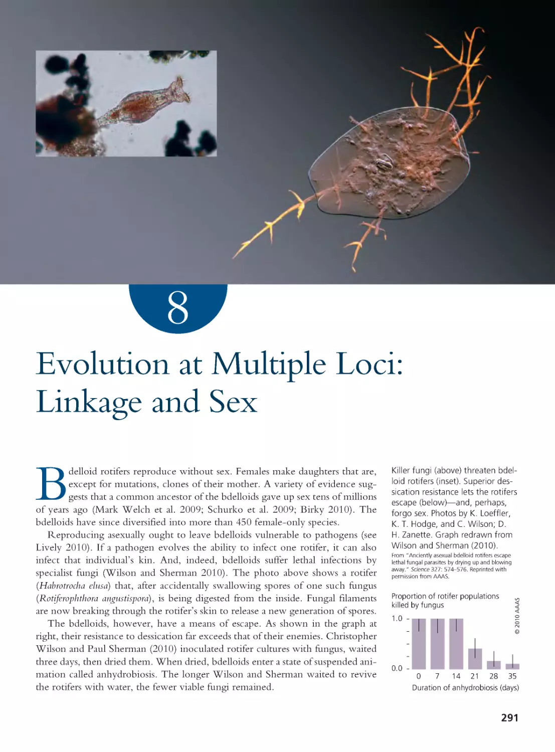
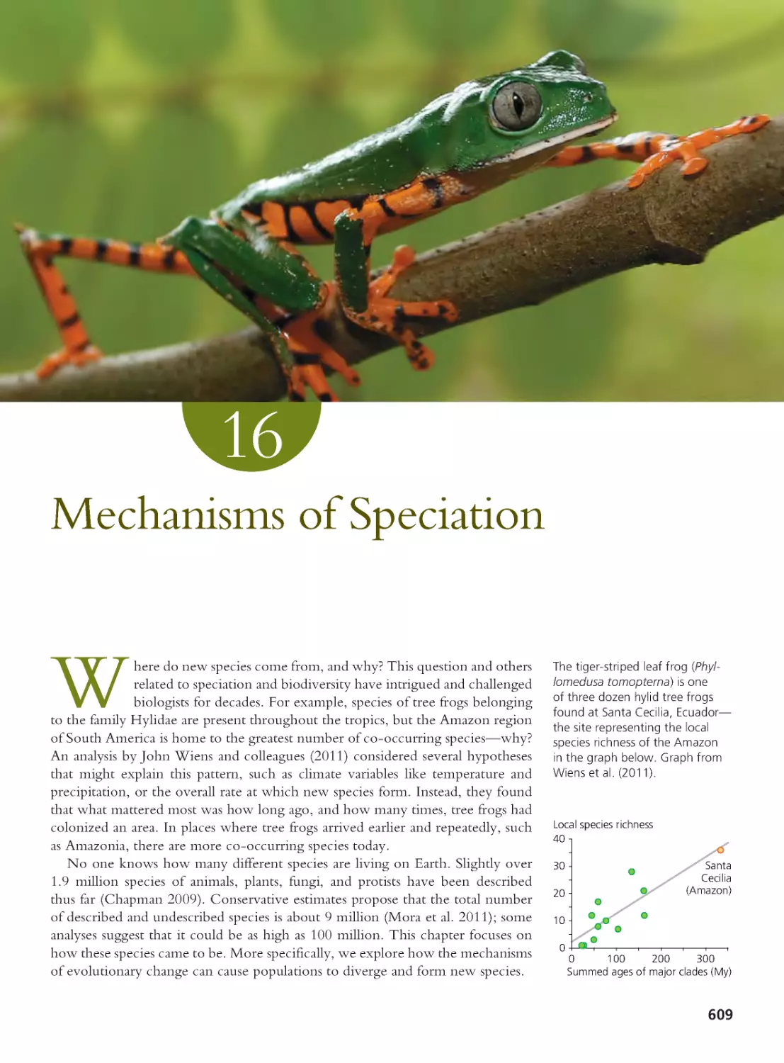
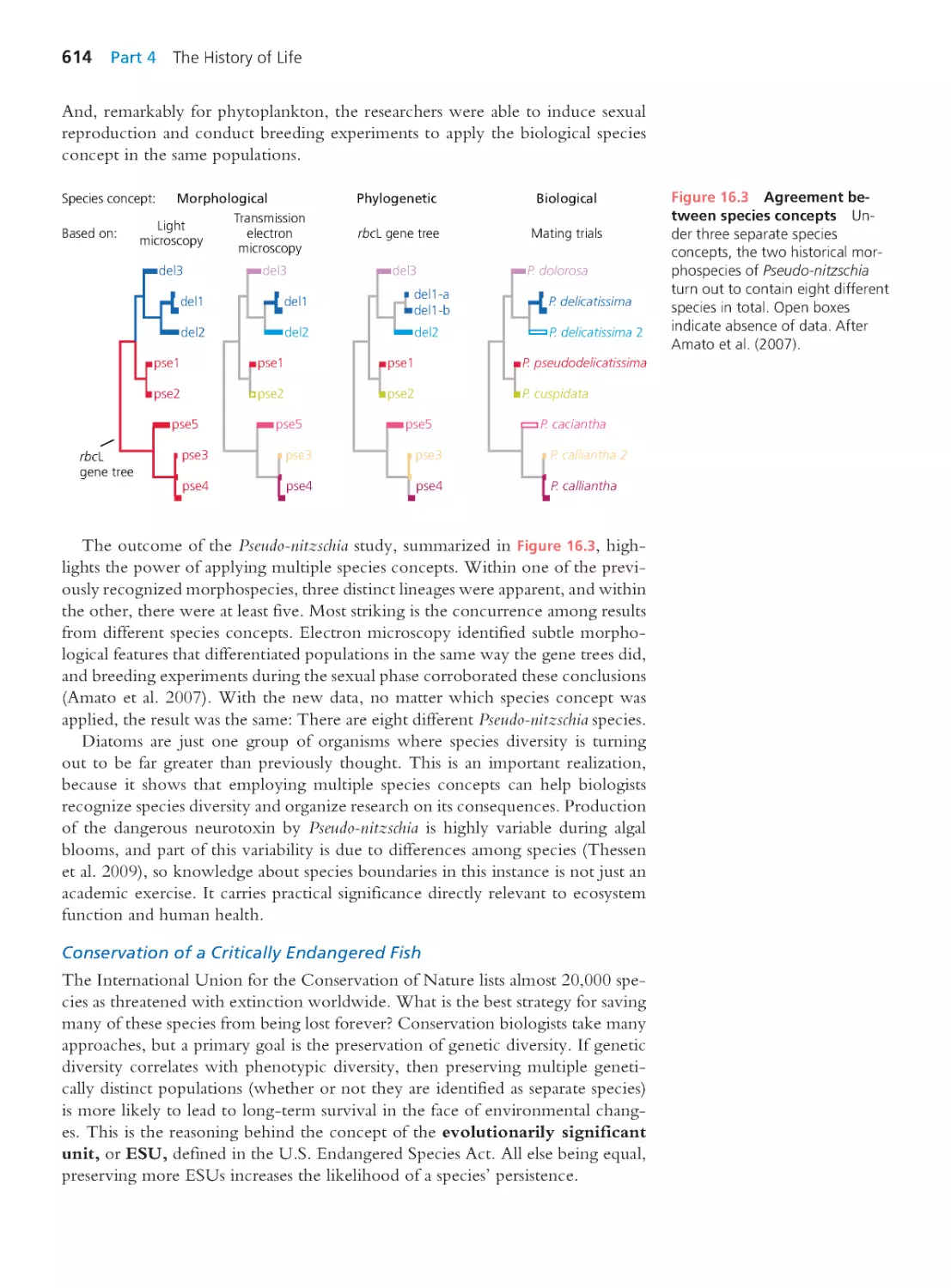
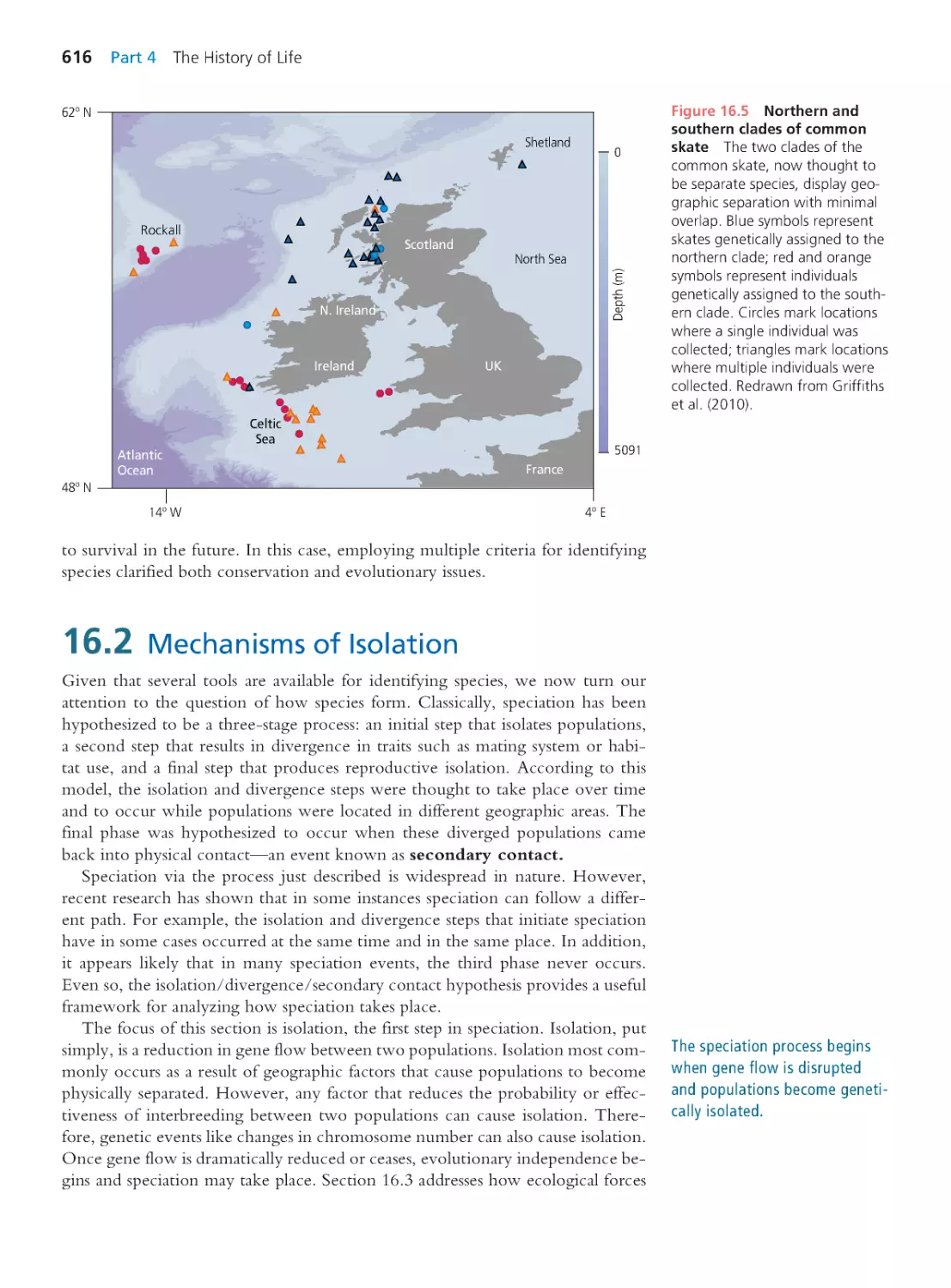
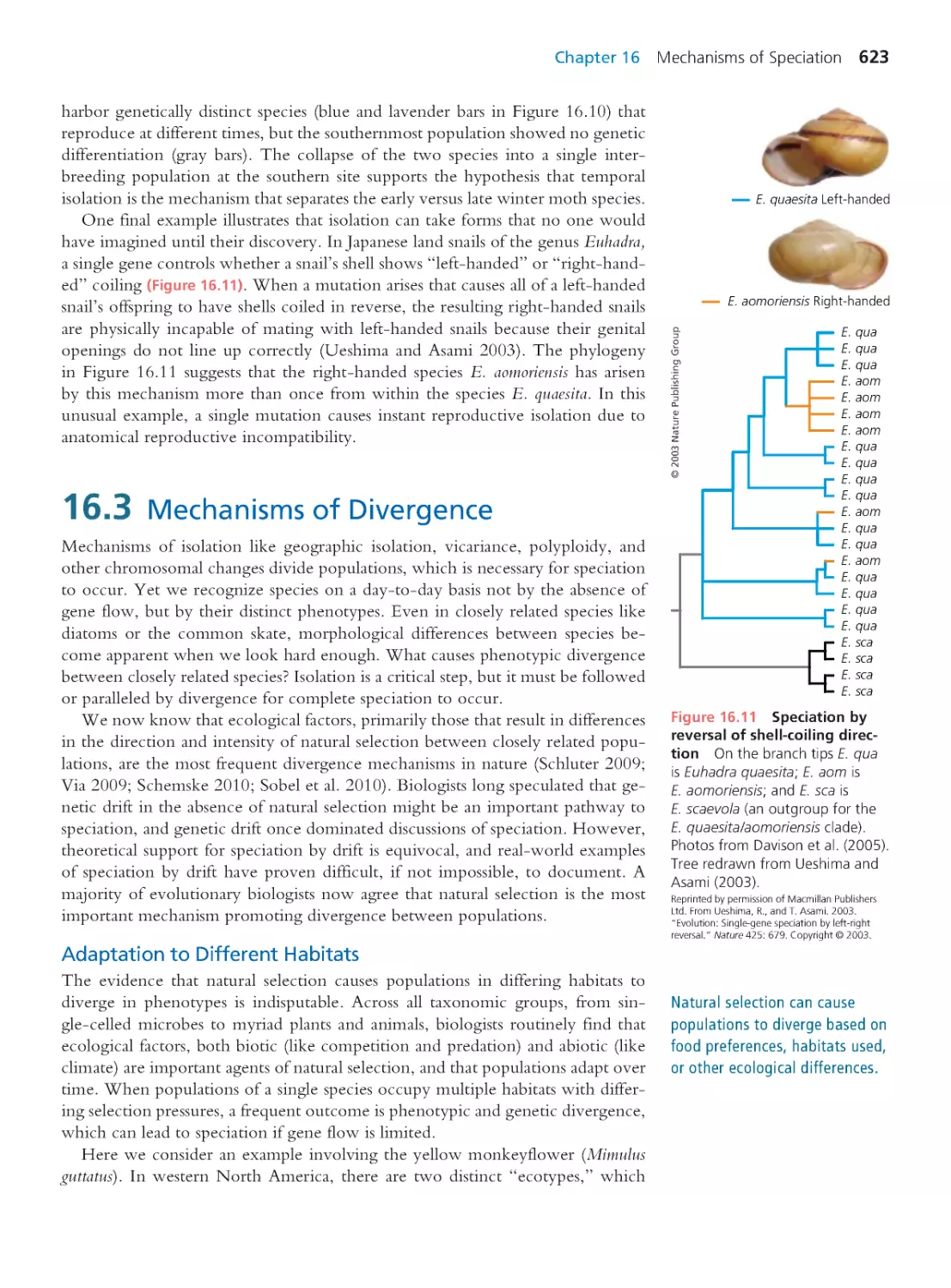
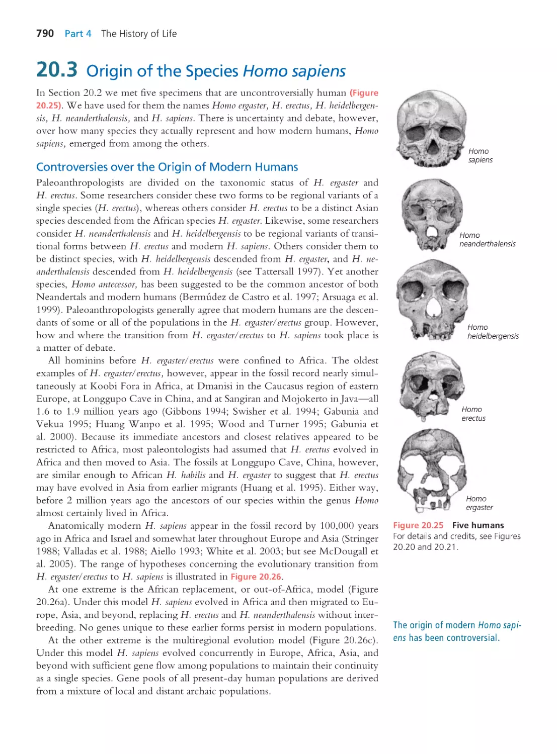
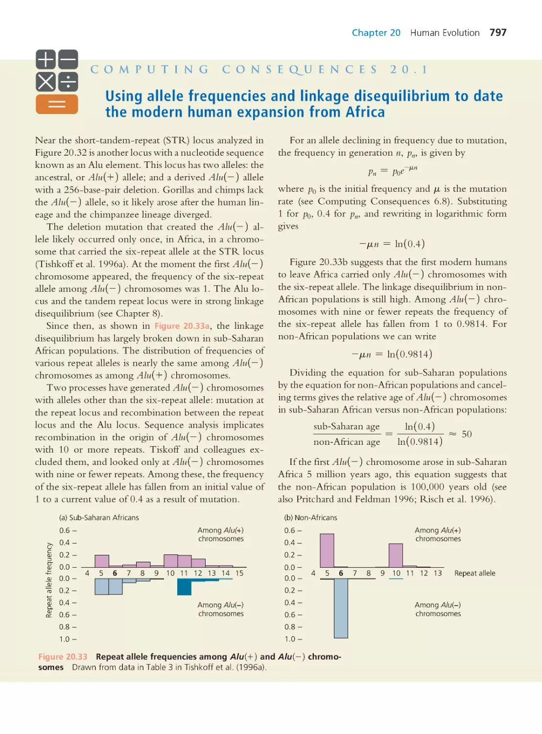
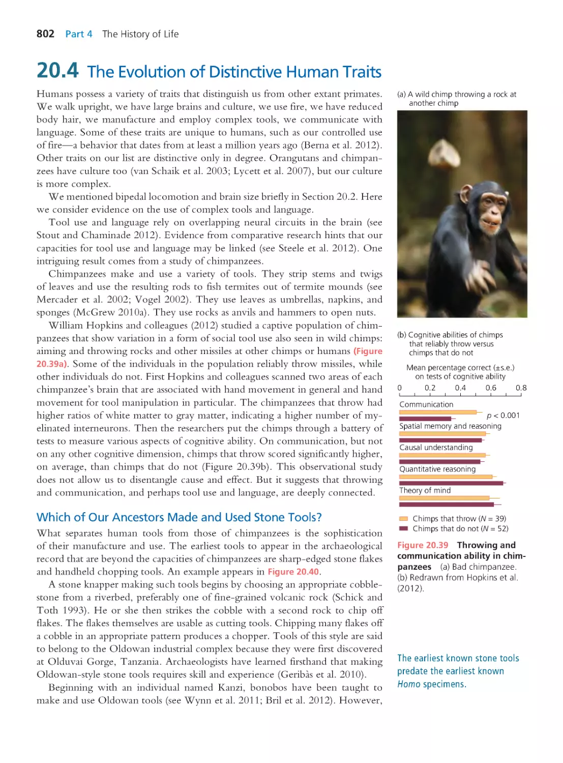
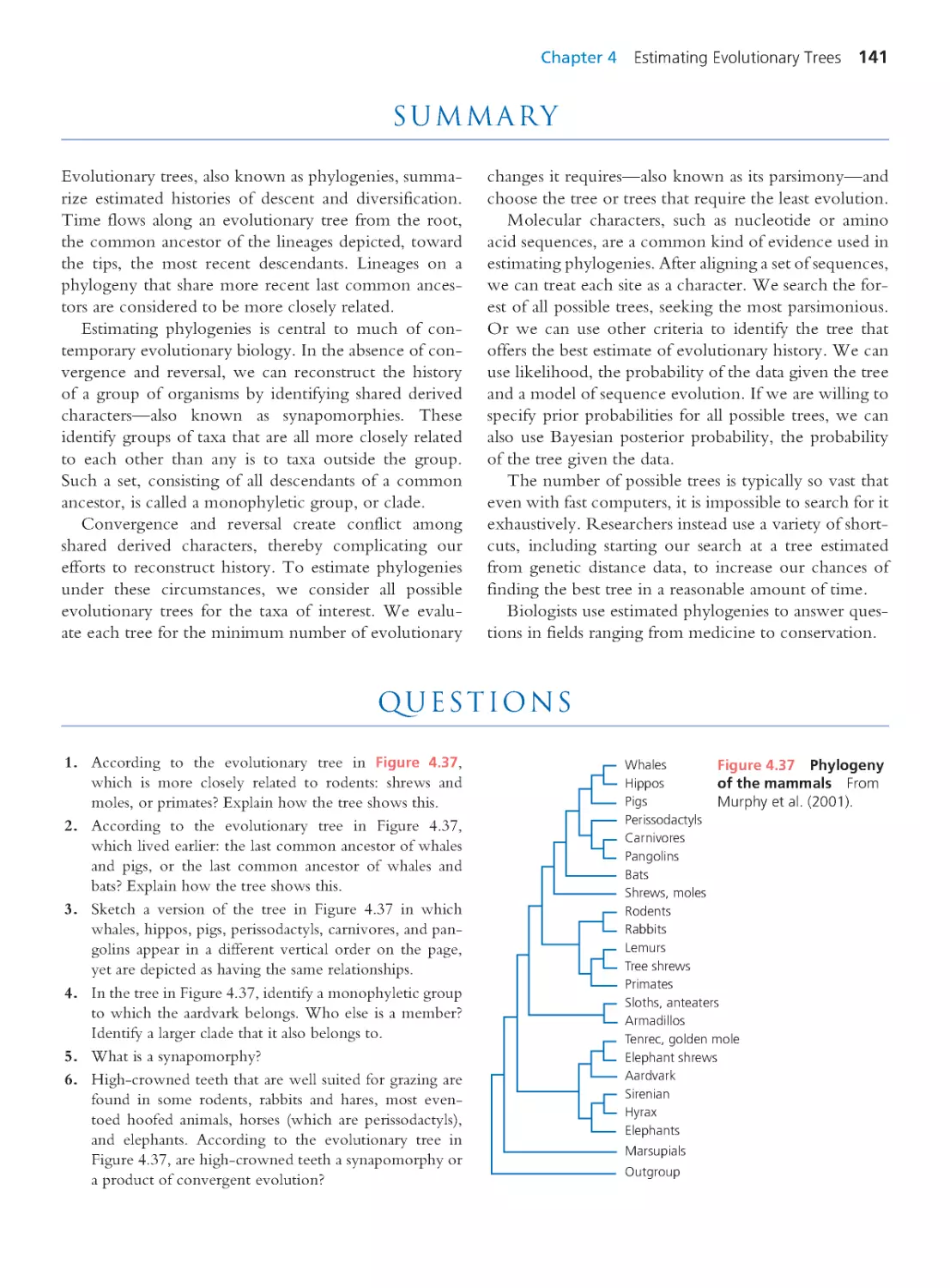
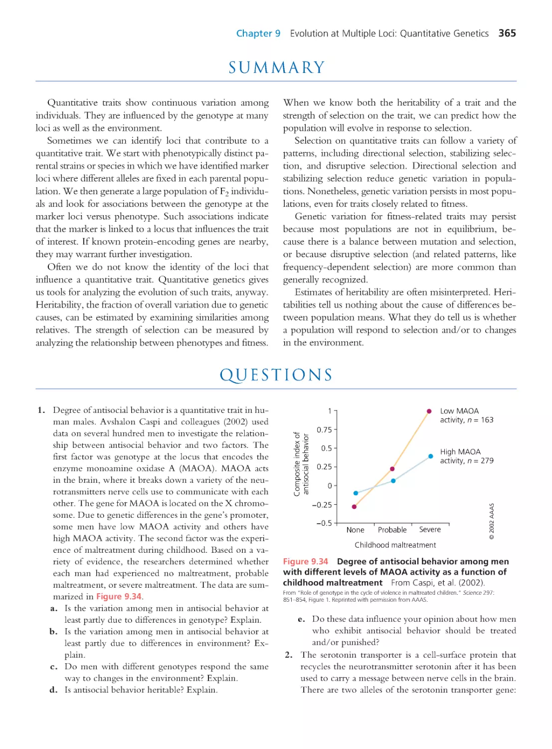
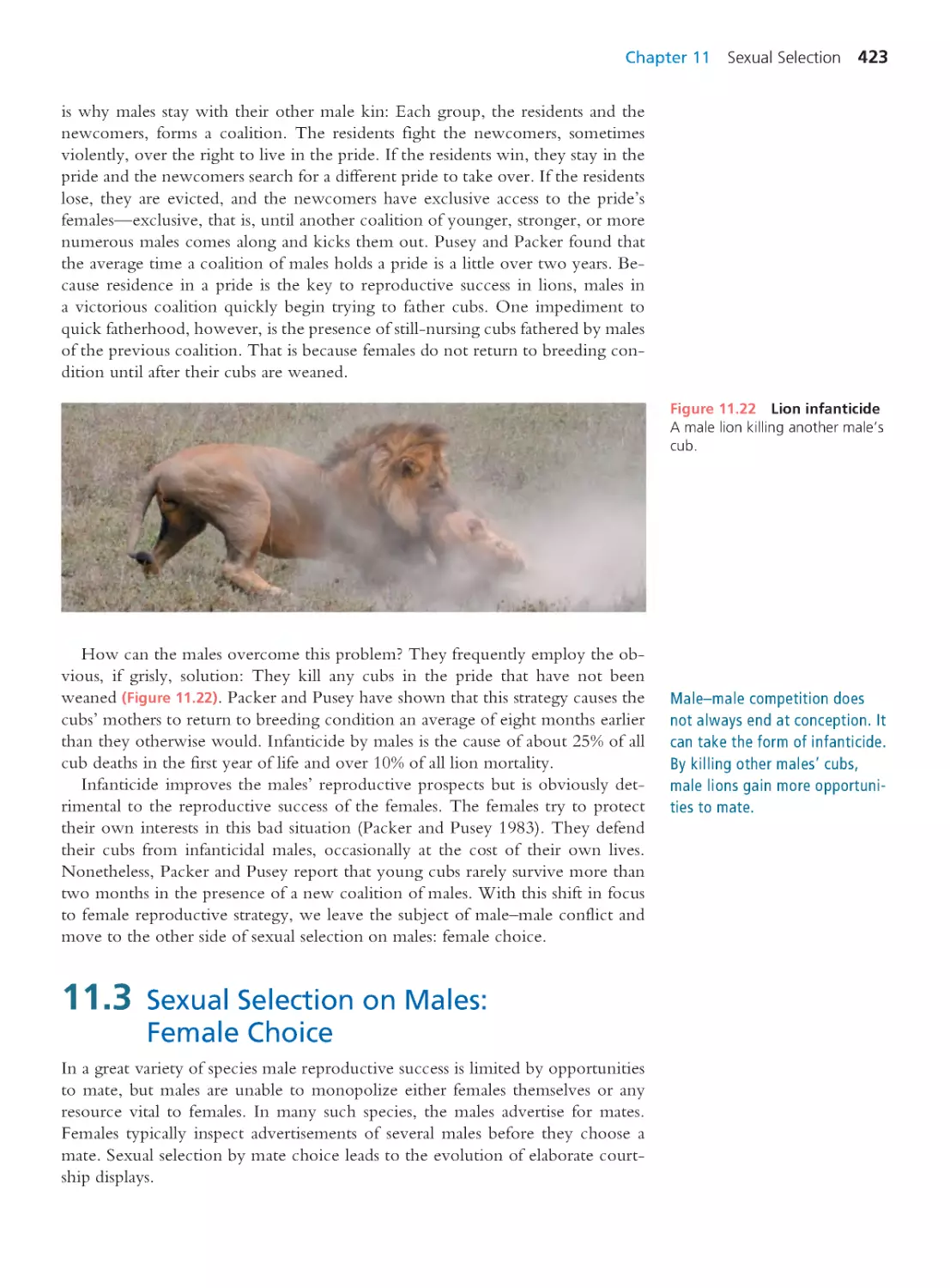
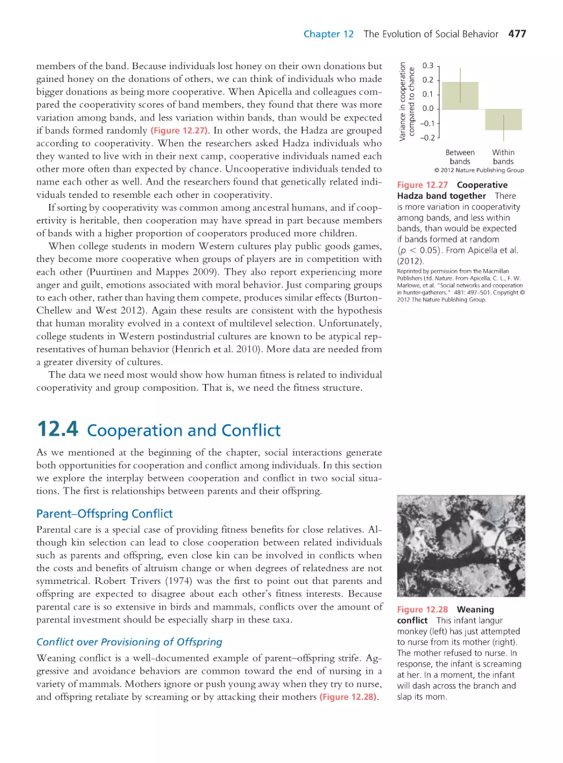
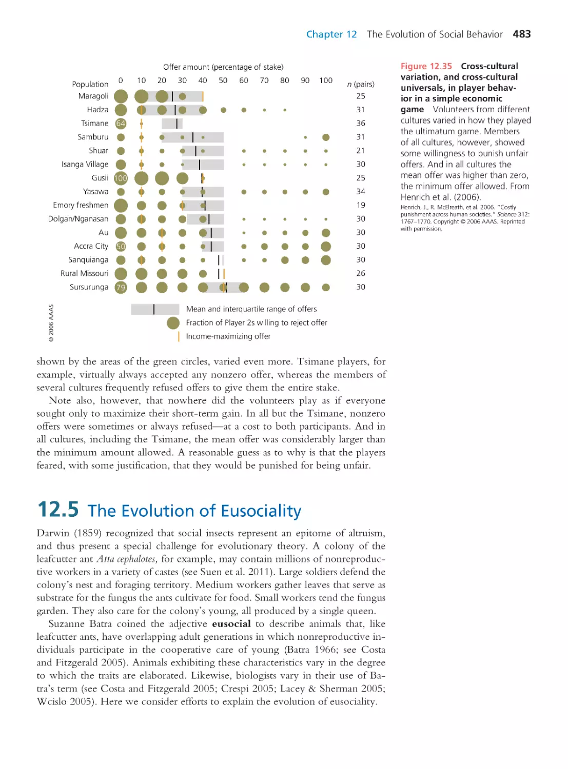
Author: Herron Jon C. Freeman Scott

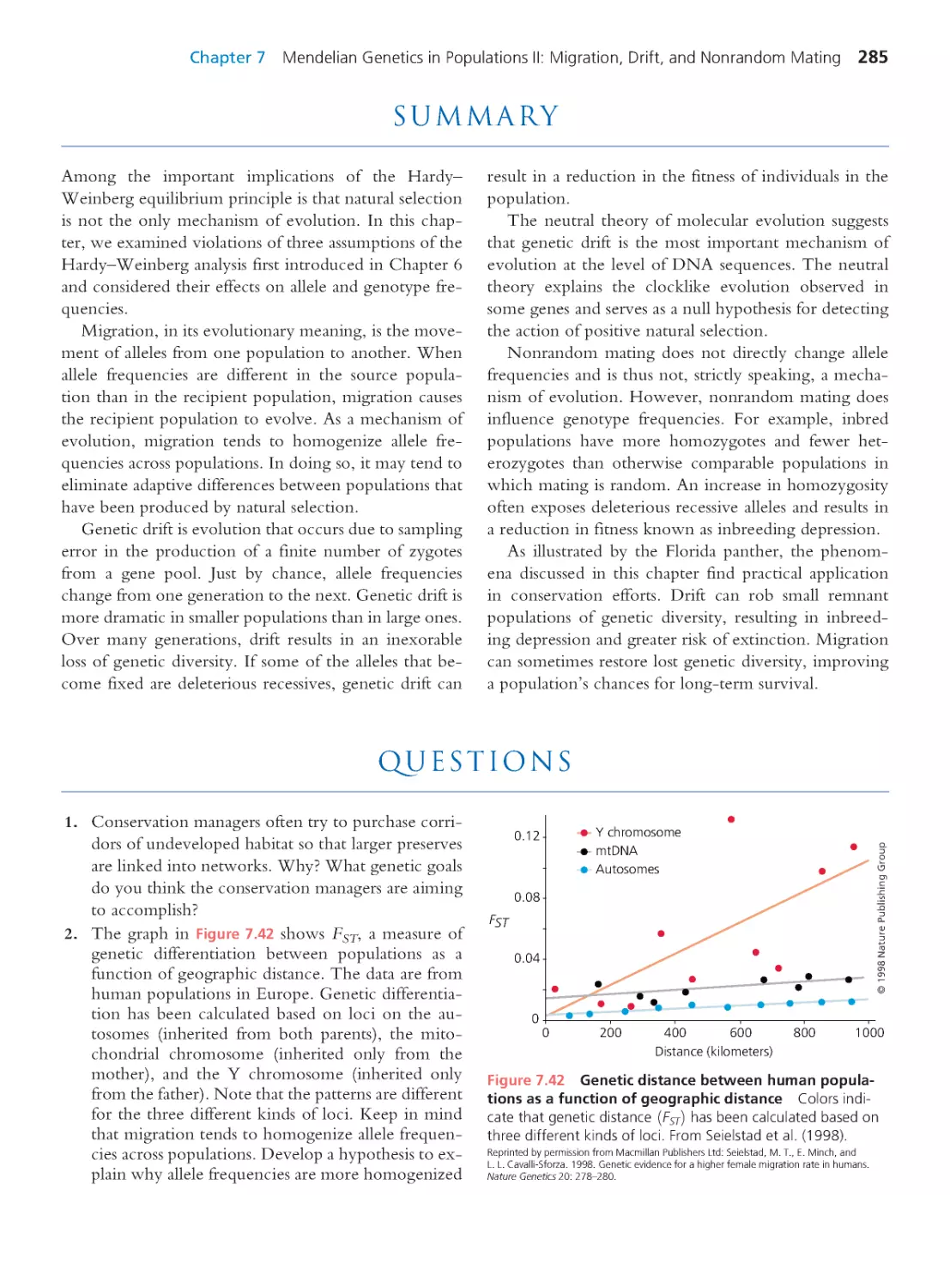
Tags: evolutionary process evolutionary biology

ISBN: 0-321-61667-7

Year: 2013

Similar

Biology

Molecular Biotechnology. Principles and Applications of Recombinant DNA

Mathematical models in biology

Sampling: Design and Analysis

Text

Evolutionary
Analysis
FIFTH EDITION
Jon C. Herron
University of Washington
Scott Freeman
University of Washington
Boston Columbus Indianapolis New York San Francisco Upper Saddle River
Amsterdam Cape Town Dubai London Madrid Milan Munich Paris Montreal Toronto
Delhi Mexico City Sao Paulo Sydney Hong Kong Seoul Singapore Taipei Tokyo
With contr ibutions by
Jason Hodin
Hopkins Marine Station
of Stanford University
and University of Washington
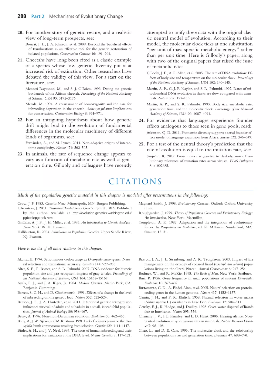
Brooks Miner
Cornell University
Christian Sidor
University of Washington

Editor-in-Chief: Beth Wilbur
Senior Acquisitions Editor: Michael Gillespie
Executive Director of Development: Deborah Gale
Project Editor: Laura Murray
Assistant Editor: Eddie Lee
Manager, Text Permissions:Tim Nicholls
Text Permissions Specialist: Kim Schmidt, S4Carlisle
Publishing Services
Director of Production: Erin Gregg
Managing Editor: Michael Early
Production Project Manager: Lori Newman
Production Management Services: Progressive
Publishing Alternatives
Copyeditor: Chris Thillen
Design Manager: Mark Ong
Cover and Inter ior Designer: Mark Ong
Art Developer, Illustrator: Robin Green
Senior Photo Editor:Travis Amos
Photo Research and Permissions Management:
Bill Smith Group
Content Producer: Daniel Ross
Media Project Manager: Shannon Kong
Director of Marketing: Christy Lesko
Executive Marketing Manager: Lauren Harp
Manufacturing Buyer: Christy Hall
Cover and Text Printer: Courier Kendalville
Cover Photo Credit: Auke Holwerda / Getty Images
Credits and acknowledgments for materials bor rowed from other sources and reproduced, with
permission, in this textbook appear on the appropriate page within the text [or on p. 822].
Copyr ight ©2014, 2007, 2004, 2001, 1998 by Jon C. Her ron and Scott Freeman. Published by Pearson
Education, Inc. All rights reserved. Manufactured in the United States of Amer ica. This publication is
protected by Copyright, and permission should be obtained from the publisher prior to any prohibited
reproduction, storage in a retr ieval system, or transmission in any form or by any means, electronic,
mechanical, photocopying, recording, or likewise. To obtain per mission(s) to use mater ial from this
work, please submit a wr itten request to Pearson Education, Inc., Permissions Department, 1900
E. Lake Ave., Glenview, IL 60025. For information regarding permissions, call (847) 486-2635.
Readers may view, browse, and/or download material for temporary copying purposes only, provided
these uses are for noncommercial personal purposes. Except as provided by law, this material may not
be further reproduced, distr ibuted, transmitted, modified, adapted, performed, displayed, published, or
sold in whole or in part, without prior written permission from the publisher.
Many of the designations used by manufacturers and sellers to distinguish their products are claimed as
trademarks. Where those designations appear in this book, and the publisher was aware of a trademark
claim, the designations have been printed in initial caps or all caps.
Library of Cong ress Cataloging-in-Publication Data is available upon request.
ISBN 10: 0-321-61667-7; ISBN 13: 978-0-321-61667-8 (Student Edition)
ISBN 10: 0-321-92799-0; ISBN 13: 0-321-92799-6 (Instructor’s Review Copy)
ISBN 10: 0-321-92816-4; ISBN 13: 978-0-321-92816-0 (Books a la Carte Edition)
12345678910—CRK—1716151413
Library of Congress Control Number : 2013943730
www.pearsonhighered.com

Brief Contents
PART 1
INTRODUCTION
1
CHAPTER 1 A Case for Evolutionary
Thinking: Understanding HIV
1
CHAPTER 2 The Patter n of Evolution
37
CHAPTER 3 Evolution by Natural Selection
73
CHAPTER 4 Estimating Evolutionary Trees
109
PART 2
MECHANISMS OF
EVOLUTIONARY CHANGE
147
CHAPTER 5 Var iation Among Individuals
147
CHAPTER 6 Mendelian Genetics in
Populations I: Selection and
Mutation
179
CHAPTER 7 Mendelian Genetics in
Populations II: Migration, Drift,
and Nonrandom Mating
233
CHAPTER 8 Evolution at Multiple Loci:
Linkage and Sex
291
CHAPTER 9 Evolution at Multiple Loci:
Quantitative Genetics
329
PART 3
ADAPTATION
369
CHAPTER 10 Studying Adaptation:
Evolutionary Analysis of
Form and Function
369
CHAPTER 11 Sexual Selection
407
CHAPTER 12 The Evolution of Social Behavior 455
CHAPTER 13 Aging and Other Life-History
Characters
491
CHAPTER 14 Evolution and Human Health 535
CHAPTER 15 Genome Evolution and the
Molecular Basis of Adaptation
581
PART 4
THE HISTORY OF LIFE
609
CHAPTER 16 Mechanisms of Speciation
609
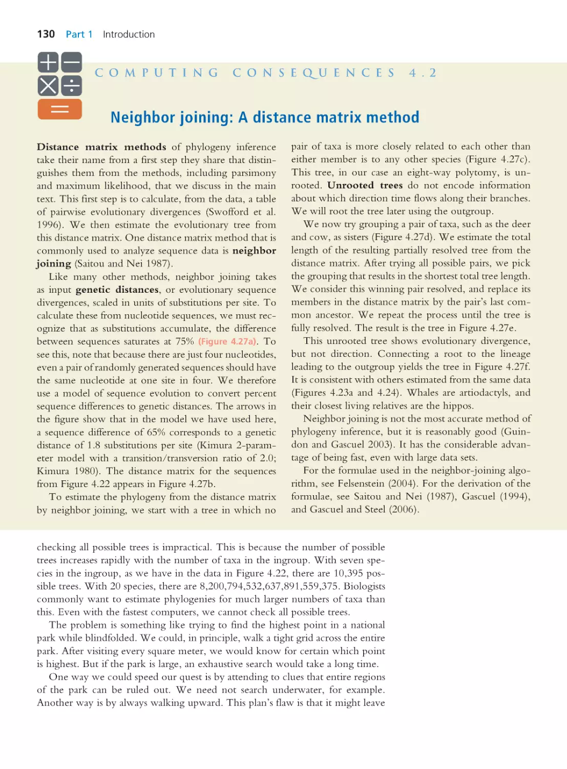
CHAPTER 17 The Origins of Life
and Precambrian Evolution
645
CHAPTER 18 Evolution and the Fossil Record 691
CHAPTER 19 Development and Evolution
735
CHAPTER 20 Human Evolution
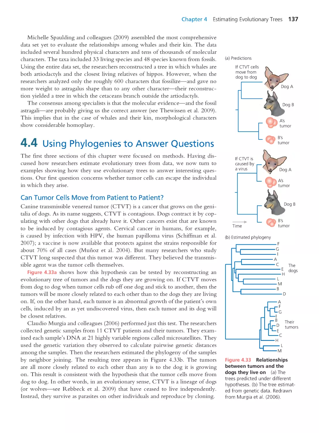
769
iii

Contents
CHAPTER 3
Evolution by Natural Selection
73
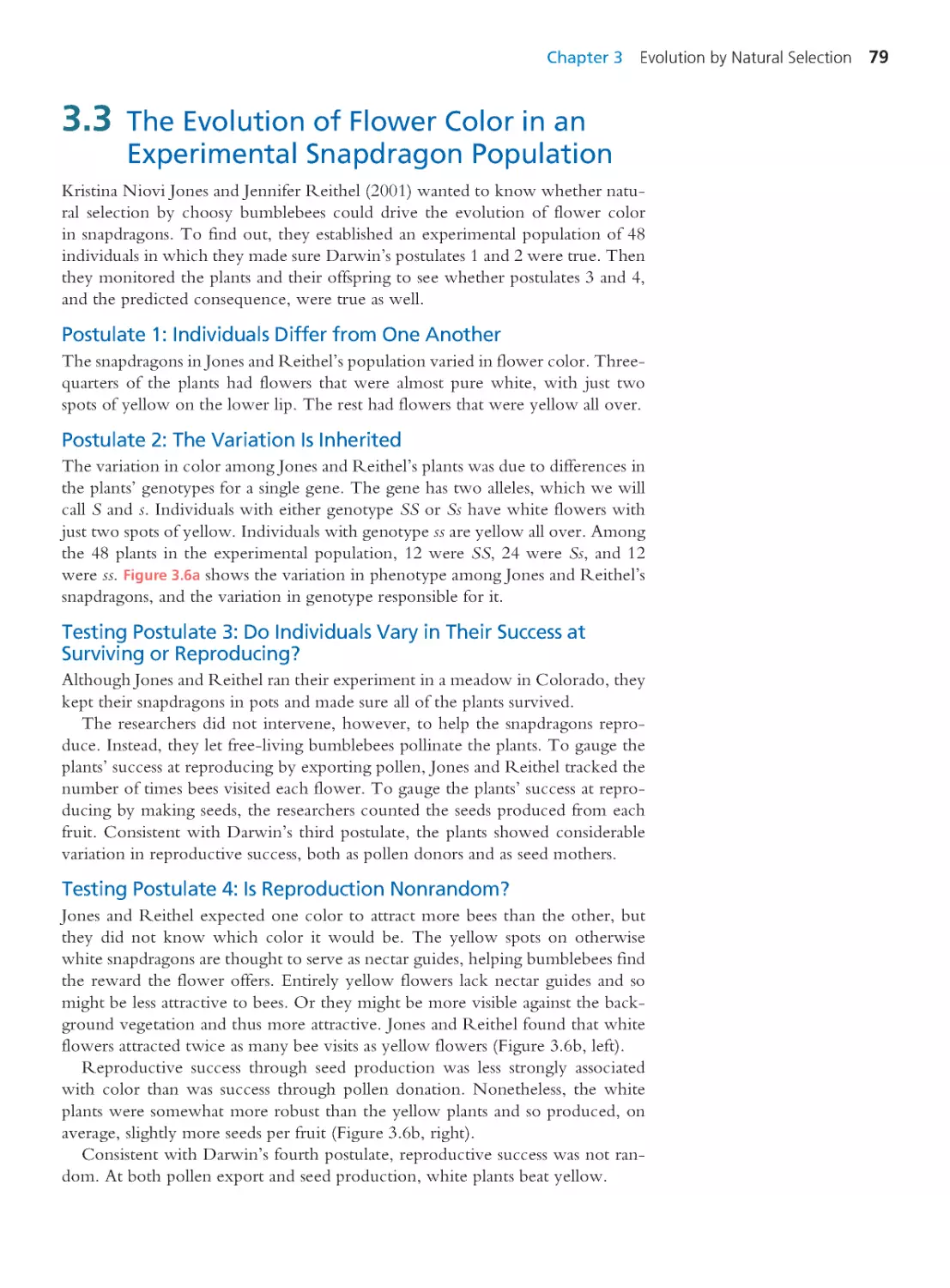
3.1 Artificial Selection: Domestic Animals
and Plants
74
3.2 Evolution by Natural Selection
77
3.3 The Evolution of Flower Color in an
Experimental Snapdragon Population 79
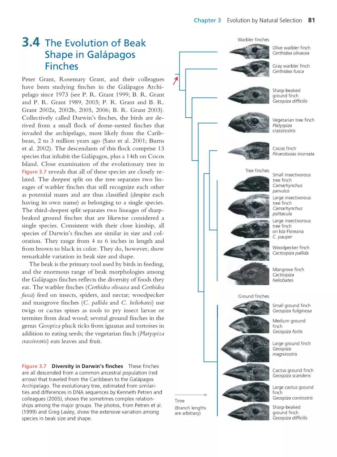
3.4 The Evolution of Beak Shape in
Galápagos Finches
81
Computing Consequences 3.1 Estimating
heritabilities despite complications
84
3.5 The Nature of Natural Selection
90
3.6 The Evolution of Evolutionary Biology 94
3.7 Intelligent Design Creationism
97
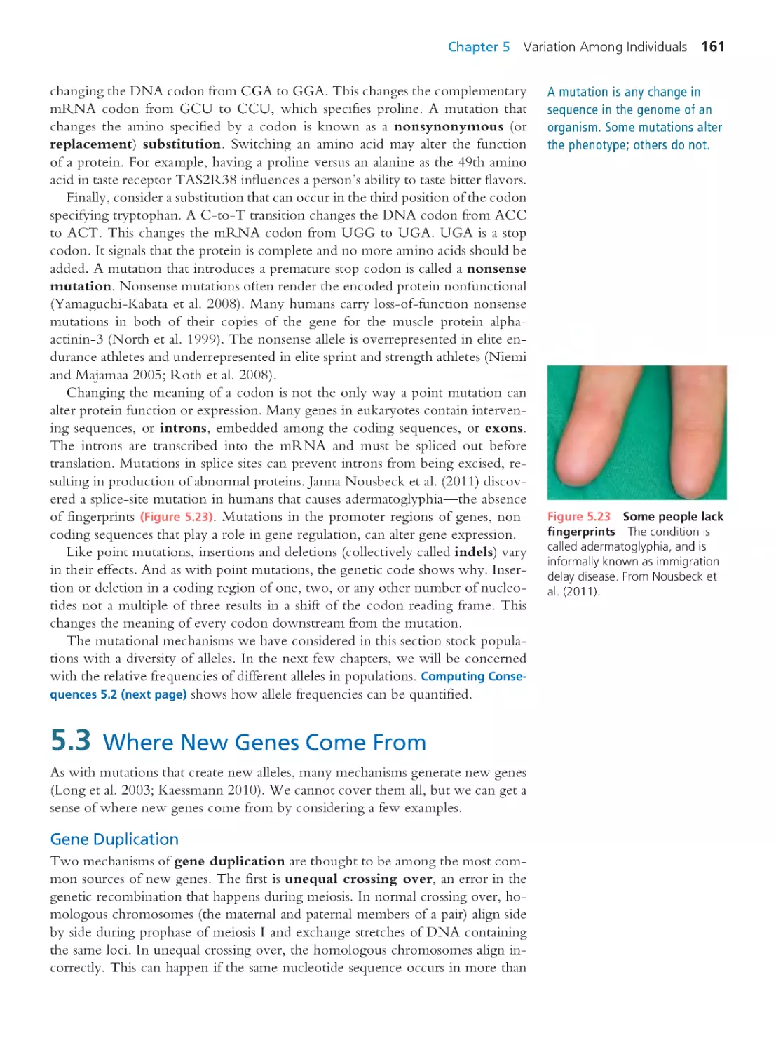
Summary 104 • Questions 105
Exploring the Literature 106 • Citations 106
CHAPTER 4
Estimating Evolutionary Trees
109
4.1 How to Read an Evolutionary Tree
110
4.2 The Logic of Infer ring Evolutionary
Trees
114
4.3 Molecular Phylogeny Inference and
the Origin of Whales
123
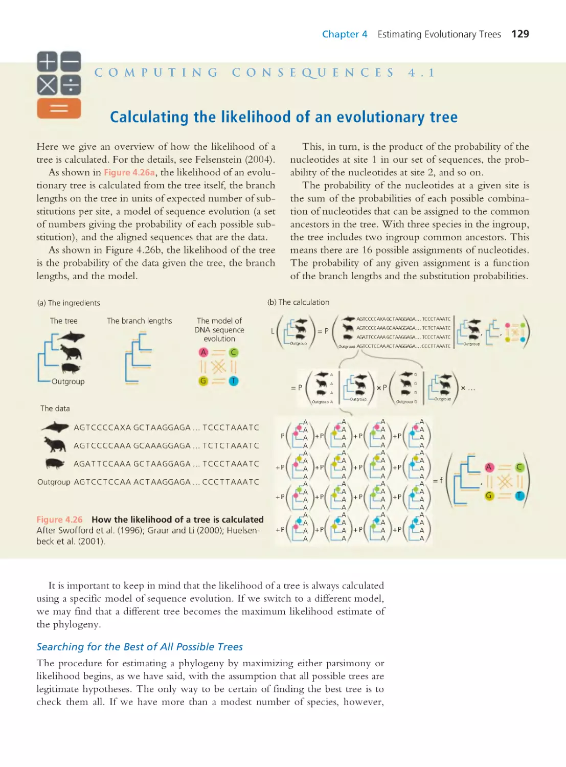
Computing Consequences 4.1 Calculating
the likelihood of an evolutionary tree
129
Computing Consequences 4.2 Neighbor
joining: A distance matrix method
130
Pref ace
ix
PART 1
INTRODUCTION
1
CHAPTER 1
A Case for Evolutionary Thinking:
Understanding HIV
1
1.1 The Natural History of the HIV
Epidemic
2
1.2 Why Does HIV Therapy Using Just
One Drug Ultimately Fail?
9
1.3 Are Human Populations Evolving as a
Result of the HIV Pandemic?
15
1.4 Where Did HIV Come From?
18
1.5 Why Is HIV Lethal?
23
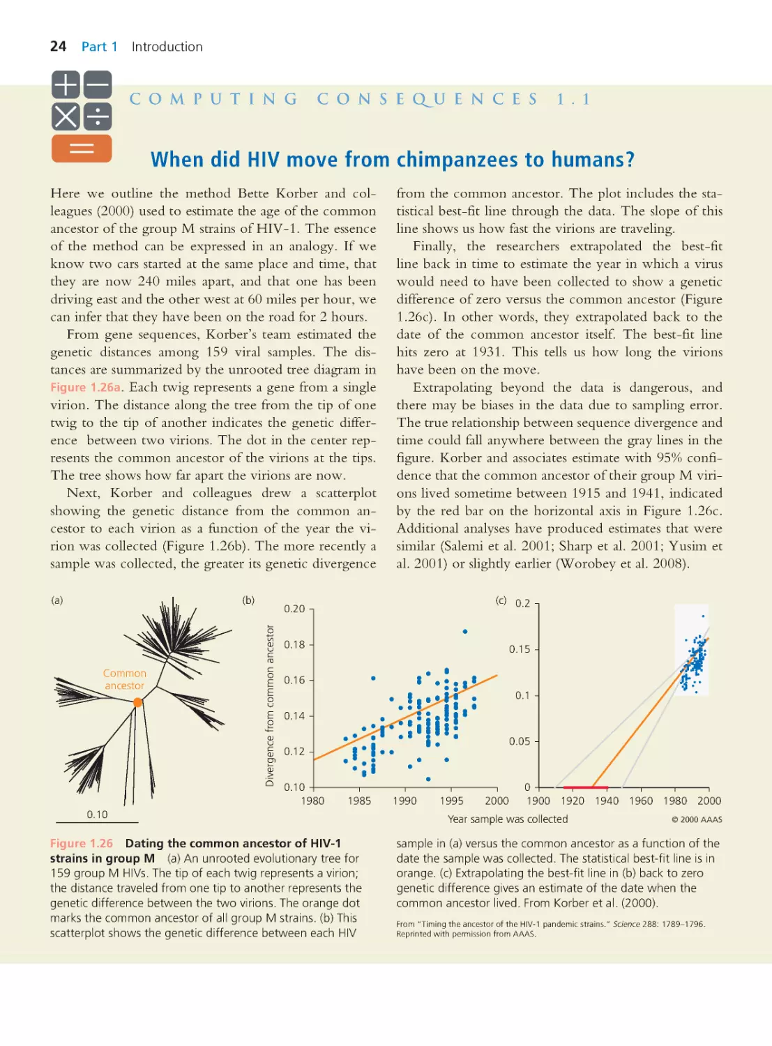
Computing Consequences 1.1 When did
HIV move from chimpanzees to humans?
24
Summary 31 • Questions 31
Exploring the Literature 32 • Citations 33
CHAPTER 2
The Pattern of Evolution
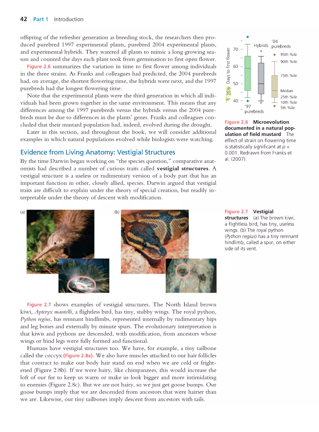
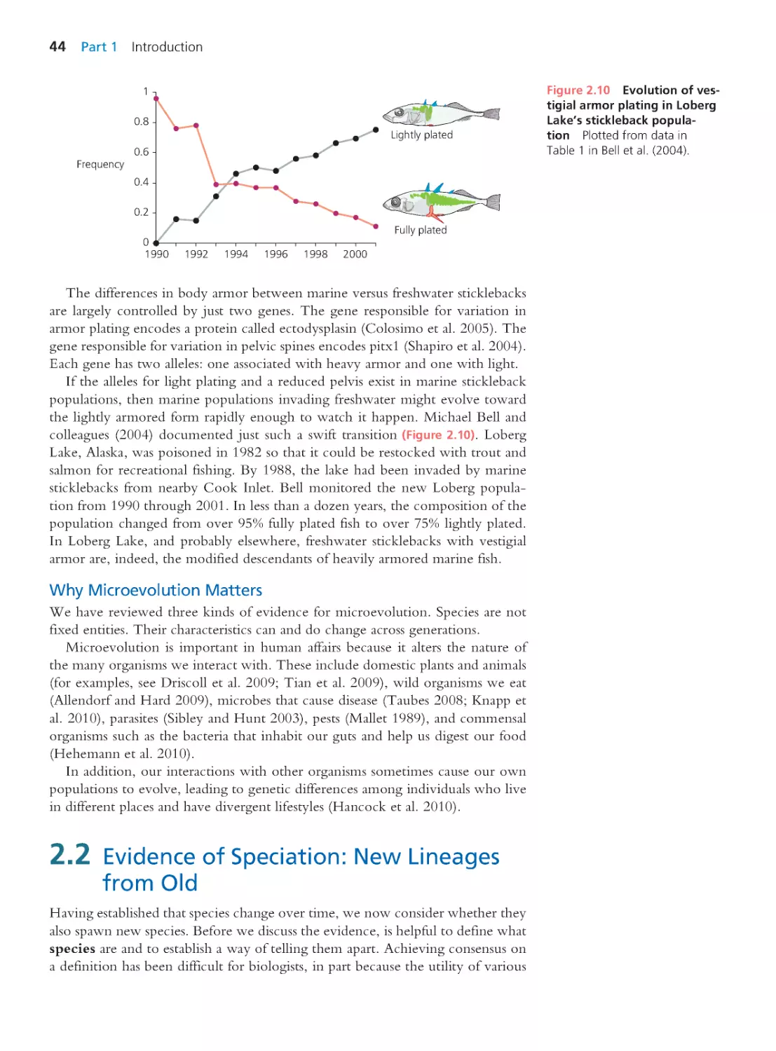
37
2.1 Evidence of Microevolution: Change
through Time
39
2.2 Evidence of Speciation: New Lineages
from Old
44
2.3 Evidence of Macroevolution:
New For ms from Old
49
2.4 Evidence of Common Ancestry:
All Life-Forms Are Related
55
2.5 The Age of Earth
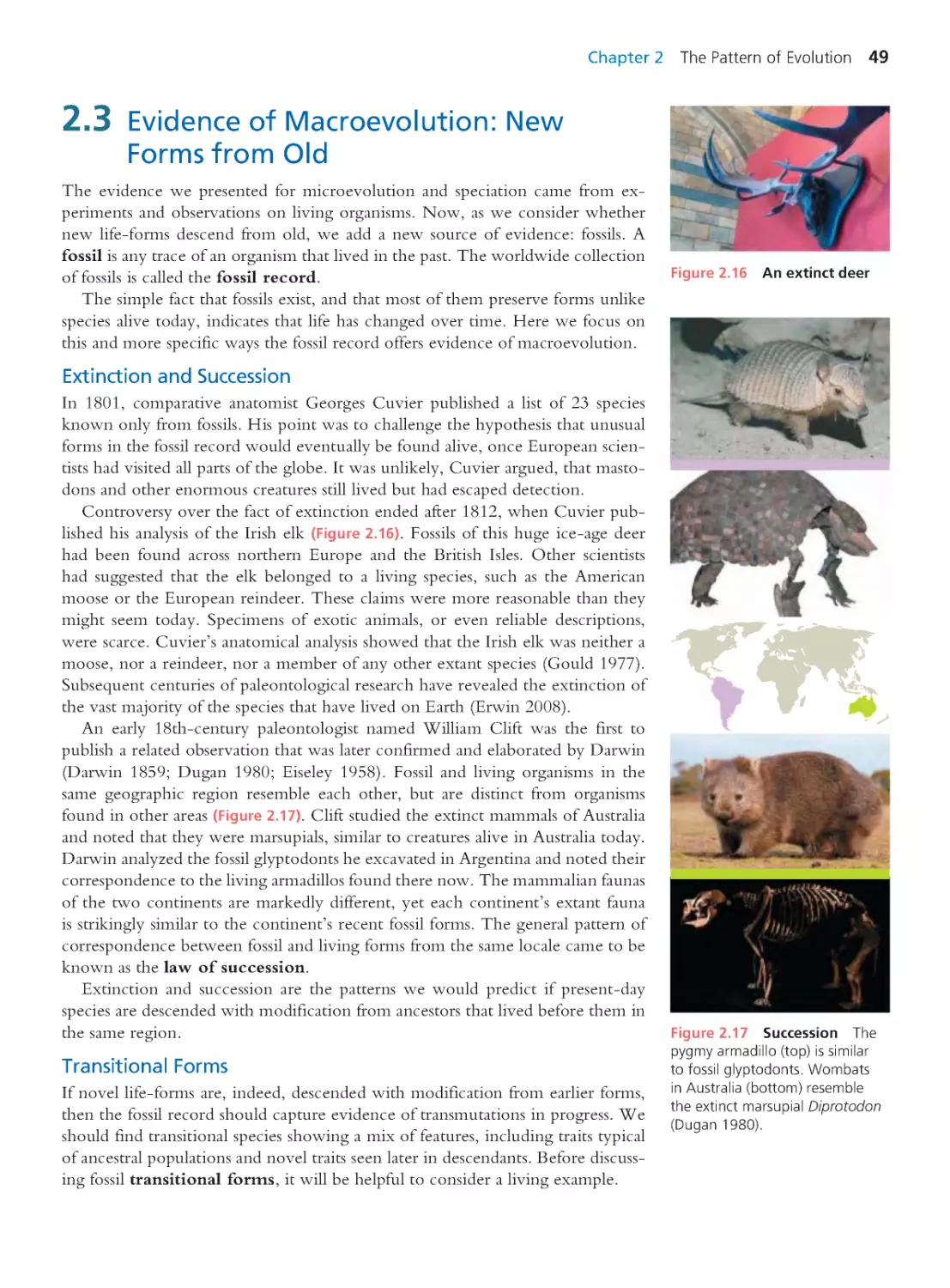
62
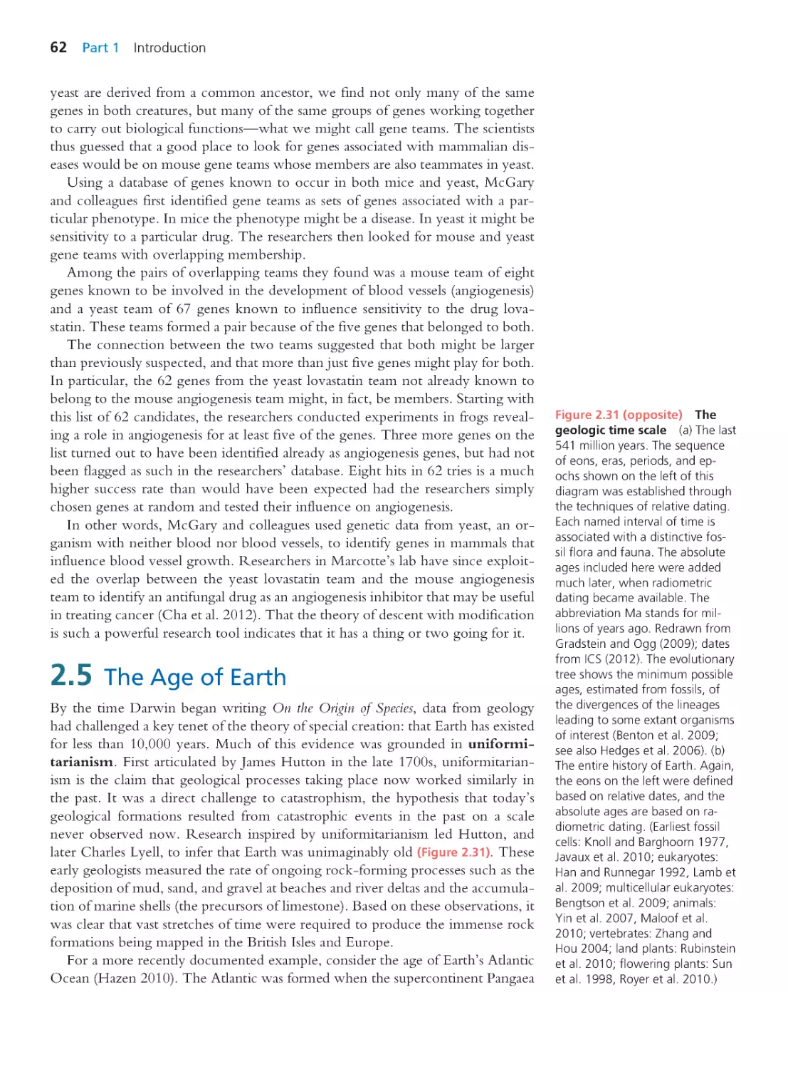
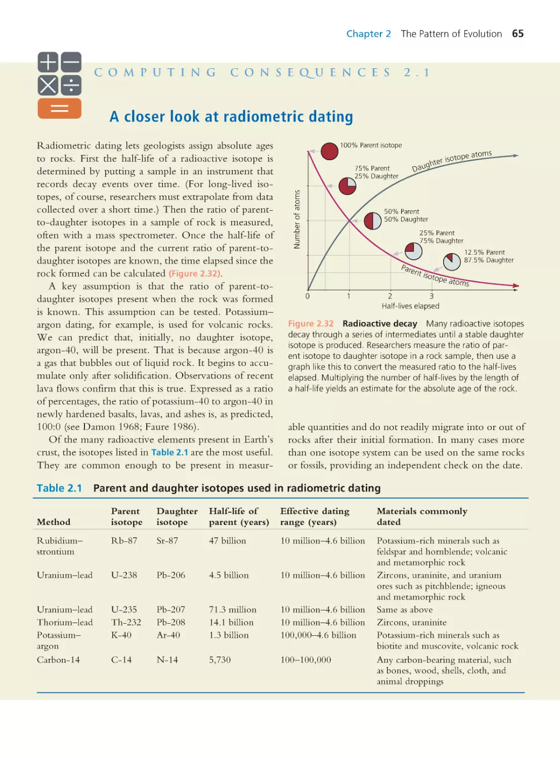
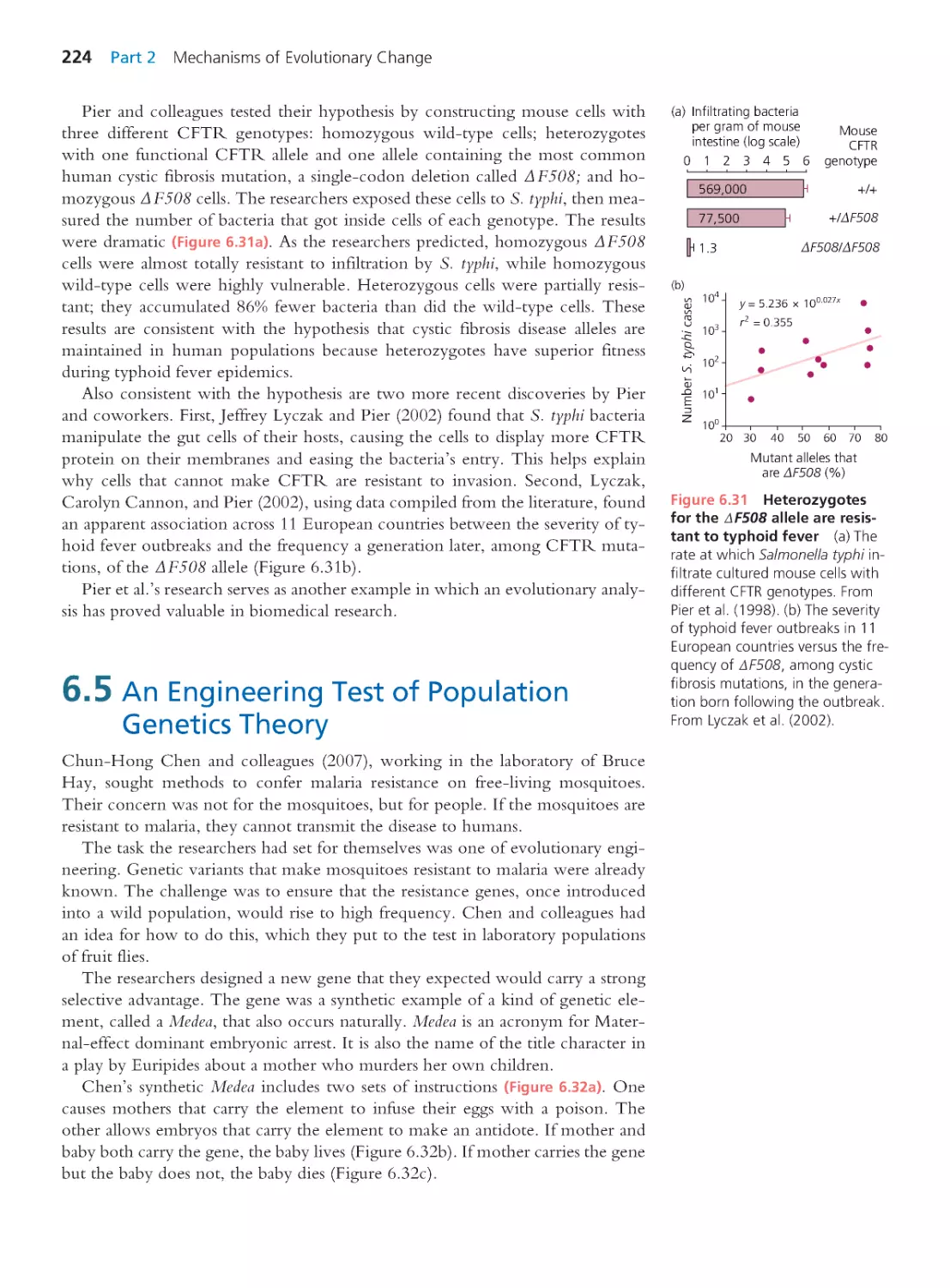
Computing Consequences 2.1 A closer look
at radiometric dating
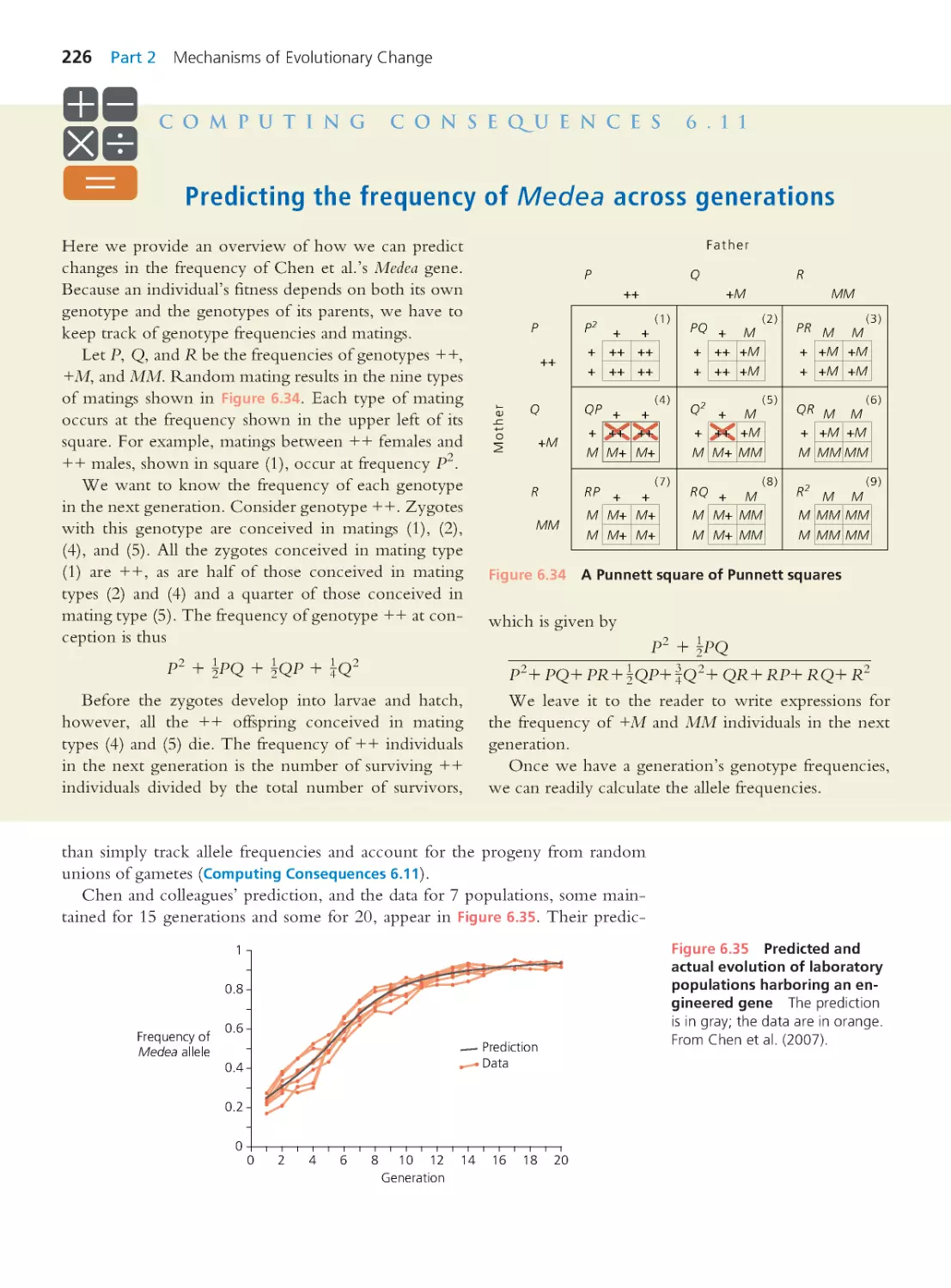
65
Summary 66 • Questions 67
Exploring the Literature 68 • Citations 69
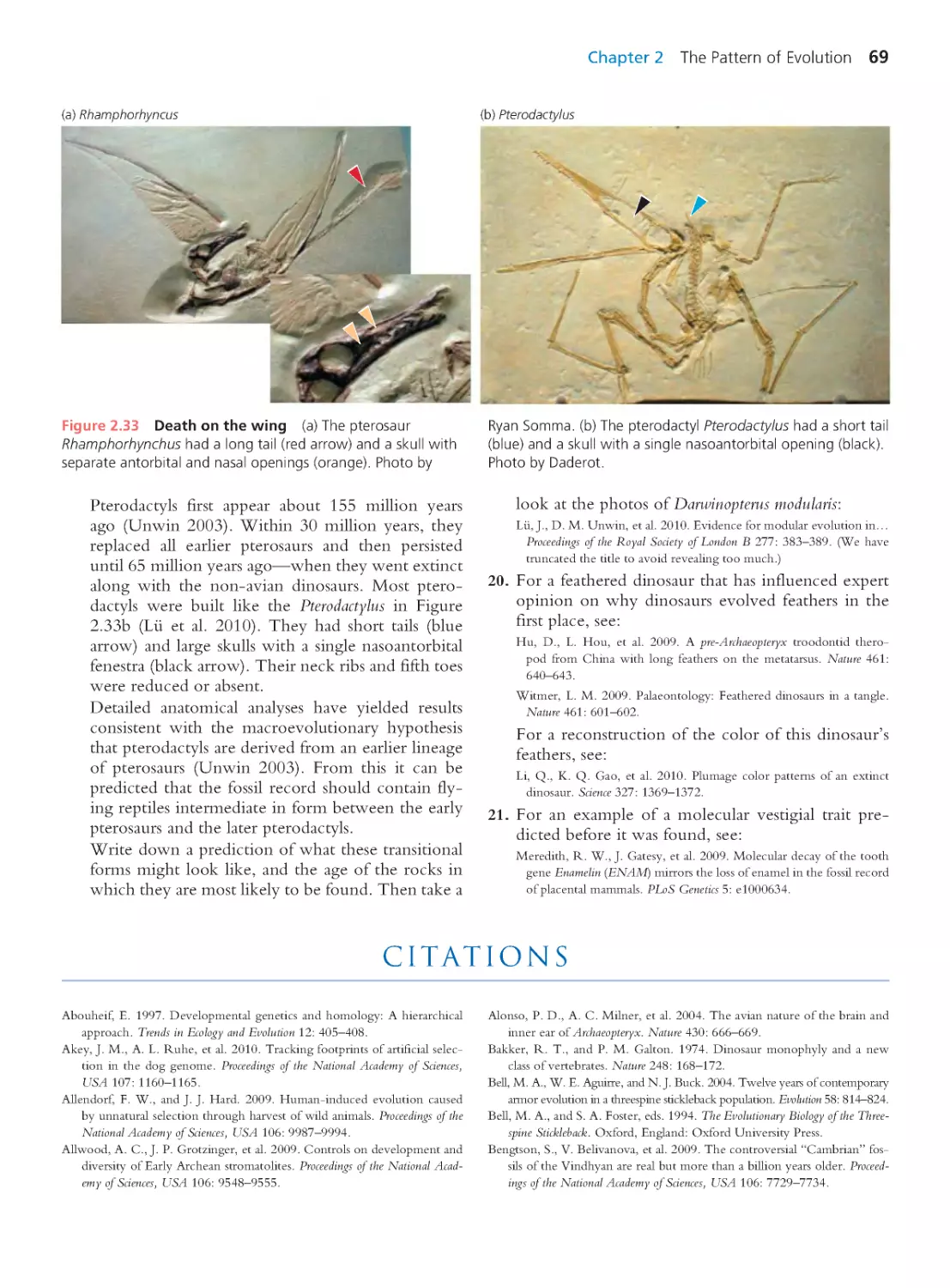
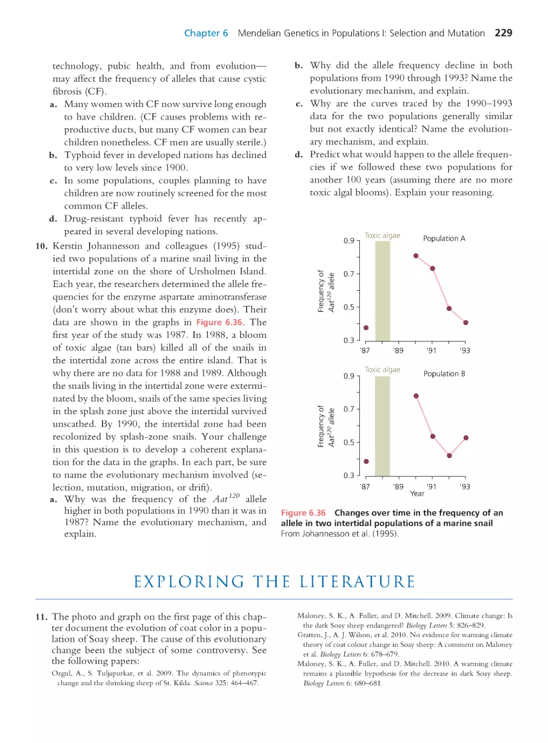
iv

4.4 Using Phylogenies to Answer
Questions
137
Summary 141 • Questions 141
Exploring the Literature 143 • Citations 143
PART 2
MECHANISMS OF
EVOLUTIONARY CHANGE
147
CHAPTER 5
Var iation Among Individuals
147
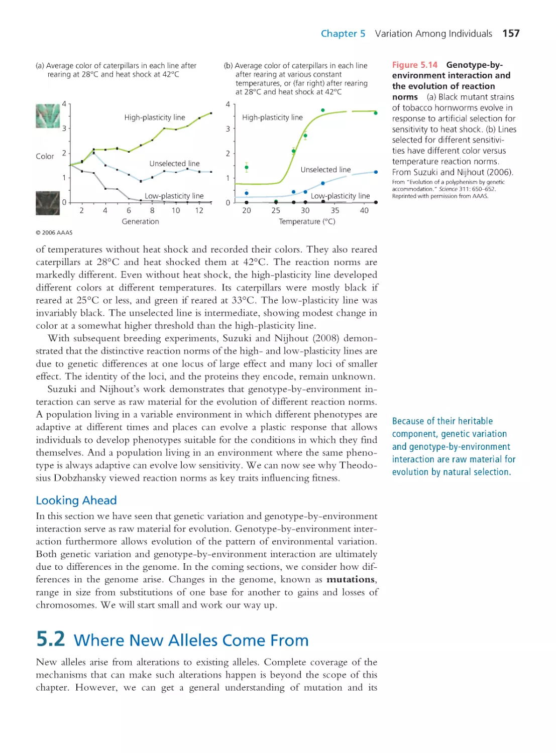
5.1 Three Kinds of Variation
148
Computing Consequences 5.1 Epigenetic
inheritance and evolution
154
5.2 Where New Alleles Come From
157
5.3 Where New Genes Come From
161
Computing Consequences 5.2 Measuring
genetic variation in natural populations
162
5.4 Chromosome Mutations
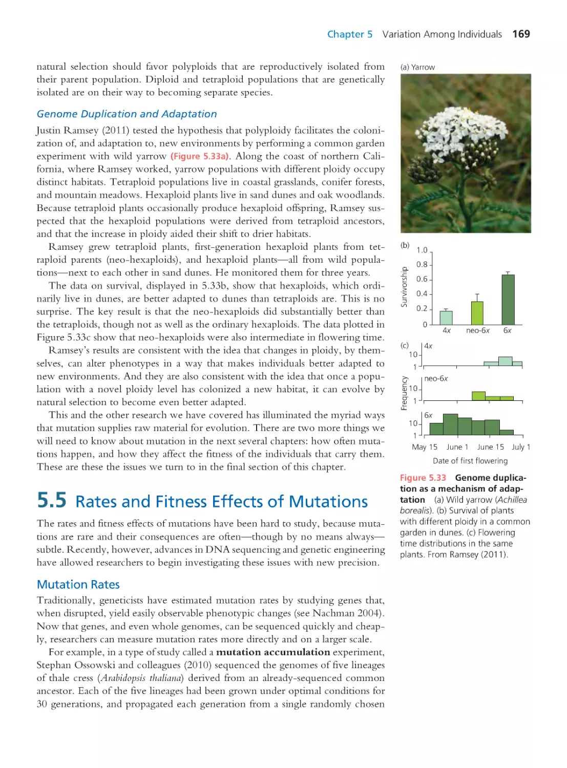
166
5.5 Rates and Fitness Effects of Mutations 169
Summary 174 • Questions 175
Exploring the Literature 176 • Citations 176
CHAPTER 6
Mendelian Genetics in Populations I:
Selection and Mutation
179
6.1 Mendelian Genetics in Populations:
Hardy–Weinberg Equilibrium
180
Computing Consequences 6.1 Combining
probabilities
185
Computing Consequences 6.2 The Hardy–
Weinberg equilibrium principle with more
than two alleles
189
6.2 Selection
191
Computing Consequences 6.3 A general
treatment of selection
194
Contents v
Computing Consequences 6.4 Statistical
analysis of allele and genotype frequencies
using the
2
(chi-square) test
198
Computing Consequences 6.5 Predicting
the frequency of the CCR5- 32 allele
in future generations
201
6.3 Patter ns of Selection: Testing
Predictions of Population Genetics
Theory
201
Computing Consequences 6.6 An algebraic
treatment of selection on recessive and
dominant alleles
204
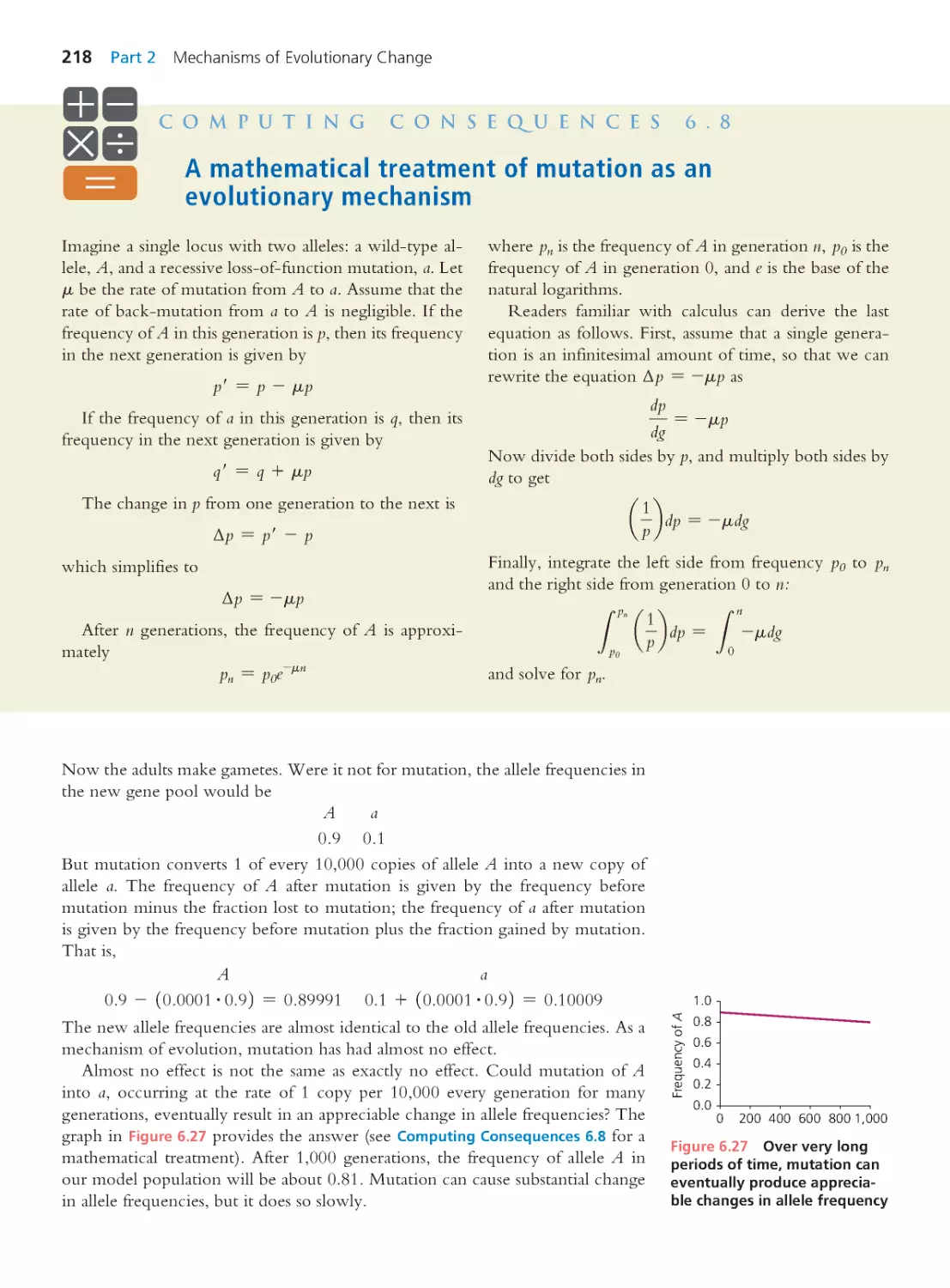
Computing Consequences 6.7 Stable
equilibria with heterozygote superiority and
unstable equilibria with heterozygote inferiority 208
6.4 Mutation
216
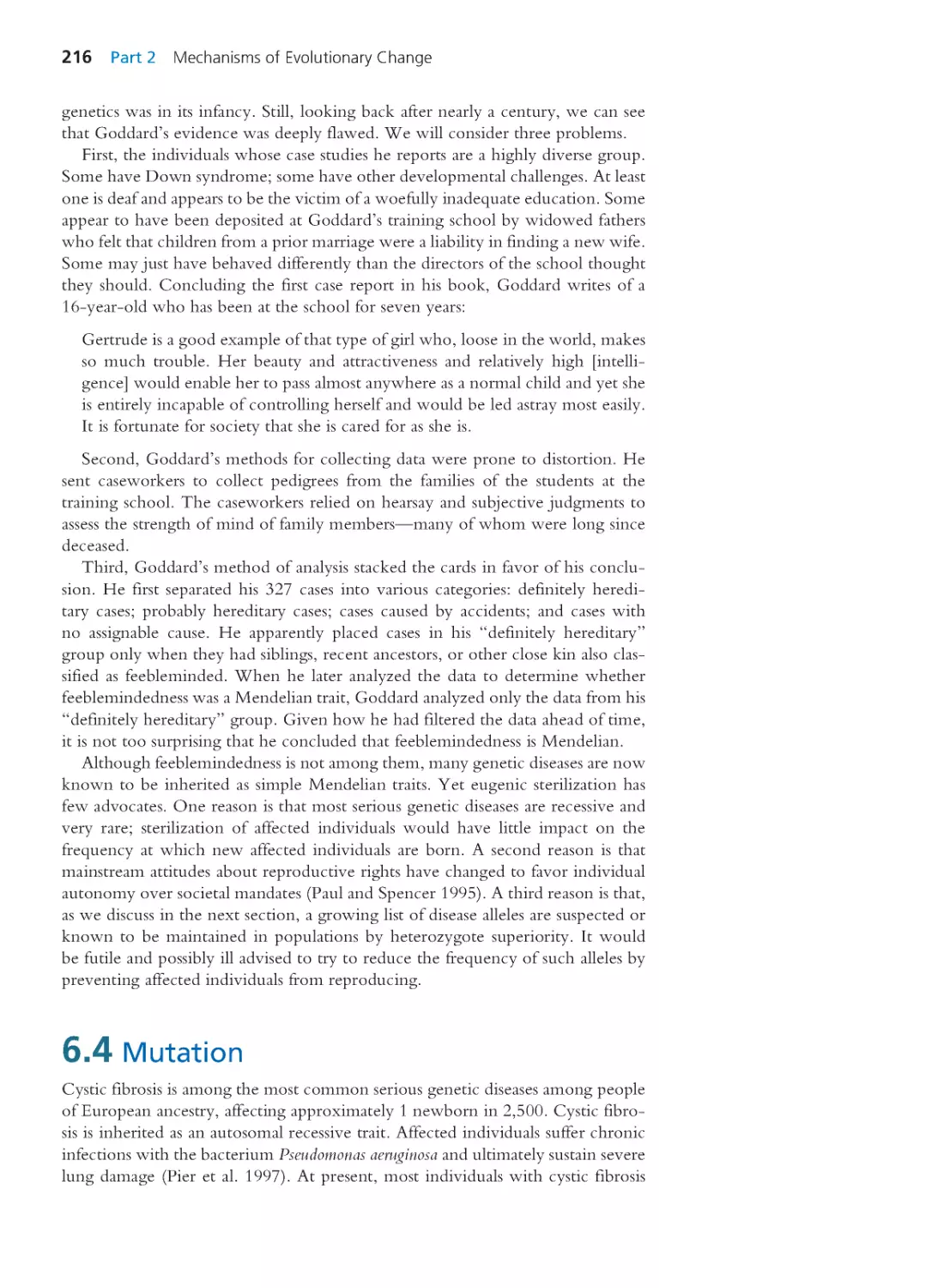
Computing Consequences 6.8
A mathematical treatment of mutation as
an evolutionary mechanism
218
Computing Consequences 6.9 Allele
frequencies under mutation–selection balance
220
Computing Consequences 6.10 Estimating
mutation rates for recessive alleles
222
6.5 An Engineering Test of Population
Genetics Theory
224
Computing Consequences 6.11 Predicting
the frequency of Medea across generations
226
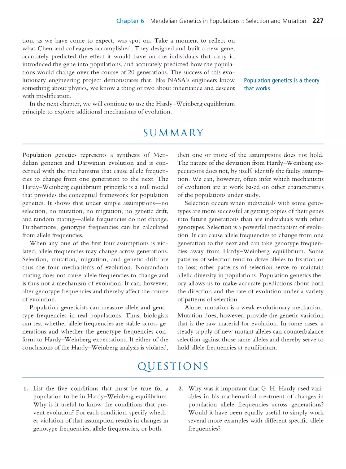
Summary 227 • Questions 227
Exploring the Literature 229 • Citations 231
CHAPTER 7
Mendelian Genetics in Populations II:
Migration, Drift, and
Nonrandom Mating
233
7.1 Migration
234
Computing Consequences 7.1 An algebraic
treatment of migration as an evolutionary
process
236
Computing Consequences 7.2 Selection
and migration in Lake Erie water snakes
238
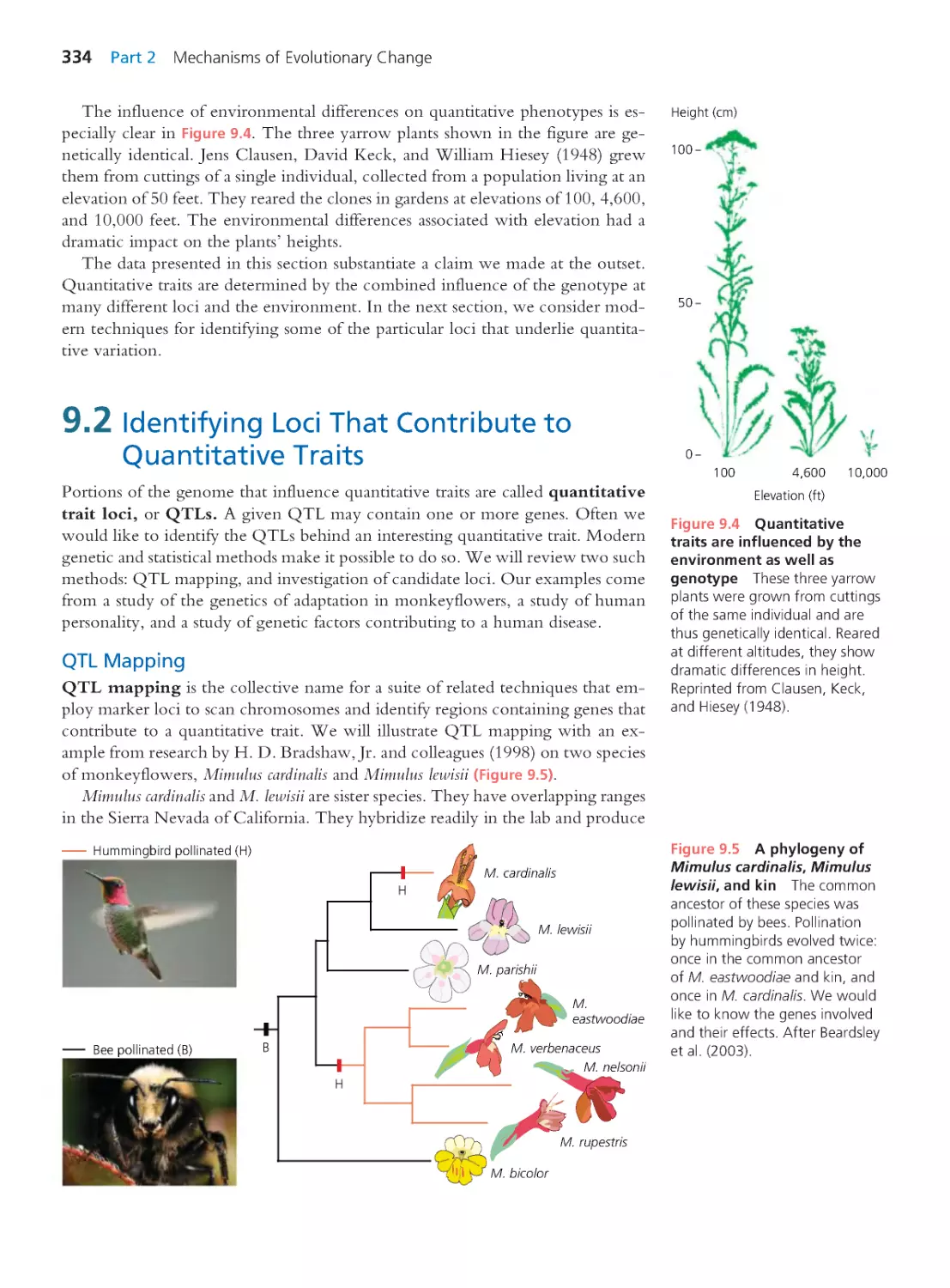
7.2 Genetic Drift
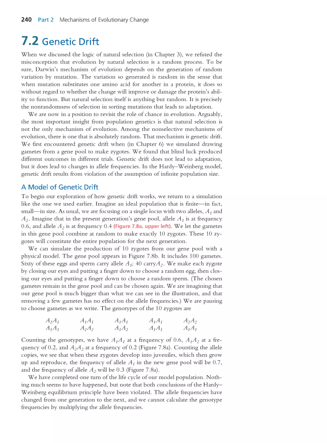
240
Computing Consequences 7.3 The
probability that a given allele will be the
one that drifts to fixation
248
Computing Consequences 7.4 Effective
population size
251
Computing Consequences 7.5 The rate of
evolutionary substitution under genetic drift 256

7.3 Genetic Drift and Molecular
Evolution
260
7.4 Nonrandom Mating
275
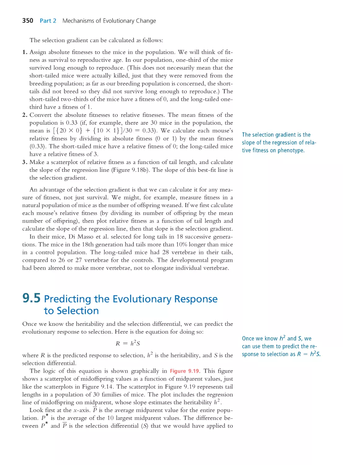
Computing Consequences 7.6 Genotype
frequencies in an inbred population
279
7.5 Conservation Genetics of the Florida
Panther
283
Summary 285 • Questions 285
Exploring the Literature 287 • Citations 288
CHAPTER 8
Evolution at Multiple Loci:
Linkage and Sex
291
8.1 Evolution at Two Loci: Linkage
Equilibrium and Linkage
Disequilibrium
292
Computing Consequences 8.1
The coefficient of linkage disequilibrium
295
Computing Consequences 8.2 Hardy–
Weinberg analysis for two loci
296
Computing Consequences 8.3 Sexual
reproduction reduces linkage disequilibrium
301
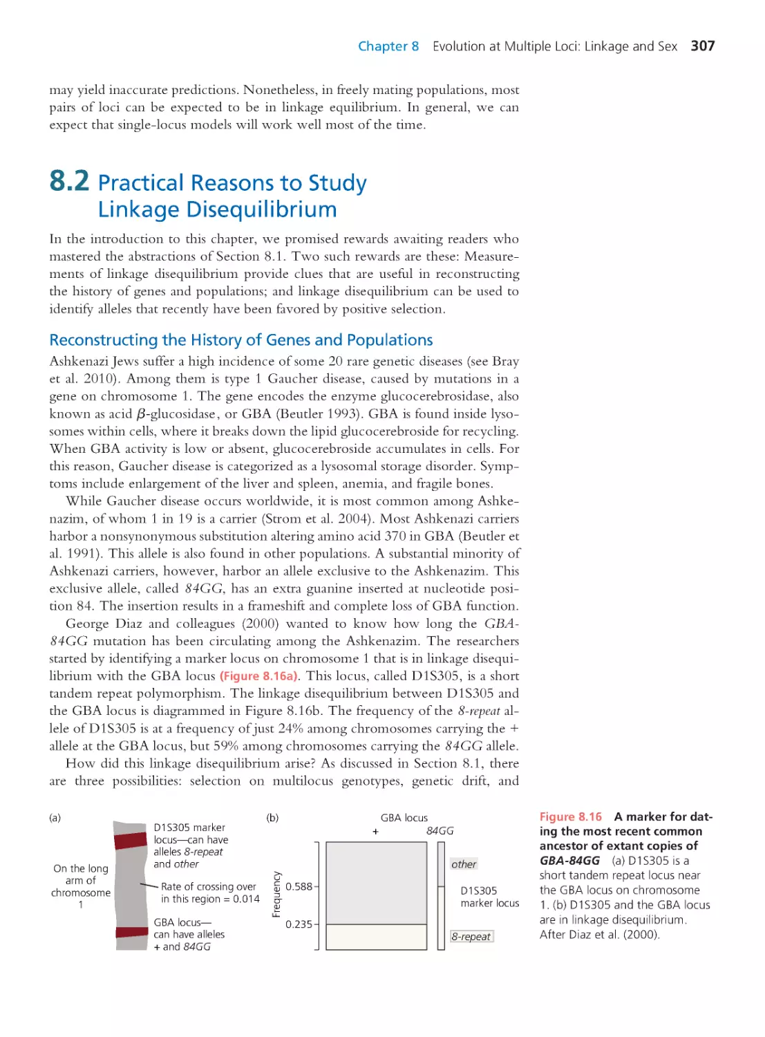
8.2 Practical Reasons to Study Linkage
Disequilibrium
307
Computing Consequences 8.4 Estimating
the age of the GBA–84GG mutation
309
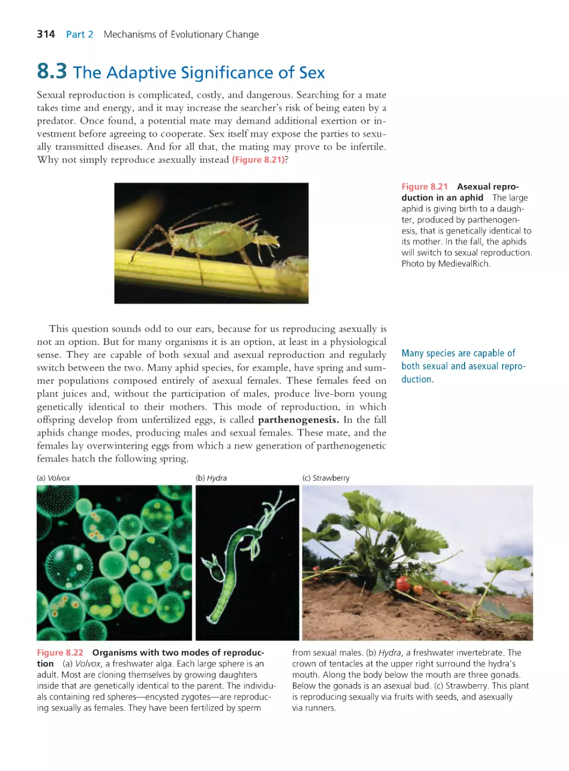
8.3 The Adaptive Significance of Sex
314
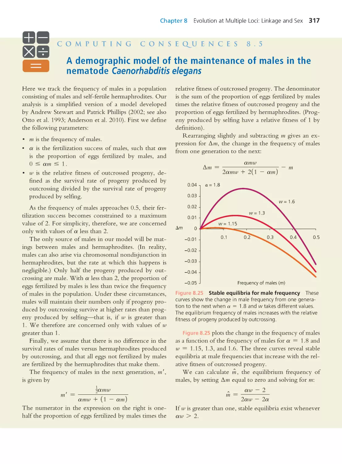
Computing Consequences 8.5
A demographic model of the maintenance of
males in the nematode Caenorhabditis elegans 317
Summary 324 • Questions 325
Exploring the Literature 326 • Citations 327
CHAPTER 9
Evolution at Multiple Loci:
Quantitative Genetics
329
9.1 The Nature of Quantitative Traits
330
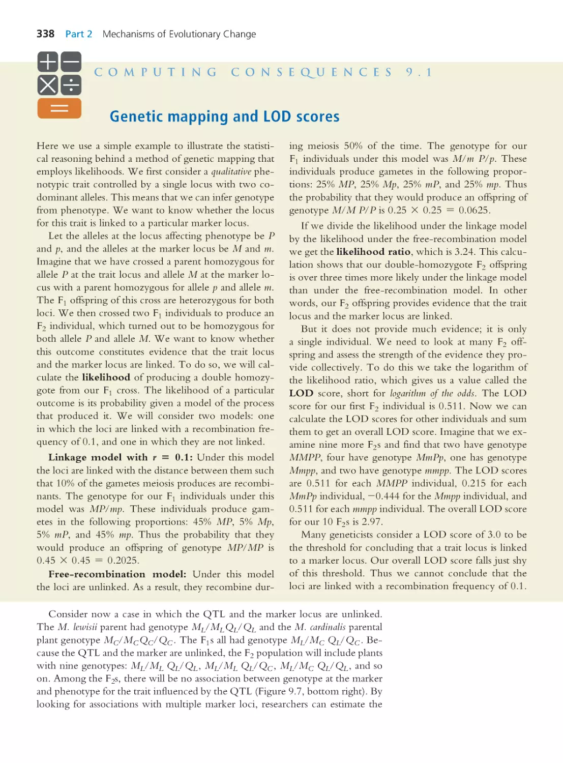
9.2 Identifying Loci That Contr ibute to
Quantitative Traits
334
Computing Consequences 9.1 Genetic
mapping and LOD scores
338
9.3 Measur ing Heritable Variation
343
Computing Consequences 9.2 Additive
genetic variation versus dominance genetic
variation
345
9.4 Measur ing Differences in Survival
and Reproductive Success
348
vi Contents
Computing Consequences 9.3 The selection
gradient and the selection differential
349
9.5 Predicting the Evolutionary Response
to Selection
350
9.6 Modes of Selection and the
Maintenance of Genetic Variation
356
9.7 The Bell-Curve Fallacy and Other
Misinterpretations of Heritability
360
Summary 365 • Questions 365
Exploring the Literature 367 • Citations 367
PART 3
ADAPTATION
369
CHAPTER 10
Studying Adaptation: Evolutionary
Analysis of For m and Function
369
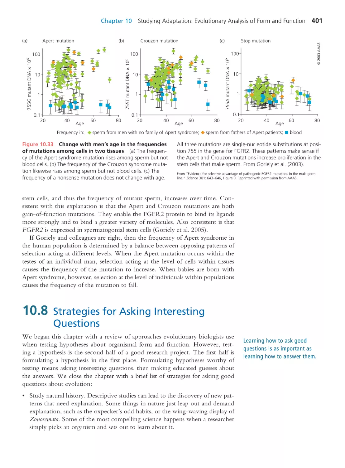
10.1 All Hypotheses Must Be Tested:
Oxpeckers Reconsidered
370
10.2 Experiments
373
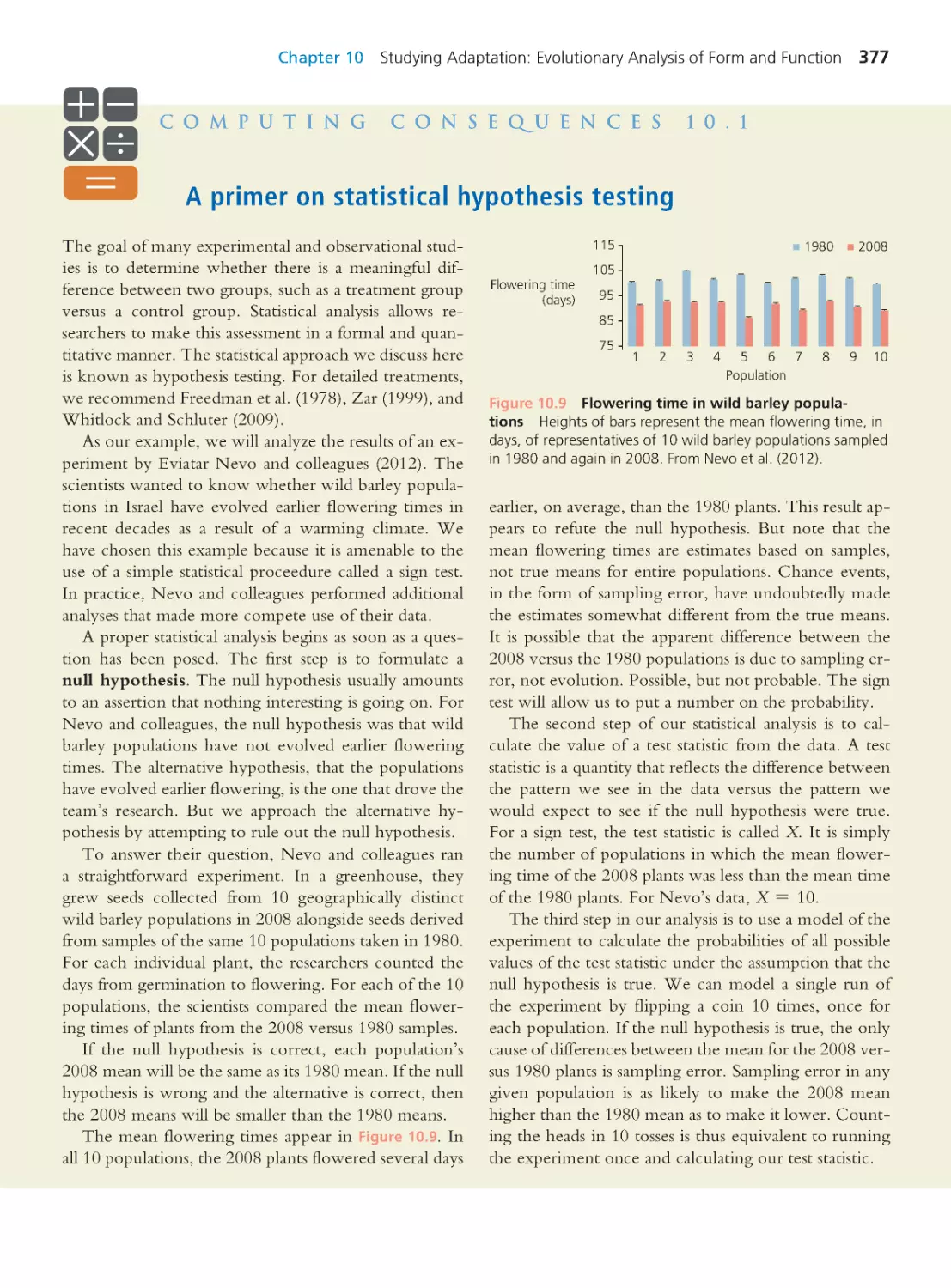
Computing Consequences 10.1
A primer on statistical testing
377
10.3 Observational Studies
378
10.4 The Comparative Method
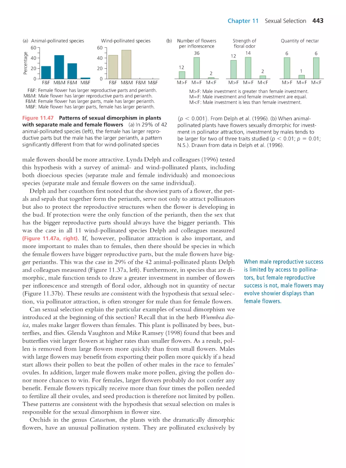
382
Computing Consequences 10.2 Calculating
phylogenetically independent contrasts
384
10.5 Phenotypic Plasticity
387
10.6 Trade-Offs and Constraints
389
10.7 Selection Operates on Different
Levels
397
10.8 Strategies for Asking Interesting
Questions
401
Summary 402 • Questions 402
Exploring the Literature 404 • Citations 405

CHAPTER 11
Sexual Selection
407
11.1 Sexual Dimorphism and Sex
408
11.2 Sexual Selection on Males:
Competition
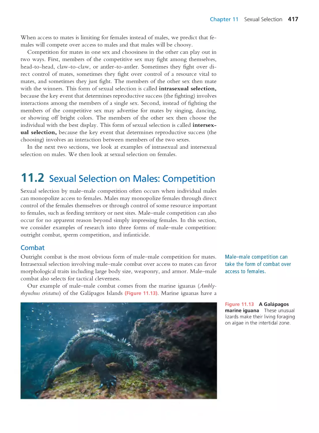
417
11.3 Sexual Selection on Males:
Female Choice
423
Computing Consequences 11.1 Runaway
sexual selection
430
11.4 Sexual Selection on Females
438
11.5 Sexual Selection in Plants
441
11.6 Sexual Dimorphism in Humans
444
Summary 448 • Questions 448
Exploring the Literature 450 • Citations 451
CHAPTER 12
The Evolution of Social Behavior
455
12.1 Four Kinds of Social Behavior
456
12.2 Kin Selection and Costly Behavior
459
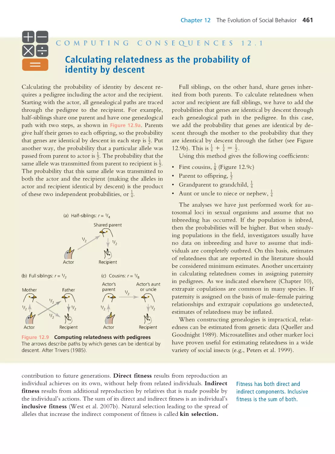
Computing Consequences 12.1 Calculating
relatedness as the probability of identity
by descent
461
12.3 Multilevel Selection and Cooperation 471
Computing Consequences 12.2 Different
perspectives on the same evolutionary process 473
12.4 Cooperation and Conflict
477
12.5 The Evolution of Eusociality
483
Summary 486 • Questions 487
Exploring the Literature 488 • Citations 489
CHAPTER 13
Aging and Other Life-History
Characters
491
13.1 Basic Issues in Life-History Analysis 493
13.2 Why Do Organisms Age and Die?
495
Contents vii
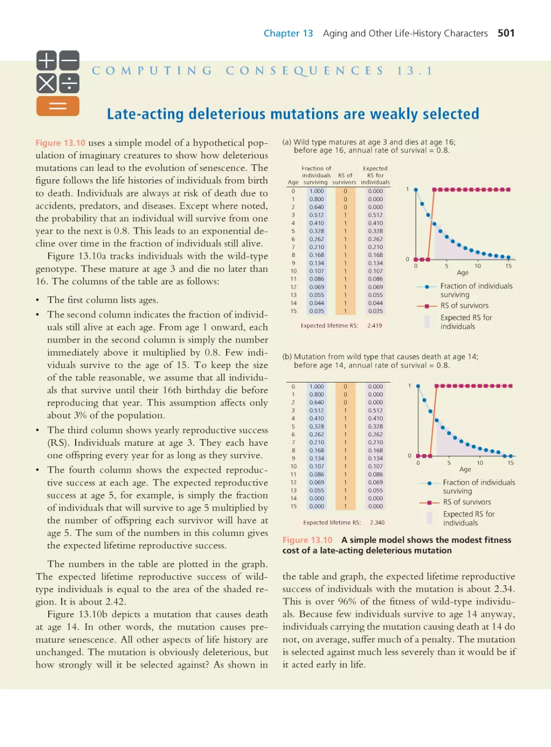
Computing Consequences 13.1 Late-acting
deleterious mutations are weakly selected
501
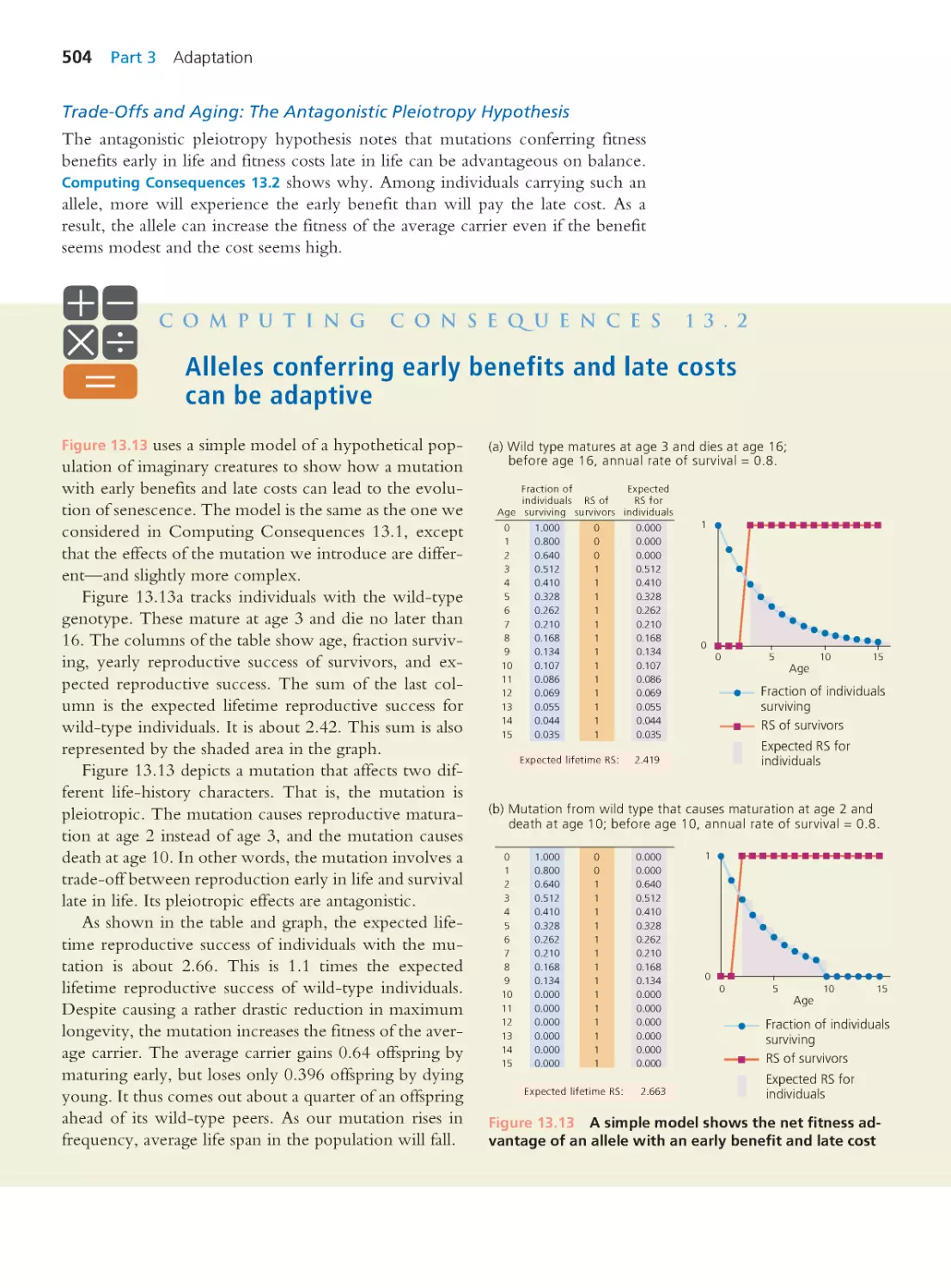
Computing Consequences 13.2 Alleles
conferring early benefits and late costs can
be adaptive
504
13.3 How Many Offspring Should an
Individual Produce in a Given Year? 513
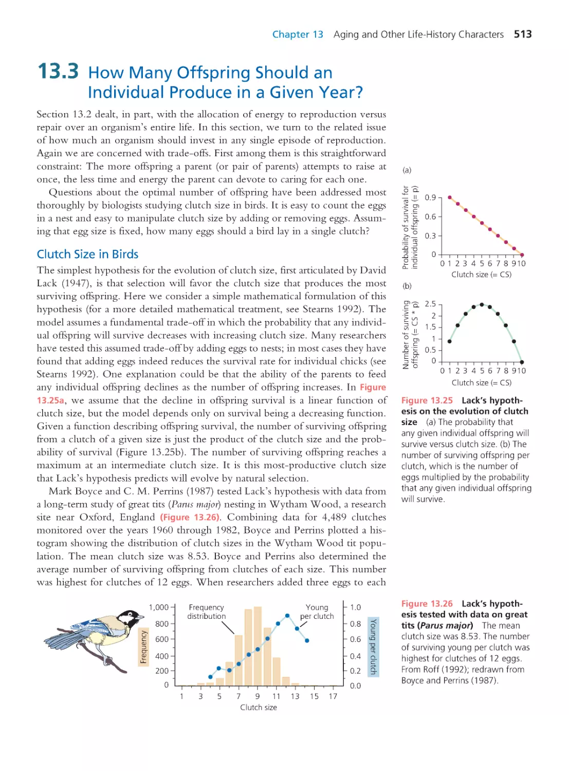
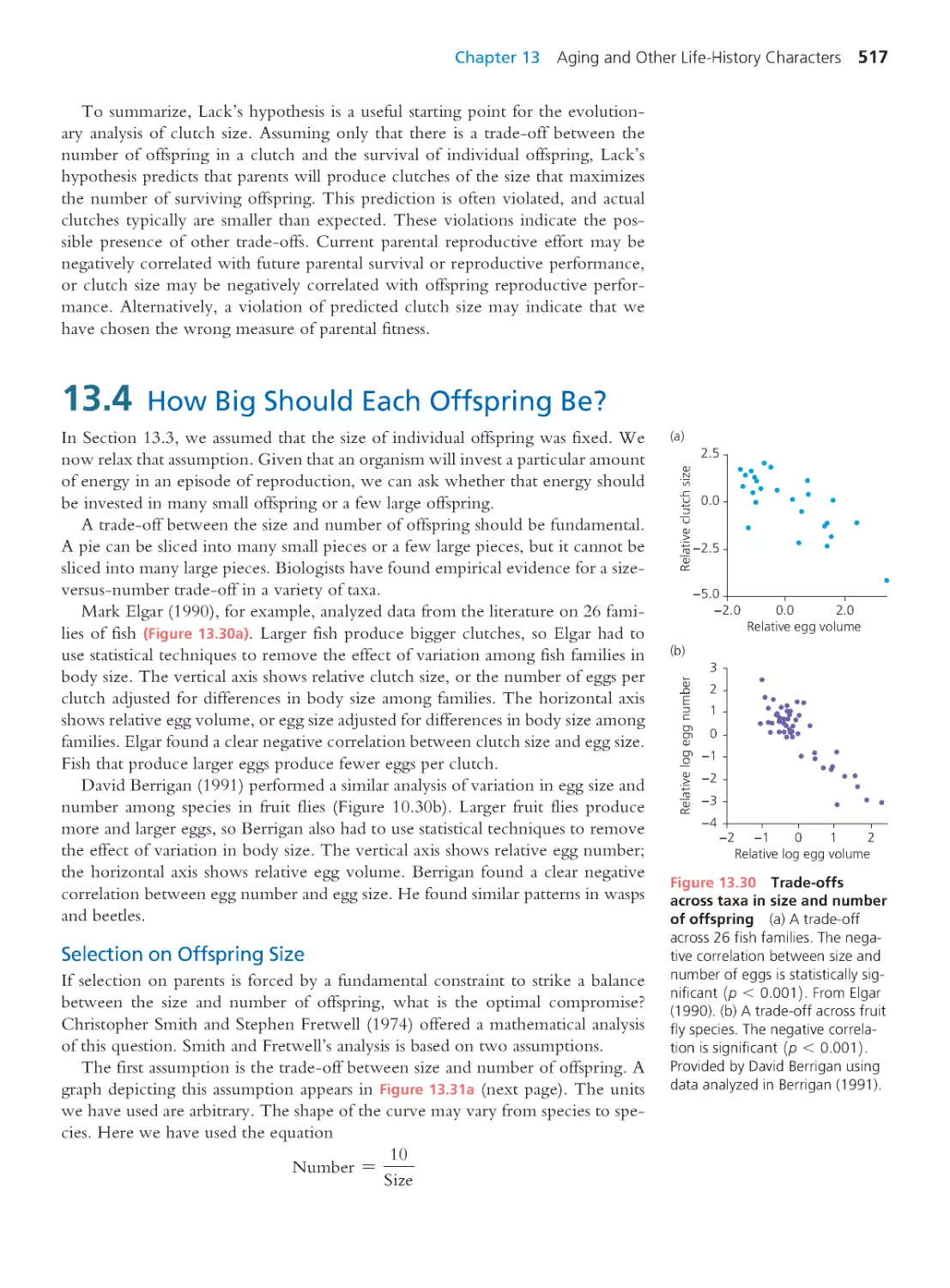
13.4 How Big Should Each Offspring Be? 517
13.5 Conflicts of Interest between Life
Histories
522
13.6 Life Histor ies in a Broader
Evolutionary Context
525
Summary 530 • Questions 530
Exploring the Literature 532 • Citations 532
CHAPTER 14
Evolution and Human Health
535
14.1 Evolving Pathogens: Evasion of the
Host’s Immune Response
537
14.2 Evolving Pathogens: Antibiotic
Resistance
545
14.3 Evolving Pathogens:Virulence
548
14.4 Tissues as Evolving Populations
of Cells
553
14.5 Selection Thinking Applied to Humans 556
14.6 Adaptation and Medical Physiology:
Fever
564
14.7 Adaptation and Human Behavior:
Parenting
567
Computing Consequences 14.1 Is cultural
evolution Darwinian?
569
Summary 575 • Questions 575
Exploring the Literature 577 • Citations 577
CHAPTER 15
Genome Evolution and the
Molecular Basis of Adaptation
581
15.1 Diversity among Genomes
582
15.2 Mobile Genetic Elements
586
15.3 The Evolution of Mutation Rates
591
15.4 Gene Duplication and Gene Families
594
15.5 The Locus of Adaptation in Natural
Populations
601
Summary 606 • Questions 606
Exploring the Literature 607 • Citations 608

viii Contents
PART 4
THE HISTORY OF LIFE
609
CHAPTER 16
Mechanisms of Speciation
609
16.1 Species Concepts
610
16.2 Mechanisms of Isolation
616
16.3 Mechanisms of Divergence
623
16.4 Hybridization and Gene Flow
between Species
629
16.5 What Drives Diversification?
637
Summary 640 • Questions 641
Exploring the Literature 642 • Citations 643
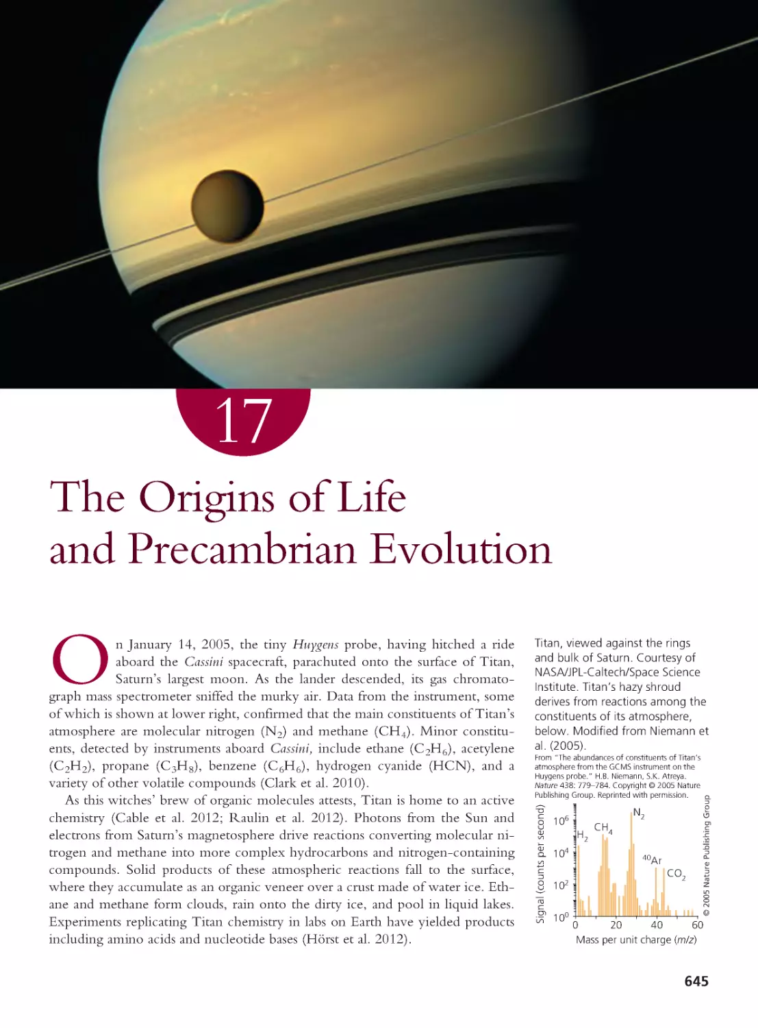
CHAPTER 17
The Origins of Life and
Precambrian Evolution
645
17.1 What Was the First Living Thing?
647
17.2 Where Did the First Living Thing
Come From?
655
17.3 What Was the Last Common Ancestor
of All Extant Organisms and What Is
the Shape of the Tree of Life?
663
17.4 How Did LUCA’s Descendants Evolve
into Today’s Organisms?
678
Summary 683 • Questions 684
Exploring the Literature 686 • Citations 686
CHAPTER 18
Evolution and the Fossil Record
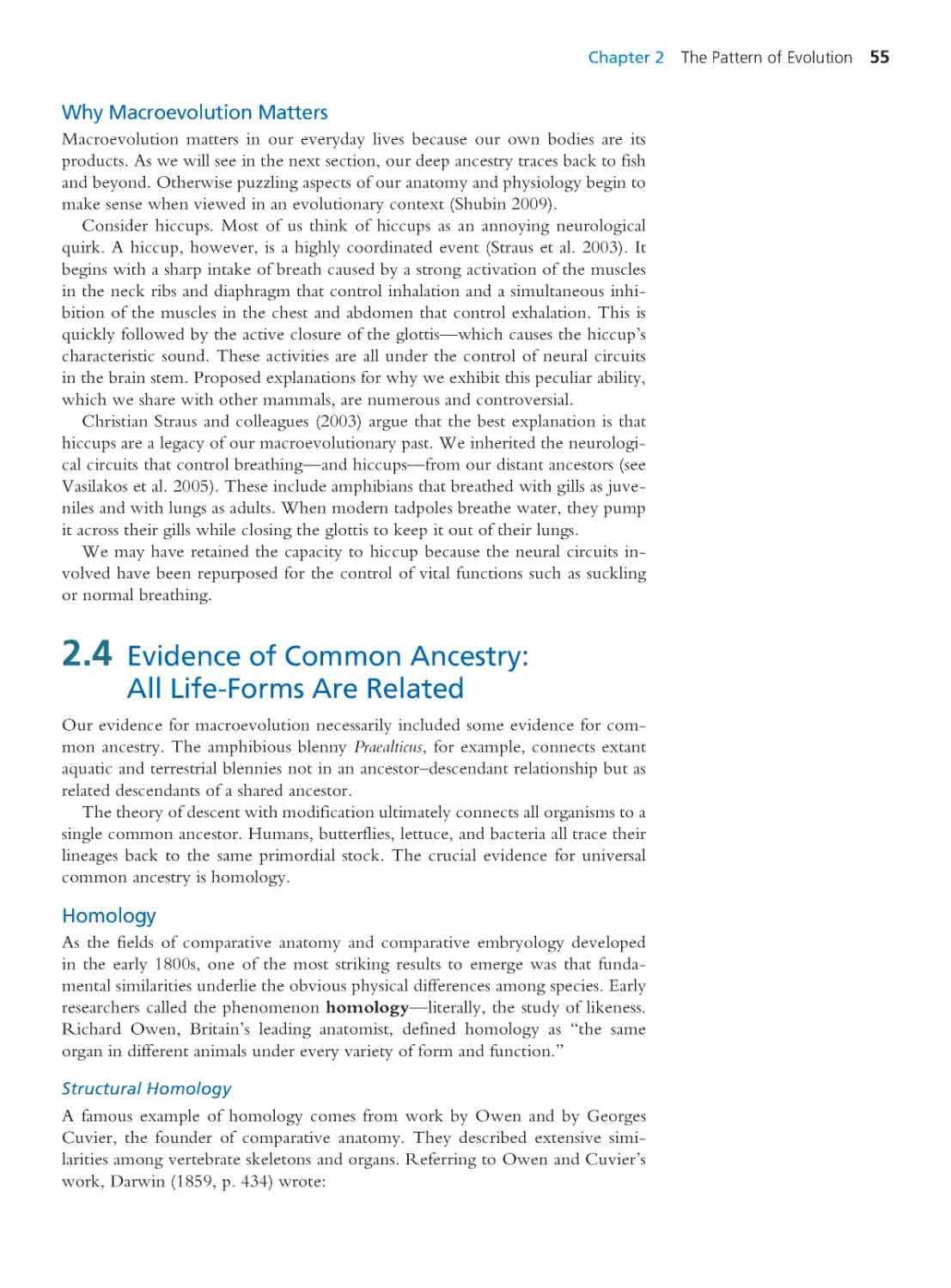
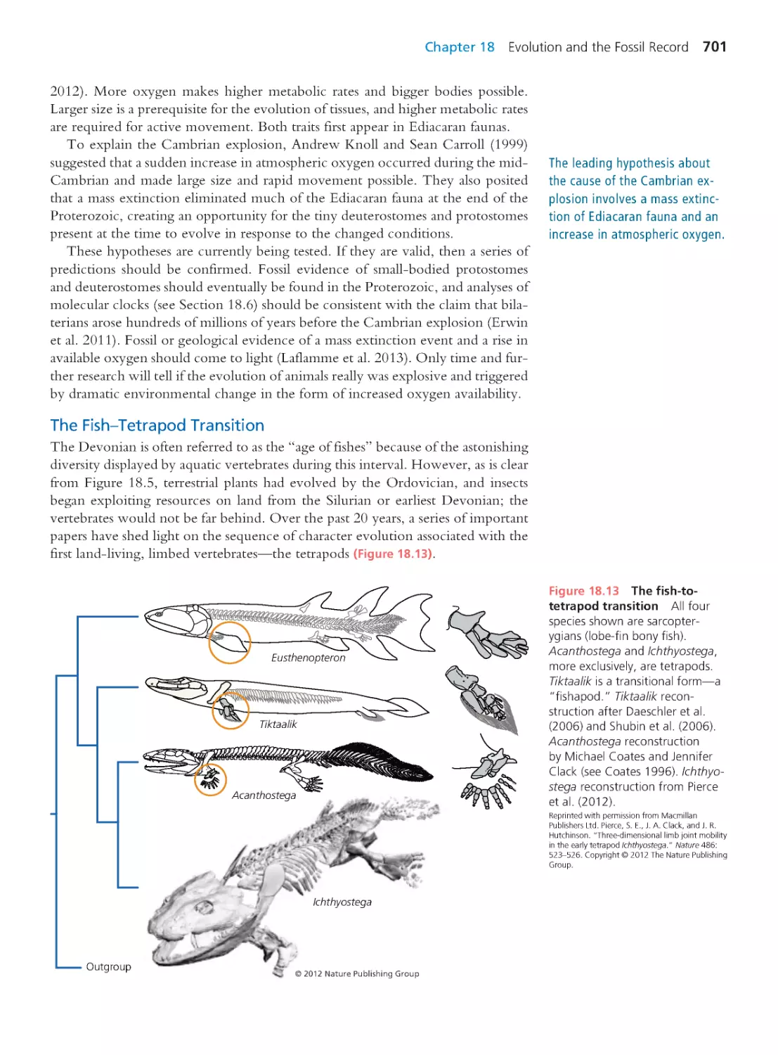
691
18.1 The Nature of the Fossil Record
692
18.2 Evolution in the Fossil Record
696
Computing Consequences 18.1
Evolutionary trends
706
18.3 Taxonomic and Morphological
Diversity over Time
707
18.4 Mass and Background Extinctions
709
18.5 Macroevolution
719
18.6 Fossil and Molecular Divergence
Timing
727
Summary 730 • Questions 731
Exploring the Literature 732 • Citations 732
CHAPTER 19
Development and Evolution
735
19.1 The Divorce and Reconciliation of
Development and Evolution
736
19.2 Hox Genes and the Birth of Evo-Devo 738
19.3 Post Hox: Evo-Devo 2.0
744
19.4 Hox Redux: Homology or Homoplasy? 763
19.5 The Future of Evo-Devo
764
Summary 765 • Questions 766
Exploring the Literature 766 • Citations 767
CHAPTER 20
Human Evolution
769
20.1 Relationships among Humans
and Extant Apes
770
20.2 The Recent Ancestry of Humans
780
20.3 Origin of the Species Homo sapiens
790
Computing Consequences 20.1 Using allele
frequencies and linkage disequilibrium to date
the modern human expansion from Africa
797
20.4 The Evolution of Distinctive Human
Traits
802
Summary 807 • Questions 807
Exploring the Literature 809 • Citations 810
Glossary
815
Credits
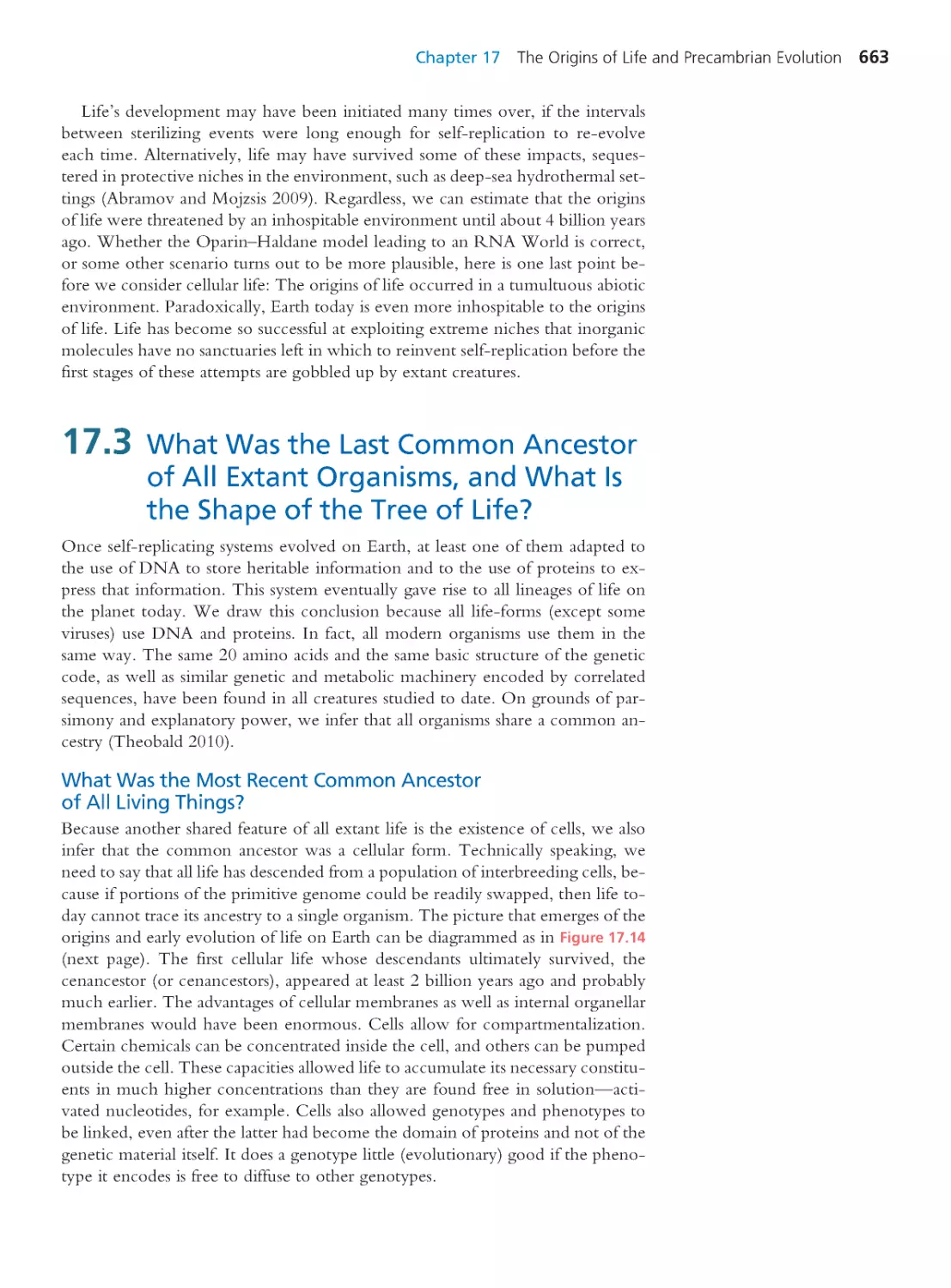
822
Index
830

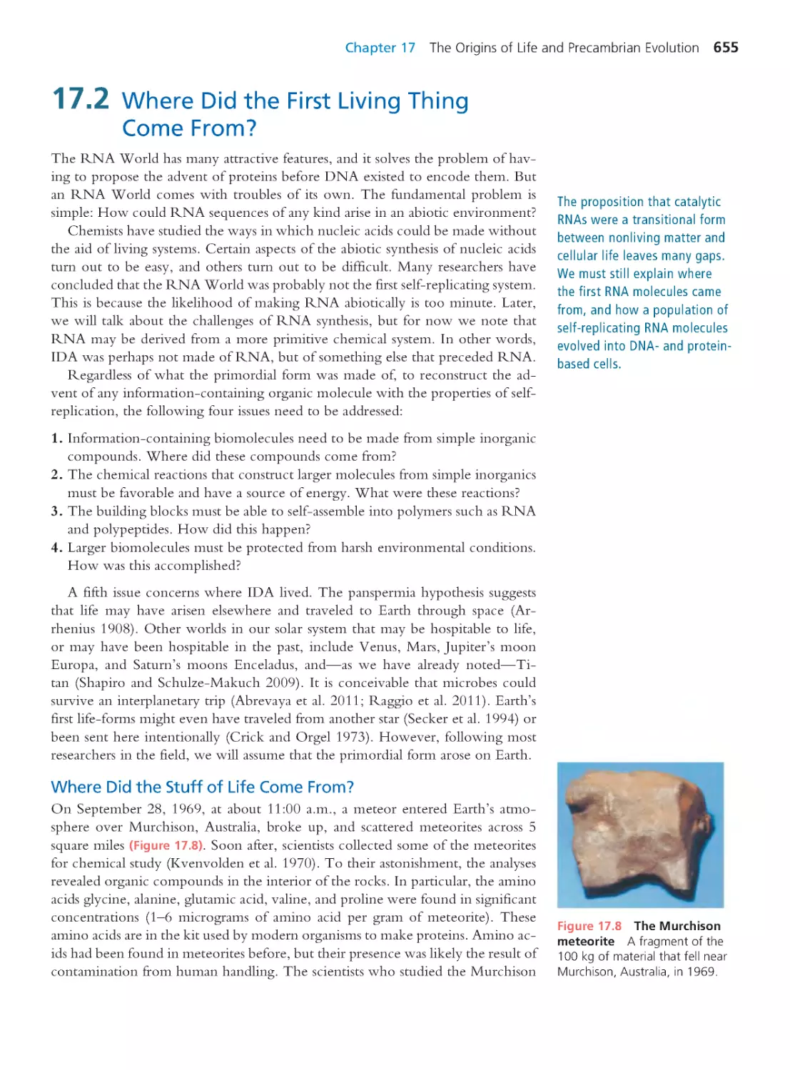
Preface
Evolutionar y biology has changed dramatically dur ing the 15 years we have
worked on Evolutionary Analysis. As one measure of this change, consider
that when the first edition went to press, the genomes of just five cellular
organisms had been sequenced: three bacter ia, one archaean, and one eukaryote.
As the fifth edition goes to press, Erica Bree Rosenblum and colleagues reported
in the Proceedings of the National Academy of Sciences (110: 9385–9390) that they had
sequenced the genomes of 29 strains of a single species, the chytr id fungus Batra-
chochytrium dendrobatidis.This work was part of an effort to unravel the evolutionary
history of an emerging pathogen that has decimated amphibian populations around
the world and driven some species to extinction. The avalanche of sequence data
has allowed evolutionary biologists to answer long-standing questions with greatly
increased depth and clar ity. In Chapter 20, Human Evolution, for example, we dis-
cuss a recent analysis of differences among genomic regions in the evolutionary
relationships among humans, chimpanzees, and gor illas. For some questions, the
answers have changed completely. In the fourth edition we noted that available
sequence data provided no support for the hypothesis that modern humans and
Neandertals interbred. But in the fifth edition we descr ibe genomic analyses sug-
gesting that the two lineages interbred after all.
Evolutionary Analysis provides an entry to this dynamic field of study for
undergraduates majoring in the life sciences. We assume that readers have com-
pleted much or all of their introductory coursework and are beginning to explore
in more detail areas of biology relevant to their personal and professional lives.
Therefore, throughout the book we attempt to show the relevance of evolution
to all of biology and to real-world problems.
Since the first edition, our primary goal has been to encourage readers to think
like scientists. We present evolutionary biology not as a collection of facts but as an
ongoing research effort. When exploring an issue, we begin with questions. Why
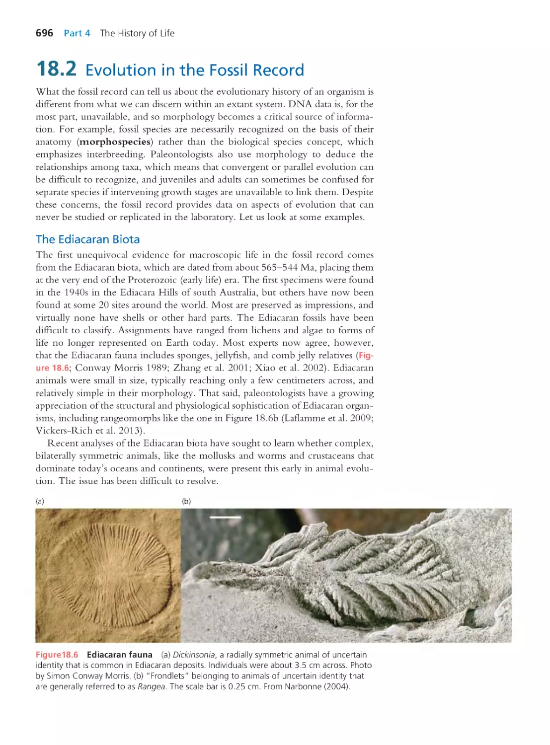
are untreated HIV infections typically fatal? Why do purebred Flor ida panthers
show such poor health, and what can be done to save their dwindling population?
Why do mutation rates decrease with genome size among some kinds of organisms,
but increase with genome size among others? We use such questions to engage stu-
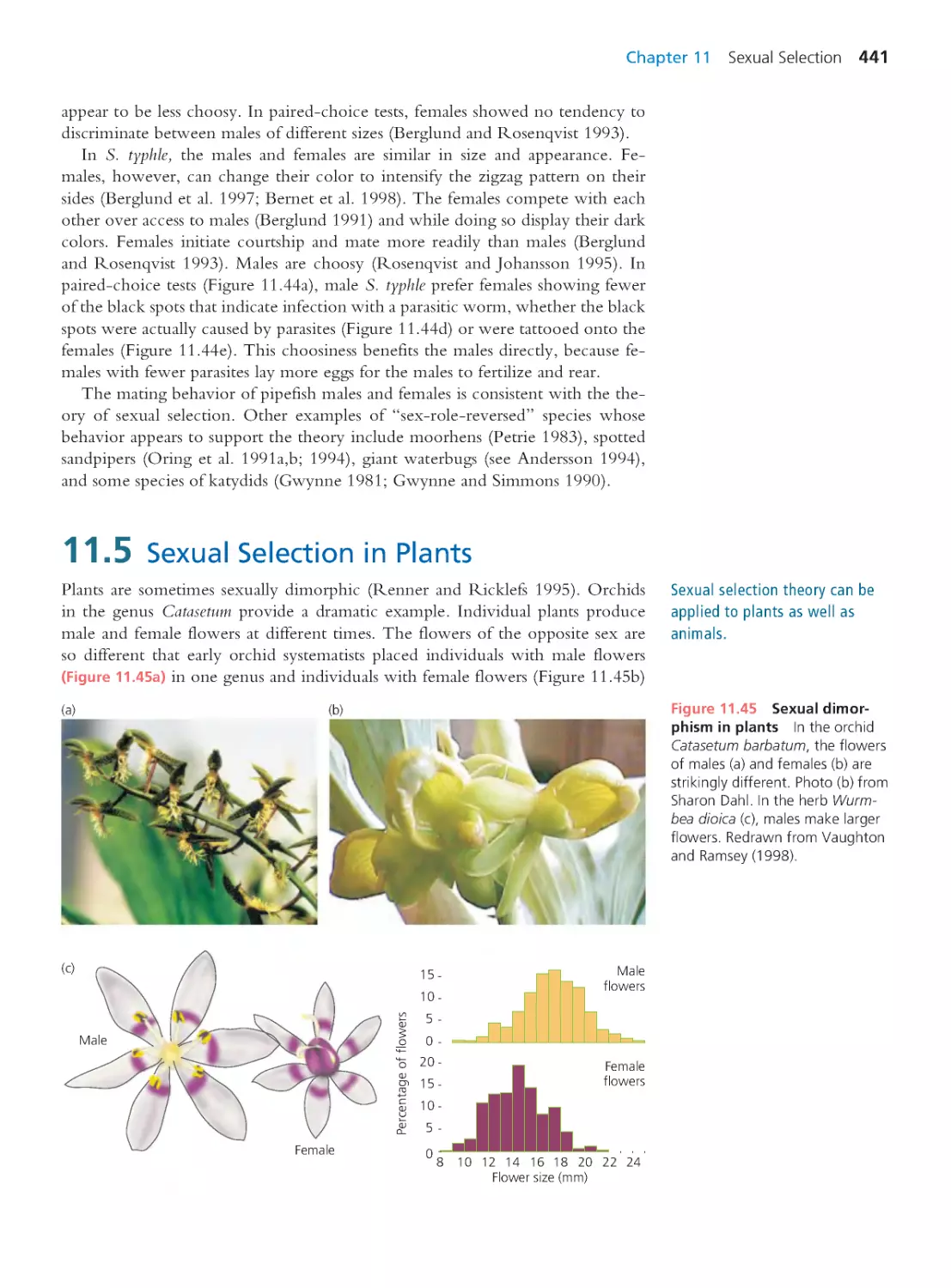
dents’ cur iosity and to motivate discussions of background infor mation and theory.
These discussions enable us to frame alter native hypotheses, consider how they
can be tested, and make predictions. We then present and analyze data, consider its
implications, and highlight new questions for future research. The analytical and
technical skills readers learn from this approach are broadly applicable, and will stay
with them long after the details of particular examples have faded.
New to This Edition
Many of the research areas we cover are advancing at a rate we would
not have dreamed possible just a few years ago.We have looked close-
ly at every chapter to both improve how we are teaching today’s
students and to thoroughly update our coverage.
ix

• We have enhanced our traditional emphasis on scientific reasoning by includ-
ing a data graph, evolutionary tree, or other piece of evidence to accom-
pany the photo on the first page of every chapter. These one-page case studies
engage students as active readers and help them become skilled at working
with and interpreting data.
• We have enhanced our strong coverage of tree thinking by thoroughly
revising Chapter 4. Consistent with the ever-growing use of phylogenetic
analysis by scientists, we incor porate more phylogenies throughout the book.
Among the new examples are a tree-based discussion of evolution of ver-
tebrate eyes (Chapter 3); a new case study reconstructing the histor y of a
patient’s cancer (Chapter 14); and phylogeny-based reconstructions of the
fish-tetrapod transition, the dinosaur-bird transition, and the or igin of mam-
mals (Chapter 18). Frequent practice at tree thinking helps students develop
this essential skill.
Every chapter contains something new. Most of the new mater ial is from the
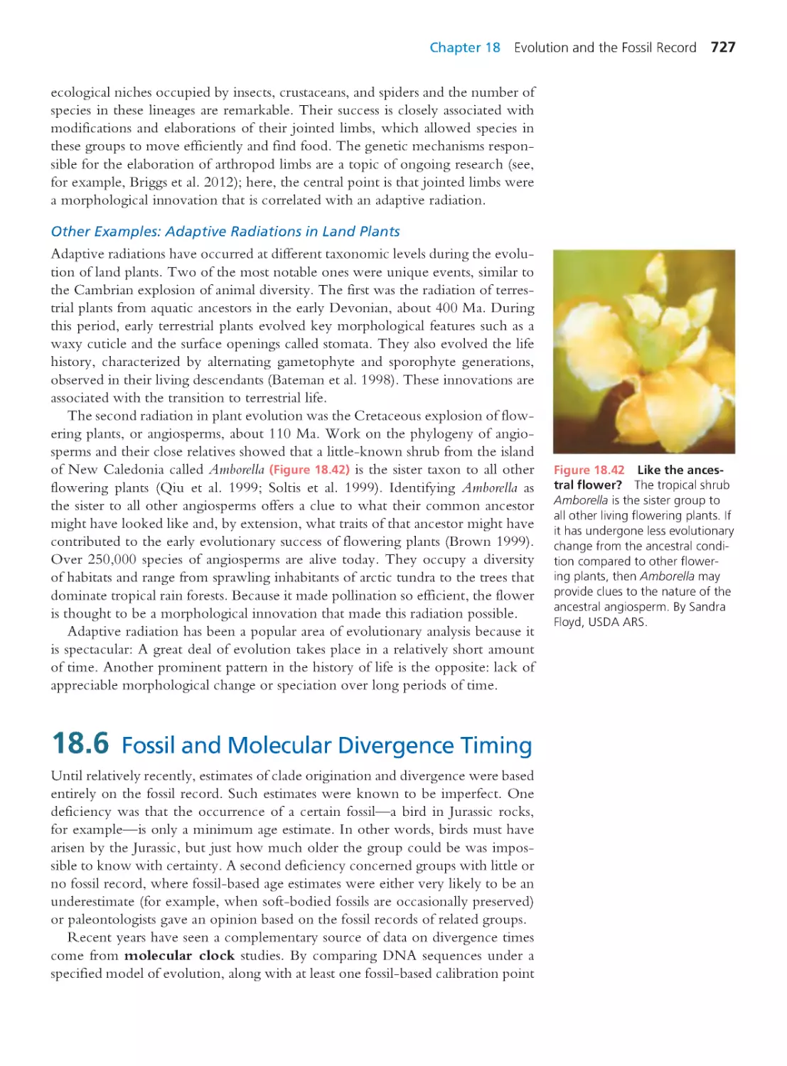
recent literature.
• Chapter 1 includes updated statistics on the status of the HIV pandemic, newer
thinking on how HIV causes AIDS, new data on the or igin of HIV, and new
ideas and evidence on why HIV is lethal.
• Chapter 2 has a new organization featuring sections on evidence for micro-
evolution, speciation, macroevolution, and common ancestry; discussions of
why evolution at each level is relevant to humans outside of textbooks and
classrooms; evidence of macroevolution presented using evolutionary trees
showing the order in which derived traits are inferred to have evolved; and
several new examples, including a terrestrial fish that does not like to swim.
• Chapter 3 brings new evidence on the evolution of development in the beaks
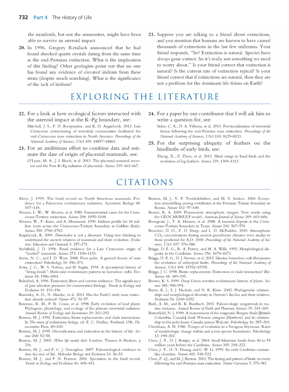
of Darwin’s finches, a new example of exaptation featur ing car nivorous plants,
and new coverage of the evolution of complex organs featuring a phylogeny-
based discussion of the evolution of vertebrate eyes.
• Chapter 4 has been completely rewritten to offer an improved introduction to
tree thinking; more detailed explanations of parsimony, maximum likelihood,
and Bayesian phylogeny inference; and new examples of phylogenies used to
answer interesting questions—such as identifying the surprising infectious
agent responsible for a sexually transmitted tumor in dogs.
• Chapter 5 includes a new section on kinds of var iation, featur ing new and
detailed examples of genetic var iation and environmental var iation; geno-
type-by-environment interaction; improved discussion of the mechanisms
and consequences of mutation; new examples of gene duplication; and cov-
ers rates and fitness effects of mutation in a dedicated section with new ex-
amples and data.
• Chapter 6 is bookended with a powerful new example in which genetic engi-
neers made a new gene, accurately predicted its effects on individuals car rying it,
introduced it into a population, and used population genetics theory to accurately
predict how its frequency would change over a span of 20 generations.
• Chapter 7 is bookended with a new example of conservation genetics involv-
ing the Flor ida panther. The chapter also includes a new example illustrating
the founder effect in Polynesian field cr ickets; improved coverage of the inter-
x Preface

action of drift and selection, the neutral theory, and the nearly neutral theory;
and a new introduction to coalescence.
• Chapter 8 carries a new example—on Crohn’s disease in humans—showing
how linkage disequilibrium due to genetic hitchhiking can lead to spurious
associations between genotype and phenotype and a revised and updated sec-
tion on the adaptive significance of sex, featuring recent experiments using
C. elegans as a model organism.
• Chapter 9 has improved nar rative coherence due to the inclusion throughout
the chapter of examples on the quantitative genetics of perfor mance and prize
winnings in thoroughbred racehorses.
• Chapter 10 includes an improved primer on statistical hypothesis testing, using
research on the evolution of wild barley populations in response to a war ming
climate, and a new example of comparative research involving color in feather lice.
• Chapter 11 improves our coverage of the evolution of female choice by
presenting the Fisher-Kirkpatrick-Lande model as the null hypothesis. New
examples and data consider Bateman’s principle in a hermaphrodite; female
preferences in genetically modified zebrafish; correlated displays and prefer-
ences in Hawaiian crickets; and sexual selection in humans.
• Chapter 12 features enhanced coverage, with examples, of the four basic kinds
of social behavior; improved coverage of kin selection and spite; a new section
on multilevel selection and the evolution of cooperation; and several data sets
on human social behavior.
• Chapter 13 has new examples on telomeres and aging; the evolution of meno-
pause; life history traits and biological invasion; and life history traits and vul-
nerability to extinction.
• Chapter 14 discusses new evidence, from genome architecture, on the or igin
of influenza A; a new example using phylogenetic analysis to reconstruct the
history of a cancer; and updated coverage of diseases of civilization, including
a dramatic example from Iceland and new mater ial on obesity.
• Chapter 15 has been completely rewritten, bringing new sections on the evo-
lution of genome architecture; the evolution of mutation rates and gene fami-
lies; and updated treatment of mobile genetic elements and the molecular basis
of adaptation.
• Chapter 16 features new sections on mechanisms of divergence; hybridization
and gene flow; and drivers of diversification.The chapter includes new examples
illustrating the application of species concepts; updated coverage of vicar iance
in snapping shrimp; and new examples on mechanisms of isolation—including
temporal isolation in a moth and single-gene speciation in snails.
• Chapter 17 incorporates updated coverage of the effort to create self-replicating
RNAs and of the prebiotic synthesis of activated nucleotides.
• Chapter 18 has greatly expanded coverage of evolutionary transitions, fea-
turing phylogeny-based reconstructions of the fish-tetrapod transition,
the dinosaur-bird transition, and the origin of mammals; a new section on
taxonomic and morphological diversity over time; updated treatment of mass
extinctions, including the Per mian-Triassic extinction; and a new section on
fossil and molecular divergence timing.
Preface xi

• Chapter 19 has been completely rewr itten. It includes revised coverage of Hox
genes and detailed discussions of deep homology, developmental constraints
and trade-offs, and the evolution of novel traits.
• Chapter 20 discusses new evidence from complete genomes on incomplete
lineage sorting among humans, chimps, and gorillas, and on genetic differ-
ences between these species; new evidence, also from complete genomes, on
hybridization between modern humans and Neandertals and between mod-
ern humans and Denisovans; and updated coverage of the human fossil record
and the evolution of spoken language.
Hallmark Features
While fully updating this edition, we also maintained core strengths for
which this book is recognized.
• We continue to strive for clar ity of presentation, ensuring each chapter con-
tains a coherent, accessible narrative that students can follow.
• We remain committed to strong information design and a tight integration
between the text and illustration program. Nearly all phylogenies are presented
horizontally, with time running from left to right, because research has shown
this makes it easier for students to interpret them correctly.
• Boxes contain detailed explorations of quantitative issues discussed in the main
text. These are called Computing Consequences, after physicist Richard Feyn-
man’s concise description of the scientific method: “First, we guess . . . No!
Don’t laugh—it’s really true.Then we compute the consequences of the guess
to see if this law that we guessed is right—what it would imply. Then we
compare those computation results to nature—or, we say, to experiment, or
experience—we compare it directly with observation to see if it works. If it
disagrees with exper iment, it’s wrong.”
All chapters end with a set of questions that encourage readers to review the
mater ial, apply concepts to new issues, and explore the primary literature.
Additional Resources for Instructors and Students
Atthe Pearson Instructor Resource Center, you can download JPEG and
PowerPoint files containing all of the line art, tables, and photos from
the book.You can access versions with and without labels to best suit
your needs.
A thorough test bank and TestGen software is available to help you gener-
ate tests. Each chapter has dozens of multiple choice, short answer, and essay
questions.
The updated Companion Website has been revised and updated to reflect the
new edition. The website can be found at: www.pearsonhighered.com/herron
Activities such as case studies and simulations challenge students to pose questions,
formulate hypotheses, design exper iments, analyze data, and draw conclusions. Many
of these activities accompany downloadable software programs that allow students
to conduct their own virtual investigations. Students will also find chapter study
quizzes that allow them to check their understanding of key ideas in each chapter.
xii Preface

Preface xiii
Acknowledgments
Evolutionary Analysis is a team effort.The book owes its existence and qual-
ity to the generosity and talents of a large community of colleagues,
students, and friends. They have reviewed chapters; made suggestions;
answered our questions; shared their photos, data, and insights; and lent us their
expertise in countless other ways. Getting to spend time with and learn from such
smart and interesting people is the best part of our job.
For the fifth edition we have had the great fortune to work with three extraor-
dinary contributors.
• Brooks Miner, Cornell University, wrote the entirely new Chapter 15 and
extensively revised and updated Chapter 16.
• Christian Sidor, University of Washington, thoroughly revised and expanded
Chapter 18.
• Jason Hodin, Hopkins Marine Station of Stanford University and University of
Washington, wrote the entirely new Chapter 19.
Mark Ong provided the beautiful and rational design of the new edition. Rob-
in Green designed and produced art that is both engaging and effective, and is
responsible for the coherent integration of the illustrations with the text.
The editorial, production, and marketing team at Pearson Education has offered
steadfast guidance and support: Michael Gillespie, Senior Acquisitions Editor—
Biology; Beth Wilbur, VP and Editor-in-Chief of Biology and Environmental
Science; Paul Corey, President—Science, Business, and Technology; Lauren Harp,
Executive Marketing Manager; Lori Newman, Production Project Manager;
Deborah Gale, Executive Director of Development—Biology; Laura Murray,
Project Editor; and Eddie Lee, Assistant Editor.
Our preparation of the fifth edition has been guided by thoughtful, detailed,
and constructive cr itiques by
Mirjana Brockett, Georgia Institute
of Technology
Jeremy Brown, LSU
Michael Emer man, University of
Washington
Charles Fenster, University of Maryland
Matthew Hahn, University of Indiana
Michael E. Hellberg, LSU
Christopher Hess, Butler University
Gene Hunt, Smithsonian Institution
Ben Kerr, University of Washington
Craig Lending, SUNY Brockport
Carlos MacHado, University of
Maryland
Kurt McKean, University at Albany
James Mullins, University of Washington
Christopher Parkinson, University of
Central Florida
Yale Passamaneck, University of Hawaii
Bruno Pernet, California State
University, Long Beach
Thomas Ray, University of Oklahoma
Doug Schemske, Michigan State
University
Billie J. Swalla, University of Washington
Sara Via, University of Maryland
Rebecca Zufall, University of Houston
Finally, we extend a special thank you to Christopher Parkinson and his stu-
dents at the University of Central Florida and to Carol E. Lee and her students at
the University of Wisconsin. Both groups class-tested preliminary versions of the
chapters and provided insightful feedback that improved the final drafts.

This page intentionally left blank

1
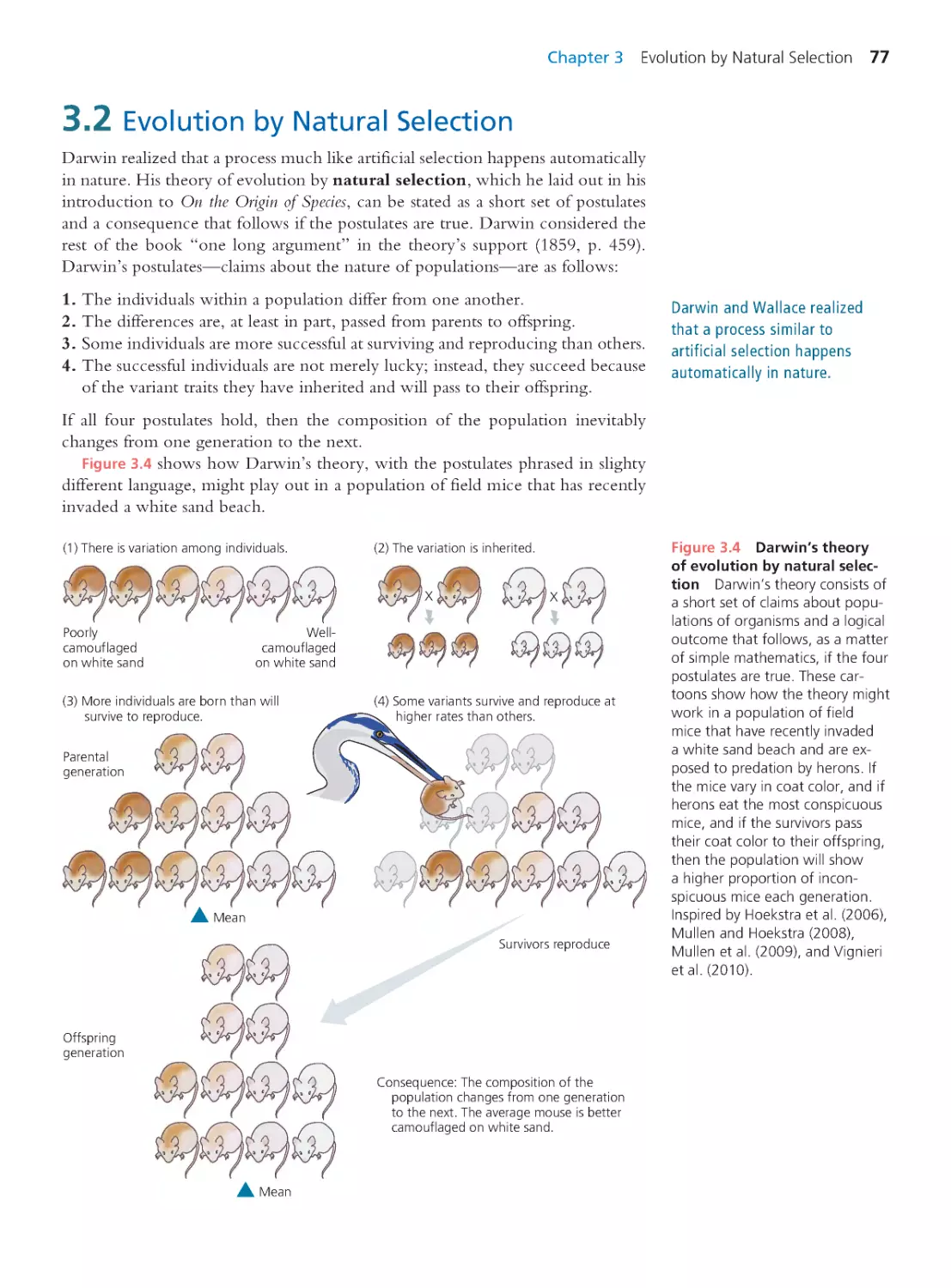
Why study evolution? An incentive for Charles Darwin (1859) was
that understanding evolution can help us know ourselves. “Light
will be thrown,” he wrote, “on the origin of man and his history.”
The allure for Theodosius Dobzhansky (1973), an architect of our modern view
of evolution, was that evolutionary biology is the conceptual foundation for all
of life science. “Nothing in biology makes sense,” he said, “except in the light
of evolution.” The motive for some readers may simply be that evolution is a
required course. This, too, is a valid inducement.
Here we suggest an additional reason to study evolution: The tools and tech-
niques of evolutionary biology offer crucial insights into matters of life and death.
To back this claim, we explore the evolution of HIV (human immunodeficiency
virus). Infection with HIV causes AIDS (acquired immune deficiency syndrome)—
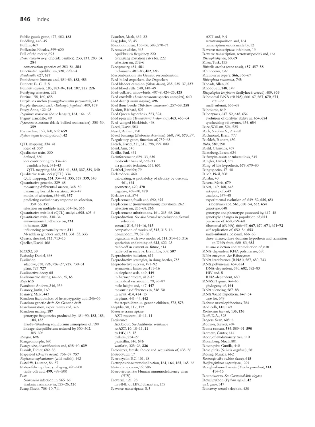
sometimes, as shown at right, despite triple-drug therapy.
Our main objective in Chapter 1 is to show that evolution matters outside of
labs and classrooms. However, a deep look at HIV will serve other goals as well.
It will illustrate the kinds of questions evolutionary biologists ask, show how an
evolutionary perspective can inform research throughout biology, and introduce
concepts that we will explore in detail elsewhere in the book.
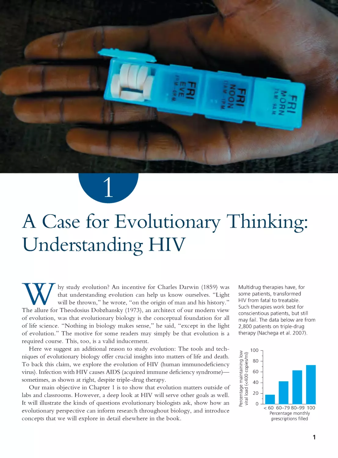
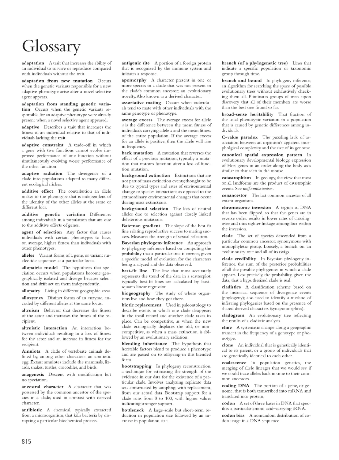
Multidrug therapies have, for
some patients, transformed
HIV from fatal to treatable.
Such therapies work best for
conscientious patients, but still
may fail. The data below are from
2,800 patients on triple-drug
therapy (Nachega et al. 2007).
1
A Case for Evolutionary Thinking:
Understanding HIV
P
e
r
c
e
n
t
a
g
e
m
a
i
n
t
a
i
n
i
n
g
l
o
w
v
i
r
a
l
l
o
a
d
(
<
4
0
0
c
o
p
i
e
s
/
m
l
)
Percentage monthly
prescriptions filled
< 60 60–79 80–99 100
0
20
40
60
80
100

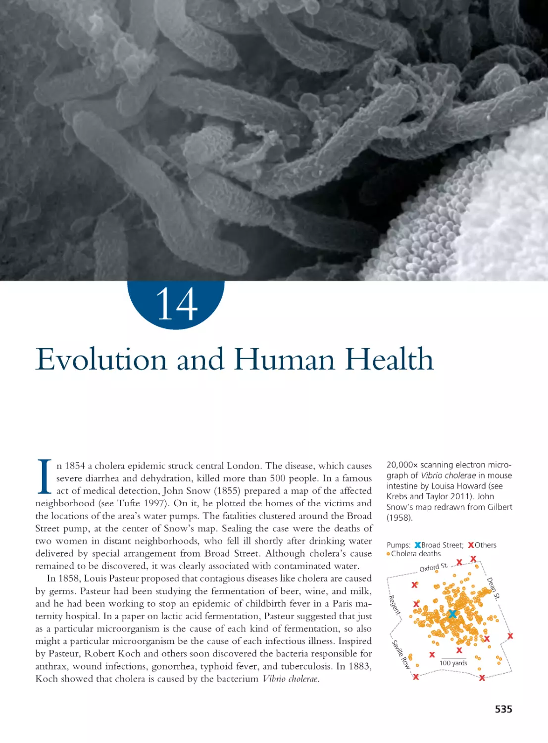
HIV makes a compelling case study because it illustrates public health issues
likely to influence the life of every reader. It is an emerging pathogen. It rapidly
evolves drug resistance. And, of course, it is deadly. AIDS is among the 10 lead-
ing causes of death worldwide (Lopez et al. 2006; WHO 2008).
Here are the questions we address:
• What is HIV, how does it spread, and how does it cause AIDS?
• Why do therapies using just one drug, and sometimes therapies using multiple
drugs, work well at first but ultimately fail?
• Are human populations evolving as a result of the HIV pandemic?
• Where did HIV come from?
• Why are untreated HIV infections usually fatal?
While one of these questions contains the word evolution, some of the others
may appear unrelated to the subject. But evolutionary biology is devoted to un-
derstanding how populations change over time and how new forms of life arise.
These are the issues targeted by our queries about HIV and AIDS. In preparation
to address them, the first section covers some requisite background.
1.1 The Natural History of the HIV Epidemic
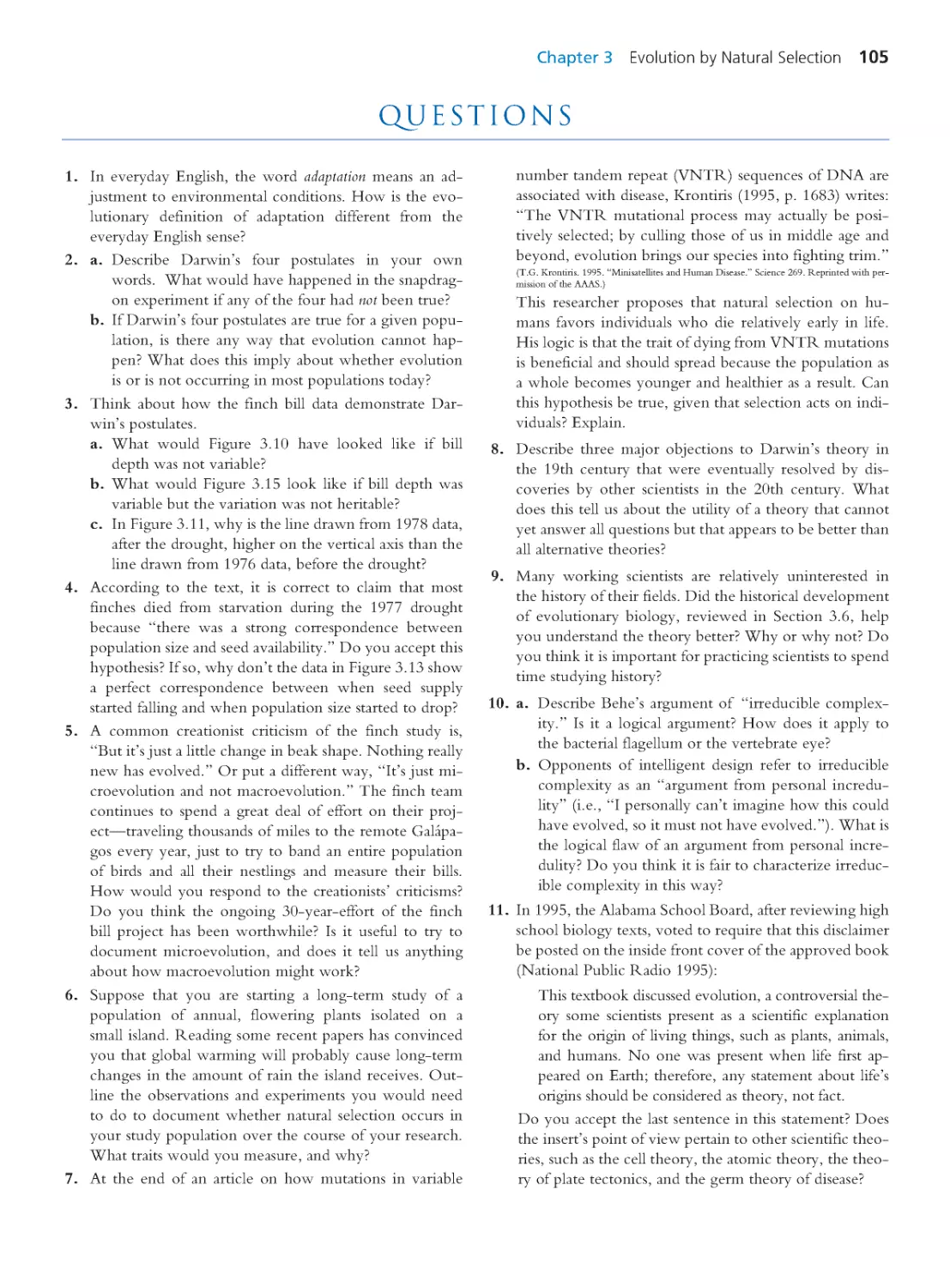
AIDS was recognized in 1981, when doctors in the United States reported rare
forms of pneumonia and cancer among men who have sex with men (Fauci
2008). The virus responsible, HIV, was identified shortly thereafter (Barré-
Sinoussi et al. 1983; Gallo et al. 1984; Popovic et al. 1984). Nearly always fatal,
HIV/AIDS was devastating for those infected. But few physicians or researchers
foresaw the magnitude of the epidemic to come (Figure 1.1).
Indeed, many were optimistic about the prospects for containing HIV (Walk-
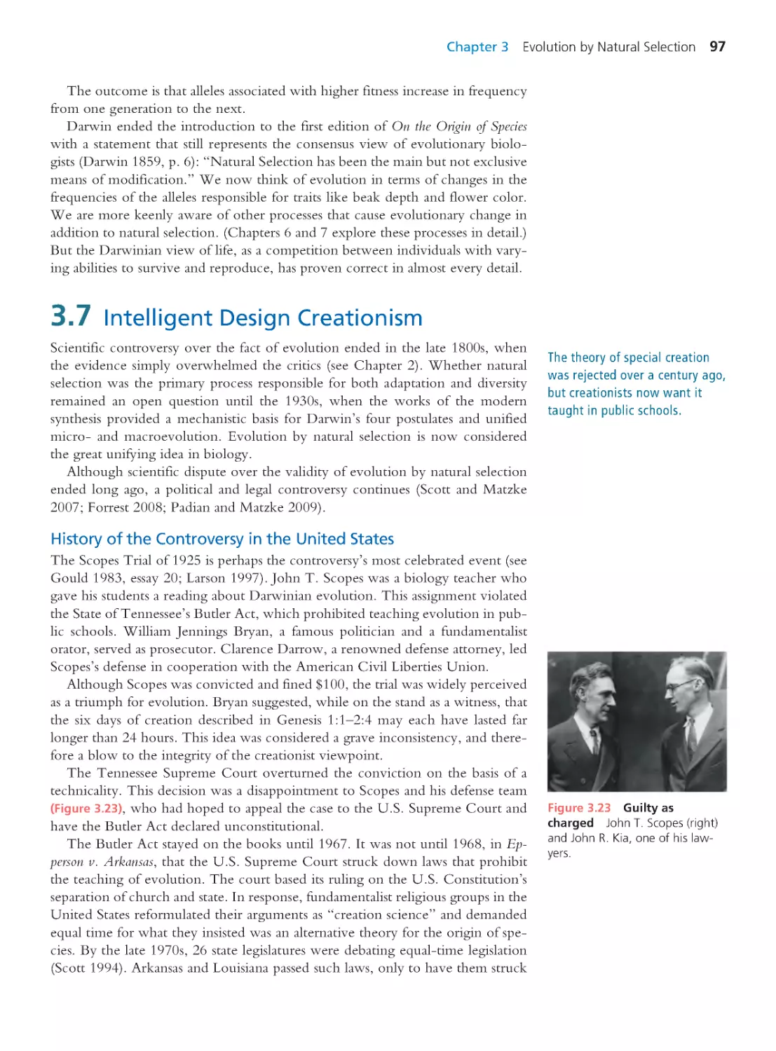
er and Burton 2008). Smallpox had been declared eradicated in 1980 (Moore et
2 Part 1 Introduction
23.5
million
1.4 million
(a)
5%
1%
0.25 to 0.49%
0 to 0.24%
0.75 to 1%
0.50 to 0.74%
N
u
m
b
e
r
o
f
i
n
f
e
c
t
e
d
p
e
o
p
l
e
(
m
i
l
l
i
o
n
s
)
United Kingdom
United States
India
South Africa
Adult
prevalence
(% infected)
Number of people
living with HIV
(b)
Year
230,000
1.4 million
53,000
% Women % Men % Children
Percentage of infected people who
are women vs. men vs . children
830,000
1.4 million
900,000
300,000
4.0 million
1990 1996 2002 2008
0.0
0.4
0.8
1.2
0
0.03
0.06
0.09
1990 1996 2002 2008
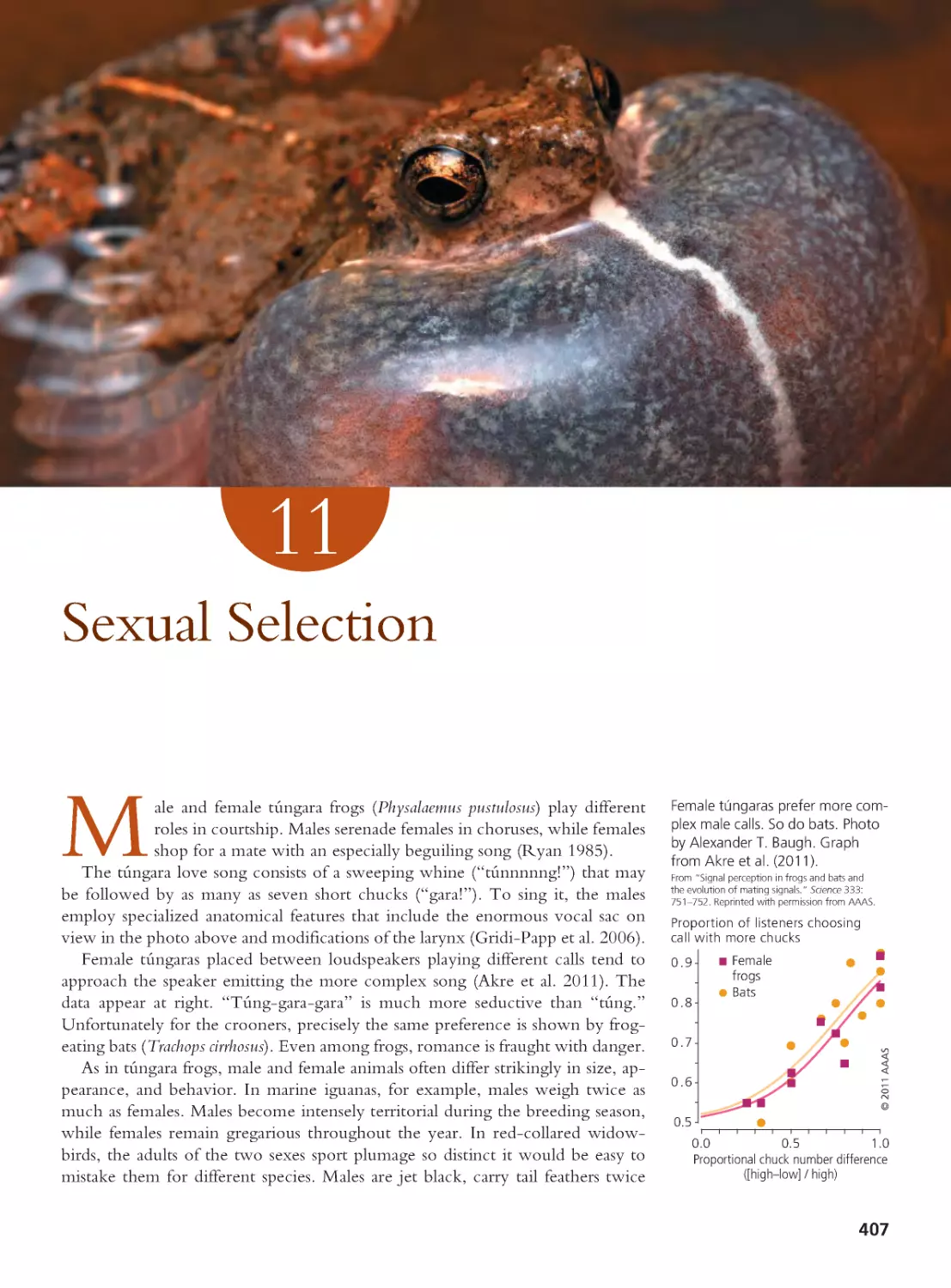
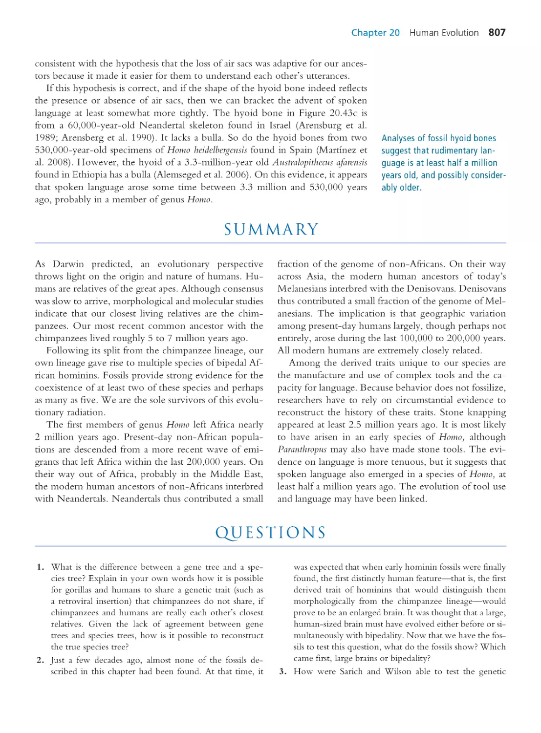
0
2
4
6
1990 1996 2002 2008 1990 1996 2002 2008
0
1.0
2.0
3.0
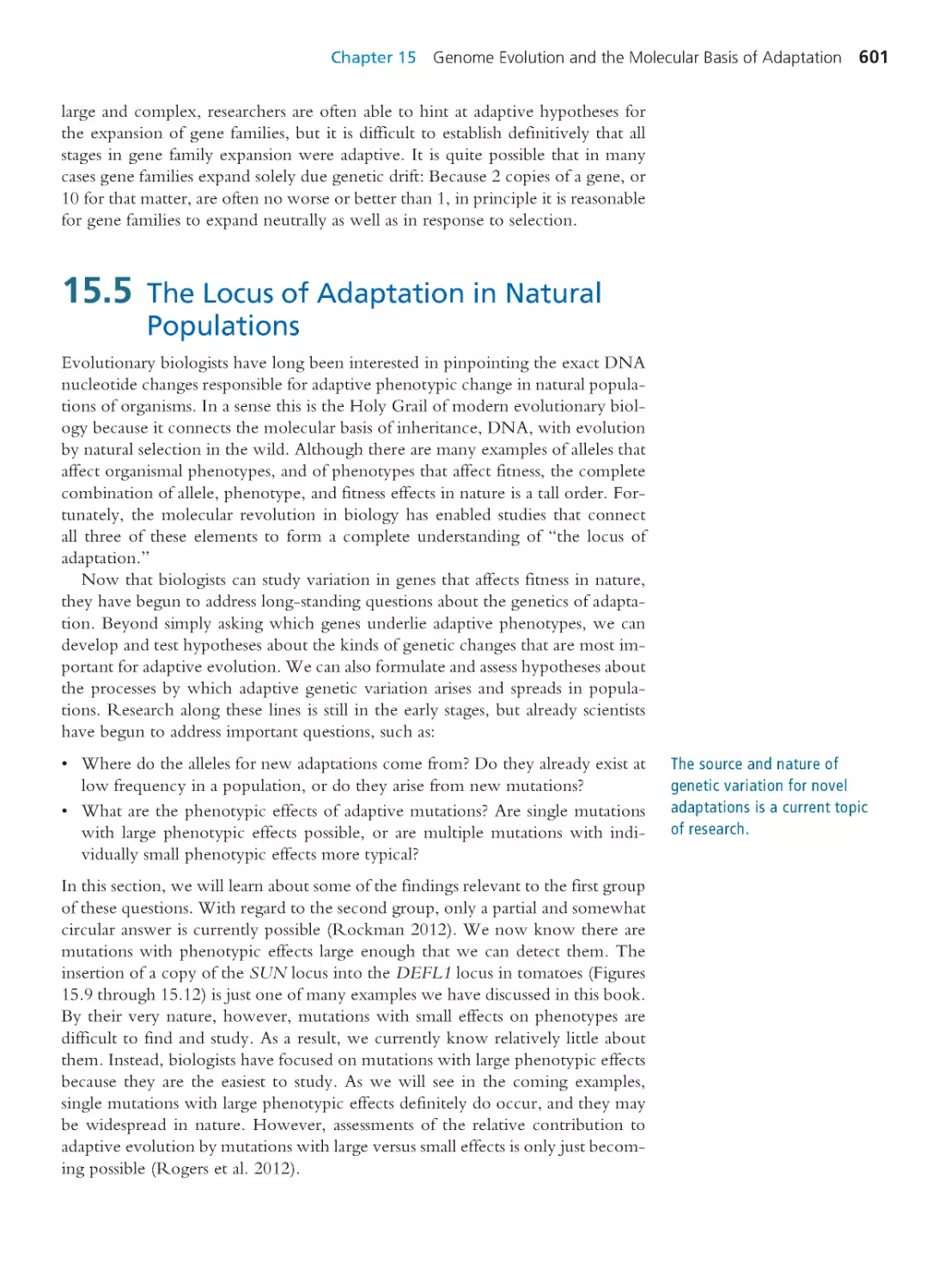
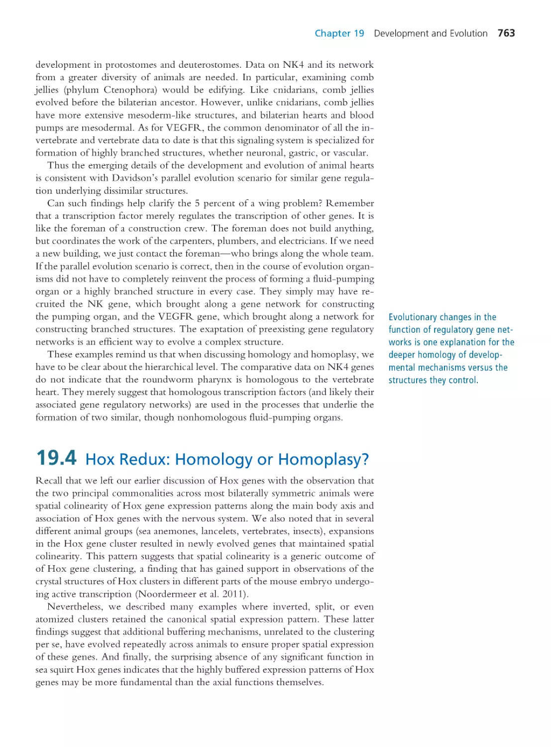
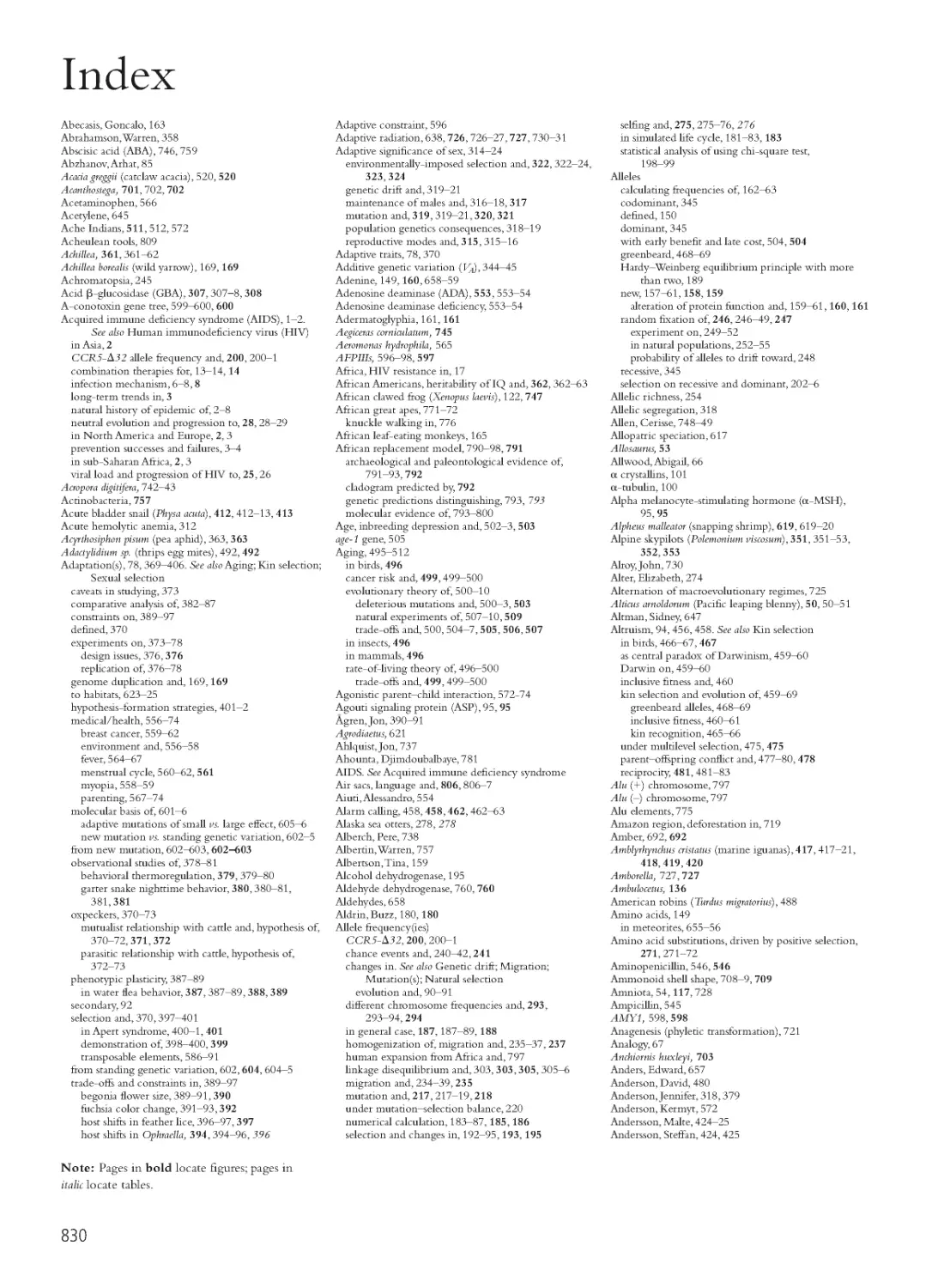
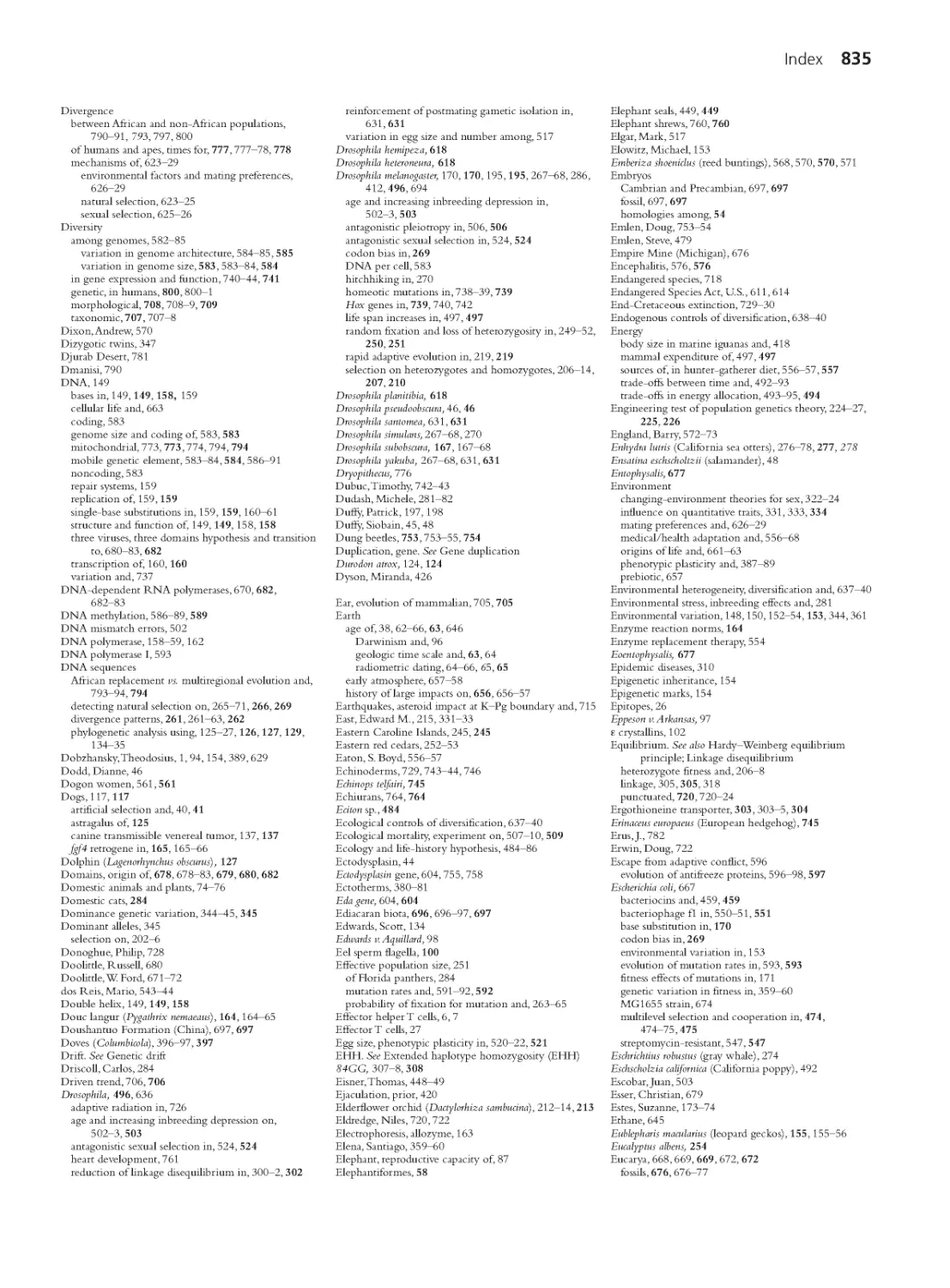
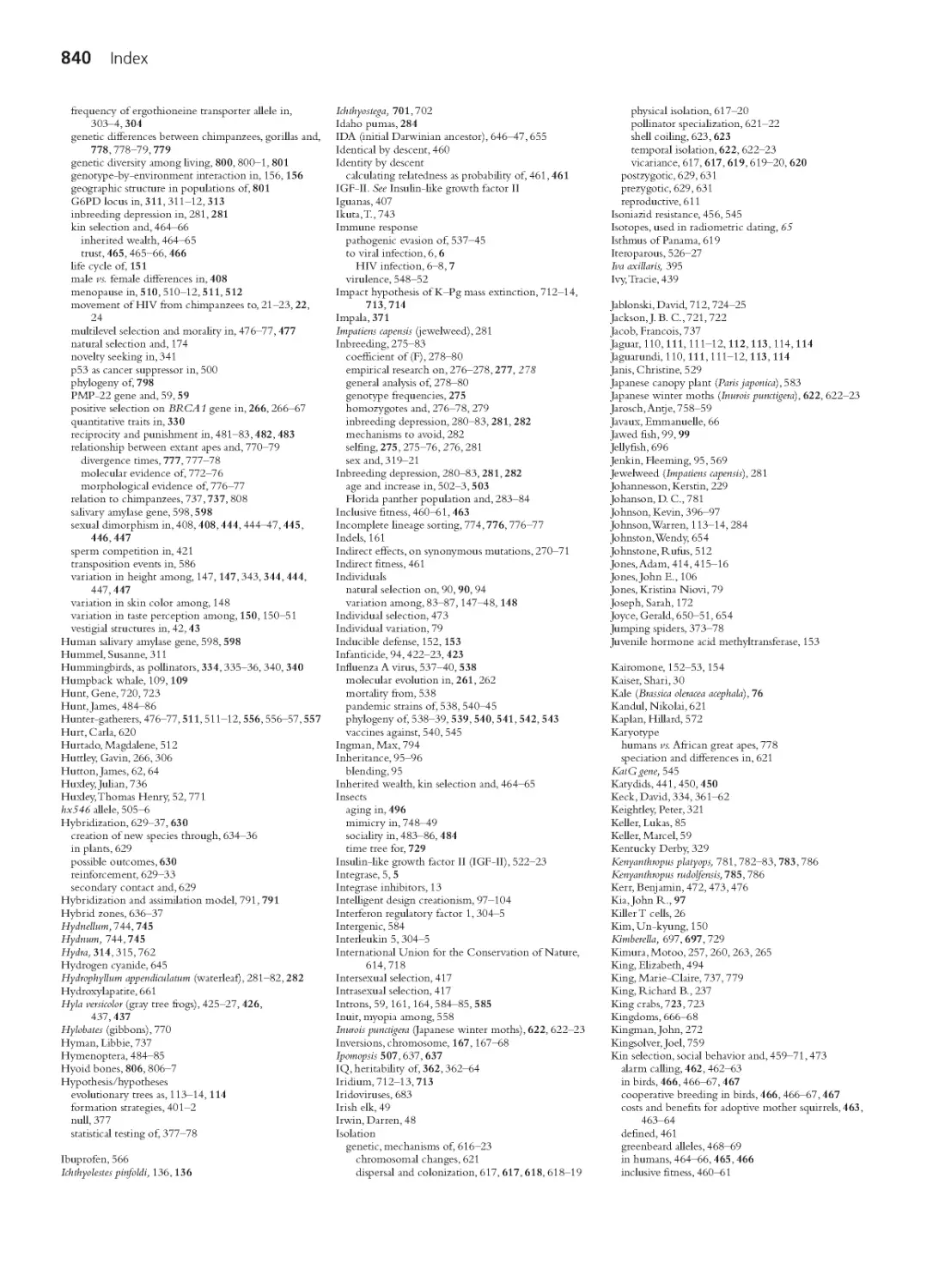
Figure 1.1 The HIV/AIDS
pandemic The map (a) shows
the geographic distribution of
HIV infections. The color of each
region indicates the fraction of
adults infected with HIV (UNAIDS
2012b). The areas of the circles
are proportional to the number
of individuals living with HIV
(UNAIDS 2012b). The bars divide
individuals living with HIV by sex
and age (UNAIDS 2008). The
graphs (b) show the growth of
the epidemic from 1990 to 2008
in four countries. Prepared with
data from UNAIDS (2008).
As a case study, HIV will
demonstrate how evolutionary
biologists study adaptation and
diversity.

al. 2006), and vaccines and antibiotics had brought many other infectious diseases
under control. In 1984 the U.S. Secretary of Health and Human Services, Mar-
garet Heckler, predicted that an AIDS vaccine would be ready for testing in two
years. Actual events have, of course, played out rather differently.
HIV has infected over 65 million people (UNAIDS 2010, 2012a). Roughly
30 million have died of the opportunistic infections that characterize AIDS. The
disease is the cause of about 3.1% of all deaths worldwide (WHO 2008/2011).
AIDS is responsible for fewer deaths than heart disease (12.8%), strokes (10.8%),
and lower respiratory tract infections (6.1%)—common agents of death among
the elderly. But it causes more deaths than tuberculosis (2.4%), lung and other
respiratory cancers (2.4%), and traffic accidents (2.1%).
Figure 1.1 summarizes the global AIDS epidemic. The map reveals substantial
variation among regions in the number of people living with HIV, the percent-
age of the population infected, and the proportion of infected individuals who
are women versus men versus children. The graphs show that the number of
people infected has peaked in some countries but continues to climb in others.
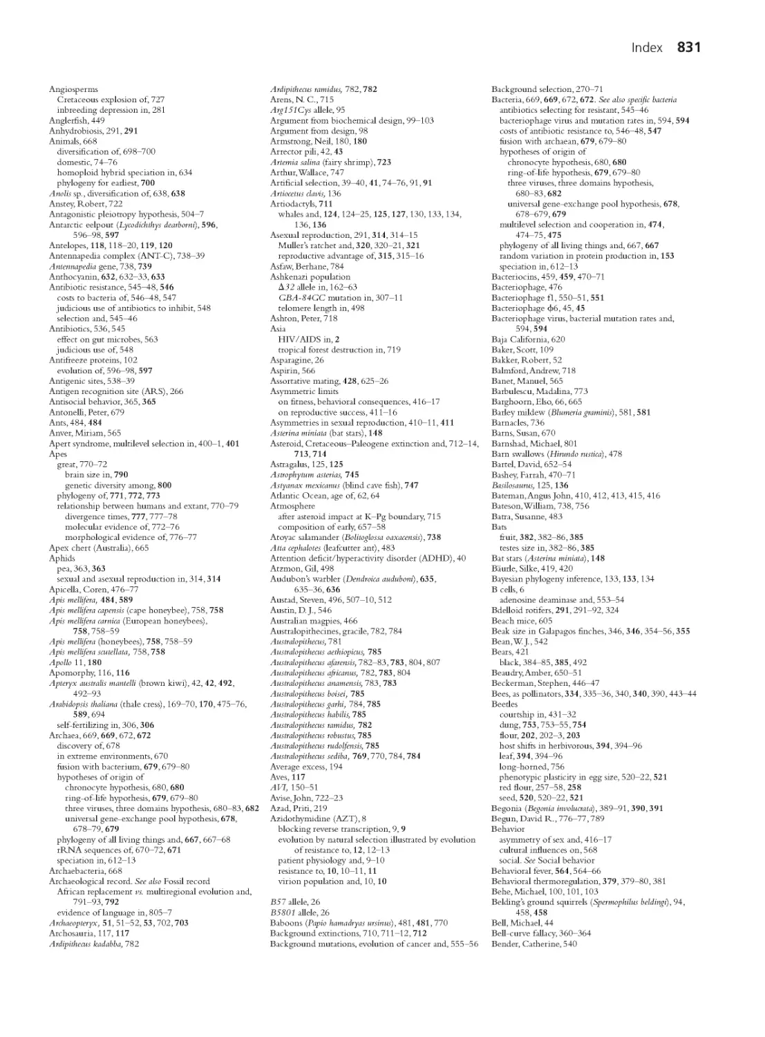
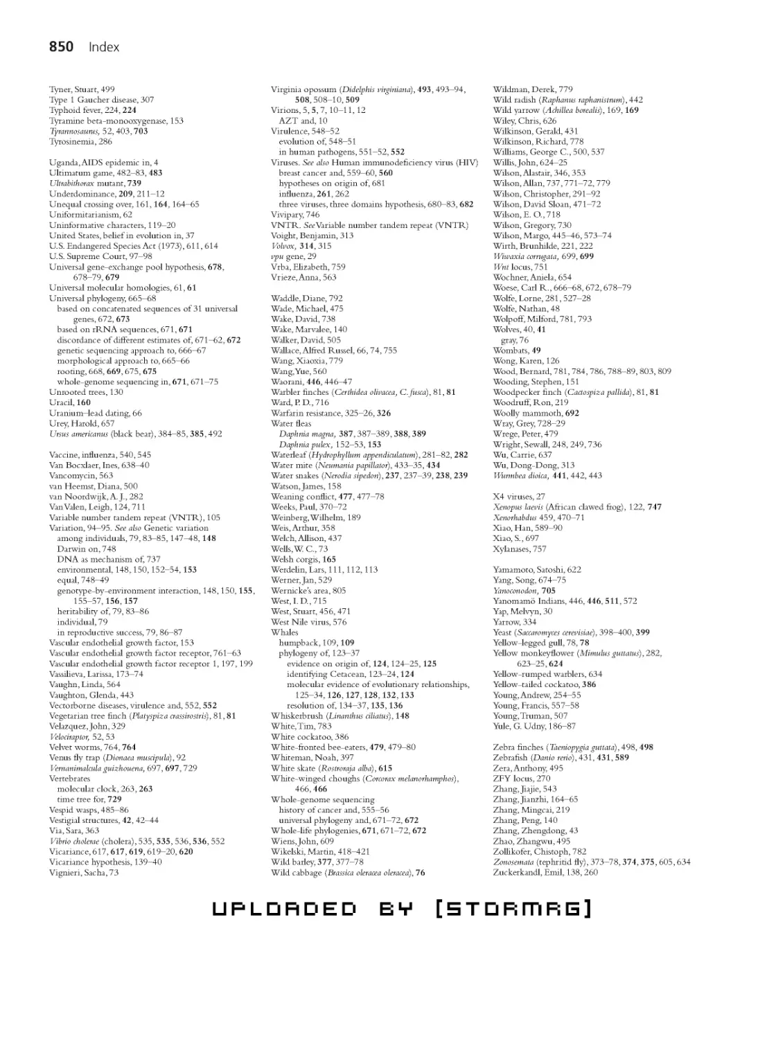
The epidemic has been most devastating in sub-Saharan Africa, where 1 in 20
adults is living with HIV (UNAIDS 2008). Worst hit is Swaziland, with 26% of
adults infected, followed by Botswana at 24%; Lesotho, 23%; and South Africa,
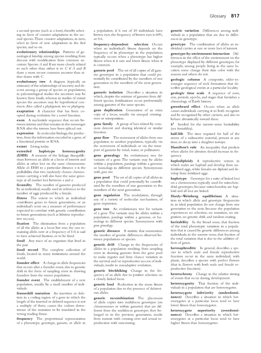
18%. Across southern Africa, life expectancy at birth has dropped below 50, a
level last seen in the early 1960s (Figure 1.2a). The good news is that the annual
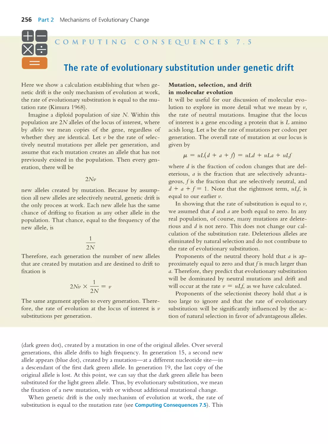
rate of new infections in sub-Saharan Africa has been falling for over a decade
(UNAIDS 2012). This has meant that the global rate of new infections has been
falling as well (Figure 1.2b).
In developed countries, overall infection rates are much lower than in sub-Sa-
haran Africa (UNAIDS 2008). In western and central Europe, 0.3% of adults are
infected. In Canada the rate is 0.4%, and in the United States it is 0.6% . For cer-
tain risk groups, however, infection rates rival those in southern Africa. Among
men who have sex with men, the infection rate is 12% in London, 18% in New
York City, and 24% in San Francisco (CDC 2005; Dodds et al. 2007; Scheer et
al. 2008). Among injection drug users, the infection rate is 12% in France, 13%
in Canada, and 16% in the United States (Mathers et al. 2008).
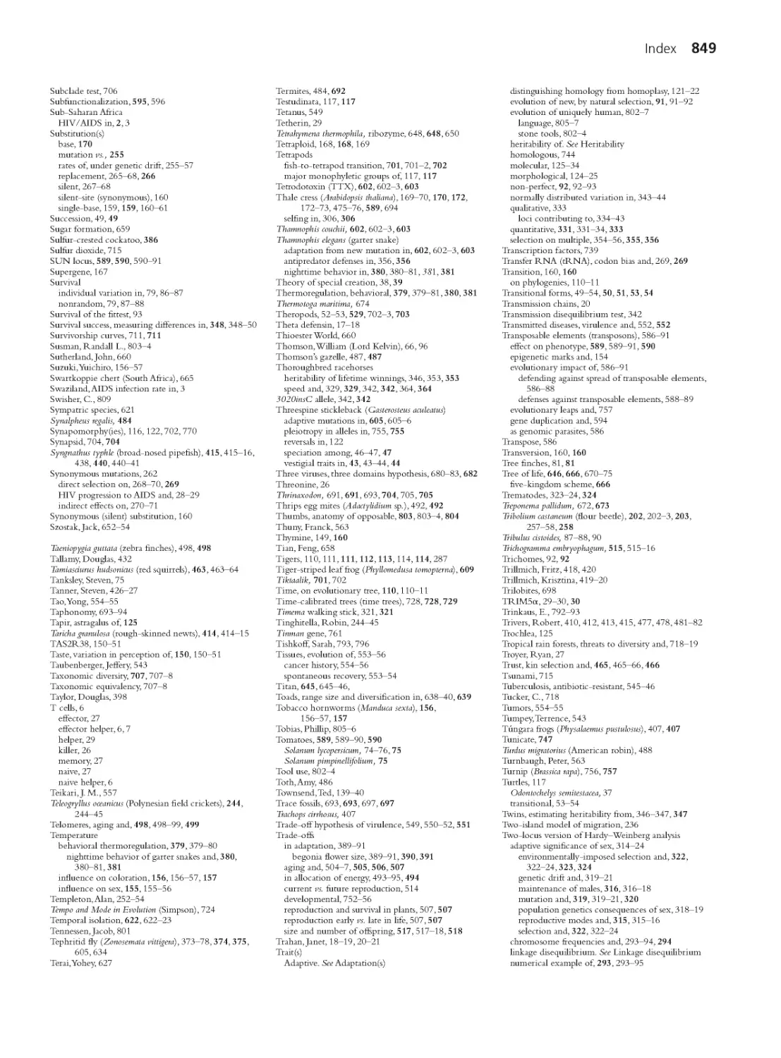
How Does HIV Spread, and How Can It Be Slowed?
A new HIV infection starts when a bodily fluid carries the virus from an infected
person directly onto a mucous membrane or into the bloodstream of an unin-
fected person. HIV travels via semen, vaginal and rectal secretions, blood, and
breast milk (Hladik and McElrath 2008). It can move during heterosexual or
homosexual sex, oral sex, needle sharing, transfusion with contaminated blood
products, other unsafe medical procedures, childbirth, and breastfeeding.
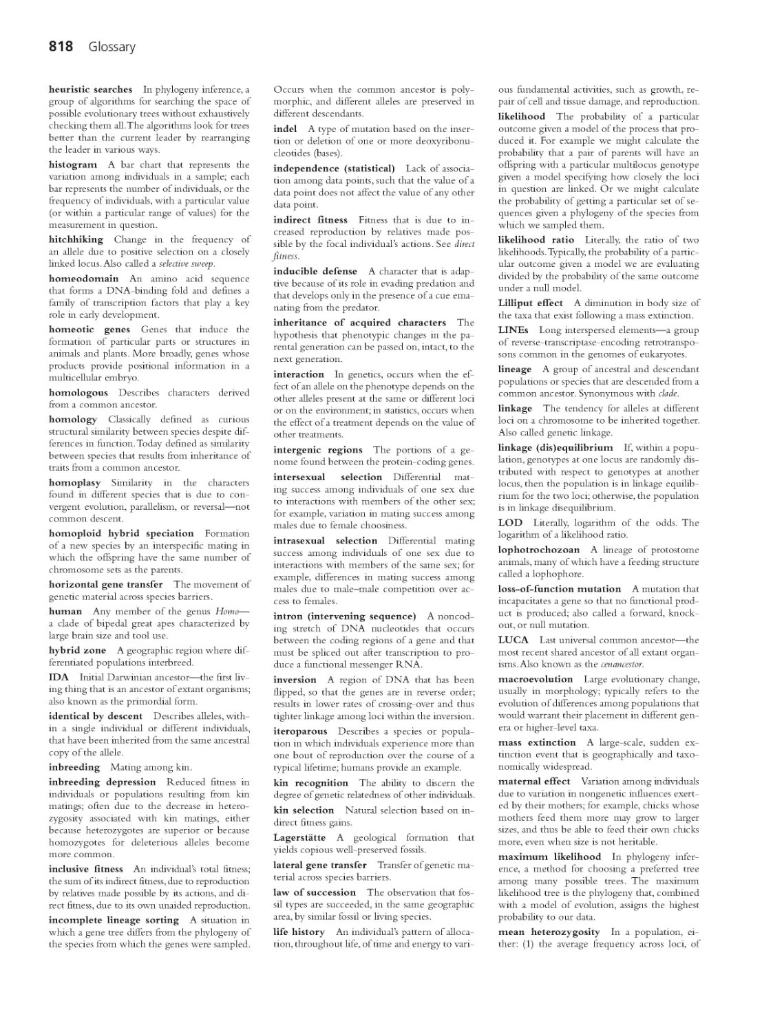
HIV has spread by different routes in different regions (Figure 1.3, next page).
In sub-Saharan Africa and parts of south and southeast Asia, heterosexual sex
has been the most common mode of transmission. In other regions, including
Europe and North America, male–male sex and needle sharing among injec-
tion drug users have predominated. Certain activities are particularly risky. For
example, data on men who have sex with men in Victoria, Australia, show that
having receptive anal intercourse with casual partners without the protection of a
condom is a dangerous behavior. Individuals who report practicing it are nearly
60 times as likely to be infected with HIV as individuals who do not report prac-
ticing it (Read et al. 2007).
Chapter 1 A Case for Evolutionary Thinking: Understanding HIV 3
1950
1975
2000
70
30
50
(a) Life expectancy at birth in
southern Africa (years)
(b) Number of people newly
infected each year (millions)
0
1990
2010
4
2000
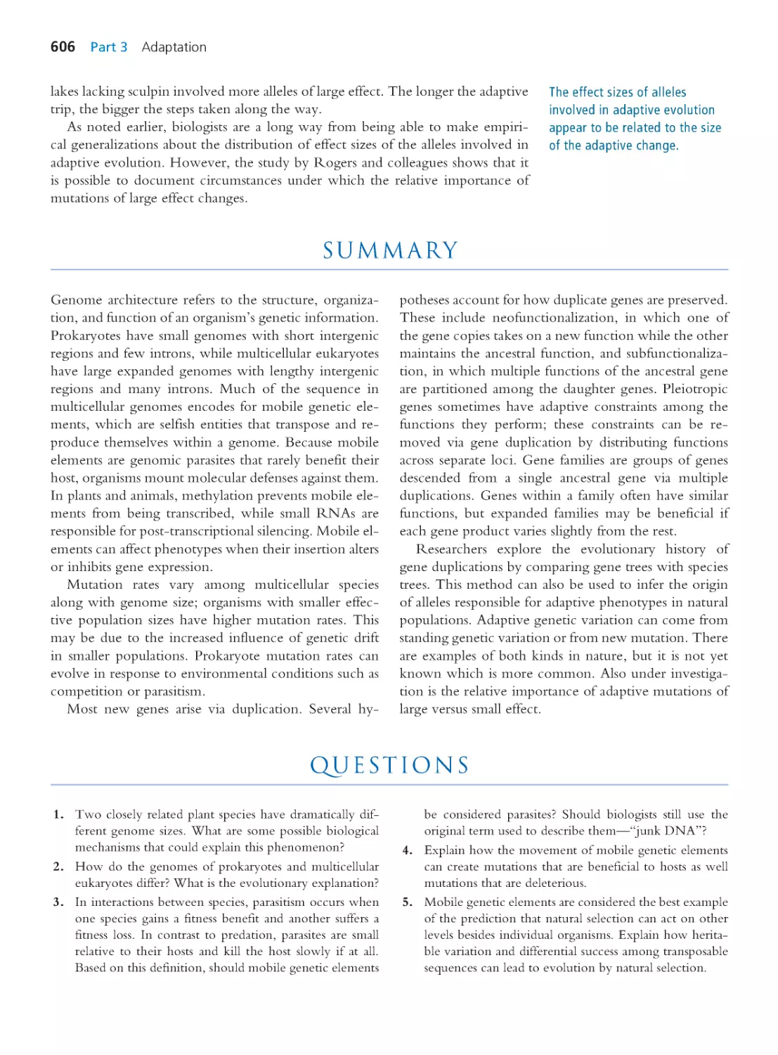
2
Figure 1.2 Long-term trends
in HIV/AIDS (a) In southern
Africa, the epidemic has caused a
sharp reduction in life expectancy
at birth. From UNAIDS (2008). (b)
Worldwide, the annual number
of new infections has been fall-
ing since the late 1990s. Red line
shows best estimate; gray band
shows range of estimates. From
UNAIDS (2012).
An HIV infection can be
contracted only from someone
else who already has it.

Clinical studies in which volunteers are randomly assigned to treatment versus
control groups have identified medical interventions that reduce the rate of HIV
transmission. Use of antiviral drugs, for example, lowers the risk that infected
mothers will pass the virus to their infants by about 40% (Suksomboon et al.
2007). Antivirals are similarly effective in reducing transmission among men who
have sex with men (Grant et al. 2010). Circumcision reduces the risk that men
will contract HIV by about half (Bailey et al. 2007; Gray et al. 2007). Antiviral
vaginal gels are comparably beneficial for women (Abdool Karim et al. 2010).
The value of encouraging people to change their behavior is less clear. Be-
havioral change undoubtedly has the potential to curtail transmission. Consistent
use of condoms, for example, may reduce the risk of contracting HIV by 80%
or more (Pinkerton and Abramson 1997; Weller and Davis 2002). And there are
apparent success stories. In Uganda, for instance, a campaign discouraging casual
sex and promoting condom use and voluntary HIV testing is thought to have
substantially reduced the local AIDS epidemic (Slutkin et al. 2006; but see Oster
2009). On the other hand, the results of randomized controlled trials have been
somewhat disappointing. A study of over 4,000 HIV-negative men who have
sex with men in the United States offered extensive one-on-one counseling to
members of the experimental group and conventional counseling to the control
group (Koblin et al. 2004). As hoped, the experimental subjects engaged in fewer
risky sexual behaviors than the controls. However, the rates at which the experi-
mentals versus the controls contracted HIV were not statistically distinguishable.
There is clearly no room for complacency. The graph in Figure 1.4 tracks the
number of new infections each year among men who have sex with men in the
United States. After falling from the mid 1980s to the early 1990s, the annual
number of new infections has since been rising steadily. The same thing seems to
be happening elsewhere (Hamers and Downs 2004; Giuliani et al. 2005). Results
of surveys suggest that the introduction of effective long-term drug therapies,
which for some individuals has at least temporarily transformed HIV into a man-
ageable chronic illness, has also prompted an increase in risky sexual behavior
(Crepaz, Hart, and Marks 2004; Kalichman et al. 2007).
What Is HIV?
Like all viruses, HIV is an intracellular parasite incapable of reproducing on its
own. HIV invades specific types of cells in the human immune system. The virus
hijacks the enzymatic machinery, chemical materials, and energy of the host cells
to make copies of itself, killing the host cells in the process.
4 Part 1 Introduction
80
40
20
0
60
76
84
92
00
N
e
w
i
n
f
e
c
t
i
o
n
s
(
1
,
0
0
0
s
)
Year
Figure 1.4 New HIV infec-
tions among men who have
sex with men in the United
States From Hall et al. (2008).
(b) Estimated new infections, by
likely mode of transmission:
(a) Estimated new infections, by
likely mode of transmission:
Cambodia
2002
Honduras
2002
Kenya
1998
Russia
2002
Indonesia
2002
U.S . 2006 Canada 2005 U.K. 2007
Male–male sex (MMS)
MMS & IDU
Injection drug use (IDU)
Heterosexual sex
Other
Heterosexual sex with a partner at high risk
Casual heterosexual sex
Male–male sex
Sex work
Injection drug use
Figure 1.3 HIV’s main routes
of transmission in various
regions (a) From Pisani et al.
(2003). (b) From Hall et al. (2008),
Public Health Agency of Canada
(2006), Health Protection Agency
(2008). The authors of the re-
ports on Canada and the United
Kingdom note that many of the
individuals who contracted HIV
through heterosexual sex likely
did so in sub-Saharan Africa. See
also UNAIDS (2008).

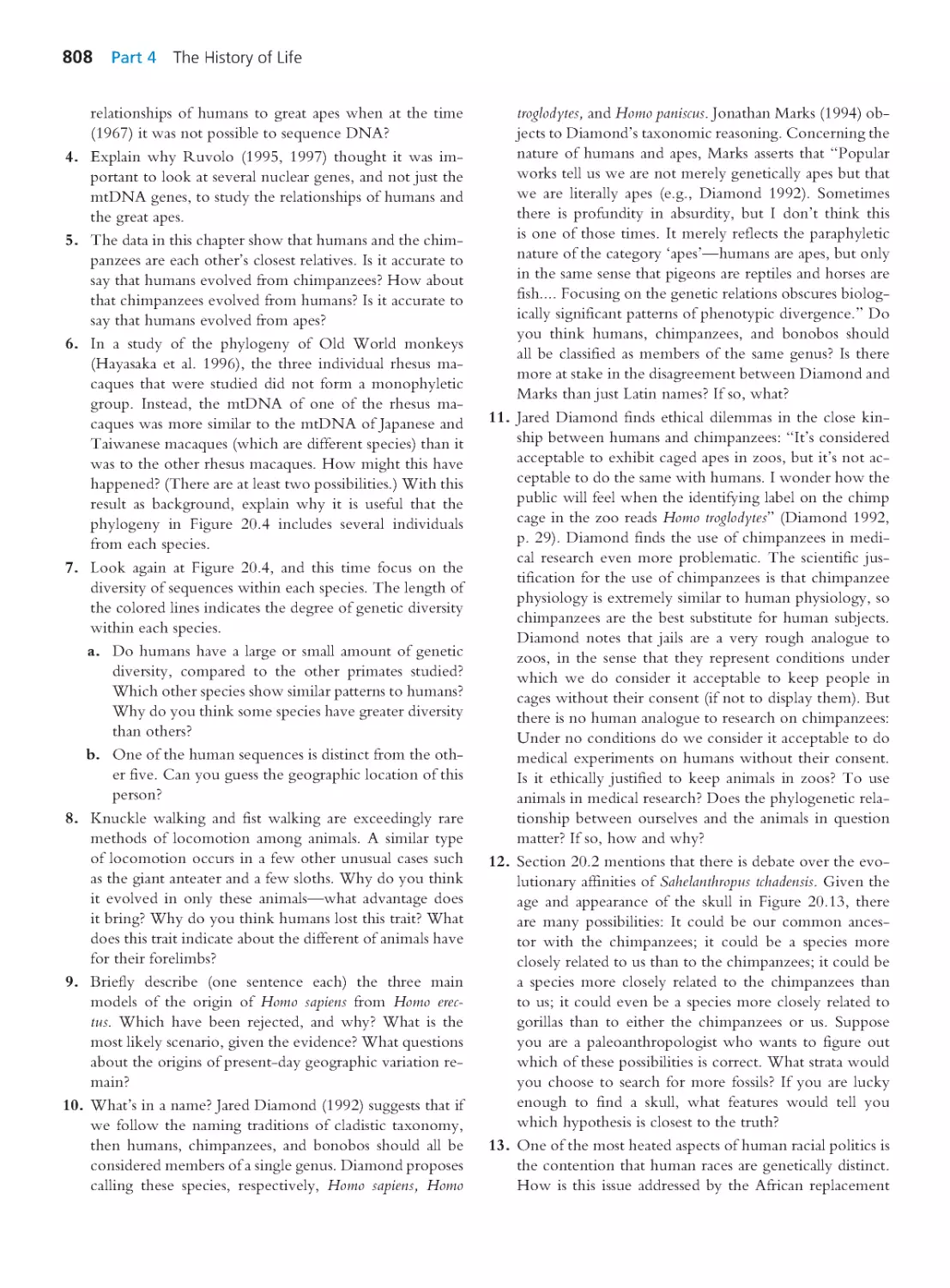
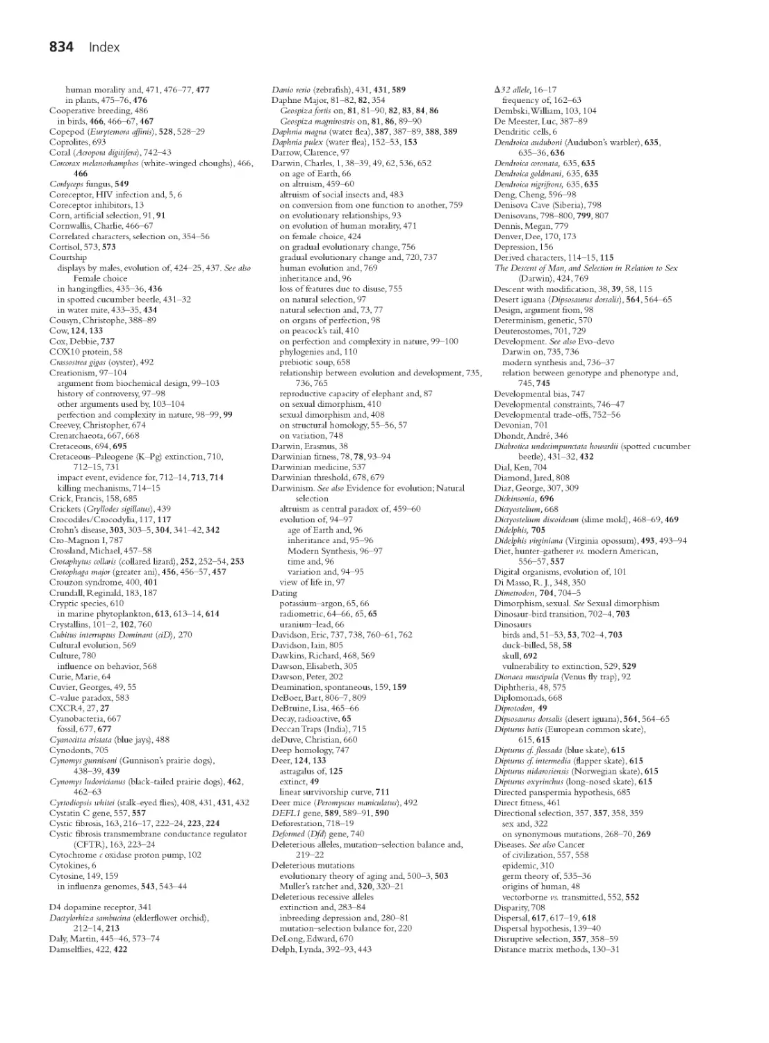
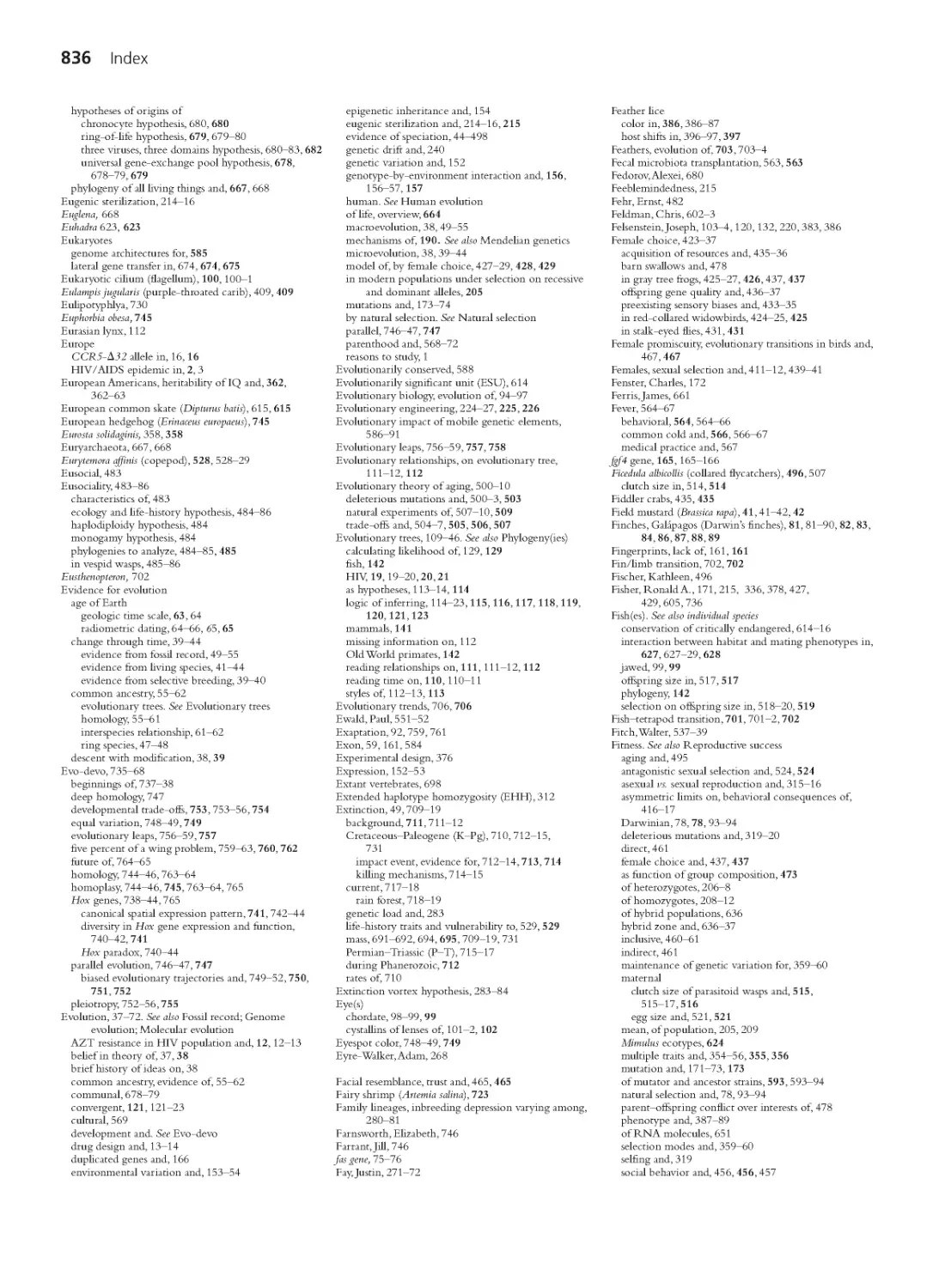
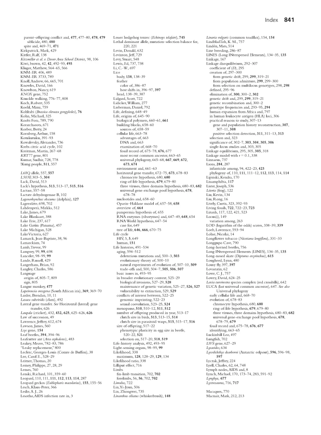
Figure 1.5 outlines HIV’s life cycle in more detail (Nielsen et al. 2005; Ganser-
Pornillos et al. 2008). The life cycle includes an extracellular phase and an intra-
cellular phase. During the extracellular, or infectious phase, the virus moves from
one host cell to another and can be transmitted from host to host. The extracel-
lular form of a virus is called a virion or virus particle. During the intracellular, or
replication phase, the virus replicates.
HIV initiates its replication phase by latching onto two proteins on the surface
of a host cell. After adhering first to CD4, HIV attaches to a second protein, called
a coreceptor. This leads to fusion of the virion’s envelope with the host’s cell
membrane and spills the contents of the virion into the cell. The contents include
the virus’s genome (two copies of a single-stranded RNA molecule) and two viral
enzymes: reverse transcriptase, which transcribes the virus’s RNA genome into
DNA; and integrase, which splices this DNA genome into the host cell’s genome.
Once HIV’s genome has infiltrated the host cell’s DNA, the host cell’s RNA
polymerase transcribes the viral genome into viral mRNA. The host cell’s ribo-
somes synthesize viral proteins. New virions assemble at the host cell’s membrane,
then bud off into the bloodstream or other bodily fluid. Inside the new virions,
HIV’s protease enzyme cleaves precursors of various viral proteins into functional
forms, allowing the virions to mature. The new virions are now ready to invade
new cells in the same host or to move to a new host.
A notable feature of HIV’s life cycle is that the virus uses the host cell’s own
enzymatic machinery—its polymerases, ribosomes, and tRNAs, and so on—in
Chapter 1 A Case for Evolutionary Thinking: Understanding HIV 5
HIV
proteins
7
Translation
Coreceptor
Host cell
6 Transcription
8
New
virion
assembly
Integrase
Protease
RNA genome (2 copies)
Reverse
transcriptase
gp120 (surface protein)
1
HIV virion
gp41
(anchor protein
for gp120)
HIV
RNA
HIV
DNA
5 DNA
splicing
Host-cell
nucleus
Host-cell
DNA
HIV
mRNA
HIV reverse
transcriptase
HIV
integrase
9
Budding
Mature virus
Host-cell
membrane
4 DNA
synthesis
2
Binding
3
Fusion
10
maturation
CD4
Protease
Figure 1.5 The life cycle of HIV (1, upper left) HIV’s
extracellular form, known as a virion, encounters a host cell
(usually a helper T cell). (2) HIV’s gp120 surface protein binds
first to CD4, then to a coreceptor (usually CCR5; sometimes
CXCR4) on the surface of the host cell. (3) The HIV virion
fuses with the host cell; HIV’s RNA genome and enzymes
enter the host cell’s cytoplasm. (4) HIV’s reverse transcriptase
enzyme synthesizes HIV DNA from HIV’s RNA template.
(5) HIV’s integrase enzyme splices HIV’s DNA genome into the
host cell’s genome. (6) HIV’s DNA genome is transcribed into
HIV mRNA by the host cell’s RNA polymerase. (7) HIV’s mRNA
is translated into HIV precursor proteins by host cell’s ribo-
somes. (8) A new generation of virions assembles at the mem-
brane of the host cell. (9) New virions bud from the host cell’s
membrane. (10) HIV’s protease enzyme cleaves precursors
into mature viral proteins, allowing the new virions to mature.
HIV is a parasite that afflicts
cells of the human immune
system. HIV virions enter host
cells by binding to proteins on
their surface, then use the host
cells’ own machinery to make
new virions.

almost every step. This is why HIV, and viral disease
in general, is so difficult to treat. It is a challenge to
find drugs that interrupt the viral life cycle without also
disrupting the host cell’s enzymatic functions and thus
causing debilitating side effects. Effective antiviral ther-
apies usually target enzymes specific to the virus, such
as reverse transcriptase and integrase.
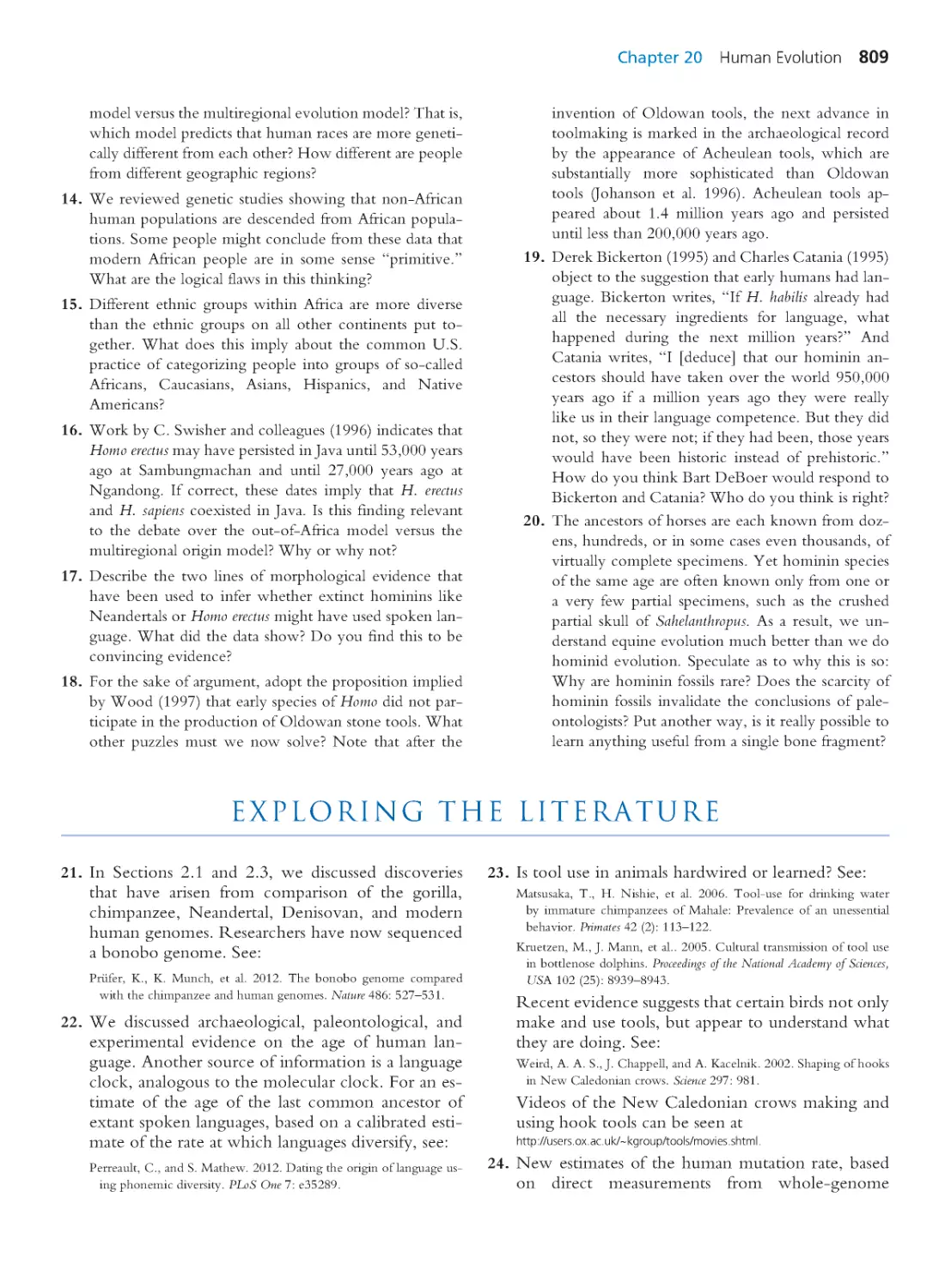
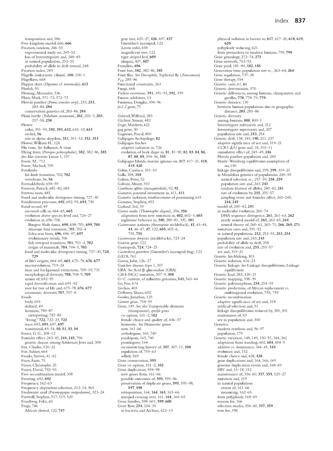
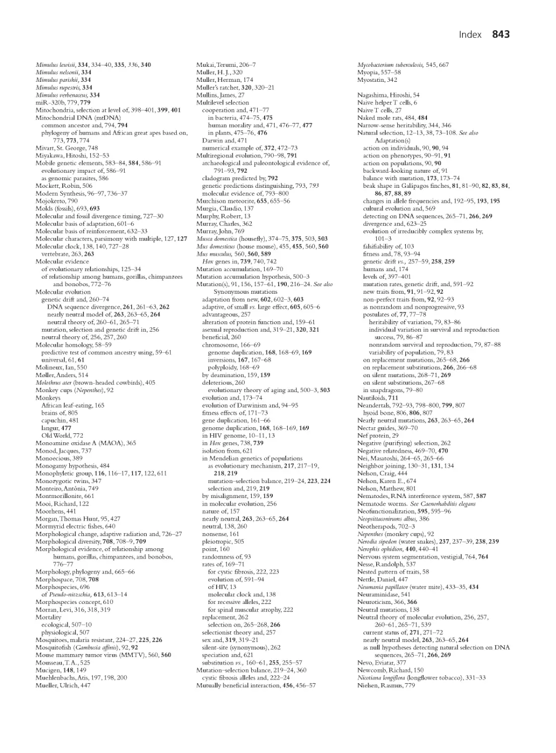
How Does the Immune System React to HIV?
A patient’s immune system mobilizes to fight HIV the
same way it moves to combat other viral invaders. Key
aspects of the immune response appear in Figure 1.6 .
Sentinels called dendritic cells patrol vulnerable tis-
sues, such as the lining of the digestive and reproduc-
tive tracts (Banchereau and Steinman 1998). When a
dendritic cell captures a virus, it travels to a lymph node
or other lymphoid tissue and presents bits of the virus’s
proteins to specialized white blood cells called naive
helper T cells (Sprent and Surh 2002).
Naive helper T cells carry highly variable proteins
called T-cell receptors. When a dendritic cell presents a
helper T cell with a bit of viral protein that binds to the
T cell’s receptor, the helper T cell activates. It grows
and divides, producing daughter cells called effector
helper T cells. Effector helper T cells help coordinate
the immune response.
Effector helper T cells issue commands, in the form
of molecules called cytokines, that help mobilize a va-
riety of immune cells to join the fight. They induce B
cells to mature into plasma cells, which produce anti-
bodies that bind invading virions and mark them for
elimination (McHeyzer-Williams et al. 2000). They
activate killer T cells, which destroy infected host cells
(Williams and Bevan 2007). And they recruit macro-
phages (not shown), which destroy virus particles or kill
infected cells (Seid et al. 1986; Abbas et al. 1996).
Most effector helper T cells die within a few weeks.
However, a few survive and become memory helper
T cells (Harrington et al. 2008). If the same pathogen
invades again, the memory cells produce a new popula-
tion of effector helper T cells.
How Does HIV Cause AIDS?
As we noted earlier, HIV invades host cells by first
latching onto two proteins on the host cell’s surface.
The first of these is CD4; the second is a called a core-
ceptor. Different strains of HIV exploit different core-
ceptors, but most strains responsible for new infections
use a protein called CCR5. Cells that carry both CD4
and CCR5 on their membranes, and are thus vulner-
6 Part 1 Introduction
Virus
(+)
(+) cytokines
(a) Dendritic cells capture the virus and present bits of its proteins to
naive helper T cells. Once activated, these naive cells divide to
produce effector helper T cells.
Dendritic cell
Naive
helper
T cell
Effector
helper
T cell
Antibodies
Plasma cells
B cell
Effector
killer T cells
T-cell
receptor
Effector helper T cells also help activate killer T cells, which destroy
host cells infected with the virus.
(b) Effector helper T cells stimulate B cells displaying the same bits of
viral protein to mature into plasma cells, which make antibodies
that bind and in some cases inactivate the virus.
Effector
helper
T cell
Effector
helper
T cells
Effector
helper
T cells
Memory
helper T cell
Naive
killer T cell
(c) Most effector T cells are short lived, but a few become long-lived
memory helper T cells.
Figure 1.6 How the immune system fights a viral infec-
tion After NIAID (2003) and Watkins (2008).

Chapter 1 A Case for Evolutionary Thinking: Understanding HIV 7
able to HIV, include macrophages, effector helper T cells, and memory helper T
cells (Figure 1.7).
The progress of an HIV infection can be monitored by periodically measuring
the concentration of HIV virions in the patient’s bloodstream and the concentra-
tion of CD4 T cells in the patient’s bloodstream and in the lymphoid (immune
system) tissues associated with the mucous membranes of the gut. A typical un-
treated infection progresses through three phases.
In the acute phase, HIV virions enter the host’s body and replicate explosively.
The concentration of virions in the blood climbs steeply (Figure 1.8). The con-
centrations of CD4 T cells plummet—especially in the lymphoid tissues of the
gut. During this time, the host may show general symptoms of a viral infection.
The acute phase ends when viral replication slows and the concentration of viri-
ons in the bloodstream drops. The host’s CD4 T-cell counts recover somewhat.
During the chronic phase, the patient usually has few symptoms. HIV con-
tinues to replicate, however. The concentration of virions in the blood may sta-
bilize for a while, but eventually rises again. Concentrations of CD4 T cells fall.
The AIDS phase begins when the concentration of CD4 T cells in the blood
drops below 200 cells per cubic millimeter. By now the patient’s immune sys-
tem has begun to collapse and can no longer fend off a variety of opportunistic
viruses, bacteria, and fungi that rarely cause problems for people with robust
immune systems. Without effective anti-HIV drug therapy, a patient diagnosed
with AIDS can expect to live less than three years (Schneider et al. 2005).
The mechanisms by which an HIV infection depletes the patient’s CD4 T
cells and undermines the patient’s immune system are complex. Despite a quarter
century of research, they remain incompletely understood (Pandrea et al. 2008;
Douek et al. 2009; Silvestri 2009). The simple infection and destruction of host
CD4 T cells may explain their precipitous loss during the acute phase of infec-
tion. But the immune system has an impressive capacity to regenerate these cells.
Furthermore, during the chronic phase no more than one CD4 T cell in a hun-
dred is directly infected. There must be more to the story.
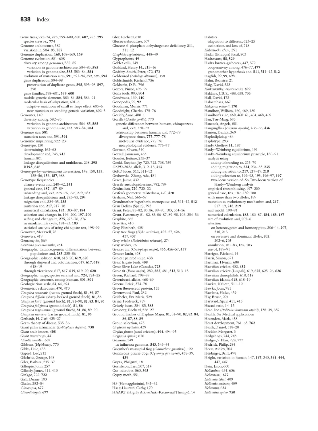
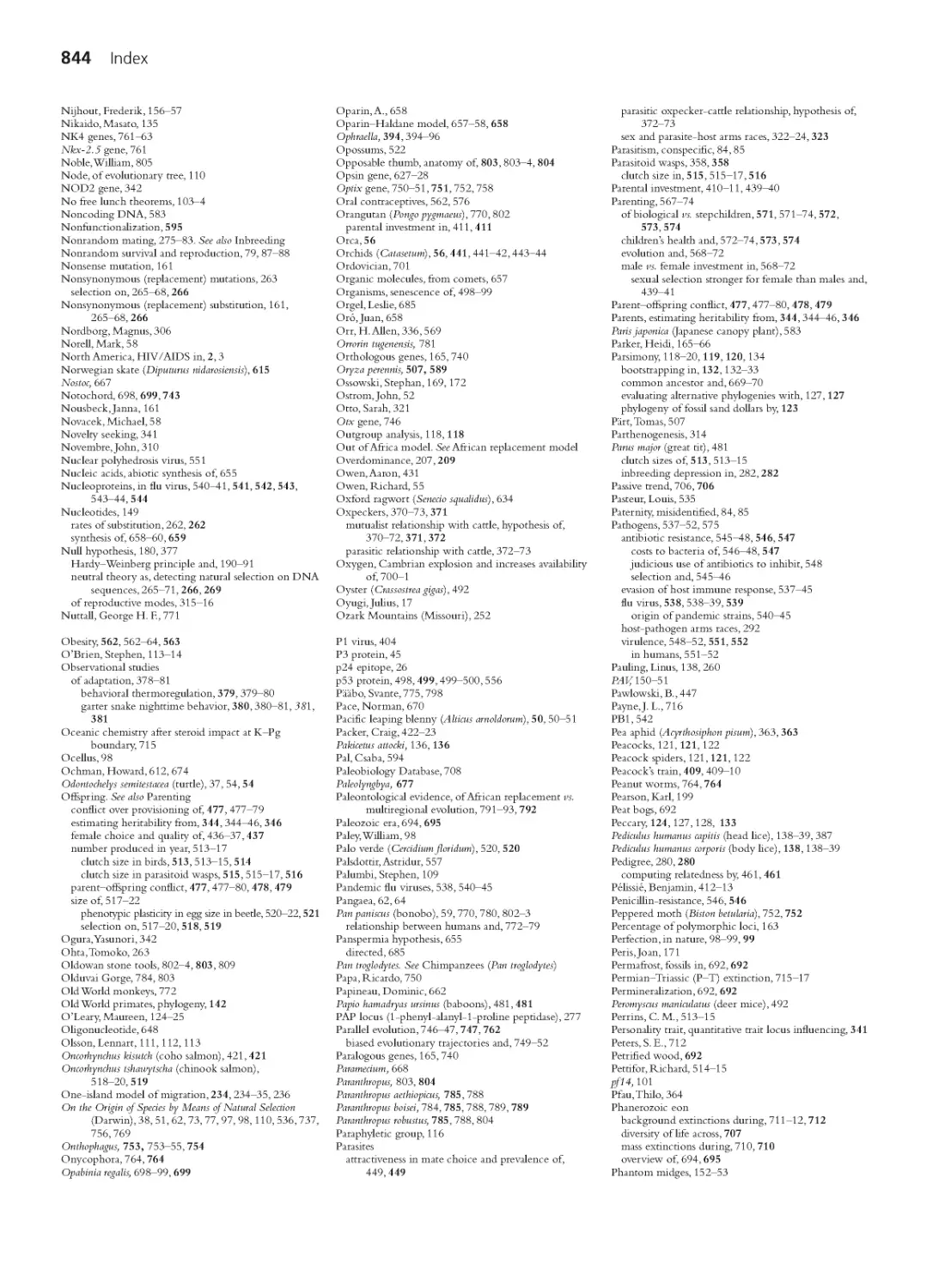
Figure 1.9 (next page) outlines key events thought to lead from HIV infection
to AIDS (Appay and Sauce 2008; Pandrea et al. 2008; Douek et al. 2009; Silvestri
2009). HIV’s attack on the CD4 T cells in the gut (top) initiates a vicious cycle.
This attack not only destroys a large fraction of the patient’s helper T cells, it also
damages other tissues in the gut that help provide a barrier between gut bacteria
Viral load
(HIV RNA copies per ml of plasma)
CD4 T-cell count
(percentage of pre-infection value)
0
20
100
80
60
40
Circulating in blood
Threshold for
onset of AIDS
~ 200 cells
per mm3
Acute
Chronic
AIDS
Phase:
061
21235791
1
Time since infection
Weeks
Years
106
105
104
103
102
Acute
Chronic
AIDS
Phase:
061
21235791
1
Time since infection
Weeks
Years
In lymphoid tissues of
gut and other mucosa
Figure 1.8 Typical clinical
course of an untreated HIV in-
fection By the time the concen-
tration of CD4 T cells in the blood
stream falls below about 200 cells
per cubic millimeter, the patient’s
immune system begins to col-
lapse. After Bartlett and Moore
(1998), Brenchley et al. (2006),
Pandrea et al. (2008).
Effector
helper T cells
Macrophage
Memory
helper T cells
Figure 1.7 Immune system
cells that carry both CD4 and
CCR5 on their membranes, and
are thus vulnerable to HIV.
Data from UNAIDS (2008).

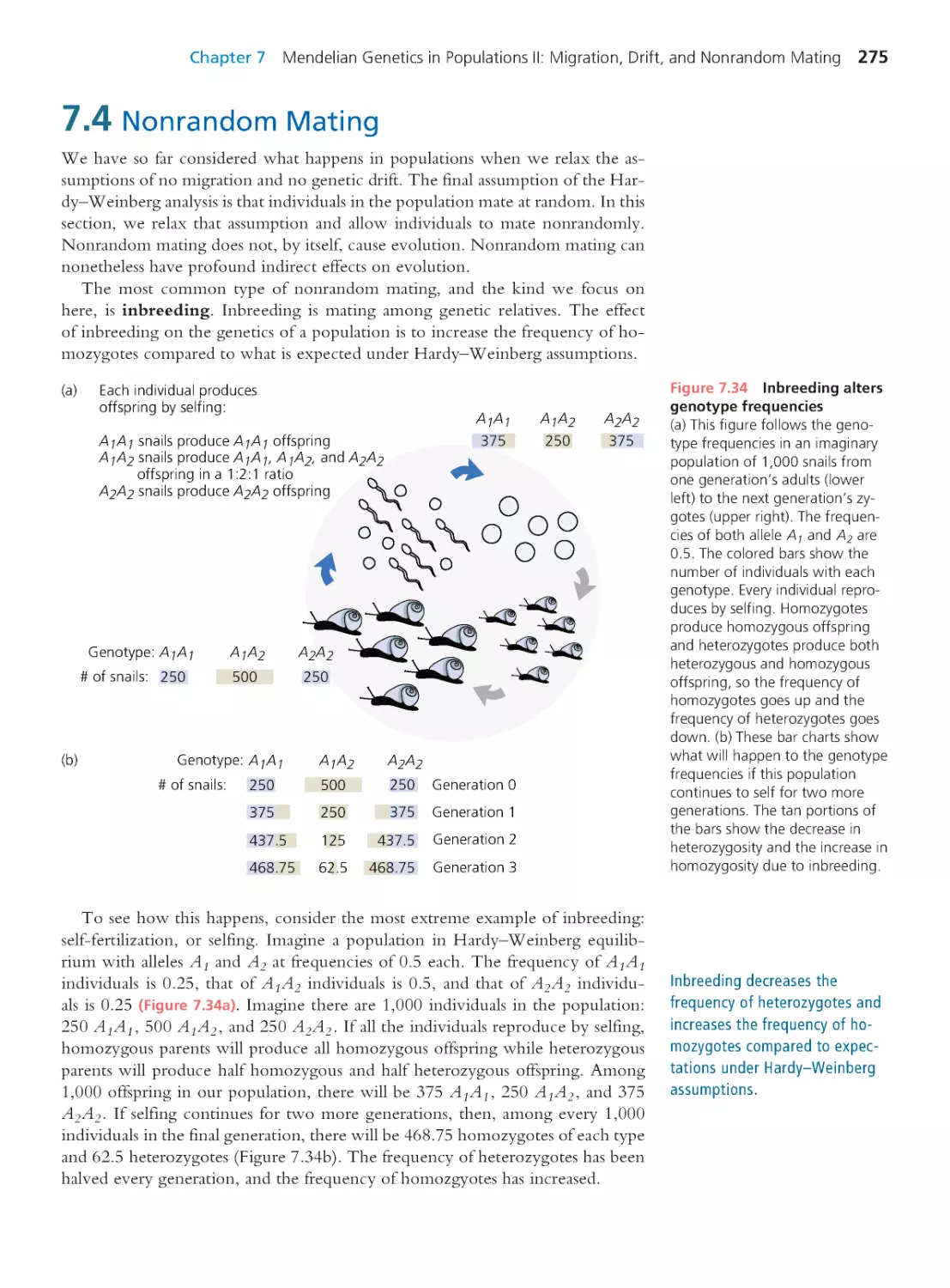
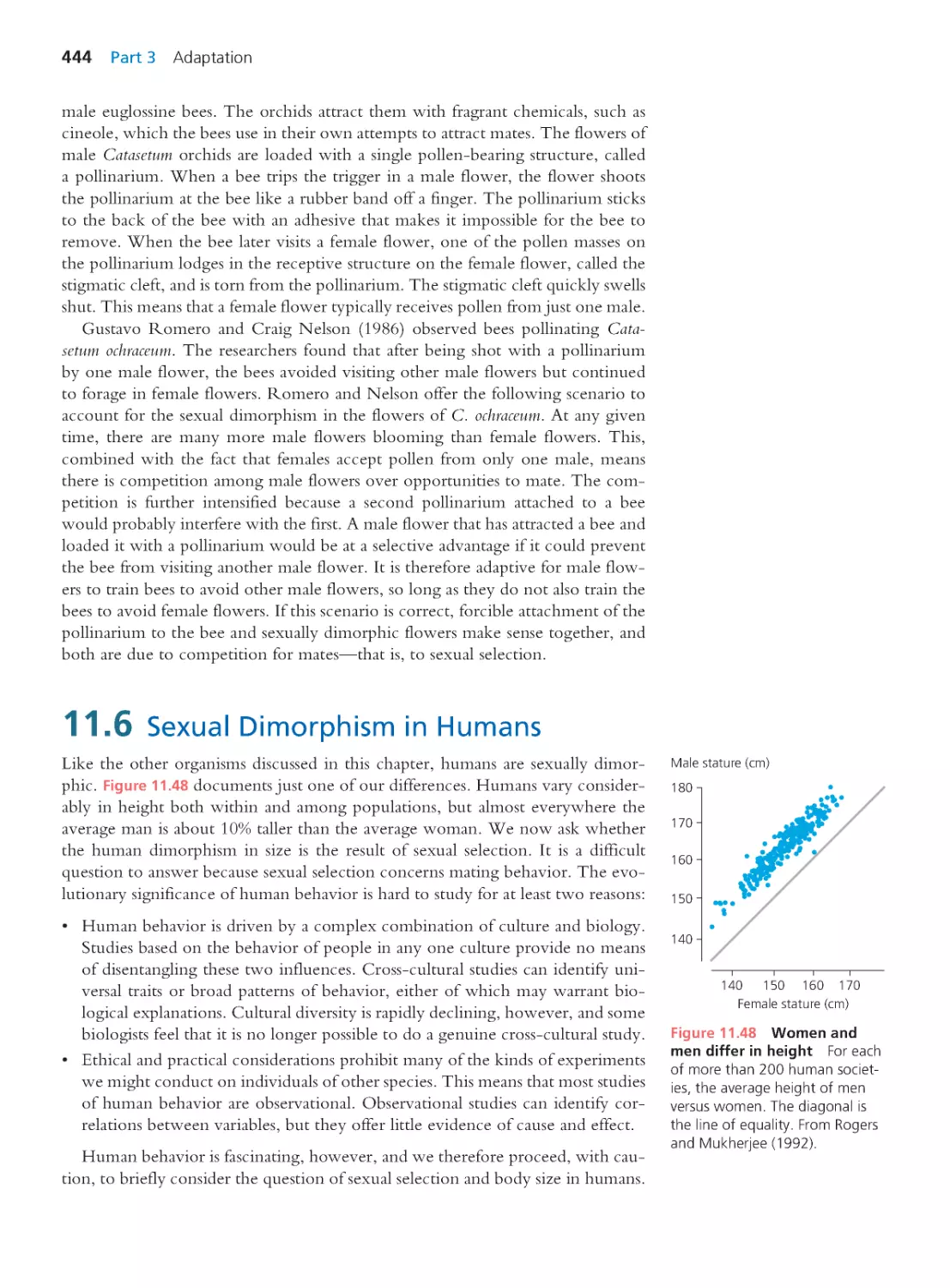
8 Part 1 Introduction
and the bloodstream. The weakening of this barrier lets bacteria and their prod-
ucts move (translocate) from the gut into the blood (Figure 1.9, upper right).
The translocation of bacterial products into the blood triggers a high level of
immune activation, to which the HIV infection itself also contributes (Biancotto
et al. 2008). As we saw in Figure 1.6, activation of the immune system induces B
cells and T cells to proliferate. This aggressive immune response has benefits, at
least temporarily. For example, the anti-HIV killer T cells it yields help restrain
HIV’s replication. This and the production of new helper T cells allow the pa-
tient’s concentrations of CD4 T cells to recover somewhat (Figure 1.8). But in
the case of HIV, a strong immune response comes with heavy costs. The reason is
that HIV replicates most efficiently in activated CD4 T cells. In other words, the
immune system’s best efforts to douse the HIV infection just add fuel to the fire.
A major battleground in the ongoing fight between HIV and the immune
system is the patient’s lymph nodes (Lederman and Margolis 2008). The lymph
nodes are, among other things, the places where naive T cells are activated.
Chronic infection and inflammation eventually damages the lymph nodes irre-
versibly and exhausts the immune system’s capacity to generate new T cells. As
the patient’s T-cell concentrations inexorably fall, the immune system loses its
ability to fight other pathogens. The ultimate result is AIDS.
How might HIV be stopped before it leads to AIDS? The obvious answer is to
prevent it from replicating. The first drug to do so, azidothymidine, or AZT, was
approved for therapeutic use in 1987 (De Clercq 2009). Clinical experience with
AZT, and every antiviral developed since, brings us to the first of our organizing
questions. Why do single drugs offer only temporary benefits?
HIV infects
CD4+ T
cells in gut,
HIV induces
immune
activation.
A steady supply of
target cells allows
HIV to replicate
prolifically.
HIV infection
depletes CD4+ T
cells in gut;
damages gut
tissues.
Impaired gut
defenses allow
translocation of
bacteria and
their products
from gut into
bloodstream.
Bacterial
products in
bloodstream
induce immune
activation.
Immune system activation causes effector T-cell proliferation.
T-cell
proliferation
gives HIV
more target
cells.
Chronic infection
and inflammation
permanently
damage lymph
nodes and
exhaust T-cell
proliferative
capacity, leading
to diminished T-
cell supply.
HIV replicates
most efficiently
in activated
CD4+ T cells.
Memory
T cells
Naive
T cells
Effector
T cells
x
x
x
x
x
x
x
x
x
x
x
x
x
B cells
Blood
cells
x
Bacteria
Figure 1.9 A model for how
HIV causes AIDS To read the
figure, start at the top, with HIV
depleting CD4+ T cells in the gut.
Then proceed clockwise. Direct
effects of the virus are indicated
by smaller pink arrows in the cen-
ter; indirect effects by larger tan
arrows around the outside. After
Appay and Sauce (2008); Pandrea
et al. (2008); Douek et al. (2009);
Silvestri (2009).
HIV directly and indirectly
induces immune activation, then
replicates in activated immune
system cells. When the ongoing
battle damages the immune
system to the point that it can
no longer produce enough T
cells to function properly, AIDS
begins.

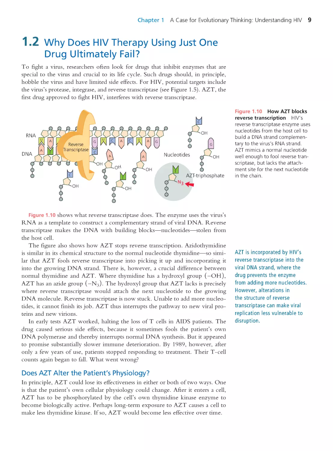
1.2 Why Does HIV Therapy Using Just One
Drug Ultimately Fail?
To fight a virus, researchers often look for drugs that inhibit enzymes that are
special to the virus and crucial to its life cycle. Such drugs should, in principle,
hobble the virus and have limited side effects. For HIV, potential targets include
the virus’s protease, integrase, and reverse transcriptase (see Figure 1.5). AZT, the
first drug approved to fight HIV, interferes with reverse transcriptase.
Chapter 1 A Case for Evolutionary Thinking: Understanding HIV 9
T
U
G
A
C
U
G
A
C
UA
A
O
H
C
OH
A
OH
C
OH
G
OH
A
T
T
N3
RNA
DNA
AZT-triphosphate
OH
Nucleotides
Reverse
Transcriptase
C
OH
Figure 1.10 How AZT blocks
reverse transcription HIV’s
reverse transcriptase enzyme uses
nucleotides from the host cell to
build a DNA strand complemen-
tary to the virus’s RNA strand.
AZT mimics a normal nucleotide
well enough to fool reverse tran-
scriptase, but lacks the attach-
ment site for the next nucleotide
in the chain.
Figure 1.10 shows what reverse transcriptase does. The enzyme uses the virus’s
RNA as a template to construct a complementary strand of viral DNA. Reverse
transcriptase makes the DNA with building blocks—nucleotides—stolen from
the host cell.
The figure also shows how AZT stops reverse transcription. Azidothymidine
is similar in its chemical structure to the normal nucleotide thymidine—so simi-
lar that AZT fools reverse transcriptase into picking it up and incorporating it
into the growing DNA strand. There is, however, a crucial difference between
normal thymidine and AZT. Where thymidine has a hydroxyl group 19OH2,
AZT has an azide group 19N32. The hydroxyl group that AZT lacks is precisely
where reverse transcriptase would attach the next nucleotide to the growing
DNA molecule. Reverse transcriptase is now stuck. Unable to add more nucleo-
tides, it cannot finish its job. AZT thus interrupts the pathway to new viral pro-
teins and new virions.
In early tests AZT worked, halting the loss of T cells in AIDS patients. The
drug caused serious side effects, because it sometimes fools the patient’s own
DNA polymerase and thereby interrupts normal DNA synthesis. But it appeared
to promise substantially slower immune deterioration. By 1989, however, after
only a few years of use, patients stopped responding to treatment. Their T-cell
counts again began to fall. What went wrong?
Does AZT Alter the Patient’s Physiology?
In principle, AZT could lose its effectiveness in either or both of two ways. One
is that the patient’s own cellular physiology could change. After it enters a cell,
AZT has to be phosphorylated by the cell’s own thymidine kinase enzyme to
become biologically active. Perhaps long-term exposure to AZT causes a cell to
make less thymidine kinase. If so, AZT would become less effective over time.
AZT is incorporated by HIV’s
reverse transcriptase into the
viral DNA strand, where the
drug prevents the enzyme
from adding more nucleotides.
However, alterations in
the structure of reverse
transcriptase can make viral
replication less vulnerable to
disruption.

10 Part 1 Introduction
Patrick Hoggard and colleagues (2001) tested this hypothesis by periodically
checking the intracellular concentrations of phosphorylated AZT in a group of
patients taking the same dose of AZT for a year. The data refute the hypothesis.
The concentrations of phosphorylated AZT did not change over time.
Does AZT Alter the Population of Virions Living in the Patient?
The other way AZT could lose its effectiveness is that the population of virions
living inside the patient could change so that the virions themselves would be
resistant to disruption by AZT.
To find out whether populations of virions become resistant to AZT over
time, Brendan Larder and colleagues (1989) repeatedly took samples of HIV from
patients and grew the virus on cultured cells in petri dishes. Figure 1.11 shows
data for two patients the researchers monitored for many months. Each colored
curve in the graphs represents a particular sample. Each curve falls to show how
rapidly HIV’s ability to replicate is curbed by increasing concentrations of AZT.
>10
10
9
8
7
6
5
4
3
2
1
0.1
0
A
Z
T
r
e
s
i
s
t
a
n
c
e
(
9
5
%
i
n
h
i
b
i
t
o
r
y
d
o
s
e
(
␮
M
)
0510152025
Months of therapy
Figure 1.12 In many patients,
AZT resistance evolves within
six months This graph plots
resistance in 39 patients checked
at different times. Redrawn from
Larder et al. (1989).
Concentration
of AZT (␮M)
111
16
0.001 0.01 0.1 1 10
Months
of therapy
Patient 2
0
50
100
0
50
100
Months
of therapy
2
11
20
Patient 1
Concentration
of AZT (␮M)
0.001 0.01 0.1 1 10
Resistance of virions
(% relative viability in
presence of AZT)
Figure 1.11 HIV popula-
tions evolve resistance to AZT
within individual patients As
therapy continued in these pa-
tients, higher concentrations of
AZT were required to curtail HIV’s
replication. Redrawn from Larder
et al. (1989).
Examine the three curves for Patient 1. Virions sampled from this patient after
he had been taking AZT for two months were still susceptible to the drug. At
moderate concentrations of AZT, the virions lost their ability to replicate almost
entirely. Virions sampled from the patient after 11 months on AZT were partially
resistant. They could be stopped, but it took about 10 times as much AZT to
do it. Virions taken after 20 months on AZT were highly resistant. They were
completely unaffected by AZT concentrations that stopped the first sample and
could still replicate fairly well at concentrations that stopped the second sample.
The data for Patient 2 tell the same story. Populations of virions within indi-
vidual patients change to become resistant to AZT. In other words, the popula-
tions evolve.
In many patients taking AZT, drug-resistant populations of HIV evolve with-
in just six months (Figure 1.12).
What Makes HIV Resistant to AZT?
What is the difference between a resistant virion versus a susceptible one? To
answer this question, consider a thought experiment. If we wanted to engineer
an HIV virion capable of replicating in the presence of AZT, what would we
do? We would have to modify the virus’s reverse transcriptase enzyme so that it
either avoids inserting AZT molecules into the growing DNA strand in the first

place or, having inserted an AZT molecule, is more likely to take it back out so
that the DNA strand can continue to grow (Figure 1.13).
In practice, we could expose large numbers of HIV virions to a mutagenic
chemical or ionizing radiation. This would generate strains of HIV with altered
nucleotide sequences in their genomes—and thus altered amino acid sequences
in their proteins. If we generated enough mutants, at least a few would carry
changes in the active site of the reverse transcriptase molecule—the part that
recognizes nucleotides, adds them to the growing DNA strand, and corrects mis-
takes. If one of the reverse transcriptases with an altered binding site were less
likely to mistake AZT for the normal nucleotide, or more likely to remove AZT
after insertion, then the mutant variant of HIV would be able to continue repli-
cating in the presence of the drug. If we treated our population of mutant virions
with AZT, HIV strains unable to replicate in the presence of AZT would decline
in numbers, and the resistant strain would become common.
The steps involved in this thought experiment are just what happens inside
the bodies of HIV patients like the ones followed by Larder and colleagues. How
do we know? In studies similar to Larder’s, researchers took repeated samples
of HIV virions from patients receiving AZT. The researchers found that viral
strains present late in treatment were genetically different from viral strains that
had been present before treatment in the same hosts. The mutations associated
with AZT resistance were often the same from patient to patient (St. Clair et al.
1991; Mohri et al. 1993; Shirasaka et al. 1993) and caused amino acid changes in
reverse transcriptase’s active site (Figure 1.14).
The altered reverse transcriptase enzymes still pick up AZT and insert it into
the growing DNA strand, but they are more likely to subsequently remove the
AZT and, therefore, be able to continue building the DNA copy (Boyer et al.
2001). Possession of such a modified reverse transcriptase enables HIV virions to
replicate in the presence of AZT.
Note that, unlike the situation in our thought experiment, no conscious ma-
nipulation took place. How, then, did the change in the viral strains occur?
The answer is that, despite having some ability to correct transcription errors,
reverse transcriptase is prone to mistakes. Over half the DNA transcripts it makes
contain at least one error—one mutation—in their nucleotide sequence (Hüb-
ner et al. 1992; Wain-Hobson 1993). Because thousands of generations of HIV
replication take place within each patient during an infection, a single strain of
HIV produces enormous numbers of reverse transcriptase variants in every host.
Simply because of their numbers, it is a virtual certainty that one or more of
these variants contains an amino acid substitution that improves reverse tran-
scriptase’s ability to recognize and remove AZT. If the patient takes AZT, the
replication of unaltered HIV variants is suppressed, but the resistant mutants will
still be able to synthesize some DNA and produce new virions. As the resistant
virions propagate and the nonresistant virions fail, the fraction of the virions in
the patient’s body that are resistant to AZT increases over time. Furthermore,
each new generation in the viral population contains virions with additional mu-
tations, some of which may further enhance the ability of reverse transcriptase to
function in the presence of AZT. Because they reproduce faster, the virions that
carry these new mutations will also increase in frequency.
This process of change over time in the composition of the viral population
is called evolution by natural selection. It has occurred so consistently in patients
taking AZT that use of AZT alone has long been abandoned as an AIDS therapy.
Chapter 1 A Case for Evolutionary Thinking: Understanding HIV 11
Reverse
Transcriptase
N3
N
3
A
T
OH
AZT
A
T
AZT
T
Reverse
Transcriptase
N3
Figure 1.13 Two ways re-
verse transcriptase could resist
AZT A resistant enzyme might
avoid AZT (top) or, having in-
serted AZT into the growing DNA
strand, take it back out (bottom).
Figure 1.14 AZT-resistant re-
verse transcriptase The green
and blue strands are the template
RNA and growing DNA. The solid
spheres show the structure of
reverse transcriptase. Amino acid
changes correlated with resistance
to AZT are in red. They are in the
enzyme’s active site. By Lori Kohl-
staedt; from Cohen (1993).

Evolution by Natural Selection
The process we have described involves four steps (Figure 1.15):
1. Replication errors produce mutations in the reverse transcriptase gene. Viri-
ons carrying different reverse transcriptase genes produce versions of the re-
verse transcriptase enzyme that vary in their resistance to AZT.
2. The mutant virions pass their reverse transcriptase genes, and thus their AZT
resistance or susceptibility, to their offspring. In other words, AZT resistance
is heritable.
3. During treatment with AZT, some virions are better able to survive and re-
produce than others.
4. The virions that persist in the presence of AZT are the ones with mutations in
their reverse transcriptase genes that confer resistance.
The result is that the composition of the viral population within the host
changes over time. Virions resistant to AZT comprise an ever larger fraction of
the population; virions susceptible to AZT become rare. There is nothing mys-
terious or purposeful about evolution by natural selection; it just happens. It is an
automatic consequence of heritable differences in replication.
Because evolution by natural selection is an automatic consequence of cold
arithmetic, it can happen in any population in which the four steps occur. That
is, it can happen in any population in which there is heritable variation in repro-
ductive success. We will see many examples in the chapters to come.
One measure of whether we understand a process is whether we can control
it. If we truly understand the mechanism of evolution by natural selection as it
operates inside the bodies of HIV patients, we should be able to find a way to
12 Part 1 Introduction
Time
Mutation
Mutation
Errors in reverse transcription
generate a variable population. Some
variants differ in resistance to AZT.
Resistance (or susceptibility)
is passed from parents to
offspring.
During treatment with AZT,
many virions fail to reproduce.
The variants that persist are
the ones that can reproduce
in the presence of AZT.
... s us c eptible to AZT
... partly resistant to AZT
... highly resistant to AZT
Result: The composition of the
population has changed over time.
Virion with reverse transcriptase...
AZT
Figure 1.15 Evolution by natural selection, as illustrated by the evolution of resis-
tance to AZT in an HIV population After Richman (1998).
Heritable traits that lead
to survival and abundant
reproduction spread in
populations; heritable traits
that lead to reproductive failure
disappear. This is evolution by
natural selection.

Chapter 1 A Case for Evolutionary Thinking: Understanding HIV 13
stop it—or at least slow it down. We next consider how understanding the evo-
lution of resistance allowed researchers to devise more effective therapies.
Understanding Evolution Helps Researchers Design Better
Therapies
Since AZT was introduced, the number of drugs approved for treatment of HIV
has grown to over two dozen (De Clercq 2009). The categories of drugs in use,
in order of the stage of HIV’s life cycle they are intended to disrupt, include
• Coreceptor inhibitors. These bar HIV from entering host cells in the first
place by preventing them from latching onto the host cell’s CCR5 molecules.
• Fusion inhibitors. These bar HIV from entering host cells by interfering
with HIV’s gp120 or gp41 proteins.
• Reverse transcriptase inhibitors. Some, like AZT, inhibit reverse tran-
scriptase by mimicking the normal building blocks of DNA. Others inhibit
reverse transcriptase by interfering with the enzyme’s active site.
• Integrase inhibitors. These block HIV’s integrase from inserting HIV’s
DNA into the host genome, preventing the transcription of new viral RNAs.
• Protease inhibitors. These prevent HIV’s protease enzyme from cleaving
viral precursor proteins to produce mature components for new virions.
Experience so far indicates that when any antiretroviral drug is used alone, the
outcome will be the same as we have seen with AZT. The virus population in
the host quickly evolves resistance (see, for example, St. Clair et al. 1991; Condra
et al. 1996; Ala et al. 1997; Deeks et al. 1997; Doukhan and Delwart 2001).
Why do HIV populations evolve resistance so easily? With any single drug,
just one or a few mutations in the gene for the targeted viral protein can render
the virus resistant. With its high mutation rate, short generation time, and large
population size, HIV generates so many mutant genomes that variants with the
crucial combination of mutations are likely to be present much of the time.
When the HIV population in a patient harbors genetic variation for replication
in the presence of a drug, and the patient takes the drug, the population evolves.
This analysis suggests that the way to improve anti-HIV therapy is to increase
the number of mutations that must be present in a virion’s genome to render the
virion resistant. The more mutations needed for resistance, the lower the prob-
ability that they will occur together in a single virion. In other words, we need
a strategy to reduce the genetic variation for resistance. Without genetic varia-
tion—without differences in survival and reproduction that are passed from one
generation to the next—the viral population cannot evolve.
The simplest way to raise the number of mutations required for resistance is to
use two or more drugs at once. For this to work, a mutation that renders a virion
resistant to one drug must not render it resistant to the others. Indeed, in the best
scenario, a mutation that makes HIV resistant to one of the drugs will simultane-
ously make the virus more susceptible to the others (see St. Clair et al. 1991).
Treatment cocktails using combinations of drugs have, in fact, proven much
more effective than single drugs used alone. Robert Murphy and colleagues
(2008) tracked the viral loads of 100 patients who, as their first treatment for
HIV, used a cocktail including two reverse transcriptase inhibitors and a prote-
ase inhibitor. Seven years later, 61 of the patients were still participating in the
study, and 58 had viral loads under 50 copies per ml of blood—low enough to be
By reducing the genetic
variation for resistance in
populations of virions, cocktails
of drugs that target different
points in HIV’s life cycle limit
the evolution of resistant
strains. This, in turn, has
dramatically improved patient
survival.

undetectable in standard tests. Results like these have earned regimens including
three or more drugs that block HIV in two or more different ways the nickname
highly active antiretroviral therapy, or HAART. (For more information on drug
combinations used in HAART, see Hammer et al. 2008.)
Nicolai Lohse and colleagues (2007) followed 3,990 HIV-infected patients in
Denmark from 1995 to 2005. Figure 1.16 tracks the survival of the patients dur-
ing three treatment eras and compares them to the survival of 379,872 controls
from the general population. HAART dramatically improved patient survival,
and it got better over time—as more drugs became available, and as researchers,
doctors, and patients learned how best to deploy them. Understanding how resis-
tance evolves has helped prolong lives.
Unfortunately, even the best drug cocktails do not cure HIV infection. A
reservoir of viable HIV genomes remains in the body, hidden in resting white
blood cells and other tissues (Maldarelli et al. 2007; Brennan et al. 2009). As a
result, when patients go off HAART, their viral loads climb rapidly (Chun et al.
1999; Davey et al. 1999; Kaufmann et al. 2004).
The Evolution of HIV Strains Resistant to Multiple Drugs
Because HAART cannot eradicate HIV, the evolution of strains resistant to
multiple drugs is a constant threat for patients. Richard Harrigan and colleagues
(2005) followed 1,191 patients on HAART. By the end of three years, the HIV
populations in 25% of the patients had evolved resistance to at least one anti-
retroviral drug. The HIV populations in some patients were resistant to both
reverse transcriptase inhibitors and protease inhibitors. Not surprisingly, patients
with drug-resistant strains of HIV face a higher risk of death (Hogg et al. 2006).
Some patients have the bad luck to become infected with HIV strains that are
already drug resistant (Johnson et al. 2008). Other patients inadvertently allow
their HIV populations to evolve by failing to follow their treatment regimens
strictly enough. Any time the concentration of a drug in the patient’s body falls
to levels that allow partially resistant virions to replicate, there is an opportunity
for fully resistant mutants to appear. When the concentration of the drug rises
again, such mutants will enjoy a strong selective advantage.
Harrigan and colleagues (2005) gauged patient adherence to treatment by cal-
culating the percentage of prescription refills each patient picked up. Figure 1.17
plots the hazard ratio for the evolution of multidrug-resistant HIV as a function
of refill percentage. The hazard ratio is the fraction of patients in a given adher-
ence category who evolved resistant HIV divided by the fraction of patients in
14 Part 1 Introduction
0
–
2
0
2
0
–
4
0
4
0
–
6
0
6
0
–
8
0
8
0
–
9
0
9
0
–
9
5
>
9
5
=
n=75 64 129 90 66 96671
H
a
z
a
r
d
r
a
t
i
o
f
o
r
r
e
s
i
s
t
a
n
c
e
t
o
m
u
l
t
i
p
l
e
d
r
u
g
c
a
t
e
g
o
r
i
e
s
0
2
4
6
7
5
3
1
Percentage of
prescriptions refilled
Figure 1.17 HIV evolves resis-
tance to multiple drugs most
readily in patients who take
most, but not all of their pre-
scribed doses Redrawn from
Harrigan et al. (2005).
Pre-HAART (1995–1996)
Early HAART (1997–1999)
Late HAART (2000–2005)
Population controls
Probability
of survival
Age (years)
0
0.25
0.5
0.75
1
25303540455055606570
Figure 1.16 Treatment with
multiple drugs prolongs
the lives of patients with
AIDS Redrawn from Lohse et al.
(2007).

Chapter 1 A Case for Evolutionary Thinking: Understanding HIV 15
the 0 to 20% refill category who evolved resistant HIV. For an example of how
to read the graph, patients who picked up 40% to 60% of their refills were be-
tween three and four times as likely to evolve resistant HIV. Patients who refilled
most, but not all, of their prescriptions evolved resistant HIV at the highest rate.
Given what we know about how evolution by natural selection works, the ex-
planation is straightforward. Patients who took few of their doses subjected their
HIV populations to weak selection. Patients who took all their doses shut down
virtually all viral replication. Patients who took most, but not all, of their doses
subjected their HIV populations to strong selection, but allowed some viral rep-
lication—thus creating permissive conditions for evolution.
One reason patients fail to take all of their prescribed doses is that antiretrovi-
rals cause serious side effects. Among the reasons patients dropped out of Mur-
phy’s (2008) study were changes in body fat distribution, liver damage, elevated
cholesterol, diarrhea, and joint pain. Anti-HIV therapies that are easily tolerated
and that permanently suppress viral replication remain a goal of ongoing research.
We noted earlier that evolution by natural selection will happen in any popula-
tion in which there are differences among individuals that are passed from parents
to offspring and that influence survival and procreation. Variants associated with
reproductive success automatically become common while variants associated
with failure disappear. This broad applicability brings us to our next question.
1.3 Are Human Populations Evolving as a
Result of the HIV Pandemic?
In Section 1.2, we saw how the HIV population inside a patient evolves in re-
sponse to AZT. The drug influences which genetic variants of HIV survive and
reproduce. Strains that do well despite the drug become common; strains that do
poorly because of the drug become rare. In Section 1.1, we saw that the HIV
pandemic is influencing which members of the human population survive and
reproduce—particularly in southern Africa, where infection rates are high. This
raises the question: Will human populations change over time in response to the
pandemic? That is, will we evolve?
The answer depends on whether the humans who survive the pandemic owe
their good fortune, at least in part, to genetic characteristics they can transmit
to their offspring. If there are heritable differences among those who succumb
versus those who live on, then traits conducive to surviving HIV will rise in fre-
quency. Whether such differences exist is of more than academic interest. If we
can identify genetic variants that confer resistance to HIV, then understanding
how they work might suggest strategies for fighting the virus.
How might we discover genetic variants that make their carriers resistant to
HIV? One way is to look for people who have not contracted the virus despite
repeated exposure, or who remain healthy despite being infected. In the early
1990s, several laboratories demonstrated that both kinds of individuals exist (see
Cao et al. 1995). By studying them, researchers have uncovered genetic variants
that offer at least some protection against HIV (see An and Winkler 2010).
A Missing Coreceptor
In 1996, several groups of researchers identified the cell surface protein CCR5
as an important coreceptor for HIV (Deng et al., 1996, and Dragic et al., 1996,
Sometimes HIV populations
evolve resistance even in
patients taking multidrug
cocktails. The risk is highest in
patients who fill most, but not
all, of their prescriptions.
For a population to evolve, it
must harbor genetic differences
among individuals.

were first into print). Rong Liu and coworkers (1996) and Michel Samson and
associates (1996), among others, immediately guessed that resistant individuals
might have unusual forms of CCR5 that thwart HIV’s entry into host cells.
To test this hypothesis, Liu and colleagues examined the gene that encodes
CCR5 from two individuals who had been repeatedly exposed to HIV but re-
mained uninfected. Samson and colleagues looked at the gene from three HIV-
infected individuals who were long-term survivors. As predicted, both of Liu’s
subjects were homozygotes for a mutant form of the gene and one of Sam-
son’s subjects was a heterozygote. Because the mutant form is distinguished by a
32-base-pair deletion in the normal sequence of DNA, it has come to be known
as the Δ32 allele ( Δ is the Greek letter delta).
Investigating further, Liu showed that the version of CCR5 encoded by the
mutant allele fails to appear on the surface of the cell. Samson showed that cells
making only the Δ32 form are nearly impervious to invasion by the strains of
HIV responsible for most new infections. Samson also found that individuals car-
rying one or two copies of the Δ32 allele were substantially less common among
Europeans infected with HIV than among the European population at large.
Together these results indicated that the Δ32 allele confers strong (though not
perfect) protection against HIV, a conclusion later confirmed by research that
followed initially uninfected high-risk subjects over time (Marmor et al. 2001).
To find out how common the Δ32 allele is in various human populations,
Samson and colleagues took DNA samples from a large number of individuals
of northern European, Japanese, and African heritage, examined the gene for
CCR5 in each individual, and calculated the frequency of the normal and Δ32
alleles in each population. The mutant allele turned out to be present at a rela-
tively high frequency of 9% in the Europeans, but was completely absent among
the individuals of Asian or African descent. Subsequent research has confirmed
this result. The CCR5@Δ32 allele is common in northern Europe and declines
dramatically in frequency toward both the south and the east (Figure 1.18).
The data on the CCR5@Δ32 allele show that human populations harbor heri-
table variation for resistance to HIV, but this variation will influence who lives
and who dies only if HIV is present. Comparing the map of Δ32 frequency in
Figure 1.18 with the map of HIV prevalence in Figure 1.1 reveals a striking dis-
connect. The Δ32 allele is common in a part of the world where HIV is rare,
16 Part 1 Introduction
70°
60°
50°
40°
30°
20°
10°
0°
30°
60°
90°
120°
0.00
0.02
0.04
0.06
0.08
0.10
0.12
0.14
0.16
East
West
N
o
r
t
h
Frequency of
CCR5-Δ32 allele
Figure 1.18 The frequency of
the CCR5- Δ32 allele in the Old
World Blue dots indicate popu-
lations analyzed; colors between
contour lines indicate inferred
allele frequencies. Areas masked
with dark gray are too far from
the sources of data for reliable
inferrence. From Novembre et al.
(2005).
In human populations, some
individuals carry alleles that
make them resistant to infection
with HIV.
Curiously, the frequency of the
best-known protective allele
is highest in regions with low
rates of HIV infection.

Chapter 1 A Case for Evolutionary Thinking: Understanding HIV 17
and HIV is rampant in parts of the world where the Δ32 allele is rare. Do hu-
mans in sub-Saharan Africa vary in resistance to HIV?
Genetic Variation for HIV Resistance in African Populations
If different versions of the gene for HIV’s coreceptor, CCR5, influence the risk
of contracting the virus, perhaps the same is true of different versions of the gene
for the virus’s main receptor. As was shown in Figure 1.5, this is the cell-surface
protein CD4. The most common allele of the gene for CD4 contains the nucle-
otide C at position 868. An alternative version, called C868T, has the nucleotide
T instead, resulting in the substitution of the amino acid tryptophan for arginine.
With a frequency of over 15%, this allele is fairly common among Kenyans.
Julius Oyugi and colleagues (2009) followed a group of Kenyan female sex
workers who were uninfected when they volunteered to participate in the study.
Among these women, 29 had genotype CC and 16 had genotype CT. (Individu-
als with genotype TT also exist, but there were too few of them in the group to
allow for meaningful analysis.) Figure 1.19 traces the percentage of women with
each genotype who remained uninfected as a function of time. The women with
genotype CT contracted HIV significantly more quickly.
Oyugi’s study, as well as others (see Gonzalez et al. 1999; Winkler et al. 2004;
Pelak et al. 2010), shows that African populations harbor heritable variation for
resistance to HIV. Indeed, some scientists have suggested that one reason the
rates at which individuals are contracting HIV have begun to fall in some of the
worst-hit regions (see Figure 1.2b) is that many of the most susceptible individuals
are already infected (Nagelkerke et al. 2009). If the African epidemic continues,
we can expect genetic variants that confer resistance to become more common
while variants that confer susceptibility dwindle. In other words, human popula-
tions in Africa are likely evolving in response to mortality imposed by HIV.
Evolutionary changes take time. It is probably too soon to expect the HIV
pandemic to have produced measurable changes in the frequencies of particular
genetic variants (Schliekelman et al. 2001; Ramaley et al. 2002; Cromer et al.
2010). Later in the book we will develop a model of evolution that allows us to
predict the rate at which populations will change (Chapter 6).
A Missing Protective Allele
In addition to the protective genetic variants known to exist in human popu-
lations, biologists have discovered loss-of-function mutations that increase our
susceptibility to HIV infection. This implies that back-mutations restoring the
lost functions might make us more resistant. As an example, consider retrocyclin.
Retrocyclin is among a number of proteins vertebrate cells make that block
stages of the retroviral life cycle (see Wolf and Goff 2008; Ortiz et al. 2009). The
evolution of these intrinsic defenses is not surprising given the long history of
retroviral infections suffered by our forebears. Evidence of this history litters our
DNA. Roughly 8% of the human genome consists of remnants of retroviruses
that inserted themselves into our ancestors’ chromosomes (IHGSC 2001).
Retrocyclin is the human version of a protein, called theta defensin, that was
originally discovered in rhesus macaques and subsequently found in Old World
monkeys, lesser apes, and orangutans (Tang et al. 1999; Nguyen et al. 2003).
Theta defensin is a small, circular protein made by joining two copies of a smaller
linear precursor. Although human cells have the gene for retrocyclin’s precur-
sor, they ordinarily cannot make the protein. This is because our version of the
100
80
60
40
20
0
0
2000 4000 6000
Days
Percentage uninfected
Genotype CC
Genotype CT
Figure 1.19 Among Kenyan
female sex workers, genotype
for the cell-surface protein
CD4 influences risk of con-
tracting HIV Redrawn from
Oyugi et al. (2009).
It appears that HIV is too
new a human disease to
have triggered substantial
evolutionary change in human
populations.

gene—along with those carried by chimpanzees and gorillas—is disabled by a
loss-of-function mutation that creates a premature stop codon. Our cells tran-
scribe mRNA from the retrocylin gene but cannot translate it into protein.
Alexander Cole and colleagues (2002) synthesized retrocyclin and showed that
it protects cultured human CD4+ T cells from HIV infection. This experiment
suggests that if our cells could make retrocyclin, it would help us fight the virus.
Nitya Venkataraman and colleagues (2009) genetically engineered human cells
to give them working copies of the gene for the retrocyclin precursor. The mod-
ified cells were able to make the precursor and process it into functional retro-
cyclin. We can infer that a simple back-mutation, involving just two nucleotide
substitutions that would restore our retrocyclin gene to its original sequence,
would allow us to make the protein. It is a reasonable hypothesis that the ability
to make retrocyclin would confer some resistance to HIV.
Although individuals carrying it might enjoy higher rates of survival in regions
being ravaged by HIV, a functional version of the retrocyclin gene has yet to be
found in humans. The missing functional retrocyclin allele is a useful reminder
that without genetic variation, populations cannot evolve.
Practical Applications
The hunt for genetic variants resistant to HIV has yielded practical benefits. The
discovery of CCR5@Δ32 homozygotes—who lack functional CCR5, suffer few
ill effects, and are resistant to sexually transmitted strains of HIV—suggested a
new strategy for antiretroviral therapy: use of drugs that bind to CCR5 and thus
stop HIV from latching onto its coreceptor. The first CCR5 blocker, maraviroc,
was approved for patients in the United States in 2007 (Hammer et al. 2008).
Other treatments may be coming. For example, experiments in tissue culture
by Phalguni Gupta and colleagues (2012) suggest that retrocyclin RC-101, used
as a vaginal microbicide, could help block sexual transmission of HIV.
An Unresolved Mystery
Astute readers will have noticed that we have left a glaring question unanswered.
Why is the CCR5@Δ32 allele common in Europe and rare everywhere else? The
current HIV pandemic is both too young and too geographically incongruous
to explain the pattern. Samson and coworkers (1996) offered two general expla-
nations: (1) The CCR5@Δ32 allele may have been recently favored by natural
selection in European populations; or (2) the allele could have risen to high fre-
quency by chance, in a process called genetic drift. Researchers have proposed a
variety of more specific hypotheses under each scenario. Later, we will revisit the
puzzle of CCR5@Δ32>s history and geographic distribution (Chapters 6 and 8).
For now, we turn to a puzzle concerning the history of HIV itself.
1.4 Where Did HIV Come From?
Viruses, like other organisms, come from reproduction of their kind. So where
did the first HIV virions come from? In preparation for discussing the analyses
that have revealed the answer, we tell the story of a doctor accused of murder.
Louisiana v. Richard J. Schmidt
Nurse Janet Trahan had a multifarious relationship with Dr. Richard Schmidt
(State of Louisiana v. Richard J. Schmidt 1997). She was his colleague at a Louisi-
18 Part 1 Introduction
Humans carry a loss-of-function
mutation in the retrocyclin gene
that appears to increase our
susceptiblity to HIV. An allele
with the back-mutation might
be protective, but no such allele
is known.

ana hospital, she was his romantic partner during a 10-year affair, and she was
his patient. She eventually ended the affair, but continued as Schmidt’s patient
and colleague. Shortly after she broke off the affair, Trahan accepted Schmidt’s
offer to visit her apartment to administer her regular vitamin injection. Within
a few weeks, Trahan experienced symptoms of a generalized viral infection, and
five months after the injection she tested positive for HIV. On the theory that
Schmidt had instructed his nurse to draw extra blood from an HIV-positive pa-
tient he saw on the day he visited Trahan’s apartment, then intentionally injected
the infected blood into Trahan, the local district attorney’s office prosecuted
Schmidt for second degree attempted murder.
To help them make their case, the prosecutors contacted evolutionary biolo-
gist David Hillis. Hillis and colleagues analyzed HIV from Trahan and Schmidt’s
patient and estimated their evolutionary relationships (Metzker et al. 2002).
Reconstructing Evolutionary History
Hillis’s team took advantage of the fact that HIV diversifies rapidly, even within
individual hosts. As we saw in Section 1.2, HIV’s high mutation rate generates
considerable genetic var iation. Over time, the abundance of different variants
changes as a result of selection imposed by antiviral therapy. The HIV population
also changes as a result of selection by the host’s immune system. And it even
changes when mutations that have no effect on HIV’s survival become more
common—or dwindle—simply due to chance.
We can summarize HIV’s history of diversification within a patient with an
evolutionary tree. The tree in Figure 1.20 summarizes the evolutionary history
that was depicted in detail in Figure 1.15. The tree grew from the root at the left
toward the branch tips at the right. Each split in the tree represents the genera-
tion of a new variant; the original variant continues on one branch and the novel
form continues on the other. The branch tips represent different living or extinct
variants. Reading backwards from the tips to the root, we can see lineages that
have a common ancestor merge with one another. Note that the middle and
bottom variants in our tree share a more recent common ancestor with each
other than either does with the top variant. By definition, we say that variants
sharing a more recent common ancestor are more closely related to each other.
Figure 1.21 shows a small portion of the estimated evolutionary tree for HIV
variants sampled from a real patient. The branch tips on the right represent indi-
vidual virions collected from the patient at different times.
To prepare the tree in Figure 1.21, Raj Shankarappa and colleagues (1999)
estimated the relationships among the different virions by comparing the nucleo-
tide sequences in their genes. The methods for estimating evolutionary trees
from genetic sequences are complex in their details. We will cover them in some
depth in later chapters. The basic principle, however, is straightforward. The
researchers arrange the sequences and the order of branching so that less-di-
vergent sequences are on neighboring branches. In the particular tree shown in
the figure, the genetic difference between any two virions is represented by the
total horizontal distance traveled when tracing down the tree from one virion’s
branch tip, through one or more shared branch points, and back up the tree to
the other virion’s branch tip.
Each time an HIV virion moves from one host to another to establish a new
infection, it becomes the root of a new evolutionary tree. Figure 1.22a (next
page) depicts this process for three individuals in a chain of transmission.
Chapter 1 A Case for Evolutionary Thinking: Understanding HIV 19
HIV from
someone
else
HIV in
patient
Figure 1.20 HIV evolves
rapidly and diversifies within
individual hosts We can sum-
marize the pattern of diversifica-
tion with an evolutionary tree.
Figure 1.21 A small portion
from the evolutionary tree for
the HIV population within a
real host Redrawn from Shan-
karappa et al. (1999).

The combined evolutionary tree spanning all three patients appears in Figure
1.22b. Note that the tree for the last link in the chain—Patient 3—arises as a
branch within the tree for the middle link. And that the tree for the middle link
arises, in turn, as a branch within the tree for the first link. As shown in Figure
1.22c, researchers analyzing a chain of transmission will typically have access to
just one or a few variants from each patient. Even so, in an evolutionary tree es-
timated from these samples, the virions taken from patients close together in the
chain will appear as closest relatives (Figure 1.22d).
We know this method of reconstructing chains of transmission works for
HIV. Thomas Leitner and colleagues (1996) tested it against a transmission chain
that was already known from detailed information about the pattern and timing
of contacts among the patients involved. The researchers used a variety of tech-
niques for estimating evolutionary trees from the patients’ viral genetic sequences,
then compared the results to the known chain. The reconstructed histories were
not always perfect matches for the truth. This result serves as a useful reminder
that evolutionary trees are estimates, not revelations. But the discrepancies be-
tween the true tree versus the estimated trees, when they appeared, were minor.
Evolution as Witness for the Prosecution
According to the prosecution’s theory of the crime in Louisiana v. Schmidt,
Schmidt’s patient and Trahan were consecutive links in a chain of transmission.
To check this prediction, Hillis and colleagues analyzed the genetic sequences
of viruses collected from Schmidt’s patient, from Trahan, and from a number
of other HIV-infected individuals from the city where they both lived (Figure
1.23a). If Schmidt is innocent, then Trahan likely contracted HIV from someone
other than Schmidt’s patient. The HIVs from Schmidt’s patient and from Tra-
han would probably not be closely related (Figure 1.23b). If, on the other hand,
Schmidt is guilty, then the evolutionary tree reconstructed from the sequences
will show his patient’s HIV and Trahan’s HIV as closest relatives (Figure 1.23c).
A portion of the evolutionary tree that Hillis and colleagues estimated from
the HIV sequence data appears in Figure 1.24 .
20 Part 1 Introduction
Trahan
Local
controls
(a)
(b)
(c)
Local control
Schmidt's patient
Local control
Local control
Trahan
Local control
Local control
Local control
Schmidt's patient
Trahan
Local control
Local control
Local control
Local control
Schmidt's
patient
Figure 1.23 Reconstructing
evolutionary history tests
the prosecution’s theory of a
crime (a) The individuals from
whom HIV samples were col-
lected. (b) The viral evolutionary
tree predicted if the suspect is
innocent. (c) The evolutionary tree
predicted if the suspect is guilty.
Patient 1
Patient 2
Patient 3
(a)
(b)
(c)
(d)
Figure 1.22 Evolutionary
trees for a chain of HIV trans-
mission (a) As HIV moves from
host to host, it diversifies inside
each patient. (b) In the evolution-
ary tree for the entire chain, the
tree for the last link arises as a
branch within the tree for the
middle link, which in turn arises
as a branch within the first link.
(c) For most transmission chains,
we are likely to have access to
only one or a few virions from
each host. (d) Nonetheless, in a
tree estimated from the available
samples, consecutive links in the
chain will appear as closest rela-
tives on the tree.

The tree is consistent with the prosecution’s hypothesis. Not only does it
show that the viruses from Schmidt’s patient and from Trahan are closest rela-
tives, it shows that Trahan’s viruses occupy a branch arising within the tree for
the viruses from Schmidt’s patient. This is what we would expect if Schmidt’s
patient was the donor of the HIV that infected Trahan (Scaduto et al. 2010).
It is important to note that this tree, by itself, does not prove Schmidt’s guilt
(Pillay et al. 2007). Perhaps Trahan contracted HIV from Schmidt’s patient with-
out Schmidt’s involvement. She might, for example, have participated in the
patient’s care herself and accidently pricked her own finger with a needle after
drawing his blood. Or perhaps there were intervening links between Schmidt’s
patient and Trahan whose viral strains were not included in the analysis (see
Learn and Mullins 2003 for an example). Such additional links might be revealed
by the inclusion of more local controls. But the totality of evidence, which in-
cluded a great deal more than just the evolutionary tree, was sufficient to con-
vince the jury. Schmidt is now serving 50 years at hard labor (State of Louisiana v.
Richard J. Schmidt 2000).
The Origin of HIV
The procedure Hillis and colleagues used to help convict Richard Schmidt can
be applied on a larger scale to estimate the relationships among more distantly
related organisms. We are now ready use it to trace the origin of HIV.
The first clue to where HIV came from is that the virus’s genome and life
cycle are similar to those of the simian immunodeficiency viruses (SIVs), a family
of viruses that infect a variety of primates. A logical hypothesis is that HIV is de-
rived from one of the SIVs and that the global AIDS epidemic started when this
SIV moved from its primate host into humans. To test this hypothesis, Beatrice
Hahn and colleagues sequenced genes from several SIVs and compared them to
genes found in a variety of HIV strains (Gao et al. 1999; Hahn et al. 2000).
Hahn’s reconstruction appears in Figure 1.25a (next page). The black branches
represent viral lineages that parasitize a variety of Old World monkeys. The col-
ored branches trace lineages that infect chimpanzees and humans. Note that the
HIV lineages in orange arise from within the tree of chimp SIVs. The chimp SIV
branches (blue) arise, in turn, from within the tree of monkey SIVs. We got HIV
from chimps, probably as a result of butchering them for food. Chimps got SIV
from monkeys.
Chapter 1 A Case for Evolutionary Thinking: Understanding HIV 21
Local control
Trahan
Schmidt's patient
Figure 1.24 Incriminating evi-
dence This reconstructed evo-
lutionary history is consistent with
the prosecution’s charges. Re-
drawn from Metzker et al. (2002).
An evolutionary tree, also
known as a phylogeny, shows
the relationships among a group
of viruses or organisms.

22 Part 1 Introduction
The orange branches represent variants of the human virus that has been the
topic of this chapter. In the tree it is called by its more proper name, HIV-1 . This
is to distinguish it from a different kind of HIV that appears at the bottom of the
figure. HIV-2 circulates primarily in West Africa and is less virulent than HIV-1 .
Humans contracted HIV-2 from monkeys, most likely sooty mangabeys hunted
for food or kept as pets. (The stump-tailed macaque virus included in the tree was
obtained from a captive animal that had contracted SIV from a sooty mangabey.)
The tree in Figure 1.25b, estimated by Jean-Christophe Plantier and colleagues
(2009) gives more details on the history of HIV-1 . Note that strains of HIV-1
appear on distinct branches arising from within the chimp SIVs. This is evidence
that SIV has jumped from great apes to humans at least three times. HIV-1 Group
M, in orange, is responsible for 95% of HIV infections (Sharp and Hahn 2008).
HIV-1:
Human
SIVcpz:
Chimpanzee
HIV-1:
Human
SIVcpz: Chimpanzee
SIVlhoest:
L'Hoest’s
monkey
SIVsun:
Sun-tailed
monkey
SIVmnd:
Mandrill
SIVagm:
African green monkey
HIV-2:
Human
SIVsm:
Sooty mangabey
HIV-2:
Human
SIVstm:
Stump-tailed
macaque
SIVsyk:
Sykes'
monkey
SIVcpz:
Chimpanzee
SIVcpz:
Chimpanzee
SIVcpz:
Chimpanzee
HIV-1 Group M:
Human
HIV-1 Group N:
Human
SIVgor:
Gorilla
SIVgor: Gorilla
HIV-1 Group P:
Human
HIV-1 Group O:
Human
(a)
(b)
Time
Time
Figure 1.25 The origin of HIV (a) Estimated evolutionary
tree for immunodeficiency viruses from humans, chimpanzees,
and African monkeys. Redrawn from Hahn et al. (2000).
(b) Estimated evolutionary tree for immunodeficiency viruses
from humans, chimpanzees, and gorillas. Redrawn from Plan-
tier et al. (2009).
The two main types of HIV,
HIV-1 and HIV-2, were
transmitted to humans from
different sources. HIV -2
originated in sooty mangabeys,
and HIV-1 was transmitted to
humans from chimpanzees.

The branches leading to HIV-1 Groups O and P and to gorilla SIV are shown
in black to indicate uncertainty about just how the ancestors of these viruses
traveled from chimpanzees to their current hosts. A number of scenarios are con-
sistent with the tree (Takehisa et al. 2009). Related strains of chimp SIV could
have separately infected humans (becoming HIV-1 Group O) and gorillas, after
which the gorilla strain jumped to humans (becoming HIV-1 Group P). Or a
single strain of chimp SIV could have jumped to gorillas, after which the gorilla
strain jumped to humans twice. It is even possible that a single strain of chimp
SIV jumped to humans (becoming the ancestor of HIV-1 Groups O and P), after
which the human strain jumped to gorillas twice. Given the nature of the inter-
actions among humans, chimps, and gorillas, this last scenario seems unlikely.
When Did SIV Move from Chimpanzees to Humans?
Work on this question has focused on the group M branch of HIV, at the bottom
of the tree in Figure 1.25b. This is because group M is responsible for the bulk
of the global AIDS pandemic. Several groups of researchers have used sequence
data from various group M strains to estimate the age of their last common an-
cestor (see Computing Consequences 1.1, next page). Despite considerable uncer-
tainty, the best estimate is that the last common ancestor of the group M HIV-1
viruses lived in the 1930s or earlier. Corroboration comes from an analysis of
the two earliest-known samples of HIV-1 (Worobey et al. 2008). Both of these
are from patients who lived in Kinshasa, Democratic Republic of Congo; one
sample was collected in 1959, the other in 1960. Both are group M viruses, but
they are quite different from each other. One is most closely related to subtype
A, the other to subtype D. In other words, by 1960 strains of pandemic HIV-1
had already had time to diverge considerably from their common ancestor. This
common ancestor could, in principle, have lived in either a chimpanzee or a
human. However, the available evidence is most consistent with a human host
(Hillis 2000; Rambaut et al. 2001; Sharp et al. 2001). The implication is that the
group M strains of HIV-1 originated in a transfer of SIV from chimps to humans
that happened more than 70 years ago.
One medical lesson of the fact that HIV-1 is derived from SIV is that the
study of primate immunodeficiency virus infections is likely to yield insights into
AIDS. A key difference between SIV infections in monkeys versus SIV infections
in chimps and HIV-1 infections in humans is that when monkey SIVs infect their
natural hosts, they generally cause little or no overt disease (Keele et al. 2009;
Paiardini et al. 2009). What makes SIVcpz, and especially HIV, unusual?
1.5 Why Is HIV Lethal?
This final section concerns the most difficult of the questions we consider in the
chapter. There is no definitive explanation for the nearly universal lethality of
HIV-1 . Scientists have made progress, however. Here, we briefly review three
approaches that apply an evolutionary perspective to the problem.
A Correlation between Lethality and Transmission?
Dying of AIDS is clearly bad for the host. If there is heritable variation among
humans in their resistance to HIV and AIDS, then as discussed in Section 1.3,
we can expect that resistance will spread throughout the human population as
Chapter 1 A Case for Evolutionary Thinking: Understanding HIV 23
Each major subgroup of HIV-1
originated in an independent
transmission event from
chimpanzees to humans.
The common ancestor of
HIV-1 group M, the strain
primarily responsible for the
AIDS pandemic, probably lived
between 1915 and 1941.

24 Part 1 Introduction
When did HIV move from chimpanzees to humans?
COMPUTING CONSEQUENCES 1.1
Here we outline the method Bette Korber and col-
leagues (2000) used to estimate the age of the common
ancestor of the group M strains of HIV-1. The essence
of the method can be expressed in an analogy. If we
know two cars started at the same place and time, that
they are now 240 miles apart, and that one has been
driving east and the other west at 60 miles per hour, we
can infer that they have been on the road for 2 hours.
From gene sequences, Korber’s team estimated the
genetic distances among 159 viral samples. The dis-
tances are summarized by the unrooted tree diagram in
Figure 1.26a. Each twig represents a gene from a single
virion. The distance along the tree from the tip of one
twig to the tip of another indicates the genetic differ-
ence between two virions. The dot in the center rep-
resents the common ancestor of the virions at the tips.
The tree shows how far apart the virions are now.
Next, Korber and colleagues drew a scatterplot
showing the genetic distance from the common an-
cestor to each virion as a function of the year the vi-
rion was collected (Figure 1.26b). The more recently a
sample was collected, the greater its genetic divergence
from the common ancestor. The plot includes the sta-
tistical best-fit line through the data. The slope of this
line shows us how fast the virions are traveling.
Finally, the researchers extrapolated the best-fit
line back in time to estimate the year in which a virus
would need to have been collected to show a genetic
difference of zero versus the common ancestor (Figure
1.26c). In other words, they extrapolated back to the
date of the common ancestor itself. The best-fit line
hits zero at 1931. This tells us how long the virions
have been on the move.
Extrapolating beyond the data is dangerous, and
there may be biases in the data due to sampling error.
The true relationship between sequence divergence and
time could fall anywhere between the gray lines in the
figure. Korber and associates estimate with 95% confi-
dence that the common ancestor of their group M viri-
ons lived sometime between 1915 and 1941, indicated
by the red bar on the horizontal axis in Figure 1.26c.
Additional analyses have produced estimates that were
similar (Salemi et al. 2001; Sharp et al. 2001; Yusim et
al. 2001) or slightly earlier (Worobey et al. 2008).
0.10
Common
ancestor
(a)
1900
2000
1920 1940 1960 1980
0
0.2
0.1
0.05
0.15
Year sample was collected
D
i
v
e
r
g
e
n
c
e
f
r
o
m
c
o
m
m
o
n
a
n
c
e
s
t
o
r
1980 1985 1990 1995 2000
0.10
0.20
0.12
0.14
0.16
0.18
(b)
(c)
Figure 1.26 Dating the common ancestor of HIV-1
strains in group M (a) An unrooted evolutionary tree for
159 group M HIVs. The tip of each twig represents a virion;
the distance traveled from one tip to another represents the
genetic difference between the two virions. The orange dot
marks the common ancestor of all group M strains. (b) This
scatterplot shows the genetic difference between each HIV
sample in (a) versus the common ancestor as a function of the
date the sample was collected. The statistical best-fit line is in
orange. (c) Extrapolating the best-fit line in (b) back to zero
genetic difference gives an estimate of the date when the
common ancestor lived. From Korber et al. (2000).
From “Timing the ancestor of the HIV-1 pandemic strains.” Science 288: 1789–1796.
Reprinted with permission from AAAS.
© 2000 AAAS

Chapter 1 A Case for Evolutionary Thinking: Understanding HIV 25
generations pass. However, the organism we want to focus on here is not the
host, but the virus. Is killing the host not also bad for the virus? After all, when
the host dies, the virions living inside the host die too.
Evolutionary logic suggests an answer if we recognize that even for a benign
pathogen, all hosts eventually die. To persist beyond the life span of the host, a
viral population must colonize new hosts. Thus a second level of natural selec-
tion is acting on HIV. The first level is the one we have already explored: There
are differences among virions in their ability to survive and reproduce within a
given host. The second level occurs when viral strains differ in their ability to
move from one host to another. Strains that are good at getting transmitted will
become more common over time; strains that are bad will disappear (Anderson
and May 1982; Ewald 1983).
Rare strains of HIV-1 exist that kill their hosts more slowly than common
strains (Deacon et al. 1995; Geffin et al. 2000; Rhodes et al. 2000; Tobiume et
al. 2002; Churchill et al. 2006). The fact that these milder strains are rare suggests
that they are seldom transmitted from one host to another. HIV-2 is also less
damaging to its hosts than most strains of HIV-1 (Marlink et al. 1994). It, too, is
transmitted at lower rates (Kanki et al. 1994). These observations hint that some
damage to the host is inevitable if a strain of HIV is to be transmitted readily.
Christophe Fraser and colleagues (2007) evaluated this hypothesis in more de-
tail by analyzing two data sets. The first data set, collected in Amsterdam before
the development of highly effective antiretroviral therapy, involved 123 men
who have sex with men. These data allowed Fraser and colleagues to estimate the
effect of viral load during the asymptomatic phase of infection on the time until
progression to AIDS (Figure 1.27a). Note that duration of AIDS-free infection is
the dependent variable: The higher the viral load, the more quickly patients de-
velop symptoms. The second data set, collected in Zambia, involved over 1,000
heterosexual couples in which one partner had HIV and the other did not. These
D
u
r
a
t
i
o
n
o
f
A
I
D
S
-
f
r
e
e
i
n
f
e
c
t
i
o
n
(
y
e
a
r
s
)
T
r
a
n
s
m
i
s
s
i
o
n
r
a
t
e
(
i
n
f
e
c
t
i
o
n
s
/
y
e
a
r
)
T
r
a
n
s
m
i
s
s
i
o
n
p
o
t
e
n
t
i
a
l
(
i
n
f
e
c
t
i
o
n
s
)
20
10
0
0
0
0.6
0.4
0.2
2.0
1.0
Viral load (geometric mean copies per ml of blood)
Viral load
F
r
a
c
t
i
o
n
o
f
p
a
t
i
e
n
t
s
(a)
(b)
0%
30%
0%
30%
Amsterdam
Zambia
20%
10%
20%
10%
(c)
(e)
(d)
F
r
a
c
t
i
o
n
o
f
p
a
t
i
e
n
t
s
103
104
105
106
103
104
105
106
103
104
105
106
103
104
105
106
102
103
104
105
106
102
Figure 1.27 Viral load, pro-
gression to AIDS, and trans-
mission The graphs on the left
show three key properties of an
HIV infection as a function of the
concentration of virions in the
patient’s bloodstream during the
asymptomatic phase: (a) the aver-
age duration of the asymptom-
atic phase; (b) the rate at which
the virus is transmitted to new
hosts; and (c) the transmission
potential. Lines show mean value;
gray areas show 95% confidence
interval. The histograms on the
right show the variation in viral
load among the patients in (d)
Amsterdam and (e) Zambia. Re-
drawn from Fraser et al. (2007).

data allowed the researchers to estimate the effect of viral load on the rate of
transmission (Figure 1.27b). The higher the viral load, the greater the rate at
which the infected partner passed the virus on. Finally, the researchers multiplied
the duration of AIDS-free infection (in years) by the rate of transmission (in new
infections per year) to estimate the transmission potential (in new infections) as
a function of viral load (Figure 1.27c). For a hypothetical population in which
most individuals are uninfected and spread of the virus is not limited by the rate
at which people change partners, the HIV strains that establish the most new in-
fections are the ones that maintain intermediate viral loads in their hosts.
Fraser’s calculations suggest that there may be an optimum viral load for HIV
transmission. For the patients in Amsterdam and Zambia on which the calcula-
tions are based, the actual average viral loads are on the same order of magnitude
as the predicted optimum (Figure 1.27d and e).
Left unexplained is why viral loads of this magnitude are damaging to the host.
This is a puzzle, given that natural hosts of monkey SIVs maintain similarly high
viral loads without getting sick (Pandrea et al. 2008). For additional insights, we
take a closer look at the evolution of viral populations inside individual hosts.
Shortsighted Evolution?
In Section 1.2, we covered evidence that HIV populations within individual
hosts evolve resistance to AZT and other antiretroviral drugs. HIV populations
also evolve the ability to evade the host’s immune response. The immune system
attacks HIV with antibodies and killer T cells (see Figure 1.6). These eliminate
many of the virions in the HIV population, but not all. Due to errors during rep-
lication, the HIV population is genetically variable. Some of the variants are less
susceptible than others to the immune system’s assault.
Antibodies and killer T cells recognize HIV and HIV-infected cells by binding
to epitopes—short pieces of viral protein displayed on the surface of the virion or
the infected cell. These epitopes are encoded in HIV’s genes. Mutations in the
genes change the epitopes and may enable the mutant virion to evade detection
by the host’s current arsenal of antibodies and killer T cells. By the time a new in-
fection enters the chronic phase (see Figure 1.8), the HIV population has already
changed. Variants easily targeted by the first wave of the immune attack have dis-
appeared; variants less easily detected persist (Price et al. 1997; Allen et al. 2000).
Research by A. J . Leslie and colleagues (2004) documents an example of a
mutation that helps HIV virions evade the immune response in some patients.
The mutation affects an epitope in a protein, called p24, that is a component of
the capsule that surrounds the core of the HIV virion. Infected host cells display
this epitope on their surface, along with a host protein called a human leucocyte
antigen, or HLA. When a killer T-cell recognizes the foreign epitope alongside
the self HLA protein, it destroys the infected cell.
In a survey of virions from more than 300 patients, Leslie and colleagues
found that in most strains of HIV, the third amino acid in the epitope is threo-
nine. However, in most HIV strains from patients who carry either of two par-
ticular alleles of HLA-B—B5801 or B57—the third amino acid is asparagine.
Experiments in test tubes showed why. Leslie and colleagues took white blood
cells from a patient with the B5801 allele and exposed them to different versions
of the p24 epitope (Figure 1.28). The patient’s cells reacted much more strongly
to the version with threonine than to the version with asparagine. White blood
cells from patients with the B57 allele showed a similar pattern.
26 Part 1 Introduction
400
800
1,200
1,600
0
I
m
m
u
n
e
r
e
s
p
o
n
s
e
10−9
10−7
10−5
Epitope
concentration (M)
TSTLQEQIAW
TSNLQEQIAW
Epitope:
Figure 1.28 An HIV escape
mutation Each letter in the
epitope represents an amino acid:
T for threonine; S for serine; N for
asparagine; and so on. The units
of immune response are number
of cells, per million, producing
interleukin-gamma. From Leslie
and colleagues (2004).
One possible reason HIV
infections are fatal: Traits that
enhance the virus’s ability to
infect new hosts, such as the
maintenance of a moderately
high viral load, may also
predispose HIV to kill.

The evolution of the HIV population appears to contribute to the death of the
host in at least three ways. First, the continuous evolution toward novel epitopes
enables the viral population to stay far enough ahead of the immune response to
avoid elimination.
Second, the viral population within many hosts evolves toward ever more
aggressive replication. Ryan Troyer and colleagues (2005) took sequential HIV
samples from several untreated patients. The researchers grew the virions from
each sample on white blood cells from an uninfected donor. To each culture
dish, the researchers added one of four control strains of HIV against which the
virions from the patient would have to compete. In each dish, the viral strain
that could replicate most efficiently became numerically predominant. Troyer
and colleagues assessed the competitive fitness of the virions from the patients’
samples based on their overall performance against the four control strains. The
results appear in Figure 1.29 . Each color represents the sequential samples from a
particular patient. In seven of eight cases, the competitive fitness of the patient’s
virions steadily increased over time. The longer a patient harbors an HIV popula-
tion, the more damaging the virions in the population become.
Third, in at least half of all hosts, strains of HIV evolve that can infect naive
T cells (Shankarappa et al. 1999; Moore et al. 2004). An HIV virion’s ability to
infect a given cell type is determined by the coreceptor the virion uses. Early
in most HIV infections, most virions use CCR5 as their coreceptor. CCR5 is
found on macrophages and on regulatory, resting, and effector T cells (see Figure
1.6). As the infection progresses and the HIV population evolves, virions often
emerge that exploit a different coreceptor. These strains, called X4 viruses, use a
protein called CXCR4. CXCR4 is found on naive T cells.
Because naive T cells are the progenitors of memory and effector T cells, the
emergence of virions that can infect and kill naive T cells is typically bad news for
the host. Hetty Blaak and colleagues (2000) sampled the viral populations of 16
HIV patients to determine whether they contained X4 virions. Then, for a time
span running from a year before to a year after the date of this sample, the re-
searchers calculated the average helper T-cell counts in the blood of patients with
X4 viruses versus the patients without. The results appear in Figure 1.30. The
average T-cell counts in the patients without X4 viral strains held fairly steady
over time; the average counts in the patients with X4 strains fell. When virions
arise that undermine the immune system’s ability to replenish its stock of T cells,
they apparently accelerate the immune system’s demise.
The evolution of the HIV population within a host is shortsighted (Levin and
Bull 1994; Levin 1996). The virions do not look to the future and anticipate that
as their population evolves, it will ultimately kill its host. Virions are just tiny,
unthinking, molecular machines. Evolution by natural selection does not look to
the future either. It just happens automatically.
A Surprising Clue
Besides abetting the lethality of HIV infection, evolution within hosts has given
researchers an unexpected clue to another contributory factor. This clue was un-
covered by Philippe Lemey and colleagues (2007). Lemey reanalyzed an extraor-
dinary data set collected by Raj Shankarappa and colleagues in the laboratory
of James Mullins (1999). Shankarappa periodically collected HIV samples from
nine patients from the time they first tested positive until, 6 to 12 years later,
seven of them had developed AIDS. For each HIV sample, Shankarappa read the
Chapter 1 A Case for Evolutionary Thinking: Understanding HIV 27
Months since first
positive HIV test
C
o
m
p
e
t
i
t
i
v
e
f
i
t
n
e
s
s
o
f
p
a
t
i
e
n
t
'
s
v
i
r
i
o
n
s
0
40
80
120
0
2
4
6
Figure 1.29 HIV populations
in many hosts evolve toward
more aggressive replication
Redrawn from Troyer et al. (2005).
06121824
200
400
600
C
D
4
+
T
-
c
e
l
l
c
o
u
n
t
Time (months)
Hosts without
X4 virions
Hosts with
X4 virions
Figure 1.30 HIV strains that
use CXCR4 as a coreceptor has-
ten the collapse of their hosts’
immune systems Redrawn
from Blaak et al. (2000).
A second possible reason HIV
infection is fatal: During an
infection, the viral population
evolves—to evade the immune
system, replicate more rapidly,
and use a different coreceptor.

28 Part 1 Introduction
sequence of nucleotides for the gene that encodes two of the proteins found on
HIV’s envelope.
Lemey first estimated the evolutionary tree for the viruses in each patient. A
portion of the tree for Patient 1 appears in Figure 1.31a. The dashed lines mark
the collection times for the samples. The tree traces the diversification of the
viruses from the common ancestor on the lower left to the surviving lineages on
the upper right. The tree has many side branches (shown in blue) that ultimately
end in extinction (all black lines except the ones at upper right). This is probably
because HIV populations accumulate many lineages burdened with damaging
mutations. The tree also has one lineage (shown in red) that persists throughout
the infection. The trees for the other eight patients showed similar patterns.
Lemey then looked at the mutations that accumulated along the red branch,
separately tallying the rate of evolution for non-synonymous versus synonymous
changes. Non-synonymous mutations alter the sequence of amino acids in the
encoded protein and thus may be subject to natural selection. Synonymous mu-
tations do not alter the sequence of amino acids and are thus more likely to be
neutral (but see Ngandu et al. 2008).
We might have predicted that the speed at which the patients progressed to
AIDS would be connected to the rate at which non-synonymous mutations accu-
mulate. Immune systems doing a better job of blocking HIV’s replication might,
for example, impose stronger selection for altered protein structure and progress
more slowly. In fact, Lemey found no such association.
Instead, as shown in Figure 1.31b, Lemey found a relationship between pro-
gression to AIDS and the rate at which synonymous mutations accumulate.
Synonymous evolution is generally the result of chance. New variants arise by
mutation and, usually, disappear again shortly thereafter. A few variants, how-
ever, have a different fate. Simply by luck, rather than by providing a survival
advantage, they rise to high frequency.
Rate of neutral evolution
(substitutions per site per month)
P
r
o
g
r
e
s
s
i
o
n
t
i
m
e
(
m
o
n
t
h
s
)
60
80
100
120
140
0.0001
0.0002
0.0003
0.0004
160
0.0005
(a)
(b)
Figure 1.31 Neutral evolution and progression to AIDS
(a) A partial evolutionary tree for the HIV virions sampled from
a single patient. The red line traces the sole surviving lineage.
(b) The relationship across patients between progress to AIDS
and the rate at which synonymous mutations accumulate in
the surviving lineage. Redrawn from Lemey et al. (2007).
Patients in which the HIV
population shows a higher
rate of nonadaptive evolution
progress more rapidly to AIDS....

Why would patients’ whose HIV lineages experience more rapid neutral evo-
lution advance more quickly to AIDS? This odd result begins to make sense
when considered in light of our current understanding, outlined in Figure 1.9, of
how HIV causes AIDS. The infection triggers, directly and indirectly, a height-
ened state of immune activation characterized by extensive proliferation of help-
er T cells. But helper Ts are the cells in which HIV replicates most efficiently.
This sets up a vicious cycle that causes extensive collateral damage to the immune
system. Patients whose immune systems activate most aggressively against HIV
develop AIDS more quickly (Sousa et al. 2002). They also likely experience
higher rates of viral replication. More replication means more mutations, and
more mutations mean a higher rate of neutral evolution.
Lemey’s finding is thus consistent with a model of AIDS in which the problem
is not so much the virus as the immune system’s response to it. This model is also
supported by studies of monkeys that are natural hosts of SIVs (see, for example,
Silvestri et al. 2005). Despite high rates of viral replication, natural hosts of SIV
avoid chronic immune activation and also avoid AIDS (Pandrea et al. 2008).
These results raise another question. Does the failure of humans to either tol-
erate or fight off HIV result from something unusual about HIV as a retrovirus,
something unusual about humans as a host, or both?
Unusual Features of HIV or Humans?
Comparison of HIV versus a variety of SIVs suggests that HIV has unusual prop-
erties. Among these is the possession of an extra gene, called vpu (see Schindler
et al. 2006; Kirchhoff 2009). This extra gene appears to have arisen in the com-
mon ancestor of a group of closely related SIVs that infect monkeys in the genus
Cercopithecus. Subsequently, the vpu gene was picked up by an ancestor of chim-
panzee SIV when two different strains of SIV infected the same animal (Bailes et
al. 2003; Kirchhoff 2009).
One thing the Vpu protein does in many of the retroviruses that make it,
including HIV-1 group M, is block the action of a host protein called tetherin
(Sauter et al. 2009). Tetherin, as its name suggests, ties maturing virions to the
membrane of the host cell, thereby preventing their release (Neil et al. 2008;
Perez-Caballero et al. 2009).
In SIVs in which Vpu does not interfere with tetherin, another viral protein,
called Nef, often plays this role. Human tetherin is resistant to Nef. This resis-
tance is due to the loss, resulting from a deletion in the tetherin gene, of five
amino acids from the protein (Zhang et al. 2009).
That HIV-1 group M has evolved a version of Vpu that blocks tetherin is
likely one of the reasons group M has spread so rapidly. And perhaps the posses-
sion of a Vpu that blocks tetherin, which presumably allows greater production
of virions from infected cells, conferred an advantage on viral strains that induce
higher levels of immune activation in their hosts (Kirchhoff 2009).
Just as comparative studies have revealed unusual features of HIV-1 as a retro-
virus, so too have they revealed unusual features of humans as a host. Research
on a host-cell protein called TRIM5a provides an example.
TRIM5a, like tetherin, blocks retroviral replication. Precisely how it does so
is unclear, but TRIM5a interacts with the contents of the invading virion after
they have entered the cell and before reverse transcription of the viral genome
begins (Johnson and Sawyer 2009). TRIM5a’s ability to restrict retroviral infec-
tion was discovered by Matt Stremlau and colleagues (2004), who demonstrated
Chapter 1 A Case for Evolutionary Thinking: Understanding HIV 29
...This is consistent with
a model of AIDS in which
heightened immune activation
offers HIV more opportunities to
replicate and is thus among the
factors that leads to disease....
...And this, in turn, suggests
a third reason HIV infection is
fatal: Both the virus and its host
have unusual properties.
Among the unusual features
of HIV as a virus is the ability
to make a protein, Vpu, that
blocks a host defensive protein,
tetherin.

that the version of the protein made by rhesus macaques can disrupt the life cycle
of HIV. Somewhat perversely, human TRIM5a cannot block HIV’s replication
nearly as well.
Sara Sawyer and colleagues (2005) suspected that retroviruses and their mam-
malian hosts are engaged in a long-running arms race. The viruses are constantly
evolving to evade their hosts’ TRIM5a, and the hosts are constantly evolving to
counteract the evasion. The researchers compared the sequences of the TRIM5a
genes from 20 different primates, including humans. They found that the evo-
lutionary history of primate TRIM5a has featured an extraordinarily high rate
of diversification among species in the amino acid sequence of the protein. The
changes have been concentrated in a small patch in a region of the gene called the
SPRY domain, which the researchers suspected is the point of contact between
TRIM5a and the viral components it acts on. In experiments with genetically
engineered cells, Sawyer and colleagues (2005) confirmed that swapping the rhe-
sus monkey version of the SPRY patch into the human TRIM5a gene gave the
encoded protein the ability to block HIV replication. Conversely, swapping the
human version of the patch into the rhesus monkey TRIM5a diminished its
potency against the virus. These results are consistent with Sawyer’s arms-race
hypothesis.
Sawyer’s experiments suggest that modest changes in the human gene for
TRIM5a might substantially improve our resistance to HIV-1 . Indeed, in a sim-
ilar study, Melvyn Yap and colleagues (2005) found that the mere substitution of
glutamine for arginine at position 332 substantially improved human TRIM5a’s
ability to stop HIV. Why, then, does our TRIM5a not have glutamine at posi-
tion 332? Shari Kaiser and colleagues (2007) hypothesized that human TRIM5a
is adapted to fight not the recently arrived HIV, but an extinct retrovirus that
once plagued our ancestors.
Kaiser and colleagues suspected that the extinct virus in question was PtERV1.
This virus is known from the many copies of its genome, disabled by muta-
tions, that persist in the chromosomes of chimpanzees and gorillas. By examin-
ing copies with different mutations, Kaiser was able to infer the sequence of the
PtERV1’s gag gene. This is the gene that encodes the viral proteins disrupted by
TRIM5a. Kaiser modified a mouse retrovirus by replacing its gag gene with the
one from PtERV1, then tested the virus’s ability to infect target cells that make
no TRIM5a, normal human TRIM5a, and human TRIM5a with glutamine at
position 332. The results appear in Figure 1.32 . Human TRIM5a does, in fact,
confer strong resistance to PtERV1. And it confers much stronger resistance to
PtERV1 than does human TRIM5a with glutamine. Note that the pattern of
resistance to HIV-1 is just the opposite: TRIM5a with glutamine confers stron-
ger resistance than the normal human protein. This trade-off is consistent with
the notion that humans are susceptible to HIV in part because of past selection
for resistance to PtERV1.
The explanations for HIV’s lethality that we have considered in this section
are mutually compatible. The grim course of infection with the virus may best
be viewed as resulting from the combined effects of selection for high transmis-
sibility, shortsighted evolution within patients, and unusual features of both the
virus and its host.
In this section, and throughout the chapter, an evolutionary analysis has—as
promised—given us crucial insights into matters of life and death. We will see
many examples in the rest of the book.
30 Part 1 Introduction
100
100
2
61
0
20
40
60
80
Relative susceptibility
to PtERV
100
28
13
0
20
40
60
80
100
None Human Human
R332Q
None Human Human
R332Q
Relative susceptibility
to HIV-1
TRIM5a:
TRIM5a:
Figure 1.32 Human suscep-
tibility to an extinct retrovi-
rus R332Q is the version of
TRIM5a with glutamine instead
of arginine at position 332. From
Kaiser et al. (2007).
From “Restriction of an extinct retrovirus by the
human TRIM5a antiviral protein. ” Science 316:
1756–1758. Reprinted with permission from
AAAS.
Among the unusual features of
humans as a host is that our
TRIM5a protein is relatively
ineffective in blocking HIV’s
replication, apparently because
the protein is adapted to fight
an extinct virus that afflicted
our ancestors.
© 2007 AAAS

Chapter 1 A Case for Evolutionary Thinking: Understanding HIV 31
The story of HIV demonstrates that evolutionary analysis
has practical applications outside of textbooks and class-
rooms. HIV/AIDS has killed some 30 million people,
most of them Africans.
Each time an HIV virion invades a host cell, the virion
reverse-transcribes its RNA genome into a DNA copy
that serves as the template for the next generation of virus
particles. Because reverse transcription is error prone, an
HIV population quickly develops substantial genetic di-
versity. Some genetic variants replicate rapidly while oth-
ers die. As a result, the composition of the population
changes over time. That is, the population evolves.
HIV populations within patients quickly evolve re-
sistance to any single antiretroviral drug and can even
evolve resistance to multidrug cocktails. Without effec-
tive antiretroviral therapy, HIV populations also con-
tinuously evolve to evade the host’s immune response,
a process that ultimately contributes to the collapse of
the immune system and the onset of AIDS.
Just as HIV populations evolve in response to selec-
tion imposed by their hosts, so too host populations may
evolve in response to selection imposed by the virus.
Human populations harbor genetic variation for suscep-
tibility to HIV infection. If, during the AIDS epidemic,
susceptible individuals die at higher rates than resistant
individuals, then genetic composition of these popula-
tions will change over time. The search for genetic vari-
ation for resistance to HIV has led to the development
of new antiretroviral drugs.
HIV belongs to a family of viruses that infect a va-
riety of primates. Evolutionary trees based on genetic
comparisons reveal that HIV-1 jumped to humans from
chimpanzees and has done so more than once. HIV-1
also may have jumped to humans from gorillas. The
strains responsible for the bulk of the HIV/AIDS pan-
demic, HIV-1 group M, have a common ancestor that
lived several decades ago.
Comparison of HIV to evolutionarily related viruses,
and of humans to related hosts, has provided insight
into why HIV infection is lethal. HIV-1 possesses a
gene not present in most SIVs. This gene may have
made it advantageous for another of HIV’s genes to lose
its ability to suppress immune activation in the host.
Immune activation, in turn, plays a crucial role in pro-
gression to AIDS. Humans may be particularly suscep-
tible to HIV due to a genetic change that evolved in
our ancestors because it conferred resistance to another
retrovirus that is now extinct.
By focusing in this chapter on adaptation and di-
versification in HIV, we introduced topics that will
resonate throughout the text: mutation and variation,
competition, natural selection, evolutionary tree re-
construction, lineage diversification, and applications of
evolutionary theory to scientific and human problems.
Summary
1. In an editoral published on March 28, 2009, The Lan-
cet quoted Benedict XVI on Africa’s battle with HIV/
AIDS. The problem, the Pope said, “cannot be over-
come by the distribution of condoms. On the contrary,
they increase it.” Not surprisingly, this statement gen-
erated some controversy. Consider the relevant scien-
tific evidence. Is the Pope’s first statement correct? How
about his second statement? How do we know?
2. Review the process by which the HIV population inside
a human host evolves resistance to the drug AZT. What
traits of HIV contribute to its rapid evolution? How
might a similar scenario explain the evolution of antibi-
otic resistance in a population of bacteria?
3. In the early 1990s, researchers began to find AZT-resis-
tant strains of HIV-1 in recently infected patients who had
never received AZT. How can this be?
4. Given the risk of evolution of resistance, why do you
think the two patients shown in Figure 1.11 were not
given high doses of AZT immediately, rather than start-
ing them with low doses?
5. The idea behind multidrug therapy for HIV is to in-
crease the number of mutations required for resistance
and thus reduce genetic variation in the viral population
for survival in the presence of drugs. Could we achieve
the same effect by using antiretroviral drugs in sequence
instead of simultaneously? Why or why not?
6. Some physicians have advocated “drug holidays” as a
way of helping HIV patients cope with the side effects
of multidrug therapy. Under this plan, every so often
the patient would stop taking drugs for a while. From an
evolutionary perspective, does this seem like a good idea
or a bad idea? Justify your answer.
Questions

7. In a monograph published in 1883, Alexander Graham
Bell wrote that “natural selection no longer influences
mankind to any great extent.” Do you agree? What is
your evidence?
8. Design a study to test our prediction that human popu-
lations will evolve in response to selection imposed by
HIV. Where would you conduct it? What data would
you collect? How would you present your results?
9. When did HIV enter the human population, and from
what source? How do we know?
10. Suppose that HIV were the ancestor of the SIVs, instead
of the other way around. If immunodeficiency viruses
were originally transmitted from humans to monkeys
and chimpanzees, make a sketch of what Figure 1.25a
would look like.
11. Recall that we discussed two different types of selection
in this chapter: selection of different virus strains within
one host and selection of those virus strains that are able
to transmit themselves from host to host. Now consider
the hypothesis, traditionally championed by biomedical
researchers, that disease-causing agents naturally evolve
into more benign forms as the immune systems of their
hosts evolve more efficient responses to them. Is the
evidence we have reviewed on the evolution of HIV
within and among hosts consistent with this hypothesis?
Why or why not?
12. Not all viruses are dangerous. (The common cold is an
example.) HIV, however, is nearly 100% lethal. Describe
three major hypotheses for why HIV is so highly lethal.
13. What is the evidence that the evolution of our ancestors
to resist infection with an extinct retrovirus necessarily
left us vulnerable to HIV-1? Can you think of a genetic
change that might simultaneously protect an individual
against both HIV-1 and PtERV1?
14. Authors in various fields often make interesting state-
ments about evolution:
a. A traditional view, particularly in parasitology and
medicine, was that relationships between parasites and
their hosts inevitably evolve toward peaceful coexis-
tence (see Ewald 1983). Among the arguments for this
view was that a parasite population is likely to survive
longer if its host remains unharmed. Are the traditional
view and the argument for it consistent with what you
know about HIV—and about other diseases and para-
sites? What experiments do they suggest?
b. HIV is a tiny, robotic, molecular machine. Many
science fiction books describe robots that evolve to
become intelligent and conscious (and, usually, seek
freedom, develop emotions, and start wars with
humans). Under what conditions could robots actu-
ally evolve? Is it necessary that the robots reproduce,
for example?
32 Part 1 Introduction
15. We discussed where HIV came from and when the pan-
demic started. But we did not much discuss how. For an
investigation into this question, see:
de Sousa, J. D., V. Muller, et al. 2010. High GUD incidence in the
early 20th century created a particularly permissive time window for
the origin and initial spread of epidemic HIV strains. PLoS One 5:
e9936.
16. Drug resistance has evolved in a wide variety of viruses,
bacteria, and other parasites. This paper describes the
evolution of drug resistance in the bacterium that causes
tuberculosis:
Blower, S. M ., and T. Chou. 2004. Modeling the emergence of “hot
zones”: Tuberculosis and the amplification dynamics of drug resis-
tance. Nature Medicine 10: 1111–1116.
This paper concerns hepatitis B virus (HBV):
Shaw, T. A ., A. Bartholomeusz, and S. Locarnini. 2006. HBV drug
resistance: Mechanisms, detection and interpretation. Journal of Hepa-
tology 44: 593–606.
17. Question 5 concerned treating HIV by using multiple
drugs sequentially instead of simultaneously. For a clinical
trial comparing these strategies, see:
Gulick, R . M . , J. W. Mellors, et al. 1998. Simultaneous vs sequential
initiation of therapy with Indinavir, Zidovudine, and Lamivudine for
HIV-1 infection: 100-week follow-up. JAMA 280: 35.
18. Our discussions of retrocyclin and TRIM5a revealed
cases in which small genetic changes would render hu-
mans more resistant to HIV. For a third example, see:
Gupta, R. K ., S. Hue, et al. 2009. Mutation of a single residue renders
human tetherin resistant to HIV-1 Vpu-mediated depletion. PLoS
Pathogens 5: e1000443.
19. Antiretroviral drugs have, for many patients, transformed
HIV into a treatable chronic condition. But a treatment
is not a cure; patients have to remain on drug therapy
for life. To date, exactly one patient with HIV has been
cured. To read about how, see:
Hutter, G., D. Nowak, et al. 2009 . Long-term control of HIV by
CCR5 Delta32/Delta32 stem-cell transplantation. New England Jour-
nal of Medicine 360: 692–698.
20. The discovery of genetic variation for resistance to HIV
has suggested ways that HIV infection might be treated
with gene therapy. For an example, see:
Perez, E. E ., J. Wang, et al. 2008. Establishment of HIV-1 resistance in
CD4+ T cells by genome editing using zinc-finger nucleases. Nature
Biotechnology 26: 808–816.
Hutter, G., D. Nowak, et al. 2009 . Long-term control of HIV by
CCR5 Delta32/Delta32 stem-cell transplantation. New England Jour-
nal of Medicine 360: 692–698.
Exploring the Literature

Chapter 1 A Case for Evolutionary Thinking: Understanding HIV 33
21. For a paper that uses estimated evolutionary trees to ex-
amine the mechanism of HIV transmission among men
who have sex with men, see:
Butler, D. M ., W. Delport, et al. 2010 . The origins of sexually trans-
mitted HIV among men who have sex with men. Science Translational
Medicine 2: 18re1.
22. Stanley Trask and colleagues hypothesize that most
HIV-1 transmissions in sub-Saharan Africa occur be-
tween married couples. That is, the husband acquires
HIV and then passes it to his wife, or the wife acquires
HIV and then passes it to her husband. The research-
ers then use a reconstructed evolutionary tree to test
their hypothesis. Think about how this test might work.
What would the tree look like if the hypothesis is true? If
it is false? Then look up Trask et al.’s paper:
Trask, S. A., C. A . Derdeyn, U. Fideli, et al. 2002 . Molecular epide-
miology of human immunodeficiency virus type 1 transmission in a
heterosexual cohort of discordant couples in Zambia. Journal of Virol-
ogy 76: 397–405 .
Also see a follow-up of this topic, which found that risk
of acquiring HIV from an infected partner is higher if
the two partners share certain immune system alleles:
Dorak, M., J. Tang, J. Penman-Aguilar, et al. 2004. Transmission of
HIV-1 and HLA-B allele-sharing within serodiscordant heterosexual
Zambian couples. Lancet 363: 2137–2139.
23. AIDS has generated a number of controversial fringe
theories. One of these contends that HIV originated not
from wild chimpanzees but from an experimental oral
polio vaccine that was derived from chimpanzee cell cul-
tures and was administered to many Africans during the
late 1950s. Researchers have managed to obtain samples
of the polio vaccine that was used in Africa in the 1950s.
By sequencing ribosomal RNAs present in the vaccines,
they were able to test whether the species used to pre-
pare the vaccine was really chimpanzee, as proposed. In
addition, information is available on whether and where
there are wild chimpanzee populations that harbor the
SIV type that is most closely related to HIV. See:
Berry, N., A . Jenkins, J. Martin, et al. 2005. Mitochondrial DNA and
retroviral RNA analyses of archival oral polio vaccine (OPV CHAT)
materials: Evidence of macaque nuclear sequences confirms substrate
identity. Vaccine 23: 1639–1648.
Keele, B. F ., F. Van Heuverswyn, et al. 2006. Chimpanzee reservoirs
of pandemic and nonpandemic HIV-1 . Science 313: 523–526 .
Abbas, A. K. , K . M . Murphy, and A. Sher. 1996. Functional diversity of
helper T lymphocytes. Nature 383: 787–793.
Abdool Karim, Q. , S. S. Abdool Karim, et al. 2010. Effectiveness and safety
of tenofovir gel, an antiretroviral microbicide, for the prevention of HIV
infection in women. Science 329: 1168–1174 .
Ala, P. J., E. E . Huston, et al. 1997. Molecular basis of HIV-1 protease drug
resistance: Structural analysis of mutant proteases complexed with cyclic
urea inhibitors. Biochemistry 36: 1573–1580 .
Allen, T. M., D. H. O’Connor, et al. 2000. Tat-specific cytotoxic T lym-
phocytes select for SIV escape variants during resolution of primary vi-
raemia. Nature 407: 386–390.
An, P., and C. A . Winkler. 2010 . Host genes associated with HIV/AIDS:
Advances in gene discovery. Trends in Genetics 26: 119–131 .
Anderson, R. M ., and R. M . May. 1982 . Coevolution of hosts and parasites.
Parasitology 85: 411–426.
Appay, V., and D. Sauce. 2008 . Immune activation and inflammation in HIV-1
infection: Causes and consequences. Journal of Pathology 214: 231–241 .
Bailes, E., F. Gao, et al. 2003. Hybrid origin of SIV in chimpanzees. Science
300: 1713.
Bailey, R. C ., S. Moses, et al. 2007 . Male circumcision for HIV prevention
in young men in Kisumu, Kenya: A randomised controlled trial. Lancet
369: 643–656 .
Banchereau, J., and R. M. Steinman. 1998. Dendritic cells and the control
of immunity. Nature 392: 245–252 .
Barré-Sinoussi, F . , J. Chermann, et al. 1983. Isolation of a T-lymphotrophic
retrovirus from a patient at risk for acquired immune-deficiency syn-
drome (AIDS). Science 220: 868–871.
Bartlett, J. G ., and R. D . Moore. 1998 . Improving HIV therapy. Scientific
American 279 (July): 84–89.
Bell, A. G . 1883. Upon the formation of a deaf variety of the human race.
Memoirs of the National Academy of Sciences: 2 (4th memoir).
Biancotto, A. , S. J. Iglehart, et al. 2008 . HIV-1 induced activation of CD4+
T cells creates new targets for HIV-1 infection in human lymphoid tis-
sue ex vivo. Blood 111: 699–704.
Blaak, H., A. B . van’t Wout, et al. 2000 . In vivo HIV-1 infection of
CD45RA + CD4+ T cells is established primarily by syncytium-inducing
variants and correlates with the rate of CD4+ T cell decline. Proceedings of
the National Academy of Sciences USA 97: 1269–1274.
Boyer, P . L. , S. G . Sarafianos, et al. 2001 . Selective excision of AZTMP
by drug-resistant human immunodeficiency virus reverse transcriptase.
Journal of Virology 75: 4832–4842.
Brenchley, J. M., D. A . Price, and D. C. Douek. 2006. HIV disease: Fallout
from a mucosal catastrophe? Nature Immunology 7: 235–239.
Brennan, T. P., J. O . Woods, et al. 2009 . Analysis of human immunodeficiency
virus type 1 viremia and provirus in resting CD4+ T cells reveals a novel
source of residual viremia in patients on antiretroviral therapy. Journal of Vi-
rology 83: 8470–8481 .
Cao, Y ., L. Qin, et al. 1995. Virologic and immunologic characterization of
long-term survivors of human immunodeficiency virus type 1 infection.
New England Journal of Medicine 332: 201–208 .
Centers for Disease Control (CDC). 2005 . HIV prevalence, unrecognized
infection, and HIV testing among men who have sex with men—five
U.S. cities, June 2004–April 2005. Morbidity and Mortality Weekly Re-
port 54 (24): 597–601 .
Chun, T. -W., R. T . Davey, Jr., et al. 1999 . Re-emergence of HIV after
stopping therapy. Nature 401: 874–875.
Churchill, M. J., D . I. Rhodes, et al. 2006 . Longitudinal analysis of human
immunodeficiency virus type 1 nef/long terminal repeat sequences in a
cohort of long-term survivors infected from a single source. Journal of
Virology 80: 1047–1052.
Cohen, J. 1993. AIDS research: The mood is uncertain. Science 260: 1254–1261 .
Cole, A. M., T. Hong, et al. 2002. Retrocyclin: A primate peptide
that protects cells from infection by T- and M-tropic strains of
HIV-1. Proceedings of the National Academy of Sciences USA 99:
1813–1818.
Condra, J. H ., D. J . Holder, et al. 1996. Genetic correlates of in vivo viral
resistance to indinavir, a human immunodeficiency virus type 1 prote-
ase inhibitor. Journal of Virology 70: 8270–8276 .
Citations

34 Part 1 Introduction
Crepaz, N., T. A. Hart, and G. Marks. 2004 . Highly active antiretroviral thera-
py and sexual risk behavior: A meta-analytic review. JAMA 292: 294–236.
Cromer, D., S. M . Wolinsky, and A. R. McLean. 2010 . How fast could HIV
change gene frequencies in the human population? Proceedings of the Royal
Society B 277: 1981–1989 .
Darwin, C. R. 1859 . On the Origin of Species by Means of Natural Selection, Or the
Preservation of the Favoured Races in the Struggle for Life. London: John Murray.
Davey, R. T . Jr., N. Bhat, et al. 1999. HIV-1 and T cell dynamics after in-
terruption of highly active antiretroviral therapy (HAART) in patients
with a history of sustained viral suppression. Proceedings of the National
Academy of Sciences USA 96: 15109–15114.
Deacon, N. J., A. Tsykin, et al. 1995 . Genomic structure of an attenuated
quasi species of HIV-1 from a blood transfusion donor and recipients.
Science 270: 988–991.
De Clercq, E . 2009. Anti-HIV drugs: 25 compounds approved within 25
years after the discovery of HIV. International Journal of Antimicrobial
Agents 33: 307–320.
Deeks, S. G . , M . Smith, et al. 1997 . HIV-1 protease inhibitors. Journal of the
American Medical Association 277: 145–153.
Deng, H., R. Liu, et al. 1996 . Identification of a major co-receptor for pri-
mary isolates of HIV-1. Nature 381: 661–666.
Dobzhansky, T . 1973. Nothing in biology makes sense except in the light of
evolution. American Biology Teacher 35: 125–129.
Dodds, J. P ., A. M. Johnson, et al. 2007 . A tale of three cities: Persisting
high HIV prevalence, risk behaviour and undiagnosed infection in com-
munity samples of men who have sex with men. Sexually Transmitted
Infections 83: 392–396 .
Douek, D. C., M. Roederer, and R. A . Koup. 2009. Emerging concepts
in the immunopathogenesis of AIDS. Annual Review of Medicine 60:
471–484 .
Doukhan, L., and E. Delwart. 2001 . Population genetic analysis of the pro-
tease locus of human immunodeficiency virus type 1 quasispecies under-
going drug selection, using a denaturing gradient-heteroduplex tracking
assay. Journal of Virology 75: 6729–6736.
Dragic, T., V. Litwin, et al. 1996 . HIV-1 entry into CD4+ cells is mediated
by the chemokine receptor CC-CKR-5 . Nature 381: 667–673.
Ewald, P . W. 1983. Host-parasite relations, vectors, and the evolution of
disease severity. Annual Review of Ecology and Systematics 14: 465–485 .
Fauci, A . 2008. 25 years of HIV. Nature 453: 289–290 .
Fraser, C., T. D . Hollingsworth, et al. 2007 . Variation in HIV-1 set-point
viral load: Epidemiological analysis and an evolutionary hypothesis. Pro-
ceedings of the National Academy of Sciences USA 104: 17441–17446 .
Gallo, R . , S. Salahuddin, et al. 1984. Frequent detection and isolation of
cytopathic retroviruses (HTIL-III) from patients with AIDS and at risk
for AIDS. Science 224: 500–503.
Ganser-Pornillos, B. K ., M. Yeager, and W. I . Sundquist. 2008. The structural
biology of HIV assembly. Current Opinion in Structural Biology 18: 203–217.
Gao, F., E. Bailes, et al. 1999. Origin of HIV-1 in the chimpanzee Pan trog-
lodytes troglodytes. Nature 397: 436–441.
Geffin, R., D. Wolf, et al. 2000. Functional and structural defects in HIV
type 1 nef genes derived from pediatric long-term survivors. AIDS Re-
search and Human Retroviruses 16: 1855–1868.
Giuliani, M ., A. D. Carlo, et al. 2005 . Increased HIV incidence among men
who have sex with men in Rome. AIDS 19: 1429–1431.
Gonzalez, E., M. Bamshad, et al. 1999 . Race-specific HIV-1 disease-modi-
fying effects associated with CCR5 haplotypes. Proceedings of the National
Academy of Sciences USA 96: 12004–12009.
Grant, R. M ., J. R . Lama, et al. 2010 . Preexposure chemoprophylaxis for
HIV prevention in men who have sex with men. New England Journal of
Medicine 363: 2587–2599.
Gray, R. H ., G. Kigozi, et al. 2007. Male circumcision for HIV prevention
in men in Rakai, Uganda: A randomised trial. Lancet 369: 657–666 .
Gupta, P., D. Ratner, et al. 2012 . Retrocyclin RC-101 blocks HIV-1 trans-
mission across cervical mucosa in an organ culture. Journal of Acquired Im-
mune Deficiency Syndromes 60: 455–461.
Hahn, B. H., G. M. Shaw, et al. 2000. AIDS as a zoonosis: Scientific and
public health implications. Science 287: 607–614.
Hall, H. I ., R. Song, et al. 2008 . Estimation of HIV incidence in the United
States. JAMA 300: 520–529.
Hamers, F. F., and A. M . Downs. 2004. The changing face of the HIV epi-
demic in Western Europe: What are the implications for public health
policies? Lancet 364: 83–94 .
Hammer, S. M ., J. J. Eron, Jr., et al. 2008. Antiretroviral treatment of adult
HIV infection: 2008 recommendations of the International AIDS Soci-
ety-USA panel. JAMA 300: 555–570.
Harrigan, P. R ., R. S. Hogg, et al. 2005 . Predictors of HIV drug-resistance
mutations in a large antiretroviral-naive cohort initiating triple antiretro-
viral therapy. Journal of Infectious Diseases 191: 339–347 .
Harrington, L. E., K. M . Janowski, et al. 2008. Memory CD4 T cells emerge
from effector T-cell progenitors. Nature 452: 356–360.
Health Protection Agency. 2008. HIV in the United Kingdom: 2008 report.
Available at http://www.hpa.org.uk/.
Hillis, D . M. 2000 . AIDS. Origins of HIV. Science 288: 1757–1759.
Hladik, F., and M. J. McElrath. 2008 . Setting the stage: Host invasion by
HIV. Nature Reviews Immunology 8: 447–457.
Hogg, R. S., D. R. Bangsberg, et al. 2006 . Emergence of drug resistance
is associated with an increased risk of death among patients first starting
HAART. PLoS Medicine 3: e356.
Hoggard, P. G. , J . Lloyd, et al. 2001 . Zidovudine phosphorylation deter-
mined sequentially over 12 months in human immunodeficiency virus-
infected patients with or without previous exposure to antiretroviral
agents. Antimicrobial Agents and Chemotherapy 45: 976–980 .
Hübner, A., M. Kruhoffer, et al. 1992 . Fidelity of human immunodeficien-
cy virus type 1 reverse transcriptase in copying natural RNA. Journal of
Molecular Biology 223: 595–600.
International Human Genome Sequencing Consortium (IHGSC) 2001. Ini-
tial sequencing and analysis of the human genome. Nature 409: 860–921.
Johnson, J. A ., J. F . Li, et al. 2008. Minority HIV-1 drug resistance muta-
tions are present in antiretroviral treatment-naive populations and associ-
ate with reduced treatment efficacy. PLoS Medicine 5: e158.
Johnson, W. E., and S. L. Sawyer. 2009 . Molecular evolution of the antiret-
roviral TRIM5 gene. Immunogenetics 61: 163–176 .
Kaiser, S. M ., H. S. Malik, and M. Emerman. 2007. Restriction of an extinct
retrovirus by the human TRIM5a antiviral protein. Science 316: 1756–1758.
Kalichman, S. C ., L. Eaton, et al. 2007. Beliefs about treatments for HIV/
AIDS and sexual risk behaviors among men who have sex with men,
1997–2006. Journal of Behavioral Medicine 30: 497–503.
Kanki P. J., K. U. Travers, et al. 1994 . Slower heterosexual spread of HIV-2
than HIV-1 . Lancet 343: 943–946.
Kaufmann, D. E. , M. Lichterfeld, et al. 2004. Limited durability of viral
control following treated acute HIV infection. PLoS Medicine 2: e36.
Keele, B. F. , J. H. Jones, et al. 2009 . Increased mortality and AIDS-like im-
munopathology in wild chimpanzees infected with SIVcpz. Nature 460:
515–519.
Kirchhoff, F . 2009. Is the high virulence of HIV-1 an unfortunate coincidence
of primate lentiviral evolution? Nature Reviews Microbiology 7: 467–476.
Koblin, B., M. Chesney, and T. Coates. 2004 . Effects of a behavioural interven-
tion to reduce acquisition of HIV infection among men who have sex with
men: The EXPLORE randomised controlled study. Lancet 364: 41–50.
Korber, B., M. Muldoon, et al. 2000 . Timing the ancestor of the HIV-1
pandemic strains. Science 288: 1789–1796 .
Lancet editorial. 2009. Redemption for the pope? Lancet 373: 1054.
Larder, B. A ., G. Darby, and D. D . Richman. 1989 . HIV with reduced sen-
sitivity to Zidovudine (AZT) isolated during prolonged therapy. Science
243: 1731–1734.
Learn, G. H., and J. I . Mullins. 2003. The microbial forensic use of HIV se-
quences. In HIV Sequence Compendium 2003, ed. T. Leitner, B . Foley, et
al. Los Alamos: Theoretical Biology and Biophysics Group, Los Alamos
National Laboratory, LA-UR number 04-7420. Available at http://www
.hiv.lanl.gov/content/sequence/HIV/REVIEWS/reviews.html.

Chapter 1 A Case for Evolutionary Thinking: Understanding HIV 35
Lederman, M. M ., and L. Margolis. 2008. The lymph node in HIV patho-
genesis. Seminars in Immunology 20: 187–195.
Leitner, T., D. Escanilla, et al. 1996. Accurate reconstruction of a known
HIV-1 transmission history by phylogenetic tree analysis. Proceedings of the
National Academy of Sciences USA 93: 10864–10869.
Lemey, P., S. L. Kosakovsky Pond, et al. 2007 . Synonymous substitution
rates predict HIV disease progression as a result of underlying replication
dynamics. PLoS Computational Biology 3: e29.
Leslie, A . J ., K. J. Pfafferott, et al. 2004. HIV evolution: CTL escape muta-
tion and reversion after transmission. Nature Medicine 10: 282–289.
Levin, B. R . 1996 . The evolution and maintenance of virulence in micro-
parasites. Emerging Infectious Diseases 2: 93–102.
Levin, B. R ., and J. J. Bull. 1994. Short-sighted evolution and the virulence
of pathogenic microorganisms. Trends in Microbiology 2: 76–81.
Liu, R., W. A . Paxton, et al. 1996 . Homozygous defect in HIV-1 coreceptor
accounts for resistance of some multiply-exposed individuals to HIV-1
infection. Cell 86: 367–377.
Lohse, N., A. B. Hansen, et al. 2007. Survival of persons with and without HIV
infection in Denmark, 1995–2005 . Annals of Internal Medicine 146: 87–95 .
Lopez, A. D., C. Mathers, et al. 2006. Global and regional burden of dis-
ease and risk factors, 2001: Systematic analysis of population health data.
Lancet 367: 1747–1757.
Maldarelli, F., S. Palmer, et al. 2007. ART suppresses plasma HIV-1 RNA to
a stable set point predicted by pretherapy viremia. PLoS Pathogens 3: e46.
Marlink, R., P. Kanki, et al. 1994. Reduced rate of disease development
after HIV-2 infection as compared to HIV-1 . Science 265: 1587–1590 .
Marmor, M., H. W . Sheppard, et al. 2001. Homozygous and heterozygous
CCR5@Δ 32 genotypes are associated with resistance to HIV infection.
Journal of Acquired Immune Deficiency Syndromes 27: 472–481.
Mathers, B. M. , L. Degenhardt, et al. 2008. Global epidemiology of inject-
ing drug use and HIV among people who inject drugs: A systematic
review. Lancet 372: 1733–1745 .
McHeyzer-Williams, M. G ., L . J. McHeyzer-Williams, et al. 2000 . Anti-
gen-specific immunity. Th cell-dependent B cell responses. Immunologic
Research 22: 223–236 .
Metzker, M. L., D. P . Mindell, et al. 2002. Molecular evidence of HIV-1
transmission in a criminal case. Proceedings of the National Academy of Sci-
ences USA 99: 14292–14297.
Mohri, H., M. K. Singh, et al. 1993. Quantitation of Zidovudine-resistant
human immunodeficiency virus type 1 in the blood of treated and untreat-
ed patients. Proceedings of the National Academy of Sciences USA 90: 25–29.
Moore, J. P ., S. G. Kitchen, et al. 2004 . The CCR5 and CXCR4 co-
receptors—central to understanding the transmission and pathogenesis
of human immunodeficiency virus type 1 infection. AIDS Research and
Human Retroviruses 20: 111–126.
Moore, Z. S ., J. Seward, and J. M. Lane. 2006 . Smallpox. Lancet 367: 425-435.
Murphy, R. L ., B. A . da Silva, et al. 2008 . Seven-year efficacy of a lopina-
vir/ritonavir-based regimen in antiretroviral-naive HIV-1 -infected pa-
tients. HIV Clinical Trials 9: 1–10.
Nachega, J. , M . Hislop, et al. 2007. Adherence to nonnucleoside reverse
transcriptase inhibitor-based HIV therapy and virologic outcomes. An-
nals of Internal Medicine 146: 564–573.
Nagelkerke, N. J. D., S. J. de Vlas, et al. 2009. Heterogeneity in host HIV
susceptibility as a potential contributor to recent HIV prevalence de-
clines in Africa. AIDS 23: 125–130 .
National Institute of Allergy and Infectious Diseases (NIAID). 2003 . Un-
derstanding the Immune System: How It Works. NIH Publication No.
03-5423. Available at http://www.niaid.nih.gov/publications/immune/ the_
immune_system.pdf.
Neil, S. J ., T. Zang, and P. D . Bieniasz. 2008. Tetherin inhibits retrovirus
release and is antagonized by HIV-1 Vpu. Nature 451: 425–430.
Ngandu, N . K ., K. Scheffler, et al. 2008 . Extensive purifying selection acting
on synonymous sites in HIV-1 Group M sequences. Virology Journal 5: 160.
Nguyen, T. X., A. M. Cole, and R. I. Lehrer. 2003. Evolution of primate
u@defensins: A serpentine path to a sweet tooth. Peptides 24: 1647–1654.
Nielsen, M. H ., F. S. Pedersen, and J. Kjems. 2005. Molecular strategies to
inhibit HIV-1 replication. Retrovirology 2: 10.
Novembre, J., A. P. Galvani, and M. Slatkin. 2005 . The geographic spread
of the CCR5 Delta32 HIV-resistance allele. PLoS Biology 3: e339.
Ortiz, M., N. Guex, et al. 2009. Evolutionary trajectories of primate genes in-
volved in HIV pathogenesis. Molecular Biology and Evolution 26: 2865–2875.
Oster, E. 2009 . Routes of infection: Exports and HIV incidence in sub-Saharan
Africa. National Bureau of Economic Research Working Paper Number 13610.
Available at http://faculty.chicagobooth.edu/emily.oster/papers/ index.html.
Oyugi, J. O ., F. C . Vouriot, et al. 2009 . A common CD4 gene variant is
associated with an increased risk of HIV-1 infection in Kenyan female
commercial sex workers. Journal of Infectious Diseases 199: 1327–1334 .
Paiardini, M., I. Pandrea, et al. 2009. Lessons learned from the natural hosts
of HIV-related viruses. Annual Review of Medicine 60: 485–495 .
Pandrea, I ., D. L. Sodora, et al. 2008. Into the wild: Simian immunodeficien-
cy virus (SIV) infection in natural hosts. Trends in Immunology 29: 419–428.
Pelak, K., D. B. Goldstein, et al. 2010 . Host determinants of HIV-1 control
in African Americans. Journal of Infectious Diseases 201: 1141–1149.
Perez-Caballero, D. , T. Zang, et al. 2009 . Tetherin inhibits HIV-1 release
by directly tethering virions to cells. Cell 139: 499–511 .
Pillay, D. , A. Rambaut, et al. 2007. HIV phylogenetics. British Medical Jour-
nal 335: 460–461.
Pinkerton, S. D., and P. R . Abramson. 1997. Effectiveness of condoms in
preventing HIV transmission. Social Science & Medicine 44: 1303–1312.
Pisani, E., G. P . Garnett, et al. 2003. Back to basics in HIV prevention:
Focus on exposure. British Medical Journal 326: 1384–1387 .
Plantier, J. C., M. Leoz, et al. 2009 . A new human immunodeficiency virus
derived from gorillas. Nature Medicine 15: 871–872 .
Popovic, M., M. Sarngadharan, et al. 1984 . Detection, isolation, and con-
tinuous production of cytopathic retroviruses (HTLV-III) from patients
with AIDS and pre-AIDS. Science 224: 497–500.
Price, D. A., P. J. R . Goulder, et al. 1997. Positive selection of HIV-1 cyto-
toxic T lymphocyte escape variants during primary infection. Proceedings
of the National Academy of Sciences USA 94: 1890–1895.
Public Health Agency of Canada. 2006 . Estimates of the number of people
living with HIV in Canada, 2005. Available at http://www.phacaspc
. gc.ca/media/nr-rp/2006/20060731-hiv-vih-eng.php.
Ramaley, P. A ., N. French, et al. 2002. Chemokine-receptor genes and
AIDS risk. Nature 417: 140.
Rambaut, A., D. L . Robertson, et al. 2001 . Human immunodeficiency virus.
Phylogeny and the origin of HIV-1 . Nature 410: 1047–1048 .
Read, T. R. H ., J. Hocking, et al. 2007 . Risk factors for incident HIV infection
in men having sex with men: A case-control study. Sexual Health 4: 35–39 .
Rhodes, D . I. , L. Ashton, et al. 2000. Characterization of three nef-defective
human immunodeficiency virus type 1 strains associated with long-term
nonprogression. Journal of Virology 74: 10581–10588.
Richman, D. D . 1998 . How drug resistance arises. Scientific American 279: 88.
St. Clair, M. H., J. L . Martin, et al. 1991. Resistance to ddI and sensitivity
to AZT induced by a mutation in HIV-1 reverse transcriptase. Science
253: 1557–1559 .
Salemi, M., K. Strimmer, et al. 2001 . Dating the common ancestor of SIVcpz
and HIV-1 group M and the origin of HIV-1 subtypes using a new method
to uncover clock-like molecular evolution. FASEB Journal 15: 276–278 .
Samson, M., F. Libert, et al. 1996. Resistance to HIV-1 infection in Cauca-
sian individuals bearing mutant alleles of the CCR-5 chemokine recep-
tor gene. Nature 382: 722–725.
Sauter, D., M. Schindler, et al. 2009. Tetherin-driven adaptation of Vpu and
Nef function and the evolution of pandemic and nonpandemic HIV-1
strains. Cell Host Microbe 6: 409–421.
Sawyer, S. L., L. I. Wu, et al. 2005. Positive selection of primate TRIM5a
identifies a critical species-specific retroviral restriction domain. Proceed-
ings of the National Academy of Sciences USA 102: 2832–2837 .
Scaduto, D. I., J. M . Brown, et al. 2010. Source identification in two crimi-
nal cases using phylogenetic analysis of HIV-1 DNA sequences. Proceed-
ings of the National Academy of Sciences, USA 107: 21242–21247.

Scheer, S., T. Kellogg, et al. 2008 . HIV is hyperendemic among men who
have sex with men in San Francisco: 10-year trends in HIV incidence,
HIV prevalence, sexually transmitted infections and sexual risk behav-
iour. Sexually Transmitted Infections 84: 493–498.
Schindler, M., J. Münch, et al. 2006 . Nef-mediated suppression of T cell
activation was lost in a lentiviral lineage that gave rise to HIV-1 . Cell
125: 1055–1067.
Schliekelman, P., C. Garner, and M. Slatkin. 2001 . Natural selection and
resistance to HIV. Nature 411: 545–546 .
Schneider, M. F., S. J. Gange, et al. 2005 . Patterns of the hazard of death
after AIDS through the evolution of antiretroviral therapy: 1984–2004 .
AIDS 19: 2009–2018.
Seid, J. M., M. Liberto, et al. 1986. T cell-macrophage interactions in the
immune response to herpes simplex virus: The significance of interfer-
on-gamma. Journal of General Virology 67: 2799–2802 .
Shankarappa, R. , J. B. Margolick, et al. 1999. Consistent viral evolution-
ary changes associated with the progression of human immunodeficiency
virus type 1 infection. Journal of Virology 73: 10489–10502.
Sharp, P. M ., and B. H. Hahn. 2008. AIDS: Prehistory of HIV-1. Nature
455: 605–606 .
Sharp, P . M. , E . Bailes, et al. 2001. The origins of acquired immune defi-
ciency syndrome viruses: Where and when? Philosophical Transactions of
the Royal Society of London B 356: 867–876.
Shirasaka, T., R. Yarchoan, et al. 1993. Changes in drug sensitivity of
human immunodeficiency virus type 1 during therapy with azidothy-
midine, didieoxycytidine, and dideoxyinosine: An in vitro comparative
study. Proceedings of the National Academy of Sciences USA 90: 562–566.
Silvestri, G . 2009 . Immunity in natural SIV infections. Journal of Internal
Medicine 265: 97–109.
Silvestri, G., A. Fedanov, et al. 2005 . Divergent host responses during primary
simian immunodeficiency virus SIVsm infection of natural sooty mangabey
and nonnatural rhesus macaque hosts. Journal of Virology 79: 4043–4054 .
Slutkin, G., S. Okware, et al. 2006. How Uganda reversed its HIV epi-
demic. AIDS and Behavior 10: 351–360.
Sousa, A. E., J. Carneiro, et al. 2002 . CD4 T cell depletion is linked directly
to immune activation in the pathogenesis of HIV-1 and HIV-2 but only
indirectly to the viral load. Journal of Immunology 169: 3400–3406 .
Sprent, J., and C. D . Surh. 2002. T cell memory. Annual Review of Immunol-
ogy 20: 551–579.
State of Louisiana v. Richard J. Schmidt. 1997. K97–249 . LA Court of Ap-
peal, 3rd Circuit. 699 So.2d 488.
State of Louisiana v. Richard J. Schmidt. 2000. 99 -1412. LA Court of Ap-
peal, 3rd Circuit. 771 So.2d 131.
Stremlau, M. , C. M. Owens, et al. 2004. The cytoplasmic body component
TRIM5a restricts HIV-1 infection in Old World monkeys. Nature 427:
848–853 .
Suksomboon, N., N. Poolsup, and S. Ket-Aim. 2007 . Systematic review of
the efficacy of antiretroviral therapies for reducing the risk of mother-
to-child transmission of HIV infection. Journal of Clinical Pharmacy and
Therapeutics 32: 293–311.
Takehisa, J., M. H . Kraus, et al. 2009. Origin and biology of simian immunodefi-
ciency virus in wild-living western gorillas. Journal of Virology 83: 1635–1648.
Tang, Y. -Q., J. Yuan, et al. 1999. A cyclic antimicrobial peptide produced
in primate leukocytes by the ligation of two truncated a@defensins. Sci-
ence 286: 498–502.
Tobiume, M., M. Takahoko, et al. 2002. Inefficient enhancement of viral
infectivity and CD4 downregulation by human immunodeficiency virus
type 1 nef from Japanese long-term nonprogressors. Journal of Virology
76: 5959–5965 .
Troyer, R. M ., K. R . Collins, et al. 2005. Changes in human immunode-
ficiency virus type 1 fitness and genetic diversity during disease progres-
sion. Journal of Virology 79: 9006–9018.
UNAIDS (Joint United Nations Programme onf HIV/AIDS). 2008. Report
on the global HIV/AIDS epidemic 2008. Available at http://www.unaids
.org/en/resources/documents/2008/.
UNAIDS. 2010. Global report fact sheet. Available at http://www.unaids.org/
globalreport/Press_kit.htm.
UNAIDS 2012a. Global fact sheet: World AIDS Day 2012. Available at
http://www.unaids.org/en/resources/presscentre/factsheets/.
UNAIDS. 2012b. Global report: UNAIDS report on the global AIDS epi-
demic. Available at http://www.unaids.org/en/resources/documents/2012/.
Venkataraman, N., A. L . Cole, et al. 2009. Reawakening retrocyclins: An-
cestral human defensins active against HIV-1. PLoS Biology 7: e95.
Wain-Hobson, S . 1993 . The fastest genome evolution ever described:
HIV variation in situ. Current Opinion in Genetics and Development 3:
878–883 .
Walker, B. D., and D. Burton. 2008. Toward an AIDS vaccine. Science 320:
760–764.
Watkins, D. I. 2008 . The vaccine search goes on. Scientific American 299: 69–76.
Weller, S., and K. Davis. 2002 . Condom effectiveness in reducing hetero-
sexual HIV transmission. Cochrane Database of Systematic Reviews Issue 1:
Article No. CD003255.
Williams, M. A ., and M. J. Bevan. 2007. Effector and memory CTL differ-
entiation. Annual Review of Immunology 25: 171–192.
Winkler, C., P. An, and S. J. O’Brien. 2004. Patterns of ethnic diversi-
ty among the genes that influence AIDS. Human Molecular Genetics 13
(Spec. No 1): R9–19.
Wolf, D ., a nd S. P . Goff. 2008. Host restriction factors blocking retroviral
replication. Annual Review of Genetics 42: 143–163.
World Health Organization. (WHO). 2008/2011. The top ten causes of
death. Fact Sheet No 310. Available at http://www.who.int/mediacentre/
factsheets/fs310/en/ index.html.
Worobey, M., M. Gemmel, et al. 2008. Direct evidence of extensive diver-
sity of HIV-1 in Kinshasa by 1960. Nature 455: 661–664.
Yap, M. W ., S. Nisole, and J. P . Stoye. 2005. A single amino acid change in
the SPRY domain of human TRIMa leads to HIV-1 restriction. Current
Biology 15: 73–78.
Yusim, K., M. Peeters, et al. 2001. Using human immunodeficiency virus
type 1 sequences to infer historical features of the acquired immune
deficiency syndrome epidemic and human immunodeficiency virus
evolution. Philosophical Transactions of the Royal Society of London B 356:
855–866.
Zhang, F., S. J. Wilson, et al. 2009 . Nef proteins from simian immunode-
ficiency viruses are tetherin antagonists. Cell Host & Microbe 6: 54–67.
36 Part 1 Introduction

37
This 220-million-year-old fossil
turtle, Odontochelys semitestacea,
has a full shell covering its belly
(above) and expanded ribs
protecting its back (below).
Its anatomy is consistent with a
hypothesis of turtle origins based
on how the shell develops in living
embryonic turtles. From Li et al.
(2008); see also Burke (2009),
Nagashima et al. (2009).
Reprinted by permission from Macmillan Publishers
Ltd: Nature 456: 497–501, copyright 2008.
2
The Pattern of Evolution
Where do we come from, we humans and the myriad other organisms,
turtles included, that share our planet? Biologists have established the
answer, but members of the general public remain divided.
For an international view of public sentiment, Jon D. Miller and colleagues
(2006) assembled data from recent surveys conducted in 32 European countries,
the United States, and Japan. All the polls had included this question:
True or False? Human beings, as we know them, developed from earlier species of
animals.
Iceland, Sweden, Denmark, and France ranked highest. In these countries, 80%
or more of adults affirmed descent with modification (Figure 2.1, next page).
Japan was next, at 78%. The United States ranked second to last: 40% accepted
evolution, 39% rejected it, and 21% were unsure. (Turkey, where scarcely one in
four adults accepted evolution, was last.)
All readers, even in countries with high levels of acceptance, are bound to find
themselves in conversation with individuals who remain unconvinced or reject
evolution outright. Some of the doubters will be school board members, legisla-
tors, or teachers (see Berkman et al. 2008; Forrest 2008; Branch and Scott 2009).
This alone is sufficient reason for covering the evidence for evolution.
© 2008 Nature Publishing Group
© 2008 Nature Publishing Group

But the chapter serves other purposes as well. It summarizes the pattern of
life’s history that the theory of evolution was developed to explain. It introduces
concepts, such as homology and deep time, that will be important throughout
the book. And it complements our discussion of HIV (Chapter 1) in providing
additional examples of why evolution matters outside classrooms and textbooks.
We will organize our presentation around the points of difference between
two competing models of the history of life on Earth. The first model is the
theory of special creation (Figure 2.2a, facing page). In this view, species are im-
mutable—unchanged since their origin—and variation among individuals is lim-
ited. All species were created separately and are thus genealogically unrelated to
each other. In the traditional version of special creation, the Earth and its living
creatures are young—with a beginning as recent as 6,000 years ago (Ussher 1658;
Brice 1982). As expressed by John Ray (1686), the first scientist to give a biologi-
cal definition of species, “One species never springs from the seed of another.”
When the English naturalist Charles Darwin began to study biology seriously,
as a college student in the 1820s, the theory of special creation was still the lead-
ing explanation in Europe for the origin of species. Scholars had, however, begun
to challenge it. The notion of biological change had been proposed by several
authors in the late 1700s and early 1800s, including Georges-Louis Leclerc (often
referred to by his title, Comte de Buffon), Erasmus Darwin (Charles’s grandfa-
ther), and Jean-Baptiste Lamarck (Eiseley 1958; Desmond and Moore 1991).
By the time Darwin began working on the problem himself, in the 1830s,
dissatisfaction with special creation had begun to grow in earnest. Research in
the biological and geological sciences was advancing rapidly, and the data clashed
with special creation’s claims.
The idea of evolution had thus been under discussion for decades. But it was
Darwin’s most famous book, On the Origin of Species by Means of Natural Selec-
tion, first published in 1859, that convinced the scientific community that it was
true—that Earth’s species are the products of descent with modification from a
common ancestor (Mayr 1964). Darwin had worked on the material for more
than 20 years before publishing. Drawing on his own work and that of others, he
had gathered an overwhelming collection of detailed evidence from a variety of
fields of biology. His masterful presentation was persuasive. Within a decade, the
fact of evolution had achieved general acceptance among scientists.
The theory of descent with modification includes five elements missing from
special creation (Figure 2.2b). First, species are not immutable, but change through
time. In a population of birds, for example, the average beak size may change from
one generation to the next. This is known as microevolution. Second, lineages
split and diverge, thereby increasing the number of species. An ancestral species of
birds, for instance, may give rise to two distinct descendant species. This is called
speciation. Third, over long periods of time, novel forms of life can derive from
earlier forms. Tetrapods, for example, arose from a lineage of fish. This kind of
dramatic change over time is called macroevolution. Fourth, species are derived
not independently, but from common—that is, shared—ancestors. All species are
thus genealogically related. “I should infer,” Darwin said in On the Origin of Species
(1859, p. 484), “that probably all the organic beings which have ever lived on this
earth have descended from some one primordial form.” Finally, the Earth and life
are considerably more than 6,000 years old.
The five sections of the chapter review evidence that supports each of these
elements in Darwin’s view of life’s history. The evidence—some of it presented
38 Part 1 Introduction
United Kingdom
Iceland
Denmark
Sweden
France
Japan
Norway
Belgium
Spain
Germany
Italy
Netherlands
Hungary
Luxembourg
Ireland
Slovenia
Finland
Czech Republic
Estonia
Portugal
Malta
Switzerland
Slovak Republic
Poland
Austria
Croatia
Romania
Greece
Bulgaria
Lithuania
Latvia
Cyprus
United States
Turkey
02
04
0
Percentage of responses
60
80 100
False
True
Not sure
True or false?
Human beings, as we know them,
developed from earlier species of
animals.
Figure 2.1 Acceptance of evo-
lution in 34 countries Sample
sizes range from 500 to 2,146;
most are near 1,000 . Redrawn
from Miller et al. (2006).
From “Science communication. Public acceptance
of evolution. ” Science 313: 765–766. Reprinted
with permission from AAAS.
The theory of special creation
and the theory of descent with
modification make different
assertions about species, where
they came from, and how they
are related, as well as different
assertions about the age of
Earth. These assertions can be
checked against evidence.
©
2
0
0
6
A
A
A
S

by Darwin, much of it accumulated since—has convinced virtually all scientists
who study life that Darwin was right. Darwin called the pattern he saw “descent
with modification.” It has since come to be known as evolution.
2.1 Evidence of Microevolution: Change
through Time
Numerous lines of evidence demonstrate that populations of organisms change
across generations. Here we review data from selective breeding, direct observa-
tion of natural populations, and the anatomy of living species.
Evidence from Selective Breeding
That a population of organisms can change over time can be demonstrated by
anyone with sufficient patience. The trick is selective breeding, also known as ar-
tificial selection. Each generation, the experimenter examines the population and
chooses as breeders only those individuals with the most desirable characteristics.
Ted Garland and colleagues bred strains of mice that voluntarily run extraordi-
nary distances on exercise wheels (Swallow et al. 1998). From a large population
of lab mice, the researchers established four high-runner lines and four control
lines, each consisting of 10 mated pairs. The scientists let the pairs breed, gave
the offspring exercise wheels, and recorded the distance each mouse ran per day.
For the high-runner lines, the researchers selected from each family the male
and female that ran the greatest distance. These they paired at random—except
that siblings were not allowed to breed with each other—to produce the next
generation. For the control lines, the researchers used as breeders a male and fe-
male from each family chosen at random.
Chapter 2 The Pattern of Evolution 39
Time
(a) Special Creation
Speciation
Common
Figure 2.2 Two views of the
history of life These cartoons
illustrate the contrasting claims
made by the theory of special cre-
ation versus the theory of descent
with modification.

40 Part 1 Introduction
After 24 generations of selective breeding, the mice in the selected versus
control lines clearly differed in their propensity for voluntary exercise (Figure
2.3). The females in the high-runner lineages traveled, on average, 2.78 times as
far each day as the females in the control lineages (Garland 2003). There are, of
course, two ways that the high runners might accomplish this. They could spend
more time running, or they could run faster. It turns out that mostly what they
do is run faster (Garland et al. 2011).
Garland’s high-runner mice also differ from the controls in genotype (Garland
et al. 2002; Kelly et al. 2010), physiology (Malisch et al. 2008; Meek et al. 2009),
and morphology (Yan et al. 2008).
Perhaps most dramatic, however, are neurological differences (Rhodes et al.
2005). The high-runner mice resemble humans with attention deficit/hyperac-
tivity disorder (ADHD). For example, Ritalin—a drug used to treat ADHD in
humans—reduces the intensity of exercise in high-runner mice but has little ef-
fect on control mice.
The extent to which lineages of organisms can be sculpted using artificial
selection is dramatically illustrated by the fact that most domesticated plants and
animals come in an abundance of distinct pure-breeding varieties. In each case,
the distinctive varieties derive from common stock.
All breeds of dogs, for example, are descended from wolves (Wayne and Os-
trander 2007; vonHoldt et al. 2010). The enthusiasm with which they hybridize
demonstrates that, despite their differences, all dogs still belong to a single species.
Compared to their wolf ancestors, dogs exhibit an astonishing diversity of sizes,
shapes, colors, and behaviors (Figure 2.4). The differences persist when dogs of
different breeds are reared together, showing that breed characteristics are the
result of genetic divergence (see also Akey et al. 2010; Boyko et al. 2010; Shearin
and Ostrander 2010).
Mouse and wheel
drawn to scale
0
5
10
15
20
25
30
0
5
10
15
0
5,000
10,000
15,000
20,000
25,000
Control mice
(79 individuals)
Selected mice
(221 individuals)
Revolutions per day
P
e
r
c
e
n
t
a
g
e
o
f
i
n
d
i
v
i
d
u
a
l
s
Figure 2.3 Microevolu-
tion under selective breed-
ing After 24 generations of
selective breeding for distance
voluntarily run on an exercise
wheel, female mice from selected
lineages ran nearly three times as
far, on average, as female mice
from control lineages (14,458
versus 5,205 revolutions per day,
as indicated by orange triangles).
Mice and wheels are not shown
to scale; in reality, the wheels
were much larger. Redrawn from
Garland (2003).
Observations on living
organisms provide direct
evidence of microevolution by
showing that populations and
species change over time.

Evidence from Direct Observation of Natural Populations
Laboratories, farms, and kennels are not the only places where populations of
organisms evolve rapidly enough that we can watch it happen. In recent decades,
biologists have documented numerous examples of microevolution in natural
populations. Looking just at studies of animals, for example, Andrew Hendry and
colleagues (2008) reviewed thousands of measurements of change across genera-
tions in dozens of different species. For 17 species, there was definitive evidence
that the modification across generations was at least partly due to changes in
genes. A similar volume of research reports observations of microevolution in
plants (Bone and Farres 2001).
Research on field mustard by Steven Franks and colleagues (2007) provides
an elegant example. Field mustard, Brassica rapa, is a small herb closely related
to turnip and broccoli rabe (Figure 2.5). Franks and colleagues studied a natural
population in coastal Southern California.
The plants in this population depend on a rainy season that runs from winter
into spring. Individuals germinate, grow, flower, set seed, and die within a single
year. For several years in the mid 1990s the seasonal rains lasted into late spring,
giving the plants unusually long growing seasons. In long growing seasons indi-
viduals that delay flowering, and thereby grow larger before reproducing, make
more seeds. For several years in the early 2000s, in contrast, the seasonal rains
ended early. In short growing seasons, individuals that flower early, and thereby
avoid dying of dehydration before setting seed, enjoy higher reproductive suc-
cess. Franks and colleagues (2007) hypothesized that during the drought, their
field mustard population had evolved an earlier average flowering time.
Fortunately, the researchers had a collection of seeds they had gathered from
the population in 1997, before the drought struck. This collection was effectively
a fossil record, but one from which seeds would germinate and grow. Franks and
colleagues gathered more seeds in 2004 for an experimental comparison.
Under ideal conditions in a greenhouse, Franks and colleagues first grew a
refresher generation of mustard plants from each collection. This step was needed
to eliminate any differences between the seeds from 1997 versus 2004 caused
by the longer dormancy endured by the 1997 seeds or by the different environ-
ments experienced by the parents that produced the two sets of seeds. Using the
Chapter 2 The Pattern of Evolution 41
Figure 2.4 Dogs illustrate the
capacity of lineages to change
under artificial selection The
ancestors of dogs looked like
today’s wolves (left). A papillon
and a great dane (right) show the
diversity among dog breeds.
Figure 2.5 Field mustard,
Brassica rapa

42 Part 1 Introduction
offspring of the refresher generation as breeding stock, the researchers then pro-
duced purebred 1997 experimental plants, purebred 2004 experimental plants,
and experimental hybrids. They watered all plants to mimic a long growing sea-
son and counted the days each plant took from germination to first open flower.
Figure 2.6 summarizes the variation in time to first flower among individuals
in the three strains. As Franks and colleagues had predicted, the 2004 purebreds
had, on average, the shortest flowering time, the hybrids were next, and the 1997
purebreds had the longest flowering time.
Note that the experimental plants were the third generation in which all indi-
viduals had been grown together in the same environment. This means that any
differences among the 1997 purebreds versus the hybrids versus the 2004 pure-
breds must be due to differences in the plants’ genes. Franks and colleagues con-
cluded that their mustard population had, indeed, evolved during the drought.
Later in this section, and throughout the book, we will consider additional
examples in which natural populations evolved while biologists were watching.
Evidence from Living Anatomy: Vestigial Structures
By the time Darwin began working on “the species question,” comparative anat-
omists had described a number of curious traits called vestigial structures. A
vestigial structure is a useless or rudimentary version of a body part that has an
important function in other, closely allied, species. Darwin argued that vestigial
traits are difficult to explain under the theory of special creation, but readily in-
terpretable under the theory of descent with modification.
Median
5th %ile
25th %ile
10th %ile
75th %ile
95th %ile
90th %ile
‘04
purebreds
Hybrids
D
a
y
s
t
o
f
i
r
s
t
f
l
o
w
e
r
‘97
purebreds
40
50
60
70
Figure 2.6 Microevolution
documented in a natural pop-
ulation of field mustard The
effect of strain on flowering time
is statistically significant at p <
0.001 . Redrawn from Franks et
al. (2007).
Figure 2.7 shows examples of vestigial structures. The North Island brown
kiwi, Apteryx mantelli, a flightless bird, has tiny, stubby wings. The royal python,
Python regius, has remnant hindlimbs, represented internally by rudimentary hips
and leg bones and externally by minute spurs. The evolutionary interpretation is
that kiwis and pythons are descended, with modification, from ancestors whose
wings or hind legs were fully formed and functional.
Humans have vestigial structures too. We have, for example, a tiny tailbone
called the coccyx (Figure 2.8a). We also have muscles attached to our hair follicles
that contract to make our body hair stand on end when we are cold or fright-
ened (Figure 2.8b). If we were hairy, like chimpanzees, this would increase the
loft of our fur to keep us warm or make us look bigger and more intimidating
to enemies (Figure 2.8c). But we are not hairy, so we just get goose bumps. Our
goose bumps imply that we are descended from ancestors that were hairier than
we are. Likewise, our tiny tailbones imply descent from ancestors with tails.
(a)
(b)
Figure 2.7 Vestigial
structures (a) The brown kiwi,
a flightless bird, has tiny, useless
wings. (b) The royal python
(Python regius) has a tiny remnant
hindlimb, called a spur, on either
side of its vent.

Chapter 2 The Pattern of Evolution 43
Vestigial traits also occur at the molecular level. Humans have one such trait
on chromosome 6. It is a DNA sequence that looks like a gene for the enzyme
CMAH (CMP-N -acetylneuraminic acid hydroxylase), except that it is disabled
by a 92-base-pair deletion (Chou et al. 1998). Most mammals, including chim-
panzees, bonobos, gorillas, and orangutans, make CMAH in abundance, but hu-
mans cannot (Chou et al. 2002). CMAH converts an acidic sugar, destined for
display on the surface of cells, from one form to another. Because of our inability
to make CMAH, we humans have a different biochemical signature on our cell
membranes. This appears to explain why humans and chimpanzees are largely
immune to each other’s malaria parasites (Martin et al. 2005).
In a survey of the human genome, Zhengdong Zhang and colleagues (2010a)
found 75 more examples of human genes that are disrupted by devastating muta-
tions and whose functions have been lost from our species’ biochemical tool kit.
These nonfunctional genes are difficult to reconcile with the notion that humans
were created in their present form. But they are readily explicable if humans are
descended from ancestors that made CMAH and the other 75 proteins.
In some cases, the interpretation of vestigial traits as evidence of evolution
can be tested. The threespine stickleback, Gasterosteus aculeatus, is a small fish that
lives in coastal ocean waters throughout the Northern Hemisphere and readily
invades freshwater (Bell and Foster 1994). Marine sticklebacks carry heavy body
armor, featuring bony plates protecting their sides and pelvic fins modified into
spines (Figure 2.9a). Freshwater sticklebacks, however, often carry light armor.
They have fewer bony plates, and their pelvic structures may be reduced to ves-
tiges or absent altogether (Figure 2.9b). Freshwater and marine sticklebacks typi-
cally interbreed without hesitation, confirming their close relationship.
Skin
Hair
Arrector pili
muscle
Sebaceous
gland
(a)
(b)
(c)
Figure 2.8 Human vestigial
structures (a) The coccyx,
a rudimentary tailbone. (b) The
arrector pili, a muscle at the
base of each hair follicle. When
it contracts, the hair stands up.
(c) In a chimpanzee, contrac-
tion of the arrectores pilorum
increases the loft of the fur.
(a) Fully armored
Lateral plates
Pelvic structure
Vestigial pelvic structure
(b) Reduced armor with vestigial pelvic structure
Figure 2.9 Reduced armor in
freshwater sticklebacks (a)
Marine sticklebacks are heavily
armored with bony plates and
pelvic spines. (b) Freshwater stick-
lebacks often have light armor
plating and reduced or absent
pelvic structures. [These particular
individuals are offspring produced
in a laboratory breeding experi-
ment (Cresko et al. 2007) and are
used here for illustration.] Photos
courtesy of William A. Cresko.
Both the anatomy and genomes
of living organisms show
evidence of descent with
modification in the form of
reduced or useless parts.

44 Part 1 Introduction
The differences in body armor between marine versus freshwater sticklebacks
are largely controlled by just two genes. The gene responsible for variation in
armor plating encodes a protein called ectodysplasin (Colosimo et al. 2005). The
gene responsible for variation in pelvic spines encodes pitx1 (Shapiro et al. 2004).
Each gene has two alleles: one associated with heavy armor and one with light.
If the alleles for light plating and a reduced pelvis exist in marine stickleback
populations, then marine populations invading freshwater might evolve toward
the lightly armored form rapidly enough to watch it happen. Michael Bell and
colleagues (2004) documented just such a swift transition (Figure 2.10). Loberg
Lake, Alaska, was poisoned in 1982 so that it could be restocked with trout and
salmon for recreational fishing. By 1988, the lake had been invaded by marine
sticklebacks from nearby Cook Inlet. Bell monitored the new Loberg popula-
tion from 1990 through 2001. In less than a dozen years, the composition of the
population changed from over 95% fully plated fish to over 75% lightly plated.
In Loberg Lake, and probably elsewhere, freshwater sticklebacks with vestigial
armor are, indeed, the modified descendants of heavily armored marine fish.
Why Microevolution Matters
We have reviewed three kinds of evidence for microevolution. Species are not
fixed entities. Their characteristics can and do change across generations.
Microevolution is important in human affairs because it alters the nature of
the many organisms we interact with. These include domestic plants and animals
(for examples, see Driscoll et al. 2009; Tian et al. 2009), wild organisms we eat
(Allendorf and Hard 2009), microbes that cause disease (Taubes 2008; Knapp et
al. 2010), parasites (Sibley and Hunt 2003), pests (Mallet 1989), and commensal
organisms such as the bacteria that inhabit our guts and help us digest our food
(Hehemann et al. 2010).
In addition, our interactions with other organisms sometimes cause our own
populations to evolve, leading to genetic differences among individuals who live
in different places and have divergent lifestyles (Hancock et al. 2010).
2.2 Evidence of Speciation: New Lineages
from Old
Having established that species change over time, we now consider whether they
also spawn new species. Before we discuss the evidence, is helpful to define what
species are and to establish a way of telling them apart. Achieving consensus on
a definition has been difficult for biologists, in part because the utility of various
2000
1990 1992 1994 1996 1998
1
0
0.2
0.4
0.6
0.8
Frequency
Fully plated
Lightly plated
Figure 2.10 Evolution of ves-
tigial armor plating in Loberg
Lake’s stickleback popula-
tion Plotted from data in
Table 1 in Bell et al. (2004).

criteria for distinguishing species depends on the type of organism under study
and the problem to be solved (de Quieroz 2007).
In this chapter, we use a definition codified by Ernst Mayr (1942). Species
are populations, or groups of populations, within and among which individuals
actually or potentially interbreed and outside of which they do not interbreed.
The virtue of this definition, known as the biological species concept, is that we
can let the organisms themselves tell us whether they belong to the same species.
If individuals from different populations have the opportunity to mate but are
disinclined to do so, or if such individuals mate but fail to produce healthy, fertile
offspring, then the individuals belong to different species.
The evidence we will examine comes from both laboratory experiments and
observations of natural populations.
Evidence from Laboratory Experiments
Siobain Duffy and colleagues (2007) set up an experiment to encourage specia-
tion in populations of a virus called ␾6 (Figure 2.11). ␾6 is an RNA virus that in-
fects the bacterium Pseudomonas syringae. Different strains of the virus interbreed
when they infect the same host cell and exchange bits of genetic material.
Wild-type ␾6 virions, ␾6WT, can infect four different varieties of P. syringae.
While studying the virus, Duffy and colleagues had found a spontaneously oc-
curring mutant strain with an extended host range. This strain, ␾6broad, carries an
altered version of the gene for a protein called P3. P3 enables the virus to attach
to host cells and initiate an infection. The modified P3 allows ␾6broad to infect an
additional variety of P. syringae plus the bacterium Pseudomonas pseudoalcaligenes.
Duffy and her team set up four experimental populations of ␾6broad and grew
them on P. pseudoalcaligenes. Every day for a month, the researchers transferred a
random sample of a few hundred virions from each experimental population to a
new petri dish of uninfected hosts. This procedure allowed the viral populations
to cycle through a total of about 150 generations.
Duffy expected the experimental populations to evolve by natural selection.
Because RNA viruses have high mutation rates, new mutant strains of ␾6 would
arise. Most would fare poorly in competition with the other individuals in the
population, and would remain rare or disappear. However, due to the large
number of virions that proliferate in a dish of bacteria, and thus the large variety
of mutants getting a tryout, the researchers anticipated that a few mutant strains
would arise that could replicate especially quickly in P. pseudoalcaligenes. Over the
month, these strains would become common. This is, indeed, what happened.
Of particular interest is a mutant strain that appeared in experimental popula-
tion 1 about midway through the month. The researchers detected this strain
while periodically checking whether virions from each of the experimental pop-
ulations could still infect the five different strains of P. syringae. The new strain,
which the researchers called ␾6E1narrow , could not. It carried another alteration
in the gene for P3. This alteration had two consequences. It endowed virions
with an enhanced ability to infect P. pseudoalcaligenes and a resulting competitive
advantage that allowed them to rise to high frequency (Figure 2.12). And it ren-
dered them incapable of infecting any strain of P. syringae.
By the biological species concept, ␾6WT and ␾6E1narrow are different species.
They cannot infect the same host, and so they are incapable of interbreeding.
Duffy’s experiment demonstrates one way viruses can switch hosts. And it shows
that, contrary to John Ray’s claim, a species can spring from the seed of another.
Chapter 2 The Pattern of Evolution 45
Figure 2.11 Bacteriophage
␾6 Scale bar = 50 nm. Elec-
tron micrograph by Hans Acker-
mann.
F
r
e
q
u
e
n
c
y
o
f
s
p
e
c
i
a
l
i
s
t
s
t
r
a
i
n
Time (days)
01
02
03
0
0.0
0.5
1.0
Figure 2.12 Evolution in an
experimental population of
bacteriophage ␾6 The spe-
cialist strain that appeared mid-
way through the experiment is
capable of infecting only
P. pseudoalcaligenes. Redrawn
from Duffy et al. (2007).

46 Part 1 Introduction
Similar experiments with more complex organisms, most frequently insects,
have been conducted over the past several decades [for reviews, see Rice and
Hostert (1993); Florin and Ödeen (2002)]. A study by Dianne Dodd (1989) on
the fruit fly Drosophila pseudoobscura provides an example.
Dodd worked with lab populations descended from a common ancestral wild
stock. Four populations had been evolving for a year on a starch-based diet and
four on a maltose-based diet. Both diets were stressful for the flies, so it had taken
months, and several generations of evolution, for the populations to thrive.
Dodd ran mating trials to gauge whether flies adapted to different diets were
inclined to interbreed. In each trial, she placed virgin males and females from a
starch population together with virgins from a maltose population, then watched
the flies mate. Most of the matings, 602 of 904, were between flies from the same
food-based population (Figure 2.13). Dodd’s flies had not yet separated into dif-
ferent species, but their aversion to mating with flies from populations adapted to
a different diet suggests they were moving in that direction.
Dodd’s results, which are typical for experiments of this type, may at first seem
somewhat disappointing (Florin and Ödeen 2002). Unlike Duffy’s experiment
with viruses, laboratory natural selection on insects has generally produced only
partial reproductive isolation. On the other hand, barriers to interbreeding may
in most organisms accumulate slowly. The evolution of complete reproductive
isolation may require hundreds of thousands, if not millions, of years (Coyne and
Orr 1997; Gourbière and Mallet 2010). Instead of being disappointed, we should
perhaps be impressed that partial isolation evolves fast enough for us to watch.
Evidence from Natural Populations
A lesson from experiments like Dodd’s is that speciation is typically not a sudden
event, but a gradual process (Nosil et al. 2009). Figure 2.14a illustrates a version
of the speciation process thought to be common. If it is, then we should find
examples in nature of populations in all stages. This we do, as Andrew Hendry
and colleagues (2009) illustrate by reviewing research on threespine sticklebacks.
Speciation starts with a single population in which there is variation among
individuals. Because variation is ubiquitous, virtually any population could serve
as an example. Hendry and colleagues use the stickleback population in Rob-
ert’s Lake on Vancouver Island, Canada. Among other traits, the fish vary in the
relative length of their gill rakers (Figure 2.14b). The rakers form a sieve inside
a stickleback’s mouth that the fish can use to catch tiny planktonic prey such as
copepods. In Robert’s Lake, sticklebacks with long rakers for their body size
consume a diet richer in copepods. Fish with short rakers eat a higher proportion
of non-planktonic prey, such as insect larvae gleaned from the lake bottom.
The second stage of speciation involves a population divided into readily dis-
tinguishable subpopulations that nonetheless still interbreed. David Berner and
colleagues (2008, 2009) found such a situation when they compared the stick-
lebacks in Robert’s Lake to the fish living in Robert’s Creek, which drains the
lake. The creek fish are larger than the lake fish (Figure 2.14c). The lake fish have
relatively longer gill rakers and draw a larger portion of their diet from plank-
ton. However, the transition in body types between lake fish versus creek fish is
smooth rather than abrupt. Genetic analysis confirms that lake fish and creek fish
sometimes mate with each other.
The third stage of speciation features distinct populations with limited
interbreeding. Paxton Lake on Texada Island, Canada, is home to two kinds of
Starch
Maltose
Females
Starch
Maltose
Males
290
149
312
153
Figure 2.13 Mating prefer-
ences of fruit flies from popu-
lations adapted to different
diets Boxes the number of
matings between each type of
couple. Data from Dodd (1989).
Observations on living
organisms provide direct
evidence of speciation by
showing that populations
can diverge to the point that
their individuals can no longer
interbreed.

sticklebacks (see Schluter 2010). One kind, called the benthic form, is large with
short gill rakers (Figure 2.14d). It specializes on lake-bottom invertebrates. The
other kind, the limnetic form, is small with long gill rakers. It specializes on plank-
ton. Genetic studies show that limnetics and benthics mate with each other on
occasion. Their hybrid offspring, though viable and fertile, compete poorly with
purebred forms. Some experts consider the two forms to be different species.
Speciation ends with distinct populations whose reproductive isolation is ir-
reversible. This state is rare in threespine sticklebacks, but it has been achieved
by the two types that inhabit Akkeshi Bay, Japan (Kitano et al. 2007). One is the
same type that occurs elsewhere in the Pacific Ocean; the other is found only
in the Japan Sea (Figure 2.14e). The two types show similar lifestyles and diets,
but clear differences in appearance—including different patterns of armor plating
on their tails—and in mating behavior. They also exhibit clear genetic differ-
ences, including different sex chromosomes (Kitano et al. 2009). The two forms
hybridize only rarely, and when they do, the male offspring are sterile. Akkeshi
Bay’s two sticklebacks meet Mayr’s definition of species.
The fact that biologists have found threespine stickleback populations in all
four stages is consistent with the hypothesis that speciation is constantly taking
place in nature. Many other organisms show similar patterns. In a few cases, pop-
ulations show all four stages in a geographically continuous loop. These, known
as ring species, serve as our final piece of evidence for speciation.
Ring species offer particularly compelling evidence that one species can split
into two. Our example is the Siberian greenish warbler (Phylloscopus trochiloides,
Chapter 2 The Pattern of Evolution 47
Single variable
population
Robert’s Lake
(a) Speciation as a process over time
(b) Robert’s Lake
(c) Robert’s Lake and Outlet
(d) Paxton Lake
(e) Akkeshi Bay
Size-adjusted gill
raker length
−2
3
0
N
u
m
b
e
r
o
f
f
i
s
h
0
20
40
60
Benthic (lake bottom)
Limnetic (open water)
Robert’s Creek
Pacific
Japan Sea
Distinguishable but
interbreeding
subpopulations
Distinct populations
with limited
interbreeding
Reproductively isolated
populations
= species
Figure 2.14 Threespine sticklebacks illustrate stages of
speciation (a) Speciation is typically a gradual process. After
Hendry et al. (2009) and Nosil et al. (2009). (b) Variation in
gill raker length among sticklebacks in Robert’s Lake. Diagram
from Berner et al. (2008); graph redrawn from Hendry et al.
(2009). (c) Individual sticklebacks representing subpopulations
from Robert’s Lake and Robert’s Creek. Photo by Daniel Ber-
ner; see Berner et al. (2009), Hendry et al. (2009). (d) Individu-
als representing the two populations that share Paxton Lake.
Photo by Todd Hatfield; from Schluter (2010). (e) Individuals
representing the two species that share Akkeshi Bay. From
Kitano et al. (2007).

48 Part 1 Introduction
Figure 2.15a), whose range forms a ring around the Tibetan Plateau (Figure 2.15b).
Although their songs increase in complexity from south to north around both
sides of this loop, the birds view each other as conspecifics—and interbreed—ev-
erywhere they meet (Irwin et al. 2001; Wake 2001). The exception is in central
Siberia, where the northeastern and northwestern forms decline to mate.
Darren Irwin and colleagues (2005) present genetic evidence that there are
no other biological boundaries, aside from the one in central Siberia, between
one form of greenish warbler and another. All belong to a single population that
circles around on itself. However, genetic differences among the birds increase
with geographic distance (Figure 2.15c). And their songs, crucial in mating ritu-
als, diverge with genetic distance (Figure 2.15d; Irwin et al. 2008). Irwin argues
that today’s greenish warblers are descended from a southern population that ex-
panded northward in two directions. By the time the two fronts met generations
later, the birds were modified enough to be mutually disinterested in romance.
Greenish warblers show that over space and time, a species can gradually di-
vide into two. For another well-documented ring species, the salamander Ensa-
tina eschscholtzii, see Kuchta et al. (2009) and Pereira and Wake (2009).
Why Speciation Matters
Siobain Duffy’s study of host switching in phage ␾6 shows the relevance of spe-
ciation to humans. Nathan Wolfe and colleagues (2007) review the origins of 25
major human diseases. Several are caused by pathogens that originated in other
animals, switched hosts, and evolved into new species that infect only humans.
Diphtheria is likely derived from a disease of domesticated herbivores (Martin
et al. 2003), measles from a disease of cattle (Westover and Hughes 2001), and
smallpox from a virus of rodents or camels (Hughes et al. 2010). For early warn-
ing of emerging epidemics, Wolfe and colleagues advocate better surveillance of
pathogens infecting people who are in regular contact with wild animals.
Tibetan
Plateau
Variants meet
without interbreeding
Gap due to
deforestation
(a)
(b)
(c)
(d)
−1
0
5
10
G
e
n
e
t
i
c
d
i
s
t
a
n
c
e
0
4,500
9,000
Geographic distance around ring (km)
02468
Genetic distance
0
1
2
3
4
S
o
n
g
d
i
s
t
a
n
c
e
Figure 2.15 A warbler shows
that one species can split into
two (a) A Siberian greenish
warbler (Phylloscopus trochiloi-
des). Photo by D. Irwin, from
Wake (2001). (b) Ranges, indi-
cated by different colors, of the
greenish warbler’s geographic
variants. The variants interbreed
everywhere they meet around the
Tibetan Plateau, except where
the northwestern form meets
the northeastern form. From
Irwin et al. (2005). (c) Genetic
divergence between popula-
tions increases with geographic
distance. (d) Song divergence
between populations increases
with genetic divergence. From
Irwin et al. (2008).
(a) Reprinted by permission from Macmillan Pub-
lishers Ltd: Nature 409: 299–300 , copyright 2001.
(c) From “Speciation by distance in a ring species. ”
Science 307: 414–416. Reprinted with permission
from AAAS.
© 2005 AAAS
© 2001 Nature Publishing Group

2.3 Evidence of Macroevolution: New
Forms from Old
The evidence we presented for microevolution and speciation came from ex-
periments and observations on living organisms. Now, as we consider whether
new life-forms descend from old, we add a new source of evidence: fossils. A
fossil is any trace of an organism that lived in the past. The worldwide collection
of fossils is called the fossil record.
The simple fact that fossils exist, and that most of them preserve forms unlike
species alive today, indicates that life has changed over time. Here we focus on
this and more specific ways the fossil record offers evidence of macroevolution.
Extinction and Succession
In 1801, comparative anatomist Georges Cuvier published a list of 23 species
known only from fossils. His point was to challenge the hypothesis that unusual
forms in the fossil record would eventually be found alive, once European scien-
tists had visited all parts of the globe. It was unlikely, Cuvier argued, that masto-
dons and other enormous creatures still lived but had escaped detection.
Controversy over the fact of extinction ended after 1812, when Cuvier pub-
lished his analysis of the Irish elk (Figure 2.16). Fossils of this huge ice-age deer
had been found across northern Europe and the British Isles. Other scientists
had suggested that the elk belonged to a living species, such as the American
moose or the European reindeer. These claims were more reasonable than they
might seem today. Specimens of exotic animals, or even reliable descriptions,
were scarce. Cuvier’s anatomical analysis showed that the Irish elk was neither a
moose, nor a reindeer, nor a member of any other extant species (Gould 1977).
Subsequent centuries of paleontological research have revealed the extinction of
the vast majority of the species that have lived on Earth (Erwin 2008).
An early 18th-century paleontologist named William Clift was the first to
publish a related observation that was later confirmed and elaborated by Darwin
(Darwin 1859; Dugan 1980; Eiseley 1958). Fossil and living organisms in the
same geographic region resemble each other, but are distinct from organisms
found in other areas (Figure 2.17). Clift studied the extinct mammals of Australia
and noted that they were marsupials, similar to creatures alive in Australia today.
Darwin analyzed the fossil glyptodonts he excavated in Argentina and noted their
correspondence to the living armadillos found there now. The mammalian faunas
of the two continents are markedly different, yet each continent’s extant fauna
is strikingly similar to the continent’s recent fossil forms. The general pattern of
correspondence between fossil and living forms from the same locale came to be
known as the law of succession.
Extinction and succession are the patterns we would predict if present-day
species are descended with modification from ancestors that lived before them in
the same region.
Transitional Forms
If novel life-forms are, indeed, descended with modification from earlier forms,
then the fossil record should capture evidence of transmutations in progress. We
should find transitional species showing a mix of features, including traits typical
of ancestral populations and novel traits seen later in descendants. Before discuss-
ing fossil transitional forms, it will be helpful to consider a living example.
Chapter 2 The Pattern of Evolution 49
Figure 2.16 An extinct deer
Figure 2.17 Succession The
pygmy armadillo (top) is similar
to fossil glyptodonts. Wombats
in Australia (bottom) resemble
the extinct marsupial Diprotodon
(Dugan 1980).

50 Part 1 Introduction
A Living Transitional Form
Before meeting this creature, we must visit another. The Pacific leaping blenny
(Alticus arnoldorum) is a terrestrial fish (Figure 2.18a). Leaping blennies spend their
larval phase in the plankton, but then leave the ocean and move into the supra-
tidal zone—the wave-splashed area just above the high tide line. There they feed
on algae scraped from rocks, claim territories around moisture-trapping tunnels,
court mates, lay eggs, and defend their nests (Bhikajee and Green 2002; Bhikajee
et al. 2006). S . Tonia Hsieh (2010) reports that when knocked into the water,
the fish immediately jump back out. They never voluntarily go for a swim.
Terrestrial blennies exhibit a number of traits that help them survive on land.
They breathe air through both their gills and skin (Martin and Lighton 1989;
Brown et al. 1992). They can climb up a vertical sheet of plexiglass (Hsieh 2010).
They can move across the rocks at speeds of more than 1.5 meters per second.
To learn just how they manage this last feat, Hsieh (2010) shot high-speed
video of Alticus arnoldorum and two other blennies. These others, commonly
known as rockskippers, can likewise breathe air but spend much less time out of
water. Praealticus labrovittatus feeds on land at low tide, but stays close to the water
and flees there when disturbed. Hsieh considers it amphibious. Blenniella gib-
bifrons typically appears on land only between waves. Hsieh considers it aquatic.
Hsieh filmed all three blennies moving in air along a damp wooden track.
Aquatic blennies that find themselves out of water curl their tail around to
their head and fling themselves into the air; but once airborne, they flail. Am-
phibious blennies display better coordination. They curl their tail, then push off
to make a controlled forward hop. Terrestrial blennies, however, are in a class by
themselves (Figure 2.18b). They curl their tail, twist it so as to press their fanned
tail fin onto the ground, then vault forward up to three body lengths at a time.
The amphibious blenny Praealticus labrovittatus is our living transitional form
(Figure 2.19). Its behavior and physiology place it between the aquatic blenny
Blenniella gibbifrons and the terrestrial blenny Alticus arnoldorum.
(a)
(b)
Figure 2.18 A terrestrial fish
(a) A Pacific leaping blenny
(Alticus arnoldorum) on a damp
wooden racetrack in the lab.
(b) Time series showing a single
leap. The white spot is a fixed
point. All photos by S. Tonia
Hsieh.
Alticus
terrestrial
Blenniella
aquatic
Praealticus
amphibious
Aquatic
common
ancestor
Transition from
aquatic to
amphibious
Transition from
amphibious to
terrestrial
Time
Figure 2.19 Amphibious blen-
nies represent a transitional
form in the inferred history of
speciation and macroevolution
leading to terrestrial blen-
nies Horizontal lines represent
lineages. Splits in these lines rep-
resent speciation events. Circles
mark the evolution of novel traits.
After Hsieh (2010).

By calling the amphibious blenny a transitional form, we are not claiming that
it is a descendant of the aquatic blenny or the ancestor of the terrestrial blenny.
These claims would be problematic, given that all three species are alive today.
Instead, we are claiming that the distribution of traits among the blennies is
consistent with the hypothesis that all three are derived from a common ances-
tor. This ancestor was probably, like most blennies, aquatic. At some point the
ancestral lineage split—that is, it underwent speciation. One of its daughter lin-
eages remained aquatic and is represented today by Blenniella. The other evolved
novel traits, including coordinated hopping, that made it amphibious. Later, the
amphibious lineage also split. One of its daughter lineages remained amphibious
and is represented today by Praealticus. The other evolved additional novel traits,
including tail twisting, that made it terrestrial. It is represented today by Alticus.
What makes the amphibious blenny Praealticus a transitional form? It is derived
from, and thus represents, a lineage that had evolved some, but not all, of the
novel traits that transform an aquatic blenny into a terrestrial one. It shows that
an intermediate species, with only some of these traits, is viable. And it indicates
that coordinated hopping evolved before tail twisting.
A Fossil Transitional Bird
Few transitional fossils were known in Darwin’s day, and he argued that they
should be rare. The fossil record has grown, however, and many have been found.
The most famous transitional form is Archaeopteryx (Figure 2.20a), discov-
ered shortly after Darwin published On the Origin of Species (see Christiansen
Chapter 2 The Pattern of Evolution 51
Dinosaur
(Allosaurus)
(a) Archaeopteryx
(b) Archaeopteryx’s position as a
transitional form
Common
ancestor
(dinosaur)
Archaeopteryx
Flight feathers
Gliding
Reduced tail
Toothless beak
Powered flight
Time
Modern bird
(crow)
Figure 2.20 A bird with a dinosaur’s skeleton (a) Archaeopteryx had flight feathers like a modern
bird’s and a dinosaur-like skeleton with teeth and a long tail. Museum für Naturkunde. (b) The distribution of
traits in dinosaurs, birds, and Archaeopteryx is consistent with the idea that they share an ancestor. (Phylog-
eny simplified from Lloyd et al. 2008; Hu et al. 2009 . Archaeopteryx reconstruction after Longrich 2006.)

52 Part 1 Introduction
and Bonde 2004). Archaeopteryx was a crow-sized animal that lived 145 to 150
million years ago in what is now Germany. It sported essentially modern flight
feathers. At least one specimen preserves some of the feathers’ original chemis-
try (Bergmann et al. 2010). Archaeopteryx appears to have been adept at gliding,
if not at rudimentary powered flight (Longrich 2006; Nudds and Dyke 2010).
Archaeopteryx’s feathers and aeronautical abilities identify it as a bird (Padian and
Chiappe 1998; Alonso et al. 2004). The creature’s skeleton, however, is so reptil-
ian—with teeth, three-clawed hands, and a long, bony tail—that specimens have
been mistaken for remains of the dinosaur Compsognathus (see Wellnhofer 1988).
Among the first to note the skeletal similarities of dinosaurs and birds was Dar-
win’s friend and champion Thomas Henry Huxley (1868). Huxley suggested that
Archaeopteryx, with its mixture of traits, documents an evolutionary transition.
Archaeopteryx was not in the direct line of descent from dinosaurs to modern
birds (Hu et al. 2009). Instead, Archaeopteryx shows a combination of traits con-
sistent with the hypothesis that it shared a common ancestor with both kinds of
animals (Figure 2.20b). Archaeopteryx indicates that birds are derived from dino-
saurs. And it reveals that birds evolved their birdness piecewise. Feathers came
first, followed by the skeletal and muscular modifications associated with modern
powered flight (Garner et al. 1999).
Transitional Forms Allow Predictive Tests of Evolutionary Hypotheses
Transitional forms give us a way to test specific hypotheses about macroevolu-
tion by making predictions that we can confirm or refute by digging for fossils.
In this way, transitional forms offer their most powerful evidence for evolution.
Archaeopteryx serves as the starting point for an example. Huxley’s contention
that Archaeopteryx was descended from a lineage of dinosaurs led to a prediction
that additional transitional fossils eventually would be unearthed.
John Ostrom (1973, 1974) argued, from detailed anatomical analyses, that the
dinosaurs from which birds are most likely derived were theropods—a group of
bipedal carnivores that includes Compsognathus, Velociraptor, and Tyrannosaurus
rex. Robert Bakker and Peter Galton (1974) noted that if Ostrom is correct, then
“feathers may have been widespread in bird-like theropods.” The undiscovered
fossil record, in other words, should hold theropod dinosaurs with feathers in
various stages of evolution. At the time, no such animals were known.
Some two decades later, Pei-ji Chen and colleagues (1998) reported the dis-
covery, in China’s Liaoning Province, of a theropod called Sinosauropteryx. The
fossils, one of which appears in Figure 2.21a, were the most exquisitely preserved
dinosaur remains found to that date (Unwin 1998). Sinosauropteryx, about the
size of a chicken, bore bristly structures on its neck, back, flanks, and tail. Many
paleontologists took these bristles to be simple feathers (Chen et al. 1998; Unwin
1998; Currie and Chen 2001). This interpretation was controversial (see Geist
and Feduccia 2000; Lingham-Soliar et al. 2007). That the bristles are, indeed,
feathers is now supported by the fact that they contain structures, revealed under
electron microscopy, identical to the pigment-bearing organelles (melanosomes)
in the feathers of modern birds (Vinther et al. 2008; Zhang et al. 2010b).
Many more feathered dinosaurs soon turned up (see Norell and Xu 2005).
Among the most striking is Similicaudipteryx, shown in Figure 2.21b. This animal,
which grew to about the size of a goose, wore vaned feathers on both its tail and
forelimbs (He et al. 2008; Xu et al. 2010). Unlike the flight feathers of modern
birds, Similicaudipteryx’s feathers are symmetrical.
Transitional fossils document
the past existence of species
displaying mixtures of traits
typical of distinct groups
of organisms. Sometimes
transitional forms are predicted
before they are found, allowing
biologists to test hypotheses
about macroevolution.

Chapter 2 The Pattern of Evolution 53
Sinosauropteryx and Similicaudipteryx confirm the prediction that paleontolo-
gists would find theropod dinosaurs with transitional feathers (Figure 2.21c). That
feathers occur in well over a dozen species ranging from dromaeosaurs to tyran-
nosaurs confirms the prediction that feathers would turn out to be widespread
in theropods (Norell and Xu 2005; Xu and Zhang 2005; Zhang et al. 2008; Hu
et al. 2009; Xu et al. 2010). The various theropod feathers now known match
intermediate stages predicted by a model of feather evolution based on how feath-
ers develop in extant birds (Prum and Brush 2002; Xu et al. 2009; McKellar et al.
2011). On this and other evidence, there is little doubt that birds are descended
with modification from dinosaurs (Prum 2002; Padian and de Ricqlès 2009).
Indeed, it has become difficult to say just what a bird is and what distinguishes
it from an ordinary theropod. It used to be easy: If it had feathers, it was a bird.
Under that definition, however, Sinosauropteryx, Similicaudipteryx, and even some
tyrannosaurs were birds (Xu et al. 2004). A more restrictive, but reasonable, defi-
nition is that if it has feathers and can fly, or if it is descended from an animal that
had feathers and could fly, then it is a bird. Even by this criterion, it may turn out
that dromaeosaurs like Velociraptor, a predator much loved by movie makers, was
a bird (see Turner et al. 2007; Lloyd et al. 2008; Hu et al. 2009).
A Transitional Turtle
Another transitional fossil appears on the first page of the chapter. To understand
its significance, it helps to know a bit about how turtles are put together. One of
(a) Sinosauropteryx
(b) Similicaudipteryx
(c) Sinosauropteryx and Similicaudipteryx as transitional forms
Common
ancestor
(dinosaur)
Flight feathers
Gliding
Vaned feathers
Rudimentary
feathers
Archaeopteryx
Dinosaur
(Allosaurus)
Sinosauropteryx
Similicaudipteryx
Reduced tail
Toothless beak
Powered flight
Time
Modern bird
(crow)
Figure 2.21 Dinosaurs with feathers (a) Sinosaurop-
teryx had rudimentary feathers on its neck, back, flanks, and
tail. From Chen et al. (1998). (b) Similicaudipteryx had vaned
feathers on its tail (top) and forelimbs (bottom). The speci-
men shown here is a young juvenile. From Xu et al. (2010).
(c) The distribution of traits among the species shown is
consistent with the hypothesis that birds evolved from dino-
saurs. (Evolutionary tree simplified from Lloyd et al. 2008; Hu
et al. 2009 .)
(b) Reprinted by permission from Macmillan Publishers Ltd: Nature 464: 1338–1341, © 2010.
©
2
0
1
0
N
a
t
u
r
e
P
u
b
l
i
s
h
i
n
g
G
r
o
u
p

the key events during development that makes a turtle a turtle has been detailed
Hiroshi Nagashima and colleagues (2009).
Turtles belong to the amniotes—a group that includes mammals, reptiles, and
birds. In a typical amniote, the ribs follow the curve of the body wall as they
travel outward from the spine. As a result, the ribs pass under the shoulder blade.
In turtles, the ribs ignore the curving body wall (Figure 2.22a). As the ribs travel
outward they fan apart, pushing the body wall in front of them and forcing it to
fold back on itself. This allows the ribs to pass over the shoulder blade. Later, the
ribs expand and fuse to form the shell on the turtle’s back (Figure 2.22b).
Nagashima and colleagues argue that Odontochelys, the fossil on the first page
of the chapter, represents a predictable intermediate step in the transmutation
of a typical amniote into a turtle (Figure 2.22c). Odontochelys has expanded ribs
that grow outward, but do not fan apart and thus do not travel over the shoulder
blade. Odontochelys thus helps document the descent with modification of turtles
from a typical amniote ancestor (see also Burke 2009; Lyson et al. 2010).
We have presented just a few transitional fossils, but paleontologists have
found a great many more (see Luo 2007; Prothero 2008). We will encounter
some of them—including intermediates between fish and tetrapods and between
great apes and humans—in later chapters.
54 Part 1 Introduction
ribs
Shoulder
blade
Common
ancestor
(amniote)
Expanded
ribs grow
outward
Ribs fan apart, cover
shoulder blade
Time
(a) Turtle embryo—ribs growing over shoulder blade
(c) Odontochelys as a transitional form
(b) Later embryo—ribs fusing to form shell
ribs
Shoulder
blade
Odontochelys
Typical amniote
Modern turtle
Figure 2.22 How the turtle got its shell (a) Embryo
showing ribs growing over shoulder blade. From Sanchez-
Villagra (2009). (b) Later embryo showing ribs fusing to
form shell. Courtesy of the RIKEN Center for Developmental
Biology. (c) Odontochelys (shown on first page of chapter)
represents an intermediate stage in shell evolution. Redrawn
from Nagashima et al. (2009). For more on the relationship
between turtles and other amniotes, see Lyson et al. (2010).
(c) From “Evolution of the turtle body plan by the folding and creation of new muscle con-
nections. ” Science 325: 193–196. Reprinted with permission from AAAS.
© 2009 AAAS

Chapter 2 The Pattern of Evolution 55
Why Macroevolution Matters
Macroevolution matters in our everyday lives because our own bodies are its
products. As we will see in the next section, our deep ancestry traces back to fish
and beyond. Otherwise puzzling aspects of our anatomy and physiology begin to
make sense when viewed in an evolutionary context (Shubin 2009).
Consider hiccups. Most of us think of hiccups as an annoying neurological
quirk. A hiccup, however, is a highly coordinated event (Straus et al. 2003). It
begins with a sharp intake of breath caused by a strong activation of the muscles
in the neck ribs and diaphragm that control inhalation and a simultaneous inhi-
bition of the muscles in the chest and abdomen that control exhalation. This is
quickly followed by the active closure of the glottis—which causes the hiccup’s
characteristic sound. These activities are all under the control of neural circuits
in the brain stem. Proposed explanations for why we exhibit this peculiar ability,
which we share with other mammals, are numerous and controversial.
Christian Straus and colleagues (2003) argue that the best explanation is that
hiccups are a legacy of our macroevolutionary past. We inherited the neurologi-
cal circuits that control breathing—and hiccups—from our distant ancestors (see
Vasilakos et al. 2005). These include amphibians that breathed with gills as juve-
niles and with lungs as adults. When modern tadpoles breathe water, they pump
it across their gills while closing the glottis to keep it out of their lungs.
We may have retained the capacity to hiccup because the neural circuits in-
volved have been repurposed for the control of vital functions such as suckling
or normal breathing.
2.4 Evidence of Common Ancestry:
All Life-Forms Are Related
Our evidence for macroevolution necessarily included some evidence for com-
mon ancestry. The amphibious blenny Praealticus, for example, connects extant
aquatic and terrestrial blennies not in an ancestor–descendant relationship but as
related descendants of a shared ancestor.
The theory of descent with modification ultimately connects all organisms to a
single common ancestor. Humans, butterflies, lettuce, and bacteria all trace their
lineages back to the same primordial stock. The crucial evidence for universal
common ancestry is homology.
Homology
As the fields of comparative anatomy and comparative embryology developed
in the early 1800s, one of the most striking results to emerge was that funda-
mental similarities underlie the obvious physical differences among species. Early
researchers called the phenomenon homology—literally, the study of likeness.
Richard Owen, Britain’s leading anatomist, defined homology as “the same
organ in different animals under every variety of form and function.”
Structural Homology
A famous example of homology comes from work by Owen and by Georges
Cuvier, the founder of comparative anatomy. They described extensive simi-
larities among vertebrate skeletons and organs. Referring to Owen and Cuvier’s
work, Darwin (1859, p. 434) wrote:

56 Part 1 Introduction
What could be more curious than that the hand of a man, formed for grasping,
that of a mole for digging, the leg of the horse, the paddle of the porpoise, and
the wing of the bat, should all be constructed on the same pattern, and should
include the same bones, in the same relative positions?
His point was that the underlying design of these vertebrate forelimbs is similar,
even though their function and appearance are different (Figure 2.23).
This makes the similarity in design among vertebrate forelimbs different from,
say, that between a shark and a whale (Figure 2.24). Both shark and whale have a
streamlined shape, short fins or flippers for steering, and a strong tail for propul-
sion. These similarities in form make sense in view of their function: fast move-
ment in water. Human engineers use the same features in watercraft. In contrast,
the internal similarity between forelimbs with radically different functions seems
arbitrary. Would an engineer design tools for grasping, digging, running, swim-
ming, and flying using the same structural elements in the same arrangement?
Darwin himself (1862) analyzed the anatomy of orchid flowers and showed
that, despite their diversity in shape and in the pollinators they attract, they are
constructed from the same set of component pieces. Like vertebrate forelimbs,
the flowers have the same parts in the same relative positions (Figure 2.25).
Ulna
Carpals
Metacarpals
Phalanges
Human
Humerus
Radius
Dolphin
Horse
Bat
Mole
Figure 2.23 Structural ho-
mologies These vertebrate
forelimbs are used for different
functions, but have the same
sequence and arrangement of
bones. In this illustration, homolo-
gous bones are colored in the
same way and are labeled on the
human arm.
Figure 2.24 Nonhomologous
similarities This shark and Orca
both have streamlined shapes,
powerful tails, and short fins or
flippers, even though one is a fish
and the other a mammal. These
similarities all make sense in the
context of their function and are
not homologous.
Phalaenopsis
anther
stigma
lip
anther
stigma
Thelymitra paludosa
Paphiopedilum
Figure 2.25 More structural
homologies Orchid flowers are
diverse in size and shape, but are
comprised of elements that are
similar in structure and orienta-
tion. After Darwin (1862).

What causes these similarities in construction despite differences in form and
function? Darwin argued that descent from a common ancestor is the most logi-
cal explanation. He argued that the orchids in Figure 2.25 are similar because
they share a common ancestor. Likewise, the tetrapods in Figure 2.23 have simi-
lar forelimbs because they are descended from a single lineage, from which they
inherited the fundamental design of their appendages.
Using Homology to Test the Hypothesis of Common Ancestry
We can use homologous traits shared among species to test Darwin’s hypothesis
of common ancestry. We will show the logic using evolutionary novelties shared
among imaginary snail species derived with modification from a single lineage.
Figure 2.26a shows the evolutionary history. The common ancestor is the lin-
eage of squat-shelled blue snails at far left. This lineage underwent speciation (1).
One of the daughter lineages persisted to the present with no further changes
in its shell (2). The other lineage evolved elongated shells (3). The lineage with
elongated shells underwent speciation (4). One daughter lineage evolved bands
on its shell (5), then persisted to the present with no further changes (6). The
other daughter evolved pink shells (7), then split (8). One daughter lineage
evolved high-spired shells (9). The other persisted with no further changes (10).
The high-spired lineage split (11). One daughter lineage persisted with no fur-
ther changes (12). The other evolved spikes on its shell (13), then persisted with
no further changes (14). These events yielded the five extant species at far right.
Figure 2.26b shows the novel shell traits shared by the four species that exhibit
them. Note that these traits are shared in a nested pattern. The species with spikes
is nested within the set of species with high spires. The set of species with high
spires is nested within the set of species with pink shells. And the set of species
with pink shells is nested within the set of species with elongated shells.
Chapter 2 The Pattern of Evolution 57
Elongated shell
Pink shell
High spire
(b) Novel traits shared by extant species
Bands
Spikes
Common
ancestor
Elongated
shell
Time
Pink shell
High
spire
(a) Evolutionary history
Spikes
(9)
(10)
(11)
(12)
(14)
(13)
Bands
(2)
(5)
(6)
(7)
(8)
(1)
(3)
(4)
Extant
species
Figure 2.26 Descent with
modification produces nested
sets of shared traits (a) The
evolutionary history of a suite of
hypothetical snail species. See
text for explanation of numbers.
(b) The novel traits shared by the
extant species.

58 Part 1 Introduction
Our hypothetical snails demonstrate that the theory of descent with modifica-
tion from common ancestors makes a prediction. Extant organisms should share
nested sets of novel traits.
And, indeed, they do. For example, humans are nested within the apes—a
group of species that have large brains and no tails. The apes, in turn, are nested
within the primates—which have grasping hands, and feet, with flat nails instead
of claws. The primates are nested within the mammals—defined by hair and
feeding milk to their young. The mammals are nested within the tetrapods, the
tetrapods within the vertebrates, and so on. The nested pattern of traits shared
among extant species thus confirms a prediction of Darwin’s theory.
But we can go further. Look again at Figure 2.26 and compare part (b) to part
(a). Notice that the most deeply nested sets are defined by traits, such as spikes,
that evolved relatively late. If we start with one of these sets and work our way
out across the progressively larger sets that enclose it, we encounter additional
traits that evolved ever earlier in time. Spikes were preceded by high spires. High
spires, in turn, were preceded by pink shells. And pink shells were preceded by
elongated shells. Even if we had only the five extant species and did not know
their evolutionary history, we could still use the nesting of the traits they share to
predict the order in which the traits should appear in the fossil record. We could
then check the fossil record to see if our prediction is correct.
Mark Norell and Michael Novacek (1992) performed such tests on two dozen
groups of vertebrates. Representative results appear in Figure 2.27 . In six cases,
such as the duck-billed dinosaurs, there was no significant correlation between
the predicted order in which traits arose versus the actual order (Figure 2.27a).
However, in the other 18 cases, including the reptiles and the elephants and kin,
the correlation was significant or strongly so (Figure 2.27b and c).
More sophisticated methods of assessing the correspondence between trait-
based reconstructions of evolutionary history versus the order traits appear in the
fossil record have since been developed (see Wills et al. 2008). The correspon-
dence is generally high, at least for well-studied groups of organisms that fossilize
readily. This pattern is consistent with descent from common ancestors.
Molecular Homology
Curious similarities unrelated to functional need appear at the molecular level as
well. Consider a genetic flaw on chromosome 17 in humans. Shared flaws are
especially useful in distinguishing between special creation versus descent from a
common ancestor. The reason is familiar to any instructor who has caught a stu-
dent cheating on an exam. If A sat next to B and wrote identical correct answers,
it tells us little. But if A sat next to B and wrote identical wrong answers, our
suspicions rise. Likewise, shared flaws in organisms suggest common ancestry.
The flaw on chromosome 17 sits near the gene for a protein called peripheral
myelin protein-22, or PMP-22. The gene is flanked on both sides by identi-
cal sequences of DNA, called the CMT1A repeats (Figure 2.28a). This situation
arose when the distal repeat, which contains part of the gene for a protein called
COX10, was duplicated and inserted on the other side of the PMP-22 gene
(Reiter et al. 1997). The presence of the proximal CMT1A repeat has to be con-
sidered a genetic flaw because it occasionally lines up with the distal repeat dur-
ing meiosis, resulting in unequal crossing over (Figure 2.28b; Lopes et al. 1998).
Among the products are a chromosome with two copies of PMP-22 and a chro-
mosome that is missing the PMP-22 gene altogether. If either of these abnormal
012345 6 7
Actual order of appearance
1.2
1.0
0.8
0.6
0.4
0.2
0.0
1.2
1.0
0.8
0.6
0.4
0.2
0.0
1.2
1.0
0.8
0.6
0.4
0.2
0.0
P
r
e
d
i
c
t
e
d
o
r
d
e
r
o
f
a
p
p
e
a
r
a
n
c
e
Hadrosaurs
01234567
Reptilia
Elephantiformes
81012
0246
Figure 2.27 Predictive tests
of common ancestry Each
graph plots, for a given group of
vertebrate species, the order in
which traits are predicted, based
on their nestedness, to appear in
the fossil record versus the order
in which the traits actually do
appear. The correlation between
predicted versus actual order is
not significant for hadrosaurs.
The correlation is significant
for reptiles (p 6 0.05 ) and el-
ephants and kin (p 6 0.05). Re-
drawn from Norell and Novacek
(1992).

chromosomes participates in a fertilization, the resulting zygote is predisposed to
neurological disease (Figure 2.28c). Individuals with three copies of PMP-22 suf-
fer from Charcot-Marie-Tooth disease type 1A. Individuals with only one copy
of PMP-22 suffer from hereditary neuropathy with liability to pressive palsies.
Motivated by the hypothesis that humans share a more recent common an-
cestor with the chimpanzees than either humans or chimps do with any other
species, Marcel Keller and colleagues (1999) examined the chromosomes of
common chimpanzees, bonobos (also known as pygmy chimpanzees), gorillas,
orangutans, and several other primates. Both common chimps and bonobos share
with us the paired CMT1A repeats that can induce unequal crossing over. The
proximal repeat is absent, however, in gorillas, orangutans, and all other species
the researchers examined. This result is difficult to explain under the view that
humans and chimpanzees were separately created. But it makes sense under the
hypothesis that humans are a sister species to the two chimpanzees. All three spe-
cies inherited the proximal repeat from a recent common ancestor, just as three
of the snail species in Figure 2.26 inherited pink shells.
A Predictive Test of Common Ancestry Using Molecular Homologies
Our second example of molecular homology concerns another kind of genetic
quirk that might be considered a flaw: processed pseudogenes. Before we
explain what processed pseudogenes are, note that most genes in the human
genome consist of small coding bits, or exons, separated by noncoding interven-
ing sequences, or introns. After a gene is transcribed into messenger RNA, the
introns have to be spliced out before the message can be translated into protein.
Note also that the human genome is littered with retrotransposons, retrovirus-
like genetic elements that jump from place to place in the genome via transcrip-
tion to RNA, reverse transcription to DNA, and insertion at a new site (see
Luning Prak and Kazazian 2000). Some of the retrotransposons in our genome
are active and encode functional reverse transcriptase.
Now we can explain that processed pseudogenes are nonfunctional copies
of normal genes that originate when processed mRNAs are accidentally reverse
transcribed to DNA by reverse transcriptase, then inserted back into the genome
Chapter 2 The Pattern of Evolution 59
(a) Map of the PMP-22
locus and flanking
repeats on human
chromosome 17
(b) Unequal crossing
over that can
occur as a result of
misalignment
during meiosis
(c) Genotypes resulting
from fertilizations
involving products
of unequal crossing
over
Charcot-Marie-Tooth
disease type 1A
Proximal
Distal
PMP-22 gene
CMT1A Repeat
CMT1A Repeat
Hereditary neuropathy
with liability to pressive
palsies
Figure 2.28 A genetic flaw
that humans share with
chimpanzees (a) The proximal
CMT1A repeat, near the gene for
PMP-22 , is a duplication of the
distal repeat on the other side of
the gene. (b) The proximal repeat
can align with the distal repeat
during meiosis, resulting in un-
equal crossing over. (c) The geno-
types that result from the unequal
crossing over are associated with
neurological disorders.

60 Part 1 Introduction
at a new location (Figure 2.29a). Processed pseudogenes are readily distinguished
from their mother genes because they lack both introns and promoters.
A useful feature of processed pseudogenes is that we can estimate their ages.
Because processed pseudogenes have no function, they tend to accumulate mu-
tations. The older a processed pseudogene, the more mutations it will have ac-
cumulated. By comparing the sequence of a processed pseudogene with that of
its mother gene, we can estimate the number of mutations the pseudogene has
accumulated. And from the mutations, we can estimate the pseudogene’s age.
We can use the ages of pseudogenes to devise a test of Darwin’s view of life’s
history. If species are related by descent from a common ancestor, then older
processed pseudogenes should be shared by a greater variety of species. The logic
behind this claim is illustrated in Figure 2.29b. The earlier the ancestor in which
a processed pseudogene arose, the more descendant species will have inherited
it. Some descendants may have lost the pseudogene by deletion of the entire
sequence, but if we examine enough species the overall pattern should be clear.
Felix Friedberg and Allen Rhoads (2000) estimated the ages of six processed
pseudogenes in the human genome. The ages ranged from 11 million years to
36 million years. The researchers then looked for the same six processed pseu-
dogenes in the genomes of the chimpanzee, gorilla, orangutan, rhesus monkey,
black-capped capuchin monkey, and hamster. The results, shown in Figure
2.29c, are consistent with our prediction. Humans share the youngest of the
six pseudogenes only with the African great apes (chimpanzee and gorilla). We
share the four pseudogenes of intermediate age with an increasing diversity of
Pseudogene Estimated age
␣-Enolase ⌿1
AS ⌿7
CALM II ⌿2
AS ⌿1
AS ⌿3
CALM II ⌿3
11 mya
16 mya
19 mya
21 mya
25 mya
36 mya
(c) Distribution of six human pseudogenes of various ages
Human
Chimp
Gorilla Orangutan
Rhesus
monkey
Capuchin
monkey Hamster
(a) Where processed pseudogenes come from
(b) Predicting the distribution of processed pseudogenes
Reverse transcription
Exon
Exon
DNA
TTTT
Insertion at
another locus
Exon
Intron
Exon
Transcription
Exon
Intron
Exon
Processing
DNA
mRNA
Exon
Exon
mRNA
AAAA
The processed pseudogene
has no promoter and no introns.
Mother gene
Human
Young
pseudogene
Intermediate
pseudogene
Common
ancestor
Old
pseudogene
Time
A
B
C
A
A
A
A
B
B
BC
C
Figure 2.29 Processed pseudogenes test the hypoth-
esis of common ancestry (a) Processed pseudogenes arise
when processed messenger RNAs are reverse transcribed and
inserted into the genome; the mutations they have accumu-
lated indicate their age. (b) If Darwin’s hypothesis of common
ancestry is correct, then older processed pseudogenes will
occur in a broader range of species. (c) The distributions of
processed pseudogenes are consistent with this prediction.
The theory of descent with
modification from common
ancestors makes a testable
prediction about the distribution
of evolutionary novelties among
species: They should form
nested sets. That they do is
evidence of common ancestry.

Chapter 2 The Pattern of Evolution 61
primates (although the 16-million-year-old pseudogene appears to have been lost
in gorillas). Finally, we share the oldest pseudogene with the African great apes,
the Asian great ape (orangutan), the Old World monkey (rhesus), and the New
World monkey (capuchin). These processed pseudogenes are molecular homol-
ogies, whose distribution among primates is evidence for common ancestry.
Universal Molecular Homologies
The molecular homologies we have discussed so far have been confined to small
numbers of species. Advances in molecular genetics have revealed, however,
many fundamental similarities among organisms.
Prominent among them is the genetic code. With minor exceptions (Knight
et al. 2001), all organisms studied to date use the same nucleotide triplets, or
codons, to specify the same amino acids to be incorporated into proteins (Figure
2.30). This is why genetic engineers can, for example, take the gene for green
fluorescent protein from a jellyfish, transfer it into the fertilized eggs of a mon-
key, and get green fluorescent baby monkeys (Yang et al. 2008).
Like the forelimbs in Figure 2.23, the genetic code appears highly evolved
(Judson and Haydon 1999). The pattern of codon assignments to amino acids
reduces ill effects of point mutations and translation errors (Freeland et al. 2003)
and facilitates rapid evolution of proteins by selection (Zhu and Freeland 2006).
Also like the forelimbs, however, many details of the code have clearly arisen
as a result of something other than functional necessity. An enormous number
of alternative codes are theoretically possible, some of which would work better
than the real one (Koonin and Novozhilov 2009; Kurnaz et al. 2010).
Furthermore, having a unique genetic code might offer distinct advantages.
For example, if humans used a different genetic code from chimpanzees, we
would not have been susceptible to the chimpanzee virus that jumped to humans
and became HIV (see Chapter 1). When the virus attempted to replicate inside
human cells, its proteins would have been garbled during translation.
If alternative genetic codes are possible, and if using them would be advanta-
geous, then why do virtually all organisms use the same one? Darwin provided a
logical answer a century before the genetic code was deciphered: All organisms
inherited their fundamental internal machinery from a common ancestor.
The Modern Concept of Homology
Darwin’s interpretation of homology has become deeply embedded in biological
thinking. So deeply, in fact, that the interpretation has become the definition.
Under Owen’s definition, homology referred to curious similarity in structure
despite differences in function. Now many biologists define homology as simi-
larity due to the inheritance of traits from a common ancestor (Abouheif 1997;
Mindell and Meyer 2001).
Why Common Ancestry Matters
Common ancestry is the conceptual foundation upon which all of modern biol-
ogy, including biomedical science, is built. Because we are descended from the
same ancestral lineage as monkeys, mice, baker’s yeast, and even bacteria, we
share with these organisms numerous homologies in the internal machinery of
our cells. This is why studies of other organisms can teach us about ourselves.
Consider work on mice and yeast by Kriston McGary and colleagues (2010)
in the lab of Edward Marcotte. The researchers knew that because mice and
UGU
UGC
UGA
UGG
CGU
CGC
CGA
CGG
AGU
AGC
AGA
AGG
GGU
GGC
GGA
GGG
RNA
Codon
Amino
acid
Abbreviation
Cysteine
Cysteine
Stop
Tryptophan
C
C
W
Arginine
Arginine
Arginine
Arginine
R
R
R
R
Serine
Serine
Arginine
Arginine
S
S
R
R
Glycine
Glycine
Glycine
Glycine
G
G
G
G
First
base
U
Second base
G
Third
base
U
C
A
G
C
U
C
A
G
A
U
C
A
G
G
U
C
A
G
Figure 2.30 A universal mo-
lecular homology: the genetic
code In almost every organism,
the same nucleotide triplets, or
codons, specify the same amino
acids to be incorporated into pro-
teins. This chart shows a portion
of the code. (The entire code ap-
pears in Chapter 5, Figure 5.21 .)

62 Part 1 Introduction
yeast are derived from a common ancestor, we find not only many of the same
genes in both creatures, but many of the same groups of genes working together
to carry out biological functions—what we might call gene teams. The scientists
thus guessed that a good place to look for genes associated with mammalian dis-
eases would be on mouse gene teams whose members are also teammates in yeast.
Using a database of genes known to occur in both mice and yeast, McGary
and colleagues first identified gene teams as sets of genes associated with a par-
ticular phenotype. In mice the phenotype might be a disease. In yeast it might be
sensitivity to a particular drug. The researchers then looked for mouse and yeast
gene teams with overlapping membership.
Among the pairs of overlapping teams they found was a mouse team of eight
genes known to be involved in the development of blood vessels (angiogenesis)
and a yeast team of 67 genes known to influence sensitivity to the drug lova-
statin. These teams formed a pair because of the five genes that belonged to both.
The connection between the two teams suggested that both might be larger
than previously suspected, and that more than just five genes might play for both.
In particular, the 62 genes from the yeast lovastatin team not already known to
belong to the mouse angiogenesis team might, in fact, be members. Starting with
this list of 62 candidates, the researchers conducted experiments in frogs reveal-
ing a role in angiogenesis for at least five of the genes. Three more genes on the
list turned out to have been identified already as angiogenesis genes, but had not
been flagged as such in the researchers’ database. Eight hits in 62 tries is a much
higher success rate than would have been expected had the researchers simply
chosen genes at random and tested their influence on angiogenesis.
In other words, McGary and colleagues used genetic data from yeast, an or-
ganism with neither blood nor blood vessels, to identify genes in mammals that
influence blood vessel growth. Researchers in Marcotte’s lab have since exploit-
ed the overlap between the yeast lovastatin team and the mouse angiogenesis
team to identify an antifungal drug as an angiogenesis inhibitor that may be useful
in treating cancer (Cha et al. 2012). That the theory of descent with modification
is such a powerful research tool indicates that it has a thing or two going for it.
2.5 The Age of Earth
By the time Darwin began writing On the Origin of Species, data from geology
had challenged a key tenet of the theory of special creation: that Earth has existed
for less than 10,000 years. Much of this evidence was grounded in uniformi-
tarianism. First articulated by James Hutton in the late 1700s, uniformitarian-
ism is the claim that geological processes taking place now worked similarly in
the past. It was a direct challenge to catastrophism, the hypothesis that today’s
geological formations resulted from catastrophic events in the past on a scale
never observed now. Research inspired by uniformitarianism led Hutton, and
later Charles Lyell, to infer that Earth was unimaginably old (Figure 2.31). These
early geologists measured the rate of ongoing rock-forming processes such as the
deposition of mud, sand, and gravel at beaches and river deltas and the accumula-
tion of marine shells (the precursors of limestone). Based on these observations, it
was clear that vast stretches of time were required to produce the immense rock
formations being mapped in the British Isles and Europe.
For a more recently documented example, consider the age of Earth’s Atlantic
Ocean (Hazen 2010). The Atlantic was formed when the supercontinent Pangaea
Figure 2.31 (opposite) The
geologic time scale (a) The last
541 million years. The sequence
of eons, eras, periods, and ep-
ochs shown on the left of this
diagram was established through
the techniques of relative dating.
Each named interval of time is
associated with a distinctive fos-
sil flora and fauna. The absolute
ages included here were added
much later, when radiometric
dating became available. The
abbreviation Ma stands for mil-
lions of years ago. Redrawn from
Gradstein and Ogg (2009); dates
from ICS (2012). The evolutionary
tree shows the minimum possible
ages, estimated from fossils, of
the divergences of the lineages
leading to some extant organisms
of interest (Benton et al. 2009;
see also Hedges et al. 2006). (b)
The entire history of Earth. Again,
the eons on the left were defined
based on relative dates, and the
absolute ages are based on ra-
diometric dating. (Earliest fossil
cells: Knoll and Barghoorn 1977,
Javaux et al. 2010; eukaryotes:
Han and Runnegar 1992, Lamb et
al. 2009; multicellular eukaryotes:
Bengtson et al. 2009; animals:
Yin et al. 2007 , Maloof et al.
2010; vertebrates: Zhang and
Hou 2004; land plants: Rubinstein
et al. 2010; flowering plants: Sun
et al. 1998 , Royer et al. 2010 .)

Chapter 2 The Pattern of Evolution 63
AGE
(Ma)
Epoch
Era Period
Eon
H
u
m
a
n
C
h
i
m
p
E
l
e
p
h
a
n
t
K
a
n
g
a
r
o
o
C
h
i
c
k
e
n
A
l
l
i
g
a
t
o
r
S
t
i
c
k
l
e
b
a
c
k
L
a
m
p
r
e
y
S
e
a
u
r
c
h
i
n
F
r
u
i
t
f
l
y
M
a
c
a
q
u
e
P
l
a
t
y
p
u
s
(a) The last 542 million years
C
a
t
D
o
g
F
r
o
g
S
h
a
r
k
100.5
145
163.5
174
201
235
247
252
56
34
23
5.3
2.6
66
419
433
497
323
383
393
443
260
458
470
485
509
521
541
272
299
359
541
AGE
(Ma)
2,500
4,000
4,600
. ..c ells (3,260 Ma)
... eukaryotes
(1,800 to 2,000
Ma)
. ..m ulticellular
eukaryotes
(1,650 Ma)
... land
plants
(472 Ma)
. ..a nimals
(632 to
660 Ma)
... flowering plants
(125 to 135 Ma)
... ve rtebrates
(530 Ma)
Approximate age of
the oldest fossil...
(b) The last 4.6 billion years
Human
vs. Stickleback
416 Ma
Human
vs. Shark
421.8 Ma
Human
vs. Lamprey
460.6 Ma
Human vs. Sea urchin
518.5 Ma
Human vs. Fruit fly
531.5 Ma
Human
vs. Chicken
312.3 Ma
Human
vs. Frog
330.4 Ma
Chicken
vs. Alligator
239 Ma
Human
vs. Kangaroo
124 Ma
Human
vs. Platypus
162.9 Ma
Human
vs. Dog
61.5 Ma
Human
vs. Elephant
62.5 Ma
Human
vs. Chimp
6.5 Ma
Human
vs. Macaque
23.5 Ma
Dog
vs. Cat
39.7 Ma
Eon
P
h
a
n
e
r
o
z
o
i
c
P
r
o
t
e
r
o
z
o
i
c
A
r
c
h
e
a
n
H
a
l
d
e
a
n
Quaternary Holocene
N
e
o
g
e
n
e
Miocene
Pliocene
Pleistocene
C
e
n
o
z
o
i
c
P
a
l
e
o
g
e
n
e
Eocene
Paleocene
Oligocene
C
r
e
t
a
c
e
o
u
s
J
u
r
a
s
s
i
c
M
e
s
o
z
o
i
c
Late
Late
Middle
Early
Early
T
r
i
a
s
s
i
c
P
e
r
m
i
a
n
Late
Middle
Early
Guadalupian
Cisuralian
Lopingian
P
h
a
n
e
r
o
z
o
i
c
C
a
r
b
o
n
i
f
e
r
o
u
s
P
e
n
n
-
s
y
l
v
a
-
n
i
a
n
M
i
s
s
i
s
s
i
p
p
i
a
n
Late
Late
Middle
Early
Middle
Early
S
i
l
u
r
i
a
n
O
r
d
o
v
i
c
i
a
n
D
e
v
o
n
i
a
n
P
a
l
e
o
z
o
i
c
Late
Llandovery
Late
Middle
Early
Middle
Early
Pridoli
Wenlock
Ludlow
C
a
m
b
r
i
a
n
Furongian
Series 3
Series 2
Terreneuvian

split apart, and this ocean continues to widen at a rate of 2.5 centimeters per year
as new crust forms along the Mid-Atlantic Ridge and the Americas drift ever far-
ther from Europe and Africa. At that rate, it must have taken roughly 148,000,000
years for the Atlantic to achieve its current width of 3,700 kilometers.
The Geologic Time Scale
Once they recognized the extreme antiquity of Earth, Hutton and his followers
embarked on a 50-year effort to put the rock formations and fossil-bearing strata
of Europe in a younger-to-older sequence. Their technique was called relative
dating, because its objective was to determine how old each rock formation was
compared to other strata. Relative dating was an exercise in logic based on rea-
sonable assumptions: that younger rocks are deposited on top of older; that lava
and sedimentary rocks were originally laid down in a horizontal position so that
any tipping or bending must have occurred later; that boulders, cobbles, or other
fragments found in a body of rock are older than their host rock; and so on.
Using these rules, geologists established the chronology of relative dates known
as the geologic time scale. They also created the concept of the geologic column,
which is a geologic history of Earth based on a composite, older-to-younger se-
quence of rock strata. Although some sedimentary rock formations—such as the
Green River Shale in Wyoming and Utah—expose more than a million annual
layers (Hazen 2010), there is no one place on Earth where all rock strata ever
formed are still present. Instead, there are always gaps where some strata have
eroded completely away. But by combining data from different locations, geolo-
gists are able to assemble a complete record of geologic history.
Included with the geologic time scale in Figure 2.31a are ages now known
from radiometic dating and an evolutionary tree showing the currently accepted
relationships among a few familiar extant organisms. The divergence times noted
on the evolutionary tree are minimum ages estimated from the fossil record
(Benton et al. 2009). Figure 2.31b shows the entire history of Earth along with
the ages of a few key fossil “firsts.”
Radiometric Dating
By the mid-19th century, Hutton, Lyell, and their followers had established, be-
yond a reasonable doubt, that Earth was old. But how old? And how much time
has passed since life on Earth began? Marie Curie’s discovery of radioactivity in
the early 1900s gave scientists a way to answer these questions. Using a technique
called radiometric dating, physicists and geologists began to assign absolute ages
to the relative dates established by the geologic time scale.
The technique for radiometric dating uses unstable isotopes of naturally oc-
curring elements. These isotopes decay, meaning that they change into either
different elements or different isotopes of the same element. Each isotope decays
at a particular and constant rate, measured in a unit called a half-life. One half-
life is the amount of time it takes for 50% of the parent isotope present to decay
into its daughter isotope. The number of decay events observed in a rock sample
over time depends only on how many radioactive atoms are present. Decay rates
are not affected by temperature, moisture, or any other environmental factor. As
a result, radioactive isotopes function as natural clocks. For more details on how
rocks can be dated using these natural clocks, see Computing Consequences 2.1 .
Because of their long half-lives, potassium–argon and uranium–lead systems
are the isotopes of choice for determining the age of Earth. What rocks can be
64 Part 1 Introduction
Several independent lines of
evidence indicate that Earth
is billions of years old—old
enough for the diversity of life
to have arisen by descent with
modification from a common
ancestor.

Chapter 2 The Pattern of Evolution 65
Radiometric dating lets geologists assign absolute ages
to rocks. First the half-life of a radioactive isotope is
determined by putting a sample in an instrument that
records decay events over time. (For long-lived iso-
topes, of course, researchers must extrapolate from data
collected over a short time.) Then the ratio of parent-
to-daughter isotopes in a sample of rock is measured,
often with a mass spectrometer. Once the half-life of
the parent isotope and the current ratio of parent-to-
daughter isotopes are known, the time elapsed since the
rock formed can be calculated (Figure 2.32).
A key assumption is that the ratio of parent-to-
daughter isotopes present when the rock was formed
is known. This assumption can be tested. Potassium–
argon dating, for example, is used for volcanic rocks.
We can predict that, initially, no daughter isotope,
argon-40, will be present. That is because argon-40 is
a gas that bubbles out of liquid rock. It begins to accu-
mulate only after solidification. Observations of recent
lava flows confirm that this is true. Expressed as a ratio
of percentages, the ratio of potassium-40 to argon-40 in
newly hardened basalts, lavas, and ashes is, as predicted,
100:0 (see Damon 1968; Faure 1986).
Of the many radioactive elements present in Earth’s
crust, the isotopes listed in Table 2.1 are the most useful.
They are common enough to be present in measur-
able quantities and do not readily migrate into or out of
rocks after their initial formation. In many cases more
than one isotope system can be used on the same rocks
or fossils, providing an independent check on the date.
A closer look at radiometric dating
COMPUTING CONSEQUENCES 2.1
Table 2.1 Parent and daughter isotopes used in radiometric dating
Parent
Daughter Half-life of
Effective dating
Materials commonly
Method
isotope isotope
parent (years) range (years)
dated
Rubidium–
Rb-87 Sr-87
47 billion
10 million–4.6 billion Potassium-rich minerals such as
strontium
feldspar and hornblende; volcanic
and metamorphic rock
Uranium–lead U-238
Pb-206
4.5 billion
10 million–4.6 billion Zircons, uraninite, and uranium
ores such as pitchblende; igneous
and metamorphic rock
Uranium–lead U-235
Pb-207
71.3 million
10 million–4.6 billion Same as above
Thorium–lead Th-232 Pb-208
14.1 billion
10 million–4.6 billion Zircons, uraninite
Potassium–
K-40
Ar-40
1.3 billion
100,000–4.6 billion
Potassium-rich minerals such as
argon
biotite and muscovite, volcanic rock
Carbon-14
C-14
N-14
5,730
100–100,000
Any carbon-bearing material, such
as bones, wood, shells, cloth, and
animal droppings
0123
Half-lives elapsed
N
u
m
b
e
r
o
f
a
t
o
m
s
100% Parent isotope
75% Parent
25% Daughter
50% Parent
50% Daughter
25% Parent
75% Daughter
12.5% Parent
87.5% Daughter
D
a
u
g
h
t
e
r
i
s
o
t
o
p
e
a
toms
P
a
r
e
n
t
i
s
o
t
o
p
e
a
t
o
m
s
Figure 2.32 Radioactive decay Many radioactive isotopes
decay through a series of intermediates until a stable daughter
isotope is produced. Researchers measure the ratio of par-
ent isotope to daughter isotope in a rock sample, then use a
graph like this to convert the measured ratio to the half-lives
elapsed. Multiplying the number of half-lives by the length of
a half-life yields an estimate for the absolute age of the rock.

66 Part 1 Introduction
Before Charles Darwin published On the Origin of Spe-
cies in 1859, special creation was the leading explanation
for where Earth’s organisms came from. Arguing from
a trove of carefully documented evidence, Darwin ad-
vocated a different view of the pattern of life’s history.
All organisms are descended, with modification, from a
common ancestor. Darwin’s evidence was sufficiently
persuasive that within a decade the fact of evolution
had achieved general acceptance among biologists.
The evidence showing that Darwin’s view is correct
has only grown since then. We reviewed evidence on
each point of difference between descent with modifi-
cation versus special creation.
The results of laboratory selection experiments, the
selective breeding of domestic plants and animals, direct
observations of change in natural populations, and ves-
Summary
tested to determine when Earth first formed? Current models of Earth’s forma-
tion predict that the planet was molten for much of its early history, which
makes answering this question difficult. If we assume that all of the components
of our solar system were formed at the same time, however, two classes of can-
didate rocks become available to date the origin of Earth: moon rocks and mete-
orites. Both uranium–lead and potassium–argon dating systems place the age of
the moon rocks brought back by the Apollo astronauts at 4.53 billion years. Also,
virtually every meteorite found on Earth that has been dated yields an age of 4.6
billion years. Scientists thus infer that our planet is about 4.6 billion years old.
How long has life on Earth been evolving? Emmanuelle Javaux and colleagues
(2010) have found convincing fossils of unicellular organisms that are 3.2 billion
years old (see also Buick 2010). Andrew Knoll and Elso Barghoorn (1977) found
what appear to be fossils of dividing bacterial cells in rocks that are 3.26 billion
years old. And Abigail Allwood and colleagues (2009) have analyzed a 3.43 -
billion-year-old geological formation in Australia that was likely a reef built by
microorganisms. Life on Earth is well over 3 billion years old.
Why Earth’s Age Matters
The extreme age of Earth and of life matter, because descent with modification
is slow. The instantaneous appearance of organisms postulated by adherents of
special creation was compatible with the 6,000-year-young Earth many of them
claimed. Darwin rejected this age in favor of contemporary estimates based on
geological processes. These estimates counted Earth’s age in hundreds of millions
of years. Only over such a vast span could gradual changes generate the present
diversity of life from a common ancestral stock.
Darwin was gravely distressed when physicist William Thomson (Lord Kelvin)
argued that the Sun, and by implication the Earth, was not more than 20 million
years old. Unable to offer a rebuttal, Darwin, in a letter to Alfred Russell Wallace,
compared Thomson’s calculation to “an odious spectre” (Darwin 1887, page 146).
We now know that Darwin need not have lost sleep on Thomson’s account.
Thomson assumed the Sun was fueled by combustion—nuclear fusion had yet to
be discovered. As Thomson himself recognized might happen, the discovery of a
new source of heat rendered his calculations moot (see Turnbull 1935).
Radiometery has now revealed that life has existed at least 175 times longer
than Thomson’s calculation allowed, and more than 580,000 times longer than
supposed by advocates of special creation. Three and a half billion years is ample
time for descent with modifcation to do its work.

Chapter 2 The Pattern of Evolution 67
tigial structures all demonstrate that populations change
across generations. Change in a population from one
generation to the next is called microevolution.
The results of laboratory experiments involving se-
lection for divergence, observations of natural popula-
tions with different degrees of reproductive isolation,
and studies of ring species establish that lineages split
and diverge. The separation of one species into two is
called speciation.
Extinction, succession, and transitional forms—in-
cluding transitional fossils predicted before they were
found—show that over long time spans, new life-forms
can arise from old lineages. This is macroevolution.
Structural and genetic homologies indicate, and pre-
dictive tests using the fossil record and shared genetic
flaws confirm, that all of Earth’s organisms are related
by common ancestry. There is but one tree of life.
Finally, relative and absolute dating show that the
Earth and life are billions of years old.
In addition to establishing the fact of evolution, Dar-
win had set himself a second goal in On the Origin of
Species. This was to elucidate the mechanism respon-
sible for evolution. The mechanism Darwin identified
was, of course, natural selection. In contrast to the rapid
acceptance of the fact of descent with modification,
natural selection was not widely accepted as the mecha-
nism of adaptive evolution until the 1930s.
Natural selection is the subject of the next chapter.
1. Review the kinds of evidence for evolution analyzed in
Sections 2.1–2.5 . List the sources of evidence that were
available to Darwin and those that appeared later. For
example, of the evidence for microevolution discussed
in Section 2.1, Darwin knew, and wrote, about diver-
gent strains of domestic plants and animals and about
vestigial structures. However, in Darwin’s day no one
had ever directly observed change across generations in
natural populations. For each section, indicate which
evidence you consider strongest and which you consider
weakest. Explain why.
2. Consider the experiment described in Section 2.1 in
which Ted Garland and colleagues bred mice to run
long distances on exercise wheels. We presented the re-
sults as evidence that two dozen generations of selec-
tive breeding had altered the experimental population.
How does the control strain support this interpretation?
If Garland had simply compared the behavior of the
24th experimental generation to the behavior of the first
experimental generation, would the evidence for evolu-
tion be as strong? Explain.
3. In addition to dogs, list at least two or three other species
of domestic plants or animals you are familiar with in
which selective breeding has resulted in distinctive pure-
breeding varieties. How could you verify, in each case
on your list, that the varieties are, in fact, all descended
from a common ancestor?
4. Look back at Figure 2.14d, which shows the two kinds
of threespine sticklebacks that live in Paxon Lake. There
used to be a similar limnetic/benthic pair in Enos Lake
(see Hendry et al. 2009). However, recent studies have
revealed that the two forms in Enos Lake have recently
merged into a single highly variable population. How
does this bear on the claim that the two forms in Paxton
Lake are different species? How does it bear on the claim
that varying degrees of divergence among stickleback
populations provide evidence for speciation?
5. Figures 2.20 through 2.22 show examples of transitional
fossils. If Darwin’s theory of evolution is correct, and
all organisms are descended with modification from a
common ancestor, predict some other examples of tran-
sitional forms that should have existed and that might
have produced fossils. If such fossils are someday found,
will that strengthen the hypothesis that such transitional
species once existed? Conversely, if such fossils have not
been found, does this weaken the hypothesis that the
transitional species once existed?
6. The transitional fossils in Figure 2.21 demonstrate that
dinosaurs evolved feathers long before they evolved
flight. Clearly, feathers did not evolve for their aero-
dynamic advantages. What else, besides aerodynamics,
do feathers do for birds today? What advantages might
feathers have offered for dinosaurs? Can you think of a
way to test your hypothesis?
7. Section 2.4 presented two definitions of homology: the
classical definition articulated by Richard Owen and the
modern definition favored by many contemporary bi-
ologists. Look at the vestigial organs shown in Figure
2.7. Is the tiny wing of a brown kiwi homologous to the
wing of an eagle? Are the spurs of a rubber boa homolo-
gous to the hindlimbs of a kangaroo? By which defini-
tion of homology?
8. Analogy and homology are important concepts used in
comparing species. Traits are homologous if they are
derived, evolutionarily and developmentally, from the
same source structure. Traits are analogous if they have
Questions

similar functions but are derived, evolutionarily and de-
velopmentally, from different source structures. A clas-
sic example of analogous structures is insect wings and
bat wings. Which of the following pairs of structures are
analogous and which are homologous?
a. The dorsal fins of a porpoise and a salmon
b. The flippers of a porpoise and the pectoral fins (front
fins) of a salmon
c. The jointed leg of a ladybird beetle and a robin
d. A rhesus monkey’s tail and a human’s coccyx
e. The bright red bracts (modified leaves) of a poinsettia
and the green leaves of a rose
f. Red bracts on a poinsettia and red petals on a rose
9. Figure 2.26 is an evolutionary tree showing the rela-
tionships among five living species of snails. Draw a ge-
nealogical pedigree of your family or a friend’s family,
starting with the oldest and continuing to the youngest
generation. Compare the pedigree to the evolutionary
tree. How are evolutionary trees and pedigrees similar?
How are they different?
10. According to the evolutionary tree shown in Figure
2.26, is the snail with spikes on its shell more closely
related to the snail with a plain high-spired pink shell or
to the snail with a simple elongated pink shell? Why?
11. According to the evolutionary tree in Figure 2.31, are
cats more closely related to elephants or humans? Why?
12. In the early 20th century, radiometric dating allowed
geologists to assign absolute ages to most fossil-bearing
strata. The absolute dates turned out to be entirely con-
sistent with the relative dating done in the early 19th
century. What does this result say about the assumptions
behind relative dating?
68 Part 1 Introduction
13. Darwin’s On the Origin of Species still stands as one
of the most influential books written in the last
two centuries. The first edition is the best version
to read. The full text of On the Origin, along with
virtually everything else Darwin wrote, is available
free online at:
http://darwin-online.org.uk/
14. For an artificial selection experiment similar to
Garland’s on mice—that also yielded a dramatic re-
sponse to selection—see:
Weber, K. E. 1996. Large genetic change at small fitness cost in large
populations of Drosophila melanogaster selected for wind tunnel flight:
Rethinking fitness surfaces. Genetics 144: 205–213 .
15. Additional examples of microevolution docu-
mented in natural populations come from studies of
soapberry bugs:
Carroll, S. P ., and C. Boyd. 1992. Host race radiation in the soapberry
bug: Natural history with the history. Evolution 46: 1052–1069.
Carroll, S. P . , H. Dingle, and S. P . Klassen. 1997 . Genetic differentia-
tion of fitness-associated traits among rapidly evolving populations of
the soapberry bug. Evolution 51: 1182–1188.
Carroll, S. P ., J. E . Loye, et al. 2005. And the beak shall inherit—evo-
lution in response to invasion. Ecology Letters 8: 944–951 .
studies of snakes:
Phillips, B. L ., and R. Shine. 2006. An invasive species induces rapid
adaptive change in a native predator: Cane toads and black snakes in
Australia. Proceedings of the Royal Society of London B 273: 1545–1550 .
and studies of sticklebacks:
Kitano, J., D. I. Bolnick, et al. 2008. Reverse evolution of armor plates
in the threespine stickleback. Current Biology 18: 769–774.
16. To better understand the evolution of the dog
under domestication, Russian biologist Dmitry K.
Belyaev initiated a long-term project to domesti-
cate the silver fox by selectively breeding for tame-
ability. For a review of this work, see:
Trut, L., I. Oskina, and A. Kharlamova. 2009. Animal evolution dur-
ing domestication: The domesticated fox as a model. BioEssays 31:
349–360.
17. Our examples of speciation all involved a single an-
cestral lineage splitting into two. New species also
sometimes arise by hybridization between two an-
cestral lineages:
Mavárez, J., C. A. Salazar, et al. 2006 . Speciation by hybridization in
Heliconius butterflies. Nature 441: 868–871.
18. We interpreted the amphibious blenny as a tran-
sitional form between the aquatic and terrestrial
blennies. Whether the terrestrial blenny (Alticus)
will also prove to be a transitional form is unknow-
able. It is tempting to see it as the future ancestor
of a lineage of bizarre, fully terrestrial fish. Such a
lineage has evolved before. We are among its prog-
eny. However, the supratidal zone may be as far
out of the water as any marine fish will get. See:
Graham, J. B., and H. J . Lee. 2004. Breathing air in air: In what ways
might extant amphibious fish biology relate to prevailing concepts
about early tetrapods, the evolution of vertebrate air breathing, and
the vertebrate land transition? Physiological and Biochemical Zoology 77:
720–731.
19. Pterosaurs arise in the fossil record about 210 mil-
lion years ago (Unwin 2003). For the next 55 mil-
lion years, most were built like the Rhamphorhyncus
in Figure 2.33a (Lü et al. 2010). They had long tails
(red arrow) and relatively small skulls with two sep-
arate openings, called the antorbital fenestra and the
nasal fenestra (orange arrows). They had neck ribs
and elongated fifth toes (not visible in this fossil).
Exploring the Literature

Chapter 2 The Pattern of Evolution 69
Pterodactyls first appear about 155 million years
ago (Unwin 2003). Within 30 million years, they
replaced all earlier pterosaurs and then persisted
until 65 million years ago—when they went extinct
along with the non-avian dinosaurs. Most ptero-
dactyls were built like the Pterodactylus in Figure
2.33b (Lü et al. 2010). They had short tails (blue
arrow) and large skulls with a single nasoantorbital
fenestra (black arrow). Their neck ribs and fifth toes
were reduced or absent.
Detailed anatomical analyses have yielded results
consistent with the macroevolutionary hypothesis
that pterodactyls are derived from an earlier lineage
of pterosaurs (Unwin 2003). From this it can be
predicted that the fossil record should contain fly-
ing reptiles intermediate in form between the early
pterosaurs and the later pterodactyls.
Write down a prediction of what these transitional
forms might look like, and the age of the rocks in
which they are most likely to be found. Then take a
look at the photos of Darwinopterus modularis:
Lü, J., D. M . Unwin, et al. 2010. Evidence for modular evolution in...
Proceedings of the Royal Society of London B 277: 383–389 . (We have
truncated the title to avoid revealing too much.)
20. For a feathered dinosaur that has influenced expert
opinion on why dinosaurs evolved feathers in the
first place, see:
Hu, D. , L. Hou, et al. 2009. A pre-Archaeopteryx troodontid thero-
pod from China with long feathers on the metatarsus. Nature 461:
640–643.
Witmer, L. M . 2009 . Palaeontology: Feathered dinosaurs in a tangle.
Nature 461: 601–602.
For a reconstruction of the color of this dinosaur’s
feathers, see:
Li, Q., K. Q . Gao, et al. 2010 . Plumage color patterns of an extinct
dinosaur. Science 327: 1369–1372.
21. For an example of a molecular vestigial trait pre-
dicted before it was found, see:
Meredith, R. W., J. Gatesy, et al. 2009. Molecular decay of the tooth
gene Enamelin (ENAM) mirrors the loss of enamel in the fossil record
of placental mammals. PLoS Genetics 5: e1000634.
(a) Rhamphorhyncus
(b) Pterodactylus
Figure 2.33 Death on the wing (a) The pterosaur
Rhamphorhynchus had a long tail (red arrow) and a skull with
separate antorbital and nasal openings (orange). Photo by
Ryan Somma. (b) The pterodactyl Pterodactylus had a short tail
(blue) and a skull with a single nasoantorbital opening (black).
Photo by Daderot.
Abouheif, E . 1997. Developmental genetics and homology: A hierarchical
approach. Trends in Ecology and Evolution 12: 405–408 .
Akey, J. M ., A. L . Ruhe, et al. 2010 . Tracking footprints of artificial selec-
tion in the dog genome. Proceedings of the National Academy of Sciences,
USA 107: 1160–1165 .
Allendorf, F. W., and J. J. Hard. 2009. Human-induced evolution caused
by unnatural selection through harvest of wild animals. Proceedings of the
National Academy of Sciences, USA 106: 9987–9994 .
Allwood, A. C., J. P. Grotzinger, et al. 2009 . Controls on development and
diversity of Early Archean stromatolites. Proceedings of the National Acad-
emy of Sciences, USA 106: 9548–9555.
Alonso, P. D ., A. C . Milner, et al. 2004. The avian nature of the brain and
inner ear of Archaeopteryx. Nature 430: 666–669.
Bakker, R. T., and P. M . Galton. 1974 . Dinosaur monophyly and a new
class of vertebrates. Nature 248: 168–172.
Bell, M. A., W. E . Aguirre, and N. J. Buck. 2004. Twelve years of contemporary
armor evolution in a threespine stickleback population. Evolution 58: 814–824.
Bell, M. A ., and S. A . Foster, eds. 1994. The Evolutionary Biology of the Three-
spine Stickleback. Oxford, England: Oxford University Press.
Bengtson, S ., V. Belivanova, et al. 2009 . The controversial “Cambrian” fos-
sils of the Vindhyan are real but more than a billion years older. Proceed-
ings of the National Academy of Sciences, USA 106: 7729–7734 .
Citations

Benton, M. J., P. C . J. Donoghue, and R. J. Asher. 2009 . Calibrating and
constraining molecular clocks. In The TimeTree of Life, ed. S. B. Hedges
and S. Kumar. New York: Oxford University Press, 35–85.
Bergmann, U., R. W. Morton, et al. 2010. Archaeopteryx feathers and bone
chemistry fully revealed via synchrotron imaging. Proceedings of the Na-
tional Academy of Sciences, USA 107: 9060–9065.
Berkman, M. B., J. S. Pacheco, and E. Plutzer. 2008. Evolution and creation-
ism in America’s classrooms: A national portrait. PLoS Biology 6: e124.
Berner, D., D. C. Adams, et al. 2008. Natural selection drives patterns of
lake-stream divergence in stickleback foraging morphology. Journal of
Evolutionary Biology 21: 1653–1665.
Berner, D., A. C . Grandchamp, and A. P . Hendry. 2009. Variable progress
toward ecological speciation in parapatry: Stickleback across eight lake-
stream transitions. Evolution 63: 1740–1753 .
Bhikajee, M., and J. M . Green. 2002. Behaviour and habitat of the Indian
Ocean amphibious blenny, Alticus monochrus. African Zoology 37: 221–230.
Bhikajee, M., J. M . Green, and R. Dunbrack. 2006. Life history charac-
teristics of Alticus monochrus, a supratidal blenny of the southern Indian
Ocean. African Zoology 41: 1–7.
Bone, E., and A. Farres. 2001. Trends and rates of microevolution in plants.
Genetica 112: 165–182.
Boyko, A. R., P. Quignon, et al. 2010 . A simple genetic architecture under-
lies morphological variation in dogs. PLoS Biology 8: e1000451.
Branch, G ., a nd E. Scott. 2009. The latest face of creationism. Scientific
American 300: 92–99.
Brice, W. R . 1982. Bishop Ussher, John Lightfoot and the age of creation.
Journal of Geological Education 30: 18–26.
Brown, C. R., M. S . Gordon, and K. L. M . Martin. 1992. Aerial and aquat-
ic oxygen uptake in the amphibious Red Sea rockskipper fish, Alticus
kirki (Family Blenniidae). Copeia 1992: 1007–1013.
Buick, R . 2010. Early life: Ancient acritarchs. Nature 463: 885–886.
Burke, A. C . 2009. Turtles... ...again. Evolution and Development 11: 622–624.
Cha, H. J., M . Byrom, et al. 2012. Evolutionarily repurposed networks
reveal the well-known antifungal drug thiabendazole to be a novel
vascular disrupting agent. PLoS Biology 10: e1001379.
Chen, P.- J., Z. M . Dong, and S. N. Zhen. 1998 . An exceptionally well-
preserved theropod dinosaur from the Yixian Formation of China. Na-
ture 391: 147–152.
Chou, H. -H., T. Hayakawa, S. Diaz, et al. 2002. Inactivation of
CMP-N-acetylneuraminic acid hydroxylase occurred prior to brain ex-
pansion during human evolution. Proceedings of the National Academy of
Sciences, USA 99: 11736-11741.
Chou, H. -H., H. Takematsu, et al. 1998 . A mutation in human CMP-sialic
acid hydroxylase occurred after the Homo–Pan divergence. Proceedings of
the National Academy of Sciences, USA 95: 11751–11756.
Christiansen, P., and N. Bonde. 2004. Body plumage in Archaeopteryx: A
review and new evidence from the Berlin specimen. Comptes Rendus
Palevol 3: 99–118.
Colosimo, P. F ., K. E . Hosemann, et al. 2005. Widespread parallel evolu-
tion in sticklebacks by repeated fixation of Ectodysplasin alleles. Science
307: 1928–1933 .
Coyne, J. A., and H. A . Orr. 1997. “Patterns of speciation in Drosophila’’
revisited. Evolution 51: 295–303.
Cresko, W. A ., K. L. McGuigan, et al. 2007. Studies of threespine stickleback
developmental evolution: Progress and promise. Genetica 129: 105–126.
Currie, P. J ., and P. J. Chen. 2001. Anatomy of Sinosauropteryx prima from Lia-
oning, northeastern China. Canadian Journal of Earth Sciences 38: 1705–1727 .
Damon, P . E . 1968. Potassium–argon dating of igneous and metamorphic
rocks with applications to the basin ranges of Arizona and Sonora. In
Radiometric Dating for Geologists, ed. E . I. Hamilton and R. M . Farquhar.
London: Interscience Publishers.
Darwin, C. R . 1859. On the Origin of Species by Means of Natural Selection,
First Edition. London: John Murray.
Darwin, C . R . 1862 . The Various Contrivances by Which Orchids are Fertilized
by Insects. London: John Murray.
Darwin, Francis (ed.). 1887. The life and letters of Charles Darwin, including an
autobiographical chapter. London: John Murray. Volume 3.
De Queiroz, K. 2007. Species concepts and species delimitation. Systematic
Biology 56: 879–886.
Desmond, A., and J. Moore. 1991 . Darwin. New York: Norton.
Dodd, D. M. B. 1989 . Reproductive isolation as a consequence of adaptive
divergence in Drosophila pseudoobscura. Evolution 43: 1308–1311.
Driscoll, C. A., D. W . Macdonald, and S. J. O’Brien. 2009 . From wild ani-
mals to domestic pets, an evolutionary view of domestication. Proceedings
of the National Academy of Sciences, USA 106: 9971–9978.
Duffy, S., C. L. Burch, and P. E . Turner. 2007 . Evolution of host specificity
drives reproductive isolation among RNA viruses. Evolution 61: 2614–2622.
Dugan, K . G . 1980. Darwin and Diprotodon: The Wellington Caves fossils
and the law of succession. Proceedings of the Linnean Society of New South
Wales 104: 265–272.
Eiseley, L . 1958. Darwin’s Century. Garden City, NY: Anchor Books.
Erwin, D. H . 2008. Extinction as the loss of evolutionary history. Proceedings
of the National Academy of Sciences, USA 105 (Suppl 1): 11520–11527.
Faure, G. 1986. Principles of Isotope Geology. New York: John Wiley & Sons.
Florin, A. B., and A. Ödeen. 2002. Laboratory environments are not con-
ducive for allopatric speciation. Journal of Evolutionary Biology 15: 10–19 .
Forrest, B . 2008. Still creationism after all these years: Understanding and
counteracting intelligent design. Integrative and Comparative Biology 48: 189.
Franks, S. J., J. C . Avise, et al. 2008. The resurrection initiative: Storing an-
cestral genotypes to capture evolution in action. BioScience 58: 870–873 .
Franks, S. J., S. Sim, and A. E. Weis. 2007. Rapid evolution of flowering
time by an annual plant in response to a climate fluctuation. Proceedings of
the National Academy of Sciences, USA 104: 1278–1282.
Freeland, S. J., T. Wu, and N. Keulmann. 2003 . The case for an error mini-
mizing standard genetic code. Origins of Life and Evolution of Biospheres
33: 457–477.
Friedberg, F ., and A. R . Rhoads. 2000. Calculation and verification of the
ages of retroprocessed pseudogenes. Molecular Phylogenetics and Evolution
16: 127–130.
Garland, T., Jr. 2003. Selection experiments: An under-utilized tool in bio-
mechanics and organismal biology. In Vertebrate Biomechanics and Evolu-
tion, ed. V . L . Bels, J. -P . Gasc, and A. Casinos. Oxford, England: BIOS
Scientific Publishers, 23-56.
Garland, T . , Jr. , S . A. Kelly, et al. 2011. How to run far: Multiple solutions
and sex-specific responses to selective breeding for high voluntary activ-
ity levels. Proceedings of the Royal Society of London B 278: 574–581.
Garland, T., M. T . Morgan, et al. 2002 . Evolution of a small-muscle poly-
morphism in lines of house mice selected for high activity levels. Evolu-
tion 56: 1267–1275 .
Garner, J. P., G. K. Taylor, and A. L . R. Thomas. 1999. On the origins of
birds: The sequence of character acquisition in the evolution of avian
flight. Proceedings of the Royal Society of London B 266: 1259–1266.
Geist, N. R ., and A. Feduccia. 2000 . Gravity-defying behaviors: Identifying
models for protaves. American Zoologist 40: 664–675.
Gould, S. J. 1977. Ever Since Darwin: Reflections in Natural History. New
York: Norton.
Gourbière, S., and J. Mallet. 2010 . Are species real? The shape of the spe-
cies boundary with exponential failure, reinforcement, and the “missing
snowball.” Evolution 64: 1–24.
Gradstein, F. M. , and J. G. Ogg. 2009. The geologic time scale. In The
TimeTree of Life, ed. S. B . Hedges and S. Kumar. New York: Oxford
University Press, 26 –34.
Han, T. M ., and B. Runnegar. 1992 . Megascopic eukaryotic algae from the
2.1-billion-year-old Negaunee Iron-Formation, Michigan. Science 257:
232–235 .
Hancock, A. M ., D. B. Witonsky, et al. 2010 . Human adaptations to diet,
subsistence, and ecoregion are due to subtle shifts in allele frequency. Pro-
ceedings of the National Academy of Sciences, USA 107 (Suppl 2): 8924–8930.
Hazen, R. M . 2010 . How old is Earth, and how do we know? Evolution:
Education and Outreach 3: 198–205 .
70 Part 1 Introduction

Chapter 2 The Pattern of Evolution 71
He, T., X. L . Wang, and Z. H. Zhou. 2008. A new genus and species of
caudipterid dinosaur from the Lower Cretaceous Jiufotang Formation of
Western Liaoning, China. Vertebrata PalAsiatica 46: 178–189 .
Hedges, S. B ., J. Dudley, and S. Kumar. 2006. TimeTree: A public knowledge-
base of divergence times among organisms. Bioinformatics 22: 2971–2972 .
Hehemann, J. H., G. Correc, et al. 2010 . Transfer of carbohydrate-active en-
zymes from marine bacteria to Japanese gut microbiota. Nature 464: 908–912.
Hendry, A. P ., D. I. Bolnick, et al. 2009. Along the speciation continuum in
sticklebacks. Journal of Fish Biology 75: 2000–2036.
Hendry, A. P ., T. J. Farrugia, and M. T . Kinnison. 2008. Human influences
on rates of phenotypic change in wild animal populations. Molecular Ecol-
ogy 17: 20–29.
Hsieh, S. T . 2010. A locomotor innovation enables water–land transition in
a marine fish. PLoS One 5: e11197.
Hu, D., L. Hou et al. 2009. A pre-Archaeopteryx troodontid theropod from
China with long feathers on the metatarsus. Nature 461: 640–643 .
Hughes, A. L ., S. Irausquin, and R. Friedman. 2010. The evolutionary biol-
ogy of poxviruses. Infection, Genetics and Evolution 10: 50–59 .
Huxley, T. H. 1868. On the animals which are most nearly intermediate
between birds and reptiles. Geological Magazine 5: 357–365.
ICS (International Commission on Stratigraphy). 2012. International Chro-
nostratigraphic Chart. Available at http://www.stratigraphy.org/column
.php?id=Chart/Time%20Scale.
Irwin, D. E ., S. Bensch, and T. D. Price. 2001. Speciation in a ring. Nature
409: 333-337.
Irwin, D. E ., S. Bensch, et al. 2005. Speciation by distance in a ring species.
Science 307: 414-416 .
Irwin, D. E ., M. P. Thimgan, and J. H . Irwin. 2008. Call divergence is cor-
related with geographic and genetic distance in greenish warblers (Phyl-
loscopus trochiloides): A strong role for stochasticity in signal evolution?
Journal of Evolutionary Biology 21: 435–448.
Javaux, E. J., C. P. Marshall, and A. Bekker. 2010. Organic-walled micro-
fossils in 3.2 -billion-year-old shallow-marine siliciclastic deposits. Nature
463: 934–938 .
Judson, O. P ., and D. Haydon. 1999. The genetic code: What is it good for?
An analysis of the effects of selection pressures on genetic codes. Journal
of Molecular Evolution 49: 539–550.
Keller, M. P ., B. A. Seifried, and P. F . Chance. 1999. Molecular evolution
of the CMT1A-REP region: A human- and chimpanzee-specific repeat.
Molecular Biology and Evolution 16: 1019–1026.
Kelly, S. A., D. L. Nehrenberg, et al. 2010. Genetic architecture of voluntary exer-
cise in an advanced intercross line of mice. Physiological Genomics 42: 190–200.
Kitano, J., S. Mori, and C. L. Peichel. 2007. Phenotypic divergence and
reproductive isolation between sympatric forms of Japanese threespine
sticklebacks. Biological Journal of the Linnean Society 91: 671–685 .
Kitano, J., J. A. Ross, et al. 2009. A role for a neo-sex chromosome in stick-
leback speciation. Nature 461: 1079–1083 .
Knapp, C. W ., J. Dolfing, et al. 2010. Evidence of increasing antibiotic
resistance gene abundances in archived soils since 1940. Environmental
Science & Technology 44: 580–587.
Knight, R. D., S. J . Freeland, and L. F . Landweber. 2001. Rewiring the key-
board: Evolvability of the genetic code. Nature Reviews Genetics 2: 49–58.
Knoll, A. H., and E. S. Barghoorn. 1977. Archean microfossils showing cell
division from the Swaziland system of South Africa. Science 198: 396–398.
Koonin, E. V ., and A. S. Novozhilov. 2009. Origin and evolution of the
genetic code: The universal enigma. IUBMB Life 61: 99–111 .
Kuchta, S. R ., D. S. Parks, et al. 2009. Closing the ring: Historical bioge-
ography of the salamander ring species Ensatina eschscholtzii. Journal of
Biogeography 36: 982–995.
Kurnaz, M. L., T. Bilgin, and I. A . Kurnaz. 2010. Certain non-standard
coding tables appear to be more robust to error than the standard genetic
code. Journal of Molecular Evolution 70: 13–28.
Lamb, D . M. , S. M. Awramik, et al. 2009. Evidence for eukaryotic diversifi-
cation in the ~1800 -million-year-old Changzhougou Formation, North
China. Precambrian Research 173: 93–104.
Li, C., X. -C. Wu, et al. 2008. An ancestral turtle from the Late Triassic of
southwestern China. Nature 456: 497–501 .
Lingham-Soliar, T., A. Feduccia, and X. Wang. 2007. A new Chinese
specimen indicates that ‘protofeathers’ in the Early Cretaceous theropod
dinosaur Sinosauropteryx are degraded collagen fibres. Proceedings of the
Royal Society B 274: 1823–1829.
Lloyd, G. T ., K. E . Davis, et al. 2008. Dinosaurs and the cretaceous terres-
trial revolution. Proceedings of the Royal Society B 275: 2483–2490.
Longrich, N. 2006 . Structure and function of hindlimb feathers in Archaeop-
teryx lithographica. Paleobiology 32: 417.
Lopes, J., N. Ravisé, et al. 1998. Fine mapping of de novo CMT1A and
HNPP rearrangements within CMT1A-REPs evidences two distinct
sex-dependent mechanisms and candidate sequences involved in re-
combination. Human Molecular Genetics 7: 141–148 .
Lü, J., D. M. Unwin, et al. 2010 . Evidence for modular evolution in a long-
tailed pterosaur with a pterodactyloid skull. Proceedings of the Royal Society
of London B 277: 383–389.
Luning Prak, E. T ., and H. H. Kazazian, Jr. 2000 . Mobile elements and the
human genome. Nature Reviews Genetics 1: 135–144 .
Luo, Z. X. 2007. Transformation and diversification in early mammal evo-
lution. Nature 450: 1011–1019 .
Lyson, T. R., G. S . Bever, et al. 2010. Transitional fossils and the origin of
turtles. Biology Letters 6: 830–833.
Malisch, J. L., C. W. Breuner, et al. 2008 . Circadian pattern of total and
free corticosterone concentrations, corticosteroid-binding globulin, and
physical activity in mice selectively bred for high voluntary wheel-run-
ning behavior. General and Comparative Endocrinology 156: 210–217 .
Mallet, J. 1989. The evolution of insecticide resistance: Have the insects
won? Trends in Ecology & Evolution 4: 336–340 .
Maloof, A. C., C. V . Rose, et al. 2010 . Possible animal-body fossils in pre-
Marinoan limestones from South Australia. Nature Geoscience 3: 653–659.
Martin, J. F ., C. Barreiro, et al. 2003 . Ribosomal RNA and ribosomal pro-
teins in corynebacteria. Journal of Biotechnology 104: 41–53.
Martin, K. L . M ., and J. R. B. Lighton. 1989 . Aerial CO2 and O2 exchange
during terrestrial activity in an amphibious fish, Alticus kirki (Blenniidae).
Copeia 1989: 723–727.
Martin, M. J., J. C . Rayner, et al. 2005. Evolution of human-chimpanzee
differences in malaria susceptibility: Relationship to human genetic loss
of N-glycolylneuraminic acid. Proceedings of the National Academy of Sci-
ences, USA 102: 12819–12824 .
Mayr, E . 1942. Systematics and the Origin of Species. New York: Columbia
University Press.
Mayr, E. 1964. Introduction to: Darwin, C., 1859. On the Origin of Species: A
Facsimile of the First Edition. Cambridge, MA: Harvard University Press.
McGary, K. L ., T. J. Park, et al. 2010. Systematic discovery of nonobvious
human disease models through orthologous phenotypes. Proceedings of the
National Academy of Sciences, USA 107: 6544–6549.
McKellar, R. C ., B. D. Chatterton, et al. 2011. A diverse assemblage of Late Creta-
ceous dinosaur and bird feathers from Canadian amber. Science 333: 1619–1622.
Meek, T. H ., B. P . Lonquich, et al. 2009 . Endurance capacity of mice se-
lectively bred for high voluntary wheel running. Journal of Experimental
Biology 212: 2908–2917 .
Miller, J. D., E. C . Scott, and S. Okamoto. 2006. Science communication.
Public acceptance of evolution. Science 313: 765–766.
Mindell, D. P ., and A. Meyer. 2001. Homology evolving. Trends in Ecology
and Evolution 16: 434–440.
Nagashima, H., F. Sugahara, et al. 2009. Evolution of the turtle body plan by
the folding and creation of new muscle connections. Science 325: 193–196.
Norell, M. A . , and M. J. Novacek. 1992. The fossil record and evolution:
Comparing cladistic and paleontologic evidence for vertebrate history.
Science 255: 1690–1693.
Norell, M . A ., and Xing Xu. 2005. Feathered dinosaurs. Annual Review of
Earth and Planetary Sciences 33: 277–299.
Nosil, P., L. J. Harmon, and O. Seehausen. 2009. Ecological explanations
for (incomplete) speciation. Trends in Ecology and Evolution 24: 145–156.

Nudds, R. L ., and G. J . Dyke. 2010 . Narrow primary feather rachises in Con-
fuciusornis and Archaeopteryx suggest poor flight ability. Science 328: 887–889 .
Ostrom, J. H . 1973. The ancestry of birds. Nature 242: 136.
Ostrom, J. H . 1974 . Archaeopteryx and the origin of flight. Quarterly Review
of Biology 49: 27–47.
Padian, K., and L. M. Chiappe. 1998. The origin and early evolution of
birds. Biological Reviews 73: 1–42.
Padian, K., and A. de Ricqlès. 2009. L’origine et l’évolution des oiseaux: 35
années de progrès. Comptes Rendus Palevol 8: 257–280 .
Pereira, R. J., and D. B. Wake. 2009. Genetic leakage after adaptive and
nonadaptive divergence in the Ensatina eschscholtzii ring species. Evolution
63: 2288–2301.
Prothero, D. R . 2008. What missing link? New Scientist, March 1, 2008 ,
35–41.
Prum, R . O. 2002. Why ornithologists should care about the theropod ori-
gin of birds. The Auk 119: 1–17.
Prum, R . O ., and A. H . Brush. 2002. The evolutionary origin and diversifi-
cation of feathers. Quarterly Review of Biology 77: 261–295.
Ray, J. 1686. Historia Plantarum. London. (Vol. 1, p. 40; translated by E. T .
Silk, as reproduced in Beddall 1957.)
Reiter, L. T., T. Murakami, et al. 1997. The human COX10 gene is dis-
rupted during homologous recombination between the 24 kb proximal
and distal CMT1A-REPs. Human Molecular Genetics 6: 1595–1603.
Rhodes, J. S., T. J . Garland, and S. C . Gammie. 2003. Patterns of brain
activity associated with variation in voluntary wheel-running behavior.
Behavioral Neuroscience 117: 1243–1256 .
Rice, W. R., and E. E . Hostert. 1993. Laboratory experiments on specia-
tion: What have we learned in 40 years? Evolution 47: 1637–1653.
Royer, D. L., I. M . Miller, et al. 2010 . Leaf economic traits from fossils
support a weedy habit for early angiosperms. American Journal of Botany
97: 438–445 .
Rubinstein, C. V ., P. Gerrienne, et al. 2010. Early Middle Ordovician evi-
dence for land plants in Argentina (eastern Gondwana). New Phytologist
188: 365–369.
Sanchez-Villagra, M. R., H. Muller, et al. 2009. Skeletal development in the
Chinese soft-shelled turtle Pelodiscus sinensis (Testudines: Trionychidae).
Journal of Morphology 270: 1381–1399 .
Schluter, D. 2010. Resource competition and coevolution in sticklebacks.
Evolution: Education and Outreach 3: 54–61 .
Shapiro, M. D., M. E . Marks, et al. 2004. Genetic and developmental basis of
evolutionary pelvic reduction in threespine sticklebacks. Nature 428: 717–723 .
Shearin, A. L ., and E. A . Ostrander. 2010. Canine morphology: Hunting for
genes and tracking mutations. PLoS Biology 8: e1000310.
Shubin, N. 2009. Your Inner Fish. New York: Vintage Books.
Sibley, C. H., and S. Y . Hunt. 2003 . Drug resistance in parasites: Can we
stay ahead of the evolutionary curve? Trends in Parasitology 19: 532–537.
Straus, C. , K. Vasilakos, et al. 2003. A phylogenetic hypothesis for the origin
of hiccough. BioEssays 25: 182–188 .
Sun, G., D. L . Dilcher, et al. 1998. In search of the first flower: A Jurassic
angiosperm, Archaefructus, from northeast China. Science 282: 1692.
Swallow, J. G ., P. A. Carter, and T. Garland, Jr. 1998. Artificial selection
for increased wheel-running behavior in house mice. Behavior Genetics
28: 227–237 .
Taubes, G. 2008 . The bacteria fight back. Science 321: 356–361 .
Tian, F ., N. M . Stevens, and E. S. Buckler IV. 2009 . Tracking footprints
of maize domestication and evidence for a massive selective sweep on
chromosome 10. Proceedings of the National Academy of Sciences, USA 106
(Suppl 1): 9979–9986.
Turnbull, C . 1935. Kelvin and the age of the Sun. Nature 136: 761.
Turner, A. H ., P. J. Makovicky, and M. A . Norell. 2007. Feather quill
knobs in the dinosaur Velociraptor. Science 317: 1721.
Unwin, D. M . 1998 . Feathers, filaments, and theropod dinosaurs. Nature
391: 119–120 .
Unwin, D . M. 2003 . On the phylogeny and evolutionary history of pterosaurs.
In Evolution and Palaeobiology of Pterosaurs, ed. E. Buffetaut and J. -M. Mazin.
London, UK: Geological Society, 139 –190 , Special Publications 217.
Ussher, James. 1658 . The Annals of the World. London: Printed by E. Tyler
for J. Crook and G. Bedell.
Vasilakos, K., R. J. Wilson, et al. 2005 . Ancient gill and lung oscillators may
generate the respiratory rhythm of frogs and rats. Journal of Neurobiology
62: 369–385.
Vinther, J. , D. E. Briggs, et al. 2008. The colour of fossil feathers. Biology
Letters 4: 522–525.
vonHoldt, B. M ., J. P . Pollinger, et al. 2010. Genome-wide SNP and haplo-
type analyses reveal a rich history underlying dog domestication. Nature
464: 898–902 .
Wake, D. B. 2001. Speciation in the round. Nature 409: 299–300.
Wayne, R. K., and E. A . Ostrander. 2007 . Lessons learned from the dog
genome. Trends in Genetics 23: 557–567 .
Wellnhofer, P. 1988 . A new specimen of Archaeopteryx. Science 240: 1790–1792.
Westover, K. M., and A. L . Hughes. 2001. Molecular evolution of viral fu-
sion and matrix protein genes and phylogenetic relationships among
the Paramyxoviridae. Molecular Phylogenetics and Evolution 21: 128–
134.
Wills, M. A ., P. M . Barrett, and J. F . Heathcote. 2008 . The modified gap
excess ratio (GER*) and the stratigraphic congruence of dinosaur phy-
logenies. Systematic Biology 57: 891–904.
Wolfe, N. D., C. P . Dunavan, and J. Diamond. 2007 . Origins of major
human infectious diseases. Nature 447: 279–283.
Xu, X., M. A . Norell, et al. 2004. Basal tyrannosauroids from China and
evidence for protofeathers in tyrannosauroids. Nature 431: 680–684.
Xu, X. , and F. Zhang. 2005 . A new maniraptoran dinosaur from China with
long feathers on the metatarsus. Naturwissenschaften 92: 173–177 .
Xu, X., X. Zheng, and H. You. 2009. A new feather type in a nonavian
theropod and the early evolution of feathers. Proceedings of the National
Academy of Sciences, USA 106: 832–834.
Xu, X. , X. Zheng, and H. You. 2010. Exceptional dinosaur fossils show
ontogenetic development of early feathers. Nature 464: 1338–1341 .
Yan, R . H ., J. L. Malisch, et al. 2008. Selective breeding for a behavioral
trait changes digit ratio. PLoS ONE 3: e3216.
Yang, S. H., P. H . Cheng, et al. 2008 . Towards a transgenic model of Hun-
tington’s disease in a non-human primate. Nature 453: 921–924.
Yin, L., M. Zhu, et al. 2007. Doushantuo embryos preserved inside diapause
egg cysts. Nature 446: 661–663 .
Zhang, X. G ., and X. G . Hou. 2004. Evidence for a single median fin-fold
and tail in the Lower Cambrian vertebrate, Haikouichthys ercaicunensis.
Journal of Evolutionary Biology 17: 1162–1166 .
Zhang, F., S. L . Kearns, et al. 2010b. Fossilized melanosomes and the colour
of Cretaceous dinosaurs and birds. Nature 463: 1075–1078 .
Zhang, F . , Z . Zhou, et al. 2008. A bizarre Jurassic maniraptoran from China
with elongate ribbon-like feathers. Nature 455: 1105–1108 .
Zhang, Z . D. , A. Frankish, et al. 2010a. Identification and analysis of uni-
tary pseudogenes: Historic and contemporary gene losses in humans and
other primates. Genome Biology 11: R26.
Zhu, W ., and S. Freeland. 2006. The standard genetic code enhances adap-
tive evolution of proteins. Journal of Theoretical Biology 239: 63–70.
72 Part 1 Introduction

3
Evolution by Natural Selection
0
4
81216
Number of attacks
On light soil
On dark soil
Using plasticine models painted
to mimic natural variation in
coat color, Sacha Vignieri and
colleagues (2010) found that
conspicuous mice suffer more
predator attacks.
In his masterwork, On the Origin of Species by Means of Natural Selection, Charles
Darwin (1859) scrutinized evidence on the pattern of life’s history and came
to a conclusion that startled many of his contemporaries. Earth’s organisms
were not independently created, but are instead descended with modification
from a single common ancestor or a few.
Darwin knew as well as anyone, however, that the mere recognition of a pat-
tern does not constitute a scientific theory. “Such a conclusion,” he wrote (p. 3),
“even if well founded, would be unsatisfactory, until it could be shown how the
innumerable species inhabiting this world have been modified.”
In other words, if we are to claim any understanding of life’s history, we must
explain not only what happened but also the mechanism responsible. What is the
process that yields the pattern we call evolution? Darwin’s answer, natural selec-
tion, is the subject of this chapter.
Natural selection is sufficiently straightforward that at least two authors dis-
covered it well before Darwin (Darwin 1872). In 1813, W. C. Wells used it to
explain how human populations on different continents came to differ in their
physical appearance and resistance to disease. In 1831, Patrick Matthew discussed
it in a treatise on farming trees for lumber with which to build ships. Neither
work was widely read, and neither came to Darwin’s attention until after he had
published the first edition of The Origin.
73

74 Part 1 Introduction
A third author, Alfred Russel Wallace, discovered natural selection indepen-
dently while Darwin was incubating his ideas. Indeed, it was his receipt of a
manuscript sent to him by Wallace that finally prompted Darwin to go public.
Papers by Darwin and Wallace were read before the Linnean Society of London
in 1858, and Darwin published his book the following year.
Straightforward though it may be, natural selection features subtleties that
warrant careful attention. Natural selection is a process in which events that befall
individuals alter the collective properties of populations, requiring us to think
statistically. And natural selection depends on aspects of genetics that were not
understood in Darwin’s time—except by Gregor Mendel, whose work on gar-
den peas and the mechanism of inheritance was ignored by virtually everyone.
For these and other reasons, biologists greeted natural selection with consid-
erably greater skepticism than the fact of evolution itself (see Mayr and Provine
1980; Gould 1982; Bowler 2002). Lamarckism and a variety of other hypothetical
processes remained popular until the 1930s. It took the rediscovery of Mendel’s
ideas in 1900 and over three decades of work on population genetics before
natural selection was widely accepted as the mechanism of adaptive evolution.
The first section of the chapter sets the stage for our discussion of natural selec-
tion by considering artificial selection—the selective breeding of domestic plants
and animals. The second section develops the theory of natural selection as a set
of claims about populations and a consequence that automatically follows if the
claims are true. The third and fourth sections cover in detail examples of research
in which the claims and the consequence have been verified. The remaining
sections consider natural selection’s subtleties, progress since Darwin’s time in
our understanding of natural selection, and objections to natural selection that
continue to be raised by present-day adherents to the theory of special creation.
3.1 Artificial Selection: Domestic Animals
and Plants
To understand the mechanism of evolution in nature, Darwin studied the mech-
anism of evolution under domestication. That is, he studied the method breeders
use to modify their crops and livestock. Darwin’s favorite domestic organism was
the pigeon. He bred pigeons himself to learn the experts’ techniques. To refine a
breed of pigeon so that, for example, the birds’ tail feathers fan more spectacular-
ly, breeders employ artificial selection. They scrutinize their flocks and select the
individuals with the most desirable traits. These the breeders cross to produce the
next generation. If the desirable traits are passed from parents to offspring, then
the next generation—the progeny of the selected birds—will show the desirable
traits in a higher proportion than last year’s flock.
We will study evolution under domestication by considering the tomato. The
domestic tomato, Solanum lycopersicum, occurs around the world, both in culti-
vation and as a weedy escapee. It is closely related to, and can interbreed with,
several species of wild tomatoes, all found in western South America (Spooner et
al. 2005). The domestic tomato was first cultivated by Native Americans before
Europeans arrived in the New World (Tanksley 2004). It traveled to Europe with
returning early explorers and spread around the globe from there (Albala 2002).
The power of artificial selection is evident in Figure 3.1. All species of wild
tomato have fruits that, like the currant tomato on the left, are typically less than
To increase the frequency of
desirable traits in their stocks,
plant and animal breeders
employ artificial selection.

Wild tomato
(Solanum pimpinellifolium)
Domestic tomato
(Solanum lycopersicum)
Figure 3.1 Wild and domestic
tomatoes Wild tomatoes have
tiny fruit, like that of the currant
tomato on the left. Domestic to-
matoes are descended from tiny-
fruited ancestors, but as a result
of artificial selection have large
fruit, like that of the Red Giant on
the right. From Frary et al. (2000).
Genetically unmanipulated
domestic tomato
Sibling of
unmanipulated tomato
with wild allele of
fw2.2 added
Figure 3.2 A genetically de-
termined difference in fruit
size The tomato on the left
carries only domestic alleles of
the fw2.2 gene. Its sibling on the
right carries copies of the wild al-
lele. From Frary et al. (2000).
Tanksley envisions a scenario in which early tomato farmers noticed varia-
tion in fruit size among their plants (Nesbitt and Tanksley 2002; Tanksley 2004).
Some of this variation was due to the plants’ possession of different alleles of the
fw2.2 gene. Large-fruited alleles might have been present as rare variants before
domestication, or they might have arisen as new mutations in cultivated popula-
tions. Because the farmers preferred larger tomatoes, year after year they planted
their fields with seeds from the largest fruit of the previous crop. By this disci-
pline, the farmers eventually eliminated small-fruited alleles from their stocks.
Bin Cong and colleagues (2008) identified a second gene, called fas, that influ-
ences fruit size by controlling the number of compartments in the mature fruit.
Alleles associated with fewer compartments are common in wild tomatoes and
medium-sized domestic varieties. Alleles associated with more compartments are
Chapter 3 Evolution by Natural Selection 75
a centimeter across and weigh just a few grams (Frary et al. 2000). The ancestor
of the domestic tomato probably had similarly tiny fruit. Modern varieties of do-
mestic tomato, like the Red Giant on the right, have fruit 15 cm or more across
that can weigh more than a kilogram. Descent with modification, indeed.
The disparity in fruit size between wild versus domestic tomatoes is largely due
to genetic differences. Tomatoes carry a gene called fw2.2 (Tanksley 2004). The
gene encodes a protein made during early fruit development (Frary et al. 2000).
The protein’s job is to repress cell division. The more of the protein a plant
makes, the smaller its fruit (Liu et al. 2003). Changes in the nucleotide sequence
in the fw2.2 promoter—the gene’s on-off switch—alter the timing of production
and the amount of repressor made (Cong et al. 2002; Nesbitt and Tanksley 2002).
Every wild tomato tested has carried alleles of fw2.2 associated with high produc-
tion of the repressor and small fruit (Tanksley 2004). Every cultivated tomato has
carried alleles associated with low production of the repressor and large fruit.
Anne Frary and colleagues (2000), working in the lab of Steven Tanksley,
demonstrated the influence of fw2.2 on fruit size with an elegant experiment.
The researchers used genetic engineering to insert copies of a small-fruited allele
into domestic tomatoes. The fruit on the left in Figure 3.2 is from an unmanipu-
lated plant; the fruit on the right is from a sibling that has been genetically modi-
fied to carry the wild, small-fruited allele. The fruits differ in size by about 30%.

76 Part 1 Introduction
common in large domestic varieties. Cong and colleagues infer that the fas alleles
associated with more compartments and large fruit derive from a mutation that
arose in a domesticated tomato population. This novel source of variation gave
farmers new opportunities to selectively cultivate large-fruited plants.
Farmers practicing artificial selection can, of course, change more than the size
of a plant’s fruit. The vegetables shown in Figure 3.3 —broccoli, brussels sprouts,
cauliflower, kale, and kohlrabi—are strikingly different in architecture. Yet all
are varieties of the wild cabbage, Brassica oleracea, from which they are derived.
The dramatic differences between wild versus domestic varieties raises a ques-
tion. If traits like large fruit in tomatoes evolve so readily under domestication,
why have they not evolved in nature? The likely answer is that organisms with
traits favored by humans would fare badly in the wild. Imagine a chihuahua liv-
ing among wolves. Regarding tomatoes, Tanksley (2004) argues that in the wild,
small fruits are better because they are more easily carried by the small animals
that disperse the seeds. As far as we know, this hypothesis has not been tested.
The general hypothesis that traits favored under domestication are deleteri-
ous in the wild has, however, been tested in other organisms. In rare cases, traits
evolved under domestication are advantageous in nature. By interbreeding with
domestic dogs, for example, North American gray wolves have acquired a genetic
variant conferring a black coat that benefits individuals living in forests (Anderson
et al. 2009). In the vast majority of cases, however, traits selected under domes-
tication are disastrous in nature (Frankham 2008). Fifth-generation farm salmon
released into the wild to compete with stream fish, for instance, had an aver-
age lifetime reproductive success totaling just 16% that of their native cousins
(Fleming et al. 2000). The fate organisms in nature brings us to natural selection.
Kohlrabi
(swollen stems and
leaf bases)
Broccoli
(flower cluster)
Cabbage (condensed shoot)
Brussels sprouts (lateral buds)
Wild cabbage
Figure 3.3 Wild and domestic
varieties of Brassica oleracea
Cauliflower (Brassica oleracea
botrytis), broccoli (Brassica ol-
eracea italica), brussels sprouts
(Brassica oleracea gemmifera),
kale (Brassica oleracea acephala),
and kohlrabi (Brassica oleracea
gongylodes) are all derived from
wild cabbage (Brassica oleracea
oleracea). After Niklaus (1997).

Chapter 3 Evolution by Natural Selection 77
3.2 Evolution by Natural Selection
Darwin realized that a process much like artificial selection happens automatically
in nature. His theory of evolution by natural selection, which he laid out in his
introduction to On the Origin of Species, can be stated as a short set of postulates
and a consequence that follows if the postulates are true. Darwin considered the
rest of the book “one long argument” in the theory’s support (1859, p. 459).
Darwin’s postulates—claims about the nature of populations—are as follows:
1. The individuals within a population differ from one another.
2. The differences are, at least in part, passed from parents to offspring.
3. Some individuals are more successful at surviving and reproducing than others.
4. The successful individuals are not merely lucky; instead, they succeed because
of the variant traits they have inherited and will pass to their offspring.
If all four postulates hold, then the composition of the population inevitably
changes from one generation to the next.
Figure 3.4 shows how Darwin’s theory, with the postulates phrased in slighty
different language, might play out in a population of field mice that has recently
invaded a white sand beach.
X
X
Consequence: The composition of the
population changes from one generation
to the next. The average mouse is better
camouflaged on white sand.
Poorly
camouflaged
on white sand
Well-
camouflaged
on white sand
(1) There is variation among individuals.
(4) Some variants survive and reproduce at
higher rates than others.
(2) The variation is inherited.
(3) More individuals are born than will
survive to reproduce.
Survivors reproduce
Parental
generation
Offspring
generation
Mean
Mean
Figure 3.4 Darwin’s theory
of evolution by natural selec-
tion Darwin’s theory consists of
a short set of claims about popu-
lations of organisms and a logical
outcome that follows, as a matter
of simple mathematics, if the four
postulates are true. These car-
toons show how the theory might
work in a population of field
mice that have recently invaded
a white sand beach and are ex-
posed to predation by herons. If
the mice vary in coat color, and if
herons eat the most conspicuous
mice, and if the survivors pass
their coat color to their offspring,
then the population will show
a higher proportion of incon-
spicuous mice each generation.
Inspired by Hoekstra et al. (2006),
Mullen and Hoekstra (2008),
Mullen et al. (2009), and Vignieri
et al. (2010).
Darwin and Wallace realized
that a process similar to
artificial selection happens
automatically in nature.

Low
Normal
High
02
55
07
51
0
0
Percentage of individuals among gulls
taken by humans with guns ( )
or by trained raptors ( )
Muscle condition
(a) A yellow-legged gull
(b) Selective predation
by trained raptors
Figure 3.5 Darwinian versus
physical fitness (a) A yellow-
legged gull (Larus michahellis).
(b) The relative frequencies of
gulls with low, normal, and high
muscle condition among two
samples from a large population.
Blue bars represent a random
sample, among which gulls with
both low and high physical fitness
are rare. Green bars represent
a sample taken by raptors. The
predators killed both a dispro-
portionately high number of gulls
with low muscle condition and a
disproportionately high number
of gulls with high muscle condi-
tion. Exceptional physical fitness
failed to confer exceptional
Darwinian fitness. Plotted from
data in Table 3 of Genovart et al.
(2010).
The logic is straightforward. Inherited traits conducive to survival and repro-
duction are passed to offspring frequently and thus become ever more common;
inherited traits conducive to death without issue are passed to offspring rarely
and thus become ever more scarce. As a result, the characteristics of the popula-
tion change slightly with each succeeding generation. This gradual change in the
population is Darwinian evolution.
While straightforward, the logic contains a subtlety that can cause confusion.
To understand how natural selection works, we have to think statistically. The
selection itself—the surviving and reproducing—happens to individuals, but
what changes is populations. Individual beach mice, for example, either get eaten
or escape detection because of their coat color. But individuals do not change the
color of their coats. And they produce offspring whose coats, on average, look
just like mom and dad’s. The population does not change because the individual
mice want to change or need to change. Instead, the population changes as a
result of simple, cold arithmetic. Some mice make babies, and their traits persist
into the next generation. Other mice fail to make babies, and their traits vanish.
Darwin thought of individuals whose variant traits improve their chances of
living and procreating as having been naturally selected, just as a tomato with
large fruits is artificially selected as seed stock by a farmer. It is crucial to recog-
nize, however, that during natural selection there is no conscious intent and no
ultimate goal in mind. During natural selection, it just happens to be the case that
individuals with particular variant traits do better.
Darwin described individuals who are better at surviving and reproducing, and
whose offspring make up a greater percentage of the population in the next gen-
eration, as more fit. He thus gave the everyday English words fit and fitness new
meanings. Darwinian fitness is an individual’s ability to survive and reproduce.
The individuals that are fittest in the Darwinian sense are not always the ones
we would ordinarily think of as being the most physically fit. This distinction is il-
lustrated by data that Meritxell Genovart and colleagues (2010) collected during a
government-run culling program designed to control an exploding population of
yellow-legged gulls (Figure 3.5a). The blue bars in Figure 3.5b show the relative
numbers of birds with low, normal, or high muscle condition among 506 gulls
shot by human hunters—presumably a random sample of the population. The
green bars show the proportions among 122 gulls killed by trained falcons and
hawks. Compared to the random sample, gulls with low muscle condition are, as
we might expect, overrepresented among the birds taken by raptors. However,
birds with high muscle condition are also overrepresented. During predation, the
gulls with the best physical fitness did not have the highest Darwinian fitness.
Note that fitness is relative. It refers to how well an individual survives and
reproduces compared to other individuals of its species. A trait that increases an
organism’s fitness relative to individuals lacking it, such as a well-camouflaged
pelt, is called an adaptation. Such a trait is also said to be adaptive.
One of the most attractive aspects of the theory of evolution by natural se-
lection is that each of the four postulates, and the consequence, can be verified
independently. That is, the theory is testable. There are neither hidden assump-
tions nor facets that have to be accepted uncritically. In the next two sections, we
examine each of the four postulates, and the predicted consequence, by review-
ing two studies: an experiment on snapdragons and an ongoing study of finches
in the Galápagos Islands off the coast of Ecuador. These studies show that the
theory of evolution by natural selection has been verified by direct observation.
78 Part 1 Introduction
Natural selection is a process
that results in descent with
modification, or evolution.

Chapter 3 Evolution by Natural Selection 79
3.3 The Evolution of Flower Color in an
Experimental Snapdragon Population
Kristina Niovi Jones and Jennifer Reithel (2001) wanted to know whether natu-
ral selection by choosy bumblebees could drive the evolution of flower color
in snapdragons. To find out, they established an experimental population of 48
individuals in which they made sure Darwin’s postulates 1 and 2 were true. Then
they monitored the plants and their offspring to see whether postulates 3 and 4,
and the predicted consequence, were true as well.
Postulate 1: Individuals Differ from One Another
The snapdragons in Jones and Reithel’s population varied in flower color. Three-
quarters of the plants had flowers that were almost pure white, with just two
spots of yellow on the lower lip. The rest had flowers that were yellow all over.
Postulate 2: The Variation Is Inherited
The variation in color among Jones and Reithel’s plants was due to differences in
the plants’ genotypes for a single gene. The gene has two alleles, which we will
call S and s. Individuals with either genotype SS or Ss have white flowers with
just two spots of yellow. Individuals with genotype ss are yellow all over. Among
the 48 plants in the experimental population, 12 were SS, 24 were Ss, and 12
were ss. Figure 3.6a shows the variation in phenotype among Jones and Reithel’s
snapdragons, and the variation in genotype responsible for it.
Testing Postulate 3: Do Individuals Vary in Their Success at
Surviving or Reproducing?
Although Jones and Reithel ran their experiment in a meadow in Colorado, they
kept their snapdragons in pots and made sure all of the plants survived.
The researchers did not intervene, however, to help the snapdragons repro-
duce. Instead, they let free-living bumblebees pollinate the plants. To gauge the
plants’ success at reproducing by exporting pollen, Jones and Reithel tracked the
number of times bees visited each flower. To gauge the plants’ success at repro-
ducing by making seeds, the researchers counted the seeds produced from each
fruit. Consistent with Darwin’s third postulate, the plants showed considerable
variation in reproductive success, both as pollen donors and as seed mothers.
Testing Postulate 4: Is Reproduction Nonrandom?
Jones and Reithel expected one color to attract more bees than the other, but
they did not know which color it would be. The yellow spots on otherwise
white snapdragons are thought to serve as nectar guides, helping bumblebees find
the reward the flower offers. Entirely yellow flowers lack nectar guides and so
might be less attractive to bees. Or they might be more visible against the back-
ground vegetation and thus more attractive. Jones and Reithel found that white
flowers attracted twice as many bee visits as yellow flowers (Figure 3.6b, left).
Reproductive success through seed production was less strongly associated
with color than was success through pollen donation. Nonetheless, the white
plants were somewhat more robust than the yellow plants and so produced, on
average, slightly more seeds per fruit (Figure 3.6b, right).
Consistent with Darwin’s fourth postulate, reproductive success was not ran-
dom. At both pollen export and seed production, white plants beat yellow.

SS
Ss
ss
0
0.25
0.50
Fraction of
plants
77%
23%
(c) Composition of offspring population
SS
Ss
ss
0
1
2
Number of
bee visits
per flower
(b) Differences in reproductive success through male function (left) and female function (right)
SS
Ss
ss
0
1.0
Relative
seed set
SS
Ss
ss
0
12
24
Number of
plants
75%
25%
(a) Composition of parental population
Figure 3.6 Evolution by natu-
ral selection demonstrated in
an experimental population
of snapdragons (a) The plants
in the parental population vary
in flower color. This variation in
phenotype is due to variation in
genotype. The graph shows the
number of plants in the popula-
tion with each of the three pos-
sible genotypes. (b) The white
plants are more successful at
reproducing. They are visited by
bumblebees twice as often (left),
and make more seeds (right). (c)
Because plants with white flowers
are more successful at passing on
their genes, they occupy a larger
fraction of the population in the
next generation. Prepared from
data in Jones and Reithel (2001).
[In (b) left, the vertical bars show
the size of the standard error;
they indicate the accuracy of the
researchers’ estimate of the mean
number of bee visits. In (b) right,
the values for relative seed set
were calculated as the fraction of
seeds actually produced by plants
with a particular genotype divided
by the fraction of seeds expected
based on the frequencies of the
genotypes.]
80 Part 1 Introduction
Testing Darwin’s Prediction: Did the Population Evolve?
The bumblebees that volunteered to participate in Jones and Reithel’s experi-
ment played the same role that Darwin himself played in breeding pigeons: They
selected particular individuals in the target population and granted them high
reproductive success. Since white plants had higher reproductive success than
yellow, and since flower color is determined by genes, the next generation of
snapdragons should have had a higher proportion of white flowers.
Indeed, the next generation did have a higher proportion of white flowers
(Figure 3.6c). Among the plants in the starting population, 75% had white flow-
ers; among their offspring, 77% had white flowers. The snapdragon population
evolved as predicted. An increase of two percentage points in the proportion of
white flowers might not seem like much. But modest changes can accumulate
over many generations. With Jones and Reithel’s population evolving at this
rate, it would not take many years for white flowers to all but take over.
Jones and Reithel’s experiment shows that Darwin’s theory works, at least in
experimental populations when researchers have made certain that Darwin’s first
two postulates hold. But does the theory work in completely natural populations,
in which researchers have manipulated nothing? To find out, we turn to research
on Darwin’s finches in the Galápagos Islands.
The theory of evolution by
natural selection is testable.
When researchers set up a plant
population in which postulates
1 and 2 were true, they found
that postulates 3 and 4 also
were true—as was Darwin’s
prediction that the population
would evolve as a result.

(Branch lengths
are arbitrary)
Time
Ground finches
Small ground finch
Geospiza fuliginosa
Medium ground
finch
Geospiza fortis
Large ground finch
Geospiza
magnirostris
Cactus ground finch
Geospiza scandens
Large cactus ground
finch
Geospiza conirostris
Sharp-beaked
ground finch
Geospiza difficilis
Tree finches
Small insectivorous
tree finch
Camarhynchus
parvulus
Large insectivorous
tree finch
Camarhynchus
psittacula
Large insectivorous
tree finch
on Isla Floreana
C. pauper
Woodpecker finch
Cactospiza pallida
Mangrove finch
Cactospiza
heliobates
Cocos finch
Pinaroloxias inornata
Vegetarian tree finch
Platyspiza
crassirostris
Gray warbler finch
Certhidea fusca
Olive warbler finch
Certhidea olivacea
Warbler finches
Sharp-beaked
ground finch
Geospiza difficilis
Figure 3.7 Diversity in Darwin’s finches These finches
are all descended from a common ancestral population (red
arrow) that traveled from the Caribbean to the Galápagos
Archipelago. The evolutionary tree, estimated from similari-
ties and differences in DNA sequences by Kenneth Petren and
colleagues (2005), shows the sometimes complex relation-
ships among the major groups. The photos, from Petren et al.
(1999) and Greg Lasley, show the extensive variation among
species in beak size and shape.
Chapter 3 Evolution by Natural Selection 81
3.4 The Evolution of Beak
Shape in Galápagos
Finches
Peter Grant, Rosemary Grant, and their colleagues
have been studying finches in the Galápagos Archi-
pelago since 1973 (see P. R . Grant 1999; B. R. Grant
and P. R. Grant 1989, 2003; P. R. Grant and B. R.
Grant 2002a, 2002b, 2005, 2006; B. R . Grant 2003).
Collectively called Darwin’s finches, the birds are de-
rived from a small flock of dome-nested finches that
invaded the archipelago, most likely from the Carib-
bean, 2 to 3 million years ago (Sato et al. 2001; Burns
et al. 2002). The descendants of this flock comprise 13
species that inhabit the Galápagos, plus a 14th on Cocos
Island. Close examination of the evolutionary tree in
Figure 3.7 reveals that all of these species are closely re-
lated. The deepest split on the tree separates two lin-
eages of warbler finches that still recognize each other
as potential mates and are thus classified (despite each
having its own name) as belonging to a single species.
The third-deepest split separates two lineages of sharp-
beaked ground finches that are likewise considered a
single species. Consistent with their close kinship, all
species of Darwin’s finches are similar in size and col-
oration. They range from 4 to 6 inches in length and
from brown to black in color. They do, however, show
remarkable variation in beak size and shape.
The beak is the primary tool used by birds in feeding,
and the enormous range of beak morphologies among
the Galápagos finches reflects the diversity of foods they
eat. The warbler finches (Certhidea olivacea and Certhidea
fusca) feed on insects, spiders, and nectar; woodpecker
and mangrove finches (C. pallida and C. heliobates) use
twigs or cactus spines as tools to pry insect larvae or
termites from dead wood; several ground finches in the
genus Geospiza pluck ticks from iguanas and tortoises in
addition to eating seeds; the vegetarian finch (Platyspiza
crassirostris) eats leaves and fruit.

Figure 3.8 The medium
ground finch, Geospiza for-
tis (top) An adult male; (bot-
tom) an adult female. Peter R.
Grant, Princeton University.
(b)
Plateau
O
u
t
e
r slo
p
e
I
n
n
e
r
slo
p
e
Boat
landing
F
o
o
t
p
a
t
h
100 meters
N
(c)
Crater
Cr Camp
South
America
Galápagos
Cocos
Genovesa
Equator
Marchena
Pinta
Wolf
Darwin
2
1N
0
1S
0
1S
92W
91
92W
91
90
Santa Fe
Española
Santiago
Santa Cruz
Isabela
Fernandina
Floreana
Tortuga
50 km
Daphne
San Cristóbal
Pinzón
Champion
Gardner
(a)
Figure 3.9 The Galápagos Archipelago and Daphne
Major (a) Cocos Island and the Galapágos Archipelago,
home of Darwin’s finches. Isla Daphne Major is a tiny speck
between Santa Cruz and Santiago. (b) Daphne Major, seen
from a boat approaching the island. Visible as a faint white
line running upward from left to right is the footpath that
runs from the boat landing (at the waterline) to the campsite
(on the rim of the crater). Courtesy of Robert D. Podolsky. (c)
A map of Daphne Major. Note the island’s tiny size. Redrawn
from Boag and Grant (1984a).
82 Part 1 Introduction
For a test of the theory of evolution by natural selection, we focus on data
Grant and Grant and colleagues have gathered on the medium ground finch,
Geospiza fortis, on Isla Daphne Major (Figure 3.8).
Daphne Major’s location and tiny size make it a superb natural laboratory.
Like all islands in the Galápagos, it is the top of a volcano (Figure 3.9). It rises
from the sea to a maximum elevation of just 120 meters. It has a main crater and
a small secondary crater. Only one spot on the island is both flat enough and large
enough to pitch a camp. It takes a mere 20 minutes to walk from the campsite all
the way around the main crater’s rim and back to camp. Despite the equatorial
location, the climate is seasonal. A warmer, wetter season from January through
May alternates with a cooler, drier season from June through December. The
vegetation consists of dry forest and scrub along with several species of cactus.
The medium ground finches on Daphne Major make an ideal study popula-
tion. Few finches migrate onto or off of the island, and the population is small
enough to be studied exhaustively. In an average year, the population consists
of about 1,200 individuals. By 1977, Grant and Grant’s team had captured and
marked more than half of them; since 1980, virtually 100% of the population
has been marked. Medium ground finches live up to 16 years (Grant and Grant
2000). Their generation time is 4.5 years (Grant and Grant 2002a).

Number
of
finches
67891
01
11
21
31
4
30
60
90
N=751
Beak depth (mm)
Figure 3.10 Variation in beak
depth in medium ground
finches This histogram shows
the distribution of beak depth
in medium ground finches on
Daphne Major in 1976. A few
birds have shallow beaks; a few
birds have deep beaks; most birds
have medium beaks. N stands
for sample size; the blue triangle
along the horizontal axis indicates
the mean, or average. Redrawn
from Boag and Grant (1984b).
Testing Postulate 2: Is Some of the Variation among Individuals
Heritable?
Within the Daphne Major population, individual finches could vary in beak
depth because the environments they have experienced are different, or because
their genotypes are different, or both. There are several ways that environmental
variation could cause the variation in beak depth documented in Figure 3.10.
Variation in the amount of food that individual birds happened to have received
as chicks could lead to variation in beak depth among adults. Injuries or abrasion
against hard seeds or rocks could also affect beak size and shape.
To determine whether at least part of the variation among finch beaks is ge-
netically based, and thus passed from parents to offspring, Peter Boag, a colleague
of Peter Grant and Rosemary Grant, estimated the heritability of beak depth.
The heritability of a trait is defined as the fraction of the variation in a popula-
tion that is due to differences in genes. It can take any value between 0 and 1.
We will develop the theory of heritability estimation more fully later (in Chapter
Chapter 3 Evolution by Natural Selection 83
Medium ground finches are primarily seed eaters. The birds crack seeds by
grasping them at the base of the bill and applying force. Grant and Grant and
their colleagues have shown that both within and across finch species, beak size is
correlated with the size of seeds harvested. In general, birds with bigger beaks eat
larger seeds, and birds with smaller beaks eat smaller seeds. This is because birds
with different beak sizes are able to handle different sizes of seeds more efficiently
(Bowman 1961; Grant et al. 1976; Abbott et al. 1977; Grant 1981).
Testing Postulate 1: Is the Finch Population Variable?
The researchers mark every finch they catch by placing on its legs a numbered
aluminum band and three colored plastic bands. This allows the scientists to
identify individual birds in the field. The scientists also weigh each bird and
measure its wing length, tail length, beak width, beak depth, and beak length. All
of these traits show diversity. For example, when Grant and Grant plotted beak
depth in the Daphne Major population, the data indicated that the trait varies
considerably (Figure 3.10). All of the finch characteristics Grant and Grant have
measured conform to Darwin’s first postulate. Variation among the individuals
within populations is virtually universal (see Chapter 5).
Some Geospiza fortis have beaks
that are only half as deep as
those of other individuals.

8.0
9.0
10.0
11.0
8.0
9.0
10.0
11.0
Midparent beak depth (mm)
Midoffspring beak
depth (mm)
1978
1976
Figure 3.11 Heritability of
beak depth in Geospiza for-
tis This graph shows the rela-
tionship between the beak depth
of parents and their offspring.
Midparent value is the average of
the mother and father; midoff-
spring value is the average of the
offspring. The lines in the graph
are statistical best-fit lines. Data
for both 1978 and 1976 show a
strong relationship between the
beak depth of parents and their
offspring. Redrawn from Boag
(1983).
Heritabilities are estimated by measuring the similarity
of traits among close relatives. For example, in a plot
of midoffspring trait values versus midparent trait val-
ues such as Figure 3.11, the slope of the best-fit line—
which ranges from 0 if there is no resemblance to 1 if
there is perfect resemblance—gives an estimate of the
heritability. The idea is that genes run in families. If
the variation in phenotype among individuals is due in
part to variation in genotype, then relatives will tend
to resemble one another. But a number of confound-
ing issues can complicate this approach. We consider
four such issues here: misidentified paternity, conspe-
cific nest parasitism, shared environments, and maternal
effects.
Misidentified paternity In many species of birds,
even socially monogamous birds like medium ground
finches, females sometimes have extrapair sex. This
means that a chick’s social father is not always its bio-
logical father. If researchers simply assume that the social
father at a nest is the biological father of all the chicks,
they may underestimate the heritability. Misidentified
paternity can be avoided by using genetic paternity
tests, but they are expensive and time consuming.
Conspecific nest parasitism In some species of birds,
females sneak into each other’s nests and lay extra eggs.
This means that even the social mother at a nest might
not be the biological parent of all the chicks. Again,
researchers may underestimate the heritability. As with
misidentified paternity, this problem can be avoided by
using genetic tests.
Shared environments Relatives share their environ-
ment as well as their genes, and any correlation that is
due to their shared environment inflates the estimate
of heritability. For example, birds tend to grow larger
when well fed as chicks. But the bountiful breeding
territories are often claimed and defended by the largest
adults in the population. Young from these territories
will tend to become the largest adults in the next gen-
eration. As a result, a researcher might measure a strong
relationship between parent and offspring beak and
Estimating heritabilities despite complications
COMPUTING CONSEQUENCES 3.1
9). For now, we note that if the differences among individuals are due to differ-
ences in the alleles they have inherited, then offspring will resemble their parents.
Boag compared the average beak depth of families of G. fortis young, after
they had attained adult size, to the average beak depth of their parents. Boag’s
data reveal a strong correspondence among relatives. As the plot in Figure 3.11
shows, parents with shallow beaks tend to have chicks with shallow beaks, and
84 Part 1 Introduction

body size and then claim a high heritability for these
traits, when in reality there is none. In this case, the real
relationship is between the environments that parents
and their young each experienced as chicks.
In many species, this problem can be circumvented
with what are called cross-fostering, common garden,
or reciprocal-transplant experiments. In birds, such
studies involve stealing eggs and placing them in the
nests of randomly assigned foster parents. Measurements
of young, taken once they are grown, are compared
with the data from their biological parents. This experi-
mental treatment removes any bias in the analysis cre-
ated because parents and offspring share environments.
Maternal effects Even cross-fostering experiments
cannot remove environmental effects due to differences
in the nutrient stores or hormonal contents of eggs.
These are called maternal effects. They can be largely
avoided by estimating heritabilities from the resem-
blance between offspring and their fathers only.
Lukas Keller and colleagues (2001) have made pains-
taking estimates of the heritability of morphological
traits in Daphne Major’s medium ground finches. The
researchers used genetic analyses to confirm the parent-
age of all the chicks in their sample. They found no
evidence of conspecific nest parasitism, but did find that
20% of the chicks had been fathered by extrapair males.
Excluding these chicks from their data, Keller and col-
leagues estimated that the heritability of beak depth is
0.65 (with a standard error of 0.15). That is, about 65%
of the variation among finches in beak depth is due to
differences in genes. This estimate is uncontaminated
by extrapair paternity, conspecific nest parasitism, and
maternal effects. It might, however, contain some error
due to shared environments.
The Galápagos researchers have been unable to per-
form a cross-fostering experiment on Darwin’s finches.
Because the Galápagos are a national park, experiments
that manipulate individuals beyond catching and mark-
ing are forbidden. But the finches themselves have run
a sort of cross-fostering experiment: As mentioned
earlier, about 20% of the chicks have been raised by
males who are not their biological fathers. If some of
the resemblance between parents and offspring is due to
shared environments, then these chicks should resemble
their social fathers. Using data on the social fathers and
their foster offspring, Keller and colleagues calculated
the “heritability” of beak depth. It was less than 0.2 and
was not statistically distinguishable from zero. The data
suggest that shared environments have little influence
on the resemblance among relatives’ beaks.
Chapter 3 Evolution by Natural Selection 85
parents with deep beaks tend to have chicks with deep beaks. This is evidence
that a large proportion of the observed variation in beak depth is genetically
based and can be transmitted to offspring (Boag and Grant 1978; Boag 1983).
Boag himself would be the first to note that caution is warranted in interpret-
ing these data. Environments shared by family members, maternal effects, con-
specific nest parasitism, and misidentified paternity can cause graphs like the one
in Figure 3.11 to exaggerate, or to underplay, the heritability of traits. However,
Lukas Keller and colleagues (2001) have used modern genetic analyses of G. fortis
to eliminate most of these confounding factors (Computing Consequences 3.1). It
is clear that Darwin’s second postulate is true for the medium ground finches on
Daphne Major. A substantial fraction of the variation in beak size is due to varia-
tion in genotype and is transferred across generations.
We do not know the identity of the genes responsible for variation in beak
size among medium ground finches. However, Otger Campàs and colleagues
(2010), extending earlier work by Arhat Abzhanov and coworkers (2004), of-
fered a clue.
Campàs and colleagues focused on a growth factor, bone morphogenic pro-
tein 4 (BMP4), known to be active during embryonic development. BMP4 is a
signaling molecule that helps sculpt the shape of bird beaks (Wu et al. 2004). For
each of the six species of ground finch, the researchers treated three embryos of
a particular developmental age with a fluorescent probe that binds to messenger
RNA made by Bmp4, the gene encoding BMP4. For each embryo, the scientists
In finches, the beak depths
of parents and offspring are
similar. This suggests that some
alleles tend to produce shallow
beaks, while other alleles tend
to produce deeper beaks.

quantified Bmp4 expression in the upper beak bud by measuring the maximum
fluorescence in the epithelium (the outer layer of the bud) and the mesenchyme
(the tissue under the epithelium), then dividing the latter by the former. This
procedure gave a standardized value for mesenchymal Bmp4 expression.
The top row of photos in Figure 3.12a shows a stained beak bud for each spe-
cies, arranged by increasing mesenchymal Bmp4 expression. The bottom row
shows the beaks of adult birds. The graph in Figure 3.12b demonstrates that spe-
cies with higher Bmp4 expression have deeper beaks. Abzhanov and colleagues
(2004) suggested that the different species of ground finches harbor alternate ver-
sions of one or more of the genes that determine when, where, and how strongly
the gene encoding BMP4 is activated.
The genetic mechanisms responsible for variation among individuals within
species may or may not be the same as those responsible for differences between
species (see McGregor et al. 2007). But a reasonable hypothesis would be that
genetically encoded differences in Bmp4 expression are responsible for some of
the variation in beak size among Daphne Major’s medium ground finches.
Testing Postulate 3: Do Individuals Vary in Their Success at
Surviving and Reproducing?
Because Grant and Grant and their colleagues have been monitoring the finches
on Daphne Major every year since 1973, two members of the team, Peter Boag
and Laurene Ratcliffe, were on the island in 1977 to witness a terrible drought
86 Part 1 Introduction
Large
ground finch
Geospiza magnirostris
Bmp4 mRNA at stage 26
Low
High
Small
ground finch
Geospiza fuliginosa
Medium
ground finch
Geospiza fortis
Cactus
ground finch
Geospiza scandens
Large cactus
ground finch
Geospiza conirostris
Sharp-beaked
ground finch
Geospiza difficilis
123456
0.5
1.0
1.5
2.0
0.5 1.0 1.5 2.0 2.5 3.0
1
2
3
4
5
6
Relative beak depth
Relative intensity of
mesenchymal Bmp4 expression
(a)
(b)
Mesenchyme
Epithelium
Figure 3.12 Bone morphogenic protein 4 and beak
depth in Darwin’s ground finches (a) Top row shows
cross sections of upper beak buds of stage 26 embryos treated
with a fluorescent probe for Bmp4 mRNA. The species are ar-
ranged in order of mesenchymal Bmp4 expression (maximum
fluorescence in mesenchyme , maximum fluorescence in
epithelium). Bottom row shows beaks of adult birds. Embryos
from Campàs et al. (2010); adult finch photos from Petren et
al. (1999). (b) Beak depth versus mesenchymal Bmp4 expres-
sion. All values on both axes scaled relative to Geospiza diffici-
lis. Redrawn from Campàs et al. (2010).

(Boag and Grant 1981; Grant 1999). Instead of the usual 130 mm
of rain during the wet season, the island got only 24 mm. The
plants made few flowers and few seeds. The medium ground
finches did not even try to breed. Over a span of 20 months,
84% of the Geospiza fortis on Daphne Major disappeared (Fig-
ure 3.13a). The researchers inferred that most died of starvation.
The decline in numbers was simultaneous with a decline in the
availability of the seeds the birds eat (Figure 3.13b); 38 emaci-
ated birds were actually found dead; none of the missing birds
reappeared the next year. Clearly, only a fraction of the popula-
tion survived to reproduce in 1978.
Mortality on this scale is not unusual. Rosemary Grant has
shown that 89% of Geospiza conirostris individuals die before
they breed (Grant 1985). Trevor Price and coworkers (1984)
determined that 19% and 25% of the G. fortis on Daphne Major
died during droughts in 1980 and 1982.
In fact, in every natural population studied, more offspring
are produced each generation than survive to breed. In a popu-
lation of constant size, each parent, over its lifetime, leaves an
average of one offspring that survives to breed. But the repro-
ductive capacity of organisms is vastly higher than this. Darwin
(1859) picked the elephant to illustrate this point, because it
was the slowest breeder then known among animals. He cal-
culated that if all the descendants of a single pair survived and
reproduced, then after 750 years there would be 19 million of
them. The numbers are even more startling for rapid breeders.
Dodson (1960) calculated that if all the descendants of a pair of
starfish survived and reproduced, then after just 16 years they
would exceed 1079
, the estimated number of electrons in the
visible universe. The only thing that saves us from being buried
in starfish and elephants is massive mortality.
Similarly, data show that in most populations, some individu-
als that survive to breed do better at mating and making off-
spring than others. Darwin’s third postulate is universally true.
Testing Postulate 4: Are Survival and Reproduction
Nonrandom?
Darwin’s fourth claim was that the individuals who survive and
go on to reproduce, or who reproduce the most, are those with
certain variations. Did a nonrandom, or naturally selected, sub-
set of the medium ground finch population survive the 1977
drought? The answer is yes.
As the drought wore on, the number as well as the types
of seeds available changed (Figure 3.13c). Finches on Daphne
Major eat seeds from a variety of plants. The seeds range from
small and soft to large and hard. The small, soft seeds, easy to
crack, are the birds’ favorites. During the drought, as at other
times, the finches ate the small, soft seeds first. Once most of
those were gone, the large, hard fruits of a plant called Tribulus
cistoides became a key food item. Only large birds with deep,
Chapter 3 Evolution by Natural Selection 87
200
600
1,000
1,400
N
u
m
b
e
r
o
f
f
i
n
c
h
e
s
(a)
4.0
8.0
12.0
A
b
u
n
d
a
n
c
e
o
f
s
e
e
d
s
(
g
/
m
)
(b)
1975
1976
1977
1978
C
h
a
r
a
c
t
e
r
i
s
t
i
c
s
o
f
t
h
e
a
v
e
r
a
g
e
s
e
e
d
4.0
5.0
6.0
Small
and soft
Large
and hard
(c)
2
Figure 3.13 Death by starvation during the
1977 drought (a) The number of medium ground
finches on Daphne Major before, during, and after
the drought. The vertical lines through each data
point represent the standard error, an indication of
the variation in census estimates. (b) The abundance
of seeds on Daphne Major before, during, and after
the drought. (c) The characteristics of the average
seed available as food to medium ground finches
before, during, and after the drought. The hardness
index plotted on the vertical axis is a special measure
created by Boag and Grant (1981). Redrawn from
Boag and Grant (1981).
From “Intense natural selection in a population of Darwin’s finches
(Geospizinae) in the Galápagos. ” Science 214: 82–85. Reprinted with
permission from AAAS.
©
1
9
8
1
A
A
A
S

88 Part 1 Introduction
narrow beaks can successfully crack and eat Tribulus fruits. The rest were left to
turn over rocks and scratch the soil in search of the few remaining smaller seeds.
The top graph in Figure 3.14 shows the beak sizes of a large random sample of
the birds on Daphne Major the year before the drought. The bottom graph shows
the beak sizes of a random sample of 90 birds who survived. The survivors had
deeper beaks, on average, than the pre-drought birds (and, we can infer, than the
birds that starved). Because beak depth and body size are correlated, and because
large birds tend to win fights over food, the survivors had larger body sizes too.
The 1977 selection episode, dramatic as it was, was not an isolated event. In
1980 and 1982 there were similar droughts, and individuals with deep beaks and
large body size were again naturally selected (Price et al. 1984). Then, in 1983,
an influx of warm surface water off the South American coast, called an El Niño,
created a wet season with 1,359 mm of rain on Daphne Major—almost 57 times
as much as in 1977. This environmental shift led to a superabundance of small,
soft seeds and, subsequently, to strong selection for smaller body size (Gibbs and
Grant 1987). In wet years, small birds with shallow beaks survive better and
reproduce more because they harvest small seeds more efficiently. Larger birds
are favored in drought years, but smaller birds are favored in wet years. Natural
selection is dynamic.
Testing Darwin’s Prediction: Did the Population Evolve?
All four of Darwin’s postulates are true for the medium ground finch population
on Daphne Major. Darwin’s theory therefore predicts a change in the composi-
tion of the population from one generation to the next. When the deep-beaked
birds who survived the drought of 1977 bred to produce a new generation, they
should have passed their genes for deep beaks to their offspring. Figure 3.15 con-
firms that they did. The chicks hatched in 1978 had deeper beaks, on average,
than the 1976 chicks. The population evolved.
Number
of
finches
67891
01
11
21
31
4
30
60
90
N=751
Number
of
finches
67891
01
11
21
31
4
N=90
4
8
12
1976 all Daphne Major birds
1978 survivors
Beak depth (mm)
Figure 3.14 Beak depth
before and after the
drought These histograms
show the distribution of beak
depth in medium ground finches
on Daphne Major before and
after the drought of 1977. The
blue triangles indicate the popula-
tion means. Redrawn from Boag
and Grant (1984b).
During a terrible drought,
finches with larger, deeper
beaks had an advantage in
feeding, and thus in surviving.
Because of the drought, the
finch population evolved.
Selection occurs within
generations; evolution occurs
between generations.

Peter Grant and Rosemary Grant and colleagues have con-
tinued to monitor the Daphne Major finch population since the
1970s. Thanks to unpredictable changes in the climate and bird
community, and consequent changes in the island’s plant com-
munity, the researchers have witnessed selection events when
deep-beaked individuals survived at higher rates and selection
events when shallow-beaked individuals survived at higher rates.
Figure 3.16 tracks changes in the population averages for three
traits across three decades. Each trait is a statistical composite of
measurable characteristics, like beak depth. For example, “PC1
beak size” (Figure 3.16a) combines beak depth, beak length, and
beak width. If there had been no evolution in beak size, the 95%
confidence intervals for all data points would have overlapped
the gray band—the 95% confidence interval for 1973, the first
year with complete data. That many do not overlap means the
population showed statistically detectable evolution.
Figure 3.16a shows, first, that during the drought of 1977 the
finch population evolved a significantly larger average beak size.
This change is indicated in blue. The figure further shows that
the population remained at this large mean beak size until the
mid-1980s, then evolved back to the average size it started with.
There the population stayed until another drought struck.
The drought of 2003 and 2004 was as bad as the one of 1977
(Grant and Grant 2006). Again many medium ground finches
starved. This time, however, the medium ground finches faced
competition from a substantial population of large ground
finches (Geospiza magnirostris) that had recently appeared on the
island. The large ground finches dominated access to, and ate,
Chapter 3 Evolution by Natural Selection 89
1
0.5
0
−0 .5
Large
Small
1970
1980
1990
2000
PC1
body size
Pointed 0.5
0
−0 .5
Blunt
PC2
beak shape
Large
Small
0.5
0
−0 .5
PC1
beak size
(a)
(b)
(c)
−1 .0
Estimated population mean
95% confidence interval
for each sampling period
95% confidence interval
for 1973 data
Figure 3.16 A finch population evolves Mean
adult beak and body dimensions. Drought years in
blue. Data from Grant and Grant (2002, 2006).
(a) From “Evolution of character displacement in Darwin’s finches. ” Science
313: 224–226 . (b, c) From “Unpredictable evolution in a 30-year study of
Darwin’s finches. ” Science 296: 707–711 . Reprinted with permission from
AAAS.
Beak size (depth in mm)
Number
of
finches
Number
of
finches
Finches hatched in 1976,
the year before the drought
Finches hatched in 1978,
the year after the drought
0
10
20
30
0
10
20
30
40
7.3 7.8 8.3 8.8 9.3 9.8 10.310.811.3
7.3 7.8 8.3 8.8 9.3 9.8 10.310.811.3
Figure 3.15 Beak depth in the finches hatched
the year before the drought versus the year
after the drought The red triangles represent
population means. Redrawn from Grant and Grant
(2003).
© 2006 AAAS
©
2
0
0
2
A
A
A
S

90 Part 1 Introduction
the Tribulus fruits that the large-beaked medium ground finches had survived on
in 1977. As a result, medium ground finches with large beaks died at higher rates
than those with small beaks, and the population evolved toward smaller beaks.
The medium ground finch population also showed substantial evolution in
mean beak shape and mean body size (Figure 3.16b and c). The average bird in
2001 had a significantly sharper beak, and was significantly smaller, than the aver-
age bird in the mid 1970s (Grant and Grant 2002).
Grant and Grant’s study shows that Darwin’s mechanism of evolution can be
documented in natural populations. When all four of Darwin’s postulates are
true, populations evolve. The study also shows that small evolutionary changes
over short time spans can accumulate into larger changes over longer time spans.
3.5 The Nature of Natural Selection
Although the theory of evolution by natural selection can be stated concisely,
tested rigorously in natural populations, and validated, it can be challenging to
understand thoroughly. One reason is that evolution is a statistical process—a
change in the trait distributions of populations. Statistical thinking does not come
naturally to most people, and a number of widely shared ideas about natural se-
lection are incorrect. Our goal in this section is to cover some key points about
how selection does, and does not, operate.
Natural Selection Acts on Individuals, but Its Consequences
Occur in Populations
When snapdragons were selected by bumblebees, or finches were selected as a
result of food shortages, none of the selected individuals changed. Some snap-
dragons simply reproduced more than competing plants. Some finches survived
the drought while others perished. What changed were the characteristics of the
snapdragon and finch populations. There was a higher frequency of white-flower
genotypes among the seeds produced by the snapdragons and a larger average
beak size among the finches.
The effort of cracking Tribulus seeds did not make the beaks of individual
finches grow larger. Nor did the birds’ need for more food, or their desire for
bigger beaks, make their beaks grow. Instead, the average beak depth in the finch
population increased due to the simple, if cruel, fact that more small-beaked
finches died (Figure 3.17). Likewise, the effort of attracting pollinators had no
effect on the pigments in the flowers of individual snapdragons. Instead, the pro-
portion of white versus yellow flowers changed simply because white plants ex-
ported more pollen and made more seeds.
To be sure, exposure to particular environmental circumstances alters the phe-
notypes of individuals in myriad ways. Spending time in the sun, for example,
induces many humans to deposit more melanin in their skin—that is, to tan. But
such changes are not transmitted to offspring. A woman who sunbathes while
pregnant does not give birth to a baby with darker skin. What she and the father
transmit to the baby is not a tan, but a heritable tanning capacity.
Natural Selection Acts on Phenotypes, but Evolution Consists of
Changes in Allele Frequencies
Finches with large bodies and deep beaks would have survived at higher rates
during the drought even if all of the variation in the population had been en-
Average
Average
Before selection
After selection
Beak size
Figure 3.17 Natural selec-
tion happens to individuals,
but what changes is popula-
tions During the drought on
Daphne Major, individuals did not
change their beak sizes; they sim-
ply lived or died. What changed
was the average beak size, a
characteristic of the population.

vironmental in origin (that is, if heritabilities had been zero). But no evolution
would have occurred. Selection would have altered the frequencies of the phe-
notypes in the population, but in the next generation the phenotype distribution
might have gone back to what it was before selection occurred (Figure 3.18a).
Only when the survivors of selection pass their successful phenotypes to their
offspring, via genotypes that help determine phenotypes, does natural selection
cause populations to change from one generation to the next (Figure 3.18b). On
Daphne Major, the variation in finch phenotypes that selection acted on had a
genetic basis. As a result, the new phenotypic distribution seen among the survi-
vors persisted into the next generation.
Natural Selection Is Not Forward Looking
Offspring are descended from the survivors of selection imposed by condi-
tions that prevailed before the offspring were born. The finches that hatched
on Daphne Major in 1978 were better adapted to drought, on average, than the
finches that hatched in 1976. But if the environment had changed again during
the lifetime of the 1978 birds, they might not have been any better adapted to
the new conditions than the 1976 birds were to a shortage of small, soft seeds.
Students new to evolution may harbor the misconception that organisms can
be adapted in advance to future conditions, or that selection can anticipate envi-
ronmental changes that will occur during future generations. This is impossible.
Evolution by natural selection involves no conscious entity with foresight. It is
an unthinking, unfeeling mathematical process. And as a result, evolving popula-
tions always lag at least a generation behind changes in the environment.
Although Selection Acts on Existing Traits, New Traits Can Evolve
Selection itself generates no new genetic variation, adaptive or otherwise. Dif-
ferences in survival or reproduction occur only among variants that already exist.
The starvation of small-beaked individuals, for example, does not instantaneously
create more variation in beak size among finches. In particular, it does not cre-
ate finches with big beaks optimal for cracking Tribulus fruits. Starvation merely
winnows the breeding population down to the largest-beaked birds already alive.
This might seem to imply that under natural selection, new traits cannot
evolve. But the evolution of new traits is, in fact, possible. There are two reasons:
The first applies to all species, the second to species that reproduce sexually. Dur-
ing reproduction in all species, random mutations produce new alleles. During
reproduction in sexual species, meiosis and fertilization recombine existing alleles
into new genotypes. Mutation and recombination yield new suites of traits that
selection may subsequently sort among.
Consider, for example, an artificial selection study run at the University of Il-
linois (Moose et al. 2004). Since the study began in 1896, with 163 ears of corn,
researchers have been sowing for next year’s crop only seeds from the plants with
the highest oil content in their kernels. In the starting population, oil content
ranged from 4% to 6% by weight. After 100 generations of selection, the average
oil content in the population was about 20% (Figure 3.19). That is, a typical plant
in the present population has over three times the oil content of the most oil-
rich plant in the founding population. Mutation, recombination, and selection
together produced a new phenotype.
Persistent natural selection can lead to the evolution of new functions for
existing behaviors, structures, or genes. Carnivorous plants provide examples. The
Chapter 3 Evolution by Natural Selection 91
(b) If beak size is heritable
(a) If beak size is not heritable
Beak size
The survivors:
Their offspring:
The survivors:
Their offspring:
Figure 3.18 Populations
evolve only if traits are heri-
table If variation is due to dif-
ferences in genotype, then the
survivors of selection pass their
successful phenotypes to their
offspring.
100
0
10
20
02
04
06
08
0
Generation
Original population range
Average
oil content
of corn
kernels
(%)
Figure 3.19 Persistent
long-term selection can re-
sult in dramatic changes in
traits Data from the Illinois
Long-Term Selection Experiment
document the increase in oil con-
tent in corn kernels during 100
generations of artificial selection.
The average for the 100th gener-
ation lies far outside the range of
the founding generation. Modi-
fied from Moose et al. (2004).

92 Part 1 Introduction
butterwort Pinguicula moranensis captures small insects in a sticky liquid exuded
in droplets from glandular hairs, or trichomes, covering its leaves (Figure 3.20a).
Glandular trichomes are common herbivore deterrents in plants, suggesting that
butterworts first became carnivorous when an existing defensive trait began serv-
ing a novel role in prey capture. Consistent with this hypothesis, Raúl Alcalá
and colleagues (2010) found that butterworts denuded of trichomes suffered in-
creased damage from herbivores, in both the field and the lab (Figure 3.20b).
A trait that is used in a novel way is known as an exaptation (see Gregory
2008). Exaptations represent happenstance. An exaptation enhances an individu-
al’s fitness fortuitously, not because natural selection is conscious or foresighted.
Such a trait may eventually be elaborated into a completely new structure by
selection related to its new function. Additional modifications that arise during
this process are called secondary adaptations. The Venus fly trap (Dionaea mus-
cipula), with leaves modified into snap traps, and the monkey cups (Nepenthes),
with pitfall traps that develop from tendrils on leaf tips, evolved from an ancestor
with flypaper traps like the butterwort’s (Figure 3.20c; Heubl et al. 2006).
Natural Selection Does Not Lead to Perfection
The previous paragraphs argue that populations evolving by natural selection
become better adapted over time. It is equally important to realize, however, that
evolution does not result in organisms that are perfect.
One reason is that populations may face contradictory patterns of selection.
Consider the male mosquitofish (Gambusia affinis), whose anal fin is modified to
serve as a copulatory organ, or gonopodium. Brian Langerhans and colleagues
(2005) found that females prefer males with larger gonopodia. But when preda-
tors attack, a big gonopodium is literally a drag, slowing a male’s escape. A per-
fect male would be irresistible to females and fleet enough to evade any predator.
Alas, no male can be both. Instead, each population evolves a phenotype that
strikes a compromise between opposing agents of selection (Figure 3.21).
Herbivory damage (%)
0510152025
F
i
e
l
d
L
a
b
Control
Glands removed
(a)
(b)
Snap traps
Flypaper
traps
Triphyophyllum
Dioncophyllum
Habropetalum
Ancistrocladus
Drosophyllum
Nepenthes
Drosera
Dionaea
Aldovandra
Flypaper
traps
Pitfall
traps
Carnivory
loss
(c)
Figure 3.20 Evolutionary novelties in carnivorous
plants (a) Leaves of the butterwort (P. moranensis) are
covered with glandular trichomes that exude a sticky liquid.
(b) P. moranensis’s trichomes serve in defense as well as
trapping prey. Redrawn from Alcalá et al. (2010). (c) In
the order Caryophyllales, lineages with flypaper traps have
evolved pitfall traps and snap traps. Phylogeny redrawn from
Heubl et al. (2006).
5mm
Figure 3.21 No guy is per-
fect These males sport gonopo-
dia that attract mates but hinder
escape. The lower male is from a
high-predation population. From
Langerhans et al. (2005).

Another reason organisms are not perfect is that evolution by natural selection
shapes their bodies by culling from available variants. The result is body plans
that can look cobbled together from spare parts rather than rationally designed.
Compare, for example, a flatfish to a skate (Coyne 2009). Both have compressed
bodies, cryptic coloration, and the habit of lying on the bottom, all apparently
adaptations that enhance survival by reducing predation. The bodies of skates
are compressed dorsoventrally and retain their symmetry. Flatfish, however, are
tipped over on their sides. They begin life as upright, symmetrical fry. As they
mature, one eye migrates to the other side of the head, the body becomes asym-
metrical, and the fish lie down. Next to skates, flatfish look decidedly jury-rigged.
Natural selection occurs among extant variants and cannot simultaneously op-
timize all traits. It leads to adaptation, not perfection.
Natural Selection Is Nonrandom, but It Is Not Progressive
Evolution by natural selection is sometimes characterized as a random or chance
process, but this is wrong. Mutation and recombination, the processes that gen-
erate genetic variation, are random with respect to the changes they produce in
phenotypes. But natural selection, the automatic sorting among variant pheno-
types and genotypes, is the opposite of random. It is, by definition, the nonran-
dom superiority at survival and reproduction of some variants over others. This
is why evolution by natural selection increases adaptation to the environment.
Nonrandom selection as it occurs in nature is, however, completely free of
conscious intent. Darwin came to regret using the phrase “naturally selected,”
because to some readers it implied decision by a sentient entity. But natural
selection is not the work of an invisible hand. It just happens. The undirected
quality of natural selection is evident in the data in Figure 3.16. As conditions
on the island changed, the finch population first evolved one way, then another.
A related point is that while the complexity, degree of organization, and spe-
cialization of organisms have tended to increase over geologic time, evolution is
not progressive in the sense of moving toward a predetermined goal. Evolving
populations improve only in that their average adaptation to the environment
increases. There is no inexorable trend toward more advanced forms of life. Com-
plex traits are often lost, and many organisms are simpler than their ancestors.
Contemporary tapeworms, for example, have no digestive system. Snakes evolved
from ancestors with legs. Early fossil birds had teeth, but living birds do not.
Unfortunately, a progressivist view of evolution dies hard. Even Darwin had
to remind himself to “never use the words higher or lower” when discussing
evolutionary relationships. All extant and fossil organisms trace their ancestry
back to the same primordial lineage. And all, in their time, were adapted to their
environments, able to survive and reproduce. None is “higher” or “lower.”
Fitness Is Not Circular
The theory of evolution by natural selection is sometimes criticized by nonbiolo-
gists as tautological, or circular in its reasoning. The supposed circularity is cap-
tured in the phrase “the survival of the fittest.” The fittest are, by definition, those
who survive and reproduce. The phrase—coined by Herbert Spencer (1864,
p. 444) and later adopted by Darwin (e.g., 1868, p. 6)—can thus be rendered as
“the survival of the survivors.” Which must be true, but explains nothing.
The key to resolving the issue is to recognize that “survival of the fittest” is
an oversimplified, and thus misleading, characterization of Darwin’s theory. The
Chapter 3 Evolution by Natural Selection 93
There is no such thing as a
higher or lower plant or animal.

essential feature of natural selection is that certain heritable variants do better
than others. As long as a nonrandom subset of the population survives at higher
rates and leaves more offspring, evolution will result. In the snapdragon and finch
examples, researchers not only determined that survival and reproduction were
nonrandom, they also uncovered why some individuals did better than others.
It should also be clear that Darwinian fitness is not an abstract quantity. It can
be measured in nature. This is done by counting the offspring that individuals
produce, or by observing their ability to survive a selection event, and comparing
each individual’s performance to that of others in the population. These are in-
dependent and objective criteria for assessing fitness. When heritable variants are
found to be associated with differences in fitness, populations evolve as predicted.
Selection Acts on Individuals, Not for the Good of the Species
One of the most pervasive misconceptions about natural selection, especially se-
lection on animal behavior, is that individual organisms perform actions for the
good of the species. Self-sacrificing, or altruistic, acts do occur in nature. When
mammalian predators approach, Belding’s ground squirrels draw attention to
themselves by giving alarm calls. Lion mothers sometimes nurse cubs that are not
their own. But traits cannot evolve by natural selection unless they increase the
fitness of the genes responsible for them relative to the fitness of other genes (see
Chapter 12). This happens when, for example, the beneficiaries of generocity are
kin or can be counted on to repay the favor.
The idea that animals will do things for the good of the species is so ingrained
that we will make the same point a second way. Lions live in social groups called
prides. Coalitions of males fight to take over prides. If a new coalition defeats
and expels a pride’s males, the newcomers quickly kill the pride’s unweaned
cubs. These cubs are unrelated to the killers. Killing the cubs increases the new
males’ fitness because pride females become fertile again sooner and will conceive
offspring by the new males (Packer and Pusey 1983, 1984). Infanticide is wide-
spread in animals. Clearly, behavior like this does not exist for the good of the
species. Rather, infanticide exists because, under certain conditions, it enhances
the fitness of individuals who perform the behavior relative to those who do not.
3.6 The Evolution of Evolutionary Biology
Because evolution by natural selection is a general organizing feature of living
systems, Darwin’s theory ranks as one of the great ideas in intellectual history. Its
impact on biology is like that of Newton’s laws on physics, Copernicus’s Sun-
centered theory of the universe on astronomy, and the theory of plate tectonics
on geology. In the words of evolutionary geneticist Theodosius Dobzhansky
(1973), “Nothing in biology makes sense except in the light of evolution.”
For all its scope and power, however, the theory of evolution by natural selec-
tion was not universally accepted by biologists until some 70 years after it was
initially proposed. As originally formulated by Darwin, the theory had three seri-
ous problems.
Variation
Because Darwin knew nothing about mutation, he had no idea how variability
was generated in populations. Thus he could not answer critics who maintained
that the amount of variability in populations was strictly limited and that natu-
94 Part 1 Introduction
Individuals do not do things for
the good of their species. They
behave in a way that maximizes
their genetic contribution to
future generations.

ral selection would grind to a halt when variability ran out. It was not until the
early 1900s, when geneticists such as Thomas Hunt Morgan began experiment-
ing with fruit flies, that biologists began to appreciate the continuous and univer-
sal nature of mutation. Morgan and colleagues showed that mutations occur in
every generation and in every trait.
Inheritance
Because Darwin knew nothing about genetics, he had no idea how variations
are passed to offspring (see Charlesworth and Charlesworth 2009). Biologists did
not understand inheritance until Mendel’s work with peas was rediscovered and
verified, 35 years after its original publication. Mendel’s laws of segregation and
independent assortment confirmed the mechanism behind Darwin’s postulate 2,
which states that some of the variation seen in populations is heritable.
Before Mendel’s laws became known, many biologists thought inheritance
worked like pigments in paint. Advocates of this hypothesis, called blending in-
heritance, argued that favorable variants would merge into existing traits and be
lost. In 1867, Scottish engineer Fleeming Jenkin published a mathematical treat-
ment of blending inheritance along with a thought experiment. If a dark-skinned
sailor were stranded on an equatorial island inhabited by light-skinned people,
Jenkin’s model predicted that no matter how advantageous dark skin might
be (in, say, reducing skin cancer), the population would never become dark-
skinned. If the dark-skinned sailor had children with a light-skinned woman, the
kids would be brown-skinned. If they, in turn, had children with light-skinned
people, their children would be light-brown-skinned, and so on. Conversely, if a
light-skinned sailor were stranded on a northern island inhabited by dark-skinned
people, blending inheritance argued that, no matter how advantageous light skin
might be (in, say, facilitating the synthesis of vitamin D with energy from UV
light), the population would never become light. Under blending inheritance,
new variants are diluted away. For populations to evolve by natural selection,
favorable new variations have to be passed to offspring intact and remain discrete.
We now understand that phenotypes blend in some traits, including skin color,
but genotypes do not. Figure 3.22 shows why for skin color. Color is determined
mainly by pigments produced in cells called melanocytes (Figure 3.22a). Mela-
nocytes make eumelanin, a brownish-black pigment, when alpha melanocyte-
stimulating hormone (a@MSH) binds to their melanocortin 1 receptors (MC1Rs;
Figure 3.22b). Melanocytes make pheomelanin, a reddish-yellow pigment, when
their MC1Rs are dysfunctional or when they are blocked by agouti signaling
protein (ASP; Figure 3.22c). Variation in human coloration has been tied to al-
lelic variation in both the gene for MC1R and the gene for ASP (Harding et al.
2000; Schaffer and Bolognia 2001; Kanetsky et al. 2002). For example, homo-
zygotes for the Arg151Cys allele of the gene for MC1R almost always have red
hair and fair skin (Smith et al. 1998). The effects of alleles in determining phe-
notype may blend. An individual with just one copy of the Arg151Cys allele, for
instance, may have intermediate coloration. But the alleles themselves are passed
on intact to offspring, and two Arg151Cys heterozygotes can have a homozygous
red-haired offspring. Inheritance is thus particulate, not blending.
Jenkin’s hypothetical population would, in fact, become increasingly darker or
lighter skinned if selection were strong and mutation continually added darker-
or lighter-skinned variants to the population via changes in the genes that regu-
late the production of melanins.
Chapter 3 Evolution by Natural Selection 95
Nucleus
Pheomelanin
Pheomelanin
Melanocyte
MSH receptor
(MC1R)
Agouti signaling
protein (ASP)
(a)
(b)
(c)
Eumelanin
Melanocyte
MSH receptor
(MC1R)
Melanocyte
Nucleus
Nucleus
a-MSH
MSH receptor
(MC1R)
a-MSH
Figure 3.22 Regulation of
skin color in humans Color is
determined largely by pigments
made by cells called melanocytes.
The organelles that produce and
store the pigments are called me-
lanosomes. (a) Melanocytes make
eumelanin, a dark brown pig-
ment, when alpha melanocyte-
stimulating hormone 1a@MSH2
binds to its receptor (MC1R). (b
and c) Melanocytes make phe-
omelanin, a reddish yellow pig-
ment, if MC1R is dysfunctional
or blocked by agouti signaling
protein (ASP). After Schaffer and
Bolognia (2001).

Darwin himself struggled with the problem of inheritance, eventually adopt-
ing an incorrect view based on the work of French biologist Jean-Baptiste La-
marck. In the early 19th century, Lamarck proposed that species evolve through
the inheritance of changes wrought in individuals. Lamarck’s idea was a break-
through: It recognized that species have changed through time and proposed a
mechanism to explain how. His theory was wrong, however, because offspring
do not inherit phenotypic changes acquired by their parents. If people bulk up by
lifting weights, their offspring are not more powerful. If giraffes stretch for leaves,
it has no consequence for the reach of their offspring.
Time
Physicist William Thomson (Lord Kelvin) published papers in the early 1860s
estimating the age of Earth at 15–20 million years. His analyses were based on
measurements of the Sun’s heat and the temperature of Earth. Because fire was
the only known heat source, Thomson assumed that the Sun was combusting
like a giant lump of coal and slowly burning out. Likewise, geologists and physi-
cists believed the surface of Earth was gradually cooling. This notion was based
on the assumption that Earth was changing from a molten state to a solid one by
radiating heat to the atmosphere—a view apparently supported by measurements
of higher temperatures deeper down in mineshafts. These data allowed Thomson
to calculate the rate of radiant cooling.
Thomson calculated that the transition from a hot to cold Sun and hot to cold
Earth left a narrow window of time when life on Earth was possible. The win-
dow was too small to allow the gradual changes of Darwinism to accumulate, and
thus supported a role for special creation in explaining adaptation and diversity.
The discovery of radioactive isotopes early in the 20th century changed all
that. Thomson’s calculations were correct, but his assumptions were wrong.
Earth’s heat is a by-product of radioactive decay, not radiant cooling, and the
Sun’s heat is from nuclear fusion, not combustion.
The Modern Synthesis
Variability, inheritance, and time posed such difficult problems that the first 70
years of evolutionary biology were fraught with turmoil (see Provine 1971; Mayr
1980, 1991). But between 1932 and 1953, a series of landmark books integrated
genetics with Darwin’s four postulates and led to a reformulation of the theory of
evolution. This reformulation, known as the modern synthesis or the evolution-
ary synthesis, was a consensus grounded in two propositions. The first was that
gradual evolution results from small genetic changes that rise and fall in frequency
under natural selection. The second was that the origin of species and higher
taxa, or macroevolution, can be explained in terms of natural selection acting on
individuals, or microevolution.
With the synthesis, Darwin’s original four postulates and their outcome could
be restated along the following lines:
1. Individuals vary as a result of mutation creating new alleles, and segregation
and independent assortment shuffling alleles into new combinations.
2. Individuals pass their alleles on to their offspring intact.
3. In every generation, some individuals are more successful at surviving and
reproducing than others.
4. The individuals most successful at surviving and reproducing are those with
the alleles and allelic combinations that best adapt them to their environment.
96 Part 1 Introduction
The modern synthesis resolved
decades of controversy over the
validity of evolution by natural
selection.

The outcome is that alleles associated with higher fitness increase in frequency
from one generation to the next.
Darwin ended the introduction to the first edition of On the Origin of Species
with a statement that still represents the consensus view of evolutionary biolo-
gists (Darwin 1859, p. 6): “Natural Selection has been the main but not exclusive
means of modification.” We now think of evolution in terms of changes in the
frequencies of the alleles responsible for traits like beak depth and flower color.
We are more keenly aware of other processes that cause evolutionary change in
addition to natural selection. (Chapters 6 and 7 explore these processes in detail.)
But the Darwinian view of life, as a competition between individuals with vary-
ing abilities to survive and reproduce, has proven correct in almost every detail.
3.7 Intelligent Design Creationism
Scientific controversy over the fact of evolution ended in the late 1800s, when
the evidence simply overwhelmed the critics (see Chapter 2). Whether natural
selection was the primary process responsible for both adaptation and diversity
remained an open question until the 1930s, when the works of the modern
synthesis provided a mechanistic basis for Darwin’s four postulates and unified
micro- and macroevolution. Evolution by natural selection is now considered
the great unifying idea in biology.
Although scientific dispute over the validity of evolution by natural selection
ended long ago, a political and legal controversy continues (Scott and Matzke
2007; Forrest 2008; Padian and Matzke 2009).
History of the Controversy in the United States
The Scopes Trial of 1925 is perhaps the controversy’s most celebrated event (see
Gould 1983, essay 20; Larson 1997). John T. Scopes was a biology teacher who
gave his students a reading about Darwinian evolution. This assignment violated
the State of Tennessee’s Butler Act, which prohibited teaching evolution in pub-
lic schools. William Jennings Bryan, a famous politician and a fundamentalist
orator, served as prosecutor. Clarence Darrow, a renowned defense attorney, led
Scopes’s defense in cooperation with the American Civil Liberties Union.
Although Scopes was convicted and fined $100, the trial was widely perceived
as a triumph for evolution. Bryan suggested, while on the stand as a witness, that
the six days of creation described in Genesis 1:1–2:4 may each have lasted far
longer than 24 hours. This idea was considered a grave inconsistency, and there-
fore a blow to the integrity of the creationist viewpoint.
The Tennessee Supreme Court overturned the conviction on the basis of a
technicality. This decision was a disappointment to Scopes and his defense team
(Figure 3.23), who had hoped to appeal the case to the U.S. Supreme Court and
have the Butler Act declared unconstitutional.
The Butler Act stayed on the books until 1967. It was not until 1968, in Ep-
person v. Arkansas, that the U.S . Supreme Court struck down laws that prohibit
the teaching of evolution. The court based its ruling on the U.S. Constitution’s
separation of church and state. In response, fundamentalist religious groups in the
United States reformulated their arguments as “creation science” and demanded
equal time for what they insisted was an alternative theory for the origin of spe-
cies. By the late 1970s, 26 state legislatures were debating equal-time legislation
(Scott 1994). Arkansas and Louisiana passed such laws, only to have them struck
Chapter 3 Evolution by Natural Selection 97
Figure 3.23 Guilty as
charged John T. Scopes (right)
and John R. Kia, one of his law-
yers.
The theory of special creation
was rejected over a century ago,
but creationists now want it
taught in public schools.

98 Part 1 Introduction
down in state courts. The Louisiana law was then appealed to the U.S . Supreme
Court, which decided in 1987 (Edwards v. Aquillard) that because creationism
is essentially a religious idea, teaching it in the public schools violates the First
Amendment. Two justices, however, formally wrote that it would still be ac-
ceptable for teachers to present alternative theories to evolution (Scott 1994).
Opponents of evolution responded by dropping the words creation and creator
from their literature. But they called for equal time either for teaching that no
evolution has occurred or for teaching a proposal called intelligent design theory,
which infers a designer from the perfection of adaptation in extant organisms
(Scott 1994; Schmidt 1996). In 2005, Kitzmiller et al. v . Dover Area School District
was tried in Dover, Pennsylvania. The district had enacted a policy requiring that
biology students “be made aware of gaps/problems in Darwin’s theory and of
other theories of evolution including, but not limited to, intelligent design.” A
group of parents sued the district on the grounds, again, that the policy violates
the First Amendment. The court agreed (Goodstein 2005; Jones 2005).
The complexity and perfection of organisms is a timeworn objection to evo-
lution by natural selection. Darwin was aware of it. In his Origin he devoted a
section of the chapter “Difficulties on Theory” to “Organs of extreme perfec-
tion.” How can natural selection, by sorting random changes in the genome,
produce elaborate and integrated traits such as, for example, the vertebrate eye?
Perfection and Complexity in Nature
English cleric William Paley (1802) promoted special creation with a line of
reasoning now known as the argument from design (Dawkins 1986). Paley imag-
ined finding a watch—a complex, precise machine—and inferring that it must be
the handiwork of a skilled craftsman. As with the watch, Paley said, so too with
the vertebrate eye. He held that organisms are so well engineered they must be
the work of a conscious designer.
Because we see perfection and complexity in the natural world, evolution
by natural selection seems to defy credulity. There are two concerns. The first
is whether random changes can lead to order. They can. Mutations are chance
events, so the generation of variation in a population is random. But selection on
this variation is nonrandom. It distills the variants that increase fitness from those
that do not. And adaptations—structures or behaviors that increase fitness—are
what we perceive as ordered, complex, or even perfect in the natural world.
Natural selection produces the appearance of design without a designer.
The second concern is that the theory of evolution predicts that traits evolve
in small increments, and that each new step increases the fitness of the individuals
that show it. This scenario is plausible for relatively simple traits, like beaks. It is
easy to imagine that a modestly enlarged beak as an advantageous intermediate
stage on the way to a greatly enlarged beak. But what about complex organs with
many intricately interdependent parts? What good is half an eye?
As it turns out, half an eye is sometimes quite useful. Evidence for this comes
from the tremendous diversity of light-sensing organs borne by extant creatures,
many of which are considerably simpler than the standard vertebrate eye.
Figure 3.24 shows the light-sensing organs on the heads of five chordates. All
contain a type of light-detecting cell called a ciliary photoreceptor (Lamb et al.
2007). In the lancelet these are found behind a cup of pigmented cells in a struc-
ture called the frontal eye (Lacalli et al. 1994). In larval sea squirts, a small cluster
of them are surrounded by a single pigmented cell in a structure called an ocellus.
The argument from design
contends that adaptations—
traits that increase the fitness of
individuals that possess them—
must result from the actions of
a conscious entity.

In hagfish the photoreceptors sit in rudimentary retinas, under layers of translucent
skin, in paired eye patches. Because hagfish behave as if nearly blind, the eye patch-
es are thought to function in regulating circadian rhythms. In lampreys a diversity
of cone-like ciliary photoreceptors appear in the retinas of camara eyes with a lens,
an iris, and exterior muscles that swivel the eye and focus it by changing the shape
of the cornea. In jawed fish, two distinct types of ciliary photoreceptors, rods and
cones, appear in the retinas of eyes that, in addition to a lens and iris, contain inte-
rior muscles that focus the eye by altering the shape of the lens.
Based on the evolutionary relationships of these and other organisms, the
structure of their photoreceptors and light-sensing organs, the way the organs
develop and the genes involved, Trevor Lamb and colleagues (2007) have devel-
oped a detailed hypothesis for the evolution of the vertebrate eye. A few of the
key innovations are indicated on the evolutionary tree in Figure 3.24.
Much remains to be learned. For example, because the evolutionary relation-
ships among hagfish, lampreys, and jawed fish are unresolved, it is unclear how
we should interpret the hagfish’s eyes. Anatomical analyses suggest that lampreys
and jawed fish share a more recent common ancestor with each other than either
does with hagfish. This would imply that hagfish eyes represent a transitional
form between the ocelli of sea squirts and the camera eyes of lampreys. However,
genetic analyses suggest that hagfish and lampreys are closest relatives (Smith et
al. 2010). This would imply that hagfish eyes are reduced from camera-like eyes.
Lampreys, hagfish, sea squirts, and lancelets nonetheless demonstrate that eyes
simpler than our own serve as contemporary adaptations to the problem of sens-
ing light. They make it plausible, as Darwin argued in his section on extreme
perfection, that the vertebrate eye evolved by incremental improvement. (For
more about eye evolution, see Salvini-Plawen and Mayr 1977; Nilsson and Pel-
ger 1994; Gehring 2004; Fernald 2004; Oakley and Pankey 2008; Nilsson 2009.)
The Argument from Biochemical Design
Summarizing his views on perfection and complexity, Darwin wrote (1859,
p. 189): “If it could be demonstrated that any complex organ existed, which
Chapter 3 Evolution by Natural Selection 99
Lancelet
Sea squirt
Hagfish
Lamprey
Jawed fish
Ocellus
Eye patch
Ciliary photoreceptors
Head
Animal
Evolutionary relationships
Ciliary
photo-
receptors
rod
cone
cone-like
Paired eye
vesicles on head
Proto-retina
Proto-lens
Intrinsic muscles that
focus lens
Rod photoreceptors
Frontal
eye
Figure 3.24 Chordate eyes of
varying complexity Jawed fish
have typical vertebrate photore-
ceptors and eyes, similar to our
own. The light-sensitive cells and
light-sensing organs of lampreys,
hagfish, sea squirts, and lancelets
range from slightly to consider-
ably less complex. Considered
along with their evolutionary
relationships, the eyes of these
chordates offer clues about the
order and timing of innovations
that contributed to the evolution
of the vertebrate eye. Modified
from Lamb et al. (2007). Photo
of lancelet head by David Ferrier
from a slide in the Cole collection
in the Cole Museum of Zoology.
Lancelet photoreceptor from Fain
et al. (2010).
The argument from design is
wrong.

could not possibly have been formed by numerous, successive, slight modifica-
tions, my theory would absolutely break down. But I can find out no such case.”
Creationist Michael Behe (1996) believes he has found a profusion of cases.
Behe claims that many of the molecular machines found inside cells are irre-
ducibly complex and cannot have been built by natural selection. By irreducibly
complex, Behe (p. 39) means “a single system composed of several well-matched,
interacting parts that contribute to the basic function, wherein the removal of
any one of the parts causes the system to effectively cease functioning.”
Among the examples Behe offers is the eukaryotic cilium (also known, when
it is long, as a flagellum). Figures 3.25a and 3.25b show a cross section of the stalk,
or axoneme, of one of these cellular appendages. Its main components are micro-
tubules, made of the proteins a@tubulin and b@tubulin. At its core are two singlet
microtubules bound by a protein bridge. Surrounding these are nine doublet
microtubules connected to the central pair by protein spokes. Neighboring dou-
blets are connected to each other by an elastic protein called nexin. The cilium is
powered by dynein motors on the doublet microtubules. As the motors on each
doublet crawl up their neighbor, they cause the entire axoneme to bend.
According to Behe (1998), the components of the cilium “combine to per-
form one task, ciliary motion, and all of these proteins must be present for the
cilium to function. If the tubulins are absent, then there are no filaments to slide;
if the dynein is missing, then the cilium remains rigid and motionless; if nexin or
the other connecting proteins are missing, then the axoneme falls apart when the
filaments slide.” Because he thinks the cilium is irreducibly complex, Behe finds
it implausible that this structure arose by a stepwise process in which each step
is an incremental improvement over what came before. Having concluded that
the cilium cannot have arisen by natural selection, he infers that it was designed.
At least two of Behe’s three assertions about the cilium are amenable to sci-
entific investigation (Felsenstein 2007). We can test his claims that (1) the cilium
is irreducibly complex; and (2) irreducibly complex biological systems cannot
evolve by natural selection. Both claims are wrong.
The Eukaryotic Cilium Is Not Irreducibly Complex
The eukaryotic cilium is certainly not irreducibly complex in an evolutionary
sense. This is demonstrated by organisms with cilia simpler in structure than the
one pictured in Figures 3.24a and b (see Miller 1999). Figure 3.24c, for example,
shows an eel sperm’s flagellum. It is fully functional, despite lacking the central
pair of singlet microtubules, the spokes, and the outer row of dynein motors.
The cilium is not even irreducibly complex in a mechanical sense. Its mechani-
100 Part 1 Introduction
Inner row dynein
B-tubule
A-tubule
Radial spoke
Central pair complex
(a)
(b)
(c)
Outer row dynein
Figure 3.25 Eukaryotic fla-
gella (a) Electron micrograph
of cross section through a flagel-
lum of the alga Chlamydomonas.
Scale bar = 100 nm. (b) Interpre-
tive drawing of components in
(a). (c) Flagellum of an eel sperm.
(a) and (b) from Mitchell (2000);
(c) from Woolley (1997).
Intelligent design creationism is
a modern version of the argu-
ment from design.

Chapter 3 Evolution by Natural Selection 101
cal reducibility is shown by a mutation, known as pf14, in the single-celled alga
Chlamydomonas. The flagella of cells with this mutation lack spokes. Although
the pf in pf14 stands for paralyzed flagella, the flagella of mutant cells still function
under the right chemical conditions and genetic backgrounds (Frey et al. 1997).
Irreducibly Complex Systems Can Evolve by Natural Selection
Even if the cilium were irreducibly complex, Behe would still be wrong to con-
clude that it cannot have been built by natural selection. Behe’s argument as-
sumes that evolution by natural selection builds molecular machines and their
components from scratch, and that the individual component proteins are useless
until the entire structure has been assembled in its final form. In fact, evolution
by natural selection cobbles together molecular machines from preexisting and
functional component proteins that it co-opts for new roles (True and Carrol
2002). If the components of complex molecular machines are recruited from
other jobs, then we no longer have to explain how the individual components
were maintained by selection while the machine evolved from scratch.
By studying populations of digital organisms, Richard Lenski and colleagues
(2003) showed that evolution by natural selection can, in fact, build complex
machines in just this way. A digital organism is a self-replicating computer pro-
gram living in a virtual world. Each of the organisms in the virtual world has a
genome composed of a series of simple instructions—low-level scraps of com-
puter code. There are some two dozen possible instructions in all, and they can
be strung together in any order and repeated any number of times. Most possible
sequences of instructions do nothing. Some allow an organism to copy itself. Still
others allow an organism to take numbers as inputs, perform logical functions
on them, and produce meaningful outputs. The researchers started with a large
population of identical organisms whose modest-sized genomes allowed them to
replicate themselves but not to perform logical functions. Replication was im-
perfect, meaning that occasionally one or more of the instructions in the genome
was replaced with another chosen at random, or an instruction was inserted or
deleted at random. The organisms had to compete for the chance to run their
instructions and reproduce. If an organism appeared that could correctly perform
one or more logical functions, it was rewarded with additional running time.
The capacity to perform simple logical functions evolved first. Complex func-
tions evolved later, building on the simple ones and co-opting them for new
purposes. In genomes capable of performing the most complex function, many
of the individual instructions were crucial; deleting them destroyed the organ-
ism’s ability to perform the function. Intriguingly, some of the mutations on the
path to the most complex function were initially harmful. That is, they disrupted
the machinery for one or more simple functions. But they set the stage for later
mutations that helped assemble new and more complex functions from old.
A striking demonstration of protein co-option in real organisms comes from
the crystallins of animal eye lenses (True and Carrol 2002). Crystallins are wa-
ter-soluble proteins that form densely packed, transparent, light-refracting ar-
rays constituting about a third of the mass of the lens. Animal eyes contain an
astonishing diversity of crystallins. Some, such as the a and bg crystallins, are
widely distributed across the vertebrates and must have evolved early. These
ancient crystallins evolved from duplicate copies of genes for proteins with other
functions. Other crystallins are unique to particular taxa and must have evolved
recently. Most of these recently evolved crystallins are similar or identical to
Like the classical argument
from design, the claims of
intelligent design creationism
are demonstrably wrong.

enzymes that function outside the eye (Figure 3.26). Some, in fact, are enzymes
that function outside the eye. That is, in some cases a single gene encodes a single
protein that functions as an enzyme in some tissues and as a crystallin in the lens.
The e crystallin in chickens, for instance, is a metabolic enzyme called lactate
dehydrogenase B. Additional examples of proteins co-opted for new functions
come from the antifreeze proteins in the blood of Arctic and Antarctic marine
fishes (Baardsnes and Davies 2001; Fletcher et al. 2001).
Crystallins and antifreeze proteins have switched roles during their evolution,
but have not been incorporated into complex molecular machines. However,
most components of the molecular machines Behe cites are homologous to pro-
teins with other functions. The microtubules and dyneins of the eukaryotic cili-
um, for example, are similar to components of the spindle apparatus used in cell
division. And work on simple examples such as crystallins has paved the way for
progress on more challenging problems. Researchers have begun reconstructing
the evolutionary origins of complex molecular machines and metabolic path-
ways. Examples include the Krebs citric acid cycle (Meléndez-Hevia et al. 1996;
Huynen et al. 1999), the cytochrome c oxidase proton pump (Musser and Chan
1998), the blood-clotting cascade (Krem and Di Cera 2002), and various bacte-
rial flagella (Pallen and Matzke 2006; Liu and Ochman 2007).
102 Part 1 Introduction
d
dt
dtp
e
de
de
r
b/g
a
m
h
z
z
l
Æ
g lost
L
SO
a
a
a
a
a
a
a
a
a
a
b
b
b
b
b
b
b
b
b
b
g
g
g
g
g
g
g
g
g
Frog
Turtle
Lizard
Crocodile
Bird
Kangaroo
Human
Guinea pig
Rabbit
Camel
Squid
Octopus
a
b/g
r
d
t
p
small heat-shock proteins
related to bacterial stress protein
NADPH-dependent reductase
arginosuccinate lyase
a-enolase
glyceraldehyde phosphate dehydrogenase
Ancestral protein function
Crystallin
e
m
h
z
l
L
S
Æ
O
lactate dehydrogenase
similar to bacterial ornithine deaminase
aldehyde dehydrogenase
alcohol dehydrogenase
hydroxyacyl-CoA dehydrogenase
aldehyde dehydrogenase
glutathione S-transferase
aldehyde dehydrogenase
similar to yeast TSF1
Figure 3.26 Gene co-option in the crystallins of animal
eye lenses Crystallin proteins are major components of the
lenses in animal eyes. All are derived from proteins with other
functions. In some cases crystallins are encoded by duplicates
of the genes for the proteins they are derived from; in others
crystallins are encoded by the same genes. The evolutionary
tree shows the relationships among various animals. Color-
coded Greek letters indicate crystallins found in the lenses of
each animal. The table lists the proteins the crystallins are de-
rived from. Redrawn from True and Carroll (2002).

Chapter 3 Evolution by Natural Selection 103
Behe is right that we have not yet worked out in detail the evolutionary his-
tories of the molecular machines he takes as examples of irreducible complexity.
He would have us give up and attribute them all to miracles. But that is no way
to make progress. Ironically, Behe began claiming that the origins of cellular
biochemistry would never be deciphered just as the techniques and data required
to do so were becoming available. Among these are automated DNA sequenc-
ers and the whole-genome sequences they are providing. We predict that in the
coming decades, all of Behe’s examples of irreducible complexity will yield to
evolutionary analysis.
Other Objections
Here are three additional arguments that creationists use regularly, with responses
from an evolutionary perspective (see Gish 1978; Kitcher 1982; Futuyma 1983;
Gould 1983 essays 19, 20, 21; Dawkins 1986; Swinney 1994):
1. Evolution by natural selection is unscientific because it is not fal-
sifiable and because it makes no testable predictions. Each of Darwin’s
postulates is independently testable, so the theory meets the criterion that ideas
must be falsifiable to be considered scientific. Also, the claim that evolutionary
biologists do not make predictions is false. Paleontologists routinely (and cor-
rectly) predict which strata will bear fossils of certain types (a spectacular example
was that fossil marsupial mammals would be found in Antarctica); Peter Grant
and Rosemary Grant have used statistical techniques based on evolutionary theo-
ry to correctly predict the amount and direction of change in finch characteristics
during selection events in the late 1980s and early 1990s (Grant and Grant 1993,
1995). Scientific creationism, on the other hand, is an oxymoron. In the words of
one of its leading advocates, Dr. Duane Gish (1978, p. 42): “We cannot discover
by scientific investigations anything about the creative processes used by God.”
2. Because organisms progress from simpler to more complex
forms, evolution violates the second law of thermodynamics. Although
the second law has been stated in various ways since its formulation in the 19th
century, the most general version is “Natural processes tend to move toward a
state of greater disorder” (Giancoli 1995). The second law is focused on the con-
cept of entropy. This is a quantity that measures the state of disorder in a system.
The second law, restated in terms of entropy, is “The entropy of an isolated
system never decreases. It can only stay the same or increase” (Giancoli 1995).
The key to understanding the second law’s relevance to evolution is the word
isolated. The second law is true only for closed systems. Organisms, however, live
in an open system: Earth, where photosynthetic life-forms capture the radiant
energy of the Sun and convert it to chemical energy that they and other organ-
isms can use. Because energy is constantly being added to living systems, the
second law does not apply to their evolution.
A similar objection is William Dembski’s (2002) assertion that natural selec-
tion cannot lead the evolution of complex and meaningful genetic information
because it is no better than a random search. He stakes this claim on a set of
results in theoretical computer science called the no free lunch theorems. These
show that averaged over all possible problems, no set of rules for finding a solu-
tion is better than any other, including random trial and error.
Joe Felsenstein (2007) has pointed out, however, that the no free lunch theo-
rems, while mathematically correct, are irrelevant to populations evolving by
natural selection. In an evolving population, natural selection amounts to a set of

rules for finding genetic sequences that improve fitness: First, make small random
changes to generate sequences similar to the ones you already have; then, test
the sequences for fitness and keep the best performers. The no free lunch theo-
rems establish that, averaged over all possible ways that fitness might be related
to DNA sequence, the natural selection method works no better than random
search. But among all the possible ways that fitness might be related to DNA
sequence, most are the equivalent of assigning a random fitness value to every
unique sequence. Changing a single nucleotide in a sequence would give it a
completely unrelated fitness value. The real biological world does not work like
that. In the real world, similar sequences often have similar fitnesses. And natural
selection demonstrably results in increased adaptation.
If Dembski were correct in applying the no free lunch theorems to biology,
then no trait in any population would ever systematically evolve toward higher
average fitness. Not only would natural selection fail to produce adaptation, but
artificial selection would fail to increase the frequency of desirable traits in popu-
lations of crops, livestock, or pets. In fact, of course, selection predictably and
demonstrably increases the mean fitness of populations.
3. No one has ever seen a new species formed, so evolution is un-
proven. And because evolutionists say that speciation is too slow to be
directly observed, evolution is unprovable and thus based on faith. First,
it is simply wrong that the only way to establish that something happened is to
observe it directly. Imagine that you and two friends are stranded on an other-
wise deserted island. You find one friend face down with a knife in his back, and
you know that you had nothing to do with the murder. Although you did not
directly observe the killing, you can, beyond a reasonable doubt, infer the iden-
tity of the guilty party. We make inferences of this sort all the time in everyday
life. They are common in science as well. We cannot observe atoms directly, for
example, but we have considerable evidence by which to infer that they exist.
Second, although speciation is a slow process, it is ongoing and can be studied.
And its consequences can be predicted and verified. Elsewhere in the book we
discuss examples that include speciation directly observed in a laboratory popula-
tion of viruses and data consistent with speciation in progress in natural popula-
tions of birds and fish (Chapter 2). We also discuss research of scientists who used
the theory of descent with modification to make and confirm predictions about
macroevolution (Chapter 2), and additional experimental and observational stud-
ies of speciation in action (Chapter 16).
104 Part 1 Introduction
Before Darwin began to work on the origin of spe-
cies, many scientists had become convinced that species
change through time. The unique contribution made
by Darwin and Wallace was to realize that the process
of natural selection provided a mechanism for this pat-
tern, which Darwin termed descent with modification.
Evolution by natural selection is the logical outcome
of four facts: (1) Individuals vary in most or all traits; (2)
some of this variation is genetically based and can be
passed on to offspring; (3) more offspring are born than
can survive to breed, and of those that do breed, some
are more successful than others; and (4) the individuals
that reproduce the most are a nonrandom, or more fit,
subset of the general population. This selection process
causes changes in the genetic makeup of populations
over time, or evolution.
Summary

Chapter 3 Evolution by Natural Selection 105
Questions
1. In everyday English, the word adaptation means an ad-
justment to environmental conditions. How is the evo-
lutionary definition of adaptation different from the
everyday English sense?
2. a . Describe Darwin’s four postulates in your own
words. What would have happened in the snapdrag-
on experiment if any of the four had not been true?
b. If Darwin’s four postulates are true for a given popu-
lation, is there any way that evolution cannot hap-
pen? What does this imply about whether evolution
is or is not occurring in most populations today?
3. Think about how the finch bill data demonstrate Dar-
win’s postulates.
a. What would Figure 3.10 have looked like if bill
depth was not variable?
b. What would Figure 3.15 look like if bill depth was
variable but the variation was not heritable?
c. In Figure 3.11, why is the line drawn from 1978 data,
after the drought, higher on the vertical axis than the
line drawn from 1976 data, before the drought?
4. According to the text, it is correct to claim that most
finches died from starvation during the 1977 drought
because “there was a strong correspondence between
population size and seed availability.” Do you accept this
hypothesis? If so, why don’t the data in Figure 3.13 show
a perfect correspondence between when seed supply
started falling and when population size started to drop?
5. A common creationist criticism of the finch study is,
“But it’s just a little change in beak shape. Nothing really
new has evolved.” Or put a different way, “It’s just mi-
croevolution and not macroevolution.” The finch team
continues to spend a great deal of effort on their proj-
ect—traveling thousands of miles to the remote Galápa-
gos every year, just to try to band an entire population
of birds and all their nestlings and measure their bills.
How would you respond to the creationists’ criticisms?
Do you think the ongoing 30-year-effort of the finch
bill project has been worthwhile? Is it useful to try to
document microevolution, and does it tell us anything
about how macroevolution might work?
6. Suppose that you are starting a long-term study of a
population of annual, flowering plants isolated on a
small island. Reading some recent papers has convinced
you that global warming will probably cause long-term
changes in the amount of rain the island receives. Out-
line the observations and experiments you would need
to do to document whether natural selection occurs in
your study population over the course of your research.
What traits would you measure, and why?
7. At the end of an article on how mutations in variable
number tandem repeat (VNTR) sequences of DNA are
associated with disease, Krontiris (1995, p. 1683) writes:
“The VNTR mutational process may actually be posi-
tively selected; by culling those of us in middle age and
beyond, evolution brings our species into fighting trim.”
(T.G . Krontiris. 1995 . “Minisatellites and Human Disease.” Science 269. Reprinted with per-
mission of the AAAS.)
This researcher proposes that natural selection on hu-
mans favors individuals who die relatively early in life.
His logic is that the trait of dying from VNTR mutations
is beneficial and should spread because the population as
a whole becomes younger and healthier as a result. Can
this hypothesis be true, given that selection acts on indi-
viduals? Explain.
8. Describe three major objections to Darwin’s theory in
the 19th century that were eventually resolved by dis-
coveries by other scientists in the 20th century. What
does this tell us about the utility of a theory that cannot
yet answer all questions but that appears to be better than
all alternative theories?
9. Many working scientists are relatively uninterested in
the history of their fields. Did the historical development
of evolutionary biology, reviewed in Section 3.6, help
you understand the theory better? Why or why not? Do
you think it is important for practicing scientists to spend
time studying history?
10. a . Describe Behe’s argument of “irreducible complex-
ity.” Is it a logical argument? How does it apply to
the bacterial flagellum or the vertebrate eye?
b. Opponents of intelligent design refer to irreducible
complexity as an “argument from personal incredu-
lity” (i.e., “I personally can’t imagine how this could
have evolved, so it must not have evolved.”). What is
the logical flaw of an argument from personal incre-
dulity? Do you think it is fair to characterize irreduc-
ible complexity in this way?
11. In 1995, the Alabama School Board, after reviewing high
school biology texts, voted to require that this disclaimer
be posted on the inside front cover of the approved book
(National Public Radio 1995):
This textbook discussed evolution, a controversial the-
ory some scientists present as a scientific explanation
for the origin of living things, such as plants, animals,
and humans. No one was present when life first ap-
peared on Earth; therefore, any statement about life’s
origins should be considered as theory, not fact.
Do you accept the last sentence in this statement? Does
the insert’s point of view pertain to other scientific theo-
ries, such as the cell theory, the atomic theory, the theo-
ry of plate tectonics, and the germ theory of disease?

12. In his final opinion on the Dover intelligent design trial
of 2005, Judge John E. Jones wrote (in part): “To be
sure, Darwin’s theory of evolution is imperfect. How-
ever, the fact that a scientific theory cannot yet render
an explanation on every point should not be used as
a pretext to thrust an untestable alternative hypothesis
grounded in religion into the science classroom or to
misrepresent well-established scientific propositions.”
Do you agree with Judge Jones? Why or why not?
(For more information on this trial, see Kitzmiller v.
Dover Area School District, item 21.)
13. A 2005 poll of U.S . adults found that 42% of the respon-
dents believe that life on Earth “has existed in its present
form since the beginning of time.” Given the evidence
for evolution by natural selection, comment on why so
few people in the United States accept it.
106 Part 1 Introduction
14. For more on the genetic control of beak shape in Dar-
win’s finches, see:
Mallarino, R., P. R. Grant, et al. 2011 . Two developmental mod-
ules establish 3D beak-shape variation in Darwin’s finches. Proceed-
ings of the National Academy of Sciences USA 108: 4057–4062 .
15. Hundreds of viruses, bacteria, fungi, insects, and weeds
have evolved resistance to drugs, herbicides, fungicides,
or pesticides, providing examples of evolution in action.
In many cases, we know the molecular mechanisms of
the evolutionary changes involved. Think about how
the evidence from these studies compares with the evi-
dence for evolution in Darwin’s finches and HIV:
Davies, J. 1994 . Inactivation of antibiotics and the dissemination of
resistance genes. Science 264: 375–382.
Gaines, T. A ., W. Zhang, et al. 2010 . Gene amplification confers
glyphosate resistance in Amaranthus palmeri. Proceedings of the National
Academy of Sciences USA 107: 1029–1034.
Van Rie, J., W. H . McGaughey, et al. 1990. Mechanism of insect re-
sistance to the microbial insecticide Bacillus thuringiensis. Science 247:
72–74.
16. We mentioned flatfish as an example of apparently jury-
rigged design. For a transitional fossil that sheds light on
how the strange body plan of flatfish evolved, see:
Friedman, M. 2008. The evolutionary origin of flatfish asymmetry.
Nature 454: 209–212.
17. For more on the evolution of animal eyes, see the special
issue of Evolution: Education & Outreach, published in Octo-
ber 2008 (vol. 1, no. 4).
18. For more on the evolution of carnivorous plants, see:
Gibson, T. C., and D. M . Waller. 2009. Evolving Darwin’s “most
wonderful” plant: Ecological steps to a snap-trap. New Phytologist
183: 575–587.
19. For detailed critical discussions of intelligent design cre-
ationism, see:
Pennock, R .T. (ed.). 2001 . Intelligent Design Creationism and Its Crit-
ics. Cambridge, MA: MIT Press. (See especially Chapter 10 by M.
J. Behe, Chapter 11 by Philip Kitcher, and Chapter 12 by M. J.
Brauer and D. R . Brumbaugh.)
Young, M. , and T. Edis (eds.). 2004. Why Intelligent Design Fails: A Sci-
entific Critique of the New Creationism. New Brunswick, NJ: Rutgers
University Press.
20. For a detailed account of the 2005 Dover School
Board intelligent design case (Kitzmiller v. Dover Area
School District), see:
Padian, K., and N. Matzke. 2009. Darwin, Dover, “Intelligent De-
sign” and textbooks. Biochemical Journal 417: 29–42.
For the decision in the 2005 Dover School Board intel-
ligent design case (Kitzmiller vs. Dover School District), see:
http://www.pamd.uscourts.gov/kitzmiller/kitzmiller_342 .pdf
Exploring the Literature
Citations
Abbott, I., L. K. Abbott, and P. R . Grant. 1977 . Comparative ecology of
Galápagos ground finches (Geospiza Gould): Evaluation of the impor-
tance of floristic diversity and interspecific competition. Ecological Mono-
graphs 47: 151–184.
Abzhanov, A., M. Protas, et al. 2004 . Bmp4 and morphological variation of
beaks in Darwin’s finches. Science 305: 1462–1465 .
Albala, K. 2002 . Eating Right in the Renaissance. Berkeley: University of Cali-
fornia Press. Page 237.
Alcalá, R. E ., N. A. Mariano, et al. 2010. An experimental test of the de-
fensive role of sticky traps in the carnivorous plant Pinguicula moranensis
(Lentibulariaceae). Oikos 119: 891–895 .
Anderson, T. M., B. M. vonHoldt, et al. 2009. Molecular and evolutionary his-
tory of melanism in North American gray wolves. Science 323: 1339–1343 .
Baardsnes, J ., a nd P. L. Davies. 2001 . Sialic acid synthase: The origin of fish
type III antifreeze protein? Trends in Biochemical Sciences 26: 468–469.
Behe, M . 1996. Darwin’s Black Box: The Biochemical Challenge to Evolution.
New York: Free Press/Simon and Schuster.
Behe, M. 1998. Molecular machines: Experimental support for the design
inference. Cosmic Pursuit (Spring): 27–35 . http://www.discovery.org/a/54.
Boag, P. T. 1983. The heritability of external morphology in Darwin’s
ground finches (Geospiza) on Isla Daphne Major, Galápagos. Evolution
37: 877–894.
Boag, P. T ., and P. R . Grant. 1978 . Heritability of external morphology in
Darwin’s finches. Nature 274: 793–794.
Boag, P. T ., and P. R . Grant. 1981. Intense natural selection in a population
of Darwin’s finches (Geospizinae) in the Galápagos. Science 214: 82–85.

Chapter 3 Evolution by Natural Selection 107
Boag, P. T ., and P. R . Grant. 1984a. Darwin’s finches (Geospiza) on Isla
Daphne Major, Galápagos: Breeding and feeding ecology in a climati-
cally variable environment. Ecological Monographs 54: 463–489.
Boag, P. T ., and P. R . Grant. 1984b. The classical case of character release:
Darwin’s finches (Geospiza) on Isla Daphne Major, Galápagos. Biological
Journal of the Linnean Society 22: 243–287 .
Bowler, P. J. 2002 . Evolution: History. In Encyclopedia of Life Sciences. Macmillan
Publishers Ltd. Nature Publishing Group. Available at http://www.els.net.
Bowman, R . I . 1961 . Morphological differentiation and adaptation in the
Galápagos finches. University of California Publications in Zoology 58: 1–302.
Burns, K. J., S. J . Hackett, et al. 2002. Phylogenetic relationships and morpholog-
ical diversity in Darwin’s finches and their relatives. Evolution 56: 1240–1252.
Campàs, O ., R. Mallarino, et al. 2010. Scaling and shear transformations
capture beak shape variation in Darwin’s finches. Proceedings of the Na-
tional Academy of Sciences USA 107: 3356–3360.
Charlesworth, B., and D. Charlesworth. 2009. Darwin and genetics. Genetics
183: 757–766 .
Cong, B., L. S . Barrero, and S. D. Tanksley. 2008. Regulatory change in
YABBY-like transcription factor led to evolution of extreme fruit size
during tomato domestication. Nature Genetics 40: 800–804.
Cong, B., J. Liu, and S. D. Tanksley. 2002 . Natural alleles at a tomato fruit
size quantitative trait locus differ by heterochronic regulatory mutations.
Proceedings of the National Academy of Sciences, USA 99: 13606–13611.
Coyne, J. A . 2009. Why Evolution Is True. Oxford: Oxford University Press.
Darwin, C. R . 1859 . On the Origin of Species by Means of Natural Selection, 1st
ed. London: John Murray.
Darwin, C. R. 1868. The Variation of Animals and Plants Under Domestication.
London: John Murray.
Darwin, C. R. 1872 . The Origin of Species by Means of Natural Selection, 6th ed.
London: John Murray.
Dawkins, R . 1986. The Blind Watchmaker. Essex: Longman Scientific.
Dembski, W. A. 2002 . No Free Lunch: Why Specified Complexity Cannot Be
Purchased Without Intelligence. Lanham, MA: Rowman & Littlefield.
Dobzhansky, T. 1973. Nothing in biology makes sense except in the light of
evolution. American Biology Teacher 35: 125–129.
Dodson, E. O. 1960 . Evolution: Process and Product. New York: Reinhold.
Fain, G. L., R. Hardie, and S. B. Laughlin. 2010. Phototransduction and the
evolution of photoreceptors. Current Biology 20: R114–R124.
Felsenstein, J. 2007 . Has natural selection been refuted? The arguments of Wil-
liam Dembski. Reports of the National Center for Science Education 27: 20–26 .
Fernald, R. D. 2004 . Evolving eyes. International Journal of Developmental Bi-
ology 48: 701–705 .
Fleming, I . A. , K. Hindar, et al. 2000. Lifetime success and interactions of
farm salmon invading a native population. Proceedings of the Royal Society
B 267: 1517–1523.
Fletcher, G. L ., C. L. Hew, and P. L. Davies. 2001 . Antifreeze proteins of
teleost fishes. Annual Review of Physiology 63: 359–390.
Forrest, B . 2008 . Still creationism after all these years: Understanding and coun-
teracting intelligent design. Integrative and Comparative Biology 48: 189–201 .
Frankham, R. 2008. Genetic adaptation to captivity in species conservation
programs. Molecular Ecology 17: 325–333.
Frary, A ., T. C. Nesbitt, et al. 2000. fw2.2: A quantitative trait locus key to
the evolution of tomato fruit size. Science 289: 85–88.
Frey, Erica, C. J. Brokaw, and C. K. Omoto. 1997. Reactivation at low
ATP distinguishes among classes of paralyzed flagella mutants. Cell Motil-
ity and the Cytoskeleton 38: 91–99.
Futuyma, D. J. 1983. Science on Trial: The Case for Evolution. New York:
Pantheon.
Gehring, W. J. 2004 . Historical perspective on the development and evo-
lution of eyes and photoreceptors. International Journal of Developmental
Biology 48: 707–717.
Genovart, M., N. Negre, et al. 2010. The young, the weak and the sick:
Evidence of natural selection by predation. PLoS ONE 5: e9774.
Giancoli, D . C. 1995. Physics: Principles with Applications. Englewood Cliffs,
NJ: Prentice Hall.
Gibbs, H. L., and P. R. Grant. 1987 . Oscillating selection on Darwin’s
finches. Nature 327: 511–513 .
Gish, D. T . 1978 . Evolution: The Fossils Say No! San Diego: Creation-Life
Publishers.
Goodstein, L. 2005. Judge bars “Intelligent Design” from Pa. classes.
New York Times, December 20. http://www.nytimes.com/2005/12/21/
education/21evolution.html.
Gould, S. J. 1982 . Introduction to reprinted edition of Dobzhansky, T . G. 1937 .
Genetics and the Origin of Species. New York: Columbia University Press.
Gould, S. J. 1983. Hen’s Teeth and Horse’s Toes. New York: Norton.
Grant, B. R . 1985. Selection on bill characters in a population of Darwin’s
finches: Geospiza conirostris on Isla Genovesa, Galápagos. Evolution 39:
523–532.
Grant, B. R. 2003. Evolution in Darwin’s finches: A review of a study on
Isla Daphne Major in the Galápagos Archipelago. Zoology 106: 255–259.
Grant, B. R ., and P. R. Grant. 1989. Evolutionary Dynamics of a Natural
Population. Chicago: University of Chicago Press.
Grant, B. R ., and P. R. Grant. 1993. Evolution of Darwin’s finches caused by a
rare climatic event. Proceedings of the Royal Society of London B 251: 111–117 .
Grant, B. R ., and P. R . Grant. 2003 . What Darwin’s finches can teach us
about the evolutionary origin and regulation of biodiversity. BioScience
53 (10): 965–975.
Grant, P . R . 1981 . The feeding of Darwin’s finches on Tribulus cistoides (L.)
seeds. Animal Behavior 29: 785–793.
Grant, P. R . 1999 . Ecology and Evolution of Darwin’s Finches, 2nd ed.
Princeton: Princeton University Press.
Grant, P. R . , and B. R . Grant. 1995 . Predicting microevolutionary responses
to directional selection on heritable variation. Evolution 49: 241–251.
Grant, P. R., and B. R . Grant. 2000. Non-random fitness variation in two
populations of Darwin’s finches. Proceedings of the Royal Society of London
B 267: 131–138.
Grant, P. R., and B. R. Grant. 2002a. Unpredictable evolution in a 30-year
study of Darwin’s finches. Science 296: 707–711 .
Grant, P. R ., and B. R . Grant. 2002b. Adaptive radiation of Darwin’s
finches. American Scientist 90 (2): 130–139.
Grant, P. R., and B. R . Grant. 2005 . Darwin’s finches. Current Biology 15:
R614–R615.
Grant, P. R., and B. R . Grant. 2006 . Evolution of character displacement in
Darwin’s finches. Science 313: 224–226.
Grant, P. R ., B. R. Grant, et al. 1976. Darwin’s finches: Population varia-
tion and natural selection. Proceedings of the National Academy of Sciences
USA 73: 257–261.
Gregory, T. R . 2008. The evolution of complex organs. Evolution: Education
and Outreach 1: 358–389.
Harding, R. M., E. Healy, et al. 2000 . Evidence for variable selective pres-
sures at MC1R. American Journal of Human Genetics 66: 1351–1361 .
Heubl, G., G. Bringmann, and H. Meimberg. 2006 . Molecular phylogeny
and character evolution of carnivorous plant families in Caryophyllales—
revisited. Plant Biology 8: 821–830.
Hoekstra, H. E ., R. J . Hirschmann, et al. 2006 . A single amino acid mutation
contributes to adaptive beach mouse color pattern. Science 313: 101–104 .
Huynen, M. A ., T. Dandekar, and P. Bork. 1999 . Variation and evolution of the
citric-acid cycle: A genomic perspective. Trends in Microbiology 7: 281–291 .
Jones, J. E., III. 2005. Tammy Kitzmiller v. Dover Area School District, Memo-
randum Opinion. U.S. District Court for the Middle District of Pennsyl-
vania, Case No. 04cv2688.
Jones, K. N., and J. S. Reithel. 2001. Pollinator-mediated selection on a
flower color polymorphism in experimental populations of Antirrhinum
(Scrophulariaceae). American Journal of Botany 88: 447–454.
Kanetsky, P . A. , J. Swoyer, et al. 2002. A polymorphism in the agouti sig-
naling protein gene is associated with human pigmentation. American
Journal of Human Genetics 70: 770–775 .
Keller, L. F . , P . R . Grant, et al. 2001. Heritability of morphological traits in
Darwin’s finches: Misidentified paternity and maternal effects. Heredity
87: 325–336.

Kitcher, P . 1982. Abusing Science: The Case Against Creationism. Cambridge,
MA: MIT Press.
Krem, M. M., and E. Di Cera. 2002. Evolution of enzyme cascades from
embryonic development to blood coagulation. Trends in Biochemical Sci-
ences 27: 67–74.
Krontiris, T . G. 1995. Minisatellites and human disease. Science 269: 1682–1683 .
Lacalli, T. C., N. D. Holland, and J. E . West. 1994. Landmarks in the ante-
rior central nervous system of amphioxus larvae. Philosophical Transactions
of the Royal Society B 344: 165–185.
Lamb, T. D., S. P . Collin, and E. N. J. Pugh. 2007 . Evolution of the ver-
tebrate eye: Opsins, photoreceptors, retina and eye cup. Nature Reviews
Neuroscience 8: 960–976.
Langerhans, R. B., C. A . Layman, and T. J. DeWitt. 2005. Male geni-
tal size reflects a tradeoff between attracting mates and avoiding
predators in two live-bearing fish species. Proceedings of the National
Academy of Sciences USA 102: 7618–7623.
Larson, E. J. 1997 . Summer for the Gods: The Scopes Trial and America’s Continuing
Debate Over Science and Religion. Cambridge, MA: Harvard University Press.
Lenski, R. E ., C. Ofria, et al. 2003. The evolutionary origin of complex
features. Nature 423: 139–144.
Liu, J., B. Cong, and S. D. Tanksley. 2003. Generation and analysis of an
artificial gene dosage series in tomato to study the mechanisms by which
the cloned quantitative trait locus fw2.2 controls fruit size. Plant Physiol-
ogy 132: 292–299 .
Liu, R., and H. Ochman. 2007. Stepwise formation of the bacterial flagellar
system. Proceedings of the National Academy of Sciences USA 104: 7116–7121.
Mayr, E. 1980 . Prologue: Some thoughts on the history of the evolution-
ary synthesis. In The Evolutionary Synthesis: Perspectives on the Unification
of Biology, ed. E. Mayr and W. B. Provine. Cambridge, MA: Harvard
University Press, 1 –48.
Mayr, E. 1991 . One Long Argument: Charles Darwin and the Genesis of Modern
Evolutionary Thought. Cambridge, MA: Harvard University Press.
Mayr, E., and W. B. Provine (eds.). 1980 . The Evolutionary Synthesis: Perspec-
tives on the Unification of Biology. Cambridge, MA: Harvard University Press.
McGregor, A. P. , V. Orgogozo, et al. 2007. Morphological evolution through
multiple cis-regulatory mutations at a single gene. Nature 448: 587–590.
Meléndez-Hevia, E., T. G. Waddell, and M. Cascante. 1996 . The puzzle of
the Krebs citric acid cycle: Assembling the pieces of chemically feasible
reactions, and opportunism in the design of metabolic pathways during
evolution. Journal of Molecular Evolution 43: 293–303 .
Miller, K. R . 1999. Finding Darwin’s God: A Scientist’s Search for Common
Ground Between God and Evolution. New York: Cliff Street Books.
Mitchell, D. R . 2000. Chlamydomonas flagella. Journal of Phycology 36: 261–273.
Moose, S. P ., J. W. Dudley, and T. R . Rocheford. 2004. Maize selection
passes the century mark: A unique resource for 21st century genomics.
Trends in Plant Science 9: 358–364.
Mullen, L. M., and H. E . Hoekstra. 2008. Natural selection along an en-
vironmental gradient: A classic cline in mouse pigmentation. Evolution
62: 1555–1570.
Mullen, L. M ., S. N. Vignieri, et al. 2009 . Adaptive basis of geographic vari-
ation: Genetic, phenotypic and environmental differences among beach
mouse populations. Proceedings of the Royal Society B 276: 3809–3818.
Musser, S. M. , a nd S. I. Chan. 1998. Evolution of the cytochrome c oxidase
proton pump. Journal of Molecular Evolution 46: 508–520.
National Public Radio. 1995 . Evolution disclaimer to be placed in Alabama
textbooks. Morning Edition, Transcript 1747, Segment 13.
Nesbitt, T. C., and S. D . Tanksley. 2002. Comparative sequencing in the
genus Lycopersicon: Implications for the evolution of fruit size in the do-
mestication of cultivated tomatoes. Genetics 162: 365–379.
Niklaus, K . J. 1997. The Evolutionary Biology of Plants. Chicago: University
of Chicago Press.
108 Part 1 Introduction
Nilsson, D. -E . 2009. The evolution of eyes and visually guided behaviour.
Philosophical Transactions of the Royal Society of London B 364: 2833–2847.
Nilsson, D. -E ., and S. Pelger. 1994. A pessimistic estimate of the time re-
quired for an eye to evolve. Proceedings of the Royal Academy of London B
256: 53–58.
Oakley, T. H ., and M. S. Pankey. 2008. Opening the “Black Box”: The
genetic and biochemical basis of eye evolution. Evolution: Education and
Outreach 1: 390–402.
Packer, C. , and A. E. Pusey. 1983 . Adaptations of female lions to infanticide
by incoming males. American Naturalist 121: 716–728 .
Packer, C., and A. E . Pusey. 1984. Infanticide in carnivores. In Infanticide,
ed. G . Hausfater and S. B . Hrdy. New York: Aldine, 31–42.
Padian, K., and N. Matzke. 2009. Darwin, Dover, “Intelligent Design” and
textbooks. Biochemical Journal 417: 29–42 .
Paley, W. 1802 . Natural Theology: Or, Evidence of the Existence and Attributes of
the Deity, Collected from the Appearances of Nature. London: R. Faulder.
Pallen, M. J., and N. J. Matzke. 2006. From The Origin of Species to the ori-
gin of bacterial flagella. Nature Reviews Microbiology 4: 784–790.
Petren, K., B. R . Grant, and P. R . Grant. 1999. A phylogeny of Darwin’s
finches based on microsatellite DNA length variation. Proceedings of the
Royal Society of London B 266: 321–329 .
Petren, K., P. R . Grant, et al. 2005. Comparative landscape genetics and the
adaptive radiation of Darwin’s finches: The role of peripheral isolation.
Molecular Ecology 14: 2943–2957.
Price, T. D., P. R . Grant, et al. 1984. Recurrent patterns of natural selection
in a population of Darwin’s finches. Nature 309: 787–789 .
Provine, W. B. 1971 . The Origins of Theoretical Population Genetics. Chicago:
University of Chicago Press.
Salvini-Plawen, L. V ., and E. Mayr. 1977. On the evolution of photorecep-
tors and eyes. Evolutionary Biology 10: 207–263 .
Sato, A., H. Tichy, et al. 2001. On the origin of Darwin’s finches. Molecular
Biology and Evolution 18: 299–311 .
Schaffer, J. V ., and J. L. Bolognia. 2001 . The melanocortin-1 receptor: Red
hair and beyond. Archives of Dermatology 137: 1477–1485 .
Schmidt, K. 1996 . Creationists evolve new strategy. Science 273: 420–422.
Scott, E . C. 1994 . The struggle for the schools. Natural History 7: 10–13.
Scott, E. C., and N. J. Matzke. 2007 . Biological design in science classrooms.
Proceedings of the National Academy of Sciences, USA 104 (Suppl 1): 8669–8676.
Smith, J. J ., N. R . Saha, and C. T. Amemiya. 2010. Genome biology of
the cyclostomes and insights into the evolutionary biology of vertebrate
genomes. Integrative and Comparative Biology 50: 130–137.
Smith, R., E. Healy, et al. 1998 . Melanocortin 1 receptor variants in an Irish
population. Journal of Investigative Dermatology 111: 119–122.
Spencer, H . 1864 . The Principles of Biology, Vol. 1. London: Williams and
Norgate.
Spooner, D. M ., I. E. Peralta, and S. Knapp. 2005 . Comparison of AFLPs
with other markers for phylogenetic inference in wild tomatoes [Solanum
L. section Lycopersicon (Mill.) Wettst.] Taxon 54: 43–61.
Swinney, S. 1994 . Evolution: Fact or Fiction. Kansas City, MO: 1994 Staley
Lecture Series, KLJC Audio Services.
Tanksley, S. D . 2004. The genetic, developmental, and molecular bases of
fruit size and shape variation in tomato. Plant Cell 16: S181–S189.
True, J. R ., and S. B. Carroll. 2002 . Gene co-option in physiological and
morphological evolution. Annual Review of Cell and Developmental Biology
18: 53–80 .
Vignieri, S. N., J. G. Larson, and H. E . Hoekstra. 2010. The selective ad-
vantage of crypsis in mice. Evolution 64: 2153–2158.
Woolley, D. M., 1997. Studies on the eel sperm flagellum. I. The structure
of the inner dynein arm complex. Journal of Cell Science 110: 85–94.
Wu, P., T.- X. Jiang, et al. 2005. Molecular shaping of the beak. Science 305:
1465–1466.

109
Scott Baker and Stephen Palumbi (1994) traveled to Japan with a portable
genetics lab. They visited retail food markets and bought samples of whale
meat. Back in their hotel room, the scientists extracted and copied mito-
chondrial DNA from the samples. They later sequenced the DNA and compared
it to genetic material from known specimens. The result of their analysis was an
inferred evolutionary history, or phylogenetic tree. Part of this evolutionary tree
is shown at right. Sample 19b appeared to have come from a humpback whale.
Additional evidence suggested the humpback was from the North Pacific. Unless
the meat from this whale had been in storage for decades, it likely came from an
individual that had been harvested in violation of international whaling treaties.
Forensic identification of unknown specimens is but one of many kinds of
problems that can be addressed by reconstructing evolutionary relationships
among species, populations, or individual organisms. The reconstruction of evo-
lutionary relationships, and the kinds of questions it can answer, are our topics
for this chapter.
When biologists reconstruct evolutionary relationships, they typically summa-
rize their results the way Baker and Plumbi did: with tree diagrams. Evolutionary
trees have become so ubiquitous that it is crucial for all students to understand
Humpback whales are
endangered. It is illegal to hunt
them under international whaling
treaties. Photo © Chris Huss.
4
Estimating Evolutionary Trees
N. Atlantic
Sample 19b
N. Pacific
Gray whales
Blue whales
Humpbacks
Time

them in some detail. We therefore open the chapter with a section on how to
read evolutionary trees. This is followed by sections that cover methods biolo-
gists use to reconstruct evolutionary history from the morphology of organisms
and from genetic data. For the latter, we briefly consider studies providing em-
pirical evidence on the accuracy of evolutionary reconstructions. We close with
a section on using evolutionary trees to answer interesting questions.
4.1 How to Read an Evolutionary Tree
An evolutionary tree, also known as a phylogenetic tree or a phylogeny,
is a diagram showing the history of divergence and evolutionary change leading
from a single ancestral lineage to a suite of descendants. In other words, it depicts
a group of organisms’ genealogical relationships as they are understood according
to Darwin’s theory of descent with modification from common ancestors.
How to Read Time on an Evolutionary Tree
In 1837 or 1838, in a notebook he used to record his thoughts on the transmuta-
tion of species, Darwin himself sketched the earliest phylogenies. On page 36 of
the notebook, for example, he drew the evolutionary tree shown in Figure 4.1a.
The line Darwin labeled “1” represents the root of the tree, the species that is
the common ancestor of species A, B, C, and D (and of the lineages represented
by unlabeled branches). The sole illustration in Darwin’s 490-page On the Origin
of Species was an evolutionary tree, part of which we have redrawn in Figure
4.1b. Here, the root is at the bottom of the tree. Moving upward from the root,
the lines trace the divergences leading from the common ancestor to its descen-
dants, living and extinct. Darwin’s evolutionary trees, like all other phylogenies,
should be thought of as having grown over time, like the visible portion of a real
tree. At first just a single shoot reaches up from the root. Soon, however, the
shoot begins to bifurcate, producing branches. These, too, bifurcate, producing
smaller branches and finally twigs. The shape of the mature tree thus records a
history of the tree’s development. In this history, time flows from the root along
the trunk, through the branches, toward the twigs.
Most evolutionary trees in this book are drawn like the one in Figure 4.2 .
Here, the root is on the left and time proceeds from left to right. The splitting
branches trace the evolutionary history leading to eight living species of wild cats,
all derived from a single ancestral lineage represented by the root. Starting at the
root and reading across the tree, the first branch point we encounter is node 1.
Node 1 represents the most recent common ancestor of the eight living species.
This population split into two. One daughter population became the common
ancestor of the Canada lynx and the bobcat. The other became the common an-
cestor of the jaguarundi, snow leopard, tiger, jaguar, lion, and leopard. The most
recent common ancestor of the lynx and bobcat is represented by node 6. The
last common ancestor of the remaining extant species is represented by node 2.
The population represented by node 6 split, producing a lineage that evolved
into the lynx and a lineage that evolved into the bobcat.
The population represented by node 2 split, producing a lineage that evolved
into the jaguarundi and a lineage that became the common ancestor of the snow
leopard, tiger, jaguar, lion, and leopard.
The cat phylogeny includes some of the evolutionary modifications, or transi-
tions, that occurred as the various cat lineages diverged. For example, sometime
110 Part 1 Introduction
T
i
m
e
(a)
(b)
Figure 4.1 Darwin’s evolu-
tionary trees (a) An evolution-
ary tree Darwin sketched in his
Notebook B: Transmutation of
Species (1987–1838). (b) A por-
tion of the evolutionary tree that
was the only illustration in On the
Origin of Species (1859).

between its divergence from the other lineages at node 1 and its own diversifica-
tion at node 6, the common ancestor of the lynx and bobcat evolved a bobbed
tail. Sometime after its divergence at node 2 from the lineage that would become
the snow leopard, tiger, jaguar, lion, and leopard, the ancestor of the jaguarundi
evolved a spotlessly uniform coat. And sometime after its divergence at node 2,
but before its diversification at node 3, the common ancestor of the snow leop-
ard, tiger, jaguar, lion, and leopard evolved rosettes—clusters of spots featuring a
central fleck surrounded by smaller flecks.
We excerpted this cat phylogeny from a larger tree reconstructed by Lars
Werdelin and Lennart Olsson (1997) for a paper they called “How the Leopard
Got Its Spots.” According to Werdelin and Olsson’s hypothesis, the leopard got
its spots by descent with modification, most recently from ancestors with a coat
like the leopard’s own and more distantly from ancestors with flecked coats.
How to Read Relationships on an Evolutionary Tree
The evolutionary relationships among species on a phylogeny are defined by
the relative time elapsed since they last shared common ancestors. For example,
in Figure 4.2 the last ancestor the lynx shares with the bobcat is represented by
node 6. The last ancestor either the lynx or bobcat shares with any other species
is represented by node 1. The node 6 population lived more recently than the
node 1 population. Because they share a more recent last common ancestor with
each other than either shares with any other species, the lynx and bobcat are con-
sidered sister species. They are each other’s closest living relatives.
With this concept of relatedness, we can use the evolutionary tree in Figure
4.2 to answer other questions. For example, is the snow leopard more closely
related to the Canada lynx or to the jaguar? The last common ancestor of the
Chapter 4 Estimating Evolutionary Trees 111
Sister
taxa
Tips or
terminal
nodes
Nodes
Branches
Root
More ancient
Time
More recent
Lion (cub)
Jaguar
Leopard
Tiger
Snow
leopard
Jaguarundi
Bobcat
Canada
lynx
Transitions
Most recent common
ancestor of all cats
rosettes
stripes
bobbed
tail
uniform
coat
Most recent common ancestor
of Canada lynx and bobcat
1
2
3
4
5
6
flecked
coat
Figure 4.2 An evolution-
ary tree for eight species of
cats After Werdelin and Olsson
(1997).
Phylogenies, also known
as evolutionary trees, are
hypotheses about the history
of descent with modification
from a common ancestor that
produced a set of species or
other taxa. Time flows along a
phylogeny from the root toward
the branch tips.
Lineages that share more
recent common ancestors are
considered more closely related.

snow leopard and the jaguar (node 3) lived more recently than the last common
ancestor of the snow leopard and the lynx (node 1), so the snow leopard is more
closely related to the jaguar.
The simplified cat phylogeny in Figure 4.3 shows exactly the same relation-
ships for the snow leopard, Canada lynx, and jaguar. In preparing this tree, we
pruned out the bobcat (along with node 6), the jaguarundi (along with node 2),
and the lion. We also swiveled the branches for the leopard and jaguar at node 5,
to put the jaguar below the leopard. It does not matter that in this tree we now
have to cross fewer nodes to get from the snow leopard to the lynx than from the
snow leopard to the jaguar. And it does not matter that the snow leopard is now
closer on the page to the lynx than to the jaguar. Evolutionary relationships are
defined solely by the order of the branch points on the tree, and the relative ages
of the common ancestors this order identifies. In this tree, as in the one in Fig-
ure 4.2, the last common ancestor of the snow leopard and jaguar (node 3) lived
more recently than the last common ancestor of the snow leopard and lynx (node
1), so the snow leopard is more closely related to the jaguar than to the lynx.
None of the living cats at the tips of the tree are descended from any of the
others. The leopard is not derived from the jaguar. Neither is the jaguar derived
from the leopard. Instead, both are descended from the common ancestor at
node 5. And all the cats are descended from the common ancestor at node 1.
The three-way split at node 5 in Figure 4.2, reproduced in Figure 4.4, indi-
cates uncertainty about the evolutionary relationships among the jaguar, the lion,
and the leopard. Werdelin and Olsson had insufficient evidence to conclude that
any two of these cats were more closely related to each other than to the third
species, so the researchers showed all three lineages diverging simultaneously.
Evolutionary Trees Do Not Show Everything
Any particular evolutionary tree contains only what the author who prepared it
deemed relevant to the analysis at hand. It is important to keep in mind that a
great many details of evolutionary history are missing from any given phylogeny.
For example, the tree in Figure 4.2 shows some of the changes in coat color
and tail length that occurred during the evolution of eight species of cats. It does
not show changes in body size, or the evolution of the mane in lions. Nor does it
show any number of genetic, behavioral, or physiological changes that occurred.
The absence of transitions marked on a branch thus does not imply that no evo-
lution occurred. And the timing of the transitions that are marked on a phylog-
eny is generally known less precisely than the diagram might seem to imply. The
placement of a particular transition on a particular branch indicates only that the
transition occurred somewhere between the nodes at the branch’s ends.
Furthermore, the tree in Figure 4.2 shows the relationships among only eight
species of cats. It does not include the Eurasian lynx, more closely related to the
Canada lynx than to the bobcat ( Johnson et al. 2006). It does not include the
clouded leopard, more closely related to the snow leopard, tiger, jaguar, lion,
and leopard than to the jaguarundi. Nor does it include dozens of other cat spe-
cies, living and extinct. A phylogeny speaks only about relationships among taxa
(named groups of orgnanisms) it includes; it says nothing about taxa not included.
Evolutionary Trees Can Be Drawn in Various Styles
Because the order of branching carries all the information a phylogeny contains
about relative relatedness, evolutionary trees can be drawn in many different
112 Part 1 Introduction
Time
Jaguar
Leopard
Tiger
Snow
leopard
Canada
lynx
1
3
4
5
Figure 4.3 An evolutionary
tree for five species of cats
Time
Lion (cub)
Jaguar
Leopard
Tiger
4
5
Figure 4.4 An evolutionary
tree for four species of cats

styles. Figure 4.5 presents the cat phylogeny from Figure 4.2 in four alternative
styles. All four show the same evolutionary history and the same relationships
among the cats as the tree in Figure 4.2 . In all branches on all trees, time flows
from the root toward the tips.
Evolutionary Trees Are Hypotheses
Only under extremely rare circumstances do we know the evolutionary history
of populations or species by direct observation. These usually involve lineages
maintained and managed in laboratories (see, for example, Hillis et al. 1992). The
rest of the time, history is unrecorded and we are left to infer it from what clues
we can gather and piece together. We consider data and methods used to infer
phylogenies shortly. But it bears emphasizing that an evolutionary tree is virtu-
ally never a revealed truth. Instead, it is a hypothesis based on a particular data set
that has been analyzed with a particular technique.
Consider the cat phylogeny, assembled by Werdelin and Olsson, that we have
looked at in this section. Neither Werdelin and Olsson, nor we, nor anyone
else, knows the true evolutionary history of the leopard and its kin. Not only do
we not know the true history of coat colors, we do not know the true pattern
of branching on the tree from the common ancestor to today’s cats. The best
Werdelin and Olsson could do was use the available evidence to identify the
most plausible scenarios.
This distinction between our hypotheses and the (almost always) unknowable
truth helps explain why researchers using different data sets and different meth-
ods have inferred somewhat different phylogenies for the cats. Warren Johnson
and Stephen O’Brien (1997), for example, reconstructed a phylogeny in which
Chapter 4 Estimating Evolutionary Trees 113
C
a
n
a
d
a
l
y
n
x
B
o
b
c
a
t
J
a
g
u
a
r
u
n
d
i
S
n
o
w
l
e
o
p
a
r
d
T
i
g
e
r
J
a
g
u
a
r
L
i
o
n
L
e
o
p
a
r
d
C
a
n
a
d
a
l
y
n
x
B
o
b
c
a
t
J
a
g
u
a
r
u
n
d
i
S
n
o
w
l
e
o
p
a
r
d
T
i
g
e
r
J
a
g
u
a
r
L
i
o
n
L
e
o
p
a
r
d
Canada lynx
Bobcat
Jaguarundi
Snow leopard
Tiger
Jaguar
Lion
Leopard
Canada lynx
Bobcat
Jaguarundi
Snow leopard
Tiger
Jaguar
Lion
Leopard
Time
Figure 4.5 Four different
versions of the same evolu-
tionary tree All show the
same evolutionary relationships
among the eight extant cat spe-
cies as is depicted in Figure 4.2 .
In all branches on all trees, time
flows from the root toward the
tips. After Gregory (2008). Trees
prepared using PHYLIP-drawgram
(Felsenstein 2009).
Evolutionary relationships are
depicted solely by the order of
branching in a phylogeny.

114 Part 1 Introduction
lions and tigers are each other’s closest relatives. Michelle Mattern and Debo-
rah McLennan (2000) reconstructed a tree in which tigers and jaguars are each
other’s closest relatives. And Warren Johnson and colleagues (2006) reconstruct-
ed a tree in which jaguars and lions are each other’s closest kin.
Only when the evidence is strong—when, for example, multiple data sets ana-
lyzed by different teams of researchers using a variety of techniques support the
same hypothesis—can we begin to think of a particular evolutionary tree as well
established. Even then, it should be regarded as provisional. As of this writing,
the best-supported hypothesis for the relationships among the eight cats we have
been considering is the phylogeny in Figure 4.6 .
Having considered how to interpret the hypotheses embodied in evolutionary
trees, we now turn to the logic and methods researchers use to infer them.
4.2 The Logic of Inferring Evolutionary
Trees
We begin our exploration in this section by considering an ideal case. We then
consider complications that arise in the real world.
Phylogeny Inference in an Ideal Case
Imagine that we want to infer the evolutionary relationships among the four fic-
titious bird species on the right side of Figure 4.7a. Imagine, in addition, that we
know the following:
• The four species are descended with modification from the common ancestor
on the left side of Figure 4.7a. Note that this ancestor is an undecorated bird
with a short beak. Knowledge of the common ancestor’s characteristics allows
us to identify the long beak and various decorations adorning the four species
on the right as evolutionary novelties particular to this group of birds.
• Each of the evolutionary novelties evolved exactly once. This knowedge
allows us to interpret the novelties as evidence of common ancestry.
• Once each of the novelties evolved in a lineage, it was never lost.
Under these circumstances, inferring the evolutionary history of the four species
is straightforward (see Felsenstein 1982).
First we note which of the evolutionary novelties, also known as derived
characters, are unique to one species and which are shared (Figure 4.7b). The
characters unique to one species—long bills and dark tails—must have evolved
after the lineages leading to these species diverged from the lineages leading to
the other species. Otherwise, other species would have long bills and dark tails
too. This conclusion allows us to begin drawing the evolutionary tree for the
birds—starting from the twigs and moving backward. As shown in Figure 4.7c,
we can add a twig leading to the long-billed bird and a twig leading to the dark-
tailed bird, and we can mark each twig with a transition indicating the appear-
ance of the unique novel character.
Now we look at the shared derived characters. Note that orange wing tips are
shared by exactly two species. This evidence identifies the orange-tipped birds
as sister species, and tells us that orange tips must have evolved after the lineage
leading to the orange-tipped species diverged from the lineages leading to the
other species. Otherwise, other species would have orange tips too. Continuing
Canada lynx
Bobcat
Jaguarundi
Lion
Leopard
Jaguar
Tiger
Snow leopard
Time
Figure 4.6 A recent and well-
supported hypothesis for the
relationships among eight spe-
cies of wild cats The relation-
ships among the lion, leopard,
jaguar, tiger, and snow leopard
(genus Panthera) are from Davis
et al. (2010), who focused specifi-
cally on these big cats. The rela-
tionships between Panthera and
the other cats are from Johnson
et al. (2006), who studied a larger
diversity of species.

to draw our tree backward in time, as shown in Figure 4.7d, we can now add
a twig leading to the light-tailed orange-tipped species, connect it to the twig
leading to the dark-tailed orange-tipped species, and place these connected twigs
on a branch marked with the transition to orange tips.
That masks are shared by the two orange-tipped birds and the long-billed bird
tells us that these three species are more closely related to each other than any of
them is to the remaining species. And the fact that all four species have tail bars
tells us that this trait must have evolved before any of the lineages leading to the
four birds diverged from each other. We can now complete our tree. The fin-
ished phylogeny appears in Figure 4.7e.
We noted elsewhere (in Section 2.4) that descent with modification from
common ancestors automatically produces species displaying nested sets of shared
evolutionary novelties, that the order of nesting allows us to predict the order
in which the novelties evolved, and that we can test Darwin’s theory of descent
with modification by checking such predictions against the fossil record. Here
we have taken this logic just a step further. We have used nested sets of shared
derived characters to reconstruct the history of diversification among lineages.
That is, we have used shared derived characters to infer a phylogeny.
Chapter 4 Estimating Evolutionary Trees 115
Long
bill
Dark
tail
Wing
tips
Mask
Tail
bar
Time
(a)
(b)
(c)
(d)
(e)
?
Time
Time
Time
Figure 4.7 Inferring evolutionary relationships in an ideal case
In an ideal case, we can infer
the evolutionary history of a
set of species from their nested
sets of shared evolutionary
innovations.

116 Part 1 Introduction
Key Concepts in Phylogeny Inference
An evolutionary novelty, or derived character, is known as an apomorphy
(“separate form”). This is in contrast to a preexisting, or ancestral character,
which is also known as a plesiomorphy (“near form”). The proper application
of these concepts depends on the context. For our imaginary birds the mask is an
apomorphy within the set of all four living species, but a plesiomorphy within
the set of masked species (Figure 4.8). A derived character shared by two or more
lineages, such as the masks shared by three lineages within the set of four extant
bird species, is called a synapomorphy (“similarly separate form”).
The mask is an
apomorphy
(derived character)
within the set of
all four species.
The mask is a
plesiomorphy
(ancestral character)
within the set of
masked species.
Time
Figure 4.8 A character can be
a plesiomorphy in one context
and an apomorphy in another
A monophyletic group, also known as a clade, consists of an ancestor and
all of its descendants. For our birds, the orange-tipped species and their orange-
tipped common ancestor form a monophyletic group (Figure 4.9a). This group
is nested within another monophyletic group consisting of the masked birds and
their masked common ancestor (Figure 4.9b). And this group, in turn, is nested
within another monophyletic group consisting of the bar-tailed birds and their
bar-tailed common ancestor (Figure 4.9c). A group consisting of an ancestor and
some, but not all, of its descendants, such as the light-tailed birds and their light-
tailed common ancestor in Figure 4.9c, is described as paraphyletic. A group
that contains some, but not all, of an ancestor’s descendants, and that also excludes
the ancestor, such as the living masked light tails, is called polyphyletic.
We can now concisely state a fundamental principle of phylogeny inference,
advocated by the German entomologist Willi Hennig (1966): Synapomorphies
identify monophyletic groups.
Time
Time
Time
(a)
(b)
(c)
Figure 4.9 Monophyletic groups Each consists of an ancestor and all its descendants.
Shared derived traits identify
monophyletic groups—sets of
taxa that include an ancestor
and all of its descendants.

Figure 4.10 shows the major monophyletic groups of living terrestrial verte-
brates along with some of the synapomorphies that distinguish them. Dogs, for
example, belong to the mammals, with which they share hair and lactation. They
also belong to the amniotes, a larger group with which they share an egg with an
amniotic membrane. And, finally, dogs belong to the tetrapods, an even larger
group with which they share limbs.
Note that the deepest branch point within the Reptilia is represented as a
three-way split, or polytomy, rather than one bifurcation followed by another.
We have drawn the tree this way due to lingering uncertainty about the evolu-
tionary relationships among the Squamata, Testudinata, and Archosauria. Some
data sets and analyses suggest that the lizard and snake lineage and the bird and
crocodile lineage are more closely related to each other than either is to the turtle
lineage (Werneburg and Sanchez-Villagra 2009; Lyson et al. 2010). Others sug-
gest that the bird and crocodile lineage and the turtle lineage are more closely
related to each other than either is to the lizard and snake lineage (Iwabe et al.
2005; Hugall et al. 2007). Still others suggest that the lizard and snake lineage
and the turtle lineage are more closely related to each other than either is to the
bird and crocodile lineage (Becker et al. 2011). This confusion demonstrates, if
any demonstration were needed, that real biological history rarely conforms to
our ideal case. We now consider ways to infer phylogenies despite real-world
complications.
Chapter 4 Estimating Evolutionary Trees 117
Fish
Frogs and
salamanders
Mammals
Lizards and
snakes
Turtles
Crocodiles
Birds
Tetrapoda
Limbs
Reptilia
Egg with mineralized
outer membrane
Archosauria
Egg with heavily
mineralized, hard
outer membrane
Amniota
Amniotic egg;
horny nails
on digits
Lissamphibia
Unique ear anatomy;
gas exchange across skin
Mammalia
Hair; lactation
Squamata
Skin specializations
associated with shedding;
hemipenes
Testudinata
Bony shell, including carapace
formed from costal bones with fused ribs
Crocodylia
Hepatic piston breathing
Aves
Feathers
~6,600 species
~5,500 species
~9,000 species
~3 00 species
24 species
~10 ,000 species
Time
Figure 4.10 Major monophyletic groups of tetra-
pods Gray triangles at branch tips represent diversifications
within monophyletic groups that could, space permitting,
be represented by multifarious evolutionary trees. Based on
Gans and Clark (1976), Meylan (2001), Alibardi and Maderson
(2003), Kearney (2003), Mindell and Brown (2005), Carroll
(2007), Laurin and Reisz (2007), Claessens (2009), Hoffmann
et al. (2010), Laurin (2011), and Laurin and Gauthier (2011).
Uncertainty about the order
of branching in a phylogeny is
indicated by polytomies—nodes
where a lineage splits into more
than two descendant lineages
simultaneously.

118 Part 1 Introduction
Phylogeny Inference in Non-ideal Cases
In most cases where we seek to reconstruct evolutionary history, we lack all of
the special conditions attached to the ideal case we considered earlier. First, we
do not know the characteristics of the common ancestor that the species of inter-
est are derived from. Second, similar evolutionary novelties sometimes evolve
independently in different lineages. And third, evolutionary novelties, once they
evolve, are sometimes lost. We will use three imaginary antelope species, de-
scended with modification from a common ancestor, to illustrate the problems
that arise. Figure 4.11a shows the antelopes, emphasizing characters of interest.
We would like to infer the antelopes’ evolutionary relationships. That is,
which two are more closely related to each other than either is to the third?
Because we do not know what the antelopes’ most recent common ancestor
looked like, we do not know which of the characters that differ among the spe-
cies is ancestral and which is derived. Is a spotted rump a shared derived trait—a
synapomorphy—identifying B and C as closest relatives? Or was a spotted rump
the ancestral condition, and spotlessness a derived trait unique to species A and
thus of no use in sorting out the relationships?
Figure 4.11b shows that trying to group the species by the characters they
share is of little use. All have brown legs, but otherwise the species do not form
nested sets. Instead, they form sets that overlap willy-nilly. A and B share dark
tails; B and C share a spotted rump; A and C share horns and masks. This indi-
cates that either some of the characters evolved more than once independently,
or that some have been lost in lineages whose ancestors had them, or both.
How are we to proceed? The next two subsections introduce outgroup analy-
sis and parsimony analysis, two strategies that together provide one of several
methods that can help us untangle the antelopes’ evolutionary past.
Outgroup Analysis
Outgroup analysis involves including in our historical reconstruction one or
more additional species (Maddison et al. 1984). These should be relatives of the
ingroup—the species whose relationships we wish to infer—but less closely relat-
ed to them than the members of the ingroup are to each other. This ensures from
the outset that in our finished reconstruction, the ingroup will be monophyletic.
In the simplest possible outgroup analysis, illustrated here, we add an out-
group of just one species (Figure 4.12). We assume there has been no evolution-
ary change in the outgroup’s lineage since it diverged from the lineage that gave
rise to the ingroup. As we will soon see, this assumption allows us to make infer-
ences about the characteristics of the ingroup’s most recent common ancestor.
There are three possible resolutions of the relationships among the three
species in our ingroup. A and B could be sister species, A and C could be sister
species, or B and C could be sister species. We take these as hypotheses and com-
pare them using parsimony analysis, the first of several criteria we will dicusss.
Parsimony Analysis
Under parsimony analysis, we prefer the hypothesis that requires the fewest
evolutionary changes in the characters of interest (see Felsenstein 2004). We
evaluate each character on each possible tree, looking for the simplest evolution-
ary scenario that can explain the distribution of the character states among the
species at the tips. We add up the total number of evolutionary changes required
by each hypothesis, and identify the hypothesis for which the total is lowest.
B
A
C
A
B
C
(b)
(a)
Figure 4.11 Three imaginary
antelope species illustrate a
non-ideal case for phylogeny
inference
A
B
C
Outgroup
?
Time
Figure 4.12 Outgroup analy-
sis Adding another species to
our reconstruction allows us to
make inferences about the most
recent common ancestor of the
ingroup.

The three possible evolutionary trees for our antelope species are shown at
the top of Figure 4.13 . The simplest scenarios for each character on each tree are
shown in the lower portion of the figure.
Brown legs occur in all three of our ingroup antelopes, so each of our three
hypotheses requires just one evolutionary change: the appearance of brown legs
in the last common ancestor of the ingroup. Spotted rumps occur in the out-
group and all but one of the ingroup species, so all three hypotheses again require
just one evolutionary change: the loss of rump spots in the recent ancestry of
species A. Because the simplest scenarios require the same number of changes
under all three hypotheses, striped legs and spotted rumps are uninformative
characters for our analysis.
Chapter 4 Estimating Evolutionary Trees 119
A
B
C
A
B
C
A
B
C
Time
Time
Time
or
1+1+1+2+2=7
1+1+2+1+1=6
1+1+2+2+2=8
A
C
B
+
−
+
+
+
A
B
C
+
−
+
+
+
B
A
C
+
−
+
+
+
A
C
B
−
+
+
+
−
A
B
C
−
+
+
+
−
B
A
C
+
+
+
−
−
A
C
B
+
−
+
−
+
A
B
C
+
−
−
+
+
+
A
B
C
+
−
−
+
+−
or
B
A
C
+
−
−
+
+
+
B
A
C
+
−
−
+
+−
or
A
C
B
+
−
−
+
+
+
A
C
B
+
−
−
+
+−
A
B
C
+
−
+
−
+
B
A
C
−
−
+
+
+
+
or
B
A
C
−
−
+
+
+
−
or
A
C
B
+
−
−
+
+
+
A
C
B
+
−
−
+
+−
A
B
C
+
−
+
−
+
or
B
A
C
−
−
+
+
+
+
B
A
C
−
−
+
+
+
−
Total changes:
Character
Hypothesis 1
Hypothesis 2
Hypothesis 3
Scenarios requiring the fewest evolutionary changes under each hypothesis
Figure 4.13 Parsimony analysis Each column evaluates one of our three hypotheses.
Plus signs show the presence or gain of a character; minus signs indicate absence or loss.

120 Part 1 Introduction
The remaining three characters are informative. The distribution of dark tails
can be explained by a single evolutionary change under Hypothesis 1: a gain in
the last common ancestor of species A and B. Under Hypotheses 2 and 3, how-
ever, two changes are required. These could be independent gains in the recent
ancestry of species A and species B, or a gain in the last common ancestor of the
ingroup followed by a loss in the recent ancestry of species C.
The distributions of horns and masks can be explained by a single change for
each character under Hypothesis 2. Under Hypotheses 1 and 3, two changes for
each character are required.
Counting the minimum number of total changes under each hypothesis, we
find that Hypothesis 1 requires 7 changes, Hypothesis 2 requires 6, and Hypoth-
esis 3 requires 8. Parsimony analysis therefore leads us to favor Hypothesis 2 as
our estimate of the evolutionary relationships among our ingroup antelopes.
Time
Time
or
A
B
C
A
B
C
Figure 4.14 Antelope phy-
logeny inferred by parsimony
analysis These two hypotheses
require the fewest evolutionary
changes.
We can also infer, as shown in Figure 4.14, that the most recent common an-
cestor of the ingroup had brown legs and a spotted rump, that horns and masks
are synapomorphies of species A and C, and that a spotless rump is an apomorphy
of species A. The evolutionary history of dark tails remains ambiguous.
It might be tempting to further conclude that the last common ancestor of all
four species looked just like the outgroup. Recall, however, that we assumed this
resemblance from the start. In fact, an equally parsimonious scenario is that the
last common ancestor of all four species had brown legs and that this character
was subsequently lost on the lineage leading to the outgroup. The last common
ancestor of all four species may also have had a dark tail.
Parsimony analysis allows us to make inferences about the answers to questions
that might otherwise be intractable. In reality, of course, evolutionary history
may not always proceed according to the simplest possible scenario. Whether
parsimony analysis is justified, and on what grounds, is largely beyond the scope
of this chapter. Some biologists view it as justified by Ockham’s razor, the prin-
ciple that all else being equal, simpler explanations are better. Others view it as
justified because of its properties as a statistical estimator of the unknown phy-
logeny (but see Felsenstein 1978). Still others view it as justified because, when
used on known evolutionary trees, it yields reasonably accurate reconstructions.
For further exploration of this issue, and for other methods of parsimony analysis,
discussions by Joseph Felsenstein (1982, 1983, 2004) are good places to start.
Most real examples do not
work like our ideal case.
Different characters often
suggest different evolutionary
relationships. In such
circumstances, we consider
all possible evolutionary trees
as viable hypotheses and
compare them using any of
several criteria. One criterion
is parsimony—the minimum
amount of evolutionary change
implied by a tree.

The Number of Possible Trees
In our antelope example, we inferred the relationships among the brown-legged
antelopes by considering all possible trees and choosing the one that required the
fewest evolutionary changes (Figure 4.13). Because our ingroup had only three
species, there were only three possible trees to consider. However, the number
of possible trees increases rapidly with the number of species (see Felsenstein
2004). With four species in the ingroup, there are 15 possible bifurcating trees.
With five species, there are 105. With 10 species, there are 34,459,425—more
than the number of seconds in a year. It should be obvious why, in practice, most
parsimony analyses are carried out with the assistance of computers.
Convergence and Reversal
The independent appearance in different lineages of similar derived characters is
called convergent evolution. The loss of derived traits in a lineage, resulting in
a return to the ancestral condition, is called reversal. As we saw in the antelope
example, both phenomena result in conflicting patterns of shared derived charac-
ters that can mislead us in our efforts to reconstruct evolutionary history. Similar-
ity in character states due to convergence and/or reversal is called homoplasy.
Morphological similarities like those shown in Figure 4.15 can arise indepen-
dently, by convergent evolution, when lineages experience similar patterns of
natural selection due to similar environmental challenges. Both peacocks (Figure
4.15a) and male peacock spiders (Figure 4.15b) carry colorful fans on their backs
and raise them to attract mates (Hill 2009; Otto and Hill 2010; Dakin and Mont-
gomerie 2011). Both caimans (Figure 4.15c) and hippos (Figure 4.15d) have
their eyes, nostrils, and ears at the tops of their skulls. This character is thought
to be adaptive because it lets them see, smell, and hear above the water while
Chapter 4 Estimating Evolutionary Trees 121
(a) Peacock
(b) Peacock spider
(c) Caiman
(d) Hippopotamuses
Figure 4.15 Convergent evolution These pairs of species have adapted to similar challenges. (b) Photo
by Jurgen Otto.
Many of the complications in
inferring phylogenies result
from convergent evolution and
reversal. The independent
appearance of a character’s
state in more than one place
on a phylogeny is called
homoplasy.

remaining mostly submerged (Osburn 1903; Caldicott et al. 2005). Other exam-
ples of convergent evolution include the wings of bats and birds, the streamlined
shapes of sharks and whales, and the elongated bodies of snakes and legless lizards.
Reversal may occur when formerly adaptive derived characters are lost be-
cause environmental changes have rendered them more costly than beneficial
(Fong et al. 1995; Hall and Colegrave 2008). Snakes and legless lizards, in their
(convergent) loss of limbs, illustrate reversal (see Skinner et al. 2008; Skinner
and Lee 2009). Other reversals include the loss of eyes in cave-dwelling animals,
of teeth in birds, and of body armor in freshwater threespine sticklebacks. In a
rare double reversal, the lineage leading to Guenther’s marsupial frog (Gastrotheca
guentheri) re-evolved true teeth set in the lower jaw—a trait lost in the common
ancestor of all modern frogs at least 230 million years ago (Wiens 2011).
We can save ourselves trouble in estimating phylogenies when we can identify
examples of convergence and reversal ahead of time, and thereby avoid apparent
conflict among the patterns of shared derived characters in our data sets. In other
words, it is useful to try to restrict our analyses to evolutionary innovations that
are shared because they are homologous—inherited from a common ancestor—
and that are present in all of the common ancestor’s descendants. Characters that
meet these criteria are synapomorphies that identify monophyletic groups.
In some cases, convergence and reversal are easy to identify. No one would
mistake the mating displays of the peacock and the peacock spider, for example,
as evidence of common ancestry. One uses feathers, and the other a pair of
abdominal flaps. What makes their similarity striking is not that it holds up to
detailed scrutiny, but that one display belongs to a bird and the other to a spider.
Likewise, the loss of legs in snakes is readily discovered by noting the vestigial
limbs that remain in some species and the existence of fossil snakes with legs
(Tchernov et al. 2000; Rieppel et al. 2003).
In other cases, homoplasy is exposed only by careful investigation. The mag-
nificent tree frog (Litoria splendida) and African clawed frog (Xenopus laevis) secrete
identical versions of the skin toxin caerulein, a short protein consisting of 10
amino acids. Production of caerulein might easily be taken for a synapomorphy.
However, the protein is encoded by a different gene in each species (Roelants et
al. 2010). In the tree frog, caerulein is encoded by a locus that arose as a duplica-
tion of the gastrin gene. In the clawed frog, caerulein is encoded by a locus that
arose as a duplication of the cholecystokinin gene. Production of the same toxin
in these frogs is not a synapomorphy, but a stunning example of convergence.
In still other cases, unfortunately, homoplasy can be discovered only by recon-
structing a phylogeny and finding that the distribution of some characters cannot
be explained without convergence, reversal, or both (Wake et al. 2011). In other
words, homoplasy is a fact of life in phylogeny inference. It represents “noise”
in the data sets used to reconstruct evolutionary history. Homoplastic traits are
analogous to the faulty or misleading measurements that are present in almost
every data set used in science. The best way to avoid being misled by the noise
of homoplasy is to analyze many independent characters in reconstructing evo-
lutionary relationships instead of just one or a few. Richard Mooi and colleagues
(2000) used a parsimony analysis of 24 structural characters to estimate the evo-
lutionary tree of fossil sand dollars shown in Figure 4.16 . The most parsimonious
tree required just one transition each for 21 of the characters. These transitions
are marked in blue. The remaining three characters, marked by other colors,
were homoplastic. Each of them required two changes in state.
122 Part 1 Introduction
Recall that homology is
similarity due to common
ancestry. Synapomorphies
are a particular category
of homologous traits. They
are similarities derived from
common ancestors shared only
by a subset of the species under
consideration. Simply put, in the
context of the lineages being
studied, they are evolutionary
novelties.

Chapter 4 Estimating Evolutionary Trees 123
Convergence and reversal are particularly common when the characters ana-
lyzed are nucleotides at particular sites in a DNA sequence. Here, there are only
four possible states for a given character—A, T, G, or C—and a switch from one
state to another, as a result of mutation, can happen easily. We discuss the use of
DNA sequences in phylogeny estimation in the next section. We do so by ex-
ploring a case study in some detail: the evolutionary origin of whales.
4.3 Molecular Phylogeny Inference
and the Origin of Whales
Whales, dolphins, and porpoises, along with a number of extinct species known
only from fossils, form a monophyletic group. Some researchers call this clade
Cetacea (Uhen 2010). Others call it Cetaceamorpha, reserving the name Cetacea
exclusively for the smaller clade containing only modern forms (Spaulding et al.
2009). For simplicity, we use the term Cetacea in its more inclusive sense.
What Is a Cetacean?
Cetacea is identified as a monophyletic group by a number of synapomorphies in
the skull (Uhen 2007, 2010). Cetaceans have an enlarged, thickened, and dense
auditory bulla, a bony shell at the base of the skull that surrounds the structures
of the ear. This is thought to be an adaptation for hearing underwater (Nummela
et al. 2007). Cetaceans have skulls with a narrow postorbital/temporal region.
And they have an elongated snout that places the front teeth (the incisors and
1
2
3
3
4
5
67
8
8
9
10
1
1
:
1
t
o
0
12
1
3
:
0
t
o
1
13:0to1
13:0to2 14
15
1
6
:
0
t
o
1
1
6
:
1
t
o
2
22
1820212324
17
19
Outgroup (Proscutella)
Iheringiella
patagoniensis
Leodia
sexiesperforata
Encope
grandis
Monophraster
darwini
Amplaster
coloniensis
Amplaster
alatus
1–5
00000
00000
01111
01011
01101
111?1
11101
6–10
00000
00100
00001
00001
11100
11110
11100
11–15
10000
10100
00001
00001
10210
11100
10100
16–20
0?0?0
0?0?0
20111
10111
11101
11101
11101
21–24
0000
0000
1111
1011
1011
?011
1011
Characters
Time
Transitions are 0 to 1 unless noted.
Scale bars are 10 mm.
States
Figure 4.16 Phylogeny of fos-
sil sand dollars estimated by
parsimony analysis Most of
the anatomical characters used to
infer this evolutionary tree have
two possible states; a few have
three. The string of numbers next
to each sand dollar lists its state
for each character. Redrawn from
Mooi et al. (2000).

124 Part 1 Introduction
Durodon atrox
Narrow postorbital/
temporal region
Enlarged and thickened
auditory bulla
Elongated snout places incisors and
canines in line with premolars and
molars, instead of in an arc across the
front of the mouth.
Figure 4.17 The skull of Durodon atrox This 37 million-
year-old fossil illustrates three of the shared derived traits that
define the clade Cetacea, whose living members include the
whales, dolphins, and porpoises. From Uhen (2010).
Cow
Deer
Hippo
Pig
Peccary
Camel
Whale
Outgroup
Whale
Artiodactyls
(a)
(b)
Time
Figure 4.18 Two hypotheses
on the origin of whales
(a) Whales are artiodactyls.
(b) Whales are kin to artiodactyls.
canines) in line with the cheek teeth (the premolars and molars), instead of in an
arc across the front of the mouth as in most mammals. These three evolutionary
innovations are illustrated by the anatomy of Durodon atrox, shown in Figure 4.17 .
Cetaceans also share derived dental characters.
It may seem odd that we have not mentioned leglessness, flippers, dorsal fins,
and flukes. These are, after all, the most obvious of the unusual modifications
that adapt whales, dolphins, and porpoises for life in the water. But early ceta-
ceans did not have these characters. Durodon, for example, had hindlimbs—albeit
small ones. The earliest cetaceans, which come from rocks in the Himalayas
that are about 53 million years old, had full-sized hindlimbs and probably spent
some of their time on land (Thewissen and Hussain 1993; Thewissen et al. 1994;
Bajpai and Gingerich 1998). The fossil evidence thus indicates that modern ceta-
ceans are derived from terrestrial ancestors. But who were these ancestors? And
which of today’s land mammals are the modern cetaceans’ closest living relatives?
Morphological Evidence on the Origin of the Cetacea
As early as 1883 William H. Flower speculated, based on shared characteristics
of various internal organs, that cetaceans might be related to the ungulates—the
hoofed mammals. With some whimsey, Flower mentioned pigs as possibly the
cetaceans’ closest living relatives. This would place whales within the artiodac-
tyls, the even-toed hoofed mammals whose living representatives include cows,
deer, sheep, hippos, pigs, peccaries, and camels. In 1966 Leigh Van Valen argued,
based on shared dental characters seen in fossils, that cetaceans are derived from
an ancient ungulate group called the mesonychians. This would make cetaceans
relatives of the artiodactyls, but not members of the artiodactyl clade. Figure 4.18
compares the two hypotheses.
When biologists began using formal parsimony analysis of morphological
characters to address the question, their results tended to support the hypothesis
that cetaceans are close kin to, but not members of, the Artiodactyla. Maureen

O’Leary and Jonathan Geisler (1999), for example, reconstructed the evolution-
ary relationships of whales, several living artiodactyls, and numerous extinct spe-
cies known from fossils. A simplified version of their tree appears in Figure 4.19 .
Among the living species, whales are the artiodactyls’ closest kin.
This result was less than fully satisfying. The most prominent of the synapo-
morphies that identify the Artiodactyla as a monophyletic group is the shape of a
bone in the ankle called the astragalus (Luckett and Hong 1998; Thewissen et al.
1998). The unique shape of the artiodactyl astragalus is illustrated in Figure 4.20 .
In most mammals, the head of the astragalus is rounded, forming the ball in a
ball-and-socket joint with the bones further toward the foot (the navicular bone
and sometimes the cuboid bone). In artiodactyls, the head of the astragalus is
instead pulley-shaped (trochleated), forming a hinge joint—also called a trochlea
(Thewissen and Madar 1999). This shape allows the foot to rotate in a wide arc
around the end of the ankle and contributes to the long stride and strong running
ability observed in many artiodactyls. Living whales, of course, have no ankles.
The shape of their astragalus cannot be assessed.
As we have already noted, some fossil cetaceans have hindlimbs. However,
in some of these extinct species, such as Basilosaurus, the legs are tiny and the
astragalus is fused with other bones in the ankle, making it impossible to judge
its shape (Gingerich et al. 1990). In others, the known specimens were, until re-
cently, too fragmentary to support definitive conclusions about whether whales’
ankles qualify them as artiodactyls (Thewissen et al. 1998; Thewissen and Madar
1999). Faced with such uncertainty, it made sense to consult other types of data.
Chapter 4 Estimating Evolutionary Trees 125
Hippo
Pig
Camel
Outgroup
Whale
Artiodactyls
Sheep
Time
Figure 4.19 A tree suggesting
that cetaceans are kin to artio-
dactyls Simplified from O’Leary
and Geisler (1999).
(a) Dog
Tibial
trochlea
(b) Tapir— a nonartiodactyl
ungulate
(c) Deer— an artiodactyl
ungulate
Astragalus
Trochleated
head
Tibia
Figure 4.20 The astragalus is
a synapomorphy that defines
artiodactyls (a) The astragalus
is the highest bone in the ankle,
around which the foot rotates to
extend forward or backward. (b)
The astragalus of a nonartiodactyl
ungulate (left) and an artiodactyl
ungulate (right). In the artiodac-
tyl, both ends of the astragalus
are pulley shaped. After Schaeffer
(1948) and Gingerich (2001).
Molecular Evidence of Evolutionary Relationships
DNA sequences and other molecular characters offer an additional source of in-
formation we can use to estimate evolutionary relationships. Compared to skele-
tal and other morphological characters, molecular evidence has disadvantages and
advantages. On the downside, although DNA or protein sequences can some-
times be recovered from fossils (Campbell et al. 2010; Green et al. 2010; Lari et
al. 2011), molecular data are readily available only for extant or recently extinct
taxa. And because only four character states exist at each site in a DNA sequence
(A, C, G, and T), homoplasy can be difficult to recognize and almost impossible
to entirely avoid. On the upside, thanks to technological advances, the cost of
generating large amounts of sequence data has fallen drastically. In addition, evo-
lutionary biologists have developed sophisticated models to analyze how differ-
ent types of DNA sequences should change through time. If used properly, these
models make it possible to accurately estimate the phylogeny implied by the data.
We can infer evolutionary trees
using molecular characters,
such as nucleotide or amino
acid sequences, in addition to
morphological characters.

Next, we briefly review methods for inferring phylogenies from DNA
sequences using examples from artiodactyls and cetaceans. Many of the methods
we consider are also used for protein sequences. Our discussion is intended as
an overview. For practical tutorials, see Baldauf (2003), Harrison and Langdale
(2006), and Hall (2011). For more theoretically detailed treatments, see Graur
and Li (2000) and Felsenstein (2004).
Aligning Sequences
The methods we discuss take as input a set of homologous sequences. In other
words, the data are examples of the same gene from different lineages, descended
from a common ancestral copy. Most of the methods also require that the sequences
are aligned. This means that any insertions or deletions that have occurred in some
lineages but not in others have been identified, and the sequences have been shifted
to bring them into register. The result is that not only are the sequences homolo-
gous, but every site within the sequences is homologous.
Our examples will use sequences from exon 7 of the gene for a milk protein
called b@casein (Gatesy et al. 1999). Among other insertions and deletions, the
cow sequence, in comparison to the whale sequence, has a 3-nucleotide-long
deletion starting at site 61. Figure 4.21 shows the two animals’ sequences in the
neighborhood of the deletion before and after alignment. The effect of the align-
ment on how well the sequences match may be less easy to see in the nucleotide
sequences than in the amino acid sequences they encode.
126 Part 1 Introduction
A
A
A
A
A
A
A
A
A
A
C
C
C
C
C
C
C
C
C
C
C
C
T
T
T
T
T
T
T
T
G
G
G
whale:
...
...
A
A
A
A
A
C
A
A
A
C
C
C
C
C
–
–
C
C
C
C
C
C
C
T
C
G
–
A
T
T
G
G
G
cow:
...
...
60
50
70
A
A
A
A
A
A
A
A
A
AC
C
C
C
C
C
C
C
C
C
C
C
T
T
T
T
T
T
T
T
G
G
G
whale:
...
...
A
A
C
C
C
C
C
C
C
A
T
T
G
G
G
cow:
A
A
A
A
A
C
AC
C
C
CC
T
C
G...
...
60
50
70
Nucleotide sequence before alignment
After alignment
Gly Pro
Pro
Ile
Asn
Gly Pro
Thr
Pro
Ile
Tyr
Asn
Pro
Ile
Leu
Gln
...
Pro
Asn
Ser Leu
Gln
...
...
...
whale:
cow:
whale:
cow:
Encoded amino acid sequence before alignment
After alignment
Gly Pro
Pro
Pro
Ile
Asn
Asn
—
Ser Leu
Gln
Gly Pro
Thr
Pro
Ile
Tyr
Asn
Pro
Ile
Leu
Gln
...
...
...
...
Figure 4.21 Sequences before
and after alignment Compare
these short stretches of the gene
for b@casein, and the amino acids
it encodes, before and after the
right portion of the cow sequence
is shifted three sites to compen-
sate for a deletion.
Researchers typically align sequences using a mix of computer software and
human judgment (see Liu et al. 2009). Proper alignment is crucial. If sequences
are poorly aligned, information they contain regarding evolutionary history may
be lost. Moreover, faulty alignment can be misleading. Karen Wong and col-
leagues (2008) showed that different alignments of the same sequences, produced
by different software, can lead to the reconstruction of different phylogenies.
Conversely, more accurate alignments lead to more accurate reconstructions of
evolutionary relationships (Ogden and Rosenberg 2006; Wang et al. 2011).
To illustrate different methods of phylogeny inference, we will use the eight
aligned sequences shown in Figure 4.22 . A small piece of the b@casein gene,
these represent a fraction of a much larger data set analyzed by John Gatesy and
The first step in reconstructing
evolutionary history using
sequence data is to align the
sequences. We then compare
alternative phylogenetic
hypotheses using any of several
criteria, including parsimony.

colleagues (1999). We will show trees estimated from the sequences in the figure,
all of which are consistent with the tree Gatesy estimated from b@casein sequenc-
es 1,100 nucleotides long. Some readers may wish to reproduce our analyses.
Evaluating Alternative Phylogenies with Parsimony
One way to estimate evolutionary trees from sequence data is to treat each site in
sequence as an independent character and look for synapomorphies that identify
monophyletic groups. That is, we can analyze nucleotides at sequence sites the
same way we analyzed morphological characters in Section 4.2.
Examination of the sequences in Figure 4.22 reveals that some sites are unin-
formative. At site 142, for example, all eight taxa have the same character state,
G. At site 192 only one taxon, camels, differs from the other seven. Other sites
are informative. Site 166 features what appears to be a shared derived character
state, C, identifying whales and hippos as sister lineages. And this synapomorphy
is nested inside another one, a T at site 162, that appears to identify cows, deer,
whales, and hippos as a monophyletic group. However, the characters at site
162 are in conflict with those at site 177. There, T appears to be a shared de-
rived character identifying whales, hippos, pigs, and peccaries as a monophyletic
group. We are clearly dealing with a non-ideal case.
When we encountered conflict among morphological characters, we turned
to parsimony analysis. We can do the same with sequence data (Felsenstein 1988).
We consider all possible trees as hypotheses, determine the minimum amount of
evolution required to explain the distribution of nucleotides at each site on each
tree, and seek the tree that requires the least change overall. Figure 4.23 evaluates
three of our 60 molecular characters, the nucleotides at sites 162, 166, and 177,
on two of the 10,395 possible trees. Tree (a), in which whales are artiodactyls
and form a monophyletic group with hippos, requires six nucleotide substitu-
tions. Tree (b), in which whales are merely kin to artiodactyls, requires nine. We
have made some arbitrary choices between convergence and reversal. The reader
may find other equally parsimonious scenarios for some sites.
Using a computer program (Felsenstein 2009) to find the most parsimonious
among all 10,395 trees for all 60 characters, we learn that the tree in Figure 4.23a
is the winner, requiring 41 substitutions. The tree in Figure 4.23b requires 47.
Chapter 4 Estimating Evolutionary Trees 127
G
G
C
C
T
T
C
142
162 166
177
192
Cow:
Deer:
Whale:
Hippo:
Pig:
Peccary:
Outgroup:
Camel:
A
G
A
A
A
A
C
A
A
A
A
A
A
A
A
T
G
G
G
G
G
G
G
G
T
T
T
T
A
A
T
T
C
C
C
C
T
C
C
C
C
T
C
C
T
C
C
C
C
C
C
C
C
C
T
C
C
C
C
C
C
C
C
C
A
A
X
A
A
A
A
A
A
A
A
A
A
A
A
A
G
G
G
G
G
C
A
A
T
T
C
C
C
C
C
C
G
G
T
A
T
T
T
T
A
X
A
A
A
A
A
A
A
A
A
A
A
A
A
A
G
G
G
G
G
G
G
G
G
G
G
G
G
G
G
G
A
A
A
A
A
A
A
A
G
G
G
G
G
G
G
G
A
A
A
A
A
A
A
A
T
T
T
T
T
T
T
T
T
T
T
T
T
T
T
T
C
C
C
C
C
C
C
C
T
T
T
T
C
C
C
C
A
A
A
A
A
G
A
A
T
T
T
T
T
T
T
TC
G
G
C
C
G
G
T
A
A
A
A
A
A
A
A
A
A
A
A
A
A
A
A
A
G
G
G
G
G
G
G
G
C
C
C
C
C
C
C
C
A
A
A
A
G
G
T
G
A
A
A
A
A
A
A
A
A
G
A
A
A
A
A
A
G
A
A
A
A
A
A
A
C
C
C
C
C
C
C
C
C
C
C
C
C
A
C
C
C
C
T
T
T
T
C
C
T
T
T
T
C
C
T
T
T
T
T
T
T
T
T
T
A
A
A
A
A
A
A
C
G
G
G
G
G
G
G
G
A
A
A
A
G
G
T
A
A
A
A
A
A
A
T
A
A
A
A
A
A
A
A
A
C
C
C
C
C
T
C
C
T
T
T
T
T
T
T
T
G
G
G
G
G
G
G
G
C
C
C
C
C
C
C
C
T
T
T
T
T
C
C
T
C
C
G
C
C
C
C
C
T
T
T
T
T
T
T
T
C
C
C
C
C
C
C
G
C
C
C
T
C
C
C
C
C
C
C
C
C
C
T
T
T
T
T
T
T
T
T
T
A
A
C
C
C
C
C
C
A
A
A
A
A
A
A
A
A
A
A
A
A
A
A
G
Figure 4.22 Sequence data for phylogeny inference This table shows 60 nucleotides of aligned se-
quence (sites 141 through 200) from exon 7 of the b@casein gene. The data are from six artiodactyls, a whale
(the dolphin Lagenorhynchus obscurus), and a rhinoceros as the outgroup (Gatesy et al. 1999). An X at a site
indicates an ambiguously identified nucleotide.
Out
Out
TGC
TGC
TCT
TCT
CGT
CGT
CTC
162 166 177
CAC
TGC
TGC
TCT
CGT
CGT
CAC
CTC
TCT
T
C
T
C
T
C
G
T
A
T
C
G
G
T
C
G
C
T
A
T
T
C
T
C
T
C
T
C
T
C
(a) Whale + hippo
(b) Whale + artiodactyl
Time
Figure 4.23 Parsimony analy-
sis of three molecular char-
acters on two trees Tree (a)
requires six evolutionary changes,
whereas tree (b) requires nine. For
these characters, tree (a) is more
parsimonious.

128 Part 1 Introduction
0.07 Substitutions
Outgroup
Time
Figure 4.24 A maximum like-
lihood phylogeny Estimated
using PhyML, with all options at
their default settings (Chevenet
et al. 2006; Dereeper et al. 2008;
Guindon et al. 2010).
Likelihood
Outgroup
Likelihood
Outgroup
Likelihood
Outgroup
0.02 Substitutions
Figure 4.25 Finding the
tree with the highest likeli-
hood Before the trees are com-
pared, the branch lengths of each
are adjusted to maximize the
likelihood.
Figure 4.25 shows a simple example. It uses the data for the whale, hippo, pig,
and outgroup from Figure 4.22 . With just three species in the ingroup, there are
three possible evolutionary trees. After the branch lengths have been optimized
for each tree, we find that the last tree has the highest likelihood. It indicates that
whales and hippos are more closely related to each other than either is to pigs,
and is consistent with the phylogenies for all eight taxa in Figures 4.24 and 4.23a.
Evaluating Alternative Phylogenies with Likelihood
Parsimony is not the only criterion we can use to evaluate possible trees and
identify the ones that offer the best estimate of evolutionary relationships.
Another commonly used metric is likelihood (Felsenstein 1981). The calcula-
tions involved in a likelihood analysis are cumbersome, but the fundamental idea
is straightforward. Our explanation of the idea will make more sense if we first
look at the kind of tree it will allow us to produce.
Figure 4.24 displays a tree estimated using likelihood and the data in Figure
4.22. The tree has a feature not yet seen in the phylogenies we have shown. It
displays information not only in the order of branching but also in the branch
lengths. These are proportional to the number of nucleotide substitutions per
site estimated to have occurred on each branch. The peccary, for example, is
estimated to have accumulated more substitutions than has the pig since their lin-
eages diverged. Estimating the branch lengths is integral to a likelihood analysis.
The logic of the analysis is as follows. If we have a proposed evolutionary tree,
with branch lengths measured in expected number of substitutions per site, and a
model of sequence evolution—a set of numbers describing the rates at which the
various possible substitutions occur—we can calculate the probability of evolving
the particular set of sequences we have found in our data. The probability of the data
given a tree, its branch lengths, and a model of evolution is called the likelihood
of the tree. It can be written as L1tree2 = P1data 0 tree, branch lengths, model2.
We offer an overview of the steps required to calculate the likelihood of a tree in
Computing Consequences 4.1 . It will come as no surprise that biologists virtually
always perform the calculations with computers.
To reconstruct evolutionary history using likelihood, biologists run soft-
ware that adjusts the branch lengths of each possible tree to maximize the tree’s
likelihood, then compares the trees to find the one whose likelihood is highest
(Huelsenbeck and Crandall 1997). The winner is the maximum likelihood esti-
mate of the phylogeny. It is the tree with the best chance of producing the data.
Using maximum likelihood
as a criterion for comparing
phylogenies, we prefer the tree
with the highest probability of
producing our data.

It is important to keep in mind that the likelihood of a tree is always calculated
using a specific model of sequence evolution. If we switch to a different model,
we may find that a different tree becomes the maximum likelihood estimate of
the phylogeny.
Searching for the Best of All Possible Trees
The procedure for estimating a phylogeny by maximizing either parsimony or
likelihood begins, as we have said, with the assumption that all possible trees are
legitimate hypotheses. The only way to be certain of finding the best tree is to
check them all. If we have more than a modest number of species, however,
Chapter 4 Estimating Evolutionary Trees 129
Here we give an overview of how the likelihood of a
tree is calculated. For the details, see Felsenstein (2004).
As shown in Figure 4.26a, the likelihood of an evolu-
tionary tree is calculated from the tree itself, the branch
lengths on the tree in units of expected number of sub-
stitutions per site, a model of sequence evolution (a set
of numbers giving the probability of each possible sub-
stitution), and the aligned sequences that are the data.
As shown in Figure 4.26b, the likelihood of the tree
is the probability of the data given the tree, the branch
lengths, and the model.
This, in turn, is the product of the probability of the
nucleotides at site 1 in our set of sequences, the prob-
ability of the nucleotides at site 2, and so on.
The probability of the nucleotides at a given site is
the sum of the probabilities of each possible combina-
tion of nucleotides that can be assigned to the common
ancestors in the tree. With three species in the ingroup,
the tree includes two ingroup common ancestors. This
means there are 16 possible assignments of nucleotides.
The probability of any given assignment is a function
of the branch lengths and the substitution probabilities.
Calculating the likelihood of an evolutionary tree
COMPUTING CONSEQUENCES 4.1
G
C
T
Outgroup
(a) The ingredients
The model of
DNA sequence
evolution
The tree
The branch lengths
A
AGTC C
CC XA GCTAAGGAGA T
AA
CCCT ATC
A
AGTC C
CC AA GCAAAGGAGA T
AA
CTCT ATC
A
AGATTCC AA GCTAAGGAGA TA
A
CCCT ATC
C
AGTCCTC AA ACTAAGGAGA C
AA
CCT T ATC
Outgroup
The data
...
...
...
...
(b) The calculation
L=
P
,,
+
A
A
A
A
P+
A
A
A
A
P+
A
A
A
A
P
+
A
A
A
A
P+
A
A
A
A
P+
A
A
A
A
P
+
A
A
A
A
P+
A
A
A
A
P+
A
A
A
A
P
+P
+
A
A
A
A
P+
A
A
A
A
P+
A
A
A
A
P
=f
,
Outgroup
A
AGTC C
CC XAGCTAAGGAGA T
AA
CCCT ATC
A
AGTC C
CC AA GCAAAGGAGA T
AA
CTCT ATC
A
AGATTCC AA GCTAAGGAGA TA
A
CCCT ATC
C
AGTCCTC AA ACTAAGGAGA C
AA
CCT T ATC
Outgroup
...
...
...
...
Outgroup
=P
×
Outgroup
×...
Outgroup
G
AC
T
A
A
A
A
Outgroup
P
G
G
G
G
Outgroup
A
A
A
A
P
A
A
A
A
+P
A
A
A
A
+P
A
A
A
A
A
Figure 4.26 How the likelihood of a tree is calculated
After Swofford et al. (1996); Graur and Li (2000); Huelsen-
beck et al. (2001).

checking all possible trees is impractical. This is because the number of possible
trees increases rapidly with the number of taxa in the ingroup. With seven spe-
cies in the ingroup, as we have in the data in Figure 4.22, there are 10,395 pos-
sible trees. With 20 species, there are 8,200,794,532,637,891,559,375. Biologists
commonly want to estimate phylogenies for much larger numbers of taxa than
this. Even with the fastest computers, we cannot check all possible trees.
The problem is something like trying to find the highest point in a national
park while blindfolded. We could, in principle, walk a tight grid across the entire
park. After visiting every square meter, we would know for certain which point
is highest. But if the park is large, an exhaustive search would take a long time.
One way we could speed our quest is by attending to clues that entire regions
of the park can be ruled out. We need not search underwater, for example.
Another way is by always walking upward. This plan’s flaw is that it might leave
130 Part 1 Introduction
Distance matrix methods of phylogeny inference
take their name from a first step they share that distin-
guishes them from the methods, including parsimony
and maximum likelihood, that we discuss in the main
text. This first step is to calculate, from the data, a table
of pairwise evolutionary divergences (Swofford et al.
1996). We then estimate the evolutionary tree from
this distance matrix. One distance matrix method that is
commonly used to analyze sequence data is neighbor
joining (Saitou and Nei 1987).
Like many other methods, neighbor joining takes
as input genetic distances, or evolutionary sequence
divergences, scaled in units of substitutions per site. To
calculate these from nucleotide sequences, we must rec-
ognize that as substitutions accumulate, the difference
between sequences saturates at 75% (Figure 4.27a). To
see this, note that because there are just four nucleotides,
even a pair of randomly generated sequences should have
the same nucleotide at one site in four. We therefore
use a model of sequence evolution to convert percent
sequence differences to genetic distances. The arrows in
the figure show that in the model we have used here,
a sequence difference of 65% corresponds to a genetic
distance of 1.8 substitutions per site (Kimura 2-param-
eter model with a transition/transversion ratio of 2.0;
Kimura 1980). The distance matrix for the sequences
from Figure 4.22 appears in Figure 4.27b.
To estimate the phylogeny from the distance matrix
by neighbor joining, we start with a tree in which no
Neighbor joining: A distance matrix method
COMPUTING CONSEQUENCES 4.2
pair of taxa is more closely related to each other than
either member is to any other species (Figure 4.27c).
This tree, in our case an eight-way polytomy, is un-
rooted. Unrooted trees do not encode information
about which direction time flows along their branches.
We will root the tree later using the outgroup.
We now try grouping a pair of taxa, such as the deer
and cow, as sisters (Figure 4.27d). We estimate the total
length of the resulting partially resolved tree from the
distance matrix. After trying all possible pairs, we pick
the grouping that results in the shortest total tree length.
We consider this winning pair resolved, and replace its
members in the distance matrix by the pair’s last com-
mon ancestor. We repeat the process until the tree is
fully resolved. The result is the tree in Figure 4.27e.
This unrooted tree shows evolutionary divergence,
but not direction. Connecting a root to the lineage
leading to the outgroup yields the tree in Figure 4.27f.
It is consistent with others estimated from the same data
(Figures 4.23a and 4.24). Whales are artiodactyls, and
their closest living relatives are the hippos.
Neighbor joining is not the most accurate method of
phylogeny inference, but it is reasonably good (Guin-
don and Gascuel 2003). It has the considerable advan-
tage of being fast, even with large data sets.
For the formulae used in the neighbor-joining algo-
rithm, see Felsenstein (2004). For the derivation of the
formulae, see Saitou and Nei (1987), Gascuel (1994),
and Gascuel and Steel (2006).

Chapter 4 Estimating Evolutionary Trees 131
us trapped on a hill, unaware of higher peaks elsewhere in the park. But we could
overcome this by doing several searches, each starting from a different place.
Authors of phylogeny inference software use analogous strategies to speed the
search for the best of all possible trees (Felsenstein 2004). One strategy, called
branch and bound, eliminates groups of trees from consideration upon dis-
covering that all their members are worse than the best tree found so far. Other
strategies, collectively called heuristic searches, look for trees superior to the
current leader by rearranging the leader in various ways and evaluating the re-
sults. To avoid being trapped on a local peak, the search may be repeated from
different starting points. Or the search may be started with a tree we have reason
to believe may already be close the best possible tree, because it was constructed
with an algorithm that usually performs fairly well (Guindon and Gascuel 2003).
An example of such an algorithm is discussed in Computing Consequences 4.2.
0.0 0.5 1.0 1.5 2.0 2.5 3.0
0
10
20
30
40
50
60
70
Cow
Deer
Hippo
Pig
Peccary
Camel
Whale
Outgroup
0.02
Time
Genetic distance (substitutions per site)
S
e
q
u
e
n
c
e
d
i
f
f
e
r
e
n
c
e
(
%
)
Outgroup
0.244 0.262 0.314 0.323 0 .226
0.357
0.323
Camel
0.221 0.239 0.282 0.339
0.346
0.290
Peccary
0.268 0.286 0.128
0.340
0.339
Pig
0.194 0.211
0.264
0.259
Hippo
0.053
0.194
0.149
Whale
0.203
0.156
Deer 0.070
Deer Whale Hippo Pig Peccary Camel
Cow
(a) Converting sequence differences into genetic
distances with a model of sequence evolution
(b) The distance matrix
Outgroup
Outgroup
(c) The initial star phylogeny
(d) The star phylogeny with the
first pair of neighbors joined
Outgroup
(e) The fully resolved unrooted phylogeny
(f) The resolved
phylogeny rooted
on the outgroup
lineage
Figure 4.27 Estimating a phylogeny by neighbor
joining (a) The Kimura 2-parameter model of sequence
evolution (with a transition/transversion ratio of 2.0). After
Felsenstein (2004). (b) Distance matrix for the sequences
in Figure 4.22. Calculated with PHYLIP-dnadist (Felsenstein
2009). (c–e) Neighbor-joining analysis done with PHYLIP-
neighbor, trees drawn with PHYLIP-drawtree (Felsenstein
2009). (f) Tree drawn with MEGA5 (Tamura et al. 2011).
The number of possible trees is
usually so vast that we cannot
come close to evaluating them
all. Instead, we must use
computational shortcuts to find
the best hypothesis.

132 Part 1 Introduction
Estimating Uncertainty in Phylogenies by Bootstrapping
Once we have estimated a phylogeny, the first question we should ask is how
much confidence we can place in it. Does our conclusion that whales are artio-
dactyls, for example, depend on just a few characters in our data set that we were
lucky enough to capture, or is it supported by most of the characters?
The best way to find out would be to collect data for more characters and do
the analysis again. And again. If we replicated the study 100 times, and found that
97 of our estimated trees put whales within the artiodactyls, we could feel some
confidence in our conclusions. But this would take time and money we may not
have. A fast and cheap alternative is to use a computer to simulate replicating the
study. One such method, often used in other kinds of statistical analyses, is called
bootstrapping. A way to employ bootstrapping in phylogenetic analyses was
developed by Joseph Felsenstein (1985). His method can be used with any type
of phylogeny estimation. In Figure 4.28, we show its use in a parsimony analysis.
Figure 4.28a shows an imaginary data set for a whale, a hippo, a camel, and an
outgroup. For each animal we have a sequence of six nucleotides. The most par-
simonious phylogeny for our ingroup shows the whale and hippo as sister taxa.
To bootstrap this phylogeny we use our computer to make artifical data sets,
called bootstrap replicates, from our original data set (Figure 4.28b). We do this
by sampling at random, with replacement, from our original characters—the six
sites, each of which is shown in a different color. Notice that in our first repli-
cate, site 1 (black) happened to get chosen twice while site 3 (orange) got left out
altogether. In our second replicate, sites 4 (olive) and 6 (dark blue) got chosen
twice while sites 1 (black) and 5 (light blue) got left out.
We then estimate the phylogeny from each of the bootstrap replicates using
the same method we used on the original data. For our 1st, 3rd, 4th, and 5th
replicates, the most parsimonious tree has the whale and hippo as closest relatives.
For replicate two, the most parsimonious tree has the camel and hippo as sisters.
Finally, we draw a tree, called the majority-rule consensus phylogeny, contain-
ing all the monophyletic groups that appear in at least half of our bootstrap repli-
cates (Figure 4.28c). The only clade within our ingroup that meets this criterion
is the one with the whale and hippo as sister taxa. We label the node at the base
of this clade with the percentage of replicates in which it appeared. This number,
the bootstrap support for the clade, estimates the confidence we can have that the
Outgroup:
G
G
A
A
T
T
C
C
C
C
G
G
T
G
T
G
T
C
C
T
C
C
T
C
Out
8 steps
G
G
A
A
G
G
A
A
T
T
C
C
T
G
T
G
T
C
C
T
C
C
T
C
Out
8 steps
G
G
A
A
G
G
A
A
G
G
A
A
T
G
T
G
T
C
C
T
C
C
T
C
Out
8 steps
T
T
C
C
C
C
G
G
T
G
T
G
T
G
T
G
C
C
T
C
C
C
T
C
Out
8 steps
C
C
G
G
C
C
G
G
C
C
G
G
T
G
T
G
T
G
T
G
T
C
C
T
Out
9 steps
G
G
A
A
T
T
C
C
T
T
C
C
T
G
T
G
T
G
T
G
C
C
T
C
Out
8 steps
Out
80
(a) Original data
(b) Bootstrap replicates
(c) Majority-rule consensus
Bootstrap support (%)
123456
Site:
1st
2nd
3rd
4th
5th
(No bootstrap support
appears at the base of the
ingroup, because we assumed
from the outset that the
ingroup is monophyletic.)
Figure 4.28 Bootstrapping a phylogeny estimate After Baldauf (2003).
Bootstrapping is the generation
of artificial data sets by random
sampling, with replacement,
from the actual data set.
Analyzing the artificial data
sets gives an idea of how much
the results might change if the
study were replicated many
times.

presence of the clade in our reconstruction would hold up to modest changes in
the characters we sampled. In other words, high bootstrap support indicates that
the clade is a strong winner across our entire data set (Baldauf 2003).
When researchers bootstrap evolutionary trees, they typically generate 100 or
more replicates. Figure 4.29 shows bootstrap support, based on 1,000 replicates,
for several monophyletic groups in a maximum likelihood phylogeny estimated
from b@casein sequences 1,100 nucleotides long. There is a strong signal in this
data set (99% bootstrap support) indicating that whales belong to a monophyletic
group with cows, deer, hippos, pigs, and peccaries—embedded within the artio-
dactyls. There is also strong support (100%) indicating that whales are members
of a more exclusive clade with cows, deer, and hippos. There is weaker support
(59%) for the hypothesis that whales and hippos are sister taxa.
How closely this estimate resembles the true evolutionary history of the eight
species depends on how well the b@casein gene represents the rest of the genome.
Analysis of different genes may yield different trees (see White et al. 2009).
Bayesian Phylogeny Inference
When we used maximum likelihood as our criterion for evaluating trees, we
calculated for each possible tree the probability of the data given the tree,
P1data 0 tree2. This quantity is not the same as the probability of the tree given the
data, P1tree 0 data2. And the probability of the tree given the data, also known as
the posterior probability of the tree, is what we really want to know. Bayes’
theorem provides a way to calculate it, by means of this formula (Bayes 1763):
P1tree 0 data2 =
P1data 0 tree2P1tree2
P1data2
The first term in the numerator on the right is the likelihood of the tree. The
second term, P1tree2, is the prior probability of the tree. It is the probability
we assigned to the tree before taking into account the data. The denominator,
P(data), is the prior probability of the data. It is the sum of the values we obtain
by multiplying each possible tree’s likelihood by its prior probability (Huelsen-
beck et al. 2001). Thus we can calculate what we want—the probability of the
tree given the data—only if we are willing to supply prior probabilities for all
possible trees. Some biologists are comfortable doing this, and typically specify
equal prior probabilities for all possible trees. Others are not (Felsenstein 2004).
Because the number of possible trees is usually enormous, we typically can-
not calculate their posterior probabilities analytically. However, we can find the
trees that have non-negligible posterior probabilities, and estimate what those
probabilities are, by using computer software that simulates sampling trees from
a population in which each possible tree is represented at a frequency equal to its
posterior probability (Huelsenbeck et al. 2001). The algorithm employed moves
from tree to tree, spending more time with trees that have higher likelihoods and
higher prior probabilities, and periodically takes a snapshot of the tree it is with.
After gathering a large number of snapshots, the computer can estimate posterior
probabilities by how often each possible tree appears in snapshot collection.
The appeal of Bayesian phylogeny inference is that its results are easy to
interpret. Figure 4.30 shows results from the 1,100-nucleotide b@casein sequences
used earlier. Figure 4.30a gives the posterior probabilities of the three trees that
appeared in the snapshots. These sum to 1. Figure 4.30b shows the consensus
tree based on majority rule among the snapshots. Each clade is marked with the
sum of the posterior probabilities of the trees it occurs in—its clade credibility.
Chapter 4 Estimating Evolutionary Trees 133
0.02 Substitutions
Outgroup
Time
59
100
99
100
100
Figure 4.29 Percentage
of bootstrap support on a
maximum likelihood phy-
logeny Tree estimated from
1,100 -nucleotide-long sequences
from the b@casein gene (Gatesy
et al. 1999). Bootstrap analysis
by PhyML, all options at default
(Guindon and Gascuel 2003).
pp=0.86 pp=0.135
Co
D
W
H
Pi
Pe
Ca
O
Co
D
W
H
Pi
Pe
Ca
O
Co
D
W
H
Pi
Pe
Ca
O
pp = 0.005
100
86
100
100
100
0.02 Substitutions
Outgroup
Time
(a) Trees with non-neglibible
posterior probabilities (pp)
(b) Consensus tree
Clade
credibility
Figure 4.30 Bayesian phylog-
eny inference Tree estimated
from same data as in Figure 4.29 ,
with MrBayes (Ronquist and
Huelsenbeck 2003).

Comparing Methods of Phylogeny Inference
Having met a variety of methods for reconstructing evolutionary history from
sequence data, it is natural to ask how well they work. Researchers have sought
to answer this question by generating known evolutionary histories and checking
whether various methods of phylogeny inference can recover the true evolution-
ary trees. Sometimes the known evolutionary histories are for lineages of organ-
isms, such as viruses, grown in the lab (Hillis et al. 1992; Hillis et al. 1994; Sousa
et al. 2008). More often they are for sequences evolved by computer simulation
(Guidon and Gascuel 2003; Hall 2005; Kolaczkowski and Thornton 2005).
Such studies show that under optimal conditions, all the methods we have dis-
cussed—parsimony, maximum likelihood, neighbor joining, and Bayesian infer-
ence—recover the branching pattern in the true tree with accuracies approaching
100%. All the methods do better with the sequences that have diverged from
each other substantially (0.35 or more substitutions per site) but not so much that
their divergence is approaching saturation (less than about 65% sequence differ-
ence). Within this range, all the methods do better with longer sequences.
Which method is best? Neighbor joining is not quite as good as the others,
although its speed makes it a useful adjunct to the other methods. Parsimony,
maximum likelihood, and Bayesian inference all have strengths and weaknesses
(Felsenstein 1978; Kolaczkowski and Thornton 2005). For this reason research-
ers often use a variety of methods and check whether the trees they produce are
consistent with each other (Huelsenbeck and Hillis 1993; Hillis et al. 1994).
Phylogeny inference is an active area of research, and new methods are con-
stantly being devised. For example, Kevin Liu and colleagues (Liu et al. 2009;
Liu et al. 2011) have developed a likelihood-based method that simultaneously
estimates both sequence alignments and evolutionary trees. Scott Edwards (2009)
reviews the development of methods for combining evidence from different
genes to increase the number of independent characters analyzed and thereby
make more reliable estimates of the relationships among species.
Summary of Evidence Thus Far on Cetacean Evolution
In the process of discussing techniques for analyzing sequence data, we have
given the b@casein sequences a thorough workout. All of our trees point to the
same conclusion. Whales are not merely kin to artiodactyls, they are artiodactyls.
And our analyses provide some support for the hypothesis that whales and hippos
are sister taxa. A close relationship between hippos and whales has a certain intui-
tive charm because hippos are semiaquatic and whales fully so. The whale–hippo
hypothesis received additional strong support from Gatesy and colleagues’ (1999)
analyses of other genes besides b@casein and other taxa.
Recall that the morphological evidence we reviewed tended to support the
hypothesis that whales are kin to artiodactyls rather than members of the clade.
The apparent conflict between the implications of the molecular versus morpho-
logical evidence prompted a continuing hunt of other sources of data. This led to
discoveries in both paleontology and molecular biology.
Toward a Resolution on Whales
The new molecular data clarifying the phylogeny of whales emerged before the
fossil finds. The molecular data in question are the presence or absence of DNA
sequences that occasionally insert themselves into new locations in a genome.
The genetic elements involved are called SINEs and LINEs, for Short or Long
134 Part 1 Introduction

Chapter 4 Estimating Evolutionary Trees 135
INterspersed Elements. The presence or absence of a particular SINE or LINE at
a homologous location in the genomes of two different species can be used as a
trait in phylogeny inference.
David Hillis (1999) outlined the potential advantages of using SINEs and
LINEs in phylogeny inference. It is well established that transposition events,
in which a parasitic genetic element inserts itself in a new location in the host
genome, are relatively rare. As a result, it is unlikely that two homologous SINEs
would insert themselves into two independent host lineages at exactly the same
location. This kind of convergence is possible but improbable. Reversal to the
ancestral condition is also unlikely, because the loss of a SINE or LINE can usu-
ally be detected. When SINEs and LINEs are lost, it is common also to observe
the associated loss of part of the host genome. As a result, researchers can usually
tell if a particular parasitic gene is absent or has been lost. If convergence and re-
versal are rare or can be identified, then homoplasy is unlikely. SINEs and LINEs
should be extraordinarily reliable characters to use in phylogeny inference.
What do SINEs and LINEs have to say about whale evolution? Masato Nikai-
do and colleagues (1999) answered this question by analyzing 20 different SINEs
and LINEs found in the genomes of artiodactyls. The data for the taxa we have
been considering are given in Figure 4.31, along with a tree that shows how these
data map onto the whale + hippo tree. Look at each of the 20 genes in turn, and
note that the presence or absence of each SINE or LINE acts as a synapomorphy
that identifies exactly one clade in the phylogeny. Stated another way, there is no
homoplasy at all in this data set and thus no conflict among the characters when
they are mapped onto the tree. The analysis is remarkably clean and strongly cor-
roborates the conclusion from the DNA sequence studies.
Not long after Nikaido and coworkers published their conclusions, two
research teams simultaneously announced fossil finds that were characterized as
“one of the most important events in the past century of vertebrate palaeontol-
ogy” (de Muizon 2001). The oldest of the fossils came from 48-million-year-old
Cow
Deer
Hippo
Pig
Peccary
Camel
Whale
8, 11, 14, 15, 17
4,5,6,7
9, 10, 12, 13
19, 20
Time
Locus 1 2
4
67
19 20
5
3
89
1112131415161718
10
Cow 0
000
0
0
0
0
0
11 11111111
1
Deer 0
000
0
0
0
0
0
1? 11111?11
1
Whale 11 11
1
00
1
1
0? 011000?1
1
Hippo 0? 11
1
00
1
0
01 011000?1
1
Camel 0
000
0
0
0
0
0
00 000000?0
0
Peccary
?
???
?
1
1
?
?
?? ????????
?
Pig 0
0?0
0
1
1
0
0
0? 00??00?1
0
1,2,3
18
16
Figure 4.31 Nearly perfect
phylogenetic characters? This
table shows the presence (1) or
absence (0) of a SINE or LINE
at 20 loci in the genomes of six
artiodactyls and a whale (Baird’s
beaked whale, Berardius bairdii).
Question marks (?) indicate loci
that are questionable in some
taxa. Data are from Nikaido et al.
(1999). The phylogenetic tree was
produced by a parsimony analysis
of these 20 characters. The pres-
ence of a SINE or LINE at loci 4–7
defines a clade of whales and
hippos.
Some molecular characters
come close to presenting ideal
cases for phylogeny inference.

136 Part 1 Introduction
rocks and represented two species: the fox-sized Ichthyolestes pinfoldi and the wolf-
sized Pakicetus attocki (Thewissen et al. 2001). Both were long-legged, long-tailed
creatures that were clearly terrestrial. Both species show the synapomorphies in
the skulls and ear bones that identify the cetaceans, as well as the pulley-like
astragalus that diagnoses the artiodactyls (Figure 4.32). The same characteristics
are also present in two slightly more recent species, Artiocetus clavis (not shown
here) and Rodhocetus kasrani, dated to 47 million years ago (Gingerich et al.
2001). Taken together, the suite of new fossils confirm what the molecular
evidence has been telling us. Whales are artiodactyls (Uhen 2010). As shown
in the figure, the fossil record now documents that the transition to an aquatic
lifestyle took place in a lineage of artiodactyls that became today’s whales,
dolphins, and porpoises. Recent analyses of the fossil record have also identi-
fied an extinct group of semiaquatic artiodactyls as the sister group to hippos
(Boisserrie et al. 2005). This report creates a link between the ancestors of today’s
hippopotamuses and the ancestors of today’s whales, and suggests that both may
descend from the same semiaquatic ancestor (Orliac et al. 2010).
Remaining Issues
It would give us pleasure to be able to report that the morphological and
molecular evidence on the evolutionary affinities of whales are in now in com-
plete accord. Alas, we cannot do so.
50 cm
20 cm
1m
Ichthyolestes (left) and
Pakicetus (right)
48 million years old
Ambulocetus
48–47 million
years old
Rodhocetus
47 million years old
Basilosaurus
38 million years old
1m
Pakicetus
astragalus
Rodhocetus
astragalus
Figure 4.32 Whales are
artiodactyls The fossils
pictured here document the
anatomy of animals bearing
derived skull characters diag-
nostic of cetaceans and derived
ankle characters diagnostic of
artiodactyls. The fossils also docu-
ment some of the changes that
occurred early in whale evolution
as members of this lineage made
the transition from land to water.
Ichthyolestes and Pakicetus, plus
Pakicetus astragalus after Thewis-
sen et al. (2001). Ambulocetus
redrawn from Thewissen et al.
(1994). Rodhocetus redrawn from
Gingerich et al. (2001). Rodhoce-
tus astragalus after Uhen (2010).
Basilosaurus redrawn from Ging-
erich et al. (1990).
Ichthyolestes and Pakicetus, plus Pakicetus as-
tragalus reprinted by permission from Macmillan
Publishers Ltd: Nature, J. G. M. Thewissen et al. ,
2001, “Skeletons of terrestrial cetaceans and the
relationship of whales to artiodactyles,” Nature
413: 277–281, Figures 1 and 2. © 2001 Macmil-
lan Magazines Limited. Rodhocetus from “Origins
of whales from early artiodactyls: Hands and feet
of Eocene Protocetidae from Pakistan,” Science
293:2239–2242, Figure 3, illustration Douglas
Boyer. © 2001 AAAS. Reprinted with permission
from AAAS.
Different kinds of evidence on
evolutionary relationships can
be used to cross-check each
other.
© 2001 AAAS
© 2001 Nature Publishing Group

Michelle Spaulding and colleagues (2009) assembled the most comprehensive
data set yet to evaluate the relationships among whales and their kin. The data
included several hundred physical characters and tens of thousands of molecular
characters. The taxa included 33 living species and 48 species known from fossils.
Using the entire data set, the researchers reconstructed a tree in which whales are
both artiodactyls and the closest living relatives of hippos. However, when the
researchers analyzed only the roughly 600 characters that fossilize—and gave no
more weight to astragalus shape than to any other character—their reconstruc-
tion yielded a tree in which the cetaceans branch outside the artiodactyls.
The consensus among specialists is that the molecular evidence—and the fossil
astragali—are probably giving us the correct answer (see Thewissen et al. 2009).
This implies that in the case of whales and their kin, morphological characters
show considerable homoplasy.
4.4 Using Phylogenies to Answer Questions
The first three sections of this chapter were focused on methods. Having dis-
cussed how researchers estimate evolutionary trees from data, we now turn to
examples showing how they use evolutionary trees to answer interesting ques-
tions. Our first question concerns whether tumor cells can escape the individual
in which they arise.
Can Tumor Cells Move from Patient to Patient?
Canine transmissible venereal tumor (CTVT) is a cancer that grows on the geni-
talia of dogs. As its name suggests, CTVT is contagious. Dogs contract it by cop-
ulating with other dogs that already have it. Other cancers exist that are known
to be induced by contagious agents. Cervical cancer in humans, for example,
is caused by infection with HPV, the human papilloma virus (Schiffman et al.
2007); a vaccine is now available that protects against the strains responsible for
about 70% of all cases (Muñoz et al. 2004). But many researchers who study
CTVT long suspected that this tumor was different. They believed the transmis-
sible agent was the tumor cells themselves.
Figure 4.33a shows how this hypothesis can be tested by reconstructing an
evolutionary tree of tumors and the dogs they are growing on. If CTVT moves
from dog to dog when tumor cells rub off one dog and stick to another, then the
tumors will be more closely related to each other than to the dogs they are living
on. If, on the other hand, each tumor is an abnormal growth of the patient’s own
cells, induced by an as yet undiscovered virus, then each tumor and its dog will
be closest relatives.
Claudio Murgia and colleagues (2006) performed just this test. The researchers
collected genetic samples from 11 CTVT patients and their tumors. They exam-
ined each sample’s DNA at 21 highly variable regions called microsatellites. They
used the genetic variation they observed to calculate pairwise genetic distances
among the samples. Then the researchers estimated the phylogeny of the samples
by neighbor joining. The resulting tree appears in Figure 4.33b. The tumors
are all more closely related to each other than any is to the dog it is growing
on. This result is consistent with the hypothesis that the tumor cells move from
dog to dog. In other words, in an evolutionary sense, CTVT is a lineage of dogs
(or wolves—see Rebbeck et al. 2009) that have ceased to live independently.
Instead, they survive as parasites on other individuals and reproduce by cloning.
Chapter 4 Estimating Evolutionary Trees 137
Dog A
Dog A
Dog B
Dog B
A’s
tumor
A’s
tumor
B’s
tumor
B’s
tumor
Time
A
F
I
G
D
E
B
C
H
L
M
L
M
H
E
C
A
B
D
I
G
F
The
dogs
Their
tumors
(a) Predictions
(b) Estimated phylogeny
If CTVT cells
move from
dog to dog
If CTVT is
caused by
a virus
Figure 4.33 Relationships
between tumors and the
dogs they live on (a) The
trees predicted under different
hypotheses. (b) The tree estimat-
ed from genetic data. Redrawn
from Murgia et al. (2006).

When Did Humans Start Wearing Clothes?
Some of our most basic questions about the history of life concern when major
events occurred. Some evolutionary events can be dated from the fossil record.
But what options are available when fossil data are missing? In at least some in-
stances, it should be possible to address questions about timing by analyzing mo-
lecular traits that change at a steady rate. This hypothesis, called the molecular
clock, originated with Emile Zuckerkandl and Linus Pauling (1962).
There are reasons to expect that some types of DNA sequences change in a
clocklike fashion. Many mutations change an individual’s DNA but not its phe-
notype. In most cases, mutations like these are not exposed to natural selection.
Instead, these neutral changes evolve by a random process called genetic drift.
As we will discuss elsewhere, the neutral theory of molecular evolution predicts
that neutral changes in DNA should accumulate in populations at a rate equal
to the mutation rate. If the mutation rate stays reasonably constant, and if gen-
eration times remain similar, then the number of neutral molecular differences
between two taxa should be proportional to the age of their most recent com-
mon ancestor. By counting distinct neutral mutations observed in two species
and multiplying by a calibration rate representing how frequently neutral changes
occur per million years, researchers can estimate when the species diverged.
Although the possibility of dating events from estimates of genetic divergence
is tantalizing, there are several important caveats. For example, it is critical to
realize that the mutation rate to neutral alleles will vary from gene to gene and
lineage to lineage, and even from base to base. For reasons explained in another
chapter, silent site changes in the third positions of codons are more likely to be
neutral with respect to fitness, and thus to accumulate at a clocklike rate, than
replacement changes that occur at the first and second positions in codons. And
if allele frequencies change rapidly due to strong selection at a particular gene, it
is unlikely that the mutations involved are accumulating in a clocklike fashion.
Finally, rates of change calibrated for a particular gene and lineage are unlikely to
work for other groups, which may have different generation times and selection
histories (Martin et al. 1992; Martin and Palumbi 1993; Hillis et al. 1996).
Even if clocklike change occurs in a particular gene and lineage, how can the
rate be determined? Investigators have to rely on the fossil or geological records.
The idea is to measure the genetic distance between two taxa whose divergence
date is known from fossil or geological data and then to use this calibration to
date the divergence times of groups that have no fossil record.
As an example of how researchers use molecular clocks to date events, con-
sider work by Ralf Kittler and colleagues (2003, 2004) on the origin of human
body lice. Body lice (Pediculus humanus corporis) are similar to head lice (Pediculus
humanus capitis). Body lice feed on the body but live in clothing (Figure 4.34a),
while head lice feed on the scalp and live in hair. Both species are restricted to
humans—chimpanzees and our other close relatives have their own specialized
species of lice.
Kittler reasoned that if human body lice are adapted to live in clothing, then
they must have diverged from human head lice about the time humans began
wearing clothes. Based on sequence data from head and body lice collected from
humans in 12 different populations from around the world, they estimated the
average percentage of bases that differed between head lice and body lice.
To convert this estimate of genetic divergence into chronological divergence,
the biologists analyzed homologous sequences in lice that parasitize chimps.
138 Part 1 Introduction
(a) Body lice making babies
770,000
years ago
107,000
years ago
(b) Phylogeny of head and body lice
B
H
H
H/B
B
H
B
B
H
H
H
H
H
100
88
51
100
0.01
H
H
Figure 4.34 The evolution
of body lice (a) Body lice
(Pediculus humanus corporis).
(b) An evolutionary tree of head
and body lice. The last common
ancestor of all extant body lice
lived approximately 107,000 years
ago. Redrawn from Kittler et al.
(2003, 2004).

They took from other sources, including the fossil record, an estimate that the
common ancestor of humans and chimps lived about 5.5 million years ago. By
assuming that the head lice of humans and chimps diverged at the same time their
host species did, the group estimated the percentage of bases that change per mil-
lion years. When they multiplied this rate by the amount of divergence observed
among body lice, they got an estimate of approximately 107,000 years ago for
the origin of body lice, and thus of clothing (Figure 4.34b).
How Did the Seychelles Chameleon Cross the Indian Ocean?
The effort to understand where organisms live and how they came to be there is
called biogeography. Biogeographers ask questions about why certain species
are found in certain parts of the world and how geographic distributions have
changed through time. When researchers turn to phylogenies for help in answer-
ing these types of questions, the research program is called phylogeography.
We will use phylogeographic approaches to study the origin and radiation of
human populations elsewhere (Chapter 20). Here we introduce the strategy by
following the trail of a curious lizard.
Chapter 4 Estimating Evolutionary Trees 139
Figure 4.35 The Seychellean
tiger chameleon Photo by
Hans Stieglitz.
The Seychellean tiger chameleon (Calumma tigris), shown in Figure 4.35, is a
native of the Seychelles islands. The Seychelles are located in the Indian Ocean,
about 1,100 km northeast of Madagascar and some 1,600 km east of Africa. How
did a small lizard travel to such a remote outpost?
Because chameleons are poor swimmers, and even worse fliers, there would
seem to be two possibilities. One is that the chameleon simply stayed put and
rode the islands to their current position. The Seychelles were once part of the
supercontinent of Gondwana. When Gondwana broke up, the chameleon could
have traveled as a passenger as the Seychelles drifted out to sea. The second possi-
bility is that the chameleon reached the Seychelles by floating on a raft of vegeta-
tion, either from Madagascar or Africa. The first scenario is called the vicariance
hypothesis; the second is called the dispersal hypothesis.
Ted Townsend and colleagues (2011) sought to distinguish between these
hypotheses by reconstructing a phylogeny and using a molecular clock. The logic
is as follows. The breakup of Gondwana happened in stages. Some 160 million
years ago, the Indigascar landmass, which would later become India, Madagascar,

140 Part 1 Introduction
and the Seychelles, separated from Africa. About 88 million years ago, Mada-
gascar separated from the India–Seychelles landmass. Finally, about 65 million
years ago, India and the Seychelles separated from each other (Figure 4.36a). If
the tiger chameleon went along for the ride, we might expect that it would be
most closely related to other chameleons from India or Madagascar, and that its
last common ancestor with them would date to at least 65 to 88 million years
ago (Figure 4.36b). This is what Peng Zhang and Marvalee Wake (2009) found
for Seychellean caecilians. If, on the other hand, the tiger chameleon reached the
Seychelles by raft, it might share a much more recent common ancestor with
chameleons from Madagascar or Africa, depending on where it came from.
Townsend and colleagues used sequence data to reconstruct a phylogeny of
42 species of chameleons and used a molecular clock to estimate their divergence
times. A simplified phylogeny appears in Figure 4.36c. The Seychellean chame-
leon’s closest living relatives are African. Its last common ancestor with these
kin lived roughly 40 million years ago. This rules out the vicariance hypothesis,
instead suggesting that the tiger chameleon traveled by sea.
Confirmation that chameleons can disperse by raft over open ocean comes
from the chameleons of the Comoros archipelago and Reunion island (Raxwor-
thy et al. 2002). The Comoros and Reunion are volcanic, and have never been
connected to any mainland. These are impressive journeys for such small lizards.
125 Mya
90 Mya
55 Mya
−60
0
60
−90
−60
−30
0
160 Mya
Brookesia
Seychellean tiger chameleon
Kinyongia
Chamaeleo
Rhampholeon
Nadzikambia
Calumma
Trioceros
Furcifer
Calumma
Rieppeleon brevicaudatus
Rieppeleon kerstenii
80
60
40
20 Mya
South
America
Africa
Madagascar
Seychelles
India
Australia
Antarctica
160 Mya
88 Mya
65 Mya
Africa
Africa
Seychelles
Seychelles
Madagascar
Madagascar
India
India
38.4 Mya
(a) The fragmentation of Gondwana by continental drift
(b) The phylogeny of continents and islands
(c) The phylogeny of the Seychellean tiger chameleon and its kin
Figure 4.36 Clues to the tiger chameleon’s travels
(a) The breakup of Gondwana. Maps prepared from data as-
sembled by Hay et al. (1999). (b) The resulting phylogeny of
landmasses. (c) A phylogeny of the Seychellean chameleon
and kin, with molecular clock estimates of divergence time.
Redrawn from Townsend et al. (2011).

Chapter 4 Estimating Evolutionary Trees 141
Evolutionary trees, also known as phylogenies, summa-
rize estimated histories of descent and diversification.
Time flows along an evolutionary tree from the root,
the common ancestor of the lineages depicted, toward
the tips, the most recent descendants. Lineages on a
phylogeny that share more recent last common ances-
tors are considered to be more closely related.
Estimating phylogenies is central to much of con-
temporary evolutionary biology. In the absence of con-
vergence and reversal, we can reconstruct the history
of a group of organisms by identifying shared derived
characters—also known as synapomorphies. These
identify groups of taxa that are all more closely related
to each other than any is to taxa outside the group.
Such a set, consisting of all descendants of a common
ancestor, is called a monophyletic group, or clade.
Convergence and reversal create conflict among
shared derived characters, thereby complicating our
efforts to reconstruct history. To estimate phylogenies
under these circumstances, we consider all possible
evolutionary trees for the taxa of interest. We evalu-
ate each tree for the minimum number of evolutionary
changes it requires—also known as its parsimony—and
choose the tree or trees that require the least evolution.
Molecular characters, such as nucleotide or amino
acid sequences, are a common kind of evidence used in
estimating phylogenies. After aligning a set of sequences,
we can treat each site as a character. We search the for-
est of all possible trees, seeking the most parsimonious.
Or we can use other criteria to identify the tree that
offers the best estimate of evolutionary history. We can
use likelihood, the probability of the data given the tree
and a model of sequence evolution. If we are willing to
specify prior probabilities for all possible trees, we can
also use Bayesian posterior probability, the probability
of the tree given the data.
The number of possible trees is typically so vast that
even with fast computers, it is impossible to search for it
exhaustively. Researchers instead use a variety of short-
cuts, including starting our search at a tree estimated
from genetic distance data, to increase our chances of
finding the best tree in a reasonable amount of time.
Biologists use estimated phylogenies to answer ques-
tions in fields ranging from medicine to conservation.
Summary
1. According to the evolutionary tree in Figure 4.37,
which is more closely related to rodents: shrews and
moles, or primates? Explain how the tree shows this.
2. According to the evolutionary tree in Figure 4.37,
which lived earlier: the last common ancestor of whales
and pigs, or the last common ancestor of whales and
bats? Explain how the tree shows this.
3. Sketch a version of the tree in Figure 4.37 in which
whales, hippos, pigs, perissodactyls, carnivores, and pan-
golins appear in a different vertical order on the page,
yet are depicted as having the same relationships.
4. In the tree in Figure 4.37, identify a monophyletic group
to which the aardvark belongs. Who else is a member?
Identify a larger clade that it also belongs to.
5. What is a synapomorphy?
6. High-crowned teeth that are well suited for grazing are
found in some rodents, rabbits and hares, most even-
toed hoofed animals, horses (which are perissodactyls),
and elephants. According to the evolutionary tree in
Figure 4.37, are high-crowned teeth a synapomorphy or
a product of convergent evolution?
Questions
Whales
Hippos
Pigs
Perissodactyls
Carnivores
Pangolins
Bats
Shrews, moles
Rodents
Rabbits
Lemurs
Tree shrews
Primates
Sloths, anteaters
Armadillos
Tenrec, golden mole
Elephant shrews
Aardvark
Sirenian
Hyrax
Elephants
Marsupials
Outgroup
Figure 4.37 Phylogeny
of the mammals From
Murphy et al. (2001).

142 Part 1 Introduction
7. Assuming the four living species in Figure 4.38 evolved
from their common ancestor without convergence or
reversal, reconstruct their evolutionary relationships
and label the transitions. Which evolved first: stripes, or
spiky back fins? How do you know?
Common ancestor
Living species
Figure 4.38 Four fish and their common ancestor
8. The four fish in Figure 4.39 evolved from a common
ancestor with some homoplasy. What are the possible
evolutionary trees for the ingroup? Which is the most
parsimonious?
9. What is homoplasy? Why does homoplasy make it more
challenging to estimate evolutionary history?
10. Referring to the information in Figure 4.10, explain
why the bones found in bird wings and bat wings are
homologous. Then explain why the use of the forelimb
for powered flight is a convergent trait in birds and bats.
11. What is the difference between a molecular phylogeny
reconstructed by parsimony versus maximum likelihood?
12. Why is it seldom possible to exhaustively check all pos-
sible trees for a suite of taxa? What are some shortcuts?
13. A clade in a phylogeny bears a label at its base giving a
bootstrap support of 97%. What does this mean?
Outgroup
Figure 4.39 Three fish and an outgroup
14. Examine the three primate phylogenies shown in Figure
4.40 . Do the three phylogenies show the same relation-
ships and the same order of branching? Do the phylog-
enies appear to lend different levels of support to the
misconception that humans are the “highest” species of
primate? Explain.
15. Historically, some scientists hypothesized that dogs are
derived from wolves. Other scientists thought that some
breeds of dogs were derived from wolves, while others
were derived from other species of wild canids, such as
jackals. Sketch the evolutionary trees for wolves, dogs,
jackals, and coyotes under each hypothesis. Explain why
the trees look different.
16. Sketch the tree you would expect for dogs, wolves,
jackals, and coyotes if dogs are derived from wolves, but
different breeds are derived from different wolf popula-
tions. (Include several lineages of wolves and dogs.)
17. Darwin maintained that among living species, there is
no such thing as a higher (more evolved) or lower (less
evolved) animal or plant. Explain what he meant.
(a)
(c)
(b)
Gibbon
Siamang
Gorilla
Chimpanzee
Bonobo
Human
Orangutan
Barbary macaque
Lion-tailed macaque
Rhesus macaque
Crab-eating macaque
Stump-tailed macaque
Assamese macaque
Bonnet macaque
Common
ancestor
of
Old World
primates
Assamese
macaque
R
h
e
s
u
s
m
a
c
a
q
u
e
G
i
b
b
o
n
S
i
a
m
a
n
g
O
r
a
n
g
u
t
a
n
G
o
r
i
l
l
a
C
h
i
m
p
B
o
n
o
b
o
H
u
m
a
n
Human
Chimp
Barbary
macaque
Lion-tailed
macacque
Bonnet
macaque
Stump-tailed
macacque
Crab-eating
macaque
Rhesus macaque
Figure 4.40 Phylogenies showing the relationships of
some Old World primates (Branch lengths are not scaled.)

Chapter 4 Estimating Evolutionary Trees 143
18. For a striking example of convergent evolution,
see:
Rosenblum, E. B ., H. Rompler, et al. 2010 . Molecular and function-
al basis of phenotypic convergence in white lizards at White Sands.
Proceedings of the National Academy of Sciences, USA 107: 2113–2117.
19. For an example of convergent character loss, see:
Meredith, R. W ., J. Gatesy, et al. 2009 . Molecular decay of the tooth
gene Enamelin (ENAM) mirrors the loss of enamel in the fossil
record of placental mammals. PLoS Genetics 5: e1000634.
20. Could we use molecular phylogenies to confirm
that birds evolved from within the dinosaurs? For
an attempt to recover molecular sequences from a
dinosaur and place them on a phylogeny, see:
Organ, C. L ., M. H. Schweitzer, et al. 2008 . Molecular phylogenet-
ics of mastodon and Tyrannosaurus rex. Science 320: 499.
This study has proven controversial. For an overview,
see:
Dalton, R. 2008 . Fresh doubts over T-rex chicken link. Nature 454:
1035–1035 .
For a reanalysis of the raw data, see:
Bern, M., B. S . Phinney, and D. Goldberg. 2009 . Reanalysis of Tyran-
nosaurus rex mass spectra. Journal of Proteome Research 8: 4328–4332.
Finally, for sequences recovered from another dinosaur
and placed on a phylogeny, see:
Schweitzer, M. H ., W. Zheng, et al. 2009 . Biomolecular charac-
terization and protein sequences of the Campanian hadrosaur B.
canadensis. Science 324: 626–631 .
21. In Chapter 1, we discussed the use of a molecular
phylogeny as evidence in a criminal case involv-
ing a doctor who intentionally infected a patient
with HIV. For two more cases in which molec-
ular phylogenies helped convict men accused of
knowingly transmitting HIV, see:
Scaduto, D. I ., J. M . Brown, et al. 2010 . Source identification in
two criminal cases using phylogenetic analysis of HIV-1 DNA se-
quences. Proceedings of the National Academy of Sciences, USA 107:
21242–21247 .
22. For an estimated phylogeny used to trace the ori-
gin of the human malaria parasite, see:
Liu, W., Y. Li, et al. 2010 . Origin of the human malaria parasite Plas-
modium falciparum in gorillas. Nature 467: 420–425.
Compare to an earlier result. Which is more credible?
Rich, S. M ., F. H . Leendertz, et al. 2009 . The origin of malignant
malaria. Proceedings of the National Academy of Sciences, USA 106:
14902–14907 .
23. The phylogeny in Figure 4.10 features an unre-
solved polytomy for lizards and snakes versus turtles
versus crocodilians and birds. For a late-breaking
study that attempts to resolve this polytomy, see:
Crawford, N. G ., B. C. Faircloth, et al. 2012. More than 1000 ultra-
conserved elements provide evidence that turtles are the sister group
of archosaurs. Biology Letters 8: 783–786.
24. Figure 4.33 offers evidence that CTVT spreads
from host to host. For phylogenetic evidence on
one mechanism by which the tumor lineage has
evolved, despite reproducing asexually, see:
Rebbeck, C. A., A. M . Leroi, and A. Burt. 2011. Mitochondrial cap-
ture by a transmissible cancer. Science 331: 303
Exploring the Literature
Alibardi, L., and P. F . Maderson. 2003. Observations on the histochemis-
try and ultrastructure of the epidermis of the tuatara, Sphenodon punctatus
(Sphenodontida, Lepidosauria, Reptilia): A contribution to an understand-
ing of the lepidosaurian epidermal generation and the evolutionary origin
of the squamate shedding complex. Journal of Morphology 256: 111–133.
Bajpai, S., and P. D . Gingerich. 1998. A new Eocene archaeocete (Mam-
malia, Cetacea) from India and the time of origin of whales. Proceedings of
the National Academy of Science, USA 95: 15464–15468 .
Baker, C. S ., and S. R . Palumbi. 1994 . Which whales are hunted? A molec-
ular-genetic approach to monitoring whaling. Science 265: 1538–1539.
Baldauf, S. L . 2003. Phylogeny for the faint of heart: A tutorial. Trends in
Genetics 19: 345–351 .
Bayes, T. 1763. An essay towards solving a problem in the doctrine of
chances. Philosophical Transactions of the Royal Society 53: 370–418.
Becker, R. E., R. A . Valverde, and B. I. Crother. 2011 . Proopiomelano-
cortin (POMC) and testing the phylogenetic position of turtles (Tes-
tudines). Journal of Zoological Systematics and Evolutionary Research 49:
148–159 .
Boisserie, J. -R ., F. Lihoreau, and M. Brunet. 2005. The position of Hip-
popotamidae within Cetartiodactyla. Proceedings of the National Academy
of Sciences, USA 102: 1537-1541 .
Caldicott, D. G ., D. Croser, et al. 2005 . Crocodile attack in Australia: An
analysis of its incidence and review of the pathology and management
of crocodilian attacks in general. Wilderness & Environmental Medicine 16:
143–159.
Campbell, K. L. , J. E . Roberts, et al. 2010. Substitutions in woolly mam-
moth hemoglobin confer biochemical properties adaptive for cold toler-
ance. Nature Genetics 42: 536–540.
Carroll, R. L. 2007. The Palaeozoic ancestry of salamanders, frogs and
caecilians. Zoological Journal of the Linnean Society 150 (Suppl 1):
1–140.
Chevenet, F., C. Brun, et al. 2006. TreeDyn: Towards dynamic graphics
and annotations for analyses of trees. BMC Bioinformatics 7: 439.
Claessens, L . P . 2009 . A cineradiographic study of lung ventilation in Alliga-
tor mississippiensis. Journal of Experimental Zoology. Part A, Ecological Genet-
ics and Physiology 311: 563–585 .
Dakin, R., and R. Montgomerie. 2011 . Peahens prefer peacocks displaying
more eyespots, but rarely. Animal Behaviour 82: 21–28.
Darwin, C. R . 1837 –1838 . Notebook B: [Transmutation of species (1837–
1838)]. CUL-DAR121. Transcribed by K. Rookmaaker. (Darwin
Online, http://darwin-online.org.uk/).
Darwin, C. R . 1859. On the Origin of Species. London: John Murray.
Citations

Davis, B. W., G. Li, and W. J. Murphy. 2010. Supermatrix and species tree
methods resolve phylogenetic relationships within the big cats, Panthera
(Carnivora: Felidae). Molecular Phylogenetics and Evolution 56: 64–76 .
de Muizon, D . 2001.Walking with whales. Nature 413: 259–260.
Dereeper, A., V. Guignon, et al. 2008. Phylogeny.fr: Robust phylogenetic
analysis for the non-specialist. Nucleic Acids Research 36: W465–W469.
Edwards, S. V . 2009. Is a new and general theory of molecular systematics
emerging? Evolution 63: 1–19.
Felsenstein, J. 1978 . Cases in which parsimony or compatibility methods
will be positively misleading. Systematic Zoology 27: 401–410.
Felsenstein, J. 1981. Evolutionary trees from DNA sequences: A maximum
likelihood approach. Journal of Molecular Evolution 17: 368–376.
Felsenstein, J . 1982. Numerical methods for inferring evolutionary trees.
Quarterly Review of Biology 57: 379–404 .
Felsenstein, J. 1983. Parsimony in systematics: Biological and statistical is-
sues. Annual Review of Ecology and Systematics 14: 313–333.
Felsenstein, J. 1985 . Confidence-limits on phylogenies—An approach using
the bootstrap. Evolution 39: 783–791 .
Felsenstein, J. 1988 . Phylogenies from molecular sequences: Inference and
reliability. Annual Review of Genetics 22: 521–565 .
Felsenstein, J. 2004. Inferring Phylogenies. Sunderland, MA: Sinauer.
Felsenstein, J . 2009. PHYLIP (Phylogeny Inference Package), Version 3.69. Dis-
tributed by the author. Department of Genome Sciences, University of
Washington, Seattle. http://evolution.genetics.washington.edu/phylip/
Flower, W. H . 1883. On whales, past and present, and their probable origin.
Nature 28: 199–202 , 226 –230.
Fong, D. W., T. C . Kane, and D. C. Culver. 1995. Vestigialization and loss
of nonfunctional characters. Annual Review of Ecology and Systematics 26:
249–268 .
Gans, C. , and B. Clark. 1976 . Studies on ventilation of Caiman crocodilus
(Crocodilia: Reptilia). Respiration Physiology 26: 285–301.
Gascuel, O. 1994. A Note on Sattath and Tversky’s, Saitou and Nei’s , and
Studier and Keppler’s algorithms for inferring phylogenies from evolu-
tionary distances. Molecular Biology and Evolution 11: 961–963 .
Gascuel, O . , and M. Steel. 2006. Neighbor-joining revealed. Molecular Biol-
ogy and Evolution 23: 1997–2000.
Gatesy, J., M . Milinkovitch, et al. 1999. Stability of cladistic relationships
between Cetacea and higher-level Artiodactyl taxa. Systematic Biology 48:
6–20 .
Gingerich, P. D., B. H . Smith, and E. L . Simons. 1990. Hind limbs of
Eocene Basilosaurus: Evidence of feet in whales. Science 249: 154–157 .
Gingerich, P . D. 2001. Research on the origin and early evolution of whales (Ce-
tacea). http://www-personal.umich.edu/~gingeric/PDGwhales/ Whales.htm.
Gingerich, P. D ., M. ul Haq, et al. 2001. Origin of whales from early ar-
tiodactyls: Hands and feet of Eocene Protocetidae from Pakistan. Science
293: 2239–2242.
Guindon, S., J. F . Dufayard, et al. 2010. New algorithms and methods to
estimate maximum-likelihood phylogenies: Assessing the performance
of PhyML 3.0. Systematic Biology 59: 307–321 .
Guindon, S., and O. Gascuel. 2003 . A simple, fast, and accurate algorithm
to estimate large phylogenies by maximum likelihood. Systematic Biology
52: 696–704.
Graur, D., and W.-H . Li. 2000. Fundamentals of Molecular Evolution. 2nd ed.
Sunderland, MA: Sinauer.
Green, R. E ., J. Krause, et al. 2010. A draft sequence of the Neandertal
genome. Science 328: 710–722.
Gregory, T . R . 2008. Understanding evolutionary trees. Evolution: Education
and Outreach 1: 121–137.
Hall, A. R ., and N. Colegrave. 2008. Decay of unused characters by selec-
tion and drift. Journal of Evolutionary Biology 21: 610–617.
Hall, B. G . 2005 . Comparison of the accuracies of several phylogenetic
methods using protein and DNA sequences. Molecular Biology and Evolu-
tion 22: 792–802.
Hall, B. G . 2011. Phylogenetic Trees Made Easy: A How-To Manual. 4th ed.
Sunderland, MA: Sinauer.
Harrison, C. J., and J. A. Langdale. 2006. A step by step guide to phylogeny
reconstruction. Plant Journal 45: 561–572 .
Hay, W. W ., R. DeConto, et al. 1999 . Alternative global cretaceous paleo-
geography. In The Evolution of Cretaceous Ocean/Climate Systems, ed. E .
Barrera and C. Johnson. Geological Society of America Special Paper
332, 1–47. Mapping facility available at http://www.odsn.de/odsn/services/
paleomap/paleomap.html.
Hennig, W. 1966. Phylogenetic Systematics. Translated by D. D . Davis and R.
Zangerl. Urbana: University of Illinois Press.
Hill, D. E . 2009. Euophryine jumping spiders that extend their third legs
during courtship (Araneae: Salticidae: Euophryinae: Maratus, Saitis).
Peckhamia 74.1: 1–27 .
Hillis, D. M. 1999. SINEs of the perfect character. Proceedings of the National
Academy of Sciences, USA 96: 9979–9981.
Hillis, D . M ., J. J. Bull, et al. 1992. Experimental phylogenetics: Generation
of a known phylogeny. Science 255: 589–592.
Hillis, D. M., J. P. Huelsenbeck, and C. W . Cunningham. 1994 . Applica-
tion and accuracy of molecular phylogenies. Science 264: 671–677.
Hillis, D. M . , B. K. Mable, and C. Moritz. 1996 . Applications of molecular
systematics: The state of the field and a look to the future. In Molecular
Systematics, ed. D. M . Hillis, C. Moritz, and B. K. Mable. Sunderland,
MA: Sinauer, 515–543.
Hoffmann, M ., C . Hilton-Taylor, et al. 2010 . The impact of conservation
on the status of the world’s vertebrates. Science 330: 1503–1509 .
Huelsenbeck, J. P. , and K. A. Crandall. 1997. Phylogeny estimation and
hypothesis testing using maximum likelihood. Annual Review of Ecology
and Systematics 28: 437–466 .
Huelsenbeck, J. P ., and D. M. Hillis. 1993. Success of phylogenetic methods
in the four-taxon case. Systematic Biology 42: 247–264.
Huelsenbeck, J. P ., and F. Ronquist. 2001 . MRBAYES: Bayesian inference
of phylogeny. Bioinformatics 17: 754–755.
Huelsenbeck, J. P., F. Ronquist, et al. 2001 . Bayesian inference of phylog-
eny and its impact on evolutionary biology, Supporting Online Material.
Science 294: 2310–2314 .
Hugall, A. F ., R. Foster, and M. S . Lee. 2007. Calibration choice, rate
smoothing, and the pattern of tetrapod diversification according to the
long nuclear gene RAG-1. Systematic Biology 56: 543–563.
Iwabe, N., Y. Hara, et al. 2005 . Sister group relationship of turtles to the
bird-crocodilian clade revealed by nuclear DNA-coded proteins. Molecu-
lar Biology and Evolution 22: 810–813.
Johnson, W. E ., E. Eizirik, et al. 2006 . The late Miocene radiation of mod-
ern Felidae: A genetic assessment. Science 311: 73–77.
Johnson, W. E. , and S. J. O’Brien. 1977 . Phylogenetic reconstruction of the
Felidae using 16S rRNA and NADH-5 mitochondrial genes. Journal of
Molecular Evolution 44: S98–S116.
Kearney, M. 2003. Systematics of the Amphisbaenia (Lepidosauria: Squa-
mata) based on morphological evidence from recent and fossil forms.
Herpetological Monographs 17: 1–74.
Kimura, M. 1980 . A simple method for estimating evolutionary rate of base
substitutions through comparative studies of nucleotide sequences. Jour-
nal of Molecular Evolution 16:111–120.
Kittler, R . , M . Kayser, and M. Stoneking. 2003. Molecular evolution of
Pediculus humanus and the origin of clothing. Current Biology 13: 1414–
1417.
Kittler, R., M. Kayser, and M. Stoneking. 2004 . Erratum: Molecular evolu-
tion of Pediculus humanus and the origin of clothing. Current Biology 14:
2309.
Kolaczkowski, B., and J. W. Thornton. 2004 . Performance of maximum
parsimony and likelihood phylogenetics when evolution is heteroge-
neous. Nature 431: 980–984.
Lari, M., E. Rizzi, et al. 2011 . The complete mitochondrial genome of an
11,450-year-old Aurochsen (Bos primigenius) from Central Italy. BMC
Evolutionary Biology 11: 32.
Laurin, M. 2011 . Terrestrial vertebrates. Stegocephalians: Tetrapods and
other digit-bearing vertebrates. Version April 21, 2011. Available at
144 Part 1 Introduction

http://tolweb.org/Terrestrial_Vertebrates/14952/2011.04 .21 in The Tree of
Life Web Project, http://tolweb.org/
Laurin, M. , and J. A . Gauthier. 2011. Amniota. Mammals, reptiles (turtles,
lizards, Sphenodon, crocodiles, birds) and their extinct relatives. Version
April 22, 2011 . Available at http://tolweb.org/Amniota/14990/2011.04.22
in The Tree of Life Web Project, http://tolweb.org/
Laurin, M., and R. R . Reisz. 2007. Synapsida. Mammals and their extinct
relatives. Version April 6, 2007. Available at http://tolweb.org/Synapsi-
da/14845/2007.04.06 in The Tree of Life Web Project, http://tolweb.org/
Liu, K ., S . Raghavan, et al. 2009. Rapid and accurate large-scale coestima-
tion of sequence alignments and phylogenetic trees. Science 324: 1561–
1564.
Liu, K., T. J. Warnow, et al. 2011. SATé-II: Very fast and accurate simul-
taneous estimation of multiple sequence alignments and phylogenetic
trees. Systematic Biology 61: 90–106.
Luckett, W. P ., and N. Hong. 1998. Phylogenetic relationships between the
orders Artiodactyla and Cetacea: A combined assessment of morphologi-
cal and molecular evidence. Journal of Mammalian Evolution 5: 127–182 .
Lyson, T. R ., G. S. Bever, et al. 2010 . Transitional fossils and the origin of
turtles. Biology Letters 6: 830–833.
Maddison, W. P., M. J. Donoghue, and D. R . Maddison. 1984. Outgroup
analysis and parsimony. Systematic Zoology 33: 83–103.
Martin, A. P., G. J. P . Naylor, and S. R . Palumbi. 1992 . Rates of mitochon-
drial DNA evolution in sharks are slow compared with mammals. Nature
357: 153–155 .
Martin, A. P ., and S. R . Palumbi. 1993. Body size, metabolic rate, genera-
tion time, and the molecular clock. Proceedings of the National Academy of
Sciences, USA 90: 4087–4091 .
Mattern, M. Y., and D. A. McLennan. 2000 . Phylogeny and speciation of
felids. Cladistics 16: 232–253.
Meylan, P . A . 2001. Testudines. Turtles, tortoises and terrapins. Version
May 31, 2001. Available at http://tolweb.org/Testudines/14861/2001.05.31
in The Tree of Life Web Project, http://tolweb.org/
Mindell, D. P ., and J. W . Brown. 2005. Neornithes. Modern birds. Version
December 14, 2005 (under construction). Available at http://tolweb.org/
Neornithes/15834/2005.12.14 in The Tree of Life Web Project, http://
tolweb.org/
Mooi, R., S. Martinez, and S. G . Parma. 2000. Phylogenetic systematics
of Tertiary monophorasterid sand dollars (Clypeasteroida: Echinoidea)
from South America. Journal of Paleontology 74: 263–281.
Muñoz, N., F. X. Bosch, et al. 2004 . Against which human papillomavirus
types shall we vaccinate and screen? The international perspective. Inter-
national Journal of Cancer 111: 278–285.
Murgia, C., J. K. Pritchard, et al. 2006. Clonal origin and evolution of a
transmissible cancer. Cell 126: 477–487.
Murphy, W . J ., E. Eizirik, et al. 2001. Resolution of the early placental
mammal radiation using Bayesian phylogenetics. Science 294: 2348–
2351.
Nikaido, M., A. P . Rooney, and N. Okada. 1999. Phylogenetic relationships
among cetartiodactyls based on insertions of short and long interspersed
elements: Hippopotamuses are the closest extant relatives of whales. Pro-
ceedings of the National Academy of Sciences, USA 96: 10261–10266.
Nummela, S. , J. G. Thewissen, et al. 2007. Sound transmission in archaic
and modern whales: Anatomical adaptations for underwater hearing.
Anatomical Record: Advances in Integrative Anatomy and Evolutionary Biology
290: 716–733 .
Ogden, T. H ., and M. S. Rosenberg. 2006. Multiple sequence alignment
accuracy and phylogenetic inference. Systematic Biology 55: 314–328.
O’Leary, M. A ., and J. H . Geisler. 1999 . The position of Cetacea within
Mammalia: Phylogenetic analysis of morphological data from extinct and
extant taxa. Systematic Biology 48: 455–490.
Orliac, M., J. R. Boisserie, et al. 2010 . Early Miocene hippopotamids (Ce-
tartiodactyla) constrain the phylogenetic and spatiotemporal settings of
hippopotamid origin. Proceedings of the National Academy of Sciences, USA
107: 11871–11876.
Osburn, R . C. 1903. Adaptation to aquatic, arboreal, fossorial and curso-
rial habits in mammals. I. Aquatic adaptations. American Naturalist 37:
651–665.
Otto, J. C ., and D. E . Hill. 2010. Observations of courtship display by a
male Maratus amabilis Karsch 1878 (Araneae: Salticidae). Peckhamia 79.1:
1–16.
Raxworthy, C. J., M. R. Forstner, and R. A. Nussbaum. 2002 . Chameleon
radiation by oceanic dispersal. Nature 415: 784–787.
Rebbeck, C. A ., R. Thomas, et al. 2009. Origins and evolution of a trans-
missible cancer. Evolution 63: 2340–2349.
Rieppel, O., H. Zaher, et al. 2003 . The anatomy and relationships of
Haasiophis terrasanctus, a fossil snake with well-developed hind limbs
from the mid-cretaceous of the Middle East. Journal of Paleontology 77:
536–558 .
Roelants, K., B. G . Fry, et al. 2010. Identical skin toxins by convergent
molecular adaptation in frogs. Current Biology 20: 125–130 .
Ronquist, F., and J. P . Huelsenbeck. 2003. MRBAYES 3: Bayesian phy-
logenetic inference under mixed models. Bioinformatics 19: 1572–1574.
Saitou, N., and M. Nei. 1987 . The neighbor-joining method—A new
method for reconstructing phylogenetic trees. Molecular Biology and Evo-
lution 4: 406–425.
Schaeffer, B. 1948. The origin of a mammalian ordinal character. Evolution
2: 164–175.
Schiffman, M ., P . E . Castle, et al. 2007 . Human papillomavirus and cervical
cancer. Lancet 370: 890–907 .
Skinner, A., and M. S. Y . Lee. 2009. Body-form evolution in the scincid
lizard clade Lerista and the mode of macroevolutionary transitions. Evo-
lutionary Biology 36: 292–300.
Skinner, A., M. S. Y . Lee, and M. N. Hutchinson. 2008. Rapid and repeat-
ed limb loss in a clade of scincid lizards. BMC Evolutionary Biology 8: 310.
Sousa, A., L. Ze-Ze, et al. 2008 . Exploring tree-building methods and dis-
tinct molecular data to recover a known asymmetric phage phylogeny.
Molecular Phylogenetics and Evolution 48: 563–573.
Spaulding, M., M. A . O’Leary, and J. Gatesy. 2009 . Relationships of Ce-
tacea (Artiodactyla) among mammals: Increased taxon sampling alters
interpretations of key fossils and character evolution. PLoS ONE 4:
e7062.
Swofford, D. L ., G. J. Olsen, et al. 1996 . Phylogenetic inference. In Mo-
lecular Systematics, ed. D. M . Hillis, C. Moritz, et al. Sunderland, MA:
Sinauer, 407–514 .
Tamura, K. , D. Peterson, et al. 2011. MEGA5: Molecular evolutionary
genetics analysis using maximum likelihood, evolutionary distance, and
maximum parsimony methods. Molecular Biology and Evolution 28: 2731-
2739.
Tchernov, E., O. Rieppel, et al. 2000. A fossil snake with limbs. Science 287:
2010–2012.
Thewissen, J. G . M., L. N. Cooper, et al. 2009. From land to water: The
origin of whales, dolphins, and porpoises. Evolution: Education and Out-
reach 2: 272–288.
Thewissen, J. G. M ., and S. T. Hussain. 1993 . Origin of underwater hearing
in whales. Nature 361: 444–445 .
Thewissen, J. G . M . , S. T. Hussain, and M. Arif. 1994. Fossil evidence
for the origin of aquatic locomotion in archaeocete whales. Science 263:
210–212.
Thewissen, J. G. M., and S. I . Madar. 1999 . Ankle morphology of the earli-
est cetaceans and its implications for the phylogenetic relations among
ungulates. Systematic Biology 48: 21–30 .
Thewissen, J. G . M ., S. I. Madar, and S. T. Hussain. 1998. Whale ankles and
evolutionary relationships. Nature 395: 452.
Thewissen, J. G. M ., E . M . Williams, et al. 2001. Skeletons of terrestri-
al cetaceans and the relationship of whales to artiodactyls. Nature 413:
277–281.
Townsend, T. M ., K. A. Tolley, et al. 2011. Eastward from Africa: Palaeo-
current-mediated chameleon dispersal to the Seychelles islands. Biology
Letters 7: 225–228 .
Chapter 4 Estimating Evolutionary Trees 145

Uhen, M. D . 2007. Evolution of marine mammals: Back to the sea after
300 million years. Anatomical Record: Advances in Integrative Anatomy and
Evolutionary Biology 290: 514–522.
Uhen, M. D. 2010. The origin(s) of whales. Annual Review of Earth and
Planetary Sciences 38: 189–219.
Van Valen, L. M. 1966. Deltatheridia, a new order of mammals. Bulletin of
the American Museum of Natural History 132: 1–126.
Wake, D. B., M. H. Wake, and C. D. Specht. 2011. Homoplasy: From
detecting pattern to determining process and mechanism of evolution.
Science 331: 1032–1035.
Wang, L. S., J. Leebens-Mack, et al. 2011. The impact of multiple protein
sequence alignment on phylogenetic estimation. IEEE –ACM Transac-
tions on Computational Biology and Bioinformatics 8: 1108–1119.
Werdelin, L., and L. Olsson. 1997. How the leopard got its spots: A phylo-
genetic view of the evolution of felid coat patterns. Biological Journal of the
Linnean Society 62: 383–400.
Werneburg, I., and M. R . Sanchez-Villagra. 2009. Timing of organogenesis
support basal position of turtles in the amniote tree of life. BMC Evolu-
tionary Biology 9: 82.
White, M. A ., C. Ané, et al. 2009. Fine-scale phylogenetic discordance
across the house mouse genome. PLoS Genetics 5: e1000729.
Wiens, J. J. 2011 . Re-evolution of lost mandibular teeth in frogs after more
than 200 million years, and re-evaluating Dollo’s law. Evolution 65:
1283–1296.
Wong, K. M., M. A . Suchard, and J. P . Huelsenbeck. 2008. Alignment
uncertainty and genomic analysis. Science 319: 473–476.
Zhang, P., and M. H. Wake. 2009. A mitogenomic perspective on the phy-
logeny and biogeography of living caecilians (Amphibia: Gymnophi-
ona). Molecular Phylogenetics and Evolution 53: 479–491.
Zuckerkandl, E ., and L. Pauling. 1962. Molecular disease, evolution and
genic heterogeneity. In Horizons in Biochemistry, ed. M. Kasha and B.
Pullman. New York: Academic Press, 189–225.
146 Part 1 Introduction

147
We humans show tremendous variation in body size and a great va-
riety of other traits. Indeed, the ways in which we differ from one
another are so numerous and so obvious that we have little trouble
distinguishing among the thousands of people we meet over a lifetime.
Ann McKellar and Andrew Hendry (2009) wondered why humans seem to be
more variable than other species. One possibility is that humans are more variable.
Another possibility, however, is that we just pay more attention to the variation
among people. We tend to perceive humans as individuals, but other organisms
as examples of their type (see Nettle 2010). McKellar and Hendry scoured the
literature for data that would let them calculate coefficients of variation for body
length in animal species and for height in human populations. The coefficient of
variation (CV), defined as the standard deviation of a sample divided by the mean,
allows us to compare the variablity present in sets of things as different as apples
and oranges. The graph at right compares the distribution of CVs for male body
length in 210 animal species and male height in 99 human populations. The pat-
terns for female length and height look the same. The data show that, compared
to other animals, the variation in height among humans is actually rather modest.
Whether we notice it or not, variation among individuals is ubiquitous.
Tracy McGrady (6 feet, 8 inches)
and Muggsy Bogues (5 feet,
3 inches) illustrate variation in
height. Data compiled by Ann
McKellar and Andrew Hendry
(2009) show that human height
variation is modest compared to
body length variation in other
animals.
5
Variation Among Individuals
0.0
0.4
Coefficient of variation
for body length or height
0.0 0 .05 0 .10 0.15 0.20
P
r
o
p
o
r
t
i
o
n
Animal species
0.0
0.4
0.8
Human populations

Variation among individuals is the raw material for evolution. Figure 5.1 shows
more examples. But to serve as raw material for evolution, the variation must
exhibit a particular property. It must be transmitted genetically from parents to
offspring.
In this chapter we explore variation in detail. In the first section we consider
three different kinds of variation, the mechanisms behind them, and the role they
play in evolution. In Sections 5.2, 5.3, and 5.4 we consider the ultimate source
of genetic variation: the mutations that generate new alleles, new genes, and new
chromosomes. Finally, in Section 5.5, we discuss the rates at which mutations
occur, how they alter the fitness of the individuals that carry them, and how rates
and fitness effects influence the long-term evolution of populations.
5.1 Three Kinds of Variation
Throughout this chapter, and the rest of the book, it will be useful to distinguish
three different kinds of variation among individuals. These are genetic varia-
tion, environmental variation, and genotype-by-environment interac-
tion. Some of these terms may be unfamiliar, but the reader is likely already
acquainted with the kinds of variation they describe.
Consider the variation in skin color among humans. Newborns show differ-
ences in skin color as a result of differences in the genes they have inherited from
their parents (Parra 2007). This is genetic variation.
In addition, individuals change their color upon exposure to sunlight—that is,
they tan (Miyamura et al. 2011). Identical twins may have matching skin tones
until one spends winter break sunbathing in the Caribbean while the other stays
home to study in the library. This is environmental variation.
Finally, people differ in their ability to tan as a result of differences in the genes
they have inherited from their parents (Han et al. 2008; Nan et al. 2009). When
two friends with similar skin colors spend a day at the beach, one may turn
brown while the other turns red. This is genotype-by-environment interaction.
Before exploring these three kinds of variation in more detail, it will be help-
ful to review the fundamental machinery of life.
The Machinery of Life
Much of the structure of living things is provided by proteins. Proteins also carry
out much of the work of being alive. It is because they contain different proteins
that the cells shown in Figure 5.2 are able to perform different functions. Red
blood cells contain large amounts of a protein called hemoglobin, which picks
148 Part 2 Mechanisms of Evolutionary Change
Figure 5.1 Variation among
individuals Top, whiskerbrush
(Linanthus ciliatus). Photo by Eric
Knapp. Center, bat stars (Asterina
miniata). Bottom, variable ground
snakes (Sonora semiannulata).
Photo by Alison Davis Rabosky
and Christian Cox.
(a) Red blood cells
(b) Goblet cell
(c) Rod cells
Figure 5.2 Different kinds of
cells are distinguished by the
proteins they make (a) Human
red blood cells are filled with
hemoglobin. (b) Human goblet
cell filled with mucigen (red).
(c) Human rod cells (blue) contain
rhodopsin.

up oxygen when the cells pass through the lungs and drops it off when they pass
through other tissues. Goblet cells, found in the lining of the small intestine,
manufacture granules, of a protein called mucigen. When a goblet cell releases
these granules, they combine with water to make mucin, a component of the
mucus that lubricates the intestine. Rod cells, which serve as light detectors in
the eye, contain a light-absorbing protein called rhodopsin.
Proteins are chains of amino acids. The 20 different amino acids that serve as
components of proteins have diverse chemical properties. The properties of the
amino acids in a given protein, and the order in which they are strung together,
cause the protein to coil and fold into a characteristic three-dimensional shape.
A model of the shape of hemoglobin appears in Figure 5.3 . A protein’s three-
dimensional shape is crucial to its ability to perform its life-sustaining functions.
Organisms carry instructions for how to build the proteins they use, as well as
for when, where, and in what quantities to make them, in their genetic material.
The genetic material is RNA in some viruses. In other viruses, and all cellular
forms of life, the genetic material is DNA. For the remainder of this section, we
will focus on DNA-based organisms.
A DNA molecule is shaped like a twisted ladder, or double helix (Figure 5.4).
Each half of the ladder is a chain of nucleotides. Each nucleotide consists of a
phosphate group, a sugar called deoxyribose, and a base. The four bases found in
DNA—adenine, thymine, guanine, and cytosine—give the four kinds of DNA
nucleotides the abbreviated names A, T, G, and C. The bases in opposing strands
pair to form the rungs of the ladder. A always pairs with T. C always pairs with
G. Because of this, the two opposing strands in a DNA molecule are comple-
mentary. If we know the sequence of A’s, T’s, G’s, and C’s on one strand, we
can infer the sequence on the opposing strand.
The protein-specifying information carried by a DNA molecule is encoded in
the order of the A’s, T’s, G’s, and C’s along its nucleotide strands. In portions of
the molecule called coding regions, cells read the sequence of bases (along one
strand or the other) as a series of three-letter words. Each word, or codon, speci-
fies that a particular amino acid goes in a particular position in the encoded pro-
tein. A nucleotide sequence encoding plans for making a protein is called a gene.
Genes in organisms are embedded in long DNA molecules called chromo-
somes. A typical chromosome carries numerous genes. The physical location of
a gene on a chromosome is called the gene’s locus. Figure 5.5 shows the loci of a
few of the hundreds of protein-encoding genes on human chromosome 7.
The number of chromosomes, their sizes, the genes they contain, and the loci
where those genes appear are similar across individuals in a species. Humans,
for example, have 23 pairs of chromosomes containing roughly 22,500 protein-
encoding genes (Pertea and Salzberg 2010). In contrast, chimpanzees have 24
pairs of chromosomes, dogs have 39 pairs, and wine grapes have 19.
The corpus of genetic instructions carried by an individual is called its ge-
nome. When organisms reproduce, they copy their genomes and bestow copies
on their offspring.
With this background in mind, we can consider the mechanisms responsible
for genetic variation, environmental variation, and genotype-by-environment
interaction. Genetic variation is the result of differences among individuals that
are encoded in their DNA. The instructions written in different individuals’
genes may specify different versions of particular proteins, or they may specify
the manufacture of certain proteins in different quantities or different times or
Chapter 5 Variation Among Individuals 149
Figure 5.3 A three-dimen-
sional model of hemoglo-
bin From Richard Weeler
(Zephyris) 2007.
DNA Double Helix
T
A
CG
T
A
CG
C
G
C
G
Complementary chains of
A’s, T’s, C’s, and G’s
Figure 5.4 The DNA double-
helix
Glucokinase
Elastin
Pendrin
CFTR
Leptin
Taste receptor,
type 2, member 38
Figure 5.5 Some of the genes
on human chromosome 7
From the National Center for Bio-
technology Information.

places. Environmental variation arises when external factors influence how much
protein is made from particular genes, or how the proteins work. When individ-
uals experience different environments, they make different amounts of proteins
or show differences in protein function. Genotype-by-environment interaction
is the result of differences among individuals that are encoded into their DNA
and that make them differ in their sensitivity to environmental influences. Differ-
ent individuals thus react differently to a changing environment.
We will illustrate these generalizations with examples.
Genetic Variation
Humans show considerable variation in their perception of taste. One way to
demonstrate this variation is to offer people small quantities of the chemical
phenylthiocarbamide (PTC). Some individuals find it intensely bitter and un-
pleasant; others can scarcely taste it at all (Wooding 2006).
An experience of taste begins at a taste receptor protein in the surface mem-
brane of a taste receptor cell in a taste bud on the tongue (Yarmolinsky et al.
2009). Taste receptor proteins have diverse shapes and chemical properties. Each
kind of taste receptor protein binds with a subset of the chemicals in food, cor-
responding to sweet, sour, salty, umami (savory), and bitter flavors (Figure 5.6a).
When the right chemical binds to the receptors on its membrane, a taste receptor
cell sends nerve impulses to the brain. The brain integrates messages from taste
receptors across the tongue and generates a conscious sensation of flavor.
The receptor proteins responsible for bitter flavors are the type 2 taste re-
ceptors (TAS2Rs). The one that binds PTC is TAS2R38, encoded by a gene
on chromosome 7 (see Figure 5.5). The coding region of the gene specifies a
sequence of 333 amino acids. Un-kyung Kim and colleagues (2003) examined
the TAS2R38 genes of a number of individuals. They found three places where
different versions of the gene encode different amino acids. The 49th codon in
the gene may specify either proline or alanine, the 262nd codon may specify ei-
ther alanine or valine, and the 296th codon either valine or isoleucine. Different
versions of a gene are called alleles. The most common TAS2R38 alleles, named
for the amino acids they specify at the variable sites, are AVI and PAV.
Everyone has two chromosome 7s: one inherited from their mother, the
other from their father. The two chromosomes may carry the same allele of the
TAS2R38 gene, or they may carry different alleles. The combination of alleles an
individual carries is called his or her genotype. Considering just alleles AVI and
PAV, the three possible genotypes are AVI/AVI, AVI/PAV, and PAV/PAV.
The suite of traits an individual exhibits is called his or her phenotype. The
aspect of phenotype we are interested in here is sense of taste. To show that
TAS2R38 genotype influences sensory phenotype, Richard Newcomb and col-
leagues (2012) asked people with different genotypes to taste a standard PTC
solution and rate the intensity of the flavor. Figure 5.6b presents the results.
There is variation among the subjects plotted on each graph, showing that factors
other than TAS2R38 genotype influence an individual’s sensitivity to PTC. But
TAS2R38 genotype clearly matters (see also Bufe et al. 2005). Individuals with
genotype PAV/PAV are most sensitive, those with AVI/AVI are least sensitive,
and those with AVI/PAV fall in between. Switching just 3 of the 333 amino acids
in TAS2R38 changes the protein’s shape and/or chemical properties enough to
alter either the protein’s ability to bind PTC (Figure 5.6c), its ability to trigger a
nerve impulse in response to binding, or both (see Biarnés et al. 2010).
150 Part 2 Mechanisms of Evolutionary Change
Taste receptor cell
in taste bud
Taste
receptor
protein
Chemicals in food
PTC Taste receptor
encoded by PAV allele
PTC Taste receptor
encoded by AVI allele
PTC
(a)
(c)
(b)
AVI/AVI
n=146
0
20
40
AVI/PAV
n=265
0
20
40
PAV /PAV
n=108
0
20
40
P
e
r
c
e
n
t
a
g
e
o
f
s
u
b
j
e
c
t
s
Intensity of PTC flavor
Low
High
Figure 5.6 Genetic variation
for bitter taste perception
(a) Taste receptors bind chemicals
in food. (b) PTC tastes different to
people with different versions of
TAS2R38, perhaps because (c) the
version encoded by allele PAV
binds PTC more strongly. Graphs
from Newcomb et al. (2012).

PTC does not naturally occur in food. The ability to taste it might seem un-
important. However, different versions of TAS2R38 also respond differently to
other bitter flavors (Sandell and Breslin 2006). Among these flavors are chemicals
found in broccoli and its relatives, including mustard greens, turnips, and horse-
radish. People with genotype PAV/PAV rate these vegetables as more bitter than
do people with genotype AVI/AVI. There is some evidence that AVI/AVI indi-
viduals eat more vegetables than individuals with other genotypes (Tepper 2008;
Duffy et al. 2010; but see Gorovic et al. 2011).
To the extent that differences among individuals in the ability to taste bitter
flavors are due to differences in genotype, they are transmitted from parents to
offspring. Figure 5.7a shows the human life cycle. The figure does the book-
keeping for chromosome counts, highlighting chromosome 7 as an example. For
most of our life cycle, our cells carry two chromosome 7s. When we make gam-
etes, each egg or sperm receives a copy, selected at random, of one chromosome
7 or the other. When egg and sperm unite, they yield a zygote that once again
has two chromosome 7s. If the gametes were produced by parents who both
carried allele AVI on one chromosome 7 and allele PAV on the other, then all
three genotypes are possible among the offspring (Figure 5.7b). In a large sample
of offspring, we expect the genotypes to occur in a 1:2:1 ratio.
Given that the PAV allele tends to make people who carry it dislike broccoli
and related vegetables, and that eating vegetables is good for one’s health, we
might expect that individuals with allele PAV would be less likely to survive and
reproduce, and that the allele would disappear. Consider, however, that vegeta-
bles contain natural toxins—an adaptive trait that discourages animals from eating
them. Consuming a healthy diet thus requires balancing one’s intake of nutri-
tious plants against one’s ingestion of the toxins they contain, some of which
taste bitter. That alleles PAV and AVI are both common in human populations
all over the world suggests that historically the best genotype for survival and
reproduction has been AVI/PAV (Wooding et al. 2004).
Stephen Wooding (2005, 2006) speculates that although the version of the
PTC receptor encoded by allele AVI is less sensitive to the toxins in broccoli
and its kin, it is perhaps more sensitive to toxins found in other plants. If this is
so, then individuals with genotype AVI/PAV would be able to detect a wider
variety of toxins in their food than individuals with either genotype AVI/AVI or
PAV/PAV. Such individuals might have an advantage in seeking a nutritious diet
that avoids an overdose of any particular plant toxin. Note that this is a hypoth-
esis, not an established fact. It will have to be tested with careful experiments.
Chapter 5 Variation Among Individuals 151
M
e
i
o
s
i
s
F
e
r
t
i
l
i
z
a
t
i
o
n
D
e
v
e
l
o
p
m
e
n
t
Eggs
and sperm:
Haploid,
1x23=23
Zygote:
Diploid,2x23=46
Adult:
Diploid,
2x23=46
7
7
AVI
PAV
AVI
PAV
AVI
PAV
AVI
PAV
AVI/AVI AVI/PAV
AVI/PAV PAV/PAV
(a)
(b)
Figure 5.7 The human life
cycle (a) We spend most of our
lives in a diploid phase, carrying a
complete set of chromosomes re-
ceived via the egg and a complete
set received via the sperm. Each
gamete we make receives one
member of each chromosome
pair. (b) We can thus use a Pun-
nett square to calculate the odds
that a zygote will have a particu-
lar genotype.
Genetic variation consists of
differences among individuals
that are encoded in the genome
and transmitted from parents to
offspring.

Genetic Variation and Evolution
We have already discussed other examples of genetic variation. We have looked
at genetic variation among HIV virions in their susceptibility to the antiretroviral
drug AZT as well as genetic variation among humans in the susceptibility to HIV
infection. We have considered genetic variation among sticklebacks in the extent
of body armor and genetic variation in fruit size in tomatoes. We will see many
more examples throughout the book.
We have also discussed the role of genetic variation in evolution. Because
genes are passed from parents to offspring, genetic variants associated with higher
survival and reproductive success automatically become more common in popu-
lations over time, while variants associated with untimely death and reproductive
failure disappear. Genetic variation is the raw material for evolution.
But there is more to the story of variation and evolution. That is why we now
turn to environmental variation.
Environmental Variation
Our example of environmental variation concerns a prey species, the water flea,
and its predator, a larval insect. The fossil record shows that phantom midges
have been eating water fleas for 145 million years (Kotov and Taylor 2011).
Water fleas are tiny freshwater crustaceans that inhabit lakes and ponds all
over the world (Lampert 2011). Among the traits that make water fleas useful for
the study of environmental variation is that when conditions are auspicious they
reproduce by cloning, switching to sexual reproduction only when conditions
deteriorate. Also useful is that certain environmental cues trigger changes in their
morphology, physiology, and behavior. Together these characteristics make it
possible for researchers to expose genetically identical water fleas to different cues
and get a pure look at how changes in the environment influence phenotype.
The water flea Daphnia pulex suffers substantial predation by phantom midge
larvae, but only at certain times and places. Daphnia pulex is capable of develop-
ing a morphology that is well defended against phantom midges (Figure 5.8a).
It can nearly double the strength and thickness of its carapace and grow ridges,
called neckteeth, on the back of its head (Laforsch et al. 2004). These defenses
are costly, however (Hammill et al. 2008). Apparently as a result, D. pulex has
evolved the capacity to grow anti-midge armor only when it smells midges. The
water fleas in Figure 5.8 look different not because they carry different genes, but
because they have been exposed to different chemical environments.
The chemical the water flea can detect emanating from phantom midges
remains to be identified. Biologists refer to it by the generic term kairomone.
Daphnia pulex’s growth of armor in response to phantom midge kairomone is an
example of an inducible defense.
Hitoshi Miyakawa and colleagues (2010) suspected that to grow anti-midge
armor, a water flea has to boost its production of a variety of proteins involved
in development. The researchers exposed Daphnia pulex to kairomone from the
phantom midge Chaoborus flavicans and compared them to genetically identical
unexposed individuals. The researchers looked at the production, or expres-
sion, of dozens of candidate proteins they had reason to think, from earlier
research, might play a role in Daphnia’s inducible defenses. They measured pro-
tein production indirectly, by quantifying the production of messenger RNA,
the molecular intermediary that carries genetic information from the DNA in the
nucleus to the ribosomes in the cytoplasm where proteins are built.
152 Part 2 Mechanisms of Evolutionary Change
Environmental variation
consists of differences among
individuals due to exposure to
different environments. One
way environments can influence
phenotype is by altering gene
expression.

The graph in Figure 5.8b shows the expression of 29 candidate genes in kai-
romone-exposed D. pulex relative to their expression in unexposed individuals.
In every case, the exposed water fleas made more messenger RNA and thus pre-
sumably more protein. The proteins with the largest increase in expression upon
exposure to kairomone were extradenticle (exd), juvenile hormone acid methyl-
transferase (JHAMT), and tyramine beta-monooxygenase (TBM). Exd acts dur-
ing development to influence the identity of appendages in arthropods. JHAMT
is an enzyme required for the synthesis of juvenile hormone, a major regulator
of arthropod development. TBM is an enzyme that catalyzes the synthesis of
neurotransmitters, chemicals used by nerve cells to send messages to each other.
Many details remain to be discovered, but Miyakawa’s results show that the
mechanism by which D. pulex changes its phenotype when it smells phantom
midges involves changes in the production of a variety of proteins.
Environmental Variation and Evolution
Many other organisms alter the identity or quantity of the proteins they make
in response to changes in the environment, thereby altering their phenotype.
Human athletes living at low altitude, but training at simulated high altitude,
produce more vascular endothelial growth factor (VEGF) than athletes living and
training at low altitude (Hoppeler and Vogt 2001). The extra VEGF stimulates
the growth of capillaries in the muscles. Environmental variation is ubiquitous.
The non-genetic influences on protein expression, and thus phenotype, even
include chance. The Escherichia coli bacteria in Figure 5.9 are genetically identical.
Michael Elowitz and colleagues (2002) inserted into the DNA of their common
ancestor two copies of the gene for green fluorescent protein (GFP). The two
copies encode distinct variants of GFP that emit different colors of light when
they fluoresce. They are controlled by identical promoters—the switches that
turn genes on or off. A bacterium making equal amounts of both versions of GFP
would be yellow, a cell making more of one version would be green, and a cell
making more of the other version would be orange. The explanation for the di-
versity of colors in the photo is random variation in the interactions between the
promoters and the regulatory proteins that activate and deactivate them.
Despite its ubiquity, environmental variation supplies no raw material for evo-
lution. This is because environmentally induced changes in phenotype are not
transmitted to future generations. Whether a water flea born by clonal repro-
duction has neckteeth is determined not by the genes she inherits, but by the
Chapter 5 Variation Among Individuals 153
0
5
10
11.522.533.54
Relative expression
(kairomone-exposed ÷ control)
N
u
m
b
e
r
o
f
g
e
n
e
s
tyramine beta-mono -
oxygenase (TBM)
juvenile hormone acid
methyltransferase (JHAMT)
extradenticle (exd)
(a)
(b)
200 μm
5μm
Figure 5.8 Inducible defenses in Daphnia (a) Juveniles that
smell phantom midge larvae grow neck teeth and other defenses.
Photo by Christian Laforsch. (b) This involves boosting produc-
tion of many proteins. From data in Miyakawa et al. (2010).
Figure 5.9 Random variation
in protein production in genet-
ically identical bacteria These
cells are different colors be-
cause they are making different
amounts of two fluorescent pro-
teins. From Elowitz et al. (2002).

154 Part 2 Mechanisms of Evolutionary Change
Under Darwin’s theory of evolution by natural selec-
tion, populations change from one generation to the
next if there is particulate—that is, non-blending—in-
heritance of variable traits associated with fitness. There
are examples of environmental factors that induce phe-
notypic changes subsequently transmitted to offspring
(Cropley et al 2006; Li et al. 2011). Could such envi-
ronmental variation provide raw material for evolution?
One mechanism of non-genetic inheritance in-
volves the chemical modification—attachment of a
methyl group—of cytosine nucleotides in DNA (Rich-
ards 2006). These and other modifications, some-
times referred to as epigenetic marks, are managed
by enzymes encoded in the genome and can influence
phenotype by altering gene expression. Epigenetic
marks may be transmitted from parent to offspring be-
cause they are copied during DNA replication or even
because they trigger behavior by parents that provokes
their fresh establishment in offspring (Danchin et al.
2011). In some cases, including that of the toadflax
variant shown in Figure 5.10, epigenetic marks can be
propagated for many generations (Cubas et al. 1999; Jo-
hannes et al. 2009). Researchers working with bacteria
and plants have found evidence that a few generations
of selection on populations in which most of the varia-
tion is epigenetic, rather than genetic, can produce lin-
eages with measurably distinct phenotypes (Adam et al.
2008; Hauben et al. 2009). Together these facts suggest
that environmentally induced epigenetic differences
could, in principle, serve as raw material for evolution.
This suggestion is tempered by consideration of the
crucial functions epigenetic marks serve in organisms.
There are at least three (Feng et al. 2010; Shea et al.
2011). Epigenetic marks silence transposons, integrated
viruses, and other genomic parasites. They allow indi-
viduals to communicate to their offspring, and some-
times their grand-offspring, useful information about
the state of the environment they are likely to encoun-
ter (Whittle et al. 2009; Scoville et al. 2011). And in
multicellular organisms, they facilitate and maintain cell
differentiation. Nicholas Shea and colleagues (2011)
point out that the latter two functions require that epi-
genetic marks be periodically reset. This may explain
why many epigenetic marks induced by environmental
factors appear to be reprogrammed at some point in the
life cycle or to decay over several generations (Feng et
al. 2010; Paszkowski and Grossniklaus 2011; Shea et
al. 2011). The impermanence of most epigenetic marks
precludes a substantial contribution by epigenetic varia-
tion to long-term evolution (Slatkin 2009).
Epigenetic inheritance and evolution
COMPUTING CONSEQUENCES 5.1
presence or absence of kairomones. (For exceptions to this general rule, and
consideration of their implications, see Computing Consequences 5.1).
This is not to say that how the relationship between genotype and phenotype
is altered by the environment is irrelevant to descent with modification. Indeed,
as Theodosius Dobzhansky pointed out in 1937, “Selection deals not with the
genotype as such, but with its dynamic properties, its reaction norm, which is the
sole criterion of fitness in the struggle for existence.” To understand this claim,
we turn to genotype-by-environment interaction.
(a) Typical toadflax
(b) Radially symmetrical variant
Figure 5.10 A heritable epigenetic variant (a) Typical
flowers of common toadflax (Linaria vulgaris). (b) Radially sym-
metrical flowers from a plant of the same species. This variant
was described by Linnaeus over 250 years ago and has been
inherited since (Paun et al. 2010). It is caused by epigenetic
marks that prevent expression of a gene called Lcyc (Cubas et
al. 1999). From Grant-Downton and Dickinson (2006).

Genotype-by-Environment Interaction
We will start with another example of environmental variation, this time in the
leopard gecko (Figure 5.11a). In leopard geckos, as in many other reptiles (see
Bull 1980), an individual’s sex is determined largely by the temperature at which
it incubates while developing in the egg. Leopard geckos that develop at cool or
hot temperatures become female, whereas those that grow at intermediate tem-
peratures tend to be male (Figure 5.11b). Development along the female versus
the male pathway involves changes in the production of a variety of proteins
(Shoemaker and Crews 2009). For example, expression of the gene Sox9 in the
gonad ceases earlier in leopard geckos developing as females than as males (Val-
leley et al. 2001). Sox9 encodes a transcription factor that directs the expression
of other genes and thus commits the gonad to being a testis versus an ovary.
Turk Rhen and colleagues (2011) wanted to know whether leopard geckos
harbor genetic variation in the threshold temperatures for developing as female
versus male. Analyzing data from 13 generations of geckos maintained in a breed-
ing colony, the researchers compared the sex ratios among offspring that shared a
father and hatched from eggs that had incubated at different temperatures.
Each of the dozen lines in Figure 5.11c represents the offspring of a particular
father who had anywhere from 7 to 27 offspring reared at each temperature.
Some offspring were full siblings and others were half sibs (with different moth-
ers). The ends of each line show the sex ratio among the offspring reared at each
temperature. Analyzing offspring with the same father but a variety of mothers
allowed the researchers to statistically factor out variation due to non-genetic
influences (called maternal effects) mothers might have had on their offspring
via hormones, proteins, or messenger RNAs they might have placed in the eggs.
Note the variation among paternal families in the effect of temperature on sex
ratio. For some families, such as the one highlighted in green, incubation at 30°C
versus 32.5°C had little effect on sex ratio. For other families, such as the one in
orange, incubation at different temperatures had a dramatic effect. The pattern of
phenotypes an individual may develop upon exposure to different environments
is called its reaction norm. The reaction norms in Figure 5.11c, and data on the
Chapter 5 Variation Among Individuals 155
%
M
a
l
e
0
20
40
60
80
100
26
30
32
28
34
Incubation temperature (°C)
0
20
40
60
80
100
30
32.5
(a)
(b)
(c)
Figure 5.11 Both genotype and temperature influence
sex in leopard geckos (a) A leopard gecko (Eublepharis
macularius). (b) Individuals incubated at intermediate tempera-
ture are more likely to be male. This graph, drawn from data
in Viets et al. (1993), shows the average relationship for the
species. (c) There is variation among fathers in the effect of
temperature on the sex ratio of their offspring. Redrawn from
Rhen et al. (2011).
(c) T. Rhen, A . Schroeder, J .T. Sakata, V. Huang, D. Crews. “ Segregating variation for temper-
ature-dependent sex determination in a lizard. ” Heredity 106: 649–660 . Copyright © 2011
Nature Publishing Group. Reprinted with permission.
Genotype-by-environment
interactions consists of
differences among individuals,
encoded in the genome, in the
way the environment influences
phenotype.
©
2
0
1
1
N
a
t
u
r
e
P
u
b
l
i
s
h
i
n
g
G
r
o
u
p

offspring of many more sires in the breeding colony, reveal significant variation
in temperature sensitivity due to the genes bequeathed by different fathers. This
is a striking example of genotype-by-environment interaction.
The identities of the gene or genes responsible for variation in temperature
sensitivity, and the proteins they encode, remain to be discovered.
Genotype-by-Environment Interaction and Evolution
Like genetic variation and environmental variation, genotype-by-environment
interaction is common. Many instances have been documented in humans.
Figure 5.12 shows an example. Among people with genotype ll for the serotonin
transporter gene, maltreatment in childhood has little effect on the probability
of major depression in early adulthood, whereas among people with genotype
ss maltreatment increases the probability of depression substantially (Caspi et al.
2003; Brown and Harris 2008; Caspi et al. 2010). The serotonin transporter is a
cell-surface protein that mops up the neurotransmitter serotonin after nerve cells
in the brain have used it to send messages to each other. The two alleles of the
gene encode identical versions of the protein, but the l allele specifies production
of the transporter in higher quantities. Individuals with genotype ss make less
serotonin transporter, and are more sensitive to trauma in childhood.
An organism that develops different phenotypes in different environments is
said to exhibit phenotypic plasticity. When populations harbor genetic varia-
tion for environmental sensitivity, populations can evolve greater or lesser plas-
ticity. Documentation of this claim comes from an elegant study by Yuichiro
Suzuki and Frederik Nijhout on tobacco hornworms (Manduca sexta).
Ordinary tobacco hornworm caterpillars are green (Figure 5.13a). Suzuki and
Nijhout (2006) worked with a laboratory strain in which the caterpillars are black
(Figure 5.13b). They are black, that is, unless they are exposed to high tempera-
ture shortly before molting. After a heat shock, they may emerge from molting
with green coloration. Figure 5.13c shows the variation in color among individ-
uals in Suzuki and Nijhout’s laboratory population following exposure to 42°C.
Note that some individuals are highly sensitive to heat shock. These are the
ones with a color score of 3. They turned nearly as green as ordinary caterpillars,
which have a color score of 4. Other individuals are insensitive to heat shock.
They remained black, earning a color score of 0. This variation in sensitivity is an
example of genotype-by-environment interaction.
Suzuki and Nijhout took the most sensitive caterpillars and used them as
founders of a high-plasticity line. They took the least sensitive and used them as
founders of a low-plasticity line. And they picked caterpillars at random and used
them as founders of an unselected line. The researchers maintained the three
lines for 13 generations. Each generation they gave the caterpillars a heat shock,
then selected breeders according to the same criteria they used for the founders.
Suzuki and Nijhout’s artificial selection program yielded dramatic evolution
in both selected lines. Figure 5.14a documents change over time in the heat-
induced color of caterpillars in each line. The low-plasticity line lost all sensitivity
to heat shock. Its caterpillars remained completely black regardless. The high-
plasticity line became extremely sensitive. Many of its caterpillars turned as green
as ordinary tobacco hornworms and the rest nearly so. The unselected line, as
expected, retained roughly the same sensitivity over time.
Figure 5.14b compares the reaction norms of the three lines in the 13th gen-
eration. To prepare this graph, Suzuki and Nijhout reared caterpillars at a variety
156 Part 2 Mechanisms of Evolutionary Change
ss
sl
ll
None Probable Severe
.70
.50
.30
P
r
o
b
a
b
i
l
i
t
y
o
f
m
a
j
o
r
d
e
p
r
e
s
s
i
v
e
e
p
i
s
o
d
e
Childhood maltreatment
genotype
Figure 5.12 Human geno-
type-by-environment inter-
action People with different
genotypes differ in sensitivity to
maltreatment during childhood.
Redrawn from Caspi et al. (2003).
23
1
0
0
20
40
60
Percent
Color after heat shock
(a) Typical caterpillar
(b) Black strain caterpillar
(c) Response of black caterpillars to
heat shock
Figure 5.13 Insect genotype-
by-environment interaction
(a) A normal tobacco horn-
worm. (b) A black mutant. From
Pennisi (2006). (c) Some black
mutants turn green after heat
shock. Redrawn from Suzuki and
Nijhout (2006).

of temperatures without heat shock and recorded their colors. They also reared
caterpillars at 28°C and heat shocked them at 42°C. The reaction norms are
markedly different. Even without heat shock, the high-plasticity line developed
different colors at different temperatures. Its caterpillars were mostly black if
reared at 25°C or less, and green if reared at 33°C. The low-plasticity line was
invariably black. The unselected line is intermediate, showing modest change in
color at a somewhat higher threshold than the high-plasticity line.
With subsequent breeding experiments, Suzuki and Nijhout (2008) demon-
strated that the distinctive reaction norms of the high- and low-plasticity lines are
due to genetic differences at one locus of large effect and many loci of smaller
effect. The identity of the loci, and the proteins they encode, remain unknown.
Suzuki and Nijhout’s work demonstrates that genotype-by-environment in-
teraction can serve as raw material for the evolution of different reaction norms.
A population living in a variable environment in which different phenotypes are
adaptive at different times and places can evolve a plastic response that allows
individuals to develop phenotypes suitable for the conditions in which they find
themselves. And a population living in an environment where the same pheno-
type is always adaptive can evolve low sensitivity. We can now see why Theodo-
sius Dobzhansky viewed reaction norms as key traits influencing fitness.
Looking Ahead
In this section we have seen that genetic variation and genotype-by-environment
interaction serve as raw material for evolution. Genotype-by-environment inter-
action furthermore allows evolution of the pattern of environmental variation.
Both genetic variation and genotype-by-environment interaction are ultimately
due to differences in the genome. In the coming sections, we consider how dif-
ferences in the genome arise. Changes in the genome, known as mutations,
range in size from substitutions of one base for another to gains and losses of
chromosomes. We will start small and work our way up.
5.2 Where New Alleles Come From
New alleles arise from alterations to existing alleles. Complete coverage of the
mechanisms that can make such alterations happen is beyond the scope of this
chapter. However, we can get a general understanding of mutation and its
Chapter 5 Variation Among Individuals 157
Color
6
8
10 12
24
0
1
2
3
4
Generation
Temperature (°C)
High-plasticity line
High-plasticity line
Unselected line
Unselected line
Low-plasticity line
Low-plasticity line
(a) Average color of caterpillars in each line after
rearing at 28°C and heat shock at 42°C
(b) Average color of caterpillars in each line
after rearing at various constant
temperatures, or (far right) after rearing
at 28°C and heat shock at 42°C
0
1
2
3
4
20
25
30
35
40
Figure 5.14 Genotype-by-
environment interaction and
the evolution of reaction
norms (a) Black mutant strains
of tobacco hornworms evolve in
response to artificial selection for
sensitivity to heat shock. (b) Lines
selected for different sensitivi-
ties have different color versus
temperature reaction norms.
From Suzuki and Nijhout (2006).
From “Evolution of a polyphenism by genetic
accommodation. ” Science 311: 650–652.
Reprinted with permission from AAAS.
Because of their heritable
component, genetic variation
and genotype-by-environment
interaction are raw material for
evolution by natural selection.
© 2006 AAAS

consequences by considering the structure and function of DNA in somewhat
more detail than we have already.
As shown in Figure 5.15a, a single-stranded DNA molecule is built on a sugar–
phosphate backbone held together by covalent bonds called phosphodiester link-
ages. Double-stranded DNA consists of two such strands twisted around each
other (Figure 5.15b). The two strands are held together by hydrogen bonds
between the purines (A and G) and pyrimidines (T and C) on opposite strands.
A and T form two hydrogen bonds, whereas G and C form three (Figure 5.15c).
When James Watson and Francis Crick deduced that this was the structure of
DNA, they realized that complementary base pairing provides a mechanism for
copying the hereditary material (Watson and Crick 1953a, 1953b). As Figure 5.16
shows, the two strands unzip via the release of their hydrogen bonds. Each strand
then serves as a template for duplication of the other. The result is two identical
double-stranded DNAs. The enzymes that copy DNA in cells are called DNA
polymerases. The first to be discovered was isolated by Arthur Kornberg in 1960.
158 Part 2 Mechanisms of Evolutionary Change
5'
3'
5'
3'
TA
GC
AT
AT
GC
AT
TA
GC
TA
(b)
(c)
Cytosine
Hydrogen
bond
Thymine
Adenine
Guanine
(a)
Purines
Phosphodiester
linkage
5'
end
3'
end
Phosphate
group
5–Carbon
sugar
Pyrimidines
N
N
N
N
N
H
H
H
H
N
N
O
N
N
N
H
H
H
H
N
N
N
O
H
H
H
H
Adenine
Guanine
Cytosine
N
N
O
H3C
H
O
H
Thymine
O
CH2
1'
2'
3'
4'
5'
O
OP
O-
O
O
O
CH2
1'
2'
3'
4'
5'
O
OP
O-
O
O
CH2
1'
2'
3'
4'
5'
O
OP
O-
O
O
CH2
1'
2'
3'
4'
5'
O
OP
O-
O
N
N
N
N
N
H
H
H
H
N
N
O CH3
H
O
H
N
N
O
N
N
NH
H
H
H
N
N
N
O
H
H
H
H
Sugar–phosphate
backbone
Figure 5.15 The structure of
the genetic material (a) The
structure of a single strand of
DNA. (b) The double helix formed
by double-stranded DNA. (c) The
hydrogen bonds that hold the
two strands together. After Wat-
son (1977).
T
A
G
C
T
A
T
A
G
C
T
A
G
C
G
C
G
C
T
A
G
C
T
A
G
C
G
T
A
T
AT
A
G
C
G
G
G
C
C
T
A
T
T
A
T
A
T
A
T
A
G
C
G
C
T
A
T
A
T
A
T
A
G
C
C
Figure 5.16 DNA replicates by
complementary base pairing
Modified from an illustration by
Madeleine Price Ball.

Mutations creating new alleles can arise as a result of alterations to DNA that
escape repair before or during replication, or because of errors that occur during
replication itself and escape repair afterward.
For an example mutation due to DNA alteration, a cytosine that has already
been chemically modified by the addition of a methyl group 1CH32 will some-
times spontaneously react with water, lose an amine group 1NH22, and there-
by transform into thymine (Figure 5.17; Lindahl 1993; Arnheim and Calabrese
2009). If the resulting mismatched T-G base pair is not recognized and corrected
before replication, one of the resulting DNA molecules will possess a T-A pair in
substitution for the ancestral C-G pair (Figure 5.18).
For an example of mutation due to copying error, during replication the tem-
plate and nascent DNA strands can become misaligned, particularly where the
same base is repeated many times, resulting in the insertion or deletion of nucle-
otides (Pearson et al. 2005; Garcia-Diaz and Kunkel 2006). If the insertion or de-
letion evades repair before the next replication, the insertion or deletion becomes
permanent in one of the daughter DNA molecules (Figure 5.19).
We have noted that alterations to DNA due to chemical degradation and
replication errors must evade correction to become persistent mutations. DNA
alterations still susceptible to repair, like those shown at the left of Figures 5.18
and 5.19, are known as premutations. Premutations are appallingly common.
A typical mammalian cell suffers roughly 20,000 cases of spontaneous chemi-
cal decay in its genome each day, and 100,000 replication errors per division
(Preston et al. 2010). Fortunately, most premutations are identified and fixed by
a battery of enzymes encoded in the genome. These include mismatch repair
and proofreading enzymes. The value of these enzymes is revealed by their loss.
Tina Albertson and colleagues (2009) studied genetically engineered mice whose
DNA polymerases lacked the ability to proofread and correct newly synthesized
DNA. The mice suffered high rates of cancer and had dramatically reduced life
spans (Figure 5.20). Deficient DNA maintenance and repair also appears to be an
underlying defect in a variety of human cancers (Loeb 2011).
How Mutations Alter Protein Function
Mutations to new alleles can influence phenotypes if they alter the expression
and/or function of proteins. When a cell makes a protein from the instructions
Chapter 5 Variation Among Individuals 159
N
N
N
O
H
H
H
H3C
5-methylcytosine
N
N
O
O
H
H
Thymine
H3C
+ H2O
+ NH3
Figure 5.17 Spontaneous
deamination Methylated cy-
tosines can react with water to
become thymines.
–A
TT
TA
–
–T
AA
AT
–
–A
T
A
TTA–
–T
AA
Template:
Nascent:
–A
TT TA–
–T
AA
A
T–
T
A
–A
TT
TA
–
–T
AA
AT
–
During replication
After replication
After next replication
Single base-pair
insertion
A
Figure 5.19 Mutation by mis-
alignment The template and
nascent DNA strand can slip out
of register at repeat sites, result-
ing in duplications and deletions.
5’–A T
C
T GT–3’
3’–T A
G
A CA–5’
*
5’–A T
T
T GT–3’
3’–T A
G
A CA–5’
Deamination
5’– A
T
T
T
G
T
–
3
’
3’– T
A
G
A
C
A
–
5
’
A
C
A
–
5
’
C
G
T
–
3
’
Replication
5’–A T
T
T GT–3’
3’–TA
A
A CA–5’
5’–A T
C
T GT–3’
3’–TA
G
A CA–5’
Completed substitution Figure 5.18 Mutation by de-
amination If a cytosine that
has turned into a thymine goes
undetected until the next rep-
lication, the mutation becomes
permanent.
Normal mice
S
u
r
v
i
v
a
l
(
%
a
l
i
v
e
)
Deficient mice
Doubly deficient mice
Deficient mice
30
24
18
12
6
0
0
100
Age (months)
Figure 5.20 The importance
of proofreading during DNA
replication The gray graph
shows the survival of normal lab
mice. The magenta and blue
graphs track mice with one or
another proofreading-deficient
DNA polymerase. The purple
graph tracks mice with both. Data
from Preston et al. (2010).

160 Part 2 Mechanisms of Evolutionary Change
encoded in a gene, it follows a two-step process (Figure 5.21a). In the first step,
called transcription, it uses the DNA as a template and copies the sequence of
bases into a complementary messenger RNA (mRNA). In the second step, called
translation, it uses the mRNA as a template to construct a protein.
The cell reads mRNA as a series of three-letter codons, each specifying a par-
ticular amino acid. The genetic code used by most organisms appears in Figure
5.21b. Because there are 64 codons to specify 20 amino acids (plus start and stop),
the code is redundant. Most amino acids are specified by more than one codon.
We can now see why the smallest possible mutation, the substitution of one
base for another (also called a point mutation) can have a variety of effects.
There are 12 possible nucleotide substitutions. Substitution of a purine for a
purine or a pyrimidine for a pyrimidine is called a transition. Substitution of a
purine for a pyrimidine, or vice versa, is called a transversion (Figure 5.22). De-
pending on which base is substituted for which, in which position, and in which
codon, a point mutation may have no effect, a subtle effect, or a drastic effect.
Consider the substitution of any base for any other in the third position of any
codon specifying valine. An example would be an A-to-T transversion chang-
ing the DNA codon CAA to CAT. This changes the complementary mRNA
codon from GUU to GUA, which still specifies valine. Such a mutation leaves
the encoded protein unaltered, and is thus known as a synonymous (or silent)
substitution. Inspection of the code will reveal that third-position substitutions
are much more likely to be silent than first- and second-position substitutions.
Now consider the substitution of an alternative nucleotide into the first posi-
tion of a codon specifying alanine. An example would be a C-to-G transversion
F
i
r
s
t
b
a
s
e
U
UC
Second base
AG
T
h
i
r
d
b
a
s
e
U
C
A
G
C
A
G
Codon Amino acid
(b) The RNA genetic code
(a) The flow of genetic information
C
G
A
U
A
U
Valine
T
A
T
A
C
G
Lysine
C
G
C
G
G
C
Glycine
A
U
A
U
C
G
Cysteine
G
C
G
C
A
U
Proline
Example
DNA
mRNA
Protein
UUU
UUC
UUA
UUG
Phenylalanine
Phenylalanine
Leucine
Leucine
CUU
CUC
CUA
CUG
Leucine
Leucine
Leucine
Leucine
AUU
AUC
AUA
AUG
Isoleucine
Isoleucine
Isoleucine
Start (Methionine)
GUU
GUC
GUA
GUG
Valine
Valine
Valine
Valine
CCU
CCC
CCA
CCG
CAU
CAC
CAA
CAG
CGU
CGC
CGA
CGG
ACU
ACC
ACA
ACG
AAU
AAC
AAA
AAG
AGU
AGC
AGA
AGG
GCU
GCC
GCA
GCG
GAU
GAC
GAA
GAG
GGU
GGC
GGA
GGG
UCU
UCC
UCA
UCG
Serine
Serine
Serine
Serine
Proline
Proline
Proline
Proline
Threonine
Threonine
Threonine
Threonine
Alanine
Alanine
Alanine
Alanine
UAU
UAC
UAA
UAG
Tyrosine
Tyrosine
Stop
Stop
Histidine
Histidine
Glutamine
Glutamine
Asparagine
Asparagine
Lysine
Lysine
Aspartic acid
Aspartic acid
Glutamic acid
Glutamic acid
UGU
UGC
UGA
UGG
Cysteine
Cysteine
Stop
Tryptophan
Arginine
Arginine
Arginine
Arginine
Serine
Serine
Arginine
Arginine
Glycine
Glycine
Glycine
Glycine
nonpolar polar
basic
acidic
Transcription
Translation
U
C
A
G
U
C
A
G
U
C
A
G
Figure 5.21 The genetic
code (a) Genetic information
flows from DNA to mRNA to
protein. Note that RNA contains
a nitrogenous base called uracil
instead of thymine. An adenine
in DNA specifies a uracil in RNA.
(b) In the genetic code, each of
the 64 mRNA codons specifies
an amino acid or the start or end
of a transcription unit. Note that
in many instances, changing the
third base in a codon does not
change the message.
Purines
Pyrimidines
Transitions
Transversions
A
G
C
T
Figure 5.22 Transitions and
transversions

changing the DNA codon from CGA to GGA. This changes the complementary
mRNA codon from GCU to CCU, which specifies proline. A mutation that
changes the amino specified by a codon is known as a nonsynonymous (or
replacement) substitution. Switching an amino acid may alter the function
of a protein. For example, having a proline versus an alanine as the 49th amino
acid in taste receptor TAS2R38 influences a person’s ability to taste bitter flavors.
Finally, consider a substitution that can occur in the third position of the codon
specifying tryptophan. A C-to-T transition changes the DNA codon from ACC
to ACT. This changes the mRNA codon from UGG to UGA. UGA is a stop
codon. It signals that the protein is complete and no more amino acids should be
added. A mutation that introduces a premature stop codon is called a nonsense
mutation. Nonsense mutations often render the encoded protein nonfunctional
(Yamaguchi-Kabata et al. 2008). Many humans carry loss-of-function nonsense
mutations in both of their copies of the gene for the muscle protein alpha-
actinin-3 (North et al. 1999). The nonsense allele is overrepresented in elite en-
durance athletes and underrepresented in elite sprint and strength athletes (Niemi
and Majamaa 2005; Roth et al. 2008).
Changing the meaning of a codon is not the only way a point mutation can
alter protein function or expression. Many genes in eukaryotes contain interven-
ing sequences, or introns, embedded among the coding sequences, or exons.
The introns are transcribed into the mRNA and must be spliced out before
translation. Mutations in splice sites can prevent introns from being excised, re-
sulting in production of abnormal proteins. Janna Nousbeck et al. (2011) discov-
ered a splice-site mutation in humans that causes adermatoglyphia—the absence
of fingerprints (Figure 5.23). Mutations in the promoter regions of genes, non-
coding sequences that play a role in gene regulation, can alter gene expression.
Like point mutations, insertions and deletions (collectively called indels) vary
in their effects. And as with point mutations, the genetic code shows why. Inser-
tion or deletion in a coding region of one, two, or any other number of nucleo-
tides not a multiple of three results in a shift of the codon reading frame. This
changes the meaning of every codon downstream from the mutation.
The mutational mechanisms we have considered in this section stock popula-
tions with a diversity of alleles. In the next few chapters, we will be concerned
with the relative frequencies of different alleles in populations. Computing Conse-
quences 5.2 (next page) shows how allele frequencies can be quantified.
5.3 Where New Genes Come From
As with mutations that create new alleles, many mechanisms generate new genes
(Long et al. 2003; Kaessmann 2010). We cannot cover them all, but we can get a
sense of where new genes come from by considering a few examples.
Gene Duplication
Two mechanisms of gene duplication are thought to be among the most com-
mon sources of new genes. The first is unequal crossing over, an error in the
genetic recombination that happens during meiosis. In normal crossing over, ho-
mologous chromosomes (the maternal and paternal members of a pair) align side
by side during prophase of meiosis I and exchange stretches of DNA containing
the same loci. In unequal crossing over, the homologous chromosomes align in-
correctly. This can happen if the same nucleotide sequence occurs in more than
Chapter 5 Variation Among Individuals 161
Figure 5.23 Some people lack
fingerprints The condition is
called adermatoglyphia, and is
informally known as immigration
delay disease. From Nousbeck et
al. (2011).
A mutation is any change in
sequence in the genome of an
organism. Some mutations alter
the phenotype; others do not.

162 Part 2 Mechanisms of Evolutionary Change
Classical views of genetic variation held that one al-
lele of each gene should confer higher fitness than all
others. Natural selection should preserve the best al-
lele, called the wild type, and eliminate the rest—which
were considered mutants and expected to be rare.
Pioneering work by Harris (1966) and Lewontin
and Hubby (1966) revealed that most populations har-
bor many alleles. The deeper biologists have looked for
allelic variation, the more they have found. Today, evo-
lutionary biologists recognize that the vast majority of
natural populations harbor substantial genetic variation.
Determining Genotypes
The first step in measuring the diversity of alleles pres-
ent at a particular gene is to determine the genotypes of
a large sample of individuals in a population. To do so,
biologists usually look directly at the DNA.
As an example, consider the human CCR5 gene,
which encodes a cell-surface protein used as a core-
ceptor by sexually transmitted strains of HIV-1. One
CCR5 allele has a 32-base-pair deletion in the coding
sequence. As a result, the encoded protein is shortened
and nonfunctional. We will call the functional allele
CCR5@ + , or just + , and the allele with the 32-base-
pair deletion CCR5@Δ32, or just Δ32. Individuals
with genotype + > + are susceptible to infection with
HIV-1, individuals with genotype + > Δ32 are suscep-
tible but may progress to AIDS more slowly, and in-
dividuals with genotype Δ32 > Δ32 are resistant.
Upon learning of the CCR5@Δ32 allele, AIDS re-
searchers immediately wanted to know how common
it is. Michel Samson and colleagues (1996) developed a
genotype test. Researchers extract DNA from a sample
of the subject’s cells, then use a polymerase chain reac-
tion (PCR) to make copies of a region of the gene,
several hundred base pairs long, that contains the site of
the 32-base-pair deletion. (PCR duplicates a targeted
sequence many times over by using a test-tube DNA
replication system in which specifically tailored prim-
er sequences direct DNA polymerase to copy just the
locus of interest.) Finally, the researchers cut the dupli-
cated sequences with a restriction enzyme and run the
resulting fragments on an electrophoresis gel.
Results appear in Figure 5.24 . Both alleles
yield two DNA fragments. The fragments from a
CCR5@ + allele are 332 and 403 base pairs long. Those
from a CCR5@Δ32 allele are 332 and 371 base pairs
long. Homozygotes have just two bands in their lane
on the gel, whereas heterozygotes have three bands.
Calculating Allele Frequencies
Now that we can determine who carries the Δ32 allele,
we want to know how common it is. To find out, we
use data on the genotypes of individuals to calculate the
frequency of the Δ32 allele in populations. The fre-
quency of an allele is its fractional representation among
all the gene copies present in a population.
We will calculate the frequency of the Δ32 allele in
an Ashkenazi population studied by Jeremy Martinson
and colleagues (1997). Martinson’s sample contained 43
individuals: 26 with genotype + > + , 16 with genotype
+ > Δ32, and 1 with genotype Δ32> Δ32. The sim-
plest way to calculate allele frequencies is to count allele
copies. Martinson and colleagues tested 43 individuals.
Each individual carries 2 gene copies, so the researchers
tested a total of 2 * 43 = 86 copies. Of these 86 gene
copies, 18 were copies of the Δ32 allele: 1 from each
of the 16 heterozygotes, and 2 from the single homozy-
gote. The frequency of the Δ32 allele in the Ashkenazi
sample is the number of Δ32 copies divided by the total
number of gene copies:
18
86
= 0.209
or 20.9% . We can check our work by calculating the
frequency of the + allele. It is
152 + 162
86
= 0.791
Measuring genetic variation in natural populations
COMPUTING CONSEQUENCES 5.2
403 bp
371 bp
332 bp
+
/
+
Δ
3
2
/
Δ
3
2
+
/
Δ
3
2
Figure 5.24 Determining
CCR5 genotypes Each
lane holds fragments made
from DNA of one person.
The locations of the spots, or
bands, show the fragments’
sizes. Samson et al. (1996).
Reprinted by permission from Macmillan
Publishers Ltd: Nature 382: 722–725,
copyright 1996.
©
1
9
9
6
N
a
t
u
r
e
P
u
b
l
i
s
h
i
n
g
G
r
o
u
p

Chapter 5 Variation Among Individuals 163
or 79.1%. If our calculations are correct, the frequencies
of the two alleles should sum to one, which they do.
An alternative method of figuring the allele frequen-
cies is to calculate them from the genotype frequencies.
Martinson and colleagues tested 43 individuals, so the
genotype frequencies are as follows:
+ /++
/Δ32
Δ32/Δ32
26
43 = 0.605
16
43=0.372 1
43 = 0.023
The frequency of the Δ32 allele is the frequency of
Δ32/Δ32 plus half the frequency of + /Δ32:
0.023 + 1
210.3722 = 0.209
This is the same value we got by the first method. It is
an unusually high frequency for the Δ32 allele.
How Much Genetic Diversity Exists in a Typical
Population?
Studies on allelic diversity, similar to the work on the
frequency of the Δ32 allele in humans, have been done
in a wide variety of populations. Biologists use two
statistics to summarize these types of data: the mean
heterozygosity, and the percentage of polymorphic
genes. The mean heterozygosity can be interpreted
in two equivalent ways: as the average frequency of
heterozygotes across loci, or as the fraction of genes
that are heterozygous in the genotype of the average
individual. The percentage of polymorphic loci is
the fraction of genes in a population that have at least
two alleles.
Early efforts to study allelic diversity used a tech-
nique called allozyme electrophoresis. Researchers
isolated proteins from a large sample of individuals, sep-
arated the proteins in an electrophoresis gel, and then
stained the gel to visualize the proteins produced by a
particular gene. If the allelic proteins in a population
were different enough in amino acid sequence that they
had different sizes or charges, then they would migrate
differently in the gel and appear as distinct bands.
Allozyme electrophoresis studies showed that most
natural populations harbor substantial genetic variation.
Figure 5.25 summarizes data on mean heterozygosities
from invertebrates, vertebrates, and plants. As a broad
generalization, in a typical natural population, between
33% and 50% of the genes that code for enzymes are
polymorphic, and the average individual is heterozy-
gous at 4%–15% of its genes (Mitton 1997).
Because not every change in the DNA sequence of a
gene produces an electrophoretically distinguishable pro-
tein, methods that directly examine the DNA of alleles
are much more powerful for revealing diversity. Among
the most intensively studied genes is the one associated
with cystic fibrosis in humans. This gene encodes a cell-
surface protein, called the cystic fibrosis transmembrane
conductance regulator (CFTR), that is expressed in the
mucous membranes lining the intestines and lungs. Indi-
viduals homozygous for loss-of-function mutations have
cystic fibrosis and suffer chronic infections. Geneticists
have found more than 1,400 different disease-causing
mutations at this one locus (Kreindler 2010). These al-
leles include amino acid substitutions, frameshifts, splice-
site mutations, nonsense mutations, indels, and promoter
variants (CFMD 2011).
This work and similar studies show that the amount
of genetic variation in most populations is high (Ju et al.
2011; Nelson et al. 2012). Among the full genomes of
1,092 humans, Goncalo Abecasis and colleagues (2012)
found 38 million single-nucleotide polymorphisms and
over 1.4 million insertions and deletions. The old view
of genetic diversity, under which little variation was ex-
pected in most populations, is wrong.
20
10
0
18
12
6
0
0
0.10 0.20 0.30 0.40
Plants
(785 species)
10
5
0
Invertebrates
(370 species)
Vertebrates
(648 species)
F
r
a
c
t
i
o
n
o
f
p
o
p
u
l
a
t
i
o
n
s
(
%
)
Figure 5.25 Analysis of proteins reveals that most pop-
ulations harbor considerable genetic diversity These
histograms show the distribution of enzyme heterozygosities
among species of animals and plants. For example, about 7%
of all plant species have a heterozygosity between 0.10 and
0.12. Data from John C. Avise (1994).

164 Part 2 Mechanisms of Evolutionary Change
one place on the chromosome, as when copies of a transposable element have
inserted at multiple loci (Figure 5.26a). The consequence of misalignment is that
the DNA segments exchanged are out of register. One of the participating chro-
matids ends up with a duplication, while the other sustains a deletion.
The second mechanism, depicted in Figure 5.26b, is called retroposition
or retroduplication. Retroposition begins when a processed messenger RNA,
from which the introns have been spliced out, is reverse-transcribed by the
enzyme reverse transcriptase to form a double-stranded segment of DNA. If
this DNA segment integrates into one of the main chromosomes, the genome
acquires a duplicated copy of the original gene. In many cases the new copy is
a nonfunctional pseudogene, because it lacks regulatory sequences that cause
it to be transcribed. If, however, the duplicate inserts near existing regulatory
sequences, subsequently acquires them via a transposable element insertion, or
evolves them from scratch, it may become a functional gene.
Retroposition and unequal crossing over leave distinctive footprints in the ge-
nome. Among other clues to their origin, retroduplicated genes lack introns and
are usually found far from the original gene. Genes that were duplicated by un-
equal crossing over, in contrast, contain the same introns as their parental genes
and are found in tandem with them on the same chromosome.
A New Gene Generated by Unequal Crossing Over
An example of a gene created by unequal crossing over comes from work by
Jianzhi Zhang and colleagues (2002) on the douc langur (Pygathrix nemaeaus) of
Southeast Asia. The douc has an unusual diet for a monkey: It eats leaves. The
leaves are fermented by bacteria living in the monkey’s foregut. Further along
the digestive tract, the monkey digests the bacteria and absorbs the nutrients
they contain. Like ruminants, which have a similar diet and digestive strategy,
the douc maintains a relatively high concentration of RNASE1 in its foregut.
RNASE1 is an enzyme, made by the pancreas, that breaks down RNA. This lib-
erates the nitrogen in the RNA for recycling by the monkey’s own metabolism.
Zhang and colleagues examined the genes for RNASE1 in douc langurs and
other primates. Most primates have just one locus encoding RNASE1, but doucs
have two. Zhang named the second enzyme RNASE1B. Figure 5.27a displays an
Repeated
sequence
Exon 1 Exon 2
Homologous
chromosomes
align incorrectly
Inner
chromatids
cross over
at non-allelic
repeat loci
Duplication
Deletion
Transcription
Introns spliced
out
Nascent mRNA
Processed mRNA
Reverse
transcription
Integration
DNA copy
New gene
(a) Duplication by unequal crossing over
(b) Duplication by retroposition
New gene
Figure 5.26 Two mechanisms
of gene duplication (a) Un-
equal crossing over during meio-
sis. (b) Retroposition.
100
Douc langur
RNASE1B
Douc langur
RNASE1
Green monkey
Talapoin monkey
Baboon
Pig-tailed macaque
Rhesus monkey
Humans and
great apes
New World
monkeys
Lemur
0.025
subs./site
Gene
duplication
Time
0
0.1
0.2
0.3
0.4
3
RNase activity on yeast tRNA (sec.
−1)
RNASE1B
RNASE1
pH
9
6
5
47
8
(a) Phylogeny of RNASE1 genes
(b) Enzyme reaction norms
© 2002 Nature Publishing Group
© 2002 Nature Publishing Group
Figure 5.27 A new gene from
unequal crossing over
(a) Phylogeny of RNASE1 genes.
(b) RNASE1 reaction norms.
(a, b) Reprinted by permission from Macmillan
Publishers Ltd: Zhang, J . , Y. P. Zhang, and H. F.
Rosenberg. 2002 . “ Adaptive evolution of a dupli-
cated pancreatic ribonuclease gene in a leaf-eating
monkey. ” Nature Genetics 30: 411–415 .

evolutionary tree, based on nucleotide sequence data, for the singleton RNASE1
genes of 15 primates, plus the two RNASE1 genes of doucs. The langur genes
are each other’s closest relatives. The simplest explanation is that the RNASE1B
gene in doucs arose as a recent duplication of the monkey’s RNASE1 gene. The
two langur genes each have an intron, and their introns are nearly identical. This
suggests that the duplication arose by unequal crossing over.
Zhang and colleagues found nine amino acid substitutions distinguishing the
proteins encoded by the douc langur’s two RNASE1 genes. To see whether the
enzymes had diverged in function, the researchers tested their RNase activity at
a variety of pHs. The reaction norms appear in Figure 5.27b. RNASE1B is more
active at the relatively low pHs characteristic of the douc langur small intestine.
RNASE1, on the other hand, retains an optimal pH similar to that of other
primate RNASE1s. In addition, the researchers found that douc RNASE1B has
lost the ability to break down double-stranded RNA, a capacity seen in other
RNASE1s and thought to play a role in defense against viruses.
These results are consistent with the hypothesis that following the duplication
creating RNASE1B, the new gene evolved to encode an enzyme specialized for
the digestive demands of the douc langur’s unusual diet, while the parental gene
retained its ancestral, generalist function. Similar duplications and specializations
of RNASE1 genes appear to have occurred independently in ruminants (Zhang
2003) and African leaf-eating monkeys (Zhang 2006; Yu et al. 2010).
Genes that are duplicated within a genome and later diverge in function, like
RNASE1 and RNASE1B in douc langurs, are described as paralogous. Paralo-
gous genes can be contrasted with orthologous genes. These are genes that are
derived from a common ancestral sequence and separated by a speciation event,
like RNASE1 in douc langurs and RNASE1 in humans.
A New Gene Generated by Retroposition
An example of a new gene created by retroposition comes from the work of
Heidi Parker and colleagues (2009) on dogs. The researchers sought to find
the gene or genes responsible for chondrodysplasia, the short-legged condition
characteristic of corgis, dachshunds, bassets, and a variety of other breeds (Fig-
ure 5.28a). Scanning the dog genome for differences between breeds with and
without chondrodysplasia, Parker and colleagues found, on chromosome 18, a
duplicate copy of the gene for fibroblast growth factor 4 (fgf4). Possession of the
duplicate is strongly associated with chondrodysplasia. Figure 5.28b sorts breeds
with and without the condition into three categories. In most breeds all individu-
als tested either carried the duplicate on both copies of chromosome 18 (DD), or
on neither copy (NN). A few breeds were polymorphic, meaning that different
individuals had different genotypes. (The breeds classified as Other in which all
dogs carried two copies of the duplicate—cairn terrier, Norwich terrier, and shih
tzu—have short legs but do not meet a stringent definition of chondrodysplasia.)
The duplicate copy of fgf4 lacks introns and is located some distance from the
parent copy. These and other clues indicate that the duplicate arose by retroposi-
tion. Parker and colleagues found that in dogs that carry it, the duplicate gene
is expressed in the joint-forming cartilage in the long bones of puppies, as is the
parent copy. It appears that the duplicate acquired a promoter by serendipitously
inserting into the middle of a transposable element. Fine control over when and
where the encoded protein is actually made likely involves regulatory sequences
in the untranslated portion of the mRNA.
Chapter 5 Variation Among Individuals 165
0
10
0
10
20
All NN Polymorphic All DD
N
u
m
b
e
r
o
f
b
r
e
e
d
s
(a) Who’s a good girl?
Chondrodysplastic breeds
Other breeds
(b) Fgf4 retrogene genotypes
in dogs of various breeds
Figure 5.28 A new copy of
the gene fgf4 from retroposi-
tion (a) Like other Welsh corgis,
Juno has chondrodysplasia—a
condition characterized by short
legs. (b) Across dog breeds,
chondrodysplasia is strongly as-
sociated with the presence of a
retroduplicated copy of the gene
for fibroblast growth factor 4.
Prepared using data from Parker
and colleagues (2009).

166 Part 2 Mechanisms of Evolutionary Change
All the chondroplastic breeds that Parker and colleagues tested carried the
same duplicate gene at the same locus. It thus appears that the duplicate arose
only once, before the development of today’s breeds. It has subsequently been
driven to high frequency in modern short-legged breeds by artificial selection.
Duplicated Genes and Evolution
Gene duplication accounts for a substantial fraction of the genomic variation
among individuals, and thus the raw material for evolution. Recent estimates
suggest that more of the genome is affected by copy number variation than by
differences derived from point mutations (Mills et al. 2011). Variation among
individuals in gene copy number can, by itself, serve as a substrate for adaptive
evolution (Perry et al. 2007). And serial duplication followed by gene divergence
has generated families of functionally related genes that, as in the case of olfactory
receptor genes, can include hundreds of members (Young et al. 2008).
New Genes from Scratch
Although most new genes are born as duplicates of existing genes, some genes
appear to be born from noncoding DNA. David Knowles and Aoife McLysaght
(2009) found evidence for three examples in humans. We will briefly discuss one.
C22orf45 is a gene of unknown function unique to humans. It is transcribed in
a variety of tissues, and its mRNA is known to be translated into protein.
Even though the gene is unique to humans, similar nucleotide sequences
occur at the homologous locus in chimpanzees, gorillas, orangutans, gibbons, and
macaques. The sequences in all of these nonhuman primates contain elements,
including premature stop codons, that would substantially alter the encoded pro-
tein were the sequence transcribed and translated. One of the premature stop
codons is shared by all five nonhuman species (Figure 5.29).
The most parsimonious explanation for this pattern is that the sequence was
noncoding in the last common ancestor of humans and the other five species, and
became a coding gene in the lineage leading to modern humans.
Having discussed mutations that create new alleles and new genes, we now
turn to the most drastic mutations: those that alter large portions of chromosomes
or even the entire genome.
5.4 Chromosome Mutations
The mutations discussed thus far occur on the scale of a single base pair in DNA
to segments containing tens of thousands of base pairs. These alterations pale in
comparison to mutations that alter the gross morphology of chromosomes. Some
of these mutations affect only gene order and organization; others produce dupli-
cations or deletions that affect the total amount of genetic material. They can also
Human
Chimp
Gorilla
Orangutan
Gibbon
Macacque
Stop codon
TGGAGAGGCCGAGTCCTCCC
TGGAGAGGCTGAGTCCTCCC
TGGAGAGGCTGAGTCCTCCC
TGGAGAGGCTGAGTCCTTCC
TGCAGAGGCTGAGTCCTTCC
TGGAGAGGCTGAGTCCTCCC
Figure 5.29 A new human
gene from noncoding DNA
In other apes and in macaques,
the sequence homologous to the
human gene C22orf45 contains
a premature stop codon. From
Knowles and McLysaght (2009).
Gene duplication is an
important category of mutation
for evolution. An increase in
copy number may itself be
adaptive. Duplication followed
by divergence in function
generates gene families.

Chapter 5 Variation Among Individuals 167
involve the entire DNA molecule or segments of varying sizes. Here we focus on
two types of chromosome alterations that are particularly important in evolution.
Inversions
Chromosome inversions often result from a multistep process that starts when
radiation causes two double-strand breaks in a chromosome. After breakage, a
chromosome segment can detach, flip, and reanneal in its original location. As
Figure 5.30 shows, gene order along the chromosome is now inverted.
In addition to involving much larger stretches of DNA than point mutations
and gene duplications, inversions have different consequences. Inversions affect
a phenomenon known as genetic linkage. Linkage is the tendency for alleles of
different genes to assort together at meiosis. Genes on the same chromosome
tend to be more tightly linked (that is, more likely to be inherited together) than
genes on nonhomologous chromosomes. Similarly, the closer together genes are
on a chromosome, the tighter the linkage. Crossing over at meiosis, on the other
hand, breaks up allele combinations and reduces linkage (see Chapter 8).
When inversions are heterozygous, meaning that one chromosome copy con-
tains an inversion and the other does not, the inverted sequences cannot align
properly when homologs synapse during prophase of meiosis I. Successful cross-
ing-over events are rare. The result is that alleles inside the inversion are locked
so tightly together that they are inherited as a single “supergene.”
Inversions are common in Drosophila. Are they important in evolution? To
answer this question, consider a series of inversions found in populations of Dro-
sophila subobscura. This fruit fly is native to western Europe, North Africa, and the
Middle East, and has six chromosomes. Five of these chromosomes are poly-
morphic for at least one inversion (Prevosti et al. 1988), meaning that chromo-
somes with and without the inversions exist. Biologists have known since the
1960s that the frequencies of these inversions vary regularly with latitude and
climate. This type of regular change in the frequency of an allele or an inversion
over a geographic area is called a cline. Several authors have argued that differ-
ent inversions must contain specific combinations of alleles that function well
together in cold, wet weather or hot, dry conditions. But is the cline really the
result of natural selection on the supergenes? Or could it be a historical accident,
caused by differences in the founding populations long ago?
A natural experiment has settled the issue. In 1978 D. subobscura showed up
in the New World for the first time, initially in Puerto Montt, Chile, and then
four years later in Port Townsend, Washington, USA. Several lines of evidence
argue that the North American population is derived from the South American
one. For example, of the 80 inversions present in Old World populations, pre-
cisely the same subset of 19 is found in both Chile and Washington State. Within
a few years of their arrival on each continent, the D. subobscura populations had
expanded extensively along each coast and developed the same clines in inversion
frequencies found in the Old World (Figure 5.31). The clines are even correlated
with the same general changes in climate type: from wet marine environments
to mediterranean climates to desert and dry steppe habitats (Prevosti et al. 1988;
Ayala et al. 1989). This is strong evidence that the clines result from natural selec-
tion and are not due to historical accident.
Which genes are locked in the inversions, and how do they affect adaptation
to changes in climate? In the lab, D. subobscura lines bred for small body size tend
to become homozygous for the inversions found in the dryer, hotter part of the
ABCDEF
AB
C
D
EF
Breaks
Reanneals
Figure 5.30 Chromosome in-
version Inversions result when
a chromosome segment breaks
in two places and reanneals with
the internal segment reversed.
Note the order, before and after,
of the genes labeled C, D, and E.
South America
North America
F
r
e
q
u
e
n
c
y
o
f
E
s
t
i
n
v
e
r
s
i
o
n
South latitude
North latitude
30
40
50
45
55
65
75
30
40
50
45
55
65
75
Figure 5.31 Inversion fre-
quencies form clines in Dro-
sophila subobscura From data
in Prevosti et al. (1988); see also
Balanyà et al. (2003).

range (Prevosti 1967). Research by George Gilchrist and colleagues (2004) has
confirmed that pronounced and parallel clines in body size exist in fly popula-
tions from North America, South America, and Europe. These results hint that
alleles in the inversions affect body size, and that natural selection favors large
flies in cold, wet climates and small flies in hot, dry areas. The fly study illustrates
a key point about inversions: They are an important class of mutations because
they affect selection on groups of alleles.
Genome Duplication
The final type of mutation we will consider occurs at the largest scale possible:
entire sets of chromosomes. For example, if homologous chromosomes fail to
segregate during meiosis I or if sister chromatids do not separate properly during
meiosis II, the resulting cells may have double the number of chromosomes of
the parent cell. In plants, because the germ line is not segregated, similar muta-
tions can occur during the mitotic cell divisions that lead up to gamete forma-
tion. Mutations like these can lead to the formation of a diploid gamete in species
where gametes are normally haploid.
Figure 5.32 shows one possible outcome of a chromosome-doubling mutation.
In the diagram, the individual that produces diploid gametes contains both male
and female reproductive structures and can self-fertilize. When it does so, a tet-
raploid (4n) offspring results. If this offspring self-fertilizes when it matures, or if
it mates with its parent or a tetraploid sibling that also produces diploid gametes,
then a population of tetraploids can become established.
Organisms with more than two chromosome sets are said to be polyploid.
Polyploid organisms can be tetraploid (4n), hexaploid (6n), octoploid (8n), or
more. Polyploidy is common in plants and rare in animals—probably because
self-fertilization is more common in plants than animals. Nearly half of all flow-
ering plant species and the vast majority of the ferns are descended from ances-
tors where polyploidization occurred. In animals, polyploidy occurs in taxa like
earthworms and some flatworms where individuals contain both male and female
gonads and can self-fertilize. It is also present in animal groups that are capable of
producing offspring without fertilization, through a process called parthenogen-
esis. In some species of beetles, sow bugs, moths, shrimp, goldfish, and salaman-
ders, a type of parthenogenesis occurs that can lead to chromosomal doubling.
There are at least two reasons that polyploidy is an important type of mutation
in evolution. First, it can lead to new species being formed. Second, it alters cell
size, cell geometry, and gene dosage, and thus may endow individuals with new
phenotypes that allow them to colonize and adapt to new environments.
Polyploidy and Speciation
To see why genome duplication can lead to speciation, imagine the outcome
of matings between individuals in a tetraploid population and the most closely
related diploid population. If individuals from the two populations mate, they
produce triploid offspring. When these individuals mature and meiosis occurs,
the homologous chromosomes cannot synapse correctly, because they are pres-
ent in an odd number. As a result, the vast majority of the gametes produced by
triploids end up with the wrong number of chromosomes and fail to survive.
Triploid individuals have extremely low fertility.
In contrast, when tetraploid individuals continue to self-fertilize or mate
among themselves, then fully fertile tetraploid offspring will result. In this way,
168 Part 2 Mechanisms of Evolutionary Change
2n
4n
4n
4n
P
a
r
e
n
t
1
s
t
-
g
e
n
e
r
a
t
i
o
n
o
f
f
s
p
r
i
n
g
G
a
m
e
t
e
s
G
a
m
e
t
e
s
2
n
d
-
g
e
n
e
r
a
t
i
o
n
o
f
f
s
p
r
i
n
g
2n
2n
+
2n
2n
+
Self-fertilizes,
mates with
4n sibling, or
"backcrosses"
to parent
Mutation
causes
production
of diploid
gametes;
self-fertiliza-
tion
occurs
4n
Figure 5.32 How tetraploid
plants are produced
Chromosomal inversions
suppress recombination
and thus help maintain
combinations of alleles across
nearby loci.
Duplications of the entire
genome are an important
mechanism of speciation—
particularly in plants.

natural selection should favor polyploids that are reproductively isolated from
their parent population. Diploid and tetraploid populations that are genetically
isolated are on their way to becoming separate species.
Genome Duplication and Adaptation
Justin Ramsey (2011) tested the hypothesis that polyploidy facilitates the coloni-
zation of, and adaptation to, new environments by performing a common garden
experiment with wild yarrow (Figure 5.33a). Along the coast of northern Cali-
fornia, where Ramsey worked, yarrow populations with different ploidy occupy
distinct habitats. Tetraploid populations live in coastal grasslands, conifer forests,
and mountain meadows. Hexaploid plants live in sand dunes and oak woodlands.
Because tetraploid plants occasionally produce hexaploid offspring, Ramsey sus-
pected that the hexaploid populations were derived from tetraploid ancestors,
and that the increase in ploidy aided their shift to drier habitats.
Ramsey grew tetraploid plants, first-generation hexaploid plants from tet-
raploid parents (neo-hexaploids), and hexaploid plants—all from wild popula-
tions—next to each other in sand dunes. He monitored them for three years.
The data on survival, displayed in 5.33b, show that hexaploids, which ordi-
narily live in dunes, are better adapted to dunes than tetraploids are. This is no
surprise. The key result is that the neo-hexaploids did substantially better than
the tetraploids, though not as well as the ordinary hexaploids. The data plotted in
Figure 5.33c show that neo-hexaploids were also intermediate in flowering time.
Ramsey’s results are consistent with the idea that changes in ploidy, by them-
selves, can alter phenotypes in a way that makes individuals better adapted to
new environments. And they are also consistent with the idea that once a popu-
lation with a novel ploidy level has colonized a new habitat, it can evolve by
natural selection to become even better adapted.
This and the other research we have covered has illuminated the myriad ways
that mutation supplies raw material for evolution. There are two more things we
will need to know about mutation in the next several chapters: how often muta-
tions happen, and how they affect the fitness of the individuals that carry them.
These are these the issues we turn to in the final section of this chapter.
5.5 Rates and Fitness Effects of Mutations
The rates and fitness effects of mutations have been hard to study, because muta-
tions are rare and their consequences are often—though by no means always—
subtle. Recently, however, advances in DNA sequencing and genetic engineering
have allowed researchers to begin investigating these issues with new precision.
Mutation Rates
Traditionally, geneticists have estimated mutation rates by studying genes that,
when disrupted, yield easily observable phenotypic changes (see Nachman 2004).
Now that genes, and even whole genomes, can be sequenced quickly and cheap-
ly, researchers can measure mutation rates more directly and on a larger scale.
For example, in a type of study called a mutation accumulation experiment,
Stephan Ossowski and colleagues (2010) sequenced the genomes of five lineages
of thale cress (Arabidopsis thaliana) derived from an already-sequenced common
ancestor. Each of the five lineages had been grown under optimal conditions for
30 generations, and propagated each generation from a single randomly chosen
Chapter 5 Variation Among Individuals 169
10
1
10
1
10
1
1.0
0.8
0.6
0.4
0.2
0
S
u
r
v
i
v
o
r
s
h
i
p
(a) Yarrow
(b)
(c)
4x neo-6x 6x
May15 June1 June15 July1
Date of first flowering
F
r
e
q
u
e
n
c
y
4x
neo-6x
6x
Figure 5.33 Genome duplica-
tion as a mechanism of adap-
tation (a) Wild yarrow (Achillea
borealis). (b) Survival of plants
with different ploidy in a common
garden in dunes. (c) Flowering
time distributions in the same
plants. From Ramsey (2011).

seed. The lineages had thus been allowed to accumulate mutations that were not
culled by natural selection. In comparing the genomes of the descendants to their
common ancestor, the researchers found 99 base substitutions and 17 insertions
and deletions. From these data, the researchers estimated mutation rates.
Figure 5.34 summarizes estimates of the rate of base substitutions in thale cress
and other taxa. Some estimates are based on whole genomes and others on repre-
sentative genes. Mutation rates are diverse, spanning several orders of magnitude.
Different kinds of organisms have different rates. Mutation rate clearly evolves.
The rate of insertions and deletions relative to base substitutions seems roughly
comparable in other organisms to that in thale cress, although it too shows con-
siderable variation. In the fruit fly Drosophila melanogaster, Cathy Haag-Liautard
and colleagues (2007) found one indel for every three base substitutions. In ana-
lyzing data on humans, Michael Lynch (2010b) estimated that one indel occurs
for every 17 base substitutions. In the nematode Caenorhabditis elegans, Dee Den-
ver and colleagues (2004) found slightly more indels than base substitutions.
There are fewer directly measured rates of gene duplication, but given the
variation in gene copy number among individuals in most populations, they must
be high (Schrider and Hahn 2010). Kendra Lipinski and colleagues (2011) com-
pared 10 lineages of the nematode C. elegans from a mutation-accumulation ex-
periment like Ossowski’s on thale cress. They estimated that duplications occur
atarateof1.2 *10-7
per gene per generation. A given gene in the C. elegans
genome is more likely to be duplicated from one generation to the next than a
given nucleotide within the gene is to experience a substitution.
All of these data indicate that mutation rates are low in cellular organisms.
Genomes, however, are large. Multiplying the human base substitution rate in
Figure 5.34, roughly a dozen mutations per billion base pairs per generation, by
the 3.2 billion base pairs in a haploid human genome (Lander et al. 2001) sug-
gests that every human inherits about three dozen point mutations via each of the
gametes that united to form the zygote he or she grew from.
Research by Donald Conrad et al. (2011) corroborates this calculation. The
researchers sequenced the genomes of both parents and a daughter in each of
two families (Figure 5.35). In the first family, they found that the daughter had
170 Part 2 Mechanisms of Evolutionary Change
RNA viruses
Retrovirus
Single-stranded DNA viruses
Double-stranded DNA viruses
Eubacteria
Archaea
Unicellular eukarya
Invertebrates
Plant
Mammals
10−2
10−3
10−4
10−5
10−6
10−7
10−8
10−9
10−10
10−11
Chrysanthemum
chlorotic mottle
viroid
HIV
Herpes
simplex
Fruit fly
Thale cress
E. coli
Plasmodium falciparum
Haloferax
volcanii
Poliovirus
Nematode
Human Mouse
Substitutions per base pair per generation
Brewer’s yeast
Figure 5.34 Rates of base substitution in various organisms Prepared using estimates compiled by Lynch (2010a) and,
for HIV, Mansky and Temin (1995).
Family 1
Western/Northern European
from Utah, USA
Family 2
Yoruban
from Ibadan, Nigeria
49 new mutations:
92% via sperm
8% via egg
35 new mutations:
36% via sperm
64% via egg
Figure 5.35 Everyone is a
mutant New germ-line muta-
tions found by sequencing the
genomes of parents and an off-
spring in two families. From Con-
rad et al. (2011).

inherited 49 new germ-line mutations, most of them in the haploid genome
she received from her father. In the second family, they found the daughter had
inherited 35 new germ-line mutations, most of them in the haploid genome
she received from her mother. The team’s analysis covered about 80% of the
genome, and they used stringent criteria that, they estimate, allowed them to
identify only 70 to 75% of new germ-line mutations. Given these limitations, the
number of mutations they found is close to what we would expect based on the
mutation rate in Figure 5.34. The results also hint at differences in the mutation
rate for the male versus female germ line, and even more strongly at differences in
rate among individuals. More data will be required before clear patterns emerge.
Fitness Effects of Mutations
Ronald Fisher predicted, in 1930, that most mutations altering fitness are delete-
rious (see Orr 2005). The most complete data on how mutations affect fitness
come from viruses. Biologists have used a technique called site-directed mutagen-
esis to introduce random point mutations into the genomes of viruses, inserted
the altered genomes into the cells of the viruses’ hosts, and compared the fitness
of the mutant viral strains—typically their population growth rate under optimal
conditions—to that of the strain they were prepared from (Sanjuán 2010).
Figure 5.36a shows a typical result, from Joan Peris and colleagues (2010). The
graph plots the distribution of relative fitness effects of 100 random point muta-
tions in the genome of bacteriophage f1, a single-stranded DNA virus of E. coli.
The relative fitness of lethal mutations and the ancestral strain are, by definition,
0 and 1. Nearly a quarter of the mutations are lethal. Over 40% are neutral. Of
the rest, most are deleterious. Only two mutations are demonstrably beneficial.
Figure 5.36b displays data from a similar experiment with a cellular organism,
brewer’s yeast (Saccharomyces cerevisiae). Crucial to the design of the study is that
Chapter 5 Variation Among Individuals 171
0.0
0.1
0.2
0.3
0.4
0.5
0.0
0.2
0.4
0.6
0.8
1.0
F
r
e
q
u
e
n
c
y
Fitness relative to ancestral strain
Lethal
Neutral
(a) Bacteriophage f1
(b) Brewer’s yeast
N
u
m
b
e
r
o
f
l
i
n
e
s
0.00 0.67 0.73 0.79 0.85 0.91 0.97 1.03
0
30
20
20
10
10
Fitness
Mutation accumulation lines
Ancestors
Figure 5.36 The distribution
of fitness effects of new muta-
tions (a) Fitness effects of 100
random mutations engineered
into the genome of a virus. Re-
drawn from Peris et al. (2010).
(b) Fitnesses of 144 mutation
accumulation lineages in brewer’s
yeast compared to ancestral lin-
eages. Redrawn from Hall and
Joseph (2010).
Our knowledge of mutation
rates is increasing dramatically
thanks to genome sequencing.
Mutation rates vary among
loci in the genome, among
individuals, and among kinds
of organisms.

172 Part 2 Mechanisms of Evolutionary Change
yeast has a life cycle with diploid and haploid phases. It switches from the diploid
phase to the haploid phase by undergoing meiosis, and from the haploid phase
to the diploid phase by fertilization. Within each phase, it propagates by mitosis.
David Hall and Sarah Joseph (2010) started with a diploid strain homozygous
at virtually all loci in the genome and used it as the ancestral stock for 144 mu-
tation accumulation lines. They grew the lines under optimal conditions in the
lab. Every other day, Hall and Joseph transferred a single cell from each line to
fresh medium. Any mutant that happened to arise and get transferred to a new
dish was thus protected from competition with nonmutant strains. Any muta-
tions lethal to diploid cells would be lost, as would some mutations that dramati-
cally reduce mitotic growth rate before their first chance of being transferred.
All other kinds of mutations have the potential of being captured and preserved.
By the 50th transfer, the mutation accumulation lines had been propagated
for 1,012 cell generations. Hall and Joseph induced the yeast to undergo meiosis
and make haploid spores. The researchers separated the spores, placed them on
fresh medium, and measured the growth rates of the resulting colonies. Fig-
ure 5.36b compares the relative growth rates of the 144 mutation accumulation
strains to 42 colonies started from the ancestral stock. Fourteen of the mutation
accumulation lines carried defects that rendered them unable to survive as hap-
loids. Seventy-five lines had growth rates statistically indistinguishable from that
of the ancestral stock. Thirty-five lines carried deleterious but nonlethal muta-
tions. Twenty lines, about 14%, carried beneficial mutations.
Figure 5.37 shows data on a multicellular organism grown under natural con-
ditions. Mathew Rutter, Frank Shaw, and Charles Fenster (2010) studied 100
thale cress mutation accumulation lines produced by the same experiment that
generated the lines sequenced by Stephan Ossowski and colleagues discussed at
the beginning of this section. They planted 70 seedlings from each line, plus 504
individuals representing the premutation genotype, in a field. The plants had to
compete with each other and with the local plant community. After the plants
set seed, the researchers counted the number of fruits each had produced.
The figure compares the average number of fruits produced by plants in each
lineage to the average production of six sublines of the ancestral genotype. Plants
that died before fruiting were included in the averages as having contributed zero
fruit. The absence of lineages with zero fitness is unsurprising, because any lethal
mutations would have been lost during the mutation accumulation phase of the
experiment. That many of the experimental lineages carried deleterious or neu-
tral mutations is also unsurprising, because it is what the data on bacteriophage f1
and brewer’s yeast led us to expect. It is surprising, however, that so many of the
mutation accumulation lines carried beneficial mutations.
Mutation
accumulation
lines
Premutation
lines
Thale cress
14
0
12
10
8
6
4
2
2
101214161820222426
Fruit number
N
u
m
b
e
r
o
f
l
i
n
e
s
Figure 5.37 The distribu-
tion of fitness effects of new
mutations Fitnesses of 100
thale cress mutation accumula-
tion lines compared to control
lines. Redrawn from Rutter et al.
(2010). Photo by Janne Lempe
and Suresh Balasubramanian/Max
Planck Institute.

Rutter and colleagues offer two intriguing explanations for the high propor-
tion of beneficial mutations among their thale cress lines. The first is that plants
do not have an isolated germ line. The seeds produced by consecutive plant
generations are thus separated by many generations of somatic cell division. Cell
lineages carrying deleterious mutations produced during mitosis will be out-
competed by other cell lineages, and thus less likely to participate in the produc-
tion of seeds. Furthermore, many plant loci are expressed in pollen, providing
another chance for natural selection to weed out deleterious mutations. In other
words, using a mutation accumulation protocol with plants might offer less pro-
tection against natural selection than we might have thought.
The scientists’ second suggestion is that the ancestral lineages used in the
experiment were from a stock that had been grown in the lab for 50 years.
After evolving to adapt to laboratory conditions, this stock may have been poorly
adapted for life in the natural field where the experiment was done. Research on
viruses has shown that in lineages that are poorly adapted to begin with, a higher
proportion of new mutations prove to be beneficial (Silander et al. 2007).
The studies we have reviewed demonstrate two patterns that appear to be
general (Eyre-Walker and Keightley 2007). First, mutations come in four kinds:
lethal, deleterious, neutral, and beneficial. Second, lethal and deleterious muta-
tions outnumber beneficial mutations, usually by a considerable margin. These
two patterns have important evolutionary consequences.
Mutations and Evolution
That lethal and deleterious mutations outnumber beneficial mutations means that
a population not experiencing natural selection will show declining average fit-
ness over time. That beneficial mutations occasionally appear, however, means
that a population under selection can show increasing average fitness over time.
Demonstration of these claims comes from work by Larissa Vassilieva and col-
leagues (2000) and Suzanne Estes and Michael Lynch (2003) on the nematode
Caenorhabditis elegans (Figure 5.38). C . elegans have both male and female gonads and
can self-fertilize. This characteristic allowed Dee Denver and colleagues (2004) to
set up mutation accumulation lines from a single common ancestor and propagate
them from a single worm each generation. Each line was maintained in the most
benign environment possible, with optimal temperature and humidity, minimal
crowding of individuals, abundant food, and no predators or parasites. This treat-
ment insulated the worms as much as possible from natural selection.
Chapter 5 Variation Among Individuals 173
0
80
160
240
320
Generation
85
90
95
100
P
e
r
c
e
n
t
a
g
e
s
u
r
v
i
v
i
n
g
t
o
m
a
t
u
r
i
t
y
Control
Mutation accumulation
Recovery
Caenorhabditis elegans
Figure 5.38 The balance
between mutation and natural
selection Nematode lineages
insulated from natural selection
declined in fitness relative to
control lineages as they accu-
mulated deleterious mutations.
The lineages recovered upon
exposure to natural selection due
to the elimination of deleterious
mutations and the preservation
of favorable ones. Redrawn from
Vassilieva et al. (2000), Estes
and Lynch (2003). Photo by Bob
Goldstein.
Most mutations are neutral,
deleterious, or lethal. However,
a detectable fraction of
mutations are beneficial.

174 Part 2 Mechanisms of Evolutionary Change
Over a span of 214 C. elegans generations, Vassilieva and colleagues periodi-
cally assessed the rate at which individuals in the mutation accumulation lines
survived to adulthood. The red dots and best-fit line in Figure 5.38 show the
data. As mutations piled up, the genetic quality of the worm population de-
clined. Some lineages died out altogether.
The researchers simultaneously maintained control lines, founded from the
same common ancestor but propagated from large numbers of individuals each
generation. Any new mutants that appeared in these lines were in competition
with nonmutant worms. Mutants with poor survival were less likely to be rep-
resented in future generations. As shown by the black dots and best-fit line, this
continuous natural selection maintained the genetic quality of the control lines.
After the 240th generation, Estes and Lynch set up duplicates of the mutation
accumulation lines, which they call recovery lines. They started each line with a
single individual, but thereafter propagated the lines from large numbers of in-
dividuals each generation. In this way, they restored the conditions required for
natural selection.
The only source of genetic variation in the recovery lines was new muta-
tions that appeared as the experiment progressed. But any new mutation that
conferred a higher rate of survival had a better-than-average chance of being rep-
resented in the next generation. As shown by the blue dots and line in the figure,
the recovery populations evolved quickly. Within 80 generations, their average
survival rate had risen to match that of the control populations.
All populations experience a small but steady input of mutations, most of
them deleterious. It is the action of natural selection, culling damaging variants
and preserving the advantageous ones, that saves populations from inexorable
decline. Evolutionary geneticists from Herman Muller (1950) to Michael Lynch
(2010b) have noted the many ways modern humans are insulated from natural
selection (see, for example, Ulizzi et al. 1998). The implications for the future are
ominous, and the obvious solutions unappealing. The balance between mutation
and selection is a topic we will return to in the chapters to come.
In this chapter we explored two of the four claims made
by the theory of evolution by natural selection. The first
claim is that there is variation among individuals. Indi-
viduals differ because they carry different genes (genetic
variation), because they have experienced different envi-
ronments (environmental variation), and because the dif-
ferent genes they carry cause them to react differently to
the environment (genotype-by-environment interaction).
Genetic variation and genotype-by-environment interac-
tion satisfy the theory’s second claim, which is that some
of the variation is transmitted from parents to offspring.
Genetic information is encoded by the sequence of
bases in DNA (and RNA). The ultimate source of ge-
netic variation is thus changes in nucleotide sequences, or
mutations. Mutations can be as small as the substitution of
one nucleotide for another. They can involve insertions or
deletions of short or long runs of bases. They can entail the
duplication of entire genes, making possible the evolution
of new functions. Or they can be as large as rearrange-
ments of chromosomes or doubling of the genome.
On a per-nucleotide basis, mutation rates are small.
Genomes are sufficiently large, however, that every indi-
vidual carries a number of new mutations. Some muta-
tions are lethal; typically, even more are neutral or nearly
so. Most of the rest are deleterious. But some mutations,
perhaps more than we might have expected, are beneficial.
In the absence of natural selection, deleterious mutations
accumulate and the average fitness of populations declines.
When selection is acting, however, beneficial mutations
can accumulate and mean fitness can rise.
In the next chapter, we consider the action of selection
on genetic variation in more detail.
Summary
Mutation, by itself, tends to
erode the genetic quality of
populations. However, mutation
supplies the genetic variation
necessary for evolution,
including adaptive evolution.
Thus mutation in combination
with natural selection can allow
a population to maintain or
even increase its mean fitness
across generations.

Chapter 5 Variation Among Individuals 175
1. What is the difference between genetic variation, en-
vironmental variation, and genotype-by-environment
interaction? Give examples of each. Try to think of po-
tential examples not covered in this chapter.
2. We noted on the first page of the chapter that humans
vary considerably in height. State a hypothesis about
whether this reflects genetic variation, environmental
variation, or genotype-by-environment interaction (any
hypothesis is okay). What kinds of evidence might settle
the question? Are there experiments that, at least in prin-
ciple, would decide the matter? Would it be easier to do
them with another species, such as mice?
3. Because you are studying different subjects, the diver-
sity of knowledge among you and your classmates is
larger now than it was at the beginning of the school
year. What kind of variation is this? Could the diversity
in knowledge serve as raw material for evolution of the
campus population? Why or why not?
4. What are reaction norms, and why do they matter?
Draw your own reaction norm for mood as a function of
the temperature outside. What kind of variation allows
reaction norms to evolve?
5. Consider the nucleotide sequence TGACTAACG-
GCT. Transcribe this sequence into mRNA. Use the
genetic code to translate it into a string of amino acids.
Give an example of a point mutation, an insertion, a
deletion, a frameshift mutation, a synonymous substi-
tution, a nonsynonymous substitution, and a nonsense
mutation. Which of your examples seem likely to dra-
matically influence protein function? Which seem likely
to have little effect? Why?
6. Consider a population containing the following geno-
types: Aa, Aa, AA, aA, aa, Aa, aa, aA, aa, Aa. What is
the frequency of genotype aa? Allele A? Allele a? Can
you tell which genotype is most advantageous? Can you
tell whether Aa resembles AA or aa? Why or why not?
7. How many redheads live in a village of 250 people,
where the frequency of red hair is 0.18?
8. Diagram two processes through which genes can be du-
plicated. How can you tell whether a duplicate copy of a
gene arose by unequal crossing over or retroposition?
9. If a gene gets retroduplicated, how can you distinguish
the original gene from the copy?
10. How do chromosome inversions happen? What conse-
quences do they have for the evolution of populations?
11. Diagram the sequence of events that leads to the forma-
tion of second-generation polyploid individuals in plants
that can self-fertilize.
12. Discuss factors that might cause mutation rates to vary
among individuals in populations, and among species.
13. Which kind of mutation is most common: lethal, non-
lethal but deleterious, neutral, or beneficial? Draw a
graph to illustrate your answer. According to the graph,
do most mutations have large or small effects on fitness?
14. Compare and contrast the evolutionary roles of point
mutations, chromosome inversions, gene duplications,
and polyploidization.
15. Suppose a silent mutation occurs in an exon that is part
of the gene for TAS2R38 in a human. Has a new allele
been created? Defend your answer.
16. The amino acid sequences encoded by the red and green
visual pigment genes found in humans are 96% identical
(Nathans et al. 1986). These two genes are found close
together on the X chromosome, while the gene for the
blue pigment is located on chromosome 7. Among pri-
mates, only Old World monkeys, the great apes, and hu-
mans have a third pigment gene—New World monkeys
have only one X-linked pigment gene. Comment on
the following three hypotheses:
• One of the two visual pigment loci on the X chromo-
some originated in a gene duplication event.
• The gene duplication event occurred after New
World and Old World monkeys had diverged from
a common ancestor, which had two visual pigment
genes.
• Human males with a mutated form of the red or green
pigment gene experience the same color vision of our
male primate ancestors.
17. Chromosome number can evolve by smaller-scale
changes than duplication of entire chromosome sets.
For example, domestic horses have 64 chromosomes
per diploid set while Przewalski’s horse, an Asian sub-
species, has 66. Przewalski’s horse is thought to have
evolved from an ancestor with 2n = 64 chromosomes.
The question is: Where did its extra chromosome
pair originate? It seems unlikely that an entirely new
chromosome pair was created from scratch in
Przewalski’s horse. To generate a hypothesis
explaining the origin of the new chromosome
in Przewalski’s horse, examine the adjacent
figure. The drawing at right shows how cer-
tain chromosomes synapse in the hybrid off-
spring of a domestic horse–Przewalski’s horse
mating (Short et al. 1974). The remaining
chromosomes show a normal 1:1 pairing. Do you think
this sort of gradual change in chromosome number in-
volves a change in the actual number of genes present,
or just rearrangement of the same number of genes?
Questions

176 Part 2 Mechanisms of Evolutionary Change
18. Some evolutionary geneticists have suggested that the
genetic code has been shaped by natural selection to
minimize the deleterious consequences of mutations.
For an entry into the literature on this issue, see:
Caporaso, J. G ., M. Yarus, and R. Knight. 2005 . Error minimization
and coding triplet/binding site associations are independent fea-
tures of the canonical genetic code. Journal of Molecular Evolution
61: 597–607.
Freeland, S. J., and L. D. Hurst. 1998 . Load minimization of the ge-
netic code: History does not explain the pattern. Proceedings of the
Royal Society London B 265: 2111–2119.
Freeland, S. J., and L. D. Hurst. 1998. The genetic code is one in a
million. Journal of Molecular Evolution 47: 238–248.
Knight, R. D., S. J. Freeland, and L. F . Landweber. 1999. Selection,
history and chemistry: The three faces of the genetic code. Trends
in Biochemical Sciences 24: 241–247.
19. We discussed temperature-dependent sex determina-
tion in geckos. Many other reptiles have environmental
sex determination as well. For a paper exploring why
temperature-dependent sex determination might be
adaptive, see:
Warner, D. A. , a nd R. Shine. 2008. The adaptive significance of
temperature-dependent sex determination in a reptile. Nature 451:
566–568 .
20. Figure 5.12 presented evidence that people with certain
genotypes for the serotonin transporter gene are more
sensitive to maltreatment during childhood. For an ex-
ploration of possible benefits associated with the sensi-
tive genotype, see:
Homberg, J. R ., and K. P . Lesch. 2011. Looking on the bright side
of serotonin transporter gene variation. Biological Psychiatry 69:
513–519.
21. For an example of chromosomal rearangements main-
taining a supergene with multiple alleles, see:
Joron, M., L. Frezal, et al. 2011 . Chromosomal rearrangements main-
tain a polymorphic supergene controlling butterfly mimicry. Nature
477: 203–206.
22. For an estimate of the number of loss-of-function mu-
tations present in the genome of a typical human, see:
MacArthur, D. G . , and C. Tyler-Smith. 2010. Loss-of-function vari-
ants in the genomes of healthy humans. Human Molecular Genetics
19: R125–R130.
23. Are there circumstances under which it is good to have
a high mutation rate? See:
Gentile, C. F. , S. C . Yu, et al. 2011. Competition between high- and
higher-mutating strains of Escherichia coli. Biology Letters 7: 422–424.
24. For evidence that new genes may evolve from scratch
more often than previously thought, see:
Carvunis, A. R., T. Rolland, et al. 2012. Proto-genes and de novo gene
birth. Nature 487: 370–374.
Exploring the Literature
Abecasis, G. R ., A. Auton, et al. 2012 . An integrated map of genetic varia-
tion from 1,092 human genomes. Nature 491: 56–65.
Adam, M. , B. Murali, et al. 2008. Epigenetic inheritance based evolution of
antibiotic resistance in bacteria. BMC Evolutionary Biology 8: 52.
Albertson, T. M., M. Ogawa, et al. 2009. DNA polymerase e and d
proofreading suppress discrete mutator and cancer phenotypes in
mice. Proceedings of the National Academy of Sciences USA 106: 17101–
17104.
Arnheim, N., and P. Calabrese. 2009 . Understanding what determines the
frequency and pattern of human germline mutations. Nature Reviews Ge-
netics 10: 478–488 .
Avise, J. C. 1994. Molecular Markers, Natural History and Evolution. New
York: Chapman & Hall.
Ayala, F. J ., L. Serra, and A. Prevosti. 1989 . A grand experiment in evolution:
The Drosophila subobscura colonization of the Americas. Genome 31: 246–255 .
Balaynà, J., L. Serra, et al. 2003. Evolutionary pace of chromosomal poly-
morphism in colonizing populations of Drosophila subobscura: An evolu-
tionary time series. Evolution 57: 1837–1845 .
Biarnés, X., A. Marchiori, et al. 2010 . Insights into the binding of phenyl-
tiocarbamide (PTC) agonist to its target human TAS2R38 bitter recep-
tor. PLoS ONE 5: e12394.
Brown, G. W ., and T. O. Harris. 2008. Depression and the serotonin
transporter 5-HTTLPR polymorphism: A review and a hypothesis
concerning gene-environment interaction. Journal of Affective Disorders
111: 1–12 .
Bufe, B. , P . A. S. Breslin, et al. 2005 . The molecular basis of individual dif-
ferences in phenylthiocarbamide and propylthiouracil bitterness percep-
tion. Current Biology 15: 322–327.
Bull, J. J. 1980. Sex determination in reptiles. Quarterly Review of Biology 55: 3–21.
Caspi, A., A. R . Hariri, et al. 2010. Genetic sensitivity to the environment:
The case of the serotonin transporter gene and its implications for studying
complex diseases and traits. American Journal of Psychiatry 167: 509–527.
Caspi, A., K. Sugden, et al. 2003. Influence of life stress on depression: Mod-
eration by a polymorphism in the 5-HTT gene. Science 301: 386–389.
CFMD (Cystic Fibrosis Mutation Database). 2011. CFMDB Statistics. Avail-
able at http://www.genet.sickkids.on .ca/cftr/StatisticsPage.html.
Conrad, D. F., J. E . Keebler, et al. 2011. Variation in genome-wide mutation
rates within and between human families. Nature Genetics 43: 712–714.
Cropley, J. E ., C. M . Suter, et al. 2006. Germ-line epigenetic modification
of the murine Avy allele by nutritional supplementation. Proceedings of the
National Academy of Sciences USA 103: 17308–17312.
Cubas, P., C. Vincent, and E. Coen. 1999. An epigenetic mutation respon-
sible for natural variation in floral symmetry. Nature 401: 157–161.
Danchin, E ., A. Charmantier, et al. 2011. Beyond DNA: Integrating inclu-
sive inheritance into an extended theory of evolution. Nature Reviews
Genetics 12: 475–486 .
Denver, D. R ., K. Morris, et al. 2004. High mutation rate and predominance of
insertions in the Caenorhabditis elegans nuclear genome. Nature 430: 679–682 .
Dobzhansky, T . 1937. Genetics and the Origin of Species. New York: Colum-
bia University Press.
Citations

Chapter 5 Variation Among Individuals 177
Duffy, V. B., J. E . Hayes, et al. 2010 . Vegetable intake in college-aged adults
is explained by oral sensory phenotypes and TAS2R38 genotype. Che-
mosensory Perception 3: 137–148.
Elowitz, M. B ., A. J. Levine, et al. 2002. Stochastic gene expression in a
single cell. Science 297: 1183–1186.
Estes, S. , and M. Lynch. 2003. Rapid fitness recovery in mutationally de-
graded lines of Caenorhabditis elegans. Evolution 57: 1022–1030 .
Eyre-Walker, A ., a nd P. D. Keightley. 2007. The distribution of fitness ef-
fects of new mutations. Nature Reviews Genetics 8: 610–618.
Feng, S. , S . E . Jacobsen, and W. Reik. 2010. Epigenetic reprogramming in
plant and animal development. Science 330: 622–627.
Fisher, R. A . 1930. The Genetical Theory of Natural Selection. Oxford: Oxford
University Press.
Garcia-Diaz, M., and T. A . Kunkel. 2006 . Mechanism of a genetic glis-
sando: Structural biology of indel mutations. Trends in Biochemical Sciences
31: 206–214.
Gilchrist, G. W., R. B. Huey, et al. 2004 . A time series of evolution in
action: A latitudinal cline in wing size in South American Drosophila
subobscura. Evolution 58: 768–780.
Gorovic, N. , S. Afzal, et al. 2011. Genetic variation in the hTAS2R38 taste
receptor and brassica vegetable intake. Scandinavian Journal of Clinical &
Laboratory Investigation 71: 274–279.
Grant-Downton, R. T ., and H. G . Dickinson. 2006. Epigenetics and its im-
plications for plant biology 2. The “epigenetic epiphany”: Epigenetics,
evolution and beyond. Annals of Botany 97: 11–27.
Haag-Liautard, C., M. Dorris, et al. 2007. Direct estimation of per nucleo-
tide and genomic deleterious mutation rates in Drosophila. Nature 445:
82–85.
Hall, D. W., and S. B . Joseph. 2010 . A high frequency of beneficial muta-
tions across multiple fitness components in Saccharomyces cerevisiae. Genet-
ics 185: 1397–1409 .
Hammill, E., A. Rogers, and A. P. Beckerman. 2008. Costs, benefits and the
evolution of inducible defenses: A case study with Daphnia pulex. Journal
of Evolutionary Biology 21: 705–715.
Han, J., P . Kraft, et al. 2008 . A genome-wide association study identifies
novel alleles associated with hair color and skin pigmentation. PLoS Ge-
netics 4: e1000074.
Harris, H . 1966 . Enzyme polymorphisms in man. Proceedings of the Royal
Society of London B 164: 298–310.
Hauben, M., B. Haesendonckx, et al. 2009. Energy use efficiency is char-
acterized by an epigenetic component that can be directed through ar-
tificial selection to increase yield. Proceedings of the National Academy of
Sciences, USA 106: 20109–20114 .
Hoppeler, H. , and M. Vogt. 2001. Muscle tissue adaptations to hypoxia.
Journal of Experimental Biology 204: 3133–3139.
Johannes, F., E. Porcher, et al. 2009. Assessing the impact of transgen-
erational epigenetic variation on complex traits. PLoS Genetics 5:
e1000530.
Ju, Y. S ., J. I. Kim, et al. 2011. Extensive genomic and transcriptional diver-
sity identified through massively parallel DNA and RNA sequencing of
eighteen Korean individuals. Nature Genetics 43: 745–752.
Kaessmann, H . 2010. Origins, evolution, and phenotypic impact of new
genes. Genome Research 20: 1313–1326.
Kim, U. -K., E. Jorgenson, et al. 2003. Positional cloning of the human
quantitative trait locus underlying taste sensitivity to phenylthiocarba-
mide. Science 299: 1221–1225.
Knowles, D. G ., and A. McLysaght. 2009. Recent de novo origin of human
protein-coding genes. Genome Research 19: 1752–1759.
Kornberg, A. 1960. Biologic synthesis of deoxyribonucleic acid. Science 131:
1503–1508.
Kotov, A. A ., and D. J. Taylor. 2011. Mesozoic fossils (>145 Mya) suggest
the antiquity of the subgenera of Daphnia and their coevolution with
chaoborid predators. BMC Evolutionary Biology 11: 129.
Kreindler, J. L. 2010. Cystic fibrosis: Exploiting its genetic basis in the hunt
for new therapies. Pharmacology & Therapeutics 125: 219–229.
Laforsch, C ., W. Ngwa, et al. 2004. An acoustic microscopy technique re-
veals hidden morphological defenses in Daphnia. Proceedings of the Na-
tional Academy of Sciences USA 101: 15911–15914.
Lampert, W. 2011 . Daphnia: Development of a model organism in ecology
and evolution. In Excellence in Ecology, Book 21, ed. O. Kinne. Olden-
dorf/Luhe, Germany: International Ecology Institute.
Lander, E. S., A. Heaford, et al. 2001 . Initial sequencing and analysis of the
human genome. Nature 409: 860–921.
Lewontin, R. C ., and J. L . Hubby. 1966 . A molecular approach to the study
of genetic heterozygosity in natural populations. II. Amount of variation
and degree of heterozygosity in natural populations of Drosophila pseu-
doobscura. Genetics 54: 595–609.
Li, C. C ., J. E . Cropley, et al. 2011 . A sustained dietary change increases
epigenetic variation in isogenic mice. PLoS Genetics 7: e1001380.
Lindahl, T. 1993. Instability and decay of the primary structure of DNA.
Nature 362: 709–715.
Lipinski, K. J., J. C . Farslow, et al. 2011. High spontaneous rate of gene
duplication in Caenorhabditis elegans. Current Biology 21: 306–310 .
Loeb, L. A. 2011. Human cancers express mutator phenotypes: Origin, con-
sequences and targeting. Nature Reviews Cancer 11: 450–457.
Long, M., E. Betrán, et al. 2003. The origin of new genes: Glimpses from
the young and old. Nature Reviews Genetics 4: 865–875 .
Lynch, M. 2010a. Evolution of the mutation rate. Trends in Genetics 26: 345–352 .
Lynch, M. 2010b. Rate, molecular spectrum, and consequences of human mu-
tation. Proceedings of the National Academy of Sciences, USA 107: 961–968 .
Mansky, L. M., and H. M . Temin. 1995. Lower in vivo mutation rate of
human immunodeficiency virus type 1 than that predicted from the fi-
delity of purified reverse transcriptase. Journal of Virology 69: 5087–5094.
Martinson, J. J. , N. H . Chapman, et al. 1997. Global distribution of the
CCR5 gene 32-base-pair deletion. Nature Genetics 16: 100–1103.
McKellar, A. E ., and A. P. Hendry. 2009. How humans differ from other
animals in their levels of morphological variation. PLoS ONE 4: e6876.
Mills, R. E ., K. Walter, et al. 2011. Mapping copy number variation by
population-scale genome sequencing. Nature 470: 59–65.
Mitton, J. B. 1997 . Selection in Natural Populations. Oxford: Oxford Univer-
sity Press.
Miyakawa, H., M. Imai, et al. 2010. Gene up-regulation in response to
predator kairomones in the water flea, Daphnia pulex. BMC Developmen-
tal Biology 10: 45.
Miyamura, Y., S. G . Coelho, et al. 2011. The deceptive nature of UVA
tanning versus the modest protective effects of UVB tanning on human
skin. Pigment Cell & Melanoma Research 24: 136–147.
Muller, H. J. 1950. Our load of mutations. American Journal of Human Genet-
ics 2: 111–176 .
Nachman, M. W. 2004. Haldane and the first estimates of the human muta-
tion rate. Journal of Genetics 83: 231–233.
Nan, H., P. Kraft, et al. 2009. Genome-wide association study of tanning
phenotype in a population of European ancestry. Journal of Investigative
Dermatology 129: 2250–2257 .
Nathans, J., D. Thomas, and D. S. Hogness. 1986. Molecular genetics of
human color vision: The genes encoding blue, green, and red pigments.
Science 232: 193–202 .
Nelson, M. R ., D. Wegmann, et al. 2012 . An abundance of rare functional
variants in 202 drug target genes sequenced in 14,002 people. Science
337: 100–104.
Nettle, D. 2010 . Understanding of evolution may be improved by thinking
about people. Evolutionary Psychology 8: 205–228 .
Newcomb, R. D., M. B. Xia, and D. R. Reed. 2012 . Heritable differences
in chemosensory ability among humans. Flavour 1: 9.
Niemi, A. -K. , and K. Majamaa. 2005. Mitochondrial DNA and ACTN3
genotypes in Finnish elite endurance and sprint athletes. European Journal
of Human Genetics 13: 965–969.
North, K. N., N. Yang, et al. 1999. A common nonsense mutation results
in alpha-actinin-3 deficiency in the general population. Nature Genetics
21: 353–354 .

Nousbeck, J., B. Burger, et al. 2011 . A mutation in a skin-specific isoform
of SMARCAD1 causes autosomal-dominant adermatoglyphia. American
Journal of Human Genetics 89: 302–307.
Orr, H. A. 2005. The genetic theory of adaptation: A brief history. Nature
Reviews Genetics 6: 119–127.
Ossowski, S. , K . Schneeberger, et al. 2010. The rate and molecular spectrum
of spontaneous mutations in Arabidopsis thaliana. Science 327: 92–94.
Parker, H. G ., B. M . VonHoldt, et al. 2009. An expressed fgf4 retrogene is
associated with breed-defining chondrodysplasia in domestic dogs. Sci-
ence 325: 995–998 .
Parra, E. J. 2007 . Human pigmentation variation: Evolution, genetic basis,
and implications for public health. American Journal of Physical Anthropol-
ogy (Suppl) 45: 85–105.
Paszkowski, J., and U. Grossniklaus. 2011. Selected aspects of transgenera-
tional epigenetic inheritance and resetting in plants. Current Opinion in
Plant Biology 14: 195–203 .
Paun, O., R. M. Bateman, et al. 2010 . Stable epigenetic effects impact ad-
aptation in allopolyploid orchids (Dactylorhiza: Orchidaceae). Molecular
Biology and Evolution 27: 2465–2473 .
Pearson, C . E ., K . Nichol Edamura, and J. D. Cleary. 2005. Repeat instability:
Mechanisms of dynamic mutations. Nature Reviews Genetics 6: 729–742.
Peris, J. B., P. Davis, et al. 2010. Distribution of fitness effects caused by sin-
gle-nucleotide substitutions in bacteriophage f1. Genetics 185: 603–609 .
Perry, G. H. , N . J. Dominy, et al. 2007. Diet and the evolution of human
amylase gene copy number variation. Nature Genetics 39: 1256–1260.
Pertea, M., and S. L . Salzberg. 2010 . Between a chicken and a grape: Esti-
mating the number of human genes. Genome Biology 11: 206.
Preston, B. D., T. M . Albertson, and A. J . Herr. 2010 . DNA replication
fidelity and cancer. Seminars in Cancer Biology 20: 281–293.
Prevosti, A . 1967. Inversion heterozygosity and selection for wing length in
Drosophila subobscura. Genetical Research Cambridge 10: 81–93.
Prevosti, A . , G. Ribo, et al. 1988 . Colonization of America by Drosophila
subobscura: Experiment in natural populations that supports the adaptive
role of chromosomal-inversion polymorphism. Proceedings of the National
Academy of Science, USA 85: 5597–5600.
Ramsey, J. 2011. Polyploidy and ecological adaptation in wild yarrow. Pro-
ceedings of the National Academy of Sciences, USA 108: 7096–7101 .
Rhen, T., A. Schroeder, et al. 2011 . Segregating variation for temperature-
dependent sex determination in a lizard. Heredity 106: 649–660 .
Richards, E . J. 2006. Inherited epigenetic variation—Revisiting soft inheri-
tance. Nature Reviews Genetics 7: 395–401.
Roth, S. M . , S. Walsh, et al. 2008. The ACTN3 R577X nonsense allele
is underrepresented in elite-level strength athletes. European Journal of
Human Genetics 16: 391–394.
Rutter, M. T ., F. H. Shaw, and C. B. Fenster. 2010. Spontaneous mutation
parameters for Arabidopsis thaliana measured in the wild. Evolution 64:
1825–1835.
Samson, M. , F . Libert, et al. 1996. Resistance to HIV-1 infection in Cauca-
sian individuals bearing mutant alleles of the CCR5 chemokine receptor
gene. Nature 382: 722–725.
Sandell, M. A ., and P. A . Breslin. 2006. Variability in a taste-receptor gene de-
termines whether we taste toxins in food. Current Biology 16: R792–R794.
Sanjuán, R . 2010. Mutational fitness effects in RNA and single-stranded
DNA viruses: Common patterns revealed by site-directed mutagenesis
studies. Philosophical Transactions of the Royal Society B 365: 1975–1982.
Schrider, D. R ., and M. W. Hahn. 2010. Gene copy-number polymor-
phism in nature. Proceedings of the Royal Society B 277: 3213–3221.
Scoville, A . G . , L. L. Barnett, et al. 2011 . Differential regulation of a MYB
transcription factor is correlated with transgenerational epigenetic in-
heritance of trichome density in Mimulus guttatus. New Phytologist 191:
251–263 .
Shea, N., I. Pen, and T. Uller. 2011 . Three epigenetic information channels and
their different roles in evolution. Journal of Evolutionary Biology 24: 1178–1187 .
Shoemaker, C . M. , and D. Crews. 2009. Analyzing the coordinated gene
network underlying temperature-dependent sex determination in rep-
tiles. Seminars in Cell & Developmental Biology 20: 293–303.
Short, R. V ., A. C . Chandley, et al. 1974. Meiosis in interspecific equine
hybrids. II. The Przewalski horse/domestic horse hybrid. Cytogenetics
and Cell Genetics 13: 465–478.
Silander, O. K. , O. Tenaillon, and L. Chao. 2007. Understanding the evo-
lutionary fate of finite populations: The dynamics of mutational effects.
PLoS Biology 5: e94.
Slatkin, M. 2009. Epigenetic inheritance and the missing heritability prob-
lem. Genetics 182: 845–850.
Suzuki, Y . , and H. F . Nijhout. 2006. Evolution of a polyphenism by genetic
accommodation. Science 311: 650–652.
Suzuki, Y., and H. F . Nijhout. 2008. Genetic basis of adaptive evolution of
a polyphenism by genetic accommodation. Journal of Evolutionary Biology
21: 57–66.
Tepper, B. J . 2008 . Nutritional implications of genetic taste variation: The
role of PROP sensitivity and other taste phenotypes. Annual Review of
Nutrition 28: 367–388 .
Ulizzi, L., P. Astolfi, and L. A . Zonta. 1998 . Natural selection in industrial-
ized countries: A study of three generations of Italian newborns. Annals
of Human Genetics 62: 47–53.
Valleley, E. M ., E. J . Cartwright, et al. 2001. Characterisation and expression
of Sox9 in the Leopard gecko, Eublepharis macularius. Journal of Experimen-
tal Zoology Part B: Molecular and Developmental Evolution 291: 85–91.
Vassilieva, L. L. , A . M . Hook, and M. Lynch. 2000. The fitness effects of
spontaneous mutations in Caenorhabditis elegans. Evolution 54: 1234–1246.
Viets, B. E ., A. Tousignant, et al. 1993. Temperature-dependent sex deter-
mination in the leopard gecko, Eublepharis macularius. Journal of Experi-
mental Zoology 265: 679–683 .
Watson, J. D. 1977 . Molecular Biology of the Gene. 3rd ed. Menlo Park, CA:
W. A . Benjamin.
Watson, J. D., and F. H. C . Crick. 1953a. A structure for deoxyribose nu-
cleic acid. Nature 171: 737–738.
Watson, J. D ., and F. H . C. Crick. 1953b. Genetical implications of the
structure of deoxyribonucleic acid. Nature 171: 964–967 .
Whittle, C . A ., S . P . Otto, et al. 2009. Adaptive epigenetic memory of
ancestral temperature regime in Arabidopsis thaliana. Botany 87: 650–657.
Wooding, S . 2005. Evolution: A study in bad taste? Current Biology 15:
R805–R807.
Wooding, S. 2006. Phenylthiocarbamide: A 75-year adventure in genetics
and natural selection. Genetics 172: 2015–2023.
Wooding, S., U. K. Kim, et al. 2004. Natural selection and molecular evo-
lution in PTC, a bitter-taste receptor gene. American Journal of Human
Genetics 74: 637–646 .
Yamaguchi-Kabata, Y. , M. K. Shimada, et al. 2008 . Distribution and effects
of nonsense polymorphisms in human genes. PLoS ONE 3: e3393.
Yarmolinsky, D. A ., C. S . Zuker, and N. J. Ryba. 2009. Common sense
about taste: From mammals to insects. Cell 139: 234–244.
Young, J. M ., R. M. Endicott, et al. 2008. Extensive copy-number variation
of the human olfactory receptor gene family. American Journal of Human
Genetics 83: 228–242 .
Yu, L ., X. Y. Wang, et al. 2010 . Adaptive evolution of digestive RNASE1
genes in leaf-eating monkeys revisited: New insights from ten additional
colobines. Molecular Biology and Evolution 27: 121–131 .
Zhang, J. 2003 . Parallel functional changes in the digestive RNases of ru-
minants and colobines by divergent amino acid substitutions. Molecular
Biology and Evolution 20: 1310–1317.
Zhang, J. 2006. Parallel adaptive origins of digestive RNases in Asian and
African leaf monkeys. Nature Genetics 38: 819–823 .
Zhang, J., Y. P. Zhang, and H. F. Rosenberg. 2002 . Adaptive evolution of a
duplicated pancreatic ribonuclease gene in a leaf-eating monkey. Nature
Genetics 30: 411–415 .
178 Part 2 Mechanisms of Evolutionary Change

179
6
Mendelian Genetics in Populations I:
Selection and Mutation
Darwin’s theory of evolution by natural selection provides a mechanistic
explanation of descent with modification that is supported by consid-
erable evidence. However, as Darwin himself recognized, the theory
is incomplete without an accurate understanding of the mechanism of inheritance
(see Darwin 1868). That understanding has been provided by Mendelian and
molecular genetics. With Darwin’s insights and modern genetics, we have the
tools we need to develop a more complete model of the mechanism of evolution.
Population genetics, the subject of this chapter (as well as Chapters 7 and 8),
integrates evolution by natural selection with Mendelian genetics (for a history,
see Provine 1971). The crucial insight of population genetics is that changes in
the relative abundance of traits in a population can be tied to changes in the rela-
tive abundance of the genetic variants that influence them. A decline over several
decades in the frequency of dark-colored Soay sheep in St. Kilda, Scotland, for
example, is tied to a decline in the frequency of the dominant allele responsible
for dark coloration. From a population geneticist’s perspective, evolution can be
defined as change across generations in the frequencies of alleles. Population
genetics provides the theoretical foundation for much of our modern understanding
of evolution.
Some Soay sheep are light, others
dark, due to alleles of the gene
for tyrosinase-related protein 1
(TRYP1). Recently, the frequency
of the G allele, which confers dark
color, has declined—and with
it the frequency of dark sheep
(Graph from Gratten et al. 2008;
photo by Arpat Ozgul).
Graph from “A localized negative genetic correla-
tion constrains microevolution of coat color in wild
sheep. ” Science 319: 318–320 . Reprinted with
permission from AAAS.
40
45
50
55
1985 1990 1995 2000 2005
Frequency of TRYP1 G allele
©
2
0
0
8
A
A
A
S

180 Part 2 Mechanisms of Evolutionary Change
Scientists evaluate theories by using them to make predictions, then checking
whether the predictions come true. Some of the clearest tests of theory are found
in engineering. When Neil Armstrong and Buzz Aldrin traveled to the surface
of the moon and back in July of 1969, they demonstrated that NASA’s engineers
understand a thing or two about thrust, inertia, and gravity (Figure 6.1). In this
chapter, we present data from predictive tests of population genetics theory. At
the end, we tell the story of a team of genetic engineers who designed and built
a new gene, introduced it into a population of fruit flies, and used population
genetics theory to predict the trajectory of its changing frequency 20 generations
into the future.
Our first task, however, is to introduce the fundamentals of population ge-
netics. In Section 6.1, we introduce an algebraic model that allows us to track
Mendelian alleles across generations in an idealized population under simplifying
assumptions. This model will show us circumstances under which evolution does
not occur. In Section 6.2, we relax one of the simplifying assumptions and learn
to predict how populations evolve under natural selection. In Section 6.3, we
look at data that puts a variety of predictions of evolution by natural selection
to the test. In Section 6.4, we relax another assumption to look at mutation as
a mechanism of evolution. In Section 6.5, we close with the genetic engineer-
ing story. Throughout the chapter, we use population genetics theory to address
practical issues arising from human diseases and human evolution. The first of
these issues involves human evolution in response to the HIV epidemic.
6.1 Mendelian Genetics in Populations:
Hardy–Weinberg Equilibrium
Most people are susceptible to HIV. Their best hope of avoiding infection is to
avoid contact with the virus. There are, however, a few individuals who remain
uninfected despite repeated exposure. In 1996, AIDS researchers discovered that
at least some of this variation in susceptibility has a genetic basis (see Chap-
ters 1 and 5). The gene responsible encodes a cell-surface protein called CCR5.
CCR5 is the handle exploited by most sexually transmitted strains of HIV-1 as a
means of binding to white blood cells. A mutant allele of the CCR5 gene, called
CCR5@Δ32, has a 32-base-pair deletion that destroys the encoded protein’s abil-
ity to function. Individuals who inherit two copies of this allele have no CCR5
on the surface of their cells and are therefore resistant to HIV-1. Given that
individuals homozygous for CCR5@Δ32 are much less likely to contract HIV,
we might ask whether the global AIDS epidemic will cause an increase in the
frequency of the Δ32 allele in human populations. If so, how fast will it happen?
Before we can hope to answer such questions, we need to understand how the
CCR5@Δ32 allele would behave without the AIDS epidemic. In other words,
we need to develop a null model for the behavior of genes in populations. This
null model should specify, under the simplest possible assumptions, what will
happen across generations to the frequencies of alleles and genotypes. The model
should apply not just to humans, but to any population of organisms that are both
diploid and sexual. In this first section of the chapter, we develop such a model
and explore its implications. In the next section we add natural selection to the
model, which will enable us to address our questions about the AIDS epidemic
and the CCR5@Δ32 allele.
Figure 6.1 Engineering suc-
cess demonstrates the value
of theory Apollo 11’s lunar
module “Eagle,” carrying Neil
Armstrong and Buzz Aldrin,
returns from the surface of the
moon to dock with the com-
mand service module. The photo
was taken on 21 July 1969 by
command module pilot Michael
Collins. Note Earth rising in the
background.
Population genetics begins with
a model of what happens to
allele and genotype frequen-
cies in an idealized population.
Once we know how Mendelian
genes behave in the idealized
population, we will be able to
explore how they behave in real
populations.

Chapter 6 Mendelian Genetics in Populations I: Selection and Mutation 181
We develop our model by scaling Mendelian genetics up from the level of
families, where the reader has used it until now, to the level of populations. We
illustrate the model with an idealized population of mice (Figure 6.2). A popu-
lation is a group of interbreeding individuals and their offspring. The crucial
events in the life cycle of a population are these: Adults produce gametes, gametes
combine to make zygotes, zygotes develop into juveniles, and juveniles grow up
to become the next generation of adults. We want to track the fate of Mendelian
genes in a population. We want to know whether particular alleles or genotypes
become more common or less common across generations, and why.
Imagine that the mice in Figure 6.2 have in their genome a Mendelian locus,
the A locus, with two alleles: A and a. We can begin tracking these alleles at any
point in the life cycle. We then follow them through one complete turn of the
cycle, from one generation to the next, to see if their frequencies change.
A Simulation
Our task of following alleles around the life cycle will be simplest if we start with
the gametes produced by the adults when they mate. We will assume that the
adults choose their mates at random. A useful mental trick is to picture random
mating happening like this: We take all the eggs and sperm produced by all the
adults in the population, dump them together in a barrel, and stir. This barrel is
known as the gene pool. Each sperm in the gene pool swims about at random
until it collides with an egg, whereupon the egg and sperm fuse to make a zy-
gote. Something rather like this actually happens in sea urchins and other marine
creatures that simply release their gametes onto the tide. For other organisms, like
mice and humans, this picture is obviously a simplification.
The adults in our mouse population are diploid, so each carries two copies
of the A locus. But the adults made their eggs and sperm by meiosis. Following
Mendel’s law of segregation, each gamete received just one copy of the A locus.
Imagine that 60% of the eggs and sperm received a copy of allele A, and 40%
received a copy of allele a. That is, the frequency of allele A in the gene pool is
0.6, and the frequency of allele a is 0.4.
What happens when eggs meet sperm? For example, what fraction of the
zygotes they produce have genotype AA? And once these zygotes develop into
juveniles, grow up, and spawn, what are the frequencies of alleles A and a in the
next generation’s gene pool?
Adults
Gametes
Zygotes
Population
Gene pool
Juveniles
Figure 6.2 The life cycle of an
idealized population The la-
bels highlight the stages that will
be important in our development
of population genetics.
Starting with the eggs and
sperm that constitute the gene
pool, our model tracks alleles
through zygotes and adults and
into the next generation’s gene
pool.

182 Part 2 Mechanisms of Evolutionary Change
One way to find out is by simulation. We can close our eyes and put a finger
down on Figure 6.3 to choose an egg. Perhaps it carries a copy of allele A. Now
we close our eyes and put down a finger to choose a sperm. Perhaps it carries a
copy of allele a. If we combine these gametes, we get a zygote with genotype
Aa. We encourage the reader to carry out this process to make a large sample of
zygotes—50, say, or even 100. We have paused to do so as we write. Among the
100 zygotes we made, 34 had genotype AA, 57 had Aa, and 9 had aa.
Now let us imagine that all these zygotes develop into juveniles, and that all
the juveniles survive to adulthood. Imagine, furthermore, that when the adults
reproduce, they all donate the same number of gametes to the gene pool. We
can choose any number of gametes we like for the standard donation, so we will
choose 10 to make the arithmetic easy. We are not worried about whether a
particular adult makes eggs or sperm; instead, we are simply counting gametes:
Our 34 AA adults together make 340 gametes: 340 carry allele A; none carry allele a.
Our 57 Aa adults together make 570 gametes: 285 carry allele A; 285 carry allele a.
Our 9 aa adults together make 90 gametes: none carry allele A; 90 carry allele a.
Summing the gametes carrying copies of each allele, we get 625 carrying A and
375 carrying a, for a total of 1,000. The frequency of allele A in the new gene
pool is 0.625; the frequency of allele a is 0.375.
A
A
A
A
A
A
A
A
A
A
A
A
a
a
a
a
a
a
a
a
A
A
A
A
A
A
A
A
A
A
A
A
a
a
a
a
a
a
a
a
A
A
A
A
A
A
A
A
A
A
A
A
a
a
a
a
a
a
a
a
A
A
A
A
A
A
A
A
A
A
A
A
a
a
a
a
a
a
a
a
A
A
A
A
A
A
A
A
A
A
A
A
a
a
a
a
a
a
a
a
A
A
A
A
A
A
A
A
A
A
A
A
a
a
a
a
a
a
a
a
A
A
A
A
A
A
A
A
A
A
A
A
a
a
a
a
a
a
a
a
A
A
A
A
A
A
A
A
A
A
A
A
a
a
a
a
a
a
a
a
A
A
A
A
A
A
A
A
A
A
A
A
a
a
a
a
a
a
a
a
A
A
A
A
A
A
A
A
A
A
A
A
a
a
a
a
a
a
a
a
Figure 6.3 A gene pool with frequencies of 0.6 for allele A and 0.4 for allele a

Chapter 6 Mendelian Genetics in Populations I: Selection and Mutation 183
We have followed the alleles around one complete turn of the population’s
life cycle and found that their ending frequencies are somewhat different from
their starting frequencies (Figure 6.4). In other words, our population has evolved.
The genotype frequencies among the zygotes in the reader’s sample, and the
frequencies of the alleles in the reader’s next generation, will almost certainly be
somewhat different from ours. Indeed, we carried out the simulation two more
times ourselves and got different results each time. In our second simulation, we
got zygotes in proportions of 41% AA, 44% Aa, and 15% aa. The allele frequen-
cies in the next generation’s gene pool were 0.63 for A and 0.37 for a. In our
third simulation, we got zygotes in proportions of 34% AA, 49% Aa, and 17% aa.
The allele frequencies in the next generation were 0.585 for A and 0.415 for a.
Our three results are not wildly divergent, but neither are they identical. In
two cases the frequency of allele A rose, whereas in one it fell. We got different
results because in each simulation, blind luck in picking gametes from the gene
pool gave us a different number of zygotes with each genotype. The fact that
blind luck can cause a population to evolve unpredictably is an important result
of population genetics. This mechanism of evolution is called genetic drift. (We
will return to drift in Chapter 7.) For now, however, we are interested not in
whether evolution is sometimes unpredictable, but whether it is ever predictable.
We want to know what would have happened in our simulations if chance had
played no role.
A Numerical Calculation
We can discover the luck-free result of combining eggs and sperm to make zy-
gotes by using a Punnett square. Punnett squares, invented by Reginald Crundall
Punnett, are more typically used in Mendelian genetics to predict the genotypes
among the offspring of a particular male and female. Figure 6.5, for example,
shows the Punnett square for a mating between an Aa female and an Aa male.
We write the genotypes of the eggs made by the female, in the proportions we
expect her to make them, along the side of the square. We write the genotypes
of the sperm made by the male, in the proportions we expect him to make them,
along the top. Then we fill in the boxes in the square to get the genotypes of the
zygotes. This Punnett square predicts that among the offspring of an Aa female
and an Aa male, one-quarter will be AA, one-half Aa, and one-quarter aa.
Adults
Gametes
Zygotes
Juveniles
34
57
9
34
57
Initial allele frequencies
A
0.6
AAAaaa
Genotype
Number of
adults
Final allele frequencies
AAAaaa
Genotype
Number of
juveniles
AAAaaa
Genotype
Number of
zygotes
34
57
9
a
0.4
A
0.625
a
0.375
9
Figure 6.4 Allele and geno-
type frequencies throughout
the life cycle in a numerical
simulation We made the
zygotes by picking gametes at
random from the gene pool in
Figure 6.3 and assumed that all
the zygotes survived. The reader’s
results, on repeating this exercise,
will likely be somewhat different.
Eggs
Sperm
A
A
Zygotes
a
a
AA
aA
Aa
aa
Figure 6.5 Punnett square for
a cross between two hetero-
zygotes This device makes
accurate predictions about the
genotype frequencies among
the zygotes because the geno-
types of the eggs and sperm are
represented in the proportions in
which the parents produce them.
In simulated populations, allele
frequencies change somewhat
across generations. This is evo-
lution resulting from blind luck.

184 Part 2 Mechanisms of Evolutionary Change
We can use the same device to predict the genotypes among the offspring of
an entire population (Figure 6.6a). The trick is to write the egg and sperm geno-
types along the side and top of the Punnett square in proportions that reflect their
frequencies in the gene pool. Sixty percent of the eggs carry copies of allele A
and 40% carry copies of allele a, so we have written six A’s and four a’s along the
side of the square. Likewise, for the sperm, we have written six A’s and four a’s
along the top. Filling in the boxes in the square, we find that among 100 zygotes
in our population, we can expect 36 AA’s, 48 Aa’s, and 16 aa’s. Note that our
population Punnett square has predicted genotype proportions different from the
1:0, 1:1, or 1:2:1 ratios that appear in single-family Punnett squares.
The Punnett square in Figure 6.6a suggests that we could also predict the geno-
type frequencies among the zygotes by multiplying probabilities. Figure 6.6b
shows the four possible combinations of egg and sperm, the resulting zygotes, and
a calculation specifying the probability of each (see also Computing Consequences
6.1). For example, if we look into the gene pool and pick an egg to watch, there
is a 60% chance that it will have genotype A. When a sperm comes along to fer-
tilize the egg, there is a 60% chance that the sperm will have genotype A. The
probability that we will witness the production of an AA zygote is therefore
0.6*0.6 =0.36
If we watched the formation of all the zygotes, 36% of them would have geno-
type AA. The calculations in Figure 6.6b show that random mating in the gene
pool produces zygotes in the following proportions:
AA Aa
aa
0.36 0.48 0 .16
(The Aa category includes heterozygotes produced by combining either an A egg
with an a sperm or an a egg with an A sperm.) Notice that
0.36+0.48+0.16=1
This confirms that we have accounted for all of the zygotes.
AA
0.6×0.6 =0.36
&
Aa
0.6×0.4 =0.24
&
aA
0.4×0.6 =0.24
&
aa
0.4×0.4 =0.16
&
0.48
+
36 AA
24 aA
24 Aa
AA
Aa
aA
aa
Eggs
Sperm
Aa
A
a
Zygotes
A
A
A
A
A
a
a
a
AAAAAa a a
16 aa
Aa
aa
Total
36
48
16
100
+=
+
+=
+
AA
Egg Sperm Zygote Probability
(a)
(b)
Figure 6.6 When blind luck
plays no role, random mating
in the gene pool of our model
mouse population produces
zygotes with predictable
genotype frequencies (a) A
Punnett square. The genotypes
of the gametes are listed along
the left and top edges of the
box in proportions that reflect
the frequencies of A and a eggs
and sperm in the gene pool.
The shaded areas inside the box
represent the genotypes among
100 zygotes formed by random
encounters between gametes in
the gene pool. (b) We can also
calculate genotype frequencies
among the zygotes by multiplying
allele frequencies. (See Comput-
ing Consequences 6.1 .)

We now let the zygotes grow to adulthood, and we let the adults produce
gametes to make the next generation’s gene pool. When chance plays no role,
will the frequencies of alleles A and a in the new gene pool change from one
generation to the next?
If we assume, as we did before, that 100 adults each make 10 gametes, then
The 36 AA adults together make 360 gametes: 360 carry allele A; none carry allele a.
The 48 Aa adults together make 480 gametes: 240 carry allele A; 240 carry allele a.
The 16 aa adults together make 160 gametes: none carry allele A; 160 carry allele a.
Summing the gametes carrying each allele, we get 600 carrying copies of A and
400 carrying copies of a, for a total of 1,000. The frequency of allele A in the new
gene pool is 0.6; the frequency of allele a is 0.4 .
As Figure 6.7a shows graphically, we can also calculate the composition of
the new gene pool using frequencies. Because adults of genotype AA constitute
Chapter 6 Mendelian Genetics in Populations I: Selection and Mutation 185
COMPUTING CONSEQUENCES 6.1
The combined probability that two independent events
will occur together is the product of their individual
probabilities. For example, the probability that a tossed
penny will come up heads is
1
2. The probability that a
tossed dime will come up heads is also
1
2. If we toss both
together, the outcome for the penny is independent of
that for the dime. Thus the probability of getting heads
on the penny and heads on the dime is
1
2*
1
2=
1
4.
The combined probability that one or the other of
two mutually exclusive events will occur is the sum of
their individual probabilities. When rolling a die we can
get a one or we can get a two (among other possibili-
ties), but we cannot get both a one and a two at once.
The individual probability of each outcome is
1
6. The
combined probability of rolling either a one or a two is
therefore
1
6+
1
6=
1
3.
Combining probabilities
AA
AA
AA
AA
AA
AA
Aa
Aa
Aa
Aa
Aa
Aa
Aa
Aa
Aa
aa
aa
a
a
a
A
A
A
A
A
A
a
a
a
a
a
a
A
A
A
a
Aa
A
aA
A
A
A
A
A
A
A
AA
A
A
A
A
AA
A
AA
a
aa
a
aa
aa
0.36 +
A
(0.48) + 0.16 = 0.4
a
. . . yieldsgametes...
(0.48) = 0.6
1
2
1
2
0.36
0.48
0.16
Adults
Gametes
++
AA
Aa
aa
Total
1.0
=
Aa
Total
1.0
++
=
+=
+
=
0.36
+ 0.24
0.6
0.24
+ 0.16
0.4
(a)
(b)
A population with genotype frequencies of 0.36 , 0 .48 , and 0.16 . . .
. . . with frequencies of 0.6 and 0.4
Aa
Aa
Aa
AA
AA
AA
aa
aa
Figure 6.7 When the adults in our model mouse
population make gametes, they produce a gene pool in
which the allele frequencies are identical to the ones we
started with a generation ago (a) Calculations using fre-
quencies. (b) A geometrical representation. The area of each
box represents the frequency of an adult or gamete genotype.
Note that half the gametes produced by Aa adults carry allele
A, and half carry allele a.

186 Part 2 Mechanisms of Evolutionary Change
36% of the population, they will make 36% of the gametes. All of these gametes
carry copies of allele A. Likewise, adults of genotype Aa constitute 48% of the
population and will make 48% of the gametes. Half of these gametes carry copies
of allele A. So the total fraction of the gametes in the gene pool that carry copies
ofAis
0.36 + 11
220.48 = 0.6
The figure also shows a calculation establishing that the fraction of the gametes in
the gene pool that carry copies of allele a is 0.4 . Notice that
0.6+0.4 =1
This confirms that we have accounted for all of the gametes. Figure 6.7b shows a
geometrical representation of the same calculations.
We have come full circle (Figure 6.8). And this time, unlike in our simulations,
we have arrived precisely where we began. We started with allele frequencies of
60% for A and 40% for a in our population’s gene pool. We followed the alleles
through zygotes, juveniles, and adults and into the next generation’s gene pool.
The allele frequencies in the new gene pool are still 60% and 40%. When blind
luck plays no role, the allele frequencies for A and a in our population are in
equilibrium: They do not change from one generation to the next. The popula-
tion does not evolve.
The first biologist to work a numerical example, tracing the frequencies of
Mendelian alleles from one generation to the next in an ideal population, was
G. Udny Yule in 1902. He started with a gene pool in which the frequencies of
two alleles were 0.5 and 0.5 and showed that in the next generation’s gene pool,
the allele frequencies were still 0.5 and 0.5. The reader may want to reproduce
Yule’s calculations as an exercise.
Like us, Yule concluded that the allele frequencies in his imaginary popula-
tion were in equilibrium. Yule’s conclusion was both groundbreaking and cor-
rect, but he took it a bit too literally. He had worked only one example, and
he believed that allele frequencies of 0.5 and 0.5 represented the only possible
equilibrium state for a two-allele system. For example, Yule believed that if a
AAAaaa
Genotype
AAAaaa
Genotype
Number of
juveniles
Number of
adults
Initial allele frequencies
A
0.6
Final allele frequencies
a
0.4
A
0.6
a
0.4
36
48
16
36
48
16
Genotype
Number of
zygotes
AAAaaa
36
48
16
Figure 6.8 When blind luck
plays no role in our model
population, the allele frequen-
cies do not change from one
generation to the next We
made the zygotes with the Pun-
nett square in Figure 6.6 and
assumed that all the zygotes
survived.
Numerical examples show
that when blind luck plays no
role, allele frequencies remain
constant from one generation to
the next.

Chapter 6 Mendelian Genetics in Populations I: Selection and Mutation 187
single copy of allele A appeared as a mutation in a population whose gene pool
otherwise contained only copies of a, then the A allele would automatically in-
crease in frequency until copies of it constituted one-half of the gene pool. Yule
argued this claim during the discussion that followed a talk given in 1908 by none
other than Reginald Punnett. Punnett thought that Yule was wrong, but he did
not know how to prove it.
We have already demonstrated, of course, that Punnett was correct in reject-
ing Yule’s claim. Our calculations showed that a population with allele frequen-
cies of 0.6 and 0.4 is in equilibrium too. What Punnett wanted, however, is a
general proof. This proof should show that any allele frequencies, so long as they
sum to 1, will remain unchanged from one generation to the next.
Punnett took the problem to his mathematician friend Godfrey H. Hardy,
who produced the proof in short order (Hardy 1908). Hardy simply repeated the
calculations that Yule had performed, using variables in place of the specific allele
frequencies that Yule had assumed. Hardy’s calculation of the general case indeed
showed that any allele frequencies can be in equilibrium.
The General Case
For our version of Hardy’s general case, we again work with our imaginary
mouse population. We are concerned with a single locus with two alleles: A1
and A2 . We use capital letters with subscripts because we want our calculation to
cover cases in which the alleles are codominant as well as cases in which they are
dominant and recessive. The three possible diploid genotypes are A1A1 , A1A2 ,
and A2A2 .
As in our simulations and numerical example, we will start with the gene pool
and follow the alleles through one complete turn of the life cycle. The gene pool
will contain some frequency of A1 gametes and some frequency of A2 gametes.
We will call the frequency of A1 in the gene pool p and the frequency of A2 in
the gene pool q. There are only two alleles in the population, so
p+q=1
The first step is to let the gametes in the gene pool combine to make zygotes.
Figure 6.9a shows the four possible combinations of egg and sperm, the zygotes
they produce, and a calculation specifying the probability of each. For example,
if we pick an egg to watch at random, the chance is p that it will have genotype
A1. When a sperm comes along to fertilize the egg, the chance is p that the sperm
will have genotype A1. The probability that we will witness the production of an
A1A1 zygote is therefore
p*p=p
2
If we watched the formation of all the zygotes, p
2
of them would have genotype
A1A1. The calculations in Figure 6.9a show that random mating in our gene pool
produces zygotes in the following proportions:
A1A1 A1A2 A2A2
p2
2pq
q2
Figure 6.9b shows a Punnett square that yields the same genotype frequencies.
The Punnett square also shows geometrically that
p2+2pq+q2
=1
Egg Sperm Zygote Probability
A1 A1
A1A1 p×p=p2
&
A1 A2
A1A2 p×q=pq
&
A2 A1
A2A1 q×p=qp
&
A2 A2
A2A2 q×q=q2
&
2pq
fr(A1) = p fr(A2) = q
fr(A1) = p
fr(A2) = q
fr(A1A1)
=p2
fr(A1A2)
=pq
fr(A2A1)
=qp
fr(A2A 2)
=q2
Sperm
E
g
g
s
Zygotes
p2
2pq
q2
++
A1A1
A1 A2
A2A 2 Total
1.0
=
++
=
(b)
(a)
+
Figure 6.9 The general case
for random mating in our
model population (a) We can
predict the genotype frequencies
among the zygotes by multiplying
the allele frequencies. (b) A Pun-
nett square. The variables along
the left and top edges of the box
represent the frequencies of A
and a eggs and sperm in the gene
pool. The expressions inside the
box represent the genotype fre-
quencies among zygotes formed
by random encounters between
gametes in the gene pool.

188 Part 2 Mechanisms of Evolutionary Change
This confirms that we have accounted for all the zygotes. The same result can
be demonstrated algebraically by substituting 11 - p2 for q in the expression
p2+2pq+q2
, then simplifying.
We have gone from the allele frequencies in the gene pool to the genotype
frequencies among the zygotes. We now let the zygotes develop into juveniles,
let the juveniles grow up to become adults, and let the adults produce gametes to
make the next generation’s gene pool.
We can calculate the frequency of allele A1 in the new gene pool as follows.
Because adults of genotype A1A1 constitute a proportion p
2
of the population,
they will make p
2
of the gametes. All of these gametes carry copies of allele A1.
Likewise, adults of genotype A1 A2 constitute a proportion 2pq of the population,
and will make 2pq of the gametes. Half of these gametes carry copies of allele A1.
So the total fraction of the gametes in the gene pool that carry copies of A1 is
p2+11
222pq = p
2
+pq
We can simplify the expression on the right by substituting 11 - p2 for q. This
gives
p2+pq=p
2
+p11-p2
=p
2
+p-p
2
=p
Figure 6.10 shows this calculation graphically. The figure also shows a calculation
establishing that the fraction of the gametes in the gene pool that carry copies of
allele A2 is q. We assumed at the outset that p and q sum to 1, so we know that
we have accounted for all the gametes.
Once again, we have come full circle and are back where we started. We
started with allele frequencies of p and q in our population’s gene pool. We fol-
lowed the alleles through zygotes and adults and into the next generation’s gene
pool. The allele frequencies in the new gene pool are still p and q. The allele
frequencies p and q can be stable at any values at all between 0 and 1, as long as
they sum to 1. In other words, any allele frequencies can be in equilibrium, not
just p = q = 0.5 as Yule thought.
This is a profound result. At the beginning of the chapter we defined evolution
as change in allele frequencies in populations. The calculations we just performed
show, given simple assumptions, that in populations following the rules of Men-
delian genetics, allele frequencies do not change.
p2
2pq
q2
Adults
Gametes
++
A1A1
A1A2
A2A2
Total
1.0
=
A1
A2
Total
1.0
++
=
+=
+=
p2
+ 1/2(2pq)
p
1/2(2 pq)
+q2
q
Figure 6.10 A geometrical
representation of the general
case for the allele frequencies
produced when the adults in
our model population make
gametes The area of each box
represents the frequency of an
adult or gamete genotype.
The challenge now is to prove
algebraically that there was
nothing special about our
numerical examples. Any allele
frequencies will remain constant
from generation to generation.
Our model has shown that our
idealized population does not
evolve. This conclusion is known
as the Hardy–Weinberg equilib-
rium principle.

Chapter 6 Mendelian Genetics in Populations I: Selection and Mutation 189
Imagine a single locus with several alleles. We can call
the alleles Ai, Aj, Ak, and so on, and we can represent
the frequencies of the alleles in the gene pool with the
variables pi, pj, pk, and so on. The formation of a zygote
with genotype AiAi requires the union of an Ai egg
with an Ai sperm. Thus, the frequency of the homo-
zygous genotype AiAi is pi
2
. The formation of a zygote
with genotype AiAj requires either the union of an Ai
egg with an Aj sperm, or an Aj egg with an Ai sperm.
Thus, the frequency of the heterozygous genotype AiAj
is 2pipj.
For example, if there are three alleles with frequen-
cies p1, p2 , and p3 such that
p1+p2+p3=1
then the genotype frequencies are given by
1p1+p2+p322
=p1
2
+p2
2
+p3
2
+ 2p1p2 + 2p1p3 + 2p2p3
and the allele frequencies do not change from genera-
tion to generation.
The Hardy–Weinberg equilibrium principle with more than
two alleles
COMPUTING CONSEQUENCES 6.2
We have presented this result as the work of Hardy (1908). It was derived in-
dependently by Wilhelm Weinberg (1908) and has become known as the Hardy–
Weinberg equilibrium principle. Some evolutionary biologists refer to it as the
Hardy–Weinberg–Castle equilibrium principle, because William Castle (1903)
worked a numerical example and stated the general equilibrium principle non-
mathematically five years before Hardy and Weinberg explicitly proved the gen-
eral case (see Provine 1971). The Hardy–Weinberg equilibrium principle yields
two fundamental conclusions:
• Conclusion 1: The allele frequencies in a population will not change, genera-
tion after generation.
• Conclusion 2: If the allele frequencies in a population are given by p and q,
the genotype frequencies will be given by p2
, 2pq, and q2
.
We get an analogous result if we generalize the analysis from the two-allele
case to the usual case of a population containing many alleles at a locus (see Com-
puting Consequences 6.2).
What Use Is the Hardy–Weinberg Equilibrium Principle?
It may seem puzzling that in a book about evolution we have devoted so much
space to a proof apparently showing that evolution does not happen. Evolution
does, of course, happen—we saw it happen in this chapter in our own simula-
tions. What makes the Hardy–Weinberg equilibrium principle useful is that it
rests on a specific set of simple assumptions. When one or more of these assump-
tions is violated, the Hardy–Weinberg conclusions no longer hold.
We left some of the assumptions unstated when we developed our null model
of Mendelian alleles in populations. We can now make them explicit. The crucial
assumptions are as follows:
1. There is no selection. All members of our model population survived
at equal rates and contributed equal numbers of gametes to the gene pool. When
this assumption is violated—when individuals with some genotypes survive and

190 Part 2 Mechanisms of Evolutionary Change
reproduce at higher rates than others—the frequencies of alleles may change from
one generation to the next.
2. There is no mutation. In the model population, no copies of existing
alleles were converted by mutation into copies of other existing alleles, and no
new alleles were created. When this assumption is violated, and, for example,
some alleles have higher mutation rates than others, allele frequencies may change
from one generation to the next.
3. There is no migration. No individuals moved into or out of the mod-
el population. When this assumption is violated, and individuals carrying some
alleles move into or out of the population at higher rates than individuals carry-
ing other alleles, allele frequencies may change from one generation to the next.
4. There are no chance events that cause individuals with some genotypes
to pass more of their alleles to the next generation than others. That is, blind luck
plays no role. We saw the influence of blind luck in our simulations. We avoided
it in our analysis of the general case by assuming that the eggs and sperm in the
gene pool collided with each other at their actual frequencies of p and q and that
no deviations were caused by chance. Another way to state this assumption is
that the model population was infinitely large. When this assumption is violated,
and by chance some individuals contribute more alleles to the next generation
than others, allele frequencies may change from one generation to the next. This
mechanism of allele frequency change is called, as we said earlier, genetic drift.
5. Individuals choose their mates at random. We explicitly set up the
gene pool to let gametes find each other at random. In contrast to assumptions
1 through 4, when this assumption is violated—when, for example, individuals
prefer to mate with other individuals of the same genotype—allele frequencies do
not change from one generation to the next. Genotype frequencies may change,
however. Such shifts in genotype frequency, in combination with a violation of
one of the other four assumptions, can influence the evolution of populations.
By furnishing a list of ideal conditions under which populations will not evolve,
the Hardy–Weinberg equilibrium principle identifies the set of events that can
cause evolution in the real world (Figure 6.11). This is how the Hardy–Wein-
berg principle serves as a null model. Biologists can measure allele and genotype
frequencies in nature, and determine whether the Hardy–Weinberg conclusions
Mutation
Aa
Selection
Migration
Drift
Aa
Figure 6.11 Summary of
the mechanisms of evolu-
tion Four processes can cause
allele frequencies to change from
one generation to the next. Selec-
tion occurs when individuals with
different genotypes survive or
make gametes at different rates.
Migration occurs when individuals
move into or out of the popu-
lation. Mutation occurs when
mistakes during meiosis turn cop-
ies of one allele into copies of an-
other. Genetic drift occurs when
blind chance allows gametes with
some genotypes to participate in
more fertilizations than gametes
with other genotypes.
The Hardy–Weinberg equilib-
rium principle becomes useful
when we list the assumptions
we made about our idealized
population. By providing a set
of explicit conditions under
which evolution does not hap-
pen, the Hardy–Weinberg analy-
sis identifies the mechanisms
that can cause evolution in real
populations.

Chapter 6 Mendelian Genetics in Populations I: Selection and Mutation 191
hold. A population in which they hold is said to be in Hardy–Weinberg equi-
librium. If a population is not in Hardy–Weinberg equilibrium—if the allele
frequencies change from generation to generation or if the genotype frequencies
cannot, in fact, be predicted by multiplying the allele frequencies—then one or
more of the Hardy–Weinberg model’s assumptions are being violated. Such a
discovery does not, by itself, tell us which assumptions are being violated, but it
indicates that further research may be rewarded with interesting discoveries.
In the remaining sections of Chapter 6, we consider how violations of as-
sumptions 1 and 2 affect the two Hardy–Weinberg conclusions, and we explore
empirical research on selection and mutation as mechanisms of evolution. (In
Chapter 7, we consider violations of assumptions 3, 4, and 5.)
Changes in the Frequency of the CCR5@Δ32 Allele
We began this section by asking whether we can expect the frequency of the
CCR5@Δ32 allele to change in human populations. Now that we have developed
a null model for how Mendelian alleles behave in populations, we can give a par-
tial answer. As long as individuals of all CCR5 genotypes survive and reproduce
at equal rates, as long as no mutations convert some CCR5 alleles into others, as
long as no one moves from one population to another, as long as populations are
infinitely large, and as long as people choose their mates at random, then no, the
frequency of the CCR5@Δ32 allele will not change.
This answer is, of course, thoroughly unsatisfying. It is unsatisfying because
none of the assumptions will be true in any real population. We asked the ques-
tion in the first place precisely because we expect Δ 32 > Δ32 individuals to sur-
vive the AIDS epidemic at higher rates than individuals with either of the other
two genotypes. In the next two sections, we will see that our null model, the
Hardy–Weinberg equilibrium principle, provides a framework that allows us to
assess with precision the importance of differences in survival.
6.2 Selection
Our analysis in Section 6.1 was motivated by a desire to predict whether the
frequency of the CCR5@Δ32 allele will change as a result of the AIDS epidemic.
We started by scaling Mendelian genetics up from single crosses to whole popu-
lations. This is the first step in integrating Mendelism with Darwin’s theory of
evolution by natural selection. The next step is to add differences in survival and
reproductive success. Doing so makes the algebra a bit more complicated. But it
also lets us glimpse the predictive strength of population genetics.
In the model we used to derive the Hardy–Weinberg equilibrium principle,
first on our list of assumptions was that all individuals survive at equal rates and
contribute equal numbers of gametes to the gene pool. Systematic violations of
this assumption are examples of selection. Selection happens when individuals
with particular phenotypes survive to sexual maturity at higher rates than those
with other phenotypes, or when individuals with particular phenotypes produce
more offspring during reproduction than those with other phenotypes. The bot-
tom line in either kind of selection is differential reproductive success. Some indi-
viduals have more offspring than others. Selection can lead to evolution when the
phenotypes that exhibit differences in reproductive success are heritable—that is,
when certain phenotypes are associated with certain genotypes.
First on the list of assumptions
about our idealized population
was that individuals survive
at equal rates and have equal
reproductive success. We now
explore what happens to allele
frequencies when this assump-
tion is violated.

192 Part 2 Mechanisms of Evolutionary Change
Population geneticists often assume that phenotypes are determined strictly by
genotypes. They might, for example, think of pea plants as being either tall or
short, such that individuals with the genotypes TT and Tt are tall and individuals
with the genotype tt are short. Such a view is at least roughly accurate for some
traits, including the examples we use in this chapter.
When phenotypes fall into discrete classes that appear to be determined strictly
by genotypes, we can think of selection as if it acts directly on the genotypes.
We can then assign a particular level of lifetime reproductive success to each
genotype. In reality, most phenotypic traits are not, in fact, strictly determined
by genotype. Pea plants with the genotype TT, for example, vary in height.
This variation is due to genetic differences at other loci and to differences in the
environments where the pea plants grew. We will consider such complications
elsewhere (see Chapter 9). For the present, however, we adopt the simple view.
When we think of selection as if it acts directly on genotypes, its defining
feature is that some genotypes contribute more alleles to future generations than
others. In other words, there are differences among genotypes in fitness.
Our task in this section is to incorporate selection into the Hardy–Weinberg
analysis. We begin by asking whether selection can change the frequencies of
alleles in the gene pool from one generation to the next. In other words, can
violation of the no-selection assumption lead to a violation of conclusion 1 of the
Hardy–Weinberg equilibrium principle?
Adding Selection to the Hardy–Weinberg Analysis:
Changes in Allele Frequencies
We start with a numerical example showing that selection can, indeed, change
the frequencies of alleles. Imagine that in our population of mice there is a locus,
the B locus, that affects the probability of survival. Assume that the frequency of
allele B1 in the gene pool is 0.6 and the frequency of allele B2 is 0.4 (Figure 6.12).
After random mating, we get genotype frequencies for B1B1 , B1B2 , and B2B2 of
0.36, 0.48, and 0.16. The rest of our calculations will be simpler if we give the
population of zygotes a finite size, so imagine that there are 100 zygotes:
B1B1 B1B2 B2B2
36
48
16
These zygotes are represented by a bar graph on the upper right in the figure. We
will follow the individuals that develop from these zygotes. Those that survive to
adulthood will breed to produce the next generation’s gene pool.
We incorporate selection by stipulating that the genotypes differ in survival.
All of the B1B1 individuals survive, 75% of the B1B2 individuals survive, and 50%
of the B2B2 individuals survive. As shown in Figure 6.12, we now have 80 adults:
B1B1 B1B2 B2B2
36
36
8
If we assume that each survivor donates 10 gametes to the new gene pool, then
The 36 B1B1 adults together make 360 gametes: 360 carry B1; none carry B2.
The 36 B1 B2 adults together make 360 gametes: 180 carry B1; 180 carry B2.
The 8 B2 B2 adults together make 80 gametes: none carry B1; 80 carry B2.
Summing the gametes carrying copies of each allele, we get 540 carrying copies
of B1 and 260 carrying copies of B2 , for a total of 800. The frequency of allele B1
A numerical example shows that
when individuals with some
genotypes survive at higher
rates than individuals with other
genotypes, allele frequencies
can change from one generation
to the next. In other words, our
model shows that natural selec-
tion causes evolution.

Chapter 6 Mendelian Genetics in Populations I: Selection and Mutation 193
in the new gene pool is
540
800 = 0.675; the frequency of allele B2 is
260
800 = 0.325.
The frequency of allele B1 has risen by an increment of 7.5 percentage points.
The frequency of allele B2 has dropped by the same amount.
Violation of the no-selection assumption has resulted in violation of conclu-
sion 1 of the Hardy–Weinberg analysis. The population has evolved.
We used strong selection to make a point in our numerical example. Rarely
in nature are differences in survival rates large enough to cause such dramatic
change in allele frequencies in a single generation. If selection continues for many
generations, however, even small changes in allele frequency in each generation
can add up to substantial changes over the long run.
B1B1 B1B2 B2B2
Genotype
B1B1 B1B2 B2B2
Genotype
Number of
juveniles
Number of
adults
Initial allele frequencies
B1
0.6
Final allele frequencies
B2
0.4
B1
0.675
B2
0.325
36 36
8
36 36
8
Genotype
Number of
zygotes
B1B1 B1B2 B2B2
36
48
16
75%
live
50%
live
Selection
All
live
Figure 6.12 Selection can
cause allele frequencies
to change across genera-
tions This figure follows our
model mouse population from
one generation’s gene pool to the
next generation’s gene pool. The
bar graphs show the number of
individuals of each genotype in
the population at any given time.
Selection, in the form of differ-
ences in survival among juveniles,
causes the frequency of allele B1
to increase.
Selection scheme
B1B2
100
100
100
100
100
90.0
98.0
99.0
99.5
99.8
80.0
96.0
98.0
99.0
99.6
Percentage surviving
Strong
Weak
B1B1
B2B2
0
200
400
600
800
1000
0.0
0.2
0.4
0.6
0.8
1.0
Generation
F
r
e
q
u
e
n
c
y
o
f
a
l
l
e
l
e
B
1
Figure 6.13 Persistent selec-
tion can produce substantial
changes in allele frequencies
over time Each curve shows
the change in allele frequency
over time under a particular selec-
tion intensity.
Figure 6.13 illustrates the cumulative change in allele frequencies that can be
wrought by selection. The figure is based on a model population similar to the
one we used in the preceding numerical example, except that the initial allele
frequencies are 0.01 for B1 and 0.99 for B2 . The red line shows the change in
allele frequencies when the survival rates are 100% for B1B1 , 90% for B1B2 , and
80% for B2B2 . The frequency of allele B1 rises from 0.01 to 0.99 in less than 100
generations. Under weaker selection schemes, the frequency of B1 rises more
slowly, but still inexorably. (See Computing Consequences 6.3 for a general alge-
braic treatment incorporating selection into the Hardy–Weinberg analysis.)

194 Part 2 Mechanisms of Evolutionary Change
Here we develop equations that predict allele frequen-
cies in the next generation, given allele frequencies in
this generation and fitnesses for the genotypes. We start
with a gene pool in which allele A1 is at frequency p and
allele A2 is at frequency q. We allow gametes to pair at
random to make zygotes of genotypes A1A1 , A1A2 , and
A2A2 at frequencies p
2
, 2pq, and q2
, respectively. We
incorporate selection by imagining that A1A1 zygotes
survive to adulthood at rate w11 , A1A2 zygotes sur-
vive at rate w12 , and A2A2 zygotes survive at rate w22 .
All survivors produce the same number of offspring.
Therefore, a genotype’s survival rate is proportional to
the genotype’s lifetime reproductive success, or fitness.
We thus refer to the survival rates as fitnesses. The aver-
age fitness for the whole population, w, is given by
w=p
2
w11 + 2pqw12 + q2
w22
[To see this, note that we can calculate the average
ofthenumbers1,2,2,and3as11+2+2+32
4
or as
114*12+11
2*22+11
4 * 32. Our expression for
the average fitness is of the second form: We multi-
ply the fitness of each genotype by its frequency in the
population and sum the results.]
We now calculate the genotype frequencies among
the surviving adults (right before they make gametes).
The new frequencies of the genotypes are
A1A1 A1A2 A2A2
p2
w11
w
2pqw12
w
q2
w22
w
(We have to divide by the average fitness in each case to
ensure that the new frequencies still sum to 1.)
Finally, we let the adults breed, and calculate the al-
lele frequencies in the new gene pool:
• For the A1 allele: A1A1 individuals contribute
p2
w11
w
of the gametes, all of them A1 , and A1A2 individuals
contribute
2pqw12
w
of the gametes, half of them A1 .
The new frequency of A1 is thus
p2
w11 + pqw12
w
• For the A2 allele: A1A2 individuals contribute
2pqw12
w
of the gametes, half of them A2 ; A2A2 individuals
contribute
q2
w22
w
of the gametes, all of them A2 . So
the new frequency of A2 is
pqw12 + q2
w22
w
The reader should confirm that the new frequencies of
A1andA2sumto1.
It is instructive to calculate the change in the fre-
quency of allele A1 from one generation to the next.
This value, Δp , is the new frequency of A1 minus the
old frequency of A1:
Δp=
p2
w11 + pqw12
w
-
p
=
p2
w11 + pqw12
w
-
pw
w
=
p2
w11+pqw12-pw
w
=
p
w
1pw11 + qw12 - w2
The final expression is a useful one, because it shows that
the change in frequency of allele A1 is proportional to
1pw11 + qw12 - w2. The quantity 1pw11 + qw12 - w2
is sometimes called the average excess of allele A1 . It
is equal to the average fitness of allele A1 when paired
at random with other alleles 1pw 11 + qw122 minus the
average fitness of the population 1w2. When the aver-
age excess of allele A1 is positive, A1 will increase in
frequency. In other words, if the average A1@carrying
individual has higher-than-average fitness, then the fre-
quency of allele A1 will rise.
The change in the frequency of allele A2 from one
generation to the next is
Δq=
pqw12 + q2
w22
w
-
q
=
q
w
1pw12 + qw22 - w2
A general treatment of selection
COMPUTING CONSEQUENCES 6.3

Chapter 6 Mendelian Genetics in Populations I: Selection and Mutation 195
Empirical Research on Allele Frequency Change by Selection
Douglas Cavener and Michael Clegg (1981) documented a cumulative change in
allele frequencies over many generations in a laboratory-based natural selection
experiment on the fruit fly (Drosophila melanogaster). Fruit flies, like most other
animals, make an enzyme that breaks down ethanol, the poisonous active ingredi-
ent in beer, wine, and rotting fruit. This enzyme is called alcohol dehydrogenase,
or ADH. Cavener and Clegg worked with populations of flies that had two alleles
at the ADH locus: AdhF
and AdhS
. (The F and S refer to whether the protein
encoded by the allele moves quickly or slowly through an electrophoresis gel.)
The scientists kept two experimental populations on food spiked with ethanol
and two control populations of flies on normal, nonspiked food. The researchers
picked the breeders for each generation at random. This is why we are calling the
project a natural selection experiment: Cavener and Clegg set up different envi-
ronments for their different populations, but the researchers did not themselves
directly manipulate the survival or reproductive success of individual flies.
Every several generations, Cavener and Clegg took a random sample of flies
from each population, determined their ADH genotypes, and calculated the allele
frequencies. The results appear in Figure 6.14 . The control populations showed
no large or consistent long-term change in the frequency of the Adh F
allele.
The experimental populations, in contrast, showed a rapid and largely consistent
increase in the frequency of Adh F (and, of course, a corresponding decrease in
the frequency of Adh S). Hardy–Weinberg conclusion 1 appears to hold true in
the control populations, but is clearly not valid in the experimental populations.
Can we identify for certain which of the assumptions of the Hardy–Weinberg
analysis is being violated? The only difference between the two kinds of popula-
tions is that the experimentals have ethanol in their food. This suggests that it is
the no-selection assumption that is being violated in the experimental popula-
tions. Flies carrying the Adh F
allele appear to have higher lifetime reproductive
success (higher fitness) than flies carrying the Adh S
allele when ethanol is present
in the food. Cavener and Clegg note that this outcome is consistent with the
fact that alcohol dehydrogenase extracted from Adh F homozygotes breaks down
ethanol at twice the rate of alcohol dehydrogenase extracted from AdhS homo-
zygotes. Whether flies with the AdhF
allele have higher fitness because they have
higher rates of survival or because they produce more offspring is unclear.
0
0.2
0.4
0.6
0.8
1.0
01
02
03
04
05
0
Ethanol
Ethanol
Control
Control
Generation
Frequency of AdhF
Figure 6.14 Frequencies of
the allele in four populations
of fruit flies over 50 genera-
tions The black squares and
circles represent control popula-
tions living on normal food; the
magenta squares and orange
circles represent experimental
populations living on food spiked
with ethanol. From Cavener and
Clegg (1981).
Empirical research on fruit flies
is consistent with our conclusion
that natural selection can cause
allele frequencies to change.

196 Part 2 Mechanisms of Evolutionary Change
Adding Selection to the Hardy–Weinberg Analysis:
The Calculation of Genotype Frequencies
The calculations and example we have just discussed show that selection can cause
allele frequencies to change across generations. Selection invalidates conclusion
1 of the Hardy–Weinberg analysis. We now consider how selection affects con-
clusion 2 of the Hardy–Weinberg analysis. In a population under selection, can
we still calculate the genotype frequencies by multiplying the allele frequencies?
Often, we cannot. As before, we use a population with two alleles at a locus
affecting survival: B1 and B2 . We assume that the initial frequency of each al-
lele in the gene pool is 0.5 (Figure 6.15). After random mating, we get genotype
frequencies for B1B1 , B1B2 , and B2B2 of 0.25, 0.5, and 0.25. The rest of our
calculations will be simpler if we give the population of zygotes a finite size, so
imagine there are 100 zygotes:
B1B1 B1B2 B2B2
25
50
25
These zygotes are represented by a bar graph on the upper right in the figure. We
will follow the individuals that develop from these zygotes. Those that survive to
adulthood will breed to produce the next generation’s gene pool.
As in our first selection example, we incorporate selection by stipulating that
the genotypes differ in their rates of survival. This time, 60% of the B1B1 indi-
viduals survive, all of the B1B2 individuals survive, and 60% of the B2B2 indi-
viduals survive. As shown in Figure 6.15, there are now 80 adults in the mouse
population:
B1B1 B1B2 B2B2
15
50
15
If we assume that each surviving adult donates 10 gametes to the next genera-
tion’s gene pool, then
The 15 B1B1 adults together make 150 gametes: 150 carry B1; none carry B2.
The 50 B1 B2 adults together make 500 gametes: 250 carry B1; 250 carry B2.
The 15 B2 B2 adults together make 150 gametes: none carry B1; 150 carry B2.
Summing the gametes carrying each allele, we get 400 carrying B1 and 400 carry-
ing B2, for a total of 800. Both alleles are still at a frequency of 0.5. Despite strong
selection against homozygotes, the frequencies of the alleles have not changed;
the population has not evolved.
But let us calculate frequencies of the three genotypes among the surviving
adults. These frequencies are as follows:
B1B1
B1B2
B2 B2
15
80
= 0.1875
50
80
= 0.625
15
80
= 0.1875
These genotype frequencies reveal that violation of the no-selection assumption
has resulted in violation of conclusion 2 of the Hardy–Weinberg analysis. We
can no longer calculate the genotype frequencies among the adult survivors by
multiplying the frequencies of the alleles. For example:
Frequency of B1B1
1Frequency of B122
0.1875
϶
10.522
= 0.25
Natural selection can also drive
genotype frequencies away from
the values predicted under the
Hardy–Weinberg equilibrium
principle.

Chapter 6 Mendelian Genetics in Populations I: Selection and Mutation 197
We used strong selection in our numerical example to make a point. In fact,
selection is rarely strong enough to produce, in a single generation, such a large
violation of Hardy–Weinberg conclusion 2. Even if it does, a single bout of
random mating will immediately put the genotypes back into Hardy–Weinberg
equilibrium. Nonetheless, researchers sometimes find violations of Hardy–Wein-
berg conclusion 2 that seem to be the result of selection.
Empirical Research on Selection and Genotype Frequencies
Our example comes from research by Atis Muehlenbachs and colleagues (2008),
working in the laboratory of Patrick Duffy, on genetic variation for the outcome
of falciparum malaria during pregnancy. Falciparum malaria is caused by infection
with the single-celled parasite Plasmodium falciparum. When a pregnant woman
contracts the disease, the parasites invade the placenta via the mother’s circula-
tory system (Karumanchi and Haig 2008). This triggers placental inflammation
and may also interfere with placental development (Umbers et al. 2011). The
potential complications include spontaneous abortion, premature delivery, low
birth weight, and higher risk of infant death.
Pregnancy itself brings an increased risk of malaria infection, particularly a
woman’s first pregnancy (Karumanchi and Haig 2008). During a first bout of
placental malaria, women develop antibodies that confer partial resistance during
later pregnancies. Some 125 million women who live in areas affected by malaria
become pregnant each year, and malaria infection during pregnancy is estimated
to be responsible for an annual toll of 100,000 infant deaths (Umbers et al. 2011).
Muehlenbachs and colleagues (2008) suspected that the outcome of placental
malaria hinges on the fetus’s genotype at the locus encoding vascular endothelial
growth factor receptor 1 (VEGFR1), also known as fms-like tyrosine kinase 1
(Flt1). Fetal cells in the placenta release a soluble form of this protein, sVEGFR1,
into the mother’s circulation. By interacting with vascular endothelial growth
factor, VEGFR1 influences both placental development and inflammation.
Copies of the gene for VEGFR1 vary in the length of a two-nucleotide repeat
in a region that is transcribed to mRNA but not translated. Alleles cluster into a
short group (S alleles) and a long group (L alleles). Cultured cord blood cells with
genotypes SS and SL produce more VEGFR1 than do LL cells.
B1B1 B1B2 B2B2
Genotype
B1B1 B1B2 B2B2
Genotype
Number of
juveniles
Number of
adults
Initial allele frequencies
B1
0.5
Final allele frequencies
B2
0.5
B1
0.5
B2
0.5
15
50
15
15
50
15
Genotype
Number of
zygotes
B1B1 B1B2 B2B2
25
50
25
40% die 40% die
Selection
Figure 6.15 Selection can
change genotype frequencies
so that they cannot be calcu-
lated by multiplying the allele
frequencies When 40% of the
homozygotes in this population
die, the allele frequencies do not
change. But among the survivors,
there are more heterozygotes
than predicted under Hardy–
Weinberg equilibrium.

198 Part 2 Mechanisms of Evolutionary Change
Here we use data from Muehlenbachs and colleagues
(2008) to illustrate a method for determining whether
genotype frequencies deviate from Hardy–Weinberg
equilibrium. The researchers surveyed Tanzanian in-
fants born to first-time mothers during malaria season.
The genotype counts (provided by Atis Muehlenbachs
and Patrick Duffy, personal communication) were
SSSLLL
165010
The analysis proceeds in five steps:
1. Calculate the allele frequencies. The sample of 76 in-
fants is also a sample of 152 gene copies. All 32 copies
carried by the SS infants are S, as are 50 of the copies
carried by the SL infants. Thus, the frequency of S is
32+50
152 = 0.54
The frequency of L is
50+20
152 = 0.46
2. Calculate the genotype frequencies expected under
Hardy–Weinberg equilibrium. If the frequencies of
two alleles are p and q, then the expected frequencies
of the genotypes are p
2
, 2pq, and q2
.
The expected
frequencies among the infants are thus
SS
SL
LL
0.54
2
= 0.29 2#0.54
#
0.46 = 0.5 0.46
2
= 0.21
3. Calculate the expected number of infants of each
genotype under Hardy–Weinberg equilibrium. This
is simply the expected frequency of each genotype
multiplied by the total number of infants, 76:
SS
SL
LL
0.29#76=22 0.5
#
76=38 0.21
#
76=16
These expectations are different from the numbers
observed (16, 50, and 10). The actual sample con-
tains more heterozygotes and fewer homozygotes. Is
it plausible that a difference this large between ex-
pectation and reality could arise by chance? Or is the
difference statistically significant? Our null hypoth-
esis is that the difference is simply due to chance.
Statistical analysis of allele and genotype frequencies
using the x2 (chi-square) test
COMPUTING CONSEQUENCES 6.4
Working with newborn babies of first-time mothers in Muheza, Tanzania,
where malaria is a perennial scourge, Muehlenbachs and colleagues (2008) tested
their hypothesis in part by using the Hardy–Weinberg equilibrium principle.
The researchers first determined the allele frequencies among 163 infants born
from October through April, when the rate of placental malaria was at its annual
low. The frequencies were
SL
0.555 0.445
If the population of infants was in Hardy–Weinberg equilibrium, then multiply-
ing these allele frequencies will allow us to predict the genotype frequencies:
SS
SL
LL
0.555
2
= 0.308 2 # 0.555
#
0.445 = 0.494 0 .445
2
= 0.198
These predicted frequencies are, in fact, close to the actual genotype frequencies
among the off-season infants:
SS
SL
LL
49
163 = 0.301
83
163 = 0.509
31
163 = 0.190
The true frequency of heterozygotes is slightly higher than predicted, and the
frequencies of homozygotes are slightly lower, but the discrepancies are modest.
The infants thus conform to conclusion 2 of the Hardy–Weinberg analysis.

Chapter 6 Mendelian Genetics in Populations I: Selection and Mutation 199
4. Calculate a test statistic. We will use one devised in
1900 by Karl Pearson. It is called chi-square 1x22.
x2
=
a
1observed - expected22
expected
where the symbol g indicates a sum taken across
all the classes considered. In our data there are three
classes: the three genotypes. For our data set
x2
=
116 - 2222
22
+
150 - 3822
38
+
110 - 1622
16
= 7.68
5. Determine whether the test statistic is significant. x
2
is defined such that it gets larger as the difference be-
tween the observed and expected values gets larger.
How likely is it that we could get a x
2
as large as 7.68
by chance? Most statistical textbooks have a table
giving the answer. In Zar’s (1996) book. it is called
“Critical values of the chi-square distribution.”
To use this table, we need to calculate a number
called the degrees of freedom for the test statistic.
This value for x
2
is the number of classes minus the
number of independent values calculated from the
data for use in determining the expected values. For
our x
2
there are three classes: the genotypes. We
calculated two values from the data for use in deter-
mining the expected values: the total number of in-
dividuals, and the frequency of allele S. (We also cal-
culated the frequency of L, but it is not independent
of the frequency of S, because the two must sum to
1.) Thus the number of degrees of freedom is 1. (An-
other formula for calculating the degrees of freedom
inx
2
tests for Hardy–Weinberg equilibrium is
df=k -1
-
m
where k is the number of classes and m is the number
of independent allele frequencies estimated.)
According to the table, the critical value of x2 for
one degree of freedom and P = 0.05 is 3.841. This
means there is a 5% chance under the null hypoth-
esis of getting x 2 Ú 3.841. The probability under
the null hypothesis of getting x2 Ú 7.68 is therefore
(considerably) less than 5%. We reject the null hy-
pothesis and assert that our x
2
is statistically signifi-
cant at P 6 0.05. (In fact, P 6 0.006.)
The x
2
test tells us that among infants born during
malaria season, the alleles of the gene for VEGFR1 are
not in Hardy–Weinberg equilibrium. This indicates
that one or more assumptions of the Hardy–Weinberg
analysis has been violated. By itself, however, it does
not tell us which are being violated, or how.
Muehlenbachs and colleagues then determined the allele frequencies among
76 infants born from May through September, when the rate of placental malaria
was at its annual high. The frequencies were nearly the same as among the off-
season newborns:
SL
0.539 0.461
If this segment of the population was, like their off-season counterparts, in Har-
dy–Weinberg equilibrium, then multiplying the allele frequencies will again al-
low us to predict the genotype frequencies:
SS
SL
LL
0.539
2
= 0.291 2 # 0.539
#
0.461 = 0.497 0.4612
= 0.213
This time the predicted values are a poor fit to the actual frequencies:
SS
SL
LL
16
76 = 0.211
50
76 = 0.658
10
76 = 0.132
There are substantially more heterozygotes than expected, and substantially fewer
homozygotes. This discrepancy between prediction and data is statistically signifi-
cant (see Computing Consequences 6.4). The genotypes of the infants born during
peak malaria season are in violation of Hardy–Weinberg conclusion 2.
The discovery that genotype
frequencies in a population are
not in Hardy–Weinberg equilib-
rium may be a clue that natural
selection is at work.

200 Part 2 Mechanisms of Evolutionary Change
On this and other evidence, Muehlenbachs and colleagues (2008) believe the
best explanation for the missing homozygotes is that they did not survive fetal de-
velopment. A fetus’s chance of surviving depends on both its own genotype and
whether its mother contracts malaria (Figure 6.16). If the mother does not con-
tract malaria, SS infants do somewhat better than others. If, however, the mother
does contract malaria, SL infants do substantially better than others. Overall,
when malaria is common, heterozygotes survive at the highest rate. Consistent
with this explanation, where malaria is absent, S alleles occur at high frequency.
Changes in the Frequency of the CCR5@Δ32 Allele Revisited
We are now in a position to give a more satisfying answer to the question we
raised at the beginning of Section 6.1: Will the AIDS epidemic cause the fre-
quency of the CCR5@Δ32 allele to increase in human populations? The AIDS
epidemic could, in principle, cause the frequency of the allele to increase rapidly,
but at present it appears that it will probably not do so in any real population.
This conclusion is based on the three model populations depicted in Figure 6.17
(see Computing Consequences 6.5 for the algebra). Each model is based on dif-
ferent assumptions about the initial frequency of the CCR5@Δ32 allele and the
prevalence of HIV infection. Each graph shows the predicted change in the fre-
quency of the Δ32 allele over 40 generations, or approximately 1,000 years.
The model population depicted in Figure 6.17a offers a scenario in which the
frequency of the Δ32 allele could increase rapidly. In this scenario, the initial
frequency of the CCR5@Δ32 allele is 20%. One-quarter of the individuals with
genotype + > + or + > Δ32 contract AIDS and die without reproducing, where-
as all of the Δ32 > Δ32 individuals survive. The 20% initial frequency of Δ32
is approximately equal to the highest frequency reported for any population, a
sample of Ashkenazi Jews studied by Martinson et al. (1997). The mortality rates
approximate the situation in Botswana, Namibia, Swaziland, and Zimbabwe,
where up to 25% of individuals between the ages of 15 and 49 are infected with
HIV (UNAIDS 1998). In this model population, the frequency of the Δ32 allele
increases by as much as a few percentage points each generation. By the end of
40 generations, the allele is at a frequency of virtually 100%. Thus, in a human
population that combined the highest reported frequency of the Δ32 allele with
the highest reported rates of infection, the AIDS epidemic could cause the fre-
quency of the allele to increase rapidly.
At present, however, no known population combines a high frequency of the
Δ32 allele with a high rate of HIV infection. In northern Europe, many popula-
tions have Δ 32 frequencies between 0.1 and 0.2 (Martinson et al. 1997; Stephens
et al. 1998), but HIV infection rates are under 1% (UNAIDS 1998). A model
population reflecting these conditions is depicted in Figure 6.17b. The initial
frequency of the Δ32 allele is 0.2, and 0.5% of the + > + and + > Δ32 individuals
contract AIDS and die without reproducing. The frequency of the Δ32 allele
hardly changes at all. Selection is too weak to cause appreciable evolution in such
a short time.
In parts of sub-Saharan Africa, as many as a quarter of all individuals of repro-
ductive age are infected with HIV. However, the Δ32 allele is virtually absent
(Martinson et al. 1997). A model population reflecting this situation is depicted in
Figure 6.17c. The initial frequency of the Δ32 allele is 0.01, and 25% of the + > +
and + > Δ32 individuals contract AIDS and die without reproducing. Again, the
frequency of the Δ32 allele hardly changes at all. When the Δ32 allele is at low
Malaria?
No
Yes
SS
SL
LL
Figure 6.16 Probability of
fetal survival as a function of
genotype and placental malar-
ia Inferred from the patterns in
maternal and newborn genotype
frequencies in Muehlenbachs et
al. (2008).
Initial frequency: 0.2
Fraction surviving:
+/+
0.75
+/Δ32
0.75
Δ32/Δ32
1.0
Initial frequency: 0.2
Fraction surviving:
+/+
0.995
+/Δ32
0.995
Δ32/Δ32
1.0
Initial frequency: 0.01
Fraction surviving:
+/+
0.75
+/Δ32
0.75
Δ32/Δ32
1.0
Generation
F
r
e
q
u
e
n
c
y
o
f
C
C
R
5
-
Δ
3
2
a
l
l
e
l
e
(a)
(b)
(c)
0.2
0.6
1.0
0.2
0.6
1.0
0.2
0.6
1.0
0 10203040
010203040
0 10203040
Figure 6.17 Predicted change
in allele frequencies at the
CCR5 locus under different
scenarios (a) If the initial fre-
quency of CCR5- Δ32 is high and
many people become infected
with HIV, allele frequencies can
change rapidly. (b) In Europe allele
frequencies are high, but infection
rates are low. (c) In parts of Africa
the infection rates are high, but
allele frequencies are low.

Chapter 6 Mendelian Genetics in Populations I: Selection and Mutation 201
Let qg be the frequency of the CCR5@Δ32 allele in
the present generation. Based on Computing Conse-
quences 6.3, we can write an equation predicting the
frequency of the allele in the next generation, given
estimates of the survival rates (fitnesses) of individuals
with each genotype. The equation is
qg+1 =
11 - qg2qgw+Δ + qg
2
wΔΔ
11 - qg22
w++ + 211 - qg2qgw+Δ + qg
2
wΔΔ
where qg + 1 is the frequency of the Δ32 allele in the next
generation, w++ is the fitness of individuals homozygous
for the normal allele, w +Δ is the fitness of heterozygotes,
and wΔΔ is the fitness of individuals homozygous for the
CCR5@Δ32 allele.
After choosing a starting value for the frequency of
the Δ32 allele, we plug it and the estimated fitnesses
into the equation to generate the frequency of the Δ32
allele after one generation. We then plug this resulting
value into the equation to get the frequency of the allele
after two generations, and so on.
Predicting the frequency of the CCR5@Δ32 allele in future
generations
COMPUTING CONSEQUENCES 6.5
frequency, most copies are in heterozygotes. Because heterozygotes are suscep-
tible to infection, these copies are hidden from selection.
The analysis we have just described is based on a number of simplifying as-
sumptions. We have assumed, for example, that all HIV-infected individuals die
without reproducing. In fact, however, many HIV-infected individuals have
children. We have also assumed that the death rate is the same in heterozygotes
as in + > + homozygotes. In reality, although heterozygotes are susceptible to
HIV infection, they appear to progress more slowly to AIDS (Dean et al. 1996).
As a result, the fitness of heterozygotes may actually be higher than that of + > +
homozygotes. We challenge the reader to explore the evolution of human popu-
lations under a variety of selection schemes, to see how strongly our simplifying
assumptions affect the predicted course of evolution. For analyses of more com-
plex models of human evolution in response to selection imposed by AIDS, see
models by Schliekelman et al. (2001; but also Ramaley et al. 2002), by Sullivan
et al. (2001), and by Cromer et al. (2010).
6.3 Patterns of Selection: Testing Predictions
of Population Genetics Theory
In the 1927 case of Buck v. Bell, the United States Supreme Court upheld the state
of Virginia’s sterilization statute by a vote of eight to one. Drafted on the advice
of eugenicists, the law was intended to improve the genetic quality of future gen-
erations by allowing the forced sterilization of individuals afflicted with heredi-
tary forms of insanity, feeblemindedness, and other mental defects. The court’s
decision in Buck v. Bell reinvigorated a compulsory sterilization movement dating
from 1907 (Kevles 1995). By 1940, 30 states had enacted sterilization laws, and
by 1960 over 60,000 people had been sterilized without their consent (Reilly
1991; Lane 1992). In hindsight, the evidence that these individuals suffered from
Our exploration of natural
selection has given us tools we
can use to predict the future of
human populations.

202 Part 2 Mechanisms of Evolutionary Change
hereditary diseases was weak. But what about the evolutionary logic behind com-
pulsory sterilization? If the genetic assumptions had been correct, would steriliza-
tion have been an effective means of reducing the incidence of undesirable traits?
Before we try to answer this question, it will be helpful to address a more
general one. How well does the theory of population genetics actually work?
We developed this theory in Sections 6.1 and 6.2. The final product is a model
of how allele frequencies change in response to natural selection (Figures 6.12
and 6.13, Computing Consequences 6.3 and 6.5). If our model is a good one, it
should accurately predict the direction and rate of allele frequency change under
a variety of selection schemes. It should work, for example, whether the allele
favored by selection is dominant or recessive, common or rare. It should work
whether selection favors heterozygotes or homozygotes. It should even predict
what will happen when a particular allele is favored by selection under some cir-
cumstances and disfavored in others.
In this section, we will find out how well our model works. Using the theory
we have developed to predict the course of evolution under different patterns
of selection, we compare our predictions to empirical data from experimental
populations. We then return to our question about the effectiveness of eugenic
sterilization in changing the composition of populations.
Selection on Recessive and Dominant Alleles
For our first test, we focus on whether our theory accurately predicts changes in
the frequencies of recessive and dominant alleles. Our example comes from the
work of Peter Dawson (1970). Dawson had been studying a laboratory colony of
flour beetles (Figure 6.18) and had identified a gene we will call the l locus. This
locus has two alleles: + and l. Individuals with genotype + > + or + > l are pheno-
typically normal, whereas individuals with genotype l > l do not survive. In other
words, l is a recessive lethal allele.
Dawson collected heterozygotes from his beetle colony and used them to
establish two new experimental populations. Because all the founders were het-
erozygotes, the initial frequencies of the two alleles were 0.5 in both populations.
Because l > l individuals have zero fitness, Dawson expected his populations to
evolve toward ever lower frequencies of the l allele and ever higher frequencies
of the + allele. He let his two populations evolve for a dozen generations, each
generation measuring the frequencies of the two alleles.
Dawson used the equations derived in Computing Consequences 6.3 and the
method described in Computing Consequences 6.5 to make a quantitative pre-
diction of the course of evolution in his populations. We can reproduce this pre-
diction with a straightforward numerical calculation like the ones we performed
in Figures 6.12 and 6.13. Imagine a gene pool in which alleles + and l are both
at a frequency of 0.5. If we combine gametes at random to make 100 zygotes, we
get the three genotypes in the following numbers:
+>++>ll>l
255025
Now we imagine that all the l/l individuals die and that everyone else survives
to breed. Finally, imagine that each of the survivors donates 10 gametes to the
new gene pool:
The 25 + > + survivors together make 250 gametes: 250 carry + ; none carry l.
The 50 + > l survivors together make 500 gametes: 250 carry + ; 250 carry l.
Figure 6.18 Flour beetles, Tri-
bolium castaneum Courtesy of
Susan J. Brown, Professor/Kansas
State University, Kansas.

Chapter 6 Mendelian Genetics in Populations I: Selection and Mutation 203
This gives us 500 copies of the + allele and 250 copies of the l allele for a total
of 750. In this new gene pool, the frequency of the + allele is 0.67, and the fre-
quency of the l allele is 0.33. We have gone from the gene pool in generation
zero to the gene pool in generation one. The frequency of the + allele has risen,
and the frequency of the l allele has fallen.
To get from generation one’s gene pool to generation two’s gene pool, we
just repeat the exercise. We combine the gametes in generation one’s gene pool
at random to make 100 zygotes—45 + >+, 44 + >l, and 11 l>l—and so on. The
only problem with using pencil-and-paper numerical calculations to predict evo-
lution is that chasing the alleles around and around the life cycle all the way to
generation 12 is a tedious job.
With a computer, however, predicting how Dawson’s population will evolve
is quick and easy. We can use a spreadsheet application to set up the required
calculations ourselves (see Computing Consequences 6.3 and 6.5), or we can use
any of a variety of population genetics programs that are already set up to do the
calculations for us. Such programs take starting allele frequencies and genotype
fitnesses as input and use the model we have developed in this chapter to produce
predicted allele frequencies in future generations as output. We encourage the
reader to get one of these programs and experiment with it.
024681
01
2
0
0.1
0.2
0.3
0.4
0.5
Frequency of lethal
recessive l allele
Generation
024681
01
2
1.0
0.6
0.7
0.8
0.9
0.5
Frequency of viable
dominant + allele
(a)
(b)
Figure 6.19 Evolution in
laboratory populations of
flour beetles (a) The decline
in frequency of a lethal recessive
allele (blue symbols) matches the
theoretical prediction (blue curve)
almost exactly. As the allele be-
comes rare, the rate of evolution
slows dramatically. (b) This graph
plots the increase in frequency
of the corresponding dominant
allele. Redrawn from Dawson
(1970).
The prediction for Dawson’s experiment appears as a curve in each of the
graphs in Figure 6.19. The curve in the top graph predicts the falling frequency
of the l allele; equivalently, the curve in the bottom graph predicts the rising
frequency of the + allele. Our theory predicts that evolution will be rapid at first
but will slow as the experiment proceeds.
Dawson’s data appear in the graphs as colored circles and triangles. They match
our theoretical predictions closely. This tight fit between prediction and data may
seem unsurprising, even mundane. It should not. It should be astonishing. We
Empirical research on flour
beetles shows that predictions
made with population genetics
models are accurate, at least
under laboratory conditions.

204 Part 2 Mechanisms of Evolutionary Change
Here we develop equations that illuminate the differ-
ences between selection on recessive versus dominant
alleles. Imagine a single locus with two alleles. Let p be
the frequency of the dominant allele A, and let q be the
frequency of the recessive allele a.
Selection on the recessive allele
Let the fitnesses of the genotypes be given by
wAA wAa
waa
111
-
s
where s, called the selection coefficient, represents
the strength of selection against homozygous reces-
sives relative to the other genotypes. (Selection in favor
of homozygous recessives can be accommodated by
choosing a negative value for s.)
Based on Computing Consequences 6.3, the follow-
ing equation gives the frequency of allele a in the next
generation, q Ј, given the frequency of a in this genera-
tion and the fitnesses of the three genotypes:
qЈ=
pqwAa + q2
waa
w
=
pqwAa + q2
waa
p2
wAA + 2pqwAa + q2
waa
Substituting the fitness values from the table above, and
11 - q2 for p, then simplifying, gives
qЈ=
q11 - sq2
1-sq
2
If a is a lethal recessive, then s is equal to 1. Substitut-
ing this value into the preceding equation gives
qЈ=
q11-q2
1-q
2=
q11-q2
11-q211+q2
=
q
11+q2
A little experimentation shows that once a recessive
lethal allele becomes rare, further declines in frequency
are slow. For example, if the frequency of allele a in
this generation is 0.01, then in the next generation its
frequency will be approximately 0.0099.
Selection on the dominant allele
Let the fitnesses of the genotypes be given by
wAA
wAa
waa
1-s 1-s
1
where s, the selection coefficient, represents the strength
of selection against genotypes containing the dominant
allele relative to homozygous recessives. (Selection in
favor of genotypes containing the dominant allele can
be accommodated by choosing a negative value of s.)
Based on Computing Consequences 6.3, we can
write an equation that predicts the frequency of allele
A in the next generation, p Ј, given the frequency of A
in this generation and the fitness of the three genotypes:
pЈ=
p2
wAA + pqwAa
w
=
p2
wAA + pqwAa
p2
wAA + 2pqwAa + q2
waa
Substituting the fitnesses from the table, and 11 - p2
for q, then simplifying, gives
pЈ=
p11-s2
1-2sp+sp
2
If A is a lethal dominant, s is equal to 1. Substitut-
ing this value into the foregoing equation shows that
a lethal dominant is eliminated from a population in a
single generation.
Selection on recessive alleles versus selection on
dominant alleles
Selection on recessive alleles and selection on domi-
nant alleles are opposite sides of the same coin. Selec-
tion against a recessive allele is selection in favor of the
dominant allele, and vice versa.
An algebraic treatment of selection on recessive and
dominant alleles
COMPUTING CONSEQUENCES 6.6
used a simple model of the mechanism of evolution combining the fundamental
insights of Gregor Mendel with those of Charles Darwin to predict how a popu-
lation would change over 12 generations. If the creatures in question had been
humans instead of flour beetles, it would have meant forecasting events that will
happen in 300 years. And Dawson’s data show that our prediction was not just
reasonably accurate, but spot on. If we had a theory that worked like that for
picking stocks or racehorses—well, we could have retired years ago. Our model
has passed its first test.

Chapter 6 Mendelian Genetics in Populations I: Selection and Mutation 205
Figure 6.20a (left) shows 100 generations of evolution
in a model population with selection against a recessive
allele and in favor of the dominant allele. At first, the
allele frequencies change rapidly. As the recessive allele
becomes rare, however, the rate of evolution slows dra-
matically. When the recessive allele is rare, most cop-
ies in the population are in heterozygous individuals,
where they are effectively hidden from selection.
The figure also shows (right) the mean fitness of the
population (see Computing Consequences 6.3) as a
function of the frequency of the dominant allele. As the
dominant allele goes from rare to common, the mean
fitness of the population rises. Mean fitness is maximized
when the favored allele reaches a frequency of 100%.
Graphs of mean fitness as a function of allele frequency
are often referred to as adaptive landscapes.
Figure 6.20b (left) shows 100 generations of evolu-
tion in a model population with selection in favor of a
recessive allele and against the dominant allele. At first,
the allele frequencies change slowly. The recessive al-
lele is rare, most copies present are in heterozygotes,
and selection cannot see it. However, as the recessive
allele becomes common enough that a substantial frac-
tion of homozygotes appear, the rate of evolution in-
creases dramatically. Once the pace of evolution accel-
erates, the favorable recessive allele quickly achieves a
frequency of 100%. That is, the recessive allele becomes
fixed in the population.
The figure also shows (right) the mean fitness of the
population (see Computing Consequences 6.3) as a
function of the frequency of the recessive allele. As the
recessive allele goes from rare to common, the mean fit-
ness of the population rises. Mean fitness is maximized
when the favored allele reaches a frequency of 100%.
An algebraic treatment of selection on recessive and dominant alleles appears
in Computing Consequences 6.6. Even without the algebra, we can draw some
important conclusions by reflecting further on Dawson’s experiment.
Dawson’s experiment shows that dominance and allele frequency interact to
determine the rate of evolution. When a recessive allele is common (and a domi-
nant allele is rare), evolution by natural selection is rapid. In contrast, when a
recessive allele is rare, and a dominant allele is common, evolution by natural
selection is slow. The Hardy–Weinberg equilibrium principle explains why.
02
04
06
08
01
0
0
0.0
0.5
1.0
Fraction surviving:
AA
1.0
Aa
1.0
aa
0.5
Generation
F
r
e
q
u
e
n
c
y
o
f
a
(a) Selection against a recessive allele (s = 0.5) and for a dominant allele
F
r
e
q
u
e
n
c
y
o
f
A
02
04
06
08
01
0
0
0.0
0.5
1.0
Fraction surviving:
AA
0.4
Aa
0.4
aa
1.0
Generation
F
r
e
q
u
e
n
c
y
o
f
a
(b) Selection for a recessive allele and against a dominant allele (s = 0.6)
F
r
e
q
u
e
n
c
y
o
f
A
0.5
1.0
0
0.5
1.0
0.4
1.0
0
0.5
1.0
Frequency of A
M
e
a
n
f
i
t
n
e
s
s
M
e
a
n
f
i
t
n
e
s
s
Frequency of a
Fixation
Fixation
Figure 6.20 Evolution in mod-
el populations under selection
on recessive and dominant
alleles Graphs on the left show
changes in allele frequencies over
time. Graphs on the right show
adaptive landscapes: Changes
in population mean fitness as a
function of allele frequencies.

206 Part 2 Mechanisms of Evolutionary Change
First imagine a recessive allele that is common: Its frequency is, say, 0.95. The
dominant allele thus has a frequency of 0.05. By multiplying the allele frequen-
cies, we can calculate the genotype frequencies:
AA
Aa
aa
0.05
2
= 0.0025 2 # 0.05
#
0.95 = 0.095 0 .95
2
= 0.9025
Roughly 10% of the individuals in the population have the dominant phenotype,
while 90% have the recessive phenotype. Both phenotypes are reasonably well
represented, and if they differ in fitness, then the allele frequencies in the next
generation may be substantially different.
Now imagine a recessive allele that is rare: Its frequency is 0.05 . The dominant
allele thus has a frequency of 0.95. The genotype frequencies are
AA
Aa
aa
0.95
2
= 0.9025 2 # 0.95
#
0.05 = 0.095 0 .05
2
= 0.0025
Approximately 100% of the population has the dominant phenotype, while ap-
proximately 0% has the recessive phenotype. Even if the phenotypes differ greatly
in fitness, there are so few of the minority phenotype that there will be little
change in allele frequencies in the next generation. In a random mating popula-
tion, most copies of a rare recessive allele are phenotypically hidden inside het-
erozygous individuals and thereby immune from selection.
As a final consideration in our discussion of dominant and recessive alleles,
note that selection may favor or disfavor both kinds of variants. We emphasize
this point because many people new to population genetics expect that dominant
alleles are necessarily beneficial and thus tend to rise in frequency. While it is
certainly true that some dominant alleles are beneficial, many others are delete-
rious. For example, Eileen Shore and colleagues (2006) identified a dominant
mutation, located in a gene encoding a receptor for bone morphogenic protein,
as the cause of fibrodysplasia ossificans progressiva, a rare and severely disabling
condition in which skeletal muscle and connective tissue transform inexorably
into bone. In all, some 30% of the alleles known to cause human diseases are
autosomal dominants (López-Bigas et al. 2006). The terms dominant and recessive
describe the relationship between genotype and phenotype, not the relationship
between genotype and fitness.
Selection on Heterozygotes and Homozygotes
In our next two tests, we focus on whether our model can accurately predict
what happens when selection favors heterozygotes or homozygotes. Both tests
will use data on laboratory populations of fruit flies (Drosophila melanogaster).
Selection Favoring Heterozygotes
Our first example comes from research by Terumi Mukai and Allan Burdick
(1959). Like Dawson, Mukai and Burdick studied evolution at a single locus with
two alleles. We will call the alleles V, for viable, and L for lethal. This is because
flies with genotype VV or VL are alive, whereas flies with genotype LL are dead.
The researchers used heterozygotes as founders to establish two experimental
populations with initial allele frequencies of 0.5 . They let the populations evolve
for 15 generations, each generation measuring the frequency of allele V.
So far, Mukai and Burdick’s experiment sounds just like Dawson’s. If it is,
then our theory predicts that V will rise in frequency—rapidly at first, then more
Natural selection is most potent
as a mechanism of evolution
when it is acting on common
recessive alleles (and rare domi-
nant alleles). When a recessive
allele is rare, most copies are
hidden in heterozygotes and
protected from selection.

Chapter 6 Mendelian Genetics in Populations I: Selection and Mutation 207
slowly. By generation 15 it should reach a frequency of over 94%. But that is not
what happened.
Mukai and Burdick’s data appear in Figure 6.21, represented by the red sym-
bols. As expected, the frequency of V increased rapidly over the first few genera-
tions. However, in both populations the rate of evolution slowed long before
the viable allele approached a frequency of 0.94 . Instead, V seemed to reach an
equilibrium, or unchanging state, at a frequency of about 0.79.
How could this happen? An equilibrium frequency of 0.79 for the viable allele
means that the lethal allele has an equilibrium frequency of 0.21 . How could nat-
ural selection maintain a lethal allele at such a high frequency in this population?
Mukai and Burdick argue that the most plausible explanation is heterozygote
superiority, also known as overdominance. Under this hypothesis, heterozy-
gotes have higher fitness than either homozygote. At equilibrium, the selective
advantage enjoyed by the lethal allele when it is in heterozygotes exactly balances
the obvious disadvantage it suffers when it is in homozygotes.
A little experimentation with a computer should allow the reader to confirm
that Mukai and Burdick’s hypothesis explains their data nicely. The red curve in
Figure 6.21 represents evolution in a model population in which the fitnesses of
the three genotypes are as follows:
VVVLLL
0.735 1.0 0
This theoretical curve matches the data closely.
Note that in this case the fit between theory and data does not represent a rig-
orous test of our model. That is because we examined the data first, then tweaked
the fitnesses in the model to make its prediction fit. That is a bit like shooting at
a barn and then painting a target around the bullet hole. Mukai and Burdick’s
flies did, however, provide an opportunity for a test of our model that is rigorous.
And Mukai and Burdick performed it.
The researchers established two more experimental populations, this time with
the initial frequency of the viable allele at 0.975. If the genotype fitnesses are,
indeed, those required to make our model fit the red data points in Figure 6.21,
then this time our model predicts that the frequency of the V allele should fall.
As before, it should ultimately reach an equilibrium near 0.79. The predicted
fall toward equilibrium is shown by the blue curve in Figure 6.21 . Mukai and
Burdick’s data appear in the figure as blue symbols. The data match the predic-
tion closely. Our model has passed its second test.
Mukai and Burdick’s flies have shown us something new. In all our previous
examples, selection has favored one allele or the other. Under such circumstances
0.5
0.6
0.7
0.8
0.9
1.0
0
5
10
15
Generation
Frequency of
viable allele
Initial data
Prediction based
on model
Model tailored
to fit initial data
Data to
test model
Figure 6.21 Evolution in four
laboratory populations of
fruit flies When homozygous,
one allele is viable and the other
lethal. Nonetheless, populations
with a frequency of 0.5 for both
alleles (red) evolved toward an in-
termediate equilibrium. The black
populations represent a test of
the hypothesis that heterozygotes
enjoy the highest fitness. From
data in Mukai and Burdick (1959).
Research on fruit flies shows
that natural selection can act to
maintain two alleles at a stable
equilibrium. One way this can
happen is when heterozygotes
have superior fitness.

208 Part 2 Mechanisms of Evolutionary Change
Here we develop algebraic and graphical methods for
analyzing evolution at loci with overdominance and
underdominance. Imagine a population in which allele
A1 is at frequency p and allele A2 is at frequency q. In
Computing Consequences 6.3, we developed an equa-
tion describing the change in p from one generation to
the next under selection:
Δp=
p
w
1pw11 + qw12 - w2
=
p
w
1pw11+qw12-p
2
w11-2pqw12-q
2
w222
Substituting 11 - q2 for p in the first and third terms in
the expression in parentheses gives
Δp=
p
w
311 - q2w11 + qw12
-
11-q22
w11-2pqw12-q
2
w224
which, after simplifying and factoring out q, becomes
Δp=
pq
w
1w12 + w11 - qw11 - 2pw12 - qw222
Now, by definition, the frequency of allele A1 is at
equilibrium when Δp = 0. The equation above shows
thatΔp=0whenp=0orq=0.Thesetwoequi-
libria are unsurprising. They occur when one allele or
the other is absent from the population. The equation
also gives a third condition for equilibrium, which is
w12+w11-qw11-2pw12-qw22=0
Substituting 11 - p2 for q and solving for p gives
pn=
w22 - w12
w11-2w12+w22
where pn is the frequency of allele A1 at equilibrium.
Finally, let the genotype fitnesses be as follows:
A1A1 A1A2 A2A2
1-s
11
-
t
Positive values of the selection coefficients s and t rep-
resent overdominance; negative values represent under-
dominance. Substituting the fitnesses into the previous
equation and simplifying gives
pn=
t
s+t
For example, when s = 0.4 and t = 0.6, heterozygotes
have superior fitness, and the equilibrium frequency for
alleleA1is0.6.Whens = -0.4andt= -0.6,hetero-
zygotes have inferior fitness, and the equilibrium fre-
quency for allele A1 is also 0.6.
Another useful method for analyzing equilibria is to
plot Δp as a function of p. Figure 6.20a shows such a
plot for the two numerical examples we just calculated.
BothcurvesshowthatΔp=0whenp=0,p =1,
orp=0.6.
The curves in Figure 6.22a also allow us to determine
whether an equilibrium is stable or unstable. Look at
the red curve; it describes a locus with heterozygote su-
periority. Notice that when p is greater than 0.6, Δp is
negative. This means that when the frequency of allele
A1 exceeds its equilibrium value, the population will
move back toward equilibrium in the next generation.
Likewise, when p is less than 0.6, Δp is positive. When
Stable equilibria with heterozygote superiority and
unstable equilibria with heterozygote inferiority
COMPUTING CONSEQUENCES 6.7
our model predicts that sooner or later the favored allele will reach a frequency
of 100%, and the disfavored allele will disappear. By keeping a population at an
equilibrium in which both alleles are present, however, heterozygote superiority
can maintain genetic diversity indefinitely. For an algebraic treatment of hetero-
zygote superiority, see Computing Consequences 6.7 .
Selection Favoring Homozygotes
Our second example comes from work by G. G . Foster and colleagues (1972).
These researchers set up experiments to demonstrate how populations evolve
when heterozygotes have lower fitness than either homozygote. Foster and col-
leagues used fruit flies with compound chromosomes.

Chapter 6 Mendelian Genetics in Populations I: Selection and Mutation 209
the frequency of allele A1 is below its equilibrium value,
the population will move back toward equilibrium in
the next generation. The “internal” equilibrium for a
locus with heterozygote superiority is stable.
Figure 6.22b shows an adaptive landscape for a locus
with heterozygote superiority. The graph plots popula-
tion mean fitness as a function of the frequency of allele
A1. Mean fitness is low when A1 is absent, and relatively
low when A1 is fixed. As the allele frequency moves
from either direction toward its stable equilibrium, the
population mean fitness rises to a maximum.
Now, look at the blue curve in Figure 6.22a. It
describes a locus with heterozygote inferiority. If p rises
even slightly above 0.6, p will continue to rise toward
1.0 in subsequent generations; if p falls even slightly be-
low 0.6, p will continue to fall toward 0 in subsequent
generations. The internal equilibrium for a locus with
heterozygote inferiority is unstable.
Figure 6.22c shows an adaptive landscape for a locus
with heterozygote inferiority. Population mean fitness
is lowest when the frequency of allele A1 is at its unsta-
ble internal equilibrium. As the allele frequency moves
away from this equilibrium in either direction, mean
fitness rises.
A comparison of the adaptive landscape in Figure
6.22c with those in Figure 6.22b and Figure 6.20 offers
a valuable insight. As a population evolves in response
to selection, the mean fitness of the individuals in the
population tends to rise. Selection does not, how-
ever, always maximize mean fitness in a global sense.
Depending on the initial allele frequencies, the popula-
tion depicted in Figure 6.22c may evolve toward either
fixation or loss of A1. If the allele becomes fixed, the
population will be at a stable equilibrium, but the popu-
lation’s mean fitness will be substantially lower than it
would be if the allele were lost.
Compound chromosomes are homologous chromosomes that have swapped
entire arms, so that one homolog has two copies of one arm, and the other ho-
molog has two copies of the other arm (Figure 6.23a and b, next page). During
meiosis, compound chromosomes may or may not segregate. As a result, four
kinds of gametes are produced in equal numbers: gametes with both homolo-
gous chromosomes, gametes with just one member of the pair, gametes with the
other member of the pair, and gametes with neither member of the pair (Figure
6.23c). When two flies with compound chromosomes mate with each other,
one-quarter of their zygotes have every chromosome arm in the correct dose and
are thus viable (Figure 6.23d). The other three-quarters have too many or too
few of copies of one or both chromosome arms and are thus inviable. When a fly
1.2
1.3
1.4
1.5
1.6
0.4
0.5
0.6
0.7
0.8
0.0 0.2 0.4 0.6 0.8 1.0
−0 .06
0.00
0.06
0.12
p
s=0.4;t=0.6
s= –0.4;t= –0.6
Δ
p
0.0 0.2 0.4 0.6 0.8 1.0
p
0.0 0.2 0.4 0.6 0.8 1.0
p
M
e
a
n
f
i
t
n
e
s
s
M
e
a
n
f
i
t
n
e
s
s
(a) Δp as a function of p
(b) Mean fitness as a function of p
for overdominance
(c) Mean fitness as a function of p
for underdominance
Equilibrium
Equilibrium
Equilibrium
Figure 6.22 A graphical analysis of stable and unstable
equilibria at loci with overdominance and underdomi-
nance (a) A plot of Δp as a function of p. (b) and (c) Adap-
tive landscapes.

210 Part 2 Mechanisms of Evolutionary Change
with compound chromosomes mates with a fly with normal chromosomes, none
of the zygotes they make are viable (Figure 6.23e).
Foster and colleagues established two sets of laboratory populations. In the first
set of populations, some of the founders had compound second chromosomes
[C(2)] and others had compound third chromosomes [C(3)]. Note that if two flies
with compound second chromosomes mate, one-quarter of their offspring survive.
Likewise, if two flies with compound third chromosomes mate, one-quarter of
their offspring survive. But if a fly with compound second chromosomes (and
Gametes from parent with
compound chromosomes
G
a
m
e
t
e
s
f
r
o
m
p
a
r
e
n
t
w
i
t
h
n
o
r
m
a
l
c
h
r
o
m
o
s
o
m
e
s
(e) When an individual with compound
chromosomes mates with an individual
with normal chromosomes, none of their
zygotes are viable.
E
g
g
s
Sperm
(d) When individuals with compound
chromosomes mate, one quarter of their
zygotes are viable.
Zygotes
(a) A normal pair of
homologous chromosomes
(each has one magenta arm
and one yellow arm).
(b) A pair of compound
chromosomes (one has two
magenta arms, the other has
two yellow arms).
(c) Gametes made by an individual
with compound chromosomes
may contain both chromosomes,
one, or neither.
Zygote survival rates:
C(2)C(2) C(2)N(2) N(2)N(2)
0.25
0
1.0
0.6
1.0
0.2
0.4
0.8
0
01234
Generation
Zygote survival rates:
C(2)C(2) C(2)C(3) C(3)C(3)
0.25
0
0.25
0.6
1.0
0.2
0.4
0.8
0
F
r
e
q
u
e
n
c
y
o
f
C
(
2
)
02468
Generation
(f) Evolution in 11 populations of Drosophila melanogaster
containing compound second chromosomes [C(2)] and
compound third chromosomes [C(3)]. The initial frequency
of C(2) ranged from 0.4 to 0.65.
(g) Evolution in 13 populations of Drosophila melanogaster containing a
mixture of compound second chromosomes [C(2)] and normal
second chromosomes [N(2)]. The initial frequency of C(2) ranged
from 0.71 to 0.96 .
F
r
e
q
u
e
n
c
y
o
f
C
(
2
)
Figure 6.23 An experiment designed to show how pop-
ulations evolve when heterozygotes have lower fitness
than either homozygote (a–e) The experimental design
makes clever use of compound chromosomes. (f and g) The
data (orange and purple) match the theoretical predictions
(gray). Redrawn with permission from Foster et al. (1972).
From “Chromosome rearrangements for the control of insect pests. ” Science 176:875–880 .
Reprinted with permission from AAAS.
It is also possible for heterozy-
gotes to have inferior fitness.
©
1
9
7
2
A
A
A
S

Chapter 6 Mendelian Genetics in Populations I: Selection and Mutation 211
normal third chromosomes) mates with a fly with compound third chromosomes
(and normal second chromosomes), none of their offspring survive. For purposes
of analysis, then, we can treat the second and third chromosome as though they
are alleles of a single locus. Thus the founders consisted of C(2)C(2) homozygotes
and C(3)C(3) homozygotes. Based on the zygote viabilities we just described, the
fitnesses of the possible offspring genotypes in the mixed population are
C122C122 C122C132 C132C132
0.25
0
0.25
In other words, the genotypes exhibit strong underdominance.
The algebraic analysis described in Computing Consequences 6.7 predicts that
such a mixed population will be in genetic equilibrium, with both alleles present,
when the frequency of C(2) is exactly 0.5. This equilibrium is unstable, however.
If the frequency of C(2) ever gets above 0.5, then it should quickly rise to 1.0.
Likewise, if the frequency of C(2) ever dips below 0.5, it should quickly fall to
zero. Experimentation with a computer should allow the reader to reproduce
this behavior.
Intuitively, the reason for the behavior is as follows. Heterozygotes are invi-
able, so the adults in the population are all homozygotes. Imagine first a situation
in which C(2)C(2) individuals are common and C(3)C(3) individuals are rare. If
the flies mate at random, then most matings will involve C(2)C(2) flies mating
with each other, or C(2)C(2) flies mating with C(3)C(3) flies. Only rarely will
C(3)C(3) flies mate with their own kind. Consequently, most C(3)C(3) flies will
have zero reproductive success, and the frequency of C(2) will climb toward 1.0.
Now imagine that C(3)C(3) individuals are common and C(2)C(2) individuals
are rare. Under random mating, most matings involve C(3)C(3) flies mating with
each other, or C(3)C(3) flies mating with C(2)C(2) flies. As a result, most of the
C(2)C(2) flies will have zero reproductive success, and the frequency of C(2) will
fall toward zero.
Foster and colleagues set up 11 mixed populations, with C(2) frequencies
ranging from about 0.4 to about 0.65, then monitored their evolution for up to
eight generations. Predictions for the evolution of populations with initial C(2)
frequencies of 0.45 and 0.55 appear as gray lines in the graph in Figure 6.23f.
The data from Foster et al.’s flies appear as orange lines. There is some deviation
between prediction and result, probably due to genetic drift. That is, in a few of
the experimental populations the frequency of C(2) started above 0.5 but ulti-
mately fell to zero. In all 11 populations, however, once the frequency of C(2)
had moved substantially away from 0.5, it continued moving in the same direc-
tion until it hit zero or one.
In the researchers’ second set of populations, some founders had compound
second chromosomes [C(2)] and others had normal second chromosomes [N(2)].
If two flies with compound second chromosomes mate, one-quarter of their off-
spring are viable. If a fly with compound second chromosomes mates with a fly
with normal second chromosomes, none of their offspring is viable. If two flies
with normal second chromosomes mate, all of their offspring are viable. Again,
for purposes of analysis, we can treat each chromosome as though it were a
single allele. Thus the founders consisted of C(2)C(2) homozygotes and N(2)N(2)
homozygotes. The fitnesses of the genotypes in the mixed population are
C122C122 C122N122 N122N122
0.25
0
1.0

212 Part 2 Mechanisms of Evolutionary Change
As in the first set of populations, the genotypes exhibit strong underdomi-
nance. This time, however, one kind of homozygote has much higher fitness
than the other.
The algebraic analysis described in Computing Consequences 6.7 predicts an
unstable equilibrium when the frequency of C(2) is exactly 0.8 . If the frequency
of C(2) ever gets above 0.8, then it should quickly rise to 1.0 . Likewise, if the
frequency of C(2) ever dips below 0.8, it should quickly fall to zero. Experimen-
tation with a computer should allow the reader to reproduce this prediction.
The intuitive explanation is as follows. Heterozygotes are inviable, so the adults
in the population are all homozygotes. Imagine first that C(2)C(2) individuals are
common and N(2)N(2) individuals are rare. If the flies mate at random, then al-
most all matings will involve C(2)C(2) flies mating with each other, or C(2)C(2)
flies mating with N(2)N(2) flies. Only very rarely will N(2)N(2) flies mate with
their own kind. Consequently, most N(2)N(2) flies will have zero reproductive
success, and the frequency of C(2) will climb to 1.0. Now imagine that there are
enough N(2)N(2) flies present that appreciable numbers of them do mate with
each other. These matings will produce four times as many offspring as matings
between C(2)C(2) flies. Consequently, the frequency of N(2) will climb to 1.0
and the frequency of C(2) will fall to zero.
Foster and colleagues set up 13 mixed populations, with C(2) frequencies rang-
ing from 0.71 to 0.96, then monitored their evolution for up to four generations.
Predictions for the evolution of populations with initial C(2) frequencies of 0.75
and 0.85 appear as gray lines in the graph in Figure 6.23g. The data appear as pur-
ple lines. Qualitatively, the outcome matches the theoretical prediction nicely.
In populations with higher initial C(2) frequencies, C(2) quickly rose to fixation,
while in populations with lower initial C(2) frequencies, C(2) was quickly lost.
The exact location of the unstable equilibrium turned out to be approximately
0.9 instead of 0.8 . Foster and colleagues note that their C(2)C(2) flies carried
recessive genetic markers, bred into them to allow for easy identification. They
suggest that these markers reduced the relative fitness of the C(2)C(2) flies below
the value of 0.25 inferred solely on the basis of their compound chromosomes.
Our model’s predictions were not as accurate for Foster et al.’s experiments
as they were for Dawson’s and Mukai and Burdick’s. Nonetheless, the model
performed well. It predicted something we have not seen before: an unstable
equilibrium above which the frequency of an allele would rise and below which
it would fall. It predicted that the unstable equilibrium would be higher in Foster
et al.’s second set of populations than in their first. And its predictions about the
rate of evolution were roughly correct. Our model has passed its third test.
Foster et al.’s experiments demonstrate that heterozygote inferiority leads to a
loss of genetic diversity within populations. By driving different alleles to fixation
in different populations, however, heterozygote inferiority may help maintain
genetic diversity among populations.
Frequency-Dependent Selection
For our fourth and final test of population genetics theory, we will see whether
our model can predict the evolutionary outcome when the fitness of individu-
als with a particular phenotype depends on their frequency in the population.
Our example, from the work of Luc Gigord, Mark Macnair, and Ann Smithson
(2001), concerns a puzzling color polymorphism in the Elderflower orchid (Dac-
tylorhiza sambucina).
When heterozygotes have
inferior fitness, one allele tends
to go to fixation while the other
allele is lost. However, different
populations may lose different
alleles.

Chapter 6 Mendelian Genetics in Populations I: Selection and Mutation 213
Elderflower orchids come in yellow and purple (Figure 6.24a). Populations
typically include both colors, though yellow is usually more common. The flow-
ers attract bumblebees, which are the orchid’s main pollinators. But the bees that
visit Elderflower orchids are always disappointed. To the bees the orchid’s color-
ful flowers appear to advertise a reward, but in fact they offer nothing. The puzzle
Gigord and colleagues wanted to solve was this: How can two distinct deceptive
advertisements persist together in Elderflower orchid populations?
The researchers’ hypothesis grew from earlier observations by Smithson and
Macnair (1997). When naive bumblebees visit a stand of orchids to sample the
flowers, they tend to alternate between colors. If a bee visits a purple flower first
and finds no reward, it looks next in a yellow flower. Finding nothing there ei-
ther, it tries another purple one. Disappointment sends it back to a yellow, and
so on, until the bee gives up and leaves. Because bumblebees tend to visit equal
numbers of yellow and purple flowers, orchids with the less common of the two
colors receive more visits per plant. If more pollinator visits translate into higher
reproductive success, then the rare-color advantage could explain why both col-
ors persist. Selection by bumblebees favors yellow until it becomes too common,
then it favors purple. This is an example of frequency-dependent selection.
To test their hypothesis, Gigord and colleagues collected and potted wild or-
chids, then placed them in the orchids’ natural habitat in 10 experimental arrays
of 50 plants each. The frequency of yellow flowers varied among arrays, with
two arrays at each of five frequencies: 0.1, 0.3, 0.5, 0.7, and 0.9. The researchers
monitored the orchids for removal of their own pollinia (pollen-bearing struc-
tures), for deposition of pollinia from other individuals, and for fruit set. From
their data, Gigord and colleagues estimated the reproductive advantage of yellow
flowers, relative to purple, via both male and female function.
The resulting estimates of relative reproductive success, plotted as a function
of the frequency of yellow flowers, appear in Figure 6.24b and c. Consistent with
the researchers’ hypothesis, yellow-flowered orchids enjoyed higher reproductive
(b) Relative male reproductive success
(c) Relative female reproductive success
1.6
1.4
1.2
1.0
0.8
0.6
0
0.4
0.2
0.6
0.8
Frequency of yellow morph
Pollinia removal
Pollinia deposition
Fruit set
1.0
1.6
1.4
1.2
1.0
0.8
0.6
0
0.4
0.2
0.6
0.8 1.0
(a) Elderflower orchids
R
e
p
r
o
d
u
c
t
i
v
e
s
u
c
c
e
s
s
R
e
p
r
o
d
u
c
t
i
v
e
s
u
c
c
e
s
s
Figure 6.24 Frequency-
dependent selection in
Elderflower orchids (a) A
mixed population. Some plants
have yellow flowers, others have
purple flowers. (b) Through male
function, yellow flowers have
higher fitness than purple flowers
when yellow is rare, but lower
fitness than purple flowers when
yellow is common. (c) Through
female function, yellow flowers
have higher fitness than purple
flowers when yellow is rare, but
lower fitness than purple flowers
when yellow is common. The
dashed vertical lines show the
predicted frequency of yellow
flowers, which matches the
frequency in natural populations.
From Gigord et al. (2001).
Selection can also maintain two
alleles in a population if each
allele is advantageous when it
is rare.

214 Part 2 Mechanisms of Evolutionary Change
success than purple-flowered plants when yellow was rare and suffered lower re-
productive success when yellow was common.
Gigord and colleagues calculated the relative reproductive success of yellow
orchids as
RRSy =
2(RSy)
RSy + RSp
where RSy and RSp are the absolute reproductive success of yellow and purple
orchids. The relationship between relative reproductive success via male function
and the frequency of yellow flowers is given by the best-fit line in Figure 6.21b.
It is
RRSy =
-
0.66Fy + 1.452
where Fy is the frequency of yellow flowers.
We can incorporate this relationship into a population genetics model. We
might imagine, for example, that flower color is determined by two alleles at a
single locus and that yellow is recessive to purple. We set the starting frequency
of the yellow allele to an arbitrary value. We assign fitnesses to the three geno-
types as we have before, except that the fitnesses change each generation with the
frequency of yellow flowers. When we use a computer to track the evolution of
our model population, we discover that the frequency of the yellow allele moves
rapidly to equilibrium at an intermediate value. This value is precisely the allele
frequency at which yellow flowers have a relative fitness of 1. We get the same
result if we imagine that yellow flowers are dominant. Again the equilibrium
value for the yellow allele is the frequency at which yellow and purple flowers
have equal fitness.
The dashed vertical lines in Figure 6.24b and c indicate the predicted equi-
librium frequencies Gigord and colleagues calculated for each of their fitness
measures. The predictions are 61%, 69%, and 72% yellow flowers. The research-
ers surveyed 20 natural populations in the region where they had placed their
experimental arrays. The actual frequency of yellow flowers, 69 { 3%, is in good
agreement with the predicted frequency. Our model has passed its fourth test.
Gigord et al.’s study of Elderflower orchids demonstrates that frequency-
dependent selection can have an effect similar to heterozygote superiority. Both
patterns of selection can maintain genetic diversity in populations.
Compulsory Sterilization
The theory of population genetics, despite its simplifying assumptions, allows
us to predict the course of evolution. Our four tests show that the model we
have developed works remarkably well. So long as we know the starting allele
frequencies and genotype fitnesses, the model can predict how allele frequen-
cies will change, under a variety of selection schemes, many generations into
the future. The requisite knowledge is easiest to get, of course, for experimental
populations living under controlled conditions in the lab. But Gigord et al.’s
study of Elderflower orchids shows that the model can even make fairly accurate
predictions in natural populations. Given its success in the four tests, it is reason-
able to use our model to consider the evolutionary consequences of a eugenic
sterilization program. The proponents of eugenic sterilization sought to reduce
the fitness of particular genotypes to zero and thereby to reduce the frequency of
alleles responsible for undesirable phenotypes. Would their plan have worked?
We can use population genet-
ics models to evaluate whether
eugenic sterilization could have
accomplished the aims of its
proponents, had their assump-
tions about the heritability of
traits been correct. The answer
depends on the frequency of the
alleles in question, and on the
criteria for success.

Chapter 6 Mendelian Genetics in Populations I: Selection and Mutation 215
The phenotype that caught the eugenicists’ attention perhaps more than any
other was feeblemindedness. The Royal College of Physicians in England defined
a feebleminded individual as “One who is capable of earning his living under fa-
vorable circumstances, but is incapable from mental defect existing from birth or
from an early age (a) of competing on equal terms with his normal fellows or (b)
of managing himself and his affairs with ordinary prudence” (see Goddard 1914).
Evidence presented in 1914 by Henry H. Goddard, who was the director of re-
search at the Training School for Feebleminded Girls and Boys in Vineland, New
Jersey, convinced many eugenicists that strength of mind behaved like a simple
Mendelian trait (see Paul and Spencer 1995). Normal-mindedness was believed
to be dominant and feeblemindedness recessive.
A recessive genetic disease is not a promising target for a program that would
eliminate it by sterilizing affected individuals. As Figures 6.19a and 6.20a show,
rare recessive alleles decline in frequency slowly, even under strong selection.
On the other hand, eugenicists did not believe that feeblemindedness was espe-
cially rare (Paul and Spencer 1995). Indeed, they believed that feeblemindedness
was alarmingly common and increasing in frequency. Edward M. East (1917)
estimated the frequency of feeblemindedness at three per thousand. Henry H.
Goddard reported a frequency of 2% among New York schoolchildren. Tests
of American soldiers during World War I suggested a frequency of nearly 50%
among white draftees.
We will assume a frequency for feeblemindedness of 1% and reproduce a cal-
culation reported by R. C. Punnett (1917) and revisited by R. A. Fisher (1924).
Let f be the purported allele for feeblemindedness, with frequency q. If 1% of the
population has genotype ff, then, by the Hardy–Weinberg equilibrium principle,
the initial frequency of f is
q=20.01=0.1
If all affected individuals are sterilized, then the fitness of genotype ff is zero (or,
equivalently, the selection coefficient for genotype ff is 1). Using the equation
developed in Computing Consequences 6.6, we can calculate the value of q in
successive generations, and from q we can calculate the frequency of genotype ff.
The result appears in Figure 6.25 . Over 10 generations, about 250 years, the
frequency of affected individuals declines from 0.01 to 0.0025.
Whether geneticists saw this calculation as encouraging or discouraging de-
pended on whether they saw the glass as partially empty or partially full. Some
looked at the numbers, saw that it would take a very long time to completely
eliminate feeblemindedness, and argued that compulsory sterilization was such a
hopelessly slow solution that it was not worth the effort. Others, such as Fisher,
dismissed this argument as “anti-eugenic propaganda.” Fisher noted that after
just one generation, the frequency of affected individuals would drop from 100
per 10,000 to 82.6 per 10,000. “In a single generation,” he wrote, “the load of
public expenditure and personal misery caused by feeblemindedness . . . would
be reduced by over 17 percent.” Fisher also noted that most copies of the allele
for feeblemindedness are present in heterozygous carriers rather than affected
individuals. Along with East, Punnett, and others, Fisher called for research into
methods for identifying carriers.
While their evolutionary logic was sound, the eugenicists’ models were built
on dubious genetic hypotheses. It is not entirely fair to use modern standards
to criticize Goddard’s research on the genetics of feeblemindedness. Mendelian
Generation
F
r
e
q
u
e
n
c
y
o
f
a
f
f
e
c
t
e
d
i
n
d
i
v
i
d
u
a
l
s
024681
0
0.0
0.005
0.01
Figure 6.25 Predicted evolu-
tion due to sterilization The
graph shows the change in the
frequency of homozygotes for a
putative allele for feebleminded-
ness under a eugenic sterilization
program that prevents homozy-
gous recessive individuals from
reproducing.

216 Part 2 Mechanisms of Evolutionary Change
genetics was in its infancy. Still, looking back after nearly a century, we can see
that Goddard’s evidence was deeply flawed. We will consider three problems.
First, the individuals whose case studies he reports are a highly diverse group.
Some have Down syndrome; some have other developmental challenges. At least
one is deaf and appears to be the victim of a woefully inadequate education. Some
appear to have been deposited at Goddard’s training school by widowed fathers
who felt that children from a prior marriage were a liability in finding a new wife.
Some may just have behaved differently than the directors of the school thought
they should. Concluding the first case report in his book, Goddard writes of a
16-year-old who has been at the school for seven years:
Gertrude is a good example of that type of girl who, loose in the world, makes
so much trouble. Her beauty and attractiveness and relatively high [intelli-
gence] would enable her to pass almost anywhere as a normal child and yet she
is entirely incapable of controlling herself and would be led astray most easily.
It is fortunate for society that she is cared for as she is.
Second, Goddard’s methods for collecting data were prone to distortion. He
sent caseworkers to collect pedigrees from the families of the students at the
training school. The caseworkers relied on hearsay and subjective judgments to
assess the strength of mind of family members—many of whom were long since
deceased.
Third, Goddard’s method of analysis stacked the cards in favor of his conclu-
sion. He first separated his 327 cases into various categories: definitely heredi-
tary cases; probably hereditary cases; cases caused by accidents; and cases with
no assignable cause. He apparently placed cases in his “definitely hereditary”
group only when they had siblings, recent ancestors, or other close kin also clas-
sified as feebleminded. When he later analyzed the data to determine whether
feeblemindedness was a Mendelian trait, Goddard analyzed only the data from his
“definitely hereditary” group. Given how he had filtered the data ahead of time,
it is not too surprising that he concluded that feeblemindedness is Mendelian.
Although feeblemindedness is not among them, many genetic diseases are now
known to be inherited as simple Mendelian traits. Yet eugenic sterilization has
few advocates. One reason is that most serious genetic diseases are recessive and
very rare; sterilization of affected individuals would have little impact on the
frequency at which new affected individuals are born. A second reason is that
mainstream attitudes about reproductive rights have changed to favor individual
autonomy over societal mandates (Paul and Spencer 1995). A third reason is that,
as we discuss in the next section, a growing list of disease alleles are suspected or
known to be maintained in populations by heterozygote superiority. It would
be futile and possibly ill advised to try to reduce the frequency of such alleles by
preventing affected individuals from reproducing.
6.4 Mutation
Cystic fibrosis is among the most common serious genetic diseases among people
of European ancestry, affecting approximately 1 newborn in 2,500. Cystic fibro-
sis is inherited as an autosomal recessive trait. Affected individuals suffer chronic
infections with the bacterium Pseudomonas aeruginosa and ultimately sustain severe
lung damage (Pier et al. 1997). At present, most individuals with cystic fibrosis

Chapter 6 Mendelian Genetics in Populations I: Selection and Mutation 217
live into their thirties or forties (Elias et al. 1992), but until recently few survived
to reproductive age. Although cystic fibrosis was lethal for most of human his-
tory, in some populations as many as 4% of individuals are carriers. How can
alleles that cause a lethal genetic disease remain this common?
Our consideration of heterozygote superiority in the previous section hinted
at one possible answer. Another potential answer is that new disease alleles are
constantly introduced into populations by mutation. Before we can evaluate the
relative merits of these two hypotheses for explaining the persistence of any par-
ticular disease allele, we need to discuss mutation in more detail.
Elsewhere in the book (see Chapter 5), we presented mutation as the source of
all new alleles and genes. In its capacity as the ultimate source of all genetic varia-
tion, mutation provides the raw material for evolution. Here, we consider the
importance of mutation as a mechanism of evolution. How rapidly does mutation
cause allele frequencies to change over time? How strongly does mutation affect
the conclusions of the Hardy–Weinberg analysis?
Adding Mutation to the Hardy–Weinberg Analysis:
Mutation as an Evolutionary Mechanism
Mutation by itself is generally not a rapid mechanism of evolution. To see why,
return to our model population of mice. Imagine a locus with two alleles, A
and a, with initial frequencies of 0.9 and 0.1 . A is the wild-type allele, and a is a
recessive loss-of-function mutation. Furthermore, imagine that copies of A are
converted by mutation into new copies of a at the rate of 1 copy per 10,000 per
generation. This is a very high mutation rate, but it is within the range of muta-
tion rates known. Back-mutations that restore function are much less common
than loss-of-function mutations, so we will ignore mutations that convert copies
of a into new copies of A. Finally, imagine that all mutations happen while the
adults are making gametes to contribute to the gene pool.
Figure 6.26 follows the allele and genotype frequencies through one turn of the
life cycle. Among the zygotes, juveniles, and adults, the genotypes are in Hardy–
Weinberg proportions:
AA Aa
aa
0.81 0.18 0.01
AAAaaa
Genotype
Frequency
among
adults
AAAaaa
Genotype
Frequency
among
zygotes
Final allele frequencies
AAAaaa
Genotype
Frequency
among
juveniles
0.81
0.18
0.01
Initial allele frequencies
A
0.9
a
0.1
A
0.89991
a
0.10009
Mutation
Aa
0.81
0.18
0.01
0.81
0.18
0.01
Converts copies
of A into new
copies of a at
the rate of
1 per 10,000
Figure 6.26 Mutation is a
weak mechanism of evolution
In a single generation in our
model population, mutation pro-
duces virtually no change in allele
and genotype frequencies.
Second on the list of assump-
tions for the Hardy–Weinberg
equilibrium principle was that
there are no mutations. We now
explore what happens to allele
frequencies when this assump-
tion is violated.

218 Part 2 Mechanisms of Evolutionary Change
Imagine a single locus with two alleles: a wild-type al-
lele, A, and a recessive loss-of-function mutation, a. Let
m be the rate of mutation from A to a. Assume that the
rate of back-mutation from a to A is negligible. If the
frequency of A in this generation is p, then its frequency
in the next generation is given by
pЈ=p-mp
If the frequency of a in this generation is q, then its
frequency in the next generation is given by
qЈ = q+mp
The change in p from one generation to the next is
Δp=pЈ - p
which simplifies to
Δp= -mp
After n generations, the frequency of A is approxi-
mately
pn=p0e
-mn
where pn is the frequency of A in generation n, p0 is the
frequency of A in generation 0, and e is the base of the
natural logarithms.
Readers familiar with calculus can derive the last
equation as follows. First, assume that a single genera-
tion is an infinitesimal amount of time, so that we can
rewrite the equation Δp = - mp as
dp
dg
= -mp
Now divide both sides by p, and multiply both sides by
dg to get
a1
p
bdp= -mdg
Finally, integrate the left side from frequency p0 to pn
and the right side from generation 0 to n:
L
pn
p0
a1
p
bdp =
L
n
0
- mdg
and solve for pn.
A mathematical treatment of mutation as an
evolutionary mechanism
COMPUTING CONSEQUENCES 6.8
Now the adults make gametes. Were it not for mutation, the allele frequencies in
the new gene pool would be
Aa
0.9 0.1
But mutation converts 1 of every 10,000 copies of allele A into a new copy of
allele a. The frequency of A after mutation is given by the frequency before
mutation minus the fraction lost to mutation; the frequency of a after mutation
is given by the frequency before mutation plus the fraction gained by mutation.
That is,
Aa
0.9
-
10.0001 # 0.92 = 0.89991 0.1 + 10.0001 # 0 .92 = 0.10009
The new allele frequencies are almost identical to the old allele frequencies. As a
mechanism of evolution, mutation has had almost no effect.
Almost no effect is not the same as exactly no effect. Could mutation of A
into a, occurring at the rate of 1 copy per 10,000 every generation for many
generations, eventually result in an appreciable change in allele frequencies? The
graph in Figure 6.27 provides the answer (see Computing Consequences 6.8 for a
mathematical treatment). After 1,000 generations, the frequency of allele A in
our model population will be about 0.81. Mutation can cause substantial change
in allele frequencies, but it does so slowly.
0 200 400 600 800 1,000
0.0
0.2
0.4
0.6
0.8
1.0
F
r
e
q
u
e
n
c
y
o
f
A
Figure 6.27 Over very long
periods of time, mutation can
eventually produce apprecia-
ble changes in allele frequency

Chapter 6 Mendelian Genetics in Populations I: Selection and Mutation 219
As mutation rates go, the value we used in our model, 1 per 10,000 per gen-
eration, is very high. For most genes, mutation is an even less efficient mechanism
of allele frequency change.
Mutation and Selection
Although mutation alone usually does not cause appreciable changes in allele fre-
quencies, this does not mean that mutation is unimportant in evolution. In com-
bination with selection, mutation is a crucial piece of the evolutionary process.
This point is demonstrated by an experiment conducted by Mingcai Zhang, Priti
Azad, and Ron Woodruff (2011), who showed that fruit fly populations with
virtually no initial genetic variation accumulate novel alleles quickly enough to
allow rapid adaptive evolution.
Zhang and colleagues began with a stock of Drosophila melanogaster that had
been propagated by single-pair sibling matings for over 150 generations. As we
will see later (Chapter 7), this kind of intense inbreeding results in rapid loss of
genetic variation. Screening at loci that are highly variable in most populations
confirmed that all flies in the inbred stock were essentially genetically identical.
The researchers next reared larvae from their inbred stock on food spiked with
table salt (NaCl) at concentrations ranging from 1% to 6%. At least a few larvae
survived to adulthood at concentrations up to 4%, but all the larvae died at 5%.
Then Zhang and colleagues used flies from the inbred stock as founders for
six experimental populations, which they maintained for 30 generations. They
kept the population sizes large, establishing each generation with 200 pairs of
randomly chosen adults from the previous generation. The researchers kept two
of the populations under benign conditions, and four on food spiked with salt.
They distributed the salty food in patches with different concentrations, but all of
it was stressful for the flies. The conditions of the experiment allowed the popula-
tions to evolve by natural selection to adapt to their new environments, but the
populations would do so only if they accrued genetic variation via mutation.
Finally, the researchers assessed the salt tolerance of the thirtieth generation
in each of the six populations. Survival data for larvae reared on food spiked
with 5% salt appear in Figure 6.28 . The original inbred stock appears first, as a
reminder that for the founding flies, 5% salt was 100% lethal. The unstressed lines
appear next. Even though theses lines had evolved under benign conditions, both
included a few individuals that could survive in 5% salt. This result demonstrates
the accumulation of genetic variation by mutation in the absence of selection.
The salt-stressed lines appear last. They contained higher proportions of indi-
viduals that could survive 5% salt. This result demonstrates adaptive evolution as
a result of mutation and natural selection in combination. Further evidence that
the stressed lines harbored alleles for salt tolerance at higher frequency than the
unstressed lines came when Zhang and colleagues attempted to rear larvae on 6%
salt. A few individuals from each of the salt-stressed lines survived, but all the flies
from the unstressed lines died.
The experiment by Zhang and colleagues reinforces one of the messages we
discussed earler (Chapter 5). Without mutation, evolution would eventually
grind to a halt. Mutation is the ultimate source of genetic variation.
Mutation–Selection Balance
Unlike the mutations that allowed the evolution of increased salt tolerance in
Zhang et al.’s fruit fly populations, many mutations are at least mildly deleterious.
012345
Mean number of surviving
offspring from vials with five pairs
of parents and medium
containing 5% NaCl
(±standard error)
Original inbred stock
Unstressed
lines
Salt-stressed
lines
Figure 6.28 Adaptive evolu-
tion resulting from natural
selection on novel muta-
tions Bars show the salt toler-
ance of flies in the thirtieth gener-
ation of fruit fly lineages founded
from a single genetically homog-
enous stock. Prepared from data
in Zhang et al. (2011).
Hardy–Weinberg analysis shows
that mutation is a weak mecha-
nism of evolution.
Research with fruit flies illus-
trates that while mutation itself
is only a weak mechanism of
evolution, it nonetheless sup-
plies the raw material on which
natural selection acts.

220 Part 2 Mechanisms of Evolutionary Change
Here we derive equations for predicting the equilibrium
frequencies of deleterious alleles under mutation–selec-
tion balance. Imagine a single locus with two alleles, A1
and A2, with frequencies p and q. A1 is the wild type;
A2 is deleterious. Let m be the rate at which copies of
A1 are converted into copies of A2 by mutation. As-
sume that the rate of back-mutation is negligible.
Selection continuously removes copies of A2 from
the population, while mutation continuously creates
new copies. We want to calculate the frequency of A2
at which these processes cancel each other. Following
Felsenstein (1997), we will perform our calculation in a
roundabout way. We will develop an equation in terms
of p that describes mutation–selection balance for allele
A1. Then we will solve the equation for q to get the
equilibrium frequency of A2. This approach may seem
perverse, but it greatly simplifies the algebra.
Mutation–selection balance for a deleterious
recessive
Imagine that A2 is a deleterious recessive allele, such
that the genotype fitnesses are given by
w11 w12
w22
111
-
s
where the selection coefficient s gives the strength of
selection against A2.
First, we write an equation for p
*
, the frequency of
allele A1 after selection has acted, but before mutations
occur. From Computing Consequences 6.3, this is
p*
=
p2
w11 + pqw12
p2
w11 + 2pqw12 + q2
w22
Substituting the fitnesses from the table above, and
11 - p2 for q, then simplifying gives
p*
=
p
1-s11-p22
Next we write an expression for pЈ, the frequency
of allele A1 after mutations occur. Mutations convert a
fraction m of the copies of A1 into copies of A2 , leaving
behind a fraction 11 - m2. Thus
pЈ = 11-m2p*
=
11-m2p
1-s11-p22
Finally, when mutation and selection are in balance,
pЈ is equal to p, the frequency of allele A1 that we start-
ed with:
11-m2p
1-s11-p22=p
This simplifies to
11-p22
=
m
s
Substituting q for 11 - p2 and solving for q yields an
equation for qn , the equilibrium frequency of allele A2
under mutation–selection balance:
qn=
Am
s
If A2 is a lethal recessive, then s = 1, and the equi-
librium frequency of A2 is equal to the square root of
the mutation rate.
Mutation–selection balance for a lethal
dominant allele
Imagine that A2 is a lethal dominant allele, such that the
genotype fitnesses are given by
w11 w12 w22
100
Now the expression for p
*
simplifies to
p*
=1
which makes sense because, by definition, selection re-
moves all copies of the lethal dominant A2 from the
population. Now the expression for p Ј is
pЈ=1-m
and the equilibrium condition is
1-m =p
Substituting 11 - q2 for p and simplifying gives
qn=m
In other words, the equilibrium frequency of A2 is
equal to the mutation rate.
Allele frequencies under mutation–selection balance
COMPUTING CONSEQUENCES 6.9

Chapter 6 Mendelian Genetics in Populations I: Selection and Mutation 221
Selection tends to eliminate such mutations from populations. Deleterious alleles
persist, however, because they are continually created anew. When the rate at
which copies of a deleterious allele are being eliminated by selection is exactly
equal to the rate at which new copies are being created by mutation, the frequen-
cy of the allele is at equilibrium. This situation is called mutation–selection
balance.
What is the frequency of the deleterious allele at equilibrium? If the allele is
recessive, its equilibrium frequency, q
n, is given by
qn=
Am
s
where m is the mutation rate, and s, the selection coefficient, is a number be-
tween 0 and 1 expressing the strength of selection against the allele (see Comput-
ing Consequences 6.9 for a derivation). This equation captures with economy
what intuition tells us about mutation–selection balance. If the selection coef-
ficient is small (the allele is only mildly deleterious) and the mutation rate is high,
then the equilibrium frequency of the allele will be relatively high. If the selec-
tion coefficient is large (the allele is highly deleterious) and the mutation rate is
low, then the equilibrium frequency of the allele will be low.
Research by Brunhilde Wirth and colleagues (1997) on patients with spinal
muscular atrophy provides an example. Spinal muscular atrophy is a neurodegen-
erative disease characterized by weakness and wasting of the muscles that control
voluntary movement. It is caused by deletions in a locus on chromosome 5 called
the telomeric survival motor neuron gene (telSMN). In some cases, the disease
may be exacerbated by additional mutations in a nearby gene. Spinal muscular
atrophy is, after cystic fibrosis, the second most common lethal autosomal reces-
sive disease in Caucasians (McKusick et al. 1999).
Collectively, the loss-of-function alleles of telSMN have a frequency of about
0.01 in the Caucasian population. Wirth and colleagues estimate that the selec-
tion coefficient is about 0.9 . With such strong selection against them, we would
expect that disease-causing alleles would slowly but inexorably disappear from
the population. How, then, do they persist at a frequency of 1 in 100?
One possibility is that the disease alleles are being kept in the population by a
balance between mutation and selection. If we substitute the allele frequency and
selection coefficient for qn and s in the equation above, and then solve for m, we find
that this scenario requires a mutation rate of about 9.0 * 10-5 1= 0.9 * 10-42
mutations per telSMN allele per generation.
Wirth and colleagues analyzed the chromosomes of 340 individuals with spinal
muscular atrophy, and the chromosomes of their parents and other family mem-
bers. They found that 7 of the 340 affected individuals carried a new mutation
not present in either parent. These numbers allowed the scientists to estimate di-
rectly the mutation rate at the telSMN locus (see Computing Consequences 6.10).
Their estimate is 1.1 * 10-4
.
This directly measured mutation rate is in good
agreement with the rate predicted under the hypothesis of a mutation–selection
balance. Wirth and colleagues conclude that mutation–selection balance provides
a sufficient explanation for the persistence of spinal muscular atrophy alleles.
It is possible that the parents of spinal muscular atrophy patients are unusually
susceptible to mutations in telSMN. Ideally, we would determine the mutation
rate by comparing the genotypes of parents and offspring in the general popula-
tion. However, such a study would require an extremely large sample size.
At the same time selection re-
moves deleterious alleles from a
population, mutation constantly
supplies new copies. In some
cases, this balance between mu-
tation and selection may explain
the persistence of deleterious
alleles in populations.

222 Part 2 Mechanisms of Evolutionary Change
Here, we present the method used by Brunhilde Wirth
and colleagues (1997) to estimate mutation rates for
recessive alleles. The key information required is the
fraction of affected individuals that carry a brand-new
mutant allele. With modern molecular techniques, this
fraction can be obtained by direct examination of the
chromosomes of affected individuals and their relatives.
Let q be the frequency of recessive loss-of-function
allele a. Ignoring the extremely rare individuals with
two new mutant copies, there are two ways to be born
with genotype aa:
1. An individual can be the offspring of two carriers.
The probability of this outcome for a given birth is
the product of (a) the probability that an offspring of
two carriers will be affected; (b) the probability that
the mother is a carrier; and (c) the probability that
the father is a carrier. This probability is given by
c1
4
d*32q11-q24*32q11-q24
2. An individual can be the offspring of one carrier and
one homozygous dominant parent and can receive
allele a from the affected parent and a new mutant
copy of a from the unaffected parent. The probabil-
ity of this outcome for a given birth is the product
of (a) the probability that an offspring of one carrier
will receive that carrier’s mutant allele; (b) the prob-
ability that the mother is a carrier; (c) the probability
that the father is the homozygous dominant; and (d)
the mutation rate plus the same probability for the
scenario in which the father is the carrier and the
mother is the homozygous dominant:
ec12d *32q11-q24*311-q224*3m4f
+ec
1
2
d*32q11-q24*311-q224*3m4f
= 32q11-q24*311-q224*3m4
With these probabilities, we can write an expression
for r, the fraction of affected individuals that carry one
new mutant allele. This is the second probability di-
vided by the sum of the second probability and the first.
Simplified just a bit, we have
r=
2q11 - q211 - q22m
2q11-q211-q22m+q11-q2q11-q2
Simplifying further yields
r=
211 - q2m
211-q2m+q
Finally, assume that q is small, so that 11 - q2 is ap-
proximately equal to one. This assumption gives
r=
2m
2m+q
which can be solved for m:
m=
rq
2-2r
The mutation rate for spinal muscular atrophy
In Caucasian populations, spinal muscular atrophy af-
fects about 1 infant in 10,000, implying that the fre-
quency of the mutant allele is
q = 20.0001 = 0.01
Wirth and colleagues examined the chromosomes of
340 affected patients and their family members. The
researchers discovered that seven of their patients had
a new mutant allele not present in either parent. Thus
r=
7
340
= 0.021
Substituting these values for q and r into the equation
for m gives the estimate
m=
10.021210.012
2 - 210.0212
= 0.00011
The mutation rate for cystic fibrosis
In Caucasian populations, cystic fibrosis affects about
1 infant in 2,500. Wirth and colleagues cite data from
other authors to establish that only 2 of about 30,000
cystic fibrosis patients studied proved to have a new
mutant allele not present in either parent. These figures
give an estimated mutation rate of
m=6.7*10-7
Estimating mutation rates for recessive alleles
COMPUTING CONSEQUENCES 6.10

Chapter 6 Mendelian Genetics in Populations I: Selection and Mutation 223
Are the Alleles That Cause Cystic Fibrosis Maintained
by a Balance between Mutation and Selection?
Cystic fibrosis is caused by recessive loss-of-function mutations in a locus on
chromosome 7 that encodes a protein called the cystic fibrosis transmembrane
conductance regulator (CFTR). CFTR is a cell-surface protein expressed in the
mucous membrane lining the intestines and lungs. Gerald Pier and colleagues
(1997) demonstrated that one of CFTR’s key functions is to enable cells of the
lung lining to ingest and destroy Pseudomonas aeruginosa bacteria (see also Cam-
podónico et al. 2008). Figure 6.29 shows a snapshot of this process (Bajmoczi et al.
(2009). In individuals with cystic fibrosis, P. aeruginosa cause chronic lung infec-
tions that eventually lead to severe lung damage (Figure 6.30).
Selection against the alleles that cause cystic fibrosis appears to be strong. Until
recently, few affected individuals survived to reproductive age; those that do
survive are often infertile. And yet the alleles that cause cystic fibrosis have a
collective frequency of approximately 0.02 among people of European ancestry.
Could cystic fibrosis alleles be maintained at a frequency of 0.02 by mutation–
selection balance? If we assume a selection coefficient of 1 and use the equation
derived in Computing Consequences 6.9, the mutation rate creating new disease
alleles would have to be 4 * 10-4
.
The actual mutation rate for cystic fibrosis
alleles appears to be considerably lower than that: approximately 6.7 * 10-7
(see
Computing Consequences 6.10). We can conclude that a steady supply of new
mutations cannot, by itself, explain the maintenance of cystic fibrosis alleles at a
frequency of 0.02.
Our discussion of heterozygote superiority suggests an alternative explanation
(Figure 6.21 and Computing Consequences 6.7). Perhaps the fitness cost suffered
by cystic fibrosis alleles when they are in homozygotes is balanced by a fitness
advantage they enjoy when they are in heterozygotes.
Gerald Pier and colleagues (1998) hypothesized that cystic fibrosis heterozy-
gotes might be resistant to typhoid fever and therefore have superior fitness. Ty-
phoid fever is caused by Salmonella typhi bacteria (also known as Salmonella enterica
serovar typhi). The bacteria initiate an infection by crossing the layer of epithelial
cells that line the gut. Pier and colleagues suggested that S. typhi bacteria infiltrate
the gut by exploiting the CFTR protein as a point of entry. If so, then heterozy-
gotes, which have fewer copies of CFTR on the surface of their cells, should be
less vulnerable to infiltration.
Figure 6.30 Lung damage
in cystic fibrosis Left, normal
lungs. Right, lungs ravaged by
the bacterial infections that ac-
company cystic fibrosis. Photos by
James R. MacFall, Duke University
Medical Center.
10 μm
Figure 6.29 A lung epithelial
cell ingesting Pseudomonas
aeruginosa The lung cell is
red; the bacteria are green. The
bacteria on the left are already
inside the cell. They are sur-
rounded by halos of fluorescently
labeled CFTR. From Bajmoczi et
al. (2009).
In other cases, the frequency of
a deleterious allele may be too
high to explain by mutation–
selection balance. This may be
a clue that heterozygotes have
superior fitness.

224 Part 2 Mechanisms of Evolutionary Change
Pier and colleagues tested their hypothesis by constructing mouse cells with
three different CFTR genotypes: homozygous wild-type cells; heterozygotes
with one functional CFTR allele and one allele containing the most common
human cystic fibrosis mutation, a single-codon deletion called ΔF508; and ho-
mozygous ΔF508 cells. The researchers exposed these cells to S. typhi, then mea-
sured the number of bacteria that got inside cells of each genotype. The results
were dramatic (Figure 6.31a). As the researchers predicted, homozygous ΔF508
cells were almost totally resistant to infiltration by S. typhi, while homozygous
wild-type cells were highly vulnerable. Heterozygous cells were partially resis-
tant; they accumulated 86% fewer bacteria than did the wild-type cells. These
results are consistent with the hypothesis that cystic fibrosis disease alleles are
maintained in human populations because heterozygotes have superior fitness
during typhoid fever epidemics.
Also consistent with the hypothesis are two more recent discoveries by Pier
and coworkers. First, Jeffrey Lyczak and Pier (2002) found that S. typhi bacteria
manipulate the gut cells of their hosts, causing the cells to display more CFTR
protein on their membranes and easing the bacteria’s entry. This helps explain
why cells that cannot make CFTR are resistant to invasion. Second, Lyczak,
Carolyn Cannon, and Pier (2002), using data compiled from the literature, found
an apparent association across 11 European countries between the severity of ty-
hoid fever outbreaks and the frequency a generation later, among CFTR muta-
tions, of the ΔF508 allele (Figure 6.31b).
Pier et al.’s research serves as another example in which an evolutionary analy-
sis has proved valuable in biomedical research.
6.5 An Engineering Test of Population
Genetics Theory
Chun-Hong Chen and colleagues (2007), working in the laboratory of Bruce
Hay, sought methods to confer malaria resistance on free-living mosquitoes.
Their concern was not for the mosquitoes, but for people. If the mosquitoes are
resistant to malaria, they cannot transmit the disease to humans.
The task the researchers had set for themselves was one of evolutionary engi-
neering. Genetic variants that make mosquitoes resistant to malaria were already
known. The challenge was to ensure that the resistance genes, once introduced
into a wild population, would rise to high frequency. Chen and colleagues had
an idea for how to do this, which they put to the test in laboratory populations
of fruit flies.
The researchers designed a new gene that they expected would carry a strong
selective advantage. The gene was a synthetic example of a kind of genetic ele-
ment, called a Medea, that also occurs naturally. Medea is an acronym for Mater-
nal-effect dominant embryonic arrest. It is also the name of the title character in
a play by Euripides about a mother who murders her own children.
Chen’s synthetic Medea includes two sets of instructions (Figure 6.32a). One
causes mothers that carry the element to infuse their eggs with a poison. The
other allows embryos that carry the element to make an antidote. If mother and
baby both carry the gene, the baby lives (Figure 6.32b). If mother carries the gene
but the baby does not, the baby dies (Figure 6.32c).
3456
2
1
0
+/+
569,000
+/ΔF508
77,500
ΔF508/ΔF508
1.3
Mouse
CFTR
genotype
(a)
(b)
20304050607080
100
101
102
103
104
y=5.236×10
0.027x
r2
= 0.355
N
u
m
b
e
r
S
.
t
y
p
h
i
c
a
s
e
s
Mutant alleles that
are ΔF508 (%)
Infiltrating bacteria
per gram of mouse
intestine (log scale)
Figure 6.31 Heterozygotes
for the Δ F508 allele are resis-
tant to typhoid fever (a) The
rate at which Salmonella typhi in-
filtrate cultured mouse cells with
different CFTR genotypes. From
Pier et al. (1998). (b) The severity
of typhoid fever outbreaks in 11
European countries versus the fre-
quency of Δ F508, among cystic
fibrosis mutations, in the genera-
tion born following the outbreak.
From Lyczak et al. (2002).

Chapter 6 Mendelian Genetics in Populations I: Selection and Mutation 225
An embryonic fly’s fate is determined by the genotypes of both its mother and
its father. We will call the two alleles a fly can carry M (for Medea) and + (for wild
type, or lack of Medea). Punnett squares predict that if mom is a heterozygote
and dad is a ++ homozygote, half the babies will die. If mom and dad are both
heterozygotes, a quarter of the babies will die (Figure 6.33).
For all other matings, all the babies live. In experimental matings, Chen and
colleagues found these predictions to be accurate.
We claimed earlier that Chen and colleagues expected their synthetic Medea
gene to carry a strong selective advantage. This claim may be counterintuitive
for a gene that causes mothers to kill their offspring. But note that the offspring
that die all lack Medea. The selective advantage accrues not to the individuals
that carry the gene, but to the gene itself. Medea is a selfish allele that, given the
chance, kills individuals that do not carry it. If introduced into a population, Me-
dea should inexorably rise in frequency.
Chen and colleagues introduced their synthetic Medea into laboratory fruit
fly populations at a frequency of 0.25. They used the basic population genetics
theory we have discussed in this chapter to predict the trajectory of the gene’s
rise in frequency. They assumed an infinitely large population with random mat-
ing and no mutation or migration. They assumed no fitness costs of Medea other
than the mortality inflicted by the maternal poison on embryos lacking the gene.
The only complication in Chen’s model, compared to the models we have used
throughout the chapter, is that an individual’s fitness depends not just on its own
genotype but also on the genotypes of its parents. That meant Chen had to track
genotype frequencies and account for the progeny from random matings, rather
Poison made
by mom and
placed in egg
Antidote
made by
baby
(a)
Mom carries Medea
Baby carries Medea
Baby lives
(b)
Mom carries Medea
Baby lacks Medea
Baby dies
(c)
Figure 6.32 An artificial Me-
dea gene (a) The gene encodes
both a poison and its antidote.
(b) Mothers carrying Medea make
the poison and put it into their
eggs. If the baby carries Medea, it
makes the antidote and lives. (c)
If the baby does not carry Medea,
it dies. Photos from Kambris et al.
(2003).
++ ++
++
Dad
+
+++++
M+ M+
+M
++++M
MM+MM
Offspring
++
+M
Predicted
50% die
25% die
Actual
51.7 % die
25.7 % die
Mom
+M
+M
M
+
Figure 6.33 Punnett squares
for crosses in which the moth-
er carries Medea and some of
the offspring do not. Data
from Chen et al. (2007).
An attempt to design a gene
that would rise to high fre-
quency in a predictable way in
an insect population provides a
strong test of our understanding
of the mechanisms of evolution.

226 Part 2 Mechanisms of Evolutionary Change
Here we provide an overview of how we can predict
changes in the frequency of Chen et al.’s Medea gene.
Because an individual’s fitness depends on both its own
genotype and the genotypes of its parents, we have to
keep track of genotype frequencies and matings.
Let P, Q, and R be the frequencies of genotypes ++,
+M, and MM. Random mating results in the nine types
of matings shown in Figure 6.34 . Each type of mating
occurs at the frequency shown in the upper left of its
square. For example, matings between ++ females and
++ males, shown in square (1), occur at frequency P
2
.
We want to know the frequency of each genotype
in the next generation. Consider genotype ++. Zygotes
with this genotype are conceived in matings (1), (2),
(4), and (5). All the zygotes conceived in mating type
(1) are ++, as are half of those conceived in mating
types (2) and (4) and a quarter of those conceived in
mating type (5). The frequency of genotype ++ at con-
ception is thus
P2+
1
2PQ+1
2QP+1
4Q
2
Before the zygotes develop into larvae and hatch,
however, all the ++ offspring conceived in mating
types (4) and (5) die. The frequency of ++ individuals
in the next generation is the number of surviving ++
individuals divided by the total number of survivors,
which is given by
P2+
1
2PQ
P2+PQ+PR+1
2QP+3
4Q
2
+QR+RP+RQ+R2
We leave it to the reader to write expressions for
the frequency of +M and MM individuals in the next
generation.
Once we have a generation’s genotype frequencies,
we can readily calculate the allele frequencies.
Predicting the frequency of Medea across generations
COMPUTING CONSEQUENCES 6.11
than simply track allele frequencies and account for the progeny from random
unions of gametes (Computing Consequences 6.11).
Chen and colleagues’ prediction, and the data for 7 populations, some main-
tained for 15 generations and some for 20, appear in Figure 6.35 . Their predic-
Generation
0
0.2
0.4
0.6
0.8
1
Frequency of
Medea allele
024
8
6
1
2
1
61
82
0
14
10
Prediction
Data
Figure 6.35 Predicted and
actual evolution of laboratory
populations harboring an en-
gineered gene The prediction
is in gray; the data are in orange.
From Chen et al. (2007).
++
++ ++
++
++
+M
+M
MM
MM
P
P
Q
Q
R
R
Q2
+
M
+
++
M+
M
+M
MM
P2
+
+
+
++
++
+
++
++
PQ
+
+
+
++
++
M
+M
+M
PR
+
+
M
+M
+M
M
+M
+M
QP
+
M
+
++
M+
+
++
M+
QR
+
M
M
+M
MM
M
+M
MM
RP
M
M
+
M+
M+
+
M+
M+
RQ
M
M
+
M+
M+
M
MM
MM
R2
M
M
M
MM
MM
M
MM
MM
M
o
t
h
e
r
Father
(1)
(2)
(3)
(4)
(5)
(6)
(7)
(8)
(9)
Figure 6.34 A Punnett square of Punnett squares

Population genetics represents a synthesis of Men-
delian genetics and Darwinian evolution and is con-
cerned with the mechanisms that cause allele frequen-
cies to change from one generation to the next. The
Hardy–Weinberg equilibrium principle is a null model
that provides the conceptual framework for population
genetics. It shows that under simple assumptions—no
selection, no mutation, no migration, no genetic drift,
and random mating—allele frequencies do not change.
Furthermore, genotype frequencies can be calculated
from allele frequencies.
When any one of the first four assumptions is vio-
lated, allele frequencies may change across generations.
Selection, mutation, migration, and genetic drift are
thus the four mechanisms of evolution. Nonrandom
mating does not cause allele frequencies to change and
is thus not a mechanism of evolution. It can, however,
alter genotype frequencies and thereby affect the course
of evolution.
Population geneticists can measure allele and geno-
type frequencies in real populations. Thus, biologists
can test whether allele frequencies are stable across ge-
nerations and whether the genotype frequencies con-
form to Hardy–Weinberg expectations. If either of the
conclusions of the Hardy–Weinberg analysis is violated,
then one or more of the assumptions does not hold.
The nature of the deviation from Hardy–Weinberg ex-
pectations does not, by itself, identify the faulty assump-
tion. We can, however, often infer which mechanisms
of evolution are at work based on other characteristics
of the populations under study.
Selection occurs when individuals with some geno-
types are more successful at getting copies of their genes
into future generations than are individuals with other
genotypes. Selection is a powerful mechanism of evolu-
tion. It can cause allele frequencies to change from one
generation to the next and can take genotype frequen-
cies away from Hardy–Weinberg equilibrium. Some
patterns of selection tend to drive alleles to fixation or
to loss; other patterns of selection serve to maintain
allelic diversity in populations. Population genetics the-
ory allows us to make accurate predictions about both
the direction and the rate of evolution under a variety
of patterns of selection.
Alone, mutation is a weak evolutionary mechanism.
Mutation does, however, provide the genetic variation
that is the raw material for evolution. In some cases, a
steady supply of new mutant alleles can counterbalance
selection against those same alleles and thereby serve to
hold allele frequencies at equilibrium.
Chapter 6 Mendelian Genetics in Populations I: Selection and Mutation 227
Summary
tion, as we have come to expect, was spot on. Take a moment to reflect on
what Chen and colleagues accomplished. They designed and built a new gene,
accurately predicted the effect it would have on the individuals that carry it,
introduced the gene into populations, and accurately predicted how the popula-
tions would change over the course of 20 generations. The success of this evo-
lutionary engineering project demonstrates that, like NASA’s engineers know
something about physics, we know a thing or two about inheritance and descent
with modification.
In the next chapter, we will continue to use the Hardy–Weinberg equilibrium
principle to explore additional mechanisms of evolution.
1. List the five conditions that must be true for a
population to be in Hardy–Weinberg equilibrium.
Why is it useful to know the conditions that pre-
vent evolution? For each condition, specify wheth-
er violation of that assumption results in changes in
genotype frequencies, allele frequencies, or both.
2. Why was it important that G. H . Hardy used vari-
ables in his mathematical treatment of changes in
population allele frequencies across generations?
Would it have been equally useful to simply work
several more examples with different specific allele
frequencies?
Questions
Population genetics is a theory
that works.

228 Part 2 Mechanisms of Evolutionary Change
because those colors are dominant.” Discuss the
merits and/or problems with this argument. (As-
sume that the A and a alleles are in Hardy–Wein-
berg equilibrium, which was probably true at the
time of this discussion.) Generally, what does the
Hardy–Weinberg model show us about the impact
that an allele’s dominance or recessiveness has on its
frequency?
6. In humans, the COL1A1 locus codes for a certain
collagen protein found in bone. The normal allele
at this locus is denoted with S. A recessive allele s
is associated with reduced bone mineral density and
increased risk of fractures in both Ss and ss women.
A study of 1,778 women showed that 1,194 were
SS, 526 were Ss, and 58 were ss (Uitterlinden et
al. 1998). Are these two alleles in Hardy–Weinberg
equilibrium in this population? How do you know?
What information would you need to determine
whether the alleles will be in Hardy–Weinberg
equilibrium in the next generation?
7. We used Figure 6.14 as an example of how the fre-
quency of an allele (in fruit flies) does not change in
unselected (control) populations but does change in
response to selection. However, look again at the
unselected control lines in Figure 6.14. The fre-
quency of the allele in the two control populations
did change a little, moving up and down over time.
Which assumption of the Hardy–Weinberg model
is most probably being violated? If this experiment
were repeated, what change in experimental design
would reduce this deviation from Hardy–Weinberg
equilibrium?
8. Most animal populations have a 50:50 ratio of males
to females. This does not have to be so; it is theo-
retically possible for parents to produce predomi-
nantly male offspring or predominantly female off-
spring. Imagine a population with a male-biased sex
ratio, say, 70% males and 30% females. Which sex
will have an easier time finding a mate? As a result,
which sex will probably have higher average fit-
ness? Which parents will have higher fitness—those
that produce mostly males or those that produce
mostly females? Now imagine the same population
with a female-biased sex ratio, and answer the same
questions. What sort of selection is probably main-
taining the 50:50 sex ratio seen in most popula-
tions?
9. Discuss how each of the following recent develop-
ments—resulting from improvements in medicine,
3. Name the phenomenon being described in each of
these (hypothetical) examples, and describe how it
is likely to affect allele frequencies in succeeding
generations.
a. A beetle species is introduced to an island cov-
ered with dark basaltic rock. On this dark back-
ground, dark beetles, TT or Tt, are much more
resistant to predation than are light-colored bee-
tles, tt. The dark beetles have a large selective
advantage. Both alleles are relatively common in
the group of beetles released on the new island.
b. Another beetle population, this time consisting
of mostly light beetles and just a few dark beetles,
is introduced onto a different island with a mixed
substrate of light sand, vegetation, and black ba-
salt. On this island, dark beetles have only a small
selective advantage.
c. A coral-reef fish has two genetically determined
types of male. One kind of male is much small-
er than the other, and sneaks into larger males’
nests to fertilize their females’ eggs. When small
males are rare, they have a selective advantage
over large males. However, if there are too many
small males, large males switch to a more aggres-
sive strategy of nest defense, and small males lose
their advantage.
d. In a tropical plant, CC and Cc plants have red
flowers and cc plants have yellow flowers. How-
ever, Cc plants have defective flower develop-
ment and produce very few flowers.
e. In a species of bird, individuals with genotype
MM are susceptible to avian malaria, Mm birds
are resistant to avian malaria, and mm birds are
resistant to avian malaria, but the mm birds are
also vulnerable to avian pox.
4. In Muehlenbachs et al.’s study of placental malaria,
why was it important that they studied infants born
during both high and low malaria season? Can you
think of any other possible explanations for their
data?
5. Black color in horses is governed primarily by a
recessive allele at the A locus. AA and Aa horses
are nonblack colors such as bay, while aa horses are
black all over. (Other loci can override the effect of
the A locus, but we will ignore that complication.)
In an online conversation, one person asked why
there are relatively few black horses of the Arabian
breed. One response was, “Black is a rare color be-
cause it is recessive. More Arabians are bay or gray

Chapter 6 Mendelian Genetics in Populations I: Selection and Mutation 229
technology, pubic health, and from evolution—
may affect the frequency of alleles that cause cystic
fibrosis (CF).
a. Many women with CF now survive long enough
to have children. (CF causes problems with re-
productive ducts, but many CF women can bear
children nonetheless. CF men are usually sterile.)
b. Typhoid fever in developed nations has declined
to very low levels since 1900.
c. In some populations, couples planning to have
children are now routinely screened for the most
common CF alleles.
d. Drug-resistant typhoid fever has recently ap-
peared in several developing nations.
10. Kerstin Johannesson and colleagues (1995) stud-
ied two populations of a marine snail living in the
intertidal zone on the shore of Ursholmen Island.
Each year, the researchers determined the allele fre-
quencies for the enzyme aspartate aminotransferase
(don’t worry about what this enzyme does). Their
data are shown in the graphs in Figure 6.36 . The
first year of the study was 1987. In 1988, a bloom
of toxic algae (tan bars) killed all of the snails in
the intertidal zone across the entire island. That is
why there are no data for 1988 and 1989. Although
the snails living in the intertidal zone were extermi-
nated by the bloom, snails of the same species living
in the splash zone just above the intertidal survived
unscathed. By 1990, the intertidal zone had been
recolonized by splash-zone snails. Your challenge
in this question is to develop a coherent explana-
tion for the data in the graphs. In each part, be sure
to name the evolutionary mechanism involved (se-
lection, mutation, migration, or drift).
a. Why was the frequency of the Aat
120
allele
higher in both populations in 1990 than it was in
1987? Name the evolutionary mechanism, and
explain.
b. Why did the allele frequency decline in both
populations from 1990 through 1993? Name the
evolutionary mechanism, and explain.
c. Why are the curves traced by the 1990–1993
data for the two populations generally similar
but not exactly identical? Name the evolution-
ary mechanism, and explain.
d. Predict what would happen to the allele frequen-
cies if we followed these two populations for
another 100 years (assuming there are no more
toxic algal blooms). Explain your reasoning.
F
r
e
q
u
e
n
c
y
o
f
A
a
t
1
2
0
a
l
l
e
l
e
0.3
0.5
0.7
0.9
'87
'89
'91
'93
Year
'87
'89
'91
'93
Population A
Population B
F
r
e
q
u
e
n
c
y
o
f
A
a
t
1
2
0
a
l
l
e
l
e
0.3
0.5
0.7
0.9
Toxic algae
Toxic algae
Figure 6.36 Changes over time in the frequency of an
allele in two intertidal populations of a marine snail
From Johannesson et al. (1995).
11. The photo and graph on the first page of this chap-
ter document the evolution of coat color in a popu-
lation of Soay sheep. The cause of this evolutionary
change been the subject of some controversy. See
the following papers:
Ozgul, A. , S. Tuljapurkar, et al. 2009. The dynamics of phenotypic
change and the shrinking sheep of St. Kilda. Science 325: 464–467.
Maloney, S. K., A. Fuller, and D. Mitchell. 2009 . Climate change: Is
the dark Soay sheep endangered? Biology Letters 5: 826–829.
Gratten, J., A. J. Wilson, et al. 2010 . No evidence for warming climate
theory of coat colour change in Soay sheep: A comment on Maloney
et al. Biology Letters 6: 678–679.
Maloney, S. K ., A. Fuller, and D. Mitchell. 2010. A warming climate
remains a plausible hypothesis for the decrease in dark Soay sheep.
Biology Letters 6: 680–681.
Exploring the literature

For an analysis of the evolution of coat pattern in
the same sheep population, see:
Gratten, J., J. G. Pilkington, et al. 2012 . Selection and microevolution
of coat pattern are cryptic in a wild population of sheep. Molecular
Ecology 21: 2977–2990
12. Often, the first step in a study of genetic variation is
to evaluate deviations from Hardy–Weinberg equi-
librium. Read the following paper to explore how
careful examination of Hardy–Weinberg equilib-
rium is necessary for assessing gene–disease associa-
tions in humans.
Trikalinos, T. A . , G. Salanti, et al. 2006 . Impact of violations and de-
viations in Hardy–Weinberg equilibrium on postulated gene-disease
associations. American Journal of Epidemiology 163: 300–309.
13. In the Elderflower orchid, we saw that frequency-
dependent selection tends to maintain the presence
of both yellow and purple flowers in mixed popu-
lations. See the following references for additonal
cases of possible frequency-dependent selection.
How strong is the evidence in each example?
Cox, C. L ., and A. R. Davis Rabosky. In press. Spatial and tempo-
ral drivers of phonotypic diversity in polymorphic snakes. American
Naturalist. (These snakes appear in Figure 5.1, page 148.)
Eizaguirre, C., T. L. Lenz, et al. 2012. Rapid and adaptive evolution
of MHC genes under parasite selection in experimental vertebrate
populations. Nature Communications 3: 621.
Faurie, C., and M. Raymond. 2005. Handedness, homicide and nega-
tive frequency-dependent selection. Proceedings of the Royal Society of
London B 272: 25–28 .
Hori, M. 1993. Frequency-dependent natural selection in the handed-
ness of scale-eating cichlid fish. Science 260: 216–219.
Sinervo, B., and C. M . Lively. 1996 . The rock-paper-scissors game
and the evolution of alternative male strategies. Nature 380: 240–243 .
14. The version of the adaptive landscape presented in
Computing Consequences 6.6 and 6.7, in which
the landscape is a plot of mean fitness as a function
of allele frequency, is actually somewhat different
from the original version of the concept that Sewall
Wright presented in 1932. Furthermore, there is
even a third common interpretation of the adaptive
landscape idea. For a discussion of the differences
among the three versions, see Chapter 9 in
Provine, W. B . 1986. Sewall Wright and Evolutionary Biology. Chicago:
University of Chicago Press.
For Sewall Wright’s response to Provine’s history,
see:
Wright, S . 1988 . Surfaces of selective value revisited. American Natural-
ist 131: 115–123 .
Wright’s original 1932 paper is reprinted in Chapter
11 of:
Wright, S. 1986 . Evolution: Selected Papers, ed. W. B. Provine. Chicago:
University of Chicago Press.
15. If you have access to the earliest volumes of the
Journal of Heredity, read:
Bell, Alexander Graham. 1914 . How to improve the race. Journal of
Heredity 5: 1–7.
Keep in mind that population genetics was in its
infancy; Mendelism had yet to be integrated with
natural selection. What was accurate and inaccurate
in Bell’s understanding of the mechanisms of evo-
lution? Would the policy Bell advocated actually
have accomplished his aims? Why or why not? If so,
would it have done so for the reasons Bell thought
it would?
16. For an example in which strong natural selection
caused rapid change in allele frequencies in wild
populations, see:
Rank, N. E ., and E. P . Dahlhoff. 2002. Allele frequency shifts in re-
sponse to climate change and physiological consequences of allozyme
variation in a montane insect. Evolution 56: 2278–2289.
17. For an example in which strong selection for insec-
ticid resistance caused rapid change in allele frquen-
cies, see:
Mathias, D. K., E. Ochomo, et al. 2011. Spatial and temporal variation
in the kdr allele L1014S in Anopheles gambiae s.s. and phenotypic
variability in susceptibility to insecticides in Western Kenya. Malaria
Journal 10: 10.
18. For another example of a human population taken
out of Hardy–Weinberg equlibrium, apparently by
strong selection, see:
Mead, S., M. P . H. Stumpf, et al. 2003. Balancing selection at the prion
protein gene consistent with prehistoric kurulike epidemics. Science
300: 640–643.
Hedrick, P. W. 2003. A heterozygote advantage. Science 302: 57.
Mead, S. , J. Whitfield, et al. 2008. Genetic susceptibility, evolution
and the kuru epidemic. Philosophical Transactions of the Royal Society
B 363: 3741–3746 .
19. Patients with cystic fibrosis (CF) are chronically in-
fected with Pseudomonas aeruginosa bacteria. Their
immune systems are engaged in a constant battle
with the bacteria. In addition, they take powerful
antibiotics to help keep the bacterial populations
under control. Consider the consequences for the
bacteria. How would you expect a P. aeruginosa
population to evolve in the environment found in-
side a CF patient’s lungs? What novel traits would
you expect to appear? Make some predictions, then
see the following paper (we are withholding the full
title to avoid giving too much away):
Oliver, A., R. Cantón, et al. 2000 . High frequency of c in cystic
fibrosis lung infection. Science 288: 1251–1253.
20. As discussed in this chapter, the chemokine recep-
tor CCR5 is the major means by which HIV gains
entry to human white blood cells. CCR5 is also im-
portant in susceptibility to other important diseases.
One example is described in the following article.
Consider how CCR5’s multiple role in different
emerging diseases may affect its evolution, and the
implications for medical treatments.
Glass, W. G ., D. H . McDermott, et al. 2006 . CCR5 deficiency in-
creases risk of symptomatic West Nile virus infection. Journal of Ex-
perimental Medicine 203: 35–40.
230 Part 2 Mechanisms of Evolutionary Change

Crow, J. F . 1983. Genetics Notes. Minneapolis, MN: Burgess Publishing.
Felsenstein, J. 1997. Theoretical Evolutionary Genetics. Seattle, WA: ASUW
Publishing, University of Washington.
Felsenstein, J. 2011 . Theoretical Evolutionary Genetics. Seattle, WA: http://evo-
lution.genetics.washington.edu/pgbook/pgbook.html.
Griffiths, A . J. F ., J. H . Miller, et al. 1993. An Introduction to Genetic Analysis.
New York: W. H. Freeman.
Templeton, A . R. 1982. Adaptation and the integration of evolutionary
forces. In Perspectives on Evolution, ed. R . Milkman. Sunderland, MA:
Sinauer, 15 –31.
Chapter 6 Mendelian Genetics in Populations I: Selection and Mutation 231
Citations
Much of the population genetics material in this chapter is modeled after presentations in the following:
Here is the list of all other citations in this chapter:
Bajmoczi, M. , M. Gadjeva, et al. 2009. Cystic fibrosis transmembrane con-
ductance regulator and caveolin-1 regulate epithelial cell internalization
of Pseudomonas aeruginosa. American Journal of Physiology—Cell Physiology
297: C263–C277.
Campodónico, V. L ., M. Gadjeva, et al. 2008. Airway epithelial control
of Pseudomonas aeruginosa infection in cystic fibrosis. Trends in Molecular
Medicine 14: 120–133.
Castle, W. E . 1903. The laws of heredity of Galton and Mendel, and some
laws governing race improvement by selection. Proceedings of the American
Academy of Arts and Sciences 39: 223–242 .
Cavener, D. R ., and M. T. Clegg. 1981 . Multigenic response to ethanol in
Drosophila melanogaster. Evolution 35: 1–10.
Chen, C. -H ., H. Huang, et al. 2007 . A synthetic maternal-effect selfish ge-
netic element drives population replacement in Drosophila. Science 316:
597–600 .
Cromer, D., S. M . Wolinsky, and A. R . McLean. 2010. How fast could
HIV change gene frequencies in the human population? Proceedings of the
Royal Society B 277: 1981–1989.
Darwin, C. R . 1868 . The Variation of Animals and Plants Under Domestication.
London: John Murray.
Dawson, P. S. 1970. Linkage and the elimination of deleterious mutant
genes from experimental populations. Genetica 41: 147–169.
Dean, M., M. Carrington, et al. 1996. Genetic restriction of HIV-1 infec-
tion and progression to AIDS by a deletion allele of the CKR5 structural
gene. Science 273: 1856–1862.
East, E. M . 1917. Hidden feeblemindedness. Journal of Heredity 8: 215–217.
Elias, S., M. M. Kaback, et al. 1992. Statement of the American Society of
Human Genetics on cystic fibrosis carrier screening. American Journal of
Human Genetics 51: 1443–1444.
Fisher, R. A. 1924. The elimination of mental defect. Eugenics Review 16:
114–116 .
Foster, G. G ., M. J . Whitten, et al. 1972. Chromosome rearrangements for
the control of insect pests. Science 176: 875–880.
Gigord, L. D. B., M. R . Macnair, and A. Smithson. 2001. Negative frequen-
cy-dependent selection maintains a dramatic flower color polymorphism
in the rewardless orchid Dactylorhiza sambucina (L.) Soò. Proceedings of the
National Academy of Sciences, USA 98: 6253–6255.
Goddard, H. H . 1914. Feeblemindedness: Its Causes and Consequences. New
York: Macmillan.
Gratten, J., A. J. Wilson, et al. 2008. A localized negative genetic correla-
tion constrains microevolution of coat color in wild sheep. Science 319:
318–320 .
Hardy, G . H. 1908 . Mendelian proportions in a mixed population. Science
28: 49–50 .
Johannesson, K., B. Johannesson, and U. Lundgren. 1995 . Strong natural se-
lection causes microscale allozyme variation in a marine snail. Proceedings
of the National Academy of Sciences, USA 92: 2602–2606.
Kambris, Z ., H. Bilak, et al. 2003. DmMyD88 controls dorsoventral pattern-
ing of the Drosophila embryo. EMBO Reports 4: 64–69 .
Karumanchi, S . A ., and D. Haig. 2008 . Flt1, pregnancy, and malaria: Evolu-
tion of a complex interaction. Proceedings of the National Academy of Sci-
ences, USA 105: 14243–14244 .
Kevles, D. J. 1995 . In the Name of Eugenics: Genetics and the Uses of Human
Heredity. Cambridge, MA: Harvard University Press.
Lane, H. 1992. The Mask of Benevolence: Disabling the Deaf Community. New
York: Vintage Books.
López-Bigas, N., B. J. Blencowe, and C. A . Ouzounis. 2006 . Highly con-
sistent patterns for inherited human diseases at the molecular level. Bio-
informatics 22: 269–277.
Lyczak, J. B., C. L . Cannon, and G. B. Pier. 2002 . Lung infections associated
with cystic fibrosis. Clinical Microbiology Reviews 15: 194–222 .
Lyczak, J. B., and G. B. Pier. 2002. Salmonella enterica serovar typhi modulates
cell surface expression of its receptor, the cystic fibrosis transmembrane
conductance regulator, on the intestinal epithelium. Infection and Immu-
nity 70: 6416–6423 .
Martinson, J. J. , N. H . Chapman, et al. 1997 . Global distribution of the
CCR5 gene 32-base-pair deletion. Nature Genetics 16: 100–103 .
McKusick, Victor A., et al. 1999 . Spinal muscular atrophy I. Record 253300
in Online Mendelian Inheritance in Man. Center for Medical Genetics,
Johns Hopkins University (Baltimore, MD) and National Center for Bio-
technology Information, National Library of Medicine (Bethesda, MD).
Available at http://www.ncbi.nlm.nih.gov/omim/.
Muehlenbachs, A ., M. Fried, et al. 2008 . Natural selection of FLT1 alleles
and their association with malaria resistance in utero. Proceedings of the Na-
tional Academy of Sciences, USA 105: 14488–14491 .
Mukai, T., and A. B . Burdick. 1959. Single gene heterosis associated with a second
chromosome recessive lethal in Drosophila melanogaster. Genetics 44: 211–232 .
Paul, D. B., and H. G. Spencer. 1995 . The hidden science of eugenics. Na-
ture 374: 302–304.
Pier, G. B., M. Grout, and T. S. Zaidi. 1997 . Cystic fibrosis transmembrane
conductance regulator is an epithelial cell receptor for clearance of Pseu-
domonas aeruginosa from the lung. Proceedings of the National Academy of
Sciences, USA 94: 12088–12093.
Pier, G. B., M. Grout, et al. 1998. Salmonella typhi uses CFTR to enter intes-
tinal epithelial cells. Nature 393: 79–82 .
Provine, W . B. 1971. The Origins of Theoretical Population Genetics. Chicago:
University of Chicago Press.
Punnett, R . C . 1917 . Eliminating feeblemindedness. Journal of Heredity 8:
464–465.
Ramaley, P. A ., N. French, et al. 2002. Chemokine-receptor genes and
AIDS risk. Nature 471: 140.
Reilly, P . 1991. The Surgical Solution: A History of Involuntary Sterilization in
the United States. Baltimore, MD: Johns Hopkins University Press.
Schliekelman, P ., C . Garner, and M. Slatkin. 2001. Natural selection and
resistance to HIV. Nature 411: 545–546.
Shore, E. M ., M. Xu, et al. 2006 . A recurrent mutation in the BMP type I
receptor ACVR1 causes inherited and sporadic fibrodysplasia ossificans
progressiva. Nature Genetics 38: 525–527.

Smithson, A., and M. R . Macnair. 1997. Negative frequency-dependent
selection by pollinators on artificial flowers without rewards. Evolution
51: 715–723.
Stephens, J. C., D. E . Reich, et al. 1998. Dating the origin of the AIDS-
resistance allele by the coalescence of haplotypes. American Journal of Hu-
man Genetics 62: 1507–1515 .
Sullivan, A . D. , J . Wigginton, and D. Kirschner. 2001. The coreceptor muta-
tion influences the dynamics of HIV epidemics and is selected for by HIV.
Proceedings of the National Academy of Sciences, USA 98: 10214–10219.
Uitterlinden A. G., H. Burger, et al. 1998. Relation of alleles of the collagen
type IA1 gene to bone density and the risk of osteoporotic fractures in
postmenopausal women. New England Journal of Medicine 338: 1016–1021.
Umbers, A. J., E. H. Aitken, and S. J. Rogerson. 2011. Malaria in preg-
nancy: Small babies, big problem. Trends in Parasitology 27: 168–175.
UNAIDS. 1998 . AIDS epidemic update: December 1998. (Geneva, Swit-
zerland). Available at http://www.unaids.org.
232 Part 2 Mechanisms of Evolutionary Change
United States Supreme Court. 1927 . Buck v. Bell, 274 U.S . 200 .
Weinberg, W. 1908. Ueber den nachweis der vererbung beim menschen.
Jahreshefte des Vereins für Vaterländische Naturkunde in Württemburg 64:
368–382. English translation in Boyer, S. H. 1963. Papers on Human Ge-
netics. Englewood Cliffs, NJ: Prentice Hall.
Wirth, B., T. Schmidt, et al. 1997. De novo rearrangements found in 2%
of index patients with spinal muscular atrophy: Mutational mechanisms,
parental origin, mutation rate, and implications for genetic counseling.
American Journal of Human Genetics 61: 1102–1111.
Yule, G . U. 1902. Mendel’s laws and their probable relations to intraracial
heredity. New Phytologist 1: 193–207; 222–238.
Zar, J. H . 1996. Biostatistical Analysis. 3rd ed. Upper Saddle River, NJ: Pren-
tice Hall.
Zhang, M. C ., P. Azad, and R. C. Woodruff. 2011. Adaptation of Drosophila
melanogaster to increased NaCl concentration due to dominant beneficial
mutations. Genetica 139: 177–186.

233
Florida’s state animal was on the verge of extinction. The Florida pan-
ther (Puma concolor coryi) once ranged across southeastern North America
from Louisiana to South Carolina and as far north as Tennessee. By 1995,
however, the big cat had seen its confines shrink, due to habitat loss and hunt-
ing, to a pair of tiny and dwindling patches of swampland in Florida’s southern
tip (Johnson et al. 2010). Scarcely two dozen individuals remained (McBride et
al. 2008).
To make matters worse, the surviving panthers were suffering poor health
(Roelke et al. 1993). They showed high rates of heart defects, undescended tes-
tes, skeletal malformations, infectious and parasitic diseases, and, as documented
at right, sperm abnormalities associated with infertility. Exposure to environ-
mental toxins may have contributed to some of these problems, but the primary
causes appeared to be genetic.
Wildlife managers decided that intervention offered the best hope of saving
the Florida panther (see Johnson et al. 2010). Their diagnosis of the panther’s un-
derlying problem, and the treatment they prescribed, involves three population
genetics phenomena introduced earlier (in Chapter 6) but not discussed in depth:
migration, genetic drift, and nonrandom mating.
Among other health problems,
the Florida panther had high rates
of defective sperm compared
to other Puma populations and
other cats. Bars show mean { se.
Photo by Rodney Cammauf, NPS;
graph from Roelke et al. (1993).
7
Mendelian Genetics in Populations II:
Migration, Drift, & Nonrandom Mating
Leopard (13)
Tiger (13)
Cheetah (15)
P
u
m
a
s
O
t
h
e
r
c
a
t
s
Captive (16)
Colorado (7)
Texas (9)
Florida—Everglades (5)
Florida—Big Cypress (N = 11)
10
0
2
03
04
0
Sperm with acrosomal defects (%)
Domestic cat (18)
50

234 Part 2 Mechanisms of Evolutionary Change
We identified migration, drift, and nonrandom mating as factors in the evolu-
tion of populations when we developed the Hardy–Weinberg equilibrium prin-
ciple. When a population has no selection, no mutation, no migration, an infinite
number of individuals, and random choice of mates by all, then (1) the allele
frequencies do not change from one generation to the next, and (2) the genotype
frequencies can be calculated by multiplying the allele frequencies. We looked
(in Chapter 6) at what happens when we relax the assumptions of no selection
and no mutation. In this chapter, we explore what happens when we relax the
assumptions of no migration, infinite population size, and random mating.
We look at migration in Section 7.1. We devote Sections 7.2 and 7.3 to ge-
netic drift and its role in molecular evolution. We cover nonrandom mating in
Section 7.4. With these sections as background, we return in Section 7.5 to the
Florida panther and consider the intervention that may prevent its demise.
7.1 Migration
Migration, in an evolutionary sense, is the movement of alleles between popu-
lations. This use of the term migration is distinct from its more familiar meaning,
which refers to the seasonal movement of individuals. To evolutionary biologists,
migration means gene flow: the transfer of alleles from the gene pool of one
population to the gene pool of another population. Migration can be caused by
anything that moves alleles far enough to go from one population to another.
Mechanisms of gene flow range from the long-distance dispersal of juvenile ani-
mals to the transport of pollen, seeds, or spores by wind, water, or animals. The
amount of migration between populations varies enormously among species, de-
pending on the mobility of individuals or propagules across the life cycle.
Adding Migration to the Hardy–Weinberg Analysis:
Gene Flow as a Mechanism of Evolution
To investigate the role of gene flow in evolution, consider a simple model of
migration. Imagine two populations: one on a continent, the other on an island
(Figure 7.1). The island population is tiny relative to the continental population,
so any migration from the island to the continent will be inconsequential for the
continent’s allele and genotype frequencies. Migration, and the accompanying
gene flow, thus effectively go one way, from the continent to the island. Con-
sider a single locus with two alleles, A1 and A2 . Can migration take the allele and
genotype frequencies on the island away from Hardy–Weinberg equilibrium?
To see that they can, imagine that before migration, the frequency of A1 on
the island is 1.0 (that is, A1 is fixed—see Figure 7.2). When gametes in the gene
pool combine at random, the genotype frequencies among the zygotes are 1.0 for
A1A1 , 0 for A1A2 , and 0 for A2A2 . Imagine that there are 800 zygotes, which
we will let develop into juveniles and grow to adulthood.
Now suppose that the continental population is fixed for allele A2 and that
before the individuals on the island reach maturity, 200 individuals migrate from
the continent to the island. After migration, 80% of the island population is from
the island, and 20% is from the continent. The new genotype frequencies are 0.8
for A1 A1 , 0 for A1A2 , and 0.2 for A2A2 . When individuals on the island repro-
duce, their gene pool will have allele frequencies of 0.8 for A1 and 0.2 for A2 .
Migration has changed the allele frequencies in the island population, violating
Hardy–Weinberg conclusion 1. Before migration, the island frequency of A1 was
Island
Continent
Figure 7.1 The one-island
model of migration Arrows
show relative gene flow between
island and continental popula-
tions. Alleles arriving on the island
from the continent represent a
relatively large fraction of the
island gene pool, whereas alleles
arriving on the continent from the
island represent a small fraction
of the continental gene pool.

Chapter 7 Mendelian Genetics in Populations II: Migration, Drift, and Nonrandom Mating 235
1.0; after migration, the frequency of A1 is 0.8. The island population has evolved
as a result of migration. For an algebraic treatment of migration as a mechanism of
allele frequency change, see Computing Consequences 7.1 (next page).
Migration has also produced genotype frequencies among the adults on the
island that violate Hardy–Weinberg conclusion 2. Under the Hardy–Weinberg
equilibrium principle, a population with allele frequencies of 0.8 and 0.2 should
have genotype frequencies of 0.64, 0.32, and 0.04 . Compared to these expected
values, the post-migration island population has an excess of homozygotes and a
deficit of heterozygotes. A single bout of random mating will, of course, put the
population back into Hardy–Weinberg equilibrium for genotype frequencies.
Migration as a Homogenizing Evolutionary Process
Migration in our model made the island population more similar to the mainland
population than it otherwise would have been. This is the general effect of migra-
tion: It tends to homogenize allele frequencies across populations.
How far would the homogenization ultimately proceed? The algebraic models
developed in Computing Consequences 7.1 show that gene flow among popu-
lations will eventually equalize their allele frequencies. In other words, if not
opposed by another mechanism of evolution, migration will homogenize allele
frequencies across populations completely.
Barbara Giles and Jérôme Goudet (1997) documented the homogenizing effect
of gene flow on populations of red bladder campion, Silene dioica. Red bladder
campion is an insect-pollinated perennial wildflower (Figure 7.3). The popula-
tions that Giles and Goudet studied occupy islands in the Skeppsvik Archipelago,
Sweden. These islands are mounds of material deposited by glaciers during the
last ice age and left underwater when the ice melted. The area on which the is-
lands sit is rising at a rate of 0.9 centimeters per year. As a result of this geological
uplift, new islands are constantly rising out of the water. The Skeppsvik Archi-
pelago thus contains dozens of islands of different ages.
Red bladder campion seeds are transported by wind and water, and the plant
is among the first to colonize new islands. Campion populations grow to several
thousand individuals. There is gene flow among islands because of seed dispersal
Initial allele frequencies
Genotype
Number of
zygotes
Final allele frequencies
A1A1 A1A2 A2A2
Genotype
Number of
juveniles
800
A1
1.0
A2
0
A1
0.8
A2
0.2
A1A1 A1A2 A2A2
Genotype
Number of
adults
800
200
800
200 A2A2 individuals
move from mainland
Migration
A1A1 A1A2 A2A2
Figure 7.2 Migration can
alter allele and genotype fre-
quencies This diagram follows
an imaginary island population of
mice from one generation’s gene
pool (initial allele frequencies) to
the next generation’s gene pool
(final allele frequencies). The
bar graphs show the number of
individuals of each genotype in
the population at any given time.
Migration, in the form of indi-
viduals arriving from a continental
population fixed for allele A2,
increases the frequency of allele
A2 in the island population.
Figure 7.3 Red bladder cam-
pion Silene dioica is a perennial
wildflower.
Migration is a potent mecha-
nism of evolution. In practice,
migration is most important in
preventing populations from
diverging.

236 Part 2 Mechanisms of Evolutionary Change
and the transport of pollen by insects. After a few hundred years, campion patches
are invaded by other species of plants and by a pollinator-borne disease. Establish-
ment of new seedlings stops, and populations dwindle as individuals die.
Giles and Goudet predicted that young populations, having been founded by
the chance transport of just a few seeds, would vary in their allele frequencies at
a variety of loci. (We consider why in more detail in Section 7.2.) Populations
of intermediate age should be more homogeneous in their allele frequencies as
a result of migration—that is, because of gene flow among populations via seed
dispersal and pollen transport. Finally, the oldest populations, no longer exchang-
ing genes and thus structured mainly by the fortuitous survival of a few remaining
individuals, should again become more variable in their allele frequencies.
One-Island Model
Let pI be the frequency of allele A1 in an island popu-
lation, and pC be the frequency of A1 in the mainland
population. Imagine that every generation, a group
of individuals moves from the mainland to the island,
where they constitute a fraction m of the island popula-
tion. We want to know how the frequency of allele A1
on the island changes due to migration and whether
there is an equilibrium frequency for A1 at which there
will be no further change even if migration from the
mainland to the island continues.
We first write an expression for p
=
I , the frequency
of A1 on the island in the next generation. A fraction
11 - m2 of the individuals in the next generation were
already on the island. Among these individuals, the fre-
quency of A1 is pI . A fraction m of the individuals in
the next generation came from the mainland. Among
them, the frequency of A1 is pC . Thus the new fre-
quency of A1 in the island population is a weighted
average of the frequency among the residents and the
frequency among the immigrants:
p=
I = 11 - m21pI2 + 1m21pC2
We can now write an expression for ΔpI , the change
in the allele frequency on the island from one genera-
tion to the next:
ΔpI=p
=
I-pI
Substituting our earlier expression for p
=
I and simplify-
ing gives
ΔpI=11-m21pI2+1m21pC2-pI=m1pC-pI2
Finally, we can determine the equilibrium frequency
of allele A1 on the island. The equilibrium condition is
no change in pI . That is,
ΔpI=0
If we set our expression for ΔpI equal to zero, we have
m1pC-pI2=0
This expression shows that the frequency of A1 will
remain constant on the island if there is no migra-
tion 1m = 02, or if the frequency of A1 on the island
is already identical to its frequency on the mainland
1pI = pC2. In other words, without any opposing
mechanism, migration will eventually equalize the fre-
quencies of the island and mainland populations.
Two-Island Model
Let p1 and p2 be the frequencies of allele A1 on two
islands with equal population sizes. Imagine that the is-
lands trade migrants, after which the migrants constitute
fraction m of each island’s population. After migration,
the allele frequencies on the islands are
p=
1 = 11 - m21p12 + 1m21p22, and
p=
2 = 11 - m21p22 + 1m21p12
The reader should confirm that the allele frequency
for the total population across both islands remains
unchanged at 1p1 + p22 > 2, that the change in each
island’s allele frequency is proportional to the number
of migrants and the difference in frequencies, and that
so long as there is nonzero migration, the islands reach
equilibrium only when their frequencies are the same.
An algebraic treatment of migration as an evolutionary
process
COMPUTING CONSEQUENCES 7.1

Chapter 7 Mendelian Genetics in Populations II: Migration, Drift, and Nonrandom Mating 237
The researchers tested their predictions by collecting leaves from many indi-
vidual red bladder campions on 52 islands of different ages. By analyzing proteins
in the leaves, Giles and Goudet determined each individual’s genotype at six
enzyme loci. They divided their populations by age into three groups: young, in-
termediate, and old. For each of these groups, they calculated a test statistic called
FST. A value for FST refers to a group of populations and reflects the variation in
allele frequencies among the populations in the group. The value of FST can be
anywhere from 0 to 1. Larger values represent more variation in allele frequency
among populations. Populations homogenized by gene flow should have similar
allele frequencies and thus low FST values.
The results confirm Giles and Goudet’s predictions (Figure 7.4). There is less
variation in allele frequencies among populations of intermediate age than among
young and old populations. The low diversity among intermediate populations
probably reflects the homogenizing influence of gene flow. The higher diversity
of young and old populations probably represents genetic drift, which is the sub-
ject of Section 7.2 .
Empirical Research on Migration versus Selection
We noted that migration will homogenize allele frequencies across populations
unless it is balanced by another mechanism of evolution. The water snakes of
Lake Erie (Figure 7.5) provide an empirical example of migration balanced by
natural selection. These snakes (Nerodia sipedon) live on the mainland surround-
ing Lake Erie and on islands in the lake. Individuals vary in appearance, ranging
from strongly banded to unbanded. To a rough approximation, color pattern is
determined by a single locus with two alleles, and the banded allele is dominant
over the unbanded allele (King 1993a).
On the mainland nearly all snakes are banded, whereas on the islands many
are unbanded (Figure 7.6, next page). This difference between mainland versus
island populations appears to result from natural selection. On the islands, the
snakes bask on limestone rocks at the water’s edge. Following Camin and Ehrlich
(1958), Richard B. King (1993b) showed that among very young snakes, un-
banded individuals are more cryptic on island rocks than are banded individuals.
The youngest and smallest snakes are presumably most vulnerable to predators.
King (1993b) used mark-recapture studies, among other methods, to show that
on the islands unbanded snakes indeed survive at higher rates than banded snakes.
(a)
(b)
South
Bass Is.
North
Bass Is.
Middle
Bass Is.
Kelleys
Island
Middle
Island
Pelee
Island
Ohio
Lake Erie
Ontario
Ontario
MI
Ohio
NY
PA
Figure 7.5 Lake Erie water
snakes (a) Unbanded, interme-
diate, and banded snakes. Photo
by Kristin Stanford. (b) King and
colleagues’ study site. From King
and Lawson (1995).
0
0.02
0.04
0.06
0.08
Young
populations
(N=13)
Intermediate
populations
(N=30)
Old
populations
(N=30)
Variation in allele frequencies
among populations (FST)
Figure 7.4 Variation in allele
frequencies among popula-
tions The dots represent esti-
mates of FST (see text); the vertical
lines, standard errors (longer
lines mean less certain estimates).
There is less variation in allele fre-
quencies among intermediate-age
populations than young popula-
tions (P = 0.05). There is more
variation in frequencies among
old populations than intermediate
populations ( P = 0.04 ). After
Giles and Goudet (1997).

238 Part 2 Mechanisms of Evolutionary Change
If selection favors unbanded snakes on the islands, then we would expect that
the island populations would consist entirely of unbanded snakes. Why is this not
the case? The answer, at least in part, is that in every generation several banded
As described in the main text, the genetics of color pat-
tern in Lake Erie water snakes can be roughly approxi-
mated by a single locus with a dominant allele for the
banded pattern and a recessive allele for the unbanded
one (King 1993a). Selection by predators on the islands
favors unbanded snakes. If the fitness of unbanded indi-
viduals is defined as 1, then the relative fitness of band-
ed snakes is between 0.78 and 0.90 (King and Lawson
1995). Why has selection not eliminated banded snakes
from the islands? Here we calculate the effect migration
has when it introduces new copies of the banded allele
into the island population every generation.
King and Lawson (1995) lumped all the island snakes
into a single population, because snakes appear to move
among islands much more often than from the mainland
to the islands. King and Lawson used genetic techniques
to estimate that 12.8 snakes move from the mainland
to the islands every generation. The scientists estimat-
ed that the total island population is between 523 and
4,064 snakes, with a best estimate of 1,262. Migrants
thus represent a fraction of 0.003 to 0.024 of the popu-
lation each generation, with a best estimate of 0.01.
With King and Lawson’s estimates of selection and
migration, we can calculate the equilibrium allele fre-
quencies in the island population at which the effects of
selection and migration exactly balance each other. Let
A1 represent the dominant allele for the banded pattern,
and A2 the recessive allele for the unbanded pattern. Let
p represent the frequency of A1 , and q the frequency
of A2 . Following Computing Consequences 6.3, we
create individuals by random mating, then let selection
act. After selection (but before migration), the new fre-
quency of allele A2 is
q*
=
pqw12 + q2
w22
w
where w12 is the fitness of A1A2 heterozygotes, w22 is
the fitness of A2A2 homozygotes, and w is the mean
fitness of all the individuals in the population, given by
1p2
w11 + 2pqw12 + q2
w222.
For
our
first
calculation,
we
will use
w11 = w12 = 0.84, and w22 = 1. A relative fitness
of 0.84 for banded snakes is the midpoint of the range
within which King and Lawson (1995) estimated the
true value to fall. This gives
q*
=
pq10.842 + q2
3p210.842 + 2pq10.842 + q24
Substituting 11 - q2 for p gives
q*
=
11 - q2q10.842 + q2
311 - q2210.842 + 211 - q2q10.842 + q24
=
0.84q + 0.16q2
0.84 + 0.16q2
Selection and migration in Lake Erie water snakes
COMPUTING CONSEQUENCES 7.2
N=63
100
80
60
40
20
0
AB
Ontario
mainland
CD AB
Peninsular
mainland
CD
AB
Kelleys Island
CD AB
Bass complex
islands
CD AB
Middle and Pelee
islands
CD
N=64
N=16
N=214
N=188
P
e
r
c
e
n
t
a
g
e
Figure 7.6 Variation in color
pattern within and between
populations These histograms
show frequency of different color
patterns in various populations.
Category A snakes are unbanded;
category B and C snakes are
intermediate; category D snakes
are strongly banded. Snakes on
the mainland tend to be banded;
snakes on the islands tend to be
unbanded or intermediate. From
Camin and Ehrlich (1958).

Chapter 7 Mendelian Genetics in Populations II: Migration, Drift, and Nonrandom Mating 239
Now we allow migration, with the new migrants
representing, in this first calculation, a fraction 0.01 of
the island’s population (King and Lawson’s best esti-
mate). None of the new migrants carry allele A2 , so the
new frequency of A2 is
qЈ = 10.992
0.84q + 0.16q2
0.84 + 0.16q2
The change in q from one generation to the next is
Δq=qЈ -q =10.992
0.84q + 0.16q2
0.84 + 0.16q2 - q
Plots of Δq as a function of q appear in Figure 7.7 .
The red curve (b) is for the function we just calculated.
It shows that if q is greater than 0.05 and less than 0.93
in this generation, then q will be larger in the next gen-
eration ( Δq is positive). If q is less than 0.05 or greater
than 0.93 in this generation, then q will be smaller in the
next generation ( Δq is negative). The points where the
curve crosses the horizontal axis, where Δq = 0, are
the equilibrium points. The upper equilibrium point is
stable: If q is less than 0.93, then q will rise in the next
generation; if q is greater than 0.93, then it will fall in
the next generation. Thus a middle-of-the-road pre-
diction, given King and Lawson’s estimates of selection
and gene flow, is that the equilibrium frequency of the
unbanded allele in the island population will be 0.93 .
Curve (a) is a high-end estimate; it uses fitnesses of
0.78 for A1A1, 0.78 for A1A2, and 1 for A2A2, and
a migration rate of 0.003 (0.3% of every generation’s
population are migrants). It predicts an equilibrium at
q = 0.99 . Curve (c) is a low-end estimate; it uses fit-
nesses of 0.90 for A1A1 , 0.90 for A1A2 , and 1 for A2A2 ,
and a migration rate of 0.024 (2.4% of every genera-
tion’s population are migrants). It predicts an equilib-
rium at q = 0.64.
King and Lawson’s estimate of the frequency of A2 is
0.73. This value is toward the low end of our range of
predictions. Our calculation is a relatively simple one.
It leaves out many factors, including recent changes
in the population sizes of both the water snakes and
their predators, and recent changes in the frequencies
of banded versus unbanded snakes. For more details,
see King and Lawson (1995) and Hendry et al. (2001).
−0 .03
−0 .02
−0 .01
0
0.01
0.02
0.03
0.04
q
(frequency of A2 in this
generation)
Δ
q
(
c
h
a
n
g
e
i
n
t
h
e
f
r
e
q
u
e
n
c
y
o
f
A
2
f
r
o
m
t
h
i
s
g
e
n
e
r
a
t
i
o
n
t
o
t
h
e
n
e
x
t
)
0.2 0.4 0.6 0.8 1
(a) Strong
selection,
little
migration
(b) Moderate
selection,
moderate
migration
(c) Weak
selection,
much
migration
Figure 7.7 The combined effects of selection and mi-
gration on allele frequencies in island water snakes The
curves show Δq as a function of q for different combinations
of migration and selection. See text for details.
snakes move from the mainland to the islands. The migrants bring with them
copies of the allele for banded coloration. When the migrant snakes interbreed
with the island snakes, they contribute these copies to the island gene pool. In this
example, natural selection is acting as an evolutionary mechanism in opposition
to migration, preventing the island population from being driven to the same al-
lele frequency seen in the mainland population.
For an algebraic treatment of the opposing influences of migration and selec-
tion on the Lake Erie water snakes, see Computing Consequences 7.2 .
In summary, migration is the movement of alleles from population to popula-
tion. Within a participating population, migration can cause allele frequencies
to change from one generation to the next. For small populations receiving im-
migrants from large source populations, migration can be a potent mechanism of
evolution. Across groups of populations, gene flow tends to homogenize allele
frequencies, thus preventing the evolutionary divergence of populations, unless it
is balanced by an opposing mechanism of evolution.
Migration of individuals from
the mainland to islands appears
to be preventing the diver-
gence—due to selection—of
island versus mainland popula-
tions of Lake Erie water snakes.

240 Part 2 Mechanisms of Evolutionary Change
7.2 Genetic Drift
When we discussed the logic of natural selection (in Chapter 3), we refuted the
misconception that evolution by natural selection is a random process. To be
sure, Darwin’s mechanism of evolution depends on the generation of random
variation by mutation. The variation so generated is random in the sense that
when mutation substitutes one amino acid for another in a protein, it does so
without regard to whether the change will improve or damage the protein’s abil-
ity to function. But natural selection itself is anything but random. It is precisely
the nonrandomness of selection in sorting mutations that leads to adaptation.
We are now in a position to revisit the role of chance in evolution. Arguably,
the most important insight from population genetics is that natural selection is
not the only mechanism of evolution. Among the nonselective mechanisms of
evolution, there is one that is absolutely random. That mechanism is genetic drift.
We first encountered genetic drift when (in Chapter 6) we simulated drawing
gametes from a gene pool to make zygotes. We found that blind luck produced
different outcomes in different trials. Genetic drift does not lead to adaptation,
but it does lead to changes in allele frequencies. In the Hardy–Weinberg model,
genetic drift results from violation of the assumption of infinite population size.
A Model of Genetic Drift
To begin our exploration of how genetic drift works, we return to a simulation
like the one we used earlier. Imagine an ideal population that is finite—in fact,
small—in size. As usual, we are focusing on a single locus with two alleles, A1 and
A2 . Imagine that in the present generation’s gene pool, allele A1 is at frequency
0.6, and allele A2 is at frequency 0.4 (Figure 7.8a, upper left). We let the gametes
in this gene pool combine at random to make exactly 10 zygotes. These 10 zy-
gotes will constitute the entire population for the next generation.
We can simulate the production of 10 zygotes from our gene pool with a
physical model. The gene pool appears in Figure 7.8b. It includes 100 gametes.
Sixty of these eggs and sperm carry allele A1; 40 carryA2 . We make each zygote
by closing our eyes and putting a finger down to choose a random egg, then clos-
ing our eyes and putting a finger down to choose a random sperm. (The chosen
gametes remain in the gene pool and can be chosen again. We are imagining that
our gene pool is much bigger than what we can see in the illustration, and that
removing a few gametes has no effect on the allele frequencies.) We are pausing
to choose gametes as we write. The genotypes of the 10 zygotes are
A2 A1
A1 A1
A1 A1
A1 A1
A2 A2
A1 A1
A2 A2
A1 A2
A1 A1
A1 A1
Counting the genotypes, we have A1A1 at a frequency of 0.6, A1A2 at a fre-
quency of 0.2, and A2A2 at a frequency of 0.2 (Figure 7.8a). Counting the allele
copies, we see that when these zygotes develop into juveniles, which then grow
up and reproduce, the frequency of allele A1 in the new gene pool will be 0.7,
and the frequency of allele A2 will be 0.3 (Figure 7.8a).
We have completed one turn of the life cycle of our model population. Noth-
ing much seems to have happened, but note that both conclusions of the Hardy–
Weinberg equilibrium principle have been violated. The allele frequencies have
changed from one generation to the next, and we cannot calculate the genotype
frequencies by multiplying the allele frequencies.

Chapter 7 Mendelian Genetics in Populations II: Migration, Drift, and Nonrandom Mating 241
Our population has failed to conform to the Hardy–Weinberg principle sim-
ply because the population is small. In a small population, chance events produce
outcomes that differ from theoretical expectations. The chance events in our
simulated population were the blind choices of gametes to make zygotes. We
picked gametes carrying copies of A1 and A2 not in their exact predicted ratio
of 0.6 and 0.4, but in a ratio that just happened to be a bit richer in A1 and a bit
poorer in A2 . This kind of random discrepancy between theoretical expectations
and actual results is called sampling error. Sampling error in the production of
zygotes from a gene pool is called random genetic drift, or just genetic drift.
Because it is nothing more than a cumulative effect of random events, genetic
Initial allele frequencies
Number of
zygotes
Final allele frequencies
Number of
juveniles
6
22
A1
0.6
A2
0.4
A1
0.7
A2
0.3
6
22
Drift
Aa
A1A1 A1A2 A2A2
Genotype
A1A1 A1A2 A2A2
Genotype
(a)
(b)
A1
A1
A1
A1
A1
A1
A1
A1
A1
A1
A1
A1
A1
A1
A1
A1
A1
A1
A1
A1
A1
A1
A1
A1
A1
A1
A1
A1
A1
A1
A1
A1
A1
A1
A1
A1
A1
A1
A1
A1
A1
A1
A1
A1
A1
A1
A1
A1
A1
A1
A1
A1
A1
A1
A1
A1
A1
A1
A1
A1
A2
A2
A2
A2
A2
A2
A2
A2
A2
A2
A2
A2
A2
A2
A2
A2
A2
A2
A2
A2
Number of
adults
6
22
A1A1 A1A2 A2A2
Genotype
A2
A2
A2
A2
A2
A2
A2
A2
A2
A2
A2
A2
A2
A2
A2
A2
A2
A2
A2
A2
Figure 7.8 Chance events
can alter allele and genotype
frequencies (a) This diagram
follows an imaginary population
of 10 mice from one generation’s
gene pool (initial allele frequen-
cies) to the next generation’s
gene pool (final allele frequen-
cies). The bar graphs show the
number of individuals of each
genotype in the population at
any given time. Genetic drift, in
the form of sampling error in
drawing gametes from the initial
gene pool (b) to make zygotes,
increases the frequency of allele
A1 Note that many other out-
comes are also possible.
In populations of finite size,
chance events—in the form of
sampling error in drawing gam-
etes from the gene pool—can
cause evolution.

242 Part 2 Mechanisms of Evolutionary Change
drift cannot produce adaptation. But genetic drift can, as we have just seen, cause
allele frequencies to change. Blind luck is, all by itself, a mechanism of evolution.
Sometimes it is difficult to see the difference between genetic drift and natural
selection. In our simulated small population, copies of allele A1 were more suc-
cessful at getting into the next generation than were copies of allele A2 . Differen-
tial reproductive success is selection, is it not? In this case, it is not. It would have
been selection if the differential success of the alleles in our model population had
been explicable in terms of the phenotypes the alleles confer on the individuals
that carry them. Individuals with one or two copies of A1 might have been bet-
ter at surviving, finding food, or attracting mates. In fact, however, individuals
carrying copies of allele A1 were none of these things. They were just lucky.
Their gametes happened to get drawn from the gene pool more often. Selection
is differential reproductive success that happens for a reason. Genetic drift is dif-
ferential reproductive success that just happens.
Another way to see that genetic drift is different from selection is to recognize
that the genotype and allele frequencies among our 10 zygotes could easily have
been different from what they turned out to be. To prove it, we can repeat the
exercise of drawing gametes from our gene pool to make 10 zygotes. We are
again pausing to choose gametes as we write. This time, the genotypes of the
zygotes are
A1 A1
A1 A1
A1 A1
A2 A1
A1 A2
A2 A2
A1 A2
A1 A1
A2 A1
A2 A2
Among this set of zygotes, the genotype frequencies are 0.4 for A1A1 , 0.4 for
A1A2 , and 0.2 for A2A2 . The allele frequencies are 0.6 for A1 and 0.4 for A2 .
Repeating the exercise a third time produces these zygotes:
A1 A1
A1 A1
A1 A1
A1 A2
A1 A1
A1 A2
A2 A1
A2 A2
A2 A2
A2 A2
Now the genotype frequencies are 0.4 for A1A1 , 0.3 for A1A2 , and 0.3 for A2A2 ,
and the allele frequencies are 0.55 for A1 and 0.45 forA2 .
Here is a summary of the results from our model population:
Frequency of A1
In the gene pool
0.6
In the first set of 10 zygotes
0.7
In the second set of 10 zygotes
0.6
In the third set of 10 zygotes
0.55
The three sets of zygotes have shown us that if we start with a gene pool in
which allele A1 is at a frequency of 0.6 and make a population of just 10 zygotes,
the frequency of A1 may rise, stay the same, or fall. In fact, the new frequency
of A1 among a set of 10 zygotes drawn from our gene pool could turn out to be
anywhere from 0 to 1.0, although outcomes at the extremes of this range are not
likely. The graph in Figure 7.9 shows the theoretical probability of each possible
outcome. Overall, there is about an 18% chance that the frequency of allele A1
will stay at 0.6, about a 40.5% chance that it will drop to a lower value, and about
a 41.5% chance that it will rise to a higher value. But do not just take our word
for it; use the gene pool in Figure 7.8b to make a few batches of zygotes. The
results are likely to be different each time. Again, the point is that genetic drift is
evolution that simply happens by chance.
Selection is differential repro-
ductive success that happens
for a reason; genetic drift is
differential reproductive success
that just happens.

Chapter 7 Mendelian Genetics in Populations II: Migration, Drift, and Nonrandom Mating 243
Genetic Drift and Population Size
Genetic drift is fundamentally the result of finite population size. If we draw
gametes from our gene pool to make a population of more than 10 zygotes, the
allele frequencies among the zygotes will get closer to the values predicted by the
Hardy–Weinberg equilibrium principle. Closing our eyes and pointing at a book
quickly becomes tedious, so we used a computer to simulate drawing gametes
to make not just 10, but 250 zygotes (Figure 7.10a). As the computer drew each
gamete, it gave a running report of the frequency of A1 among the zygotes it had
made so far. At first this running allele frequency fluctuated wildly. For example,
the first zygote turned out to have genotype A2A2 , so the running frequency of
allele A1 started at zero. The next several zygotes were mostly A1A1 and A1A2 ,
which sent the running frequency of allele A1 skyrocketing to 0.75. As the cumu-
lative number of zygotes made increased, the frequency of allele A1 in the new
generation bounced around less and less, gradually settling toward the expected
value of 0.6 . The deviations from expectation that we see along the way to a large
number of zygotes are random, as illustrated by the graphs in Figure 7.10b and
c. These graphs show two more sets of draws to make 250 zygotes. In each, the
allele frequency in the new generation fluctuates wildly at first, but in a unique
pattern. As in the first graph, however, the allele frequency in the new generation
always eventually settles toward the theoretically predicted value of 0.6 .
Our simulations demonstrate that sampling error diminishes as sample size
increases. If we kept drawing gametes forever, to make an infinitely large popula-
tion of zygotes, the frequency of allele A1 among the zygotes would be exactly
0.6 . Genetic drift is a powerful evolutionary mechanism in small populations, but
its power declines in larger populations. We will return to this point later.
Empirical Research on Sampling Error as a Mechanism
of Evolution: The Founder Effect
To observe genetic drift in nature, the best place to look is in small populations.
Populations are often small when they have just been founded by a group of in-
dividuals that have moved, or been moved, to a new location. The allele frequen-
cies in the new population are likely, simply by chance, to be different from what
they were in the source population. This is called the founder effect.
The founder effect is a direct result of sampling error. For example, if 35 dif-
ferent alleles are present at a single locus in a continental population of lizards, but
just 15 individuals are riding on a mat of vegetation that floats to a remote island
(see Censky et al. 1998 for a documented example), the probability is zero that
0
0.04
0.08
0.12
0.16
00.10.20.30.40.50.60.70.80.91
New frequency of allele A1
Probability
Overall probability that
new frequency is
greater than 0.6 is
approximately 41.5%.
Overall probability
that new frequency
is less than 0.6 is
approximately
40.5%.
Probability that new frequency is
exactly 0.6 is approximately 18%.
Figure 7.9 The possible out-
comes in our model popula-
tion of 10 mice When we
make 10 zygotes by drawing
from a gene pool in which alleles
A1 and A2 have frequencies of
0.6 and 0.4 , the single most
probable outcome is that the
allele frequencies will remain
unchanged. However, the chance
of this happening is only about
18%.
0
0.2
0.4
0.6
0.8
1
0
0.2
0.4
0.6
0.8
1
0
0.2
0.4
0.6
0.8
1
0
100
200
Cumulative number
of zygotes made
F
r
e
q
u
e
n
c
y
o
f
a
l
l
e
l
e
A
1
(a)
(b)
(c)
Figure 7.10 A simulation of
drawing alleles from a gene
pool, run three times At
first the new frequency of allele
A1 fluctuates considerably, in a
unique trajectory for each run.
As the number of zygotes made
increases, however, the new fre-
quency of A1 settles toward the
expected value of 0.6 .
Genetic drift is most important
in small populations.

244 Part 2 Mechanisms of Evolutionary Change
the new island population will contain all of the alleles present on the continent.
If, by chance, any of the founding individuals are homozygotes, allele frequencies
in the new population will have shifted even more dramatically. In any founder
event, some degree of random genetic differentiation is almost certain between
old and new populations. In other words, the founding of a new population by a
small group of individuals typically represents not only the colonization of a new
patch of habitat but also the instantaneous evolution of differences between the
new population and the old one.
Robin Tinghitella and colleagues (2011) investigated evolution via founder
effects in populations of Polynesian field crickets (Figure 7.11). Polynesian field
crickets (Teleogryllus oceanicus) are native to northern Australia and New Guinea.
The crickets are also found on islands across the Pacific, including Hawaii. How
do crickets cross the ocean? Over short distances, they might fly or raft on float-
ing vegetation. To reach destinations as remote as Hawaii, however, they would
almost certainly need boats. Their first opportunity to travel by boat to Vanuatu,
Fiji, and points east would have been some 3,000 years ago, as stowaways—or
invited guests—of the Polynesians.
If Polynesian crickets dispersed across the Pacific by hopping from island to is-
land aboard boats, then each island’s population would likely have been founded
by a small number of individuals. And these founders would have carried with
them just a subset of the genetic variants that were present on the island they em-
barked from. Unless there is ongoing migration after the invasion of new islands,
cricket populations should harbor ever fewer alleles with greater distance from
the Australian continent.
Tinghitella and colleagues determined the genotypes of 394 crickets from 19
populations at seven microsatellite loci. Microsatellites are regions of noncoding
DNA with many easily identifiable alleles. The alleles are distinguished by the
number of times a short sequence of nucleotides is repeated. The results for a
representative locus, called Totri 9a, appear in Figure 7.12 . All the bar graphs are
Female
Male
Sperm
sac
Figure 7.11 Polynesian field
crickets in love Photo by
Gerald McCormack, Cook Islands
Natural Heritage Project.
Oahu Hawaii
Kauai
Carnarvon Broome
Kununurra
Darwin
Mission Beach
Cairns
Daintree
Cooktown
Vanuatu
Samoa
Marquesas
Vanua Levu
Viti Levu
Atiu Rarotonga
Fiji
Cook Islands
Alleles
Frequency
0
1
1,500 km
Society
Islands
Figure 7.12 Allelic diversity
at a representative microsatel-
lite locus in Pacific field cricket
populations from Australia,
Oceania, and Hawaii The bar
graphs show the frequencies of
alleles of the Totri 9a locus in
eight populations from Austra-
lia (orange), eight populations
from Oceania (purple), and three
populations from Hawaii (green).
Sample sizes range from 5 to
25 individuals per population.
Redrawn from Tinghitella et al.
(2011).

Chapter 7 Mendelian Genetics in Populations II: Migration, Drift, and Nonrandom Mating 245
plotted on the same scale. The height of each bar represents the frequency of a
particular allele.
The Australian populations appear in orange. Each harbors numerous alleles,
all of them at fairly low frequency. The populations from Vanuatu, Fiji, Samoa,
the Cook Islands, the Society Islands, and the Marquesas appear in purple. They
harbor fewer alleles, some of them at higher frequency. The populations from
Hawaii, the remotest of the islands the researchers sampled, harbor just two or
three alleles each, one of them at high frequency.
The overall pattern across all seven loci was the same. The cricket populations
from Hawaii carried significantly less allelic diversity than those from Oceania.
The populations from Oceania, in turn, harbored significantly less allelic diversity
than those from Australia. This pattern is consistent with dispersal aboard Polyne-
sian boats, and with genetic drift in the form of the founder effect.
(a)
(b)
Australia
New
Guinea
Pingelap
Atoll
Figure 7.13 Founder effect in
a human population
(a) Pingelap Atoll, photographed
from the space shuttle Challenger
in 1984. Image courtesy of NASA
Headquarters. (b) A Pingelapese
achromat wearing sunglasses to
protect his light-sensitive eyes.
Photo by John Amato.
Founder effects are often seen in genetically isolated human populations. For
example, the Pingelapese people of the Eastern Caroline Islands, located about
2,700 miles southwest of Hawaii, are descended from 20 survivors of a typhoon
and subsequent famine that devastated Pingelap Atoll, shown in Figure 7.13a, in
about 1775 (Sheffield 2000). Among the survivors was a heterozygous carrier of
a recessive loss-of-function allele of the CNGB3 gene (Sundin et al. 2000). This
gene, located on chromosome eight, encodes one component of a protein crucial
to the function of cone cells, the photoreceptors in the retina that give us color
vision. We know this survivor was a carrier because four generations after the
typhoon, homozygotes for the mutant allele began to appear among his descen-
dants. These individuals have achromatopsia, a condition characterized by com-
plete color blindness, extreme sensitivity to light, and poor visual acuity (Figure
7.13b). Achromatopsia is rare in most populations, affecting less than 1 person in
20,000 (Winick et al. 1999). Among today’s 3,000 Pingelapese, however, about
1 in 20 are achromats.
The high frequency of the achromatopsia allele among the Pingelapese is
probably not due to any selective advantage it confers on either heterozygotes or
homozygotes. Instead, the high frequency of the allele is simply due to chance.
Sampling error by the typhoon, a founder effect, left the allele at a frequency of
at least 2.5% . Further genetic drift in subsequent generations carried it still higher,
to its current frequency of more than 20%.
Our examples from Polynesian crickets and the Pingelapese illustrate not only
the founder effect, but the cumulative nature of genetic drift. In the next section
we consider the cumulative consequences of genetic drift in more detail.
When a new population is
founded by a small number
of individuals, it is likely that
chance alone will cause the
allele frequencies in the new
population to be different from
those in the source population.
This is the founder effect.

246 Part 2 Mechanisms of Evolutionary Change
Random Fixation of Alleles and Loss of Heterozygosity
We have seen that genetic drift can change allele frequencies in a single genera-
tion, and that drift is even more powerful as a mechanism of evolution when its
effects are compounded over many generations. We can further investigate the
cumulative effects of genetic drift with the same physical model we have used be-
fore: closing our eyes and picking gametes from a paper gene pool. Our starting
point will be the gene pool in Figure 7.14a, with alleles A1 and A2 at frequencies
of 0.6 and 0.4. We will call the parents who produced this gene pool generation
zero. As we did before, we now blindly select gametes to simulate the produc-
tion of 10 zygotes by random mating. This time, the allele frequencies among the
newly formed zygotes turn out to be 0.5 for A1 and 0.5 for A2 . We will call these
zygotes generation one. The reader’s own results will likely vary.
To continue the simulation for another generation, we need to set up a new
gene pool, with alleles A1 and A2 at frequencies of 0.5 and 0.5 (Figure 7.14b).
Drawing gametes from this gene pool, we get the zygotes for generation two.
Generation two’s allele frequencies happen to be 0.4 for A1 and 0.6 forA2 .
We now set up a gene pool with alleles A1 and A2 at frequencies of 0.4 and
0.6 (Figure 7.14c) and draw zygotes to make generation three. Generation three’s
allele frequencies are 0.45 for A1 and 0.55 forA2 .
Now we need a gene pool with alleles A1 and A2 at frequencies of 0.45 and
0.55, and so on. The advantage of using a computer to simulate drawing gametes
from gene pools is rapidly becoming apparent. We can have the computer run
the simulation for us generation after generation for as long as we like, then plot
graphs tracing the frequency of allele A1 over time.
Graphs in Figure 7.15a, b, and c show the results of 100 successive generations
of genetic drift in simulated populations of different sizes. Each graph tracks allele
frequencies in eight populations. Every population starts with allele frequencies
of 0.5 for A1 and 0.5 for A2 . The populations tracked in graph (a) have just 4
individuals each, the populations tracked in graph (b) have 40 individuals each,
and the populations tracked in graph (c) have 400 individuals each. Three pat-
terns are evident:
1. Because the fluctuations in allele frequency from one generation to the next
are caused by random sampling error, every population follows a unique evo-
lutionary path.
2. Genetic drift has a more rapid and dramatic effect on allele frequencies in small
populations than in large populations.
3. Given sufficient time, genetic drift can produce substantial changes in allele
frequencies even in populations that are fairly large.
Note that if genetic drift is the only evolutionary mechanism at work in a pop-
ulation—if there is no selection, no mutation, and no migration—then sampling
error causes allele frequencies to wander between 0 and 1. This wandering is par-
ticularly apparent in the population whose evolution is highlighted in the graph
in Figure 7.15b. During the first 25 generations, allele A1 >s frequency rose from
0.5 to over 0.9. Between generations 25 and 40 it dropped back to 0.5. Between
generations 40 and 80 the frequency bounced between 0.5 and 0.8 . Then the
frequency of A1 dropped precipitously, so that by generation 85 it hit 0 and A1
disappeared from the population altogether. The wandering of allele frequencies
produces two important and related effects: (1) Eventually alleles drift to fixation
or loss, and (2) the frequency of heterozygotes declines.
AAA22
(c) Generation 2: 40% A1 ; 60% A2
A2
A1
A1
A1
A1
A1
A1
A1
A1
A1
A2
A1
A2
A2
A2
A1
A1
A2
A1
A1
A1
A1
A2
A1 A1
A2
A2
A1
A1
A2
A1
A1
A1
A1
A1
A1
A2
A1
A1
A2
A1
A2
A1
A1
A1
A1
A2
A2
A2
A1
A1
A1
A1
A2
A1
A1
A2
A2
A2
A1
A2
A2
A2
A2
A2
A2
A2
A2
A2
A2
A2
A2
A2
A2
A2
A2
A2
A2
A2
A2
A2
A2
A2
A2
A2
A2
A2
A2
A2
A2
A2
A2
A2
A2
A2
A2
A2
A2
A2
(b) Generation 1: 50% A1 ; 50% A2
A1
A1
A1
A1
A1
A1
A1
A1
A1
A1
A2
A1
A1
A2
A2
A1
A1
A2
A1
A1
A1
A1
A1
A1
A1
A1
A1
A1
A1
A2
A1
A1
A1
A1
A1
A1
A2
A1
A1
A1
A1
A1
A1
A1
A1
A1
A2
A1
A2
A1
A1
A1
A1
A1
A1
A1
A1
A2
A2
A1
A2
A2
A2
A2
A2
A2
A2
A2
A2
A2
A2
A2
A2
A2
A2
A2
A2
A2
A2
A2
A2
A2
A2
A2
A2
A2
A2
A2
A2
A2
A2
A2
A2
A2
A2
A2
A2
A2
A2
A2
(a) Generation 0: 60% A1 ; 40% A2
A1
A1
A1
A1
A1
A1
A1
A1
A1
A1
A1
A1
A1
A1
A1
A1
A1
A1
A1
A1
A1
A1
A1
A1
A1
A1
A1
A1
A1
A1
A1
A1
A1
A1
A1
A1
A1
A1
A1
A1
A1
A1
A1
A1
A1
A1
A1
A1
A1
A1
A1
A1
A1
A1
A1
A1
A1
A1
A1
A1
A2
A2
A2
A2
A2
A2
A2
A2
A2
A2
A2
A2
A2
A2
A2
A2
A2
A2
A2
A2
A2
A2
A2
A2
A2
A2
A2
A2
A2
A2
A2
A2
A2
A2
A2
A2
A2
A2
A2
A2
Figure 7.14 Modeling the cu-
mulative effects of drift The
gametes that make each genera-
tion’s zygotes are drawn, with
sampling error, from the previous
generation’s gene pool.

Chapter 7 Mendelian Genetics in Populations II: Migration, Drift, and Nonrandom Mating 247
Random Fixation of Alleles
As any allele drifts between frequencies of 0 and 1.0, sooner or later it will meet
an inevitable fate: Its frequency will hit one boundary or the other. If the allele’s
frequency hits 0, then the allele is lost forever (unless it is reintroduced by mu-
tation or migration). If the allele’s frequency hits 1, then the allele is said to be
Generation
(a) Population size = 4
F
r
e
q
u
e
n
c
y
o
f
a
l
l
e
l
e
A
1
02
04
06
08
01
0
0
0.0
0.2
0.4
0.6
0.8
1.0
(b) Population size = 40
F
r
e
q
u
e
n
c
y
o
f
a
l
l
e
l
e
A
1
02
04
06
08
01
0
0
0.0
0.2
0.4
0.6
0.8
1.0
(c) Population size = 400
F
r
e
q
u
e
n
c
y
o
f
a
l
l
e
l
e
A
1
02
04
06
08
01
0
0
0.0
0.2
0.4
0.6
0.8
1.0
Generation
(d) Population size = 4
A
v
e
r
a
g
e
h
e
t
e
r
o
z
y
g
o
s
i
t
y
02
04
06
08
01
0
0
0.0
0.1
0.2
0.3
0.4
0.5
(e) Population size = 40
A
v
e
r
a
g
e
h
e
t
e
r
o
z
y
g
o
s
i
t
y
02
04
06
08
01
0
0
0.0
0.1
0.2
0.3
0.4
0.5
(f) Population size = 400
A
v
e
r
a
g
e
h
e
t
e
r
o
z
y
g
o
s
i
t
y
02
04
06
08
01
0
0
0.0
0.1
0.2
0.3
0.4
0.5
0.0 0.2 0.4 0.6 0.8 1.0
0.0
0.1
0.2
0.3
0.4
0.5
Frequency of allele A1 [= p]
Frequency of
heterozygotes
[= 2(p)(1−p)]
Figure 7.15 Simulations of genetic drift in populations
of different sizes Plots (a), (b), and (c) show the frequency
of allele A1 across 100 generations. Eight populations are
tracked in each plot, one of them highlighted in red. Plots (d),
(e), and (f) show the average frequency of heterozygotes over
100 generations in the same sets of simulated populations.
The gray curves represent the rate of decline predicted by
theory. The inset in plot (d) shows the frequency of het-
erozygotes in a population in Hardy–Weinberg equilibrium,
calculated as 2 1p2(1- p2, where p is the frequency of allele
A1. Collectively, the graphs in this figure show that (1) genetic
drift leads to random fixation of alleles and loss of heterozy-
gosity; and (2) drift is a more potent mechanism of evolution
in small populations.

248 Part 2 Mechanisms of Evolutionary Change
Sewall Wright (1931) developed a detailed theory of
genetic drift. Among many other results, he showed
that the probability that a given allele will be the one
that drifts to fixation is equal to that allele’s initial fre-
quency. Wright’s model of genetic drift is beyond the
scope of this book, but we can provide an intuitive ex-
planation of fixation probabilities.
Imagine a population of N individuals. This popula-
tion contains a total of 2N gene copies. Imagine that ev-
ery one of these gene copies is a unique allele. Assume
that drift is the only mechanism of evolution at work.
At some point in the future, one of the 2N alleles
will drift to fixation, and all the others will be lost. Each
allele must have an equal chance of being the one that
drifts to fixation; that is what we meant when we as-
sumed that drift is the only mechanism of evolution at
work. So we have 2N alleles, each with an equal prob-
ability of becoming fixed. Each allele’s chance must
therefore be
1
2N.
Now imagine that instead of each allele being unique,
there are x copies of allele A1 , y copies of allele A2 , and
z copies of allele A3 . Each copy of allele A1 has a
1
2N
chance of being the one that drifts to fixation. There-
fore, the overall probability that a copy of allele A1 will
be the allele that drifts to fixation is
x*
1
2N
=
x
2N
Likewise, the probability that the allele that drifts to
fixation will be a copy of A2 is
y
2N , and the probability
that a copy of allele A3 will be the allele that drifts to
fixation is
z
2N.
Notice that
x
2N,
y
2N, and
z
2N are also the initial fre-
quencies of A1 , A2 , and A3 in the population. We have
shown that the probability that a given allele will be the
one that drifts to fixation is equal to that allele’s initial
frequency.
The probability that a given allele will be the one that
drifts to fixation
COMPUTING CONSEQUENCES 7.3
fixed, also forever. Among the eight populations tracked in Figure 7.15a, allele
A1 drifted to fixation in five and to loss in three. Among the populations tracked
in Figure 7.15b, A1 drifted to fixation in one and loss in three. It is just a matter of
time before A1 will become fixed or lost in the other populations as well. As some
alleles drift to fixation and others to loss, the allelic diversity in a population falls.
Now imagine a finite population where several alleles are present at a par-
ticular locus: A1 , A2 , A3 , A4 , and so on. If genetic drift is the only evolutionary
mechanism at work, then eventually one of the alleles will drift to fixation. At the
same moment one allele becomes fixed, the last of the others will be lost.
We would like to be able to predict which alleles will meet which fate. We
cannot do so with certainty, but we can give odds. Sewall Wright (1931) proved
that the probability that any given allele in a population will be the one that drifts
to fixation is equal to that allele’s initial frequency (see Computing Consequences
7.3). If, for example, we start with a finite population in which A1 is at a fre-
quency of 0.73, and A2 is at a frequency of 0.27, there is a 73% chance that the
allele that drifts to fixation will be A1 and a 27% chance that it will be A2.
Loss of Heterozygosity
As allele frequencies in a finite population drift toward fixation or loss, the fre-
quency of heterozygotes decreases. Graphs (d), (e), and (f) in Figure 7.15 show
the decline in the frequency of heterozygotes in our simulated populations.
To see why the frequency of heterozygotes declines, look at the inset in graph
(d). The inset plots the frequency of heterozygotes in a random mating population
Under genetic drift, every
population follows a unique
evolutionary path. Genetic drift
is rapid in small populations
and slow in large populations.
If genetic drift is the only
evolutionary process at work,
eventually one allele will drift
to a frequency of 1 (that is, to
fixation) and all other alleles
will be lost.

Chapter 7 Mendelian Genetics in Populations II: Migration, Drift, and Nonrandom Mating 249
as a function of p, the frequency of allele A1 . Random mating allows us to calcu-
late the frequency of heterozygotes as 21p211 - p2. The frequency of heterozy-
gotes has its highest value, 0.5, when A1 is at frequency 0.5. As the frequency of
A1 drops toward 0 or rises toward 1, the frequency of heterozygotes falls. If the
frequency of A1 reaches 0 or 1, the frequency of heterozygotes falls to 0.
Now look at graphs (a), (b), and (c). In any given generation, the frequency of
A1 may move toward or away from 0.5 in any particular population (so long as
A1 has not already been fixed or lost). Thus the frequency of heterozygotes in any
particular population may rise or fall. But the overall trend across all populations
is for allele frequencies to drift away from intermediate values and toward 0 or 1.
So the average frequency of heterozygotes, across populations, should tend to fall.
Finally, look at graphs (d), (e), and (f). In each graph, the blue line tracks the
frequency of heterozygotes averaged across the eight populations. The frequency
of heterozygotes indeed tends to fall, rapidly in small populations and slowly in
large populations. Eventually one allele or the other will become fixed in every
population, and the average frequency of heterozygotes will fall to 0.
The frequency of heterozygotes in a population is sometimes called its
heterozygosity. We would like to be able to predict just how fast the heterozygosity
of finite populations can be expected to decline. Sewall Wright (1931) showed that,
averaged across many populations, heterozygosity obeys the relationship
Hg+1 = Hg31 -
1
2N4
where Hg + 1 is the heterozygosity in the next generation, Hg is the heterozygos-
ity in this generation, and N is the number of individuals in the population. The
value of 31 -
1
2N4 is always between
1
2 and 1, so the expected frequency of het-
erozygotes in the next generation is always less than the frequency of heterozy-
gotes in this generation. In Figure 7.15, the gray curves in graphs (d), (e), and (f)
show the declines in heterozygosity predicted by Wright’s equation.
We can assess the differentiation among a set of populations due to genetic
drift by calculating FST, a statistic we mentioned earlier. It is defined as follows:
FST =
HT-HS
HT
where HT is the expected heterozygosity under Hardy–Weinberg equilibirum in
a total population created by combining all of our separate populations, and HS
is the average across separate populations (also known as subpopulations) in their
expected heterozygosities. At the start of the simulation depicted in graph (a), FST
is zero, because both HT and HS are 0.5 . By the end, FST is 1, because—with
all subpopulations fixed—HS is 0. FST is sometimes called the fixation index.
To appreciate just one implication of the inevitable loss of heterozygosity in
finite populations, imagine you are managing a captive population of an endan-
gered species. Suppose there are just 50 breeding adults in zoos around the world.
Even if you could transport adults or semen to accomplish random mating, you
would still see a loss in heterozygosity of 1% every generation due to genetic drift.
An Experiment on Random Fixation and Loss of Heterozygosity
Our discussion of random fixation and heterozygosity loss has so far been based
on simulated populations and mathematical equations. Peter Buri (1956) studied
these phenomena empirically, in laboratory populations of the fruit fly Drosophila
melanogaster. Adopting an approach used earlier by Kerr and Wright (1954), Buri
As alleles drift to fixation or
loss, the frequency of het-
erozygotes in the population
declines.

250 Part 2 Mechanisms of Evolutionary Change
established 107 populations of flies, each with eight fe-
males and eight males. All the founders were heterozy-
gotes for an eye-color gene called brown. They all had
the genotype bw
75
/bw . Thus, in all 107 populations, the
initial frequency of the bw
75
allele was 0.5 . Buri main-
tained these populations for 19 generations. For every
population in every generation, Buri kept the popula-
tion size at 16 by picking eight females and eight males
at random to be the breeders for the next generation.
What results would we predict? If neither allele bw
75
nor allele bw confers a selective advantage, we expect
the frequency of allele bw
75
to wander at random by
genetic drift in every population. Nineteen generations
should be enough, in populations of 16 individuals, for
many populations to become fixed for one allele or the
other. Because allele bw
75
has an initial frequency of
0.5, we expect it to be lost about as often as it becomes
fixed. As bw
75
is drifting toward fixation or loss in each
population, we expect the average heterozygosity across
all populations to decline. The rate of decline should
follow Wright’s equation, given in the previous section.
Buri’s results confirm these predictions. Each small
graph in Figure 7.16 is a histogram summarizing the al-
lele frequencies in all 107 populations in a particular
generation. The horizontal axis represents the frequen-
cyofthebw
75
allele, and the vertical axis represents the
number of populations showing each frequency. The
frequency of bw
75
was 0.5 in all populations in genera-
tion zero, which is not shown in the figure. After one
generation of genetic drift, most populations still had
an allele frequency near 0.5, although one had an allele
frequency as low as 0.22 and another had an allele fre-
quency as high as 0.69 . As the frequency of bw
75
rose in
some populations and fell in others, the distribution of
allele frequencies rapidly spread out. In generation four,
the frequency of bw
75
hit 1 in a population for the first
time. In generation six, the frequency of bw
75
hit0in
a population for the first time. As the allele frequency
reached 0 or 1 in ever more populations, the distribu-
tion of frequencies became U-shaped. By the end of the
experiment, bw
75
had been lost in 30 populations and
had become fixed in 28. The 30:28 ratio of losses to
fixations is very close to the 1:1 ratio we would predict
under genetic drift. During Buri’s experiment there was
dramatic evolution in nearly all 107 of the fruit fly pop-
ulations, but natural selection had nothing to do with it.
The genetic properties of brown were such that Buri
could identify all three genotypes from their phenotypes.
Thus Buri was able to directly assess the frequency of
heterozygotes in each population. All the founding flies
Generation
1
2
3
4
5
6
7
8
9
10
11
12
13
14
15
16
17
18
19
0
30
0
0.25
0.50
0.75
1.00
Frequency of bw75 allele
N
u
m
b
e
r
o
f
p
o
p
u
l
a
t
i
o
n
s
Figure 7.16 Drift in 107 populations of 16 flies Each
histogram summarizes allele frequencies in all 107 populations
in a particular generation. The horizontal axis represents the
frequency of the bw75 allele; the vertical axis represents the
number of populations showing each frequency. The fre-
quency of bw75 was 0.5 in all populations in generation zero
(not shown). By generation 19, bw75 had been lost from 30
populations, and fixed at a frequency of 100% in 28 popula-
tions. From data in Buri (1956), after Ayala and Kiger (1984).

Chapter 7 Mendelian Genetics in Populations II: Migration, Drift, and Nonrandom Mating 251
were heterozygotes, so the heterozygosity in generation one was 0.5. Every gen-
eration thereafter, Buri noted the frequency of heterozygotes in each population,
then took the average across all 107 populations. Figure 7.17 tracks these values
for average heterozygosity over the 19 generations of the study. Look first at the
red dots, which show the actual data. Consistent with our theoretical prediction,
the average frequency of heterozygotes steadily declined.
The fit between theory and results is not perfect, however. The dashed gray
curve in the figure shows the predicted decline in heterozygosity, using Wright’s
equation and a population size of 16. The actual decline in heterozygosity was
more rapid than expected. The solid gray curve shows the predicted decline for a
population size of 9; it fits the data well. Buri’s populations lost heterozygosity as
though they contained only 9 individuals instead of 16. In other words, the effec-
tive population size in Buri’s experiment was 9 (see Computing Consequences
7.4). Among the explanations are that some of the flies in each population may
0
5
10
15
20
0.0
0.1
0.2
0.3
0.4
0.5
Generation
Heterozygosity
(averaged over
107 populations)
Actual
heterozygosity
Theoretical prediction
for a population of 16
Theoretical prediction
for a population of 9
Figure 7.17 Buri’s drift ex-
periment summarized The
frequency of heterozygotes de-
clined with time in Buri’s experi-
mental populations. This graph
demonstrates that (1) heterozy-
gosity decreases across genera-
tions in small populations; and
(2) although all the populations
had an actual size of 16 flies,
their effective size was roughly
9. Replotted from data in Buri
(1956), after Hartl (1981).
The effective population size is the size of an ideal theo-
retical population that would lose heterozygosity at the
same rate as an actual population of interest. The effec-
tive population size is virtually always smaller than the
actual population size. In Buri’s experiment, two pos-
sible reasons for the difference in effective versus actual
population size are that (1) some of the flies in each bot-
tle died (by accident) before reproducing, and (2) fruit
flies exhibit sexual selection by both male–male combat
and female choice (see Chapter 11)—either of which
could have prevented some males from reproducing.
The effective population size is particularly sensitive
to differences in the number of reproductively active
females versus males. When there are different numbers
of each sex in a population, the effective population size
Ne can be estimated as
Ne=
4NmNf
1Nm + Nf2
where Nm is the number of males and Nf is the number
of females.
To see how strongly an imbalanced sex ratio can
reduce the effective population size, use the formula
to show that when there are 5 males and 5 females,
Ne = 10; when there is 1 male and 9 females, Ne = 3.6;
and when there is 1 male and 1,000 females, Ne = 4.
Consider the logistical problems involved in maintain-
ing a captive breeding program for a species in which
the males are extremely aggressive and will not tolerate
each other’s presence.
Effective population size
COMPUTING CONSEQUENCES 7.4
Empirical studies confirm that
under genetic drift alleles
become fixed or lost, and the
frequency of heterozygotes
declines. Indeed, these pro-
cesses often happen faster than
predicted.

252 Part 2 Mechanisms of Evolutionary Change
have died due to accidents before reproducing, or some males may have been
rejected as mates by the females.
Buri’s experiment with fruit flies shows that the theory of genetic drift allows
us to make accurate qualitative predictions, and reasonably accurate quantitative
predictions, about the behavior of alleles in finite populations—at least in the lab.
In the next section, we consider evidence on random fixation of alleles and loss
of heterozygosity in natural populations.
Random Fixation and Loss of Heterozygosity
in Natural Populations
Alan Templeton and colleagues (1990) tested predictions about the random fixa-
tion of alleles by documenting the results of a natural experiment in Missouri’s
Ozark Mountains. Although now largely covered in oak–hickory forest, the
Ozarks were part of a desert during an extended period of hot, dry climate that
lasted from 8,000 to 4,000 years ago. The desert that engulfed the Ozarks was
contiguous with the desert of the American Southwest. Many southwestern des-
ert species expanded their ranges eastward into the Ozarks. Among them was the
collared lizard (Figure 7.18). When the warm period ended, the collared lizard’s
range retracted westward and the Ozarks were largely overgrown with savannas.
Within these mixed woodlands and grasslands, however, on exposed rocky out-
crops, were small remnants of desert habitat called glades. Living in these glades
were relict populations of collared lizards.
Every five years or so, wildfires swept the Ozark savannas (Templeton et al.
2001). This periodic burning was essential to the maintenance of the savanna
plant community. We know this because of what happened after European set-
tlers arrived. First the Europeans clear-cut the Ozark woodlands. Then, starting
in about 1950, they suppressed all fires. These interventions allowed the oak–
hickory forest that covers the area today to invade the savannas. And they allowed
eastern red cedars to invade the glades.
The invasion of the glades by eastern red cedars, and the other woody plants
that followed, was bad news for collared lizards (Templeton et al. 2001). The
cedars partially overgrew many of the glades, drastically reducing their size. The
oak–hickory forest between the glades was even worse. Its dense understory pre-
vented the lizards from migrating from one glade to another. Most of the lizard
populations, even some separated by just 50 meters of oak–hickory forest, were
sufficiently isolated from each other that there was little or no gene flow among
Figure 7.18 A collared lizard
(Crotaphytus collaris). Photo by
Alan R. Templeton.

Chapter 7 Mendelian Genetics in Populations II: Migration, Drift, and Nonrandom Mating 253
them. And the relict populations in the few remaining glades were tiny; most
harbored no more than a few dozen lizards.
Because of the small size and genetic isolation of the glade populations, Tem-
pleton and colleagues (1990) predicted that Ozark collared lizards would bear a
strong imprint of genetic drift. Within each population, most loci should be fixed
for a single allele, and genetic variation should be very low. Which allele became
fixed in any particular population should be a matter of chance, however, so
there should be considerable genetic diversity among populations.
Templeton and colleagues (1990) assayed glade populations for genetic varia-
tion. The researchers screened lizards for their genotypes at a variety of enzyme
loci, for their ribosomal DNA genotypes, and for their mitochondrial DNA
genotypes. They identified among the lizards seven distinct multilocus genotypes
(Figure 7.19a). Confirming the predicted consequences of isolation and small
population size, most glade populations were fixed for a single multilocus geno-
type, and different genotypes were fixed in different glades (Figure 7.19b and c).
Templeton and colleagues (2001) believed that the nearly complete loss of
genetic diversity in the glade populations had doomed the Ozark collared lizards
to extinction. This extinction would happen one glade at a time and have any of
a number of proximate causes. If a pathogen appeared that could infect and kill
one of the lizards in a glade, it could infect and kill all lizards in the glade—be-
cause they were virtually identical. As the biological and physical environment
changed, the lizard populations would be unable to evolve in response—because
genetic variation is the raw material for adaptive evolution. And if an adaptation
did evolve in one of the populations, it would be unable to spread to other glades
because the lizards were unable to cross the oak–hickory forests that divided
them. Templeton and colleagues surveyed 130 Ozark glades. Consistent with
their expectations, two-thirds of them were already devoid of collared lizards.
If Templeton and colleagues were right, simple measures could save the Ozark
collared lizards. One is the relocation of lizards to repopulate the empty glades.
In the 1980s, with the cooperation of the Missouri Department of Conserva-
tion, Templeton and colleagues established three new populations in the Stegall
Mountain Natural Area, a former ranch with many glades but no lizards. The
lizards in the new populations thrived but did not migrate, neither from popula-
tion to population nor to any of the empty glades. As long as the oak–hickory
S/FAI
FAII
FCI
FAIII
FBII
FAI
FDI
(a)
1km
T
a
u
m
S
a
u
k
C
r
e
e
k
(c)
(b)
MDH
MtDNA
rDNA
Genomic region Variants
S&F
A–D
I–III
Multilocus genotyes:
Figure 7.19 Genetic variation
in Ozark glade populations of
collared lizard (a) Key to seven
distinct multilocus genotypes,
each characterized by a malate
dehydrogenase (MDH) genotype
[with “slow” (S) and “fast” (F)
alleles], a mitochondrial DNA
haplotype (A–D), and a ribosomal
DNA genotype (I–III). (b) Ge-
netic compositions of nine glade
populations in southern Missouri.
(c) Expanded map of a small piece
of (b), with compositions of five
more populations. From Temple-
ton et al. (1990).
Empirical data from a natural
experiment confirm that due to
drift, small isolated populations
lose their genetic diversity.

254 Part 2 Mechanisms of Evolutionary Change
forest was in the way, the populations would remain isolated and suffer the long-
term consequences of genetic drift. Starting in 1994, the Missouri Department of
Conservation and the United States Forest Service began using controlled burns
to clear the oak–hickory forest at Stegall Mountain. The lizards responded almost
immediately, moving among populations and colonizing many of the empty
glades. This behavior should restore the genetic diversity of the glade populations
and dramatically improve the collared lizard’s prospects for long-term survival.
Jennifer Brisson, Jared Strasburg, and Templeton (2003) monitored the results
of a controlled experiment at Taum Sauk Mountain State Park, 80 km from Ste-
gall Mountain. They compared the collared lizard populations occupying glades
in an area that had been treated with a series of controlled burns versus popu-
lations occupying glades in an unburned area. Consistent with observations at
Stegall Mountain, the burned area supported a much larger population of lizards,
and the lizards there moved from glade to glade and colonized empty glades at
much higher rates.
In their research on collared lizards, Templeton and colleagues documented
the random fixation of alleles and loss of heterozygosity in small populations.
Working with plants, Andrew Young and colleagues (1996) reviewed evidence
of these processes among populations of various sizes. The researchers compiled
data from the literature on three flowering herbs and a tree. From these data they
plotted two measures of overall genetic diversity against census breeding popula-
tion size. The first measure was genetic polymorphism, the fraction of loci within
the genome that have at least two alleles with frequencies higher than 0.01. The
Eucalyptus albens
11
01
0
2
103 104
105
P
o
l
y
m
o
r
p
h
i
s
m
(
p
e
r
c
e
n
t
a
g
e
)
r=0.52
p<0.05
r=0.56
p<0.01
r=0.82
p < 0.001
r=0.71
p < 0.005
r=0.49
p<0.05
r=0.33
p<0.11
r=0.54
p<0.05
r=0.62
p<0.01
0
25
50
75
100
A
l
l
e
l
i
c
r
i
c
h
n
e
s
s
Population size
1.0
1.5
2.0
2.5
3.0
3.5
11
01
0
2
103 104
105
Population size
Gentiana pneumonanthe
Salvia pratensis
Scabiosa columbaria
Figure 7.20 Population size
and genetic diversity Each
data point on these scatterplots
represents a population of flower-
ing plants. Polymorphism, plotted
on the vertical axis of the top
graph, is the proportion of allo-
zyme loci at which the frequency
of the most common allele in
the population is less than 0.99 .
In other words, polymorphism
is the fraction of alleles that are
substantially polymorphic. Allelic
richness, plotted on the vertical
axis of the bottom graph, is the
average number of alleles per
locus. The statistic r, the Pearson
correlation coefficient, varies from
0 (no association between vari-
ables) to 1 (perfect correlation). P
specifies the probability that the
correlation coefficient is signifi-
cantly different from zero. Euca-
lyptus albens is a tree; dark green
dots represent small populations
isolated by less than 250 m. Salvia
pratensis, Scabiosa columbaria,
and Gentiana pneumonanthe are
flowering herbs. After Young et
al. (1996) and sources therein.

Chapter 7 Mendelian Genetics in Populations II: Migration, Drift, and Nonrandom Mating 255
second was allelic richness, the average number of alleles per locus. Both mea-
sures are related to heterozygosity. Imagine a single locus in a randomly mating
population. As the number of alleles at the locus increases and as the fraction of
those alleles that have substantial frequencies increases, the frequency of hetero-
zygotes at the locus increases as well. If, on the other hand, the locus is fixed for a
single allele, then no individual in the population will be a heterozygote. Genetic
polymorphism, allelic richness, and heterozygosity rise and fall together. Because
genetic drift is more pronounced in small populations than in large ones, and
because drift results in the loss of heterozygosity, Young and colleagues predicted
that small populations would have lower levels of polymorphism and allelic rich-
ness. Plots of the data appear in Figure 7.20. Consistent with the prediction, in
almost every case smaller populations did indeed harbor less genetic diversity.
The studies by Templeton et al. and Young et al. show that in at least some
natural populations, genetic drift leads—as predicted—to random fixation and re-
duced heterozygosity. The loss of genetic diversity in small populations is of par-
ticular concern to conservation biologists, for two reasons. First, genetic diversity
is the raw material for adaptive evolution. Imagine a species reduced to a few
remnant populations by habitat destruction or some other environmental change.
Genetic drift may rob the remnant populations of their potential to evolve in
response to a changing environment at precisely the moment the environment
is changing most drastically. Second, a loss of heterozygosity also entails an in-
crease in homozygosity. Increased homozygosity often leads to reduced fitness in
experimental populations (see, for example, Polans and Allard 1989; Barrett and
Charlesworth 1991). Presumably this involves the same mechanism as inbreed-
ing depression: It exposes deleterious alleles to selection. We consider inbreeding
depression in Section 7.4 .
The Rate of Evolution by Genetic Drift
The theory and experiments we have discussed in this section establish that sam-
pling error can be an important mechanism of evolution. Next we consider the
rate of evolution when genetic drift is the only process at work.
First, we need to define what we mean by the rate of evolution at a single lo-
cus. We will take the rate of evolution to be the rate at which new alleles created
by mutation are substituted for other alleles already present. Figure 7.21 illustrates
the process of substitution and distinguishes substitution from mutation. The
figure follows a gene pool of 10 alleles for 20 generations. Initially, all of the al-
leles are identical (light green dots). In the fourth generation, a new allele appears
Mutation from to
Mutation from to
Substitution of for
Time (generations)
A
l
l
e
l
e
s
p
r
e
s
e
n
t
Figure 7.21 Mutation versus
substitution Mutation is the
creation of a new allele; substitu-
tion is the fixation of the new
allele, with or without additional
mutational change. This graph
shows the 10 alleles present in
each of 20 successive generations
in a hypothetical population of
five individuals. During the time
covered, the dark green allele was
substituted for the light green
allele. The blue allele may ulti-
mately be substituted for the dark
green allele, or it may be lost.

256 Part 2 Mechanisms of Evolutionary Change
(dark green dot), created by a mutation in one of the original alleles. Over several
generations, this allele drifts to high frequency. In generation 15, a second new
allele appears (blue dot), created by a mutation—at a different nucleotide site—in
a descendant of the first dark green allele. In generation 19, the last copy of the
original allele is lost. At this point, we can say that the dark green allele has been
substituted for the light green allele. Thus, by evolutionary substitution, we mean
the fixation of a new mutation, with or without additional mutational change.
When genetic drift is the only mechanism of evolution at work, the rate of
substitution is equal to the mutation rate (see Computing Consequences 7.5). This
Here we show a calculation establishing that when ge-
netic drift is the only mechanism of evolution at work,
the rate of evolutionary substitution is equal to the mu-
tation rate (Kimura 1968).
Imagine a diploid population of size N. Within this
population are 2N alleles of the locus of interest, where
by alleles we mean copies of the gene, regardless of
whether they are identical. Let v be the rate of selec-
tively neutral mutations per allele per generation, and
assume that each mutation creates an allele that has not
previously existed in the population. Then every gen-
eration, there will be
2Nv
new alleles created by mutation. Because by assump-
tion all new alleles are selectively neutral, genetic drift is
the only process at work. Each new allele has the same
chance of drifting to fixation as any other allele in the
population. That chance, equal to the frequency of the
new allele, is
1
2N
Therefore, each generation the number of new alleles
that are created by mutation and are destined to drift to
fixation is
2Nv *
1
2N
=v
The same argument applies to every generation. There-
fore, the rate of evolution at the locus of interest is v
substitutions per generation.
Mutation, selection, and drift
in molecular evolution
It will be useful for our discussion of molecular evo-
lution to explore in more detail what we mean by v,
the rate of neutral mutations. Imagine that the locus
of interest is a gene encoding a protein that is L amino
acids long. Let u be the rate of mutations per codon per
generation. The overall rate of mutation at our locus is
given by
m=uL1d+a+f2=uLd+uLa+uLf
where d is the fraction of codon changes that are del-
eterious, a is the fraction that are selectively advanta-
geous, f is the fraction that are selectively neutral, and
d+a+f=1.Notethattherightmostterm,uLf,is
equal to our earlier v.
In showing that the rate of substitution is equal to v,
we assumed that d and a are both equal to zero. In any
real population, of course, many mutations are delete-
rious and d is not zero. This does not change our cal-
culation of the substitution rate. Deleterious alleles are
eliminated by natural selection and do not contribute to
the rate of evolutionary substitution.
Proponents of the neutral theory hold that a is ap-
proximately equal to zero and that f is much larger than
a. Therefore, they predict that evolutionary substitution
will be dominated by neutral mutations and drift and
will occur at the rate v = uLf, as we have calculated.
Proponents of the selectionist theory hold that a is
too large to ignore and that the rate of evolutionary
substitution will be significantly influenced by the ac-
tion of natural selection in favor of advantageous alleles.
The rate of evolutionary substitution under genetic drift
COMPUTING CONSEQUENCES 7.5

Chapter 7 Mendelian Genetics in Populations II: Migration, Drift, and Nonrandom Mating 257
is true regardless of the population size, because two effects associated with popu-
lation size cancel each other out: More mutations occur in a larger population,
but in a large population each new mutation has a smaller chance of drifting
to fixation. Under genetic drift, large populations generate and maintain more
genetic variation than small populations, but populations of all sizes accumulate
substitutions at the same rate.
Of course, mechanisms of evolution other than drift are often at work. We
can allow some natural selection into our model and still get a similar result.
Imagine that some mutations are deleterious while others are selectively neutral.
The deleterious mutations will be eliminated by natural selection and will never
become fixed. The rate of substitution will then be equal to the rate at which
neutral mutations occur.
Evolutionary biologists are divided on the relevance of this calculation to real
populations. All agree that one kind of mutation, and thus one kind of selection,
has been left out (see Computing Consequences 7.5). Some mutations are selec-
tively advantageous and are swept to fixation by natural selection more surely and
much faster than drift would ever carry them. Evolutionists are of two minds,
however, over how often this happens.
Proponents of the neutral theory, long championed by Motoo Kimura (1983),
hold that advantageous mutations are exceedingly rare and that most alleles of
most genes are selectively neutral. Neutralists predict that for most genes in most
populations, the rate of evolution will be equal to the neutral mutation rate.
Proponents of the selectionist theory, most strongly championed by John Gil-
lespie (1991), hold that advantageous mutations are common enough that they
cannot be ignored. Selectionists predict that for many genes in most populations,
the rate of substitution will reflect the action of natural selection on advantageous
mutations. The neutralist–selectionist debate has largely been fought in the arena
of molecular evolution, so that is where we go, in the next section, to explore it.
Before doing so, however, it will be worthwhile to consider how genetic drift
and natural selection interact.
Genetic Drift versus Natural Selection
In an ideal population of infinite size, natural selection favoring one allele over
others will inexorably carry the favored allele to fixation. If the same beneficial
allele occurs in a finite population, however, sampling error will cause the al-
lele’s frequency to fluctuate at random around the trajectory it would have taken
in a population of infinite size. Sometimes the allele’s frequency will rise, and
sometimes it will fall. The allele may even go extinct. Likewise, in an infinitely
large population, selection favoring heterozygotes will maintain multiple alleles
at equilibrium frequencies indefinitely. In a finite population, genetic drift may
cause one allele to become fixed and the other to be lost. Whether drift or selec-
tion plays the predominant role in determining the evolutionary outcome will
depend on both the size of the population and the strength of selection.
Stephen S. Rich and colleagues (1979) studied the interplay between natural
selection and genetic drift in laboratory populations of the red flour beetle (Tribo-
lium castaneum). As the name suggests, red flour beetles are typically red. But not
always. Rich and colleagues took advantage of genetic variation for color at the
b locus. The wild-type allele is called b
+
. A mutant allele that can be maintained
in lab populations is called b. Beetles with genotype b
+
b + are red, beetles with
genotype b
+
b are brown, and beetles with genotype bb are black.
When mutation, genetic drift,
and selection interact, three
processes occur: (1) Deleteri-
ous alleles appear and are
eliminated by selection; (2)
neutral mutations appear and
are fixed or lost by chance; and
(3) advantageous alleles appear
and are swept to fixation by se-
lection. The relative importance
of (2) and (3) in determining
the overall substitution rate is a
matter of debate.

258 Part 2 Mechanisms of Evolutionary Change
As part of a larger experiment, Rich and colleagues set up 24 populations
of flour beetles in which the initial frequencies of allele b
+
and allele b were
both 0.5 . They started 12 populations with 50 males and 50 females and 12
with 5 males and 5 females. They maintained the populations at these sizes for
20 generations, each generation choosing adults at random to serve as breeders
for the next generation. Every generation, they examined 240 randomly chosen
individuals from each population to assess the frequencies of the two alleles.
Figure 7.22 displays the data. The tan lines trace the frequency of allele b
+
in
the individual populations. The black lines trace the average frequency of b +
across all 12 populations in each set. Three patterns are notable.
First, the black lines show an overall trend toward higher frequencies of allele
b+
.
In analyzing data across the entire experiment, Rich and colleagues found
the trend statistically significant. This pattern is consistent with natural selection.
The researchers estimated the relative fitnesses of genotypes b
+
b+
,b
+
b,andbbto
be 1, 0.95, and 0.9. The data are also consistent with a model in which heterozy-
gotes have the highest fitness, but the equilibrium frequency of b + is fairly high.
Second, the tan lines document considerable variation in allele frequencies
among populations. This pattern is consistent with genetic drift.
Third, comparison of graphs (a) and (b) reveals that the small populations
traveled considerably more diverse evolutionary paths than did the large ones. In
these populations, drift was predominant. Indeed, in one of them the allele asso-
ciated with higher fitness went extinct while the allele associated with lower fit-
ness became fixed. In the large populations, however, selection was predominant.
0.00
0.25
0.50
0.75
1.00
0.00
0.25
0.50
0.75
1.00
(a) Population size = 100
(b) Population size = 10
F
r
e
q
u
e
n
c
y
o
f
a
l
l
e
l
e
b
+
F
r
e
q
u
e
n
c
y
o
f
a
l
l
e
l
e
b
+
0
5
10
15
20
Generation
0
5
10
15
20
Figure 7.22 Natural selec-
tion and random genetic drift
in flour beetle populations
of different size The black
lines, which trace the average
allele frequency for each set
of 12 populations, show that
the strength of selection was
similar in large (a) versus small (b)
populations. The tan lines, which
trace individual populations, show
that genetic drift played a larger
role in the evolution of the small
populations. Modified from Rich
et al. (1979).
When populations are subject to
both selection and genetic drift,
smaller populations follow more
diverse evolutionary paths.

Chapter 7 Mendelian Genetics in Populations II: Migration, Drift, and Nonrandom Mating 259
Just how large an advantage or liability must an allele carry, in a population of
a given size, for selection to overcome drift and play a role in determining the
allele’s fate? One way to approach this question is to consider the likely fate of
a novel allele created by mutation. In a diploid population of N individuals, a
new allele has a frequency of
1
2N . This means that unless the population is tiny,
the new allele will be rare. If genetic drift is the only mechanism of evolution
at work, the allele’s chance of eventually reaching fixation is, as we showed in
Computing Consequences 7.3, equal to its frequency:
1
2N . In populations evolv-
ing by drift alone, most new mutations disappear shortly after they arise.
It is possible to calculate the extent to which selection improves or impairs a
novel mutation’s probability of rising to fixation. The math required is beyond
the scope of this text (Kimura 1964), but the result can be summarized graphi-
cally. Figure 7.23 presents an example (Charlesworth 2009). The vertical axis
shows the probability that a new allele created by mutation will ultimately rise to
fixation. This probability is scaled in multiples of what it would be in a popula-
tion evolving by drift alone 1
1
2N2 . The horizontal axis shows a composite variable
combining the effective population size 1Ne2 and the strength of selection (s).
This variable is scaled in multiples of 2Nes .
If 2Nes is equal to zero, as it would be in the absence of selection, then a new
allele’s chance of becoming fixed is 1
1
2N2 . If 2Nes is equal to 5, on the other hand,
then a new allele’s chance of becoming fixed is five times higher. There are two
ways for 2Nes to be high: large effective population size or strong selection. In a
population with an effective size of 10,000 a selection coefficient of just 0.0005
would increase a new mutant’s chances of becoming fixed by factor of 10. On
the other hand, 10 times a tiny chance is still a tiny chance.
If 2Nes is negative, as in the case of selection against a deleterious mutation, the
chance of fixation is less than it would be in a population evolving by drift alone.
If 2Nes is less than - 5, a new allele has virtually no chance of becoming fixed. If
the population is small, however, or if selection is weak, a deleterious mutation
may have nearly the same chance of fixation as a neutral or beneficial one.
In summary, genetic drift is a nonadaptive mechanism of evolution. As a result
of chance sampling error, allele frequencies can change from one generation to
the next. Drift can lead to the fixation of some alleles, the loss of others, and an
overall decline in genetic diversity. Drift is most influential in small populations,
when selection is weak, and when its effects are compounded across generations.
−
7−6
−
5−4
−
3−2
−
1012345678910
1
2
3
4
5
6
7
8
9
10
0
2Ne s
P
r
o
b
a
b
i
l
i
t
y
o
f
f
i
x
a
t
i
o
n
f
o
r
A
2
1
2
N
(
×
)
Genotype:
Fitness:
A2 A2
(1+s)
A1 A2
(1+0.5s)
A1 A1
1
N = Census population size
Ne = Effective population size
s = Selection coefficient
Figure 7.23 Genetic drift
and natural selection The red
curve shows the probability that
a new allele created by mutation
will rise to fixation, relative to its
chances under genetic drift, as a
function of effective population
size and the strength of selection.
After Charlesworth (2009).
If twice the effective population
size multiplied by the selection
coefficient is less than – 1 or
greater than 1, then selection
substantially alters an allele’s
chances of loss or fixation.

260 Part 2 Mechanisms of Evolutionary Change
7.3 Genetic Drift and Molecular Evolution
The study of molecular evolution began in the mid-1960s, when biochemists
succeeded in determining the amino acid sequences of hemoglobin, cytochrome
c, and other abundant and well-studied proteins found in humans and other ver-
tebrates. These sequences provided the first opportunity for evolutionary biolo-
gists to compare the amount and rate of molecular change among species.
Early workers in the field made several striking observations. Foremost among
them were calculations by Motoo Kimura (1968). Kimura took the number of
sequence differences in the well-studied proteins of humans versus horses and
converted them to rates of sequence change over time using divergence dates
estimated from the fossil record. He then extrapolated these rates to all of the
protein-coding loci in the genome. The result implied that as the two lineages
diverged from their common ancestor, mutations leading to amino acid replace-
ments had, on average, risen to fixation once every two years. Given that most
mutations are thought to be deleterious, this rate seemed too high to be due to
natural selection. Beneficial mutations fixed by natural selection should be rare.
A second observation, by Emil Zuckerkandl and Linus Pauling (1965), was
that the rate of amino acid sequence change in certain proteins appeared to have
been constant over time, or clocklike, during the diversification of vertebrates.
This too seemed inconsistent with natural selection, which should be episodic
and correlated with environmental change rather than with time.
In short, early data on molecular evolution did not match expectations derived
from the notion that most evolutionary change was due to natural selection. But
if natural selection does not explain evolution at the molecular level, then what
process is responsible for rapid, clocklike sequence change? Many researchers
believe the answer is genetic drift.
The Neutral Theory of Molecular Evolution
Kimura (1968, 1983) formulated the neutral theory of molecular evolution to
explain the observed patterns of amino acid sequence divergence. To understand
the neutral theory’s central claim, note that with respect to effect on fitness, there
are three kinds of mutations. Some mutations are deleterious, some are neutral,
and some are beneficial. Mutations that are deleterious tend to be eliminated by
natural selection and thus contribute little to molecular evolution. Mutations
that are neutral (or nearly so—more on that later) rise and fall in frequency as a
result of genetic drift. Many are lost, but some become fixed. Mutations that are
beneficial are often lost to drift while still at low frequency, but otherwise tend to
rise to fixation as a result of natural selection. Kimura’s neutral theory holds that
effectively neutral mutations that rise to fixation by drift vastly outnumber bene-
ficial mutations that rise to fixation by natural selection. Genetic drift, not natural
selection, is thus the mechanism responsible for most molecular evolution.
Based on his view that drift dominates sequence evolution, and on the calcula-
tion detailed in Computing Consequences 7.5, Kimura postulated that the rate
of molecular evolution is, to a good approximation, equal to the mutation rate.
Kimura’s theory was startling to many evolutionary biologists. Given that drift
has a larger influence on allele frequencies in small populations than in large ones,
the absence of an effect of population size on the rate of evolution was counter-
intuitive. So was the assertion that sequence evolution by natural selection was so
rare, compared to evolution by drift, as to be insignificant.
Early analyses of molecular evo-
lution suggested that rates of
change were high and constant
through time. These conclusions
appeared to be in conflict with
what might be expected under
natural selection.
The neutral theory models the
fate of new alleles that were
created by mutation and whose
frequencies change by genetic
drift. It claims to explain most
evolutionary change at the level
of nucleotide sequences.

Chapter 7 Mendelian Genetics in Populations II: Migration, Drift, and Nonrandom Mating 261
Although Kimura’s theory appeared to explain why the amino acid sequences
of hemoglobin, cytochrome c, and other proteins change steadily over time, the
theory was inspired by limited amounts of data. How did the neutral theory hold
up, once large volumes of DNA sequence data became available?
Patterns in DNA Sequence Divergence
During the late 1970s and 1980s, biologists mined growing databases of DNA
sequences to analyze the amounts and rates of change in different loci. They be-
gan to see patterns that varied by the type of sequence examined. The most basic
distinction was between coding versus noncoding sequences. Coding sequences
contain instructions for tRNAs, rRNAs, or proteins; noncoding sequences in-
clude introns, regions that flank coding regions, regulatory sites, and pseudo-
genes. What predictions does the neutral theory make about the rate and pattern
of change in different types of sequences, and have they been verified or rejected?
Pseudogenes Establish a Canonical Rate of Neutral Evolution
Pseudogenes are functionless stretches of DNA that result from gene duplications
(see Chapter 5). Because they do not encode proteins, mutations in pseudogenes
should be neutral with respect to fitness. When such mutations achieve fixation
in populations, it should happen solely as a result of drift. Pseudogenes are thus
considered a paradigm of neutral evolution (Li et al. 1981). As predicted by the
neutral theory, the divergence rates recorded in pseudogenes—which should be
equal to the neutral mutation rate v—are among the highest seen for loci in nu-
clear genomes (Li et al. 1981; Li and Graur 2000). This finding is consistent with
the neutral theory’s explanation for evolutionary change at the molecular level. It
also quantifies the rate of evolution due to drift. For humans versus chimps, this
rate is about 2.5 * 10-8
mutations per nucleotide site per generation (Nachman
and Crowell 2000). How do rates of change in other types of sequences compare
to the standard, or canonical, rate?
Silent Sites Change Faster than Replacement Sites in Most Coding Loci
Recall (from Chapter 5) that bases in DNA are read in three-letter codons, and
that the genetic code contains considerable redundancy. In the portion of the
code shown in Figure 7.24a, two codons specify phenylalanine, two specify leu-
cine, and four code for serine. As shown in Figure 7.24b, base-pair changes
F
i
r
s
t
b
a
s
e
Second base
T
h
i
r
d
b
a
s
e
U
C
A
G
U
UC
UUU
UUC
UUA
UUG
Phenylalanine
Phenylalanine
Leucine
Leucine
UCU
UCC
UCA
UCG
Serine
Serine
Serine
Serine
(a)
A
U
G
C
T
A
A
U
G
C
A
U
Serine
A
U
A
U
T
A
Leucine
Synonymous Nonsynonymous
Original
(b)
DNA
RNA
Amino
acid
(c)
0
5
10
15
20
N
u
m
b
e
r
o
f
n
u
c
l
e
o
t
i
d
e
s
u
b
s
t
i
t
u
t
i
o
n
s
0.1
0.2
Years
Nonsynonymous
(13.05 × 10
−3 per site per year)
Synonymous
(3.59 × 10
−3 per site per year)
Serine
Figure 7.24 Molecular evolution in influenza viruses is
consistent with the neutral theory Because the genetic
code is redundant (a), there are two kinds of point mutations
(b). The neutral theory predicts that both will accumulate by
drift, but synonymous substitutions will accumulate faster.
(c) Data from the flu virus. From Gojobori et al. (1990).
The evolution of pseudogenes
conforms to the assumptions
and predictions of the neutral
theory.

262 Part 2 Mechanisms of Evolutionary Change
may or may not lead to amino acid sequence changes. DNA sequence changes
that do not result in amino acid changes are called silent-site (or synonymous)
mutations; sequence changes that do result in an amino acid change are called
replacement (or nonsynonymous) mutations.
Figure 7.24c presents data on the rate of silent versus replacement substitution
in a gene belonging to the influenza virus, based on comparisons of flu viruses
collected over a span of 20 years with a reference sample collected in 1968 (Go-
jobori et al. 1990). Both kinds of substitution accumulated in a linear, clocklike
fashion, but the rate of evolution for silent changes is much higher than the rate
of evolution for replacement changes.
This pattern accords with the neutral theory. Silent changes are not exposed
to natural selection on protein function, because they do not alter the amino
acid sequence. New alleles created by silent mutations should thus increase or
decrease in frequency largely as a result of drift. Replacement mutations, in con-
trast, change the amino acid sequences of proteins. If most of these alterations are
deleterious, then most of them should be eliminated by natural selection without
ever becoming common enough to be detected. This type of natural selection is
called negative or purifying selection, as opposed to positive selection on
beneficial mutations. Less frequently, replacement mutations occur that have no
effect on protein function and may be fixed by drift.
Molecular biologists have compared the rate of replacement versus silent sub-
stitutions in a great variety of coding loci. In Figure 7.25, the dashed line marks
where the data would fall if the nonsynonymous and synonymous substitutions
accumulate at equal rates. Genes in which nonsynonymous changes accumulate
faster would appear above the line. Genes in which synonymous changes accu-
mulate faster fall below it. In the vast majority of genes studied, the rate of evo-
lution involving silent changes is far higher than the rate of evolution involving
replacements.
In a similar vein, Austin Hughes and colleagues (2003) examined the DNA of
102 ethnically diverse humans to quantify the standing genetic diversity at 1,442
single-nucleotide polymorphisms. A single-nucleotide polymorphism is a point
in the genome at which some individuals have one nucleotide and other indi-
viduals have another. The researchers found lower standing diversity, measured
as the fraction of individuals who are heterozygotes, for polymorphisms that in-
volve amino acid changes versus polymorphisms that do not. These results imply
that most single-nucleotide mutations that swap one amino acid for another are
deleterious and held at low frequency by negative selection.
0
2
4
02468
Histones
Actins
Hormones,
neuropeptides,
other active peptides
Hemoglobins
and myoglobin
Apolipoproteins
Immunoglobins
Interferons
Rate of synonymous subsitutions ( × 10 9 )
R
a
t
e
o
f
n
o
n
s
y
n
o
n
y
m
o
u
s
s
u
b
s
i
t
u
t
i
o
n
s
(
×
1
0
9
)
Figure 7.25 Rates of nucleo-
tide substitution vary among
genes and among sites within
genes Data points report rates
of replacement and silent substi-
tutions in protein-coding genes
compared between humans and
either mice or rats. Units are sub-
stitutions per site per billion years.
The number of codons compared
per gene ranges from 28 to 435.
Data from Li and Graur (1991).
Natural selection against delete-
rious mutations is called nega-
tive selection.
Natural selection favoring
beneficial mutations is called
positive selection.
In most coding sequences,
substitution rates are higher at
silent sites than at replacement
sites. This result is consistent
with the notion that molecular
evolution is dominated by drift
and negative selection.

Chapter 7 Mendelian Genetics in Populations II: Migration, Drift, and Nonrandom Mating 263
These observations are consistent with the patterns predicted if most mutations
are either deleterious or neutral and drift dominates molecular evolution. They
support the central tenet of the neutral theory.
Variation among Loci: Evidence for Functional Constraints
The data in Figure 7.25 contain another important pattern. When homologous
coding sequences from humans and rodents are compared, some loci are found
to be nearly identical, while others have undergone rapid divergence. This result
turns out to be typical. Rates of molecular evolution vary widely among loci.
The key to explaining this pattern is that genes responsible for the most vital
cellular functions appear to have the lowest rates of replacement substitutions.
Histone proteins, for example, interact with DNA to form structures called nu-
cleosomes. These protein–DNA complexes are a major feature of the chromatin
fibers in eukaryotic cells. Changes in the amino acid sequences of histones disrupt
the structural integrity of the nucleosome and have ill consequences for DNA
transcription and synthesis. In contrast, genes less vital to the cell, and thus under
less stringent functional constraints, show more rapid rates of replacement substi-
tutions. When functional constraints are lower, a larger fraction of replacement
mutations are neutral with respect to fitness and may fix by drift.
Nearly Neutral Mutations
Although the neutral theory appeared to account for several important patterns
in molecular evolution, data indicating clocklike change in proteins compared
across species presented a problem. The issue was that the neutral mutation rate
v should vary among species as a function of generation time, not clock time.
Over a given interval of clock time, more neutral substitutions should accumu-
late in species with short generation times than in species with long generation
times. Contrary to expectation, at least some protein sequence comparisons re-
veal clocklike change in absolute time—independent of differences in generation
time among the species compared. The data points in Figure 7.26 fall along lines,
despite comparing humans to species with drastically different generation times.
To account for this observation, Tomoko Ohta and Motoo Kimura (1971;
Ohta 1972, 1977) considered how the probability of fixation for a novel muta-
tion depends on the effective population size and the strength of selection. We
looked at an example of this relationship in Figure 7.23. If the product of twice
the effective population size and the selection coefficient is sufficiently close to
zero—because the population is tiny, selection is weak, or both—the probability
0
Divergence time (MY)
based on the fossil record
Sequence divergence
(per site)
0
0.2
0.4
0.6
0.8
1.0
1.2
1.4
1
2
3
4
5
6
7
8
9
100 200 300 400
Synonymous
substitutions
Nonsynonymous
substitutions
Humans versus...
1 chimpanzee
2 orangutan
3 macaque
4 mouse
5 cow
6 opossum
7 chicken
8 western clawed frog
9 zebrafish
Figure 7.26 The vertebrate
molecular clock ticks in cal-
endar time, not generation
time The data points, showing
sequence divergence versus clock
time, fall on lines—regardless of
whether they compare humans
with other species with long
generation times (chimpanzees,
orangutans) or short generation
times (mouse, zebrafish). Each
point represents an average for
over 4,000 genes. From Nei et al.
(2010).

264 Part 2 Mechanisms of Evolutionary Change
of fixation is roughly the same as it would be if the mutation had no effect on fit-
ness at all. The allele’s frequency will evolve primarily as a result of genetic drift.
In population genetics models of evolution in finite populations, neutral alleles
and nearly neutral alleles behave the same way.
We have reproduced part of Figure 7.23 in Figure 7.27 . Examination of the
figure will reveal that the threshold value of 0 2Nes 0 below which we will call a
mutation nearly neutral is somewhat arbitrary. It also depends on how the se-
lection coefficient is defined. Ohta and Kimura’s (1971) analysis suggests that,
with the selection coefficient defined as in the figure, a reasonable criterion is
02Nes0...1,or0s0...
1
2Ne
. This range is covered by the green band in the graph.
How does the consideration of nearly neutral mutations explain the observa-
tion that molecular clocks tick in absolute time rather than in the number of
generations? As Lin Chao and David Carr (1993) have shown, there is a strong
negative correlation between average population size in a species and its genera-
tion time. Species with short generation times tend to have large populations;
species with long generation times tend to have small populations (Figure 7.28).
This is important because, Ohta argued, as generation time goes up, popula-
tion size, and thus 0 2Nes 0 , go down. As a result, a larger fraction of the mutations
that arise—in particular, a larger fraction of the mildly deleterious mutations that
are typically abundant in most species—are effectively neutral. Mutations that
would be eliminated by purifying selection in a large population of short-lived
individuals instead evolve by drift a small population of long-lived individuals.
This tends to equalize the rate of evolutionary substitution, measured in absolute
time, across species with different generation times.
Matsatoshi Nei (2005) has suggested that a more biologically meaningful defi-
nition of a neutral mutation would consider how much the mean fitness of the
−
3−2
−
101234
−4
1
2
3
4
0
2Ne s
Probability of
fixation for A2
1
2N
(×)
Genotype:
Fitness:
A2 A2
(1+s)
A1 A2
(1+0.5s)
A1 A1
1
N = Census population size
Ne = Effective population size
s = Selection coefficient
Figure 7.27 A definition of
nearly neutral evolution The
green band shows a range of
values for 2Nes over which the
frequency of a new mutation
changes mostly by genetic drift.
After Charlesworth (2009).
Log (generation time)
Log (population size)
−3
−4
−2
−10123
0
10
20
Figure 7.28 Population
size versus generation
time Across organisms, as gen-
eration time goes up, population
size goes down. Statistical tests
confirm the strong inverse cor-
relation displayed in this log-log
plot. From Chao and Carr (1993).
The nearly neutral model ex-
plains why, in some cases, rates
of sequence change correlate
with absolute time instead of
generation time.

Chapter 7 Mendelian Genetics in Populations II: Migration, Drift, and Nonrandom Mating 265
population would change were the mutation to become fixed. If s is defined as
in Figure 7.27, Nei would call a mutation effectively neutral if 0 s 0 ... 0.002 . In
population genetics models of extremely large populations, selection this weak
can drive an allele to fixation. But the time required for it to do so may be unre-
alistically long (Nei et al. 2010). Furthermore, for an allele so weakly associated
with fitness, the strength and even direction of selection are likely to change over
time, across different environments, and on different genetic backgrounds.
The Neutral Theory as a Null Hypothesis: Detecting Natural
Selection on DNA Sequences
Since their inception, the neutral and nearly neutral theories have been contro-
versial (see Berry 1996; Ohta and Kreitman 1996). Discussion has focused on the
claims by Kimura (1983) and King and Jukes (1969) that the number of beneficial
mutations fixed by positive natural selection is inconsequential compared to the
number of mutations that change in frequency under the influence of drift. Is this
claim accurate? How can we determine that natural selection has been respon-
sible for changes observed at the molecular level?
When researchers compare homologous DNA sequences among individuals
and want to explain the differences they observe, they routinely use the neutral
theory as a null hypothesis. The neutral theory specifies the rates and patterns of
sequence change that occur in the absence of natural selection. If the changes that
are actually observed are significantly different from the predictions made by the
neutral theory, and if a researcher can defend the proposition that the sequences
in question have functional significance for the organism, then there is convinc-
ing evidence that natural selection has caused molecular evolution.
Here we examine a few of the strategies being used to detect molecular evolu-
tion due to natural selection. We begin with studies of replacement changes, then
explore evidence that many silent-site mutations are also under selection.
Selection on Replacement Mutations
We noted earlier that according to the neutral theory, silent mutations are ex-
pected to evolve largely by genetic drift. Replacement mutations are expected
either to be deleterious, in which case they are eliminated by negative selection
and we will not see them, or to be neutral, in which case they, too, evolve by
drift. If the neutral theory is wrong for a particular gene, however, and replace-
ment mutations are advantageous, then they will be rapidly swept to fixation by
positive selection. Thus, to find out whether replacements within a particular
gene are deleterious, neutral, or advantageous, we can compare two sequences
and calculate the rate of nonsynonymous substitutions per site 1dN2 and the rate
of synonymous substitutions per site 1dS2. If we take their ratio, we will get
dN
dS
6 1 when replacements are deleterious,
dN
dS
= 1 when replacements are neutral, and
dN
dS
7 1 when replacements are advantageous
Austin Hughes and Masatoshi Nei (1988) tested the neutral theory by estimat-
ing the ratio of replacement to silent substitutions in genes vital to immune func-
tion. When mammalian cells are infected by a bacterium or a virus, they respond
The neutralist–selectionist con-
troversy is a debate about the
relative importance of drift and
positive selection in explaining
molecular evolution.
When sequences evolve by drift
and negative selection, synony-
mous substitutions outnumber
replacement substitutions.
When sequences evolve by drift
and positive selection, replace-
ment substitutions outnumber
synonymous substitutions.

266 Part 2 Mechanisms of Evolutionary Change
by displaying pieces of bacterial or viral protein on their surfaces. Immune system
cells then kill the infected cell, which prevents the bacterium or virus inside the
cell from replicating. The membrane proteins that display pathogen proteins are
encoded by a cluster of genes called the major histocompatibility complex, or
MHC. The part of an MHC protein that binds to the foreign peptide is called the
antigen recognition site (ARS). Hughes and Nei (1988) studied sequence changes
in the ARS of MHC loci in humans and mice.
When Hughes and Nei compared alleles from the MHC complexes of 12 dif-
ferent humans and counted the number of differences observed in silent versus
replacement sites, they found significantly more replacement-site than silent-site
changes. The same pattern occurred in the ARS of mouse MHC genes, although
the differences were not as great. This pattern could result only if the replacement
changes were selectively advantageous. The logic here is that positive selection
causes replacement changes to spread through the population much more quickly
than neutral alleles can spread by chance.
It is important to note, however, that Hughes and Nei found this pattern only
in the ARS. Other exons within the MHC showed more silent than replacement
changes, or no difference. At sites other than the ARS, then, they could not rule
out the null hypothesis that sequence change is dominated by drift.
Research by Gavin Huttley and colleagues (2000) on BRCA1, a gene associated
with breast cancer, provides another example. BRCA1 encodes a protein that
participates in the repair of damaged DNA (see O’Connell 2010) and in the regu-
lation of programmed cell death during neural development (Pulvers and Huttner
2009). Huttley and colleagues sequenced exon 11 from the BRCA1 genes of a
variety of mammals, then inferred the rates of nonsynonymous and synonymous
substitution along the branches of the evolutionary tree that connects the extant
species to their common ancestors (Figure 7.29). Along most branches of the phy-
logeny the value of
dN
dS
was less than one, consistent with the neutral theory. On
the branches connecting humans and chimpanzees to their common ancestor,
however,
dN
dS
was significantly greater than one. This suggests that the sequence of
exon 11 has been under positive selection in the ancestors of today’s humans and
human
3.1
2.6
1.1
0.4
0.4
0.6
0.5
0.5
0.7
0.9
0.7
0.7
0.9
0.5
0.8
0.5
0.5
chimpanzee
macaque
gorilla
orangutan
rat
mouse
Nonsynonymous substitution rate
Synonymous substitution rate
BRCA1 Exon 11
howler
monkey
bush
baby
flying
lemur
Figure 7.29 Positive selection
on the BRCA1 gene in humans
and chimpanzees On most
branches of this phylogeny, the
ratio of replacement to silent
substitution rates is less than one,
consistent with neutral evolution.
On the branches leading to hu-
mans and chimps, however, the
ratio is significantly greater than
one—consistent with positive
selection.
Reprinted by permission from Macmillan Publishers
Ltd: Huttley, G . A . , E. Easteal, M. C . Southey, et al.
2000. Nature Genetics 25: 410–413.
In many examples, replace-
ment substitutions outnumber
synonymous substitutions—a
signature of positive selection.
© 2000 Nature Publishing Group

Chapter 7 Mendelian Genetics in Populations II: Migration, Drift, and Nonrandom Mating 267
chimps. The selective agent responsible remains unknown, although Pulvers and
Huttner (2009) speculate that it may involve brain size.
Comparing Silent and Replacement Changes within and between Species. The re-
search by Hughes and Nei and by Huttley and colleagues provides clear examples
of gene segments where neutral substitutions do not predominate. Thanks to the
efforts of numerous researchers, many other loci have been found where replace-
ment substitutions outnumber silent substitutions.
Even though the
dN
dS
criterion for detecting positive selection has been useful,
Paul Sharp (1997) notes that it is extremely conservative. Replacement substitu-
tions will outnumber silent substitutions only when positive selection has been
strong. In a comparison of 363 homologous loci in mice and rats, for example,
only one showed an excess of replacement over silent changes. But as Sharp notes
(1997, p. 111), “It would be most surprising if this were the only one of these
genes that had undergone adaptive changes during the divergence of the two spe-
cies.” Are more sensitive methods for detecting natural selection available?
John McDonald and Martin Kreitman (1991) invented a test for natural se-
lection that is widely used. The McDonald–Kreitman, or MK, test is based on
the neutral theory’s assertion that all standing variation at both silent sites and
replacement sites consists of neutral alleles evolving by drift (see Fay 2011). If this
assertion is true, then the ratio of nonsynonymous to synonymous substitutions
between closely related species,
dN
dS
, should be the same as the ratio of synonymous
to nonsynonymous polymorphisms within species,
pN
pS . A polymorphism is a
locus at which different individuals in a population carry different alleles. Positive
selection on nonsynonymous substitutions within species can elevate
dN
dS
above
pN
pS
because beneficial mutations rise quickly to fixation within populations. They
thus contribute only briefly to polymorphism, but permanently and cumulatively
to interspecific divergence.
McDonald and Kreitman’s initial use of this test compared sequence data from
the alcohol dehydrogenase (Adh) gene of 12 Drosophila melanogaster, 6 D. simulans,
and 12 D. yakuba individuals. Adh was an interesting locus to study because fruit
flies feed on rotting fruit that may contain toxic concentrations of ethanol, and
the alcohol dehydrogenase enzyme catalyzes the conversion of ethanol to a non-
toxic product. Because of the enzyme’s importance to these species, and because
ethanol concentrations vary among food sources, it is reasonable to suspect that
the locus is under selection when populations begin exploiting different fruits.
In an attempt to sample as much within-species variation as possible, the in-
dividuals chosen for the study were from geographically widespread locations.
McDonald and Kreitman aligned the Adh sequences from each individual in
the study and identified sites where a base differed from the most commonly
observed nucleotide, or what is called the consensus sequence. The researchers
counted differences as fixed if they were present in all individuals from a particu-
lar species, and as polymorphisms if they were present in only some individuals
from a particular species. Differences that were fixed in one species and polymor-
phic in another were counted as polymorphic.
McDonald and Kreitman found that 29% of the differences that were fixed be-
tween species were replacement substitutions. Within species, however, only 5%
of the polymorphisms in the study represented replacements. Rather than being
the same, these ratios show an almost sixfold, and statistically significant, differ-
ence 1p = 0.0062. This is strong evidence against the neutral model’s prediction.
Researchers have developed
statistical tests for detecting
positive selection that are more
sensitive than the simple ratio
of nonsynonymous to synony-
mous substitution.

268 Part 2 Mechanisms of Evolutionary Change
McDonald and Kreitman’s interpretation is that the differences in replacement
mutations fixed in different species are selectively advantageous. They suggest
that these mutations occurred after D. melanogaster, D. simulans, and D. yakuba
had diverged and spread rapidly to fixation due to positive selection in the differ-
ing environments occupied by these species.
Using the MK test, natural selection has now been detected in loci from plants,
protists, and a variety of animals (Escalante et al. 1998; Purugganan and Suddith
1998). With an extension of the MK test applied to 35 genes in D. simulans and
D. yakuba, Nick Smith and Adam Eyre-Walker (2002) estimated that 45% of
all amino acid substitutions between the genomes of the two species were fixed
by positive selection. With an extension applied to the genomes of humans and
chimpanzees, Carlos Bustamante and colleagues (2005) identified 304 human
genes that have evolved under positive selection.
Which Loci Are under Strong Positive Selection? Thanks to studies employing
the Hughes and Nei analysis, the MK test, and other strategies, generalizations are
beginning to emerge concerning the types of loci where positive natural selec-
tion has been particularly strong (Yang and Bielawski 2000; Vallender and Lahn
2004; Nielsen 2005; Nielsen et al. 2005). Replacement substitutions appear to
be particularly abundant in loci involved in arms races between pathogens and
their hosts (for example, Hughes and Nei 1989), in loci with a role in reproduc-
tive conflicts such as sperm competition and egg–sperm interactions (Swanson
and Vacquier 1998; Dorus et al. 2004), and in recently duplicated genes that
have attained new functions (Zhang et al. 1998). Positive selection has also been
detected in genes involved in sex determination, gametogenesis, sensory percep-
tion, interactions between symbionts, tumor suppression, and programmed cell
death as well as in genes that code for certain enzymes or regulatory proteins.
As data accumulate from genome-sequencing projects in closely related spe-
cies, such as humans and chimpanzees, the number and quality of comparative
studies are exploding. Even before the era of genome sequencing began, how-
ever, it became clear that silent substitutions, as well as replacement changes, are
subject to natural selection.
Selection on “Silent” Mutations
The term silent mutation was coined to reflect two aspects of base changes at
certain positions of codons: They do not result in a change in the amino acid se-
quence of the protein product, and they are not exposed to natural selection. The
second proposition had to be discarded, however, in the face of data on phenom-
ena known as codon bias, hitchhiking, and background selection. How can mu-
tations that do not alter an amino acid sequence be affected by natural selection?
Direct Selection on Synonymous Mutations: Codon Bias and Other Factors. Most
of the 20 amino acids are encoded by more than one codon. We have empha-
sized that changes among redundant codons do not cause changes in the amino
acid sequences of proteins, and we have implied that these silent changes are neu-
tral with respect to fitness. If this were strictly true, we would expect codon usage
to be random, and in a given species each codon in a suite of synonymous codons
to be present in proportions that reflect the G + C content of the species’ genome.
But early sequencing studies confirmed that codon usage is highly nonrandom
(Figure 7.30). This phenomenon is known as codon bias.
Positive selection seems to be
particularly common in genes
involved in biological conflict.

Chapter 7 Mendelian Genetics in Populations II: Migration, Drift, and Nonrandom Mating 269
Several important patterns have emerged from studies of codon bias. Codon
bias is strongest in highly expressed genes—such as those for the proteins found
in ribosomes—and weak to nonexistent in rarely expressed genes. In addition,
the suite of codons that are used most frequently correlates strongly with the most
abundant species of tRNA in the cell (Figure 7.31).
The leading hypothesis to explain these observations is natural selection for
translational efficiency (Sharp and Li 1986; Sharp et al. 1988; Akashi 1994). The
logic here is that if a “silent” mutation in a highly expressed gene creates a co-
don that is rare in the pool of tRNAs, the mutation will be selected against. The
selective agent is the speed and accuracy of translation. Speed and accuracy are
especially important when the proteins encoded by particular genes are turning
over rapidly and the corresponding genes must be transcribed continuously. It is
reasonable, then, to observe the strongest codon bias in highly expressed genes.
Selection against certain synonymous mutations represents a form of negative
selection; it slows the rate of molecular evolution. As a result, codon bias may
Bacterium
Escherichia coli
Yeast
Saccharomyces cerevisiae
Fruit fly
Drosophila melanogaster
L
e
u
c
i
n
e
c
o
d
o
n
s
V
a
l
i
n
e
c
o
d
o
n
s
Use in genes that
are transcribed...
. .. heavily:
... lightly:
. .. heavily:
... lightly:
U
U
A
U
U
G
C
U
U
C
U
C
C
U
A
C
U
G
G
U
U
G
U
C
G
U
A
G
U
G
Figure 7.30 Codon bias Bars
show relative use of possible
codons for two amino acids in
genes with different transcrip-
tion levels. Lightly transcribed
genes use all available codons in
roughly equal amounts. Heavily
transcribed genes tend to use one
or two codons to the exclusion of
others. Drawn from data in Sharp
et al. (1998).
1.0
0.8
0.4
0
F
r
e
q
u
e
n
c
i
e
s
o
f
c
o
d
o
n
u
s
a
g
e
Highly expressed
genes
Rarely expressed
genes
1.0
0.8
0.4
0
CUG
CUC
+
CUU
CUA
UUG
+
UUA
CUA
+
CUG
CUC
+
CUU
UUG UUA
1.0
0.8
0.4
0
Highly
expressed
genes
Rarely expressed
genes
1.0
0.8
0.4
0
F
r
e
q
u
e
n
c
i
e
s
o
f
c
o
d
o
n
u
s
a
g
e
1.0
0.8
0.4
0
F
r
e
q
u
e
n
c
i
e
s
o
f
t
R
N
A
s
p
e
c
i
e
s
Bacterium—Escherichia coli
(a)
CUG
CUC
+
CUU
CUA
UUG
+
UUA
t
R
N
A
L
e
u
2
t
R
N
A
L
e
u
U
U
R
t
R
N
A
L
e
u
C
U
A
t
R
N
A
L
e
u
1
1.0
0.8
0.4
0
F
r
e
q
u
e
n
c
i
e
s
o
f
t
R
N
A
s
p
e
c
i
e
s
Yeast—Saccharomyces cerevisiae
(b)
CUA
+
CUG
CUC
+
CUU
UUG UUA
t
R
N
A
L
e
u
3
t
R
N
A
L
e
u
U
U
A
t
R
N
A
L
e
u
2
t
R
N
A
L
e
u
1
Figure 7.31 Codon bias cor-
relates with the relative fre-
quencies of tRNA species The
bar chart in the top row of both
(a) and (b) shows the frequencies
of four different tRNA species
that carry leucine in E. coli (a) and
the yeast Saccharomyces cere-
visiae (b). The bar charts in the
middle and bottom rows report
the frequency of the mRNA
codons corresponding to each of
these tRNA species in the same
organisms. The mRNA codons
were measured in two different
classes of genes: those that are
highly transcribed (middle) and
those that are rarely transcribed
(bottom). The data show that
codon usage correlates strongly
with tRNA availability in highly
expressed genes, but not at all in
rarely expressed genes. Redrawn
from Li and Graur (1991).
Codon bias suggests that some
synonymous mutations are not
selectively neutral.

270 Part 2 Mechanisms of Evolutionary Change
explain the observation that silent changes do not accumulate as quickly as base
changes in pseudogenes. Other synonymous mutations may experience selection
as a result of their effects on mRNA stability or exon splicing (see Chamary et al.
2006). The general message here is that not all redundant sequence changes are
“silent” with respect to natural selection.
Indirect Effects on Synonymous Mutations: Hitchhiking and Background Selec-
tion. Another phenomenon that affects the rate and pattern of change at silent
sites is referred to as hitchhiking, or a selective sweep. Hitchhiking can occur
when strong positive selection acts on a particular amino acid change. As a favor-
able mutation increases in frequency, neutral or even slightly deleterious muta-
tions closely linked to the favored site will increase in frequency along with the
beneficial locus. These linked mutations are swept along by selection and may
even ride to fixation. Note that this process occurs when only recombination fails
to break up the linkage between the hitchhiking sites and the site under selection.
A striking example of hitchhiking happened on the fourth chromosome of
fruit flies. The Drosophila fourth chromosome is unusual because it shows no re-
combination. The entire chromosome is inherited like a single gene.
Andrew Berry and colleagues (1991) sequenced a 1.1 -kb region of the fourth
chromosome in 10 Drosophila melanogaster and 9 D. simulans. The region includes
the introns and exons of a gene that is expressed in fly embryos and called cubitus
interruptus Dominant (ciD). Within it Berry et al. found no differences whatsoever
among the D. melanogaster individuals surveyed. The entire 1.1 kb of sequence
was identical in all 10 individuals. Among the D. simulans they found only one
base difference. In other words, there was almost no polymorphism in this re-
gion. In contrast, when the researchers compared the sequences between the two
species, they found 54 substitutions.
Other chromosomes surveyed in the same individuals showed normal amounts
of polymorphism. These latter data serve as a control and confirm that the lack
of variation in and around the ciD locus is not caused by an unusual sample of
individuals. Rather, there is something unusual about the fourth chromosome.
Berry et al. suggest that recent selective sweeps cleaned out all or most of the
variation on the fourth chromosome in each species. An advantageous mutation
anywhere on the fourth chromosome would eliminate all within-species poly-
morphism as it rose to fixation. New variants, like the one polymorphism ob-
served in the D. simulans sampled, will arise only through mutation. In this way,
selective sweeps leave a footprint in the genome: a striking lack of polymorphism
within linkage groups. Similar footprints have been found in other chromosomal
regions where the frequency of recombination is low, including the ZFY locus
of the human Y chromosome (Dorit et al. 1995) and a variety of loci in D. mela-
nogaster and other flies (for example, see Nurminsky et al. 1998).
Has hitchhiking produced all of these regions of reduced polymorphism? Prob-
ably not. Another process, called background selection, can produce a similar
pattern (Charlesworth et al. 1993). Background selection results from negative
selection against deleterious mutations, rather than positive selection for advanta-
geous mutations. Like hitchhiking, it occurs in regions of reduced recombina-
tion. The idea here is that selection against deleterious mutations removes closely
linked neutral mutations and yields a reduced level of polymorphism.
Although hitchhiking and background selection are not mutually exclusive,
their effects can be distinguished in at least some cases. Hitchhiking results in
Selection at nearby sites can
influence the evolutionary fate
of synonymous mutations.

Chapter 7 Mendelian Genetics in Populations II: Migration, Drift, and Nonrandom Mating 271
dramatic reductions in polymorphism as an occasional advantageous mutation
quickly sweeps through a population. Background selection causes a slow, steady
decrease in polymorphism as frequent deleterious mutations remove individuals
from the population.
Status of the Neutral Theory
The neutral theory of molecular evolution explains the clocklike evolution of
nucleotide sequences we saw in Figures 7.24 and 7.26. It also explains why silent
substitutions outnumber replacement substitutions in most genes, as we saw in
Figures 7.24 and 7.25. And the neutral theory serves as a null hypothesis that
allows researchers to identify examples of positive selection on nucleotide se-
quences, as illustrated in Figure 7.29. By all these criteria, the neutral theory of
molecular evolution is extraordinarily useful.
What about the theory’s fundamental claim that the vast majority of nucleo-
tide changes that become fixed in populations are selectively neutral and that
molecular evolution is largely due to genetic drift? To assess this claim, we need
(1) data for as many substitutions as possible in as many species as possible, and (2)
a breakdown of the proportion of substitutions that are neutral versus deleterious
versus beneficial. The data we need are accumulating. To assemble the infor-
mation summarized in Figure 7.32, Justin Fay combed the literature to compile
estimates of a, the fraction of amino acid substitutions driven by positive selec-
tion. He included data on 38 species for which multiple genes have been studied.
Burkholderia pseudomallei
Chlamydophila pneumoniae
Ehrlichia ruminantium
Shigella flexneri
Staphylococcus aureus
S. pneumoniae
Streptococcus pyogenes
Yersinia pestis
H
e
l
i
c
o
b
a
c
t
e
r
p
y
l
o
r
i
N
e
i
s
s
e
r
i
a
m
e
n
i
n
g
i
t
i
d
i
s
S
a
l
m
o
n
e
l
l
a
e
n
t
e
r
i
c
a
C
a
m
p
y
l
o
b
a
c
t
e
r
j
e
j
u
n
i
P
s
e
u
d
o
m
o
n
a
s
s
y
r
i
n
g
a
e
E
s
c
h
e
r
i
c
h
i
a
c
o
l
i
S. cerevisiae
S. paradoxus—Euro.
S. paradoxus—Far East
Saccharomyces paradoxus—N.A.
D
r
o
s
o
p
h
i
l
a
m
e
l
a
n
o
g
a
s
t
e
r
D
.
m
i
r
a
n
d
a
D
.
a
n
a
n
a
s
s
a
e
D
.
p
s
e
u
d
o
o
b
s
c
u
r
a
D
.
s
i
m
u
l
a
n
s
D
.
a
m
e
r
i
c
a
n
a
A. lyrata
Arabidopsis thaliana
Boechera stricta
Oryza rufipugon
Oryza sativa
Populus balsamifera
Schiedea globosa
Sorghum bicolor
Zea mays
P
o
p
u
l
u
s
t
r
e
m
u
l
a
C
a
p
s
e
l
l
a
g
r
a
n
d
i
f
l
o
r
a
H
e
l
i
a
n
t
h
u
s
p
e
t
i
o
l
a
r
i
s
H
.
a
n
n
u
u
s
Homo sapiens
G
a
l
l
u
s
g
a
l
l
u
s
M
u
s
m
u
s
c
u
l
u
s
c
a
s
t
a
n
e
u
s
Estimates of the fraction of amino acid substitutions
driven by positive selection
0.0
0.2
0.4
0.6
0.8
0.0
0.2
0.4
0.6
0.8
0.0
0.0
0.2
0.4
0.6
0.8
0.0
0.2
0.4
0.6
0.8
B
a
c
t
e
r
i
a
F
u
n
g
i
I
n
s
e
c
t
s
P
l
a
n
t
s
V
e
r
t
e
b
r
a
t
e
s
Figure 7.32 Estimates for dif-
ferent species of the fraction
of amino acid substitutions
driven by positive selection
Null signs indicate a lack of
statistically significant evidence,
based on the McDonald–Kreit-
man test, for positive selection.
Light plus signs indicate that
there is conflicting evidence from
different studies. The agents of
selection are generally unknown.
Data from Fay (2011).
As a null hypothesis for detect-
ing positive selection in molecu-
lar evolution, the neutral theory
has been highly successful.

272 Part 2 Mechanisms of Evolutionary Change
Alpha can be estimated from a McDonald–Kreitman test as the elevation of
dN
dS
above
pN
pS:
a=1-
1pN
pS2
1dN
dS
2
Plus signs appear in the graph only for those species for which the McDonald–
Kreitman test gave statistically significant evidence of positive selection.
At first glance, the data appear to refute—at least for some species—the neu-
tral theory’s claim that selectively neutral mutations that rise to fixation by drift
vastly outnumber beneficial mutations that rise to fixation by natural selection.
Fay argues, however, that it is too early to draw such a conclusion. The Mc-
Donald–Kreitman test does not distinguish between positive selection and other
mechanisms that can lead to elevated levels of nonsynonymous divergence be-
tween species (see also Hughes 2007; Nei et al. 2010). One alternative is reduced
population size, which can lead to fixation by drift of mildly deleterious muta-
tions. Another is hitchhiking. If an unknown number of linked deleterious sub-
stitutions ride to fixation with a single positively selected one, the true proportion
of substitutions driven by positive selection is obscured.
The jury is still out on the neutral theory’s fundamental claim.
Coalescence
Before closing our discussion of genetic drift and molecular evolution, we want
to mention another area of research in which sequence data and the null model
of genetic drift are being put to productive use. This is the study of coalescence.
Here we consider coalescence as a tool for estimating effective population size,
although it has a great variety of other applications.
Coalescence Defined
Figure 7.21 showed an evolving population in cartoon form. New alleles arose
by mutation and became more common over time as each copy propagated ad-
ditional copies into future generations. Imagine what we would see if we could
reverse the flow of time and watch the population de-evolve. The blue allele
would become rarer as descendent copies merged into their common ancestors.
So, too, would the dark green allele. The blue allele would disappear as the origi-
nal copy merged into the dark green copy it sprang from. Then the dark green
allele would disappear as the original copy merged into its light green progenitor.
Now imagine that we have a sample of real alleles from a population of organ-
isms. Each represents an unbroken lineage of copies descended from copies in
ever earlier generations. If we could trace these lineages back in time, we would
see them merge until only one lineage, the last common ancestor of our sampled
alleles, remained. The merging of genealogical lineages as we trace allele copies
backward in time is called coalescence.
The term was coined by John Kingman (see Kingman 2000), who found a
way to simulate the coalescence of alleles in a population evolving backward in
time by genetic drift. Among his method’s virtues is that it requires no informa-
tion about the rest of the population other than its size (see Felsenstein 2004).
The result is an evolutionary tree of genes—a gene tree or gene genealogy.
Figure 7.33a shows several gene genealogies resulting from simulated coales-
cence of seven alleles in populations of 1,000 and 5,000 individuals. Notice first
that every one of the simulated gene trees is unique. We are modeling genetic
Data are now accumulating that
will allow researchers to evalu-
ate the neutral theory’s
claim that most molecular evo-
lution is dominated by negative
selection and drift. For now, the
issue is undecided.
If we could run the movie of
molecular evolution backward,
we would see alleles become
less divergent and eventu-
ally merge into their common
ancestral sequence. This process
is called coalescence.
Mathematical descriptions of
coalescence provide an efficient
means of simulating evolution
by genetic drift.

Chapter 7 Mendelian Genetics in Populations II: Migration, Drift, and Nonrandom Mating 273
01
02
03
04
05
06
07
08
09
01
0
0
2
4
6
8
10
0
01
02
0
2
4
6
8
10
0
Ne
= 1,000
Ne
= 5,000
(a) Simulated gene genealogies in populations of different sizes evolving by genetic drift
0
5
0
5
10
15
20
25
30
35
Generations (× 1,000)
Tree depth (generations × 1,000)
N
u
m
b
e
r
o
f
t
r
e
e
s
(
×
1
0
0
)
(b) Distributions of tree depth for
10,000 simulated genealogies
Ne
= 1,000
Ne
= 5,000
Figure 7.33 Gene genealo-
gies produced by simulation
of coalescence (a) Examples of
genealogies produced by simulat-
ing genetic drift running back-
ward in time. The five trees in the
column on the left are examples
of the results from simulating the
coalescence of seven alleles in
a population of 1,000 individu-
als. The five trees in the column
on the right are examples of
the results from simulating the
coalescence of seven alleles from
a population of 5,000 individuals.
All trees are drawn to the same
scale. (b) Distributions of tree
depth, or time (in generations)
back to the most recent common
ancestor, for 10,000 simulated
trees from a population of 1,000
and a population of 5,000 . Simu-
lations performed and distribu-
tions generated by Mesquite
(Maddison 2011; Maddison and
Maddison 2011). Trees drawn by
PHYLIP (Felsenstein 2009a).

274 Part 2 Mechanisms of Evolutionary Change
drift, so the differences among trees are due to chance events. Second, notice that
the coalescent trees for alleles in populations of 5,000 (right column) tend to be
deeper than the trees for alleles in populations of 1,000 (left column). We have to
travel further back in time to find the common ancestor of alleles sampled from
a large population. This makes sense. Randomly chosen individuals from a large
population are likely to be more distantly related than randomly chosen individu-
als from a small population (Kuhner 2009).
Figure 7.33b documents this observation in more detail. It shows the distribu-
tion of tree depths among 10,000 simulated coalescent trees for each population
size. Like the trees, the distributions are drawn on the same scale. The distribu-
tions overlap, but they nonetheless suggest a method we could use to estimate the
effective size of a real population.
Coalescence Applied
Imagine we had a sample of allelic sequences from seven randomly chosen indi-
viduals from a population of unknown size. Imagine further that we knew the
true genealogy of the seven alleles and its depth (which would require that we
also knew the mutation rate). Finally, imagine that the depth was, say, 10,000
generations. Comparing the two distributions in Figure 7.33b shows that we
could not infer the size of our population with certainty. But we could conclude
that 5,000 is a much better guess than 1,000.
Of course, we do not know the true genealogy of our seven alleles, nor do
we know the mutation rate. We could simply estimate the tree (with methods
discussed in Chapter 4) and the mutation rate (using data discussed in Chapter 5).
It would be tempting to make these estimations and treat the results as true for
purposes of comparison with our simulated gene trees. The problem with doing
so is that it ignores the uncertainty associated with estimation (Felsenstein 2009b).
A better approach is to use techniques related to the likelihood and Bayesian
methods for inferring phylogenies that we discussed earlier (Chapter 4). We start
with a model of molecular evolution, which in the present case would include
parameters for the mutation rate and population size. We then use a type of soft-
ware called a coalescent genealogy sampler to search the universe of possible gene
trees and parameter values (see Kuhner 2008). For each combination of tree and
parameter values it considers, the software calculates a metric reflecting how good
an explanation that particular model offers for our data. At the end of the search,
which is long and computationally demanding, the software can give us a range
of plausible values for the size of the population our set of alleles came from. We
can increase the accuracy of our estimate by including sequence data for sets of
alleles at as many independent loci as possible (Felsenstein 2006).
Elizabeth Alter and colleagues (2007) used the approach we have outlined to
estimate the effective population size of the gray whale (Eschrichtius robustus). The
researchers analyzed data for several dozen alleles at each of 10 independent loci.
Coalescence analysis indicated that the whales’ genetic diversity was consistent
with deeper gene genealogies, and thus a much larger effective population size
than would be expected from their current census population size. The best ex-
planation is the obvious one. Commercial whaling in the recent past drastically
reduced the population size and, despite claims to the contrary, the whales’ num-
bers have yet to return to their pre-whaling abundance.
For more on the coalescent theory and its applications, see Felsenstein (2004).
For a book-length treatment, see Wakeley (2009).
Coalescence models can be fit
to data, yielding estimates for
parameters such as population
size.

Chapter 7 Mendelian Genetics in Populations II: Migration, Drift, and Nonrandom Mating 275
7.4 Nonrandom Mating
We have so far considered what happens in populations when we relax the as-
sumptions of no migration and no genetic drift. The final assumption of the Har-
dy–Weinberg analysis is that individuals in the population mate at random. In this
section, we relax that assumption and allow individuals to mate nonrandomly.
Nonrandom mating does not, by itself, cause evolution. Nonrandom mating can
nonetheless have profound indirect effects on evolution.
The most common type of nonrandom mating, and the kind we focus on
here, is inbreeding. Inbreeding is mating among genetic relatives. The effect
of inbreeding on the genetics of a population is to increase the frequency of ho-
mozygotes compared to what is expected under Hardy–Weinberg assumptions.
To see how this happens, consider the most extreme example of inbreeding:
self-fertilization, or selfing. Imagine a population in Hardy–Weinberg equilib-
rium with alleles A1 and A2 at frequencies of 0.5 each. The frequency of A1A1
individuals is 0.25, that of A1A2 individuals is 0.5, and that of A2A2 individu-
als is 0.25 (Figure 7.34a). Imagine there are 1,000 individuals in the population:
250 A1A1 , 500 A1A2 , and 250 A2A2 . If all the individuals reproduce by selfing,
homozygous parents will produce all homozygous offspring while heterozygous
parents will produce half homozygous and half heterozygous offspring. Among
1,000 offspring in our population, there will be 375 A1A1 , 250 A1A2 , and 375
A2A2 . If selfing continues for two more generations, then, among every 1,000
individuals in the final generation, there will be 468.75 homozygotes of each type
and 62.5 heterozygotes (Figure 7.34b). The frequency of heterozygotes has been
halved every generation, and the frequency of homozgyotes has increased.
Genotype:
# of snails: 250
500
250
Each individual produces
offspring by selfing:
A1A1 snails produce A1A1 offspring
A1A2 snails produce A1A1, A1A2, and A2A2
offspring in a 1:2:1 ratio
A2A2 snails produce A2A2 offspring
A1A1 A1A2 A2A2
375
250
375
Genotype:
# of snails: 250
500
250
375
250
375
125
437.5
437.5
62.5
468.75
468.75
Generation 0
Generation 1
Generation 2
Generation 3
(a)
(b)
A1A1
A1A2
A2A2
A1A1
A1A2
A2A2
Figure 7.34 Inbreeding alters
genotype frequencies
(a) This figure follows the geno-
type frequencies in an imaginary
population of 1,000 snails from
one generation’s adults (lower
left) to the next generation’s zy-
gotes (upper right). The frequen-
cies of both allele A1 and A2 are
0.5 . The colored bars show the
number of individuals with each
genotype. Every individual repro-
duces by selfing. Homozygotes
produce homozygous offspring
and heterozygotes produce both
heterozygous and homozygous
offspring, so the frequency of
homozygotes goes up and the
frequency of heterozygotes goes
down. (b) These bar charts show
what will happen to the genotype
frequencies if this population
continues to self for two more
generations. The tan portions of
the bars show the decrease in
heterozygosity and the increase in
homozygosity due to inbreeding.
Inbreeding decreases the
frequency of heterozygotes and
increases the frequency of ho-
mozygotes compared to expec-
tations under Hardy–Weinberg
assumptions.

276 Part 2 Mechanisms of Evolutionary Change
Table 7.1 Changes in genotype frequency with selfing
The frequency of allele A1 is p and the frequency of allele A2 is q. Note that allele fre-
quencies do not change from generation to generation—only the genotype frequen-
cies. After Crow (1983).
Generation
A1 A1
Frequency of
A1 A2
A2 A2
0
p2
2pq
q2
1
p2 + 1pq/22
pq
q2 + 1pq/22
2
p2 + 13pq/42
pq/2
q2 + 13pq/42
3
p2 + 17pq/82
pq/4
q2 + 17pq/82
4
p2 + 115pq/162
pq/8
q2 + 115pq/162
Conclusion 2 of the Hardy–Weinberg analysis is violated when individuals
self: We cannot predict the genotype frequencies by multiplying the allele fre-
quencies. Note that in generation three, in Figure 7.34b, the allele frequencies
are still 0.5 for A1 and 0.5 forA2 . Yet the frequency of heterozygotes is far less
than 2(0.5)(0.5). Compared to Hardy–Weinberg expectations, there is a deficit
of heterozygotes and an excess of homozygotes. The general case under selfing is
shown algebraically in Table 7.1 .
What about Hardy–Weinberg conclusion 1? Do the allele frequencies change
from generation to generation under inbreeding? They did not in our numerical
example. We can check the general case by calculating the frequency of allele A1
in the gene pool produced by the population shown in the last row of Table 7.1 .
The frequency of allele A1 in the gene pool is equal to the frequency of
A1A1 adults in the population a = p
2
+
15pq
16
b plus half the frequency of
A1A2a=
1
2
cpq
8
db. That gives
p2+
15pq
16
+
1
2
cpq
8
d=p
2
+
15pq
16
+
pq
16
=p
2
+pq
Now substitute 11 - p2 for q to give p
2
+p11-p2=p.Thisisthesamefre-
quency for allele A1 that we started out with at the top of Table 7.1. Although
inbreeding does cause genotype frequencies to change from generation to gen-
eration, it does not cause allele frequencies to change. Inbreeding by itself, there-
fore, is not a mechanism of evolution. As we will see, however, inbreeding can
have important evolutionary consequences.
Empirical Research on Inbreeding
Because inbreeding can produce a large excess of homozygotes, Hardy–Wein-
berg analysis can be used to detect inbreeding in nature. As an example, we
consider research on California sea otters (Enhydra lutris). Sea otters (Figure 7.35)
were once abundant on the West Coast of North America from Alaska to Baja
California. They were nearly wiped out, however, by the fur trade in the 18th
and 19th centuries. At its lowest, the California otter population numbered fewer
than 50 individuals (Lidicker and McCollum 1997). The good news is that since

Chapter 7 Mendelian Genetics in Populations II: Migration, Drift, and Nonrandom Mating 277
they were placed under protection in 1911, the California otters have been mak-
ing a comeback. By the end of the 20th century, there were some 1,500 of them.
Because of the bottleneck, the California otter population harbors less genetic
diversity than before the fur hunters arrived (Larson et al. 2002). William Lidicker
and F. C. McCollum (1997) investigated whether the reduced size and density of
the otter population also led to inbreeding.
Lidicker and McCollum determined the genotypes of a number of California
otters for each of 31 allozyme loci. One of them was the PAP locus (1-phenyl-
alanyl-1-proline peptidase), for which the otter population harbored two alleles:
S (for slow) and F (for fast). Among a sample of 33 otters, the number of indi-
viduals with each genotype were
SSSFFF
16710
The sample of 33 otters includes 66 alleles. The frequencies of S and F are
SF
2(16) + 7
66
Ϸ 0.6
7 + 2(10)
66
Ϸ 0.4
If the otter population were in Hardy–Weinberg equilibrium, the genotype
frequencies would be
SS
SF
FF
(0.6)2
= 0.36 2(0.6)(0.4) = 0.48 (0.4)2
= 0.16
The actual frequencies, however, were
SS
SF
FF
16
33
= 0.485
7
33
= 0.212
10
33
= 0.303
There are more homozygotes and fewer heterozygotes than expected in a popu-
lation where individuals are mating at random. Lidicker and McCollum also
Figure 7.35 A sea otter feed-
ing in a kelp bed near Mon-
terey, California
Data revealing a deficit of
heterozygotes and an excess of
homozygotes may be evidence
of inbreeding.

278 Part 2 Mechanisms of Evolutionary Change
determined the PAP genotypes of six sea otters from Alaska, where the popula-
tion experienced a less severe bottleneck. Their sample size was small, but the
Alaskan otters showed no evidence of missing heterozygotes (1 had genotype SS;
3hadSF;2hadFF).
Table 7.2 gives the mean frequencies of heterozygotes across all 31 loci for all
the otters Lidicker and McCollum examined. The overall results are consistent
with the results for the PAP locus. The California otter population shows a sub-
stantial deficit of heterozygotes. This is consistent with inbreeding.
Strictly speaking, the excess of homozygotes shows only that one or more
of the Hardy–Weinberg assumptions are being violated in the otter population.
In principle, a deficit of heterozygotes could result from selection against them
and in favor of homozygotes. The appearance of a heterozygote deficit could
also arise if the California otters, which Lidicker and McCollum treated as a
single population, actually comprise two separate populations with different al-
lele frequencies. Lidicker and McCollum consider these alternative explanations,
however, and conclude that inbreeding is more plausible. They recommend that
recovering otter populations be monitored for evidence of inbreeding depres-
sion, a phenomenon we discuss later in this section.
General Analysis of Inbreeding
So far our treatment of inbreeding has been limited to self-fertilization and sibling
mating. But inbreeding can also occur as matings among more distant relatives,
such as cousins. Inbreeding that is less extreme than selfing produces the same ef-
fect as selfing—it increases the proportion of homozygotes—but at a slower rate.
For a general mathematical treatment of inbreeding, population geneticists use a
conceptual tool called the coefficient of inbreeding. This quantity is symbol-
ized by F, and is defined as the probability that the two alleles in an individual
are identical by descent (meaning that both alleles came from the same ancestor
allele in some previous generation). Computing Consequences 7.6 shows that in
an inbred population that otherwise obeys Hardy–Weinberg assumptions, the
genotype frequencies are
A1A1
A1A2
A2A2
p2(1-F)+pF 2pq(1-F) q2(1-F)+qF
The reader can verify these expressions by substituting the values F = 0, which
gives the original Hardy–Weinberg genotype ratios, and F = 0.5, which repre-
sents selfing and gives the ratios shown for generation 1 in Table 7.1 .
Table 7.2 Observed and expected number of heterozygotes for
California and Alaska sea otters
The numbers given here are means across 31 loci for 74 otters from California and 9
from Alaska. For each population, the observed number of individuals with a particu-
lar kind of genotype is compared to the number expected under Hardy–Weinberg
conditions of random mating and no mutation, selection, migration, or genetic drift.
California
Alaska
Heterozygotes observed
4.6%
6.8%
Heterozygotes expected
7.2%
7.7%
Source: Lidicker and McCollum (1997).

Chapter 7 Mendelian Genetics in Populations II: Migration, Drift, and Nonrandom Mating 279
The same logic applies when many alleles are present in the gene pool. Then,
the frequency of any homozygote AiAi is given by
pi
211-F2+piF
and the frequency of any heterozygote AiAj is given by
2pipj11 - F2
where pi is the frequency of allele Ai and pj is the frequency of allele Aj .
Here we add inbreeding to the Hardy–Weinberg analy-
sis. Imagine a population with two alleles at a single
locus: A1 and A2 , with frequencies p and q. We can cal-
culate the genotype frequencies in the next generation
by letting gametes find each other in the gene pool, as
we would for a random mating population. The twist
added by inbreeding is that the gene pool is not thor-
oughly mixed. Once we have picked an egg to watch,
for example, we can think of the sperm in the gene pool
as consisting of two fractions: a fraction 11 - F2 car-
rying alleles that are not identical by descent to the one
in the egg, and the fraction F carrying alleles that are
identical by descent to the one in the egg (because they
were produced by relatives of the female that produced
the egg). The calculations of genotype frequencies are
as follows:
• A1A1 homozygotes: There are two ways we might
witness the creation of an A1A1 homozygote. The
first way is that we pick an egg that is A1 (an event
with probability p) and watch it get fertilized by a
sperm that is A1 by chance, rather than by common
ancestry. The frequency of unrelated A1 sperm in the
gene pool is p11 - F2, so the probability of getting a
homozygote by chance is
p*p11-F2=p
2
11-F2
The second way to get a homozygote is to pick an
egg that is A1 (an event with probability p) and watch
it get fertilized by a sperm that is A1 because of com-
mon ancestry (an event with probability F ). The
probability of getting a homozygote this way is pF.
The probability of getting an A1A1 homozygote by
either the first way or the second way is the sum of
their individual probabilities:
p211-F2+pF
• A1A2 heterozygotes: There are two ways we might
get an A1A2 heterozygote. The first way is to pick an
egg that is A1 (an event with probability p) and watch
it get fertilized by an unrelated sperm that is A2 . The
frequency of A2 unrelated sperm is q11 - F2, so the
probability of getting a heterozygote this first way is
pq11 - F2. The second way is to pick an egg that is
A2 (probability: q) and watch it get fertilized by an
unrelated sperm that is A1 [probability: p11 - F2].
The probability of getting a heterozygote the second
way is qp11 - F2. The probability of getting a het-
erozygote by either the first way or the second way
is the sum of their individual probabilities:
pq11-F2+qp11-F2=2pq11-F2
• A2A2 homozygotes: We can get an A2A2 homo-
zygote either by picking an A2 egg (probability: q)
and watching it get fertilized by an unrelated A2
sperm [probability: q11 - F2], or by picking an A2
egg (probability: q) and watching it get fertilized
by a sperm that is A2 because of common ancestry
(probability: F ). The overall probability of getting an
A2A2 homozygote is
q211-F2+qF
The reader may wish to verify that the genotype fre-
quencies sum to 1.
Genotype frequencies in an inbred population
COMPUTING CONSEQUENCES 7.6

280 Part 2 Mechanisms of Evolutionary Change
The last expression states that the fraction of individuals in a population that
are heterozygotes (that is, the population’s heterozygosity) is proportional to
11 - F2. If we compare the heterozygosity of an inbred population, HF , with
that of a random mating population, H0 , then the relationship will be
HF=H011-F2
Anytime F is greater than 0, the frequency of heterozygotes is lower in an inbred
population than it is in a random mating population.
Computing F
To measure the degree of inbreeding in actual populations, we need a way to
calculate F. Doing this directly requires a pedigree—a diagram showing the ge-
nealogical relationships of individuals. Figure 7.36a shows a pedigree leading to
a focal female who is the daughter of half-siblings. She is inbred because her
parents share a common ancestor in her grandmother. For the focal female to
have gene copies that are identical by descent, the following would have to have
happened (reading clockwise from the focal female): The female’s mother passed
to her, via the egg, a copy of the same gene copy the mother received from the
grandmother 1an event with probability
1
22; the father received from the grand-
mother a copy of the same gene copy the mother received from the grandmother
1probability
1
22; the focal female received from her father, via the sperm, a copy
of the same gene copy the father received from the grandmother 1probability
1
22.
F is the probability of all three events happening together, or 1
1
223
=
1
8. Figure
7.36b shows that for an offspring of full sibs, there are two loops passing through a
common ancestor, each with three internal links. F in this case is thus
1
8+
1
8=
1
4.
(a)
Focal
Mother
Father
mother
Grand-
F=1
2
1
2
1
2
1
8
=
××
1
2
1
2
1
2
(b)
=
××
1
2
1
2
1
2
1
8
or
1
2
1
2
1
2
1
8
=
××
F1
8
1
8
1
4
=
=+
Figure 7.36 Calculating F
from a pedigree Squares
represent males; circles represent
females; gray arrows represent
transmission of gene copies via
gametes; orange arrows show
links through which gene copies
must pass for the focal individual
to have two copies identical by
descent from a common ances-
tor. After Hartl (1981) and Felsen-
stein (2011).
Inbreeding Depression
Although inbreeding does not directly change allele frequencies, it can still affect
evolution. Among the most important consequences of inbreeding for evolution
is inbreeding depression (see Charlesworth and Willis 2009).
Inbreeding depression usually results from the exposure of deleterious reces-
sive alleles to selection. To see how this works, consider the extreme case illus-
trated by loss-of-function mutations. These alleles are often recessive, because
a single wild-type allele can still generate enough functional protein, in most
instances, to produce a normal phenotype. Even though they may have no fitness
consequences at all in heterozygotes, loss-of-function mutations can be lethal in
homozygotes. By increasing the proportion of individuals in a population that
Inbreeding may lead to reduced
mean fitness if it generates off-
spring homozygous for deleteri-
ous alleles.

Chapter 7 Mendelian Genetics in Populations II: Migration, Drift, and Nonrandom Mating 281
are homozygotes, inbreeding increases the frequency with which deleterious re-
cessives affect phenotypes. Inbreeding depression refers to the effect these alleles
have on the average fitness of offspring in the population.
Studies on humans have shown that inbreeding does, in fact, expose deleteri-
ous recessive alleles, and data from numerous studies consistently show that chil-
dren of first cousins have higher mortality rates than children of unrelated parents
(Figure 7.37). Strong inbreeding depression has also been frequently observed in
captive populations of animals (for example, Hill 1974; Ralls et al. 1979).
Perhaps the most powerful studies of inbreeding depression in natural popula-
tions concern flowering plants, in which the inbreeding can be studied experi-
mentally. In many angiosperms, selfed and outcrossed offspring can be produced
from the same parent through hand pollination. In experiments like these, in-
breeding depression can be defined as
d=1 -
ws
wo
where ws and wo are the fitnesses of selfed and outcrossed progeny, respectively.
This definition makes levels of inbreeding depression comparable across species.
Three patterns are starting to emerge from experimental studies.
First, inbreeding effects are often easiest to detect when plants undergo some
sort of environmental stress. For example, when Michele Dudash (1990) com-
pared the growth and reproduction of selfed and outcrossed rose pinks (Sabatia
angularis), the plants showed some inbreeding depression when grown in the
greenhouse or garden, but their performance diverged more strongly when they
were planted in the field. Lorne Wolfe (1993) got a similar result with a waterleaf
(Hydrophyllum appendiculatum): Selfed and outcrossed individuals had equal fitness
when grown alone, but differed significantly when grown under competition.
And in the common annual called jewelweed (Impatiens capensis), McCall et al.
(1994) observed the strongest inbreeding effects on survival when an unplanned
insect outbreak occurred during the course of their experiment.
Second, inbreeding effects are more likely to show up later in the life cycle
(Figure 7.38, next page)—not, for example, during the germination or seedling
stage. Why? Wolfe (1993) suggests that maternal effects—specifically, the seed
mother’s influence on offspring phenotype through provisioning of seeds—can
mask the influence of deleterious recessives until later in the life cycle.
0
10
20
30
40
50
01
02
03
04
05
0
Mortality rate among children
of unrelated parents
M
o
r
t
a
l
i
t
y
r
a
t
e
a
m
o
n
g
c
h
i
l
d
r
e
n
o
f
f
i
r
s
t
c
o
u
s
i
n
s
Figure 7.37 Inbreeding de-
pression in humans Each dot
represents childhood mortality
rates for a human population.
The horizontal axis represents
mortality rates for children of
unrelated parents; the vertical
axis represents mortality rates
for children of first cousins. The
gray line shows where the points
would fall if mortality rates for
the two kinds of children were
equal. Plotted from data in Bittles
and Neel (1994).

282 Part 2 Mechanisms of Evolutionary Change
Third, inbreeding depression varies among family lineages. Michele Dudash
and colleagues (1997) compared the growth and reproductive performance of
inbred versus outcrossed individuals from each of several families in two an-
nual populations of the herb Mimulus guttatus. Some families showed inbreeding
depression; others showed no discernible effect of type of mating; still others
showed improved performance under inbreeding.
Inbreeding depression has been documented in natural populations of animals
as well. Long-term studies in two separate populations of a bird called the great
tit (Parus major) have shown that inbreeding depression can have strong effects
on reproductive success. When Paul Greenwood and coworkers (1978) defined
inbred matings as those between first cousins or more closely related individuals,
they found that the survival of inbred nestlings was much lower than that of out-
bred individuals. Similarly, A. J . van Noordwijk and W. Scharloo (1981) showed
that in an island population of tits, there is a strong relationship between the
level of inbreeding in a pair and the number of eggs in a clutch that fail to hatch
(Figure 7.39). More recently, Keller et al. (1994) found that outbred individuals
in a population of song sparrows in British Columbia, Canada, were much more
likely than inbred individuals to survive a severe winter.
Given the theory and data we have reviewed on inbreeding depression, it
is not surprising that animals and plants have evolved mechanisms to avoid it.
Mechanisms of inbreeding avoidance include mate choice, genetically controlled
self-incompatibility, and dispersal. But under some circumstances, inbreeding
may be unavoidable. In small populations, for example, the number of potential
mates for any particular individual is limited. If a population is small and remains
small for many generations, and if the population receives no migrants from other
populations, then eventually all the individuals in the population will be related
to each other even if mating is random. Thus small populations eventually be-
come inbred, and the individuals in them may suffer inbreeding depression. This
can be a problem for rare and endangered species, and it creates a challenge for
the managers of captive breeding programs, as we describe in Section 7.5.
In summary, nonrandom mating does not, by itself, alter allele frequencies. It
is not, therefore, a mechanism of evolution. Nonrandom mating does, however,
Seed set
0.0 0.1
0.2 0.3
Coefficient of inbreeding depression
Seed weight
Length of first leaf
Percent emergence
Emergence time
Size at establishment
Size at autumn
Size at spring
Size at flowering
Number of reproductive shoots
Number of inflorescences
Seed weight,
second generation
Figure 7.38 Inbreeding
depression in flowering
plants increases as individuals
age These data are for water-
leaf, a biennial. The open bars
show data from the first year of
growth; the filled bars indicate
traits expressed in the second
year (when the plants mature,
flower, and die). Inbreeding
depression is much more pro-
nounced in the second year than
the first. Redrawn from Wolfe
(1993).
N
u
m
b
e
r
o
f
e
g
g
s
t
h
a
t
f
a
i
l
t
o
h
a
t
c
h
Inbreeding coefficient (F)
2
1
1
16
1
4
1
64
Figure 7.39 Inbreeding in-
creases egg failure in great tits
From van Noordwijk and Scharloo
(1981).

Chapter 7 Mendelian Genetics in Populations II: Migration, Drift, and Nonrandom Mating 283
alter the frequencies of genotypes. It can thereby change the distribution of phe-
notypes in a population and alter the pattern of natural selection and the evo-
lution of the population. For example, inbreeding increases the frequency of
homozygotes and decreases the frequency of heterozygotes. This can expose del-
eterious recessive alleles to selection, leading to inbreeding depression.
7.5 Conservation Genetics of the Florida
Panther
We opened this chapter with the case of the Florida panther, a once abundant
big cat that in the mid-1990s appeared to be destined for extinction. Like a great
many other vulnerable and endangered species, the panther’s worst enemies are
humans with plows, bulldozers, and guns. Yet habitat loss and hunting are not
the panther’s only problem.
The cat was placed under the protection of the State of Florida in 1958 and
listed as endangered by the federal government in 1967 (Pimm et al. 2006). In
the 1980s, after a time during which the panther was thought to be extinct, gov-
ernment and citizen groups sought to aid the panther’s recovery by protecting
additional habitat, changing the way its prey are managed, and building high-
way underpasses to reduce road deaths (Culver et al. 2008; Johnson et al. 2010).
Nonetheless, the panther’s population size hovered at less than three dozen from
the mid-1989s to the mid-1990s. Something else was now threatening the sur-
vival of the Florida panther, but what?
Our discussion of migration, genetic drift, and nonrandom mating has given
us the tools to understand the likely answer. Human activity did two things to
the panther. First, it directly reduced the size of the cat’s population. Second, it
isolated the cat from other puma populations that it is closely related to—and that
it once interbred with.
A small population with little or no gene flow is precisely the place where
genetic drift is most influential. And genetic drift results in random fixation and
declining heterozygosity. If some of the alleles that become fixed are deleterious
recessives, then the average fitness of individuals will be reduced. A reduction in
fitness due to genetic drift is reminiscent of inbreeding depression. In fact, it is
inbreeding depression. Reduced heterozygosity due to drift and increased homo-
zygosity due to inbreeding are two sides of the same coin. In a small population
all individuals are related, and there is no choice but to mate with kin.
Michael Lynch and Wilfried Gabriel (1990) have proposed that an accumula-
tion of deleterious recessives (a phenomenon known as genetic load) can lead to
the extinction of small populations. They noted that when exposure of deleteri-
ous mutations produces a reduction in population size, the effectiveness of drift
is increased. The speed and proportion of deleterious mutations going to fixation
subsequently increases, which further decreases population size. Lynch and Ga-
briel termed this synergistic interaction between mutation, population size, and
drift a “mutational meltdown.”
The Florida panther appeared to be trapped in just such a scenario. As the
population dwindled, the cats began to display conditions we mentioned in the
introduction—heart defects, low sperm counts, and susceptibility to infection—
that looked like symptoms of inbreeding depression. This inbreeding depression
reduced individual reproductive success and caused the remnant population to
A loss of allelic diversity under
genetic drift appears to have
caused inbreeding depression in
Florida panthers.

284 Part 2 Mechanisms of Evolutionary Change
continue its decline. The continued decline in population size led to even more
drift, which led to worse inbreeding depression, and so on. The cats had fallen
into an “extinction vortex” (see Soulé and Mills 1998).
To test this hypothesis, Carlos Driscoll and colleagues (2002) assessed the ge-
netic diversity of Florida panthers relative to other puma populations and other
species of cats at several different kinds of loci. Figure 7.40 shows a typical result.
Florida panthers have substantially lower heterozygosity than other populations
or species of cat.
Philip Hedrick and colleagues (Culver et al. 2008) compared the genetic varia-
tion of present-day Florida panthers to that of museum specimens collected in
the 1890s. Although their sample sizes were small, their results were consistent
with Driscoll’s. Present-day panthers have microsatellite heterozygosities roughly
a third of those shown by museum specimens.
Hedrick and colleagues solved Sewall Wright’s equation for the decline in
heterozygosity across generations for Ne, plugged in the heterozygosities from
1890 and today along with generation times ranging from 4 to 6 years, and cal-
culated how small the effective population size must be to reduce heterozygosity
by two-thirds over the course of a century. The answer was fewer than 10. If the
bottleneck in the Florida panther’s population size was shorter and more recent,
the breeding population may at one point have consisted of just two individuals.
In sum, consistent with the extinction vortex hypothesis, the Florida panther is
genetically depauperate compared to both its own ancestral population and other
present-day populations.
The final test of the extinction vortex hypothesis was to use it to develop a
conservation strategy. If the problem for the Florida panther is reduced genetic
diversity, then the solution is gene flow. Migrants from other populations should
bring with them the alleles that have been lost in Florida. Reintroduction of these
lost alleles should reverse the effects of drift and eliminate inbreeding depression.
Natural migration of panthers into Florida ceased long ago. But in 1995, manag-
ers trapped eight Texas pumas and released them in southern Florida.
The plan seems to be working. Warren Johnson and colleagues (2010) report
that the Texas and Florida panthers are interbreeding, and that heterozygosity is
rising (Figure 7.41a). John Benson and colleagues (2011) report that higher het-
erozygosity has led to improved survival (Figure 7.41b). And the population has
risen to over 100 cats. The Florida panther is not completely back in the woods
yet, but its chances of avoiding extinction have improved.
In this chapter and the previous one, we have traveled a great distance by
analyzing evolution at one locus at a time. In the next chapter, we will begin to
consider two or more loci at once.
Lions
Cheetahs
Domestic cats
Idaho pumas
So. American
pumas
FL panthers
0 0.2 0.4 0.6 0.8
Average heterozygosity
at microsatellite loci
Figure 7.40 Genetic variation
in Florida panthers relative to
other puma populations and
other cats Drawn from data in
Driscoll et al. (2002).
0.10
1.00
0.90
0.80
0.70
0.40
0.30
0.20
Average heterozygosity
M
o
d
e
l
-
a
v
e
r
a
g
e
d
a
n
n
u
a
l
s
u
r
v
i
v
a
l
He
E
s
t
i
m
a
t
e
d
h
e
t
e
r
o
z
y
g
o
s
i
t
y
(
%
)
25
23
21
19
1986 1992 1998 2004
Pure Florida panthers
F1 panthers
Other admixed panthers
(a)
(b)
Figure 7.41 Genetic restora-
tion of the Florida panther
(a) Heterozygosity has increased
since the introduction of Texas
pumas. (b) So, as a result, has sur-
vival. From Johnson et al. (2010)
and Benson et al. (2011).
(a) From Johnson, W. E ., Onorato, D. P ., et al.
2010. “ Genetic restoration of the Florida pan-
ther. ” Science 329: 1641–1645. Reprinted with
permission from AAAS.
Arranged migration of panthers
from Texas to Florida appears
to be replenishing the allelic
diversity of the Florida popula-
tion and alleviating inbreeding
depression.
© 2010 AAAS

Chapter 7 Mendelian Genetics in Populations II: Migration, Drift, and Nonrandom Mating 285
Among the important implications of the Hardy–
Weinberg equilibrium principle is that natural selection
is not the only mechanism of evolution. In this chap-
ter, we examined violations of three assumptions of the
Hardy–Weinberg analysis first introduced in Chapter 6
and considered their effects on allele and genotype fre-
quencies.
Migration, in its evolutionary meaning, is the move-
ment of alleles from one population to another. When
allele frequencies are different in the source popula-
tion than in the recipient population, migration causes
the recipient population to evolve. As a mechanism of
evolution, migration tends to homogenize allele fre-
quencies across populations. In doing so, it may tend to
eliminate adaptive differences between populations that
have been produced by natural selection.
Genetic drift is evolution that occurs due to sampling
error in the production of a finite number of zygotes
from a gene pool. Just by chance, allele frequencies
change from one generation to the next. Genetic drift is
more dramatic in smaller populations than in large ones.
Over many generations, drift results in an inexorable
loss of genetic diversity. If some of the alleles that be-
come fixed are deleterious recessives, genetic drift can
result in a reduction in the fitness of individuals in the
population.
The neutral theory of molecular evolution suggests
that genetic drift is the most important mechanism of
evolution at the level of DNA sequences. The neutral
theory explains the clocklike evolution observed in
some genes and serves as a null hypothesis for detecting
the action of positive natural selection.
Nonrandom mating does not directly change allele
frequencies and is thus not, strictly speaking, a mecha-
nism of evolution. However, nonrandom mating does
influence genotype frequencies. For example, inbred
populations have more homozygotes and fewer het-
erozygotes than otherwise comparable populations in
which mating is random. An increase in homozygosity
often exposes deleterious recessive alleles and results in
a reduction in fitness known as inbreeding depression.
As illustrated by the Florida panther, the phenom-
ena discussed in this chapter find practical application
in conservation efforts. Drift can rob small remnant
populations of genetic diversity, resulting in inbreed-
ing depression and greater risk of extinction. Migration
can sometimes restore lost genetic diversity, improving
a population’s chances for long-term survival.
Summary
1. Conservation managers often try to purchase corri-
dors of undeveloped habitat so that larger preserves
are linked into networks. Why? What genetic goals
do you think the conservation managers are aiming
to accomplish?
2. The graph in Figure 7.42 shows FST, a measure of
genetic differentiation between populations as a
function of geographic distance. The data are from
human populations in Europe. Genetic differentia-
tion has been calculated based on loci on the au-
tosomes (inherited from both parents), the mito-
chondrial chromosome (inherited only from the
mother), and the Y chromosome (inherited only
from the father). Note that the patterns are different
for the three different kinds of loci. Keep in mind
that migration tends to homogenize allele frequen-
cies across populations. Develop a hypothesis to ex-
plain why allele frequencies are more homogenized
Questions
Autosomes
mtDNA
Y chromosome
FST
0.08
0.04
0.12
200
400
600
800
1000
0
0
Distance (kilometers)
Figure 7.42 Genetic distance between human popula-
tions as a function of geographic distance Colors indi-
cate that genetic distance ( FST ) has been calculated based on
three different kinds of loci. From Seielstad et al. (1998).
Reprinted by permission from Macmillan Publishers Ltd: Seielstad, M. T. , E . Minch, and
L. L . Cavalli-Sforza. 1998. Genetic evidence for a higher female migration rate in humans.
Nature Genetics 20: 278–280 .
©
1
9
9
8
N
a
t
u
r
e
P
u
b
l
i
s
h
i
n
g
G
r
o
u
p

286 Part 2 Mechanisms of Evolutionary Change
tablished on remote islands? Do you think is-
land endemics are more likely to evolve in some
groups of plants and animals than others?
b. Consider a new population that has just arrived
at a remote island. Is the population likely to
be large or small? Will founder effects, genetic
drift, and additional waves of migration from the
mainland play a relatively large or a small role
in the evolution of the new island population
(compared to a similar population on an island
closer to the mainland)? Do your answers help
explain why unusual endemic species are more
common on remote islands than on islands close
to the mainland?
7. By using the start codon AUG as a guidepost, re-
searchers can determine whether substitutions in
pseudogenes correspond to silent changes or re-
placement changes. In contrast to most other loci,
the rate of silent and replacement changes is identi-
cal in pseudogenes. Explain this observation in light
of the neutral theory of evolution.
8. When researchers compare a gene in closely related
species, why is it logical to infer that positive natu-
ral selection has taken place if replacement substitu-
tions outnumber silent substitutions?
9. What is codon bias? Why is the observation of non-
random codon use evidence that certain codons
might be favored by natural selection? If you were
given a series of gene sequences from the human
genome, how would you determine whether co-
don usage is random or nonrandom?
10. Sequences are now available for both the human
and the chimpanzee genomes. Outline how you
would analyze homologous genes in the two spe-
cies to determine which of the observed sequence
differences result from drift and which result from
selection.
11. Recall that the fourth chromosome of Drosophila
melanogaster does not recombine during meiosis.
The lack of genetic polymorphism on this chromo-
some has been interpreted as the product of a selec-
tive sweep. If the fourth chromosome had normal
rates of recombination, would you expect the level
of polymorphism to be different? Why?
12. As we have seen, inbreeding can reduce offspring
fitness by exposing deleterious recessive alleles.
However, some animal breeders practice genera-
tions of careful inbreeding within a family, or “line
breeding,” and surprisingly many of the line-bred
across populations for autosomal and mitochondrial
loci than for Y-chromosome loci. Then go to the
library and look up the following paper, to see if
your hypothesis is similar to the one favored by the
biologists who prepared the graph:
Seielstad, M. T., E. Minch, and L. L . Cavalli-Sfor-
za. 1998. Genetic evidence for . . . in humans.
Nature Genetics 20: 278–280. [Part of title deleted
to encourage readers to develop their own hy-
potheses.]
3. Consider three facts: (i) Loss of heterozygosity may
be especially detrimental at MHC loci, because
allelic variability at these loci enhances disease re-
sistance; (ii) Microsatellite loci show that the gray
wolves on Isle Royale, Michigan, are highly in-
bred (Wayne et al. 1991); (iii) This wolf popula-
tion crashed during an outbreak of canine parvo-
virus during the 1980s. How might these facts be
linked? What other hypotheses could explain the
data? How could you test your ideas?
4. If you were a manager charged with conserving
the collared lizards of the Ozarks, one of your tasks
might be to reintroduce the lizards into glades in
which they have gone extinct. When reintroducing
lizards to a glade, you will have a choice between
using only individuals from a single extant glade
population or from several extant glade populations.
What would be the evolutionary consequences of
each choice, for both the donor and recipient pop-
ulations? Which strategy will you follow, and why?
5. Bodmer and McKie (1995) review several cases,
similar to achromatopsia in the Pingelapese, in
which genetic diseases occur at unusually high
frequency in populations that are, or once were,
relatively isolated. An enzyme deficiency called
hereditary tyrosinemia, for example, occurs at an
unusually high rate in the Chicoutimi region north
of Quebec City in Canada. A condition called por-
phyria is unusually common in South Africans of
Dutch descent. Why are genetic diseases so com-
mon in isolated populations? What else do these
populations all have in common?
6. Remote oceanic islands are famous for their en-
demic species—unique forms that occur nowhere
else (see Quammen 1996 for a gripping and highly
readable account). Consider the roles of migration
and genetic drift in the establishment of new species
on remote islands.
a. How do plant and animal species become es-

Chapter 7 Mendelian Genetics in Populations II: Migration, Drift, and Nonrandom Mating 287
animals, from champion dogs to prize cows, have
normal health and fertility. How can it be pos-
sible to continue inbreeding for many generations
without experiencing inbreeding depression due to
recessive alleles? (Hint: Consider some of the dif-
ferences between animal breeders and natural selec-
tion in the wild.) Generally, if a small population
continues to inbreed for many generations, what
will happen to the frequency of the deleterious re-
cessive alleles over time?
13. In the mid-1980s, conservation biologists reluc-
tantly recommended that zoos should not try to
preserve captive populations of all the endangered
species of large cats. For example, some biologists
recommended ceasing efforts to breed the ex-
tremely rare Asian lion, the beautiful species seen
in Chinese artwork. In place of the Asian lion, the
biologists recommended increasing the captive
populations of other endangered cats, such as the
Siberian tiger and Amur leopard. By reducing the
number of species kept in captivity, the biologists
hoped to increase the captive population size of
each species to several hundred, preferably at least
500. Why did the conservation biologists think that
this was so important as to be worth the risk of los-
ing the Asian lion forever?
14. In this chapter we saw that in many cases, gene fre-
quencies in small populations change at different
rates than in large populations. As a review, state
how the following processes tend to vary in speed
and effects in small versus large populations. (As-
sume the typical relationship of population size and
generation time.)
Selection
Migration
Genetic drift
Inbreeding
New mutations per individual
New mutations per generation in the whole pop-
ulation
Substitution of a new mutation for an old allele
Fixation of a new mutation
15. For a paper that explores migration as a homogeniz-
er of allele frequencies among human populations,
see:
Parra, E. J., A. Marcini, et al. 1998. Estimating African-American ad-
mixture proportions by use of population-specific alleles. American
Journal of Human Genetics 63: 1839–1851.
For genetic analysis of a long-isolated human population
with low genetic diversity, see:
Gómez-Pérez, L. , M . A. Alfonso-Sánchez, et al. 2011. Alu polymor-
phisms in the Waorani tribe from the Ecuadorian Amazon reflect the
effects of isolation and genetic drift. American Journal of Human Biology
23: 790–795.
16. Human genome sequences are being examined
with a variety of new techniques to assess the role
of positive natural selection in recent human evolu-
tion. For a start on this literature, see:
Voight, B. F. , S. Kudaravalli, et al. 2006. A map of recent positive
selection in the human genome. PLoS Biology 4 (3): e72.
17. For another example like the research on collared
lizards by Templeton and colleagues (1990), in
which biologists took advantage of a natural experi-
ment to test predictions about the effect of genetic
drift on genetic diversity, see:
Eldridge, M. D. B., J. M. King, et al. 1999. Unprecedented low levels
of genetic variation and inbreeding depression in an island population
of the black-footed rock-wallaby. Conservation Biology 13: 531–541.
18. We mentioned in Section 7.4 that inbreeding de-
pression is a concern for biologists trying to con-
serve endangered organisms with small population
sizes. Inbreeding depression turns out to vary among
environments and among families. In addition, new
genetic techniques are enabling more precise mea-
sures of inbreeding in wild populations that have
unknown genealogies. For more information, see:
Spielman, D., B. W . Brook, and R. Frankham. 2004. Most species are
not driven to extinction before genetic factors impact them. Proceed-
ings of the National Academy of Sciences, USA 101 (42): 15261–15264.
Hedrick, P. W., and S. T . Kalinowski. 2000. Inbreeding depression in
conservation biology. Annual Review of Ecology, Evolution, and System-
atics 31: 139–162.
Liberg, O., H. Andren, et al. 2005. Severe inbreeding depression in a
wild wolf (Canis lupus) population. Biology Letters 1: 17–20.
19. An essential step of any conservation program is to
determine the minimum population size necessary
to make the extinction of a species unlikely over the
long term. The following papers explore this ques-
tion:
Lande, R. 1995 . Mutation and conservation. Conservation Biology 9:
782–791.
Lynch, M . 1996. A quantitative genetic perspective on conservation
issues. In Conservation Genetics: Case Histories from Nature, ed. J. C.
Avise and J. Hamrick. New York: Chapman and Hall, 471–501.
Exploring the literature

288 Part 2 Mechanisms of Evolutionary Change
20. For another story of genetic rescue, and a realistic
view of long-term prospects, see:
Bouzat, J. L., J. A. Johnson, et al. 2009. Beyond the beneficial effects
of translocations as an effective tool for the genetic restoration of
isolated populations. Conservation Genetics 10: 191–201.
21. Cheetahs have long been cited as a classic example
of a species whose low genetic diversity put it at
increased risk of extinction. Other researchers have
debated the validity of this view. For a start on the
literature, see:
Menotti-Raymond, M., and S. J. O’Brien. 1993. Dating the genetic
bottleneck of the African cheetah. Proceedings of the National Academy
of Sciences, USA 90: 3172–3176.
Merola, M. 1994. A reassessment of homozygosity and the case for
inbreeding depression in the cheetah, Acinonyx jubatus: Implications
for conservation. Conservation Biology 8: 961–971.
22. For an intriguing hypothesis about how genetic
drift might lead to the evolution of fundamental
differences in the molecular machinery of different
kinds of organisms, see:
Fernández, A., and M. Lynch. 2011. Non-adaptive origins of interac-
tome complexity. Nature 474: 502–505 .
23. In animals, the rate of sequence change appears to
vary as a function of metabolic rate as well as gen-
eration time. Gillooly and colleagues have recently
attempted to unify these data with the original clas-
sic neutral model of evolution. According to their
model, the molecular clock ticks at one substitution
“per unit of mass-specific metabolic energy” rather
than per unit time. Here is Gillooly’s paper, along
with two of the original papers that raised the issue
of metabolic rate:
Gillooly, J. F ., A . P . Allen, et al. 2005. The rate of DNA evolution: Ef-
fects of body size and temperature on the molecular clock. Proceedings
of the National Academy of Sciences, USA 102: 140–145.
Martin, A. P ., G. J. P. Naylor, and S. R . Palumbi. 1992. Rates of mi-
tochondrial DNA evolution in sharks are slow compared with mam-
mals. Nature 357: 153–155.
Martin, A. P ., and S. R . Palumbi. 1993. Body size, metabolic rate,
generation time, and the molecular clock. Proceedings of the National
Academy of Sciences, USA 90: 4087–4091.
24. For evidence that languages experience founder
effects analogous to those seen in gene pools, read:
Atkinson, Q . D. 2011. Phonemic diversity supports a serial founder ef-
fect model of language expansion from Africa. Science 332: 346–349 .
25. For a test of the neutral theory’s prediction that the
rate of evolution is equal to the mutation rate, see:
Sanjuám. R . 2012 . From molecular genetics to phylodynamics: Evo-
lutionary relevance of mutation rates across viruses. PLoS Pathogens
8: e1002685.
Crow, J. F. 1983. Genetics Notes. Minneapolis, MN: Burgess Publishing.
Felsenstein, J. 2011. Theoretical Evolutionary Genetics. Seattle, WA. Published
by the author. Available at http://evolution.genetics.washington.edu/
pgbook/pgbook.html
Griffiths, A. J. F ., J. H. Miller, et al. 1993. An Introduction to Genetic Analysis.
New York: W. H. Freeman.
Halliburton, R. 2004. Introduction to Population Genetics. Upper Saddle River,
NJ: Pearson.
Maynard Smith, J. 1998 . Evolutionary Genetics. Oxford: Oxford University
Press.
Roughgarden, J. 1979. Theory of Population Genetics and Evolutionary Ecology:
An Introduction. New York: Macmillan.
Templeton, A. R . 1982 . Adaptation and the integration of evolutionary
forces. In Perspectives on Evolution, ed. R . Milkman. Sunderland, MA:
Sinauer, 15–31.
Citations
Much of the population genetics material in this chapter is modeled after presentations in the following:
Here is the list of all other citations in this chapter:
Akashi, H. 1994 . Synonymous codon usage in Drosophila melanogaster: Natu-
ral selection and translational accuracy. Genetics 144: 927–935 .
Alter, S. E ., E . Rynes, and S. R . Palumbi. 2007. DNA evidence for historic
population size and past ecosystem impacts of gray whales. Proceedings of
the National Academy of Sciences, USA 104: 15162–15167.
Ayala, F. J., and J. A. Kiger, Jr. 1984 . Modern Genetics. Menlo Park, CA:
Benjamin Cummings.
Barrett, S. C . H ., and D. Charlesworth. 1991 . Effects of a change in the level
of inbreeding on the genetic load. Nature 352: 522–524 .
Benson, J. F . , J. A. Hostetler, et al. 2011. Intentional genetic introgression
influences survival of adults and subadults in a small, inbred felid popula-
tion. Journal of Animal Ecology 80: 958–967 .
Berry, A. 1996 . Non-non -Darwinian evolution. Evolution 50: 462–466 .
Berry, A., J. W. Ajioka, and M. Kreitman. 1991 . Lack of polymorphism on the Dro-
sophila fourth chromosome resulting from selection. Genetics 129: 1111–1117.
Bittles, A. H ., and J. V . Neel. 1994 . The costs of human inbreeding and their
implications for variations at the DNA level. Nature Genetics 8: 117–121 .
Brisson, J. A., J. L. Strassburg, and A. R. Templeton. 2003. Impact of fire
management on the ecology of collared lizard (Crotaphytus collaris) popu-
lations living on the Ozark Plateau. Animal Conservation 6: 247–254.
Bodmer, W., and R. McKie. 1995 . The Book of Man. New York: Scribner.
Buri, P . 1956. Gene frequency in small populations of mutant Drosophila.
Evolution 10: 367–402 .
Bustamante, C. D., A. Fledel-Alon, et al. 2005. Natural selection on protein-
coding genes in the human genome. Nature 437: 1153–1157.
Camin, J. H., and P. R. Ehrlich. 1958 . Natural selection in water snakes
(Natrix sipedon L.) on islands in Lake Erie. Evolution 12: 504–511.
Censky, E. J., K. Hodge, and J. Dudley. 1998 . Over-water dispersal of lizards
due to hurricanes. Nature 395: 556.
Chamary, J. V ., J. L. Parmley, and L. D . Hurst. 2006. Hearing silence: Non-
neutral evolution at synonymous sites in mammals. Nature Reviews Genet-
ics 7: 98–108 .
Chao, L., and D. E . Carr. 1993 . The molecular clock and the relationship
between population size and generation time. Evolution 47: 688–690 .

Chapter 7 Mendelian Genetics in Populations II: Migration, Drift, and Nonrandom Mating 289
Charlesworth, B . 2009 . Effective population size and patterns of molecular
evolution and variation. Nature Reviews Genetics 10: 195–205 .
Charlesworth, B., M. T . Morgan, and D. Charlesworth. 1993. The effects
of deleterious mutations on neutral molecular variation. Genetics 134:
1289–1303.
Charlesworth, D ., and J. H. Willis. 2009 . The genetics of inbreeding depres-
sion. Nature Reviews Genetics 10: 783–796 .
Culver, M., P. W. Hedrick, et al. 2008 . Estimation of the bottleneck size in
Florida panthers. Animal Conservation 11: 104–110 .
Dorit, R . L. , H . Akashi, and W. Gilbert. 1995. Absence of polymorphism at
the ZFY locus on the human Y chromosome. Science 268: 1183–1185.
Dorus, S., P. D. Evans, et al. 2004. Rate of molecular evolution of the semi-
nal protein gene SEMG2 correlates with levels of female promiscuity.
Nature Genetics 12: 1326–1329 .
Driscoll, C. A ., M. Menotti-Raymond, et al. 2002. Genomic microsatellites
as evolutionary chronometers: A test in wild cats. Genome Research 12:
414–423 .
Dudash, M. R . 1990 . Relative fitness of selfed and outcrossed progeny in a
self-compatible, protandrous species, Sabatia angularis L. (Gentianaceae):
A comparison in three environments. Evolution 44: 1129–1139.
Dudash, M. R ., D. E. Carr, and C. B . Fenster. 1997 . Five generations of
enforced selfing and outcrossing in Mimulus guttatus: Inbreeding depres-
sion variation at the population and family level. Evolution 51: 54–65.
Escalante, A. A., A. A. Lal, and F. J. Ayala. 1998. Genetic polymorphism
and natural selection in the malaria parasite Plasmodium falciparum. Genet-
ics 149: 189–202.
Fay, J. C . 2011 . Weighing the evidence for adaptation at the molecular level.
Trends in Genetics 27: 343–349 .
Felsenstein, J. 2004. Inferring Phylogenies. Sunderland, MA: Sinauer.
Felsenstein, J. 2006. Accuracy of coalescent likelihood estimates: Do we
need more sites, more sequences, or more loci? Molecular Biology and
Evolution 23: 691–700 .
Felsenstein, J. 2009a. PHYLIP (Phylogeny Inference Package),Version 3.69.
Distributed by the author. Department of Genome Sciences, University
of Washington, Seattle. Available at http://evolution.genetics.washington
.edu/phylip/.
Felsenstein, J. 2009b. Coalescents in full bloom. Evolution 63: 3275–3276 .
Giles, B. E . , a nd J. Goudet. 1997 . Genetic differentiation in Silene dioica
metapopulations: Estimation of spatiotemporal effects in a successional
plant species. American Naturalist 149: 507–526.
Gillespie, J. H . 1991. The Causes of Molecular Evolution. New York: Oxford
University Press.
Gojobori, T., E. N. Etsuko, and M. Kimura. 1990. Molecular clock of viral
evolution, and the neutral theory. Proceedings of the National Academy of
Sciences USA 87: 10015–10018 .
Greenwood, P. J., P. H. Harvey, and C. M . Perrins. 1978. Inbreeding and
dispersal in the great tit. Nature 271: 52–54.
Hartl, D . L. 1981. A Primer of Population Genetics. Sunderland, MA: Sinauer.
Hendry, A. P ., T. Day, and E. B. Taylor. 2001 . Population mixing and the
adaptive divergence of quantitative traits in discrete populations: A theo-
retical framework for empirical tests. Evolution 55: 459–466 .
Hill, J. L. 1974 . Peromyscus: Effect of early pairing on reproduction. Science
186: 1042–1044.
Hughes, A . L. 2007. Looking for Darwin in all the wrong places: The mis-
guided quest for positive selection at the nucleotide sequence level. He-
redity 99: 364–373 .
Hughes, A. L. , a nd M. Nei. 1988 . Pattern of nucleotide substitution at major
histocompatibility complex class I loci reveals overdominant selection.
Nature 335: 167–170 .
Hughes, A. L. , and M. Nei. 1989. Nucleotide substitution at major histo-
compatibility complex class-II loci—Evidence for overdominant selec-
tion. Proceedings of the National Academy of Sciences, USA 86: 958–962 .
Hughes, A . L. , B. Packer, et al. 2003. Widespread purifying selection at
polymorphic sites in human protein-coding loci. Proceedings of the Na-
tional Academy of Sciences, USA 100: 15754–15757.
Huttley, G. A ., E. Easteal, et al. 2000. Adaptive evolution of the tumor
suppressor BRCA1 in humans and chimpanzees. Nature Genetics 25:
410–413.
Johnson, W. E ., D. P . Onorato, et al. 2010 . Genetic restoration of the Flor-
ida panther. Science 329: 1641–1645.
Keller, L., P. Arcese, et al. 1994. Selection against inbred song sparrows dur-
ing a natural population bottleneck. Nature 372: 356–357 .
Kerr, W. E ., and S. Wright. 1954 . Experimental studies of the distribution
of gene frequencies in very small populations of Drosophila melanogaster.
I. Forked. Evolution 8: 172–177.
Kimura, M . 1964. Diffusion models in population genetics. Journal of Applied
Probability 1: 177–232.
Kimura, M. 1968. Evolutionary rate at the molecular level. Nature 217:
624–626.
Kimura, M. 1983 . The Neutral Theory of Molecular Evolution. New York:
Cambridge University Press.
King, J. L., and T. H . Jukes. 1969 . Non-Darwinian evolution. Science 164:
788–798.
King, R. B . 1993a. Color pattern variation in Lake Erie water snakes: Inheri-
tance. Canadian Journal of Zoology 71: 1985–1990.
King, R. B. 1993b. Color-pattern variation in Lake Erie water snakes: Pre-
diction and measurement of natural selection. Evolution 47: 1819–1833 .
King, R. B., and R. Lawson. 1995. Color-pattern variation in Lake Erie
water snakes: The role of gene flow. Evolution 49: 885–896.
Kingman, J. F. 2000. Origins of the coalescent. 1974–1982. Genetics 156:
1461–1463.
Kuhner, M. K. 2009 . Coalescent genealogy samplers: Windows into popula-
tion history. Trends in Ecology and Evolution 24: 86–93.
Larson, S ., R . Jameson, et al. 2002 . Loss of genetic diversity in sea otters (En-
hydra lutris) associated with the fur trade of the 18th and 19th centuries.
Molecular Ecology 11: 1899–1903 .
Li, W.- H., T. Gojobori, and M. Nei. 1981. Pseudogenes as a paradigm of
neutral evolution. Nature 292: 237–239.
Li, W. -H ., and D. Graur. 1991. Fundamentals of Molecular Evolution. Sunder-
land, MA: Sinauer.
Li, W. -H ., and D. Graur. 2000. Fundamentals of Molecular Evolution, 2nd ed.
Sunderland, MA: Sinauer.
Lidicker, W. Z., and F. C. McCollum. 1997. Allozymic variation in Califor-
nia sea otters. Journal of Mammology 78: 417–425 .
Lynch, M., and W. Gabriel. 1990 . Mutation load and the survival of small
populations. Evolution 44: 1725–1737.
Maddison, W.P . 2011. Coalescence Package for Mesquite. Version 2.75. Avail-
able at http://mesquiteproject.org.
Maddison, W. P. , and D. R. Maddison. 2011. Mesquite: A Modular System for
Evolutionary Analysis. Version 2.75 . Available at http://mesquiteproject.org.
McBride, R. T ., R. T . McBride, et al. 2008 . Counting pumas by categoriz-
ing physical evidence. Southeastern Naturalist 7: 381–400.
McCall, C., D. M . Waller, and T. Mitchell-Olds. 1994 . Effects of serial
inbreeding on fitness components in Impatiens capensis. Evolution 48:
818–827.
McDonald, J. H. , and M. Kreitman. 1991. Adaptive protein evolution at the
Adh locus in Drosophila. Nature 351: 652–654 .
Nachman, M. W., and S. L. Crowell. 2000 . Estimate of the mutation rate
per nucleotide in humans. Genetics 156: 297–304.
Nei, M. 2005. Selectionism and neutralism in molecular evolution. Molecular
Biology and Evolution 22: 2318–2342.
Nei, M., Y. Suzuki, and M. Nozawa. 2010. The neutral theory of molecular
evolution in the genomic era. Annual Review of Genomics and Human
Genetics 11: 265–289.
Nielsen, R . 2005. Molecular signatures of natural selection. Annual Review
of Genetics 39: 197–218.
Nielsen, R., C. Bustamante, et al. 2005. A scan for positively selected genes
in the genomes of humans and chimpanzees. PLoS Biology 3: e170.
Nurminsky, D. I., M. V . Nurminskaya, et al. 1998. Selective sweep of a
newly evolved sperm-specific gene in Drosophila. Nature 396: 572–575.

290 Part 2 Mechanisms of Evolutionary Change
O’Connell, M . J. 2010 . Selection and the cell cycle: Positive Darwinian
selection in a well-known DNA damage response pathway. Journal of
Molecular Evolution 71: 444–457.
Ohta, T. 1972. Evolutionary rate of cistrons and DNA divergence. Journal of
Molecular Evolution 1: 150–157 .
Ohta, T . 1977. Extension to the neutral mutation random drift hypothesis.
In Molecular Evolution and Polymorphism, ed. M . Kimura. Mishima, Japan:
National Institute of Genetics, 148–176.
Ohta, T., and M. Kimura. 1971. On the constancy of the evolutionary rate
of cistrons. Journal of Molecular Evolution 1:18–25.
Ohta, T . , a nd M. Kreitman. 1996. The neutralist–selectionist debate. BioEs-
says 18: 673–683.
Pimm, S. L ., L. Dollar, and O. L . Bass Jr. 2006. The genetic rescue of the
Florida panther. Animal Conservation 9: 115–122.
Polans, N. O ., and R. W . Allard. 1989. An experimental evaluation of the
recovery potential of ryegrass populations from genetic stress resulting
from restriction of population size. Evolution 43: 1320–1324.
Pulvers, J. N., and W. B. Huttner. 2009 . Brca1 is required for embryonic
development of the mouse cerebral cortex to normal size by preventing
apoptosis of early neural progenitors. Development 136: 1859–1868.
Purugganan, M. D ., and J. I . Suddith. 1998. Molecular population genetics
of the Arabidopsis CAULIFLOWER regulatory gene: Nonneutral evo-
lution and naturally occurring variation in floral homeotic evolution.
Proceedings of the National Academy of Sciences, USA 95: 8130–8134.
Quammen, D. 1996. The Song of the Dodo. New York: Touchstone.
Ralls, K. , K. Brugger, and J. Ballou. 1979. Inbreeding and juvenile mortality
in small populations of ungulates. Science 206: 1101–1103.
Rich, S. S ., A. E . Bell, and S. P . Wilson. 1979. Genetic drift in small popula-
tions of Tribolium. Evolution 33: 579–584 .
Roelke, M. E ., J. S . Martenson, and S. J. O’Brien. 1993. The consequences
of demographic reduction and genetic depletion in the endangered Flor-
ida panther. Current Biology 3: 340–350 .
Seielstad, M. T., E. Minch, and L. L. Cavalli-Sforza. 1998. Genetic evidence
for a higher female migration rate in humans. Nature Genetics 20: 278–280.
Sharp, P. M. 1997. In search of molecular Darwinism. Nature 385: 111–112 .
Sharp, P. M., E. Cowe, et al. 1988. Codon usage patterns in Escherichia coli,
Bacillus subtilis, Saccharomyces cerevisiae, Schizosaccharomyces pombe, Drosoph-
ila melanogaster, and Homo sapiens: A review of the considerable within-
species diversity. Nucleic Acids Research 16: 8207–8211 .
Sharp, P. M ., and W. -H . Li . 1986. An evolutionary perspective on synony-
mous codon usage in unicellular organisms. Journal of Molecular Evolution
24: 28–38 .
Sheffield, V . C. 2000. The vision of Typhoon Lengkieki. Nature Medicine
6: 746–747.
Smith, N. G . C. , and A. Eyre-Walker. 2002 . Adaptive protein evolution in
Drosophila. Nature 415: 1022–1024.
Soulé, M. E ., and L. S. Mills. 1998. No need to isolate genetics. Science 282:
1658–1659.
Sundin, O. H ., J.-M . Yang, et al. 2000 . Genetic basis of total colourblindness
among the Pingelapese islanders. Nature Genetics 25: 289–293.
Swanson, W. J., and V. D. Vacquier. 1998. Concerted evolution in an egg
receptor for a rapidly evolving abalone sperm protein. Science 281: 710–
712.
Templeton, A. R . , R. J. Robertson, et al. 2001. Disrupting evolutionary
processes: The effect of habitat fragmentation on collared lizards in the
Missouri Ozarks. Proceedings of the National Academy of Sciences, USA 98:
5426–5432.
Templeton, A. R ., K. Shaw, et al. 1990. The genetic consequences of habi-
tat fragmentation. Annals of the Missouri Botanical Garden 77: 13–27 .
Tinghitella, R. M., M. Zuk, et al. 2011 . Island hopping introduces Polyne-
sian field crickets to novel environments, genetic bottlenecks and rapid
evolution. Journal of Evolutionary Biology 24: 1199–1211 .
Vallender, E. J., and B. T . Lahn. 2004. Positive selection on the human
genome. Human Molecular Genetics 13: R245–R254.
van Noordwijk, A. J., and W. Scharloo. 1981 . Inbreeding in an island popu-
lation of the great tit. Evolution 35: 674–688.
Wakeley, J. 2009 . Coalescent Theory: An Introduction. Greenwood Village,
CO: Roberts and Company.
Wayne, R. K., N. Lehman, et al. 1991 . Conservation genetics of the endan-
gered Isle Royale gray wolf. Conservation Biology 5: 41–51.
Winick, J. D., M. L . Blundell, et al. 1999. Homozygosity mapping of the
achromatopsia locus in the Pingelapese. American Journal of Human Genet-
ics 64: 1679–1685.
Wolfe, L. M. 1993. Inbreeding depression in Hydrophyllum appendiculatum:
Role of maternal effects, crowding, and parental mating history. Evolu-
tion 47: 374–386 .
Wright, S . 1931. Evolution in Mendelian populations. Genetics 16: 97–159.
Yang, Z ., and J. P . Bielawski. 2000. Statistical methods for detecting mo-
lecular adaptation. Trends in Ecology and Evolution 15: 496–503.
Young, A., T. Boyle, and T. Brown. 1996. The population genetic conse-
quences of habitat fragmentation for plants. Trends in Ecology and Evolu-
tion 11: 413–418 .
Zhang, J. Z ., H. F. Rosenberg, and M. Nei. 1998. Positive Darwinian selec-
tion after gene duplication in primate ribonuclease genes. Proceedings of
the National Academy of Sciences, USA 95: 3708–3713.
Zuckerkandl, E ., and L. Pauling. 1965. Evolutionary divergence and con-
vergence in proteins. In Evolving Genes and Proteins, ed. V . Bryson and H.
J. Vogel. New York: Academic Press, 97–165.

291
Bdelloid rotifers reproduce without sex. Females make daughters that are,
except for mutations, clones of their mother. A variety of evidence sug-
gests that a common ancestor of the bdelloids gave up sex tens of millions
of years ago (Mark Welch et al. 2009; Schurko et al. 2009; Birky 2010). The
bdelloids have since diversified into more than 450 female-only species.
Reproducing asexually ought to leave bdelloids vulnerable to pathogens (see
Lively 2010). If a pathogen evolves the ability to infect one rotifer, it can also
infect that individual’s kin. And, indeed, bdelloids suffer lethal infections by
specialist fungi (Wilson and Sherman 2010). The photo above shows a rotifer
(Habrotrocha elusa) that, after accidentally swallowing spores of one such fungus
(Rotiferophthora angustispora), is being digested from the inside. Fungal filaments
are now breaking through the rotifer’s skin to release a new generation of spores.
The bdelloids, however, have a means of escape. As shown in the graph at
right, their resistance to dessication far exceeds that of their enemies. Christopher
Wilson and Paul Sherman (2010) inoculated rotifer cultures with fungus, waited
three days, then dried them. When dried, bdelloids enter a state of suspended ani-
mation called anhydrobiosis. The longer Wilson and Sherman waited to revive
the rotifers with water, the fewer viable fungi remained.
Killer fungi (above) threaten bdel-
loid rotifers (inset). Superior des-
sication resistance lets the rotifers
escape (below)—and, perhaps,
forgo sex. Photos by K. Loeffler,
K. T. Hodge, and C. Wilson; D.
H. Zanette. Graph redrawn from
Wilson and Sherman (2010).
From “Anciently asexual bdelloid rotifers escape
lethal fungal parasites by drying up and blowing
away. ” Science 327: 574–576. Reprinted with
permission from AAAS.
8
Evolution at Multiple Loci:
Linkage and Sex
1.0
0.0
Proportion of rotifer populations
killed by fungus
Duration of anhydrobiosis (days)
0714212835
©
2
0
1
0
A
A
A
S

292 Part 2 Mechanisms of Evolutionary Change
Desiccated rotifers are tiny and light, and readily disperse by wind. Wilson and
Sherman suggest that by drying up and blowing away, bdelloids in nature can
temporarily escape their fungal killers. By achieving a defense their pathogens
have not been able to match, the bdelloids appear to have won an arms race.
Many other hosts are not so lucky. Instead, they and their pathogens experi-
ence perpetual cycles of evolving defense and offense. This, in turn, may help
explain why so few other organisms have joined the bdelloids in totally eschew-
ing sex. The connection between host–pathogen arms races and sex is, to say
the least, not immediately apparent. It becomes clear from consideration of the
consequences of sex at the level of genes in populations.
Earlier we introduced basic population genetics, built on the Hardy–Weinberg
equilibrium principle (Chapters 6 and 7). The models we discussed are elegant
and powerful. As with many theories, however, basic population genetics buys its
elegance at the price of simplification. The models we used track allele frequen-
cies at just one locus at a time. We were thus able to consider only the evolution
of traits that are (or appear to be) controlled by a single gene. The genomes of real
organisms, of course, contain hundreds or thousands of loci. And many traits are
determined by the combined influence of numerous genes. Among such traits are
the ability to infect a host, or to defend oneself against infection.
In Chapter 8, we take our models of the mechanics of evolution closer to real
organisms by considering two or more loci simultaneously. Our first step in that
direction, the subject of Section 8.1, is an extension of the Hardy–Weinberg
analysis that follows two loci at a time. The two-locus model will tell us when we
can use the single-locus models developed in earlier chapters to make predictions
and when we must take into account the confounding influence of selection at
other loci.
Our discussion of the two-locus version of Hardy–Weinberg analysis, which
introduces terms like linkage disequilibrium, may at first seem dauntingly abstract.
But effort invested in understanding it will produce two surprising payoffs. These
are the subjects of Sections 8.2 and 8.3 . First, the two-locus model provides
tools we can use to reconstruct the history of genes and populations. We use
these tools to address, among other issues, an unresolved question from our ear-
lier discussions (in Chapters 1, 5, and 6) of CCR5@Δ32 , the allele that protects
against HIV: Where did the Δ32 allele come from, and why does it occur only
in Europe? Second, the two-locus model provides insight into the adaptive sig-
nificance of sexual reproduction.
8.1 Evolution at Two Loci: Linkage
Equilibrium and Linkage Disequilibrium
In this section, we expand the one-locus version of Hardy–Weinberg analysis to
consider two loci simultaneously. In principle, we could focus on any pair of loci
in an organism’s genome. Our discussion will be easier to understand, however, if
we focus on a pair of loci located sufficiently close together on the same chromo-
some that crossing over between them is rare. That is, we consider two loci that
are physically linked (Figure 8.1). We will imagine that locus A has two alleles, A
and a, and that locus B has two alleles, B and b.
In the single-locus version of Hardy–Weinberg analysis, we were concerned
primarily with tracking allele frequencies. In the two-locus version, we are
Locus A—can have allele A or a
Locus B—can have allele B or b
Figure 8.1 Linked loci

Chapter 8 Evolution at Multiple Loci: Linkage and Sex 293
concerned with tracking both allele frequencies and chromosome frequencies.
Note that the assumptions we made in the previous paragraph allow four differ-
ent chromosome genotypes: AB, Ab, aB, and ab. The multilocus genotype of a
chromosome or gamete is sometimes referred to as its haplotype (a term that
comes from the contraction of haploid genotype).
Our main goal is to determine whether selection at the A locus will interfere
with our ability to use the models of earlier chapters to make predictions about
evolution at the B locus. The answer is: sometimes—depending on whether the
loci are in linkage equilibrium or linkage disequilibrium. We will define linkage
equilibrium and linkage disequilibrium shortly.
A Numerical Example
A numerical example illustrates key concepts and helps us define terms. Figure
8.2 shows two hypothetical populations, each with a gene pool containing 25
chromosomes. In studying the genetic structure of these populations, the first
thing we might do is calculate allele frequencies. In population 1, for example,
15 of the 25 chromosomes carry allele A at locus A. Thus the frequency of A is
15
25 = 0.6 . The same is true for population 2. In fact, the allele frequencies at both
loci are identical in the two populations. If we were studying locus A only, or
locus B only, we would conclude that the two populations are identical.
But the populations are not identical. This we discover when we calculate the
chromosome frequencies. In population 1, for example, 12 of the 25 chromo-
somes carry haplotype AB, giving this haplotype a frequency of 0.48 . In popula-
tion 2, on the other hand, the frequency of AB chromosomes is 11 of 25, or 0.44.
This is the first lesson of two-locus Hardy–Weinberg analysis: Populations can
have identical allele frequencies but different chromosome frequencies.
Frequency calculations
AlleleA: 15÷25=0.6
a: 10÷25=0.4
B: 20÷25=0.8
b: 5÷25=0.2
Chromosome AB: 11 ÷ 25 = 0.44
Ab: 4÷25=0.16
aB: 9÷25=0.36
ab: 1÷25=0.04
(b) Population 2 is in linkage disequilibrium
(a) Population 1 is in linkage equilibrium
Frequency calculations
AlleleA: 15÷25=0.6
a: 10÷25=0.4
B: 20÷25=0.8
b: 5÷25=0.2
Chromosome AB: 12 ÷ 25 = 0.48
Ab: 3÷25=0.12
aB: 8÷25=0.32
ab: 2÷25=0.08
A
B
A
B
A
B
A
B
A
B
A
B
A
B
A
B
A
B
A
B
A
B
A
B
a
B
a
B
a
B
a
B
a
B
a
B
a
B
a
B
A
b
A
b
A
b
a
b
a
b
a
b
A
b
A
b
A
b
A
b
A
B
A
B
A
B
A
B
A
B
A
B
A
B
A
B
A
B
A
B
A
B
a
B
a
B
a
B
a
B
a
B
a
B
a
B
a
B
a
B
Figure 8.2 Populations with
identical allele frequencies,
but different chromosome
frequencies (a) In population 1
the frequency of allele B among
A-bearing chromosomes (12 of
15,or0.8)isthesameasitis
among a-bearing chromosomes
(8 of 10, or 0.8). (b) In population
2 the frequencies of B among
A-bearing versus a-bearing chro-
mosomes are different (11 of 15,
or 0.73, versus 9 or 10, or 0.9).
Population 2 is said to be in link-
age disequilibrium.
When we use population genet-
ics models to analyze evolution
at a particular locus, do we
need to worry about the effects
of selection at other loci? Only
if the locus of interest and the
other loci are in linkage disequi-
librium.

294 Part 2 Mechanisms of Evolutionary Change
Another way to see the difference between the populations in Figure 8.2 is to
calculate the frequency of allele B on chromosomes carrying allele A versus chro-
mosomes carrying allele a. In population 1 there are 15 chromosomes carrying A,
12 of which carry B. The frequency of B on A chromosomes is thus
12
15 = 0.8.In
the same population there are 10 chromosomes carrying a, 8 of which carry B.
The frequency of B on a chromosomes is thus
8
10 = 0.8. In population 1, then,
the frequency of B is the same on chromosomes carrying A as it is on chromo-
somes carrying a. The same is not true for the population 2. There, the frequency
of B is 0.73 on A chromosomes, but 0.9 on a chromosomes.
The bar graphs in Figure 8.3 provide a visual representation of the difference
between the populations. The widths of the two bars in each graph represent
the frequencies of A-bearing chromosomes versus a-bearing chromosomes. Note
that the combined widths of the two bars must equal 1, so if one bar gets wider,
the other must get narrower. The darkly shaded versus lightly shaded portion of
each bar represents the frequency of allele B versus allele b on the chromosomes
in question. The graphs show at a glance what we discovered earlier by calcula-
tion. In population 1 the frequency of B is the same on A chromosomes as on
a chromosomes—the same fraction is shaded in both bars. In population 2 the
frequency of B is lower on A chromosomes than on a chromosomes.
The differences we have identified between our populations may seem incon-
sequential. Imagine, however, that individuals with genotype AABB are resistant
B on A chromosomes:
11÷15=0.73
B on a chromosomes:
9÷10=0.9
(b) Population 2 is in linkage disequilibrium
A-bearing
chromosomes
a-bearing
chromosomes
B-bearing
chromosomes
b-bearing
chromosomes
Frequency of A- vs . a-bearing chromosomes
F
r
e
q
u
e
n
c
y
o
f
B
o
n
A
-
o
r
a
-
b
e
a
r
i
n
g
c
h
r
o
m
o
s
o
m
e
s
0
0.2
0.4
0.6
0.8
1.0
00.20.40.600.20.4
AB
aB
Ab
ab
A-bearing
chromosomes
a-bearing
chromosomes
B-bearing
chromosomes
b-bearing
chromosomes
Frequency of A- vs . a-bearing chromosomes
F
r
e
q
u
e
n
c
y
o
f
B
o
n
A
-
o
r
a
-
b
e
a
r
i
n
g
c
h
r
o
m
o
s
o
m
e
s
0
0.2
0.4
0.6
0.8
1.0
00.20.40.600.20.4
AB
aB
Ab
ab
(a) Population 1 is in linkage equilibrium
B on A chromosomes:
12÷15=0.8
B on a chromosomes:
8÷10=0.8
Frequency calculations
Figure 8.3 A graphical repre-
sentation of populations with
identical allele frequencies but
different chromosome fre-
quencies These are the same
populations shown in Figure 8.2 .
The width of each bar represents
the frequencies of A- versus
a-bearing chromosomes. The
shading of each bar represents
the frequencies of B- versus b-
bearing chromosomes.
To understand linkage disequi-
librium, it is helpful to recognize
that when we consider two
linked loci at once, popula-
tions can have identical allele
frequencies, but different
chromosome (that is, haplotype)
frequencies.

Chapter 8 Evolution at Multiple Loci: Linkage and Sex 295
to a lethal pathogen and all others are susceptible. Random sampling of gametes
from population 1’s gene pool will produce a higher frequency of resistant indi-
viduals than will random sampling from population 2’s gene pool. For this and
other reasons, the differences between the populations could matter after all.
Linkage Disequilibrium Defined
In population 1 in Figures 8.2 and 8.3, locus A and locus B are in linkage equilib-
rium. In population 2, the loci are in linkage disequilibrium. Two loci in a popu-
lation are in linkage equilibrium when the genotype of a chromosome at one
locus is independent of its genotype at the other locus. This means that knowing
the genotype of the chromosome at one locus is of no use at all in predicting the
genotype at the other. Two loci are in linkage disequilibrium when there is a
nonrandom association between a chromosome’s genotype at one locus and its
genotype at the other locus. If we know the genotype of a chromosome at one
locus, it provides a clue about the genotype at the other.
These definitions are rather abstract. More concretely, the following condi-
tions are true for a pair of loci if, and only if, they are in linkage equilibrium:
1. The frequency of B on chromosomes carrying allele A is equal to the fre-
quency of B on chromosomes carrying allele a.
2. The frequency of any chromosome haplotype can be calculated by multiplying
the frequencies of the constituent alleles. For example, the frequency of AB
chromosomes can be calculated by multiplying the frequency of allele A and
the frequency of allele B.
3. The quantity D, known as the coefficient of linkage disequilibrium, is equal to
zero. D is calculated as
gABgab - gAbgaB
where gAB , gab , gAb , and gaB are the frequencies of AB, ab, Ab, and aB chro-
mosomes (see Computing Consequences 8.1).
The coefficient of linkage disequilibrium, symbolized
by D, is defined as
gABgab - gAbgaB
where gAB, gab, gAb, and gaB are the frequencies of AB,
ab, Ab, and aB chromosomes.
To see why D is called the coefficient of linkage dis-
equilibrium, recall that when two loci are in linkage
equilibrium, the allele frequencies at one locus are in-
dependent of allele frequencies at the other locus. Let p
andqbethefrequenciesofAanda,andletsandtbe
the frequencies of B and b. If a population is in linkage
equilibrium, then gAB = ps, gAb = pt, gaB = qs, and
gab = qt . And furthermore,
D=psqt-ptqs=0
If, on the other hand, the population is in linkage
disequilibrium, then g AB ϶ ps, gAb ϶ pt, g aB ϶ qs,
andgab϶qt.AndD϶0.
The maximum value that D can assume is 0.25,
when AB and ab are the only chromosomes present and
each has a frequency of 0.5. The minimum value that
D can assume is -0.25, when Ab and aB are the only
chromosomes present and each is at a frequency of 0.5 .
Thus calculating D is a useful way to quantify the de-
gree of linkage disequilibrium in a population.
The coefficient of linkage disequilibrium
COMPUTING CONSEQUENCES 8.1
When genotypes at one locus
are independent of genotypes at
another locus, the two loci are
in linkage equilibrium. Other-
wise, the loci are in linkage
disequilibrium.

296 Part 2 Mechanisms of Evolutionary Change
We have already established, by calculation and with bar graphs, that the first
condition is true for the top population in Figure 8.2 but false for the bottom
population. The reader should verify that the second and third conditions are
likewise true for the top population but false for the bottom one.
The Two-Locus Version of Hardy–Weinberg Analysis
We can perform a two-locus version of the Hardy–Weinberg analysis that is
analogous to the single-locus version we performed earlier (in Chapter 6). We
assume no selection, no mutation, no migration, infinite population size, and
random mating, and we follow chromosome frequencies through one complete
turn of our population’s life cycle, from gametes in the gene pool to zygotes
to juveniles to adults and back to gametes in the gene pool. This calculation is
given in Computing Consequences 8.2 . It provides our first piece of evidence
Here we develop the two-locus version of the Hardy–
Weinberg equilibrium principle. We show that when
an ideal population is in linkage equilibrium, the chro-
mosome frequencies do not change across generations.
In the single-locus Hardy–Weinberg analysis intro-
duced in Chapter 6, we followed allele frequencies for a
complete turn of the life cycle, from the gene pool into
zygotes, then juveniles, then adults, and from adults
into the next generation’s gene pool. We use a similar
strategy here, except that we are tracking not allele fre-
quencies but chromosome frequencies. The chromo-
somes in our organisms contain two loci: the A locus,
with alleles A and a; and the B locus, with alleles B and
b. (We do not intend these symbols to necessarily imply
a dominant–recessive relationship between alleles. We
use them only because they make the equations easier
to read than alternative notations.) There are four kinds
of chromosomes: AB, Ab, aB, and ab.
Imagine an ideal population in whose gene pool
chromosomes AB, Ab, aB, and ab are present at fre-
quencies gAB , gAb , gaB , and gab , respectively. If the
gametes in the gene pool combine at random to make
zygotes, among the possible zygote genotypes is AB/
AB. Its frequency will equal the probability that a ran-
domly chosen egg contains an AB chromosome multi-
plied by the probability that a randomly chosen sperm
contains an AB chromosome, or gAB * gAB . Another
possible zygote genotype is AB/Ab. Its frequency will
be 2 * gAB * gAb . This expression contains a 2 be-
cause there are two ways to make an AB/Ab zygote: An
AB egg can be fertilized by an Ab sperm, or an Ab egg
can be fertilized by an AB sperm. Overall, there are 10
possible zygote genotypes. Their frequencies are
AB/AB Ab/Ab aB/aB ab/ab AB/Ab
gAB gAB gAb gAb
gaB gaB
gab gab 2gABgAb
AB/aB AB/ab Ab/aB Ab/ab
aB/ab
2gAB gaB 2gABgab 2gAb gaB 2gAb gab 2gaB gab
If we allow these zygotes to grow to adulthood with-
out selection, then the genotype frequencies among the
adults will be the same as they are among the zygotes.
We have followed the chromosome frequencies from
gene pool to zygotes to juveniles to adults. We can now
calculate the chromosome frequencies in the next gen-
eration’s gene pool. Consider chromosome AB. Gam-
etes containing AB chromosomes can be produced by
5 of the 10 adult genotypes. The adults that can make
AB gametes, together with the allotment of AB gametes
they contribute to the new gene pool, are
AB gametes
Adult contributed
Notes
AB/AB gAB gAB
AB/Ab 11
2212gAB gAb2
AB/aB 11
2212gAB gaB2
AB/ab 11 - r21
1
2212gAB gab2 r = recombination rate
Ab/aB 1r21
1
2212gAb gaB2
r = recombination rate
Hardy–Weinberg analysis for two loci
COMPUTING CONSEQUENCES 8.2
Under Hardy–Weinberg assump-
tions, chromosome frequencies
remain unchanged from one
generation to the next, but only
if the loci in question are in
linkage equilibrium. If the loci
are in linkage disequilibrium,
the chromosome frequencies
move closer to linkage equilib-
rium each generation.

Chapter 8 Evolution at Multiple Loci: Linkage and Sex 297
that linkage equilibrium is important in evolution. If the two loci in our ideal
population are in linkage equilibrium, then under Hardy–Weinberg conditions
chromosome frequencies will not change from one generation to the next. If,
instead, the loci are in linkage disequilibrium, then the chromosome frequencies
will change across generations.
What Creates Linkage Disequilibrium in a Population?
Three mechanisms can create linkage disequilibrium in a random-mating popula-
tion: selection on multilocus genotypes, genetic drift, and population admixture.
We consider each of these mechanisms in turn. As we mentioned earlier, the
mechanisms that create linkage disequilibrium may be easier to visualize if the
reader imagines how they would apply to a pair of loci that are not assorting in-
dependently because they are physically linked.
The first row in this table is straightforward. AB/
AB adults constitute a fraction gAB gAB of the popula-
tion. They therefore contribute a fraction gAB g AB of
the gametes in the population’s gene pool. All of these
gametes are AB. The second row is also straightforward:
AB/Ab adults constitute a fraction 2gAB g Ab of the popu-
lation and therefore contribute 2gAB gAb of the gametes
in the gene pool, half of them AB. The third row is
straightforward as well. Only the last two rows of the
table require explanation.
Adults of genotype AB/ab will produce gametes
containing AB chromosomes only when meiosis occurs
without crossing over between the A locus and the B
locus. When no crossing over occurs, half of the gam-
etes produced by AB/ab adults carry AB chromosomes.
If r is the rate of crossing over, or recombination, be-
tween the A locus and the B locus, then the allotment
of AB gametes contributed to the gene pool by AB/ab
individuals is 11 - r21
1
2212gAB gab2.
Adults of genotype Ab/aB produce gametes contain-
ing AB chromosomes only when meiosis occurs with
crossing over between the A locus and the B locus.
When crossing over occurs, half of the gametes pro-
duced by Ab/aB adults carry AB chromosomes. If r is
the rate of crossing over, then the allotment of AB gam-
etes contributed to the gene pool by Ab/aB individuals
is 1r21
1
2212gAb gaB2.
We can now write an expression for g AB
=
, the fre-
quency of AB chromosomes in the new gene pool:
gAB
=
= gABgAB + 11
2212gAB gAb2 + 11
2212gAB g aB2
+11-r21
1
2212gAB gab2 + 1r21
1
2212gAb g aB2
= gABgAB + gABgAb + gABgaB
+ gABgab - rgABgab + rgAbgaB
= gAB1gAB+gAb+gaB+gab2
-
r1gABgab - gAbgaB2
We can simplify this expression further by not-
ing that 1gAB+gAb+gaB+gab2=1, and that
gAB gab - gAb gaB is D, defined in the text and Comput-
ing Consequences 8.1. This gives us
gAB
=
=gAB-rD
We leave it to the reader to derive the expressions
for the other three chromosome frequencies, which are
gAb
=
=gAb+rD
gaB
=
=gaB+rD
gab
=
=gab -rD
The expressions for g AB
=
, gAb
=
, gaB
=
, and gab
=
show
that when a population is in linkage equilibrium—
when D = 0—the chromosome frequencies do not
change from one generation to the next. When, on
the other hand, the population is in linkage disequi-
librium—when D ϶ 0—the chromosome frequencies
do change from one generation to the next. Whether a
given chromosome’s frequency rises or falls depends on
whether D is positive or negative. The first population
geneticist to report this result was H. S . Jennings (1917).
We should note that allele frequencies at a pair of
loci can be in linkage disequilibrium even when the
loci are on different chromosomes. For loci on differ-
ent chromosomes, it is appropriate to speak of gamete
frequencies rather than chromosome frequencies. The
Hardy–Weinberg analysis for such a situation is identi-
cal to the one we have developed here, except that r is
always equal to exactly 1
2.
In random-mating populations,
three mechanisms create link-
age disequilibrium: selection on
multilocus genotypes, genetic
drift, and population admixture.

298 Part 2 Mechanisms of Evolutionary Change
Selection on Multilocus Genotypes Can Create Linkage Disequilibrium
To see how selection on multilocus genotypes can create linkage disequilibrium,
start with the population whose gene pool is shown in Figure 8.2a. Locus A and
locus B are in linkage equilibrium. Imagine that the gametes in this gene pool
combine at random to make zygotes. The 10 kinds of zygotes produced, and
their expected frequencies, appear in the grid in Figure 8.4a. Because 32% of the
eggs are aB, for example, and 32% of the sperm are aB, we predict that the fre-
quency of aB/aB zygotes will be 0.32 * 0.32 = 0.1024 .
Now let the zygotes develop into adults, and assign phenotypes as follows:
Individuals with genotype ab/ab have a size of 10. For other genotypes, every
copy of A or B adds 1 unit to the individual’s size. For example, aB/aB individuals
have a size of 12, and AB/Ab individuals have a size of 13. Finally, imagine that
predators catch and eat every individual whose size is less than 13. The survivors,
which represent 65.28% of the original population, appear in color in the grid in
Figure 8.4b.
In the population of survivors, locus A and locus B are in linkage disequilib-
rium. Perhaps the easiest way to see this is to calculate the frequency of allele a
and allele b. Here is one way to calculate the frequency of a: Of the survivors,
the fraction carrying copies of allele a is 10.1536 + 0.15362/0.6528 Ϸ 0.47. All
of these carriers of allele a are heterozygotes. Therefore, the frequency of allele a
in the population of survivors is 0.5 * 0.47 Ϸ 0.24. The frequency of b is ap-
proximately 0.09 . If our two loci were in linkage equilibrium, then, by criterion
2 on our list, the frequency of ab chromosomes among the survivors would be
0.24 * 0.09 Ϸ 0.02. In fact, the frequency of ab chromosomes is 0. Because a
nonrandom subset of multilocus genotypes survived, our two loci are in linkage
disequilibrium.
As an exercise, the reader should demonstrate that the loci are in linkage dis-
equilibrium by criteria 1 and 3 as well.
0.0384
0
.
0
3
8
4
0.0384
0
.
0
3
8
4
0.1024
0.0096
0.0096
0
.
0
2
5
6
0.0256
0.0064
0
.
0
1
4
4
0.48 AB
0.32 aB
0.12 Ab
0.08 ab
0.48 AB
0.32 aB
0.12 Ab
0.08 ab
Fr(AB/AB)
= 0.2304
0
.
0
5
7
6
0.0576
0.1536
0.1536
0.0384
0
.
0
3
8
4
0.0384
0
.
0
3
8
4
0.1024
0.0096
0.0096
0
.
0
2
5
6
0.0256
0.0064
Sperm:
Eggs:
AB
aB
Ab
AB
aB
Ab
AB/AB
0.2304
A
B
/
A
b
0
.
0
5
7
6
Ab/AB
0.0576
aB/AB
0.1536
AB/aB
0.1536
(a) Zygotes produced from random mating
(b) Survivors of predation
0
.
0
1
4
4
Figure 8.4 Selection on multilocus genotypes can cre-
ate linkage disequilibrium (a) The expected frequencies
of zygotes produced by random mating among the individuals
in the population in linkage equilibrium from Figure 8.2a.
(b) The genotypes that survive after predators kill all individu-
als with fewer than three capital-letter alleles in their geno-
type. The population of survivors is in linkage disequilibrium
because some possible genotypes are missing.

Chapter 8 Evolution at Multiple Loci: Linkage and Sex 299
Genetic Drift Can Create Linkage Disequilibrium
To see how genetic drift can create linkage disequilibrium, look at the scenario
diagrammed in Figure 8.5. This scenario starts with a gene pool in which the
only chromosomes present are AB and Ab (Figure 8.5a). In other words, cop-
ies of allele a do not exist in this population. Locus A and locus B are in linkage
equilibrium.
Now imagine that in a single Ab chromosome, a mutation converts allele A
into allele a. This creates a single ab chromosome (Figure 8.5b).
The mutation also puts the population in linkage disequilibrium because there
is now a possible chromosome haplotype—aB—that is missing. The missing hap-
lotype could be created by another mutation or by recombination during meiosis
in an AB/ab diploid, but it may be many generations before either happens.
Finally, imagine that selection favors allele a over allele A, so that a increases
in frequency and A decreases (Figure 8.4c). This increases the degree of linkage
disequilibrium between locus A and locus B.
The reader may wonder why we are ascribing the linkage disequilibrium cre-
ated in this scenario to genetic drift, when the key events seem to be mutation
and selection. The reason is that the scenario, as we described it, could happen
only in a finite population. In an infinite population, the mutation converting
allele A into allele a would happen not once, but many times each generation,
on both AB and Ab chromosomes. At no point would aB chromosomes be miss-
ing. Selection favoring a over A would simultaneously increase the frequency of
both ab and aB chromosomes. Locus A and locus B would never be in linkage
disequilibrium. Because our scenario can create linkage disequilibrium only in
a finite population, the crucial evolutionary mechanism at work is genetic drift.
It was sampling error that caused the mutation creating allele a to happen only
once, and in an Ab chromosome.
Population Admixture Can Create Linkage Disequilibrium
Finally, to see how population admixture can create linkage disequilibrium,
imagine two gene pools (Figure 8.6). In one, there are 60 AB chromosomes, 20
Ab chromosomes, 15 aB chromosomes, and 5 ab chromosomes. In the other,
there are 10 AB, 40 Ab, 10 aB, and 40 ab chromosomes. Locus A and locus B
are in linkage equilibrium in both gene pools, as the first two bar graphs in the
figure show. Now combine the two gene pools. This produces a new gene pool
in which there are 70 AB, 60 Ab, 25 aB, and 45 ab chromosomes. In this new
gene pool, locus A and locus B are in linkage disequilibrium.
Population admixture, genetic drift, and selection on multilocus genotypes
can all create linkage disequilibrium because they can all produce populations in
which some chromosome haplotypes are underrepresented and others overrepre-
sented, compared to what their frequencies would be under linkage equilibrium.
F
r
e
q
u
e
n
c
y
(a)
(b)
(c)
F
r
e
q
u
e
n
c
y
F
r
e
q
u
e
n
c
y
0
0.2
0.4
0.6
0.8
1.0
0
0.2
0.4
0.6
0.8
1.0
0
0.2
0.4
0.6
0.8
1.0
0 0.20.4 0.60.81.0
0 0.20.40.60.8 0
0 0.20.40.6 0 0.20.4
Frequency
Mutation in an Ab
chromosome
Selection increases
the frequency of a
converts A to a
A
b
a
b
AB
Ab
AB
Ab
ab
AB
Ab
a
b
A
chrom's
A
chrom's
a
chrom's
B
c
h
r
o
m
'
s
b
c
h
r
o
m
'
s
A
chrom's
a
chrom's
Figure 8.5 Genetic drift can
create linkage disequilibrium
(a) Chromosome frequencies in
a finite population in which only
allele A is present; (b) after a
mutation creates a copy of allele
a; and (c) after selection in favor
of a increases the frequency of ab
chromosomes.
F
r
e
q
u
e
n
c
y
0
0.2
0.4
0.6
0.8
1.0
0 0.20.40.60.80 0.2
0 0.20.4 0 0.20.4
00.20.40.6 0 0.2
+=
Frequency
a chrom's
B
c
h
r
o
m
'
s
b
c
h
r
o
m
'
s
60
AB
15
aB
20
Ab
5
ab
10 AB
10 aB
40
Ab
40
ab
70
AB
25
aB
60
Ab
45
ab
A chrom's
Figure 8.6 Population ad-
mixture can create linkage
disequilibrium The first two
bar charts represent chromosome
frequencies in two populations,
each in linkage equilibrium.
Mixed together, these yield the
third population—which is in link-
age disequilibrium.

300 Part 2 Mechanisms of Evolutionary Change
In our multilocus selection scheme, for example, selection acted more strongly
against ab than any other haplotype because no individual containing an ab chro-
mosome survived. In our drift scenario, a chance event led to the creation of an
ab chromosome but no aB chromosome. In our population admixture example,
a simple combination of populations with different allele and chromosome fre-
quencies created a new population with an excess of AB and ab chromosomes.
What Eliminates Linkage Disequilibrium from a Population?
At the same time that selection, drift, and admixture may be creating linkage dis-
equilibrium in a population, sexual reproduction inexorably reduces it. By sexual
reproduction, we mean meiosis with crossing over and outbreeding. The union
of gametes from unrelated parents brings together chromosomes with different
haplotypes. When the zygotes grow to adulthood and themselves reproduce,
crossing over during meiosis breaks up old combinations of alleles and creates
new ones. The creation of new combinations of alleles during sexual reproduc-
tion is called genetic recombination. Because genetic recombination tends to
randomize genotypes at one locus with respect to genotypes at another, it tends
to reduce the frequency of overrepresented chromosome haplotypes and to in-
crease the frequency of underrepresented haplotypes. In other words, genetic
recombination reduces linkage disequilibrium.
The action of sexual reproduction in reducing linkage disequilibrium is dem-
onstrated algebraically in Computing Consequences 8.3 . The analysis shows that
under Hardy–Weinberg assumptions, the rate of decline in linkage disequilibrium
between a pair of loci is proportional to the rate of recombination between them.
Predictions of the rate of decline for different rates of recombination, r, appear
in Figure 8.7 . Each curve in the figure shows the decline in linkage disequilib-
rium, according to the equation D Ј = D11 - r2, for a different value of r. With
r = 0.5, which corresponds to the free recombination of loci on different chro-
mosomes, the population reaches linkage equilibrium in less than 10 generations.
With r = 0.01, which corresponds to closely linked loci, linkage disequilibrium
persists for many generations.
Michael Clegg and colleagues (1980) documented the decay of linkage dis-
equilibrium in laboratory populations of fruit flies. Every population they studied
harbored two alleles at each of two loci on chromosome 3. One locus encodes
the enzyme esterase-c; we will call it locus A, and its alleles A and a. The other
locus encodes the enzyme esterase-6; we will call it locus B, and its alleles B and b.
0
0.05
0.1
0.15
0.2
0.25
0
5
10
15
20
25
r=0
r=0.01
r=0.05
r=0.1
r=0.5
Generation
C
o
e
f
f
i
c
i
e
n
t
o
f
l
i
n
k
a
g
e
d
i
s
e
q
u
i
l
i
b
r
i
u
m
(
D
)
Recombination rate
Figure 8.7 With sexual repro-
duction and random mating,
linkage disequilibrium falls
over time This graph shows
the level of linkage disequilib-
rium between two loci over 25
generations in random-mating
populations with different rates
of recombination, r. The popula-
tions start with the coefficient of
linkage disequilibrium, D, at its
maximum possible value, 0 .25.
After Hedrick (1983).
One mechanism reduces linkage
disequilbrium: genetic recom-
bination resulting from meiosis
and outbreeding (that is, sex).

Chapter 8 Evolution at Multiple Loci: Linkage and Sex 301
Clegg and colleagues set up fly populations with only AB and ab chromo-
somes, each at a frequency of 0.5. They also set up populations with only Ab and
aB chromosomes, again at frequencies of 0.5 . Thus every population was initially
in complete linkage disequilibrium, with either D = 0.25 or D = - 0.25.
The researchers maintained their fly populations for 48 to 50 generations, at
sizes of approximately 1,000 individuals, and let the flies mate as they pleased.
Every generation or two, the researchers sampled each population to determine
the frequencies of the four chromosome haplotypes and calculated the level of
linkage disequilibrium between the two loci. For reasons beyond the scope of our
discussion, the researchers measured linkage disequilibrium not with D, but with
a related statistic called the correlation of allelic state. The correlation of allelic
state, r, is defined as follows:
r=
D
2pqst
where p and q are the frequencies of A and a, and s and t are the frequencies of B
and b. There is no one-to-one relationship between values of D and the correla-
tion of allelic state, but as a general rule we can say that as linkage disequilibrium
in a population declines, and as D moves from 0.25 or - 0 .25 toward 0, the cor-
relation of allelic state declines as well, moving toward 0 from 1.0 or - 1.0 . Clegg
and colleagues predicted that this is just what they would see in their freely mat-
ing fruit fly populations.
Here we show that the level of linkage disequilibrium
inexorably declines in a random-mating sexual popula-
tion. We do so by starting with the definition of D,
given in the text and Computing Consequences 8.1,
and deriving an expression for D Ј, the coefficient of
linkage disequilibrium in the next generation.
By the definition of D,
DЈ=gAB
=
gab
=
-
gAb
=
gaB
=
Substituting the expressions for gAB
=
, gab
=
, gAb
=
, and gaB
=
that were derived in Computing Consequences 8.2
gives
D=
= 31gAB - rD21gab - rD24
-
31gAb + rD21gaB + rD24
= 3gABgab - gABrD - gabrD + 1rD224
-
3gAbgaB + gAbrD + gaBrD + 1rD224
= gABgab - gABrD - gabrD + 1rD22
-
gAbgaB - gAbrD - gaBrD - 1rD22
Canceling and rearranging terms gives
D=
= gABgab - gAbgaB - gABrD
-
gabrD - gAbrD - gaBrD
= 1gABgab - gAbgaB2 - rD1gAB
+gab+gAb+gaB2
Finally, the expression 1gAB gab - gAb gaB2 is equal to D,
and the expression 1gAB + gab + gAb + gaB2 is equal to
1, so we have
DЈ=D-rD=D11-r2
Recall that r is the rate of recombination during mei-
osis, which is always between 0 and
1
2 . This means that
11 - r2 is always between
1
2 and 1. Thus, unless there is
no recombination at all between a pair of loci, the link-
age disequilibrium between them will move closer to 0
every generation. The higher the rate of recombination
between the loci, the faster the population reaches link-
age equilibrium.
Sexual reproduction reduces linkage disequilibrium
COMPUTING CONSEQUENCES 8.3

302 Part 2 Mechanisms of Evolutionary Change
The results appear in Figure 8.8 . The smooth gray curves show the predicted
pattern of decline; the jagged colored lines show the data. As predicted, crossing
over during meiosis created the missing chromosome haplotypes, and the linkage
disequilibrium between the loci declined. Indeed, linkage disequilibrium declined
somewhat faster than predicted. Clegg and colleagues believe that the faster-than-
expected decline was the result of heterozygote superiority at the enzyme loci
they were studying. Heterozygote superiority would increase the frequency of
individuals heterozygous for both loci and thus provide more opportunities for
crossing over to break down nonrandom associations between alleles at one locus
and alleles at the other.
Why Does Linkage Disequilibrium Matter?
We have defined linkage disequilibrium as a nonrandom association between
genotypes at different loci. We have identified multilocus selection, genetic drift,
and population admixture as evolutionary mechanisms that can create it. We have
seen that sexual reproduction reduces it, restoring populations to a state of link-
age equilibrium. And we have demonstrated that in an ideal Hardy–Weinberg
Freq. of:
= 0.38
= 0.36
= 0.17
= 0.09
Aa
B
b
A
B
A
b
a
B
a
b
AB aB
Ab ab
10
0
2
03
04
05
0
Generation
0
−1.0
1.0
0.8
0.6
0.4
0.2
−0.2
−0.4
−0.6
−0.8
Linkage disequilibrium
(correlation of allelic state)
Prediction
Data
Aa
B
b
Freq. of:
=0
= 0.5
= 0.5
=0
A
B
A
b
a
B
a
b
aB
Ab
Starting chromosome frequencies
for purple and gold populations
Average final chromosome frequencies
across all populations
Esterase-c: A, a
Esterase-6: B, b
Aa
B
b
AB ab
Starting chromosome frequencies
for blue and magenta populations
Freq. of:
= 0.5
=0
=0
= 0.5
A
B
A
b
a
B
a
b
Figure 8.8 An empirical demonstration that sexual reproduction reduces link-
age disequilibrium Each of several populations of fruit flies began in complete linkage
disequilibrium (bar graphs at upper and lower left). Over 50 generations, all populations
approached linkage equilibrium (bar graph at right). Redrawn from Clegg et al. (1980);
frequencies in the bar graph at right are inferred from data therein.

Chapter 8 Evolution at Multiple Loci: Linkage and Sex 303
population that is in linkage equilibrium, chromosome frequencies do not change
from one generation to the next. We have not, however, addressed what we said
was to be this section’s primary goal: determining whether selection at a locus can
interfere with our ability to use single-locus models to predict the course of evolu-
tion at other loci. We are ready to do so now.
The Bad News about Linkage Disequilibrium
The bad news is that if locus A and locus B are in linkage disequilibrium, then
selection at locus A changes the frequencies of the alleles at locus B. This means
that a single-locus population genetics model looking only at locus B will make
inaccurate predictions about evolution.
AB
aB
Ab
ab
AB
aB
Ab
ab
Selection
for A
Figure 8.9 Linkage disequilib-
rium, selection, and allele fre-
quencies at a linked locus In
a population in linkage disequilib-
rium, selection in favor of allele A
at locus A changes the frequency
of allele B at locus B.
CCCTTT
1
1.5
Genotype
O
d
d
s
r
a
t
i
o
(
c
h
a
n
c
e
o
f
d
e
v
e
l
o
p
i
n
g
C
r
o
h
n
’
s
r
e
l
a
t
i
v
e
t
o
t
h
a
t
f
o
r
g
e
n
o
t
y
p
e
C
C
)
Figure 8.10 Ergothioneine
transporter genotype is statis-
tically associated with the risk
of Crohn’s disease Whiskers
show 95% confidence inter-
vals. Redrawn from Wang et al.
(2011).
Figure 8.9 illustrates how selection on locus A can change allele frequencies at
locus B. Before selection, allele b is at low frequency overall. However, among
A-bearing chromosomes, which are relatively rare, the frequency of b is high.
Selection in favor of allele A increases the frequency of both AB and Ab chromo-
somes. But because there are more Ab chromosomes than AB chromosomes, the
result at locus B is that the frequency of allele b rises.
Note that in this scenario, selection has acted only at locus A. Genotypes at
locus B had no effect on fitness. Instead, the frequency of allele b rose simply be-
cause copies of the allele got carried along for the ride. If we had been monitoring
only locus B, and watching the frequency of allele b rise over time, we might
erroneously have concluded that the target of selection was locus B itself. Allele
b could even have been mildly deleterious, instead of merely neutral, if the selec-
tive advantage conferred by allele A were sufficiently high.
We introduced this phenomenon earlier (in Chapter 7), under the name ge-
netic hitchhiking. Hitchhiking leads to the most depressing lesson of the two-
locus version of Hardy–Weinberg analysis: Because of linkage disequilibrium,
single-locus studies can yield misleading conclusions.
An example comes from the locus on human chromosome 5 that encodes the
ergothioneine transporter. This gene caught the attention of human geneticists
because one of its alleles, called L503F, is statistically associated with an individ-
ual’s risk of developing Crohn’s disease, a serious autoimmune disorder of the di-
gestive tract (Peltekova et al. 2004). Allele L503F has in its coding region a single
nucleotide substitution—a C-to-T transition—that results in the substitution of a
phenylalanine for a leucine at amino acid position 503. As shown in Figure 8.10,
individuals with genotype TT are about 1.5 times more likely to exhibit Crohn’s
disease than individuals with genotype CC (Wang et al. 2011).
Ergothioneine is made by fungi but found in most plants and animals (Grün-
demann et al. 2005). Plants absorb it via their roots; animals obtain it in their diet.
The ergothioneine transporter enables cells to take up the chemical and sequester
it. This capacity appears to be adaptive because ergothioneine is an antioxidant. It
protects DNA, proteins, and lipids from oxidative stress (Paul and Snyder 2010).
When a pair of loci are in link-
age disequilibrium, selection
at one locus can change allele
frequencies at the other locus.
This means that single-locus
models may make inaccurate
predictions.

304 Part 2 Mechanisms of Evolutionary Change
The substitution in allele L503F increases the transporter’s affinity for ergothi-
oneine and boosts the efficiency of uptake (Taubert et al. 2005). Individuals with
genotype TT accumulate higher concentrations of ergothioneine in their tissues
than individuals with genotype CC (Taubert et al. 2009). The obvious implica-
tion is that elevated concentrations of ergothioneine may contribute to Crohn’s
disease. Biologists have expended some effort trying to ascertain whether this is
the case and, if so, what the physiological mechanism might be (Ey et al. 2007;
Petermann et al. 2009). There is, however, an alternative explanation.
The ergothioneine transporter gene is in linkage disequilibrium with several
other nearby genes, any of which could be the locus at which allelic variation
influences the risk of Crohn’s disease (Silverberg et al. 2007). Chad Huff and col-
leagues (2012) examine this explanation in detail.
Figure 8.11 shows the frequency of L503F across the Old World. In parts of
Europe, the frequency is 50% or more. Beyond the Middle East, it is low. Huff
and colleagues hypothesize that L503F appeared as a unique mutation in a single
copy of chromosome 5. The allele then rose to high frequency due to natural
selection, carrying with it the multilocus genotype of which it happened to be a
part. By a scenario similar to that in Figure 8.5, this event created linkage disequi-
librium that has since been decaying under the influence of recombination. Based
on the current level of linkage disequilibrium, and on estimates of the recombi-
nation rate, Huff and colleagues calculate the age of the L503F allele to be about
12,000 years. We discuss this method of estimating allele age in Section 8.2 .
Huff and colleagues note that the estimated age of L503F makes the appear-
ance of the allele roughly contemporaneous with the earliest evidence of farming.
The first farmers grew wheat, barley, peas, and lentils, all of which are low in
ergothioneine. Huff and colleagues conjecture that this shift in diet made L503F,
which might otherwise have been lost to drift or negative selection, adaptive.
Huff and colleagues suggest that two genes located near the ergothioneine
transporter gene are better candidates as causal factors influencing the risk of
Crohn’s disease (Figure 8.12a). IRF1 encodes interferon regulatory factor 1. IL5
encodes interleukin 5. Both gene products play a role in the immune response.
Huff and colleagues determined the frequency of chromosomes carrying L503F
among 1,868 patients with Crohn’s disease and 5,540 controls. The researchers
Ergothioneine
transporter
IRF1 IL5
L503F
no recombination
L503F
recombination
Cases
0.107
0.374
Controls
0.102
0.324
Chromosome 5
(a)
(b)
Haplotype
Frequency among
Figure 8.12 Recombina-
tion breaks the association
between L503F and Crohn’s
disease (a) Map of chromo-
some 5 near the ergothioneine
transporter gene. (b) The associa-
tion between Crohn’s and L503F
chromosomes in which there has
not been recombination between
the ergothioneine transporter
gene and IL5 is statistically sig-
nificant(p = 2.6 *10-8).The
association between Crohn’s and
L503F chromosomes in which
there has been recombination is
not significant (p = 2.1 ) . From
Huff et al (2012).
F
r
e
q
u
e
n
c
y
o
f
L
5
0
3
F
0.0
> 0.5
0.1
0.2
0.3
0.4
No data
Figure 8.11 The frequency of
ergothioneine transporter al-
lele L503F in Old World human
populations Based on 1,726
individuals from 85 populations.
From Huff et al. (2012).

Chapter 8 Evolution at Multiple Loci: Linkage and Sex 305
split the L503F chromosomes into two groups: (1) those in which the original
multilocus genotype where L503F arose has been disrupted by recombination
between the ergothioneine transporter gene and IL5 and (2) those in which that
haplotype has not been disrupted. As shown in Figure 8.12b, nonrecombinant
L503F chromosomes occur at significantly higher frequency in Crohn’s cases
than in controls. Recombinant L503F chromosomes occur at nearly the same
rate in both groups. That is, recombination between the ergothioneine transport-
er gene and IL5 breaks the statistical association between the L503F allele and
Crohn’s disease. This is consistent with the hypothesis that the apparent connec-
tion between Crohn’s and ergothioneine is a spurious result of linkage disequi-
librium, and that the true culprit is an as-yet-unidentified allele of IRF1 or IL5.
The Good News about Linkage Disequilibrium
The good news is that if linkage disequilibrium is absent—if locus A and locus B
are in linkage equilibrium—then selection on locus A has no effect whatsoever
on allele frequencies at locus B.
AB
aB
Ab
ab
AB
aB
Ab
ab
Selection
for A
Figure 8.13 Linkage equilib-
rium, selection, and allele fre-
quencies at a linked locus In a
population in linkage equilibrium,
selection in favor of allele A at
locus A has no effect on the fre-
quency of allele B at locus B.
Look at Figure 8.13 . Selection in favor of allele A again eliminates many aB
chromosomes. But because the frequency of B is the same among A-bearing
chromosomes as among a-bearing chromosomes, every copy of allele B that is
lost is replaced by another copy of B. If selection at locus A has no effect on al-
lele frequencies at locus B, then it will not interfere with our use of single-locus
models to analyze locus B’s evolution.
Still better news is that in random-mating populations, sex is so good at elimi-
nating linkage disequilibrium that most pairs of loci are in linkage equilibrium
most of the time. Research by Elisabeth Dawson and colleagues (2002) illus-
trates this claim. Dawson and colleagues surveyed linkage disequilibrium among
1,504 marker loci on human chromosome 22 in a population of European fami-
lies. The marker loci were sites showing allelic variation in single nucleotides
or small insertions or deletions. Figure 8.14a shows the average level of linkage
L
i
n
k
a
g
e
d
i
s
e
q
u
i
l
i
b
r
i
u
m
(
r
2
)
(a)
(b)
01
02
03
0
Chromosome position (Mb)
1
0.8
0.6
0.4
0.2
0
0
200
400
600
800
1,000
Physical distance between loci in pairs (kb)
Chr 22
Figure 8.14 On human chro-
mosome 22, most pairs of loci
are in linkage equilibrium
(a) Calculations of the average
linkage disequilibrium (squared
correlation of allelic state) among
nearby loci reveal localized peaks.
(b) However, the disequilibrium
between loci falls with distance.
From Dawson et al. (2002).
Reprinted by permission from Macmillan Publishers
Ltd: Dawson, E ., G. R . Abecasis, S. Bumpstead,
et al. 2002 . “ A first-generation linkage disequilib-
rium map of human chromosome 22. Nature 418:
544–548.
© 2002 Nature Publishing Group

306 Part 2 Mechanisms of Evolutionary Change
disequilibrium among marker loci within a 1.7-megabase-wide window as it
slides along the long arm of the chromosome. The graph shows that nearby loci
tend to be in linkage disequilibrium with each other in some regions. However,
Figure 8.14b shows that the amount of linkage disequilibrium among 18,736
pairs of loci falls rapidly with the physical distance between the loci in the pairs.
Pairs of loci separated by more than 1,000 kilobases—roughly 3% of the length
of the long arm of the chromosome—show virtually no linkage disequilibrium.
Gavin Huttley and colleagues (1999) surveyed the entire human genome for
linkage disequilibrium among short tandem repeat loci. This type of locus is a
spot where a short nucleotide sequence is repeated several times. Such loci typi-
cally have several alleles. Huttley and colleagues conducted 200,000 pairwise tests
of linkage disequilibrium involving 5,000 loci distributed across all 22 autosomes.
Like Dawson, Huttley and colleagues found several places where neighboring
loci exhibit substantial linkage disequilibrium. One such region, known from
earlier studies, is an area on chromosome 6 containing the human leukocyte
antigen (HLA) loci. The HLA loci encode proteins the immune system uses to
recognize foreign invaders. The HLA loci are under strong selection, and the
disequilibrium among them is probably due to selection on multilocus geno-
types. Overall, however, pairs of loci exhibiting linkage disequilibrium were in
the minority. The pairs most likely to show disequilibrium were closely linked
physically—that is, situated near enough to each other on the same chromosome
that crossing over between them is rare. Huttley and colleagues focused on pairs
of loci close enough that crossing over occurs between them in 4% or fewer of
meiotic cell divisions. Of these pairs, just 4% exhibited linkage disequilibrium.
The International HapMap Consortium (2005) assembled a database of over
1 million loci in the human genome with allelic variation at single nucleotides,
and determined the complete genotypes at these sites for 269 individuals in four
populations. Researchers have used these data to analyze patterns of linkage dis-
equilibrium across the entire genome (see McVean et al. 2005 for an overview).
They have confirmed the general findings of earlier studies. There are blocks of
sequence throughout the genome in which nearby loci are in linkage disequilib-
rium, but on a larger scale disequilibrium falls rapidly with distance between loci
(see De La Vega et al. 2005; International HapMap Consortium 2005).
In a similar study, Magnus Nordborg and colleagues (2005) surveyed the ge-
nome of the plant Arabidopsis thaliana, a member of the mustard family. One
might expect the Arabidopsis genome to harbor considerable linkage disequilib-
rium, even among loci far apart or on different chromosomes. This is because
Arabidopsis typically self-fertilizes, which leads to increased homozygosity and
reduced opportunity for recombination. For each of 96 plants from around the
world, Nordborg and colleagues determined the sequences of short fragments
of 876 loci scattered throughout the genome. They found that linkage disequi-
librium between pairs of loci declines rapidly with the distance between them
(Figure 8.15). The researchers concluded that Arabidopsis outcrosses enough that
its genome resembles that of other sexually reproducing species. A small amount
of recombination goes a long way toward reducing linkage disequilibrium.
We can summarize the take-home message in our exploration of two-locus
Hardy–Weinberg analysis as follows. Population geneticists need to be aware that
any particular locus of interest may be in linkage disequilibrium with other loci,
especially other loci located nearby. If the locus of interest is, in fact, in linkage
disequilibrium with another locus, then single-locus population genetics models
1.0
0.8
0.6
0.4
0.2
0
L
D
r
2
0
40
80 120
Distance (kb)
Figure 8.15 Linkage disequilib-
rium in a highly selfing plant
Even in Arabidopsis thaliana, a
plant thought to reproduce by
self-fertilization nearly all of the
time, linkage disequilibrium falls
rapidly with the distance between
loci. From Nordborg et al. (2005).
When a pair of loci are in link-
age equilibrium, selection at
one locus has no effect on allele
frequencies at the other, and
we can use single-locus models
with confidence. Fortunately,
sex is so good at reducing link-
age disequilibrium that most
pairs of loci are in linkage equi-
librium most of the time.

Chapter 8 Evolution at Multiple Loci: Linkage and Sex 307
may yield inaccurate predictions. Nonetheless, in freely mating populations, most
pairs of loci can be expected to be in linkage equilibrium. In general, we can
expect that single-locus models will work well most of the time.
8.2 Practical Reasons to Study
Linkage Disequilibrium
In the introduction to this chapter, we promised rewards awaiting readers who
mastered the abstractions of Section 8.1. Two such rewards are these: Measure-
ments of linkage disequilibrium provide clues that are useful in reconstructing
the history of genes and populations; and linkage disequilibrium can be used to
identify alleles that recently have been favored by positive selection.
Reconstructing the History of Genes and Populations
Ashkenazi Jews suffer a high incidence of some 20 rare genetic diseases (see Bray
et al. 2010). Among them is type 1 Gaucher disease, caused by mutations in a
gene on chromosome 1. The gene encodes the enzyme glucocerebrosidase, also
known as acid b@glucosidase , or GBA (Beutler 1993). GBA is found inside lyso-
somes within cells, where it breaks down the lipid glucocerebroside for recycling.
When GBA activity is low or absent, glucocerebroside accumulates in cells. For
this reason, Gaucher disease is categorized as a lysosomal storage disorder. Symp-
toms include enlargement of the liver and spleen, anemia, and fragile bones.
While Gaucher disease occurs worldwide, it is most common among Ashke-
nazim, of whom 1 in 19 is a carrier (Strom et al. 2004). Most Ashkenazi carriers
harbor a nonsynonymous substitution altering amino acid 370 in GBA (Beutler et
al. 1991). This allele is also found in other populations. A substantial minority of
Ashkenazi carriers, however, harbor an allele exclusive to the Ashkenazim. This
exclusive allele, called 84GG, has an extra guanine inserted at nucleotide posi-
tion 84. The insertion results in a frameshift and complete loss of GBA function.
George Diaz and colleagues (2000) wanted to know how long the GBA-
84GG mutation has been circulating among the Ashkenazim. The researchers
started by identifying a marker locus on chromosome 1 that is in linkage disequi-
librium with the GBA locus (Figure 8.16a). This locus, called D1S305, is a short
tandem repeat polymorphism. The linkage disequilibrium between D1S305 and
the GBA locus is diagrammed in Figure 8.16b. The frequency of the 8-repeat al-
lele of D1S305 is at a frequency of just 24% among chromosomes carrying the +
allele at the GBA locus, but 59% among chromosomes carrying the 84GG allele.
How did this linkage disequilibrium arise? As discussed in Section 8.1, there
are three possibilities: selection on multilocus genotypes, genetic drift, and
+
84GG
F
r
e
q
u
e
n
c
y
0.235
0.588
GBA locus
D1S305
marker locus
D1S305 marker
locus—can have
alleles 8-repeat
and other
GBA locus—
can have alleles
+ and 84GG
(a)
(b)
Rate of crossing over
in this region = 0.014
On the long
arm of
chromosome
1
other
8-repeat
Figure 8.16 A marker for dat-
ing the most recent common
ancestor of extant copies of
GBA-84GG (a) D1S305 is a
short tandem repeat locus near
the GBA locus on chromosome
1. (b) D1S305 and the GBA locus
are in linkage disequilibrium.
After Diaz et al. (2000).

308 Part 2 Mechanisms of Evolutionary Change
population admixture. Selection on multilocus genotypes is an unlikely candi-
date, because D1S305 is a noncoding locus and its alleles appear to be selectively
neutral. Population admixture is also unlikely, because it would require a source
population in which the frequency of the 84GG allele is much higher than it is in
the Ashkenazim, and no such population exists. That leaves genetic drift.
Diaz and colleagues believe that, similar to the scenario in Figure 8.5, all cop-
ies of 84GG now circulating among the Ashkenazim are derived from a single
common ancestor that carried the 8-repeat allele at D1S305. The ancestral copy
of 84GG might have been a new mutation that arose in an Ashkenazi individual.
It might have been a mutation carried into the Ashkenazi population by a single
heterozygous migrant from a population in which 84GG was subsequently lost.
Or it might have been the only copy to survive the genetic drift that accompa-
nied a bottleneck, or reduction in the size of the Ashkenazi population.
When there was only one copy of 84GG in the population, the linkage dis-
equilibrium between the GBA locus and D1S305 was complete. The frequency
of the 8-repeat allele on chromosomes carrying 84GG was 100%. Soon, however,
84GG had produced multiple descendants and the disequilibrium began to break
down. Crossing over swapped other alleles at the short tandem repeat locus onto
chromosomes carrying 84GG. Eventually the frequency of the 8-repeat allele will
be the same on 84GG chromosomes as it is on normal chromosomes.
Diaz and colleagues measured linkage disequilibrium as the difference be-
tween the frequency of the 8-repeat allele on 84GG chromosomes versus normal
chromosomes. They used the rate of crossing over between the GBA locus and
D1S305 to estimate the rate at which the disequilibrium is decaying (Figure 8.17,
purple curve). Then they used the rate of decay and the present level of disequi-
librium to calculate that the most recent common ancestor of all extant 84GG
alleles existed between 750 and 2,325 years ago, with a best estimate of 1,375
years ago (Figure 8.17, orange lines; see Computing Consequences 8.4 for details).
Analysis of linkage disequilibrium can thus allow us to reconstruct the history
of an allele. But it can do more, because the history of alleles illuminates the his-
tory of populations. As we have mentioned, the Ashkenazim carry at unusually
high frequency alleles causing a number of other genetic disorders, including
Tay-Sachs disease, Fanconi anemia type C, and elevated risk of breast cancer.
Neil Risch and colleagues (2003) reviewed efforts, including that of Diaz and
colleagues, to estimate the ages of the most recent common ancestors of 11 Ash-
kenazi disease alleles. The ages fall roughly into three categories: about 12 genera-
tions old, about 50 generations old, and more than 100 generations old.
These dates are broadly consistent with the history of the Ashkenazi popula-
tion. The Ashkenazim trace their recent ancestry to eastern and central Europe
and their more ancient ancestry to the Middle East. The disease alleles whose
most recent common ancestors are over 100 generations old can be explained
by a founder effect accompanying the departure of Jewish populations from the
Middle East 2,000 to 3,000 years ago (Risch et al. 2003). The alleles whose most
recent common ancestors are about 50 generations old can be explained by a
founder effect associated with the arrival of the Ashkenazim in central Europe
1,000 to 1,500 years ago. And the alleles whose most recent common ancestors
are about 12 generations old can be explained by a founder effect associated with
the arrival of the Ashkenazim in Lithuania within the last 400 years.
While they generally confirm accounts of Ashkenazi history, the genetic anal-
yses suggest that the migrations of this population have entailed more severe
02
04
06
08
01
0
0
0.2
0.4
0.6
0.8
Time (generations)
Decay of
linkage disequilibrium
Present level
Linkage disequilibrium
Figure 8.17 Dating the most
recent common ancestor of
the GBA-84GG allele The pur-
ple curve shows the decay in link-
age disequilibrium between the
GBA locus and D1S305 since the
time of the most recent common
ancestor. Linkage disequilibrium
is quantified as the difference
between the frequency of the
8-repeat allele on normal chrom-
somes versus 84GG chromo-
somes. The orange lines show the
present level of linkage disequi-
librium and the inferred number
of generations elapsed since the
most recent common ancestor. If
the generation time is 25 years,
then the most recent common
ancestor of extant 84GG alleles
existed about 1,375 years ago.
Based on data and calculations in
Diaz et al. (2000).
Because the list of mechanisms
that create linkage disequi-
librium is short, the presence
of linkage disequilibrium in a
population provides clues to the
population’s past.

Chapter 8 Evolution at Multiple Loci: Linkage and Sex 309
Here we outline the calculation George Diaz and col-
leagues (2000) used to estimate the age of the most re-
cent common ancestor of all copies of the GBA@84GG
mutation in the Ashkenazim (see also Slatkin and Ran-
nala 2000). The GBA locus is on chromosome 1 (see
Figure 8.16). For our purposes it has two alleles: the
normal allele, + , and 84GG. Nearby is the short tan-
dem repeat locus D1S305, with alleles 8 (for the num-
ber of repeats) and other .
The GBA locus and D1S305 are in linkage disequi-
librium: The frequency of allele 8 is higher on chromo-
somes carrying 84GG than on chromosomes carrying
+ . Assuming this disequilibrium is not being maintained
by selection on multilocus genotypes, it will be in the
process of decaying due to recombination. Diaz and
colleagues developed an equation to describe this decay.
They started with an equation that predicts the fre-
quency of 8 on 84GG chromosomes in any given gen-
eration from its frequency in the generation before. The
researchers assumed that 84GG chromosomes are rare
enough that they virtually always pair with + chromo-
somes, that the frequency of 8 on + chromosomes is
constant over time, and that there is no mutation. The
equation is
Xt=11-c2Xt-1+cY
where Xt is the frequency of 8 on 84GG chromosomes
in generation t, Y is the frequency of 8 on + chromo-
somes, and c is the rate of crossing over between the
GBA locus and the short tandem repeat locus. The first
term on the right accounts for the 84GG 98 chromo-
somes that do not experience recombination. The sec-
ond accounts for the 84GG chromosomes that receive
a copy of the 8 as a result of recombination.
Subtracting Y from both sides gives
Xt-Y =11-c2Xt-1
-
Y+cY
Factoring - Y out of the two rightmost terms gives
Xt-Y =11-c2Xt-1
-
Y11-c2
And now factoring 11 - c2 out on the right gives
Xt-Y =11-c21Xt-1
-
Y2
We can think of 1Xt - Y2 as a measure of linkage
disequilibrium, because if GBA and D1S305 were in
equilibrium it would be zero. Our equation thus de-
scribes the decay of disequilibrium. Compare it to the
equation we derived in Computing Consequences 8.3.
By our equation, each generation the difference be-
tween the frequency of 8 on 84GG versus + chromo-
somes declines by a factor of 11 - c2. This implies that
Xt-Y=11-c2
t
1X0-Y2
where X0 is the frequency of 8 on 84GG chromosomes
in the generation in which the 84GG mutation last ap-
peared in the population as just a single gene copy. Note
that when the population contained only one copy of
84GG (which was on an 84GG 98 chromosome), the
frequency of 8 on 84GG chromosomes was 100%. In
other words, X0 = 1. Thus
Xt-Y=11-c2
t
11-Y2
Dividing both sides by 11 - Y2 and taking the natu-
ral logarithm of both sides allows us to solve for t:
lnc1Xt - Y2
11-Y2d=ln311-c2
t
4
lnc1Xt - Y2
11-Y2d=tln11-c2
t=
1
ln11 - c2
* lnc1Xt - Y2
11-Y2d
All we have to do to estimate t is plug estimates of Xt ,
Y, and c into this equation.
Based on a sample of 85 + chromosomes and 58
84GG chromosomes, Diaz and colleagues estimated
that Xt = 0.588 and Y = 0.235. Their estimate of the
recombination rate, c , was 0.014. These values put the
time of the last common ancestor of all copies of 84GG
at 55 generations ago. If the generation time is 25 years,
the last common ancestor existed about 1,375 years ago.
This estimate is sensitive to the recombination rate,
which is small and hard to measure accurately. Allowing
for error in the recombination rate, Diaz and colleagues
concluded that the 84GG carrier of the ancestral allele
probably lived between 750 and 2,325 years ago.
Estimating the age of the GBA-84GG mutation
COMPUTING CONSEQUENCES 8.4

310 Part 2 Mechanisms of Evolutionary Change
bottlenecks than might otherwise have been appreciated. There is debate over
whether genetic drift is sufficient to explain the high frequencies of all Ashkenazi
disease alleles. Some researchers have concluded that it is (Behar et al. 2004; Slat-
kin 2004; Bray et al. 2010); others invoke selection favoring heterozygotes for at
least some categories of alleles (Cochran et al. 2006).
History of the CCR5 Gene
Although not associated with a genetic disease, another allele that is surprising-
ly common among the Ashkenazim, as well as other European populations, is
CCR5@Δ32. This allele (which we discussed in Chapters 1, 5, and 6) is a loss-of-
function mutation at the CCR5 locus. It protects homozygotes against sexually
transmitted strains of HIV-1. Unresolved issues from our earlier discussions are
where the Δ32 allele came from and why is it common only in Europe.
J. Claiborne Stephens and colleagues (1998) addressed these issues with an
analysis similar to that by Diaz and colleagues on GBA-84GG . Stephens and col-
leagues found that the CCR5 locus is in strong linkage disequilibrium with two
nearby marker loci, both noncoding and apparently neutral. Most chromosomes
carrying the Δ32 allele at the CCR5 locus also carry a specific haplotype at the
marker loci. This suggests that the Δ32 allele arose just once, as a unique muta-
tion. As the Δ32 allele subsequently rose to high frequency, the marker alleles
that happened to be linked with it came along for the ride.
The linkage disequilibrium between the CCR5 locus and the marker loci is no
longer perfect. Since Δ32 appeared, recombination and/or additional mutations
have put the allele into new haplotypes. Stephens and colleagues used estimates
of the rates of crossing over and mutation to calculate how fast the disequilibrium
is breaking down, then used the result to estimate the age of the last common an-
cestor of all extant Δ32 copies. They concluded that the common ancestor lived
275 to 1,875 years ago, with a best estimate of about 700 years ago.
This tantalizing result implied that the frequency of Δ32 in Europe had risen
from virtually zero to 15% or more in roughly 30 generations. Such a rapid climb
can be explained most readily by strong natural selection. What might have been
the selective agent that gave the Δ32 allele such an advantage? The obvious sus-
pects were epidemic diseases. One was the Black Death (Stephens et al. 1998),
which swept Europe during the 14th century and killed a third of the population.
Another was smallpox (Lalani et al. 1999; Galvani and Slatkin 2003).
John Novembre, Alison Galvani, and Montgomery Slatkin (2005) developed
a population genetics simulation of how an allele might increase in frequency as
it spread across Europe. Their model included parameters describing the distance
individuals move in a lifetime and the strength of selection. Consistent with the
epidemic hypothesis, the model suggested that Δ32 could not have achieved its
present distribution as fast as it apparently did without the aid of natural selection.
The story did not end there, however. Pardis Sabeti and colleagues (2005)
pointed out that Stephens and colleagues had based their calculations on a genetic
map that turned out to be flawed. The marker loci Stephens used are closer to
the CCR5 locus, and the recombination rates between the markers and CCR5
are therefore lower than first thought. Using a larger set of genetic markers, Sa-
beti and colleagues calculated that the common ancestor of all extant copies of
the Δ32 allele lived between 3,150 and 7,800 years ago, with a best estimate of
5,075 years ago. On this and other evidence, Sabeti and colleagues argued that
the current frequency and distribution of Δ 32 can be explained by genetic drift.

Chapter 8 Evolution at Multiple Loci: Linkage and Sex 311
Corroboration came from Susanne Hummel and colleagues (2005; see also
Hedrick and Verrelli 2006), who recovered DNA sequences from the CCR5
locus in the skeletons of 17 Bronze Age Europeans. The skeletons’ owners lived
2,900 years ago in what is now northwestern Germany and were buried in Lich-
tenstein Cave. Four were heterozygous carriers of the Δ32 allele. This confirms
that the allele is at least a few thousand years old. It also puts the Bronze Age
frequency of the allele at about 12%—well within the modern range. Given this
older age for Δ32, Novembre’s model no longer rules out Sabeti’s genetic drift
hypothesis (Novembre and Han 2012).
In summary, the Δ32 allele appears to have been created by a unique muta-
tion that occurred in Europe within the past several thousand years. The allele
does not occur outside Europe, either because the mutation creating it has never
occurred in a non-European population or because when the mutation has oc-
curred outside Europe, it has not been favored by selection. Whether the allele
was ever favored by selection in Europe—and if so, why—remains uncertain.
Detecting Positive Selection
We have seen that a unique mutation, by the mere fact of its birth, puts its locus
in linkage disequilibrium with nearby markers. This linkage disequilibrium im-
mediately begins to break down. This means that when we find a locus in link-
age disequilibrium with nearby markers, we suspect that the locus may harbor
a young allele. If a young allele is at high frequency, we suspect that during its
short life the allele has been favored by positive natural selection. Using this logic,
Pardis Sabeti, David Reich, and colleagues (2002) developed a general method
for identifying alleles recently favored by selection. Sabeti and colleagues demon-
strated their method by applying it to the G6PD locus in humans.
The G6PD locus, located on the X chromosome, encodes an essential house-
keeping enzyme called glucose-6 -phosphate dehydrogenase (Ruwende and Hill
1998). The locus is highly variable. Hundreds of alleles are known, distinguish-
able by the encoded protein’s biochemical properties. Dozens of these variants
reach frequencies of 1% or more. And many common alleles have reduced enzy-
matic activity (Figure 8.18). Indeed, with 400 million people affected worldwide,
Frequency of G6PD-
deficient males (%):
< 0.5
0.5 –2 .9
3.0–6.9
7.0 –9.9 10 .0–14.9 15.0 –26 .0
Countries with regions of endemic malaria (as of 2000):
Figure 8.18 Glucose-6 -phos-
phate dehydrogenase defi-
ciency is common, especially
in regions with malaria This
map shows the frequency of
G6PD deficiency in various parts
of the world. Regions where
malaria is common are outlined
in black. Redrawn from Luzzatto
and Notaro (2001) and Centers
for Disease Control, Division of
Parasitic Diseases (2001).
From “Protecting against bad air. ” Science 293:
442–443. Reprinted with permission from AAAS.
© 2001 AAAS

312 Part 2 Mechanisms of Evolutionary Change
G6PD deficiency is the most common enzyme deficiency known. Individuals
with mild G6PD deficiency often have no symptoms, but individuals with more
severe deficiencies can suffer episodes in which their red blood cells rupture, a
condition known as acute hemolytic anemia.
Why is this potentially serious genetic condition so common? The geographic
distribution of G6PD deficiency suggests that it confers some resistance to ma-
laria. This inference is supported by epidemiological evidence. For example, in-
dividuals carrying the allele G6PD-202A, a reduced-activity variant common in
Africa, have a substantially lower risk of suffering severe malaria. Sabeti, Reich,
and colleagues reasoned that if the G6PD-202A allele confers resistance to ma-
laria, then it should bear the signature of recent positive selection.
To see what this signature might look like, it helps to think about alleles that
have not experienced recent selection. Imagine a new mutant allele appearing in
a finite population. The allele is unique and consequently exists only in a single
haplotype, physically linked to the particular alleles found at other loci on the
chromosome in which it arose. If it is neutral, meaning that its frequency evolves
by genetic drift, our new allele will experience one of three fates. It may disap-
pear. It may persist but remain rare. Or it may persist and gradually drift to high
frequency. If our allele persists, its association with a particular haplotype will
break down under the influence of recombination. The farther away the other
loci are, the more rapidly the association will break down.
In a population evolving by mutation and genetic drift, we can therefore ex-
pect to find three kinds of alleles. Some alleles will be rare and, because they are
young, strongly associated with a particular haplotype. Some alleles will be rare
and, because they are old, weakly associated with a particular haplotype. And
some alleles will be common and, because they are old, weakly associated with a
particular haplotype. What we do not expect to find is alleles that are common
and strongly associated with a particular haplotype.
The signature of recent positive selection is thus a high frequency combined
with strong association with a particular haplotype. The higher the frequency,
and the farther the association extends from the locus of interest, the stronger the
recent selection must have been.
The G6PD-202A allele has a frequency of about 18% in the three African
populations Sabeti and colleagues studied. To assess G6PD-202A’s association
with a particular haplotype, the researchers examined the X chromosomes of
230 men. First the scientists looked at the G6PD gene on each chromosome.
They found nine distinct alleles of the gene, among them G6PD-202A. The re-
searchers next determined each X chromosome’s genotype for marker loci out-
side the G6PD gene, located at distances ranging up to 413,000 base pairs away.
Sabeti and colleagues calculated a quantity they call the extended haplotype
homozygosity, or EHH. A given allele’s extended haplotype homozygosity
to a particular outside distance x is defined as the probability that two randomly
chosen chromosomes carrying the allele will also carry the same alleles at all
marker loci out to x. The higher an allele’s EHH, the stronger its association with
a particular haplotype. Another way to describe EHH is as an allele-specific mea-
sure of linkage disequilibrium. Sabeti and colleagues found that the G6PD-202A
allele had higher linkage disequilibrium, extending farther away from the G6PD
gene, than any of the other alleles (Figure 8.19a).
Is this a strong enough signature of positive selection to rule out genetic drift?
To find out, Sabeti and colleagues ran computer simulations of genetic drift,
When an allele at a coding locus
is in linkage disequilibrium with
alleles at nearby neutral marker
loci, we can infer that the cod-
ing allele is relatively young.
When a young allele is at high
frequency, we can infer that it
has recently been favored by
positive selection.

Chapter 8 Evolution at Multiple Loci: Linkage and Sex 313
producing several thousand replicates of their actual data set. The frequencies
of the alleles in these simulated data sets, and their EHH values at 413 kb, are
plotted in the graph in Figure 8.19b. They form a gray cloud that clings to the
horizontal and vertical axes. Consistent with the verbal argument we made ear-
lier, neutral alleles evolving by drift can have a high frequency, or high linkage
disequilibrium, but not both. G6PD-202A and the other alleles from the actual
data set are also plotted in the graph. The other alleles, shown in blue, fall well
within the gray cloud. Their numbers are easily explainable by drift. But G6PD-
202A, shown in red, is clearly an outlier. Sabeti and colleagues concluded that
G6PD-202A has recently been favored by natural selection. Matthew Saunders
and colleagues (2005), analyzing additional data, reached the same conclusion.
The method developed by Sabeti and colleagues is applicable to other loci.
Dong-Dong Wu and colleagues (2010) used it to show that an allele of a gene
involved in skeletal development has recently been favored by positive selection
in humans, primarily in European populations (Figure 8.20). A different allele of
the same gene appears to have been favored in Asian populations (see also Wu
et al. 2012). The selective agent responsible is unclear. Failure of the method to
reveal positive selection on CCR5@Δ32 was among the results that suggested to
Sabeti and colleagues (2005) that Δ32 achieved its current frequency by drift.
Benjamin Voight, Jonathan Pritchard, and colleagues (2006) used an exten-
sion of Sabeti et al.’s method to scan the entire human genome for loci showing
evidence of recent positive selection in East Asians, Europeans, and West Africans
(Yoruba). Among the loci bearing, in one or more of these groups, the signature
of positive selection—in the form of high frequency and high linkage disequi-
librium—are genes involved in sperm motility and fertilization, olfaction, skin
color, skeletal development, and carbohydrate metabolism.
We have shown that an understanding of linkage disequilibrium yields power-
ful tools for reconstructing the history of alleles and for detecting positive selec-
tion. An additional reward we promised readers was that understanding linkage
disequilibrium would help us understand the adaptive significance of sexual re-
production. The mystery of sex is the subject of the next section.
0
0.2
0.4
0.6
0.8
1.0
–400
–300
–200
–100
0
Distance from G6PD locus (kb)
0
0
2
4
6
8
10
12
0.1
0.2
0.3
0.4
0.5
Allele frequency
L
i
n
k
a
g
e
d
i
s
e
q
u
i
l
i
b
r
i
u
m
(
e
x
t
e
n
d
e
d
h
a
p
l
o
t
y
p
e
h
o
m
o
z
y
g
o
s
i
t
y
)
L
i
n
k
a
g
e
d
i
s
e
q
u
i
l
i
b
r
i
u
m
(
r
e
l
a
t
i
v
e
E
H
H
)
G6PD
locus
G6PD-202A
Others
Data for 5,000
simulated alleles
95th
75th
50th percentiles
for simulated
alleles
G6PD-202A
Others
(a)
(b)
Figure 8.19 The signature of recent positive selection
(a) G6PD-202A (red) has higher linkage disequilibrium, extend-
ing farther, than other alleles (blue) of G6PD. (b) G6PD-202A’s
disequilibrium, and its high frequency, distinguish it from
other alleles of G6PD and from neutral alleles in simulated
populations evolving by drift. (An allele’s relative EHH is its
EHH at the most distant marker divided by the average EHH at
that marker of all other alleles.) From Sabeti et al. (2002).
Reprinted by permission from Macmillan Publishers Ltd: Sabeti, P. C . , D . E . Reich, J. M. Hig-
gins, et al. 2002 . “ Detecting recent positive selection in the human genome from haplotype
structure. ” Nature 419: 832–837.
0
20
16
12
8
4
0 0.2 0.4 0.6 0.8 1.0
Allele frequency
L
i
n
k
a
g
e
d
i
s
e
q
u
i
l
i
b
r
i
u
m
(
r
e
l
a
t
i
v
e
E
H
H
)
Percentiles
Most common
allele of BMP3
Alleles at
other loci on
chromosome 4
9
9
t
h
9
5
t
h
9
0
t
h
Figure 8.20 Evidence of
recent positive selection on
the most common allele of the
gene BMP3 BMP3 encodes
bone morphogenic protein 3, also
known as osteogenin. The most
common BMP3 allele has a com-
bination of high linkage disequi-
librium with nearby markers and
high frequency that is unusual
among other loci on chromosome
4, and is unlikely to be due to
drift. From Wu et al. (2010).
© 2002 Nature Publishing Group

314 Part 2 Mechanisms of Evolutionary Change
8.3 The Adaptive Significance of Sex
Sexual reproduction is complicated, costly, and dangerous. Searching for a mate
takes time and energy, and it may increase the searcher’s risk of being eaten by a
predator. Once found, a potential mate may demand additional exertion or in-
vestment before agreeing to cooperate. Sex itself may expose the parties to sexu-
ally transmitted diseases. And for all that, the mating may prove to be infertile.
Why not simply reproduce asexually instead (Figure 8.21)?
This question sounds odd to our ears, because for us reproducing asexually is
not an option. But for many organisms it is an option, at least in a physiological
sense. They are capable of both sexual and asexual reproduction and regularly
switch between the two. Many aphid species, for example, have spring and sum-
mer populations composed entirely of asexual females. These females feed on
plant juices and, without the participation of males, produce live-born young
genetically identical to their mothers. This mode of reproduction, in which
offspring develop from unfertilized eggs, is called parthenogenesis. In the fall
aphids change modes, producing males and sexual females. These mate, and the
females lay overwintering eggs from which a new generation of parthenogenetic
females hatch the following spring.
Figure 8.21 Asexual repro-
duction in an aphid The large
aphid is giving birth to a daugh-
ter, produced by parthenogen-
esis, that is genetically identical to
its mother. In the fall, the aphids
will switch to sexual reproduction.
Photo by MedievalRich.
(a) Volvox
(b) Hydra
(c) Strawberry
Figure 8.22 Organisms with two modes of reproduc-
tion (a) Volvox, a freshwater alga. Each large sphere is an
adult. Most are cloning themselves by growing daughters
inside that are genetically identical to the parent. The individu-
als containing red spheres—encysted zygotes—are reproduc-
ing sexually as females. They have been fertilized by sperm
from sexual males. (b) Hydra, a freshwater invertebrate. The
crown of tentacles at the upper right surround the hydra’s
mouth. Along the body below the mouth are three gonads.
Below the gonads is an asexual bud. (c) Strawberry. This plant
is reproducing sexually via fruits with seeds, and asexually
via runners.
Many species are capable of
both sexual and asexual repro-
duction.

Chapter 8 Evolution at Multiple Loci: Linkage and Sex 315
Many other organisms are capable of both sexual and asexual reproduction
(Figure 8.22). Volvox, for example, like aphids, alternate between sexual and asex-
ual phases (Figure 8.22a). Hydra can reproduce sexually and asexually at the same
time (Figure 8.22b). So can the many species of plants that reproduce both by
developing flowers that exchange pollen with other individuals and by sending
out runners (Figure 8.22c).
Which Reproductive Mode Is Better?
The existence of two different modes of reproduction in the same population
raises the question of whether one mode will replace the other over time. John
Maynard Smith (1978) approached this question by developing a null model. The
null model explores, under the simplest possible assumptions, the evolutionary
fate of a population in which some females reproduce sexually and others repro-
duce asexually. Maynard Smith made just two assumptions:
1. A female’s reproductive mode does not affect how many offspring she makes.
2. A female’s reproductive mode does not affect the probability that her offspring
will survive.
Maynard Smith also noted that all the offspring of a parthenogenetic female are
themselves female, whereas the offspring of a sexual female are a mixture, typi-
cally with equal numbers of daughters and sons.
In a population conforming to Maynard Smith’s assumptions, asexual females
produce twice as many grandchildren as sexual females (Figure 8.23). This means
that asexual females will constitute a larger fraction of the population each gen-
eration. Ultimately, asexual females should completely take over. In principle,
all that would be required is for a mutation to produce a single asexual female in
an otherwise exclusively sexual population. From the moment the mutation oc-
curred, the population would be destined to be overwhelmed by asexuals.
And yet such asexual takeovers do not seem to have happened very often. The
vast majority of multicellular species are sexual, and there are many species, like
aphids, Volvox, and hydra, in which sexual and asexual reproduction stably coex-
ist. Maynard Smith’s model demonstrates, as he intended it to, that these facts
represent a paradox for evolutionary theory.
Obviously, sex must confer benefits that allow it to persist despite the strong
reproductive advantage offered by parthenogenesis. But what are these benefits?
1
1/3
Generation
Sexuals
Asexuals
Fraction of individuals
that are asexual
2
1/2
3
2/3
×
×
×
×
×
×
×
Figure 8.23 The reproduc-
tive advantage of asexual
females The population
imagined here is founded by a
sexual female, a sexual male, and
an asexual female. Each genera-
tion, each sexual female makes
two daughters and two sons.
Each asexual female makes four
daughters. Under these simple
assumptions, the fraction of indi-
viduals in the population that are
asexual females increases every
generation. After John Maynard
Smith (1978).
The persistence of sex is a para-
dox, because a simple model
shows that asexual females
should rapidly take over any
population.

316 Part 2 Mechanisms of Evolutionary Change
The mathematical logic of Maynard Smith’s model is correct, so the benefits of
sex must lie in the violation of one or both of the assumptions. This is the model’s
greatest value. By making a short list of explicit assumptions, Maynard Smith fo-
cused the inquiry on just a few essential facts of biology.
The first assumption, that the number of offspring a female can make does
not depend on whether she is sexual or asexual, is violated in species in which
fathers provide resources or other forms of parental care essential for producing
young. With no male to provide help, asexual females are likely to produce fewer
offspring. Species in which female reproductive success is limited by male paren-
tal care certainly exist. Examples include humans, many birds, and pipefish (see
Chapter 11). However, species with male parental care are in the minority. In
most species—most mammals and most insects, for example—males contribute
only genes. A general advantage to sex is thus more likely to be found in the vio-
lation of the second assumption, that the probability that a female’s offspring will
survive does not depend on whether she produces them asexually or sexually.
An Experimental Model for the Maintenance of Males
To explore conditions under which offspring fathered by males might have high-
er rates of survival, Levi Morran and colleagues (2009; 2011) performed labora-
tory natural selection experiments with the nematode Caenorhabditis elegans (Fig-
ure 8.24). This 1-mm-long worm, which ordinarily lives in soil, has a generation
time of three or four days and is easy to maintain on artificial medium in the lab.
Individuals can survive freezing and thawing, making it possible to store reference
populations for future testing.
C. elegans individuals come in two sexes: self-compatible hermaphrodites and
males. Hermaphrodites reproduce by either selfing or outcrossing with males.
That is, they produce eggs which they fertilize with sperm they make themselves
or sperm they get from a male, but never with sperm from another hermaphro-
dite. Males reproduce by fertilizing eggs made by hermaphrodites.
When hermaphrodites self, all of their offspring are female. When they out-
cross, half of their offspring are female and half are male. This is because C. elegans
has chromosomal sex determination, where females are XX and males XØ.
As with Maynard Smith’s conceptual model, it is a challenge with C. elegans
to explain how males persist (see Anderson et al. 2010). Only half of the eggs a
male fertilizes yield male offspring. This means that males will disappear unless (a)
they collectively fertilize a proportion of eggs that exceeds their own frequency
in the population, or (b) they produce offspring that have a higher probability
of surviving than the offspring produced by selfing hermaphrodites, or (c) some
combination of both. The demographic model developed in Computing Conse-
quences 8.5 shows that the condition for male persistence is
aw72
where a is the fertilization success of males, such that a times the frequency of
males is the proportion of eggs fertilized by males, and w is the relative fitness of
offspring produced by outcrossing versus selfing.
Intriguingly, and usefully, when this condition is met males can be maintained
at equilibrium frequencies between 0 and 0.5. All else being equal, the equilib-
rium frequency of males goes up with increasing values of a and with increasing
values of w. This means that in laboratory populations with intermediate male
frequencies, changes in male frequency indicate changes in a, w, or both.
Figure 8.24 Caenorhabditis
elegans Photo by Bob Gold-
stein, UNC Chapel Hill.

Chapter 8 Evolution at Multiple Loci: Linkage and Sex 317
Here we track the frequency of males in a population
consisting of males and self-fertile hermaphrodites. Our
analysis is a simplified version of a model developed
by Andrew Stewart and Patrick Phillips (2002; see also
Otto et al. 1993; Anderson et al. 2010). First we define
the following parameters:
• m is the frequency of males.
• a is the fertilization success of males, such that am
is the proportion of eggs fertilized by males, and
0...am...1.
• w is the relative fitness of outcrossed progeny, de-
fined as the survival rate of progeny produced by
outcrossing divided by the survival rate of progeny
produced by selfing.
As the frequency of males approaches 0.5, their fer-
tilization success becomes constrained to a maximum
value of 2. For simplicity, therefore, we are concerned
only with values of a less than 2.
The only source of males in our model will be mat-
ings between males and hermaphrodites. (In reality,
males can also arise via chromosomal nondisjunction in
hermaphrodites, but the rate at which this happens is
negligible.) Only half the progeny produced by out-
crossing are male. With a less than 2, the proportion of
eggs fertilized by males is less than twice the frequency
of males in the population. Under these circumstances,
males will maintain their numbers only if progeny pro-
duced by outcrossing survive at higher rates than prog-
eny produced by selfing—that is, if w is greater than
1. We therefore are concerned only with values of w
greater than 1.
Finally, we assume that there is no difference in the
survival rates of males versus hermaphrodites produced
by outcrossing, and that all eggs not fertilized by males
are fertilized by the hermaphrodites that make them.
The frequency of males in the next generation, m Ј,
is given by
mЈ=
1
2amw
amw+11-am2
The numerator in the expression on the right is one-
half the proportion of eggs fertilized by males times the
relative fitness of outcrossed progeny. The denominator
is the sum of the proportion of eggs fertilized by males
times the relative fitness of outcrossed progeny and the
proportion of eggs fertilized by hermaphrodites. (Prog-
eny produced by selfing have a relative fitness of 1 by
definition).
Rearranging slightly and subtracting m gives an ex-
pression for Δ m, the change in the frequency of males
from one generation to the next:
Δm=
amw
2amw+211-am2
-
m
A demographic model of the maintenance of males in the
nematode Caenorhabditis elegans
COMPUTING CONSEQUENCES 8.5
−0 .05
−0 .04
−0 .03
−0 .02
−0 .01
0
0.01
0.02
0.03
0.04
0.1
0.2
0.3
0.4
0.5
¢m
Frequency of males (m)
w=1.15
w=1.3
w=1.6
α=1.8
Figure 8.25 Stable equilibria for male frequency These
curves show the change in male frequency from one genera-
tion to the next when a = 1.8 and w takes different values.
The equilibrium frequency of males increases with the relative
fitness of progeny produced by outcrossing.
Figure 8.25 plots the change in the frequency of males
as a function of the frequency of males for a = 1.8 and
w = 1.15, 1.3, and 1.6. The three curves reveal stable
equilibria at male frequencies that increase with the rel-
ative fitness of outcrossed progeny.
We can calculate mn , the equilibrium frequency of
males, by setting Δm equal to zero and solving for m:
mn=
aw-2
2aw-2a
If w is greater than one, stable equilibria exist whenever
aw72.

318 Part 2 Mechanisms of Evolutionary Change
Jennifer Anderson and colleagues (2010) maintained 10 distinct strains of
C. elegans in the lab for a dozen generations, then assessed the frequency of males.
Over half the strains either lost males altogether or maintained them only at
low frequencies. Other strains, however, maintained males at higher frequencies.
One maintained them at a frequency of 35%. This variation in the equilibrium
frequency of males indicates that the product of male fertilization success and the
relative fitness of outcrossed progeny is often below, but sometimes above, the
threshold for male maintenance. It also suggests that the genetic composition of a
population matters. Other researchers have documented genetic variation among
strains for male fertilization success (Teotónio et al. 2006; Murray et al. 2011).
The variation is attributable to differences in both male mating ability and her-
maphrodite receptivity (Wegewitz et al. 2008).
Of particular use to researchers, mutations are known that can peg the fre-
quency of males in a C. elegans population at 0 or 0.5 (see Anderson et al. 2010).
For example, a mutation that renders hermaphrodites unable to make sperm,
effectively converting them into females, maintains males at a frequency of 0.5 .
And a mutation that is lethal to males eliminates them from a population.
The experiments Morran and colleagues (2009, 2011) have conducted with
C. elegans identify conditions under which populations maintain high frequencies
of males. We use these experiments to introduce hypotheses about the benefits of
sex. We then look at evidence from other organisms as well. Before we do all of
this, we need to consider what sex does to genes in populations.
The Population Genetics Consequences of Sex
When population geneticists talk about sex, what they usually mean, and what
we mean here, is reproduction involving (1) meiosis with crossing over and (2)
matings between unrelated individuals, such as occur during random mating. Or-
ganisms that reproduce by cloning themselves, such as summer aphids, lack both
meiosis and outcrossing. Organisms that reproduce by self-fertilization, such as
selfing hermaphroditic C. elegans, have meiosis but lack outcrossing.
In concert, meiosis and outcrossing result in allelic segregation and genetic
recombination. If we follow a lineage of allele copies through several generations,
in every generation the allele will be part of a different multilocus genotype. At
its own locus, our allele may be part of a homozygote in one generation and a
heterozygote in the next. At other loci, our allele will be linked to different vari-
ants each generation. For example, a particular allele for blue eyes may be part
of a genotype that includes alleles for blond hair in one generation and part of a
genotype that includes alleles for brown hair in the next generation.
If we follow the whole population across generations, segregation will tend to
restore the population to Hardy–Weinberg equilibrium. (This was a central con-
clusion of Chapter 6.) Genetic recombination will tend to restore the population
to linkage equilibrium. This was a central conclusion of Section 8.1 .
A population genetics theory that would explain the maintenance of sex via
segregation must include a mechanism that takes populations away from Hardy–
Weinberg equilibrium and a reason that the restoration of equilibrium is ben-
eficial (see Agrawal 2009). A population genetics theory that would explain the
maintenance of sex via genetic recombination must likewise include a mecha-
nism that takes populations away from linkage equilibrium and a reason that
the restoration of equilibrium is beneficial (Felsenstein 1988). Evolutionary bi-
ologists have devoted considerably more attention to theories that explain the
Males can persist in a popula-
tion of facultatively sexual
females if they have sufficiently
high fertilization success, if they
produce offspring that survive
at a sufficiently elevated rate,
or both.
Sex, to a population geneticist,
means allelic segregation and
genetic recombination.
In a population genetics analy-
sis, sex does only two things: It
restores Hardy–Weinberg equi-
librium, and it restores linkage
equilibrium.

Chapter 8 Evolution at Multiple Loci: Linkage and Sex 319
maintenance of sex via its effect on linkage disequilibrium (see Otto 2003). These
theories are our primary focus here. We will, however, keep the effect of sex on
Hardy–Weinberg equilibrium in mind as well.
Mutation, Drift, Inbreeding, and Sex
Morran and colleagues (2009) worked with a strain of C. elegans, called CB4856,
that maintains males at a frequency of 10% to 20%. The researchers set up rep-
licate populations and watched them evolve by natural selection for 50 genera-
tions. The scientists kept their research subjects in an environment that required
the worms to cross rugged terrain to find food. This requirement imposed selec-
tion against deleterious mutations. At the end of 50 generations, the researchers
measured the mean fitness of each population, relative to that of the ancestor,
by assessing the population’s growth rate in competition with a reference strain.
The replicate populations the researchers used were of three kinds. The first
kind were fixed for a mutation lethal to males and thus consisted of obligately
selfing hermaphrodites. The second kind were wild type and consisted of her-
maphrodites and males. The third kind were fixed for a mutation that renders
hermaphrodites unable to make sperm and thus consisted of equal numbers of
obligately outcrossing females and males.
The black symbols in Figure 8.26a show what happened to the mean fitness of
the three kinds of populations. The obligately selfing populations (with an out-
crossing rate of zero) suffered a decline in fitness relative to their ancestor. The
likely explanation for this loss is the accumulation of deleterious mutations. In
contrast, the wild-type and obligately outcrossing populations (with outcrossing
rates of 0.3 and 1) showed modest gains in relative fitness.
The orange symbols in Figure 8.26a show what happened to the same three
kinds of populations when Morran and colleagues dosed the worms with a chem-
ical mutagen every other generation. This treatment increased the mutation rate
by a factor of four. Now the obligately selfing populations suffered a dramatic
loss of fitness and the wild-type populations a substantial loss. Only the obligately
outcrossing populations maintained a fitness equivalent to that of their ancestor.
In the wild-type populations, composed of hermaphrodites and males, the
outcrossing rate—the fraction of offspring fathered by males—evolved. This ap-
pears in the higher outcrossing rates for the mutated versus control wild-type
populations in Figure 8.26a and in the time-series plots in Figure 8.26b. A higher
mutation rate selected for more frequent outcrossing, and thus more males.
–80
–60
–40
–20
0
20
Exposed to
mutagen
Exposed to mutagen
Control
Control
(b) Outcrossing rate in wild-type populations
(a) Selfing versus wild type versus outcrossing
Outcrossing rate
Generation
C
h
a
n
g
e
i
n
f
i
t
n
e
s
s
r
e
l
a
t
i
v
e
t
o
a
n
c
e
s
t
o
r
(
%
)
O
u
t
c
r
o
s
s
i
n
g
r
a
t
e
0
0.2
0.4
0.6
0.8
1
0
0.2 0.4 0.6 0.8
1
50
02
0
10
30
40
Figure 8.26 Elevated muta-
tion rate selects for outcross-
ing in C. elegans (a) Mean
relative fitness ±2 s.e . of popu-
lations after 50 generations of
laboratory natural selection. Five
replicates per symbol. (b) Evolu-
tion of outcrossing rate (the frac-
tion of individuals produced by
outcrossing) in wild-type popula-
tions. From Morran et al. (2009).
Reprinted by permission from Macmillan Publishers
Ltd: Morran, L. T ., M . D. Parmenter, and P. C . Phil-
lips. 2009 . “ Mutation load and rapid adaptation
favour outcrossing over self-fertilization.” Nature
462: 350–352.
© 2009 Nature Publishing Group

320 Part 2 Mechanisms of Evolutionary Change
Morran and colleagues’ results suggest that outcrossing is, at least in part, an ad-
aptation for maintaining fitness in the face of deleterious mutations. The problem
created by deleterious mutations, and the solution offered by sex, are perhaps best
appreciated by imagining an asexual female that reproduces by cloning.
If a parthenogenetic female sustains a deleterious mutation in her germ line,
she will pass it to all her offspring. They, in turn, will pass it to all their offspring.
The female’s lineage will be hobbled by the mutation forever. The only hope of
escape is if one of her descendants is lucky enough to experience either a back-
mutation or an additional mutation that compensates for the first. In the mean-
time, the descendants are at risk of sustaining additional deleterious mutations.
Now, following H. J . Muller (1964), imagine a population of asexual indi-
viduals that occasionally sustain deleterious mutations. Because the mutations en-
visioned by Muller are deleterious, they will be selected against. The frequency
of each mutant allele in the population will reflect the mutation rate, the strength
of selection, and, if the population is finite, genetic drift (see Chapters 6 and 7).
At any given time, the population may include individuals that carry no muta-
tions, individuals that carry one mutation, individuals that carry two mutations,
and so on. Because the population is asexual, we can think of these groups as
distinct subpopulations and plot the relative number of individuals in each sub-
population in a histogram (Figure 8.27). The number of individuals in each group
may be quite small, depending on the size of the entire population and on the
balance between mutation and selection. The group with zero mutations is the
one whose members, on average, enjoy the highest fitness. But if this group
is small, then in any given generation chance events may conspire to prevent
the reproduction of all individuals in the group. If this happens just once, then
the zero-mutation subpopulation is lost, and the members of the one-mutation
group are now the highest-fitness individuals. The only way the zero-mutation
group will reappear is if a member of the one-mutation group sustains the back-
mutation that converts into a zero-mutation individual.
With the demise of the zero-mutation group, the members of the one-
mutation subpopulation enjoy the highest mean fitness. But this group may also
be quite small and may be lost by chance in any given generation. Again, the loss
of the group by drift is much easier than its re-creation by back-mutation. Each
time the most fit group is lost, it is as if a ratchet has turned one click. As the
ratchet clicks away, and highest-fitness group after highest-fitness group is lost
from the population, the average fitness of the population declines over time.
The burden imposed by the accumulating mutations is known as the genetic
load. Eventually, the genetic load carried by the asexual population becomes so
high that the population goes extinct.
Sex breaks Muller’s ratchet. If the no-mutation group is lost by chance in any
given generation, it can be reconstituted by outcrossing and recombination. If
two individuals mate, each carrying a single deleterious mutation, one-quarter
of their offspring will be mutation free. Even individuals who do not possess
a single mutation-free chromosome between them can generate mutation-free
chromosomes by mating. Outcrossing followed by meiosis with recombination
in the offspring will do the job, so long as the mutations occur at different loci.
The crux of Muller’s ratchet is that linkage disequilibrium is created by drift.
Particular multilocus genotypes are at lower-than-linkage-equilibrium frequen-
cies because chance events have eliminated them. These missing multilocus
genotypes are the zero-mutation genotype, then the one-mutation genotype, and
012 345
012 345
012 345
N
u
m
b
e
r
o
f
i
n
d
i
v
i
d
u
a
l
s
N
u
m
b
e
r
o
f
i
n
d
i
v
i
d
u
a
l
s
N
u
m
b
e
r
o
f
i
n
d
i
v
i
d
u
a
l
s
At the start:
A few generations
later:
A few generations
later still:
Number of
deleterious mutations
Number of
deleterious mutations
Number of
deleterious mutations
Figure 8.27 Muller’s ratchet:
Asexual populations accumu-
late deleterious mutations
Each histogram shows a snapshot
of a finite asexual population. In
any given generation, the class
with the fewest deleterious muta-
tions may be lost by drift. Because
forward-mutation to deleterious
alleles is more likely than back-
mutation to wild-type alleles, the
distribution slides inexorably to
the right. After Maynard Smith
(1988).
Sex may be advantageous
because it re-creates favorable
multilocus genotypes that have
been lost to drift. The genes for
sex then ride to high frequency
in the high-fitness genotypes
they help to create.

Chapter 8 Evolution at Multiple Loci: Linkage and Sex 321
so on. Sex reduces linkage disequilibrium by re-creating the missing genotypes.
The genes responsible for sex are maintained in populations because they help
to create zero-mutation genotypes. As these zero-mutation genotypes increase in
frequency, the genes for sex hitchhike to high frequency with them.
Haigh (1978; reviewed in Maynard Smith 1988) developed and explored an
explicit mathematical model of Muller’s ratchet. Not surprisingly, the most criti-
cal parameter in the model is population size. In populations of 10 or fewer indi-
viduals, drift is a potent mechanism of evolution and the ratchet turns rapidly. In
populations of more than 1,000, drift is a weak mechanism of evolution and the
ratchet does not turn at all. Also important are the mutation rate and the impact
of deleterious mutations. The ratchet operates fastest with mildly deleterious mu-
tations. This is because severely deleterious mutations are eliminated by selection
before drift can carry them to fixation.
The situation is somewhat more complicated when we compare selfing to
outcrossing hermaphrodites, because both have meiosis. The appearance of a new
deleterious mutation renders the locus where it occurs heterozygous. Selfing then
leads to a rapid increase in homozygosity. The original allele and the deleterious
mutation thus quickly segregate into homozygotes. In effect, this reduces the
mutation rate by half but doubles the effect of each mutation (Lynch et al. 1995;
Schultz and Lynch 1997). Otherwise, the conditions under which Muller’s ratch-
et turns are essentially the same in selfing populations as in asexual populations
(Heller and Maynard Smith 1978). The ratchet still operates fastest with mildly
deleterious mutations, and sex still breaks it by recreating missing genotypes.
To assess whether Muller’s ratchet operates in nature, Lee Henry and col-
leagues (2012) took advantage of a natural experiment. They studied six asexual
species of Timema walking stick and the six sexual species from which the asexu-
als are independently derived (Figure 8.28a). The estimated ages of the asexual
species range from 400,000 to 1,850,000 years. The researchers predicted that
by now the asexuals should have accumulated a considerable load of deleterious
mutations.
Henry and colleagues examined the sequences in all 12 species of three genes
thought to be subject to strong purifying selection. For each gene, they calcu-
lated the ratio of nonsynonymous to synonymous substitutions among the asexual
versus sexual species. The results appear in Figure 8.28b. Consistent with the re-
searcher’s expectation that the genes are subject to purifying selection, the over-
all ratio of nonsynonymous to synonymous substitutions was low. Consistent
with the operation of Muller’s ratchet, the asexual species accumulated far more
nonsynonymous mutations than the sexual species. Also consistent with Muller’s
ratchet, the nonsynonymous mutations accumulated by the asexual species were
more likely, on average, to encode a replacement amino acid with chemical
properties substantially different from those of the original. This suggests that the
mutations were, indeed, deleterious.
The examples we have discussed demonstrate that Muller’s ratchet works in
theory, in laboratory experiments, and in nature. By counteracting the ratchet,
sex can confer benefits. Working with a more general model of disequilibrium
arising from deleterious mutations, Peter Keightley and Sarah Otto (2006) found
sex beneficial even in—indeed, more so in—large populations.
Drift is not the only source of disequilibrium, however. We next consider
whether disequilibrium generated by selection can also lead to situations in which
the reduction of disequilibrium confers benefits.
(a) Timema walking stick
(b) Ratio of nonsynonymous to
synonymous substitutions
1.0
0.8
0
0.2
0.4
0.6
d
N
/
d
S
Actin
Hsp70
COI
Asexuals
Sexuals
Figure 8.28 Muller’s ratchet
in asexual walking sticks (a)
A Timema walking stick. Photo
by Joyce Gross. (b) The ratio of
nonsynonymous to synonymous
substitutions in three highly con-
served genes among six asexual
species and the six sexual species
they are derived from. From
Henry et al. (2012).

322 Part 2 Mechanisms of Evolutionary Change
Selection, Parasites, Environmental Change, and Sex
Building on the earlier work with C. elegans strain CB4856, Levi Morran and
colleagues (2011) set up new replicate populations of wild-type worms and
watched them evolve in the lab. The scientists first treated all the worms with a
chemical mutagen for three generations to introduce genetic variation. They sub-
sequently cultivated the populations in an environment that required the worms
to cross a lawn of pathogenic bacteria and a stripe of antibiotic to find food. The
pathogenic bacteria were Serratia marcescens, which cause an often-lethal infec-
tion in C. elegans that eat them. Every few generations, the researchers assessed
the frequency of males and inferred the total fraction of the population that had
been produced by outcrossing versus selfing parents. They tracked changes in the
outcrossing rate for 30 generations. The results appear in Figure 8.29 .
First look at the control populations (black). The controls were exposed to
heat-killed pathogenic bacteria, which are not dangerous to C. elegans. Across the
entire experiment, the controls maintained males at a frequency of roughly 20%.
Now look at the evolution populations (red). These populations were exposed
to pathogenic bacteria drawn from a stock population. The pathogens killed
many worms, imposing selection for resistance to infection. The worms’ out-
crossing rate evolved as well. It rose over eight generations to a peak of over 80%.
Then it slowly fell back to the level of outcrossing displayed by the controls.
Finally, look at the coevolution populations (green). These were exposed to
pathogenic bacteria harvested from the dead carcasses of worms that had been
infected and killed in the previous generation. This imposed selection on the
worms for resistance to infection and on the bacteria for the ability to infect and
kill. This time the outcrossing rate rose across the first 20 generations to a high of
about 90%, where it remained for the duration of the experiment.
Morran’s evolution treatment suggests that sex is beneficial in populations sub-
ject to directional selection. The mechanism is similar to Muller’s ratchet. In a
finite population, some advantageous genotypes will be missing due to sampling
error. Sex is adaptive because it recreates these missing genotypes through segre-
gation and recombination (Otto and Lenormand 2002).
Once optimal genotypes arise, however, sex becomes disadvantageous. This
is because segregation and recombination break up the advantageous genotypes
they recently helped to create (see Otto 2009). This may explain why, by the end
0.2
0.4
0.6
0.8
1
0
Generation
0
Control
Evolution
Coevolution
4
8
12
16
20
24
28
32
Outcrossing rate
(±2 se)
Figure 8.29 Pathogens
select for outcrossing in
C. elegans Frequency of out-
crossing in C. elegans populations
evolving by natural selection in
the lab. Control populations were
exposed to heat-killed pathogenic
bacteria, evolution populations
to pathogenic bacteria from a
stock population, and coevolution
populations to pathogens under
selection for their ability to infect
and kill the worms. From Morran
et al. (2011).
From “Running with the Red Queen: host-parasite
coevolution selects for biparental sex. ” Science
333: 216–218. Reprinted with permission from
AAAS.
Selection—on any sort of
trait—seems to favor recombi-
nation.
© 2011 AAAS

Chapter 8 Evolution at Multiple Loci: Linkage and Sex 323
of Morran’s experiment, the rate of outcrossing in the evolution populations had
fallen back to where it started.
Morran’s coevolution treatment suggests that sex remains beneficial indefinitely
in populations subject to an ever-changing selection regime. In the coevolution
treatment, the worms and their pathogens were locked in an ongoing arms race.
As the worm population was evolving ever-better defenses, the pathogen popula-
tion was simultaneously evolving ever-better means of infecting the worms.
Figure 8.30 illustrates how this situation can make sex perpetually beneficial.
Both resistance and infectivity are likely influenced by genotype at a variety of
loci. Imagine a pathogen population with two genotypes, one common and one
rare (Figure 8.30a). Imagine a host population with genetic variation for resis-
tance, such that hosts resistant to pathogen genotype I are susceptible to patho-
gen genotype II and vice versa (Figure 8.30b). The host population will evolve
resistance to whichever pathogen genotype is more common (Figure 8.30c).
In response, the pathogen population will evolve toward a higher frequency of
whichever genotype is currently rare. Sex remains adaptive because, as during
simple directional selection, segregation and recombination help recreate geno-
types that are, at any given time, both rare or missing and favored by selection.
The notion that sex is adaptive during perpetual arms races between biological
antagonists is called the Red Queen hypothesis (for reviews, see Seger and Ham-
ilton 1988; Lively 2010). The hypothesis is named for a character in Lewis Car-
roll’s Through the Looking Glass who runs as fast as she can just to stay in one place.
The crux of the Red Queen hypothesis is disequilibrium created by selection.
Particular genotypes are at lower-than-equilibrium frequencies because individu-
als who carry them have recently fared poorly. Soon, however, these genotypes
become advantageous. Sex reduces linkage disequilibrium by re-creating the
missing genotypes. The genes responsible for sex are maintained in populations
because they hitchhike to high frequency with genotypes they recreate.
Similar scenarios favoring sex can also arise if the environment perpetually
changes (Sturtevant and Mather 1938, reviewed in Felsenstein 1988), or if indi-
viduals perpetually migrate among different environments (Agrawal 2009).
Curtis Lively (1992) investigated whether parasites select in favor of sex in na-
ture. Lively studied the freshwater snail Potamopyrgus antipodarum, which lives in
lakes and streams throughout New Zealand and is the host of over a dozen species
of parasitic trematode worms. The trematodes typically castrate their host by eat-
ing its gonads. Trematodes thus exert strong selection on snail populations for re-
sistance to infection. Most populations of the snail contain two kinds of females:
obligately sexual females that produce a mixture of male and female offspring, and
obligately parthenogenetic females whose daughters are clones of their mother.
Both kinds of female must have an ovary to reproduce; the difference is that the
eggs of the parthenogenetic females do not have to be fertilized. The propor-
tion of sexuals versus asexuals varies from population to population. So does the
frequency of trematode infection. If an evolutionary arms race between the snails
and the trematodes selects in favor of sex in the snails, then sexual snails should be
more common in populations with higher trematode infection rates.
Lively sampled snails from 66 lakes and determined the sex and infection sta-
tus of each individual. He used the frequency of males in each population as an
index of the frequency of sexual females, on the logic that sexual females are the
only source of males. Lively found that, as predicted, a higher proportion of the
females are sexual in more heavily parasitized populations. This result, shown in
III
(a) Pathogen population
R
e
s
i
s
t
a
n
c
e
t
o
p
a
t
h
o
g
e
n
g
e
n
o
t
y
p
e
I
I
Resistance to pathogen
genotype I
(b) Host population
Genotype
Frequency
III
III
(c) Perpetual arms race
selects
for
selects
for
selects
for
selects
for
Figure 8.30 A host para-
site arms race can make sex
beneficial Hosts resistant to
parasite genotype I are necessarily
susceptible to parasite genotype
II, and vice versa. As the parasite
population evolves in response to
the hosts, it first selects for hosts
resistant to parasite genotype I,
then for hosts resistant to parasite
genotype II. Genes for sex ride to
high frequency in the currently
more fit genotypes they help to
create.

324 Part 2 Mechanisms of Evolutionary Change
Figure 8.31, is open to alternative causal interpretations. One is the Red Queen
hypothesis. Another is that males are more susceptible to infection. Experiments
rule out the latter, because in the lab males are no more vulnerable to the parasite
than females (Lively 1989). Overall, the result in Figure 8.31, as well as others on
the snails and trematodes (see, for example, Jokela et al. 2009; King et al. 2009)
are consistent with the hypothesis that parasites select in favor of sex.
We introduced this section by asking why sex is so common. We have learned
that by reducing disequilibrium, sex both helps maintain fitness despite deleteri-
ous mutation and facilitates evolution in response to selection. We might now ask
why sex is not universal. Recall the bdelloid rotifers we discussed at the start of
the chapter. They have evolved a foolproof method of evading their pathogens.
When their environment turns disagreeable they enter a state of suspended ani-
mation and wait until conditions improve. And they are extraordinarily good at
repairing damage to their DNA (Gladyshev and Meselson 2008). Together these
unusual traits apparently make sex superfluous—or at least worth less than its cost.
(a)
0.00
0.00
0.01
0.05
0.10
0.15
0.20
0.30
0.40
(b)
0.01 0.05 0.10 0.15 0.20 0.30 0.40 0.50
Total infection
M
a
l
e
f
r
e
q
u
e
n
c
y
Figure 8.31 The frequency
of sexual individuals in
populations of a host snail is
positively correlated with the
frequency of its trematode
parasites (a) Pie diagrams show
the frequency of males (white)
in 66 lakes. (b) The frequency of
males versus the proportion of
snails infected with trematodes,
with best-fit line. Males are more
frequent in populations where
more snails are infected. From
Lively (1992).
Single-locus models are powerful, but potentially over-
simplified. Extension of the Hardy–Weinberg analysis
to two loci reveals complications. When genotypes at
one locus are nonrandomly associated with genotypes at
the other, the loci are in linkage disequilibrium. Even
under Hardy–Weinberg assumptions, chromosome fre-
quencies change across generations. Furthermore, se-
lection on one locus can alter allele frequencies at the
other, and single-locus models may make inaccurate
predictions. When genotypes at one locus are indepen-
dent of genotypes at the other locus, however, the loci
are in linkage equilibrium. Chromosome frequencies
do not change across generations. Selection on one lo-
cus has no effect on allele or genotype frequencies at
the other, and we can use single-locus models to make
predictions about evolution.
In a random-mating population, linkage disequil-
ibrium can be created by selection on multilocus geno-
types, genetic drift, and population admixture. These
mechanisms create an excess of some chromosome
haplotypes and a deficit of others. Linkage disequi-
librium is reduced by sexual reproduction. Sex brings
together chromosomes with different haplotypes, and
crossing over during meiosis allows the chromosomes
to exchange genes. This genetic recombination tends to
break up overrepresented haplotypes and create under-
represented haplotypes.
Measurements of linkage disequilibrium are useful in
inferring the history of alleles. If an allele is in linkage
disequilibrium with nearby neutral marker loci, we can
infer that the allele is relatively young. If we have an es-
timate of the rate at which disequilibrium between the
allele and the nearby neutral marker loci breaks down,
then we can use the strength of the persisting disequi-
librium to estimate the allele’s age. If an allele is both
young, as indicated by linkage disequilibrium, and pres-
ent at high frequency, then we can infer that the allele
has recently been favored by positive natural selection.
Summary
In environments that are chang-
ing—especially because they
include enemies that are evolv-
ing—sex may be advantageous
because it re-creates favorable
multilocus genotypes that were
recently eliminated by selection.
Again, the genes for sex then
ride to high frequency in the
high-fitness genotypes they help
to create.

Chapter 8 Evolution at Multiple Loci: Linkage and Sex 325
1. Describe the three mathematical consequences of link-
age equilibrium. That is, what three equations about
genotype and chromosome frequencies will be true if
a population is in linkage equilibrium? What is D, and
how is it calculated?
2. Figure 8.4 presented an example of selection favoring
certain multilocus genotypes. The chapter text demon-
strated that, after selection, the population failed crite-
rion 2 for linkage equilibrium. Now test the same popu-
lation in some different ways:
a. What is the frequency of B on chromosomes that
are carrying allele A? What is the frequency of B on
chromosomes carrying allele a? Does the population
meet criterion 1?
b. What is D, the coefficient of linkage disequilibrium?
Does the population meet criterion 3?
c. From the postselection population in Figure 8.4b, de-
velop a bar graph like the ones in Figure 8.3 . Does
this bar graph confirm that the postselection popula-
tion is in linkage disequilibrium?
3. In horses, the basic color of the coat is governed by the
E locus. EE and Ee horses can make black pigment,
while ee horses are a reddish chestnut. A different locus,
the R locus, can cause roan, a scattering of white hairs
throughout the basic coat color. However, the roan al-
lele has a serious drawback: RR embryos always die dur-
ing fetal development. Rr embryos survive and are roan,
while rr horses survive and are not roan. The E locus and
the R locus are tightly linked.
Suppose that several centuries ago, a Spanish galleon
with a load of conquistadors’ horses was shipwrecked by
a large grassy island. Just by chance, the horses that sur-
vived the shipwreck and swam to shore were 20 chestnut
roans (eeRr) and 20 nonroan homozygous blacks (EErr).
On the island, they interbred with each other and estab-
lished a wild population. The island environment exerts
no direct selection on either locus.
a. What was D, the coefficient of linkage disequilibrium,
in the initial population of 20 horses? Was the initial
population in linkage equilibrium or not? If not, what
chromosomal genotypes were underrepresented?
b. Do you expect the frequency of the chestnut allele,
e, to increase or decrease in the first crop of foals?
Would your answer be different if the founding pop-
ulation had been just 10 horses (5 of each color)? Ex-
plain your reasoning.
c. If you could travel to this island today, can you pre-
dict what D would be now? Do you have predictions
about whether more horses will be roan versus non-
roan, or chestnut versus black? If not, explain what
further information you would need.
4. Imagine a population of pea plants that is in linkage equi-
librium for two linked loci, flower color (P = purple, p =
pink) and pollen shape (L = long, l = round).
a. What sort of selection event would create linkage dis-
equilibrium? For example, will selection at just one
locus (e.g ., all red-flowered plants die) create link-
age disequilibrium? How about selection at two loci
(e.g ., red-flowered plants die, and long-pollen plants
die)? How about selection on a certain combination
of genotypes at two loci (e.g ., only plants that are
both red-flowered and have long pollen grains die)?
b. Now imagine a population that is already in linkage
disequilibrium for these two loci. Will selection for
purple flowers affect evolution of pollen shape? How
is your answer different from that to part a, and why?
5. Would it be possible for male C. elegans to persist if the
proportion of eggs they collectively fertilize is less than
their own frequency in the population? How?
6. In 1992, Spolsky, Phillips, and Uzzell reported genetic
evidence that asexually reproducing lineages of a sala-
mander species have persisted for about 5 million years.
Is this surprising? Why or why not? Speculate about
what sort of environment these asexual salamanders live
in, and whether their population sizes are typically small
(say, less than 100) or large (say, more than 1,000).
7. How can you identify an allele that has experienced re-
cent strong positive selection?
8. Populations of rats exposed to the poison warfarin rap-
idly evolve resistance. The gene for warfarin resistance is
located on rat chromosome 1. Michael Kohn and col-
leagues (2000) surveyed rats in five German rat popula-
tions known to vary in their recent exposure to warfarin
and in their resistance. The researchers determined the
genotype of each rat at a number of marker loci near
the warfarin resistance gene. For each population, the
Questions
Knowing that sexual reproduction reduces linkage
disequilibrium provides a key to understanding why
sexual reproduction persists. Simple theoretical argu-
ments suggest that asexual reproduction should sweep
to fixation in any population in which it appears. Em-
pirical observations and experiments indicate, however,
that sex confers substantial benefits. These benefits can
be found in the population genetics consequences of
sex. When drift or selection has reduced the frequency
of particular multilocus genotypes below their expected
levels under linkage equilibrium, sex can be favored be-
cause it re-creates the missing genotypes.

326 Part 2 Mechanisms of Evolutionary Change
researchers calculated the average heterozygosity (H)
among the marker loci, the fraction of loci that were
out of Hardy–Weinberg equilibrium (HWE), and the
fraction of marker–locus pairs that were in linkage dis-
equilibrium (LD). Their results appear in Figure 8.32.
Based on these graphs, rank the five populations in or-
der, from lowest to highest, for exposure to warfarin and
resistance. Explain your reasoning.
9. Describe the major hypotheses for the cause of high
frequency of the CCR5@Δ32 allele among European
populations. Why is the age of the allele relevant for dis-
tinguishing among the hypotheses? Do we know how
old this allele is, and if so, what is the evidence?
10. Volvox (Figure 8.22a) are abundant and active in lakes
during the spring and summer. During winter they are
inactive, existing in a resting state. During most of the
spring and summer, Volvox reproduce asexually; but at
times they switch and reproduce sexually instead. When
would you predict that Volvox would be sexual: spring,
early summer, or late summer? Explain your reasoning.
11. In mammals, sex is determined by the X and Y chromo-
somes. Females are XX; males are XY. The Y chromo-
some contains a gene that causes development of testes,
which then causes the embryo to become male. The Y
chromosome does not undergo crossing over with the X
during spermatogenesis in males, but the two X’s cross
over with each other during oogenesis in females.
a. The Y chromosome is thought to have once been
the same size as the large, fully functional X chromo-
some. But during the evolution of the mammals, the
Y chromosome seems to have accumulated an enor-
mous number of deleterious mutations. It has also lost
almost all of its genes and has shrunk to a rudimentary
chromosome containing just the testis-determining
gene, a few other genes, and some nonfunctional
remnants of other genes. Why has this occurred?
b. Birds use a reverse system, in which females have
two different chromosomes (called WZ in birds) and
males have two of the same kind of chromosome
(ZZ). In birds, sex is determined by a gene on the W
chromosome that causes ovary formation, which then
causes the bird embryo to become female. Would
you predict one of these chromosomes might have
accumulated mutations in the same way that the Y
chromosome has? If so, which one?
c. Some plants also have genetically determined sex but
are polyploid. Should their sex chromosomes show
accumulation of mutations?
0.65
0.60
0.55
0.50
0.45
HT
LH
PS
BK WU
50
40
30
20
10
(b)
(a)
H
P
e
r
c
e
n
t
l
o
c
i
o
u
t
o
f
H
W
E
HT
BK
WU
LH
PS
(c)
20
15
10
5
P
e
r
c
e
n
t
l
o
c
i
i
n
L
D
WU
BK
PS
HT
LH
BK = Olfen
HT = Drensteinfurt
LH = Ludwigshafen
PS = Dorsten
WU = Stadtlohn
The missing horizontal axes plot warfarin resistance. Does resistance increase or decrease from left to right across these graphs?
Figure 8.32 Population genetics data on five rat populations Redrawn from Kohn et al. (2000).
12. To read more about the accumulation of mutations in
sex chromosomes, see:
Berlin, S., and H. Ellegren. 2006 . Fast accumulation of non-
synonymous mutations on the female-specific W chromosome in
birds. Journal of Molecular Evolution 62: 66–72.
Gerrard, D. T., and D. A . Filatov. 2005 . Positive and negative selec-
tion on mammalian Y chromosomes. Molecular Biology and Evolution
22: 1423–1432.
13. Many human pathogens, including bacteria and eukary-
otes, are capable of both asexual reproduction and genet-
ic recombination (that is, sex in the population genetics
sense). The frequency of recombination in a pathogen
can have medical implications. (Think about how fast re-
sistance to multiple antibiotics will evolve in a population
of bacteria that has recombination versus one that does
not.) How can we tell whether a pathogen population is
engaging in genetic recombination or is predominantly
clonal? Recombination is such a powerful mechanism
for reducing linkage disequilibrium that the amount of
disequilibrium in a population gives a clue. See:
Xu, J. 2004 . The prevalence and evolution of sex in microorganisms.
2004. Genome 47: 775–780 .
Maynard Smith, J., N. H. Smith, et al. 1993. How clonal are bacteria?
Proceedings of the National Academy of Sciences, USA 90: 4384–4388 .
Burt, A., D. A . Carter, et al. 1996. Molecular markers reveal cryptic sex
in the human pathogen Coccidioides immitis. Proceedings of the National
Academy of Sciences, USA 93: 770–773.
Gräser, Y., et al. 1996 . Molecular markers reveal that population struc-
ture of the human pathogen Candida albicans exhibits both clonality
and recombination. Proceedings of the National Academy of Sciences USA
93: 12473–12477.
Exploring the Literature

Chapter 8 Evolution at Multiple Loci: Linkage and Sex 327
Cavalli-Sforza, L. L ., and W. F . Bodmer. 1971. The Genetics of Human Popu-
lations. San Francisco: W. H. Freeman.
Felsenstein, J. 1997. Theoretical Evolutionary Genetics. Seattle, WA: ASUW
Publishing, University of Washington.
Felsenstein, J. 1988. Sex and the evolution of recombination. In The Evolu-
tion of Sex, ed. R . E . Michod and B. R . Levin. Sunderland, MA: Sinauer,
74–86.
Hartl, D. L . 1981. A Primer of Population Genetics. Sunderland, MA: Sinauer.
Maynard Smith, J. 1998. Evolutionary Genetics. 2nd ed. Oxford: Oxford Uni-
versity Press.
Citations
Please note that much of the population genetics in this chapter is modeled after presentations in the following:
14. Most biologists assume that genetic recombination in
bacteria, via processes such as conjugation and transduc-
tion, is equivalent to eukaryotic sex—and that it is fa-
vored by selection for similar reasons. For an argument
that recombination in bacteria is nothing like eukaryotic
sex and evolved for entirely different reasons, see:
Redfield, R. J. 2001. Do bacteria have sex? Nature Reviews Genetics 2:
634–639.
15. For late-breaking news of a possible selective agent con-
tributing to selection on CCR5@Δ32, see:
Alonzo, F. , L. Kozhaya, et al. 2013. CCR5 is a receptor for Staphylococ-
cus aureus leukotoxin ED. Nature 493: 51–55.
16. For evidence, based on linkage disequilibrium, that a ge-
netic variant allowing some humans to digest milk sugar
in adulthood has recently been favored by selection, see:
Bersaglieri, T., P. C. Sabeti, et al. 2004. Genetic signatures of recent
positive selection at the lactase gene. American Journal of Human Genet-
ics 74: 1111-1120.
For evidence that different alleles confer lactase persis-
tence in different populations, see:
Gallego Romero, I. , C. Basu Mallick, et al. 2012. Herders of Indian
and European cattle share their predominant allele for lactase persis-
tence. Molecular Biology and Evolution 29: 249–260.
Tishkoff, S. A., F. A . Reed, et al. 2007. Convergent adaptation of
human lactase persistence in Africa and Europe. Nature Genetics 39:
31–40.
17. For evidence that sex is beneficial for organisms that
move among different habitats, using an experimental
system similar to Morran’s C. elegans, see:
Becks, L., and A. F. Agrawal. 2010. Higher rates of sex evolve in spa-
tially heterogeneous environments. Nature 468: 89–92 .
Here is the listing of all citations in this chapter:
Agrawal, A . F. 2009 . Spatial heterogeneity and the evolution of sex in dip-
loids. American Naturalist 174 (Suppl 1): S54–S70.
Anderson, J. L ., L. T . Morran, and P. C. Phillips. 2010. Outcrossing and the
maintenance of males within C. elegans populations. Journal of Heredity
101 (Suppl 1): S62–S74.
Behar, D., M. F . Hammer, et al. 2004. MtDNA evidence for a genetic bot-
tleneck in the early history of the Ashkenazi Jewish population. European
Journal of Human Genetics 12: 355–364.
Beutler, E . 1993 . Gaucher disease as a paradigm of current issues regarding
single gene mutations of humans. Proceedings of the National Academy of
Sciences, USA 90: 5384-5390.
Beutler, E ., T. Gelbart, et al. 1991. Identification of the second common
Jewish Gaucher disease mutation makes possible population-based
screening for the heterozygous state. Proceedings of the National Academy of
Sciences, USA 88: 10544–10547.
Birky, C. W. 2010 . Positively negative evidence for asexuality. Journal of
Heredity 101: S42–S45.
Bray, S. M., J. G . Mulle, et al. 2010 . Signatures of founder effects, admix-
ture, and selection in the Ashkenazi Jewish population. Proceedings of the
National Academy of Sciences, USA 107: 16222–16227.
Carroll, L. 1872 . Through the Looking-Glass. London: Macmillan.
Centers for Disease Control, Division of Parasitic Diseases. 2001. Malaria.
Available at http://www.dpd.cdc.gov/dpdx/HTML/Malaria.asp?body=Frames/
M-R/Malaria/body_Malaria_page2.htm.
Clegg, M. T ., J. F . Kidwell, and C. R . Horch. 1980. Dynamics of correlated
genetic systems. V . Rates of decay of linkage disequilibria in experimen-
tal populations of Drosophila melanogaster. Genetics 94: 217–234 .
Cochran, G., J. Hardy, and H. Harpending. 2006. Natural history of Ashke-
nazi intelligence. Journal of Biosocial Science 38: 659–693 .
Dawson, E ., G. R. Abecasis, et al. 2002. A first-generation linkage disequilib-
rium map of human chromosome 22. Nature 418: 544–548.
De La Vega, F. M., H. Isaac, et al. 2005 . The linkage disequilibrium maps
of three human chromosomes across four populations reflect their de-
mographic history and a common underlying recombination pattern.
Genome Research 15: 454–462.
Diaz, G. A ., B. D. Gelb, et al. 2000 . Gaucher disease: The origins of the
Ashkenazi Jewish N370S and 84GG acid b@glucosidase mutations. Amer-
ican Journal of Human Genetics 66: 1821–1832 .
Ey, J., E. Schömig, and D. Taubert. 2007. Dietary sources and antioxidant effects
of ergothioneine. Journal of Agricultural and Food Chemistry 55: 6466–6474.
Felsenstein, J. 1988 . Sex and the evolution of recombination. In The Evolu-
tion of Sex, ed. R . E . Michod and B. R . Levin. Sunderland, MA: Sinauer,
74–86.
Galvani, A. P., and M. Slatkin. 2003 . Evaluating plague and smallpox as
historical selective pressures for the CCR5@Δ32 HIV-resistance allele.
Proceedings of the National Academy of Sciences, USA 100: 15276–15279 .
Gladyshev, E., and M. Meselson. 2008. Extreme resistance of bdelloid ro-
tifers to ionizing radiation. Proceedings of the National Academy of Sciences,
USA 105: 5139–5144.
Gründemann, D ., S. Harlfinger, et al. 2005. Discovery of the ergothione-
ine transporter. Proceedings of the National Academy of Sciences, USA 102:
5256–5261 .
Haigh, J. 1978. The accumulation of deleterious mutations in a population:
Muller’s ratchet. Theoretical Population Biology 14: 251–267 .
Hedrick, P. W. 1983 . Genetics of Populations. Boston: Science Books International.
Hedrick, P. W., and B. C . Verrelli. 2006 . “Ground truth” for selection on
CCR5@Δ32. Trends in Genetics 22: 293–296 .
Heller, J., and J. Maynard Smith. 1979 . Does Muller’s Ratchet work with
selfing? Genetical Research 8: 269–294.
Henry, L., T. Schwander, and B. J. Crespi. 2012 . Deleterious mutation ac-
cumulation in asexual Timema stick insects. Molecular Biology and Evolu-
tion 29: 401–408 .
Huff, C. D. , D . Witherspoon, et al. 2012 . Crohn’s disease and genetic hitch-
hiking at IBD5. Molecular Biology and Evolution 29: 101–111 .
Hummel, S. , D. Schmidt, et al. 2005. Detection of the CCR5@Δ32 HIV
resistance gene in Bronze Age skeletons. Genes and Immunity 6: 371–374.
Huttley, G. A ., M. W. Smith, et al. 1999 . A scan for linkage disequilibrium
across the human genome. Genetics 152: 1711–1722 .
The International HapMap Consortium. 2005. A haplotype map of the hu-
man genome. Nature 437: 1299–1320.

328 Part 2 Mechanisms of Evolutionary Change
Peltekova, V. D., R. F . Wintle, et al. 2004. Functional variants of OCTN
cation transporter genes are associated with Crohn disease. Nature Genet-
ics 36: 471–475.
Petermann, I., C. M . Triggs, et al. 2009. Mushroom intolerance: A novel diet–
gene interaction in Crohn’s disease. British Journal of Nutrition 102: 506–508.
Risch, N., H. Tang, et al. 2003. Geographic distribution of disease mu-
tations in the Ashkenazi Jewish population supports genetic drift over
selection. American Journal of Human Genetics 72: 812–822.
Ruwende, C. , and A. Hill. 1998. Glucose-6-phosphate dehydrogenase defi-
ciency and malaria. Journal of Molecular Medicine 76: 581–588.
Sabeti, P. C., D. E . Reich, et al. 2002 . Detecting recent positive selection
in the human genome from haplotype structure. Nature 419: 832–837.
Sabeti, P. C., E. Walsh, et al. 2005. The case for selection at CCR5@Δ32.
PLoS Biology 3: e378.
Saunders, M . A. , M . Slatkin, et al. 2005. The extent of linkage disequilib-
rium caused by selection on G6PD in humans. Genetics 171: 1219–1229.
Schultz, S. T ., a nd M. Lynch. 1997. Mutation and extinction: The role of
variable mutational effects, synergistic epistasis, beneficial mutations, and
degree of outcrossing. Evolution 51: 1363–1371.
Schurko, A. M., M. Neiman, and J. M. Logsdon. 2009. Signs of sex: What we
know and how we know it. Trends in Ecology and Evolution 24: 208–217.
Seger, J., and W. D. Hamilton. 1988. Parasites and sex. In The Evolution of Sex,
ed. R. E . Michod and B. R. Levin. Sunderland, MA: Sinauer, 176–193.
Silverberg, M. S., R. H. Duerr, et al. 2007 . Refined genomic localization
and ethnic differences observed for the IBD5 association with Crohn’s
disease. European Journal of Human Genetics 15: 328–335 .
Slatkin, M. 2004. A population-genetic test of founder effects and implications for
Ashkenazi Jewish diseases. American Journal of Human Genetics 75: 282–293 .
Slatkin, M., and B. Rannala. 2000. Estimating allele age. Annual Review of
Genomics and Human Genetics 1: 225–249 .
Spolsky, C. M. , C. A . Phillips, and T. Uzzell. 1992. Antiquity of clonal sala-
mander lineages revealed by mitochondrial DNA. Nature 356: 706–710 .
Stephens, J. C., D. E . Reich, et al. 1998. Dating the origin of the CCR5@Δ32
AIDS-resistance allele by the coalescence of haplotypes. American Journal
of Human Genetics 62: 1507–1515.
Stewart, A. D ., and P. C. Phillips. 2002 . Selection and maintenance of an-
drodioecy in Caenorhabditis elegans. Genetics 160: 975–982.
Strom, C. M ., B. Crossley, et al. 2004. Molecular screening for diseases fre-
quent in Ashkenazi Jews: Lessons learned from more than 100,000 tests
performed in a commercial laboratory. Genetics in Medicine 6: 145–152.
Sturtevant, A. H ., and K. Mather. 1938 . The interrelations of inversions,
heterosis, and recombination. American Naturalist 72: 447–452.
Taubert, D., G. Grimberg, et al. 2005. Functional role of the 503F variant of the
organic cation transporter OCTN1 in Crohn’s disease. Gut 54: 1505–1506.
Taubert, D. , N. Jung, et al. 2009. Increased ergothioneine tissue concentra-
tions in carriers of the Crohn’s disease risk-associated 503F variant of the
organic cation transporter OCTN1. Gut 58: 312–314.
Teotónio, H., D. Manoel, and P. C. Phillips. 2006. Genetic variation for out-
crossing among Caenorhabditis elegans isolates. Evolution 60: 1300–1305.
Voight, B. F ., Sridhar Kudaravalli, et al. 2006. A map of recent positive
selection in the human genome. PLoS Biology 4: e72.
Wang, J. , X. Wang, et al. 2011. Contribution of the IBD5 locus to inflam-
matory bowel disease: A meta-analysis. Human Genetics 129: 597–609.
Wegewitz, V ., H. Schulenburg, and A. Streit. 2008. Experimental insight into
the proximate causes of male persistence variation among two strains of
the androdioecious Caenorhabditis elegans (Nematoda). BMC Ecology 8: 12.
Wilson, C . G. , and P. W. Sherman. 2010 . Anciently asexual bdelloid rotifers escape
lethal fungal parasites by drying up and blowing away. Science 327: 574–576.
Wu, D. D., W. Jin, et al. 2010. Evidence for positive selection on the Osteo-
genin (BMP3) gene in human populations. PLoS ONE 5: e10959.
Wu, D. D ., G. M. Li, et al. 2012. Positive selection on the osteoarthritis-risk
and decreased-height associated variants at the GDF5 gene in East Asians.
PLoS ONE 7: e42553.
Jennings, H. S . 1917. The numerical results of diverse systems of breeding,
with respect to two pairs of characters, linked or independent, with spe-
cial relation to the effects of linkage. Genetics 2: 97–154 .
Jokela, J., M. F. Dybdahl, and C. M. Lively. 2009 . The maintenance of sex,
clonal dynamics, and host-parasite coevolution in a mixed population of
sexual and asexual snails. American Naturalist 174 (Suppl 1): S43–S53.
Keightley, P. D., and S. P . Otto. 2006 . Interference among deleterious muta-
tions favors sex and recombination in finite populations. Nature 443: 89–92 .
King, K. C., L. F . Delph, et al. 2009. The geographic mosaic of sex and the
Red Queen. Current Biology 19: 1438–1441 .
Kohn, M. H., H. -J. Pelz, and R. K. Wayne. 2000. Natural selection map-
ping of the warfarin-resistance gene. Proceedings of the National Academy of
Science, USA 97: 7911–7915.
Lalani, A. S., J. Masters, et al. 1999. Use of chemokine receptors by poxvi-
ruses. Science 286: 1968–1971.
Lively, C. M. 1989 . Adaptation by a parasitic trematode to local populations
of its snail host. Evolution 43: 1663–1671.
Lively, C. M . 1992. Parthenogenesis in a freshwater snail: Reproductive as-
surance versus parasitic release. Evolution 46: 907–913 .
Lively, C. M . 2010. A review of Red Queen models for the persistence of
obligate sexual reproduction. Journal of Heredity 101: S13–S20.
Luzzatto, L., and R. Notaro. 2001. Protecting against bad air. Science 293:
442–443 .
Lynch, M., J. Conery, and R. Burger. 1995 . Mutational melt-downs in
sexual populations. Evolution 49: 1067–1080.
Maynard Smith, J. 1978. The Evolution of Sex. Cambridge, UK: Cambridge
University Press.
Maynard Smith, J. 1988 . The evolution of recombination. In The Evolution of
Sex, ed. R. E. Michod and B. R. Levin. Sunderland, MA: Sinauer, 106–125 .
McVean, G., C. C. A. Spencer, and R. Chaix. 2005. Perspectives on Hu-
man Genetic Variation from the HapMap Project. PLoS Genetics 1: e54.
Mark Welch, D. B. , C. Ricci, and M. Meselson. 2009. Bdelloid rotifers:
Progress in understanding the success of an evolutionary scandal. In Lost
Sex: The Evolutionary Biology of Parthenogenesis, ed. I. Schön, K. Martens,
and P. van Dijk. Heidelberg: Springer, 259–279.
Morran, L. T ., M. D. Parmenter, and P. C. Phillips. 2009 . Mutation load
and rapid adaptation favour outcrossing over self-fertilization. Nature
462: 350–352 .
Morran, L. T., O. G . Schmidt, et al. 2011. Running with the Red Queen:
Host–parasite coevolution selects for biparental sex. Science 333: 216–218 .
Muller, H. J. 1964 . The relation of recombination to mutational advance.
Mutation Research 1: 2–9.
Murray, R. L., J. L. Kozlowska, and A. D. Cutter. 2011. Heritable determi-
nants of male fertilization success in the nematode Caenorhabditis elegans.
BMC Evolutionary Biology 11: 99.
Nordborg, M.,T. T . Hu, et al. 2005. The pattern of polymorphism in Ara-
bidopsis thaliana. PLoS Biology 3: e196.
Novembre, J., A. P . Galvani, and M. Slatkin. 2005. The geographic spread
of the CCR5@Δ32 HIV-resistance allele. PLoS Biology 3: e339.
Novembre, J., and E. Han. 2012. Human population structure and the
adaptive response to pathogen-induced selection pressures. Philosophical
Transactions of the Royal Society B 367: 878–886.
Otto, S. P . 2003 . The advantages of segregation and the evolution of sex.
Genetics 164: 1099–1118.
Otto, S. P . 2009 . The evolutionary enigma of sex. American Naturalist 174
(Suppl 1): S1–S14.
Otto, S. P., and T. Lenormand. 2002 . Resolving the paradox of sex and
recombination. Nature Reviews Genetics 3: 252–261.
Otto, S. P ., C. Sassaman, and M. W . Feldman. 1993 . Evolution of sex de-
termination in the conchostracan shrimp Eulimnadia texana. American
Naturalist 141: 329–337.
Paul, B. D ., and S. H . Snyder. 2010. The unusual amino acid L-ergothioneine
is a physiologic cytoprotectant. Cell Death and Differentiation 17: 1134–1140 .

329
Moving toward the rail as they passed the grandstand for the first time,
the thoroughbreds running the 137th Kentucky Derby sorted them-
selves into a living histogram. We can see at a glance how they var-
ied in speed over the start of the race. The graph at right is a histogram showing
how the horses varied in distance yet to run when the eventual winner, the slow-
starting Animal Kingdom under jockey John Velazquez, crossed the finish line.
At the moment captured in the photo, Animal Kingdom and his rider, wearing a
red helmet and green jersey, were in 14th place. With a late charge they nabbed
for the horse’s owners a purse of $1,411,800. Provided he lives to retirement,
Animal Kingdom will likely earn the owners another fortune in stud fees.
Whether money spent on thoroughbred breeding fees is a good investment
surely depends on whether variation in racing performance is at least partly due to
differences in the genes the horses inherit from their parents. Only if performance
is heritable will selective breeding lead to the evolution of better runners.
We can predict whether and how populations will evolve, sometimes with
considerable precision, thanks to the population genetics models discussed earlier
(Chapters 6, 7, and 8). However, we can use these models only when we are
content to analyze the evolution of just one or two loci at a time. That is often, as
Thoroughbred race horses, in-
cluding the entrants in the 2011
Kentucky Derby, vary in speed.
Graph plotted from official results
published in the Daily Racing
Form (drf.com).
9
Evolution at Multiple Loci:
Quantitative Genetics
0
1
2
3
4
5
N
u
m
b
e
r
o
f
h
o
r
s
e
s
0510152025
Distance behind winner at finish
(horse lengths)

330 Part 2 Mechanisms of Evolutionary Change
in the case of thoroughbreds, not good enough. Many interesting traits, including
race performance, are determined by the combined influence of alleles at many
loci. Worse still, when studying such traits, we often do not know the identities
of the particular loci involved.
This chapter introduces quantitative genetics, the branch of evolution-
ary biology that provides tools for analyzing the evolution of multilocus traits.
The material we present features some abstract ideas, but there are payoffs. Our
discussion of quantitative genetics gives us insight into the evolution of most
ecologically important traits. It also allows us to assess the wisdom of paying
thoroughbred stud fees, and to debunk erroneous claims about the cause of dif-
ferences among human ethnic groups in mean IQ score.
In Section 9.1 we explore the nature of multilocus, continuously variable traits,
and in Section 9.2 we see how researchers can identify some of the underlying
genes. In Sections 9.3, 9.4, and 9.5 we cover methods for estimating how much
of the variation in a trait is heritable, how to quantify the strength of selection,
and how to predict the evolutionary response. In Section 9.6 we discuss the evo-
lutionary mechanisms that maintain genetic variation in populations. Finally, in
Section 9.7, we debunk erroneous claims about differences between populations.
9.1 The Nature of Quantitative Traits
Throughout our coverage of evolutionary genetics, we have been discussing
traits whose phenotypes come in discrete categories. An Elderflower orchid is
either purple or yellow; a person either has cystic fibrosis or does not. We might
call characters such as these qualitative traits, because we can assign individuals
to categories just by looking at them, or perhaps by using a simple genetic test.
Traits with discrete phenotypes are special examples; most traits in most or-
ganisms show continuous variation. Examples of human traits with continuous
variation are height, athletic ability, and intelligence (Figure 9.1). For traits with
0
10
20
−3 .0
−2 .0
−1 .0
0
1.0
2.0
Intelligence
0
4
8
12
(b) Swimming speed
0
4
8
N
u
m
b
e
r
o
f
i
n
d
i
v
i
d
u
a
l
s
1.4
1.5
1.6
Swimming speed (m/s)
Women
Men
(c) Intelligence
F
r
e
q
u
e
n
c
y
(a) Height
Figure 9.1 Quantitative traits
in humans (a) Students and
faculty at the University of Con-
necticut line up by height to form
a living histogram. Women are
wearing white; men are in blue.
(b) Variation in average speed
over a distance of 1,500 meters
for swimmers at the U.S. national
championship. Plotted from USA
Swimming (2002). (c) Varia-
tion in intelligence, or general
cognitive ability, assessed as a
statistical composite—called a
principal component score—of
performance in a variety of tests.
Participants were Swedish twins.
For more details, see discussion
of twins in Section 9.3. Redrawn
from McClearn et al. (1997).
(c) From “Substantial genetic influence on
cognitive abilities in twins 80 or more years old,”
Science 276: 1560–1563, Figure 1A. Reprinted
with permission from AAAS.
© 1997 AAAS

Chapter 9 Evolution at Multiple Loci: Quantitative Genetics 331
continuous variation, we cannot assign individuals to discrete phenotypic catego-
ries by simple inspection. Instead, we have to take measurements. For this rea-
son, characters with continuously distributed phenotypes are called quantitative
traits. Quantitative traits are determined by the combined influence of (1) the
genotype at many different loci, and (2) the environment.
Early in the 20th century, there was considerable debate among biologists over
whether Gregor Mendel’s model of genetics can be applied to quantitative traits
(see Provine 1971). Among the first researchers to provide convincing affirmative
evidence was Edward East (1916). East worked with populations of longflower
tobacco (Nicotiana longiflora). The trait he studied was the length of the corolla,
the part of the flower formed by the petals. In longflower tobacco the corolla is
shaped like a tube.
East started with two pure-breeding strains of Nicotiana, one with short corol-
las and the other with long corollas. He crossed individuals from these parental
strains to produce F1 hybrids, then let the F1 hybrids self-fertilize to produce an F2
generation. Before looking at East’s data on corolla length in the F1 s and F2 s , let
us first make predictions under alternative models based on Mendelian genetics.
The simplest Mendelian model is one in which corolla length is determined
by a single locus with two alleles. We will imagine the alleles are codominant, so
there are three phenotypes. Genotype aa will produce short flowers, aA medium
flowers, and AA long flowers (Figure 9.2a). By this model, East’s first cross is be-
tween aa and AA parents (first row). All the F1 s will have genotype aA, and all
will have medium flowers (second row). When the F1 s self-fertilize, the F2 s they
produce will have genotypes aa, aA, and AA in proportions
1
4Ϻ
1
2Ϻ
1
4 (third row).
The reader can reproduce this prediction with a 2 * 2 Punnett square.
0
10
20
30
40
50
Short
Tall
Short
Tall
Short
Tall
P
e
r
c
e
n
t
a
g
e
Parents
F1
F2
Short
Tall
Short
Tall
Short
Tall
aA
aAbB
aAbBcCdDeEfF
(a) One locus
(b) Two loci
(c) Six loci
aa
AA
×
aabb
AABB
×
aabbccddeeff
AABBCCDDEEFF
×
×××
Figure 9.2 Mendelian models
can explain quantitative
traits (a), (b), and (c) show the
predicted genotypes and phe-
notypes for parental, F1 , and F2
longflower tobacco plants under
Mendelian models in which co-
rolla length is determined by the
alleles at one, two, and six loci.
See text for more details. After
East (1916); Ayala (1982).
Quantitative traits are traits
for which the distribution of
phenotypes is continuous rather
than discrete.

332 Part 2 Mechanisms of Evolutionary Change
East knew from his prior experience with longflower tobacco that this model
is much too simple. In most populations corolla length is highly variable, and the
variations form a continuum, not three distinct phenotypes. However, a straight-
forward modification of our simple Mendelian model will improve its prospects
for accurately predicting the results of East’s crosses.
Instead of imagining that corolla length is determined by the alleles at a single
locus, we will imagine it is determined by the alleles at two loci (Figure 9.2b).
We still have our first locus, with alleles a and A, but now we add a second, with
alleles b and B. As with the first locus, each copy of an allele designated by a capi-
tal letter independently contributes to a longer corolla. In our new model there
are five phenotypes, associated with genotypes that have 0, 1, 2, 3, or 4 capital-
letter alleles. East’s parental cross, aabb * AABB, yields F1 s with genotype aAbB
and medium corollas (first and second rows). When the F1 s self-fertilize, the
F2 s they make will have phenotypes ranging from short to long in proportions
1
16Ϻ
4
16Ϻ
6
16Ϻ
4
16Ϻ
1
16 (third row). The reader can reproduce this prediction with a
4 * 4 Punnett square (the gametes from an aAbB plant are ab, aB, Ab, and AB).
The two-locus model is a step in the right direction, but still produces F2 s
with discrete phenotypes. We can fix this by skipping ahead to a model in which
corolla length is determined by several loci. Figure 9.2c shows the predictions
for a model with six. This model yields 13 phenotypes, associated with geno-
types that have 0 to 12 capital-letter alleles. East’s parental cross in this model
is aabbccddeeff * AABBCCDDEEFF (first row). The F1 s will have genotype
aAbBcCdDeEfF and medium corollas (second row). The F2 s they produce will
have corolla length phenotypes running from short to long in proportions
1
4096 Ϻ
12
4096 Ϻ
66
4096 Ϻ
220
4096 Ϻ
495
4096 Ϻ
792
4096 Ϻ
924
4096 Ϻ
792
4096 Ϻ
495
4096 Ϻ
220
4096 Ϻ
66
4096 Ϻ
12
4096 Ϻ
1
4096 (last row).
This prediction can be reproduced with a 64 * 64 Punnett square, but we sus-
pect the reader will just take our word for it.
By the time there are 13 different phenotypes, they begin to grade into one
another, and with real plants it will be difficult to assign individuals to discrete
categories. Instead, to characterize a plant’s phenotype we will have to use a ruler.
In other words, in our six-locus model, corolla length is a quantitative trait.
Now we come to East’s two key predictions. Note that in the one-locus and
two-locus models, substantial numbers of F2 plants have phenotypes identical to
those of the parental strains. In the six-locus model there are also F2 plants with
phenotypes identical to the parental strains, but not very many of them. Just 1 in
4,096 F2 plants, for example, has genotype aabbccddeeff and the shortest possible
corollas. East’s first prediction was that unless we breed and measure thousands
of plants, the range of variation we will see in the F2 s will not extend all the way
to the original parental phenotypes. Note also that just because parental pheno-
types do not appear in a population of a few hundred F2 s does not mean they
have been lost forever. The alleles necessary to produce genotypes aabbccddeeff
and AABBCCDDEEFF are still present in the population. They are just all in
heterozygotes. East’s second prediction was that with a few generations of selec-
tive breeding for short or tall corollas, we should be able to recover the original
parental phenotypes.
East’s data appear in Figure 9.3 . When he crossed short- and long-flowered
parents, they produced F1 s with medium flowers. When he let the F1 s self-fertil-
ize, the F2 s they made showed greater variation in phenotype than the F1 s. But
because he examined only 454 F2 plants, not several thousand, he found no F2 s
with phenotypes approaching the extremes of the parental generation. Finally,
Quantitative traits are consis-
tent with Mendelian genetics.
They are influenced by the com-
bined effects of the genotype at
many loci.

Chapter 9 Evolution at Multiple Loci: Quantitative Genetics 333
starting with the F2 plants, East selectively bred for short corollas and long corol-
las. By the time he reached the F5 generation, most plants in his selected lines had
corolla lengths within the ranges of the original parents. East’s data confirm his
predictions. His experiment, and others like it, established that quantitative traits
are determined by the combined influence of Mendelian alleles at many loci.
The fit between East’s data and his Mendelian model is impressive, but there
is one respect in which it is not perfect. Under a strict interpretation of even the
six-locus model, the short parental plants should all have been exactly the same.
Likewise, the long parental plants and the F1 s should all have been exactly the
same. If, as we have assumed, all the plants in each of these groups have the same
genotype, then they should also all have the same phenotype. But, of course,
they do not. One possibility is that despite coming from true-breeding stocks,
East’s parental plants were not all homozygous at all loci. More important, there
is some phenotypic variation even among genetically identical plants. The reason
is that each plant, even in East’s experimental garden, was exposed to a unique
environment. Some got a little more water, others got a little more sun. These
small differences in environment produced small differences in phenotype.
Parents
F1
F2
0
10
20
30
40
50
60
70
0
10
20
30
40
50
0
10
20
30
0
10
20
30
40
50
60
34
100
40465258647076828894
P
e
r
c
e
n
t
a
g
e
P
e
r
c
e
n
t
a
g
e
P
e
r
c
e
n
t
a
g
e
P
e
r
c
e
n
t
a
g
e
F5
Selected for
short corollas
Selected for
tall corollas
Corolla height (mm)
Figure 9.3 Edward East’s data
confirm the predictions of the
Mendelian model in Figure
9.2c East crossed short and
long-flowered parental plants to
produce medium-flowered F1 s.
He then selfed the F1 s, which
produced an F2 generation that
was more variable than the F 1
generation, but did not approach
the extremes of the parental
strains. Finally, East recovered the
parental phenotypes by selec-
tively breeding from the F2 plants.
Drawn from data in Table 1 of
East (1916); after Ayala (1982).
Quantitative traits are also
influenced by the environment.

334 Part 2 Mechanisms of Evolutionary Change
The influence of environmental differences on quantitative phenotypes is es-
pecially clear in Figure 9.4. The three yarrow plants shown in the figure are ge-
netically identical. Jens Clausen, David Keck, and William Hiesey (1948) grew
them from cuttings of a single individual, collected from a population living at an
elevation of 50 feet. They reared the clones in gardens at elevations of 100, 4,600,
and 10,000 feet. The environmental differences associated with elevation had a
dramatic impact on the plants’ heights.
The data presented in this section substantiate a claim we made at the outset.
Quantitative traits are determined by the combined influence of the genotype at
many different loci and the environment. In the next section, we consider mod-
ern techniques for identifying some of the particular loci that underlie quantita-
tive variation.
9.2 Identifying Loci That Contribute to
Quantitative Traits
Portions of the genome that influence quantitative traits are called quantitative
trait loci, or QTLs. A given QTL may contain one or more genes. Often we
would like to identify the QTLs behind an interesting quantitative trait. Modern
genetic and statistical methods make it possible to do so. We will review two such
methods: QTL mapping, and investigation of candidate loci. Our examples come
from a study of the genetics of adaptation in monkeyflowers, a study of human
personality, and a study of genetic factors contributing to a human disease.
QTL Mapping
QTL mapping is the collective name for a suite of related techniques that em-
ploy marker loci to scan chromosomes and identify regions containing genes that
contribute to a quantitative trait. We will illustrate QTL mapping with an ex-
ample from research by H. D . Bradshaw, Jr. and colleagues (1998) on two species
of monkeyflowers, Mimulus cardinalis and Mimulus lewisii (Figure 9.5).
Mimulus cardinalis and M. lewisii are sister species. They have overlapping ranges
in the Sierra Nevada of California. They hybridize readily in the lab and produce
Height (cm)
100
4,600 10,000
Elevation (ft)
100
50
0
Figure 9.4 Quantitative
traits are influenced by the
environment as well as
genotype These three yarrow
plants were grown from cuttings
of the same individual and are
thus genetically identical. Reared
at different altitudes, they show
dramatic differences in height.
Reprinted from Clausen, Keck,
and Hiesey (1948).
M. cardinalis
M. lewisii
M. parishii
M.
eastwoodiae
M. verbenaceus
M. nelsonii
M. rupestris
M. bicolor
Hummingbird pollinated (H)
Bee pollinated (B)
B
H
H
Figure 9.5 A phylogeny of
Mimulus cardinalis, Mimulus
lewisii, and kin The common
ancestor of these species was
pollinated by bees. Pollination
by hummingbirds evolved twice:
once in the common ancestor
of M. eastwoodiae and kin, and
once in M. cardinalis. We would
like to know the genes involved
and their effects. After Beardsley
et al. (2003).

Chapter 9 Evolution at Multiple Loci: Quantitative Genetics 335
fertile offspring (Figure 9.6). Yet hybrids have never been found in the field. The
reason is that the two monkeyflowers attract different pollinators. Mimulus cardi-
nalis is pollinated by hummingbirds; M. lewisii is pollinated by bees.
The difference in pollinators between M. lewisii versus M. cardinalis is reflected
in their flowers. Bees do not see well in the red part of the visible spectrum and
need a platform to land on before they can crawl into a flower and forage. Hum-
mingbirds, in contrast, see red well, have long, narrow beaks, and hover while
sipping nectar. M . lewisii has a prominent landing pad, while M. cardinalis has an
elongated tube with a nectar reward at the end. Indeed, the flowers of M. lewisii
and M. cardinalis conform to classical bee- and bird-pollinated colors and shapes.
As the phylogeny in Figure 9.5 shows, the most recent common ancestor of
M. lewisii and M. cardinalis was likely pollinated by bees (Beardsley et al. 2003).
This implies that many characteristics of M. lewisii’s bee-pollinated flower are
(a)
(b)
(c)
(d)
(e)
(f)
(g)
(h)
(i)
(j)
(k)
(l)
Figure 9.6 Mimulus lewisii,
Mimulus cardinalis, and their
F1 and F2 descendants Photo
(a) shows M. lewisii, photo (b)
shows an F1 hybrid, and photo (c)
shows M. cardinalis. The remain-
ing photos (d–l) show F2 hybrids
produced by crosses between
F1s . The F2s show wide variation
in their floral characters. Reprint-
ed from Schemske and Bradshaw
(1999).

336 Part 2 Mechanisms of Evolutionary Change
ancestral and that M. cardinalis’s more tubular, reddish, hummingbird-pollinated
flower is derived. The questions are: What genes are responsible for the radical
makeover of M. cardinalis’s flower? How many of them are there? How strong are
their effects? QTL mapping offers a way to find out.
Bradshaw and colleagues’ interest in these questions was motivated in part by
fascination with the plants and in part by a debate in theoretical evolutionary
genetics. Starting with Ronald Fisher (1930), most evolutionary geneticists have
held that the alleles driven to fixation by natural selection, and thus responsible
for the adaptive differences between species, virtually all exert small effects on
the phenotype. A minority of theoreticians, most prominently H. Allen Orr,
have instead contended that some alleles fixed during adaptive evolution exhibit
large phenotypic effects (Orr and Coyne 1992; Orr 1998, 1999). Bradshaw and
coworkers saw monkeyflowers as an ideal test case. If Orr’s view is correct, the
researchers would find QTLs with obvious effects on floral phenotype; if Fisher’s
view is correct, they would find only QTLs with subtle effects.
Bradshaw and colleagues crossed M. lewisii and M. cardinalis to make F1 hybrids
(Figure 9.6a–c), then crossed the F1 s to make 465 F2 individuals. The F2 s show
a diversity of floral phenotypes (Figure 9.6d–l). This result is similar to Edward
East’s (shown in Figure 9.3) and has a similar genetic explanation. The parental
forms, M. lewisii and M. cardinalis, were essentially homozygous at all loci influ-
encing floral appearance. As a result, the F1 s were all heterozygous. The F2 s are
the product of genetic recombination among the F1 heterozygotes. At any given
locus, a given F2 may be a homozygote for the M. lewisii allele, a heterozygote, or
a homozygote for the allele. Bradshaw and colleagues scored all 465 F2 plants for
each of a dozen floral characters that differ between the two species (Table 9.1).
Table 9.1 Flowers of Mimulus cardinalis versus Mimulus lewisii
Traits scored by Bradshaw et al. (1998) are listed in the first column, grouped by function in pollination. The direction of
the difference between species is listed in the second and third columns. After Bradshaw et al. (1998).
Characteristic
M. cardinalis M. lewisii Notes
Pollinator attraction
Purple pigment (anthocyanins) in petals high
low
Yellow pigment (carotenoids) in petals high
low
The yellow pigment in M. lewisii petals is arranged in
stripes called nectar guides, which are interpreted as a
runway for bees as they land on wide petals.
Lateral petal width
high
low
Corolla width
low
high
Corolla projected area
low
high
Upper petal reflexing
high
low
Lateral petal reflexing
high
low
Pollinator reward
Nectar volume
high
low
Higher nectar volume in M. cardinalis is probably
adaptive simply because birds drink more than bees.
Pollinator efficiency
Stamen (male structure) length
high
low
The difference in stamen and pistil length is impor-
tant. In M. cardinalis these structures extend beyond
the flower and touch the hummingbird’s forehead as
the bird feeds.
Pistil (female structure) length
high
low
Corolla aperture width
low
high
Corolla aperture height
high
low

Chapter 9 Evolution at Multiple Loci: Quantitative Genetics 337
Bradshaw and colleagues also determined the genotype of each F2 plant at 66
marker loci randomly distributed across the monkeyflower genome. A marker
locus is a known site in the genome where the nucleotide sequence varies among
chromosomes and where a simple genetic test will identify different alleles. Brad-
shaw and colleagues chose marker loci at which M. cardinalis are all homozygous
for one allele and M. lewisii are all homozygous for another. This meant that the
F1 plants were all heterozygous, and that the F2 s could be homozygous for the
M. lewisii allele, heterozygous, or homozygous for the M. cardinalis allele.
To map QTLs in the Mimulus genome, the researchers examined the F2 popu-
lation for statistical associations between genotype at marker loci and phenotype.
If phenotype was associated with genotype at a particular marker locus, they
could interpret the association as evidence that a QTL influencing the trait of
interest is located near the marker.
To see the logic of QTL mapping, imagine a marker locus at which the lewisii
allele is ML and the cardinalis allele is MC . Imagine also a quantitative trait locus
that influences one of the monkeyflower floral traits. We will call the lewisii allele
QL and the cardinalis allele QC . Consider first a case in which the QTL and the
marker locus are physically linked—that is, close together on the same chromo-
some. The M. lewisii parent had genotype ML QL/MLQL and the M. cardina-
lis parental plant genotype MCQC/MCQC , where MCQC indicates a two-locus
genotype on a single chromosome (Figure 9.7). The F1 plants all had genotype
MLQL/MCQC . In rare cases crossing over will occur between the QTL and
the marker locus, but except for these, the F2 population will consist of plants
with three genotypes: MLQL/ML QL, MLQL/MC QC , and MCQC/MCQC . Plants
homozygous for the lewisii marker allele will tend toward the lewisii phenotype,
heterozygotes will have intermediate phenotypes, and plants homozgyous for
the cardinalis marker allele will tend toward the cardinalis phenotype (top right).
In other words, the marker locus and the QTL are in linkage disequilibrium (see
Chapter 8). Of the four possible chromosome genotypes, only two are present.
This linkage disequilibrium reveals itself in a nonrandom association between the
genotype at the marker locus and the phenotype influenced by the QTL.
M
a
r
k
e
r
i
s
l
i
n
k
e
d
t
o
a
Q
T
L
MC
ML
QC
QL
M
a
r
k
e
r
i
s
n
o
t
l
i
n
k
e
d
t
o
a
Q
T
L
P
e
r
c
e
n
t
a
g
e
Parents
F1
F2
F2 phenotype distributions
Trait value
M. cardinalis
value
M. lewisii
value
MC MC
MLMC
ML ML
MC MC
MLMC
ML ML
××
××
Figure 9.7 The logic of QTL
mapping In QTL mapping,
researchers cross parents from
different species to produce F1
hybrids, then self or intercross
the F1 hybrids to produce a large
population of F2 s (see Figure
9.6). For each F2 individual the
researchers measure the phe-
notype for the quantitative trait
of interest and the genotype at
marker loci distributed across the
genome. Examining the entire F2
population, researchers com-
pare individuals with different
genotypes at each marker locus.
If phenotypes differ among indi-
viduals with different genotypes
at a particular marker (top right),
then we can infer that the marker
locus sits near a locus that con-
tributes to the quantitative trait.
We can detect the presence
and location of loci influencing
a quantitative trait by cross-
ing parents from populations
with fixed differences. Among
the grandoffspring, we look for
associations between phenotype
and genotype at marker loci.

338 Part 2 Mechanisms of Evolutionary Change
Consider now a case in which the QTL and the marker locus are unlinked.
The M. lewisii parent had genotype ML/ML QL/QL and the M. cardinalis parental
plant genotype MC/MCQC/QC . The F1 s all had genotype ML/MC QL/QC . Be-
cause the QTL and the marker are unlinked, the F2 population will include plants
with nine genotypes: ML/ML QL/QL , ML/ML QL/QC , ML/MC QL/QL , and so
on. Among the F2s, there will be no association between genotype at the marker
and phenotype for the trait influenced by the QTL (Figure 9.7, bottom right). By
looking for associations with multiple marker loci, researchers can estimate the
Here we use a simple example to illustrate the statisti-
cal reasoning behind a method of genetic mapping that
employs likelihoods. We first consider a qualitative phe-
notypic trait controlled by a single locus with two co-
dominant alleles. This means that we can infer genotype
from phenotype. We want to know whether the locus
for this trait is linked to a particular marker locus.
Let the alleles at the locus affecting phenotype be P
and p, and the alleles at the marker locus be M and m.
Imagine that we have crossed a parent homozygous for
allele P at the trait locus and allele M at the marker lo-
cus with a parent homozygous for allele p and allele m.
The F1 offspring of this cross are heterozygous for both
loci. We then crossed two F1 individuals to produce an
F2 individual, which turned out to be homozygous for
both allele P and allele M. We want to know whether
this outcome constitutes evidence that the trait locus
and the marker locus are linked. To do so, we will cal-
culate the likelihood of producing a double homozy-
gote from our F1 cross. The likelihood of a particular
outcome is its probability given a model of the process
that produced it. We will consider two models: one
in which the loci are linked with a recombination fre-
quency of 0.1, and one in which they are not linked.
Linkage model with r ؍ 0.1: Under this model
the loci are linked with the distance between them such
that 10% of the gametes meiosis produces are recombi-
nants. The genotype for our F1 individuals under this
model was MP/mp. These individuals produce gam-
etes in the following proportions: 45% MP, 5% Mp,
5% mP, and 45% mp. Thus the probability that they
would produce an offspring of genotype MP/MP is
0.45 * 0.45 = 0.2025.
Free-recombination model: Under this model
the loci are unlinked. As a result, they recombine dur-
ing meiosis 50% of the time. The genotype for our
F1 individuals under this model was M/mP/p. These
individuals produce gametes in the following propor-
tions: 25% MP, 25% Mp, 25% mP, and 25% mp. Thus
the probability that they would produce an offspring of
genotype M/MP/P is 0.25 * 0.25 = 0.0625.
If we divide the likelihood under the linkage model
by the likelihood under the free-recombination model
we get the likelihood ratio, which is 3.24. This calcu-
lation shows that our double-homozygote F2 offspring
is over three times more likely under the linkage model
than under the free-recombination model. In other
words, our F2 offspring provides evidence that the trait
locus and the marker locus are linked.
But it does not provide much evidence; it is only
a single individual. We need to look at many F2 off-
spring and assess the strength of the evidence they pro-
vide collectively. To do this we take the logarithm of
the likelihood ratio, which gives us a value called the
LOD score, short for logarithm of the odds. The LOD
score for our first F2 individual is 0.511. Now we can
calculate the LOD scores for other individuals and sum
them to get an overall LOD score. Imagine that we ex-
amine nine more F2 s and find that two have genotype
MMPP, four have genotype MmPp, one has genotype
Mmpp, and two have genotype mmpp. The LOD scores
are 0.511 for each MMPP individual, 0.215 for each
MmPp individual, - 0.444 for the Mmpp individual, and
0.511 for each mmpp individual. The overall LOD score
for our 10 F2s is 2.97.
Many geneticists consider a LOD score of 3.0 to be
the threshold for concluding that a trait locus is linked
to a marker locus. Our overall LOD score falls just shy
of this threshold. Thus we cannot conclude that the
loci are linked with a recombination frequency of 0.1 .
Genetic mapping and LOD scores
COMPUTING CONSEQUENCES 9.1

Chapter 9 Evolution at Multiple Loci: Quantitative Genetics 339
number of QTLs, their locations, and the strength of their influence on pheno-
type. For more on QTL mapping, see Computing Consequences 9.1 .
In practice, at most of the marker loci that Bradshaw and colleagues used,
one allele was dominant and the other recessive. As a result, it was possible to
distinguish only two genotypes: homozygous recessive versus other. Nonethe-
less, it was still possible to look for, and find, associations between marker locus
genotypes and floral phenotypes. For each of the dozen floral traits the researchers
scored, they found between one and six QTLs that influence flower phenotype.
But what about other recombination frequencies? We
could just as well have chosen a recombination fre-
quency of 0.05 for our linkage model, or 0.2, or any
value between 0 and 0.5. Figure 9.8a plots the overall
LOD score for our data under all possible linkage mod-
els. The model under which the LOD score reaches its
maximum value, 3.10, is one in which the recombina-
tion rate is 0.05 . We can conclude that the trait locus
and the marker locus are linked, and that the best esti-
mate for the recombination rate between them is 0.05 .
If the genetic basis of our trait is more complex, and
we are trying to assess whether a QTL influencing the
trait is linked to our marker, the data will consist of
phenotypes for the trait of interest and genotypes for
the marker. Our model will include parameters for the
mean phenotypes of individuals with different QTL
genotypes, the variance among individuals with the
same QTL genotype, and the recombination rate. We
seek the suite of parameter values that maximizes the
the LOD score for linkage. The value of the recombi-
nation parameter estimates the position of the QTL; the
values of the other parameters estimate its effects.
By using data for multiple marker loci, researchers
can scan chromosomes for evidence of multiple QTLs.
Often they summarize their analyses with plots of LOD
score as a function of the chromosomal location of the
QTL under the linkage model. Figure 9.8b, for exam-
ple, shows LOD score as a function of location on chro-
mosome 10 for three quantitative traits in tomatoes—
fruit mass, concentration of soluble solids, and pH—in a
study by Andrew Paterson and colleagues (1988). Tak-
ing 2.4 as their threshold LOD score for detecting a
single QTL on a chromosome, the researchers found
strong evidence for a locus in the middle of chromo-
some 10 that influences pH. There may also be a QTL
influencing pH near the left end of the chromosome.
There is no evidence of QTLs on chromosome 10 that
influence fruit mass or soluble solids.
The difference between the analysis for our simpli-
fied example and the analysis for a quantitative trait
using multiple markers is largely in the details of the
probability calculations. For an overview of QTL map-
ping, see Tanksley (1993). For a detailed treatment, see
Lynch and Walsh (1998).
0.0
0.1
0.2
0.3
0.4
0.5
0.0
0.5
1.0
1.5
2.0
2.5
3.0
3.5
Recombination rate
L
O
D
s
c
o
r
e
f
o
r
t
h
e
d
a
t
a
g
i
v
e
n
t
h
e
r
e
c
o
m
b
i
n
a
t
i
o
n
r
a
t
e
Location on chromosome
L
O
D
s
c
o
r
e
(a)
(b)
Chromosome 10
8
7
6
5
4
3
2
1
0
pH
soluble-solids
concentration
fruit mass
Figure 9.8 Results from QTL mapping studies are often
summarized with plots of LOD score LOD score measures
the degree to which we can better explain the data with a
model in which a locus influencing phenotype is linked to the
marker loci examined versus a model without such linkage.
Where LOD score crosses a threshold chosen by the research-
ers, they conclude there is evidence of linkage. (a) LOD score
versus recombination rate for our hypothetical example. (b)
LOD score as a function of chromosomal location for three
quantitative traits in tomatoes. From Paterson et al. (1988).
(b) Reprinted by permission from Macmillan Publishers Ltd: A. H . Paterson, E . S. Lander,
et al. , 1988, “Resolution of quantitative traits into Mendelian factors by using a complete
linkage map of restriction fragment length polymorphisms,” Nature 335: 721–726, Figure 3.
©
1
9
8
8
N
a
t
u
r
e
P
u
b
l
i
s
h
i
n
g
G
r
o
u
p

340 Part 2 Mechanisms of Evolutionary Change
Differences in genotype for most of these QTLs explained only a modest
amount of the variation in flower phenotype, as indicated by the fact that most
of the QTLs fall in bars on the left side of the graphs in Figure 9.9. However,
some of the QTLs Bradshaw and colleagues found had pronounced effects on
the appearance of the flowers. For 9 of the 12 floral traits, there was at least one
QTL at which differences in genotype explained more than 25% of the variation
in phenotype. These QTLs with large phenotypic effects fall in the bars on the
center and right portions of the graphs in the figure.
To confirm that the QTLs that Bradshaw and colleagues identified were, in-
deed, the loci subject to selection during the diversification of the two species,
Douglas Schemske and Bradshaw (1999) reared a large series of F2 individuals in
the greenhouse and recorded the amount of purple pigment, yellow pigment,
and nectar in their flowers, along with overall flower size. Then they planted
the individuals in a natural habitat where both species of monkeyflowers natu-
rally coexist, and recorded which pollinators visited which flowers. Their data
revealed a strong trend. Bees prefer large flowers and avoid flowers with a high
concentration of yellow pigments. Hummingbirds, in contrast, tended to visit the
most nectar-rich flowers and those with the highest amounts of purple pigment.
By collecting tissues from each F2 individual planted in the field and determin-
ing which QTL markers they contained, the researchers were able to calculate
that an allele associated with increased concentration of yellow pigments reduced
bee visits by 80%, while an allele responsible for increasing nectar production
doubled hummingbird visits. It is reasonable to surmise that changes in the fre-
quencies of these alleles, driven by differential success in attracting hummingbirds
as pollinators, were the mechanism behind the diversification of the two mon-
keyflowers.
Bradshaw and Schemske (2003) reproduced an event that might have been the
first step in the evolution of M. cardinalis from a bee-pollinated ancestor. They
bred plants that had the M. lewisii genotype across virtually the entire genome,
except that they carried the M. cardinalis genotype at a QTL, mentioned in the
previous paragraph, that strongly influences the amount of yellow pigment in the
petals. This single genetic change turns M. lewisii’s petals from purplish-pink to
pale yellow-orange (Figure 9.10). When they monitored these plants in a natural
habitat, the researchers found that the M. lewisii plants with the novel genotype
were considerably less attractive to bees than the wild type, but dramatically more
attractive to hummingbirds. The yellow-orange M. lewisii were still much less
attractive to hummingbirds than are wild-type M. cardinalis, but they had been
given a good start down the path toward switching pollinators. The results of
M. lewisii genome
M. cardinalis genome
Attraction
Reward
Efficiency
Percentage of variance explained
(b)
16
14
12
10
8
6
4
2
0
20406080
N
u
m
b
e
r
o
f
Q
T
L
s
(a)
10
8
6
4
2
N
u
m
b
e
r
o
f
Q
T
L
s
0
Percentage of variance explained
20406080
QTLs involved in:
Figure 9.9 QTLs for floral
traits in Mimulus lewisii and
Mimulus cardinalis, sorted by
the strength of their effects
on the phenotype There are
separate graphs for M. lewisii and
M. cardinalis because most of the
marker loci used by Bradshaw
and colleagues can be detected
only in one species or the other.
However, the QTLs probably oc-
cur in both genomes. Redrawn
from Bradshaw et al. (1998).
(a) Wild-type M. lewisii
(b) M. lewisii with M. cardinalis
genotype at the YUP locus
Figure 9.10 A novel allele at
a single locus can dramatically
alter a flower’s attractiveness
to different pollinators The
monkeyflowers shown here are
full siblings. Genetically they are
virtually identical, except that they
carry different alleles at the YUP
locus. The flower in (a) is about
6 times more attractive to bees
than the flower in (b). The flower
in (b) is roughly 70 times more
attractive to hummingbirds than
the flower in (a). From Bradshaw
and Schemske (2003).
Reprinted by permission from Macmillan Publishers
Ltd: Nature 426: 176–178, copyright 2007.
©
2
0
0
7
N
a
t
u
r
e
P
u
b
l
i
s
h
i
n
g
G
r
o
u
p

Chapter 9 Evolution at Multiple Loci: Quantitative Genetics 341
Bradshaw and Schemske’s monkeyflower research are consistent with Orr’s view
that adaptive evolution often involves the selective fixation of alleles with large
effects. The results are inconsistent with Fisher’s view.
QTL mapping can reveal the number of genomic regions that influence a
quantitative trait, the magnitude of their effects on phenotype, and their location
in the genome. It cannot, however, tell us the identity of the loci and the proteins
they encode. To determine these, researchers must evaluate candidate loci.
Candidate Loci
To detect a QTL and find its location, we look for an association between a
marker locus genotype and phenotype. To learn the identity of a QTL and the
protein it encodes, we have to look for associations between a coding-locus ge-
notype, the structure and function of the locus’s gene product, and phenotype.
Sometimes we know to evaluate a particular coding locus because we already
know something about the function of its gene product and suspect it may play a
role in phenotype. At other times we know to evaluate a particular coding locus
because its location matches that of a QTL we have mapped with markers.
Our first example comes from a study of human personality, most aspects
of which are quantitative traits. Jonathan Benjamin and colleagues (1996) were
interested in a personality trait called novelty seeking. Novelty seeking, assessed
with questionnaires, is highly variable among individuals and has the familiar bell-
shaped distribution. People with high novelty-seeking scores tend to be more
impulsive, excitable, and exploratory, whereas people with low scores tend to
be reflective, stoic, and rigid (Ebstein et al. 1996). Benjamin and colleagues had
reason to suspect that some of the variation in novelty seeking might be associ-
ated with allelic variation in the gene for the D4 dopamine receptor, or D4DR.
D4DR is a neurotransmitter receptor. It sits on the surface of neurons in the
brain, waiting for messages from other cells in the form of dopamine, a neu-
rotransmitter. Benjamin and colleagues knew that neurons using D4DR as a
receptor participate in thought and emotion in humans and exploratory behavior
in animals. And they knew that one of the coding regions in the gene for D4DR
harbors a 48-base-pair tandem repeat. The number of repeats varies from two to
eight. Alleles with different numbers have distinguishable physiological effects.
To see if the D4DR gene is a QTL influencing novelty seeking, Benjamin
and colleagues determined the novelty-seeking scores and D4DR genotypes of
315 people. The researchers divided the D4DR alleles they found into two cat-
egories: short (S) for alleles with two to five repeats versus long (L) for alleles
with six to eight repeats. They divided their subjects into two categories by
their D4DR genotypes: a group with two short alleles (SS) versus a group with
at least one long allele (SL or LL). When the researchers compared the novelty-
seeking scores for the two groups, they found that people with at least one long
allele scored three points higher, on average, than people with two short alleles
(Figure 9.11). This difference is slight; it explains only 3% to 4% of the variation
in novelty seeking. Some SS individuals scored much higher than some SL or
LL individuals. But genotype at the locus encoding D4DR does appear to exert
some influence on this personality trait (see also Schinka et al. 2002).
Our second example comes from a study of Crohn’s disease, a chronic diges-
tive disorder characterized by inflammation of the intestine. Crohn’s disease tends
to run in families, suggesting that it may be caused, in part, by genetic factors.
Furthermore, its frequency has increased in recent decades, suggesting that it
3642485460667278
Novelty-seeking score
N
u
m
b
e
r
o
f
i
n
d
i
v
i
d
u
a
l
s
SS
LSorLL
0
10
20
30
40
0
10
20
30
40
Mean = 55.1
Mean = 58.1
Figure 9.11 Identification
of a quantitative trait locus
influencing a personality
trait Sequence variation at the
D4 dopamine receptor locus can
be reduced to two categories
of alleles: short (S) and long (L).
Individuals with genotype LS or
LL tend to score slightly but sig-
nificantly higher on psychological
tests of novelty seeking. Redrawn
from Benjamin et al. (1996).
We can confirm that a particular
locus influences a quantitative
trait by looking for associations
between genotype and pheno-
type.

342 Part 2 Mechanisms of Evolutionary Change
may also be caused, in part, by environmental factors, such as bacterial pathogens
(Hugot et al. 2001) or even reduced exposure to intestinal worms (Moreels and
Pelckmans 2005; Summers et al. 2005a, 2005b). The severity of Crohn’s disease
ranges from mild to extreme. We can think of it as a quantitative trait.
Yasunori Ogura and colleagues (2001) knew, from mapping studies using
marker loci, that a QTL influencing susceptibility to Crohn’s disease is located in
a particular region of chromosome 16. This region contains several coding loci,
some of which had been evaluated previously and shown to play no role in the
disease. Ogura and colleagues investigated a gene called NOD2. NOD2 encodes
a protein that helps regulate the immune response to bacteria in the intestine
(Kobayashi et al. 2005). It makes sense that genotypes at the NOD2 locus might
be associated with the risk of developing Crohn’s disease.
Ogura and colleagues sequenced the NOD2 genes from a dozen patients with
Crohn’s disease. In three patients they found a frameshift mutation, a single-
nucleotide insertion that creates, downstream, a premature stop codon. This al-
lele, called 3020insC, encodes a truncated protein with compromised function.
To see whether the 3020insC allele increases the risk of Crohn’s disease, the
researchers performed what is called a transmission disequilibrium test (see Lynch
and Walsh 1998). They screened a large sample of Crohn’s disease patients and
found 56 independent cases in which a patient had a parent who carried one copy
of 3020insC and thus had the opportunity to pass the allele to the patient (see
Figure 9.12 for a family with two such parents). If the allele plays no role in the
disease, then we would expect the heterozygous parent to have transmitted the
allele to the patient in half the cases. If, on the other hand, the allele does play a
role, we would expect the parents to have transmitted the allele in more than half
the cases. In fact, the parent transmitted the allele in 39 cases and failed to trans-
mit it in only 17. A chi-square test shows that this result is statistically significant.
The 3020insC allele is clearly not the sole cause of Crohn’s disease. Many
Crohn’s patients do not carry the allele, and many individuals who carry the al-
lele do not have Crohn’s. But the allele does appear to increase a person’s risk of
developing the disease.
Our third and final example comes from a study of speed in thoroughbred
racehorses. Emmeline Hill and colleagues (2012) measured the top speeds of 85
horses during training runs that simulated races. They genotyped the horses for
a single-nucleotide polymorphism in a noncoding region of the gene for myo-
statin. Myostatin is a protein known to regulate muscle mass in a variety of mam-
mals, including mice (McPherron et al. 1997), cattle (McPherron and Lee 1997),
dogs (Mosher et al. 2007), and humans (Schuelke et al. 2004). At the site Hill and
colleagues examined, some copies of the gene carry nucleotide C, while others
carry T. The results appear in Figure 9.13 . By a statistically significant margin,
horses with genotype CC had faster top speeds than horses with genotype TT.
Heterozygotes were intermediate.
Note that while Hill et al.’s study documents genetic variation for a compo-
nent of racing performance, it does not show that money invested in breeding
fees is well spent. There is more to winning than sheer speed. Endurance matters
too. Earlier work by Hill and colleagues (2010) had already revealed that among
race-winning horses CC individuals did best at short races, CT individuals at
middle distances, and TT individuals at long races. However, in comparing hors-
es that had won a race to horses that had not, Hill and colleagues found no differ-
ence in allele frequency—suggesting that earnings may be unrelated to genotype.
14
Wild-type
allele
3020insC
allele
23
14
23
Figure 9.12 Transmission of a
suspect allele in a family with
Crohn’s disease The parents in
this family are unaffected; both
children have Crohn’s disease.
The electrophoresis gel shows
DNA fragments from PCR ampli-
fication of a portion of the NOD2
gene. Both parents are carriers of
the 3020insC allele; both children
are homozygotes. These data are
consistent with the hypothesis
that 3020insC homozygotes are
at higher risk for Crohn’s disease.
From Ogura et al. (2001).
Reprinted by permission from Macmillan Publishers
Ltd: Nature 411: 603–606 , copyright 2001.
Genotype
T
o
p
s
p
e
e
d
(
d
i
s
t
a
n
c
e
i
n
m
o
v
e
r
6
s
)
CC
CT
TT
185
190
195
200
Figure 9.13 A QTL for top
speed in thoroughbreds Box
plots showing median, interquar-
tile range, range, and an outlier
(pink) are for top speed of 85
horses genotyped for a single-
nucleotide polymorphism in in-
tron 1 of the myostatin gene. Top
speed is measured as distance
traveled over the 6 seconds be-
fore reaching maximum velocity.
From Hill et al. (2012).
©
2
0
0
1
N
a
t
u
r
e
P
u
b
l
i
s
h
i
n
g
G
r
o
u
p

Chapter 9 Evolution at Multiple Loci: Quantitative Genetics 343
The examples we have discussed show that it is possible to trace a quantitative
trait to the genomic regions and, sometimes, to the Mendelian loci that influence
it. This effort, however, is time consuming and expensive. We need tools that al-
low us to analyze and understand the genetics and evolution of quantitative traits
even when we do not know the identities of the many specific genes involved.
These tools are the subject of the next three sections of the chapter.
9.3 Measuring Heritable Variation
Recall the basic tenets of Darwin’s theory of evolution by natural selection: If
there is heritable variation among the individuals in a population, and if there are
differences in survival and/or reproductive success among the variants, then the
population will evolve. Quantitative genetics includes tools for measuring heri-
table variation, tools for measuring differences in survival and/or reproductive
success, and tools for predicting the evolutionary response to selection. In this
section, we focus on the first challenge—measuring heritable variation.
Imagine a population whose individuals show continuous variation in a trait.
For example, imagine a human population in which there is continuous variation
in height. Continuously variable traits are typically normally distributed, so that a
histogram has a bell-shaped curve. Assuming our human population follows this
pattern, a few people are short, many people are more or less average in height,
and a few people are tall. We want to know: Is height heritable?
It is worth thinking carefully about what this question means. Questions about
heritability are often expressed in terms of nature versus nurture. But such ques-
tions are meaningful only if they concern comparisons among individuals. It
makes no sense to focus only on a woman on the far left of Figure 9.1a (page 330)
and ask, without reference to the other individuals, whether this woman is 5 feet
tall because of her genes (nature) or because of her environment (nurture). She
had to have both genes and an environment to be alive and of any height at all.
She did not get 3 feet of her height from her genes, and 2 feet from her environ-
ment, so that 3 + 2 = 5. Instead, she got all of her 5 feet from the activity of her
genes operating within her environment. For this single student we cannot, even
in principle, disentangle the influence of nature and nurture.
The only kind of question it makes sense to ask is comparative: Is the shortest
woman shorter than the tallest woman because they have different genes, grew
up in different environments, or both? This we can answer. In principle, for ex-
ample, we could take an identical twin of the short woman and raise her in the
environment experienced by the tall woman. If the twin still grew up to be 5 feet
tall, we would know that the difference between the shortest and tallest women is
due entirely to differences in their genes. If the twin grew up to be 6 feet 2 inches
tall, we would know that the difference between the shortest and tallest women
is due entirely to differences in their environments. If the twin grew up to be
somewhere between 5 feet and 6 feet 2 inches, it would indicate that the differ-
ence between the women is partly due to differences in their genes and partly due
to differences in their environments. Considering the whole population, we can
ask: What fraction of the variation in height among the students is due to varia-
tion in their genes, and what fraction is due to variation in their environments?
The fraction of the total variation in a trait that is due to variation in genes is
called the heritability of the trait. The total variation in a trait is referred to as
Quantitative genetics allows us
to analyze evolution by natural
selection in traits controlled by
many loci.
The first step in a quantitative
genetics analysis is to determine
the extent to which the trait
in question is heritable. That
is, we must partition the total
phenotypic variation 1VP2 into
a component attributable to
genetic variation 1VG2 and a
component attributable to envi-
ronmental variation 1VE2.

344 Part 2 Mechanisms of Evolutionary Change
the phenotypic variation and is symbolized by VP . Variation among individuals
that is due to variation in their genes is called genetic variation and is symbol-
ized by VG . Variation among individuals due to variation in their environments is
called environmental variation and is symbolized by VE . Thus, we have
heritability =
VG
VP
=
VG
VG+VE
More precisely, this fraction is known as the broad-sense heritability, or
degree of genetic determination. We will define the narrow-sense heritability
shortly. Heritability is always a number between 0 and 1.
Estimating Heritability from Parents and Offspring
Before we wade any deeper into symbolic abstractions, note that if the varia-
tion among individuals is due to variation in their genes, then offspring will
resemble their parents. It is easy, in principle, to check whether they do. We
make a scatterplot with offspring’s trait values represented on the vertical axis,
and their parents’ trait values on the horizontal axis (Figure 9.14). We have two
parents for every offspring, so we use the midparent value—the average of the
parents. If we have more than one offspring per family, we use a midoffspring
value. We draw the best-fit line through the points. If offspring do not resemble
their parents, then the slope of the best-fit line will be near 0 (Figure 9.14a).
This is evidence that the variation among individuals is due to variation in their
environments, not variation in their genes. If offspring strongly resemble their
parents, the slope of the best-fit line will be near 1 (Figure 9.14c); this is evidence
that variation among individuals is due to variation in their genes, not variation
in their environments. Most traits in most populations fall somewhere in the
middle—offspring show moderate resemblance to their parents (Figure 9.14b);
this is evidence that the variation among individuals is partly due to variation in
their environments and partly due to variation in their genes. Figure 9.14d shows
data for an actual population of students.
The examples in Figure 9.14 illustrate that the slope of the best-fit line for a
plot of midoffspring versus midparents is a number between 0 and 1 that reflects
the degree to which variation in a population is due to variation in genes. In
other words, we can take the slope of the best-fit line as an estimate of the heri-
tability. If we determine the best-fit line using the method of least-squares linear
regression, which minimizes the sum of the squared vertical distances between
the points and the line, then the slope represents a version of the heritability sym-
bolized by h 2
and known as the narrow-sense heritability. Least-squares linear
regression is the standard method taught in introductory statistics texts and used
by statistical software packages to determine best-fit lines. (For readers familiar
with statistics, it may prevent some confusion if we note that h 2 is not the fraction
of the variation among the offspring that is explained by variation in the parents.
That quantity would be r
2
. Instead, h
2
is an estimate of the fraction of the varia-
tion among the parents that is due to variation in their genes.)
To explain the difference between narrow-sense heritability and broad-sense
heritability, we need to distinguish between two components of genetic varia-
tion: additive genetic variation versus dominance genetic variation. Additive ge-
netic variation 1VA2 is variation among individuals due to the additive effects of
genes, whereas dominance genetic variation 1VD2 is variation among individuals
due to gene interactions such as dominance (see Computing Consequences 9.2).
Midparent height
(average height of
mother and father)
Short
Tall
Short
Tall
Short
Tall
Tall
Short
Tall
Short
Tall
Short
Midparent height (inches)
M
i
d
o
f
f
s
p
r
i
n
g
h
e
i
g
h
t
(
a
v
e
r
a
g
e
h
e
i
g
h
t
o
f
o
f
f
s
p
r
i
n
g
)
M
i
d
o
f
f
s
p
r
i
n
g
h
e
i
g
h
t
(
i
n
c
h
e
s
)
Students and their parents
60
64
68
72
76
6064687276
Slope
= 0.84
(d)
Heritability 1
(c)
~
~
Heritability 0.5
(b)
~
~
Heritability 0
(a)
~
~
Figure 9.14 Scatterplots of
offspring height as a function
of parent height These graphs
show data for hypothetical
populations in which offspring re-
semble their parents (a) not at all,
(b) moderately, and (c) strongly;
and for an actual population (d)
of students in an evolution course
at a U.S . university.

Chapter 9 Evolution at Multiple Loci: Quantitative Genetics 345
Here we use a numerical example to distinguish addi-
tive versus dominance genetic variation. For simplicity,
we analyze a single locus with two alleles as if it were a
quantitative trait. We assume there is no environmen-
tal variation: An individual’s phenotype is determined
solely and exactly by its genotype. The alleles at the
locus are A1 and A2, each has a frequency of 0.5, and
the population is in Hardy–Weinberg equilibrium. We
consider two situations: (1) the alleles are codominant;
(2) allele A2 is dominant over allele A1.
Situation 1: Codominant alleles
A1A1 individuals have a phenotype of 1. In A1A2 and
A2A2 individuals, each copy of A2 adds 0.5 to the phe-
notype. At the left in Figure 9.15a is a histogram show-
ing the distribution of phenotypes in the population.
At the center and right are scatterplots that allow us
to analyze the genetic variation. The x-axis represents
genotype, calculated as the number of copies of A2. The
y-axis represents phenotype. The horizontal gray line
shows the mean phenotype for the population 1= 1.52.
The plot at center shows that the total genetic variation
VG is a function of the deviations of the data points from
the population mean (green arrows). We can quantify
VG by calculating the sum of the squared deviations.
The plot at right shows the best-fit line through the
data points (blue). The additive genetic variation VA
is defined as that fraction of the total genetic variation
explained by the best-fit line (orange arrows). In this
case, the best-fit line explains all the genetic variation,
so VG = VA . There is no dominance genetic variation.
Situation 2: Recessive and dominant alleles
This time, A1A1 individuals again have a phenotype of
1. The effects of substituting copies of A2 for copies of
A1 are not strictly additive, however: The first copy
of A2 (which makes the genotype A1A2) changes the
phenotype from 1 to 2. The second copy of A2 (which
makes the genotype A2A2) does not alter the phenotype
any further. At left in Figure 9.15b is a histogram show-
ing the distribution of phenotypes in the population. At
center and right are scatterplots that allow us to analyze
the genetic variation. The plot at center shows that the
total genetic variation VG is a function of the deviations
of the data points (green arrows) from the population
mean (gray line) of 1.75. The plot at right shows the
best-fit line through the data points (blue). The additive
genetic variation VA is that fraction of the total genetic
variation that is explained by the best-fit line (orange
arrows). The dominance genetic variation VD is that
fraction of the total genetic variation left unexplained
by the best-fit line (red arrows). In this case, the best-
fit line explains only part of the genetic variation, so
VG=VA+VD.
Additive genetic variation versus
dominance genetic variation
COMPUTING CONSEQUENCES 9.2
0
0.25
0.5
0.75
11.52
0.5
1
1.5
2
012
0.5
1
1.5
2
012
0
0.25
0.5
0.75
11.52
0.5
1
1.5
2
012
0.5
1
1.5
2
012
Genotype (number of A2 alleles)
P
h
e
n
o
t
y
p
e
P
h
e
n
o
t
y
p
e
Phenotype
Phenotype
F
r
a
c
t
i
o
n
o
f
p
o
p
u
l
a
t
i
o
n
F
r
a
c
t
i
o
n
o
f
p
o
p
u
l
a
t
i
o
n
Complete dominance. Phenotypes:
No dominance. Phenotypes: A1 A1 = 1; A1 A2 = 1.5; A2 A2 = 2
A1A1=1;A1A2=2;A2A2=2
(b)
(a)
Histogram
Histogram
VG
VG=VA+VD
VG
VG=VA+VD;VD=0
Genotype (number of A2 alleles)
Figure 9.15 Additive genetic
variation versus dominance
genetic variation in a trait
controlled by two alleles at a
single locus (a) No dominance.
(b) Complete dominance. After
Felsenstein (2011).

346 Part 2 Mechanisms of Evolutionary Change
The total genetic variation is the sum of the additive and dominance genetic vari-
ation: VG = VA + VD . The broad-sense heritability, defined earlier, is VG/VP.
The narrow-sense heritability, h
2
, is defined as follows:
h2
=
VA
VP
=
VA
VA+VD+VE
When evolutionary biologists mention heritability without noting whether they
are using the term in the broad or narrow sense, they almost always mean the
narrow-sense heritability. We use the narrow-sense heritability in the rest of this
discussion. It is the narrow-sense heritability, h
2
, that allows us to predict how a
population will respond to selection—because it describes the extent to which
offspring resemble their parents.
When estimating the heritability of a trait in a population, it is important to
keep in mind that offspring can resemble their parents for reasons other than the
genes the offspring inherit. Environments run in families too. Among humans,
for example, some families exercise more than others, and different families eat
different diets. Our estimate of heritability will be accurate only if we can make
sure there is no correlation between the environments experienced by parents
and those experienced by their offspring. We obviously cannot do so in a study of
humans. In an animal study, however, we could collect all the offspring at birth,
then distribute them at random with foster parents. In a plant study, we could
place seeds at random locations in a field.
James Smith and André Dhondt (1980), for example, studied song sparrows
(Melospiza melodia) to determine the heritability of beak size. They collected
young from natural nests, sometimes as eggs and sometimes as hatchlings, and
moved them to the nests of randomly chosen foster parents. When the chicks
grew up, Smith and Dhondt calculated midoffspring values for the chicks and
midparent values for both the biological and foster parents. Graphs of offspring
beak depth versus parental beak depth appear in Figure 9.16. The chicks resembled
their biological parents strongly. They resembled their foster parents not at all—
that is, the regression slope was not distinguishable from zero. These results show
that virtually all the variation in beak depth in this population is due to variation
in genes. Smith and Dhondt estimated that the heritability of beak depth is 0.98 .
Alastair J. Wilson and Andrew Rambaut (2008) assembled pedigrees and life-
time prize winnings for some 2,500 thoroughbred racehorses. Lifetime winnings
are, of course, of more interest to a breeder than peak running speed. The re-
searchers estimated that the heritability of lifetime winnings is just 0.095 { 0.034 .
Most of the variation in winnings is due to environmental, not genetic, factors.
Estimating Heritability from Twins
There are other methods for estimating heritability of traits in populations besides
calculating the regression of offspring on parents. For example, studies of twins
can be used. The logic of twin studies works as follows (Figure 9.17). Monozy-
gotic (identical) twins share their environment and all of their genes, whereas
dizygotic (fraternal) twins share their environment and half of their genes. If
heritability is high, and variation among individuals is due mostly to variation in
genes, then monozygotic twins will be more similar to each other than are dizy-
gotic twins. If heritability is low, and variation among individuals is due mostly
to variation in environments, then monozygotic twins will be as different from
each other as dizygotic twins.
Biological midparent
beak depth (mm)
M
i
d
o
f
f
s
p
r
i
n
g
b
e
a
k
d
e
p
t
h
(
m
m
)
5.4
5.8
6.2
5.4
5.8
6.2
5.4
5.8
6.2
Foster midparent
beak depth (mm)
5.4
5.8
6.2
y=0.98x−0.01
r2
= 0.496
p < 0.001
y= − 0.18x+6.86
r2
= 0.011
N.S .
Figure 9.16 A field experi-
ment on the heritability of
beak size in song sparrows
The top scatterplot shows the re-
lationship between midoffspring
beak depth and biological mid-
parent beak depth. The bottom
scatterplot shows the relationship
between midoffspring beak depth
and foster midparent beak depth.
Chicks resemble their biological
parents strongly, and their foster
parents not at all. From Smith and
Dhondt (1980).
The heritability, h2, is a mea-
sure of the (additive) genetic
variation in a trait.

Chapter 9 Evolution at Multiple Loci: Quantitative Genetics 347
Gerald McClearn and colleagues (1997) used a twin study to estimate the
heritability of general cognitive ability, a measure of intelligence, in a Swedish
population. Figure 9.1c (page 330) shows the distribution of this trait among
110 pairs of monozygotic twins and 130 pairs of same-sex dizygotic twins. All
of the study subjects were at least 80 years old. The monozygotic twins tended
to resemble each other much more strongly in general cognitive ability than did
the dizygotic twins. McClearn and colleagues estimated that the heritability of
general cognitive ability in their study population is between 0.29 and 0.75, with
a best estimate of 0.62.
One might expect that the heritability of a trait like cognitive ability would
decline with the age of the population studied, because environmental differences
have had a longer time to exert their effects. Rather surprisingly, however, the
heritability of a variety of psychological traits—including intelligence—tends to
increase with age (Bergen et al. 2007). One possible explanation is that individu-
als with different genotypes may actively choose different life experiences (Kend-
ler and Baker 2007).
Comparisons between different kinds of twins assume that the environments
shared by members of monozygotic twin pairs and the environments shared by
members of dizygotic twin pairs are equally similar. This assumption may not be
entirely justified. Comparisons of different kinds of twins are also complicated by
the fact that monozygotic twins, unlike dizygotic twins, often share a placenta.
The best kind of twin study is to look at the singleton children of pairs of mono-
zygotic twins (see Lynch and Walsh 1998). Such children grow up as if they were
merely first cousins, but genetically they are half sibs. If the trait of interest is
heritable, there will be more variation among such pairs of “half sibs” than there
is between the half sibs within pairs.
For detailed treatments of methods for measuring heritability, see Falconer
(1989) and Lynch and Walsh (1998). Data on the heritability of traits are fre-
quently misinterpreted, particularly when the species under study is humans. We
will return to this issue in Section 9.7.
Heritability
Low
Heritability
High
+
Monozygotic twins
+
+
Dizygotic twins
Monozygotic twins
resemble each other
more strongly than
dizygotic twins.
Monozygotic twins
resemble each other
no more strongly
than dizygotic twins.
Figure 9.17 Estimating
heritability from twin stud-
ies Monozygotic twins develop
from a single zygote and thus
share all their genes. Dizygotic
twins develop from separate zy-
gotes and share half their genes.
If the heritability of a trait is high,
monozygotic twins will resemble
each other more strongly than
dizygotic twins.
We can estimate the heritability
from comparisons among rela-
tives, including twins. If a trait
is heritable, monozygotic twins
will resemble each other more
strongly than dizygotic twins.

348 Part 2 Mechanisms of Evolutionary Change
9.4 Measuring Differences in Survival and
Reproductive Success
In the preceding section we developed techniques for measuring the heritable
variation in quantitative traits, the first tenet of Darwin’s theory of evolution by
natural selection. The next tenet of Darwin’s theory is that there are differences
in survival and/or reproductive success among individuals. We now discuss tech-
niques for measuring differences in success—that is, for measuring the strength
of selection. Once we can measure both heritable variation and the strength of
selection, we will be able to predict evolutionary change in response to selection.
The kind of differences in success envisioned by Darwin’s theory are system-
atic differences. On average, individuals with some values of a trait survive at
higher rates, or produce more offspring, than individuals with other values of a
trait. To measure the strength of selection, we first note who survives or repro-
duces and who fails to do so. Then we quantify the difference between the win-
ners and the losers in the trait of interest.
In selective-breeding experiments, the strength of selection is easy to calculate.
Consider, for example, an experiment conducted by R. J . Di Masso and col-
leagues (1991). These researchers set out to breed mice with longer tails. They
wanted to know how the developmental program that constructs a mouse’s tail
would change under selection. Would a mouse embryo make a longer tail by
elongating the individual vertebrae or by adding extra ones? Every generation,
the researchers measured the tails of all the mice in their population. Then they
picked the mice with the longest tails and let them breed among themselves to
produce the next generation.
To see how to quantify the strength of selection, suppose the researchers
picked as breeders the one-third of the mice whose tails are the longest. The sim-
plest measure of the strength of selection is the difference between the mean tail
length of the breeders and the mean tail length of the entire population (Figure
9.18a). This measure of selection is called the selection differential and is symbol-
ized by S.
A second measure of the strength of selection is useful because of its broad ap-
plicability. This measure is called the selection gradient (Lande and Arnold 1983).
As we describe how the selection gradient is calculated, it may not appear at first
1
2
3
4
5
6
(a) Selection differential
N
u
m
b
e
r
o
f
i
n
d
i
v
i
d
u
a
l
s
0
1
2
3
(b) Selection gradient
Slope = selection
gradient
R
e
l
a
t
i
v
e
f
i
t
n
e
s
s
8
9
10
11
Tail length (cm)
Tail length (cm)
Difference between
means = selection
differential
tt
*
8
9
10
11
Figure 9.18 Measuring the
strength of selection (a) The
variation in tail length in a fic-
tional population of mice. Orange
bars represent mice chosen as
breeders. Gray triangle indicates
the average tail length for the
entire population; orange triangle
indicates the average tail length
for breeders. The difference
between these averages is the se-
lection differential. (b) Scatterplot
for the same population showing
relative fitness versus tail length.
Orange dots represent breeders.
The slope of the best-fit line (red)
is the selection gradient.
The second step in a quanti-
tative genetic analysis is to
measure the strength of selec-
tion on the trait in question.
One measure is the selection
differential, S, equal to the
difference between the mean of
the selected individuals and the
mean of the entire population.

Chapter 9 Evolution at Multiple Loci: Quantitative Genetics 349
glance that the selection gradient and the selection differential have much to do
with each other. In fact, they are closely related, and each can be converted into
the other. If we are analyzing selection on a single trait like tail length, then the
selection gradient is equal to the selection differential divided by the variance in
tail length (see Computing Consequences 9.3).
The selection differential is an intuitively straightfor-
ward measure of the strength of selection: It is the dif-
ference between the mean of a trait among the survivors
and the mean of the trait among the entire population.
The selection gradient, while more abstract, has several
advantages. Among them is that the selection gradient
can be calculated for a wider variety of fitness measures.
Because it is closely related to the selection differential,
the selection gradient has some of the same intuitive
appeal.
Here we show that in our example on tail length in
mice (Figure 9.18), the selection gradient for tail length
t is equal to the selection differential for tail length di-
vided by the variance of tail length. Imagine that we
have 30 mice in our population. First, note that the
selection differential is
S=t
*
-
t
where t
*
is the mean tail length of the 10 mice we kept
as breeders, and t is the mean tail length of the entire
population of 30 mice.
The selection gradient is the slope of the best-fit line
for relative fitness w as a function of tail length. The
slope of the best-fit line in linear regression is given by
the covariance of y and x divided by the variance of x:
slope =
cov1y, x2
var1x2
The covariance of y and x is defined as
cov1y, x2 =
1
na
n
i=1
1yi-y21xi-x2
and the variance of x is defined as
var1x2 =
1
na
n
i=1
1xi - x22
where n is the number observations, y is the mean value
of y, and x is the mean value of x. The selection gradi-
ent for t is therefore:
selection gradient =
cov1w, t2
var1t2
Thus, we need to show that cov 1w, t2 = t
*
-
t.
Because (by definition) the mean relative fitness is 1,
we can write
cov1w, t2 =
1
30a
30
i=1
1wi-121ti-t2
=
1
30a
30
i=1
1wi ti2 -
1
30a
30
i=1
1wi t2
-
1
30a
30
i=1
1ti2 +
1
30a
30
i=1
1t2
=
1
30a
30
i=1
1witi2 - t
-
t+t
=
1
30a
30
i=1
1witi2 - t
=t
*
-
t
The last step may not be transparent. To see that
1
30a
30
i=1
1witi2 = t
*
note that for the first 20 mice wi = 0, and for the last
10 mice wi = 3. This means that
1
30a
30
i=1
1wi ti2 =
1
30a
30
i=21
13ti2
=
3
30a
30
i=21
1ti2
=
1
10a
30
i=21
1ti2=t
*
The selection gradient and the selection differential
COMPUTING CONSEQUENCES 9.3
A second (and related) measure
of the strength of selection is
the selection gradient.

350 Part 2 Mechanisms of Evolutionary Change
The selection gradient can be calculated as follows:
1. Assign absolute fitnesses to the mice in the population. We will think of fit-
ness as survival to reproductive age. In our population, one-third of the mice
survived long enough to reproduce. (This does not necessarily mean that the
short-tailed mice were actually killed, just that they were removed from the
breeding population; as far as our breeding population is concerned, the short-
tails did not breed so they did not survive long enough to reproduce.) The
short-tailed two-thirds of the mice have a fitness of 0, and the long-tailed one-
third have a fitness of 1.
2. Convert the absolute fitnesses to relative fitnesses. The mean fitness of the
population is 0.33 (if, for example, there are 30 mice in the population, the
mean is 3520 * 06 + 510 * 164/30 = 0.33). We calculate each mouse’s
relative fitness by dividing its absolute fitness (0 or 1) by the mean fitness
(0.33). The short-tailed mice have a relative fitness of 0; the long-tailed mice
have a relative fitness of 3.
3. Make a scatterplot of relative fitness as a function of tail length, and calculate
the slope of the regression line (Figure 9.18b). The slope of this best-fit line is
the selection gradient.
An advantage of the selection gradient is that we can calculate it for any mea-
sure of fitness, not just survival. We might, for example, measure fitness in a
natural population of mice as the number of offspring weaned. If we first calculate
each mouse’s relative fitness (by dividing its number of offspring by the mean
number of offspring), then plot relative fitness as a function of tail length and
calculate the slope of the regression line, then that slope is the selection gradient.
In their mice, Di Masso et al. selected for long tails in 18 successive genera-
tions. The mice in the 18th generation had tails more than 10% longer than mice
in a control population. The long-tailed mice had 28 vertebrae in their tails,
compared to 26 or 27 vertebrae for the controls. The developmental program
had been altered to make more vertebrae, not to elongate individual vertebrae.
9.5 Predicting the Evolutionary Response
to Selection
Once we know the heritability and the selection differential, we can predict the
evolutionary response to selection. Here is the equation for doing so:
R=h
2
S
where R is the predicted response to selection, h
2
is the heritability, and S is the
selection differential.
The logic of this equation is shown graphically in Figure 9.19 . This figure
shows a scatterplot of midoffspring values as a function of midparent values, just
like the scatterplots in Figure 9.14. The scatterplot in Figure 9.19 represents tail
lengths in a population of 30 families of mice. The plot includes the regression
line of midoffspring on midparent, whose slope estimates the heritability h 2
.
Look first at the x-axis. P is the average midparent value for the entire popu-
lation. P
*
is the average of the 10 largest midparent values. The difference be-
tween P
*
and P is the selection differential (S) that we would have applied to
The selection gradient is the
slope of the regression of rela-
tive fitness on phenotype.
Once we know h2 and S, we
can use them to predict the re-
sponse to selection as R = h2S.

Chapter 9 Evolution at Multiple Loci: Quantitative Genetics 351
this population had we picked as our breeders only the 10 pairs of parents with
the largest midparent values.
Now look at the y-axis. O is the average midoffspring value for the entire
population. O
*
is the average midoffspring value for the 10 pairs of parents with
the largest midparent values. The difference between O
*
and O is the evolution-
ary response (R) we would have gotten as a result of selecting as breeders the 10
pairs of parents with the largest midparent values.
The slope of a line can be calculated as the rise over the run. If we compare
the population averages with selection versus the averages without selection, we
have a rise of 1O*
-
O2overarunof1P*
-
P2, so
h2
=
1O*
-
O2
1P*
-
P2
=
R
S
In other words, R = h
2
S.
We now have a set of tools for studying the evolution of quantitative traits
under natural selection. We can estimate how much of the variation in a trait is
due to variation in genes, quantify the strength of selection that results from dif-
ferences in survival or reproduction, and put these two together to predict how
much the population will change from one generation to the next.
Alpine Skypilots and Bumblebees
As an example of the questions biologists answer with quantitative genetics, we
review Candace Galen’s (1996) research on flower size in the alpine skypilot (Pol-
emonium viscosum), a perennial Rocky Mountain wildflower (Figure 9.20a). Galen
studied populations on Pennsylvania Mountain, Colorado, including populations
growing at the timberline and populations in the higher-elevation tundra. At the
timberline, skypilots are pollinated by a diversity of insects, including flies, small
solitary bees, and some bumblebees. In the tundra, they are pollinated almost
exclusively by bumblebees (Figure 9.20b). The flowers of tundra skypilots are,
on average, 12% larger in diameter than those of timberline skypilots. Previ-
ously, Galen (1989) had documented that larger flowers attract more visits from
bumblebees and that skypilots that attract more bumblebees produce more seeds.
Galen wanted to know whether the selection on flower size imposed by bum-
blebees is responsible for the larger flowers of tundra skypilots. If it is, she also
wanted to know how long it would take for selection by bumblebees to increase
the average flower size in a skypilot population by 12%—the difference between
tundra and timberline flowers.
[P*–P]
P
O
O*
P*
Midparent value
M
i
d
o
f
f
s
p
r
i
n
g
v
a
l
u
e
Slope = h2 ==
R=h2S
S
R
8
9
10
11
8
9
10
11
[O*–O]
S
R
Figure 9.19 Predicting the
response to selection, R Mid-
offspring and midparent values
appear as dots on the scatter-
plot and diamonds on the axes.
Orange symbols show the 10
families with the largest mid-
parent values. P is the average
midparent for the entire popula-
tion; P* is the average midparent
of the orange families. O is the
average midoffspring for the
entire population; O* is the aver-
age midoffspring for the orange
families. After Falconer (1989).
(a)
(b)
Figure 9.20 An alpine sky-
pilot and a bumblebee
(a) Alpine skypilot (Polemonium
viscosum). (b) Bumblebee (Bom-
bus sp.) .

352 Part 2 Mechanisms of Evolutionary Change
Galen worked with a small-flowered timberline population. First, she estimat-
ed the heritability of flower size. She measured the flower diameters of 144 skypi-
lots and collected their seeds. She germinated these and planted the 617 resulting
seedlings at random in the same habitat their parents had lived in. Seven years
later, 58 had matured and Galen could measure their flowers. This let her plot
offspring flower diameter (corolla flare) as a function of maternal, or seed-parent,
diameter (Figure 9.21). The slope of the regression line is approximately 0.5. The
slope of the regression line for offspring versus a single parent (as opposed to the
midparent) is an estimate of
1
2h
2
(see Falconer 1989). Thus the heritability of
flower size in the timberline skypilots is roughly 2 * 0.5 = 1. Note, however,
that the scatter in Figure 9.21 makes the true slope uncertain. Galen’s analysis
indicated that she could safely conclude only that the heritability of flower size is
between 0.2 and 1. That is, at least 20% of the phenotypic variation in skypilot
flower size is due to additive genetic variation.
Next Galen estimated the strength of selection imposed by bumblebees. Recall
that bumblebees prefer to visit larger flowers and that more bumblebee pollinators
means more seeds. Galen built a screen-enclosed cage at her study site, moved 98
soon-to-flower skypilots into it, and added bumblebees. The cage kept the bees
in and other pollinators out. When the caged plants flowered, Galen measured
their flowers. Later she collected their seeds, germinated them in the lab, and
planted the seedlings at random back in the parental habitat. Six years later, Galen
counted the surviving offspring of the original caged plants. Using the number
of surviving 6-year-old offspring as her measure of fitness, Galen plotted relative
fitness as a function of flower size and calculated the slope of the best-fit line
(Figure 9.22). This slope, 0.13, is the selection gradient resulting from bumblebee
pollination. Multiplying the selection gradient by the variance in flower size,
5.66, gives the selection differential: S = 0.74 mm. The average flower size was
14.2 mm. Thus the selection differential can also be expressed as
0.74
14.2
= 0.05, or
5%. Roughly, this means that when skypilots attempt to reproduce by attracting
bumblebees, the plants that succeed have flowers 5% larger than average.
Galen performed two control experiments to confirm that bumblebees select
for larger flowers. In one, she pollinated skypilots by hand (without regard to
flower size); in the other, she allowed skypilots to be pollinated by all other natu-
ral pollinators except bumblebees. In neither control was there any relationship
between flower size and fitness. Only bumblebees select for larger flowers.
Galen’s data allowed her to predict how the population of timberline skypilots
should respond to selection by bumblebees. The scenario she imagined was that a
population of timberline skypilots that had been pollinated by a variety of insects
moved (by seed dispersal) to the tundra, where the plants are now pollinated
exclusively by bumblebees. Using the low-end estimate that h 2
= 0.2, and the
estimate that S = 0.05, Galen predicted that the response to selection would be
R=h
2
S = 0.2 * 0.05 = 0.01. Using the high-end estimate that h 2
= 1,and
the estimate that S = 0.05, Galen predicted that the response to selection would
beR=h
2
S = 1 * 0.05 = 0.05. In other words, a single generation of selec-
tion by bumblebees should produce an increase of 1% to 5% in the average flower
size of a population of timberline skypilots moved to the tundra.
Galen’s prediction was, therefore, that flower size would evolve rapidly under
selection by bumblebees. Is this prediction correct? Recall the experiment de-
scribed earlier, in which Galen reared offspring of timberline skypilots that had
been pollinated by hand and offspring of timberline skypilots that been pollinated
17
19
15
13
9
7
7
Maternal corolla flare (mm)
O
f
f
s
p
r
i
n
g
c
o
r
o
l
l
a
f
l
a
r
e
(
m
m
)
11
9 11131517
Figure 9.21 Estimating the
heritability of flower size
(corolla flare) in alpine skypi-
lots This scatterplot shows off-
spring corolla flare as a function
of maternal plant corolla flare
for 58 skypilots. The slope of the
best-fit line is 0.5 . Redrawn from
Galen (1996).
4
5
3
2
1
0
Corolla flare (mm)
R
e
l
a
t
i
v
e
f
i
t
n
e
s
s
20
81
21
6
Figure 9.22 Estimating the
selection gradient for al-
pine skypilots pollinated by
bumblebees This scatterplot
shows relative fitness (number
of surviving 6-year-old offspring
divided by average number of
surviving 6-year-old offspring) as
a function of maternal flower size
(corolla flare). The slope of the
best-fit line is 0.13 . Prepared with
data provided by Candace Galen.

Chapter 9 Evolution at Multiple Loci: Quantitative Genetics 353
exclusively by bumblebees. Galen calculated the mean flower size of each group
and found that the offspring of bumblebee-pollinated skypilots had flowers that
were, on average, 9% larger than those of hand-pollinated skypilots (Figure 9.23).
Her prediction was correct: Skypilots show a strong and rapid response to selec-
tion. In fact, the response is even larger than Galen predicted.
Galen concluded that the 12% difference in flower size between timberline
and tundra skypilots can be plausibly explained by the fact that timberline skypi-
lots are pollinated by a diversity of insects, whereas tundra skypilots are polli-
nated almost exclusively by bumblebees. Timberline skypilots can set seed even
if bumblebees avoid them, but tundra skypilots cannot. Furthermore, it would
take only a few generations of bumblebee-only pollination for a population of
timberline skypilots to evolve flowers that are as large as those of tundra skypilots.
Thoroughbred Racehorses and Breeding Fees
We have already noted that the heritability of lifetime prize winnings in thor-
oughbreds is about 0.095. While most of the variation is due to differences in
training, jockeys, races entered, and other environmental factors—including
luck—there is nonetheless some genetic variation. This suggests that there are
horses with good genes that breeders could buy.
Horse breeders do not employ mass selection, like biologists breeding for long
tails in mice or bumblebees pollinating skypilots. We cannot calculate a simple
selection differential. However, Alastair Wilson and Andrew Rambaut (2008)
used data on 554 stallions serving as studs and the heritability of winnings to pre-
dict the lifetime winnings of the studs’ hypothetical offspring. Predicted winnings
ranged from $57,500 to $140,000. The stud fees commanded by the stallions
ranged from nominal to $500,000. Figure 9.24 shows the relationship between
predicted winnings and stud fee. The slope of the best-fit line is just 0.02, and not
significantly different from zero. This suggests that every additional dollar spent
on stud fees returns about 2 cents in additional prize winnings. Winning prizes
is not the only way a horse can earn money for its owners, but breeders do not
appear to be getting good value for their investments.
In Sections 9.3, 9.4, and 9.5, we have used the tools of quantitative genetics to
analyze the evolution of just one trait at a time. The tools we have developed can
be generalized, however, to analyze the simultaneous evolution of multiple traits.
2
6
8
44
8
–
1
0
1
0
–
1
2
1
2
–
1
4
1
4
–
1
6
1
6
–
1
8
1
4
6
16
7
8
–
1
0
1
0
–
1
2
1
2
–
1
4
1
4
–
1
6
1
6
–
1
8
Offspring of hand-
pollinated plants
(a)
(b) Offspring of bumblebee-
pollinated plants
Corolla flare (mm)
Corolla flare (mm)
N
u
m
b
e
r
o
f
i
n
d
i
v
i
d
u
a
l
s
N
u
m
b
e
r
o
f
i
n
d
i
v
i
d
u
a
l
s
Figure 9.23 Measuring the
evolutionary response to
selection in alpine skypi-
lots These histograms show
the distribution of flower size
(corolla flare) in the offspring
of hand-pollinated skypilots
(a; mean = 13.1 mm) and
bumblebee-pollinated skypilots
(b; mean = 14.4 mm). Redrawn
from Galen (1996).
0
8
10
12
14
51
0
2
0
15
Stud fee (× 103 US$)
Predicted offspring lifetime
prize winnings (× 104 US$)
Figure 9.24 Do more ex-
pensive studs father bigger
winners? No. A small number
of very high stud fees have been
omitted for clarity. From Wilson
and Rambaut (2008).

354 Part 2 Mechanisms of Evolutionary Change
Selection on Multiple Traits and Correlated Characters
Selection in nature often acts on several traits at once. Here we provide a brief
introduction to how the techniques of quantitative genetics can be extended to
analyze selection on multiple traits. For mathematical details, see Lande and Ar-
nold (1983), Phillips and Arnold (1989), and Brodie et al. (1995).
Earlier in the book (Chapter 3), we discussed natural selection on beak size in
Darwin’s finches. During the drought of 1976–1977 on Daphne Major Island,
medium ground finches with deeper beaks survived at higher rates. Beak depth is
heritable, so the population evolved. Peter Grant and Rosemary Grant have re-
analyzed the data from this selection episode, looking at selection on several traits
simultaneously. Here, we discuss their analysis of beak depth and beak width.
We present a qualitative overview; for the numbers, see Grant and Grant (1995).
The medium ground finches of Daphne Major vary both in beak depth and
beak width. These traits are strongly correlated. Deep beaks tend to be wide;
shallow beaks tend to be narrow. While there are a variety of reasons this might
be so, the one that most interests us here is that the traits are genetically corre-
lated. That is, finches that inherit genes for deep beaks tend also to inherit genes
for wide beaks, and vice versa. Depth and width may be genetically correlated
because the same genes influence both traits, or because selection in the past has
favored particular combinations of alleles of depth genes and of width genes.
During the drought of 1976–1977, when food was scarce and many finches
starved, selection acted on both beak depth and width. If we were looking at
just one of these characteristics, we could measure the strength of selection as
the slope of the regression line relating fitness to beak size. This is the selection
gradient. To look at both characteristics at once, we can measure the strength of
selection as the slope of the regression plane relating fitness to both beak depth
and beak width. This slope is the two-dimensional selection gradient.
Look at the three-dimensional diagram in Figure 9.25a. Beak depth is rep-
resented on one horizontal axis and width on the other. Fitness is represented
on the vertical axis. The surface given by the blue grid is the regression plane.
The fitness at each corner of this selection surface is marked with a blue triangle.
Selection during the drought favored birds with beaks that were both deep and
narrow. The finch with the highest chance of surviving would have been a bird
located at the selection surface’s right rear corner.
Recall that beak depth and width are genetically correlated, however. This cor-
relation is represented by the gray oval, which encompasses the variation found
in the finch population. Because this variation tends to run from shallow, nar-
row beaks to deep, wide beaks, the population can evolve most readily along the
double-headed black arrow. During the drought, selection pushed most strongly
in the direction indicated by the wide dark blue arrow. But because of the genetic
correlation between beak depth and beak width, the poplation actually evolved
along a route between the dark blue arrow and the path of least resistance. Selec-
tion favored deep beaks more strongly than it favored narrow beaks. As a result,
the population average moved toward a beak that was deeper and wider than it
was before the drought. This change is represented by the wide orange arrow.
Three-dimensional graphs can be difficult to interpret, so we have included
Figures 9.25b–d, which illustrate the same analysis with two-dimensional graphs.
Figure 9.25b shows the selection gradient on beak depth with width held con-
stant. Selection favored deeper beaks. Figure 9.25c shows the selection gradi-
ent on beak width with depth held constant. Selection favored narrower beaks.
When characters are genetically
correlated, selection on one can
drag the other along for the
ride.

Chapter 9 Evolution at Multiple Loci: Quantitative Genetics 355
Figure 9.25d shows the correlation between beak width and beak depth (gray
oval), where the intensity of blue color across the graph indicates fitness. Selec-
tion pushed the population average toward a bird with a deep, narrow beak (dark
blue arrow), but because of the genetic correlation between depth and width,
the population tended toward the path of least resistance (double-headed black
arrow). Selection favored increased depth more strongly than decreased width, so
the population moved toward a deeper, wider beak (orange arrow).
Grant and Grant’s analysis of selection on finch beaks illustrates the advantages
of looking at several traits at once, of using selection gradients to measure the
strength of selection, and of recognizing that traits may be genetically correlated
with each other. Imagine that we were to look only at beak width, and calculate
the selection differential. The average survivor had a wider beak than did the
average bird alive before the drought. The selection differential, the difference
between the population mean before and after selection, would suggest that se-
lection favored wider beaks. But the multidimensional analysis reveals that this
was not the case. Beak width was selected against, but was dragged along for the
ride as a result of stronger selection on beak depth.
%
o
f
p
o
p
u
l
a
t
i
o
n
%
o
f
p
o
p
u
l
a
t
i
o
n
Beak depth
B
e
a
k
w
i
d
t
h
F
i
t
n
e
s
s
Beak width
F
i
t
n
e
s
s
Beak depth
F
i
t
n
e
s
s
Beak depth
B
e
a
k
w
i
d
t
h
(a)
(b)
(c)
(d)
Figure 9.25 A multidimensional analysis of selection on beak size in medium ground finches
(a) The grid plane shows the relationship between fitness and both beak depth and beak width. Birds with
deep and narrow beaks had highest fitness. (b–d) show the same scenario in two-dimensional graphs.

356 Part 2 Mechanisms of Evolutionary Change
Grant and Grant assumed for their analysis that the relationship between beak
depth, beak width, and fitness was linear, as shown by the planar selection surface
in Figure 9.25a. However, the relationship between a pair of traits and fitness
can have other shapes. Work by Edmund Brodie (1992) provides an example.
Brodie monitored the survival of several hundred individually marked juvenile
garter snakes. He estimated the effect on fitness of two traits that help the snakes
evade predators: color pattern (striped versus unstriped or spotted) and escape be-
havior (straight-line escape versus many reversals of direction). Brodie’s analysis
produced the selection surface shown in Figure 9.26 . The snakes with the highest
rates of survival were those with stripes that fled in a straight line, and those with-
out stripes that performed many reversals of direction. Snakes with other combi-
nations of traits were apparently more easily spotted by predators and eaten.
Given a selection surface, we can follow the evolution of a population by track-
ing the position of the average individual. In general, a population is expected to
evolve so as to move up the steepest slope from its present location. As Grant and
Grant’s study of finch beaks demonstrated, however, correlations among traits
may prevent a population from following this route. Selection surfaces like those
shown in Figures 9.25a and 9.26 are sometimes referred to as adaptive landscapes.
This term has a complex history, however, and several different meanings (see
Chapter 9 in Provine 1986; Chapter 11 of Wright 1986; Wright 1988).
9.6 Modes of Selection and the Maintenance
of Genetic Variation
In our discussions of selection on quantitative traits, we have assumed that the
relationship between phenotype and fitness is simple. In our mice, long tails were
better than short tails; in skypilots, bigger flowers were better than smaller flow-
ers. Before leaving the topic of selection on quantitative traits, we note that the
relationship between phenotype and fitness may be complex. A variety of pat-
terns, or modes of selection, are possible.
F
i
t
n
e
s
s
Stripe
Reversals
0.1
1.1
2.2
3.3
4.3
5.4
2.5
0.7
–1 .1
3.5
1.2
– 1.1
Figure 9.26 A multidimen-
sional analysis of selection
on antipredator defenses in
garter snakes The grid surface
shows the relationship between
fitness and both color pattern
and evasive behavior. From Brodie
(1992).

Chapter 9 Evolution at Multiple Loci: Quantitative Genetics 357
Figure 9.27 shows three distinct modes of selection acting on a hypothetical
population. Each column represents a different mode. The histogram in the top
row shows the distribution of values for a phenotypic trait before selection. The
graph in the middle row shows the relationship between phenotype and fitness,
plotted as the probability that a given phenotype will survive. The histogram
in the bottom row shows the distribution of phenotypes among the survivors.
The triangle and bar below each histogram show the mean and variation in the
population. (The bar representing variation encompasses { 2 standard deviations
around the mean, or approximately 95% of the individuals in the population.)
In directional selection, fitness consistently increases (or decreases) with the
value of a trait (Figure 9.27, first column). Directional selection on a continuous
trait changes the average value of the trait in the population. In the hypothetical
population shown, the mean phenotype before selection was 6.9, whereas the
mean phenotype after selection was 7.4 . Directional selection also reduces the
variation in a population, although often not dramatically. In our population, the
standard deviation before selection was 1.92, whereas after selection it was 1.89 .
In stabilizing selection, individuals with intermediate values of a trait have
highest fitness (Figure 9.27, middle column). Stabilizing selection on a continu-
ous trait does not alter the average value of the trait in the population. Stabilizing
selection does, however, reduce the number of individuals in the tails of the trait’s
distribution, thereby reducing the variation. In our hypothetical population, the
standard deviation before selection was 1.92, whereas after selection it was 1.04 .
0
10
20
30
40
0
10
20
30
40
0.2
0.4
0.6
0.8
Directional selection
Stabilizing selection
Disruptive selection
01234567891011121314
01234567891011121314
01234567891011121314
01234567891011121314
01234567891011121314
01234567891011121314
0
1
01234567891011121314
01234567891011121314
01234567891011121314
0
10
20
30
40
0
10
20
30
40
0
0.2
0.4
0.6
0.8
1
0
10
20
30
40
0
10
20
30
40
0
0.2
0.4
0.6
0.8
1
Phenotype
Phenotype
Phenotype
Number of
individuals
before selection
Probability of
surviving
Number of
individuals
after selection
(a)
(b)
(c)
Figure 9.27 Three modes of selection Each column
represents a mode of selection. Row (a) shows the distribution
of a phenotypic trait in a hypothetical population before selec-
tion. Row (b) shows different patterns of selection. Row (c)
shows the distribution of the trait in the survivors. Under each
histogram, the blue triangle shows the mean of the popula-
tion and the blue bar shows the variation ( { 2 standard devia-
tions from the mean). After Cavalli-Sforza and Bodmer (1971).
Selection on a population may
take any of several forms. Di-
rectional selection and stabiliz-
ing selection tend to reduce
the amount of variation in a
population; disruptive selection
tends to increase the amount of
variation.

358 Part 2 Mechanisms of Evolutionary Change
In disruptive selection, individuals with extreme values of a trait have the
highest fitness (Figure 9.27, last column). Disruptive selection on a continuous
trait does not alter the average value of the trait in the population. Disruptive se-
lection does, however, trim off the top of the trait’s distribution, thereby increas-
ing the variance. In our hypothetical population, the standard deviation before
selection was 1.92, whereas after selection it was 2.33.
All three modes of selection cull individuals with low fitness and preserve in-
dividuals with high fitness. As a result, all three modes of selection increase the
mean fitness of the population.
We have already seen examples of directional selection. In alpine skypilots pol-
linated by bumblebees, for instance, plants with larger flowers have higher fitness.
And in medium ground finches, the drought of 1976–1977 on Daphne Major
selected for birds with deeper beaks (see Chapter 3).
Research by Arthur Weis and Warren Abrahamson (1986) provides an elegant
example of stabilizing selection. Weis and Abrahamson studied a fly called Eurosta
solidaginis. The female in this species injects an egg into a bud of the tall golden-
rod, Solidago altissima. After hatching, the fly larva digs into the stem and induces
the plant to form a protective gall. As it develops inside its gall, the larva may fall
victim to two kinds of predators. First, a female parasitoid wasp may insert her
egg into the gall, where the wasp larva will eat the fly larva. Second, a bird may
spot the gall and break it open, again to eat the larval fly. Weis and Abrahamson
established that genetic variation among the flies is partly responsible for the
variation in the size of the galls they induce. The researchers also collected several
hundred galls and, by dissecting them, learned the fate of the larva inside each.
Weis and Abrahamson discovered that parasitoid wasps impose on the gall-
making flies strong directional selection favoring larger galls (Figure 9.28a, left).
Nearly all larvae in galls under about 16 mm in diameter were killed by wasps,
whereas larvae in larger galls had at least some chance of surviving. However,
the researchers also found that birds impose on the gall makers strong directional
selection favoring smaller galls (Figure 9.28a, right). Selection by birds almost,
though not entirely, counterbalances selection by wasps on gall size. Figure 9.28b
shows the distribution of sizes among the galls before and after selection.
Research by Thomas Bates Smith (1993) provides an example of disruptive se-
lection. Bates Smith studied an African finch called the black-bellied seedcracker.
%
P
a
r
a
s
i
t
i
s
m
100
80
90
70
60
50
50
30
40
20
10
0
(a)
12.5 16.5 20.5 24.5 28.5
(b) Relative frequency
Gall diameter (mm)
Gall diameter (mm)
12.5 16.5 20.5 24.5 28 .5
0.00
0.04
0.08
0.12
Before
selection
After
selection
12.5 16.5 20.5 24.5 28.5
Figure 9.28 Stabilizing selec-
tion on a gall-making fly
(a) Parasitoid wasps kill fly larvae
in small galls at higher rates than
larvae in large galls (left). Birds kill
larvae in large galls at higher rates
than they kill larvae in small galls
(right). (b) The distribution of gall
sizes before (tan + red portion
of bars) and after (red portion)
selection by parasitoids and birds.
Overall, fly larvae in medium galls
survived at the highest rates.
From Weis and Abrahamson
(1986).

Chapter 9 Evolution at Multiple Loci: Quantitative Genetics 359
Birds in this species exhibit two distinct beak sizes: large and small. The birds in
the two groups specialize on different kinds of seeds. Bates Smith followed the
fate of over 200 juvenile birds. The graphs in Figure 9.29 show the distribution
of beak sizes among all juveniles and among juveniles that survived to adulthood.
The survivors were the birds whose bills were either relatively large or relatively
small. Birds with medium beaks did not survive. (Note that an element of stabi-
lizing selection appears here too: Except in the case of birds with extremely long
bills, the birds with the most extreme phenotypes did not survive.)
Evolutionary biologists generally assume that directional selection and stabiliz-
ing selection are common, whereas disruptive selection is rare. If the preponder-
ance of directional and stabilizing selection is real, however, it presents a puzzle.
Recall from Figure 9.27 that both directional and stabilizing selection reduce the
phenotypic variation in a population. If the trait in question is heritable, these
modes of selection will reduce the genetic variation in the population too. Even-
tually, the genetic variation in any trait related to fitness should be eliminated,
and the population should reach an equilibrium at which the mean value of the
trait, the variation in the trait, and the mean fitness of the population all cease to
change. The puzzle is that populations typically exhibit substantial genetic varia-
tion, even in traits closely related to fitness. How is this variation maintained?
Here are three possible solutions to the puzzle of how genetic variation for
fitness is maintained:
1. Most populations are not in evolutionary equilibrium with respect to direc-
tional and/or stabilizing selection. In any population there is a steady, if slow,
supply of new favorable mutations creating genetic variation for fitness-related
traits. While favorable mutations are rising in frequency, but have not yet be-
come fixed, the population will exhibit genetic variation for fitness. We will
call this the “Fisher’s fundamental theorem hypothesis.” It was Ronald Fisher
who first showed mathematically that the rate at which the mean fitness of a
population increases is proportional to the additive genetic variation for fitness,
a result he called the fundamental theorem of natural selection.
2. In most populations, there is a balance between deleterious mutations and
selection. In any population, there is a steady supply of new deleterious muta-
tions. We showed earlier that unless the mutation rate is high or selection is
weak, selection will keep any given deleterious allele at low frequency (Chap-
ter 6). But quantitative traits are determined by the combined influence of
many loci of small effect. Thus selection on the alleles at any single locus
affecting a quantitative trait may be very weak, allowing substantial genetic
variation to persist at the equilibrium between mutation and selection.
3. Disruptive selection, or patterns of selection with similar effects, may be more
common than is generally recognized. Other patterns of selection that can
maintain genetic variation in populations include frequency-dependent selec-
tion, in which rare phenotypes (and genotypes) have higher fitness than com-
mon phenotypes, and selection imposed by a fluctuating environment.
All three hypotheses are controversial and have been the subject of considerable
theoretical and empirical research (see, for example, Barton and Turelli 1989).
A detailed discussion is beyond the scope of this text. We can, however, briefly
review an intriguing experiment by Santiago Elena and Richard Lenski.
Elena and Lenski (1997) studied six populations of the bacterium Escherichia coli
established from a common ancestral culture. Each population was founded by a
10 12.8 15.7 18 .5
10
20
30
40
50
60
Lower mandible width (mm)
N
u
m
b
e
r
(a)
(b)
6
8.5
11
10
20
30
40
Lower mandible length (mm)
N
u
m
b
e
r
Died
Survived
Figure 9.29 Disruptive
selection on bill size in the
black-bellied seedcracker
(Pyrenestes o. ostrinus) Each
graph shows the distribution of
lower bill widths (a) or lengths (b)
in a population of black-bellied
seedcrackers, an African finch.
The light-colored portion of each
bar represents juveniles that did
not survive to adulthood; the
dark-colored portion represents
juveniles that did survive. The
survivors were those individuals
whose bills were either relatively
large or relatively small. Redrawn
from Bates Smith (1993).
Reprinted by permission from Macmillan Publishers
Ltd: Bates Smith, T. 1993. Disruptive selection and
the genetic basis of bill size polymorphism in the
African finch Pyrenestes. Nature 363: 618–620.
©
1
9
9
3
N
a
t
u
r
e
P
u
b
l
i
s
h
i
n
g
G
r
o
u
p

360 Part 2 Mechanisms of Evolutionary Change
single bacterium, so within any given population all genetic variation had arisen
as a result of new mutations. The six populations had been evolving in a constant
lab environment for 10,000 generations. During this time, the mean fitness of
each population, assessed via competition experiments, had increased by over
50% relative to their common ancestor. However, much of the increase in fitness
had occurred in the first few thousand generations. After 10,000 generations, the
populations appeared to have arrived at an evolutionary equilibrium. Elena and
Lenski assessed the genetic variation in fitness among the various strains present
in each of their six populations and found it to be significant. On average, two
strains selected from the same population differed in fitness by about 4%.
Elena and Lenski tested the Fisher’s fundamental theorem hypothesis by using
the standing genetic variation in fitness within each population to predict how
much additional improvement in fitness should occur in a further 500 genera-
tions of evolution. Depending on the assumptions used, the researchers predicted
an additional increase in fitness of between 4% and 50%. In fact, between gen-
erations 10,000 and 10,500, none of the six populations showed any significant
increase in mean fitness. Elena and Lenski concluded that the genetic variation in
fitness within their E. coli populations is not the result of a continuous supply of
new favorable mutations in the process of rising to fixation.
Elena and Lenski tested the mutation–selection balance hypothesis by noting
that two of their populations had evolved extraordinarily high mutation rates—
some 100 times higher than the other four populations and the common ances-
tor. If the genetic variation in fitness within each population is maintained by
mutation–selection balance, then the two populations with high mutation rates
should show by far the highest standing genetic variation in fitness. One of the
high-mutation populations, indeed, exhibited much higher genetic variation for
fitness than the low-mutation populations. But the other one did not. Elena and
Lenski concluded that the genetic variation in fitness within their populations is
probably not the result of a balance between deleterious mutations and selection.
Finally, Elena and Lenski tested the hypothesis that frequency-dependent se-
lection is maintaining the genetic variation for fitness in their populations. The
researchers used competition experiments to determine whether the various
strains present in each population enjoyed a fitness advantage when rare. They
found that a typical E. coli strain, when rare, did indeed have a fitness edge of
about 2% relative to its source population. Furthermore, across the six bacterial
populations, the intensity of frequency-dependent selection was significantly cor-
related with the amount of standing genetic variation for fitness. Elena and Lenksi
noted that the three hypotheses they tested are mutually compatible. Nonethe-
less, the researchers concluded that the best explanation for the variation in fitness
in their populations is frequency-dependent selection. Whether this conclusion
applies to other populations and other organisms remains to be seen.
9.7 The Bell-Curve Fallacy and Other
Misinterpretations of Heritability
We promised, in the introduction to this chapter, that our discussion of quanti-
tative genetics would enable us to debunk erroneous claims about the causes of
differences in IQ scores among various ethnic groups. We are now ready to make
good on that promise.

Chapter 9 Evolution at Multiple Loci: Quantitative Genetics 361
A key point is that the formula for heritability includes both genetic variation,
VG , and environmental variation, VE . Any estimate of heritability is, therefore,
specific to a particular population living in a particular environment. As a result,
heritability tells us nothing about the causes of differences between populations
living in different environments. We can illustrate this point with data from Jens
Clausen, David Keck, and William Hiesey (1948). Clausen, Keck, and Hiesey
studied Achillea, a perennial wildflower. Achillea will grow from cuttings, making
it possible to create duplicates—clones—of a single individual. The researchers
collected seven plants from a wild population and took two cuttings from each.
They grew one cutting from each plant in an experimental garden at Mather,
California (Figure 9.30, top row). As the cuttings grew up side by side, they lived
in the same soil, got the same amount of water, the same amount of sunlight, and
so on. Because the plants experienced virtually the same environment, differences
among them in height at maturation are almost entirely due to genetic variation.
The heritability of size in the population grown at Mather is approximately 1.
Clausen, Keck, and Hiesey grew the second cutting from each plant in an
experimental garden at Stanford, California (Figure 9.30, bottom row). As the
cuttings grew up side by side, they lived in the same soil, got the same amount of
0
50
100
50
0
H
e
i
g
h
t
(
c
m
)
AB CD EFG
Genotype
Mather
Stanford
Figure 9.30 High heritabil-
ity within populations tells us
nothing about the cause of
differences between popula-
tion means We know the vari-
ation in height among the plants
within each of these populations
is entirely due to differences in
their genes, because the plants
grew in experimental common
gardens where all experienced
the same environment. The
plants in the Stanford population
are taller, on average, than the
plants in the Mather population.
Does this mean that the Stanford
population is genetically superior
to the Mather population? No:
We know these two populations
are genetically identical because
they were grown from cuttings of
the same seven plants. Reprinted
from Clausen, Keck, and Hiesey
(1948).

362 Part 2 Mechanisms of Evolutionary Change
water, the same amount of sunlight, and so on. Because the plants experienced
virtually the same environment, differences among them in height at maturation
are almost entirely due to genetic variation. The heritability of size in the popula-
tion grown at Stanford is approximately 1.
Notice that the plants in the population grown at Stanford are, on average,
taller than those in the population grown at Mather. We have high heritability
in both populations, and a difference in mean height between populations. Does
this mean that the Stanford population is genetically superior to the Mather pop-
ulation with respect to height? Of course not; Clausen, Keck, and Hiesey set up
the populations to be identical in genetic composition. The fact that heritability
is high in each population tells us nothing about the cause of differences in mean
between them, because the populations were reared in different environments.
Unsupported Claims about IQ
The mistaken notion that heritability can tell us something about the causes of
differences between population means has been especially pernicious in claims
about human intelligence. As an example, consider Charles Murray and Richard
J. Herrnstein (1994). First they note:
Most scholars accept that I.Q. in the human species as a whole is substantially
heritable, somewhere between 40 percent and 80 percent, meaning that much
of the observed variation in I.Q . is genetic. And yet this information tells us
nothing for sure about the origin of the differences between groups.
This is incorrect. As we have shown, the fact that IQ is heritable tells us nothing
at all about the origin of differences between groups. Nonetheless, Murray and
Herrnstein proceed to argue that the difference in mean IQ between African and
European Americans—the mean for European Americans tends to be somewhat
higher—is at least partly due to genetic differences between populations.
Murray and Herrnstein’s argument amounts to little more than an appeal to
personal incredulity. They find it implausible that the differences in mean IQ
between ethnic groups could be due solely to differences in environment.
Such an appeal is no substitute for science. A scientific approach to Murray
and Herrnstein’s hypothesis would be to conduct a common garden experiment:
Rear European Americans and African Americans together in an environment
typically experienced by European Americans, and then compare their IQ scores.
This design, and the reciprocal experiment, in which everyone is reared in an en-
vironment typically experienced by African Americans, is shown in Figure 9.31 .
50
100 150
50
100
IQ score
F
r
a
c
t
i
o
n
o
f
p
o
p
u
l
a
t
i
o
n
F
r
a
c
t
i
o
n
o
f
p
o
p
u
l
a
t
i
o
n
IQ score
150
50
100 150
50
100 150
Rear everyone in an
environment typically
experienced by European
Americans.
Rear everyone in an
environment typically
experienced by African
Americans.
Outcome if differences
between groups are due to
differences in genes
Outcome if differences
between groups are due to
differences in environments
Experiment
Figure 9.31 An experiment
that would test Murray and
Herrnstein’s claim The left
column describes two experimen-
tal treatments. The middle and
right columns show the predicted
outcomes under the hypothesis
that differences between groups
are due to differences in genes
versus the predicted outcomes
under the hypothesis that differ-
ences between groups are due to
differences in environments.
Studies of heritability are often
misinterpreted as implying that
differences between populations
are due to differences in genes.

Chapter 9 Evolution at Multiple Loci: Quantitative Genetics 363
We cannot do this experiment with humans. It might be suggested that we
could approximate it by studying European American and African American
children that have been adopted into similar families. But the children would still
differ in appearance and might be treated differently by their parents, teachers,
peers, and so on. In other words, even though they lived in similar families, the
children might experience very different environments. Because we cannot do
the definitive experiment, we simply have no way to assess whether genetics has
anything to do with the difference in IQ score between ethnic groups.
But experiments like the one in Figure 9.31 have been done with plants and
animals. It is instructive to look at the results. For example, Sara Via conducted
common garden experiments with the pea aphid Acyrthosiphon pisum. Via mea-
sured the fecundity, or reproductive output, of aphids from a population living
on clover and a population living on alfalfa (Figure 9.32a). The clover aphids had
somewhat higher mean fecundity. Is this difference in the means due to genetic
differences between the populations? When Via reared the same genotypes of
clover and alfalfa aphids in common gardens on both crops, she found that while
clover aphids have higher fecundity on clover, alfalfa aphids have higher fecun-
dity on alfalfa (Figure 9.32b).
This result was unanticipated in the experimental design we outlined in Figure
9.31. It reveals genetic differences between clover and alfalfa aphids in how each
group responds to the environment. And it reveals that each population has high-
er fecundity on the crop it came from. This unanticipated outcome demonstrates
that hypothetical claims about the causes of differences between populations are
no substitute for experimental results. What would happen if we could do this
kind of experiment with African and European Americans? No one has any idea.
Finally, it is worth noting that heritability also tells us nothing about the role
of genes in shaping phenotypic traits that are shared by all members of a popu-
lation. There is virtually no variation among humans in number of noses. The
−20
−10
010203040
Reared on
clover
Reared on
alfalfa
Relative fecundity
Alfalfa aphids
Alfalfa aphids
Clover aphids
Alfalfa aphids
Clover aphids
−20
−10
010203040
Relative fecundity
Clover aphids
(a) Clover aphids have slightly higher mean fecundity
(b) A common garden experiment reveals local adaptation
Figure 9.32 A common
garden experiment with
pea aphids Diamonds show
fecundities of various aphid clonal
genotypes. Black triangles show
population means. Prepared with
data presented in Via (1991).
The only way to determine the
cause of differences between
populations is to rear individu-
als from each of the populations
in identical environments.

364 Part 2 Mechanisms of Evolutionary Change
heritability of nose number is undefined, because VA > VP = 0/0. This obviously
does not mean that our genes are not important in determining how many noses
we have.
Why Measure Heritability?
So what good does it do us to measure the heritability of a trait? If the heritability
is greater than zero, it tells us that selecting on the trait will cause a population
to evolve. Conversely, if the heritability is less than 1, it tells us that altering the
environment can shift a population’s trait distribution. The latter is clearly more
pertinent to anyone interested in improving human intelligence. Knowing that
the heritability of IQ in human populations is between 0.4 and 0.8 tells us noth-
ing about the causes of differences among groups, but it does tell us that all groups
have the capacity to respond to changes in their environment.
A striking illustration of how a change in the environment can alter a trait
with substantial environmental variation comes from an analysis of thoroughbred
racing performance by Thilo Pfau and colleagues (2009). The graph in Figure
9.33 plots the speed of the winner, and the all-time record, for the Derby Stakes,
an annual horse race in Great Britain. Between 1897 and 1910, the record time
for the race dropped dramatically. The improvement had nothing to do with
the horses or their genes. Instead, it was due to a change in the riding style used
by the jockeys. The modern style, in which the jockey rides high on the horse’s
back, squats in the stirrups, and moves relative to the horse as the animal runs,
substantially reduces the biomechanical cost to the horse of carrying the rider.
T
i
m
e
o
f
f
a
s
t
e
s
t
h
o
r
s
e
(
s
/
m
i
l
e
)
Year
1840 1860 1880 1900 1920 1940 1960 1980 2000
120
115
110
105
100
Figure 9.33 Winning and
all-time record speeds for the
Derby Stakes The striking
improvement in the race record
between 1897 and 1910 was due
to a change in the riding style
employed by the jockeys. From
Pfau et al. (2009).
From “Modern riding style improves horse racing
times. ” Science 325: 289. Reprinted with permis-
sion from AAAS.
© 2009 AAAS

Chapter 9 Evolution at Multiple Loci: Quantitative Genetics 365
Quantitative traits show continuous variation among
individuals. They are influenced by the genotype at many
loci as well as the environment.
Sometimes we can identify loci that contribute to a
quantitative trait. We start with phenotypically distinct pa-
rental strains or species in which we have identified marker
loci where different alleles are fixed in each parental popu-
lation. We then generate a large population of F2 individu-
als and look for associations between the genotype at the
marker loci versus phenotype. Such associations indicate
that the marker is linked to a locus that influences the trait
of interest. If known protein-encoding genes are nearby,
they may warrant further investigation.
Often we do not know the identity of the loci that
influence a quantitative trait. Quantitative genetics gives
us tools for analyzing the evolution of such traits, anyway.
Heritability, the fraction of overall variation due to genetic
causes, can be estimated by examining similarities among
relatives. The strength of selection can be measured by
analyzing the relationship between phenotypes and fitness.
When we know both the heritability of a trait and the
strength of selection on the trait, we can predict how the
population will evolve in response to selection.
Selection on quantitative traits can follow a variety of
patterns, including directional selection, stabilizing selec-
tion, and disruptive selection. Directional selection and
stabilizing selection reduce genetic variation in popula-
tions. Nonetheless, genetic variation persists in most popu-
lations, even for traits closely related to fitness.
Genetic variation for fitness-related traits may persist
because most populations are not in equilibrium, be-
cause there is a balance between mutation and selection,
or because disruptive selection (and related patterns, like
frequency-dependent selection) are more common than
generally recognized.
Estimates of heritability are often misinterpreted. Heri-
tabilities tell us nothing about the cause of differences be-
tween population means. What they do tell us is whether
a population will respond to selection and/or to changes
in the environment.
Summary
1. Degree of antisocial behavior is a quantitative trait in hu-
man males. Avshalon Caspi and colleagues (2002) used
data on several hundred men to investigate the relation-
ship between antisocial behavior and two factors. The
first factor was genotype at the locus that encodes the
enzyme monoamine oxidase A (MAOA). MAOA acts
in the brain, where it breaks down a variety of the neu-
rotransmitters nerve cells use to communicate with each
other. The gene for MAOA is located on the X chromo-
some. Due to genetic differences in the gene’s promoter,
some men have low MAOA activity and others have
high MAOA activity. The second factor was the experi-
ence of maltreatment during childhood. Based on a va-
riety of evidence, the researchers determined whether
each man had experienced no maltreatment, probable
maltreatment, or severe maltreatment. The data are sum-
marized in Figure 9.34 .
a. Is the variation among men in antisocial behavior at
least partly due to differences in genotype? Explain.
b. Is the variation among men in antisocial behavior at
least partly due to differences in environment? Ex-
plain.
c. Do men with different genotypes respond the same
way to changes in the environment? Explain.
d. Is antisocial behavior heritable? Explain.
e. Do these data influence your opinion about how men
who exhibit antisocial behavior should be treated
and/or punished?
2. The serotonin transporter is a cell-surface protein that
recycles the neurotransmitter serotonin after it has been
used to carry a message between nerve cells in the brain.
There are two alleles of the serotonin transporter gene:
Questions
1
0.75
0.5
0.25
0
−0 .25
−0 .5
None Probable Severe
Childhood maltreatment
C
o
m
p
o
s
i
t
e
i
n
d
e
x
o
f
a
n
t
i
s
o
c
i
a
l
b
e
h
a
v
i
o
r
Low MAOA
activity, n = 163
High MAOA
activity, n = 279
Figure 9.34 Degree of antisocial behavior among men
with different levels of MAOA activity as a function of
childhood maltreatment From Caspi, et al. (2002).
From “Role of genotype in the cycle of violence in maltreated children. ” Science 297:
851–854, Figure 1. Reprinted with permission from AAAS.
©
2
0
0
2
A
A
A
S

366 Part 2 Mechanisms of Evolutionary Change
s and l. Klaus-Peter Lesch and colleagues (1996) found
that people with genotypes ls and ss, score slightly, but
significantly, higher than people with genotype ll on
psychological tests of neuroticism (see Figure 9.35).
a. Are these data consistent with the hypothesis that the
serotonin transporter gene is a QTL that influences
neuroticism? Explain.
b. Is the serotonin transporter gene the gene for neuroti-
cism? Explain.
c. Can you think of another plausible explanation, in
which the serotonin transporter gene plays no role at
all in neuroticism? Explain.
3. An owner of racing greyhounds asks you how she can
identify some of the loci and alleles that distinguish win-
ners from losers. Describe, in as much detail as possible,
a research program that might reveal this information.
4. Suppose you are telling your roommate that you learned
in biology class that within any given human population,
height is highly heritable. Your roommate, who is study-
ing nutrition, says, “That doesn’t make sense, because
just a few centuries ago most people were shorter than
they are now, clearly because of diet. If most variation in
human height is due to genes, how could diet make such
a big difference?” Your roommate is obviously correct
that poor diet can dramatically affect height. How do
you explain this apparent paradox to your roommate?
5. Now consider heritability in more general terms. Sup-
pose heritability is extremely high for a certain trait in a
certain population.
a. First, can the trait be strongly affected by the environ-
ment despite the high heritability value? To answer
this question, suppose that all the individuals within a
certain population have been exposed all their lives to
the same level of a critical environmental factor. Will
the heritability value reflect the fact that the environ-
ment is very important?
b. Second, can the heritability value change if the envi-
ronment changes? To answer this question, imagine
that the critical environmental factor changes such
that different individuals are now exposed to different
levels of this environmental factor. What happens to
variation in the trait in the whole population? What
happens to the heritability value?
6. A dog breeder has asked you for advice. The breed-
er keeps Alaskan huskies, which she races in sledding
events. She would like to breed huskies that run faster.
The table below gives data on the running speeds (m/s)
of 15 families of dogs in the breeder’s kennel.
Family
Midparent
Midoffspring
1
12.7
10.8
2
7.6
8.0
3
14.4
8.0
4
4.3
9.7
5
11.3
6.6
6
12.5
6.2
7
8.9
12.5
8
8.2
7.4
9
6.3
3.4
10
12.7
6.7
11
13.9
7.9
12
7.3
13.6
13
5.9
7.4
14
12.8
12.1
15
12.5
11.3
a. Use a piece of graph paper to prepare a scatterplot
of midoffspring values versus midparent values. Ap-
proximately what is the heritability of running speed
in the breeder’s dog population?
b. If the breeder selectively breeds her dogs, will the
next generation run substantially faster than the dogs
she has now?
c. What else would you suggest the breeder should try if
she wants to win more races?
7. Imagine that the dog breeder in Question 6 were to pick
just the five pairs of parents with the highest midparent
values and use them as breeders for the next generation
of dogs.
a. Calculate the selection differential and the selection
gradient the breeder has imposed on her population.
b. Use your estimate of the heritability from Question
6 and the selection differential you just calculated to
predict the response to selection. What is the pre-
dicted average running speed of the dogs in the next
generation?
c. How does your predicted speed of the next genera-
tion compare to the actual average running speed of
offspring of the fastest five families? Discuss.
8. In our discussion of Weis and Abrahamson’s work on
goldenrod galls (data plotted in Figure 9.28), we men-
tioned that the researchers established that there is heri-
table variation among flies in the size of the galls they
induce. How do you think Weis and Abrahamson did
this? Describe the necessary experiment in as much detail
as possible.
Neuroticism score
%
o
f
s
u
b
j
e
c
t
s
slorss
ll
Figure 9.35 Distribution of neuroticism score among
people with different genotypes of the serotonin trans-
porter gene Redrawn from Lesch et al. (1996).
From “Association of anxiety-related traits with a polymorphism in the serotonin transporter gene
regulatory regions,” Science 274: 1527–1531, Figure 3. Reprinted with permission from AAAS.
©
1
9
9
6
A
A
A
S

Chapter 9 Evolution at Multiple Loci: Quantitative Genetics 367
9. Given the strength of selection that bumblebees exert
on alpine skypilots, why haven’t flower corollas in the
tundra population evolved to be even larger than they
are now? Develop at least two hypotheses, and describe
how you could you test your ideas.
10. a . Describe, in your own words, the three major modes
of selection and their general effects on population
means and on population variation.
b. Which mode of selection is at work on gall size of the
gall-making flies?
c. If parasitoid wasps became extinct, which mode of
selection would affect the next generation of gall-
making flies? Predict what would happen to average
gall size in subsequent generations.
11. For an analysis identifying QTLs involved in the
local adaptation of pea aphids to different crops,
and consideration of the role genetic correlations
may play in speciation, see:
Hawthorne, D. J ., and S. Via. 2001. Genetic linkage of ecological special-
ization and reproductive isolation in pea aphids. Nature 412: 904–907.
12. For a study in which researchers used quantitative
genetics to predict how behavior in a bird might
evolve in response to global warming, see:
Pulido, F., P. Berthold, et al. 2001. Heritability of the timing of au-
tumn migration in a natural bird population. Proceedings of the Royal
Society of London B 268: 953–959.
13. How far and how fast can directional selection on a
quantitative trait shift the distribution of the trait in
a population? For one answer, see:
Weber, K. E . 1996. Large genetic change at small fitness cost in large
populations of Drosophila melanogaster selected for wind tunnel flight:
Rethinking fitness surfaces. Genetics 144: 205–213.
14. As genome-wide mapping techniques become in-
creasingly sophisticated and cost effective, QTLs are
rapidly being identified for many human diseases.
For some examples, see:
Kissebah, A. H ., G. E . Sonnenberg, et al. 2000. Quantitative trait loci
on chromosomes 3 and 17 influence phenotypes of the metabolic
syndrome. Proceedings of the National Academy of Sciences, USA 97:
14478–14483.
Arya, R. , R . Duggirala, et al. 2004 . Evidence of a novel quantitative-
trait locus for obesity on chromosome 4p in Mexican Americans.
American Journal of Human Genetics 74: 272–282.
Nyholt, D. R ., K. I. Morley, et al. 2005. Genomewide significant link-
age to migrainous headache on chromosome 5q21. American Journal
of Human Genetics 77: 500–512.
15. For further information on genetic and environ-
mental effects on human intelligence, see:
Greenwood, P. M., and R. Parasuraman. 2003. Normal genetic varia-
tion, cognition, and aging. Behavioral and Cognitive Neuroscience Re-
views 2: 278–306 .
Posthuma, D., M. Luciano, et al. 2005. A genomewide scan for intel-
ligence identifies quantitative trait loci on 2q and 6p. American Journal
of Human Genetics 77: 318–326.
16. For study mapping quantitiative trait loci that influ-
ence burrowing behavior in a pair of closely related
mice, see:
Weber, J. N., B. K. Peterson, and H. E . Hoekstra. 2013. Discrete ge-
netic modules are responsible for complex burrow evolution in Pero-
myscus mice. Nature 493: 402–405.
Exploring the Literature
Ayala, F. J . 1982. Population and Evolutionary Genetics: A Primer. Menlo Park,
CA: Benjamin Cummings.
Falconer, D. S . 1989. Introduction to Quantitative Genetics. New York: John
Wiley & Sons.
Felsenstein, J. 2011 . Theoretical Evolutionary Genetics. Seattle, WA: http://evo-
lution.genetics.washington.edu/pgbook/pgbook.html
Jorde, L. B., J. C. Carey, et al. 1999. Medical Genetics. 2nd ed. St. Louis:
Mosby.
Lynch, M ., and B. Walsh. 1998. Genetics and Analysis of Quantitative Traits.
Sunderland, MA: Sinauer.
Maynard Smith, J. 1998. Evolutionary Genetics. 2nd ed. Oxford: Oxford Uni-
versity Press.
Citations
Please note that much of the quantitative genetics in this chapter is modeled after presentations in the following:
Here is the listing of all citations in this chapter:
Ayala, F. J . 1982. Population and Evolutionary Genetics: A Primer. Menlo Park,
CA: Benjamin Cummings.
Barton, N. H. , and M. Turelli. 1989 . Evolutionary quantitative genetics:
How little do we know? Annual Review of Genetics 23: 337–370.
Bates Smith, T. 1993. Disruptive selection and the genetic basis of bill size
polymorphism in the African finch Pyrenestes. Nature 363: 618–620 .
Beardsley, P. M ., A. Yen, and R. G. Olmstead. 2003. AFLP phylogeny of
Mimulus, section Erythranthe and the evolution of hummingbird pollina-
tion. Evolution 57: 1397–1410 .
Benjamin, J., L. Li, et al. 1996. Population and familial association between
the D4 dopamine receptor gene and measures of novelty seeking. Nature
Genetics 12: 81–84 .
Bergen, S. E., C. O. Gardner, and K. S. Kendler. 2007. Age-related changes
in heritability of behavioral phenotypes over adolescence and young
adulthood: A meta-analysis. Twin Research & Human Genetics 10: 423–433.
Bradshaw, H. D., Jr., K. G . Otto, et al. 1998 . Quantitative trait loci affecting
differences in floral morphology between two species of monkeyflower
(Mimulus). Genetics 149: 367–382 .

368 Part 2 Mechanisms of Evolutionary Change
Bradshaw, H. D., Jr., and D. W. Schemske. 2003. Allele substitution at a
flower colour locus produces a pollinator shift in monkeyflowers. Nature
426: 176–178 .
Brodie, E. D., III. 1992 . Correlational selection for color pattern and anti-
predator behavior in the garter snake Thamnophis ordinoides. Evolution 46:
1284–1298.
Brodie, E. D., III, A. J. Moore, and F. J. Janzen. 1995. Visualizing and
quantifying natural selection. Trends in Ecology and Evolution 10: 313–318 .
Caspi, A ., J. McClay, et al. 2002. Role of genotype in the cycle of violence
in maltreated children. Science 297: 851–854.
Cavalli-Sforza, L. L ., and W. F . Bodmer. 1971. The Genetics of Human Popu-
lations. San Francisco: W. H . Freeman.
Clausen, J., D. D. Keck, and W. M . Hiesey. 1948 . Experimental Studies on the Na-
ture of Species. III. Environmental Responses of Climatic Races of Achillea. Washing-
ton, D.C.: Carnegie Institution of Washington Publication No. 581, 45–86.
Di Masso, R. J., G. C. Celoria, and M. T. Font. 1991. Morphometric traits
and femoral histomorphometry in mice selected for body conformation.
Bone and Mineral 15: 209–218 .
East, E . M . 1916. Studies on size and inheritance in Nicotiania. Genetics 1: 164–176.
Ebstein, R. P ., O. Novick, et al. 1996. Dopamine D4 receptor (D4DR)
exon III polymorphism associated with the human personality trait of
novelty seeking. Nature Genetics 12: 78–80.
Elena, S. F ., and R. E . Lenski. 1997 . Long-term experimental evolution in
Escherichia coli. VII. Mechanisms maintaining genetic variability within
populations. Evolution 51: 1058–1067.
Falconer, D. S. 1989 . Introduction to Quantitative Genetics. New York: John
Wiley & Sons.
Felsenstein, J. 2011. Theoretical Evolutionary Genetics. Seattle, WA: http://evo-
lution.genetics.washington.edu/pgbook/pgbook.html
Fisher, R. A. 1930 . The Genetical Theory of Natural Selection. Oxford, UK:
Clarendon Press.
Galen, C . 1989 . Measuring pollinator-mediated selection on morphometric
floral traits: Bumblebees and the alpine sky pilot, Polemonium viscosum.
Evolution 43: 882–890.
Galen, C . 1996. Rates of floral evolution: Adaptation to bumblebee pollina-
tion in an alpine wildflower, Polemonium viscosum. Evolution 50: 120–125 .
Grant, P. R ., and B. R . Grant. 1995. Predicting microevolutionary responses
to directional selection on heritable variation. Evolution 49: 241–251 .
Hill, E. W., J. Gu, et al. 2010. A sequence polymorphism in MSTN predicts
sprinting ability and racing stamina in thoroughbred horses. PLoS ONE
5: e8645.
Hill, E . W. , R. G . Fonseca, et al. 2012 . MSTN genotype (g.66493737C/T)
association with speed indices in thoroughbred racehorses. Journal of Ap-
plied Physiology 112: 86–90 .
Hugot, J.- P. , M. Chamaillard, et al. 2001. Association of NOD2 leucine-rich
repeat variants with susceptibility to Crohn’s disease. Nature 411: 599–603 .
Kendler, K. S., and J. H. Baker. 2007. Genetic influences on measures of the
environment: A systematic review. Psychological Medicine 37: 615–626.
Kobayashi, K . S ., M. Chamaillard, et al. 2005 . Nod2-dependent regulation of
innate and adaptive immunity in the intestinal tract. Science 307: 731–734.
Lande, R ., and S. J. Arnold. 1983 . The measurement of selection on cor-
related characters. Evolution 37: 1210–1226 .
Lesch, K.- P. , D. Bengel, et al. 1996 . Association of anxiety-related traits
with a polymorphism in the serotonin transporter gene regulatory re-
gion. Science 274: 1527–1531.
Lynch, M. , and B. Walsh. 1998. Genetics and Analysis of Quantitative Traits.
Sunderland, MA: Sinauer.
McClearn, G. E ., B. Johansson, et al. 1997 . Substantial genetic influence on
cognitive abilities in twins 80 or more years old. Science 276: 1560–1563 .
McPherron A. C., A. M . Lawler, and S. -J. Lee. 1997. Regulation of skeletal
muscle mass in mice by a new TGF-beta superfamily member. Nature
387: 83–90.
McPherron, A. C ., and S.- J. Lee. 1997. Double muscling in cattle due to
mutations in the myostatin gene. Proceedings of the National Academy of
Sciences, USA 94: 12457–12461.
Moreels, T. G ., and P. A. Pelckmans. 2005. Gasterointestinal parasites: Po-
tential therapy for refractory inflammatory bowel diseases. Inflammatory
Bowel Disease 11: 178–184.
Mosher, D. S., P. Quignon, et al. 2007 . A mutation in the myostatin gene
increases muscle mass and enhances racing performance in heterozygote
dogs. PLoS Genetics 3: e79.
Murray, C., and R. J. Herrnstein. 1994 . Race, genes and I.Q .— An apologia.
The New Republic 211 (October 31): 27–37.
Ogura, Y., D. K . Bonen, et al. 2001 . A frameshift mutation in NOD2 associated
with susceptibility to Crohn’s disease. Nature 411: 603–606 .
Orr, H. A. 1998. The population genetics of adaptation: The distribution of
factors fixed during adaptive evolution. Evolution 52: 935–949 .
Orr, H. A. 1999. The evolutionary genetics of adaptation: A simulation
study. Genetical Research, Cambridge 74: 207–214.
Orr, H. A., and J. A. Coyne. 1992 . The genetics of adaptation: A reassess-
ment. American Naturalist 140: 725–742.
Paterson, A. H. , E . S. Lander, et al. 1988 . Resolution of quantitative traits
into Mendelian factors by using a complete linkage map of restriction
fragment length polymorphisms. Nature 335: 721–726 .
Pfau, T., A. Spence, et al. 2009. Modern riding style improves horse racing
times. Science 325: 289.
Phillips, P . C., and S. J. Arnold. 1989. Visualizing multivariate selection.
Evolution 43: 1209–1222.
Provine, W. B. 1971 . The Origins of Theoretical Population Genetics. Chicago:
University of Chicago Press.
Provine, W. B. 1986. Sewall Wright and Evolutionary Biology. Chicago: Uni-
versity of Chicago Press.
Schemske, D. W ., and H. D. Bradshaw, Jr. 1999. Pollinator preference and
the evolution of floral traits in monkeyflowers (Mimulus). Proceedings of
the National Academy of Science USA 96: 11910–11915 .
Schinka, J. A ., E. A. Letsch, and F. C. Crawford. 2002. DRD4 and nov-
elty seeking: Results of meta-analyses. American Journal of Medical Genetics
(Neuropsychiatric Genetics) 114: 643–648.
Schuelke, M., K. R . Wagner, et al. 2004. Myostatin mutation associated
with gross muscle hypertrophy in a child. New England Journal of Medicine
350: 2682–2688.
Smith, J. M. N., and A. A. Dhondt. 1980 . Experimental confirmation of
heritable morphological variation in a natural population of song spar-
rows. Evolution 34: 1155–1160.
Summers, R. W., D. E . Elliot, et al. 2005a. Trichuris suis therapy in Crohn’s
disease. Gut 54: 87–90 .
Summers, R . W ., D. E . Elliot, et al. 2005b. Tichuris suis therapy for active
ulcerative colitis: A randomized controlled trial. Gastroenterology 128:
825–832.
Tanksley, S. D . 1993. Mapping polygenes. Annual Review of Genetics 27: 205–233.
USA Swimming. 2002. http://www.usaswimming.org/fast_times/template.
pl?opt=results&eventid=471.
Via, S. 1991. The genetic structure of host plant adaptation in a spatial
patchwork: Demographic variability among reciprocally transplanted pea
aphid clones. Evolution 45: 827–852.
Weis, A. E., and W. G . Abrahamson. 1986. Evolution of host-plant ma-
nipulation by gall makers: Ecological and genetic factors in the Solidago-
Eurosta system. American Naturalist 127: 681–695 .
Wilson, A. J., and A. Rambaut. 2008. Breeding racehorses: What price good
genes? Biology Letters 4: 173–175.
Wright, S . 1986. Evolution: Selected papers. William B. Provine, editor. Chi-
cago: University of Chicago Press.
Wright, S. 1988. Surfaces of selective value revisited. American Naturalist.
131: 115–121.

369
Why do the flowers of the South African iris Lapeirousia oreogena have
white arrowheads on their petals? Dennis Hansen and colleagues
(2012) suspected they knew the answer. Similar high-contrast
markings appear on the petals of many other kinds of flowers. Called nectar
guides, these markings are generally thought to help pollinators locate rewards
hidden in the flowers. If pollinators find well-marked flowers more attractive, the
plants that display them should enjoy higher reproductive success.
Hansen and colleagues tested this hypothesis with a straightforward experi-
ment. They used black ink to fill in the white arrowheads on experimental flow-
ers. They applied similar amounts of ink to the dark areas of control flowers, but
left the white arrowheads alone. The researchers predicted that if the nectar guide
hypothesis is correct, control flowers would be more attractive than experimental
flowers to the long-proboscid flies (Prosoeca sp.) that pollinate the iris.
The biologists monitored pairs of experimental and control flowers in a natural
iris population. Whenever a fly came to visit, they noted which flower the fly vis-
ited first. As documented in the figure at right, the flies showed a clear preference
for flowers with a full complement of white markings. The preference increased
with the difference between the control versus experimental flower.
The long-proboscid flies that polli-
nate the iris Lapeirousia oreogena
prefer flowers with six nectar
guides over flowers with three,
one, or none . Redrawn from
Hansen et al. (2012).
10
Studying Adaptation: Evolutionary
Analysis of Form and Function
100
50
Percentage of visits in which
pollinator preferred control
versus experimental flower
Control
Experimental

Additional experiments showed that control flowers had higher reproductive
success than arrowhead-free flowers, via both male (pollen) and female (seeds)
function. Collectively, the data indicate that Hansen and colleagues were right.
The explanation of organismal design is among the triumphs of the theory of
evolution by natural selection. Individuals in previous generations varied in heri-
table aspects of their design, and the ones with the best designs passed on their
genes in greater numbers. A trait, or integrated suite of traits, that increases the
fitness of its possessor is called an adaptation and is said to be adaptive.
Demonstrating that the traits of organisms are indeed adaptations has been one
of the major activities of evolutionary biology since the time of Darwin (Mayr
1983). Roughly speaking, to demonstrate that a trait is an adaptation, we need
first to determine what a trait is for and then show that individuals possessing the
trait contribute more genes to future generations than individuals lacking it.
The adaptive significance of some traits may seem obvious. Eyes are manifestly
devices for detecting objects at a distance by gathering and analyzing light; in
many animal species, individuals with good eyesight will be better able to find
food and avoid predators than individuals with poor eyesight. Other traits of-
fer more subtle advantages. Understanding their adaptive significance requires
considerable ingenuity and effort. Still other traits, or trait values, may not be
adaptive at all.
This chapter explores the analysis of adaptation. In the first section, we con-
sider a cautionary tale on the dangers of being seduced by obvious explanations.
No hypothesis for the adaptive value of a trait should be accepted simply because
it is plausible and charming (Gould and Lewontin 1979). Instead, all hypotheses
should be tested. This can be done by using them to make predictions, then
checking whether the predictions are correct. In the next three sections we con-
sider a variety of methods evolutionary biologists use to test hypotheses about
adaptations, including experiments, observational studies, and the comparative
method. These are followed by three sections in which we also explore com-
plexities of biological form and function that continue to make the study of ad-
aptation a challenging and active area of research. We close with a set of strategies
for asking interesting questions.
10.1 All Hypotheses Must Be Tested:
Oxpeckers Reconsidered
Oxpeckers call for an explanation (Figure 10.1). Why do these birds flock to large
mammals? Why do their hosts tolerate them? Most readers either have heard, or
will quickly conceive, the traditional answer. The oxpeckers are looking for an
easy meal of ticks and a safe place to eat it. Their hosts are happy to oblige in
return for a free cleaning. This mutually advantageous association sometimes runs
even deeper, as when the birds apparently minister to their mammalian benefac-
tors by cleaning their open wounds.
The trouble with this traditional answer is that on careful observation, neither
the oxpeckers nor their hosts seem to believe it. This we know from Paul Weeks
(1999), who spent a year in Zimbabwe watching red-billed oxpeckers feed on
domestic cattle. Weeks was able to establish that oxpeckers indeed sometimes eat
ticks, because he found tick parts in the pellets of indigestible material that the
birds occasionally regurgitate. But he seldom witnessed oxpeckers eating ticks.
370 Part 3 Adaptation
A plausible hypothesis about
the adaptive value of a trait is
the beginning of a careful study,
not the end.

More often, Weeks watched the birds ignore ticks that the biologist himself could
plainly see. Instead, the oxpeckers devoted more than 85% of their feeding time
to three activities: licking blood from open wounds; probing their hosts’ ears, ap-
parently for wax; and scissoring their beaks through their hosts’ hair, apparently
gleaning and eating dead skin. The hosts, in turn, seemed anything but pleased
to have the oxpeckers around. When oxpeckers were bothering their wounds or
poking in their ears, the cattle tried, once or twice per minute and with limited
success, to shoo the birds away.
To better understand what oxpeckers do, Weeks (2000) set up an oxpecker
exclusion experiment. He divided a small herd of cattle, at random, into two
groups. One group he allowed oxpeckers to visit as usual. The other group he
protected from oxpeckers by paying an assistant to chase the birds away. Weeks
ran the experiment for a month, then switched the treatments and ran the experi-
ment for another month. Finally, he shuffled the cattle to form two new groups
and ran the experiment for a third month. At the beginning and end of each
month, Weeks counted the ticks on every ox.
The graph in Figure 10.2 shows, for each month, the change in tick load for
cattle with oxpeckers versus cattle without. If oxpeckers serve their hosts by eat-
ing ticks, the change in tick load should be worse—more positive or less nega-
tive—for cattle without oxpeckers than for cattle with oxpeckers. This is what
happened in trials one and three. But the opposite happened in trial two, and
there was no significant difference between cattle with versus without oxpeckers
in any trial. Oxpeckers have no discernible effect on their hosts’ tick loads.
Chapter 10 Studying Adaptation: Evolutionary Analysis of Form and Function 371
Figure 10.1 Oxpecker on
an impala The association
between oxpeckers and large
mammals has traditionally been
considered mutually beneficial.
The oxpeckers get an easy meal
of ticks and a safe place to eat it;
their hosts receive a free clean-
ing. But does the traditional view
stand up to careful scrutiny?
C
h
a
n
g
e
i
n
t
i
c
k
l
o
a
d
o
v
e
r
o
n
e
m
o
n
t
h
10
5
0
−5
−10
1st treatment
p>0.6
2nd treatment
p>0.08
3rd treatment
p>0.07
Figure 10.2 Red-billed ox-
peckers have no effect on the
tick loads of cattle This graph
shows, for each of three month-
long trials, the change in tick
load from the beginning of the
month to the end for domestic
cattle exposed versus unexposed
to oxpeckers. There is no clear
pattern in the data, and none of
the comparisons are statistically
significant. Each bar includes data
for 8 to 11 cattle. Redrawn from
Weeks (2000).

Before and after each month-long trial, Weeks also counted the number of
open wounds on each ox. These results appear in Figure 10.3, and this time they
are clear. Cattle exposed to oxpeckers have, on average, many more open wounds
than cattle protected from the birds. We have already mentioned Weeks’s obser-
vation that oxpeckers spend a considerable fraction of their feeding time drinking
blood from open wounds. He also saw the oxpeckers enlarge existing wounds,
and found that wounds took longer to heal when oxpeckers were present.
372 Part 3 Adaptation
M
e
a
n
n
u
m
b
e
r
o
f
w
o
u
n
d
s
p
e
r
o
x
1st treatment
2nd treatment
3rd treatment
p < 0.003
p < 0.007
p < 0.005
5
4
3
2
1
0
Figure 10.3 Red-billed
oxpeckers maintain open
wounds on their hosts This
graph shows, for each of three
month-long trials, the mean
number of open wounds per in-
dividual on cattle exposed versus
unexposed to oxpeckers. Each bar
includes data for 8 to 11 cattle.
Redrawn from Weeks (2000).
C
h
a
n
g
e
i
n
e
a
r
w
a
x
s
c
o
r
e
o
v
e
r
o
n
e
m
o
n
t
h
3
2
1
0
−1
1st treatment
2nd treatment
3rd treatment
p < 0.0002
p<0.01
p < 0.0005
Figure 10.4 Red-billed ox-
peckers remove their hosts’
earwax This graph shows, for
each of three month-long trials,
the change in the amount of
wax in the ears of cattle exposed
versus unexposed to oxpeckers.
Whether having their earwax
removed is good or bad for the
hosts is unclear. Each bar includes
data for 8 to 11 cattle. Redrawn
from Weeks (2000).
Finally, Weeks scored the amount of wax in the ears of each ox. Again the
results, which appear in Figure 10.4, are clear. Cattle exposed to oxpeckers have
considerably less earwax. Whether this is good or bad for the cattle is unclear.
Weeks concluded that oxpeckers are vampires and eaters of earwax. Even
when they do eat ticks, oxpeckers prefer adult females that have already engorged
themselves with blood—that is, ticks that have already done their damage to the
host. Weeks acknowledges the possibility that oxpeckers may eat enough ticks to
provide a benefit for other hosts or in other environments. For the cattle Weeks
studied, however, oxpeckers appear to be less mutualists than parasites.
One flaw in Weeks’s study is that domestic cattle are not among the oxpeckers’
native hosts. Alan McElligott and colleagues (2004) watched oxpeckers feeding

on a pair of black rhinoceroses. Consistent with their behavior in Weeks’s study,
the birds spent most of their foraging time at open wounds. Moreover, most of
the wounds on the two rhinos were injuries the researchers watched the oxpeck-
ers create. On the available evidence, it appears that the conventional wisdom
about oxpeckers and their hosts is wrong.
The oxpecker example demonstrates that we cannot uncritically accept a hy-
pothesis about the adaptive significance of a behavior, or any other trait, simply
because it is plausible or because everyone knows that it must be true. Instead, we
must subject all hypotheses to rigorous testing.
Other considerations to keep in mind when studying adaptations are these:
• Differences among populations or species are not always adaptive. There are
two species of oxpecker; one has red bills, the other yellow. It is possible
that each color is adaptive for the species that displays it. It is also possible,
however, that the difference is not adaptive at all. Mutations causing different
colors may have become fixed in the two oxpeckers by genetic drift. At the
molecular level, much of the variation among individuals, populations, and
species may be selectively neutral (see Chapter 7).
• Not every trait of an organism, or every use of a trait by an organism, is an ad-
aptation. While feeding on large mammals, oxpeckers may sometimes meet a
potential mate. This does not necessarily mean that feeding on large mammals
evolved because it creates mating opportunities.
• Not every adaptation is perfect. Feeding on the blood and earwax of large
mammals may provide oxpeckers with high-quality meals. But because many
large mammals migrate long distances, it may also expose oxpeckers to the risk
of an unpredictable food supply.
In the next three sections, we review three methods evolutionary biologists
use to test hypotheses about the adaptive significance of traits. The first of these
sections concerns experiments, the second looks at observational studies, and the
third explores the comparative method.
10.2 Experiments
Experiments are among the most powerful tools in science. A well-designed
experiment allows us to isolate the effect that a single, well-defined factor has
on the phenomenon in question. We have reviewed a variety of experiments in
earlier chapters. An experiment on mice, for example, compared two lineages of
mice derived from a common ancestor to isolate the effect of selective breeding
on voluntary wheel running. Another experiment, this time on fruit flies, isolated
the effect of population size on genetic drift. Here our focus is on the process of
planning and interpreting experiments. We have chosen our example because it
illustrates several aspects of good experimental design.
What Is the Function of the Wing Markings and Wing-Waving
Display of the Tephritid Fly Zonosemata?
The tephritid fly Zonosemata vittigera has dark bands on its wings. When disturbed,
the fly holds its wings perpendicular to its body and waves them up and down.
Entomologists had noticed that this display seems to mimic the leg-waving,
territorial threat display of jumping spiders (species in the family Salticidae). These
Chapter 10 Studying Adaptation: Evolutionary Analysis of Form and Function 373
All hypotheses must be tested.
Alternative explanations must
also be considered.
Experiments are the most
powerful method for testing
hypotheses. A good experiment
restricts the difference between
study groups to a single vari-
able.

entomologists suggested that, because jumping spiders are fast and have a nasty
bite, a fly mimicking a jumping spider might be avoided by other predators. Erick
Greene and colleagues (1987) had a different idea. Because jumping spiders are
Zonosemata’s major predators (Figure 10.5), Greene and colleagues proposed that
the fly uses its wing-waving display to intimidate the jumping spiders themselves.
The fly, in other words, is a sheep in wolf ’s clothing. Mimicry of a predator’s
behavior by its own prey had never before been recorded.
Both mimicry explanations are plausible hypotheses about the adaptive value
of the fly’s wing-waving display, but unless we test them they are just good sto-
ries. Can these hypotheses be tested rigorously? Greene and his coworkers (1987)
sought to do so with an experiment.
The first step in any evolutionary analysis is to phrase the question as precisely
as possible. In this case: Do the wing markings and the wing waving of Zonose-
mata vittigera mimic the threat displays that jumping spiders use on each other, and
thereby allow the flies to escape predation? Stating a question precisely makes it
easier to design an experiment that will provide a clear answer.
The researchers’ next step was to list alternative explanations for the behavior.
Good experiments test as many competing hypotheses as possible (Platt 1964).
Note that each of the following is a biologically realistic explanation, not an im-
plausible straw man proposed just to give the impression of rigor.
Hypothesis 1: The flies do not mimic jumping spiders. This is a distinct
possibility, because other fly species have dark wing bands and wing-flicking
displays that do not deter predators. In many species, the flies use their mark-
ings and displays during courtship.
Hypothesis 2: The flies mimic jumping spiders, but the flies behave like
spiders to deter other, nonspider predators. Other fly predators that might be
intimidated by a jumping spider, or a jumping spider mimic, include other
kinds of spiders, assassin bugs, praying mantises, and lizards.
Hypothesis 3: The flies mimic jumping spiders, and this mimicry functions
specifically to deter predation by the jumping spiders themselves.
To test these alternatives, Greene and colleagues needed flies with some fea-
tures, but not all, of the Zonosemata display. The biologists found they could cut
the wings off a Zonosemata fly and glue them back on with household glue. And
they could cut the wings off a Zonosemata fly and replace them with the wings
of a housefly (Musca domestica), which are clear and unmarked. Remarkably, the
surgically altered Zonosemata still waved their wings normally and could even fly.
374 Part 3 Adaptation
Figure 10.5 A sheep in wolf’s
clothing? This photograph
shows the tephritid fly Zonose-
mata vittigera (right) facing one
of its predators, the jumping spi-
der Phidippus apacheanus (left).
Photo by Erick Greene, University
of Montana.
Good experimental designs test
the predictions made by several
alternative hypotheses.
In an ideal experiment, the
control and experimental groups
are treated identically except for
exactly one factor.

Greene and colleagues created a total of five experimental groups of flies (Fig-
ure 10.6). The five treatments distinguish among the three hypotheses, because
each hypothesis makes a different suite of predictions about what will happen in
encounters between predators and flies. The treatments also allow the researchers
to determine whether both the wing markings and the wing-waving display are
important in mimicry. This is a powerful experimental design.
To run the experiment, Greene and coworkers had to measure the responses
of jumping spiders and other predators to the five types of experimental flies.
When confronted with a test fly, would the predators retreat, stalk and attack, or
kill? The researchers starved 20 jumping spiders from 11 different species for two
days. Then they presented one of each of the five experimental fly types to each
spider, in random order. The researchers made these presentations in a test arena
and recorded each jumping spider’s most aggressive response during a 5-minute
interval. There was a clear difference: Jumping spiders tended to retreat from
flies that gave the wing-waving display with marked wings, but attacked flies that
lacked either wing markings, wing waving, or both (Figure 10.7, top graph).
Chapter 10 Studying Adaptation: Evolutionary Analysis of Form and Function 375
Treatment
Purpose
Predictions under hypothesis 1: No mimicry occurs.
Jumping spider will:
Other predator will:
Predictions under hypothesis 2: Mimicry deters predators other than jumping spiders.
Jumping spider will:
Other predator will:
Predictions under hypothesis 3: Mimicry deters jumping spiders.
Jumping spider will:
Other predator will:
Attack
A
Zonosemata
untreated
Test effect of
wing markings
plus wing
waving
Attack
Attack
Retreat
Retreat
Attack
B
Zonosemata
with own wings
cut and reglued
Control for
effects of
operation
Attack
Attack
Attack
Retreat
Retreat
Attack
C
Zonosemata
with housefly
wings
Test effect of
wing waving
without wing
markings
Attack
Attack
Attack
Attack
Attack
Attack
D
Housefly with
Zonosemata
wings
Test effect of
wing markings
without wing
waving
Attack
Attack
Attack
Attack
Attack
Attack
E
Housefly
untreated
Test effect
of no wing
markings
and no
waving
Attack
Attack
Attack
Attack
Attack
Attack
Figure 10.6 Surgical treat-
ments used in experiments
testing the function of wing-
waving display The predicted
outcomes when different preda-
tors encounter flies with different
treatments. Note that each hy-
pothesis makes a unique suite of
predictions. (The predictions listed
for hypotheses 2 and 3 assume
that both Zonosemata’s wing
markings and wing waving are
necessary for effective mimicry.)
ABCDE
R
e
s
p
o
n
s
e
s
o
f
j
u
m
p
i
n
g
s
p
i
d
e
r
s
Stalk and attack
Attack and kill
Retreat
0
10
20
Attack and kill
0
20
40
Not
tested
Not
tested
Treatment
R
e
s
p
o
n
s
e
s
o
f
o
t
h
e
r
p
r
e
d
a
t
o
r
s
Figure 10.7 Tephritid flies
mimic jumping spiders to
avoid spider predation Bar
heights represent the number of
predators showing each response
to the fly types listed in Figure
10.6 . Red bars indicate that statis-
tical analysis showed the jumping
spider responses to treatments A
and B to be significantly different
from the responses to C, D, and
E. From Greene et al. (1987).
From “A tephritid fly mimics the territorial displays
of its jumping spider predators,” Science 236:
310–312. Reprinted with permission from AAAS.
©
1
9
8
7
A
A
A
S

When the researchers tested treatments A, C, and E against other predators
(nonsalticid spiders, assassin bugs, mantises, and whiptail lizards), all of the test
flies were captured and eaten (Figure 10.7, bottom graph). In fact, when Greene
and colleagues placed flies before these nonsalticid predators, there was no ap-
preciable difference in the time it took the predators to catch the different kinds
of flies.
Comparison of Figures 10.6 and 10.7 shows that the results are consistent with
hypothesis 3, but inconsistent with hypotheses 1 and 2. Thus, Greene’s experi-
ment supports the hypothesis that tephritid flies mimic their own jumping-spider
predators to avoid being eaten (see also Mather and Roitberg 1987).
The Greene study illustrates important points about experimental design:
• Defining and testing effective control groups is critical. In Greene’s study,
groups A and B (Figures 10.6 and 10.7) served as controls. These individuals
demonstrated that the wing surgery itself had no effect on the behavior of the
flies or the spiders. When the Zonosemata in group C were attacked and eaten
by jumping spiders, Green and colleagues could be sure that this was because
the flies no longer had markings on their wings, not simply because their wings
had been cut and glued.
• All of the treatments (controls and experimentals) must be handled exactly
alike. It was critical that Greene and colleagues used the same test arena, the
same time interval, and the same definitions of predator response in each test.
Using standard conditions allows a researcher to avoid bias and increase the
precision of the data (Figure 10.8). Think about the problems that could arise if
a different test arena were used for each of the five treatment groups.
• Randomization is a key technique for equalizing other, miscellaneous effects
among control and experimental groups. In essence, it is another way to avoid
bias. Greene and colleagues presented the different kinds of test flies to the
spiders and other predators in random order. What problems could arise if they
had presented the five types of flies in the same sequence to each spider?
• Repeating the test on many individuals is essential. It is almost universally true
in experimental (and observational) work that larger sample sizes are better.
This is because any single test result is contaminated by at least a small amount
of random environmental variation. With enough replicates, these random
differences cancel each other out.
Replicated experiments or observations do two things:
• They reduce the amount of distortion in the estimate caused by unusual in-
dividuals or circumstances. For example, 4 of the 10 Zonosemata with marked
wings that were attacked were captured and killed before they even had a
chance to display (groups A and B in Figures 10.6 and 10.7). Because Greene
and colleagues were using standardized conditions, it was not acceptable to
simply throw out these data points, even though they might represent bad
luck. If events like this really do represent bad luck, they will be rare and will
not bias the result as long as the sample size is large.
• Replicated experiments allow researchers to understand how precise their es-
timate is by measuring the amount of variation in the data. Knowing how
precise the data are allows the use of statistical tests. Statistical tests, in turn,
allow us to quantify the probability that the result we observed was simply due
to chance (see Computing Consequences 10.1).
376 Part 3 Adaptation
P
r
e
c
i
s
i
o
n
:
L
o
w
v
e
r
s
u
s
h
i
g
h
Bias: Small versus large
Figure 10.8 Bias and pre-
cision When designing an
experiment or set of observations
with the goal of estimating some
quantity, it is important to mini-
mize bias and maximize precision.
In this illustration the quantity
being estimated in a study is
represented by the bull’s -eye, and
the data points collected are rep-
resented by red dots. Techniques
like standardizing the experimen-
tal conditions and randomizing
other factors help to minimize
bias and increase precision. Note
that our ability to measure preci-
sion depends on having a large
number of data points.
Large sample sizes are better,
but researchers have to trade
off the costs and benefits of col-
lecting ever more data.

Chapter 10 Studying Adaptation: Evolutionary Analysis of Form and Function 377
The goal of many experimental and observational stud-
ies is to determine whether there is a meaningful dif-
ference between two groups, such as a treatment group
versus a control group. Statistical analysis allows re-
searchers to make this assessment in a formal and quan-
titative manner. The statistical approach we discuss here
is known as hypothesis testing. For detailed treatments,
we recommend Freedman et al. (1978), Zar (1999), and
Whitlock and Schluter (2009).
As our example, we will analyze the results of an ex-
periment by Eviatar Nevo and colleagues (2012). The
scientists wanted to know whether wild barley popula-
tions in Israel have evolved earlier flowering times in
recent decades as a result of a warming climate. We
have chosen this example because it is amenable to the
use of a simple statistical proceedure called a sign test.
In practice, Nevo and colleagues performed additional
analyses that made more compete use of their data.
A proper statistical analysis begins as soon as a ques-
tion has been posed. The first step is to formulate a
null hypothesis. The null hypothesis usually amounts
to an assertion that nothing interesting is going on. For
Nevo and colleagues, the null hypothesis was that wild
barley populations have not evolved earlier flowering
times. The alternative hypothesis, that the populations
have evolved earlier flowering, is the one that drove the
team’s research. But we approach the alternative hy-
pothesis by attempting to rule out the null hypothesis.
To answer their question, Nevo and colleagues ran
a straightforward experiment. In a greenhouse, they
grew seeds collected from 10 geographically distinct
wild barley populations in 2008 alongside seeds derived
from samples of the same 10 populations taken in 1980.
For each individual plant, the researchers counted the
days from germination to flowering. For each of the 10
populations, the scientists compared the mean flower-
ing times of plants from the 2008 versus 1980 samples.
If the null hypothesis is correct, each population’s
2008 mean will be the same as its 1980 mean. If the null
hypothesis is wrong and the alternative is correct, then
the 2008 means will be smaller than the 1980 means.
The mean flowering times appear in Figure 10.9. In
all 10 populations, the 2008 plants flowered several days
earlier, on average, than the 1980 plants. This result ap-
pears to refute the null hypothesis. But note that the
mean flowering times are estimates based on samples,
not true means for entire populations. Chance events,
in the form of sampling error, have undoubtedly made
the estimates somewhat different from the true means.
It is possible that the apparent difference between the
2008 versus the 1980 populations is due to sampling er-
ror, not evolution. Possible, but not probable. The sign
test will allow us to put a number on the probability.
The second step of our statistical analysis is to cal-
culate the value of a test statistic from the data. A test
statistic is a quantity that reflects the difference between
the pattern we see in the data versus the pattern we
would expect to see if the null hypothesis were true.
For a sign test, the test statistic is called X. It is simply
the number of populations in which the mean flower-
ing time of the 2008 plants was less than the mean time
of the 1980 plants. For Nevo’s data, X = 10.
The third step in our analysis is to use a model of the
experiment to calculate the probabilities of all possible
values of the test statistic under the assumption that the
null hypothesis is true. We can model a single run of
the experiment by flipping a coin 10 times, once for
each population. If the null hypothesis is true, the only
cause of differences between the mean for the 2008 ver-
sus 1980 plants is sampling error. Sampling error in any
given population is as likely to make the 2008 mean
higher than the 1980 mean as to make it lower. Count-
ing the heads in 10 tosses is thus equivalent to running
the experiment once and calculating our test statistic.
A primer on statistical hypothesis testing
COMPUTING CONSEQUENCES 10.1
75
85
95
105
115
Population
1980 2008
Flowering time
(days)
1234567891
0
Figure 10.9 Flowering time in wild barley popula-
tions Heights of bars represent the mean flowering time, in
days, of representatives of 10 wild barley populations sampled
in 1980 and again in 2008. From Nevo et al. (2012).

In sum, Greene et al.’s experimental design was successful because it allowed
independent tests of the effect that predator type, wing type, and wing display
have on the ability of Zonosemata flies to escape predation. Experiments are the
most powerful means of testing hypotheses about adaptation. In the next section,
we consider how careful observational studies can sometimes be nearly as good.
10.3 Observational Studies
Some hypotheses about adaptations are difficult or impossible to test with experi-
ments. It is hard to imagine, for example, how we could do a controlled experi-
ment to test alternative hypotheses about why giraffes have long necks. To do
so, we would have to be able to make giraffes that are identical in all respects
378 Part 3 Adaptation
We have just flipped a coin 10 times and gotten five
heads. That, by itself, does not tell us much. But if we
simulate many replicates of the experiment, we can be-
gin to see how much more often we get 5 heads than
6 heads, or 7 heads, or 2. The large graph in Figure
10.10 shows the calculated probability for all possible
outcomes of 10 coin flips of a fair coin. The probability
of getting 5 heads is just under 0.25. For 6 heads, it is
just over 0.2. For 2 heads, it is a bit over 0.04.
The fourth step in our analysis is to use the distribu-
tion of possible outcomes to calculate the probability,
under the null hypothesis, of values of the test statis-
tic at least as extreme as the one we got. The small
graphs in Figure 10.10 show that the probability of 8 or
more heads is 0.055, the probability of 9 or more heads
is 0.011, and the probability of 10 heads is 0.00098.
These probabilities are known as p-values. After analyz-
ing Nevo’s data with the sign test, we can report that
p = 0.00098, or that p 6 0.001. Nevo’s results would
be possible, but highly improbable, if the null hypoth-
esis were true. This does not prove the alternative hy-
pothesis correct, but is certainly consistent with it.
The fifth and final step of our analysis is to decide
whether to call our results “statistically significant.”
There is no hard-and-fast rule. By convention, how-
ever, if the p-value for a statistical test is less than 0.05,
biologists consider it significant. This convention repre-
sents a comprise between the risk of erroneously reject-
ing the null hypothesis even though it is true (a type I
error) versus erroneously failing to reject the null hy-
pothesis even though it is false (a type II error). Keep
in mind, however, that “p 6 0.05” is not synonymous
with “the null hypothesis is wrong,” or with “the al-
ternative hypothesis is correct.” Indeed, Ronald Fisher,
who first used the term significant in association with
p-values, interpreted a value of less than 0.05 as mere-
ly indicating that the experiment that produced it was
worthy of being repeated (see Goodman 2008).
For the data depicted in the top graph in Figure 10.7,
Greene and colleagues’ null hypothesis was that the true
rate of attack by jumping spiders was the same for all
types of flies. The researchers chose a test statistic that
reflects differences among the observed rates. They cal-
culated that under the null hypothesis, the probability
of seeing rates at least as different as those between flies
waving marked wings (groups A and B) versus other
kinds of flies (groups C, D, and E) was less than 0.01.
For all other comparisons, the p-values were greater
than 0.1 .
Although the hypothesis-testing approach to statisti-
cal analysis is widely used by biologists and other sci-
entists, it is controversial among statisticians. For criti-
cism and an introduction to alternative approaches, see
Berger and Berry (1988) and Dienes (2011).
0.00
0.05
0.10
0.15
0.20
0.25
P
r
o
b
a
b
i
l
i
t
y
Number of heads
in 10 tosses
0 2345678
19
1
0
Probability of...
8 or more
= 0.055
9 or more
= 0.011
10
= 0.00098
Figure 10.10 The probabilities of possible outcomes for
10 tosses of a fair coin

Chapter 10 Studying Adaptation: Evolutionary Analysis of Form and Function 379
except the lengths of their necks. Experiments may also be inappropriate when a
hypothesis makes predictions about how organisms will behave in nature. When
experiments are impractical or inappropriate, careful observations can sometimes
yield sufficient information to evaluate a hypothesis.
Behavioral Thermoregulation
The vast majority of organisms are ectothermic. An ectotherm’s body tempera-
ture is determined by the temperature of its environment. As Figure 10.11 dem-
onstrates for nematode worms (Caenorhabditis elegans), body temperature has a
profound effect on an ectotherm’s physiological performance and thus fitness.
In the lab, Jennifer Anderson and colleagues (2011) estimated two measures of
fitness for strains of C. elegans at temperatures ranging from 10°C to 25°C. The
first measure was the lifetime reproductive success of individuals (orange symbols
and solid lines); the second was the intrinsic rate of increase of lineages (blue sym-
bols and dotted lines). As temperature climbs, fitness first rises and then plateaus.
Above the mid 20s, the worms overheat and collapse. Intrinsic rate of increase
shows a higher optimal temperature than lifetime reproductive success. This is
likely because worms develop faster and thus have shorter generation times at
higher temperatures. As generation time falls, intrinsic rate of increase rises but
lifetime reproductive success is unaffected (see Huey and Berrigan 2001).
The relationship between physiological performance and temperature is called
a thermal performance curve. The shapes of the C. elegans thermal performance
curves for fitness are typical of the curves for physiological processes—ranging
from hearing efficiency to sprint speed to endurance—in many organisms (Huey
and Kingsolver 1989). Given the sensitivity of physiology and fitness to tempera-
ture, we can predict that ectotherms will exhibit behavioral thermoregulation.
That is, we predict that ectotherms will move around in their environments and
maintain themselves at or near the temperature at which they perform the best.
When, for example, Anderson and colleagues (2011) placed large numbers
of C. elegans on a thermal gradient at an uncomfortably warm temperature, the
worms did not just passively accept the consequences. Instead, nearly all moved
to cooler locations (Figure 10.11, gray bars). As shown by the black triangles,
on average the worms prefer temperatures near where their fitness is highest.
Intriguingly, some strains—such as CB4857—prefer temperatures where their
intrinsic rate of increase is highest, whereas other strains—such as CB4854—
prefer temperatures where their lifetime reproductive success is highest.
L
i
f
e
t
i
m
e
r
e
p
r
o
d
u
c
t
i
v
e
s
u
c
c
e
s
s
300
200
100
0
Temperature (̊C)
10
15
20
25
10
15
20
25
I
n
t
r
i
n
s
i
c
r
a
t
e
o
f
i
n
c
r
e
a
s
e
(
r
)
2
1
0
Strain CB4857
Strain CB4854
Relative
number of
worms
Figure 10.11 Fitness of two
strains of nematode worm
(Caenorhabditis elegans) as
a function of body tempera-
ture Dots show mean {se of
two fitness measures for 15
worms at each temperature.
Arrows mark means of gray distri-
butions—which display tempera-
tures chosen by approximately
1,100 worms placed on a thermal
gradient. Redrawn from Ander-
son et al. (2011).
When an experiment is im-
practical, a careful observa-
tional study may be the next
best method for evaluating a
hypothesis.

380 Part 3 Adaptation
Do nematodes show behavioral thermoregulation in nature like they do in
the lab? The question is hard to answer for an organism as small as C. elegans, but
more tractable for larger creatures like lizards and snakes. To demonstrate behav-
ioral thermoregulation in nature, we must show (1) that the animal in question
is choosing particular temperatures more often than it would encounter those
temperatures if it simply moved at random through its environment, and (2) that
its choice of temperatures is adaptive.
Do Garter Snakes Make Adaptive Choices When Looking for a
Nighttime Retreat?
Ray Huey and colleagues (1989b) made a detailed study of the thermoregulatory
behavior of the garter snake (Thamnophis elegans) at Eagle Lake, California. Garter
snakes are affected by temperature in the same way as nematodes. They have a
range of temeratures within which their physiological function improves, then
plateus, then crashes as temperature climbs. Also important for Huey et al’s study
are the lowest and highest critical temperatures, called CTmin and CTmax, that
snakes can endure briefly and survive. Huey et al. surgically implanted several
snakes with miniature radio transmitters. Each transmitter emits a beeping signal
that allows a biologist with a handheld receiver and directional antenna to find
the implanted snake, even when the snake is hiding under a rock or in a burrow.
The transmitter reports the snake’s temperature by the rate at which it beeps.
Garter snakes in the lab prefer to stay at temperatures between 28°C and
32°C. Huey and colleagues found that snakes in nature do a remarkable job of
thermoregulating in the same range. Figure 10.12 shows the body temperatures of
two implanted snakes, each over the course of a 24-hour day. Both snakes kept
their temperature within or near the preferred range. How do snakes manage to
thermoregulate so well? The two shown in the figure spent the day under or near
rocks. Other options include moving up and down a burrow or staying on the
surface while shuttling between sunshine and shade.
Huey and colleagues compared the relative merits of each of these thermoreg-
ulatory strategies by monitoring the environmental temperature under rocks of
various sizes, and at various depths in a burrow, and by monitoring the tempera-
ture of a model snake left on the surface in the sun or shade (Figure 10.13). For a
snake under a rock, the thickness of the rock proves critical. A snake under a thin
rock (Figure 10.13a) would not only get dangerously cold at night, but would
60
50
40
30
20
10
0
T
e
m
p
e
r
a
t
u
r
e
(
̊
C
)
Hour of day
03691215182124
03691215182124
(a)
Snake 1
29–30 July 1979
(b)
Snake 2
11–12 July 1985
CTmax
CTmin
Tp range
CTmax
CTmin
Tp range
Sunrise
Sunset
Under rock
Exposed
60
Under rock
50
40
30
20
10
0
Figure 10.12 Body temperatures of garter snakes in na-
ture (a) Snake 1 spent part of the day under a rock and part
of the day in the sun. (b) Snake 2, monitored at short enough
intervals that the data points, if shown, would run together,
spent the entire day under a rock. Tp is the preferred tempera-
ture range, measured in the lab. CTmax and CTmin are the ex-
tremes snakes can survive. Both snakes kept their temperature
near 30°C for the entire day. From Huey et al. (1989b).
A good observational study
seeks to find circumstances in
nature that resemble an experi-
ment.

fatally overheat in the daytime. A snake under a thick rock (Figure 10.13c) would
remain safe all day, but would never reach its preferred temperature. Rocks of
medium thickness are just right (Figure 10.13b). By moving around under the
rock, a snake under a rock of medium thickness can stay close to or within its
preferred temperature range for the entire day. A snake moving up and down a
burrow could do reasonably well (Figure 10.13d), but would get colder at night
than a snake under a medium-sized rock. Finally, a snake on the surface could
thermoregulate effectively in the daytime by moving between sun and shade, but
would get dangerously cold at night (Figure 10.13e). Putting these observations
together, it appears that snakes have many options for thermoregulation during
the daytime, as long as they avoid thin rocks or direct sun in the afternoon. At
night, however, the best place to be is under a rock of medium thickness.
Most garter snakes do, in fact, retreat under rocks at night. Under the hypoth-
esis of behavioral thermoregulation, Huey and colleagues predicted that snakes
would choose their nighttime retreats adaptively. That is, they predicted that
snakes would select rocks of medium thickness. Huey et al. tested their predic-
tion by comparing the availability of rocks of different sizes at Eagle Lake to the
sizes of the rocks actually chosen as nighttime retreats by radio-implanted snakes
(Table 10.1). Thin, medium, and thick rocks are equally available, so if the snakes
chose their nocturnal retreats at random, they should be found equally often un-
der rocks of each size. In fact, however, the garter snakes are almost always found
under medium rocks or thick rocks. The fact that snakes avoid thin rocks is good
evidence that the snakes are active behavioral thermoregulators.
What made the observational study by Huey and colleagues effective in testing
the hypothesis that garter snakes thermoregulate is the care with which the re-
searchers monitored the snakes’ environment. By determining the options avail-
able to snakes, and measuring the frequency of each option in the environment,
the researchers were able to show that the snakes they observed were not simply
picking their retreats at random, but were instead making an adaptive choice. In
the next section, we consider a kind of observational study that looks at adapta-
tions on a broader scale. Biologists using the comparative method evaluate hy-
potheses by looking at patterns of evolution among species.
Table 10.1 Rocks available versus rocks chosen by snakes
Thin, medium, and thick rocks are equally abundant at Eagle Lake, but garter snakes
retreating under rocks at night show a strong preference for medium 1p 6 0.05; x2
test with thin and thick rocks combined because of small expected values2.
Thin (< 20 cm) Medium (20–40 cm) Thick (> 40 cm)
Rocks available
32.4%
34.6%
33%
Rocks chosen
7.7%
61.5%
30.8%
Source: From Table 1 in Huey et al. (1989b).
(a) Under a thin rock
60
50
40
30
20
10
0
036912151821
CTmax
CTmin
Tp range
Edge 4 cm
Center 4 cm
(c) Under a thick rock
60
50
40
30
20
10
0
036912151821
Edge 43 cm
Center 43 cm
(b) Under a medium rock
60
50
40
30
20
10
0
036912151821
South edge
Point D rock (30 cm)
East edge
Center
Hour of day
(e) For a model on the surface
60
50
40
30
20
10
0
036912151821
Exposed
Shaded
2.5 cm
(d) In a burrow
60
50
40
30
20
10
0
036912151821
5cm
50 cm
15 cm
Temperatures (°C):
Figure 10.13 Environmental temperatures available to garter snakes at Eagle
Lake Graphs show the daily cycle of temperatures in various places a snake might go.
Under a thin (4 cm) rock (a), it is cold at night and hot during the day. Under a medium
(30 cm) rock (b), there is virtually always a spot within the range of temperatures preferred
by snakes. Under a thick (43 cm) rock (c), it is cool all the time. In a burrow (d), it is cool at
night and cool to warm in the daytime—depending on depth within the burrow. On the
surface (e), it is cold at night and just right to hot in the daytime—depending on whether a
snake is in shade or direct sunlight. From Huey et al. (1989b).
Chapter 10 Studying Adaptation: Evolutionary Analysis of Form and Function 381

382 Part 3 Adaptation
10.4 The Comparative Method
In Sections 10.2 and 10.3, we considered how experiments and observations on
individuals within populations can be used to test hypotheses about adaptation.
Here we examine how comparisons among species can be used to study the evo-
lution of form and function. Our first example comes from a group of bats called
the Megachiroptera, which includes the fruit bats and flying foxes (Figure 10.14).
Why Do Some Bats Have Bigger Testes than Others?
Males in some of these bat species have larger testes for their body size than oth-
ers. Based on work on a variety of other animals, David Hosken (1998) hypoth-
esized that large testes are an adaptation for sperm competition. Sperm competi-
tion occurs when a female mates with two or more males during a single estrus
cycle, and the sperm from the different males are in a race to the egg. One way a
male can increase his reproductive success in the face of sperm competition is to
produce larger ejaculates. By entering more sperm into the race, he increases his
odds of winning. And the way to produce larger ejaculates is to have larger testes.
To evaluate the sperm competition hypothesis, Hosken needed to use it to
develop a testable prediction. Hosken knew that fruit bats and flying foxes roost
in groups, and that the size of a typical group varies dramatically among species,
from two or three individuals to tens of thousands. Hosken reasoned that females
living in larger groups would have more opportunities for multiple matings and
that males living in larger groups would thus experience greater sperm compe-
tition. Hosken predicted that whenever a bat species evolves a preference for
roosting in larger groups, its males will also evolve larger testes for their body size.
Figure 10.14 A grey-headed
flying fox (Pteropus polio-
cephalus)
Log social group size
0.4
0.2
0
– 0.2
– 0.4
– 0.6
– 0.8
Relative log testes mass
00.511.5
2.5
2
3.5
3
4.5
45
Figure 10.15 Variation in tes-
tis size among fruit bats and
flying foxes This graph plots
relative testes size (that is, testes
size adjusted for body size) as a
function of roost group size for
17 species of fruit bats and flying
foxes. The best-fit line (the regres-
sion line) is in gray. From Hosken
(1998).
The simplest way to test this hypothesis is to gather data for a variety of spe-
cies and prepare a scatterplot showing relative testes size as a function of roost
group size. When Hosken did this, he found that the two variables are strongly
correlated (Figure 10.15). Bat species that live in larger groups have larger testes
for their body size. As Hosken knew, however, there may be less evidence in this
graph than meets the eye.
Figure 10.16 illustrates why. Imagine, for simplicity, a graph for only six spe-
cies. We will call them A, B, C, D, E, and F. Figure 10.16a shows a scatterplot for
relative testes size versus group size. Like the real scatterplot in Figure 10.15, this
graph shows a positive correlation between the two traits. Now imagine that the
evolutionary relationships among our six species are as shown in the phylogeny in
The comparative method seeks
to evaluate hypotheses by test-
ing for patterns across species,
such as correlations among
traits, or correlations between
traits and features of the envi-
ronment.

Chapter 10 Studying Adaptation: Evolutionary Analysis of Form and Function 383
Figure 10.16b. A, B, and C are all closely related to each other, as are D, E, and
F. It may be that A, B, and C all inherited their small group sizes and their small
testes from their common ancestor (blue arrow). Likewise, it may be that D, E,
and F all inherited their large group sizes and large testes from their common an-
cestor (green arrow). The possibility that our six species inherited their traits from
just two common ancestors deflates the strength of our evidence considerably.
When we use a scatterplot as the basis for claims about nature, we want all the
data points to be independent of each other. If they are independent, then each
makes a separate statement for or against our claim. Furthermore, independence
of the data points is a requirement for traditional statistical tests. To make sure our
scatterplot accurately reflects the nature of the evidence, we should thus replace
the points for species A, B, and C with a single point representing their common
ancestor, and we should do the same with the points for species D, E, and F.
The graph in Figure 10.16c shows the result. It may be true that group size and
testes size evolve together, and that sperm competition is the reason. But a scat-
terplot with only two data points is weak evidence on which to base such a claim.
Joe Felsenstein (1985) developed a better way to evaluate cross-species correla-
tions among traits. What we look at in Felsenstein’s method are patterns of diver-
gence as sister species evolve independently away from their common ancestors.
Figure 10.17 shows a graphical interpretation of the method’s basic approach.
The first thing we need is a phylogeny for the species we are studying. Figure
10.17a shows a hypothetical phylogeny for five extant species. We will call these
species M through Q. The phylogeny also includes the common ancestors that
lived at all the nodes on the tree. These are species R, S, T, and U. Note that
there are four places on this phylogeny where sister species diverged from a com-
mon ancestor; each is indicated by a different color. For example, M and N are
sister species that diverged from common ancestor S. Likewise, S and O are sister
species that diverged from common ancestor T. What we want to know is this:
When species diverge from a common ancestor, does the species that evolves
larger group sizes also evolve larger testes?
We can answer this question by first plotting all the pairs of sister species on a
scatterplot with lines connecting their data points (Figure 10.17b). We then slide
each pair (without stretching or tilting their connector) until the left point rests
on the origin (Figure 10.17c). Finally, we can erase the points at the origin and
the connecting lines. We are left with a scatterplot with four data points (Fig-
ure 10.17d). Each data point represents the divergence, or contrast, that arose
between a pair of sister species as they evolved away from their common ances-
tor. Because each contrast represents a separate divergence, they are collectively
(b)
Group size
R
e
l
a
t
i
v
e
t
e
s
t
e
s
s
i
z
e
(c)
A
B
C
D
EF
R
e
l
a
t
i
v
e
t
e
s
t
e
s
s
i
z
e
(a)
Group size
A
B
C
D
E
F
Figure 10.16 A simple scatterplot may provide only weak evidence that two traits evolve in tan-
dem See text for explanation. After Lauder et al. (1995).
M
N
O
P
Q
R
S
T
U
(a)
(c)
Group size contrasts
R
e
l
a
t
i
v
e
t
e
s
t
e
s
s
i
z
e
c
o
n
t
r
a
s
t
s
(d)
Group size contrasts
R
e
l
a
t
i
v
e
t
e
s
t
e
s
s
i
z
e
c
o
n
t
r
a
s
t
s
(b)
Group size
R
e
l
a
t
i
v
e
t
e
s
t
e
s
s
i
z
e
M
N
S
P
T
O
R
Q
Figure 10.17 Graphical depic-
tion of Felsenstein’s phyloge-
netically independent con-
trasts See text for explanation.

384 Part 3 Adaptation
known as phylogenetically independent contrasts. If the contrasts are corre-
lated with each other, then we can conclude that when a species evolved a larger
group size than its sister species, it also tended to evolve larger testes. In practice,
we must make adjustments to the data before we can do statistical tests to evalu-
ate the strength of any patterns. These adjustments are described in Computing
Consequences 10.2 .
Hosken (1998) repeated his analysis of testes size and group size in bats using
Felsenstein’s method, which is called the method of phylogenetically indepen-
dent contrasts. Figure 10.19a shows a phylogeny of the 17 bat species whose data
Hosken analyzed. Figure 10.19b shows a plot of the contrasts in relative testes
size versus the contrasts in group size. There is a significant positive correlation
among the contrasts. In other words, when analyzed correctly the data show that
when a bat species evolved larger roosting group sizes than its sister species, it also
tended to evolve larger testes for its body size. Hosken concluded that the evi-
dence from flying foxes and fruit bats is consistent with the hypothesis that large
testes are an adaptation to sperm competition.
With data on 57 species representing all kinds of bats, Scott Pitnick and col-
leagues (2006) used phylogenetically independent contrasts to show that across
species there is a negative association between testis size and brain size. That
Here we use an example from Garland and Adolph
(1994) to illustrate the calculation of independent con-
trasts from a phylogeny (see also Felsenstein 1985; Mar-
tins and Garland 1991; Garland et al. 1999; Garland et
al. 2005). The phylogeny we will use appears in Fig-
ure 10.18 . It shows the relationships among polar bears,
grizzly bears, and black bears, and gives the body mass
and home range of each. (For a more recent bear phy-
logeny, see Hailer et al. 2012.) We will calculate inde-
pendent contrasts for both traits as follows:
1. Calculate the contrasts for pairs of sibling species at
the tips of the phylogeny. In our three-species tree,
there is just one pair of siblings in which both species
reside at the tips: polar bears and grizzly bears. The
polar bear–grizzly bear contrast for body mass is
265-251=14
The polar bear–grizzly bear contrast for range is
116-83 =33
2. Prune each contrasted pair from the tree, and esti-
mate the trait values for their common ancestor by
taking the weighted average of the descendants’ phe-
notypes. Weight each species by the reciprocal of the
branch length leading to it from the common ances-
tor. We are pruning polar bears and grizzlies from the
tree and estimating the body mass and home range of
their common ancestor A. The branch lengths from
A to its descendants are both two units long. Thus,
the weighted average for body mass is
MassofA=
1122265 + 11
22251
1122 + 11
22
= 258
The weighted average for home range is
RangeofA=
1122116 + 11
2283
1122 + 11
22
= 99.5
3. Lengthen the branch leading to the common ances-
tor of each pruned pair by adding to it the product of
the branch lengths from the common ancestor to its
descendants, divided by their sum. We are lengthen-
ing the branch leading to A. The new length is
3+
2*2
2+2
=4
Calculating phylogenetically independent contrasts
COMPUTING CONSEQUENCES 10.2
Proper application of the
comparative method requires
knowledge of the evolutionary
relationships among the species
under study.

Chapter 10 Studying Adaptation: Evolutionary Analysis of Form and Function 385
4. Continue down the tree, calculating contrasts, es-
timating phenotypes of common ancestors, and
lengthening branches. Our only remaining contrast
is between species A and black bears. We need not
estimate the phenotype of species B or lengthen the
branch leading to it, because B is at the root of our
tree. The species A–black bear contrast for mass is
258-93 =165
The species A–black bear contrast for home range is
99.5
-
57 = 42.5
5. Divide each contrast by its standard deviation to
yield the standardized contrasts. The standard devia-
tion for a contrast is the square root of the sum of its
(adjusted) branch lengths. The standard deviation for
the polar bear–grizzly bear contrast is
22+2=2
The standard deviation for the species A–black bear
contrast is
24+5=3
The standardized contrasts for our example are given
in Figure 10.18.
Once we have calculated the standardized contrasts,
we can use them to prepare a scatterplot and to perform
traditional statistical tests.
Contrast
Value for
body mass
Standard
deviation
Standardized
contrast
Polar–Grizzly
A–Black bear
265–251 =14
258–93 =165
2
3
7
55
Contrast
Value for
home range
Standard
deviation
Standardized
contrast
Polar–Grizzly
A–Black bear
116–83 =33
99.5 –57 =42.5
2
3
16.5
14.17
Polar bear
Grizzly bear
Black bear
Body
mass
(kg)
Home
range
(km2)
265 116
251 83
93
57
Branch lengths
(in millions of years)
A
B
2
3
5
Figure 10.18 An example showing how the data are
adjusted when calculating phylogenetically independent
contrasts From Garland and Adolph (1994).
Acerodon mackloti
(a)
Pteropus giganteus
Pteropus tonganus
Pteropus poliocephalus
Pteropus alecto
Pteropus scapulatus
Dobsonia peroni
Eidolon helvum
Rousettus aegyptiacus
Rousettus amplexicaudatus
Macroglossus minimus
Macroglossus sobrinus
Eonycteris spelaea
Epomops buettikoferi
Epomophorus anurus
Micropteropus pusillus
Cynopterus sphinx
(b)
R
e
s
i
d
u
a
l
c
o
n
t
r
a
s
t
s
i
n
t
e
s
t
e
s
m
a
s
s
Contrasts in group size
–1 .5
–1
–0.5
0.5
0
1 1.5
–0.4
–0.3
–0.2
–0.1
0
0.1
0.2
0.3
Species
Group
size
325
900
4
1.5
65
2
3,000
3
3
650
3,000
50,000
147.5
50,000
1,200
50,000
3,020
Testes
mass (g)
3.25
8.4
0.36
0.23
0.9
0.299
0.798
0.317
0.287
0.74
3.5
5.5
1.64
5.3
5.1
6.75
3.8
Body
mass (g)
35
32.5
80
160
60
23
15.9
91.8
142
325
224
400
800
677
850
1021
518
Figure 10.19 Correlated evolution of group size and
testes size in fruit bats and flying foxes (a) A phylogeny
for 17 species of bats, showing roost group size, body mass,
and testes mass for each species. (b) Independent contrasts for
relative testes size versus group size. The points on this graph
show that when a bat species evolved larger (or smaller) group
sizes than its sister species, it also tended to evolve larger (or
smaller) testes (p = 0.027 ). From Hosken (1998).

386 Part 3 Adaptation
is, bat species that have evolved larger testes have also tended to evolve smaller
brains. This association does not tell us whether the evolution of one of these
traits drove the evolution of the other, or whether both traits were driven by
some third factor. Pitnick and colleagues suggest that because brains and testes
are metabolically expensive to grow and operate, bat species that invest heavily
in one have only limited resources to invest in the other. The negative correla-
tion does not appear to hold for fruit-eating bats, however, perhaps because—for
a variety of reasons—their energy budgets are not as tight as those of other bats.
Since Felsenstein introduced phylogenetically independent contrasts, research-
ers have generalized the method and expanded its uses (see, for example, Grafen
1989; Martins and Hansen 1997; Felsenstein 2008). Comparative methods re-
main an active area of investigation (Revell and Collar 2009; Stone et al. 2011;
Felsenstein 2012).
Sometimes it is possible to control for phylogenetic relationships simply by
careful choice of study subjects. Our example concerns feather lice.
Why Do Feather Lice Come in Different Colors?
Feather lice are a common and costly affliction of birds (Clayton et al. 1999).
Birds control the lice by preening, and their beaks feature adaptations that fa-
cilitate louse removal (Clayton et al. 2005). Sarah Bush and colleagues (2010)
suspected that louse color evolves in response to selection imposed by preening
such that louse populations come to be well camouflaged.
The researchers tested their hypothesis by comparing 16 pairs of closely related
body lice that infest pairs of related light versus dark birds. Each pair of lice rep-
resents an evolutionarily independent contrast. Figure 10.20a shows an example.
The louse Neopsittaconirums albus, which infests a white cockatoo, is white. The
closely related louse Neopsittaconirums borgiolii, which infests a black cockatoo, is
black. Each louse is well camouflaged against the feathers of its own host, but
poorly camouflaged against the other’s host.
Bush and colleagues photographed the lice and used software to measure the
light-versus-dark color, or luminosity, of each. Consistent with their hypothesis,
the lice from light hosts were, on average, significantly lighter (Figure 10.20b).
Body lice
(N=16)
L
u
m
i
n
o
s
i
t
y
s
c
o
r
e
(
m
e
a
n
±
s
t
d
e
r
r
o
r
)
200
225
Head lice
(N=10)
vs.
p<0.05
Lice from light birds
Lice from dark birds
(a) Lice from light and dark birds on feathers of light and dark birds
(b) Mean luminosity of body and head
lice from light and dark birds
Figure 10.20 Adaptive color-
ation in feather lice (a) Body
lice of the sulfur-crested cockatoo
(left) and the yellow-tailed black
cockatoo (right) photographed on
the feathers of each bird. Louse
photos from Bush et al. (2010).
(b) Dark versus light color of
members of 16 pairs of body lice
from light and dark birds and 10
pairs of head lice from light and
dark birds. Redrawn from Bush et
al. (2010).

Chapter 10 Studying Adaptation: Evolutionary Analysis of Form and Function 387
Bush and colleagues also compared 10 pairs of closely related head lice that
infest pairs of related light versus dark birds. Head lice are much less vulnerable
than body lice to removal by a preening host. This time—again, consistent with
the researchers’ hypothesis—there was no difference in color between the lice
from light versus dark birds (Figure 10.20b).
We have now considered three methods biologists use to evaluate hypotheses
about adaptation. In the next two sections of the chapter, we turn to complexities
in organismal form and function that are active areas of current research. In the
examples we discuss, researchers use experiments, observational studies, and the
comparative method to investigate hypotheses about phenotypic plasticity (Sec-
tion 10.5) and trade-offs and constraints on adaptation (Section 10.6).
10.5 Phenotypic Plasticity
Throughout much of this book, we treat phenotypes as though they were deter-
mined solely and immutably by genotypes. We know, however, that phenotypes
are often strongly influenced by the environment as well. Elsewhere we have
discussed methods for estimating how much of the phenotypic variation among
individuals is due to variation in genotypes and how much is due to variation in
environments (Chapter 9). Here, we focus on the interplay between genotype,
environment, and phenotype.
Another way to say that an individual’s phenotype is influenced by its environ-
ment is to say that its phenotype is plastic. When phenotypes are plastic, individu-
als with the same genotype may have different phenotypes if they live in different
environments. Phenotypic plasticity is itself a trait that can evolve, and it may or
may not be adaptive. As with the other traits we have discussed, to demonstrate
that an example of phenotypic plasticity is adaptive, we must first determine its
function, then show that individuals who have it achieve higher fitness than in-
dividuals who lack it.
Phenotypic Plasticity in the Behavior of Water Fleas
To illustrate phenotypic plasticity, we present the water flea, Daphnia magna.
Daphnia magna is a tiny filter-feeding crustacean that lives in freshwater lakes (Fig-
ure 10.21). Conveniently for evolutionary biologists, Daphnia reproduce asexually
most of the time. In other words, Daphnia clone themselves. This makes them
ideal for studies of phenotypic plasticity, because researchers can grow genetically
identical individuals in different environments and compare their phenotypes.
Luc De Meester (1996) studied phenotypic plasticity in D. magna’s phototac-
tic behavior. An individual is positively phototactic if it swims toward light and
negatively phototactic if it swims away from light. De Meester measured the
phototactic behavior typical of different genotypes of D. magna. In each single
test, De Meester placed 10 genetically identical individuals in a graduated cyl-
inder, illuminated them from above, gave them time to adjust to the change
in environment, and then watched to see where in the column they swam. De
Meester summarized the results by calculating an index of phototactic behavior.
The index can range in value from -1 to +1. A value of -1 means that all the
Daphnia in the test swam to the bottom of the column, away from the light. A
value of + 1 means that all the Daphnia in the test swam to the top of the column,
toward the light. An intermediate value indicates a mixed result.
Figure 10.21 A water flea,
Daphnia magna The branched
appendages are antennae; the
water flea uses them like oars
for swimming. The dark object
nearby is an eyespot. Also visible
through the transparent carapace
are the intestine and other inter-
nal organs, plus several darkly col-
ored eggs. Enlarged about 10×.
When formulating and testing
hypotheses about adaptation,
biologists must keep in mind
that organisms, and the lives
they live, are complex.

388 Part 3 Adaptation
De Meester measured the phototactic behavior of 10 Daphnia genotypes (also
called clones) from each of three lakes. The data, indicated by maroon dots in Fig-
ure 10.22, show that most Daphnia tend somewhat to avoid light. They also show
that each lake harbors considerable genetic variation in phototactic behavior.
De Meester also measured the phototactic behavior of the same 30 Daphnia
genotypes in water that previously had been occupied by fish. The results are
indicated by the orange squares in Figure 10.22. The dot and square for each
genotype are connected by a line. These lines are called reaction norms; they
show a genotype’s change in phenotype across a range of environments. Daph-
nia magna’s phototactic behavior is phenotypically plastic. In Lake Blankaart, in
particular, most Daphnia genotypes score considerably lower on the phototactic
index when tested in the presence of chemicals released by fish.
Finally, and most importantly, De Meester’s results demonstrate that pheno-
typic plasticity is a trait that can evolve. Recall that a trait can evolve in a popu-
lation only if the population harbors genetic variation for the trait. Each of the
Daphnia populations De Meester studied contains genetic variation for pheno-
typic plasticity. That is, some genotypes alter their behavior more than others
in the presence versus absence of fish (see Figure 10.22). Genetic variation for
phenotypic plasticity is called genotype-by-environment interaction.
Has phenotypic plasticity evolved in the Daphnia populations De Meester
studied? It apparently has. The average genotype in Lake Blankaart shows con-
siderably more phenotypic plasticity than the average genotype in either of the
other lakes. Blankaart is the only one of the lakes with a sizable population of
fish. Fish are visual predators, and they eat Daphnia. A reasonable interpretation
is that predation by fish selects in favor of Daphnia that avoid well-lit areas when
fish are present.
Christophe Cousyn, De Meester, and colleagues (2001) tested this hypothesis
by taking advantage of the fact that Daphnia produce resting eggs that remain
viable even after being buried in sediment for decades. The researchers took
sediment cores from Oud Heverlee Pond, a small human-made lake constructed
in 1970. From sediments of three different depths, representing distinct episodes
in the history of the pond, the researchers hatched Daphnia clones. Each set of
clones is a sample from the population’s past. The researchers measured the pho-
totactic behavior of the reawakened genotypes in the presence and absence of
chemicals released by fish.
The people who built Oud Heverlee Pond began stocking it with planktivo-
rous fish in 1973. They stocked it heavily until the mid-1980s, then less heavily
0.6
1.0
0.2
−0.2
−0.6
−1.0
P
h
o
t
o
t
a
c
t
i
c
b
e
h
a
v
i
o
r
(
l
)
Blankaart
Driehoekvijver
Citadelpark
Fish-
induced
Control
Fish-
induced
Control
Fish-
induced
Control
Figure 10.22 Variation
in phototactic behavior in
Daphnia magna The data are
for Daphnia from three lakes in
Belgium with different densities
of fish. Each symbol represents
the mean result from three to five
tests of the phototactic behavior
of a single genotype. Gray lines
connect tests of the same geno-
type. Black lines connect means
across genotypes. Redrawn from
De Meester (1996).
Genetically identical individu-
als reared in different environ-
ments may be different in form,
physiology, or behavior. Such
individuals demonstrate pheno-
typic plasticity.
When there is genetic variation
for the degree or pattern of
phenotypic plasticity, plasticity
itself can evolve. Plasticity is
adaptive when it allows individ-
uals to adjust their phenotype
so as to increase their fitness in
the particular environment in
which they find themselves.

Chapter 10 Studying Adaptation: Evolutionary Analysis of Form and Function 389
through the late 1980s. Cousyn, De Meester, and colleagues predicted that the
Daphnia population in the pond would have evolved in response to fish preda-
tion, and that genotypes preserved in resting eggs from the period of heavy stock-
ing would show greater phenotypic plasticity in phototactic behavior than earlier
or later genotypes.
The results appear in Figure 10.23 . As predicted, the water flea population in
Oud Heverlee changed over time. Clones from the period of heaviest fish stock-
ing show the greatest shift in behavior across environments. They stay out of the
light when they smell predators.
Phenotypic plasticity is widespread, and perhaps underapprectiated as an ad-
aptation. As Theodosius Dobzhansky pointed out in 1937 (page 170), “Selection
deals not with the genotype as such, but with its dynamic properties, its reaction
norm, which is the sole criterion of fitness in the struggle for existence.”
10.6 Trade-Offs and Constraints
It is impossible for any population of organisms to evolve optimal solutions to all
selective challenges at once. We have mentioned examples of trade-offs in pass-
ing. In Section 10.4, for example, we noted that large testes help bats win at sperm
competition but appear to impose metabolic costs that lead to the evolution of
smaller and less energetically demanding brains. In an earlier passage (Chapter 3),
we lamented the male mosquitofish whose large gonopodium entices mates but
slows his escape from predators. In this section, we explore additional factors that
limit adaptive evolution. These include trade-offs, functional constraints, and lack
of genetic variation.
Female Flower Size in a Begonia: A Trade-Off
The tropical plant Begonia involucrata is monoecious—that is, there are separate
male and female flowers on the same plant. The flowers are pollinated by bees. As
the bees travel among male flowers gathering pollen, they sometimes also transfer
pollen from male flowers to female flowers. The male flowers offer the bees a
reward, in the form of the pollen itself. The female flowers offer nothing; instead
they get pollinated by deceit (Ågren and Schemske 1991). Not surprisingly, bees
make more and longer visits to male flowers than to female flowers.
0.0
0.2
~1988
1976–1979
1970–1972
−0.2
−0.4
−0.6
−1.0
P
h
o
t
o
t
a
c
t
i
c
b
e
h
a
v
i
o
r
(
l
)
Fish-
induced
Control
Fish-
induced
Control
Fish-
induced
Control
−0.0
Figure 10.23 Evolution of
phototactic behavior in Daph-
nia magna Connected symbols
show behavior of genotypes in
the absence versus presence of
chemicals released by fish; black
lines show means across clones.
The first sample is from before
Oud Heverlee Pond was stocked
with plankivorous fish, the middle
sample from the era of heavy
stocking, and the last from a time
of reduced stocking. Redrawn
from Cousyn et al. (2001).
It is impossible to build a
perfect organism. Organismal
design reflects a compromise
among competing demands.

390 Part 3 Adaptation
The female flowers resemble the male flowers in color, shape, and size (Figure
10.24a). This resemblance is presumably adaptive. Given that bees avoid female
flowers in favor of male flowers, the rate at which female flowers are visited
should depend on how closely they mimic male flowers. The ability to attract
pollinators should, in turn, influence fitness through female function, because
seed set is limited by pollen availability. Presumption is not evidence, however.
There are other possibilities.
Doug Schemske and Jon Ågren (1995) sought to distinguish between two
hypotheses about how bees might select on female flower size:
Hypothesis 1: The more closely female flowers mimic typical male flowers,
the more often they will trick bees into visiting. Selection on female flowers is
stabilizing, and the best phenotype for females is identical to the mean pheno-
type of males (Figure 10.25a).
Hypothesis 2: The more closely female flowers mimic the most rewarding
male flowers, the more often they will succeed in duping bees. If larger male
flowers offer bigger rewards, then selection on female flowers is directional,
and bigger flowers are always favored over smaller flowers (Figure 10.25b).
Schemske and Ågren made artificial flowers of three different sizes (Figure
10.26a), arrayed equal numbers of each in the forest, and watched to see how
often bees approached and visited them. The results were clear: The larger the
flower, the more bee approaches and visits it attracted (Figure 10.26b). Selection
by bees on female flowers is strongly directional.
Taken at face value, this result suggests that female flower size in Begonia invo-
lucrata is maladaptive. Selection by bees favors larger flowers, yet female flowers
are no bigger than those of males. Why are female flowers not huge? One solu-
tion to this paradox is that B. involucrata simply lacks genetic variation for female
(a)
(b)
Figure 10.24 Begonia invo-
lucrata (a) Both male (left) and
female flowers feature white or
pinkish petaloid sepals framing
yellow anthers or stigmas. Stig-
mas of females resemble anthers.
(b) This inflorescence, or stalk, is
unusual in having flowers of both
sexes open at once. Typically, the
male flowers open first. Courtesy
of Douglas W. Schemske, Michi-
gan State University, and Jon
Ågren, Uppsala University.
Mean
male size
Stabilizing selection hypothesis
#
P
o
l
l
i
n
a
t
o
r
v
i
s
i
t
s
Female flower size
(a)
Mean
male size
Directional selection hypothesis
#
P
o
l
l
i
n
a
t
o
r
v
i
s
i
t
s
Female flower size
(b)
Figure 10.25 Two hypotheses
about the pattern of selection
on female flower size in Bego-
nia involucrata

Chapter 10 Studying Adaptation: Evolutionary Analysis of Form and Function 391
flowers that are substantially larger than male flowers. Schemske and Ågren have
no direct evidence on this suggestion; B. involucrata is a perennial that takes a long
time to reach sexual maturity, so quantitative genetic experiments are difficult.
Another solution is that focusing on individual female flowers gives too nar-
row a view of selection. Schemske and Ågren expanded their focus from individ-
ual flowers to inflorescences (see Figure 10.24b). When the researchers measured
the size and number of the female flowers on 74 inflorescences, they discovered
a trade-off. The larger the female flowers, the fewer flowers there are (Figure
10.26c). Such a trade-off makes intuitive sense. If an individual plant has a finite
supply of energy and nutrients to invest in flowers, it can slice this pie into a few
large pieces or many small pieces—but not into many large pieces. Inflorescences
with more flowers may be favored by selection for two reasons. First, bees may be
more attracted to inflorescences with more flowers. Second, more female flowers
means greater potential seed production. Schemske and Ågren hypothesize that
female flower size in B. involucrata has been determined by a compromise be-
tween selection for larger individual flowers and more flowers per inflorescence.
Flower Color Change in a Fuchsia: A Constraint
Fuchsia excorticata, also known as the Kotukutuku, is a bird-pollinated tree en-
demic to New Zealand (Delph and Lively 1989). Its flowers hang downward like
bells (Figure 10.27).
Small
Natural
Large
(a)
#
P
o
l
l
i
n
a
t
o
r
a
p
p
r
o
a
c
h
e
s
Artificial flower size
(b)
150
125
100
75
50
25
0
Small Natural Large
(c)
60
50
40
30
20
10
SNL
50
100
150
200
0
#
F
l
o
w
e
r
s
p
e
r
i
n
f
l
o
r
e
s
c
e
n
c
e
Area of petaloid sepal (mm2)
01
02
030
mm
Figure 10.26 Selection on
female flower size in Begonia
involucrata (a) Three sizes
of artificial flowers. (b) Pollina-
tor preference as a function of
flower size. Tan represents bees
that approached artificial flowers;
orange represents pollinators that
actually visited. (c) A statistically
significant trade-off between
flower size and number of female
flowers per inflorescence. From
Schemske and Ågren (1995).
Figure 10.27 Fuchsia excor-
ticata This bird-pollinated tree
is native to New Zealand. Why
do its flowers change color? By
Lynda Delph, Indiana University.
Resources devoted to one
body part or function may be
resources stolen from another
part or function.

392 Part 3 Adaptation
Because a Kotukutuku flower hangs downward, its ovary is at the top (Figure
10.28a). The body of the bell consists of the hypanthium, or floral tube, and the
sepals. The style resembles an elongated clapper. It is surrounded by shorter sta-
mens and a set of reduced petals.
The hypanthium and sepals are the most conspicuously showy parts of the
flower. They remain green for about 5.5 days after the flower opens, then begin
to turn red (Figure 10.28b). The transition from green to red lasts about 1.5 days,
at the end of which the hypanthium and sepals are fully red. The red flowers re-
main on the tree for about five days. The red flowers then separate from the ovary
at the abscission zone and drop from the tree.
Pollination occurs during the green phase and into the intermediate phase, but
it is complete by the time the flowers are fully red. The flowers produce nectar
on days 1 through 7 (Figure 10.28b). Most flowers have exported more than 90%
of their pollen by the end of that time. The stigmas are receptive to pollen at least
until the second day of the fully red phase, but rarely does pollen arriving after
the first day of the red phase actually fertilize eggs. Not surprisingly, bellbirds and
other avian pollinators strongly prefer green flowers and virtually ignore nectar-
less red flowers (Delph and Lively 1985).
Why do the flowers of this tree change color? A general answer, supported by
research in a variety of plants, is that color change serves as a cue to pollinators,
alerting them that the flowers are no longer offering a reward (for a review, see
Delph and Lively 1989). By paying attention to this cue, pollinators can increase
their foraging efficiency; they do not waste time looking for nonexistent rewards.
Individual plants benefit in return, because when pollinators forage efficiently
they also transfer pollen efficiently. They do not deposit viable pollen on unre-
ceptive stigmas, and they do not deposit nonviable pollen on receptive stigmas.
This answer is only partially satisfying, however. Why does F. excorticata not
just drop its flowers immediately after pollination is complete? Dropping the
flowers would give an unambiguous signal to pollinators that a reward is no lon-
ger being offered, and it would be metabolically cheaper than maintaining the red
flowers for several days. Retention of the flowers beyond the time of pollination
seems maladaptive.
Lynda Delph and Curtis Lively (1989) consider two hypotheses for why
F. excorticata keeps its flowers (and changes them to red) instead of just letting
them drop. The first is that red flowers may still attract pollinators to the tree
displaying them, if not to the red flowers themselves. Once drawn to the tree,
5mm
(a)
(b)
Color of hypanthium and sepals over time
Days after opening
P
e
r
c
e
n
t
a
g
e
o
f
f
l
o
w
e
r
s
0
60
70
80
10
20
30
40
50
90
100
123456789101112131415
Nectar
Abscised
Green
Red
Intermediate
Ovary
Abscission
zone
Hypanthium
(floral tube)
Style
Stigma
Sepal
Petal
Figure 10.28 Flower color
change in Fuchsia excorti-
cata (a) A Fuchsia excorticata
flower. (b) The horizontal axis
shows flower age, in days after
opening. The vertical axis and
graph lines show the percentage
of flowers that are in each color
phase at each age. From Delph
and Lively (1989).

Chapter 10 Studying Adaptation: Evolutionary Analysis of Form and Function 393
pollinators could then forage on the green flowers still present. Thus, retention of
the red flowers could increase the overall pollination efficiency of the individual
tree retaining them.
If this hypothesis is correct, then green flowers surrounded by red flowers
should receive more pollen than green flowers not surrounded. Delph and Lively
tested this prediction by removing red flowers from some trees but not from oth-
ers, and from some branches within trees but not from others. The researchers
then compared the amount of pollen deposited on green flowers in red-free trees
and branches versus red-retaining trees and branches. They found no significant
differences. The pollinator-attraction hypothesis does not explain the retention of
the red flowers in F. excorticata.
The second hypothesis Delph and Lively consider is that a physiological con-
straint prevents F. excorticata from dropping its flowers any sooner than it does.
This physiological constraint is the growth of pollen tubes. After a pollen grain
lands on a stigma, the pollen germinates. The germinated pollen grain grows a
tube down through the style to the ovary. The pollen grain’s two sperm travel
through this tube to the ovary, where one of the sperm fertilizes an egg. The
growth of pollen tubes takes time, especially in a plant like F. excorticata, which
has long styles. If the plant were to drop its flowers before the pollen tubes had
time to reach the ovaries, the result would be the same as if the flowers had never
been pollinated at all.
Delph and Lively pollinated 40 flowers by hand. After 24 hours, they plucked
10 of the flowers, dissected them, and examined them under a microscope to see
whether the pollen tubes had reached the ovary. After 48 hours, they plucked
and dissected 10 more flowers, and so on. The results appear in Table 10.2 . It takes
about three days for the pollen tubes to reach the ovary.
Table 10.2 Pollen tube growth in Fuchsia excorticata
Days since pollination
1234
Percentage of 10 flowers with pollen tubes in ovary 0
20% 100% 100%
Source: After Delph and Lively (1989).
This result is consistent with the physiological constraint hypothesis. F . excor-
ticata cannot start the process of dropping a flower until about three days after
the flower is finished receiving pollen. Dropping a flower involves forming a
structure called an abscission zone between the ovary and the flower (Figure
10.28a). The abscission zone consists of several layers of cells that form a division
between the ovary and the flower. In F. excorticata, the growth of the abscission
layer takes at least 1.5 days. The plant is therefore constrained to retain its flowers
for at least 4.5 days after pollination ends. In fact, the plant retains its flowers for
approximately five days.
Delph and Lively suggest that flower color change in F. excorticata is an adapta-
tion that evolved to compensate for the physiological constraints that necessitate
flower retention. Given that the plant had to retain its flowers, selection favored
individuals offering cues that allow their pollinators to distinguish the receptive
versus unreceptive flowers on their branches. The pollinators deposit the incom-
ing pollen onto receptive stigmas only, and they carry away only outgoing pollen
that is viable.
Traits or behaviors that would
appear to be adaptive may,
in fact, be physiologically or
mechanically problematic.

394 Part 3 Adaptation
Host Shifts in an Herbivorous Beetle: Constrained by Lack
of Genetic Variation?
In several previous chapters, we have noted that genetic variation is the raw ma-
terial for evolution by natural selection. Because natural selection is the process
that produces adaptations, genetic variation is also the raw material from which
adaptations are molded. Conversely, populations of organisms may be prevented
from evolving particular adaptations simply because they lack the necessary ge-
netic variation to do so.
Here is an extreme example: Pigs have not evolved the ability to fly. We can
imagine that flying might well be adaptive for pigs. It would enable them to
escape from predators and to travel farther in search of their favorite foods. Pigs
do not fly, however, because the vertebrate developmental program lacks genetic
variation for the growth of both a trotter and a wing from the same shoulder.
Other vertebrates have evolved the ability to fly, of course. But in bats and in
birds, the developmental program has been modified to convert the entire fore-
limb from a leg to a wing; in neither group does an entirely new limb sprout from
the body. Too bad for pigs.
Pig flight makes a vivid example, but in the end it is a trivial one. The wished-
for adaptation is unrealistic. Douglas Futuyma and colleagues sought to determine
whether lack of genetic variation has constrained adaptation in a realistic and
meaningful example (Funk et al. 1995; Futuyma et al. 1995; references therein).
Futuyma and colleagues studied host plant use by herbivorous leaf beetles
in the genus Ophraella. Among these small beetles, each species feeds, as larvae
and adults, on the leaves of one or a few closely related species of composites
(plants in the sunflower family, the Asteraceae). Each species of host plant makes
a unique mixture of toxic chemicals that serve as defenses against herbivores. For
the beetles, the ability to live on a particular species of host plant is a complex
adaptation that includes the ability to recognize the plant as an appropriate place
to feed and lay eggs, as well as the ability to detoxify the plant’s chemical defenses.
An estimate of the phylogeny for 12 species of leaf beetle appears in Figure
10.29 . The figure also lists the host plant for each beetle species. The evolutionary
history of the beetle genus has included several shifts from one host plant to an-
other. Four of the host shifts were among relatively distantly related plant species.
Beetle clades
1 = communa subclade
2 = slobodkini clade
3 = conferta clade
4 = pilosa clade
Host tribes
Astereae
Heliantheae
Anthemideae
Eupatorieae
Beetle
species
O. arctica
O. bilineata
O. communa
O. artemisiae
O. nuda
O. notulata
O. slobodkini
O. conferta
O. sexvittata
O. cribrata
O. notata
O. pilosa
Host
plant(s)
Solidago multiradiata
Chrysopsis villosa
Ambrosia spp., Iva axillaris
Artemisiae spp.
Iva axillaris
Iva frutescens
Ambrosia artemisiifolia
Solidago altissima complex
Solidago altissima complex
Solidago juncea, S . altissima
Eupatorium spp.
Aster spp., Solidago bicolor
1
2
3
4
Figure 10.29 Phylogeny
of the leaf beetles, genus
Ophraella The numbers on the
tree define the major branches
(clades) of beetles. The shading
of branches indicates the tribes
of host species. The evolutionary
history of the beetle genus has
included four host shifts across
tribes. From Funk et al. (1995);
see also Futuyma et al. (1995).

Chapter 10 Studying Adaptation: Evolutionary Analysis of Form and Function 395
These involved switches from a plant in one tribe of the Asteraceae to a plant
in another tribe and are indicated in the figure by changes in the shading of the
phylogeny. Other shifts involved movement to a new host in the same genus as
the ancestral host, or in a genus closely related to that of the ancestral host.
Each combination of a beetle species and the host plant used by one of its
relatives represents a plausible evolutionary scenario for a host shift that might
have happened, but did not. For example, the beetle Ophraella arctica might have
switched to the host Iva axillaris. Futuyma and colleagues have attempted to elu-
cidate why some host shifts have actually happened while others have remained
hypothetical.
Here are two hypotheses:
Hypothesis 1: All host shifts are genetically possible. That is, every beetle
species harbors sufficient genetic variation in its feeding and detoxifying mech-
anisms to allow at least some individuals to feed and survive on every potential
host species. If a few individuals can feed and survive, they can be the founders
for a new population of beetles that will evolve to become well adapted to the
new host. Because all host shifts are genetically possible, the pattern of actual
host shifts has been determined by ecological factors and by chance. Ecologi-
cal factors might include the abundance of the various host species within the
geographic ranges of the beetle species and the predators and competitors as-
sociated with each host species.
Hypothesis 2: Most host shifts are genetically impossible. That is, most bee-
tle species lack sufficient genetic variation in their feeding and detoxifying
mechanisms to allow any individuals to feed and survive on any but a few of
the potential host species. The pattern of actual host shifts has been largely
determined by what was genetically possible. Genetically possible host shifts
have happened; genetically impossible host shifts have not.
We have presented these hypotheses as mutually exclusive. In fact, the truth is
almost certainly that the actual pattern of host shifts has resulted from a mixture of
genetic constraints, ecological factors, and chance. What Futuyma and colleagues
were looking for was concrete evidence that genetic constraints have been at least
part of the picture.
Futuyma and colleagues used a quantitative genetic approach (see Chapter
9) to determine how much genetic variation the beetles harbor for feeding and
surviving on other potential hosts. The researchers examined various combina-
tions of four of the beetle species listed in Figure 10.29 with six of the host plants.
Their tests revealed little genetic variation in most beetle species for feeding and
surviving on most potential host species. In 18 of 39 tests of whether larvae or
adults of a beetle species would recognize and feed on a potential host plant, the
researchers found no evidence of genetic variation for feeding. In 14 of 16 tests
of whether larvae could survive on a potential host plant, the researchers found
no evidence of genetic variation for survival. These results suggest that hypothesis
2 is at least partially correct. Many otherwise plausible host shifts appear to be
genetically impossible.
Futuyma and colleagues performed an additional test of hypothesis 2 by look-
ing for patterns in their data on genetic variation for larval and adult feeding. If
hypothesis 2 is correct, then a beetle species is more likely to show genetic varia-
tion for feeding on a potential new host if the new host is a close relative of the
beetle’s present host.

396 Part 3 Adaptation
Table 10.3 Summary of tests for genetic variation in larval or
adult feeding on potential host plants
(a) Tests for genetic variation in larval or adult feeding, by relationship among host plants
Genetic Variation?
Beetle tested for feeding on a plant that is...
Yes
No
... in the same tribe as the beetle’s actual host
7
1
... in a different tribe than the beetle’s actual host
14
17
Conclusion: Genetic variation for feeding is more likely to be found when a beetle is
tested on a potential host that is closely related to its actual host.
(b) Tests for genetic variation in larval or adult feeding, by relationship among beetles
Genetic Variation?
Beetle tested for feeding on a plant that is...
Yes
No
... the host of a beetle in the same major clade
12
4
... the host of a beetle in a different major clade
9
14
Conclusion: Genetic variation for feeding is more likely to be found when a beetle is
tested on a potential host that is the actual host of a closely related beetle.
Source: From Table 7 in Futuyma et al. (1995).
Futuyma et al.’s data confirm this prediction (Table 10.3a).
Likewise, if hypothesis 2 is correct, then a beetle species is more likely to show
genetic variation for feeding on a potential new host if the new host is the actual
host of one of the beetles’ close relatives.
Futuyma et al.’s data also confirm this prediction (Table 10.3b).
Futuyma and colleagues conclude that hypothesis 2 is at least partially correct.
The history of host shifts in the beetle genus Ophraella has been constrained by
the availability of genetic variation for evolutionary change.
Host Shifts in Feather Lice: Constrained by Dispersal Ability?
In the study we have just discussed, Futuyma and colleagues sought to show that
host shifts are sometimes constrained by lack of genetic variation. The alterna-
tive explanations for why some host shifts have happened and others have not
are ecological factors and chance. Dale Clayton and Kevin Johnson (2003) have
identified a case in which shifts appear constrained by an ecological factor.
Clayton and Johnson analyzed the history of host shifts in the feather lice that
infest doves. These ectoparasites include lice that live on wing feathers (genus
Columbicola) and lice that live on body feathers (genus Physconelloides). Figure
10.30a compares the evolutionary trees for several dove species versus their wing-
feather lice. The phylogenies are not congruent, indicating that wing-feather
lice have switched host species frequently. Figure 10.30b compares the evolu-
tionary trees for the same dove species versus their body-feather lice. This time
the phylogenies are highly congruent, indicating that body-feather lice have not
switched host species. Instead, they have simply gone along for the ride, speciat-
ing only when their hosts have speciated.
Why have wing-feather lice switched host species often while body-feather
lice have not? Experiments in which Clayton and colleagues (2003) transferred
Populations sometimes lack the
genetic variation that would
provide the raw material to
evolve particular adaptations.

Chapter 10 Studying Adaptation: Evolutionary Analysis of Form and Function 397
feather lice to novel hosts suggest that many host switches are genetically pos-
sible. Transplanted lice attach and feed on novel hosts. They can also evade the
host’s preening as long as their new host is similar in body size to their native
host. Instead of being constrained by lack of variation for the ability to survive
on novel hosts, Clayton and Johnson think that body-feather lice simply have
fewer chances to switch host species. This is because body-feather lice disperse
among individual hosts less readily than wing-feather lice do. Field observations
by Noah Whiteman and colleagues (2004) support this contention. These re-
searchers looked for wing and body lice from Galápagos doves on Galápagos
hawks. The two parasite species are equally common on doves, their native host,
but on hawks dove-wing lice are much more common than dove-body lice.
One way feather lice move from one host to another is via direct bodily con-
tact between the two birds. Another way is by hitching a ride on the legs of a
parasitic hippoboscid fly, as shown in Figure 10.31 . The flies are less host-specific
than lice, so a stowaway louse may find itself deposited on a novel host. Pub-
lished records suggest that wing-feather lice hitch rides on flies much more often
than body-feather lice. Apparently the reason body-feather lice have so rarely
switched host species is that they could not get a lift.
In this section and the previous one, we have examined complications of
organismal form and function that must be taken into account when studying
adaptation. In the next section, we consider another kind of complication that
must sometimes be taken into account—a complication in the action of natural
selection itself.
10.7 Selection Operates on Different Levels
In the examples we have discussed, both in this chapter and in the book, we have
been concerned with natural selection operating at the level of individuals within
populations. At this level it is the birth, reproduction, and death of individual
organisms that determines which alleles become common and which disappear.
If an allele influences phenotype such that the average individual carrying it has
greater than average reproductive success, then the allele’s frequency will rise;
otherwise, its frequency will fall.
Claravis pretiosa
Columbina inca
Columbina passerina
Patagioenas fasciata
Patagioenas subvinacea
Patagioenas plumbea
Patagioenas speciosa
Geotrygon montana
Zenaida asiatica
Zenaida macroura
Leptotila plumbeiceps
Leptotila jamaicensis
Leptotila verreauxi
Columbicola passerinae 1
Columbicola passerinae 2
Columbicola extinctus
Columbicola macrourae 3
Columbicola macrourae 5
Columbicola adamsi
Columbicola macrourae 1
Columbicola macrourae 2
Columbicola gracilicapitis
Columbicola baculoies
Claravis pretiosa
Columbina passerina
Columbina inca
Patagioenas fasciata
Patagioenas speciosa
Patagioenas plumbea
Patagioenas subvinacea
Geotrygon montana
Leptotila plumbeiceps
Leptotila jamaicensis
Leptotila verreauxi
Zenaida asiatica
Zenaida macroura
Physconelloides eurysema 2
Physconelloides eurysema 3
Physconelloides eurysema 1
Physconelloides spenceri 1
Physconelloides spenceri 2
Physconelloides anolaimae 1
Physconelloides anolaimae 2
Physconelloides cubanus
Physconelloides ceratoceps 2
Physconelloides ceratoceps 1
Physconelloides ceratoceps 3
Physconelloides wisemani
Physconelloides zenaidurae
(a)
(b)
Doves
Wing-feather lice
Doves
Body-feather lice
Figure 10.30 Phylogenetic congruence and discord for
doves and their feather lice (a) The tree on the left is
for doves; the tree on the right is for their wing-feather lice
(genus Columbicola). Lines connect the parasite species to the
bird species they infect. The many crossing lines indicate fre-
quent host shifts in the evolutionary history of the lice. (b) The
tree on the left is for doves; the tree on the right is for their
body-feather lice (genus Physconelloides). Lines connect the
parasite species to the bird species they infect. The absence of
crossing lines indicates that the lice have not changed hosts.
Instead, they have gone along for the ride, diverging when
their hosts have. Redrawn from Clayton and Johnson (2003).
Figure 10.31 Dispersal via
a lousy fly Wing-feather lice
hitching a ride on a parasitic fly.
After Clayton et al. (2004).

398 Part 3 Adaptation
Selection can act at other levels as well. In this section, we first describe an
experiment demonstrating that selection can act at the level of organelles within
cells. We then discuss a genetic disease in humans that may be maintained at
unexpectedly high frequency due to a similar phenomenon. Selection may favor
the causative allele at the level of cells within individuals despite strong selection
against the allele at the level of individuals within populations.
A Demonstration that Selection Acts at Different Levels
Douglas Taylor and colleagues (2002) used yeast (Saccaromyces cerevisiae) and their
mitochondria to demonstrate that selection can act simultaneously at different
levels. The researchers chose yeast because normal yeast cells can harvest energy
in two ways: by fermentation and by respiration. This means that for yeast, unlike
for most eukaryotes, the ability to respire is not essential for life.
Respiration in yeast cells, as in other eukaryotes, is carried out by mitochon-
dria. Mitochondria occasionally sustain large deletions in their genomes that ren-
der them unable to respire. These non-respiratory mitochondria are intracellular
parasites. They extract energy and material from their host cells and provide
nothing in return. For most eukaryotic cells, having exclusively parasitic mito-
chondria would be fatal. For yeast cells, however, it is merely disadvantageous.
It limits the yeast cells to harvesting energy by fermentation, but it does not kill
them.
Taylor and colleagues established yeast populations in which the founding
individuals contained both normal and parasitic mitochondria. That is, each cell
in the yeast population was itself home to a genetically variable population of mi-
tochondrial genomes. These mitochondrial genomes replicate independently of
the host cell’s nuclear genome. Some mitochondrial genomes may replicate more
rapidly than others. This means that the population of mitochondrial genomes
within a cell can evolve by natural selection, just as any other population can. Mi-
tochondrial genomes that replicate rapidly will become common; mitochondrial
genomes that replicate slowly will become rare.
At the level of mitochondrial genomes within a yeast cell, selection favors par-
asites over normal mitochondria. This is because parasitic mitochondrial genomes
can replicate faster. If we stayed inside a yeast cell and tracked the evolution of its
mitochondrial population, we would expect parasitic mitochondria to inexorably
increase in frequency.
At the level of yeast cells within a petri dish, however, selection favors the
ability to respire. Yeast cells that can respire can harvest energy more quickly and
thus replicate faster. If we stayed inside a petri dish and tracked the evolution of
its yeast population, we would expect respiration-competent yeast cells to inexo-
rably increase in frequency.
Selection at the level of mitochondria within yeast cells is thus in opposition
to selection at the level of yeast cells within petri dishes. What is the ultimate
outcome? That depends on the relative intensities of selection at the two differ-
ent levels.
Taylor and colleagues maintained their yeast cultures for 150 generations at
three population sizes: small (about 10 yeast cells), medium (about 250 yeast
cells), and large (about 18,000 cells). In small populations, selection among yeast
cells is largely insignificant. Sampling error during propagation is the primary
determinant of which yeast lineages persist and which disappear. In small popu-
lations, therefore, Taylor and colleagues predicted that selection at the level of
Organisms harbor populations
of cells, organelles, and nucleo-
tide sequences. Selection can
operate within these popula-
tions.

Chapter 10 Studying Adaptation: Evolutionary Analysis of Form and Function 399
mitochondria within cells would dominate. They expected that at the end of
their experiment, most yeast cells in their small cultures would contain exclusive-
ly parasitic mitochondria. In large populations, however, selection among yeast
cells is important. Sampling error during propagation is negligible, and speed of
growth and replication is the primary determinant of which yeast lineages persist
and which disappear. In large populations, therefore, the researchers expected
that yeast cells containing exclusively parasitic mitochondria would be rare.
As a control, the researchers established yeast cultures in which the founding
individuals contained both chloramphenicol-susceptible and chloramphenicol-
resistant mitochondria. Chloramphenicol susceptibility was selectively neutral
under the conditions of the experiment. Averaged across populations, Taylor and
colleagues expected the frequency of yeast cells containing exclusively susceptible
mitochondria to remain at intermediate frequency.
The results, shown in Figure 10.32, confirm the researchers’ predictions. In
small populations most yeast cells contained exclusively parasitic mitochondria,
whereas in large populations few yeast cells contained exclusively parasitic mi-
tochondria. In control cultures the frequency of yeast cells containing exclu-
sively chloramphenicol-susceptible mitochondria, averaged across populations,
remained at intermediate levels.
This experiment demonstrates that when selection among yeast cells is rela-
tively weak, selection among mitochondria within yeast cells can lead to the
fixation of traits that decrease the mean fitness of the yeast population. Had we
not recognized that selection acts on different levels, we might have mistakenly
Frequency after 150 generations
of yeast cells containing only
parasitic mitochondria
Frequency after 150 generations
of yeast cells containing only
chloramphenicol-susceptible mitochondria
(a)
0
1
F
r
e
q
u
e
n
c
y
Small
(10 cells)
Medium
(250 cells)
Large
(18,000 cells)
Cell population size
(b)
0
1
F
r
e
q
u
e
n
c
y
Small
(10 cells)
Medium
(250 cells)
Large
(18,000 cells)
Figure 10.32 Selection at the level of cells in popula-
tions versus selection at the level of mitochondria inside
cells (a) Each bar represents the average of five experimental
populations started with yeast cells containing a mixture of
normal versus parasitic mitochondria. Among mitochondria
within yeast cells, selection favors parasites, because they
replicate faster. This selective advantage was constant across
experiments. Among yeast cells within populations, selection
favors yeast containing normal mitochondria, because they
can harvest energy by respiration as well as fermentation. This
selective advantage varies among yeast cultures maintained at
different population sizes; it is weakest in small populations
and strongest in large populations. Parasitic mitochondria
thrive in small yeast populations but fall to low frequency in
large yeast populations. (b) Each bar represents the average
of four or five control populations started with yeast cells
containing a mixture of chloramphenicol-resistant versus
chloramphenicol-susceptible mitochondria. Chloramphenicol
resistance is selectively neutral at both levels of selection. From
Taylor et al. (2002).

400 Part 3 Adaptation
concluded that loss of the ability to respire is somehow adaptive for yeast cells
living in small populations. Instead, we can see that a trait that is maladaptive for
the organism that carries it may be driven to fixation by selection at lower levels.
Taylor and colleagues believe their work will also provide insight into the pro-
gression of degenerative genetic diseases associated with the accumulation, within
tissues, of mutant mitochondria.
Just as a yeast cell is home to an evolving population of self-replicating mi-
tochondrial genomes, an animal is home to an evolving population of self-
replicating cellular genomes. Recent research has suggested that evolution of cell
populations can explain puzzling features of a human genetic disease.
Multilevel Selection in Apert Syndrome?
Apert syndrome is a genetic disease caused by a mutation in the gene for fibro-
blast growth factor receptor 2 (FGFR2). The manifestations are severe, includ-
ing premature fusion of the suture joints in the skull, facial malformation, and
fusion of the fingers and toes. Given that the condition is dominant and affected
individuals have low fitness, it is not surprising that most cases are caused by new
mutations. Less expected is that the mutant allele virtually always comes from the
father. The risk of Apert syndrome increases with the father’s age, and the inci-
dence among newborns suggests a rather high mutation rate.
To better understand these facts, Anne Goriely and colleagues (2003) used
molecular techniques to assess the frequency of mutant alleles among the sperm
produced by men of different ages. The most common Apert mutation is a sin-
gle-nucleotide substitution at nucleotide 755, the middle position in codon 252,
in the gene for FGFR2. The normal codon reads TCG, specifying the amino
acid serine. There are three possible substitutions for C, yielding three different
codons. TGG encodes tryptophan and causes Apert syndrome. TTG encodes
leucine and results in either a normal phenotype or a condition known as Crou-
zon syndrome. TAG is a stop codon and has not been documented as a germline
mutation, suggesting that it may be lethal to embryos (see Arman et al. 1999).
Goriely and colleagues determined the frequency of each substitution among
the sperm and blood cells of men of different ages. The data appear in Figure
10.33 . Look first at graph (a) and note the diamonds, which represent the fre-
quencies of the Apert mutation among the sperm of men with no family history
of the syndrome and of fathers of Apert patients. There is much variation, but a
general pattern of increase with age. We might explain the increase by positing
that the mutation occassionally occurs among the stem cell lineages that divide to
produce sperm, and that as men age they accumulate more mutant lineages. The
same argument might apply to the Crouzon mutation (Figure 10.33b). What this
scenario does not explain, however, is that the frequency of the premature stop
mutation does not increase with age (Figure 10.33c). It also fails to explain why
none of the frequencies change with age in blood cells, as shown by the squares.
Goriely and colleagues think there is a better explanation, one that accounts
for all of these puzzling features (see also Crow 2003). They suggest that all three
substitutions occur only rarely in the stem cell lineages that yield both sperm
and blood. When either the Apert mutation or the Crouzon mutation occurs in
spermatogonia, however, it enables the cells that carry it to divide more rapidly,
essentially giving rise to small cancers that continue to produce sperm. Because
the mutant cells enjoy higher reproductive success, the population of spermato-
gonia—which now harbors genetic variation—evolves. The frequency of mutant
Selection at the level of cells,
organelles, or sequences may be
in opposition to selection at the
level of whole organisms.

Chapter 10 Studying Adaptation: Evolutionary Analysis of Form and Function 401
stem cells, and thus the frequency of mutant sperm, increases over time. Con-
sistent with this explanation is that the Apert and Crouzon mutations are both
gain-of-function mutations. They enable the FGFR2 protein to bind its ligands
more strongly and to bind a greater variety of molecules. Also consistent is that
FGFR2 is expressed in spermatogonial stem cells (Goriely et al. 2005).
If Goriely and colleagues are right, then the frequency of Apert syndrome in
the human population is determined by a balance between opposing patterns of
selection acting at different levels. When the Apert mutation occurs within the
testes of an individual man, selection acting at the level of cells within tissues
causes the frequency of the mutation to increase. When babies are born with
Apert syndrome, however, selection at the level of individuals within populations
causes the frequency of the mutation to fall.
10.8 Strategies for Asking Interesting
Questions
We began this chapter with a review of approaches evolutionary biologists use
when testing hypotheses about organismal form and function. However, test-
ing a hypothesis is the second half of a good research project. The first half is
formulating a hypothesis in the first place. Formulating hypotheses worthy of
testing means asking interesting questions, then making educated guesses about
the answers. We close the chapter with a brief list of strategies for asking good
questions about evolution:
• Study natural history. Descriptive studies can lead to the discovery of new pat-
terns that need explanation. Some things in nature just leap out and demand
explanation, such as the oxpecker’s odd habits, or the wing-waving display of
Zonosemata. Some of the most compelling science happens when a researcher
simply picks an organism and sets out to learn about it.
100
10
1
0.1
(a)
7
5
5
G
m
u
t
a
n
t
D
N
A
×
1
0
6
20
40
60
80
Age
20
40
60
80
Age
40
60
80
Age
20
(b)
(c)
Frequency in:
sperm from men with no family of Apert syndrome; sperm from fathers of Apert patients; blood
100
10
1
0.1
7
5
5
T
m
u
t
a
n
t
D
N
A
×
1
0
6
100
10
1
0.1
7
5
5
A
m
u
t
a
n
t
D
N
A
×
1
0
6
Apert mutation
Crouzon mutation
Stop mutation
Figure 10.33 Change with men’s age in the frequencies
of mutations among cells in two tissues (a) The frequen-
cy of the Apert syndrome mutation rises among sperm but not
blood cells. (b) The frequency of the Crouzon syndrome muta-
tion likewise rises among sperm but not blood cells. (c) The
frequency of a nonsense mutation does not change with age.
All three mutations are single-nucleotide substitutions at posi-
tion 755 in the gene for FGFR2. These patterns make sense if
the Apert and Crouzon mutations increase proliferation in the
stem cells that make sperm. From Goriely et al. (2003).
From “Evidence for selective advantage of pathogenic FGFR2 mutations in the male germ
line,” Science 301: 643–646, Figure 3. Reprinted with permission from AAAS.
Learning how to ask good
questions is as important as
learning how to answer them.
©
2
0
0
3
A
A
A
S

402 Part 3 Adaptation
• Question conventional wisdom. It is often untested. What makes Weeks’s
work on oxpeckers so captivating is that it undermines an adaptive scenario
long accepted as fact.
• Question the assumptions underlying a popular hypothesis or research tech-
nique. Felsenstein’s development of an improved method of comparative
analysis, using independent contrasts, grew out of the recognition that the tra-
ditional approach to comparative research was violating its own assumptions.
• Draw analogies that transfer questions from field to field or taxon to taxon. If
fruit bats and flying foxes that evolve larger group sizes also evolve larger testes
for their body size, might not the same be true of other kinds of animals?
• Ask why not. The studies reviewed on trade-offs and constraints were mo-
tivated by researchers who thought their study organisms were failing to do
something that might be adaptive.
Among the major activities of evolutionary biology is
analyzing the form and function of organisms to deter-
mine whether and why particular traits are adaptive. To
establish that a trait is adaptive, researchers must for-
mulate hypotheses about how the trait is used and why
individuals possessing the trait have higher fitness than
those lacking it. Then, because no hypothesis should be
accepted simply because it is plausible, researchers must
put their hypotheses to test. Researchers test hypotheses
by using them to make predictions, then collecting data
to determine whether the predictions are correct.
Researchers use a variety of approaches in collect-
ing data to test hypotheses. The most powerful method
is the controlled experiment. Controlled experiments
involve groups of organisms that are identical but for
a single variable of interest. The experimental variable
can then be confidently identified as the cause of any
differences in survival and reproductive success among
the groups. When controlled experiments are impracti-
cal, careful observational studies can yield data valuable
for testing hypotheses. Finally, comparisons among spe-
cies can be used to confirm or refute predictions, so
long as researchers take into account the shared evolu-
tionary history of the species under study.
When analyzing adaptations, we do well to keep in
mind that organisms are complicated. Individuals may
be phenotypically plastic, so that genetically identical
individuals reared in different environments have dif-
ferent phenotypes. The function of a particular trait
may change over evolutionary time, and it may reflect
a compromise among competing environmental or
physiological demands. Finally, populations may simply
lack the genetic variation required to become perfectly
adapted to their environments.
We also do well to keep in mind that selection can
act at multiple levels. When selection at the level of
organisms within populations is relatively weak, selec-
tion at the level of organelles within cells or cells within
tissues can drive the evolution of traits that are mal-
adaptive for the organisms that carry them. These and
other complications are the subjects of current research
by evolutionary biologists.
Summary
1. Describe in your own words the difference between an
experimental study, an observational study, and a com-
parative study. What sorts of questions are they each
suited for (i.e ., why don’t researchers always use the ex-
perimental method)? Give an example of each type of
study from this chapter.
2. What were Futuyma and colleagues’ two hypotheses to
explain why leaf beetles have not colonized all possible
species of host plants? What did the researchers do to
test the hypotheses? How do their results illuminate the
general question of whether all traits in all organisms are
adaptive?
Questions

Chapter 10 Studying Adaptation: Evolutionary Analysis of Form and Function 403
3. For which of the following studies would you recom-
mend the use of Felsenstein’s method of phylogeneti-
cally independent contrasts? Why?
a. A comparison of feather parasite burden and beak
shape in different species of birds.
b. An experiment that tests whether birds whose beak
shapes are experimentally altered will end up with
greater parasite loads (similar to Clayton et al.’s study).
c. An observational study that measures the correla-
tions among beak shape of individual birds with their
preening behavior, and with their parasite loads.
4. What is an evolutionary trade-off? Why do they occur?
Give two examples. How does the occurrence of trade-
offs illuminate the general question of whether all traits
are adaptive?
5. What is an evolutionary constraint? Why do they occur?
Give two examples. How does their occurrence illumi-
nate the general question of whether all traits are adap-
tive?
6. How does Apert syndrome explain why some traits oc-
cur that may be maladaptive?
7. As a review, list all the reasons you can think of that may
cause a given trait not to be adaptive, despite the action
of positive natural selection on the trait.
8. a . Why was it important that Greene and colleagues
tested tephritid flies whose wings had been cut off
and then glued back on?
b. Why did they do the wing-cutting experiments at
all? For example, why didn’t they just compare intact
tephritid flies to houseflies?
c. Why was it important that the five types of flies were
presented to each spider in random order?
9. In Huey et al.’s experiment, snakes often chose thick
rocks despite the associated risk of being too cool. Out-
line two hypotheses for why snakes sometimes choose
thick rocks. Are your hypotheses testable? Do both hy-
potheses assume that the behavioral trait of choosing
thick rocks is adaptive?
10. Geckos are unusual lizards in that they are active at night.
Describe the difficulties a gecko would face in trying to
use behavior to regulate its temperature at night. Would
you predict that geckos have an optimal temperature for
sprinting that is the same, higher, or lower than that of a
typical diurnal lizard? Huey et al. (1989a) found that the
geckos they studied had optimal temperatures that are
the same as those of typical diurnal lizards (a finding in
conflict with the researchers’ own hypothesis). Can you
think of an explanation?
11. Suppose that fish were introduced into Lake Citadel-
park, one of the lakes De Meester studied. What do you
predict will happen to phenotypic plasticity in the Daph-
nia of Lake Citadelpark? Outline the observations you
would need to make to test your prediction.
12. Throughout this chapter, we have stressed this fun-
damental question: How can we test whether a given
trait is adaptive or not? As a further exercise, think about
the costs and benefits of being a certain body size. For
example, a mouse can easily survive a 30-foot fall. A hu-
man falling 30 feet would probably be injured, and an
elephant falling 30 feet would probably be killed. Final-
ly, a recent study of the bone strength of Tyrannosaurus
rex revealed that if a fast-running T. rex ever tripped,
it would probably die (Farlow, Smith, and Robinson
1995). Given these costs, why has large body size ever
evolved? Can you think of some costs of small body size?
How would you test your ideas?
13. Imagine you are an explorer who has just discovered
two previously unknown large islands. Each island has a
population of a species of shrub unknown elsewhere. On
Island A, the shrubs have high concentrations of certain
poisonous chemicals in their leaves. On Island B, the
shrubs have nonpoisonous, edible leaves. The islands dif-
fer in many ways—for instance, Island A has less rainfall
and a colder winter than Island B, and it has some plant-
eating insects that are not found on Island B. Island A
also has a large population of muntjacs, a small tropical
deer that loves to eat shrubs. You suspect the muntjacs
have been the selective force that has caused evolution of
leaf toxins. How could you test this hypothesis? What al-
ternative hypotheses can you think of? What data would
disprove your hypothesis, and what data would disprove
the other hypotheses?
14. Consider skin color in humans. Does this trait show
genetic variation? Phenotypic plasticity? Genotype-by-
environment interaction? Give examples documenting
each phenomenon. Could phenotypic plasticity for skin
color evolve in human populations? How?
15. The example on begonias (Section 10.6) illustrated
that organisms are frequently caught between opposing
agents of selection. Each of the following examples also
illustrates a tug-of-war between several agents of natu-
ral selection. For each example, hypothesize about what
selective patterns may maintain the trait described and
what selective patterns may oppose it.
a. A male moose grows new antlers, made of bone, each
year.
b. Douglas fir trees often grow to more than 60 feet tall.
c. A termite’s gut is full of cellulose-digesting microor-
ganisms.
d. Maple trees lose all of their leaves in the autumn.
e. A male moth has huge antennae, which can detect
female pheromones.
f. A barnacle attaches itself permanently to a rock when
it matures.
16. Schemske and Ågren (1995) used artificial flowers in-
stead of real flowers in their experiment (Section 10.6).

404 Part 3 Adaptation
What were the advantages of using artificial flowers?
(There are at least two important ones.) What were the
disadvantages?
17. P1 is a virus that infects bacteria. It often resides for long
periods as a plasmid inside a bacterial cell, replicating
and being transmitted to descendants of the original cell.
Among the genes in P1’s genome are two loci that form
what is called an addiction module. One of the genes
(called doc, which stands for “death on cure”) encodes
a small protein that is both highly poisonous to bacterial
cells and chemically stable. The other gene (called phd,
which stands for “prevent host death”) encodes a protein
that serves as an antidote to the poison. This antidote is
chemically unstable because it is degraded by a bacterial
protease. If a bacterial cell containing the P1 plasmid di-
vides and produces a daughter cell that does not contain
the plasmid, that daughter cell’s protoplasm still contains
the poison and the antidote. The antidote breaks down
quickly, and the poison persists. The daughter cell then
dies. Explain why it might be selectively advantageous
for the P1 virus to carry an addiction module. How does
selection at the level of the virus and its genes affect se-
lection at the level of the bacteria that harbor them? (For
more information on this example, see Lehnherr et al.
1993; Lehnherr and Yarmolinsky 1995.)
18. An exercise used in some graduate programs is to have
students list 20 questions they would like to answer.
Groups of students discuss the questions and help each
other sort out which would be most interesting to pur-
sue. There are many criteria for deciding that a question
is interesting. Is it new? Does it address a large or oth-
erwise important issue? Would pursuing it lead to other
questions? Is it feasible, or would development of a new
technique make it feasible? Try this exercise yourself.
19. An important aspect of evaluating scientific papers
is to consider other explanations for the data that
the authors might have overlooked. See if you can
think of alternate explanations for the data present-
ed in the following papers:
Benkman, C. W., and A. K. Lindholm. 1991 . The advantages and evo-
lution of a morphological novelty. Nature 349: 519–520.
Soler, M ., and A. P . Møller. 1990. Duration of sympatry and coevolu-
tion between the great spotted cuckoo and its magpie host. Nature
343: 748–750 .
Finally, see the following review of Soler and
Møller’s work for an example of how scientific crit-
icism can result in better science by all involved:
Lotem, A., and S. I. Rothstein. 1995. Cuckoo-host coevolution: From
snapshots of an arms race to the documentation of microevolution.
Trends in Ecology and Evolution 10: 436–437.
20. Male sticklebacks sometimes steal eggs from other
males’ nests to rear as their own. Sievert Rohwer
suggested that egg stealing is a courtship strategy.
Males often eat eggs out of their own nests, in effect
robbing the reproductive investment made by their
mates and using the proceeds to fund their own
reproductive activities. Females, in consequence,
should prefer to lay eggs in nests already containing
the eggs of other females, thereby reducing the risk
to their own. A female preference for nests already
containing eggs would mean that males without
eggs in their nests could increase their attractiveness
by stealing eggs from other males. See:
Rohwer, S. 1978. Parent cannibalism of offspring and egg raiding as a
courtship strategy. American Naturalist 112: 429–440 .
For a related phenomenon in birds, see:
Gori, D. F. , S. Rohwer, and J. Caselle. 1996. Accepting unrelated
broods helps replacement male yellow-headed blackbirds attract fe-
males. Behavioral Ecology 7: 49–54.
21. For a dramatic example of phenotypic plasticity in
which an herbivorous insect uses the chemical de-
fenses of its host as a cue for the development of
defenses against its predators, see:
Greene, Erick. 1989 . A diet-induced developmental polymorphism in
a caterpillar. Science 243: 643–646 .
See this paper for a discussion of an organism’s
“choice” about when to change phenotype:
Nishimura, Kinya. 2006 . Inducible plasticity: Optimal waiting time for
the development of an inducible phenotype. Evolutionary Ecology Re-
search 8 (3): 553–559.
22. Among the challenges faced by parasites is moving
from one host to another. This challenge is a par-
ticularly potent agent of selection for parasites in
which every individual must spend different parts
of its life cycle in different hosts. What adaptations
might you expect to find in parasites to facilitate
dispersal from host to host? For dramatic examples
in which parasites manipulate their hosts’ behavior
or appearance, see:
Tierney, J. F ., F. A . Huntingford, and D. W. T . Crompton. 1993. The
relationship between infectivity of Schistocephalus solidus (Cestoda)
and antipredator behavior of its intermediate host, the three-spined
stickleback, Gasterosteus aculeatus. Animal Behavior 46: 603–605.
Lafferty, K. D ., and A. K . Morris. 1996 . Altered behavior of parasitized
killifish increases susceptibility to predation by bird final hosts. Ecology
77: 1390–1397 .
Exploring the Literature

Chapter 10 Studying Adaptation: Evolutionary Analysis of Form and Function 405
Bakker, T. C. M., D. Mazzi, and S. Zala. 1997 . Parasite-induced
changes in behavior and color make Gammarus pulex more prone to
fish predation. Ecology 78: 1098–1104 .
House, P. K ., A. Vyas, and R. Sapolsky. 2011 . Predator cat odors ac-
tivate sexual arousal pathways in brains of Toxoplasma gondii infected
rats. PLoS One 6: e23277.
23. Brown-headed cowbirds (Molothrus ater) lay their
eggs in other birds’ nests, a behavior called nest par-
asitism. When this strategy succeeds, the host birds
accept the cowbird egg as one of their own and rear
the cowbird chick. When it fails, the host birds rec-
ognize the cowbird egg as an imposter and eject it
from the nest. Why do any host species accept cow-
bird eggs in their nests? Given the obvious cost of
rearing a chick of another species, acceptance seems
maladaptive. Evolutionary biologists have proposed
two competing hypotheses to explain why some
host species accept cowbird eggs. The evolutionary
lag hypothesis posits that species that accept cow-
bird eggs simply have not yet evolved ejection be-
havior. Either the host species lack genetic variation
that would allow them to evolve ejection behavior,
or the host species have been exposed to cowbird
nest parasitism only recently and therefore have not
had sufficient time for such behavior to evolve. The
evolutionary equilibrium hypothesis posits that host
species that accept cowbird eggs do so because they
face a fundamental mechanical constraint: Their
bills are too small to allow them to grasp a cowbird
egg, and if they tried to puncture the cowbird egg
they would destroy too many of their own eggs in
the process. Given this constraint, host species have
evolved a strategy that makes the best of a bad situ-
ation. Think about how you would test each of the
competing hypotheses. Then see:
Rohwer, S., and C. D . Spaw. 1988. Evolutionary lag versus bill-size
constraints: A comparative study of the acceptance of cowbird eggs
by old hosts. Evolutionary Ecology 1988: 27–36.
Rohwer, S., C. D. Spaw, and E. Røskaft. 1989. Costs to northern
orioles of puncture-ejecting parasitic cowbird eggs from their nests.
Auk 106: 734–738.
Røskaft, E., S. Rohwer, and C. D. Spaw. 1993. Cost of puncture ejec-
tion compared with costs of rearing cowbird chicks for northern ori-
oles. Ornis Scandinavica 24: 28–32.
Sealy, S. G. 1996. Evolution of host defenses against brood parasit-
ism: Implications of puncture-ejection by a small passerine. Auk 113:
346–355.
Given that some host species eject cowbird eggs by
first puncturing the egg, then lifting it out of the
nest, what adaptations would you expect to find in
cowbird eggs? Would these adaptations carry any
costs? See:
Spaw, C. D., and S. Rohwer. 1987. A comparative study of eggshell
thickness in cowbirds and other passerines. Condor 89: 307–318.
Picman, J . 1997. Are cowbird eggs unusually strong from the inside?
Auk 114: 66–73 .
24. For additional examples in which evolutionary bi-
ologists used a comparative approach employing in-
dependent contrasts to address interesting questions,
see:
Downes, S. J. , and M. Adams. 2001. Geographic variation in antisnake
tactics: The evolution of scent-mediated behavior in a lizard. Evolu-
tion 55: 605–615.
Pearce, E., and R. Dunbar. 2011. Latitudinal variation in light levels
drives human visual system size. Biology Letters 8: 90–93.
Iwaniuk, A. N., S. M. Pellis, and I. Q. Whishaw. 1999. Brain size is not
correlated with forelimb dexterity in fissiped carnivores (Carnivora):
A comparative test of the principle of proper mass. Brain, Behavior,
and Evolution 54: 167–180.
25. For an experiment addressing why humans, who
have much-reduced body hair compared to our
closest relatives, have not lost our body hair entire-
ly, see:
Dean, I., and M. T. Siva-Jothy. 2011 . Human fine body hair enhances
ectoparasite detection. Biology Letters 8: 358–361 .
Ågren, J., and D. W . Schemske. 1991 . Pollination by deceit in a Neotropical
monoecious herb, Begonia involucrata. Biotropica 23: 235–241.
Anderson, J. L. , L. Albergotti, et al. 2011. Does thermoregulatory behavior
maximize reproductive fitness of natural isolates of Caenorhabditis elegans?
BMC Evolutionary Biology 11: 157.
Arman, E., R. Haffner-Krausz, et al. 1999 . Fgfr2 is required for limb out-
growth and lung-branching morphogenesis. Proceedings of the National
Academy of Sciences, USA 96: 11895–11899.
Berger, J. O. , and D. A . Berry. 1988. Statistical analysis and the illusion of
objectivity. American Scientist 76: 159–165.
Bush, S. E. , D. Kim, et al. 2010. Evolution of cryptic coloration in ectopara-
sites. American Naturalist 176: 529–535.
Clayton, D. H., S. E . Bush, et al. 2003 . Host defense reinforces host–parasite cospe-
ciation. Proceedings of the National Academy of Sciences, USA 100: 15694–15699.
Clayton, D. H., S. E . Bush, and K. P . Johnson. 2004 . Ecology of congru-
ence: Past meets present. Systematic Biology 53: 165–173 .
Clayton, D. H ., and K. P . Johnson. 2003. Linking coevolutionary history to
ecological process: Doves and lice. Evolution 57: 2335–2341.
Clayton, D. H., P. L . M. Lee, et al. 1999. Reciprocal natural selection on
host-parasite phenotypes. American Naturalist 154: 261–270.
Clayton, D. H . , B. R. Moyer, et al. 2005. Adaptive significance of avian
beak morphology for ectoparasite control. Proceedings of the Royal Society
of London B 272: 811–817.
Cousyn, C., L. De Meester, et al. 2001 . Rapid, local adaptation of zooplankton
behavior to changes in predation pressure in the absence of neutral genetic
changes. Proceedings of the National Academy of Sciences, USA 98: 6256-6260 .
Crow, J. F . 2003. There’s something curious about paternal-age effects. Sci-
ence 301: 606–607.
Citations

406 Part 3 Adaptation
Delph, L. F ., and C. M . Lively. 1985. Pollinator visits to floral colour phases
of Fuchsia excorticata. New Zealand Journal of Zoology 12: 599–603.
Delph, L. F., and C. M . Lively. 1989 . The evolution of floral color change:
Pollinator attraction versus physiological constraints in Fuchsia excorticata.
Evolution 43: 1252–1262 .
De Meester, L. 1996. Evolutionary potential and local genetic differentiation
in a phenotypically plastic trait of a cyclical parthenogen, Daphnia magna.
Evolution 50: 1293–1298 .
Dienes, Z . 2011 . Bayesian versus Orthodox statistics: Which side are you
on? Perspectives on Psychological Science 6: 274–290 .
Dobzhansky, T. 1937. Genetics and the Origin of Species. New York: Colum-
bia University Press.
Farlow, J. D., M. B . Smith, and J. M . Robinson. 1995 . Body mass, bone
“strength indicator,” and cursorial potential of Tyrannosaurus rex. Journal
of Vertebrate Paleontology 15: 713–725.
Felsenstein, J. 1985. Phylogenies and the comparative method. American
Naturalist 125: 1–15.
Felsenstein, J. 2008 . Comparative methods with sampling error and within
species variation: Contrasts revisited and revised. American Naturalist 171:
713–725 .
Felsenstein, J. 2012 . A comparative method for both discrete and con-
tinuous characters using the threshold model. American Naturalist 179:
145–156 .
Freedman, D., R. Pisani, and R. Purves. 1978. Statistics. New York: Norton.
Funk, D. J., D. J. Futuyma, et al. 1995. A history of host associations and
evolutionary diversification for Ophraella (Coleoptera: Chrysomelidae):
New evidence from mitochondrial DNA. Evolution 49: 1008–1017 .
Futuyma, D. J., M. C. Keese, and D. J. Funk. 1995 . Genetic constraints on
macroevolution: The evolution of host affiliation in the leaf beetle genus
Ophraella. Evolution 49: 797–809.
Garland, T., Jr., and S. C . Adolph. 1994 . Why not do two-species compara-
tive studies: Limitations on inferring adaptation. Physiological Zoology 67:
797–828 .
Garland, T., Jr., A. F . Bennett, and E. L. Rezende. 2005. Phylogenetic ap-
proaches in comparative physiology. Journal of Experimental Biology 208:
3015–3035.
Garland, T., Jr., P. E. Midford, and A. R . Ives. 1999. An introduction to
phylogenetically based statistical methods, with a new method for confi-
dence intervals on ancestral values. American Zoologist 39: 374–388.
Goodman, Steven. 2008. A dirty dozen: Twelve P-value misconceptions.
Seminars in Hematology 45: 135–140 .
Goriely, A., G. A . T. McVean, et al. 2003 . Evidence for selective advan-
tage of pathogenic FGFR2 mutations in the male germ line. Science 301:
643–646 .
Goriely, A., G. A . T. McVean, et al. 2005 . Gain-of-function amino acid
substitutions drive positive selection of FGFR2 mutations in human
spermatogonia. Proceedings of the National Academy of Sciences, USA 102:
6051–6056.
Gould, S. J., and R. C. Lewontin. 1979 . The spandrels of San Marco and
the Panglossian paradigm: A critique of the adaptationist programme.
Proceedings of the Royal Society of London B 205: 581–598 .
Grafen, A . 1989. The phylogenetic regression. Philosophical Transactions of the
Royal Society of London B 326: 119–157.
Greene, E., L. J. Orsak, and D. W. Whitman. 1987. A tephritid fly mim-
ics the territorial displays of its jumping spider predators. Science 236:
310–312 .
Hailer, F., V. E. Kutschera, et al. 2012. Nuclear genomic sequences reveal
that polar bears are an old and distinct bear lineage. Science 336: 344–347 .
Hansen, D. M ., T. Van der Niet, and S. D. Johnson. 2012. Floral signposts:
Testing the significance of visual “nectar guides” for pollinator behaviour
and plant fitness. Proceedings of the Royal Society B 279: 634–639.
Hosken, D. J. 1998. Testes mass in megachiropteran bats varies in accor-
dance with sperm competition theory. Behavioral Ecology and Sociobiology
44: 169–177.
Huey, R. B., and D. Berrigan. 2001. Temperature, demography, and ecto-
therm fitness. American Naturalist 158: 204–210 .
Huey, R. B., and J. G . Kingsolver. 1989. Evolution of thermal sensitivity
of ectotherm performance. Trends in Ecology and Evolution 4: 131–135.
Huey, R. B., P. H. Niewiarowski, et al. 1989a. Thermal biology of noc-
turnal ectotherms: Is sprint performance of geckos maximal at low body
temperatures? Physiological Zoology 62: 488–504.
Huey, R. B., C. R . Peterson, et al. 1989b. Hot rocks and not-so-hot rocks:
Retreat-site selection by garter snakes and its thermal consequences. Ecol-
ogy 70: 931–944 .
Lauder, G. V ., R. B. Huey, et al. 1995 . Systematics and the study of organ-
ismal form and function. BioScience 45: 696–704 .
Lehnherr, H., E. Maguin, et al. 1993 . Plasmid addiction genes of bacterio-
phage P1: doc, which causes death on curing of prophage, and phd, which
prevents host death when prophage is retained. Journal of Molecular Biology
233: 414–428.
Lehnherr, H ., and Y. B. Yarmolinsky. 1995. Addiction protein Phd of plas-
mid prophage P1 is a substrate of the ClpXP serine protease of Escherichia
coli. Proceedings of the National Academy of Sciences, USA 92: 3274–3277.
Martins, E . P ., a nd T. Garland, Jr. 1991. Phylogenetic analyses of the cor-
related evolution of continuous characters: A simulation study. Evolution
45: 534–557.
Martins, E. P ., and T. F . Hansen. 1997. Phylogenies and the comparative
method: A general approach to incorporating phylogenetic information
into the analysis of interspecific data. American Naturalist 149: 646–667.
Erratum: Martins, E. P ., and T. F . Hansen. 1999. Erratum. American
Naturalist 153: 448.
Mather, M. H ., and B. D. Roitberg. 1987 . A sheep in wolf’s clothing: Teph-
ritid flies mimic spider predators. Science 236: 308–310 .
Mayr, E. 1983 . How to carry out the adaptationist program? American Natu-
ralist 121: 324–334 .
McElligott, A. G., I. Maggini, et al. 2004. Interactions between red-billed
oxpeckers and black rhinos in captivity. Zoo Biology 23: 347–354.
Nevo, E., Y. B . Fu, et al. 2012 . Evolution of wild cereals during 28 years
of global warming in Israel. Proceedings of the National Academy of Sciences,
USA 109: 3412–3415 .
Pitnick, S., K. E . Jones, and G. S. Wilkinson. 2006 . Mating system and brain
size in bats. Proceedings of the Royal Society B 273: 719–724.
Platt, J. R . 1964. Strong inference. Science 146: 347–353 .
Revell, L . J ., and D. C. Collar. 2009. Phylogenetic analysis of the evolution-
ary correlation using likelihood. Evolution 63: 1090–1100.
Schemske, D. W. , and J. Ågren. 1995. Deceit pollination and selection on
female flower size in Begonia involucrata: An experimental approach. Evo-
lution 49: 207–214.
Stone, G. N., S. Nee, and J. Felsenstein. 2011 . Controlling for non-
independence in comparative analysis of patterns across populations
within species. Philosophical Transactions of the Royal Society of London B
366: 1410–1424.
Taylor, D. R . , C. Zeyl, and E. Cooke. 2002 . Conflicting levels of selection
in the accumulation of mitochondrial defects in Saccharomyces cerevisiae.
Proceedings of the National Academy of Sciences, USA 99: 3690–3694.
Weeks, P. 1999. Interactions between red-billed oxpeckers, Buphagus eryth-
rorhynchus, and domestic cattle, Bos taurus, in Zimbabwe. Animal Behav-
iour 58: 1253–1259 .
Weeks, P. 2000 . Red-billed oxpeckers: Vampires or tickbirds? Behavioral
Ecology 11: 154–160.
Whiteman, N. K ., D. Santiago-Alarcon, et al. 2004. Differences in straggling
rates between two genera of dove lice (Insecta: Phthiraptera) reinforce
population genetic and cophylogenetic patterns. International Journal for
Parasitology 34: 1113–1119 .
Whitlock, M. C., and D. Schluter. 2009. The Analysis of Biological Data.
Greenwood Village, CO: Roberts and Company.
Zar, J. H . 1999. Biostatistical Analysis. 4th ed. Upper Saddle River, NJ: Pren-
tice Hall.

407
Male and female túngara frogs (Physalaemus pustulosus) play different
roles in courtship. Males serenade females in choruses, while females
shop for a mate with an especially beguiling song (Ryan 1985).
The túngara love song consists of a sweeping whine (“túnnnnng!”) that may
be followed by as many as seven short chucks (“gara!”). To sing it, the males
employ specialized anatomical features that include the enormous vocal sac on
view in the photo above and modifications of the larynx (Gridi-Papp et al. 2006).
Female túngaras placed between loudspeakers playing different calls tend to
approach the speaker emitting the more complex song (Akre et al. 2011). The
data appear at right. “Túng-gara-gara” is much more seductive than “túng.”
Unfortunately for the crooners, precisely the same preference is shown by frog-
eating bats (Trachops cirrhosus). Even among frogs, romance is fraught with danger.
As in túngara frogs, male and female animals often differ strikingly in size, ap-
pearance, and behavior. In marine iguanas, for example, males weigh twice as
much as females. Males become intensely territorial during the breeding season,
while females remain gregarious throughout the year. In red-collared widow-
birds, the adults of the two sexes sport plumage so distinct it would be easy to
mistake them for different species. Males are jet black, carry tail feathers twice
11
Sexual Selection
Female túngaras prefer more com-
plex male calls. So do bats. Photo
by Alexander T. Baugh. Graph
from Akre et al. (2011).
From “Signal perception in frogs and bats and
the evolution of mating signals. ” Science 333:
751–752. Reprinted with permission from AAAS.
Proportional chuck number difference
([high–low] / high)
Proportion of listeners choosing
call with more chucks
Female
frogs
Bats
0.0
0.5
1.0
0.5
0.7
0.9
0.8
0.6
©
2
0
1
1
A
A
A
S

408 Part 3 Adaptation
the length of their own bodies, and wear a bright red collar. Females dress in
cryptic brown colors and have short tails and no collars. In stalk-eyed flies, both
sexes protrude their eyes on the ends of long, thin stalks, but males have longer
eyestalks than females. In some species of pipefish, females display blue stripes and
skin folds on their bellies. Males lack these ornaments. The photos in Figure 11.1
provide additional examples.
In humans, too, females and males differ conspicuously. Our differences ex-
ceed the obvious and essential ones in genitalia and reproductive organs. They are
found in the appearance of our faces, the sound of our voices, the distribution of
our body fat and body hair, our size, and our behavior (Figure 11.2).
A difference between the males and females of a species is called a sexual
dimorphism. In this chapter, we ask why sexual dimorphism occurs in such a
great variety of organisms. It is a question Charles Darwin (1871) wrote half a
book about, and it has captivated evolutionary biologists ever since.
The first section of the chapter discusses potential explanations for why sexual
dimorphism evolves and introduces the concept of sexual selection. The second
and third sections look at how sexual selection on males leads to the evolution
of exclusively male traits used in combat and mating displays. The fourth section
looks at how sexual selection on females leads to the evolution of exclusively
female traits. The fifth section considers sexual selection in plants. The chapter
closes with a section on the role of sexual selection in the evolution of sexually
dimorphic traits in humans.
11.1 Sexual Dimorphism and Sex
Elsewhere in the book, we have explained the traits of organisms with the theory
of evolution by natural selection. We have seen, for example, how natural selec-
tion sculpts the beaks of medium ground finches on Daphne Major (Chapter
3). During droughts, when small, soft seeds are scarce, birds with bigger beaks
can more readily crack large, hard seeds and thus get more to eat. When the
big-beaked survivors reproduce, they pass genes for big beaks to their offspring.
Natural selection can account for a great variety of other traits as well, from the
bars on fly wings to the hiding places chosen by garter snakes (Chapter 10).
Figure 11.2 Male versus fe-
male differences in humans
(a) Great frigate birds
(b) Greater kudu
(c) Giant scale insects
Figure 11.1 Male versus female differences (a) In great
frigate birds, the male (right) has an inflatable red throat
pouch. The female (left) does not. (b) In greater kudu, the
male (right), has horns, a mane , and a beard. (c) In these giant
scale insects, the male (lower left) and female (upper right)
are so different it would be difficult to guess that they belong
together had the photographer not caught them copulating.
Photo by Dan L. Perlman.
A difference between the sexes
is called a sexual dimorphism.

Chapter 11 Sexual Selection 409
The theory of evolution by natural selection can readily explain some cases of
sexual dimorphism (Hedrick and Temeles 1989). Divergent traits may be adap-
tive for the two sexes for ecological reasons, as when males and females eat dif-
ferent foods. This appears to be the case in the purple-throated carib (Figure
11.3a). Given a choice, both sexes of this hummingbird prefer to sip nectar from
the flowers of Heliconia caribaea (Temeles et al. 2009). In nature, however, the
males—which are larger and socially dominant—tend to monopolize this favored
food (Temeles et al. 2005). Females are, instead, more strongly associated with
the flowers of Heliconia bihai (Temeles et al. 2000; Temeles and Kress 2003). Heli-
conia bihai has longer and more tightly curved flowers than H. caribaea. The lon-
ger and more tightly curved beaks of female purple-throated caribs appear to be
adaptive because they enable the females to exploit H. bihai flowers more easily.
Divergent traits may also be adaptive for intrinsic reasons, as when males and
females play different roles in reproduction. This appears to be the case in the
hollyhock weevil (Figure 11.3b). The females of this beetle use their elongated
snouts to bore holes deep into the buds of their host plant, into which they de-
posit their eggs (Wilhelm et al. 2011).
However, a great many other cases of sexual dimorphism present consider-
ably more challenging puzzles. To see why, try to imagine how we might use
natural selection to account for the peacock’s train (Figure 11.4). Two problems
Figure 11.4 Peafowl The hen
is on the left.
(a) Purple-throated carib (Eulampis jugularis)
(b) Hollyhock weevil (Rhopalapion longirostre)
Figure 11.3 Examples of sex-
ual dimorphism attributable to
natural selection Photo (b) by
Gilles San Martin.

410 Part 3 Adaptation
arise. First, if a fan of iridescent eyespots improves the survival or fecundity of
a peafowl, why do the hens not have trains too? Second, how could a fan of
iridescent eyepots improve survival or fecundity in the first place? As with com-
plex songs of túngara frogs, trains probably make peacocks easier for predators to
find and catch. Furthermore, elaborate plumage requires considerable energy to
grow, maintain, and drag around (see Walther and Clayton 2005). Energy spent
on feathers is energy that cannot be spent on making offspring. It is therefore
less than immediately apparent how the theory of evolution by natural selection
might explain why peacocks and peahens are different. And it is less than obvious
why the birds’ most striking trait, the elaborate train, exists at all.
“The sight of a feather in a peacock’s tail,” Darwin (1860) complained to his
friend Asa Gray, “whenever I gaze at it, makes me sick!”
Sex Provides Another Explanation
As Darwin himself was later the first to recognize, sex provides another solution
to the puzzle of sexual dimorphism. Consider, for a moment, life without sex.
For organisms that reproduce without sex (see Chapter 8), getting genes into the
next generation is straightforward, if not always easy. The two big challenges are
surviving to adulthood, then reproducing. Sex adds a third major challenge: find-
ing a member of the opposite sex and persuading him or her to cooperate.
Darwin realized that individuals vary not only in their success at surviving and
reproducing but also in their success at persuading members of the opposite sex
to mate. About birds, for example, Darwin wrote,
Inasmuch as the act of courtship appears to be with many birds a prolonged
and tedious affair, so it occasionally happens that certain males and females do
not succeed during the proper season, in exciting each other’s love, and con-
sequently do not pair. (1871, page 107)
Failing to obtain a mate, like dying young, can severely curtail an individual’s
genetic contribution to future generations.
Darwin had already applied the label natural selection to differential reproduc-
tive success due to variation among individuals in survival and fecundity. Differ-
ential reproductive success due to variation among individuals in success at get-
ting mates, he called sexual selection. We can develop a theory of evolution by
sexual selection that is logically equivalent to the theory of evolution by natural
selection: If there is heritable variation in a trait that affects the ability to obtain
mates, then variants conducive to success will become more common over time.
Asymmetries in Sexual Reproduction
If sexual selection is to explain differences between the sexes, it will have to act
on the sexes differently. Angus John Bateman (1948) argued that it often does.
The logic he developed to support his claim was later refined by Robert Trivers
(1972). It hinges on a simple observation: In many animals, eggs (or pregnancies)
are more expensive than ejaculates.
More generally, mothers typically make a larger parental investment in each
offspring than fathers do. By parental investment, we mean energy and time
expended constructing and caring for the offspring. Ultimately, this investment is
measured in fitness. Parental investment increases the reproductive success of the
offspring receiving it. At the same time, it decreases the remaining reproductive
success that the parent may achieve in the future by way of additional offspring.
Sexual dimorphism presents a
challenging evolutionary puzzle.

Chapter 11 Sexual Selection 411
Consider the parental investments made by orangutans (Figure 11.5). Adult
orangutans of opposite sex tolerate each other’s company for one purpose only
(Nowak 1991). After a brief tryst, including a copulation that lasts about 15 min-
utes, the lovers go their separate ways. If a pregnancy results, then the mother,
who weighs about 40 kg, will carry the fetus for 8 months, give birth to a 1-kg
baby, nurse it for about 3 years, and continue to protect it until it reaches the
age of 7 or 8. For the father, who weighs about 70 kg, the beginning and end of
parental investment is a few grams of semen—which he can replace in a matter
of hours or days. In their pattern of parental investment, orangutans are typical
mammals. In more than 90% of mammal species, females provide substantial pa-
rental care and males provide little or none (Woodroffe and Vincent 1994).
Because mammalian mothers provide such intensive parental care, mammals
may offer a somewhat extreme example of disparity in parental investment. In
most animal species, neither parent cares for the young. Mated pairs of parents
just make eggs, fertilize them, and leave them. But in these species, too, females
usually make a larger investment in each offspring than males. Eggs are typically
large and yolky, with a big supply of stored energy and nutrients. Think of a sea
turtle’s eggs, some of which are as large as a hen’s eggs. Most sperm, on the other
hand, are little more than DNA with a propeller. Even when a single ejaculate
delivers hundreds of millions of sperm, the ejaculate seldom represents more than
a tiny fraction of the investment contained in a clutch of eggs.
April Hayward and James Gillooly (2011) combed the literature for data that
would allow them to estimate the daily energetic investment in gametes by fe-
males versus males in a variety of animals. The results appear in the log-log plot
in Figure 11.6 . Hayward and Gillooly calculate that during the breeding season
a typical female devotes to the production of eggs about three times the energy
required to maintain her basal metabolism. A typical male, on the other hand,
devotes to the production of sperm about one thousandth the energy required for
basal metabolism. Including the additional components of seminal fluid raises his
total expenditure on ejaculates to four thousandths the energy spent on basal me-
tabolism. Making babies generally costs mom considerably more than it costs dad.
Asymmetric Limits on Reproductive Success
When eggs are more expensive than ejaculates—when mothers make a larger pa-
rental investment than fathers—the factors limiting lifetime reproductive success
Figure 11.5 Parental invest-
ment by mothers versus
fathers Orangutan mothers
invest considerably more time
and energy in each offspring than
orangutan fathers do.
mammals
birds
re ptiles
amphibians
fishes
invertebrates
l
o
g
T
-
c
o
r
r
e
c
t
e
d
d
a
i
l
y
g
a
m
e
t
e
p
r
o
d
u
c
t
i
o
n
r
a
t
e
(
W
)
log body mass (g)
−8
−4
4
8
0
−10
0
−15
5
−5
Males
Females
Figure 11.6 Investment in
gametes by mothers versus
fathers The vertical axis plots
daily energy expenditure in eggs
or sperm, calculated in Watts and
corrected for differences in tem-
perature, for adults in a variety of
animals. The horizontal axis repre-
sents body mass in grams. Note
that both axes use logarithmic
scales. From Hayward and Gillooly
(2011).
The key to explaining sexual di-
morphism is in recognizing that
sexual reproduction imposes dif-
ferent patterns of selection on
females versus males.

412 Part 3 Adaptation
will often be different for males versus females. A female’s potential reproductive
success will be relatively small, and her realized reproductive success is likely to
be limited more by the number of eggs she can make or pregnancies she can carry
than by the number of males she can convince to mate with her. In contrast, a
male’s potential reproductive success will be relatively large, and his realized re-
productive success is likely to be limited more by the number of females he can
convince to mate with him than by the number of ejaculates he can make. Access
to mates will be a limiting resource for males, but not for females. Under such
circumstances, Bateman and Trivers predicted that sexual selection—differential
reproductive success due to variation in mating success—will be a more potent
mechanism in the evolution of males than in the evolution of females.
Bateman (1948) tested this prediction in laboratory populations of fruit flies
(Drosophila melanogaster). He found that, indeed, number of mates had a larger
impact on the reproductive success of males than on the reproductive success
of females. His results were not as clean as they might have been, however, and
in hindsight his study can be criticized on methodological grounds (see Tang-
Martinez and Ryder 2005). Nonetheless Bateman’s key insight, that to under-
stand sexual dimorphism we must quantify the relationship between number of
mates and reproductive success for both males and females, is central to the theory
of sexual selection (see Arnold 1994; Arnold and Duvall 1994). It will thus be
useful to consider in some detail recent replications of Bateman’s study using
other species.
We will discuss cases in which researchers assessed the influence of mating suc-
cess on reproductive success in a hermaphroditic snail, a newt, and a fish.
Mating Success and Reproductive Success in a Hermaphrodite
Benjamin Pélissié and colleagues (2012) assessed the effect of mating success on
reproductive success in a freshwater snail (Figure 11.7). The acute bladder snail
(Physa acuta) is hermaphroditic. Every adult can simultaneously reproduce as both
a male and a female. They are capable of selfing, but prefer not to. None of the
snails fertilized its own eggs during the researchers’ study.
Pélissié and colleagues established 24 mating groups of five virgins each for a
total of 120 snails. They let the snails mate with each other, watched who copu-
lated with who in the role of male and/or female, then placed them in isolation
and collected the eggs they laid. The researchers let the eggs hatch and noted
which juveniles survived for at least two weeks. They used genetic tests to assign
paternity for offspring with more than one possible father. Finally, the scientists
calculated each parent’s reproductive success as a mother and as a father by count-
ing the surviving juvenile offspring it produced in each role.
All but one of the snails copulated at least once, but not all copulations pro-
duced offspring. This means that there may be a difference between an indi-
vidual’s copulatory mating success versus its genetic mating success. Its copulatory
mating success is simply the number of times it copulated. Its genetic mating suc-
cess is the number of copulations it engaged in that yielded at least one biological
offspring. Pélissié and colleagues assessed the influence of both kinds of mating
success on reproductive success. The patterns they found for the two kinds of
mating success were qualitatively similar. We focus on the patterns for genetic
mating success here, because that is what researchers measure in most studies.
In total, 100 of the snails made at least one offspring as a father, and 103 made
at least one offspring as a mother. About two-thirds of the snails played both
Figure 11.7 Acute bladder
snail (Physa acuta)

Chapter 11 Sexual Selection 413
roles. Across individuals, mating success as a male was uncorrelated with mating
success as a female. Likewise, reproductive success as a male was uncorrelated
with reproductive success as a female. Pélissié and colleagues interpret this to
mean that the production of one kind of gamete did not cause the snails to ex-
pend energy that could otherwise have been spent on the other kind of gamete.
Given the relatively trivial energetic cost of ejaculates that was documented by
Hayward and Gillooly (2011), perhaps we should have expected as much.
The lack of correlation between success as a male and success as a female
makes the experiment a nearly ideal test of Bateman and Trivers’s prediction that,
simply due to the relative cost of eggs versus ejaculates, the reproductive success
of males is more closely associated with mating success than is the reproductive
success of females. There are no uncontrolled differences between the males and
the females, because the males and females are the same individuals. The only
variables at play are the ones we are interested in: the relative costs of producing
eggs versus ejaculates, and the influence of multiple mating on male versus female
reproductive success.
The results appear in Figure 11.8 . The colored symbols show the mean repro-
ductive success ( { standard error) for individuals that mated successfully as (a)
males and (b) females as a function of genetic mating success. Each graph includes
two best-fit lines. The solid line is for all the data; the dashed line is for data on
individuals that mated at least once. The number connected with each line gives
the estimated slope. When the snails reproduced as males, each additional mating
increased their reproductive success nearly as much as the first mating. When the
snails reproduced as females, each additional mating increased their reproductive
success only modestly over the first mating. Apparently a single copulation pro-
vided sufficient sperm to fertilize all of an individual’s eggs, and further copula-
tions provided little added benefit. Whether we look at all individuals or only
those that mated at least once, mating success is a more important contributor to
male reproductive success than to female reproductive success.
This pattern is consistent with Bateman and Trivers’s prediction. All else being
equal, the different costs of eggs versus ejaculates mean that sexual selection is a
more powerful mechanism for the evolution of male traits than for female traits.
All else is seldom equal, of course. Furthermore, in bladder snails stronger
sexual selection on male function than on female function cannot lead to the
evolution of sexual dimorphism. By definition, hermaphrodites cannot be dimor-
phic. It will therefore be instructive to look at additional examples from species
with separate sexes.
Male mating success
0
0
50
25
75
23
1
Female mating success
02
3
1
M
a
l
e
r
e
p
r
o
d
u
c
t
i
v
e
s
u
c
c
e
s
s
25.85
26.07
0
50
25
75
F
e
m
a
l
e
r
e
p
r
o
d
u
c
t
i
v
e
s
u
c
c
e
s
s
2.17
17.04
(a)
(b)
Figure 11.8 For bladder
snails, sexual selection on
male function is stronger than
sexual selection on female
function (a) Male reproductive
success versus male genetic mat-
ing success. (b) Female reproduc-
tive success versus female genetic
mating success. Best-fit lines are
significantly steeper for males ver-
sus females (p 6 0.05). Redrawn
from Pélissié et al. (2012).
When one parent invests more
than the other in each offspring,
the reproductive success of the
heavily investing parent is often
limited by resources and time.
In contrast, the reproductive
success of the lightly investing
parent is limited by number of
mates.

414 Part 3 Adaptation
Mating Success and Reproductive Success in a Newt
Adam Jones and colleagues (2002) quantified the relative strength of sexual selec-
tion on male and female rough-skinned newts (Taricha granulosa). Male rough-
skinned newts gather in ponds in early winter to wait for females. Females dribble
in during January and February, easily draw the attention of amorous males (Fig-
ure 11.9), and finish mating quickly. As a result, at any given time more males
than females are prowling the pond. After mating, females lay 300 or more eggs,
one at a time, over several weeks or months. Because neither parent cares for the
young, the cost of eggs and sperm account for the entirety of parental investment.
The investment per offspring is larger for females than for males.
0
20
40
60
80
0
20
40
60
80
0
3
6
9
12
15
0
2
4
6
8
Number of mates
012345
01
00200
Number of offspring
300
N
u
m
b
e
r
o
f
m
a
l
e
s
N
u
m
b
e
r
o
f
f
e
m
a
l
e
s
Number of mates
N
u
m
b
e
r
o
f
o
f
f
s
p
r
i
n
g
(a)
(d)
Number of mates
012345
010
02
00
Number of offspring
300
0
100
200
300
012345
0
100
200
300
012345
68
Number of mates
N
u
m
b
e
r
o
f
o
f
f
s
p
r
i
n
g
N
u
m
b
e
r
o
f
m
a
l
e
s
N
u
m
b
e
r
o
f
f
e
m
a
l
e
s
(b)
(e)
(c)
(f)
Figure 11.10 Asymmetries in
sexual reproduction in rough-
skinned newts (a) Variation in
mating success of males.
(b) Variation in reproductive suc-
cess of males. (c) Reproductive
success versus mating success for
males. (d) Variation in mating suc-
cess of females. (e) Variation in
reproductive success of females.
(f) Reproductive success versus
mating success for females. The
slope of the best-fit line, or Bate-
man gradient, is steeper for males
than for females (p 6 0.001).
Plotted from data provided by
Adam G. Jones, Texas A&M
University.
Figure 11.9 A mating ball of
rough-skinned newts (Taricha
granulosa) Somewhere in the
center is a female, surrounded by
males hoping to mate with her.
Jones and colleagues captured all the newts from a pond when mating was
finished and the females were laying eggs. The biologists housed the females indi-
vidually, induced them to lay the rest of their eggs with hormones, and reared the
eggs to hatching. The researchers used genetic tests to identify each hatchling’s
father. This gave Jones and colleagues sufficient information to determine the
number of mates, and the number of offspring, for all the adults in their sample.
Most of the males failed to mate (Figure 11.10a). Of those that succeeded, most
mated just once or twice. Not surprisingly, the males showed pronounced varia-
tion in number of offspring (Figure 11.10b). Those who failed to mate fathered
no young while the lucky few fathered as many as 300 or more. In sharp contrast,

Chapter 11 Sexual Selection 415
all females mated, and most mated two or three times (Figure 11.10d). All females
had offspring, most between 100 and 300 of them (Figure 11.10e).
Of greatest interest is the extent to which access to mates determined repro-
ductive success. Figure 11.10c plots number of offspring versus number of mates
for males, along with best-fit line showing the average effect of a change in
mating success on reproductive success (Arnold and Duvall 1994). The associa-
tion between number of mates and number of offspring was strong and highly
significant. For males, more mates meant more offspring. Figure 11.10e plots the
analogous relationship for females. It appears that mating with more than one
male may have carried some benefit. The slope of the best-fit line, however, is
not statistically distinguishable from zero.
This result is consistent with Bateman and Trivers’s prediction. In rough-
skinned newts, sexual selection is a more potent force in the evolution of males
than in the evolution of females. Heritable traits that are associated, in males, with
failure to mate will tend to disappear, while heritable traits associated with mating
success will tend to become common. Male rough-skinned newts develop crests
on their tails during the breeding season, and Jones and colleagues found that
males who found mates displayed significantly taller crests than males that failed.
We can infer that tail crests evolved as a result of sexual selection.
The pattern we have seen in newts is common. For males more than females
in many species, fitness is determined by access to mates. But the pattern is by no
means universal. This we can see from data on broad-nosed pipefish.
Mating Success and Reproductive Success in a Pipefish
Broad-nosed pipefish (Syngnathus typhle) live in eelgrass beds (Figure 11.11a). In
pipefish families, as in their kin, the seahorses, the father provides all the parental
care. The male has a brood pouch into which the female lays her eggs. The male
carries the eggs, protects them, and provides them with oxygen and nutrients
until they hatch (Figure 11.11b). Adam Jones and colleagues (2000; see also Jones
et al. 2005) caught pipefish off the coast of Sweden before the breeding season
began and let them mate in barrels in the lab. The data in Figure 11.12 come from
two experiments. In the first, each barrel contained four males and four females.
(a)
(b)
Figure 11.11 Broad-nosed
pipefish (Syngnathus typhle)
(a) A mating pair. The male is on
the left. Photo by Anders Berg-
lund. (b) A hatchling emerging
from his father’s brood pouch.
Photo by Stefan von Bothmer,
courtesy of Anders Berglund.
0
3
6
9
12
15
0
4
8
12
0
10
20
30
0
10
20
30
04080120
Number of mates
Number of offspring
N
u
m
b
e
r
o
f
m
a
l
e
s
N
u
m
b
e
r
o
f
f
e
m
a
l
e
s
Number of mates
N
u
m
b
e
r
o
f
o
f
f
s
p
r
i
n
g
(a)
(d)
Number of mates
01234
Number of offspring
Number of mates
N
u
m
b
e
r
o
f
o
f
f
s
p
r
i
n
g
N
u
m
b
e
r
o
f
m
a
l
e
s
N
u
m
b
e
r
o
f
f
e
m
a
l
e
s
(b)
(e)
(c)
(f)
01234
0
40
80
120
01234
0
40
80
120
01234
04080120
6
26
Figure 11.12 Asymmetries in
sexual reproduction in broad-
nosed pipefish (a) Variation
in mating success of males.
(b) Variation in reproductive
success of males. (c) Reproduc-
tive success versus mating suc-
cess for males. (d) Variation in
mating success of females.
(e) Variation in reproductive suc-
cess of females. (f) Reproductive
success versus mating success
for females. The slope of the
best-fit line, or Bateman gradient,
is steeper for females than for
males (p 6 0.004 ). Plotted from
data provided by Adam G. Jones,
Texas A&M University.

416 Part 3 Adaptation
In the second, each barrel contained two males and six females. The second ex-
periment probably mimics natural conditions more closely than the first. It takes
a female less time to produce a clutch of eggs than it takes a male to rear them
to hatching (Berglund et al. 1989). As a result, at any given time there are more
females with eggs to lay than males with space to accept them.
Jones and colleagues used genetic tests to determine each offspring’s mother.
As in the newt study, this enabled the biologists to determine the number of
mates and the number of offspring for each adult.
The results for pipefish are similar to those for newts, except that the roles of
the sexes are reversed. In pipefish, more females than males failed to mate (Fig-
ure 11.12a and d). Consequently, the reproductive success of females was more
skewed than the reproductive success of males and had a sharper distinction be-
tween the winners and the losers (Figure 11.12b and e). Most important, it was
in females that reproductive success depended most strongly on mating success
(Figure 11.12c and f ). In broad-nosed pipefish, sexual selection is a more potent
force in the evolution of females than it is in the evolution of males. Heritable
traits that are associated, in females, with failure to mate will tend to disappear,
while heritable traits associated with mating success will become more common.
We need to keep this result in mind as we consider the behavioral consequences
of asymmetrical limits on fitness.
Behavioral Consequences of Asymmetrical Limits on Fitness
An asymmetry in the factors that limit reproductive success for females versus
males allows us to predict differences in mating behavior. Consider the pattern
in rough-skinned newts. For males, reproductive success is limited by access to
mates, and at any given time there are more males than females in the pond look-
ing for love. Under such circumstances, we can predict that males will compete
among themselves for opportunities to fertilize eggs. For females, in contrast,
reproductive success is limited by capacity to make eggs, mating involves the
commitment of a large investment, and there is an excess of willing partners. We
can expect that females will be selective about which partners they accept.
More generally, when sexual selection is strong for one sex and weak for the
other, we can predict that:
• Members of the sex subject to strong sexual selection will be competitive.
• Members of the sex subject to weak sexual selection will be choosy.
These predictions have been confirmed in a great variety of animal species. We
will look at some examples shortly.
In making these general predictions, we have used inclusive language for a
reason. It is easy to get carried away with generalities, as Bateman and many who
followed appear, in hindsight, to have done (see Knight 2002). Bateman thought
that greater sexual selection on males than on females is inherent in maleness and
femaleness as such. He and others therefore assumed that the optimal strategy for
males, in virtually any species, would be to mate with as many females as pos-
sible, and that the optimal strategy for females would be to choose one male and
mate with him only. These assumptions have often turned out to be wrong. We
will see, later in the chapter, that males often have good reasons to stick with one
mate and that females often have good reasons to be promiscuous.
Furthermore, as Jones et al.’s pipefish study shows, greater sexual selection
on males than on females is not inherent in the identity of the sexes themselves.
Theory predicts that when one
sex is subject to sexual selec-
tion and the other is not, the
members of the sex experienc-
ing selection will compete over
mates and the members of the
other sex will be choosy.

Chapter 11 Sexual Selection 417
When access to mates is limiting for females instead of males, we predict that fe-
males will compete over access to males and that males will be choosy.
Competition for mates in one sex and choosiness in the other can play out in
two ways. First, members of the competitive sex may fight among themselves,
head-to-head, claw-to-claw, or antler-to-antler. Sometimes they fight over di-
rect control of mates, sometimes they fight over control of a resource vital to
mates, and sometimes they just fight. The members of the other sex then mate
with the winners. This form of sexual selection is called intrasexual selection,
because the key event that determines reproductive success (the fighting) involves
interactions among the members of a single sex. Second, instead of fighting the
members of the competitive sex may advertise for mates by singing, dancing,
or showing off bright colors. The members of the other sex then choose the
individual with the best display. This form of sexual selection is called intersex-
ual selection, because the key event that determines reproductive success (the
choosing) involves an interaction between members of the two sexes.
In the next two sections, we look at examples of intrasexual and intersexual
selection on males. We then look at sexual selection on females.
11.2 Sexual Selection on Males: Competition
Sexual selection by male–male competition often occurs when individual males
can monopolize access to females. Males may monopolize females through direct
control of the females themselves or through control of some resource important
to females, such as feeding territory or nest sites. Male–male competition can also
occur for no apparent reason beyond simply impressing females. In this section,
we consider examples of research into three forms of male–male competition:
outright combat, sperm competition, and infanticide.
Combat
Outright combat is the most obvious form of male–male competition for mates.
Intrasexual selection involving male–male combat over access to mates can favor
morphological traits including large body size, weaponry, and armor. Male–male
combat also selects for tactical cleverness.
Our example of male–male combat comes from the marine iguanas (Ambly-
rhynchus cristatus) of the Galápagos Islands (Figure 11.13). Marine iguanas have a
Figure 11.13 A Galápagos
marine iguana These unusual
lizards make their living foraging
on algae in the intertidal zone.
Male–male competition can
take the form of combat over
access to females.

418 Part 3 Adaptation
lifestyle unique among the lizards. They make their living grazing on algae in the
intertidal zone. Between bouts of grazing, they bask on rocks at the water’s edge.
Basking aids digestion and warms them for their next foray into the cold water.
Marine iguanas grow to different sizes on different islands (see Wikelski 2005),
but on any given island the males get larger than the females (Figure 11.14a).
The size dimorphism in marine iguanas is an excellent example for the study
of sexual selection, because we know a great deal about how marine iguana size is
affected by natural selection (Wikelski et al. 1997; Wikelski and Trillmich 1997).
Martin Wikelski and Fritz Trillmich documented natural selection on iguana
body size by monitoring the survival of marked individuals on two islands over
one to two years. Natural selection was harsher on Genovesa than on Santa Fé,
but it was happening on both. Moreover, selection was stabilizing. Medium-sized
iguanas survived at higher rates than either small or large iguanas (Figure 11.14b).
Potential agents of natural selection on size are few. The iguanas do not com-
pete with other species and have virtually no predators. Other than reproduction,
about all they have to contend with is competition for food among themselves.
Larger iguanas can harvest more algae and thus gather more energy, but they
also expend more energy on metabolism. Wikelski and colleagues (1997) found
during two different years that small iguanas ran a net energy surplus, but large
iguanas ran a net energy deficit. Consistent with the hypothesis that the avail-
ability of food limits body size, the largest iguanas on Santa Fé and Genovesa lost
weight during both 1991–1992, a bad year for algae, and 1992–1993, a fairly
good year (see also Wikelski and Thom 2000). The largest sizes at which iguanas
were able to maintain their weight are indicated by the asterisks in Figure 11.14a.
Now compare Figure 11.14a with Figure 11.14b. The maximum sizes at
which iguanas could sustain their weight are close to the optimal sizes for sur-
vival. The largest females on each island are near the optimal size for survival, but
the largest males are much larger than the optimal size. The large body size of
male marine iguanas is thus an evolutionary puzzle. It is a challenge to explain it
with natural selection, because Wikelski and Trillmich have documented natural
selection acting against it. It is exactly the kind of puzzle for which Darwin in-
voked sexual selection.
As we discussed earlier, a crucial issue in sexual selection is the relative parental
investment per offspring made by females versus males. In marine iguanas, the
Females
Males
60
40
20
0
60
80
40
20
0
40
20
0
40
20
0
F
r
e
q
u
e
n
c
y
(a)
n=
(b)
2 513527 2737 2815
60 42 32 62110103 9
10479 6
Santa Fé
n=
121942354415
6226371
Females
Males
Genovesa
140 200 260 320 380 > 410
Size classes (mm)
S
u
r
v
i
v
a
l
(
%
)
100
50
0
100
50
0
Males
Santa Fé
Females
Santa Fé
Males
Genovesa
Females
Genovesa
140 200 260
Snout–vent length (mm)
320 380 440
Figure 11.14 Natural selec-
tion on body size in marine
iguanas (a) Size distributions of
iguanas on Genovesa and Santa
Fé. Asterisks mark maximum sizes
at which iguanas maintained their
weight in two different years
(1991–1992 and 1992–1993).
From Wikelski et al. (1997).
(b) Survival rates of marked indi-
viduals of different sizes (snout–
vent length, mm) from March
1991 to March 1992 on Genove-
sa and from February 1990 to
February 1992 on Santa Fé. n =
sample sizes. From Wikelski and
Trillmich (1997).
Male marine iguanas fight
over territories where females
congregate. Large iguanas win
more fights, claim better terri-
tories, and thus get to copulate
with more females.

Chapter 11 Sexual Selection 419
parental investment by females is much larger. Each female digs a nest on a beach
away from the basking and feeding areas, buries her eggs, guards the nest for a few
days, and then abandons it (Rauch 1988). Males provide no parental care at all.
So parental investment by females consists mostly of producing eggs, and parental
investment by males consists entirely of producing ejaculates. Females lay a single
clutch of one to six eggs each year, into which they put about 20% of their body
mass (Rauch 1985; Rauch 1988; Wikelski and Trillmich 1997). Compared to the
female investment, the cost of the single ejaculate needed to fertilize all the eggs
in a clutch is trivial. This difference in investment suggests that the maximum po-
tential reproductive success of males is much higher than that of females. Number
of mates will limit the lifetime reproductive success of males, but not females.
The iguanas’ mating behavior is consistent with these inferences. Females
copulate only once each reproductive season. Martin Wikelski, Silke Bäurle, and
their field assistants followed several dozen marked females on Genovesa. The
researchers watched the females from dawn to dusk every day during the entire
month-long mating season in 1992–1993 and 1993–1994 (Wikelski and Bäurle
1996). They also watched the marked females from dawn to dusk every day dur-
ing the subsequent nesting seasons. Every marked female that dug a nest and laid
eggs had been seen copulating, but no marked female had been seen copulating
more than once. Male iguanas, in contrast, attempt to copulate many times with
many different females. But the opportunity to copulate with females is a privi-
lege that a male iguana has to fight for (Figure 11.15).
Before the mating season each year, male iguanas stake out territories on the
rocks where females bask between feeding bouts. In these small, densely packed
territories (Figure 11.16a), males attempt to claim and hold ground by ousting
male interlopers. Confrontations begin with head-bobbing threats and escalate to
chases and head pushing. If neither backs down, fights can end with bites leaving
serious injuries on the head, neck, flanks, and legs (Trillmich 1983). Males that
hold territories are more attractive to females than males that do not (Trillmich
1983; Rauch 1985; Partecke et al. 2002). Because only some males manage to
claim territories, because some owners maintain their claims longer than others,
and because females prefer some territories and owners over others, there is ex-
treme variation among males in copulatory mating success (Figure 11.16b).
Because claiming and holding a territory requires combat, bigger males tend to
win. In the iguana colony Krisztina Trillmich (1983) studied on Camaaño Islet,
the male that got 45 copulations, far more than any other male, was iguana 59. His
neighbor, iguana 65, was the second most successful with 10 copulations. Both of
their territories were females’ favorite early-morning and late-afternoon basking
Figure 11.15 Male marine
iguanas in combat Note the
number painted on the individual
on the right; he is participating in
a study. By Martin C. Wikelski.
Number of copulations
Number of males
(b)
10
8
6
4
012345678910 45
2
0
(a)
Sea
3m
76
63
75
64
80
62
57
71
72
50
65
59
29
132
131
69
66
78
67 60
4
5
6
Figure 11.16 Mating success
in male marine iguanas
(a) Iguana mating territories on
Camaaño Islet, Galápagos. Num-
bers identify territory owners.
Asterisk shows where Krisztina
Trillmich sat to watch. From
Trillmich (1983). (b) Variation in
copulations obtained by males on
territories shown in (a). Note the
break in the horizontal scale; the
most successful male, iguana 59,
got more than four times as many
copulations as any rival. Includes
only males that held a territory
at least briefly during the mating
season. From Trillmich (1983).

420 Part 3 Adaptation
places. Trillmich reported that iguana 59 was the largest male in the colony; that
to claim his territory, he had to eject four other males who tried to take it; and
that during his tenure, he lost parts of it to four neighboring males who were
pushing their territories in from the sides. Wikelski and coworkers studied iguana
colonies on Genovesa and Santa Fé (Wikelski et al. 1996; Wikelski and Trillmich
1997). Consistent with Krisztina Trillmich’s observations, these researchers found
that the mean size of males that actually got to copulate was significantly larger
than the mean size of all males that tried to copulate (Figure 11.17).
If we assume that body size is heritable in marine iguanas, then we have varia-
tion, heritability, and differential mating success. These are the elements of evo-
lution by sexual selection. We thus have an explanation for why male marine
iguanas get so much bigger than the optimal size for survival. Male iguanas get big
because bigger males get more mates and pass on more of their big-male genes.
Male–male combat, analogous to that in marine iguanas, happens in a great va-
riety of species. In addition to large size, this kind of sexual selection leads to the
evolution of other traits that are assets in combat, such as weaponry and armor.
Male–male combat can also lead to the evolution of alternative mating strategies.
Alternative Male Mating Strategies
Victory in male–male combat typically goes to the large, strong, and well armed.
But what about the smaller males? Is their only chance at fitness to survive until
they grow big enough to win brawls? Often small males attempt to mate by em-
ploying alternative strategies. Sometimes they succeed.
In marine iguanas, small adult males are ousted from the mating territories on
the basking grounds. But many do not give up; they continue trying to convince
females to copulate with them. The small males are only rarely successful, but
they do get about 5% of the matings in the colony (Wikelski et al. 1996). Small
males attempting to mate are often harassed by other males. This happens to large
territorial males too, but it happens more often to small males. Furthermore,
copulations by small males are more likely to be disrupted before the male has
time to ejaculate—which typically happens after about 3 minutes (Figure 11.18).
The small males solve this problem by ejaculating ahead of time (Wikelski and
Bäurle 1996). They use the stimulation of an attempted copulation, or even of
seeing a female pass by, to induce ejaculation. The males then store the ejaculate
in their cloacal pouches. If he gets a chance to mate, a small male transfers his
stored ejaculate to the female at the beginning of copulation. Martin Wikelski
and Silke Bäurle examined the cloacae of a dozen females caught immediately
after copulations that had lasted less than 3 minutes. None of these females had
copulated earlier that mating season, but 10 of the 12 females had old ejaculates in
their cloacae that must have been transferred during the short copulation.
The sperm in these old ejaculates were viable. From dawn to dusk every day
for about a month, Wikelski and Bäurle watched five of the females until they
laid their eggs. None of the five copulated again, but all laid fertilized eggs.
Prior ejaculation appears to be a strategy practiced more often by small nonter-
ritorial males than by large territorial males. Wikelski and Bäurle caught 13 non-
territorial and 13 territorial males at random; 85% of the nonterritorial males had
stored ejaculates in their cloacal pouches, versus only 38% of the territorial males
1p 6 0.052. This difference is unlikely to result from more frequent copulation
by territorial males, because even territorial males copulate only about once every
6 days (Wikelski et al. 1996).
200
250
300
350
400
Santa Fé
Genovesa
A
v
e
r
a
g
e
s
i
z
e
(
m
m
s
n
o
u
t
–
v
e
n
t
l
e
n
g
t
h
)
±
s
t
a
n
d
a
r
d
d
e
v
i
a
t
i
o
n
n=253;343 n=25;147
SSD = 0.42
SSD = 0.77
Males that
copulated
All males
that tried to
Figure 11.17 Sexual selec-
tion differentials for body
size in marine iguanas SSD
= standardized selection differ-
ential. SSD is the difference be-
tween the males that copulated
versus all the males that tried to,
expressed in standard deviations
of the distribution of all males
that tried. Both SSDs are posi-
tive (p 6 0.05 ), indicating that
males who got to copulate were,
on average, larger. n = sample
size. After Wikelski and Trillmich
(1997).
F
r
e
q
u
e
n
c
y
8
4
0
8
4
0
3-min boundary
Small nonterritorial males
(a)
1
5
10
>14
3-min boundary
(b) Large territorial males
1
5
10
>14
Duration of copulation (minutes)
F
r
e
q
u
e
n
c
y
Disrupted
Undisrupted
Figure 11.18 Length of copu-
lations by male iguanas Small
males (a) are more often dis-
rupted before ejaculating. From
Wikelski and Bäurle (1996).

Chapter 11 Sexual Selection 421
Alternative, or sneaky, male mating strategies also have evolved in a variety
of other species. In coho salmon, Oncorhynchus kisutch, for example, males return
from the sea to spawn and die at one or the other of two distinct ages (Gross
1984, 1985, 1991). One group, called hooknoses, returns at 18 months. They are
large, armed with enlarged hooked jaws, and armored with cartilaginous deposits
along their backs. The other group, called jacks, returns at 6 months. They are
small, poorly armed, and poorly armored.
When a female coho is ready to mate, she digs a nest and lays her eggs in it. As
she prepares the nest, males congregate. The males use one of two strategies in
trying to fertilize the female’s eggs (Figure 11.19). Some males fight for a position
close to the female. These fighters quickly sort themselves out by size, making
a line downstream of the nest. When the female lays her eggs, the males spawn
over them in order. The first male to spawn fertilizes the most eggs. Males using
the other strategy do not fight for position but instead look for a hiding place near
the female, perhaps in a shallow or behind a rock. When the female lays her eggs,
these sneakers attempt to dart out and spawn over the eggs.
Among hooknoses, those that adopt the fighting strategy are more successful.
Among jacks, those that adopt the sneaky strategy are more successful. The rela-
tive fitness of hooknoses versus jacks depends, in part, on the frequency of each
type of male in the breeding population.
There is an important distinction between the iguana example and the coho
example. In marine iguanas, the small nonterritorial males appear to be making
the best of a bad situation while they grow big enough to fight for a territory. In
coho, a male irreversibly becomes either a hooknose or a jack. Which strategy a
male coho pursues depends on a mixture of environmental and genetic factors.
Sperm Competition
Male–male competition does not necessarily stop when copulation is over. The
real determinant of a male’s mating success is not whether he copulates, but
whether his sperm fertilize eggs. If an animal has internal fertilization, and if a
female mates with two or more different males within a short period, then the
sperm from the males will be in a race to the eggs. Indeed, females may produce
litters or clutches in which different offspring are fathered by different males.
Batches of offspring with multiple fathers have been documented in a variety of
animals, including squirrels (Boellstorff et al. 1994), bears (Schenk and Kovacs
1995), birds (Gibbs et al. 1990), lizards (Olsson et al. 1994), and spiders (Watson
1991). It happens in humans too; Smith (1984) reviews several reports of twins
with different fathers.
direction of water flow
Figure 11.19 Alternative mat-
ing strategies in coho The big
fish at right (upstream) is a female
that has built a nest and is ready
to lay eggs. Downstream are
three hooknose males and a jack
that have opted to fight and have
sorted themselves by size. Two
sneaky jacks lurk nearby. After
Gross (1991).
When there is intense competi-
tion among males over access
to mates, alternative sneaky
mating strategies sometimes
evolve.
Male–male competition can
take the form of sperm competi-
tion. If a female mates with two
or more males, the male whose
sperm win the race to the eggs
has higher reproductive success.

422 Part 3 Adaptation
Given sperm competition, what traits contribute to victory? One useful trait
might simply be the production of large ejaculates containing many sperm. If
sperm competition is something of a lottery, then the more tickets a male buys,
the better his chances of winning. This hypothesis has been tested by Matthew
Gage (1991) with the Mediterranean fruit fly, Ceratitis capitata (Figure 11.20).
Gage’s experiment was based on the observation that, although ejaculates are
cheap, they are not free (see, for example, Nakatsuru and Kramer 1982). Gage
reasoned that if male Mediterranean fruit flies are subject to any constraints on
sperm production, they might benefit from conserving sperm, using during each
copulation only the minimum number necessary to ensure complete fertilization
of the female’s eggs. However, if larger ejaculates contribute to victory in sperm
competition, males whose sperm are at risk of competition should release more
sperm during copulation than males whose sperm are not at risk. If the number of
sperm released is unimportant to the outcome of competition, then males should
release the same number of sperm regardless of the risk of competition.
Gage raised and mated male medflies under two sets of conditions. One group
of 20 he raised by themselves and allowed to mate in private; the other group of
20 he raised in the company of another male and allowed to mate in the presence
of that second male. Immediately after each mating, Gage dissected the females
and counted the number of sperm the males had released. Males raised and mated
in the presence of a potential rival ejaculated more than 2
1
2 times as many sperm
1average { standard error = 3,520 { 4172 as males raised and mated in isola-
tion 11,379 { 2412, a highly significant difference 1p 6 0.00012. Gage’s inter-
pretation was that large ejaculates do contribute to victory in sperm competition
and that male medflies dispense their sperm to balance the twin priorities of
ensuring successful fertilization and conserving sperm.
In addition to large ejaculates, sperm competition has apparently led to vari-
ous other adaptations. Males may guard their mates, prolong copulation, deposit
a copulatory plug, or apply pheromones that reduce the female’s attractiveness
(Gilbert 1976; Beecher and Beecher 1979; Sillén-Tullberg 1981; Thornhill and
Alcock 1983; Schöfl and Taborsky 2002). During copulation in many species of
damselflies, the male uses special structures on his penis to scoop out sperm left
by the female’s previous mates (Figure 11.21; Waage 1984, 1986). R . E. Hooper
and M. T. Siva-Jothy (1996) used genetic paternity tests to show that this strategy
is highly effective. In the damselfly species they studied, the second male to mate
with a female fertilized nearly all of the eggs produced during her first postcopula-
tory bout of oviposition.
Infanticide
In some species of mammals, competition between males continues even beyond
conception. One example, discovered by B. C . R . Bertram (1975) and also stud-
ied by Craig Packer and Anne Pusey (reviewed in Packer et al. 1988), happens
in lions. The basic social unit for lions is the pride. The core of a pride is a group
of closely related females—mothers, daughters, sisters, nieces, aunts—and their
cubs. Also in the pride is a small group of adult males; two or three is a typical
number. The males are usually related to each other but not to the adult females.
This system is maintained because females reaching sexual maturity stay in the
pride they were born into, whereas newly mature males move to another pride.
The move for young adult males from one pride to another is no stroll in the
park. The adult males already resident in the new pride resist the invaders. That
Figure 11.20 A Mediter-
ranean fruit fly, Ceratitis
capitata
Male
Female
Penis
Sperm vesicle
Oviduct
Bursa
copulatrix
Spermatheca
Figure 11.21 Sperm competi-
tion in damselflies During
copulation (top), the male uses
the barbed horns on his penis
(bottom) to remove sperm left
by the female’s previous mates.
Redrawn from Waage (1984).

Chapter 11 Sexual Selection 423
is why males stay with their other male kin: Each group, the residents and the
newcomers, forms a coalition. The residents fight the newcomers, sometimes
violently, over the right to live in the pride. If the residents win, they stay in the
pride and the newcomers search for a different pride to take over. If the residents
lose, they are evicted, and the newcomers have exclusive access to the pride’s
females—exclusive, that is, until another coalition of younger, stronger, or more
numerous males comes along and kicks them out. Pusey and Packer found that
the average time a coalition of males holds a pride is a little over two years. Be-
cause residence in a pride is the key to reproductive success in lions, males in
a victorious coalition quickly begin trying to father cubs. One impediment to
quick fatherhood, however, is the presence of still-nursing cubs fathered by males
of the previous coalition. That is because females do not return to breeding con-
dition until after their cubs are weaned.
How can the males overcome this problem? They frequently employ the ob-
vious, if grisly, solution: They kill any cubs in the pride that have not been
weaned (Figure 11.22). Packer and Pusey have shown that this strategy causes the
cubs’ mothers to return to breeding condition an average of eight months earlier
than they otherwise would. Infanticide by males is the cause of about 25% of all
cub deaths in the first year of life and over 10% of all lion mortality.
Infanticide improves the males’ reproductive prospects but is obviously det-
rimental to the reproductive success of the females. The females try to protect
their own interests in this bad situation (Packer and Pusey 1983). They defend
their cubs from infanticidal males, occasionally at the cost of their own lives.
Nonetheless, Packer and Pusey report that young cubs rarely survive more than
two months in the presence of a new coalition of males. With this shift in focus
to female reproductive strategy, we leave the subject of male–male conflict and
move to the other side of sexual selection on males: female choice.
11.3 Sexual Selection on Males:
Female Choice
In a great variety of species male reproductive success is limited by opportunities
to mate, but males are unable to monopolize either females themselves or any
resource vital to females. In many such species, the males advertise for mates.
Females typically inspect advertisements of several males before they choose a
mate. Sexual selection by mate choice leads to the evolution of elaborate court-
ship displays.
Figure 11.22 Lion infanticide
A male lion killing another male’s
cub.
Male–male competition does
not always end at conception. It
can take the form of infanticide.
By killing other males’ cubs,
male lions gain more opportuni-
ties to mate.

424 Part 3 Adaptation
Charles Darwin first asserted that female choice is an important mechanism of
selection in 1871, in The Descent of Man, and Selection in Relation to Sex. Although
widely accepted today, the notion that females actively discriminate among indi-
vidual males was controversial for decades. Most evolutionary biologists thought
that female discrimination was limited to choosing a male of the right species
(see Trivers 1985). Beyond this function, male courtship displays were thought
to function primarily in overcoming a general female reluctance to mate. Once
ready to mate, a female would accept any male at hand.
We begin this section with two sets of experiments demonstrating that fe-
males are in fact highly selective, actively choosing particular males from among
the many available. We then consider whether female choosiness is adaptive.
Potential benefits to a choosy female include acquiring genes for her offspring
that will make her sons attractive, acquiring genes for her offspring that confer
general fitness benefits, and acquiring resources offered by males. Alternatively,
females may prefer male displays that exploit preexisting sensory biases built into
the females’ nervous systems.
Female Choice in Red-Collared Widowbirds
Our first experiment demonstrating active female choice comes from the work
of Sarah Pryke and Steffan Andersson (2005) on the red-collared widowbird
(Euplectes ardens). During the breeding season, red-collared widowbirds are highly
dimorphic. Adult males are jet black with long tail feathers and a crimson collar
(Figure 11.23). Adult females are streaked with yellow and brown, and they have
normal-length tail feathers.
Inspired by a classic study by Malte Andersson (1982) on long-tailed widow-
birds, Pryke and Andersson captured 120 males before they had claimed nesting
territories and assigned every other one to the control group or the experimental
group. The researchers trimmed the tail feathers of the control birds to a maxi-
mum length of 20 cm, just 2 cm below the population average. They trimmed
the tail feathers of the experimental birds to a maximum length of 12.5 cm. The
researchers weighed the birds and measured their legs. The researchers then put a
unique set of colored ankle bands on each of the birds and released them.
Pryke and Andersson recaptured about half of the males at various times dur-
ing the breeding season and reweighed them. For each one they calculated an
Figure 11.23 A male red-
collared widowbird During
the breeding season, adult males
wear jet-black plumage, long tail
feathers, and a red collar.
When males cannot
monopolize access to females,
they often compete by advertis-
ing for mates. Although biolo-
gists were long skeptical that
females discriminate among the
advertising males, female choice
is now well established.

Chapter 11 Sexual Selection 425
index of body condition that reflects the bird’s mass relative to its leg length. The
data appear in Figure 11.24 . The control males, who retained their long tails, lost
weight much faster than the experimental males. This despite the fact that the
control males spent less time flying around and showing off their tails to females.
It appears that long tail feathers are simply expensive to drag around and main-
tain. In other words, natural selection probably acts against them. As with large
body size in male marine iguanas, long tail feathers in widowbirds are just the sort
of dimorphic trait Darwin invoked sexual selection to explain.
Could long tail feathers be a signal that males use to intimidate their rivals in
the competition to claim territories? Apparently not. Forty-eight of the males
with shortened feathers were able to acquire territories versus 43 of the control
males, roughly the same success rate for each group. And the territories the two
groups claimed were of similar size and quality. Pryke and Andersson concluded
that long tail feathers did not evolve as a result of intrasexual selection.
Why, then, do male red-collared widowbirds have long tail feathers? Pryke
and Andersson suspected from the beginning that the reason was that female
red-collared widowbirds think long tails are sexy. The researchers monitored
each male’s territory throughout the breeding season, noting the number of fe-
males he enticed to nest there. As shown in Figure 11.25, on average the control
males attracted nearly three times as many mates as the males with experimentally
shortened feathers. We would need genetic tests to be certain, but presumably
the control males enjoyed higher reproductive success as well.
Prkye and Andersson’s experiment corroborates Darwin’s contention that fe-
males are choosy. They actively discriminate among males of their own species
and select particular kinds for their mates.
Female Choice in Gray Tree Frogs
Our second set of experiments demonstrating active female choice comes from
the work of H. Carl Gerhardt and colleagues on gray tree frogs. Gray tree frogs,
Hyla versicolor, live in woodlands in the eastern United States. During breeding
season, the males serenade the females. The love song of the gray tree frog is a
series of calls, each call consisting of a number of pulses, or trills. Some males
give long calls with many trills; other males give short calls with few trills. Ger-
hardt and colleagues suspected, for at least two reasons, that female gray tree
frogs discriminate among potential mates on the basis of their songs. First, they
knew that when a male hears others joining him to make a chorus, he sometimes
– 0.2
– 0.1
0
0.1
0.2
B
o
d
y
c
o
n
d
i
t
i
o
n
i
n
d
e
x
Control
Short
Days since territory establishment
0
100
80
60
40
20
Figure 11.24 Long tail feath-
ers are a ball and chain for
male red-collared widow-
birds This graph shows the
decline in body condition (weight
relative to linear size) throughout
the breeding season for males
with experimentally shortened
tail feathers versus controls. The
control males lost weight much
more quickly. From Pryke and
Andersson (2005).
0
1
2
3
4
N
u
m
b
e
r
o
f
a
c
t
i
v
e
n
e
s
t
s
Control
Short
Figure 11.25 Female red-
collared widowbirds prefer
long-tailed males Symbols
show mean {standard deviation
number of females that nested in
territories of control versus short
males. From Pryke and Andersson
(2005).

426 Part 3 Adaptation
increases the length of his calls. Second, several times in the field the researchers
had watched females go right past one singer to mate with a more distant one.
The male in Figure 11.26 is doing his best to sound that attractive. The researchers
hypothesized that females prefer to mate with longer-calling males.
Gerhardt, Miranda Dyson, and Steven Tanner (1996) caught female gray tree
frogs and tested their preferences in the lab. In one experiment, the researchers
released females between a pair of loudspeakers (Figure 11.27a). Each speaker
played a computer-synthesized mating call. To make the experiment conserva-
tive, the researchers made the call they expected to be less attractive louder, either
by increasing the volume on that speaker or by releasing the female closer to it.
Then they waited to see which speaker the female would approach. They found
that 30 of 40 females (75%) preferred long calls to short calls, even when the short
calls were louder. In another experiment, the researchers released female frogs
Figure 11.26 A male gray tree
frog (Hyla versicolor) singing
to attract a mate
(a) Females prefer long calls versus short calls...
... and will pass by short calls to approach long calls
Long call vs. Short call
# Females choosing:
# Females choosing:
1 sec
quiet
call
Loudspeaker
(b) Females discriminate most strongly among short calls
Long call vs. Short call
30
10
38
15
P
u
l
s
e
s
/
c
a
l
l
p = 0.048
p>0.8
10 vs. 11 (10% difference)
10 vs. 12 (20% difference)
10 vs. 13 (30% difference)
10 vs. 15 (50% difference)
18 vs. 20 (11% difference
18 vs. 22 (22% difference)
18 vs. 24 (33% difference)
18 vs. 27 (50% difference)
0
0.2
0.4
0.6
0.8
1
Proportion of females
choosing longer call
Figure 11.27 Preferences of female gray tree frogs
(a) Most females prefer long to short calls, even when the
short calls are initially louder (p 6 0.001 ). Most females
will pass a loudspeaker playing short calls to approach one
playing long calls (p 6 0.001 ). After Gerhardt et al. (1996).
(b) Females discriminate most strongly among short calls. Each
dot represents the proportion of females, in a group of 16 to
61 individuals, that preferred a long call over a short call in a
paired choice test. The whiskers show the 95% confidence
limits. When the shorter call had just 10 pulses, significantly
more females preferred a call that was 50% longer.

Chapter 11 Sexual Selection 427
facing two loudspeakers. The closer speaker played short calls, while the more
distant speaker played long calls. The scientists found that 38 of 53 females (72%)
went past the short-calling speaker to approach the long-calling speaker.
Gerhardt, Steven Tanner, and colleagues (2000) assessed female tastes more
precisely. They gave females a choice between short calls and calls that were 10%,
20%, 30% and 50% longer. The longer the call, the more females liked it (Figure
11.27b). However, when offered a medium call and calls that were 11%, 22%,
33%, and 50% longer, females were less picky. Majorities preferred longer calls,
but calls 50% longer were no more attractive than calls 11% longer (see also Bush
et al. 2002). These results are consistent with observations made under more
natural conditions by Joshua Schwartz, Bryant Buchanan, and Gerhardt (2001).
In the midst of a chorus of singing males and other background noise, females are
less able to make fine distinctions among males. But they do continue to discrimi-
nate, especially against short calls, and call length continues to explain a modest
but statistically significant fraction of the variation in mating success among males.
The experiments of Gerhardt and colleagues show that female gray tree frogs
are choosy and prefer, as predicted, males giving longer calls. And they show that
longer-calling males are more likely to find mates.
Female choice, as illustrated by red-collared widowbirds and gray tree frogs, is
thought to be the selective agent responsible for the evolution of a great variety
of male advertisement displays—from the gaudy tail feathers of the peacock to
the chirping of crickets to the leg tufts of wolf spiders. Some male displays, like
those of peacocks, are loud and clear; others are more subtle. In barn swallows,
for example, a mere 2 cm added to—or subtracted from—a male’s tail feathers
can alter his attractiveness enough to dramatically influence his reproductive suc-
cess (Møller 1988). Why should the females care about such a small difference?
And for that matter, why should females care about any of the advertisements,
even loud ones, that males use to attract mates?
Models of Female Preference
Evolutionary biologists have devised numerous hypotheses about how and why
female preferences evolve (see Mead and Arnold 2004; Jones and Ratterman
2009). We consider four explanations, starting with the simplest.
The Traits by Which Females Choose Their Mates May Be Arbitrary
The first scenario we consider derives from an idea advanced by Ronald Fisher
in 1915 and is perhaps traceable to a remark made by T. H. Morgan in 1903
(reviewed in Andersson 1994). It makes the fewest assumptions possible for a
mechanism with any potential to describe the evolution of a male display and a
female preference for it. It can thus be considered a null model for sexual selec-
tion by female choice (Kirkpatrick and Ryan 1991; Prum 2010).
Imagine a population with genetic variation among individuals for a display
expressed in males and a preference expressed in females. Both the display and
the preference can be arbitrary in the sense that they are neutral with regard to
natural selection. The display can be any trait detectable by females. The prefer-
ence need not require sophisticated perceptual or mental faculties on the part of
females. It can involve any aspect of biology that makes a female more likely to
mate with males showing particular values of the display versus other males. The
ultimate source of the genetic variation in both the display and the preference is
random genetic mutation.
Choosy females raise a ques-
tion. Why should females prefer
one male display over another?
The simplest hypothesis for
female choice is that female
preferences are arbitrary.

428 Part 3 Adaptation
With these features alone, our model population already exhibits several in-
teresting properties. To see the first of these, let the females choose mates (Figure
11.28a). Females that favor minimal displays choose minimally decorated males,
females that like medium displays pick moderately decorated males, and females
that prefer extreme displays take extravagantly decorated males. In other words,
the individuals in our simple population show assortative mating for preference
and display.
To see the second property, consider the genetic variants our mated pairs
will transmit to their offspring. Offspring that receive from their fathers variants
conferring minimal displays also receive from their mothers variants conferring
a preference for minimal displays. And offspring that receive from their father
genes for extreme displays also receive from their mother variants conferring a
preference for extreme displays. Across generations, preference and display will
become genetically correlated (Figure 11.28b). If we examine the offspring in a
number of families, we will find that the sons’ displays are similar to the daugh-
ters’ preferences.
To see the third property, reflect on the pattern of selection in the population.
If the average male display matches the average female preference, then selection
is stabilizing. Males with deviant displays are less likely to find mates. And females
with deviant preferences have sons that are less likely to find mates. This means
that there is a line of equilibrium, shown in Figure 11.28c. As long as a popula-
tion’s average display and average preference place it on the line, the population
will not evolve.
Sons’
display
Daughters’
preference
Correlated
response
Selection
... e xtreme display
and preference
... minimal display
and preference
Offspring get genes for...
Mean
display
Mean
preference
(a)
F
e
m
a
l
e
s
M
a
l
e
s
(b)
(c)
(d)
Equilibrium line
Display
Display
Preference
Preference
Figure 11.28 A simple
model of evolution by female
choice (a) Genetic variation in a
female preference and a male dis-
play leads to assortative mating.
(b) Assortative mating leads to a
genetic correlation. Each point
represents the midoffspring (that
is, mean) values for a family. After
Arnold (1983). (c) Populations
in which the population mean
display matches the population
mean preference are at evolu-
tionary equilibrium. Triangles
represent means for the particular
population shown. After Kirkpat-
rick (1987). (d) Selection on either
the display or the preference
leads to a correlated response in
the other. Here, the black dots
represent families chosen as
breedstock because the daugh-
ters show extreme preferences.
Triangles show the population
means before and after selection.
After Falconer (1989).

Chapter 11 Sexual Selection 429
Finally, to see the fourth property, consider what will happen if we impose
selection on the population. We might, for example, choose as breeding stock
only families whose females prefer extreme displays (Figure 11.28d). Because
display and preference are genetically correlated, selecting for female preference
yields a correlated response in display. Likewise, selecting for male display yields
a correlated response in preference.
Mean
Display
Optimal display
for mating success
Optimal display
for survival
Equilibrium line
Mean
Preference
Figure 11.29 A simple model
of evolution by female choice
with natural selection on the
display Populations are at
evolutionary equilibrium when
the mean display is a compromise
between the average female
preference versus the optimum
for survival. After Kirkpatrick and
Ryan (1991); Prum (2010).
Female preferences for elabo-
rate displays can evolve simply
as a by-product of genetic varia-
tion for an arbitrary male trait
and a corresponding female
preference.
The most obvious deficiency in our model is that the display is neutral with
respect to natural selection. After all, Darwin devised the theory of evolution
by sexual selection to explain the existence of displays that appear deleterious to
survival. We can incorporate natural selection on the display by imagining that
there is a value of the display trait that is optimal for survival (Figure 11.29). This
rotates the line of equilibrium. Now a population will not evolve as long as the
average display is a compromise between the average preference and the optimal
value for survival.
Following a verbal description by Ronald Fisher (1958), Russell Lande (1981)
and Mark Kirkpatrick (1982) devised equations that describe a population evolv-
ing according to this model. In exploring how these equations behave, both
researchers confirmed an intriguing phenomenon (see Prum 2010 for a review).
Imagine that the population is displaced such that its mean display and preference
are no longer on the equilibrium line. This might happen by genetic drift or any
other mechanism of evolution. When it does, two outcomes are possible.
The population may return to the equilibrium line at some distance from the
point it occupied before displacement. The population moves to a new equi-
librium point because, as we showed in Figure 11.28d, selection on either the
display or the character produces a correlated response in the other.
Alternatively, the population may evolve away from the line indefinitely.
This second outcome is called runaway selection. It happens when correlated
responses to selection carry the population further from equilibrium than it was
immediately after the displacement. See Computing Consequences 11.1 for a more
detailed graphical explanation.
The rather startling implication is this: All that may be required for any geneti-
cally variable male trait to evolve a considerable distance away from the optimal
value for survival is a genetically variable female preference and a bit of genetic
drift. In other words, females may prefer long tail feathers, or longer, more com-
plex love songs, simply because they prefer them.

430 Part 3 Adaptation
Here we present a brief graphical explanation of run-
away sexual selection. For more detailed accounts, see
Arnold (1983), Kirkpatrick and Ryan (1991), and Prum
(2010). For full mathematical treatment, see Lande
(1981) and Kirkpatrick (1982).
Recall (from Chapter 9) that populations evolve only
when they harbor genetic variation. In particular, recall
(from Figure 9.25) that when characters are correlated,
populations are constrained to evolve more readily to-
ward some combinations of trait values than others.
Imagine a model population, as described in the
main text, displaced by genetic drift from equilibrium.
Figure 11.30 shows four possibilities. Each graph shows
the equilibrium line, data points representing families,
and a dashed line along which the population means for
display and preference can most readily evolve.
For the populations in Figure 11.30a the variation
in display and preference and the correlation between
them is such that the lines along which the populations
can evolve cross the equilibrium line. Whether the cur-
rent mean display is below or above the equilibrium
line, the populations can evolve back to equilibrium.
For populations in Figure 11.30b, as the mean dis-
play evolves up or down toward the equilibrium line,
the correlated response in preference carries it ever fur-
ther away. This is runaway sexual selection.
Runaway sexual selection
COMPUTING CONSEQUENCES 11.1
Display
(a)
Equilibrium line
Preference
Display
(b)
Equilibrium line
Preference
Display
Equilibrium line
Preference
Display
Equilibrium line
Preference
Figure 11.30 A population displaced from equilibrium may or may not return

Chapter 11 Sexual Selection 431
Does the null model describe a process that happens in real populations? We
can get some insight into whether it might by checking its key features.
Females sometimes show preferences for male traits that appear, at least at first
glance, to be arbitrary. Aaron Owen and colleagues (2012), for example, tested
whether female zebrafish (Danio rerio) prefer red GloFish males versus normal
males (Figure 11.31). Red GloFish are zebrafish genetically engineered to produce
a red fluorescent protein. Across four experiments involving females reared in a
variety of environments, most but not all females spent more time near a GloFish
male than near a normal male.
Species with choosy females have been documented to show genetic correla-
tions between preference and display, such that selecting on one yields a response
in the other. Research by Gerald Wilkinson and Paul Reillo (1994) on stalk-eyed
flies provides an example. Stalk-eyed flies carry their eyes on the ends of long,
thin stalks. In both sexes bigger flies have longer eyestalks, but males have longer
stalks for their size than females. By day the flies are solitary and forage for rotting
plants. In the evening, the flies congregate beneath overhanging stream banks,
where they cling in small groups to exposed root hairs and spend the night (Figure
11.32a). At dawn and dusk, flies roosting together often mate with each other.
Wilkinson and Reillo collected stalk-eyed flies (Cyrtodiopsis dalmanni) in Ma-
laysia and established three laboratory populations. In one, the unselected line, the
researchers chose their breeding stock at random. In another, the long-selected
line, the researchers chose females at random and males for their extra-long stalks.
In the third, the short-selected line, the researchers chose females at random and
males for their extra-short stalks. After 13 generations, the populations had di-
verged substantially in eyestalk length.
Wilkinson and Reillo then performed paired-choice tests to assay female pref-
erences. In each test, five females shared a cage with two males. One male was
from the long-selected line, the other from the short-selected line. The males
were separated by a clear plastic barrier, and each had his own artificial root hair
on which to roost. In the center of the barrier was a hole, just large enough to
allow the females to pass back and forth but too small for the males, with their
longer eyestalks, to fit. Wilkinson and Reillo watched to see which male attracted
more females. In both the control and the long-selected lines, more females chose
to roost with the long-stalked male. In the short-selected line, however, more fe-
males chose to roost with the short-stalked male (Figure 11.32b). Artificial selec-
tion for short eyestalks in males had changed the mating preferences of females.
Female preferences and male displays can be self-reinforcing. The spot-
ted cucumber beetle (Diabrotica undecimpunctata howardi) illustrates. The female
0
0.2
0.4
0.6
0.8
1
P
r
o
p
o
r
t
i
o
n
o
f
t
i
m
e
f
e
m
a
l
e
s
p
e
n
t
n
e
a
r
r
e
d
v
s
.
n
o
r
m
a
l
m
a
l
e
1234
Experiment
Figure 11.31 Female zebra-
fish prefer red fluorescent
males Each tick represents a fe-
male. In all experiments, females
given a choice spent, on average,
significantly more time near a red
fluorescent male than a normal
male. Graph redrawn from Owen
et al. (2012).
1.5
1
0.5
0
−0.5
−1
−1.5
N
u
m
b
e
r
o
f
f
e
m
a
l
e
s
w
i
t
h
L
m
a
l
e
m
i
n
u
s
n
u
m
b
e
r
w
i
t
h
S
m
a
l
e
Un-
selected Long
Eye-span selection line
of test females
Short
(a)
(b)
Figure 11.32 Correlated
evolution of display and
preference (a) Stalk-eyed flies
(Cyrtodiopsis whitei) on a root
hair. The largest is male; the
rest female. Gerald S.Wilkinson,
University of Maryland. (b) Females
from the unselected and long
lines preferred long-stalked males
(p = 0.0033; p = 0.005). Those
from the short line preferred short-
stalked males (p = 0.023). From
Wilkinson and Reillo (1994).

432 Part 3 Adaptation
discriminates among males to some extent by how they smell (Brodt et al. 2006).
For the most part, however, she decides whether to allow a male to fertilize
her eggs based on how he behaves during copulation (Figure 11.33). While they
copulate, the male uses his antennae to stroke the female (Tallamy et al. 2002).
The faster his movements, the more likely she is to relax the muscle that allows
him to deposit his sperm in her reproductive tract. Douglas Tallamy and col-
leagues (2003) assigned females at random to be paired with either a fast male
or a slow male. Because they had no choice, most of the females eventually ac-
cepted sperm from their assigned mate. Females mated with fast-stroking males
versus slow-stroking males laid similar numbers of eggs and saw their eggs hatch
at similar rates. The offspring of the two groups of females developed at similar
rates, reached similar sizes, and enjoyed similar fecundities. The offspring sired
by fast males versus slow males survived to adulthood at a somewhat higher rate,
but the difference was not statistically significant. The only significant differences
Tallamy and colleagues could find between the offspring of fast versus slow males
were that the sons of fast-stroking males grew up to be fast strokers themselves,
and that—apparently as a result—the sons of fast-stroking males had their sperm
accepted by females at over twice the rate as sons of slow-stroking males.
Finally, it appears that populations can evolve along a line of equilibrium on
which display and preference are matched. Jaime Grace and Kerry Shaw (2011)
measured the mean pulse rate of male mating songs and the mean preferences of
females in 13 populations of the cricket Laupala cerasina on the Big Island of Ha-
waii (Figure 11.34a). Figure 11.34b plots mean display against mean preference.
The males’ songs and the females’ preferences are strongly correlated. This pat-
tern is consistent with the notion that the populations diverged by the mechanism
described in the Lande-Kirkpatrick null model.
Of course, Grace and Shaw’s cricket populations may have diverged by some
other mechanism. In all of the examples we have discussed, the null model could
be ruled out—at least as the sole explanation—by the discovery of processes at
work that are not included among the model’s assumptions. Indeed, other pro-
cesses are known to be at work in stalk-eyed flies. Males fight with each other,
and the one with longer eyestalks typically wins (Burkhardt and de la Motte
1983, 1987; Panhuis and Wilkinson 1999). In addition, the female preference for
long-stalked males may not be entirely arbitrary (David et al. 1998; Wilkinson et
al. 1998; Wilkinson and Taper 1999).
Figure 11.33 Spotted cucum-
ber beetles in love The male is
on the left.
M
a
l
e
p
u
l
s
e
r
a
t
e
m
e
a
n
(
p
p
s
)
Female pulse rate preference mean (pps)
3.1
3.0
2.9
2.8
2.7
2.6
2.5
2.4
2.3
2.2
2.2 2.3 2.4 2.5 2.6 2.7 2.8
3.1
3.0
2.9
(a)
(b)
Figure 11.34 A cross-
population correlation be-
tween display and preference
in the Hawaiian cricket Each
point represents the average
pulse rate of male songs versus
the average preference for female
preferences. Error bars show 95%
confidence intervals. From Grace
and Shaw (2011). Photo by Jaime
Grace.

Chapter 11 Sexual Selection 433
Richard Prum (2010) has argued, however, that when we lack such evidence
that other factors are at work we should provisionally assume that female pref-
erences are arbitrary and that preferences and displays have evolved by Lande-
Kirkpatrick sexual selection. Based on a comparative analysis of the elaborate
courtship rituals of manakins, Prum (1997) concluded that the null model offers a
plausible explanation for the evolution of many elements of male display.
The additional explanations for female choice that we consider next start with
the null model and add features.
Choosy Females May Have Preexisting Sensory Biases
Perhaps the most obvious feature to add to the model is natural selection on
the female preference. Under this new feature, there is an optimal preference
that confers on females maximal survival and fecundity. This addition collapses
the equilibrium line to a single point (Figure 11.35). The population will remain
unchanged only if the mean preference is the optimal preference and the mean
display is a compromise between the optimal display for mating success and the
optimal display for survival.
One reason natural selection might act on preference is that females use their
sensory organs and nervous systems for many other purposes than just discrimi-
nating among potential mates. Selection for such abilities as avoiding predators,
finding food, and identifying members of the same species may result in sensory
biases that make females particularly responsive to certain cues (see Enquist and
Arak 1993). This pattern of responsiveness can select on males to display those
cues. In other words, the preexisting bias, or sensory exploitation, hypothesis
holds that female preferences evolve first and that male mating displays follow.
Research by Heather Proctor on the water mite Neumania papillator illustrates
possible sensory exploitation (1991, 1992). Members of this species are small
freshwater animals that live amid aquatic plants and make their living by ambush-
ing copepods. Water mites have simple eyes that can detect light but cannot form
images. Instead of vision, water mites rely heavily on smell and touch. Both males
and females hunt copepods by adopting a posture that Proctor calls net-stance.
The hunting mite stands on its four hind legs on an aquatic plant, rears up, and
spreads its four front legs to form a sort of net. The mite waits until it detects
Mean
Display
Optimal display
for mating success
Optimal display
for survival
Equilibrium point
Mean
Preference
Optimal preference
for natural selection
Figure 11.35 Natural selec-
tion on female preference
reduces the equilibrium condi-
tion to a single point After
Kirkpatrick and Ryan (1991).

434 Part 3 Adaptation
vibrations in the water that might be produced by a swimming copepod, then
turns toward the source of the vibrations and clutches at it.
Mating in Neumania papillator does not involve copulation. Instead, the male
attaches sperm-bearing structures called spermatophores to an aquatic plant, then
attempts to induce the female to accept them. He does this by fanning water
across the spermatophores toward the female. The moving water carries to the
female pheromones released by the spermatophores. When the female smells the
pheromones, she may pick up the spermatophores.
Male water mites search for females by moving about on aquatic vegetation.
When a male smells a female, he walks in a circle while lifting and trembling his
front legs (Figure 11.36a). If the male has detected a female that is still there, not
just the scent of one that has recently left, the female typically turns toward the
trembling male. Often she also clutches at him. At this point, the male deposits
his spermatophores and begins to fan (Figure 11.36b).
Proctor suspected that male leg-trembling during courtship evolved in N. pa-
pillator because it mimics the vibrations produced by copepods and thereby elicits
predatory behavior from the female. She tested this hypothesis with a series of
experiments in which she watched water mites under a microscope. First, Proctor
measured the frequency of vibrations produced by trembling males and compared
it to the frequency of vibrations produced by copepods. Water mites tremble
their legs at frequencies of 10 to 23 cycles per second, well within the copepod
range of 8 to 45 cycles per second. Second, Proctor observed the behavior during
net-stance of female water mites when they were alone, when they were with
copepods, and when they were with males. Females in net-stance rarely turned
and never clutched unless copepods or males were present, and the behavior
of females toward males was similar to their behavior toward copepods. Third,
Proctor observed the responses to male mites of hungry females versus well-fed
females. Hungry females turned toward males, and clutched them, significantly
more often than well-fed females. All of these results are consistent with the hy-
pothesis that male courtship trembling evolved to exploit the predatory behavior
of females.
Males employing leg trembling during courtship probably benefit in several
ways. First, males appear to use the female response to trembling to determine
whether a female is actually present. Proctor observed that a male that has initi-
ated courtship by trembling is much more likely to deposit spermatophores if
(a)
(b)
Figure 11.36 Courtship in
the water mite, Neumania
papillator (a) The female (on
the right) is in net-stance, wait-
ing to ambush a copepod; the
male has found her and is now
trembling his legs. (b) The female
has turned toward the male in
response to the trembling. The
male has deposited spermato-
phores and is now fanning water
across them. After Proctor (1991).
Sometimes choosy females may
simply be responding to court-
ing males as though the males
were prey.

Chapter 11 Sexual Selection 435
the female clutches him than if she does not. Second, trembling appears to allow
males to distinguish between receptive females versus unreceptive ones. Proctor
observed that a male has a strong tendency to deposit spermatophores for the first
female he encounters that remains in place after he initiates courtship, but that
virgin females are more likely to remain in place than are nonvirgins. Third, males
appear to use the female response to trembling to determine which direction the
female is facing. Proctor observed that males deposit their spermatophores in
front of the female more often than would be expected by chance. These benefits
mean that a male that trembles should get more of his spermatophores picked up
by females than would a hypothetical male that does not tremble. In other words,
a male that trembles would enjoy higher mating success. This conclusion is con-
sistent with the hypothesis that trembling evolved by sexual selection.
A key prediction of the sensory exploitation hypothesis is that net-stance
evolved before male trembling. Proctor tested this hypothesis by using a suite of
morphological characters to estimate the phylogeny of Neumania papillator and
several related water mites. (Methods for estimating phylogenies were discussed
in Chapter 4.) She noted which species have net-stance and which species have
male courtship trembling. She then inferred the places on the phylogeny at which
net-stance and courtship trembling are most likely to have evolved, based on the
assumption that simpler evolutionary scenarios are more probable.
Proctor concluded that one of two evolutionary scenarios is most likely to be
correct (Figure 11.37). In the first scenario, net-stance and courtship trembling
both evolved at the base of the branch that includes all species with either or
both of these traits, and trembling was subsequently lost once (Figure 11.37a). In
the second scenario, net-stance evolved at the base of the branch, and courtship
trembling subsequently evolved twice (Figure 11.37b). The first scenario sup-
plies insufficient evidence to test the prediction that net-stance evolved before
trembling. We simply cannot tell, under this scenario, whether one trait evolved
before the other, or the two traits evolved simultaneously. The second scenario
is consistent with the prediction that net-stance evolved first. Which scenario is
closest to the truth remains unknown. However, given the phylogenetic evi-
dence in combination with the data from her observations of water mite behav-
ior, Proctor concludes that sensory exploitation is the best explanation for the
evolution of courtship trembling.
For another example in which male courtship displays appear to have evolved
to exploit preexisting female sensory biases, see the work of John Christy and
colleagues on fiddler crabs (Christy et al. 2003; Kim et al. 2007). Males in some
species build sand hoods over the burrows from which they court females (Figure
11.38). The team has evidence that these hoods are attractive to females because
they look like good places to seek shelter from predators.
Choosy Females May Benefit Directly through the
Acquisition of Resources
Another scenario in which natural selection can act on female preference is when
the exercise of the preference during mating confers advantage on females. In
many species the males provide food, parental care, or some other resource that
is beneficial to the female and her young. If it is possible to distinguish good pro-
viders from poor ones, then choosy females reap a direct benefit in the form of
the resource provided. Such is the case in the hangingfly (Bittacus apicalis), studied
by Randy Thornhill (1976). Hangingflies live in the woods of eastern North
?
?
Net-stance
(N)
Tremble
(T)
−T
+N +T
?
?
+N
(a)
(b)
+T
+T
Figure 11.37 A phylogeny
of the water mite Neumania
papillator and several related
species The boxes at the tips
indicate which species have
net-stance and which have male
courtship trembling. Color indi-
cates the trait is present; white
indicates the trait is absent. The
two versions of the tree show
the most likely scenarios for the
evolution of these traits. Redrawn
from Proctor (1992).
Figure 11.38 A fiddler crab
ready to attract a mate The
sand hood over his burrow helps
entice females to visit. Photo by
John H. Christy, STRI.

436 Part 3 Adaptation
America, where they hunt for other insects. After a male catches an insect, he
hangs from a twig and releases a pheromone to attract females. When a female
approaches, the male presents his prey. If she accepts it, the pair copulates while
she eats (Figure 11.39).
Figure 11.39 Courtship and
mating in hangingflies A fe-
male (right) copulates with a male
while eating a blowfly he has cap-
tured and presented to her. Photo
by Randy Thornhill, University of
New Mexico.
(a)
D
u
r
a
t
i
o
n
o
f
c
o
p
u
l
a
t
i
o
n
(
m
i
n
)
Bittacus apicalis: In nature
Lady beetle
Body size, length × width (mm2)
of nuptial prey
(b)
1020304050
Duration of copulation (minutes)
N
o
.
s
p
e
r
m
t
r
a
n
s
f
e
r
r
e
d
(
x
1
0
0
)
Bittacus apicalis: In lab
3
9
1521273339
0
10
20
30
0
4
12
16
8
20
24
Figure 11.40 Female choice
in hangingflies (a) The larger
the gift the male presents, the
longer the pair copulates. Copula-
tion ends after about 20 minutes,
even if the female is still eating.
(b) The longer a pair copulates,
the more sperm the female allows
the male to transfer. The male
must present a gift that takes
at least 5 minutes to eat or the
female breaks off the copulation
without accepting any sperm.
From Thornhill (1976).
Choosy females sometimes get
food or other resources from
their mates.
Choosy females sometimes get
better genes for their offspring.
The larger the prey, the longer it takes her to eat it, and the longer the pair
copulates (Figure 11.40a). The longer the pair copulates, the more sperm the
female accepts from the male (Figure 11.40b). If she finishes her meal in less
than 20 minutes, the female breaks off the copulation and flies away looking for
another male and another meal. The female’s preference for males bearing large
gifts benefits her in two ways: (1) It provides her with more nutrients, allow-
ing her to lay more eggs; and (2) it saves her from the need to hunt for herself.
Hunting is dangerous, and males die in spider webs at more than twice the rate
of females. The males behave in accord with the same kind of economic analysis:
If the female is still eating after accepting all the sperm she can, the male grabs his
gift back and flies off to look for a second female to share it with.
Choosy Females May Get Better Genes for Their Offspring
The final scenario we consider is one in which natural selection acts on female
preference not directly, as in our previous two scenarios, but indirectly via the
production of high-fitness offspring. Perhaps the displays presented by males are
indicators of genetic quality. If males with attractive displays are genetically supe-
rior to males giving less attractive displays, then choosy females will secure better
genes for their offspring (Fisher 1915; Williams 1966; Zahavi 1975). In math-
ematical models of the good genes hypothesis, the required genetic correlation

Chapter 11 Sexual Selection 437
between display and general viability tends to break down over time (Kirkpatrick
1987). If the genetic correlation is between display and resistance to disease, how-
ever, it can be maintained by the perpetual arms race between host and pathogen
(Hamilton and Zuk 1982).
Allison Welch and colleagues (1998) used an elegant experiment to investigate
whether male gray tree frogs giving long calls are genetically superior to males
giving short calls (Figure 11.41). During two breeding seasons, the researchers
collected unfertilized eggs from wild females. They divided each female’s clutch
into separate batches of eggs, then fertilized one batch of eggs with sperm from
a long-calling male and the other batch of eggs with sperm from a short-calling
male. They reared some of the tadpoles from each batch of eggs on a generous
diet and the others on a restricted diet.
This experimental design allowed Welch and colleagues to compare the fit-
ness of tadpoles that were maternal half-siblings—that is, tadpoles with the same
mother but different fathers. When comparing tadpoles fathered by long-calling
males versus short-calling males, the researchers did not have to worry about
uncontrolled differences in the genetic contribution of the mothers, because the
mothers were the same.
Welch and colleagues measured five aspects of offspring performance related
to fitness: larval growth rate (faster is better); time as a tadpole (shorter is better);
mass at metamorphosis (bigger is better); larval survival; and post-metamorphic
growth (faster is better). The results of their comparisons appear in Figure 11.42 .
In 18 comparisons between the offspring of long-calling males versus short-calling
males, there was either no significant difference or better performance by the off-
spring of long callers. The offspring of short callers never did better. Overall, the
data indicate that the offspring of long-calling males have significantly higher fit-
ness. This result is consistent with the good genes hypothesis. At least one genetic
difference between long-calling males versus short-calling males is that they feed
more voraciously as tadpoles, even when a predator is present (Doty and Welch
2001). The nature of other genetic differences between long-calling frogs versus
short-calling frogs is a subject of ongoing research.
The overarching lesson of our exploration of female choice is that a variety of
mechanisms can cause the evolution of male mating displays, even displays that
are costly for survival, and that different mechanisms appear to be at work in dif-
ferent species.
Long-calling
male
+
+
Short-calling
male
High food diet
High food diet
Low food diet
Low food diet
quiet
call
Female
Compare
fitness
Compare
fitness
Figure 11.41 An experiment
to determine whether male
gray tree frogs that give long
calls are genetically superior
to males that give short calls
Overall, the experiment included
batches of eggs from 20 differ-
ent females fertilized with sperm
from 25 different pairs of males.
High food
Low food
Larval growth
Time as tadpole
Froglet mass
Larval survival
Froglet growth
‘95 ‘96
Offspring of
long-calling
males
Offspring of
short-calling
males
‘95 ‘96
Figure 11.42 Fitness of off-
spring of long-calling versus
short-calling males Arrow-
heads indicate that offspring of
long callers did better. Blanks
indicate there was no signifi-
cant difference. Dashes indicate
no data were taken. Overall,
offspring of long callers had sig-
nificantly higher fitness than their
paternal half-sibs fathered by
short callers (p 6 0.0008 ). After
Welch and colleagues (1998).

438 Part 3 Adaptation
11.4 Sexual Selection on Females
We mentioned earlier that biologists were slow to accept that females actively
discriminate among their suitors. Biologists were also slow to recognize that fe-
males themselves experience sexual selection. Part of the problem was concep-
tual. When a single insemination delivers vastly more sperm than a female needs
to fertilize her eggs, and when mating exposes a female to diseases and other
dangers, biologists could see little that a female might gain from mating more
than once, let alone with more than one male. But the problem was also practical.
Few biologists could watch their research subjects closely enough to witness mul-
tiple matings. Modern genetic tests that would reveal multiple paternity within
clutches or litters had not been developed. There were hints, however. There
were species of birds and fish, such as the greater painted snipe (see Knight 2002)
and the broad-nosed pipefish, in which the females are showier and the males
provide the parental care. And there were biologists, such as Sarah Hrdy (1979),
who watched as females in the species they studied pursued multiple mates.
When biologists began using genetic tests, they discovered that multiple mat-
ing is rampant. Lisle Gibbs and colleagues (1990), for example, tested two families
of red-winged blackbirds. In both nests some of the chicks had been fathered
not by the mother’s social mate, but by the male who owned the territory next
door. Elizabeth Gray (1997) used DNA fingerprints to assess the frequency of
extrapair copulation in an entire population of red-winged backbirds in eastern
Washington state. She estimated that in a given breeding season, between 50%
and 64% of all nests contained at least one chick sired by a male other than its
social parent. With similar methods, biologists have discovered that many socially
monogamous birds engage in frequent extrapair copulations.
Genetic analyses have, in fact, revealed that females in a great many animal
species mate with more than one male (see Knight 2002). True monogamy, it
turns out, is the mating system that is rare. The obvious question is: Why?
Polyandry: Multiple Mating by Females
John Hoogland (1998) studied polyandry in Gunnison’s prairie dogs (Cynomys
gunnisoni). His study is unusual, and valuable, because it relied on careful obser-
vation instead of genetic tests. Genetic tests can identify females that have con-
ceived with more than one male. Direct observation can, in addition, identify
matings that did not result in conception or birth. Prairie dogs mate in burrows,
so Hoogland did not witness copulations. But he could infer from their above-
ground behavior what the prairie dogs were doing. Among other things, before
or after copulating, male prairie dogs often bark a unique call.
During 15,000 person-hours of observation over a 7-year study, Hoogland
and his assistants gathered data on the mating behavior and reproductive success
of more than 200 female prairie dogs. Hoogland found that 65% of these females
mated with more than one male, and a few mated with as many as four or five.
The females have good reason to seek multiple mates. The probability of getting
pregnant and giving birth was 92% for females that had only one or two mates,
but 100% for females that had three or more. Hoogland thinks the reason is that
some males are either permanently sterile or temporarily depleted of sperm. Fe-
male prairie dogs are fertile only once a year, and for a very short time. By mating
with more than one male, a female increases her chances of receiving enough
viable sperm to fertilize all her eggs.
Sexual selection occurs among
females too.

Chapter 11 Sexual Selection 439
Among females that gave birth, litter size on the day the pups first came
aboveground increased with number of mates (Figure 11.43). This pattern may in
part be due to associations with a third factor, female body size. Larger females
can support larger pregnancies. They may also attract more attention from amo-
rous males, or be better able to resist a mate’s attempts to prevent them from
seeking other mates. But associations with body size are not the whole story,
because when Hoogland used statistical methods to remove them, females with
more mates still had larger litters. This might be due to increased genetic diversity
among pups with different fathers. The more genetically diverse a female’s pups,
the less likely all will be killed by the same disease or parasite. Or perhaps sperm
competition increases the chance that the sperm that fertilize eggs are of high ge-
netic quality. Although the precise reasons remain to be discovered, Hoogland’s
data show that female Gunnison’s prairie dogs experience sexual selection.
In some species, benefits garnered by mating with multiple males have led to
the evolution of special mechanisms that help females avoid mating twice with
the same partner. For example, when given a choice, female crickets (Gryllodes
sigillatus) show a clear preference for mating with novel males versus previous
mates. Do the females avoid mating twice with the same male by remembering
what he smells like? Or do the females recognize their own lingering scent? Tra-
cie Ivy and colleagues (2005) let female crickets choose between a novel male and
the inbred brother of a male they had already mated with. The females did not
discriminate between the males. But when the researchers gave females a choice
between a novel male and a male who had mated with the female’s own inbred
sister, most chose the novel male. Ivy and colleagues concluded that female crick-
ets scent-mark their mates so that they can avoid them in the future.
When Sexual Selection Is Stronger for Females than for Males
In Section 11.1 we argued that knowing the relative strength of sexual selection
on males versus females allows us to predict how the sexes will approach an op-
portunity to mate. The sex subject to stronger selection should be competitive;
the other should be choosy. We saw these predictions confirmed when sexual
selection is stronger for males. What happens when it is stronger for females?
Sexual selection is most likely to be stronger for females than males when
males provide parental care. When fathers care for young, male parental invest-
ment per offspring may be comparable to, or even greater than, female parental
investment. Species with male parental care include humans, many fish, about 5%
of frogs, and over 90% of birds. When males actually do invest more per offspring
than females, access to mates will be a limiting resource for females.
Litter size at first
juvenile emergence
5
4
55
52
42
13
5
Number of mother's sexual partners
12345
3
1
0
2
Figure 11.43 Female Gun-
nison’s prairie dogs increase
their reproductive success by
mating with multiple males
Bars show average litter sizes,
{1 standard error, on the day
the pups came aboveground for
the first time. Numbers on bars
show the number of females in
each category. Litter size was cor-
related with number of partners
(r = 0.226; p = 0.003). Re-
drawn from Hoogland (1998).
Females often benefit from mat-
ing with more than one male.
Species in which males invest
more in each offspring, and
are thus a limiting resource for
females, provide a valuable
opportunity to test the rules of
sexual selection.

440 Part 3 Adaptation
In Figure 11.12 (page 415), we examined data on a species in which sexual
selection is stronger for females than for males: the broad-nosed pipefish, Syngna-
thus typhle. We return to pipefish now. The work we will review was done on
S. typhle and another pipefish, Nerophis ophidion, by Gunilla Rosenqvist, Anders
Berglund, and colleagues.
Recall that in pipefish males provide all the parental care. In N. ophidion, the
male has a brood patch on his belly; in S. typhle, the male has a brood pouch.
In both species, the female lays her eggs directly onto or into the male’s brood
structure. The male supplies the eggs with oxygen and nutrients until they hatch.
Although the extensive parental care provided by male pipefish requires en-
ergy, the pivotal currency for pipefish reproduction is not energy but time (Ber-
glund et al. 1989). Females of both N. ophidion and S. typhle can make eggs faster
than males can rear them to hatching. As a result, access to male brood space
limits female reproductive success. If the theory of sexual selection we have de-
veloped is correct, then in these pipefish the females should compete over access
to mates, and the males should be choosy.
In N. ophidion, females are larger than males and have two traits males lack:
dark blue stripes and skin folds on their bellies. These traits appear to function
primarily as advertisements for attracting mates. Females develop skin folds dur-
ing the breeding season and lose them after, and in captivity females develop
skin folds only when males are present (Rosenqvist 1990). In paired-choice tests
(Figure 11.44a), N. ophidion males are choosy, preferring larger females (Figure
11.44b) and females with larger skin folds (Figure 11.44c). Females, in contrast,
N
e
r
o
p
h
i
s
o
p
h
i
d
i
o
n
S
y
n
g
n
a
t
h
u
s
t
y
p
h
l
e
7
0
Large Small
9
1
Large Small
18
5
Few Many
12
2
Few Many
80
40
0
80
40
0
80
40
0
80
40
0
Choice frequency
(% males choosing each
type of female)
Choice frequency
(% males choosing each
type of female)
(b) Female body size
(c) Female skin fold size
(d) Female spots (parasites) (e) Female spots (tattoos)
(a) Experimental design for paired-choice tests
Male’s aquarium
Researchers note
whether male spends
more time near, for
example, the larger
or smaller female.
Female’s aquarium
Female’s aquarium
One-way mirror allows
male to see females.
Screen prevents females from seeing each other.
Figure 11.44 Male choice in
pipefish (a) In paired-choice
tests, researchers place a male
pipefish in an aquarium from
which he can see two females.
The researchers infer which
female the male would prefer as
a mate from where he spends
more of his time. In (b–d) the
numbers above the bars indicate
the number of males tested. After
Rosenqvist and Johansson (1995).
(b) Male pipefish prefer large
females (p = 0.022 ). Replotted
from Rosenqvist (1990). (c) Male
pipefish prefer females with large
skin folds (p = 0.016 ). Replotted
from Rosenqvist (1990). (d) Male
pipefish prefer females with
fewer black spots caused by para-
sites (p 6 0.05 ). Replotted from
Rosenqvist and Johansson (1995).
(e) Males still prefer females with
fewer spots, even when the spots
are tattooed onto parasite-free
females (p 6 0.01 ). Replotted
from Rosenqvist and Johansson
(1995).

Chapter 11 Sexual Selection 441
appear to be less choosy. In paired-choice tests, females showed no tendency to
discriminate between males of different sizes (Berglund and Rosenqvist 1993).
In S. typhle, the males and females are similar in size and appearance. Fe-
males, however, can change their color to intensify the zigzag pattern on their
sides (Berglund et al. 1997; Bernet et al. 1998). The females compete with each
other over access to males (Berglund 1991) and while doing so display their dark
colors. Females initiate courtship and mate more readily than males (Berglund
and Rosenqvist 1993). Males are choosy (Rosenqvist and Johansson 1995). In
paired-choice tests (Figure 11.44a), male S. typhle prefer females showing fewer
of the black spots that indicate infection with a parasitic worm, whether the black
spots were actually caused by parasites (Figure 11.44d) or were tattooed onto the
females (Figure 11.44e). This choosiness benefits the males directly, because fe-
males with fewer parasites lay more eggs for the males to fertilize and rear.
The mating behavior of pipefish males and females is consistent with the the-
ory of sexual selection. Other examples of “sex-role-reversed” species whose
behavior appears to support the theory include moorhens (Petrie 1983), spotted
sandpipers (Oring et al. 1991a,b; 1994), giant waterbugs (see Andersson 1994),
and some species of katydids (Gwynne 1981; Gwynne and Simmons 1990).
11.5 Sexual Selection in Plants
Plants are sometimes sexually dimorphic (Renner and Ricklefs 1995). Orchids
in the genus Catasetum provide a dramatic example. Individual plants produce
male and female flowers at different times. The flowers of the opposite sex are
so different that early orchid systematists placed individuals with male flowers
(Figure 11.45a) in one genus and individuals with female flowers (Figure 11.45b)
Male
Female
8 1012141618202224
0
5
10
15
0
5
10
15
20
Flower size (mm)
P
e
r
c
e
n
t
a
g
e
o
f
f
l
o
w
e
r
s
Male
flowers
Female
flowers
(c)
(a)
(b)
Figure 11.45 Sexual dimor-
phism in plants In the orchid
Catasetum barbatum, the flowers
of males (a) and females (b) are
strikingly different. Photo (b) from
Sharon Dahl. In the herb Wurm-
bea dioica (c), males make larger
flowers. Redrawn from Vaughton
and Ramsey (1998).
Sexual selection theory can be
applied to plants as well as
animals.

442 Part 3 Adaptation
in another. The herb Wurmbea dioica, from Australia, provides a more typical ex-
ample. The males make larger flowers than the females (Figure 11.45c). We have
seen that sexual selection can explain sexual dimorphism in animals. Can it also
explain sexual dimorphism in plants?
Many of the ideas we have developed about sexual selection in the context of
animal mating can, in fact, be applied to plants (Bateman 1948; Willson 1979;
but see Grant 1995). In plants, mating involves the movement of pollen from
one individual to another. The recipient, the seed parent, must produce a fruit.
As a result, the seed parent may make a larger reproductive investment per seed
than the pollen donor, which must make only pollen. When pollen is transported
from individual to individual by animals, a plant’s access to mates is a function of
its access to pollinators. Based on the principles of sexual selection in animals, we
can hypothesize that access to pollinators limits the reproductive success of pollen
donors to a greater extent than it limits the reproductive success of seed parents.
Maureen Stanton and colleagues (1986) tested this hypothesis in wild radish
(Raphanus raphanistrum). Wild radish is a self-incompatible annual herb that is pol-
linated by a variety of insects, including honeybees, bumblebees, and butterflies.
Many natural populations of wild radish contain a mixture of white-flowered and
yellow-flowered individuals. Flower color is determined by a single locus: White
(W) is dominant to yellow (w). Stanton and colleagues set up a study population
with eight homozygous white plants (WW) and eight yellow plants (ww). The
scientists monitored the number of pollinator visits to plants of each color, then
measured reproductive success through female and male function.
Measuring reproductive success through female function was easy: The re-
searchers just counted the number of fruits produced by each plant of each color.
Measuring reproductive success through male function was harder; in fact, it was
not possible at the level of individual plants. Note, however, that a yellow seed
parent (ww) will produce yellow offspring (ww) if it mated with a yellow pol-
len donor (ww), but white offspring (Ww) if it mated with a white pollen donor
(WW). Thus, by rearing the seeds produced by the yellow seed parents and not-
ing the color of their flowers, Stanton and colleagues could compare the popula-
tion-level reproductive success of white versus yellow pollen donors. The relative
reproductive success of pollen donors through yellow seed parents should be a
reasonable estimate of the pollen donors’ relative reproductive success through
seed parents of both colors. The scientists repeated their experiment three times.
As Stanton and colleagues expected from previous research, the yellow-
flowered plants got about three-quarters of the pollinator visits (Figure 11.46a).
If reproductive success is limited by pollinator visits, the yellow-flowered plants
should also have gotten about three-quarters of the reproductive success. This
was true for reproductive success through pollen donation (Figure 11.46c), but
not for reproductive success through seed production (Figure 11.46b). Repro-
ductive success through seed production was simply proportional to the number
of plants of each type. These results are consistent with the typical pattern in ani-
mals: The reproductive success of males is more limited by access to mates than
is the reproductive success of females. The results also suggest that the evolution
of showy flowers that attract pollinators has been driven more by their effect on
male versus female reproductive success (Stanton et al. 1986).
If it is true, in general, that the number of pollinator visits is more important to
male than to female reproductive success, then in animal-pollinated plant species
with separate male and female flowers, the flowers should be dimorphic and the
P
r
o
p
o
r
t
i
o
n
o
f
s
e
e
d
s
f
a
t
h
e
r
e
d
b
y
y
e
l
l
o
w
Population
Paternal function
(c)
1
1.0
0.5
23
293 235 93
P
r
o
p
o
r
t
i
o
n
o
f
f
r
u
i
t
s
p
r
o
d
u
c
e
d
b
y
y
e
l
l
o
w
Maternal function
(b)
1
1.0
0.5
23
215 166 152
Population
P
r
o
p
o
r
t
i
o
n
o
f
v
i
s
i
t
s
t
o
y
e
l
l
o
w
p
l
a
n
t
s
Pollinator discrimination
(a)
1
1.0
0.5
23
375 335 209
Population
Figure 11.46 Reproductive
success through pollen dona-
tion is more strongly affected
by the number of pollinator
visits than is reproductive suc-
cess through the production
of seeds The numbers inside
each bar represent the number
of pollinator visits (a), the number
of fruits (b), and the number of
seeds (c) examined. Bars marked
with an asterisk have heights
significantly different from 0.5
(p 6 0.0001 ). (a) In populations
with equal numbers of white
and yellow flowers, yellow got
most of the visits. (b) Despite the
inequality in visits, white- and
yellow-flowered plants produced
equal numbers of fruits. (c) Most
of the seeds, however, were
fathered by yellow plants. From
Stanton et al. (1986).
From “Floral evolution: Attractiveness to pollinators
increases male fitness,” Science 232: 1625–1727,
Figure 1. Reprinted with permission from AAAS.
©
1
9
8
6
A
A
A
S

Chapter 11 Sexual Selection 443
male flowers should be more attractive. Lynda Delph and colleagues (1996) tested
this hypothesis with a survey of animal- and wind-pollinated plants, including
both dioecious species (separate male and female individuals) and monoecious
species (separate male and female flowers on the same individual).
Delph and her coauthors first noted that the showiest parts of a flower, the pet-
als and sepals that together form the perianth, serve not only to attract pollinators
but also to protect the reproductive structures when the flower is developing in
the bud. If protection were the only function of the perianth, then the sex that
has the bigger reproductive parts should always have the bigger perianth. This
was the case in all 11 wind-pollinated species Delph and colleagues measured
(Figure 11.47a, right). If, however, pollinator attraction is also important, and
more important to males than to females, then there should be species in which
the female flowers have bigger reproductive parts, but the male flowers have big-
ger perianths. This was the case in 29% of the 42 animal-pollinated plants Delph
and colleagues measured (Figure 11.37a, left). Furthermore, in species that are di-
morphic, male function tends to draw a greater investment in number of flowers
per inflorescence and strength of floral odor, although not in quantity of nectar
(Figure 11.37b). These results are consistent with the hypothesis that sexual selec-
tion, via pollinator attraction, is often stronger for male than for female flowers.
Can sexual selection explain the particular examples of sexual dimorphism we
introduced at the beginning of this section? Recall that in the herb Wurmbea dio-
ica, males make larger flowers than females. This plant is pollinated by bees, but-
terflies, and flies. Glenda Vaughton and Mike Ramsey (1998) found that bees and
butterflies visit larger flowers at higher rates than smaller flowers. As a result, pol-
len is removed from large flowers more quickly than from small flowers. Males
with large flowers may benefit from exporting their pollen more quickly if a head
start allows their pollen to beat the pollen of other males in the race to females’
ovules. In addition, larger male flowers make more pollen, giving the pollen do-
nor more chances to win. For females, larger flowers probably do not confer any
benefit. Female flowers typically receive more than four times the pollen needed
to fertilize all their ovules, and seed production is therefore not limited by pollen.
These patterns are consistent with the hypothesis that sexual selection on males is
responsible for the sexual dimorphism in flower size.
Orchids in the genus Catasetum, the plants with the dramatically dimorphic
flowers, have an unusual pollination system. They are pollinated exclusively by
Number of flowers
per inflorescence
(b)
Strength of
floral odor
Quantity of nectar
12
36
2
M>F M=F M<F
12
14
2
M>F M=F M<F
6
1
6
M>F M=F M<F
M > F: Male investment is greater than female investment.
M = F: Male investment and female investment are equal.
M<F: Male investment is less than female investment.
Animal-pollinated species
Wind-pollinated species
F&F M&M
M&F
F&M
P
e
r
c
e
n
t
a
g
e
F&F M&M
M&F
F&M
(a)
F&F:
M&M:
F&M:
M&F:
Female flower has larger reproductive parts and perianth.
Male flower has larger reproductive parts and perianth.
Female flower has larger parts, male has larger perianth.
Male flower has larger parts, female has larger perianth.
0
20
40
60
0
20
40
60
Figure 11.47 Patterns of sexual dimorphism in plants
with separate male and female flowers (a) In 29% of 42
animal-pollinated species (left), the female has larger repro-
ductive parts but the male has the larger perianth, a pattern
significantly different from that for wind-pollinated species
(p 6 0.001 ). From Delph et al. (1996). (b) When animal-
pollinated plants have flowers sexually dimorphic for invest-
ment in pollinator attraction, investment by males tends to
be larger for two of three traits studied (p 6 0.01; p = 0.01;
N.S .) . Drawn from data in Delph et al. (1996).
When male reproductive success
is limited by access to pollina-
tors, but female reproductive
success is not, male flowers may
evolve showier displays than
female flowers.

444 Part 3 Adaptation
male euglossine bees. The orchids attract them with fragrant chemicals, such as
cineole, which the bees use in their own attempts to attract mates. The flowers of
male Catasetum orchids are loaded with a single pollen-bearing structure, called
a pollinarium. When a bee trips the trigger in a male flower, the flower shoots
the pollinarium at the bee like a rubber band off a finger. The pollinarium sticks
to the back of the bee with an adhesive that makes it impossible for the bee to
remove. When the bee later visits a female flower, one of the pollen masses on
the pollinarium lodges in the receptive structure on the female flower, called the
stigmatic cleft, and is torn from the pollinarium. The stigmatic cleft quickly swells
shut. This means that a female flower typically receives pollen from just one male.
Gustavo Romero and Craig Nelson (1986) observed bees pollinating Cata-
setum ochraceum. The researchers found that after being shot with a pollinarium
by one male flower, the bees avoided visiting other male flowers but continued
to forage in female flowers. Romero and Nelson offer the following scenario to
account for the sexual dimorphism in the flowers of C. ochraceum. At any given
time, there are many more male flowers blooming than female flowers. This,
combined with the fact that females accept pollen from only one male, means
there is competition among male flowers over opportunities to mate. The com-
petition is further intensified because a second pollinarium attached to a bee
would probably interfere with the first. A male flower that has attracted a bee and
loaded it with a pollinarium would be at a selective advantage if it could prevent
the bee from visiting another male flower. It is therefore adaptive for male flow-
ers to train bees to avoid other male flowers, so long as they do not also train the
bees to avoid female flowers. If this scenario is correct, forcible attachment of the
pollinarium to the bee and sexually dimorphic flowers make sense together, and
both are due to competition for mates—that is, to sexual selection.
11.6 Sexual Dimorphism in Humans
Like the other organisms discussed in this chapter, humans are sexually dimor-
phic. Figure 11.48 documents just one of our differences. Humans vary consider-
ably in height both within and among populations, but almost everywhere the
average man is about 10% taller than the average woman. We now ask whether
the human dimorphism in size is the result of sexual selection. It is a difficult
question to answer because sexual selection concerns mating behavior. The evo-
lutionary significance of human behavior is hard to study for at least two reasons:
• Human behavior is driven by a complex combination of culture and biology.
Studies based on the behavior of people in any one culture provide no means
of disentangling these two influences. Cross-cultural studies can identify uni-
versal traits or broad patterns of behavior, either of which may warrant bio-
logical explanations. Cultural diversity is rapidly declining, however, and some
biologists feel that it is no longer possible to do a genuine cross-cultural study.
• Ethical and practical considerations prohibit many of the kinds of experiments
we might conduct on individuals of other species. This means that most studies
of human behavior are observational. Observational studies can identify cor-
relations between variables, but they offer little evidence of cause and effect.
Human behavior is fascinating, however, and we therefore proceed, with cau-
tion, to briefly consider the question of sexual selection and body size in humans.
180
170
160
150
Male stature (cm)
140
140 150 160 170
Female stature (cm)
Figure 11.48 Women and
men differ in height For each
of more than 200 human societ-
ies, the average height of men
versus women. The diagonal is
the line of equality. From Rogers
and Mukherjee (1992).

Chapter 11 Sexual Selection 445
The most basic knowledge of human reproductive biology suggests that the
reproductive success of men is more likely to be associated with mating success
than is the reproductive success of women. The data in Figure 11.49a, from a pre-
industrial Finnish society, are consistent with this prediction. Among individuals
with at least one marriage, additional marriages increase the reproductive success
of men but add little to the reproductive success of women. The data in Figure
11.49b, however, are not consistent with the prediction. These data come from
a marginalized horticultural society in Tanzania. Clearly, the association between
mating success and reproductive success varies from population to population.
We should not be surprised to see humans pursuing different reproductive strat-
egies in different circumstances (Brown et al. 2009). Indeed, even within our
own culture, most of us know individuals who seem to be pursing reproductive
success through monogamy and parental investment and others who seem to be
pursuing reproductive success through high mating success.
If we assume, for the sake of argument, that sexual selection is typically stron-
ger for men than for women, the most obvious kind of sexual selection to look
at is male–male competition. This is because male–male competition drives the
evolution of large male size in a great variety of other species. Men do, on oc-
casion, compete among themselves over access to mates. But so do women. Do
men compete more intensely?
On the reasoning that homicide is an unambiguous indication of conflict, and
that virtually all homicides are reported to the police, Martin Daly and Margo
Wilson (1988) assembled data on rates of same-sex homicide from a variety of
modern and traditional cultures. In all of these cultures, men kill men at much
higher rates than women kill women. In the culture with the most balanced rates
of male–male versus female–female killings, men committed 85% of the same-
sex homicides. In several cultures, men committed all of the same-sex homicides.
0
0
5
10
15
20
Male mating success
R
e
p
r
o
d
u
c
t
i
v
e
s
u
c
c
e
s
s
with
null MS
without
null MS
0
5
10
15
20
Female mating success
R
e
p
r
o
d
u
c
t
i
v
e
s
u
c
c
e
s
s
(a)
(b)
1 234
01234
n=1
n=10
n=100
12>
2
3
4
5
6
7
8
9
M
e
a
n
±
2
S
E
s
u
r
v
i
v
i
n
g
o
f
f
s
p
r
i
n
g
12>
2
Men
Women
Number of spouses
3
4
5
6
7
8
9
Figure 11.49 Sexual selection
on men and women (a) Pre-
industrial Finnish. From Courtiol
et al. (2012). (b) The Pimbwe, a
horticultural society in Tanzania.
MS is mating success. From Borg-
erhoff Mulder (2009).

446 Part 3 Adaptation
Data from the United States and Canada show that most of the perpetrators, and
victims, of male–male homicides are in their late teens, twenties, and early thir-
ties. On these and other grounds, Daly and Wilson interpret much male–male
homicide as a manifestation of sexually selected competition among men.
If Daly and Wilson’s interpretation is correct, then men who are more success-
ful in male–male combat should have higher mating success and higher fitness,
at least in premodern cultures without formal police and criminal justice systems.
Napoleon Chagnon (1988) reported data on the Y̧anomamö that confirm this
prediction, at least for one culture. The Y̧anomamö are a premodern people that
live in the Amazon rain forest in Venezuela and Brazil. They take pride in their
ferocity. Roughly 40% of the adult men in Chagnon’s sample had participated in
a homicide, and roughly 25% of the mortality among adult men was due to ho-
micide. The Y̧anomamö refer to men who have killed as unokais. Chagnon’s data
show that unokais have significantly more wives, and significantly more children,
than non-unokais (Figure 11.50a).
The Y̧anomamö fight with clubs, arrows, spears, machetes, and axes. It would
be reasonable to predict that unokais are larger than non-unokais. Chagnon (1988)
reports, however, that
Personal, long-term familiarity with all the adult males in this study does not
encourage me to conclude at this point that they could easily be sorted into
two distinct groups on the basis of obvious biometric characters, nor have de-
tailed anthropometric studies of large numbers of Y̧anomamö males suggested
this as a very likely possibility.
Stephen Beckerman and colleagues (2009) conducted a similar study of the
Waorani, a traditional society that lives in the rain forest of Ecuador. The Wa-
orani are even more violent than the Y̧anomamö. Over 40% of all deaths are due
to homicide. Among the Waorani, in contrast to the Y̧anomamö, zealous war-
riors had fewer wives and surviving children, although the differences were not
statistically significant.
0
0.5
1
1.5
2
2.5
20–24 25–30 31–40 >41
Unokais
Non-unokais
0
1
2
3
4
5
6
7
20–24 25–30 31 –40 >41
Unokais
Non-unokais
Age
A
v
g
.
n
u
m
b
e
r
o
f
c
h
i
l
d
r
e
n
A
v
g
.
n
u
m
b
e
r
o
f
w
i
v
e
s
(a) Yanomamö
(b) Waorani
Zealous warriors
Others
0
1
2
3
4
5
6
7
C
u
m
u
l
a
t
i
v
e
n
u
m
b
e
r
o
f
c
h
i
l
d
r
e
n
s
u
r
v
i
v
i
n
g
Warrior age interval
1929394959
C
u
m
u
l
a
t
i
v
e
n
u
m
b
e
r
o
f
w
i
v
e
s
0
0.5
1
1.5
2
Zealous warriors
Others
69
19 29
Age
Warrior age interval
394959
̧
Figure 11.50 Male–male
aggression, mating success,
and reproductive success in
two traditional societies
(a) Among the Y̧anomamö,
unokais (killers) are more
successful than non-unokais
(p 6 0.00001 ). Plotted from
data in Chagnon (1988).
(b) Among the Waorani, zeal-
ous warriors are less successful
than others. The differences
shown here were not statistically
significant. From Beckerman et al.
(2009).

Chapter 11 Sexual Selection 447
In summary, what little information we have on male–male combat in tradi-
tional societies is contradictory on whether aggressiveness, let alone large size, are
associated with mating and reproductive success.
B. Pawlowski and colleagues (2000) investigated the hypothesis that the sexual
dimorphism in human body size is a result of female choice. The researchers
gathered data from medical records of 3,201 Polish men. They used statistical
techniques to remove the effects of various confounding variables. Pawlowski
and colleagues then compared bachelors to married men. The married men were
taller by a slight but statistically significant margin. In addition, men with one
or more children were significantly taller than childless men (Figure 11.51). The
exception to this pattern was the group of men in their fifties, within which there
was no difference in height between fathers versus childless men. Pawlowski and
colleagues note that the men in their fifties reached marrying age shortly after
World War II, when the ratio of women to men in Poland was unusually high.
The researchers speculate that the men in their fifties had experienced less intense
sexual selection through female choice than is the norm.
Additional evidence suggesting that female choice favors tall men comes from
a study by Ulrich Mueller and Allan Mazur (2001). Mueller and Mazur surveyed
members of the class of 1950 from the United States Military Academy at West
Point. Among these career officers, unlike in many other more diverse popu-
lations, height was not associated with social status or socioeconomic success.
Height was, however, associated with reproductive success. The tallest men had,
over their lifetimes, more wives, and younger second wives, than other men. As
a result, the tallest men had more children.
Daniel Nettle (2002) examined the relationship between height and repro-
ductive success in women. Analyzing data from a large national health survey in
Britain, Nettle found a weak but significant effect. Unlike in men, selection on
women is stabilizing. Women of slightly less than average height had more chil-
dren than either shorter or taller women. The cause appears to be that women of
moderate height were healthier, on average, than extremely short or extremely
tall women. That is, the higher fitness of slightly shorter-than-average women is
due to natural selection. (See also Guégan and colleagues 2000).
Rebecca Sear and Frank Marlowe (2009) examined the effect of height on
mating success among the Hadza, a hunter-gatherer society in Tanzania. Unlike
in modern societies, among the Hadza they found no evidence that couples mate
assortatively for height, or that height is associated with number of marriages.
Based on the data we have reviewed, the evolutionary significance of sexual
size dimorphism in humans remains unresolved. The studies we have discussed
are observational, and the associations they documented either small or inconsis-
tent. Thus the evidence they provide about causation is suggestive at best. It is
also possible that we humans simply inherited our sexual size dimorphism from
our ancestors, who were more sexually dimorphic in size than we are (McHenry
1992). To settle the issue, data are needed from a larger number of cultures on
the relationship between body size, number of mates, survival, and reproductive
success for both women and men. Preferably, the data would come from hunter-
gatherer cultures, whose members live lifestyles ancestral for our species. The
most challenging factor, given the high rate of extrapair paternity in some cul-
tures (Cerda-Flores et al. 1999; Scelza 2011), is to accurately measure the repro-
ductive success of men. Modern techniques have made it feasible, in principle, to
collect such data. However, much research remains to be done.
n
H
e
i
g
h
t
(
m
)
Age (years)
20s 30s 40s 50s
1.4
1.6
1.8
2.0
942
217
613
504
203
313
141
268
Kids: None At least
one
Figure 11.51 Men with
children are taller, on aver-
age, than childless men The
heavy horizontal bars show,
for a sample of Polish men, the
average height of individuals in
each age class, by whether they
have children. The colored boxes
show {1 standard deviation
around the mean; the whis-
kers show the range about the
mean that includes 95% of the
men. n is the number of men
in each category. Though small,
the differences between men
with versus without children are
statistically significant for men
in their twenties (p = 0.005 ),
thirties (p = 0.001 ), and forties
(p = 0.002). The difference is
not significant for men in their
fifties (p = 0.863 ). From Paw-
lowski et al. (2000).
Reprinted by permission from Macmillan Publish-
ers Ltd: B. Pawlowski, R . I . M . Dunbar, and A.
Lipowicz, 2000 , “Tall men have more reproductive
success,” Nature 403: 156, Figure 1b. Copyright ©
2000 Macmillan Magazines Limited.
It is unclear whether sexual
selection helps maintain the
sexual dimorphism in body size
in humans. Males compete
for mates, but larger males do
not necessarily win. Females
are choosy, and limited data
suggest a slight preference for
taller men in some cultures but
not others.
© 2000 Nature Publishing Group

448 Part 3 Adaptation
Sexual dimorphism, a difference in form or behavior be-
tween females and males, is common. The difference of-
ten involves traits, like the enormous tail feathers of the
peacock, that appear to be opposed by natural selection.
To explain these puzzling traits, Darwin invoked sexual
selection. Sexual selection is differential reproductive suc-
cess resulting from variation in mating success.
Mating success is often a more important determinant
of fitness for one sex than for the other. Often, but by
no means always, it is males whose reproductive success is
limited by mating opportunities, and females whose repro-
ductive success is limited by other resources.
The members of the sex experiencing strong sexual se-
lection typically compete among themselves over access
to mates. This competition may involve direct combat,
gamete competition, infanticide, or advertisement.
The members of the sex whose reproductive success
is limited by resources rather than matings are typically
choosy. This choosiness may be arbitrary with respect to
natural selection, it may be the result of a preexisting sen-
sory bias, or it may provide the chooser with direct ben-
efits such as food or indirect benefits such as better genes
for its offspring.
Females, like males, often benefit from having multiple
mates. When access to mates is limiting to females, they
may compete over choosy males.
The theory of sexual selection was developed to explain
sexual dimorphism in animals, but it applies to plants as
well. In plants, access to pollinators is sometimes more lim-
iting to reproductive success via pollen donation than to
reproductive success via seed production. This can lead to
the evolution of sexual dimorphism in which male flowers
are showier than female flowers.
Humans, like many other animals, are sexually dimor-
phic. Patterns of sexual selection in humans vary from
population to population. So far, the evidence is equivo-
cal on whether sexual selection is the explanation for our
dimorphism in body size.
Summary
1. Under what conditions will sexual selection produce differ-
ent traits in the two sexes (i.e ., sexual dimorphism)? Why is
one sex often “choosy” while the other is “showy”?
2. What is the difference between intersexual selection and
intrasexual selection? What kinds of traits do they each tend
to produce? Give three examples of each.
3. In marine iguanas and red-collared widowbirds, what evi-
dence is there that sexual selection acts contrary to natural
selection? That is, what is the evidence that the sexually
selected trait may reduce survival? What does this imply
about survival rates of “attractive” males in many species, as
compared to less attractive or less competitive males?
4. What are four reasons that females may choose males with
particular traits and reject other males? Give one example
for each. Does she always benefit from her choice?
5. Which parts of a flower are under more intensive selection
for “showiness” (size, scent, color), the seed-producing
parts or the pollinator-producing parts? Why? In plants that
have separate genders, are the showier flowers found on
male plants or female plants? In the sex that has less showy
flowers, why does it have flowers at all?
6. In our discussion of rough-skinned newts, we inferred that
tail crests in males evolved by sexual selection. Why is this a
reasonable inference? Do you think the mechanism of sex-
ual selection was male–male competition or female choice?
Why? Design an experiment to find out.
7. Figure 11.12 shows the results of the experiment by Jones
et al. (2000), in which broad-nosed pipefish mated in bar-
rels in the lab. Each barrel contained either 4 males and 4
females, or 2 males and 6 females. Jones and colleagues also
did experiments in which each barrel contained 6 males
and 2 females. What do you think the analogous graphs
from these experiments looked like? Why?
8. Males in many species often attempt to mate with strik-
ingly inappropriate partners. Ryan (1985), for example,
describes male túngara frogs clasping other males. Some
orchids mimic female wasps and are pollinated by amorous
male wasps—who have to be fooled twice for the strategy
to work. Would a female túngara or a female wasp make
the same mistake? Why or why not? (Think of general
explanations that are applicable to a wide range of species.)
9. Male butterflies and moths commonly drink from puddles,
a behavior known as puddling. Scott Smedley and Thomas
Eisner (1996) report a detailed physiological analysis of
puddling in the moth Gluphisia septentrionis. A male G. sep-
tentrionis may puddle for hours at a time. He rapidly pro-
cesses huge amounts of water, extracting the sodium and
Questions

Chapter 11 Sexual Selection 449
expelling the excess liquid in anal jets (see Smedley and
Eisner’s paper for a dramatic photo). The male moth will
later give his harvest of sodium to a female during mating.
The female will then put much of the sodium into her
eggs. Speculate on the role this gift plays in the moth’s mat-
ing ritual and in the courtship roles taken by the male and
the female. How would you test your ideas?
10. The graphs in Figure 11.52 show the variation in lifetime
reproductive success of male versus female elephant seals
(Le Boeuf and Reiter 1988). Note that the scales on the
horizontal axes are different. Why is the variation in re-
productive success so much more extreme in males than
females? Draw a graph showing your hypothesis for the
relationship between number of mates and reproductive
success for male and female elephant seals. Why do you
think male elephant seals are four times larger than females?
Why aren’t males even bigger?
11. What sex would you guess is the sage grouse pictured in
Figure 11.53? What is it doing and why? Do you think
this individual provides parental care? What else can you
guess about the social system of this species?
12. In some species of deep-sea anglerfish, the male lives as a
symbiont permanently attached to the female (see Gould
1983, essay 1). The male is tiny compared to the female.
Many of the male’s organs, including the eyes, are reduced,
though the testes remain large. Other structures, such as the
jaws and teeth, are modified for attachment to the female.
The circulatory systems of the two sexes are fused, and
the male receives all of his nutrition from the female via
the shared bloodstream. Often, two or more males are at-
tached to a single female. What are the costs and benefits
of the male’s symbiotic habit for the male? For the female?
What limits the lifetime reproductive success of each sex—
the ability to gather resources, or the ability to find mates?
Do you think that the male’s symbiotic habit evolved as a
result of sexual selection or natural selection? (It may be
helpful to break the male symbiotic syndrome into separate
features, such as staying with a single female for life, physi-
cal attachment to the female, reduction in body size, and
nutritional dependence on the female.)
13. The scatterplot in Figure 11.54 shows the relationship be-
tween the importance of attractiveness in mate choice (as
reported by subjects responding to a questionnaire) and the
prevalence of six species of parasites (including leprosy, ma-
laria, and filaria) in 29 cultures (Gangestad 1993; Gangestad
and Buss 1993). (Statistical techniques have been used to
remove the effects of latitude, geographic region, and mean
income.) What is the pattern in the graph? Does this pat-
tern make sense from an evolutionary perspective? One of
the parasitic diseases is schistosomiasis. There is evidence
that resistance to schistosomiasis is heritable (Abel et al.
1991). What do women gain (evolutionarily) by choosing
an attractive mate? What do men gain (evolutionarily) by
choosing an attractive mate? Can you offer a cultural expla-
nation that could also account for this pattern?
Males
100
75
50
P
e
r
c
e
n
t
a
g
e
25
Number offspring weaned
0
Light region represents
death before maturity
Females
75
50
P
e
r
c
e
n
t
a
g
e
25
0
0
Number of offspring weaned
01 2345678910
0
1
–
1
0
1
1
–
2
0
9
1
–
1
0
0
8
1
–
9
0
7
1
–
8
0
6
1
–
7
0
5
1
–
6
0
4
1
–
1
0
3
1
–
4
0
2
1
–
3
0
Figure 11.52 Distributions of
lifetime reproductive success
in male and female elephant
seals From Le Boeuf and Reiter
(1988).
Figure 11.53 Sage grouse
I
m
p
o
r
t
a
n
c
e
o
f
p
h
y
s
i
c
a
l
a
t
t
r
a
c
t
i
v
e
n
e
s
s
Parasite prevalence
r=0.72
Figure 11.54 Importance of physical attractiveness
in mate choice versus parasite prevalence in 29 hu-
man cultures Redrawn from Gangestad (1993).

450 Part 3 Adaptation
14. In many katydids, the male delivers his sperm to the fe-
male in a large spermatophore that contains nutrients the
female eats (for a photo, see Gwynne 1981).The female
uses these nutrients in the production of eggs. Darryl
Gwynne and L. W. Simmons (1990) studied the behav-
ior of caged populations of an Australian katydid under
low-food (control) and high-food (extra) conditions.
Some of their results are graphed in Figure 11.55 . (The
graph shows the results from four sets of replicate cages;
calling males = number of males calling at any given
Control Extra
Control Extra
Control Extra
Control Extra
Control Extra
0
2
4
6
8
10
0
0.4
0.8
1.2
0
10
20
30
40
50
0
20
40
60
0
10
20
30
60
Food level
Calling males
Matings/female % Reject by M
% Reject by F % with F–F comp
Figure 11.55 Behavior of
male and female katydids un-
der control versus extra-food
conditions Data from Gwynne
and Simmons (1990).
time; matings >female = number of times each female
mated; % reject by M = fraction of the time a female
approached a male for mating and was rejected; % re-
ject by F = fraction of the time a female approached a
male but then rejected him before copulating; % with
F–F comp = fraction of matings in which one or more
females were seen fighting over the male.) Based on the
graphs, when were the females choosy and the males
competitive? When were the males choosy and the fe-
males competitive? Why?
15. If a single insemination provides all the sperm nec-
essary to fertilize an entire clutch of eggs, then what
do females gain by engaging in extrapair copula-
tions? Earlier we presented data showing that fe-
male Gunnison’s prairie dogs that mate with mul-
tiple males are more likely to get pregnant and have
larger litters. For more hypotheses and tests, see:
Kempenaers, B., G. R. Verheyn, et al. 1992 . Extra-pair paternity re-
sults from female preference for high-quality males in the blue tit.
Nature 357: 494–496.
Madsen, T. , R . Shine, et al. 1992. Why do female adders copulate so
frequently? Nature 355: 440–441.
Gray, E.M . 1996 . Female control of offspring paternity in a western
population of red-winged blackbirds (Agelaius phoeniceus). Behavioral
Ecology and Sociobiology 38: 267–278 .
Gray, E . M. 1997. Do female red-winged blackbirds benefit genetically
from seeking extra-pair copulations? Animal Behaviour 53: 605–623 .
Gray, E. M. 1997 . Female red-winged blackbirds accrue material ben-
efits from copulating with extra-pair males. Animal Behaviour 53:
625–629 .
16. Why do females sometimes copulate more than
once with the same male?
Petrie, M. 1992 . Copulation frequency in birds: Why do females
copulate more than once with the same male? Animal Behaviour 44:
790–792 .
17. In many species, the male guards the female after
copulation, following her closely, apparently in an
effort to prevent sperm competition from other
males that she may mate with later. In many insects,
the male may even remain attached to the female in
a copulatory position. See this paper for an interest-
ing case of a grasshopper in which the male spends
as long as 17 days mounted on the female:
Cueva del Castillo, R. 2003 . Body size and multiple copulations in a
neotropical grasshopper with an extraordinary mate-guarding dura-
tion. Journal of Insect Behavior 16: 503–522 .
18. For a bizarre story about sexual selection in a her-
maphroditic nudibranch, see:
Sekizawa, A. , S . Seki, et al. 2013. Disposable penis and its replenish-
ment in a simultaneous hermaphrodite. Biology Letters. doi:10.1098/
rsbl.2012.1150.
19. Peacocks are among the most famous animals with
an elaborate male mating display. For research on
sexual selection in peacocks, see:
Loyau, A., M. S. Jalme, et al. 2005 . Multiple sexual advertisements
honestly reflect health status in peacocks (Pavo cristatus). Behavioral
Ecology and Sociobiology 58: 552–557.
Loyau, A., M. S . Jalme, and G. Sorci. 2005 . Intra- and intersexual selection
for multiple traits in the peacock (Pavo cristatus). Ethology 111: 810–820 .
Petrie, M. 1992. Peacocks with low mating success are more likely to
suffer predation. Animal Behaviour 44: 585–586.
Petrie, M., T. Halliday, and C. Sanders. 1991. Peahens prefer peacocks
with elaborate trains. Animal Behaviour 41: 323–331 .
Exploring the Literature

Chapter 11 Sexual Selection 451
20. Figure 11.14 (page 418) shows that iguanas of in-
termediate size survive bad years at higher rates. For
evidence of a surprising adaptation that may help
big iguanas survive bad years, see:
Wikelski, M., and C. Thom. 2000. Marine iguanas shrink to survive El
Niño. Nature 403: 37–38.
21. We presented a null model for the evolution of fe-
male choice under which female preferences are ar-
bitrary. This model hinges on a genetic correlation
between male display and female preference. For
evidence of such a correlation in threespine stickle-
backs, see:
Rick, I. P ., M. Mehlis, and T. C . Bakker. 2011 . Male red ornamenta-
tion is associated with female red sensitivity in sticklebacks. PLoS
One 6: e25554.
22. What is the evidence that male displays and female
preferences can be self-reinforcing? See these two
papers for two very different stories:
Gustafsson, L., and A. Qvarnstrom. 2006. A test of the “sexy son” hy-
pothesis: Sons of polygynous collared flycatchers do not inherit their
fathers’ mating status. American Naturalist 167: 297–302.
Gwinner, H., and H. Schwabl. 2005. Evidence for sexy sons in Eu-
ropean starlings (Sturnus vulgaris). Behavioral Ecology and Sociobiology
58: 375–382.
23. Our discussion of sexual selection in plants focused
mostly on the plants’ perspective. See this paper for
the perspective of the pollinators, who have their
own preferences about which flowers they want to
visit:
Abraham, J . N. 2005. Insect choice and floral size dimorphism: Sexual
selection or natural selection? Journal of Insect Behavior 18: 743–756.
24. We have seen that in most cases, the “showier” sex
will be the one that provides less parental care. See
this paper for an interesting exception to the rule:
Heinsohn, R., S. Legge, and J. A. Endler. 2005. Extreme reversed
sexual dichromatism in a bird without sex role reversal. Science 309:
617–619.
25. We discussed the hypothesis that male ornaments
may evolve in response to a preexisting sensory bias
of females. But why would females have a preexist-
ing “sensory bias” in the first place? See these three
papers for evidence that male ornaments and court-
ship behavior can evolve in response to female sen-
sory biases that evolved originally for foraging for
orange and red fruits and for grapes, respectively:
Grether, G . F ., G. R. Kolluru, et al. 2005. Carotenoid availability af-
fects the development of a colour-based mate preference and the
sensory bias to which it is genetically linked. Proceedings of the Royal
Society of London B 272: 2181–2188.
Smith, C., I. Barber, et al. 2004. A receiver bias in the origin of three-
spined stickleback mate choice. Proceedings of the Royal Society of Lon-
don B 271: 949–955.
Madden, J. R., and K. Tanner. 2003 . Preferences for coloured bower
decorations can be explained in a nonsexual context. Animal Behav-
iour 65: 1077–1083.
26. For a parasite that manipulates mate choice in its
host, see:
Dass, S. A., A. Vasudevan, et al. 2011. Protozoan parasite Toxoplasma
gondii manipulates mate choice in rats by enhancing attractiveness of
males. PLoS One 6: e27229.
27. For evidence that human height is at an equilibrium
set by contrasting patterns of selection in women
versus men, see:
Stulp, G., B. Kuijper, et al. 2012 . Intralocus sexual conflict over human
height. Biology Letters 8: 976–978 .
Abel, L., F. Demenais, et al. 1991. Evidence for the segregation of a major
gene in human susceptibility/resistance to infection by Schistosoma man-
soni. American Journal of Human Genetics 48: 959–970 .
Akre, K. L ., H. E . Farris, et al. 2011 . Signal perception in frogs and bats and
the evolution of mating signals. Science 333: 751–752 .
Andersson, M . 1982. Female choice selects for extreme tail length in a wid-
owbird. Nature 299: 818–820.
Andersson, M. 1994 . Sexual Selection. Princeton, NJ: Princeton University Press.
Arnold, S. J. 1983 . Sexual selection: The interface of theory and empiricism. In
P. Bateson, ed. Mate Choice. Cambridge: Cambridge University Press, 67–107.
Arnold, S. J. 1994 . Bateman’s principles and the measurement of sexual se-
lection in plants and animals. American Naturalist 144: S126–S149.
Arnold, S. J., and D. Duvall. 1994. Animal mating systems: A synthesis based
on selection theory. American Naturalist 143: 317–348 .
Bateman, A. J . 1948 . Intra-sexual selection in Drosophila. Heredity 2: 349–368.
Beckerman, S., P. I. Erickson, et al. 2009. Life histories, blood revenge, and
reproductive success among the Waorani of Ecuador. Proceedings of the
National Academy of Sciences, USA 106: 8134–8139 .
Beecher, M. D., and I. M . Beecher. 1979 . Sociobiology of bank swallows:
Reproductive strategy of the male. Science 205: 1282–1285.
Berglund, A. 1991. Egg competition in a sex-role reversed pipefish: Sub-
dominant females trade reproduction for growth. Evolution 45: 770–774.
Berglund, A., and G. Rosenqvist. 1993. Selective males and ardent females
in pipefish. Behavioral Ecology and Sociobiology 32: 331–336.
Berglund, A ., G . Rosenqvist, and P. Bernet. 1997. Ornamentation predicts
reproductive success in female pipefish. Behavioral Ecology and Sociobiology
40: 145–150 .
Berglund, A., G. Rosenqvist, and I. Svensson. 1989 . Reproductive success
of females limited by males in two pipefish species. American Naturalist
133: 506–516.
Bernet, P., G. Rosenqvist, and A. Berglund. 1998. Female-female com-
petition affects female ornamentation in the sex-role reversed pipefish
Syngnathus typhle. Behaviour 135: 535–550.
Bertram, C. R. 1975. Social factors influencing reproduction in wild lions.
Journal of Zoology 177: 463–482 .
Boellstorff, D. E ., D. H . Owings, et al. 1994. Reproductive behavior and
multiple paternity of California ground squirrels. Animal Behaviour 47:
1057–1064.
Borgerhoff Mulder, M. 2009. Serial monogamy as polygyny or polyandry?
Human Nature 20: 130–150.
Citations

Brodt, J. F., D. W. Tallamy, and J. Ali. 2006 . Female choice by scent recog-
nition in the spotted cucumber beetle. Ethology 112: 300–306.
Brown, G. R ., K. N. Laland, and M. B. Mulder. 2009. Bateman’s principles
and human sex roles. Trends in Ecology and Evolution 24: 297–304.
Burkhardt, D., and I. de la Motte. 1983. How stalk-eyed flies eye stalk-eyed
flies: Observations and measurements of the eyes of Cyrtodiopsis whitei
(Dopsidae, Diptera). Journal of Comparative Physiology 151: 407–421 .
Burkhardt, D., and I. de la Motte. 1987. Physiological, behavioural, and
morphometric data elucidate the evolutive significance of stalked eyes in
Diopsidae (Diptera). Entomologia Generalis 12: 221–233 .
Bush, S. L., H. C. Gerhardt, and J. Schul. 2002 . Pattern recognition and call
preferences in treefrogs (Anura: Hylidae): A quantitative analysis using a
no-choice paradigm. Animal Behaviour 63: 7–14.
Cerda-Flores, R. M., S. A . Barton, et al. 1999. Estimation of nonpaternity in
the Mexican population of Nuevo Leon: A validation study with blood
group markers. American Journal of Physical Anthropology 109: 281–293.
Chagnon, N. A. 1988 . Life histories, blood revenge, and warfare in a tribal
population. Science 239: 985–992 .
Christy, J. H., P. R . Y. Backwell, and U. Schober. 2003 . Interspecific attrac-
tiveness of structures built by courting male fiddler crabs: Experimental
evidence of a sensory trap. Behavioral Ecology and Sociobiology 53: 84–91.
Courtiol, A., J. E. Pettay, et al. 2012. Natural and sexual selection in a mo-
nogamous historical human population. Proceedings of the National Acad-
emy of Sciences, USA 109: 8044–8049.
Daly, M ., a nd M. Wilson. 1988. Homicide. New York: Aldine de Gruyter.
Darwin, C. 1860. Letter to Asa Gray. In Darwin, F. (ed.). 1887 . The Life and
Letters of Charles Darwin, Including an Autobiographical Chapter. London:
John Murray, Vol. 2, p. 296 .
Darwin, C. 1871. The Descent of Man, and Selection in Relation to Sex. London:
John Murray.
David, P., A. Hingle, et al. 1998 . Male sexual ornament size but not asym-
metry reflects condition in stalk-eyed flies. Proceedings of the Royal Society
of London B 265: 2211–2216.
Delph, L. F ., L. F . Galloway, and M. L . Stanton. 1996. Sexual dimorphism
in flower size. American Naturalist 148: 299–320.
Doty, G . V . , and A. M . Welch. 2001 . Advertisement call duration indicates
good genes for offspring feeding rate in gray tree frogs (Hyla versicolor).
Behavioral Ecology and Sociobiology 49: 150–156 .
Enquist, M., and A. Arak. 1993 . Selection of exaggerated male traits by
female aesthetic senses. Nature 361: 446–448.
Falconer, D. S. 1989 . Introduction to Quantitative Genetics. New York: John
Wiley & Sons.
Fisher, R. A . 1915. The evolution of sexual preference. Eugenics Review 7:
184–192 .
Fisher, R. A. 1958 . The Genetical Theory of Natural Selection. 2nd ed. New
York: Dover.
Gage, M. J. G . 1991 . Risk of sperm competition directly affects ejaculate size
in the Mediterranean fruit fly. Animal Behaviour 42: 1036–1037.
Gangestad, S. W . 1993 . Sexual selection and physical attractiveness: Implica-
tions for mating dynamics. Human Nature 4: 205–235.
Gangestad, S. W ., and D. M . Buss. 1993 . Pathogen prevalence and human
mate preferences. Ethology and Sociobiology 14: 89–96.
Gerhardt, H. C., M. L. Dyson, and S. D . Tanner. 1996. Dynamic properties
of the advertisement calls of gray tree frogs: Patterns of variability and
female choice. Behavioral Ecology 7: 7–18 .
Gerhardt, H. C., S. D . Tanner, et al. 2000. Female preference functions
based on call duration in the gray tree frog (Hyla versicolor). Behavioral
Ecology 11: 663–669 .
Gibbs, H. L. , P . J. Weatherhead, et al. 1990. Realized reproductive success
of polygynous red-winged blackbirds revealed by DNA markers. Science
250: 1394–1397.
Gilbert, L . E . 1976. Postmating female odor in Heliconius butterflies: A male-
contributed anti-aphrodisiac? Science 193: 419–420 .
Gould, S. J. 1983 . Hen’s Teeth and Horse’s Toes. New York: Norton.
452 Part 3 Adaptation
Grace, J. L ., and K. L. Shaw. 2011. Coevolution of male mating signal and
female preference during early lineage divergence of the Hawaiian crick-
et, Laupala cerasina. Evolution 65: 2184–2196.
Grant, V. 1995 . Sexual selection in plants: Pros and cons. Proceedings of the
National Academy of Sciences, USA 92: 1247–1250.
Gray, E . M . 1997 . Do female red-winged blackbirds benefit genetically from
seeking extra-pair copulations? Animal Behaviour 53: 605–623.
Gridi-Papp, M., A. S. Rand, and M. J. Ryan. 2006 . Animal communication:
Complex call production in the túngara frog. Nature 441: 38.
Gross, M. R. 1984. Sunfish, salmon, and the evolution of alternative repro-
ductive strategies and tactics in fishes. In Fish Reproduction: Strategies and
Tactics, ed. G . W. Potts and R. J . Wootton. London: Academic Press,
55–75.
Gross, M . R . 1985. Disruptive selection for alternative live histories in salm-
on. Nature 313: 47–48 .
Gross, M. R . 1991. Salmon breeding behavior and life history evolution in
changing environments. Ecology 72: 1180–1186.
Guegan, J. F ., A. T. Teriokhin, and F. Thomas. 2000. Human fertility
variation, size-related obstetrical performance and the evolution of sex-
ual stature dimorphism. Proceedings of the Royal Society of London B 267:
2529–2535.
Gwynne, D. T. 1981. Sexual difference theory: Mormon crickets show role
reversal in mate choice. Science 213: 779.
Gwynne, D. T., and L. W. Simmons. 1990 . Experimental reversal of court-
ship roles in an insect. Nature 346: 172–174 .
Hamilton, W. D. , and M. Zuk. 1982. Heritable true fitness and bright birds:
A role for parasites? Science 218: 384–387.
Hayward, A., and J. F. Gillooly. 2011 . The cost of sex: Quantifying ener-
getic investment in gamete production by males and females. PLoS One
6: e16557.
Hedrick, A. V ., and E. J. Temeles. 1989 . The evolution of sexual dimor-
phism in animals: Hypotheses and tests. Trends in Ecology and Evolution
4: 136–138.
Hoogland, J. L. 1998. Why do female Gunnison’s prairie dogs copulate with
more than one male? Animal Behaviour 55: 351–359.
Hooper, R. E., and M. T . Siva-Jothy. 1996. Last male sperm precedence in a
damselfly demonstrated by RAPD profiling. Molecular Ecology 5: 449–452.
Hrdy, S. B. 1979. Infanticide among animals: A review, classification, and
examination of the implications for the reproductive strategies of fe-
males. Ethology and Sociobiology 1: 13–40.
Ivy, T. M ., C. B. Weddle, and S. K. Sakaluk. 2005. Females use self-referent
cues to avoid mating with previous mates. Proceedings of the Royal Society
of London B 272: 2475–2478.
Jones, A. G ., J. R . Arguello, and S. J. Arnold. 2002 . Validation of Bateman’s prin-
ciples: A genetic study of sexual selection and mating patterns in the rough-
skinned newt. Proceedings of the Royal Society of London B 269: 2533–2539 .
Jones, A. G., and N. L . Ratterman. 2009. Mate choice and sexual selection:
What have we learned since Darwin? Proceedings of the National Academy
of Sciences, USA 106 (Suppl 1): 10001–10008 .
Jones, A. G ., G. Rosenqvist, et al. 2000 . The Bateman gradient and the cause
of sexual selection in a sex-role-reversed pipefish. Proceedings of the Royal
Society of London B 267: 677–680.
Jones, A. G ., G. Rosenqvist, et al. 2005. The measurement of sexual selection
using Bateman’s principles: An experimental test in the sex-role-reversed
pipefish Syngnathus typhle. Integrative and Comparative Biology 45: 874–884.
Kim, T. W., J. H. Christy, and J. C. Choe. 2007. A preference for a sexual
signal keeps females safe. PLoS One 2: e422.
Kirkpatrick, M . 1982. Sexual selection and the evolution of female choice.
Evolution 82:1–12.
Kirkpatrick, M. 1987. Sexual selection by female choice in polygynous ani-
mals. Annual Review of Ecology and Systematics 18: 43–70 .
Kirkpatrick, M., and M. J. Ryan. 1991 . The evolution of mating preferences
and the paradox of the lek. Nature 350: 33–38.
Knight, J. 2002. Sexual stereotypes. Nature 415: 254–256.

Lande, R . 1981 . Models of speciation by sexual selection on polygenic traits.
Proceedings of the National Academy of Sciences, USA 78: 3721–3725.
Le Boeuf, B. J. , and J. Reiter. 1988. Lifetime reproductive success in north-
ern elephant seals. In Reproductive Success: Studies of Individual Variation in
Contrasting Breeding Systems, ed. T. H . Cutton-Brock. Chicago: Univer-
sity of Chicago Press, 344 –362.
McHenry, H. M . 1992. Body size and proportions in early hominids. Ameri-
can Journal of Physical Anthropology 87: 407–431.
Mead, L. S., and S. J. Arnold. 2004. Quantitative genetic models of sexual
selection. Trends in Ecology and Evolution 19: 264–271.
Møller, A. P. 1988. Female choice selects for male sexual tail ornaments in
the monogamous swallow. Nature 332: 640–642.
Mueller, U., and A. Mazur. 2001 . Evidence of unconstrained directional
selection for male tallness. Behavioral Ecology and Sociobiology 50: 302–311.
Nakatsuru, K., and D. L. Kramer. 1982 . Is sperm cheap? Limited male fer-
tility and female choice in the lemon tetra (Pisces, Characidae). Science
216: 753–755 .
Nettle, D . 2002. Women’s height, reproductive success and the evolution of
sexual dimorphism in modern humans. Proceedings of the Royal Society of
London B 269: 1919–1923.
Nowak, R. M . 1991. Walker’s Mammals of the World. Baltimore, MD: Johns
Hopkins University Press.
Olsson, M., A. Gullberg, and H. Tegelstrom. 1994 . Sperm competition in
the sand lizard, Lacerta agilis. Animal Behaviour 48: 193–200.
Oring, L. W ., M. A . Colwell, and J. M . Reed. 1991a. Lifetime reproductive
success in the spotted sandpiper (Actitis macularia)—sex -differences and
variance-components. Behavioral Ecology and Sociobiology 28: 425–432.
Oring, L. W., J. M . Reed, et al. 1991b. Factors regulating annual mating
success and reproductive success in spotted sandpipers (Actitis macularia).
Behavioral Ecology and Sociobiology 28: 433–442 .
Oring, L. W., J. M. Reed, and S. J. Maxson. 1994. Copulation patterns and
mate guarding in the sex-role reversed, polyandrous spotted sandpiper,
Actitis macularia. Animal Behaviour 47: (5) 1065–1072.
Owen, M. A., K. Rohrer, and R. D . Howard. 2012 . Mate choice for a novel
male phenotype in zebrafish, Danio rerio. Animal Behaviour 83: 811–820.
Packer, C ., L . Herbst, et al. 1988 . Reproductive success of lions. In Reproduc-
tive Success: Studies of Individual Variation in Contrasting Breeding Systems, ed.
T. H . Clutton-Brock. Chicago: University of Chicago Press, 263–283.
Packer, C. , and A. E. Pusey. 1983 . Adaptations of female lions to infanticide
by incoming males. American Naturalist 121: 716–728 .
Panhuis, T. M., and G. S. Wilkinson. 1999 . Exaggerated male eye span in-
fluences contest outcome in stalk-eyed flies (Diopsidae). Behavioral Ecol-
ogy and Sociobiology 46: 221–227.
Partecke, J., A. von Haeseler, and M. Wikelski. 2002 . Territory establish-
ment in lekking marine iguanas, Amblyrhynchus cristatus: Support for the
hotshot mechanism. Behavioral Ecology and Sociobiology 51: 579–587.
Pawlowski, B., R. I. M. Dunbar, and A. Lipowicz. 2000 . Tall men have
more reproductive success. Nature 403: 156.
Pélissié, B ., P . Jarne, and P. David. 2012 . Sexual selection without sexual
dimorphism: Bateman gradients in a simultaneous hermaphrodite. Evolu-
tion 66: 66–81.
Petrie, M. 1983. Female moorhens compete for small fat males. Science 220:
413–415 .
Proctor, H. C . 1991 . Courtship in the water mite, Neumania papillator: Males
capitalize on female adaptations for predation. Animal Behaviour 42: 589–598.
Proctor, H. C. 1992 . Sensory exploitation and the evolution of male mat-
ing behaviour: A cladistic test using water mites (Acari: Parasitengona).
Animal Behaviour 44: 745–752 .
Prum, R. O . 1997. Phylogenetic tests of alternative intersexual selection
mechanisms: Trait macroevolution in a polygynous clade (Aves: Pipri-
dae). American Naturalist 149: 668–692 .
Prum, R. O . 2010. The Lande-Kirkpatrick mechanism is the null model of
evolution by intersexual selection: Implications for meaning, honesty,
and design in intersexual signals. Evolution 64: 3085–3100 .
Chapter 11 Sexual Selection 453
Pryke, S. R., and S. Andersson. 2005 . Experimental evidence for female
choice and energetic costs of male tail elongation in red-collared widow-
birds. Biological Journal of the Linnean Society 86: 35–43.
Rauch, N. 1985 . Female habitat choice as a determinant of the reproduc-
tive success of the territorial male marine iguana (Amblyrhynchus cristatus).
Behavioral Ecology and Sociobiology 16: 125–134.
Rauch, N. 1988. Competition of marine iguana females Amblyrhynchus cris-
tatus for egg-laying sites. Behaviour 107: 91–106 .
Renner, S. S., and R. E . Ricklefs. 1995. Dioecy and its correlates in the
flowering plants. American Journal of Botany 82: 596–606 .
Rogers, A. R ., and A. Mukherjee. 1992. Quantitative genetics of sexual
dimorphism in human body size. Evolution 46: 226–234 .
Romero, G. A ., and C. E . Nelson. 1986. Sexual dimorphism in Catasetum
orchids: Forcible pollen emplacement and male flower competition. Sci-
ence 232: 1538–1540 .
Rosenqvist, G. 1990. Male mate choice and female-female competition for
mates in the pipefish Nerophis ophidion. Animal Behaviour 39: 1110–1115.
Rosenqvist, G., and K. Johansson. 1995 . Male avoidance of parasitized females
explained by direct benefits in a pipefish. Animal Behaviour 49: 1039–1045.
Ryan, M. J . 1985 . The Túngara Frog: A Study in Sexual Selection and Com-
munication. Chicago: University of Chicago Press.
Scelza, B. A . 2011 . Female choice and extra-pair paternity in a traditional
human population. Biology Letters 7: 889–891 .
Schenk, A., and K. M . Kovacs. 1995. Multiple mating between black bears
revealed by DNA fingerprinting. Animal Behaviour 50: 1483–1490.
Schöfl, G., and M. Taborsky. 2002. Prolonged tandem formation in firebugs
(Pyrrhocoris apterus) serves mate-guarding. Behavioral Ecology and Sociobiol-
ogy 52: 426–433.
Schwartz, J. J ., B. W. Buchanan, and H. C . Gerhardt. 2001. Female mate
choice in the gray treefrog (Hyla versicolor) in three experimental envi-
ronments. Behavioral Ecology and Sociobiology 49: 443–455.
Sear, R., and F. W. Marlowe. 2009. How universal are human mate choices?
Size does not matter when Hadza foragers are choosing a mate. Biology
Letters 5: 606–609.
Sillén-Tullberg, B. 1981. Prolonged copulation: A male “postcopulatory”
strategy in a promiscuous species, Lygaeus equestris (Heteroptera: Lygaei-
dae). Behavioral Ecology and Sociobiology 9: 283–289.
Smedley, S. R ., and T. Eisner. 1996. Sodium: A male moth’s gift to
its offspring. Proceedings of the National Academy of Sciences, USA 93:
809–813.
Smith, R . L. 1984 . Human sperm competition. In Sperm Competition and
the Evolution of Animal Mating Systems, ed. R . L . Smith. Orlando, FL:
Academic Press, 601–659 .
Stanton, M. L ., A. A. Snow, and S. N. Handel. 1986 . Floral evolution: At-
tractiveness to pollinators increases male fitness. Science 232: 1625–1627.
Tallamy, D. W. , M . B. Darlington, et al. 2003 . Copulatory courtship signals
male genetic quality in cucumber beetles. Proceedings of the Royal Society
of London B 270: 77–82.
Tallamy, D. W., B. E . Powell, and J. A . McClafferty. 2002 . Male traits un-
der cryptic female choice in the spotted cucumber beetle (Coleoptera:
Chrysomelidae). Behavioral Ecology 13: 511–518.
Tang-Martinez, Z ., and T. B. Ryder. 2005. The problem with paradigms:
Bateman’s worldview as a case study. Integrative and Comparative Biology
45: 821–830 .
Temeles, E . J. , R . S. Goldman, et al. 2005. Foraging and territory economics
of sexually dimorphic purple-throated caribs (Eulampis jugularis) on three
Heliconia morphs. Auk 122: 187–204 .
Temeles, E. J., C. R . Koulouris, et al. 2009. Effect of flower shape and size
on foraging performance and trade-offs in a tropical hummingbird. Ecol-
ogy 90: 1147–1161.
Temeles, E . J., and W. J. Kress. 2003 . Adaptation in a plant-hummingbird
association. Science 300: 630–633 .
Temeles, E. J., I. L . Pan, et al. 2000. Evidence for ecological causation of
sexual dimorphism in a hummingbird. Science 289: 441–443.

Thornhill, R . 1976 . Sexual selection and nuptial feeding behavior in Bittacus
apicalis (Insecta: Mecoptera). American Naturalist 110: 529–548.
Thornhill, R . , and J. Alcock. 1983. The Evolution of Insect Mating Systems.
Cambridge, MA: Harvard University Press.
Trillmich, K. G . K . 1983 . The mating system of the marine iguana (Ambly-
rhynchus cristatus). Zeitschrift für Tierpsychologie 63: 141–172 .
Trivers, R. L. 1972. Parental investment and sexual selection. In Sexual Se-
lection and the Descent of Man 1871–1971, ed. B. Campbell. Chicago:
Aldine, 136–179 .
Trivers, R. 1985. Social Evolution. Menlo Park, CA: Benjamin Cummings.
Vaughton, G. , and M. Ramsey. 1998. Floral display, pollinator visitation,
and reproductive success in the dioecious perennial herb Wurmbea dioica
(Liliaceae). Oecologia 115: 93–101.
Waage, J. K. 1984 . Sperm competition and the evolution of Odonate mating
systems. In Sperm Competition and the Evolution of Animal Mating Systems,
ed. R . L. Smith. Orlando, FL: Academic Press, 251–290.
Waage, J. K . 1986. Evidence for widespread sperm displacement ability
among Zygoptera (Odonata) and the means for predicting its presence.
Biological Journal of the Linnean Society 28: 285–300.
Walther, B. A ., and D. H . Clayton. 2005 . Elaborate ornaments are costly to
maintain: Evidence for high maintenance handicaps. Behavioural Ecology 16:
89–95 .
Watson, P . J. 1991. Multiple paternity as genetic bet-hedging in female si-
erra dome spiders, Linyphia litigiosa (Linyphiidae). Animal Behaviour 41:
343–360 .
Welch, A. M ., R. D. Semlitsch, and H. Carl Gerhardt. 1998 . Call duration as an
indicator of genetic quality in male gray tree frogs. Science 280: 1928–1930 .
Wilhelm, G., S. Handschuh, et al. 2011 . Sexual dimorphism in head struc-
tures of the weevil Rhopalapion longirostre (Olivier 1807)(Coleoptera:
Curculionoidea): A response to ecological demands of egg deposition.
Biological Journal of the Linnean Society 104: 642–660 .
454 Part 3 Adaptation
Wikelski, M. 2005. Evolution of body size in Galapagos marine Iguanas.
Proceedings of the Royal Society of London B 272: 1985–1993.
Wikelski, M ., and S. Bäurle. 1996 . Precopulatory ejaculation solves time
constraints during copulations in marine iguanas. Proceedings of the Royal
Society of London B 263: 439–444.
Wikelski, M ., C. Carbone, and F. Trillmich. 1996. Lekking in marine igua-
nas: Female grouping and male reproductive strategies. Animal Behaviour
52: 581–596.
Wikelski, M., V. Carrillo, and F. Trillmich. 1997 . Energy limits to body size
in a grazing reptile, the Galápagos marine iguana. Ecology 78: 2204–2217.
Wikelski, M., and C. Thom. 2000. Marine iguanas shrink to survive El
Niño. Nature 403: 37.
Wikelski, M. , and F. Trillmich. 1997 . Body size and sexual size dimorphism
in marine iguanas fluctuate as result of opposing natural and sexual selec-
tion: An island comparison. Evolution 51: 922–936.
Wilkinson, G. S ., D. C. Presgraves, and L. Crymes. 1998. Male eye span
in stalk-eyed flies indicates genetic quality by meiotic drive suppression.
Nature 391: 276–279 .
Wilkinson, G. S., and P. R . Reillo. 1994. Female choice response to artifi-
cial selection on an exaggerated male trait in a stalk-eyed fly. Proceedings
of the Royal Society of London B 255: 1–6.
Wilkinson, G. S., and M. Taper. 1999 . Evolution of genetic variation for
condition-dependent traits in stalk-eyed flies. Proceedings of the Royal So-
ciety of London B 266: 1685–1690.
Williams, G . C . 1966. Adaptation and Natural Selection: A Critique of Some
Current Evolutionary Thought. Princeton University Press, Princeton, NJ.
Willson, M. F. 1979 . Sexual selection in plants. American Naturalist 113: 777–790 .
Woodroffe, R., and A. Vincent. 1994. Mother’s little helpers: Patterns of
male care in mammals. Trends in Ecology and Evolution 9: 294–297.
Zahavi, A . 1975. Mate selection—A selection for a handicap. Journal of Theo-
retical Biology 53: 205–214 .

455
Female house mice (Mus domesticus) aggressively defend their pups against
same-species intruders. When Stephen Gammie and colleagues (2006)
counted the seconds lactating mothers spent attacking intruding males
during 3-minute trials, they found that some females defend their pups more ag-
gresively than others. Based on the resemblance between mothers and daughters,
the researchers estimated that about 60% of the variation among females in their
outbred lab population was due to differences in genes.
Gammie and colleagues then randomly assigned mice to a control line and a
selected line. Each generation, the researchers chose females at random from the
control line and kept their offspring as breeders. For the selected line, they kept
the offspring of the most aggressive female in each family. By the eighth genera-
tion, the females in the selected line were defending their pups significantly more
vigorously than the females in the control line. On average they spent 15 seconds
attacking intruding males, whereas the control females spent just 3.77. The brains
of the selected mice showed altered expression of a number of genes, including
the neuropeptide neurotensin (Gammie et al. 2007; Gammie et al. 2009).
The results of this artificial selection experiment, summarized in the graph at
right, show that social behavior evolves by the same mechanism as other traits.
Maternal defense of pups evolves
in response to artificial selection
in house mice. In the graph, rela-
tive aggression of the selected
line is calculated as the average
duration of attacks on intruders
divided by the average duration
for the control line. Plotted with
data from Gammie et al. (2006).
12
The Evolution of Social Behavior
1
3
5
7
9
−
1012345678
Control
Selected
Generation
Relative aggression

456 Part 3 Adaptation
The evolution of social behavior—of interactions among members of the same
species—warrants a chapter of its own for at least two reasons. First, because
we humans are highly social animals, we tend to find social behavior inherently
interesting. Second, because social interactions create opportunities for both co-
operation and conflict, they raise intriguing challenges for evolutionary theory.
The most prominent of these challenges, explaining the evolution of altruistic
behavior, will occupy much of our attention.
We begin the chapter by considering four categories of simple social interac-
tion, two of which are difficult to explain. Sections 12.2 and 12.3 explore two
frameworks, kin selection and multilevel selection, that biologists have devel-
oped for resolving these difficulties. Section 12.4 looks at the tension between
cooperation and conflict in a variety of social interactions. Finally, Section 12.5
examines the pinnacle of social evolution, eusociality.
12.1 Four Kinds of Social Behavior
The simplest possible social interaction involves two individuals: an actor and a
recipient. When the actor does something with, to, or for the recipient, the out-
come may be good or bad for either or both players. A good outcome increases
a player’s direct fitness, or genetic contribution to future generations via personal
reproduction. A bad outcome decreases an individual’s direct fitness.
As shown in Figure 12.1, these considerations imply four kinds of simple social
interaction (Hamilton 1964a). We follow the recommendations of Stuart West
and colleagues (2007a) on the most appropriate terms to describe the interac-
tions. In a mutually beneficial interaction, both the actor and recipient enjoy
increased reproductive success. In a selfish interaction, the actor benefits at the
expense of the recipient. In an altruistic interaction, the actor makes a sacrifice
on behalf of the recipient. And in a spiteful interaction, the actor suffers a loss in
order to impose a penalty on the recipient. We consider examples of each.
Mutual Benefit
The greater ani (Crotophaga major, Figure 12.2a) is a member of the cuckoo fam-
ily that lives and nests near water in tropical forests ranging from Panama to
Argentina (Riehl and Jara 2009). Adult males and females form mated pairs, but
the pairs seldom nest alone. Instead, genetically unrelated couples nest together,
typically in groups of two or three pairs (Riehl 2011). All the females lay eggs
(Figure 12.2b), and all the adults work together to incubate the eggs, feed the
Actor
Recipient
+
+
−
−
+
−
+
−
Mutual benefit
Selfishness
Altruism
Spite
Figure 12.1 The four kinds of
simple social interaction
The plus and minus signs indicate
whether an interaction increases
or decreases an individual’s fit-
ness.
(a) A greater ani
(b) A communal nest
Figure 12.2 Greater anis nest
communally (a) An adult. (b)
A nest containing 11 eggs laid by
three females. Photo by Christina
Riehl.
There are four basic kinds of so-
cial interaction, defined by the
fitness outcome for the actor
and recipient.

Chapter 12 The Evolution of Social Behavior 457
chicks, and defend the nest. The greatest threat to eggs and nestlings comes from
predators—mostly snakes, but occasionally monkeys. When a predator appears,
the adult anis attempt to drive it away by mobbing.
To learn why mated pairs join forces instead of building their own single-
family nests, Christina Riehl (2011, 2012) spent four years tracking several dozen
nesting groups along the shores of Lake Gatún, Panama. She used genetic tests to
match biological parents and offspring.
Riehl saw only two pairs that tried to nest alone. In both cases, all the eggs
were taken by predators and the parents consequently produced no offspring. In
contrast, two-pair coalitions were more successful at defending their nests and
fledging chicks, and three-pair coalitions did better still. Regardless of the order
in which they laid their first egg, all the females in a coalition gained roughly
equal reproductive success (Figure 12.3). The same was true for the males, even
though some appeared to work considerably harder than others.
Life in a communal nest is less than perfectly harmonious. Before each female
lays her first egg, she tosses out any eggs already laid by her coalition partners.
The first female to lay in a group nest therefore always loses at least one egg. And
it remains unknown why some males work harder than others, despite the lack
of a fitness payoff.
Nonetheless, in its basic features communal breeding in greater anis meets
our definition of mutual benefit. And the explanation for why mated pairs join
coalitions is straightforward. Each pair achieves higher reproductive success by
working together than any of the pairs could on its own.
The fitness benefit to the actor offers a general explanation for the evolution of
mutual benefit. However, the frequent presence of conflict within mutually ben-
eficial interactions, the risk of exploitation by cheaters, and other considerations
make mutual benefit a rich field of investigation. We will revisit mutual benefit,
conflict, and cheating later in the chapter.
Selfishness
Cane toad tadpoles (Rhinella marina, formerly known as Bufo marinus) routinely
eat cane toad eggs (Figure 12.4). Michael Crossland and Richard Shine (2011)
wanted to know whether the tadpoles are merely generalist consumers that eat
conspecific eggs when they happen to come across them, or targeted cannibals
that actively seek conspecific eggs to eat. The researchers put pairs of funnel traps
in a pond in Australia, where cane toads are a troublesome invasive species. The
pond was home to tadpoles of both cane toads and native frogs. Crossland and
Shine chose one trap from each pair at random and baited it with cane toad eggs
in a mesh container. They left the other trap empty as a control.
When Crossland and Shine checked the traps the next day, they found 14 na-
tive frog tadpoles in the control traps versus 12 in the baited traps. Native frog
tadpoles are not attracted to cane toad eggs. In contrast, the researchers found 70
cane toad tadpoles in the control traps versus 6,009 in the baited traps. Additional
experiments showed that cane toad tadpoles are specifically attracted to chemicals
released by cane toad eggs late in development. Crossland and Shine concluded
that cane toad tadpoles are targeted cannibals.
Crossland and colleages (2012) identified the chemical cues released by eggs as
toxins, called bufogenins, that cane toads make to deter heterospecific predators.
While most predators avoid bufogenins, cane toad tadpoles find them irresist-
able. So irresistable, in fact, as to suggest a promising strategy for controlling the
Nestlings fledged per female
2.0
1.6
1.2
0.8
0.4
0
2-pair
groups
3-pair
groups
1st to lay an egg
2nd
1st
2nd
3rd
Figure 12.3 Reproductive suc-
cess of individual female anis
in nesting coalitions of two
or three pairs Symbols show
mean { standard error (se).
Redrawn from Riehl (2011).
Figure 12.4 Cane toad tad-
poles cannibalizing eggs
Photo by Mattias Hagman.

458 Part 3 Adaptation
Australian cane toad invasion. By baiting funnel traps with bufogenins, Crossland
and colleagues found that they could clear a pond of cane toad tadpoles in a mat-
ter of days.
Crossland, Mark Hearnden, and colleagues (2011) suspected that the acquisi-
tion of toxins might be the reason cane toads evolved their cannibalistic bent.
Cane toad eggs are sufficiently poisonous that tadpoles of the native frog Litoria
rothii die after eating just one. Late-stage cane toad tadpoles, on the other hand,
are sufficiently nontoxic that frog tadpoles can eat them with impunity. Contrary
to the researchers’ hypothesis, cane toad tadpoles that have cannibalized eggs are
not significantly more poisonous to frogs than cane toad tadpoles that have not.
In search of another explanation for the cannibalism, the researchers reared
cane toad tadpoles under a variety of conditions. They found that tadpoles can
complete development and metamorphose into toads on a diet consisting solely
of cannibalized eggs. And they found that the reduction in population density
that results from cannibalism enables tadpoles to grow faster, metamorphose more
quickly, and survive at higher rates. Cannibalism thus provides at least two ben-
efits: nutrition and the reduction of future competition.
Cannibalism in cane toad tadpoles meets our definition of selfishness. The ex-
planation for its evolution is as straightforward as that for mutual benefit. Selfish
tadpoles achieve higher fitness than unselfish ones. The fitness benefit to the actor
is the general explanation for the evolution of selfish behavior.
Altruism
Altruistic behavior can be tricky to identify. Research by Paul Sherman (1985) on
Belding’s ground squirrels shows why. Belding’s ground squirrels (Spermophilus
beldingi) live in groups in the mountains of the western United States. When a
squirrel notices that the group is being stalked by a predator, it sometimes gives
a loud, high-pitched call (Figure 12.5). These warnings, known as alarm calls,
alert nearby individuals and allow them to flee or dive for cover. They may also
expose the caller to danger. But all is not always as it appears.
Belding’s ground squirrels give two kinds of alarms: They trill in response to
mammals approaching on foot and whistle in response to hawks attacking on the
wing. During 14 years of observation, Sherman and his assistants witnessed 30
natural predator attacks in which ground squirrels were captured and killed.
Sherman’s data show that when squirrels spot an attacking hawk and whistle,
the whistling squirrel is captured only 2% of the time while nonwhistling squir-
rels are captured 28% of the time. The squirrel raising the alarm reduces its own
chances of dying, perhaps by informing the hawk that the caller has seen it. At
the same time, the caller sows panic and confusion among the other squirrels.
Whistles, in other words, are selfish.
When squirrels spot a stalking mammal and trill, however, the trilling squirrel
is killed 8% of the time while non-trilling squirrels are killed just 4% of the time.
The squirrel raising the alarm increases its own peril to the benefit of other squir-
rels nearby. Trills meet our definition of altruism.
The evolution of altruism is a challenge to understand because the actor suf-
fers a fitness loss. Altruistic behavior appears to be common, however. Examples
include slime molds that sacrifice themselves to help others reproduce, birds that
help at their parents’ nests, and humans who risk death to save others from fire
or drowning. Why does altruism exist in nature? In upcoming sections of the
chapter, we consider a variety of explanations.
Figure 12.5 A Belding’s
ground squirrel gives an alarm
call

Chapter 12 The Evolution of Social Behavior 459
Spite
Most bacteria make proteins, called bacteriocins, that are lethal to other members
of the same species (Riley and Wertz 2002; Riley et al. 2003). The makers of a
given bacteriocin are either immune to their own poison because they lack the
poison’s molecular target or resistant because they make an antidote. Figure 12.6
shows a nutrient plate seeded with E. coli from two strains (Majeed et al. 2011).
One strain makes a bacteriocin called colicin E2; the other makes colicin E7.
Note that by day 5, many E2 colonies have merged, as have many E7 colonies.
Blocks of E2 versus E7, however, are separated by bacteria-free bands. Any bac-
terial cell straying into these border zones is killed by the other strain’s toxin.
Because bacteriocins require energy and materials to make, strains that pro-
duce them grow somewhat more slowly than otherwise identical strains that do
not (Inglis et al. 2011). Furthermore, many strains that make bacteriocins release
the toxins by rupturing their cell walls and spilling their contents to the outside
(Riley and Wertz 2002; Morales-Soto and Forst 2011). By making and releasing
bacteriocins, a bacterial cell therefore reduces its direct fitness. And because the
weapons are lethal, a bacterial cell that constructs and deploys them reduces the
direct fitness of susceptible recipient cells. Bacteriocin production thus meets our
definition of spite (Gardner et al. 2004; West and Gardner 2010).
To investigate whether spiteful interactions among bacteria occur in nature,
Hadas Hawlena and colleagues (2010) isolated 36 strains of the bacterium Xe-
norhabdus bovienii from two soil samples taken from an Illinois forest. X. bovienii
is a lethal insect pathogen transmitted by nematode worms. The first 18 strains
came from the first soil sample, while the remaining 18 strains came from the
second sample. The locations of the two samples were separated by a distance of
just four meters. Hawlena and colleagues tried all 1,260 pairwise combinations in
which one bacterial strain served as actor (bacteriocin donor) and a different strain
served as recipient (bacteriocin recipient). For each trial, the researchers induced
cells of the actor strain to make bacteriocins, prepared a cell-free extract of their
contents, and tested its ability to inhibit the growth of the recipient strain.
Figure 12.7 summarizes the remarkably consistent results. No strain inhibited
any other strain from its own soil sample. And every strain from each sample
inhibited all the strains from the other sample. Additional tests supported the
researchers’ interpretation that the inhibition was due to bacteriocins. That natu-
rally occurring X. bovienii can make costly poisons that are deadly to members of
the same species living just a few meters away suggests that wild bacteria indeed
behave spitefully toward each other.
Like altruism, the evolution of spite is difficult to understand. Heritable be-
haviors causing fitness loss for the actor should disappear from populations. How-
ever, bacteriocin production and other examples show that spite occurs (Gardner
and West 2006; Gardner et al. 2007). In the next section, we see that one of the
explanations biologists have developed to explain altruism can also explain spite.
12.2 Kin Selection and Costly Behavior
Altruism is a central paradox of Darwinism. An allele that results in behavior ben-
efiting other individuals at the expense of the allele’s bearer would seem destined
for elimination by natural selection. Charles Darwin (1859, p. 236) viewed the
apparent existence of altruism as a “special difficulty, which at first appeared to
Day 3
Day 5
Figure 12.6 Two strains of
E. coli that make mutually le-
thal bacteriocins From Majeed
et al. (2011).
A
c
t
o
r
Recipient
Sample 1
strain
Sample 2
strain
Sample 1
strain
Sample 2
strain
Inhibition
Inhibition
No
inhibition
No
inhibition
Figure 12.7 Mutual spite
among naturally occurring
bacterial strains found in soil
samples collected just 4 meters
apart After Hawlena et al.
(2010).

460 Part 3 Adaptation
me insuperable, and actually fatal to my whole theory.” But he glimpsed a resolu-
tion. Selection could favor traits that result in decreased direct fitness if they in-
crease the survival and reproductive success of close relatives. This crucial insight
had to wait over a hundred years to be formalized and widely applied.
Inclusive Fitness
In 1964, William D. Hamilton devised a genetic model showing how an allele
causing altruistic behavior can spread (Hamilton 1964a). His crucial insight was
that an individual is seldom the sole repository of his or her genes. Copies occur
in other individuals too, most predictably in kin. This means that the behavior of
an individual toward others can influence the success of the actor’s genes. A key
parameter in Hamilton’s model is the relatedness, r, of the actor and recipient.
Biologists use somewhat different definitions of relatedness in different contexts,
but by all definitions r is a measure of the genetic similarity between individuals.
Using his model, Hamilton derived a condition, called Hamilton’s rule,
under which altruism will increase in frequency:
Br-C70
where B is the benefit to the recipient and C is the cost to the actor. Both B and
C are measured in units of surviving offspring. This simple inequality indicates
that altruism is more likely to spread when the benefits to the recipient are great,
the cost to the actor is low, and the participants are closely related.
A simple derivation of Hamilton’s rule, from John Maynard Smith (1998), ap-
pears in Figure 12.8 . Imagine a rare dominant allele, A, in a large randomly mating
population of birds that always lays two eggs. Because the allele is rare, nearly
all copies are in heterozygotes. A’s only influence on phenotype, relative to a, is
that when it finds itself in an older sibling, A causes its carrier to beg less aggres-
sively for food the parents bring to the nest. This diminishes the older sibling’s
prospects, ultimately reducing the number of eggs it can expect to produce over
its lifetime by C. Because half the eggs lost would have carried a copy of A, the
altruistic behavior reduces the number of copies transmitted by C
2 . The younger
sibling, however, is better fed. Its prospects rise, ultimately increasing the number
of eggs it can expect to produce over its lifetime by B. This increases the number
of copies of A transmitted by
Bp
2 , where p is the probability that allele A occurs in
the younger sibling. Note that A has a net gain in copies transmitted if Bp 7 C.
To estimate p, note that because A is rare, it will occur in the younger sibling
only if one or the other of the younger sibling’s gene copies is identical by
descent to the copy of A in the older sibling. The probability that a gene copy
sampled from one individual is identical by descent to a gene copy present in
another individual is a commonly used definition of relatedness. A method for
calculating relatedness this way is described in Computing Consequences 12.1 .
The condition for A to increase in frequency is thus Br 7 C, which is Hamil-
ton’s rule. If the birds are monogamous, so that the chicks in a clutch are always
full sibs, r is
1
2. The older chick will value the survival and reproduction of its sib-
ling at half the worth of its own. If they are half-sibs, r is
1
4. The older chick will
value the fitness of its sibling at a quarter the worth of its own.
More general derivations of Hamilton’s rule—requiring fewer assumptions
about, among other things, the number, frequency, and dominance of the
genes involved—are possible (Grafen 1985; Gardner et al. 2011). The essence
of all derivations is the inclusion of two components of an individual’s genetic
Actor
(older sib)
Recipient
(younger sib)
Aa
?
Genotype
Change
in RS
−CB
Change
in copies
ofA
passed
on
−CB
p
A comes
out
ahead if
Bp>C
22
Figure 12.8 A simple deriva-
tion of Hamilton’s rule See
text for explanation. RS is repro-
ductive success. After Maynard
Smith (1998).
Personally costly behavior can
evolve if the benefit to kin is
sufficiently high.

Chapter 12 The Evolution of Social Behavior 461
contribution to future generations. Direct fitness results from reproduction an
individual achieves on its own, without help from related individuals. Indirect
fitness results from additional reproduction by relatives that is made possible by
the individual’s actions. The sum of its direct and indirect fitness is an individual’s
inclusive fitness (West et al. 2007b). Natural selection leading to the spread of
alleles that increase the indirect component of fitness is called kin selection.
Calculating the probability of identity by descent re-
quires a pedigree including the actor and the recipient.
Starting with the actor, all genealogical paths are traced
through the pedigree to the recipient. For example,
half-siblings share one parent and have one genealogical
path with two steps, as shown in Figure 12.9a. Parents
give half their genes to each offspring, so the probability
that genes are identical by descent in each step is
1
2. Put
another way, the probability that a particular allele was
passed from parent to actor is
1
2. The probability that the
same allele was transmitted from parent to recipient is
1
2.
The probability that this same allele was transmitted to
both the actor and the recipient (making the alleles in
actor and recipient identical by descent) is the product
of these two independent probabilities, or
1
4.
Full siblings, on the other hand, share genes inher-
ited from both parents. To calculate relatedness when
actor and recipient are full siblings, we have to add the
probabilities that genes are identical by descent through
each genealogical path in the pedigree. In this case,
we add the probability that genes are identical by de-
scent through the mother to the probability that they
are identical by descent through the father (see Figure
12.9b). This is
1
4+
1
4=
1
2.
Using this method gives the following coefficients:
• First cousins,
1
8 (Figure 12.9c)
• Parent to offspring,
1
2
• Grandparent to grandchild,
1
4
• Aunt or uncle to niece or nephew,
1
4
The analyses we have just performed work for au-
tosomal loci in sexual organisms and assume that no
inbreeding has occurred. If the population is inbred,
then the probabilities will be higher. But when study-
ing populations in the field, investigators usually have
no data on inbreeding and have to assume that indi-
viduals are completely outbred. On this basis, estimates
of relatedness that are reported in the literature should
be considered minimum estimates. Another uncertainty
in calculating relatedness comes in assigning paternity
in pedigrees. As we indicated elsewhere (Chapter 10),
extrapair copulations are common in many species. If
paternity is assigned on the basis of male–female pairing
relationships and extrapair copulations go undetected,
estimates of relatedness may be inflated.
When constructing genealogies is impractical, relat-
edness can be estimated from genetic data (Queller and
Goodnight 1989). Microsatellites and other marker loci
have proven useful for estimating relatedness in a wide
variety of social insects (e.g., Peters et al. 1999).
Calculating relatedness as the probability of
identity by descent
COMPUTING CONSEQUENCES 12.1
Full siblings: r = 1/2
(b)
Actor
Recipient
Father
Mother
1/2
1/2
1/2
1/2
Half-siblings: r = 1/4
Actor
Recipient
Shared parent
1/2
1/2
(a)
Cousins: r = 1/8
(c)
Actor
Recipient
Actor’s
parent
Actor’s aunt
or uncle
1/2
1/2
1/2
Figure 12.9 Computing relatedness with pedigrees
The arrows describe paths by which genes can be identical by
descent. After Trivers (1985).
Fitness has both direct and
indirect components. Inclusive
fitness is the sum of both.

462 Part 3 Adaptation
Alarm Calling in Black-Tailed Prairie Dogs
To see the power of kin selection in explaining the evolution of altruism, we
go first to the Black Hills of South Dakota, where John Hoogland (1983, 1994,
1995) studied black-tailed prairie dogs (Cynomys ludovicianus). Prairie dogs are
large squirrels that live in family groups called coteries. Each coterie holds a terri-
tory within a prairie dog town. Females typically remain in their birth coterie for
life, whereas males disperse at maturity. Prairie dogs are prey to badgers, bobcats,
coyotes, eagles, and falcons, and spend as much as half of their aboveground time
standing watch. When it spies a predator, a prairie dog often sounds the alarm
with the high-pitched bark that gave the species its common name (Figure 12.10).
Despite logging over 50,000 person-hours watching individually marked prai-
rie dogs in a town in South Dakota, Hoogland and his assistants were unable to
document for certain whether prairie dog alarms are selfish or altruistic. Hoogland
suspected that they are altruistic, however, and sought to determine whether the
prairie dogs’ calling behavior was consistent with the hypothesis that it evolved
as a result of kin selection. Hoogland simulated predator attacks by having an as-
sistant pull a stuffed badger through a prairie dog town on a sled while watching
to see who gave alarm calls and who just dove for cover.
Males
Females
Males
Females
Without vs.
with kin
With parents
or full sibs vs.
offspring
50
0
25
50
0
25
Percentage of
simulated
badger attacks
in which
prairie dogs
gave alarm
calls
p = 0.019
p = 0.027
p>0.05
p>0.05
Prairie dogs living
in home coterie: (a)
(b)
Figure 12.11 Black-tailed
prairie dogs give alarms under
circumstances predicted by
kin selection theory (a) Rates
of alarm calling by prairie dogs
without versus with kin nearby.
(b) Rates of alarm calling by males
and females living with non-
offspring kin versus offspring.
Redrawn from Hoogland (1995).
0
20
40
60
80
100
Percentage
of simulated
badger
attacks in
which male
prairie dogs
gave alarm
calls
Stage of life:
Living in birth
coterie with
parents, sibs,
and other kin
Have moved to
breeding coterie,
but not yet sired
pups
Living in
breeding
coterie with
offspring
Evicted from
breeding
coterie, no
kin nearby
Figure 12.12 Male black-
tailed prairie dogs change
their alarm-calling behavior
when their living situation
changes This graph plots the
rate of alarm calling by five indi-
vidual males at different stages
of life. The males increased or
decreased their rate of calling
according to whether kin were
nearby. Redrawn from Hoogland
(1995).
Figure 12.10 A black-tailed
prairie dog barks an alarm
Both male and female prairie dogs are more likely to give alarm calls if their
coterie includes genetic kin (Figure 12.11a). These calls are not simply a form of
parental care: Individuals give calls nearly as often when the kin they live with
are parents and siblings as when they are offspring (Figure 12.11b). Hoogland was
even able to follow individual males across different stages of life, and saw them
modify their rate of calling with changes in their proximity to kin (Figure 12.12).
Hoogland’s data show that apparently altruistic alarm calls are not dispensed
randomly. They are nepotistic. Self-sacrifice is directed at close relatives and thus
Prairie dogs are more likely to
give alarm calls when close
relatives are nearby.

Chapter 12 The Evolution of Social Behavior 463
should result in indirect fitness gains. We turn next to a study in which researchers
were able to quantify the costs, benefits, and indirect fitness gains more precisely.
Measuring Costs and Benefits for Adoptive Mother Squirrels
Stan Boutin and colleagues have followed a population of North American red
squirrels (Tamiasciurus hudsonicus) near Kluane Lake, Canada, since 1987 (Boutin
et al. 2006; McAdam et al. 2007). Each squirrel defends a feeding territory that,
except when mothers are caring for kittens, it occupies alone. During spring and
summer the researchers livetrap and tag the squirrels, monitor reproduction by
the females, and track the growth and survival of their litters. From 1989 through
2008, the scientists gathered data on the survival and reproductive success of
6,793 juveniles from 2,230 litters birthed by 1,101 mothers (Gorrell et al. 2010).
This sample includes 34 litters orphaned during lactation, from which a kitten
could have been adopted and nursed to weaning by one or more lactating females
nearby (Figure 12.13a). For seven of the litters, a genetic relative was among the
available adoptive mothers. A kitten was adopted from five of these litters, always
by the relative. For the other 27 litters, there were no relatives among the avail-
able adoptive mothers. No kittens were adopted from any of these. The associa-
tion between kinship and adoption is consistent with Hamilton’s rule. But the
data allow a deeper look at why some related females adopted and others did not.
Because they knew how the size of a litter affects the probability that any given
kitten will survive, Jamieson Gorrell and colleagues (2010) could estimate the
direct fitness cost to a potential adoptive mother of adding a kitten to her litter.
This cost is shown by the black line in Figure 12.13b. Adding a kitten reduces
the chance that each of her existing offspring will survive (Humphries and Boutin
2000), so the mother’s direct fitness cost increases with her original litter size.
And because Gorrell and colleagues had maternal genealogies for all the squir-
rels in their population—and some data from genetic tests—they were able to
estimate the indirect fitness benefit to a potential adoptive mother of caring for
a related kitten. This indirect benefit, shown by the gray lines in Figure 12.13b,
is the probability that the adopted kitten will survive, which falls as a function
of litter size, multiplied by the relatedness between the kitten and the mother.
The figure includes three lines that cover the estimated values of r for each of the
seven litters that might have been adopted by a relative. In five cases, r was at least
0.125, equivalent to the relationship between first cousins. In one case, r was at
least 0.25, equivalent to half-siblings. In the remaining case, r was 0.368 .
0.00
0.05
0.10
0.15
Mother’s original litter size
F
i
t
n
e
s
s
c
o
s
t
o
r
b
e
n
e
f
i
t
Direct fitness
cost of adding
one juvenile
r = 0.125
r=0.25
r = 0.368
0123456
Indirect fitness
benefit (B × r)
of adding
one juvenile
Adoptions
Non-adoptions
(a)
(b)
Figure 12.13 Inclusive fitness
and adoption in red squirrels
(a) A female red squirrel moving a
juvenile from one nest to another.
(b) Estimates of terms in Hamil-
ton’s rule for five adoptions and
two non-adoptions by kin. From
Gorrell et al. (2010).
(a) Reprinted by permission from Macmillan
Publishers Ltd: Nature Communications 1: 22.
Copyright 2010. (b) Reprinted by permission from
the Macmillan Publishers Ltd. Nature Communica-
tions. Gorrell, J. C ., A. G . McAdam, et al. “Adopt-
ing kin enhances inclusive fitness in asocial red
squirrels,” 1: 22. Copyright © 2010 The Nature
Publishing Group.
Female red squirrels adopt
related kittens when the result
is a net gain in the mother’s
inclusive fitness.
©
2
0
1
0
N
a
t
u
r
e
P
u
b
l
i
s
h
i
n
g
G
r
o
u
p
©
2
0
1
0
M
a
c
m
i
l
l
a
n
P
u
b
l
i
s
h
e
r
s
L
t
d

464 Part 3 Adaptation
The intersection between an indirect benefit line and the direct cost line is the
break-even point for a given value of r. In the five cases where mothers adopted,
the indirect benefit was above the break-even point, whereas in the two cases
where they did not, the benefit was below the break-even point. Red squirrel
mothers act as if they understand Hamilton’s rule.
Kin Selection and Human Behavior
We humans often feel inclined toward helping our kin. Do we, too, act as though
we understand Hamilton’s rule?
Kin Selection and Inherited Wealth
Martin Smith and colleagues (1987) examined 1,000 wills written by 552 men
and 448 women in Vancouver, British Columbia. The researchers assumed that
humans care what happens to our wealth when we die because we want the re-
sources we have accumulated to keep working on our genes’ behalf. If this view
is correct, Hamilton’s rule should predict who people bequeath money to.
The researchers’ first prediction was that people will leave a greater share to
kin than to non-kin. Money left to relatives is more likely to help an individual’s
genes propagate than is money left to strangers. The only complication is how to
classify spouses. A surviving spouse is not genetic kin, but might manage inherited
wealth for the benefit of descendants shared with the deceased. Ignoring spouses,
who received 37% of the wealth left behind, the average will writer bequeathed
55.3% of his or her wealth to kin, versus
7.7% to non-kin
This pattern is consistent with the prediction.
Smith and colleagues predicted that among genetic kin, larger slices of the pie
would go to individuals more closely related to the deceased. Consisent with this
prediction, the average citizen of Vancouver left
46.5% of their wealth to offspring and siblings 1r = 0.52
8.3% to grandkids, nieces, and nephews 1r = 0.252
0.6% to cousins 1r = 0.1252
Finally, Smith and colleagues considered how much of the wealth divided
among relatives with r = 0.5 should go to offspring versus siblings. Given that
most people probably expect to live well past their prime reproductive years,
and that most people are approximately the same age as their siblings, money left
to offspring is more likely to encourage the production of another grandchild
than money left to a sibling is to encourage the production of another niece or
nephew. The researchers therefore predicted that more offspring would get more
money than siblings. Consistent with this prediction, Vancouver will writers gave
38.6% of their wealth to offspring
7.9% to siblings
Smith and colleagues concluded that the data are in broad accord with kin
selection theory. This does not require us to imagine that people composing wills
routinely draw pedigrees, calculate direct costs and indirect benefits, and divide
their wealth accordingly. It suggests only that natural selection among our ances-
tors left us with a tendency to feel more generous to more closely related kin.

Chapter 12 The Evolution of Social Behavior 465
A limitation of Smith and colleagues’ study is that it concerns observational
research done within a single culture. As a result, it leaves open the possibility
that some uncontrolled variable, such as familiarity or local custom, offers a better
explanation for the patterns in the data than kin selection. Next we consider an
experimental study that partially avoids this problem.
Kin Selection and Trust
Lisa DeBruine (2002) asked 24 student volunteers to play a simple two-player
bargaining game. Figure 12.14a summarizes each player’s choices and the payoffs
for each possible outcome. Player 1 first chooses whether to trust versus not trust
Player 2. If Player 1 chooses to trust, then Player 2 chooses to be unselfish versus
selfish. If Player 2 chooses to be unselfish, each player gets $3. If Player 2 chooses
to be selfish, Player 2 gets $4 while Player 1 gets just $1. If Player 1 chooses not
to trust, Player 2 has no decision to make and each player gets $2. The actual
payouts varied somewhat from game to game, but the incentives and temptations
always followed the same pattern. Trusting always gave Player 1 a chance to get
more money at the risk of getting less. Being selfish always gave Player 2 the big-
gest reward and not being trusted the smallest.
DeBruine’s volunteers played at a computer against a series of opponents
whose pictures appeared on the screen before each game. Unbeknownst to the
volunteers, their opponents were not students at remote computers, but avatars
that DeBruine had programmed in advance. And each opponent’s photo was a
computer-generated blend of two individuals’ faces (Figure 12.14b). Sometimes
the volunteer’s own face was a component in the blend, making the blend re-
semble a family member; at other times the volunteer’s own face was not part
of the blend. By the end, each volunteer had gotten three chances to trust a
self-blended opponent and three chances to trust a nonself-blended opponent,
plus three chances to be unselfish toward a self-blended opponent and three to
be unselfish toward a nonself-blended opponent. On the logic that indirect fit-
ness offers an extra incentive to trust and reduces the sting of betrayal, DeBruine
predicted that her volunteers would be more prosocial toward self-blended versus
nonself-blended opponents.
The results appear in Figure 12.14c. DeBruine took the number of prosocial
choices each volunteer made as Player 1 (P1) against self-blended opponents and
subtracted the number of prosocial choices they made against nonself-blended
opponents. The average of these differences, represented by the top bar in the
graph, was significantly greater than zero. The volunteers were more trusting
toward opponents who looked like kin. However, when DeBruine did the same
for the choices the volunteers made as Player 2 (P2), she found that the volun-
teers were no less selfish to opponents who looked like kin than to opponents
who did not.
At first glance, this looks like a decidedly mixed result. But we have yet to
carefully apply Hamilton’s rule. Given the payouts shown in Figure 12.14c, we
can calculate the expected inclusive fitness gain for each player making each
choice. We start with Player 2 because the calculation is simpler. For an unselfish
Player 2, the direct fitness gain is 3 and the indirect fitness gain through the op-
ponent is 3r, making the total inclusive fitness gain 3 + 3r. For a selfish Player 2,
the total inclusive fitness gain is 4 + r. The two choices offer equivalent payoffs
when
3+3r=4+r,or,aftersolvingforr,r =
1
2
Unselfish Selfish
Trust $3 $3 $1 $4
Not trust
$2
$2
Player 2
P
l
a
y
e
r
1
(a)
(b)
(c)
Face 1
Face 2
Blend
0.8
0.6
0.4
0.2
0
− 0.2
− 0.4
Average difference (± se) in
prosocial choices toward
self versus nonself blends
As P1
As P2
Figure 12.14 Facial resem-
blance and trust (a) Payoffs
for each player in a simple game.
Trusting and being unselfish are
prosocial choices. (b) Volunteers
played against virtual oppo-
nents whose faces were blends.
(c) Volunteers were significantly
more trusting toward self-blends
(p 6 0.005), but no more unself-
ish. Modified from DeBruine
(2002).

466 Part 3 Adaptation
If the opponent is anything less than a full sibling, being selfish offers a higher
inclusive payout. This is a fairly high threshold for nepotism.
To calculate Player 1’s expected inclusive fitness gain, we need to know the
probability that Player 2 will be unselfish. Let us assume for the sake of argument
that this probability is zero. In this case, the expected inclusive fitness gain for a
trusting Player 1 is 1 + 4r. The expected inclusive fitness gain for an untrusting
Player 1 is 2 + 2r. The two strategies will be equivalent when
1+4r=2+2r,orr=
1
2
Trusting a selfish Player 2 makes sense only if he or she is at least a full sibling.
But if there is any chance that Player 2 will be unselfish, trusting makes sense at
lower values of r (Figure 12.15). In other words, the threshold for Player 1 to be
nepotistic is probably lower than the threshold for Player 2 to be. DeBruine sug-
gests this as the explanation for the fact that apparent relatedness influenced the
volunteers’ choices as Player 1, but not as Player 2. Indeed, it is somewhat puz-
zling that the volunteers were not both more trusting as Player 1 and more selfish
as Player 2. There appears to be more at stake in these human social interactions
than just inclusive fitness. We will return to this point later.
Cooperative Breeding in Birds
In the examples covered so far, we have seen that Hamilton’s rule can help us
understand the behavior of individuals within species. To see how it can also il-
luminate patterns of behavior among species, we turn to cooperative breeding
in birds. In species from a wide variety of bird families, young that are old enough
to breed on their own instead remain and help their parents rear their brothers,
sisters, or half-siblings. Helpers assist with nest building, nest defense, and/or food
delivery to incubating parents and chicks.
In some species, including white-winged choughs (Figure 12.16), breeders
are incapable of fledging young without help (Heinsohn 1992). Although most
white-winged chough groups consist of genetic relatives (Beck et al. 2008), adults
occasionally kidnap recent fledglings from neighboring groups, care for them un-
til they reach independence, and then recruit them as helpers (Heinsohn 1991).
As with prairie dogs, red squirrels, and humans, kin selection helps explain the
behavior of individuals within cooperatively breeding species. For example, in
the chestnut-crowned babbler (Pomatostomus ruficeps), helpers with a choice about
which individuals to assist offer their care to kin (Browning et al. 2012).
Charlie Cornwallis and colleagues (2010) asked a broader question. They
wanted to know whether kin selection helps explain evolutionary transitions
from noncooperative breeding to cooperative breeding, and vice versa. The re-
searchers focused on relatedness. The average relatedness among the maternal
siblings in a family varies from 0.25 if each has a different father to 0.5 if they all
have the same father. All else being equal, higher relatedness among the siblings
in a family should facilitate the evolution of helping at the nest, and lower relat-
edness should facilitate the loss of helping.
All else is never equal, of course. Relatedness, r, is just one of three terms in
Hamilton’s rule. The benefit to the recipient, B, and the cost to the actor, C,
matter as well. Costs and benefits are influenced by ecological factors and life his-
tory traits that vary dramatically across species (Hatchwell and Komdeur 2000).
Cornwallis and colleagues knew of species, such as Australian magpies, with low
relatedness among siblings that breed cooperatively (Hughes et al. 2003). And
Probability that Player 2
will be unselfish (u)
Relatedness (r)
r=
1−2u
2−u
Player 1
does better
trusting
Player 1
does better
not trusting
0
0.5
1
0
0.5
1
Figure 12.15 Player 1’s
threshold relatedness for trust
as a function of the chance
that Player 2 will be unselfish
After DeBruine (2002).
Figure 12.16 White-winged
choughs (Corcorax melano-
rhamphos) in a mud nest

Chapter 12 The Evolution of Social Behavior 467
they knew of species, such as puffins, with high relatedness among siblings that
breed noncooperatively (Anker-Nilssen et al. 2008). The scientists nonetheless
hypothesized that relatedness has a substantial influence on evolutionary trends.
Cornwallis and colleagues estimated the evolutionary tree for 267 bird species
for which the breeding system and degree of female promiscuity are known (Fig-
ure 12.17a). Based on the evolutionary relationships, breeding systems, and levels
of female promiscuity in the extant species, the researchers inferred the breeding
systems and level of promiscuity for the ancestral lineages. In the reconstructed
phylogeny, cooperative breeding evolved 33 times independently and was lost
20 times independently. When the researchers looked at noncooperative ances-
tors, they found that the ones that gave rise to only cooperative descendants were
significantly less promiscuous than those that gave rise to only noncooperative
descendants (Figure 12.17b, top; p 6 0.001). The difference in promiscuity be-
tween cooperative ancestors that gave rise to only cooperative versus only non-
cooperative descendants was not statistically significant (Figure 12.17b, bottom;
p = 0.07). Cornwallis and colleagues also found that transitions from coopera-
tive to noncooperative breeding tend to be accompanied by increases in promis-
cuity, whereas transitions from noncooperative to cooperative breeding tend to
be accompanied by decreases in promiscuity (Figure 12.17c).
These patterns are consistent with the hypothesis that low levels of female pro-
miscuity facilitate the evolution of cooperative breeding. When maternal siblings
in a nest are more closely related to each other, the investments older offspring
make in helping their parents breed yield greater gains in indirect fitness.
15
10
5
0
−5
−10
−15
25
20
15
10
5
0
20
15
10
5
0
...all noncooperative
. ..all cooperative
.. .both
Ancestral promiscuity (%) among noncooperative
ancestors that gave rise to descendants that
were...
...all noncooperative
. ..all cooperative
.. .both
Ancestral promiscuity (%) among cooperative
ancestors that gave rise to descendants that
were...
Change in female promiscuity during
evolutionary transitions from...
Ctoc
Cton-c
N-ctoc
N-c to n-c
(a)
(b)
(c)
Cooperative
Noncooperative
Ancestral
promiscuity
Figure 12.17 Female promiscuity and evolutionary transitions in breeding behavior in birds
(a) Estimated phylogeny of 267 bird species. Known or inferred breeding system is shown by branch color. In-
ferred ancestral promiscuity is indicated by the size of the green dot at each node. (b) Mean { se female pro-
miscuity of ancestors that gave rise to descendants with different breeding systems. (c) Mean { se change in
female promiscuity during evolutionary transitions in breeding system. From Cornwallis et al. (2010).
Reprinted by permission from the Macmillan Publishers Ltd. Nature. Cornwallis, C . K. , S. A . West, et al. “ Promiscuity and the evolutionary transition to complex
societies. ” Nature 466: 969–972. Copyright © 2010 The Nature Publishing Group.
Cooperative breeding evolves
most readily in bird lineages
in which potential helpers and
beneficiaries tend to be more
closely related to each other.
©
2
0
1
0
N
a
t
u
r
e
P
u
b
l
i
s
h
i
n
g
G
r
o
u
p

468 Part 3 Adaptation
Greenbeard Alleles
In the examples of kin selection we have discussed so far, alleles for altruistic be-
havior have risen to high frequency by playing the odds. Some of the kin that the
alleles cause their carriers to help contain copies of the alleles; other recipients do
not. But so long as the alleles for altruism induce their carriers to obey Hamilton’s
rule—helping kin only when the product of benefit and relatedness is sufficiently
high and the cost is sufficiently low—the alleles win more often than they lose.
Hamilton (1964b) recognized that there is another mechanism that could drive
an allele for altruism to high frequency, at least in principle. Richard Dawkins
(1976) called this mechanism the greenbeard effect. Dawkins imagined an allele
that simultaneously causes its carriers to grow green beards, to recognize green
beards on others, and to behave altruistically toward them. Carriers of such an al-
lele would not have to distinguish full siblings versus half-siblings versus cousins
and adjust their behavior accordingly. Under the greenbeard effect, alleles for al-
truism would not have to play the odds. Instead, they could bet on a sure winner.
We might expect the greenbeard effect to be little more than a theoretical
curiosity, interesting in principle but rare in nature. The reason is that the ef-
fect requires a single allele to generate three complex and distinct phenotypes:
the beard, the ability to recognize it, and the discriminating altruism. Rare the
greenbeard effect may be, but it is not unknown. David Queller and colleagues
(2003) reported an example that comes close to matching the scenario Hamilton
and Dawkins had in mind.
Queller and colleagues studied the slime mold Dictyostelium discoideum. Indi-
viduals in this soil-dwelling species germinate from spores and spend most of their
lives as free-living, single-celled amoebae (Figure 12.18a, facing page). When food
runs short, however, the amoebae send each other chemical signals and, under
their influence, stream together to form a mass containing thousands of cells. This
mass differentiates into a slug that travels about for a time, then transforms into
a tall, thin stalk that supports a fruiting body. The cells in the fruiting body form
spores, which disperse to new locations and begin the cycle anew. The cells in
the stalk, some 20% of the amoebae that aggregated to form the collective, altru-
istically sacrifice themselves to support the reproduction and dispersal of the rest.
The particular allele Queller and colleagues studied is the wild-type allele of
a gene called csA. Relative to loss-of-function mutations, the wild-type allele
exhibits all the properties of a greenbeard allele. The protein encoded by csA sits
on the surface of slime mold amoebae and sticks to other copies of itself on the
surface of other cells. Thus the wild-type csA allele simultaneously specifies a trait
(the protein) and the ability to recognize the trait in others (by adhesion). The
remaining greenbeard trait is discriminating altruism.
Queller and colleagues mixed wild-type amoebae with amoebae carrying a
knock-out allele of the csA gene, grew them on agar plates in the lab, then starved
them to encourage them to stream together and make fruiting bodies. The re-
searchers found that wild-type cells were disproportionately represented in the
stalks (Figure 12.18b). The wild-type cells apparently ended up on the bottom,
relegated to a supporting and nonreproductive role, because they stuck to each
other more strongly. So far, the wild-type allele appears to be not a greenbeard
but the opposite: an altruist that sacrifices itself for the beardless. In lab cultures
growing on agar plates, it should quickly disappear.
The situation is reversed, however, when mixed cultures are grown in soil,
their natural environment (Figure 12.18c). It is more difficult for amoebae to
Most alleles favored by kin
selection rise to high frequency
by inducing altruism toward
individuals likely to be carry-
ing copies of the same allele.
Greenbeard alleles would rise
to high frequency by inducing
altruism toward individuals
certain to be carrying copies of
the same allele.

Chapter 12 The Evolution of Social Behavior 469
stream together in soil than it is on agar plates. Wild-type cells can stick to each
other and pull each other along. Now wild-type cells are disproportionately rep-
resented among the spores in fruiting bodies as well as in the stalks. Knock-out
cells are less adhesive and tend to get left out of aggregations altogether. Under
natural conditions, then, the wild-type allele of csA renders its carriers preferen-
tially altruistic toward other wild-type cells. Kin selection works not just at the
level of individual organisms but also at the level of individual alleles.
Our final topic in this section is whether kin selection sheds light on the other
kind of costly and thus puzzling behavior we introduced in Section 12.1: spite.
Kin Selection and Spite
We have seen how kin selection can help explain altruistic behavior. However,
as Hamilton (1970) himself recognized, it can also help explain spite. Hamilton’s
rule states that an allele for a social behavior will be favored if Br - C 7 0. In
a spiteful interaction, the “benefit” to the recipient is actually a cost. This means
that B is negative. However, Br can still be positive, and potentially larger than
C, if r is also negative (Gardner and West 2004).
Negative Relatedness
How can relatedness be negative? If we are defining relatedness as the probability
of identity by descent, then r cannot be negative. A probability cannot be less
Stalk
formation
Mature
fruiting body
Spores
Free-living
amoebae
Aggregation
Slug
csA
wild-type
cells
csA
loss-of-function
cells
(b) On agar plates
in the lab,
wild-type cells
are maladaptive
altruists.
(c) In soil, wild-type
cells are
greenbeard
altruists.
(a) When slime mold
amoebae aggregate
to make fruiting
bodies, the cells that
form the stalk
sacrifice themselves
on behalf of the cells
that form spores.
Figure 12.18 Life cycle of
the slime mold Dictyostelium
discoideum (a) When free-
living amoebae aggregate to form
a fruiting body, 20% of them
sacrifice themselves on behalf of
the others. The altruists form a
stalk that supports the fruiting
body proper. Only the amoebae
in the fruiting body make spores.
The spores disperse, germinate,
and start a new life cycle. (b and
c) The outcome in genetically
mixed aggregates depends on the
environment.

470 Part 3 Adaptation
than zero. However, a more general definition of relatedness measures the genet-
ic similarity of the actor and recipient in the context of the population to which
they belong (Grafen 1985). Figure 12.19 illustrates this definition of relatedness
geometrically. In the example illustrated, Actor is a homozygote for an allele that
is at fairly low frequency in the whole population. Recipient 1 is a heterozygote,
and Recipient 2 is a homozygote for the other allele. The cartoon at the top
shows the frequency of the allele in the genotypes of the three individuals and
in the entire population. The relatedness between Actor and a recipient is the
distance from the frequency in the population to the frequency in the recipient’s
genotype as a fraction of the distance from the frequency in the population to the
frequency in Actor. Actor and Recipient 1 have positive relatedness. Actor and
Recipient 2, however, have negative relatedness. This is because Recipient 2 sits
on the opposite side of the population frequency from Actor.
Figure 12.19 shows relatedness at a single locus. In principle, however, we
could perform this calculation using genetic distances based on the entire genome
(Grafen 1985). If we do so for individuals in a large randomly mating population,
this definition of r yields the same relatedness values for kin as does the probability
of identity by descent. Consider, for example, the relatedness between a mother
and one of her offspring. At each locus, one of the offspring’s alleles comes from
the mother and one comes from her mate. This means that, on average, the
offspring’s genotype will be halfway between that of the mother and her mate.
Under the assumption of random mating, the average mate is at the population
mean. Thus the distance from the population mean to the offspring will be half
the distance from the population mean to the mother. The relatedness between
the mother and her offspring is
1
2.
Now look back at the two recipients in Figure 12.19. Recipient 1 is more
genetically similar to Actor than is the average individual in the population. This
means that when Recipient 1 reproduces, it increases the frequency of Actor’s al-
lele in the population. If Actor helps Recipient 1 reproduce, it contributes to Ac-
tor’s inclusive fitness (Gardner and West 2004). Recipient 2, on the other hand,
is less genetically similar to Actor than is the average individual in the population.
When Recipient 2 reproduces, it decreases the frequency of Actor’s allele in the
population. If Actor impedes Recipient 2 from reproducing, it contributes to
Actor’s inclusive fitness. This explains how spite can evolve.
The Enemy of My Enemy Is My Friend
Spite can be thought of as a kind of altruism in which individuals with positive
relatedness to the actor indirectly benefit when the actor pays a cost to reduce
the fitness of competitors with negative relatedness to the actor. Hamilton’s rule
shows that this is possible in theory, but does it work in practice?
Recall the example of spite we discussed in Section 12.1 . Bacteria, which
compete among themselves over small distances, produce and release costly tox-
ins that kill other members of the same species while leaving clonemates of the
self-sacrificing producer unharmed. Farrah Bashey and colleagues (2012) sought
to find out whether spiteful individuals of the bacterium Xenorhabdus bovienii im-
prove the competitive success of their clonemates under seminatural conditions.
Xenorhabdus bovienii is a pathogen of insects. From soil, Bashey and colleagues
isolated two strains. One, which we will call spiteful, makes bacteriocins that
kill a third strain, the susceptible competitor. The other, which we will call be-
nign, does not. Neither the spiteful nor the benign strain can kill a strain of
0
0.5
1.0
Allele frequency
Actor
Recipient 1
Recipient 2
Population
Relatedness (r) between Actor and
Recipient 1 =
−
Distance between individual allele
frequency and population allele
frequency:
Relatedness (r) between Actor and
Recipient 2 =
Figure 12.19 Grafen’s
geometric relatedness After
Grafen (1985).
Spite toward individuals less
closely related to the actor than
the average member of the
population may increase the
actor’s inclusive fitness.

Chapter 12 The Evolution of Social Behavior 471
X. koppenhoeferi, the resistant competitor. Finally, neither the susceptible com-
petitor nor the resistant competitor makes bacteriocins of its own.
Bashey and colleagues performed two controls. In the first, they inoculated the
spiteful and benign strains by themselves into caterpillars and monitored the bac-
terial growth rates. When each is living alone, the two strains show no significant
difference in growth (Figure 12.20a). In the second, the researchers inoculated
the spiteful strain into caterpillars along with the resistant competitor. They did
the same with the benign strain. In competition with the resistant competitor,
the benign strain grew significantly faster than the spiteful strain (Figure 12.20b).
To test the hypothesis that against a susceptible competitor bacteriocin produc-
tion can improve the competitive prospects of clonemates of the spiteful actors,
Bashey and colleagues inoculated the spiteful strain into caterpillars along with
the susceptible competitor. They did the same with the benign strain. This time,
the spiteful strain grew significantly faster than the benign strain (Figure 12.20c).
This result is consistent with the notion that spiteful production of bacteriocins
evolved by kin selection. So was the result of a second experiment involving a
different pair of spiteful and benign strains.
Intriguingly, caterpillars inoculated with a mixture of the susceptible competi-
tor and the spiteful strain survived longer than did caterpillars inoculated with
either strain alone. In contrast, caterpillars inoculated with a mixture of the sus-
ceptible competitor and the benign strain died just as fast as caterpillars inoculated
with either strain alone. It appears that spiteful interactions between pathogens
can alter the course of infection for the host.
In sum, the examples in this section have demonstrated how kin selection
helps explain the evolution of costly behaviors in a variety of organisms. In the
next section, we explore an explanatory framework called multilevel selection.
12.3 Multilevel Selection and Cooperation
As with kin selection, the notion of multilevel selection can be traced back
to Charles Darwin (see Marshall 2011). Among the problems Darwin tackled
in The Descent of Man was the evolution of human morality. “[A]lthough a high
standard of morality gives but a slight or no advantage to each individual man
and his children over the other men of the same tribe,” he wrote (1871, p. 166),
a high frequency of moral individuals will “give an immense advantage to one
tribe over another.”
Following Stuart West and colleagues (2007a), we will use the term coopera-
tion for behavioral traits that, like morality as Darwin described it, are beneficial
or even costly to the actor, beneficial to the recipient, and selected for at least
in part because the recipient benefits. Cooperation in this sense encompasses all
cases of altruism and some cases of mutual benefit. The interesting cases of mutual
benefit are those in which the recipient gains more than the actor. Like altruism,
these cases of unbalanced mutual benefit raise questions about how a trait that
does more for the fitness of others than it does for fitness of the individuals that
carry it can spread in populations. In this section, we consider whether coopera-
tion can evolve when it confers benefits on groups.
David Sloan Wilson (1975) developed a model showing that cooperators can
increase in overall frequency when the higher productivity of groups with many
cooperators outweighs the lower relative fitness of cooperators within groups.
–2 .00
–1.00 0.00 1.00
Relative growth
(a) Control 1:
Spiteful and benign strains alone
Spiteful
Benign
–1 4.00
–10.00
–6 .00
Relative growth
(b) Control 2:
Spiteful and benign strains
grown with resistant competitor
Spiteful
Benign
–2.00 2.00 6.00 10.00
Relative growth
(c) Experiment:
Spiteful and benign strains
grown with susceptible competitor
Spiteful
Benign
Figure 12.20 Spite alters
the outcome of bacterial
competition (a) p = 0.85 .
(b)p 6 0.0001.(c)p 6 0.0001.
From Bashey et al. (2012).

472 Part 3 Adaptation
A Numerical Example of Multilevel Selection
We introduce multilevel selection by means of a numerical example similar to
one discussed by David Sloan Wilson (1975). Our treatment draws heavily on the
exposition by Benjamin Kerr and Peter Godfrey-Smith (2002).
Imagine a population with two types of individuals, cooperative and selfish, at
frequencies of 0.5 (Figure 12.21). The individuals reproduce by cloning. Before
reproducing, they form groups of three at random. If the population is very large,
there will be groups with 0, 1, 2, or 3 cooperators in proportions of 1:3:3:1. Re-
production takes place within the groups. Afterward, the adults die and the off-
spring disperse. We want to know how frequency of cooperators changes across
generations. This depends, of course, on their relative reproductive success.
An individual’s success depends on its own behavior and that of its group
mates. In groups with no cooperators, each individual has 2 offspring. In groups
with one cooperator, the cooperator has 3 offspring and each selfish individual
has 4. In groups with two cooperators, each cooperator has 5 offspring and the
selfish individual has 6. In groups with three cooperators, each has 7 offspring.
Note that a cooperator always increases the reproductive success of everyone
in its group, but can be exploited to additional advantage by selfish individuals. As
a result, within mixed groups the frequency of cooperators falls from one genera-
tion to the next. In groups with one cooperator, we saw it fall from
1
3to
3
11. In
groups with two cooperators, it fell from
2
3to
5
8.
Nonetheless, cooperators raise the productivity of their groups so much that when
the offspring mingle, the frequency of cooperators in the offspring population as a
whole is higher than it was in the parental population. Among the parents the over-
all frequency of cooperators was 0.5; among the offspring it is 0.56 . This pattern of
contrasting trends within groups versus a population is called Simpson’s paradox.
Scenarios of this sort are described as models of multilevel selection. In com-
parisons of individuals within groups, selfish individuals have higher fitness than
cooperators. In comparisons between groups within the population, groups with
more cooperators produce more offspring. In our example, between-group se-
lection outweighs within-group selection and cooperation spreads.
Groups form at random.
Frequency of
=
1/3
Frequency of
=
2/3
Individuals reproduce; fitness
depends on phenotype and
group composition.
Frequency of
=
3/11 Frequency of
=
5/8
Groups break up.
Frequency of
= 0.5
Frequency of
= 0.56
Cooperative
Selfish
Figure 12.21 How coopera-
tion can increase in frequency
under multilevel selection
Each generation the members
of a population form groups
of three at random. Individuals re-
produce by cloning and die, after
which the groups break up. An
individual’s reproductive success
is a function of its own pheno-
type—cooperative or selfish—and
the phenotypes of its group
mates. Within mixed groups, the
frequency of cooperation falls.
However, group productivity
increases dramatically with the
number of cooperators in the
group, and the overall population
frequency of cooperation rises.
If cooperators provide sufficient
benefit to their social groups,
cooperation may increase in
frequency in the population at
large, even if it decreases in
frequency within groups.

Chapter 12 The Evolution of Social Behavior 473
Many variants of multilevel selection are possible. The groups can be of any
size. Instead of forming at random, they can be composed of kin or of individuals
sharing genes or phenotypes. Behavior can be a polygenic trait. The organisms
can be sexual. Fitness can depend on phenotype and group composition accord-
ing to any pattern we choose (Kerr et al. 2004). Cooperation—sometimes even
altruism—rises to fixation in some scenarios, disappears in some, and is main-
tained at intermediate frequency in still others (Kerr and Godfrey-Smith 2002).
Biologists vary in the words they use to describe the mechanisms of evolution
that operate in populations structured into groups (West et al. 2007a). This can
give the impression of more disagreement over process than actually exists (Lion
2011; Marshall 2011). How biologists would describe evolution in our example
largely depends on how they do the accounting (Computing Consequences 12.2).
Here we follow Kerr and Godfrey-Smith (2002) in dis-
tinguishing two mathematically equivalent perspectives
on the evolutionary model shown in Figure 12.21.
A fully useful model of an evolving population lets us
predict change in the frequency of alleles or phenotypes
from generation to generation indefinitely. To do so
with models like the one in Figure 12.21, we need
• The initial frequencies of types of individuals.
• The rule by which social groups form. If this rule lets
us determine the relative frequencies of all types of
groups from the frequencies of types of individuals,
then we need not know anything about the groups
present in earlier generations.
• The set of rules by which reproductive success is de-
termined. This is called the fitness structure.
Figure 12.22 shows two views of the fitness structure
of the population in Figure 12.21. Figure 12.22a plots
individual fitness as a function of group composition.
Biologists who prefer this view tend to focus on fitness
as an individual attribute with direct and indirect com-
ponents, and to use the terms individual selection and kin
selection. Figure 12.22b shows group productivity (left)
and fraction of offspring that are cooperators (right) as
functions of group composition. Biologists who pre-
fer this view tend to emphasize that variation in group
composition and group productivity are required for
cooperation to spread, and to use the terms multilevel
selection and group selection.
Note, however, that each view of the fitness struc-
ture contains all the information needed to draw the
other, and both predict the same evolutionary change.
Different perspectives on the same evolutionary process
COMPUTING CONSEQUENCES 12.2
0
1
2
3
4
5
6
7
0123
0
7
14
21
0123
0
0.25
0.50
0.75
1.00
0123
Number of cooperators in group
N
u
m
b
e
r
o
f
o
f
f
s
p
r
i
n
g
p
e
r
i
n
d
i
v
i
d
u
a
l
Number of cooperators in group
Number of cooperators in group
N
u
m
b
e
r
o
f
o
f
f
s
p
r
i
n
g
p
e
r
g
r
o
u
p
F
r
a
c
t
i
o
n
o
f
o
f
f
s
p
r
i
n
g
t
h
a
t
a
r
e
c
o
o
p
e
r
a
t
o
r
s
Selfish
individuals
Cooperators
(a)
(b)
Figure 12.22 Two depictions of the same fitness struc-
ture Both parts show the fitness structure of the model in
Figure 12.21 . (a) Fitness of individuals as a function of group
composition. (b) Productivity of groups (left) and proportion
of offspring that are altruists (right) as a function of group
composition. After Kerr and Godfrey-Smith (2002).

474 Part 3 Adaptation
Multilevel Selection and Cooperation in Bacteria
The example we discussed on the previous two pages shows that, in principle,
cooperation can spread under multilevel selection. Does this happen in practice?
(a) Two kinds of E. coli bacteria
Selfish
Cooperative
(makes antidote)
(b) Grown without poison
(c) Grown with poison, separately
(d) Grown with poison, together
Figure 12.23 Bacteria geneti-
cally engineered to be selfish
or cooperative (a) Otherwise
identical to the selfish strain,
cooperative bacteria make and
release the antidote to a poi-
son. The poison is the antibiotic
chloramphenicol; the antidote
is a molecule that triggers the
expression of choramphenicol
resistance. (b–d) Which strain
grows faster depends on whether
the other strain and the poison
are present. After Chuang et al.
(2009).
John Chuang and colleagues (2009) investigated experimentally. They geneti-
cally engineered strains of E. coli bacteria to be selfish or cooperative, like the
creatures in our multilevel selection model. As shown in Figure 12.23, the co-
operative bacteria make and release the antidote to a poison. They also make a
fluorescent protein, which makes them easy to identify. The selfish bacteria make
neither product, but are otherwise genetically identical. Producing the antidote
and green fluorescent protein is costly, so when the bacteria are grown in the
absence of the poison, the selfish bacteria grow faster (Figure 12.23b). In contrast,
when each strain is grown separately in the presence of the poison, the coopera-
tive bacteria grow faster (Figure 12.23c). The crux of the experiment is what
happens when the two strains are grown together in the presence of the poison
(Figure 12.23d). The freeloading selfish bacteria pick up the antidote released by
the cooperators, escape the effects of the poison without paying the cost of pro-
duction, and thereby grow faster than the cooperators.
Chuang and colleagues set up 21 replicates of their experiment. Each replicate
consisted of 12 bacterial cultures with initial frequencies of cooperators ranging
from 0 to 1. The cultures fixed for selfish individuals or cooperators served as
controls. The 10 mixed cultures together represented a large bacterial population
temporarily segregated into groups. The researchers added poison to the cultures,
let them grow overnight, and then assessed each one’s growth rate and ending
frequency of cooperators. Finally, the researchers combined the 10 mixed cul-
tures and assessed the change from start to finish in global cooperator frequency.
The results, which were the same across all 21 replicates, appear in Figure 12.24
(next page). The higher the proportion of cooperators in any given culture, the
faster the culture grew (Figure 12.24a). This result is consistent with the notion
that the cooperators provided a common good to their social groups.
Within every mixed culture, the frequency of cooperators fell overnight (Fig-
ure 12.24b). This result is consistent with the notion that the selfish bacteria ben-
efited from the common good without paying the cost of production. In other
words, within any given culture, selection favored the selfish freeloaders.

Chapter 12 The Evolution of Social Behavior 475
When the scientists combined the mixed cultures in each replicate, however,
they found that the global frequency of cooperators always rose (Figure 12.24c).
This result can be described as a case where selection against cooperators within
cultures was outweighed by selection among cultures favoring cooperators.
We can think of selection as happening among cultures only when there is
sufficient variation from culture to culture in the frequency of cooperators. In
the experiment we have described, there was variation among cultures because
Chuang and colleagues deliberatiely set them up that way. However, the re-
searchers hypothesized that adequate variation would arise by chance if each cul-
ture were established by a small number of randomly chosen founders. The re-
searchers diluted a stock culture with a 10% frequency of cooperators so that the
average aliquot drawn from it contained just two or three bacteria. They used ali-
quots to establish 288 subcultures. After letting the subcultures grow, the reseach-
ers pooled them, diluted the resulting population, and drew samples again to start
another set of 288 cultures. After five rounds of dilution and growth, the global
frequency of cooperators had risen to over 95% (Figure 12.25). Under the right
conditions, cooperation can, indeed, spread in a context of multilevel selection.
Multilevel Selection in a Plant
The appearance of plants in a chapter on social behavior may at first glance seem
surprising. However, plants compete both above and below the ground, and they
show genetic variation in both tolerance for competition and the ability to sup-
press the growth of their neighbors (Willis et al. 2010; Wolf et al. 2011).
Inspired by Michael Wade’s (1977) work on beetles, Charles Goodnight
(1985) investigated multilevel selection in thale cress (Arabidopsis thaliana). He
set up populations consisting of 144 individuals divided into 9 social groups of
16 plants. The plants in each group lived together in a tub of nutrient medium.
0
0.2
0.4
0.6
0.8
1
Relative
growth of
culture
−0 .1
−0.05
0
Starting frequency of cooperators
01
10-culture pool
Within-well
change in
cooperator
frequency
G
l
o
b
a
l
c
h
a
n
g
e
i
n
c
o
o
p
e
r
a
t
o
r
f
r
e
q
u
e
n
c
y
(a)
(b)
(c)
0.08
0.10
0.12
Figure 12.24 Multilevel selec-
tion favoring cooperative
bacteria Colors represent rep-
licates of the same experiment.
(a) The higher the frequency
of cooperators in a culture, the
faster the culture grows.
(b) Within individual cultures, the
frequency of cooperators falls
over time. (c) Nonetheless, due
to the enhanced productivity of
cultures with a high frequency of
cooperators, the global frequency
of cooperators rises over time.
From Chuang et al. (2009).
From Chuang, J. S. , O. Rivoire, and S. Leibler.
2009. “ S impson’s paradox in a synthetic microbial
system. ” Science 323: 272–275. Copyright ©
2009 AAAS. Reprinted with permission.
012345
0
0.2
0.4
0.6
0.8
1
Rounds of dilution / selection
Global frequency of cooperators
Figure 12.25 Evolution of
altruism under multilevel
selection in a bacterial popula-
tion with randomly founded
groups From Chuang et al.
(2009).
From Chuang, J. S. , O. Rivoire, and S. Leibler.
2009. “ S impson’s paradox in a synthetic microbial
system. ” Science 323: 272–275. Copyright ©
2009 AAAS. Reprinted with permission.
© 2009 AAAS
©
2
0
0
9
A
A
A
S

476 Part 3 Adaptation
Goodnight subjected 12 populations to selection for increased leaf area at the
level of groups. This meant that each generation, he picked the three groups with
the highest mean leaf area to serve as breeders. Each selected breeding group pro-
duced the seeds that served as founders for three of the next generation’s groups.
Goodnight subjected another 12 populations to group-level selection for reduced
leaf area and kept a further 12 unselected populations.
Within each set of 12 populations, Goodnight subjected 4 populations to ad-
ditional selection for increased leaf area at the level of individuals. This meant that
instead of choosing breeders at random from each selected group, he chose the
eight individuals with the highest leaf area. Goodnight subjected four populations
to individual selection for decreased leaf area and left four unselected at the level
of individuals.
In total, then, Goodnight’s experiment had three individual-selection treat-
ments nested within three group-selection treatments. He maintained the popu-
lations through eight episodes of selection.
The results are summarized in Figure 12.26 . The strongest response Goodnight
saw was to selection for increased leaf area at the level of groups, shown in green.
This response was most dramatic in the absence of individual selection, shown
in the green point at center. Selection at the level of individuals within groups
interfered with this response, even when the individual selection was for in-
creased leaf area. Among the explanations Goodnight proposes is that individual
selection favored traits involved in interference competition. When individuals
that interefere with their neighbors are present in a group, the entire group may
suffer. In contrast, selection at the level of groups may favor competitive restraint.
Benjamin Kerr and colleagues (2006) got a similar result in experiments with a
bacteriophage. Limited migration among culture wells, which effectively divided
the phage population into groups, led to the evolution of competitive restraint.
Competitive restraint can be viewed as a kind of cooperation.
Multilevel Selection and Human Morality
We began this section with Darwin’s hypothesis that the human moral sense
evolved in the context of multilevel selection. The hypothesis appears plausible,
but it is difficult to test.
Until about 10,000 years ago, all humans lived as hunter-gatherers. Few tra-
ditional hunter-gatherer societies remain, and fewer still occupy habitats, harvest
resources, and use tools unaffected by contact with outsiders. Nonetheless, study-
ing present-day hunter-gatherers is the closest we can come to watching how our
ancestors lived while fundamental human traits were evolving.
Kim Hill and colleagues (2011) compiled data on 32 such societies. Hunter-
gatherers live in social groups, or bands, of six to several dozen people. The mean
size of a band is 28.2 individuals. Both men and women move between bands.
For a typical individual, fewer than 10% of the other adults in the band are par-
ents, siblings, or first degree in-laws. The rest are friends.
To find out how bands form among the Hadza hunter-gatherers of Tanzania,
Coren Apicella and colleagues (2012) measured cooperativity by asking individu-
als to play a public goods game. They gave each subject four honey sticks and
offered them the option of anonymously donating as many as they wished to the
public good. For every stick a subject donated, the researchers donated three.
The researchers explained that after all the Hadza in a band had made their do-
natations, the researchers would divide the public pool of sticks evenly among the
Group
selection
Down
None
None
Up
1.1
0.8
0.9
1.0
Loge leaf area (cm2)
Down
Individual selection
Up
Figure 12.26 Evolution by
multilevel selection in a plant
Redrawn from Goodnight (1985).

Chapter 12 The Evolution of Social Behavior 477
members of the band. Because individuals lost honey on their own donations but
gained honey on the donations of others, we can think of individuals who made
bigger donations as being more cooperative. When Apicella and colleagues com-
pared the cooperativity scores of band members, they found that there was more
variation among bands, and less variation within bands, than would be expected
if bands formed randomly (Figure 12.27). In other words, the Hadza are grouped
according to cooperativity. When the researchers asked Hadza individuals who
they wanted to live with in their next camp, cooperative individuals named each
other more often than expected by chance. Uncooperative individuals tended to
name each other as well. And the researchers found that genetically related indi-
viduals tended to resemble each other in cooperativity.
If sorting by cooperativity was common among ancestral humans, and if coop-
ertivity is heritable, then cooperation may have spread in part because members
of bands with a higher proportion of cooperators produced more children.
When college students in modern Western cultures play public goods games,
they become more cooperative when groups of players are in competition with
each other (Puurtinen and Mappes 2009). They also report experiencing more
anger and guilt, emotions associated with moral behavior. Just comparing groups
to each other, rather than having them compete, produces similar effects (Burton-
Chellew and West 2012). Again these results are consistent with the hypothesis
that human morality evolved in a context of multilevel selection. Unfortunately,
college students in Western postindustrial cultures are known to be atypical rep-
resentatives of human behavior (Henrich et al. 2010). More data are needed from
a greater diversity of cultures.
The data we need most would show how human fitness is related to individual
cooperativity and group composition. That is, we need the fitness structure.
12.4 Cooperation and Conflict
As we mentioned at the beginning of the chapter, social interactions generate
both opportunities for cooperation and conflict among individuals. In this section
we explore the interplay between cooperation and conflict in two social situa-
tions. The first is relationships between parents and their offspring.
Parent–Offspring Conflict
Parental care is a special case of providing fitness benefits for close relatives. Al-
though kin selection can lead to close cooperation between related individuals
such as parents and offspring, even close kin can be involved in conflicts when
the costs and benefits of altruism change or when degrees of relatedness are not
symmetrical. Robert Trivers (1974) was the first to point out that parents and
offspring are expected to disagree about each other’s fitness interests. Because
parental care is so extensive in birds and mammals, conflicts over the amount of
parental investment should be especially sharp in these taxa.
Conflict over Provisioning of Offspring
Weaning conflict is a well-documented example of parent–offspring strife. Ag-
gressive and avoidance behaviors are common toward the end of nursing in a
variety of mammals. Mothers ignore or push young away when they try to nurse,
and offspring retaliate by screaming or by attacking their mothers (Figure 12.28).
V
a
r
i
a
n
c
e
i
n
c
o
o
p
e
r
a
t
i
o
n
c
o
m
p
a
r
e
d
t
o
c
h
a
n
c
e
–0 .2
–0 .1
0.0
0.1
0.2
0.3
Between
bands
Within
bands
Figure 12.27 Cooperative
Hadza band together There
is more variation in cooperativity
among bands, and less within
bands, than would be expected
if bands formed at random
(p 6 0.05). From Apicella et al.
(2012).
Reprinted by permission from the Macmillan
Publishers Ltd. Nature. From Apicella, C . L. , F . W .
Marlowe, et al. “ Social networks and cooperation
in hunter-gatherers. ” 481: 497–501. Copyright ©
2012 The Nature Publishing Group.
Figure 12.28 Weaning
conflict This infant langur
monkey (left) has just attempted
to nurse from its mother (right).
The mother refused to nurse. In
response, the infant is screaming
at her. In a moment, the infant
will dash across the branch and
slap its mom.
© 2012 Nature Publishing Group

478 Part 3 Adaptation
Weaning conflict is just one form of disagreement between parents and off-
spring about the amount and duration of parental provisioning. To see the logic
of conflict over provisioning, imagine a mother bird feeding a clutch of chicks.
Feeding chicks is adaptive because it increases the probability that the chicks will
survive. It carries costs, however. Care expended on one offspring is care that
cannot be expended on others. Caring for present offspring may even reduce the
number of offspring a parent will be able to produce in the future.
Figure 12.29 presents a graphical analysis of this situation developed by Rob-
ert Trivers (1974). The blue line traces the benefit to an offspring of being fed
as a function of the size of the parental investment. At first, the probability the
offspring will survive increases steeply with the amount of provisioning. Even-
tually, however, the benefit levels off. Once the probability of survival is high,
additional parental investment does little to raise it further. The upper orange line
traces the cost to the parent in additional offspring that cannot be produced. The
level of investment that maximizes the parent’s reproductive success is the one
with the largest difference between benefit and cost.
Now look at the situation from the perspective of one of the chicks. The ben-
efit of being fed is the same for the chick as for the parent. The cost to the chick
in lost siblings, however, is discounted for the chick relative to the parent. This
is because siblings carry only a fraction of the chick’s genes. Full siblings have a
relatedness of
1
2. The cost to the chick in lost full sibs is shown by the middle
orange line in the figure. The parental investment that maximizes the offspring’s
inclusive fitness is larger than the investment that maximizes the parent’s fitness.
If the lost siblings are half-sibs, their relatedness is
1
4, and the optimal parental in-
vestment for the chick is higher still. Any given chick in the nest, then, disagrees
with the parent over how much food should go to itself versus its nestmates. A
more detailed analysis appears in Lessells and Parker (1999).
Chicks attempt to influence the way their parents distribute food by begging
(Figure 12.30). This behavior, which is physiologically demanding and dangerous
(Moreno-Rueda and Redondo 2011; Ibáñez-Álamo et al. 2012), provides an op-
portunity to test Trivers’s analysis. If the analysis is right, chicks should beg more
vigorously when their nestmates are less closely related. Giuseppe Boncoraglio
and colleagues (2008, 2009) found this to be true in experimentally manipulated
clutches of barn swallows (Hirundo rustica).
For a broader comparative test, James Briskie and colleagues (1994) recorded
the begging calls of chicks in a variety of bird species for which estimates of the
Benefit to offspring
Cost to parent
—
Cost to parent
1
2
—
Cost to parent
1
4
Cost or benefit
Parental investment
PO
fOh
Maximum
net RS for
parent
Maximum IF
for offspring
Figure 12.29 The logic of par-
ent–offspring conflict over the
amount of provisioning
RS = reproductive success; IF =
inclusive fitness. P, Of, and Oh
mark the optimal parental invest-
ment for the parent, an offspring
whose lost siblings are full sibs,
and an offspring whose lost
siblings are half-sibs. After Trivers
(1974).
Many social interactions bring
opportunities for both coopera-
tion and conflict. Individuals
may change their behavior as
the costs and benefits to their
inclusive fitness change.

Chapter 12 The Evolution of Social Behavior 479
rate of extrapair paternity were known. Using a phylogney of the species in their
data set, the researchers calculated, for pairs of taxa, the divergence in the loud-
ness of begging and the divergence in the frequency of clutches sired by multiple
fathers (see Section 10.4). As shown in Figure 12.30, these evolutionary changes
are positively correlated. That is, when a bird species evolves a higher level of
female promiscuity—and thus a lower average relatedness among the chicks in
a nest—it also tends to evolve louder begging by chicks. This result is consistent
with Trivers’s analysis of parent–offspring conflict.
Harassment in White-Fronted Bee-Eaters
Another dramatic example of parent–offspring conflict occurs in the white-
fronted bee-eaters. Steve Emlen and Peter Wrege (1992) have collected data
suggesting that fathers occasionally coerce sons into helping to raise their siblings.
They do this by harassing sons who are trying to raise their own young.
A variety of harassment behaviors are observed at bee-eater colonies. Individu-
als chase resident birds off their territory, physically prevent the transfer of food
during courtship feeding, or repeatedly visit nests that are not their own before
egg laying or hatching. During the course of their study, Emlen and Wrege ob-
served 47 cases of harassment. Over 90% of the instigators were male, and over
70% were older than the targeted individual. In 58% of the episodes, the instigator
and victim were kin. In fact, statistical tests show that harassment behavior is not
targeted randomly, but is preferentially directed at close kin 1p 6 0.01; x2 test2.
Emlen and Wrege interpret this behavior by proposing that instigators are
actively trying to break up the nesting attempts of close kin. Furthermore, they
suggest that instigators do this to recruit the targeted individuals as helpers at their
own (the instigator’s) nest.
What evidence do Emlen and Wrege present to support this hypothesis? In 16
of the 47 harassment episodes observed, the behavior actually resulted in recruit-
ment: The harassed individuals abandoned their own nesting attempts and helped
at the nest of the instigator. Of these successful events, 69% involved a parent and
offspring and 62% involved a father and son. The risk of being recruited is clearly
highest for younger males and for males with close genetic relatives breeding
within their clan (Figure 12.31).
These data raise the question of why sons do not resist harassment more effec-
tively. Emlen and Wrege suggest that harassment can be successful because sons
are equally related to their own offspring and to their siblings. Parents, in con-
trast, are motivated to harass because they are more closely related to their own
offspring 1r =
1
22 than they are to their grandchildren 1r =
1
42. On average, each
helper is responsible for an additional 0.47 offspring being raised. In comparison,
Contrasts
in begging
loudness
Contrasts in extrapair parentage
0
−4
−8
4
8
0
0.01
0.02
0.03
Figure 12.30 Loudness of
begging versus extrapair
parentage in birds Contrasts
reflect evolutionary divergences
between sister taxa. Species that
evolve higher levels of extrapair
parentage tend to evolve louder
begging (p = 0.022 ). Redrawn
from Briskie et al. (1994).
0.5 0.25
R
i
s
k
o
f
r
e
c
r
u
i
t
m
e
n
t
(
%
)
30
20
10
0
31
24
12
Age (yr)
41
44
Kinship
Figure 12.31 Bee-eaters re-
cruit helpers who are younger
and closely related Emlen and
Wrege (1992) considered each
paired male in a colony who had
a same-age or older male present
in its clan, and calculated the
percentage of these individuals
who were recruited as helpers
after experiencing harassment.
Kinship represents the relatedness
of the targeted individual and the
offspring in the instigator’s nest.
(bottom) Reprinted by permission from Macmillan
Publishers Ltd. Nature. Emlen, S. T . , and P. H .
Wrege. 1992. “ Parent-offspring conflict and the
recruitment of helpers among bee-eaters. ” Nature
356: 331–333 . Copyright © 1992.
© 1992 Nature Publishing Group

480 Part 3 Adaptation
parents at a nest unaided by relatives are able to raise 0.51 offspring. This means
that for a first-time breeder, the fitness payoff from finding a mate and breeding
without helpers is only slightly greater than the fitness payoff from helping. The
payoffs are close enough to suggest that parents can change the bottom line of the
fitness accounting. Perhaps harassing a son tips the balance by increasing his cost
of rearing young. Then helping becomes a more favorable strategy for the son
than raising his own young. Emlen and Wrege’s data imply that bee-eater fathers
recognize sons and coerce them into serving the father’s reproductive interests.
Siblicide
In certain species of birds and mammals, it is common for young siblings to kill
each other while parents look on passively. How can this behavior be adaptive,
given that the parents and siblings are related by a relatedness of one half?
Lynn Lougheed and David Anderson (1999) took an experimental approach to
this question. They studied seabirds called the masked booby and the blue-footed
booby (Figure 12.32a and b). In both species, females normally lay a two-egg
clutch. One chick hatches 2–10 days before the other. In the masked booby, the
older chick pushes its younger sibling from the nest within a day or two of hatch-
ing. There the smaller chick quickly dies of exposure or is taken by a predator.
Siblicide is more complex in the blue-footed booby. The older chick does not
always kill its sibling at hatching. During short-term food shortages, Anderson
and Robert Ricklefs (1995) found that older chicks eat less, thereby helping the
sib survive. But if famine continues, the older chick attacks and kills the younger
one. Presumably, reduced competition raises the chick’s odds of surviving.
Lougheed and Anderson (1999) wanted to understand whether parents play
a role in these events. In both booby species, siblicide makes sense in light of
the relatedness asymmetry between individuals (where r = 1) and their siblings
(where r =
1
2 ). But parents are equally related to each chick and would be ex-
pected to intervene and prevent attacks.
To explore whether parental behavior differs between masked boobies and
blue-footed boobies, Lougheed and Anderson performed a reciprocal transplant
experiment. They placed newly hatched masked booby chicks in blue-footed
booby nests, and vice versa. As controls, they also monitored the fate of masked
booby chicks transferred to other masked booby nests and blue-footed booby
broods transferred to other blue-footed booby nests.
As shown in Figure 12.32c, the fate of the chicks varied dramatically across
treatments. Chicks were more likely to die if they had a masked booby nestmate.
This result is consistent with the observation that siblicide is virtually universal
in this species. But chicks were also more likely to die if they had masked booby
parents. Lougheed and Anderson suggest that masked booby parents tolerate sib-
licidal chicks, while blue-footed booby parents attempt to intervene and prevent
the death of their younger offspring. This data set was the first to indicate that in
some siblicidal species, parents act to defend their reproductive interests.
Why masked booby parents tolerate siblicide is unclear. The available evidence
is consistent with the notion that the second egg has value as insurance against the
failure of the first (Anderson 1990a). However, the egg would have more value if
it yielded a surviving offspring. Masked booby parents appear to be as capable of
feeding a second chick as blue-footed booby parents (Anderson 1990b; Anderson
and Ricklefs 1992). Given the inclusive fitness masked booby chicks could often
gain through a sibling, it is also unclear why they are invariably siblicidal.
(b) Blue-footed boobies
(a) Masked boobies
0
20
40
60
80
100
Masked
Blue
Ø
%
S
i
b
l
i
c
i
d
e
s
Parents
Chicks
Masked
Blue
25
20
20
17
(c)
Figure 12.32 Two species
of boobies (a and b) Masked
and blue-footed boobies nest in
adjacent colonies in the Galápa-
gos Islands. (c) In experimental
clutches, the rate of infanticide
varies with the species of both
parents and chicks. Data from
Lougheed and Anderson (1999).

Chapter 12 The Evolution of Social Behavior 481
Cooperation and Conflict among Non-Kin
The social interactions we have so far considered in this section have involved
kin. We now turn to cooperation and conflict among non-kin.
Reciprocity
Among the ways that non-kin cooperate is by trading favors (Trivers 1971).
Doing a favor for another individual may be costly in the short term, but if the
recipient eventually pays it back with a favor of greater value, the actor comes
out ahead in the long run. The exchange of favors that ulitimately benefit both
participants is called reciprocity.
Dorothy Cheney and colleagues (2010) found evidence of reciprocity among
unrelated baboons (Papio hamadryas ursinus). Among the favors one baboon can
offer another are grooming and providing support in aggressive encounters with
a third baboon. Cheney and colleagues recorded the threat grunts of a number
of individuals. A threat grunt is a call a baboon makes when attempting to in-
timidate a subordinate individual; it puts the subordinate on notice and helps the
caller recruit allies. The researchers then played the recorded grunts back to other
baboons. In some cases, the subject hearing the call had been groomed by the
recorded caller at least 10 minutes before the playback. In other cases, the subject
had been threatened by the caller at least 10 minutes before. The researchers
noted whether the first movement the subject made after hearing the call was
toward the caller. Figure 12.33 shows the results. Listeners that had been groomed
by the caller were significantly more likely to move closer than were listeners
who had been threatened by the caller 1p = 0.0042.
A key feature of reciprocity is that while it is mutually beneficial in the long
run, it leaves the individual who acts first vulnerable to a net loss in the short run.
This can happen if the recipient cheats by failing to return the favor—a strategy
that is adaptive any time the cheater can get away with it. One way actors can
avoid being taken advantage of is to offer aid only to individuals they know
well. Gloria Sabbatini and colleagues (2012) found that when captive capuchin
monkeys (Cebus apella) are given a choice of who to share food with, the quality
of their long-term social relationships with each of the potential partners is more
important than their recent history of food sharing. Similarly, Ada Grabowska-
Zhang and colleagues (2012) found that great tits (Parus major) are much more
likely to help a neighbor defend its nest from predators if they are familiar with
the neighbor from the previous year. Another way to avoid being taken advan-
tage of is, as we will see shortly, to punish cheaters (Raihani et al. 2012).
Robert Trivers (1971) noted that reciprocity is most likely to evolve when the
same individuals repeatedly interact with each other, have many opportunities
to exchange favors, sometimes need and sometimes can offer favors, and have
good memories. Accordingly, we expect reciprocity in long-lived, intelligent,
social species with small group size, low rates of dispersal from the group, and a
high degree of mutual dependence in group defense, foraging, or other activities.
Reciprocity is generally thought to be fairly rare (Clutton-Brock 2009), which is
a bit surprising given its intuitive appeal. Reciprocity seems straightforward to us
humans because in our species it is common.
Reciprocity and Punishment in Humans
Robert Trivers (1971, 1985) has proposed that human emotions like moralistic
aggression, gratitude, guilt, and trust are adaptations that evolved in response to
Frequency of movement toward call
0 0.1 0.2 0.3
0.5
0.4
Caller groomed subject before trial
Caller threatened subject before trial
Figure 12.33 Reciprocity in
baboons Baboons recently
groomed by a recorded caller are
more likely to move closer than
are baboons recently threatened
by the caller. Graph redrawn from
Cheney et al. (2010).

482 Part 3 Adaptation
selection for reciprocity. He suggests that these emotions function as scorekeep-
ing mechanisms. Studies indicate that humans are particularly good at detecting
cheaters in social exchanges (Stone et al. 2002; Sugiyama et al. 2002; Cosmides et
al. 2010). Among the strategies we use to limit cheating is punishment.
Ernst Fehr and Simon Gächter (2002) asked students to play a public goods
game, for cash prizes, in groups of four. Each player started with a stake of 20
points. Each round, players had the option to donate up to 20 points to a group
pool. For each point donated, the group received 1.6 points that were divided
evenly among the members (0.4 point to each). Thus each player lost points on
their own donations, but gained points on everyone else’s. If all four players do-
nated 20 points, each received 32. Sometimes the game included an additional
rule. At the end of every round, each player had the option of paying to pun-
ish any or all of their group mates. For each point a player paid, the punished
individual lost three. Some groups played six rounds with punishment followed
by six rounds without. Other groups played six rounds without punishment fol-
lowed by six rounds with.
Figure 12.34 tracks the mean donation to the common good in both sets of
groups throughout the entire tournament. When punishment was not an option,
the mean donation started at an intermediate level and fell as players reacted to
being taken advantage of. When punishment was allowed, the mean donation
started at an intermediate level and rose as players paid to fine each other.
We noted earlier that college students in Western postindustrial societies are
poor representatives of typical human behavior. It is important to recognize that
the tendency to punish insufficient cooperation varies across cultures.
Documentation of this variation comes from Joseph Henrich et al. (2006),
who asked volunteers from 15 different societies to play an ultimatum game.
The subjects ranged from traditional hunter-gatherers to Western college stu-
dents. They played the game in pairs. The first player was asked to propose a
division, in increments of 10%, of an amount of money equal to a day’s wages.
The second player had to decide, before hearing the offer, which offers would be
acceptable and which would not. If the actual offer was acceptable, the players
kept the amounts agreed to; otherwise neither got anything. If Player 2 sought
only to maximize the return for participating, he would accept any offer greater
than zero. If Player 1 could count on this and shared the same motive, she would
always offer the smallest nonzero amount allowed: 10% of the stake.
Figure 12.35 summarizes the players’ behavior. Note first that player behavior
varied dramatically across cultures. The mean offer, shown by the black vertical
lines, ranged from 25% to 50% of the stake. The rate of refusal of different offers,
With punishment
Without punishment
123456
Period
Mean cooperation
(money units)
With punishment
Without punishment
0
2
4
6
8
10
12
14
16
18
20
123456
Figure 12.34 Punishment en-
hances cooperation in a public
goods game When players
were allowed to pay to punish
each other, they achieved higher
levels of cooperation. Redrawn
from Fehr and Gächter (2002).
Nonrelatives may cooperate
by exchanging favors. They
may also punish each other for
failure to cooperate.

Chapter 12 The Evolution of Social Behavior 483
shown by the areas of the green circles, varied even more. Tsimane players, for
example, virtually always accepted any nonzero offer, whereas the members of
several cultures frequently refused offers to give them the entire stake.
Note also, however, that nowhere did the volunteers play as if everyone
sought only to maximize their short-term gain. In all but the Tsimane, nonzero
offers were sometimes or always refused—at a cost to both participants. And in
all cultures, including the Tsimane, the mean offer was considerably larger than
the minimum amount allowed. A reasonable guess as to why is that the players
feared, with some justification, that they would be punished for being unfair.
12.5 The Evolution of Eusociality
Darwin (1859) recognized that social insects represent an epitome of altruism,
and thus present a special challenge for evolutionary theory. A colony of the
leafcutter ant Atta cephalotes, for example, may contain millions of nonreproduc-
tive workers in a variety of castes (see Suen et al. 2011). Large soldiers defend the
colony’s nest and foraging territory. Medium workers gather leaves that serve as
substrate for the fungus the ants cultivate for food. Small workers tend the fungus
garden. They also care for the colony’s young, all produced by a single queen.
Suzanne Batra coined the adjective eusocial to describe animals that, like
leafcutter ants, have overlapping adult generations in which nonreproductive in-
dividuals participate in the cooperative care of young (Batra 1966; see Costa
and Fitzgerald 2005). Animals exhibiting these characteristics vary in the degree
to which the traits are elaborated. Likewise, biologists vary in their use of Ba-
tra’s term (see Costa and Fitzgerald 2005; Crespi 2005; Lacey & Sherman 2005;
Wcislo 2005). Here we consider efforts to explain the evolution of eusociality.
Maragoli
Hadza
Tsimane
Samburu
Shuar
Isanga Village
Gusii
Yasawa
Emory freshmen
Dolgan/Nganasan
Au
Accra City
Sanquianga
Rural Missouri
Sursurunga
Population
Fraction of Player 2s willing to reject offer
Mean and interquartile range of offers
Income-maximizing offer
25
31
36
31
21
30
25
34
19
30
30
30
30
26
30
n (pairs)
Offer amount (percentage of stake)
0102030405060708090100
64
100
50
79
Figure 12.35 Cross-cultural
variation, and cross-cultural
universals, in player behav-
ior in a simple economic
game Volunteers from different
cultures varied in how they played
the ultimatum game. Members
of all cultures, however, showed
some willingness to punish unfair
offers. And in all cultures the
mean offer was higher than zero,
the minimum offer allowed. From
Henrich et al. (2006).
Henrich, J. , R . McElreath, et al. 2006 . “ Costly
punishment across human societies. ” Science 312:
1767–1770. Copyright © 2006 AAAS. Reprinted
with permission.
©
2
0
0
6
A
A
A
S

484 Part 3 Adaptation
The Haplodiploidy Hypothesis
Eusociality was first recognized in ants, wasps, and bees (Figure 12.36a and b).
William Hamilton (1972) proposed that these taxa are predisposed to eusociality
by their unusual form of sex determination. In ants, bees, and wasps, as in other
members of the order Hymenoptera, the males are haploid while the females are
diploid. Males develop from unfertilized eggs; females develop from fertilized
eggs. As a result of this system, called haplodiploidy, female ants, bees, and
wasps are more closely related to their sisters than they are to their own offspring.
This follows because sisters share all of the genes inherited from their father,
which is half their genome, and half the genes received from their mother (the
colony’s queen), which is the other half of their genome. Thus, the probabil-
ity that homologous alleles in hymenopteran sisters are identical by descent is
11*1
22+11
2*
1
22=
3
4. To their own offspring, however, females have the
usual relatedness of
1
2. Hamilton argued that females can maximize their inclusive
fitness by acting as workers and investing in the production of sisters, rather than
by acting as reproductives.
Although once popular, the haplodiploidy hypothesis has largely been aban-
doned (Nowak et al. 2010; West and Gardner 2010). That haplodiploidy is not
necessary for the evolution of eusociality is demonstrated by eusocial species with
ordinary diploid inheritance, including termites (Thorne 1997), the sponge-
dwelling shrimp shown in Figure 12.36c (Duffy 1996), and the naked mole rat
shown in Figure 12.36d (Alexander et al. 1991). That haplodiploidy is not suf-
ficient for the evolution of eusociality is demonstrated by the many haplodiploid
taxa, including many hymenoptera, that are not eusocial. Finally, recent theoreti-
cal work has suggested that haplodiploidy may not even facilitate the evolution
of eusociality (Gardner et al. 2012a, 2012b).
The Monogamy Hypothesis
An alternative hypothesis currently under discussion is that lifelong monogamy
facilitates the evolution of eusociality (Boomsma 2009; West and Gardner 2010).
The idea behind the monogamy hypothesis is that when an individual can be
certain that future siblings will be full siblings, a new brother or sister increases an
individual’s inclusive fitness just as much as an offspring does. The relatedness is
1
2
in each case. Whether it is better for an individual to help its parents or to repro-
duce on its own depends only on the relative costs and benefits of each strategy.
If a species’ life history or the ecological conditions under which it lives make
helping easier than reproducing, then eusociality is favored by selection.
Consistent with this notion, data compiled by William Hughes and colleagues
(2008) indicate that in most or all of the nearly three dozen lineages in which
eusociality has independently evolved, females mated with just one male. Mo-
nogamy clearly is not sufficient for the evolution of eusociality. Hughes and col-
leagues’ analysis shows that monogamy is ancestral for all of the eusocial hyme-
noptera, but they belong to a clade with more solitary than social species (Hunt
2012). Monogamy may nonetheless be necessary for eusociality to evolve.
On the other hand, monogamy may not be required for eusociality at all. In-
stead, it may merely be correlated with other traits that are (Nonacs 2011).
The Ecology and Life-History Hypothesis
To understand which traits are most closely associated with the evolution of
eusociality in hymenoptera, James Hunt (1999) analyzed the evolutionary tree
(a) Army ant workers carrying larvae
(b) Honeybee queen with workers
(c) Sponge-dwelling shrimp workers
(d) Naked mole rats
Figure 12.36 Four eusocial
animals (a) Eciton sp. (b) Apis
mellifera. (c) Synalpheus regalis.
Photo by J. Emmett Duffy. (d)
Heterocephalus glaber.

Chapter 12 The Evolution of Social Behavior 485
shown in Figure 12.37 . Because all hymenopterans are haplodiploid, Hunt could
infer that this system of sex determination evolved at the root of the tree. Euso-
ciality is found in just a few families of hymenopterans, however. Because these
families are scattered around the tree, eusociality likely evolved not just once,
but multiple times independently. Most important, Hunt noted that eusociality
evolved only in groups that build complex nests and that care for their larvae for
extended periods.
The association between nest building, care of larvae, and eusociality is impor-
tant because it suggests that the primary factors favoring reproductive altruism in
insects involve details of ecology and life history. Nest building and the need to
supply larvae with a continuous supply of food make it difficult or impossible for
a female to breed on her own (see Alexander et al. 1991). Also, when predation
rates are high but young are dependent on parental care for a long period, then
individuals who breed alone are unlikely to survive long enough to bring their
young to adulthood (Queller 1989; Queller and Strassmann 1998). Finally, other
eusocial lineages—including aphids, termites, thrips, shrimps, naked mole rats,
and the sole eusocial beetle known—also occupy fortress nests (Wilson 2008;
West and Gardner 2010).
A Scenario for the Evolution of Eusociality in Vespid Wasps
Based on detailed study of the life histories of social wasps (see Hunt 2007), James
Hunt (2012) has proposed a scenario for how some wasp lineages came to be eu-
social. Wasps make good subjects for such an inquiry because extant species show
a great diversity of social orgnizations, which Hunt takes to represent transitional
forms. Some wasps are solitary. Each female reproduces on her own, and thus car-
ries out all requisite maternal tasks, including building a nest, gathering food, lay-
ing eggs, and caring for young. Some wasps are facultatively eusocial. Each female
Haplo-
diploidy
Carnivorous larvae
Larvae that are
legless and
relatively immobile
Chrysidoidea
Heterogynaidae
Sphecidae (sphecid wasps)
Apidae (honeybees)
Sierolomorphidae
Rhopalosomatidae
Formicidae (ants)
Vespidae (paper wasps, yellow jackets)
Scoliidae
Bradynobaenidae
Pompilidae
Mutillidae
Sapygidae
Tiphiidae
6 groups of families
that feed on plants
10 groups of families
that parasitize insects
Origins of
nesting behavior
Figure 12.37 A phylogeny of
the hymenoptera The taxa
at the tips of this tree are either
families or groups of families.
Families that include eusocial
species are indicated in bold blue
type. (Not all of the species in
these families are eusocial, how-
ever.) The colored boxes indicate
points where certain key traits
evolved. Modified from Hunt
(1999).
Eusocial species present
extreme examples of altruistic
behavior. The evolution of euso-
ciality hinges on ecological and
life-history factors.

486 Part 3 Adaptation
has a choice whether to nest on her own or in cooperation with others, and
females that begin their reproductive careers as helpers often eventually become
breeders. Still other species are primitively eusocial. Most females spend most of
their adult lives as either helpers or reproductives, but remain capable of switch-
ing roles. Finally, some wasps show advanced eusociality. Females exhibit distinct
worker or queen phenotypes and in some cases are committed to one role for life.
Hunt suggests that facultative eusociality evolves because cooperative breed-
ing is mutually beneficial. Reproductives get help defending the nest and raising
young. Newly emerged helpers stay in their birth nest because food is available
there. While in the nest, they respond to cues from larvae by exhibiting normal
maternal care. The origin of worker behavior is thus readily explained.
Support for the notion that worker behavior is derived from normal maternal
behavior comes from a study by Amy Toth, Hunt, and colleagues (2007) on gene
expression in the brains of females in Polistes metricus, a primitively eusocial wasp.
Workers showed expression similar to that of foundresses establishing new colo-
nies and providing maternal care to their first batch of young. Worker expression
was, however, distinct from that of established queens and that of females emerg-
ing in the fall and preparing to overwinter, neither of which care for young.
In contrast, Hunt asserts that the evolution of distinct queen and worker castes
hinges on relatedness among nestmates. He finds multilevel selection a useful
perspective. Alleles associated with reproductive altruism increase in frequency
because colonies with a higher proportion of altruists produce more offspring. He
expects this hypothesis to be testable once complete genome sequencing allows
the identification of genetic variants associated with eusociality (see Woodard et
al. 2011).
Behavior evolves like any other aspect of phenotype.
There are four kinds of simple social interaction, classi-
fied by their effect on the fitness of the actor and recipi-
ent: mutual benefit 1+ ,+ 2; selfishness 1+ ,- 2; altruism
1- ,+ 2; and spite 1- , - 2. Because they involve the actor
exhibiting a behavior that lowers its fitness, altruism and
spite, in particular, require explanation.
One explanation for costly behavior arises from the
recognition that the actor’s behavior can influence the
fate of copies of its genes that reside in other individu-
als. We expect natural selection to produce behavior
that allows individuals to maximize their inclusive fit-
ness. This is the sum of their genetic contribution to
future generations via their own unassisted reproduc-
tive efforts (direct fitness) and via the assistance they
provide to relatives (indirect fitness). Hamilton’s rule
states that a gene for altruism or spite will spread when
Br - C 7 0, where B is the benefit to the recipient, C
is the cost to the actor, and r is the relatedness of the two
individuals—a measure of genetic similarity. Hamilton’s
rule shows that the adaptive value of an altruistic act is
highest when the cost to the actor is low, the benefit to
the recipient is high, and the individuals are genetically
similar, typically because they are kin. It also shows that
the adaptive value of a spiteful act is highest when the
cost to the actor is low, the “benefit” (damage inflicted)
to the recipient is high, and the recipient is less geneti-
cally similar to the actor than to the average individual
in the population.
Another way to look at the evolution of costly be-
havior is to recognize that selection acts on multiple
levels. Altruistic behavior disfavored by selection within
groups can still spread in the larger population if there
is sufficient variation among groups in the frequency
of altruists and if groups with more altruists enjoy suf-
ficiently elevated productivity. For behaviors that take
place in populations divided into social groups, kin se-
lection models and multilevel selection models are often
mathematically interchangeable.
Ongoing relationships among individuals often en-
tail a mixture of cooperation and conflict. Parents and
offspring may disagree over how much food offspring
Summary

Chapter 12 The Evolution of Social Behavior 487
should receive and how many siblings they should share
the parents’ attention with. These conflicts make evolu-
tionary sense when we realize that parents and offspring
do not share the same relatedness with the interested
parties. For example, a parent is equally related to two
of its offspring, but an offspring is more related to itself
than to its sibling. Given divergent interests, individu-
als in families may attempt to manipulate each other’s
behavior by altering the costs and benefits of different
strategies. Unrelated individuals engaged in reciprocal
exchanges that are mutually beneficial in the long run
may attempt to discourage their partners from cheating
by punishing them if they do.
Eusocial animals display extreme altruism; castes of
nonreproductive workers spend their lives helping re-
productives reproduce. Current efforts to explain the
evolution of eusociality are focused as much on how
the details of life history and ecology influence the costs
and benefits of helping as on the role of relatedness
among individuals.
Humans engage in a great variety of social interac-
tions. Individual selection, kin selection, and multilevel
selection all offer insights into human behavior. Com-
pared to other species, humans seem particularly adept
at maintaining reciprocity with unrelated individuals,
at least in part by punishing free riders. Still, there is
considerable variation in human behavior due to differ-
ences in culture.
1. Suppose adult bee-eaters could raise only 0.3 more off-
spring with a helper than without a helper. Would you
still expect male bee-eaters to give in to the harassment
of their fathers, or would male bee-eaters tend to fight off
their fathers? Explain your reasoning.
2. When a Thomson’s gazelle detects a stalking cheetah,
the gazelle often begins bouncing up and down with a
stiff-legged gait called stotting (see Figure 12.38). Stot-
ting was originally assumed to be an altruistic behavior
that distracts the cheetah from the gazelle’s kin and also
alerts the gazelle’s kin to the presence of the predator, at
considerable risk to the stotting gazelle. However, T. M.
Caro reports that stotting does not seem to increase the
gazelle’s risk of being attacked. In fact, once a gazelle
begins to stott, the cheetah often gives up the hunt.
a. If Caro is right, how does C (the cost of stotting) for a
gazelle compare to C (the cost of trilling) for a Beld-
ing’s ground squirrel?
b. Do you think stotting is altruistic, selfish, spiteful, or
cooperative (mutualistic)? If you are not sure, what
further studies could you do to answer this question?
c. With this in mind, make a prediction about whether
a gazelle will stott when no other gazelles are around,
and then look up Caro’s papers to see if your predic-
tions is right.
Caro, T . M. 1986. The function of stotting in Thomson’s gazelles:
Some tests of the hypotheses. Animal Behaviour 34: 663–684.
Caro, T . M . 1994. Ungulate antipredator behaviour: Preliminary and
comparative data from African bovids. Behaviour 128: 189–228 .
3. The cubs of spotted hyenas often begin fighting within
moments of birth, and often one hyena cub dies. The
mother hyena does not interfere. How could such a be-
havior have evolved? For instance:
a. From the winning sibling’s point of view, what must
B (benefit of siblicide) be, relative to C (cost of sibli-
cide), to favor the evolution of siblicide?
b. From the parent’s point of view, what must B be,
relative to C, for the parent to watch calmly rather
than interfere?
c. In general, when would you expect parents to evolve
“tolerance of siblicide” (watching calmly while sib-
lings kill each other without interfering).
For more about the unusual social system of spotted hy-
enas and for studies of wild hyenas, see:
Frank, L G., S. E . Glickman, and P. Licht. 1991. Fatal sibling aggres-
sion, precocial development, and androgens in neonatal spotted
hyenas. Science 252: 702–704 .
Frank, L. G. 1997. Evolution of genital masculinization: Why do fe-
male hyaenas have such a large “penis”? Trends in Ecology and Evolu-
tion 12: 58–62 .
Golla, W., H. Hofer, and M. L. East. 1999 . Within-litter sibling ag-
gression in spotted hyaenas: Effect of maternal nursing, sex and age.
Animal Behaviour 58: 715–726.
Questions
Figure 12.38 A Thomson’s gazelle stotting

488 Part 3 Adaptation
13. Given that an individual in a cooperatively breeding
bird species is helping at its parents’ nest instead of
breeding on its own, is there anything else it can do
to maximize its reproductive success? See:
McDonald, P. G ., and J. Wright. 2011. Bell miner provisioning calls
are more similar among relatives and are used by helpers at the nest to
bias their effort towards kin. Proceedings of the Royal Society of London
B 278: 3403–3411.
14. We have noted that many social interactions are
characterized by a mixure of cooperation and con-
flict. This is true even in eusocial insects. See:
Hughes, W. O ., and J. J. Boomsma. 2008. Genetic royal cheats in leaf-
cutting ant societies. Proceedings of the National Academy of Sciences,
USA 105: 5150–5153 .
15. Özgür Gürek and colleagues asked student volun-
teers to play a public goods game in which differ-
ent groups competed with each other. Individuals
in some groups were allowed to punish each other;
individuals in other groups were not. At first, most
students chose to join non-punishing groups. As
the tournament progressed, however, they changed
their minds. See:
Gurerk, O. , B. Irlenbusch, and B. Rockenbach. 2006. The competi-
tive advantage of sanctioning institutions. Science 312: 108–111 .
16. For an example of humans using punishment to en-
force cooperation in the real world, see:
Mathew, S., and R. Boyd. 2011. Punishment sustains large-scale co-
operation in prestate warfare. Proceedings of the National Academy of
Sciences, USA 108: 11375–11380.
17. In addition to being alert to cheaters, humans are
concerned with their own reputation. For docu-
mentation of how this affects human behavior, see:
Francey, D., and R. Bergmüller. 2012. Images of eyes enhance invest-
ments in a real-life public good. PLoS One 7: e37397.
18. For another cross-cultural study documenting the
influence of culture on human behavior, see:
Henrich, J., J. Ensminger, et al. 2010. Markets, religion, communi-
ty size, and the evolution of fairness and punishment. Science 327:
1480–1484.
19. For an account of a mollusk clever enough to cheat
in social interactions and get away with it, see:
Brown, C., M. P . Garwood, and J. E. Williamson. 2012. It pays to
cheat: Tactical deception in a cephalopod social signalling system.
Biology Letters 8: 729–732.
20. For a test of Hamilton’s rule using robots, see:
Waibel, M ., D. Floreano, and L. Keller. 2011 . A quantitative test
of Hamilton’s rule for the evolution of altruism. PLoS Biology 9:
e1000615.
Exploring the Literature
4. Blue jays (Cyanocitta cristata) seem better than American
robins (Turdus migratorius) at recognizing individuals. In
one study (Schimmel and Wasserman 1994), blue jays
raised with robins could distinguish strange from familiar
robins better than the robins themselves. Do you think
these species differ in occurrence of kin selection or reci-
procity (or both)? Why?
5. When an interviewer asked evolutionary biologist
J. B . S. Haldane if he would risk his life to save a drown-
ing man, he reportedly answered, “No, but I would for
two brothers or eight cousins.” Explain his reasoning.
6. Look at Figure 12.21 on page 472.
a. What would have happened to the frequency of co-
operators in the global population if all groups had
two cooperators and one selfish individual? Why?
b. What would have happened to the frequency of co-
operators in the global population if the cooperators
and selfish individuals had sorted themselves into
groups like the Hadza do? Why?
c. Now look at Figure 12.25 on page 475. What would
have happened to the global frequency of cooperators
if, instead of diluting the bacterial culture and trans-
ferring a small number of individuals, the researchers
had simply transferred a large aliquot? Why?
7. The text claims that eusociality has evolved several times
independently within the hymenoptera. What is the evi-
dence for this statement? If it is true, in what sense is
eusociality in ants, bees, and wasps an example of con-
vergent evolution? (See Chapter 4.)
8. Speculate about why some greater ani couples form
2-pair coalitions when 3-pair coalitions have higher re-
productive success. How could you test your idea?
9. House sparrows often produce two successive broods
of young. Males feed their first brood only briefly, but
feed their second brood for much longer. Why do males
feed first broods less than second broods? (Hint: Consider
how C, the cost of feeding the current brood, changes.)
How could you test your hypothesis? How is this situa-
tion analogous to weaning conflict in mammals?
10. Which is more common in human cultures—eusociality
(look back at the three requirements of eusociality; can
you think of any human cultures that fit?) or a helper-at-
the-nest social system? Which do you think is generally
more common in social animals? Why?
11. Human siblings often show intense sibling rivalry that
typically declines during the teenage years. Suggest an
evolutionary explanation for this pattern.
12. The writers of wills in Vancouver discounted distant
kin rather more steeply than we might expect based on
Hamilton’s rule. Can you explain why this might be so?
On the other hand, why invest in distant kin when closer
kin are available?

Chapter 12 The Evolution of Social Behavior 489
Alexander, R. D ., K. M . Noonan, and B. J. Crespi. 1991. The evolution of eu-
sociality. In The Biology of the Naked Mole Rat, ed. P . W. Sherman, J. U. M.
Jarvis, and R. D. Alexander. Princeton, NJ: Princeton University Press, 3–44.
Anderson, D. J. 1990a. Evolution of obligate siblicide in boobies. 1. A test of
the insurance-egg hypothesis. American Naturalist 135: 334–350 .
Anderson, D. J. 1990b. Evolution of obligate siblicide in boobies. 2: Food
limitation and parent-offspring conflict. Evolution 44: 2069–2082 .
Anderson, D. J., and R. E . Ricklefs. 1992 . Brood size and food provisioning
in masked and blue-footed boobies (Sula spp.). Ecology 73: 1363–1374.
Anderson, D. J ., and R. E. Ricklefs. 1995. Evidence of kin-selected tolerance by
nestlings in a siblicidal bird. Behavioral Ecology and Sociobiology 37: 163–168 .
Anker-Nilssen, T., O. Kleven, et al. 2008. No evidence of extra-pair pater-
nity in the Atlantic puffin Fratercula arctica. Ibis 150: 619–622 .
Apicella, C. L ., F. W. Marlowe, et al. 2012. Social networks and cooperation
in hunter-gatherers. Nature 481: 497–501.
Bashey, F., S. K . Young, et al. 2012. Spiteful interactions between sympatric
natural isolates of Xenorhabdus bovienii benefit kin and reduce virulence.
Journal of Evolutionary Biology 25: 431–437.
Batra, S. W. T. 1966 . Nests and social behavior of halictine bees of India
(Hymenoptera: Halictidae). Indian Journal of Entomology 28: 375.
Beck, N. R ., R. Peakall, and R. Heinsohn. 2008. Social constraint and an
absence of sex-biased dispersal drive fine-scale genetic structure in white-
winged choughs. Molecular Ecology 17: 4346–4358.
Boncoraglio, G. , M . Caprioli, and N. Saino. 2009 . Fine-tuned modulation
of competitive behaviour according to kinship in barn swallow nestlings.
Proceedings of the Royal Society of London B 276: 2117–2123.
Boncoraglio, G. , a nd N. Saino. 2008. Barn swallow chicks beg more loudly
when broodmates are unrelated. Journal of Evolutionary Biology 21: 256–262.
Boomsma, J. J. 2009. Lifetime monogamy and the evolution of eusociality.
Philosophical Transactions of the Royal Society B 364: 3191–3207.
Boutin, S. , L. A. Wauters, et al. 2006. Anticipatory reproduction and popu-
lation growth in seed predators. Science 314: 1928–1930.
Briskie, J. V ., C. T. Naugler, and S. M. Leech. 1994. Begging intensity of
nestling birds varies with sibling relatedness. Proceedings of the Royal Society
of London B 258: 73–78 .
Browning, L. E ., S. C. Patrick, et al. 2012. Kin selection, not group aug-
mentation, predicts helping in an obligate cooperatively breeding bird.
Proceedings of the Royal Society of London B 279: 3861–3869.
Burton-Chellew, M. N., and S. A . West. 2012. Pseudocompetition among
groups increases human cooperation in a public-goods game. Animal Be-
haviour 84: 947–952 .
Cheney, D. L., L. R . Moscovice, et al. 2010 . Contingent cooperation be-
tween wild female baboons. Proceedings of the National Academy of Sciences
USA 107: 9562–9566 .
Chuang, J. S ., O. Rivoire, and S. Leibler. 2009 . Simpson’s paradox in a
synthetic microbial system. Science 323: 272–275 .
Clutton-Brock, T. 2009. Cooperation between non-kin in animal societies.
Nature 462: 51–57.
Cornwallis, C. K ., S. A . West, et al. 2010 . Promiscuity and the evolutionary
transition to complex societies. Nature 466: 969–972 .
Cosmides, L., H. C . Barrett, and J. Tooby. 2010 . Colloquium paper: Adaptive
specializations, social exchange, and the evolution of human intelligence.
Proceedings of the National Academy of Sciences, USA 107 (Suppl 2): 9007–9014.
Costa, J. T., and T. D. Fitzgerald. 2005. Social terminology revisited: Where
are we ten years later? Annales Zoologici Fennici 42: 559–564 .
Crespi, B. J. 2005. Social sophistry: Logos and mythos in the forms of coop-
eration. Annales Zoologici Fennici 42: 569–571.
Crossland, M. R ., T. Haramura, et al. 2012 . Exploiting intraspecific com-
petitive mechanisms to control invasive cane toads (Rhinella marina). Pro-
ceedings of the Royal Society of London B 279: 3436–3442.
Crossland, M. R ., M. N. Hearnden, et al. 2011 . Why be a cannibal? The
benefits to cane toad, Rhinella marina [=Bufo marinus], tadpoles of con-
suming conspecific eggs. Animal Behaviour 82: 775–782 .
Crossland, M. R ., and R. Shine. 2011. Cues for cannibalism: Cane toad tadpoles use
chemical signals to locate and consume conspecific eggs. Oikos 120: 327–332.
Darwin, C. R . 1859. On the Origin of Species. London: John Murray.
Darwin, C. R . 1871 . The Descent of Man and Selection in Relation to Sex.
London: John Murray.
Dawkins, R . 1976. The Selfish Gene. Oxford: Oxford University Press.
DeBruine, L. M. 2002. Facial resemblance enhances trust. Proceedings of the
Royal Society of London B 269: 1307–1312.
Duffy, J. E . 1996. Eusociality in a coral-reef shrimp. Nature 381: 512–514.
Emlen, S. T ., and P. H. Wrege. 1992. Parent–offspring conflict and the re-
cruitment of helpers among bee-eaters. Nature 356: 331–333 .
Fehr, E., and S. Gachter. 2002. Altruistic punishment in humans. Nature
415: 137–140.
Gammie, S. C., A. P . Auger, et al. 2007. Altered gene expression in mice se-
lected for high maternal aggression. Genes, Brain & Behavior 6: 432–443.
Gammie, S. C., K. L . D’Anna, et al. 2009 . Neurotensin inversely modulates
maternal aggression. Neuroscience 158: 1215–1223.
Gammie, S. C., T. J. Garland, and S. A . Stevenson. 2006 . Artificial selec-
tion for increased maternal defense behavior in mice. Behavior Genetics
36: 713–722 .
Gardner, A ., J. Alpedrinha, and S. A. West. 2012a. Haplodiploidy and the
evolution of eusociality: Split sex ratios. American Naturalist 179: 240–
256.
Gardner, A., J. Alpedrinha, and S. A. West. 2012b. Correction. American
Naturalist 179: 554–555.
Gardner, A. , I. C. Hardy, et al. 2007 . Spiteful soldiers and sex ratio conflict
in polyembryonic parasitoid wasps. American Naturalist 169: 519–533.
Gardner, A., and S. A . West. 2004 . Spite and the scale of competition. Jour-
nal of Evolutionary Biology 17: 1195–1203.
Gardner, A., and S. A . West. 2006 . Spite. Current Biology 16: R662–R664.
Gardner, A., S. A . West, and A. Buckling. 2004. Bacteriocins, spite and
virulence. Proceedings of the Royal Society of London B 271: 1529–1535 .
Gardner, A., S. A . West, and G. Wild. 2011. The genetical theory of kin
selection. Journal of Evolutionary Biology 24: 1020–1043 .
Goodnight, C. J. 1985. The influence of environmental variation on group
and individual selection in a cress. Evolution 39: 545–558.
Gorrell, J. C ., A. G . McAdam, et al. 2010. Adopting kin enhances inclusive
fitness in asocial red squirrels. Nature Communications 1: 22.
Grabowska-Zhang, A. M., B. C. Sheldon, and C. A . Hinde. 2012. Long-
term familiarity promotes joining in neighbour nest defence. Biology Let-
ters 8: 544–546.
Grafen, A. 1985. A geometric view of relatedness. Oxford Surveys in Evolu-
tionary Biology 2: 28–89 .
Hamilton, W. D. 1964a. The genetical evolution of social behaviour. I.
Journal of Theoretical Biology 7: 1–16.
Hamilton, W. D. 1964b. The genetical evolution of social behaviour. II.
Journal of Theoretical Biology 7: 17–52.
Hamilton, W. D . 1970. Selfish and spiteful behaviour in an evolutionary
model. Nature 228: 1218–1220.
Hamilton, W. D. 1972 . Altruism and related phenomena, mainly in the so-
cial insects. Annual Review of Ecology and Systematics 3: 193–232.
Hatchwell, B. J., and J. Komdeur. 2000 . Ecological constraints, life history traits
and the evolution of cooperative breeding. Animal Behaviour 59: 1079–1086 .
Hawlena, H., F. Bashey, et al. 2010 . Spiteful interactions in a natural popula-
tion of the bacterium Xenorhabdus bovienii. American Naturalist 175: 374–381 .
Heinsohn, R . G . 1991 . Kidnapping and reciprocity in cooperatively breed-
ing white-winged choughs. Animal Behaviour 41: 1097–1100.
Heinsohn, R. G . 1992 . Cooperative enhancement of reproductive success in
white-winged choughs. Evolutionary Ecology 6: 97–114 .
Henrich, J., S. J. Heine, and A. Norenzayan. 2010 . The weirdest people in
the world? Behavioral and Brain Sciences 33: 61-83; discussion 83–135.
Henrich, J., R. McElreath, et al. 2006 . Costly punishment across human
societies. Science 312: 1767–1770.
Citations

490 Part 3 Adaptation
Hill, K. R., R. S. Walker, et al. 2011. Co-residence patterns in hunter-gath-
erer societies show unique human social structure. Science 331: 1286–1289.
Hoogland, J. L . 1983. Nepotism and alarm calling in the black-tailed prairie
dog (Cynomys ludovicianus). Animal Behaviour 31: 472–479.
Hoogland, J. L . 1994. Nepotism and infanticide among prairie dogs. In In-
fanticide and Parental Care, ed. S . Parmigiani and F. S. vom Saal. Chur,
Switzerland: Harwood Academic Publishers, 321-337.
Hoogland, J. L. 1995 . The Black-Tailed Prairie Dog: Social Life of a Burrowing
Mammal. Chicago: University of Chicago Press.
Hughes, J. M ., P. B. Mather, et al. 2003. High levels of extra-group pater-
nity in a population of Australian magpies Gymnorhina tibicen: Evidence
from microsatellite analysis. Molecular Ecology 12: 3441–3450.
Hughes, W. O. H., B. P. Oldroyd, et al. 2008. Ancestral monogamy shows
kin selection is key to the evolution of eusociality. Science 320: 1213–1216.
Humphries, M. M ., and S. Boutin. 2000. The determinants of optimal litter
size in free-ranging red squirrels. Ecology 81: 2867–2877.
Hunt, J. H. 1999 . Trait mapping and salience in the evolution of eusocial
vespid wasps. Evolution 53: 225–237.
Hunt, J. H. 2007. The Evolution of Social Wasps. New York: Oxford University Press.
Hunt, J. H . 2012 . A conceptual model for the origin of worker behaviour
and adaptation of eusociality. Journal of Evolutionary Biology 25: 1–19 .
Ibáñez-Álamo, J. D., L. Arco, and M. Soler. 2012 . Experimental evidence
for a predation cost of begging using active nests and real chicks. Journal
of Ornithology 153: 801–807.
Inglis, R. F ., P. G. Roberts, et al. 2011. Spite and the scale of competition in
Pseudomonas aeruginosa. American Naturalist 178: 276–285.
Kerr, B ., a nd P. Godfrey-Smith. 2002 . Individualist and multilevel perspectives
on selection in structured populations. Biology & Philosophy 17: 477–517 .
Kerr, B., P. Godfrey-Smith, and M. W. Feldman. 2004. What is altruism?
Trends in Ecology and Evolution 19: 135–140 .
Kerr, B., C. Neuhauser, et al. 2006. Local migration promotes competitive re-
straint in a host-pathogen “tragedy of the commons.” Nature 442: 75–78.
Lacey, E. A., and P. W. Sherman. 2005 . Redefining eusociality: Concepts,
goals and levels of analysis. Annales Zoologici Fennici 42: 573–577 .
Lessells, C. M., and G. A. Parker. 1999 . Parent-offspring conflict: The full-sib–
half-sib fallacy. Proceedings of the Royal Society of London B 266: 1637–1643.
Lion, S., V. A . Jansen, and T. Day. 2011. Evolution in structured populations: Be-
yond the kin versus group debate. Trends in Ecology and Evolution 26: 193–201.
Lougheed, L. W., and D. J. Anderson. 1999 . Parent blue-footed boobies suppress
siblicidal behavior of offspring. Behavioral Ecology and Sociobiology 45: 11–18 .
Majeed, H ., O. Gillor, et al. 2011 . Competitive interactions in Escherichia coli
populations: The role of bacteriocins. ISME Journal 5: 71–81.
Marshall, J. A . 2011. Group selection and kin selection: Formally equivalent
approaches. Trends in Ecology and Evolution 26: 325–332.
Maynard Smith, J. 1998. Evolutionary Genetics. 2nd ed. Oxford: Oxford Uni-
versity Press.
McAdam, A. G ., S. Boutin, et al. 2007. Life histories of female red squirrels
and their contributions to population growth and lifetime fitness. Ecosci-
ence 14: 362–369.
Morales-Soto, N., and S. A . Forst. 2011. The xnp1 P2-like tail synthesis
gene cluster encodes xenorhabdicin and is required for interspecies com-
petition. Journal of Bacteriology 193: 3624–3632 .
Moreno-Rueda, G., and T. Redondo. 2011. Begging at high level simulta-
neously impairs growth and immune response in southern shrike (Lanius
meridionalis) nestlings. Journal of Evolutionary Biology 24: 1091–1098.
Nonacs, P . 2011. Monogamy and high relatedness do not preferentially fa-
vor the evolution of cooperation. BMC Evolutionary Biology 11: 58.
Nowak, M. A., C. E . Tarnita, and E. O. Wilson. 2010. The evolution of
eusociality. Nature 466: 1057–1062.
Peters, J. M ., D. C. Queller, et al. 1999. Mate number, kin selection and
social conflicts in stingless bees and honeybees. Proceedings of the Royal
Society of London B 266: 379–384.
Queller, D. C . 1989 . The evolution of eusociality: Reproductive head starts of
workers. Proceedings of the National Academy of Sciences, USA 86: 3224–3226.
Queller, D. C ., and K. F . Goodnight. 1989 . Estimating relatedness using
genetic markers. Evolution 43: 258–275.
Queller, D. C., E. Ponte, et al. 2003. Single-gene greenbeard effects in the
social amoeba Dictyostelium discoideum. Science 299: 105–106 .
Queller, D . C ., and J. E. Strassmann. 1998 . Kin selection and social insects.
BioScience 48: 165–175.
Puurtinen, M. , and T. Mappes. 2009. Between-group competition and hu-
man cooperation. Proceedings of the Royal Society of London B 276: 355–360.
Raihani, N. J., A. Thornton, and R. Bshary. 2012. Punishment and coop-
eration in nature. Trends in Ecology and Evolution 27: 288–295 .
Riehl, C. 2011 . Living with strangers: Direct benefits favour non-kin co-
operation in a communally nesting bird. Proceedings of the Royal Society B
278: 1728–1735.
Riehl, C. 2012. Mating system and reproductive skew in a communally
breeding cuckoo: Hard-working males do not sire more young. Animal
Behaviour 84: 707–714.
Riehl, C. , and L. Jara. 2009. Natural history and reproductive biology of
the communally breeding greater ani (Crotophaga major) at Gatún Lake,
Panama. Wilson Journal of Ornithology 121: 679–687 .
Riley, M. A ., C. M . Goldstone, et al. 2003 . A phylogenetic approach to assessing
the targets of microbial warfare. Journal of Evolutionary Biology 16: 690–697 .
Riley, M. A., and J. E. Wertz. 2002. Bacteriocins: Evolution, ecology, and
application. Annual Review of Microbiology 56: 117–137.
Sabbatini, G ., A . De Bortoli Vizioli, et al. 2012. Food transfers in capuchin
monkeys: An experiment on partner choice. Biology Letters 8: 757–759 .
Schimmel, K. L., and F. E . Wasserman. Individual and species preference in
two passerine birds: Auditory and visual cues. 1994. Auk 111: 634–642.
Sherman, P. W. 1985 . Alarm calls of Belding’s ground squirrels to aerial predators:
Nepotism or self-preservation? Behavioral Ecology and Sociobiology 17: 313–323.
Smith, M. S., B. J. Kish, and C. B . Crawford. 1987 . Inheritance of wealth as
human kin investment. Ethology and Sociobiology 8: 171–182.
Stone, V. E ., L. Cosmides, et al. 2002. Selective impairment of reasoning
about social exchange in a patient with bilateral limbic system damage.
Proceedings of the National Academy of Sciences, USA 99: 11531–11536 .
Suen, G., C. Teiling, et al. 2011 . The genome sequence of the leaf-cutter ant
Atta cephalotes reveals insights into its obligate symbiotic lifestyle. PLoS
Genetics 7: e1002007.
Sugiyama, L. S ., J. Tooby, and L. Cosmides. 2002. Cross-cultural evidence
of cognitive adaptations for social exchange among the Shiwiar of Ec-
uadorian Amazonia. Proceedings of the National Academy of Sciences, USA
99: 11537–11542.
Thorne, B. L. 1997 . Evolution of eusociality in termites. Annual Review of
Ecology and Systematics 28: 27–54.
Trivers, R . L. 1971. The evolution of reciprocal altruism. Quarterly Review
of Biology 46: 35–57.
Trivers, R. L. 1974. Parent-offspring conflict. American Zoologist 14: 249–264.
Trivers, R. L. 1985 . Social Evolution. Menlo Park, CA: Benjamin Cummings.
Toth, A. L ., K. Varala, et al. 2007 . Wasp gene expression supports an evolution-
ary link between maternal behavior and eusociality. Science 318: 441–444 .
Wade, M. J . 1977. An experimental study of group selection. Evolution 31: 134–153.
Wcislo, W. T. 2005. Social labels: We should emphasize biology over termi-
nology and not vice versa. Annales Zoologici Fennici 42: 565–568 .
West, S. A ., and A. Gardner. 2010. Altruism, spite, and greenbeards. Science
327: 1341–1344.
West, S. A ., A. S. Griffin, and A. Gardner. 2007a. Social semantics: Altruism,
cooperation, mutualism, strong reciprocity and group selection. Journal of
Evolutionary Biology 20: 415–432 .
West, S. A. , A. S. Griffin, and A. Gardner. 2007b. Evolutionary explanations
for cooperation. Current Biology 17: R661–R672.
Willis, C. G., M. T. Brock, and C. Weinig. 2010. Genetic variation in tol-
erance of competition and neighbour suppression in Arabidopsis thaliana.
Journal of Evolutionary Biology 23: 1412–1424.
Wilson, D . S . 1975. A theory of group selection. Proceedings of the National
Academy of Sciences, USA 72: 143–146.
Wilson, E. O. 2008. One giant leap: How insects achieved altruism and
colonial life. BioScience 58: 17–25.
Wolf, J. B ., J. J. Mutic, and P. X. Kover. 2011. Functional genetics of intra-
specific ecological interactions in Arabidopsis thaliana. Philosophical Trans-
actions of the Royal Society of London B 366: 1358–1367.
Woodard, S. H., B. J. Fischman, et al. 2011 . Genes involved in convergent
evolution of eusociality in bees. Proceedings of the National Academy of Sci-
ences, USA 108: 7472–7477.

491
Male blue-footed boobies seek to attract mates by showing off their
feet (Velando et al. 2006). Foot color ranges from dull blue to bright
green and is due in part to the concentration of the carotenoid pig-
ment zeaxanthin in the skin. Bright green feet are more attractive to females.
The color of a male’s feet can change rapidly depending on how well fed he
is, and how healthy (Velando et al. 2006; Torres and Velando 2007). Maintain-
ing enough pigment in his feet to stay in the mating game gets harder as he ages
(Velando et al. 2010). As shown in the graph at right, however, males that take
a year off from reproduction have brighter feet for their age. This result is open
to alternative interpretations. Perhaps males that failed to reproduce last year in-
crease the proportion of their energy budget they devote to advertising this year.
Or perhaps males that are well rested, instead of exhausted from helping their
mates rear chicks, simply have a larger budget overall. Either way, the pattern
suggests that there is a conflict between reproductive investment this year versus
future years. Males that strike the best compromise will enjoy the highest lifetime
reproductive success.
Reproductive success is ultimately the trait on which natural selection al-
ways acts. Despite selection on the same trait, however, organisms go about the
Male blue-footed boobies that
skipped breeding last year have
brighter, more attractive feet for
their age. Graph redrawn from
Velando et al. (2010).
13
Aging and Other
Life-History Characters
0.50
0.51
0.52
0.53
0.54
Foot brightness
(proportion of reflectance
between 460 and 620 nm)
Age (years)
46810121416
Skipped breeding vs. bred last year

492 Part 3 Adaptation
business of reproducing in a great variety of ways. A few examples will illustrate
the tremendous diversity:
• Some mammals mature early and reproduce quickly, whereas others mature
late and reproduce slowly. For example, female deer mice (Peromyscus manicu-
latus) mature at about seven weeks and have three or four litters of pups each
year, whereas female black bears (Ursus americanus) mature at four or five years
and produce cubs only once every two years (Nowak 1991).
• Plants have a wide range of reproductive life spans. Some, like the California
poppy (Eschscholzia californica), live and flower for just a single season. Others,
like the black cherry (Prunus serotina), flower yearly for decades.
• Some bivalves produce enormous numbers of tiny eggs, whereas others pro-
duce small numbers of large eggs (Strathmann 1987). The oyster Crassostrea
gigas releases 10 to 50 million eggs in a single spawn, each 50–55 micrometers
in diameter. The clam Lasaea subviridis, in contrast, broods fewer than 100 eggs
at a time, each some 300 micrometers in diameter.
The branch of evolutionary biology that attempts to make sense of the diversity
in reproductive strategies is called life-history analysis.
We might imagine that an organism perfected for reproduction would mature
at birth, continuously produce high-quality offspring in large numbers, and live
forever. Some actual organisms come close to this ideal in some respects, but all
fall strikingly short in others.
For example, the female thrips egg mite (Adactylidium sp.) is mature at birth
and already inseminated, having hatched inside her mother’s body and mated
with her brother (Elbadry and Tawfik 1966). But she produces just one clutch of
offspring during a short life. She dies at the age of just four days, when her own
offspring eat her alive from the inside (Figure 13.1a).
Another example, the brown kiwi (Apteryx australis mantelli), produces high-
quality offspring (Taborsky and Taborsky 1993). Female kiwis weigh about 6
pounds and lay eggs that weigh 1 pound (Figure 13.1b). The chicks that hatch
from these huge eggs become largely self-reliant within a week. However, kiwi
parents cannot produce these chicks continuously, and they cannot produce
them in large numbers. It takes the female over a month to make each of the eggs
(a)
(b)
Figure 13.1 Extreme reproductive strategies (a) Having devoured their mother from the inside, three
thrips egg mites (Adactylidium sp.) prepare to depart her empty cuticle. The mother’s legs are visible at lower
right 1180* 2. Reproduced by permission from Elbadry and Tawfik (1966). (b) An X-ray of a female brown kiwi
(Apteryx australis mantelli) ready to lay an egg.

Chapter 13 Aging and Other Life-History Characters 493
in a typical two-egg clutch. The male has to incubate the eggs for about three
months, during which time he loses some 20% of his body weight.
As the egg mite and the kiwi suggest, the laws of physics and biology impose
fundamental trade-offs. The amount of energy an organism can harvest is finite,
and biological processes take time. Energy and time devoted to one activity are
energy and time that cannot be devoted to another. For example, an individual
can allocate energy to growth for a long time, which may enable it to reach a
larger size and ultimately produce more offspring. This benefit of size, however,
is balanced by a cost. The time required to grow is time during which preda-
tors, diseases, or accidents may strike. An individual that takes the time to grow
large thus incurs a greater risk of dying without reproducing at all. Elsewhere,
we introduced the concept of trade-offs and discussed how they constrain the
evolution of adaptations (Chapter 10). Whenever there is a trade-off between
different components of fitness, we expect natural selection to favor individuals
that allocate energy and time with an optimal balance between benefits and costs,
thereby maximizing lifetime reproductive success. Because different balances are
optimal in different environments, environmental variation is the source of much
of the life-history variation seen among living organisms.
The first section of this chapter discusses the fundamental issues biologists con-
sider when they analyze life histories. Sections 13.2 through 13.4 look at costs and
benefits, and fitness trade-offs, as they apply to questions about why organisms
age and die, about how many offspring individuals produce, and about offspring
size. Section 13.5 explores what happens when the optimal life-history strategies
for male versus female parents are in conflict. Finally, Section 13.6 places life-
history analysis in a broader evolutionary context by considering the maintenance
of genetic variation and evolutionary transitions in life history.
13.1 Basic Issues in Life-History Analysis
An example of a life history, one that we return to near the end of Section 13.2,
appears in Figure 13.2 . The figure follows the career of a hypothetical female Vir-
ginia opossum (Didelphis virginiana). As a baby, this female nursed for a little more
than three months, was then weaned, and became independent. She continued to
grow for another several months, reaching sexual maturity at an age of about 10
months. Shortly thereafter the female had her first litter, consisting of eight off-
spring. A few months later, she had a second litter, this time with seven offspring.
At the age of 20 months, the female was killed by a predator.
Baby
Juvenile
Adult
Birth Independence
Maturity
Maturity
Killed by
predator
Age (months): 01234567891
01
11
21
31
41
51
61
71
81
92
0
Energy source: Mother
Gathered by self
Energy used for:
Growth, metabolism, and repair
Metabolism, repair, and reproduction
1st litter
(8 pups)
2nd litter
(7 pups)
Figure 13.2 The life history of
a hypothetical female Virginia
opossum (Didelphis virgin-
iana) This hypothetical female
has a life history typical of female
Virginia opossums living in the
mainland United States (Austad
1988, 1993). Figure designed af-
ter Charnov and Berrigan (1993).
Organisms face fundamental
trade-offs in their use of energy
and time.

494 Part 3 Adaptation
Figure 13.2 also indicates where the female opossum got her energy at dif-
ferent stages of her life, and the functions to which she allocated that finite en-
ergy supply. Before she became sexually mature, the female used her energy for
growth, metabolic functions like thermoregulation, and the repair of damaged
tissues. After she became sexually mature, the female stopped growing, thereafter
using her energy for metabolism, repair, and reproduction.
Fundamentally, differences among life histories concern differences in the al-
location of energy. For example, a different female opossum than the one shown
in Figure 13.2 might stop allocating energy to growth at an earlier age, thereby
reaching sexual maturity more quickly. This strategy involves a trade-off: The
female also matures at a smaller size, which means that she will produce smaller
litters. Still another female might, after reaching sexual maturity, allocate less
energy to reproduction and more to repair, thereby keeping her tissues in bet-
ter condition. Again there is a trade-off: Allocating less energy to reproduction
means having smaller litters.
Elizabeth King and colleagues (2011a) documented a trade-off in the alloca-
tion of energy by female sand crickets. Natural populations of this insect contain
two kinds of females: short-winged and long-winged (Figure 13.3). Any given
female develops one body or the other due to the influence of both genetic and
environmental factors (Zera and Denno 1997). King and colleagues reared over
5,000 females from 63 paternal half-sib families at three different food levels
ranging from near-starvation rations to all you can eat. A week after the females
reached adulthood, the researchers dissected them and weighted their flight mus-
cles, ovaries, and remaining tissues. The researchers used these and other data to
estimate, for each female, the fraction of her total energy budget she allocated to
reproduction versus flight capacity. The points in Figure 13.3 represent means.
Within each food level, short-winged females devoted a larger share of their
energy budget to reproduction, whereas long-winged females devoted a larger
share to flight capacity. The breeding design allowed King and colleagues to
show that a significant fraction of this variation in allocation strategy was due to
differences in genes. That is, at each food level, females that inherited genes mak-
ing them devote more energy to reproduction also inherited genes making them
devote less to flight. Likewise, females that inherited genes making them devote
more energy to flight also inherited genes making them devote less to reproduc-
tion. Additional analyses confirmed that female sand crickets slice the energy they
use for reproduction and for flight capacity from a single pie (King et al. 2011b).
Short-winged females
Long-winged females
0
0.1
0.2
0.3
0.4
0
0.1 0.2 0.3
Low food
High food
Proportion of energy budget
allocated to flight
Proportion of energy budget
allocated to reproduction
Figure 13.3 A trade-off be-
tween reproduction and flight
capacity in female sand crick-
ets (Gryllus firmus) Whether
fed low, medium, or high quanti-
ties of food, long-winged females
invest more in flight capacity
during early adulthood, while
short-winged females invest more
in reproduction. Drawn from data
presented in King et al. (2011a).
Changes in life history are
caused by changes in the alloca-
tion of energy.

Chapter 13 Aging and Other Life-History Characters 495
Anthony Zera and colleagues have investigated biochemical and metabolic
changes responsible for the differences in energy allocation between short versus
long-winged females (see Zera 2005). They studied nearly pure-breeding stocks
of short-winged and long-winged crickets produced by artificial selection. When
long-winged females emerge as adults they have, in addition to well-developed
flight muscles, elevated rates of fatty-acid synthesis. The bulk of the fatty acids
they make are triglycerides, which they store to serve as fuel for their flight
muscles (Zhao and Zera 2002; Zera and Zhao 2003). In contrast, short-winged
females have not only poorly developed flight muscles, but lower rates of fatty-
acid synthesis. The fatty acids they make are mostly phospholipids, rather than
triglycerides. They put these phospholipids into their eggs.
These metabolic differences between short- versus long-winged crickets are
due in part to differences in the activity of the enzyme NADP+
@isocitrate dehy-
drogenase 1NADP+
@ID H2. This enzyme produces NADPH, which is required
for fatty-acid synthesis. Long-winged females have higher NADP+
@I DH activity
than short-winged flies. Rudolf Schilder, Zera, and colleagues (2011) found that
pure-breeding long-winged lines have higher NADP+
@ID H activity because they
make more mRNA from the NADP+
@IDH
gene, and thus more of the enzyme.
The implication is that female sand crickets manage at least this aspect of the
trade-off between reproduction and flight capability by means of gene regulation.
The differences in gene regulation between short- versus long-winged crickets
are under hormonal control. Zera and Zhangwu Zhao (2004) demonstrated this
by treating long-winged females with methoprene. Methoprene is a biochemical
analog of juvenile hormone, a potent regulator of insect development. Treatment
with methoprene induced the crickets to develop the short-winged phenotype.
For female sand crickets, the ability to fly is adaptive under some circumstances
(see Zera 2005). If a female finds herself in a poor environment, she can seek a
better one elsewhere. The ability to fly comes with a fitness cost, however. Be-
cause they receive less energy, the ovaries of long-winged females grow more
slowly than those of short-winged females. As a result, long-winged females have
lower early-life fecundity. Consistent with the view that this represents a fitness
cost, by the end of their second week of adulthood, most long-winged females
have broken down their flight muscles and shifted the remaining energy they
contain to their ovaries (see King et al. 2011b).
In summary, sand crickets appear to face an inescapable trade-off in the alloca-
tion of energy to different activities crucial to fitness. They have genetic, devel-
opmental, and physiological mechanisms that allow different individuals to pur-
sue divergent strategies, each of which is adaptive under certain circumstances.
Many other organisms face trade-offs in energy allocation. As in sand crickets,
natural selection on life histories leads to adjustments in energy allocation that
maximize the total lifetime production of offspring.
13.2 Why Do Organisms Age and Die?
Aging, or senescence, is a late-life decline in an individual’s fertility and prob-
ability of survival (Partridge and Barton 1993). Figure 13.4 (next page) documents
aging in three animal species: a bird, a mammal, and an insect. All three show
declines in both fertility and survival. All else being equal, aging reduces an indi-
vidual’s fitness. Aging should therefore be opposed by natural selection.
Aging should be opposed by
natural selection.

496 Part 3 Adaptation
We consider two theories on why aging persists. The first, called the rate-of-
living theory, invokes an evolutionary constraint (see Chapter 10); it posits that
populations lack the genetic variation to respond any further to selection against
aging. The second, called the evolutionary theory, invokes, in part, a trade-off
between the allocation of energy to reproduction versus repair.
The Rate-of-Living Theory of Aging
The rate-of-living theory of senescence holds that aging is caused by the ac-
cumulation of irreparable damage to cells and tissues (reviewed in Austad and
Fischer 1991). Damage to cells and tissues is caused by errors during replication,
transcription, and translation, and by the accumulation of poisonous metabolic
by-products. Under the rate-of-living theory, all organisms have been selected
to resist and repair cell and tissue damage to the maximum extent physiologically
possible. They have reached the limit of biologically possible repair. In other
words, populations lack the genetic variation that would enable them to evolve
more effective repair mechanisms than they already have.
The rate-of-living theory makes two predictions: (1) Because cell and tissue
damage is caused in part by the by-products of metabolism, aging rate should be
correlated with metabolic rate; and (2) because organisms have been selected to
resist and repair damage to the maximum extent possible, species should not be
able to evolve longer life spans, whether subjected to natural or artificial selection.
Tests of the Rate-of-Living Theory
Steven Austad and Kathleen Fischer (1991) tested the first prediction, that aging
will correlate with metabolic rate, with a comparative study of mammals. Using
(a)
(b)
(c)
N
u
m
b
e
r
f
l
e
d
g
e
d
M
e
a
n
c
a
l
v
e
s
p
e
r
y
e
a
r
M
e
a
n
e
g
g
s
p
e
r
d
a
y
N
u
m
b
e
r
a
l
i
v
e
P
r
o
b
a
b
i
l
i
t
y
o
f
s
u
r
v
i
v
a
l
N
u
m
b
e
r
o
f
s
u
r
v
i
v
o
r
s
Age (years)
Age from start of assay (days)
Age (years)
Age (years)
Adult age (days)
Age (years)
−1
0
0
0.5
1.0
1.5
2.0
1
2
12
36
60
84
Hinds
Stags
Hinds
Stags
12345
3
1
57911131517
12345
02468101214
8
04
8
40
32
24
16
20406080
0
0.2
0.3
0.4
0.5
0.6
50
100
250
500
750
1,000
0
20
40
60
(378) (184) (73) (26) (39) ***
(365) (177) (73) (18) (33) Figure 13.4 Aging in three
animals (a) For female collared
flycatchers, the number of young
fledged each year declines after
age 3 (p 6 0.001). The probabil-
ity of survival from year to year
declines slightly, but not signifi-
cantly, after age 2. Sample sizes
in parentheses. From Gustafsson
and Pärt (1990). (b) For male
red deer, the number of calves
fathered each year declines after
age 9; for females, the number
of calves produced declines after
age 13. For both sexes, the prob-
ability of surviving from year to
year plummets after age 9. From
Clutton-Brock et al. (1988). (c) For
female fruit flies (Drosophila me-
lanogaster), the average number
of eggs laid per day declines after
12 days. In three lab populations,
the probability of surviving from
day to day falls at about 20 days.
Modified from Rose (1984).
(a) Reprinted by permission of Macmillan Publish-
ers Ltd. Gustafsson, L. , and T. Pärt. 1990. “ Ac-
celeration of senescence in the collared flycatcher
(Ficedula albicollis) by reproductive costs. ” Nature
347: 279–281. Copyright © 1990.
One theory holds that aging is a
function of metabolic rate...
© 1990 Nature Publishing Group

Chapter 13 Aging and Other Life-History Characters 497
data from the literature, Austad and Fischer calculated the energy expended per
gram of tissue per lifetime for 164 species in 14 orders. According to the rate-of-
living theory, all should expend about the same amount of energy per gram per
lifetime, whether they burn it slowly over a long life or rapidly over a short one.
In fact, there is wide variation among mammals (Figure 13.5). Energy expen-
diture ranges from 39 kilocalories per gram (kcal/g) per lifetime in an elephant
shrew to 1,102 kcal/g per lifetime in a bat. Even within orders, energy expendi-
ture varies greatly. Bat species burn 325 to 1,102 kcal/g per lifetime. As a group,
bats have metabolic rates similar to those of other mammals of the same size,
but life spans averaging nearly three times longer. Marsupial species burn 43 to
406 kcal/g per lifetime. As a group, marsupials have metabolic rates significantly
lower than those of other mammals of the same size but life spans significantly
shorter. These patterns contradict the rate-of-living theory.
Leo Luckinbill and colleagues (1984) tested the second prediction, that spe-
cies cannot evolve longer life spans, by artificially selecting for longevity in fruit
flies (Drosophila melanogaster). Luckinbill et al. collected wild flies to establish four
laboratory populations. In two, the researchers selected for early reproduction
by gathering eggs from young adults (two to six days after eclosion) and using
the individuals that hatched from these eggs as the next generation’s breeders.
Longevity in these populations did not change significantly across 13 generations
(Figure 13.6). In the other two, Luckinbill and colleagues selected for late repro-
duction by gathering eggs from old adults. “Old” meant 22 days after eclosion at
the beginning of the experiment and 58 days after eclosion by the end. Longevity
in these populations increased dramatically. At the beginning of the experiment,
the average life span was about 35 days; by the end, it was about 60.
Other researchers running similar experiments have confirmed that life span
increases in Drosophila populations in response to selection for late-life reproduc-
tion (Rose 1984; Partridge 1987; Partridge and Fowler 1992; Roper et al. 1993).
These results are consistent with the rate-of-living theory only if the long-
lived populations have evolved lower metabolic rates. Phillip Service (1987)
found that fruit flies selected for long life span indeed had lower metabolic rates
than controls, but only in the first 15 days of life. It is not clear that an evolved
difference in metabolic rate can explain an evolved difference in life span as large
as that obtained by Luckinbill and colleagues.
Lifetime energy expenditure (kcal/g)
Mammalian order
0
500
1,000
Artiodactyla = Deer, sheep, pigs, hippos
Carnivora = Dogs, bears, weasels, cats
Chiroptera = Bats
Edentata = Anteaters, sloths, armadillos
Hyracoidea = Hyraxes
Insectivora = Hedgehogs, moles, shrews
Lagomorpha = Pikas, rabbits, hares
Macroscelidea = Elephant shrews
Marsupialia = Opossums, koala, kangaroos
Monotremata = Spiny anteaters, platypus
Primates = Lemurs, monkeys, apes
Rodentia = Rats, mice, squirrels, capybara
Scandentia = Tree shrews
Tubulidentata = Aardvark
Figure 13.5 Variation among
mammals in lifetime energy
expenditure This box plot
represents the range of lifetime
energy expenditure within each
of 14 orders of mammals. The
vertical line dividing each box
represents the median value for
that order. The right and left ends
of each box represent the 75th
and 25th percentiles. The hori-
zontal lines extending to the right
and left of each box represent
the range of values; the asterisks
represent statistical outliers. From
Austad and Fischer (1991).
1591
5
30
40
50
60
70
Late reproducing
Early reproducing
A
v
e
r
a
g
e
l
o
n
g
e
v
i
t
y
(
d
a
y
s
)
Generations
Figure 13.6 Artificial selec-
tion increases life span in fruit
flies The graph shows average
life span in each of four labora-
tory populations of Drosophila
melanogaster over 13 generations
of selection. The vertical lines
show the 95% confidence inter-
vals for the estimated population
averages. From Luckinbill et al.
(1984).
...but data on variation in
metabolic rate and aging among
mammals refute this theory.

498 Part 3 Adaptation
The experiments and observations we have discussed largely contradict the
predictions of the rate-of-living theory. However, the general idea that organisms
age and die due to intrinsic physiological limits on cells and tissues has persisted.
Its tenacity is due, in part, to the discovery of cellular and genetic mechanisms
that appeared to link the senescence of organisms to the senescence of cells.
Senescence of Cells and Senescence of Organisms
One such mechanism in animals is based on the cumulative effects not of energy
expenditure, but of cell division. Most normal animal cells are capable of du-
plicating their chromosomes and dividing only a limited number of times, after
which the cells cease proliferating and eventually die (Campisi 1996). The excep-
tions are germ-line cells, some embryonic and blood stem cells, and cancer cells.
The mechanism that limits the number of times a cell can divide involves
its telomeres (Donate and Blasco 2011; Shay and Wright 2011). Telomeres are
tandem repeat sequences found at the ends of eukaryotic chromosomes. In ver-
tebrates, including humans, the repeated sequence is TTAGGG. The telomeres
and the proteins that bind to them prevent the ends of the chromosomes from
being mistaken for strand breaks by the DNA repair machinery in the cell.
Every time a cell duplicates its DNA, the telomeres get shorter. The reason is
that as DNA polymerase approaches the end of a linear chromosome, it cannot
replicate the final stretch of the template strand that has a loose 3 Ј end. The lost
bits can be restored by telomerase, an enzyme that uses an RNA strand as a tem-
plate to append new repeats to DNA. In humans, telomerase is expressed in the
germ line, early embryos, stem cells, and cancers, but not in most other cells. In
cells lacking telomerase, the telomeres get shorter with every cell division.
When a cell’s telomeres become too short, or if they sustain too much oxida-
tive damage, sensor kinase enzymes activate a protein called p53 (Donehower
2009; Hewitt et al. 2012). p53 is a transcription factor that initiates the expression
of a number of proteins that may put the cell into a permanently nondividing
state, known as cell senescence, or induce it to undergo programmed cell death.
The observation that telomere shortening is associated with the replicative se-
nescence of cells suggests a simple explanation for the aging and death of animals.
Perhaps animals die, in part, because their telomeres are lost and their chromo-
somes become too damaged to function. If this is the case, then we should see an
association between telomere length and longevity.
Looking at variation among individuals within populations, researchers have
found examples of such an association. Britt Heidinger and colleagues (2012)
followed a cohort of captive zebra finches (Taeniopygia guttata) from 25 days af-
ter hatching until death from natural causes. The length of the telomeres in the
finches’ red blood cells—which retain their nuclei in birds—declined with age
(Figure 13.7a). And telomere length at the age of 25 days was significantly associ-
ated with longevity (Figure 13.7b). Gil Atzmon and colleagues (2010) compared
a group of Ashkenazi Jewish subjects who were at least 100 years old, their chil-
dren, and unrelated controls who matched the children’s ages. Both the centenar-
ians and their kids had longer telomeres than did the controls.
However, looking at variation among species in a broad diversity of mam-
mals, Nuno Gomes and colleagues (2011) found precisely the opposite associa-
tion. These researchers assessed telomere length in cultured connective tissue cells
from 57 species, including whales, hoofed mammals, dogs, cats, bats, rodents,
rabbits, primates, shrews, elephants, and an opossum. After removing the effects
T
e
l
o
m
e
r
e
l
e
n
g
t
h
(
T
/
S
r
a
t
i
o
)
L
i
f
e
s
p
a
n
(
y
e
a
r
s
)
1.1
1.0
0.9
0.8
0.7
0.6
0.5
Age (years)
Telomere length [ln(T/S ratio)]
9
8
7
6
5
4
3
2
1
0
−1.0
−0.5 0 0.5 1.0 1.5
01234567
Figure 13.7 Telomeres and
longevity in zebra finches
(a) Mean telomere length
{ standard error declines with
age. (b) Finches with longer telo-
meres at 25 days of age tended
to live longer (p 6 0.001). The
unit of measure for telomere
length, T/S ratio, is the length of a
telomere, T , divided by the length
of a protein-coding gene used as
a standard, S. From Heidinger et
al. (2012).

Chapter 13 Aging and Other Life-History Characters 499
of evolutionary relationship, they found that longer-lived mammals tend to have
shorter telomeres (Figure 13.8). This pattern is not consistent with the notion that
the longevity of organisms is limited by the longevity of their cells.
Indeed, Gomes and colleagues suggest that short telomeres facilitate long life
span in mammals. They argue that the evolution of endothermy would have
elevated the mutation rate in early mammals, increasing their risk of develop-
ing cancer. The repression of telomerase expression in most cells was adaptive
because it enlisted the telomeres as accurate counters of cell divisions. Limiting
divisions, in turn, reduced the probability that enough mutations would accumu-
late within cell lineages for cancer to arise. While short telomeres might thus have
been adaptive, they entail a cost. Short telomeres have to be protected from oxi-
dative damage to avoid triggering cell senescence or programmed death too soon.
Gomes and colleagues’ analysis indicates that low telomerase expression and
short telomeres were likely ancestral for the placental mammals. Elevated telo-
merase expression and long telomeres have evolved independently several times.
Using telomerase to maintain long telomeres would reduce the need for pro-
tection from oxidation. Consistent with this idea, Gomes and colleagues found
that short-lived mammals, and mammals with longer telomeres, are in fact less
resistant to chemicals that induce oxidative damage. The downside may be an
increased susceptibility to cancer. Mice are among the species with elevated telo-
merase and long telomeres. They are much smaller than humans and have much
shorter life spans, yet suffer a similar incidence of cancer (Shay and Wright 2011).
A Trade-Off between Cancer Risk and Aging
Research on p53, which we mentioned earlier, suggests that whether a species
is well or poorly protected against cancer, individuals face a trade-off between
cancer risk and aging. Stuart Tyner and colleagues (2002) compared genetically
manipulated mice with deficient, elevated, or normal p53 activity.
Mice deficient in p53 are highly susceptible to cancer. As a result, such mice
tend to die early, before showing other signs of old age (Figure 13.9, blue curve).
It appears p53 is failing to halt replication in cells whose DNA is badly damaged.
Mice with elevated p53 activity are highly resistant to cancer, but die of pre-
mature aging (orange curve). Tyner and colleagues think the explanation lies
in p53’s effects on stem cells. Stem cells play a key role in the maintenance and
repair of organs and tissues. Their job is to divide and produce daughter cells
that serve as replacements for mature cells that have worn out and died or been
0
52
104
156
Age (weeks)
0
0.2
0.4
0.6
0.8
1.0
C
u
m
u
l
a
t
i
v
e
s
u
r
v
i
v
a
l
Normal p53
activity (n = 56)
> 45% tumor
(a)
(b)
(c)
Elevated p53
activity (n = 35)
6% tumor
Deficient p53
activity (n = 217)
> 80% tumor
Figure 13.9 The tumor sup-
pressor p53 trades off cancer
risk with rate of aging
(a) Survival of mice with different
p53 activities. (b) A normal mouse
looks healthy at age 104 weeks.
(c) A mouse with elevated p53
looks old at the same age. From
Tyner et al. (2002).
(a) Reprinted by permission from Macmillan
Publishers Ltd: From Tyner, et al. , 2 0 0 2 , p53
mutant mice that display early ageing-associated
phenotypes. Nature 415: 45–53, Figure 2a, page
47. Copyright © 2002. (b and c) Reprinted by
permission from Macmillan Publishers Ltd: Nature
415: 45–53. Copyright 2002.
20
Maximum life span (years)
50
40
30
20
10
Telomere length (kb)
406080200220
Figure 13.8 Longer-lived
mammals have shorter telo-
meres Controlling for shared
evolutionary history, mammals
show a significant inverse as-
sociation between telomere
length and maximum life span
(p = 0.0032). From Gomes et al.
(2011).
©
2
0
0
2
N
a
t
u
r
e
P
u
b
l
i
s
h
i
n
g
G
r
o
u
p
© 2002 Macmillan Publishers Ltd
© 2002 Macmillan Publishers Ltd

500 Part 3 Adaptation
destroyed by illness or injury. If p53 is too active—if it is overly sensitive to signs
of even minor damage—it may cause stem cells to stop dividing and die earlier
than they should. As they lose their ability to maintain and repair their body parts,
mice with overactive p53 age prematurely.
Mice with normal p53 activity suffer intermediate rates of cancer and live the
longest (purple curve). Normal p53 activity appears to strike an optimal balance
between cancer risk and aging rate. The photos in Figure 13.9b and (c) show a
normal mouse and a mouse with elevated p53 activity at the same age.
p53 is an important cancer suppressor in humans as well (see Ferbeyre and
Lowe 2002). Germ-line mutations in the p53 gene cause increased susceptibility
to a variety of cancers, and more cancers carry mutations in the p53 gene, wheth-
er transmitted via the germ line or acquired somatically, than in any other gene.
Human populations harbor a nonsynonymous polymorphism at codon po-
sition 72 in the p53 gene. One allele encodes arginine, the other proline. In
combining data from numerous studies, Diana van Heemst and colleagues (2005)
found that individuals homozygous for the proline allele have a somewhat higher
risk of getting cancer than do arginine homozygotes. If they avoid dying of cancer
or other causes until age 85, however, proline homozygotes tend to live longer.
To summarize, the rate-of-living theory and related hypotheses about aging
have been scientific successes in the sense that they have stimulated considerable
research and pointed the way to important discoveries. Among these discoveries
is a paradox. Many populations, like Luckinbill’s fruit flies, harbor genetic varia-
tion that would allow the evolution of longer life spans. And yet, longer life spans
have not evolved. Furthermore, some species—such as mice—appear to have
evolved short life spans in exchange for reduced maintenance costs. Another dis-
covery is that organisms face trade-offs between the rate of aging and other traits
as well. To see how the recognition of additional trade-offs helps solve the para-
dox of populations that age faster and have shorter life spans than their genetic
variation might allow, we turn to the evolutionary theory of aging.
The Evolutionary Theory of Aging
If selection can lead to longer life spans, why has it not produced this result in
all populations? The evolutionary theory of senescence offers two related mech-
anisms to resolve this conundrum (Medawar 1952; Williams 1957; Hamilton
1966; Partridge and Barton 1993; Nesse and Williams 1995; Partridge 2001).
Under the evolutionary theory, aging is caused not so much by cell and tissue
damage itself as by the failure of organisms to completely repair such damage. This
failure leads to gradual decay and ultimate collapse. George C. Williams argued
that complete repair ought to be physiologically possible (Williams 1957; Nesse
and Williams 1995). Given that organisms are capable of constructing themselves
from scratch, they should also be capable of maintaining their organs and tis-
sues. Upkeep is, in principle, easier than manufacture. Indeed, organisms do have
remarkable abilities to replace or repair damaged parts. Yet in many organisms,
repair is incomplete. Under the evolutionary theory of senescence, the failure to
completely repair damage is ultimately caused by either deleterious mutations or
trade-offs between repair and reproduction.
Deleterious Mutations and Aging: The Mutation Accumulation Hypothesis
The mutation accumulation hypothesis notes that mutations causing premature
senescence are selected against weakly. Computing Consequences 13.1 shows why.
Many populations harbor
genetic variation for longevity,
yet longer life spans have not
evolved.

Chapter 13 Aging and Other Life-History Characters 501
Figure 13.10 uses a simple model of a hypothetical pop-
ulation of imaginary creatures to show how deleterious
mutations can lead to the evolution of senescence. The
figure follows the life histories of individuals from birth
to death. Individuals are always at risk of death due to
accidents, predators, and diseases. Except where noted,
the probability that an individual will survive from one
year to the next is 0.8. This leads to an exponential de-
cline over time in the fraction of individuals still alive.
Figure 13.10a tracks individuals with the wild-type
genotype. These mature at age 3 and die no later than
16. The columns of the table are as follows:
• The first column lists ages.
• The second column indicates the fraction of individ-
uals still alive at each age. From age 1 onward, each
number in the second column is simply the number
immediately above it multiplied by 0.8 . Few indi-
viduals survive to the age of 15. To keep the size
of the table reasonable, we assume that all individu-
als that survive until their 16th birthday die before
reproducing that year. This assumption affects only
about 3% of the population.
• The third column shows yearly reproductive success
(RS). Individuals mature at age 3. They each have
one offspring every year for as long as they survive.
• The fourth column shows the expected reproduc-
tive success at each age. The expected reproductive
success at age 5, for example, is simply the fraction
of individuals that will survive to age 5 multiplied by
the number of offspring each survivor will have at
age 5. The sum of the numbers in this column gives
the expected lifetime reproductive success.
The numbers in the table are plotted in the graph.
The expected lifetime reproductive success of wild-
type individuals is equal to the area of the shaded re-
gion. It is about 2.42.
Figure 13.10b depicts a mutation that causes death
at age 14. In other words, the mutation causes pre-
mature senescence. All other aspects of life history are
unchanged. The mutation is obviously deleterious, but
how strongly will it be selected against? As shown in
the table and graph, the expected lifetime reproductive
success of individuals with the mutation is about 2.34 .
This is over 96% of the fitness of wild-type individu-
als. Because few individuals survive to age 14 anyway,
individuals carrying the mutation causing death at 14 do
not, on average, suffer much of a penalty. The mutation
is selected against much less severely than it would be if
it acted early in life.
Late-acting deleterious mutations are weakly selected
COMPUTING CONSEQUENCES 13.1
Age
Fraction of
individuals
surviving
RS of
survivors
Expected
RS for
individuals
0
1.000
0
0.000
1
0.800
0
0.000
2
0.640
0
0.000
3
0.512
1
0.512
4
0.410
1
0.410
5
0.328
1
0.328
6
0.262
1
0.262
7
0.210
1
0.210
8
0.168
1
0.168
9
0.134
1
0.134
10
0.107
1
0.107
11
0.086
1
0.086
12
0.069
1
0.069
13
0.055
1
0.055
14
0.044
1
0.044
15
0.035
1
0.035
0
1
0
5
10
15
Age
Fraction of individuals
surviving
RS of survivors
Expected RS for
individuals
Expected lifetime RS: 2.419
0
1.000
0
0.000
1
0.800
0
0.000
2
0.640
0
0.000
3
0.512
1
0.512
4
0.410
1
0.410
5
0.328
1
0.328
6
0.262
1
0.262
7
0.210
1
0.210
8
0.168
1
0.168
9
0.134
1
0.134
10
0.107
1
0.107
11
0.086
1
0.086
12
0.069
1
0.069
13
0.055
1
0.055
14
0.000
1
0.000
15
0.000
1
0.000
0
1
0
5
10
15
Age
Fraction of individuals
surviving
RS of survivors
Expected RS for
individuals
Expected lifetime RS: 2.340
(a) Wild type matures at age 3 and dies at age 16;
before age 16, annual rate of survival = 0.8.
(b) Mutation from wild type that causes death at age 14;
before age 14, annual rate of survival = 0.8.
Figure 13.10 A simple model shows the modest fitness
cost of a late-acting deleterious mutation

502 Part 3 Adaptation
Few individuals survive long enough to experience the ill effects of a late-acting
deleterious mutation. This means that individuals who carry such a mutation—
even a lethal one—suffer only a modest reduction in fitness.
At first glance, it may seem surprising that a mutation causing death could
be only mildly deleterious. Many mutations that cause death are, in fact, highly
deleterious. For the population of imaginary creatures considered in Comput-
ing Consequences 13.1, a mutation causing death at age 2, for example, would
be selected against strongly. Individuals carrying such a mutation would have
an expected lifetime reproductive success of zero. But mutations causing death
after reproduction has begun are selected against less strongly. The later in life
such mutations exert their deleterious effects, the more weakly they are selected
against. Mutations selected against only weakly can persist in mutation–selection
balance (see Chapter 6). The accumulation in populations of deleterious muta-
tions whose effects occur only late in life is one evolutionary explanation for
aging (Medawar 1952).
What kind of mutation could cause death, but only at an advanced age? One
possibility is a mutation that reduces an organism’s ability to maintain itself in
good repair. Humans provide an example. Among the kinds of cellular damage
that humans (and other organisms) must repair are DNA mismatch errors. Mis-
matched nucleotide pairs can be created by mistakes during DNA replication, or
they can be induced by chemical damage to DNA (Vani and Rao 1996). Repair
of these errors is performed by a suite of special enzymes. Germ-line mutations in
the genes that code for these enzymes can result in the accumulation of mismatch
errors, which in turn can result in cancer.
Germ-line mutations in DNA mismatch repair genes cause a form of cancer in
humans called hereditary nonpolyposis colon cancer (Eshleman and Markowitz
1996; Fishel and Wilson 1997). In one study, the age at which individuals were
diagnosed with hereditary nonpolyposis colon cancer ranged from 17 to 92 years.
The median age of diagnosis was 48 (Rodriguez Bigas et al. 1996). Thus, most
people carrying mutations in the genes for DNA mismatch repair enzymes do not
suffer the deleterious consequences of the mutations until well after the age when
reproduction begins. In an evolutionary sense, hereditary nonpolyposis colon
cancer is a manifestation of senescence that is caused by deleterious mutations.
These deleterious mutations persist in populations because they reduce survival
only late in life.
Kimberly Hughes and colleagues (2002) used inbreeding depression to detect
deleterious mutations associated with aging in fruit flies (Drosophila melanogaster).
If inbreeding depression is caused by deleterious recessive alleles, and if late-acting
deleterious alleles are maintained at higher frequency under mutation–selection
balance than early-acting deleterious alleles, then the severity of inbreeding de-
pression should increase with age.
Hughes and colleagues tested this prediction by preparing 10 inbred stocks of
fruit flies. Within each stock, all individuals were homozygous at most loci. The
researchers then performed all 100 possible crosses among their inbred stocks.
Ten of these crosses involved inbred lines crossed with themselves. The progeny
of these crosses were inbred. The other 90 crosses involved crosses among inbred
lines. The progeny of these crosses were outbred. That is, they were heterozy-
gous at most loci. The researchers measured the reproductive success of the prog-
eny at various ages. They calculated inbreeding depression as the difference in fit-
ness between outbred versus inbred lines, divided by the fitness of outbred lines.
To understand why populations
have not evolved longer life
spans, researchers explore how
natural selection varies as a
function of an individual’s age.
Natural selection is weak late
in life, so alleles that cause ag-
ing are only mildly deleterious.
They may persist in mutation–
selection balance or rise to high
frequency by drift.

Chapter 13 Aging and Other Life-History Characters 503
The results, shown in Figure 13.11, reveal that, as predicted, inbreeding depres-
sion increases with age. The fruit fly stocks that Hughes and colleagues studied
harbor deleterious mutations that contribute to senescence.
Juan Escobar and colleagues (2008) did a similar study with a self-compatible
hermaphroditic snail. Inbreeding depression increased with age. The benefit of
outcrossing among individuals from different populations increased with age as
well, suggesting that populations harbor distinct mutations contributing to aging.
Deleterious mutations that contribute to aging can accumulate rapidly. David
Reed and Edwin Bryant (2000) documented the accumulation of late-acting
deleterious mutations in populations of houseflies (Musca domestica). Reed and
Bryant established laboratory populations with wild flies. Each generation, the
researchers allowed the adults to reproduce for only four or five days, then used
the offspring produced during this window to establish the next generation. This
procedure in essence limited the adult life span of every fly to less than a week.
Reed and Bryant reasoned that any late-acting deleterious mutations present in
their populations would thus be rendered neutral. Some of these now-neutral al-
leles should drift to high frequency. Because neutral evolution proceeds as rapidly
in large populations as in small ones (see Chapter 7), the researchers expected the
effect to proceed at the same pace regardless of population size.
Reed and Bryant monitored the accumulation of late-acting deleterious muta-
tions in their housefly populations by periodically allowing the flies to live out
their natural life spans. As shown in Figure 13.12, in both large populations and
small populations the natural longevity of the houseflies declined substantially
over 24 generations. These results are consistent with the mutation accumulation
hypothesis of senescence.
0
7
1421283542
0.2
0.4
0.6
0.8
1.0
Age (days)
Inbreeding depression
Figure 13.11 Inbreeding de-
pression increases with age in
fruit flies Drawn from data in
Hughes et al. (2002).
Large populations
35
32.5
30
27.5
25
Mean longevity (days)
0
6
12
18
24
Generation
Females
Males
Small populations
Figure 13.12 Life span
declines rapidly in housefly
populations allowed to breed
only early in life This is likely
due to the accumulation of late-
acting deleterious mutations.
Redrawn from Reed and Bryant
(2000).
Reprinted by permission of Macmillan Publishers
Ltd. D . Reed and E. Bryant. 2000. “ The evolution
of senescence under curtailed life span in labora-
tory populations of Musca domestica (housefly). ”
Heredity 85: 1115–1121. Copyright © 2000.
©
2
0
0
0
N
a
t
u
r
e
P
u
b
l
i
s
h
i
n
g
G
r
o
u
p

504 Part 3 Adaptation
Trade-Offs and Aging: The Antagonistic Pleiotropy Hypothesis
The antagonistic pleiotropy hypothesis notes that mutations conferring fitness
benefits early in life and fitness costs late in life can be advantageous on balance.
Computing Consequences 13.2 shows why. Among individuals carrying such an
allele, more will experience the early benefit than will pay the late cost. As a
result, the allele can increase the fitness of the average carrier even if the benefit
seems modest and the cost seems high.
Figure 13.13 uses a simple model of a hypothetical pop-
ulation of imaginary creatures to show how a mutation
with early benefits and late costs can lead to the evolu-
tion of senescence. The model is the same as the one we
considered in Computing Consequences 13.1, except
that the effects of the mutation we introduce are differ-
ent—and slightly more complex.
Figure 13.13a tracks individuals with the wild-type
genotype. These mature at age 3 and die no later than
16. The columns of the table show age, fraction surviv-
ing, yearly reproductive success of survivors, and ex-
pected reproductive success. The sum of the last col-
umn is the expected lifetime reproductive success for
wild-type individuals. It is about 2.42. This sum is also
represented by the shaded area in the graph.
Figure 13.13 depicts a mutation that affects two dif-
ferent life-history characters. That is, the mutation is
pleiotropic. The mutation causes reproductive matura-
tion at age 2 instead of age 3, and the mutation causes
death at age 10. In other words, the mutation involves a
trade-off between reproduction early in life and survival
late in life. Its pleiotropic effects are antagonistic.
As shown in the table and graph, the expected life-
time reproductive success of individuals with the mu-
tation is about 2.66 . This is 1.1 times the expected
lifetime reproductive success of wild-type individuals.
Despite causing a rather drastic reduction in maximum
longevity, the mutation increases the fitness of the aver-
age carrier. The average carrier gains 0.64 offspring by
maturing early, but loses only 0.396 offspring by dying
young. It thus comes out about a quarter of an offspring
ahead of its wild-type peers. As our mutation rises in
frequency, average life span in the population will fall.
Alleles conferring early benefits and late costs
can be adaptive
COMPUTING CONSEQUENCES 13.2
Age
Fraction of
individuals
surviving
RS of
survivors
Expected
RS for
individuals
0
1.000
0
0.000
1
0.800
0
0.000
2
0.640
0
0.000
3
0.512
1
0.512
4
0.410
1
0.410
5
0.328
1
0.328
6
0.262
1
0.262
7
0.210
1
0.210
8
0.168
1
0.168
9
0.134
1
0.134
10
0.107
1
0.107
11
0.086
1
0.086
12
0.069
1
0.069
13
0.055
1
0.055
14
0.044
1
0.044
15
0.035
1
0.035
0
1
0
5
10
15
Age
Fraction of individuals
surviving
RS of survivors
Expected RS for
individuals
Expected lifetime RS: 2.419
(a) Wild type matures at age 3 and dies at age 16;
before age 16, annual rate of survival = 0.8 .
0
1.000
0
0.000
1
0.800
0
0.000
2
0.640
1
0.640
3
0.512
1
0.512
4
0.410
1
0.410
5
0.328
1
0.328
6
0.262
1
0.262
7
0.210
1
0.210
8
0.168
1
0.168
9
0.134
1
0.134
10
0.000
1
0.000
11
0.000
1
0.000
12
0.000
1
0.000
13
0.000
1
0.000
14
0.000
1
0.000
15
0.000
1
0.000
0
1
0
5
10
15
Age
Fraction of individuals
surviving
RS of survivors
Expected RS for
individuals
Expected lifetime RS: 2.663
(b) Mutation from wild type that causes maturation at age 2 and
death at age 10; before age 10, annual rate of survival = 0.8 .
Figure 13.13 A simple model shows the net fitness ad-
vantage of an allele with an early benefit and late cost

Chapter 13 Aging and Other Life-History Characters 505
Alleles that influence more than one trait are said to be pleiotropic. An allele
conferring both a benefit and a cost has pleiotropic effects that are antagonistic.
Selection for alleles with pleiotropic effects that trade reproduction or survival
late in life for increased reproductive success early in life is a second evolution-
ary explanation for aging (Williams 1957; Rose 1991). As such alleles increase in
frequency in a population, the average life span declines.
What kind of mutation could increase reproduction early in life at the same
time it reduced reproduction or survival late in life? Perhaps a mutation that
causes less energy to be allocated to repair early in life and more energy to be al-
located to reproduction (see Figure 13.2 on page 493). Researchers have found
several genes that appear to have this kind of pleiotropic action (Leroi et al. 2005).
Research by David Walker and colleagues (2000) on the age-1 gene in Cae-
norhabditits elegans provides an example. C . elegans is a tiny nematode worm,
about 1 mm in length, that lives in soil and eats bacteria. In C. elegans the protein
encoded by age-1 plays a role in an intracellular signaling pathway involved in the
control of development and the determination of stress resistance. The age-1 gene
product also plays a role in senescence. Mutations in the gene increase life span
by as much as 80%. Carriers of such mutations appear to be otherwise normal.
They develop at the same rate as wild-type worms, have similar activity levels,
and achieve comparable total fertility.
Walker and colleagues sought more subtle effects on fitness of a mutant age-1
allele called hx546. The researchers established laboratory populations of worms
in which the individuals were genetically identical except that some were homo-
zygous for the normal age-1 allele whereas others were homozygous for hx546.
All the worms were hermaphrodites and reproduced by self-fertilization. The
researchers tracked the frequency of the hx546 allele over 10–12 generations. If
the allele were beneficial, its frequency would rise; if it were deleterious, its fre-
quency would fall. Given that the only obvious difference between hx546 worms
and normal worms is that the hx546 worms live considerably longer, one might
expect that the allele would be advantageous.
Walker and colleagues first reared populations in which they gave the worms
ample food. The researchers established two populations in which the starting
frequency of hx546 was 0.9, two in which it was 0.5, and two in which it was
0.1 . Surprisingly, the frequency of the allele changed little over 10 generations,
regardless of its starting frequency (Figure 13.14a). The hx546 allele was not ad-
vantageous, but neither was it deleterious. This result suggests that the benefit of
longer life span was balanced by a roughly equivalent cost.
(b)
Generation
0.0
0.1
0.2
0.3
0.4
0.5
0.6
(a)
Generation
0.0
0.2
0.4
0.6
0.8
1.0
01
2
48
F
r
e
q
u
e
n
c
y
o
f
h
x
5
4
6
F
r
e
q
u
e
n
c
y
o
f
h
x
5
4
6
01
0
2468
Figure 13.14 Under semi-
natural conditions, the age-1
gene in the nematode worm
C. elegans exhibits antagonis-
tic pleiotropy (a) Frequency of
longevity allele hx546 in popula-
tions reared in the lab with ample
food. (b) Frequency of hx546 in
populations reared under semi-
natural conditions characterized
by periodic bouts of starvation.
From Walker et al. (2000).
Reprinted with permissions of Macmillan Publish-
ers, Ltd. D . W . Walker, et al., 2000. “Evolution of
life span in C. elegans. ” Nature 405: 296–297.
Copyright © 2000.
Because natural selection is
weaker late in life, alleles that
enhance early-life reproduction
may be favored even if they also
hasten death.
© 2000 Nature Publishing Group

506 Part 3 Adaptation
The true cost of carrying the hx546 allele was revealed when Walker and
colleagues reared populations under conditions that more closely resemble what
C. elegans experiences in nature. Each time they established a new culture, they
let the worms eat all of the bacteria in their petri dish. The researchers let the
worms starve for four days, then gave them more bacteria to eat. Finally, the
researchers used only eggs the worms produced in the first 24 hours after feeding
resumed to establish the next culture. From start to finish, each starvation cycle
lasted about 2 generations. Walker and colleagues tracked the frequency of hx546
for six starvation cycles in five populations, all with a starting frequency of 0.5 .
The result was dramatic. The frequency of hx546 plummeted to an average of
0.06 in 12 generations (Figure 13.14b). For the frequency of hx546 to fall that far,
the fitness of hx546 worms must have been less than 80% that of normal worms.
Additional observations established that the only worms that reproduced dur-
ing the 24 hours after feeding resumed in the experimental cultures were young
adults. It must thus be during young adulthood that hx546 is deleterious. The
implication is that, compared to hx546, the normal allele acts in just the way the
antagonistic pleiotropy hypothesis of senescence predicts: It increases the repro-
ductive success of its carriers in young adulthood, at the cost of a shorter life span.
A gene in the fruit fly, Drosophila melanogaster, has similar effects. When Yi-
Jyun Lin and colleagues (1998) discovered this gene, they named it methuselah
because homozygotes for a mutant allele with reduced expression live 35% longer
than normal flies. The methuselah mutation attracted notice because, in addition
to increasing longevity, it enhances resistance to starvation, heat, and the her-
bicide paraquat (see Pennisi 1998). A cost-free mutation that extends life span
and increases tolerance to a variety of stresses would challenge the evolutionary
theory of senescence.
But is the methuselah mutation free of costs? To find out, Robin Mockett and
Rajindar Sohal (2006) reared females with different genoptyes and counted the
offspring each fly produced over her life span. The researchers confirmed that
flies carrying the mutation live longer (Figure 13.15a). However, the mutants also
lay fewer eggs during early adulthood, resulting in lower lifetime reproductive
success (Figure 13.15b). Compared to the mutation, the normal allele of methu-
selah thus appears to trade stress resistance and longevity for reproductive fitness.
Intriguingly, the effects of genotype depend on temperature. The flies tracked in
Figure 13.15 lived at 29°C. At 18°C, normal females lived just as long as mutants
but had lower reproductive success. This may explain why alleles of the methu-
selah gene vary in frequency among natural populations (Schmidt et al. 2000).
0
20
30
40
50
10
M
e
a
n
f
e
m
a
l
e
l
i
f
e
s
p
a
n
a
t
2
9
o
C
(a)
Genotype:
Experiment 1
(b)
p < 0.0005
wwmwwmmm
Adult offspring per female at 29oC (mean ± std dev)
ww
ww
mm
mm
01
02
03
04
05
06
07
08
0
Experiment 2
p<0.05
n.s .
Figure 13.15 The methuse-
lah gene controls a trade-off
between reproductive success
versus longevity and stress
resistance (a) Normal female
fruit flies (ww) die younger than
methuselah mutants (mw, wm ,
mm). (b) Normal flies, however,
have considerably higher lifetime
reproductive success than ho-
mozygous mutants. Data from
Mockett and Sohal (2006).
Researchers have documented
trade-offs between reproduction
early in life and longevity.

Chapter 13 Aging and Other Life-History Characters 507
In addition to identifying specific genes exhibiting antagonistic pleiotropy, bi-
ologists have found widespread evidence that there is indeed a trade-off between
reproduction early in life and reproduction or survival late in life. Most of this
evidence comes from the analysis of quantitative genetic or phenotypic trade-offs
between traits. In the paragraphs that follow, we review two examples.
Lars Gustafsson and Tomas Pärt (1990) studied trade-offs in a bird, the collared
flycatcher (Ficedula albicollis), on the Swedish island of Gotland. Over a span of 10
years, Gustafsson and Pärt followed the life histories of individuals from hatch-
ing to death. Some female flycatchers begin breeding at age 1, whereas others
wait until age 2. Females that breed at age 1 have smaller clutch sizes throughout
life (Figure 13.16a), indicating that there is a late-life cost to breeding early. To
investigate further, Gustafsson and Pärt manipulated early reproductive effort by
giving some first-year breeders extra eggs. The females given extra eggs had pro-
gressively smaller clutch sizes in subsequent years, whereas control females did
not show reproductive senescence until age 4 (Figure 13.16b). Gustafsson and
Pärt conclude that there is a trade-off in collared flycatchers between early-life
and late-life reproduction. This suggests that if there is genetic variation for age at
first breeding, there is likely antagonistic pleiotropy. Despite the trade-off, first-
year breeders had higher lifetime reproductive success than second-year breeders
11.24 {0.08 versus 0.90 {0.14 offspring surviving to adulthood; p 6 0.052.
Truman Young (1990) studied trade-offs in plants. Young reviewed data from
the literature on the energy allocated to reproduction by closely related pairs of
annuals versus perennials. Each bar in Figure 13.17 shows the estimated allocation
by annuals in multiples of the estimated allocation by perennials. The numbers
range from 1.7 to 5.3 . Annuals, which reproduce once and die, always allocate
more energy to their sole bout of reproduction than perennials allocate to any
given bout. This pattern indicates that there is a trade-off in plants between re-
production and survival. Annual plants enjoy enhanced reproduction in their first
reproductive season at the expense of drastically accelerated senescence.
A Natural Experiment on Ecological Mortality and the Evolution of Aging
Steven Austad took advantage of a natural experiment to compare populations
historically exposed to different rates of mortality caused by extrinsic factors such
as predators, diseases, and accidents. We will call this kind of mortality ecological
mortality, in contrast to mortality caused by processes intrinsic to the organism,
like the wearing out of body parts (which we could call physiological mortality.)
The evolutionary theory of senescence predicts that populations with lower
rates of ecological mortality will evolve delayed senescence (Austad 1993). What
012345
5.6
5.8
6.0
6.2
6.4
6.6
6.8
7.0
7.2
(a)
C
l
u
t
c
h
s
i
z
e
Age (years)
8
625152
62
8
7
012345
5.4
6.2
6.0
5.8
5.6
6.4
6.6
(b)
C
l
u
t
c
h
s
i
z
e
Age (years)
11
5
4
6
6
12 12
12
Bred
atage1
Waited until
age 2
Controls
Given extra
eggs in
first year
Figure 13.16 A trade-off
between early versus late
reproduction Mean clutch size
{ std. error , with sample sizes,
for (a) female collared flycatchers
that first bred at different ages,
and (b) females given extra eggs
in first year versus controls. From
Gustafsson and Pärt (1990).
Reprinted by permission of Macmillan Publishers
Ltd. From Gustafsson, L. , and T. Pärt. 1990. “ Ac-
celeration of senescence in the collared flycatcher
(Ficedula albicollis) by reproductive costs.” Nature
347: 279–281. Copyright © 1990.
Oryza perennis
Oryza perennis
Gentiana spp.
Lupinus spp.
Helianthus spp.
Temperate herbs
Old-field herbs
Ipomopsis aggregata
Sesbania spp.
Hypochaeris spp.
123456
Allocation by annuals
Allocation by perennials
Figure 13.17 Reproductive
allocation by annual versus
perennial plants The com-
parisons for Oryza perennis (two
studies) and Ipomopsis aggre-
gata are within species; all other
comparisons are between species.
Prepared with data compiled and
analyzed by Young (1990).
© 1990 Nature Publishing Group

508 Part 3 Adaptation
is the logic behind this prediction? Both of the evolutionary mechanisms that lead
to senescence have reduced effectiveness in populations with lower ecological
mortality rates.
In the case of late-acting deleterious mutations, lower ecological mortality
means that a higher fraction of zygotes will live long enough to experience the
deleterious effects. Late-acting deleterious mutations are thus more strongly se-
lected against and will be held at lower frequency in mutation–selection balance.
In the case of mutations with pleiotropic effects, lower ecological mortality
means that a higher fraction of zygotes will live long enough to experience both
the early-life benefits and the late-life costs. The change in the fraction of zygotes
experiencing the benefits and costs is more pronounced, however, for the costs.
Thus mutations with pleiotropic effects are less strongly favored by selection.
All else being equal, if the evolutionary theory of aging is correct, individuals
in populations with lower ecological mortality should show later senescence.
Austad (1993) studied the Virginia opossum (Figure 13.18). He compared a
population living in the mainland southeastern United States to a population
living on Sapelo Island, located off the coast of Georgia. In the mainland popula-
tion, opossums have high ecological mortality rates. In one study reviewed by
Austad, more than half of all naturally occurring opossum deaths were caused by
predators. When identifiable, two-thirds of the predators were mammals, includ-
ing bobcats and feral dogs. Mammalian predators are absent on Sapelo Island,
however. Sapelo Island supports an opossum population that has been isolated
from the mainland population for 4,000–5,000 years. Other than the difference
in mammalian predators, Sapelo Island differs little from Austad’s mainland study
site at Savannah River, South Carolina. The two habitats are similar in tempera-
ture, rainfall, opossum ectoparasite loads, and food available per opossum. The
evolutionary theory of senescence predicts that the Sapelo Island opossums will
show delayed senescence relative to the mainland opossums.
Figure 13.18 A Virginia opossum and her young Opossums, like other marsupials, have relatively short
life spans for mammals. But opossums in some populations have shorter life spans than opossums in others.
This finding suggests that rates of aging evolve in nature.

Chapter 13 Aging and Other Life-History Characters 509
To test this prediction, Austad put radio collars on 34 island females and 37
mainland females and followed their life histories from birth until death. By three
different measures, island females indeed show delayed senescence:
• Island females show delayed senescence in month-to-month probability of
survival. This is indicated not by the fact that the island curve is higher than
the mainland curve in Figure 13.19a, but by the shapes of the curves. For island
opossums, ln(proportion surviving) versus age traces a relatively straight line.
This means that their risk of dying in their 40th month of life is not much
higher than their risk of dying in their 20th month. In other words, the island
opossums do not seem to accumulate much wear and tear. For mainland opos-
sums, however, ln(proportion surviving) versus age traces a precipitous down-
ward curve. Their risk of dying in their 28th month (approximately 100%)
is much higher than their risk of dying in their 20th month. The immediate
cause of death for most mainland opossums is predation. But older opossums
are much more vulnerable to predation, because they are getting stiff and slow.
As a result, the average life span of island females is significantly longer than the
average life span of mainland females (24.6 versus 20.0; p 6 0.02).
• Island females show delayed senescence in reproductive performance (Fig-
ure 13.19b). Austad measured reproductive performance by monitoring the
growth rates of litters of young. For mainland females, litters produced in
the mother’s second year of reproduction grew more slowly than litters pro-
duced in the mother’s first year of reproduction. This difference indicates that
second-year mothers are less efficient at nourishing their young. Island females
show no such decline in performance with age.
• Island females show delayed senescence in connective tissue physiology (Fig-
ure 13.19c). As mammals age, the collagen fibers in their tendons develop
cross-links between protein molecules. These cross-links reduce the flexibility
of the tendons. The amount of cross-linking in a tendon can be determined
by measuring how long it takes for collagen fibers from the tendon to break.
T
o
t
a
l
l
i
t
t
e
r
m
a
s
s
(
g
)
T
o
t
a
l
l
i
t
t
e
r
m
a
s
s
(
g
)
100
0
200
300
400
500
L
n
(
p
r
o
p
o
r
t
i
o
n
s
u
r
v
i
v
i
n
g
)
12162024283236404448
– 2.00
– 3.00
– 4.00
– 1.00
0.00
100
0
200
300
400
500
15
5
2
53
54
55
56
5
Age of litter (days)
Age (months)
Age (months)
L
n
(
f
i
b
e
r
b
r
e
a
k
i
n
g
t
i
m
e
i
n
m
i
n
u
t
e
s
)
7.5
(c)
(a)
(b)
6.0
Mainland
Island
Mainland
Island
Island
4.5
1.5
3.0
51
01
52
02
53
0
Mainland
First year
Second year
First year
Second year
Figure 13.19 Female opos-
sums on Sapelo Island age
more slowly than female
opossums on the main-
land (a) The rate of survival
versus age for mainland and
island opossums. (b) Total litter
mass as a function of litter age
for females in their first and
second years of reproduction. In
mainland females, offspring in
second-year litters grow more
slowly than offspring in first-year
litters (p 6 0.001 ). In island
females, second-year litters grow
just as fast as first-year litters.
(c) Tail collagen fiber-breaking
time versus age. Increase with
age is slower in island females
than in mainland females
(p 6 0.001). From Austad
(1993).

510 Part 3 Adaptation
In both island and mainland opossums, breaking time in tail-tendon collagen
increases with age, but it increases less rapidly with age in island opossums. In
other words, island opossums have slower rates of physiological aging.
These results are all consistent with the evolutionary theory of senescence.
While they support the conclusion that ecological mortality is an important
factor in the evolution of senescence, Austad’s results do not allow us to deter-
mine which of the evolutionary theory’s two hypotheses is more important. Is
the more rapid aging of mainland opossums due to late-acting deleterious mu-
tations, or to trade-offs between early reproduction and late reproduction and
survival? At least part of the difference in rates of senescence appears to be due
to trade-offs. Island opossums have, on average, significantly smaller litters (5.66
versus 7.61; p 6 0.001). This finding suggests that mainland opossums are, phys-
iologically and evolutionarily, trading increased early reproduction for decreased
later reproduction and survival.
In summary, the evolutionary theory of senescence hinges on the observa-
tion that the power of natural selection declines late in life. This is because most
individuals die—due to predators, diseases, or accidents—before reaching late
life. Two mechanisms can lead to the evolution of senescence: (1) Deleterious
mutations whose effects occur late in life can accumulate in populations; and (2)
when there are trade-offs between reproduction and maintenance, selection may
favor investing in early reproduction even at the expense of maintaining cells and
tissues in good repair. The evolutionary theory of senescence has been successful
in explaining variation in life history among populations and species.
Before leaving the topic of aging, we consider whether evolutionary theory
can help explain an unusual aspect of the reproductive life histories of human
females: menopause.
An Evolutionary Explanation for Menopause?
In humans, reproductive capacity declines earlier and more rapidly in women
than in men (Figure 13.20a). The early decline in the reproductive capacity of
women is puzzling, especially given that other measures of women’s physiologi-
cal capacity decline much more slowly (Figure 13.20b). Why should women’s
reproductive systems shut down by age 50, while the rest of their organs and tis-
sues are still in good repair?
We consider two hypotheses. One hypothesis suggests that menopause is a
nonadaptive artifact of our modern lifestyle (see Austad 1994). The other hypoth-
esis suggests that menopause is a life-history adaptation associated with the contri-
bution grandmothers make to feeding their grandchildren (Hawkes at al. 1989).
Advocates of the artifact hypothesis point out that archaeologists reconstruct-
ing the demography of ancient peoples have often concluded that in premodern
cultures, virtually all adults died by age 50 or 55 (see Hill and Hurtado 1991). If
death by age 50 or 55 was the rule for our hunter-gatherer ancestors, then the
modern situation, in which individuals often live into their 80s and 90s, is un-
precedented in our evolutionary history. Menopause cannot be an adaptation,
because our hunter-gatherer ancestors never lived long enough to experience it.
When other mammals are kept in captivity and given modern medical care,
they too live far longer than individuals of the same species do in nature. Fur-
thermore, in captive mammals, females in at least some species show a decline in
reproductive capacity well in advance of the decline in male reproductive capac-
ity, and long before death. Data on reproductive capacity as a function of age in
(a) Yearly probability of birth
Age (years)
(b) % maximum function remaining
Age (years)
Females
Males
Cardiac
0.00
0.10
0.20
0.30
0.40
203040506070
0
20
40
60
80
100
20
80
70
60
50
40
30
Fertility
Vital capacity
Renal plasma
flow (diodrast)
Breathing capacity
Figure 13.20 Menopause in
humans (a) Probability that
women and men will have a child
born during the year that they
are any given age. Data are from
the Ache hunter-gatherers of
Paraguay. From Hill and Hurtado
(1996). (b) Functional capacity of
various physiological systems in
women versus age. From Hill and
Hurtado (1991).
In populations where mortality
rates are high, individuals tend
to invest more heavily in early
reproduction.

Chapter 13 Aging and Other Life-History Characters 511
captive rats appear in Figure 13.21 . They suggest that menopause in humans may
need no other explanation than that our modern lifestyle has extended our life
span beyond that experienced by our ancestors.
Critics of the artifact hypothesis point out that in contemporary hunter-
gatherer societies, many individuals live into their 60s and 70s (Figure 13.22).
These data may be more reliable indicators of the demography of our hunt-
er-gatherer ancestors than are archaeological reconstructions (Hill and Hurtado
1991; see also Austad 1994; Gurven and Kaplan 2007). If a substantial fraction
of our female hunter-gatherer ancestors lived long enough to experience meno-
pause, then menopause needs an evolutionary explanation.
Advocates of the grandmother hypothesis note that human children depend
on their mothers for food for several years after weaning. This is true in contem-
porary hunter-gatherer cultures, particularly when mothers harvest foods that
yield a high return for adults, but are difficult for children to process (Hawkes et
al. 1989). Thus, a woman’s ability to have additional children may be substan-
tially limited by her need to provision her older, still-dependent children. Fur-
thermore, as a woman gets older, several relevant trends are likely to occur: (1)
The probability that she will live long enough to be able to nurture another baby
from birth to independence declines, (2) the risks associated with pregnancy and
childbirth rise, and (3) her own daughters will themselves start to have children.
The grandmother hypothesis suggests that older women may reach a point at
which they can get more additional copies of their genes into future generations
by ceasing to reproduce themselves and instead helping to provision their weaned
grandchildren so their daughters can have more babies. In other words, grand-
mothers face a trade-off between investment in children versus grandchildren.
Kristen Hawkes and colleagues (1989, 1997) studied postmenopausal women
in the Hadza, a contemporary hunter-gatherer society in East Africa. If the grand-
mother hypothesis is correct, then women in their 50s, 60s, and 70s should con-
tinue to work hard at gathering food. If the grandmother hypothesis is wrong,
then we might expect older women (who no longer have dependent children) to
relax. In fact, older Hadza women work harder at foraging than any other group
(Figure 13.23a). Furthermore, for at least some crops at some times of year, older
women are the most effective foragers (Figure 13.23b). Older women do with
Percentage of maximum function
Age (months)
0
100
50
51
01
52
02
5
Males
Females
Figure 13.21 Reproductive
capacity versus age in captive
rats Data from Austad (1994).
S
u
r
v
i
v
o
r
s
h
i
p
t
o
a
g
e
x
Age (years)
!Kung
Yanomamo
Ache females
0.00
0.20
0.40
0.60
0.80
1.00
0 102030 40506070 80
Figure 13.22 Fraction of
individuals surviving versus
age in three hunter-gatherer
cultures From Hill and Hurtado
(1991).
Wet season
Dry season
(a)
M
i
n
u
t
e
s
p
e
r
d
a
y
Relative age
M
i
n
u
t
e
s
p
e
r
d
a
y
Relative age
0
600
100
200
300
400
500
(Younger)
(Older)
0
700
600
100
200
300
400
500
(Younger)
(Older)
I
II
III
I
II
III
(b)
Figure 13.23 Hadza grandmothers (a) Time spent forag-
ing by Hadza women who I, have reached puberty, but not
yet married or given birth; II, are pregnant or have young chil-
dren; III, are past childbearing and have no kids under 15. Blue
circles represent lactating women. From Hawkes et al. (1989).
(b) This Hadza woman, about 65 years old, is using a digging
stick and muscle power to dig tubers from under rocks. Dig-
ging tubers requires knowledge, skill, patience, strength, and
experience, making Hadza grandmothers the most productive
foragers. By James F. O’Connell, University of Utah.

512 Part 3 Adaptation
their extra food exactly what the grandmother hypothesis predicts: They share it
with young relatives, thereby improving the children’s nutritional status.
These data are consistent with the grandmother hypothesis (Hawkes et al.
1998), but they do not provide a definitive test. As Austad (1994) points out, the
crucial issue is whether daughters of helpful grandmothers are able to have more
children, and whether the grandmothers thereby achieve higher inclusive fitness
(see Chapter 12) than they would by trying to have more kids of their own.
Kim Hill and Magdalena Hurtado (1991, 1996) addressed this issue with data
on the Ache hunter-gatherers of Paraguay. Hill and Hurtado’s data show that the
average 50-year-old woman has 1.7 surviving sons and 1.1 surviving daughters.
The researchers calculate that by helping these children reproduce, the average
Ache grandmother can gain the inclusive fitness equivalent of only 5% of an addi-
tional offspring of her own. This is scant support for the grandmother hypothesis.
Other researchers have sought to answer a slightly different question: Is it
adaptive for women to remain alive after menopause? Mirkka Lahdenperä and
colleagues (2004) analyzed large data sets, compiled from church and government
records, on premodern Finnish and Canadian women. After controlling statisti-
cally for socioeconomic status, geography, and change over time in living condi-
tions, they found that a typical woman acquired two additional grandchildren for
every decade she survived past age 50 (Figure 13.24). In contrast, Lorena Madrigal
and Mauricio Meléndez-Obando (2008), analyzing data on Costa Rican women
who lived during the 1500s through the 1900s, found that longer life span was
associated with fewer grandchildren. It appears that survival past menopause is
sometimes but not always advantageous. It is unclear whether investing in grand-
children is ever a better strategy than investing in additional children would be.
Michael Cant and Rufus Johnstone (2008) suggest an additional factor that
might help explain the evolution of menopause. In a majority of traditional soci-
eties, women tend to live with their husband’s family. This creates an opportu-
nity for competition between women and their daughters-in-law over resources
needed for reproduction. The daughters-in-law have more at stake in this con-
flict and are therefore more likely to win. This is because helping a mother-in-
law reproduce offers no fitness benefit, whereas helping a daughter-in-law does.
The pattern of selection on menopause in modern industrial societies is likely
different than it was for our ancestors. In analyzing data from the Framingham
Heart Study, Sean Byars and colleagues (2010) found that age at menopause is
heritable and that later menopause confers higher lifetime reproductive success.
They predict later menopause in future generations.
5060708090100
5060708090100
5
10
15
20
25
35
40
45
50
n=339
n = 2,362
Life span (years)
Life span (years)
G
r
a
n
d
c
h
i
l
d
r
e
n
b
o
r
n
(
m
e
a
n
±
s
e
)
(a) Finnish women in fishing /farming villages,
born during years 1702–1823
(b) Canadian women in Saguenay, Quebec,
born during years 1850–1879
Figure 13.24 Number of
grandchildren versus post-
menopausal life span in pre-
modern women In both popu-
lations, longer-lived women had
more grandkids (p = 0.0002 ,
both data sets). From Lahdenperä
et al. (2004).
Reprinted by permission of Macmillan Publishers
Ltd. Lahdenperä, M. , V. Lummaa, et al. 2004.
“ Fitness benefits of prolonged post-reproductive
lifespan in women. ” Nature 428: 178–181.
Copyright © 2004.
© 2004 Nature Publishing Group

Chapter 13 Aging and Other Life-History Characters 513
13.3 How Many Offspring Should an
Individual Produce in a Given Year?
Section 13.2 dealt, in part, with the allocation of energy to reproduction versus
repair over an organism’s entire life. In this section, we turn to the related issue
of how much an organism should invest in any single episode of reproduction.
Again we are concerned with trade-offs. First among them is this straightforward
constraint: The more offspring a parent (or pair of parents) attempts to raise at
once, the less time and energy the parent can devote to caring for each one.
Questions about the optimal number of offspring have been addressed most
thoroughly by biologists studying clutch size in birds. It is easy to count the eggs
in a nest and easy to manipulate clutch size by adding or removing eggs. Assum-
ing that egg size is fixed, how many eggs should a bird lay in a single clutch?
Clutch Size in Birds
The simplest hypothesis for the evolution of clutch size, first articulated by David
Lack (1947), is that selection will favor the clutch size that produces the most
surviving offspring. Here we consider a simple mathematical formulation of this
hypothesis (for a more detailed mathematical treatment, see Stearns 1992). The
model assumes a fundamental trade-off in which the probability that any individ-
ual offspring will survive decreases with increasing clutch size. Many researchers
have tested this assumed trade-off by adding eggs to nests; in most cases they have
found that adding eggs indeed reduces the survival rate for individual chicks (see
Stearns 1992). One explanation could be that the ability of the parents to feed
any individual offspring declines as the number of offspring increases. In Figure
13.25a, we assume that the decline in offspring survival is a linear function of
clutch size, but the model depends only on survival being a decreasing function.
Given a function describing offspring survival, the number of surviving offspring
from a clutch of a given size is just the product of the clutch size and the prob-
ability of survival (Figure 13.25b). The number of surviving offspring reaches a
maximum at an intermediate clutch size. It is this most-productive clutch size
that Lack’s hypothesis predicts will evolve by natural selection.
Mark Boyce and C. M. Perrins (1987) tested Lack’s hypothesis with data from
a long-term study of great tits (Parus major) nesting in Wytham Wood, a research
site near Oxford, England (Figure 13.26). Combining data for 4,489 clutches
monitored over the years 1960 through 1982, Boyce and Perrins plotted a his-
togram showing the distribution of clutch sizes in the Wytham Wood tit popu-
lation. The mean clutch size was 8.53. Boyce and Perrins also determined the
average number of surviving offspring from clutches of each size. This number
was highest for clutches of 12 eggs. When researchers added three eggs to each
P
r
o
b
a
b
i
l
i
t
y
o
f
s
u
r
v
i
v
a
l
f
o
r
i
n
d
i
v
i
d
u
a
l
o
f
f
s
p
r
i
n
g
(
=
p
)
Clutch size (= CS)
0
0.3
0.6
0.9
(a)
(b)
0123 45678910
N
u
m
b
e
r
o
f
s
u
r
v
i
v
i
n
g
o
f
f
s
p
r
i
n
g
(
=
C
S
*
p
)
Clutch size (= CS)
0
0.5
1
1.5
2
2.5
0123 45678910
Figure 13.25 Lack’s hypoth-
esis on the evolution of clutch
size (a) The probability that
any given individual offspring will
survive versus clutch size. (b) The
number of surviving offspring per
clutch, which is the number of
eggs multiplied by the probability
that any given individual offspring
will survive.
F
r
e
q
u
e
n
c
y
Y
o
u
n
g
p
e
r
c
l
u
t
c
h
Clutch size
200
0
400
600
800
1,000
0.2
0.0
0.4
0.6
0.8
1.0
1357911131517
Frequency
distribution
Young
per clutch
Figure 13.26 Lack’s hypoth-
esis tested with data on great
tits (Parus major) The mean
clutch size was 8.53 . The number
of surviving young per clutch was
highest for clutches of 12 eggs.
From Roff (1992); redrawn from
Boyce and Perrins (1987).

514 Part 3 Adaptation
of a large number of clutches, the most productive clutch size was still 12 (but
see below). In other words, birds that produced smaller clutches apparently could
have increased their reproductive success for the year by laying 12 eggs. Taken
at face value, these data indicate that natural selection in Wytham Wood favors
larger clutches than the birds in the population actually produce. Because the av-
erage clutch size was less than the most productive clutch size, the results are not
consistent with Lack’s hypothesis.
The literature on Lack’s hypothesis is extensive, and many researchers have
done studies similar to that of Boyce and Perrins (see reviews in Roff 1992 and
Stearns 1992). The results of Boyce and Perrins are typical: Most studies have
shown that birds lay smaller clutches than predicted. How can we explain this
discrepancy? The mathematical logic of Lack’s hypothesis is correct. The hypoth-
esis must therefore make one or more implicit assumptions that often turn out to
be wrong. Evolutionary biologists have identified and tested several assumptions
implicit in Lack’s hypothesis. We discuss three of them now.
First, Lack’s hypothesis assumes there is no trade-off between a parent’s repro-
ductive effort in one year and its survival or reproductive performance in future
years. As we discussed in Section 13.2, however, reproduction often entails ex-
actly such costs. The data in Figure 13.16b, page 507, demonstrated that when
female collared flycatchers are given an extra egg in their first year, their clutch
size in future years is lower than that of control females. In a review of the litera-
ture on reproductive costs in birds, Mats Lindén and Anders Møller (1989) found
that 26 of the 60 studies that looked for trade-offs between current reproductive
effort and future reproductive performance found them. In addition, Lindén and
Møller found that 4 of the 16 studies that looked for trade-offs between current
reproductive effort and future survival found them. When reproduction is costly
and selection favors withholding some reproductive effort for the future, the op-
timal clutch size may be less than the most productive clutch size.
Second, Lack’s hypothesis assumes that the only effect of clutch size on off-
spring is in determining whether the offspring survive. Being part of a large clutch
may, however, impose other costs on individual offspring than just reducing their
probability of survival. Dolph Schluter and Lars Gustafsson (1993) added or re-
moved eggs from the nests of collared flycatchers, put leg bands on the chicks that
hatched from the nests, and then monitored the chicks’ subsequent life histories.
When the female chicks matured and built nests of their own, there was a strong
relationship between the size of the clutches they produced and how much the
clutch they were reared in had been manipulated (Figure 13.27). Females reared
in nests from which eggs had been removed produced larger clutches, whereas
females reared in nests to which eggs had been added produced smaller clutches.
This result indicates that clutch size affects not only offspring survival but also
offspring reproductive performance. These data suggest that there is a trade-off
between the quality and quantity of offspring produced. When larger clutches
entail lower offspring reproductive success, the optimal clutch size will be smaller
than the most numerically productive clutch size.
Third, the discrepancy between Lack’s hypothesis and the behavior of indi-
vidual birds may sometimes be more apparent than real. When Richard Pettifor,
Perrins, and R. H. McCleery (2001) reanalyzed the data on egg addition experi-
ments used by Boyce and Perrins (1987), they concluded that Boyce and Perrins
had compared their experimental birds to an inappropriate control group. Pet-
tifor, Perrins, and McCleery found that when they used an appropriate control
4.8
5.2
5.6
6.0
6.4
6.8
−
3−
2−
10123
D
a
u
g
h
t
e
r
’
s
c
l
u
t
c
h
s
i
z
e
Manipulation to
mother’s clutch
Figure 13.27 Does clutch size
affect offspring reproductive
performance? This graph
shows the relationship between
daughters’ clutch sizes and the
number of eggs added to or re-
moved from the mothers’ nests in
which the daughters were reared.
From Schluter and Gustafsson
(1993).
Lack’s hypothesis predicts that
parents will attempt to rear
that number of young that
maximizes the number of surviv-
ing offspring. Data indicate
that parents often rear fewer
offspring. Efforts to identify
which of Lack’s assumptions are
violated have led to the discov-
ery of additional trade-offs and
improved estimates of lifetime
fitness.

Chapter 13 Aging and Other Life-History Characters 515
group, there was in fact no evidence that the birds that received extra eggs pro-
duced more surviving young than they would have had they been left alone.
This result suggests that, in the observational data represented in Figure 13.26,
the birds that laid fewer than 12 eggs did so because they had lower reproductive
capacities—and that each bird was producing a clutch size that would optimize
its own reproductive success.
Note that we have assumed that clutch size is fixed for any given genotype.
In fact, clutch size is often phenotypically plastic (see Chapter 10). If clutch size
is plastic, and if birds can predict whether they are going to have a good year or
a bad year, we would predict that individuals will adjust their clutch size to the
optimum value for each kind of year (for example, see Sanz and Moreno 1995).
Lack’s Hypothesis Applied to Parasitoid Wasps
Although Lack’s hypothesis often proves too simple to accurately predict clutch
size, the examples we have reviewed demonstrate that is a useful null model. By
explicitly specifying what we should expect to observe under minimal assump-
tions, Lack’s hypothesis alerts us to interesting patterns we might not otherwise
have noticed. This application of Lack’s hypothesis is not limited to birds.
Eric Charnov and Samuel Skinner (1985) used Lack’s hypothesis to explore
the evolution of clutch size in parasitoid wasps. Parasitoid wasps use a stingerlike
ovipositor to inject their eggs into the eggs or body cavity of a host insect. When
the larval parasitoids hatch, they eat the host alive from the inside. The larvae
then pupate inside the empty cuticle of the host and emerge as adults.
For a parasitoid, a host is like a nest. A female parasitoid can lay one or more
eggs in a single host. The larvae compete among themselves for food, so there is a
trade-off between clutch size and the survival of individual larvae. An added twist
with insects is that adult size is plastic. In addition to reducing offspring survival,
competition for food may result in larvae simply becoming smaller adults. The
maternal fitness associated with a given clutch size must therefore be calculated as
the product of the clutch size, the probability of survival of individual larvae, and
the expected lifetime egg production by offspring of the size that will emerge.
Charnov and Skinner used this modified version of Lack’s hypothesis to ana-
lyze the oviposition behavior of female parasitoid wasps in the species Tricho-
gramma embryophagum. This wasp deposits its eggs in the eggs of a variety of host
insects. Using data from the literature, Charnov and Skinner calculated maternal
fitness as a function of clutch size for three different host species (Figure 13.28a).
Figure 13.28b plots the actual clutch sizes female wasps lay in each species of host
egg against the most productive clutch sizes. The data indicate that female wasps
shift their behavior in a manner appropriate to different hosts. Females lay fewer
F
e
m
a
l
e
f
i
t
n
e
s
s
Number of eggs laid
1
0
2
3
Ellopia
Bupalus
Anagasta
4
2
04
6
8
1
0
Host
02468
0
2
4
6
8
Anagasta
Ellopia
Bupalus
Lack’s optimal clutch size
A
c
t
u
a
l
c
l
u
t
c
h
s
i
z
e
(a)
(b)
Figure 13.28 Lack’s hypoth-
esis applied to a parasitoid
wasp (a) Fitness of female
parasitoid wasps (Trichogramma
embryophagum) versus clutch
size in three different hosts. From
Charnov and Skinner (1985).
(b) Actual range of clutch sizes fe-
male parasitoids lay in each of the
hosts. Dashed line marks actual
= predicted. Drawn from data in
Charnov and Skinner (1985).
Lack’s hypothesis is a useful
null model for other organisms
in addition to birds.

516 Part 3 Adaptation
eggs in the relatively poor hosts and more eggs in the relatively good hosts. As
with many birds, however, female wasps tend to lay smaller clutches than those
predicted by Lack’s hypothesis.
Why do female wasps typically lay clutches smaller than the predicted sizes?
Charnov and Skinner consider three reasons. Two of the three are similar to
factors we discussed for birds. Larger clutch sizes may reduce offspring fitness in
ways that Charnov and Skinner did not include in their calculations. And there
may be trade-offs between a female’s investment in a particular clutch and her
own future survival or reproductive performance. Charnov and Skinner’s third
hypothesis is novel to parasitoid wasps.
Unlike birds, female parasitoid wasps may produce more than one clutch in
rapid succession. Soon after she has laid one clutch, a female wasp may begin
looking for another host to parasitize. The appropriate measure of a wasp’s fitness
with regard to clutch size may not be the discrete fitness she gains from a single
clutch. Instead, it may be the rate at which her fitness rises as she searches for hosts
and lays eggs in them. Readers familiar with behavioral ecology may recognize
this as an optimal foraging problem.
Figure 13.29 presents a graphical analysis of a female’s rate of increase in fitness
over time. The figure follows the female from the time she sets out to find a host
egg until she leaves that host egg to look for another. While she is searching, the
female gains no fitness. Once she finds a host and begins to lay eggs in it, howev-
er, her fitness begins to rise. The fitness she gets from a clutch of any given size is
determined by a parabolic function, as in our original depiction of Lack’s hypoth-
esis (Figure 13.25). In this example, if a female leaves to look for a new host after
laying just one egg, her total fitness gain from the first host is 0.9 . Her average
rate of fitness gain from the time she set out looking for the first host to the time
she leaves to look for a second is given by 0.9 divided by the total elapsed time.
This rate of fitness gain is equal to the slope of the diagonal line from the origin
to the point representing a clutch size of one. Likewise, if the female stays to lay
five eggs, her average rate of fitness gain for the whole trip is given by the slope
of the upper diagonal line. In this example, the female would get the highest rate
of fitness gain from this host if she left after laying four eggs. This is one egg less
than the most productive clutch size. Thus, if female parasitoids are selected to
maximize their rate of fitness increase, they may produce smaller clutches than
those predicted by Lack’s hypothesis.
Time
Fitness gained
from host
Number of eggs laid before leaving
Time spent searching for host
Time spent laying eggs
Slope = average rate of increase in
fitness over time for a female that
lays one egg in host
Slope = average rate of increase in fitness over time
for a female that lays five eggs in host
0
0.5
1
1.5
2
2.5
01234 567891
0
Figure 13.29 Rate of increase
in parasitoid maternal fitness
with time spent searching for
hosts and laying eggs The
horizontal axis represents the
time spent by a female searching
for a host egg and depositing a
clutch. The vertical axis represents
female fitness, in units of surviv-
ing offspring. The red dots show
the relationship between number
of surviving offspring and clutch
size, as in Lack’s hypothesis. After
Charnov and Skinner (1985).

Chapter 13 Aging and Other Life-History Characters 517
To summarize, Lack’s hypothesis is a useful starting point for the evolution-
ary analysis of clutch size. Assuming only that there is a trade-off between the
number of offspring in a clutch and the survival of individual offspring, Lack’s
hypothesis predicts that parents will produce clutches of the size that maximizes
the number of surviving offspring. This prediction is often violated, and actual
clutches typically are smaller than expected. These violations indicate the pos-
sible presence of other trade-offs. Current parental reproductive effort may be
negatively correlated with future parental survival or reproductive performance,
or clutch size may be negatively correlated with offspring reproductive perfor-
mance. Alternatively, a violation of predicted clutch size may indicate that we
have chosen the wrong measure of parental fitness.
13.4 How Big Should Each Offspring Be?
In Section 13.3, we assumed that the size of individual offspring was fixed. We
now relax that assumption. Given that an organism will invest a particular amount
of energy in an episode of reproduction, we can ask whether that energy should
be invested in many small offspring or a few large offspring.
A trade-off between the size and number of offspring should be fundamental.
A pie can be sliced into many small pieces or a few large pieces, but it cannot be
sliced into many large pieces. Biologists have found empirical evidence for a size-
versus-number trade-off in a variety of taxa.
Mark Elgar (1990), for example, analyzed data from the literature on 26 fami-
lies of fish (Figure 13.30a). Larger fish produce bigger clutches, so Elgar had to
use statistical techniques to remove the effect of variation among fish families in
body size. The vertical axis shows relative clutch size, or the number of eggs per
clutch adjusted for differences in body size among families. The horizontal axis
shows relative egg volume, or egg size adjusted for differences in body size among
families. Elgar found a clear negative correlation between clutch size and egg size.
Fish that produce larger eggs produce fewer eggs per clutch.
David Berrigan (1991) performed a similar analysis of variation in egg size and
number among species in fruit flies (Figure 10.30b). Larger fruit flies produce
more and larger eggs, so Berrigan also had to use statistical techniques to remove
the effect of variation in body size. The vertical axis shows relative egg number;
the horizontal axis shows relative egg volume. Berrigan found a clear negative
correlation between egg number and egg size. He found similar patterns in wasps
and beetles.
Selection on Offspring Size
If selection on parents is forced by a fundamental constraint to strike a balance
between the size and number of offspring, what is the optimal compromise?
Christopher Smith and Stephen Fretwell (1974) offered a mathematical analysis
of this question. Smith and Fretwell’s analysis is based on two assumptions.
The first assumption is the trade-off between size and number of offspring. A
graph depicting this assumption appears in Figure 13.31a (next page). The units
we have used are arbitrary. The shape of the curve may vary from species to spe-
cies. Here we have used the equation
Number =
10
Size
R
e
l
a
t
i
v
e
c
l
u
t
c
h
s
i
z
e
Relative egg volume
−2 .5
−5 .0
0.0
2.5
(a)
0.0
−2.0
2.0
Relative log egg volume
(b)
R
e
l
a
t
i
v
e
l
o
g
e
g
g
n
u
m
b
e
r
−4
−3
−2
−1
0
1
2
3
−1
01
2
−2
Figure 13.30 Trade-offs
across taxa in size and number
of offspring (a) A trade-off
across 26 fish families. The nega-
tive correlation between size and
number of eggs is statistically sig-
nificant (p 6 0.001 ). From Elgar
(1990). (b) A trade-off across fruit
fly species. The negative correla-
tion is significant (p 6 0.001 ).
Provided by David Berrigan using
data analyzed in Berrigan (1991).

518 Part 3 Adaptation
The second assumption is that individual offspring will have a better chance of
surviving if they are larger. There must be a minimum size below which offspring
have no chance of survival. As offspring get larger, their probability of surviving
rises. If survival probability approaches one, it must do so in a saturating fashion,
because survival probability cannot exceed one. A graph depicting this assump-
tion appears in Figure 13.31b. Again, we have used arbitrary units. The shape
of the curve may vary from species to species. Here we have used the equation
Survival = 1 -
1
size
Given the two assumptions, the analysis is simple: The expected fitness of a
parent producing offspring of a particular size is the number of such offspring the
parent can make multiplied by the probability that any individual offspring will
survive. A plot of expected parental fitness versus offspring size, which appears in
Figure 13.31c, reveals the size of offspring that gives the highest parental fitness.
For example, given the equations and units used here, if a parent makes offspring
of size 5, it can make two of them. Each has a probability of survival of 0.8. Thus,
the expected fitness gained by the parent from this clutch is 2 * 0.8 = 1.6 .
The optimal offspring size depends on the shapes of the relationships for off-
spring number versus size and offspring survival versus size. Often (though not
always), the optimal offspring size is intermediate. In our example, parental fitness
is maximized by making five offspring, each of size 2. The key point is that selec-
tion on parents often favors offspring smaller than the size favored by selection on
offspring themselves. This identification of a potential conflict of interest between
parents and offspring is the primary contribution of Smith and Fretwell’s model.
The shape of the offspring survival curve is particularly important (Figure
13.31b). In Smith and Fretwell’s model, survival probability increases with off-
spring size, but the rate of increase declines: That is, increasingly large offspring
gain a progressively smaller survival benefit. This leads directly to the prediction
of an intermediate offspring size that gives the highest parental fitness (Figure
13.31c). If the offspring survival curve were a linear relationship instead of a con-
cave curve (Vance 1973), the model would predict selection favoring extremes
of offspring size: the smallest offspring capable of development, or the largest
offspring that a female could manufacture, rather than some optimal intermediate
offspring size (see Levitan 1993, 1996; Podolsky and Strathmann 1996).
It is possible to test Smith and Fretwell’s analysis empirically only if there is
substantial variation in offspring size among parents within a population. Varia-
tion in offspring size is relatively small in most species (Stearns 1992). We review
two studies that have confirmed both the assumptions and the conclusion of
Smith and Fretwell’s analysis. In one study, researchers took advantage of the
large variation in egg size in a population of fish. In the other study, researchers
took advantage of phenotypic plasticity in egg size in a beetle.
Selection on Offspring Size in a Population of Fish
Daniel Heath and colleagues (2003) studied chinook salmon (Oncorhynchus tshaw-
ytscha) at a commercial hatchery in British Columbia, Canada. When adult salm-
on return to the hatchery, workers harvest eggs from the females and fertilize
them with sperm from the males. After the fry have hatched and grown for a
time, the hatchery workers release them into natural rivers. When the fry ma-
ture, they return to the hatchery to continue the cycle. Eggs produced by female
salmon at the hatchery range in mass from less than 0.15 g to more than 0.30 g.
N
u
m
b
e
r
o
f
o
f
f
s
p
r
i
n
g
S
u
r
v
i
v
a
l
p
r
o
b
a
b
i
l
i
t
y
f
o
r
i
n
d
i
v
i
d
u
a
l
o
f
f
s
p
r
i
n
g
P
a
r
e
n
t
a
l
f
i
t
n
e
s
s
a
c
h
i
e
v
e
d
t
h
r
o
u
g
h
t
h
i
s
c
l
u
t
c
h
Size of individual offspring
Size of individual offspring
Size of individual offspring
(a)
(b)
(c)
0
2
4
6
8
10
0
0.2
0.4
0.6
0.8
0
0.5
1
1.5
2
2.5
024681
0
024681
0
024681
0
Figure 13.31 The optimal
compromise between size and
number of offspring (a) As-
sumption 1: There is a trade-off
between size and number of off-
spring. (b) Assumption 2: Above
a minimum size, the probability
that any individual offspring will
survive is an increasing function
of its size. (c) Analysis: The paren-
tal fitness gained from a single
clutch of offspring of a given size
is the number of offspring in the
clutch multiplied by the probabil-
ity that any individual offspring
will survive. After Smith and
Fretwell (1974).

Chapter 13 Aging and Other Life-History Characters 519
Heath and colleagues tested the first assumption of Smith and Fretwell at the
level of individual females. The plot in Figure 13.32a shows the relationship be-
tween female relative fecundity—that is, the number of eggs a female lays per kg
of her body mass—and the average size of a female’s eggs. For the year shown,
and for the three other years the researchers analyzed, there was a trade-off be-
tween size and number of eggs.
Heath and colleagues tested the second assumption of Smith and Fretwell by
tracking the fates of individual fry. The plot in Figure 13.32b shows the probabil-
ity of survival as a function of the mass of the egg a fry hatches from. For the year
shown, and for the three other years the researchers analyzed, larger offspring
survived at higher rates. Furthermore, the relationship between survival and size
followed a concave curve, just as Smith and Fretwell assumed.
How do the trade-off between egg size versus number and the selection on fry
combine to select on the egg size produced by the mothers? Heath and colleagues
estimated the relationship between maternal fitness and egg size by multiplying
the fitted curve in Figure 13.32a and the fitted curve in Figure 13.32b. The result
appears in Figure 13.32c. Female fitness is maximal at intermediate egg sizes. The
optimal egg size for females breeding at the hatchery was just over 0.15 g.
The optimal egg size for hatchery females turns out to be lower than the opti-
mal egg size for females in the wild. This is because the hatchery provides a safe
environment for young fry. Small fry, in particular, are more likely to survive in
(a)
(b)
(c)
(d)
(e)
E
g
g
m
a
s
s
(
g
)
0.28
0.24
0.20
1980 1985 1990 1995
Hatchery
Nahmint River
(4% of spawners are
hatchery fish)
0.5
0.4
0.4
0.3
0.5
0.4
0.3
0.6
0.5
0.4
E
g
g
v
o
l
u
m
e
(
c
m
3
)
Nanaimo River
(16% are hatchery fish)
Quinsam River
(43% are hatchery fish)
Robertson Creek
(28% are hatchery fish)
Year
M
a
t
e
r
n
a
l
f
i
t
n
e
s
s
Equilibrium egg mass
1,500
1,000
500
0
0 0.05 0.10 0.15 0 .20 0.25 0 .30
Egg mass (g)
2000
1988
Mean egg mass (g)
0.1
0.2
0.3
0.4
100
75
50
25
E
g
g
s
u
r
v
i
v
a
l
(
p
e
r
c
e
n
t
a
g
e
)
y = 167x0.46
y=1631 −2633x
R
e
l
a
t
i
v
e
f
e
c
u
n
d
i
t
y
(
e
g
g
s
/
k
g
)
1,500
1,000
500
1999
0.1
0.2
0.3
0.4
1980 1985 1990 1995
Figure 13.32 Evolution of
reduced egg size in hatch-
ery salmon (a) Controlling
for mass, female salmon face a
trade-off between number vs.
size of eggs. (b) Offspring survival
increases with egg size. (Although
the curve appears to be linear,
it is the power function given
by the equation.) (c) Maternal
fitness, the product of relative
fecundity and offspring survival,
is maximized at intermediate
egg size. The optimal egg size
for hatchery salmon, however, is
smaller than that for wild salmon.
The points show mean values for
salmon in a recently established
hatchery population for each of
several years. (d) The average
egg size in the hatchery popula-
tion evolved toward smaller sizes
over a period of just a few years.
(e) Egg size also declined in wild
populations receiving substantial
numbers of immigrants from the
hatchery population (Quinsam
River and Robertson Creek) but
remained stable in wild popula-
tions receiving relatively few
immigrants from the hatchery
(Nahmint River and Nanaimo
River). From Heath et al. (2003).
From D. D. Heath, et al. 2003 . “ Rapid evaluation
of egg size in captive salmon. ” Science 299: 1738–
1740. Reprinted with permission from AAAS.
Organisms face a trade-off
between making many low-
quality offspring or a few
high-quality offspring. Selection
on parents favors a compromise
between the quality and quan-
tity of offspring, but selection
on individual offspring favors
high quality.
© 2003 AAAS

520 Part 3 Adaptation
the hatchery than they are in natural rivers. When small fry are more likely to
survive, females that make more and smaller fry have higher reproductive success.
This finding enabled Heath and colleagues to predict that the hatchery popula-
tion, which was founded in the late 1980s from wild stock, should be evolving
toward smaller average egg sizes. Data from the hatchery confirm this prediction,
as can be seen from the data points in Figure 13.32c and the time series in Figure
13.32d. In other words, the commercial hatchery has been running an uninten-
tional experiment that confirms the predictions of Smith and Fretwell’s analysis.
The evolution of hatchery populations toward smaller egg sizes has implica-
tions for the conservation of wild salmon stocks. A widespread conservation strat-
egy for salmon is to supplement wild populations with fish from hatcheries. This
amounts to migration from hatchery populations into wild populations. Heath
and colleagues analyzed data from four rivers on Vancouver Island in which chi-
nook stocks are being supplemented with hatchery fish. The amount of supple-
mentation varies among the four rivers: 4% of the fish spawning in the Nahmint
River are migrants from the hatchery, as are 16% of the fish in the Nanaimo Riv-
er, 28% of the fish in Roberston Creek, and 43% of the fish in Quinsam River.
As the time series in Figure 13.32e show, the chinook populations in Quinsam
River and Robertson Creek have been evolving toward smaller egg sizes since at
least 1980. Gene flow from the hatchery appears to be driving the evolution of
suboptimal egg size in heavily supplemented wild chinook populations.
Phenotypic Plasticity in Egg Size in a Beetle
Charles Fox and colleagues (1997) studied the seed beetle Stator limbatus. The
females of this small beetle lay their eggs directly onto the surface of host seeds
(Figure 13.33). The larvae hatch and burrow into the seed. Inside, the larvae feed,
grow, and pupate. They emerge from the seed as adults. S. limbatus is a generalist
seed predator; it has been reared on the seeds of over 50 different host species.
Fox and colleagues studied S. limbatus on two natural hosts: an acacia (Acacia
greggii) and a palo verde (Cercidium floridum). The acacia is a good host; most larvae
living in its seeds survive to adulthood. The palo verde is a poor host; fewer than
half the larvae living in its seeds survive. When we add hosts of different quality
to the Smith and Fretwell analysis, we get a clear prediction: Females should lay
larger eggs on the poor host than on the good host. Recall (from Chapter 10) that
when selection favors different phenotypes at different times or places, organisms
sometimes evolve phenotypic plasticity. The Smith and Fretwell analysis predicts
that S. limbatus should exhibit phenotypic plasticity in egg size.
Figure 13.33 The seed beetle,
Stator limbatus This female
is looking for a place to lay her
eggs on the seeds of catclaw
acacia (Acacia greggii) and blue
palo verde (Cercidium floridum).
Photo by Timothy A. Mousseau,
University of South Carolina.

Chapter 13 Aging and Other Life-History Characters 521
Figure 13.34 explains why. As before, we assume a trade-off between size and
number of offspring (Figure 13.34a). As before, we assume that there is a mini-
mum size below which individual offspring do not survive. Above this size, the
probability that any individual offspring will survive is an increasing function.
Unlike before, we have two curves depicting this relationship: one for the good
host, another for the bad host (Figure 13.34b). The minimum size for offspring
survival is smaller on the good host. And survival is higher on the good host at
all sizes above the minimum. When we calculate the parental fitness gained for
a clutch of offspring of a given size—by multiplying the number of offspring in
the clutch by the probability that they will survive—we get two curves as well
(Figure 13.34c). The analysis shows that the optimal offspring size for the mother
is bigger on the poor host than on the good host.
Fox and colleagues found that, as predicted, female S. limbatus adjust the size
of the eggs they lay to the host on which they deposit them. When the research-
ers took newly emerged females from the same population and gave them only
one kind of seed, females given palo verde seeds (the poor host) laid significantly
larger eggs than females given acacia seeds, the good host (Figure 13.35a). Con-
firming assumption 1 of Smith and Fretwell, these larger eggs came at the cost of
fewer eggs produced over a lifetime (Figure 13.35b).
For females laying on poor seeds, the production of large eggs is adaptive. Fox
et al. manipulated females into laying small eggs on poor seeds by keeping the
females on good seeds until they laid their first egg, then moving them to poor
seeds. Only 0.3% of the larvae hatching from small eggs on poor seeds survived
to adulthood, whereas 24% of the larvae hatching from large eggs on poor seeds
survived 1p 6 0.00012. Confirming assumption 2 of Smith and Fretwell, even
among the large eggs on poor seeds, the probability of survival from egg to adult
was positively correlated with egg size. For females laying on good seeds, the
production of small eggs is adaptive. Given that nearly all larvae hatching on
good seeds survive, females producing more and smaller eggs have higher lifetime
reproductive success.
(a)
(b)
(c)
N
u
m
b
e
r
o
f
o
f
f
s
p
r
i
n
g
S
u
r
v
i
v
a
l
p
r
o
b
a
b
i
l
i
t
y
f
o
r
i
n
d
i
v
i
d
u
a
l
o
f
f
s
p
r
i
n
g
P
a
r
e
n
t
a
l
f
i
t
n
e
s
s
a
c
h
i
e
v
e
d
t
h
r
o
u
g
h
t
h
i
s
c
l
u
t
c
h
0
0.2
0.4
0.6
0.8
1
0
1
2
3
4
0
2
4
6
8
10
Size of individual offspring
Size of individual offspring
Size of individual offspring
024681
0
024681
0
0 24681
0
Good
host
Poor host
Good host
Poor host
Figure 13.34 Offspring size
and host quality (a) Assumed
number vs. size trade-off. (b) As-
sumed pattern of survival versus
size. (c) Parental fitness per clutch
versus offspring size. After Smith
and Fretwell (1974).
(a)
(c)
(d)
E
g
g
l
e
n
g
t
h
(
m
m
)
0.50
0.53
0.56
0.59
0.62
0.65
2.0 2.4
Good
Poor
Good
Poor
2.8 3.2 3.6 4.0
Host:
Host:
Female weight (mg)
L
i
f
e
t
i
m
e
f
e
c
u
n
d
i
t
y
0
10
20
30
40
50
2.0 2.4 2.8 3.2 3.6 4.0
Female weight (mg)
Good poor
Poor good
Good
Poor
E
g
g
l
e
n
g
t
h
(
m
m
)
0.52
0.55
0.57
0.60
0.62
0.65 Host:
012
48
36
24
60 72
Hours
E
g
g
l
e
n
g
t
h
(
m
m
)
0.52
0.55
0.57
0.60
0.62
0.65
Host:
012
48
36
24
60 72
Hours
(b)
Figure 13.35 Phenotypic
plasticity in egg size in Stator
limbatus (a) Females laying
on Cercidium floridum lay larger
eggs for their size (p 6 0.001).
(b) Females laying on A. greggii
have higher fecundity (number of
eggs) for their size (p 6 0.001).
(c) Egg size versus time for the 72
hours after females were allowed
to lay their first egg, then moved
to a new host. (d) Control experi-
ment for (c). Females stayed on
one kind of seed for life. From
Fox et al. (1997).

522 Part 3 Adaptation
Fox and colleagues even showed that individual females that had started to lay
size-appropriate eggs on one host could readjust their egg size when switched to
the other host (Figure 13.35c). Control females left on one kind of seed consis-
tently produced large or small eggs for life (Figure 13.35d).
In summary, selection on offspring size often involves a conflict of interest be-
tween parents and offspring. Because making larger offspring also means making
fewer offspring, selection on parents can favor smaller offspring sizes than are op-
timal for offspring survival. The exact balance between size and number depends
on the relationship between offspring size and survival. Poor environments pose
a greater obstacle to offspring survival and thus favor larger offspring.
13.5 Conflicts of Interest between Life Histories
Analyzing trade-offs has helped explain much of the extraordinary life-history
diversity among organisms. However, this view can sometimes obscure the fact
that the life history of each organism unfolds in an ecological context that in-
cludes other individuals. For example, the opossum life history in Figure 13.2
shows reproduction by a hypothetical female but does not show the males that
she mated with to produce offspring. This simplification might imply that the
males are mere sperm providers and that their interests in the production of off-
spring are the same as the interests of the female. In fact, the reproductive inter-
ests of males and females will often be different. In this section, we discuss two
such conflicts of interest and their evolutionary consequences.
Genetic Conflict between Mates: Genomic Imprinting
Opossums and other mammals that nourish their offspring through a placenta
offer a surprising opportunity for conflict between the reproductive interests of
females (which brood the offspring) and males (which do not). Consider the cop-
ies of a mammalian gene inherited from the father versus the mother. Why might
these alleles be in conflict? In most mammals, females carry offspring from many
different males in the course of a lifetime. Indeed, offspring with different fathers
are frequently found in the same litter. Because the mother is related to each of
these offspring equally, natural selection should act to equalize her physiological
investment in each. Natural selection should, on the other hand, favor a father
that can coerce the mother into investing more heavily in his offspring at the
expense of offspring from other males.
Consistent with this prediction, at least some loci are biochemically marked
(or imprinted) in mammals, to distinguish paternal and maternal alleles (Barlow
1995). This marking of alleles occurs in the testis and ovary during production
of gametes. Imprinting affects the subsequent transcription of the marked genes
within cells of the embryo after fertilization. The paternal allele of a hormone
called insulin-like growth factor II (IGF-II), for example, is widely expressed in
mice, while the maternal copy is hardly transcribed. This is a surprising pattern of
gene expression for a diploid organism, because natural selection should favor the
equal expression of both alleles. Equal expression protects the offspring against
the effects of deleterious recessive mutations that interfere with the function of
one allele (Hurst 1999). Why should a mother imprint her IGF-II alleles to re-
duce transcription of this gene in her offspring, especially when the paternal allele
of the same gene is actively transcribed?
When different males father
offspring within the same lit-
ter or clutch, the reproductive
interests of the fathers and the
mother conflict.
Genomic imprinting occurs
when male and female alleles
contain distinct chemical mark-
ers and are transcribed differ-
ently.

Chapter 13 Aging and Other Life-History Characters 523
The answer hinges on the function of IGF-II and its interaction with other
molecules. This hormone is a general stimulant to cell division and acts through
a cell-surface protein called the type-1 IGF-II receptor. However, it happens
that another abundant cell-surface protein in mice, called the cation-independent
mannose-6 -phosphate receptor (CI-MPR), also has a binding site for IGF-II
(this alternative binding site is called the type-2 receptor). CI-MPR’s function
is completely unrelated to growth, and in mouse embryos it is transcribed only
from the maternal allele.
David Haig and colleagues have proposed that this bizarre arrangement of hor-
mones, receptors, and transcription patterns results from a tug-of-war between
the interests of maternal and paternal alleles within the uterus. According to this
interpretation, the paternally transcribed IGF-II is selected to maximize rates of
cell division in the developing embryo. This increases growth rates and monopo-
lizes the flow of maternal resources to the embryo through the placenta. The
maternal IGF-II allele is turned off to conserve resources for future reproduction.
In contrast, the maternally transcribed type-2 receptor is selected to bind excess
paternal hormone, mitigate the effects of IGF-II overtranscription, and equalize
the flow of resources to different embryos, while the paternal type-2 receptor
allele is turned off to maximize the influence of the paternal IGF-II hormone on
the mother (Haig and Graham 1991; Moore and Haig 1991).
Consistent with this interpretation, CI-MPR does not bind IGF-II in chickens
and frogs; their embryos are provisioned before fertilization. Chicken and frog
fathers have no opportunity to manipulate the distribution of maternal resources
among offspring. This is a hint that the type-2 receptor of mammals evolved after
the advent of the placenta, in response to selection that favored equalization of
maternal resources among all offspring. Genomic imprinting has also been con-
firmed in flowering plants and may have been important in the evolution of the
nutritive tissue called endosperm (see Haig and Westoby 1989, 1991).
The qualitative predictions of Haig’s hypothesis for genomic imprinting have
generally been confirmed, though there is some debate over whether quantita-
tive variation in imprinting occurs and whether multiple paternity is necessary for
imprinting to arise (Haig 1999; Hurst 1999; Spencer et al. 1999). For example,
alleles could vary in the amount of transcription rather than being turned “on” or
“off.” Imprinting is known to be widespread in mammalian genomes (see refer-
ences in Spencer et al. 1999), and the details of the imprinting mechanism and
interactions among imprinted alleles could vary among genes and species.
Finally, it is important to note that mammals are not the only animals that have
evolved placental development. For example, lizards (Guillette and Jones 1985),
sharks (Wourms 1993), and numerous marine invertebrate groups (Strathmann
1987) have evolved structures like a placenta that transfer materials between the
maternal body and the internally brooded offspring. Haig’s hypothesis predicts
that imprinted genes should be found in these groups, and that these will be
genes that moderate the conflict among offspring within a brood as they compete
for maternal resources. The hypothesis has not yet been tested in these groups,
however (Spencer et al. 1999).
Physiological Conflict between Mates: Sexual Coevolution
Earlier we introduced the idea of adaptations arising in competing species, such
as hosts and pathogens, that counteract each other’s effects so that neither lineage
shows a net gain in fitness (Chapter 8). In these circumstances, fitness evolves

524 Part 3 Adaptation
around a kind of dynamic equilibrium in which the environment, and thus the
nature of selection acting on a population of organisms, is largely determined by
interactions with other organisms and their adaptations (Van Valen 1973).
This idea can be extended to life-history adaptations arising within species as
well. Experiments by William Rice and colleagues show that, where the repro-
ductive interests of male and female fruit flies differ, sexual selection may favor
adaptations that arise in one sex but are actually detrimental to the other sex. One
of these adaptations involves the biochemistry of male seminal fluid, which has
evolved to influence female behavior, such as egg-laying rate or the tendency to
remate with another male (Fowler and Partridge 1989). These effects are benefi-
cial to a male if his mate is likely to have multiple partners, because these adap-
tations will tend to increase the number of eggs that are fertilized by his sperm.
Such seminal fluid is toxic and increases mortality of females, however (Fowler
and Partridge 1989). Toxic effects favor the subsequent evolution of resistance
among females, followed by more extreme adaptations among males to overcome
female resistance. This iterated process has been called chase-away sexual selec-
tion (Rice 1987; Rice and Holland 1997; Holland and Rice 1998).
Direct evidence for this kind of antagonistic sexual adaptation comes from ex-
periments conducted by Rice (1996). In these experiments, male flies competed
with each other for matings with females. Females, in turn, were able to mate
with multiple partners. The competition among males resulted in selection for
traits such as high rate of remating with the same female and highly toxic seminal
fluid. However, only male offspring were retained from each generation of ex-
perimental mating. After each round of selection, the selected males were mated
to females from a control group in which competition for mates was not occur-
ring. In this way, Rice kept the female response to male sexual adaptations static
while the selected males competed with each other to overcome female defenses.
The results of 31–41 generations of such selection are shown in Figure 13.36 .
Compared to males in the control group, selected males had higher fitness (more
sons born per male, shown as the net fitness assays in Figure 13.36a). The data
on the right-hand side of Figure 13.36a suggest that two traits contributed to the
higher fitness of selected males. They were more likely to remate with the same
female, and they fertilized a much higher proportion of eggs when the female
was remated to another male (defense assays, Fig. 13.36a). These benefits to male
Unselected
males
0
5
10
15
20
A
v
e
r
a
g
e
n
u
m
b
e
r
o
f
d
e
a
d
f
e
m
a
l
e
s
p
e
r
v
i
a
l
(
o
u
t
o
f
3
2
t
o
t
a
l
)
(b)
Net fitness
Remating Defense
Assay
Selected
males
(a)
1.00
1.50
1.25
0.75
0.50
R
e
l
a
t
i
v
e
f
i
t
n
e
s
s
EAEBCACB
Selected Unselected
Male line
31
generations
32
generations
Figure 13.36 Antagonis-
tic sexual selection in fruit
flies (a) Sons per father, remat-
ing rate, and defense in males
selected for mating competitive-
ness versus unselected males.
Assayed after 31 and 32 gen-
erations in two populations per
treatment. (b) After 41 genera-
tions, females mated to selected
males (EA and EB) had higher
mortality rates than those mated
to unselected males (CA and CB)
(p = 0.0194). After Rice (1996).
Reprinted by permissions of Macmillan Publishers
Ltd. W . R . Rice. 1996. “ Sexually antagonistic
male adaptation triggered by experimental arrest
of female evolution. ” Nature 381: 232–234.
Copyright © 1996.
When mates are not monoga-
mous, the life-history strategy
that is optimal for one sex may
be suboptimal for the other.
© 1996 Nature Publishing Group

Chapter 13 Aging and Other Life-History Characters 525
reproductive success came at a cost to females, however: After 41 generations of
selection, the mortality rate for females mated to selected males was about 50%
higher than the mortality rate for females mated to unselected males (Figure
13.36b). The experiment suggests that males and females are engaged in a repro-
ductive arms race, and that males win if female countermeasures are prevented.
It is important to recognize, however, that this result is based on a particu-
lar mating system. By enforcing monogamous mating upon flies from the same
source population for many generations, Holland and Rice (1999) showed that
the effects of antagonistic sexual adaptation could actually be reversed: Monoga-
mous lines of flies evolved lower sperm toxicity in males and lower resistance to
sperm toxicity in females. These results make sense in light of the new relation-
ship between male and female fitness: Males with only one lifetime mate depend
on the fitness of that female alone to produce offspring, and they have no fear
of being cuckolded by another male. These males should evolve less harmful
life-history traits in order to increase their own fitness. The defenses evolved by
females against toxic male seminal fluid (or other male life-history traits) become
less beneficial as males evolve more benign traits of their own. If female resistance
is expensive in time or energy, then resistance traits should be selected against
(Holland and Rice 1999).
13.6 Life Histories in a Broader Evolutionary
Context
In this final section of the chapter, we place life histories in a broader evolutionary
context. We briefly consider examples of research addressing the maintenance of
genetic variation in life-history traits and the importance of life-history variation
in microevolutionary and macroevolutionary processes.
The Maintenance of Genetic Variation
Natural selection on a trait should reduce the genetic variation for the trait (Fisher
1930). A simple example illustrates why (Roff 1992). Imagine a series of loci,
each with two alleles, that collectively affect a single trait correlated with fitness.
At each locus, one allele (“0”) contributes to the trait in such a way as to add zero
units to the fitness of individuals, whereas the other allele (“1”) contributes one
unit to individual fitness. The genotype with the highest fitness is homozygous
for allele “1” at all loci. Over time, selection should lead to the fixation of the
“1” allele at each locus, and there will no longer be genetic variation in the trait.
Life-history traits, because of their intimate connection with reproduction,
should be more closely correlated with fitness than other kinds of traits, includ-
ing behavioral, physiological, or morphological traits (Mousseau and Roff 1987).
Consequently, life-history traits should show less genetic variation—lower heri-
tability—than other kinds of traits (for a discussion of heritability, see Chapter 9).
To test this hypothesis, Mousseau and Roff (1987) assembled from the litera-
ture a sample of 1,120 estimates of the heritability of various traits. They summa-
rized their data set by plotting cumulative frequency distributions for four kinds
of traits. A cumulative frequency distribution is a running sum, moving across a
histogram, of the heights of the bars. The more rapidly the curve in a cumulative
frequency distribution rises to 1, the lower the mean of the histogram. Mousseau
and colleagues compared estimated heritabilities of life-history traits, behavioral
Life-history traits are closely
correlated with fitness and have
relatively low heritabilities.

526 Part 3 Adaptation
traits, physiological traits, and morphological traits. They found that life-history
traits indeed tend to have the lowest heritabilities (Figure 13.37). This result is
consistent with the expectation from our simple theoretical treatment (for an
alternative interpretation, see Price and Schluter 1991).
Nonetheless, Mousseau and Roff ’s review documents that life-history traits
typically have substantial genetic variation. What evolutionary forces maintain
genetic variation in populations? The list of possibilities includes mutation, het-
erozygote advantage, frequency-dependent selection, and genotype-by-environ-
ment interaction in which different genotypes have higher fitness in different
environments or at different times (see Chapters 6–10).
Richard Grosberg (1988) studied the maintenance of genetic variation for
life-history traits in a population of the sea squirt Botryllus schlosseri (Figure 13.38).
B. schlosseri is a colonial animal that lives attached to hard surfaces in shallow
marine waters of the temperate zone. Colonies consist of a number of identical
modules. The modules in a colony are physiologically connected, and their life
histories are synchronous.
The population Grosberg studied contains two distinct life-history morphs.
One morph is semelparous: Upon reaching sexual maturity, the modules in
a colony reproduce once and die. The other morph is iteroparous: Colonies
have at least three episodes of sexual reproduction before they die. In a series of
experiments in which he grew sea squirts in a common environment and bred
the morphs with each other, Grosberg demonstrated that the two morphs are
genetically determined.
0.75
0.50
0.25
0.00
−0.4
0.0
0.4
0.8
1.2
1.00
Cumulative
frequency
Heritability estimates
Life-history
traits
Behavioral
traits
Morphological
traits
Physiological
traits
Figure 13.37 Heritabilities of
four kinds of traits Life-history
traits tend to have the lowest
heritabilities. From Mousseau and
Roff (1987).
Reprinted by permissions of Macmillan Publishers
Ltd. From Mousseau, T. A . , and D. A . Roff. 1987.
“ Natural selection and the heritability of fitness
components. ” Heredity 1987: 181–197. Copyright
© 1987.
Figure 13.38 A colony of the
sea squirt, Botryllus schlosseri
Photo by Richard K. Grosberg,
University of California-Davis.
©
1
9
8
7
N
a
t
u
r
e
P
u
b
l
i
s
h
i
n
g
G
r
o
u
p

Chapter 13 Aging and Other Life-History Characters 527
What maintains genetic variation for life-history
morphs in this sea squirt population? Grosberg tracked
the seasonal frequency of the two morphs over two
years (Figure 13.39). In both years, the semelparous
morph dominated the population in the spring and ear-
ly summer, whereas the iteroparous morph dominated
in the late summer. This result indicates that the two
morphs are maintained in the population by seasonal
variation in selection. One important selective factor
may be competitive interactions with another sea squirt
(Botryllus leachi). This competitor, which becomes more
abundant late in the summer, overgrows colonies of the
semelparous B. schlosseri morph but not the iteroparous
morph—a genotype-by-environment interaction.
Genotype-by-environment interaction for a variety
of traits, including life-history traits, is a key factor in
the phenomenon we consider next: biological invasions.
Biological Invasions
How does a species that is benign on one continent
transmogrify into a pest when transported to another
continent? Research by Lorne Wolfe and colleagues on
the snowy campion, Silene latifolia, provides an exam-
ple. Snowy campion is a small perennial herb native to
Europe, where it is innocuous. Accidentally introduced
into North America some 200 years ago, it has there be-
come an agricultural weed. The traditional explanation
is that when the plant moved to the New World, it left
all of its natural enemies behind. These include, among
many others, a fungus that attacks the plant’s anthers
and a seed-eating caterpillar. Freed from the burdens
imposed by these mortal foes, snowy campion thrived
in America.
Amy Blair and Wolfe (2004) suspected there was
more to the story—that snowy campion had not just
escaped its enemies but had also evolved. They tested
their hypothesis by planting seeds from European and
North American snowy campions together in a com-
mon garden in the United States. Since the plants would
all experience the same environment, any differences in
phenotype must be due to genotype. Consistent with
the researchers’ prediction, the European and American
plants were not the same. The American plants ger-
minated earlier, grew faster, made more flowers, and
survived at higher rates than the European plants.
How could a plant that had been evolving in Eu-
rope for millions of years suddenly become so superior
in North America? Blair and Wolfe had evidence to
suggest that the answer involved a life-history trade-
off. With few enemies, a change in energy budget was
F
r
a
c
t
i
o
n
o
f
p
o
p
u
l
a
t
i
o
n
Age at first
reproduction
(cycles of module
growth in colony)
Number of
clutches over
lifetime
0.5
1.0
0.5
0
0
0
1.0
0.5
1.0
0
0.5
1.0
0
0.5
1.0
0
0.5
1.0
0
0.5
1.0
0
0.5
1.0
S
e
m
e
l
p
a
r
o
u
s
I
t
e
r
o
p
a
r
o
u
s
S
e
m
e
l
p
a
r
o
u
s
I
t
e
r
o
p
a
r
o
u
s
Date
1–15 June
1–15 July
16–31 July
1–15 August
16–31 August
1–15 September
16–30 September
16–30 June
5
–
6
7
–
8
9
–
1
0
1
1
–
1
2
1
3
–
1
7
1
–
2
3
–
4
5
–
6
7
–
1
0
1979
1980
Figure 13.39 Annual cycles in the frequencies of two
life-history morphs in a population of sea squirts Each
of the bar graphs shows a frequency distribution for the popu-
lation during a two-week period. Colonies of the semelparous
morph (brown and tan bars) reproduce at an early age (age
cycles of module growth in the colony) and produce only a
single clutch of offspring. Colonies of the iteroparous morph
(blue and green bars) reproduce at a late age and produce at
least three clutches of offspring. From Grosberg (1988).

528 Part 3 Adaptation
possible, even adaptive. Mutants that skimped on defense to invest more heavily
in reproduction should enjoy higher fitness.
Wolfe and colleagues (2004) planted a second common garden experiment
in Europe. Consistent with the results from the American garden, the campi-
ons from the two continents were strikingly different. This time, however, the
difference was that the American plants were easy pickings for predators and
pathogens. Figure 13.40a shows the American plants’ greater susceptibility to an-
ther smut fungus. Figure 13.40b shows their greater vulnerability to seed-eating
moths. Upon repatriation to Europe, the snowy campion’s evolved defenseless-
ness was a grave liability. Wolfe and colleagues concluded that what had turned
snowy campion into a weed was life-history evolution toward an optimal energy
budget in a new habitat.
Invading species sometimes encounter new life-history constraints, rather than
escaping old ones. Carol E. Lee and colleagues have studied the invasion of fresh-
water habitats by the copepod Eurytemora affinis (Figure 13.41), which ordinarily
lives in saline estuaries and salt marshes. Lee and colleagues (2003) used a com-
mon garden experiment to compare freshwater E. affinis from Lake Michigan to
individuals from a closely related saline population in the St. Lawrence marsh.
The data in Figure 13.42a and (b) show the rates of survival to hatching, meta-
morphosis, and adulthood as a function of salinity. They reveal a trade-off be-
tween capacity to survive in salt water versus freshwater. When populations of
E. affinis invade freshwater, they undergo dramatic evolution in osmoregulatory
physiology (Lee et al. 2007, 2011, 2012).
The data in Figure 13.42c document differences in life history between the
freshwater versus saline populations. Across all salinities, individuals from the
freshwater population take longer to reach metamorphosis but less time to reach
adulthood. Lee believes that slower development to metamorphosis is adaptive
in freshwater because it allows juveniles to accumulate larger stores of key nutri-
24
89
10
20
30
0
%
F
r
u
i
t
p
r
e
d
a
t
i
o
n
Snowy campion
(b) Moths
20
40
60
80
%
I
n
f
e
c
t
i
o
n
0
(a) Anther smut fungus
24
5
A
m
e
r
i
c
a
n
p
l
a
n
t
s
E
u
r
o
p
e
a
n
p
l
a
n
t
s
A
m
e
r
i
c
a
n
p
l
a
n
t
s
E
u
r
o
p
e
a
n
p
l
a
n
t
s
Figure 13.40 Life-history evo-
lution in snowy campion
Grown in Europe, American
campions were more vulnerable
to (a) diseases (p = 0.008) and
(b) predators (p = 0.042 ) than
European campions. Wolfe et al.
divided plants by size for analysis;
we have included only the largest.
From Wolfe et al. (2004).
Figure 13.41 The copepod
Eurytemora affinis Photo by
Carol Eunmi Lee, University of
Wisconsin.
S
u
r
v
i
v
a
l
(
%
)
D
e
v
e
l
o
p
m
e
n
t
t
i
m
e
(
d
a
y
s
)
(c)
Lake Michigan
St. Lawrence marsh
(a) St. Laurence (saline) (b) Lake Michigan (fresh)
Salinity (PSU)
Salinity (PSU)
Hatching
Adult
Meta-
morphosis
30
20
10
0
05
15
25
20
40
60
80
100
0
051525
051525
Adult
Meta-
morphosis
Figure 13.42 Evolved differ-
ences between closely related
E. affinis populations from dif-
ferent habitats (a and b) Sur-
vival to different developmental
stages as a function of salinity for
individuals from the saline habitat
and freshwater populations.
(c) Development time versus salin-
ity. PSU = practical salinity units.
From Lee et al. (2003).

Chapter 13 Aging and Other Life-History Characters 529
ents that are scarce in freshwater habitats. Like the snowy campion example, the
copepod example suggests that genetic variation for life-history traits facilitates
biological invasion.
Biological invasions are microevolutionary processes. Evidence suggests that
differences in life-history traits among lineages may also play a role in macroevo-
lutionary processes.
Life-History Traits and Vulnerability to Extinction
The largest terrestrial animals ever to walk the Earth were the sauropod dinosaurs
(Sander and Clauss 2008). With body masses up to 800,000 kg, they were 10
times larger than the biggest terrestrial mammals. And they persisted for over 100
million years. What allowed the sauropods to evolve sizes so much bigger than
mammals, and to survive for so long? Jan Werner and Eva Maria Griebeler (2011)
suggest that a difference in life-history strategy between dinosaurs and mammals
might be a crucial part of the answer.
Pursuing a hypothesis advanced by Christine Janis and Matthew Carrano
(1992), Werner and Griebeler compiled data on body mass and clutch or lit-
ter size in dinosaurs, birds, and mammals. Because the sauropods were ground-
nesting herbivores, the researchers focused on ground-breeding, herbivorous
birds and herbivorous mammals.
Figure 13.43 reveals that as herbivorous mammals get larger, their litter sizes
get smaller. The largest herbivorous mammals produce just one high-quality off-
spring at a time. In contrast, the clutch sizes of herbivorous birds do not change
with body mass. Birds divide their reproductive investment into more offspring,
but of lower quality. The limited data available suggests that dinosaurs, including
the sauropods, resemble birds rather than mammals.
Werner and Griebeler argue that lineages that produce larger clutches are less
vulnerable to extinction, because their higher reproductive capacity allows them
to recover more quickly from population bottlenecks. And being less prone to
extinction would have given sauropod lineages more opportunity to evolve
enormous sizes. Life-history analysis thus illuminates a macroevolutionary trend.
1
2
3
4
5
10
20
30
1
10
100
1,000
10,000
Body mass (kg)
C
l
u
t
c
h
o
r
l
i
t
t
e
r
s
i
z
e
Herbivorous mammals
Ground-breeding
herbivorous birds
Prosauropod
(herbivorous)
Sauropod
(herbivorous)
Sauropod
(herbivorous)
Theropods
(carnivorous)
Dinosaurs
Hadrosaurs
(herbivorous)
Figure 13.43 Clutch or lit-
ter size versus body mass in
herbivorous birds, herbivo-
rous mammals, and dino-
saurs Plotted with data from
Werner and Griebeler (2011).
Life-history differences among
lineages may influence macro-
evolutionary patterns.

530 Part 3 Adaptation
Organisms face fundamental trade-offs. The amount of
energy available is finite, and energy devoted to one
function—such as growth or repair—cannot be de-
voted to others—such as reproduction. Furthermore,
biological processes take time. An individual growing
to a large size before maturing may gain higher fitness,
but risks dying before ever reproducing. Fundamental
trade-offs involving energy and time mean that every
organism’s life history is an evolutionary compromise.
Senescence evolves because natural selection is
weaker late in life. Late-acting deleterious mutations
can persist in populations under mutation–selection bal-
ance. And selection may favor increased investment in
reproduction early in life at the expense of repair. Both
mechanisms can result in a decline in reproductive per-
formance and survival with age.
A trade-off between the number of offspring in a
clutch and the survival of individual offspring constrains
the evolution of clutch size. Additional constraints may
involve trade-offs between present parental reproduc-
tive effort and future reproductive performance or sur-
vival, as well as trade-offs between clutch size and off-
spring reproductive performance.
A trade-off between the size and number of offspring
constrains the evolution of offspring size. Selection on
parents may favor smaller offspring than does selection
on the offspring themselves.
Life-history traits may reflect conflicts of interest be-
tween individuals. These conflicts have led to the evo-
lution of differential gene expression (imprinting) and
sexually antagonistic traits in males and females.
Theory predicts that life-history traits should have
low heritability because they are closely related to fit-
ness. Life-history traits do tend to have lower herita-
bility than other kinds of traits, but nonetheless they
typically show substantial genetic variation. One mech-
anism demonstrated to maintain genetic variation in
life-history traits is temporally varying selection.
Variation in life-history traits plays important roles
in microevolutionary processes, such as biological in-
vasions. It may even influence macroevolutionary pro-
cesses, such as risk of extinction.
Summary
1. Look again at Figure 13.4, which illustrates fertility and
survival as a function of age in three different species.
a. What similarities are there across all three species?
What is the general trend in fertility and in annual
probability of survival? Why are these trends consid-
ered to be an evolutionary puzzle?
b. Which species has the best probability of survival
even in old age? This is a characteristic of this taxon.
Do you remember another animal (a mammal, dis-
cussed later in this chapter) that has a similarly high
probability of survival in old age? What trait do these
long-lived animals have in common?
c. In red deer, how do patterns of survival and repro-
duction vary with the two sexes? Why do you think
these differences occur between males and females?
2. What are the two predictions of the rate-of-living theory
of aging? What data exist to support or refute the two
predictions?
3. What is a telomere? Describe how telomere shortening
is thought to influence variation in life span among in-
dividuals. Is telomere length associated with life span in
zebra finches? In elderly humans? In different mammal
species, after controlling for shared evolutionary history?
What is different about the role of telomeres in the biol-
ogy of aging in mice versus humans?
4. What is the evolutionary theory of aging? What two ma-
jor mechanisms are associated with it? Is natural selection
crucial in both mechanisms?
5. Listed below are four possible causes of aging that were
discussed in the text and in the questions above. As a re-
view, name the theory that is associated with each cause,
and describe whether selection for a longer life span is
possible under each theory. What predictions does each
theory make about the effect of ecological mortality
(death due to external causes—predators, starvation, etc.)
on aging rate?
• “Wearing out” due to metabolic activity
• Reduction in size of telomeres with each cell division
• Mutations that have negative effects late in life
• Mutations that have positive effects early and negative
effects late in life
6. Most domestic female rabbits will get uterine cancer if
they are not spayed. The cancer usually appears after
the age of 2 years. Describe a hypothesis for why rabbits
Questions

Chapter 13 Aging and Other Life-History Characters 531
have not evolved better defenses against uterine cancer.
What do you think the average life span of a wild female
rabbit might be? What do you think is a typical cause
of death in wild rabbits? Why do you think that uterine
cancer, and not (say) pancreatic cancer or throat cancer,
is the most common cancer in female rabbits?
7. We have seen how aging can evolve due to two differ-
ent phenomena: First, aging may evolve due to muta-
tions that have deleterious effects only late in life. As a
review, explain how such mutations could ever become
common in a population. Second, aging may evolve due
to mutations with pleiotropic effects that cause “trade-
offs”—positive effects early and negative effects late.
What would happen if a mutation arose with a reverse
trade-off—that is, a mutation with negative effects early
and positive effects late in life? Could such a mutation
ever be selected for?
8. Does the p53 gene in humans provide an example of
antagonistic pleiotropy? Why or why not?
9. Look again at Figures 13.10 and 13.13, which show life-
history trade-offs for a hypothetical species. Suppose you
are studying these animals, and you discover a new mu-
tation from the wild type that causes its carriers to have
two offspring per year instead of one. The new mutation
does not alter the age of maturation, which still occurs at
3 years. Your initial observations indicate that the new
mutation may cause an early death, but you are not cer-
tain exactly how early. You do notice, however, that the
new mutation is increasing in frequency and the wild-
type allele is decreasing. Make a prediction about the
minimum possible age of death of organisms that carry
this mutation, and explain your reasoning.
10. Now suppose that during your research, you bring a large
population of these animals into captivity. You notice
that their annual survival rate immediately jumps from
0.80 to 0.95, primarily due to protection from predators.
Make a prediction about whether the captive population
will evolve changes in fertility or life span, simply due to
this reduction in predation. Could this same process be
occurring in zoo populations of captive animals today?
Explain your reasoning.
11. Assuming that the grandmother hypothesis of meno-
pause is correct, speculate on what aspects of a species’
behavior and sociality may make menopause likely to
evolve. For instance, is it important whether the spe-
cies is highly social, or whether the species lives in kin
groups? Might the age of independence of the young be
important? Could menopause ever evolve in a species
without parental care, such as aphids or willow trees? As
fuel for thought, consider the likelihood of evolution of
menopause in (1) orangutans, who live in small groups
consisting simply of a female and her dependent young;
(2) lions, in which females are very social and remain
with their female kin for most of their lives; and (3) Ara-
bian oryx, a species of antelope that lives in small family
groups in arid deserts and must sometimes find distant
waterholes known only to the older oryx.
12. As a review, describe why hatchery salmon may be
evolving smaller egg size, and the implications for wild
populations. What could hatchery managers do to re-
verse the effects on wild populations?
13. The examples of the chinook salmon and seed beetles
indicate that females, in general, cannot produce many
large eggs. Instead, they must choose between produc-
ing many small eggs or producing a few large eggs (and
sometimes, in unfortunate cases, just a few small eggs).
Explain, then, how it is possible for a queen honeybee
to produce a very large number of relatively large eggs.
(Hint: Consider what the other bees are doing.) Does
this suggest a general way in which a female can escape
from the size–number trade-off?
14. Two old science fiction movies, Godzilla (1998) and
Aliens (1986), depict fictional large female carnivores.
The Godzilla female lives off a large prey population of
humans and fishes but has no assistance from others of
her kind. In a few days, she produces hundreds of 7-ft-
tall eggs, enough to fill Madison Square Garden. The
Aliens female lives off a small prey population of a few
dozen humans, is assisted by nonreproducing workers,
and produces hundreds of large eggs in a few weeks.
Comment on what is realistic and unrealistic about the
life-history traits and egg production abilities of each of
these fictional animals. If they were real, would they
have long or short life spans? Why?
15. Dairy farmers are sometimes frustrated in their attempts
to breed a better milk cow because heritability values for
milk production and reproductive traits are low—gener-
ally below 0.10. In addition, those cows that produce the
most milk tend to have longer intervals between birth of
successive calves and require more breedings to a bull be-
fore the cow will conceive. Do these patterns make sense
in light of evolutionary life-history theory? Explain.
16. What is Lack’s hypothesis? Is it supported by most ex-
perimental data? If not, why not?
17. Many human generations ago, most women worldwide
began childbearing in their mid-teens. Today, a large
proportion of women worldwide delay childbearing
until their 20s. Among college-educated women in de-
veloped nations, the trend in delaying reproduction has
been taken even further; childbearing often is delayed
until past age 30 due to education and career pressures.
Suppose that most women worldwide were to delay
childbearing until age 30, and that women were to con-
tinue to make this choice for many human generations.
Make a prediction about how human life span and fertil-
ity might evolve in response.

532 Part 3 Adaptation
18. A near-starvation diet prolongs life span markedly
in a variety of animals. See the following reviews
for insight into the mechanism and implications:
Alic, N., and L. Partridge. 2011 . Death and dessert: Nutrient signalling
pathways and ageing. Current Opinion in Cell Biology 23: 738–743.
Nakagawa, S., M. Lagisz, et al. 2012 . Comparative and meta-analyt-
ic insights into life extension via dietary restriction. Aging Cell 11:
401–409 .
19. For a lizard with an extraordinary life history, see:
Karsten, K. B., L. N. Andriamandimbiarisoa, et al. 2008 . A unique
life history among tetrapods: An annual chameleon living mostly
as an egg. Proceedings of the National Academy of Sciences, USA 105:
8980–8984.
20. For evidence that a life-history trait is evolving by
natural selection in a human population, see:
Milot, E., F. M . Mayer, et al. 2011. Evidence for evolution in response
to natural selection in a contemporary human population. Proceedings
of the National Academy of Sciences, USA 108: 17040–17045.
21. For a trade-off between the growth of one body
part versus another, see:
Maginnis, T. L . 2006. Leg regeneration stunts wing growth and hinders
flight performance in a stick insect (Sipyloidea sipylus). Proceedings of the
Royal Society of London B 273: 1811–1814 .
22. Look back at the data on blue-footed boobies on
the first page of the chapter. One interpretation is
that taking a year off from breeding has rejuvenat-
ing effects for males. Imagine that you are a male
blue-footed booby and that you contract an infec-
tion. If you are relatively young, with a long future
ahead, what should you do? What if you are old,
with a short future ahead? For hypotheses and an
experimental test, see:
Velando, A., H. Drummond, and R. Torres. 2006. Senescent birds
redouble reproductive effort when ill: Confirmation of the terminal
investment hypothesis. Proceedings of the Royal Society of London B 273:
1443–1448.
23. Mating in spiders sometimes involves extreme in-
teractions between males and females. And it can
lead to extreme life-history strategies. Not for the
faint of heart, nor the arachnophobic:
Lee, Q. Q., J. Oh, et al. 2012. Emasculation: Gloves-off strategy en-
hances eunuch spider endurance. Biology Letters 8: 733–735 .
24. Graham Bell distinguished between the rate-of-
living versus evolutionary theories of aging by com-
paring invertebrates that have a distinct soma and
germ line with invertebrates that have no such divi-
sion. According to the rate-of-living theory, both
kinds of organisms will accumulate irreparable dam-
age. According to the evolutionary theory, genes
responsible for senescence will accumulate only in
organisms with a disposable soma. See:
Bell, G. 1984 . Evolutionary and nonevolutionary theories of senes-
cence. American Naturalist 124: 600–603 .
25. For tests of the evolutionary theory of aging em-
ploying comparisons between eusocial versus non-
eusocial insects and comparisons between castes of
worker ants, see:
Keller, L., and M. Genoud. 1997. Extraordinary life spans in ants: A test
of evolutionary theories of ageing. Nature 389: 958–960.
Chapuisat, M., and L. Keller. 2002 . Division of labour influences the
rate of ageing in weaver ant workers. Proceedings of the Royal Society of
London B 269: 909–913.
26. Populations with high ecological mortality may not
always evolve short life spans. See:
Reznick, D. N., M. J. Bryant, et al. 2004. Effect of extrinsic mortality
on the evolution of senescence in guppies. Nature 431: 1095–1099.
Bronikowski, A. M., and D. E . L. Promislow. 2005 . Testing evolu-
tionary theories of aging in wild populations. Trends in Ecology and
Evolution 20: 271–273.
Williams, P. D., T. Day, et al. 2006. The shaping of senescence in the
wild. Trends in Ecology and Evolution 21: 458-463.
Exploring the Literature
Atzmon, G., M. Cho, et al. 2010. Genetic variation in human telomerase is
associated with telomere length in Ashkenazi centenarians. Proceedings of
the National Academy of Sciences, USA 107 (Suppl 1): 1710–1717 .
Austad, S . N. 1988. The adaptable opossum. Scientific American (February):
98–104.
Austad, S. N. 1993. Retarded senescence in an insular population of Virginia
opossums (Didelphis virginiana). Journal of Zoology, London 229: 695–708.
Austad, S. N. 1994. Menopause: An evolutionary perspective. Experimental
Gerontology 29: 255–263.
Austad, S. N., and K. E . Fischer. 1991. Mammalian aging, metabolism, and
ecology: Evidence from the bats and marsupials. Journal of Gerontology
46: B47–B53.
Barlow, D. P . 1995 . Gametic imprinting in mammals. Science 270: 1610–
1613.
Berrigan, D. 1991 . The allometry of egg size and number in insects. Oikos
60: 313–321.
Blair, A. C ., and L. M . Wolfe. 2004. The evolution of an invasive plant: An
experimental study with Silene latifolia. Ecology 85: 3035–3042 .
Boyce, M. S ., and C. M . Perrins. 1987. Optimizing great tit clutch size in a
fluctuating environment. Ecology 68: 142–153.
Byars, S. G., D. Ewbank, et al. 2010. Natural selection in a contemporary
human population. Proceedings of the National Academy of Sciences, USA
107 (Suppl 1): 1787–1792.
Campisi, J . 1996. Replicative senescence: An old lives’ tale? Cell 84: 497–500.
Citations

Chapter 13 Aging and Other Life-History Characters 533
Cant, M. A., and R. A . Johnstone. 2008. Reproductive conflict and the
separation of reproductive generations in humans. Proceedings of the Na-
tional Academy of Sciences, USA 105: 5332–5336.
Charnov, E. L., and D. Berrigan. 1993. Why do female primates have such
long life spans and so few babies? or Life in the slow lane. Evolutionary
Anthropology 1: 191–194.
Charnov, E. L ., and S. W . Skinner. 1985 . Complementary approaches to the
understanding of parasitoid oviposition decisions. Environmental Entomol-
ogy 14: 383–391 .
Clutton-Brock, T. H., S. D . Albon, and F. E . Guinness. 1988 . Reproduc-
tive success in male and female red deer. In Reproductive Success: Studies
of Individual Variation in Contrasting Breeding Systems, ed. T . H. Clutton-
Brock. Chicago: University of Chicago Press, 325 –343.
Donate, L. E ., and M. A. Blasco. 2011. Telomeres in cancer and ageing.
Philosophical Transactions of the Royal Society of London B 366: 76–84.
Donehower, L. A . 2009 . Using mice to examine p53 functions in cancer,
aging, and longevity. Cold Spring Harbor Perspectives in Biology 1: a001081.
Elbadry, E. A., and M. S. F . Tawfik. 1966 . Life cycle of the mite Adac-
tylidium sp. (Acarina: Pyemotidae), a predator of thrips eggs in the United
Arab Republic. Annals of the Entomological Society of America 59: 458–461.
Elgar, M. A . 1990. Evolutionary compromise between a few large and many
small eggs: Comparative evidence in teleost fish. Oikos 59: 283–287.
Escobar, J. S., P. Jarne, et al. 2008 . Outbreeding alleviates senescence in her-
maphroditic snails as expected from the mutation-accumulation theory.
Current Biology 18: 906–910.
Eshleman, J. R ., and S. D . Markowitz. 1996 . Mismatch repair defects in hu-
man carcinogenesis. Human Molecular Genetics 5: 1489–1494.
Ferbeyre, G., and S. W. Lowe. 2002 . The price of tumor suppression? Nature
415: 26–27.
Fishel, R., and T. Wilson. 1997. MutS homologs in mammalian cells. Cur-
rent Opinion in Genetics and Development 7: 105–133.
Fisher, R . A . 1930. The Genetical Theory of Natural Selection. Oxford: Clar-
endon Press.
Fowler, K., and L. Partridge. 1989 . A cost of mating in female fruit flies.
Nature 338: 760–761 .
Fox, C. W., M. S. Thakar, and T. A. Mousseau. 1997. Egg size plasticity in a
seed beetle: An adaptive maternal effect. American Naturalist 149: 149–163.
Gomes, N. M ., O. A. Ryder, et al. 2011. Comparative biology of mamma-
lian telomeres: Hypotheses on ancestral states and the roles of telomeres
in longevity determination. Aging Cell 10: 761–768 .
Grosberg, R . K. 1988 . Life-history variation within a population of the co-
lonial ascidian Botryllus schlosseri. I. The genetic and environmental con-
trol of seasonal variation. Evolution 42: 900–920.
Guillette, L. J ., Jr., and R. E . Jones. 1985. Ovarian, oviductal and placental
morphology of the reproductively bimodal lizard, Sceloporus aeneus. Jour-
nal of Morphology 184: 85–98.
Gurven, M. , a nd H. Kaplan. 2007. Longevity among hunter-gatherers: A
cross-cultural examination. Population and Development Review 33: 321–365.
Gustafsson, L., and T. Pärt. 1990. Acceleration of senescence in the collared
flycatcher (Ficedula albicollis) by reproductive costs. Nature 347: 279–281.
Haig, D. 1999. Multiple paternity and genomic imprinting. Genetics 151:
1229–1231.
Haig, D., and C. Graham. 1991. Genomic imprinting and the strange case of
the insulin-like growth factor II receptor. Cell 64: 1045–1046.
Haig, D ., and M. Westoby. 1989. Parent-specific gene expression and the
triploid endosperm. American Naturalist 134: 147–155.
Haig, D., and M. Westoby. 1991 . Genomic imprinting in endosperm: Its effect
on seed development in crosses between species, and between different
ploidies of the same species, and its implications for the evolution of apo-
mixis. Philosophical Transactions of the Royal Society of London B 333: 1–13 .
Hamilton, W. D. 1966. The moulding of senescence by natural selection.
Journal of Theoretical Biology 12: 12–45.
Hawkes, K., J. F . O’Connell, and N. G . Blurton Jones. 1989. Hardwork-
ing Hadza grandmothers. In Comparative Socioecology, ed. V . Standen and
R. A. Foley. Oxford: Blackwell Scientific Publications, 341 –366.
Hawkes, K., J. F . O’Connell, and N. G . Blurton Jones. 1997. Hadza wom-
en’s time allocation, offspring provisioning, and the evolution of long
postmenopausal life spans. Current Anthropology 38: 551–577.
Hawkes, K., J. F. O’Connell, et al. 1998. Grandmothering, menopause, and
the evolution of human life histories. Proceedings of the National Academy
of Sciences, USA 95: 1336–1339.
Heath, D. D ., J. W . Heath, C. A . Bryden, et al. 2003. Rapid evolution of
egg size in captive salmon. Science 299: 1738–1740 .
Heidinger, B. J., J. D. Blount, et al. 2012 . Telomere length in early life predicts
lifespan. Proceedings of the National Academy of Sciences, USA 109: 1743–1748.
Hewitt, G., D. Jurk, et al. 2012 . Telomeres are favoured targets of a per-
sistent DNA damage response in ageing and stress-induced senescence.
Nature Communications 3: 708.
Hill, K., and A. M . Hurtado. 1991. The evolution of premature reproduc-
tive senescence and menopause in human females: An evaluation of the
“ grandmother hypothesis.” Human Nature 2: 313–351.
Hill, K., and A. M. Hurtado. 1996. Ache Life History: The Ecology and Demog-
raphy of a Foraging People. New York: Aldine de Gruyter.
Holland, B., and W. R . Rice. 1998 . Perspective: Chase-away sexual selec-
tion: Antagonistic seduction versus resistance. Evolution 52: 1–7.
Holland, B., and W. R. Rice. 1999. Experimental removal of sexual selection
reverses intersexual antagonistic coevolution and removes a reproductive
load. Proceedings of the National Academy of Sciences, USA 96: 5083–5088.
Hughes, K. A ., J. A . Alipaz, et al. 2002. A test of evolutionary theories of ag-
ing. Proceedings of the National Academy of Sciences, USA 99: 14286–14291.
Hurst, L. D . 1999. Is multiple paternity necessary for the evolution of ge-
nomic imprinting? Genetics 153: 509–512.
Janis, C. M ., and M. Carrano. 1992. Scaling of reproductive turnover in
archosaurs and mammals: Why are large terrestrial mammals so rare? An-
nales Zoologici Fennici 28: 201–216.
King, E. G ., D. A . Roff, and D. J. Fairbairn. 2011a. The evolutionary genet-
ics of acquisition and allocation in the wing dimorphic cricket, Gryllus
firmus. Evolution 65: 2273–2285.
King, E. G ., D. A . Roff, and D. J. Fairbairn. 2011b. Trade-off acquisition
and allocation in Gryllus firmus: A test of the Y model. Journal of Evolu-
tionary Biology 24: 256–264 .
Lack, D. 1947 . The significance of clutch size. Ibis 89: 302–352.
Lahdenperä, M., V. Lummaa, et al. 2004. Fitness benefits of prolonged post-
reproductive lifespan in women. Nature 428: 178–181.
Lee, C. E ., M. Kiergaard, et al. 2011. Pumping ions: Rapid parallel evolution
of ionic regulation following habitat invasions. Evolution 65: 2229–2244.
Lee, C. E ., M. Posavi, and G. Charmantier. 2012. Rapid evolution of body
fluid regulation following independent invasions into freshwater habitats.
Journal of Evolutionary Biology 25: 625–633 .
Lee, C. E ., J. L. Remfert, and Y. M. Chang. 2007. Response to selection
and evolvability of invasive populations. Genetica 129: 179–192.
Lee, C. E., J. L . Remfert, and G. W. Gelembiuk. 2003. Evolution of physi-
ological tolerance and performance during freshwater invasions. Integra-
tive and Comparative Biology 43: 439–449.
Leroi, A. M., A. Bartke, et al. 2005. What evidence is there for the existence
of individual genes with antagonistic pleiotropic effects? Mechanisms of
Ageing and Development 126: 421–429 .
Levitan, D. R . 1993 . The importance of sperm limitation to the evolution
of egg size in marine invertebrates. American Naturalist 141: 517–536 .
Levitan, D . R. 1996 . Predicting optimal and unique egg sizes in free-spawn-
ing marine invertebrates. American Naturalist 148: 174–188.
Lin, Y.-J., L. Seroude, and S. Benzer. 1998. Extended life-span and stress
resistance in the Drosophila mutant methuselah. Science 282: 943–946 .
Lindén, M ., and A. P . Møller. 1989. Cost of reproduction and covariation
of life history traits in birds. Trends in Ecology and Evolution 4: 367–371 .
Luckinbill, L . S ., R . Arking, et al. 1984. Selection for delayed senescence in
Drosophila melanogaster. Evolution 38: 996–1003.
Madrigal, L., and M. Meléndez-Obando. 2008 . Grandmothers’ longevity
negatively affects daughters’ fertility. American Journal of Physical Anthro-
pology 136: 223–229.

534 Part 3 Adaptation
Medawar, P. B. 1952 . An Unsolved Problem in Biology. London: H. K . Lewis.
Mockett, R. J., and R. S. Sohal. 2006. Temperature-dependent trade-offs
between longevity and fertility in the Drosophila mutant, methuselah. Ex-
perimental Gerontology 41: 566–573 .
Moore, T., and D. Haig. 1991. Genomic imprinting in mammalian develop-
ment—a parental tug-of-war. Trends in Genetics 7: 45–49.
Mousseau, T. A. , and D. A. Roff. 1987. Natural selection and the heritability
of fitness components. Heredity 1987: 181–197.
Nesse, R. M ., and G. C. Williams. 1995. Why We Get Sick: The New Science
of Darwinian Medicine. New York: Vintage Books.
Nowak, R. M . 1991. Walker’s Mammals of the World. 5th ed. Baltimore, MD:
Johns Hopkins University Press.
Partridge, L. 1987 . Is accelerated senescence a cost of reproduction? Func-
tional Ecology 1: 317–320.
Partridge, L. 2001. Evolutionary theories of ageing applied to long-lived
organisms. Experimental Gerontology 36: 641–650 .
Partridge, L. , and N. H. Barton. 1993 . Optimality, mutation, and the evolu-
tion of ageing. Nature 362: 305–311.
Partridge, L., and K. Fowler. 1992. Direct and correlated responses to selec-
tion on age at reproduction in Drosophila melanogaster. Evolution 46: 76–91 .
Pennisi, E. 1998 . Singe gene controls fruit fly life-span. Science 282: 856.
Pettifor, R. A., C. M . Perrins, and R. H. McCleery. 2001. The individu-
al optimization of fitness: Variation in reproductive output, including
clutch size, mean nestling mass and offspring recruitment, in manipulated
broods of great tits Parus major. Journal of Animal Ecology 70: 62–79 .
Podolsky, R. D., and R. R. Strathmann. 1996 . Evolution of egg size in free-
spawners: Consequences of the fertilization-fecundity trade-off. American
Naturalist 148: 160–173.
Price, T ., and D. Schluter. 1991. On the low heritability of life-history traits.
Evolution 45: 853–861.
Reed, D. H ., and E. H. Bryant 2000. The evolution of senescence un-
der curtailed life span in laboratory populations of Musca domestica (the
housefly). Heredity 85: 115–121.
Rice, W. R . 1987. The accumulation of sexually antagonistic genes as a
selective agent promoting the evolution of reduced recombination be-
tween primitive sex chromosomes. Evolution 41: 911–914 .
Rice, W. R . 1996. Sexually antagonistic male adaptation triggered by ex-
perimental arrest of female evolution. Nature 381: 232–234.
Rice, W. R., and B. Holland. 1997 . The enemies within: Intergenomic
conflict, interlocus contest evolution (ICE), and the intraspecific Red
Queen. Behavioral Ecology and Sociobiology 41: 1–10.
Rodriguez Bigas, M. A., P. H . U . Lee, et al. 1996 . Establishment of a he-
reditary nonpolyposis colorectal cancer registry. Diseases of the Colon &
Rectum 39: 649–653.
Roff, D. A. 1992. The Evolution of Life Histories. New York: Chapman & Hall.
Roper, C., P. Pignatelli, and L. Partridge. 1993. Evolutionary effects of se-
lection on age at reproduction in larval and adult Drosophila melanogaster.
Evolution 47: 445–455.
Rose, M. R . 1984 . Laboratory evolution of postponed senescence in Dro-
sophila melanogaster. Evolution 38: 1004–1010.
Rose, M. R. 1991 . Evolutionary Biology of Aging. New York: Oxford University Press.
Sander, P. M ., and M. Clauss. 2008. Paleontology. Sauropod gigantism. Sci-
ence 322: 200–201 .
Sanz, J. J., and J. Moreno. 1995. Experimentally induced clutch size enlargements
affect reproductive success in the pied flycatcher. Oecologia 103: 358–364 .
Schilder, R. J., A. J. Zera, et al. 2011 . The biochemical basis of life history
adaptation: Molecular and enzymological causes of NADP(+)-isocitrate
dehydrogenase activity differences between morphs of Gryllus firmus that
differ in lipid biosynthesis and life history. Molecular Biology and Evolution
28: 3381–3393.
Schluter, D., and L. Gustafsson. 1993 . Maternal inheritance of condition and
clutch size in the collared flycatcher. Evolution 47: 658–667.
Schmidt, P. S ., D. D. Duvernell, and W. F . Eanes. 2000. Adaptive evolu-
tion of a candidate gene for aging in Drosophila. Proceedings of the National
Academy of Sciences, USA 97: 10861–10865.
Service, P . 1987 . Physiological mechanisms of increased stress resistance in
Drosophila melanogaster selected for postponed senescence. Physiological
Zoology 60: 321–326 .
Shay, J. W., and W. E. Wright. 2011. Role of telomeres and telomerase in
cancer. Seminars in Cancer Biology 21: 349–353.
Smith, C. C., and S. D. Fretwell. 1974. The optimal balance between size
and number of offspring. American Naturalist 108: 499–506 .
Spencer, H. G ., A. G . Clark., and M. W. Feldman. 1999 . Genetic conflicts
and the evolutionary origin of genomic imprinting. Trends in Ecology and
Evolution 14: 197–201 .
Stearns, S. C . 1992. The Evolution of Life Histories. Oxford: Oxford University Press.
Strathmann, M. F . 1987. Reproduction and Development of Marine Invertebrates
of the Northern Pacific Coast. Seattle: University of Washington Press.
Taborsky, M., and B. Taborsky. 1993 . The kiwi’s parental burden. Natural
History 1993: 50–56.
Torres, R ., and A. Velando. 2007. Male reproductive senescence: The price
of immune-induced oxidative damage on sexual attractiveness in the
blue-footed booby. Journal of Animal Ecology 76: 1161–1168.
Tyner, S. D., S. Venkatachalam, J. Choi, et al. 2002. p53 mutant mice that
display early ageing-associated phenotypes. Nature 415: 45–53.
Vance, R. R . 1973. On reproductive strategies in marine benthic inverte-
brates. American Naturalist 107: 339–352.
Vani, R. G ., and M. R . S . Rao. 1996. Mismatch repair genes of eukaryotes.
Journal of Genetics 75: 181–192 .
van Heemst, D., S. P. Mooijaart, et al. 2005. Variation in the human TP53
gene affects old age survival and cancer mortality. Experimental Gerontol-
ogy 40: 11–15.
Van Valen, L. 1973. A new evolutionary law. Evolutionary Theory 1: 1–30 .
Velando, A., R. Beamonte-Barrientos, and R. Torres. 2006 . Pigment-based
skin colour in the blue-footed booby: An honest signal of current condition
used by females to adjust reproductive investment. Oecologia 149: 535–542 .
Velando, A., H. Drummond, and R. Torres. 2010 . Senescing sexual orna-
ments recover after a sabbatical. Biology Letters 6: 194–196.
Walker, D. W ., G. McColl, N. L . Jenkins, et al. 2000. Evolution of lifespan
in C. elegans. Nature 405: 296–297.
Werner, J., and E. M . Griebeler. 2011. Reproductive biology and its impact
on body size: Comparative analysis of mammalian, avian and dinosaurian
reproduction. PLoS One 6: e28442.
Williams, G . C. 1957. Pleiotropy, natural selection, and the evolution of
senescence. Evolution 11: 398–411.
Wolfe, L. M ., J. A. Elzinga, and A. Biere. 2004. Increased susceptibility to
enemies following introduction in the invasive plant Silene latifolia. Ecol-
ogy Letters 7: 813–820.
Wourms, J. P . 1993. Maximization of evolutionary trends for placental vi-
viparity in the spadenose shark, Scoliodon laticaudus. Environmental Biology
of Fish 38: 269–294.
Young, T . P . 1990. Evolution of semelparity in Mount Kenya lobelias. Evo-
lutionary Ecology 4: 157–171.
Zera, A. J. 2005. Intermediary metabolism and life history trade-offs: Lipid
metabolism in lines of the wing-polymorphic cricket, Gryllus firmus, se -
lected for flight capability vs. early age reproduction. Integrative and Com-
parative Biology 45: 511–524 .
Zera, A. J., and R. F. Denno. 1997 . Physiology and ecology of dispersal
polymorphism in insects. Annual Review of Entomology 42: 207–230.
Zera, A. J., and Z. Zhao. 2003. Life-history evolution and the microevolution
of intermediary metabolism: Activities of lipid-metabolizing enzymes in life-
history morphs of a wing-dimorphic cricket. Evolution 57: 586–596.
Zera, A. J., and Z. Zhao. 2004 . Effect of a juvenile hormone analogue on
lipid metabolism in a wing-polymorphic cricket: Implications for the
endocrine-biochemical bases of life-history trade-offs. Physiological and
Biochemical Zoology 77: 255–266.
Zhao, Z ., a nd A. J. Zera. 2002. Differential lipid biosynthesis underlies a
tradeoff between reproduction and flight capability in a wing-poly-
morphic cricket. Proceedings of the National Academy of Sciences, USA 99:
16829–16834 .

535
In 1854 a cholera epidemic struck central London. The disease, which causes
severe diarrhea and dehydration, killed more than 500 people. In a famous
act of medical detection, John Snow (1855) prepared a map of the affected
neighborhood (see Tufte 1997). On it, he plotted the homes of the victims and
the locations of the area’s water pumps. The fatalities clustered around the Broad
Street pump, at the center of Snow’s map. Sealing the case were the deaths of
two women in distant neighborhoods, who fell ill shortly after drinking water
delivered by special arrangement from Broad Street. Although cholera’s cause
remained to be discovered, it was clearly associated with contaminated water.
In 1858, Louis Pasteur proposed that contagious diseases like cholera are caused
by germs. Pasteur had been studying the fermentation of beer, wine, and milk,
and he had been working to stop an epidemic of childbirth fever in a Paris ma-
ternity hospital. In a paper on lactic acid fermentation, Pasteur suggested that just
as a particular microorganism is the cause of each kind of fermentation, so also
might a particular microorganism be the cause of each infectious illness. Inspired
by Pasteur, Robert Koch and others soon discovered the bacteria responsible for
anthrax, wound infections, gonorrhea, typhoid fever, and tuberculosis. In 1883,
Koch showed that cholera is caused by the bacterium Vibrio cholerae.
20,000× scanning electron micro-
graph of Vibrio cholerae in mouse
intestine by Louisa Howard (see
Krebs and Taylor 2011). John
Snow’s map redrawn from Gilbert
(1958).
14
Evolution and Human Health
O
x
f
o
r
d
S
t
.
R
e
g
e
n
t
100 yards
S
a
v
i
l
l
e
R
o
w
D
e
a
n
S
t
.
Pumps: Broad Street; Others
Cholera deaths

536 Part 3 Adaptation
The germ theory of disease was arguably the most important breakthrough in
the development of modern medicine. It led to the identification of numerous
pathogens, the development of antiseptic surgery by Joseph Lister, the discovery
of antibiotics by Alexander Fleming and others, and dramatic improvements in
sanitation. The impact of sanitation and antibiotics on public health can be seen
in Figure 14.1, which plots the death rate due to tuberculosis in the United States
from 1900 through 1997. From 1900 to 1945, the death rate dropped from nearly
200 per 100,000 to about 40. This decline was largely due to improvements in
sanitation, housing, and nutrition. Then, in 1945, the death rate began falling
more sharply still. The accelerated decline was due to the introduction of antibi-
otics, including streptomycin and isoniazid. By 1997, the tuberculosis death rate
was fewer than 0.4 per 100,000, less than two-tenths of 1% what it was in 1900.
Charles Darwin published On the Origin of Species in 1859, the year after Pas-
teur proposed the germ theory. Evolutionary biology and modern medicine were
born at the same time and have grown up in parallel. The relevance of evolution-
ary biology to human health is deep. Some kinds of evolutionary analysis, such
as phylogenetics, are routinely used in health-related research. Figure 14.2, for
example, shows a phylogeny of cholera samples estimated by Rene Hendriksen
and colleagues (2011). It suggests Nepal as the geographic source of the bacteria
responsible for a devastating cholera epidemic that ravaged Haiti in 2010, though
other locations in South Asia and elsewhere cannot be definitively excluded (see
Keim et al. 2011; Mutreja et al. 2011; Pun 2011; Hasan et al. 2012).
0
50
100
150
200
Tuberculosis death rate
(deaths per 100,000)
1900 1920 1940 1960 1980 2000
Year
Streptomycin
Isoniazid
Figure 14.1 Tuberculosis
death rate as a function of
time in the United States Be-
tween 1900 and 1950, the TB
death rate declined dramatically,
largely as a result of improve-
ments in sanitation and housing.
The introduction of antibiotics at
mid-century further hastened the
decline.
Bangladesh 2002
Bangladesh 1994
Bangladesh 1971
Kenya1985
India/Bangladesh 1992
Mexico 1991
Mozambique 2004
Nepal
(17 samples)
Nepal
Nepal
Nepal
Nepal
Nepal
Nepal
Nepal
25 Substitutions
Haiti
Haiti
Haiti
Figure 14.2 Evolutionary
relationships among chol-
era strains This tree includes
cholera bacteria collected in
Nepal and Haiti in 2010, plus
bacteria collected earlier in other
regions. It is consistent with other
evidence suggesting that cholera
was inadvertently brought to Haiti
from Nepal by United Nations
peacekeeping troops (see Frerichs
et al. 2012). Redrawn from Hen-
driksen et al. (2011).

Chapter 14 Evolution and Human Health 537
Other kinds of evolutionary analysis, such as selection thinking, are gaining
recognition as useful tools in health research. George C. Williams and Randolph
Nesse have been leaders in the expanded application of evolutionary biology to
human health. They are viewed as founders of a field they call Darwinian medi-
cine (Williams and Nesse 1991; Nesse and Williams 1994, 1998).
Throughout this book we have highlighted medical applications of evolu-
tionary analysis. We have discussed the evolution of HIV (Chapter 1). We have
considered the impact of infectious diseases such as AIDS, malaria, and cystic fi-
brosis on the evolution of human populations (Chapters 5–8). We have explored
senescence and menopause (Chapter 13). Here we devote an entire chapter to
medical applications we have not elsewhere had the chance to address.
The chapter is divided into two parts. In Sections 14.1 through 14.4, we
consider medical consequences of the fact that populations evolve. Examples in-
clude the evolution of pathogen populations and the evolution of cell populations
within individual patients. In Sections 14.5 through 14.7, we turn our attention
from pathogen and cell populations to the human animal as it has been shaped by
natural selection. We consider applications of selection thinking (introduced in
Chapter 10) in understanding puzzling aspects of human physiology and behav-
ior. The message throughout is that evolutionary analysis is an invaluable tool for
researchers and clinicians seeking to improve public health.
14.1 Evolving Pathogens: Evasion of the
Host’s Immune Response
The fundamental event in evolution is a change in the frequencies of genotypes
within a population. There are two kinds of populations whose ongoing evolu-
tion is important in medicine: populations of pathogens, and populations of hu-
man cells within individual patients. We consider evolving pathogen populations
first, then evolving populations of cells.
A population of pathogens and their host are, by definition, in conflict. The
pathogens attempt to consume the host’s tissues and convert them into more
pathogens; the host attempts to limit the damage by slowing or killing the patho-
gens. When we become hosts, our bodies employ an impressive array of weap-
ons against the invaders. Our immune systems can recognize billions of for-
eign proteins, mount an aggressive and multifaceted response, and remember the
structure of the pathogen’s proteins so as to mobilize more quickly next time.
Pathogens are formidable enemies, however. Many have large population sizes,
short generation times, and high mutation rates. These traits mean that pathogen
populations evolve quickly. Any mutation that enables its possessors to evade or
withstand the host’s immune response should be strongly selected and should
quickly increase in frequency. If we can understand how particular pathogens
evolve in response to attack by the human immune system, we should be better
able to intervene in the conflict and improve the odds of a favorable outcome.
Walter Fitch and colleagues (1991) investigated whether selection imposed by
the human immune system is responsible for detectable evolution in populations
of influenza A viruses. If they could discern how and why flu populations have
evolved in the past, perhaps they would be able to predict how currently circu-
lating populations will evolve in the future. Such predictions would be of great
help to the developers of flu vaccines, which have to be redesigned every year.
Conflicts among organisms
are inevitable. In the conflict
between a parasite and its
host, the host’s immune system
selects for parasites that can
evade detection.

538 Part 3 Adaptation
Flu Virus Evolution
Influenza A is responsible for annual flu epidemics and for occasional global pan-
demics, such as occurred in 1918, 1957, and 1968. Most of us think of flu as
merely an annoyance—worse than a cold, certainly, but not as bad as chick-
enpox. In fact, flu can be deadly. In an ordinary flu season, the disease kills
about 20,000 Americans. The 1918 pandemic flu was among the most devastat-
ing plagues in history. Within a period of months, it sickened some 20% of the
world’s population and killed between 50 and 100 million people (Kolata 1999;
Johnson and Mueller 2002).
Influenza A, diagrammed in Figure 14.3, has a genome composed of eight
RNA strands that encode a total of 13 proteins (Webster et al. 1992; Chen et al.
2001; Wise et al. 2009; Jagger et al. 2012). These proteins include polymerases,
structural proteins, and coat proteins. The predominant coat protein is called
hemagglutinin. Hemagglutinin initiates an infection by binding to sialic acid on
the surface of a host cell (Laver et al. 1999).
Hemagglutinin is also the primary protein recognized, attacked, and remem-
bered by the host’s immune system. To stay alive, any given strain of influenza A
must either find a steady supply of naive hosts who have never been exposed to
its version of hemagglutinin or alter its hemagglutinin so that previously exposed
hosts no longer recognize it. Walter Fitch and colleagues focused on mutations
that alter the amino acids in hemagglutinin’s antigenic sites (Figure 14.4). Anti-
genic sites are the specific parts of a foreign protein that the immune system
recognizes and remembers. The researchers hypothesized that flu strains with
novel antigenic sites would enjoy a selective advantage.
To test their hypothesis, the researchers examined the hemagglutinin genes of
influenza A viruses that had been isolated from infected humans, and stored in
freezers, between 1968 and 1987. Flu viruses evolve a million times faster than
mammals, so the period of 20 years spanned by the frozen virus samples is equiva-
lent to roughly four times the duration that separates humans from our common
ancestor with the chimpanzees. In other words, the frozen flu samples constitute
a fossil record—but one from which we can sequence genes.
From the sequences of the hemagglutinin genes, Fitch and colleagues esti-
mated rate of evolution and the phylogeny of the frozen flu samples. The results
appear in Figure 14.5 (facing page). Two patterns are apparent. First, the flu strains
accumulated nucleotide substitutions in their hemagglutinin genes at a steady
rate, about 6.7 * 10-3
per nucleotide per year (Figure 14.5a). Second, most of
the flu samples represent extinct side branches on the evolutionary tree (Figure
14.5b). The flu lineages that persisted into the 1980s were not a diverse assembly
of strains descended from a variety of ancestors from the late 1960s and early
1970s. Instead the strains alive in the 1980s were close relatives, and all were
descended from a single one of the late-1960s strains. The progeny of the other
late-sixties and early-seventies strains had all died out.
What allowed the surviving lineage to endure while the other lineages per-
ished? According to the researchers’ hypothesis, it was nucleotide substitutions
resulting in amino acid replacements in hemagglutinin’s antigenic sites. From
the nucleotide sequences, the researchers inferred all of the amino acid replace-
ments that had occurred in the surviving lineage and in the extinct lineages.
Then they noted whether each replacement had occurred in an antigenic site
or a nonantigenic site. Fitch and colleagues predicted that, compared with the
extinct lineages, the surviving lineage would have a higher fraction of its amino
Neuraminidase
Hemagglutinin
Matrix
8 RNAs
Figure 14.3 The influenza
A virus The flu virus has two
major surface proteins, hemag-
glutinin and neuraminidase. The
viral genome is carried on eight
separate pieces of RNA. Redrawn
from Webster et al. (1992).
Figure 14.4 Hemagglutinin
Five antigenic sites, regions recog-
nized by the immune system,
appear in color. From Plotkin and
Dushoff (2003).

Chapter 14 Evolution and Human Health 539
acid replacements in its antigenic sites. The amino acid replacements, 109 in total,
were distributed as follows:
In antigenic sites
In nonantigenic sites
Surviving lineage
33
10
Extinct lineages
31
35
Consistent with the researchers’ prediction, more than three-quarters of the sur-
viving lineage’s replacements had occurred in regions of hemagglutinin recog-
nized by the immune system, compared with fewer than half of the extinct lin-
eages’ replacements. This association between a lineage’s fate and the location of
its replacements is statistically significant 1p = 0.0022.
Robin Bush, Walter Fitch, and colleagues (1999) followed up on this result by
examining nucleotide substitutions in a phylogeny of hemagglutinin genes from
357 influenza A strains isolated between 1985 and 1996. The researchers took as
their null hypothesis the neutral theory of molecular evolution (see Chapter 7).
Recall that under the neutral theory, two processes dominate molecular evolu-
tion: (1) Mutations resulting in amino acid replacements are typically deleterious
and are eliminated by selection, and (2) mutations to synonymous codons are
neutral and may become fixed in the population by genetic drift. According to
the neutral theory, when we look at the nucleotide substitutions that have oc-
curred on an evolutionary tree, silent substitutions should outnumber replace-
ments. Of the 331 nucleotide substitutions that Bush, Fitch, and colleagues ana-
lyzed, 191 (58%) were silent and 140 (42%) were replacement substitutions. This
result is consistent with the neutral theory (see Figure 7.24, page 261).
However, the researchers also identified 18 codons in the hemagglutinin gene
in which there had been significantly more replacement substitutions than silent
substitutions. The ratios in these 18 codons ranged from 4 replacement substitu-
tions and 0 silent substitutions to 20 replacement substitutions and 1 silent sub-
stitution. An excess of replacement substitutions over silent substitutions is not
consistent with the neutral theory. Bush, Fitch, and colleagues concluded that
1965
0
20
40
60
80
100
120
Genetic divergence from original sample
(nucleotide substitutions in the hemagglutinin gene)
1970 1975 1980 1985 1990
Year sample was collected
(a)
(b)
Wyoming '87
Houston '85
Ecuador '86
Bangkok '79
England '77
Alabama '81
Bangkok '79
Port Chalmers
'73
England '72
Hokkaido '71
Aichi '68
Northern Territories '68
Memphis '72
Texas '77
Queensland '70
Memphis '71
England '69
Victoria '76
Alberta '76
Victoria '75
Figure 14.5 A phylogenetic
analysis of frozen flu samples
(a) The molecular evolution of
the influenza A hemagglutinin
gene as a function of time. The
surviving lineage accumulated
nucleotide substitutions at a
constant rate. (b) A phylogeny
of flu viruses isolated between
1968 and 1987. From Fitch et al.
(1991).

540 Part 3 Adaptation
these 18 codons had been under positive selection for changes in the encoded
amino acid. All 18 of the positively selected codons were for amino acids in
antigenic sites of the hemagglutinin protein. It appears that the human immune
system does, indeed, exert strong selection on flu virus hemagglutinin genes and
that virus populations evolve in response.
This result is potentially useful to the makers of flu vaccines. Flu vaccines
work by exposing the patient’s immune system to killed flu viruses. Even though
the viruses are dead, the immune system recognizes the viral proteins as foreign,
mounts a response against them, and remembers their structure. In the event of
a later infection by live viruses, the immune system can respond immediately. It
can respond immediately, that is, as long as the hemagglutinin on the live invad-
ers is similar enough to the hemagglutinin on the dead viruses that were in the
vaccine. The problem is that flu populations evolve rapidly, and vaccines take
months to prepare in large quantities. Vaccine makers must begin production
well in advance of the flu season. That means their scientific advisors must try
to predict which among recently circulating flu strains are most likely to be re-
sponsible for next season’s epidemic, so that they know which strains to include
in the vaccine.
Robin Bush, Catherine Bender, and colleagues (1999; see also Bush 2001)
devised a way to predict which of the currently circulating flu strains is most
likely to have surviving descendants in the future. The survivor, they reasoned, is
most likely to be the currently circulating strain with the most mutations in the
18 codons known to be under positive selection (Figure 14.6). On this basis, the
researchers were able to accurately “predict,” for 9 of 11 recent flu seasons, which
of each season’s strains would be the one to survive while the rest became extinct.
Bush, Bender, and colleagues are careful to note that predicting which of this
season’s flu strains will be the ancestor of future lineages is not the same as pre-
dicting which, if any, of this season’s strains will be responsible for next season’s
epidemic. Nonetheless, the predictive technique devised by Bush, Bender, and
colleagues adds an additional tool to the kit of forecasting methods already avail-
able. And it has spurred other researchers to look for ways to refine the technique
(Ferguson and Anderson 2002; Plotkin et al. 2002; Ito et al. 2011).
The Origin of Pandemic Flu Strains
The fact that flu viruses with novel hemagglutinin genes appear to be at a selec-
tive advantage in evading their hosts’ immune systems suggests a mechanism by
which a strain could gain the ability to cause a pandemic. If a flu strain could
somehow radically alter the structure of its hemagglutinin so that it was different
from any hemagglutinin that had ever been seen by any human’s immune system,
then the strain could sweep the world and potentially infect everyone alive.
How could a flu strain radically alter the structure of its hemagglutinin? The
organization of the influenza genome indicates a way (Figure 14.3). Recall that
the flu genome has eight different RNA strands that encode a total of 13 different
genes. If two flu strains simultaneously infect the same host cell, their genomes
can recombine. That is, when new virions form, they may contain some RNA
strands from strain 1 and other RNA strands from strain 2. Strain 1, for example,
might produce offspring carrying strain 2’s hemagglutinin gene.
The phylogeny in Figure 14.7 provides evidence that flu strains do, in fact,
swap genes. This phylogeny, by Owen Gorman and colleagues (1991), is based
on nucleotide sequences of influenza nucleoprotein genes.
Year 1
Year 2
Figure 14.6 Predicting which
lineages of flu will survive to
cause future epidemics Muta-
tions continually generate new
lineages of flu, represented on
an evolutionary tree as new
branches. Among the lineages
alive at any given time, one (red
line) will ultimately survive; the
rest (gray lines) will eventually
go extinct. Which lineage will
survive? Usually, it is the one with
the most amino acid replace-
ments in its hemagglutinin anti-
genic sites (indicated by colored
dots). Redrawn from Bush (2001).
Reprinted by permission of Macmillan Publishers
Ltd. R . M. Bush. 2001. “ Predicting adaptive evolu-
tion. ” Nature Reviews Genetics 2(5): 387–392.
Copyright © 2001.
Phylogenetic analyses show
that flu strains are more likely
to survive if they have novel
amino acid sequences in pro-
teins recognized by the host’s
immune system.
Phylogenetic analyses shed
light on where, when, and how
epidemics emerge.
© 2001 Nature Publishing Group

Chapter 14 Evolution and Human Health 541
Nucleoprotein is thought to be the viral protein
most responsible for host specificity. The structure of a
strain’s nucleoprotein enables the strain to infect partic-
ular species of hosts. The structure of its nucleoprotein
also tends to confine the strain to those species only.
Phylogenies based on the nucleoprotein gene should
therefore be reliable indicators of flu strain history.
The nucleoprotein phylogeny has several distinct
clades. A clade, in this context, is a set of strains derived
from a particular common ancestor. The distinct clades
on the flu phylogeny include one that infects mainly
horses, one that infects mainly humans, another that
infects mainly pigs, and two that infect mainly birds.
Unusual hosts within clades are marked with asterisks.
Look at the branch tips, their colors, and their la-
bels. The colors indicate the species from which each
strain was isolated. The labels give the year of isolation
and the viral subtype. The subtype H3N2, for example,
means hemagglutinin-3, neuraminidase-2 . Neuramini-
dase, like hemagglutinin, is a coat protein. The num-
bers refer to groups of hemagglutinins or neuramini-
dases, which are defined by the ability of host antibodies
to recognize them. The most important point for our
purposes is that each hemagglutinin group constitutes a
clade. That is, all H1s are more closely related to each
other than to any H2 or H3 or H4. The same is true of
the neuraminidases.
Find the human strains Human/Victoria/1968
(H2N2) and Human/Northern Territory/60/1968
(H3N2); they are set in boldface type. These strains
have nucleoproteins that are closely related. They share
a more recent common ancestor with each other than
either does with all but one of the other strains on the
tree. The two 1968 strains also have neuraminidases
that are closely related. Both carry neuraminidase N2.
But they have hemagglutinins that are distantly related.
One carries H2, the other carries H3.
How is it possible that two flu strains can have some
genes that are closely related and others that are dis-
tantly related? The simplest explanation is that flu strains
can trade genes. An examination of the phylogeny will
reveal numerous additional examples. Appearing at the
bottom of the larger bird clade, for instance, are a mink
strain and a bird strain with closely related nucleopro-
teins but distantly related hemagglutinins and neur-
aminidases.
Returning to the 1968 strains, note that before the
global pandemic of that year, human flu viruses had
never carried H3. This suggests that it was the acquisi-
tion of H3 from a nonhuman strain that allowed the
Equine strains
Human
strains
Swine
strains
Avian
strains
(gulls)
Avian
strains
(ducks,
turkeys,
chickens,
etc.)
100
Nucleotide changes
1956 (H7N7)
1963 (H3N8)
1973 (H7N7)
1986 (H3N8)
1986 (H3N8)
Swine 1935 (H1N1)
1933 (H1N1)
1934 (H1N1)
1934 (H1N1) (Cambridge)
1934 (H1N1)
1977 (H1N1)
1978 (H1N1)
1955 (H1N1)
1957 (H2N2)
Victoria/1968 (H2N2)
1947 (H1N1)
1950 (H1N1)
Northern Territory/60/1968 (H3N2)
Swine 1976 (H3N2)
1972 (H3N2)
1977 (H3N2)
1978 (H1N1)
Swine 1983 (H3N2)
1983 (H3N2)
1960 (H2N2)
1930 (H1N1)
1931 (H1N1)
1946 (H1N1)
1942 (H1N1)
1949 (H1N1)
1935 (H1N1)
1937 (H1N1)
'57
(H1N1)
'61
(H1N1)
1954 (H1N1)
1981 (H1N1)
1981 (H1N1)
1979 (H1N1)
Human 1976 (H1N1)
1982 (H3N2)
1981 (H1N1)
Human 1988 (H1N1)
1988 (H1N1)
1976 (H1N1)
1977 (H1N1)
1984 (H13N6)
1977 (H13N6)
1978 (H13N9)
1979 (H13N6)
1980 (H13N6)
Whale 1984 (H13N2)
1980 (H13N6)
1977 (H11N9)
1966 (H5N9)
1953 (H10N7)
1969 (H6N1)
1977 (H4N6)
Swine 1982 (H3N2)
1980 (H1N1)
1978 (H3N6)
1982 (H14N6)
1982 (H14N5)
1980 (H7N7)
Mink 1984 (H10N4)
1972 (H6N5)
Swine 1981 (H1N1)
Swine 1985 (H1N1)
Swine 1989 (H1N1)
Whale 1976 (H1N3)
1973 (H7N1)
1977 (H1N1)
1975 (H3N2)
1974 (H3N8)
1983 (H5N2)
Seal 1980 (H7N7)
1979 (H4N4)
1949 (H10N7)
1956 (H4N6)
1956 (H11N6)
1960 (H11N8)
1962 (H4N6)
1961 (H5N3)
1934 (H7N1)
1978 (H2N2)
1985 (H4N6)
1980 (H4N2)
1981 (H1N1)
1927 (H7N7)
1976 (H4N6)
*
*
*
*
*
*
*
*
*
*
*
*
*
Figure 14.7 A phylogeny of flu virus nucleoprotein
genes Indicated for each viral strain is the host species, the
year of isolation, and the type of hemagglutinin and neur-
aminidase it carries. Redrawn from Gorman et al. (1991).

542 Part 3 Adaptation
1968 flu to infect people worldwide. What was the source of the H3 gene?
Figure 14.8 shows a phylogeny from W. J. Bean and colleagues (1992) of hu-
man and nonhuman H3 genes; equine H2 genes and bird H4 genes are the
outgroups. The human H3 genes branch from within the bird H3s. Northern
Territory/60/1968’s H3 sits near the base of the human clade. Apparently, the
1968 human pandemic flu strain acquired its H3 gene from a bird virus.
Similar evidence indicates that the 1968 pandemic strain also picked up a new
version of the gene for a component of its polymerase enzyme called PB1. Again,
the source was a bird virus (Parrish and Kawaoka 2005). Eleven years earlier, the
1957 pandemic was caused by a human strain that had replaced genes for three
of its proteins—hemagglutinin, neuraminidase, and PB1—with copies it took up
from a bird virus.
How do human flu strains acquire genes from bird strains? The nucleopro-
tein phylogeny in Figure 14.7, key parts of which are reproduced in Figure 14.9,
contains clues. The nucleoprotein phylogeny reveals that human flu strains some-
times infect pigs (for example, Swine 1976, which was isolated in Hong Kong;
Figure 14.9a). It reveals that bird strains sometimes infect pigs (Swine 1982, also
from Hong Kong; Figure 14.9b). And that pig strains sometimes infect humans
(Human 1976, from New Jersey; Figure 14.9c). A popular hypothesis among flu
researchers is that pandemics begin when human strains and bird strains simulta-
neously infect a pig, swap genes with each other and perhaps with pig strains, and
later move from pigs to people (Webster et al. 1992). Phylogenetic analysis by
Gavin Smith and colleagues (2009) indicates that such a scenario was responsible
for generating a new human strain of H1N1 influenza A that appeared in 2009.
Human strains
Swine strains
Avian strains
Avian strains
Equine strains
1977 (H4N6)
1956 (H4N6)
1979 (H4N4)
1976 (H4N6)
1975 (H4N8)
1985 (H4N2)
1976 (H4N6)
1980 (H4N2)
Seal 1982 (H4N5)
1985 (H2N8)
1986 (H2N8)
1986 (H2N8)
1986 (H2N8)
1987 (H2N8)
1979 (H2N8)
1979 (H2N8)
1973 (H2N8)
1980 (H2N8)
1972 (H2N8)
1971 (H2N8)
1963 (H2N8)
1963 (H2N8)
1985 (H3N2)
1985 (H3N2)
1986 (H3N2)
1985 (H3N2)
Swine 1984 (H3N2)
1971 (H3N2)
Northern Territory/60/1968 (H3N2)
1977 (H3N2)
1985 (H3N8)
1985 (H3N8)
1980 (H3N8)
Swine 1982 (H3N2)
Swine 1978 (H3N2)
1974 (H3N8)
1982 (H3N8)
1963 (H3N8)
1978 (H3N2)
1976 (H3N8)
1980 (H3N8)
1982 (H3N8)
1979 (H3N2)
1977( H3N2)
1976 (H3N2)
Swine 1977 (H3N2)
1972 (H3N2)
1972 (H3N2)
1968 (H3N2)
*
*
*
*
*
Figure 14.8 A phylogeny of flu virus hemagglutinin
genes Indicated for each viral strain is the species it was
isolated from, the year, and the type of hemagglutinin and
neuraminidase it carries. The 1968 human flu appears to
have acquired its hemagglutinin gene from a bird flu strain.
Redrawn from Bean et al. (1992).
Victoria/1968 (H2N2)
Northern Territory/60/1968 (H3N2)
Swine 1976 (H3N2)
1972 (H3N2)
1977 (H3N2)
1978 (H1N1)
Swine 1983 (H3N2)
1983 (H3N2)
1960 (H2N2)
1981 (H1N1)
1981 (H1N1)
1979 (H1N1)
Human 1976 (H1N1)
1982 (H3N2)
1981 (H1N1)
Human 1988 (H1N1)
1988 (H1N1)
1976 (H1N1)
1977 (H1N1)
Swine 1982 (H3N2)
1980 (H1N1)
1978 (H3N6)
1982 (H14N6)
1982 (H14N5)
1980 (H7N7)
Mink 1984 (H10N4)
1972 (H6N5)
1975 (H3N2)
Human
strains
(a)
(b)
(c)
Bird
strains
Pig
strains
*
*
*
*
*
*
Figure 14.9 Branches from
the nucleoprotein phylogeny
revealing cross-species trans-
missions (a) Human flu can
infect pigs. (b) Bird flu can infect
pigs. (c) Pig flu can infect people.

Chapter 14 Evolution and Human Health 543
Of course, the pandemic flu we most need to understand is the scourge of
1918. Toward this end Jeffery Taubenberger, Ann Reid, and colleagues (2005)
have sequenced the genome of a flu strain recovered from the body of an Inuit
woman who died in 1918 at Brevig Mission, Alaska, and was buried in perma-
frost. Terrence Tumpey and colleagues (2005) recreated live flu virus from the
sequence, tested it in mice, and confirmed that it is extraordinarily deadly.
Reid, Taubenberger, and coworkers have analyzed the evolutionary history
of each gene of the 1918 virus (Reid et al. 1999, 2000, 2002, 2004a; Basler et al.
2001; Taubenberger et al. 2005). The results for the nucleoprotein gene are typi-
cal (see Reid et al. 2004b). It is these we will focus on here.
An evolutionary tree of nucleoprotein genes, including the one from 1918,
appears in Figure 14.10a. Like the nucleoprotein phylogeny in Figure 14.7, the
genes on this tree form clades based on the animals they infect. The gene from
the 1918 flu branches near the base of the clade that infects humans and pigs. This
implies that all more recent human and pig strains are descended from the 1918
flu or one of its close relatives. The molecular clock plot in Figure 14.10b allows
us to estimate the age of the common ancestor of the human and pig strains in the
clade. This common ancestor lived shortly before the great pandemic.
Where did the virus that wrought havoc in 1918 and begat all subsequent hu-
man influenzas come from? Alas, the data yield no definitive answer. The prob-
lem is that the human–swine clade does not arise from within any other clade on
the tree. The founder of the human–swine clade could have come from an earlier
human or swine strain, a horse strain, a bird strain, or a strain that infects some
other animal not represented in the tree at all. After completing a more extensive
phylogenetic analysis, in which they reconstructed trees for each of eight genes
from several thousand flu strains, Jiajie Zhang and colleagues (2011) reached a
similar conclusion.
There are, however, additional clues in influenza genomes. Figure 14.11, from
Mario dos Reis and colleagues (2009), compares the G+ C content of various
influenza genomes. G+ C content is simply the fraction of nucleotides that are
guanine or cytosine. The black and gray points represent influenza A strains that
infect birds or have recently jumped from birds to humans. They show that
strains adapted to birds have G+ C contents close to 0.45 . The green points rep-
resent influenza B strains that have been replicating in humans for a long time.
They show that strains adapted to humans have G+ C contents below 0.42. The
red and blue points represent human and swine influenza A H1N1 strains. These
show that since 1918, human and swine H1N1 lineages have been evolving from
a birdlike G+ C content toward a humanlike G+ C content. Statistical analysis
(a)
(b)
0.02
Swine
Human 1918
Rval
= 0.988 R
val
= 0.989
300
200
100
0
1910 1940 1970 2000
Year of isolation
B
r
a
n
c
h
l
e
n
g
t
h
1918
Human
strains
Swine
strains
Equine
strains
Avian
strains
Brevig 1918 *
Figure 14.10 Evolutionary
analysis of flu nucleoprotein
genes (a) Phylogeny of various
flu strains. (b) Molecular clock
plot for human and swine strains.
From Reid et al. (2004a).
A / H1N1 waterfowl
A / H5N1 that jumped from birds
to humans but failed to spread
Influenza B human
A / H1N1 human
A / H1N1 1977 reintroduction
A / H1N1 classical swine
1920 1940 1960 1980 2000
G+C content
of genome
0.42
0.43
0.44
0.45
Figure 14.11 Guanine and
cytosine content in influenza
genomes The open red dots
represent human H1N1 strains
that reappeared in 1977 after a
quarter-century of evolutionary
stasis, most likely in a laboratory
freezer (see Wertheim 2010).
Their isolation times have been
adjusted to account for time
spent frozen. From dos Reis et al.
(2009).

544 Part 3 Adaptation
confirmed that the nucleotide substitution rates for human and swine lineages are
significantly different from those rates for avian lineages. This result is consistent
with the hypothesis that the ultimate reservoir from which the 1918 flu emerged
was a bird influenza population.
In a subsequent study, dos Reis and colleagues (2011) analyzed the nucleopro-
tein genes from 430 H1N1 influenza samples. Figure 14.12a shows an estimated
phylogeny. Note that the 1918 sequence branches near the base of the human
clade, that the human and classical swine clades are closest relatives, that the 2009
human sequence arises within the classical swine clade, and that the Eurasian
swine clade arises from within the avian clade.
From the gene sequences, dos Reis and colleagues inferred the amino acid
sequences. They scanned the amino acid sequences to identify sites where the
distribution of amino acids found in human versus bird samples were significantly
different. This analysis allowed them to calculate an index, for each nucleoprotein
in the sample, of how well the protein was adapted to living in humans versus
birds. The results appear in Figure 14.12b. The plot reveals a number of inter-
esting patterns. First, the avian flu proteins are highly adapted to birds, whereas
the human flu proteins range from poorly adapted to their host—including the
1918 and 2009 sequences—to well, but imperfectly adapted. Although time is
not shown in the figure, more recent human flu proteins are—with some ex-
ceptions—better adapted to humans. Second, classical swine strains, which have
been evolving in a mammal considerably longer than Eurasian swine strains, have
proteins better adapted to humans. Third, the 2009 human strain, which jumped
from pigs to humans, appears typical of classic swine strains. Fourth, the esti-
mated sequence of the nucleoprotein in the flu that first jumped from birds into a
mammal, indicated in orange in both the tree and the graph, was typical of birds.
Finally, the 1918 human flu nucleoprotein is better adapted to humans than are
swine proteins. Analyses of five other flu proteins yielded similar results.
These patterns are consistent with a scenario in which the 1918 flu had an
origin similar to that of the 2009 flu. The virus ultimately arose in birds, then
jumped into pigs. After evolving better adaptedness to pigs, the virus was able to
switch to humans. The exact timing of the host shifts cannot be determined with
certainty. Dos Reis et al. (2009, 2011) estimate that they took place between a
few years and a few decades before 1918.
H
u
m
a
n
a
d
a
p
t
e
d
n
e
s
s
Avian adaptedness
Avian
Human H1N1
Classical swine
Eurasian swine
Post-1977 H1N1
1918 H1N1
2009 H1N1
Estimated
pre-1918
host shift
0.6 0.7 0.8 0.9 1.0
0.6
0.7
0.8
0.9
1.0
1.1
(a) Nucleoprotein phylogeny
(b) Human versus bird trade-off
0.1 substitutions per site
1918
2009
Figure 14.12 Adaptedness of
flu nucleoproteins to humans
versus birds (a) Phylogeny of
the nucleoprotein genes ana-
lyzed. Colors represent hosts as in
(b). (b) The trade-off in nucleo-
protein adaptedness to humans
versus birds. From dos Reis et al.
(2011).
Clues from the structure of flu
virus genomes suggest that the
ultimate source of influenza A
virus is birds.

Chapter 14 Evolution and Human Health 545
As a result of the discoveries discussed in this section—the work of evolution-
ary biologists applying the tools of their discipline to a practical problem—an in-
ternational team of researchers maintains constant surveillance of flu strains circu-
lating in pigs, birds, and humans. Their goal is to spot new pandemic strains early
enough to allow the production and distribution of large quantities of vaccine.
The flu surveillance researchers keep an especially keen watch for recombinant
strains and for strains that are moving from species to species.
14.2 Evolving Pathogens: Antibiotic
Resistance
Antibiotics are chemicals that kill bacteria by disrupting biochemical processes.
For patients, antibiotics are lifesaving drugs. For populations of bacteria, how-
ever, antibiotics are agents of selection. An antibiotic quickly sorts resistant bac-
teria (those that can tolerate the drugs) from susceptible ones (those that cannot).
An evolutionary perspective suggests that antibiotics should be used judiciously;
otherwise, these miracle drugs may undermine their own effectiveness.
There are numerous antibiotics and many molecular mechanisms whereby
bacteria can become resistant (for reviews, see Nikaido 2009; MacLean et al.
2010). Some of these mechanisms of resistance involve losses of function. Re-
sistance to isoniazid in the tuberculosis pathogen Mycobacterium tuberculosis pro-
vides an example. Isoniazid poisons bacteria by interfering with the production
of components of the cell wall (Rattan et al. 1998). Before it can do so, however,
isoniazid must be converted by a bacterial enzyme into its biologically active
form. The conversion is performed by the enzyme catalase/peroxidase, encoded
by a gene called KatG. Mutations in KatG that reduce or eliminate catalase/per-
oxidase activity render bacteria tolerant or immune to isoniazid’s effects.
Other mechanisms of resistance involve gains of function. Numerous extra-
chromosomal elements of bacteria, such as plasmids and transposons, carry genes
conferring resistance to one or more antibiotics. The plasmid Tn3, for example,
found in Escherichia coli, contains a gene called bla. This gene encodes an enzyme,
b@lactamase, that breaks down the antibiotic ampicillin.
Evidence That Antibiotics Select for Resistant Bacteria
Evidence that antibiotics select in favor of resistant bacteria comes from a va-
riety of studies. On the smallest scale are studies of bacterial evolution within
individual patients. William Bishai and colleagues (1996) monitored an AIDS
patient with tuberculosis. When they initially determined that the patient had
tuberculosis, the researchers cultured bacteria from the patient’s lungs and found
them sensitive to a variety of antibiotics, including rifampin. They and other doc-
tors treated the patient with rifampin in combination with several other drugs.
The patient responded well to treatment. At one point, the patient was so nearly
recovered that the researchers were unable to culture tuberculosis bacteria from
his lungs. Soon, however, the patient relapsed and died. After his death, the re-
searchers found that the tuberculosis bacteria in the patient’s lungs had resurged.
They screened these bacteria for resistance to antibiotics. The bacteria were still
susceptible to most drugs, but they were resistant to rifampin. The researchers
sequenced the rpoB gene from some of the resistant bacteria. In the gene, they
found a point mutation known to confer rifampin resistance.
Several lines of evidence show
that antibiotics select in favor
of resistant bacteria, and that
bacterial populations evolve
rapidly in response.

546 Part 3 Adaptation
Did the rifampin-resistant strain of tuberculosis evolve in the patient’s lungs, or
had he been infected with a new strain that was already resistant when he got it?
The researchers prepared genetic fingerprints of rifampin-sensitive bacteria from
the patient’s initial infection and rifampin-resistant bacteria from the patient’s
autopsy. Other than the rpoB point mutation, the genetic fingerprints of the
two groups of bacteria were identical. The researchers examined over 100 other
strains of bacteria from patients living in the same city at the same time. Only two
had genetic fingerprints matching the strain that killed the patient, and neither
was rifampin resistant. The simplest explanation for these results is that the rpoB
point mutation occurred in bacteria living in the patient’s lungs and ultimately
rose to high frequency due to selection imposed by treatment with rifampin.
On a larger scale, researchers can compare the incidence of susceptible versus
resistant bacterial strains among patients who are newly diagnosed, and thus have
not been previously treated with antibiotics, versus patients who have relapsed
after antibiotic treatment. If antibiotics select in favor of drug resistance, then a
higher fraction of relapsed patients should harbor antibiotic-resistant bacteria.
Alan Bloch and colleagues (1994) reported the results of a survey of tuberculosis
patients conducted by the Centers for Disease Control. The results for bacterial
susceptibility to isoniazid are as follows:
New cases
Relapsed cases
Number with resistant bacteria
243
41
Number with susceptible bacteria
2728
150
Fraction resistant
8.2%
21.5%
These numbers are consistent with the notion that populations of bacteria within
patients evolve in response to treatment.
Finally, on the largest scale, researchers can examine the relationship over
time between the fraction of patients with resistant bacteria and the society-wide
level of antibiotic use. If antibiotics select in favor of resistance, then the level
of resistance should track antibiotic consumption. D . J . Austin and colleagues
(1999) plotted data on penicillin resistance among Pneumococcus bacteria in chil-
dren in Iceland (Figure 14.13a). In the late 1980s and the early 1990s, the frac-
tion of children whose bacteria were resistant to penicillin rose dramatically. In
response, Icelandic public health authorities waged a campaign to reduce the use
of penicillin. Between 1992 and 1995, the per capita consumption of penicillin
by children dropped by about 13%. The level of penicillin resistance peaked at
just under 20% in 1993, then fell below 15% by 1996. Lova Sun and colleagues
(2012) combined data gathered in the United States from 1999 through 2007 to
plot seasonal changes in aminopenicillin prescriptions and the frequency of am-
picillin resistance in E. coli. Figure 14.13b shows that the frequency of antibiotic
resistance tracks changes in the number of prescriptions. Once again, the data are
consistent with the hypothesis that bacterial populations evolve in response to
selection imposed by antibiotics.
Evaluating the Costs of Resistance to Bacteria
Presumably, antibiotic resistance falls with declining antibiotic use because an-
tibiotic resistance is costly to bacteria. If resistance comes at a cost, then when
antibiotics are absent, sensitive bacteria will have higher fitness.
Costs of resistance are common (Andersson and Hughes 2010). When antibi-
otic resistance is conferred by loss-of-function mutations, costs can be levied by
J
−1 .45
−1 .00
−0 .50
0.50
0.00
1.00
−1.00
−0.50
0.50
1.00
0.00
1.40
FMAMJ JASOND
Ampicillin
resistance
(%)
Aminopenicillin
prescriptions
(millions)
(b)
1989 1991 1993 1995
0
5
10
15
20
Year
R
e
s
i
s
t
a
n
c
e
(
%
)
(a)
Figure 14.13 Antibiotic use
and antibiotic resistance
(a) The frequency of penicillin
resistance among Pneumococcus
bacteria in Icelandic children as
a function of time. When public
health officials waged a public
campaign to reduce the use of
penicillin, the incidence of resis-
tant strains declined. Redrawn
from Austin et al. (1999). (b) Sea-
sonal pattern of change, relative
to the mean, in aminopenicillin
prescriptions and E. coli ampicillin
resistance in the United States.
Redrawn from Sun et al. (2012).

Chapter 14 Evolution and Human Health 547
the loss of function itself. When resistance is conferred by gains of function, costs
can be levied by the expense of maintaining new genes and proteins.
Costs to bacteria associated with antibiotic resistance should be good news for
public health. If an antibiotic begins to lose its effectiveness because too many
bacteria are resistant, doctors and patients could simply make a collective agree-
ment to suspend the use of the antibiotic until bacterial populations have evolved
back to the point that they are again dominated by susceptible strains.
However, while resistance typically comes at a cost, the cost does not always
persist. Additional mutations elsewhere in the bacterial genome may compensate,
making resistant bacteria equal in fitness to sensitive ones even when antibiotics
are absent. Stephanie Schrag and colleagues (1997) investigated whether com-
pensatory mutations could alleviate the cost of streptomycin resistance in E. coli.
Schrag and colleagues started with a population of streptomycin-sensitive
E. coli and screened for new streptomycin-resistant mutants. Streptomycin inter-
feres with protein synthesis by binding to a ribosomal protein encoded by the rpsL
gene. Point mutations in the rpsL gene render bacteria resistant to streptomycin.
In one set of experiments, the researchers competed newly streptomycin-resistant
strains against identical strains restored to sensitivity by replacement of the mutant
version of rpsL with the wild-type version. If resistance comes at a cost, at least in
the short term, then in mixed cultures the streptomycin-sensitive bacteria should
increase in frequency over time. This is exactly what happened (Figure 14.14a).
In a second set of experiments, Schrag and colleagues let streptomycin-
resistant strains evolve for many generations. The researchers again competed
streptomycin-resistant strains against identical strains restored to sensitivity by
genetic manipulation. If compensatory mutations had occurred and become fixed
while the resistant strains were evolving, then in mixed cultures the streptomycin-
sensitive strains should fail to increase in frequency over time. In fact, the result was
even more dramatic: The sensitive strains decreased in frequency (Figure 14.14b).
Time (generations)
01
02
03
0
(a)
0.1
1
10
100
1000
S
e
n
s
i
t
i
v
e
/
R
e
s
i
s
t
a
n
t
(b)
0.1
1
10
100
1000
S
e
n
s
i
t
i
v
e
/
R
e
s
i
s
t
a
n
t
01
02
03
0
Bacterium
Spontaneous
mutation
Many
generations
of evolution
Genetic
manipulation
Wild-type, streptomycin-sensitive rpsL gene
Mutant, streptomycin-resistant rpsL gene
Key:
Genetic
manipulation
vs.
vs.
Streptomycin-
resistant
on unevolved
genetic
background
Streptomycin-
sensitive
on unevolved
genetic
background
Streptomycin-
resistant
on evolved
genetic
background
Streptomycin-
sensitive
on evolved
genetic
background
Figure 14.14 An assessment
of the costs of antibiotic
resistance to bacteria, over the
short versus long term
(a) New mutations conferring
streptomycin resistance in E. coli
come at a cost. (b) Given time for
compensatory evolution, the cost
of resistance disappears. Indeed,
the resistance mutations become
beneficial. See text for details.
Scatterplots from Schrag et al.
(1997).
Antibiotic resistance is gener-
ally assumed to be costly to
bacteria; but over the long term,
costs of resistance can be elimi-
nated by natural selection.

548 Part 3 Adaptation
Schrag and colleagues concluded that compensatory evolution had not only al-
leviated the cost of streptomycin resistance, it had created a multilocus genotype,
or genetic background, on which the resistant allele of rpsL enjoyed a fitness
advantage over the sensitive allele.
Judicious Use of Antibiotics
As Schrag et al.’s results show, there is no guarantee that an antibiotic can be re-
stored to medical effectiveness simply by withdrawing it from use until bacterial
populations have evolved back to sensitivity. If we want to maintain an arsenal of
potent antibiotics for use when patients’ lives are at stake, it would be wise to try
to avoid letting bacterial populations evolve resistance in the first place.
Bacteriologist Stuart Levy (1998) recommends guidelines for the limitation of
antibiotic resistance. The guidelines are intended to prevent people from con-
tracting bacterial infections, restrict unnecessary uses of antibiotics that may se-
lect for resistance in potentially pathogenic bacterial bystanders, and ensure that,
when antibiotics are used, they exterminate the targeted bacterial population be-
fore resistance evolves. Among Levy’s guidelines are these:
• To avoid contracting foodborne bacteria, consumers should wash fruits and
vegetables and avoid raw eggs and undercooked meat.
• Consumers should use antibacterial soaps and cleaners only when they are
needed to prevent infection in patients with compromised immune systems.
• Patients should not request antibiotics for viral infections, such as colds or flu.
• When they take antibiotics, patients should complete the course of treatment.
Patients should not save antibiotics prescribed for one infection and use them
to treat another.
• To avoid spreading infections from patient to patient, doctors should wash
their hands thoroughly between patients.
• Doctors should not prescribe unneeded antibiotics, even when patients ask.
• When they prescribe antibiotics, doctors should use drugs that target the nar-
rowest possible range of bacterial species.
• Doctors should isolate patients infected with bacteria resistant to several drugs
to reduce the risk that such bacteria will spread.
14.3 Evolving Pathogens: Virulence
The final issue we consider regarding the evolution of pathogen populations
is virulence. Virulence is the harm done by a pathogen to the host during the
course of an infection. Virulence varies dramatically among human pathogens.
Some pathogens, like cholera and smallpox, are often lethal. Others, including
some herpes viruses and cold viruses, produce few or no symptoms. Evolutionary
biologists investigating virulence seek to explain this diversity.
How Virulence Evolves
There are three general models to explain the evolution of virulence (Bull 1994;
Ewald 1994; Levin 1996):
1. The coincidental evolution hypothesis. The virulence of many patho-
gens in humans may not be a target of selection itself, but rather an accidental
The best defense against
antibiotic-resistant bacteria is to
avoid letting bacterial popula-
tions evolve resistance in the
first place.
Virulence, the harm done by a
parasite to its host, is a trait
that can evolve.

Chapter 14 Evolution and Human Health 549
by-product of selection on other traits. For example, tetanus is caused by a soil
bacterium, Claustridium tetani. When tetanus bacteria find themselves inside a
human wound, they can grow and divide. They also produce a potent neu-
rotoxin, making tetanus infections highly lethal. However, tetanus bacteria
ordinarily do not live in humans and are not transmitted by humans. The abil-
ity of these bacteria to produce tetanus toxin is probably the result of selection
during their ordinary life in the soil, not selection inside human hosts.
2. The shortsighted evolution hypothesis. Pathogens may experience many
generations of evolution by natural selection within an individual host before
they have the opportunity to move to a new host. As a result, traits that en-
hance the within-host fitness of pathogen strains may rise to high frequency
even if they are detrimental to transmission of the pathogen to new hosts.
Poliovirus may provide an example. Ordinarily, polioviruses infect only cells
that line the digestive tract, produce no symptoms, and are transmitted via
feces. Occasionally, however, polio virions invade the cells of the nervous
system. Acquiring the ability to invade the nervous system probably increases
within-host fitness, because the virions that can do so have fewer intraspecific
competitors. But the virions living in the nervous system are unlikely to ever
be transmitted to a new host.
3. The trade-off hypothesis. Biologists traditionally believed that all pathogen
populations would evolve toward ever-lower virulence. The reasoning was
that damage to the host must ultimately be detrimental to the interests of the
pathogens that live inside it. If the host dies, for example, the pathogens die
with it. Thus, it was thought, more benign pathogens should enjoy higher life-
time reproductive success. This view was naive. Recall our earlier discussion
of the evolution of aging (Chapter 13). There we concluded that genes that
hasten the death of their carriers can nonetheless rise in frequency if they con-
fer a sufficient enhancement of early-life reproductive success. As with genes,
so too with pathogens. A strain can be virulent but nonetheless increase in
frequency in the total pathogen population if, in the process of killing its hosts,
it sufficiently increases its chances of being transmitted (Figure 14.15). Natural
selection should favor pathogens that strike an optimal balance between the
costs and benefits of harming their hosts.
Figure 14.15 A parasite that
kills its host before reproducing
The Cordyceps fungus shown
here invaded the body of a fly
and grew inside. Finally, the
fungus killed the fly and sprouted
fruiting bodies that will release
spores. Killing its host is not
necessarily detrimental to the
interests of a parasite.

550 Part 3 Adaptation
We explored the shortsighted evolution hypothesis, as it applies to HIV, ear-
lier in the book (Chapter 1). Here, we focus on the trade-off hypothesis. A key
assumption of the trade-off hypothesis is that a pathogen cannot reproduce inside
its host without doing the host some harm. Every offspring the pathogen makes
is constructed with energy and nutrients stolen from the host. In addition, the
pathogen produces metabolic wastes that the host must detoxify and eliminate.
These are the reasons the host mounts an immune response against the patho-
gen—an expensive endeavor that compounds the host’s costs but that may be
better for the host than the alternative.
All else being equal, pathogens with higher within-host reproductive rates
should be transmitted to new hosts at higher rates as well. But all else is equal
only up to a point. Because reproducing faster within the host necessarily means
harming the host more severely, it is possible for the pathogen to reproduce too
fast. Reproducing too fast may mean debilitating the host so severely, or killing it
so quickly, that the rate of transmission to new hosts is reduced.
Sharon Messenger, Ian Molineux, and James Bull (1999) tested the trade-
off hypothesis by using E. coli as the host and a virus, bacteriophage f1, as the
pathogen. Phage f1 produces lasting, nonlethal infections in E. coli. The phage
invades a bacterium and lives inside it as a plasmid. It induces the machinery of
the host cell to produce new phage copies that are secreted from the cell as phage
chromosomes encased in protein filaments. Production of new phages slows the
growth rate of the host bacterium to about a third of normal. But when the host
bacterium does divide, copies of phage f1 typically travel with both daughter cells.
Thus phage f1 has two modes of transmission: It is transmitted vertically, from
one host generation to the next, when the host cell divides, and it is transmitted
horizontally, from one host to another, when secreted virions invade new hosts.
Messenger and colleagues maintained cultures of phage f1 in which they forced
the viruses to alternate between the two modes of transmission. During the verti-
cal transmission phase, the researchers prevented secreted virions from infecting
new bacterial cells. The only way phages could spread was via the reproduction
of their hosts. During the horizontal transmission phase, the researchers harvested
secreted virions and introduced them to cultures of uninfected bacteria. Now the
only way the phages could spread was via secretion.
The researchers maintained two sets of cultures. For one set they alternated
1-day-long vertical transmission phases with brief horizontal transmission phases.
For the other set, they alternated 8-day-long vertical transmission phases with
brief horizontal transmission phases. After 24 days, the researchers measured
phage virulence and phage reproductive rate. They measured virulence as the
growth rate of infected hosts, where lower growth rates indicated more virulent
viruses. They measured phage reproductive rate as the rate of virion secretion
from hosts, where more rapid secretion indicated faster phage reproduction.
Messenger and colleagues made two predictions. First they predicted that,
across their cultures, they would find a correlation between phage virulence and
phage reproduction rate. In other words, phages that induced their hosts to pro-
duce and secrete more phage copies would slow the growth of their hosts more
severely. Second, they predicted that the cultures subjected to eight-day vertical
transmission phases would evolve lower reproductive rates and lower virulence
than the cultures subjected to one-day vertical transmission phases. Their reason-
ing here was that during the vertical transmission phase, natural selection should
favor viral strains that allow their host bacteria to divide more quickly, whereas
According to the trade-off
hypothesis, selection favors
parasites that reproduce more
quickly within their hosts—until
the parasites begin to harm the
hosts so severely that the prob-
ability of transmission begins
to fall.

Chapter 14 Evolution and Human Health 551
during the horizontal transmission phase, selection should favor viral stains that
induce their host bacteria to secrete more viral copies. The eight-day cultures
experienced more selection to allow their hosts to divide and less selection to
induce secretion, so they should evolve lower virulence.
The results appear in Figure 14.16. The figure is a scatterplot showing the re-
productive rate and virulence of each of 13 one-day cultures and 13 eight-day
cultures. First, note the strong correlation across both experiments between vi-
ral reproductive rate and virulence. As Messenger and colleagues predicted, the
phage strains that slow their hosts’ growth rate most dramatically are the strains
that reproduce more quickly within their hosts. Second, note that the eight-day
cultures had lower reproductive rates and lower virulence than the one-day cul-
tures. As the researchers predicted, different patterns of selection favor different
levels of virulence. These results are consistent with the trade-off hypothesis.
Other researchers have also found experimental support for the trade-off hy-
pothesis. Vaughn Cooper and colleagues (2002), for example, selected for rapid
replication in populations of nuclear polyhedrosis virus by allowing transmission
from host to host only during the early stages of infection. Compared to viral
strains transmitted late, the early transmission strains not only had higher replica-
tion rates, they were also significantly more likely to kill their gypsy moth hosts.
Virulence in Human Pathogens
Paul Ewald (1993, 1994) considered how the trade-off hypothesis might apply to
human pathogens. He used the hypothesis to guide his thinking about how the
details of disease transmission should select for different levels of virulence. His
key insight was that some pathogens thrive only so long as their hosts are reason-
ably healthy, whereas other pathogens thrive even when their hosts are severely
ill. Here we discuss two of Ewald’s specific predictions, along with the tests he
devised using comparative data compiled from the literature.
Ewald’s first prediction concerns the virulence of diseases like colds and flu,
which are transmitted by direct contact between an infected person and an un-
infected person, versus diseases like malaria, which are transmitted by insect vec-
tors. Ewald reasoned that diseases transmitted by direct contact cannot afford to
be virulent. If a host is so incapacitated by illness that she stays home and avoids
Virulence
(= −1 × ln[host density after 24 h growth])
P
h
a
g
e
r
e
p
r
o
d
u
c
t
i
v
e
r
a
t
e
(
=
l
n
[
c
o
n
c
e
n
t
r
a
t
i
o
n
o
f
p
h
a
g
e
a
f
t
e
r
1
h
g
r
o
w
t
h
]
)
8-day vertical
transmission phases
1-day vertical
transmission phases
2
1
−1
−2
2
1
−1
−2
Figure 14.16 A trade-off
between the virulence and
within-host reproductive
rate of a virus that infects
E. coli When researchers gave
the viruses more opportunities
for horizontal transmission (red
dots), the viruses evolved higher
virulence and higher reproduc-
tive rates than viruses given
fewer opportunities for horizontal
transmission (blue dots). Redrawn
from Messenger et al. (1999).
Parasites transmitted by insect
vectors or water can thrive
even when their host is severely
debilitated. As a result, they
tend to be more virulent than
parasites that are transmitted
by direct contact.

552 Part 3 Adaptation
contact with uninfected individuals, the pathogen has no chance to be transmit-
ted. Vectorborne diseases, on the other hand, can afford to be highly virulent. An
insect vector can carry pathogens away from even a severely debilitated host and
might, in fact, be at less risk of being killed in the process. Ewald compiled data
on the mortality rates of a variety of vectorborne and directly transmitted diseases.
These data are consistent with Ewald’s prediction (Figure 14.17). The vast major-
ity of directly transmitted diseases have mortality rates under 0.1%, whereas more
than 60% of vectorborne diseases have mortality rates of 0.1% or higher.
Ewald’s second prediction concerns bacteria that infect the digestive tract and
cause diarrhea. These bacteria can typically be transmitted both directly from
person to person and via contaminated water. Ewald reasoned that contaminated
water can play the same role that insect vectors did in his first prediction. That is,
when sewage enters the drinking water supply, even a severely incapacitated host
can transmit bacteria to remote individuals over long distances. Ewald assembled
data on roughly 1,000 outbreaks of illness caused by nine different kinds of bacte-
ria. Some of the bacteria have a stronger tendency to be spread by direct contact;
others have a stronger tendency to be spread by contaminated water. For each
kind of bacteria, Ewald calculated both the fraction of outbreaks attributed to
contaminated water and the victim mortality rate. He predicted that diseases with
a higher frequency of waterborne transmission would be more virulent. The data,
plotted in Figure 14.18, are consistent with Ewald’s prediction. The most virulent
of the nine bacteria in the study is classical Vibrio cholerae, the pathogen respon-
sible for the waterborne, and lethal, cholera outbreak in London during 1854.
The trade-off hypothesis for the evolution of virulence implies that human
behavior can affect the severity of human diseases. For example, when people
dump untreated sewage directly into rivers, or when health-care workers fail to
wash their hands thoroughly between patients, they create conditions that may
select for increased virulence in human pathogens. Conversely, when people
keep their drinking-water supplies pure, and when health-care workers avoid
becoming inadvertent vectors, they create conditions that may select for reduced
virulence in human pathogens.
We now turn our attention from evolving populations of pathogens to another
group of evolving populations important to human health: populations of hu-
man cells inside individual humans. It may seem surprising to even propose that
human cell populations can evolve, because we are used to thinking of all the
cells in a human body as being genetically identical. In fact, however, there are
mechanisms that produce genetic diversity among somatic cells, as well as condi-
tions under which somatic cell populations can evolve.
80
60
40
20
0
>
1
0
%
1
.
0
–
1
0
.
0
%
0
.
1
–
1
.
0
%
<
0
.
1
%
80
60
40
20
0
Vectorborne
Deaths per infection (%)
Directly
transmitted
F
r
e
q
u
e
n
c
y
o
f
p
a
t
h
o
g
e
n
s
(
%
)
Figure 14.17 The virulence
of vectorborne versus directly
transmitted diseases Diseases
carried from host to host by in-
sects (top) are, on average, more
virulent. From Ewald (1994).
Classical Vibrio cholerae
0
5
10
15
Deaths per infection (%)
02
55
07
51
0
0
Fraction of outbreaks that are waterborne (%)
C
a
m
p
y
l
o
b
a
c
t
e
r
j
e
j
u
n
i
Salmonella typhi
S
h
i
g
e
l
l
a
f
l
e
x
n
e
r
i
S
h
i
g
e
l
l
a
s
o
n
n
e
i
Shigella dysenteriae Type I
El Tor Vibrio cholerae
E
n
t
e
r
o
t
o
x
i
g
e
n
i
c
E
.
c
o
l
i
N
o
n
t
y
p
h
o
i
d
S
a
l
m
o
n
e
l
l
a
Figure 14.18 The virulence
of intestinal bacteria, as a
function of tendency toward
waterborne transmission The
higher the fraction of a disease’s
outbreaks that are waterborne,
the more virulent the disease.
Plotted with data from Ewald
(1991), after Ewald et al. (1998).

Chapter 14 Evolution and Human Health 553
14.4 Tissues as Evolving Populations of Cells
All the cells in an individual’s body are descended from a common ancestor, the
zygote. If, during the development of a tissue, a mutation occurs in a cell still
capable of continued division, then we can think of the tissue as a population of
reproducing cells with heritable genetic variation. If one of the genetic variants
leads to increased cell survival or faster reproduction, then the tissue will evolve
by natural selection, just like a population of free-living organisms.
A Patient’s Spontaneous Recovery
Rochelle Hirschhorn and colleagues (1996) documented a case in which tissue
evolution saved the life of a boy with a genetic disease. The disease is adenosine
deaminase deficiency. Adenosine deaminase (ADA), encoded by a locus on chro-
mosome 20, is a housekeeping enzyme normally made in all cells of the body.
ADA’s job is to recycle purines. Cells lacking ADA accumulate two poisonous
metabolites—deoxyadenosine and deoxyadenosine triphosphate. The cells in the
body most susceptible to these poisons are the lymphocytes, including the T cells
and B cells vital to the immune system (Youssoufian 1996). Individuals who in-
herit loss-of-function mutations in both copies of the ADA gene have no T cells
and have B cells that are nonfunctional or absent (Klug and Cummings 1997). In
consequence, these individuals suffer from severe combined immunodeficiency.
Without treatment, they usually die of opportunistic infections at an early age.
Both parents of the boy that Hirschhorn and colleagues studied carry, in het-
erozygous state, a recessive loss-of-function allele for ADA. One of the boy’s
older siblings inherited two loss-of-function alleles, made no ADA, and died
of severe combined immunodeficiency at age 2. The boy himself also inherited
both his parents’ mutant alleles, and during his first five years he suffered the
recurrent bacterial and fungal infections characteristic of severe combined immu-
nodeficiency. Between the ages of 5 and 8, however, the boy spontaneously and
mysteriously recovered. He was 12 years old when Hirschhorn and colleagues
published their paper, and he had been clinically healthy for four years.
With a careful genetic analysis of the mother, father, and son, Hirschhorn and
colleagues were able to reconstruct a plausible explanation for the boy’s recovery.
Although the boys’ parents are both carriers for ADA deficiency, they are carri-
ers for different loss-of-function alleles (Figure 14.19). Hirschhorn and colleagues
showed that the son’s blood cells are a genetic mosaic. The father’s mutation is
present in all of the boy’s peripheral leukocytes (white blood cells) and lymphoid
B cells. The mother’s mutation is present in all of the boy’s peripheral leukocytes,
but absent in most of his B cells.
How could this happen? Hirschhorn and colleagues found evidence that the
cell ancestral to most of the boy’s existing lymphoid B cells had sustained a lucky
back-mutation in the allele the boy inherited from his mother, thus spontaneous-
ly reverting to wild type, or normal. Over time, the descendants of this reverted
cell apparently became more and more abundant in the boy’s B-cell population.
Eventually, reverted B cells became abundant enough, and made and released
enough ADA, that the boy’s clinical symptoms of ADA deficiency vanished.
Hirschhorn and colleagues believe that the increase in frequency of reverted B
cells in the boy’s B-cell population happened by natural selection. It is also pos-
sible that the increase happened by drift. It is likely, however, that reverted cells
are at a distinct selective advantage. Because they make their own supply of a
A
A
AT
G
G
G
GC
C
C
C
C
C
C
C
......
Wild type:
A
A
AT
A
G
G
GC
C
C
C
C
C
C
C
......
Dad’s mutation:
A
A
AT
G
G
A
GC
C
C
C
C
C
C
C
......
Mom’s mutation:
Figure 14.19 A short piece
of the gene for adenosine
deaminase Point mutations
causing loss of function appear
in orange. Dad’s mutation is in
an intron/exon splice site. Mom’s
mutation results in an amino acid
substitution. From Hirschhorn et
al. (1996).
Reprinted by permission of Macmillan Publishers
Ltd. Hirschorn, R . , D . R. Yang, et al. 1996. “ Spon-
taneous in vivo reversion to normal of an inherited
mutation in a patient with adenosine deaminase
deficiency. ” Nature Genetics 13: 290–295. Copy-
right © 1996.
© 1996 Nature Publishing Group

554 Part 3 Adaptation
crucial housekeeping enzyme, they should live longer than cells that have to pick
up the enzyme after it has been released by the cells that make it.
The boy’s story may have implications for the treatment of other individuals
with ADA deficiency. The outlook for patients with ADA deficiency improved
in recent decades. In 1987, researchers developed a form of injectable ADA that is
an effective enzyme replacement treatment for many ADA patients (Hershfield et
al. 1987). In the early 1990s, researchers began the first clinical experiments with
somatic-cell gene therapy (Blaese et al. 1995; Bordignon et al. 1995). Somatic-cell
gene therapy involves removing lymphocytes and/or bone marrow cells from the
patient, inserting a functioning version of the ADA gene with its own promoter
into their chromosomes, and returning the cells to the patient’s body. In other
words, gene therapy is an attempt to accomplish by design the reversion mutation
that happened spontaneously in the boy studied by Hirschhorn and colleagues.
The early trials have shown that the engineered cells can survive for years, and
that they can grow and divide. In some early trials, gene therapy appears to have
been responsible for dramatic improvements in the patients’ clinical health.
As a precaution against the failure of gene therapy, researchers conducting
gene-therapy trials have kept their patients on enzyme replacement therapy.
Hirschhorn and colleagues suggest, however, that enzyme replacement may re-
duce the effectiveness of gene therapy. If enzyme replacement reduces the selec-
tive advantage the engineered cells have over ADA-deficient cells, it will slow
the rate at which the patients’ blood cell population evolves by natural selection.
Consistent with this idea, Alessandro Aiuti and colleagues (2002b) report on
an ADA gene therapy patient in which the genetically modified cells appeared
to enjoy a stronger selective advantage when enzyme replacement therapy was
stopped. For the short term, gene therapists will have to balance the benefits
of encouraging rapid selective fixation of engineered cells against the risks of
depriving patients of the insurance provided by continued enzyme replacement
therapy. For the long term, researchers are working on new methods to give
genetically modified cells a selective advantage inside patients (Aiuti et al. 2002a;
Persons and Nienhuis 2002).
Reconstructing the History of a Cancer
Another medical context in which it is productive to view tissues as evolving
populations of cells is cancer (Shibata et al. 1996). A cancer starts with a cell that
has accumulated mutations that free it from the normal controls on cell division.
The cell divides, and its offspring divide, and so on, to produce a large population
of descendants—that is, a tumor. The cells in some kinds of cancer have extreme-
ly high mutation rates, allowing tumors to accumulate measurable genetic diver-
sity. Some of these mutations may be adaptive, allowing cells that possess them
to replicate more rapidly and increase in frequency in the tumor cell population.
Occasionally, a cell may leave the tumor it was born in and migrate elsewhere
to initiate a new tumor. This process is called metastasis. The new tumor repre-
sents a new population of cells. Because it was founded by a single individual, this
new population will have low genetic diversity. As it grows, however, the popu-
lation will evolve. Like the population from which its founder came, the new
tumor will accumulate genetic diversity as a result of mutation and genetic drift.
As in the original tumor population, some of the new mutations may be adaptive.
Adopting this perspective, Yong Tao and colleagues (2011) reconstructed the
history of cancer cell populations in the body of a patient. The patient, a woman
Populations of cells inside an
individual’s body may exhibit
genetic variation and differen-
tial fitness and thus may evolve.

Chapter 14 Evolution and Human Health 555
in her 30s, was diagnosed with liver cancer associated with a hepatitis B infection.
The cancer, a type known as hepatocellular carcinoma, consisted of liver cells
dividing out of control. As shown in Figure 14.20a, the primary tumor—the first
tumor discovered—encompassed much of the large lobe of the patient’s liver.
Surgeons removed the primary tumor along with a margin of apparently normal
tissue. The patient’s liver regenerated, as livers do. Fifteen months later, the sur-
geons removed two recurrent—that is, apparently new—tumors. One was in the
regenerated portion of the large lobe; the other was in the small lobe.
Tao and colleagues used whole-genome sequencing, among other techniques,
to identify mutations in tissue specimens collected from the primary tumor (T0–
T6), the recurrent tumors (R1 and R2), and apparently normal nearby tissues
(N0–N6). These mutations allowed the scientists to reconstruct the evolutionary
tree of cell lineages shown in Figure 14.20b. The inferred tree reveals that the
patient’s tumors contained at least four distinct cell lineages that vary in their
growth rates. It also indicates that “recurrent” tumor 2 was probably already pres-
ent, though undetected, at the time of the first surgery.
During the patient’s life before the divergence of the tumor lineages, the tu-
mors’ ancestors accumulated 188 silent mutations and 19 nonsynonymous muta-
tions. Most of these alterations, which the researchers call background mutations,
also appear in the seemingly normal tissues most closely related to the tumors.
Regenerated
portion
M1 M2
M3
M4
5q del
(includes loci of
M1 and M2)
Primary
tumor
(T0–T6)
Primary tumor
(parts of T3, T6)
Recurrent
tumor 1
Recurrent
tumor 2
Last common ancestor
of all tumor cells
First
surgery
Second
surgery
Normal tissues
(N0–N6)
Background mutations
(19 nonsynonymous; 188 silent)
(a)
(b)
Nonsynonymous mutations that
distinguish tumor lineages
Silent mutations in intergenic
regions and introns that
distinguish tumor lineages
15
months
Patient’s liver
Portion removed in first surgery
Primary
tumor
T1
T2 T3
T4
T5
T6
T0
Recurrent
tumor 1
Recurrent
tumor 2
R1
R2
N0
T0, T1 –T6: Samples from the primary
tumor(8×7×7cm3)
R1: Sample from the recurrent tumor 1
(4.5×3×2.5cm3)
R2: Sample from the recurrent tumor 2
(1.8×1.5×1cm3)
N0, N1–N6: Samples from the adjacent
non-tumor tissues
N1–N6
Figure 14.20 The evolution-
ary history of liver cancer
within an individual patient
(a) Locations of tumors and tissue
samples in the patient’s liver.
(b) Inferred evolutionary history of
tumor cell lineages. Tan triangles
represent rapidly growing tumor
cell populations. Redrawn from
Tao et al. (2011).
The analytical tools evolution-
ary biologists use to reconstruct
the history of populations can
also be used to reconstruct the
history of tissues and tumors
within a patient’s body.

556 Part 3 Adaptation
The nonsynonymous background mutations include a frameshift in the gene
for the tumor suppressor p53 and amino acid substitutions in genes encoding
proteins involved in immune defense and cell anchoring. The nonsynonymous
background mutations appear to confer on cells the ability to form tumors. How-
ever, judging from the tumor lineage that contains no additional nonsynonymous
mutations, the background mutations do not confer the ability to grow rapidly.
The mutation that appears to have allowed the lineage that formed recurrent
tumor 2 to grow rapidly, M3, results in an amino acid substitution in a protein
called cyclin G1. This protein helps regulate the cell cycle and is a target of p53.
The mutation that appears to have allowed the lineage that formed the primary
tumor to grow rapidly, 5q del, was a deletion on the long arm of chromosome 5.
This deletion shortened and joined two genes, resulting in production of a novel
transcript. Growth of recurrent tumor 1 may have been facilitated by M4, which
caused an amino acid substitution in p62. This protein has roles in autophagy and
programmed cell death. The effects of the mutations on different genetic back-
grounds will perhaps be revealed by similar analyses of cancers in other patients.
This example shows that evolutionary reasoning applied to a medical case his-
tory can yield novel insights into the natural history and genetic causes of cancer.
14.5 Selection Thinking Applied to Humans
We now shift our focus from pathogen and cell populations that evolve within
humans to the human animal itself. Our goal is to illustrate how researchers
use selection thinking to understand aspects of human physiology and behavior
relevant to medicine and public health. Scientists using selection thinking, also
sometimes called the adaptationist program, identify traits that appear to be adap-
tive (see Chapter 10). On the assumption that these traits are products of natural
selection, the scientists test hypotheses about how the traits enhance fitness.
Section 14.5 considers complications that arise when applying selection think-
ing to a species that alters its own environment at a rate that outpaces evolution
by natural selection. Section 14.6 uses fever to show how selection thinking can
be applied to physiological puzzles. Finally, Section 14.7 explores parenting as an
example of how selection thinking can be used to analyze human behavior.
Adaptation to What Environment?
Before attempting to apply selection thinking to humans, it is crucial to ask: To
what environment are humans adapted? Until the advent of agriculture some
10,000 years ago, all humans lived as hunter-gatherers (Figure 14.21). Hunter-
gatherers occupied, and still do occupy, a wide variety of habitats, ranging from
deserts to Arctic tundra. But none of these environments resembles that of a
modern urbanite. In other words, our lives are not like the lives of our ancestors.
S. Boyd Eaton and various colleagues have attempted to reconstruct some of
the basic features of our ancestral Stone Age lifestyle (Cordain et al. 1997; Eaton
et al. 1997; Eaton and Cordain 1997; Cordain, Eaton et al. 2002). Their evi-
dence comes from observations of present-day hunter-gatherers, archaeological
remains, and analyses of uncultivated edible plants and wild game animals.
Figure 14.22 (facing page) shows the researchers’ estimate of the energy sources
in a typical hunter-gatherer diet, compared with the energy sources in a typical
modern American diet. While hunter-gatherers get more of their energy from
Figure 14.21 A huaorani
hunter-gatherer from the
Amazon rain forest of Ecua-
dor Equipped for hunting, he
is carrying the blowgun he uses
to shoot poisoned darts at game
animals.

Chapter 14 Evolution and Human Health 557
meat, they eat far leaner meat, more fruits and vegetables, fewer cereal grains, and
fewer milk products.
Hunter-gatherers also get considerably more exercise (O’Keefe et al. 2010).
Among the !Kung hunter-gatherers of the Kalahari Desert, for example, a typical
individual walks 8 to 10 kilometers each day (5 to 6 miles). A modern American
office worker, in contrast, typically walks only 2.4 kilometers (1.5 miles). Curi-
ously, after adjusting for fat-free body mass, hunter-gatherers and modern ur-
banites expend about the same amount of energy each day (Pontzer et al. 2012).
Eaton notes that the impact of our novel lifestyle on health has not been as-
sessed through rigorous controlled experiments. However, in observational stud-
ies, features of the modern lifestyle, such as a high-fat diet, are associated with a
variety of diseases, including heart disease, strokes, and cancer. These conditions,
rare in hunter-gatherers, are often referred to as diseases of civilization (Nesse and
Williams 1994). One might expect such diseases to be agents of selection.
Hunter-gatherer
energy sources
American
energy sources
65%
35%
28%
17%
55%
Lean game, wild fowl, eggs,
fish, shellfish
Fruits, vegetables,
nuts, honey
Fatty meat,
poultry, eggs,
fish, shellfish
Fruits,
vegetables,
legumes, nuts
Cereal grains, milk, milk products,
sugar, sweeteners,
separated fats, alcohol
Figure 14.22 A typical
hunter-gatherer diet versus
a typical modern American
diet Modified from Eaton and
Cordain (1997), after Cordain et
al. (2002).
80
60
40
20
1800
1840
1880
Year of birth
Year
1920
(a)
(b)
Women
Men
0
1
2
3
4
5
6
7
1905 1925 1945 1965 1985
L
6
8
Q
F
r
e
q
u
e
n
c
y
(
p
e
r
1
0
,
0
0
0
)
L
i
f
e
s
p
a
n
(
y
e
a
r
s
)
Figure 14.23 A change in
life span for Icelandic carriers
of a mutation in the cystatin
C gene alters the pattern of
selection (a) Life span versus
year of birth for adult carriers of
the L68Q mutation. From Palsdot-
tir et al. (2008). (b) Change in the
frequency of the L68Q allele dur-
ing the 20th century. Plotted with
data from Palsdottir et al. (2008),
courtesy of Astridur Palsdottir.
The analytical tools evolution-
ists use to study form and
function in other organisms can,
with appropriate caution, also
be used to study form and func-
tion in humans.
A dramatic example comes from work by Astridur Palsdottir and colleagues
(2008) on Icelandic carriers of a nonsynonymous substitution in the gene for
cystatin C. Individuals carrying copies of allele L68Q tend to die of strokes by
their early 30s. This was not always the case, however. Two hundred years ago,
adult carriers tended to live just as long, if not longer, than their spouses. Since
then, the average life span of carriers has plummeted (Figure 14.23a). Not surpris-
ingly, the frequency of L68Q has crashed as well (Figure 14.23b). Palsdottir and
colleagues believe that a change in lifestyle is the likely culprit. The researchers
suspect increased consumption of carbohydrates and/or salt.
There are, to be sure, many cases in which human populations have evolved in
response to selection imposed by changes in lifestyle (Laland et al. 2010). Produc-
tion of lactase is among the best-studied examples (Gerbault et al. 2011). Lactase
is the enzyme that enables us to digest milk sugar, or lactose. The only source

558 Part 3 Adaptation
of milk sugar in the diet of most mammals is mother’s milk, so there would be
no advantage, and probably some cost, in continuing to produce lactase after
weaning. Indeed, individuals stop producing lactase around the age of wean-
ing in most mammal species and in many populations of humans. However, for
modern humans with lifelong access to cows’ milk, continuing to produce lactase
after weaning can be advantageous. In human populations with a long history of
drinking fresh milk, and only in these populations, many individuals have a heri-
table ability to continue producing lactase as adults (Durham 1991).
Consider, however, that in a milk-drinking culture the ability to produce lac-
tase is probably beneficial throughout life. Many diseases of civilization, on the
other hand, strike only late in life. As a result, selection on genetic susceptibility
to these diseases is probably weak (see Chapter 13). This pattern, combined with
the fact that many novel aspects of our modern lifestyle date back just a few gen-
erations, implies that we should not expect that evolution by natural selection in
human populations will have kept pace with our changing way of life. In other
words, even the most sophisticated modern urbanites have bodies and brains that
are at least partly designed for life in earlier eras—including the Stone Age.
The recognition that the environment we live in is different from the environ-
ment we are adapted to has at least two implications. It helps make sense of some
otherwise puzzling features of our physiology, and it suggests ways to reduce
some of the risks associated with modern life. Myopia provides an example of the
former; breast cancer and obesity provide examples of the latter.
Myopia
In many populations the incidence of myopia, or nearsightedness, is 25% or
more. Researchers have used twin studies to determine whether variation in vi-
sion has a genetic basis. For example, J. M. Teikari and colleagues (1991) assessed
the similarities in vision between monozygotic versus dizygotic twins. If a trait is
heritable, then monozygotic twins resemble each other more strongly than dizy-
gotic twins (see Chapter 9). Teikari et al.’s data are as follows:
Monozygotic twins
Dizygotic twins
Concordant pairs
36
19
Discordant pairs
18
36
Two-thirds of the monozygotic twin pairs were concordant—that is, both near-
sighted or both normal—versus only one-third of the dizygotic twin pairs. These
data suggest that nearsightedness is partially heritable.
But how could nearsightedness be even partially heritable? Many modern ur-
banites are legally blind without their corrective lenses. These people would be
at a serious disadvantage if forced to live as hunter-gatherers. Surely natural se-
lection among hunter-gatherers would quickly eliminate alleles associated with
myopia. And if natural selection eliminated alleles that caused myopia among our
hunter-gatherer ancestors, they cannot have passed such alleles to us.
The solution to the puzzle of myopia is to recognize that modern humans live
a lifestyle that is as novel in its visual demands as in its diet and activity levels.
Hunter-gatherers do not spend their childhoods indoors reading under artificial
light. Perhaps the alleles that predispose some of us to myopia actually cause myo-
pia only in a modern environment.
Evidence to evaluate this hypothesis comes from populations of people who
have only recently adopted a modern lifestyle. Francis Young and colleagues
The pace of cultural change has
been so much faster than the
pace of evolution by natural
selection that modern humans
are still to some extent adapted
to life in the Stone Age.
Human populations have not
had time to adapt to the en-
vironment we live in; this can
help explain some of our appar-
ently maladaptive traits.

Chapter 14 Evolution and Human Health 559
(Young et al. 1969; Sorsby and Young 1970) went to Barrow, Alaska, to mea-
sure the incidence of myopia among Inuit. The researchers chose this population
because most of the families in it had moved to Barrow from isolated communi-
ties during and after World War II, drawn by the economic activity associated
with a naval research laboratory, a radar station, and oil exploration. As the town
of Barrow grew, a school system grew with it. Most of the children Young and
colleagues examined attended formal, American-style schools and did a great deal
of reading. Most of the adults over 35 had attended less formal, ungraded schools
for a maximum of six years. Young et al.’s data on the incidence of myopia in
younger versus older individuals are as follows:
Age Number myopic
Number not myopic Fraction myopic
6–35
146
202
42%
36–88
8
152
5%
The children, who had been much more strongly exposed to a modern visual
lifestyle, had a substantially higher incidence of myopia.
Young et al.’s study was observational, not experimental, and the amount of
schooling was just one of many differences between the environments of the
children versus the adults. Nonetheless, the data are consistent with a variety of
studies on humans and animals indicating that the shape of the growing eye is
molded by visual experience (see Norton and Wildsoet 1999 for a review). This
body of human and animal research suggests that myopia is caused by a combina-
tion of genetic susceptibility and close-in visual work. The older Inuit in Barrow
had grown up in a visual environment more like that of our hunter-gatherer
ancestors. The older adults had the same alleles they passed to their children and
grandchildren, but they themselves were not myopic. In other words, myopia
can be partially heritable because the alleles that predispose some modern humans
to myopia do not cause myopia in a hunter-gatherer environment.
Breast Cancer
About one in eight North American women gets breast cancer during her life-
time. Some of these women die while still in their child-bearing years. Breast
cancer is commonly thought to result from a combination of genetic susceptibil-
ity and environmental factors. But if we take a Darwinian view, breast cancer
presents a puzzle (Cochran et al. 2000). If genes are responsible for a substantial
fraction of breast cancers, natural selection should have eliminated breast cancer
alleles from our ancestors’ populations. And if breast cancer is caused by environ-
mental factors to which our ancestors were long exposed, evolution by natural
selection should have favored individuals immune to their effects.
So why is the rate of breast cancer so high? Here are two possible solutions to
this puzzle:
• Breast cancer may be caused by a pathogen, such as a virus or bacterium. Vi -
ruses and bacteria are living organisms. As we have seen, pathogen populations
evolve in response to selection imposed by the host’s immune system. Thus
we do not expect host populations to be able to evolve complete immunity to
all diseases.
• Breast cancer may be a disease of civilization, like myopia. That is, it may be
caused by the interaction between genes and novel environments that our
ancestors were never exposed to.

560 Part 3 Adaptation
Breast Cancer as a Viral Disease
Mice carry a virus, called mouse mammary tumor virus (MMTV), that causes
the mouse equivalent of breast cancer. A small group of researchers have long
suspected that MMTV, or something like it, can cause breast cancer in humans
(Mason et al. 2011). We briefly consider two suggestive pieces of evidence.
The first piece of evidence comes from Yue Wang and colleagues (1995),
working in the lab of Beatriz G. -T. Pogo. Wang and colleagues sought to extract
from human tissue samples DNA sequences similar to a piece of one of MMTV’s
genes. The researchers analyzed 314 tissue samples from breast cancers and 107
tissue samples from normal breasts. Their results were as follows:
Number of samples MMTV positive Fraction positive
Cancer tissue
314
121
38.5%
Normal tissue
107
2
1.9%
Sequences similar to MMTV’s lurked in over a third of the samples from breast
cancers but almost none of the samples from normal tissues. Pogo and colleagues
later found viral particles in cultured breast cancer cells (see Pogo et al. 2010).
James Lawson and Benjamin Heng (2010) reviewed 23 studies in 11 countries
attempting to replicate Wang et al.’s results. In 17 of these studies, researchers
found evidence of MMTV or something like it in breast tumors. There was little
evidence of MMTV in normal breast tissues. Chiara Mazzanti and colleagues
(2011) used labeled probes to locate MMTV-like sequences in the nuclei of
breast cancer cells. With other methods, they found that viral load was higher in
more advanced tumors.
The second piece of evidence comes from work by T. H . M. Stewart and col-
leagues (2000). These researchers looked at rates of breast cancer among women
in various countries across Europe. The researchers knew that the species of
house mouse found in western Europe is Mus domesticus, whereas the species
found in eastern Europe is Mus musculus. And they knew that Mus domesticus
tends to be more heavily infected with MMTV. The researchers reasoned that if
MMTV causes breast cancer in humans, than the rate of breast cancer should be
higher in countries with Mus domesticus than in countries with Mus musculus. The
data, shown in Figure 14.24, are consistent with this prediction.
All of the studies we have reviewed are observational. They demonstrate that
MMTV is associated with a substantial fraction of breast cancers, but cannot
reveal whether the virus is causing the cancers. One way researchers could in-
vestigate cause is with a randomized-controlled vaccine trial (Mason et al. 2011).
Although it may ultimately explain some cases of breast cancer, MMTV will
certainly not explain them all. We should therefore also consider the hypothesis
that breast cancer is, in part, a disease of civilization.
Breast Cancer and Menstrual Cycling
The monthly menstrual cycling experienced by most modern women is usually
considered normal. However, epidemiological evidence suggests that continu-
ous menstrual cycling increases a woman’s risk of breast cancer. A woman’s risk
of cancer is higher the earlier she begins to menstruate, the later she has her first
child, and the less time she spends nursing (see, for example, Layde et al. 1989;
Berkey et al. 1999). Menstrual cycling appears to elevate the risk of breast cancer
because the combination of estrogen and progesterone present during the post-
ovulatory phase of the cycle stimulates cell division in the lining of the milk ducts
Incidence (cases per
100,000 per year)
N. Ireland
Belgium
Netherlands
Iceland
France
Italy
England
Switzerland
Ireland
Saarland
Portugal
Mallorca
Spain
Sicily
Finland
Moldova
Czech Rep.
Poland,Romania
Slovenia,Ukraine
Estonia
Latvia
Belarus
Lithuania
95
29
M. domesticus
lands
M. musculus
lands
Figure 14.24 Incidence of
breast cancer versus local
house mouse species Rates
of breast cancer, which range
from 29 to 95 cases per 100,000
women per year, are higher
where Mus domesticus lives.
From Stewart et al. (2000).
Reprinted by permission of Macmillan Publishers
Ltd. H . M. Stewart, R. D. Sage, A. F. R . Stewart, &
D. W. Cameron. 2000 . “ Breast cancer incidence
highest in the range of one species of house
mouse, Mus domesticus. ” British Journal of Cancer
82: 446–451 . Copyright © 2000.
©
2
0
0
0
N
a
t
u
r
e
P
u
b
l
i
s
h
i
n
g
G
r
o
u
p

Chapter 14 Evolution and Human Health 561
(Henderson et al. 1993). With more cell divisions come more opportunities for
mutations that may create cancers. Given the high incidence of breast cancer
among modern women—about one in eight in North America—it is worth
knowing whether continuous menstrual cycling really is normal.
Beverly Strassmann (1999) spent two years observing menstrual cycling among
the Dogon of Mali (Figure 14.25). The Dogon are a traditional society who use
no contraceptives. Their culture is an easy one within which to study menstrual
cycling because custom dictates that the women sleep in special menstrual huts
while they are menstruating. Strassmann confirmed that menstruating women
do, in fact, sleep in the huts, and that women sleeping in the huts are menstruat-
ing, by regularly collecting urine samples from 93 women for two and one-half
months and checking for metabolites of estrogen and progesterone.
Strassmann then tracked visits to the huts by the Dogon women over a period
of two years. She found that women between the ages of 20 and 35 spend little
time cycling (Figure 14.26a). Instead, they are usually either pregnant or experi-
encing lactational amenorrhea—a suppression of cycling due to nursing. On any
given day, about 25% of adult Dogon women are cycling, about 15% are preg-
nant, about 30% are in lactational amenorrhea, and about 30% are past meno-
pause (Figure 14.26b). Strassmann estimates that the average Dogon woman has a
total of about 100 menstrual cycles during her lifetime. This is less than one-third
the number for a typical modern urban woman.
Strassmann’s data suggest that women’s bodies may not have been designed
by natural selection to tolerate long periods of continuous menstrual cycling. If
continuous cycling is not normal for women, then we can think of the high rates
of breast cancer among modern women as another maladaptive consequence of
life in a novel environment. Strassmann does not have data on the incidence of
breast cancer among Dogon women, but she notes that among urban West Af-
rican women, whose menstrual patterns parallel those of the Dogon, the breast
cancer rate is about one-twelfth that among North American women.
Perhaps modern women should consider using hormonal treatments that main-
tain their bodies in a hormonal state more consistent with the state experienced
Figure 14.25 Dogon women
grinding millet with a mortar
and pestle The Dogon are a
traditional society located in Mali,
northwestern Africa.
(a)
(b)
Postmenopausal
Amenorrhea
Pregnant
Cycling
Reproductive profile
Months
P
r
o
p
o
r
t
i
o
n
o
f
w
o
m
e
n
0
0510152025
4812162024
1.0
0.8
0.6
0.4
0.2
0
15–19
20–24
25–29
30–34
35–39
40–44
45+
Age
(yrs)
Number of menses
Figure 14.26 Menstrual
cycling in Dogon women
(a) Cycles during a two-year pe-
riod. (b) Reproductive profile over
time. From Strassmann (1999).

562 Part 3 Adaptation
by our ancestors. Oral contraceptives reduce the risk of endometrial and ovarian
cancer among modern women who use them, but they do not reduce the risk
of breast cancer (Henderson et al. 1993). Darcy Spicer and colleagues have de-
veloped an oral contraceptive regimen that suppresses ovarian function, does not
stimulate cell division in the breast, and contains sufficient concentrations of sex
steroids to avoid adverse side effects such as accelerated osteoporosis (Spicer et al.
1991; Henderson et al. 1993; Pike et al. 2004). They predict that their strategy
will be equally as effective as present oral contraceptives at reducing the risk of
ovarian cancer, about half as effective at reducing the risk of endometrial cancer,
and much better at reducing the risk of breast cancer. They have tested the regi-
men on small numbers of women, including carriers of mutations increasing the
risk of breast cancer (Spicer et al. 1994; Weitzel et al. 2007). With minimal side
effects, the treatment group showed significantly reduced mammographic density
of breast tissue relative to controls. This is a positive sign, because mammographic
density is associated with the risk of breast cancer (Boyd et al. 2011). More ex-
tensive trials are needed.
Obesity
Waistlines in industrialized countries have been expanding for decades. Figure
14.27a shows that between the Civil War and World War II, the average military
academy cadet in America went from borderline underweight to normal weight.
Figure 14.27b shows that between the late 1970s and the middle 2000s, the aver-
age adult American went from borderline overweight to overweight. The graphs
show variation in body mass index, calculated as weight (in kilograms) divided by
height (in meters) squared. Individuals with higher body mass indexes are heavier
for their height.
Some of the variation in body mass index among people within populations is
due to differences in genes, but much of the variation between populations is due
to differences in environments (Swinburn 2011). Evidence for the latter claim
comes from immigrants to the United States (Goel et al. 2004). The average
Underweight
Normal
Over-
weight
Obese
2005–2006
1976–1980
0
5
10
50
45
40
35
30
25
20
15
10
P
e
r
c
e
n
t
a
g
e
Body mass index (kg/m2)
(b) Adults 20–74 years of age
(a) 18-year-olds
P
e
r
c
e
n
t
a
g
e
0
25
U.S . 1950s
Citadel cadets
1920–1939
Citadel cadets
1870–1909
West Point Cadets
1860s
Figure 14.27 Change over
time in the body mass index
distributions of Americans
(a) Military academy cadets be-
tween 1860 and 1939, plus the
general population of 18-year-
olds in the 1950s. Data from
Komlos and Brabec (2011).
(b) Adults in the late 1970s and
mid-2000s. From Ogden et al.
(2007).
Human populations have not
had time to adapt to the life-
style we live; this may explain
why we lack physiological
defenses against many diseases
of civilization.

Chapter 14 Evolution and Human Health 563
immigrant is leaner than the average U.S . -born resident. However, the longer an
immigrant lives in the United States, the more his or her body mass index tends
to rise. Suspected environmental culprits are legion. They range from viral infec-
tions to endocrine disrupters to sleep debt (McAllister et al. 2009). Here we con-
sider just one suspect: disruption of the microbial community in the human gut.
The microbes in our gut are a feature of our environment whose importance
to our physiology and health has only recently begun to be fully appreciated (see
Nicholson et al. 2012). The composition of the gut microbial community varies
across populations, among individuals, and over time within individuals (Hut-
tenhower et al. 2012; Yatsunenko et al. 2012). Among the aspects of a modern
lifestyle that alter the composition of our gut community is the consumption of
antibiotics (Dethlefsen et al. 2008; Dethlefsen and Relman 2010).
The consequences can be dire. For example, the use of antibiotics makes pa-
tients more susceptible to infection by Clostridium difficile, which can result in
severe diarrhea and colitis (Loo et al. 2011). The traditional treatment for Clos-
tridium difficile is more antibiotics, which can further damage the gut microbiota
and leave the patient vulnerable to reinfection (Borody and Khoruts 2012).
An alternative approach involves trying to restore the gut community to its
pre-antibiotic state (Borody and Khoruts 2012). A growing list of case histories
suggests that fecal microbiota transplantation—that is, inoculation of the gut with
microbes harvested from the stool of a healthy individual—is often effective.
A hint that our gut microbiota might play a role in obesity came from work
by Peter Turnbaugh and colleagues (2006) on germ-free mice. Not surprisingly,
given that they lack intestinal bacteria to help digest their food, germ-free mice
are lean. Inoculating their gut with microbes from another mouse induces them
to gain weight. Turnbaugh and colleagues found that germ-free mice inoculated
with microbes from a genetically obese mouse gained more weight than those
inoculated with microbes from a normal mouse (Figure 14.28).
Obese versus lean people harbor different communities of gut microbes (Ley
et al. 2006). Perhaps differences in genotype, diet, lifestyle, and environment that
lead to obesity also lead to differences in the gut community. Or perhaps differ-
ences in the gut community are among the causes of obesity. To evaluate the
latter hypothesis, Franck Thuny and colleagues (2010) followed 48 adults who
required antibiotic treatment for bacterial endocarditis and an equal number of
age-matched controls. A year after leaving the hospital, the patients who had been
treated with a combination of vancomycin and gentamycin had gained enough
weight to increase their body mass index by an average of 2.3 1p = 0.032,
whereas the patients treated with other antibiotics and the controls showed no
significant changes. This result suggests that disruption of the gut microbiota can
contribute to obesity.
The best kind of study for establishing cause and effect is, as we have empha-
sized elsewhere, a randomized controlled trial. In the first such experiment to
test fecal microbiota transplantation as a treatment for obesity, Anna Vrieze and
colleagues (2012) enlisted 18 male volunteers with metabolic syndrome—obesity
and insulin resistance—and assigned them at random to two groups of 9. The pa-
tients in the treatment group were inoculated with microbes from a lean donor.
The controls were re-infused with their own microbes. Six weeks later, the treat-
ment group showed a significant improvement in insulin sensitivity 1p 6 0.052.
The controls showed no change. A follow-up study is under way (see Kootte et
al. 2012). Stay tuned to the literature for more details.
60
40
20
0
Increase in
body fat (%)
Donor: +/+ ob/ob
n=10
n=9
Figure 14.28 Weight gain
over two weeks in germ-free
mice inoculated with microbes
from the guts of normal (+/+)
versus genetically obese (ob/
ob) mice The difference is
significant at p 6 0.05 . From
Turnbaugh et al. (2006).
Reprinted by permission of Macmillan Publishers
Ltd. Turnbaugh, P. J., R. E. Ley, et al. 2006 . “An
obesity-associated gut microbiome with increased
capacity for energy harvest. ” Nature 444:
1027–1131.
©
2
0
0
6
N
a
t
u
r
e
P
u
b
l
i
s
h
i
n
g
G
r
o
u
p

564 Part 3 Adaptation
Keeping in mind that the environment modern humans live in may not be the
environment that we are adapted to, we devote the remaining two sections of
this chapter to examples showing how researchers use an adaptationist framework
to develop and test hypotheses about medical physiology and hypotheses about
fundamental aspects of human behavior.
14.6 Adaptation and Medical Physiology:
Fever
Many people consider the symptoms that accompany illness to be a nuisance.
A common response to the fever associated with a cold or flu, for example, is
to take aspirin, acetaminophen, or ibuprofen. These drugs reduce the fever, but
they do not combat the virus that is causing the cold or flu. Here we ask whether
taking drugs to reduce fever is a good idea. To answer the question, we need to
know why people run a fever when they are sick.
An evolutionary perspective suggests two interpretations of fever. One is that
fever may reflect manipulation of the host by the pathogen. Viruses or bacteria
may release chemicals that cause the host to elevate its body temperature so as to
increase the pathogen’s growth or reproductive rate. If this hypothesis is correct,
then reducing a fever would probably help the host combat the infection. The
second interpretation is that fever may be an adaptive defense. The pathogen may
grow and reproduce more slowly at higher temperatures, or the host’s immune
response may be more effective at higher temperatures. If this hypothesis is cor-
rect, then taking drugs that alleviate fever might be counterproductive.
Matthew Kluger has advocated the second hypothesis—that fever is an adap-
tive defense against disease. In 1974, Linda Vaughn, Harry Bernheim, and Kluger
discovered that the desert iguana (Dipsosaurus dorsalis, Figure 14.29a) develops a
Desert iguana
(Dipsosaurus dorsalis)
(a)
%
S
u
r
v
i
v
a
l
0
0
(c)
42 °C (24)
40 °C (12)
38 °C (36)
34 °C (12)
36 °C (12)
12
(b)
Temperature (C)
Injected with saline
After
After
Injected with dead bacteria
Before
Before
Upper limit
of preferred
temperature
range
Lower limit
of preferred
temperature
range
36 37
41
43
40
42
39
38
34
40
20
56
60
80
100
7
Time (days)
© 1974 Nature Publishing Group
© 1975 AAAS
Figure 14.29 Behavioral fever
in the desert iguana (Dipso-
saurus dorsalis) (a) A desert
iguana. (b) Average upper and
lower preferred temperatures,
or set points ( { standard error),
before and after injection with
saline or dead bacteria. There was
no significant change in either set
point for the nine saline-injected
lizards. The 10 bacteria-injected
animals significantly increased
both set points (p 6 0.001).
From Vaughn et al. (1974).
(c) Survival of infected lizards
(sample sizes in parens). From
Kluger, Ringler, and Anver (1975).
(b) Reprinted by permission of Macmillan Publish-
ers Ltd. L. K. Vaughn, H . A. Bernheim, and M.
Kluger. 1974. “ Fever in the lizard Dipsosaurus dor-
salis. Nature 252. Copyright © 1974. (c) From M. J.
Kluger, D . H . Ringler, & M. R . Anver. 1975. “ Fever
and survival. ” Science 188: 166–168. Reprinted
with permission of the AAAS.
An evolutionary perspective
can help medical research-
ers develop hypotheses about
physiological function.

Chapter 14 Evolution and Human Health 565
behavioral fever in response to infection with a bacterium called Aeromonas hy-
drophila. Recall that iguanas, being ectotherms, use behavior instead of physiol-
ogy to regulate their body temperatures (Chapter 10). They move to hot spots
to warm themselves and to cold spots to cool themselves. Vaughn et al. found
that when they injected desert iguanas with dead bacteria, the lizards chose body
temperatures about 2°C higher than they normally choose (Figure 14.29b).
Is behavioral fever an adaptive response to infection, or are the bacteria ma-
nipulating the iguanas? To distinguish between these hypotheses, Kluger, Daniel
Ringler, and Miriam Anver (1975) infected desert iguanas with live bacteria,
then prevented the lizards from thermoregulating by keeping them in fixed-
temperature incubators. Most of the iguanas kept at temperatures mimicking
behavioral fever survived, whereas most of the iguanas kept at lower temperatures
died (Figure 14.29c). This result suggests that behavioral fever is, in fact, adaptive
for desert iguanas infected with A. hydrophila.
If fever is an adaptive defense against A. hydrophila, then it would probably
be a bad idea for infected lizards to take aspirin. This is not as silly a statement as
it sounds, at least in one sense: The researchers found that the aspirin-like drug
sodium salicylate reduces behavioral fever in iguanas just as it reduces physi-
ological fever in mammals. Apparently thermoregulation is controlled by similar
neurological mechanisms in both groups of animals. Bernheim and Kluger (1976)
infected 24 desert iguanas with bacteria, then gave half of the infected lizards
sodium salicylate. The researchers allowed all the iguanas to behaviorally thermo-
regulate. All of the control iguanas developed behavioral fever, and all but one of
them survived the infection. Five of the medicated lizards developed behavioral
fever despite the medication, and all of them survived. The other seven medi-
cated iguanas failed to develop behavioral fever, and all of them died.
Since the mid 1970s, researchers have documented behavioral fever in a wide
variety of reptiles, amphibians, fishes, and invertebrates. In several animal stud-
ies, researchers have shown that fever increases survival (see Kluger 1992 for a
review). These results broadly support the hypothesis that fever is an adaptive
response to infection.
Fever is much harder to study in endotherms than it is in ectotherms. Re-
searchers cannot force endotherms to be at an arbitrary body temperature simply
by putting them in an incubator. And as we will see shortly, drugs that reduce
fever have effects on the immune system that are independent of fever.
In an attempt to disentangle the effects of the increased metabolic rate that ac-
companies a fever from the increase in body temperature per se, Manuel Banet
used rats implanted with cooling devices and infected with Salmonella enteritidis.
First, Banet (1979) implanted cooling devices in the brains of rats and used them
to chill the hypothalamus. This technique induced the infected rats to develop
extra-high fevers, without dramatically elevating their metabolic rates. The rats
with extra-high fevers survived the infection at much lower rates than control rats.
Second, Banet (1981a) cooled the spinal cords of infected rats. This procedure
induced the rats to increase their metabolic rates while preventing them from el-
evating their body temperatures. The rats with high metabolic rates survived the
infection at somewhat higher rates than did those with normal metabolic rates.
Finally, Banet (1981b) carefully monitored the body temperatures and metabolic
rates of a group of infected rats, some of which had implants but none of which
were heated or cooled. Banet found that the rats that ran the highest fevers had
the lowest rates of survival, but the rats that showed the highest metabolic rates

566 Part 3 Adaptation
had the highest rates of survival. Together, Banet’s results suggest that moderate
fever is beneficial to infected rats, that the benefits of fever may be associated not
so much with elevated temperature itself as with increased metabolic rate or other
effects on the immune system, and that high fever in rats is deleterious to survival.
It is unclear how the results with iguanas and rats might apply to humans.
Fewer clinical studies have been done on this question than might be expected
(Kluger 1992; Green and Vermeulen 1994; Carey 2010). We review just one.
Fever and the Common Cold
Neil Graham and colleagues (1990) intentionally infected 56 consenting adult
volunteers with rhinovirus type 2, one of the viruses that can cause the com-
mon cold. Assigned to groups double-blind and at random, 14 subjects took a
placebo. The rest took common over-the-counter antifever medications: 13 took
ibuprofen, 15 took aspirin, and 14 took acetaminophen. The volunteers taking
the placebo suffered less nose stuffiness (Figure 14.30a) and made more antibodies
against the rhinovirus (Figure 14.30b) than did the volunteers taking antifever
medicines. The reason for the reduced antibody response in volunteers taking
medicine may be that the medicines prevented monocytes, a class of white blood
cells, from moving from the blood to the infected tissues (Figure 14.30c). Once
in the infected tissues, monocytes differentiate into macrophages, which help
mount an immune response against the virus (Graham et al. 1990).
The simple interpretation is that the antifever medications interfered with the
immune response to the common cold and therefore that fever is an adaptive
defense against the disease. Kluger (1992) points out, however, that few of the
subjects in the study ran a fever. Furthermore, the fraction of subjects taking the
placebo who did run a fever (14%) was not significantly higher than the fraction
of subjects taking medicine who ran a fever (7%). Kluger’s interpretation is that
few people infected with rhinovirus type 2 run a fever and thus that the study did
not test the hypothesis that fever is adaptive.
The study by Graham and colleagues did show, however, that antifever medi-
cines interfered with the immune response to the virus. This result demonstrates
Fraction of subjects with nasal
obstruction score greater than 5
Mean change in monocyte count
from baseline level
(a)
(b)
(c)
Day 5
p=0.84
Day 10
p=0.07
Day 14
p=0.04
Day 28
p=0.10
Placebo
(n=14)
Ibuprofen
(n=13)
Aspirin
(n=15)
Acetaminophen
(n=14)
0.2
0
0.3
0.1
0.4
G
e
o
m
e
t
r
i
c
m
e
a
n
t
i
t
e
r
o
f
a
n
t
i
-
r
h
i
n
o
v
i
r
u
s
a
n
t
i
b
o
d
i
e
s
Day since infection
with rhinovirus
0
7
14
28
Placebo
Ibuprofen
Aspirin
60
40
50
30
20
10
0
40
−40
80
−80
120
0
Acetaminophen
Figure 14.30 Do antifever medicines have any effect
on the course of the common cold? (a) Volunteers taking
a placebo had less-stuffy noses than volunteers taking one of
three antifever medicines (p = 0.02 ). (b) Volunteers taking
a placebo made more antibodies against the rhinovirus that
caused their cold than did volunteers taking one of three
antifever medicines. On day 28, the difference between the
placebo group and the other three groups combined was sig-
nificant at p = 0.03. (c) Monocytes are white blood cells that
circulate to infected tissues, then leave the blood and differen-
tiate into macrophages. Volunteers taking a placebo showed
a drop in the concentration of monocytes in their blood over
time (indicating that the cells had moved into the tissues),
whereas volunteers taking one of three antifever medicines
showed an increase in the concentration of monocytes. From
Graham et al. (1990).

Chapter 14 Evolution and Human Health 567
that antifever medicines have multiple physiological effects. As we noted earlier,
this fact makes it extremely difficult to design studies on the adaptive significance
of fever in mammals. Studies using traditional antifever medicines cannot separate
fever from other aspects of the immune response.
Fever and Medical Practice
Jane Carey (2010) reviewed the literature on the value of treating fever in hu-
mans, concluding that it offers weak guidance. More research is needed on the
adaptive significance of fever in humans and on the costs and benefits of using
various antifever medications.
Even if researchers find clear evidence that fever in humans is, indeed, an adap-
tive response to some infections, no responsible doctor (or evolutionary biologist)
would suggest that it is always a bad idea to suppress fever. First, fever may be an
adaptive response against some pathogens, but not against others. Some bacteria
or viruses may grow and reproduce faster at fever temperatures than at normal
temperatures. In other words, the adaptive-response and pathogen-manipulation-
of-host hypotheses may be mutually exclusive for any particular pathogen, but
they are not mutually exclusive across all pathogens. Second, even when fever is
beneficial, it carries costs as well (Nesse and Williams 1994). In the case of mild
illness and low fever, sometimes the benefits of antifever medicines in alleviating
symptoms and allowing people to continue their normal activities outweigh the
costs of a somewhat diminished immune response. In the case of serious illness
and high fever, the fever itself can deplete nutrient reserves and can even cause
temporary or permanent tissue damage. Finally, in some circumstances fever may
cause damage directly, unconnected with its role in infections. For example,
experiments with animals and observational studies of humans suggest that fever
following a stroke causes neurological damage and reduces the likelihood of sur-
vival (Azzimondi et al. 1995).
14.7 Adaptation and Human Behavior:
Parenting
When using selection thinking to understand human behavior, evolutionary psy-
chologists assume that the brain’s properties as a regulator of behavior have been
shaped by natural selection. The brain is a flexible machine, not a computer slav-
ishly converting input to output according to some fixed program. It runs on a
complex mix of conscious and unconscious perception, emotion, experience,
and calculation, in pursuit of a variety of goals. But in the view of evolutionary
psychologists,
The ultimate objective of our conspicuously purposive physiology and psy-
chology is not longevity or pleasure or self-actualization or health or wealth
or peace of mind. It is fitness. Our appetites and ambitions and intellects and
revulsions exist because of their historical contributions to this end. Our per-
ceptions of self-interest have evolved as proximal tokens of expected gains
and losses of fitness, “expected” being used here in its statistical sense of what
would be anticipated on average from the cumulative evidence of the past
(Daly and Wilson 1988b, page 10).

568 Part 3 Adaptation
This adaptationist approach to human behavior requires caution. In its capac-
ity as a regulator of behavior, the human brain is influenced by culture as well as
by evolutionary history. Culture evolves by its own set of rules (see Computing
Consequences 14.1). Furthermore, culture can manifestly induce individuals to
behave in ways contrary to the interests of their genetic fitness. The mass suicide
of 39 members of the Heaven’s Gate cult in March of 1997, for example, defies
adaptationist explanation.
The influence of culture on human behavior means that studies of behavior
within a single society cannot disentangle the effects of culture from those of
evolutionary history. To make a plausible claim that a psychological trait or pat-
tern of behavior is a product of natural selection, evolutionary psychologists must
show that the trait or pattern is broadly cross-cultural. Cross-cultural diversity has
fallen dramatically during the last century. All but the most remote and isolated
traditional societies have been contacted, and Western ideas and artifacts have
spread virtually everywhere (see Diamond 1992). Some biologists feel it is no
longer possible to conduct a genuine cross-cultural study. Others feel that such
studies are still worth pursuing, particularly when new findings are combined
with information extracted from databases of earlier anthropological research.
Another caveat for the study of human behavior is one we have already dis-
cussed. The environments most humans live in today are strikingly different from
the environments all humans lived in for most of our evolutionary history. From
the time of the earliest members of the genus Homo, over 2 million years ago (see
Chapter 20), until the advent of agriculture, at about 8000 B.C ., all humans lived
in small groups and made their living by hunting and gathering. The pace of cul-
tural change has been accelerating ever since, and many changes have likely been
too fast for genetic evolution to keep up. As a result, it is of little use to ask why
natural selection would have produced human behaviors, such as a willingness to
ski down a mountainside at 75 miles per hour, that can occur only in a modern
context. So long as we are careful to allow for our incomplete understanding
of the hunter-gatherer lifestyle, however, it may make sense to ask why natural
selection would have built into us a desire for the social rewards that we can at-
tain, under the right circumstances, through dramatic demonstrations of superior
athleticism and bravery. Scientists pursuing such an inquiry would formulate and
test hypotheses about how a recipient of these social rewards, living in a hunter-
gatherer society, might convert them into reproductive success.
Evolution and Parenthood
We now explore evolutionary psychology by considering aspects of parenthood.
We begin with a prediction. On the assumption that the psychology of parenting
has been shaped by natural selection, we can predict that human adults should
direct more of their parental caregiving to their own genetic offspring than to
the genetic offspring of others. We would make the same prediction about any
organism that provides parental care. Care is expensive to the caregiver, and
caregivers who reserve their efforts for their own genetic young should enjoy
higher lifetime reproductive success than caregivers who are indiscriminate. The
generality of this prediction gives us confidence that it is legitimate for human
hunter-gatherers. And it has hidden subtleties, as an animal example will show.
Reed buntings (Emberiza shoeniclus) are small ground-nesting birds in which
both males and females provide parental care. Most nesting pairs are socially
monogamous: Each partner tends no other nest than the one they tend together.
An evolutionary perspective
can help researchers develop
hypotheses about patterns of
human behavior.

Chapter 14 Evolution and Human Health 569
The mechanisms of cultural evolution are beyond the
scope of this chapter. In fact, they are probably beyond
the scope of evolutionary biology altogether.
Richard Dawkins, in his 1976 book The Selfish Gene,
suggested that we might develop a theory of cultural
evolution by natural selection that works exactly like
our theory of biological evolution. Central to this sug-
gestion is the idea that natural selection is a generalizable
process. Natural selection works on organisms because
they have four key features: mutation, reproduction,
inheritance, and differential reproductive success. In
principle, natural selection should operate on any enti-
ties that have the same four properties.
Dawkins noted that elements of culture have these
four properties, and thus should evolve by natural selec-
tion. A new word, song, idea, or style is analogous to
a new allele created by mutation. The Shakers’ austere
and beautiful style of furniture design, for example, is an
element of culture. A new piece of culture reproduces
when other people adopt it and pass it on, as when a
woodworker admires a Shaker table and imitates the
design. Some bits of culture are more successful than
others at getting themselves transmitted from person to
person. Shaker-style furniture has achieved wider adop-
tion than Shaker-style lifelong celibacy. Culture evolves
as the relative frequencies of styles and ideas change.
Dawkins coined the term meme for the fundamental
unit of cultural evolution. He saw the meme as analo-
gous to the gene, the fundamental unit of biological
evolution. Dawkins envisioned a detailed theory of
population memetics that would be similar to the theory
of population genetics (covered in Chapters 5 through
8). [For a more recent exposition on the potential ex-
planatory power of this idea, see Dennett (1995).]
The trouble with Dawkins’s suggestion, noted by
Dawkins himself (see also the 1989 edition of his book),
is that the effectiveness of natural selection as a mech-
anism of evolution depends not just on the property
of inheritance but also on the details of how inheri-
tance works. This fact was first recognized by Fleeming
Jenkin, one of Darwin’s critics, in 1867. In Darwin’s
time, the prevailing model of inheritance involved the
blending in the offspring of infinitely divisible particles
contributed by the parents. Jenkin pointed out that
blending inheritance undermines evolution by natural
selection because of the fate it implies for new varia-
tions. In a sexual population with blending inheritance,
any new variation would quickly vanish, like a single
drop of black paint dissolving into a bucket of white.
Mendelian genetics rescues Darwin’s theory, because
Mendelian inheritance is particulate. Genes do not
blend. A new recessive mutation can remain hidden in
a population for generations. Eventually, the mutant al-
lele may reach a high enough frequency that heterozy-
gotes start to mate with each other, producing among
their offspring a few homozygous recessives.
In correct form, then, the generalizable theory of
evolution by natural selection applies to entities with
mutation, reproduction, particulate inheritance, and dif-
ferential reproductive success. The crucial question for
the theory of cultural evolution by natural selection is
whether memes are transmitted by particulate or blend-
ing inheritance. As Allen Orr (1996) puts it, “Do street
fashion and high fashion segregate like good genes, or
do they first mix before replicating in magazines or
storefronts?” Nobody knows. If memes are transmit-
ted by blending inheritance, then natural selection is, at
best, a weak mechanism of cultural evolution. We need
other mechanisms to explain cultural evolution.
Although biological evolution and cultural evolu-
tion may proceed by different mechanisms, this does
not mean that either is irrelevant to the other. Cul-
tural evolution can set the stage for biological evolu-
tion. Most humans, for example, stop producing the
enzyme lactase in childhood, but the cultural practice
of dairy farming led to the evolution of lifelong lac-
tase production in many human populations (Durham
1991). Likewise, biological evolution can influence cul-
tural evolution. For example, the division of the visible
light spectrum into verbally distinguished colors fol-
lows cross-culturally universal patterns (Durham 1991).
These patterns are determined by the way our eyes and
brains encode visual information, indicating that the
structure of our nervous systems has constrained cul-
tural variation in color terminology. Cultural and bio-
logical evolution are distinct but interdependent.
Is cultural evolution Darwinian?
COMPUTING CONSEQUENCES 14.1

570 Part 3 Adaptation
Genetic testing by Andrew Dixon and colleagues (1994) revealed that there is
more to the reed bunting mating system than meets the eye. They found that
55% of chicks were sired by males other than their mother’s social mate and that
86% of all nests included at least one such chick. Dixon predicted that males, if
they could tell what fraction of the chicks they had sired in any given nest, would
adjust their parental effort accordingly. Dixon looked at the chick-feeding be-
havior of 13 pairs of buntings that raised two clutches of chicks in a single season.
The males fed the chicks more often in the nest where they had sired a higher
proportion of the chicks (Figure 14.31a). The females, who were the genetic
mothers of all the chicks in both nests, showed no such pattern (Figure 14.31b).
We have presented the reed bunting example because evolutionary biologists
using Darwinism to understand human behavior are often accused of genetic
determinism (see, for example, Lewontin 1980). Genetic determinism is the no-
tion that fundamental characteristics of human societies are unchangeably pro-
grammed into our genes. Note, however, the sense in which genes do and do not
determine the parental behavior of male reed buntings. A male’s genotype does
not specify a particular level of parental care that the male will provide no matter
what. Instead, each male’s genotype specifies a range of phenotypic plasticity in
parental care (see Chapter 10). That is, the bird’s brain has a mechanism that ad-
justs the effort the male expends in caring for a brood, based on cues that indicate
his probable level of paternity in that brood. If a male’s social or biological envi-
ronment changes, he alters his level of parental care accordingly, as Figure 14.31a
shows. The pattern of phenotypic plasticity in a trait is called the trait’s reaction
norm. Reaction norms for reed bunting parental care presumably vary from male
to male—or at least did vary in ancestral populations. This genetic variation in
reaction norms provides the raw material for the evolution of parental behavior.
The average reaction norm of today’s reed buntings appears to be adaptive. The
average reaction norm might be described as “reed bunting nature.”
More chicks are
his in 1st brood,
and he fed 1st
brood more.
More chicks are
his in 1st brood,
but he fed 2nd
brood more.
More chicks are
his in 1st brood;
she fed 2nd
brood more.
More chicks are
his in 1st brood;
she fed 1st
brood more.
More chicks are
his in 2nd brood;
she fed 2nd
brood more.
More chicks are
his in 2nd brood;
she fed 1st
brood more.
More chicks are
his in 2nd brood,
and he fed 2nd
brood more.
More chicks are
his in 2nd brood,
but he fed 1st
brood more.
(a)
(b)
D
i
f
f
e
r
e
n
c
e
i
n
m
a
l
e
f
e
e
d
s
(
p
e
r
c
h
i
c
k
h
o
u
r
)
D
i
f
f
e
r
e
n
c
e
i
n
f
e
m
a
l
e
f
e
e
d
s
(
p
e
r
c
h
i
c
k
h
o
u
r
)
Difference in % EPP
Difference in % EPP
−10 0
100
−1 00
100
0.3
0.2
0.1
−0.1
−0.2
−0.3
0.3
0.2
0.1
−0.1
−0.2
−0.3
Figure 14.31 Male reed bun-
tings adjust parental effort
(a) Each dot represents a male
who raised two broods. The x-axis
plots the difference between the
two broods in the percentage of
extrapair paternity (% EPP), or
fraction of chicks sired by another
male. The y-axis plots the differ-
ence in how frequently the male
fed chicks in the first versus sec-
ond brood. Most males fed chicks
more often in the nest where
they had sired a higher fraction
(p = 0.0064). (b) Each dot rep-
resents a female who raised two
broods. Females showed no rela-
tionship between parenting effort
and the relative number of chicks
sired by extrapair males. Redrawn
from Dixon et al. (1994).
Reprinted by permission of Macmillan Publishers
Ltd. Dixon, A., D. Ross, S. L. C . O’Malley, and T.
Burke. 1994. “ Paternal investment inversely related
to degree of extra-pair paternity in the reed bun-
ting. ” Nature 371: 698–700. Copyright © 1994.
©
1
9
9
4
N
a
t
u
r
e
P
u
b
l
i
s
h
i
n
g
G
r
o
u
p

Chapter 14 Evolution and Human Health 571
Evolutionary psychologists studying human behavior are likewise interested
in phenotypic plasticity—that is, reaction norms. They recognize that human
reaction norms allow wide latitude for social and environmental circumstances
to modify human behavior, and they recognize that reaction norms vary from
person to person. What evolutionary psychologists do is formulate and test hy-
potheses about average human reaction norms.
Are humans as discriminating as male reed buntings in adjusting their provi-
sion of parental care? The question is difficult to study directly, at least in modern
Western cultures, where most of the interactions between parents and children
take place in private. Other cultures, however, are more amenable to study.
Mark Flinn (1988) conducted an extensive and detailed observational study
of interactions between parents and offspring in a small village in rural Trinidad.
Flinn interviewed all residents of the village to determine which people were
genetically related and which people were living together. Then, once or twice
a day for six months, Flinn walked a standard route through the village that took
him within 20 meters of every house and public building. He started at a differ-
ent, randomly determined point each day, so as not to regularly pass particular
places at particular times. Each time he saw any of the village’s 342 residents,
Flinn recorded what the person was doing, who he or she was with, and the na-
ture of the interaction they were having. The houses and buildings are all rather
open, so Flinn was able to see much that went on inside as well as outside.
Fourteen of the village’s 112 households included mothers who were the ge-
netic mothers of all the resident children and fathers who were the genetic fathers
of some of the resident children and the stepfathers of others. These 14 families
included 28 genetic offspring and 26 step-offspring of the fathers. There can be
no hidden differences between the genetic fathers and the stepfathers because the
genetic fathers and the stepfathers are the same men.
Flinn calculated the amount of time the fathers spent with their children and
the fraction of their interactions with their children that were agonistic. An ago-
nistic interaction was one that “involved physical or verbal combat (e.g., spanking
or arguing) or expressions of injury inflicted by another individual (e.g., scream-
ing in pain or anguish or crying)” (Flinn 1988). Note that, overall, only 6% of the
parent–offspring interactions Flinn saw were agonistic, and 94% of these involved
only verbal exchanges. During his study, Flinn was not aware of any interactions
between parents and children that would be considered physical child abuse.
(“Screaming in pain or anguish” may sound like evidence of physical child abuse,
but anyone who has spent time with a 2-year-old knows that this is not neces-
sarily so.) In other words, Flinn’s research concerns parent–offspring interactions
that most anyone would consider normal.
Flinn found that the 14 fathers with both genetic offspring and step-offspring
spent more of their time with their genetic offspring (Figure 14.32a). Further-
more, a smaller fraction of the father–genetic offspring interactions were agonis-
tic (Figure 14.32b). These results are consistent with the prediction that parents
discriminate among children on the basis of their genetic relationship with them.
This is an observational study, however, and there is a potentially confound-
ing variable. The pattern in Flinn’s data could be explained by the late arrival of
the stepfathers in the lives of their stepchildren. Men might feel less affection and
concern for their stepchildren simply because they joined the family when the
stepchildren were older, whereas the men were already in the family when all of
their own genetic children were born.
(a)
95%
confidence
interval
p<0.01
p<0.01
Genetic
offspring
(N=28)
Step-
offspring
(N=26)
% of interactions
% Agonistic
(b)
Genetic
offspring
(N=28)
Step-
offspring
(N=26)
01234567
024681
0
Figure 14.32 Fathers with
both step- and biological chil-
dren spend more time, and get
along better, with their bio-
logical children (a) The fraction
of their time (% of all observed
interactions) that 14 fathers spent
with their biological children
versus their stepchildren. (b) The
fraction of interactions between
14 fathers and their children that
were agonistic (see text for defini-
tion). Data from Flinn (1988).

572 Part 3 Adaptation
Flinn’s data for this village, remarkably, include 23 stepchildren born when
their mothers and stepfathers were already living together, plus 11 stepchildren
born before their mothers and stepfathers moved in together. (This sample in-
cludes all the stepfathers in the village, not just those who also have genetic chil-
dren living in the same house.) If a man’s parental affection is simply a function of
the fraction of the child’s life during which the man has lived with the child, then
the stepfathers who have lived with their stepchildren from the children’s births
should be more affectionate. In fact, the opposite appears to be true. The stepfa-
thers spent more of their time, and had a lower fraction of agonistic interactions,
with stepchildren born before the stepfathers joined the family (Figure 14.33).
We noted earlier that studies within a single society offer no means of disentan-
gling the influences of culture and evolutionary history. We could argue that the
pattern of discrimination revealed in Flinn’s study is simply a product of culture
and has nothing to do with our species’ adaptive history. Evidence is accumulat-
ing, however, that parental discrimination between own and others’ genetic off-
spring is a cross-cultural phenomenon. For example, Kim Hill and Hillard Kaplan
(1988) studied the survival of biological children versus stepchildren in the Ache
Indians, a traditional foraging culture in Paraguay. Hill and Kaplan found that
81% of children raised by both biological parents survived to their 15th birthday,
whereas only 57% of children raised by one biological parent and one steppar-
ent survived. Napoleon Chagnon (1992; see also 1988) studied the Y̧anomamö
Indians, a traditional hunting, gathering, and gardening culture in Venezuela and
Brazil. The Y̧anomamö are polygynous, which means that women have little
trouble finding husbands, but men often have difficulty finding wives. Chagnon
reports that men work harder to find wives for their biological sons than for their
stepsons. Frank Marlowe (1999) studied Hadza hunter-gatherers in Tanzania. He
found that compared with stepfathers, genetic fathers spend more time near their
children, and play with them, talk with them, and nurture them more. Kermyt
Anderson and colleagues (1999) studied modern American men living in Albu-
querque, New Mexico. They found that men invest more toward the college
education of their genetic children than that of their stepchildren.
Parental Discrimination and Children’s Health
Discrimination by parents against stepchildren becomes a public health issue
when we consider its impact on the childrens’ physiological state. Mark Flinn
and Barry England (1995, 1997) went to another rural Caribbean village, this
time in Dominica. They gave chewing gum to children, then asked the children
(a)
p=0.05
p<0.05
Step-offspring
born when
mother and
stepfather
were coresident
(N=23)
Step-offspring
born when
mother and
stepfather were
not coresident
(N=11)
% of interactions
% Agonistic
(b)
Step-offspring
born when
mother and
stepfather
were coresident
(N=23)
Step-offspring
born when
mother and
stepfather were
not coresident
(N=11)
012345
0
51
01
5
Figure 14.33 Stepfathers
spend more time, and get
along better, with their step-
children if the stepchildren are
born before the stepfather
joins the family (a) Fraction of
time (% of all observed interac-
tions) that stepfathers spent with
their stepchildren. (b) Fraction of
interactions between stepfathers
and their stepchildren that were
agonistic (see text for definition).
Data from Flinn (1988).

Chapter 14 Evolution and Human Health 573
to provide saliva samples in which the researchers measured the concentration of
cortisol. Cortisol is a hormone that animals produce when under stress. Over the
short term, high levels of cortisol cause an animal to divert resources to immedi-
ate demands, for example by increasing metabolic rate and alertness and inhibit-
ing growth and reproduction. Over the long term, chronically high cortisol can
inhibit the immune system, deplete energy stores, and induce social withdrawal.
Flinn and England found that among children in the village they studied, in-
dividuals with relatively high concentrations of cortisol in their saliva were sick
more often (Figure 14.34a). Not surprisingly, it was the stepchildren who had the
highest cortisol levels (Figure 14.34b) and higher frequencies of illness (Figure
14.34c). Ultimately, stepchildren had lower reproductive success during early
adulthood (Figure 14.34d) and were more likely to leave town.
Martin Daly and Margo Wilson approached the public health consequences
of parental discrimination by analyzing case files of homicides in which parents
killed their children (Daly and Wilson 1988b; see also Daly and Wilson 1988a,
1994a, 1994b). Daly and Wilson predicted that children would be killed at a
higher rate by stepparents than by biological parents.
10.0
0
−1
0
1
Mean cortisol (standardized)
Genetic
offspring
(N=25)
Step-
offspring
(N=27)
C
o
r
t
i
s
o
l
(
s
t
a
n
d
a
r
d
i
z
e
d
)
1
0
−1
%
d
a
y
s
i
l
l
10
5
0
Genetic
offspring
Step-
offspring
%
d
a
y
s
i
l
l
2.0
(a)
(b)
(c)
p<0.01
r2 = 0.522;
p < 0.001
In 34 of 43 coresident
half-sib pairs in which one
was a step and the other the
genetic offspring of both
parents, the stepchild was ill
more often (p < 0.0001).
1.5
1.0
0.5
0
No
stepparent
Coresident
stepparent
No
stepparent
Coresident
stepparent
F
e
m
a
l
e
s
M
a
l
e
s
Reproductive success
(d)
p<0.05
p<0.02
Figure 14.34 Stress, cortisol levels, illness, and reproductive success for stepchildren versus genetic
children (a) Children with higher levels of the stress hormone cortisol in their blood get sick more often.
Negative numbers indicate lower than average cortisol concentrations; positive numbers higher than aver-
age concentrations. (b) Step-offspring have higher concentrations of cortisol in their blood than do biological
children. (a, b) From Flinn and England (1995). (c) The difference in health between biological children and
stepchildren is larger than the differences attributable to socioeconomic status (different colors indicate differ-
ent levels of status). From Flinn and England (1997). (d) Biological children have higher reproductive success
during early adulthood (ages 18–28 for women, 20 –30 for men) than do stepchildren. Data from Flinn (1988).
Researchers investigating
Darwinian predictions have
discovered patterns of human
behavior with profound conse-
quences for public health.

574 Part 3 Adaptation
Data on murders of children in Canada dramatically confirm Daly and Wil-
son’s prediction: Stepparents kill stepchildren at a much higher rate than biologi-
cal parents kill biological children (Figure 14.35).
It is worth discussing this result a bit. In absolute numbers (that is, simply
counting up homicides), more children are killed by biological parents than by
stepparents (341 versus 67 in Daly and Wilson’s study). But this is because only
a small minority of children have stepparents. This pattern is especially true for
young children, the most common victims of parental homicide. In 1984, only
0.4% of Canadian children one to four years old lived with a stepparent. To ad-
just for the fact that few young children live with stepparents, Daly and Wilson
reported the data in Figure 14.35 as rates: the number of homicides per million
child-years that parents or stepparents and children spend living together. Epide-
miologists often summarize the results of such a study by reporting a relative risk.
Here the relative risk of homicide in stepchildren versus biological children is the
rate at which stepparents kill stepchildren divided by the rate at which biological
parents kill biological children. For children zero to two years old, the relative
risk of parental homicide for stepchildren versus biological children is about 70.
This is an extraordinarily high relative risk. For comparison, the relative risk of
lung cancer in smokers versus nonsmokers is about 11.
Daly and Wilson do not suggest that killing stepchildren, in and of itself, is
or ever was adaptive for humans. Anyone who kills someone else’s child, even
in a traditional hunter-gatherer society, is likely to suffer social penalties that
outweigh any potential benefits of eliminating an unwelcome demand for step-
parental investment. Instead, what Daly and Wilson suggest is adaptive is the
combination of two traits: (1) an intellectual and psychological apparatus that
perceives a personal interest in the distinction between one’s own and others’
genetic offspring, and (2) the emotional motivation to turn this perception into
active discrimination between the two kinds of children. Whenever such an ap-
paratus exists, individuals will, rarely, commit errors of excess. These errors of
excess become Daly and Wilson’s data.
Daly and Wilson’s data come from an observational study in which it was im-
possible to control, as Flinn (1988) was able to, for differences between biological
parents and stepparents. Nonetheless, they provide an argument that research
conducted within a Darwinian framework can yield insights useful to public
health workers and providers of social services.
Age of
child
Natural parent
6–8
0–2
3–5
9–11
12–14
15–17
Stepparent
Victims per million child-years
of "parent" – child co-residence
600 700
500
400
300
200
100
0
Figure 14.35 Risk to children
of being killed by a biologi-
cal versus stepparent Graphs
show the rates at which parents
killed children (homicides per
million child-years that parents
and children spent living in the
same house). Children aged 2 or
younger are killed by stepparents
at a rate about 70 times higher
than such children are killed by
biological parents. The data are
for Canada, 1974–1983 . From
Daly and Wilson (1988a, 1988b).

Chapter 14 Evolution and Human Health 575
Evolutionary biology has numerous applications in
medicine. This chapter has considered two general
ways in which evolutionary analysis improves our un-
derstanding of issues relating to human health. First, we
used our knowledge of the mechanisms of evolution to
study pathogens and tumors. Second, we used selection
thinking to address questions about human physiology
and behavior.
Pathogens and their hosts are locked in a perpetual
evolutionary arms race. Our immune systems and the
drugs we take impose strong selection on the viruses
and bacteria that infect our tissues. Because pathogens
have short generation times, large population sizes, and
often high mutation rates, populations of viruses and
bacteria evolve quickly. Phylogenetic analysis helps us
reconstruct the history of pathogen evolution, and in
the case of flu, understand some of the mechanisms that
create pathogen strains capable of causing epidemics.
Selection thinking also helps us predict when patho-
gen populations will become resistant to drugs, whether
drug resistance will persist in pathogen populations if
drug use is suspended, and what makes some diseases
virulent and others benign.
Humans, like other organisms, are a product of evolu-
tion by natural selection. As a result, selection thinking can
help us understand aspects of our own form and function.
Selection thinking suggests, for example, that symptoms
of disease, such as fever, may be adaptive facets of our im-
mune response. And aspects of our behavior with signifi-
cant public health consequences, such as cross-culturally
consistent patterns in the way we treat children, may be
interpretable as psychological adaptations. It is also impor-
tant to keep in mind that change in our environment in
recent centuries has far outpaced the rate of adaptive evo-
lution. Modern epidemics of myopia, breast cancer, and
obesity may be the result of our exposure to novel envi-
ronments.
Recognition that evolutionary biology is a medical sci-
ence has, in some respects, been slow in arriving. We ex-
pect that interactions between evolutionary biologists and
medical researchers will become more frequent and more
productive in the years to come.
Summary
1. a . As a review, summarize the evidence discussed in this
chapter that antibiotic resistance is due to evolution
(i.e ., due to new mutations that increase in frequency
due to antibiotic exposure).
b. What would health-care workers, patients, and
healthy people do if they wanted antibiotic resistance
to evolve as quickly as possible? Do you know of any
cases where humans are (unintentionally) doing this?
2. Some biologists regard our bodies as small ecosystems that
exert selective pressure for the evolution of invasive meta-
static cancer. If this is true, why don’t we all get cancer?
(Hint: Consider the speed of evolution.) However, these
same biologists believe that humans have certain genes that
have evolved specifically to prevent cancer. How is it pos-
sible to have both strong selection for cancer and strong
selection for anticancer genes? (Hint: Consider which pop-
ulation is under selection in each case.)
3. We have seen how the genetic diversity within a tumor
can be used to estimate the tumor’s history (see Figure
14.20).
a. In what ways is this similar to the process of recon-
structing the evolutionary history of organisms? In
what ways is it different?
b. Do the genetic traits we use to reconstruct a tumor’s
history need to be selectively neutral? Why or why
not?
4. Pathogens require a minimum population size of potential
hosts. If the host population is too small, in a short time the
entire population has either been killed by the pathogen
or has survived the initial infection and become immune.
If this occurs, the pathogen dies out. What evolutionary
changes in a pathogen might increase its ability to survive
in a smaller population? For example, measles requires a
host population of about 500,000 humans, while diphthe-
ria can get by with only about 50,000 humans. Develop
some hypotheses for why diphtheria can survive with just
one-tenth the number of hosts. For example, how might
these two diseases differ from each other in transmission
rate, virulence, latency to infection, or mutation rate?
5. a . In the study of streptomycin resistance, why did Shrag
and colleagues use genetically manipulated bacteria,
instead of the original wild-type bacteria, to compare
sensitive versus resistant strains?
b. Summarize the key finding of Shrag et al.’s study.
Why are these results worrying to the medical and
veterinary professions?
Questions

576 Part 3 Adaptation
lated from the birds, from two human patients that died,
from one dead horse, and from mosquitoes. (Data com-
piled from Anderson et al. 1999 and Lanciotti et al. 1999.)
a. Were the birds, the horse, and the humans all suffer-
ing from the same disease?
b. Do you think the outbreak was caused by St. Louis
encephalitis virus?
c. Does this cladogram suggest how the disease might be
spread?
11. It has now become clear that birds are the primary host of
West Nile virus. If the virus reaches a human (or horse),
it is not spread from human to human (nor from horse to
horse) and is unlikely to be transferred back to birds. Is the
virulence of the virus in humans and horses an example of
coincidental evolution or shortsighted evolution? Explain
your reasoning.
12. In a review on the effect of oral contraceptives (OCs) on
various cancers, Pike and Spicer (2000) stated: “Direct ob-
servational studies of breast-cell proliferation in women
taking OCs suggest that the total breast-cell proliferation
is very similar over an OC cycle and a normal menstrual
cycle. These results predict that breast cancer risk should
not be substantially affected by OC use, as is observed.”
If it is correct that oral contraceptives have no more ef-
fect on breast cancer than does a normal menstrual cycle,
does it follow that OCs do not affect the risk of breast
cancer? [Hint: The risk as compared to what?]
13. An avian influenza virus of type H5N1 has recently evolved
a “high pathogenicity” (hp) strain that causes severe illness
in most wild birds (except ducks) as well as in domestic
poultry. A few humans have been infected. The World
Health Organization (WHO) currently inspects every
human case with particular attention to how the patients
contracted the virus. Why is this virus a cause for concern,
and why are WHO officials so interested in each patient’s
source of infection?
6. Review the studies on fever that were presented in this
chapter, and summarize each in a sentence or two. Do you
agree with Kluger that the study on fever in human colds
did not really test the adaptive fever hypothesis? If so, can
you design an experiment that will truly test the hypoth-
esis? Is your experiment ethical?
7. The male reed buntings in Dixon et al.’s study (Figure
14.31) seem to be consciously aware of genetic relation-
ships and “trying” to increase their reproductive success.
Can evolution cause reed buntings (and other animals)
to behave as if they are aware of the evolutionary conse-
quences of their actions, without actually being aware of
them? Does your answer also apply to humans?
8. Daly and Wilson’s data on infanticide risks might be ex-
plained by stepfathers having, on average, more violent
personalities than biological fathers. Could this “violent
personality” explanation also apply to Flinn’s data from
the Trinidad village? Why or why not? Daly and Wilson’s
study involved general data about a large number of fami-
lies, whereas Flinn’s study involved detailed data on a small
number of families. What are the advantages and disadvan-
tages of each kind of study?
9. An evolutionary biologist once hypothesized that if evolu-
tion has affected human social behavior, then a mother’s
brothers should take a particular interest in her children—
more so than the father’s brothers, and perhaps even more
so than the father himself. Why did he hypothesize this?
(As it turns out, there are many cultures in which men do,
in fact, direct parental care primarily to their sisters’ kids.)
10. In 1999, a mysterious outbreak of human encephalitis oc-
curred in the northeastern United States. The cause was
tentatively identified as St. Louis encephalitis virus. At the
same time, an unusual number of dead birds were noticed
along the northeastern Atlantic coast. Figure 14.36 shows
genetic relationships of three known encephalitis viruses
(St. Louis, Japanese, and West Nile) and several viruses iso-
St. Louis encephalitis
Japanese encephalitis
West Nile encephalitis, Romania
West Nile encephalitis, Israel
Unknown virus, New York, horse
Unknown virus, Connecticut, mosquito
Unknown virus, New Jersey, crow
Unknown virus, New York, crow
Unknown virus, New York, mosquito
Unknown virus, New York, human 1
Unknown virus, New York, human 2
Figure 14.36 A phylogeny of encephalitis viruses
isolated from various hosts in the northeastern
United States during 1999 Based on data and analy-
ses in Anderson et al. (1999) and Lanciotti et al. (1999).

Chapter 14 Evolution and Human Health 577
14. For insight into whether and how highly pathogen-
ic strains of avian H5N1 influenza A virus might
evolve a capacity for airborne transmission between
humans, researchers in the laboratory of Ron A. M.
Fouchier used experimental evolution to produce
a laboratory strain capable of airborne transmission
among ferrets. At the request of the U.S. Nation-
al Science Advisory Board for Biosecurity, which
feared that terrorists might use the results as a recipe
for a biological weapon, the journal Science initially
declined to publish the study. After months of con-
troversy, and with the approval of a majority of the
biosecurity board, Science published the study, and a
companion paper, after all:
Herfst, S., E. J. Schrauwen, et al. 2012. Airborne transmission of influ-
enza A/H5N1 virus between ferrets. Science 336: 1534–1541.
Russell, C. A., J. M . Fonville, et al. 2012. The potential for respiratory
droplet-transmissible A/H5N1 influenza virus to evolve in a mam-
malian host. Science 336: 1541–1547.
These papers were part of a special section, includ-
ing news and commentary, that Science has made
freely available at
http://www.sciencemag.org/site/special/h5n1/index.xhtml
For more news, commentary, and a similar study in
Nature that was part of the same debate, visit
http://www.nature.com/news/specials/mutantflu/index.html#research
15. For evidence that the community of microbes liv-
ing in the human mouth has changed in association
with historical shifts in diet, see:
Adler, C. J., K. Dobney, et al. 2013. Sequencing ancient calcified den-
tal plaque shows changes in oral microbiota with dietary shifts of
the Neolithic and Industrial revolutions. Nature Genetics 45: 450–455.
16. For a randomized clinical trial of fecal microbiota
transplantation for the treatment of Clostridium dif-
ficle infection—that was stopped early because it
produced such dramatic results—see:
van Nood, E., A. Vrieze, et al. 2013. Duodenal infusion of donor feces
for recurrent Clostridium difficile. New England Journal of Medicine 368:
407–415.
17. For experimental evidence that gastric bypass sur-
gery is effective in treating obesity because it alters
the community of bacteria in the patient’s gut, see:
Liou, A. P., M. Paziuk, et al. 2013 . Conserved shifts in the gut micro-
biota due to gastric bypass reduce host weight and adiposity. Science
Translational Medicine 5: 178ra41.
18. For a review of common notions about obesity that
are unsupported or contradicted by evidence, see:
Casazza, K., K. R. Fontaine, et al. 2013. Myths, presumptions, and
facts about obesity. New England Journal of Medicine 368: 446–454.
19. A crucial question in deciding whether modern
women should use hormonal treatments that sup-
press menstruation is whether menstruation itself is
adaptive. The issue is controversial. For an intro-
duction to the controversy, see:
Profet, M. 1993 . Menstruation as a defense against pathogens trans-
ported by sperm. Quarterly Review of Biology 68: 335–381 .
Strassmann, B. I. 1996 . The evolution of endometrial cycles and men-
struation. Quarterly Review of Biology 71: 181–220 .
20. We presented evidence in Section 14.5 that myo-
pia is a disease of civilization and that the crucial
change in lifestyle responsible for myopia is close
visual work in childhood. For evidence that mod-
ern diets may also be involved in myopia, see:
Cordain, L., S. B. Eaton, et al. 2002 . An evolutionary analysis of the
aetiology and pathogenesis of juvenile-onset myopia. Acta Ophthal-
mologica Scandinavica 80: 125–135 .
21. For evidence that acne is a disease of civilization,
see:
Cordain, L., S. Lindeberg, et al. 2002. Acne vulgaris: A disease of
Western civilization. Archives of Dermatology 138: 1584–1590 .
Bek-Thomsen, M., H. B. Lomholt, and M. Kilian. 2008 . Acne is not
associated with yet-uncultured bacteria. Journal of Clinical Microbiology
46: 3355–3360.
Smith, R . N., N. J. Mann, et al. 2007 . A low-glycemic-load diet im-
proves symptoms in acne vulgaris patients: A randomized controlled
trial. American Journal of Clinical Nutrition 86: 107–115.
22. For more on cancer as an evolutionary process, see:
Greaves, M. 2013 . Cancer stem cells as “units of selection.” Evolution-
ary Applications 6: 102–108.
Exploring the Literature
Aiuti, A ., S . Slavin, et al. 2002a. Correction of ADA-SCID by stem cell
gene therapy combined with nonmyeloablative conditioning. Science
296: 2410–2413.
Aiuti, A. , S. Vai, et al. 2002b. Immune reconstitution in ADA-SCID after
PBL gene therapy and discontinuation of enzyme replacement. Nature
Medicine 8: 423–425 .
Anderson, J. F., T. G . Andreadis, et al. 1999. Isolation of West Nile virus
from mosquitoes, crows, and a Cooper’s hawk in Connecticut. Science
286: 2331–2333.
Anderson, K., H. Kaplan, and J. Lancaster. 1999. Paternal care by genetic
fathers and stepfathers I: Reports from Albuquerque men. Evolution and
Human Behavior 20: 405–431 .
Andersson, D. I., and D. Hughes. 2010 . Antibiotic resistance and its cost: Is
it possible to reverse resistance? Nature Reviews Microbiology 8: 260–271.
Austin, D. J., K. G . Kristinsson, and R. M . Anderson. 1999 . The relationship
between the volume of antimicrobial consumption in human communi-
ties and the frequency of resistance. Proceedings of the National Academy of
Sciences, USA 96: 1152–1156.
Citations

Azzimondi, G., L. Bassein, et al. 1995. Fever in acute stroke worsens prognosis: A
prospective study. Stroke 26: 2040–2043 .
Banet, M. 1979. Fever and survival in the rat. Pflügers Archive 381: 35–38.
Banet, M. 1981a. Fever and survival in the rat. The effect of enhancing the
cold defense response. Experientia 37: 985–986 .
Banet, M. 1981b. Fever and survival in the rat. Metabolic rate versus tem-
perature response. Experientia 37: 1302–1304.
Basler, C. F., A. H. Reid, et al. 2001. Sequence of the 1918 pandemic influ-
enza virus nonstructural gene (NS) segment and characterization of re-
combinant viruses bearing the 1918 NS genes. Proceedings of the National
Academy of Sciences, USA 98: 2746–2751.
Bean, W. J., Schell, M., et al. 1992 . Evolution of the H3 influenza virus hemag-
glutinin from human and nonhuman hosts. Journal of Virology 66: 1129–1138 .
Berkey, C. S ., A. L . Frazier, et al. 1999. Adolescence and breast carcinoma
risk. Cancer 85: 2400–2409 .
Bernheim, H. A ., and M. J. Kluger. 1976. Fever: Effect of drug-induced
antipyresis on survival. Science 193: 237–239 .
Bishai, W. R ., N. M . H. Graham, et al. 1996 . Rifampin-resistant tubercu-
losis in a patient receiving rifabutin prophylaxis. New England Journal of
Medicine 334: 1573–1576.
Blaese, R. M ., K. W . Culver, et al. 1995. T. lymphocyte-directed gene ther-
apy for ADA-SCID: Initial trial results after 4 years. Science 270: 475–480 .
Bloch, A. B., G. M. Cauthen, et al. 1994 . Nationwide survey of drug-re -
sistant tuberculosis in the United States. Journal of the American Medical
Association 271: 665–671 .
Bordignon, C ., L. D. Notarangelo, et al. 1995 . Gene therapy in peripheral
blood lymphocytes and bone marrow for ADA-immunodeficient pa-
tients. Science 270: 470–475.
Borody, T. J., and A. Khoruts. 2012 . Fecal microbiota transplantation and
emerging applications. Nature Reviews Gastroenterology & Hepatology 9: 88–96 .
Boyd, N. F ., L. J. Martin, et al. 2011 . Mammographic density and breast
cancer risk: Current understanding and future prospects. Breast Cancer
Research 13: 223.
Bull, J. J. 1994. Virulence. Evolution 48: 1423–1437.
Bush, R . M . 2001. Predicting adaptive evolution. Nature Reviews Genetics
2: 387–392.
Bush, R . M. , C. A. Bender, et al. 1999. Predicting the evolution of human
influenza A. Science 286: 1921–1925.
Bush, R. M ., W. M . Fitch, et al. 1999. Positive selection on the H3 hemag-
glutinin gene of human influenza virus A. Molecular Biology and Evolution
16: 1457–1465.
Carey, J. V . 2010. Literature review: Should antipyretic therapies routinely
be administered to patients with fever? Journal of Clinical Nursing 19:
2377–2393.
Chagnon, N. A. 1988. Male manipulations of kinship classifications of fe-
male kin for reproductive advantage. In Human Reproductive Behavior:
A Darwinian Perspective, ed. L. Betzig, M. Borgerhoff Mulder, and P.
Turke. Cambridge: Cambridge University Press, 23 –48.
Chagnon, N. A. 1992. Y̧anomamö. Fort Worth, TX: Harcourt Brace College
Publishers.
Chen, W., P. A . Calvo, et al. 2001. A novel influenza A virus mitochondrial
protein that induces cell death. Nature Medicine 7: 1306–1312.
Cochran, G. M ., P. W. Ewald, and K. D . Cochran. 2000 . Infectious causa-
tion of disease: An evolutionary perspective. Perspectives in Biology and
Medicine 43: 406–448.
Cooper, V. S., M. H. Reiskind, et al. 2002. Timing of transmission and the
evolution of virulence of an insect virus. Proceedings of the Royal Society of
London B 269: 1161–1165.
Cordain, L., S. B . Eaton, et al. 2002. The paradoxical nature of hunter-gath-
erer diets: Meat-based, yet non-atherogenic. European Journal of Clinical
Nutrition 56: S42–S52.
Cordain, L., R. W. Gotshall, and S. B. Eaton. 1997 . Evolutionary aspects of
exercise. World Review of Nutrition and Dietetics 81: 49–60 .
Daly, M., and M. Wilson. 1988a. Evolutionary social psychology and family
homicide. Science 242: 519–524.
Daly, M., and M. Wilson. 1988b. Homicide. New York: Aldine de Gruyter.
Daly, M . , and M. I. Wilson. 1994a. Some differential attributes of lethal as-
saults on small children by stepfathers versus genetic fathers. Ethology and
Sociobiology 15: 207–217.
Daly, M ., and M. Wilson. 1994b. Stepparenthood and the evolved psy-
chology of discriminative parental solicitude. In Infanticide and Parental
Care, ed. S. Parmigiani and F. S. vom Saal. London: Harwood Academic
Publishers, 121–133.
Dawkins, R. 1976 . The Selfish Gene. 1st ed. Oxford: Oxford University Press.
Dawkins, R . 1989. The Selfish Gene. 2nd ed. Oxford: Oxford University Press.
Dennett, D. C. 1995 . Darwin’s Dangerous Idea. New York: Simon & Schuster.
Dethlefsen, L., S. Huse, et al. 2008. The pervasive effects of an antibiotic on
the human gut microbiota, as revealed by deep 16S rRNA sequencing.
PLoS Biology 6: e280.
Dethlefsen, L., and D. A . Relman. 2010. Incomplete recovery and individu-
alized responses of the human distal gut microbiota to repeated antibiotic
perturbation. Proceedings of the National Academy of Sciences, USA 108:
4554–4561.
Diamond, J. 1992. The Third Chimpanzee. New York: HarperCollins.
Dixon, A., D. Ross, et al. 1994 . Paternal investment inversely related to
degree of extra-pair paternity in the reed bunting. Nature 371: 698–700.
dos Reis, M., A. J. Hay, and R. A . Goldstein. 2009 . Using non-homoge-
neous models of nucleotide substitution to identify host shift events: Ap-
plication to the origin of the 1918 “Spanish” influenza pandemic virus.
Journal of Molecular Evolution 69: 333–345 .
dos Reis, M., A. U. Tamuri, et al. 2011 . Charting the host adaptation of
influenza viruses. Molecular Biology and Evolution 28: 1755–1767.
Durham, W. H. 1991. Coevolution: Genes, Culture, and Human Diversity.
Stanford, CA: Stanford University Press.
Eaton, S. B., and L. Cordain. 1997 . Evolutionary aspects of diet: Old genes,
new fuels. World Review of Nutrition and Dietetics 81: 26–37.
Eaton, S. B ., S. B . Eaton III, and M. J. Konner. 1997 . Paleolithic nutrition
revisited: A twelve-year retrospective on its nature and implications. Eu-
ropean Journal of Clinical Nutrition 51: 207–216 .
Ewald, P . W. 1991. Waterborne transmission and the evolution of virulence
among gastrointestinal bacteria. Epidemiology and Infection 106: 83–119.
Ewald, P. W . 1993. The evolution of virulence. Scientific American (April): 86–93 .
Ewald, P. W. 1994. Evolution of Infectious Disease. Oxford: Oxford University
Press.
Ewald, P. W., J. B . Sussman, et al. 1998. Evolutionary control of infectious
disease: Prospects for vectorborne and waterborne pathogens. Mem Inst
Oswaldo Cruz 93: 567–576 .
Ferguson, N. M., and R. M . Anderson. 2002. Predicting evolutionary
change in the influenza A virus. Nature Medicine 8: 562–563.
Fitch, W. M ., J. M. Leiter, et al. 1991. Positive Darwinian evolution in
human influenza A viruses. Proceedings of the National Academy of Sciences,
USA 88: 4270–4274.
Flinn, M. V . 1988 . Step- and genetic-parent-offspring relationships in a Ca-
ribbean village. Ethology and Sociobiology 9: 335–369.
Flinn, M . V ., and B. G. England. 1995. Childhood stress and family environ-
ment. Current Anthropology 36: 854–866.
Flinn, M. V., and B. G. England. 1997 . Social economics of childhood gluco-
corticoid stress response. American Journal of Physical Anthropology 102: 33–53 .
Frerichs, R. R ., P. S. Keim, et al. 2012 . Nepalese origin of cholera epidemic
in Haiti. Clinical Microbiology and Infection 18: E158–E163 .
Gerbault, P., A. Liebert, et al. 2011. Evolution of lactase persistence: An ex-
ample of human niche construction. Philosophical Transactions of the Royal
Society B 366: 863–877.
Gilbert, E. W. 1958 . Pioneer maps of health and disease in England. Geo-
graphical Journal 124: 172–183 .
Goel, M. S., E. P . McCarthy, et al. 2004. Obesity among U.S . immigrant
subgroups by duration of residence. JAMA 292: 2860–2867 .
Gorman, O. T ., W. J. Bean, et al. 1991 . Evolution of influenza A virus
nucleoprotein genes: Implications for the origins of H1N1 human and
classical swine viruses. Journal of Virology 65: 3704–3714 .
578 Part 3 Adaptation

Graham, N . M . H ., C. J. Burrell, et al. 1990. Adverse effects of aspirin,
acetaminophen, and ibuprofen on immune function, viral shedding, and
clinical status in rhinovirus-infected volunteers. Journal of Infectious Dis-
eases 162: 1277–1282.
Green, M. H., and C. W. Vermeulen. 1994 . Fever and the control of Gram-
negative bacteria. Research in Microbiology 145: 269–272.
Hasan, N. A ., S. Y . Choi, et al. 2012. Genomic diversity of 2010 Haitian
cholera outbreak strains. Proceedings of the National Academy of Sciences,
USA 109: E2010–E2017.
Henderson, B. E ., P. K. Ross, and M. C. Pike. 1993. Hormonal chemopre-
vention of cancer in women. Science 259: 633–638 .
Hendriksen, R. S ., L. B. Price, et al. 2011 . Population genetics of Vibrio chol-
erae from Nepal in 2010: Evidence on the origin of the Haitian outbreak.
mBio 2: e00157–11.
Hershfield, M. S., R. H . Buckley, et al. 1987. Treatment of adenosine de-
aminase deficiency with polyethylene glycol-modified adenosine deami-
nase. New England Journal of Medicine 316: 589–596.
Hill, K., and H. Kaplan. 1988 . Trade-offs in male and female reproduc-
tive strategies among the Ache, part 2. In Human Reproductive Behavior:
A Darwinian Perspective, ed. L . Betzig, M. Borgerhoff Mulder, and P.
Turke. Cambridge: Cambridge University Press, 291 –305.
Hirschhorn, R., D. R . Yang, et al. 1996 . Spontaneous in vivo reversion to
normal of an inherited mutation in a patient with adenosine deaminase
deficiency. Nature Genetics 13: 290–295 .
Huttenhower, C., D. Gevers, et al. 2012. Structure, function and diversity of
the healthy human microbiome. Nature 486: 207–214.
Ito, K., M. Igarashi, et al. 2011. Gnarled-trunk evolutionary model of influ-
enza A virus hemagglutinin. PLoS One 6: e25953.
Jagger, B. W., H. M. Wise, et al. 2012. An overlapping protein-coding region in
influenza A virus segment 3 modulates the host response. Science 337: 199–204.
Johnson, N. P . A . S., and J. Mueller. 2002. Updating the accounts: Global
mortality of the 1918–1920 “Spanish” influenza pandemic. Bulletin of the
History of Medicine 76: 105–115.
Keim, P. S ., F. M. Aarestrup, et al. 2011. Reply to “South Asia instead of
Nepal may be the origin of the Haitian cholera outbreak strain. ” mBio
2: e00245–11 .
Klug, W. S., and M. R . Cummings. 1997. Concepts of Genetics. 5th ed. Upper
Saddle River, NJ: Prentice Hall.
Kluger, M. J. 1992 . Fever revisited. Pediatrics 90: 846–850 .
Kluger, M. J., D. H . Ringler, and M. R . Anver. 1975 . Fever and survival.
Science 188: 166–168.
Koch, R.1883. Der zweite bericht der deutschen cholerakommission.
Deutsche Medizinische Wochenschrift 9: 743–744.
Kolata, G. 1999 . Flu. New York: Farrar, Straus, and Giroux.
Komlos, J., and M. Brabec. 2011. The trend of BMI values of U.S . adults
by deciles, birth cohorts 1882–1986 stratified by gender and ethnicity.
Economics and Human Biology 9: 234–250 .
Kootte, R. S ., A. Vrieze, et al. 2012. The therapeutic potential of manipu-
lating gut microbiota in obesity and type 2 diabetes mellitus. Diabetes,
Obesity, and Metabolism 14: 112–120.
Krebs, S. J., and R. K. Taylor. 2011. Protection and attachment of Vib-
rio cholerae mediated by the toxin-coregulated pilus in the infant mouse
model. Journal of Bacteriology 193: 5260–5270.
Laland, K. N., J. Odling-Smee, and S. Myles. 2010 . How culture shaped
the human genome: Bringing genetics and the human sciences together.
Nature Reviews Genetics 11: 137–148.
Lanciotti, R. S ., J. T . Roehrig, et al. 1999. Origin of West Nile virus respon-
sible for an outbreak of encephalitis in the northeastern United States.
Science 286: 2333–2337 .
Laver, W. G., N. Bischofberger, and R. G. Webster. 1999 . Disarming flu
viruses. Scientific American 280 (January): 78–87.
Lawson, J. S ., and B. Heng. 2010 . Viruses and breast cancer. Cancers 2: 752–772 .
Layde P. M ., L. A . Webster, et al. 1989. The independent associations of
parity, age at first full term pregnancy, and duration of breastfeeding with
the risk of breast cancer. Journal of Clinical Epidemiology 42: 963–973.
Levin, B. R. 1996. The evolution and maintenance of virulence in micro-
parasites. Emerging Infectious Diseases 2: 93–102 .
Levy, S. B. 1998. The challenge of antibiotic resistance. Scientific American
278 (March): 46–53.
Lewontin, R. C. 1980 . Sociobiology: Another biological determinism. Inter-
national Journal of Health Services 10: 347–363 .
Ley, R. E ., P. J. Turnbaugh, et al. 2006 . Microbial ecology—Human gut
microbes associated with obesity. Nature 444: 1022–1023.
Loo, V. G ., A. M. Bourgault, et al. 2011 . Host and pathogen factors for Clos-
tridium difficile infection and colonization. New England Journal of Medicine
365: 1693–1703 .
MacLean, R. C ., A. R. Hall, et al. 2010 . The population genetics of anti-
biotic resistance: Integrating molecular mechanisms and treatment con-
texts. Nature Reviews Genetics 11: 405–414.
Marlowe, F. 1999 . Showoffs or providers? The parenting effort of Hadza
men. Evolution and Human Behavior 20: 391–404.
Mason, A. L., S. Y. Gilady, and J. R. Mackey. 2011. Mouse mammary tu-
mor virus in human breast cancer red herring or smoking gun? American
Journal of Pathology 179: 1588–1590.
Mazzanti, C. M ., M. Al Hamad, et al. 2011. A mouse mammary tumor
virus env-like exogenous sequence is strictly related to progression of
human sporadic breast carcinoma. American Journal of Pathology 179:
2083–2090.
McAllister, E. J., N. V . Dhurandhar, et al. 2009 . Ten putative contributors to the
obesity epidemic. Critical Reviews in Food Science and Nutrition 49: 868–913 .
Messenger, S . L. , I. J. Molineux, and J. J. Bull. 1999. Virulence evolution
in a virus obeys a trade-off. Proceedings of the Royal Society of London B
266: 397–404.
Mutreja, A., D. W. Kim, et al. 2011 . Evidence for several waves of global
transmission in the seventh cholera pandemic. Nature 477: 462–465 .
Nesse, R. M., and G. C . Williams. 1994. Why We Get Sick. New York:
Vintage Books.
Nesse, R. M ., and G. C. Williams. 1998. Evolution and the origins of dis-
ease. Scientific American (November): 86–93.
Nicholson, J. K. , E . Holmes, et al. 2012. Host-gut microbiota metabolic
interactions. Science 336: 1262–1267.
Nikaido, H. 2009 . Multidrug resistance in bacteria. Annual Review of Bio-
chemistry 78: 119–146 .
Norton, T. T ., and C. Wildsoet. 1999 . Toward controlling myopia progres-
sion? Optometry and Vision Science 76: 341–342.
Ogden C. L., M. D. Carroll, et al. 2007. Obesity among adults in the United
States—no change since 2003–2004. NCHS data brief no 1. Hyattsville,
MD: National Center for Health Statistics.
O’Keefe, J. H. , R . Vogel, et al. 2010. Achieving hunter-gatherer fitness in the
21(st) century: Back to the future. American Journal of Medicine 123: 1082–
1086.
Orr, H. A . 1996. Dennett’s dangerous idea. Evolution 50: 467–472.
Palsdottir, A . , A . Helgason, et al. 2008. A drastic reduction in the life span
of cystatin CL68Q carriers due to life-style changes during the last two
centuries. PLoS Genetics 4: e1000099.
Parrish, C. R., and Y. Kawaoka. 2005. The origins of new pandemic viruses:
The acquisition of new host ranges by canine parvovirus and influenza A
viruses. Annual Review of Microbiology 59: 553–586.
Pasteur, L . 1858. Mèmoire sur la fermentation appeleé lactique. Annales de
Chimie et de Physique 3e. sér. 52: 404–418.
Persons, D. A., and A. W . Nienhuis. 2002 . In vivo selection to improve
gene therapy of hematopoietic disorders. Current Opinion in Molecular
Therapeutics 4: 491–498.
Pike, M. C., C. L. Pearce, and A. H. Wu. 2004. Prevention of cancers of the
breast, endometrium and ovary. Oncogene 23: 6379–6391 .
Pike, M. C., and D. V . Spicer. 2000 . Hormonal contraception and chemo-
prevention of female cancers. Endocrine-Related Cancer 7: 73–83 .
Plotkin, J. B ., and J. Dushoff. 2003. Codon bias and frequency-dependent
selection on the hemagglutinin epitopes of influenza A virus. Proceedings
of the National Academy of Sciences, USA 100: 7152–7157.
Chapter 14 Evolution and Human Health 579

Plotkin, J. B., J. Dushoff, and S. A. Levin. 2002. Hemagglutinin sequence
clusters and the antigenic evolution of influenza A virus. Proceedings of the
National Academy of Sciences, USA 99: 6263–6268 .
Pogo, B. G., J. F . Holland, and P. H . Levine. 2010 . Human mammary tu-
mor virus in inflammatory breast cancer. Cancer 116: 2741–2744.
Pontzer, H., F. F. Chehab, et al. 2012. Hunter-gatherer energetics and hu-
man obesity. PLoS One 7: e40503.
Pun, S. B. 2011 . South Asia instead of Nepal may be the origin of the Hai-
tian cholera outbreak strains. mBio 2: e00219–11.
Rattan, A ., A. Kalia, and N. Ahmad. 1998. Multidrug-resistant Mycobac-
terium tuberculosis: Molecular perspectives. Emerging Infectious Diseases 4:
195–209 .
Reid, A. H., T. G. Fanning, et al. 1999 . Origin and evolution of the 1918
“Spanish” influenza virus hemagglutinin gene. Proceedings of the National
Academy of Sciences, USA 96: 1651–1656.
Reid, A. H., T. G . Fanning, et al. 2000 . Characterization of the 1918 “Span-
ish” influenza neuraminidase gene. Proceedings of the National Academy of
Sciences, USA 97: 6785–6790.
Reid, A. H., T. G . Fanning, et al. 2002 . Characterization of the 1918 “Span-
ish” influenza virus matrix gene segment. Journal of Virology 76: 10717–
10723.
Reid, A. H., T. G . Fanning, et al. 2004a. Novel origin of the 1918 pandemic
influenza virus nucleoprotein gene. Journal of Virology 78: 12462–12470.
Reid, A. H., J. K. Taubenberger, and T. G . Fanning. 2004b. Evidence of
an absence: The genetic origins of the 1918 pandemic influenza virus.
Nature Reviews Microbiology 2: 909–914.
Schrag, S. J., V. Perrot, and B. R. Levin. 1997. Adaptation to the fitness costs
of antibiotic resistance in Escherichia coli. Proceedings of the Royal Society of
London B S264: 1287–1291.
Shibata, D. , W. Navidi, et al. 1996. Somatic microsatellite mutations as mo-
lecular tumor clocks. Nature Medicine 2: 676–681 .
Smith, G. J. , D. Vijaykrishna, et al. 2009. Origins and evolutionary genom-
ics of the 2009 swine-origin H1N1 influenza A epidemic. Nature 459:
1122–1125.
Snow, J. 1855. On the Mode of Communication of Cholera. 2nd ed. London:
John Churchill.
Sorsby, A . , and F. A . Young. 1970. Transmission of refractive errors within
Eskimo families. American Journal of Optometry 47: 244–249 .
Spicer, D. V ., D. Shoupe, and M. C . Pike. 1991. GnRH agonists as con-
traceptive agents: Predicted significantly reduced risk of breast cancer.
Contraception 44: 289–310 .
Spicer, D. V., G. Ursin, et al. 1994 . Changes in mammographic densities
induced by a hormonal contraceptive designed to reduce breast cancer
risk. Journal of the National Cancer Institute 86: 431–436.
Stewart, T. H . M ., R. D. Sage, et al. 2000. Breast cancer incidence highest
in the range of one species of house mouse, Mus domesticus. British Journal
of Cancer 82: 446–451 .
Strassmann, B. I. 1999 . Menstrual cycling and breast cancer: An evolutionary
perspective. Journal of Women’s Health 8: 193–202.
Sun, L., E. Y . Klein, and R. Laxminarayan. 2012. Seasonality and tempo-
ral correlation between community antibiotic use and resistance in the
United States. Clinical Infectious Diseases 55: 687–694.
Swinburn, B. A., G. Sacks, et al. 2011 . The global obesity pandemic: Shaped
by global drivers and local environments. Lancet 378: 804–814 .
Tao, Y., J. Ruan, et al. 2011. Rapid growth of a hepatocellular carcinoma
and the driving mutations revealed by cell-population genetic analysis of
whole-genome data. Proceedings of the National Academy of Sciences, USA
108: 12042–12047 .
Taubenberger, J. K., A. H . Reid, et al. 2005 . Characterization of the 1918
influenza virus polymerase genes. Nature 437: 889–893
Teikari, J. M ., J. O’Donnell, et al. 1991 . Impact of heredity in myopia. Hu-
man Heredity 41: 151–156.
Thuny, F., H. Richet, et al. 2010. Vancomycin treatment of infective en-
docarditis is linked with recently acquired obesity. PLoS One 5: e9074.
Tufte, E . R. 1997 . Visual Explanations. Cheshire, CT: Graphics Press.
Tumpey, T. M ., C. F . Basler, et al. 2005 . Characterization of the recon-
structed 1918 Spanish influenza pandemic virus. Science 310: 77–80.
Turnbaugh, P. J ., R. E . Ley, et al. 2006 . An obesity-associated gut microbi-
ome with increased capacity for energy harvest. Nature 444: 1027–1131.
Vaughn, L. K ., H. A . Bernheim, and M. Kluger. 1974. Fever in the lizard
Dipsosaurus dorsalis. Nature 252: 473–474.
Vrieze, A., E. van Nood, et al. 2012. Transfer of intestinal microbiota from
lean donors increases insulin sensitivity in subjects with metabolic syn-
drome. Gastroenterology 143: 913–916 .e7.
Wang, Y., J. F. Holland, et al. 1995 . Detection of mammary tumor virus ENV
gene-like sequences in human breast cancer. Cancer Research 55: 5173–5179 .
Webster, R. G., W. J. Bean, et al. 1992 . Evolution and ecology of influenza
A viruses. Microbiological Reviews 56: 152–179.
Weitzel, J. N., S. S. Buys, et al. 2007. Reduced mammographic density with
use of a gonadotropin-releasing hormone agonist-based chemopreven-
tion regimen in BRCA1 carriers. Clinical Cancer Research 13: 654–658.
Wertheim, J. O. 2010. The re-emergence of H1N1 influenza virus in 1977:
A cautionary tale for estimating divergence times using biologically un-
realistic sampling dates. PLoS One 5: e11184.
Williams, G. C., and R. M. Nesse. 1991 . The dawn of Darwinian medicine.
Quarterly Review of Biology 66: 1–22.
Wise, H. M ., A. Foeglein, et al. 2009 . A complicated message: Identification
of a novel PB1-related protein translated from influenza A virus segment
2 mRNA. Journal of Virology 83: 8021–8031 .
Yatsunenko, T., F. E . Rey, et al. 2012. Human gut microbiome viewed
across age and geography. Nature 486: 222–227.
Young, F. A., W. R. Baldwin, et al. 1969. The transmission of refractive
errors with Eskimo families. American Journal of Optometry 46: 676–685.
Youssoufian, H . 1996. Natural gene therapy and the Darwinian legacy. Na-
ture Genetics 13: 255–256 .
Zhang, J., A. M. Mamlouk, et al. 2011 . PhyloMap: An algorithm for visual-
izing relationships of large sequence data sets and its application to the
influenza A virus genome. BMC Bioinformatics 12: 248.
580 Part 3 Adaptation

581
Powdery mildews are fungal pathogens that grow and reproduce on living
plants. They infect approximately 10,000 flowering plants worldwide,
including important crops such as wheat, rice, and barley. When Pietro
Spanu (2010) and colleagues sequenced the complete genomes of three powdery
mildew species, they were surprised to discover that the genomes were at least
three times larger than those of other closely related fungi that are not obligate
pathogens. This despite the fact that the powdery mildew genomes have fewer
functional genes than other fungi. Powdery mildew genomes are bloated because
a large portion of their genome sequence (64% in the case of the barley mildew
Blumeria graminis) comes from mobile genetic elements, which are parasitic self-
replicating DNA entities we consider in detail later in this chapter.
Up to this point, we have focused on the evolution of traits in organisms by con-
sidering the evolutionary mechanisms (Chapters 5–9) and agents of natural selection
(Chapters 10–14) that result in the adaptation of organisms to their environments.
The outcomes of evolution that we have considered are the phenotypes of organ-
isms: features of morphology, physiology, life history, and behavior that can be seen
and measured. Here we broaden this approach by considering an additional feature
of organisms that can now be studied: their genomes.
15
Genome Evolution and the
Molecular Basis of Adaptation
Blumeria graminis (Bg) and its kin
(orange) have big genomes. Data
from Spanu et al. (2010).
From “Genome expansion and gene loss in
powdery mildew fungi reveal tradeoffs in extreme
parasitism. ” Science 330: 1543–1546. Reprinted
with permission from AAAS.
Genome size (Mb)
Bg
Basidiomycetes
E
u
a
s
c
o
m
y
c
e
t
e
s
H
e
m
i
a
s
c
o
-
m
y
c
e
t
e
s
0 50100150
© 2010 AAAS

582 Part 3 Adaptation
While not a phenotype in the classic sense, a genome can be observed and
measured to illuminate important elements of its genome architecture—the
structure and organization of the information encoded within. The development
of high-throughput DNA sequencing technologies (see Mardis 2011; Niedring-
haus et al. 2011) has enabled scientists to record the complete genome sequences
of thousands of different species. Genome sequences—the ordered series of in-
dividual DNA bases encoded in the nucleus of each cell in an organism—have
been obtained from organisms all across the web of life, from microbes living in
hydrothermal vents on the ocean floor to the black cottonwood trees present in
many forests of western North America.
Using these genome sequences, scientists have begun asking important ques-
tions about genome architecture, such as:
• How big or small are genomes, in terms of the number of DNA bases they
contain? Is there variation among species in the size of genomes? Do more
complex organisms have more genes?
• How is the information in a genome organized? How are genes separated from
each other, and what exists between them?
• Much of the genetic information in multicellular organisms does not contain
protein-coding genes. Where do noncoding sequences come from, and what
do they do?
• Where do new genes come from? What evolutionary processes ensure the
preservation of new genes?
• What genes underlie adaptations in nature, and where do they come from?
Questions like these are the subject of this chapter. As we will see, the answers are
not always what we might have expected. The analysis of genomes has uncovered
some of the most surprising findings of modern biology.
Section 15.1 presents an overview of genome diversity. Section 15.2 considers
mobile genetic elements, the genomic parasites we mentioned earlier. Sections
15.3 and 15.4 look at the evolution of mutation rates and genome duplication.
Finally, Section 15.5 examines recent studies of loci within genomes that are
targets of selection.
Throughout our study of genome evolution, we should keep one concept in
mind. Although this part of the book is entitled “Adaptation,” many aspects of
genomes may not have arisen as a result of natural selection. Instead, some ge-
nome features, particularly those of larger, more complex organisms, likely have
resulted from other mechanisms of evolution, such as mutation and genetic drift
(Lynch 2007; Lynch et al. 2011). Genome features that are not the result of natu-
ral selection are nonadaptive, but this does not necessarily mean they are bad for
an organism. Under the right conditions, harmless but useless genetic informa-
tion can accumulate through the neutral process of genetic drift. The challenge
for scholars of genome evolution is to uncover the evolutionary processes, both
adaptive and nonadaptive, that have led to the content, structure, and functions
encoded in genomes.
15.1 Diversity among Genomes
The first questions we address concern the size and content of genomes. It seems
intuitive that the amount of DNA in an organism’s genome should bear some

Chapter 15 Genome Evolution and the Molecular Basis of Adaptation 583
relationship to the organism’s size and complexity, such as whether it is single
celled or multicellular, or how many different cell types are created by the same
genome. Yet genome sizes turn out to be more enigmatic than this simple hy-
pothesis would suggest.
Variation in Genome Size
Long before genome sequencing was possible, biologists could measure the total
amount of DNA found in a cell, called its C-value. They found that prokaryotes
usually had smaller C-values than eukaryotes, but within eukaryotes there was lit-
tle correlation between DNA quantity and an organism’s perceived morphologi-
cal complexity. The Japanese canopy plant (Paris japonica) has about 150 billion
basepairs (bp) of DNA per cell (Pellicer et al. 2010). Humans, in contrast, have
only 3.2 billion bp (Morton 1991), and the fruit fly Drosophila melanogaster has just
180 million bp (Adams et al. 2000). This puzzle, called the C-value paradox,
was eventually explained by two phenomena: whole-genome duplications result-
ing in polyploidy (discussed in Chapter 5), and the existence of large portions of
an organism’s genome that are largely functionless from the cell’s viewpoint.
10−3
10−2
10−1
100
101
102
103
104
10−3
10−2
10−1
100
101
102
103
104
Genome size (Mb)
Prokaryotes
Land plants
Green algae
Fungi
Other unicellular
eukaryotes
100%
10%
Vertebrate animals
Invertebrate animals
Viruses
1%
P
r
o
t
e
i
n
-
c
o
d
i
n
g
D
N
A
(
M
b
)
Figure 15.1 Contribution of
protein-coding DNA to total
genome size Both x- and y-
axes are on a log scale, and the
dashed lines illustrate propor-
tional relationships that exist for
points on each line. For example,
points near the 10% line
represent organisms for which
approximately 10% of the DNA
in the genome codes for proteins.
Redrawn from Lynch (2006) and
Lynch et al. (2011).
The relationship between an organism’s genome size and the amount of its
DNA that is coding, meaning it codes for functional proteins, is shown in Figure
15.1 . At the smaller end of the spectrum, there is a clear relationship: Larger ge-
nomes have more DNA that codes for proteins (see the viruses, prokaryotes, and
single-celled eukaryotes in the graph). There is no C-value paradox here. But for
multicellular organisms, the paradox emerges. The size of a plant or animal’s ge-
nome is unrelated to its body size or phylogenetic position. More puzzling, most
plant and animal genomes are largely composed of noncoding DNA that does
not directly code for proteins (for an exception see Ibarra-Laclette et al. 2013).
There are now reasons to believe that some noncoding DNA serves to regulate
the expression of protein-coding genes. In complex organisms like mammals,
RNA molecules transcribed from noncoding regions of the genome have roles
in regulating gene expression, even though these RNAs do not code for proteins
(Mercer et al. 2009).
Long before this realization, however, the discovery of mobile genetic ele-
ments was a critical milestone in our understanding of genome biology. Mobile
A multicellular organism’s
genome size is unrelated to its
body size or phylogenetic posi-
tion. Genomes of multicelluar
organisms typically contain a
great deal of noncoding DNA.

584 Part 3 Adaptation
genetic elements replicate and insert themselves in an organism’s genome by hi-
jacking the same cellular machinery that replicates and transcribes protein-coding
DNA. In rare cases, mobile genetic elements disrupt the function of protein-
coding genes because they happen to get inserted right in the middle of a coding
sequence of DNA. These insertions result in obvious changes to an organism’s
phenotype. But in the vast majority of cases, mobile genetic elements have no
effect on an organism’s phenotype, even though taken together they often com-
prise most of an organism’s genome.
We discuss the biology of mobile genetic elements in detail in the following
section, but for now consider the broad patterns. In the human genome, for ex-
ample, some 45% of the DNA sequence is derived from mobile elements (Lander
et al. 2001). As shown in Figure 15.2, this turns out to be typical of multicellular
genomes, for which this value is usually at least 10% (Lynch et al. 2011). This
pattern starkly contrasts with that for unicellular organisms, which often have no
mobile elements in their genomes (Lynch 2006). Clearly, there are important dif-
ferences among categories of organisms, and no account of genome biology and
evolution is complete without considering the role of mobile elements.
Variation in Genome Architecture
Mobile genetic elements and their remnants make up most of the intergenic
regions of eukaryotic genomes—the space between protein-coding genes. But
eukaryotic genomes also contain other important forms of noncoding DNA, the
most predominant of which are introns.
Introns occur within the coding regions of genes and are transcribed into
mRNA when genes are expressed, but are then removed and the remaining
protein-coding exons spliced together before proteins are translated. In multi-
cellular species, most genes contain introns, which are often much longer than
the exons. Unicellular eukaryotes typically have 1–2 introns per genome, but the
average among vertebrate animals, for example, is 5–8 introns per gene (Koonin
2009). A typical vertebrate genome thus contains thousands of introns. The net
Land plants
Green algae
Fungi
Other unicellular eukaryotes
10−3
10−2
10−1
100
101
102
103
104
Genome size (Mb)
M
o
b
i
l
e
e
l
e
m
e
n
t
c
o
n
t
e
n
t
(
M
b
)
10−3
10−2
10−1
100
101
102
103
104
100%
10%
1%
Vertebrate animals
Invertebrate animals
Figure 15.2 Contribution of
mobile genetic element DNA
to total genome size Both
axes are on a log scale, and the
diagonal lines illustrate specific
proportional relationships, in this
case between genome size and
mobile element content. Prepared
with data provided by Michael
Lynch, after Lynch et al. (2011).
The genomes of multicellular
organisms typically contain
large numbers of mobile genetic
elements.
Eukaryotic genomes typically
contain introns, but the number
of introns varies dramatically.

Chapter 15 Genome Evolution and the Molecular Basis of Adaptation 585
result is that, as documented in Figure 15.3, introns make up a striking proportion
of noncoding DNA in multicellular genomes.
In comparing the genome sequences of hundreds of species, the clearest pat-
tern to emerge is that there are essentially two kinds of genomes: the small,
compact genomes of prokaryotes with short intergenic regions and no introns,
and the large, expanded genomes of multicellular eukaryotes, which have vast
intergenic regions and several introns per gene (Figure 15.4; Koonin 2009).
Prokaryotes
Land plants
Green algae
Fungi
Other unicellular eukaryotes
10−3
10−2
10−1
100
101
102
103
104
10−5
10−4
10−3
10−2
10−1
100
101
102
103
104
Genome size (Mb)
I
n
t
r
o
n
D
N
A
(
M
b
)
0.1%
1%
100%
10%
Viruses
Vertebrate animals
Invertebrate animals
Figure 15.3 Contribution
of introns to total genome
size Both axes are on a log
scale, and the diagonal lines
illustrate specific proportional
relationships. Many prokaryotes
and viruses have no introns
(points along x-axis), while almost
all land plants and all animals
have at least 10% intron content.
Redrawn from Lynch (2006) and
Lynch et al. (2011).
(a) Prokaryote
(b) Unicellular eukaryote, compact genome
(c) Multicellular eukaryote, expanded genome
Complete genes
Intergenic regions
Introns
Exons
Figure 15.4 Generalized
genome architectures for taxo-
nomic groups (a) Prokaryotes
have compact genomes with few
mobile elements or introns.
(b) Some eukaryotes have com-
pact genomes that are similar to
those of prokaryotes, but contain
the occasional gene with introns.
(c) Multicellular eukaryotes
typically have genomes that are
expanded, with long intergenic
regions (often containing mobile
elements) and frequent introns.
Redrawn from Koonin (2009).
Where do introns come from? And are they adaptive? This remains one of the
biggest mysteries in genome biology. It could be that introns are simply excess
genetic material that serves no purpose in the organism, like mobile elements.
But if introns do not do anything, their presence would likely be quite variable.
Instead, the positions of introns are well conserved across distantly related organ-
isms (Rodríguez-Trelles et al. 2006; Roy & Gilbert 2006). Because the evolu-
tionary origin and biological mechanisms that create and maintain introns are not
well understood, we can only speculate as to their function, if any.

586 Part 3 Adaptation
15.2 Mobile Genetic Elements
Because much of the genetic information encoded in the eukaryotic genomes,
including our own, is derived from mobile genetic elements, we cannot fully
understand the structure and functioning of these genomes without understand-
ing mobile elements. How do they work? Where did they come from? And most
important, what effects do they have on the fitness of their hosts?
Mobile Genetic Elements Are Genomic Parasites
“Mobile genetic element” is really an umbrella term for genes with a diverse set
of characteristics. Most mobile elements contain only the sequences required to
transpose, or move, from one location to another in the genome; this is why
they are often referred to as transposable elements or transposons. Most
leave a copy of themselves behind when they move; these are known as ret-
rotransposons. For these elements, transposition events lead to an increase in
element abundance within the host genome. If transposition occurs in the host’s
germ line, then the increased abundance of the transposable element will be
passed on to the host’s offspring.
Transposition can increase the fitness of a mobile element among a popula-
tion of genes within a genome, but how is the rest of the genome affected? This
depends on the new location that the element transposes into. If the new loca-
tion is an intergenic region, there may be no effect on the phenotype of the host.
But if a mobile element lands within the coding sequence of a gene, deleterious
knock-out mutations usually result. In humans, transposition events have resulted
in many kinds of heritable diseases, including hemophilia, cystic fibrosis, and
cancer (see Cordaux & Batzer 2009). Because they can disrupt coding sequences
and may place an energetic burden on the cell, mobile genetic elements are most
accurately characterized as genome parasites. Carrying mobile elements in the
genome appears to be neutral at best and maladaptive at worst.
What is the key to their evolutionary success? The answer is that while se-
lection at the level of hosts may select against mobile elements, selection at the
level of the elements themselves favors their spread. Even if a transposition event
reduces the survival and reproductive capacity of the host slightly, the extra cop-
ies of the mobile element now present in the gene pool can make up the deficit
and result in the parasite’s spread throughout the host population. According to
models developed by Brian Charlesworth and Charles Langley (1989), mobile el-
ements that replicate themselves most efficiently and with the least fitness cost to
the host genome are, on balance, favored by natural selection and tend to spread.
The Evolutionary Impact of Mobile Genetic Elements
Once biologists recognized the nature of mobile elements and had characterized
their diversity and distribution, the next challenge was to understand their dy-
namics. If mobile elements are parasitizing hosts, do host genomes have mecha-
nisms to counter them? And how do mobile elements affect phenotypes?
Defending against the Spread of Mobile Elements
In most plants and many animals, the attachment of methyl 19 CH32 groups to
DNA nucleotides, called methylation, is common and prevents the transcrip-
tion of DNA into RNA. Interestingly, methylation is especially common in re-
gions of the genome associated with mobile elements. This finding led to the
Mobile genetic elements are
genomic parasites. They spread
within genomes, sometimes
with deleterious consequences
for their host.

Chapter 15 Genome Evolution and the Molecular Basis of Adaptation 587
hypothesis that organisms use methylation to restrict the proliferation of mobile
elements by preventing them from transposing (Yoder et al. 1997). Several re-
search groups supported this hypothesis by experimentally reducing the amount
of methylation in an organism’s genome and finding that this prodecure increases
the activity of mobile genetic elements. This result holds for both plants (Miura
et al. 2001) and mammals (Bourc’his and Bestor 2004), suggesting that DNA
methylation of mobile elements is an ancient mechanism that predates the plant/
animal divergence.
Following the finding that DNA methylation restricts the activity of mobile
genetic elements, an additional mechanism was discovered, called RNA inter-
ference or RNAi. RNAi was first described in nematode worms as a general
phenomenon in which the insertion into nematode cells of short sequences of
double-stranded RNA that matched a particular gene would effectively silence
expression of that gene (Fire et al. 1998). Biologists soon realized that small RNA
molecules were an important component of gene regulation in many organisms.
In the ensuing flurry of research on small RNAs, Titia Sijen and Ronald Plas-
terk (2003) hypothesized that nematodes possess an innate RNA interference sys-
tem that targets transposons in the germ line as an evolved defense against trans-
poson proliferation in offspring. They checked whether wild-type nematodes
had small interfering RNAs in their cells that target the nematode transposon
Tc1. As shown by the bands in the wild-type lane of the electrophoresis gel in Fig-
ure 15.5, the scientists found many such RNAs. This result indicated that normal
nematodes make small RNAs that likely silence Tc1 transposons in the germ line.
Next Sijen and Plasterk guessed that some mutant nematode lineages had ex-
cessive transposon activity because their innate RNA interference mechanism
was broken. Indeed, the scientists found that mutants with extra transposon activ-
ity had almost no small RNAs targeted to Tc1 (mutant lanes in Figure 15.5). This
was the first example of small RNAs suppressing mobile elements in a genome.
We now know that small RNA mechanisms for silencing mobile genetic ele-
ments exist in many kinds of organisms. For example, as shown in Figure 15.6, a
large proportion of the small RNAs that appear during various stages of gamete
development in mice and Drosophila have sequences that match to mobile genetic
elements (Aravin et al. 2007; Brennecke et al. 2007; Kuramochi-Miyagawa et al.
2008; Tam et al. 2008; Watanabe et al. 2008).
Mobile element repeats
All other sequences
Mouse
spermatocytes
Drosophila
ovaries
Mouse
oocytes
35%
42%
72%
Figure 15.6 The fraction of
small RNAs in germ-line cells
that match mobile element
sequences From Aravin et al.
(2007), Watanabe et al. (2008),
and Brennecke et al. (2007).
w
i
l
d
-
t
y
p
e
m
u
t
a
n
t
1
m
u
t
a
n
t
2
25 nt
24 nt
23 nt
22 nt
21 nt
20 nt
19 nt
RNA size
Figure 15.5 Nematode mu-
tants are missing small RNAs
targeted to transposons RNA
molecules were sorted by size and
assayed with a probe that bound
to molecules targeting the trans-
poson Tc1 (black bands on gels).
From Sijen and Plasterk (2003).
Reprinted by permission from Macmillan Publishers
Ltd: Nature 426: 310–314. Copyright 2003.
Host genomes have evolved
a number of defenses against
mobile genetic elements.
© 2003 Macmillan Publishers Ltd

588 Part 3 Adaptation
As shown in Figure 15.7a, when critical proteins associated with these small
RNA molecules are knocked out by researchers, the transcription of mobile ele-
ment RNA often increases drastically (Aravin et al. 2007; Carmell et al. 2007).
Following this finding came yet another surprise.
So far we have discussed an RNA interference method of combating mobile
elements called post-transcriptional silencing, meaning that after mobile ele-
ments are transcribed into RNA, the RNA molecules are targeted and destroyed.
Methylation, in contrast, is a form of pre-transcriptional silencing because the
attached methyl groups prevent DNA from being transcribed into RNA in the
first place. In mice and probably other mammals such as ourselves, it turns out
that these two mechanisms are linked.
As documented in Figure 15.7b, when researchers knocked out critical com-
ponents of retrotransposon RNA-silencing pathways during mouse gamete de-
velopment, they found that methylation of retrotransposon DNA in the genome
decreased dramatically (Aravin et al. 2007; Kuramochi-Miyagawa et al. 2008).
This is a striking discovery: Small RNAs are responsible for targeting the destruc-
tion of mobile element RNA or DNA during transposition, but they are also re-
sponsible for targeting the methylation of mobile elements DNA in the genome,
which prevents future transposition.
The Evolutionary Origin of Defenses against Mobile Elements
It is clear that both DNA methylation and RNA silencing are mechanisms that
restrict the activity of mobile elements in most multicellular organisms. When
traits are evolutionarily conserved, meaning the trait and its molecular ma-
chinery are broadly similar among organisms that are distantly related, we can in-
fer that they were likely present in their common ancestor. For example, because
elevated methylation of mobile element DNA is present in the genomes of most
plants and animals (Figure 15.8, facing page) researchers believe that methylation-
regulated gene expression existed in the common ancestor of plants and animals.
Methylation is an ancient phenomenon (Feng et al. 2010; Zemach et al. 2010).
Control
−/− Homozygote for gene knock-out
Knock-out 1
Knock-out 2
ABAB
0
4
8
12
R
e
l
a
t
i
v
e
e
x
p
r
e
s
s
i
o
n
o
f
m
o
b
i
l
e
e
l
e
m
e
n
t
s
(a)
Knock-out 1
Knock-out 2
ABA B
P
e
r
c
e
n
t
a
g
e
o
f
m
e
t
h
y
l
a
t
i
o
n
(b)
0
20
40
60
80
100
Mobile element type
Mobile element type
Small RNA knock-out type
Small RNA knock-out type
Control
−/− Homozygote for gene knock-out
40
0
4
8
12
0
4
8
12
20
0
Figure 15.7 Importance
of small RNA molecules in
restricting the activity of mo-
bile genetic elements
(a) Mobile element gene expres-
sion increases when key proteins
of the mouse small RNA defense
system are knocked out. Knock-
out 1 redrawn from Aravin et al.
(2007); knock-out 2 from Carmell
et al. (2007). (b) Knocking out
small RNA defense proteins also
results in a large decrease in the
amount of methylation of two
kinds of mobile elements. Drawn
from data presented in Kuramo-
chi-Miyagawa et al. (2008).

Chapter 15 Genome Evolution and the Molecular Basis of Adaptation 589
Given that methylation and small RNAs may date back to the origin of mul-
ticellularity, is it possible that these mechanisms originally evolved in response to
the arrival of mobile genetic elements? Or did these mechanisms have a differ-
ent origin, as innate regulators of gene expression, and were then co-opted via
natural selection to also defend against the spread of parasitic DNAs? These are
fascinating questions, but a definitive answer has been elusive.
Mobile Elements Can Affect Phenotypes: The Case of the Roma Tomato
An intriguing example of how a transposable element can affect phenotype comes
from tomatoes. To explore the genetic differences between oval tomatoes and
their round ancestors (Figure 15.9), Han Xiao and collaborators collected DNA
sequences from the region of the tomato genome known to influence fruit shape.
The obvious difference between the oval and round lineages was the presence
of an extra piece of DNA, 24,700 nucleotides in length, in the allele carried by
plants with oval fruits. As shown in Figure 15.10, this long stretch of DNA was
located inside another gene, called DEFL1 (Xiao et al. 2008). The round-fruit
Arabidopsis thaliana
Populus trichocarpa
Chlamydomonas reinhardtii
Oryza sativa
M
e
t
h
y
l
a
t
i
o
n
l
e
v
e
l
s
(
%
)
upstream repeat downstream
0
20
40
60
80
0
20
40
60
80
100
0
20
40
60
80
100
0
3
6
9
12
15
18
0
0.5
1
1.5
2
2.5
3
0
10
20
30
40
50
60
70
80
90
100
50
60
70
80
90
100
Apis mellifera
Ciona intestinalis
Danio rerio
Mus musculus
upstream repeat downstream
Figure 15.8 Methylation of
repetitive mobile element
DNA within genomes The
center of each graph repre-
sents regions of repetitive DNA
associated with mobile genetic
elements. Note that the scale of
the y-axis varies greatly among
organisms. For all except the Apis
bumblebee, methylation is higher
in repetitive mobile element DNA
than in nearby regions. Redrawn
from Feng et al. (2010).
Round (wild-type)
tomato,
chromosome 7
DEFL1
Round tomato,
chromosome 10
Oval tomato,
chromosome 7
SUN
DEFL1
Oval tomato,
chromosome 10
SUN
Rider
SUN
Rider
Rider
DEFL1
Figure 15.10 Duplication and
transposition of the SUN locus
in the oval tomato Wild-type
plants, which produce round
fruits, have a single occurrence of
the SUN locus on chromosome
10. Lineages that produce oval
fruits have a duplication of SUN
that is inserted into DEFL1 on
chromosome 7. Modified from
Xiao et al. (2008).
Figure 15.9 Round versus
oval roma tomatoes

590 Part 3 Adaptation
allele also had DEFL1 but without the extra piece stuck in the middle. Where did
the extra 24.7 kilobases of DNA come from? The researchers found a matching
sequence on chromosome 10. This region was present in both oval and round to-
matoes; oval tomatoes just have an extra copy of this DNA fragment sitting inside
DEFL1 on chromosome 7. The 24.7-kb region had been duplicated, a common
mechanism of gene creation (see Chapter 5).
How was the 24.7 -kb DNA fragment duplicated? Xiao and associates found
that one end of the fragment contained the sequence of a retrotransposon, which
they named Rider (often when researchers discover a new mobile element, they
give it a name that implies motion or mobility). They hypothesized that when
Rider had transposed from chromosome 10, it had mistakenly included a lengthy
stretch of DNA that bordered it. This resulted in the 24.7 -kb fragment that was
inserted at the new location on chromosome 7, inside DEFL1. Rider had inad-
vertently caused gene duplication, and it had probably disrupted the function of
DEFL1 in the process.
To confirm their hypothesis that the DNA fragment inserted into DEFL1
was responsible for oval fruits, Xiao and colleagues examined the expression of
DEFL1 and the genes present on the duplicated fragment in both round and oval
tomatoes (Figure 15.11). As they suspected, DEFL1 was nonfunctional in the oval
lineage, although it was expressed in the round lineage just at the time when oval
fruits elongate. In addition, one of the genes in the transposed fragment, called
SUN (van der Knaap et al. 2004), was expressed at this time in the oval fruits but
not in the round fruits. The transposition event had caused DEFL1 to be turned
off, and another gene, SUN, to be turned on in its place.
To confirm their findings, Xiao and collaborators inserted just a piece of the
transposed fragment from oval tomatoes, containing SUN and a portion of the
DEFL1 sequence that is just upstream, into round tomatoes. Their results showed
the effect of SUN on fruit shape to be dosage dependent: The more SUN that
was expressed, the more elongated the fruits got (Figure 15.12).
Oval
Round
SUN
DEFL1
P
r
e
-
f
l
o
w
e
r
i
n
g
F
l
o
w
e
r
i
n
g
P
o
s
t
-
f
l
o
w
e
r
i
n
g
P
r
e
-
f
l
o
w
e
r
i
n
g
F
l
o
w
e
r
i
n
g
P
o
s
t
-
f
l
o
w
e
r
i
n
g
Figure 15.11 Expression pat-
tern of SUN in oval tomatoes
is similar to DEFL1 in round
tomatoes Gene expression was
measured by Northern blots of
RNA at three times during flower
development. From Xiao et al.
(2008).
1.15
0.95
1.00
1.50
1.10
0.90
0 0.5 1.0 1.5 2.0 2.5 3.0
F
r
u
i
t
s
h
a
p
e
3.5
Round lineage:
Round lineage with oval gene
Oval lineage:
Oval lineage with round gene
SUN relative expression level
Figure 15.12 Effect of the
SUN locus on fruit shape is
dosage dependent Examples
of fruits from oval and round
lineages transformed with the
SUN gene from the opposite type
appear at bottom. From Xiao
et al. (2008).
(Top) From “A retrotransposon-mediated gene
duplication underlies morphological variation of
tomato fruit. ” Science 319: 1527–1530. Reprinted
with permission from AAAS.
© 2008 AAAS

Chapter 15 Genome Evolution and the Molecular Basis of Adaptation 591
The complete story becomes apparent when we put these lines of evidence
together. When SUN was inserted into DEFL1, its expression pattern changed
because SUN’s upstream regulatory elements changed. Gene regulation by near-
by noncoding sequences is called cis-regulation. After transposition, SUN had
the cis-regulatory elements of DEFL1, so it was expressed when DEFL1 was
normally expressed, during fruit development, and the result was oval fruits. This
example illustrates three important features of gene and genome evolution:
• The SUN locus was modified by a mobile element. Mobile elements exist
throughout multicellular genomes, but they rarely affect organisms’ phenotypes.
• The specific modification of SUN was a duplication that created an extra copy
of a locus present elsewhere in the genome. Gene duplication is a pervasive
mode of genome evolution that we discuss in detail later in this chapter.
• The duplication of SUN resulted in a change in gene expression via the altera-
tion of its cis-regulation. Changes in cis-regulation have been proposed as an
important source of morphological novelty in evolution (see Wittkopp and
Kalay 2012).
15.3 The Evolution of Mutation Rates
Mutation rates vary among organisms (see Chapter 5). This variation in muta-
tion rates across the web of life shows some striking patterns. Figure 15.13a, for
example, reveals that mutation rates decrease with increasing genome size across
a variety of microorganisms. However, the four open circles—which were not
used in calculating the best-fit line—hint at a different trend among many eu-
karyotes. This trend is confirmed by the data in Figure 15.13b. Why should
mutation rates decrease with genome size in some organisms, but increase with
genome size in others? Michael Lynch (2010) proposed a hypothesis based upon
the mathematical logic of population genetics, suggesting that the lower limit on
mutation rates is set by the interplay between natural selection and genetic drift.
The influence of genetic drift is stronger in smaller populations (see the theory
and examples in Chapter 7). When natural selection and genetic drift jointly
influence a phenotype, the ability of natural selection to favor an improved phe-
notype is opposed by the tendency of drift to cause a loss in genetic diversity for
Genome size (Mb)
Genome size (Mb)
M
u
t
a
t
i
o
n
r
a
t
e
(
s
u
b
s
t
i
t
u
t
i
o
n
s
p
e
r
b
p
p
e
r
g
e
n
e
r
a
t
i
o
n
)
10−11
10−10
10−09
10−08
10−07
10−06
0.01 0.1
1
10 100
Single-stranded viruses
Double-stranded viruses
Archaea
Bacteria
Eucarya
Mammals
Invertebrates Plant
Unicellular eucarya
Bacteria
Archaea
10−11
10−09
10−07
1
10
100
1,000
10−10
10−08
(a)
(b)
Figure 15.13 Scaling of
mutation rates with genome
size (a) For viruses, prokaryotes,
and some unicellular eukaryotes,
the relationship is negative; that
is, organisms with larger genomes
have lower per-basepair muta-
tion rates. Data from Sung et al
(2012). (b) For many eukaryotes,
however, the relationship is posi-
tive. Redrawn from Saxer et al.
(2012).
Mobile genetic elements
occasionally influence their
host’s phenotype.
Among most microorganisms,
mutation rate decreases with
genome size. However, among
many eukaryotes—particularly
multicellular ones—mutation
rate increases with genome size.

592 Part 3 Adaptation
the phenotype. In the present case, the phenotype of interest is mutation rate. If
we assume that selection for a low mutation rate is strong across all organisms,
this selection will be opposed by an influence of genetic drift that increases for
organisms with smaller effective population sizes. As effective population size
goes down, the influence of drift goes up, limiting the ability of natural selection
to produce the optimal phenotype—a low mutation rate.
For decades, intriguing hypotheses like this about broad patterns in molecular
evolution have been untestable. For most of biology’s history, scientists have not
been able to measure baseline mutation rates, in part because they are so low.
However, genome sequencing has permitted the collection of the requisite data.
Michael Lynch’s hypothesis about the role of effective population size in de-
termining the lower limit for mutation rates is supported by the observed rela-
tionship between these two values, shown in Figure 15.14 . Organisms with larger
body sizes, such as mammals and land plants, have smaller effective population
sizes and greater mutation rates than smaller organisms like invertebrate animals
and single-celled eukaryotes and prokaryotes.
Is Lynch’s hypothesis that baseline mutation rates are determined by the bal-
ance between selection and drift, mediated by effective population size, correct?
To fully evaluate the hypothesis would require manipulating the effective popu-
lation sizes of different organisms and observing whether mutation rates evolved
in response. Although such an experiment is impractical, Lynch’s hypothesis
highlights an important reality in genome evolution: Not all features of genomes
and their evolution are necessarily adaptive. We might be tempted to devise
adaptive explanations for all genomic phenomena we observe. We might, for ex-
ample, speculate that it is adaptive for mammals to have an elevated mutation rate
compared to land plants. Adaptive hypotheses like this may indeed turn out to be
correct, but nonadaptive hypotheses should be considered with equal attention.
Can the Mutation Rate Evolve to Become Higher or Lower?
Regardless of how mutation rates scale with genome size or effective popula-
tion size, we can ask why the mutation rate of a particular species is not lower
or higher. It is easy to assume that natural selection favors an optimal mutation
rate—one that is not so low as to be laborious to maintain, yet not so high that
individuals suffer from frequent deleterious mutations. But can the hypothesized
Effective population size
0.0001
0.0010
0.0100
0.1000
1.0000
Mutations per coding DNA
per generation
Unicellular eucarya
Mouse
Bacteria
Human
Plant
Fruit fly
Nematode
104
105
106
107
108
Figure 15.14 Scaling of
mutation rates with effective
population size Taxa with
larger effective population sizes
have lower mutation rates. Data
from Sung et al. (2012).
The lower limit of mutation
rate may be set by the interplay
between natural selection and
genetic drift.

Chapter 15 Genome Evolution and the Molecular Basis of Adaptation 593
connection between mutation rate and fitness be tested experimentally? In fact, it
can for organisms that have short enough generation times.
Lawrence Loeb and collaborators took an ingenious approach to studying the
evolution of mutation rates by creating over 60 different strains of E. coli bacteria
that each had a slightly different form of DNA polymerase I (PolI), an enzyme
involved in DNA replication and repair (Loh et al. 2010). Because of the varia-
tion in PolI, the bacterial strains exhibited mutation rates that ranged from
1
1,000
the normal E. coli mutation rate to 1,000 times greater than the normal rate.
Although some researchers have proposed a trade-off between DNA replication
fidelity and growth rate for single-celled organisms like E. coli, the strains that
Loeb and colleagues created had similar growth rates. Therefore the researchers
were able to test which mutation rate resulted in highest fitness in the absence of
any growth-rate cost. To do so, they put all 66 E. coli strains together to compete
for resources in several replicate populations for many generations.
The results of the competition experiments are shown in Figure 15.15 . In all
replicates, the E. coli lineages that took over the population had mutation rates
10 to 47 times higher than wild-type E. coli. Bacterial strains with higher than
normal, but not the absolute highest, mutation rates had optimal fitness.
Was this because strains with higher mutation rates were more likely dur-
ing the 350 generations of the experiment to acquire beneficial mutations that
raised their fitness? Loeb and colleagues compared the winning mutator strains
from the end of the competition experiment against their direct ancestors, with
matching mutation rates, from before the experiment (Figure 15.16). The result
was that pre-competition mutators had lower fitness than wild-type E. coli, but
1,000
100
10
0.01
0.1
1
(×4)
Competitive fitness
(relative recovery in
mixed cultures, %)
Mutation rate relative to wild type
40
30
20
10
Figure 15.15 Evolution of
mutation rate during competi-
tion among E. coli strains The
range of mutation rates explored
is shown along the horizontal
scale at bottom. Each point rep-
resents a different E. coli strain.
The graph shows the frequency
of E. coli strains recovered after
experimental competition among
all strains. From Loh et al. (2010).
02
04
06
08
01
0
0
0
0.2
0.4
0.6
0.8
1.0
M
u
t
a
n
t
:
w
i
l
d
-
t
y
p
e
r
a
t
i
o
Generation
Winning mutator strain A
Winning mutator strain B
Winning mutator strain C
Ancestral mutator strain A
Ancestral mutator strain B
Ancestral mutator strain C
Figure 15.16 Relative fit-
ness of mutator and ancestor
strains Ancestor strains have
the same mutator phenotype as
their descendants that won the
competition experiment, but have
not experienced the competi-
tion. This shows that the mutator
phenotype itself does not increase
fitness. Instead, winning mutator
strains must have acquired in-
creased fitness during the course
of the competition experiment.
Redrawn from Loh et al. (2010).

594 Part 3 Adaptation
post-competition winning mutators outcompeted the wild-type strain. This is
convincing evidence that the winning strains were not superior at the beginning
of the competition and must have acquired beneficial mutations during the 350
generations of competition.
The experiments by Loeb and colleagues demonstrate that under certain en-
vironmental conditions, a mutation rate higher than wild type is adaptive. How-
ever, this result cannot apply in all environments; otherwise, the mutation rate of
wild-type E. coli would already have evolved to the higher rate. Some insight into
this interplay can be gained from a study of bacteria evolving in the presence or
absence of a parasitic virus. Csaba Pal and collaborators (2007) seeded 36 labora-
tory microcosms from the same starting population of the bacterium Pseudomonas
fluorescens and grew them for 170 generations. They also established a parallel set
of 36 microcosms in which the bacteria coexisted with a harmful virus.
The results appear in Figure 15.17 . After 170 bacterial generations, the muta-
tion rate of the bacteria had increased ten- to a hundredfold in many of the popu-
lations evolving with virus, but not in the populations evolving without virus (Pal
et al. 2007). The fitness advantage of a higher mutation rate was environment
specific: Bacteria with an elevated mutation rate had an advantage in the virus-
containing environment, but not in the virus-free environment.
The preceding experiments demonstrate that bacterial mutation rates tend to
evolve to elevated levels when in short-term competition or the presence of para-
sites. Clearly, genome-wide mutation rates can evolve by natural selection. It is
not known whether these findings will extend to multicellular organisms.
15.4 Gene Duplication and Gene Families
The duplication of existing genes is the primary source of new genes in evolution
(see Chapter 5). Gene duplication can occur as a consequence of whole-genome
duplication (polyploidization) or in much smaller sections of the genome, by a
process called segmental duplication. Segmental duplication can copy a single
complete gene, a piece of a gene, or a stretch of DNA that contains several genes.
The most common molecular mechanism causing segmental duplication is un-
equal cross-over between chromosomes during meiosis (refer to Figure 5.26a,
page 164). Another important mechanism for gene duplication involves the ac-
tivity of mobile genetic elements, as we considered earlier for oval tomatoes.
Mutation rate
Number of bacteria
populations
0
2
4
6
8
10
12
14
10−8 10−7 .5 10−7 10−6 .5 10−6 10−5 .5 10−5
Evolved with virus
Evolved without virus
Figure 15.17 Bacteria evolve
higher mutation rates in the
presence of a harmful bacte-
riophage virus Although most
populations had endpoint muta-
tion rates in the starting range of
10-8 to 10-7
, the only popula-
tions that evolved increased
mutation rates were those in the
virus treatment. Drawn from data
in Figure 2 of Pal et al. (2007).
Mutation rate is a trait that
evolves by natural selection.
Gene duplication is the primary
source of new genes.

Chapter 15 Genome Evolution and the Molecular Basis of Adaptation 595
Although biologists have long appreciated the importance of gene duplica-
tion, understanding the evolutionary mechanisms that result in the preservation
of duplicate genes is challenging. Initially, a duplication event is often selectively
neutral because it does not affect phenotype. Neutral alleles will only rarely drift
to fixation (see Chapter 7); this means most duplications are soon lost from a
population due to drift. So why are some gene duplications preserved, and how
do they go on to evolve changes in function?
Mechanisms for the Preservation of Duplicate Genes
We now consider several evolutionary hypotheses, or models, for how duplicated
genes are preserved (Ohno 1970; Hahn 2009). All involve three phases, illus-
trated in Figure 15.18 (Innan & Kondrashov 2010).
After a gene is duplicated in a single individual, the new two-gene allele must
achieve fixation within the population. Most duplications have no selective ad-
vantage and are lost due to drift, but in rare cases the duplicated allele will rise to
fixation (yellow to tan transition). Following this, one of the gene copies acquires
a mutation that changes its function. This new allele, comprised of copy A that
performs the original function and copy B that performs a new function, then
rises to fixation in the population (tan to blue). The reason for its preservation
is typically attributed to selection: The new function of copy B increases fitness.
In the model known as neofunctionalization, the gene copy that mutates
from the original acquires an entirely new function that by chance benefits the
organism. Because two gene copies are present, one copy can continue to per-
form the ancestral function while the other acquires mutations that give it a new
function (Figure 15.19). This is a widely accepted mechanism for the preservation
0
0.5
1.0
F
r
e
q
u
e
n
c
y
Time
Preservation
phase
Fate-determination
phase
Fixation
phase
Pre-duplication
phase
A
AA
AB
duplication
fixation
change of fuction
mutation
fixation
Figure 15.18 A model for
the preservation of duplicate
genes First, a duplicated allele
must rise to fixation in a popula-
tion. Next, one of the duplicates
acquires a mutation that changes
its function from A to B. If this
new allele rises to fixation,
then two genes with different
functions have been preserved.
Redrawn from Innan and Kon-
drashov (2010).
Reprinted by permission from Macmillan Publishers
Ltd: Innan, H. & Kondrashov, F. (2010). “The
evolution of gene duplications: classifying and
distinguishing between models. ” Nature Review
Genetics 11: 97–108.
Duplication
Subfunctionalization
Gene conservation
Nonfunctionalization
Neofunctionalization
Full function
Dead function
New function
Figure 15.19 Possible
outcomes of gene duplica-
tion Redrawn from Lynch
(2007) and Hahn (2009).
© 2010 Nature Publishing Group

596 Part 3 Adaptation
of duplicate genes, but it is unknown how often neofunctionalization occurs
relative to other mechanisms that have been proposed. In the related subfunc-
tionalization model, the ancestral gene has two different functions. After the
ancestral two-function gene is duplicated, one of the copies acquires a mutation
that inhibits function A, while still performing function B effectively. Eventu-
ally the remaining two-function copy acquires a complementary mutation that
inhibits function B, at which point each copy performs only a single function and
both are required for survival of the organism.
A third model involves a subfunctionalization event that allows for a new, or
at least greatly improved, function to evolve. This model relies on the presence
of an adaptive constraint in which multiple functions or phenotypes cannot
both be optimized at the same time: A gene cannot get any better at perform-
ing function A without getting worse at performing function B, and vice versa.
Because a single locus performs both functions, it can perform each function only
moderately well, and it cannot improve either function via evolution by natural
selection because of the adaptive constraint.
When an adaptive constraint is present for a gene that performs multiple func-
tions, one possible mechanism to preserve gene duplication is called escape
from adaptive conflict (Piatigorsky & Wistow 1991; Des Marais & Rausher
2008). In this model, gene duplication provides a pathway by which each of two
genes can become specialized to a single function, and in the end both functions
are performed better.
Escape from Adaptive Conflict in the Evolution of Antifreeze Proteins
Many fishes of the polar oceans have evolved specialized antifreeze proteins that
inhibit the formation of ice crystals in body tissue, protecting the fish from death
by freezing. Cheng Deng and colleagues were curious about the evolutionary
origin of antifreeze proteins in the Antarctic eelpout Lycodichthys dearborni (see
Figure 15.20), because its genes for antifreeze proteins (called AFPIIIs) are similar
to part of a different gene it possesses called sialic acid synthase B (SAS-B). Even
though SAS-B is an enzyme that helps create sialic acids inside cells, and AFPIIIs
are proteins secreted into blood plasma that bind to ice crystals, the researchers
hypothesized that the AFPIIIs were the result of a duplication of SAS-B. They
also hypothesized that the mechanism by which AFPIIIs evolved from duplicated
SAS-B would fit the model of escape from adaptive conflict (Deng et al. 2010).
To test the first hypothesis, Deng’s team first sequenced the region of the
eelpout genome containing the SAS-B gene and the separate region on a differ-
ent chromosome containing the AFPIII genes. Although AFPIII has sequence
similarity with SAS-B, it is much shorter, suggesting that AFPIII resulted from
a duplication of SAS-B followed by a large deletion (Figure 15.21, facing page).
To support the escape-from-adaptive-conflict model, the researchers needed
to satisfy three predictions that differentiate it from other models of duplication.
First, the ancestral gene, before duplication, must possess two distinct functions.
Second, there must be an adaptive constraint between these two functions that
prevents improvement in one function without simultaneously inhibiting the
other function. Third, the duplicated genes must each improve one of the two
functions. This third prediction is critical because under the standard neofunc-
tionalization model, the single ancestral function does not improve; rather, one
daughter gene takes on a new adaptive function while the other daughter main-
tains the original function unchanged.
Figure 15.20 Antarctic eel-
pout Lycodichthys dearborni
After a photo by Christina Cheng.
Following a duplication event,
copies of a gene can experience
a variety of fates.

Chapter 15 Genome Evolution and the Molecular Basis of Adaptation 597
To assess the first prediction, the researchers inserted and expressed the SAS-
B gene from eelpout in laboratory bacteria, generating the SAS-B protein. This
protein is responsible for the creation of sialic acid, but it also turned out to have
ice-binding affinity. An ice crystal always grows in a circular shape in pure water,
but in the presence of SAS-B, ice crystal growth was inhibited and crystals were
hexagonal (Figure 15.22).
However, SAS-B also possesses its original function, catalyzing the formation
of sialic acid, which it did even better than its ancestor protein, SAS-A (Figure
15.23). Clearly the ancestral gene, before the duplication that led to the AFPIIIs,
had two functions: helping to create sialic acid and inhibiting ice crystals.
To evaluate the prediction that ice binding and catalyzing sialic acid synthesis
are functions that constrain each other within SAS-B, the researchers changed the
sequence of SAS-B slightly, altering four amino acids to match those in AFPIII.
These changes were previously known to increase antifreeze properties. Sure
enough, the slightly modified SAS-B was unable to catalyze sialic acid formation
(see Figure 15.23). Making SAS-B a little bit more like an antifreeze protein de-
stroyed its original function, helping to create sialic acid.
What about the third prediction, that after duplication both copies of the now
subfunctionalized gene evolved adaptively to improved function? There is al-
ready evidence for this, as noted earlier: AFPIII inhibits ice formation better than
AFPIII
SAS-B exons 1–6 in
original location
AFPIII results from a deletion
mutation in SAS-B duplicate.
SAS-B duplicate in new location
SAS-B is duplicated and translocated
to a different chromosome.
Sialic acid synthase B locus (SAS-B)
E1
E2
E3 E4
E5
E6
E1
E2
E3 E4
E5
E6
E1
E2
AFPIII AFPIII
320 kb
Tandem repeats
AFPIII AFPIII
AFPIII is duplicated into a
string of tandem repeats.
SAS-B
L
Figure 15.21 The origin
of and duplication of AFPIII
antifreeze proteins SAS-B
was duplicated and translocated
to a different locus, but a large
portion of the locus was deleted
during the process. The resulting
AFPIII locus was then duplicated
many times into a string of tan-
dem repeats. Modified from Deng
et al. (2010).
(a)
(c)
(b)
Figure 15.22 Ice-binding af-
finity of the ancestral SAS-B
protein (a) Normal ice crystals
grow in a circular shape in pure
water. (b) In the presence of
SAS-B , ice crystal growth was at
first inhibited. (c) The crystals that
eventually grew had a hexagonal
shape. Images reprinted from
Deng et al. (2010).
0.0
0.5
1.0
1.5
2.0
2.5
3.0
R
e
l
a
t
i
v
e
s
i
a
l
i
c
a
c
i
d
s
y
n
t
h
e
t
i
c
a
c
t
i
v
i
t
y
SAS-A SAS -B modified
SAS-B
Figure 15.23 Catalytic activity
of SAS-A and two versions
of SAS-B Drawn from data in
Figure S4B of Deng et al. (2010).

598 Part 3 Adaptation
SAS-B, and SAS-B helps create sialic acid faster than its ancestor SAS-A. Deng
and colleagues also tested this prediction in another way, by testing for positive
selection (as discussed in Section 7.3 under “Selection on Replacement Muta-
tions”). In the case of SAS-B and AFPIII, nonsynonomous substitutions were
much more common than synonomous substitutions, suggesting that positive
selection for altered function occurred for both genes following duplication.
Other Hypotheses for the Preservation of Duplicate Genes
The models for preserving gene duplicates discussed earlier each assume that
initial duplication events are selectively neutral. Duplication events can also be
initially adaptive if they increase gene expression. This is the case for the human
salivary amylase gene, which encodes a protein expressed in saliva that breaks
down starch in foods. As documented in Figure 15.24, individuals with more cop-
ies of the gene in their genome have higher concentrations of amylase in their
saliva (Perry et al. 2007). People from populations with a history of high starch
consumption have, on average, more copies of the amylase gene than people
from populations with a history of low starch consumption. This study suggests
that in populations that consumed high-starch foods, repeated duplication of the
salivary amylase gene has been favored by natural selection as a mechanism to
increase amylase concentrations in saliva.
Gene Families
Single gene duplications can be evolutionary endpoints, but in many cases repeat-
ed duplication events occur, as in the amylase example. This phenomenon results
in gene families—groups of anywhere from two to hundreds of genes that are
all descendants of a single ancestor gene. All genes in a gene family typically have
similar structure and function. In most cases, though, they do not perform iden-
tical functions; rather, each produces a slightly different protein. Sometimes the
existence of gene families is inferred to be adaptive; in other cases, the benefits of
gene families are unknown.
One striking example of gene family evolution comes from venomous cone
snails (Figure 15.25). All species of cone snails produce small molecules called
1
2
3
4
5
6
7
0
0
AMY1 diploid gene copy number
mg AMY1 protein / ml saliva
24681
01
21
41
6
Figure 15.24 People with
more copies of AMY1 in their
genome have more AMY1 pro-
tein in their saliva Redrawn
from Perry et al. (2007).
Reprinted by permission from Macmillan Publish-
ers Ltd: Perry, G. H ., N. J . Dominy, et al. 2007.
“ Diet and the evolution of human amylase gene
copy number variation. ” Nature Genetics 39:
1256–1260.
Figure 15.25 A cone snail
preparing to ambush its
prey The snail (Conus stria-
tus) will harpoon the fish with a
venomous barb. The poison will
quickly immobilize the fish, which
the snail will then swallow whole.
The entire process will take about
15 seconds.
Serial gene duplication can
result in the evolution of gene
families—groups of genes with
similar functions derived from a
common ancestor.
©
2
0
0
7
N
a
t
u
r
e
P
u
b
l
i
s
h
i
n
g
G
r
o
u
p

Chapter 15 Genome Evolution and the Molecular Basis of Adaptation 599
conotoxins that immobilize prey. There are literally hundreds of different cono-
toxin molecules, even within a single species, and researchers have hypothesized
that the genes encoding conotoxins were generated by gene duplications. Nicolas
Puillandre and colleagues explored the evolutionary history of one conotoxin
gene family in a group of fish-hunting cone snails (Puillandre et al. 2010). To
evaluate whether the conotoxin genes showed evidence of ancient gene dupli-
cations, they first constructed a phylogeny of 11 cone snail species based upon
noncoding DNA sequences (Figure 15.26).
They then collected DNA sequences for the genes encoding molecules known
as A-conotoxins. From the 11 species in their study, they found over 90 different
DNA sequences encoding A-conotoxins. The researchers used these sequences
to create a phylogeny of A-conotoxin genes. This phylogeny of individual genes,
known as a gene tree, could then be compared against the phylogeny of the
cone snail species, known as a species tree.
Let us first consider the obvious features of the A-conotoxin gene tree (Figure
15.27, next page). There are clearly four major phylogenetic groups (a3 > 5, a4 > 4,
a4 > 7, and kA), indicating more recent common ancestry within each group.
Because all of the genes encoding a4 > 7 conotoxins in each species, for example,
are more closely related to each other than to genes encoding a3 > 5 conotoxins,
the genes encoding a4 > 7 conotoxins must be descended from a common ances-
tor gene. This means that long before all of the a4 > 7 and a3 > 5 genes diversified,
the common ancestor gene of both groups was duplicated. Because both groups
contain genes from multiple cone snail species, the gene duplication that gave
rise to a3 > 5 and a4 > 7 conotoxins must have occurred before the species them-
selves diverged. This is an important point: If the gene duplications of the a4 > 7
0.1
C. striolatus
C. circumcisus
C. stercusmuscarum
C. gauguini
Conus striatus
C. aurisiacus
C. catus
C. magus
C. consors
C. achatinus
C. monachus
Figure 15.26 Relationships
among Conus species Species
tree created from mitochondrial
and nuclear genes. Scale bar rep-
resents substitutions per site. Tree
redrawn from Puillandre et al.
(2010); photos from same source.

600 Part 3 Adaptation
conotoxins had occurred after the species separated, then the a4 > 7 genes from
each species would form separate clades on the tree, instead of being all mixed
together. This logic applies to all four of the major groups on the gene tree.
The gene tree led Puillandre and colleagues to conclude that three major gene
duplication events, separating the four major clades, and several more recent
duplications, had led to the diverse array of A-conotoxin genes in this group.
But why? The answer is not definitive, but the researchers have two lines of evi-
dence to suggest that the expansion of the A-conotoxin gene family was adaptive.
First, there are functional differences among the four major groups. For example,
a@conotoxins have a distinct structure and block nerve signals in the muscles of
cone snail prey, while kA@conotoxins have a different structure and cause nerves
to fire uncontrollably. If we assume that having multiple toxic peptides with dif-
ferent modes of action in the prey helps cone snails to more easily acquire food,
then the functional expansion of the A-conotoxin gene family may have been
adaptive. In addition, Puillandre and his collaborators looked at the rates of non-
synonymous versus synonomous nucleotide substitution in the conotoxin genes,
just like in the antifreeze example discussed earlier (and as detailed in Chapter 7).
All four of the major groups had
dN
dS
ratios above 1.0, indicating positive selection
favoring changes in the peptide structure.
This method of comparing gene trees and species trees, testing for positive se-
lection, and exploring differences in function among gene products is common to
many studies of the evolution of gene families. Because gene families are typically
C. striolatus
C. circumcisus
C. stercusmuscarum
C. gauguini
Conus striatus
C. aurisiacus
C. catus
C. magus
C. consors
C. achatinus
C. monachus
Species tree
striolatus
circumcisus
circumcisus
circumcisus
circumcisus
circumcisus
circumcisus
circumcisus
circumcisus
circumcisus
stercusmuscarum
stercusmuscarum
stercusmuscarum
stercusmuscarum
stercusmuscarum
stercusmuscarum
stercusmuscarum
gauguini
gauguini
striatus
striatus
striatus
striatus
striatus
striatus
striatus
striatus
striatus
striatus
striatus
striatus
striatus
striatus
striatus
striatus
aurisiacus
aurisiacus
aurisiacus
aurisiacus
aurisiacus
aurisiacus
aurisiacus
aurisiacus
aurisiacus
catus
catus
catus
catus
catus
catus
magus
magus
magus
magus
magus
magus
magus
magus
consors
consors
consors
consors
consors
consors
consors
consors
consors
consors
consors
achatinus
achatinus
achatinus
achatinus
achatinus
achatinus
achatinus
achatinus
achatinus
achatinus
achatinus
achatinus
achatinus
achatinus
monachus
monachus
monachus
monachus
monachus
monachus
monachus
monachus
monachus
mA
0.1
c
c
c
4/7
4/4
3/5
Conotoxin gene tree
Figure 15.27 Relationships among conotoxin genes across species Because the conotoxin genes
from within the same species do not group together on the phylogeny, we can infer that the conotoxin gene
duplications must have occurred before these 11 species separated from each other. The species tree from
Figure 15.26 is inset at upper left. Scale bar reresents substitutions per site. Redrawn from Puillandre et al.
(2010).

Chapter 15 Genome Evolution and the Molecular Basis of Adaptation 601
large and complex, researchers are often able to hint at adaptive hypotheses for
the expansion of gene families, but it is difficult to establish definitively that all
stages in gene family expansion were adaptive. It is quite possible that in many
cases gene families expand solely due genetic drift: Because 2 copies of a gene, or
10 for that matter, are often no worse or better than 1, in principle it is reasonable
for gene families to expand neutrally as well as in response to selection.
15.5 The Locus of Adaptation in Natural
Populations
Evolutionary biologists have long been interested in pinpointing the exact DNA
nucleotide changes responsible for adaptive phenotypic change in natural popula-
tions of organisms. In a sense this is the Holy Grail of modern evolutionary biol-
ogy because it connects the molecular basis of inheritance, DNA, with evolution
by natural selection in the wild. Although there are many examples of alleles that
affect organismal phenotypes, and of phenotypes that affect fitness, the complete
combination of allele, phenotype, and fitness effects in nature is a tall order. For-
tunately, the molecular revolution in biology has enabled studies that connect
all three of these elements to form a complete understanding of “the locus of
adaptation.”
Now that biologists can study variation in genes that affects fitness in nature,
they have begun to address long-standing questions about the genetics of adapta-
tion. Beyond simply asking which genes underlie adaptive phenotypes, we can
develop and test hypotheses about the kinds of genetic changes that are most im-
portant for adaptive evolution. We can also formulate and assess hypotheses about
the processes by which adaptive genetic variation arises and spreads in popula-
tions. Research along these lines is still in the early stages, but already scientists
have begun to address important questions, such as:
• Where do the alleles for new adaptations come from? Do they already exist at
low frequency in a population, or do they arise from new mutations?
• What are the phenotypic effects of adaptive mutations? Are single mutations
with large phenotypic effects possible, or are multiple mutations with indi-
vidually small phenotypic effects more typical?
In this section, we will learn about some of the findings relevant to the first group
of these questions. With regard to the second group, only a partial and somewhat
circular answer is currently possible (Rockman 2012). We now know there are
mutations with phenotypic effects large enough that we can detect them. The
insertion of a copy of the SUN locus into the DEFL1 locus in tomatoes (Figures
15.9 through 15.12) is just one of many examples we have discussed in this book.
By their very nature, however, mutations with small effects on phenotypes are
difficult to find and study. As a result, we currently know relatively little about
them. Instead, biologists have focused on mutations with large phenotypic effects
because they are the easiest to study. As we will see in the coming examples,
single mutations with large phenotypic effects definitely do occur, and they may
be widespread in nature. However, assessments of the relative contribution to
adaptive evolution by mutations with large versus small effects is only just becom-
ing possible (Rogers et al. 2012).
The source and nature of
genetic variation for novel
adaptations is a current topic
of research.

602 Part 3 Adaptation
New Mutation versus Standing Genetic Variation
When a population of organisms is exposed to a novel selection pressure, natural
selection favors the evolution of new adaptive phenotypes, but where does the
genetic variation that encodes these phenotypes come from? If the phenotypes
of individuals in a population are going to change over time, the alleles that en-
code the new phenotypes must come from somewhere. The short answer is that
adaptive genetic variation, like all genetic variation, was originally generated by
mutational processes (as we learned in Chapter 5). In the case of new adaptations,
though, we might wonder whether the mutations that created alleles favored by
a new selection pressure arose recently or in the distant past.
If the alleles that encode a novel adaptive phenotype appear after a new selec-
tive challenge arises, this is known as adaptation from new mutation. In this
situation natural selection challenges a population, and by chance a new mutation
arises that meets the challenge. The newly mutated allele, because it provides
a fitness advantage, rises to fixation in the population. A different possibility is
that alleles favored by the new selective challenge were already present at low
frequency in the population before the challenge arose. These alleles, newly ben-
eficial in the face of the selective challenge, could have been selectively neutral in
the previous environment, or even mildly deleterious but present at low frequen-
cy due to chance or other factors. When the alleles that encode a novel adaptive
phenotype were present in the population before the novel selection challenge
arose, this is known as adaptation from standing genetic variation.
When natural populations evolve in response to changing selection pressure,
do they rely on standing genetic variation or new mutations? The best answer we
currently have is that both phenomena are possible.
Adaptation from New Mutation in Garter Snakes
In western North America there are several species of garter snake that make
their living eating newts that possess a potent neurotoxin. This poison is called
tetrodotoxin (TTX). TTX binds to voltage-gated sodium channels in nerves and
muscles and blocks the movement of sodium ions across cell membranes. This
inhibits nerve impulses and results in paralysis and even death. Yet multiple spe-
cies of garter snakes are immune to the effects of TTX and can prey upon toxic
newts with no negative effects. Because being able to eat toxic newts provides
garter snakes with a prey resource that few other predators can eat, it is easy to
see why TTX resistance would be favored by natural selection.
Shana Geffeney and collaborators determined that the physiological mecha-
nism underlying TTX resistance in the common garter snake was sodium chan-
nels in skeletal muscle cell membranes that were unaffected by TTX (Geffeney et
al. 2002). The researchers traced the genetic basis of TTX resistance to just a few
key amino acid changes in the gene encoding the skeletal muscle sodium channel,
NaV1.4 (Geffeney et al. 2005). But where did the NaV1.4 alleles responsible for
TTX resistance come from? Were they present as standing genetic variation in
the ancestor of all TTX-resistant snake species, or did they arise from new muta-
tions in each snake lineage?
Chris Feldman and colleagues (2009) approached this question in a manner
similar to that employed in earlier examples in this chapter: by comparing gene
trees and species trees. They chose populations of three garter snake species in
California that are resistant to TTX (Figure 15.28). The common ancestor of these
three species may or may not have been resistant to TTX, but newts with TTX
Oregon
Nevada
Willow
Creek
Molino
Creek
Cold
Springs
Creek
100 m
N
Thamnophis sirtalis, Willow Creek
T. atratus, Molino Creek
T. couchii, Cold Springs Creek
Figure 15.28 TTX-resistant
Thamnophis garter snakes
and their distributions Map
redrawn from Feldman et al.
(2009); photos from same source.

Chapter 15 Genome Evolution and the Molecular Basis of Adaptation 603
did exist at that time in history. It is possible that the alleles conferring TTX
resistance first arose in the common ancestor and were passed down to each spe-
cies. If this were the case, the nucleotide sequences of NaV1.4 in each species
would be similar, and the gene tree for NaV1.4 would show the alleles for these
species being each other’s closest relatives (Figure 15.29a). However, if the alleles
conferring TTX resistance had arisen more recently from separate new mutations
in each species, then the gene tree would match the species tree estimated from
mtDNA, in which some TTX-resistant species are more closely related to non-
TTX-resistant species than to the other TTX-resistant species (Figure 15.29b).
Feldman and his team sequenced NaV1.4 alleles to generate the gene phylog-
eny for 14 species of garter snakes. They also measured TTX resistance in each
species. Their results, shown in Figure 15.30, are consistent with the hypothesis
that the alleles for TTX resistance arose separately in each species. The gene tree
matches the species tree, and the amino acid sequences of the TTX-resistant so-
dium channels are different in each species. The amino acid changes must have
arisen from independent mutations in each species.
Th.cyrtopsis
Th.ordinoides
Th.elegans
Th.radix
Th.errans
Th.nigronuchalis
Th.proximus
Th.sirtalis
Th.atratus
Molino Creek
Th.couchii
Cold Springs Creek
Th.sirtalis
Willow Creek
Nerodia sipedon
Virginia striatula
Th.cyrtopsis
Th.ordinoides
Th.atratus
Molino Creek
Th.couchii
Cold Springs Creek
Th.elegans
Th.radix
Th.errans
Th.nigronuchalis
Th.proximus
Th.sirtalis
Willow Creek
Th.sirtalis VA
Nerodia sipedon
Virginia striatula
(b) Hii: Multiple origins of adaptive alleles
NaV1.4 tree L mtDNA species tree
VA
(a) Hi: Single origin of adaptive alleles
NaV1.4 tree Z mtDNA species tree
Figure 15.29 Alternative hypotheses for the origin of
sodium channel alleles conferring resistance to TTX
(a) A resistant allele arose once, in the common ancestor
of all presently resistant snake species. (b) Resistance alleles
arose independently in each resistant species. The hypotheti-
cal sodium channel gene tree in (b) matches a species tree
reconstructed from mitochondrial DNA sequences. Redrawn
from Feldman et al. (2009).
2
2
>100
83
>100
2
1
1
1
2
5
7
TTX
Resistance
<1
2
Th.cyrtopsis
Th.ordinoides
Th.atratus
Molino Creek
Th.couchii
Cold Springs Creek
Th.elegans
Th.radix
Th.errans
Th.nigronuchalis
Th.proximus
Th.sirtalis
Willow Creek
Th.sirtalis WC-nr
Th.sirtalis VA
Nerodia sipedon
Virginia striatula
Figure 15.30 Phylogeny of
Thamnophis sodium channel
gene and resistance of each
species to TTX Because this
gene tree matches the species
tree of Figure 15.29b, we can
infer that the alleles for TTX resis-
tance arose independently in each
species. Redrawn from Feldman
et al. (2009).

604 Part 3 Adaptation
Adaptation from Standing Genetic Variation in Sticklebacks
A similar story, but with a different conclusion, exists for the adaptive evolution
of freshwater threespine stickleback fish from their marine ancestors. A key dif-
ference between marine and freshwater sticklebacks is that marine forms have
bony armor plates down the sides of the body while freshwater forms have lost
most of these plates. The loss of plates has been shown to evolve rapidly in ex-
perimental introductions to freshwater (Barrett et al. 2008), so the change in
phenotype is clearly adaptive. Pamela Colosimo and colleagues traced the loss in
plates in freshwater stickleback to a single large-effect gene called Ectodysplasin, or
Eda (Colosimo et al. 2005). Because freshwater forms have evolved from the ma-
rine ancestor in multiple independent locations across the globe, the researchers
were able to ask whether the Eda alleles responsible for the loss in plates in several
freshwater populations were similar to each other, indicating a shared ancestry
supportive of adaptation from standing variation, or had arisen independently.
Colosimo and colleagues took an approach similar to that of the research-
ers who investigated TTX resistance in garter snakes. They collected DNA se-
quences from a number of populations, both freshwater with few bony plates
and marine with many. They then constructed both a gene tree for the Eda
locus that is responsible for the loss of plates and a population tree that shows
the evolutionary history of relationships among the different groups. Because
freshwater populations from different regions of the world represent separate in-
vasions, most freshwater populations are more closely related to nearby marine
populations than to geographically distant freshwater populations (Figure 15.31a).
But the phylogeny of Eda alleles is different. All but one of the low-plate alleles
form a single clade that is separate from the marine alleles (Figure 15.31b). In
every freshwater population except NAKA, the low-plate Eda alleles are de-
scended from a single common ancestor allele that must have been present in the
ancestral marine population before sticklebacks invaded freshwater. Rather than
each population evolving a new mutation at the Eda locus that was favored in the
transition to freshwater, adaptation at the Eda locus arose from standing genetic
variation in the marine ancestor.
LLOY
NEU
GJOG
NHR
AKMA
NAVR
SRMA
JAMA
LITC
JASE
LLOY
NEU
GJOG
NHR
AKMA
JAMA
LITC
JASE
(b)
(a)
BLAU
NOST
OMPL
SCX
FADA
PAXB
SRST
AKST
WALL
PAXL
COND
SFC
WMSO
FRIL
NAKA
BLAU
NOST
OMPL
SCX
FADA
PAXB
WALL
PAXL
COND
WMSO
FRIL
NAKA
Atlantic
Pacific
Freshwater
low-plate
phenotype
Marine
complete-plate
phenotype
Figure 15.31 Shared origin of freshwater stickleback Eda alleles (a) Species phylogeny of marine
(red) and freshwater (blue) stickleback populations. (b) Gene phylogeny of the Eda locus, which confers the
low-plate phenotype to freshwater populations. Redrawn from Colosimo et al. (2005).
From “Widespread Parallel Evolution in Sticklebacks by Repeated Fixation of Ectodysplasin Alleles. ” Science 307: 1928–1933. Reprinted with permission from AAAS.
© 2005 AAAS
© 2005 AAAS

Chapter 15 Genome Evolution and the Molecular Basis of Adaptation 605
Which Is More Common?
The preceding studies are among the best examples for which the molecular basis
of adaptive phenotypes has been traced to its origin. In one case adaptive alleles
resulted from mutations that arose after the selective challenge favoring them had
arrived. In the other case, the allele was present at low frequency before it became
adaptive due to an altered environment. Biologists would like to know which
scenario is more common, and what kinds of adaptations or species are more
likely to have relied upon one or the other. While other examples exist, such as
fur-color evolution from new mutations in beach mice (Linnen et al. 2009) and
host shifts using standing variation in tephritid flies (Feder 2003), more studies on
more organisms are needed before definitive judgments can be made.
Adaptive Mutations of Small versus Large Effect
Sean Rogers and colleagues (2012) looked at threespine sticklebacks to investigate
the relative importance, during morphological evolution, of adaptive mutations
of small versus large effect. They took advantage of the fact that marine stickle-
backs have invaded a great variety of freshwater habitats. Adaptation to freshwater
involves more dramatic evolutionary change under some circumstances than oth-
ers. For example, stickleback populations in lakes without prickly sculpin under-
go more dramatic morphological evolution than stickleback populations in lakes
with prickly sculpin. Among the reasons is that sculpin eat sticklebacks, thereby
selecting for partial retention of the armor that sticklebacks bring from the ocean.
Based on an argument originally developed by Ronald Fisher (1930; see Orr
2005), Rogers and colleagues predicted that adaptation to lakes lacking sculpin
would involve more mutations of large effect. Particularly if mutations affect
more than one trait—that is, if they are pleiotropic—a novel allele of large effect
is more likely to be maladaptive, and thus less likely to be adaptive, for an indi-
vidual already close to the optimum phenotype than for an individual far away.
To test this prediction, the scientists mated marine sticklebacks with freshwater
sticklebacks from two lakes with sculpin and two lakes without. They then per-
formed a quantitative trait loci (QTL) analysis to identify genetic loci involved in
morphological adaptation to freshwater (see Chapter 9). The distributions of QTL
effect sizes appear in Figure 15.32 . Consistent with the prediction, adaptation to
−0.5
0.0
0.5
1.0
0
6
0
2
F
r
e
q
u
e
n
c
y
0
7
0
5
Cranby
Hoggan
Paq
Graham
Genetic effect sizes of all stickleback QTL (in mm)
Figure 15.32 Distribution of
effect sizes of QTL involved
in morphological evolution
of threespine sticklebacks in
lakes with and without scul-
pin Redrawn from Rogers et al.
(2012).
In some cases the alleles
involved in adaptive evolution
arise from standing genetic
variation. In other cases they
arise from new mutations.

606 Part 3 Adaptation
lakes lacking sculpin involved more alleles of large effect. The longer the adaptive
trip, the bigger the steps taken along the way.
As noted earlier, biologists are a long way from being able to make empiri-
cal generalizations about the distribution of effect sizes of the alleles involved in
adaptive evolution. However, the study by Rogers and colleagues shows that it
is possible to document circumstances under which the relative importance of
mutations of large effect changes.
Genome architecture refers to the structure, organiza-
tion, and function of an organism’s genetic information.
Prokaryotes have small genomes with short intergenic
regions and few introns, while multicellular eukaryotes
have large expanded genomes with lengthy intergenic
regions and many introns. Much of the sequence in
multicellular genomes encodes for mobile genetic ele-
ments, which are selfish entities that transpose and re-
produce themselves within a genome. Because mobile
elements are genomic parasites that rarely benefit their
host, organisms mount molecular defenses against them.
In plants and animals, methylation prevents mobile ele-
ments from being transcribed, while small RNAs are
responsible for post-transcriptional silencing. Mobile el-
ements can affect phenotypes when their insertion alters
or inhibits gene expression.
Mutation rates vary among multicellular species
along with genome size; organisms with smaller effec-
tive population sizes have higher mutation rates. This
may be due to the increased influence of genetic drift
in smaller populations. Prokaryote mutation rates can
evolve in response to environmental conditions such as
competition or parasitism.
Most new genes arise via duplication. Several hy-
potheses account for how duplicate genes are preserved.
These include neofunctionalization, in which one of
the gene copies takes on a new function while the other
maintains the ancestral function, and subfunctionaliza-
tion, in which multiple functions of the ancestral gene
are partitioned among the daughter genes. Pleiotropic
genes sometimes have adaptive constraints among the
functions they perform; these constraints can be re-
moved via gene duplication by distributing functions
across separate loci. Gene families are groups of genes
descended from a single ancestral gene via multiple
duplications. Genes within a family often have similar
functions, but expanded families may be beneficial if
each gene product varies slightly from the rest.
Researchers explore the evolutionary history of
gene duplications by comparing gene trees with species
trees. This method can also be used to infer the origin
of alleles responsible for adaptive phenotypes in natural
populations. Adaptive genetic variation can come from
standing genetic variation or from new mutation. There
are examples of both kinds in nature, but it is not yet
known which is more common. Also under investiga-
tion is the relative importance of adaptive mutations of
large versus small effect.
Summary
1. Two closely related plant species have dramatically dif-
ferent genome sizes. What are some possible biological
mechanisms that could explain this phenomenon?
2. How do the genomes of prokaryotes and multicellular
eukaryotes differ? What is the evolutionary explanation?
3. In interactions between species, parasitism occurs when
one species gains a fitness benefit and another suffers a
fitness loss. In contrast to predation, parasites are small
relative to their hosts and kill the host slowly if at all.
Based on this definition, should mobile genetic elements
be considered parasites? Should biologists still use the
original term used to describe them—“junk DNA”?
4. Explain how the movement of mobile genetic elements
can create mutations that are beneficial to hosts as well
mutations that are deleterious.
5. Mobile genetic elements are considered the best example
of the prediction that natural selection can act on other
levels besides individual organisms. Explain how herita-
ble variation and differential success among transposable
sequences can lead to evolution by natural selection.
Questions
The effect sizes of alleles
involved in adaptive evolution
appear to be related to the size
of the adaptive change.

Chapter 15 Genome Evolution and the Molecular Basis of Adaptation 607
6. Suppose a researcher discovers a new population of mice
with higher expression of retrotransposon RNA than
wild-type mice. Can you predict the behavior of other
molecular mechanisms in this new mouse lineage that
may be related to retrotransposon activity?
7. Consider Michael Lynch’s hypothesis that mutation rates
are determined by an interplay between natural selection
and genetic drift. Now imagine an experiment in which
you keep many different populations of E. coli bacteria,
each at a different effective population size, for many
thousands of generations. How would Lynch’s hypoth-
esis predict that mutation rates would evolve in popula-
tions of different sizes?
8. After a gene is duplicated, what eventual evolutionary
outcomes are possible? What is the most likely outcome?
9. Suppose you discover a new gene family in your favor-
ite study organism, which includes many similar but not
identical genes that all arose from a single ancestral gene
via duplication events. What data would you gather, and
what calculations would you make, to explore the hy-
pothesis that the expansion of the gene family was fa-
vored by natural selection (i.e., adaptive)?
10. All teleost fish species have two copies of the sodium
channel gene SCN4A: scn4aa and scn4ab.
a. From the evidence in Figure 15.33a, did the duplica-
tion of SCN4A happen just once in teleosts, or mul-
tiple times independently? Explain your reasoning.
b. In two lineages of electric fish, the expression of scn-
4aa is restricted to the myogenic electric organ. From
the evidence in Figure 15.33b, did this change in ex-
pression happen just once, or multiple times indepen-
dently? Explain.
c. From the evidence in Figure 15.33b, has scn4aa un-
dergone adaptive evolution following the change in
expression? Explain.
Mormyroid
electric fish
scn4aa
Gymnotiform
electric fish
scn4aa
Scn4aa expression
restricted to myogenic
electric organ
0
1.0
ratio
dN
dS
0.1 NS substitutions / codon
Rat SCN4A
Channel catfish scn4ab
Longtail knifefish scn4ab
Zebrafish scn4ab
Channel catfish scn4aa
Longtail knifefish scn4aa
Zebrafish scn4aa
Non-electric fish
(a)
(b)
Figure 15.33 Sodium channel gene trees (a) SCN4A
from rat and several fish. From Novak et al. (2006). (b) Scn4aa
from two clades of electric fish and from several non-electric
fish. From Arnegard et al. (2010).
11. What kinds of information can be gained by compar-
ing gene trees and species trees? What kinds of questions
about evolutionary history can be answered?
12. What is the difference between adaptation from new
mutation and adaptation from existing genetic variation?
Why is this distinction important?
13. For clues about how and why introns form, see:
Kang, L., Z. Zhu, et al. 2012 . Newly evolved introns in human ret-
rogenes provide novel insights into their evolutionary roles. BMC
Evolutionary Biology 12: 128.
14. In evolving populations, the fitness effects of ben-
eficial mutations may change over time:
Barrick, J. E ., D. S. Yu, et al. 2009. Genome evolution and adap-
tation in a long-term experiment with Escherichia coli. Nature 461:
1243–1247.
15. For evidence that the mutation rate of evolving
populations influences evolutionary outcomes, see:
Racey, D., R. F. Inglis, et al. 2010. The effect of elevated mutation
rates on the evolution of cooperation and virulence of Pseudomonas
aeruginosa. Evolution 64: 515–521.
16. For evidence that transposable elements have played
a role in the evolution of gene regulation, see:
Emera, D., C. Casola, et al. 2012 . Convergent evolution of endome-
trial prolactin expression in primates, mice, and elephants through the
independent recruitment of transposable elements. Molecular Biology
and Evolution 29: 239–247.
17. For a clever use of parallel adaptation from stand-
ing genetic variation to identify loci associated with
body size and weight in mice, see:
Akey, J. M. 2012 . Parallel selection: Evolution’s surprising predictabil-
ity. Current Biology 22: R407–R409.
Chan, Y. F ., F. C. Jones, et al. 2012. Parallel selection mapping us-
ing artificially selected mice reveals body weight control loci. Current
Biology 22: 794–800.
Exploring the Literature

608 Part 3 Adaptation
Adams, M. D., et al. 2000 . The genome sequence of Drosophila melanogaster.
Science 287: 2185–2195.
Aravin, A. A. , R. Sachidanandam, et al. 2007 . Developmentally regulated pi-
RNA clusters implicate MILI in transposon control. Science 316: 744–747 .
Arnegard, M. E., D. J . Zwickl, et al. 2010. Old gene duplication facilitates or-
igin and diversification of an innovative communication system—twice.
Proceedings of the National Academy of Sciences, USA 107: 22172–22177.
Barrett, R. D. H., S. M . Rogers, and D. Schluter 2008. Natural selection
on a major armor gene in threespine stickleback. Science 322: 255–257.
Bourc’his, D., and T. H . Bestor. 2004. Meiotic catastrophe and retrotranspo-
son reactivation in male germ cells lacking Dnmt3L. Nature 431: 96–99.
Brennecke, J., A. A . Aravin, et al. 2007. Discrete small RNA-generating loci as
master regulators of transposon activity in Drosophila. Cell 128: 1089–1103.
Carmell, M. A ., A. Girard, et al. 2007 . MIWI2 is essential for spermatogen-
esis and repression of transposons in the mouse male germline. Develop-
mental Cell 12: 503–514.
Charlesworth, B., and C. H . Langley. 1989 . The population genetics of
Drosophila transposable elements. Annual Review of Genetics 23: 251–287 .
Colosimo, P. F., K. E. Hosemann, et al. 2005. Widespread parallel evolution in
sticklebacks by repeated fixation of ectodysplasin alleles. Science 307: 1928–1933 .
Cordaux, R., and M. A . Batzer. 2009. The impact of retrotransposons on
human genome evolution. Nature Reviews Genetics 10: 691–703.
Deng, C., C. -H. C. Cheng, et al. 2010 . Evolution of an antifreeze protein
by neofunctionalization under escape from adaptive conflict. Proceedings
of the National Academy of Sciences, USA 107: 21593–21598.
Des Marais, D. L. , and M. D. Rausher. 2008. Escape from adaptive conflict
after duplication in an anthocyanin pathway gene. Nature 454: 762–765.
Feder, J. L . 2003. Allopatric genetic origins for sympatric host-plant shifts
and race formation in Rhagoletis. Proceedings of the National Academy of
Sciences, USA 100: 10314–10319.
Feldman, C. R ., E. D. Brodie, et al. 2009. The evolutionary origins of bene-
ficial alleles during the repeated adaptation of garter snakes to deadly prey.
Proceedings of the National Academy of Sciences, USA 106: 13415–13420.
Feng, S., S. J. Cokus, et al. 2010. Conservation and divergence of methyla-
tion patterning in plants and animals. Proceedings of the National Academy
of Sciences, USA 107: 8689–8694.
Fire, A., S. Xu, et al. 1998 . Potent and specific genetic interference by dou-
ble-stranded RNA in Caenorhabditis elegans. Nature 391: 806–811.
Fisher, R. A . 1930 . The Genetical Theory of Natural Selection. Oxford: Oxford
University Press.
Geffeney, S., E . D. Brodie, et al. 2002. Mechanisms of adaptation in a predator-
prey arms race: TTX-resistant sodium channels. Science 297: 1336–1339.
Geffeney, S. L ., E. Fujimoto, et al. 2005. Evolutionary diversification of TTX-
resistant sodium channels in a predator-prey interaction. Nature 434: 759–763 .
Hahn, M . W. 2009. Distinguishing among evolutionary models for the
maintenance of gene duplicates. Journal of Heredity 100: 605–617 .
Ibarra-Laclette, E., E. Lyons, et al. 2013 . Architecture and evolution of a minute
plant genome. Nature doi:10.1038/nature12132.
Innan, H . , and F. Kondrashov. 2010 . The evolution of gene duplications: Classi-
fying and distinguishing between models. Nature Reviews Genetics 11: 97–108 .
Koonin, E. V . 2009 . Evolution of genome architecture. International Journal
of Biochemistry & Cell Biology 41: 298–306.
Kuramochi-Miyagawa, S ., T. Watanabe, et al. 2008. DNA methylation of
retrotransposon genes is regulated by Piwi family members MILI and
MIWI2 in murine fetal testes. Genes & Development 22: 908 –917 .
Lander, E. S., L. M. Linton, et al. 2001. Initial sequencing and analysis of the
human genome. Nature 409: 860–921.
Linnen, C. R., E. P . Kingsley, et al. 2009. On the origin and spread of an
adaptive allele in deer mice. Science 325: 1095–1098.
Loh, E., J. J. Salk, and L. A. Loeb. 2010 . Optimization of DNA polymerase
mutation rates during bacterial evolution. Proceedings of the National Acad-
emy of Sciences, USA 107: 1154–1159.
Lynch, M. 2006. Streamlining and simplification of microbial genome archi-
tecture. Annual Review of Microbiology 60: 327–349.
Lynch, M. 2007. The Origins of Genome Architecture. Sunderland, MA: Sinauer.
Lynch, M . 2010 . Evolution of the mutation rate. Trends in Genetics 26: 345–352.
Lynch, M., L.-M . Bobay, et al. 2011 . The repatterning of eukaryotic genomes by
random genetic drift. Annual Review of Genomics and Human Genetics 12: 347–366.
Mardis, E . R . 2011. A decade’s perspective on DNA sequencing technology.
Nature 470: 198–203 .
Mercer, T. R ., M. E . Dinger, and J. S. Mattick. 2009 . Long non-coding
RNAs: Insights into functions. Nature Reviews Genetics 10: 155–159.
Miura, A. , S. Yonebayashi, et al. 2001. Mobilization of transposons by a muta-
tion abolishing full DNA methylation in Arabidopsis. Nature 411: 212–214.
Morton, N. E . 1991. Parameters of the human genome. Proceedings of the
National Academy of Sciences, USA 88: 7474–7476.
Niedringhaus, T. P., D. Milanova, et al. 2011. Landscape of next-generation
sequencing technologies. Analytical Chemistry 83: 4327–4341.
Novak, A. E ., M. C. Jost, et al. 2006 . Gene duplications and evolution of verte-
brate voltage-gated sodium channels. Journal of Molecular Evolution 63: 208–221.
Ohno, S . 1970 . Evolution by Gene Duplication. Berlin: Springer.
Orr, H. A . 2005 . The genetic theory of adaptation: A brief history. Nature
Reviews Genetics 6: 119–127.
Pal, C., M. D . Maciá, et al. 2007. Coevolution with viruses drives the evolu-
tion of bacterial mutation rates. Nature 450: 1079–1081 .
Pellicer, J., M. F . Fay, and I. J. Leitch. 2010 . The largest eukaryotic genome
of them all? Botanical Journal of the Linnean Society 164: 10–15.
Perry, G. H., N. J. Dominy, et al. 2007 . Diet and the evolution of human
amylase gene copy number variation. Nature Genetics 39: 1256–1260 .
Piatigorsky, J. and G. Wistow. 1991 . The recruitment of crystallins: New
functions precede gene duplication. Science 252: 1078–1079.
Puillandre, N. , M. Watkins, and B. M. Olivera 2010. Evolution of Conus
peptide genes: Duplication and positive selection in the A-superfamily.
Journal of Molecular Evolution 70: 190–202 .
Rockman, M. V . 2012. The QTN program and the alleles that matter for
evolution: All that’s gold does not glitter. Evolution 66: 1–17.
Rodríguez-Trelles, F., R. Tarrío, and F. J. Ayala. 2006 . Origins and evolu-
tion of spliceosomal introns. Annual Review of Genetics 40: 47–76.
Rogers, S. M ., P. Tamkee, et al. 2012. Genetic signature of adaptive peak
shift in threespine stickleback. Evolution 66: 2439–2450.
Roy, S.W. , and W. Gilbert. 2006 . The evolution of spliceosomal introns:
Patterns, puzzles and progress. Nature Reviews Genetics 7: 211–221.
Saxer, G ., P . Havlak, et al. 2012. Whole genome sequencing of mutation
accumulation lines reveals a low mutation rate in the social amoeba Dic-
tyostelium discoideum. PLoS One 7: e46759.
Sijen, T., and R. H . A . Plasterk. 2003. Transposon silencing in the Cae-
norhabditis elegans germ line by natural RNAi. Nature 426: 310–314 .
Spanu, P. D., J. C. Abbott, et al. 2010. Genome expansion and gene loss in powdery
mildew fungi reveal tradeoffs in extreme parasitism. Science 330: 1543–1546.
Sung, W., M . S. Ackerman, et al. 2012. Drift-barrier hypothesis and mutation-rate
evolution. Proceedings of the National Academy of Sciences, USA 109: 18488–18492.
Tam, O. H ., A. A. Aravin, et al. 2008. Pseudogene-derived small interfering
RNAs regulate gene expression in mouse oocytes. Nature 453: 534–538.
van der Knaap, E., A. Sanyal, et al. 2004 . High-resolution fine mapping
and fluorescence in situ hybridization analysis of sun, a locus controlling
tomato fruit shape, reveals a region of the tomato genome prone to DNA
rearrangements. Genetics 168: 2127–2140 .
Watanabe, T., Y. Totoki, et al. 2008 . Endogenous siRNAs from naturally
formed dsRNAs regulate transcripts in mouse oocytes. Nature 453: 539–543.
Wittkopp, P . J. , and G. Kalay. 2012. Cis-regulatory elements: Molecular
mechanisms and evolutionary processes underlying divergence. Nature
Reviews Genetics 13: 59–69.
Xiao, H., N. Jiang, et al. 2008. A retrotransposon-mediated gene duplication
underlies morphological variation of tomato fruit. Science 319: 1527–1530.
Yoder, J. A ., C. P . Walsh, and T. H. Bestor. 1997 . Cytosine methylation and
the ecology of intragenomic parasites. Trends in Genetics 13: 335–340.
Zemach, A. , I. E . McDaniel, et al. 2010. Genome-wide evolutionary analy-
sis of eukaryotic DNA methylation. Science 328: 916–919 .
Citations

609
Where do new species come from, and why? This question and others
related to speciation and biodiversity have intrigued and challenged
biologists for decades. For example, species of tree frogs belonging
to the family Hylidae are present throughout the tropics, but the Amazon region
of South America is home to the greatest number of co-occurring species—why?
An analysis by John Wiens and colleagues (2011) considered several hypotheses
that might explain this pattern, such as climate variables like temperature and
precipitation, or the overall rate at which new species form. Instead, they found
that what mattered most was how long ago, and how many times, tree frogs had
colonized an area. In places where tree frogs arrived earlier and repeatedly, such
as Amazonia, there are more co-occurring species today.
No one knows how many different species are living on Earth. Slightly over
1.9 million species of animals, plants, fungi, and protists have been described
thus far (Chapman 2009). Conservative estimates propose that the total number
of described and undescribed species is about 9 million (Mora et al. 2011); some
analyses suggest that it could be as high as 100 million. This chapter focuses on
how these species came to be. More specifically, we explore how the mechanisms
of evolutionary change can cause populations to diverge and form new species.
The tiger-striped leaf frog (Phyl-
lomedusa tomopterna) is one
of three dozen hylid tree frogs
found at Santa Cecilia, Ecuador—
the site representing the local
species richness of the Amazon
in the graph below. Graph from
Wiens et al. (2011).
16
Mechanisms of Speciation
0
100
200
300
Summed ages of major clades (My)
10
20
30
40
Local species richness
Santa
Cecilia
(Amazon)
0

610 Part 4 The History of Life
Speciation is among the most fundamental events in the history of life. It has
occurred millions, if not billions, of times since life began over 3 billion years ago.
In addition to its intrinsic importance, studying speciation has practical applica-
tions. Understanding what species are and how they form is central to efforts to
preserve biodiversity. We begin with a critical question: What is a species?
16.1 Species Concepts
All human cultures recognize different types of organisms in nature and name
them. These taxonomic or naming systems are based on the degree of similar-
ity among organisms. People intuitively group like with like. The challenge to
biologists has been to move beyond these informal judgments to a definition of
species that is mechanistic and testable, and to a system for classifying the diversity
of life that accurately reflects evolutionary history.
These goals have been difficult to achieve, even though most biologists agree
on what a species is: the smallest evolutionarily independent unit. Evolutionary
independence occurs when mutation, selection, gene flow, and drift operate on
populations separately. Evolution consists of changes in allele frequencies, and
species form a boundary to the spread of alleles. As a result, different species fol-
low different evolutionary paths. By this definition, it is clear that the essence of
speciation is lack of gene flow when populations are in contact with each other.
Although defining species by evolutionary independence sounds straightfor-
ward, it is often difficult in practice. The challenge is to establish practical criteria
for identifying when populations are actually evolving independently. To illus-
trate this point, we consider the three most important species concepts currently
in use. Each of the three agrees that species are evolutionarily independent units
that are isolated by lack of gene flow, but employs a different criterion for deter-
mining that independence is actually in effect.
The Morphospecies Concept
In traditional cultures, people name species based on morphological similarities
and differences. In biology, careful analyses of phenotypic differences are the basis
of identifying morphospecies.
The great advantage of the morphospecies concept is that it is widely appli-
cable. Morphospecies can be identified in individuals that are extinct or living,
and in organisms that reproduce sexually or asexually. A disadvantage of the mor-
phospecies concept is that when it is not applied carefully, species definitions can
become arbitrary and idiosyncratic. In the worst-case scenario, species designa-
tions made by different researchers are not comparable. In addition, the concept
can be difficult to apply in groups like bacteria, archaea, and many fungi that are
small and have few measurable morphological characters.
Paleontologists have to work around other restrictions when identifying spe-
cies. Fossil species that differed in color or the anatomy of soft tissues cannot be
distinguished. Neither can populations that are similar in morphology but were
strongly divergent in traits like songs, temperature or drought tolerance, habitat
use, or courtship displays. Whether living or fossil, populations like these are
called cryptic species. The adjective cryptic is appropriate because groups that
were or are actually independent of one another appear to be members of the
same species based on morphological similarity.
Species consist of interbreeding
populations that evolve inde-
pendently of other populations.

Chapter 16 Mechanisms of Speciation 611
The Phylogenetic Species Concept
The phylogenetic species concept (PSC) focuses on a criterion for identifying
species that is known as monophyly. Monophyletic groups are defined as lineages
that contain all of the known descendants of a single common ancestor (for a
more detailed discussion, see Chapter 4). Under the phylogenetic species con-
cept, species are identified by estimating the phylogeny of closely related popula-
tions and finding the smallest monophyletic groups. On a tree like this, species
form the tips. For example, if the taxa labeled A–G in Figure 16.1 represent popu-
lations—as opposed to genera, families, orders, or other types of taxa—then they
are the smallest monophyletic groups on the tree and represent distinct species. In
contrast, if populations cannot be clearly distinguished in a phylogeny by unique,
derived characters, then they will form clusters like the populations designated
B1-3, E1-2, and G1-4
.
The populations that make up these clusters would be
considered part of the same species.
The rationale behind the phylogenetic species concept is that traits can distin-
guish populations on a phylogeny only if the populations have been isolated in
terms of gene flow and have diverged genetically, and possibly morphologically
as well. Put another way, to be called separate phylogenetic species, populations
must have been evolutionarily independent long enough for the diagnostic traits
to have evolved. Populations within species have shared, derived traits that dis-
tinguish them from populations of other species (see Chapter 4).
The appeals of this approach are that it can be applied to any type of organ-
ism—including asexual and fossils—and that it is testable: Species are named on
the basis of statistically significant differences in the traits used to estimate the
phylogeny. The challenge comes with putting the phylogenetic species concept
into practice, particularly when making the arbitrary decision of which specific
traits to use in constructing the phylogeny. Different sources of information can
lead to differing phylogenies, resulting in conflicting species designations under
the PSC. In addition, it is widely recognized that instituting the phylogenetic spe-
cies concept could easily double the number of named species and might create
a great deal of confusion if traditional names and species identities are changed.
Proponents of the concept are not bothered by the prospect of recognizing
many additional species. They claim that if a dramatic increase in the number of
named species did occur, it would be necessary to reflect biological reality. As
predicted, recent analyses have found that the PSC often distinguishes multiple
cryptic species in populations that were formerly considered a single species (e.g.,
(Suatoni et al. 2006; Amato et al. 2007; Malenke et al. 2009; Griffiths et al. 2010).
For organisms such as fungi, the PSC has been immensely useful in identifying
possible species boundaries that can then be further explored experimentally (Gi-
raud et al. 2008).
The Biological Species Concept
Under the biological species concept (BSC), the criterion for identifying evolu-
tionary independence is reproductive isolation. Specifically, if populations of
organisms do not hybridize regularly in nature, or if they fail to produce fertile
offspring when they do, then they are reproductively isolated and considered
separate species. The biological species concept has been widely accepted since
Ernst Mayr championed it in 1942. It is used in practice by many biologists and
is the legal definition employed in the U.S . Endangered Species Act of 1973, the
flagship biodiversity legislation in the United States.
A
B1
C
D
F
G2
B2
B3
E1
E2
G3
G4
G1
Figure 16.1 Phylogenetic
species The taxa labeled A–G
on the tips of this phylogeny
represent distinct species. Groups
labeled G1, G2, etc. represent
populations of the same species.

612 Part 4 The History of Life
The great strength of the BSC is that reproductive isolation is a meaningful
criterion for identifying species because it confirms lack of gene flow. Lack of
gene flow is the key test of evolutionary independence in organisms that re-
produce sexually. Although this criterion is compelling in concept and useful
in some situations, it is often difficult to apply. For example, if nearby popula-
tions do not actually come in contact, it can be difficult for researchers to assess
whether they are reproductively isolated. Instead, biologists have to make judg-
ments to the effect that, “If these populations were to meet in the future, we
believe that they are divergent enough already that they would not interbreed, so
we will name them different species.” In these cases, species designations cannot
easily be tested. Furthermore, the biological species concept cannot be tested in
fossil forms and is irrelevant to asexual populations. Despite these limitations, the
biological species concept has proven to be the most useful because it provides a
mechanistic framework that allows biologists to assess the evolutionary status of
populations in a non-arbitrary manner (Schemske 2010).
What about Bacteria and Archaea?
Much of the research reviewed in this chapter focuses on events that lead to
reproductive isolation and result in lack of gene flow. Indeed, the BSC treats
reproductive isolation as the criterion of speciation. But in many eukaryotes and
in all bacteria and archaea, reproduction takes place asexually. Thus, there is no
exchange of genetic material when bacteria and archaea reproduce. When gene
flow does occur between bacterial cells, it is limited to small segments of the ge-
nome, and the exchange does not have to go both ways. Gene flow in bacteria
and archaea occurs in the absence of reproduction and can result in genetic re-
combination, in which new combinations of alleles are created.
Although biologists have confirmed that several processes can result in gene
transfer between bacterial or archaeal species, researchers are just beginning to
quantify the extent of gene flow in nature. One thing is certain, though: Al-
leles are routinely transferred between members of widely diverged bacterial and
archaeal lineages. In some cases the species involved have genomes whose base
sequences have diverged up to 16% (Cohan 1994, 1995). In contrast, genetic
exchange between eukaryotes is generally limited to organisms whose genomes
have diverged a total of 2% or less.
A key point here is that what most of us consider normal sex—meaning
meiosis followed by the reciprocal exchange of homologous halves of genomes,
among members of the same species—is unheard of in bacteria and archaea. As a
result, gene flow plays a relatively minor role in homogenizing allele frequencies
among bacteria populations. In these organisms the primary consequence of gene
flow is that certain cells acquire alleles—via one-way flow from other cells—with
high fitness advantages, such as sequences that confer antibiotic resistance or give
the recipient cell the ability to use a new type of sugar or other energy source.
Based on these observations, Lawrence and Ochman (1998) have proposed
that gaining novel alleles by lateral transfer is the primary mechanism of speciation
in bacteria. Their hypothesis is that gene flow triggers divergence among bacterial
populations, even though it prevents divergence among eukaryotes. If correct,
it means that bacterial species may consist of cells that recently descended from
a common ancestor and that have not experienced gene flow via lateral transfer.
More recent work comparing the complete genomes of strains of the same
bacterial species has yielded a similar conclusion—specifically, that bacterial and

Chapter 16 Mechanisms of Speciation 613
archaeal species should be identified on the basis of gene content, or which genes
are present (Konstantinidis and Tiedje 2005). The logic here is that bacterial and
archaeal species are best defined in an ecological context, based on their ability to
thrive in a particular environment. This ability, in turn, is dependent on which
genes are present in the genomes of these organisms. Because the genes required
for using particular sources of food are often acquired through gene flow, the
ecological view coincides nicely with the idea that gene flow triggers speciation
in bacteria and archaea, instead of impeding speciation as it does in eukaryotes.
Applying Species Concepts: Two Case Histories
Although it is probably unrealistic to insist on a single, all-purpose criterion for
identifying species, the primary species concepts are productive when applied in
appropriate situations. Consider, for example, how recent efforts to apply more
than one species concept have improved our understanding of diversity in an
abundant group of ocean-dwelling algae and informed efforts to preserve the
largest ray species in the world.
Cryptic Species in Marine Phytoplankton
At the base of the marine food web are single-celled photosynthesizing plants
and bacteria known as phytoplankton, or algae. In addition to being responsible
for primary production in the world’s oceans, phytoplankton sometimes explode
in density in certain coastal areas, resulting in algal blooms. Whether a bloom is
harmful to other living creatures depends on many factors, but the most dan-
gerous are blooms of phytoplankton species that produce neurotoxins. These
so-called harmful algal blooms occur in many regions of the world. Along the
western coast of North America, a genus of diatoms called Pseudo-nitzschia is re-
sponsible for harmful blooms due to its production of domoic acid, a neurotoxin
that can accumulate in shellfish and poison people who consume it.
Historically, the partitioning of Pseudo-nitzschia populations into species was
based upon morphological appearance, typically under a light microscope. Al-
berto Amato and colleagues recently chose two Pseudo-nitzschia morphospecies
for further investigation using modern microscopy and molecular tools (2007).
These morphospecies are defined by their needle-shaped cells and the way
that cells overlap to form chains (Figure 16.2). But the differences are subtle. Are
these really two separate species? Perhaps they are just two different cell types of
the same species, or perhaps more than two distinct evolutionary lineages exist.
To address this question, Amato and colleagues used multiple species concepts.
To apply the morphospecies concept with increased rigor, they viewed algal
cells under high-power transmission electron microscopy. To apply the phylo-
genetic species concept, they constructed phylogenies from DNA sequence data.
(a)
(b)
Figure 16.2 Morphospecies of
Pseudo-nitzschia Historically,
the two morphospecies shown in
(a) and (b) were distinguished via
light microscopy based upon the
way cells overlap to form chains.
Scale bars = 20 mm. From
Amato et al. (2007).
Species can be identified by
distinctive morphological traits,
reproductive isolation, and/
or phylogenetic independence.
Each species concept has advan-
tages and disadvantages.

614 Part 4 The History of Life
And, remarkably for phytoplankton, the researchers were able to induce sexual
reproduction and conduct breeding experiments to apply the biological species
concept in the same populations.
The outcome of the Pseudo-nitzschia study, summarized in Figure 16.3, high-
lights the power of applying multiple species concepts. Within one of the previ-
ously recognized morphospecies, three distinct lineages were apparent, and within
the other, there were at least five. Most striking is the concurrence among results
from different species concepts. Electron microscopy identified subtle morpho-
logical features that differentiated populations in the same way the gene trees did,
and breeding experiments during the sexual phase corroborated these conclusions
(Amato et al. 2007). With the new data, no matter which species concept was
applied, the result was the same: There are eight different Pseudo-nitzschia species.
Diatoms are just one group of organisms where species diversity is turning
out to be far greater than previously thought. This is an important realization,
because it shows that employing multiple species concepts can help biologists
recognize species diversity and organize research on its consequences. Production
of the dangerous neurotoxin by Pseudo-nitzschia is highly variable during algal
blooms, and part of this variability is due to differences among species (Thessen
et al. 2009), so knowledge about species boundaries in this instance is not just an
academic exercise. It carries practical significance directly relevant to ecosystem
function and human health.
Conservation of a Critically Endangered Fish
The International Union for the Conservation of Nature lists almost 20,000 spe-
cies as threatened with extinction worldwide. What is the best strategy for saving
many of these species from being lost forever? Conservation biologists take many
approaches, but a primary goal is the preservation of genetic diversity. If genetic
diversity correlates with phenotypic diversity, then preserving multiple geneti-
cally distinct populations (whether or not they are identified as separate species)
is more likely to lead to long-term survival in the face of environmental chang-
es. This is the reasoning behind the concept of the evolutionarily significant
unit, or ESU, defined in the U.S . Endangered Species Act. All else being equal,
preserving more ESUs increases the likelihood of a species’ persistence.
Mating trials
Biological
Species concept:
Based on:
Light
microscopy
Transmission
electron
microscopy
Morphological
Phylogenetic
rbcL gene tree
rbcL
gene tree
P. caciantha
P. calliantha
P. calliantha 2
P. cuspidata
P. pseudodelicatissima
P. dolorosa
P. delicatissima 2
P. delicatissima
del2
del1-a
del1-b
pse5
pse3
pse4
pse2
pse1
del3
del3
del2
del1
pse5
pse3
pse4
pse2
pse1
del3
del2
del1
pse2
pse1
pse5
pse3
pse4
Figure 16.3 Agreement be-
tween species concepts Un-
der three separate species
concepts, the two historical mor-
phospecies of Pseudo-nitzschia
turn out to contain eight different
species in total. Open boxes
indicate absence of data. After
Amato et al. (2007).

Chapter 16 Mechanisms of Speciation 615
Of all marine species threatened with extinction as a result of overfishing, the
European common skate (Dipturus batis) is perhaps closest to being lost. At up to
2.5 meters long, it is the largest species of skate, a group of cartilaginous fishes
that group with rays and are closely related to sharks. Once widespread in the
Northeast Atlantic, it was recognized over 30 years ago as being the first docu-
mented case of a fish species brought to the brink of extinction by commercial
fishing (Brander 1981). Its last strongholds now exist along the western coasts of
the British Isles and Norway.
The taxonomic history of the common skate has been marked with confusion
because morphospecies are difficult to identify. Until the 1920s it was widely
regarded as two distinct species, the blue skate and the flapper skate, but in 1926
these were combined into a single species and have been viewed that way ever
since (Figure 16.4a). Two recent studies used molecular data to challenge this
single-species classification (Griffiths et al. 2010; Iglésias et al. 2010). Although
the two studies were conducted independently and relied upon DNA sequence
data from different loci, the findings matched. As shown in Figure 16.4b, there
are two distinct species of common skate.
Informed by this new phylogenetic classification, one research group was then
able to define morphological features that can be used to distinguish the two spe-
cies (Iglésias et al. 2010). Among these features are the shape of the skates’ teeth,
shown in Figure 16.4c and d. The other group found a geographic pattern in
the distribution of the two species—a northern clade and a southern clade, with
almost no overlap (Figure 16.5, next page).
These findings are important to the conservation of common skates. Not only
are we now aware that two, not one, critically endangered species exist, but there
is reason to believe that preserving the genetic variation of both species will in-
crease the chances that at least one will persist. Because the range of temperatures
experienced in the northern and southern habitats differs (Griffiths et al. 2010),
each species may possess unique thermal adaptations that could prove essential
White skate
Rostroraja alba
Malacoraja kreffti
Raja brachyura
Raja microocellata
Dipturus gigas
Norwegian skate
Dipturus nidarosiensis
Blue skate
Dipturus
cf. flossada
Long-nosed skate
Dipturus
oxyrinchus
Flapper skate
Dipturus
cf. intermedia
European common skate, Dipturus batis
(erroneous 1926 classification)
(b)
(a)
(c)
(d)
Figure 16.4 A molecular phy-
logeny reveals the existence
of two common skate species
(a) A European common skate,
formerly classified as Dipturus
batis. (b) A sequence-based
phylogeny revealing distinct
lineages of common skate that
are not even each other’s closest
relatives. Redrawn from Iglésias
et al. (2010). (c) and (d) Photos
showing tooth shape, one of the
morphological characters that
distinguish the two lineages of
common skate. The teeth shown
are from the lower jaws of adult
females. Scale bars = 1 mm.
Photos by Samuel Iglésias.
Reliable criteria for identify-
ing species are essential for
preserving biodiversity.

616 Part 4 The History of Life
to survival in the future. In this case, employing multiple criteria for identifying
species clarified both conservation and evolutionary issues.
16.2 Mechanisms of Isolation
Given that several tools are available for identifying species, we now turn our
attention to the question of how species form. Classically, speciation has been
hypothesized to be a three-stage process: an initial step that isolates populations,
a second step that results in divergence in traits such as mating system or habi-
tat use, and a final step that produces reproductive isolation. According to this
model, the isolation and divergence steps were thought to take place over time
and to occur while populations were located in different geographic areas. The
final phase was hypothesized to occur when these diverged populations came
back into physical contact—an event known as secondary contact.
Speciation via the process just described is widespread in nature. However,
recent research has shown that in some instances speciation can follow a differ-
ent path. For example, the isolation and divergence steps that initiate speciation
have in some cases occurred at the same time and in the same place. In addition,
it appears likely that in many speciation events, the third phase never occurs.
Even so, the isolation/divergence/secondary contact hypothesis provides a useful
framework for analyzing how speciation takes place.
The focus of this section is isolation, the first step in speciation. Isolation, put
simply, is a reduction in gene flow between two populations. Isolation most com-
monly occurs as a result of geographic factors that cause populations to become
physically separated. However, any factor that reduces the probability or effec-
tiveness of interbreeding between two populations can cause isolation. There-
fore, genetic events like changes in chromosome number can also cause isolation.
Once gene flow is dramatically reduced or ceases, evolutionary independence be-
gins and speciation may take place. Section 16.3 addresses how ecological forces
Rockall
Ireland
N. Ireland
Scotland
UK
North Sea
Shetland
France
Celtic
Sea
Atlantic
Ocean
62o N
48o N
4oE
14o W
D
e
p
t
h
(
m
)
0
5091
Figure 16.5 Northern and
southern clades of common
skate The two clades of the
common skate, now thought to
be separate species, display geo-
graphic separation with minimal
overlap. Blue symbols represent
skates genetically assigned to the
northern clade; red and orange
symbols represent individuals
genetically assigned to the south-
ern clade. Circles mark locations
where a single individual was
collected; triangles mark locations
where multiple individuals were
collected. Redrawn from Griffiths
et al. (2010).
The speciation process begins
when gene flow is disrupted
and populations become geneti-
cally isolated.

Chapter 16 Mechanisms of Speciation 617
cause genetically isolated populations to diverge. In Section 16.4, we consider
what happens if secondary contact occurs.
Physical Isolation as a Barrier to Gene Flow
Gene flow tends to homogenize gene frequencies and reduce the differentiation
of populations (for a detailed discussion, with models, see Chapter 7). You may
recall the example of water snakes from mainland and island habitats in Lake Erie,
and experiments that showed a selective advantage for unbanded snakes on island
habitats. But because migration of banded forms from the mainland to the islands
occurs regularly, and because banded and unbanded forms subsequently inter-
breed, the island populations did not completely diverge from mainland forms.
Migration continually introduced alleles for bandedness, even though selection
tended to eliminate them from the island populations.
Now consider a thought experiment: What would happen if lake currents
changed in a way that effectively stopped the migration of banded forms from the
mainland to the islands? Gene flow between the two populations would end, and
the balance between migration and natural selection would change. The island
population would be free to differentiate as a consequence of mutation, natural
selection, and drift. These processes would occur among the island snakes inde-
pendently of the processes acting among mainland forms.
This scenario illustrates a classical theory for how speciation begins, called the
allopatric model (Mayr 1942, 1963). Translated literally, allopatric means “dif-
ferent country or homeland.” The essence of allopatric speciation is that physical
isolation creates an effective barrier to gene flow. Research has shown that in
many cases, geographic isolation has been an important trigger for the second
stage in the speciation process: genetic and ecological divergence.
Geographic isolation can come about via two mechanisms (Figure 16.6). The
first is dispersal across a physical barrier followed by colonization of a new habitat,
such as a when a group of organisms rides a raft of vegetation to an island (Censky
et al. 1998). The second is vicariance, in which an existing range is split by the
appearance of a new physical barrier—which may be as small as a road or as large
as an ocean (Clark et al. 2010; Chakrabarty et al. 2012).
During
(a)
(b)
Before
After
During
Before
After
Dispersal
Vicariance
Figure 16.6 Isolation by
dispersal and vicariance In
the diagram of dispersal (a), the
arrows indicate movement of
individuals. In the diagram of
vicariance (b), the arrows indicate
an encroaching physical feature
such as a river, glacier, lava flow,
or new habitat.
Geographic isolation produces
reproductive isolation, and thus
genetic isolation.

618 Part 4 The History of Life
Geographic Isolation through Dispersal and Colonization
One of the most spectacular adaptive radiations among insects is also a superb
example of geographic isolation through dispersal. The Hawaiian drosophilids,
close relatives of the fruit flies we have encountered before, include an estimated
1,000 species and are renowned for their exceptional ecological diversity. Hawai-
ian flies can be found from sea level to montane habitats and from dry scrub to
rain forests. Food sources, especially the plant material used as the medium for
egg laying and larval development, vary widely among species. One of the Ha-
waiian flies even lays its eggs in spiders, while another has aquatic larvae. In addi-
tion, many species have elaborate traits, such as patterns on their wings or modi-
fied head shapes, that are used in combat or in courtship displays (Figure 16.7a).
The leading explanation for this diversity begins with dispersal and coloniza-
tion. Many of the Hawaiian flies are island endemics, meaning that their range
is restricted to a single island in the archipelago. If small populations of flies, or
perhaps even single gravid females, disperse to new habitats or islands, then the
colonists establish new populations that are physically cut off from the ancestral
species. Divergence begins after the founding event, resulting from genetic drift
and natural selection acting on the genes responsible for courtship displays and
habitat use.
Older
island
Younger
island
More ancient
divergence
More recent
divergence
Hawaii
Maui
Molokai
Oahu
Kauai
Niihau
N
(a)
(b)
(c)
Outgroup
D. hemipeza
(Oahu)
D. differens
(Molokai)
D. silvestris (Hawaii)
D. heteroneura (Hawaii)
D. planitibia
(Maui)
Drosophila hemipeza
Drosophila heteroneura
Drosophila planitibia
Figure 16.7 Evidence for spe-
ciation by dispersal and coloni-
zation events (a) Drosophila
hemipeza, D. planitibia, and
D. heteroneura illustrate the
remarkable diversity—in body
size, wing coloration, and other
traits—among the Drosophila
found in Hawaii. Photos by Karl
Magnacca, DNA Barcoding En-
demic Hawaiian Species Project,
University of Hawaii at Hilo.
(b) The Hawaiian islands are part
of an archipelago that stretches
from the island of Hawaii to the
Emperor Seamounts near Siberia.
The youngest landform in the
chain is the island of Hawaii,
which still has active volcanoes.
(c) The five Drosophila species
on this tree are a closely related
group. Only the sequence of
divergences matters; the branch
lengths on the tree are arbitrary.
Note that the older-to-younger
sequence of divergences on the
phylogeny corresponds to the
older–younger sequence of island
formation shown in part (b).This
pattern is consistent with the hy-
pothesis that at least some of the
speciation events in this group
were the result of island hopping.
After Bonacum et al. (2005).
Populations can become geo-
graphically isolated when indi-
viduals colonize a new habitat.

Chapter 16 Mechanisms of Speciation 619
The logic of the dispersal-and-colonization hypothesis is compelling, but do
we have evidence, other than endemism, that these events actually occurred?
Because the geology of the Hawaiian islands is well known, the hypothesis makes
a strong prediction about speciation patterns in flies. The Hawaiian islands are
produced by a volcanic hotspot under the Pacific Ocean. The hotspot is station-
ary but periodically spews magma onto the Pacific Plate, forming islands. After
islands form, continental drift carries them with the Pacific Plate to the north and
west (Figure 16.7b). As time passes, the volcanic cones gradually erode down to
atolls and submarine mountains.
The dispersal-and-colonization hypothesis makes two predictions based on
these facts: (1) Closely related species should be found on adjacent islands; and
(2) the sequence of branching events should correspond to the sequence of island
formation. James Bonacum and coworkers (2005) used DNA sequence differ-
ences in a series of mitochondrial and nuclear genes to estimate the phylogeny
of closely related Hawaiian flies and found exactly these patterns (Figure 16.7c).
This is strong evidence that dispersal to new habitats triggered speciation. Similar
patterns have been observed in the phylogenies of Hawaiian crickets (Mendelson
and Shaw 2005) and Galápagos tortoises (Beheregaray et al. 2004).
As a mechanism for producing physical isolation and triggering speciation, the
dispersal-and-colonization hypothesis is relevant to a wide variety of habitats in
addition to oceanic islands. Hot springs, deep-sea vents, fens, bogs, caves, moun-
taintops, and lakes or ponds with restricted drainage also represent habitat islands
(for example, Dawson and Hamner 2005). Dispersal to novel environments has
proven to be a general mechanism for initiating speciation.
Geographic Isolation through Vicariance
Vicariance events split a species’ distribution into two or more isolated ranges and
discourage or prevent gene flow between them. There are many possible mecha-
nisms of vicariance, ranging from slow processes, such as the rise of a mountain
range, to rapid events such as a mile-wide lava flow that bisects a snail population.
Nancy Knowlton and colleagues studied a classic vicariance event: the recent
separation of marine organisms on either side of Central America. Geological
evidence has established that the Isthmus of Panama closed about 3 million years
ago. As the isthmus rose and created a land bridge between North and South
America, populations of marine organisms became separated on the Atlantic and
Pacific sides. When the oceans were separated in this way, did the populations
that ended up on either side speciate?
To address this question, Knowlton and coworkers (1993; Hurt et al. 2009)
analyzed snapping shrimp (genus Alpheus) populations from either side of the
isthmus (Figure 16.8a). Based on the morphospecies concept, the populations they
sampled appeared to represent seven closely related species pairs, or sister species,
with one member of each pair found on each side of the land bridge. The phy-
logeny of these shrimp, estimated from DNA sequence data, confirms this hy-
pothesis (Figure 16.8b). The species pairs from either side of the isthmus, reputed
to be sisters on the basis of morphology, are indeed each others’ closest relatives.
This result is consistent with the vicariance hypothesis.
Furthermore, when Knowlton and coworkers put males and females of various
species pairs together in aquaria and watched for aggressive or courtship interac-
tions, the researchers found a strong correlation between the degree of genetic
distance between species pairs and how interested the shrimp were in mating.
(b)
(a)
Pacific D
Pacific A
Caribbean A
Pacific C
Caribbean C
Pacific G
Caribbean D
Caribbean G
Pacific H
Caribbean E
Caribbean B
Pacific B
Pacific F
Pacific E
Caribbean F
Caribbean H
Figure 16.8 Snapping shrimp
speciation due to vicariance
(a) Alpheus malleator, found on
the Pacific side of the Panama-
nian isthmus. Carl C. Hansen/
Nancy Knowlton/Smithsonian
Institution Photo Services. (b) Phy-
logeny estimated from sequence
divergence in mitochondrial DNA.
Morphological sister species from
opposite sides of the isthmus are
identified by letters and colors.
Redrawn from Hurt et al. (2009).

620 Part 4 The History of Life
Males and females from species with greater genetic divergence, indicative of
longer isolation times, were less interested in one another. Finally, almost none of
the pairs that formed during the courtship experiments produced fertile clutches.
This last observation confirms that the Pacific and Caribbean populations are
indeed separate species under all three of the species concepts we have reviewed.
One of the most interesting aspects of the study, though, was that the data
contradicted an original prediction made by the vicariance hypothesis. If the land
bridge had formed rapidly, we would expect that genetic distances and degrees of
reproductive isolation would be identical in all seven species pairs. This is not the
case. For example, DNA sequence divergence between species pairs varied from
about 6.5% to more than 19% (Knowlton and Weigt 1998).
What is going on? Upon reflection, a prediction of identical divergence was
naive, because it is unlikely that the land bridge popped up suddenly. Instead, as
the land rose and the ocean gradually split and retreated on either side, shrimp
populations would become isolated in a staggered fashion, depending on the
depth of water each occupies and how efficiently their larvae disperse. The ranges
of deeper-water species, or those with less-motile larvae, would be split first.
To explore this hypothesis, Carla Hurt and colleagues applied statistical meth-
ods to DNA sequences from multiple loci in the shrimp genomes to estimate
how long ago each species pair diverged (Hurt et al. 2009). As shown in Figure
16.9, four pairs diverged with similar timing and fairly recently. The other four
pairs diverged at different times in the more distant past. Consistent with the hy-
pothesis regarding water depth, the species with more distant divergence inhabit
deep water, while the four species with the most recent divergence live in shal-
lower water along the coast (see Knowlton and Weigt 1998). Note also that the
timing of divergence in the four most recent species pairs is very similar. These
are the lowest values observed, perhaps indicating “the final break” between the
two oceans 3 million years ago.
An array of similar studies has convinced biologists that vicariance has been
an important isolating mechanism and trigger for speciation in a wide variety of
groups. Other well-studied examples include a seaway that separated the north-
ern and southern portions of the Baja California peninsula about 1 million years
ago (see Riginos 2005) and the fragmentation of habitats by glacial advances dur-
ing the Pleistocene (Weir and Schluter 2004; Hoskin et al. 2005).
0
0.02
0.04
0.06
0.08
0.1
0.12
0.14
20
60
120
10
Time (million years ago)
0
Pair B
Pair C
Pair D
Pair E
Pair F
Pair G
Pair H
Pair A
P
r
o
b
a
b
i
l
i
t
y
t
h
a
t
d
i
v
e
r
g
e
n
c
e
o
c
c
u
r
r
e
d
a
t
t
i
m
e
x
40 50
708090100110
30
Figure 16.9 Estimated diver-
gence times for Caribbean-
Pacific snapping shrimp spe-
cies pairs Pairs A, C, D, and E
speciated more recently than the
other four pairs. Consistent with
the vicariance hypothesis due to
the rising isthmus, the four spcies
with older divergence times live
in the deepest waters. Redrawn
from Hurt et al. (2009).
Populations also can become
geographically isolated when
a species’ former range is split
into two or more distinct areas.

Chapter 16 Mechanisms of Speciation 621
A Role for Mutation: Polyploidy and Other Chromosome
Changes May Reduce Gene Flow
Theory predicts that populations may speciate after becoming physically isolated
due to dispersal or vicariance, and data have confirmed that these events are
common triggers for speciation. But it is also possible for gene flow between
populations to be reduced even in the absence of physical isolation. For example,
mutations resulting in polyploidization can produce instant reproductive isolation
between parental and daughter populations (Chapter 5). Differences in ploidy,
as when a tetraploid (four copies of each chromosome, or 4n) lineage descends
from a diploid (2n) ancestor, almost always cause reproductive isolation because
of dysfunctional chromosome complements that result from crosses.
How important is polyploidization as a mechanism of speciation? Biologists
estimate that among the approximately 300,000 species of land plants, at least 2%
to 4% are derived directly from polyploidization events. Although speciation by
polyploidy is much less common in animals than in plants, researchers have docu-
mented a few instances in vertebrates such as freshwater fishes (Machordom and
Doadrio 2001; Cunha et al. 2008), water frogs (Christiansen and Reyer 2009),
and whiptail lizards (Lutes et al. 2011).
Changes in chromosome number less drastic than polyploidization may also be
important in speciation, because crossing between lineages differing in chromo-
some number rarely results in fertile offspring due to problems during meiosis.
For example, butterfly species of the genus Agrodiaetus have striking diversity in
total chromosome number: from 10 to 134, depending on the species. Nikolai
Kandul and colleagues hypothesized that differences in chromosome number are
important in maintaining boundaries between Agrodiaetus species that share geo-
graphic ranges. This hypothesis is supported by the finding that recently diverged
sympatric species—those that overlap geographically—are more likely to differ
in chromosome number than distantly related allopatric species (Kandul et al.
2007). Sympatric species with matching chromosome number are rare, likely
because coexisting populations are not able to diverge into separate species with-
out a boundary to gene flow. In this case, differences in chromosome number
provide the necessary boundary for isolation.
It is common to find small-scale chromosomal changes like these when the
karyotypes of closely related species are compared. Although these mutations
could be important in causing genetic divergence between populations, much of
the extensive work on chromosomal differentiation done to date is only correla-
tive. That is, many studies have measured chromosome differences in related spe-
cies and claimed that chromosomal incompatibilities are responsible for isolation.
But in many cases, the chromosome differences likely arose after speciation and
occurred due to other causes, leading some researchers to conclude that specia-
tion by chromosomal changes alone is very rare (Coyne and Orr 2004). Work
continues on establishing causative links between small-scale karyotype differ-
ences and speciation (see Faria and Navarro 2010).
Other Mechanisms of Isolation
Physical isolation due to geography and reproductive incompatibility due to chro-
mosomal differences are widespread in nature, but other forms of isolation exist.
In plants, other common isolating mechanisms include differences in flowering
time or visitation by different pollinators. Elsewhere we discussed the difference
in flower morphology between two species of monkeyflowers (Chapter 9). One
Changes in chromosome num-
ber isolate populations geneti-
cally.
Speciation triggered by changes
in chromosome number has
been especially important in
plants.

622 Part 4 The History of Life
has flowers pollinated by bees, the other has flowers visited by hummingbirds.
Because neither bees nor hummingbirds visit both species, there is no opportu-
nity for pollen from one species to be deposited on a flower of the other species.
The two species are genetically isolated by pollinator specialization.
Biologists increasingly appreciate that isolation takes many forms. The annual
timing of reproduction, long known to be important for flowering plants, can
cause isolation for animals too. The Japanese winter moth offers a compelling
example. Satoshi Yamamoto and Teiji Sota (2009) found that in cold habitats,
the moth Inurois punctigera consists of two genetically isolated populations that
meet the criteria for distinct species under the BSC and PSC. The two species co-
occur across Japan, so geography cannot account for their isolation. Instead, they
are separated by the annual timing of reproduction. One species emerges as adults,
breeds, and lays eggs in late autumn/early winter. The other does so in late win-
ter/early spring (Figure 16.10a). Although the moths favor cool wintry conditions
for emergence and reproduction, deep snow and extreme cold preclude them
from being active during midwinter, so two temporally isolated species exist.
Although temporal isolation is a compelling hypothesis for Japanese winter
moths, the early winter and late winter species could be isolated for other reasons
as well. Perhaps each is differentially adapted to subtle environmental differences
across the winter season. Or maybe they would not choose to interbreed if given
the chance, due to pheromone differences unknown to us. If so, they still would
be considered separate species, but reproductive timing would not be the only
isolating mechanism.
Fortunately, the temporal isolation hypothesis can be tested by comparing
populations across Japan because the intensity of midwinter varies with latitude.
When the researchers studied southern moths that reproduced throughout the
milder southern winter, they found that the isolation between the two species
had disappeared (Figure 16.10b; Yamamoto and Sota 2009). The northerly sites
(a)
Gifu
DJFM
Sendai
Kobuchizawa
Kyoto
0
10
20
30
40
DJM
200 km
0
(b)
DJFM
DJFM
M
o
t
h
o
c
c
u
r
r
e
n
c
e
Month
F
Mean temperature
of coldest month:
below 0°C
0–3°C
above 3°C
Northerly sites have
temporally distinct adult populations
Sourtherly sites have just one population
N
winter
summer
spring
autumn
egg
adult
pupa
pupa
larva
egg
larva
pupa
pupa
adult
pupa
adult egg
early
summer
spring
autumn
late
winter
Figure 16.10 Temporal isola-
tion among Japanese winter
moth populations (a) Charts
of the seasonal activities of
Inurois punctigera show that
at northerly sites, which have
cold winters, the moths have
two temporally isolated popula-
tions. At southerly sites, which
have warmer winters, the moths
show no temporal isolation.
(b) Temporal frequency distribu-
tions of adult moths during the
winter at four study sites (open
circles) across Japan confirm that
temporal isolation is correlated
with latitude and winter cold. In
the most southerly location with
the highest minimum tempera-
ture, no temporal isolation exists,
but at the other three sites there
are temporally and genetically dis-
tinct populations. Redrawn from
Yamamoto and Sota (2009).

Chapter 16 Mechanisms of Speciation 623
harbor genetically distinct species (blue and lavender bars in Figure 16.10) that
reproduce at different times, but the southernmost population showed no genetic
differentiation (gray bars). The collapse of the two species into a single inter-
breeding population at the southern site supports the hypothesis that temporal
isolation is the mechanism that separates the early versus late winter moth species.
One final example illustrates that isolation can take forms that no one would
have imagined until their discovery. In Japanese land snails of the genus Euhadra,
a single gene controls whether a snail’s shell shows “left-handed” or “right-hand-
ed” coiling (Figure 16.11). When a mutation arises that causes all of a left-handed
snail’s offspring to have shells coiled in reverse, the resulting right-handed snails
are physically incapable of mating with left-handed snails because their genital
openings do not line up correctly (Ueshima and Asami 2003). The phylogeny
in Figure 16.11 suggests that the right-handed species E. aomoriensis has arisen
by this mechanism more than once from within the species E. quaesita. In this
unusual example, a single mutation causes instant reproductive isolation due to
anatomical reproductive incompatibility.
16.3 Mechanisms of Divergence
Mechanisms of isolation like geographic isolation, vicariance, polyploidy, and
other chromosomal changes divide populations, which is necessary for speciation
to occur. Yet we recognize species on a day-to-day basis not by the absence of
gene flow, but by their distinct phenotypes. Even in closely related species like
diatoms or the common skate, morphological differences between species be-
come apparent when we look hard enough. What causes phenotypic divergence
between closely related species? Isolation is a critical step, but it must be followed
or paralleled by divergence for complete speciation to occur.
We now know that ecological factors, primarily those that result in differences
in the direction and intensity of natural selection between closely related popu-
lations, are the most frequent divergence mechanisms in nature (Schluter 2009;
Via 2009; Schemske 2010; Sobel et al. 2010). Biologists long speculated that ge-
netic drift in the absence of natural selection might be an important pathway to
speciation, and genetic drift once dominated discussions of speciation. However,
theoretical support for speciation by drift is equivocal, and real-world examples
of speciation by drift have proven difficult, if not impossible, to document. A
majority of evolutionary biologists now agree that natural selection is the most
important mechanism promoting divergence between populations.
Adaptation to Different Habitats
The evidence that natural selection causes populations in differing habitats to
diverge in phenotypes is indisputable. Across all taxonomic groups, from sin-
gle-celled microbes to myriad plants and animals, biologists routinely find that
ecological factors, both biotic (like competition and predation) and abiotic (like
climate) are important agents of natural selection, and that populations adapt over
time. When populations of a single species occupy multiple habitats with differ-
ing selection pressures, a frequent outcome is phenotypic and genetic divergence,
which can lead to speciation if gene flow is limited.
Here we consider an example involving the yellow monkeyflower (Mimulus
guttatus). In western North America, there are two distinct “ecotypes,” which
E. qua
E. qua
E. qua
E. aom
E. aom
E. aom
E. aom
E. qua
E. qua
E. qua
E. qua
E. aom
E. qua
E. qua
E. aom
E. qua
E. qua
E. qua
E. qua
E. sca
E. sca
E. sca
E. sca
E. quaesita Left-handed
E. aomoriensis Right-handed
Figure 16.11 Speciation by
reversal of shell-coiling direc-
tion On the branch tips E. qua
is Euhadra quaesita; E. aom is
E. aomoriensis; and E. sca is
E. scaevola (an outgroup for the
E. quaesita/aomoriensis clade).
Photos from Davison et al. (2005).
Tree redrawn from Ueshima and
Asami (2003).
Reprinted by permission of Macmillan Publishers
Ltd. From Ueshima, R ., a nd T. Asami. 2003 .
“ Evolution: Single-gene speciation by left-right
reversal. ” Nature 425: 679. Copyright © 2003.
Natural selection can cause
populations to diverge based on
food preferences, habitats used,
or other ecological differences.
©
2
0
0
3
N
a
t
u
r
e
P
u
b
l
i
s
h
i
n
g
G
r
o
u
p

624 Part 4 The History of Life
most biologists view as partway along the process toward speciation (recall our
discussion of speciation in Chapter 2). Along the Pacific coast, M. guttatus has a
perennial life history, surviving year-round in soil that is consistently moist—due
to the relatively benign coastal climate—and flowering in late summer. However,
at inland sites with hot dry summers, M. guttatus has an annual life history, flower-
ing and setting seeds promptly in the early summer and then dying off during the
summer drought (Hall and Willis 2006). These two life-history strategies result in
dramatically different phenotypes: The coastal perennial ecotype invests consid-
erable energy into vegetative growth early in the season and produces flowers in
late summer, while the inland annual ecotype invests little in vegetative growth
and produces flowers quickly in early summer (Figure 16.12).
Are these divergent phenotypes the result of evolution by natural selection?
This question can be answered with a common garden experiment. David Lowry
and John Willis collected plants from coastal and inland sites and replanted them
into both their native habitat and into the alternative habitat (2010). If natural
selection favors particular life-history strategies in each habitat, the hypothesis
predicts that survival and/or reproductive success will differ based upon life-
history strategies. This is exactly what the researchers found. As shown by the
dark symbols and lines in Figure 16.13, in each habitat type the plants with the
highest survival and reproductive success were the plants native to that habitat.
Lowry and Willis also added another twist in this experiment by measuring the
effects of a particular genome region on survival and reproductive success. Based
on earlier studies, they knew that a particular region on one chromosome had a
large effect on the life-history phenotype. Using controlled breeding, they were
able to create M. guttatus lineages with genomes composed entirely of material
from one of the parental populations, except for the known large-effect region,
which came from the other parental population. The results for these genetic
mosaics, represented by light symbols and lines in Figure 16.13, show that a
mostly coastal perennial genome with the critical region from the annual popula-
tion has a fitness phenotype that is intermediate (light blue line).
One reason this study is particularly compelling is that the critical genomic
region is rearranged on the chromosome in perennial versus annual ecotypes. In
the perennial genome, the DNA bases in this region read in one direction, but
in the annual genome, the entire region is inverted and the bases read in the op-
posite direction. Chromosomal inversions like these are important because they
suppress recombination between the two types: When the chromosomes line up
during meiosis, the nucleotides in the inverted region do not match, and crossing
Figure 16.12 Two ecotypes
of Mimulus guttatus The
coastal ecotype (left) is perennial
and invests energy into vegetate
growth while the inland ecotype
(right) is an annual that produces
flowers quickly. From Lowry and
Willis (2010).
Inland annual plant
Coastal perennial plant
Mostly inland annual
Mostly coastal perennial
Coastal
field site
Inland
field site
Coastal
field site
Inland
field site
P
r
o
p
o
r
t
i
o
n
f
l
o
w
e
r
i
n
g
(a)
1.0
0.8
0.6
0.4
0.2
0
(b)
E
x
p
e
c
t
e
d
f
i
t
n
e
s
s
12
8
4
0
Figure 16.13 Fittness mea-
sures in a common garden ex-
periment The dark symbols and
lines represent the two Mimulus
ecotypes found in nature. The
light lines and symbols represent
genetic mosaics. Redrawn from
Lowry and Willis (2010).

Chapter 16 Mechanisms of Speciation 625
over cannot take place in this region. This means that all of the genes in the in-
verted region (and there could be several) will always be inherited together and
cannot be shuffled between the two ecotypes. Lowry and Willis’s study is strik-
ing not simply because it shows that natural selection can cause populations to
diverge in different habitats, but because an unusual chromosomal phenomenon
is responsible for divergent phenotypes that may lead to reproductive isolation in
nature. This result raises the possibility that chromosomal inversions may some-
times play an important role in adaptive divergence and perhaps speciation, a
hypothesis that has been suggested by others.
Assortative Mating
Another way that populations can diverge in ways that promote speciation in-
volves mating behavior. In species that reproduce only sexually, successful repro-
duction always involves finding and choosing a mate, leading to the opportunity
for sexual selection to act on phenotypes involved in mating (see Chapter 11).
Traits that influence the way species choose mates can lead to assortative mat-
ing, in which individuals with certain traits more often choose mates that share
those same traits. When assortative mating is strong enough, it can contribute to
reproductive isolation between populations that may lead to speciation.
In the Hawaiian cricket genus Laupala, females choose male mates based upon
the songs they produce using specialized wing structures. The songs consist of a
simple series of pulses, and the pulse rate is highly conserved within species but
differs widely among species (Figure 16.14a). Males of some species sing at a rapid
Male song pulse rate
N
u
m
b
e
r
o
f
i
n
d
i
v
i
d
u
a
l
s
0
5
25
20
15
10
4.5
4.0
3.5
3.0
2.5
2.0
1.5
1.0
0.5
0
L. paranigra
K. kohalensis
(a)
(b)
N
L. paranigra
K. kohalensis
1.0
0.5
0
0.2
vs.
1.2
0.7
vs
1.7
1.2
vs.
2.2
1.7
vs.
2.7
2.2
vs.
3.2
2.7
vs.
3.7
3.2
vs.
4.2
3.7
vs.
4.7
0.2
vs.
1.2
0.7
vs
1.7
1.2
vs.
2.2
1.7
vs.
2.7
2.2
vs.
3.2
2.7
vs.
3.7
3.2
vs.
4.2
3.7
vs.
4.7
1.0
0.5
0
1.0
0.8
0
0.6
0.2
0.4
1.0
0.8
0
0.6
0.2
0.4
Proportion
of females
responding
to faster
male song
pulse rate
Proportion of
females
responding
to male song
Figure 16.14 Male song and
female preference in Hawai-
ian crickets (a) Males of the
species Laupala paranigra and
L. kohalensis have mating songs
that pulse at different rates.
Photo by Jaime Grace; graph
redrawn from Shaw et al. (2007).
(b) Female preference in the two
species favors pulse rates closer
to the true pulse rate in males of
that species. Redrawn from Shaw
(2000).
Assortative mating can contrib-
ute to reproductive isolation.

626 Part 4 The History of Life
pulse rate, while males of other species have a much slower pulse rate. Females
choose their mates largely based upon this pulse rate, so male song and female
preference for song are traits important in maintaining reproductive isolation
among the 38 species in this diverse genus (Mendelson and Shaw 2005). For
example, males of Laupala kohalensis have a faster pulse rate than males of Laupala
paranigra (Shaw et al. 2007). As shown in Figure 16.14b, females prefer songs that
more closely match the pulse rate of males from their own species (Shaw 2000).
What is the basis for the divergence in male song and female preference be-
tween L. kohalensis and L. paranigra? Previous experiments had shown that both
male song and female preference have a complex genetic basis controlled by
many genes (Shaw et al. 2007). Why, then, is the genetic variation for male song
and female preference so completely partitioned between the two species? Chris
Wiley and Kerry Shaw (2010) explored the genetic connection between male
song and female preference with breeding experiments. They created hybrids of
the two species and backcrossed them repeatedly to L. kohalensis mates. This gen-
erated a set of hybrid families that were genetically more similar to L. kohalensis
than L. paranigra, but that varied widely in male song and female preference
genotypes and phenotypes (Figure 16.15a). Some families happened to retain more
L. paranigra genes for male song or female preference, while others lost most of
these and had genes and phenotypes most similar to L. kohalensis. The researchers
then measured male song and female preference within each unique family.
The results are astonishing. A strong and obvious relationship exists among
families: Those with males that sang at faster pulse rates had females that more
strongly preferred faster songs (Figure 16.15b). Although each family had a
unique male song pulse rate, within a family the pulse rate of the male song and
the females’ preference were closely matched (Wiley and Shaw 2010). All of the
genetic shuffling caused by repeated meiosis events over multiple crosses and
backcrosses between the two species could not separate male song from female
preference. The two traits are strongly genetically linked. Most surprisingly, the
genetic linkage cannot be the result of just a few genes with large effects. Rather,
the complex genetic basis of the two phenotypes is spread among many loci
throughout the genome, and even then the genetic linkage between male song
and female preference cannot be broken.
Although the molecular mechanism responsible for the strong genetic correla-
tion between male song and female preference is not yet known, the presence
of the correlation provides a compelling explanation for why Hawaiian Laupala
crickets have diverged into so many different species. If every time a particular
population evolved a slightly different male song it also evolved a slight difference
in female preference favoring the new song, then assortative mating would keep
this population reproductively isolated from its nearby relatives. Laupala crickets
are a compelling example of speciation that has resulted largely from sexual selec-
tion rather than ecological differences among populations.
Red Fish, Blue Fish: Environmental Factors and Mating
Preferences Can Act Together
The monkeyflower example discussed earlier shows that habitat characteristics
can drive phenotypic divergence between populations, while the cricket example
shows that populations can diverge in sexually selected phenotypes in ways that
promote reproductive isolation. In many biological systems, these two categories
of divergence interact. Different habitats influence traits involved in mate choice,
Female
preference
Male song
M
e
a
n
f
e
m
a
l
e
p
r
e
f
e
r
e
n
c
e
o
f
B
2
b
a
c
k
c
r
o
s
s
m
a
l
e
s
o
n
g
Mean pulse rate of
B2 backcross male song
3.6
3.4
3.2
3.0
2.8
3.6
3.4
3.2
3.0
2.8
Pulses per second
1
.
8
5
2
.
2
5
2
.
6
5
3
.
0
5
3
.
4
5
3
.
8
5
12
10
8
6
4
2
0
60
50
40
30
20
10
0
N
u
m
b
e
r
o
f
B
2
i
n
d
i
v
i
d
u
a
l
s
(a)
(b)
Figure 16.15 Female prefer-
ence and male song in hybrid
families of the two Laupala
species Experimentally cre-
ated hybrid families varied widely
in how much of their genomes
came from L. paranigra versus
L. kohalensis. This resulted in
(a) wide variation in female pref-
erences and male song pulse rate.
However, a surprising pattern
emerges: (b) Within each family,
the pulse rate of the male song
and female preference are strong-
ly correlated. Redrawn from Wiley
and Shaw (2010).

Chapter 16 Mechanisms of Speciation 627
and populations therefore diverge in mating preferences as a result. Species of
cichlid fish from Lake Victoria in Africa provide a system in which the interaction
between habitat and mating phenotypes has been thoroughly explored.
In the water of Lake Victoria, blue wavelengths of light tend to get absorbed
near the surface, while longer yellow and red wavelengths always penetrate much
deeper, depending on overall water clarity. This means that the visual environ-
ment in deeper water is composed mostly of yellow and red light. Work by
Yohey Terai and collaborators has shown that cichlid species inhabiting different
depths have different alleles of a key opsin gene, called LWS, related to color
vision. Species found in deeper water have LWS alleles that encode opsins that
respond more strongly to red light than those in species found in shallower water
(Terai et al. 2006). The researchers found evidence of strong natural selection on
the LWS gene, suggesting that different underwater habitats have favored diver-
gence of the LWS gene in ways that improve color vision for cichlids in each.
Cichlid species that live in shallow water near rocky shorelines exist in isolated
locations around different islands within Lake Victoria. At many islands, two
sympatric species are present: Pundamilia pundamilia and Pundamilia nyererei. At
some islands the two species have more divergent phenotypes than at others (Fig-
ure 16.16). In these locations, P. pundamilia males have blue-gray coloration that
attracts females of their species (hereafter called the “blue species”), while P. nyer-
erei males are yellow with a bright red dorsum (hereafter called the “red species”).
However, a range of intermediate phenotypes are present at some islands. An
important habitat characteristic that varies among islands is overall water clarity,
because water clarity varies not only with depth but also among islands within the
lake. At islands with lower water clarity, the two Pundamilia species look some-
what similar and coexist at the same shallow depths in the water, but at islands
where the water is clearer, the difference in phenotypes is much more obvious.
There is depth stratification also: The red species is found in deeper water and the
blue species in shallow water.
At this point we have established that cichlid species from different depths
typically have different LWS opsin alleles as a result of selection for improved
color vision. We also know that male coloration differs between two particular
Pundamilia species, and this difference is stronger at islands where the water is
clearer and the two species separate into different depth environments. Might
there be an evolutionary connection between these two observations? Ole See-
hausen and colleagues hypothesized that there is, and that it occurred through
a mechanism called speciation by sensory drive (2008). This hypothesis begins
Pundamilia
pundamilia
Pundamilia
nyererei
Color
scale:
0
Blue
1
234
Intermediate
Red
Figure 16.16 Phenotypes of
island Pundamilia cichlids in
Lake Victoria P. pundamilia
males have blue-gray coloration
that attracts females of their spe-
cies, while P. nyererei males have
a bright red dorsum that attracts
females of their species. Depend-
ing on the island and the water
clarity associated with it, a range
of intermediate phenotypes exist.
Photos by Dr. Ole Seehausen.
After Seehausen et al. (2008), van
der Sluijs et al. (2010).

628 Part 4 The History of Life
with the observation that adaptation to different habitats can result in divergence
between populations in sensory phenotypes, such as visual perception of different
colors of light. Under sensory drive, the differing sensory abilities of two popula-
tions then influence the way that individuals choose mates using the same sensory
trait. In the case of Pundamilia, the hypothesis predicts the following:
1. A higher frequency of red-shifted alleles of the LWS opsin gene and predomi-
nantly red-colored males will be found in the species inhabiting deeper water.
2. Female preference for male color will also be associated with LWS alleles, such
that females with red-shifted alleles choose red males as mates.
3. The strongest associations among water depth, LWS allele frequency, male
color, and female preference will occur at sites with greater water clarity,
where fish are spread out across a wider range of depths and there is greater
difference between the light environments that the two species experience.
To test these predictions, Seehausen and his team collected male cichlids at a
range of depths at five different islands that differed in overall water clarity. They
measured male color and LWS opsin allele frequency at each depth at each island.
They also measured female preference for male color in females from all depths
for two of the islands.
The results, shown in Figure 16.17, support the sensory drive hypothesis (See-
hausen et al. 2008). The divergence in both male color and LWS opsin allele
Marumbi
Luanso
Kissenda
Python
Makobe
1
2
3
4
5
6
7
8
D
e
p
t
h
(
m
)
051015
203040
100 150
00 00
55
10
10
10
15
15
20
50
(a)
(b)
0
75
150
225
300
W
a
t
e
r
c
l
a
r
i
t
y
Phenotype
Alleles
Male nuptial
color phenotypes
Red, class 4
Intermediate
Blue
Red
Other
Red, class 3
Blue
(c)
Red
No preference
Blue
Female preference score
F
r
e
q
u
e
n
c
y
12
8
4
0
6
4
2
−.4 −.3
−.2
−.1
0.1
.2
.3
.4 More
Female preference score
−.4 −.3 −.2 −.1 0
.1
.2
.3
.4 More
Female preference
for male nuptial color
Python
Luanso
Figure 16.17 Speciation
by sensory drive in cich-
lids Among five different
islands, as water clarity increases
(left to right), (a) male color
and depth distribution become
increasingly divergent between
the two species, as does (b) LWS
opsin allele frequency. (c) Finally,
females from an island with
clearer water showed much
stronger color preferences in
mates (right graph) than females
from an island with murkier water
(left). Redrawn from Seehausen et
al. (2008).
Reprinted by permission of Macmillan Publishers
Ltd. Seehausen, O. , Y. Terai, et al. 2008 . “ Specia-
tion through sensory drive in cichlid fish. ” Nature
455: 620–626. Copyright © 2008.
© 2008 Nature Publishing Group

Chapter 16 Mechanisms of Speciation 629
frequency between species was greater at sites with clearer water (Figure
16.17a,b). At islands with the murkiest water, the males of each species did not
look as different, and a single LWS opsin allele class dominated in both species.
Furthermore, females from the island with clearer water showed much stronger
color preferences, indicating that assortative mating is stronger at clearer water
sites (Figure 16.17c). This pattern represents a striking interaction between natu-
ral selection and sexual selection that has resulted in speciation. Natural selection
favors divergence in color vision between cichlids in different underwater light
environments, and this divergence influences females’ choice of mates, which in
turn results in dramatically different male coloration between the two species.
16.4 Hybridization and Gene Flow
between Species
Even when two populations are considered separate species under one or more
species concepts, there may be gene flow between them. When speciation oc-
curs between geographically isolated populations, interbreeding between the two
sister species can follow due to migration or geographic changes. This is referred
to as secondary contact. For species that have always overlapped geographi-
cally, interbreeding and gene flow are always possible. In either case, the possible
outcomes of hybridization between two species are diverse and consequential.
Hybridization between recently diverged species is common in plants. For
example, over 700 of the plant species that have been introduced to the British
Isles in the recent past have hybridized with native species at least occasionally,
and about half of these native/nonnative matings produce fertile offspring (Ab-
bott 1992). In at least some cases, the fate of these hybrid offspring determines the
course of speciation. Will the hybrids thrive, interbreed with each of the parental
populations, and eventually erase the divergence between them? Or will hybrids
have new characteristics and create a distinct population of their own? What hap-
pens if hybrid offspring have reduced fitness relative to the parental populations?
Possible Outcomes of Contact between Closely Related Species
When two species overlap in geography, the potential for interbreeding and
gene flow always exists. What keeps two sympatric species separate? Two gen-
eral mechanisms are involved: (1) prezygotic isolation, in which hybrid off-
spring (zygotes) are never formed, usually because mating between species does
not take place; and (2) postzygotic isolation, in which hybrid offspring suffer
from inviability, sterility, or reduced fitness. When species do interbreed, possible
evolutionary outcomes include reinforcement of prezygotic isolation, hybrid spe-
ciation, or stable hybrid zones, all of which are described shortly. A conceptual
diagram of these outcomes is shown in Figure 16.18 (next page).
Reinforcement
The geneticist Theodosius Dobzhansky (1937) reasoned that if populations have
diverged during a period when the groups lived in different geographic areas,
then any hybrid offspring that are produced should have markedly reduced fitness
relative to individuals in each of the parental populations. The logic here is that if
natural selection produced adaptations to distinct habitats, if sexual selection pro-
duced changes in the mating system, or if genetic drift led to the fixation of alleles
Hybridization occurs when
recently diverged populations
interbreed.

630 Part 4 The History of Life
that do not work well together when heterozygous, then hybrid offspring would
have low fitness. As a result, there should be strong natural selection in favor of
assortative mating—meaning that selection should favor individuals that choose
mates only from the same population. Selection that reduces the frequency of
hybrids in this way is called reinforcement (Figure 16.18).
The reinforcement hypothesis predicts that when closely related species come
into contact and hybridize, a mechanism that reduces the occurrence of hy-
bridization will evolve. For example, selection might favor mutations that alter
aspects of mate choice or life history (such as the timing of breeding). Diver-
gence in these traits prevents fertilization from occurring and results in prezygotic
Number
of species: 12
Hybrid speciation
Selection favors hybrids
in novel habitat not occupied
by parental species
Reinforcement
and/or
Genetic incompatibility
Selection against hybrids
Hybrid zone
Selection favors hybrids
in transitional habitats
Speciation
Time
Number
of species: 22
Time
Number
of species: 23
Time
Number
of species:
22
Time
(d)
(c)
(b)
(a)
Figure 16.18 Possible out-
comes of hybridization
between species The process
of speciation (top; compare to
Figure 2.14 on page 47) can be
followed by at least three differ-
ent outcomes when hybridization
occurs between species.
Reinforcement occurs when hy-
brid offspring have low fitness,
and natural selection leads
to assortative mating and the
prezygotic isolation of popula-
tions.

Chapter 16 Mechanisms of Speciation 631
isolation of the two species. Hybridization can be prevented even when mating
between two different species occurs. Here we must keep in mind the distinction
between premating isolation and prezygotic isolation. Even when mating between
species occurs, it does not necessarily result in fertilization and the formation of
a zygote. Any trait that prevents fertilization can contribute to reinforcement.
Reinforcement of Postmating Gametic Isolation in Drosophila
An intriguing example of reinforcement comes from two Drosophila species in-
habiting the islands of São Tomé and Príncipe, off the coast of Africa. Drosophila
yakuba and Drosophila santomea occur in both sympatry and allopatry on the is-
lands (Figure 16.19). At sympatric locations, both species are present and come
into regular contact with each other, while at allopatric sites only one of the two
species is present. In the sympatric region, the two species hybridize regularly and
form what is known as a hybrid zone. However, hybridization carries a reproduc-
tive cost because all hybrid males are sterile. Daniel Matute (2010) investigated
the hypothesis that reinforcement has occurred between the two species in the
hybrid zone where the two species coexist. Because reinforcement is the result of
selection against hybrids in regions of sympatry, Matute’s hypothesis predicts that
populations of D. yakuba and D. santomea from sympatric areas will show greater
prezygotic isolation than those that occur in allopatry.
To test his hypothesis, Matute conducted laboratory matings between the two
species. He mated D. santomea females to D. yakuba males, and vice versa, and
then counted the number of eggs that resulted from each mating. Most impor-
tant, each female was known to come from a sympatric or an allopatric popula-
tion. If postmating, prezygotic isolation has evolved via reinforcement, the result
would be a mechanism in sympatric females that avoids the production of hy-
brid zygotes. For D. yakuba females, this is exactly what he found. Females of
D. yakuba from the sympatric area laid fewer eggs after mating with a D. santomea
male than did females from allopatric areas (Figure 16.20a).
Matute also ran an experiment in which D. yakuba females mated with a male
of each species before laying eggs: First a female mated with a male of the other
species, then several days later with a male of her own species. The result was that
females from allopatric populations produced about equal numbers of offspring
sired by each male, but sympatric females produced offspring that were mostly
fathered by the male of the same species (Figure 16.20b). D . yakuba females show
evidence of reinforcement because they preferentially produce zygotes sired by
males of the same species, even when mated first with a male of the other species
(Matute 2010). This phenomenon, in which gametes from the same species are
preferentially selected to produce zygotes, is known as gametic isolation.
Allopatric D. yakuba
Sympatric D. yakuba
Allopatric D. santomea
Sympatric D. santomea
São Tomé
Príncipe
10 km
10 km
Africa
Zone of
sympatry
(a)
(b)
São Tomé
Príncipe
Figure 16.19 Both sympatric
and allopatric populations of
Drosophila occur on the island
of São Tomé (a) Islands of São
Tomé and Príncipe, near Africa.
From www.planiglobe.com.
(b) Sample locations. Redrawn
from Matute (2010).
0
100
Eggs laid after heterospecific crosses
Allopatric
crosses
Sympatric
crosses
0
100
Number of eggs laid
First mating:
Heterospecific
(days 1–4)
Second mating:
Conspecific
(days 5–15)
Allopatric
Sympatric
(a)
(b)
Figure 16.20 Reinforcement
via gametic isolation (a) After
mating with a heterospecific,
females from sympatric regions
laid fewer eggs. (b) After mating
first with a heterospecific, fol-
lowed by a conspecific, females
from sympatric regions produced
more eggs from the mating with
the correct species. Redrawn from
Matute (2010).

632 Part 4 The History of Life
The Molecular Basis of Reinforcement of Premating Isolation in Phlox
Although it is not yet known what genes are responsible for gametic isolation in
D. yakuba females, in other systems the reinforcement of reproductive isolation
between species has been traced to specific loci. For example, Phlox drummondii
and Phlox cuspidata are wildflower species with similar light blue flowers through-
out most of their native ranges in Texas. Both are pollinated by the same array
of moths and butterflies, meaning that hybridization due to pollen arriving at
flowers of the other species could be common in regions of sympatry. However,
in regions of sympatry, P. drummondii produces dark red flowers (Figure 16.21a).
Could this novel flower phenotype have evolved to avoid hybridization with
P. cuspidata by attracting different pollinator species? Donald Levin first explored
this hypothesis with a simple experiment: He collected both light-blue-flowered
and dark-red-flowered P. drummondii plants and placed them within a natural
population of P. cuspidata. By measuring the species identity of the offspring that
his experimental P. drummondii plants produced, he was able to assess whether
dark red flowers resulted in fewer hybrid offspring. The results, shown in Figure
16.21b, support Levin’s hypothesis: Red-flowered plants had many fewer hybrid
offspring than light-blue-flowered plants (Levin 1985). Because hybrid offspring
between the two species are known to be frequently sterile, it makes sense that
selection against hybrids has favored the reinforcement of premating isolation in
sympatry via divergent flower colors between the two species.
What kinds of genes might be responsible for the evolution of dark red flower
color from a light-blue-flowered ancestor? Robin Hopkins and Mark Rausher
(2011) approached this question by crossing the two species and then crossing the
resulting F1 individuals to create a population of F2 hybrids. In the F2 generation,
they found four distinct flower colors, rather than a wide range of shades from red
to blue (Figure 16.22a, facing page). The occurrence of only four different colors,
and the fact that the colors occurred in a 9:3:3:1 ratio, suggested that the flower-
color phenotype was controlled by only two genes, each of which had dominant
and recessive alleles. The researchers then measured the quantities of anthocyanin
pigments, which affect flower color, and found that while light blue flowers con-
tained the pigments peonidin, cyanidin, and maldivin, dark red flowers produced
no maldivin and increased amounts of peonidin and cyanidin (Figure 16.22b).
What mutations underlie these differences in flower pigment content? Fortu-
nately, the anthocyanin biosynthesis pathway is well understood (Figure 16.22c),
and there is a clear split point between two branches of the pathway, one of
which results in maldivin while the other results in peonidin and cyanidin. Hop-
kins and Rausher hypothesized that two different mutations were responsible for
the switch from light blue to dark red flowers. One would adjust the biosynthesis
pathway so that no maldivin is produced, resulting in a red rather than a blue
flower. The other would upregulate the entire anthocyanin pathway so that in-
creased amounts of pigment are produced, resulting in a darker overall flower
color. The researchers called these two kinds of loci the hue locus (because it
affects the color) and the intensity locus (because it affects how dark the color is).
Hopkins and Rausher considered three possible candidate genes for the hue
locus (see Figure 16.22c), each of which could have mutated to a state that pre-
vented the pathway from completing synthesis of maldivin. For the intensity lo-
cus, the researchers considered another set of three candidate genes, two of which
were core enzymes of the pathway, plus a transcription factor known to regulate
the expression of several enzymes in the pathway (see Figure 16.22c). Using
Dark red
Light blue
Parental P. drummondii
flower color
P
e
r
c
e
n
t
a
g
e
o
f
o
f
f
s
p
r
i
n
g
100
80
60
40
20
0
Phlox drummondii
Offspring type
P. drummondii–
P. cuspidata hybrid
P. cuspidata
Phlox drummondii
(a)
(b)
Dark red
(found in
sympatry with
P. cuspidata)
Light
blue
Figure 16.21 Flower color
and hybridization frequency
(a) Red-flowered and blue-
flowered variants of Phlox drum-
mondii. (b) After being planted
within an existing population of
Phlox cuspidata, which has blue
flowers, red-flowered variants of
P. drummondii produced fewer
hybrid offspring sired by P. cuspi-
data than did blue-flowered vari-
ants. Redrawn from Levin (1985).

Chapter 16 Mechanisms of Speciation 633
molecular markers in each of the candidate genes, the researchers documented
an association between floral hue and the F3́5́H locus, which they verified by
measuring F3́5́H expression in blue and red flowers from both the F2 genera-
tion and from natural populations (Figure 16.23a). The transcription factor (called
Myb) was associated with color intensity, which the researchers also verified by
measuring expression in both F2 and natural plants (Figure 16.23b).
The Drosophila and Phlox examples just described illustrate two important
points about the process of reinforcement. First, it can occur at any point that
prevents the formation of hybrid zygotes between two species. In the Phlox ex-
ample, flower-color changes increase premating isolation, while in the Drosophila
example, isolation occurs after mating, at the level of gametes. Second, the mo-
lecular basis of traits that contribute to reinforcement can be quite simple: Only
two mutations are required to change from a light blue to a dark red flower,
which effectively decreases the formation of hybrid offspring by P. drummondii.
(a)
Dark blue
341
Light blue
115
Dark red
118
Light red
44
(b)
Number of F2
phenotypes
0.0
0.5
1.0
1.5
2.0
2.5
3.0
Malvidin
Cyanindin
Peonidin
Light
blue
Dark
red
R
e
l
a
t
i
v
e
a
m
o
u
n
t
o
f
p
i
g
m
e
n
t
Anthocyanin pigments
(c)
R2R3-Myb
transcription factor
F3’H
F3’5 ’H
Malvidin
Cyanindin
Peonidin
Flower color
Anthocyanin biosynthetic pathway
(loss-of-
function
gene)
Intensity
Hue
0.0
0.2
0.4
0.6
0.8
1.0
0.0
0.2
0.4
0.6
0.8
1.0
1.2
Light blue
populations
Dark red
populations
1.2
Light blue
populations
Dark red
populations
Field
populations
F2 hybrids
F2 cross 1
F2 cross 2
R
e
l
a
t
i
v
e
e
x
p
r
e
s
s
i
o
n
o
f
F
3
’
5
’
H
(
h
u
e
)
(a)
(b)
F2 hybrids
Field
populations
0.0
0.2
0.4
0.6
0.8
1.0
R
e
l
a
t
i
v
e
e
x
p
r
e
s
s
i
o
n
o
f
t
r
a
n
s
c
r
i
p
t
i
o
n
f
a
c
t
o
r
M
y
b
(
i
n
t
e
n
s
i
t
y
)
Light
F2 cross
0.0
0.2
0.4
0.6
0.8
1.0
Dark
Light blue
Dark red
Light blue
Dark red
Figure 16.23 Gene expres-
sion correlates with flower
hue and intensity (a) In both
F2 hybrids and their parental
populations, expression of F3’5 ’H
was observed in blue flowers
only. (b) In addition, expression of
the transcription factor Myb was
higher in F2 flowers with darker
color (whether blue or red) and
in the original dark-red-flowered
populations. Redrawn from Hop-
kins and Rausher (2011).
Reprinted by permission of Macmillan Publishers
Ltd. Hopkins, R . , and M. D . Rausher. 2011. “ Identi-
fication of two genes causing reinforcement in the
Texas wildflower Phlox drummondi. ” Nature 469:
411–414 . Copyright © 2011.
Figure 16.22 Flower color,
pigment concentration, and
candidate genes (a) Among F2
hybrids, only four flower colors
were present, suggesting control
by two genes. (b) Dark red flow-
ers differ from light blue flowers
because they produce no maldivin
and increased amounts of peoni-
din and cyanidin. (c) The authors
investigated candidate genes in
the anthocyanin pathway that
could affect color intensity by
upregulating the entire pathway,
and candidate genes that could
affect color hue by altering the
balance between malvidin and
cyanidin/peonidin. Redrawn from
Hopkins and Rausher (2011).
(b and c) Reprinted by permission of Macmillan
Publishers Ltd. Hopkins, R. , a nd M. D. Rausher.
2011. “ Identification of two genes causing
reinforcement in the Texas wildflower Phlox drum-
mondi. ” Nature 469: 411–414 . Copyright © 2011.
© 2011 Nature Publishing Group
©
2
0
1
1
N
a
t
u
r
e
P
u
b
l
i
s
h
i
n
g
G
r
o
u
p
© 2011 Nature Publishing Group

634 Part 4 The History of Life
Formation of New Species through Hybridization
Reinforcement should occur when hybrid offspring have reduced fitness. But
what happens to hybrid offspring that survive and reproduce well? If hybrid off-
spring occupy habitats that are different from those occupied by either parental
population, the hybrid offspring could have higher fitness in the novel habitat
than either of the parental species. If so, will these hybrid populations occupy the
new environment and become distinct species (Figure 16.18)? Such outcomes
have been documented in recent years in both plants and animals. How fre-
quently hybrid speciation occurs in nature is still an open question—it may be a
very rare event—but because it is known to occur, it is worth exploring.
First we must draw a distinction within hybrid speciation. Sometimes when
species hybridize, the resulting offspring have an increase in ploidy, resulting in
genetic incompatibilities with both parental species. This requires that the hybrids
mate either with only themselves or with other similar hybrids. This is an example
of polyploid hybrid speciation, which we discussed earlier. In contrast, when
ploidy stays the same following hybridization, there is no chromosomal isolation
between hybrids and parental species. This is known as homoploid hybrid
speciation. Although definable in the abstract, homoploid hybrid speciation was
once thought not to happen in nature, because no examples were known. Yet it
is inherently difficult to detect, because a convincing case can be made only with
genomic data. Today, genomic tools have let researchers begin investigating pos-
sible cases of homoploid hybrid speciation in both plants and animals.
One of the first compelling examples came from sunflowers. Loren Rieseberg
and colleagues (1996) showed that experimentally produced hybrids of Helianthus
anuus and H. petiolaris had a genetic composition that matched closely with a third
natural species, Helianthus anomalus. This suggested that H. anomalus originated
as a hybrid of the other two species. Further work by Rieseberg (2003) showed
that two additional sunflowers, Helianthus deserticola and Helianthus paradoxus, are
also hybrid species descended from the same parental species. Another example of
homoploid hybrid speciation in plants comes from Oxford ragwort (Senecio squal-
idus) in the British Isles, which was introduced from Sicily in the 18th century.
The parental species S. aethnensis and S. chrysanthemifolius have a natural hybrid
zone in Sicily. Hybrids from this zone were introduced to the UK, resulting in a
hybrid species that remained distinct from its parental species due to geographic
isolation (James and Abbott 2005). Interestingly, the hybrid species S. squalidus
shows dramatic differences in gene expression from its parental species, suggesting
that changes in gene regulation have enabled the hybrids to colonize the British
Isles (Hegarty et al. 2009). Homoploid hybrid speciation is much less common
among plants than polyploid speciation, but some researchers count about 20
convincing cases to date (Rieseberg and Willis 2007).
Does homoploid hybrid speciation occur in animals? Recent results suggest
it is more common than once assumed. Although recognized in plants since the
1990s, the first compelling example of homoploid hybrid speciation in animals
was not reported until 2005 (Schwarz et al. 2005). Since then, several more cases
have been discovered in a diverse array of animals. A selection of recent examples
includes tephritid fruit flies (Schwarz et al. 2005, 2007), Heliconius butterflies
(Mavárez et al. 2006; Melo et al. 2009; Salazar et al. 2010; Merrill et al. 2011—
but see also Brower 2010), Lycaeides butterflies (Gompert et al. 2006), yellow-
rumped warblers (Brelsford and Irwin 2009; Brelsford et al. 2011), Caribbean bats
(Larsen et al. 2010), and sculpin fish (Stemshorn et al. 2011).
Researchers have experimen-
tally re-created a speciation
event that occurred naturally via
hybridization.

Chapter 16 Mechanisms of Speciation 635
Hybrid Origin of Audubon’s Warbler
Audubon’s warbler is one of the more intriguing cases of homoploid hybrid spe-
ciation because it is one of the few in tetrapods and the only known example in
birds. There are four species within the yellow-rumped warbler complex, which
have at various times been recognized either as separate species or as merely
distinct subspecies. Audubon’s warbler, Dendroica auduboni, occurs in temper-
ate latitudes of western North America, while closely related species have other
geographic ranges: D. coronata lives to the north in higher latitudes in Canada and
Alaska, D. nigrifrons to the south in Mexico, and D. goldmani the farthest south,
in Central America (see Figure 16.24). Based on previous research, Alan Brels-
ford and colleagues suspected that D. auduboni was a hybrid species. To test this
hypothesis, they sampled warblers across the ranges of all four species, collecting
both DNA and phenotypic measurements (Brelsford et al. 2011).
From the DNA samples, the researchers assessed variation in mitochondrial
sequences and at markers in the nuclear genome. They then conducted a com-
putational analysis that inferred the number of genetic clusters present in the data,
analyzing the nuclear and mitrochondrial data separately. If each species is distinct
and none has arisen recently via hybridization, four genetic clusters would be
expected. However, fewer genetic clusters, with overlap among species, could
indicate a hybrid species origin.
The results, shown in Figure 16.24, support the hybrid origin hypothesis. D .
coronata, D. nigrifrons, and D. goldmani form distinct genetic clusters for both nu-
clear and mitochondrial data, shown by the red, blue and purple bars. However,
D. auduboni does not form a distinct genetic cluster. D . audoboni is, instead, com-
posed of a combination of D. coronata and D. nigrifrons haplotypes. Furthermore,
b
a
dc
e
f
h
g
i
j
l
k
o
p
q
m
n
a
b
c
d
e
f
g
h
i
j
l
m
o
p
q
D. coronata
D. auduboni
D. nigrifrons
D. goldmani
Site
Nuclear
markers mt DNA Phenotype
Figure 16.24 Geographic
range and genetic clustering
of Dendroica warblers
Although D. coronata, D. nigri-
frons, and D. goldmani each
form entirely separate genetic
clusters, D. auduboni does not
form its own genetic cluster. It
is instead identified as having
nuclear DNA most closely related
to D. nigrifrons and mitochon-
drial DNA most closely related
to D. coronata. Redrawn from
Brelsford et al. (2011).

636 Part 4 The History of Life
the geographic breakpoints within D. auduboni in the molecular and phenotypic
data differ across traits and DNA regions. This is apparent in Figure 16.25, which
shows the frequency, from south to north, of particular phenotypic and molecu-
lar characters. Some characters, such as throat color and mitochondrial DNA,
have abrupt geographic breakpoints, although not at the same location. Throat
color shows a geographic break at the junction of D. auduboni and D. coronata,
while the mitochondrial DNA switches abruptly at a cryptic location within the
D. auduboni range that is not associated with any differences in phenotype. Other
characters, such as wing length and the frequencies of nuclear markers, change
gradually across the range of D. auduboni.
The molecular and phenotypic evidence suggests that D. auduboni is a ho-
moploid hybrid. Rather than being a direct descendant of a single species that
became reproductively isolated, it was formed by the combination of genetic
material from its neighbors to the north and south.
Hybrid Zones
A hybrid zone is a region where diverged populations interbreed and hybrid off-
spring are common. Hybrid zones are usually produced when secondary contact
occurs between species that have diverged in allopatry.
Data from Drosophila, Phlox, Helianthus, and Dendroica show that it is possible
for hybrid offspring to have lower or higher fitness than purebred offspring, with
very different consequences: reinforcement of parental forms versus the forma-
tion of a new species. A third outcome is also possible: the formation of a stable
hybrid zone where hybridization is ongoing and hybrid offspring are common.
To understand what maintains a hybrid zone requires detailed knowledge of
hybrid fitness. Biologists often compare the fitness of hybrid individuals between
locations within a hybrid zone and locations in areas where only one of the two
parental species is present. However, it is important to consider the specific kinds
of hybrids being tested. For example, first-generation hybrids 1F1 individuals2
are heterozygous at all loci that differ between parent species, with one allele
from each. Second-generation hybrids 1F2 individuals2 have a more complex and
variable mixture of alleles from the two species due to meiosis and crossing over
P
o
p
u
l
a
t
i
o
n
m
e
a
n
t
r
a
i
t
v
a
l
u
e
Wing length
74.0
82.0
0.0
1.0
Throat color
mtDNA clade
0.0
1.0
Nuclear markers
0.1
−0 .1
M
a
r
k
e
r
f
r
e
q
u
e
n
c
y
nigrifrons auduboni
coronata
Distance from coronata/auduboni hybrid zone (km)
−3,000 −2 ,000 −1 ,000 0 1 ,000 2 ,000 3,000
Figure 16.25 Geographic
breakpoints within Den-
droica auduboni differ among
traits Some traits, such as wing
length and nuclear DNA markers,
change gradually across the range
of D. auduboni, while others
change abruptly but in different
locations. X’s represent coastal
sampling sites; diamonds repre-
sent interior sites. Redrawn from
Brelsford et al. (2011).
Hybridization can have a variety
of outcomes, depending on the
fitness of the hybrids relative to
the parental forms. The out-
comes include creation of a new
species made up of hybrid in-
dividuals, formation of a stable
hybrid zone, and reinforcement.

Chapter 16 Mechanisms of Speciation 637
when the F1s produce gametes. Backcrosses (offspring of a cross between an F1
and a parental species) have yet another mix of alleles. Because hybrid zones are
inhabited by a variety of hybrid crosses, not just F1 individuals, measuring fitness
across hybrid types is the best way to study the dynamics of hybrid zones.
Diane Campbell, Carrie Wu, and colleagues took such an approach in study-
ing a pair of mountain wildflowers in Colorado, Ipomopsis aggregata and I. tenuitu-
ba. These are sister species that show little genetic divergence (Wu and Campbell
2005). They coexist in many locations in western North America, but form stable
hybrid zones only at some sites, particularly in Colorado (Aldridge 2005). Camp-
bell and colleagues investigated hybrid fitness in nature by generating F1, F2, and
backcross hybrids and planting them, along with the parental species, at two sites:
one within a natural hybrid zone and another where only I. aggregata occur. They
then measured lifetime fitness, which they summarized by calculating l, the finite
rate of population increase (Campbell et al. 2008).
The results of this experiment demonstrate the environmental dependence of
hybrid fitness. At the site where only I. aggregata occurs naturally, all hybrid forms
except for F2s had lower fitness than pure I. aggregata individuals (Figure 16.26,
top). But at the site within the hybrid zone, no hybrid form had lower fitness,
and many had higher fitness, than both parental species (Figure 16.26, bottom).
Whether or not hybrid forms can persist depends entirely on their location. In
appropriate transitional habitats, hybrid individuals come to dominate because of
superior fitness, and the result is a stable hybrid zone. One surprising result of this
study concerns the fitness of the F2 individuals outside the hybrid zone. Many
biologists had previously assumed that while F1 hybrids often fared well in con-
tact zones between two species, F2 individuals would suffer reduced fitness due
to genetic incompatibilities between the parental genomes that would be exposed
following meiosis and gamete production in F1 parents. However, the outcome
for F2 hybrids in this study runs directly counter to this assumption.
16.5 What Drives Diversification?
At this point it should be clear that the key ingredient required for the forma-
tion of new species is reproductive isolation between populations. Following or
in concert with the requisite isolation, environmental factors commonly facili-
tate phenotypic divergence, at least in the cases where biologists understand the
mechanism of divergence. These findings suggest that environmental heteroge-
neity could be a major factor in the diversification of life. However, it is unrea-
sonable to draw such a conclusion from just a few examples, in part because di-
versification has not occurred at a constant rate. Rather, the rate of speciation has
changed over time in particular groups of organisms, remaining relatively low for
long time spans interspersed with periods of accelerated diversification (Hedges
and Kumar 2009). These large-scale evolutionary patterns require an explanation.
What causes periods of rapid diversification? Do environmental factors influ-
ence the overall rate of speciation? These hard questions are at the forefront of
current studies of diversification. Put simply, biologists want to know whether
evolution over long spans of time is any different than evolution on the shorter
timescales that we can observe directly. Researchers have begun to address these
issues by combining genomic data with phylogenetic tools. While the field is far
from consensus, a few recent examples highlight the power of such analyses.
Hybrid site
Ipomopsis aggregata site
Proportion of genes
from I. tenuituba
F
i
n
i
t
e
r
a
t
e
o
f
i
n
c
r
e
a
s
e
(
l
)
2
1
0
0.75
0 0.25 0.50
1.00
F2
1
0
F1
F1
Back-
cross
Back-
cross
Pure
Pure
Figure 16.26 Population
growth rates of Ipomopsis
parental species and hybrids
in two different locations At
the site where only I. aggregata is
found, pure I. aggregata individu-
als have the highest growth rates,
and an increase in the proportion
of genes from I. tenuituba results
in a decrease in growth rate
(top panel). However, at the site
where hybrids are common, the
two parental species have similar
growth rates, and hybrids fare ei-
ther the same or better. Redrawn
from Campbell et al. (2008).

638 Part 4 The History of Life
Ecological Controls on Species Richness in Caribbean Lizards
At any given time, a certain number of species exist within any particular group
of organisms. For example, there are currently 914 bird species in the United
States and Canada. If the environment were to remain unchanged and we re-
turned in 100 years, how many species would we find then? Would new ones
have formed? Or is North America already full of bird species, with no remaining
ecological niches to be exploited? These questions all stem from a single issue:
We do not know whether enough time has passed for species richness in any giv-
en habitat to reach equilibrium. When a new habitat is first exploited by a certain
group of organisms, an adaptive radiation often results, in which many new
species form rapidly. Eventually the rate of diversification slows as the habitat fills
with species, but how quickly does this occur? When is a radiation complete?
The primary challenge in answering these questions is that we have only a
snapshot of current species diversity, without knowing when each species formed.
Recently, researchers have begun to overcome this problem by using computa-
tional methods to infer when species were formed, based on the structure of
the species’ phylogeny. This knowledge can then be used to estimate the rate of
speciation over time. Daniel Rabosky and Richard Glor took this approach to
studying species diversification in Anolis lizards on islands of the Caribbean.
1
5
25
50
300 km
Time
N
u
m
b
e
r
o
f
s
p
e
c
i
e
s
(
l
n
)
0.0
Caribbean islands
Cuba
Hispaniola
Jamaica
Puerto
Rico
0.2
0.4
0.6
0.8
1.0
Figure 16.27 Diversification
of Anolis species over time on
four Caribbean islands For
all islands, the rate at which new
species are added (the slope of
the curve) declines over time.
Smaller islands have reached a
plateau, while larger islands are
approaching one. The formation
of new species does not occur at
a constant rate and must depend
on the ecology of each island,
particularly its size. From Rabosky
and Glor (2010).
For each of four islands, the researchers used the Anolis phylogeny to con-
struct lineage accumulation curves showing how the number of species increased
over time for each island (Rabosky and Glor 2010). These curves appear in Fig-
ure 16.27 . For the smaller islands of Jamaica and Puerto Rico, the curves have
reached a plateau at a total number of species smaller than for the larger islands of
Cuba and Hispaniola. Even for the larger islands, the overall shape of the curve
suggests that a plateau has almost been reached. In the case of Cuban anoles,
new species do not form at a constant rate but instead form less often as time
progresses, suggesting that each island reaches a carrying capacity of species. The
ecology of each island, especially its size, appears to control diversification.
Range Size and Diversification in Toads
The tendency of a lineage of organisms to diversify depends on several factors,
including its dispersal ability and range size. Species with small range sizes and low
dispersal are less likely to be exposed to new environments and selective pres-
sures than those with larger ranges, but high dispersal can also act as a barrier to
speciation due to continuing gene flow among populations. Ines Van Bocxlaer
and collaborators investigated the importance of range size in the worldwide

Chapter 16 Mechanisms of Speciation 639
diversification of toads. They hypothesized that toad lineages with phenotypes
that allowed them to expand their ranges were more likely to speciate because of
introduction to novel environments (Van Bocxlaer et al. 2010).
To test their hypothesis, Van Bocxlaer and colleagues compared the pheno-
types of extant toad species with large versus small ranges and defined a set of
phenotypes shared only by toads with large ranges. This set included large body
size, glands that enhance toxicity and rehydration ability, extra fat storage ability,
the ability to lay eggs in diverse habitats, large clutch size, and larvae that consume
food directly from the environment. Based on these phenotypes, the researchers
created a single numerical value summarizing the range-expansion ability of each
species. This value, called p, runs from zero, denoting no range-expansion char-
acters to one, denoting the optimal range-expansion phenotype. The researchers
then inferred the phylogeny of all toad species to see whether their range expan-
sion values showed any patterns on the tree. An important element of analysis in-
volved ancestral reconstruction, in which the researchers inferred the phenotypes
of ancestral toad lineages based on the phenotypes of their descendants.
The results appear in Figure 16.28. Before dispersing beyond South America,
toads lacked range-expanding phenotypes. However, before toads colonized new
continents, the lineages that underwent rapid diversification acquired phenotypes
associated with larger range sizes (compare nodes a, b, and c, as well as nodes d,
e, and f). Furthermore, many lineages reverted to phenotypes less associated with
range expansion near the end of the period of global colonization (nodes x, y, and
z). This correlation between phenotype and diversification suggests that periods of
Major
period
of global
expansion
d
e
f
x
y
z
0
10
20
30
40
50
Pr(Optimal range-expansion phenotype)
<.01 .05
.25
.75
.9 5 >.99
.50
E
o
c
e
n
e
O
l
i
g
o
c
e
n
e
M
i
o
c
e
n
e
P
I
I
P
I
Colonization of Old World
S
u
b
c
o
s
m
o
p
o
l
i
t
a
n
S
o
u
t
h
A
m
e
r
i
c
a
South America/
Middle America
T
i
m
e
(
m
y
a
)
North
America
Middle
America
South
America
Africa
Europe/
SE Asia SE Asia
SE Asia
Africa
Dispersal events
Dispersal beyond South/Middle America
a
b
c
Figure 16.28 Diversification of toads over time corre-
lates with their phenotype Toads with traits associated
with large range sizes have higher values of p. At points on
the phylogeny where rapid diversification occurred (gray shad-
ing), the toads had higher values of p than at other times. This
correlation suggests that the rate of formation of new toad
species has been influenced by the phenotypes toads pos-
sessed at that time. Redrawn from Van Bocxlaer et al. (2010).
Van Bocxlaer, I. , S . P. Loader, et al. 2010. “ Gradual adaptation toward a range-expansion
phenotype initiated the global radiation of toads. ” Science 327: 679–682 . Reprinted with
permission of the AAAS.
© 2010 AAAS

640 Part 4 The History of Life
rapid speciation may not be driven primarily by environmental change. Instead,
toad diversification may have increased 35 million years ago simply because certain
toad lineages happened to become more likely to expand their ranges and colonize
novel habitats, which eventually led to numerous speciation events.
Ecological versus Endogenous Controls of Diversification
Our lizard example shows that environmental parameters, such as island size, may
determine speciation rates and how they change over time. This is an example
of an external ecological control on diversification. Although diversification on
each island was triggered by the arrival of the first anoles, the rate of diversifica-
tion and the total number of species formed was determined by the habitat. The
toad example, in contrast, shows how a property of an organism, rather than of its
environment, can determine speciation rates. As toads attained phenotypic char-
acters that enabled them to expand their ranges, a burst of diversification resulted.
It was not the environment that changed and favored the formation of new toad
species. It was the toads themselves that evolved phenotypes that allowed them
to expand and subsequently diversify.
Which of these two types of causes has been more common in driving diver-
sification during the history of life on Earth? It is too soon to know, but recent
research had demonstrated that both drivers of diversity are important, depend-
ing on the study system. In addition to the anole example, recent work by Paul
Martin and colleagues (2010) shows that climatic changes during the past 3 mil-
lion years have caused bird species at higher latitudes to overlap in range more
frequently than in tropical latitudes, resulting in greater diversification in color
pattern in breeding plumage. On the other end of the spectrum, the diversifica-
tion of mormyrid electric fishes in Africa appears to have been caused by the
evolution of specific brain anatomy that allowed individuals greater ability to
discriminate between electric signals among species (Carlson et al. 2011), rather
than any property of the fishes’ environment. The overall implication of these
findings is that diversification can be driven by both external, ecological factors
and endogenous, lineage-specific phenotypes.
There is no universally recognized criterion for defin-
ing species boundaries. Instead, multiple species con-
cepts have proven useful to biologists. These include
the morphological species concept (based upon mor-
phology), the biological species concept (based upon
reproductive isolation), and the phylogenetic species
concept (based upon shared derived traits). The for-
mation of new species requires isolation, which occurs
as a result of physical separation (allopatric speciation),
polyploidy or other chromosomal changes, or a lack of
mating due to temporal, pollinator, or other forms of
isolation. However, the establishment of isolation be-
tween populations does not necessarily mean that they
will become different species. For speciation to occur,
there must be a mechanism that promotes divergence
between populations. Divergence frequently occurs as a
result of adaptation to different habitats, such as in an-
nual and perennial forms of monkeyflower, but can also
result from assortative mating within populations, as in
Hawaiian Laupala crickets. Environmental variation and
mating preferences can act in concert to promote spe-
ciation, as is the case in the cichlids of Lake Victoria that
are adapted to different light environments and have
different nuptial coloration.
When two closely related species come into contact
with each other, hybridization and gene flow between
speciation often occurs. There are several possible results
of interbreeding between species. One of these is rein-
forcement of prezygotic isolation, in which selection
favors traits that reduce the occurrence of interbreeding
Summary
Rates of diversification may be
driven by both ecological factors
and by intrinsic properties of
organisms.

Chapter 16 Mechanisms of Speciation 641
1. What does it mean to say that species are “evolutionarily
independent” or that “species form a boundary for gene
flow”?
2. Compare and contrast the morphospecies concept, the
biological species concept, and the phylogenetic species
concept. What criterion does each use to identify spe-
cies? What are the pros and cons of each?
3. The text discusses work on speciation in marine phyto-
plankton and European skates. In each case, did applica-
tion of the phylogenetic species concept lead to the rec-
ognition of fewer, the same, or more species? Explain.
4. Explain the difference between dispersal versus vicari-
ance. Why might dispersal or vicariance events initiate
speciation?
5. When the Panama land bridge between North and
South America was uncovered, some North American
mammal lineages crossed to South America and under-
went dramatic radiations. For terrestrial species, did the
completion of the land bridge represent a vicariance or
dispersal event? Did the recent construction of the Pan-
ama Canal represent a vicariance or dispersal event for
terrestrial organisms? For marine organisms?
6. What does it mean to call a pair of closely related spe-
cies “allopatric species” versus “sympatric species”? How
do these definitions relate to the difference between the
processes of allopatric versus sympatric speciation?
7. In the chapter, we described in detail two broad catego-
ries of isolation mechanisms between species: physical
isolation and chromosomal isolation. But other catego-
ries exist, such as the temporal isolation described for the
case of Japanese winter moths. Can you think of other
mechanisms of isolation that may exist in nature that do
not fit into the broad categories of physical separation or
chromosomal incompatibilities?
8. Morphologically similar species of snapping shrimp that
are each others’ closest relatives live on either side of the
Isthmus of Panama. Why does this observation support
the hypothesis that speciation occurred via vicariance?
9. Phylogenetic analyses show that in many cases, closely
related Hawaiian species occur in the following pattern:
The more ancestral groups occupy older islands in the
archipelago, while the more derived populations occupy
younger islands. Why does this observation support the
hypothesis that speciation has occurred via dispersal?
10. Would glaciation in northern Europe and North Amer-
ica have created vicariance events over the past 150,000
years? If so, how? (It may help to find a map showing the
extent of the glaciers. Also think about the changes that
took place in areas not covered with ice.) Which organ-
isms might have been affected? For example, consider
the different effects glaciation might have on small mam-
mals, migratory birds, and trees.
11. It is often difficult to disentangle the roles of environ-
mental factors and mating preferences in creating and
maintaining species boundaries. This is why the cichlid
example in Section 16.3 is so unique, and also why it
can be difficult to understand. Study Figure 16.17 and
answer the following questions by comparing the two
most extreme island habitats of Marumbi (left column)
and Makobe (right column):
a. How do the two environments differ?
b. What color are the male fish in these two habitats,
and at what depth are the different colors of male fish
found?
c. What LWS opsin alleles are present in the two popu-
lations, and what does it mean for a female to have a
“blue” or a “red” LWS opsin allele?
Finally, ask yourself why the environmental context is
so important for these cichlids. What colors of male fish
would be present in Lake Victoria if all habitats were
similar to Marumbi (low water clarity)?
12. What are the possible outcomes when species that have
long been separated geographically come back into con-
tact and begin hybridizing, and under what conditions
does each outcome occur?
13. What is reinforcement? Is it an example of genetic drift,
natural selection, or sexual selection?
Questions
because hybrids have low fitness. Hybrid speciation is
also possible, in which a third entirely independent spe-
cies is formed from the combination of two parental
species. A third outcome is the formation of hybrid
zones in particular geographic regions where the ranges
of two species overlap.
The formation of new species over time does not oc-
cur at a constant rate, leading researchers to investigate
the possible causes of diversification across evolution-
ary history. In some instances, adaptive radiations result
from a lineage invading a new habitat such as an island,
after which the rate of diversification is determined by
ecological factors. However, rapid bursts of speciation
can also be caused by the evolution of key phenotypes
that permit a lineage to colonize new ecological niches
or diversify in mating preferences.

642 Part 4 The History of Life
16. Species boundaries within Bacteria and Archaea
have been particularly difficult for biologists to de-
fine. Recent work with thermoacidophilic (spe-
cializing in hot, acidic environments) Archaea in
a hot spring in the Russian Far East suggests that
two closely related but genetically distinct Archaea
lineages coexist in the same habitat. The authors ar-
gue that this finding is consistent with the biological
species hypothesis. See:
Cadillo-Quiroz, H ., X. Didelot, et al. 2012. Patterns of gene flow de-
fine species of thermophilic Archaea. PLoS Biology 10: e1001265.
17. In Section 16.3, we explored how assortative mat-
ing can contribute to species boundaries in Hawai-
ian Laupala crickets. In particular, the data in Figure
16.15b indicate that the traits of male song pulse
rate, and female preference for male song pulse rate,
are genetically linked. Further experiments by Ker-
ry Shaw’s research group have explored the specific
genetic basis of this genetic linkage:
Wiley, C., C. K. Ellison, and K. L . Shaw. 2011. Widespread genetic
linkage of mating signals and preferences in the Hawaiian cricket
Laupala. Proceedings of the Royal Society of London B 279: 1203–1209.
18. When hybrids between closely related species have
lower fitness than either parental type, it is known
as extrinsic postzygotic isolation. Reinforcement is
one form of extrinsic postzygotic isolation that in-
volves assortative mating, as in the Phlox example
described in this chapter. But assortative mating is
not required for low hybrid fitness to contribute to
isolation between groups in the early stages of spe-
ciation. For an example from butterflies, see:
McBride, C. S ., and M. C. Singer. 2010 . Field studies reveal strong
postmating isolation between ecologically divergent butterfly popula-
tions. PLoS Biology 8: e1000529.
19. Research by Peter Grant and Rosemary Grant and
colleagues on Darwin’s finches in the Galápagos
Islands has contributed considerably to our under-
standing of natural selection and evolution. A re-
cent paper by Grant and Grant tells a new story
about what happens when species that diverged in
allopatry (geographically separated) then come to-
gether in the same habitat:
Grant, P. R., and B. R . Grant. 2009. The secondary contact phase of
allopatric speciation in Darwin’s finches. Proceedings of the National
Academy of Sciences, USA 106: 20141–20148.
20. One mechanism of isolation that may lead to spe-
ciation is polyploidization, but the benefits to the
individual of polyploidy are often unclear. Else-
where in the book we discuss one inquiry (Figure
5.33, page 169). For another, see:
Vamosi, J. C., and J. R. McEwen. 2012. Origin, elevation, and evo-
lutionary success of hybrids and polyploids in British Columbia,
Canada. Botany 91: 182–188.
21. Traits that influence mating behavior, such as those
based upon sex pheromones, are fundamental to
maintaining species boundaries in many groups of
animals. The specific genetic mechanisms that un-
derlie pheromone-based behaviors are largely un-
known, but an intriguing example involving a fatty-
acyl reductase gene comes from the European corn
borer Ostrinia nubilalis:
Lassance, J. -M ., A. T . Groot, et al. 2010 . Allelic variation in a fatty-acyl
reductase gene causes divergence in moth sex pheromones. Nature
466: 486–489.
22. How do sex chromosomes (such as the X and Y
chromosomes in humans) evolve, and are they in-
volved in speciation? An example from a recent-
ly evolved sex chromosome system (or “neo-sex
Exploring the Literature
14. Within the past 50 years, soapberry bug populations in
the United States have diversified into populations distin-
guished by markedly different beak lengths. These bugs
eat the seeds at the center of soapberry fruits. Native and
recently introduced varieties of soapberries differ greatly
in fruit size. Describe the experiments or observations
you would make to launch an in-depth study of specia-
tion in these bugs. What data would tell you whether
they are separate populations evolving independently,
or a single interbreeding population? Many museums
contain insect specimens from decades ago. What would
you examine in these old specimens? What information
about the host plants would be useful?
15. Red crossbills (Loxia curvirostra species complex) are small
finches specialized for eating seeds pried out of the cones
of conifer trees. They fly thousands of kilometers each
year in search of productive cone crops. Despite their
mobility, crossbills have diverged into several “types”
that differ in bill shape, body size, and vocalizations.
Each type prefers to feed on a different species of conifer,
and each species of conifer is found only in certain for-
ests. Bill size and shape affect how efficiently a bird can
open cones of a certain conifer species. Explain how a
highly mobile animal such as the red crossbill could have
diverged into different types in the absence of any geo-
graphic barrier. If crossbills could not fly, do you think
speciation would occur more quickly or more slowly?
If conifer species were not patchily distributed (i.e ., in
different forests), do you think crossbill speciation would
occur more quickly or more slowly? Compare your an-
swers to the analyses and data presented in Benkman
(2003).

Chapter 16 Mechanisms of Speciation 643
Abbott, R . J. 1992 . Plant invasions, interspecific hybridization and the evo-
lution of new plant taxa. Trends in Ecology and Evolution 7: 401–405 .
Aldridge, G. 2005 . Variation in frequency of hybrids and spatial structure among
Ipomopsis Polemoniaceae contact sites. New Phytologist 167: 279–288 .
Amato, A., W. Kooistra, et al. 2007. Reproductive isolation among sympat-
ric cryptic species in marine diatoms. Protist 158: 193–207.
Beheregaray, L. B ., J. P . Gibbs, et al. 2004 . Giant tortoises are not so slow:
Rapid diversification and biogeographic consensus in the Galápagos. Pro-
ceedings of the National Academy of Sciences, USA 101: 6514–6519 .
Benkman, C. W . 2003 . Divergent selection drives the adaptive radiation of
crossbills. Evolution 57: 1176–1181 .
Bonacum, J. , P. M. O’Grady, et al. 2005. Phylogeny and age of diversifica-
tion of the planitibia species group of the Hawaiian Drosophila. Molecular
Phylogenetics and Evolution 37: 73–82 .
Brander, K. 1981 . Disappearance of common skate Raia batis from Irish Sea.
Nature 290: 48–49.
Brelsford, A ., a nd D. E. Irwin. 2009 . Incipient speciation despite little assortative
mating: The yellow-rumped warbler hybrid zone. Evolution 63: 3050–3060.
Brelsford, A., B. Milá, and D. E. Irwin. 2011. Hybrid origin of Audubon’s
warbler. Molecular Ecology 20: 2380–2389.
Brower, A . V . Z. 2010. Hybrid speciation in Heliconius butterflies? A review
and critique of the evidence. Genetica 139: 589–609 .
Campbell, D. R ., N. M . Waser, et al. 2008 . Lifetime fitness in two genera-
tions of Ipomopsis hybrids. Evolution 62: 2616–2627.
Carlson, B. A., S. M. Hasan, et al. 2011. Brain evolution triggers increased
diversification of electric fishes. Science 332: 583–586.
Censky, E. J., K. Hodge, and J. Dudley. 1998. Over-water dispersal of lizards
due to hurricanes. Nature 395: 556.
Chakrabarty, P., M. P . Davis, and J. S . Sparks. 2012. The first record of
a trans-oceanic sister-group relationship between obligate vertebrate
troglobites. PLoS One 7: e44083.
Chapman, A. D. 2009 . Numbers of Living Species in Australia and the World.
2nd ed. Canberra: Australian Biological Resources Study.
Christiansen, D . G . , and H. Reyer. 2009. From clonal to sexual hybrids:
Genetic recombination via triploids in all-hybrid populations of water
frogs. Evolution 63: 1754–1768 .
Clark, R. W ., W. S. Brown, et al. 2010 . Roads, interrupted dispersal, and ge-
netic diversity in timber rattlesnakes. Conservation Biology 24: 1059–1069.
Cohan, F. M. 1994 . Genetic exchange and evolutionary divergence in pro-
karyotes. Trends in Ecology and Evolution 9: 175–180.
Cohan, F. M. 1995. Does recombination constrain neutral divergence
among bacterial taxa? Evolution 49:164–175 .
Coyne, J. A. , and H. A. Orr. 2004. Speciation. Sunderland, MA: Sinauer.
Cunha, C., I. Doadrio, and M. M. Coelho. 2008 . Speciation towards tet-
raploidization after intermediate processes of non-sexual reproduction.
Philosophical Transactions of the Royal Society of London B 363: 2921–2929 .
Davison, A., S. Chiba, et al. 2005 . Speciation and gene flow between snails
of opposite chirality. PLoS Biology 3: e282
Dawson, M. N. , and W. M. Hamner. 2005. Rapid evolutionary radiation
of marine zooplankton in peripheral environments. Proceedings of the Na-
tional Academy of Sciences, USA 102: 9235–9240.
Dobzhansky, T. 1937 . Genetics and the Origin of Species. New York: Colum-
bia University Press.
Faria, R., and A. Navarro. 2010. Chromosomal speciation revisited: Rearranging
theory with pieces of evidence. Trends in Ecology and Evolution 25: 660–669.
Giraud, T., G. Refrégier, et al. 2008. Speciation in fungi. Fungal Genetics and
Biology 45: 791–802 .
Gompert, Z., J. A . Fordyce, et al. 2006 . Homoploid hybrid speciation in an
extreme habitat. Science 314: 1923–1925.
Griffiths, A. M., D. W. Sims, et al. 2010. Molecular markers reveal spatially
segregated cryptic species in a critically endangered fish, the common skate
Dipturus batis. Proceedings of the Royal Society of London B 277: 1497–1503.
Hall, M. C ., and J. H. Willis. 2006. Divergent selection on flowering time
contributes to local adaptation in Mimulus guttatus populations. Evolution
60: 2466–2477.
Hedges, S. B., and S. Kumar. 2009. The Timetree of Life. New York: Oxford
University Press.
Hegarty, M. J., G. L . Barker, et al. 2009. Extreme changes to gene expression
associated with homoploid hybrid speciation. Molecular Ecology 18: 877–889.
Hopkins, R., and M. D . Rausher. 2011. Identification of two genes causing re-
inforcement in the Texas wildflower Phlox drummondii. Nature 469: 411–414 .
Hoskin, C . J. , M. Higgie, et al. 2005. Reinforcement drives rapid allopatric
speciation. Nature 437: 1353–1356 .
Hurt, C., A. Anker, and N. Knowlton. 2009. A multilocus test of simultane-
ous divergence across the Isthmus of Panama using snapping shrimp in
the genus Alpheus. Evolution 63: 514–530.
Iglésias, S. P ., L. Toulhoat, and D. Y. Sellos. 2010. Taxonomic confusion
and market mislabelling of threatened skates: Important consequences
for their conservation status. Aquatic Conservation: Marine and Freshwater
Ecosystems 20: 319–333 .
Citations
chromosome”) suggests that sex-chromosome evo-
lution and speciation can be linked. See:
Kitano, J., J. A. Ross, et al. 2009. A role for a neo-sex chromosome in
stickleback speciation. Nature 461: 1079–1083 .
23. Can simple climatic variables influence overall rates
of evolution? One possible example suggests the an-
swer is yes, in the case of limited water availability
in Australian deserts. See:
Goldie, X. , L. Gillman, et al. 2010 . Evolutionary speed limited by wa-
ter in arid Australia. Proceedings of the Royal Society of London B 277:
2645–2653.
24. Most snails have right-handed shells. When muta-
tion leads to a reversal of coiling direction, the re-
sulting left-handed snails are not only reproductive-
ly isolated from their right-handed relatives, they
are also typically at a selective disadvantage. For one
thing, they have trouble finding compatible mates.
For another, they often suffer other deleterious de-
velopmental problems. See:
Utsuno, H ., T. Asami, et al. 2011. Internal selection against the evolu-
tion of left-right reversal. Evolution 65: 2399–2411 .
Given these inherent barriers, speciation by reversal
of shell-coiling direction should be rare. Develop a
hypothesis about conditions that might increase the
probability of speciation by reversal of shell-coiling
direction. Then see:
Hoso, M., Y. Kameda, et al. 2010 . A speciation gene for left-right
reversal in snails results in anti-predator adaptation. Nature Commu-
nications 1: 133.
Hoso, M . 2012. Non-adaptive speciation of snails by left-right reversal
is facilitated on oceanic islands. Contributions to Zoology 81: 79–85.

644 Part 4 The History of Life
James, J. K., and R. J. Abbott. 2005 . Recent, allopatric, homoploid hybrid
speciation: The origin of Senecio squalidus Asteraceae in the British Isles
from a hybrid zone on Mount Etna, Sicily. Evolution 59: 2533–2547.
Kandul, N. P., V. A . Lukhtanov, and N. E . Pierce. 2007. Karyotypic di-
versity and speciation in Agrodiaetus butterflies. Evolution 61: 546–559.
Knowlton, N., and L. A. Weigt. 1998. New dates and new rates for diver-
gence across the Isthmus of Panama. Proceedings of the Royal Society of
London B 265: 2257–2263.
Knowlton, N., L. A . Weigt, et al. 1993. Divergence in proteins, mitochon-
drial DNA, and reproductive compatibility across the Isthmus of Pana-
ma. Science 260: 1629–1632 .
Konstantinidis, K. T ., and J. M . Tiedje. 2005. Genomic insights that advance
the species definition for prokaryotes. Proceedings of the National Academy
of Sciences, USA 102: 2567–2572.
Larsen, P. A ., M. R . Marchán-Rivadeneira, and R. J. Baker. 2010. Natural
hybridization generates mammalian lineage with species characteristics.
Proceedings of the National Academy of Sciences, USA 107: 11447–11452.
Lawrence, J. G ., and H. Ochman. 1998. Molecular archaeology of the Esch-
erichia coli genome. Proceedings of the National Academy of Sciences, USA
95: 9413–9417.
Levin, D . A. 1985. Reproductive character displacement in Phlox. Evolution
39: 1275–1281.
Lowry, D .B. , and J. H. Willis. 2010. A widespread chromosomal inversion
polymorphism contributes to a major life-history transition, local adapta-
tion, and reproductive isolation. PLoS Biology 8: e1000500.
Lutes, A. A ., D. P . Baumann, et al. 2011 . Laboratory synthesis of an inde-
pendently reproducing vertebrate species. Proceedings of the National Acad-
emy of Sciences, USA 108: 9910 –9915 .
Machordom, A., and I. Doadrio. 2001. Evolutionary history and speciation
modes in the cyprinid genus Barbus. Proceedings of the Royal Society of
London B 268: 1297–1306.
Malenke, J. R., K. P . Johnson, and D. H. Clayton 2009. Host specialization dif-
ferentiates cryptic species of feather-feeding lice. Evolution 63: 1427–1438 .
Martin, P. R ., R. Montgomerie, and S. C. Lougheed. 2010. Rapid sympatry
explains greater color pattern divergence in high latitude birds. Evolution
64: 336–347.
Matute, D. R . 2010 . Reinforcement of gametic isolation in Drosophila. PLoS
Biology 8: e1000341.
Mavárez, J., C. A. Salazar, et al. 2006 . Speciation by hybridization in Helico-
nius butterflies. Nature 441: 868–871.
Mayr, E . 1942. Systematics and the Origin of Species, from the Viewpoint of a
Zoologist. Cambridge, MA: Harvard University Press.
Mayr, E. 1963. Animal Species and Evolution. Cambridge, MA: Belknap Press
of Harvard University Press.
Melo, M. C. , C. Salazar, et al. 2009. Assortative mating preferences among
hybrids offers a route to hybrid speciation. Evolution 63: 1660–1665 .
Mendelson, T. C ., and K. L . Shaw. 2005 . Sexual behaviour: Rapid specia-
tion in an arthropod. Nature 433: 375–376.
Merrill, R. M ., B. Van Schooten, et al. 2011. Pervasive genetic associations
between traits causing reproductive isolation in Heliconius butterflies. Pro-
ceedings of the Royal Society of London B 278: 511–518 .
Mora, C., D. P . Tittensor, et al. 2011. How many species are there on Earth
and in the ocean? PLoS Biology 9(8): e1001127.
Rabosky, D. L ., and R. E. Glor. 2010. Equilibrium speciation dynamics
in a model adaptive radiation of island lizards. Proceedings of the National
Academy of Sciences, USA 107: 22178–22183.
Rieseberg, L. H. 2003. Major ecological transitions in wild sunflowers facili-
tated by hybridization. Science 301: 1211–1216.
Rieseberg, L. H ., B. Sinervo, et al. 1996 . Role of gene interactions in hybrid
speciation: Evidence from ancient and experimental hybrids. Science 272:
741–745 .
Rieseberg, L. H. , and J. H. Willis. 2007. Plant speciation. Science 317: 910–
914.
Riginos, C . 2005. Cryptic vicariance in Gulf of California fishes parallels
vicariant patterns found in Baja California mammals and reptiles. Evolu-
tion 59: 2678–2690.
Salazar, C., S. W. Baxter, et al. 2010 . Genetic evidence for hybrid trait spe-
ciation in Heliconius butterflies. PLoS Genetics 6: e1000930.
Schemske, D. W. 2010. Adaptation and the origin of species. American Natu-
ralist 176: S4–S25.
Schluter, D. 2009. Evidence for ecological speciation and its alternative. Sci-
ence 323: 737–741.
Schwarz, D., B. M . Matta, et al. 2005. Host shift to an invasive plant triggers
rapid animal hybrid speciation. Nature 436: 546–549.
Schwarz, D., K. D. Shoemaker, et al. 2007. A novel preference for an in-
vasive plant as a mechanism for animal hybrid speciation. Evolution 61:
245–256.
Seehausen, O., Y. Terai, et al. 2008 . Speciation through sensory drive in
cichlid fish. Nature 455: 620–626 .
Shaw, K. L . 2000. Interspecific genetics of mate recognition: Inheritance
of female acoustic preference in Hawaiian crickets. Evolution 54: 1303–
1312.
Shaw, K. L ., Y. M . Parsons, and S. C. Lesnick. 2007. QTL analysis of a
rapidly evolving speciation phenotype in the Hawaiian cricket Laupala.
Molecular Ecology 16: 2879–2892.
Sobel, J. M., G. F . Chen, et al. 2010 . The biology of speciation. Evolution
64: 295–315.
Stemshorn, K. C. , F . A . Reed, et al. 2011. Rapid formation of distinct hy-
brid lineages after secondary contact of two fish species Cottus sp. Molecu-
lar Ecology 20: 1475–1491.
Suatoni, E., S. Vicario, et al. 2006. An analysis of species boundaries and bio-
geographic patterns in a cryptic species complex: The rotifer—Brachionus
plicatilis. Molecular Phylogenetics and Evolution 41: 86–98 .
Terai, Y., O. Seehausen, et al. 2006 . Divergent selection on opsins drives
incipient speciation in Lake Victoria cichlids. PLoS Biology 4: e433.
Thessen, A. E ., H. A . Bowers, and D. K. Stoecker. 2009. Intra- and inter-
species differences in growth and toxicity of Pseudo-nitzschia while using
different nitrogen sources. Harmful Algae 8: 792–810.
Ueshima, R., and T. Asami. 2003 . Evolution: Single-gene speciation by
left–right reversal. Nature 425: 679.
Van Bocxlaer, I., S. P. Loader, et al. 2010. Gradual adaptation toward a
range-expansion phenotype initiated the global radiation of toads. Science
327: 679–682.
van der Sluijs, I., O. Seehausen, et al. 2010. No evidence for a genetic as-
sociation between female mating preference and male secondary sexual
trait in a Lake Victoria cichlid fish. Current Zoology 56: 57–64 .
Via, S . 2009. Natural selection in action during speciation. Proceedings of the
National Academy of Sciences, USA 106: 9939–9946 .
Weir, J. T ., and D. Schluter. 2004. Ice sheets promote speciation in boreal
birds. Proceedings of the Royal Society of London B 271: 1881–1887.
Wiens, J. J., R. A. Pyron, and D. S. Moen. 2011. Phylogenetic origins of
local-scale diversity patterns and the causes of Amazonian megadiversity.
Ecology Letters 14: 643–652.
Wiley, C., and K. L. Shaw. 2010 . Multiple genetic linkages between female
preference and male signal in rapidly speciating Hawaiian crickets. Evolu-
tion 64: 2238–2245.
Wu, C. A., and D. R . Campbell. 2005. Cytoplasmic and nuclear markers re-
veal contrasting patterns of spatial genetic structure in a natural Ipomopsis
hybrid zone. Molecular Ecology 14: 781–792.
Yamamoto, S., and T. Sota. 2009 . Incipient allochronic speciation by cli-
matic disruption of the reproductive period. Proceedings of the Royal Soci-
ety of London B 276: 2711–2719 .

645
On January 14, 2005, the tiny Huygens probe, having hitched a ride
aboard the Cassini spacecraft, parachuted onto the surface of Titan,
Saturn’s largest moon. As the lander descended, its gas chromato-
graph mass spectrometer sniffed the murky air. Data from the instrument, some
of which is shown at lower right, confirmed that the main constituents of Titan’s
atmosphere are molecular nitrogen (N2) and methane (CH4). Minor constitu-
ents, detected by instruments aboard Cassini, include ethane (C2H6), acetylene
(C2H2), propane (C3H8), benzene (C6H6), hydrogen cyanide (HCN), and a
variety of other volatile compounds (Clark et al. 2010).
As this witches’ brew of organic molecules attests, Titan is home to an active
chemistry (Cable et al. 2012; Raulin et al. 2012). Photons from the Sun and
electrons from Saturn’s magnetosphere drive reactions converting molecular ni-
trogen and methane into more complex hydrocarbons and nitrogen-containing
compounds. Solid products of these atmospheric reactions fall to the surface,
where they accumulate as an organic veneer over a crust made of water ice. Eth-
ane and methane form clouds, rain onto the dirty ice, and pool in liquid lakes.
Experiments replicating Titan chemistry in labs on Earth have yielded products
including amino acids and nucleotide bases (Hörst et al. 2012).
Titan, viewed against the rings
and bulk of Saturn. Courtesy of
NASA/JPL-Caltech/Space Science
Institute. Titan’s hazy shroud
derives from reactions among the
constituents of its atmosphere,
below. Modified from Niemann et
al. (2005).
From “The abundances of constituents of Titan’s
atmosphere from the GCMS instrument on the
Huygens probe. ” H.B . Niemann, S.K . Atreya.
Nature 438: 779–784. Copyright © 2005 Nature
Publishing Group. Reprinted with permission.
17
The Origins of Life
and Precambrian Evolution
S
i
g
n
a
l
(
c
o
u
n
t
s
p
e
r
s
e
c
o
n
d
)
Mass per unit charge (m/z)
H2
CH4
N2
40Ar
CO2
02
04
06
0
104
100
106
102
©
2
0
0
5
N
a
t
u
r
e
P
u
b
l
i
s
h
i
n
g
G
r
o
u
p

646 Part 4 The History of Life
These observations and experimental results show that building blocks of mo-
lecular biology can form under natural conditions. And they raise the possibility
that Titan might harbor life—albeit life rather different from that found on Earth
(Norman and Fortes 2011). Some astrobiologists rank Titan as the top-priority
world to search for extraterrestrial life in our solar system (Shapiro and Schulze-
Makuch 2009). The discovery of an additional form of life would double our
sample size, thereby dramatically improving our understanding of the conditions
and probabilities under which life arises (Joyce 2012a).
In this chapter, we take up the origins of life and other mysteries concerning
the big picture of life on Earth. We review work by scientists trying to answer
some of the most intriguing, profound, and difficult questions in biology. The
first two sections consider the nature of the first living thing and where it came
from. Section 17.3 investigates the last common ancestor of all extant organisms
and the shape of the tree of life. To conclude, Section 17.4 asks how the last
common ancestor’s descendants evolved into modern organismal forms.
These issues concern events of the far-distant past. Rocks dating from the time
of Earth’s formation do not exist on the planet’s surface, but radiometric dating
of meteorites yields an estimated age for the solar system, and hence Earth, of 4.5
to 4.6 billion years (see Badash 1989). The newborn Earth remained inhospitable
for a few hundred million years. At first it was simply too hot. This is because the
collisions of the planetesimals that coalesced to form Earth released enough heat
to melt the entire planet all the way through (Wetherill 1990). Eventually, Earth’s
outer surface cooled and solidified to form a crust, and water vapor released from
the planet’s interior cooled and condensed to form the oceans. By the best esti-
mates, life arose on the Earth a bit less than 4 billion years ago.
No physical record of the first biological events has survived. In contrast to the
evolutionary processes we have investigated so far in this book, the origins of life
must be reconstructed using indirect evidence alone. Consequently, biologists
have turned to gathering disparate bits of information and fitting them together
like pieces of a jigsaw puzzle. When more complete, this puzzle should present a
clearer picture of life’s origins.
Figure 17.1 shows a hypothetical history of life on Earth that will organize our
discussion. Given that we are here to wonder what it was, there must have been
a first living thing, represented by the purple dot at the left. The first living thing
is sometimes referred to as the primordial form (Darwin 1859), or as IDA,
for initial Darwinian ancestor (Yarus 2011). IDA presumably begat a diversity of
descendant lineages (gray branches), most of which are long since extinct. Among
X
X
X
Extant
organisms
Most recent common ancestor of all
extant organisms.
Also known as LUCA (for last universal
common ancestor); the cenancestor.
Extinct
lineages
First living thing
Also known as IDA (for initial Darwinian
ancestor); the primordial form.
Figure 17.1 Cartoon of the
tree of life The first living thing
presumably had several descen-
dant lineages, all but one of
which died out. The most recent
common ancestor of all living
things is the organism whose
immediate descendants diverged
into the lineages that became all
extant organisms.

Chapter 17 The Origins of Life and Precambrian Evolution 647
IDA’s descendants was the last common ancestor of all extant organisms (orange
dot), sometimes referred to as the cenancestor (Fitch and Upper 1987) or as
LUCA, for last universal common ancestor (Forterre and Philippe 1999). The
history of LUCA’s descendants (blue branches) constitutes the tree of life.
It is important to keep in mind that the history in Figure 17.1 is hypotheti-
cal and subject to revision. For example, as we will see in Section 17.3, recent
discoveries suggest that LUCA might not have been a single species, but instead
a community of interbreeding forms.
17.1 What Was the First Living Thing?
In the early 1980s, two teams of scientists independently discovered small en-
zymes that could break and reform the chemical bonds that link nucleic acids
together in chains. The enzymes did their job poorly. Compared to the hundreds
of other such enzymes already known, they were slow at their catalytic task and
showed little versatility. Yet the discovery has been recognized as among the
most significant biological breakthroughs of the era. In 1989, the teams’ leaders,
Sidney Altman and Thomas Cech, shared the Nobel Prize.
Why were biologists so excited by the new enzymes? The answer is that the
enzymes were made not of protein, but of nucleic acid—specifically RNA. Un-
til 1982, all known enzymes were proteins. RNA was often considered to be
DNA’s poor cousin, relegated to the task of shuttling genetic information from
DNA, where the information is stored, to proteins, which carry out the actual
work of the cell. But Altman and Cech’s discovery of RNA enzymes, or ribo-
zymes, changed how biologists view the operations of the cell. Perhaps more
important, the existence of ribozymes changed how biologists view the origin of
IDA—how they think life originated and evolved on the early Earth.
The origin of life has been under investigation, via observation and experi-
mentation, for many decades (see Fry 2006). Biologists have made artificial cells
and cell membranes, and they have zeroed in on chemical reactions that could
have built cellular materials from nonliving sources. Early on, however, a quan-
dary became apparent. Which of its two most vital substances did life acquire first,
proteins or DNA? Proteins can perform all sorts of complicated biological tasks,
but there is no evidence that proteins can propagate themselves. They cannot
store and transmit the information needed to replicate. DNA, on the other hand,
is perfectly suited to store and transmit genetic information by complementary
base pairing, but it was not known to be able to perform any biological work.
Neither DNA nor proteins seems to be of any use without the other, but it is
implausible that they appeared simultaneously.
This chicken-and-egg problem was essentially resolved with the discovery of
catalytic RNA. Because RNA has both a capacity for information storage and
transmission and the ability to perform biological work, researchers now think
that it preceded both proteins and DNA in the origin of life. Was there once a
time when life was based entirely on RNA—an RNA World (Gilbert 1986)?
This question is the topic of Section 17.1.
An RNA World is appealing because it would possess many characteristics of
modern life without the need for more than a few organic molecules in solution.
The RNA World hypothesis is based on the realization, since the discovery of
ribozymes, that RNA can possess both a genotype and a phenotype (Joyce 1989).
The RNA World hypothesis
proposes that catalytic RNA
molecules were a transitional
form between nonliving matter
and the earliest cells.

648 Part 4 The History of Life
The genotype is the primary sequence of nucleotides along the RNA (Fig-
ure 17.2a), much like the genotype of a modern organism is the sequence of
nucleotides along the DNA in the chromosome. Catalytic RNA, for example,
contains between 30 and 1,000 ribonucleotides that form its primary sequence,
and hence its genotype. The Tetrahymena ribozyme discovered by Cech and col-
leagues (Kruger et al. 1982; Zaug and Cech 1986) stretches some 400 nucleotides
from head (the 5 Ј end) to tail (the 3Ј end). This RNA is an intron (an interven-
ing sequence between two genes) that separates two regions of the Tetrahymena
genome that code for ribosomal RNA (rRNA) genes.
Unlike genomic DNA, which is usually double stranded, RNA typically exists
as a single-stranded molecule that folds back on itself to form a three-dimensional
structure. In ribozymes, this folded state can have an active site that enables the
RNA to catalyze a chemical reaction on a substrate, like a protein enzyme. This
reactivity gives RNA its phenotype. The ribozyme Cech and colleagues found
has the catalytic capability to splice itself out from between the two adjacent
rRNAs after they have been transcribed (Kruger et al. 1982). In test tubes, a
shortened version of the ribozyme can catalyze a phosphoester transfer reaction
on a short RNA substrate, called an oligonucleotide (a piece of single-stranded
nucleic acid 5 to 30 nucleotides in length). In the reaction, the 3 Ј half of the
substrate is broken off by the ribozyme and attached to the ribozyme’s own 3Ј
end (Figure 17.2b).
Defining Life
All living organisms possess a genotype and a phenotype. In fact, when we con-
sider what life really is, and how living systems can be distinguished from nonliv-
ing ones, the ability to store and transmit information (genotype) and the ability
to express that information (phenotype) are perhaps the most important criteria
that set life apart from nonlife. There is no neat list of characteristics that define
life. Most biologists would include traits like growth and reproduction on such
a list, but they cannot agree on what else should be used to exclude such life-
like systems as a growing salt crystal or a computer virus (if, indeed, these should
be excluded). However, many now agree that the ability to evolve is a crucial
5'
OH
3'
Ribozyme
(b)
(a)
P
OH
P
Mg++
P
OH
5'
3'
cU
A
A
A
OH
A
G
uG
cG
uA
cG
uG
GC
UG
UA
AU
UG
CG
AU
GC
GC
CA
AC
UG
a
a
a
C
G
UC
CG
UA
UA
UA
A
AU
AU
AU
CG
CG
AC
AU
UA
AC
GG
AU
U
A...
A
...A
U
CG
C
A
Substrate
(see part b)
Substrate
Figure 17.2 The ribozyme
from Tetrahymena thermophila
(a) The primary nucleotide
sequence is the genotype. A sec-
ondary structure is formed when
nucleotides pair as the molecule
folds back on itself. (b) The cataly-
sis performed by the ribozyme in
vitro is the phenotype. A short
oligonucleotide substrate (blue)
binds to the 5 Ј end of the ribo-
zyme (orange) through comple-
mentary base pairing (green
ticks). The ribozyme catalyzes the
breakage of a phosphoester bond
in the substrate and the ligation
of the 3Ј fragment to its own 3Ј
end.

Chapter 17 The Origins of Life and Precambrian Evolution 649
component of any definition of life. Evolution—descent with modification—re-
quires both the ability to record and make alterations in heritable information and
a sorting process that distinguishes valuable changes from detrimental ones. The
former is a property of genotype, while the latter occurs as a result of variation
among individuals in phenotype.
Dozens of naturally occurring ribozymes have been discovered (Gesteland et al.
1999). The phenotypes of most involve the formation and breaking of phospho-
ester bonds in RNA or DNA (Figure 17.2b). The chemistry of these reactions is
precisely what is needed to replicate nucleic acids. This observation gives support
to the idea of a primordial RNA World, where RNA would be responsible for
replicating itself. If an RNA molecule could make a copy of itself while accom-
modating the possibility of mistakes—mutations—then it would exhibit many of
the characteristics of modern life and could therefore be considered alive.
The Case for RNA as an Early Life-Form
The RNA World hypothesis posits that the primordial form was an RNA-based
living system that later evolved into life-forms like those we see today, in which
DNA stores biological information and proteins manifest this information. DNA
is better suited as an information repository because it is chemically more stable
than RNA. Especially when double stranded, DNA can better withstand high
temperatures and spontaneous degradation by acids or bases.
What is the evidence that RNA is ancient? The existence of catalytic RNA is
critical, but there are other indicators as well. One clue that RNA was involved
in early life-forms is its role in the machinery cells use for replication and me-
tabolism (Crick 1966; White 1976). The most conserved and universal compo-
nent of the information processing machinery, for example, is the apparatus for
translation of genetic information into protein: the ribosome (Harris et al. 2003;
Koonin 2003). This apparatus, while it incorporates proteins, is built on a frame
of RNA (rRNA). Ribosomes not only contain RNA themselves, they require
RNA adaptors (tRNAs) to do their job. Furthermore, it is the RNA portion of
ribosomes that actually carries out the catalytic steps in protein synthesis (Nissen
et al. 2000; Steitz and Moore 2003). Another argument for the antiquity of RNA
is that the basic currency for biological energy is ribonucleoside triphosphates,
such as ATP and GTP (Joyce 1989). These molecules are involved in almost
every energy-transfer operation of all cells and are even components of electron-
transfer cofactors such as NAD (nicotinamide adenine dinucleotide), FAD (flavin
adenine dinucleotide), and SAM (S-adenosyl methionine). With these ghosts of
an RNA World in mind, we turn next to the question: Can RNA evolve?
The Experimental Evolution of RNA
RNA sequences can provide a blueprint for their own replication. For any RNA
sequence, we can build a complementary sequence by base pairing. Thus RNA,
like DNA, has the capacity to store heritable information that can be propagated.
A good example is the life cycle of the HIV virus (see Chapter 1). HIV uses
the protein enzyme reverse transcriptase to copy its RNA strand into a DNA
complement, which can then be converted into double-stranded DNA. Given
that RNA can store genetic information, populations of RNA molecules should
be able to evolve. If an RNA molecule has a phenotype that involves catalyzing
a specific chemical reaction, can we apply selection to improve or modify this
phenotype and observe a heritable change?
Here is one way we might de-
fine life: If it forms populations
capable of evolving by natural
selection, then it is alive.
One way researchers have test-
ed the RNA World hypothesis is
to check whether populations
of RNA molecules can evolve by
natural selection.

650 Part 4 The History of Life
Following pioneering work by Donald Mills and colleagues (1967), Amber
Beaudry and Gerald Joyce (1992) exploited the catalytic capacity of the Tetrahy-
mena ribozyme to address this question. They used the ribozyme’s ability to pick
up a new 3 Ј tail, as shown in Figure 17.2b, to distinguish ribozymes that perform
catalysis from those that do not.
Beaudry and Joyce (1992) first made a large population of RNA molecules
by sprinkling random mutations throughout the Tetrahymena ribozyme at a rate
of 5% per position. Then, this mutant population was challenged with a novel
task to select certain genotypes (Figure 17.3a). The task in this case was that the
substrate oligonucleotide was provided in the form of DNA, not RNA. The
naturally occurring sequence of the Tetrahymena ribozyme (the “wild type”) used
to start these experiments could cleave a DNA substrate only at a miserably slow
rate. Beaudry and Joyce hoped that in the mutant pool there were variant se-
quences that, by chance, had an increased capacity for DNA cleavage.
The researchers incubated the mutant RNA population with a DNA sub-
strate for an hour and then amplified the ribozyme RNA into many more copies
by adding two protein enzymes—reverse transcriptase and RNA polymerase.
Because ribozymes pick up a 3Ј tail as a consequence of cleaving the substrate,
a DNA primer for reverse transcriptase that is complementary to the 3 Ј tail dis-
criminates sequences that catalyzed a reaction with the DNA substrate from se-
quences that did not. The 3 Ј tail is necessary to bind the primer, which in turn
is necessary to initiate reverse transcription, which is in turn necessary to make
more RNA (Figure 17.3b). The population of new RNAs that result from this
cycle harbors novel variations resulting from copying errors and can be used to
seed a completely new cycle.
(a) DNA substrate Primer
Challenge ribozyme to
catalyze reaction involving
DNA substrate, as shown
in Figure 17.2b.
Add primer that is
complementary to the
substrate tail picked
up in (a)...
Use additional primers,
reverse transcriptase,
and RNA polymerase to make
copies of successful
ribozymes. Some of these
copies may carry mutations
that improve the performance
of the ribozyme on DNA
substrates.
P
P
Ribozyme
Reverse
Transcriptase
cDNA
P
DNA substrate
Primer 1
cDNA
Reverse
transcriptase
Primer 2
Reverse
transcriptase
Promoter
dsDNA
Ribozyme
RNA
Polymerase
(b)
... and reverse transcriptase to make
cDNA copy of ribozymes that
succeeded in catalyzing reaction with
DNA substrate.
Figure 17.3 Test-tube selec-
tion and reproduction of
RNA (a) Selection. A pool of
RNAs (orange), made by random
mutagenesis of a ribozyme, is
challenged to perform a desired
chemical reaction. Only those that
perform the reaction acquire a
short “tail” of DNA nucleotides
attached to their 3 Ј end (blue).
(b) Reproduction. RNA sequences
that have acquired a 3 Ј tail (top)
bind primer 1 by complementary
base pairing and are copied by
reverse transcriptase into comple-
mentary DNA (cDNA). A second
primer then binds to the cDNA
so that the reverse transcriptase,
which copies DNA in addition to
RNA, can make the DNA double
stranded. Primer 2 contains
the promoter region for RNA
polymerase, so that the double-
stranded DNA can be copied
back into RNA. From Beaudry and
Joyce (1992).
From “Directed evolution of an RNA enzyme. ” Sci-
ence 257: 635–641, Figure 1, page 636. Copyright
© 1992. Reprinted with permission from AAAS.
© 1992 AAAS

Chapter 17 The Origins of Life and Precambrian Evolution 651
After 10 such generations, the activity of the average RNA in the population
in cleaving DNA substrates and attaching one of the resulting fragments to its
own 3 Ј end had improved by a factor of 30. Importantly, Beaudry and Joyce
could trace this phenotypic enhancement to changes in nucleotide sequence
(Figure 17.4). Specific mutations at four nucleotide positions in the ribozyme’s
sequence were responsible for most of the catalytic improvement. Individual ri-
bozymes carrying mutations at positions 94, 215, 313, and 314 proved to have a
catalytic efficiency over 100 times greater than the ancestral sequence.
This experiment demonstrated that RNA molecules in solution can possess
features of living organisms that allow them to evolve. Each RNA can be ascribed
a particular fitness, which is a function of both survival (substrate catalysis) and
reproduction (ability to be reverse- and forward-transcribed). The fitness of the
molecule is a reflection of its phenotype, which, in the case of ribozymes, is im-
mediately specified by their primary sequence. Variation in an RNA population
can be introduced at the outset by the randomization of a wild-type sequence,
as was the case with the Beaudry and Joyce (1992) experiment. Alternatively, an
investigator can rely on the intrinsic error rates of the protein enzymes used in
RNA amplification and can even alter the chemical environment to make the
error rates higher. With such online mutagenesis the system becomes truly evolu-
tionary, and selection can operate on variants of variants over many generations.
Thus, it is easy to see a parallel between an evolving population of RNA in a test
tube and an evolving population of modern organisms in the natural environ-
ment (Lehman and Joyce 1993).
In test-tube experiments like these, researchers have evolved many ribozymes
with either improved function or an entirely new function. The catalytic reper-
toire of RNA has greatly expanded (Joyce 1998), and we now know that RNA
can catalyze such reactions as phosphorylation (Lorsch and Szostak 1994), amino-
acyl transfer (Illangasekare et al. 1995), peptide-bond formation (Zhang and Cech
1997), and carbon–carbon bond formation (Tarasow et al. 1997; Fusz et al. 2005).
Ribozymes have been designed that are allosteric, requiring a small-molecule co-
factor to carry out catalysis (Tang and Breaker 1997). Ribozymes can be selected
5'
3'
0.6
0.4
0.2
94
215
313, 314
Frequency in the RNA pool
of RNAs carrying mutations
at each sequence position
Figure 17.4 Allele frequency
changes in an evolving RNA
population This histogram,
built on a crude representation of
the folded secondary structure of
the 413-nucleotide Tetrahymena
ribozyme, shows the frequencies
of mutations in the test-tube RNA
population after nine rounds of
selection and reproduction. Four
mutations, at nucleotides 94,
215, 313 , and 314, have risen to
frequencies over 50% and are
mainly responsible for the new
phenotypic characteristics of the
population. Reprinted with per-
mission from Beaudry and Joyce
(1992).
From “Directed evolution of an RNA enzyme. ” Sci-
ence 257: 635–641, Figure 1, page 636. Copyright
© 1992 AAAS. Reprinted with permission from
AAAS.
Populations of catalytic RNA
molecules exhibit variation in
nucleotide sequence. This varia-
tion is heritable when RNA is
replicated. And researchers have
devised experimental conditions
under which sequence variation
results in differences in survival.
© 1992 AAAS

652 Part 4 The History of Life
that can play a role in ribonucleotide synthesis (Unrau and Bartel 1998), retain
activity with only three of four nucleotides (Rogers and Joyce 1999), and oper-
ate without divalent metal–ion cofactors (Geyer and Sen 1997). RNA sequences,
called aptamers, can be selected to bind tightly to almost any other molecule
desired (Ellington and Szostak 1990; Tuerk and Gold 1990), much like the im-
munoglobulin proteins of the mammalian immune system. Together, these de-
velopments implicate RNA as a possible living system that preceded cells.
Darwin deduced that when the individuals in a population exhibit (1) varia-
tion, (2) inheritance, (3) excess reproduction, and (4) variation in survival or
reproductive success, populations will evolve (see Chapter 3). When these traits
are stripped of the particular characteristics of an intact, complex organism, we
realize that traits (1) and (2) are about having a genotype, trait (3) is about being
self-replicating, and trait (4) is about having a phenotype that makes a difference.
Consequently, a self-replicating population of RNA would have the essence of
life, even without the cells or organelles or tissues or leaves or fur or behavioral
characteristics, and so on, that we are accustomed to seeing in living creatures.
Self-Replication
From what we have discussed so far, there is a crucial piece conspicuously missing
from the evidence that today’s organisms could be descended from inhabitants of
an RNA world. We know that RNA is a versatile molecule and that it can evolve
under the right circumstances. In the experiments we have described, however,
RNA was copied by protein enzymes. These proteins would not have existed in
the RNA World. A main premise of the RNA World hypothesis is that RNA
predates the use of proteins to do most biological work. The piece of evidence
that we lack is thus the demonstration that RNA can copy itself. The “RNA-
dependent RNA autoreplicase” remains an elusive quarry for origins-of-life re-
search (Bartel and Unrau 1999; Müller 2006). Whether the RNA World used
only one type of self-replicating RNA or a suite of interacting RNAs, an RNA
with a replicase phenotype would be necessary (Bartel 1999). The acquisition of
the ability to self-replicate by a collection of organic molecules, such as RNA, is
arguably the point at which nonliving matter came to life.
The hypothesis that an RNA molecule could replicate itself, serving as a simple
proto-organism, is testable. If the hypothesis is correct, then we should be able
to make a self-replicating RNA molecule in the lab. Although this has not been
achieved to date, researchers have made significant advances. David Bartel and
coworkers, for example, have used test-tube evolution to search for ribozymes
capable of synthesizing RNA (Bartel and Szostak 1993; Ekland et al. 1995).
Figure 17.5 shows the selection scheme Bartel and Jack Szostak (1993) used to
make ribozymes that catalyze the formation of a phosphoester bond to link a pair
of adjacent RNA nucleotides. The researchers started with a large pool of RNA
polynucleotides. This pool constituted the population to be subjected to selec-
tion. Every RNA in the pool had the same sequence on its 5 Ј and 3Ј ends (repre-
sented by lines), plus a unique 220-nucleotide stretch of random sequence in the
middle (represented by the box labeled Random 220). Figure 17.5 follows two
RNAs from the pool: Random 220 A (left column) and Random 220 B (right).
Bartel and Szostak bound the pool RNAs to agarose beads by means of a base-
pairing interaction on their 3 Ј ends. The scientists then bathed the pool RNAs in
a solution containing many copies of a specific substrate polynucleotide (Figure
17.5a). This short RNA molecule had, on its 5 Ј end, a sequence of nucleotides
Although populations of
catalytic RNA molecules have
most of the properties required
for evolution by natural selec-
tion, they still cannot evolve on
their own without considerable
help from human researchers.
This is because catalytic RNA
molecules cannot yet copy
themselves.

Chapter 17 The Origins of Life and Precambrian Evolution 653
forming a tag, whose function will soon become clear. On its 3 Ј end, the sub-
strate RNA had a sequence of nucleotides complementary to the free end of the
pool RNA molecules. The substrate molecules quickly became bound, by base-
pairing hydrogen bonds, to the pool RNAs (Figure 17.5b).
This annealing brought into adjacent position the triphosphate group (PPP) on
the 5Ј end of the pool RNA and the hydroxyl group (OH) on the 3Ј end of the
substrate RNA. If, by chance, the 220-nucleotide stretch of random sequence in
a pool RNA molecule had some ability to catalyze the formation of phosphoester
bonds, then it catalyzed the formation of such a bond between the substrate and
pool RNA molecules. In Figure 17.5c, Random 220 A has catalyzed such a reac-
tion, liberating a diphosphate molecule, whereas Random 220 B has not.
Bartel and Szostak then rinsed the pool RNAs under conditions that washed
away any substrate RNAs not covalently bound (by phosphoester bonds) to pool
RNAs, and liberated the pool RNAs from their agarose beads (Figure 17.5d).
Random 220 A still has its substrate (with tag); Random 220 B does not.
Finally, the scientists ran the pool RNAs through an affinity column (Fig-
ure 17.5e). The affinity column caught hold of the tag sequence on the sub-
strate RNA by base pairing. The column thus captured any pool RNA whose
220-nucleotide stretch of random sequence had catalytic activity (like Random
220 A) and let pass any pool RNA whose 220-nucleotide sequence did not. This
(a)
(b)
(c)
(d)
(e)
Substrate
Tag
G
PPP
HO—C
5'
Random
220 A
Pool RNA molecule
3'
Random
220 B
Pool RNA molecule
Substrate
3'
Tag
G
PPP
HO—C
5'
3'
5'
3'
PPP
HO—C
PPP
HO—C
5'
G
G
PPP
PPP
HO—C
3'
G
PP
C
5'
3'
G
C
5'
3'
G
3'
5'
G
3'
G
C
5'
Agarose
bead
Agarose
bead
Affinity
column
Affinity
column
Figure 17.5 Test-tube selec-
tion scheme for identifying
ribozymes that can synthesize
RNA (a) A large pool of RNA
molecules containing random
sequences of 220 nucleotides
are bound by base-pairing to
agarose beads. Copies of a short
substrate RNA are added. (b) The
substrate binds by base-pairing
to the free end of the pool RNAs.
(c) If the random portion of a
pool RNA’s sequences confers
appropriate ribozyme activity, the
pool RNA permanently attaches
the substrate to its own free end
by forming a phosphoester bond.
(d) Substrate RNAs not bound by
phosophoester bonds are washed
away, and the pool RNAs are
released from their beads. (e) The
pool RNAs are run through an
affinity column that catches them
by base-pairing with a tag on the
free end of the substrate. Only
pool RNAs with substrate bound
are caught. After Bartel and
Szostak (1993).
Researchers are performing
selective breeding experiments
with populations of catalytic
RNAs in an effort to develop
catalytic RNAs that can replicate
themselves. If the researchers
succeed, then by the definition
we proposed earlier, they will
have created life.

654 Part 4 The History of Life
selection step is analogous to the discrimination between tailed and untailed Tet-
rahymena ribozymes in the experiment of Beaudry and Joyce (1992).
Now Bartel and Szostak released the captured pool RNAs from the affinity
column, made many copies of each by using replication enzymes that allowed
some mutations, and repeated the whole process. Notice that Bartel and Szostak’s
protocol also gives, to the pool RNAs, all the properties necessary and sufficient
for evolution by natural selection. The RNAs have reproduction with heritabil-
ity (via the copying process), variation (due to mutation), and differential survival
(in the affinity column). The RNAs most likely to survive from one generation
to the next are the ones that are most efficient at catalyzing phosphoester bonds.
After 10 rounds of selection, the RNA pool had evolved ribozymes that could
catalyze the formation of phosphoester bonds at a rate 7 million times faster than
such bonds form without a catalyst (Figure 17.6).
Aniela Wochner and colleagues (2011), using a strategy similar in spirit to that
of Bartel and Szostak, produced a ribozyme that can synthesize another ribozyme.
The researchers started with R18, a ribozyme generated by Wendy Johnston and
colleagues (2001) that can use an RNA template to add 14 RNA nucleotides to
an RNA primer. Wochner and colleagues subjected a population of R18 copies
to selection for the ability to synthesize longer RNAs. They identified particular
sequence changes responsible for improved performance, then used genetic en-
gineering to incorporate these beneficial mutations into R18. The result was a
new ribozyme, tC19, that can synthesize RNA molecules 95 nucleotides long—
nearly half tC19’s own size. The scientists subjected a second population of R18
copies to selection for the ability to copy a greater variety of template sequences,
identified mutations conferring improved performance, and engineered them
into tC19. The final result, tC19Z, proved able to synthesize, with 99.8% accu-
racy, functional copies of a different ribozyme (Figure 17.7). Ribozyme tC19Z is
not capable of self-replication. But it appears that biochemists are homing in on
an RNA sequence, or set of sequences, that are (Lincoln and Joyce 2009).
As Gerald Joyce (1996) put it, “Once an RNA enzyme with RNA replicase
activity is in hand, the dreaming stops and the fun begins.” Given the right or-
ganic molecules to feed on, a population of self-replicating RNAs should evolve
on its own by mutation and natural selection. Would a species of self-replicating
RNA evolve a DNA genome with DNA replication and transcription? Would
it invent proteins and translation? Would its machinery be anything like the
machinery in naturally evolved organisms? Perhaps one day answers will come.
L
i
g
a
t
i
o
n
r
a
t
e
(
p
e
r
h
o
u
r
)
Round
U
n
c
a
t
.
012345678910
101
100
10−1
10−2
10−3
10−4
10−5
10−6
Figure 17.6 Evolution of
catalytic ability in a laboratory
population of ribozymes The
graph shows the average rate
at which the members of Bartel
and Szostak’s (1993) RNA pool
catalyzed the formation of phos-
phoester bonds (ligation rate) as
a function of round of selection.
Note the logarithmic scale on
the vertical axis. From Bartel and
Szostak (1993).
-3’
A
A
A
A
A
A
A
A
A
A
A
A
A
A
A
A
A
A
A
A
A
A
A
C
C
C
C
C
C
C
C
C
C
C
C
C
C
C
C
C
C
C
C
C
C
C
C
C
C
G
G
G
G
G
G
G
G
G
G
G
G
G
G
G
G
G
G
G
G
G
G
G
U
U
U
U
U
U
U
U
U
U
U
U
U
U
U
U
U
U
U
U
U
5’-
-3’
5’-
3’-
-5’
tC19Z ribozyme
Template
Primer Synthesized by tC19Z
Working hammerhead nuclease ribozyme
Hammerhead
nuclease
Substrate
RNA
Cleavage
product
C
o
n
t
r
o
l
E
x
p
e
r
i
m
e
n
t
(a)
(b)
Figure 17.7 An RNA poly-
merase ribozyme that can
synthesize another ribozyme
(a) The secondary structure of
tC19Z plus the template for
another ribozyme—called a ham-
merhead nuclease—that, given
a primer, tC19Z can copy. After
Bentin (2011) and Wochner et al.
(2011). (b) Electrophoresis gels
demonstrating that the ham-
merhead nuclease synthesized
by tC19Z can cleave an RNA
substrate. From Wochner et al.
(2011).

Chapter 17 The Origins of Life and Precambrian Evolution 655
17.2 Where Did the First Living Thing
Come From?
The RNA World has many attractive features, and it solves the problem of hav-
ing to propose the advent of proteins before DNA existed to encode them. But
an RNA World comes with troubles of its own. The fundamental problem is
simple: How could RNA sequences of any kind arise in an abiotic environment?
Chemists have studied the ways in which nucleic acids could be made without
the aid of living systems. Certain aspects of the abiotic synthesis of nucleic acids
turn out to be easy, and others turn out to be difficult. Many researchers have
concluded that the RNA World was probably not the first self-replicating system.
This is because the likelihood of making RNA abiotically is too minute. Later,
we will talk about the challenges of RNA synthesis, but for now we note that
RNA may be derived from a more primitive chemical system. In other words,
IDA was perhaps not made of RNA, but of something else that preceded RNA.
Regardless of what the primordial form was made of, to reconstruct the ad-
vent of any information-containing organic molecule with the properties of self-
replication, the following four issues need to be addressed:
1. Information-containing biomolecules need to be made from simple inorganic
compounds. Where did these compounds come from?
2. The chemical reactions that construct larger molecules from simple inorganics
must be favorable and have a source of energy. What were these reactions?
3. The building blocks must be able to self-assemble into polymers such as RNA
and polypeptides. How did this happen?
4. Larger biomolecules must be protected from harsh environmental conditions.
How was this accomplished?
A fifth issue concerns where IDA lived. The panspermia hypothesis suggests
that life may have arisen elsewhere and traveled to Earth through space (Ar-
rhenius 1908). Other worlds in our solar system that may be hospitable to life,
or may have been hospitable in the past, include Venus, Mars, Jupiter’s moon
Europa, and Saturn’s moons Enceladus, and—as we have already noted—Ti -
tan (Shapiro and Schulze-Makuch 2009). It is conceivable that microbes could
survive an interplanetary trip (Abrevaya et al. 2011; Raggio et al. 2011). Earth’s
first life-forms might even have traveled from another star (Secker et al. 1994) or
been sent here intentionally (Crick and Orgel 1973). However, following most
researchers in the field, we will assume that the primordial form arose on Earth.
Where Did the Stuff of Life Come From?
On September 28, 1969, at about 11:00 a.m ., a meteor entered Earth’s atmo-
sphere over Murchison, Australia, broke up, and scattered meteorites across 5
square miles (Figure 17.8). Soon after, scientists collected some of the meteorites
for chemical study (Kvenvolden et al. 1970). To their astonishment, the analyses
revealed organic compounds in the interior of the rocks. In particular, the amino
acids glycine, alanine, glutamic acid, valine, and proline were found in significant
concentrations (1–6 micrograms of amino acid per gram of meteorite). These
amino acids are in the kit used by modern organisms to make proteins. Amino ac-
ids had been found in meteorites before, but their presence was likely the result of
contamination from human handling. The scientists who studied the Murchison
Figure 17.8 The Murchison
meteorite A fragment of the
100 kg of material that fell near
Murchison, Australia, in 1969.
The proposition that catalytic
RNAs were a transitional form
between nonliving matter and
cellular life leaves many gaps.
We must still explain where
the first RNA molecules came
from, and how a population of
self-replicating RNA molecules
evolved into DNA- and protein-
based cells.

656 Part 4 The History of Life
meteorites fractured them in the lab and analyzed only the interior portions. In
addition, the amino acids they found in the Murchison stones were racemic.
They included roughly equal proportions of the D- and L-stereoisomers (mirror-
image forms). By contrast, biological amino acids are almost purely of the L-form,
and thus terrestrial life could not be the source of the Murchison compounds.
Why were the Murchison meteorites significant? The biomolecules of life, as
well as their likely precursors, all require the elements carbon, hydrogen, oxy-
gen, nitrogen, sulfur, and phosphorus in large amounts, plus trace quantities of
other elements such as magnesium, calcium, and potassium. Moreover, these
elements must be in a chemical form that allows them to be used in the construc-
tion of biological building blocks like amino acids, sugars, and carbohydrates. If
these building blocks could have been synthesized on the primitive Earth, then
presumably they would have been available for condensation into larger biomol-
ecules. But if they could not have been made on Earth, we would have to look
to extraterrestrial sources, such as meteors, to account for their presence.
The problem with terrestrial sources is that, 4 billion years ago, Earth’s envi-
ronment may or may not have been permissive for the synthesis of life’s building
blocks. In addition to temperature and pressure, a key feature of the environment
is whether it was primarily oxidizing, with high abundances of molecular oxygen
1O 22 and carbon dioxide 1CO 22, or primarily reducing, with high concentra-
tions of hydrogen 1H22, methane 1CH42, and ammonia 1NH32. Or it could
have been intermediate in oxidizing activity. Which state it was in would have
determined which chemical reactions were possible.
The composition of the early atmosphere remains uncertain (Lazcano and
Miller 1996; Chyba 2005; Parker et al. 2011), and atmospheric chemists are look-
ing for mechanisms by which organic molecules could have been synthesized,
even in relatively unpermissive mixtures of gases (Kasting 1993). Some feel that
geochemical evidence points to an atmosphere unfavorable for the generation of
biologically important molecules, at least in the concentrations needed for the
origins of life. Thus, many have explored an alternative hypothesis that certain
critical biochemicals were made elsewhere in the solar system and delivered to
Earth in vehicles such as the Murchison meteorite.
The young Earth experienced heavy bombardment by meteors and comets.
Figure 17.9 shows the history of very large impacts on both Earth and the Moon.
Time (billions of years before present)
D
e
p
t
h
o
f
o
c
e
a
n
e
v
a
p
o
r
a
t
e
d
(
m
)
I
m
p
a
c
t
e
n
e
r
g
y
(
j
o
u
l
e
s
)
43210
3,000
30
lm
Or
lrA
V
Su
M
Ty
Ch
0.3
0.003
10
33
10
31
10
29
10
27
10
25
10
23
10
21
TsH
L
Co
m
Terrestrial craters:
m = large impact thought
to have formed Moon
h1 = hypothetical
h2 = hypothetical
A = Archaean spherule beds
V = Vredevort
Su = Sudbury
M = Manicougan
Ch= Chicxulub
Lunar craters:
h3 = hypothetical
Im = Imbrium
Or = Orientale
Ir = Iridium
Ts = Tsiolkovski
H = Hausen
L = Langrenus
Co = Copernicus
Ty = Tycho
h1
h2
Global ocean vaporized
Largest impacts likely
to have hit Earth
h3
Figure 17.9 The history of
large impacts on Earth and the
Moon Each box encloses the
range of times during which a
particular impact is estimated to
have occurred, and the range of
energies the impact is estimated
to have fallen within. From Sleep
et al. (1989).
“ Annihilation of ecosystems by large asteroid im-
pacts on the early Earth. ” N . H. Sleep, et al. Nature
342: 139–142. Copyright © 1989 The Nature
Publishing Group. Reprinted with permission.
©
1
9
8
9
N
a
t
u
r
e
P
u
b
l
i
s
h
i
n
g
G
r
o
u
p

Chapter 17 The Origins of Life and Precambrian Evolution 657
Like the Murchison meteorite, several carbonaceous chondrite meteorites, be-
lieved to be fragments of asteroids, have proven to contain an abundance of or-
ganic molecules (see Chyba et al. 1990; Lazcano and Miller 1996). Many comets
also contain a variety of organic molecules (Chyba et al. 1990; Cruikshank 1997),
including amino acids (Elsila et al. 2009). And organic compounds occur in in-
terstellar space (Kwok and Zhang 2011). It is thus possible, at least in principle,
that the stuff of life was delivered to Earth from elsewhere.
There is at least one difficulty with the hypothesis that life’s building blocks
came from space. When meteors and comets crash to Earth, friction with the
atmosphere and collision with the ground generate tremendous heat (Anders
1989). This heat may destroy most or all of the organic molecules the meteors
and comets carry (Chang 1999). Edward Anders (1989) notes that very small in-
coming particles are slowed gently enough by the atmosphere to avoid incinerat-
ing all of their organics; he suggests that dust may have been the primary source of
the young Earth’s organic molecules. Christopher Chyba (1990) and colleagues
look instead to the possibility that the early atmosphere was dense with carbon
dioxide. A dense CO 2 atmosphere may have provided a soft enough landing,
even for large meteors and comets, for some of their organics to survive. The
Murchison meteorites certainly provide direct evidence that at least some organic
molecules can survive a descent to Earth.
The Oparin–Haldane Model
Originally, there was great hope that Earth itself could provide the “right stuff ”
for prebiotic synthesis. In 1953, Stanley Miller, then a graduate student in Harold
Urey’s laboratory at the University of Chicago, reported a simple and elegant
experiment. He built an apparatus that boiled water and circulated the hot vapor
through an atmosphere of methane, ammonia, and hydrogen, past an electric
spark, and finally through a cooling jacket that condensed the vapor and directed
it back into the boiling flask. Miller let the apparatus run for a week; the water
inside turned deep red and cloudy. Using paper chromatography, Miller identi-
fied the cause of the red color as a mixture of organic molecules, most notably the
amino acids glycine, a@alanine, and b@alanine. Since 1953, chemists working on
the prebiotic synthesis of organic molecules have, in similar experiments, docu-
mented the formation of a tremendous diversity of organic molecules, including
amino acids, nucleotides, and sugars (see Fox and Dose 1972; Miller 1992; John-
son et al. 2008; Powner et al. 2009; Parker et al. 2011).
Miller used methane, ammonia, and hydrogen as his atmosphere; in the 1950s,
this highly reducing mixture was thought to model the atmosphere of the young
Earth. The implication of Miller’s result was that if lightning or UV radiation
could have played the role that the spark did in his experiment, then the young
Earth’s oceans would have quickly become rich in biological building blocks.
Many atmospheric chemists believe that Earth’s early atmosphere was not so
reducing, being dominated by carbon dioxide rather than methane and by mo-
lecular nitrogen 1N22 rather than ammonia (Kasting 1993; Trail et al. 2011). This
conclusion is based on the gases released by contemporary volcanoes, improved
knowledge of chemical reactions in the upper atmosphere, and analysis of zir-
con crystals that are the oldest known terrestrial solids. Reaching a consensus on
the prebiotic environment is important, because an atmosphere dominated by
carbon dioxide and molecular nitrogen appears less conducive to the formation
of certain organic molecules. However, the formation of aldehydes, especially
The simple organic molecules
from which life was built may
have formed in space and
then fallen to Earth. Research-
ers have tested this idea by
looking for amino acids and
other organic molecules inside
meteorites.
The simple organic molecules
from which life was built may
also have formed on Earth. Re-
searchers have tested this idea
by trying to re-create the chemi-
cal conditions on the early Earth
and replicate the chemical reac-
tions that might have created
amino acids and nucleotides.

658 Part 4 The History of Life
formaldehyde 1H2CO2, from carbon dioxide has been deemed plausible by sev-
eral researchers—particularly in light of work by Feng Tian and colleagues (2005)
suggesting that the early atmosphere might have contained as much as 30% mo-
lecular hydrogen 1H22. Aldehydes are necessary in the construction of the ribose
sugars needed to make the nucleotides of an RNA World (Mojzsis et al. 1999).
The view that Earth possessed all the necessary ingredients for the origins of
life is perhaps the most thoroughly investigated hypothesis and holds great ap-
peal for many scientists. This opinion dates back to the efforts of A. Oparin and
J. B. S. Haldane, in the first half of the 20th century, to reconstruct how life may
have begun. These scientists and others (including Charles Darwin) created a
lasting image of life arising in an aqueous environment brimming with biologi-
cal building blocks. This was Darwin’s “warm little pond” (Darwin 1887), the
famous “prebiotic soup.” There are many severe criticisms of this vision, not the
least of which is whether liquid water existed on Earth at the time of life’s origin.
Nonetheless, this view remains as sort of a null model against which deviations
can be tested, much like the Hardy–Weinberg equilibrium principle in popula-
tion genetics. This scenario is often referred to as the Oparin–Haldane model.
We can break the Oparin–Haldane model into a series of steps that occurred
sequentially in the waters or moist soil of the young Earth (Figure 17.10). First,
nonbiological processes synthesized organic molecules, such as amino acids and
nucleotides, that would later serve as the building blocks of life. Then, the organ-
ic building blocks in the prebiotic soup were assembled into biological polymers,
such as proteins and nucleic acids. Finally, some combination of biological poly-
mers were assembled into a self-replicating organism that fed off of the existing
organic molecules, much as we discussed earlier for the RNA World.
From Simple Inorganics to the Building Blocks of Life
Previously, we saw how easily amino acids can be made from simple inorgan-
ics like methane, ammonia, and hydrogen. What about nucleotides? A second
monumental achievement in origins-of-life research was the demonstration by
Juan Oró (1961) that the nitrogenous base adenine (a purine) could be made via
a thermodynamically favorable reaction involving only ammonia and hydrogen
3'
5'
CO2
HCN
H2O
H2
NH3
N2
N
N
N
N
NH2
O
OH
HO
O
P
O–
O
CH3
C
O
O–
C
H
H3N
+
3'
5'
C
O
O–
N
+
H3
C
O
O–
N
+
H3
Nucleotides
Amino acids
Proteins
Nucleic acids
O–
1. Assemble simple
molecules into
building blocks for
complex polymers.
2. Assemble polymers that can store
information and catalyze reactions.
3. Add membranes and
an energy source to
make a living organism.
Figure 17.10 Synopsis of the
Oparin–Haldane model The
first stage would have been the
formation of biological building
blocks (nucleotides and amino
acids) from existing inorganic
material on the early Earth. The
second stage would have been
the polymerization of these
building blocks to form bio-
logical macromolecules (nucleic
acids and proteins). Finally, these
macromolecules would have
directed the formation of other
biological structures, such as cell
membranes.

Chapter 17 The Origins of Life and Precambrian Evolution 659
cyanide (HCN). When these compounds are heated in water, adenine is pro-
duced in yields as high as 0.5%, which is significant if the early atmosphere was
reducing and contained large amounts of ammonia and hydrogen cyanide. Miller
referred to this reaction as the “rock of faith” for terrestrial prebiotic synthesis.
Other chemists have had similar results for other purine bases. Pyrimidines (C,
U, and T) are more difficult to construct abiotically, but chemists have had some
successes (Voet and Schwartz 1982). Finally, the ribose sugars that form nucleo-
tides can, at least under the right environmental conditions, be derived from a
cascade of condensation reactions that begin only with formaldehyde.
The description of mostly independent, plausible chemical pathways that
could have produced amino acids, nucleotides, and sugars leaves us far from fully
formed building blocks on the verge of becoming a self-replicating system. One
problem is exemplified by sugar formation. Not only does the sugar in nucleic
acids (ribose) constitute a small percentage of all the sugars produced by formal-
dehyde condensation, there also exist multiple equally probable ways the purine
bases can be attached to the sugar. Each of these produces a subtly, but important-
ly, different nucleotide isomer than that used by RNA. Pyrimidine bases cannot
be made to attach to the sugar at all. To make matters worse, each building block
needs to be activated, or chemically charged, before it can be incorporated into
a polymer. Activation requires a preexisting source of chemical energy. Without
cell membranes to concentrate this energy, it is challenging to understand how
building blocks became activated in the RNA World (Orgel 1986).
Matthew Powner and colleagues (2009) discovered a clever solution (Figure
17.11). The traditional method of synthesizing activated nucleotides (blue) has
been to make the sugar and base in separate reactions, combine them to make a
nucleoside, then phosphorylate the nucleoside to make an activated nucleotide
(Szostak 2009). Powner and colleagues found that in the presence of inorganic
phosphate, the same starting materials will form a different series of intermedi-
ates (green) and activated pyrimidine nucleotides will appear as the final product.
O
HO
NN
O
O
P
O
OO–
O
HO
NN
O
NH2
HO
OH
O
HO
OH
HO
OH
O
HO
OH
OH
OH
HO
OH
O
OH
O
HO
P
OH
OO–
N
H
N
O
H2N NH2
O
O
CN
H2N
O
N
NH2
O
O
N
HO
HO
NH2
O
O
N
HO
HO
N
CN
+H2O
– H2O
CN
+
–H2O
– H2O
+H2O
NH2
–H2O
– 2H2O
NH2
NH2
Activated
cytidine
Ribose
(2 forms)
glyceraldehyde
glycolaldehyde
Inorganic
phosphate
urea
cyanoacetaldehyde
cyanamide
2-amino-oxazole
pentose
amino-
oxazoline
Anhydroarabinonucleoside
cyanoacetylene
Cytidine
Cytosine
This step
does not work.
Figure 17.11 Prebiotic syn-
thesis of activated pyrimidine
ribonucleotides Starting
materials are highlighted in gray.
The final product is highlighted in
lavender. The traditional method
of making activated nucleotides,
which does not work with pyrimi-
dine bases, is shown in orange.
The new method discovered by
Powner and colleagues (2009) is
shown in green. There is more
than one way to skin a cat. Modi-
fied from Powner et al. (2009).

660 Part 4 The History of Life
Based on this and other work, Powner and John Sutherland (2011) advocate a
search for additonal one-pot recipes, using plausible reactants and under plausible
prebiotic conditions, for the building blocks of life.
Another problem is the origin of chirality, or handedness. As noted earlier,
living systems today use only one stereoisomer, or mirror-image form, of the
amino acids in their proteins, and the same is true of nucleotides. In many of the
chemical syntheses described by adherents to the Oparin–Haldane model, both
mirror images of the building blocks are made in roughly equal quantities, and it
is difficult to devise mechanisms that produce only one or the other. Exacerbating
this problem is the fact that one mirror-image form would inhibit the polymer-
ization of the other during any type of polymer self-replication (see Joyce et al.
1987). Prebiotic chemists are making progress on this front too. Jason Hein and
colleagues (2011), for example, found that when they included amino acids in
the mixture of reactants used to synthesize RNA precursors, the products were
strongly biased toward the biologically natural stereoisomer.
An additional possibility under investigation for the origin of the RNA World
is that the RNA World did not arise from scratch in a warm little pond. Instead,
RNA may have been a later stage in an evolutionary lineage that derived from a
simpler genetic system. Several non-RNA self-replicating systems have been pro-
posed (see Orgel 2000; Joyce 2012b). Among them are the following: polymers
made up not of ribonucleotides as we know them today, but of ribonucleotide
analogs that have only one stereoisomer (Joyce et al. 1987); polymers made up of
a hybrid between peptides and nucleic acids (Egholm et al. 1992); polymers made
up of nucleotides composed of pyranose or tetrose sugar (Eschenmoser 1999;
Schöning et al. 2000) or propylene glycol (Zhang et al. 2005) instead of ribose
sugar; and even polymers made up of inorganic substances such as clay (Cairns-
Smith et al. 1992). Christian deDuve (1991) has outlined a “Thioester World”
in which information transfer is linked to the metabolic turnover of thioester
linkages in a complex chemical milieu. All of these scenarios are based on the pre-
sumption that another self-replicating system could arise abiotically with higher
probability than RNA. Some are envisioned such that RNA could develop from
them; presumably, the preexistence of a self-replicator could overcome some of
the challenges of RNA synthesis. Other scenarios are envisioned as alternatives
to an RNA World, many formulated in a way that would favor the construction
and use of catalysts other than RNA.
To demonstrate the plausibility of alternative genetic polymers, Vitor Pinheiro
and colleagues (2012) synthesized half a dozen of them in which the ribose or
deoxyribose of DNA or RNA have been replaced by other sugars or sugar-like
compounds. For one of the alternatives, the researchers subjected a population of
sequences to selection, and saw it evolve in response.
We do not know for certain the identity of the first self-replicating molecule,
or where its building blocks came from, but prebiotic chemists are making rapid
progress toward plausible answers.
The Assembly of Biological Polymers
The second step in the Oparin–Haldane theory, the formation of biological poly-
mers from the building blocks in the prebiotic soup, has presented other theoreti-
cal and practical challenges. The prebiotic soup would contain organic building
blocks dissolved in water, and although biological polymers can readily be syn-
thesized in water, they also break down by hydrolysis. This problem raises doubts

Chapter 17 The Origins of Life and Precambrian Evolution 661
that polymers sufficiently long to serve as the basis of a self-replicating primordial
organism would ever have formed in a simple organic soup (Ferris et al. 1996).
James Ferris and colleagues (1996), extending a tradition that dates from the
1940s and 1950s (see Ferris 1993), demonstrated a plausible mechanism to over-
come the hydrolysis problem. Ferris et al. prepared a simple prebiotic soup in
the lab and added the common clay mineral montmorillonite. Montmorillonite
is a naturally occurring aluminum-silicate clay to which organic molecules read-
ily adhere. When activated nucleotides (that is, nucleoside triphosphates) stick
to montmorillonite, the clay acts as a catalyst and will join them together in a
polynucleotide chain. While bound to the clay, the polynucleotides form more
rapidly than they are hydrolyzed, and the researchers succeeded in encouraging
the formation of polynucleotide chains containing 8–10 nucleotides in a row.
Ferris and colleagues then demonstrated that it was possible to prepare much
longer polynucleotides by the daily addition of activated nucleotides to a pre-
made oligonucleotide primer. They started with a polyadenylate primer 10 nu-
cleotides long and let it bind to the montmorillonite. The scientists then added
to the polyadenylate/clay solution a bath of activated adenosine nucleotides. The
activated nucleotides reacted with the polyadenylate primers, adding themselves
to the nucleotide chains. Ferris and colleagues then used a centrifuge to spin
down the clay (and its attached nucleotide chains), poured off the spent solution,
and added a fresh bath of activated nucleotides. By repeating this process, adding
a fresh bath of activated nucleotides once each day, Ferris et al. synthesized poly-
adenylates over 40 nucleotides long (Figure 17.12). Ferris and his colleagues have
since refined their recipe to the point that in one step, run over a single day, it
can produce polynucleotides up to 50 nucleotides long (Huang and Ferris 2006).
Ferris and Orgel have used repeated-bathing procedures to grow polypeptides
up to 55 amino acids long on the minerals illite and hydroxylapatite (Ferris et al.
1996; Hill et al. 1998). The teams assert that their method models a mechanism
by which biological polymers could have grown on the early Earth. Minerals in
sediments that were repeatedly splashed with the prebiotic soup, or continuously
bathed by it, could have nursed the formation of polymers that were long enough
to become a self-replicating primordial form. Recombination among short poly-
mers may have played a role as well (Lehman et al. 2011). This view has its critics
(see Shapiro 2006), but the clay-catalysis research has given the second step of the
Oparin–Haldane model at least some experimental support. We briefly discuss
the third step in Section 17.3 .
Protecting Life from the Environment
At this point, one can grapple with the possibility that we will discover a logical
chain of events that led from simple inorganics, such as carbon dioxide, ammo-
nia, and hydrogen cyanide, to nucleic acids. All these events could have taken
place on Earth, or some could have taken place on extraterrestrial bodies. Some
researchers have even suggested that certain chemical reactions might have oc-
curred in the atmosphere itself, perhaps suspended in water droplets that rose and
fell with the temperature. Regardless of the chemistry of the early atmosphere,
early Earth probably offered many local opportunities for organic synthesis—
hydrothermal environments, ocean water rich in ferrous iron, or the caldera of
volcanoes, just to name a few. However, the final challenge for any model of the
origins of life is not whether the early Earth would have provided for the needs
of life, but whether it would have been hospitable enough to allow life to evolve.
Number of successive
baths
24681
0
starting
poly-
nucleotide
Figure 17.12 Synthesis of
long nucleotide chains on
clay This electrophoresis gel has
separated mixtures of polyad-
enylates by size. The right lane
contains a single band that cor-
responds to nucleotide chains 10
bases long; this was the starting
point for Ferris et al. ’s (1996)
experiment. The left lane contains
the mixture of polynucleotides
produced when 10-nucleotide
polyadenylates were allowed to
bind to montmorillonite, then
given two successive baths with
activated adenosine nucleotides.
Each successive band represents
a one-nucleotide difference in
length. The leftmost lane thus
contains polyadenylates rang-
ing from 11 to 20 nucleotides
in length. The second lane from
the left shows the results of four
successive baths with activated
nucleotides, and so on. Reac-
tions run without montmorillon-
ite failed to produce elongated
nucleotide chains. From Ferris et
al. (1996).
The building blocks of life may
have been assembled into
polymers on the surface of clay
crystals. Adhering to clay helps
a growing polymer avoid being
broken apart by hydrolysis.

662 Part 4 The History of Life
Sedimentary rocks from Isua, Greenland, contain evidence suggesting that life
was already established on Earth by 3.7 billion years ago (Figure 17.13a). The
rocks, once part of the seafloor, have been exposed to high temperatures and
pressures that have compacted the rocks and crystallized many of the miner-
als they contain. This transformation would have destroyed any microfossils the
rocks might have originally harbored. The rocks do contain microscopic graphite
globules, however (Figure 17.13b). Graphite is a mineral form of carbon.
Minick Rosing (1999) hypothesized that the graphite globules in the Green-
land rocks are chemical fossils of ancient organisms. Rosing tested this hypothesis
by measuring the isotopic composition of the graphite. Carbon has two stable
isotopes:
12
C and
13
C. When organisms capture and fix environmental carbon,
during photosynthesis for example, they harvest
12
C at a slightly higher rate than
13
C. As a result, carbonaceous material produced by biological processes has a
slightly higher ratio of
12
Cto
13
C than does carbonaceous material produced by
nonbiological processes. When Rosing assayed the graphite globules, he found
carbon isotope ratios characteristic of life. The results of subsequent analyses are
consistent with this interpretation (Rosing and Frei 2004; Fedo et al. 2006; Nut-
man 2010), although Dominic Papineau and colleagues (2011) have called for
confirmation that the graphite globules are as old as the rock around them, and
Juske Horita (2005) has pointed out that there are nonbiological explanations for
depleted
13
C.
Other researchers have examined rocks from Greenland that may be as much
as 3.85 billion years old. Some have concluded that these rocks, too, contain
chemical fossils of ancient life (Schidlowski 1988; Mojzsis et al. 1996). These
conclusions have proven controversial (see Whitehouse et al. 2009; Lepland and
Whitehouse 2011).
Are we likely to find evidence of life much earlier than the 3.7 (or 3.85) bil-
lion years ago demonstrated by the Greenland rocks? Probably not, for at least
two reasons. First, erosion, plate tectonics, and volcanic eruptions have obliter-
ated virtually all rocks from crust that might have existed earlier. Second, even if
crust and oceans did exist earlier, continued bombardment of the planet by large
meteors may have prevented life from being established much earlier than 3.7
to 3.85 billion years ago (see Figure 17.9). Large meteor impacts generate heat,
create sun-blocking dust, and produce a blanket of debris. As time passed, and
the largest planetesimals got swept up by Earth and other planets, the sizes of the
largest impacts decreased. Norman Sleep and colleagues (1989) estimated that
the last impact with sufficient energy to vaporize the entire global ocean, and
thereby frustrate the emergence of any self-replicating system, probably happened
between 4.44 and 3.8 billion years ago.
abFigure 17.13 3 .7 -billion-
year-old evidence suggesting
life (a) This sedimentary rock
is 3.7 billion years old. Note
geologist’s hammer for scale.
(b) The rock contains microscopic
graphite particles, which appear
as black dots. The particles con-
tain ratios of carbon isotopes that
suggest they are derived from
living cells. From Rosing (1999).
Although we still lack a com-
plete scenario for how the first
living things arose from nonliv-
ing matter, it appears that they
did so quickly— almost as soon
as early Earth was habitable.

Chapter 17 The Origins of Life and Precambrian Evolution 663
Life’s development may have been initiated many times over, if the intervals
between sterilizing events were long enough for self-replication to re-evolve
each time. Alternatively, life may have survived some of these impacts, seques-
tered in protective niches in the environment, such as deep-sea hydrothermal set-
tings (Abramov and Mojzsis 2009). Regardless, we can estimate that the origins
of life were threatened by an inhospitable environment until about 4 billion years
ago. Whether the Oparin–Haldane model leading to an RNA World is correct,
or some other scenario turns out to be more plausible, here is one last point be-
fore we consider cellular life: The origins of life occurred in a tumultuous abiotic
environment. Paradoxically, Earth today is even more inhospitable to the origins
of life. Life has become so successful at exploiting extreme niches that inorganic
molecules have no sanctuaries left in which to reinvent self-replication before the
first stages of these attempts are gobbled up by extant creatures.
17.3 What Was the Last Common Ancestor
of All Extant Organisms, and What Is
the Shape of the Tree of Life?
Once self-replicating systems evolved on Earth, at least one of them adapted to
the use of DNA to store heritable information and to the use of proteins to ex-
press that information. This system eventually gave rise to all lineages of life on
the planet today. We draw this conclusion because all life-forms (except some
viruses) use DNA and proteins. In fact, all modern organisms use them in the
same way. The same 20 amino acids and the same basic structure of the genetic
code, as well as similar genetic and metabolic machinery encoded by correlated
sequences, have been found in all creatures studied to date. On grounds of par-
simony and explanatory power, we infer that all organisms share a common an-
cestry (Theobald 2010).
What Was the Most Recent Common Ancestor
of All Living Things?
Because another shared feature of all extant life is the existence of cells, we also
infer that the common ancestor was a cellular form. Technically speaking, we
need to say that all life has descended from a population of interbreeding cells, be-
cause if portions of the primitive genome could be readily swapped, then life to-
day cannot trace its ancestry to a single organism. The picture that emerges of the
origins and early evolution of life on Earth can be diagrammed as in Figure 17.14
(next page). The first cellular life whose descendants ultimately survived, the
cenancestor (or cenancestors), appeared at least 2 billion years ago and probably
much earlier. The advantages of cellular membranes as well as internal organellar
membranes would have been enormous. Cells allow for compartmentalization.
Certain chemicals can be concentrated inside the cell, and others can be pumped
outside the cell. These capacities allowed life to accumulate its necessary constitu-
ents in much higher concentrations than they are found free in solution—acti-
vated nucleotides, for example. Cells also allowed genotypes and phenotypes to
be linked, even after the latter had become the domain of proteins and not of the
genetic material itself. It does a genotype little (evolutionary) good if the pheno-
type it encodes is free to diffuse to other genotypes.

664 Part 4 The History of Life
It is a long way from self-replicating RNA to the cenancestors, and many
questions remain. For example, how did the earliest organisms acquire cellular
form? One potential answer has come from the work of Sidney Fox and col-
leagues, who found that mixtures of polyamino acids in water or salt solution
spontaneously organize themselves into microspheres with properties reminiscent
of living cells (see Fox and Dose 1972; Fox 1988, 1991). Similarly, under the
right conditions fatty acids and related molecules form vesicle-enclosing bilayers
(Apel et al. 2002). As shown in Figure 17.15, such vesicles can serve as containers
for nucleic acids. The vesicles can grow by absorbing more of their constituent
molecules and will divide if squeezed through a small hole (Hanczyc et al. 2003).
Sheref Mansy and colleagues (2008) demonstrated that fatty-acid-based vesicles
are permeable to nucleic acids, which will diffuse into the interior and participate
in template-based nucleic acid synthesis. Another potential answer holds that the
precursors to cells were tiny compartments formed by inorganic mineral deposits
(Martin and Russell 2003; Hansma 2010).
About the ancestral cellular lineage, like the first self-replicating system, we
can ask what its general characteristics were, when it lived, and by what route
its descendants evolved into today’s orchids, ants, mushrooms, amoebae, and
bacteria. Again, these events occurred early in Earth’s history and much direct
information has been lost. But if we know what questions to ask, the available
data in the geological record can begin to remove the mystery of the first cellular
life (Schopf 1994b).
The first place we might look in trying to identify the ancestral cells is the fos-
sil record. In principle, a complete fossil record would allow us to trace lines of
descent from living organisms all the way back to the cenancestors. However, it
does not appear that the fossil record so far assembled can take us that deep into
the past.
Several researchers have reported fossil cells preserved in rocks that are 3.2 to
3.5 billion years old (see Schopf 2006 for a review). For example, the fossils in
RNA World? DNA-
based
life
Cambrian
radiation
540 million
years ago
End-Permian
extinction
250 million
years ago
Dinosaur
extinction
65 million
years ago
Universe begins
with Big Bang
16 billion
years ago
Solar System
condenses
from interstellar
dust cloud
Earth forms
4.5 billion
years ago
Heavy
bombardment
ends 4 billion
years ago
Oldest
terrestrial
rocks
4.3 billion
years ago
Abundant
cellular life
3.5 billion
years ago
O2 atmosphere
2.5 billion years ago
Time
Figure 17.14 Overview of the evolution of life In the tree of life shown here (blue),
the fusion of branches represents the acquisition of symbionts and other forms of horizon-
tal gene transfer, phenomena we discuss later in the chapter. After Atkins and Gesteland
(© 1998) in Gesteland et al. (1999); W. F. Doolittle (2000).
Figure 17.15 Model of an
early cell This photo shows
a vesicle made of the fatty-acid
derviative myristoleate (green)
containing fluorescently labeled
RNA (orange). Scale bar = 1 mi-
cron. From Hanczyc et al. (2003).
Little is known about how the
first self-replicating molecules
evolved into cellular life-forms,
although researchers have
shown that structures reminis-
cent of cell membranes form
spontaneously.

Chapter 17 The Origins of Life and Precambrian Evolution 665
Figure 17.16a–d, discovered by Andrew Knoll and Elso Barghoorn (1977; see also
Westall et al. 2001), are from a geological formation called the Swartkoppie chert
in South Africa. Originally thought to be 3.4 billion years old, the cells are now
estimated to be slightly younger. Among other reasons, Knoll and Barghoorn
identified them as cells based on their carbon content, size distribution, location
in sedimentary rocks, and resemblance to dividing bacteria (Figure 17.16e–h).
William Schopf (1993) reported fossils of what he believes are cyanobacteria
from the slightly older Apex chert of Western Australia. Schopf ’s evidence has
been the subject of considerable controversy (see Brasier et al. 2002; Dalton
2002; Kázmierczak and Kremer 2002; Kempe et al. 2002; Schopf et al. 2002a,
2002b; Pasteris and Wopenka 2002; De Gregorio et al. 2009; Marshall et al.
2011). Indeed, skeptics have questioned the biological origin of virtually all pur-
ported fossils more than 3 billion years old (Brasier et al. 2006). However, one of
these skeptics coauthored a recent study reporting fossils of cells in rocks from the
3.4 -billion-year-old Strelley Pool formation, also in Western Australia (Wacey et
al. 2011; see also Javaux 2011).
Unfortunately, even if some or all of these purported fossils are genuine, they
do not answer our present question. The fossil record for times earlier than 2.5
billion years ago is too spotty to allow paleontologists to trace lines of evolution-
ary descent from present-day organisms back to the fossils in the Swartkoppie or
Apex cherts (Altermann and Schopf 1995). As a result, we have no direct way of
knowing whether the organisms recorded in these rocks represent extinct or liv-
ing branches of the tree of life, or whether they lived before or after the last com-
mon ancestor. If we want to discover the characteristics of ancestral cell lineages,
we must use methods other than examination of the fossil record.
The Phylogeny of All Living Things
Another way to study the ancestral lineage is to reconstruct the phylogeny of all
living things. A universal phylogeny should allow us to infer additional charac-
teristics of the earliest life-forms beyond just their cellular nature (see Chapter
4). The first attempts to reconstruct the phylogeny of everything were based
on the morphologies of organisms (see reviews in Woese 1991; Doolittle and
Brown 1994). The morphological approach was productive for biologists in-
terested in the branches of the tree of life that contain eukaryotes. Morphology
was, historically, the basis of the phylogeny of many taxonomic groups. The
(a)
(b)
(c)
(d)
(e)
(f)
(g)
(h)
Figure 17.16 3 .26 -billion-
year-old fossils of dividing
cells The top row (a–d) shows
microscopic fossils in 3.26-billion-
year-old rocks from South Africa.
The bottom row (e–h) shows liv-
ing bacterial cells in various stages
of division. Note the striking
resemblance between the fossils
and the living cells. From Knoll
and Barghoorn (1977).
One way to learn about the
characteristics of the earliest
cells is to look for their fossils.

666 Part 4 The History of Life
morphological approach led only to frustration, however, for biologists interested
in the branches of the universal phylogeny containing prokaryotes. Prokaryotes
lack sufficient structural diversity to allow the reconstruction of morphology-
based evolutionary trees.
When biologists developed methods for reading the sequences of amino acids
in proteins, and the sequences of nucleotides in DNA and RNA, a new tech-
nique for estimating phylogenies quickly became established (Zuckerkandl and
Pauling 1965). Some of the details of this technique are devilish (see Chapter 4),
but the basic idea is straightforward. Imagine that we have a group of species, all
carrying in their genomes a particular gene. We can read the sequence of nucleo-
tides in this gene in each of the species, then compare the sequences. If species are
closely related, their sequences ought to be fairly similar. If species occupy distant
branches on the evolutionary tree, then their sequences ought to be less similar.
As a result, we can use the relative similarity of the sequences of species to infer
their evolutionary relationships. We place species with more similar sequences
on neighboring branches of the evolutionary tree and species with less similar
sequences on more distant branches.
The challenge in using sequence data to estimate the evolutionary tree for all
living things is to find a gene that shows recognizable sequence similarities even
between species as distantly related as Escherichia coli and Homo sapiens (Woese
1991). We need a gene that is present in all organisms and that encodes a product
whose function is essential and thus subject to strong stabilizing selection. With-
out strong stabilizing selection, billions of years of genetic drift will have obliter-
ated any recognizable similarities in the sequences of distantly related organisms.
Also, the function of the gene must have remained the same in all organisms.
This is because when a gene product’s function shifts in some species but not in
others, selection on the new function can cause a rapid divergence in nucleotide
sequence that makes species look more distantly related than they actually are.
One gene that meets all the criteria for use in reconstructing the universal
phylogeny is the gene that codes for the small-subunit ribosomal RNA (Woese
and Fox 1977; Woese 1991). All organisms have ribosomes, and in all organisms
the ribosomes have a similar composition, including both rRNA and protein. All
ribosomes have a similar tertiary structure, including small and large subunits. In
all organisms, the function of the ribosomes is the same: They are the machines
responsible for translation. Translation is so vital, and organisms are under such
strong natural selection to maintain it, that the ribosomal RNAs of humans and
their intestinal bacteria show recognizable similarities in nucleotide sequence,
even though humans and bacteria last shared a common ancestor billions of years
ago. The small-subunit rRNA was the molecule chosen by Carl R. Woese, the
chief pioneer of the use of molecular sequences in estimating the universal phy-
logeny (Fox et al. 1977; Woese and Fox 1977; see also Doolittle and Brown
1994). Though it is not a perfect solution, the small-subunit rRNA remains an
informative resource for whole-life phylogenies.
Before presenting the tree of life as revealed by small-subunit rRNA sequences,
it is worth recalling what biologists thought it looked like when Woese embarked
on his project (Figure 17.17). According to the five-kingdom model (Whittaker
1969), the first split in the tree separates what will become the prokaryotes—the
bacteria—on the left from what will become the eukaryotes on the right. The
eukaryotes comprise three kingdoms containing the large multicellular organisms
we are familiar with in daily life, plus a fourth kingdom of microorganisms.
Monera
(= bacteria)
Fungi
Plants
Animals
Protists
Eukaryotes
Prokaryotes
Figure 17.17 The tree of life,
according to the five-kingdom
scheme According to this
scheme, the deepest node on
the universal phylogeny is the
split between the lineages that
evolved into today’s prokaryotes
(bacteria) versus eukaryotes (fun-
gi, plants, animals, and protists).
Another way to learn about the
earliest cells is to estimate the
phylogeny of all living things,
then infer the characteristics of
the common ancestors.

Chapter 17 The Origins of Life and Precambrian Evolution 667
An estimate of the universal phylogeny based on sequences of the small-
subunit rRNA appears in Figure 17.18 . This whole-life rRNA phylogeny prompt-
ed a dramatic revision of our traditional view of the organization of life, because
it reveals that the five-kingdom system of classification bears only a limited re-
semblance to actual evolutionary relationships (Woese et al. 1990; for a contrary
view, see Margulis 1996).
The prokaryotes, for example, which are all grouped in kingdom Monera in
the traditional classification, occupy two of the three main branches of the rRNA
tree. One of these branches, the Bacteria, includes virtually all of the well-known
prokaryotes. The Gram-positive bacteria, for instance, include Mycobacterium tu-
berculosis, the tuberculosis pathogen. The purple bacteria include E. coli. (The
purple bacteria are so named because some of them are purple and photosynthet-
ic, although E. coli is neither.) The cyanobacteria, all of which are photosynthetic,
include Nostoc, an organism often seen in introductory biology labs.
The other prokaryote branch, the Archaea, is not as well known. Many of
the Archaea live in physiologically harsh environments, are difficult to grow in
culture, and were discovered only recently (see Madigan and Marrs 1997). Most
of the Crenarchaeota, for example, are hyperthermophiles, living in hot springs at
temperatures as high as 110°C. Many of the Euryarchaeota are anaerobic meth-
ane producers. Another group in the Euryarchaeota, the Haloarchaea, are highly
salt dependent and are thus referred to as extreme halophiles.
Because of their prokaryotic cell structure, the Archaea were originally con-
sidered bacteria. When Woese and colleagues discovered that these organisms
were only distantly related to the rest of the bacteria, they renamed them the
archaebacteria (Fox et al. 1977; Woese and Fox 1977). Eventually biologists re-
alized that, as the phylogeny in Figure 17.18 shows, the archaebacteria are in
fact more closely related to the eukaryotes than they are to the true bacteria (see
Bult et al. 1996; Olsen and Woese 1996). In recognition of this, Woese and
Crenarchaeota
Euryarchaeota
Thermotogales
Flavobacteria
Cyanobacteria
Purple bacteria
Gram-positive bacteria
Green non-sulfur bacteria
Pyrodictium
Thermoproteus
Thermococcus celer
Methanococcus
Methanobacterium
Methanosarcina
Haloarchaea
Entamoebae
Slime molds
Animals
Fungi
Plants
Ciliates
Flagellates
Trichomonads
Diplomonads
Microsporidia
LUCA
Bacteria
Archaea
Eucarya
Figure 17.18 An estimate of
the phylogeny of all living
organisms This tree is based
on the analysis of nucleotide
sequences of small-subunit
rRNAs. LUCA is the last univer-
sal common ancestor of extant
organisms. The scanning electron
micrographs show E. coli repre-
senting the Bacteria, Sulfolobus
sp. representing the Archaea, and
an ant representing the Eucarya.
Redrawn from Woese (1996).
The first whole-life phylogenies
based on sequence data were
estimated on the basis of small-
subunit rRNA genes. These
rRNA phylogenies revealed that
the traditional five-kingdom
system of classification offers a
misleading view of evolutionary
relationships.

668 Part 4 The History of Life
colleagues (1990) proposed the new classification used in Figure 17.18. Woese
and colleagues dropped the bacteria from archaebacteria, renaming this group the
Archaea. Given that the Bacteria and the Archaea do not form a monophyletic
group, some biologists feel the term prokaryote should be dropped as well (Pace
2006). The most inclusive taxonomic units in the new classification are three
domains corresponding to the three main branches on the tree of life: the Bacte-
ria, the Archaea, and the Eucarya. Woese and colleagues proposed that the two
fundamental branches of the Archaea, the Crenarchaeota and the Euryarchaeota,
be designated as kingdoms.
Woese et al. (1990) declined to offer a detailed proposal on how to divide the
Eucarya into kingdoms. The Protista, a single kingdom in the traditional classi-
fication, are scattered across several fundamental limbs on the eukaryotic branch
of the tree of life. The diplomonads, for example, which include the intestinal
parasite Giardia lamblia, represent one of the deepest branches of the Eucarya.
They are well separated from such other protists as the flagellates, which include
Euglena, and the ciliates, which include Paramecium. If we want our kingdoms to
be natural evolutionary groups, they should be monophyletic. That is, each king-
dom should include all the descendants of a single common ancestor. Unless we
want the kingdom Protista to include the animals, plants, and fungi, it will have
to be disbanded and replaced by several new kingdoms.
The remaining three kingdoms in the traditional classification, the Animals,
Plants, and Fungi, require only minor revision. To make the Fungi a natural
group, for example, the cellular slime molds (such as Dictyostelium, a favorite of
developmental biologists) has to be removed.
The universal rRNA phylogeny demonstrates, however, that the Animals,
Plants, and Fungi, the kingdoms that have absorbed most of the attention of evo-
lutionary biologists (and represent most of the examples in this book), are mere
twigs on the tip of one branch of the tree of life. The multicellular, macroscopic
organisms in these three kingdoms are newcomers on the evolutionary scene;
they have a relatively recent last common ancestor. For genes shared among all
organisms, such as the gene for the small-subunit rRNA, Animals, Plants, and
Fungi appear to possess less than 10% of the nucleotide-level diversity observed
on Earth (Olsen and Woese 1996).
An Examination of Early Cellular Life
Now that we have a universal phylogeny, what does it tell us about the earliest
cellular life-forms? The orange dot in Figure 17.18 marks the last common ances-
tor of all extant organisms. According to this tree, LUCA’s descendants diverged
to become the Bacteria on one side and the Archaea–Eucarya on the other.
Rooting the tree of life in this way was, and remains, a challenge because there
is no outgroup to work with. The position of the root shown in Figure 17.18 is
based on the work of several groups of researchers who used different analytical
tricks (Figure 17.19), but who all came up with approximately the same answer:
The Archaea and Eucarya are more closely related to each other than either is to
the Bacteria (Gogarten et al. 1989; Iwabe et al. 1989; Brown and Doolittle 1995;
Baldauf et al. 1996). More recent data have yielded surprises, as we will discuss
shortly. Estimating the location of the root remains an active area of research (see
Zhaxybayeva et al. 2005; Dagan et al. 2010; Fournier and Gogarten 2010).
Assuming that we can accurately estimate a phylogeny that extends so far
back in time, and that our placement of the root is reasonable, we can make

Chapter 17 The Origins of Life and Precambrian Evolution 669
inferences about when certain fundamental cellular traits evolved and in which
lineages. Recall (from Chapter 4) that we can map character-state changes onto
phylogenies using the principle of parsimony. For examples of how we might do
this on the universal phylogeny, look at Figure 17.20 . If a trait occurs in all three
domains (Figure 17.20a), or if it occurs in the Bacteria and the Archaea but not
in the Eucarya (Figure 17.20b), or if it occurs in the Bacteria and the Eucarya but
not in the Archaea (Figure 17.20c), we can infer that the trait was present in the
common ancestor and was lost on the lineage (if there is one) that lacks it. Al-
ternative scenarios would require that the trait arose independently two or three
times. If we assume that losses of fundamental cellular traits happen more readily
than gains, then these alternative scenarios are less parsimonious.
We have already noted that the most conserved pieces of machinery inside
cells function in the translation of genetic information from nucleic acids into
proteins. Of the roughly 60 genes that occur in the genomes of all cellular organ-
isms in all domains, 30 are ribosomal proteins and 15 are aminoacyl-tRNA syn-
thetases—enzymes that attach amino acids to their tRNAs (Koonin 2003). We
can infer that the last common universal ancestor had enzymes made of protein
and a well-elaborated capacity for manufacturing them.
Can parsimony tell us whether the common ancestor of all extant organisms
was already storing its genetic information in DNA? The fact that all extant or-
ganisms use DNA suggests that the common ancestor did the same. An alterna-
tive possibility is that the common ancestor stored its genetic information in some
other molecule, such as RNA, but that storage in DNA was favored so strongly
by natural selection that a conversion from RNA storage to DNA storage oc-
curred independently in more than one domain. Use of DNA by the common
ancestor appears more likely than this scenario of convergent evolution. One clue
Outgroup
Ingroup
Bacillus stearothermophilus
Trichomonas vaginalis
Neurospora crassa mt./cy.
Saccharomyces cerevisiae mt./cy.
Aquifex pyrophilus
Staphylococcus aureus
Thermotoga maritima
Sulfolobus acidoacaldanus
Pyrococcus funosus
Methanobacterium thermoautotrophicum
Saccharomyces cerevisiae
Nosema iocustae
Human
Tetrahymena thermophila
E. coli
0.5
Lactobacillus cassei
Bacillus subtilis
E. coli
Human
Bacillus subtilis
E. coli
Neurospora crassa mt.
Saccharomyces douglassi mt.
Saccharomyces cerevisiae mt.
IleRS
ValRS
LeuRS
100
100
100
100
100
100
85
82
88
71
75
97
97
61
68
93
93
93
Root for
IleRS tree
Bacteria
Archaea
Eucarya
Figure 17.19 Rooting the
universal phylogeny Root-
ing the tree of life, which has no
organism to serve as an out-
group, requires an analytical trick.
Here, gene families that arose
in ancient duplications provide
a molecular outgroup. The
aminoacyl-tRNA synthetase gene
family is our example. Keeping in
mind that the phylogeny shown
here is a gene tree, not an organ-
ism tree, look at the top portion,
shown in black, blue, green, and
gray. This portion is a phylogeny
of the isoleucine aminoacyl-tRNA
synthetase (IleRS) genes of organ-
isms representing all three do-
mains (the Bacteria, the Archaea,
and the Eucarya). Genes for valine
(ValRS) and leucine (LeuRS) ami-
noacyl-tRNA synthetase from a
variety of bacteria and eukaryotes
are the outgroups that root the Il-
eRS tree. The outgroup phylogeny
is shown in lavender lines. From
Brown and Doolittle (1995).
Bacteria
Archaea
Eucarya
Universal traits
(a)
(b) Bacterial / Archaeal traits
(c) Bacterial / Eukaryotic traits
Bacteria
Archaea
Eucarya
Bacteria
Archaea
Eucarya
LUCA
LUCA
LUCA
Figure 17.20 Three possible
distributions of complex traits
among the three domains of
life Transitions marked by gray
bars represent gains; transitions
marked by open bars represent
losses.

670 Part 4 The History of Life
is that the DNA-dependent RNA polymerases used in transcription show strong
similarities across all three domains. This suggests that a DNA-dependent RNA
polymerase was present in the last common ancestor. The possession of a DNA-
dependent RNA polymerase implies the possession of DNA (Benner et al. 1989).
Likewise, DNA polymerases found in all three domains show enough similarities
to suggest that the common ancestor also had a DNA polymerase. And where
there was a DNA polymerase, again, there was probably DNA. On the other
hand, some components of the machinery for DNA replication are so different
in Bacteria versus Archaea and Eucarya that we can infer that they evolved inde-
pendently (Leipe et al. 1999). Perhaps the last universal common ancestor stored
its genetic information in DNA, but copied it differently than modern organisms.
Based on similar kinds of evidence and reasoning, many researchers have ten-
tatively concluded that the most recent common ancestor was highly evolved and
biologically sophisticated. Overall, the common ancestor appears in many ways
to have been rather like a modern bacterium (Ouzounis et al. 2006).
Our Picture of the Tree of Life, and of the Earliest Cells,
Continues to Evolve
Our understanding of the tree of life, and of the earliest cells whose descendants
survive today, depends crucially on genetic sequence data. Such data allow us to
estimate the universal phylogeny. Furthermore, sequence data provide much of
the information about the traits of organisms that, when placed on the univer-
sal phylogeny, allow us to make inferences about the common ancestors. The
amount of sequence data we have is growing explosively. Two trends in particu-
lar promise to yield many new insights.
First, our knowledge of the Archaea is increasing dramatically. As we men-
tioned earlier, many archaeans live in harsh and unusual environments. Methano-
coccus jannaschii, for example, lives anaerobically in deep-sea hydrothermal vents,
at temperatures near 85°C and depths of at least 2,600 m (Jones et al. 1983). Not
surprisingly, most known archaeans are difficult or impossible to grow in culture
and thus are hard to study.
In 1984, a team of biologists working in the laboratory of Norman Pace pio-
neered a new approach to studying the environmental distribution of the Ar-
chaea. The researchers extracted DNA directly from mud and water samples
collected in nature, then amplified and sequenced the DNA in the lab (Stahl et
al. 1984). Following this approach, Edward DeLong and colleagues examined
ribosomal RNA genes extracted from seawater collected in the Antarctic and off
the coast of North America. DeLong and colleagues found many genes that were
recognizable, based on their sequences, as belonging to previously unknown ar-
chaeans (DeLong 1992; DeLong et al. 1994). Susan Barns and colleagues (1994)
likewise looked at rRNA genes extracted directly from mud in a hot spring in
Yellowstone National Park. They also detected several rRNAs from previously
unknown archaeans. Researchers in several laboratories are now pursuing similar
studies (Service 1997; Schleper et al. 2005).
These environmental sequencing surveys have established that Archaea live
not only in extreme envirnoments, but in moderate ones as well—including
saltwater, freshwater, and soil. They are sufficiently abundant that they may turn
out to play a substantial role in global energy and chemical cycles. And they
include the only organisms capable of converting hydrogen and carbon dioxide
into methane.
Whole-life phylogenies based
on molecular data suggest
that the most recent common
ancestor of all extant life was a
sophisticated organism with a
DNA genome and much of the
machinery of modern cells....

Chapter 17 The Origins of Life and Precambrian Evolution 671
Barnes and colleagues (1996) used several new archaean rRNA sequences in
the estimate of the whole-life phylogeny shown in Figure 17.21 . This tree suggests
the existence of a previously unknown kingdom of archaeans, the Korarchaeota.
Given that the Archaea are one of the three fundamental groups of organisms,
everything we learn about them improves our understanding of the universal
phylogeny (Gribaldo and Brochier-Armanet 2006).
A second trend that will improve our understanding of both the universal
phylogeny and the biology of the most recent common ancestor is the advent of
whole-genome sequencing. When we wrote the first edition of this book, com-
plete genomes had been sequenced for five organisms. When we wrote the sec-
ond edition, 27 genomes were available; the third edition, 114. When we wrote
the fourth edition, complete genomes had been sequenced for 389 organisms:
339 bacteria, 28 archaeans, and 22 eukaryotes—including a human, a mouse, a
fruit fly, a roundworm, three plants, several fungi, and several protists. Rough
drafts were complete for an additional 345 species, and genome projects were un-
der way for 483 more (NCBI 2006). As we write the current edition, individuals
with sufficiently deep pockets can have their own genomes sequenced—and the
price is falling fast.
The availability of whole-genome sequences is allowing researchers to estimate
evolutionary relationships with unprecedented accuracy, particularly for bacteria
and archaea. Simon Harris and colleagues (2012), for example, used complete ge-
nomes to reconstruct the phylogeny of numerous strains of the bacterium Chla-
mydia trachomatis, which causes eye and urogenital infections in humans. Strains
of Chlamydia have traditionally been classified using a standard panel of antibodies
that react to a single protein. As the tree in Figure 17.22 reveals, the traditional
scheme often lumps together lineages that are only distantly related to each other.
Note, for instance, the wide distribution on the tree of lineages traditionally
placed in urogenital strain D.
The availability of whole-genome sequences also gives researchers the op-
portunity to estimate the universal phylogeny based on information from a great
variety of genes. And this work, too, has produced surprises.
We would expect estimates of the universal phylogeny based on different
genes to be broadly congruent. In fact, however, they are not. James R. Brown
and W. Ford Doolittle (1997) estimated whole-life phylogenies based on some
Thermal
spring
Pacific
Ocean
" Korarchaeota"
Crenarchaeota
Euryarchaeota
Bacteria
Archaea
Eucarya
Figure 17.21 An estimate of
the phylogeny of all extant
organisms based on rRNA
sequences Black dots indicate
lineages known only from their
rRNA genes. Branch lengths
within the Archaea and among
the domains are proportional to
genetic distances; the genetic
diversities among Bacteria and
Eucarya are not to scale. Redrawn
from Barns et al. (1996).
1,000
SNPs
A
J
G
F
E
D
B
K
Ia
Ocular
Urogenital
Traditional
strains
Figure 17.22 Relationships
among lineages of Chlamydia
trachomatis Modified from
Harris et al. (2012).
... However, whole-life phylog-
enies based on molecular data
have also yielded surprises....

672 Part 4 The History of Life
four dozen genes (Figure 17.23). Genes for proteins involved in the storage and
processing of genetic information often give a tree consistent with the small-
subunit rRNA tree (Figure 17.23a). Genes for proteins involved in metabolism,
however, often give a tree in which the Bacteria and the Archaea are closest
relatives (Figure 17.23b). Still other genes give a tree in which the Bacteria and
the Eucarya are closest relatives (17.23c), or in which there is an unresolved tri-
chotomy of the three domains (Figure 17.23d).
How can we explain the discordance among the whole-life phylogenies esti-
mated from different genes? Many researchers, Carl Woese included (1998, 2000,
2002), argue that the conflicts among data sets are too numerous and persistent to
ignore. They believe the explanation is the horizontal movement of genes among
taxa, a process known as horizontal (or lateral) gene transfer.
An example of horizontal gene transfer appears in Figure 17.24. This whole-life
phylogeny, by James R. Brown (2001), is based on the gene for the b@subunit of
phenylalanyl-tRNA synthetase, the enzyme that attaches the amino acid phenyl-
alanine to its transfer RNA. Note the b@subunits from Treponema pallidum and
Borrelia burgdorferi. These organisms are pathogenic spirochaetes. Treponema pal-
lidum causes syphilis; Borrelia burgdorferi causes Lyme disease. They are unambigu-
ously bacteria, and phylogenies based on most other components of the transla-
tion machinery put them where they belong. In Figure 17.25, for example, they
appear deep within the bacteria (at about 5 o’clock). Yet on the tree in Figure
17.24, their genes for the b@subunit of phenylalanyl-tRNA synthetase appear
to be archaeal. How could this be? The probable answer is that their b@subunit
genes are archaeal. A common ancestor of the two spirochaetes lost its native
bacterial b@subunit gene and replaced it with a gene from an archaean. We have
discussed additional examples of lateral transfer elsewhere (Chapter 15).
Argininosuccinate synthetase
Aspartyl-tRNA synthetase
ATPase alpha subunit
ATPase beta subunit
DNA polymerase B
Ef1alpha /Tu
Ef-G/2
HSP60
Isoleucyl-tRNA synthetase
Ribosomal proteins (18)
RNA polymerase subunit A
RNA polymerase subunit B
SecY
Tryptophanyl-tRNA synthetase
Tyrosyl-tRNA synthetase
ALADH
Citrate synthase
FGARAT
Glutamate dehydrogenase II
Glutamine synthetase I
Gyrase B
hisA, hisC, hisF, hisG, hislE
HSP70
IMPDH
Ribosomal proteins (3)
trpD
Archaea
Eucarya
Bacteria
Bacteria
Archaea
Eucarya
Enolase
FeMn superoxide dismutase
GAPDH
hisB
PGK
proC
trpB
Acetyl-coenzyme A synthetase
Glu-tRNA reductase
Dihydrofolate reductase
hisD, hisH
Photolyase
trpA, trpC, trpE, trpG
Bacteria
Archaea
Eucarya
(a)
(b)
(c)
(d)
Archaea
Eucarya
Bacteria
Figure 17.23 Different genes give different estimates
of the universal phylogeny When James R. Brown and
W. Ford Doolittle (1997) reconstructed the tree of life using a
variety of genes, they found that different genes give differ-
ent phylogenies. Some genes give trees in which Archaea and
Eucarya are closest relatives (a); others give trees in which
Bacteria and Archaea are closest relatives (b). Still other genes
give trees in which Bacteria and Eucarya are closest relatives
(c), or in which the relationships among the three domains are
unresolved (d). From Brown and Doolittle (1997).
... Chief among the surprises
from whole-life phylogenies is
that organisms appear to have
swapped their genes more read-
ily than anyone suspected. This
means that the phylogenies of
genes may be different from the
phylogenies of the organisms
that harbor them.

Chapter 17 The Origins of Life and Precambrian Evolution 673
Bacteria
Archaea
Eucarya
These spirochaetes are bacteria
with archaeal phenylalanyl-tRNA
synthetase genes.
Salmonella typhi
Escherichia coli
Yersinia pestis
Vibrio cholerae
Pseudomonas aeruginosa
Mycobacterium tuberculosis
Staphylococcus aureus
Chlamydia trachomatis
Helicobacter pylori
Helicobacter pylori
Treponema pallidum
Borrelia burgdorferi
Methanococcus jannaschii
Homo sapiens
Mus mus
Caenorhabditis elegans
0.1
Figure 17.24 A universal
phylogeny reveals lateral gene
transfer This tree estimates the
evolutionary relationships among
genes for the phenylalanyl-tRNA
synthetase b@subunit. The spiro-
chaetes Treponema pallidum and
Borrelia burgdorferi are bacteria,
yet their genes for the b@subunit
of the phenylalanyl-tRNA synthe-
tase enzyme branch from within
the archaea. The likely explana-
tion is that the spirochaetes have
lost their native bacterial ver-
sion of the ß-subunit gene and
replaced it with a version of the
gene picked up from an archae-
an. From Brown (2001).
H
u
m
a
n
C
h
i
m
p
R
a
t
Z
e
b
r
a
f
i
s
h
F
r
u
i
t
f
l
y
Y
e
a
s
t
R
i
c
e
M
a
l
a
r
i
a
M
e
t
h
a
n
o
c
o
c
c
u
s
j
a
n
n
a
s
c
h
i
i
E
.
c
o
l
i
K
1
2
E
.
c
o
l
i
O
1
5
7
:
H
7
S
a
l
m
o
n
e
l
l
a
t
y
p
h
i
Y
e
r
s
i
n
i
a
p
e
s
t
i
s
B
u
c
h
n
e
r
a
a
p
h
i
d
i
c
o
l
a
V
i
b
r
i
o
c
h
o
l
e
r
a
e
P
s
e
u
d
o
m
o
n
a
s
a
e
r
u
g
i
n
o
s
a
H
e
l
i
c
o
b
a
c
t
e
r
p
y
l
o
r
i
C
h
l
a
m
y
d
i
a
t
r
a
c
h
o
m
a
t
i
s
M
y
c
o
b
a
c
t
e
r
i
u
m
t
u
b
e
r
c
u
l
o
s
i
s
T
r
e
p
o
n
e
m
a
p
a
l
l
i
d
u
m
B
o
r
r
e
l
i
a
b
u
r
g
d
o
r
f
e
r
i
Bacteria
Archaea
Eucarya
gamma-proteobacteria
90–100
40–80
0–40
0.1
(bootstrap support)
(substitutions/site)
H
e
l
i
c
o
b
a
c
t
e
r
p
y
l
o
r
i
Figure 17.25 A universal phy-
logeny based on concatenated
sequences of 31 universal
genes, most for ribosomal
proteins The tree resolves the
Archaea, Bacteria, and Eucarya
into monophyletic domains and
is in good overall agreement with
the rRNA tree in Figure 17.18 .
From Ciccarelli et al. (2006).

674 Part 4 The History of Life
For any given organism, the fraction of the genome acquired by lateral gene
transfer may be startlingly high. Jeffrey Lawrence and Howard Ochman (1998)
estimated, for example, that 18% of the genes carried by E. coli strain MG1655
were picked up horizontally within the last 100 million years. And Karen E.
Nelson and colleagues (1999) estimated that 24% of the genes in the bacterium
Thermotoga maritima were picked up by lateral transfer from archaeans. Numbers
this high, if they are accurate, are probably atypical. Fen Ge and colleagues (2005)
developed stringent methodological and statistical criteria for identifying later-
ally transferred genes, then applied them to the genomes of 40 microbes. They
estimated that among these genomes, between 0 and 6.74% of the genes were
acquired by lateral transfer, with a mean of 2%. Nonetheless, lateral gene transfer
is rampant enough to raise questions about the very enterprise of reconstructing
evolutionary trees from genetic data.
Some researchers doubt that deep evolutionary history can be accurately char-
acterized by trees at all (Doolittle 1999; Gogarten et al. 2002; Bapteste et al.
2005). Christopher Creevey and colleagues (2004) investigated this issue by us-
ing hundreds of different genes to reconstruct bacterial phylogenies. Once they
had phylogenies based on individual genes, they constructed a single “supertree”
that minimized the summed differences between the supertree and the individual
gene trees. They then assessed the statistical significance of this supertree by com-
paring the summed differences between the supertree and the real gene trees
versus the supertree and randomly generated gene trees. When Creevey and
colleagues completed this exercise using genes from the genomes of 10 bacterial
species belonging to a single clade (the g@proteobacteria, 10 o’clock in Figure
17.25), they found that the supertree fit the real gene trees significantly better
than it fit randomly generated trees. That is, there is detectable consensus among
the phylogenies reconstructed from individual genes. When Creevey and col-
leagues completed the exercise using genes from the genomes of 11 bacterial
species spanning the entire bacterial domain, however, the supertree fit the real
gene trees no better than it fit random ones. Apparently, most individual genes
have either evolved so rapidly that they no longer retain any record of their deep
history, or most individual genes have such different histories that they cannot
be described by a single phylogeny. Deep evolutionary history, under the latter
interpretation, is not a tree but a web.
Is the universal tree of life an idea worth keeping? It is, as shown by recon-
structions based not on individual genes but on whole genomes (Brown 2003;
Doolittle 2005). The tree in Figure 17.25 comes from one such reconstruction.
Francesca Ciccarelli and colleagues (2006) identified 31 genes present in all of
nearly 200 species with completely sequenced genomes. Most of these genes en-
code ribosomal proteins; the rest encode proteins with other roles in translation.
The researchers avoided genes known to have been laterally transferred. For each
species, the researchers strung the sequences of the 31 genes together. They then
used these concatenated sequences to reconstruct a phylogeny. The resulting
tree resolves the Bacteria, Archaea, and Eucarya into monophyletic clades, and is
largely congruent with Woese’s rRNA tree (Figure 17.18, page 667).
Researchers using a different whole-genome method produced the tree in
Figure 17.26 . Instead of using sequence data on a limited number of genes, Song
Yang and colleagues (2005) used data on the presence or absence in the whole
genomes of 174 species of each of 1,294 protein superfamilies. Proteins are clas-
sified as belonging to the same superfamily if they show sufficient similarity—in
Bacteria
Archaea
Eucarya
Figure 17.26 A universal phy-
logeny based on the presence/
absence of protein superfami-
lies This tree, too, is in good
overall agreement with the rRNA
tree in Figure 17.18 . From Yang
et al. (2005).

Chapter 17 The Origins of Life and Precambrian Evolution 675
their amino acid sequence, their higher-level structure, and/or their function—
to indicate that they probably share a common ancestry (Murzin et al. 1995).
Yang and colleagues assigned every possible pair of organisms a genetic distance
based on the overlap in the protein superfamilies represented or lacking in their
genomes. They then used these genetic distances to reconstruct a phylogeny.
Again, the resulting tree features the three domains as monophyletic clades and is
in general agreement with Woese’s rRNA tree.
Ciccarelli’s study, Yang’s study, and others like them confirm that whole ge-
nomes can give us at least a misty view into the distant past. What we can see,
however, is not exactly what we expected. Life’s history is treelike (Kurland et al.
2003; Delsuc et al. 2005). But it is not exclusively so, and any two genes in the
same genome at the tip of a twig may have ascended there by different routes.
An important implication is that when trying to infer the nature of the last
universal common ancestor, the best metaphor for life’s history may be neither a
simple tree nor a web, but instead a set of interconnected roots like those shown
in Figure 17.27. It may be incorrect, therefore, to think of the last common an-
cestor of all extant organisms as having been a single species. A more accurate
depiction of the common ancestor may be that it was a community of interacting
species that readily traded their genes (Woese 1998; Doolittle 2000; Whitfield
2004). How the Bacteria, Eucarya, and Archaea might have emerged from this
tangled base is a topic we consider in the final section of the chapter.
The Latest Possible Date for the Root of the Tree of Life
The organisms at the base of the universal phylogeny could not have lived more
recently than any of the branch points above them. Attempts have been made to
date the branch points using sequence data and molecular clocks (for example, see
Doolittle et al. 1996; but also Hasegawa et al. 1996). However, the most defini-
tive branching times come from fossils. The fossils useful in this regard are those
Proteobacteria
Cyanobacteria
Animalia
Plantae
Archezoa
Euryarchaeota
Crenarchaeota
Fungi
Archaea
Eucarya
Bacteria
Figure 17.27 The cenances-
tor was not a single species,
but a community Given the
evidence for extensive horizontal
gene transfer (documented in
Figures 17.23 and 17.24), many
researchers have concluded that
we can no longer think of the last
common ancestor of all extant
organisms as a single species.
Instead, LUCA was a community
of species that readily traded
genes. Eventually, the three
main branches on the tree of life
emerged from this tangled base.
After Doolittle (1999).
From W. F. Doolittle. 1999. “ Phylogenetic clas-
sification and the universal tree. ” Science 284:
2124–2128, Figure 3, page 2127. Copyright ©
1999 AAAS. Reprinted with permission from
AAAS.
© 1999 AAAS

676 Part 4 The History of Life
that can be confidently identified as belonging to a particular group of organisms.
If we can place a fossil in one of the three domains in the whole-life phylogeny,
then we know that the deepest branch point is older than the fossil.
Fossils of single-celled organisms can be identified as eukaryotes if they show
sufficient structural complexity. The 590-million-year-old fossil in Figure 17.28a,
for example, is clearly eukaryotic: It is about 250 mm in diameter and, unlike
any known archaean or bacterium, it is covered with spikes. It represents either
the preserved cell wall of a single-celled eukaryote, the reproductive cyst of a
multicellular alga, or the egg case of an early animal. The 850- to 950-million-
year-old fossil in Figure 17.28b is also eukaryotic: It is about 40 mm in diameter
and covered with knobs. Like the fossil in Figure 17.28a, its exact identification is
unclear. It probably represents a single-celled organism. The 1.4- to 1.5 -billion-
year-old fossil in Figure 17.28c is about 60 mm in diameter, but simple in struc-
ture. It is probably, but not certainly, eukaryotic.
The oldest known fossils that are probably those of eukaryotes are 1.85 –2.1
billion years old (Figure 17.29). Found by Tsu-Ming Han and Bruce Runnegar
(1992) at the Empire Mine in Michigan, these fossils show a spiral-shaped organ-
ism similar to a more recent fossil named Grypania spiralis. G . spiralis is known
from fossils in Montana, China, and India ranging in age from 1.1 to 1.4 billion
years old (see Han and Runnegar 1992). Because of its size and structural com-
plexity, paleontologists believe that Grypania was a eukaryote—probably an alga.
(c)
(a)
(b)
Figure 17.28 Fossils of single-
celled Eucarya (a) Spiny fossil
from the Doushantuo Formation,
China. From Knoll (1994); see
also Knoll (1992). (b) Fossil from
the Miroyedikha Formation, Sibe-
ria. From Knoll (1994); see also
Knoll (1992). (c) Fossil cell from
the Roper Group, Australia. From
Knoll (1994). See also Javaux
et al. (2001).
Figure 17.29 2 -billion-year-
old fossils from Michigan Pa-
leontologists believe these fossils
represent eukaryotic algae. The
penny is 18.5 mm in diameter.
Photo by Tsu-Ming Han.

Chapter 17 The Origins of Life and Precambrian Evolution 677
Fossil cyanobacteria also suggest that the root of the universal phylogeny pre-
dates 2 billion years (Schopf 1994a). In a testament to the length of time that
successful organisms can remain at least superficially unchanged, many fossil cya-
nobacteria are identifiable based on their structural similarity to extant forms.
Each row of Figure 17.30 shows an extant species of cyanobacteria on the left
and a similar fossil form on the right. The fossils range in age from 850 million
to 2 billion years old. The extant cyanobacteria occupy a limb of the universal
phylogeny that is, like those occupied by the extant algae, several branch points
above the last common ancestors (Figure 17.18). Again, we can conclude that
the last common ancestors lived at least 2 billion years ago, and probably earlier.
(a)
(b)
(c)
(d)
(e)
(f)
(g)
(h)
Figure 17.30 Fossil cyanobac-
teria and their extant relatives
(a) Lyngbya (extant);
(b) Paleolyngbya fossil from the
950-million-year-old Lakhanda
Formation, Siberia;
(c) Spirulina (extant);
(d) Heliconema fossil from the
850-million-year-old Miroyedikha
Formation, Siberia;
(e) Gloeocapsa (extant);
(f) Gloeodiniopsis fossil from the
1.55 -billion-year-old Satka Forma-
tion, Bashkiria;
(g) Entophysalis (extant);
(h) Eoentophysalis fossil from
the 2-billion-year-old Belcher
Group, Canada. For more details,
see Schopf (1994a). Photos by
J. William Schopf, University of
California at Los Angeles.
Fossils that belong to identifi-
able taxa can give us a mini-
mum age for the last common
ancestor of all living things.

678 Part 4 The History of Life
In summary, we can use the estimated universal phylogeny, along with geo-
logical and paleontological data, to bracket the time when the first branching
in the universal phylogeny took place. The earliest possible date is when life on
Earth began between 4.4 and 3.7 billion years ago; the most recent possible date,
set by the oldest identifiable fossils, is at least 2 billion years ago.
17.4 How Did LUCA’s Descendants Evolve
into Today’s Organisms?
In the preceding sections of this chapter, we have explored a hypothesized early
stage of life, the RNA World. We have surveyed ideas on how the inhabitants of
RNA World might have arisen from nonliving matter. And we have looked at
reconstructions of the tree of life to see what they show us about the nature of its
root. The researchers engaged in this last pursuit had set out to find LUCA, the
last universal common ancestor, which they thought would be a single species
of microbe. What they discovered instead was evidence of lateral gene transfer
extensive enough to suggest that the last universal common ancestor was, in fact,
a community.
In this last section of the chapter, we review a variety of ideas about how this
ancestral community gave rise to the bacteria, archaeans, and eukaryotes that
populate the Earth today. Each of the hypotheses we discuss offers a different sce-
nario of lateral gene transfer to resolve apparent conflicts among the evolutionary
histories of different genes (as illustrated in Figure 17.23). All of the hypotheses
are speculative, and all are controversial.
The Universal Gene-Exchange Pool Hypothesis
The first biologist to reconstruct a universal phylogeny based on rRNA genes
was, as we have discussed, Carl Woese. In building the first whole-life phylog-
eny, Woese discovered the Archaea. He was also among the first to recognize
that the conflicts among universal phylogenies based on different genes were
revealing something unexpected about the importance of lateral gene transfer in
early evolution (Woese 1998).
Woese (2002, 2004) outlined a scenerio of early evolution in which lateral
gene transfer was so rampant that it overshadowed vertical inheritance. Genomes,
such as they existed, were modular in nature. That is, most ribozymes and pro-
teins functioned independently of other ribozymes and proteins, and the genes
encoding them could readily move from genome to genome. Organisms were
assembled more by drawing genes from a universal gene-exchange pool (Figure
17.31), than by self-replication. Genealogical lineages, as we think of them today,
did not exist. Nor did evolutionary trees.
As Woese himself asserts, the situation he describes is not conducive to evolu-
tion by natural selection. When genotypes and phenotypes are acquired rather
than inherited, differential reproductive success is of limited consequence. In-
stead, Woese postulates a non-Darwinian mechanism of communal evolution.
Gradually, as proteins became more interdependent, the modularity of genomes
gave way to a more integrated and stable format. Individual genes could no lon-
ger move so easily among genomes. Self-replication now had the more promi-
nent role in the generation of new organisms. At this point, which Woese calls
the Darwinian threshold, populations began to evolve by natural selection.
Archaea
Eucarya
Bacteria
Universal gene-
exchange pool
Darwinian
threshold
Figure 17.31 Carl Woese’s
conjecture on the origin of the
three domains of life The last
universal common ancestor was
not a single species but rather
a pool of readily exchanged
and largely independent genes.
Eventually, three cellular forms
emerged with genomes stable
enough to establish persistent
lineages. At this point, which
Woese calls the Darwinian
threshold, populations began to
evolve by natural selection. The
three lineages became the three
domains of life.

Chapter 17 The Origins of Life and Precambrian Evolution 679
Woese believes that at least three stable lineages emerged independently from
the universal gene-exchange pool. These were the ancestors of today’s Bacteria,
Archaea, and Eucarya. It is the order in which the three domains crossed their
Darwinian thresholds that makes Archaea and Eucarya appear to be each other’s
closest kin in universal phylogenies based on rRNA (Figure 17.18), ribosomal
proteins (Figure 17.25), and protein families (Figure 17.26). Bacteria crossed first,
followed by Archaea, then Eucarya. Because they continued to draw from the
universal gene exchange after the Bacteria had separated from it, the Archaea and
Eucarya have more similar genes across most, but not all, of their genomes. But
a deep phylogeny with a single unique root is a pattern we impose on the data,
rather than a pattern that emerges from the data.
It is the non-Darwinian communal evolution at the heart of Woese’s hypoth-
esis that elicits skepticism from other biologists (see Whitfield 2004). What is
the mechanism responsible? Peter Antonelli and colleagues (2003) developed a
mathematical model of the universal gene-exchange pool and demonstrated that
it was unstable. Woese asserts that other mathematical formulations of his verbal
argument are possible. He and colleagues have developed a model showing that
lateral gene transfer leads to convergence on a universal genetic code (Vestigian
et al. 2006). But until a full quantitative model of the universal gene exchange
is developed and shown to be workable, Woese’s ancestral gene exchange will
remain a rather abstract conjecture.
While they may not agree with the notion of non-Darwinian communal evo-
lution, many other researchers do concur with Woese that lateral gene transfer
was rampant enough during life’s early history that we have to think of the last
common ancestor of the three domains as a community rather than a single spe-
cies (Figure 17.32; see Kurland et al. 2006).
The Ring-of-Life Hypothesis
Like researchers reconstructing the whole-life phylogeny from different genes,
researchers comparing the genes of eukaryotes to those of bacteria and archaea
have discovered a curious pattern. Christian Esser and colleagues (2004), for ex-
ample, compared the amino acid sequences specified by more than 6,000 yeast
genes to those encoded by more than 175,000 bacterial and archaean genes. For
some 75% of the yeast genes, the most similar non-eukaryotic gene came from
a bacterium; for the rest, it came from an archaean. In general, eukaryotic genes
involved in the storage and use of genetic information, in processes such as tran-
scription and translation, tend to be more similar to archaean genes. Eukaryotic
genes involved in metabolic processes, such as the synthesis of amino acids, tend
to be more similar to bacterial genes (Simonson et al. 2005).
This pattern suggested to Maria Rivera and James Lake (2004) that the first
eukaryote arose when a bacterium fused with an archaean (see also Horiike et
al. 2002, 2004). The lineage that arose from this union retained the informa-
tional genes from the archaean and the metabolic genes from the bacterium. The
whole-life phylogeny, as shown in Figure 17.33, has a ring at its center. In some
versions of this hypothesis, the bacterial partner in the fusion that created the first
eukaryote eventually became the mitochondrion (see Chapter 15); in other ver-
sions, the eukaryote lineage acquired the mitochondrion later.
If the bacterial partner in the fusion that created the first eukaryote was the
ancestor of the mitochondrion, then the metabolic genes of eukaryotes should
arise from within the a@proteobacteria, the bacterial clade known from rRNA
Archaea
Eucarya
Bacteria
Genes for
rRNAs,
ribosomal
proteins
Other
genes
Figure 17.32 The deepest
node on the universal phy-
logeny as a community We
can reconstruct evolutionary
trees from various kinds of data,
as shown here for rRNA and
ribosomal protein genes, but
the most biologically accurate
interpretation of the data may be
to view the last common ancestor
of the three domains as a com-
munity.
+=
Eucarya arise as a fusion
of a bacterium with
an archaean.
Bacteria
Genes for
rRNAs,
ribosomal
proteins
Other
genes
Archaea
Eucarya
Figure 17.33 The ring of
life According to this idea, the
Eucarya arose from the fusion of
a bacterium with an archaean.

680 Part 4 The History of Life
phylogenies to be the source of the mitochondrion. Bjorn Canback and col-
leagues (2002) tested this prediction by reconstructing deep phylogenies for eight
enzymes involved in glycolysis. In fact, none of the glycolytic enzymes of Eu-
carya are closely related to their a@proteobacterial homologs. If the Eucarya were
born from the union of a bacterium and an archaean, that union long predated
the acquisition of the mitochondrion.
An early fusion of a bacterium and an archaean is still a possibility. Critics
argue, however, that the bacterial and archaeal genes present in the eukaryotic
genome arose at different times from different lineages (Lester et al. 2005), that
the ring-of-life hypothesis provides no explanation of where the hundreds of
proteins found only in Eucarya came from (Kurland et al. 2006), and that because
Archaea and Bacteria lack a cytoskeleton that enables phagocytosis, it is difficult
to see how they could have fused in the first place (Kurland et al. 2006, including
supporting online material).
The Chronocyte Hypothesis
Russell Doolittle (2000) is among the advocates of a scenario that offers a solu-
tion to the phagocytosis problem. In this scenario, outlined in Figure 17.34, the
deepest fork in the tree of life separates a lineage that will become the Bacteria
and the Archaea from the lineage that will become the Eucarya. Hyman Hartman
calls this lineage the chronocytes (Hartman and Fedorov 2002). The chronocyte
lineage evolved a cytoskeleton and the ability to eat other microbes by phago-
cytosis. A chronocyte then ate an archaean that resisted digestion and became
an endosymbiont. This endosymbiont eventually evolved into an organelle: the
nucleus. The nucleus preserved the information processing genes from its ar-
chaeal ancestor but incorporated cytoskeletal genes from its host.The chronocytes
had spawned the Eucarya. The Eucarya later acquired the mitochondrion and the
chloroplast in the same way.
One way to test the chronocyte hypothesis is to look for a living chronocyte.
Such a creature would have a cytoskelton and feed on other cells, but it would
lack a nucleus and mitochondria. To date, no such beast has been found.
Hyman Hartman and Alexei Fedorov (2002) assert, however, that they have
found the next best thing. In an exhaustive search of whole genomes representing
all three domains, Hartman and Fedorov identified 347 genes found in all eu-
karyotes but completely absent in the genomes of bacteria and archaeans. Among
the 347, those with known function encode proteins that build and operate the
cytoskeleton and inner membranes, modify RNA, and control various aspects of
cellular physiology. Hartman and Fedorov believe that today’s eukaryotes inher-
ited these genes from their chronocyte ancestors.
The Three Viruses, Three Domains Hypothesis
Among the proteins Hartman and Fedorov found to be nearly universal among
the Eucarya, but missing from Bacteria and Archaea, is an RNA-dependent
RNA polymerase. Eukaryotic cells use this polymerase to replicate RNAi, a
form of RNA involved in posttranscriptional gene regulation. On this and other
evidence, Hartman and Fedorov suggest that chronocytes had RNA-based ge-
nomes. This notion contradicts the tentative inference, discussed in Section 17.3,
that the last universal common ancestor stored its genetic information in DNA.
And it raises the question of how the three domains made the transition to DNA
from RNA.
Archaea
Eucarya
Bacteria
An early eukaryote engulfs
an archaean; the archaean
later becomes
the nucleus.
Chronocyte
lineage evolves
cytoskeleton,
phagocytosis
Genes for rRNAs,
ribosomal proteins,
elongation factors,
DNA replication
Figure 17.34 The chrono-
cyte hypothesis According
to this scheme, the deepest split
in the tree of life separates the
Bacteria and Archaea from the
chronocytes, which eventually will
become the Eucarya. After evolv-
ing a cytoskeleton and the ability
to ingest other cells, a member of
this lineage engulfed an archaean
that resisted digestion and
eventually became the eukaryotic
nucleus. Later still, eukaryotes
acquired the mitochondrion and
chloroplast in a similar fashion.

Chapter 17 The Origins of Life and Precambrian Evolution 681
Patrick Forterre has suggested an answer. This answer hinges on Forterre’s
view of where viruses came from. Viruses, the reader may have noticed, have
been conspicuously absent from our discussion of the origin and history of life.
This is a glaring omission, given that viruses vastly outnumber all other forms of
life (Hamilton 2006). Virologists estimate, for example, that 1,200 different kinds
of viruses inhabit the human gut, that a kilogram of marine sediment harbors a
million distinguishable viral genotypes, that the Earth is home to 1031 individual
virions, and that most of the genetic diversity among viruses remains undiscov-
ered. To connect viruses to the tree of life, researchers have offered a full range
of hypotheses on their origin (Forterre 2006a): Viruses are genes that have es-
caped from the genomes of cellular organisms; viruses are descended from cel-
lular organisms that have evolved reduced genomes in association with a parasitic
lifestyle; viruses are remnants of the earliest eras of life on Earth, including the
RNA World and the early DNA world. Forterre believes the balance of recent
evidence favors the last of these hypotheses. Among other reasons, viral genes are
often not closely related to the homologous genes of their hosts—indeed, many
viral genes have no known homologs—and structural similarities among viruses
infecting all three domains suggest that they derive from a common ancestor that
lived before the last universal common ancestor of cellular life.
If viruses evolved early, Forterre (2005, 2006a, 2006b) maintains, they provide
a plausible explanation for how and why DNA-based life evolved from RNA-
based life. The traditional view is that a switch to DNA was adaptive because
DNA is more chemically stable and because mutations converting cytosine to
uracil can be recognized and repaired in DNA but not in RNA. The trouble with
this explanation is that the advantages it cites accrue over the long term, whereas
natural selection happens in the short term. A more plausible scenario, according
to Forterre, is that the switch from RNA to DNA first happened in viruses that
made their living parasitizing cells with RNA-based genomes.
Cells that are parasitized by viruses evolve defenses. Among these defenses are
enzymes that recognize viral genomes and chop them up. In turn, viruses that
parasitize cells evolve counter-defenses. These include chemical modifications of
the parasite’s nucleic acids that prevent the host’s defensive enzymes from rec-
ognizing and destroying the parasite’s genome. Given that DNA is a chemically
modified form of RNA, it seems plausible that DNA first appeared as an adapta-
tion in a previously RNA-based virus engaged in an evolutionary arms race with
an RNA-based host. Consistent with this scenario, extant viruses illustrate many
of the required transitional forms. There are viruses with purely RNA-based
genomes (and other means of defending themselves against their hosts). There
are RNA viruses that replicate their genomes via DNA intermediates. There are
DNA viruses that replicate their genomes through RNA-based intermediates.
There are viruses with purely DNA-based genomes. There are even viruses with
DNA-based genomes that use uracil instead of thymidine.
Finally, Forterre uses this scenario to explain how the cells that were the ances-
tors of the Bacteria, Archaea, and Eucarya themselves made the transition from
RNA to DNA. Imagine that a DNA-based virus invades an RNA-based cell,
loses the genes that encode its coat proteins, and thereby becomes an obligately
intracellular extrachromosomal element. If the DNA virus carries a gene for re-
verse transcriptase, it may occasionally copy one of its host’s genes into DNA
and incorporate the gene into its own genome. Eventually the DNA genome
will absorb all of the genes from the RNA genome, along the way ceasing to

682 Part 4 The History of Life
be a parasite and instead transmogrifying into a component of the host cell. Be-
cause the DNA genome replicates more efficiently, it will outcompete the RNA
genome and ultimately cause its extinction. The RNA-based host cell has been
converted to a DNA-based cell with an expanded genetic repertoire.
To explain the phylogenetic distributions of various cellular genes, Forterre
postulates that the ancestors of the three domains of cellular life first diverged
while still carrying their genetic information in RNA and that each was convert-
ed to DNA by a separate virus (Figure 17.35). In particular, his hypothesis of three
viruses for three domains accounts for the fact, mentioned in Section 17.3, that
much of the machinery bacteria use to replicate their DNA appears unrelated to
the machinery used by archaeans and eukaryotes. The viruses that carried DNA
into the Archaea and Eucarya happened to be related to each other, but distantly
related or unrelated to the virus that carried DNA into the Bacteria.
Forterre asserts that his hypothesis also explains why there are only three do-
mains of life. Once three lineages of DNA cells had evolved, they outcompeted
and eliminated all other lineages of RNA-based cells. If, on the other hand, new
domains of life can be generated by one of the endosymbiosis or fusion mecha-
nisms discussed earlier, they should be appearing all the time.
Forterre notes that the best way to test his hypothesis would be to infect an
RNA-based cell with a DNA-based virus and see if the host’s descendants are ul-
timately transformed into DNA-based cells. Unfortunately, there are no known
cellular organisms with RNA genomes. Forterre suggests, however, that it might
be possible to use genetic engineering to make an RNA plasmid from the ge-
nome of an RNA virus, then insert it into a host cell whose genome encodes
reverse transcriptase. If his hypothesis is correct, then RNA-based genes from the
plasmid ought to turn up as DNA-based genes in the host cell’s genome.
Another way to test the three viruses, three domains hypothesis is by recon-
structing phylogenies of genes involved in managing DNA-based genomes. For-
terre’s hypothesis predicts that in such phylogenies, genes from the cellular do-
mains of life will be derived from, and thus nested within, genes from viruses.
Figure 17.36 shows a phylogeny of DNA-dependent RNA polymerases from
a sample of bacteria, archaeans, and eukaryotes, plus a variety of viruses. The tree
was prepared by Didier Raoult and colleagues (2004) as a supplement to their
DNA-based
viral genes
Archaea
Eucarya
Bacteria
RNA-based genes
for rRNAs,
ribosomal proteins
Figure 17.35 Three viruses,
three domains According to
this hypothesis, viruses infecting
RNA-based cells first evolved DNA
to counter their hosts’ defenses.
DNA was then transferred to cel-
lular life when DNA-based viruses
took up permanent residence
inside their hosts.
Mimivirus (infects Eucarya)
Iridoviruses (infect Eucarya)
Poxviruses (infect Eucarya)
African swine fever virus
RNA polymerase
Bacterial subunit ß'
and cellular and
viral homologs
% sequence difference
A. castellanii
A. thaliana
G. vacuolata
T. brucei
A. pernix
P. abyssi
A. fulgidus
Human
Yeast
Irido IIV6
Irido RTR
Irido ISKNV
Irido LDV1
Asfar
Pox AME
Fowlpox
Variola
Sheeppox
Rabbitpox
E. coli
B. subtilis
M. tuberculosis
Mimi
Bacteria
Archaea
Eucarya
Figure 17.36 A phylogeny
of cellular and viral DNA-
dependent RNA polymerases
The cellular RNA polymerases are
interspersed with the viral RNA
polymerases, consistent with the
hypothesis that the cellular genes
are derived from viral genes—but
also with the hypothesis that the
viral genes are derived from cellu-
lar genes. Gray arrows mark some
plausible roots. Regardless of
whether the root is cellular or vi-
ral, the tree requires at least three
transitions. Redrawn from supple-
ment to Raoult et al. (2004).
From “The 1.2 -megabase genome sequence of
Mimivirus. ” Science 306: 1344–1350, Figure S6,
Supplementary Materials Page 17. Reprinted with
permission from AAAS.
Researchers have proposed
many hypotheses on how the
three domains of life emerged.
The most productive hypotheses
make specific, testable predic-
tions.
© 2004 AAAS

Chapter 17 The Origins of Life and Precambrian Evolution 683
report on the complete genome of mimivirus. Mimivirus, which infects amoe-
bae, is the largest virus yet discovered. Its genome is nearly 1.2 million base pairs
long and appears to encode well over 1,000 genes. Mimivirus is, in fact, a virus.
It lacks a ribozome and thus cannot reproduce without infecting a host cell. But
it is more genetically complex than many bacteria.
The phylogeny is consistent with Forterre’s hypothesis. The clades contain-
ing the three domains are interspersed with the viral clades. Mimivirus branches
between the Eucarya and the Archaea. The iridoviruses, African swine fever
virus, and the poxviruses branch between the bacteria and the other two cel-
lular domains. One explanation for this pattern is that cellular RNA polymerases
emerged, three times independently, from viral RNA polymerases.
Unfortunately, as Forterre (2005) points out, this is not the only possible ex-
planation. The tree is also consistent with viral polymerases emerging three times
independently from cellular polymerases. Note, for example, that among the
places we could root the tree are the three gray arrows in the figure. Whether we
assume the ancestor at the root was viral or cellular, the tree requires a minimum
of three transitions.
Broader surveys of viral genomes might turn up genes that would allow us to
reconstruct more extensive trees. These, in turn, might allow us to determine
whether cellular genes evolved from viral ones, or vice versa. In the meantime,
the three viruses, three domains hypothesis will remain controversial (Whitfield
2006; Zimmer 2006)—just like the other hypotheses we have reviewed in this
section.
Life arose from an abiotic environment a bit less than
4 billion years ago. Because of its extreme antiquity,
the reconstruction of this event poses many challenges.
Life may have begun only once and spread quickly over
Earth. It may have arisen several times, each time only
to be extinguished by the vaporization of Earth’s water
by the impact of meteorites. It may have evolved en-
tirely on Earth or had its origins elsewhere in the Solar
System.
Scientists have broken down the origins of life, regard-
less of its particulars, into three phases. The first phase
would have been the synthesis of the building blocks of
life, such as amino acids, nucleotides, and simple carbo-
hydrates, from small inorganic molecules. Many plausible
scenarios for these reactions exist, but significant uncer-
tainties remain. The second phase would be the assembly
of building blocks into a polymer, such as RNA, that con-
tains and transmits information. Again, researchers have
demonstrated that many of the details of such polymeriza-
tion may be possible. And the third phase would be the
advent of cellular compartmentalization, which would al-
low significant advances in phenotypic evolution and lead
to the community of cells from which all current life is
descended—the last universal common ancestors.
The study of life’s origins is a highly collaborative ven-
ture, drawing on expertise from such diverse fields as as-
tronomy, geology, chemistry, molecular biology, and
evolutionary biology. It has forced us to consider exactly
what life means. It is an excellent example of how science
works, by formulating and testing hypotheses. It also re-
veals how great progress can be made in the absence, at this
time, of a general consensus viewpoint. Notably, the edi-
tors of Chemical and Engineering News (December 6, 1999)
asked prominent chemists what will be the major scientific
questions for the next hundred years. Three responded
that the origins of life would be one of the major topics
of study. Rita R. Colwell, director of the National Sci-
ence Foundation, remarked, “Chemists also will develop
self-replicating molecular systems to provide insights into
the molecular origins of life.” This would be a milestone
achievement, and yet it would be merely another piece in
an elusive puzzle.
Summary

684 Part 4 The History of Life
Evolutionary biologists attempt to assemble the big
picture of evolution since the last common ancestors by
reconstructing the universal phylogeny based on genomic
sequence data. Sequence-based universal phylogenies have
forced a dramatic revision of the fundamental organiza-
tion of living things. Instead of five kingdoms of life, there
are three domains: Bacteria, Archaea, and Eucarya. The
first universal phylogeny indicated that among the three
domains, Archaea and Eucarya are closest relatives. Com-
parison of phylogenies based on a variety of genes reveals,
however, that there has been considerable horizontal gene
transfer. Horizontal gene transfer may have been so ram-
pant during life’s history that it will force us to give up the
idea of a single tree of life, and with it the idea of a single
last common ancestor of all extant organisms.
How three domains of life emerged from the commu-
nity of gene-exchanging organisms that now appears to
have been the last universal common ancestor is the sub-
ject of much speculation and little consensus. As Russell
Doolittle (2000) put it, “Vast amounts of sequence data
notwithstanding, there are many things about early life on
Earth that are not yet known.”
1. The genesis of life is sometimes said to have required
four things: energy, concentration, protection, and ca-
talysis (for example, Cowen 1995). Explain why each of
these four things was necessary for the generation of the
primordial form.
2. What clues in the way RNA is used in modern cells hint
that RNA may have an ancient role in cellular metabo-
lism?
3. Briefly summarize two studies on evolution of RNA
populations in the lab. In each experiment, what
ability(ies) did the RNA population develop during
evolution (i.e., what was the change in phenotype)? Do
you think these RNA populations qualify as “life”? Do
you think that a self-replicating RNA population will be
developed in the lab in your lifetime?
4. Why was the gene for small-subunit RNA particular-
ly well suited for studies of the phylogeny of all living
things? Do you think this gene is also useful for studying
relationships among living mammals, such as for eluci-
dating the family tree of humans, chimpanzees, and go-
rillas? Why or why not?
5. Consider the classic five-kingdom model of life:
According to the “tree of life” first described by small-
subunit rRNA analysis, which of the original “five king-
doms” need to be revised and which are still valid? Has
this new tree of life stood the test of time, as other genes
have been studied?
6. Briefly outline four possible hypotheses for the emer-
gence of the three domains of life. Which is best sup-
ported (at present) from the evidence? Which is your
favorite hypothesis (this need not be the one you think is
most likely to be true!), and why?
7. It has been said that life could develop on Earth only
because Earth is just the right distance from the Sun. Any
closer, and Earth would have been too hot (like Mercury
or Venus); any farther away, there would not have been
sufficient solar energy for the evolution of living things.
Recently, communities of organisms have been found
in deep-sea vents on Earth. These communities seem to
get all of their energy from the vents rather than the
Sun. That is, the vent communities derive energy from
the inner heat of Earth (which is provided ultimately
by radioactivity). Even more recently, communities of
bacteria have been found deep in subsurface rock. How
does this discovery inform consideration of whether life
might exist on other planets or moons that are not at
“the right distance” from the Sun?
8. The SETI project (Search for Extraterrestrial Intelli-
gence) is a research program that searches for intelligent
life on other planets, using the assumptions that (a) intel-
ligent life has probably evolved elsewhere in the uni-
verse, and (b) it should be detectable by scanning regions
of the sky for anomalous radio signals. A fundamental
uncertainty in this endeavor is the probability that any
life at all will evolve on a planet, and if so, whether it will
develop a civilization that uses radio waves. On Earth,
how soon after Earth became habitable did life appear?
How long did it take until eukaryotes appeared? How
long until intelligent life appeared? The use of radio
Questions
Monera
(= bacteria)
Fungi
Plants
Animals
Protists
Eukaryotes
Prokaryotes

Chapter 17 The Origins of Life and Precambrian Evolution 685
waves? In your opinion, do the answers indicate that the
evolution of life (of any kind) on other Earth-like plan-
ets is probable or improbable? How about the evolution
of intelligent life? How about advanced civilization and
radio communications?
9. The notion, suggested by Francis Crick and Leslie Or-
gel (1973), that Earth’s first living things were sent here
intentionally by an advanced civilization is known as the
directed panspermia hypothesis. Orgel admitted to John
Horgan (1991) that he and Crick intended the hypoth-
esis as “sort of a joke.” In their 1973 paper, however,
Crick and Orgel treat the idea seriously enough to con-
sider biological patterns that might serve as evidence.
They point out, for example, that it is a little surprising
that organisms with somewhat different [genetic] codes
do not exist. The universality of the code follows natu-
rally from an “infective” theory of the origins of life. Life
on Earth would represent a clone derived from a single
extraterrestrial organism.
Since 1973, biologists have discovered that the genetic
code is not universal and that organisms with “some-
what different codes” do, in fact, exist. Our mitochon-
dria, for example, use a code slightly different from that
used by our nuclei (see Knight et al. 1999). Many ciliates
and other organisms also have slightly deviant codes (see
Osawa et al. 1992). How strongly does the discovery
that the genetic code is not universal refute the directed
panspermia hypothesis? How strongly does it refute oth-
er versions of panspermia? Explain your reasoning. Can
you think of other kinds of evidence that could (or do)
either support or refute some version of panspermia?
10. Examine closely Figure 17.4 . Recall that mutations were
introduced at 140 randomized nucleotide positions. By
the ninth round of selection, 4 nucleotides were respon-
sible for most of the evolutionary change. Look at the
other 136 nucleotides. Many of these have reverted to
their original state. Why?
11. In the experiment diagrammed in Figure 17.5, why was
it important for the researchers to include a tag on the
end of the substrate RNAs?
12. In the chain of events leading from the abiotic synthesis
of biological building blocks to the evolution of eukary-
otes (Figure 17.10), which transition appears to be the
least characterized? Why do you think this is the case?
13. Imagine an extremely primitive organism that has very
primitive ribosomes with no proteins. Would it be pos-
sible to place this organism on the tree of life shown
in Figure 17.18? Why or why not? How about an or-
ganism with no ribosomes? (Can you think of such an
organism?) Is it conceivable that there are some as-yet-
undiscovered primitive organisms that cannot be placed
on these phylogenies? How would the discovery of such
organisms affect our reconstruction of the cenancestor?
14. When biologists worked out the details of DNA replica-
tion in bacteria and eukaryotes, many researchers were
surprised to discover that there are several different DNA
polymerases, each with a different role. The machinery
for replication seemed enormously complex, and every
piece seemed essential if the whole system was to func-
tion at all. Many people found it hard to imagine how
such a complex system of interdependent parts could
have evolved by natural selection. Does the discovery
of organisms with only one DNA polymerase (such as
Methanococcus jannaschii) offer new insight into the evolu-
tion of replication? Why or why not?
15. Suppose you are trekking through remote Greenland on
a day off from your summer job at a scientific camp, and
you find an unusual layer of sedimentary rock that is not
mapped on your geological charts. You suspect this rock
might be even older than the 3.7-billion-year-old rocks
from Isua (Figure 17.13). What would you do to deter-
mine whether these rocks have any evidence of ancient
life? What results would show that life was indeed pres-
ent before 3.7 billion years ago?
16. A recurring theme in literature of the past two centuries
is that scientists should not try to “play God by trying to
create life in the lab.” Until recently, this phrase was just
an unrealistic exaggeration used to make a point. Now,
however, it appears that some scientists may be getting
close to doing exactly that, by evolving self-replicating
entities from abiotic molecules. Generally speaking, do
you think these projects are worthwhile? What have
they taught us about life and how it appeared on Earth?
17. a . A common objection to genetically modified food,
and to genetic engineering in general, is that it is “not
natural for genes to cross the species barrier.” Com-
ment on whether this argument is logically sound.
b. Whether or not it is “natural” for genes to cross spe-
cies barriers, many people have additional worries
about genetically modified food. One such concern
is the possibility that the genetically modified or-
ganisms might escape into the natural environment,
where they could, conceivably, compete with other
organisms and cause problems. Is this also a concern
for research projects aimed at evolving self-replicating
RNA populations? Which are more likely to survive
if they escape into the natural environment: geneti-
cally engineered modern organisms or self-replicating
RNA populations? Why?
c. Do you think either of these research endeavors is
unwise in any way? Why? If you were on a panel
charged with developing guidelines for research,
what safety measures would you support?

686 Part 4 The History of Life
18. For a review of the role of RNA in the origin of
life, see this compilation of papers on the subject:
Gesteland, R. F ., T. R . Cech, and J. F . Atkins (eds.). 2006. The na-
ture of modern RNA suggests a prebiotic RNA world. Cold Spring Harbor
Monograph Series 43. Cold Spring Harbor, NY: Cold Spring Harbor
Laboratory Press.
And see this paper for an interesting computer
model of what might happen once an RNA popu-
lation manages to achieve self-replication:
Kuhn, C. 2005. A computer-glimpse of the origin of life. Journal of
Biological Physics 31: 571–585 .
19. For experimental evidence on a possible RNA pre-
cursor in a pre-RNA World, see:
Yu, H., S. Zhang, and J. C . Chaput. 2012. Darwinian evolution of
an alternative genetic system provides support for TNA as an RNA
progenitor. Nature Chemistry 4: 183–187.
20. Periodic meteor impacts were not the only hazard
faced by Earth’s early life. The Sun was much less
luminous, which might have resulted in the Earth
being frozen solid during the period that life appar-
ently first arose (this is known as the Faint Young
Sun Paradox). Yet at the same time, the Sun may
also have produced more intense UV radiation,
with UV doses at sea level on Earth more than 400
times as intense as today. See these papers for some
ideas about these solar effects on the origin of life:
Karam, P. A . 2003. Inconstant sun: How solar evolution has affected
cosmic and ultraviolet radiation exposure over the history of life on
Earth. Health Physics 84: 322–333 .
Pavlov, A. A., O. B. Toon, and T. Feng. 2006. Methane runaway
in the early atmosphere—Two stable climate states of the Archean?
Astrobiology 6: 161.
Bada, J. L., C. Bigham, and S. L . Miller. 1994. Impact melting of fro-
zen oceans on the early Earth: Implications for the origin of life.
Proceedings of the National Academy of Sciences, USA 91: 1248–2350 .
21. For additional evidence that viruses were among
the earliest forms of life, see:
Nasir, A., K. M . Kim, and G. Caetano-Anolles. 2012. Giant viruses co-
existed with the cellular ancestors and represent a distinct supergroup
along with superkingdoms Archaea, Bacteria and Eukarya. BMC Evo-
lutionary Biology 12: 156.
22. The organisms on the deepest eukaryotic branches
in Figure 17.18 were long thought to lack mito-
chondria. For a review of evidence suggesting that
this belief is mistaken, see:
Palmer, J. D. 1997 . Organelle genomes: Going, going, gone! Science
275: 790–791.
23. For a startling example in which a human parasite
appears to have evolved from an ancestor that could
photosynthesize, see:
Hannaert,V . , E . Saavedra, et al. 2003 . Plantlike traits associated with
metabolism of Trypanosoma parasites. Proceedings of the National Acad-
emy of Sciences, USA 100: 1067–1071 .
24. For evidence suggesting that life can exist in a cock-
tail of hydrocarbons like that on Titan, see:
Schulze-Makuch, D., S. Haque, et al. 2011 . Microbial life in a liquid
asphalt desert. Astrobiology 11: 241–258.
25. Among the intriguing new uses biologists are mak-
ing of sequence data is to reconstruct the ancestral
sequences of genes, then synthesize the sequences,
translate them into proteins, and assess how the pro-
teins function. For an example, see:
Gaucher E. A., S. Govindarajan, and O. K . Ganesh. 2008 . Palaeotem-
perature trend for Precambrian life inferred from resurrected pro-
teins. Nature 451: 704–707 .
Exploring the Literature
Abramov, O. , and S. J. Mojzsis. 2009. Microbial habitability of the Hadean
Earth during the late heavy bombardment. Nature 459: 419–422.
Abrevaya, X. C ., I. G . Paulino-Lima, et al. 2011. Comparative survival anal-
ysis of Deinococcus radiodurans and the haloarchaea Natrialba magadii and
Haloferax volcanii exposed to vacuum ultraviolet irradiation. Astrobiology
11: 1034–1040.
Altermann, W. , and J. W. Schopf. 1995 . Microfossils from the Neoarchean
Campbell Group, Griqualand West Sequence of the Transvaal Super-
group, and their paleoenvironmental and evolutionary implications. Pre-
cambrian Research 75: 65–90.
Anders, E. 1989 . Prebiotic organic matter from comets and asteroids. Nature
342: 255–257 .
Antonelli, P. L ., L. Bevilacqua, and S. F . Rutz. 2003. Theories and models
in symbiogenesis. Nonlinear Analysis: Real World Applications 4: 743–753 .
Apel, C. L ., D. W. Deamer, and M. N . Mautner. 2002. Self-assembled vesi-
cles of monocarboxylic acids and alcohols: Conditions for stability and for
the encapsulation of biopolymers. Biochimica et Biophysica Acta 1559: 1–9.
Arrhenius, S. 1908. Worlds in the Making. New York: Harper and Row.
Badash, L . 1989. The age-of-the-Earth debate. Scientific American 261: 90–96.
Baldauf, S. L., J. D . Palmer, and W. F . Doolittle. 1996. The root of the
universal tree and the origin of eukaryotes based on elongation fac-
tor phylogeny. Proceedings of the National Academy of Sciences, USA 93:
7749–7754.
Bapteste, E., E. Susko, et al. 2005 . Do orthologous gene phylogenies really
support tree-thinking? BMC Evolutionary Biology 5: 33.
Barns, S. M. , C. F . Delwiche, et al. 1996 . Perspectives on archaeal diversity,
thermophily and monophyly from environmental rRNA sequences. Pro-
ceedings of the National Academy of Sciences, USA 93: 9188–9193.
Citations

Chapter 17 The Origins of Life and Precambrian Evolution 687
Barns, S. M ., R. E . Fundyga, et al. 1994. Remarkable archaeal diversity de-
tected in a Yellowstone National Park hot spring environment. Proceed-
ings of the National Academy of Sciences, USA 91: 1609–1613 .
Bartel, D. P. 1999 . Recreating an RNA replicase. In The RNA World (2nd
ed.), ed. R. F . Gesteland, T. R. Cech, and J. F. Atkins. Cold Spring
Harbor, NY: Cold Spring Harbor Laboratory Press, 143–162.
Bartel, D. P., and J. W. Szostak. 1993 . Isolation of new ribozymes from a
large pool of random sequences. Science 261: 1411–1418 .
Bartel, D. P ., and P. J. Unrau. 1999. Constructing an RNA World. Trends
in Cell Biology 9: M9–M13.
Beaudry, A. A., and G. F . Joyce. 1992. Directed evolution of an RNA en-
zyme. Science 257: 635–641.
Benner, S. A., A. D. Ellington, and A. Tauer. 1989 . Modern metabolism
as a palimpsest of the RNA world. Proceedings of the National Academy of
Sciences, USA 86: 7054–7058 .
Bentin, T. 2011. A ribozyme transcribed by a ribozyme. Artificial DNA,
PNA&XNA2:40.
Brasier, M. D ., O. R . Green, et al. 2002. Questioning the evidence for
Earth’s oldest fossils. Nature 416: 76–81.
Brasier, M., N. McLoughlin, et al. 2006. A fresh look at the fossil evidence
for early Archaean cellular life. Philosophical Transactions of the Royal Soci-
ety B 361: 887–902.
Brown, J. R. 2001 . Genomic and phylogenetic perspectives on the evolu-
tion of prokaryotes. Systematic Biology 50: 497–512.
Brown, J. R . 2003 . Ancient horizontal gene transfer. Nature Reviews Genetics
4: 121–132.
Brown, J. R ., and W. F. Doolittle. 1995. Root of the universal tree of life
based on ancient aminoacyl-tRNA synthetase gene duplications. Proceed-
ings of the National Academy of Sciences, USA 92: 2441–2445 .
Brown, J. R ., and W. F. Doolittle. 1997. Archaea and the prokaryote-to-eu -
karyote transition. Microbiology and Molecular Biology Reviews 61: 456–502.
Bult, C. J., et al. 1996. Complete genome sequence of the methanogenic
archaeon, Methanococcus jannaschii. Science 273: 1058–1073.
Cable, M. L ., S . M. Hörst, et al. 2012. Titan tholins: Simulating Titan
organic chemistry in the Cassini-Huygens era. Chemical Reviews 112:
1882–1909.
Cairns-Smith, A. G. , A . J. Hall, and M. J. Russell. 1992 . Mineral theories of
the origin of life and an iron sulfide example. Origins of Life and Evolution
of the Biosphere 22: 161–180 .
Canback, B, S. G. E . Andersson, and C. G . Kurland. 2002. The global phy-
logeny of glycolytic enzymes. Proceedings of the National Academy of Sci-
ences USA 99: 6097–6102.
Chang, S. 1999 . Planetary environments and the origin of life. Biological Bul-
letin 196: 308–310.
Chyba, C. F. 2005 . Rethinking Earth’s early atmosphere. Science 308: 962–963.
Chyba, C. F . , P . J. Thomas, et al. 1990. Cometary delivery of organic mol-
ecules to the early Earth. Science 249: 366–373 .
Ciccarelli, F. D ., T. Doerks, et al. 2006 . Toward automatic reconstruction of
a highly resolved tree of life. Science 311: 1283–1287.
Clark, R. N., J. M. Curchin, et al. 2010. Detection and mapping of hydro-
carbon deposits on Titan. Journal of Geophysical Research 115: E10005.
Cowen, R . 1995 . History of Life. 2nd ed. Cambridge: Blackwell Scientific
Publications.
Creevey, C. J., D. A. Fitzpatrick, et al. 2004. Does a tree-like phylogeny
only exist at the tips in the prokaryotes? Proceedings of the Royal Society of
London B 271: 2551–2558.
Crick, F. H . C. 1966. The genetic code—yesterday, today, and tomorrow.
Cold Spring Harbor Symposia on Quantitative Biology 31: 1–9.
Crick, F. H . C., and L. E. Orgel. 1973. Directed panspermia. Icarus 19: 341–346.
Cruikshank, D. P . 1997. Stardust memories. Science 275: 1895–1896.
Dagan, T., M. Roettger, et al. 2010 . Genome networks root the tree of life
between prokaryotic domains. Genome Biology and Evolution 2: 379–392.
Dalton, R . 2002. Squaring up over ancient life. Nature 417: 782–784 .
Darwin, C. 1859 . On the Origin of Species by Means of Natural Selection. Lon-
don: John Murray.
Darwin, F. 1887. The Life and Letters of Charles Darwin, vol. 2. New York:
Appleton.
DeDuve, C. 1991. Blueprint for a Cell: The Nature and Origin of Life. Burling-
ton, NC: Patterson.
De Gregorio, B. T ., T. G . Sharp, et al. 2009 . Biogenic origin for Earth’s
oldest putative microfossils. Geology 37: 631.
DeLong, E. F . 1992 . Archaea in coastal marine environments. Proceedings of
the National Academy of Sciences, USA 89: 5685–5689 .
DeLong, E. F ., K. Y . Wu, et al. 1994 . High abundance of Archaea in Antarctic
marine picoplankton. Nature 371: 695–697 .
Delsuc, F. , H . Brinkman, and H. Philippe. 2005. Phylogenomics and the
reconstruction of the tree of life. Nature Reviews Genetics 6: 361–375.
Doolittle, R . F . 2000. Searching for the common ancestor. Research in Mi-
crobiology 151: 85–89 .
Doolittle, R . F . 2005 . Evolutionary aspects of whole-genome biology. Cur-
rent Opinion in Structural Biology 15: 248–253.
Doolittle, R. F ., D. -F . Feng, et al. 1996 . Determining divergence times of
the major kingdoms of living organisms with a protein clock. Science
271: 470–477.
Doolittle, W. F. 1999. Phylogenetic classification and the universal tree. Sci-
ence 284: 2124–2128 .
Doolittle, W. F . 2000 . Uprooting the tree of life. Scientific American, Febru-
ary, 90–95.
Doolittle, W. F., and J. R. Brown. 1994. Tempo, mode, the progenote, and
the universal root. Proceedings of the National Academy of Sciences, USA 91:
6721–6728 .
Egholm, M ., O . Buchardt, et al. 1992 . Peptide nucleic acids (PNA). Oli-
gonucleotide analogues with an achiral peptide backbone. Journal of the
American Chemical Society 114: 1895–1897 .
Ekland, E. H. , J. W. Szostak, and D. P . Bartel. 1995. Structurally complex
and highly active RNA ligases derived from random RNA sequences.
Science 269: 364–370 .
Ellington, A. D ., and J. W . Szostak. 1990. In vitro selection of RNA mol-
ecules that bind specific ligands. Nature 346: 818–822.
Elsila, J. E ., D. P . Glavin, and J. P . Dworkin. 2009. Cometary glycine detect-
ed in samples returned by Stardust. Meteoritics & Planetary Science 44: 1323.
Eschenmoser A. 1999 . Chemical etiology of nucleic acid structure. Science
284: 2118–2124 .
Esser, C ., N. Ahmadinejad, et al. 2004. A genome phylogeny for mitochon-
dria among and a predominantly eubacterial ancestry of yeast nuclear
genes. Molecular Biology and Evolution 21: 1643–1660.
Fedo, C. M ., M. J. Whitehouse, and B. S. Kamber. 2006. Geological con-
straints on detecting the earliest life on Earth: A perspective from the
Early Archaean (older than 3.7 Gyr) of southwest Greenland. Philosophi-
cal Transactions of the Royal Society B 361: 851–867.
Ferris, J. P. 1993 . Catalysis and prebiotic RNA synthesis. Origins of Life and
Evolution of the Biosphere 23: 307–315.
Ferris, J. P . , A . R . Hill, Jr., et al. 1996. Synthesis of long prebiotic oligomers
on mineral surfaces. Nature 381: 59–61.
Fitch, W. M., and K. Upper. 1987. The phylogeny of tRNA sequences
provides evidence for ambiguity reduction in the origin of the genetic
code. Cold Spring Harbor Symposia on Quantitative Biology 52: 759–767 .
Fournier, G. P ., and J. P . Gogarten. 2010. Rooting the ribosomal tree of life.
Molecular Biology and Evolution 27: 1792–1801.
Forterre, P. 2005. The two ages of the RNA world, and the transition to the
DNA world: A story of viruses and cells. Biochimie 87: 793–803.
Forterre, P . 2006a. The origin of viruses and their possible roles in major
evolutionary transitions. Virus Research 117: 5–16 .
Forterre, P. 2006b. Three RNA cells for ribosomal lineages and three DNA
viruses to replicate their genomes: A hypothesis for the origin of cellular do-
main. Proceedings of the National Academy of Sciences, USA 103: 3669–3674 .
Forterre, P., and H. Philippe. 1999 . The last universal common ancestor
(LUCA), simple or complex? Biological Bulletin 196: 373–377 .
Fox, S. W. 1988 . The Emergence of Life: Darwinian Evolution from the Inside.
New York: Basic Books.

688 Part 4 The History of Life
Fox, S. W. 1991 . Synthesis of life in the lab? Defining a protoliving system.
Quarterly Review of Biology 66: 181–185 .
Fox, S. W., and K. Dose. 1972. Molecular Evolution and the Origin of Life. San
Francisco: W. H . Freeman.
Fox, G. E. , L. J. Magrum, et al. 1977. Classification of methanogenic bacteria
by 16S ribosomal RNA characterization. Proceedings of the National Academy
of Sciences, USA 74: 4537–4541.
Fry, I. 2006 . The origins of research into the origins of life. Endeavour 30: 24–28 .
Fusz, S., A. Eisenführ, et al. 2005. A ribozyme for the aldol reaction. Chem-
istry & Biology 12: 941–950 .
Ge, F ., L. -S. Wang, and J. Kim. 2005. The cobweb of life revealed by
genome-scale estimates of horizontal gene transfer. PLoS Biology 3: e316.
Gesteland, R. F ., T. R . Cech, and J. F . Atkins (eds.). 1999 . The RNA World.
2nd ed. Cold Spring Harbor, NY: Cold Spring Harbor Laboratory Press.
Geyer, C. R., and D. Sen. 1997. Evidence for the metal-cofactor indepen-
dence of an RNA phosphodiester-cleaving DNA enzyme. Chemistry &
Biology 4: 579–593.
Gilbert, W. 1986. The RNA world. Nature 319: 618.
Gogarten, J. P ., H. Kibak, et al. 1989. Evolution of the vacuolar H
+
@A T Pase:
Implications for the origin of eukaryotes. Proceedings of the National Acad-
emy of Sciences, USA 86: 6661–6665.
Gogarten, J. P., W. F. Doolittle, and J. G . Lawrence. 2002. Prokaryotic evolu-
tion in light of gene transfer. Molecular Biology and Evolution 19: 2226–2238.
Gribaldo, S., and C. Brochier-Armanet. 2006. The origin and evolution of
the Archaea: A state of the art. Philosophical Transactions of the Royal Society
B 361: 1007–1022.
Hamilton, G. 2006. The gene weavers. Nature 441: 683–685.
Han, T. -M., and B. Runnegar. 1992. Megascopic eukaryotic algae from the
2.1-billion-year-old Negaunee Iron-Formation, Michigan. Science 257:
232–235 .
Hanczyc, M. M ., S. M. Fujikawa, and J. W . Szostak. 2003. Experimental
models of primitive cellular compartments: Encapsulation, growth, and
division. Science 302: 618–622 .
Hansma, H. G . 2010. Possible origin of life between mica sheets. Journal of
Theoretical Biology 266: 175–188.
Harris, J. K., S . T. Kelley, et al. 2003. The genetic core of the universal
ancestor. Genome Research 13: 407–412.
Harris, S. R., I. N. Clarke, et al. 2012. Whole-genome analysis of diverse
Chlamydia trachomatis strains identifies phylogenetic relationships masked
by current clinical typing. Nature Genetics 44: 413–419, S1.
Hartman, H., and A. Fedorov. 2002. The origin of the eukaryotic cell: A
genomic investigation. Proceedings of the National Academy of Sciences, USA
99: 1420–1425.
Hasegawa, M., W. M. Fitch, et al. 1996. Dating the cenancestor of organ-
isms. Science 274: 1750–1753.
Hein, J. E ., E. Tse, and D. G . Blackmond. 2011. A route to enantiopure
RNA precursors from nearly racemic starting materials. Nature Chemistry
3: 704–706.
Hill, A. R ., Jr., C. Böhler, and L. E. Orgel. 1998. Polymerization on the
rocks: Negatively-charged a@amino acids. Origins of Life and Evolution of
the Biosphere 28: 235–243.
Horgan, J. 1991. In the beginning. Scientific American 264(2): 116–125 .
Horiike, T., K. Hamada, and T. Shinozawa. 2002. Origin of eukaryotic cell
by symbiosis of archaea in bacteria supported by the newly clarified ori-
gin of functional genes. Genes and Genetic Systems 77: 369–376 .
Horiike, T., K. Hamada, et al. 2004. The origin of eukaryotes is suggested
as the symbiosis of Pyrococcus into g@proteobacteria by phylogenetic tree
based on gene content. Journal of Molecular Evolution 59: 606–619.
Horita, J. 2005. Some perspectives on isotope biosignatures for early life.
Chemical Geology 218: 171–186 .
Hörst, S. M ., R. V. Yelle, et al. 2012. Formation of amino acids and nucleotide
bases in a Titan atmosphere simulation experiment. Astrobiology 12: 809–817 .
Huang, W., and J. P . Ferris. 2006. One-step, regioselective synthesis of up
to 50-mers of RNA oligomers by montmorillonite catalysis. Journal of the
American Chemical Society 128: 8914–8919.
Illangasekare, M., G. Sanchez, et al. 1995. Aminoacyl-RNA synthesis cata-
lyzed by an RNA. Science 267: 643–647.
Iwabe, N., K.- i. Kuma, et al. 1989. Evolutionary relationship of archaebacteria,
eubacteria, and eukaryotes inferred from phylogenetic trees of duplicated
genes. Proceedings of the National Academy of Sciences, USA 86: 9355–9359.
Javaux, E . J., A. H. Knoll, and M. R . Walter. 2001. Morphological and
ecological complexity in early eukaryotic ecosystems. Nature 412: 66–69.
Javaux, E . J. 2011. Palaeontology: Microfossils from early Earth. Nature Geo-
science 4: 663–665 .
Johnson, A. P ., H. J. Cleaves, et al. 2008. The Miller volcanic spark dis-
charge experiment. Science 322: 404.
Johnston, W. K., P . J. Unrau, et al. 2001. RNA-catalyzed RNA polymer-
ization: Accurate and general RNA-templated primer extension. Science
292: 1319–1325.
Jones, W. J., J. A . Leigh, et al. 1983. Methanococcus jannaschii sp. nov ., an ex-
tremely thermophilic methanogen from a submarine hydrothermal vent.
Archives of Microbiology 136: 254–261.
Joyce, G. F. 1989. RNA evolution and the origins of life. Nature 338: 217–224.
Joyce, G. F . 1996 . Ribozymes: Building the RNA world. Current Biology
6: 965–967 .
Joyce, G. F. 1998 . Nucleic acid enzymes: Playing with a fuller deck. Proceed-
ings of the National Academy of Sciences, USA 95: 5845–5847.
Joyce, G. F . 2012a. Bit by bit: The Darwinian basis of life. PLoS Biology 10:
e1001323.
Joyce, G . F. 2012b. Evolution: Toward an alternative biology. Science 336:
307–308.
Joyce, G. F ., A. Schwartz, et al. 1987. The case for an ancestral genetic
system involving simple analogues of the nucleotides. Proceedings of the
National Academy of Sciences, USA 84: 4398–4402.
Kasting, J. F. 1993 . Earth’s early atmosphere. Science 259: 920–926 .
Kázmierczak, J., and B. Kremer. 2002. Thermal alteration of the Earth’s old-
est fossils. Nature 420: 477–478 .
Kempe, A., Schopf, J. W., et al. 2002. Atomic force microscopy of Precam-
brian microscopic fossils. Proceedings of the National Academy of Sciences,
USA 99: 9117–9120.
Knight, R. D ., S. J . Freeland, and L. F . Landweber. 1999 . Selection, history,
and chemistry: The three faces of the genetic code. Trends in Biochemical
Sciences 24: 241–247 .
Knoll, A . H. 1992 . The early evolution of eukaryotes: A geological perspec-
tive. Science 256: 622–627.
Knoll, A. H . 1994. Proterozoic and Early Cambrian protists: Evidence for
accelerating evolutionary tempo. Proceedings of the National Academy of
Sciences, USA 91: 6743–6750 .
Knoll, A. H., and E. S. Barghoorn. 1977. Archean microfossils showing cell
division from the Swaziland system of South Africa. Science 198: 396–398.
Koonin, E. V . 2003 . Comparative genomics, minimal gene-sets, and the
last universal common ancestor. Nature Reviews Microbiology 1: 127–136 .
Kruger, K., P. J. Grabowski, et al. 1982. Self-splicing RNA: Autoexcision
and autocatalyzation of the ribosomal RNA intervening sequence of Tet-
rahymena. Cell 31: 147–157.
Kurland, C. G ., C. Canback, and O. G. Berg. 2003. Horizontal gene trans-
fer: A critical review. Proceedings of the National Academy of Sciences, USA
100: 9658–9662.
Kurland, C. G ., L. J. Collins, and D. Penny. 2006 . Genomes and the irre-
ducible nature of Eukaryote cells. Science 312: 1011–1014.
Kvenvolden, K., J. Lawless, et al. 1970 . Evidence for extraterrestrial amino
acids and hydrocarbons in the Murchison meteorite. Nature 228: 923–
926.
Kwok, S., and Y. Zhang. 2011 . Mixed aromatic-aliphatic organic nanoparticles
as carriers of unidentified infrared emission features. Nature 479: 80–83 .
Lawrence, J. G ., and H. Ochman. 1998 . Molecular archaeology of the Esch-
erichia coli genome. Proceedings of the National Academy of Sciences, USA 95:
9413–9417 .
Lazcano, A., and S. L . Miller. 1996 . The origin and early evolution of life:
Prebiotic chemistry, the pre-RNA world, and time. Cell 85: 793–798.

Chapter 17 The Origins of Life and Precambrian Evolution 689
Lehman, N., and G. F . Joyce. 1993. Evolution in vitro of an RNA enzyme
with altered metal dependence. Nature 361: 182–185.
Lehman, N. , C. D . Arenas, et al. 2011. Complexity through recombination:
From chemistry to biology. Entropy 13: 17–37.
Leipe, D. D., L. Aravind, and E. V . Koonin. 1999 . Did DNA replication
evolve twice independently? Nucleic Acids Research 27: 3389–3401.
Lepland, A., and M. J. Whitehouse. 2011 . Metamorphic alteration, mineral
paragenesis and geochemical re-equilibration of early Archean quartz–
amphibole–pyroxene gneiss from Akilia, Southwest Greenland. Interna-
tional Journal of Earth Sciences 100:1–22 .
Lester, L., A. Meade, and M. Pagel. 2005. The slow road to the eukaryotic
genome. BioEssays 28: 57–64 .
Lincoln, T. A ., and G. F . Joyce. 2009 . Self-sustained replication of an RNA
enzyme. Science 323: 1229–1232.
Lorsch, J. R ., and J. W. Szostak. 1994. In vitro evolution of new ribozymes
with polynucleotide kinase activity. Nature 371: 31–36.
Madigan, M. T ., and B. L. Marrs. 1997. Extremophiles. Scientific American
276(4): 82–87.
Mansy, S. S., J. P . Schrum, et al. 2008. Template-directed synthesis of a
genetic polymer in a model protocell. Nature 454: 122–125.
Margulis, L. 1996 . Archaeal-eubacterial mergers in the origin of Eukarya:
Phylogenetic classification of life. Proceedings of the National Academy of
Sciences, USA 93: 1071–1076 .
Marshall, C. P ., J. R . Emry, and A. O. Marshall. 2011 . Haematite pseudomi-
crofossils present in the 3.5 -billion-year-old Apex chert. Nature Geosci-
ence 4: 240–243 .
Martin, W. , and M. J. Russell. 2003 . On the origins of cells: A hypothesis for
the evolutionary transitions from abiotic geochemistry to chemoautotro-
phic prokaryotes, and from prokaryotes to nucleated cells. Philosophical
Transactions of the Royal Society of London B 358: 59–85.
Miller, S. L. 1953 . A production of amino acids under possible primitive
Earth conditions. Science 117: 528–529.
Miller, S. L . 1992 . The prebiotic synthesis of organic compounds as a step
toward the origin of life. In Major Events in the History of Life, ed. J. W.
Schopf. Boston: Jones and Bartlett, 1 –28.
Mills, D. R ., R. L. Peterson, and S. Spiegelman. 1967. An extracellular Dar-
winian experiment with a self-duplicating nucleic acid molecule. Proceed-
ings of the National Academy of Sciences, USA 58: 217–220.
Mojzsis, S. J., G. Arrhenius, et al. 1996 . Evidence for life on Earth before
3,800 million years ago. Nature 384: 55–59.
Mojzsis, S. J., R. Krishnamurthy, and G. Arrhenius. 1999 . Before RNA and
after: Geophysical and geochemical constraints on molecular evolution. In
The RNA World (2nd ed.), ed. R. F. Gesteland, T. R. Cech, and J. F. Atkins.
Cold Spring Harbor, NY: Cold Spring Harbor Laboratory Press. 1–47 .
Müller, U. F . 2006 . Re-creating an RNA world. Cellular and Molecular Life
Sciences 63: 1278–1293 .
Murzin, A. G., S. E . Brenner, et al. 1995. SCOP: A structural classification
of proteins database for the investigation of sequences and structures.
Journal of Molecular Biology 247: 536–540.
National Center for Biotechnology Information. 2006 . Genome sequenc-
ing projects statistics. Available at http://www.ncbi.nlm.nih.gov/genomes/
static/gpstat.html.
Nelson, K. E ., R. A . Clayton, et al. 1999 . Evidence for lateral gene transfer
between Archaea and Bacteria from genome sequence of Thermotoga ma-
ritima. Nature 399: 323–329 .
Niemann, H. B., S. K. Atreya, et al. 2005. The abundances of constituents of
Titan’s atmosphere from the GCMS instrument on the Huygens probe.
Nature 438: 779–784 .
Nissen, P ., J. Hansen, et al. 2000. The structural basis of ribosome activity in
peptide bond synthesis. Science 289: 920–930 .
Norman, L. H., and A. D. Fortes. 2011. Is there life on ... Titan? Astronomy
& Geophysics 52: 1-39 to 1-42.
Nutman, A. P ., C. R. Friend, et al. 2010. Ú 3700 Ma pre-metamorphic dolo-
mite formed by microbial mediation in the Isua supracrustal belt (W. Green-
land): Simple evidence for early life? Precambrian Research 183: 725–737.
Olsen, G. J., and C. R. Woese. 1996. Lessons from an Archaeal genome:
What are we learning from Methanococcus jannaschii? Trends in Genetics
12: 377–379 .
Orgel, L. E. 1986 . RNA catalysis and the origins of life. Journal of Theoretical
Biology 123: 127–149.
Orgel, L. 2000. A simpler nucleic acid. Science 290: 1306–1307 .
Oró, J. 1961. Mechanism of synthesis of adenine from hydrogen cyanide
under plausible primitive earth conditions. Nature 191: 1193–1194.
Osawa, S., T. H . Jukes, et al. 1992 . Recent evidence for evolution of the
genetic code. Microbiological Reviews 56: 229–264.
Ouzounis, C. A., V. Kunin, et al. 2006. A minimal estimate for the gene
content of the last universal common ancestor—exobiology from a ter-
restrial perspective. Research in Microbiology 157: 57–68.
Pace, N. R . 2006. Time for a change. Nature 441: 289.
Papineau, D., B. T. De Gregorio, et al. 2011 . Young poorly crystalline
graphite in the >3.8-Gyr-old Nuvvuagittuq banded iron formation. Na-
ture Geoscience 4: 376–379.
Parker, E. T ., H. J. Cleaves, et al. 2011 . Primordial synthesis of amines and
amino acids in a 1958 Miller H2S-rich spark discharge experiment. Pro-
ceedings of the National Academy of Sciences USA 108: 5526–5531.
Pasteris, J. D., and B. Wopenka. 2002 . Images of the Earth’s oldest fossils?
Nature 420: 476–477.
Pinheiro, V . B. , A . I. Taylor, et al. 2012 . Synthetic genetic polymers capable
of heredity and evolution. Science 336: 341–344.
Powner, M . W ., B. Gerland, and J. D. Sutherland. 2009 . Synthesis of ac-
tivated pyrimidine ribonucleotides in prebiotically plausible conditions.
Nature 459: 239–242.
Powner, M . W., a nd J. D. Sutherland. 2011. Prebiotic chemistry: A new mo-
dus operandi. Philosophical Transactions of the Royal Society B 366: 2870–
2877.
Raoult, D., S. Audic, et al. 2004. The 1.2-megabase genome sequence of
Mimivirus. Science 306: 1344–1350 .
Raggio, J., A. Pintado, et al. 2011. Whole lichen thalli survive exposure to
space conditions: Results of Lithopanspermia experiment with Aspicilia
fruticulosa. Astrobiology 11: 281–292.
Raulin, F ., C. Brassé, et al. 2012. Prebiotic-like chemistry on Titan. Chemical
Society Reviews doi:10.1039/c2cs35014a.
Rivera, M. C., and J. A. Lake. 2004. The ring of life provides evidence for a
genome fusion origin of eukaryotes. Nature 431: 152–155 .
Rogers, J., and G. F . Joyce 1999. A ribozyme that lacks cytidine. Nature
402: 323–325.
Rosing, M. T. 1999.
13
C@depletedcarbon microparticles in >3700-Ma sea-
floor sedimentary rocks from West Greenland. Science 283: 674–676.
Rosing, M. T . , and R. Frei. 2004. U -rich Archaean sea-floor sediments
form Greenland—indications of >3700 Ma oxygenic photosynthesis.
Earth and Planetary Science Letters 217: 237–244 .
Schidlowski, M. 1988 . A 3 ,800-million-year isotopic record of life from
carbon in sedimentary rocks. Nature 333: 313–318 .
Schleper, C ., G . Jurgens, and M. Jonusscheit. 2005. Genomic studies of un-
cultivated Archaea. Nature Reviews Microbiology 3: 479–488.
Schöning, K. -U. , P. Scholz, et al. 2000 . Chemical etiology of nucleic acid
structure: The oligonucleotide system. Science 290: 1347–1351.
Schopf, J. W. 1993. Microfossils of the early Archean Apex chert: New
evidence of the antiquity of life. Science 260: 640–646.
Schopf, J. W. 1994a. Disparate rates, differing fates: Tempo and mode of
evolution changed from the Precambrian to the Phanerozoic. Proceedings
of the National Academy of Sciences, USA 91: 6735–6742 .
Schopf, J. W. 1994b. The early evolution of life: Solution to Darwin’s di-
lemma. Trends in Ecology and Evolution 9: 375–378 .
Schopf, J. W. 2006 . Fossil evidence of Archaean life. Philosophical Transactions
of the Royal Society B 361: 869–885.
Schopf, J. W ., A. B . Kudryavtsev, et al. 2002a. Laser-Raman imagery of
Earth’s earliest fossils. Nature 416: 73–76.
Schopf, J. W., A. B. Kudryavtsev, et al. 2002b. Images of the Earth’s oldest
fossils? Nature 420: 477.

690 Part 4 The History of Life
Secker, J., J. Lepock, and P. Wesson. 1994. Damage due to ultraviolet and
ionizing radiation during the ejection of shielded micro-organisms from
the vicinity of 1 M main sequence and red giant stars. Astrophysics and
Space Science 219: 1–28.
Service, R. F . 1997 . Microbiologists explore life’s rich, hidden kingdoms.
Science 275: 1740–1742.
Shapiro, R. 2006 . Small molecule interactions were central to the origin of
life. Quarterly Review of Biology 81: 105–125.
Shapiro, R ., and D. Schulze-Makuch. 2009. The search for alien life in our
solar system: Strategies and priorities. Astrobiology 9: 335–343 .
Simonson, A. B., J. A . Servin, et al. 2005. Decoding the genomic tree of
life. Proceedings of the National Academy of Sciences, USA 102: 6608–6613.
Sleep, N. H ., K. J. Zahnle, et al. 1989. Annihilation of ecosystems by large
asteroid impacts on the early Earth. Nature 342: 139–142.
Stahl, D . A. , D . J. Lane, et al. 1984 . Analysis of hydrothermal vent-associated
symbionts by ribosomal RNA sequences. Science 224: 409–411.
Steitz, T. A ., and P. B. Moore. 2003. RNA, the first macromolecular catalyst:
The ribosome is a ribozyme. Trends in Biochemical Sciences 28: 411–418.
Szostak , J. W . 2009 . Origins of life: Systems chemistry on early Earth. Na-
ture 459: 171–172 .
Tang, J., and R. R. Breaker. 1997. Rational design of allosteric ribozymes.
Chemistry and Biology 4: 453–459.
Tarasow, T. M ., S. L. Tarasow, and B. E . Eaton. 1997. RNA-catalyzed
carbon–carbon bond formation. Nature 389: 54–57 .
Theobald, D. L. 2010 . A formal test of the theory of universal common
ancestry. Nature 465: 219–222.
Tian, F., O. B. Toon, et al. 2005 . A hydrogen-rich early atmosphere. Science
308: 1014–1017.
Trail, D., E. B. Watson, and N. D . Tailby. 2011. The oxidation state of
Hadean magmas and implications for early Earth’s atmosphere. Nature
480: 79–82.
Tuerk, C. , and L. Gold. 1990. Systematic evolution of ligands by exponen-
tial enrichment: RNA ligands to bacteriophage T4 DNA polymerase.
Science 249: 505–510.
Unrau, P . J., and D. P. Bartel. 1998. RNA-catalyzed nucleotide synthesis.
Nature 395: 260–263.
Vestigian, K. , C. Woese, and N. Goldenfeld. 2006. Collective evolution of
the genetic code. Proceedings of the National Academy of Sciences, USA 103:
10696–10701.
Voet, A. B., and A. W . Schwartz. 1982. Uracil synthesis via HCN oligomer-
ization. Origins of Life 12: 45–49.
Wacey, D ., M . R. Kilburn, et al. 2011. Microfossils of sulphur-metabolizing
cells in 3.4-billion-year-old rocks of Western Australia. Nature Geoscience
4: 698–702.
Westall, F., M. J. de Wit, et al. 2001 . Early Archean fossil bacteria and bio-
films in hydrothermally-influenced sediments from the Barberton green-
stone belt, South Africa. Precambrian Research 106: 93–116 .
Wetherill, G. W. 1990. Formation of the Earth. Annual Review of Earth and
Planetary Science 18: 205–256.
White, H. B. 1976. Coenzymes as fossils of an earlier metabolic state. Journal
of Molecular Evolution 7: 101–104.
Whitehouse, M. J ., J. S. Myers, and C. M. Fedo. 2009. The Akilia contro-
versy: Field, structural and geochronological evidence questions interpre-
tations of >3.8 Ga life in SW Greenland. Journal of the Geological Society
166: 335–348.
Whitfield, J. 2004. Born in a watery commune. Nature 427: 674–676 .
Whitfield, J. 2006. Base invaders. Nature 439: 130–131 .
Whittaker, R . H. 1969. New concepts of kingdoms of organisms. Science
163: 150–160.
Wochner, A ., J. Attwater, et al. 2011 . Ribozyme-catalyzed transcription of
an active ribozyme. Science 332: 209–212.
Woese, C. R . 1991. The use of ribosomal RNA in reconstructing evolu-
tionary relationships among bacteria. In Evolution at the Molecular Level,
ed. R . K . Selander, A. G . Clark, and T. S. Whittam. Sunderland, MA:
Sinauer, 1 –24.
Woese, C. R . 1996 . Phylogenetic trees: Whither microbiology? Current Bi-
ology 6: 1060–1063 .
Woese, C. R. 1998. The universal ancestor. Proceedings of the National Acad-
emy of Sciences, USA 95: 6854–6859 .
Woese, C. R . 2000 . Interpreting the universal phylogenetic tree. Proceedings
of the National Academy of Sciences, USA 97: 8392–8396.
Woese, C. R . 2002 . On the evolution of cells. Proceedings of the National
Academy of Sciences, USA 99: 8742–8747.
Woese, C. R. 2004 . A new biology for a new century. Microbiology and Mo-
lecular Biology Reviews 68: 173–186.
Woese, C. R ., and G. E . Fox. 1977 . Phylogenetic structure of the prokary-
otic domain: The primary kingdoms. Proceedings of the National Academy
of Sciences, USA 74: 5088–5090 .
Woese, C. R ., O. Kandler, and M. L . Wheelis. 1990 . Towards a natu-
ral system of organisms: Proposal for the domains Archaea, Bacteria,
and Eucarya. Proceedings of the National Academy of Sciences, USA 87:
4576–4579 .
Yang, S., R. F . Doolittle, and P. E . Bourne. 2005 . Phylogeny determined
by protein domain content. Proceedings of the National Academy of Sciences,
USA 102: 373–378.
Yarus, M. 2011. Getting past the RNA world: The initial Darwinian ances-
tor. Cold Spring Harbor Perspectives in Biology 3: a003590.
Zaug, A. J., and T. R. Cech. 1986 . The intervening sequence RNA of Tet-
rahymena is an enzyme. Science 231: 470–475 .
Zhang, B., and T. R . Cech. 1997. Peptide bond formation by in vitro se-
lected ribozymes. Nature 390: 96–100.
Zhang, L., A. Peritz, and E. Meggers. 2005. A simple glycol nucleic acid.
Journal of the American Chemical Society 127: 4174–4175 .
Zhaxybayeva, O., P. Lapierre, and J. P . Gogarten. 2005. Ancient gene dupli-
cations and the root(s) of the tree of life. Protoplasma 227: 53–64.
Zimmer, C . 2006. Did DNA come from viruses? Science 312: 870–872.
Zuckerkandl, E., and L. Pauling. 1965. Molecules as documents of evolu-
tionary history. Journal of Theoretical Biology 8: 357–366.

691
Once the fundamental life processes of DNA replication, protein syn-
thesis, respiration, and cell division had evolved, a spectacular diver-
sification of life ensued. Innovations like photosynthesis and the nu-
clear envelope evolved. These events spanned some 3.2 billion years and created
the deep branches on the tree of life. In rocks dated from 542 to about 488 Ma,
most of the animal phyla living today appear: crustaceans and other arthropods,
onychophorans, sipunculid worms, segmented worms, mollusks, and chordates.
This time interval is called the Cambrian period, and the evolutionary profusion
of body plans is known as the Cambrian explosion. The rapid appearance of so
many large, complex animals ranks as one of the great events in the history of life.
The fossil record and phylogenetic analyses have confirmed other periods of
rapid diversification over the past 542 million years, as well as five episodes of
cataclysmic extinction. In addition, the fossil record documents profound mor-
phological transitions, such as the emergence of mammals from reptile-like an-
cestors like Thrinaxodon (above and right). The time interval between the start of
the Cambrian and the present is called the Phanerozoic (“visible life”) eon. How
did life diversify to reach its current level? How was diversification stunted by
episodes of mass extinction? What can fossils tell us about the direction and rate
Above, twin Thrinaxodon babies.
By Roger Smith; see Smith and
Botha (2005). Below, a Thrinax-
odon in its burrow. By Christian
Sidor; see Sidor et al. (2008).
18
Evolution and the Fossil Record

692 Part 4 The History of Life
of evolutionary change? Questions like these are the focus of this chapter. Before
addressing them, we need to look at the basics: how paleontologists read the fossil
record and document the history of life. The chapter begins with sections on the
nature of fossils and what they show us about how organisms have changed over
time. Sections 18.3 and 18.4 look at diversification and extinction. The final two
sections consider macroevolution and the integration of fossil and molecular data.
18.1 The Nature of the Fossil Record
Earlier we introduced the geological time scale established by paleontologists in
the 19th century (Chapter 2). You may also recall that 21st-century geochro-
nologists are using radioactive isotopes to estimate the absolute age of each eon,
era, period, and epoch. For a deeper understanding of how life has changed over
time, we review the process of fossilization, examine the strengths and weak-
nesses of the fossil record, and present a time line of major events in evolution.
The Fossilization Process and Types of Fossils
A fossil is any trace left by an organism that lived in the past. Identified here are
several types of fossils that differ in their method of formation, but keep in mind
that this list is incomplete as the fossil record is enormously rich and diverse.
There are two important issues to focus on: Which part of the organism is pre-
served and available for study? What kinds of habitats produce fossils?
• Amber and freezing (Figure 18.1) are among the least altered remains avail-
able to paleontologists, but they are rare. Viscous plant resins can harden into
amber, preserving insects trapped inside so well that wing veins are visible.
Woolly mammoths dug out of permafrost have fur and tissues preserved, and
even incomplete sequences of DNA. How long can organic material remain
unaltered? Two-thousand-year-old human cadavers from the Iron Age, bur-
ied in the highly acidic environment of peat bogs, have been recovered with
flesh still intact (van der Plicht et al. 2004). Dried but otherwise unaltered
20,000-year-old dung from giant ground sloths can be found in protected,
desiccating environments such as desert caves (Hansen 1978). These types of
extraordinary preservation can give the most complete picture of ancient life.
• Permineralization and replacement (Figure 18.2) are common modes of
fossilization and can form when structures are buried in sediments and dis-
solved minerals either replace the original mineral content or precipitate in and
around it. The original shape of the fossil can be preserved (often to the level
of cellular detail), but its composition is altered. In one extraordinary case,
bones of a marine reptile from Australia were replaced with opal.
(a) Termite in amber
(b) Woolly mammoth in permafrost
Figure 18.1 Minimally altered
remains (a) A winged male
termite preserved in amber. From
the Upper Cretaceous of Canada,
it is about 125 million years
old. (b) A woolly mammoth calf
frozen in permafrost. From the
Yamal Peninsula in northern Rus-
sia, it is about 40,000 years old.
(a) Tyrannosaurus rex
(b) Petrified wood
Figure 18.2 Permineralized
fossils Permineralized fossils
are usually found in rock out-
crops after they are exposed by
weathering. (a) Skull of a preda-
tory dinosaur. (b) Petrified wood
at Petrified Forest National Park,
Arizona.

Chapter 18 Evolution and the Fossil Record 693
• Natural molds and casts (Figure 18.3) originate when remains decay after
being buried in sediment. Molds consist of unfilled spaces, whereas casts form
when new material infiltrates the space, fills it, and hardens into rock. Molds
and casts preserve information about surface shape, but not internal details.
• Trace fossils (Figure 18.4) differ from other types of fossils, which are collec-
tively termed body fossils, in that trace fossils record behavior instead of form.
Dinosaur trackways can tell us about an animal’s stride length and thus yield an
estimate of maximum speed. Coprolites, or fossilized feces, represent another
type of trace fossil. A third type is a burrow or den, which can be subsequently
in-filled by sediment during a flood, preserving a positive cast. Except in ex-
traordinary cases when the trace and trace maker are preserved together, as
with the Thrinaxodon burrow shown on the first page of the chapter, it is often
difficult to determine with confidence which species made a given trace.
Formation of most fossils depends on three key features of the specimen: du-
rability, burial (usually in a water-saturated sediment), and lack of oxygen (which
inhibits scavenging and bacterial breakdown). Each of these factors slows decom-
position and makes fossilization more likely. As a result, the fossil record consists
primarily of hard structures left in depositional environments such as river deltas,
beaches, floodplains, marshes, lakeshores, and seafloors. By contrast, soft-bodied
organisms, like slugs, have less chance of entering the fossil record. We discuss the
study of factors that contribute to the formation of the fossil record next.
Taphonomy and Sampling Bias
Taphonomy (taphos = burial) is the study of the fossilization process. Tapho-
nomic bias consists of the factors that contribute to the difference between what
was once alive and its representation in the fossil record. One type of taphonomic
bias is that organisms with hard parts preserve more easily than those that are
entirely soft-bodied. This and other pre-fossilization filters affect what initially
becomes fossilized. Another bias is caused by abundance. All else being equal,
common species have better odds of being preserved at least once. Of course,
some environments also offer better preservation potential. Bivalves that burrow
into the seafloor live in the sediments that will eventually preserve them. At the
opposite end of the spectrum, species that live in arid or rapidly eroding areas
(such as mountains) are relatively unlikely to leave fossil representatives.
Beyond limiting what becomes fossilized, other factors affect what is eventu-
ally available for study. One important post-fossilization filter is the availability of
fossiliferous rock. Sedimentary rocks from all time periods are not equally acces-
sible. Rocks in some regions are covered by rain forest, whereas in others they
form outcrops that can be mapped for kilometers. In addition to uneven geogra-
phy, older rocks are more likely to have been destroyed by the ongoing subduc-
tion of Earth’s crust. For this and other reasons, the fidelity of the fossil record
improves as one approaches the modern. The improvement of the geological and
fossil records through time is termed the pull of the recent. It is important to take
this bias into account when interpreting paleontological data.
Other biases in the fossil record are the result of human activity. Collection
bias comes in many forms: geographic (e.g ., most marine invertebrate fossils have
been collected in Europe and North America, where the most paleontologists
live), taxonomic (certain groups of fossils are preferentially collected), and mor-
phologic (certain parts of an organism are valued over others). For example, al-
though modern paleontologists are much more likely to collect entire skeletons,
Figure 18.3 Casts and molds
This horsetail stem, from the Car-
boniferous, is about 310 million
years old.
Figure 18.4 Trace fossils
These 395-million-year-old
footprints, found in a limestone
quarry in Poland, may have been
left by one of the earliest ter-
restrial tetrapods (Niedzwiedzki
et al. 2010). Photo by Grzegorz
Niedzwiedzki.

694 Part 4 The History of Life
the practice of head hunting (collecting only the skull) was common in the past.
In addition, research effort is not evenly distributed. Fossil fish are vastly under-
studied when compared to carnivorous dinosaurs or to hominoids.
It is also important to realize that the fossil record typically documents change
only at resolutions of tens to hundreds of thousands of years. This structural limi-
tation makes direct comparisons of fossil versus living populations difficult.
The existence of biases and limitations in the sources of data is not unique to
paleontology. Advances in developmental genetics depend on the generality of a
few model systems, such as Drosophila melanogaster, the roundworm Caenorhabditis
elegans, and the thale cress Arabidopsis thaliana. The important point is that the fos-
sil record, like any source of data, has characteristics that restrict the information
that can be retrieved and how broadly the data can be interpreted. The goal for
paleontologists is to recognize the constraints and work creatively within them.
With these caveats in place, we can begin our intensive use of the fossil record
with a broad look at the sequence of events during the Phanerozoic.
Life on an Evolving Earth
The geologic time scale is a hierarchy divided into eons, eras, periods, epochs,
and stages. Each named interval is defined by a suite of diagnostic fossils and
bounded by extinctions of varying severity. In general, the larger the subdivision
of time, the larger the extinction. For example, mass extinctions mark the end of
the Paleozoic and Mesozoic eras. When the scale was first formulated, in the early
1800s, the intervals were arranged by relative age only: Rocks were placed in
younger-to-older sequence. Only much later, after the discovery of radioisotopes
and the development of accurate dating techniques, were absolute times assigned
to each interval. Consequently, named intervals span different amounts of time.
The Paleozoic era lasted 292 million years and the Mesozoic 186 million. The
geologic time scale is a work in progress. Estimates for the absolute ages improve
as dating techniques become more sophisticated and more rocks are sampled.
Life evolved on a world that was itself changing. The primary driver of this
change is plate tectonics, which constantly rearranges continents and oceans.
During times of continental coalescence, climate patterns were extreme due to
the large amount of continental interior relative to the moderating effects ex-
perienced by coastlines. In addition, the collision of plates can bring increased
mountain building (orogeny), which through a pathway involving rock (espe-
cially silicate) weathering decreases carbon dioxide levels. Carbon dioxide is a
greenhouse gas. Its atmospheric concentration correlates with global temperature
(Royer et al. 2004) such that during times of high CO2, the poles were devoid
of glaciers. The physical changes set in motion by plate tectonics thus have im-
portant consequences for the environments in which the diversity of life evolved.
Figure 18.5 presents a time line for the eras that make up the Phanerozoic: the
Paleozoic (ancient life), Mesozoic (middle life), and Cenozoic (recent life). In
addition to giving a compact overview of the history of polar glaciation, carbon
dioxide and oxygen levels, and continental positions, the figure should inspire
questions about how life responded. For example, the diversification of flowering
plants in the Cretaceous (Fiz-Palacios et al. 2011) coincided with a decrease in
CO2 and increase in O2—why? (See Igamberdiev and Lea 2006.)
The history of Phanerozoic evolution includes both unique events and broad
patterns. To introduce how research in contemporary paleontology is done and
illustrate the most important concepts, we focus on a few of the broader patterns.
Figure 18.5 An overview of
the Phanerozoic The geo-
logic time scale appears at left,
including eons, eras , periods,
and epochs. The next column
gives chronological age estimates
based on radiometric dating.
Redrawn from Gradstein and Ogg
(2009); dates from ICS (2012).
Following the chronological dates
is a graph showing the extent
of polar glaciation (blue), the
concentration of carbon dioxide
in the atmosphere (purple for
estimates based on various data
sources and gold for estimates
from a comprehensive model)
and the concentration of oxygen
(green). From Berner (2009);
Breecker et al. (2010). After the
graph are various milestones in
the history of life (First verte-
brates: Zhang and Hou 2004;
land plants: Rubinstein et al.
2010; jawed fish: Sansom et al.
2012; vascular plants: Wellman
2010; bony fish: Zhu et al. 2009;
tetrapods: Niedzwiedzki et al.
2010; insects: Engel and Grimaldi
2004; winged insects: Knecht et
al. 2011; synapsids: Angielczyk
2009; dinosaurs: Nesbitt et al.
2013; mammals: Luo 2007; birds:
Lee and Worthy 2012; euthe-
rian mammals: Luo et al. 2011;
flowering plants: Sun et al. 1998;
primates: Franzen et al. 2009;
humans: Kimbel et al. 1996).
Finally, globes show the changing
locations of the continents. By
Ron Blakey (http://jan.ucc.nau
.edu/~rcb7/mollglobe.html).
Like all sources of data, the fos-
sil record has inherent strengths
and limitations.

Chapter 18 Evolution and the Fossil Record 695
AGE
(Ma)
Epoch
Era Period
Eon
100.5
145
163.5
174
201
235
247
252
56
34
23
5.3
2.6
66
419
433
497
323
383
393
443
260
458
470
485
509
521
541
272
299
359
Quaternary Holocene
N
e
o
g
e
n
e
Miocene
Pliocene
Pleistocene
C
e
n
o
z
o
i
c
P
a
l
e
o
g
e
n
e
Eocene
Paleocene
Oligocene
C
r
e
t
a
c
e
o
u
s
J
u
r
a
s
s
i
c
M
e
s
o
z
o
i
c
Late
Late
Middle
Early
Early
T
r
i
a
s
s
i
c
P
e
r
m
i
a
n
Late
Middle
Early
Guadalupian
Cisuralian
Lopingian
P
h
a
n
e
r
o
z
o
i
c
C
a
r
b
o
n
i
f
e
r
o
u
s
P
e
n
n
-
s
y
l
v
a
-
n
i
a
n
M
i
s
s
i
s
s
i
p
p
i
a
n
Late
Late
Middle
Early
Middle
Early
S
i
l
u
r
i
a
n
O
r
d
o
v
i
c
i
a
n
D
e
v
o
n
i
a
n
P
a
l
e
o
z
o
i
c
Late
Llandovery
Late
Middle
Early
Middle
Early
Pridoli
Wenlock
Ludlow
C
a
m
b
r
i
a
n
Furongian
Series 3
Series 2
Terreneuvian
Data
Model
Atmospheric CO2
concentration
(ppmV)
0
4,000
Continental
glaciation
(°paleolatitude)
90°
30°
O2 (%) 35%
10%
Mass Extinction
Mass Extinction
Mass Extinction
Mass Extinction
Mass Extinction
1st vertebrates
1st bony fish
1st tetrapods
1st synapsids
1st land plants
1st flowering plants
1st dinosaurs
1st birds
1st primates
1st humans
1st dinosaur
radiation
2nd dinosaur
radiation
Flowering plant
radiation
Mammal
radiation
1st jawed fish
Arthropod
radiation
1st insects
1st winged insects
1st mammals
1st eutherian mammals
1st vascular plants

696 Part 4 The History of Life
18.2 Evolution in the Fossil Record
What the fossil record can tell us about the evolutionary history of an organism is
different from what we can discern within an extant system. DNA data is, for the
most part, unavailable, and so morphology becomes a critical source of informa-
tion. For example, fossil species are necessarily recognized on the basis of their
anatomy (morphospecies) rather than the biological species concept, which
emphasizes interbreeding. Paleontologists also use morphology to deduce the
relationships among taxa, which means that convergent or parallel evolution can
be difficult to recognize, and juveniles and adults can sometimes be confused for
separate species if intervening growth stages are unavailable to link them. Despite
these concerns, the fossil record provides data on aspects of evolution that can
never be studied or replicated in the laboratory. Let us look at some examples.
The Ediacaran Biota
The first unequivocal evidence for macroscopic life in the fossil record comes
from the Ediacaran biota, which are dated from about 565–544 Ma, placing them
at the very end of the Proterozoic (early life) era. The first specimens were found
in the 1940s in the Ediacara Hills of south Australia, but others have now been
found at some 20 sites around the world. Most are preserved as impressions, and
virtually none have shells or other hard parts. The Ediacaran fossils have been
difficult to classify. Assignments have ranged from lichens and algae to forms of
life no longer represented on Earth today. Most experts now agree, however,
that the Ediacaran fauna includes sponges, jellyfish, and comb jelly relatives (Fig-
ure 18.6; Conway Morris 1989; Zhang et al. 2001; Xiao et al. 2002). Ediacaran
animals were small in size, typically reaching only a few centimeters across, and
relatively simple in their morphology. That said, paleontologists have a growing
appreciation of the structural and physiological sophistication of Ediacaran organ-
isms, including rangeomorphs like the one in Figure 18.6b (Laflamme et al. 2009;
Vickers-Rich et al. 2013).
Recent analyses of the Ediacaran biota have sought to learn whether complex,
bilaterally symmetric animals, like the mollusks and worms and crustaceans that
dominate today’s oceans and continents, were present this early in animal evolu-
tion. The issue has been difficult to resolve.
(a)
(b)
Figure18.6 Ediacaran fauna (a) Dickinsonia, a radially symmetric animal of uncertain
identity that is common in Ediacaran deposits. Individuals were about 3.5 cm across. Photo
by Simon Conway Morris. (b) “Frondlets” belonging to animals of uncertain identity that
are generally referred to as Rangea. The scale bar is 0.25 cm. From Narbonne (2004).

Chapter 18 Evolution and the Fossil Record 697
Fossilized embryos support the hypothesis that bilaterians evolved before the
Cambrian. These come from the Doushantuo Formation of southern China, dat-
ed from 635 to 551 Ma (Condon et al. 2005). In Doushantuo rocks, phosphate
minerals replaced soft tissue and created fossils that show fine anatomical details.
Li et al. (1998) described sponges with larvae similar to those of living sponges.
Xiao and coworkers (1998) found fossils that consist of two, four, eight, or more
round structures that appear to be blastomeres in a cleaving embryo (Figure 18.7).
Because these structures resemble the first cells seen in a developing arthropod,
the fossils have been interpreted as the embryos of a bilaterally symmetric species
(Xiao et al. 1998). Other researchers disagree, suggesting that the fossils represent
an encysting protist (Huldtgren et al. 2011; see also Conway Morris 1998a).
Controversy also exists over Ediacaran trace fossils. Some researchers have
argued that linear burrows and tracks, like those in Figure 18.8a, were made by
bilaterally symmetric organisms that had a head and tail region and moved in a
line (Waggoner 1998). Other fossils offer stronger evidence for bilaterians in the
late Precambrian: the mollusk-like Kimberella (Figure 18.8b; Fedonkin and Wag-
goner 1997) and the tiny Vernanimalcula guizhouena (Figure 18.8c; Chen et al.
2004). Taken together, the data argue that bilaterally symmetric animals were
small in size but definitely present before the Cambrian period.
The Burgess Shale Fauna
(a)
(b)
(c)
1cm
Figure 18.8 Evidence for bilaterally symmetric animals
in the Precambrian (a) These trace fossils may be tracks
of a worm-like burrowing animal that was bilaterally sym-
metrical. Each track is about 0.5 cm wide. By Guy Narbonne.
A few whole-body fossils of bilaterally symmetrical animals are
known from the Precambrian: (b) the mollusk-like Kimberella
(by Eduard Solà Vázquez); and (c) the tiny Vernanimalcula
guizhouena, shown here in cross section (Chen et al. 2004).
(a)
(b)
(c)
(d)
0.1 mm
0.1 mm
0.1 mm
0.1 mm
Figure 18.7 Precambrian embryos? These microfossils
from the Doushantuo formation may be (a) zygotes and (b–d)
cleavage-stage embryos of a Proterozoic bilateral animal.
A structure resembling an egg envelope surrounds each
embryo, the cells occur in multiples of two, and the fossils
show geometric patterns similar to the embryos of some living
arthropods and flatworms. From Xiao et al. (1998).
(a–d) Reprinted by permission from Macmillan Publishers Ltd: Nature 391: 553–558, copyright 1998.
There is increasing evidence that
small-bodied, bilaterally sym-
metric animals existed before
the Cambrian explosion.
©
1
9
9
8
M
a
c
m
i
l
l
a
n
P
u
b
l
i
s
h
e
r
s
L
t
d

698 Part 4 The History of Life
The Burgess Shale Fauna
The contrast between the fossil records of the Precambrian and Cambrian could
not be greater. Whereas a paucity of bilaterians appear among Ediacaran fossils
in the Precambrian, the Cambrian period records an astonishing variety of large
and complex bilaterally symmetric animals (Figure 18.9). The most species-rich
lineages of animals alive today—the arthropods, mollusks, vertebrates, and echi-
noderms—were all present in the Cambrian. How do we know, considering that
many of these groups lack hard parts favoring preservation? In one of the luckiest
paleontological discoveries ever, a Lagerstätte (an extraordinarily rich deposit)
preserving soft-bodied Cambrian fossils was found in British Columbia, Canada.
It came from a set of rocks called the Burgess Shale and has given us an unparal-
leled view of the early diversification of life in the Late Cambrian ocean.
The rocks of the Burgess Shale, which have been dated to about 505 Ma, and
the Chengjiang biota from Yunnan Province in China (525–520 Ma) are argu-
ably the most spectacular fossil deposits known (Conway Morris 1998b; Zhang et
al. 2001). Both Lagerstätten preserve soft-bodied animals in extraordinary detail.
There is little overlap between species found in the Ediacaran and Burgess
Shale deposits, but at least a few organisms, such as large, colonial cnidarians that
are similar to modern sea pens, are present in both (Conway Morris 1998b). The
Cambrian specimens include a wide array of complex and unusual arthropods,
including trilobites, as well as segmented worms, wormlike priapulids and sipun-
culids, and a diversity of mollusks.
Remarkably, the deposits also harbor several chordates, including species of
jawless vertebrates (Figure 18.10). These early chordates had segmented trunk
muscles and a supporting rod called a notochord. In overall morphology they
resembled extant (living) jawless vertebrates—the hagfishes and lampreys (Chen
et al. 1999; Shu et al. 1999; Shu et al. 2003).
Initially, though, many members of the Burgess Shale and Chengjiang faunas
looked so odd that biologists were perplexed. Bizarre fossils were assigned to a
jumbled group referred to as Problematica. Two examples appear in Figure 18.11 .
Some observers suggested that these species represented unique phyla, unlike
any organisms living today. However, further study revealed that most or all are
members or close relatives of living phyla. Opabinia regalis (Figure 18.11a), for
(a)
(b)
Figure 18.9 The Burgess Shale faunas The Burgess
Shale and Chengjiang faunas are dominated by large, bilater-
ally symmetric animals with well-developed segmentation,
heads, and appendages. (a) Marrella splendens. (b) Waptia
fieldensis. Photos by Jean-Bernard Caron, Royal Ontario Mu-
seum.

Chapter 18 Evolution and the Fossil Record 699
example, was first described as an elongate bilaterian with serially repeated lateral
plates, five eyes, and an elongate “nozzle” on the anterior end. This description
left Opabinia out of the classification of living phyla. However, detailed examina-
tion of the best specimens suggests that the repeated lateral structures are homolo-
gous to arthropod limbs and that Opabinia is a close arthropod relative (Zhang
and Briggs 2007). Similarly, Wiwaxia corrugata (Figure 18.11b) was formerly given
phylum status as a problematic fossil consisting of spines and plates, but further
study revealed that it is almost certainly a polychaete worm, a mollusk relative, or
a member of the stem group of the clade including annelids and mollusks (Butter-
field 1990; Conway Morris 1998b; Smith 2012). As a result of these analyses, the
number of phyla that existed during the Cambrian is now recognized as roughly
equivalent to the diversity observed today (Briggs et al. 1992; Wills et al. 1994).
This is a remarkable conclusion. The earliest members of virtually all major an-
imal lineages appeared relatively suddenly in the fossil record, at the same time, in
geographically distant parts of the globe (Conway Morris 2000; Valentine 2002).
(b)
(a)
Gill skeleton
Pieces of skull
cartilage
Dorsal fin
Fin-ray
5mm
Figure 18.10 A vertebrate
from the Cambrian:
Haikouichthys ercaicunensis
The photograph in part (a) shows
the whole specimen. The inter-
pretive drawing (b) shows some
distinctive vertebrate characters,
including a cartilaginous skull, gill
skeleton, and fin-rays. From Shu
et al. (1999).
Compared to animals pres-
ent earlier in the fossil record,
the hallmarks of the Cambrian
fauna are a dramatic increase
in body size, the origin of hard
exoskeletons and complex body
parts like limbs, and a diversifi-
cation in basic body shapes and
organization.
(a)
(b)
Figure 18.11 Problematica? Some species in the Burgess
Shale fauna are so unusual they have been hard to classify.
Many of these Problematica are now grouped with living
phyla, or at least with early Phanerozoic fossils of known
affinity. (a) Opabinia is related to arthropods (or may belong
within the arthropods). Jean-Bernard Caron, Geological Survey
of Canada. (b) Wiwaxia is most likely a relative of annelids or
mollusks. Jean-Bernard Caron, Royal Ontario Museum.

700 Part 4 The History of Life
The Burgess Shale fauna records an amazing variety and number of major mor-
phological innovations, including large body size and the first segmented body
plans, limbs, antennae, shells, external skeletons, and notochords. These animals
sat, swam, burrowed, crawled, floated, and walked. They found food in almost
every conceivable way, from filtering it out of the water to hunting it down.
What Caused the Cambrian Explosion?
An astonishing variety of body plans, cell types, and developmental patterns
evolved during the Cambrian explosion (Figure 18.12). The radiation of bilater-
ally symmetric animals was driven by how the organisms made a living. Most
Ediacaran organisms absorbed nutrients across membranes, grazed on microbial
mats, or fed on organic debris (Laflamme et al. 2009; Xiao and Laflamme 2009).
But the Burgess Shale fauna introduces a variety of benthic and pelagic predators,
filter feeders, grazers, scavengers, and detritivores, many of which actively chased
their prey (Bush and Bamach 2011). The Cambrian explosion filled many of the
ecological niches present in shallow marine habitats. Based on this observation,
the question of why the Cambrian explosion occurred turns on what environ-
mental changes made all these novel ways of life possible.
Rising oxygen concentrations in seawater during the Proterozoic were key
to the origin of multicellularity and large size (Johnston et al. 2012; Sahoo et al.
Arthropoda
Nematoda
Priapula
Mollusca
Annelida
Platyhelminthes
Brachiopoda
Chordata
Echinodermata
Cnidaria
Porifera
Bilatera
Ecdysozoa
Lophotrochozoa
Deuterostoma
485
541
610
Time (million years ago):
Late Neoproterozoic
Cambrian
Fossil deposits:
?
?
Oldest radially
symmetric impressions
Doushantuo
phosphates
Nama
carbonates
Diverse Ediacarans Burgess Shale
Chengjiang
Sirius Passet
Ctenophora
Figure 18.12 Phylogeny and
fossil record for the earliest
animals The phylogeny on
the left shows the relationships
among some of the major taxa
represented in the earliest fossil
faunas; it is based on molecular
data from living members of
these phyla (for example, Philippe
et al. 2009; Telford and Copley
2011). The purple bars to the
right of the tree indicate which
phyla are represented in the fos-
sil faunas identified in the time
scale at the bottom; question
marks indicate that the presence
of a group at a certain time is
controversial. After Knoll and Car-
roll (1999).
From A. Knoll and S. Carroll. 1999. “ Early animal
evolution: Emerging views from comparative
biology and geology. ” Science 284: 2129–2137;
figure 2, page 2131. Reprinted with permission
from AAAS.
Most animal phyla alive today
make their first appearance
in the fossil record during the
Cambrian.
© 1999 AAAS

Chapter 18 Evolution and the Fossil Record 701
2012). More oxygen makes higher metabolic rates and bigger bodies possible.
Larger size is a prerequisite for the evolution of tissues, and higher metabolic rates
are required for active movement. Both traits first appear in Ediacaran faunas.
To explain the Cambrian explosion, Andrew Knoll and Sean Carroll (1999)
suggested that a sudden increase in atmospheric oxygen occurred during the mid-
Cambrian and made large size and rapid movement possible. They also posited
that a mass extinction eliminated much of the Ediacaran fauna at the end of the
Proterozoic, creating an opportunity for the tiny deuterostomes and protostomes
present at the time to evolve in response to the changed conditions.
These hypotheses are currently being tested. If they are valid, then a series of
predictions should be confirmed. Fossil evidence of small-bodied protostomes
and deuterostomes should eventually be found in the Proterozoic, and analyses of
molecular clocks (see Section 18.6) should be consistent with the claim that bila-
terians arose hundreds of millions of years before the Cambrian explosion (Erwin
et al. 2011). Fossil or geological evidence of a mass extinction event and a rise in
available oxygen should come to light (Laflamme et al. 2013). Only time and fur-
ther research will tell if the evolution of animals really was explosive and triggered
by dramatic environmental change in the form of increased oxygen availability.
The Fish–Tetrapod Transition
The Devonian is often referred to as the “age of fishes” because of the astonishing
diversity displayed by aquatic vertebrates during this interval. However, as is clear
from Figure 18.5, terrestrial plants had evolved by the Ordovician, and insects
began exploiting resources on land from the Silurian or earliest Devonian; the
vertebrates would not be far behind. Over the past 20 years, a series of important
papers have shed light on the sequence of character evolution associated with the
first land-living, limbed vertebrates—the tetrapods (Figure 18.13).
Acanthostega
Eusthenopteron
Outgroup
Ichthyostega
Tiktaalik
Figure 18.13 The fish-to-
tetrapod transition All four
species shown are sarcopter-
ygians (lobe-fin bony fish).
Acanthostega and Ichthyostega,
more exclusively, are tetrapods.
Tiktaalik is a transitional form—a
“ fishapod. ” Tiktaalik recon-
struction after Daeschler et al.
(2006) and Shubin et al. (2006).
Acanthostega reconstruction
by Michael Coates and Jennifer
Clack (see Coates 1996). Ichthyo-
stega reconstruction from Pierce
et al. (2012).
Reprinted with permission from Macmillan
Publishers Ltd. Pierce, S. E . , J. A . Clack, and J. R .
Hutchinson. “Three-dimensional limb joint mobility
in the early tetrapod Ichthyostega. ” Nature 486:
523–526. Copyright © 2012 The Nature Publishing
Group.
The leading hypothesis about
the cause of the Cambrian ex-
plosion involves a mass extinc-
tion of Ediacaran fauna and an
increase in atmospheric oxygen.
© 2012 Nature Publishing Group

702 Part 4 The History of Life
Figure 18.13 shows four Late Devonian vertebrates that span the fish-to-
tetrapod transition. All are sarcopterygians (lobe-fin bony fish) characterized by
a single proximal bone in the fin/limb recognized as the humerus (forelimb) or
femur (hindlimb). In addition to modifying the fin into a limb, the transition
from life in water to life on land necessitated structural changes to withstand the
increased effects of gravity. Tetrapods such as Acanthostega show well-developed
joints between consecutive vertebrae (zygapophyses) that are absent in aquatic
taxa like Eusthenopteron, as well as enlarged rib attachments. Moreover, the pel-
vis was solidly connected to the vertebral column by means of novel sacral ribs.
Many physiological changes undoubtedly also occurred (e.g ., respiration, osmo-
regulation), but these are extremely difficult to gauge in the fossil record.
The loss of fin rays (lepidotrichia) and their replacement by digits (Figure 18.14)
is a tetrapod hallmark, but there is increasing evidence that the earliest tetrapods
spent much of their time in water (Coates et al. 2008; Pierce et al. 2012). For
example, Acanthostega retained a caudal fin and had a fully formed gill skeleton.
Equally surprising is the knowledge that many presumed tetrapod features were
already present in derived aquatic sarcopterygians (such as Tiktaalik), like the loss
of dorsal and anal fins and a flattened skull with dorsally facing orbits. Fossils of
Acanthostega, Ichthyostega, and other early tetrapods were recovered from rocks
interpreted as being freshwater, estuarine, or marginal marine in origin. The lack
of tetrapod fossils from marine rocks helps to eliminate some prospective habitats
for the origin of the group, but many aspects of tetrapod origins remain elusive.
Why did tetrapods invade dry land? The classic theory is largely based on the
ecology of the modern Australian lungfish, which is known to move between
ponds that shrink during the dry season. Climate models suggest that the Late
Devonian was substantially warmer than today, but also important were untapped
foods available on land, in the form of insects, which were in turn feeding on
Devonian plants. The recent discovery of tetrapod trackways from the Early De-
vonian of Poland (Niedzwiedzki et al. 2010; see Figure 18.4) suggests that pale-
ontologists may need to look in rocks approximately 18 million years older than
the Late Devonian rocks that currently provide the bulk of tetrapod body fossils.
The Dinosaur–Bird Transition
For over a century, Archaeopteryx has been famous for its position as the oldest
definitive fossil bird (Late Jurassic, ~150 Ma) as well as for its mix of avian and
“reptilian” features. Whereas the features linking the fossil to birds, like well-
developed feathers, are synapomorphies (shared derived characters), the “rep-
tilian” features are plesiomorphies and hence phylogenetically uninformative.
Plesiomorphic features in Archaeopteryx include teeth, a long tail, and three claw-
bearing fingers on the hand. Since the mid-1990s, the discovery of Lägerstatte
deposits of Early Cretaceous age from Liaoning Province in China have refo-
cused interest in the origin of birds and the transformations necessary for powered
flight because of their incredible assemblage of dinosaur fossils with soft-tissue
preservation (Norell and Xu 2005).
Figure 18.15 shows reconstructions of four theropods, which is the clade of
bipedal, carnivorous dinosaurs that includes birds as its living descendants. Re-
markably, many of the features commonly associated with birds—and in par-
ticular with flight—are present in early members of this group. For example, all
theropods (including birds) have hollow bones. A subgroup of theropods, known
as neotheropods, possess a furcula—the fused clavicles called a wishbone in mod-
ern birds. However, it was not until the discovery of the Liaoning fossils that
Sterropterygion
fin
Acanthostega
limb
humerus
radius
ulna
Figure 18.14 Forelimbs of
a lobe-fin fish and an early
tetrapod The joint geometry
in Acanthostega meant that this
tetrapod could not flex its elbow.
From Coates et al. (2008).

Chapter 18 Evolution and the Fossil Record 703
paleontologists found something completely unexpected—feathers. And even
more important, the feathers were from animals that clearly could not fly.
The discovery of Sinosauropteryx, which bears fuzzy, filamentous integumen-
tary structures, provided the first evidence of a down-like covering in theropods.
Subsequently, Liaoning fossils with feathers bearing all the hallmarks of modern
flight feathers have come to light, which begs the question: Why did feath-
ers first evolve, if not for flight? Several hypotheses have been proposed (Xu
2006), most of which center on display (feathers as sexual signaling devices; Fig-
ure 18.16) or thermoregulation (feathers for insulation or to aid in brooding eggs).
Archaeopteryx
Sinornithosaurus
Sinosauropteryx
Tyrannosaurus
Outgroup
(a)
(c)
(d)
(e) (f)
(a)
lost
(c)
lost
(b)
1m
10 cm
10 cm
10 cm
Scott Hartman
Jaime A. Headden
Jaime A. Headden
Jaime A. Headden
Figure 18.15 Evolution of theropod feathers (a–f) are derived feather types. (a) Thick monofilament.
(b) Compound feather with multiple filaments joined at base. (c) Short barbs radiating from tip of a central
filament. (d) Multiple filaments branching laterally along most of the length of a central filament. (e) Penna-
ceous feather with straight rachis and symmetrical vanes. (f) Pennaceous feather with curved rachis and asym-
metrical vanes. Dashed lines indicate uncertainty over timing of evolution. After Xu et al. (2010).
Xu, X. , X. Zheng, and H. You. 2010. “ Exceptional dinosaur fossils show ontogenetic development of early feathers. ” Nature 464: 1338–1341. Copyright © 2010
Nature Publishing Group. Reprinted with permission.
Figure 18.16 Plumage of the
dinosaur Anchiornis huxleyi
Quanguo Li and colleagues
(2010) deduced the colors of
the feathers from melanosomes
preserved in fossils. Illustration
by M. A. DiGiorgio. From Li et al.
(2010).
Li, Q. , K. Q. Gao, et al. 2010. “ Plumage color
patterns of an extinct dinosaur. ” Science 327:
1369–1372. Reprinted with permission of the
AAAS.
© 2010 AAAS
©
2
0
1
0
N
a
t
u
r
e
P
u
b
l
i
s
h
i
n
g
G
r
o
u
p

704 Part 4 The History of Life
Interestingly, as the diversity of feathered theropods increased, a wide range of
feather forms emerged, from simple filaments to modern feathers with a central
rachis and asymmetrical vanes. Models of feather development, based on modern
experimental studies, correspond with the sequence observed in the fossil record:
Single filamentous structures appear in phylogenetically basal theropods, followed
by multiple filaments and finally by compound structures (Prum 2002).
The evolution of powered flight in birds has generated myriad hypotheses that
can be dichotomized as “ground up” versus “trees down.” The former suggests
that birds evolved from terrestrial ancestors and that flight evolved to counter-
act gravity. The latter suggests that powered flight evolved via gliding. Paleon-
tologists are unlikely to find a decisive fossil, but most researchers conclude that
adult non-avian theropods were not specialized for tree climbing, so ground-up
models appear a better fit to the fossil record. Recently, Ken Dial has proposed
wing-assisted incline running as a model by which feathers that cannot be used
in flight are still useful in generating downward force to help juvenile and adult
birds scale trees and other inclined surfaces (Dial 2003). Dial and Ashley Heers
also noted that the ground-up versus trees-down polarization has probably stifled
research and that the anatomy and performance of juvenile birds might shed light
on the functional capabilities of fossil theropods (Heers and Dial 2011).
The Origin of Mammals
Extant vertebrate groups are easy to tell apart: Birds are rarely confused for mam-
mals, or turtles for frogs. However, as these groups are drawn back toward their
common ancestors, we might expect them to look ever more alike as their dis-
tinguishing characteristics fade. With a detailed fossil record, a gradation of forms
should document the steps in the divergence of groups. Such is the case with the
synapsid lineage, which captures a nearly uninterrupted transition from reptile-
like forms in the Carboniferous to the earliest mammals by the Early Jurassic
(Rubidge and Sidor, 2001). For years, this group of fossils was called the mammal-
like reptiles to emphasize their transitional nature, although the term is misleading
because the fossils belong to the Synapsida (and not to the Reptilia). A better
term might have been reptile-like mammals.
Dimetrodon (Figure 18.17a) was the top carnivore of the Early Permian. It had
most features we associate with reptiles today (sprawling posture, simple teeth,
lateral temporal fenestra
(a)
Dimetrodon
(b)
Procynosuchus reflected
lamina
dentary
Thrinaxodon
coronoid process
Figure 18.17 Derived traits of synapsids (a) Dimetrodon skeleton. (b) Skulls of Dime-
trodon, Procynosuchus, and Thrinaxodon. From Sidor and Hopson (1998).
A growing collection of tran-
sitional fossils documents the
evolution of feathers in the-
ropod dinosaurs. The earliest
feathers belonged to animals
that could not fly, prompting a
variety of hypotheses about the
initial functions of feathers and
the evolution of flight.

Chapter 18 Evolution and the Fossil Record 705
ectothermic physiology, multiple bones forming its lower jaw) but was an early
member of the synapsid lineage by virtue of its lateral temporal fenestra, among
other features. By the Late Permian and Early Triassic, more derived synapsids
like Procynosuchus (Figure 18.17b) and Thrinaxodon had evolved mammalian char-
acteristics like an enlarged dentary with a coronoid process, multicusped postca-
nine teeth, distinct thoracic and lumbar vertebrae, and a bony secondary palate
that separated the breathing and chewing functions of the oral cavity.
Procynosuchus and Thrinaxodon both belong to a synapsid group called cyn-
odonts, the clade that includes mammals as its living representatives. One of the
most fascinating evolutionary transitions that took place within cynodonts con-
cerns the middle ear. In mammals this structure includes an air-filled cavity with
three bones (malleus, incus, and stapes), whereas in early synapsids (as well as in
modern reptiles and birds) only a single element, the stapes, is present. Where did
the two extra bones come from? An extraordinary series of fossils show that the
two bones that form the jaw hinge in nonmammalian cynodonts were reduced in
size and eventually incorporated into the middle ear (Luo 2011; Figure 18.18). At
the same time, the tooth-bearing element of the lower jaw, the dentary, enlarged
and took over the role of forming the lower jaw hinge. In modern mammals, the
dentary forms the entire lower jaw, but this form represents the culmination of a
long evolutionary trend (see Computing Consequences 18.1).
Thrinaxodon (Triassic cynodont)
Primary
quadrate-articular
joint
(ectotympanic)
(malleus)
Surangular
Angular
Articular
Sinoconodon (Jurassic mammaliaform)
Incus
Secondary
dentary-
squamosal
joint
Surangular
Meckel‘s
cartilage
Incus
Angular
Articular
Yanoconodon (Cretaceous mammal)
Ossified
Meckel‘s cartilage
Ectotympanic
Manubrium
Stapes
(stirrup)
Malleus
gonial
process
Malleus
(hammer)
Incus
(anvil)
Secondary dentary-
squamosal joint
Didelphis (extant mammal)
Ectotympanic
(ring)
Outgroup
Incus
Malleus
Stapes
Human
Figure 18.18 Transitional
forms illustrating the evo-
lution of the mammalian
ear Modified from Luo (2011).

706 Part 4 The History of Life
Dinosaurs evolved larger and larger body sizes. Homi-
nid brains got bigger and more complex. Trends seem
to pervade paleontology—but are they more apparent
than real? Dan McShea (1994) outlined methods to
quantify evolutionary trends and to distinguish between
the types of mechanisms that might underlie what is
recorded in the fossil record.
An evolutionary trend can be defined as a persistent
directional change in the average attribute of a clade
over time. Therefore, depictions of evolutionary trends
typically consist of two axes: geologic position (time)
and the attribute, or state variable under consideration.
For many state variables, McShea noted the possibility
of lower or upper boundaries. For example, the maxi-
mum body size of insects is constrained by the architec-
ture of their respiratory system, and the minimum size
for any animal is theoretically a single cell. If the clade in
question originated near one of these boundaries, then
even if there were no bias in its direction of evolution,
one would expect to see diffusion away from the bound
as the clade diversified and evolved. This is what Mc-
Shea termed a passive trend (Figure 18.19a).
In contrast, a driven trend requires a bias to be present
(Figure 18.19b). This bias could be that some changes
(i.e., toward greater complexity) are more probable
than others, or that the size of the changes could be un-
even (i.e., changes toward greater complexity are larger
than changes toward reduced complexity).
Instead of looking to the fossil record for empiri-
cal examples to test this dichotomy, McShea modeled
branching evolution and was therefore able to modify
the appropriate parameters directly. He proposed three
tests to distinguish passive versus driven trends: (1) be-
havior of the minimum (in a driven trend, it tracks the
maximum); (2) ancestor–descendant (in a driven trend,
pairwise comparisons reveal a bias); and (3) subclade
(Figure 18.20). Versions of these tests have been applied
to fossil data sets and show evidence for both passive
and driven systems (Figure 18.21). More important, de-
termining the mechanism underlying an evolutionary
trend can help focus attention on its possible causes:
factors like developmental constraint, natural selection,
or species selection.
Evolutionary trends
COMPUTING CONSEQUENCES 18.1
(a)
(b)
State variable
T
i
m
e
50
40
30
20
10
−20
−10
01020
−20
−10
01020
Figure 18.19 Simulated evolutionary trends (a) A pas-
sive trend. (b) A driven trend. From McShea (1994).
State variable
F
r
e
q
u
e
n
c
y
(a)
Passive
(b)
Driven
Figure 18.20 Subclade test for distinguishing between
passive versus driven trends (a) If an evolutionary trend
is passive, then a clade and its subclades will have frequency
distributions with different shapes. (b) If an evolutionary trend
is driven, then a clade and its subclades will have frequency
distributions with similar shapes. From McShea (1994).
(a)
(b)
Equus
Merychippus
Nannippus
Mesochippus
Hyracotherium
550
450
350
250
150
50
B
o
d
y
m
a
s
s
(
k
g
)
6050403020100
Million years ago
Skull simplification
metric (SSM)
25
15 20
10
5
0
Age rank
65
55
45
35
25
Figure 18.21 Evidence distinguishing driven versus
passive evolutionary trends The behavior of the minimum
test indicates driven trends in (a) body size in horses (from
MacFadden 1986) and (b) synapsid skulls (from Sidor 2001).

Chapter 18 Evolution and the Fossil Record 707
18.3 Taxonomic and Morphological
Diversity over Time
Documenting the Cambrian explosion and evolution’s other “greatest hits” is
only part of historical biology’s portfolio. Searching for broad patterns in the fossil
record is an equally important research program. Fossils document that the types
of species on Earth have changed radically over vast reaches of time. As biologists
analyze these changes, what patterns come to light? The literature on patterns of
change across time is enormous; we can mention only a few major themes here.
Global Taxonomic Diversity
How has life diversified on Earth? The fossil record provides the most direct evi-
dence to answer this fundamental question of historical biology and, as a result,
paleontologists have studied it for over 100 years (Figure 18.22a). However, most
modern studies of Phanerozoic diversity can trace their origins to the work of one
person. Jack Sepkoski spent most of his career gathering and analyzing diversity
data for marine animals. Marine rocks yield more complete data than does the
terrestrial fossil record, but they remain only a proxy for life on Earth as a whole.
Using some of the earliest computer technology, Sepkoski first assembled a global
database of marine orders and families, recording their first and last occurrence in
the stratigraphic record. A subsequent version of the database focused on gather-
ing genus-level data. In each case, he was able to quantify diversity dynamics, as
well as extinction intensity, to a degree not seen before.
Sepkoski’s database necessitated the development of new methods of analysis
and new interpretations of their results. Paralleling ecological work on the car-
rying capacity of islands and other ecosystems, Sepkoski’s data suggested that
marine ecosystems showed logistic diversification, but that it was punctuated by
mass extinctions. He suggested the presence of three evolutionary faunas that
interacted with one another, creating a diversity curve that could be modeled
with a coupled logistic equation (Sepkoski 1984; Figure 18.22b). Although more
recent work has cast doubt on the cohesiveness of Sepkoski’s evolutionary faunas,
the ecological interpretation of paleontological data is now commonplace.
C
e
n
o
z
o
i
c
l
i
f
e
M
e
s
o
z
o
i
c
l
i
f
e
P
a
l
e
o
z
o
i
c
l
i
f
e
(a)
(b)
N
u
m
b
e
r
o
f
f
a
m
i
l
i
e
s
Geologic time (106 yrs)
900
600
300
0
600
400
200
0
Cambrian
Paleozoic
Mesozoic–Cenozoic
(modern)
Poorly preserved
Figure 18.22 Diversity of life across the Phanerozoic Colors represent distinctive
faunas. (a) Graph by John Phillips (1860). (b) Graph by Jack Sepkoski (1984).
The diversity of life has gener-
ally increased over time, but
there have been episodes of
sharp decline.

708 Part 4 The History of Life
One major criticism of Sepkoski’s method was its reliance on taxonomic equiv-
alency. For example, why should one family of ammonites count the same as one
family of bivalves, when the number of species in each could be dramatically dif-
ferent? Moreover, many traditional vertebrate families consist of only one genus
and are given family rank to emphasize morphological distinctiveness. Logically,
species are the only taxonomic unit that can be considered equivalent between
clades. Sepkoski understood the limitation of his data and considered families
and genera only proxies for species-level dynamics. In addition, the higher-level
taxonomic units were argued to be useful proxies for ecological “ways of making
a living” and therefore a useful measure of ecospace usage. Through simulation
studies, Sepkoski also showed that the inclusion of paraphyletic families would
not necessarily undermine the overall patterns obtained.
New online databases such as the Paleobiology Database (paleodb.org) can
address many of the deficiencies just noted and focus attention on research ques-
tions that once were intractable. For example, Sepkoski’s database was global in
scale, so it could not be used to investigate local or regional patterns or discover
how each might contribute to the global signal. Regional data is very important
when studying differential extinction or survivorship as well as for distinguishing
between extinction mechanisms proposed for a given event. In addition, online
databases draw on the expertise of many researchers from around the world and
so have the potential for greater reliability and timely updates.
Measuring Morphological Diversity
The morphological species concept employed by paleontologists means that tax-
onomic diversity data has an intrinsic relationship with morphological diversity;
increases in taxonomic diversity (richness) must necessarily accompany increases
in morphological diversity. However, the nature of that relationship is not always
uniform; what is considered a species-level distinction varies among fossil groups.
Moreover, morphological diversity is not uniformly distributed among types of
organisms. Instead of using taxonomic diversity as a proxy for morphological
diversity (like Sepkoski), some paleontologists have focused on measuring mor-
phological diversity directly. In particular, much work has compared the range
of theoretically possible morphologies to what is observed in the fossil record. In
this context morphological diversity is often termed disparity, and a morpho-
space is the actual or potential range of morphologies encompassed.
A plot of lengths and widths for a set of eight species can define a simple mor-
phospace (Figure 18.23). In this case, each species is represented by one point in a
two-dimensional space. However, to capture the shape of a species would prob-
ably require a greater number of measurements, with a corresponding increase
in the dimensionality of the morphospace. It should be noted that many other
attributes have been used to define a morphospace, including qualitative charac-
ters, three-dimensional landmarks, or any other attribute that can be quantified
on a sample of specimens. The disparity of each species or clade can then be
quantified by any number of statistics (such as range, variation, or average pair-
wise distance), either on the raw data or after dimensionality-reducing methods
like principal components analysis are performed. How quickly does a clade fill
its morphospace? Are certain regions of a morphospace preferentially affected by
mass extinction? These are the kinds of evolutionary questions that can be posed.
One of the earliest morphospace studies was by David Raup (1967). He de-
scribed the theoretical range of ammonoid shell shape by varying three coiling
Morphological axis 1
M
o
r
p
h
o
l
o
g
i
c
a
l
a
x
i
s
2
Figure 18.23 A simple mor-
phospace defined by two
traits The blue clade occupies a
smaller area of morphospace than
does the purple clade. This could
be quantified with any of a num-
ber of measures of morphospace
occupation: (1) area; (2) sum
of ranges; (3) average pairwise
distance; (4) variance.

Chapter 18 Evolution and the Fossil Record 709
parameters (Figure 18.24a). The resulting plot produced shell designs correspond-
ing to what is seen in nature or in the fossil record as well as others never observed.
Some areas of the morphospace are empty because they represent structurally un-
sound shells. Others were once occupied, but later vacated by extinction.
Evolutionary changes in morphospace occupation in blastozoans, crinoids, and
trilobites were explored in a series of papers by Michael Foote (see 1997 review).
Despite the variety of taxonomic groups and data sets used, a common pattern that
emerged was that disparity peaked before taxonomic diversity (Figure 18.24c, as
compared to Figure 18.24b and d), suggesting that evolutionary transitions were
larger in the early evolution of each clade, perhaps because there was more avail-
able ecospace to fill. Other disparity studies have shown that mass extinctions can
affect taxonomic diversity more severely than disparity, suggesting that extinction
was random with respect to the morphology analyzed (reviewed by Erwin 2007).
18.4 Mass and Background Extinctions
Extinction is the ultimate fate of all species. What patterns occur in the rate
of extinction? Consider a plot that David Raup (1991, 1994) constructed by
D
i
s
t
a
n
c
e
o
f
g
e
n
e
r
a
t
i
n
g
c
u
r
v
e
f
r
o
m
a
x
i
s
0.6
0.4
0.2
0
1234
Expansion rate
(a)
(b)
(c)
(d)
Figure 18.24 Explorations of
morphological diversity (a) A
morphospace for ammonoid shell
structure defined by shell-coiling
parameters. The topographic map
shows the density of forms on
the space among a sample of 405
species, along with six examples
showing the overall range of
variation. Modified from Raup
(1967). (b–d) Patterns of change
in morphological diversity and
taxonomic diversity over time.
Morphological diversity is repre-
sented by the horizontal spread
of branches; taxonomic diversity
by the number of branches at
any given time. In (c) morphologi-
cal diversity expands early while
taxonomic diversity expands later.
From Foote (1993).

710 Part 4 The History of Life
calculating, for each 1-million-year interval over the last 543 million years, the
percentage of taxa that went extinct in that interval (Figure 18.25). The histogram
has a pronounced right skew, created by a few particularly large events. The most
extreme of events are referred to as mass extinctions. They represent intervals
in which over 60% of the living species went extinct in the span of a million years.
Because of their speed and magnitude, they qualify as biological catastrophes.
0.2
Mean
0.1
0
0
Percentage extinction per 1–myr interval
F
r
e
q
u
e
n
c
y
20
40
60
80
100
Figure 18.25 Distribution of
extinction intensities David
Raup (1994) broke up the fos-
sil record for the Phanerozoic
into 1-million-year intervals and
calculated the percentage of
species that went extinct during
each such interval. Many of the
larger events plotted in this figure
were recognized early in the 19th
century and were used to define
boundaries for the eras, periods,
and epochs that make up the
geologic time scale.
Paleozoic
Mesozoic Cen
OSDCP JKPg
60
40
20
0
P
e
r
c
e
n
t
a
g
e
e
x
t
i
n
c
t
i
o
n
600
400
200
0
Age (10 6 years)
All organisms
Figure 18.26 Patterns of
extinctions of families through
time Families are groups of
closely related genera. The Big Five
mass extinctions are indicated by
orange dots. Redrawn with per-
mission from Benton (1995).
“ Diversification and extinction in the history of
life. ” Science 268: 52–58. Copyright © 1995
AAAS. Reprinted with permission of the AAAS.
How many mass extinctions have occurred during the Phanerozoic? Figure
18.26 plots the percentage of families that died out during each stage in the fossil
record over the past 510 million years (Benton 1995). The five prominent spikes
circled on the graph are traditionally recognized as mass extinctions and are re-
ferred to as the Big Five. On the geologic time scale, these events occurred at the
terminal-Ordovician (ca. 444 Ma), Late Devonian (ca. 360 Ma), end-Permian
(251 Ma), end-Triassic (ca. 200 Ma), and Cretaceous–Paleogene, or K–Pg (65.5
Ma). (Note that the Cretaceous is routinely symbolized with a K to distinguish it
from the Carboniferous.)
It is important to recognize, however, that the Big Five are responsible for
perhaps 4% of all extinctions during the Phanerozoic. The other 96% of ex-
tinctions recorded in Figures 18.25 and 18.26 are referred to as background
extinctions—meaning that they occurred at normal rates. To distinguish mass
extinctions from background extinctions, biologists point out that a mass extinc-
tion is global in extent, involves a broad range of organisms, and is rapid relative
to the expected life span of taxa that are wiped out (Jablonski 1995). It is difficult
to differentiate the two categories of extinction more precisely than this, how-
ever. As Raup’s analysis makes clear, mass extinctions simply represent the tail of
a continuous distribution of extinction events over time.
©
1
9
9
5
A
A
A
S

Chapter 18 Evolution and the Fossil Record 711
In this section we look at patterns that occur during times of background ex-
tinctions, delve into the causes of two mass extinctions, and finally ask whether a
mass extinction event, caused by human beings, is now under way.
Background Extinction
Several interesting patterns have been resolved from data on background extinc-
tions. First, within any particular group of organisms, the likelihood of particular
lineages becoming extinct is constant and independent of how long the taxa
have been in existence. Leigh Van Valen (1973) discovered this when he plotted
simple survivorship curves for a wide variety of fossil groups. Survivorship curves
show the proportion of an original sample that survives for a particular amount of
time. For fossil taxa, Van Valen plotted the number of species, genera, or families
from an order or phylum of fossil animals that survived for different intervals.
He put the number surviving on a logarithmic scale, so the slope of the curve
at any point equaled the probability of becoming extinct at that time. Virtually
every plot he constructed, from many different fossil groups and eras, produced a
straight line. This means that the probability of subgroups becoming extinct was
constant over the life span of the larger clade.
The data in Figure 18.27 are typical. Note that the slopes of the lines vary from
taxon to taxon, meaning that rates of extinction vary dramatically between lin-
eages. These data indicate that during background times, extinction rates are con-
stant within clades, but highly variable across clades. Why background extinction
rates vary among lineages is a question we return to later.
Second, in marine organisms, several studies have documented a secular decline
in global background origination and extinction rates through the Phanerozoic
(Raup and Sepkoski 1982; Foote 2003). Although the general trend is punctu-
ated by several spikes, which correspond to mass extinctions, marine biodiversity
on the whole appears to be turning over more and more slowly (Figure 18.28,
next page). Several explanations for this pattern have been proposed. Biologi-
cally, Raup and Sepkoski (1982) suggested that optimization of fitness would lead
to the observed pattern. If species in recent geological periods are better adapted,
they will survive longer and evolve more slowly. Alternatively, the energy input
to the Earth has been decreasing as solar luminosity has declined through the
Extinct genera
Extinct families
Number of taxa
(log scale)
Myr
Myr
(a)
(b)
1,000
100
10
1
1,000
100
10
1
0
100 200 300
01
02
03
0
Nautiloidea
Artiodactyla
Extinct genera
Figure 18.27 Lineage survi-
vorship curves The first step
in constructing these curves is
to select a random sample of
taxa from the fossil record of a
particular clade—say, a family or
class. The taxa included in the
sample can come from any peri-
od. The logarithm of the number
of genera or families in the clade
that survive for different intervals
is then plotted. The curves repro-
duced here are typical (Van Valen
1973): (a) is for genera and fami-
lies of fossil marine invertebrates
called nautiloids, and (b) is for
genera in the deer family.
Extinctions have occurred
throughout life’s history on
Earth. The rate of background
extinction varies from clade
to clade and appears to have
slowly declined over geologic
time.

712 Part 4 The History of Life
Phanerozoic. Thus decreases in energy flow may be responsible. Peters and Foote
(2002) suggest that a decrease in the amount of exposed sedimentary rock might
introduce a bias in estimates of extinction rates. Finally, David Jablonski (2001)
suggested that the overall decline in origination and extinction rates might result
from a tendancy of clades with intrinsically high rates of both processes to go ex-
tinct during crises, whereas less volatile clades persist. As groups with high turn-
over are replaced by groups with low turnover, the overall rate of turnover falls.
Cretaceous–Paleogene: High-Impact Extinction
Why do mass extinctions occur? The short answer is that they result from cata-
strophic episodes of environmental change. But current research suggests that
the type of environmental change, and the underlying cause, is different for each
of the Big Five. Here we examine the impact hypothesis for the extinction that
marked the end of the Cretaceous period and the beginning of the Paleogene
(Alvarez et al. 1980). The geological stratum that records the transition between
these periods is known as the Cretaceous–Paleogene (K–Pg) boundary. The K–
Pg extinction, which included the demise of the non-avian dinosaurs, is the most
recent and best understood of the Big Five. The hypothesis that this mass extinc-
tion was caused by an enormous asteroid provoked intense debate and research.
Evidence for the Impact Event
The discovery of anomalous concentrations of the element iridium in sediments
that were laid down at the K–Pg boundary (Figure 18.29a) was the first clue that
Cm
O
S
D
CPT
rJK
Pg
550
500
450
400
350
300
250
200
150
100
50
0
Geologic time (Ma)
Extinction
0
0.5
1.0
1.5
2.0
Rate
per
stage
Rate
per
stage
0
0.5
1.0
1.5
2.0
Cm
O
S
D
C
P
Tr
J
K
Pg
Origination
Raw data
Estimated rates from model
Figure 18.28 A decline in rate of both origination and extinction across the phanerozoic Estimated
rates correct for variation in the quality of the fossil record by resampling from the data. From Foote (2003).
Several times during life’s his-
tory, environmental disasters
have triggered mass extinctions.

Chapter 18 Evolution and the Fossil Record 713
an asteroid hit Earth 65.5 Ma. Iridium is rare in Earth’s crust but relatively abun-
dant in meteorites and other extraterrestrial objects. Figure 18.29b shows a typical
iridium spike found in strata that were laid down over the Cretaceous–Paleo-
gene boundary. Over 350 K–Pg boundary sites are now recorded (Schulte et al.
2010). On the basis of estimates for the amount of iridium needed to produce the
anomalies and the density of iridium in typical meteorites, Alvarez et al. (1980)
suggested that the asteroid was on the order of 10 km wide; more recent estimates
suggest that it may have been as large as 15 km wide. It was, quite literally, the
size of a mountain.
The discovery of two unusual minerals in K–Pg boundary layers provides
additional support for the hypothesis. Shocked quartz particles (Figure 18.30a),
0
P
o
s
i
t
i
o
n
(
m
e
t
e
r
s
)
Iridium concentration (ppt)
360
340
330
350
100
200
KT
Peak at
3,000 ppt
(a) Extinction of shelled organisms caused a clay layer to form.
(b) The clay layer contains high
concentrations of iridium.
Figure 18.29 Evidence for an impact at the K–Pg boundary (a) The dark band is clay at the K–Pg
boundary. The limestones on either side are made of shells of marine invertebrates. A mass extinction stopped
limestone formation and allowed clay to build up. By Alessandro Montanari. (b) The concentration of iridium,
in parts per trillion (ppt), in the strata in (a). The spike is in the clay. Modified from Alvarez et al. (1990).
(b) “Iridium profile for 10 million years across the Cretaceous-Tertiary boundary at Gubbio (Italy). ” Science 250: 1700–1702. Copyright © 1990 AAAS. (Figure 1,
page 1700). Reprinted with permission of the AAAS.
(a) Quartz grains shocked by intense pressure
(b) Quartz grains melted into glassy microtektites
Figure 18.30 More evidence for an impact event at the K–Pg boundary (a) Small quartz grains
(1–2 mm across) with parallel planes called lamellae are routinely found near meteorite strikes. The deforma-
tion is thought to be caused by the shock of impact. A shocked quartz grain is shown on the right, a normal
grain on the left. (b) Microtektites are spherical or teardrop-shaped particles of glass associated with impact
sites. These have been sectioned to show the interior. Photos by Glen A. Izett, U.S . Geological Survey.
©
1
9
9
0
A
A
A
S

714 Part 4 The History of Life
produced by intense, short-term pressure, had been found only on the margins
of well-documented meteorite impact craters until they were discovered at K–Pg
boundary sites. The other unusual structures are tiny glass particles called microtek-
tites (Figure 18.30b). These have a variety of mineral compositions, depending on
the source rock, but all originate as grains melted by the heat of an impact. If the
melted particles are ejected from the crash site instead of being cooled in place,
they are often teardrop or dumbbell shaped—a result of solidifying in flight.
The discovery of abundant shocked quartz and microtektites in K–Pg bound-
ary layers from Haiti and other localities in the Caribbean helped investigators
narrow the search for the crater. Then, in the early 1990s, a series of papers on
magnetic and gravitational anomalies confirmed the existence of a crater 180 ki-
lometers in diameter, centered near a town called Chicxulub (cheek-soo -LOOB)
in the northwest part of Mexico’s Yucatán Peninsula (Figure 18.31). The shape of
the crater suggested that it was created by an oblique impact—meaning that the
asteroid hit at an angle and splashed material to the north and west.
Subsequent dating work confirmed that microtektites from the wall of the
crater, recovered from cores drilled in the ocean floor, were 65 million years old
(Swisher et al. 1992; but see Keller et al. 2004). This is a close match to dates for
glasses ejected from the site and recovered in the Haitian K–Pg boundary layer.
The discovery of the crater was the long-sought smoking gun. It solidified a
consensus among paleontologists, physicists, geologists, and astronomers that a
large meteorite struck Earth at 65 Ma (Schulte et al. 2010). The existence of the
impact is no longer controversial; the consequences of the impact are.
Killing Mechanisms
The mountain-sized asteroid that struck the ocean would have produced a series
of events capable of affecting climate and atmospheric and oceanic chemistry
all over the globe. The ocean floor near the impact site at Chicxulub consisted
of carbonates, including large beds of anhydrite 1CaSO42. The distribution of
North America
N
South
America
Figure 18.31 Location and shape of the Chicxulub crater Gravitational anomalies outline a 180-km
diameter crater, buried beneath sediments near Chicxulub on the Yucatán Peninsula.The inset is a map of the
impact site, showing the gravity field density (Schultz and D’Hondt 1996).

Chapter 18 Evolution and the Fossil Record 715
shocked quartz and microtektites, far to the north and west of Chicxulub, con-
firms that a large quantity of this material was ejected from the site and that
significant amounts were melted or vaporized by the heat generated at impact.
What consequences did the ejected material have? Vaporization of anhy-
drite and seawater would have contributed an enormous influx of sulfur dioxide
1SO22 and water vapor to the atmosphere. These two molecules would react to
form sulfuric acid 1H2SO42 and produce intense acid rain. Sulfur dioxide is also
a strong scatterer of solar radiation in the visible spectrum, which would lead
to global cooling (McKinnon 1992). The cooling effect would have been en-
hanced by dust-sized carbonate, granitic, and other particles. These were ejected
in quantities large enough to block incoming solar radiation.
A variety of models suggest that the force of the impact was also sufficient
to trigger massive earthquakes, perhaps as large as magnitude 11 on the Richter
scale, and to set off volcanoes. The second-largest magma deposits of the Phan-
erozoic, the Deccan Traps of India, were contemporaneous with the K–Pg ex-
tinction, but it is now clear that they had already been erupting for hundreds of
thousands of years before the impact. Nonetheless, researchers have suggested
that the massive amount of climate-forcing gases injected into the atmosphere by
the Deccan eruptions had likely destabilized ecosystems, such that the impact’s
effect was even more profound. Arens and West (2008) suggest that a press-
pulse model, characterized by long-term ecological destabilization followed by
an acute event like impact, might be a general phenomenon of mass extinctions.
Finally, the impact would have created an enormous tidal wave, or tsunami,
in the Atlantic Ocean. If the asteroid was indeed 10 km wide, models suggest
that the wave produced by the strike would have been as large as 4 km high.
The mountain of rock made a mountain-sized splash. Joanne Bourgeois and col-
leagues (1988) provided evidence of the tsunami when they discovered a huge
sandstone deposit along the Brazos River in Texas, which has been mapped
throughout northeast Mexico. It is 300 km long and several meters thick and is
now interpreted by most geologists as a product of the rapid and massive deposi-
tion typical of tsunamis. Additional evidence for a tsunami is found in the 65-Ma
sediments of Haiti, where a thick jumble of coarse- and fine-grained particles
are sandwiched between the iridium-enriched clay layer above and extensive
tektite deposits below. Maurrasse and Sen (1990) interpret this middle stratum
as the product of tsunami-induced mixing and deposition. This event occurred
after the initial splash of microtektites, but before the fallout of iridium-enriched
particulates from the atmosphere.
The physical consequences of asteroid impact are dramatic, and they undoubt-
edly led directly to the rapid elimination of marine and terrestrial biotas in the
days or months immediately following the blow. However, a large proportion of
the end-Cretaceous extinctions must have been caused by ecological interactions
between organisms and their traumatized environment. The decline of many
groups was not instantaneous, but drawn out over the 500,000 years following
the impact. These extinctions were probably due to the disruption of ecological
processes, biogeochemical cycles of nutrients, and interactions among species.
Permian–Triassic: The Biggest of the Big
The mass extinction at the end of the Permian is generally regarding as the big-
gest of the Big Five. Like the K–Pg, which ended the Mesozoic era, the Perm-
ian–Triassic (P–T) extinction marked the conclusion of the Paleozoic and had a

716 Part 4 The History of Life
substantial effect on reshaping future ecosystems (see Chen and Benton 2012).
Gone were the trilobites, most brachiopods, and some archaic groups of tetra-
pods; echinoderms radiated, as did the precursors to dinosaurs. Unlike the K–Pg,
however, identifying the cause of the P–T has been difficult, and only recently
has a consensus emerged that large-scale volcanic activity, combined with low-
ered oxygen levels and runaway greenhouse conditions, was the likely culprit.
Until about 2005, the timing of the P–T extinction was poorly understood.
Was it a distinct catastrophic event like the K–Pg, or was the extinction a drawn-
out process that lasted millions of years? The lack of reliable radiometric dates
meant that paleontologists were not even sure if extinctions in the ocean and on
land took place at the same time. In the past decade numerous high-precision
dates have been recovered, and correlations between the marine and terrestrial
fossil records have been solidified (Shen et al. 2011). The results of this work
indicate that the extinction interval was less than 200,000 years, was synchro-
nous on land and in the ocean, and was centered on a date of 252.3 Ma. The
synchronous nature of the extinction suggests a common cause and greatly limits
potential mechanisms.
For many years it was thought that one contributing factor to the decrease in
biodiversity at the P–T was that the latest Permian was a time of pronounced
regression (global shallowing of the ocean), which reduced the amount of conti-
nental shelf available for marine invertebrate communities to occupy. Subsequent
transgression (oceanic deepening) restored available ecospace, but also featured
the return of Lazarus taxa, or species that disappeared in the Late Permian and
“came back from the dead” in the Triassic. Lazarus taxa show that a direct read-
ing of the fossil record can be led astray by taphonomic influences. Late Permian
regression has since been discounted, which suggests that the disappearance of
coral reefs, as well as the terrestrial plants that led to coal deposits, until about
8–9 Ma after the extinction is better interpreted as the result of poor environ-
mental conditions during Early Triassic times.
Recent work has shown that almost the entire Early Triassic (252–247 Ma)
was characterized by massive fluctuations in the global carbon cycle, indicating
long-term environmental instability. Payne and colleagues (2004) documented
a marked reduction in gastropod body size during the same time interval and
suggested an ecological relationship. The term Lilliput effect is commonly used to
characterize body-size reductions in the wake of mass extinctions, which seem to
be a common feature of the fossil record.
The fossil record of the terrestrial environment during the P–T crisis is best
known from rocks in South Africa and Russia. Ward et al. (2000) showed that
the extinction coincided with a large-scale restructuring in depositional style,
from slow-flowing, meandering streams in the Permian to fast-flowing and rela-
tively straight braided rivers in the Triassic. They hypothesized that these fluvial
changes were caused by the extinction of ground vegetation, which generally
stabilizes soils in addition to forming the primary trophic level in terrestrial eco-
systems. The fossil record of South Africa documents that Early Triassic com-
munities were remarkably uneven and numerically dominated by one genus,
Lystrosaurus. The remains of this bizarre-looking animal (Figure 18.32) have also
been found in Antarctica as well as India, China, and Russia, providing early evi-
dence for the connection of these continents. Analyses of terrestrial community
structure in Russia have shown similarly dramatic shifts across the P–T boundary
(Benton et al. 2004).
The biggest catastrophe in life’s
history was the mass extinc-
tion that marks the end of the
Permian and the beginning of
the Triassic.

Chapter 18 Evolution and the Fossil Record 717
The magnitude of the P–T extinction has led many to draw parallels between
it and the better-studied K–Pg extinction, especially in terms of potential mecha-
nisms. There is no iridium spike at the P–T, but meteor fragments were reported
from Antarctica in 2003 and a potential crater proposed north of Australia in
2004. Both of these claims have been greeted with skepticism from the scientific
community, and no lab has been able to replicate some of the geochemical results
associated with impact (Erwin 2003). Instead, the importance of massive basalt
flows in Russia, the Siberian Traps, has increased substantially. Revised estimates
of their timing (centered on 252 Ma) and size (2 million km
3
, or the largest of
the Phanerozoic) are now perfectly in line with triggering the extinction. The
Siberian eruptions elevated CO2 levels and produced short-term effects like acid
rain, wildfires, global cooling (from dust and sulfates ejected in the atmosphere),
and ocean acidification. At the same time, atmospheric models propose decreases
in atmospheric oxygen levels (estimates as low as 13%, compared to 21% today).
This information has led some researchers to hypothesize that terrestrial animals
might have been restricted to low elevations, leaving much of the interior of con-
tinents off-limits and thereby reducing ecospace substantially (Huey and Ward
2005). Oceanic anoxia is also well documented in P–T strata.
The P–T was a profound extinction, but equally profound was the protracted
duration of its recovery. Some rapidly evolving groups (e.g ., ammonoids, con-
odonts) were able to diversify within 1–2 million years after the extinction, but
for most, diversification to pre-extinction levels was delayed until the Middle
Triassic. In other words, the first ~10 million years of the Early Triassic were
a dead zone. Several studies have shown massive fluctuations in carbon isotope
values, suggesting that marine ecosystems experienced continued perturbations
that degraded the environment.
The Sixth Mass Extinction
Concern about widespread extinction is on the minds of people from all walks
of life, from schoolchildren to heads of state. But despite celebrity examples like
the dodo, passenger pigeon, and Carolina parakeet, is anything of special evo-
lutionary significance going on now? That is, are we currently experiencing or
contemplating an event anything like the Big Five in scale and speed? To find
out, we examine data on extinctions that have occurred over the past 2,000 years.
Is a Mass Extinction Event Currently Under Way?
What are current rates of extinction, and how do they compare to what is seen in
the fossil record? About 1.5 million species have been studied and named thus far,
but only about 1,100 species have become extinct since 1600. Is concern about
an impending mass extinction overblown?
Australia
South
America
Africa
India
Antarctica
Lystrosaurus
Figure 18.32 Lystrosaurus
Fossils of Lystrosaurus are known
from across Pangea, including
modern-day Africa, India, and
Antarctica as well as China and
Russia (not shown). Lystrosau-
rus reconstruction from Benton
(2003).

718 Part 4 The History of Life
To answer this question, it is important to note that the majority of recently
extinct species inhabited islands (Smith et al. 1993). These island extinctions,
in turn, usually resulted from human hunting or the introduction of nonnative
predators or competitors. This introduction process has probably peaked in in-
tensity and should be less important in the future.
Instead, current concern is focused on a different agent of extinction: habitat
loss due to expanding human populations. The current human population is
about 6.5 billion and is growing at the rate of 1.2% per year—an addition of 77
million people annually (United Nations Population Division 2004). If this rate
continues, world population will exceed 12 billion by the year 2050. Unless hu-
man population growth declines rapidly, threats to natural habitats will grow in
intensity over the next several decades.
Biologists have employed three types of approaches to predict how continued
habitat destruction will affect extinction rates (May et al. 1995):
1. Multiply the number of species found per hectare in different environments by
rates of habitat loss measured from satellite photos.
2. Quantify the rate that well-known species are moving from threatened to
endangered to extinct status in the lists maintained by conservation groups.
3. Estimate the probability that all species currently listed as threatened or endan-
gered will actually go extinct over the next 100 or 200 years.
These approaches suggest that extinctions are now occurring at 100 to 1,000
times the normal, or background, rate of extinction (May et al. 1995; Pimm et
al. 1995). For example, the International Union for the Conservation of Nature
estimates that the number of threatened and critically endangered species grew
from slightly over 10,000 in 1996 to over 15,000 in 2004. If this rate continued,
and if all of these rare species were to go extinct, it would take less than 100 years
for 60% of living species to be wiped out. These data suffer from an ascertainment
bias, however: The 2004 number is much higher than the 1996 number, simply
because much more effort has been expended recently in studying endangered
populations. Taken together, though, the analyses done to date suggest that if
current rates of habitat destruction continue, the coming centuries or millennia
will see a mass extinction on the same scale as the Big Five documented in the
fossil record (Barnosky et al. 2011). A human meteor is hitting the Earth.
Where Is the Problem Most Acute?
If you asked a biologist where habitat destruction is causing the most severe
threat to biodiversity, the answer is likely to be tropical rain forests. There are
two reasons:
• Tropical rain forests are extraordinarily rich in species. E. O . Wilson (1988)
recounts that he once collected 43 species of ants belonging to 26 genera from
a single tree in a Peruvian rain forest. These numbers are roughly equivalent to
the entire ant fauna of the British Isles. Similarly, Peter Ashton identified 700
different species of trees—the same number found in all of North America—in
just ten 1-hectare sample plots from a rain forest in Borneo. With the excep-
tion of conifers, salamanders, and aphids, nearly every well-studied lineage on
the tree of life shows a latitudinal gradient in diversity: The largest number of
species reside in the tropics. Why this pattern occurs is not clear, but the re-
sults are striking. Tropical forests occupy less than 7% of Earth’s land area but
contain at least 50% of all plant and animal species.
Human activities have increased
extinction rates above back-
ground by orders of magnitude.

Chapter 18 Evolution and the Fossil Record 719
• Tropical rain forests are presently under acute threat. Many nontropical habi-
tats in the Northern Hemisphere, as well as most oceanic islands, have been
continuously occupied by high densities of humans for several hundred years.
As a result, the flora and fauna of these nontropical habitats have already sus-
tained numerous extinctions. Andrew Balmford (1996) suggests that the long
history of dense human occupation, combined with extinctions caused by
radical climate change during the ice ages of the Pliocene and Pleistocene,
have put nontropical biomes through an “extinction filter.” The plant and
animal communities now living in these regions are expected to be relatively
resilient in the face of continued human impact. In contrast, many areas of the
tropics have been relatively unaffected by humans in recent history and were
less affected by glaciation and sea-level changes in the Pleistocene. The tropics
are now experiencing the highest rates of growth in human populations and
the highest rates of habitat loss.
The threat to these forests is grave. According to the United Nations Food and
Agriculture Organization (FAO), total forest loss currently averages about 7 mil-
lion hectares per year—an area about the size of Scotland. Most of these losses are
occurring in the tropics. South and southeast Asia are of particular concern be-
cause the total forest area is relatively small. In this region, forest loss is averaging
about 1.1% per year compared to about 0.7% per year in Africa and the Americas
(Laurance 1999). The Brazilian Amazon is also a region of interest, because it is
the largest continuous tropical forest in the world. Using satellite photographs,
Brazil’s National Institute of Space Research estimates that an average of about
25,000 square kilometers of forest was lost each year from 2002 to 2005—an an-
nual loss equivalent in size to the state of Massachusetts. The recent pace of forest
destruction is up from a rate of about 15,000 square kilometers lost annually in
the Brazilian Amazon from 1978 to 1988 (Skole and Tucker 1993). Biologists
also maintain that more than double the amount of cleared forest is adversely
affected each year because of edge effects. Forested areas adjacent to clearings
undergo dramatic changes: Light levels increase, soils dry, daily temperature fluc-
tuations increase markedly, domestic livestock encroach, and hunting pressure by
humans heightens. As Skole and Tucker (1993, p. 1909) note: the “Implications
for biological diversity are not encouraging.” Stopping the human meteor will
take a combination of lower human population growth rates and sustainable de-
velopment that preserves tropical forests.
18.5 Macroevolution
Natural selection happens when variation within a species ulitmately leads to dif-
ferential survival and reproduction—this, along with its genetic underpinnings, is
a reasonable summary of microevolution. Macroevolution, on the other hand,
is a term used to cover two distinct phenomena. The first is large-scale evolution-
ary change, such as the examples of major morphological transitions discussed
earlier (Sections 2.3 and 18.2). The second usage of macroevolution—evolution-
ary processes operating above the species level—was espoused by Steve Stanley
(1975, 1982) and in its strictest form considers species to be the focal point of
selection, akin to individuals in microevolution. This version of macroevolution
was historically linked to the theory of punctuated equilibrium, and both draw
critical data from the fossil record.

720 Part 4 The History of Life
Punctuated Equilibrium and the Importance of Stasis
The fossil record contains many cases of new species that appear and then persist
for millions of years without apparent change. Stated another way, evolution in
some groups consists of long periods of stasis that are occasionally punctuated by
speciation events that appear instantaneous in geological time. Darwin (1859) was
well aware of these cases and considered them a problem for his theory. Because
his ideas were an alternative to the theory of special creation, which predicts the
instantaneous creation of new forms, Darwin repeatedly emphasized the gradual
nature of evolution by natural selection. He attributed the sudden appearance of
new taxa to the incompleteness of the fossil record and predicted that as specimen
collections grew, the apparent gaps between species would be filled in by tran-
sitional forms. For a century thereafter, most paleontologists accepted Darwin’s
view.
In 1972, however, Niles Eldredge and Stephen Jay Gould broke from con-
vention by claiming that stasis is a real pattern in the fossil record and that most
morphological change occurs during speciation events. They called their proposal
punctuated equilibrium (Figure 18.33). The theory and its implications were
hotly debated for 20 years.
Demonstrating Stasis
One benefit of the debate over punctuated equilibrium was that it spurred pale-
ontologists to ask whether stasis is in fact real. Do the data support the claim that
stasis, punctuated by morphological change at speciation events, is the predomi-
nant feature of species histories through time?
Gene Hunt (2007) analyzed more than 250 fossil sequences, looking for sta-
tistical evidence consistent with three evolutionary models: directional change, a
random walk, and stasis. He found support for directional evolution in 5% of the
fossil sequences. The remaining 95% of sequences showed evidence of random
walks and stasis in roughly equal proportions. Stasis is clearly common.
What about the claim that morphological change is associated with speciation?
Before looking at data, it is important to clarify the requirements for testing the
pattern. The goal is to follow changes in morphology in speciating clades through
time and determine whether change occurs in conjunction with speciation events
or independently, and whether rapid change is followed by stasis or continued
change. As critics of the theory have emphasized, a rigorous test for stasis versus
gradualism is difficult. This is because the theory of punctuated equilibrium can
(a)
(b)
Morphology
Morphology
T
i
m
e
Figure 18.33 Stasis versus
gradualism When time is
plotted against morphology, two
extreme patterns are possible,
along with many intermediate or
mixed patterns. (a) In punctuated
equilibrium, all morphological
variation occurs at the time of
a speciation (branching) event;
otherwise, there is stasis. (b) In
phyletic gradualism, morphologi-
cal change occurs gradually and
is unrelated to speciation events.
After Eldredge and Gould (1972).
It is not unusual for lineages
to show little morphological
change over long spans of time.

Chapter 18 Evolution and the Fossil Record 721
become tautological. Fossil species are defined on the basis of morphology, so it
might be trivial to observe a strong correlation between speciation and morpho-
logical change. To avoid circularity, an acceptable test requires that
1. the phylogeny of the clade is known, so researchers can identify which species
are ancestral and which descendant; and
2. ancestral species survive long enough to co-occur with the new species in the
fossil record.
The second criterion is critical. If it is not fulfilled, it is impossible to know
whether the new morphospecies is indeed a product of a splitting event or wheth-
er it is the result of rapid evolution in the ancestral form without speciation taking
place. This second possibility is called phyletic transformation, or anagenesis.
These are demanding criteria, especially when compounded with other dif-
ficult practical issues: the problem of misidentifying cryptic species in the fossil
record, the need for analyzing change at the level of species, the requirement of
dense sampling in rocks with constant deposition, and the necessity of sampling
multiple localities to distinguish normal, within-species geographic variation
from authentically different morphospecies.
Stasis and Speciation in Bryozoans
Relatively few fossil series meet these stringent requirements (Jablonski 2000).
One is a series of Late Cenozoic fossils of the marine invertebrate phylum Bryo-
zoa. Experimental studies on cheilostome bryozoans alive today established that
bryozoans that are identified as morphospecies also qualify as phylogenetic species
(Jackson and Cheetham 1990, 1994). In addition to bryozoans being abundant in
the fossil record of the past 100 million years, then, we can also be confident that
species designations in this group actually reflect phylogeny.
Cheetham (1986) and Jackson and Cheetham (1994) performed a high-
resolution analysis of speciation and morphologic change in cheilostomes from
the Caribbean, starting about 15 Ma in the Miocene and ending with living taxa.
They began by defining 19 morphospecies in the genus Stylopoma, based on an
analysis of 15 skeletal characters. They estimated the phylogeny of the 19 mor-
phospecies from differences in skeletal characters and scaled the tree so that the
branch points and branch tips lined up with the dates of first and last appearance
for fossil forms. They did a similar analysis for 19 living or extinct morphospecies
in the genus Metrarabdotos.The resulting trees are pictured in Figure 18.34 .
(b)
(a) Genus Stylopoma
Genus Metrarabdotos
0
Ma
5
10
15
ABCDEFG I JKLMNOPQRS
H
"J"
"M"
0
Ma
5
10
15
20
25
tenue
auriculatum
n.sp.10
n.sp.9
pacificum
lacrymosum
unguiculatum
n.sp.1
n.sp.2
chipolanum
n.sp.4
n.sp.3
kugleri
micropora
c
o
l
l
i
g
a
t
u
m
n
.
s
p
.
5
n.sp.6
n.sp.7
n.sp.8
Morphology
Morphology
T
i
m
e
Figure 18.34 Punctuated
change in cheilostome Bryo-
zoa Phylogenies, for 19 living
and fossil morphospecies in the
genus Stylopoma (a) and 19
living and fossil morphospecies
in the genus Metrarabdotos (b),
were estimated from differences
in skeletal characters (Jackson
and Cheetham 1994). Each dot
indicates a sampled population.
None showed skeletal traits in-
termediate between species, and
the characteristics of species were
stable through time.

722 Part 4 The History of Life
The phylogenies show an unequivocal pattern of stasis punctuated by rapid
morphological change. The fact that ancestral and descendant species co-occur
defends the idea that morphologic change was strongly associated with speciation
events. This is an almost flawless example of stasis punctuated by evolutionary
change at speciation.
What Is the Relative Frequency of Stasis and Gradualism?
How common is the pattern observed in cheilostome bryozoans? Doug Erwin
and Robert Anstey (1995a, 1995b) reviewed a total of 58 studies conducted to
test the theory of punctuated equilibrium. The analyses represent a wide vari-
ety of taxa and periods. Although the studies varied in their ability to meet the
strict criteria required for a rigorous test of the theory, their sheer number may
compensate somewhat. Erwin and Anstey’s conclusion was that “Paleontological
evidence overwhelmingly supports a view that speciation is sometimes gradual
and sometimes punctuated, and that no one mode characterizes this very compli-
cated process in the history of life.” Furthermore, Erwin and Anstey noted that a
quarter of the studies reported a third pattern: gradualism and stasis.
In the largest study to date, Melanie Hopkins and Scott Lidgard (2012) ana-
lyzed 635 traits in 153 lineages. They fit statistical models to characterize the
mode of evolution for each trait in each lineage as either directional change, a
random walk, or stasis. Consistent with earlier work, they found that within most
lineages, different traits show different modes of evolution.
Once the controversy over punctuated equilibrium was resolved, biologists
turned to other questions. Is it possible that different types of organisms exhibit
distinct patterns of change through time? Researchers who have worked on the
problem are beginning to argue that gradualist patterns tend to predominate in
foraminifera, radiolarians, and other microscopic marine forms, while stasis oc-
curs more often in macroscopic fossils such as marine arthropods, bivalves, cor-
als, and bryozoans (Hunter et al. 1988; Benton and Pearson 2001). If so, why?
Research continues.
Why Does Stasis Occur?
One of Eldredge and Gould’s prominent claims about the fossil record is that
“stasis is data.” That is, lack of change is a pattern that needs to be explained.
Jackson and Cheetham’s study of bryozoans showed that virtually no change oc-
curred in these sessile invertebrates over millions of years. Why would morphol-
ogy remain unchanged for so long in these lineages? One approach to answering
this question has focused on species or clades that show little or no measurable
morphological change over extended periods. For example, the leaves of the
living gingko tree in Figure 18.35a are similar to the impression fossils of gingko
leaves in Figure 18.35b, which are 40 million years old. The living stromatolites
pictured in Figure 18.36a were made by intertidal bacteria. They resemble the fos-
sil stromatolites shown in Figure 18.36b, which are 1.8 billion years old.
Horseshoe crabs are a spectacular example of a clade showing little appreciable
morphological change. The extant species, in the genus Limulus, are virtually
identical in morphology to fossil species in a different family that existed 150 Ma.
While some horseshoe crab lineages stayed virtually unchanged, the entire radia-
tion of birds, mammals, and flowering plants took place.
Have these species failed to change simply because they lack sufficient genetic
variation? John Avise and colleagues (1994) answered this question by sequencing
(b)
(a)
Figure 18.35
“Living fossils”
Leaves from a living gingko tree
(a) are similar to 40-million-year-
old impression fossils (b).
Morphological evolution and
speciation are sometimes as-
sociated. Other times, however,
they are not.

Chapter 18 Evolution and the Fossil Record 723
several genes in the mitochondrial DNA of horseshoe crabs and comparing the
amount of genetic divergence they found to a previously published study of ge-
netic distances in another arthropod clade: the king and hermit crabs (Cunning-
ham et al. 1992). The result is striking: The horseshoe crabs show just as much
genetic divergence as the king–hermit crab clade, even though far less morpho-
logical change has occurred (Figure 18.37). This is strong evidence that stasis is not
from a lack of genetic variability (Briggs et al. 2012).
When stasis occurs despite ample genetic variation, the most obvious explana-
tion is stabilizing selection. A striking example comes from an analysis by Gene
Hunt and colleagues (2008) of a lineage of fossil sticklebacks (Gasterosteus doryssus)
closely related to the threespine sticklebacks we have discussed elsewhere in the
book. The data come from more than 5,000 individual fish from an extraor-
darily high-resolution fossil record excavated from an open-pit diatomite mine
in Nevada. The strata in the mine record change in the stickleback population
across more than 7,000 generations. In the oldest strata, the population consisted
of heavily armored fish typical of lineages that have recently invaded freshwater
from the ocean. The population rapidly evolved reduced armor, following a
(a)
(b)
Figure 18.36 More “living fossils” Contemporary stromatolite-forming bacteria from
Australia (a) are similar to 1,800-million-year-old fossil forms from the Great Slave Lake
area of Canada (b).
(a)
Artemia salina
L. polyphemus B
L. polyphemus A
C. rotundicauda A, B
T. tridentatus A, B
T. gigas B
T. gigas A
.5
.4
.3
.2
.1
0
(b)
P. bernhardus
P. acadianus
La. splendescens
Pa. camtschatica
P. longicarpus
Cl. vittatus
Artemia salina
Genetic distance
.5
.4
.3
.2
.1
0
Figure 18.37 Genetic and morphological change in
two arthropod clades The length of each branch on these
phylogenies represents a genetic distance, measured as the
percentage difference in 16S rRNA sequences in mtDNA.The
scale is the same for both trees.The fairy shrimp Artemia salina
was used as the outgroup to root each of these trees. Slightly
more genetic divergence in 16S rRNA sequences has occurred
in the horseshoe crab clade (a), even though much more mor-
phological divergence has occurred in the clade that includes
hermit crabs and allies (b). From Avise et al. (1994).
Morphological stasis does not
imply genetic stasis.

724 Part 4 The History of Life
trajectory that matches what we would predict using a population genetics model
of directional selection. Upon achieving a mean phenotype with low armor typi-
cal of freshwater sticklebacks free of predatory fish, the population thereafter re-
mained unchanged. That is, it showed the stasis that would be expected under
stabilizing selection around an optimal phenotype.
Evolution above the Species Level
Steven Stanley (1975, 1982) took the tenets of punctuated equilibrium and pro-
posed that if speciation were effectively random with regard to natural selection,
then evolution at the clade level would be decoupled from that within species.
In other words, evolutionary patterns of clades are not predicted by the effects of
natural selection acting on individuals in populations. In Stanley’s view, if natural
selection acts on variation within a species, then an analogous process should act
on variation among species. Stanley termed the latter process species selection and
suggested several parallels that could be drawn between it and natural selection
(e.g., speciation would be akin to reproduction).
Paleontologists have long recognized clade-specific variation in the fossil
record. For example, G. G . Simpson (1944) frequently compared bivalves and
mammals in his classic book, Tempo and Mode in Evolution, to show their distinct
intrinsic rates of net diversification: Bivalves always diversify much more slowly
than mammals, regardless of background or mass extinction times. Average spe-
cies durations vary in a similar way: On average, bivalve species persist for about
3–5 million years, whereas mammals last for about 1–2 million years. What are
some other species or clade-level characteristics upon which species selection
could act? Abundance, reproductive mode, generation time, geographic range,
and aspects of life history (such as feeding ecology) have all been suggested. Re-
search on macroevolution typically requires large data sets, which has limited the
number of studies performed. Highlighted next are a few examples.
Geographic range is clearly an attribute of species or clades, and not of individ-
uals, so much work has focused on how this feature might evolve over geologic
time. David Jablonski (1986) studied how the geographic range of Cretaceous
bivalves (clams and mussels) and gastropods (slugs and snails) related to their abil-
ity to survive extinction. He found that species with larger geographic ranges
had a lower extinction probability during times of background extinction (Figure
18.38a). During mass extinctions, there was a similar pattern for genera (Figure
24
Duration (myr)
6810121416
100
10
1
S
u
r
v
i
v
i
n
g
(
%
)
Geographic
range
< 1,000 km
1,000 –2 ,500 km
> 2,500 km
70
60
50
40
30
0
Number of provinces
E
x
t
i
n
c
t
i
o
n
(
%
)
24 68
(a)
(b)
Figure 18.38 Geographic
range and species survival
(a) Slopes of survival curves give
extinction rates for fossil bivalves
and gastropods. From Jablonski
(1986). (b) Bivalve genera rang-
ing across more biogeographic
provinces lost a smaller share of
species at the K–Pg boundary.
From Jablonski and Raup (1995).
(a) “Background and mass extinctions: The
alternation of evolutionary regimes. ” Science 231:
129–329 . Copyright © 1986 AAAS. (Figure 2a,
131). Reprinted with permission of the AAAS.
(b) “Selectivity of end-Cretaceous marine bivalve
extinctions. ” Science 268: 389–391. (Figure 3,
page 390). Copyright © 1995 AAAS. Reprinted
with permission of the AAAS.
Some traits of species or clades,
such as geographic range, are
associated with extinction rate.
© 1986 AAAS
© 1995 AAAS

Chapter 18 Evolution and the Fossil Record 725
18.38b; Jablonski and Raup 1995), but for species there was no significant rela-
tionship between survivorship and geographic range (Jablonski 2005). These re-
sults suggest that the accumulation of certain traits during background extinction
times could be reset when patterns of selection change during mass extinctions.
A similar alternation between background and mass extinction times has been
found for feeding type. Between the end-Triassic and end-Cretaceous mass ex-
tinctions, Jablonski (2005) showed that epifaunal suspension-feeding bivalves had
significantly longer genus durations than infaunal suspension-feeding bivalves.
But during times of mass extinction, there was no significant difference in extinc-
tion intensity between the two feeding types.
Extinction rates also vary with how far larvae disperse after eggs are fertilized
and begin development. Jablonski (1986) came to this conclusion by studying
extinction patterns in bivalve and gastropod species from the Gulf of Mexico and
the Atlantic coastal plain region over the last 16 million years of the Cretaceous
period. Jablonski found that marine invertebrate species with a planktonic larval
stage survived longer, on average, than species whose young develop directly
from the egg (Figure 18.39). In living species, planktonic larvae are carried on
currents and often disperse long distances. This gives them greater colonizing
ability, which might reduce the frequency of extinction. Populations with this
life history also tend to have larger ranges, which means that the ability to study
dispersal ability and geographic range independently is difficult. The stark differ-
ence between the species-level traits that conferred extinction resistance during
times of background extinction, and the failing of such traits to be beneficial
during mass extinction, is what Jablonski (1986) termed the “alternation of mac-
roevolutionary regimes.”
Biotic Replacement
Individuals within a species can compete for resources, as can individuals within
different species, but is it reasonable to infer that these processes scale up to clades
competing over evolutionary timescales? This theory is implicit in Sepkoski’s
model of logistic growth over the Phanerozoic (see Section 18.3), but pointing
to a pair of clades in the fossil record and demonstrating that they competed is
often very difficult, because a variety of noncompetitive mechanisms could ex-
plain changes in their levels of diversity. Benton (1991) looked at competition
and other forms of biotic replacement in the fossil record and noted that clade-
level competition should ideally produce a “double wedge” pattern of diversity
(Figure 18.40). In addition, the pair of proposed competitors should be of similar
ecologies and have lived at the same time in roughly the same geographic region.
20
(a) Planktotrophs
n=50
m=6myr
10
0
02468101214
30
20
(b) Nonplanktotrophs
Duration (myr)
S
p
e
c
i
e
s
S
p
e
c
i
e
s
n=50
m=2myr
10
0
02468101214
Figure 18.39 Persistence of
marine bivalve species Plank-
totrophs are species with larvae
that spend at least some time
feeding in the plankton. Non-
planktotrophs have larvae that
develop directly from the egg.
n is the number of species and m
the mean; myr stands for million
years. Reprinted by permission
from Jablonski (1986).
“ Background and mass extinctions: The alternation
of evolutionary regimes. ” Science 231: 129–329 .
Copyright © 1986 AAAS. Reprinted with permis-
sion of the AAAS.
T
i
m
e
Diversity
T
i
m
e
Diversity
(a)
(b)
Figure 18.40 Patterns of
biotic replacement Left, the
double-wedge pattern expected
under competitive replacement.
Right, noncompetitive biotic
replacement after a mass extinc-
tion. From Briggs (1998).
©
1
9
8
6
A
A
A
S

726 Part 4 The History of Life
Surprisingly few examples satisfy all of these criteria, which led Benton to suggest
that noncompetitive models of biotic replacement were more likely.
Extinctions can play an important role in fostering biotic replacement by miti-
gating the effects of incumbent taxa. Abundant and broadly distributed species
are predicted to be difficult to dislodge, even by a competitively superior new-
comer, simply because the incumbent species dominates the available resources.
However, after a mass extinction, if one of the newcomers were lucky enough to
survive it would thereafter compete with the incumbent on a much more level
playing field. In some cases, the new species may experience an adaptive radiation
(see next section) after a mass extinction has decreased levels of competition, but
this outcome is not guaranteed.
Adaptive Radiation
An adaptive radiation occurs when a single or small group of ancestral species
rapidly diversifies into a large number of descendant species that occupy a wide
variety of ecological niches (Figure 18.41). The Galápagos finches and Hawaiian
Drosophila, which figure prominently in earlier chapters, are well-studied exam-
ples. But adaptive radiations have occurred in a wide array of groups at intervals
throughout the history of life. They represent a prominent pattern. It is as if the
tree of life suddenly sprouts a large number of highly diverse branches.
What factors trigger adaptive radiations? Why do only certain lineages diver-
sify broadly and rapidly? The answers vary from time to time and clade to clade.
Ecological Opportunity as a Trigger
An ecological opportunity occurs when a small number of individuals or species
are suddenly presented with a wide and abundant array of resources to exploit.
The ancestors of the Hawaiian Drosophila and Galápagos finches, for example,
colonized islands that had few competitors and a wide variety of resources and
habitats to use. Such conditions favor rapid diversification and speciation.
Why certain populations colonize an area and undergo adaptive radiation is
largely a matter of blind luck, however. For example, recent phylogenies of the
Galápagos finches have shown that most of the closest living ancestors of the
group live in the Caribbean (Sato et al. 2001; Burns et al. 2002). Thus, the lead-
ing hypothesis to explain the radiation is that a small population of birds happened
to move from the Caribbean to the Galápagos and take up residence. Similarly,
the ancestor of the Hawaiian Drosophila was a fruit-fly species that happened to be
blown onto the islands millions of years ago; the ancestor of today’s diverse array
of Hawaiian silverswords was a tarweed native to California that probably arrived
in Hawaii as a seed hitchhiking on a bird’s foot or in its digestive tract.
Ecological opportunity is not created solely through colonization events, how-
ever. In the aftermath of the mass extinction at the end of the Cretaceous, mam-
mals diversified rapidly. The leading hypothesis for why they did so was that they
lacked competition, not that they had superior adaptations. The extinction of the
dinosaurs created an ecological opportunity for mammals. Ecological opportuni-
ties can be created by dispersal and colonization or extinction of competitors.
Morphological Innovation as a Trigger
Not all adaptive radiations are associated with ecological opportunity; many are
correlated with morphological innovations that represent important new adap-
tations. The diversification of arthropods is a prime example. The variety of
Morphological/ecological
divergence
Early
branches
are short.
Later branches
are long.
T
i
m
e
Figure 18.41 Adaptive radia-
tion This diagram shows the
branching pattern produced by a
hypothetical adaptive radiation.

Chapter 18 Evolution and the Fossil Record 727
ecological niches occupied by insects, crustaceans, and spiders and the number of
species in these lineages are remarkable. Their success is closely associated with
modifications and elaborations of their jointed limbs, which allowed species in
these groups to move efficiently and find food. The genetic mechanisms respon-
sible for the elaboration of arthropod limbs are a topic of ongoing research (see,
for example, Briggs et al. 2012); here, the central point is that jointed limbs were
a morphological innovation that is correlated with an adaptive radiation.
Other Examples: Adaptive Radiations in Land Plants
Adaptive radiations have occurred at different taxonomic levels during the evolu-
tion of land plants. Two of the most notable ones were unique events, similar to
the Cambrian explosion of animal diversity. The first was the radiation of terres-
trial plants from aquatic ancestors in the early Devonian, about 400 Ma. During
this period, early terrestrial plants evolved key morphological features such as a
waxy cuticle and the surface openings called stomata. They also evolved the life
history, characterized by alternating gametophyte and sporophyte generations,
observed in their living descendants (Bateman et al. 1998). These innovations are
associated with the transition to terrestrial life.
The second radiation in plant evolution was the Cretaceous explosion of flow-
ering plants, or angiosperms, about 110 Ma. Work on the phylogeny of angio-
sperms and their close relatives showed that a little-known shrub from the island
of New Caledonia called Amborella (Figure 18.42) is the sister taxon to all other
flowering plants (Qiu et al. 1999; Soltis et al. 1999). Identifying Amborella as
the sister to all other angiosperms offers a clue to what their common ancestor
might have looked like and, by extension, what traits of that ancestor might have
contributed to the early evolutionary success of flowering plants (Brown 1999).
Over 250,000 species of angiosperms are alive today. They occupy a diversity
of habitats and range from sprawling inhabitants of arctic tundra to the trees that
dominate tropical rain forests. Because it made pollination so efficient, the flower
is thought to be a morphological innovation that made this radiation possible.
Adaptive radiation has been a popular area of evolutionary analysis because it
is spectacular: A great deal of evolution takes place in a relatively short amount
of time. Another prominent pattern in the history of life is the opposite: lack of
appreciable morphological change or speciation over long periods of time.
18.6 Fossil and Molecular Divergence Timing
Until relatively recently, estimates of clade origination and divergence were based
entirely on the fossil record. Such estimates were known to be imperfect. One
deficiency was that the occurrence of a certain fossil—a bird in Jurassic rocks,
for example—is only a minimum age estimate. In other words, birds must have
arisen by the Jurassic, but just how much older the group could be was impos-
sible to know with certainty. A second deficiency concerned groups with little or
no fossil record, where fossil-based age estimates were either very likely to be an
underestimate (for example, when soft-bodied fossils are occasionally preserved)
or paleontologists gave an opinion based on the fossil records of related groups.
Recent years have seen a complementary source of data on divergence times
come from molecular clock studies. By comparing DNA sequences under a
specified model of evolution, along with at least one fossil-based calibration point
Figure 18.42 Like the ances-
tral flower? The tropical shrub
Amborella is the sister group to
all other living flowering plants. If
it has undergone less evolutionary
change from the ancestral condi-
tion compared to other flower-
ing plants, then Amborella may
provide clues to the nature of the
ancestral angiosperm. By Sandra
Floyd, USDA ARS .

728 Part 4 The History of Life
(see Parham et al. 2012), these studies produce time-calibrated trees (often called
time trees) that yield minimum and maximum divergence time estimates. Time
trees are not without controversy, however, because many early publications
suggested divergences significantly older than the fossil data would suggest. For
example, Kumar and Hedges (1998) suggested that many placental mammal or-
ders arose deep within the Cretaceous, despite their fossil record being restricted
to the Paleogene and younger. As discussed in more detail later, establishing the
timing of mammalian divergences has significant implications for the evolution-
ary importance of the end-Cretaceous mass extinction.
Dating the tree of life is an exciting interdisciplinary research effort that links
paleontology and molecular biology. However, when disparate fields become
connected, the use of common terminology is important. In particular, two dis-
tinctions need to be recognized.
First, molecular data from extant organisms are used to estimate the divergence
times of much larger clades. For example, the human–chicken divergence is the
same as the mammal–bird split. In addition, because the mammal–bird split points
to the origination time for the clade Amniota, it is equivalent to the mammal-
turtle, mammal–snake, or mammal–crocodile split (Figure 18.43).
Second, lineage divergence (cladogenesis) does not necessarily imply signifi-
cant taxonomic or morphological diversification. It is possible for sister groups
to have diverged and either left no fossils or be so morphologically similar as to
be confused for a single lineage. Cladogenesis without subsequent diversification
could yield a substantial mismatch between molecular and paleontological esti-
mates of divergence times if morphological change was slow or the early fossil
record of a clade was poor.
Figure 18.44 shows a time tree for vertebrates and insects assembled by Michael
Benton and Philip Donoghue (2007).
How do fossil and molecular divergence times correspond in practice? Next
we examine two examples from particularly important periods in the history of
life.
Was the Cambrian Explosion Really Explosive?
Many phyla and morphological innovations first appear in the Cambrian. But
it is important to recognize that these species and traits had to have existed for
some time before being immortalized in the Burgess Shale and Chengjiang de-
posits. Just how long? To answer this question, evolutionary biologists have used
molecular clocks to estimate when the earliest branches on the animal phylogeny
occurred. Changes in DNA or protein sequences that are neutral with respect to
selection should arise by mutation and then drift to fixation at a steady, clock-
like rate (see Chapter 7). By observing the amount of selectively neutral genetic
change that has occurred between taxa whose divergence is dated in the fossil or
geological record, a molecular clock can be calibrated in terms of the amount of
change expected per million years. This calibration, in turn, can then be used to
date events that are not recorded in the fossil record.
To date the origin of the bilaterians, Bruce Runnegar (1982) analyzed dif-
ferences among hemoglobin amino acid sequences in vertebrates and various
invertebrate phyla. To translate these genetic distances into times of divergence,
Runnegar used estimates of the rate of hemoglobin evolution among vertebrate
groups with known fossil ages. He concluded that the earliest branches in Figure
18.12 occurred about 900 Ma—long before the Cambrian explosion. Greg Wray,
H
u
m
a
n
K
a
n
g
a
r
o
o
P
l
a
t
y
p
u
s
T
u
r
t
l
e
S
n
a
k
e
C
r
o
c
o
d
i
l
e
C
r
o
w
C
h
i
c
k
e
n
Amniotes
Mammals
Birds
Figure 18.43 Equivalence of
divergence times Divergence
time for mammals versus birds is
the same as for mammals versus
snakes, mammals versus turtles,
and mammals versus crocodiles.

Chapter 18 Evolution and the Fossil Record 729
Jeff Levinton, and Leo Shapiro (1996) came to a simi-
lar conclusion using a different data set. Wray’s group
estimated that chordates and echinoderms diverged
about 1,000 Ma, while protostomes and deuterostomes
diverged about 1,200 Ma. This study included more
genes and more taxa but used the same vertebrate fos-
sil record for calibration as the Runnegar study. Both
of these analyses admitted some uncertainty about the
exact ages of the divergences among the bilaterally sym-
metric organisms but agreed that these divergences oc-
curred hundreds of millions of years before their first
appearance in the fossil record.
These papers generated considerable controversy,
because such early divergence dates imply a long his-
tory of animal evolution before the Cambrian explo-
sion. If the dates are correct, Proterozoic rocks should
eventually yield fossils of deuterostomes, ecdysozoans,
and lophotrochozoans. But with the exception of the
Doushantuo embryos, Kimberella, and Vernanimalcula,
they have not.
To resolve the discrepancy between the fossil record
and the predictions of the molecular clock, Andrew
Smith (1999) suggests that the lineages leading to the
living Bilateria diverged from each other over a pro-
longed period in the Proterozoic, but that the vast ma-
jority of resulting species existed as small, larvalike or-
ganisms that left no trace in the fossil record (see also
Erwin and Davidson 2002).
According to this point of view, the Cambrian ex-
plosion is an explosion of morphological diversity, but
not necessarily an explosion of lineages, which occurred
much earlier. The idea that the major animal lineages
existed long before they diversified and produced large-
bodied forms is captured in the quip that the Cambrian
explosion had a “long fuse.”
Did the End-Cretaceous Mass Extinction Release
Mammals?
The replacement of dinosaur-dominated terrestrial eco-
systems in the Cretaceous by those of mammals in the
Paleogene is perhaps the best-known example of biotic
replacement triggered by mass extinction. Because al-
most all of the traditional orders of placental mammals
are found in the Paleogene or Eocene, but not before-
hand, an evolutionary radiation in the early Cenozo-
ic was long regarded as genuine. So it was a surprise
when several molecular studies suggested that several
interordinal splits occurred in the Cretaceous and that
the mammalian radiation likely started much earlier
(Springer 1997; Kumar and Hedges 1998).
Kangaroo
Chicken
Crocodile
Toad
Opossum
Zebra finch
Emu
Lizard
Zebrafish
Platypus
Sheep
Chimp
Mouse
Dog
Cow
Pig
Human
Macaque
Rat
Cat
Horse
Takifugu
Tetraodon
Fruit fly
Mosquito
Honeybee
Medaka
Stickleback
Tenrec
Elephant
Armadillo
Rabbit
61.5; 71.2
162.5; 191.1
66.0; 86.5
66.0; 86.5
235.0; 250.4
259.7; 299.8
312.3; 330.4
330.4; 350.1
149.85; 165.2
531.5; 551.8
6.5; 10
23.0; 33.9
61.5; 100.5
10.0;
12.3
42.8;
63.8
62.3;
71.2
124.6; 138.4
48.3;
53.5
18.3;
28.5
95.3; 113
416.1; 421.75
32.25; 56.0
238.5; 307.2
238.5; 295.4
97.8;150.9
97.8; 150.9
48.4;
113
61.5;
100.5
Figure 18.44 A time tree for vertebrates and insects
The phylogeny is a consensus based on various kinds of
evidence, including molecular sequence data; the dates at the
nodes are estimated from the fossil record. The smaller num-
ber at each node is a minimum divergence time—in millions
of years ago—based on the oldest fossil assigned to either
of the lineages arising from the node. The larger number is
a maximum divergence time based on the maximum ages of
sister groups and on the absence of the taxa in question from
underlying fossil-bearing rock formations. For example, the
last common ancestor of mice and humans lived at least 61.5
million years ago—and possibly as long as 100.5 million years
ago. Modified from Benton and Donoghue (2007).

730 Part 4 The History of Life
To be clear, paleontologists had accepted some number of mammalian diver-
gences within the Mesozoic, because placental and marsupial lineages were long
recognized in the fossil record, and even some likely ungulate relatives had been
reported (Archibald 1996). However, the molecular data seemed to suggest that
a more profound Cretaceous radiation had occurred. John Alroy (1999) set out
to parse the molecular arguments. First, he pointed to fossil data suggesting that
at least seven living therian lineages could be traced to the Cretaceous, which
was similar to the number offered by the molecular studies. Second, and more
important, he argued strongly that molecular studies focused on lineage-splitting
events offer little information regarding the important aspects of an evolution-
ary radiation, such as increases in morphological or ecological diversity. Using a
precursor to the Paleobiology Database, Alroy was able to demonstrate that fossil
mammals from North America displayed the characteristics of an evolutionary
radiation only after the K–Pg boundary (e.g., increased numbers of species, in-
creased speciation rate, increased range of body size).
More recent molecular studies of mammalian divergence dating have im-
proved taxonomic sampling (>95% of extant families) and added more molecular
data with enhanced molecular clock models (Meredith et al. 2011). Another im-
portant modification to previous studies has been the use of multiple calibration
points as well as hard and soft dates. The Meredith et al. (2011) study showed
the origination date for only one mammalian order, Eulipotyphlya (hedgehogs,
shrews, moles, and some other traditional insectivorans) to be wholly within the
Cretaceous, but another six had dates centered near the K–Pg boundary. Overall,
new analyses seem to support Alroy’s view that pre-Cenozoic splits were limited
and that the mammalian radiation commenced only after the age of dinosaurs.
One study challenging this viewpoint came from an unlikely source, a team
of Mesozoic mammal experts. Gregory Wilson and colleagues (2012) analyzed
the evolution of multituberculates, an extinct group of mammals that were rela-
tively common in the Jurassic and Cretaceous. They showed that this group was
taxonomically diversifying and ecologically adapting during the Cretaceous, and
this radiation persisted through the K–Pg event. Multituberculates increased their
range of body size and tooth complexity (an indication of herbivory) in step with
the rise of angiosperm plants in the mid-Cretaceous, suggesting that ecological
opportunities associated with a new food source allowed at least one group of
mammals the opportunity to radiate in the face of dinosaur competitors.
The most efficient fossilization processes are compres-
sion, impression, casting, and permineralization. Be-
cause these events depend on the rapid burial of organic
remains in water-saturated sediments, the fossil record
is dominated by organisms with hard parts that lived
in lowland or shallow-water marine environments.
Thanks to new fossil finds and increasingly high-resolu-
tion dating techniques, the geological record of life on
Earth is steadily improving.
Although some bilaterally symmetric animals were
present in the Precambrian, most of the major animal
lineages present today first appear in the fossil record
during the Cambrian. The Cambrian explosion was
characterized by the relatively sudden appearance of
large and morphologically diverse animals that swam,
crawled, or burrowed and that filled an array of ecologi-
cal niches in shallow-water marine communities.
The Cambrian explosion is just the most spectacular
of a series of adaptive radiations that characterize the
rise of morphological complexity and diversity through
the Phanerozoic. Adaptive radiations can be triggered
by key morphological adaptations or chance events that
Summary
By combining data from the fos-
sil record, molecular sequences,
and other sources, scientists are
addressing long-standing ques-
tions about life’s history with
new precision.

Chapter 18 Evolution and the Fossil Record 731
create an ecological opportunity, such as colonizing a
new habitat or surviving a mass extinction. Prolonged
stasis is another pattern in evolutionary history. In some
lineages, morphological stasis is punctuated by rapid
change that occurs during speciation events.
The eventual fate of both new taxa and new morpho-
logical traits is extinction. The five most intense extinc-
tions are designated as mass extinctions and are commonly
distinguished from background extinctions. The K–Pg
extinction is the best understood of the Big Five mass
extinctions and was caused by an asteroid that slammed
into Earth near Mexico’s Yucatán peninsula. During both
background and mass extinctions, geographically wide-
spread species are less likely to go extinct. During recent
times, a prominent extinction has been documented in the
loss of bird species on Polynesian islands. Although dra-
matic, this event was too local to qualify as a mass extinc-
tion. But current projections of species loss due to rapid
habitat destruction indicate that a mass extinction, caused
by humans, may now be under way.
1. Explain why these are common in the fossil record:
• marine-dwelling forms
• burrowing species
• recent organisms
• pollen grains
2. Explain why these are rare in the fossil record:
• desert-dwelling forms
• species that were capable of flight
• skeletal elements from sharks and rays
• flowers
3. Define the Phanerozoic and Proterozoic eras.
4. What important events occurred during the following
time intervals?
• the boundary between the Silurian and Devonian
• the Cambrian period
• the boundary between the Permian and Triassic
• the Cretaceous period
5. In what sense is the Cambrian period “explosive”? In
what sense is the term explosion misleading?
6. Compare and contrast the Ediacaran and Burgess Shale
faunas. What phyla are found in each? How did the spe-
cies that were present differ in their morphology and
ecology?
7. What is an adaptive radiation? State two hypotheses to
explain why adaptive radiations occur.
8. Compare and contrast mass extinctions and background
extinctions. How do their size and geographic and taxo-
nomic extent differ?
9. Suppose that a species first appears in the fossil record
350 mya. Why is it logical to argue that this species actu-
ally existed before this date?
10. What data support the hypothesis that the origin of bi-
laterians, the deuterostome–protostome split, and the
lophotrochozoan–ecdysozoan split all occurred long be-
fore the Cambrian explosion?
11. If data confirm that a mass extinction event occurred at
the end of the Proterozoic era, what would be the con-
sequences for our understanding of why the Cambrian
explosion occurred?
12. Why would a rise in the availability of oxygen help ex-
plain why the Cambrian explosion occurred?
13. Give an example of an adaptive radiation. Provide evi-
dence for the claim that the radiation originated with
one or a few species, it was rapid, and the descendant
groups occupy a wide array of ecological niches. Suggest
a hypothesis to explain why the radiation occurred.
14. List the evidence in favor of the impact hypothesis for
the K–Pg extinction. Which piece of evidence do you
find most persuasive, and why?
15. Why would a meteor strike lead to global cooling, or
what researchers call an “impact winter”?
16. Do you accept the hypothesis that a mass extinction
event is currently under way? Why or why not?
17. Terrestrial fossils from a particular time (say, 230 mya)
are patchily distributed around the world. Instead of be-
ing evenly distributed over the continents in a continu-
ous thin layer, they often occur in narrow strips or pock-
ets a few miles wide. Why is this?
18. Most fossils of Mesozoic birds are from marine diving
birds. Relatively few terrestrial species are known. Does
this mean that most Mesozoic birds were, in fact, marine
diving birds? Explain your reasoning.
19. One of the (many) mysteries of the K–Pg extinction is
the different fate of ammonites and nautiloids. These
were mollusks with buoyant, chambered shells that lived
in open-water habitats. Ammonites went extinct during
the K–Pg extinction, but some nautiloids survived. The
two groups had different reproductive strategies. Am-
monites are thought to have produced many free-swim-
ming young each year that fed near the ocean surface and
grew rapidly. In contrast, a female nautilus produces just
a few large eggs each year, each of which rests quietly in
the depths for up to a year before hatching into a small,
slow-growing nautilus. Based on these different repro-
ductive strategies, suggest a possible hypothesis for why
Questions

732 Part 4 The History of Life
Alroy, J . 1999. The fossil record on North American mammals: Evi-
dence for a Paleocene evolutionary radiation. Systematic Biology 48:
107–118 .
Alvarez, L. W., W. Alvarez, et al. 1980. Extraterrestrial cause for the Creta-
ceous–Tertiary extinction. Science 208: 1095–1108.
Alvarez, W., F. Asaro, and A. Montanari. 1990 . Iridium profile for 10 mil-
lion years across the Cretaceous–Tertiary boundary at Gubbio (Italy).
Science 250: 1700–1702.
Angielczyk, K. 2009 . Dimetrodon is not a dinosaur: Using tree thinking to
understand the ancient relatives of mammals and their evolution. Evolu-
tion: Education and Outreach 2: 257–271.
Archibald, J. D. 1996 . Fossil evidence for a Late Cretaceous origin of
“ hoofed” mammals. Science 272: 1150–1153.
Arens, N. C., and I. D. West. 2008 . Press pulse: A general theory of mass
extinction? Paleobiology 34: 456–471.
Avise, J. C., W. S. Nelson, and H. Sugita. 1994. A speciational history of
“ living fossils”: Molecular evolutionary patterns in horseshoe crabs. Evo-
lution 48: 1986–2001.
Balmford, A . 1996. Extinction filters and current resilience: The significance
of past selection pressures for conservation biology. Trends in Ecology and
Evolution 11: 193–196.
Barnosky, A . D ., N. Matzke, et al. 2011. Has the Earth’s sixth mass extinc-
tion already arrived? Nature 471: 51–57 .
Bateman, R. M., P. R . Crane, et al. 1998 . Early evolution of land plants:
Phylogeny, physiology, and ecology of the primary terrestrial radiation.
Annual Review of Ecology and Systematics 29: 263–292.
Benton, M . J. 1991 . Extinction, biotic replacements, and clade interactions.
In The unity of evolutionary biology, ed. E. C. Dudley. Portland, OR: Di-
oscorides Press, 89 –102.
Benton, M. J. 1995. Diversification and extinction in the history of life. Sci-
ence 268: 52–58.
Benton, M. J. 2003 . When life nearly died. London: Thames & Hudson, p
336.
Benton, M. J., and P. C. J. Donoghue. 2007. Paleontological evidence to
date the tree of life. Molecular Biology and Evolution 24: 26–53 .
Benton, M. J., and P .N . Pearson. 2001. Speciation in the fossil record.
Trends in Ecology and Evolution 16: 405–411.
Benton, M. J ., V. P. Tverdokhlebov, and M. V. Surkov. 2004. Ecosys-
tem remodelling among vertebrates at the Permian-Triassic boundary in
Russia. Nature 432: 97–100.
Berner, R. A . 2009 . Phanerozoic atmospheric oxygen: New results using
the GEOCARBSULF model. American Journal of Science 309: 603–606 .
Bourgeois, J., T. A . Hansen, et al. 1988. A tsunami deposit at the Creta-
ceous–Tertiary boundary in Texas. Science 241: 567–570 .
Breecker, D. O ., Z. D. Sharp, and L. D . McFadden. 2010. Atmospheric
CO2 concentrations during ancient greenhouse climates were similar to
those predicted for A.D. 2100. Proceedings of the National Academy of Sci-
ences, USA 107: 576–580 .
Briggs, D. E . G., R. A. Fortey, and M. A. Wills. 1992 . Morphological dis-
parity in the Cambrian. Science 256: 1670–1673.
Briggs, D. E . G., D. J. Siveter, et al. 2012. Silurian horseshoe crab illuminates
the evolution of arthropod limbs. Proceedings of the National Academy of
Sciences, USA 109: 15702–15705 .
Briggs, J. C . 1998. Biotic replacements: Extinction or clade interaction? Bio-
Science 48: 389–395 .
Brown, K. S . 1999 . Deep Green rewrites evolutionary history of plants. Sci-
ence 285: 990–991.
Burns, K. J., S. J. Hackett, and N. K. Klein. 2002 . Phylogenetic relation-
ships and morphological diversity in Darwin’s finches and their relatives.
Evolution 56: 1240–1252.
Bush, A. M ., and R. K. Bambach. 2011 . Paleoecologic megatrends in ma-
rine metazoa. Annual Review of Earth and Planetary Sciences 39: 241–269.
Butterfield, N. J. 1990. A reassessment of the enigmatic Burgess Shale [British
Columbia, Canada] fossil Wiwaxia corrugata (Matthew) and its relation-
ship to the polychaete Canadia spinosa Walcott. Paleobiology 16: 287–303.
Cheetham, A. H . 1986 . Tempo of evolution in a Neogene bryozoan: Rates
of morphologic change within and across species boundaries. Paleobiology
12: 190–202.
Chen, J. -Y ., D. J . Bottjer, et al. 2004. Small bilaterian fossils from 40 to 55
million years before the Cambrian. Science 305: 218–222.
Chen, J.- Y., D. -Y . Huang, and C-W. Li. 1999. An early Cambrian craniate-
like chordate. Nature 402: 518–522.
Chen, Z.-Q ., and M. J. Benton. 2012 . The timing and pattern of biotic recovery
following the end-Permian mass extinction. Nature Geoscience 5: 375–383 .
Citations
22. For a look at how ecological factors interacted with
the asteroid impact at the K–Pg boundary, see:
Mitchell, J. S., P. D. Roopnarine, and K. D . Angielczyk. 2012. Late
Cretaceous restructuring of terrestrial communities facilitated the
end-Cretaceous mass extinction in North America. Proceedings of the
National Academy of Sciences, USA 109: 18857–18861.
23. For an amibitious effort to combine data and esti-
mate the date of origin of placental mammals, see:
O’Leary, M. A ., J. I. Bloch, et al. 2013. The placental mammal ances-
tor and the Post-K–Pg radiation of placentals. Science 339: 662–667 .
24. For a paper by our contributor that I will ask him to
write a question for, see:
Sidor, C. A . , D. A . Vilhena, et al. 2013. Provincialization of terrestrial
faunas following the end-Permian mass extinction. Proceedings of the
National Academy of Sciences, USA 110: 8129–8133.
25. For the surprising ubiquity of feathers on the
hindlimbs of early birds, see:
Zheng, X., Z. Zhou, et al. 2013. Hind wings in basal birds and the
evolution of leg feathers. Science 339: 1309–1312.
Exploring the Literature
the nautiloids, but not the ammonites, might have been
able to survive an asteroid impact.
20. In 1996, Gregory Retallack announced that he had
found shocked quartz crystals dating from the same time
as the end-Permian extinction. What is the implication
of this finding? Other geologists point out that no one
has found any evidence of elevated iridium from these
strata (despite much searching). What is the significance
of the lack of iridium?
21. Suppose you are talking to a friend about extinctions,
and you mention that humans are known to have caused
thousands of extinctions in the last few millennia. Your
friend responds, “So? Extinction is natural. Species have
always gone extinct. So it’s really not something we need
to worry about.” Is your friend correct that extinction is
natural? Is the current rate of extinction typical? Is your
friend correct that if extinctions are natural, then they are
not a problem for the dominant life-forms on Earth?

Chapter 18 Evolution and the Fossil Record 733
Coates, M. I. 1996 . The Devonian tetrapod Acanthostega gunnari Jarvik: Postcra-
nial anatomy, basal tetrapod interrelationships and patterns of skeletal evolu-
tion. Transactions of the Royal Society of Edinburgh: Earth Sciences 87: 363–421 .
Coates, M. I., M. Ruta, and M. Friedman. 2008 . Ever since Owen: Chang-
ing perspectives on the early evolution of tetrapods. Annual Review of
Ecology, Evolution, and Systematics 39: 571–592.
Condon, D., M. Zhu, et al. 2005 . U -Pb ages from the Neoproterozoic
Doushantuo formation, China. Science 308: 95–98.
Conway Morris, S. 1989 . Burgess Shale faunas and the Cambrian explosion.
Science 246: 339–346.
Conway Morris, S. 1998a. Early metazoan evolution: Reconciling paleon-
tology and molecular biology. American Zoologist 38: 867–877.
Conway Morris, S. 1998b. The Crucible of Creation. Oxford: Oxford Uni-
versity Press.
Conway Morris, S. 2000 . The Cambrian “explosion”: Slow-fuse or megaton-
nage? Proceedings of the National Academy of Sciences, USA 97: 4426–4429.
Cunningham, C. W., N. W. Blackstone, and L. W. Buss. 1992. Evolution of
king crabs from hermit crab ancestors. Nature 355: 539–542.
Daeschler, E. B ., N. H . Shubin, and F. A . Jenkins. 2006. A Devonian tetrapod-
like fish and the evolution of the tetrapod body plan. Nature 440: 757–763 .
Darwin, C. 1859. On the Origin of Species By Means of Natural Selection. 1st
ed. London: John Murray.
Dial, K. P . 2003 . Wing-assisted incline running and the evolution of flight.
Science 299: 402–404.
Eldredge, N., and S. J. Gould. 1972. Punctuated equilibria: An alternative
to phyletic gradualism. In Models in Paleobiology, ed. T . J. M . Schopf. San
Francisco: Freeman, Cooper & Company, 82–115.
Engel, M. S ., and D. A . Grimaldi. 2004 . New light shed on the oldest insect.
Nature 427: 627–630 .
Erwin, D. H. 2003. Impact at the Permo-Triassic boundary: A critical evalu-
ation. Astrobiology 3: 67–74 .
Erwin, D. H . 2007. Disparity: Morphological pattern and developmental
context. Palaeontology 50: 57–73 .
Erwin, D. H ., and R. L. Anstey. 1995a. Introduction. In New Approaches to
Speciation in the Fossil Record, ed. D . H. Erwin and R. L. Anstey. New
York: Columbia University Press, 1–8.
Erwin, D. H., and R. L . Anstey. 1995b. Speciation in the fossil record. In
New Approaches to Speciation in the Fossil Record, ed. D. H. Erwin and
R. L. Anstey. New York: Columbia University Press, 11–38.
Erwin, D. H ., and E. H . Davidson. 2002. The last common bilaterian ances-
tor. Development 129: 3021–3032.
Erwin, D. H., M. Laflamme, et al. 2011 . The Cambrian conundrum: Early
divergence and later ecological success in the early history of animals.
Science 334: 1091–1097 .
Fedonkin, M. A ., and B. M. Waggoner. 1997. The late Precambrian fossil
Kimberella is a mollusc-like bilaterian organism. Nature 388: 868–871.
Fiz-Palacios, O., H. Schneider, et al. 2011 . Diversification of land plants: Insights
from a family-level phylogenetic analysis. BMC Evolutionary Biology 11: 341.
Foote, M. 1993 . Discordance and concordance between morphological and
taxonomic diversity. Paleobiology 19: 185–204 .
Foote, M. 1997. The evolution of morphological diversity. Annual Review of
Ecology and Systematics 28: 129–152.
Foote, M . 2003 . Origination and extinction through the Phanerozoic: A
new approach. Journal of Geology 111: 125–148.
Franzen, J. L., P. D . Gingerich, et al. 2009. Complete primate skeleton from
the Middle Eocene of Messel in Germany: Morphology and paleobiol-
ogy. PLoS One 4: e5723.
Gradstein, F. M. , and J. G. Ogg. 2009. The geologic time scale. In The
TimeTree of Life, ed. S . B. Hedges and S. Kumar. New York: Oxford
University Press, 26 –34.
Hansen, R . M. 1978 . Shasta ground sloth food habits, Rampart Cave, Ari-
zona. Paleobiology 4: 302–319 .
Heers, A. M., and K. P . Dial. 2011 . From extant to extinct: Locomotor
ontogeny and the evolution of avian flight. Trends in Ecology and Evolu-
tion 27: 296–305.
Hopkins, M. J., and S. Lidgard. 2012. Evolutionary mode routinely varies
among morphological traits within fossil species lineages. Proceedings of the
National Academy of Sciences, USA 109: 20520–20525.
Huey, R. B., and P. D . Ward. 2005. Hypoxia, global warming, and terres-
trial Late Permian extinctions. Science 308: 398–401 .
Huldtgren, T. , J. A . Cunningham, et al. 2011 . Fossilized nuclei and germina-
tion structures identify Ediacaran “animal embryos” as encysting protists.
Science 334: 1696–1699 .
Hunt, G . 2007. The relative importance of directional change, random
walks, and stasis in the evolution of fossil lineages. Proceedings of the Na-
tional Academy of Sciences, USA 104: 18404–18408 .
Hunt, G., M. A . Bell, and M. P . Travis. 2008. Evolution toward a new
adaptive optimum: Phenotypic evolution in a fossil stickleback lineage.
Evolution 62: 700–710.
Hunter, R. S. T., A. J. Arnold, and W. C. Parker. 1988. Evolution and
homeomorphy in the development of the Paleocene Planorotalites pseu-
domenardii and the Miocene Globorotalia (Globorotalia) maragritae lineages.
Micropaleontology 34: 181–192 .
Igamberdiev, A. U ., and P. J . Lea. 2006 . Land plants equilibrate O2 and CO2
concentrations in the atmosphere. Photosynthesis Research 87: 177–194.
International Commission on Stratigraphy (ICS). 2012 . International Chro-
nostratigraphic Chart. Available at http://www.stratigraphy.org/column
. php?id=Chart/Time%20Scale.
Jablonski, D . 1986. Background and mass extinctions: The alternation of
macroevolutionary regimes. Science 231: 129–133 .
Jablonski, D. 1995. Extinctions in the fossil record. In Extinction Rates, ed.
J. H . Lawton and R. M. May. Oxford: Oxford University Press, 25–44.
Jablonski, D. 2000. Micro- and macroevolution: Scale and hierarchy in evo-
lutionary biology and paleobiology. Paleobiology 26: S15–S52.
Jablonski, D . 2005. Mass extinctions and macroevolution. Paleobiology 31:
192–210.
Jablonski, D., and D. M . Raup. 1995. Selectivity of end-Cretaceous marine
bivalve extinctions. Science 268: 389–391.
Jackson, J. B. C. , and A. H. Cheetham. 1990. Evolutionary significance of
morphospecies: A test with cheilostome bryozoa. Science 248: 579–583.
Jackson, J. B. C ., and A. H . Cheetham. 1994. Phylogeny reconstruction and the
tempo of speciation in the cheilostome Bryozoa. Paleobiology 20: 407–423 .
Johnston, T ., W. Poulton, et al. 2012. Late Ediacaran redox stability and
metazoan evolution. Earth and Planetary Science Letters 335–336: 25–35 .
Keller, G . , T. Adatte, et al. 2004. Chicxulub impact predates the K-T
boundary mass extinction. Proceedings of the National Academy of Sciences,
USA 101: 3753–3758.
Kimbel, W. H., R. C . Walter, et al. 1996. Late Pliocene Homo and Oldowan
tools from the Hadar Formation (Kada Hadar member), Ethiopia. Journal
of Human Evolution 31: 549–561.
Knecht, R. J., M. S. Engel, and J. S . Benner. 2011. Late Carboniferous
paleoichnology reveals the oldest full-body impression of a flying insect.
Proceedings of the National Academy of Sciences, USA 108: 6515–6519.
Knoll, A. H ., and S. B. Carroll. 1999. Early animal evolution: Emerging
views from comparative biology and geology Science 284: 2129–2137 .
Kumar, S., and S. B. Hedges. 1998. A molecular timescale for vertebrate
evolution. Nature 392: 917–920 .
Laflamme, M., S. A . Darroch, et al. 2013. The end of the Ediacara biota: Extinc-
tion, biotic replacement, or Cheshire Cat? Gondwana Research 23: 558–573.
Laflamme, M., S. Xiao, and M. Kowalewski. 2009 . Osmotrophy in modular
Ediacara organisms. Proceedings of the National Academy of Sciences, USA
106: 14438–14443.
Laurance, W. F . 1999. Reflections on the tropical deforestation crisis. Bio-
logical Conservation 91: 109–118.
Lee, M. S ., and T. H . Worthy. 2012. Likelihood reinstates Archaeopteryx as a
primitive bird. Biology Letters 8: 299–303.
Li, C. -W., J. -Y . Chen, and T. -E . Hua. 1998 . Precambrian sponges with
cellular structures. Science 279: 879–882 .
Li, Q. , K. Q . Gao, et al. 2010. Plumage color patterns of an extinct dinosaur.
Science 327: 1369–1372.
Luo, Z .- X. 2007 . Transformation and diversification in early mammal evo-
lution. Nature 450: 1011–1019 .
Luo, Z. -X. 2011. Developmental patterns in Mesozoic evolution of mam-
mal ears. Annual Review of Ecology, Evolution, and Systematics 42: 355–380.
Luo, Z. -X., C. X. Yuan, et al. 2011 . A Jurassic eutherian mammal and di-
vergence of marsupials and placentals. Nature 476: 442–445.
MacFadden, B. J. 1986 . Fossil horses from “Eohippus” (Hyracotherium) to Equus:
Scaling, Cope’s Law, and the evolution of body size. Paleobiology 12: 355–369 .
Maurrasse, F. J. -M . R ., and G. Sen. 1990. Impacts, tsunamis, and the Haitian
Cretaceous–Tertiary boundary layer. Science 252: 1690–1693 .
May, R. M., J. H. Lawton, and N. E. Stork. 1995. Assessing extinction rates.
In Extinction Rates, ed. J. H. Lawton and R. M . May. Oxford: Oxford.
University Press, 1–24.
McKinnon, W . B. 1992 . Killer acid at the K–T boundary. Nature 357: 15–16.
McShea, D. W . 1994. Mechanisms of large-scale evolutionary trends. Evolu-
tion 48: 1747–1763.

734 Part 4 The History of Life
Meredith, R. W., J. E . Janecka, et al. 2011 . Impacts of the Cretaceous terrestrial rev-
olution and KPg extinction on mammal diversification. Science 334: 521–524.
Narbonne, G . M. 2004. Modular construction of early Ediacaran complex
life forms. Science 305: 1141–1144.
Nesbitt, S. J., P. M . Barrett, et al. 2013. The oldest dinosaur? A Middle Tri-
assic dinosauriform from Tanzania. Biology Letters 9: 20120949.
Niedzwiedzki, G., P. Szrek, et al. 2010. Tetrapod trackways from the early
Middle Devonian period of Poland. Nature 463: 43–48.
Norell, M. A ., and X. Xu. 2005 . Feathered dinosaurs. Annual Review of Earth
and Planetary Sciences 33: 277–299.
Parham, J. F. , P . C. Donoghue, et al. 2012 . Best practices for justifying fossil
calibrations. Systematic Biology 61: 337–345.
Payne, J. L ., D. J. Lehrmann, et al. 2004 . Large perturbations of the carbon cycle
during recovery from the end-Permian extinction. Science 305: 506–509 .
Peters, S. E., and M. Foote. 2002 . Determinants of extinction in the fossil
record. Nature 416: 420–424.
Philippe, H ., R . Derelle, et al. 2009. Phylogenomics revives traditional
views on deep animal relationships. Current Biology 19: 706–712.
Phillips, J. 1860. Life on the Earth: Its Origin and Succession. Cambridge, MA: Macmillan.
Pierce, S. E . , J . A. Clack, and J. R . Hutchinson. 2012. Three-dimensional
limb joint mobility in the early tetrapod Ichthyostega. Nature 486: 523–526 .
Pimm, S. L ., G. J. Russell, et al. 1995 . The future of biodiversity. Science 269: 347–350 .
Prum, R. O . 2002. Why ornithologists should care about the theropod ori-
gin of birds. Auk 119: 1–17.
Qiu, Y.-L ., J. Lee, et al. 1999.The earliest angiosperms: Evidence from mi-
tochondrial, plastid and nuclear genes. Nature 402: 404–407.
Raup, D. M . 1967 . Geometric analysis of shell coiling: Coiling in ammo-
noids. Journal of Paleontology 41: 43–65.
Raup, D. M. 1991. A kill curve for Phanerozoic marine species. Paleobiology
17: 37–48 .
Raup, D. M. 1994. The role of extinction in evolution. Proceedings of the
National Academy of Sciences, USA 91: 6758–6763 .
Raup, D. M., and J. J. Sepkoski. 1982 . Mass extinctions in the marine fossil
record. Science 215:1501–1503 .
Royer, D. L ., R. A. Berner, et al. 2004. CO2 as a primary driver of Phanero-
zoic climate. GSA Today 14: 4–10 .
Rubidge, B. S., and C. A . Sidor. 2001. Evolutionary patterns among Permo–
Triassic therapsids. Annual Review of Ecology and Systematics 32: 449–480 .
Rubinstein, C . V. , P. Gerrienne, et al. 2010. Early Middle Ordovician evidence
for land plants in Argentina (eastern Gondwana). New Phytologist 188: 365–369.
Runnegar, B. 1982. A molecular-clock date for the origin of the animal
phyla. Lethaia 15: 199–205.
Sansom, I. J. , N. S. Davies, et al. 2012 . Chondrichthyan-like scales from the
Middle Ordovician of Australia. Palaeontology 55: 243–247.
Sato, A., H. Tichy, et al. 2001 . On the origin of Darwin’s finches. Molecular
Biology and Evolution 18: 299–311.
Shubin, N. H., E. B . Daeschler, and F. A. Jenkins. 2006. The pectoral fin of
Tiktaalik roseae and the origin of the tetrapod limb. Nature 440: 764–771.
Schulte, P ., L. Alegret, et al. 2010. The Chicxulub asteroid impact and mass
extinction at the Cretaceous-Paleogene boundary. Science 327: 1214–1218.
Schultz, P . H. , and S. D’Hondt. 1996. Cretaceous–Tertiary (Chicxulub) im-
pact angle and its consequences. Geology 24: 963–967.
Sepkoski, J . J., Jr. 1984. A kinetic model of Phanerozoic taxonomic diversity.
III: Post-Paleozoic families and multiple equilibria. Paleobiology 10: 246–267 .
Sahoo, S . K., N. J. Planavsky, et al. 2012. Ocean oxygenation in the wake of
the Marinoan glaciation. Nature 489: 546–549.
Shen, S.- Z., J. L . Crowley, et al. 2011. Calibrating the end-Permian mass
extinction. Science 334: 1367–1372.
Shu, D.- G., H.-L . Luo, et al. 1999. Lower Cambrian vertebrates from south
China. Nature 402: 42–46.
Shu, D. -G ., S. Conway Morris, et al. 2003. Head and backbone of the early
Cambrian vertebrate Haikouichthys. Nature 421: 526–529 .
Sidor, C. A. 2001. Simplification as a trend in synapsid cranial evolution.
Evolution 55: 1419–1442 .
Sidor, C. A., and J. A . Hopson. 1998 . Ghost lineages and mammalness: as-
sessing the temporal pattern of character acquisition in the Synapsida.
Paleobiology 24: 254–273.
Sidor, C. A ., M. F . Miller, and J. L. Isbell. 2008. Tetrapod burrows from
the Triassic of Antarctica. Journal of Vertebrate Paleontology 28: 277–284 .
Simpson, G. G. 1944 . Tempo and mode in evolution. New York: Columbia
University Press.
Skole, D., and C. Tucker. 1993. Tropical deforestation and habitat fragmentation
in the Amazon: Satellite data from 1978 to 1988. Science 260: 1905–1920 .
Smith, A. B. 1999 . Dating the origin of metazoan body plans. Evolution and
Development 1: 138–142 .
Smith, F. D. M., R. M. May, et al. 1993. How much do we know about
the current extinction rate? Trends in Ecology and Evolution 8: 375–378.
Smith, M. R . 2012 . Mouthparts of the Burgess Shale fossils Odontogriphus
and Wiwaxia: Implications for the ancestral molluscan radula. Proceedings
of the Royal Society of London B 279: 4287–4295.
Smith, R . , and J. Botha. 2005 . The recovery of terrestrial vertebrate diver-
sity in the South African Karoo Basin after the end-Permian extinction.
Comptes Rendus Palevolution 4: 623–636.
Soltis, P. S., D. E . Soltis, and M. W. Chase. 1999. Angiosperm phylogeny inferred
from multiple genes as a tool for comparative biology. Nature 402: 402–404.
Springer, M . S. 1997. Molecular clocks and the timing of the placental and
marsupial radiations in relation to the Cretaceous–Tertiary boundary.
Journal of Mammalian Evolution 4: 285–302.
Stanley, S. M. 1975. A theory of evolution above the species level. Proceed-
ings of the National Academy of Sciences, USA 72: 646–650 .
Stanley, S. M . 1982 . Macroevolution and the fossil record. Evolution 36: 460–473.
Sun, G., D. L. Dilcher, et al. 1998 . In search of the first flower: A Jurassic
angiosperm, Archaefructus, from northeast China. Science 282: 1692–1695.
Swisher, C. C. III, J. M . Grajales-Nishimura, et al. 1992. Coeval
40
Ar>
39
Ar
ages of 65.0 million years ago from Chicxulub crater melt rock and Cre-
taceous–Tertiary boundary tektites. Science 257: 954–958.
Telford, M. J., and R. R . Copley. 2011. Improving animal phylogenies with
genomic data. Trends in Genetics 27: 186–195 .
United Nations Population Division. 2004 . World Population Prospects, the
2000 Revision: Highlights. Available at http://www.un.org/esa/population/
publications/WPP2004/2004Highlights_finalrevised.pdf.
Valentine, J. W. 2002. Prelude to the Cambrian explosion. Annual Review of
Earth and Planetary Sciences 30: 285–306.
Van der Plicht, J., W. A. B. van der Sanden, et al. 2004. Dating bog bodies
by means of
14
C@AMS. Journal of Archaeological Science 3: 471–491 .
Van Valen, L. 1973. A new evolutionary law. Evolutionary Theory 1: 1–30 .
Vickers-Rich, P., A. Y. Ivantsov, et al. 2013. Reconstructing Rangea: New discov-
eries from the Ediacaran of southern Namibia. Journal of Paleontology 87: 1–15.
Waggoner, B . 1998. Interpreting the earliest metazoan fossils: What can we
learn? American Zoologist 38: 975–982 .
Ward, P. D ., D. R . Montgomery, and R. M . H . Smith. 2000. Altered river
morphology in South Africa related to the Permian-Triassic extinction.
Science 289: 1740–1743 .
Wellman, C. H . 2010 . The invasion of the land by plants: When and where?
New Phytologist 188: 306–309 .
Wills, M. A., D. E . G . Briggs, and R. A . Fortey. 1994 . Disparity as an
evolutionary index: A comparison of Cambrian and Recent arthropods.
Paleobiology 20: 93-130 .
Wilson, E. O . 1988. The current state of biodiversity. In Biodiversity, ed.
E. O . Wilson. Washington, DC: National Academy Press, 3 –18.
Wilson, G . P ., A. R. Evans, et al. 2012. Adaptive radiation of multitubercu-
late mammals before the extinction of dinosaurs. Nature 483: 457–460 .
Wray, G. A., J. S . Levinton, and L. H . Shapiro. 1996 . Molecular evidence for
deep Precambrian divergences among metazoan phyla. Science 274: 568–573.
Xiao, S., and M. Laflamme. 2009 . On the eve of animal radiation: Phylog-
eny, ecology and evolution of the Ediacara biota. Trends in Ecology and
Evolution 24: 31–40.
Xiao, S., X.Yuan, et al. 2002. Macroscopic carbonaceous compressions in
a terminal Proterozoic shale: A systematic reassessment of the Miaohe
biota, South China. Journal of Paleontology 76: 347–376.
Xiao, S. , Y . Zhang, and A. H. Knoll. 1998. Three-dimensional preservation of algae
and animal embryos in a Neoproterozoic phosphorite. Nature 391: 553–558 .
Xu, X. 2006. Feathered dinosaurs from China and the evolution of major
avian characters. Integrative Zoology 1: 4–11.
Xu, X. , X. Zheng, and H. You. 2010. Exceptional dinosaur fossils show
ontogenetic development of early feathers. Nature 464: 1338–1341 .
Zhang, X., and D. E . G . Briggs. 2007. The nature and significance of the appendag-
es of Opabinia from the Middle Cambrian Burgess Shale. Lethaia 40: 161–173.
Zhang, X. G ., and X. G . Hou. 2004 . Evidence for a single median fin-fold
and tail in the Lower Cambrian vertebrate, Haikouichthys ercaicunensis.
Journal of Evolutionary Biology 17: 1162–1166.
Zhang, X., D. Shu,Y. Li, and J. Han. 2001 . New sites of Chengjiang fossils:
Crucial windows on the Cambrian explosion. Journal of the Geological
Society of London 158: 211–218.
Zhu, M . , W. Zhao, et al. 2009. The oldest articulated osteichthyan reveals
mosaic gnathostome characters. Nature 458: 469–474 .

735
Akey innovation in human history was the domestication of crops, par-
ticularly high-calorie cereals such as sorghum, rice, corn, and wheat.
The wild relatives of these cereals share a trait called seed shattering. An
abscission layer forms between the seed coat and the pedicel, or seed base, that
lets mature seeds readily fall off the plant (right). Shattering facilitates seed dis-
persal, but it is problematic in domesticated crops because fallen seeds are hard to
harvest. By gathering seeds that remained on the stalk, early farmers presumably
selected for the non-shattering phenotypes now seen in all major cereal crops.
Zhongwei Lin and colleagues (2012) uncovered the genetic basis for the non-
shattering phenotype in sorghum, the world’s fifth most important cereal. Muta-
tions in the Shattering1 (Sh1) gene in domesticated sorghum are associated with
failure to form an abcission layer during seed development. Mutations in Sh1 are
also associated with non-shattering phenotypes in domesticated corn and rice.
Charles Darwin would have been pleased, for Lin’s study combines research in
two areas that were of fundamental importance to his understanding of evolution
and the evidence for it: artificial selection in domesticated plants and develop-
mental biology. “Development,” Darwin wrote (1872, p. 386), “is one of the
most important subjects in the whole round of natural history.”
Above, women harvesting sor-
ghum in Burkina Faso. Below, due
to differences in development,
vigorous shaking scatters the
seeds of wild sorghum (a and b),
but leaves the seeds of domesti-
cated sorghum firmly attached (c).
From Lin et al. (2012).
Reprinted by permission of Macmillan Publishers
Ltd. Nature Genetics 44: 720–724, copyright 2002.
19
Development and Evolution
(a)
(b)
(c)
©
2
0
0
2
M
a
c
m
i
l
l
a
n
P
u
b
l
i
s
h
e
r
s
L
t
d

736 Part 4 The History of Life
How are developmental biology and evolution related? Developmental biol-
ogy is the study of the processes by which an organism grows from zygote to
reproductive adult. Evolutionary biology is the study of changes in populations
across generations. As with non-shattering cereals, evolutionary changes in form
and function are rooted in corresponding changes in development. While evo-
lutionary biologists are concerned with why such changes occur, developmental
biology tells us how these changes happen. Darwin recognized that for a com-
plete understanding of evolution, one needs to take account of both the “why”
and the “how,” and hence, of the “important subject” of developmental biology.
In Darwin’s day, studies of development went hand in hand with evolution,
as when Alexander Kowalevsky (1866) first described the larval stage of the sea
squirt as having clear chordate affinities, something that is far less clear when
examining their adults. Darwin himself (1851a,b; 1854a,b) undertook extensive
studies of barnacles, inspired in part by Burmeister’s description (1834) of their
larval and metamorphic stages as allying them with the arthropods rather than the
mollusks. If the intimate connection between development and evolution was
so clear to Darwin and others 150 years ago, why is evolutionary developmental
biology (or evo-devo) even considered a separate subject, and not completely inte-
grated into the study of evolution? The answer seems to be historical. Although
Darwin recognized the importance of development in understanding evolution,
development was largely ignored by the architects of the 20th-century codifica-
tion of evolutionary biology known as the modern evolutionary synthesis.
In Section 19.1 of this chapter, we consider why development was thus ig-
nored. In Section 19.2 we look at how the two fields of study came back togeth-
er. The third and fourth sections cover recent trends in evo-devo. Finally, in the
last section, we look ahead to the future of evolutionary developmental biology.
19.1 The Divorce and Reconciliation of
Development and Evolution
Unaware of the work of his contemporary, Gregor Mendel, Darwin developed
his evolutionary theory without a clear understanding of inheritance. In the early
20th century, after both Darwin and Mendel had died, Mendel’s work was re-
discovered by geneticists. The modern evolutionary synthesis thus arose from the
unification of Darwinian natural selection with Mendelian genetics. This unifica-
tion allowed Ronald A. Fisher, J. B. S. Haldane, Sewell Wright, and others to lay
the foundations of population genetics (see Mayr 1982). The term modern synthe-
sis was coined by Julian Huxley to denote the compilation during the late 1930s
and early 1940s, in the context of the new evolutionary genetic framework, of
advances in the understanding of variation in natural populations, paleontology,
and speciation. Notably missing from the synthesis was developmental biology.
The Divorce
According to Ernst Mayr (1982), another key figure in the modern synthesis, the
reasons for development’s omission from the modern synthesis were practical.
Because the genetic and molecular mechanisms underlying development were so
poorly understood at the time, a direct connection to evolutionary genetics could
not be drawn. The belief was that development and genetics needed to be “prop-
erly separated” in order to make progress in both fields (Mayr 1982, p. 893).

Chapter 19 Development and Evolution 737
A second explanation for the separation was the rejection of many Darwinian
tenets by prominent developmental biologists and morphologists of the late 19th
and early 20th centuries, sometimes characterized as saltationists and structuralists.
For example, Darwin and the architects of the synthesis held that most evolution-
ary change was gradual, via almost imperceptible steps from one generation to
the next. This conception followed one of Darwin’s favorite adages, derived from
Linnaeus (1751) and repeated often in On the Origin of Species: Nature does not
make leaps. By contrast, “saltationists” believed that major evolutionary changes,
such as the origin of new species, were the result of mutations of large effect.
Another fundamental Darwinian idea was that natural selection is the primary
mechanism of change; mutation and variation merely provide the raw material
for natural selection to act. Variations, in this view, are ever present, small in scale,
and unbiased toward certain adaptations. “Structuralists,” by contrast, proposed
that physical and mathematical principles directed growth and form along defined
pathways that could account for most of life’s diversity (Thompson 1917).
Less well recognized was the comparative zoologist Libbie Hyman, whose
comprehensive studies on the invertebrates during this period fluidly combined
adult and developmental features into an encyclopedic understanding of adapta-
tions and relationships (i.e., Hyman 1940). Nevertheless, most developmental
and evolutionary biologists pursued their disciplines separately; it was only the
advent of molecular biology in the late 20th century that began to heal the rift.
The Reconciliation
In the 1940s and 50s, the identification of DNA as the genetic material finally
revealed the machinery of variation. The subsequent cracking of the genetic code
tied the information content of DNA to the amino acid content of proteins.
Using the correspondence of DNA to proteins, Marie Claire King and Al-
lan Wilson (1975) revisited a question controversial since Darwin’s day: How
closely related are humans and chimpanzees (Figure 19.1)? Comparing amino acid
sequences, they estimated the genetic similarity at 99%. Charles Sibley and Jon
Ahlquist (1987) used a different method to reach the same conclusion. More re-
cently, our close kinship to chimps has been confirmed by genome sequencing.
A second set of findings from molecular biology related to how genes are
turned on and off. Francois Jacob and Jacques Monod (1961) elucidated the
mechanism by which certain proteins regulate gene activity in bacteria. In 1963,
Ed Lewis explicitly drew the connection from Jacob and Monod’s findings to
developmental biology, describing how gene regulation could orchestrate de-
velopmental processes in insects and thus explain for the first time how a single
genome could produce a diversity of cells throughout a multicellular body.
The time was ripe for a reconciliation between evolution and development.
In 1971, Roy Britten and Eric Davidson interpreted the new discoveries of gene
regulation in an evolutionary and developmental context (p. 129): “It is clear ...
that alterations in the [regulatory] genes ... could cause enormous changes in the
developmental process and that this would be a potent source of evolutionary
change.” This proposal challenged the notion of gradualistic evolution at the
heart of the modern synthesis by suggesting that relatively modest changes at the
DNA level in regulatory genes could have profound impacts on development,
and hence evolution. Given that human and chimp DNA is 99% similar, was it
possible that relatively modest genetic changes in regulatory genes could lead to
profound evolutionary changes after all?
Figure 19.1 Humans and
chimpanzees are 99% similar
genetically Debbie Cox has
devoted her career to chimpanzee
conservation. Despite being close
relatives, humans and chimps
differ in important ways, both in
appearance and behavior. What is
the nature of our 1% genetic dif-
ference, and how can it account
for our many different physical
and behavioral features? Evo-
devo approaches will assist in our
ability to one day answer these
questions.
Due to inadequate understand-
ing of the mechanisms of devel-
opment and to disagreements
over theory, developmental biol-
ogy was left out of the modern
evolutionary synthesis.

738 Part 4 The History of Life
Stephen Jay Gould (1977) drew on the discoveries of gene regulation to sug-
gest that much evolutionary change could be attributed to alterations in the rela-
tive timing of developmental events (known as heterochrony), another example
of modest changes in gene regulation leading to dramatic morphological change.
Previously, David Wake (1966) had discussed how evolutionary patterns in
salamanders could be explained by their developmental trajectories. His student
Pere Alberch postulated developmental rules that, along with selection, deter-
mine the direction of evolution. Alberch (1981) proposed that the evolution of
large size in tree-dwelling salamanders—compare Figure 19.2a versus b—depend-
ed on a developmental modification in the relative length and shape of the distal
finger and toe bones in smaller ancestral species (Figure 19.2c). This develop-
mental change, and the associated origin of webbing between the digits, allowed
for increased suction efficiency, which let larger salamanders climb trees without
falling. A modest change in the rules of development—the relative growth of
fingers and toes versus other body parts—could facilitate a macroevolutionary
change. Alberch was offering a second-generation structuralist view of evolution
in the context of a modern understanding of developmental mechanisms.
These works, while groundbreaking, initially did not have a strong impact
either on developmental biology, which remained focused on a few well-studied
organisms like fruit flies, roundworms, thale cress, chickens, and house mice, or
on evolutionary biology, where the modern synthesis was still the dominant para-
digm. Both fields continued to expand in scope throughout the 20th century, but
they had distinct journals, different jargon, and limited integration.
And then came a discovery that suddenly had developmental biologists not
only discussing evolution, but proposing bold hypotheses regarding major evo-
lutionary issues such as the origin of animal phyla. Species from widely divergent
branches on the animal phylogeny, fruit flies and house mice, appeared to build
their segmented bodies in similar ways. The field of modern evo-devo was born.
19.2 Hox Genes and the Birth of Evo-Devo
As the tools of developmental biology became more sophisticated in the last
decades of the 20th century, Britten and Davidson’s hypothesis—that alterations
in regulatory genes could cause enormous changes in development—found in-
creasing support. It had long been known that mutations in embryonically active
genes in the fruit fly Drosophila melanogaster could dramatically alter the formation
of larval and adult structures. The most famous class of these mutations was dis-
covered in the late 19th century by William Bateson (1894), often remembered
for his saltationist views and resistance to the modern synthesis. In 1915, Calvin
Bridges uncovered the genetic basis for one of Bateson’s phenotypes. To Bateson,
and later Ed Lewis (1978), “homeotic mutations” showed that evolution could
make leaps. As we will see, they were partially correct but for the wrong reasons.
When homeotic genes are mutated, appendages appear in the wrong places.
A mutant bithorax gene yields flies with four wings instead of the normal two,
and a mutant Antennapedia gene yields flies with legs in place of antennae (Figure
19.3, next page). Lewis and others confirmed that homeotic genes were clustered
in two locations in the genome: the bithorax complex (BX-C) and the Antenna-
pedia complex (ANT-C). However, in the absence of DNA sequences and func-
tional molecular studies, the nature of these clustered genes remained a mystery.
(b) Atoyac salamander
(Bolitoglossa oaxacensis)
(a) Giant palm salamander
(Bolitoglossa dofleini)
(c) Hypothesized evolutionary
scenario
Unwebbed
Webbed
Hypothesized
transitional form
Figure 19.2 Insights on
salamander evolution The
arboreal giant palm salamander
(a), the largest of the Bolitoglos-
sine salamanders (~12 cm snout–
vent length) has more extensive
webbing between the fingers and
toes than the Atoyac salaman-
der (b), a small-bodied ground
form (~5 cm snout–vent length)
exemplifying the presumed ances-
tral condition. (c) A hypothesized
transitional species had small
body size and webbing.
B. dofleini juveniles have hands
and feet that resemble the
hypothesized intermediate. (b) by
David Wake; (c) after Alberch
(1981).

Chapter 19 Development and Evolution 739
In 1983 that all changed. Scientists in Switzerland and the United States real-
ized that the products of genes from both ANT-C and BX-C had a common
stretch of amino acids, suggesting that they were evolutionarily related (McGin-
nis et al. 1984; Scott and Weiner 1984). Soon thereafter, the Switzerland group
found multiple copies of this same amino acid sequence, the homeodomain, in a
beetle, earthworm, frog, chicken, mouse, and human. Functional studies showed
that the homeodomain directly interacted with DNA. The homeodomain pro-
teins were identified as transcription factors—they regulate the transcription
of other genes. Here were genuine developmental regulatory genes—the “Hox”
genes—that were conserved in sequence across distantly related animals.
This finding surprised biologists. Most had assumed, based on the gradualism
of the modern synthesis, that “the search for homologous genes is ... futile except
in ... close relatives” (Mayr, 1963, p. 609). A bigger shock came when the mouse
and fly Hox genes were found not only to be clustered on the chromosomes
of both animals and expressed along the anterior–posterior body axis of both
animals, but also expressed in spatial patterns that mirror the arrangement of the
clustered genes on the chromosome (Gaunt 1988). As shown in Figure 19.4a, the
(a) Wild-type fly (b) Four-winged fly
(c) Wild-type fly
(d) Fly with legs for antennae Figure 19.3 Homeotic mu-
tants in Drosophila (a) Normal
two-winged fly with wings on the
second thoracic segment (T2); the
third segment (T3) has balancer
organs. (b) Four-winged Ultrabi-
thorax (Ubx) mutant with identity
of T3 transformed into T2. (c) A
normal fly with small antennae.
(d) Antennapedia (Antp) mutant
with legs instead of antennae.
lab
pb
zen
bcd
ftz
Dfd
Scr
Antp
Ubx abd-A Abd-B
Hoxa1 Hoxa2 Hoxa3 Hoxa4 Hoxa5
Hoxa6
Hoxa7
Hoxa9 Hoxa10 Hoxa11
Hoxa13
Hoxc4 Hoxc5
Hoxc6
Hoxc8 Hoxc9 Hoxc10 Hoxc11 Hoxc12 Hoxc13
Hoxb1 Hoxb2 Hoxb3 Hoxb4 Hoxb5
Hoxb6
Hoxb7 Hoxb8 Hoxb9
Hoxb13
Hoxd1
Hoxd3 Hoxd4
Hoxd8 Hoxd9 Hoxd10 Hoxd11 Hoxd12 Hoxd13
M
o
u
s
e
F
l
y
(a)
Lb
T1
T2T3A1
A5
A9
R7
R4
R1
(b)
Mx
Md
(c)
Figure 19.4 Hox genes in flies and mice (a) Fruit fly (D. melanogaster) and (b) mouse (M. musculus)
embryos showing Hox gene expression on the anterior–posterior axis. (c) Hox gene arrangements. Flies have a
split cluster—the Antennapedia complex (left of split) and the bithorax Complex (right) are separated by 9 mil-
lion nucleotides. Mammals have four clusters, though to derive from two whole-cluster duplications followed
by gene losses. The embryonic expression domains are less discrete than shown. Colors suggest orthology of
fly and mouse genes for which strong evidence is, in some cases, lacking. Modified from Pearson et al. (2005).
Reprinted with permission from Macmillan Publishers Ltd. Nature Review Genetics. J. C . Pearson, D . Lemons, and W. McGinnis. “ Modulating Hox gene functions
during animal body patterning. ” Nature Review Genetics 6: 893 -904. Copyright © 2005 The Nature Publishing Group.
© 2005 Nature Publishing Group

740 Part 4 The History of Life
fruit fly Deformed (Dfd) gene is near one end of the cluster and is expressed in the
developing head of the embryo, whereas the next gene, Sex combs reduced (Scr),
is expressed just posterior to Dfd, and so on. This correspondence between ge-
nomic order of Hox gene loci and their spatial locations of expression along the
body axis is known as spatial colinearity.
Subsequent genetic studies showed that mutations in mouse Hox genes (see
Figure 19.4b) also cause homeotic transformations of body parts, for example by
adding extra neck vertebrae (Kessel et al. 1990). It looked as though a Rosetta
stone of animal development and evolution had been found, showing a common
developmental mechanism underlying the divergent bodies of flies and mice.
In the wake of these discoveries, students of development in the 1990s saw
numerous false-color images of mouse and fly embryos like those in Figure 19.4 .
The similarities were striking, but was the evidence sufficient to suggest a specific
evolutionary path? Are the anterior Hox genes of flies and mice really direct de-
scendants of a single gene in their last common ancestor? What would that imply
about the ancestor, which lived over 530 million years ago? Can we infer what it
looked like, where its Hox genes were expressed, and what functions they had?
Flies and mosquitoes have essentially the same number of Hox genes. The De-
formed (Dfd) gene occurs in the same position in the mosquito Hox cluster as in
the fly. We can infer that the last common ancestor of flies and mosquitoes likely
had one Dfd gene that was inherited faithfully by both species. Genes in differ-
ent species derived from a common ancestor’s gene are said to be orthologous.
In vertebrates there are four Hox clusters—Hoxa, Hoxb, Hoxc, and Hoxd—
that contain most of the same genes in the same order. We can infer that Hoxa4,
Hoxb4, Hoxc4, and Hoxd4 arose from gene duplications in an ancestral vertebrate.
Genes within a species that arise via duplication are said to be paralogous.
Can we also infer that the Hox4 genes in vertebrates and the Dfd genes in in-
sects are orthologous? Orthology determinations are difficult in Hox genes. They
are based on just a few dozen shared amino acid sequences (e.g ., Monteiro and
Ferrier 2006), leaving us low statistical confidence in evolutionary relationships.
Despite the color coding in illustrations like Figure 19.4, we do not really know
in many cases whether specific fly and mouse Hox genes are true orthologs. We
may never know, although data on a wider variety of animals could help.
The Hox genes were not the only genes found in both flies and mice. Other
classes of genes were involved in the development of mouse and fly eyes and
mouse and fly hearts. Previously, these organs in mice and flies had been thought
to have evolved independently, due to their anatomical differences and differing
embryonic origins. However, the discovery of similar developmental mecha-
nisms forced reexamination of such ideas. In 1993, Slack and colleagues proposed
that all animals would show Hox gene spatial colinearity, and that this would be
the defining feature of animals. It seemed that developmental biology was poised
to radically alter views on how animals and other complex creatures evolved.
Hox Paradox: The More Things Changed, the More They Stayed
the Same?
There is a nagging problem with this view of conservation. If evolution is about
change, does it not appear that the Hox gene story in Figure 19.4 implies same-
ness? From such conservation, how can we comprehend the diversity of life?
One resolution to the paradox comes when we look at the details more close-
ly (Figure 19.5). Since the initial Hox discoveries, the gene expression patterns,
The discovery that homologous
transcription factors influ-
ence fundamental aspects of
development in insects and
vertebrates sparked renewed
interest among developmental
biologists in evolution, and
among evolutionary biologists
in development.

Chapter 19 Development and Evolution 741
Spadella
(arrow worm)
Caenorhabditis
(roundworm)
Euperipatoides
(velvet worm)
Tribolium
(flour beetle)
Drosophila
(fruit fly)
Chaetopterus
(parchment tube worm)
Capitella
(gallery worm)
Danio
(zebrafish)
Mus
(house mouse)
Scyliorhinus
(dog fish)
Oikopleura
(larvacean)
Ciona
(transparent sea squirt)
Branchiostoma
(lancelet)
Saccoglossus
(acorn worm)
Strongylocentrotus
(purple sea urchin)
Metacrinus
(sea lily)
Nematostella
(starlet sea anemone)
Euprymna
(bobtail squid)
Gibbula
(top shell snail)
Eleutheria
(hydromedusa)
Amphimedon
(sponge)
[several species]*
(acoel flatworms)
unknown
disorganized,
split
unknown
loose
split
unknown
split
multiple, tight
multiple, tight
multiple, tight
atomized
split
tight
loose
disorganized
unknown
split/atomized
unknown
unknown
unknown
no Hox genes
atomized
Cluster
organization
?
Nervous
system
expression
?
Body axis
patterning
function
?
?
Canonical
spatial
expression
pattern
Taxon
Mesoderm
expression
evidence the feature is present
limited evidence the feature is present
Dots indicate that there is...
evidence the feature is absent
no evidence
Other symbols:
not applicable
? Evidence is questionable
See text for caveats
Figure 19.5 Diversity in Hox gene expression and function The phylogeny
shown here is a consensus from the recent literature. The affinities of acoel flatworms are
disputed; we show two alternative placements (dashed lines). *The information on acoel
flatworm Hox genes is assembled from data on several species.

742 Part 4 The History of Life
functions, and genomic arrangements of Hox genes have been elucidated in many
more phyla. Figure 19.5 shows a conservative arrangement of the still-debated
animal phylogeny, with representative groups that have well-studied Hox genes
and/or occupy key phylogenetic positions, and is designed to highlight diversity.
The most striking feature of the mouse–fly comparison (Figure 19.4) was the
parallel between Hox gene expression along the anterior–posterior body axis of
and the order of the genes on the chromosome—the spatial colinearity. What is
the connection between chromosomal position and spatial gene expression?
Let us hypothesize that chromosomal order is somehow the mechanistic key to
spatial colinearity of Hox gene expression. How would we test this conjecture?
The tools of modern evo-devo offer us two main approaches:
1. Manipulate the genomes of well-studied, amenable organisms;
2. Look for natural experiments by making comparisons between organisms that
may show variation for the developmental phenomenon in question.
In the case of spatial colinearity, approach 1 can involve generating chromo-
somal rearrangements in Hox gene clusters to see if the body segments along
the anterior–posterior axis are scrambled or maintained. Such experiments have
been carried out extensively in vertebrates, roundworms, and insects, and proper
development along the anterior–posterior axis tends to be faithfully maintained
despite disruptions in the chromosomal order of genes (Ferrier 2007, 2011).
Approach 2 involves identifying species that show variation in Hox gene clus-
tering compared to the tightly clustered, ordered Hox genes in vertebrates. How
widespread is spatial colinearity among animals as a whole? Recall that the two
fruit fly Hox complexes, ANT-C and BX-C, are in separate locations in the
genome. In fact, the Cluster organization column in Figure 19.5 shows that tight
clustering of Hox genes seems rare outside the vertebrates and lancelets. More
common is a loose clustering, in which the Hox genes are gathered on a single
part of one chromosome, but with non-Hox genes interspersed, as in many in-
sects and an acorn worm. Split clusters, with different Hox genes widely dispersed
in the genome into two or more sub-clusters, are found in a sea squirt, a gallery
(segmented) worm, a nematode, and fruit flies; different fruit fly species have dif-
ferent split points. The purple sea urchin has a disorganized cluster, where more
anterior Hox genes apparently have changed positions in the cluster with more
posterior ones. And a planktonic larvacean and an acoel flatworm have atomized
clusters, where the Hox genes are not linked at all. Nevertheless, in almost all
cases, the spatial order of gene expression along the body axis is similar to that of
the mouse. This pattern of Hox gene expression is sometimes called the canoni-
cal spatial expression pattern (see first column of symbols in Figure 19.5).
These comparative data are consistent with a scenario in which ancestral Hox
genes were clustered, and the ordered clustering has been lost multiple times. An
alternative scenario, given the lack of a single Hox cluster in sponges and anemo-
nes, is that different Hox genes arose early in animal evolution in dispersed ge-
nomic locations and clustering was a later event that linked these genes (Duboule
2007). More comparative data are needed to decide between these alternatives.
Timothy Dubuc and colleagues (2012) published data on Hox genes for a
relative of sea anemones, the coral Acropora digitifera. In A. digitifera, several Hox
genes are tightly clustered together in one location of the genome, a finding that
lends support to the ancestral cluster hypothesis. However, the coral and anem-
one Hox genes are particularly difficult to assign to specific orthology groups, so
Among the mysteries to arise
from early studies of Hox genes
was spatial colinearity—a
parallel between the order of
Hox genes on the chromosome
and their expression along the
anterior–posterior body axis.
Experiments and comparative
studies suggest that spatial
colinearity may have been
ancestral, but is not essential
to proper Hox gene function.
However, the spatial pattern of
Hox gene expression is highly
conserved.

Chapter 19 Development and Evolution 743
it is not yet possible to distinguish between a single ancestral cluster and tandem
gene duplications in different lineages, yielding independent mini-clusters.
Despite all this diversity in the degree of clustering, almost all species examined
show evidence of the canonical spatial expression pattern of their Hox genes.
Thus, a paradoxical conclusion from Figure 19.5 is that a vertebrate-like spatial
expression of Hox genes does not actually depend upon the order of the Hox
genes along chromosomes. But what about Hox gene function? It is important
to note that a gene expression pattern (i.e., the production of messenger RNA)
is not always directly indicative of expression of the protein, which actually per-
forms the cellular function of regulating transcription of other genes. As a result,
we cannot confidently ascribe a developmental function to a Hox gene simply
based upon when and where the gene is transcribed. In fact, even confirming the
presence of the protein does not, in itself, confirm a predicted function there.
As such, additional studies are required to establish gene function. Functional
studies could involve expressing a protein at inappropriate times or locations in
the embryo or interfering with normal function through mutations or other ma-
nipulations. Such functional studies in insects, nematodes, and vertebrates typi-
cally confirm that Hox gene expression patterns correspond to regions of Hox
protein function; nevertheless, there is one striking counterexample.
Sea squirts are invertebrate relatives of the vertebrates. They have a nonfeed-
ing, tadpole stage with a clear anterior–posterior axis, a brain, and a notochord
(Figure 19.6a). During a dramatic metamorphosis, the tail and notochord and
many other tadpole organs are resorbed, and the adult emerges as a sessile filter
feeder that superficially resembles a sponge more than a vertebrate (Figure 19.6b).
The sea squirt Ciona intestinalis has a split Hox cluster in which the canonical
spatial expression pattern is more or less maintained. Thus the prediction was
that sea squirt Hox genes would function as in other animals: Disruptions in Hox
gene function would cause defects along the main body axis. Ikuta and colleagues
(2010) tested this prediction in C. intestinalis using a technique called RNA in-
terference (RNAi), where an injected double-stranded RNA molecule, targeted
at a specific messenger RNA (mRNA), results in the failure of that mRNA to be
translated into protein. Ikuta and colleagues blocked production of Hox proteins
in C. intestinalis embryos, but saw only minor phenotypic changes and none of
the major impacts expected of Hox genes. Controls showed that the RNAi tech-
nique reduced protein levels. Therefore, as far as the scientists could tell, Hox
genes have no body-axis function in sea squirt embryonic development, despite
being expressed in the canonical spatial pattern. Is it possible that the canonical
spatial pattern of Hox gene expression is what has been conserved across animals,
while the functions are—like the genomic positions—more evolutionarily labile?
Another clue comes from the echinoderms, a phylum of animals with odd,
five-parted (“pentameral”) body structures that includes sea stars, sea urchins,
sea cucumbers, and sea lilies. Echinoderm embryos generally develop into a bi-
laterally symmetric larva. Then, after a period of growth and development, they
undergo a dramatic metamorphosis to the pentameral adult. Surprisingly, some
purple sea urchin (Strongylocentrotus purpuratus) Hox genes are not expressed at all
during larval development, and others are expressed in the canonical spatial pat-
tern in only a single body cavity (Arenas-Mena et al. 2000) that does not seem to
have a key function in the initial morphogenesis of either the larval or adult body
axis. Metacrinus rotundus, a sea lily, has almost the same pattern of expression in
the homologous body cavity (Hara et al. 2006). In living echinoderms, as in the
(b) Adult
(a) Larva
Notochord
Figure 19.6 An invertebrate
chordate (a) Nonfeeding tuni-
cate larva, with readily identifi-
able chordate features such as a
head, tail, and notochord. Photo
by Daniel Clemens, Napa Valley
College. (b) Filter-feeding adult
tunicate (Ciona intestinalis), with
yellow-fringed incurrent (top) and
excurrent (left) siphons.

744 Part 4 The History of Life
sea squirts, we see maintenance of the canonical spatial expression pattern despite
the lack of apparent function in patterning along the primary body axes (see Mooi
and David 2008 for a discussion of extinct echinoderms).
In some animals, Hox genes are also expressed in other locations in a pattern
parallel to the canonical one, such as the urogenital system, gut, and limbs of some
vertebrates, and the dorsal–ventral axis in an anemone (see Ryan et al. 2007).
Finally, the comparative data on pre-bilaterian Hox genes discussed earlier
(Dubuc et al. 2012) indicates that after the Cnidaria (anemones, jellyfish, coral)
split off from the line leading to the bilateral animals, and again after the bilateral
animals diversified, the Hox gene sets must have expanded substantially. Thus,
the evolutionary expansion of Hox clusters by gene duplication must have result-
ed in further subdivisions of the body into specific Hox gene expression domains.
Again, this observation indicates a primacy of the canonical spatial expression pat-
terns, perhaps independent of specific functions of the genes themselves.
With such diversity in Hox gene clustering, expression, and function, can we
make any predictions about Hox function in early animals? Figure 19.5 reveals
two things almost all animal Hox genes have in common: They show the canoni-
cal spatial expression pattern and are expressed in the nervous system. The most
parsimonious hypothesis for the common ancestor of the bilateral animals (in-
cluding beetles, snails, urchins, and humans) is that its Hox genes were expressed
in the canonical spatial pattern in the nervous system (Samadi and Steiner 2010).
Is there a way to test this hypothesis of a nervous system origin of Hox gene
expression in our deep animal ancestors? What did these ancestors look like? Did
they have segments, a heart, limbs, eyes? If the ancestral function of Hox genes
was in nervous system development, how can we account for the various func-
tions that have evolved in different animal lineages since that time? And how
can we explain the strikingly similar segmental patterns of Hox gene expression
in vertebrates, segmented worms, and arthropods? For answers, we need to go
beyond Hox genes and consider broader issues in evo-devo that have been dis-
cussed for years, but have found substantial experimental support only recently.
19.3 Post Hox: Evo-Devo 2.0
Homology and Homoplasy: The Eternal Recurrence
Organisms show curious similarities in structure, despite differences in function.
The forelimbs of a mole and a bat have the same arrangement of bones, even
though one serves as a shovel and the other as a wing (see Chapter 2). Darwin
provided the first meaningful explanation for such similarities: common descent.
Just as a child resembles her brother more than a randomly chosen classmate, a
human resembles a chimp more than a lemur. Traits shared because they were
present in, and inherited from, a common ancestor are called homologous.
However, similarity can also arise independently. Consider the similarities,
shown in Figure 19.7, between New World cacti and African euphorbs, between
tooth fungi from the genera Hydnellum and Hydnum, and between hedgehogs and
Malagasi hedgehog tenrecs. These are plants, fungi, and mammals from distantly
related families. Their similarities are due to independent evolution, not common
descent. Another term for similar features in two organisms that were not present
in, and inherited from, their most recent common ancestor is homoplasy.
The canonical spatial expres-
sion pattern of Hox genes is
most strongly conserved in the
nervous system, suggesting that
directing the nervous system’s
development was their ancestral
function.

Chapter 19 Development and Evolution 745
What does this have to do with developmental biology? Previously, we de-
fined development as the processes by which an organism grows through its life
cycle to produce the reproductive stage(s) and all of the stages in between. Let us
here consider a related, yet slightly different and more technical definition. Every
organism has a genotype, essentially the same in all cells in the body. Develop-
ment is the process by which that genotype, in coordination with the environ-
ment, produces an organism’s phenotypes through the life cycle (Figure 19.8).
In the examples of homoplasy shown in Figure 19.7, the phenotypes are strik-
ingly similar. The standard explanation is that similar selection pressures in differ-
ent taxa caused similar evolutionary changes to arise independently. But what if
the developmental processes that build those phenotypes are also the same?
One such example can be seen in the independent evolution of mangroves in
distantly related families of flowering plants (Figure 19.9). Figure 19.9a and b show
(a) Euphorbia obesa,
a succulent euphorb
(c) Hydnum, a fungus with spinelike
teeth instead of gills
(e) Erinaceus europaeus, the
European hedgehog
(b) Astrophytum asterias,
a cactus
(d) Hydnellum, a distantly related
fungus that also has teeth
(f) Echinops telfairi, the lesser
hedgehog tenrec
Figure 19.7 Homoplasy in
plants, fungi, and animals
(a, b) Distantly related plants with
similar growth forms. (c, d) Fungi
with independently derived
“ tooth fungus” phenotypes,
showing spinelike teeth instead
of gills. (e, f) Mammals with
similar morphologies. The lesser
hedgehog tenrec shown in (f) is
found only on Madagascar. Other
tenrecs occur on Madagascar and
in Africa. Different species of ten-
recs resemble hedgehogs, shrews,
and otters. Nevertheless, they
belong to the order Afrosoricida,
and are all more closely related
to aardvarks and elephants than
they are to true hedgehogs,
shrews, or otters.
Development
+
environment
Genotype
Phenotype
Figure 19.8 One conception
of development Development
is the process by which genes
are expressed in an environmen-
tal context to yield phenotypes.
Genotype is inherited, but pheno-
type is the target of selection.
Eudicots
Nymphaeales
Asterids
Lamaliales
Acanthaceae
Oleaceae
Ericales
Rosids
Rosales
Malpighiales
Caryophyllales
Nymphaea
Plumbago
Aegialitis
Passiflora
Rhizophora
Rosa
Phlox
Aegiceras
Camelia
Olea
Ruellia
Avicennia
(a) Aegiceras corniculatum
(Ericales:
Myrsinaceae)
(b) Rhizophora mucronata
(Malpighiales:
Rhizophoraceae)
(c)
Figure 19.9 Parallel evolution of developmental physiology in mangroves Mangroves, a shoreline-
adapted growth form, occur in distantly related plant families, including (a) Aegialitis and (b) Rhizophora.
The phylogeny in (c) shows a sample of mangrove genera in bold, and a few of their non-mangrove relatives.
Background colors show taxonomic groups. Lineages indicated by blue lines show reproductive vivipary.

746 Part 4 The History of Life
two such independently evolved mangroves from different plant families. Figure
19.9c shows a phylogenetic hypothesis for how these and other mangrove genera
(blue branches on the phylogeny) are related to several non-mangrove genera
(black branches). “Mangrove” describes a growth form (not a clade) of shoreline
plants whose roots are often submerged in their brackish or saltwater habitats.
Living in such an environment is challenging; mangroves need to rid their leaves
of salt, and their seeds must either root quickly when dropped or remain buoyant
until reaching a suitable spot to root. Both of these characteristics depend upon
the plant hormone abscisic acid (ABA). High levels of ABA confer salt tolerance
to leaves. Low levels of ABA in embryos cause them to start developing while the
seed is still attached to the plant. This trait, known as vivipary, confers buoyancy
and allows quick rooting.
Elizabeth Farnsworth and Jill Farrant (1998) examined ABA regulation in
leaves and embryos of four independently evolved mangrove groups (including
the two pictured in Figure 19.9) as well as in closely related non-mangroves. Ev-
ery mangrove tested had high levels of ABA in leaves, and reduced levels of ABA
in their embryos, compared to related non-mangroves. Independently evolved
mangroves thus not only look superficially similar and exist in similar habitats, but
their underlying developmental physiology is similar. This class of homoplasy,
where similarity results from the same underlying developmental mechanism, is
known as parallel evolution. This is contrasted with convergence, or similari-
ty resulting from a different underlying developmental mechanism (Hodin 2000).
It is important to recognize that the contrasting concepts of homology versus
homoplasy and parallel versus convergent evolution can be applied at hierarchi-
cal levels ranging from genes to behavior. For example, one can identify parallel
evolution at the level of amino acids, as in the independent origin of alanine-rich
antifreeze proteins in arctic and antarctic fish, or at the level of colonial behavior,
as in the independent origins of eusociality in different insect groups. It is thus
crucial to specify the hierarchical level being discussed. For example, bat wings
and pterodactyl wings are homologous as limbs, but homoplasious as flying limbs.
Since this is a chapter on evo-devo, we are considering parallel and convergent
evolution at the level of the developmental mechanism.
Parallel Evolution
As modern developmental biology is applied to comparative questions, many
examples of parallel evolution are being uncovered. For example, independently
evolved larval skeletons in two classes of echinoderms (sea urchins and brittle
stars) involve a parallel embryonic activation of genes responsible for formation of
the adult skeleton (Koga et al. 2010). Even more striking is the parallel evolution
of juvenile attachment structures in three distant groups of chordates: sea squirts,
frogs, and fish (Pottin et al. 2010). These attachment structures, shown in Figure
19.10, are clearly not homologous (Hall 2012). They have completely different
embryonic origins, their morphologies are quite different, they reside in different
locations on the respective larvae, and attachment organs are rare among chor-
dates. Nevertheless, the formation of attachment organs in sea squirts, frogs, and
fish involves the activation of related genes (Bmp and Otx). Moreover, the frog
and fish adhesive organs receive neural inputs from the same part of the brain—
the trigeminal ganglion—which processes a wide range of sensory information.
When evolution follows such similar trajectories using similar mechanisms,
this is often seen as evidence for developmental constraints, defined as a bias
Similar traits that evolved
independently may arise via the
same or different developmental
mechanisms.

Chapter 19 Development and Evolution 747
in the production of phenotypic variation due to developmental factors (Maynard
Smith et al. 1985). Three things are important to keep in mind about constraints:
1. The term bias is crucial; constraint often conjures up notions of prohibition,
whereas bias merely indicates likelihood and directionality of variation. For
this reason, Wallace Arthur (2004) advocates the term developmental bias.
2. This notion of biased development challenges the concept espoused in the
modern synthesis (following Darwin) that variation has no directionality and
that all directional evolution is due to selection.
3. It is often difficult in practice to distinguish developmental constraint from
strong directional selection.
We explore developmental constraints/biases, and the evidence for their exis-
tence, in the next section of this chapter.
Recent findings of unexpected levels of parallel evolution, such as the one il-
lustrated in Figure 19.10, have spawned a robust discussion in the evo-devo com-
munity. If independently evolved phenotypes have similar underlying develop-
mental mechanisms, does this imply that the developmental processes are in some
sense homologous? If so, does this so-called deep homology (Shubin et al. 2009)
suggest that parallel evolution is really a hybrid between homology (at the level
of the developmental mechanism) and homoplasy (at the level of the phenotype)?
One could, of course, argue that because all organisms use proteins to perform
cellular functions, any homoplasy has a deep homology in the use of proteins.
This extreme example illustrates the need to be clear about the hierarchical level
at which we are defining homology or homoplasy. In the case of developmental
mechanisms, genes are known to interact in networks of cross regulation, and
some of these networks may be billions of years old. But we must be cautious in
ascribing homologous functions to these networks. A screwdriver can be used to
turn a screw, split glued boards along their seam, and open soda bottles. If indi-
viduals in Cameroon and Paraguay use screwdrivers to open bottles, that does not
necessarily imply a meaningful homology in the mechanism of bottle opening.
Screwdrivers might just have been seized independently as the best tool at hand.
(a) Blind cave fish
(b) African clawed frog
(c) Tunicate
Figure 19.10 Parallel evolu-
tion of attachment organs in
tadpole-like larvae of distantly
related chordates (a) Blind
cave fish larva, Astyanax mexica-
nus (subphylum Vertebrata, class
Actinopterygii), and its dorsal at-
tachment organ. From Protas and
Jeffery (2012). (b) African clawed
frog tadpole, Xenopus laevis
(subphylum Vertebrata, class
Amphibia), and its ventral attach-
ment organ. Photo by Edgar Buhl,
Bristol University. (c) Tunicate
larva (subphylum Urochordata
[=Tunicata], class Ascidiacea), and
its anterior attachment organs.
Photo by Daniel Clemens, Napa
Valley College.
In a surprising number of cases,
the homologies among devel-
opmental mechanisms appear
to be much deeper than the
homologies among the similar
traits whose development they
control.

748 Part 4 The History of Life
Equal Variation under (Darwin’s) Law?
In Darwin’s time, natural selection was criticized as merely a negative mecha-
nism. St. George Mivart (1872), for example, argued that because selection sim-
ply removes the unfit, it cannot explain the origin of more-fit individuals. Mivart
noted the numerous examples of mimicry in insects. These include striking cases
of masquerade in which insects look like fresh or decaying leaves or twigs and
sometimes even act like vegetation—as when stick insects sway in a breeze. Mi-
vart objected that small, imperceptible evolutionary changes, due to culling of less
well-camouflaged individuals, could never add up to these striking resemblances.
In response, Darwin (1872), reasoned as follows:
Assuming that an insect originally happened to resemble in some degree a
dead twig or a decayed leaf, and that it varied slightly in many ways, then all
the variations which rendered the insect at all more like any such object, and
thus favoured its escape, would be preserved, whilst other variations ... if they
rendered the insect at all less like the imitated object ...would be eliminated.
The key to Darwin’s argument, as Darwin himself noted in an 1862 letter to
Charles Lyell, is that variation is always present and is unbiased in direction.
When the mean phenotype shifts toward closer mimicry, the population still
shows variation in all directions—including even better mimicry.
But is variation really of equal probability in all directions and almost always
present? In the case of insect mimicry, perhaps the variants are not of equal prob-
ability in all directions as Darwin supposed. What if certain types of variants are
more likely to arise than others? What if insects are, for some reason, more likely
to resemble a twig than a leaf? If variations are thus biased, then we must modify
the Darwinian—and modern synthesis—view of natural selection as the predom-
inant creative process of evolution, and accordingly elevate the prominence of
internal processes such as developmental bias as an explanation for life’s diversity.
Can modern evo-devo help settle this age-old debate?
Many butterfly wings have striking patterns, known as eyespots, that distract
bird predators by promoting sublethal attacks at the spots rather than at the body
(Olofsson et al. 2010). They may also be sexually selected. One particularly well-
studied species is the squinting bush brown butterfly from southern Africa, Bicy-
clus anynana. In 2008, Cerisse Allen, working with Paul Brakefield and colleagues,
reported on experiments designed to test whether characters such as eyespot size
and color could respond to selection in all directions, as hypothesized by Darwin.
Allen and colleagues selected on both eyespot size and eyespot color. As shown
in Figure 19.11a and b, B. anynana has two forewing eyespots. Using the dry sea-
son morph of B. anynana (Figure 19.11a), the scientists imposed on lab popula-
tions 10 generations of artificial selection for four distinct spot size phenotypes:
1. Larger anterior and posterior eyespots (upper right in Figure 19.11c)
2. Smaller anterior and posterior eyespots (lower left in Figure 19.11c)
3. Larger anterior and smaller posterior eyespots (upper left in Figure 19.11c)
4. Smaller anterior and larger posterior eyespots (lower right in Figure 19.11c)
As is clear from the images, 10 generations were sufficient to independently alter
both the anterior and posterior eyespot size, even though their sizes are normally
correlated across Bicyclus species.
Allen and colleagues then tried selecting on hindwing eyespot color. This time
they used the wet season form, which is more brightly colored (Figure 19.11b).

Chapter 19 Development and Evolution 749
B. anynana eyespots have three concentric colors: a gold ring surrounding a black
ring with a white center. The scientists again imposed artificial selection for 10
generations, and separately on eyespots 4 and 6 (indicated on the hindwing image
in Figure 19.11b), because these eyespots are approximately the same size. The
researchers attempted to select for the following four eyespot color phenotypes:
1. More black color in eyespots 4 and 6 (upper right in Figure 19.11d)
2. More gold color in eyespots 4 and 6 (lower left in Figure 19.11d)
3. More black in eyespot 4 and more gold in 6 (upper left in Figure 19.11d)
4. More gold in eyespot 4 and more black in 6 (lower right in Figure 19.11d)
The butterfly populations responded to selection for enhanced gold or black
color in both eyespots simultaneously, but not to selection for different color
enhancements on the two eyespots. This result, in contrast to the eyespot size se-
lection experiment, provides evidence for some constraint or bias, where certain
types of variants are much more common than others.
What is the mechanism underlying this biased pattern? The explanation may
be related to developmental timing. Classic and modern experiments on the de-
terminants of butterfly wing eyespot patterns indicate that the size of the eyespot
is determined in forming wing tissue in the late larval (caterpillar) stage, whereas
color is determined later, during the chrysalis stage (French and Brakefield 1995;
Beldade et al. 2002, Monteiro et al. 2006). Antónia Monteiro (personal com-
munication) speculates that by the time color is determined in the chrysalis, a
convenient set of positional molecular signals that can differentiate the eyespots
from each other may no longer be available.
Parallel Evolution and Biased Evolutionary Trajectories
Another dramatic example of wing-pattern variation in butterflies involves mim-
icry in the genus Heliconius. In Central and South America, Heliconius erato and
Heliconius melpomene exist in “mimicry rings.” Each species has more than a dozen
(a)
(d)
(c)
(b)
4
4
6
6
6
6
44
S
SS
S
LL
L
L
4
6
Mean
at start
Response to
10 generations
of selection
Target
phenotype
Figure 19.11 Constraint in
butterfly wing eyespot color,
but not size (a and b) Dry
season and wet season morphs
of the butterfly Bicyclus anynana.
Photos by Antónia Monteiro,
Yale University. (c) Allen and
colleagues (2008) found that lab
populations respond to selection
for all combinations of larger and
smaller forewing eyespot size.
(d) In contrast, lab populations re-
sponded to selection for only two
combinations of enhanced color
in hindwing eyespots: enhanced
black or enhanced yellow in both
eyespot 4 and eyespot 6. But the
populations did not respond to
selection for enhancement of dif-
ferent colors in the two eyespots,
an indication of a constraint on
color variation. Photos in (c and d)
from Allen et al. (2008).
Artificial selection experiments
demonstrate that evolutionary
change proceeds more readily
in some directions than oth-
ers. One explanation for this
phenomenon is developmental
bias—the notion that altera-
tions in a developmental path-
way can more easily produce
some alterations in phenotype
than others.

750 Part 4 The History of Life
genetically determined color morphs (Figure 19.12). Each morph is restricted to
a particular locale, and each has an almost perfect co-mimic in the other species.
The paired morphs are considered “co-mimics,” rather than mimic–model pairs,
because both species are unpalatable and both apparently benefit from their mu-
tual resemblance. Note that H. erato and H. melpomene are not sister species (Fig-
ure 19.12a) and cannot hybridize. Thus H. melpomene morphs not only resemble
their H. erato co-mimics more than they resemble closer relatives, they resemble
their co-mimics more than they resemble other members of their own species.
How is the diversity of phenotypes maintained within each species? Different
color morphs within each species hybridize, but offspring with intermediate phe-
notypes are quickly selected against by bird predators. Still, bird predation seems
an insufficient explanation for the observed geographic diversity.
Recent evidence has provided clues to the mystery. The genetic determinants
of wing-color pattern in Heliconius largely map to loci of single genes or tightly
linked gene clusters: one each for black, yellow/cream, and red color patterns
(Counterman et al. 2010; Joron et al. 2011). What are these genetic loci, and how
does variation in each regulate so much diversity in wing patterns while at the
same time promoting stable co-mimicry across the geographic ranges?
Robert Reed, Ricardo Papa, Owen McMillan, and colleagues (2011) made
a remarkable discovery that provides the beginning of an answer. Variation in
the expression pattern of a single homeobox transcription factor, called optix, ac-
counts for variation in red color pattern in both H. melpomene and H. erato across
their geographic ranges. Depending on the optix allele a butterfly carries, optix is
expressed in different places on the wings during chrysalis development, the stage
when color is determined. One can conceive of the expression of optix at this
stage as similar to how an artist might make a pencil sketch on a canvas before ex-
ecuting a painting. In this way, the locations of optix transcription in the forming
wing tissue of the chrysalis (as indicated by blue color in the right half of each of
the image pairs in Figure 19.13) precisely matches the locations of red coloration
in the adult wing (left half of each image pair). By contrast, optix expression zones
Panama
Costa Rica
Brazil
Venezuela
Colombia
Guyana
Suriname
Guyane
Bolivia
Nicaragua
Ecuador
Peru
(a)
(b)
H. hewitsoni
candidus
H. sapho
leuce
H. eleuchia
eleuchia
H. melpomene
melpomene
H. melpomene
xenoclea
H. melpomene
plesseni
H. melpomene
malleti
H. melpomene
meriana
H. erato
hydara
H. erato
microclea
H. erato
notabilis
H. erato
lativitta
H. erato
amalfreda
H. pachinus
H. cydno
galanthus
H. cydno
alithea
H. cydno
alithea
1,000 mi
2,000 km
H. sapho
Figure 19.12 Co-mimicry in multiple Heliconius butterfly
morphs (a) Morphs of H. melpomene and H. erato resemble
each other across species more than they resemble other
morphs in their own species. H. melpomene and H. erato are
not sisters; the closest relatives of each (H. cydno and H. sapho,
for example) look different from H. melpomene and H. erato.
Co-mimics have overlapping ranges, shown by colored dots in
(a) and map (b). The entire range of the two species is shown
in gray. Many morphs are not shown. Hatched areas have no
populations of either species. From Reed et al. (2011).
Reed RD, et al. 2011. Optix drives the repeated convergent evolution of butterfly wing pat-
tern mimicry. 2011. Science, 333: 1137-41 . Reprinted with permission of the AAAS.
© 2011 AAAS

Chapter 19 Development and Evolution 751
in the chrysalis wing tissue do not predict the adult wing’s black-, yellow-, or
cream-colored regions; these map to different genetic loci (see below).
The correspondence of optix expression in pupal wing tissues and red color
pattern in adult wings—in both species and across color morphs—seems an as-
tonishing example of adaptive parallel evolution. But is it possible that all of the
different color pattern alleles for optix were already present in the last common
ancestor of H. melpomene and H. erato? If so, then the evolution of mimicry simply
would have involved fixation of the same color pattern alleles in co-occurring
populations of the two species, inherited in both lineages from their common
ancestor. To distinguish between these “parallel evolution” and “ancient alleles”
scenarios, Heather Hines and colleagues (2011) undertook a phylogenetic analysis
of optix alleles from many populations in both species. The ancient alleles scenario
would predict that co-mimics have similar or identical optix alleles. The parallel
evolution scenario would predict unique optix alleles arising independently in the
co-mimic pairs. Hines and colleagues’ comparative analyses of optix sequences
corresponding to the rayed wing-pattern phenotypes (for example, the rear wing
patterns seen in Figure 19.13c and d) within and between species is inconsistent
with the ancient alleles scenario. This is genuine parallel evolution.
The black color phenotype in Heliconius has been mapped to the WntA locus
(Martin et al. 2012). Wnt proteins are secreted molecules with multiple functions
in cell–cell signaling and developmental patterning, and they are active in many
forms of cancer. Interestingly, the only other diffusible signaling molecule with a
known function in animal color patterning comes from another Wnt gene called
wingless, which is involved in butterfly wing patterning (Martin and Reed 2010)
and also patterns of black spots on fruit fly wings (Werner et al. 2010).
The genetic identity of the third major Heliconius locus—the determinant of
yellow- and cream-colored patterns—has not yet been identified, but it maps to
H. erato petiverana
H. erato erato
F
o
r
e
w
i
n
g
H
i
n
d
w
i
n
g
H
i
n
d
w
i
n
g
adult wing pattern
optix expression in
chrysalis wing tissue
adult wing pattern
optix expression in
chrysalis wing tissue
H. melpomene malleti
F
o
r
e
w
i
n
g
H. melpomene rosina
(a)
(b)
(c)
(d)
Figure 19.13 Optix expres-
sion patterns in chrysalis wing
tissue predict where red color
will form in the adult wing
in both H. melpomene and
H. erato (a) H. m. rosina and
(b) its co-mimic H. e. petiverana.
(c)H. m. malletiand(d)H. e.
erato, a morph with a similar
red color pattern. In each panel,
the right side shows optix mRNA
expression patterns revealed by
in situ hybridization, a technique
using a tagged RNA molecule
synthesized to complement the
nucleotide sequence of—and
bind specifically to—optix mRNA.
Wherever blue color is present
in chrysalis wing tissue, the optix
mRNA is also present. Note that
the blue patterns in every right-
side image match the red-colored
regions in the corresponding
adult wings (but not the black,
yellow, or cream). From Reed et
al. (2011).
Parallel evolution is the inde-
pendent appearance of similar
phenotypes via similar altera-
tions of the same developmen-
tal mechanism.

752 Part 4 The History of Life
the same genomic location as two wing-color pattern polymorphisms under ac-
tive investigation: the Bigeye mutant in the squinting bush brown butterfly, Bicy-
clus anynana; and the carbonaria locus underlying industrial melanism in the famous
British peppered moth, Biston betularia (Figure 19.14; Van’t Hoff et al. 2011).
Taken together, what can we conclude from these findings on the evolution-
ary genetics of butterfly wing patterns? Allen’s Bicyclus selection experiments in-
dicate that some aspects of wing patterning show a bias in variation, contradicting
Darwin’s supposition of variation as “almost always present, enough to allow any
amount of selected change.” Furthermore, the data with Heliconius also points to
some bias in evolutionary trajectories, because the same developmental-genetic
mechanisms seem to underlie a startling array of butterfly wing-pattern variation,
both within and among species.
Is it appropriate to think of these biases, or constraints, as evolutionary limita-
tions? The spectacular examples of Heliconius mimicry certainly seem to suggest
the opposite. Perhaps biases in developmental-genetic mechanisms actually favor
the rapid and repeated evolution of pattern variations, making the course of ad-
aptations in co-mimics more efficient and effective. In this conception, devel-
opmental bias or constraint is not a limitation at all, but instead an evolutionary
opportunity for organisms to respond nimbly and rapidly to selection.
Pleiotropy and Developmental Trade-Offs
Another observation that follows from these and many other studies in evo-devo
is that the same genes seem to function repeatedly at different times and places
during development. This phenomenon is known as pleiotropy. Thus the optix
gene has important functions in multiple tissues in insects including eye develop-
ment and wing patterning. Hox genes pattern the main vertebrate body axis and
also the limb proximal–distal axis. A plant homeobox gene called KNOX is in-
volved in both primary and secondary leaf (or leaflet) patterning during multiple
independent origins of compound leaf development in the orders Brassicales and
Asterales. There are hundreds of similar examples in the literature.
An implication of such findings is that evolution involves reuse and repurpos-
ing of ancestral gene networks. A gene network can be thought of as a “food
web” of genes with a complex, hierarchical series of interacting components,
including feedbacks among levels of the hierarchy. In a simple food web, plants
are eaten by grazers, which are eaten by predators, which eventually die and de-
cay, feeding back as nutrients for the plants. In a gene network, environmental
(e) Bigeye
(f) Wild type
(a) Heliconius melpomene amaryllis
(b) Heliconius melpomene aglaope
(c) Melanic peppered moth
© 2002 Macmillan Publishers Ltd
© 2002 Macmillan Publishers Ltd
(d) Typical
peppered
moth
Figure 19.14 Moths and but-
terflies with pattern variation
mapping to the same locus
The gene or genes underlying
cream and white color patterns
in Heliconius—as in (a) and (b)—
map to a single locus. The same
locus may be responsible for
melanism in Biston betularia (c vs.
d), and the Bigeye mutant in Bicy-
clus anynana (e vs. f). (a, b) from
Joron et al. (2006); (e, f) from
Beldade and Brakefield (2002).
(e and f) Reprinted by permission of Macmil-
lan Publishers Ltd: Nature Reviews Genetics 3:
442–452, copyright 2002.

Chapter 19 Development and Evolution 753
to activate a variety of genes, which carry out cellular functions that feed back to
activate or repress release of the hormone. Different gene networks have evolved
to carry out specific functions, such as setting up boundaries between regions of
an embryo, or causing cells to move a certain way, or initiating an abcission layer
in plant tissues. Such networks are modular and pleiotropic in the sense that they
are used again and again within and among organisms across evolutionary time.
An assumption regarding pleiotropy is that selection for one function might
limit or constrain selection on an alternative function. One of the big questions
in evo-devo is, to what extent does pleiotropy in genes that belong to networks,
or in entire gene networks themselves, limit potential variation? We do not yet
know the answer, but it has significant implications for Darwin’s concept of
variation as “almost always present.”
A concept related to pleiotropy is a trade-off, where one feature of an organ-
ism can be promoted only at the expense of another. This concept was discussed
earlier in the book (see Chapter 10), but here we recast the issue as a question in
evo-devo. Why are certain features of organisms traded off against others, while
other features appear able to vary independently?
sneaking
male
guarding
male
dung
female
brood ball
egg
(a)
(b)
Figure 19.15 Alternate re-
productive strategies in dung
beetles (a) An Onthophagus
dung beetle. (b) A female dung
beetle digs a tunnel below a dung
pile where she will lay her eggs,
provisioning each with a ball of
dung (“brood ball”) . Her long-
horned mate (“guarding male”)
guards the tunnel entrance, but
small-horned males (“sneaking
male”) may dig side tunnels and
surreptitiously mate with her.
Redrawn from Emlen (2000).
Many groups of dung beetles are characterized by horns on the head or thorax
of males, females, or both. The best-studied horned dung beetles are in the genus
Onthophagus (Figure 19.15a). In these beetles, the female buries dung balls to feed
her larvae, and her large-horned mate uses his horns to guard the entrance to her
tunnel, thus preventing other males from entering to mate with the female be-
low. In many Onthophagus species, large-bodied males have relatively large horns,
whereas small-bodied males have relatively small horns. Body size is determined
by larval nutrition, so the size of horns in males is phenotypically plastic. A single
genotype can produce either small or large horns, depending on its growth en-
vironment. This would seem to be disadvantageous to smaller males, but Doug
Emlen (1997) discovered that hornless small males use an alternative mating strat-
egy (Figure 19.15b): They dig their own tunnels to surreptitiously enter the bur-
row. The lack of horns allows the smaller males to dig tunnels that horned males
cannot, because the horns would get in the way.
The consequences of large horns, and potential advantages of small horns, do
not end there. Emlen (2001) identified trade-offs with not only horn size but
also horn location in different Onthophagus species. For example, antenna size is
negatively correlated with horn size, but only in species with horns projecting
from the front of the head, not from the rear of the head or the thorax. A species

754 Part 4 The History of Life
with a horn on the front of its head, O. sharpi, appears in Figure 19.16a. One with
horns on the back of its head, O. taurus, appears in Figure 19.16b. One with a
horn projecting from the front of its thorax, O. nigriventris, appears in Figure
19.16c. Figure 19.16d documents the trade-off, in O. sharpi, between horn size
and antenna size.
Emlen found other trade-offs as well. Eye size is negatively correlated with
horn size, but only in species with horns projecting from the rear of the head
(Figure 19.16e). Nocturnal species (for which large eyes aid vision under low
light) tend not to have horns at the rear of the head. Finally, wing size is nega-
tively correlated with horn size, but only in species with horns on the thorax.
In all of these cases, the horn size trade-off is with nearby structures: Eyes are at
the rear of the head, antennae are at the front of the head, and wings emerge from
the thorax. Are these merely correlations, or is there some mechanistic cause?
To address this question, Emlen (1996) artificially selected O. acuminatus males,
which have horns near their eyes at the rear of the head, for longer or shorter
horns over seven generations. The resulting beetles showed a negative correlation
with eye size. The increased horn size group had reduced eye size, while the de-
creased horn size group had increased eye size. Similar results are seen by giving
unselected beetles juvenile hormone (JH) treatments during pupal development,
the stage at which the size of these organs is determined. JH treatment results
in increased horn size and decreased eye size at a given body size. JH levels are,
likewise, known to differ between small and large males.
Taken together, these results suggest that some short-range signal or factor is
involved in determining the size of organs in these beetles and that competition
for a limited supply of this factor could explain the trade-offs. What could this
factor be? One candidate is insulin-like growth factor, which may determine or-
gan size in insects, is directly related to nutrition, and is regulated by insect juve-
nile hormone (Wu and Brown 2006; Emlen et al. 2012). In this conception, the
growing horn tissue expresses high levels of insulin receptor, which acts as a sink,
locally depleting circulating insulin and leaving less available for nearby tissues.
The fact that these events occur during pupal development, when the organism is
immobile, may explain how such processes of local depletion could occur.
However, not all beetle horn trade-offs are with nearby structures. Surgi-
cal removal of the developing genitalia results in increased horn size in adults,
and gonad size also shows a negative correlation with horn size both within and
among species (Moczek and Nijhout 2004). Therefore, we still await a definitive
Relative antenna
mass (μg)
Relative eye
area (mm2)
Relative horn size (mm2)
4
2
0
−2
−0.1 0 0.1 0.2
Relative horn size (mm2)
.04
.02
0
− .02
−0.2 0
− 0.4
0.2
(d)
(e)
O
.
s
h
a
r
p
i
(a)
(b)
(c)
O
.
t
a
u
r
u
s
O
.
n
i
g
r
i
v
e
n
t
r
i
s
©
2
0
0
1
A
A
A
S
©
2
0
0
1
A
A
A
S
Figure 19.16 Developmental
trade-offs in dung beetles
(a, b , and c) Different species
of Onthophagus have horns in
different places. (d) In O. sharpi,
the horn (colored red) is adjacent
to the antennae, and the sizes
of these structures are negatively
correlated. (e) In this Onthopha-
gus from Ecuador, eyes are adja-
cent to the paired horns (laven-
der), and horn size trades off with
eye size. Photos by Doug Emlen;
(d and e) from Emlen (2001).
(d, e) Emlen, D. J . 2001. “Costs and the Diversifica-
tion of Exaggerated Animal Structures. ” Science 291:
1534–1536. Reprinted with permission of the AAAS.
Developmental trade-offs may
arise because different body
parts compete with each other.

Chapter 19 Development and Evolution 755
mechanism to explain these trade-offs in beetles, if indeed there is a singular
mechanism. In any case, the comparative results indicate that resource allocation
trade-offs bias developmental as well as evolutionary trajectories.
Earlier, we introduced the concept of pleiotropy as related to trade-offs. Pleio-
tropy refers to multiple functions for the same gene within a single organism. The
evolutionary implication is that there is a limitation to how specialized a gene
can be for one function when it simultaneously has to perform another function.
Such a situation appears in the threespine stickleback, Gasterosteus aculeatus.
Threespine stickleback populations are essentially one of two types. Fish in
marine populations have life cycles similar to those of salmon: They live most of
their lives in salt water, but swim into freshwater lakes and streams to reproduce.
However, over the last several thousand years, various populations have come
to spend their entire lives in freshwater. A notable feature of G. aculeatus from
marine populations is their body armor: skeletal plates that offer protection from
predation by other fish (Figure 19.17a, upper row). In most freshwater popula-
tions, by contrast, the major predators are aquatic insects like dragonfly larvae,
which rely on agility rather than crushing strength to capture juvenile stickle-
backs (Marchinko 2009). Freshwater G. aculeatus populations have reduced body
armor and instead can grow faster to their adult stage, where they are no longer
subject to dragonfly predation (Figure 19.17a, lower row). These reduced-armor
freshwater fish also show increased burst swimming speeds (Bergstrom 2002).
The connection to pleiotropy comes from evidence suggesting that changes
in a single gene, Ectodysplasin, can account for both the reduction in body armor
and the increase in growth rates in freshwater populations (Figure 19.17b, c; Bar-
rett et al. 2008, 2009). This scenario suggests that body armor loss in freshwater
populations is not merely a passive process akin to what Darwin and Wallace
referred to as loss of features from “disuse.” Instead, the multiple functions of
Ectodysplasin seem to actively promote body armor loss in freshwater populations
via an automatic and pleiotropic growth advantage.
Avoiding fish
predation
Avoiding insect
predation
Growth rates
Frequency in
populations
marine fresh marine fresh marine fresh
marine fresh
?
-
+
+
++
++
+
++
+
+
-
-
? n/a
n/a
-
Ectodysplasin
genotype
“ c omplete”
CC
“low”
LL
reduced
armor
100
CC
LL
Phenotype
Genotype
CC
LL
G
r
o
w
t
h
r
a
t
e
(
m
m
/
m
o
n
t
h
)
freshwater
Genotype
P
r
o
p
o
r
t
i
o
n
o
f
f
i
s
h
h
a
v
i
n
g
e
a
c
h
p
h
e
n
o
t
y
p
e
80
60
40
20
0
intermediate
armor
full
armor
marine
3.8
3.7
3.6
3.5
3.4
(a)
(b)
(c)
Figure 19.17 Pleiotropy in
Ectodysplasin alleles in three-
spine sticklebacks (a) Sum-
mary comparing the armored and
reduced armor morphs, and their
advantages and disadvantages in
marine and freshwater habitats.
The two Ectodysplasin alleles (C—
complete; L—low) show partial
dominance, but we present only
data for homozygotes. Question
marks indicate that the optimal
phenotype depends on variable
environmental factors, such as
water clarity. (b) In the homozy-
gous offspring of heterozygotes,
Ectodysplasin genotype is closely
related to phenotype (Barrett et
al. 2009). (c) Reared in marine
conditions, CC and LL fish grow
at approximately the same rate.
But in freshwater, LL fish grow
faster. From Barrett et al. (2009).
Developmental trade-offs may
also arise because of pleiotro-
py—the involvement of a gene
in the development of traits.

756 Part 4 The History of Life
In sum, we have seen evidence—ranging from selection experiments to com-
parative biology to genome analyses—that Darwin’s postulate that variation is ev-
er-present and omnidirectional was overstated. The implications of this evidence
are significant, since it suggests that internal, developmental features of organisms
guide evolution hand in hand with selection. Although the evidence does not
topple the Darwinian pillar of the primacy of natural selection, it seems to vali-
date a substantial modification of the concept. Next, we will evaluate whether
findings in evo-devo may likewise call for restructuring a second Darwinian pil-
lar: that evolution occurs only in small steps.
Nature Sometimes Makes Leaps
In The Origin of Species (1872, p. 156), Darwin wrote: “Natural selection acts only
by taking advantage of slight successive variations; she can never take a great and
sudden leap.” This notion of gradual change was a hallmark of Darwinism and
arguably the main organizing principle of the evolutionary synthesis in the early
20th century. Has this paradigm of gradual, continuous change held up?
The opposing concept of leaps in (“saltational”) evolution has an uneven his-
tory in evolution and development. Most proponents of saltational evolution in
the late 19th and early 20th centuries set themselves in opposition to Darwin-
ian evolution. For example, Richard Goldschmidt’s name evokes, in the minds
of most evolutionary biologists, the concept of “hopeful monsters,” where ma-
jor mutational changes explain the origin of species, while microevolutionary
changes below the species level are irrelevant to the evolution of life’s diversity.
Less well known is that Goldschmidt also believed that small changes in early de-
velopment might propagate through ontogeny to yield large effects on the adult
phenotype (Goldschmidt 1940), a notion not far outside the current orthodoxy.
William Bateson (1894, pp. 410–411), whom we met when discussing homeo-
tic mutations, made a simple yet elegant point in the debate on continuous versus
discontinuous evolution. Bateson noted that the antennae of long-horned beetles
typically have 11 segments, and asked how 12-segmented antennae could arise
via gradual acquisition of a new joint. “With evidence that transitions of this
nature may be discontinuously effected,” he noted, “the difficulty is removed.”
Bateson thus demonstrated that evolution can proceed in leaps, in this case
via the addition of segments, whether in the antennal segments of long-horned
beetles or in the body-segment numbers of centipedes—which curiously are al-
ways an odd number, so must proceed in leaps of two. Another example is the
direction of spiraling of shells (dextral versus sinistral): There are only two op-
tions, so any transition between the two is a leap. Therefore the question for us is
not Does nature proceed in leaps? because it clearly does; the questions are, How
big are the leaps? How often do they occur? and How do they occur?
Perhaps the most straightforward example of evolution by leaps is cross-species
hybridization in plants, where pollen from one species fertilizes the ovum of a
another, yielding a potential third species. Rapeseed (Brassica napus) offers an
example. Rapeseed is the third most important oil crop in the world; canola is
one variety. Rapeseed originated from a hybridization between wild cabbage (B.
oleracea) and wild turnip (B. rapa) around the Middle Ages in Europe (Gupta and
Pratap 2007). This event has been intentionally replicated many times by biolo-
gists. Figure 19.18a shows an individual from one such newly synthesized B. napus
lineage, posed between plants from each of the parental species. Newly synthe-
sized B. napus lineages show considerable genetic and phenotypic variation (Pires

Chapter 19 Development and Evolution 757
et al. 2004; Gaeta et al. 2007). Warren Albertin and colleagues (2006, 2007)
re-hybridized B. oleracea and B. rapa and examined the expression of over 1,600
stem and root proteins in the B. napus hybrid offspring. Many of the proteins
showed non-additive effects, such as quantitative expression outside the range of
both parents, and none of the proteins showed mis-expression or other obvious
defects in gene regulation. These results suggest that hybrids with unique features
can form stably in a single generation.
A second mechanism for evolutionary leaps is horizontal gene transfer, in
which foreign DNA integrates stably into a new genome. Horizontal gene trans-
fer is common in microbes, and the evidence for its importance in other kinds of
organisms is growing (see Dunning Hotopp 2011). Striking examples are found
in plant-parasitic roundworms, whose genomes encode cellulases and other cell-
wall-degrading enzymes that aid the worms in exploiting their hosts. Phyloge-
netic analyses reveal that the genes for several of these enzymes, including the
xylanases depicted in Figure 19.18b, came from bacteria (Danchin et al. 2010).
Because horizontal gene transfers are all-or-none phenomena—the foreign gene
is either integrated into the genome or not—they represent evolutionary jumps.
The movement of genetic elements within genomes can also cause evolution-
ary leaps. Transposable elements, or transposons, are widespread across organ-
isms and can increase rates of evolution by elevating mutation rates. Increased
mutation rates can be harmful, and eukaryotic and prokaryotic genomes have
mechanisms to suppress mobility of transposons. Nevertheless, genome sequenc-
ing has revealed that such immobilized transposons can subsequently perform
important cellular functions. In one example, a transposon specific to tetrapods
and our lobe-finned fish ancestors is found in multiple places in the genome and
has acquired key functions, including regulation of a homeobox gene involved
in neural development (Bejerano et al. 2006). In a follow-up study, Lindblad-
Toh and colleagues (2011) analyzed noncoding DNA in 29 mammals with fully
sequenced genomes, focusing on those sequences that showed a signature for
positive selection. They determined that about 20% of such sequences are im-
mobilized transposons. Lowe and colleagues (2007) found that such sequences
showed preferential association with developmental regulatory genes.
Brassica rapa
(wild turnip)
Brassica oleracea
(wild cabbage)
Brassica napus
(rapeseed)
(a)
(b)
×
Root-knot
nematodes
Radopholinae
Fungi
Actinobacteria
Actinobacteria
Clostridium
acetobutylicum
0.3
Bacteria
Plant-parasitic
nematodes
Figure 19.18 Evolutionary leaps (a) A newly synthesized rapeseed, the offspring of a wild cabbage and
a wild turnip. Note the vigorous growth of the hybrid versus the parents. Photo by J. Chris Pires. (b) Unrooted
phylogeny of hemicellulose-digesting xylanase genes in a variety of organisms. The xylanases of nematode
worms that parasitize plants (green) branch from within the bacterial genes and are not closely related to the
xylanases of the other eukaryotes known to make the enzyme, the fungi (blue). From Danchin et al. (2010).
Via a variety of mechanisms,
evolutionary change sometimes
proceeds in discontinuous
bursts.

758 Part 4 The History of Life
An additional challenge to Darwin’s concept of evolution by slow steps is the
finding that single alleles can have major life-history and population-level effects.
Optix in Heliconius butterflies and Ectodysplasin in sticklebacks are two examples.
A third involves the cape honeybee (Apis mellifera capensis; Figure 19.19a) from
South Africa. In most honeybee colonies, a single queen reproduces. If the queen
dies, the workers can lay eggs; but because the eggs are unfertilized, they yield
only male (drone) offspring; the workers cannot re-queen the colony. This is
due to bees’ haplodiploid sex determination. Fertilized diploid eggs are female;
unfertilized haploid eggs are male. The cape honeybee is an exception. Its female
workers can asexually produce female eggs and hence re-queen a colony. When
such a reproductively active A. m. capensis worker enters a colony of the ecologi-
cally dominant African honeybee (A. m. scutellata; Figure 19.19a), she starts laying
female-determined eggs, and the local African honeybee workers treat her like a
queen. The result is chaos: The cape honeybee’s daughters themselves become
pseudo-queens, and the colony collapses in disarray. Beekeepers have unwittingly
spread this A. m. capensis social parasitism throughout southern Africa.
The genetic basis for these differences in reproductive life history is found in
a gene orthologous to the Drosophila gene gemini, which encodes a CP2 family
transcription factor involved in genital development and egg production (Jarosch
et al. 2011). The gemini allele in A. m. capensis has a 9-nucleotide deletion, which
results in a change in the protein products. All other African honeybee races and
European honeybees so far examined have those nine nucleotides intact. The
deletion seems to give honeybee workers more developed ovaries, the ability
to give birth to queens, and a queen-like cuticle pheromone profile. Antje Ja-
rosch and colleagues (2011) tested this hypothesis by feeding an RNA molecule
Apis mellifera capensis
Apis mellifera scutellata
Apis mellifera carnica
Workers lay female eggs
Developed worker ovaries
Workers with queen-like
pheromones
Gemini 9-nt deletion
+
+
+
+
–
(+)
–
–
–
(+)
–
–
Percentage of
A. m . carnica workers
with developed ovaries
Gemini
RNAi
Control
RNAi
No
RNAi
(a)
(b)
60
40
20
0
Figure 19.19 A polymorphism
in the gemini gene alters life
history in honeybee (a) The
cape honeybee (Apis mellifera
capensis) from South Africa’s
Cape of Good Hope, its neighbor
and closest relative (A. m. scutel-
lata), and the eastern European
honeybee (A. m. carnica). The
cape honeybee’s unique traits
are associated with a 9-nucleo-
tide deletion in the gemini gene.
(b) Results of feeding recently
emerged A. m. carnica work-
ers sugar water with: an RNA
molecule designed to mimic the
gemini deletion (gemini RNAi), an
RNA with a scrambled sequence
(control RNAi), or just sugar water
(no RNAi). Images at right show
a maturing ovary with active
oogenesis (arrowhead pointing to
bulge, top) compared to a non-
maturing ovary with no active
oogenesis (arrowhead, bottom).
From Jarosch et al. (2011).

Chapter 19 Development and Evolution 759
designed to mimic the effects of the deletion to European honeybees (A. m. car-
nica). Compared to controls, treated bees showed increased ovary development
(Figure 19.19b). We thus have a case in which a 9-nucleotide deletion apparently
changed the life history of the subspecies in which it arose, spread through wild
populations, and altered their dynamics, producing ecological disruption.
The reason a single gene—gemini—is thought to have such a wide range of
effects on bee reproduction, physiology, and behavior is that it (like the Hox
genes and optix) encodes a transcription factor, which itself interacts with and
regulates numerous other genes. Several other classes of genes also can have ef-
fects on multiple other genes and are additional candidates for evolution in leaps.
Among them are morphogenetic hormones, which are known to orchestrate ani-
mal and plant life histories. We discussed abscisic acid (ABA) in mangroves earlier
in the chapter. Other cases include alterations in thyroid hormone metabolism
or expression underlying the evolution of alternate life histories in salamanders,
frogs, and sea urchins; changes in ecdysteroid cellular responses underlying the
evolution of larval reproduction in flies; and changes in juvenile hormone me-
tabolism underlying many aspects of insect evolution, such as seasonal morphs in
butterflies, horn morphology and mating strategies in dung beetles, and worker
and soldier caste difference in ants. Such hormones are likely targets for evolu-
tion because small changes in their timing or mode of action can have profound
effects on the timing of life cycles (heterochrony) and their morphological and
behavioral outcomes (reviewed in Heyland et al. 2005).
In sum, while we cannot say for certain how frequent are jumps in evolution,
we can be confident that they are neither impossible nor necessarily rare.
The “5 Percent of a Wing Problem” and the Evo-Devo Solution
Although we have shown how findings in evo-devo have led to revision of some
tenets of the modern synthesis, most work in the field has confirmed the basic
concepts of descent with modification and the mechanisms of evolution. Indeed,
some of the most important discoveries in evo-devo have helped address a per-
sistent mystery in evolution, one that Stephen J. Gould (2002, p. 1220) called
the “5 percent of a wing” problem: “How can evolution ever make a wing in
Darwin’s gradualist and adaptationist mode if five percent of a wing can’t pos-
sibly provide any benefit for flight?” As with so many other puzzles in evolution,
Darwin himself (1872, p. 148) offered a key suggestion: “Bear in mind the prob-
ability of conversion from one function to another.” Gould and Elizabeth Vrba
(1982) coined the term exaptation to describe such conversions.
The proposed solution regarding wings is that the original small “proto-wings”
were either adaptive for another function or even nonadaptive, but were not for
flying. Their usefulness in flight came later as an exaptation. Joel Kingsolver and
Mimi Koehl (1985) tested the hypothesis that the proto-wings of insects func-
tioned in thermoregulation by building physical models on which they could
vary the size of the wings at will. They found that even the slightest increase
in wing size improves a model insect’s ability to regulate its body temperature.
Once these proto-wings get big enough, Kingsolver and Koehl’s experimental
models suggest that they begin to provide an aerodynamic function.
Although plausible, such conclusions remain tentative. We cannot go back in
time and recreate the evolutionary history of wings. Nevertheless, the tools of
evo-devo have allowed researchers to rigorously test some exaptation hypotheses,
thus lending support to Darwin’s solution to the 5 percent of a wing problem.
Among the mechanisms for
evolutionary leaps is mutation
in the genes encoding transcrip-
tion factors.
Novel structures sometimes
evolve via change in function.

760 Part 4 The History of Life
We can, for example, identify exaptations in protein function with some con-
fidence. If 120 of 125 amino acids in two proteins are identical, likely the two
are evolutionarily related—by either orthology or paralogy. With phylogenetic
analysis and parsimony arguments, we can assess whether the function of a given
protein has changed, and in what direction. An example appears in Figure 19.20 .
Lenses are a common feature of complex eyes, including the independently
evolved eyes of cephalopods and vertebrates. In both groups, the lenses are made
of long-lived cells that lack a nucleus and most other organelles and whose con-
tents are transparent and stable. The major structural proteins of lens cells are
called crystallins. Many of these crystallins are well-known functional enzymes
involved in basic metabolism; they are merely enriched in the lens (Wistow and
Piatgorsky 1987). So, for example, the major crystallin in bird lenses is also a
functioning urea cycle enzyme in the liver, and the major crystallin in elephant
shrews is also an alcohol detoxifying enzyme—aldehyde dehydrogenase.
Neither of these enzyme functions, which are ancient and hence predate the
evolution of eyes, are relevant when the enzymes are expressed at such high levels
in the lens. These genes were presumably exapted due to their solubility at high
concentrations, optical transparency, and longevity. In some taxa, the enzyme
crystallin genes have duplicated. One daughter gene specializes in the lens func-
tion (and has lost enzyme activity) while the other gene continues to perform the
original enzymatic function. In this sense exaptation, followed by gene duplica-
tion and functional divergence, may be a common mechanism by which new
protein functions are acquired in evolution.
Although the lenses of vertebrates and invertebrates evolved independently,
the major crystallin in both scallops and elephant shrews is an aldehyde dehy-
drogenase (Figure 19.20; Graham et al. 1996; Piatigorsky et al. 2000). Is this just
happenstance? Probably not. The total set of possible proteins that fulfill all of the
functional requirements for lens crystallin function (solubility, transparency, lon-
gevity) is a fraction of the total diversity of proteins available. It would therefore
be expected for evolution to repeat itself now and again.
This finding raises a recurring issue in research on development and evolution.
If we see a similarity between two organisms in some aspect of development, how
can we decide if that similarity is due to homology or homoplasy? This choice
was straightforward for aldehyde dehydrogenase crystallins. The original function
was clear, and the vast phylogenetic separation of shrews and scallops makes their
independent origins all but certain. But what about other cases? Comparisons of
vertebrates and invertebrates (often mouse and fly) reveal that similar genes are
involved in heart development, appendage development, anterior–posterior and
dorsal–ventral axis development, and eye development. These are basic processes
found in many groups of animals. How can we determine their evolutionary
histories, and hence judge between homology and homoplasy?
Eric Davidson (2001, pp. 189–190) notes that although the heads, hearts, ap-
pendages, and eyes in vertebrates and invertebrates look superficially similar, their
anatomy and underlying developmental processes are quite different. Nonethe-
less, “Over and over the same transcriptional regulators are found to be used for
what appear at least externally to be similar purposes.” We saw this in our discus-
sion of the Hox paradox. It is perhaps the most unexpected finding of modern
evo-devo. Anatomical structures that are classical examples of homoplasy—such
as the octopus and the human eye—in fact use similar regulatory genes during
their development.
Æ-crystallin
h-crystallin
Aldehyde
dehydrogenase
present
Figure 19.20 Ancestral and
derived functions of proteins
Aldehyde dehydrogenases are
ancient enzymes that catalyze the
oxidation of aldehydes in archaea,
bacteria, and eukaryotes; their
sequence similarities make it clear
that they are evolutionarily relat-
ed. Related (but not orthologous)
aldehyde dehydrogenases have
been independently recruited as
major structural proteins—lens
crystallins—in two divergent
groups of animals: scallops and
elephant shrews. In vertebrates,
aldehyde dehydrogenases are
enriched in the eyes, which has
probably predisposed them for
co-option as a lens crystallin in
elephant shrews.

Chapter 19 Development and Evolution 761
Davidson’s resolution to this quandary inolves exaptation (emphasis added):
However they are structured, brains must deploy neuronal differentiation pro-
grams, hearts need certain kinds of contractile cells; eyes need photo-recep-
tor cells.... So a possible solution to our paradox is that the regulatory genes
which we find [for example in insect and vertebrate hearts] originally ran the
differentiation gene batteries required for [heart] functions, and since these
genes were expressed in the right place they could be coopted during evolution to
produce successively more elaborate pattern formation functions, differently in each clade.
When Davidson speculates about the original functions of the regulatory genes
in question, he is imagining their functions in the last common ancestor of flies
and vertebrates, an organism that must have lived more than half a billion years
ago. One possibility is that this ancient ancestor had a rudimentary heart, and
the development of that ancestral heart was regulated by the regulatory genes in
question. This first scenario suggests that despite the anatomical differences and
different embryonic origins, vertebrate and insect hearts are in fact homologous;
we can call this the “ancient heart” scenario.
Davidson suggests an alternative possibility, one that does not require over-
turning the classical concept that insect and vertebrate hearts evolved indepen-
dently. While we do not know if the insect-vertebrate ancestor had a heart, we
can predict that it had structures that undergo rhythmic, pulsatile contractions
such as gut peristalsis; such functionality is found not only in the diverse descen-
dants of this ancestor, but also in the rhythmically contractile structures in more
ancient animal lineages such as jellyfish, sea anemones, and possibly even sponges.
Therefore, Davidson’s alternative scenario suggests that the original function
of these regulatory genes in the insect-vertebrate ancestor was a basic function
in rhythmic contractility. Then, independently in vertebrates and insects, hearts
evolved and came under the control of the same generic regulator of contractil-
ity. In other words, just as in the scallop and elephant shrew lens, the similar gene
regulation of insect and vertebrate hearts would have evolved in parallel.
To distinguish the ancient heart versus parallel evolution scenarios, we need to
look more deeply at vertebrate and insect hearts and the genes known to control
their development. A key homeobox-class transcriptional regulator underlying
vertebrate heart cell specification is Nkx-2.5, a gene in the NK4 class. This gene
is expressed in mesoderm that gives rise to the heart as well as associated gut cells.
Nkx-2.5 mutants in mice actually start forming a normal heart, but defects arise
later in the heart tube. Remarkably, one of the NK4 family genes in Drosophila
fruit flies, tinman, is also involved in fruit fly heart formation, though in tinman
mutant flies, the heart does not form at all (see Olson 2006 for a review).
Involvement of NK4 genes in heart development is not the only such similar-
ity. Like most transcriptional regulators, NK4 genes are part of regulatory gene
networks, which in the case of Nkx-2 .5 in vertebrates include genes for pro-
teins such as two transcription factors known as MEF2 and GATA and a signal-
ing molecule from the BMP family. Orthologs of these genes function in insect
heart development as well. Furthermore, hearts are often associated more broadly
with branched vascular structures, and vascular endothelial growth factor recep-
tor (VEGFR) is used in vascular development in both insects and vertebrates.
Indeed, family members of some of these same genes (NK4, MEF2, VEGFR) are
expressed during the development of the heart, or heart-like organs, and the as-
sociated vasculature, in other animal groups as well. These groups include squids,

762 Part 4 The History of Life
lancelets, and annelids (Figure 19.21; Yoshida et al. 2010)—all of which share the
same ancestor that insects share with vertebrates.
All of the animals just mentioned have hearts or blood-pumping organs: rhyth-
mically contractile structures that drive blood circulation in circulatory systems
that are open (insect) or closed (lancelets, squid, annelid, vertebrate). Davidson’s
parallel evolution scenario suggests that the commonality is the ancient regulation
of rhythmic contractility. Can we imagine evidence in modern organisms that
would allow us to confirm or refute the parallel evolution scenario?
The roundworm Caenorhabditis elegans is another descendant of the same in-
sect-vertebrate ancestor. It has no heart, but it does have an NK4 gene that func-
tions in the development of the pharynx—a rhythmically contractile structure
involved in digestion (Okkema et al. 1997). The hemichordate acorn worm has
a heart-like contractile cardiac vesicle; its NK4 gene is not expressed there, but is
again associated with pharynx development (Lowe et al. 2006). Still, if we want
to infer the original function of NK4 in the insect-vertebrate (“bilaterian”) ances-
tor, it would be best to have data on groups that diverged before the bilaterian
ancestor appeared. Such data exist for the cnidarian Hydra magnipapillata. Hydra
has no heart, but once again, its NK4-class gene is expressed in a contractile
pharynx-like structure near the base of the stalk (Shimizu and Fujisawa 2003).
What about VEGFR? Its expression is also known from a jellyfish Podoco-
ryne carnea. Jellyfish VEGFR is expressed in the branches of the digestive system
(which also serves as a kind of vascular system) that extend into the tentacles.
In roundworms, VEGFR is involved in chemosensory neuron branching. This
unexpected finding has prompted a search for additional functions of VEGFR in
other animals, and VEGFR orthologs have been found to be involved in neu-
ronal path finding in vertebrates, in the branched circulatory system connecting
individuals in a colonial sea squirt, and in tubular extensions in specialized “bor-
der cells” in fruit fly oocytes (reviewed in Ponnambalam and Alberghina 2011).
Data on more phyla with and without hearts would be useful, but based on
available information (Figure 19.21) it seems likely that NK4 genes originally
were involved in development of a rhythmically contractile structure, like the
pharynx, and later exapted for the development of hearts and heart-like pump-
ing organs. The lack of expression of NK4 in the simple hemichordate heart-like
organ could be explained by loss of NK4 from heart-like development in hemi-
chordates, or it could indicate the independent exaptation of NK4 genes for heart
VEGFR in other
branched structures?
VEGFR in branched
vasculature?
NK4 genes in other
contractile tissues?
NK4 genes in bpo?
Fruit fly
+
+
+
+
+
Squid
+
+
?
+
+
Segmented
worm
?
?
+?
+
+
Acorn
worm
+
?
+
–
+
Sea
squirt
+
–
?
+
+
Lancelet
?
?
?
+
+
House
mouse
+
+
+
+
+
Round-
worm
+
n/a
+
n/a
–
Hydra
?
n/a
+
n/a
–
Jellyfish
+
n/a
?
n/a
–
Heart / blood
pumping organ (bpo)?
Organism
Figure 19.21 NK4 and VEGFR:
ancient heart or parallel evolu-
tion? Diagram shows relation-
ships among animals with and
without hearts or blood pumping
organs (bpo), plus the correlation
of NK4 and VEGFR genes with
bpo and associated vasculature,
and their underlying develop-
mental processes. In all examined
cases, NK4 expression is associ-
ated broadly with contractile
structures, and VEGFR expression
with diverse branching structures,
from neuronal arborizations to
cellular fillopodial extensions.

Chapter 19 Development and Evolution 763
development in protostomes and deuterostomes. Data on NK4 and its network
from a greater diversity of animals are needed. In particular, examining comb
jellies (phylum Ctenophora) would be edifying. Like cnidarians, comb jellies
evolved before the bilaterian ancestor. However, unlike cnidarians, comb jellies
have more extensive mesoderm-like structures, and bilaterian hearts and blood
pumps are mesodermal. As for VEGFR, the common denominator of all the in-
vertebrate and vertebrate data to date is that this signaling system is specialized for
formation of highly branched structures, whether neuronal, gastric, or vascular.
Thus the emerging details of the development and evolution of animal hearts
is consistent with Davidson’s parallel evolution scenario for similar gene regula-
tion underlying dissimilar structures.
Can such findings help clarify the 5 percent of a wing problem? Remember
that a transcription factor merely regulates the transcription of other genes. It is
like the foreman of a construction crew. The foreman does not build anything,
but coordinates the work of the carpenters, plumbers, and electricians. If we need
a new building, we just contact the foreman—who brings along the whole team.
If the parallel evolution scenario is correct, then in the course of evolution organ-
isms did not have to completely reinvent the process of forming a fluid-pumping
organ or a highly branched structure in every case. They simply may have re-
cruited the NK gene, which brought along a gene network for constructing
the pumping organ, and the VEGFR gene, which brought along a network for
constructing branched structures. The exaptation of preexisting gene regulatory
networks is an efficient way to evolve a complex structure.
These examples remind us that when discussing homology and homoplasy, we
have to be clear about the hierarchical level. The comparative data on NK4 genes
do not indicate that the roundworm pharynx is homologous to the vertebrate
heart. They merely suggest that homologous transcription factors (and likely their
associated gene regulatory networks) are used in the processes that underlie the
formation of two similar, though nonhomologous fluid-pumping organs.
19.4 Hox Redux: Homology or Homoplasy?
Recall that we left our earlier discussion of Hox genes with the observation that
the two principal commonalities across most bilaterally symmetric animals were
spatial colinearity of Hox gene expression patterns along the main body axis and
association of Hox genes with the nervous system. We also noted that in several
different animal groups (sea anemones, lancelets, vertebrates, insects), expansions
in the Hox gene cluster resulted in newly evolved genes that maintained spatial
colinearity. This pattern suggests that spatial colinearity is a generic outcome of
of Hox gene clustering, a finding that has gained support in observations of the
crystal structures of Hox clusters in different parts of the mouse embryo undergo-
ing active transcription (Noordermeer et al. 2011).
Nevertheless, we described many examples where inverted, split, or even
atomized clusters retained the canonical spatial expression pattern. These latter
findings suggest that additional buffering mechanisms, unrelated to the clustering
per se, have evolved repeatedly across animals to ensure proper spatial expression
of these genes. And finally, the surprising absence of any significant function in
sea squirt Hox genes indicates that the highly buffered expression patterns of Hox
genes may be more fundamental than the axial functions themselves.
Evolutionary changes in the
function of regulatory gene net-
works is one explanation for the
deeper homology of develop-
mental mechanisms versus the
structures they control.

764 Part 4 The History of Life
Furthermore, the canonical spatial expression patterns of Hox genes are found
in three cases that do not involve anterior–posterior axial patterning: in a coelo-
mic compartment in sea urchins and sea lilies (Echinodermata); along the dorsal–
ventral axis in sea anemones (Cnidaria); and in vertebrates along the limb axis, in
the urogenital system, and in the gut. The vertebrate and echinoderm examples
seem to be exaptations and suggest that Hox genes are ideal candidates to co-opt
for regionalization along an alternate axis or an internal structure.
We are now equipped to address one of the hypotheses of Hox gene evolu-
tion: Does the strikingly similar expression and even function of Hox genes in
conferring segmental identity in arthropods and chordates suggest that segmenta-
tion itself is homologous in these two groups, and thus that the common ancestor
of the Bilateria was segmented? Instead of relying on broad, cross-phylum com-
parisons, we can address this question by looking at more closely related groups.
Although the definition of segmentation is disputed, a common one is “in-
ternal and external repetition of body structures and organs along the main body
axis.” Velvet worms are now accepted as the closest living relatives to the ar-
thropods; but unlike arthropods, velvet worms are not segmented according to
this definition. Their morphology suggests two alternative scenarios. Either the
arthropod-velvet worm ancestor was not segmented, and segmentation arose
during the early evolution of arthropods, or the arthropod-velvet worm ancestor
was segmented, and segmentation was lost in the velvet worm lineage.
Often when a character is lost it leaves a remnant, some trace of its existence—
like the hindlimb bones in a whale. We now have evidence of two cases where
segmentation was lost in animals. Two groups of unsegmented worms—spoon
worms (echiurans) and peanut worms (sipunculans)—appear to be derived from
within the phylum of segmented annelid worms (Struck et al. 2007). If so, these
two lineages must have lost segmentation sometime in their evolutionary history.
Indeed, though they show no external signs of segmentation, the embryonic
nervous systems of spoon worms and peanut worms are still segmented (Hessling
2002, 2003; Kristof et al. 2008): a clear vestige of their segmental past (Figure
19.22a, b).
What about velvet worms? Unlike spoon and peanut worms, velvet worms
show virtually no indication of segmentation in their developing nervous system,
musculature, or other internal structures (Figure 19.22c; Mayer and Whitington
2009; Whitington and Mayer 2011). This evidence supports the notion that the
arthropod-velvet worm ancestor was not segmented, and thus that segmentation
arose independently in arthropods and vertebrates, as well as annelids.
What are the implications for Hox gene evolution? If segmentation in arthro-
pods and chordates is an example of homoplasy, then the similar function of Hox
genes in regulating segmental identity in vertebrates and insects is an example of
parallel evolution, perhaps exapted from a regionalized expression of Hox genes
in the central nervous system of some worm-like bilaterian ancestor.
19.5 The Future of Evo-Devo
Recent decades have been exciting for evo-devo. We have gained profound
insights into evolution through the application of developmental biology ap-
proaches and techniques. In particular, insights into evolution have come from
studying the development of an ever-widening range of organisms. Less common
(a)
(b)
(c)
Figure 19.22 Vestigial ner-
vous system segmentation In
(a) spoon worms (echiurans)
and (b) peanut worms (sipuncu-
lans), close examination of the
nervous systems reveals vestiges
of segmentation. Not so with
(c) velvet worms (onycophora),
which are also unsegmented
but have repetitive appendages
along their body. Examination of
their nervous system reveals no
clear vestiges of segmentation.
Nervous system photo (a) by Rene
Hessling; see Hessling (2002,
2003). Nervous system photos (b)
and (c) from Kristof et al. (2008)
and Mayer and Whitington
(2009).

Chapter 19 Development and Evolution 765
has been the adoption of explicit comparative approaches, where evolutionary
questions are framed and studied with carefully chosen taxa and independent
contrasts, so that the generality of the conclusions can be assessed.
Thus far only two of the great multicellular taxa, animals and plants, have
been studied to any appreciable degree. Although some single-celled organisms
can be said to undergo a type of development during their life cycle, each ap-
pearance of multicellularity clearly involves the unique origin of a higher level
of developmental complexity. But multicellularity, and hence complex devel-
opmental processes, arose only once each in plants and animals, so we are at risk
of over-concentrating on provincial aspects of these two developmental systems.
For full appreciation of how development shapes evolution, we need to explore
the other great multicellular taxa—kelp, fungi, red algae, and green algae—some
of which, themselves, show multiple origins of multicellularity and hence com-
plex developmental processes. Because these poorly studied multicellular groups
are important in global ecosystems, we have additional impetus to expand our
horizons to include these taxa.
The integration of fields should extend beyond development and evolution.
Although much of evo-devo focuses on gene function, few practitioners are well
trained in biochemistry. To fully understand developmental biases in evolution,
we need to better incorporate biochemistry. Furthermore, the rapid explosion
in sequence information has spawned great advances in systems biology and net-
work modeling. Ultimately, our understanding of organic evolution will have to
synthesize all of these approaches. As such, evo-devo is really only a signpost on
the road to a fully integrated biology. We thus welcome the day when we can
drop the devo and fulfill Darwin’s vision by calling it simply evolution.
Darwin and his contemporaries recognized the intimate
relationship between evolution and development, but
Darwin’s writings lacked a satisfying genetic mecha-
nism. The rediscovery of Mendelian genetics in the
20th century led to the modern evolutionary synthesis,
which excluded consideration of developmental biol-
ogy. The explosion in molecular and genetic under-
standing since the late 20th century has heralded a rec-
onciliation under the auspices of evo-devo.
The discovery of Hox genes across animals brought
excitement, but Hox studies have often remained fo-
cused on commonalities among animals instead of ex-
plaining diversity. Indeed, the Hox gene story is more
complex than originally thought, and it still yields in-
teresting evolutionary insights.
Since the initial Hox discoveries, the field of evo-
devo has matured and expanded, leading to reconsid-
eration of these pillars of Darwinian thought: the pre-
dominance of gradual change in evolution, the near
ubiquity of natural selection as the predominant ex-
planation for life’s diversity, and the notion that varia-
tion is ever present and unbiased. Evo-devo has not
overturned these concepts but has elevated additional
perspectives, such as mutations of large effect, and the
surprising commonality of homoplasy as indicative of
biases or constraints in evolution.
Nevertheless, most work in evo-devo has provided
additional evidence and details about the functioning
of evolution, quite in line with Darwinian thinking.
For example, the multiple findings of co-option and
exaptation in the origin of new and perhaps novel fea-
tures of organisms were explicitly predicted by Darwin.
Evo-devo continues to yield surprising insights, such
as the counterintuitive findings that expression patterns
might be more stable evolutionarily than their canoni-
cal functions, as seen in the Hox genes and in insect
segmentation.
That evo-devo remains a separate discipline speaks
to the need to fully integrate developmental biology
into evolutionary thinking.
Summary

766 Part 4 The History of Life
1. Why did the evolutionary synthesis not include develop-
mental biology? What discoveries initiated the reconcili-
ation of development and evolution?
2. Can evolution proceed in jumps? Give examples to sup-
port your answer.
3. What is the canonical Hox gene expression pattern. Is
is it maintained when the Hox genes are not found in a
single cluster? What is the evidence?
4. How did Darwin explain the “5% of a wing problem”?
Was his explanation correct? On what evidence?
5. In what sense are the lens crystallins of elephant shrews
and scallops homologous? In what sense are they homo-
plasious? What about the red spots on the wings of Helico-
nius melpomene xenoclea and H. erao microclea?
6. Define exaptation and give an example. How do you
know the trait you chose involved a change in function?
Can you identify exaptations in your own body?
7. Do biases in developmental pathways limit evolutionary
possibilities? How can this hypothesis be tested?
8. What is the Hox paradox? Can you suggest a solution?
9. Did the common ancestor of bilateral animals have a
heart? Justify your answer by drawing an evolutionary
tree and mapping hearts on it.
10. Do you think it would be possible, with artificial selec-
tion, to breed fully-armored freshwater sticklebacks that
grow fast? Why or why not?
11. Why has it been useful to study Hox genes in many
taxa? What has it suggested about their original function?
Questions
12. Which came first, gene expression patterns or the
complex structures they regulate? We discussed seg-
mental differentiation along the anterior–posterior
body axis, where the evidence suggests that expres-
sion patterns came first. But we must beware of
hasty conclusions. Segmental gene expression pat-
terns are seen in the unsegmented limbs of velvet
worms as well as the segmented limbs of their sister
group, the arthropods, suggesting that expression
patterns came first. But recent fossil evidence shows
that some ancient lobopods—presumed ancestors
of velvet worms—had segmented limbs (though
not segmented bodies). Thus the segmental gene
expression pattern in extant velvet worm non-seg-
mented limbs was probably inherited from a lobo-
pod ancestor that had segmented limbs after all. See:
Janssen, R., B. J. Eriksson, et al. 2010 . Gene expression patterns in an
onychophoran reveal that regionalization predates limb segmentation
in pan-arthropods. Evolution and Development 12: 363–372.
Liu, J., M. Steiner, et al. 2011. An armoured Cambrian lobopodian
from China with arthropod-like appendages. Nature 470: 526–530.
For analysis of another example, see:
Pani, A. M ., E. E. Mullarkey, et al. 2012 . Ancient deuterostome origins
of vertebrate brain signalling centres. Nature 483: 289–294.
13. One might suppose that the major transitions in
evolution would have been accompanied by an in-
crease in genetic complexity. For example, the ap-
pearance of practically all modern animal phyla in
the Cambrian explosion over half a billion years ago
was often assumed to have been accompanied by an
explosion in genetic complexity. Was it? See:
Domazet-Loso, T., J. Brajkovic, and D. Tautz. 2007. A phylostrati-
graphic approach to uncover the genomic history of major adapta-
tions in metazoan lineages. Trends in Genetics 23: 533–539.
Marshall, C. R., and J. W . Valentine. 2010 . The importance of pre-
adapted genomes in the origin of the animal bodyplans and the Cam-
brian explosion. Evolution 64: 1189–1201 .
14. Although complex social behavior apparently only
evolved once in an ancestor of modern ants, the di-
vision of labor into multiple worker castes has arisen
independently in different ant lineages. An extreme
example is the origin of specialized “supersoldier”
ants with large bodies and powerful jaws. Not only
have two independent origins of supersoldiers fol-
lowed parallel modifications in hormonal regulation
during soldier ant larval and pupal development, but
related ants without supersoldiers can be induced to
make them if these same hormone regulation path-
ways are artificially altered in their larvae. See:
Rajakumar, R., D. S. Mauro, et al. 2012 . Ancestral developmental
potential facilitates parallel evolution in ants. Science 335: 79–82.
15. For experimental evidence on the involvement of a
Hox gene in the evolution of tetrapod limbs from
fish fins, see:
Freitas, R ., C . Gómez-Marín, et al. 2012. Hoxd13 contribution to the
evolution of vertebrate appendages. Developmental Cell 23: 1219–1229.
Schneider, I., and N. Shubin. 2012. Making limbs from fins. Develop-
mental Cell 23: 1121–1122 .
16. Stomata (epidermal pores) in plants are a possible
example of an evolutionary module—a quasi-sep-
arable entity within a multicellular organism that
is a potential target for evolutionary change. For a
review of the diversity, origin, and loss of stomata
in land plants, the developmental-genetic control of
stomata in thale cress (Arabidopsis), and comparative
data on how variants in stomata are generated, see:
Vatén, A., and D. C. Bergmann. 2012. Mechanisms of stomatal devel-
opment: An evolutionary view. EvoDevo 3: 11.
Exploring the Literature

Chapter 19 Development and Evolution 767
Alberch, P. 1981 . Convergence and parallelism in foot morphology in the neo-
tropical salamander genus Bolitoglossa. I. Function. Evolution 35: 84–100.
Albertin, W. , K. Alix, et al. 2007. Differential regulation of gene products in
newly synthesized Brassica napus allotetraploids is not related to protein
function nor subcellular localization. BMC Genomics 8: 56.
Albertin, W. , T. Balliau, et al. 2006 . Numerous and rapid nonstochastic
modifications of gene products in newly synthesized Brassica napus al-
lotetraploids. Genetics 173: 1101–1113.
Allen, C. E. , P . Beldade, et al. 2008. Differences in the selection response
of serially repeated color pattern characters: Standing variation, develop-
ment, and evolution. BMC Evolutionary Biology 8: 94.
Arenas-Mena, C, A. R . Cameron, and E. H . Davidson. 2000. Spatial expres-
sion of Hox cluster genes in the ontogeny of a sea urchin. Development
127: 4631–4643.
Arthur, W . 2004. Biased Embryos and Evolution. Cambridge: Cambridge Uni-
versity Press.
Barrett, R. D. H ., S. M . Rogers, and D. Schluter. 2008 . Natural selection
on a major armor gene in threespine stickleback. Science 322: 255–257.
Barrett, R. D . H ., S. M. Rogers, and D. Schluter. 2009. Environment spe-
cific pleiotropy facilitates divergence at the ectodysplasin locus in three-
spine stickleback. Evolution 63: 2831–2837 .
Bateson, W . 1894. Materials for the Study of Variation, Treated with Especial
Regard to Discontinuity in the Origin of Species. London: Macmillan.
Bejerano, G., C. B. Lowe, et al. 2006 . A distal enhancer and an ultracon-
served exon are derived from a novel retroposon. Nature 441: 87–90.
Beldade, P ., K. Koops, and P. M. Brakefield. 2002. Modularity, individual-
ity, and evo-devo in butterfly wings. Proceedings of the National Academy of
Sciences, USA 99: 14262–14267.
Bergstrom, C. A . 2002. Fast-start swimming performance and reduction in
lateral plate number in threespine stickleback. Canadian Journal of Zoology
80: 207–213.
Britten, R . J. , and E. H . Davidson. 1971 . Repetitive and non-repetitive
DNA sequences and a speculation on the origins of evolutionary novelty.
Quarterly Review of Biology 46: 111–138 .
Burmeister, H . 1834. Beiträge zur Naturgeschichte der Rankenfüsser (Cirripedia).
Berlin: G. Reimer.
Counterman, B. A., F. Araujo-Perez, et al. 2010. Genomic hotspots for
adaptation: The population genetics of Müllerian mimicry in Heliconius
erato. PLoS Genetics 6: e1000796.
Danchin, E . G. , M. N. Rosso, et al. 2010. Multiple lateral gene transfers
and duplications have promoted plant parasitism ability in nematodes.
Proceedings of the National Academy of Sciences, USA 107: 17651–17656.
Darwin, C . R . 1851a. Living Cirripedia, A monograph on the sub-class Cirripedia,
with figures of all the species. The Lepadidæ; or, pedunculated cirripedes. Vol-
ume 1. London: The Ray Society.
Darwin, C . R. 1851b. A monograph on the fossil Lepadidae, or, pedunculated cir-
ripedes of Great Britain. Volume 1. London: The Palaeontographical Society.
Darwin, C. R . 1854a. Living Cirripedia, The Balanidæ, (or sessile cirripedes); the
Verrucidæ. Volume 2. London: The Ray Society.
Darwin, C. R . 1854b. A monograph on the fossil Balanidae and Verrucidae of
Great Britain. Volume 2. London: The Palaeontographical Society.
Darwin, C. R. 1862 . Letter to C. Lyell, 22 August 1862. In The Life and
Letters of Charles Darwin: Including an Autobiographical Chapter (Volume 2,
1897), ed. Sir Francis Darwin. New York: Appleton, 180.
Darwin C. R . 1872 . The Origin of Species by Means of Natural Selection. 6th
edition. London: John Murray.
Davidson, E. H . 2001. Genomic Regulatory Systems Development and Evolution.
San Diego, CA: Academic Press.
Duboule, D. 2007. The rise and fall of Hox gene clusters. Development 134:
2549–2560.
DuBuc, T., J. Ryan, et al. 2012 . Coral comparative genomics reveal ex-
panded Hox cluster in the cnidarian-bilaterian ancestor. Integrative and
Comparative Biology 52: 835–841 .
Dunning Hotopp, J. C . 2011. Horizontal gene transfer between bacteria and
animals. Trends in Genetics 27: 157–163.
Emlen, D. J. 1996 . Artificial selection on horn length-body size allometry
in the horned beetle Onthophagus acuminatus (Coleoptera: Scarabaeidae).
Evolution 50: 1219–1230.
Emlen, D . J. 1997 . Alternative reproductive tactics and male-dimorphism
in the horned beetle Onthophagus acuminatus (Coleoptera: Scarabaeidae).
Behavioral Ecology and Sociobiology 41: 335–341.
Emlen, D. J. 2001. Costs and the diversification of exaggerated animal struc-
tures. Science 291: 1534–1536.
Emlen, D. J ., I. A. Warren, et al. 2012. A mechanism of extreme growth and reli-
able signaling in sexually selected ornaments and weapons. Science 337: 860–864.
Farnsworth, E. J., and J. M . Farrant. 1998. Reductions in abscisic acid are
linked with viviparous reproduction in mangroves. American Journal of
Botany 85: 760–769.
Ferrier, D. E . K. 2007. Evolution of Hox gene clusters. In HOX Gene Ex-
pression, ed. S. Papageorgiou. Austin, TX: Landes Bioscience, 53–67.
Ferrier, D. E. K. 2011 . Hox and ParaHox genes in evolution, development
and genomics. Genomics Proteomics and Bioinformatics 9: 63–64.
French, V . , a nd P. M. Brakefield. 1995. Eyespot development on butterfly
wing: The focal signal. Developmental Biology 168: 112–123.
Gaeta, R. T ., J. C. Pires, et al. 2007. Genomic changes in resynthesized
Brassica napus and their effect on gene expression and phenotype. Plant
Cell 19: 3403–3417 .
Gaunt, S. J. 1988. Mouse homeobox gene transcripts occupy different but
overlapping domains in embryonic germ layers and organs: A compari-
son of Hox-3.1 and Hox-1.5. Development 103: 135–144 .
Goldschmidt R. 1940. The Material Basis of Evolution. New Haven: Yale
University Press.
Gould, S. J . 1977. Ontogeny and Phylogeny. Cambridge: Harvard University Press.
Gould, S. J . 2002. The Structure of Evolutionary Theory. Cambridge: Harvard
University Press.
Gould, S. J., and E. S. Vrba. 1982. Exaptation—A missing term in the sci-
ence of form. Paleobiology 8: 4–15 .
Graham, C, J. Hodin, and G. Wistow. 1996. A retinaldehyde dehydrogenase
as a structural protein in a mammalian eye lens. Gene recruitment of eta-
crystallin. Journal of Biological Chemistry 271: 15623–15628.
Gupta, S. K ., and A. Pratap. 2007 . History, origin and evolution. In Advances
in Botanical Research-Rapeseed Breeding (Vol. 45), ed. S . K . Gupta. Lon-
don: Academic Press.
Hall, B. K. 2012 . Parallelism, deep homology, and evo-devo. Evolution &
Development 14: 29–33.
Hara, Y., M. Yamaguchi, et al. 2006. Expression patterns of Hox genes in larvae of
the sea lily Metacrinus rotundus. Development Genes and Evolution 216: 797–809.
Hessling, R. 2002. Metameric organisation of the nervous system in devel-
opmental stages of Urechis caupo (Echiura) and its phylogenetic implica-
tions. Zoomorphology 121: 221–234 .
Hessling, R. 2003. Novel aspects of the nervous system of Bonellia viridis (Echiura)
revealed by the combination of immunohistochemistry, confocal laser-scanning
microscopy and three-dimensional reconstruction. Hydrobiologia 496: 225–239.
Heyland, A., J. Hodin, and A. M . Reitzel. 2005. Hormone signaling in evolu-
tion and development: A non-model system approach. BioEssays 27: 64–75 .
Hines, H. M ., B. A. Counterman, et al. 2011 . Wing patterning gene rede-
fines the mimetic history of Heliconius butterflies. Proceedings of the Na-
tional Academy of Sciences, USA 108: 19666–19671 .
Hodin, J. 2000 . Plasticity and constraints in development and evolution.
Journal of Experimental Zoology B 288: 1–20 .
Hyman, L. H. 1940 . The Invertebrates. Volume 1, Protozoa through Cte-
nophora. New York: McGraw-Hill.
Ikuta, T., N. Satoh, and H. Saiga. 2010 . Limited functions of Hox genes
in the larval development of the ascidian Ciona intestinalis. Development
137: 1505–1513 .
Jacob, F., and J. Monod. 1961. Genetic regulatory mechanisms in the syn-
thesis of proteins. Journal of Molecular Biology 3: 318–356.
Jarosch, A., E. Stolle, et al. 2011 . Alternative splicing of a single transcription
factor drives selfish reproductive behavior in honeybee workers (Apis mel-
lifera). Proceedings of the National Academy of Sciences, USA 108: 15282–15287 .
Citations

768 Part 4 The History of Life
Joron, M., L. Frezal, et al. 2011 . Chromosomal rearrangements maintain
a polymorphic supergene controlling butterfly mimicry. Nature 477:
203–206 .
Kessel, M., R. Balling, and P. Gruss. 1990. Variations of cervical vertebrae
after expression of a Hox-1.1 transgene in mice. Cell 61: 301–306.
King, M. C., and A. C. Wilson. 1975. Evolution at two levels in humans and
chimpanzees. Science 188: 107–116.
Kingsolver, J. G ., and M. A . R . Koehl. 1985 . Aerodynamics, thermoregula-
tion, and the evolution of insect wings: Differential scaling and evolu-
tionary change. Evolution 39: 488–504 .
Koga, H., M. Matsubara, et al. 2010. Functional evolution of Ets in echi-
noderms with focus on the evolution of echinoderm larval skeletons.
Development Genes and Evolution 220: 107–115.
Kowalevsky, A . O . 1866. Entwicklungsgeschichte der einfachen Ascidien. Mé-
moires de l’Académie Impériale des Sciences de St. Pétersbourg 10: 1–19 .
Kristof, A., T. Wollesen, and A. Wanninger. 2008. Segmental mode of neu-
ral patterning in Sipuncula. Current Biology 18: 1129–1132 .
Lemaire, P . 2011 . Evolutionary crossroads in developmental biology: The
tunicates. Development 138: 2143–2152.
Lewis, E. B. 1963. Genes and developmental pathways. American Zoologist
3: 33–56.
Lewis, E. B. 1978 . A gene complex controlling segmentation in Drosophila.
Nature 276: 565–570.
Lin, Z., X. Li, et al. 2012 . Parallel domestication of the Shattering1 genes in
cereals. Nature Genetics 44: 720–724.
Lindblad–Toh, K., M. Garber, et al. 2011 . A high-resolution map of human
evolutionary constraint using 29 mammals. Nature 478: 476–482 .
Linnaeus, C. 1751. Philosophia Botanica in qua explicantur Fundamenta Botanica
etc. Stockholm: Godofr Kiesewetter.
Lowe, C. B., G. Bejerano, and D. Haussler. 2007. Thousands of human
mobile element fragments undergo strong purifying selection near de-
velopmental genes. Proceedings of the National Academy of Sciences, USA
104: 8005–8010.
Lowe, C. J., M. Terasaki, et al. 2006 . Dorsoventral patterning in hemichor-
dates: Insights into early chordate evolution. PLoS Biology 4: e291.
Marchinko, K. B. 2009. Predation’s role in repeated phenotypic and genetic
divergence of armor in threespine stickleback. Evolution 63: 127–138 .
Martin, A., R. Papa, et al. 2012. Diversification of complex butterfly wing
patterns by repeated regulatory evolution of a Wnt ligand. Proceedings of
the National Academy of Sciences, USA 109: 12632–12637.
Martin, A., and R. D. Reed. 2010 . Wingless and aristaless2 define a devel-
opmental ground plan for moth and butterfly wing pattern evolution.
Molecular Biology and Evolution 27: 2864–2878.
Mayer, G. , a nd P. M. Whitington. 2009. Neural development in Ony-
chophora (velvet worms) suggests a step-wise evolution of segmentation in
the nervous system of Panarthropoda. Developmental Biology 335: 263–275.
Maynard Smith, J., R. Burian, et al. 1985. Developmental constraints and
evolution. Quarterly Review of Biology 60: 265–287.
Mayr, E. 1963. Animal Species and Evolution. Cambridge, MA: Harvard Uni-
versity Press.
Mayr, E . 1982. The Growth of Biological Thought: Diversity, Evolution, and
Inheritance. Cambridge, MA: Harvard University Press.
McGinnis, W., M. S. Levine, et al. 1984. A conserved DNA sequence in
homoeotic genes of the Drosophila antennapedia and bithorax complexes.
Nature 308: 428–433.
Mivart, St. George J. 1872. On the Genesis of Species. London: MacMillan.
Moczek, A. P ., and H. F. Nijhout. 2004. Trade-offs during the develop-
ment of primary and secondary sexual traits in a horn dimorphic beetle.
American Naturalist 163: 184–191.
Monteiro, A. S ., and D. E . K. Ferrier. 2006. Hox genes are not always co-
linear. International Journal of Biological Sciences 2: 95–103 .
Monteiro, A., G. Glaser, et al. 2006 . Comparative insights into questions of
lepidopteran wing pattern homology. BMC Developmental Biology 6: 52.
Mooi, R., and B. David. 2008. Radial symmetry, the anterior/posterior axis,
and echinoderm Hox genes. Annual Review of Ecology, Evolution and Sys-
tematics 39: 43–62.
Noordermeer, D. , M. Leleu, et al. 2011. The dynamic architecture of Hox
gene clusters. Science 334: 222–225.
Okkema, P. G ., E. Ha, et al. 1997 . The Caenorhabditis elegans NK-2 homeo-
box gene ceh-22 activates pharyngeal muscle gene expression in combi-
nation with pha-1 and is required for normal pharyngeal development.
Development 124: 3965–3973 .
Olofsson, M., A. Vallin, et al. 2010. Marginal eyespots on butterfly wings
deflect bird attacks under low light intensities with UV wavelengths.
PLoS One 5: e10798.
Olson, E. N . 2006 . Gene regulatory networks in the evolution and develop-
ment of the heart. Science 313: 1922–1927 .
Pearson, J. C ., D. Lemons, and W. McGinnis. 2005. Modulating Hox gene func-
tions during animal body patterning. Nature Reviews Genetics 6: 893– 904.
Piatigorsky, J., Z. Kozmik, et al. 2000. Omega-crystallin of the scallop lens.
A dimeric aldehyde dehydrogenase class 1/2 enzyme-crystallin. Journal of
Biological Chemistry 275: 41064–41073.
Pires, J. C ., J. Zhao, et al. 2004 . Flowering time divergence and genomic
rearrangements in resynthesized Brassica polyploids (Brassicaceae). Bio-
logical Journal of the Linnean Society 82: 675–688.
Ponnambalam, S. , a nd M. Alberghina. 2011. Evolution of the VEGF-regu-
lated vascular network from a neural guidance system. Molecular Neuro-
biology 43: 192–206.
Pottin, K. , C. Hyacinthe, and S. Rétaux. 2010. Conservation, develop-
ment, and function of a cement gland-like structure in the fish Asty-
anax mexicanus. Proceedings of the National Academy of Sciences, USA 107:
17256–17261 .
Protas M and WR Jeffery. 2012. Evolution and development in cave ani-
mals: From fish to crustaceans. WIREs: Developmental Biology 1: 823–845.
Reed, R. D., R. Papa, et al. 2011. Optix drives the repeated convergent
evolution of butterfly wing pattern mimicry. Science 333: 1137–1141.
Ryan, J. F ., M. E . Mazza, et al. 2007. Pre-bilaterian origins of the Hox
cluster and the Hox code: Evidence from the sea anemone, Nematostella
vectensis. PLoS One 2: e153.
Samadi, L., and G. Steiner. 2010. Expression of Hox genes during the larval
development of the snail, Gibbula varia (L.)—further evidence of non-
colinearity in molluscs. Development Genes and Evolution 220: 161–172.
Scott, M. P . , and A. J. Weiner. 1984. Structural relationships among genes
that control development: Sequence homology between the Antenna-
pedia, ultrabithorax, and fushi tarazu loci of Drosophila. Proceedings of the
National Academy of Sciences, USA 81: 4115–4119.
Shimizu, H., and T. Fujisawa. 2003. Peduncle of Hydra and the heart of
higher organisms share a common ancestral origin. Genesis 36: 182–186.
Shubin, N. , C. Tabin, and S. Carroll. 2009. Deep homology and the origins
of evolutionary novelty. Nature 457: 818–823 .
Sibley, C. G ., a nd J. E . Ahlquist. 1987. DNA hybridization evidence of
hominoid phylogeny: Evidence from an expanded data set. Journal of
Molecular Evolution 26: 99–121.
Slack, J. M. W., P. W . H. Holland, and C. F . Graham. 1993. The zootype
and the phylotypic stage. Nature 361: 490–492.
Struck, T. H., N. Schult, et al. 2007 . Annelid phylogeny and the status of
Sipuncula and Echiura. BMC Evolutionary Biology 7: 57.
Thompson, D. W. 1917. On Growth and Form. Cambridge: Cambridge Uni-
versity Press.
van’t Hof, A. E ., N. Edmonds, et al. 2011 . Industrial melanism in British pep-
pered moths has a singular and recent mutational origin. Science 332: 958–960.
Wake, D . B. 1966. Comparative osteology and evolution of lungless sala-
manders, family Plethodontidae. Memoirs of the Southern California Acad-
emy of Sciences 4: 1–111 .
Werner, T., S. Koshikawa, et al. 2010. Generation of a novel wing colour
pattern by the Wingless morphogen. Nature 464: 1143–1148.
Whitington, P. M ., and G. Mayer. 2011 . The origins of the arthropod ner-
vous system: Insights from the Onychophora. Arthropod Structure & De-
velopment 40: 193–209.
Wistow, G., and J. Piatigorsky. 1987. Recruitment of enzymes as lens struc-
tural proteins. Science 236: 1554–1556 .
Wu, Q. , and M. R . Brown. 2006. Signaling and function of insulin-like
peptides in insects. Annual Review of Entomology 51: 1–24.
Yoshida, M . A ., S. Shigeno, et al. 2010. Squid vascular endothelial growth
factor receptor: A shared molecular signature in the convergent evolu-
tion of closed circulatory systems. Evolution & Development 12: 25–33.

769
The first printing of On the Origin of Species sold out on November 22,
1859, the first day Darwin’s publisher, John Murray, offered it to book-
sellers. Among the profound implications that attracted such attention
was what the book told its readers about themselves. Although Darwin saw this
as clearly as anyone, his only explicit treatment of human evolution was a single
paragraph in the last chapter, in which his strongest claim was that “Light will be
thrown on the origin of man and his history” (Darwin 1859, page 488).
Not until 12 years later did Darwin reveal the depth and breadth of his think-
ing about humans. In 1871 he published a two-volume work, The Descent of Man,
and Selection in Relation to Sex. In the introduction, Darwin explained his initial
reticence on the subject of human evolution: “During many years I collected
notes on the origin or descent of man, without any intention of publishing on
the subject, but rather with the determination not to publish, as I thought that I
should thus only add to the prejudices against my views” (Darwin 1871, page 1).
Darwin’s apprehensions were well founded. The human implications of evo-
lutionary biology have been, and remain, a cause of heated controversy. In 1925,
Tennessee schoolteacher John T. Scopes was convicted of violating a new state
law prohibiting the teaching of evolution (see Chapter 3). The Scopes case was
Australopithecus sediba, which
lived some 2 million years ago,
had thumbs more similar to those
of a modern human than a chimp
or gorilla. Photo by Peter Schmid,
courtesy Lee R. Berger and the
University of the Witwatersrand.
Graph from Kivell et al. (2011).
From “Australopithecus sediba hand demonstrates
mosaic evolution of locomotor and manipulative
abilities. ” Science 333: 1411–1417 . Reprinted with
permission from AAAS.
20
Human Evolution
35%
45%
55%
65%
Length of thumb
relative to middle
finger
Gorilla
Chimp
A. afarensis
A. sediba
Neandertal
Modern female
Modern male
©
2
0
1
1
A
A
A
S

770 Part 4 The History of Life
popularly known as the Monkey Trial, indicating that for many observers the
central issue at stake was the origin of the human species. In 2004, the school
board in Dover, Pennsylvania, adopted a policy requiring that a disclaimer be
read to students in ninth-grade biology classes. The disclaimer admonished stu-
dents to consider evolution as theory, not fact, and notified them that a book
espousing intelligent design creationism was available as a reference. The Dover
disclaimer became the subject of a widely publicized trial in which teaching intel-
ligent design in public schools was ruled unconstitutional (see Chapter 3). Again,
the origin of our species was a key issue for many involved. In a meeting leading
up to the adoption of the disclaimer policy, board member William Buckingham
declared, “It’s inexcusable to have a book that says man descended from apes with
nothing to counterbalance it” (Maldonado 2004; Jones 2005).
In this chapter, we explore research on the evolutionary history of our spe-
cies. In Section 20.1 we review attempts to determine the evolutionary relation-
ships among humans and the extant apes. In Section 20.2 we consider the fossil
evidence, including Malapa Hominin 2, the female Australopithecus sediba whose
hand appears on the previous page, bearing on the course of human evolution
following the split between our lineage and the lineage of our closest living rela-
tives. In Section 20.3 we look at fossil and molecular evidence on the emergence
of Homo sapiens. Finally, in Section 20.4 we consider the evolutionary origins
of some of our species’ defining characteristics, including tool use and language.
Our exploration illustrates that the subject of human evolution generates con-
troversies within the scientific community that, while different in focus, are as
heated as those it generates among the lay public.
20.1 Relationships among Humans and
Extant Apes
Humans (Homo sapiens) belong to the primate taxon Catarrhini (Goodman et al.
1998), which includes the Old World monkeys, such as the baboons and ma-
caques, and the apes (Figure 20.1). The apes include the gibbons (Hylobates) of
southeast Asia and the great apes. The great apes include the orangutan (Pongo
pygmaeus), also of southeast Asia, and three African species: the gorilla (Gorilla
gorilla), the common chimpanzee (Pan troglodytes), and the bonobo, or pygmy
chimpanzee (Pan paniscus).
Humans Belong to the Same Clade as the Apes
Scientists universally agree that humans evolved from within the apes. Humans
share with the apes numerous derived characteristics (synapomorphies). These
evolutionary innovations distinguish the apes from the rest of the Catarrhini and
indicate that the apes are descended from a common ancestor (see Chapter 4).
The shared derived traits of the apes include relatively large brains, the absence
of a tail, a more erect posture, greater flexibility of the hips and ankles, increased
flexibility of the wrist and thumb, and changes in the structure and use of the arm
and shoulder (Andrews 1992; see also Groves 1986; Andrews and Martin 1987;
Begun et al. 1997). In addition to this morphological evidence, the molecular
analyses described later in this chapter also unequivocally demonstrate that in an
evolutionary sense, humans are apes.

Chapter 20 Human Evolution 771
Humans Belong to the Same Clade as the African Great Apes
Figure 20.1 includes a reconstruction of the phylogenetic relationships among the
apes. This reconstruction places humans with the great apes, and more specifically
with the African great apes. The reconstruction was first proposed by Thomas
Henry Huxley (1863). Huxley’s proposal raised dispute, but in recent years, as
more data have been collected and analyzed, scientists in all fields have accepted
the tree in Figure 20.1.
Cladistic analyses of morphology support the tree. Humans and the African
great apes share a number of derived traits that distinguish them from the rest
of the apes. These include elongated skulls, enlarged browridges, short but stout
canine teeth, changes in the front of the upper jaw (premaxilla), fusion of certain
bones in the wrist, enlarged ovaries and mammary glands, changes in muscular
anatomy, and reduced hairiness (Ward and Kimbel 1983; Groves 1986; Andrews
and Martin 1987; Andrews 1992; Begun et al. 1997; Lehtonen et al. 2011).
Molecular analyses concur. They have, in fact, indicated a close relationship
between humans and the African great apes since the beginnings of modern mo-
lecular systematics. Using a technique pioneered by George H. F. Nuttall (1904)
and Morris Goodman (1962), Vincent Sarich and Allan Wilson (1967) took pu-
rified human serum albumin, a blood protein, and injected it into rabbits. After
giving the rabbits time to make antibodies against the human albumin protein,
Sarich and Wilson took blood serum from the rabbits. This serum contained
rabbit antihuman antibodies. The researchers mixed the rabbit serum with puri-
fied serum albumin from a variety of apes and Old World monkeys. Sarich and
Wilson used the strength of the immune reaction between the rabbit antihuman
Orangutan
(Pongo pygmaeus)
Old World
monkeys
[e.g., white-
throated guenon
(Cercopithecus
albogularis)]
Gibbons
(Hylobates)
Gorilla
(Gorilla gorilla)
Common chimpanzee
(Pan troglodytes)
Bonobo
(Pan paniscus)
Human
(Homo sapiens)
?
Homininae
(African great
apes and humans)
Hominidae
(great apes
and humans)
Hominoidea
(apes and
humans)
Catarrhini
(Old World
monkeys,
apes, and
humans)
Figure 20.1 Phylogeny of
the apes This evolutionary tree
shows the relationships among
the Old World monkeys, repre-
sented by a rhesus monkey, and
the apes and humans. Among the
apes, the gibbons branch off first,
followed by the orangutan. The
evolutionary relationships among
the gorilla, the two chimpanzees,
and humans (triangle with ques-
tion mark) were long the subject
of considerable dispute. For tax-
onomy, see Harrison (2010) and
Wood and Harrison (2011).
Morphological and molecular
analyses demonstrate that
humans are closely related to
gorillas and chimpanzees.

772 Part 4 The History of Life
antibodies and the primate albumins as a measure of similarity among the albu-
mins they tested, and they assumed that the similarity of two species’ serum albu-
min proteins reflects the species’ evolutionary kinship. The resulting phylogeny
shows that humans are close kin to gorillas, chimps, and bonobos (Figure 20.2).
Sarich and Wilson put a time line on their phylogeny by assuming that serum
albumin evolves at a constant rate and that, as indicated by the fossil record avail-
able at the time, the split between the apes and the Old World monkeys occurred
30 million years ago. The time line suggests that humans and the African great
apes shared a common ancestor about 5 million years ago, which is more recently
than previously suspected (see Lowenstein and Zihlman 1988). We review ad-
ditional molecular phylogenies shortly; all are consistent with Sarich and Wilson’s
tree in showing close kinship between humans and the African great apes.
The phylogenies in Figures 20.1 and 20.2 show that humans, gorillas, and the
two chimpanzees are close relatives, but they do not resolve the evolutionary
relationships among these four species. The true phylogeny for humans, goril-
las, and the two chimpanzees could be any one of the four trees shown in Figure
20.3 . It is probably safe to say that more scientists have invested more effort in
attempting to determine which of these trees is correct than has been invested in
any other species-level problem in the history of systematics.
Humans, Gorillas, Chimpanzees, and Bonobos
After decades of debate, researchers have come to a consensus that the evolution-
ary relationships among humans and the African great apes are best characterized
by the tree in Figure 20.3a. Humans and the chimpanzees are more closely re-
lated to each other than either is to gorillas. This consensus was slow in forming,
for at least two reasons: There were conflicts among molecular data sets, and
there were conflicts between molecular evidence and morphological evidence.
Molecular Evidence
Molecular biologists sought to resolve the human/African great ape phyloge-
ny by analyzing DNA sequences. Maryellen Ruvolo and colleagues (1994), for
Common
ancestor
Gibbons
Orangutan
Human
Chimpanzee
and bonobo
Gorilla
Old World
monkeys
Time (millions of years ago)
10
0
20
30
Figure 20.2 Sarich and Wil-
son’s phylogeny of the apes
Reprinted with permission from
Sarich and Wilson (1967).
From “Immunological time scale for Hominid
evolution. ” Science 158: 1200–1203. Reprinted
with permission from AAAS.
©
1
9
6
7
A
A
A
S

Chapter 20 Human Evolution 773
example, reconstructed the evolutionary tree of the apes based on sequence data
for a mitochondrial gene (Figure 20.4). On the evidence of these data, humans
and the chimpanzees diverged from each other only after their common ances-
tor diverged from the gorillas. Researchers have reconstructed the evolutionary
history of the apes with data from a great variety of loci. Most analyses have pro-
duced trees like the one in Figure 20.4, in which humans and the chimpanzees
are closest relatives (for examples, see Horai et al. 1992; Goodman et al. 1994;
Kim and Takenaka 1996).
A persistent minority of analyses, however, have produced phylogenies in
which gorillas and chimps, or even gorillas and humans, are closest relatives (Fig-
ure 20.3b and c). Madalina Barbulescu and colleagues (2001), for example, found
a locus where, in the genome of gorillas and both chimpanzees, there exists an
inserted nucleotide sequence. This insert is the genome of a retrovirus called
human endogenous retrovirus K, or HERV-K . The implication is that this par-
ticular retroviral invasion happened long ago, in the common ancestor of gorillas
and the chimpanzees. The same locus in humans lacks the HERV-K insert and
appears never to have had it. This locus, taken on its own, suggests that humans
(a)
(c)
(d)
(b)
Human
Chimpanzee
Bonobo
Gorilla
Human
Chimpanzee
Bonobo
Gorilla
Human
Chimpanzee
Bonobo
Gorilla
Human
Gorilla
Chimpanzee
Bonobo
Human
Chimpanzee
Bonobo
Gorilla
Figure 20.3 Possible phylog-
enies of humans and the Afri-
can great apes Four possible
resolutions of the evolutionary
relationships among humans and
the African great apes. All assume
that the two species of chimpan-
zee are closest relatives. The true
tree could have (a) humans and
chimpanzees as closest relatives,
(b) chimpanzees and gorillas as
closest relatives, (c) humans and
gorillas as closest relatives, or
(d) a genuine simultaneous three-
way split (polytomy).
Humans
Bonobos
Chimpanzees
Gorillas
Orangutans
Gibbons
Figure 20.4 Phylogeny of
mitochondrial cytochrome oxi-
dase II alleles in humans and
the African great apes Ruvolo
and colleagues estimated this
tree using the maximum parsi-
mony method. From Ruvolo et al.
(1994).
Molecular analyses indicate that
humans and chimpanzees are
closest relatives...

774 Part 4 The History of Life
diverged from the lineage that would give rise to gorillas and the chimps before
the latter acquired their HERV-K insertion, and that gorillas and chimpanzees
are thus more closely related to each other than either is to humans (for additional
examples, see Djian and Green 1989; Marks 1993, 1994 [but also Borowik 1995];
Deinard et al. 1998).
How can we reconcile the conflicting implications of these molecular analyses?
The answer is that we should not necessarily have expected all molecular analyses
to agree with each other in the first place. Phylogenies like the one in Figure 20.4
are gene trees, not species trees. If the ancestral species was genetically variable
for the locus under study, then the gene tree estimated from sequence data may
differ from the true species tree. This is known as incomplete lineage sorting.
Figure 20.5 illustrates the reasoning. If different descendant species lose dif-
ferent ancestral alleles (Figure 20.5a), then we can end up reconstructing only a
portion of the original gene tree. This portion may imply a different branching
pattern than that of the true species tree (Figure 20.5b).
To determine the species tree from gene trees, we can reconstruct the phylog-
eny using many independent genes. Genes for which different alleles have per-
sisted at random from a variable ancestral species will be equally likely to support
a human–chimpanzee pairing, a human–gorilla pairing, and a chimpanzee–gorilla
pairing. However, unless there has been a true three-way split (Figure 20.3d),
genes whose tree matches the species tree should agree with each other and pro-
duce a clear signal against this random background.
Ruvolo (1995, 1997) reviewed and tallied independent data sets of DNA se-
quences that were informative about the human/African great ape phylogeny.
She counted all mitochondrial DNA studies as a single data set, because all mito-
chondrial genes are linked and are thus not independent of each other. Likewise,
any groups of nuclear genes that are near each other on the same chromosome
counted as a single data set, because the genes are linked. In all, Ruvolo found
14 independent data sets. Eleven of these show humans and the chimpanzees as
closest relatives, two show gorillas and the chimpanzees as closest relatives, and
one shows humans and gorillas as closest relatives. Ruvolo calculated that under
the null hypothesis of a true trichotomy (Figure 20.3d), this distribution of results
has a probability of only 0.002. Ruvolo concluded that the molecular phylogeny
data reject the trichotomous tree and favor the tree in which humans and the
chimpanzees are closest relatives (Figure 20.3a).
(a)
(b)
2
3
5
Alleles
Gene tree
Ancestral
species
Gorilla
Human
Chimp
Species tree
1
2
3
4
5
6
1
2
4
3
5
6
2 (Gorilla)
5 (Human)
3 (Chimp) =
Gorilla
Human
Chimp
Gene tree
Species tree
Figure 20.5 Gene trees versus
species trees (a) An ancestral
species harbors six alleles for a
particular gene. The alleles are
derived from a common ancestral
allele as shown. After speciation,
one lineage retains alleles 3, 5 ,
and 6; the other retains 1, 2 , and
4. After another speciation and
further allele loss, humans retain
allele 5, chimps allele 3, and goril-
las allele 2. (b) The tree for the
surviving alleles differs from the
species tree. After Ruvolo (1994).
... but the phylogenies of genes
and the phylogenies of species
are not necessarily the same.
Combined analyses of several
molecular data sets strongly
support the hypothesis that
humans and chimps are closest
relatives.

Chapter 20 Human Evolution 775
This resolution of conflicting molecular data sets is consistent with more re-
cent analyses of even larger collections of loci (Satta et al. 2000; O’hUigin et
al. 2002; Wildman et al. 2003; Rauum et al. 2005; Elango et al. 2006; Fabre et
al. 2009). In a notable study, Abdel-Halim Salem and colleagues (2003) recon-
structed the phylogeny of the apes using Alu elements. Alu elements are a type
of short interspersed element, or SINE. SINEs are selfish DNA sequences that
occasionally insert themselves into the chromosomes of their hosts (see Chapter
4). Because insertions are infrequent, and because deletion of a SINE is usually
detectable from the sequence left behind, SINEs are nearly ideal derived traits for
reconstructing evolutionary history. Salem and colleagues found one Alu element
insertion that was shared by humans and gorillas, but absent in the chimpanzees,
versus seven insertions shared by humans and the chimpanzees but absent in
gorillas. Judging from the mutations it has accumulated, the insertion shared by
humans and gorillas is older than the seven shared by humans and the chimps.
Salem and colleagues infer that it reflects an ancestral polymorphism of the kind
diagrammed in Figure 20.5. Overall, Salem’s data strongly support the consensus
that humans and the chimps form a monophyletic clade.
Svante Pääbo (2003) offered an elegant summary of the evidence provided by
molecular analyses. Pääbo describes the human genome, and by implication the
genomes of the African great apes, as mosaics. For each genomic segment, the
homologous components from humans and the great apes have their own phy-
logeny. For some genomic segments, gorillas and the chimpanzees, or gorillas and
humans, are closest relatives. For most genomic segments, however, the closest
kin are humans and the chimpanzees.
The mosaic nature of the human, chimpanzee, and gorilla genomes was con-
firmed when Aylwyn Scally and colleagues (2012) finished sequencing the first
complete genome of a gorilla. In comparing the gorilla sequence to sequences
for a human and a common chimp, the researchers found that for roughly 30%
of the genome, gorillas and chimps, or gorillas and humans, are closest relatives
(Figure 20.6a). For the remaining 70%, humans and chimps are closest relatives.
As shown in Figure 20.6b, incomplete lineage sorting is reduced near protein-
coding genes. This reduction is expected when genes are subject to selection,
0.0
0.2
0.4
Chromosome
0.11
0.12
0.13
0.14
Scaled rate of incomplete
lineage sorting
(a)
(b)
Incomplete lineage sorting
in the human, chimpanzee,
and gorilla genomes
(fraction of sites)
123456789
1
0
1
52
1
X
18
12
Physical distance (bp) to gene start/stop
– 4×105 –2×105
2×105 4×105
0
Figure 20.6 Incomplete
lineage sorting in the human,
chimpanzee, and gorilla ge-
nomes (a) Variation in incom-
plete lineage sorting across the
genome. Each blue line shows
the estimated incomplete lineage
sorting for a 1-Mbp region. The
dotted line shows the average.
The roughly 30% incomplete
lineage sorting is split between
regions for which gorillas and
chimps or gorillas and humans
are closest relatives. (b) Incom-
plete lineage sorting (normalized
by the mutation rate) near genes.
From Scally et al. (2012).
“ Insights into hominid evolution from the
gorilla genome sequence. ” S . Scally, J.Y. Dutheil,
Nature 483: 169–175. Copyright © 2012 Nature
Publishing Group. Reprinted with permission.
Although humans and chimps
are closest relatives, it is
important to recognize that the
human genome is a mosaic. In
some portions of our genome,
we are most closely related to
gorillas.
© 2012 Nature Publishing Group

776 Part 4 The History of Life
because selection reduces the allelic diversity necessary for incomplete lineage
sorting to occur. Scally and colleagues believe that much of the selection on the
human, chimp, and gorilla genomes has been purifying. That is, it has involved
the loss of deleterious alleles.
Morphological Evidence
Paleontologists sought to solve the human/chimp/gorilla puzzle with cladistic
analyses of morphology. These researchers noted several features that are shared
by gorillas and the two chimpanzees but absent in humans. These mainly in-
clude skeletal traits associated with knuckle walking (Andrews and Martin 1987).
Knuckle walking is moving on four legs with the upper body supported on the
backs of the middle phalanges—the middle of the three bones in each finger.
Knuckle walking is derived in the African great apes. The Asian great apes—
the orangutans—do walk on their knuckles occasionally, but typically they walk
on their fists. That is, they support their weight on the backs of the proximal
phalanges—the bone in each finger that is directly connected to the hand. The
African great apes—the gorillas and both species of chimpanzee—are dedicated
knuckle walkers. They have specialized hand and wrist anatomy to go with the
habit. Humans, of course, are not knuckle walkers.
Considering knuckle walking in isolation, the simplest explanation for its dis-
tribution is that humans diverged first from the lineage that would later produce
the gorilla and the two chimpanzees (Figure 20.3b). This scenario requires only
one appearance of knuckle walking, in a common ancestor of the gorilla and the
chimps, and no losses. There is a catch, however. While the tree in Figure 20.3b
gives a parsimonious explanation for knuckle walking, it requires that several
other traits shared only by humans and the two chimps be interpreted either
as ancestral traits that were lost in gorillas or as convergent derived traits that
evolved independently in humans and the chimps. These traits include features
of the teeth, skull, and limbs, delayed sexual maturity, and prominent labia mi-
nora in females and a pendulous scrotum in males (Groves 1986; Begun 1992).
The tree in Figure 20.3b also conflicts with the consensus result from molecular
evidence, which shows that humans and the chimpanzees are closest relatives.
Resolution of the human/chimp/gorilla evolutionary tree on morphologi-
cal grounds thus depends on the identification of which traits are ancestral and
which are derived. David R. Begun classified characteristics of the skulls of the
great apes by including in his analysis an extinct European ape called Dryopithecus,
known only from fossils about 10 million years old (Begun 1992; see also Begun
1995). Dryopithecus shares several cranial traits with gorillas that are absent in the
two chimpanzees and humans. These traits might previously have been classified
as uniquely derived in gorillas, but given their presence in Dryopithecus, the traits
now appear to be ancestral. This, in turn, means that some traits thought to be
ancestral or convergent in humans and chimpanzees now appear to be derived.
When Begun reconstructed the ape evolutionary tree with the new classification
of traits, he concluded that humans and chimpanzees are closest relatives (Figure
20.3a). This implies either (1) that the most recent common ancestor of humans,
gorillas, and the chimpanzees was a knuckle walker, and that knuckle walking
was subsequently lost in the human lineage, or (2) that knuckle walking evolved
independently in gorillas and the chimps. It also implies that a number of charac-
ters of the teeth, skull, and limbs, as well as the delayed sexual maturity and shared
genital anatomy of humans and chimpanzees, need have evolved only once.

Chapter 20 Human Evolution 777
Some researchers were not convinced by Begun’s reasoning, arguing that
some of the skull features that Begun believes are shared derived traits in humans
and chimpanzees may be ancestral or convergent and that knuckle walking may
not be so readily evolved or lost as Begun’s phylogeny requires (Andrews 1992;
Dean and Delson 1992). However, more recent analyses of much-expanded
data sets seem to confirm the close relationship among chimpanzees and humans
(Shoshani et al. 1996; Begun et al. 1997; Gibbs et al. 2000; Gibbs et al. 2002;
Lockwood et al. 2004; Strait and Grine 2004; Lehtonen et al. 2011).
Furthermore, Brian Richmond and David Strait (2000) compared the wrist
bones of African fossils with those of living primates. They found evidence that
at least two extinct species thought to be more closely related to humans than to
chimpanzees or gorillas had anatomical features associated with knuckle walking
(see also Collard and Aiello 2000; Corruccini and McHenry 2001; Dainton 2001;
Lovejoy et al. 2001; Richmond and Strait 2001a, 2001b). This interpretation
is consistent with the hypothesis that humans evolved from a knuckle-walking
ancestor, and that humans and the chimpanzees are each other’s closest living
relatives (Figure 20.3a). Thus it appears that the morphological evidence is con-
verging on the same conclusion as the molecular analyses.
Estimating the Divergence Times for Humans and the Apes
Working in the laboratory of S. Blair Hedges, a team led by undergraduate Re-
becca L. Stauffer used molecular clocks to estimate the divergence times for hu-
mans and the apes (Stauffer et al. 2001). Based on the fossil record, the Old
World monkeys diverged from the apes 23.3 million years ago. From compari-
sons of sequence differences in a variety of protein-coding genes from apes versus
Old World monkeys, the researchers estimated the rate at which the genes have
evolved since the two lineages diverged. Then, by counting the sequence differ-
ences in the same genes from, for example, humans versus chimpanzees, the team
estimated the divergence times among the humans and the apes. To improve the
accuracy of their estimates, Stauffer and colleagues combined data from dozens
of genes. Their estimates are summarized in Figure 20.7 . The lineage that would
become today’s gorillas diverged from the lineage that would become humans
and the chimpanzees 6.4 { 1.5 million years ago. The human and chimpanzee
lineages split 5.4 { 1.1 million years ago.
Human
Chimpanzee
Gorilla
Orangutan
Gibbon
Old World
monkey
25
20
15
10
5
0
Million years ago
Figure 20.7 Divergence times
for the apes Stauffer and col-
leagues estimated the dates of
the common ancestors on this
phylogeny by combining data
from dozens of proteins used as
molecular clocks. The heavy bars
show {1 standard error around
the time estimates; the lighter
bars show 95% confidence inter-
vals. From Stauffer et al. (2001).
Morphological analyses also
suggest that humans and chim-
panzees are closest relatives.

778 Part 4 The History of Life
Using similar methods, an even larger data set, and an ape–Old World monkey
divergence time of 23.8 million years ago, Sudhir Kumar and colleagues (2005)
estimated that the human and chimpanzee lineages diverged 4.98 million years
ago, with a 95% confidence interval of 4.38 to 5.94 million years ago.
Richard Wilkinson and colleagues (2011) developed a method for combining
molecular data with evidence from the fossil record, some of which we discuss in
Section 20.2 . They put the human/chimp divergence at 5.7 to 9.6 million years
ago. Using a different method, data from whole genomes, and fossil evidence,
Aylwyn Scally and colleagues (2012) put the human/chimp divergence at 5.5 to
7 million years ago and the human–chimp/gorilla divergence at 8.5 to 12 million
years ago. Dating the divergence of humans and chimpanzees is still a work in
progress (see Langergraber et al. 2012; Sun et al. 2012).
Before moving on to the next section, a natural question to ask is: How large
are the genetic differences between humans and our closest relatives?
Genetic Differences between Humans, Chimpanzees, and Gorillas
The most obvious genetic difference between humans and the African great apes
is in their karyotypes. Gorillas and chimpanzees have 24 pairs of chromosomes,
whereas humans have only 23. The reason is that in the ancestors of humans,
sometime after our lineage split from that of the chimpanzees, two chromosomes
fused to become what we now know as chromosome 2 (Figure 20.8). Genomic
data are now allowing researchers to assess the genetic differences between our-
selves and our closest kin on a much finer scale.
Some of the differences are striking. Humans lack functional copies of some
genes found in chimpanzees and gorillas. For example, a frameshift mutation in
our gene for the enzyme CMP-sialic acid hydroxylase has resulted in the com-
plete loss of a cell-surface sugar common in mammals (see Gagneux and Varki
2001). And humans lack regulatory sequences found in other mammals. One is
an enhancer for the androgen receptor that, in chimpanzees and other mammals,
triggers the development of sensory whiskers on the face and of spines on the
penis (McLean et al. 2011)—although in the latter case, the resulting phenotypic
difference between human and chimps is somewhat less dramatic than it might
sound: The “spines” on a chimpanzee’s penis are tiny keratinized bumps on the
skin associated with sensory receptors (Hill 1946). Humans also have at least a few
unique genes. One of these, called JLJ33706, arose as a result of mobile element
insertions followed by nucleotide substitutions and encodes a protein expressed
most strongly in the brain (Li et al. 2010).
Other differences among great ape genomes are more subtle. Figure 20.9 pro-
vides an overview. The graph compares the sequence divergence, in 1-Mbp
segments across the genome, for humans versus chimpanzees, gorillas, and orang-
utans. The overall divergence between humans and chimps is a little over 1%.
This figure considers only nucleotide substitutions in portions of the genome
H
u
m
a
n
c
h
r
o
m
o
s
o
m
e
2
C
h
i
m
p
a
n
z
e
e
G
o
r
i
l
l
a
Figure 20.8 Human chromo-
some 2 and its homologs in
chimpanzees and gorillas The
banding patterns on stained
chromosomes reveal that human
chromosome 2 is derived from
the fusion of two chromosomes
that remain separate in the other
great apes. Redrawn from Yunis
and Prakash (1982).
... gorilla
0
2
4
3
1
5
Chromosome
Sequence
divergence
(percentage)
123456789
1
0
1
52
1X
18
12
...chimpanzee
Human versus...
...o rangutan
Figure 20.9 Sequence diver-
gence in the genomes of hu-
mans versus great apes From
Scally et al. (2012).
Insights into hominid evolution from the gorilla
genome sequence. A . Scally, J.Y . Dutheil, Nature
483: 169–175. Copyright © 2012 Nature Publish-
ing Group. Used with permission.
© 2012 Nature Publishing Group

Chapter 20 Human Evolution 779
where sequences can be aligned to one another (Britten 2002). Taking into ac-
count duplications, insertions, and deletions, about 4% of our genome differs
from that of the chimpanzees (see Varki and Nelson 2007).
The phylogeny in Figure 20.10 puts this number in perspective. The tree rep-
resents an estimate of evolutionary relationships based on shared features of whole
genomes, rather than just alignable sequences (Sims et al. 2009a). Branch lengths
are proportional to a measure of genomic distance. Humans and chimpanzees—
and even humans and rhesus monkeys—are much more similar to each other
than mice are to rats. The message is that the genomic divergence between hu-
mans and chimpanzees is rather small. Indeed, some biologists, including Derek
Wildman and colleagues (2003), argue that humans and the chimpanzees are so
closely related genetically that they belong together in the genus Homo.
As small as the differences between our genomes are, the genomes themselves
are large. Upon completing a draft sequence of a chimpanzee genome, Tarjei
Mikkelsen and colleagues (2005) reported that humans and chimpanzees are dis-
tinguished by about 35 million single-nucleotide substitutions, 5 million inser-
tions and deletions, and an assortment of chromosomal rearrangements. About
29% of the proteins encoded in our genome are identical to the homologous
protein in chimps. For the remaining proteins, the typical difference is two amino
acid substitutions. Ever since, researchers have been working to determine which
of these genetic differences between us and our closest relatives are the ones that
make us human and them chimps (see Varki et al. 2008).
Some of these differences are among the relatively small number of genes
that have been gained or lost in one lineage or the other. Xiaoxia Wang and
colleagues (2006) identified 80 genes that are active in chimps but disabled in
humans by loss-of-function mutations. These genes encode olfactory, taste and
other chemoreceptors, and proteins involved in the immune response. Cécile
Charrier and colleagues (2012) and Megan Dennis and colleagues (2012) inves-
tigated a gene unique to humans, SRGAP2C, that arose via partial duplication
of another gene, SRGAP2. SRGAP2 encodes a protein that influences the mi-
gration and maturation of nerve cells in the brain. SRGAP2C encodes a protein
that binds to SRGAP2’s gene product and inhibits its activity. The novel human
protein thus extends brain development and allows nerve cells to develop more
dendrites (see Tyler-Smith and Xue 2012).
Other key differences between humans and chimps lurk among the amino acid
substitutions in the two species’ proteins. Rasmus Nielsen and colleagues (2005)
combed the human and chimp genomes for genes with high ratios of nonsynony-
mous to synonymous substitutions. Many of the genes they turned up function
in sensory perception, immune defense, tumor suppression, and spermatogenesis.
Still more of the genetic differences that make us human lie, as predicted
decades ago by Marie-Claire King and Allan Wilson (1975), in the regulatory
regions that control when, where, and in what amount each protein is made. A
possible example, identified by Mehmet Somel and colleagues (2011), appears in
Figure 20.11 . The example involves a microRNA called miR-320b. MicroRNAs
are short noncoding RNA molecules that bind to messenger RNAs and suppress
their translation or mark them for degradation. Figure 20.11a shows that humans
make more copies of miR-320b in the brain cells of the prefrontal cortex than do
chimpanzees and rhesus macaques. Figure 20.11b shows the consequent reduc-
tion of expression of 18 known targets of miR-320b, eight of which are neuron-
related genes. The phenotypic consequences remain to be discovered.
Platypus
Opossum
Cow
Human
Chimp
Monkey
Mouse
Rat
Horse
Dog
Figure 20.10 A whole-
genome phylogeny of mam-
mals Redrawn from Sims et al.
(2009b).
7
8
9
(a) miR–320b
E
x
p
r
e
s
s
i
o
n
l
e
v
e
l
E
x
p
r
e
s
s
i
o
n
l
e
v
e
l
−4
−2
0
2
(b) miR–320b targets, n = 18
Age (years)
Age (years)
macaque
chimp
human
00.020.2 1 1188
00.020.2 1 1298
Figure 20.11 Expression of
a microRNA and its targets in
humans, chimps, and rhesus
monkeys (a) Expression of
miR-320b as a function of age.
(b) Expression of miR-320b’s
target genes as a function of age.
From Somel et al. (2011).

780 Part 4 The History of Life
20.2 The Recent Ancestry of Humans
According to the evidence presented in Section 20.1, humans and the two chim-
panzees last shared an ancestor roughly 5 to 7 million years ago. With appropriate
caution, we can use what we know about humans, chimpanzees, and bonobos to
infer something of the nature of that last common ancestor. It is probable that we
inherited from it at least some of the behaviors that are shared by its three descen-
dants today. If this is the case, then the last common ancestor, in addition to being
a knuckle walker, would have had a broad, fruit-based diet and lived in a range
of different habitats. It probably used tools to obtain and process food, and it may
have hunted, as do living bonobos, chimpanzees, and humans (McGrew 2010b).
The last common ancestor also may have had culture—behavior that is taught
and learned and varies among populations. Chimpanzees, like humans, exhibit
cultural variation today (de Waal 1999; Whiten et al. 1999; Whiten 2005). In-
deed, culture may have appeared well before our last common ancestor with
chimps and bonobos, because orangutans have it too (van Schaik et al. 2003).
Other aspects of the last common ancestor’s behavior are more elusive. Bono-
bos and common chimpanzees are equally close kin to humans, yet show striking
differences in behavior (Parish and de Waal 2000). Elements of each’s behavior
resonate, for some observers, with the behavior shown by humans in at least some
cultures. Chimpanzee societies, for example, are dominated by males that form
strategic alliances, fight viciously, and sometimes stalk and kill their rivals. Bono-
bo societies, in contrast, are dominated by females that form strong bonds with
each other, even when they are not kin, and that, while aggressive toward males,
are less violent than chimpanzees. While chimpanzees sometimes engage in ho-
mosexual behaviors, they are primarily heterosexual. Bonobos, in contrast, have
sex in all possible combinations, and for various reasons not directly connected
with procreation. Perhaps the safest inference to draw is that we humans belong
to a lineage in which behavior is flexible, both culturally and evolutionarily. For
more on the behavior of chimpanzees and bonobos, and its possible relevance to
human behavior, see Begun (1994), Parish (1994, 1996), de Waal (1997, 2005),
Manson et al. (1997), Boesch and Tomasello (1998), and Wrangham (1999).
Our goal in this section is to review evidence on the pattern of evolution lead-
ing from our last common ancestor with the chimpanzees to ourselves. Has our
history involved only the steady transformation of a single lineage, finally culmi-
nating in Homo sapiens (Figure 20.12a), or have there been splits and extinctions in
our recent evolutionary tree (Figure 20.12b)?
The Fossil Evidence
Fossils provide the only data available for distinguishing the steady transformation
versus evolutionary radiation hypotheses. The fossil record for early humans and
their kin is frustratingly sparse, but continually improving (see Tattersall 1995,
1997; Johanson et al. 1996; Wood and Leakey 2011). On the next several pages,
we present illustrations and photos of some key specimens.
Paleoanthropologists disagree about the most appropriate names for some of
these specimens. We use the names used by Wood (2010) in the belief that they
will be the names most familiar to readers. In several cases, we note alternative
names. We use the term hominin to describe any species more closely related to
humans than to chimpanzees, but note that some paleoanthropologists still prefer
the more traditional term hominid (see Gee 2001; Wood 2010).
(a) Progressive evolution of a
single lineage
(b) Evolutionary radiation
Figure 20.12 Two hypotheses
about the pattern of human
evolution since our lineage
diverged from that of the
chimpanzees

Chapter 20 Human Evolution 781
Likewise, paleoanthropologists disagree about the number of species repre-
sented by the specimens in the figures (see Tattersall 1986, 1992; Wood 2010;
Wood and Leakey 2011). For example, the specimens of Homo habilis and Homo
rudolfensis we will see in Figure 20.19 are both from Koobi Fora, Kenya, and are
both about 1.9 million years old. Some researchers consider them to be variants
of the same species, whereas others consider them different species. As with the
names, we have followed the classification used by Wood (2010).
Most of the time ranges noted in the figures are those given in Johanson et al.
(1996). They differ somewhat from the estimates of other researchers, including
those used in Figure 20.22 and those given by Strait et al. (1997) and used in
Figure 20.23.
Name: Sahelanthropus tchadensis
Also known as: " Toumaï "
Specimen: TM 266-01 -060-1
Age: 6–7 million years
Found by: Djimdoumalbaye Ahounta
Location: Djurab Desert, Chad
Figure 20.13 A possible early
hominin This 6- to 7-million-
year-old skull, found by a
member of a team led by Michel
Brunet, may represent a close
relative of our common ances-
tor with the chimpanzees. From
Wood (2002).
Reprinted by permission from Macmillan Publishers
Ltd: Nature 418: 133–135, copyright 2002.
The fossil record includes a
diversity of hominins—species
that lived after the human and
chimpanzee lineages separated
and are more closely related to
humans than to chimpanzees.
We start with Sahelanthropus tchadensis (Figure 20.13). Found in the Djurab
Desert of Chad in July 2001 by Djimdoumalbaye Ahounta, a member of a team
led by Michel Brunet, this nearly complete cranium stunned paleoanthropologists
(Brunet et al. 2002; Gibbons 2002; see also Brunet et al. 2005). For one thing,
it is 6 to 7 million years old. This places it toward the older end of the window
during which molecular biologists estimate that humans diverged from chimpan-
zees. For another, it shows a curious mixture of traits. As Bernard Wood (2002)
describes it, its small braincase (3209 380 cm
3
) makes it look, from the back,
like a chimpanzee. From the front, however, its relatively flat face makes it look
like an Australopithecus, Kenyanthropus, or Homo from as recently as 1.75 million
years ago. In other words, it looks like a closer relative of humans than anyone
expected in a fossil so old. Sahelanthropus tchadensis could be a close relative of the
last common ancestor—or even, in principle, the last common ancestor itself.
Brunet and colleagues believe that Sahelanthropus is, indeed, an early hominin,
a descendant of the last common ancestor on the human side of the evolutionary
tree. Many other paleoanthropologists are inclined to agree (see Cela-Conde and
Ayala 2003; Gibbons 2005; Wilford 2005). The view is not unanimous, however.
Among the dissenters are Brigitte Senut and Martin Pickford, discoverers of a
rival candidate for the title of oldest known hominin. Their find, Orrorin tugenen-
sis, lived about 6 million years ago in what is now Kenya. It is known primarily
from three thighbones (Aiello and Collard 2001; Senut et al. 2001; Gibbons
2002). Shortly after Brunet and colleagues reported the discovery of Sahelanthro-
pus, Senut and Pickford, along with Milford Wolpoff and John Hawks, suggested
that Sahelanthropus belongs to the lineage that produced chimpanzees, or even the
one that led to gorillas (Wolpoff et al. 2002). Brunet (2002) rejected this idea.
Part of the difficulty in interpreting Sahelanthropus is due to its crushed and
distorted skull. To overcome this problem, Brunet collaborated with a team led
© 2002 Macmillan Publishers Ltd

782 Part 4 The History of Life
by Chistoph Zollikofer and Marcia Ponce de León. The researchers X-rayed
the skull with a CT scanner and used the resulting images to prepare a corrected
three-dimensional reconstruction. The reconstructed Sahelanthropus resembles
known hominins more strongly than it does chimpanzees or gorillas, bolstering
Brunet’s view that his fossil represents the human side of the family tree (Guy
et al. 2005; Zollikofer et al. 2005). The dissenters have declined to concede
(Wolpoff et al. 2006). The issue is likely to be resolved only by the discovery of
additional fossils, including postcranial remains.
Another possible early hominin, Ardipithecus ramidus, appears in Figure 20.14 .
Originally described on the basis of fragmentary remains, including the teeth
shown here, Ardipithecus ramidus is now known in considerably more detail
(White et al. 1994; White et al. 2009). It stood about 120 cm tall; its face was
small, and it had a brain the size of a chimpanzee’s. Various features of its skeleton
indicate that it was a good climber and was also capable of walking upright on
the ground. The team that discovered and described Ardipithecus ramidus believes
it is more closely related to humans than to the chimpanzees (White et al. 2006;
White et al. 2009; White et al. 2010; see also Strait and Grine 2004). If Ardi-
pithecus ramidus is a hominin, then its older congener Ardipithecus kadabba (Haile-
Selassie et al. 2004) likely is too. Other researchers feel it is premature to draw
conclusions about whether Ardipithecus is more closely related to humans or to
the chimpanzees (Harrison 2010; Sarmiento 2010).
Figure 20.15 (opposite page) shows examples of undisputed early hominins:
the gracile australopithecines and Kenyanthropus. The species depicted in Figure
20.15a and b, Australopithecus africanus and Australopithecus afarensis, have skulls
with small braincases (400 to just over 500 cm
3
) and relatively large, projecting
faces (Johanson et al. 1996). Female Australopithecus africanus and Australopithecus
afarensis grew to heights of about 1.1 meters 13Ј7 Љ2, whereas the males were
some 1.4 to 1.5 meters 14Ј7 Љ to 4 Ј11 Љ2 tall (but see Reno et al. 2003). Both spe-
cies walked on two legs. Evidence for their erect posture comes from many bones
of the skeleton, including the hips, knees, feet, limb proportions, and vertebral
column, all of which are anatomically modified to permit upright posture and the
support of the body mass on two rather than four feet. Other evidence for bipedal
locomotion appears in the photo in Figure 20.16: fossilized footprints at Laetoli,
Tanzania, of a pair of A. afarensis that walked side by side through fresh ash from
the Sadiman volcano 3.6 million years ago (Stern and Susman 1983; White and
Suwa 1987).
Kenyanthropus platyops (Figure 20.15c), 3.5 million years old, was discovered
in August 1999 by J. Erus, an assistant to Meave Leakey and colleagues (2001).
Kenyanthropus platyops has a brain the same size as that of Australopithecus afarensis
(Figure 20.15b), which lived at the same time, and a variety of other ancestral
Name: Ardipithecus ramidus
Originally named as: Australopithecus ramidus
Specimen: ARA-VP -1/128
Age: 4.4 million years
Found by: T. Assebework
Location: Aramis, Ethiopia
Color photo of same species:
Johanson et al. (1996), page 116
Species Time Range: ~4 .4 mya
Figure 20.14 A possible early
hominin By Laszlo Meszoly,
after Figure 3b in White et al.
(1994); see also White et al.
(1995). Scale bar = 1 cm.
“ Australopithecus ramidus, a new species of early
hominid from Aramis, Ethiopia. ” Nature 371:
306–312. Copyright © 1994 Nature Publishing
Group. Reprinted with permission.
© 1994 Nature Publishing Group

Chapter 20 Human Evolution 783
skull characters. At the same time, K. platyops has smaller teeth and a flatter and
more human-looking face than A. afarensis, or any other species traditionally clas-
sified as Australopithecus. Feeling that K. platyops does not fit into either Australo-
pithecus or Homo, Leakey and colleagues assigned it to a new genus. Tim White
(2003), in contrast, argues that the more human appearance of K. platyops is an
illusion resulting because the skull has been fragmented and distorted by the rock
it is preserved in. Were the skull not so distorted, White believes it would fall
within the range of variation already known for other fossils of similar age that are
assigned to genus Australophithecus. White maintains that all these fossils, K. platy-
ops included, belong to a single lineage connecting A. anamensis (Figure 20.15d)
to A. afarensis (Figure 20.15b). The fossils show considerable structural variation,
but given the variation we can observe today among humans, among bonobos,
and among chimpanzees, White asserts that we should expect the recent ancestors
of these species to have been variable as well.
The species depicted in Figure 20.15d, Australopithecus anamensis, is less well
known than the more recent species in the figure. The structure and size of a
tibia from A. anamensis indicates that its owner was a biped somewhat larger than
A. afarensis (Leakey et al. 1995).
(a)
(b)
(d)
Name: Australopithecus africanus
Specimen: Sts 5
Age: 2.5 million years
Found by: Robert Broom and
John T. Robinson
Location: Sterkfontein, South Africa
Color photo: Johanson et al.
(1996), pages 3; 135
Species Time Range: ~2 .4 –2 .8 mya
Name: Australopithecus afarensis
Also known as: Praeanthropus africanus
Specimen: Reconstruction from fragments
Color photo of same species:
Johanson et al. (1996), page 129
Species Time Range: ~3 .0 –3 .9 mya
Name: Australopithecus anamensis
Specimen: KNM-KP 29281
Age: 4.1 million years
Found by: Peter Nzube
Location: Kanapoi, Kenya
Color photo:
Johanson et al. (1996), page 123
Species Time Range: ~3 .9 –4 .2 mya
(c) Name: Kenyanthropus platyops
Specimen: KNM-WT 40000
Age: 3.5 million years
Found by: J. Erus
Location: Lake Turkana, Kenya
Species Time Range: ~3 .5 mya
Figure 20.15 Archaic hominins
(a) By Don McGranaghan,
page 70 in Tattersall (1995).
Scalebar = 1cm.(b)ByDon
McGranaghan, page 146 in Tat-
tersall (1995). Scale bar = 1 cm.
(c) Figure 1 in Leakey et al.
(2001). Scale bar = 3 cm. (d) By
Laszlo Meszoly, after Figure 1a
in Leakey et al. (1995). Scale
unit=1cm.
(c) “Australopithecus ramidus, a new species
of early hominid from Aramis, Ethiopia. ” M. G.
Leakey, F. Spoor. Nature 371: 306–312. Copyright
© 2001 Nature Publishing Group. Reprinted with
permission. (d) “New 4-million-year-old hominid
species from Kanapoi and Allia Bay, Kenya. ” M.G.
Leakey, C .S . Feibel. Nature 376: 565–571 . Copy-
right © 1995 Nature Publishing Group. Reprinted
with permission.
Figure 20.16 Footprints of
a pair of Australopithecus
afarensis These 3.6 -million-
year-old footprints from Laetoli,
Tanzania, were made by a pair
of individuals who walked side
by side through fresh ash from a
volcanic eruption.
© 1995 Nature Publishing Group
© 2001 Nature Publishing Group

784 Part 4 The History of Life
Archaic hominins assigned to the genus Australopithecus persisted until less than
2 million years ago. The skull of a teenage male Australopithecus sediba appears in
Figure 20.17 . The skeletal remains of this individual, Malapa Hominin 1, were
found next to those of the adult female, Malapa Hominin 2, whose right hand
appears on the first page of this chapter (Berger et al. 2010). Both apparently died
when they fell through a sinkhole onto the floor of a cave (Dirks et al. 2010).
Examples of three species formerly known as the robust australopithecines,
now called Paranthropus, appear in Figure 20.18a–c . Like the gracile australopith-
ecines in Figure 20.15, these species had relatively small braincases (in most in-
stances between those of the gracile australopithecines and early Homo in relative
size) and very large faces. Unlike the gracile australopithecines, they had enor-
mous cheek teeth, robust jaws, and massive jaw muscles, sometimes anchored to
a bony crest running along the centerline on the top of the skull (Johanson et al.
1996). These adaptations for powerful chewing have given one of the species,
Paranthropus boisei, the nickname “nutcracker man.” Its nickname notwithstand-
ing, what P. boisei actually ate was grasses and sedges (Cerling et al. 2011). The
robust australopithecines were about the same size as the gracile forms, and all
were bipeds.
Berhane Asfaw and colleagues (1999) named the specimen shown in Figure
20.18d Australopithecus garhi because of the traits it shares with other members of
the genus. Unlike those others, however, A. garhi has enormous teeth. Follow-
ing Bernard Wood (2010), we have grouped it here with the other megadont, or
large-toothed, archaic hominins.
Figure 20.19 shows examples of two forms whose taxonomic status is contro-
versial. Homo habilis (Figure 20.19a) and Homo rudolfensis (Figure 20.19b) are tran-
sitional hominins that many researchers consider to be among the first humans.
Both lived in the same place at about the same time, a factor that contributes to a
dispute over whether they are different species or just large and small individuals
of a single species. Working in Olduvai Gorge, Tanzania, Robert Blumenschine
and colleagues (2003) discovered a 1.8 -million-year-old set of jaws and teeth.
The researchers assign the specimen to the species H. habilis, but note that it bears
a decided resemblance to the H. rudolfensis shown in Figure 20.19b. Blumen-
schine and colleagues believe that their specimen argues against the designation of
H. rudolfensis as a separate species, but it is unlikely to settle the issue (see Tobias
2003). Intriguingly, Blumenschine and colleagues found their H. habilis in asso-
ciation with stone tools, as well as animal bones bearing the marks of butchery.
Were Homo habilis and Homo rudolfensis human—as their traditional genus
name, Homo, implies? The H. habilis specimen shown here has a braincase volume
Name: Australopithecus sediba
Specimen: MH1
Age: 1.98 million years
Found by: Matthew Berger
Location: Malapa, South Africa
Figure 20.17 An archaic
hominin Photo by Brett Eloff,
courtesy Lee R. Berger and the
University of the Witwatersrand.
Age from Pickering et al. (2011).

Chapter 20 Human Evolution 785
Name: Paranthropus boisei
Also known as: Australopithecus boisei
Specimen: KNM-ER 406
Age: 1.7 million years
Found by: Richard Leakey
and H. Mutua
Location: Koobi Fora, Kenya
Color photo: Johanson et al.
(1996), pages 54; 159; 160
Species Time Range: ~1 .4–2 .3 mya
(b)
(a)
(c)
Name: Paranthropus robustus
Also known as: Australopithecus
robustus
Specimen: SK 48
Age: 1.5–2.0 million years
Found by: Fourie
Location: Swartkrans, South Africa
Species Time Range: ~1 .0–2 .0 mya
Name: Paranthropus aethiopicus
Also known as: Australopithecus aethiopicus
Specimen: KNM-WT 17000 (Black Skull)
Age: 2.5 million years
Found by: Alan C. Walker
Location: Lake Turkana, Kenya
Color photo: Johanson et al.
(1996), pages 153; 154
Species Time Range: ~1 .9–2 .7 mya
(d) Name: Australopithecus garhi
Specimen: BOU-VP-12/130
Age: 2.5 million years
Found by: Yohannes Haile-Selassie
Location: Bouri Formation, Ethiopia
Species Time Range: ~2 .5 mya
Figure 20.18 Megadont
archaic hominins (a) Photos
by David Brill, pages 108 and
150 in Johanson et al. (1996).
Scalebar = 1cm.(b)ByDon
McGranaghan, page 131 in Tat-
tersall (1995). Scale bar = 1 cm.
(c) By Don McGranaghan,
page 195 in Tattersall (1995).
Scale bar = 1 cm. (d) Photo by
David Brill. Scale bar = 1 cm.
(a)
(b)
Name: Homo habilis
Also known as: Australopithecus habilis
Specimen: KNM-ER 1813
Age: 1.9 million years
Found by: Kamoya Kimeu
Location: Koobi Fora, Kenya
Color photo: Johanson et al.
(1996), pages 6; 175
Species Time Range: ~1 .6 –1 .9 mya
Name: Homo rudolfensis
Also known as: H. habilis;
A. rudolfensis; K. rudolfensis
Specimen: KNM-ER 1470
Age: 1.8–1.9 million years
Found by: Bernard Ngeneo
Location: Koobi Fora, Kenya
Color photo: Johanson et al.
(1996), pages 178; 179
Species Time Range: ~1 .8–2 .4 mya
Figure 20.19 Transitional
hominins (a) By Don Mc-
Granaghan, page 134 in Tattersall
(1995). Scale bar = 1 cm.
(b) By Don McGranaghan,
page 133 in Tattersall (1995).
Scale bar = 1 cm.

786 Part 4 The History of Life
of just 510 cm
3
; the H. rudolfensis has a cranial capacity of 775 cm
3
(Johanson et
al. 1996). This means both forms have larger brains than the australopithecines,
though just barely larger in H. habilis’s case. Both have somewhat flatter faces
than the australopithecines, but they overlap the australopithecines in tooth and
body size. Bernard Wood and Mark Collard (1999) argue that H. habilis and
H. rudolfensis should not be considered human, and assign them instead to genus
Australopithecus. There are other paleoanthropologists who share this view.
Given that the Homo rudolfensis specimen shown in Figure 20.19b, KNM-
ER 1470, resembles the Kenyanthropus platyops shown in Figure 20.15c), Maeve
Leakey and colleagues (2001) suggest that the specimen should be rechristened
Kenyanthropus rudolfensis. This proposal, too, has attracted adherents (see Aiello
and Collard 2001; Lieberman 2001). KNM-ER 1470, whatever it is, seems to
bear the brunt of considerable pushing and pulling among paleoanthropologists.
Figure 20.20 shows examples of more recent, but still premodern members of
the genus Homo from Africa, Europe, and Asia. It is undisputed that even the
oldest of them, Homo ergaster (Figure 20.20d) should be considered human and
thus assigned to our own genus. Its braincase volume is 850 cm
3
(Johanson et al.
1996). In present-day humans, the average is about 1,200 cm
3
; some examples
Name: Homo ergaster
Also known as: (African) Homo erectus
Specimen: KNM-ER 3733
Age: 1.75 million years
Found by: Bernard Ngeneo
Location: Koobi Fora, Kenya
Color photo: Johanson et al.
(1996), pages 180; 181
Species Time Range: ~1 .5 –1 .8 mya
(d)
(a)
(b)
(c)
Name: Homo neanderthalensis
Specimen: Saccopastore 1
Age: ~120 ,000 years
Found by: Mario Grazioli
Location: Saccopastore quarry,
Rome, Italy
Color photo: Johanson et al.
(1996), pages 213; 214
Species Time Range: ~0 .03–0.3 mya
Name: Homo heidelbergensis
Specimen: Broken Hill 1
Age: ~300 ,000 years
Found by: Tom Zwigelaar
Location: Kabwe, Zambia
Color photo: Johanson et al.
(1996), pages 209; 210
Species Time Range: ~0 .2 –0 .6 mya
Name: Homo erectus
Specimen: Sangiran 17
Age: ~800 ,000 years
Found by: Mr. Towikromo
Location: Sangiran, Java, Indonesia
Color photo: Johanson et al.
(1996), pages 192; 193
Species Time Range: ~0 .4 –1 .2 mya
Figure 20.20 Premodern
Homo (a) By Don Mc-
Granaghan, page 83 in Tatter-
sall (1995). Scale bar = 1 cm.
(b) By Don McGranaghan,
page 54 in Tattersall (1995).
Scalebar = 1cm.(c)ByDon
McGranaghan, page 172 in Tat-
tersall (1995). Scale bar = 1 cm.
(d) By Don McGranaghan,
page 138 in Tattersall (1995).
Scale bar = 1 cm.

Chapter 20 Human Evolution 787
of H. sapiens have braincase volumes as large as 2,000 cm
3
.
Even at two-thirds
today’s average, however, H. ergaster has a much larger brain than any of the
other fossils we have discussed so far. Furthermore, compared to the fossils in
Figures 20.13, 20.15, 20.17, 20.18, and 20.19, it has a number of other features
characteristic of humans. These include a relatively smaller, flatter face; smaller
teeth and jaws; greater height; longer legs; and reduced sexual size dimorphism.
Anatomically modern Homo sapiens, including Cro-Magnon I, whose skull ap-
pears in Figure 20.21, differ from earlier forms in a variety of traits (Johanson et al.
1996). Modern humans have large braincases. Cro-Magnon I’s is over 1,600 cm
3
,
substantially over the present-day average. Associated with their large braincases,
modern humans have high, steep foreheads. They also have relatively short, flat,
vertical faces and prominent noses. Cro-Magnon I was a man who died in middle
age about 30,000 years ago. His skeleton was found in a prepared grave along
with those of two other adult men, an adult woman, and an infant. The group
had been buried with an assortment of animal bones, jewelry, and stone tools.
Interpreting the Fossil Evidence
Figure 20.22 summarizes the fossil evidence we have discussed. On the upper left
are the possible early hominins, apparently close relatives to our last common
ancestor with the chimpanzee. In the center are the archaic hominins, most of
them gracile australopithecines and all of them more closely related to us than
to the chimpanzees. From the archaic hominins emerge two distinct groups.
Name: Homo sapiens
Specimen: Cro-Magnon I
Age: 30,000 to 32,000 years
Found by: Louis Lartet and Henry Christy
Location: Abri Cro-Magnon,
Les Eyzies, France
Color photo: Johanson et al.
(1996), pages 245; 246
Species Time Range: ~0 .2 mya–Present
Figure 20.21 An anatomi-
cally modern Homo sapi-
ens By Don McGranaghan,
page 25 in Tattersall (1995).
Scale bar = 1 cm.
Millions of years ago
0
2
3
4
5
6
71
Anatomically modern Homo
Premodern Homo
Transitional hominins
Archaic hominins
Megadont archaic hominins
Possible early hominins
Sahelanthropus
tchadensis
Orrorin tugenensis
Ardipithecus ramidus
Ardipithecus kadabba
Australopithecus garhi
Paranthropus robustus
Paranthropus aethiopicus
Paranthropus boisei
Homo sapiens
Homo neanderthalensis
Homo heidelbergensis
Homo floresiensis
Homo ergaster
Homo erectus
Homo habilis
Homo rudolfensis
Homo antecessor
Australopithecus africanus
Australopithecus sediba
Kenyanthropus platyops
Australopithecus afarensis
Australopithecus anamensis
Australopithecus bahrelghazali
Figure 20.22 Summary of
fossil evidence on the recent
ancestry of humans The
horizontal axis gives approximate
time ranges for the species we
have mentioned. Colors indicate
rough groupings based on mor-
phological and (inferred) behav-
ioral and ecological similarity.
After Wood (2010); Wood and
Leakey (2011).

788 Part 4 The History of Life
Above and to the right are the megadont hominins. Below and to the right are
the transitional hominins, premodern members of genus Homo (that is, humans),
and anatomically modern humans. Can we organize these fossils any more coher-
ently, by arranging them on an evolutionary tree?
Paleoanthropologists have tried to reconstruct the evolutionary history of the
hominins with a two-step process (Strait et al. 1997). First, the researchers use a
cladistic analysis to estimate the evolutionary relationships among the various fos-
sil species. Then they make educated guesses about which fossil species represent
ancestors that lived at the branch points of the cladogram and which fossil species
represent extinct side branches.
Results of one such study, by David S. Strait and colleagues (1997), appear in
Figure 20.23 . Included are Strait et al.’s cladogram (Figure 20.23a) and a hypoth-
esis about what the cladogram tells us concerning the phylogenetic relationships
among the various species (Figure 20.23b). The cladogram is based on a variety of
skull and tooth characters. Note that in the cladogram, the lengths of the branches
are meaningless; the only information encoded in the cladogram is in the order of
branching. The hypothesized phylogeny (Figure 20.23b) makes educated guesses
about the actual lengths ascribed to the branches in the cladogram. For example,
the branch leading to Paranthropus aethiopicus is nonzero, so that P. aethiopicus is a
sister species to P. boisei and P. robustus. Another possibility, not shown here, is
that the length of the branch leading to P. aethiopicus is zero, so that P. aethiopicus
is the common ancestor of P. boisei and P. robustus.
Nearly all such analyses performed to date rely heavily on characters of skulls
and teeth. The reason is simply that the fossil record is more complete for skulls
and teeth than for other parts of the skeleton. To evaluate the value of skull and
tooth characters for reconstructing the evolutionary history of hominins, Mark
Collard and Bernard Wood (2000) attempted to reconstruct the phylogeny of the
living apes using a cladistic analysis of skull and tooth characters that are equiva-
lent to the ones typically used for hominin fossils. Collard and Wood took the
well-established molecular phylogeny of the apes (discussed in Section 20.1 and
illustrated in Figure 20.4) as the “truth.” If their analysis could reconstruct the
truth as known from the molecules, then we can have some confidence in phy-
logenies of hominin fossils reconstructed by the same method.
The startling and depressing result was that Collard and Wood’s cladistic anal-
ysis of skull and tooth characters in living apes produced a phylogeny in which
(a)
(b)
Gorilla gorilla
Pan troglodytes
Au. afarensis
Au. africanus
P. robustus
P. boisei
P. aethiopicus
H. habilis
H. rudolfensis
H. ergaster
H. sapiens
Time (mya)
1
2
3
4
Homo
sapiens
P. boisei
P. robustus
Homo ergaster
Homo habilis
Paranthropus aethiopicus
Homo rudolfensis
Au. africanus
?
?
?
Australopithecus afarensis
0
Figure 20.23 Cladogram and
phylogeny of Homo sapiens
and its recent ancestors and
extinct relatives (a) Cladogram
of three extant hominins (gorilla,
common chimp, and human) and
several extinct hominins. (b) A
hypothesis about the ancestor–
descendant relationships implied
by the cladogram in (a). Heavy
bars, colored as in Figure 20.22 ,
show known time ranges; heavy
dashes show suspected time
ranges. After Strait et al. (1997).
The phylogenetic relationships
among the species of fossil
hominins have not been defini-
tively established.

Chapter 20 Human Evolution 789
gorillas and orangutans are closest relatives, chimpanzees are their next of kin,
and humans branch first from the lineage that will become the other great apes.
In other words, the analysis failed completely to recover the known phylogeny.
This does not mean that cladistic analyses of morphology are a poor method in
general for reconstructing the phylogeny of the apes or the hominins. Indeed,
cladistic analyses of soft-tissue characters yield ape phylogenies that match the
molecular phylogeny exactly (Gibbs et al. 2000, 2002). Nor does it mean that
cladistic analyses of skull and tooth characters are unreliable for vertebrates in
general. It simply suggests that cladistic analyses of skull and tooth characters may
not produce a reliable answer to the question we are interested in here.
David Strait and Frederick Grine (2004) felt that this conclusion was too pessi-
mistic. They suspected that a cladistic reconstruction using skulls and teeth could
recover the true phylogeny of the living apes if extinct species were added to the
analysis. They used methods similar to Collard and Wood’s to infer the evolu-
tionary relationships among gibbons, orangutans, the chimpanzees, humans, and
most of the fossil taxa we have discussed in this section. The results were hearten-
ing. The relationships among the living species matched the molecular phylogeny
exactly. This suggests we can have some confidence in what the tree suggests
about the relationships among the fossil taxa, which was largely consistent with
Figure 20.23. And it indicates that gathering more evidence will yield better
answers. As David Begun (2004) observed, the mantra of every paleontologist is:
“We need more fossils!”
Some Answers
Although the phylogeny of the fossil hominins is not yet known with certainty,
the evidence we have reviewed gives a general answer to the question we posed
at the beginning of this section. The pattern of evolution leading from our com-
mon ancestor with the chimpanzees to ourselves has not been simple. Instead,
speciation has produced a diversity of lineages. Throughout most of the last 4
million years, multiple species, perhaps even as many as five at a time, have co-
existed in Africa (see Tattersall 2000). For example, specimen KNM-ER 406
(Figure 20.18b) and specimen KNM-ER 3733 (Figure 20.20d) clearly repre-
sent different species (Figure 20.24). Both were found at Koobi Fora, Kenya, in
sediments of nearly the same age. Paranthropus boisei and Homo ergaster knew each
other, but only one belonged to a lineage that persists today. We Homo sapiens are
the lone survivors of an otherwise extinct radiation of bipedal African hominins.
Figure 20.24 Evidence of a
hominin radiation Paranthro-
pus boisei (specimen KNM-ER
406, left) and Homo ergaster
(specimen KNM-ER 3733) both
lived in what is now Koobi Fora,
Kenya, about 1.7 million years
ago. Photos by David Brill, from
Johanson, Edgar, and Brill (1996).
The hominin fossil record is
sufficiently detailed to allow us
to conclude that Homo sapiens
is the sole survivor among a
diversity of species.

790 Part 4 The History of Life
20.3 Origin of the Species Homo sapiens
In Section 20.2 we met five specimens that are uncontroversially human (Figure
20.25). We have used for them the names Homo ergaster, H. erectus, H. heidelbergen-
sis, H. neanderthalensis, and H. sapiens. There is uncertainty and debate, however,
over how many species they actually represent and how modern humans, Homo
sapiens, emerged from among the others.
Controversies over the Origin of Modern Humans
Paleoanthropologists are divided on the taxonomic status of H. ergaster and
H. erectus. Some researchers consider these two forms to be regional variants of a
single species (H. erectus), whereas others consider H. erectus to be a distinct Asian
species descended from the African species H. ergaster. Likewise, some researchers
consider H. neanderthalensis and H. heidelbergensis to be regional variants of transi-
tional forms between H. erectus and modern H. sapiens. Others consider them to
be distinct species, with H. heidelbergensis descended from H. ergaster, and H. ne -
anderthalensis descended from H. heidelbergensis (see Tattersall 1997). Yet another
species, Homo antecessor, has been suggested to be the common ancestor of both
Neandertals and modern humans (Bermúdez de Castro et al. 1997; Arsuaga et al.
1999). Paleoanthropologists generally agree that modern humans are the descen-
dants of some or all of the populations in the H. ergaster/erectus group. However,
how and where the transition from H. ergaster/erectus to H. sapiens took place is
a matter of debate.
All hominins before H. ergaster/erectus were confined to Africa. The oldest
examples of H. ergaster/erectus, however, appear in the fossil record nearly simul-
taneously at Koobi Fora in Africa, at Dmanisi in the Caucasus region of eastern
Europe, at Longgupo Cave in China, and at Sangiran and Mojokerto in Java—all
1.6 to 1.9 million years ago (Gibbons 1994; Swisher et al. 1994; Gabunia and
Vekua 1995; Huang Wanpo et al. 1995; Wood and Turner 1995; Gabunia et
al. 2000). Because its immediate ancestors and closest relatives appeared to be
restricted to Africa, most paleontologists had assumed that H. erectus evolved in
Africa and then moved to Asia. The fossils at Longgupo Cave, China, however,
are similar enough to African H. habilis and H. ergaster to suggest that H. erectus
may have evolved in Asia from earlier migrants (Huang et al. 1995). Either way,
before 2 million years ago the ancestors of our species within the genus Homo
almost certainly lived in Africa.
Anatomically modern H. sapiens appear in the fossil record by 100,000 years
ago in Africa and Israel and somewhat later throughout Europe and Asia (Stringer
1988; Valladas et al. 1988; Aiello 1993; White et al. 2003; but see McDougall et
al. 2005). The range of hypotheses concerning the evolutionary transition from
H. ergaster/erectus to H. sapiens is illustrated in Figure 20.26 .
At one extreme is the African replacement, or out-of-Africa, model (Figure
20.26a). Under this model H. sapiens evolved in Africa and then migrated to Eu-
rope, Asia, and beyond, replacing H. erectus and H. neanderthalensis without inter-
breeding. No genes unique to these earlier forms persist in modern populations.
At the other extreme is the multiregional evolution model (Figure 20.26c).
Under this model H. sapiens evolved concurrently in Europe, Africa, Asia, and
beyond with sufficient gene flow among populations to maintain their continuity
as a single species. Gene pools of all present-day human populations are derived
from a mixture of local and distant archaic populations.
Homo
neanderthalensis
Homo
heidelbergensis
Homo
erectus
Homo
ergaster
Homo
sapiens
Figure 20.25 Five humans
For details and credits, see Figures
20.20 and 20.21 .
The origin of modern Homo sapi-
ens has been controversial.

Chapter 20 Human Evolution 791
Between the extremes is the hybridization and assimilation model (Figure
20.26b). It holds that modern humans evolved in Africa, then migrated to Eu-
rope, Asia, and beyond. Homo sapiens replaced archaic forms, but with hybridiza-
tion between newcomers and established residents. As a result, some genes from
archaic local populations were assimilated and persist in modern populations.
The model names and characterizations we use are based on those used by
Aiello (1993), Ayala et al. (1994), and Tattersall (1997). Not all authors would
endorse our definitions. Frayer et al. (1993), for example, apparently consider
both models (b) and (c) to be variations of the multiregional model they favor.
At stake in the debate over the three models is the nature and antiquity of the
present-day geographic races of humans. If the African replacement model is cor-
rect, then present-day racial variation is the result of recent geographic differen-
tiation that occurred within the last 100,000 to 200,000 years, after anatomically
modern H. sapiens emerged from Africa. If one of the other models is correct,
then present-day racial variation represents a mixture of recent and ancient geo-
graphic differentiation. At least some of the differences among modern humans
from different regions may derive from geographic differentiation among H. er-
gaster/erectus populations and could thus be as much as 1.5 to 2 million years old.
Argument over the models has been based on archaeological, paleontological,
and genetic evidence. In much of the discussion that follows, we focus on the
history of efforts to distinguish African replacement versus multiregional evolu-
tion. It is useful to keep in mind, however, that these models fall at the ends of a
continuum. It also is useful to keep in mind a point we return to later: Whatever
their origins, all living humans are extremely closely related.
African Replacement versus Multiregional Evolution:
Archaeological and Paleontological Evidence
David Frayer and colleagues (1993) used archaeological and paleontological data
to argue against the African replacement model (Figure 20.26a). This model
holds that long-established populations of one or more tool-using, hunter–
gatherer species (H. erectus and other archaic forms of Homo) were supplanted
wholesale throughout Europe and Asia by populations of another tool-using,
(a) African replacement
(b) Hybridization and assimilation
(c) Multiregional evolution
Europe
Africa
Asia
H. sapiens
H. erectus
Oceania
Europe
Africa
Asia
H. erectus
Oceania
H. ergaster
H. neanderthalensis
H. heidelbergensis
Europe
Africa
Asia
H. erectus
Oceania
H. ergaster
H. neanderthalensis
H. heidelbergensis
H. sapiens
H. sapiens
Figure 20.26 Hypotheses on
the transition from archaic to
anatomically modern humans
White branches represent archaic
humans; colored branches mod-
ern forms. Small orange arrows
represent gene flow. Note that
specimens identified as H. hei-
delbergensis have been found in
Europe and Africa, and specimens
identified as H. neanderthalensis
have been found in Europe and
the Middle East. After Aiello
(1993); Ayala et al. (1994); Tat-
tersall (1997).

792 Part 4 The History of Life
hunter–gatherer species (modern H. sapiens emerging from Africa). It is hard to
imagine how this could have happened, except by direct competition between
the invaders and the established residents. It is implausible that modern H. sapiens
could have been such a relentlessly superior competitor without substantially bet-
ter tools or weapons. Thus, Frayer and colleagues concluded, the African replace-
ment model predicts that the archaeological record will show abrupt changes in
technology in Europe and Asia as modern H. sapiens replaced archaic Homo. In
fact, the researchers said, too many regions lack evidence of such abrupt changes.
Frayer and colleagues (1993) also argued that African replacement predicts
that fossils of Homo populations in any given non-African region should show
distinct changes in morphology when modern H. sapiens from Africa replaced
local archaic Homo. To refute this prediction, Frayer and coworkers pointed to
distinctive traits of regional populations that have persisted from the distant past
to now. One-million-year-old fossils of H. erectus from Java, for example, have a
straighter, more prominent browridge than their contemporaries elsewhere. This
strong browridge remains a distinctive feature of present-day Australian aborigi-
nes, whose ancestors may have arrived by boat from Java up to 60,000 years ago.
Likewise, many present-day Asians have shovel-shaped upper front teeth, a trait
that characterizes virtually all fossil specimens of Asian H. erectus and H. sapiens.
(For other examples of the continuity of distinctive regional traits, see Thorne
and Wolpoff 1981; Li Tianyuan and Etler 1992; and Frayer et al. 1993.) On these
and other grounds, Frayer and colleagues rejected the replacement model.
Diane Waddle (1994) and Daniel Lieberman (1995) used statistical and cladis-
tic approaches, respectively, to evaluate predictions from the African replacement
versus multiregional evolution models. The African replacement model predicts
that all modern humans will be more closely related to each other than any is to
any archaic species and that, among the archaic forms, those from Africa will be
the most closely related to modern humans (Figure 20.27a). In contrast, the multi-
regional evolution model predicts that the archaic and modern humans in each
region will be each other’s closest relatives (Figure 20.27b).
While Lieberman stressed that his data set of only 12 characters was too small
to produce reliable inferences, both he and Waddle tentatively concluded that
all modern humans are more closely related to archaic forms from Africa than
regional groups are to local archaic forms. If Lieberman and Waddle were cor-
rect, then the examples described by Frayer and colleagues of apparent long-term
continuity of regionally distinctive traits must be the result of convergent evolu-
tion in H. erectus and H. sapiens.
Subsequent morphological analyses of Neandertal and pre-Neandertal fossils
hinted that the story of modern human origins may be more complex than Li-
eberman’s and Waddle’s results suggested. Bermúdez de Castro and colleagues
described human fossils and associated artifacts and animal remains from the Gran
Dolina section of the Atapuerca locality in Spain (Carbonell et al. 1999 and pa-
pers cited therein). The researchers attributed the human fossils from this local-
ity, which is dated to somewhere between 780,000 and 980,000 years ago, to a
new species, Homo antecessor. Their analysis showed that the Gran Dolina speci-
mens share features of both modern humans and Neandertals and suggest that it
may be a common ancestor of both. At the opposite end of the time range for
Neandertals, Trinkaus and colleagues found evidence of mixed Neandertal and
modern human characteristics in two different specimens, one from France and
the other from Portugal, both roughly 30,000 years old. Trinkaus and colleagues
Cladogram predicted by
African replacement model
Cladogram predicted by
multiregional evolution model
(a)
(b)
Modern humans
African archaic Homo
European archaic Homo
Asian archaic Homo
Australasian archaic Homo
Early H. erectus
?
?
Archaic Australasian Homo
Modern Australasians
Archaic Asian Homo
Modern Asians
Archaic European Homo
Modern Europeans
Archaic African Homo
Modern Africans
Early H. erectus
Figure 20.27 Phylogenetic
predictions of the African
replacement model versus
the multiregional evolution
model After Lieberman (1995).
Morphological analyses, though
not definitive, suggest that
modern humans evolved in
Africa, then replaced archaic hu-
mans elsewhere. However, the
evidence also hints at complexi-
ties in the story.

Chapter 20 Human Evolution 793
interpreted these fossils as possible evidence of hybridization between Neander-
tals and modern humans (Trinkaus et al. 1998; Duarte et al. 1999). This claim
provoked acrimonious debate (see Tattersall and Schwartz 1999). Nonetheless,
Homo antecessor and the possible Neandertal–modern human hybrids, all from
western Europe, kept the multiregional evolution model alive.
African Replacement versus Multiregional Evolution:
Molecular Evidence from Modern Humans
In principle, we could take Waddle’s and Lieberman’s approach and use it with
DNA sequence data. If we had sequences of genes from both modern and archaic
humans in all regions, we could estimate their phylogeny and see whether it most
closely matches the tree predicted by the African replacement model or the tree
predicted by the multiregional evolution model. The trouble is that genetic se-
quences from archaic humans that have been dead for tens of thousands of years
are hard to come by. For a long time there were simply none available.
Working with DNA sequences of present-day humans only, researchers found
it more difficult to design tests that distinguish the African replacement model
from the multiregional evolution model (see, for example, the exchange between
Sarah Tishkoff and colleagues [1996b] and Milford Wolpoff [1996]). The trouble
was that from a genetic perspective, the two models are identical in most respects.
Both describe a species originating in Africa, spreading to Europe, Asia, and
elsewhere, and then differentiating into regionally distinct populations that none-
theless remain connected by gene flow (Figure 20.28). The only difference is that
under the African replacement model this process began less than 200,000 years
ago whereas under the multiregional evolution model it began over 1.8 million
years ago. This means that any genetic patterns that might allow us to distinguish
between the two models will involve quantitative differences rather than qualita-
tive differences. Table 20.1 lists four criteria that biologists have used in the effort
to distinguish between African replacement versus multiregional evolution. We
refer to the table in the paragraphs that follow.
African replacement
Multiregional evolution
Figure 20.28 For modern hu-
mans, these two models differ
only in the time of divergence
Table 20.1 Genetic predictions of African replacement versus multiregional evolution
Each criterion in the first column is a category of data we might use to distinguish the African replacement model from
multiregional evolution. The next two columns predict the patterns in each type of data under each model. The last col-
umn explains why the distinctions implied by the predictions are not definitive. See text for more details.
Criteria
African
replacement
Mulitregional
evolution
Caveats
1. Location of ancestor of
neutral alleles
Mostly Africa
Random
African origin of H. ergaster/erectus may bias loca-
tion of alleles toward Africa even under multire-
gional evolution.
2. African vs. non-African
divergence time
200,000 years or
less
1 million years or
more
Gene flow among regional populations can reduce
the apparent age of population divergence under
multiregional evolution.
3. Genetic diversity
Genetic diversity
greater in Africa
Diversity roughly
equal in all regions
African origin of H. ergaster/erectus and gene flow
or selection may lead to greater diversity in Africa
even under multiregional evolution.
4. Sets of neutral alleles
Alleles in non-
African gene pools
are subsets of those
in Africa
No region’s alleles
are a subset of
another’s; all have
some unique alleles
African origin of H. ergaster/erectus may mean al-
leles present in non-African gene pools are subsets
of those in Africa even under multiregional evolu-
tion.

794 Part 4 The History of Life
Max Ingman and colleagues (2000) attempted to distinguish between models
by analyzing sequences of the entire mitochondrial genomes of 53 individu-
als from various places around the world. Their phylogeny has strong statistical
support and shows all non-African sequences branching from within the African
sequences (Figure 20.29). It appears that the common ancestor of all present-day
human mtDNAs lived in Africa. Does that help us decide, by criterion 1 of Table
20.1, between African replacement and multiregional evolution? Not by itself,
because both models include a common ancestry for all present-day humans that
traces back to Africa. We need to know when the common ancestor lived.
Ingman and colleagues estimated that the most recent common ancestor of all
present-day mitochondrial DNAs, at the node highlighted in maroon in Figure
20.29, lived between 120,000 and 220,000 years ago. They arrived at this esti-
mate by using a molecular clock. They verified for their data that mutations have
accumulated in mtDNAs at a constant, clocklike rate. They assumed a human–
chimpanzee divergence time of 5 million years ago and estimated the divergence
time of all human sequences by comparing them to the sequence of a chimp. By
the same method, Ingman and colleagues estimated that the most recent common
ancestor of all non-Africans, at the node highlighted in blue in Figure 20.29, lived
just 25,000 to 80,000 years ago (see Hedges 2000 for a commentary).
Chimp
Mandenka
Effik
Effik
98
98
100
100
Korean
Chinese
Asian Indian
Chinese
PNG Coast
Australian
Evenki
Buriat
Khirgiz
Warao
Warao
Siberian Inuit
Guarani
Japanese
Japanese
Ibo
Ibo
Mbenzele
Biaka
Biaka
Mbenzele
Kikuyu
Hausa
Mbuti
Mbuti
San
San
82
Most recent
common ancestor
of all modern humans:
171,500 ±50,000
years ago
98
Chukchi
Australian
Australian
Piman
Italian
PNG Highland
PNG Coast
PNG Highland
Georgian
German
Crimean Tatar
Saam
Uzbek
Dutch
French
English
Samoan
Mkamba
Ewondo
Bamileke
Lisongo
Yoruba
Yoruba
0.0005
Most recent
common ancestor
of all non-Africans:
52,000 ±27,500
years ago
Scale of sequence divergence
African
Non-African
African
Figure 20.29 An evolutionary
tree of complete mitochondri-
al DNAs of 53 humans Each
branch tip represents a single
individual, identified by his or her
population. The tree was rooted
by using a chimpanzee sequence
as the outgroup. All non-African
individuals branch from within
the Africans. Numbers at nodes
represent the strength of statisti-
cal support (percentage of 1,000
bootstrap replicates in which the
node was present). From Ingman
et al. (2000).
“ Mitochondrial genome variation and the origin
of modern humans. ” Nature 408: 708–713. Copy-
right © 2000 Nature Publishing Group. Reprinted
with permission.
Analyses of modern human DNA
suggest that modern humans
evolved in Africa, then replaced
archaic humans elsewhere.
©
2
0
0
0
N
a
t
u
r
e
P
u
b
l
i
s
h
i
n
g
G
r
o
u
p

Chapter 20 Human Evolution 795
At first glance these dates, which are consistent with the African replacement
hypothesis, appear to refute the multiregional origin hypothesis by criterion 2 of
Table 20.1. The dates suggest that non-African populations of humans diverged
from African populations no more than a hundred thousand years ago and cer-
tainly nothing like a million years ago. Examination of Figure 20.30, however,
shows that this is not necessarily the case. It is true that species cannot diverge
any earlier than the divergence of any of their alleles, but populations connected
by gene flow can.
Each diagram in the figure is a hypothetical gene phylogeny embedded within
a species or population phylogeny. In scenario (a), a mutation creates a new allele
to produce a split in the gene tree at the same time the species or population splits
into two. One allele is then lost by drift or selection in each descendant species or
population. The result is a gene tree that is exactly congruent with the species or
population tree. If we use a molecular clock to estimate the divergence time for
the species or populations, we will get the right answer.
In scenario (b), a mutation creates a new allele, producing a split in the gene
tree. Some time later, the species or population splits into two. One allele is then
lost by drift or selection in each descendant species or population. If we use a
molecular clock for the gene tree to estimate the divergence time for the species
or populations, the species or populations will appear to have diverged earlier
than they actually did.
In scenario (c), a species first splits into two. Some time later, a mutation cre-
ates a new allele, producing a split in the gene tree. Finally, one of the alleles
moves from one species to the other. This last step is impossible for species that
do not exchange genes. A molecular clock will thus not make a split between
species appear more recent than it was.
Scenario (d), however, shows that the last step in (c) is possible for populations
within a species. First, a population splits into two. Some time later, a mutation
creates a new allele, producing a split in the gene tree. Then a migrant carries
the new allele to the other population (blue arrow). Finally, the new allele is lost
in one population, and the ancestral allele is lost in the other population. If we
use a molecular clock for the gene tree to estimate the divergence time for the
population tree, the populations will appear to have diverged more recently than
they actually did.
The lesson to keep in mind when we interpret Ingman et al.’s mitochondrial
phylogeny is that the mitochondrial clock, which is effectively based on a single
gene, might make the split between African and non-African populations look
more recent than it actually was. A new mitochondrial genotype could have
arisen after modern humans left Africa, been carried from one continent to an-
other by a migrant, and then replaced older genotypes. We need to look at many
loci at once and see whether, taken together, they tell the same story of a recent
divergence between African and non-African populations.
A. M. Bowcock and colleagues (1994) looked at 30 nuclear microsatellite loci
from people in each of 14 populations. Microsatellite loci are places in the ge-
nome where a short string of nucleotides, usually two to five bases long, is repeat-
ed in tandem. The number of repeats at a given locus is highly variable among
individuals, meaning that each microsatellite locus has many alleles. Bowcock
and colleagues calculated multilocus genetic distances among the 14 populations
based on the allele frequencies at each of the 30 loci. They then used the genetic
distances among populations to estimate the population phylogeny.
Species or populations can
diverge simultaneously with
a pair of alleles.
Species or populations can
diverge after a pair of alleles
diverge.
Species cannot diverge before
a pair of alleles diverge...
...but populations connected
by gene flow can.
Species or
population tree
Gene tree
(a)
(b)
(c)
(d)
Figure 20.30 Divergence
times of species trees,
population trees, and gene
trees The divergence times on
gene trees may not coincide with
the divergence times on spe-
cies trees and population trees.
Divergence times on gene trees
can even be more recent than
divergence times on population
trees. See main text for details.

796 Part 4 The History of Life
On Bowcock et al.’s phylogeny, shown in Figure 20.31, geographically neigh-
boring populations cluster together. The deepest node separates African from
non-African populations. From the same data, D. B . Goldstein and colleagues
(1995) estimated that the split between African and non-African populations oc-
curred 75,000 to 287,000 years ago. This range, which is consistent with the
African replacement model, makes a more persuasive case than the mitochondrial
clock that the multiregional evolution model can be rejected by criterion 2 of
Table 20.1. It is still possible under multiregional evolution to argue that there
was enough gene flow to make the population split look more recent than it
was. But if there was that much gene flow, it is hard to explain how any regional
differentiation of characters could persist for a million years or more (Nei 1995).
Finally, consider a study by Sarah Tishkoff and colleagues (1996a). These re-
searchers examined allelic variation at a locus on chromosome 12 that is the site of
a short tandem repeat (STR) polymorphism. This is a region of noncoding DNA
in which the sequence TTTTC is repeated 4 to 15 times, producing a total of
12 alleles. Tishkoff and colleagues determined the genotypes of more than 1,600
people to find the allele frequencies in seven geographic regions (Figure 20.32).
The African populations show much greater allelic diversity than non-African
populations. This pattern is consistent with the African replacement model. If
non-African populations were founded by small bands of people migrating out
of Africa, then non-African populations should have reduced genetic diversity
because of the founder effect (see Chapter 7).
Notice that the graphs in Figure 20.32 are arranged by travel distance from
sub-Saharan Africa, with the closest regions at the bottom and the most distant
regions at the top. Moving up from sub-Saharan Africa to northeast Africa, then
to the Middle East and beyond, each region shows a set of alleles that is a subset
of those present in the region below. Again, this pattern is consistent with African
replacement. It is what we would expect if each more-distant region were settled
by a small band of people picking up from where their ancestors lived and mov-
ing on. The pattern of allelic diversity is not only consistent with African replace-
ment but also tends to refute multiregional evolution by criteria 3 and 4 of Table
20.1. This refutation is not definitive, however, because multiregional evolution
postulates the same pattern of migration and settlement, just earlier.
Using additional genetic data from their study, Tishkoff and colleagues calcu-
lated the age of the non-African population (see Computing Consequences 20.1).
They estimate that modern humans left Africa roughly 100,000 years ago.
47
96
91
56 68
100
84
96
100
73
100
CARPygmy
Lisongo
Zaire Pygmy
North European
North Italian
Cambodian
Chinese
Japanese
Karitiana
Surui
Mayan
Australian
New Guinean
Melanesian
0.025
Figure 20.31 Phylogenetic
tree for 14 human populations
based on allele frequencies at
30 microsatellite loci Num-
bers at nodes indicate bootstrap
support. The deepest split in the
tree was present in 100% of the
bootstrap replicates, indicating
strong statistical support for the
hypothesis that African (burgun-
dy) versus non-African (orange) is
the deepest division in this tree.
From Bowcock et al. (1994).
“High resolution of human evolutionary trees with
polymorphic microsatellites. ” Nature 368: 455–457 .
Copyright © 1994 The Nature Publishing Group.
Reprinted with permission.
Allele (number of repeats)
0
0.2
0.4
0.6
0.8
45678910 12 14
New World
0
0.2
0.4
0.6
0.8
45678910 12 14
Pacific Island and
Australo-Melanesian
0
0.2
0.4
0.6
0.8
45678910 12 14
Asian
0
0.2
0.4
0.6
0.8
45678910 12 14
European
0
0.2
0.4
0.6
0.8
45678910 12 14
Middle Eastern
0
0.2
0.4
0.6
0.8
45678910 12 14
NE African
F
r
e
q
u
e
n
c
y
0
0.2
0.4
0.6
0.8
45678910 12 14
Sub-Saharan African
Figure 20.32 Genetic diversi-
ty at a single locus among the
people of seven geographic
regions Plotted from tables in
Tishkoff et al. (1996a).
©
1
9
9
4
N
a
t
u
r
e
P
u
b
l
i
s
h
i
n
g
G
r
o
u
p

Chapter 20 Human Evolution 797
Near the short-tandem-repeat (STR) locus analyzed in
Figure 20.32 is another locus with a nucleotide sequence
known as an Alu element. This locus has two alleles: the
ancestral, or Alu1+2 allele; and a derived Alu1-2 allele
with a 256-base-pair deletion. Gorillas and chimps lack
the Alu1-2 allele, so it likely arose after the human lin-
eage and the chimpanzee lineage diverged.
The deletion mutation that created the Alu1-2 al-
lele likely occurred only once, in Africa, in a chromo-
some that carried the six-repeat allele at the STR locus
(Tishkoff et al. 1996a). At the moment the first Alu1-2
chromosome appeared, the frequency of the six-repeat
allele among Alu1-2 chromosomes was 1. The Alu lo-
cus and the tandem repeat locus were in strong linkage
disequilibrium (see Chapter 8).
Since then, as shown in Figure 20.33a, the linkage
disequilibrium has largely broken down in sub-Saharan
African populations. The distribution of frequencies of
various repeat alleles is nearly the same among Alu1-2
chromosomes as among Alu1+2 chromosomes.
Two processes have generated Alu1-2 chromosomes
with alleles other than the six-repeat allele: mutation at
the repeat locus and recombination between the repeat
locus and the Alu locus. Sequence analysis implicates
recombination in the origin of Alu1-2 chromosomes
with 10 or more repeats. Tiskoff and colleagues ex-
cluded them, and looked only at Alu1-2 chromosomes
with nine or fewer repeats. Among these, the frequency
of the six-repeat allele has fallen from an initial value of
1 to a current value of 0.4 as a result of mutation.
For an allele declining in frequency due to mutation,
the frequency in generation n, pn, is given by
pn=p0e
-mn
where p0 is the initial frequency and m is the mutation
rate (see Computing Consequences 6.8). Substituting
1 for p0, 0.4 for pn, and rewriting in logarithmic form
gives
- mn = ln10.42
Figure 20.33b suggests that the first modern humans
to leave Africa carried only Alu1-2 chromosomes with
the six-repeat allele. The linkage disequilibrium in non-
African populations is still high. Among Alu1-2 chro-
mosomes with nine or fewer repeats the frequency of
the six-repeat allele has fallen from 1 to 0.9814. For
non-African populations we can write
- mn = ln10.98142
Dividing the equation for sub-Saharan populations
by the equation for non-African populations and cancel-
ing terms gives the relative age of Alu1-2 chromosomes
in sub-Saharan African versus non-African populations:
sub@Saharan age
non@African age
=
ln10.42
ln10.98142
Ϸ50
If the first Alu1-2 chromosome arose in sub-Saharan
Africa 5 million years ago, this equation suggests that
the non-African population is 100,000 years old (see
also Pritchard and Feldman 1996; Risch et al. 1996).
Using allele frequencies and linkage disequilibrium to date
the modern human expansion from Africa
COMPUTING CONSEQUENCES 20.1
0.0
0.2
0.4
0.6
Among Alu(−)
chromosomes
Among Alu(−)
chromosomes
0.0
0.2
0.4
0.6
0.0
0.2
0.4
0.6
0.8
1.0
0.0
0.2
0.4
0.6
0.8
1.0
45678910
12
14
11
13
15
45678910
12
11
13
R
e
p
e
a
t
a
l
l
e
l
e
f
r
e
q
u
e
n
c
y
Repeat allele
Among Alu(+)
chromosomes
Among Alu(+)
chromosomes
(a) Sub-Saharan Africans
(b) Non-Africans
Figure 20.33 Repeat allele frequencies among Alu1+2 and Alu1-2 chromo-
somes Drawn from data in Table 3 in Tishkoff et al. (1996a).

798 Part 4 The History of Life
Even allowing considerable leeway for various sources of error, this date is
consistent with African replacement and tends, by criterion 2 of Table 20.1, to
refute multiregional evolution.
The balance of evidence we have reviewed appears to favor the African re-
placement model for the origin of H. sapiens. None of the tests are definitive, so
an intermediate model (Figure 20.26b) cannot be ruled out. But taken together,
the genetic data and at least some of the morphological data suggest that (1) all
present-day people are descended from African ancestors, and (2) all present-day
non-Africans are descended from H. sapiens ancestors who left Africa within the
last few hundred thousand years. Differences among races have arisen since then.
In recent years, however, new sources of data have yielded some surprises.
African Replacement versus Multiregional Evolution:
Molecular Evidence from Premodern Humans
In 2010, teams led by Svante Pääbo published draft genome sequences represent-
ing two groups of premodern humans. The first group was Neandertals. Rich-
ard Green and colleagues (2010) assembled a Neandertal genome by sequenc-
ing DNA fragments painstakingly extracted from bones (found in Vindija Cave,
Croatia) of three individuals who lived some 40,000 years ago.
The second group is known only from two molars and a fingertip bone found
in Denisova Cave, Siberia (see Gibbons 2011). The fingertip belonged to a girl
who lived 30,000 to 50,000 years ago. Upon sequencing her genome, David
Reich and colleagues (2010) confirmed what they already suspected from the
unusual shape of the molars. The girl and her population, though human, were
neither Neandertal nor Homo sapiens. The researchers call them Denisovans.
Denisova
Mezmaiskaya
Vindija
Vindija
Vindija
European (French)
Melanesian (Papuan)
Asian (Han)
African (Yoruba)
African (San)
Modern
humans
Neandertals
Denisovan
800
600
400
200
0
Approximate average genome divergence date
(thousands of years ago)
Figure 20.34 A molecular
phylogeny for modern and
premodern humans The time
scale is calibrated to the genetic
divergence between modern
humans and chimpanzees, and
assumes that this divergence
occurred 6.5 million years ago.
Redrawn from Reich et al. (2010).
“ Genetic history of an archaic hominin group
from Denisova Cave in Siberia. ” Nature 468:
1053–1060. Copyright © 2010 Nature Publishing
Group. Reprinted with permission.
A phylogeny for the Denisovan girl, four Neandertals, and five modern hu-
mans appears in Figure 20.34 . Reich and colleagues estimated the phylogeny with
neighbor joining, based on assessments of pairwise sequence divergence in 56 Mb
of autosomal DNA. The time scale estimates the average time of divergence for
sequences in the genomes of each lineage. It is calibrated to the divergence time
for chimpanzees versus modern humans, which Reich and colleagues took to be
6.5 million years ago. The tree shows that Denisovans and Neandertals are more
closely related to each other than either is to modern humans.
The availability of complete genomes for premodern humans facilitates new
tests distinguishing African replacement versus hybridization and assimilation.
© 2010 Nature Publishing Group

Chapter 20 Human Evolution 799
Green and colleagues (2010) developed a method for detecting gene flow be-
tween premodern and modern humans. The method involves scanning aligned
sequences from the genomes of a chimpanzee, a premodern human, and two
modern humans for single-nucleotide polymorphisms (SNPs). We are looking
for SNPs with just two alleles, where the premodern human and just one of the
modern humans carry a different allele than the chimp.
Figure 20.35a shows one of the two patterns that meet the criteria. Without
gene flow among lineages, the evolution of such a SNP requires at least two mu-
tations. Figure 20.35b shows one scenario; others are possible. With gene flow, as
shown in Figure 20.35c, there is an additional evolutionary path. Figure 20.35d
shows the other pattern in which the premodern human shares an allele with
only one modern human. Figure 20.35e and (f) show that without gene flow
two mutations are required, whereas with gene flow there is an additional path.
If there has been no gene flow from the premodern human into either modern
human lineage since the modern lineages diverged, then SNPs showing the pat-
tern in (a) and the pattern in (d) will be equally common. If, on the other hand,
there has been gene flow from the premodern lineage into modern human lin-
eage 1 since the modern lineages diverged, SNPs showing the pattern in (a) will
be more common. And if there has been gene flow from the premodern lineage
into human lineage 2 since the modern lineages diverged, SNPs showing the pat-
tern in (d) will be more common.
Figure 20.35g, drawn from results reported by Reich et al (2010) shows, for
quartets in which the premodern human was a Neandertal (left) or the Denisovan
(right), the excess of SNPs suggesting gene flow into one modern lineage versus
the other as a percentage of the total number of SNPs meeting the criteria. The
first three rows, with green symbols, function as controls. For example, they
give no evidence of more gene flow from the Neandertal lineage into one Eu-
ropean lineage versus another (top row). And there is no evidence of more gene
Ch
Pre
M1
M2
X
Y
X
Y
XtoY
XtoY
Chimp
Premodern
Modern1
Modern2
SNP Allele
Species
X
Y
X
Y
Ch
Pre
M1
M2
X
Y
X
Y
XtoY Y
(a)
(b)
(c)
Ch
Pre
M1
M2
X
Y
Y
X
XtoY
XtoY
Chimp
Premodern
Modern1
Modern2
X
Y
Y
X
Ch
Pre
M1
M2
X
Y
Y
X
XtoY Y
(d)
(e)
(f)
Melanesian
Eurasian
Eurasian
Melanesian
African
Eurasian
African vs...
Melanesian vs...
African vs...
Melanesian vs...
African vs...
Eurasian vs...
1050510
1050510
Neandertal with...
Denisovan with...
African vs...
Melanesian vs...
African vs...
Melanesian vs...
African vs...
Eurasian vs...
Melanesian
Eurasian
Eurasian
Melanesian
African
Eurasian
(g) Percentage excess of cases suggesting gene flow in comparisons of...
Figure 20.35 Tests for gene
flow from premodern to mod-
ern humans (a) A two-allele
SNP mapped onto the phylogeny
for a quartet of individuals. The
premodern human and one of
the modern humans carry the
same allele. (b) Without gene
flow, two mutations are required
to explain the distribution of
alleles. (c) Gene flow from the
premodern lineage to modern
human lineage 1 provides an
alternative explanation. (d–f) For
this distribution of alleles, gene
flow from the premodern lineage
to modern human lineage 2
provides an alternative. (g) Data
on the percentage excess of SNPs
like that in (a) or (d) in compari-
sons of chimps, Neandertals or
Denisovans, and the modern
humans shown. Drawn from data
in Table 1 of Reich et al. (2010).

800 Part 4 The History of Life
flow from the Denisovan lineage into one African lineage versus another (second
row). The bottom three rows tell a different story.
Look first at the orange symbols for quartets in which the premodern human
was a Neandertal. They show evidence of more gene flow from Neandertals
into Eurasians versus Africans and into Melanesians versus Africans, but not into
Eurasians versus Melanesians. In other words, averaged across the genome, Ne-
andertals are a bit more closely related to non-Africans than they are to Africans.
This is consistent with hybridization between modern humans and Neandertals
shortly after modern humans left Africa.
Now look at the pink symbols for quartets where the premodern human was
the Denisovan girl. The first row shows evidence of somewhat more gene flow
from Denisovans into Europeans versus Africans. This may be a legacy of the
common ancestry of Denisovans and Neandertals. The last two rows show evi-
dence of substantially more gene flow from Denisovans into Melanesians versus
Eurasians and into Melanesians versus Africans. That is, averaged across the ge-
nome, Denisovans are a bit more closely related to Melanesians than to other
modern humans. This pattern is consistent with hybridization between modern
humans and Denisovans when the ancestors of today’s Melanesians crossed Asia.
Reich and colleagues estimate that 2.5% of the genome of non-African mod-
ern humans is derived from Neandertals, and that an additional 4.8% of the ge-
nome of Melanesians comes from Denisovans (Figure 20.36a). This result refutes
the African replacement model. It is consistent with a scenario between replace-
ment and hybridization and assimilation (Figure 20.36b). Pääbo describes the pic-
ture suggested by genomic analysis as “leaky replacement” (see Gibbons 2011).
Despite their mixed origins all modern humans are, as we noted earlier, ex-
tremely closely related. We now present data to support this claim.
Genetic Diversity among Living Humans
One way to put the genetic diversity among living humans into perspective is
to compare the genetic diversity among humans to the genetic diversity among
other great apes. Pascal Gagneux and colleagues (1999) examined mitochondrial
DNA nucleotide sequences of 811 humans, 292 chimpanzees, 24 bonobos, and
26 gorillas. For each species, the researchers sorted all possible pairs of individu-
als by the percentage of nucleotides that were different between their sequences.
The histograms in Figure 20.37 show the distributions of pairwise differences. A
randomly chosen pair of humans is likely to be about as different as a randomly
chosen pair of eastern chimps and is likely to be substantially less different than
a randomly chosen pair of central chimps, western chimps, bonobos, or gorillas.
Leaky replacement
Europe
Africa
Asia
H. erectus
Melanesia
H. ergaster
H. neander.
H. heidel.
H. sapiens
Denisovans
(b)
Denisova
Mezmaiskaya
Vindija
Vindija
Vindija
European
Melanesian
Asian
African
African
Modern
Humans
Neandertals
Denisovan
2.5 ±0.6%
of genome
4.8 ±0.5%
of genome
(a)
Figure 20.36 The origin of
modern humans (a) Genomic
analysis suggests gene flow from
premodern to modern humans.
After Reich et al. (2010). (b) This
result is consistent with a ”leaky
replacement” scenario.
(a) “Genetic history of an archaic hominin group
from Denisova Cave in Siberia. ” D . Reich, R .E .
Green. Nature 468: 1053–1060. Copyright ©
2010 Nature Publishing Group. Reprinted with
permission.
20
0
Percentage of total
pairwise comparisons
51
01
52
0
Percentage sequence divergence
Modern humans
Eastern chimpanzees
Central chimps
Western chimps
Bonobos
Gorillas
Figure 20.37 Genetic diversity
in humans and great apes From
Gagneux et al. (1999).
Analyses of ancient human DNA
suggest that modern humans
interbred with Neandertals and
Denisovans as they left Africa
and spread across Europe and
Asia.
© 2010 Nature Publishing Group

Chapter 20 Human Evolution 801
Indeed, the researchers found several cases in which bonobos or western chim-
panzees living in the same social group were more genetically different than any
two humans from anywhere in the world. By the standards of the other African
great apes, all living humans are closely related. Furthermore, most of the genetic
diversity among living humans occurs as differences among individuals within
populations, rather than as differences between populations (Jorde et al. 2000).
Are there any genetic differences at all distinguishing present-day human pop-
ulations? To find out, Noah Rosenberg and colleagues (2002) analyzed data on
the genotypes, at 377 variable STR loci, of 1,056 individuals from 52 popula-
tions. They used a computer program to (1) define, using only the genotype
data on the 1,056 individuals, five groups with distinct allele frequencies; and (2)
assign each individual a partial membership in each group determined by how
closely his or her genotype matches each group’s membership criteria. If there are
genetic differences that distinguish human populations, then individuals from the
same geographic region should have similar group-membership profiles.
The results appear in Figure 20.38 . Each individual is represented by a thin
horizontal line. Each line is composed of five segments with different colors, rep-
resenting the individual’s partial membership in each of the five groups. It turns
out that individuals from different geographic regions do, indeed, tend to have
similar group-membership profiles.
Other teams of researchers conducting similar analyses have found similar pat-
terns. Richard Redon and colleagues (2006) analyzed the genotypes of 210 in-
dividuals at 67 loci polymorphic for insertions, deletions, or duplications. Based
on these genotypes, the researchers asked a computer to sort the individuals into
groups derived from three ancestral populations. Nearly all the individuals in
the sample ended up in a group with others from the same continent of origin.
Michael Bamshad and colleagues (2003) analyzed the genotypes of 206 individu-
als at 60 polymorphic STR loci and 100 loci polymorphic for Alu transposable
elements. Based solely on genotype, their computer assigned individuals to the
correct continent of origin with 99% accuracy.
The lesson is that genetic differences among modern human populations do
exist, but they are subtle enough that it takes extraordinarily large data sets and
considerable computational effort to find them.
On the other hand, the volume of available data is increasing dramatically. So
too is the power of computational resources. Researchers have begun to mine
large data sets to identify particular alleles whose frequency varies among popula-
tions. For example, Angela Hancock and colleagues (2011) discovered, in a gene
called KRT77, an amino acid substitution whose frequency is strongly associated,
among populations in a variety of geographic regions around the world, with the
intensity of summer solar radiation. KRT77 encodes keratin 77, a protein made
in the ducts of sweat glands.
Much human variation takes the form of rare alleles. Jacob Tennessen and
colleagues (2012) sequenced more than 15,000 protein-coding genes in some
1,300 Europeans and 1,100 Africans. The team found over half a million single-
nucleotide variants, the vast majority of which were previously unknown. Eighty-
six percent of the variants had minor allele frequencies under 0.005, and 82%
were found only in Europeans or only in Africans. The researchers estimate that
a typical individual carries rare alleles likely to influence protein function in about
300 genes. A similar project by Matthew Nelson and colleagues (2012) yielded
similar results. A great deal remains to be learned about human genetic diversity.
Bantu (Kenya)
Mandenka
Yoruba
Mbuti Pygmy
San
Biaka Pygmy
Orcadian
Adygei
Russian
Basque
French
Italian
Sardinian
Tuscan
Mozabite
Bedouin
Druze
Palestinian
Balochi
Brahui
Makrani
Sindhi
Pathan
Burusho
Hazara
Uygur
Kalash
Han
Han (N. China)
Dai
Daur
Hezhen
Lahu
Miao
Oroqen
She
Tujia
Tu
Xibo
Yi
Mongola
Naxi
Cambodian
Japanese
Yakut
Melanesian
Papuan
Karitiana
Surui
Colombian
Maya
Pima
Africa
Africa
Africa
Africa
Africa
Africa
Europe
Europe
Europe
Europe
Europe
Europe
Europe
Europe
Middle East
Middle East
Middle East
Middle East
Central/South Asia
Central/South Asia
Central/South Asia
Central/South Asia
Central/South Asia
Central/South Asia
Central/South Asia
Central/South Asia
Central/South Asia
East Asia
East Asia
East Asia
East Asia
East Asia
East Asia
East Asia
East Asia
East Asia
East Asia
East Asia
East Asia
East Asia
East Asia
East Asia
East Asia
East Asia
East Asia
Oceania
Oceania
America
America
America
America
America
Figure 20.38 Evidence of
geographic structure in living
human populations From
Rosenberg et al. (2002).

802 Part 4 The History of Life
20.4 The Evolution of Distinctive Human Traits
Humans possess a variety of traits that distinguish us from other extant primates.
We walk upright, we have large brains and culture, we use fire, we have reduced
body hair, we manufacture and employ complex tools, we communicate with
language. Some of these traits are unique to humans, such as our controlled use
of fire—a behavior that dates from at least a million years ago (Berna et al. 2012).
Other traits on our list are distinctive only in degree. Orangutans and chimpan-
zees have culture too (van Schaik et al. 2003; Lycett et al. 2007), but our culture
is more complex.
We mentioned bipedal locomotion and brain size briefly in Section 20.2. Here
we consider evidence on the use of complex tools and language.
Tool use and language rely on overlapping neural circuits in the brain (see
Stout and Chaminade 2012). Evidence from comparative research hints that our
capacities for tool use and language may be linked (see Steele et al. 2012). One
intriguing result comes from a study of chimpanzees.
Chimpanzees make and use a variety of tools. They strip stems and twigs
of leaves and use the resulting rods to fish termites out of termite mounds (see
Mercader et al. 2002; Vogel 2002). They use leaves as umbrellas, napkins, and
sponges (McGrew 2010a). They use rocks as anvils and hammers to open nuts.
William Hopkins and colleagues (2012) studied a captive population of chim-
panzees that show variation in a form of social tool use also seen in wild chimps:
aiming and throwing rocks and other missiles at other chimps or humans (Figure
20.39a). Some of the individuals in the population reliably throw missiles, while
other individuals do not. First Hopkins and colleagues scanned two areas of each
chimpanzee’s brain that are associated with hand movement in general and hand
movement for tool manipulation in particular. The chimpanzees that throw had
higher ratios of white matter to gray matter, indicating a higher number of my-
elinated interneurons. Then the researchers put the chimps through a battery of
tests to measure various aspects of cognitive ability. On communication, but not
on any other cognitive dimension, chimps that throw scored significantly higher,
on average, than chimps that do not (Figure 20.39b). This observational study
does not allow us to disentangle cause and effect. But it suggests that throwing
and communication, and perhaps tool use and language, are deeply connected.
Which of Our Ancestors Made and Used Stone Tools?
What separates human tools from those of chimpanzees is the sophistication
of their manufacture and use. The earliest tools to appear in the archaeological
record that are beyond the capacities of chimpanzees are sharp-edged stone flakes
and handheld chopping tools. An example appears in Figure 20.40 .
A stone knapper making such tools begins by choosing an appropriate cobble-
stone from a riverbed, preferably one of fine-grained volcanic rock (Schick and
Toth 1993). He or she then strikes the cobble with a second rock to chip off
flakes. The flakes themselves are usable as cutting tools. Chipping many flakes off
a cobble in an appropriate pattern produces a chopper. Tools of this style are said
to belong to the Oldowan industrial complex because they were first discovered
at Olduvai Gorge, Tanzania. Archaeologists have learned firsthand that making
Oldowan-style stone tools requires skill and experience (Geribàs et al. 2010).
Beginning with an individual named Kanzi, bonobos have been taught to
make and use Oldowan tools (see Wynn et al. 2011; Bril et al. 2012). However,
(a) A wild chimp throwing a rock at
another chimp
(b) Cognitive abilities of chimps
that reliably throw versus
chimps that do not
0.8
0.6
0.4
0.2
Mean percentage correct (±s.e .)
on tests of cognitive ability
0
Communication
Spatial memory and reasoning
Causal understanding
Quantitative reasoning
Theory of mind
p < 0.001
Chimps that throw (N = 39)
Chimps that do not (N = 52)
Figure 20.39 Throwing and
communication ability in chim-
panzees (a) Bad chimpanzee.
(b) Redrawn from Hopkins et al.
(2012).
The earliest known stone tools
predate the earliest known
Homo specimens.

Chapter 20 Human Evolution 803
neither bonobos nor common chimpanzees are known to make them in the wild.
And, despite years of practice, tools made by bonobos fall short in quality com-
pared to the artifacts from Olduvai (Toth and Schick 2009).
The oldest known Oldowan tools are from Gona, Ethiopia. Found by Sileshi
Semaw and colleagues (2003), the tools are 2.6 million years old (see also Semaw
et al. 1997). Who were the stone knappers who made them?
An obvious candidate would be an early member of the genus Homo. The
trouble is, we have no definitive evidence that any species of Homo had appeared
by 2.6 million years ago. The oldest reliably dated Homo fossil is a 2.3-million-
year-old upper jaw (maxilla) from Hadar, Ethiopia (Gibbons 1996; Kimbel et
al. 1996). Which species this fossil represents is unclear. It could be H. habilis,
H. rudolfensis, or some heretofore unknown species.
Circumstantial evidence suggests that the Hadar fossil represents the same spe-
cies that made the 2.6 -million-year-old Gona tools. Hadar is geographically close
to Gona, 2.3 million years ago is geologically close to 2.6 million years ago, and
the Hadar fossil was found near 34 Oldowan tools. It is possible that 2.6-million-
year-old Homo fossils eventually will be found at Gona and that these early hu-
mans were the Gona stone knappers. However, as Bernard Wood (1997) points
out, circumstantial evidence is not proof. If other hominins were present at the
same time and place, then they are suspects, too. This is true even at Hadar,
where the 2.3 -million-year-old Homo jaw was found near Oldowan tools.
Wood notes that Paranthropus coexisted with early Homo in the same part of
Africa over approximately the same time span as the Oldowan industrial com-
plex. While there is no good circumstantial evidence to indicate that Paranthropus
may have been responsible for Oldowan tools, some indirect evidence of their
tool-using capabilities comes from their anatomy.
Randall L. Susman (1994) makes a case based on the anatomy of opposable
thumbs. He starts by comparing the thumbs of humans versus chimpanzees (Fig-
ure 20.41). Humans have more elaborate musculature. They even have muscles,
such as the flexor pollicis longus, that chimps lack (see also Diogo et al. 2012).
Figure 20.40 Oldowan stone
tool from Melka Kunture,
Ethiopia This 1.7 -million-year-
old hand-held chopper is an
example of the earliest style of
human tool making. Photo by
Didier Descouens.
Tendon only
(flexor digitorum
profundus)
Chimpanzee
thumb
metacarpal
Flexor pollicis
longus
metacarpal
Human thumb
Figure 20.41 Human versus
chimp thumbs Reprinted with
permission from Susman (1994).
From “Fossil evidence for early hominid tool use. ”
Science 265: 1570–1573. AAAS. (Figure 3, page
1572.) Reprinted with permission from AAAS.
©
1
9
9
4
A
A
A
S

804 Part 4 The History of Life
Associated with their more elaborate musculature, humans have thicker metacar-
pal bones with broader heads (Figure 20.42a). These differences in anatomy make
the human hand more adept at precision grasping than the chimp hand. Susman
argues that the modified anatomy of the human thumb evolved in response to
selection pressures associated with the manufacture and use of complex tools.
Susman then compares the relative thickness of the thumb metacarpals in hu-
mans and chimpanzees with that in a variety of fossil hominins (Figure 20.42b).
Homo neanderthalensis, H. erectus, and P. robustus resemble H. sapiens in having
metacarpals with broad heads for their length. Australopithecus afarensis, which
disappears from the fossil record before Oldowan tools appear, is like the chim-
panzees in having metacarpals with narrow heads for their length. Susman asserts
that we can use the thumb metacarpals to diagnose whether extinct hominins
made and used stone tools. He concludes that both H. erectus and P. robustus were
toolmakers. Susman’s argument provoked debate (McGrew et al. 1995). Ham-
rick et al. (1998) argued that several australopithecine species—including A. afri-
canus (the appropriate bones are not known for A. afarensis)—possessed powerful
grasping thumbs, indicating that they may have used unmodified stones as tools.
None of the evidence we have discussed establishes for certain whether the
Oldowan tools at Gona were made by Homo or Paranthropus. Instead, the evi-
dence argues that they could have been made by either or both. If we accept
Susman’s conclusion that the robust australopithecines were toolmakers, but the
gracile australopithecines were not, and if we accept that the robust australopith-
ecines were a sister lineage to Homo, then we must make one of two inferences:
(1) The manufacture and use of complex stone tools originated in an undiscov-
ered common ancestor of Homo and Paranthropus; or (2) the manufacture and use
of complex stone tools originated independently in at least two hominin lineages.
In the absence of definitive proof—such as a fossil hand grasping a stone tool—
we may never know the answer to our question. However, most paleoanthro-
pologists favor the view that early Homo is responsible for most if not all Oldowan
tools. Whenever stone tools are found in association with fossil humans, Homo
is always there, but Paranthropus are often absent. (This includes Susman’s fossils
from Swartkrans, South Africa, where Homo erectus is also found.) And Homo
habilis, if it was present at Hadar at 2.3 million years ago, comes very close to
matching the time span of the Oldowan industrial complex. Three different spe-
cies of robust australopithecine span the time from 2.5 to 1.0 million years ago,
and there are no Oldowan tools after about 1.5 million years ago.
M
e
t
a
c
a
r
p
a
l
h
e
a
d
b
r
e
a
d
t
h
(
m
m
)
Homo sapiens
Pan paniscus
Pan troglodytes
(b)
(a)
Metacarpal length (mm)
11.0
13.0
15.0
17.0
19.0
9.0
7.0
5.0
30.0 35 .0 40 .0 45.0 50.0 55.0
Homo neanderthalensis
Homo erectus
Paranthropus robustus
Homo sapiens (41)
Shanidar 4
SK 84
SKX 5020
AL 333w-39
Tools
No tools
Australopithecus afarensis
Pan paniscus (12)
P. troglodytes (49)
Thumb metacarpal head
breadth/length (x100)
152025303540
x
y
Figure 20.42 Thumb metacar-
pal bones in various hominins
(a) Metacarpals of humans versus
chimps. (b) Metacarpals of fossil
and extant hominins. Labels on
points are specimen numbers. For
Paranthropus, breadth/width is
given as an estimated range be-
cause the bone in question is not
quite complete. Purple line sepa-
rates species with versus without
at least a temporal association
with tools. From Susman (1994).
From “Fossil evidence for early hominid tool use. ”
Science 265: 1570–1573. AAAS. (Figure 1, page
1571.) Reprinted with permission from AAAS.
Some morphological analyses
suggest that both early Homo
species and the robust austra-
lopithecines could have been
toolmakers.
Most paleoanthropologists,
however, still believe that most,
if not all, Oldowan stone tools
are the handiwork of Homo.
© 1994 AAAS

Chapter 20 Human Evolution 805
Which of Our Ancestors Had Language?
If the history of hominin tool use is murky, the history of hominin language is
murkier. Language, like tool use, is a behavior. Because behaviors do not fossil-
ize, we have no direct evidence of their history. We are left to examine circum-
stantial evidence in the archaeological and fossil record. Before the invention of
writing, language left even less circumstantial evidence than tool use.
Language is a complex adaptation located in the neural circuitry of the brain.
The vocabulary and particular grammatical rules of any given language are trans-
mitted culturally, but the capacity for language and a fundamental grammar are,
in present-day humans, both innate and universal (see Pinker 1994). Among the
evidence for this assertion is the observation that communities of deaf children,
if isolated from native signers, invent their own signed languages from scratch
(Senghas et al. 2004; Sandler et al. 2005). After two generations of transmission to
young children in the new deaf culture, these new sign languages develop all the
hallmarks of genuine language. They have a standardized vocabulary and gram-
mar, and their fluent users can efficiently communicate the full range of human
ideas and emotions. Each of these new sign languages is unique, but all reflect the
same universal grammar that linguists have identified in spoken languages.
Many of the brain’s language circuits are concentrated in an area called the peri-
sylvian cortex, usually in the left hemisphere (see Pinker 1994). These language
circuits include Broca’s area and Wernicke’s area. Homologous structures exist in
the brains of monkeys (Galaburda and Pandya 1982). The monkey homologues
of Wernicke’s area function in the recognition of sounds, including monkey calls.
The monkey homologues of Broca’s area function in controlling the muscles of
the face, tongue, mouth, and larynx. However, neither of these structures plays
a role in the production of monkey vocal calls. Instead, vocal calls are generated
by circuits in the brain stem and limbic system. These same structures control
nonlinguistic vocalizations in humans, such as laughing, sobbing, and shouting in
pain. Thus, the human language organ appears to be a derived modification of
neural circuits common to all primates. But among extant species, the nature of
this modification—its specialization for linguistic communication—appears to be
unique to humans. The implication is that the language organ, as such, evolved
after our lineage split from the lineage of chimpanzees and bonobos.
How far back in our evolutionary lineage can we trace the existence of lan-
guage, and on what evidence? Expert opinion is diverse. William Noble and Iain
Davidson (1991), for example, assert that the only reliable evidence is located in
the archaeological record. In their view, the hallmark of language is the use of ar-
bitrary symbols, standardized within a culture, to represent objects and ideas. To
find language, then, we must look for such symbols in the archaeological record.
The first unequivocally arbitrary symbols occur in cave paintings, found in Ger-
many and France, that are about 32,000 years old. Even Noble and Davidson
cannot quite accept that language is as recent an innovation as that. They note
that Homo sapiens had colonized Australia by 40,000 years ago—possibly as early
as 60,000 years ago—and confess that they cannot imagine how people could
build boats and cross the open ocean without language to facilitate planning and
coordination. However, Noble and Davidson hold the line at about 40,000 years.
This date would imply that H. sapiens is the only species ever to use language.
In contrast, after examining casts of the insides of the braincases of specimens
of Homo habilis, Phillip Tobias (1987) suggested that language may be as much as
2 million years old. In addition to their sheer size, the endocasts revealed what

806 Part 4 The History of Life
appear to be derived structural traits characteristic of our genus. Among them
were enlargements of Broca’s and Wernicke’s areas. By his own account, this
discovery converted Tobias from a skeptic to an advocate of the hypothesis that
language first emerged, at least in rudimentary form, in the earliest Homo species.
Unfortunately, subsequent studies of the brains of great apes, and of variation
among humans, has shown that external features of the brain visible in an endo-
cast cannot be used to diagnose the capacity for language (Gannon et al. 1998).
The same is true of other features of the skull that have been considered as indi-
cators of language capacity, or at least the ability to speak (Fitch 2000). These in-
clude the angle of the base of the skull and the size of the canal that carries nerves
from the brain to the tongue. Can the fossil record tell us anything?
Our vocal apparatus contains one hard part that fossilizes, the hyoid bone. It
is located in the throat and provides an anchor for the muscles of the larynx and
tongue (Figure 20.43a). The hyoid bone of a chimpanzee is shaped differently
than those of a Neandertal and a modern human (Figure 20.43b and c). In a
chimp, the body of the hyoid is larger and shaped like an inverted cup (de Boer
2012). This cup-shaped structure is called the hyoid bulla. We are looking down
on the chimpanzee hyoid bone in the photo and so cannot see the hollow space
underneath. In a modern human, in contrast, the body of the hyoid is bar shaped.
This difference in hyoid bone shape appears to be related to the air sacs that
branch from the vocal tract in chimpanzees but are absent in humans (de Boer
2012). In chimpanzees, the entrance to the air sacs passes under the hyoid bulla.
Because all other apes have air sacs too, their absence in humans appears to be
derived. The adaptive significance of air sacs is unclear. Among their effects is to
increase the low-frequency resonances of vocalizations, which makes the vocal-
izer sound bigger. The reason air sacs were lost in our ancestors is unclear as well.
An obvious hypothesis is that their absence facilitates spoken communication.
Bart de Boer (2012) tested this hypothesis by building physical models of hu-
man vocal tracts with and without air sacs. He then played vowel sounds through
them, contaminated with varying amounts of noise, and challenged volunteers to
distinguish the vowels. As shown in Figure 20.44, the volunteers required cleaner
signals to discriminate vowels played through a vocal tract with air sacs. This is
Air sac system
Larynx
Hyoid bone
Hyoid bulla
Ventricular
appendix
(a) Larynx, hyoid bone, and air sacs
(b) Chimpanzee hyoid bone
(c) Neandertal hyoid bone
Figure 20.43 Hyoid bones and air sacs (a) The larynx,
hyoid bone, and air sacs as they appear in a chimpanzee. From
de Boer (2012). (b) and (c) Hyoid bones of a chimpanzee and
a Neandertal. The scale bar, which applies to both hyoids, is in
centimeters. The hyoid of a modern human is virtually identi-
cal to that of the Neandertal. Reproduced by permission from
Arensburg, Schepartz, Tillier, Vandermeersch, and Rak (1990).
−30
−25
−20
−15
−10
Without air sacs
With air sacs
Signal/noise ratio (dB) at which
volunteers can distinguish vowels
in at least 75% of trials
[a] as in “father” vs . as in “the”
[e]
[a] as in “father” vs . [y] as in “tu”
Figure 20.44 Absence of air
sacs makes it easier to dis-
criminate vowels Box plots
indicate median, range of 2nd
and 3rd quartile, and range of
data. Both comparisons are highly
significant. Redrawn from de Boer
(2012).

Chapter 20 Human Evolution 807
consistent with the hypothesis that the loss of air sacs was adaptive for our ances-
tors because it made it easier for them to understand each other’s utterances.
If this hypothesis is correct, and if the shape of the hyoid bone indeed reflects
the presence or absence of air sacs, then we can bracket the advent of spoken
language at least somewhat more tightly. The hyoid bone in Figure 20.43c is
from a 60,000-year-old Neandertal skeleton found in Israel (Arensburg et al.
1989; Arensberg et al. 1990). It lacks a bulla. So do the hyoid bones from two
530,000-year-old specimens of Homo heidelbergensis found in Spain (Martínez et
al. 2008). However, the hyoid of a 3.3 -million-year old Australopithecus afarensis
found in Ethiopia has a bulla (Alemseged et al. 2006). On this evidence, it appears
that spoken language arose some time between 3.3 million and 530,000 years
ago, probably in a member of genus Homo.
As Darwin predicted, an evolutionary perspective
throws light on the origin and nature of humans. Hu-
mans are relatives of the great apes. Although consensus
was slow to arrive, morphological and molecular studies
indicate that our closest living relatives are the chim-
panzees. Our most recent common ancestor with the
chimpanzees lived roughly 5 to 7 million years ago.
Following its split from the chimpanzee lineage, our
own lineage gave rise to multiple species of bipedal Af-
rican hominins. Fossils provide strong evidence for the
coexistence of at least two of these species and perhaps
as many as five. We are the sole survivors of this evolu-
tionary radiation.
The first members of genus Homo left Africa nearly
2 million years ago. Present-day non-African popula-
tions are descended from a more recent wave of emi-
grants that left Africa within the last 200,000 years. On
their way out of Africa, probably in the Middle East,
the modern human ancestors of non-Africans interbred
with Neandertals. Neandertals thus contributed a small
fraction of the genome of non-Africans. On their way
across Asia, the modern human ancestors of today’s
Melanesians interbred with the Denisovans. Denisovans
thus contributed a small fraction of the genome of Mel-
anesians. The implication is that geographic variation
among present-day humans largely, though perhaps not
entirely, arose during the last 100,000 to 200,000 years.
All modern humans are extremely closely related.
Among the derived traits unique to our species are
the manufacture and use of complex tools and the ca-
pacity for language. Because behavior does not fossilize,
researchers have to rely on circumstantial evidence to
reconstruct the history of these traits. Stone knapping
appeared at least 2.5 million years ago. It is most likely
to have arisen in an early species of Homo, although
Paranthropus may also have made stone tools. The evi-
dence on language is more tenuous, but it suggests that
spoken language also emerged in a species of Homo, at
least half a million years ago. The evolution of tool use
and language may have been linked.
Summary
1. What is the difference between a gene tree and a spe-
cies tree? Explain in your own words how it is possible
for gorillas and humans to share a genetic trait (such as
a retroviral insertion) that chimpanzees do not share, if
chimpanzees and humans are really each other’s closest
relatives. Given the lack of agreement between gene
trees and species trees, how is it possible to reconstruct
the true species tree?
2. Just a few decades ago, almost none of the fossils de-
scribed in this chapter had been found. At that time, it
was expected that when early hominin fossils were finally
found, the first distinctly human feature—that is, the first
derived trait of hominins that would distinguish them
morphologically from the chimpanzee lineage—would
prove to be an enlarged brain. It was thought that a large,
human-sized brain must have evolved either before or si-
multaneously with bipedality. Now that we have the fos-
sils to test this question, what do the fossils show? Which
came first, large brains or bipedality?
3. How were Sarich and Wilson able to test the genetic
Questions
Analyses of fossil hyoid bones
suggest that rudimentary lan-
guage is at least half a million
years old, and possibly consider-
ably older.

808 Part 4 The History of Life
relationships of humans to great apes when at the time
(1967) it was not possible to sequence DNA?
4. Explain why Ruvolo (1995, 1997) thought it was im-
portant to look at several nuclear genes, and not just the
mtDNA genes, to study the relationships of humans and
the great apes.
5. The data in this chapter show that humans and the chim-
panzees are each other’s closest relatives. Is it accurate to
say that humans evolved from chimpanzees? How about
that chimpanzees evolved from humans? Is it accurate to
say that humans evolved from apes?
6. In a study of the phylogeny of Old World monkeys
(Hayasaka et al. 1996), the three individual rhesus ma-
caques that were studied did not form a monophyletic
group. Instead, the mtDNA of one of the rhesus ma-
caques was more similar to the mtDNA of Japanese and
Taiwanese macaques (which are different species) than it
was to the other rhesus macaques. How might this have
happened? (There are at least two possibilities.) With this
result as background, explain why it is useful that the
phylogeny in Figure 20.4 includes several individuals
from each species.
7. Look again at Figure 20.4, and this time focus on the
diversity of sequences within each species. The length of
the colored lines indicates the degree of genetic diversity
within each species.
a. Do humans have a large or small amount of genetic
diversity, compared to the other primates studied?
Which other species show similar patterns to humans?
Why do you think some species have greater diversity
than others?
b. One of the human sequences is distinct from the oth-
er five. Can you guess the geographic location of this
person?
8. Knuckle walking and fist walking are exceedingly rare
methods of locomotion among animals. A similar type
of locomotion occurs in a few other unusual cases such
as the giant anteater and a few sloths. Why do you think
it evolved in only these animals—what advantage does
it bring? Why do you think humans lost this trait? What
does this trait indicate about the different of animals have
for their forelimbs?
9. Briefly describe (one sentence each) the three main
models of the origin of Homo sapiens from Homo erec-
tus. Which have been rejected, and why? What is the
most likely scenario, given the evidence? What questions
about the origins of present-day geographic variation re-
main?
10. What’s in a name? Jared Diamond (1992) suggests that if
we follow the naming traditions of cladistic taxonomy,
then humans, chimpanzees, and bonobos should all be
considered members of a single genus. Diamond proposes
calling these species, respectively, Homo sapiens, Homo
troglodytes, and Homo paniscus. Jonathan Marks (1994) ob-
jects to Diamond’s taxonomic reasoning. Concerning the
nature of humans and apes, Marks asserts that “Popular
works tell us we are not merely genetically apes but that
we are literally apes (e.g ., Diamond 1992). Sometimes
there is profundity in absurdity, but I don’t think this
is one of those times. It merely reflects the paraphyletic
nature of the category ‘apes’—humans are apes, but only
in the same sense that pigeons are reptiles and horses are
fish.... Focusing on the genetic relations obscures biolog-
ically significant patterns of phenotypic divergence.” Do
you think humans, chimpanzees, and bonobos should
all be classified as members of the same genus? Is there
more at stake in the disagreement between Diamond and
Marks than just Latin names? If so, what?
11. Jared Diamond finds ethical dilemmas in the close kin-
ship between humans and chimpanzees: “It’s considered
acceptable to exhibit caged apes in zoos, but it’s not ac-
ceptable to do the same with humans. I wonder how the
public will feel when the identifying label on the chimp
cage in the zoo reads Homo troglodytes” (Diamond 1992,
p. 29). Diamond finds the use of chimpanzees in medi-
cal research even more problematic. The scientific jus-
tification for the use of chimpanzees is that chimpanzee
physiology is extremely similar to human physiology, so
chimpanzees are the best substitute for human subjects.
Diamond notes that jails are a very rough analogue to
zoos, in the sense that they represent conditions under
which we do consider it acceptable to keep people in
cages without their consent (if not to display them). But
there is no human analogue to research on chimpanzees:
Under no conditions do we consider it acceptable to do
medical experiments on humans without their consent.
Is it ethically justified to keep animals in zoos? To use
animals in medical research? Does the phylogenetic rela-
tionship between ourselves and the animals in question
matter? If so, how and why?
12. Section 20.2 mentions that there is debate over the evo-
lutionary affinities of Sahelanthropus tchadensis. Given the
age and appearance of the skull in Figure 20.13, there
are many possibilities: It could be our common ances-
tor with the chimpanzees; it could be a species more
closely related to us than to the chimpanzees; it could be
a species more closely related to the chimpanzees than
to us; it could even be a species more closely related to
gorillas than to either the chimpanzees or us. Suppose
you are a paleoanthropologist who wants to figure out
which of these possibilities is correct. What strata would
you choose to search for more fossils? If you are lucky
enough to find a skull, what features would tell you
which hypothesis is closest to the truth?
13. One of the most heated aspects of human racial politics is
the contention that human races are genetically distinct.
How is this issue addressed by the African replacement

Chapter 20 Human Evolution 809
model versus the multiregional evolution model? That is,
which model predicts that human races are more geneti-
cally different from each other? How different are people
from different geographic regions?
14. We reviewed genetic studies showing that non-African
human populations are descended from African popula-
tions. Some people might conclude from these data that
modern African people are in some sense “primitive.”
What are the logical flaws in this thinking?
15. Different ethnic groups within Africa are more diverse
than the ethnic groups on all other continents put to-
gether. What does this imply about the common U.S .
practice of categorizing people into groups of so-called
Africans, Caucasians, Asians, Hispanics, and Native
Americans?
16. Work by C. Swisher and colleagues (1996) indicates that
Homo erectus may have persisted in Java until 53,000 years
ago at Sambungmachan and until 27,000 years ago at
Ngandong. If correct, these dates imply that H. erectus
and H. sapiens coexisted in Java. Is this finding relevant
to the debate over the out-of-Africa model versus the
multiregional origin model? Why or why not?
17. Describe the two lines of morphological evidence that
have been used to infer whether extinct hominins like
Neandertals or Homo erectus might have used spoken lan-
guage. What did the data show? Do you find this to be
convincing evidence?
18. For the sake of argument, adopt the proposition implied
by Wood (1997) that early species of Homo did not par-
ticipate in the production of Oldowan stone tools. What
other puzzles must we now solve? Note that after the
invention of Oldowan tools, the next advance in
toolmaking is marked in the archaeological record
by the appearance of Acheulean tools, which are
substantially more sophisticated than Oldowan
tools (Johanson et al. 1996). Acheulean tools ap-
peared about 1.4 million years ago and persisted
until less than 200,000 years ago.
19. Derek Bickerton (1995) and Charles Catania (1995)
object to the suggestion that early humans had lan-
guage. Bickerton writes, “If H. habilis already had
all the necessary ingredients for language, what
happened during the next million years?” And
Catania writes, “I [deduce] that our hominin an-
cestors should have taken over the world 950,000
years ago if a million years ago they were really
like us in their language competence. But they did
not, so they were not; if they had been, those years
would have been historic instead of prehistoric.”
How do you think Bart DeBoer would respond to
Bickerton and Catania? Who do you think is right?
20. The ancestors of horses are each known from doz-
ens, hundreds, or in some cases even thousands, of
virtually complete specimens. Yet hominin species
of the same age are often known only from one or
a very few partial specimens, such as the crushed
partial skull of Sahelanthropus. As a result, we un-
derstand equine evolution much better than we do
hominid evolution. Speculate as to why this is so:
Why are hominin fossils rare? Does the scarcity of
hominin fossils invalidate the conclusions of pale-
ontologists? Put another way, is it really possible to
learn anything useful from a single bone fragment?
21. In Sections 2.1 and 2.3, we discussed discoveries
that have arisen from comparison of the gorilla,
chimpanzee, Neandertal, Denisovan, and modern
human genomes. Researchers have now sequenced
a bonobo genome. See:
Prüfer, K., K. Munch, et al. 2012. The bonobo genome compared
with the chimpanzee and human genomes. Nature 486: 527–531.
22. We discussed archaeological, paleontological, and
experimental evidence on the age of human lan-
guage. Another source of information is a language
clock, analogous to the molecular clock. For an es-
timate of the age of the last common ancestor of
extant spoken languages, based on a calibrated esti-
mate of the rate at which languages diversify, see:
Perreault, C. , and S. Mathew. 2012. Dating the origin of language us-
ing phonemic diversity. PLoS One 7: e35289.
23. Is tool use in animals hardwired or learned? See:
Matsusaka, T., H. Nishie, et al. 2006. Tool-use for drinking water
by immature chimpanzees of Mahale: Prevalence of an unessential
behavior. Primates 42 (2): 113–122.
Kruetzen, M., J. Mann, et al.. 2005 . Cultural transmission of tool use
in bottlenose dolphins. Proceedings of the National Academy of Sciences,
USA 102 (25): 8939–8943.
Recent evidence suggests that certain birds not only
make and use tools, but appear to understand what
they are doing. See:
Weird, A. A . S ., J. Chappell, and A. Kacelnik. 2002 . Shaping of hooks
in New Caledonian crows. Science 297: 981.
Videos of the New Caledonian crows making and
using hook tools can be seen at
http://users.ox .ac .uk/~kgroup/tools/movies.shtml.
24. New estimates of the human mutation rate, based
on direct measurements from whole-genome
Exploring the Literature

810 Part 4 The History of Life
sequences, are providing new data on which to esti-
mate divergence times among human lineages. See:
Sankararaman, S., N. Patterson, et al. 2012. The date of interbreed-
ing between Neandertals and modern humans. PLoS Genetics 8:
e1002947.
Scally, A., and R. Durbin. 2012. Revising the human mutation rate:
Implications for understanding human evolution. Nature Reviews Ge-
netics 13: 745–753.
25. Might any nonhuman animals use a simple lan-
guage? Most animals can produce vocalizations, but
few show two fundamental aspects of human lan-
guage: learned vocalizations, and the use of certain
sounds to symbolize a concept. The ability to learn
vocalizations is common in many birds, but rare in
mammals. The use of sounds to symbolize concepts
is rarer still. See these papers for two examples that
might qualify:
Janik, V. M ., L. S. Sayigh, and R. S. Wells. 2006. Signature whistle
shape conveys identity information to bottlenose dolphins. Proceedings
of the National Academy of Sciences, USA 103 (21): 8293–8297.
Seyfarth, R. M., D. L. Cheney, and P. Marler. 1980. Vervet monkey
alarm calls—semantic communication in a free-ranging primate. Ani-
mal Behaviour 28: 1070–1094.
This paper reports evidence that dogs, though they
obviously cannot produce language themselves,
may have the capability to understand the symbolic
meaning of up to 200 words, and can rapidly learn
more—at least in the case of this border collie:
Kaminski, J., J. Call, and J. Fischer. 2004. Word learning in a domestic
dog: Evidence for “fast mapping. ” Science 304: 1682–1683 .
26. Why did hominins evolve bipedality? See this pa-
per for evidence that endurance running may have
played a major role in human evolution:
Bramble, D. M., and D. E. Lieberman. 2004 . Endurance running and
the evolution of Homo. Nature 432: 345–352.
For another (creative) idea on the adaptive signifi-
cance of bipedal locomotion, see:
Sutou, S. 2012. Hairless mutation: A driving force of humanization
from a human-ape common ancestor by enforcing upright walking
while holding a baby with both hands. Genes to Cells 17: 264–272.
27. We noted that, genetically, humans and chimpan-
zees are startlingly similar. Are they similar enough
that they could produce viable hybrids? How could
we identify a hybrid if it existed? Claims that a side-
show performer named Oliver was a human–chim-
panzee hybrid were credible enough to warrant sci-
entific investigation. See:
Ely, J. J., M. Leland, et al. 1998 . Technical note: Chromosomal and
mtDNA analysis of Oliver. American Journal of Physical Anthropology
105: 395–403 .
28. For a genetic mutation whose origin appears to
correlate with morphological changes in the human
lineage, see:
Stedman, H. H ., B. W . Kozyak, et al. 2004. Myosin gene mutation
correlates with anatomical changes in the human lineage. Nature 428:
415–418 .
29. We discussed evidence that the human lineage un-
derwent considerable diversification after it split
from the chimpanzee lineage. For additional evi-
dence of diversification among early members of
genus Homo, see:
Leakey, M. G., F. Spoor, et al. 2012 . New fossils from Koobi Fora in
northern Kenya confirm taxonomic diversity in early Homo. Nature
488: 201–204 .
For genetic evidence that the chimpanzee lineage
also diversified following its split from the human
lineage, and that this diversification may be ongo-
ing, see:
Gonder, M. K., S. Locatelli, et al. 2011 . Evidence from Cameroon re-
veals differences in the genetic structure and histories of chimpanzee
populations. Proceedings of the National Academy of Sciences, USA 108:
4766–4771.
Aiello, L. C. 1993 . The fossil evidence for modern human origins in Africa:
A revised review. American Anthropologist 95: 73–96 .
Aiello, L. C., and M. Collard. 2001 . Our newest oldest ancestor? Nature
410: 526–527.
Alemseged, Z., F. Spoor, et al. 2006. A juvenile early hominin skeleton from
Dikika, Ethiopia. Nature 443: 296–301.
Andrews, P. 1992. Evolution and environment in the Hominoidea. Nature
360: 641–646.
Andrews, P . , a nd L. Martin. 1987. Cladistic relationships of extant and fossil
hominoids. Journal of Human Evolution 16: 101–118.
Arensburg, B. , A . M. Tillier, et al. 1989. A middle paleolithic human hyoid
bone. Nature 338: 758–760.
Arensburg, B., L. A . Schepartz, et al. 1990. A reappraisal of the anatomical
basis for speech in Middle Paleolithic hominids. American Journal of Physi-
cal Anthropology 83: 137–146.
Arsuaga, J. L., I. Martínez, et al.. 1999. The human cranial remains from
Gran Dolina lower-Pleistocene site (Sierra de Atapuerca, Spain). Journal
of Human Evolution 37: 431–457.
Asfaw, B., T. White, et al. 1999. Australopithecus gahri: A new species of early
hominid from Ethiopia. Science 284: 629–635 .
Ayala, F. J ., A. Escalante, et al. 1994 . Molecular genetics of speciation and human
origins. Proceedings of the National Academy of Sciences, USA 91: 6787–6794.
Bamshad, M. J., S. Wooding, et al. 2003 . Human population genetic structure
and inference of group membership. American Journal of Human Genetics 72:
578–589.
Barbulescu, M., G. Turner, et al. 2001. A HERV-K provirus in chim-
panzees, bonobos, and gorillas, but not humans. Current Biology 11:
779–783.
Begun, D. R . 1992. Miocene fossil hominids and the chimp–human clade.
Science 257: 1929–1933.
Citations

Chapter 20 Human Evolution 811
Begun, D. R . 1994. Relations among the great apes and humans: New in-
terpretations based on the fossil great ape Dryopithecus. Yearbook of Physi-
cal Anthropology 37: 11–63.
Begun, D. R . 1995 . Late-Miocene European orangutans, gorillas, humans,
or none of the above? Journal of Human Evolution 29: 169–180.
Begun, D. R . 2004 . The earliest hominins—Is less more? Science 303: 1478–
1480.
Begun, D. R ., C. V . Ward, and M. D . Rose. 1997 . Events in hominoid
evolution. In Function, Phylogeny and Fossils: Miocene Hominoid Evolution
and Adaptations, ed. D. R . Begun, C. V . Ward, and M. D. Rose. New
York: Plenum Publishing Company, 389–415.
Berger, L. R ., D. J. de Ruiter, et al. 2010. Australopithecus sediba: A new spe-
cies of Homo-like australopith from South Africa. Science 328: 195–204 .
Bermúdez de Castro, J. M ., J. L. Arsuaga, et al. 1997. A hominid from the
lower Pleistocene of Atapuerca, Spain: Possible ancestor to Neandertals
and modern humans. Science 276: 1392–1395.
Berna, F., P. Goldberg, et al. 2012 . Microstratigraphic evidence of in situ fire in
the Acheulean strata of Wonderwerk Cave, Northern Cape province, South
Africa. Proceedings of the National Academy of Sciences, USA 109: E1215–E1220.
Bickerton, Derek. 1995 . Finding the true place of Homo habilis in language evo-
lution. Open peer commentary. In Wilkins, W. K ., and J. Wakefield, Brain
evolution and preconditions. Behavioral and Brain Sciences 18: 161–226 .
Blumenschine, R. J ., C. R. Peters, et al. 2003 . Late Pliocene Homo and hominid
land use from western Olduvai Gorge, Tanzania. Science 299: 1217–1221.
Boesch, C., and M. Tomasello. 1998. Chimpanzee and human cultures.
Current Anthropology 39: 591–614 .
Borowik, O . A. 1995. Coding chromosomal data for phylogenetic analysis:
Phylogenetic resolution of the Pan-Homo-Gorilla trichotomy. System-
atic Biology 44: 563–570.
Bowcock, A. M., A. Ruiz-Linares, et al. 1994. High resolution of human
evolutionary trees with polymorphic microsatellites. Nature 368: 455–457.
Bril, B., J. Smaers, et al. 2012. Functional mastery of percussive technology
in nut-cracking and stone-flaking actions: Experimental comparison and
implications for the evolution of the human brain. Philosophical Transac-
tions of the Royal Society B 367: 59–74.
Britten, R. J. 2002 . Divergence between samples of chimpanzee and hu-
man DNA sequences is 5%, counting indels. Proceedings of the National
Academy of Sciences, USA 99: 13633–13635.
Brunet, M. 2002. Sahelanthropus or “Salhelpithecus”? Nature 419: 582.
Brunet, M., F. Guy, et al. 2002. A new hominid from the upper Miocene
of Chad, central Africa. Nature 418: 145–151 .
Brunet., M . , F. Guy, et al. 2005 . New material from the earliest hominid
from the Upper Miocene of Chad. Nature 434: 752–755.
Carbonell, E., J. M ., Bermúdez de Castro, and J. L . Arsuaga. 1999. Preface:
Special issue on Gran Dolina site: TD6 Aurora Stratum (Burgos, Spain).
Journal of Human Evolution 37: 309–311.
Catania, A. C. 1995. Single words, multiple words, and the functions of
language. Open peer commentary. In W. K. Wilkins and J. Wakefield,
Brain evolution and neurolinguistic preconditions. Behavioral and Brain
Sciences 18: 161–226.
Cela-Conde, C. J., and F. J. Ayala. 2003 . Genera of the human lineage.
Proceedings of the National Academy of Sciences, USA 100: 7684–7689.
Cerling, T. E ., E. Mbua, et al. 2011. From the Cover: Diet of Paranthropus
boisei in the early Pleistocene of East Africa. Proceedings of the National
Academy of Sciences, USA 108: 9337–9341.
Charrier, C ., K. Joshi, et al. 2012. Inhibition of SRGAP2 function by its
human-specific paralogs induces neoteny during spine maturation. Cell
149: 923–935.
Collard, M., and L. C. Aiello. 2000 . From forelimbs to two legs. Nature
404: 339–340.
Collard, M., and B. Wood. 2000 . How reliable are human phylogenetic hy-
potheses? Proceedings of the National Academy of Sciences, USA 97: 5003–5006.
Corruccini, R. S., and H. M . McHenry. 2001 . Knuckle-walking hominid
ancestors. Journal of Human Evolution 40: 507–511.
Dainton, M . 2001. Did our ancestors knuckle-walk? Nature 410: 324–325 .
Darwin, C. 1859. On the Origin of Species by Means of Natural Selection, Or the
Preservation of the Favoured Races in the Struggle for Life. London: John Murray.
Darwin, C. 1871. The Descent of Man, and Selection in Relation to Sex. London:
John Murray.
Dean, D., and E. Delson. 1992. Second gorilla or third chimp? Nature 359:
676–677 .
de Boer, B. 2012. Loss of air sacs improved hominin speech abilities. Journal
of Human Evolution 62: 1–6.
Deinard, A. S ., G. S . Sirugo, and K. K. Kidd. 1998. Hominoid phylogeny:
Inferences from a sub-terminal minisatellite analyzed by repeat expansion
detection (RED). Journal of Human Evolution 35: 313–317.
Dennis, M . Y. , X. Nuttle, et al. 2012. Evolution of human-specific neural
SRGAP2 genes by incomplete segmental duplication. Cell 149: 912–922 .
de Waal, F. B. M. 1997. Bonobo: The Forgotten Ape. Berkeley: University of
California Press.
de Waal, F. B. M . 1999 . Cultural primatology comes of age. Nature 399:
635–636 .
de Waal, F. B . M. 2005. A century of getting to know the chimpanzee.
Nature 437: 56–59.
Diamond, J. 1992. The Third Chimpanzee. New York: HarperCollins.
Dirks, P. H., J. M. Kibii, et al. 2010. Geological setting and age of Australo-
pithecus sediba from southern Africa. Science 328: 205–208 .
Diogo, R., B. G. Richmond, and B. Wood. 2012. Evolution and homologies
of primate and modern human hand and forearm muscles, with notes on
thumb movements and tool use. Journal of Human Evolution 63: 64–78.
Djian, P., and H. Green. 1989. Vectorial expansion of the involucrin gene
and the relatedness of the hominoids. Proceedings of the National Academy
of Sciences, USA 86: 8447–8451.
Duarte, C., J. Maurício, et al. 1999 . The early upper Paleolithic human
skeleton from the Abrigo do Laga Velho (Portugal) and modern human
emergence in Iberia. Proceedings of the National Academy of Sciences, USA
96: 7604–7609.
Elango, N, J. W. Thomas, et al. 2006. Variable molecular clocks in homi-
noids. Proceedings of the National Academy of Sciences, USA 103: 1370–
1375.
Fabre, P. H., A. Rodrigues, and E. J . Douzery. 2009 . Patterns of macroevo-
lution among Primates inferred from a supermatrix of mitochondrial and
nuclear DNA. Molecular Phylogenetics and Evolution 53: 808–825.
Fitch, W . T. 2000. The evolution of speech: A comparative review. Trends
in Cognitive Science 4: 258–267.
Frayer, D. W., M. H. Wolpoff, et al. 1993. Theories of modern human ori-
gins: The paleontological test. American Anthropologist 95: 14–50 .
Gabunia, L., and A. Vekua. 1995. A Plio-Pleistocene hominid from Dma-
nisi, East Georgia, Caucasus. Nature 373: 509–512.
Gabunia, L., A. Vekua, et al. 2000. Earliest Pleistocene hominid cranial re-
mains from Dmanisi, Republic of Georgia: Taxonomy, geological set-
ting, and age. Science 288: 1019–1025.
Gagneux, P., and A. Varki. 2001. Genetic differences between humans and
great apes. Molecular Phylogenetics and Evolution 18: 2–13.
Gagneux, P ., C. Wills, et al. 1999. Mitochondrial sequences show diverse
evolutionary histories of African hominoids. Proceedings of the National
Academy of Sciences, USA 96: 5077–5082.
Galaburda, A. M ., and D. N. Pandya. 1982. Role of architectonics and con-
nections in the study of primate brain evolution. In Primate Brain Evolu-
tion, ed. E. Armstrong and D. Falk. New York: Plenum.
Gannon, P. J., R. L . Holloway, et al. 1998. Asymmetry of chimpanzee pla-
num temporale: Humanlike pattern of Wernicke’s brain language area ho-
molog. Science 279: 220–222 .
Gee, H. 2001. Return to the planet of the apes. Nature 412: 131–132 .
Geribàs, N., M. Mosquera, and J. M. Vergès. 2010. What novice knappers
have to learn to become expert stone toolmakers. Journal of Archaeological
Science 37: 2857–2870.
Gibbons, A . 1994. Rewriting—and redating—prehistory. Science 263: 1087–
1088.
Gibbons, A . 1996. A rare glimpse of an early human face. Science 274: 1298.

Gibbons, A. 2002 . One scientist’s quest for the origin of our species. Science
298: 1708–1711.
Gibbons, A . 2005. Facelift supports skull’s status as oldest member of the
human family. Science 308: 179–180 .
Gibbons, A . 2011. Who were the Denisovans? Science 333: 1084–1087.
Gibbs, S. , M. Collard, and B. Wood. 2000. Soft-tissue characters in higher
primate phylogenetics. Proceedings of the National Academy of Sciences, USA
97: 11130–11132.
Gibbs, S., M. Collard, and B. Wood. 2002. Soft-tissue anatomy of the extant
hominoids: A review and phylogenetic analysis. Journal of Anatomy 200: 2–40.
Goldstein, D. B., A. Ruiz Linares, et al. 1995 . Genetic absolute dating based
on microsatellites and the origin of modern humans. Proceedings of the
National Academy of Sciences, USA 92: 6723–6727.
Goodman, M. 1962 . Evolution of the immunologic species specificity of
human serum proteins. Human Biology 34: 104–150.
Goodman, M., W. J. Bailey, et al. 1994. Molecular evidence on primate phylog-
eny from DNA sequences. American Journal of Physical Anthropology 94: 3–24.
Goodman, M., C. A . Porter, J. Czelusniak, et al. 1998 . Toward a phyloge-
netic classification of primates based on DNA evidence complemented
by fossil evidence. Molecular Phylogenetics and Evolution 9: 585–598.
Green, R. E ., J. Krause, et al. 2010 . A draft sequence of the Neandertal
genome. Science 328: 710–722 .
Groves, C. P . 1986. Systematics of the great apes. In D. R . Swindler and
J. Erwin, eds. Comparative Primate Biology, Volume 1: Systematics, Evolu-
tion, and Anatomy. New York: Alan R. Liss, 187–217 .
Guy, F., D. E . Lieberman, et al. 2005. Morphological affinities of the Sahel-
anthropus tchadensis (Late Miocene hominid from Chad) cranium. Proceed-
ings of the National Academy of Sciences, USA 102: 18836–18841.
Haile-Selassie, Y., G. Suwa, and T. D. White. 2004. Late Miocene teeth
from Middle Awash, Ethiopia, and early hominid dental evolution. Sci-
ence 303: 1503–1505 .
Hamrick M. W ., S. E . Churchill, et al. 1998 . EMG of the human flexor pol-
licis longus muscle: Implications for the evolution of Hominid tool use.
Journal of Human Evolution 34: 123–136 .
Hancock, A . M . , D. B. Witonsky, et al. 2011. Adaptations to climate-medi-
ated selective pressures in humans. PLoS Genetics 7: e1001375.
Harrison, T. 2010. Apes among the tangled branches of human origins. Sci-
ence 327: 532–534.
Hayasaka, K. , K. Fujii, and S. Horai. 1996. Molecular phylogeny of macaques:
Implications of nucleotide sequences from an 896-base-pair region of mi-
tochondrial DNA. Molecular Biology and Evolution 13: 1044–1053.
Hedges, S. B. 2000. A start for population genomics. Nature 408: 652–653 .
Hill, W. C . 1946. Note on the male external genitalia of the chimpanzee.
Proceedings of the Zoological Society of London 116: 129–132.
Hopkins, W. D., J. L . Russell, and J. A . Schaeffer. 2012. The neural and
cognitive correlates of aimed throwing in chimpanzees: A magnetic reso-
nance image and behavioural study on a unique form of social tool use.
Philosophical Transactions of the Royal Society B 367: 37–47 .
Horai, S., Y. Satta, et al. 1992. Man’s place in the Hominoidea revealed
by mitochondrial DNA genealogy. Journal of Molecular Evolution 35:
32–43.
Huang, W. P ., R. G. Ciochon, et al. 1995. Early Homo and associated arti-
facts from Asia. Nature 378: 275–278 .
Huxley, T. H . 1863. Evidence as to Man’s Place in Nature. New York:
D. Appelton.
Ingman, M ., H. Kaessmann, et al. 2000. Mitochondrial genome variations
and the origin of modern humans. Nature 408: 708–713.
Johanson, D. C., B. Edgar, and D. Brill. 1996 . From Lucy to Language. New
York: Simon & Schuster.
Jones, J. E ., III. 2005. Tammy Kitzmiller v. Dover Area School District, Memo-
randum Opinion. U.S. District Court for the Middle District of Pennsyl-
vania, Case No. 04cv2688.
Jorde, L. B., W. S . Watkins, et al. 2000. The distribution of human genetic
diversity: A comparison of mitochondrial, autosomal, and Y-chromo-
some data. American Journal of Human Genetics 66: 979–988.
Kim, H. -S ., and O. Takenaka. 1996. A comparison of TSPY genes from Y-
chromosomal DNA of the great apes and humans: Sequence, evolution,
and phylogeny. American Journal of Physical Anthropology 100: 301–309 .
Kimbel, W. H., R. C. Walter, et al. 1996 . Late Pliocene Homo and Oldowan
tools from the Hadar Formation (Kada Hadar member), Ethiopia. Journal
of Human Evolution 31: 549–561.
King, M. -C., and A. C. Wilson. 1975. Evolution at two levels in humans
and chimpanzees. Science 188: 107–116 .
Kivell, T. L., J. M. Kibii, et al. 2011 . Australopithecus sediba hand demon-
strates mosaic evolution of locomotor and manipulative abilities. Science
333: 1411–1417.
Kumar, S. , A. Filipski, et al. 2005. Placing confidence limits on the molecu-
lar age of the human-chimpanzee divergence. Proceedings of the National
Academy of Sciences, USA 102: 18842–18847 .
Langergraber, K. E ., K. Prüfer, et al. 2012. Generation times in wild chimpanzees
and gorillas suggest earlier divergence times in great ape and human evolu-
tion. Proceedings of the National Academy of Sciences, USA 109: 15716–15721.
Leakey, M. G., C. S . Feibel, et al. 1995 . New 4-million-year-old hominid
species from Kanapoi and Allia Bay, Kenya. Nature 376: 565–571 .
Leakey, M. G ., F. Spoor, et al. 2001. New hominin genus from eastern Af-
rica shows diverse middle Pliocene lineages. Nature 410: 433–440 .
Lehtonen, S., I. E . Sääksjärvi, et al. 2011 . Who is the closest extant cousin of
humans? Total-evidence approach to hominid phylogenetics via simul-
taneous optimization. Journal of Biogeography 38: 805–808 .
Li, T. Y ., and D. A. Etler. 1992. New middle pleistocene hominid crania
from Yunxian in China. Nature 357: 404–407 .
Li, C. Y ., Y. Zhang, et al. 2010. A human-specific de novo protein-coding
gene associated with human brain functions. PLoS Computational Biology
6: e1000734.
Lieberman, D. E . 1995. Testing hypotheses about recent human evolution
from skulls: Integrating morphology, function, development, and phy-
logeny. Current Anthropology 36: 159–197.
Lieberman, D. E. 2001. Another face in our family tree. Nature 410: 419–420 .
Lockwood, C. A., W. H. Kimbel, and J. M . Lynch. 2004 . Morphomet-
rics and hominoid phylogeny: Support for a chimpanzee-human clade
and differentiation among great ape subspecies. Proceedings of the National
Academy of Sciences, USA 101: 4356–4360.
Lovejoy, C. O., K. G. Heiple, and R. S. Meindl. 2001. Did our ancestors
knuckle-walk? Nature 410: 325–326.
Lowenstein, J ., and A. Zihlman. 1988. The invisible ape. New Scientist 3
(December): 56–59.
Lycett, S. J. , M. Collard, and W. C. McGrew. 2007. Phylogenetic analyses
of behavior support existence of culture among wild chimpanzees. Pro-
ceedings of the National Academy of Sciences, USA 104: 17588–17592.
Maldonado, J. 2004. Dover schools still debating biology text. York Daily
Record, June 9.
Manson, J. H ., S. Perry, and A. R. Parish. 1997 . Nonconceptive sexual behav-
ior in bonobos and capuchins. International Journal of Primatology 8: 767–786 .
Marks, J. 1993 . Hominoid heterochromatin: Terminal C-bands as a complex
genetic trait linking chimpanzee and gorilla. American Journal of Physical
Anthropology 90: 237–246 .
Marks, J. 1994. Blood will tell (won’t it?): A century of molecular discourse
in anthropological systematics. American Journal of Physical Anthropology
94: 59–79 .
Martínez, I. , J. L. Arsuaga, et al. 2008. Human hyoid bones from the middle
Pleistocene site of the Sima de los Huesos (Sierra de Atapuerca, Spain).
Journal of Human Evolution 54: 118–124.
McDougall, I., F. H. Brown, and J. G. Fleagle. 2005. Stratigraphic placement
and age of modern humans from Kibish, Ethiopia. Nature 433: 733–736.
McGrew, W. C . 2010a. Chimpanzee technology. Science 328: 579–580.
McGrew, W. C . 2010b. In search of the last common ancestor: New find-
ings on wild chimpanzees. Philosophical Transactions of the Royal Society B
365: 3267–3276 .
McGrew, W. C., M. W . Hamrick, et al. 1995. Thumbs, tools, and early
humans. Science 268: 586–589.
812 Part 4 The History of Life

McLean, C. Y., P. L . Reno, et al. 2011. Human-specific loss of regulatory
DNA and the evolution of human-specific traits. Nature 471: 216–219.
Mercader, J., M. Panger, and C. Boesch. 2002 . Excavation of a chimpanzee
stone tool site in the African rainforest. Science 296: 1452–1455 .
Mikkelsen, T. S., L. W. Hillier, et al. 2005. Initial sequence of the chimpanzee
genome and comparison with the human genome. Nature 437: 69–87.
Nei, M. 1995. Genetic support for the out-of-Africa theory of human evo-
lution. Proceedings of the National Academy of Sciences, USA 92: 6720–6722 .
Nelson, M. R ., D. Wegmann, et al. 2012. An abundance of rare functional
variants in 202 drug target genes sequenced in 14,002 people. Science:
337: 100–104.
Nielsen, R ., C. Bustamante, et al. 2005 . A scan for positively selected genes
in the genomes of humans and chimpanzees. PLoS Biology 3: e170.
Noble, W. , and I. Davidson. 1991. The evolutionary emergence of modern
human behavior: Language and its archaeology. Man 26: 223–253.
Nuttall, G . H. F. 1904. Blood, Immunity, and Blood Relationship: A Demonstra-
tion of Certain Blood-Relationships amongst Animals by Means of the Precipitin
Test for Blood. London: Cambridge University Press.
O’hUigin, C. , Y . Satta, et al. 2002. Contribution of homoplasy and of an-
cestral polymorphism to the evolution of genes in anthropoid primates.
Molecular Biology and Evolution 19: 1501–1513 .
Pääbo, S. 2003. The mosaic that is our genome. Nature 421: 409–412.
Parish, A. R . 1994 . Sex and food control in the “uncommon chimpanzee”:
How bonobo females overcame a phylogenetic legacy of male domi-
nance. Ethology and Sociobiology 15: 157–179 .
Parish, A. R . 1996 . Female relationships in bonobos (Pan paniscus): Evidence
for bonding, cooperation, and female dominance in a male-philopatric
species. Human Nature 7: 61–96 .
Parish, A. R., and F. B. M. de Waal. 2000. The other “closest living rela-
tive”: How bonobos (Pan paniscus) challenge traditional assumptions
about females, dominance, intra- and intersexual interactions, and Hom-
inid evolution. Annals of the New York Academy of Sciences 907: 97–113 .
Pickering, R., P. H . Dirks, et al. 2011. Australopithecus sediba at 1.977 Ma and
implications for the origins of the genus Homo. Science 333: 1421–1423 .
Pinker, S. 1994. The Language Instinct. New York: HarperCollins.
Pritchard, J. K., and M. W. Feldman. 1996. Genetic data and the African
origin of humans. Science 274: 1548.
Rauum, R. L., K . N . Sterner, et al. 2005. Catarrhine primate divergence dates
estimated from complete mitochondrial genomes: Concordance with fos-
sil and nuclear DNA evidence. Journal of Human Evolution 48: 237–257.
Redon, R. , S. Ishikawa, et al. 2006. Global variation in copy number in the
human genome. Nature 444: 444–454.
Reich, D., R. E . Green, et al. 2010 . Genetic history of an archaic hominin
group from Denisova Cave in Siberia. Nature 468: 1053–1060.
Reno, P. L., R. S. Meindl, et al. 2003 . Sexual dimorphism in Australopithecus
afarensis was similar to that of modern humans. Proceedings of the National
Academy of Sciences, USA 100: 9404–9409.
Richmond, B. G. , a nd D. S. Strait. 2000. Evidence that humans evolved
from a knuckle-walking ancestor. Nature 404: 382–385.
Richmond, B. G. , and D. S. Strait. 2001a. Did our ancestors knuckle-walk?
Nature 410: 326.
Richmond, B. G ., and D. S . Strait. 2001b. Knuckle-walking hominid ancestor:
A reply to Corruccini and McHenry. Journal of Human Evolution 40: 513–520 .
Risch, N., K. K. Kidd, and S. A . Tishkoff. 1996. Genetic data and the Afri-
can origin of humans—reply. Science 274: 1548–1549.
Rosenberg, N. A ., J. K. Pritchard, et al. 2002 . Genetic structure of human
populations. Science 298: 2381–2385 .
Ruvolo, M . 1994. Molecular evolutionary processes and conflicting gene trees:
The Hominoid case. American Journal of Physical Anthropology 94: 89–113.
Ruvolo, M. 1995. Seeing the forest and the trees: Replies to Marks; Rogers
and Commuzzie; Green and Djian. American Journal of Physical Anthropol-
ogy 98: 218–232.
Ruvolo, M. 1997. Molecular phylogeny of the hominoids: Inferences from
multiple independent DNA sequence data sets. Molecular Biology and Evo-
lution 14: 248–265 .
Ruvolo, M., D. Pan, et al. 1994. Gene trees and hominoid phylogeny. Pro-
ceedings of the National Academy of Sciences, USA 91: 8900–8904.
Salem, A.-H., D. A. Ray, et al. 2003. Alu elements and hominid phylogenet-
ics. Proceedings of the National Academy of Sciences, USA 100: 12787–12791.
Sandler, W., I. Meir, et al. 2005. The emergence of grammar: Systematic
structure in a new language. Proceedings of the National Academy of Sciences,
USA 102: 2661–2665 .
Sarich, V . M. , a nd A. C. Wilson. 1967. Immunological time scale for Homi-
nid evolution. Science 158: 1200–1203.
Sarmiento, E . E . 2010 . Comment on the paleobiology and classification of
Ardipithecus ramidus. Science 328: 1105; author reply 1105.
Satta, Y., J. Klein, and N. Takahata. 2000 . DNA archives and our nearest relative:
The trichotomy revisited. Molecular Phylogenetics and Evolution 14: 259–275 .
Scally, A ., J. Y . Dutheil, et al. 2012. Insights into hominid evolution from
the gorilla genome sequence. Nature 483: 169–175 .
Schick, K. D. , and N. P . Toth. 1993 . Making Silent Stones Speak: Human
Evolution and the Dawn of Technology. New York: Simon & Schuster.
Semaw, S., P. Renne, et al. 1997. 2.5-Million-year-old stone tools from
Gona, Ethiopia. Nature 385: 333–336 .
Semaw, S., M. J. Rogers, et al. 2003. 2 .6 -Million-year-old stone tools and
associated bones from OGS-6 and OGS-7, Gona, Afar, Ethiopia. Journal
of Human Evolution 45: 169–177 .
Senghas, A . , S. Kita, and A. Ozyurek. 2004 . Children creating core proper-
ties of language: Evidence from an emerging sign language in Nicaragua.
Science 305: 1779–1782 .
Senut, B. M . Pickford, et al. 2001. First hominid from the Miocene (Luke-
ino Formation, Kenya). Comptes Rendus de l’Academie des Sciences Serie II
Fascicule A-Sciences de la Terre et des Planetes 332: 137–144.
Shoshani, J., C. P . Groves, et al. 1996 . Primate phylogeny: Morphological
vs. molecular results. Molecular Phylogenetics and Evolution 5: 101–153.
Sims, G. E ., S. R . Jun, et al. 2009a. Alignment-free genome comparison
with feature frequency profiles (FFP) and optimal resolutions. Proceedings
of the National Academy of Sciences, USA 106: 2677–2682.
Sims, G. E ., S. R . Jun, et al. 2009b. Whole-genome phylogeny of mammals:
Evolutionary information in genic and nongenic regions. Proceedings of
the National Academy of Sciences, USA 106: 17077–17082.
Somel, M., X. Liu, et al. 2011 . MicroRNA-driven developmental remodel-
ing in the brain distinguishes humans from other primates. PLoS Biology
9: e1001214.
Stauffer, R. L., A. Walker, et al. 2001. Human and ape molecular clocks and
constraints on paleontological hypotheses. Journal of Heredity 92: 469–474.
Steele, J., P. F . Ferrari, and L. Fogassi. 2012. From action to language: Com-
parative perspectives on primate tool use, gesture and the evolution of
human language. Philosophical Transactions of the Royal Society B 367: 4–9.
Stout, D., and T. Chaminade. 2012. Stone tools, language and the brain in hu-
man evolution. Philosophical Transactions of the Royal Society B 367: 75–87.
Stern, J. T ., and R. L. Susman. 1983. The locomotor anatomy of Australo-
pithecus afarensis. American Journal of Physical Anthropology 60: 279–317.
Strait, D. S., and F. E . Grine. 2004. Inferring hominoid and early hominid
phylogeny using craniodental characters: The role of fossil taxa. Journal of
Human Evolution 47: 399–452 .
Strait, D. S ., F. E . Grine, and M. A . Moniz. 1997 . A reappraisal of early
hominid phylogeny. Journal of Human Evolution 32: 17–82.
Stringer, C. 1988. The dates of Eden. Nature 331: 565–566.
Sun, J. X., A. Helgason, et al. 2012. A direct characterization of human mu-
tation based on microsatellites. Nature Genetics 44: 1161–1165.
Susman, R. L . 1994. Fossil evidence for early hominid tool use. Science 265:
1570–1573.
Swisher, C. C., III, G. H. Curtis, et al. 1994 . Age of the earliest known
hominids in Java, Indonesia. Science 263: 1118–1121 .
Swisher, C. C., III, W. J. Rink, et al. 1996. Latest Homo erectus of Java:
Potential contemporaneity with Homo sapiens in Southeast Asia. Science
274: 1870–1874.
Tattersall, I. 1986 . Species recognition in human paleontology. Journal of
Human Evolution 15: 165–175 .
Chapter 20 Human Evolution 813

Tattersall, I. 1992 . Species concepts and species identification in human evo-
lution. Journal of Human Evolution 22: 341–349.
Tattersall, I. 1995. The Fossil Trail. Oxford: Oxford University Press.
Tattersall, I. 1997. Out of Africa again c and again? Scientific American 276
(April): 60–67 .
Tattersall, I. 2000 . Once we were not alone. Scientific American 282 (Janu-
ary): 56–62 .
Tattersall, I., and J. H . Schwartz. 1999. Hominids and hybrids: The place of
Neanderthals in human evolution. Proceedings of the National Academy of
Sciences, USA 96: 7117–7119 .
Tennessen, J. A . , A. W . Bigham, et al. 2012. Evolution and functional im-
pact of rare coding variation from deep sequencing of human exomes.
Science: 337: 64–69.
Thorne, A . G ., and M. H. Wolpoff. 1981. Regional continuity in Austral-
asian Pleistocene hominid evolution. American Journal of Physical Anthro-
pology 55: 337–349.
Tishkoff, S. A., E. Dietzsch, et al. 1996a. Global patterns of linkage dis-
equilibrium at the CD4 locus and modern human origins. Science 271:
1380–1387.
Tishkoff, S. A., K. K . Kidd, and N. Risch. 1996b. Interpretations of multi-
regional evolution—reply. Science 274: 706–707 .
Tobias, P. V . 1987. The brain of Homo habilis: A new level of organization in
cerebral evolution. Journal of Human Evolution 16: 741–761 .
Tobias, P. V . 2003. Encore Olduvai. Science 299: 1193–1194 .
Toth, N., and K. Schick. 2009 . The Oldowan: The tool making of early homi-
nins and chimpanzees compared. Annual Review of Anthropology 38: 289–305 .
Trinkaus, E., C. B . Ruff, et al. 1998. Locomotion and body proportions of
the Saint-Césaire 1 Châtelperronian Neandertal. Proceedings of the Na-
tional Academy of Sciences, USA. 95: 5836–5840 .
Tyler-Smith, C., and Y. Xue. 2012 . Sibling rivalry among paralogs promotes
evolution of the human brain. Cell 149: 737–739 .
Valladas, H., J. L. Reyss, et al. 1988. Thermoluminescence dating of Mous-
terian “Proto-Cro-Magnon” remains from Israel and the origin of mod-
ern man. Nature 331: 614–616 .
van Schaik, C. P., M. Ancrenaz, et al. 2003 . Orangutan cultures and the
evolution of material culture. Science 299: 102–105 .
Varki, A., D. H. Geschwind, and E. E . Eichler. 2008 . Explaining human unique-
ness: genome interactions with environment, behaviour and culture. Nature
Reviews Genetics 9: 749–763 .
Varki, A., and D. L. Nelson. 2007. Genomic comparisons of humans and
chimpanzees. Annual Review of Anthropology 36: 191–209.
Vogel, G. 2002. Can chimps ape ancient hominid toolmakers? Science 296: 1380.
Waddle, D. M. 1994. Matrix correlation tests support a single origin for
modern humans. Nature 368: 452–454.
Wang, X., W. E . Grus, and J. Zhang. 2006. Gene losses during human ori-
gins. PLoS Biology 4: e52.
Ward, S. C ., and W. H. Kimbel. 1983. Subnasal alveolar morphology and
the systematic position of Sivapithecus. American Journal of Physical Anthro-
pology 61: 157–171.
White, T . 2003 . Early hominids—diversity or distortion? Science 299: 1994–1997.
White, T. D., B. Asfaw, et al. 2003. Pleistocene Homo sapiens from Middle
Awash, Ethiopia. Nature 423: 742–747 .
White, T. D., B. Asfaw, et al. 2009 . Ardipithecus ramidus and the paleobiology
of early Hominids. Science 326: 64–64, 75–86 .
White, T. D., and G. Suwa. 1987. Hominid footprints at Laetoli: Facts and
interpretations. American Journal of Physical Anthropology 72: 485–514 .
White, T. D ., G. Suwa, and B. Asfaw. 1994. Australopithecus ramidus, a new
species of early hominid from Aramis, Ethiopia. Nature 371: 306–312.
White, T. D ., G. Suwa, and B. Asfaw. 1995 . Corrigendum: Australopithecus rami-
dus, a new species of early hominid from Aramis, Ethiopia. Nature 375: 88.
White, T. D., G. Suwa, and C. O . Lovejoy. 2010 . Response to comment on
the paleobiology and classification of Ardipithecus ramidus. Science 328: 1105.
White, T. D., G. Wolde Gabriel, et al. 2006 . Asa Issie, Aramis and the origin
of Australopithecus. Nature 440: 883–889 .
Whiten, A. 2005 . The second inheritance system of chimpanzees and hu-
mans. Nature 437: 52–55.
Whiten, A., J. Goodall, et al. 1999. Cultures in chimpanzees. Nature 399:
682–685.
Wildman, D. E ., M . Uddin, et al. 2003 . Implications of natural selection
in shaping 99.4% nonsynonymous DNA identity between humans and
chimpanzees: Enlarging genus Homo. Proceedings of the National Academy
of Sciences, USA 100: 7181–7188 .
Wilford, J. N. 2005 . Fossils of apelike creature still stir lineage debate. New
York Times, April 12.
Wilkinson, R. D., M. E . Steiper, et al. 2011. Dating primate divergences
through an integrated analysis of palaeontological and molecular data.
Systematic Biology 60: 16–31.
Wolpoff, M . H . 1996. Interpretations of multiregional evolution. Science
274: 704–706.
Wolpoff, M. H., J. Hawks, et al. 2006. An ape or the ape: Is the Toumaï
cranium TM 266 a hominid? PaleoAnthropology 2006: 36–50.
Wolpoff, M., B. Senut, et al. 2002. Sahelanthropus or “Sahelpithecus”? Nature
419: 581–582.
Wood, B. 1997. The oldest whodunnit in the world. Nature 385: 292–293 .
Wood, B. 2002. Hominid revelations from Chad. Nature 418: 133–135 .
Wood, B. 2010 . Reconstructing human evolution: Achievements,
challenges, and opportunities. Proceedings of the National Academy of Sci-
ences, USA 107 (Suppl 2): 8902–8909 .
Wood, B., and M. Collard. 1999 . The human genus. Science 284: 65–71 .
Wood, B. , and T. Harrison. 2011. The evolutionary context of the first
hominins. Nature 470: 347–352.
Wood, B., and M. Leakey. 2011. The Omo-Turkana Basin fossil hominins
and their contribution to our understanding of human evolution in Af-
rica. Evolutionary Anthropology 20: 264–292.
Wood, B., and A. Turner. 1995. Out of Africa and into Asia. Nature 378:
239–240.
Wrangham, R. W . 1999 . Evolution of coalitionary killing. Yearbook of Physi-
cal Anthropology 42: 1–30.
Wynn, T., R. A . Hernandez-Aguilar, et al. 2011 . “An ape’s view of the
Oldowan” revisited. Evolutionary Anthropology 20: 181–197.
Yunis, J. J., and O. Prakash. 1982 . The origin of man: A chromosomal picto-
rial legacy. Science 215: 1525–1530 .
Zollikofer, C. P. E ., M. S . Ponce de León, et al. 2005. Virtual cranial recon-
struction of Sahelanthropus tchadensis. Nature 434: 755–759 .
814 Part 4 The History of Life

Glossary
adaptation A trait that increases the ability of
an individual to survive or reproduce compared
with individuals without the trait.
adaptation from new mutation Occurs
when the genetic variants responsible for a new
adaptive phenotype arise after a novel selective
agent appears.
adaptation from standing genetic varia-
tion Occurs when the genetic variants re-
sponsible for an adaptive phenotype were already
present when a novel selective agent appeared.
adaptive Describes a trait that increases the
fitness of an individual relative to that of indi-
viduals lacking the trait.
adaptive constraint A trade-off in which
a gene with two functions cannot evolve im-
proved perfor mance of one function without
simultaneously evolving worse perfor mance of
the other function.
adaptive radiation The divergence of a
clade into populations adapted to many differ-
ent ecological niches.
additive effect The contr ibution an allele
makes to the phenotype that is independent of
the identity of the other alleles at the same or
different loci.
additive
genetic
var iation Differences
among individuals in a population that are due
to the additive effects of genes.
agent of selection Any factor that causes
individuals with certain phenotypes to have,
on average, higher fitness than individuals with
other phenotypes.
alleles Variant forms of a gene, or variant nu-
cleotide sequences at a particular locus.
allopatric model The hypothesis that spe-
ciation occurs when populations become geo-
graphically isolated and diverge because selec-
tion and drift act on them independently.
allopatry Living in different geographic areas.
allozymes Distinct forms of an enzyme, en-
coded by different alleles at the same locus.
altruism Behavior that decreases the fitness
of the actor and increases the fitness of the re-
cipient.
altruistic interaction An interaction be-
tween individuals resulting in a loss of fitness
for the actor and an increase in fitness for the
recipient.
Amniota A clade of vertebrate animals de-
fined by, among other characters, an amniotic
egg. Extant amniotes include the mammals, liz-
ards, snakes, turtles, crocodiles, and birds.
anagenesis Descent with modification but
no speciation.
ancestral character A character that was
possessed by the common ancestor of the spe-
cies in a clade; used in contrast with derived
character.
antibiotic A chemical, typically extracted
from a microorganism, that kills bacteria by dis-
rupting a particular biochemical process.
antigenic site A portion of a foreign protein
that is recognized by the immune system and
initiates a response.
apomorphy A character present in one or
more species in a clade that was not present in
the clade’s common ancestor; an evolutionary
novelty. Also known as a derived character.
assortative mating Occurs when individu-
als tend to mate with other individuals with the
same genotype or phenotype.
average excess The average excess for allele
a is the difference between the mean fitness of
individuals car rying allele a and the mean fitness
of the entire population. If the average excess
for an allele is positive, then the allele will rise
in frequency.
back mutation A mutation that reverses the
effect of a previous mutation; typically a muta-
tion that restores function after a loss-of-func-
tion mutation.
background extinction Extinctions that are
not part of mass extinction events; thought to be
due to typical types and rates of environmental
change or species interactions as opposed to the
extraordinary environmental changes that occur
during mass extinctions.
background selection The loss of neutral
alleles due to selection against closely linked
deleterious mutations.
Bateman g radient The slope of the best-fit
line relating reproductive success to mating suc-
cess. Measures the strength of sexual selection.
Bayesian phylogeny inference An approach
to phylogeny inference based on computing the
probability that a par ticular tree is cor rect, given
a specific model of evolution for the characters
being analyzed and the data obser ved.
best-fit line The line that most accurately
represents the trend of the data in a scatterplot;
typically best-fit lines are calculated by least-
squares linear regression.
biogeography The study of where organ-
isms live and how they got there.
biotic replacement Used in paleontology to
describe events in which one clade disappears
in the fossil record and another clade takes its
place. Can be competitive, as when the new
clade ecologically displaces the old, or non-
competitive, as when a mass extinction is fol-
lowed by an evolutionary radiation.
blending inheritance The hypothesis that
heritable factors blend to produce a phenotype
and are passed on to offspring in this blended
form.
bootstrapping In phylogeny reconstruction,
a technique for estimating the strength of the
evidence in our data for the existence of a par-
ticular clade. Involves analyzing replicate data
sets constructed by sampling, with replacement,
from our actual data. Bootstrap support for a
clade runs from 0 to 100, with higher values
indicating stronger support.
bottleneck A large-scale but short-term re-
duction in population size followed by an in-
crease in population size.
branch (of a phylogenetic tree) Lines that
indicate a specific population or taxonomic
group through time.
branch and bound In phylogeny inference,
an algorithm for searching the space of possible
evolutionary trees without exhaustively check-
ing them all. Eliminates g roups of trees upon
discovery that all of their members are worse
than the best tree found so far.
broad-sense heritability That fraction of
the total phenotypic variation in a population
that is caused by genetic differences among in-
dividuals.
C-value paradox The puzzling lack of as-
sociation between an organism’s apparent mor-
pholgical complexity and the size of its genome.
canonical spatial expression pattern In
evolutionary developmental biology, expression
of Hox genes in an order along the body axis
similar to that seen in the mouse.
catastrophism In geology, the view that most
or all landforms are the product of catastrophic
events. See uniformitarianism.
cenancestor The last common ancestor of all
extant organisms.
chromosome inversion A region of DNA
that has been flipped, so that the genes are in
reverse order; results in lower rates of crossing-
over and thus tighter linkage among loci within
the inversion.
clade The set of species descended from a
particular common ancestor; synonymous with
monophyletic group. Loosely, a branch on an
evolutionary tree and all of its twigs.
clade credibility In Bayesian phylogeny in-
ference, the sum of the poster ior probabilities
of all the possible phylogenies in which a clade
appears. Less precisely, the probability, given the
data, that a hypothesized clade is real.
cladistics A classification scheme based on
the histor ical sequence of divergence events
(phylogeny); also used to identify a method of
inferring phylogenies based on the presence of
shared derived characters (synapomorphies).
cladog ram An evolutionary tree reflecting
the results of a cladistic analysis.
cline A systematic change along a geog raphic
transect in the frequency of a genotype or phe-
notype.
clone An individual that is genetically identi-
cal to its parent, or a group of individuals that
are genetically identical to each other.
coalescence In population genetics, the
merging of allele lineages that we would see if
we could trace alleles back in time to their com-
mon ancestors.
coding DNA The portion of a gene, or ge-
nome, that is both transcr ibed into mRNA and
translated into protein.
codon A set of three bases in DNA that spec-
ifies a particular amino acid–carrying tRNA.
codon bias A nonrandom distribution of co-
don usage in a DNA sequence.
815

816 Glossary
coefficient of inbreeding (F) The prob-
ability that the alleles at any particular locus
in the same individual are identical by descent
from a common ancestor.
coefficient of linkage disequilibrium
(D) A calculated value that quantifies the de-
gree to which genotypes at one locus are non-
randomly associated with genotypes at another
locus.
coefficient of relatedness (r) The prob-
ability that the alleles at any particular locus in
two different individuals are identical by descent
from a common ancestor.
coevolution That which occurs when inter-
actions between species over time lead to recip-
rocal adaptation.
common garden experiment An experi-
ment in which individuals from different popu-
lations or treatments are reared together under
identical conditions.
communal breeding Describes a situa-
tion in which several adults cooperatively rear
a shared brood to which all have contributed
offspring.
comparative method A research prog ram
that compares traits and environments across
taxa and looks for cor relations that test hypoth-
eses about adaptation.
complementary base pairs Nucleotides
that match up and form hydrogen bonds on
opposite strands of a DNA molecule or DNA-
RNA duplex. C complements G; A comple-
ments T or U.
confidence inter val An indication of the
statistical certainty of an estimate; if a study
yielding an estimate is done repeatedly, and a
95% confidence interval is calculated for each
estimate, the confidence interval will include
the true value 95% of the time.
conjugation In bacterial genetics, the trans-
fer of one or more genes from one cell to an-
other via a plasmid that travels through a con-
jugation tube.
constraint Any factor that tends to slow the
rate of adaptive evolution or prevent a popula-
tion from evolving the optimal value of a trait.
control group A reference group that pro-
vides a basis for comparison; in an experiment,
the control group is exposed to all conditions
affecting the experimental group except one—
the potential causative agent of interest.
convergence In general, the independent ap-
pearance in different lineages of similar evolu-
tionary novelties. In evolutionary developmental
biology, the indepedent appearance in different
lineages of similar evolutionary novelties arising
from different developmental mechanisms.
convergent evolution Similarity between
species that is caused by a similar, but evolu-
tionarily independent, response to a common
environmental problem.
cooperation Describes behavior that is ben-
eficial or costly to the actor, beneficial to the
recipient, and selected for at least in part because
the recipient benefits.
cooperative breeding Describes a situation
in which individuals go without reproducing
themselves, and instead assist in the reproduc-
tion of others.
cryptic species Species that are indistin-
guishable morphologically, but divergent in
songs, calls, odor, or other traits.
cynodonts A clade of amniotes represented
among extant organisms by the mammals. Nest-
ed within the larger therapsid clade, which is
nested within the still-larger synapsid clade.
Darwinian fitness The extent to which an
individual contributes genes to future genera-
tions, or an individual’s score on a measure of
perfor mance expected to correlate with genetic
contribution to future generations (such as life-
time reproductive success).
derived character A character present in
one or more species in a clade that was not
present in the clade’s common ancestor; an evo-
lutionary novelty; also known as an apomorphy;
used in contrast with ancestral character.
deuterostome A lineage of animals that
share a pattern of development, including radial
cleavage and formation of the anus before the
mouth. Includes echinoderms and chordates.
developmental bias An aspect of an or-
ganism’s development that makes phenotypic
var iation more likely in some directions than
in others.
developmental
constraint Synonymous
with developmental bias.
differential success A difference between the
average survival, fecundity, or number of matings
achieved by individuals with certain phenotypes
ver sus individuals with other phenotypes.
dioecious Describes a species in which male
and female reproductive function occurs in sep-
arate individuals; usually used with plants.
direct fitness Fitness that an individual at-
tains from his or her own reproduction, without
help from relatives.
directional selection That which occurs
when individual fitness tends to increase or de-
crease with the value of phenotypic trait; can re-
sult in steady evolutionary change in the mean
value of the trait in the population.
disparity In paleontology, that portion of the
universe of theoretically possible morpholo-
gies actually occupied by a species or clade; the
variation observed within a taxon as compared
to the possible variation.
disruptive selection Occurs when individ-
uals with more extreme values of a trait have
higher fitness; can result in increased phenotypic
variation in a population.
distance matrix methods In phylogeny in-
ference, a group of methods in which the first
step is the estimation from the data of pairwise
evolutionary divergences. An evolutionary tree
is then estimated from the table of divergences,
or distance matrix.
dominance genetic var iation Differences
among individuals in a population that are due
to the nonadditive effects of genes, such as dom-
inance; typically means the genetic variation left
over after the additive genetic variation has been
taken into account.
drift Synonym for genetic drift.
ecdysozoan A lineage of protostome animals
distinguished by the presence of molting.
effective population size The size of an
ideal random mating population (with no se-
lection, mutation, or mig ration) that would lose
genetic variation via drift at the same rate as is
observed in an actual population.
endosymbiosis A relationship where one
organism lives inside the body or within the
cells of another organism.
environmental genomics A research pro-
gram aimed at understanding which genes are
present in a particular environment, based on
sequencing the entire genomes present. In most
cases, the genes studied come from organisms
that have never been identified or seen.
environmental sequencing A research pro-
gram aimed at understanding which species are
present in a particular environment, based on
sequencing one or more genes directly from
an environmental sample and using the data to
place the organisms present on a phylogenetic
tree. In most cases, the organisms that are iden-
tified have never been seen. Synonymous with
direct sequencing.
environmental var iation Differences among
individuals in a population that are due to dif-
ferences in the environments they have experi-
enced.
epigenetic marks Chemical modifications
of DNA, managed by enzymes encoded in the
genome, that can influence phenotype by alter-
ing gene expression.
epitope The specific part of a protein that is
recognized by the immune system and initiates
a response. Synonymous with antigenic site and
antigenic determinant.
escape from adaptive conflict A scenario
in which a gene subject to an adaptive con-
straint is dupicated, after which different daugh-
ter genes become specialized for—and better
at—different members of the original set of
conflicting functions.
eugenics The study and practice of social
control over the evolution of human popula-
tions; positive eugenics seeks to increase the
frequency of desirable traits, whereas negative
eugenics seeks to decrease the frequency of un-
desirable traits.
eusocial Describes a social system character-
ized by overlapping generations, cooperative
brood care, and specialized reproductive and
nonreproductive castes.
eusociality A social system characterized by
overlapping generations, cooperative brood care,
and specialized reproductive and nonreproduc-
tive castes.
evo-devo The study of how changes in genes
that affect embryonic development could lead
to important evolutionary changes; short for
“ evolutionary developmental biology.”
evolution Originally defined as descent with
modification, or change in the characteristics
of populations over time. Cur rently defined as
changes in allele frequencies over time.
evolutionarily conserved Describes a char-
acter that occurs as a homology in many dis-
tantly related species of a clade.
evolutionary arms race That which occurs
when an adaptation in one species (a parasite,
for example) reduces the fitness of individuals in

Glossary 817
a second species (such as a host), thereby select-
ing in favor of counter-adaptations in the sec-
ond species. These counter-adaptations, in turn,
select in favor of new adaptations in the first
species, and so on.
evolutionary relationships Patterns of ge-
nealogical kinship among species resulting from
descent with modification from common an-
cestors. Species A and B are more closely related
toeachotherthaneitheristoCifAandB
share a more recent common ancestor than ei-
ther shares with C.
evolutionary tree A diagram (typically an
estimate) of the relationships of ancestry and de-
scent among a group of species or populations;
in paleontological studies the ancestors may be
known from fossils, whereas in studies of extant
species the ancestors may be hypothetical con-
tructs. Also called a phylogenetic tree or phylogeny.
exaptation A character that has been co-
opted during evolution for a novel function.
exon A nucleotide sequence that occurs be-
tween introns and that remains in the messenger
RNA after the introns have been spliced out.
expression In molecular biology, the produc-
tion, from the information encoded in a gene, of
a functional protein or RNA.
extant Living today.
extended haplotype
homozygosity
(EHH) A measure of the linkage disequilib-
rium between an allele at a locus of interest and
alleles at other loci on the same chromosome.
Allele a’s EHH to a particular distance x is the
probability that two randomly chosen chromo-
somes carrying a will also have the same geno-
type at all marker loci between a and x.
fecundity The number of gametes produced
by an individual; usually used in reference to the
number of eggs produced by a female.
fitness The extent to which an individual
contributes genes to future generations, or an
individual’s score on a measure of perfor mance
expected to correlate with genetic contr ibution
to future generations (such as lifetime reproduc-
tive success).
fixation The elimination from a population
of all the alleles at a locus but one; the one re-
maining allele, now at a frequency of 1.0, is said
to have achieved fixation, or to be fixed.
fossil Any trace of an organism that lived in
the past.
fossil record The complete collection of
fossils, located in many institutions around the
world.
founder effect A change in allele frequencies
that occurs after a founder event, due to genetic
drift in the form of sampling error in drawing
founders from the source population.
founder event The establishment of a new
population, usually by a small number of indi-
viduals.
frameshift mutation An insertion or dele-
tion in a coding region of a gene in which the
length of the inserted or deleted sequence is not
a multiple of three; causes the codons down-
stream of the mutation to be translated in the
wrong reading frame.
frequency The proportional representation
of a phenotype, genotype, gamete, or allele in
a population; if 6 out of 10 individuals have
brown eyes, the frequency of brown eyes is 60%,
or 0.6.
frequency-dependent
selection Occurs
when an individual’s fitness depends on the
frequency of its phenotype in the population;
typically occurs when a phenotype has higher
fitness when it is rare and lower fitness when it
is common.
gamete pool The set of all copies of all gam-
ete genotypes in a population that could po-
tentially be contributed by the members of one
generation to the members of the next genera-
tion.
gametic isolation Describes a situation in
which, despite the mixture of gametes from dif-
ferent species, fertilizations occur preferentially
among gametes of the same species.
gene duplication Generation of an extra
copy of a locus, usually via unequal crossing-
over or retroposition.
gene family A group of loci related by com-
mon descent and sharing identical or similar
function.
gene flow The movement of alleles from one
population to another population, typically via
the movement of individuals or via the trans-
port of gametes by wind, water, or pollinators.
gene genealogy An evolutionary tree for
variants of a gene. The variants may be alleles
within a population, paralogs within a genome,
or homologs in different species. Synonymous
with gene tree.
gene pool The set of all copies of all alleles in
a population that could potentially be contr ib-
uted by the members of one generation to the
members of the next generation.
gene regulation The modulation, through
any of a variety of molecular mechanisms, of
gene expression.
gene tree An evolutionary tree for variants
of a gene. The variants may be alleles within a
population, paralogs within a genome, or ho-
mologs in different species. Synonymous with
gene genealogy.
genetic distance A statistic that summarizes
the number of genetic differences observed be-
tween populations or species.
genetic drift Change in the frequencies of
alleles in a population resulting from sampling
error in drawing gametes from the gene pool
to make zygotes and from chance variation in
the survival and/or reproductive success of indi-
viduals; results in nonadaptive evolution.
genetic hitchhiking Change in the fre-
quency of an allele due to positive selection on
a closely linked locus.
genetic load Reduction in the mean fitness
of a population due to the presence of deleteri-
ous alleles.
genetic recombination The placement
of allele copies into multilocus genotypes (on
chromosomes or within gametes) that are dif-
ferent from the multilocus genotypes they be-
longed to in the previous generation; results
from meiosis with crossing-over and sexual re-
production with outcrossing.
genetic var iation Differences among indi-
viduals in a population that are due to differ-
ences in genotype.
genotype The combination of alleles an in-
dividual carries at one or more loci of interest.
genotype-by-environment interaction Dif-
ferences in the effect of the environment on the
phenotype displayed by different genotypes; for
example, among people living in the same lo-
cation some change their skin color with the
seasons and others do not.
geologic column A composite, older-to-
younger sequence of rock formations that de-
scribes geological events at a particular locality.
geologic time scale A sequence of eons,
eras, periods, epochs, and stages that furnishes a
chronology of Earth history.
greenbeard effect Occurs when an allele
causes individuals carrying it to both recognize
and be recognized by other carriers, and also to
behave altruistically toward them.
h2 Symbol for the nar row-sense heritability
(see heritability).
half-life The time required for half of the
atoms of a radioactive mater ial, present at any
time, to decay into a daughter isotope.
Hamilton’s rule An inequality that predicts
when alleles for altruism should increase in fre-
quency.
haplodiploidy A reproductive system in
which males are haploid and develop from un-
fertilized eggs, while females are diploid and de-
velop from fertilized eggs.
haplotype Genotype for a suite of linked loci
on a chromosome; typically used for mitochon-
drial genotypes, because mitochondria are hap-
loid and all loci are linked.
Hardy–Weinberg equilibrium A situa-
tion in which allele and genotype frequencies
in an ideal population do not change from one
generation to the next, because the population
experiences no selection, no mutation, no mi-
gration, no genetic drift, and random mating.
heritability In the broad sense, that fraction
of the total phenotypic variation in a popula-
tion that is caused by genetic differences among
individuals; in the nar row sense, that fraction of
the total variation that is due to the additive ef-
fects of genes.
hermaphroditic In general, describes a spe-
cies in which male and female reproductive
function occur in the same individual; with
plants, describes a species with perfect flowers
(that is, flowers with both male and female re-
productive function).
heterochrony Change in the relative timing
of events that occur during development.
heterozygosity That fraction of the indi-
viduals in a population that are heterozygotes.
heterozygote inferiority (underdomi-
nance) Describes a situation in which het-
erozygotes at a particular locus tend to have
lower fitness than homozygotes.
heterozygote
superiority (overdomi-
nance) Describes a situation in which het-
erozygotes at a particular locus tend to have
higher fitness than homozygotes.

818 Glossary
heuristic searches In phylogeny inference, a
group of algorithms for searching the space of
possible evolutionary trees without exhaustively
checking them all.The algorithms look for trees
better than the cur rent leader by rearranging
the leader in various ways.
histog ram A bar chart that represents the
var iation among individuals in a sample; each
bar represents the number of individuals, or the
frequency of individuals, with a particular value
(or within a particular range of values) for the
measurement in question.
hitchhiking Change in the frequency of
an allele due to positive selection on a closely
linked locus. Also called a selective sweep.
homeodomain An amino acid sequence
that for ms a DNA-binding fold and defines a
family of transcription factors that play a key
role in early development.
homeotic genes Genes that induce the
formation of particular parts or structures in
animals and plants. More broadly, genes whose
products provide positional information in a
multicellular embryo.
homologous Describes characters derived
from a common ancestor.
homology Classically defined as curious
structural similarity between species despite dif-
ferences in function. Today defined as similarity
between species that results from inheritance of
traits from a common ancestor.
homoplasy Similarity in the characters
found in different species that is due to con-
vergent evolution, parallelism, or reversal—not
common descent.
homoploid hybrid speciation For mation
of a new species by an interspecific mating in
which the offspring have the same number of
chromosome sets as the parents.
horizontal gene transfer The movement of
genetic material across species barriers.
human Any member of the genus Homo—
a clade of bipedal great apes characterized by
large brain size and tool use.
hybrid zone A geog raphic region where dif-
ferentiated populations interbreed.
IDA Initial Darwinian ancestor—the first liv-
ing thing that is an ancestor of extant organisms;
also known as the primordial form.
identical by descent Describes alleles, with-
in a single individual or different individuals,
that have been inherited from the same ancestral
copy of the allele.
inbreeding Mating among kin.
inbreeding depression Reduced fitness in
individuals or populations resulting from kin
matings; often due to the decrease in hetero-
zygosity associated with kin matings, either
because heterozygotes are superior or because
homozygotes for deleterious alleles become
more common.
inclusive fitness An individual’s total fitness;
the sum of its indirect fitness, due to reproduction
by relatives made possible by its actions, and di-
rect fitness, due to its own unaided reproduction.
incomplete lineage sorting A situation in
which a gene tree differs from the phylogeny of
the species from which the genes were sampled.
Occurs when the common ancestor is poly-
mor phic, and different alleles are preserved in
different descendants.
indel A type of mutation based on the inser-
tion or deletion of one or more deoxyribonu-
cleotides (bases).
independence (statistical) Lack of associa-
tion among data points, such that the value of a
data point does not affect the value of any other
data point.
indirect fitness Fitness that is due to in-
creased reproduction by relatives made pos-
sible by the focal individual’s actions. See direct
fitness.
inducible defense A character that is adap-
tive because of its role in evading predation and
that develops only in the presence of a cue ema-
nating from the predator.
inheritance of acquired characters The
hypothesis that phenotypic changes in the pa-
rental generation can be passed on, intact, to the
next generation.
interaction In genetics, occur s when the ef-
fect of an allele on the phenotype depends on the
other alleles present at the same or different loci
or on the environment; in statistics, occurs when
the effect of a treatment depends on the value of
other treatments.
intergenic regions The portions of a ge-
nome found between the protein-coding genes.
intersexual
selection Differential
mat-
ing success among individuals of one sex due
to interactions with members of the other sex;
for example, var iation in mating success among
males due to female choosiness.
intrasexual selection Differential mating
success among individuals of one sex due to
interactions with members of the same sex; for
example, differences in mating success among
males due to male–male competition over ac-
cess to females.
intron (intervening sequence) A noncod-
ing stretch of DNA nucleotides that occurs
between the coding regions of a gene and that
must be spliced out after transcription to pro-
duce a functional messenger RNA.
inversion A region of DNA that has been
flipped, so that the genes are in reverse order;
results in lower rates of crossing-over and thus
tighter linkage among loci within the inversion.
iteroparous Describes a species or popula-
tion in which individuals experience more than
one bout of reproduction over the course of a
typical lifetime; humans provide an example.
kin recognition The ability to discern the
degree of genetic relatedness of other individuals.
kin selection Natural selection based on in-
direct fitness gains.
Lagerstätte A geological for mation that
yields copious well-preserved fossils.
lateral gene transfer Transfer of genetic ma-
terial across species barriers.
law of succession The observation that fos-
sil types are succeeded, in the same geog raphic
area, by similar fossil or living species.
life history An individual’s pattern of alloca-
tion, throughout life, of time and energy to vari-
ous fundamental activities, such as g rowth, re-
pair of cell and tissue damage, and reproduction.
likelihood The probability of a particular
outcome given a model of the process that pro-
duced it. For example we might calculate the
probability that a pair of parents will have an
offspring with a particular multilocus genotype
given a model specifying how closely the loci
in question are linked. Or we might calculate
the probability of getting a particular set of se-
quences given a phylogeny of the species from
which we sampled them.
likelihood ratio Literally, the ratio of two
likelihoods. Typically, the probability of a partic-
ular outcome given a model we are evaluating
divided by the probability of the same outcome
under a null model.
Lilliput effect A diminution in body size of
the taxa that exist following a mass extinction.
LINEs Long interspersed elements—a group
of reverse-transcriptase-encoding retrotranspo-
sons common in the genomes of eukaryotes.
lineage A g roup of ancestral and descendant
populations or species that are descended from a
common ancestor. Synonymous with clade.
linkage The tendency for alleles at different
loci on a chromosome to be inherited together.
Also called genetic linkage.
linkage (dis)equilibrium If, within a popu-
lation, genotypes at one locus are randomly dis-
tr ibuted with respect to genotypes at another
locus, then the population is in linkage equilib-
rium for the two loci; otherwise, the population
is in linkage disequilibrium.
LOD Literally, logarithm of the odds. The
logarithm of a likelihood ratio.
lophotrochozoan A lineage of protostome
animals, many of which have a feeding structure
called a lophophore.
loss-of-function mutation A mutation that
incapacitates a gene so that no functional prod-
uct is produced; also called a forward, knock-
out, or null mutation.
LUCA Last universal common ancestor—the
most recent shared ancestor of all extant organ-
isms. Also known as the cenancestor.
macroevolution Large evolutionary change,
usually in morphology; typically refers to the
evolution of differences among populations that
would warrant their placement in different gen-
era or higher-level taxa.
mass extinction A large-scale, sudden ex-
tinction event that is geog raphically and taxo-
nomically widespread.
maternal effect Variation among individuals
due to variation in nongenetic influences exert-
ed by their mothers; for example, chicks whose
mothers feed them more may grow to larger
sizes, and thus be able to feed their own chicks
more, even when size is not heritable.
maximum likelihood In phylogeny infer-
ence, a method for choosing a preferred tree
among many possible trees. The maximum
likelihood tree is the phylogeny that, combined
with a model of evolution, assigns the highest
probability to our data.
mean heterozygosity In a population, ei-
ther: (1) the average frequency across loci, of

Glossary 819
heterozygotes; or (2) the fraction of genes that
are heterozygous in the genotype of the average
individual.
Mendelian gene A locus whose alleles obey
Mendel’s laws of segregation and independent
assortment.
methylation Chemical modification of a
DNA nucleotide via the addition of a methyl
group 19CH32.
microevolution Changes in gene frequen-
cies and trait distributions that occur within
populations and species.
microtektites Tiny glass particles created
when minerals are melted by the heat generated
in a meteorite or asteroid impact.
midoffspring value The mean phenotype
of the offspring within a family.
midparent value The mean phenotype of
an individual’s two parents.
migration In evolution, the movement of al-
leles from one population to another, typically
via the movement of individuals or via the trans-
port of gametes by wind, water, or pollinators.
mobile genetic elements DNA sequences
that have the ability to move from location to
location within a genome. Also known as trans-
posable elements or transposons.
moder n synthesis The broad-based effort,
accomplished during the 1930s and 1940s, to
unite Mendelian genetics with the theory of
evolution by natural selection; also called the
evolutionary synthesis.
molecular clock The hypothesis that base
substitutions accumulate in populations in a
clock-like fashion; that is, as a linear function
of time.
monoecious Typically used for plants, to de-
scribe either: (1) a species in which male and
female reproductive functions occur in the same
individual; or (2) a species in which separate
male and female flowers are present on the same
individual (see also hermaphroditic).
monophyletic g roup The set of species (or
populations) descended from a common ancestor.
mor phology Structural for m, or physical
phenotype; also the study of structural form.
mor phospace The universe of morpholo-
gies occupied by a taxon, or the universe of
theoretically possible morphologies that could
be occupied.
mor phospecies Populations that are desig-
nated as separate species based on morphologi-
cal differences.
multilevel selection A conceptulatization of
adaptive evolution in which fitness is assigned to
groups, and is a function of group composition.
More broadly, an evolutionary process in which
selection acts at multiple levels.
mutation accumulation Describes an ex-
periment in which lineages of organisms are
insulated as much as possible from natural selec-
tion, and are thus allowed to accumulate muta-
tions by genetic drift. Also describes a hypoth-
esis for the evolution of senescence in which
late-acting deleter ious mutations accumulate
because they are unoppossed by selection.
mutation–selection balance Describes an
equilibrium in the frequency of an allele that oc-
curs because new copies of the allele are created
by mutation at exactly the same rate that old cop-
ies of the allele are eliminated by natural selection.
mutualism An interaction between two in-
dividuals, typically of different species, in which
both individuals benefit.
mutually beneficial interaction An inter-
action between individuals resulting in increased
fitness for both the actor and the recipient.
nar row-sense heritability That fraction of
the total phenotypic variation in a population
that is due to the additive effects of genes.
natural selection A difference, on average,
between the survival or fecundity of individuals
with certain phenoypes compared with indi-
viduals with other phenotypes.
negative selection Selection against delete-
r ious mutations. Also called purifying selection.
neighbor joining A distance matrix method
for phylogeny inference in which a polytomy
is resolved by sequentially pairing taxa so as to
make, at each step, the greatest possible reduc-
tion in the total length of the tree.
neofunctionalization The acquistion, by
one of the daughters of a gene duplication, of a
novel adaptive function.
neutral (mutation) A mutation that has no
effect on the fitness of the bearer.
neutral evolution (neutral theory) A the-
ory that models the rate of fixation of alleles
with no effect on fitness; also associated with
the claim that the vast majority of observed base
substitutions are neutral with respect to fitness.
node A point on an evolutionary tree at
which a branch splits into two or more sub-
branches.
noncoding DNA The portion of a gene, or
genome, that is not transcr ibed into mRNA and
translated into protein.
nonsense mutation A mutation creating a
new stop codon in the coding region of a gene.
nonsynonymous substitution A DNA
substitution that changes the amino acid se-
quence specified by a gene.
null hypothesis The predicted outcome,
under the simplest possible assumptions, of an
experiment or observation; in a test of whether
populations are different, the null hypothesis is
typically that they are not different and that ap-
parent differences are due to chance.
null model The set of simple and explicit as-
sumptions that allows a researcher to state a null
hypothesis.
outbreeding Mating among unrelated indi-
viduals.
orthologous Genes that diverged after a spe-
ciation event; describes the relationship among
homologous genes found in different species.
outgroup A taxonomic group that diverged
prior to the rest of the taxa in a phylogenetic
analysis.
overdominance Describes a situation in
which heterozygotes at a particular locus tend
to have higher fitness than homozygotes.
p value An estimate of the statistical support
for a claim about a pattern in data, with smaller
values indicating stronger support; an estimate
of the probability that apparent violations of the
null hypothesis are due to chance (see statistically
significant).
paleontology The study of fossil organisms.
parallel evolution The indepedent appear-
ance in different lineages of similar evolutionary
novelties arising from the same developmental
mechanism.
paralogous Duplicated genes found in the
same genome; describes the relationship among
members of the same gene family.A type of ge-
netic homology.
paraphyletic group A set of species that in-
cludes a common ancestor and some, but not all,
of its descendants.
parental investment Expenditure of time
and energy on the provision, protection, and
care of an offspring; more specifically, invest-
ment by a parent that increases the fitness of a
particular offspring and reduces the fitness the
parent can gain by investing in other offspring.
parsimony A criterion for selecting among
alternative patterns or explanations based on
minimizing the total amount of change or com-
plexity.
parthenogenesis A reproductive mode in
which offspring develop from unfertilized eggs.
percentage of polymorphic loci The frac-
tion of genes in a population that have at least
two alleles.
phenotype The set of traits an individual ex-
hibits.
phenotypic plasticity Variation, under en-
vironmental influence, in the phenotype associ-
ated with a genotype.
phenotypic var iation The total variation
among the individuals in a population.
phyletic transformation The evolution of
a new morpho-species by the gradual transfor-
mation of an ancestral species, without a specia-
tion or splitting event taking place. Also called
anagenesis.
phylogenetically independent
con-
trasts The set of pairwise divergences that
occurred within a clade as lineages arose from
the nodes.
phylogenetic tree A diagram (typically an
estimate) of the relationships of ancestry and de-
scent among a group of species or populations;
in paleontological studies the ancestors may be
known from fossils, whereas in studies of extant
species the ancestors may be hypothetical con-
structs. Also called an evolutionary tree.
phylogenomics The use of data from ge-
nome sequencing to answer questions about
evolution.
phylogeny The evolutionary history of a
group. Also used as a synonym for evolutionary
tree.
phylogeog raphy The use of evolutionary
trees in answering questions about the geo-
graphic distribution of organisms.
plasmids Small loops of DNA that can rep-
licate themselves; common in bacteria and ob-
served in a small number of eukaryotes.
pleiotropic Describes a gene that influences
more than one trait.
pleiotropy Occurs when a single gene influ-
ences more than one trait.

820 Glossary
plesiomorphy An ancestral character; that is,
a character present in the common ancestor of
a clade.
point mutation Alteration of a single base in
a DNA sequence.
polyandry A mating system in which at least
some females mate with more than one male.
polygyny A mating system in which at least
some males mate with more than one female.
polymorphic Describes a population, locus,
or trait for which there is more than one phe-
notype or allele; variable.
polymorphism The existence within a pop-
ulation of more than one variant for a pheno-
typic trait, or of more than one allele.
polyphyletic g roup A set of species that are
grouped by similarity, but not descended from a
common ancestor.
polyploid Having more than two haploid
sets of chromosomes.
polyploid hybrid speciation For mation
of a new species by an interspecific mating in
which the offspring have a different number of
chromosome sets than the parents; results in ge-
netic incompatibility between the daughter and
parental species.
polytomy A node, or branch point, on a phy-
logeny with more than two descendant lineages
emerging.
population For sexual species, a g roup of in-
terbreeding individuals and their offspring; for
asexual species, a group of individuals living in
the same area.
population genetics The branch of evo-
lutionary biology responsible for investigating
processes that cause changes in allele and geno-
type frequencies in populations.
positive selection Selection in favor of ad-
vantageous mutations.
post-transcriptional silencing A cellu-
lar defense against mobile genetic elements in
which the elements are destroyed after they
have been transcribed into RNA.
posterior probability In Bayesian statisti-
cal inference, the probability of the hypothesis
given the data. Calculated from the probability
of the data given the hypothesis, the prior prob-
ability of the hypothesis, and the prior probabil-
ity of the data.
postzygotic isolation Reproductive isola-
tion between populations caused by dysfunc-
tional development or ster ility in hybrid forms.
pre-transcriptional
silencing A cellu-
lar defense against mobile genetic elements in
which the elements are prevented from being
transcr ibed.
preadaptation A trait that changes due to
natural selection and acquires a new function.
premutations Alterations in a DNA se-
quence, due to chemical deg radation and rep-
lication errors, that may still potentially be de-
tected and repaired.
prezygotic isolation Reproductive isolation
between populations caused by differences in
mate choice or timing of breeding, so that no
hybrid zygotes are for med.
primordial for m The first organism; the first
entity capable of (1) replicating itself through
the directed chemical transfor mation of its en-
vironment, and (2) evolving by natural selection.
prior probability In Bayesian statistical in-
ference, the probability assigned to a hypothesis
before considering the data.
processed pseudogene A pseudogene that
originated when a messenger RNA from which
the introns had already been removed was re-
verse-transcribed and inserted into the genome.
protostome A lineage of animals that share a
patter n of development, including spiral cleav-
age and for mation of the mouth before the anus.
Includes arthropods, mollusks, and annelids.
proximate causation Explanations for how,
in terms of physiological or molecular mecha-
nisms, traits function.
pseudogene DNA sequences that are ho-
mologous to functioning genes, but are not
transcr ibed.
punctuated equilibrium The hypothesis
that evolution over geologic time has typical-
ly been character ized by rapid morphological
change during speciation interspersed with long
periods of stasis.
purifying selection Selection against delete-
r ious mutations. Also called negative selection.
QTL Quantitative trait locus.
QTL mapping A collection of techniques
that allow researchers to identify chromosomal
reg ions containing loci that contribute to quan-
titative traits.
qualitative trait A trait for which pheno-
types fall into discrete categories (such as af-
fected versus unaffected with cystic fibrosis).
quantitative genetics The branch of evolu-
tionary biology responsible for investigating the
evolution of continuously variable traits that are
influenced by the combined effects of genotype
at many loci and the environment. That is, for
investigating the evolution of traits not con-
trolled by genotype at a single locus.
quantitative trait A trait for which pheno-
types do not fall into discrete categories, but
instead show continuous variation among in-
dividuals; a trait determined by the combined
influence of the environment and many loci of
small effect. See qualitative trait.
quantitative trait locus (QTL) A locus at
which there is genetic variation that contrib-
utes to the phenotypic variation in a quantita-
tive trait.
radiometric dating Techniques for assign-
ing absolute ages to rock samples, based on the
ratio of parent-to-daughter radioactive isotopes
present.
random genetic drift Synonymous with
genetic drift; change in allele frequencies due
to sampling error.
reaction norm The pattern of phenotypic
plasticity exhibited by a genotype.
reciprocity An exchange of fitness benefits,
separated in time, between two individuals re-
sulting in a net gain for both.
reciprocal altruism Reciprocity.
recombination rate (r) The frequency,
during meiosis, of crossing-over between two
linked loci; ranges from 0 to 0.5.
reinforcement Natural selection that results
in assortative mating in recently diverged popu-
lations in secondary contact; also known as re-
productive character displacement.
relatedness (r) The genetic similarity be-
tween individuals. May be caluculated as the
probability that gene copies in the two indivdi-
uals are identical by descent, or as a function
of the allele frequencies in the two individuals
relative to that in the population as a whole.
relative dating Techniques for assigning
relative ages to rock strata, based on assump-
tions about the relationships between newer
and older rocks.
relative fitness The fitness of an individual,
phenotype, or genotype compared with others
in the population; can be calculated by dividing
the individual’s fitness by either (1) the mean
fitness of the individuals in the population, or
(2) the highest individual fitness found in the
population; method 1 must be used when cal-
culating the selection gradient.
replacement substitution A DNA substi-
tution that changes the amino acid or RNA
sequence specified by a gene. Also called a non-
synonymous substitution.
reproductive isolation Occurs when popu-
lations of organisms fail to hybridize regularly in
nature, or fail to produce fertile offspring when
they do hybridize.
reproductive success (RS) The number
of viable, fertile offspring produced by an in-
dividual.
response to selection (R) In quantitative
genetics, the difference between the mean phe-
notype of the offspring of the selected individu-
als in a population and the mean phenotype of
the offspring of all the individuals.
retroposition (or retroduplication) The
duplication of a genetic sequence resulting from
the retrotranscr iption of a processed mRNA
followed by integration into the genome.
retrotransposons Transposable
elements
that move via an RNA intermediate and con-
tain the coding sequence for reverse transcrip-
tase; closely related to retroviruses.
retrovirus An RNA virus whose genome
is reverse transcribed to DNA by reverse tran-
scriptase.
reversal An event that results in the reversion
of a derived trait to the ancestral form.
r ibozyme An RNA molecule that has the
ability to catalyze a chemical reaction.
root The location on a phylogeny of the
common ancestor of a clade.
sampling er ror A chance difference between
the frequency of a trait in a subset of individuals
from a population versus the frequency of the
trait in the entire population. Sampling error is
larger for small samples than for large ones.
secondary adaptation Additional adaptive
evolution of a trait following co-option for a
novel function.
secondary contact When two populations
that have diverged in isolation from a common
ancestor are reunited geog raphically.
segmental duplication Addition to the ge-
nome of a copy of a portion of a chromosome.

Glossary 821
selection Synonym for natural selection.
selection coefficient A variable used in
population genetics to represent the difference
in fitness between one genotype and another.
selection differential (S) A measure of the
strength of selection used in quantitative genet-
ics; equal to the difference between the mean
phenotype of the selected individuals (for ex-
ample, those that survive to reproduce) and the
mean phenotype of the entire population.
selection gradient A measure of the strength
of selection used in quantitative genetics; for se-
lection on a single trait, it is equal to the slope of
the best-fit line in a scatterplot showing relative
fitness as a function of phenotype.
selectionist theory The viewpoint that
natural selection is responsible for a significant
percentage of substitution events observed at
the molecular level.
selective sweep Change in the frequency of
an allele due to selection on a closely linked lo-
cus. Also called hitchhiking.
selfish interaction An interaction in which
the actor gains fitness and the recipient loses fit-
ness.
semelparous Describes a species or popula-
tion in which individuals experience only one
bout of reproduction over the course of a typi-
cal lifetime; salmon provide an example.
senescence A decline with age in reproduc-
tive performance, physiological function, or
probability of survival.
sexual dimorphism A difference between
the phenotypes of females versus males within
a species.
sexual selection A difference, among mem-
bers of the same sex, between the average
mating success of individuals with a particular
phenotype versus individuals with other phe-
notypes.
significant In scientific discussions, typically
a synonym for statistically significant.
silent substitution (or silent-site substi-
tution) A DNA substitution that does not
change the amino acid or RNA sequence
specified by the gene. Also called a synonymous
substitution.
Simpson’s paradox The appearance of a
trend within subsets of a population that is re-
versed when the subsets are combined.
SINEs Short interspersed elements—a g roup
of non-reverse-transcr iptase-encoding retro-
transposons.
sister species The species that diverged from
the same ancestral node on a phylogenetic tree.
sister taxa Lineages that diverged from the
same ancestral node on a phylogenetic tree. See
sister species.
spatial colinearity Correspondence be-
tween the locations of Hox loci in the genome
and the positions where they are expressed
along the body axis during development.
speciation The process whereby an ancestral
species gives rise to a pair of daughter species.
species Groups of interbreeding populations
that are evolutionarily independent of other
populations.
species tree A phylogeny showing the rela-
tionships among a suite of species; typically esti-
mated from numerous independent genes.
spite Behavior that decreases the fitness of
both the actor and the recipient.
spiteful interaction An interaction resulting
in a loss of fitness for both actor and recipient.
stabilizing selection That which occurs
when individuals with inter mediate values of a
trait have higher fitness; can result in reduced
phenotypic variation in a population and can
prevent evolution in the mean value of the trait.
standard deviation A measure of the varia-
tion among the numbers in a list; equal to the
square root of the variance (see variance).
standard er ror The likely size of the error
due to chance effects in an estimated value, such
as the average phenotype for a population.
stasis Lack of change.
statistically significant Describes a claim
for which there is a degree of evidence in the
data; by convention, a result is considered statis-
tically significant if the probability is less than or
equal to 0.05 that the observed violation of the
null hypothesis is due to chance effects.
subfunctionalization Occurs following du-
plication of a gene with two functions. One
daughter experiences a mutation causing loss of
one function. The other daughter experiences
a mutation causing loss of the other function.
substitution Fixation of a new mutation in
a population.
sympatric Living in the same geog raphic
area.
synapomorphy A shared, derived character;
in a phylogenetic analysis, synapomorphies are
used to define clades and distinguish them from
outgroups.
synapsids A clade of amniote vertebrates that
ultimately gave rise to the mammals. Inaccu-
rately described as mammal-like reptiles.
synonymous substitution A DNA sub-
stitution that does not change the amino acid
or RNA sequence specified by the gene. Also
called a silent (or silent-site) substitution.
systematics A scientific field devoted to the
classification of organisms.
taphonomy Study of the fossilization pro-
cess.
taxon Any named group of organisms (the
plural for m is taxa).
theory of evolution by natural selec-
tion The hypothesis that descent with modi-
fication is caused in large part by the action of
natural selection.
time tree A phylogeny calibrated against the
fossil record to estimate divergence times.
tips (of a phylogenetic tree) The ends of
the branches on a phylogenetic tree, which rep-
resent extinct or living taxa.
trade-off An inescapable compromise be-
tween one trait and another.
transfor mation In genetics, the acquisition
of DNA from the environment or another or-
ganism that becomes incorporated into an or-
ganism’s genome.
transition In DNA, a mutation that substi-
tutes a purine for a purine or a pyrimidine for
a pyrimidine.
transitional for m A species that exhibits
traits common to ancestral and derived groups,
especially when the groups are sharply differ-
entiated.
transposable elements Any DNA sequence
capable of transmitting itself or a copy of itself
to a new location in the genome.
transpose Move from one location to an-
other within a genome.
transposons Transposable
elements that
move via a DNA intermediate, and contain in-
sertion sequences along with a transposase en-
zyme and possibly other coding sequences.
transversion In DNA, a mutation that sub-
stitutes a purine for a pyrimidine, or a pyrimi-
dine for a purine.
ultimate causation Explanations for why, in
terms of fitness benefits, traits evolved.
underdominance Describes a situation in
which heterozygotes at a particular locus tend
to have lower fitness than homozygotes.
unequal cross-over A crossing-over event
between mispaired DNA strands that results in
the duplication of sequences in some daughter
strands and deletions in others.
unifor mitarianism The assumption (some-
times called a “law”) that processes identical to
those at work today are responsible for events
that occur red in the past; first articulated by
James Hutton, the founder of modern geology.
uninfor mative character A character that
fails to help distinguish among the possible trees
in a parsimony analysis because its distribu-
tion requires the same number of evolutionary
changes on all of them.
unrooted tree A phylogeny that encodes
no infor mation about the direction time flows
along the branches.
variance A measure of the variation among
the numbers in a list; to calculate the variance
of a list of numbers, first square the difference
between each number and the mean of the list,
then take the sum of the squared differences and
divide it by the number of items in the list. (For
technical reasons, when researchers calculate the
var iance for a sample of individuals, they usually
divide the sum of the squared differences by the
sample size minus one).
vestigial traits (or structures) Rudimenta-
ry traits that are homologous to fully functional
traits in closely related species.
vicariance Splitting of a population’s former
range into two or more isolated patches.
virulence The damage inflicted by a patho-
gen on its host; occurs because the pathogen
extracts energy and nutrients from the host and
because the pathogen produces toxic metabolic
wastes.
wild type A phenotype or allele common in
nature.

822
Credits
Text and Illustration Credits
CHAPTER 1 1.1 Prepared with data from UNAIDS (2008). 1.2 Based on
Figure 2.11 , page 45, in UNAIDS. 2008. Report on the global HIV/AIDS epi-
demic 2008. 1.3a Data from Pisani et al. (2003). 1.3b Data from From Hall et
al. (2008), Public Health Agency of Canada (2006), Health Protection Agency
(2008). 1.4 Data from Hall et al. (2008). 1.6 Data from NIAID (2003) and Watkins
(2008). 1 .7 Data from UNAIDS (2008). 1 .8 Data from Bartlett and Moore (1998),
Brenchley et al. (2006), Pandrea et al. (2008). 1.9 Data from Appay and Sauce
(2008); Pandrea et al. (2008); Douek et al. (2009); Silvestri (2009). 1.11 Data from
Larder et al. (1989). 1.12 Data from Larder et al. (1989). 1.17 Data from Har rigan
et al. (2005). 1.19 Redrawn from Figure 1, pg 1329, in Oyugi, J. O., F. C.Vouriot,
et al. 2009 . “A common CD4 gene variant is associated with an increased risk
of HIV-1 infection in Kenyan female commercial sex workers.” Journal of Infec-
tious Diseases 199: 1327–1334 . Reprinted with permission of Oxford University
Press. 1.21 Data from Shankarappa et al. (1999). 1.24 Data from Metzker et al.
(2002). 1.25a Data from Hahn et al. (2000). 1.25b Data from Plantier et al. (2009).
1.26 From “Timing the ancestor of the HIV-1 pandemic strains.” Science 288:
1789–1796 . Reprinted with permission from AAAS. 1.27 Data from Fraser et al.
(2007). 1 .28 Data from Leslie and colleagues (2004). 1 .29 Data from Troyer et al.
(2005). 1 .30 Blaak, H., A. B. van’t Wout, M. Brouwer, et al. 2000 . “In vivo HIV-
1 infection of CD45RA+CD4+ T cells is established primarily by syncytium-
inducing variants and correlates with the rate of CD4+ T cell decline.” Proceedings
of the National Academy of Sciences USA 97: 1269–1274 . 1.31 Lemey, P., S. L . Kosa-
kovsky Pond et al. 2007. “Synonymous substitution rates predict HIV disease pro-
gression as a result of underlying replication dynamics.” PLoS Computational Biol-
ogy 3: e29. 1.32 From “Restriction of an extinct retrovirus by the human TRIM5a
antiviral protein.” Science 316: 1756–1758 . Reprinted with permission from AAAS.
CHAPTER 2 2.01 From “Science communication. Public acceptance of evolu-
tion.” Science 313: 765–766 . Reprinted with permission from AAAS. 2.3 Theodore
Garland, Jr. , Professor of Biology, University of California, Riverside. 2.6 Franks,
S. J., S. Sim, and A. E. Weis. 2007 . “Rapid evolution of flowering time by an an-
nual plant in response to a climate fluctuation.” Proceedings of the National Academy
of Sciences, USA 104: 1278–1282 . 2.10 Based on data in Table 1 in Bell et al.
(2004). 2 .12 Data from Duffy et al. (2007). 2.13 Data from Dodd, D. M . B. 1989.
“Reproductive isolation as a consequence of adaptive divergence in Drosophila
pseudoobscura.” Evolution 43: 1308–1311 . 2.14a Data from Hendry et al (2009)
and Nosil et al. (2009). 2 .14b (diagram) Data from Berner et al. (2008). 2.14b
(graph) Hendry, A. P
. , D. I. Bolnick et al. 2009 . “Along the speciation continuum
in sticklebacks.” Journal of Fish Biology 75: 2000–2036 . Reproduced with permis-
sion of John Wiley & Sons Ltd. 2.15b Data from Irwin et al. (2005). 2.15c From
“Speciation by distance in a ring species.” Science 307: 414–416 . Reprinted with
permission from AAAS. 2.15d Irwin, D. E., M. P
. Thimgan, and J. H. Irwin. 2008.
“Call divergence is correlated with geog raphic and genetic distance in greenish
warblers (Phylloscopus trochiloides): A strong role for stochasticity in signal evolu-
tion?” Journal of Evolutionary Biology 21: 435–448. Reproduced with permission
of John Wiley & Sons Ltd. 2.19 Data from Hsieh (2010). 2.20b Evolutionary tree
based on Lloyd et al. (2008); Hu et al. (2009). Archaeopteryx reconstruction based
on Longrich (2006). 2.22c From “Evolution of the turtle body plan by the folding
and creation of new muscle connections.” Science 325: 193–196 . Reprinted with
permission from AAAS.
CHAPTER 3 3.3 Data from Niklaus (1997). 3.4 Data from Hoekstra et al.
(2006), Mullen and Hoekstra (2008), Mullen et al. (2009), Vignieri et al. (2010).
3.5b Based on data from Table 3 of Genovart et al. (2010). 3.6 Based on data
from Jones and Reithel (2001). 3.7 The evolutionary tree is based on data from
Kenneth Petren and colleagues (2005). 3.9c Data from Boag and Grant (1984a).
3.10 Data from Boag and Grant (1984b). 3.11 Based on Boag (1983). 3.12b Based
on Campàs et al. (2010). 3.13 From “Intense natural selection in a population of
Darwin’s finches (Geospizinae) in the Galápagos.” Science 214: 82–85 . Reprinted
with permission from AAAS. 3.14 Based on Boag and Grant (1984b). 3.15 Based
on Grant and Grant (2003). 3.16a From “Evolution of character displacement in
Darwin’s finches.” Science 313: 224–226 . Reprinted with permission from AAAS.
3.16b–c From “Unpredictable evolution in a 30-year study of Darwin’s finches.”
Science 296: 707–711 . Reprinted with permission from AAAS. 3 .19 Data from
Moose et al. (2004). 3.20b Redrawn from Fig. 2, page 893, in Alcalá, R. E., N. A.
Mariano, et al. 2010 . “An experimental test of the defensive role of sticky traps in
the carnivorous plant Pinguicula moranensis (Lentibulariaceae).” Oikos 119: 891–
895. Reproduced with permission of John Wiley & Sons Ltd. 3 .20c Data from
Heubl et al. (2006). Quote (pg 94) Dobzhansky, T. 1973 . American Biology Teacher
35: 125–129. 3.22 Data from After Schaffer and Bolognia (2001). 3.24 Data from
Modified Lamb et al. (2007). 3 .25b Mitchell, D. R . 2000 . “Chlamydomonas flagella.”
Journal of Phycology 36: 261–273 . Reprinted with permission from the Phyco-
logical Society of America. 3 .26 Data from True and Carroll (2002). Q7 T. G .
Krontiris. 1995 . “Minisatellites and Human Disease.” Science 269. Reprinted with
permission of the AAAS.
CHAPTER 4 CO.4 (bottom) Data from Baker et al. (1994). 4.1b On the Origin
of Species (1859). 4.2 After Werdelin and Olsson (1997). 4.3 After Werdelin and
Olsson (1997). 4.4 After Werdelin and Olsson (1997). 4.5 Data from Gregory
(2008). 4.6 The relationships among the lion, leopard, jaguar, tiger, and snow leop-
ard (genus Panthera) are based on Davis et al. (2010). The relationships between
Panthera and the other cats are based on Johnson et al. (2006). 4.10 Based on Gans
and Clark (1976), Meylan (2001), Abilardi and Maderson (2003), Kearney (2003),
Mindell and Brown (2005), Carroll (2007), Laurin and Reisz (2007), Claessens
(2009), Hoffmann et al. (2010), Laurin (2011), and Laurin and Gauthier (2011).
4.16 Used with permission from the Paleontological Society. 4.17 Republished
with permission of Annual Review Of Earth and Planetary Sciences 38: 189–219 from
“The Origin(s) of Whales”; permission conveyed through Copyright Clearance
Center. 4.19 Data from O’Leary and Geisler (1999). 4.20 Data from Schaeffer
(1948) and Gingerich (2001). 4.21 Based on the data excerpted from a dataset
made available in association with this paper: Gatesy, J., M. Milinkovitch, et al.
1999. “Stability of cladistic relationships between Cetacea and higher-level Artio-
dactyl taxa.” Systematic Biology 48: 6–20 . The dataset is here: http://hydrodictyon.
eeb.uconn .edu/systbiol/issues/48_1/Gatesy1. 4.22 Based on the data excerpted
from a dataset made available in association with this paper: Gatesy, J., M. Mil-
inkovitch, et al. 1999 . “Stability of cladistic relationships between Cetacea and
higher-level Artiodactyl taxa.” Systematic Biology 48: 6–20 . The dataset is here:
http://hydrodictyon.eeb.uconn .edu/systbiol/issues/48_1/Gatesy1. 4 .26 Data
from Swofford et al. (1996), Graur et al. (2000) and Huelsenbeck et al. (2001).
4.27a Data from Felsenstein (2004). 4.28 Data from Baldauf (2003). 4.31 Data
from Nikaido et al. (1999). 4 .32 (Ichthyolestes and Pakicetus) Reprinted by per-
mission from Macmillan Publishers Ltd: Nature, J. G. M . Thewissen et al., 2001,
“Skeletons of terrestrial cetaceans and the relationship of whales to artiodactyles,”
Nature 413: 277–281 , Figure 2. Copyright © 2001 Macmillan Magazines Limited.
4.32 (Rodhocetus) From “Origin of whales from early artiodactyls: Hands and
feet of Eocene Protocetidae from Pakistan,” Science 293: 2239–2242 , Figure 3, il-
lustration Douglas Boyer. © 2001 AAAS. Reprinted with permission from AAAS.
4.32 (Rodhocetus astragalus) Republished with permission of the Annual Re-
views, Inc., from Uhen, M. D. 2010 . “The Origin(s) of Whales.” Annual Review Of
Earth and Planetary Sciences 38: 189–219; permission conveyed through Copyright
Clearance Center, Inc. 4.33b Data from Murgia et al. (2006). 4.34b Data from
Kittler et al. (2003, 2004). 4.36a Drawn using online mapping facility provided by
ODSN. Maps prepared from data assembled by Hay et al. (1999). 4.36c The Royal
Society, Biology Letters 7: 225–228 . , Author(s):T. M .Townsend, K. A .Tolley, © 2011.
4.37 Data from Murphy et al. (2001).
CHAPTER 5 CO.5 (bottom) Data from Ann McKellar and Andrew Hendry
(2009). 5 .4 Data from Watson (1976). 5.5 National Center for Biotechnology
Infor mation. 5.6b Data from Newcomb et al. (2012). 5.8b Data from Miyakawa
et al. (2010). 5 .11b Viets, et al. 1993 . “Temperature-dependent sex deter mination
in the leopard gecko, Eublepharis macularius.” Journal of Experimental Zoology 265:
679–683 . Reproduced with permission of Wiley Inc. 5.11c T. Rhen, A. Schroeder,
J.T. Sakata,V. Huang, D. Crews, “Segregating variation for temperature-dependent
sex deter mination in a lizard.” Heredity 106: 649–660. Copyright © 2011 Na-
ture Publishing Group. Reprinted with permission. 5.12 Data from Caspi et al.
(2003). 5.13c Data from Suzuki and Nijhout (2006). 5 .14 From “Evolution of a
polyphenism by genetic accommodation.” Science 311: 650–652 . Reprinted with
permission from AAAS. 5.15a–c Data from Watson (1977). 5.16 Madeleine Price
Ball. 5.20 Data from Preston et al. (2010). 5.25 Avise, John C. 1994 . Molecular
Markers, Natural History and Evolution. New York: Chapman & Hall. Reprinted
with kind per mission from Springer Science+ Business Media B.V. 5.27a (bot-
tom) & 5.27b Reprinted by permission from Macmillan Publilshers Ltd.: Zhang,

Credits 823
8.14 Reprinted by permission from Macmillan Publishers Ltd: Dawson, E.,
G. R . Abecasis, S. Bumpstead, et al. 2002. “A first-generation linkage disequilib-
r ium map of human chromosome 22.” Nature 418: 544–548 . 8.16 Data from Diaz
et al. (2000). 8.17 Data from Diaz et al. (2000). 8.18 From “Protecting against bad
air.” Science 293: 442–443 . Reprinted with permission from AAAS. 8 .19 Reprint-
ed by permission from Macmillan Publishers Ltd: Sabeti, P. C., D. E. Reich, J. M.
Higgins, et al. 2002 . “Detecting recent positive selection in the human genome
from haplotype structure.” Nature 419: 832–837 . 8.20 Based on Wu, D. D., W. Jin,
et al. 2010 . “Evidence for positive selection on the Osteogenin (BMP3) gene in
human populations.” PLoS ONE 5: e10959. 8.23 Data from John Maynard Smith
(1978). 8 .26 by permission from Macmillan Publishers Ltd: Morran, L. T., M. D.
Parmenter, and P. C. Phillips. 2009 . “Mutation load and rapid adaptation favour
outcrossing over self-fertilization.” Nature 462: 350–352 . 8.27 Data from Maynard
Smith (1988). 8.28b Henry, L., T. Schwander, and B. J. Crespi. 2012 . “Deleteri-
ous mutation accumulation in asexual timema stick insects.” Molecular Biology and
Evolution 29: 401–408 . Reprinted with permission of Oxford University Press.
8.29 From “Running with the Red Queen: host-parasite coevolution selects for
biparental sex.” Science 333: 216–218 . Reprinted with permission from AAAS.
8.31 Lively, C. M . 1992 . “Parthenogenesis in a freshwater snail: Reproductive as-
surance versus parasitic release.” Evolution 46: 907–913 . Reproduced with permis-
sion of John Wiley & Sons Ltd. 8.32 Kohn, M. H., H.-J. Pelz, and R. K . Wayne.
2000. “Natural selection mapping of the warfarin-resistance gene.” Proceedings of
the National Academy of Science USA 97: 7911–7915 .
CHAPTER 9 9.1c From “Substantial genetic influence on cognitive abilities in
twins 80 or more years old.” Science 276: 1560–1563, Figure 1A. Reprinted with
permission from AAAS. 9 .2 Data from East (1916) and Ayala (1982). 9.3 Data
from East (1916) and Ayala (1982). 9 .4 © Carnegie Institution. 9.5 (right) From
P. M . Beardsley, A.Yen, and R. G. Olmstead. 2003 . “AFLP phylogeny of Mimulus
section Erythranthe and the evolution of hummingbird pollination.” Figure 5,
Evolution 57: 1397–1410 . Reprinted with permission of John Wiley & Sons Ltd.
9.8b Reprinted by permission from Macmillan Publishers Ltd: A. H. Paterson,
E. S. Lander, et al. 1988 . “Resolution of quantitative traits into Mendelian factors
by using a complete linkage map of restriction fragment length polymorphisms.”
Nature 335: 721–726, Figure 3. 9.9 Per mission courtesy of the Genetics Society
of America. 9.11 Data from Benjamin et al. (1996). 9.12 Reprinted by permis-
sion from Macmillan Publishers Ltd: Ogura et al., Nature 411: 603–606, Fig 2; “A
frameshift mutation in NOD2 associated with susceptibility to Crohn’s disease.”
Copyright © Macmillan Magazines Limited. 9.13 Journal of Applied Physiology by
American Physiological Society (1887– ) Reproduced with permission of Ameri-
can Physiological Society in the format reuse in a book/textbook via Copyright
Clearance Center. 9.15 Data from Felsenstein, J. (2011). 9 .16 From J. M . N. Smith
and A. A. Dhondt. 1980 . “Experimental confirmation of heritable morphologi-
cal variation in a natural population of song sparrows.” Evolution 34: 1155–1160.
Copyright © 1980 Evolution. Reproduced with permission of John Wiley & Sons
Ltd. 9.19 Data from Falconer (1989). 9 .21 Galen, C. 1996 . “Rates of floral evolu-
tion: Adaptation to bumblebee pollination in an alpine wildflower, Polemonium
viscosum.” Evolution 50: 120–125 . Reproduced with permission of John Wiley &
Sons Ltd. 9.23 Data from Galen (1996). 9.24 From Wilson, A. J. , & Rambaut A.
“Breeding racehorses: what price good genes?” The Biology Letters 4:173–175 . ©
2008. Reproduced with permission from The Royal Society. 9 .26 From E. D.
Brodie, III. 1992 . “Correlational selection for color patter n and antipredator be-
havior in the garter snake Thamnophis ordinoides.” Evolution 46: 1284–1298 , Figure
1. Copyright © 1992 Evolution. Reprinted by permission John Wiley & Sons
Ltd. 9.27 Data from Cavalli-Sforza and Bodmer (1971). 9 .28 From A. E.Weis and
W. G. Abrahamson. 1986 . “Evolution of host plant manipulation by gall makers:
Ecological and genetic factors in the solidago-eurosta system.” American Natural-
ist 127: 681–695 , Figures 2 and 3. Copyright © 1986 The University of Chicago
Press. Reprinted by permission of the The University of Chicago Press. 9.29 Re-
printed by permission from Macmillan Publishers Ltd: Bates Smith, T. 1993 . “Dis-
ruptive selection and the genetic basis of bill size polymorphism in the African
finch Pyrenestes.” Nature 363: 618–620 . 9 .30 © Carnegie Institution. 9.33 From
“Modern riding style improves horse racing times.” Science 325: 289. Reprinted
with permission from AAAS.” 9.34 From “Role of genotype in the cycle of vi-
olence in maltreated children.” Science 297: 851–854, Figure 1. Reprinted with
permission from AAAS. 9.35 From “Association of anxiety-related traits with a
polymorphism in the serotonin transporter gene regulatory regions.” Science 274:
1527–1531 , Figure 3. Reprinted with permission from AAAS.
CHAPTER 10 CO.10 (bottom) From “Floral signposts: testing the significance
of visual ‘nectar guides’ for pollinator behaviour and plant fitness.” Proceedings of
the Royal Society B 279: 634–639 . Reproduced with permission from The Royal
Society. 10.2, 10.3, 10.4 Reprinted from P. Weeks. 2000 . “Red-billed oxpeckers:
vampires or tickbirds?” Behavioral Ecology 11(2): 154–160 , Figure 1, by permission
of the International Society for Behavioral Ecology. Copyright © 2000 Inter-
national Society for Behavioral Ecology. Reprinted with permission of Oxford
University Press. 10.7 From “A tephritid fly mimics the territorial displays of its
jumping spider predators.” Science 236: 310–312 . Reprinted with permission from
AAAS. 10.9 Nevo, E. , Y. B. Fu, et al. 2012. “Evolution of wild cereals during 28
J.,Y.P
. Zhang, and H. F
. Rosenberg. 2002 . “Adaptive evolution of a duplicated pan-
creatic ribonuclease gene in a leaf-eating monkey.” Nature Genetics 30: 411–415.
5.28b Data from Parker et al. (2009). 5.29 Data from Knowles and McLysaght
(2009). 5 .31 Data from Prevosti et al. (1988). 5.33b–c Reprinted with permis-
sion of Ramsey, J. 2011 . “Polyploidy and ecological adaptation in wild yarrow.”
Proceedings of the National Academy of Sciences USA 108: 7096–7101. 5.34 Prepared
using estimates based on data from Lynch (2010a) and, for HIV, Manksy and Temin
(1995). 5 .35 Data from Conrad et al. (2011). 5.36a–b (graphs) Permission cour-
tesy of the Genetics Society of America. 5.37 (right) Redrawn from Figure 2, pg
1829, in Rutter, M.T., F. H. Shaw, and C. B. Fenster. 2010 . “Spontaneous mutation
parameters for Arabidopsis thaliana measured in the wild.” Evolution 64: 1825–1835.
Reproduced with per mission of John Wiley & Sons Ltd. 5.38 (illus) Vassilieva,
L. L ., A. M . Hook, and M. Lynch. 2000 . “The fitness effects of spontaneous
mutations in Caenorhabditis elegans.” Evolution 54: 1234–1246 . Reproduced with
permission of John Wiley & Sons Ltd.
CHAPTER 6 CO.6 (bottom) From “A localized negative genetic correla-
tion constrains microevolution of coat color in wild sheep.” Science 319: 318–320.
Reprinted with permission from AAAS. 6.14 Cavener, D. R., and M. T. Clegg.
1981. “Multigenic response to ethanol in Drosophila melanogaster.” Evolution 35:
1–10 . Reproduced with permission of John Wiley & Sons Ltd. 6 .19 Redrawn
from Figure 1, page 154, in Dawson, P. S. 1970 . “Linkage and the elimination of
deleterious mutant genes from experimental populations.” Genetica 41: 147–169.
Reprinted with kind permission from Springer Science+Business Media B.V
.
6.23 From “Chromosome rearrangements for the control of insect pests.” Science
176: 875–880 . Reprinted with permission from AAAS. 6.24b–c Gigord, L. D. B.,
M. R . Macnair, and A. Smithson. 2001 . “Negative frequency-dependent selection
maintains a dramatic flower color polymorphism in the rewardless orchid Dacty-
lorhiza sambucina (L.) Soò.” Proceedings of the National Academy of Sciences USA 98:
6253–6255 . 6 .31a Data from From Pier et al. (1998). 6.31b Data from Lyczak
et al. (2002). 6 .33 Data from Chen, C. -H., H. Huang, et al. (2007). 6.35 Data from
Chen, C. -H ., H. Huang, et al. (2007).
CHAPTER 7 CO.7 (bottom) Data from Roelke et al. (1993). 7.5b From R. B.
King, et al. 1995 . “Color-patter n variation in Lake Erie water snakes: The role of
gene flow.” Evolution 49: 885–896 . Reproduced with permission of John Wiley &
Sons Ltd. 7.6 Camin, J. H., and P. R. Ehrlich. 1958 . “Natural selection in water
snakes (Natrix sipedon L.) on islands in Lake Erie.” Evolution 12: 504–511 . Reprint-
ed with permission of John Wiley & Sons Ltd. 7.12 Tinghitella, R. M ., M. Zuk,
et al. 2011 . “Island hopping introduces Polynesian field crickets to novel environ-
ments, genetic bottlenecks and rapid evolution.” Journal of Evolutionary Biology 24:
1199–1211 . Reproduced with permission of John Wiley & Sons, Ltd. 7.16 Data
from Buri (1956), Ayala and Kiger (1984). 7.17 Data from Buri (1956), Hartl
(1981). 7.19 Reproduced by permission from Templeton et al., 1990: 77, pp. 13 –27
(Missouri Botanical Garden Press, St. Louis, MO). 7.20 (graphs) Data fromYoung
et al. (1996). 7.22 Rich, S. S., A. E. Bell, and S. P
. Wilson. 1979 . “Genetic drift in
small populations of Tribolium.” Evolution: 579–584 . Reproduced with permis-
sion of John Wiley & Sons Ltd. 7.23 Data from Charlesworth (2009). 7 .24c Data
from Gojoburi et al. (1990). 7.26 Nei, M.,Y. Suzuki, and M. Nozawa. 2010 . “The
Neutral Theory of Molecular Evolution in the Genomic Era.” Annual Review of
Genomics and Human Genetics 11: 265–289 . Per mission conveyed through Copy-
r ight Clearance Center, Inc. 7.27 Data from Charlesworth (2009). 7.28 Chao, L.
and D. E. Carr. 1993 . “The molecular clock and the relationship between popula-
tion size and generation time.” Evolution 47: 688–690 . Reproduced with permis-
sion of John Wiley & Sons Ltd. 7.29 Reprinted by permission from Macmillan
Publishers Ltd: Huttley, G. A ., E. Easteal, M. C. Southey, et al. 2000 . “Adaptive
evolution of the tumor suppressor BRCA1 in humans and chimpanzees.” Na-
ture Genetics 25: 410–413 . 7.31 Reprinted with permission of Sinauer Associates.
7.32 Data from Fay (2011). 7.38 Wolfe, L . M . 1993. “ Inbreeding depression in
Hydrophyllum appendiculatum: Role of maternal effects, crowding, and parental mat-
ing history.” Evolution 47: 374–386 . Reproduced with permission of John Wiley
& Sons Ltd. 7.39 van Noordwijk, A. J., and W. Scharloo. 1981 . “Inbreeding in an
island population of the g reat tit.” Evolution 35: 674–688 . Reproduced with per-
mission of John Wiley & Sons Ltd. 7 .40 Data from Driscoll et al. (2002). 7.41a
From Johnson, et al. 2010 . “Genetic restoration of the Florida panther.” Science
329: 1641–1645 . Reprinted with permission from AAAS. 7.41b Benson, J. F
.,
J. A . Hostetler, et al. 2011. “Intentional genetic introg ression influences survival of
adults and subadults in a small, inbred felid population.” Journal of Animal Ecology
80: 958–967. Reproduced with permission of John Wiley & Sons Ltd. 7.42 Re-
printed by permission from Macmillan Publishers Ltd: Seielstad, M. T., E. Minch,
and L. L . Cavalli-Sforza. 1998 . “Genetic evidence for a higher female mig ration
rate in humans.” Nature Genetics 20:278–280 .
CHAPTER 8 CO.8 (bottom) From “Anciently asexual bdelloid rotifers escape
lethal fungal parasites by drying up and blowing away.” Science 327: 574–576 . Re-
printed with permission from AAAS. 8.7 Data from Hedrick (1983). 8.8 Permis-
sion courtesy of the Genetics Society of America. 8.10 Data from Wang et al.
(2011). 8 .11 Huff, C. D. , D.Witherspoon, et al. 2012. “Crohn’s disease and genetic
hitch-hiking at IBD5.” Molecular Biology and Evolution 29: 101–111 . Reprinted
with permission of Oxford University Press. 8.12 Data from Huff et al. (2012).

824 Credits
Evolution 65: 2184–2196 . Reproduced with permission of John Wiley & Sons Ltd.
11.35 Data from Kirkpatrick and Ryan (1991). 11.36 Data from Proctor (1991).
11.37 Data from Proctor (1992). 11.40 From R. Thornhill. 1976 . “Sexual selec-
tion and nuptial feeding behavior in Bittacus apicalis (Insecta: Mecoptera).” American
Naturalist 110: 529–548 . Copyright © 1976 The University of Chicago Press. Re-
printed by permission of The University of Chicago Press. 11.42 Data from Welch
et al. (1998). 11.43 Data from Hoogland (1998). 11.44a,d–e Data from Rosen-
qvist and Johansson (1995). 11.44b–c Data from Rosenqvist (1990). 11.45c Data
from Vaughton and Ramsey (1998). 11.46 From “Floral evolution: Attractiveness
to pollinators increases male fitness.” Science 232: 1625–1727, Figure 1. Reprinted
with permission from AAAS. 11.47a From Delph et al. (1996). American Natu-
ralist. Reprinted by permission of The University of Chicago Press. 11.47b Data
from Delph et al. (1996). 11.48 Rogers, A. R ., and A. Mukherjee. 1992 . “Quan-
titative genetics of sexual dimorphism in human body size.” Evolution 46: 226–
234. Reproduced with permission of John Wiley & Sons Ltd. 11.49a Courtiol,
A., J. E . Pettay, et al. 2012 . “Natural and sexual selection in a monogamous histori-
cal human population.” PNAS. Published online ahead of print. DOI: 10.1073/
pnas.1118174109 . 11.49b Borgerhoff Mulder, M. 2009 . “Serial Monogamy as
Polygyny or Polyandry?” Human Nature 20: 130–150 . Reprinted with kind per-
mission from Springer Science+Business Media B.V. 11.50a Data from Chagnon
(1988). 11 .50b Becker man, S., P. I . Erickson, et al. 2009 . “Life histories, blood re-
venge, and reproductive success among the Waorani of Ecuador.” Proceedings of the
National Academy of Sciences, USA 106: 8134–8139 . 11.51 Reprinted by permission
from Macmillan Publishers Ltd: B. Pawlowski, R. I. M. Dunbar, and A. Lipow-
icz. 2000. “Tall men have more reproductive success.” Nature 403: 156, Figure 1b.
Copyright © 2000 Macmillan Magazines Limited. 11 .52 From B. J. LeBoeuf and
J. Reiter. 1988 . “Lifetime reproductive success in northern elephant seals.” In T. H.
Cutton-Brock, ed. , Reproductive Success (Chicago: University of Chicago Press),
pp. 344 –362. Copyright © 1988 by The University of Chicago Press. Reprinted
by permission of The University of Chicago Press. 11.54 Redrawn from Figure
4, page 222, in Gangestad, S.W
. 1 9 9 3 . “Sexual selection and physical attractiveness:
Implications for mating dynamics.” Human Nature 4: 205–235 . Reprinted with
kind per mission from Springer Science+Business Media B.V
.
11.55 Data from
Gwynne et al. (1990).
CHAPTER 12 CO.12 (bottom) With kind per mission from Springer Science+
Business Media. Gammie, S. C., T. J. Garland, and S. A . Stevenson. 2006 . “Artifi-
cial selection for increased mater nal defense behavior in mice.” Behavior Genetics
36: 713–722 . Copyright © 2006 Springer Science + Business Media. 12.3 Data
from Riehl, C. (2011). 12.7 Based on data from Hawlena, H., F. Bashey, et al.
(2010). 12.8 Based on Maynard Smith, J. (1998). 12.9 Based on Trivers, R. (1985).
12.11 , 12.12 From J. L . Hoogland, The Black-Tailed Prairie Dog: Social Life of a Bur-
rowing Mammal (Chicago: University of Chicago Press), pp. 173 , 174 . Copyright
© 1995 by The University of Chicago Press. Reprinted by permission of The
University of Chicago Press. 12.13b Reprinted by permission from the Macmil-
lan Publishers Ltd. Nature Communications. Gorrell, J. C., A. G. McAdam, et al.
“Adopting kin enhances inclusive fitness in asocial red squirrels,” 1:22. Copyright
© 2010 The Nature Publishing Group. 12.14 Data from DeBruine, L. M. (2002).
12.15 DeBruine, L. M . 2002 . “Facial Resemblance Enhances Trust.” Proceedings
of the Royal Society of London B 269: 1307–1312 . Reprinted with permission.
12.17 Reprinted by permission from the Macmillan Publishers Ltd. Nature. Corn-
wallis, C. K. , S. A.West, et al. “Promiscuity and the evolutionary transition to com-
plex societies.” Nature 466: 969–972 . Copyright © 2010 The Nature Publishing
Group. 12 .19 Based on Grafen, A. (1985). 12 .20 Data from Bashey, F. , S. K.Young,
et al. (2012). 12.22 Data from Kerr, B., and P. Godfrey-Smith (2002). 12.23 Data
from J.S. Chuang et al. (2009). 12.24 Chuang, J. S. , O. Rivoire, and S. Leibler.
2009. “Simpson’s paradox in a synthetic microbial system.” Science 323: 272–275.
Copyright © 2008 AAAS. Reprinted with permission. 12.25 From Chuang, J. S.,
O. Rivoire, and S. Leibler. 2009 . “Simpson’s paradox in a synthetic microbial sys-
tem.” Science 323: 272–275 . Copyright © 2009 AAAS. Reprinted with permission.
12.26 Data from C.J. Goodnight (1985). 12.27 Reprinted by permission from the
Macmillan Publishers Ltd. Nature. From Apicella, C. L. , F. W
. Marlowe, et al. “Social
networks and cooperation in hunter-gatherers.” 481: 497–501 . Copyright © 2012
The Nature Publishing Group. 12 .29 Robert L. Trivers. “Parent-Offspring Con-
flict.” American Zoologist 14:1. Copyright © 1974 Oxford University Press. Used
with permission. 12.30 (right) Briskie, J.V
. , C.T. Naugler, and S. M . Leech. 1994 .
“Begging intensity of nestling birds varies with sibling relatedness.” Proceedings of
the Royal Society of London B 258: 73–78 . Reprinted with permission of the Royal
Society Publishing. 12.31 (bottom) Reprinted by permission from Macmil-
lan Publishers Ltd. Nature, Emlen, S. T., and P. H. Wrege. 1992 . “Parent–offspring
conflict and the recruitment of helpers among bee-eaters.” Nature 356: 331–333.
Copyright © 1992. 12.32c Data from L. W
. Lougheed and D. J. Anderson (1999).
12.33 (bottom) From Cheney, D. L ., L. R. Moscovice, et al. 2010 . “Contin-
gent cooperation between wild female baboons.” Proceedings of the National Acad-
emy of Sciences USA 107: 9562–9566 . 12.34 Based on E. Fehr, S. Gachter (2002).
12.35 Henrich, J., R. McElreath, et al. 2006 . “Costly punishment across human
societies.” Science 312: 1767–1770 . Copyright © 2006 AAAS. Reprinted with per-
mission. 12.37 Based on J. H. Hunt (1999).
years of global war ming in Israel.” Proceedings of the National Academy of Sciences,
USA 109: 3412–3415 . 10.11 Data from Anderson et al. BMC Evolutionary Biology
2011, 11:157, http://www.biomedcentral.com/1471-2148/11/157 . 10.12, 10.13,
T10.1 Used by permission of the Ecological Society of America. 10 .15 From
D. J. Hosken. 1998 . “Testes mass in megachiropteran bats varies in accordance
with sperm competition theory.” Behavioral Ecology and Sociobiology 44: 169–177.
Copyright © 1998 Springer-Verlag GmbH & Co. KG. Reprinted with kind per-
mission from Springer Science+Business Media B.V. 10.16 Data from Lauder et al.
(1995). 10 .18 From T. Garland, Jr. and S.C. Adolph. 1994 . “Why not do two-spe-
cies comparative studies: Limitations on infer ring adaptation.” Physiological Zoology
67: 797–828 . Copyright © 1994 by The University of Chicago Press. Reprinted
by permission of the University of Chicago Press. 10.19 From D. J. Hosken. 1998.
“Testes mass in megachiropteran bats varies in accordance with sper m competi-
tion theory.” Behavioral Ecology and Sociobiology 44: 169–177 . Copyright © 1998
Springer-Verlag GmbH & Co. KG. Reprinted with kind permission from Spring-
er Science+Business Media B.V. 10.20b Bush, S. E., D. Kim, et al. 2010 . “Evolution
of Cryptic Coloration in Ectoparasites.” The American Naturalist 176: 529–535.
Reprinted with permission of the University of Chicago Press. 10.22 Data from
De Meester (1996). 10.23 Data from Cousyn et al. (2001). 10 .25 From D.W
.
Schemske and J. Agren. 1995 . “Deceit pollination and selection on female flower
size in Begonia involucrata: An experimental approach.” Evolution 49: 209–214.
Copyright © 1995 Evolution. Reprinted with permission of John Wiley & Sons
Ltd. 10.26 From D.W. Schemske and J. Ågren. 1995 . “Deceit pollination and se-
lection on female flower size in Begonia involucrata: An experimental approach.”
Evolution 49: 209–214 . Copyright © 1995 Evolution. Reproduced with permis-
sion of John Wiley & Sons Ltd. 10.28 From L. F
. Delph and C. M . Lively. 1989.
“The evolution of floral color change: Pollinator attraction versus physiological
constraints in Fuchsia excorticate.” Evolution 43: 1252–1262 . Copyright © 1989
Evolution. Reproduced with permission of John Wiley & Sons Ltd. 10.29 Funk,
D. J., D. J. Futuyma, G. Ortí, and A. Meyer. 1995 . “A history of host associations
and evolutionary diversification for Ophraella (Coleoptera: Chrysomelidae): New
evidence from mitochondrial DNA.” Evolution 49: 1008–1017 . Reproduced with
permission of John Wiley & Sons Ltd. T10.3 From D. J. Futuyma, M. C. Keese,
and D. J. Funk. 1995 . “Genetic constraints on macroevolution:The evolution of
host affiliation in the leaf beetle genus Ophraella.” Evolution 49: 797–809 , Table 7.
Copyright © 1995 Evolution. Reproduced with permission of John Wiley & Sons
Ltd. 10 .30 From D. H. Clayton and K. P
.
Johnson. 2003 . “Linking coevolution-
ary history to ecological process: doves and lice.” Evolution 57: 2335–2341, Figure
4. Copyright © 2003. Reproduced with permission of John Wiley & Sons Ltd.
10.31 Data from Clayton et al. (2004). 10.32 From D. R. Taylor, C. Zeyl, and E.
Cooke. 2002 . “Conflicting levels of selection in the accumulation of mitochon-
drial defects in Saccharomyces cerevisiae.” Proceedings of the National Academy of Sci-
ences USA 99: 3690–3694 , Figure 2. Copyright © 2002 National Academy of Sci-
ences, U.S.A . 10.33 From “Evidence for selective advantage of pathogenic FGFR2
mutations in the male ger m line.” Science 301: 643–646, Figure 3. Reprinted with
permission from AAAS.
CHAPTER 11 CO.11 (bottom) From “Signal perception in frogs and bats and
the evolution of mating signals.” Science 333: 751–752 . Reprinted with permission
from AAAS. 11.6 Hayward, A., and J. F
. Gillooly. 2011 . “The cost of sex: quanti-
fying energetic investment in gamete production by males and females.” PLoS
ONE 6: e16557. 11.8 Pélissié, B. , P. Jar ne, and P. David. 2012 . “Sexual selection
without sexual dimorphism: Bateman gradients in a simultaneous hermaphro-
dite.” Evolution 66: 66–81 . Reproduced with permission of John Wiley & Sons Ltd.
11.10 Drawn from data from Adam G. Jones (Texas A&M University). 11.12 Plot-
ted from data provided by Adam G. Jones (Texas A&M University). 11.14a Used
by permission of the Ecological Society of America. 11.14b Wikelski, M., and
F Trillmich. 1997 . “Body size and sexual size dimorphism in marine iguanas fluc-
tuate as result of opposing natural and sexual selection: An island comparison.”
Evolution 51: 922–936 . Reproduced with permission of John Wiley & Sons Ltd.
11.16 Data from Trillmich (1983). 11.17 Data from Wikelski and Trillmich (1997).
11.18 From Wikelski, M., and S. Baurle. “Pre-copulatory ejaculation solves time
constraints during copulations in marine iguanas.” Proceedings of the Royal Society
of London B 263: 439–444, © 1996. Reprinted with permission from The Royal
Society. 11.19 Data from Gross (1991). 11.24 From S. R. Pryke and S. Anders-
son. 2005 . “Experimental evidence for female choice and energetic costs of male
tail elongation in red-collared widowbirds.” B iological Journal of the Linnean Society
86: 35–43 , Figure 3. Reproduced with permission of John Wiley & Sons Ltd.
11.25 Data from Pryke and Andersson (2005). 11 .27a Data from Gerhardt el al.
(1996). 11.28b Data from Ar nold (1983). 11.28c Data from Kirkpatr ick (1987).
11.28d Data from Falconer (1989). 11 .29 Data from Kirkpatrick and Ryan
(1991); Prum (2010). 11.30 Data from Arnold (1983), Kirkpatr ick et al. (1991)
and Prum (2010). 11.31 Data from Owen et al. (2012). 11 .32b From Wilkinson,
Gerald, and P. R. Reillo. “Female choice response to artificial selection on an exag-
gerated male trait in a stalk-eyed fly.” Proceedings of the Royal Society of London B 255:
1–6 , © 1994. Reprinted with permission from The Royal Society. 11.34b Grace,
J. L ., and K. L . Shaw. 2011 . “Coevolution of male mating signal and female prefer-
ence during early lineage divergence of the Hawaiian cricket, Laupala cerasina.”

Credits 825
permission of John Wiley & Sons Ltd. 13.40 L. M .Wolfe, J. A. Elzinga, and A. Biere.
“Increased susceptibility to enemies following introduction the invasive plant
Silene latifolia. ” Ecology Letters. Copyright © 2004 Blackwell Publishing Ltd/CNRS.
Reproduced with permission of John Wiley & Sons Ltd. 13.42 From Lee, C. E .,
J.L.Remfert, and G.W
.
Gelembiuk. 2003 . “Evolution of physiological tolerance
and perfor mance dur ing freshwater invasions.” Integrative and Comparative Biology
43: 439–449 . Copyright © Oxford Univer sity Press. Repr inted with per mission.
13.43 J.Wer ner and E. M . Gr iebeler (2011).
CHAPTER 14 CO.14 (bottom) W. Gilber t. “ Pioneer maps of health and disease
in England.” Geographical Journal. Copyr ight © 1958 Royal Geog raphical Society.
Reproduced with permission of John Wiley & Sons, Ltd. 14 .1 U.S. Bureau of the
Census,Washington DC. 14 .2 Hendr iksen, R. S., L. B. Price, et al. 2011. “Population
genetics of Vibrio cholerae from Nepal in 2010: evidence on the or igin of the Haitian
outbreak.” MBio 2: e00157–11 . Copyright © American Society for Microbiology.
Repr inted with per mission. 14 .3 Webster, R. G., W. J. Bean, et al. 1992 . “Evolution
and ecology of influenza A viruses.” Microbiological Review 56: 152–179 . Copyright ©
1992 American Society for Microbiology. Reprinted with per mission.. 14 .4 “Codon
bias and frequency-dependent selection on the hemagglutinin epitopes of influenza
A vir us.” Proceedings of the National Academy of Science USA 100: 7152–7157 . Copy-
r ight © 2003. 14 .5 Data from W. M . Fitch et al. (1991). 14 .6 Reprinted by permis-
sion of Macmillan Publishers Ltd. R. M . Bush. 2001. “Predicting adaptive evolution.”
Nature Reviews Genetics 2(5): 387–392. Copyright © 2001. 14 .7 Gor man, O.T., W. J.
Bean, et al. 1991 . “Evolution of influenza A vir us nucleoprotein genes: Implications
for the origins of H1N1 human and classical swine vir uses.” Jour nal of Virology 65:
3704–3714 . Copyright © 1991 American Society for Microbiology. Reprinted with
permission. 14 .8 Bean, W. J., M. Schell, et al. 1992 . “Evolution of the H3 influ-
enza virus hemagglutinin from human and nonhuman hosts.” Jour nal of Virology 66:
1129–1138 . Copyright © 1992 American Society for Microbiology. Reprinted
with permission. 14 .9 Redrawn from Gor man et al. (1991). 14.10 Reid, A. H .,
T. G. Fanning, et al. 2004. “Novel or igin of the 1918 pandemic influenza vir us
nucleoprotein gene.” Jour nal of Virology 78: 12462–12470 . Copyright American
Society for Microbiology. Reprinted with permission. 14 .11 From dos Reis, M., A.
J. Hay, and R. A. Goldstein. 2009 . “Using non-homogeneous models of nucleotide
substitution to identify host shift events: application to the origin of the 1918 ‘Span-
ish’ influenza pandemic vir us.” Jour nal of Molecular Evolution. With kind per mission
of Springer Science + Business Media. 14 .12 dos Reis, M., A. U. Tamuri, et al.
“Charting the host adaptation of influenza viruses.” Molecular Biology and Evolution
28: 1755–1767. Copyright © 2011 Oxford University Press. Reprinted with per-
mission. 14 .13a From D. J. Austin, K. G. Kristinsson, and R. M . Ander son. 1999.
“The relationship between the volume of antimicrobial consumption in human
communities and the frequency of resistance.” Proceedings of the National Academy
of Sciences USA 96: 1152–1156 . Copyright © 1999 National Academy of Sciences,
U.S.A . 14 .13b Redrawn from Sun, L., E.Y. Klein, and R. Laxminarayan. “Seasonal-
ity and Temporal Correlation between Community Antibiotic Use and Resistance
in the United States.” Clinical Infectious Diseases 55:5. Copyright © 2012 Oxford
University Press. Repr inted with permission. 14.14 S. J. Schrag,V. Per rot, and B. R.
Levin. 1997 . “Adaptation to the fitness costs of antibiotic resistance in Escherichia
coli.” Proceedings of the Royal Society of London B 264: 1287–1291 . Repr inted with
permission of Royal Society Publishing. 14 .16 Data from S. L . Messenger et al.
(1999). 14 .17 From Evolution of Infectious Disease by Paul W. Ewald, Copyright ©
1994 by Paul W. Ewald. Reprinted with permission. 14 .18 P. W
. Ewald, J. B. Suss-
man, et al. (1998). 14 .19 Repr inted with permission of Macmillan Publisher s Ltd.
Hirschhor n, R., D. R.Yang, et al. 1996 . “Spontaneous in vivo reversion to nor mal
of an inherited mutation in a patient with adenosine deaminase deficiency.” Nature
Genetics 13: 290–295 . Copyr ight © 1996. 14 .20 From Y. Tao, J. Ruan, et al. 2011.
“Rapid growth of a hepatocellular carcinoma and the driving mutations revealed by
cell-population genetic analysis of whole-genome data.” Proceedings of the National
Academy of Sciences USA 108: 12042–12047. 14 .22 Based on data from S. B. Eaton
and L. Cordain (1997). 14 .23 From Palsdottir, A., A. Helgason, et al. 2008 . “A dras-
tic reduction in the life span of cystatin C L68Q carrier s due to life-style changes
during the last two centuries.” PLoS Genetics 4. 14 .24 Reprinted by permission of
Macmillan Publisher s Ltd. H. M . Stewart, R. D. Sage, A. F
.
R. Stewart, and D. W
.
Cameron. 2000. “Breast cancer incidence highest in the range of one species of
house mouse, Mus domesticus. ” British Journal of Cancer 82: 446–451. Copyright ©
2000. 14 .26 From B. I . Strassmann. 1999 . “Menstr ual cycling and breast cancer : An
evolutionary perspective.” Jour nal of Women’s Health 8: 193–202. Copyright © 1991
Mary Ann Liebert Publisher s, Inc. Reprinted with permission. 14 .27a Based on data
from J. Komlos and M. Brabec (2011). 14.27b National Center for Health Statistics.
14.28 Reprinted with permission of Macmillan Publishers Ltd. Tur nbaugh, P. J.,
R. E . Ley, et al. 2006. “An obesity-associated gut microbiome with increased capacity
for energy harvest.” Nature 444: 1027–1131 . 14.29b Reprinted with permission of
Macmillan Publishers Ltd. L. K .Vaughnn, H.A. Ber nheim, and M. Kluger. 1974. “Fe-
ver in the lizard Dipsosaurus dorsalis.” Nature 252. Copyright © 1974. 14 .29c From
M. J. Kluger, D. H. Ringler, and M. R. Anver. 1975 . “Fever and survival.” Science 188:
166–168 . Reprinted with permission of the AAAS. 14 .30 From N. M . H. Gra-
ham, C. J. Bur rell, R. M . Douglas, P. Debelle, and L. Davies. 1990 . “Adverse effects
of aspir in, acetaminophen, and ibuprofen on immune function, viral shedding, and
CHAPTER 13 CO.13 (bottom) Skipped breeding vs. bred last year, in Velando,
A., H. Drummond, and R.Tor res. 2010. “Senescing sexual or naments recover after
a sabbatical.” Biology Letters 6: 194–196 . Repr inted with permission of the Royal
Society Publishing. 13.2 E . L . Charnov and D. Ber r igan (1993). 13.3 Based on data
from E. G. King et al. (2011). 13.4a Repr inted by permission of Macmillan Publish-
er s Ltd. Gustafsson, L., and T. Pärt. 1990 . “Acceleration of senescence in the collared
flycatcher (Ficedula albicollis) by reproductive costs.” Nature 347: 279–281 . Copyright
© 1990. 13.4b Clutton-Brock,T. H ., S. D.Albon, and F. E . Guinness. 1988 . “Repro-
ductive success in male and female red deer.” In T. H . Clutton-Brock, ed. Reproduc-
tive Success. Chicago: Univer sity of Chicago Press. Copyr ight © 1988 The Univer-
sity of Chicago Press. Repr inted with permission. 13.4c M. R . Rose. “Laboratory
evolution of postponed senescence in Drosophila melanogaster.” Evolution. Copyright
© 1984 Society for the Study of Evolution. Reproduced with permission of John
Wiley & Sons Ltd. 13.05 From N. Austad and K. E . Fischer. 1991 . “Mammalian
aging, metabolism and ecology: Evidence from the bats and mar supials.” Journal of
Gerontology 46. Copyright © 1991 Oxford University Press. Used with permission.
13.6 “Selection for delayed senescence in Drosophila melanogaster.” L. S. Luckinbill,
R. Arking, et al. Evolution. Copyr ight © 1984 Society for the Study of Evolution.
Reproduced with permission of John Wiley & Sons Ltd. 13.7 From Heidinger,
B. J., J. D. Blount, et al. 2012 .“Telomere length in early life predicts lifespan.” Proceed-
ings of the National Academy of Sciences USA 109: 1743–1748 . Used with per mission.
13.8 “Comparative Biology of Mammalian Telomeres,” N. M . Gomes, O. A. Ryder,
et al. Aging Cell. Copyright © 2011 Blackwell Publishing Ltd/Anatomical Society.
Reproduced with permission of John Wiley & Sons Ltd. 13.9a Repr inted with
permission of Macmillan Publishers Ltd. From Tyner, et al. 2002 . “p53 mutant mice
that display early ageing-associated phenotypes.” Nature 415: 45–53, Figure 2a, page
47. Copyright © 2002. 13.11 Data from K. A. Hughes (2002). 13.12 Repr inted
by permission of Macmillan Publishers Ltd. D. Reed and E. Bryant. 2000. “The
evolution of senescence under curtailed life span in laboratory populations of Musca
domestica (the housefly).” Heredity 85: 1115–1121 . Copyright © 2000. 13.14 Re-
pr inted with per missions of Macmillan Publisher s, Ltd. D. W
. Walker, et al. 2000.
“Evolution of life span in C. elegans.” Nature 405: 296–297 . Copyright © 2000.
13.15 Based on R. J. Mockett and R. S. Sohal (2006). 13.16 Reprinted with per-
mission of Macmillan Publisher s, Ltd. From Gustafsson, L., and T. Pärt. 1990 . “Ac-
celeration of senescence in the collared flycatcher (Ficedula albicollis) by reproduc-
tive costs.” Nature 347: 279–281 . Copyr ight © 1990. 13.17 Data from T. P. Young
(1990). 13.19 S. N. Austad. “ Retarded senescence in an insular population of Vir-
ginia opossums (Didelphus virginiana).” Journal of Zoology. Copyr ight © 1993 The
Zoological Society of London. Reproduced with permission of John Wiley & Sons
Ltd. 13.20a With kind per mission from Springer Science+ Business Media. K. Hill
and A. M. Hurtado. 1991 . “The evolution of premature reproductive senescence
and menopause in human females: An evaluation of the ‘grandmother hypothesis.’”
Human Nature 2(4): 313–351 . Copyright © 1991 by Aldine Publisher s. 13.21 Based
on Austad (1994). 13.22 With kind per mission from Springer Science+ Business
Media. K. Hill and A. M. Hurtado. 1991. “The evolution of premature reproductive
senescence and menopause in human females: An evaluation of the ‘grandmother
hypothesis.” Human Nature 2(4): 313–351 . Copyr ight © 1991 by Aldine Publishers.
13.23a Reprinted with per mission of Br itish Ecological Society. 13.24 Repr inted
with permission of Macmillan Publishers, Ltd. Lahdenperä, M., V. Lummaa, et al.
2004. “Fitness benefits of prolonged post-reproductive lifespan in women.” Nature
428: 178–181 . Copyright © 2004. 13.26 (left) Based on D. A . Roff (1992). 13.26
(right) Boyce, M. S., and C. M . Per r ins. 1987 . “Optimizing great tit clutch size in a
fluctuating environment.” Ecology 68: 142–153 . Copyright © 1987 The Ecological
Society of America. Repr inted with per mission. 13.27 D. Schluter and L. Gustafs-
son. “Mater nal Inheritance of Condition and Clutch Size in the Collared Flycatch-
er.” Evolution. Copyright © 1993 Society for the Study of Evolution. Reproduced
with permission of John Wiley & Sons Ltd. 13.28a Reprinted with per mission of
the Entomological Society of Amer ica. 13 .28b Data from E. L . Charnov and S.W
.
Skinner (1985). 13.29 Charnov, E. L ., and S. W
. Skinner. 1985 . “Complementary
approaches to the understanding of parasitoid oviposition decisions.” Environmen-
tal Entomology 14: 383–391 . 13.30a Elgar, M. A. 1990 . “Evolutionary compromise
between a few large and many small eggs: Comparative evidence in teleost fish.”
OIKOS 59: 283–287. Copyright © 1990 John Wiley & Sons. Repr inted with per-
mission. 13.30b Data from D. Ber rigan (1991). 13.31 Based on C. C. Smith and
S. D. Fretwell (1974). 13.32 From D. D. Heath, et al. 2003 . “Rapid evaluation of
egg size in captive salmon.” Science 299: 1738–1740 . Reprinted from per mission
from AAAS. 13.34 Based on C. C. Smith and S. D. Fretwell (1974). 13.35 From
C.W
.
Fox, M. S. Thakar, and T. A. Mousseau. 1997. “Egg size plasticity in a seed
beetle:An adaptive mater nal effect.” American Naturalist 149: 149–163. Copyr ight ©
1997 by The Univer sity of Chicago. Reprinted with per mission. 13.36 Repr inted
by per missions of Macmillan Publishers Ltd. W
. R . Rice. 1996 . “Sexually antago-
nistic male adaptation triggered by experimental ar rest of female evolution.” Nature
381: 232–234 . Copyright © 1996. 13.37 Repr inted with per mission of Macmillan
Publisher s Ltd. From Mousseau, T. A., and D. A . Roff. 1987 . ”Natural selection
and the heritability of fitness components.” Heredity 1987: 181–197. Copyright ©
1987. 13.39 R. K. Grosberg. “Life-history variation within a population of the co-
lonial ascidian Botryllus schlosseri I. The genetic and environmental control seasonal
var iation.” Copyright © 1988 Society for the Study of Evolution. Reproduced by

826 Credits
CHAPTER 16 CO.16 (bottom) From Wiens, J. J., R. A. Pyron, and D. S. Moen.
2011. “Phylogenetic or igins of local-scale diversity patter ns and the causes of Ama-
zonian megadiversity.” Ecology Letters 14: 643–652. Copyr ight © 2011 Blackwell
Publishing Ltd/CNRS. Reprinted with permission of John Wiley & Sons, Inc.
16.3 Redrawn from Amato et al. (2007). 16 .4b Iglésias, S. P., L. Toulhoat, and D.Y
.
Sellos. 2010 . “Taxonomic confusion and market mislabelling of threatened skates:
Important consequences for their conservation status.” Aquatic Conser vation: Marine
and Freshwater Ecosystems 20: 319–333 . Copyright © 2010 John Wiley & Sons, Ltd.
Repr inted with per mission. 16 .5 From Griffiths, A. M., D.W
. Sims, et al. 2010. “Mo-
lecular marker s reveal spatially seg regated cryptic species in a critically endangered
fish, the common skate Dipturus batis.” Proceedings of the Royal Society of London B
277: 1497–1503 . Reprinted with permission. 16 .7b–c Based on J. Bonacum et. al
(2005). 16 .8b, 16.9 Hurt, C., A.Anker, and N. Knowlton. 2009 .“A multilocus test of
simultaneous divergence across the Isthmus of Panama using snapping shrimp in the
genus Alpheus.” Evolution 63: 514–530 . Copyright © 2009 Society for the Study of
Evolution. Reprinted with permission of John Wiley & Sons, Inc. 16 .10 Yamamoto,
S., a nd T. Sota. 2009. “Incipient allochronic speciation by climatic disruption of the
reproductive period.” Proceedings of the Royal Society of London B 276: 2711–2719.
Repr inted with per mission of the Royal Society Publishing. 16 .11 Repr inted by
permission of Macmillan Publishers Ltd. From Ueshima, R., and T. Asami. 2003.
“Evolution: Single-gene speciation by left–r ight reversal.” Nature 425: 679. Copy-
r ight © 2003. 16 .13 From Lowry, D. B. and J. H . Willis. 2010. “A Widespread
Chromosomal Inversion Polymorphism Contributes to a Major Life-History Tran-
sition, Local Adaptation, and Reproductive Isolation.” PLoS Biology 8: e1000500.
16.14b Shaw, K . L. “Interspecific Genetics of Mate Recognition.” Evolution. Copy-
r ight © 2000 The Society for the Study of Evolution. Reproduced with permission
of John Wiley & Sons Ltd. 16 .15 From Wiley, C., and K. L . Shaw. 2010. “Multiple
genetic linkages between female preference and male signal in rapidly speciating Ha-
waiian crickets.” Evolution 64: 2238–2245. Copyright © 2010 Society for the Study
of Evolution. Reprinted with per mission of John Wiley & Sons, Inc. 16 .17 Re-
printed by permission of Macmillan Publisher s Ltd. Seehausen, O., Y. Terai, et al.
2008.“Speciation through sensory drive in cichlid fish.” Nature 455: 620–626. Copy-
r ight © 2008. 16 .19 http://www.planiglobe.com/eula.html Source PDF: fig.16 .19.
Matute_2010 _Plos Biol.pdf . 16 .20 Matute, D. R. 2010. “Reinforcement of gametic
isolation in Drosophila.” PLoS. 16 .21a Based on J. R . Pannell (2012), R. Hopkins
and M. D. Rauscher (2011). 16 .21b Data from D.A. Levin (1985). 16 .22a Based on
R. Hopkins and M.D. Rauscher (2011). 16 .22b–c, 16.23 Reprinted by permission
of Macmillan Publisher s Ltd. Hopkins, R., and M. D. Rausher. 2011 . “Identifica-
tion of two genes causing reinforcement in the Texas wildflower Phlox drummondii.”
Nature 469: 411–414. Copyright © 2011. 16 .24 Brelsford, A., B. Milá, and D. E.
Irwin. 2011. “Hybrid or igin of Audubon’s warbler.” Molecular Ecology 20: 2380–2389.
Copyright © 2011 Blackwell Publishing Ltd. Reprinted with permission of John
Wiley & Sons, Inc. 16 .25 A . Brelsford, B. Mila, and D. E . Irwin. “Hybrid Or igin of
Audobon’s Warbler.” Molecular Ecology. Copyright © 2011 Blackwell Publishing Ltd.
Reproduced with permission of John Wiley & Sons, Ltd. 16 .26 Campbell, D. R.,
N. M. Waser, et al. 2008 . “Lifetime fitness in two generations of Ipomopsis hybr ids.”
Evolution 62: 2616–2627 . Copyr ight © 2008 John Wiley & Sons, Inc. Reprinted
with permission. 16 .27 Rabosky, D. L . and R. E. Glor. 2010. “Equilibrium speciation
dynamics in a model adaptive radiation of island lizards.” Proceedings of the National
Academy of Sciences USA 107: 22178–22183 . 16 .28 Van Bocxlaer, I., S. P
. Loader, et al.
2010. “Gradual adaptation toward a range-expansion phenotype initiated the global
radiation of toads.” Science 327: 679–682. Reprinted with permission of the AAAS.
CHAPTER 17 CO.17 (bottom) H. B. Niemann and S. K . Atreya. “The abun-
dances of constituents of Titan’s atmosphere from the GCMS instr ument on the
Huygens probe.” Nature 438: 779–784 . Copyright © 2005 Nature Publishing Group.
Repr inted with permission. 17 .3 From “Directed evolution of an RNA enzyme.”
Science 257: 635–641, Figure 1, page 636. Copyright © 1992. Reprinted with per-
mission from AAAS. 17 .4 From “Directed evolution of an RNA enzyme.” Science
257: 635–641, Figure 1, page 636. Copyright © 1992 AAAS. Reprinted with per-
mission from AAAS. 17 .5 After Bartel and Szostak (1993). 17 .7a After Bentin (2011)
and Wochner et al. (2011). 17 .9 N. H . Sleep, et al. “Annihilation of ecosystems by
large asteroid impacts on the early Earth.” Nature 342: 139–142 . Copyr ight © 1989
The Nature Publishing Group. Reprinted with permission. 17 .14 After Atkins and
Gesteland (© 1998) in Gesteland et al. (1999);W. F. Doolittle (2000). 17 .18 Redrawn
from Woese (1996). 17 .19 Brown, J. R., and W. F. Doolittle. 1995 . “Root of the uni-
ver sal tree of life based on ancient aminoacyl-tRNA synthetase gene duplications.”
Proceedings of the National Academy of Sciences USA 92: 2441–2445. 17 .21 Redrawn
from Bar ns et al. (1996). 17 .22 Modified from Har r is et al. (2012). 17 .23 From
J. R. Brown and W. F. Doolittle. 1997 . “Archaea and the prokaryote-to-eukaryote
transition.” Microbiology and Molecular Biology Reviews 61: 456–502, Figure 4, page
463. Reprinted with permission from the American Society for Microbiology and
Copyright Clearance Center. 17 .24 J. R. Brown. 2001 . “Genomic and phylogenetic
perspectives on the evolution of prokaryotes.” Systematic Biology 50: 497–512, Figure
2, page 504. Redrawn and reprinted with permission of Oxford Univer sity Press.
17.26 From S.Yang, R. F. Doolittle, and P. E . Bour ne. 2005. “Phylogeny deter mined
by protein domain content.” Proceedings of the National Academy of Sciences USA 102:
373–378 , Figure 4, page 376. Copyr ight © 2005 National Academy of Sciences,
clinical status in rhinovirus-infected volunteer s.” Jour nal of Infectious Diseases 162:
1277–1282 . Copyright © 1990 Journal of Infectious Diseases. Reprinted with per-
mission. 14 .31 Reprinted by permission of Macmillan Publishers Ltd. Dixon, A., D.
Ross, S. L . C. O’Malley, and T. Burke. 1994 . “Pater nal investment inversely related to
deg ree of extra-pair pater nity in the reed bunting.” Nature 371: 698–700. Copyright
© 1994. 14 .32 Based on data from M.V
. Flinn (1988). 14 .33 Data from M.V
. Flinn
(1988). 14 .34a–b From M.V
. Flinn and B. G. England. 1995 . “Childhood stress and
family environment.” Cur rent Anthropology 36: 854–866, Figures 3, page 859, and 7,
page 862. Copyright © 1995 by The University of Chicago Press. Reprinted with
permission. 14 .34c From M.V
. Flinn and B. G. England. 1997 . “Social economics of
childhood glucocorticoid stress response.” American Jour nal of Physical Anthropology
102: 33–53, Figure 5, page 43. Copyright © 1997 John Wiley & Sons, Inc. Reprinted
with permission. 14.34d Data from M.V
. Flinn (1988). 14 .36 Based on data from J. F
.
Anderson et al. (1999) and R. S. Lanciotti et al. (1999).
CHAPTER 15 CO.15 (bottom) From “Genome expansion and gene loss
in powdery mildew fungi reveal tradeoffs in extreme parasitism.” Science 330:
1543–1546 . Reprinted with permission from AAAS. 15 .1 Republished with per-
mission of Annual Reviews Inc., from Lynch, M. 2006 . “Streamlining and Sim-
plification of Microbial Genome Architecture.” Annual Review of Microbiology 60:
327–349; and Lynch, M., Bobay, L. M., Catania, F., Gout, J. F., and Rho, M. 2011.
“The Repatter ning of Eukaryotic Genomes by Random Genetic Drift.” Annual
Review of Genomics and Human Genetics 12: 347–366; permission conveyed through
Copyright Clearance Center, Inc. 15 .2 Republished with permission of Annu-
al Reviews, Inc. from Lynch, M., Bobay, L. M ., Catania, F., Gout, J. F
., and Rho,
M. 2011 . “The Repatter ning of Eukaryotic Genomes by Random Genetic Drift.”
Annual Review of Genomics and Human Genetics 12: 347–366 .; permission conveyed
through Copyr ight Clearance Center, Inc. 15.3 Republished with per mission of
Annual Reviews Inc., from Lynch, M . 2006 . “Streamlining and Simplification of
Microbial Genome Architecture.” Annual Review of Microbiology 60: 327–349; and
Lynch, M., Bobay, L. M., Catania, F., Gout, J. F
. , and Rho, M. 2011. “The Repat-
terning of Eukaryotic Genomes by Random Genetic Drift.” Annual Review of Ge-
nomics and Human Genetics 12: 347–366; per mission conveyed through Copyright
Clearance Center, Inc. 15 .4 After E. V
. Koonin (2009). 15 .6 Based on A. A . Aravin
et al. (2007), T. Watanabe et al. (2008), J. Brennecke et al. (2007). 15 .7a Data from
A. A. Aravin et al. (2007). 15 .7b Data from S. Kuramochi-Miyagawa et al. (2008).
15.8 Feng, S., et al. 2010 . “Conservation and divergence of methylation patter ning
in plants and animals.” Proceedings of the National Academy of Sciences 107: 8689–8694.
15.10 Based on H. Xiao, et al. (2008). 15.12 (top) From “A Retrotransposon-
Mediated Gene Duplication Underlies Morphological Var iation of Tomato Fruit.”
Science 319: 1527–1530 . Repr inted with permission from AAAS. 15 .13a Sung,
W., M. S. Acker man, et al. 2012 . “Drift-bar rier hypothesis and mutation-rate evolu-
tion.” Procedures of the National Academy of Science 109: 18488–18492. Reprinted with
permission. 15 .13b Saxer, G., P. Havlak, et al. 2012. “Whole genome sequencing
of mutation accumulation lines reveals a low mutation rate in the social amoeba
Dictyostelium discoideum.” PLoS One 7: e46759. 15 .14 Sung, W., M. S. Acker man,
et al. 2012 . “Dr ift-bar rier hypothesis and mutation-rate evolution.” Procedures of the
National Academy of Science 109: 18488–18492 . Reprinted with permission. 15 .15,
15.16 Loh, E. , J. J. Salk, and L. A. Loeb. 2010. “Optimization of DNA polymerase
mutation rates during bacterial evolution.” Proceedings of the National Academy of Sci-
ences 107: 1154–1159. 15 .17 C. Pal et al. (2007). 15 .18 Reprinted by permission
from Macmillan Publishers Ltd: Innan, H., and F. Kondrashov. 2010. “The evolu-
tion of gene duplications: classifying and distinguishing between models.” Nature
Reviews Genetics 11: 97–108 . 15 .19 After M. Lynch (2007); Hahn, M.W
. 2009.“Dis-
tinguishing Among Evolutionary Models for the Maintenance of Gene Duplicates.”
Journal of Heredity 100: 605–617. Repr inted with per mission of Oxford University
Press.15 .21 Deng, C., et al. 2010. “Evolution of an antifreeze protein by neofunc-
tionalization under escape from adaptive conflict.” Proceedings of the National Academy
of Sciences 107: 21593–21598. 15 .23 Data from C. Deng (2010). 15 .24 Reprinted by
permission from Macmillan Publishers Ltd: Per ry, G. H ., N. J. Dominy, et al. 2007.
“Diet and the evolution of human amylase gene copy number variation.” Nature
Genetics 39: 1256–1260. 15 .26 Redrawn/borrowed and rear ranged from Figure 1,
page 195, in Puillandre, N., M.Watkins, and B. M . Olivera. 2010. “Evolution of Co-
nus Peptide Genes: Duplication and Positive Selection in the A-Superf amily.” Journal
of Molecular Evolution 70: 190–202. Repr inted with kind per mission from Springer
Science+Business Media B.V. 15 .27 Redrawn from Figure 2, page 196, in Puillan-
dre, N., M. Watkins, and B. M . Olivera. 2010 . “Evolution of Conus Peptide Genes:
Duplication and Positive Selection in the A-Superf amily.” Journal of Molecular Evolu-
tion 70: 190–202. Reprinted with kind per mission from Springer Science+Business
Media B.V. 15 .28 (map), 15.29, 15.30 Feldman, C. R., E. D. Brodie, E. D. Brodie,
and M. E . Pfrender. 2009 . “The evolutionary origins of beneficial alleles during the
repeated adaptation of garter snakes to deadly prey.” Proceedings of the National Acad-
emy of Sciences 106: 13415–13420 . 15 .31 From “Widespread Parallel Evolution in
Sticklebacks by Repeated Fixation of Ectodysplasin Alleles.” Science 307: 1928–1933.
Repr inted with permission from AAAS. 15 .32 Roger s, S. M ., P.Tamkee, et al. 2012 .
“Genetic signature of adaptive peak shift in threespine stickleback.” Evolution 66:
2439–2450 . Reproduced with per mission of John Wiley & Sons Ltd. 15 .33a Based
on A. E . Novak et al. (2006). 15.33b Based on M. E . Ar negard (2010).

Credits 827
with permission of the AAAS. 18.40 “Biotic replacements: Extinction or clade
interaction?” BioScience 48: 389–395. Copyright © 1998 Univer sity of California
Press and American Institute of Biological Sciences. Repr inted with per mission.
18.44 M. J. Benton and P.C.J. Donoghue. “Paleontological Evidence to Date the
Tree of Life.” Molecular Biology and Evolution 24: 26–53. Copyright © 2007 Oxford
University Press. Reprinted with permission.
CHAPTER 19 19.2c Pere Alberch. “Convergence and Parallelism in Foot Mor-
phology in the Neotropical Salamander Genus Bolitoglossa I. Function.” Evolution,
Vol. 35, No. 1 (Jan. 1981), pp. 84 –100 . Copyright © 1981 Society for the Study
of Evolution. 19 .4 Reprinted with permission from Macmillan Publishers Ltd.
Nature Review Genetics. J. C. Pearson, D. Lemons, and W. McGinnis. “Modulating
Hox gene functions during animal body patter ning.” Nature Review Genetics 6: 893–
904. Copyr ight © 2005 The Nature Publishing Group. 19 .12 Reed, R. D., et al.
2011. “Optix drives the repeated convergent evolution of butterfly wing patter n
mimicry.” 2011. Science 333: 1137–1141 . Repr inted with per mission of the AAAS.
19.15b Emlen, D. J. 2000 . “Integ rating development with evolution: a case study
with beetle hor ns.” Bioscience 50: 403–418 . Copyr ight © 2000 University of Cali-
fornia Press. 19.16d–e Emlen, D. J. 2001. “Costs and the Diver sification of Exagger-
ated Animal Structures.” Science 291: 1534–1536 . Reprinted with permission of the
AAAS. 19 .17b–c Data from R.D.H . Bar rett (2009). 19.18b Danchin, E. G., M. N.
Rosso, et al. 2010. “Multiple lateral gene transfers and duplications have promoted
plant parasitism ability in nematodes.” Proceedings of the National Academy of Sciences
USA 107: 17651–17656 . Reprinted with permission. 19 .19b Jarosch, A., et al. 2011.
“Alternative splicing of a single transcription f actor drives selfish reproductive be-
havior in honeybee workers (Apis mellifera).” Proceedings of the National Academy of
Science, USA, 108: 15282–15287 . Reprinted with permission.
CHAPTER 20 CO.20 (bottom) From “Australopithecus sediba hand demon-
strates mosaic evolution of locomotor and manipulative abilities.” Science 333:
1411–1417. Copyright © 2011 AAAS. Reprinted with permission from AAAS.
20.2 From “Immunological time scale for Hominid evolution.” Science 158:
1200–1203. Reprinted with permission from AAAS. 20 .4 From Ruvolo et al.
(1994). 20 .5 After Ruvolo (1994). 20 .6 S. Scally, J. Y. Dutheil. “ Insights into
hominid evolution from the gorilla genome sequence.” Nature 483: 169–175.
Copyright © 2012 Nature Publishing Group. Reprinted with permission.
20.7 R. L. Stauffer, A. Walker, O. A. Ryder, et al. 2001. “Human and ape mo-
lecular clocks and constraints on paleontological hypotheses.” Journal of Heredity
92: 469–474, by permission of Oxford Univer sity Press. (Figure 2, page 471.).
20.8 Data from Hacia, 2001. 20.9 A . Scally and J. Y. Dutheil. “Insights into
hominid evolution from the gorilla genome sequence.” Nature 483: 169–175.
Copyright © 2012 Nature Publishing Group. Used with permission. 20.10 Sims,
G. E ., S. R . Jun, et al. 2009b. “Whole-genome phylogeny of mammals: evolu-
tionary infor mation in genic and nongenic regions.” Proceedings of the National
Academy of Sciences, USA 106: 17077–17082. 20.11 PLoS Biology. 20.14 “Aus-
tralopithecus ramidus, a new species of early hominid from Aramis, Ethiopia.”
Nature 371: 306–312. Copyright © 1994 Nature Publishing Group. Reprinted
with permission. 20.15a–b Reprinted with permission of the Department of
Anthropology, American Museum of Natural History. 20 .15c M. G. Leakey
and F. Spoor. “Australopithecus ramidus, a new species of early hominid from
Aramis, Ethiopia.” Nature 371: 306–312. Copyright © 2001 Nature Publish-
ing Group. Reprinted with per mission. 20 .15d M. G. Leakey and C. S. Feibel.
“New 4-million-year-old hominid species from Kanapoi and Allia Bay, Kenya.”
Nature 376: 565–571. Copyright © 1995 Nature Publishing Group. Reprinted
with per mission. 20.18a Redrawn from Johanson, D. C., B. Edgar, and D. Brill.
1996. From Lucy to Language. New York: Simon & Schuster Editions. 20.18b–c,
20.19, 20.20, 20.21 Reprinted with permission of the Department of An-
thropology, American Museum of Natural Histor y. 20.22 After Wood (2010);
Wood and Leakey (2011). 20 .23 Data from Strait et al (1997). 20 .25 Reprinted
with permission of the Department of Anthropology, American Museum of
Natural Histor y. 20.26 After Aiello (1993), Ayala (1994), and Tattersall (1997).
20.27 Lieber man, D. E . 1995. “Testing hypotheses about recent human evolu-
tion from skulls: Integ rating morphology, function, development, and phylog-
eny.” Current Anthropology 36: 159–197. Reprinted with permission of the Uni-
versity of Chicago Press. 20.28 After Aiello (1993), Ayala (1994), and Tattersall
(1997). 20 .29 M. Ingman. “ Mitochondrial genome variation and the origins of
moder n humans.” Nature 408: 708–713 . Copyright © 2000 Nature Publishing
Group. Reprinted with per mission. 20.31 “High resolution of human evolu-
tionary trees with polymorphic microsatellites.” Nature 368: 455–457. Copy-
r ight © 1994 The Nature Publishing Group. Reprinted with permission. 20 .34,
20.36a “Genetic histor y of an archaic hominin group from Denisova Cave in
Siberia.” Nature 468: 1053–1060 . Copyright © 2010 Nature Publishing Group.
Reprinted with permission. 20 .37 From P. Gagneux, C.Wills, et al. 1999. “Mito-
chondrial sequences show diverse evolutionary histor ies of African hominoids.”
Proceedings of the National Academy of Sciences USA 96: 5077–5082, Figure 2, page
5080. Copyright © 1999 National Academy of Sciences, U.S.A . 20 .39b Based
on Hopkins,W. D., J. L. Russell, and J.A . Schaeffer. 2012. “The neural and cogni-
tive correlates of aimed throwing in chimpanzees: a magnetic resonance image
U.S.A . 17 .27 From W. F. Doolittle. 1999. “Phylogenetic classification and the uni-
ver sal tree.” Science 284: 2124–2128, Figure 3, page 2127. Copyr ight © 1999 AAAS.
Repr inted with permission from AAAS. 17 .36 From “The 1.2-megabase genome
sequence of Mimivir us.” Science 306: 1344–1350, Figure S6, Supplementary Mater i-
als Page 17. Repr inted with permission from AAAS. Quote (pg 683) Chemical &
Engineering News, Dec. 6, 1999.
CHAPTER 18 18.05 (geologic time scale) In The Time Tree of Life, eds. S. B.
Hedges and S. Kumar. New York: Oxford Univer sity Press. Copyr ight © 2004. Re-
printed with permission. 18 .05 (oxygen concentration g raph) Berner, R. A.
2009. “Phanerozoic atmospheric oxygen: New results using the GEOCARBSULF
model.” American Jour nal of Science 309: 603–606, Fig. 2, pg 605. Phanerozoic atmo-
spheric oxygen: New results using the GEOCARBSULF Model, R.A . Ber ner, 2009.
Repr inted by permission of the American Jour nal of Science; Reprinted with permis-
sion of Robert Berner, PhD. 18 .05 (CO2 concentration) “Atmospheric CO2
concentrations during ancient greenhouse climates were similar to those predicted
for A.D. 2100 .” Proceedings of the National Academy of Sciences USA 107: 576–580 . Re-
printed with per mission. 18 .05 (continental positions map) Ron Blakey, Colo-
rado Plateau Geosystems. Used with permission. 18 .10b Reprinted with permission
from Macmillan Publisher s Ltd. Nature, D. G. Shu, et al. 1999. “Lower Cambrian
ver tebrates from south China.” Nature 402: 42–46, Figure 4c. Copyright © 1999
The Nature Publishing Group. 18 .12 From A. Knoll and S. Car roll. 1999 . “Early
animal evolution: Emerging views from comparative biology and geology.” Science
284: 2129–2137; figure 2, page 2131. Reprinted with permission from AAAS. 18 .13
(Eusthenopteron) Based on R. L. Caroll, (1988), E . Jarvik (1980). 18 .13 (Tik-
taalik) Based on E. B. Daeschler, N. H . Shubin, F. A. Jenkins (2006). 18 .13 (Acan-
thostega) Reprinted with permission of Michael I. Coates. 18.13 (Acanthostega
dorsal) Reprinted with per mission of Jennifer. A. Clack. 18 .13 (Icthyostega) Re-
printed with permission from Macmillan Publisher s Ltd. Pierce, S. E ., J. A . Clack,
and J. R. Hutchinson. “Three-dimensional limb joint mobility in the early tetrapod
Ichthyostega. ” Nature 486: 523–526. Copyright © 2012 The Nature Publishing Group.
18.14 Coates, M. I., M. Ruta, and M. Friedman. 2008. “Ever Since Owen: Changing
Perspectives on the Early Evolution of Tetrapods.” Annual Review of Ecology, Evolution,
and Systematics 39: 571–592. 18 .15 (feathers) Xu, X. , X . Zheng, and H.You. 2010.
“Exceptional dinosaur fossils show ontogenetic development of early feathers.” Na-
ture 464: 1338–1341 . Copyr ight © 2010 Nature Publishing Group. Reprinted with
permission. 18.15 (Archaeopteryx, Sinornithosaurus, Sinosauropter yx) Re-
printed with permission of Jaime Headden. 18 .15 (Tyrannosaurus) Copyright
© Scott Hartman. 18.16 Li, Q., K. Q. Gao, et al. 2010. “Plumage color patter ns
of an extinct dinosaur.” Science 327: 1369–1372 . Repr inted with permission of the
AAAS. 18 .17b Used with permission of the Paleontological Society. 18 .18 “Devel-
opmental Patter ns in Mesozoic Evolution of Mammal Ears.” Annual Review of Ecol-
ogy, Evolution, and Systematics 42: 355–380 . 18.19, 18.20 McShea, “Mechanisms of
large-scale evolutionary trends.” Evolution 48: 1747–1763 . Copyright © 1994 Society
for the Study of Evolution. Reprinted with permission. 18 .21a Used with permis-
sion of the Paleontological Society. 18 .21b C. A. Sidor. Evidence of passive and
driven evolutionary trends, in Figure 4a, page 1426, in “Simplification as a trend in
synapsid cranial evolution.” Evolution 55: 1419–1442 . Copyr ight © 2001 The Society
for the Study of Evolution. Repr inted with per mission. 18 .22a J. Phillips (1860).
18.22b Used with per mission from the Paleontological Society. 18 .24a Raup, D. M.
1967. “Geometric analysis of shell coiling: coiling in ammonoids.” Jour nal of Paleon-
tology 41: 43–65 . Copyright © 1967 Society for Sedimentar y Geology. Reprinted
with per mission of the SEPM (Society for Sedimentary Geology). 18 .24b Foote
(1993). 18 .25 “The role of extinction in evolution.” Proceedings of the National Acad-
emy of Sciences USA 91: 6758–6763 . Copyr ight © 1994 National Academy of Sci-
ences, U.S.A. Reprinted with per mission. 18 .26 “Diversification and extinction in
the history of life.” Science 268: 52–58 . Copyright © 1995 AAAS. Reprinted with
permission of the AAAS. LeighVanValen. 1973 .“A new evolutionary law.” Evolution-
ar y Theory 1: 1–30. Copyright © 2011 Leigh Van Valen. Reprinted with per mission.
18.28 M . Foote. “Origination and extinction through the Phanerozoic: A new ap-
proach.” Jour nal of Geology 111: 125-148 . Copyright © 2003 The Univer sity of Chi-
cago Press. Reprinted with permission. 18 .29b “Iridium profile for 10 million years
across the Cretaceous-Tertiary boundary at Gubbio (Italy).” Science 250: 1700–1702.
Copyright © 1990 AAAS. (Figure 1, page 1700). Reprinted with permission of
the AAAS. 18 .31 Peter H. Schultz, Steven D’Hondt. 18 .31 (crater map) Schultz,
P. H., and S. D’Hondt. 1996. “Cretaceous–Tertiary (Chicxulub) impact angle and
its consequences.” Geology 24: 963–967 . 18 .32 (map) USGS. 18 .32 (illus) Re-
printed with permission of J. A. Sibbick. 18 .33 After N. Eldredge, S. J. Gould (1972).
18.34 Used with per mission of the Paleontological Society. 18 .37 J. C. Avise, W. S.
Nelson, H. Sugita. “A speciational history of ‘living fossils’: Molecular evolutionary
patter ns in hor seshoe crabs.” Evolution 48: 1986–2001 . Copyright © 1999 The So-
ciety for the Study of Evolution. Reprinted with per mission. 18 .38a “Background
and mass extinctions:The alternation of evolutionary regimes.” Science 231: 129–329.
Copyright © 1986 AAAS. (Figure 2a, page 131). Reprinted with permission of the
AAAS. 18.38b “Selectivity of end-Cretaceous marine bivalve extinctions.” Science
268: 389–391 . (Figure 3, page 390) Copyr ight © 1995 AAAS. Repr inted with per-
mission of the AAAS. 18 .39 “Background and mass extinctions: The alternation of
evolutionary regimes.” Science 231: 129–329. Copyright © 1986 AAAS. Reprinted

828 Credits
CHAPTER 5 CO.5 NBAE/Getty Images. 5.1 (top) Eric Knapp. 5 .1 (mid-
dle) John E Mar riott/All Canada Photos/SuperStock. 5 .1 (bottom) Alison R.
Davis Rabosky and Christian Cox. 5.2a Cheryl Power/Science Source. 5 .2b Steve
Gschmeissner/Science Source. 5 .2c Steve Gschmeissner/Science Photo Library.
5.3 Richard Wheeler (Zephyris) 2007. 5 .8a Christian Laforsch. 5 .9 Elowitz, M.
B., A. J. Levine, et al. 2002. “Stochastic gene expression in a single cell.” Science 297:
1183–1186. 5 .10a Grant-Downton, R . T., a nd H. G. Dickinson. 2006. “Epigenetics
and its implications for plant biology 2.The ‘epigenetic epiphany’: Epigenetics, evolu-
tion and beyond.” Annals of Botany 97: 11–27. 5.10b Grant-Downton, R.T., and H. G.
Dickinson. 2006. “ Epigenetics and its implications for plant biology 2.The ‘epigenetic
epiphany’: Epigenetics, evolution and beyond.” Annals of Botany 97: 11–27. 5.11a Linn
Currie/Shutterstock.com . 5.13a Lori Schmidt/Alamy. 5 .13b Pennisi, E . 2006. “ Evo-
lution. Hidden genetic variation yields caterpillar of a different color.” Science 311:
591. 5.13c Suzuki,Y. , a nd H. F. Nijhout. 2006. “Evolution of a polyphenism by ge-
netic accommodation.” Science 311: 650–652 . 5 .23 Nousbeck, J., B. Burger, et al. 2011.
“A mutation in a skin-specific isofor m of SMARCAD1 causes autosomal-dominant
ader matoglyphia.” American Journal of Human Genetics 89: 302–307. 5.24 Reprinted by
permission from M. Samson, F. Libert, B.J. Doranz, et al. 1996. “Resistance to HIV-1
infection of Caucasian individuals bearing mutant alleles of the CCR5 chemokine
receptor gene.” Nature 382:722–725, Copyright 1996 Macmillan Magazines Limited.
5.27a Arco Images GmbH/Alamy. 5.28a Jon Her ron. 5.33a vaivirga/Shutterstock.
5.36a L. Cora/Science Photo Library. 5 .36b Masur. 5.37 (left) Janne Lempe and
Suresh Balasubramanian/Max Planck Institute. 5 .38 Bob Goldstein.
CHAPTER 6 CO.6a Arpat Ozgul. 6.1 NASA . 6 .18 Courtesy of Susan J. Brown,
Assoc. Professor/Kansas State University, Kansas. 6.24a Science Photo Library/
Alamy. 6.29 Bajmoczi, M., M. Gadjeva, et al. 2009 . “Cystic fibrosis transmem-
brane conductance regulator and caveolin-1 regulate epithelial cell internalization
of Pseudomonas aeruginosa.” American Journal of Physiology—Cell Physiology 297:
C263–C277 . 6.30 (left & right) James R. MacFall, Duke University Medical
Center. 6.32b–c Kambris, Z., H. Bilak, et al. 2003 . “DmMyD88 controls dorso-
ventral patterning of the Drosophila embryo.” EMBO Reports 4: 64–69 .
CHAPTER 7 CO.7 Rodney Cammauf/National Park Service. 7.5a Kris-
tin Stanford. 7.11 Gerald McCor mack, CINHT. 7 .13a NASA Headquarters.
7.13b John Amato. 7.18 Alan Templeton. 7.20 (Eucalyptus) Peter Woodward.
7.20 (Salvia) Ervin Monn/Shutterstock. 7.20 (Scabiosa) Martin Fowler/Shut-
terstock.com. 7.20 (Gentiana) Science Photo Library/Alamy. 7 .35 Richard R.
Hansen/Science Source.
CHAPTER 8 CO.8a Damián H. Zanette. CO.8b (inset) Kent Loeffler, Kathie
T. Hodge, and C. G. Wilson. 8.21 MedievalRich. 8 .22a Manfred Kage/Science
Photo Library. 8.22b M. I. Walker/Science Source. 8.22c NHPA/SuperStock.
8.24 Bob Goldstein, UNC Chapel Hill. 8.28a Joyce Gross.
CHAPTER 9 CO.9 Simon Br uty/Sports Illustrated/Getty Images. 9.1a Peter
Morenus, Univer sity of Connecticut. 9 .5 (top left) Alan Ver non/Getty Images. 9 .5
(bottom left) Joyce Gross. 9 .6a–l Courtesy Douglas W. Schemske, Michigan State
University, Michigan/W. K . Kellogg Biological Station. 9 .10a–b Reprinted by per-
mission from Nature: Monkeyflower. M. lewisii with M. cardinalis genotype at the
UYP locus. About 70 times more attractive to hummingbirds than bees. Originally
published as figure 1b on page 177 from:“Allele substitution at a flower colour locus
produces a pollinator shift in monkeyflower,” by H.D. Bradshaw Jr. & D.W
. Schem-
s ke. Nature 426: 176–178 . Copyright © 2007 Macmillan Magazines Limited. 9 .12
(inset) Reprinted by permission from Nature: Ogura et al., Nature 411: 603–606,
Fig 2; A frameshift mutation in NOD2 associated with susceptibility to Crohn’s
disease. Copyr ight © Macmillan Magazines Limited. 9 .20a Richard Parker/Science
Source. 9 .20b Stephen Dalton/Science Source. 9 .33 Pfau, T., A. Spence, et al. 2009.
“Moder n r iding style improves horse racing times.” Science 325: 289.
CHAPTER 10 CO.10 Science Photo Library/Alamy. 10.1 Villiers Steyn/Shut-
terstock. 10.5 Erick Greene, University of Montana. 10.14 Carol Buchanan/
age fotostock. 10.20a (top left) Samu/Fotolia. 10 .20a (top right) Brooke What-
nall/Shutterstock.com. 10 .20a (bottom left & right) Bush, S. E., D. Kim, et al.
2010. “Evolution of Cryptic Coloration in Ectoparasites.” The American Naturalist
176: 529–535 . 10.21 Edward Kinsman/Science Source. 10 .24a–b Courtesy of
Douglas W. Schemske, Michigan State University and Jon Agren, Uppsala Univer-
sity. 10 .27 Lynda Delph, Indiana University.
CHAPTER 11 CO.11 Alexander T. Baugh. 11 .1a Anna Azimi/Shutter stock.
11.1b Eric & David Hosking/Science Source. 11 .1c Dan L. Perlman/EcoLibrary.
org. 11 .2 Image Source/Alamy. 11 .3a (top) National Geog raphic Image Collection/
Alamy. 11.3a (bottom) SOBERKA Richard/hemis.fr/Getty Images. 11 .3b Gilles
San Martin. 11 .4 Tony Camacho/Science Source. 11 .7 B. Bor rell Casals/FLPA Im-
age Broker/Newscom. 11 .9 Stuart Wilson/Getty Images. 11 .11a Ander s Berglund.
11.11b Stefan von Bothmer/Ander s Berglund. 11 .13 Michael S Nolan/age foto-
stock. 11 .15 Martin C.Wikelski, Princeton University. 11 .22 Laura Romin & Larry
Dalton/Alamy. 11 .23 Gallo Images/Alamy. 11 .26 Andrew McLachlan/All Canada
Photos/SuperStock. 11 .31 www.glofish.com . 11 .32a Gerald S. Wilkinson, Univer-
sity of Maryland. 11 .34a Photo by Jaime Grace. 11 .38 John H. Christy, Smithsonian
Tropical Research Institute. 11 .39 Randy Thornhill, University of New Mexico.
11.45a Dowery Orchard Nursery. 11 .45b Sharon Dahl.
and behavioural study on a unique for m of social tool use.” Philosophical Transac-
tions of the Royal Society of London B 367: 37–47 . 20 .41 From “Fossil evidence for
early hominid tool use.” Science 265:1570–1573 . AAAS. (Figure 3, page 1572.)
Reprinted with per mission from AAAS. 20.42 From “Fossil evidence for early
hominid tool use.” Science 265:1570–1573 . (Figure 1, page 1571.) . Reprinted
with permission from AAAS. 20 .43a, 20.44 Data from deBoer (2012).
Photo Credits
CHAPTER 1 CO.1 Horizons WWP/Alamy 1.14 Courtesy of Lori A. Kohlstaedt,
University of California at Santa Barbara. Reproduced from L. Kohlstaedt and J. Co-
hen,“ A I DS Research:The Mood Is Uncertain,” Science 260:1254–1258, May 28, 1993.
CHAPTER 2 CO.2 Li, C., X.-C. Wu et al. 2008 . “An ancestral turtle from the
Late Triassic of southwestern China.” Nature 456: 497–501 . CO.2 (bottom) Li,
C., X.-C. Wu et al. 2008 . “An ancestral turtle from the Late Triassic of south-
wester n China.” Nature 456: 497–501 . 2.4 (left) rafi/Fotolia. 2.4 (right) Phil
Banko/CORBIS. 2.7a (top) Andrew Walmsley/Alamy. 2.7a (bottom) Rogan
Colbourne/Illustration & Graphics. 2.7b (top) marioscy/Fotolia. 2.7b (bottom)
Simon D. Pollard/Getty Images. 2.8c Mary Beth Angelo/Science Source. 2.9a–
b Cresko, W. A . , K. L . McGuigan et al. 2007 . “Studies of threespine stickleback
developmental evolution: progress and promise.” Genetica 129: 105–126 . 2.11 Hans
W. Acker mann. 2.14c Daniel Berner. 2 .14d Schluter, D. 2010 . “Resource compe-
tition and coevolution in sticklebacks.” Evolution: Education and Outreach 3: 54–61 .
Photo by Todd Hatfield. 2.14e Kitano, J., S. Mori, and C. L . Peichel. 2007 . “Phe-
notypic divergence and reproductive isolation between sympatric forms of Japa-
nese threespine sticklebacks.” B iological Journal of the Linnean Society 91: 671–685.
2.15a Wake, D. B. 2001 . “Speciation in the round.” Nature 409: 299–300. 2.16 Jon
Herron. 2 .17(top) Tom McHugh/Science Source. 2.17(2nd from top) Melba
Photo Agency/Alamy. 2 .17 (2nd from bottom) Marco Tomasini/Fotolia. 2.17e
(bottom) National Geog raphic Image Collection/Alamy. 2.18a S. Tonia Hsieh,
Temple University. 2 .18b Hsieh S-TT. 2010 . “A Locomotor Innovation Enables
Water-Land Transition in a Marine Fish.” PLoS ONE 5(6): e11197. doi:10.1371/
journal.pone.0011197 . 2.20a Museum Fur Naturkunde. 2 .21a AP Photo. 2.21b
(top) Xu, X., X. Zheng, and H.You. 2010 . “Exceptional dinosaur fossils show
ontogenetic development of early feathers.” Nature 464: 1338–1341. 2.21b (bot-
tom) Xu, X., X. Zheng, and H. You. 2010. “Exceptional dinosaur fossils show
ontogenetic development of early feathers.” Nature 464: 1338–1341 . 2.22a San-
chez-Villag ra, M. R., H. Muller et al. 2009 . “Skeletal development in the Chi-
nese soft-shelled turtle Pelodiscus sinensis (Testudines: Trionychidae).” Journal of
Morphology 270: 1381–1399 . 2.22b Riken Center for Developmental Biology.
2.33a Ryan Somma. 2 .33b Daderot/Pterodactylus antiquus, Car negie Museum
of Natural History, Pittsburgh, Pennsylvania, USA.
CHAPTER 3 CO.3a imagebroker/Alamy. 3 .1 Frary, A., T. C. Nesbitt, et al. 2000.
“fw2.2: A quantitative trait locus key to the evolution of tomato fr uit size.” Science
289: 85–88 . 3 .2 Frary, A., T. C. Nesbitt, et al. 2000 . “fw2.2: A quantitative trait locus
key to the evolution of tomato fr uit size.” Science 289: 85–88 . 3 .5a Georgios Alexan-
dris/Shutter stock. 3 .7 Petren, K., B. R. Grant, and P. R. Grant. 1999 . “A phylogeny
of Darwin’s finches based on microsatellite DNA length variation.” Proceedings of
the Royal Society of London B 266: 321–329. 3 .7 (mangrove finch) Greg W. Las-
ley. 3 .8 (top) Peter R. Grant, Pr inceton University. 3 .8 (bottom) Peter R. Grant,
Princeton University. 3 .9b Courtesy of Robert Podolsky. 3.12a (top) Campàs,
O., R. Mallarino et al. 2010. “Scaling and shear transfor mations capture beak shape
var iation in Darwin’s finches.” Proceedings of the National Academy of Sciences USA 107:
3356–3360 . 3 .12a (bottom) Petren, K., B. R. Grant, and P. R. Grant. 1999 . “A phy-
logeny of Darwin’s finches based on microsatellite DNA length variation.” Proceed-
ings of the Royal Society of London B 266: 321–329 . 3 .20a blickwinkel/Alamy. 3 .20c
(Drosophyllum) Santos Fer nández/agefotostock. 3 .20c (Nepenthes) Skynavin/
Shutter stock. 3 .20c (Dionaea) Marco Uliana/Shutter stock. 3 .21 From: Fig. 3, pg
7622: Langerhans, R.B., Layman, C.A. and DeWitt, T.J. “Male genital size reflects a
tradeoff between attracting mates and avoiding predator s in two livebearing fish spe-
cies.” Proceedings of the National Academy of Sciences, USA 102: 7618–7623 . Copyright
© 2005 National Academy of Sciences, U.S.A. 3 .23 AP Images. 3 .24 Lamb, T. D.,
S. P. Collin, and E. N. J. Pugh. 2007. “Evolution of the vertebrate eye: opsins, photo-
receptors, retina and eye cup.” Nature Reviews Neuroscience 8: 960–976 . 3 .24 (lancelet
head) David Ferrier. 3 .24 (lancelet photoreceptor) Fain, G. L ., R. Hardie, and
S. B. Laughlin. 2010 . “Phototransduction and the evolution of photoreceptors.” Cur-
rent Biology 20: R114–24/with the per mission of Cell Press, the authors, and Mar-
gery J. Fain, PhD (illustrator). 3 .25a–b Reprinted from D. R . Mitchell. 2000. “Cell
and Developmental Biology, Upstate Medical University. Chlamydomonas flagella.”
Journal of Phycology 36: 261–273, Fig. 2 . Reprinted with permission from the Jour nal
of Phycology. 3 .25c From: Jour nal of Cell. Science 110: 85–91, Fig 3, pg 87. Woolley,
D.M., 1997. Studies on the eel sper m flagellum. I .The structure of the inner dynein
ar m complex.
CHAPTER 4 CO.4 © Chris Huss/www.chrishuss.com . 4.1a Charles Darwin.
4.15a Mykhaylo Palinchak/Shutterstock. 4.15b Jurgen Otto. 4.15c Joe McDon-
ald/Corbis. 4.15d Peter Johnson/Corbis. 4.34a Volker Steger/Science Source.
4.35 Hans Stieglitz.

Credits 829
Shutterstock. 18.3 Ted Clutter/Science Source. 18.4 Grzegorz Niedzwiedzki.
18.6a Simon Conway Mor ris. 18.6b Narbonne, G. “Modular Construction of
Early Ediacaran Complex Life For ms.” Science 20, August 2004:Vol. 305 . no. 5687,
pp. 1141 –1144 . Copyright 2005 AAAS. 18.7a–d Reproduced by permission S.
Xiao,Y. Zhang, and A.H. Knoll, “ Three-dimensional preservation of algae and ani-
mal embryos in a Neoproterozoic phosphorite.” Nature 391:553–558 (February
5, 1998), fig. 5. Copyright © Macmillan Magazines Limited. 18.8a Courtesy of
Dr. Guy M. Narbonne/Queen’s University, Department of Geological Sciences
and Geological Engineering. 18.8b Eduard Solà Vázquez/This work is licensed
under a Creative Commons Attribution 3.0 Unported License. 18.8c Jun-Yuan
Chen, David J. Bottjer, et al. “Small bilaterian fossils from 40 to 55 million years
before the Cambrian.” Science 9:Vol. 305 . no. 5681, pp. 218 –222 . Copyright 2000
AAAS. 18.9a–b With permission of the Royal Ontario Museum and Parks Can-
ada © ROM. J.B. Caron. 18.10a Degan Shu, Northwest University, Xi’an, China.
18.11a Opabinia regalis GSC 40251 © Geological Survey of Canada. Photo: Jean-
Bernard Caron. 18 .11b With permission of the Royal Ontario Museum and Parks
Canada © ROM. J.B. Caron. 18.17a Superstock/Glow Images. 18.29a Alessandro
Montanari/Osservatorio Geologico di Coldigioco. 18.30a–b Glen A. Izett/U.S.
Geological Survey, Denver. 18.31 (inset) Peter H. Schultz, Brown University;
Steven D’Hondt, University of Rhode Island Graduate School of Oceanogra-
phy. 18.35a Ellie Nator/Fotolia. 18.35b Sinclair Stammers/Science Source.
18.36a LOOK Die Bildagentur der Fotografen GmbH / Alamy. 18.36b Francois
Gohier/Science Source. 18.42 USDA/ARS/Agricultural Research Service.
CHAPTER 19 CO.19 Joerg Boethling/Alamy. CO.19 (bottom) Reprinted
with permission Lin, Z., X. Li, et al. 2012 . “Parallel domestication of the Shat-
tering1 genes in cereals.” Nature Genetics 44: 720–724 . Copyright © Macmillan
Magazines Limited. 19.1 Penny Tweedie/Alamy. 19.2a National Geographic
Image Collection/Alamy. 19 .2b David B. Wake, Museum of Vertebrate Zoology.
Photo: M. Garcia-Paris. 19.3a Biology Pics/Science Source. 19.3b Edward B.
Lewis, California Institute of Technology. 19.3c Dr. Jeremy Burgess. 19.3d F. Ru-
dolf Turner, Indiana University. 19 .6a Dan Clemens. 19 .6b Arco Images GmbH/
Alamy. 19.7a Frank Vincentz. 19.7b Dr. David Midgley. 19.7c James Lindsey.
19.7d amadej trnkoczy. 19.7e Igel. 19 .7f Mike Powles/Getty Images. 19.9a M.
Cheung, 2006 . Used under a Creative Commons Attr ibution-ShareAlike license:
http://creativecommons.org/licenses/by-sa/3.0/ . 19.9b tororo reaction/Fotolia.
19.10a Protas, M., and W. R. Jeffery. 2012 . “Evolution and development in cave
animals: from fish to crustaceans.” Wiley Interdisciplinary Reviews: Developmental Bi-
ology 1: 823–845 . 19.10b Dr. Edgar Buhl. 19.10c Dan Clemens. 19.11a–b Wil-
liam Piel & Antónia Monteiro. 19.11c–d Allen, C. E., P. Beldade, B. J. Zwaan, and
P. M . Brakefield. 2008 . “Differences in the selection response of serially repeated
color pattern characters: standing variation, development, and evolution.” BMC
Evol Biol 8: 94. 19.13a–d Reed, R. D., et al. 2011 . “Optix drives the repeated
convergent evolution of butterfly wing pattern mimicry.” Science 333: 1137–1141.
19.14a–b Joron, M., C. D. Jiggins, et al. 2006 . “Heliconius wing patter ns: an evo-
devo model for understanding phenotypic diversity.” Heredity (Edinb) 97: 157–167.
19.14c–d Olaf Leillinger. 19.14e–f Reproduced by permission Beldade P. and
P.M . Brakefield. 2002 . “The genetics and evo–devo of butterfly wing patter ns.”
Nature Reviews Genetics 3: 442–452 . Copyright © Macmillan Magazines Limited.
19.15a Photoshot/Newscom. 19 .16a–c Emlen, D. J. 2000 . “Integrating devel-
opment with evolution: a case study with beetle horns.” Bioscience 50: 403–418.
19.16d–e Emlen, D. J. 2001 . “Costs and the Diversification of Exaggerated Animal
Structures.” Science 291: 1534–1536 . 19.18a Chris Pires. 19.19a (top left) Hodin.
19.19a (top middle) F1online digitale Bildagentur GmbH/Alamy. 19.19a (top
r ight) WILDLIFE GmbH/Alamy. 19.19b (top & bottom r ight) Jarosch A, et
al. 2011 . “Alternative splicing of a single transcription factor drives selfish repro-
ductive behavior in honeybee workers (Apis mellifera).” Proc Natl Acad Sci USA
108: 15282–15287 . 19.22a (top) Biosphoto/SuperStock. 19.22a (bottom) Hes-
sling R. 2002. “Metameric organisation of the nervous system in developmental
stages of Urechis caupo (Echiura) and its phylogenetic implications.” Zoomorphol-
ogy 121: 221–234 . 19 .22b (top) Kristof A, et al. 2008 . “Segmental mode of neu-
ral patterning in Sipuncula.” Curr Biol 18: 1129–1132. 19 .22b (bottom) David
Shale/Nature Picture Library. 19.22c (top) Frans Lanting/Corbis. 19.22c (bot-
tom) Mayer, G., P. M. Whitington. 2009 . “Neural development in Onychophora
(velvet worms) suggests a step-wise evolution of segmentation in the nervous
system of Panarthropoda.” Developmental Biology 335: 263–275 .
CHAPTER 20 CO.20 Image created by Peter Schmid, courtesy Lee R. Berger
and the University of the Witwatersrand. 20 .13 Reprinted with permission from
Nature, B. Wood, 2002, “Hominid revelations from Chad,” Nature 418: 133–135,
Figure 1, page 133. Copyright © 2002 Macmillan Magazines Limited. 20.16 John
Reader/Science Source. 20 .17 Photo by Brett Eloff, courtesy of Lee R. Berger
and the University of the Witwatersrand. 20.18a David L. Brill/Brill Atlanta.
20.18b Don McGranaghan. 20.18d David L. Brill/Brill Atlanta. 20.24 (left &
r ight) David L. Brill/Brill Atlanta. 20.39a Anup Shah/Nature Picture Library.
20.40 Didier Descouens. 20.43b–c Arensburg, Schepartz, Tillier, Vander meersch,
and Rak. “A reappraisal of the anatomical basis for speech in middle paleolithic
hominids.” From: American Journal of Physical Anthropology 83:137–146 .
COVER Auke Holwerda/Getty Images.
CHAPTER 12 CO.12 mammalpix/Alamy. 12.2a Glenn Bartley/Glow Im-
ages. 12.2b Christina Riehl. 12.4 Mattias Hagman. 12.5 Richard R. Hansen/
Science Source. 12.6 Majeed, H., O. Gillor, et al. 2011. Competitive interactions
in Escherichia coli populations: the role of bacteriocins. ISME Journal 5: 71–81.
12.10 D. Robert & Lorri Franz/Corbis RF. 12 .13a Reprinted by permission from
Macmillan Publishers Ltd: Gorrell, J. C., A. G. McAdam, et al. 2010 . “Adopting
kin enhances inclusive fitness in asocial red squirrels.” Nature Communications 1:
22. Copyright © Macmillan Magazines Limited. 12.16 Auscape/UIG/Getty Im-
ages. 12.28 Sarah Blaffer Hrdy/Anthro-Photo File. 12.30 (left) YK/Shutterstock.
12.31 (top) Christian Heinrich/Newscom. 12 .32a Tier und Naturfotografie/
Superstock. 12.32b tamara bizjak/shutterstock. 12.33 (top) Chris Kruger/Shut-
terstock. 12.36a Dr. Morley Read/Shutterstock. 12.36b angelshot/Shutterstock.
12.36c J. E. Duffy. 12 .36d H Schmidbauer/age fotostock.
CHAPTER 13 CO.13 Design Pics Inc./Alamy. 13 .1a Reproduced by permis-
sion from E.A. Elbadry and M.S.F
. Tawfik, 1966. “Life cycle of the mite Adactylidi-
um sp. (Acarina: Pyemotidae), a predator of thrips eggs in the United Arab Repub-
lic,” Annals of the Entomological Society of America 59(3):458–461 , May 1966, p. 460,
Fig. 6 . 13 .1b Otorohanga Kiwi House, New Zealand. 13.9b–c Reproduced by
permission from Macmillan Publishers Ltd: Tyner, Donehower, et al. 2002 . “Mu-
tant mice that display early aging-associated phenotypes.” Nature 415.5: 53. Copy-
r ight © Macmillan Magazines Limited. 13.23b James F. O’Connell, University of
Utah. 13.33 Timothy A. Mousseau, University of South Carolina. 13.38 Photo
by Richard K. Grosberg, University of California-Davis. 13.41 Photo by Carol
Eunmi Lee, University of Wisconsin.
CHAPTER 14 CO.14 Louisa Howard, Dartmouth College. 14 .4 From: fig 3, pg
7156: Plotkin & Dushoff . “Codon bias and frequency-dependent selection on the
hemagglutinin epitopes of influenza A vir us.” P NA S 10 0: 7152–7157. Copyright
© 2003 National Academy of Sciences, U.S.A. 14.15 Dr. Morley Read/Science
Source. 14 .21 Ammit Jack/Shutter stock. 14 .25 Charles & Josette Lenars/CORBIS.
CHAPTER 15 CO.15 Biophoto Associates/Science Source. 15.5 Sijen, T. &
R.H.A. Plasterk. 2003 . “Transposon silencing in the Caenorhabditis elegans germ
line by natural RNAi.” Nature 426: 310–314 . 15.11 Xiao, H., et al. 2008 . “A Ret-
rotransposon-Mediated Gene Duplication Underlies Morphological Variation of
Tomato Fruit.” Science 319: 1527–1530 . 15.12 (top & bottom) Xiao, H. , et al.
2008. “A Retrotransposon-Mediated Gene Duplication Underlies Morphological
Variation of Tomato Fruit.” Science 319: 1527–1530 . 15.22a–c Deng, C. , et al. 2010.
“Evolution of an antifreeze protein by neofunctionalization under escape from
adaptive conflict.” Proceedings of the National Academy of Sciences 107: 21593–21598 .
15.25 UIG/Getty Images. 15.26 Puillandre, N. , M . Watkins, and B. M . Olivera.
2010. “Evolution of Conus Peptide Genes: Duplication and Positive Selection in
the A-Superfamily.” Journal of Molecular Evolution 70: 190–202 . 15.28 Feldman, C.
R., E. D. Brodie, E. D. Brodie, and M. E. Pfrender. 2009 . “The evolutionary origins
of beneficial alleles during the repeated adaptation of garter snakes to deadly prey.”
Proceedings of the National Academy of Sciences 106: 13415–13420 .
CHAPTER 16 CO.16 Stephan Roletto/Getty Images. 16.2a–b Amato, A . , W.
Kooistra, et al. 2007 . “Reproductive isolation among sympatric cryptic species in
mar ine diatoms.” Protist 158: 193–207 . 16.4a NHPA/SuperStock. 16.4c–d Sam-
uel Iglésias. 16.7a (left) Karl Magnacca, DNA Barcoding Endemic Hawaiian
Species Project, University of Hawaii at Hilo. 16.7a (middle) Karl Magnacca,
DNA Barcoding Endemic Hawaiian Species Project, University of Hawaii at Hilo.
16.7a (right) Karl Magnacca, DNA Barcoding Endemic Hawaiian Species Proj-
ect, University of Hawaii at Hilo. 16.8a Carl C. Hansen/Nancy Knowlton/Smith-
sonian Institution Photo Services. 16.11 (top & middle) Davison, A., S. Chiba,
et al. 2005. “Speciation and gene flow between snails of opposite chirality.” PLoS
Biology 3: e282. 16.12 Lowry, D.B. & Willis, J.H. 2010 . “ A Widespread Chromo-
somal Inversion Polymorphism Contributes to a Major Life-History Transition,
Local Adaptation, and Reproductive Isolation.” PLoS Biology 8, e1000500. 16.14a
(left) Jaime Grace. 16.16 Dr. Ole Seehausen.
CHAPTER 17 CO.17 NASA/JPL-Caltech/Space Science Institute. 17 .7a–b
Wochner, A., J. Attwater, et al. 2011 . “Ribozyme-catalyzed transcription of an ac-
tive ribozyme.” Science 332: 209–212. 17 .8 Russell Kempton, New England Meteor-
itical Services. 17 .12 James P. Fer ris, NY Center for Studies on the Origins of Life,
Rensselaer Polytechnic Institute, Troy, NY 12180 . 17 .13a–b Geologisk Museum.
17.15 Hanczyc, M. M ., S. M . Fujikawa, and J.W
. Szostak. 2003. “Experimental models
of primitive cellular compartments: encapsulation, g rowth, and division.” Science 302:
618–622 . 17 .16a–h Andrew H. Knoll, Harvard University. 17 .18 (top right) Sci-
ence Photo Library/SuperStock. 17 .18 (middle right) Eye of Science/Science
Source. 17 .18 (bottom r ight) Robert Harding Picture Library/SuperStock.
17.28a–c Andrew H. Knoll, Harvard University. 17 .29 Han,T.-M., and B. Runnegar.
1992. “Megascopic eukaryotic algae from the 2.1-billion-year-old Negaunee Iron-
Formation, Michigan.” Science 257: 232–235 . 17 .30a–h Schopf , J.W. 1994a.“Disparate
rates, differing fates:Tempo and mode of evolution changed from the precambrian to
the phanerozoic.” Proceedings of the National Academy of Sciences USA 91: 6735–6742 .
CHAPTER 18 CO.18 Roger Smith/Iziko Museums. CO.18 (bottom) Chris-
tian Sidor. 18.1a John Koivula/Science Source. 18.1b tkachev andrey/ITAR-
TASS/Newscom. 18 .2a Francois Gohier/Science Source. 18 .2b Bill Florence/

830
Index
Abecasis, Goncalo, 163
Abrahamson, War ren, 358
Abscisic acid (ABA), 746, 759
Abzhanov, Arhat, 85
Acacia greggii (catclaw acacia), 520, 520
Acanthostega, 701, 702, 702
Acetaminophen, 566
Acetylene, 645
Ache Indians, 511 , 512, 572
Acheulean tools, 809
Achillea, 361, 361 –62
Achillea borealis (wild yarrow), 169, 169
Achromatopsia, 245
Acid ␤-glucosidase (GBA), 307, 307–8, 308
A-conotoxin gene tree, 599–600, 600
Acquired immune deficiency syndrome (AIDS), 1–2.
See also Human immunodeficiency virus (HIV)
in Asia, 2
CCR5-⌬32 allele frequency and, 200 , 200–1
combination therapies for, 13–14, 14
infection mechanism, 6–8, 8
long-ter m trends in, 3
natural history of epidemic of , 2–8
neutral evolution and progression to, 28, 28–29
in North America and Europe, 2, 3
prevention successes and f ailures, 3–4
in sub-Saharan Africa, 2, 3
viral load and prog ression of HIV to, 25, 2 6
Acropora digitifera, 742–43
Actinobacter ia, 757
Acute bladder snail (Physa acuta), 412, 412–13, 413
Acute hemolytic anemia, 312
Acyr thosiphon pisum (pea aphid), 363, 363
Adactylidium sp. (thrips egg mites), 492, 492
Adaptation(s), 78, 369 –406. See also Aging; Kin selection;
Sexual selection
caveats in studying, 373
comparative analysis of , 382 –87
constraints on, 389–97
defined, 370
experiments on, 373–78
design issues, 376, 376
replication of , 376–78
genome duplication and, 169 , 169
to habitats, 623–25
hypothesis-for mation strategies, 401–2
medical/health, 556 –74
breast cancer, 559–62
environment and, 556–58
fever, 564–67
menstrual cycle, 560–62, 561
myopia, 558 –59
parenting, 567–74
molecular basis of , 601–6
adaptive mutations of small vs. large effect, 605–6
new mutation vs. standing genetic variation, 602–5
from new mutation, 602 –603, 602 –603
observational studies of , 378–81
behavioral ther moregulation, 379, 379–80
garter snake nighttime behavior, 380 , 380–81,
381, 381
oxpeckers, 370–73
mutualist relationship with cattle and, hypothesis of ,
370–72, 371, 372
parasitic relationship with cattle, hypothesis of ,
372–73
phenotypic plasticity, 387–89
in water flea behavior, 387, 387–89, 388, 389
secondary, 92
selection and, 370, 397–401
in Apert syndrome, 400–1, 401
demonstration of, 398–400, 399
transposable elements, 586–91
from standing genetic variation, 602 , 604, 604–5
trade-offs and constraints in, 389–97
begonia flower size, 389 –91, 390
fuchsia color change, 391–93 , 392
host shifts in feather lice, 396–97, 397
host shifts in Ophraella, 394, 394–96, 396
Adaptive constraint, 596
Adaptive radiation, 638, 726, 726–27, 727, 730–31
Adaptive significance of sex, 314 –24
environmentally-imposed selection and, 322, 322–24,
323, 324
genetic drift and, 319–21
maintenance of males and, 316–18, 317
mutation and, 319 , 319–21 , 320, 321
population genetics consequences, 318–19
reproductive modes and, 315 , 315–16
Adaptive traits, 78, 370
Additive genetic variation (VA), 344–45
Adenine, 149, 160 , 658–59
Adenosine deaminase (ADA), 553 , 553–54
Adenosine deaminase deficiency, 553–54
Adermatoglyphia, 161, 161
Aegiceras corniculatum, 745
Aeromonas hydrophila, 565
AFPIIIs, 596–98, 597
Africa, HIV resistance in, 17
African Americans, heritability of IQ and, 362, 362–63
African clawed frog (Xenopus laevis), 122, 747
African g reat apes, 771–72
knuckle walking in, 776
African leaf-eating monkeys, 165
African replacement model, 790–98, 791
archaeological and paleontological evidence of ,
791–93, 792
cladogram predicted by, 792
genetic predictions distinguishing, 793, 793
molecular evidence of , 793–800
Age, inbreeding depression and, 502–3, 503
age-1 gene, 505
Aging, 495–512
in birds, 496
cancer r isk and, 499, 499–500
evolutionary theory of , 500–10
deleter ious mutations and, 500–3, 503
natural experiments of , 507–10, 509
trade-offs and, 500, 504–7, 505, 506, 507
in insects, 496
in mammals, 496
rate-of-living theory of , 496–500
trade-offs and, 499, 499–500
Agonistic parent–child interaction, 572-74
Agouti signaling protein (ASP), 95, 95
Ågren, Jon, 390 –91
Agrodiaetus, 621
Ahlquist, Jon, 737
Ahounta, Djimdoubalbaye, 781
AIDS. See Acquired immune deficiency syndrome
Air sacs, language and, 806, 806–7
Aiuti, Alessandro, 554
Alarm calling, 458, 458 , 462, 462 –63
Alaska sea otters, 278, 278
Alberch, Pere, 738
Albertin, War ren, 757
Albertson, Tina, 159
Alcohol dehydrogenase, 195
Aldehyde dehydrogenase, 760, 760
Aldehydes, 658
Aldrin, Buzz, 180, 180
Allele frequency(ies)
CCR5-⌬32, 200, 200–1
chance events and, 240–42, 241
changes in. See also Genetic drift; Migration;
Mutation(s); Natural selection
evolution and, 90–91
different chromosome frequencies and, 293 ,
293–94, 294
in general case, 187, 187–89, 188
homogenization of , mig ration and, 235 –37, 237
human expansion from Africa and, 797
linkage disequilibrium and, 303, 303 , 305, 305–6
mig ration and, 234–39 , 235
mutation and, 217, 217–19 , 218
under mutation–selection balance, 220
numer ical calculation, 183–87, 185 , 186
selection and changes in, 192–95, 193, 195
selfing and, 275, 275–76, 276
in simulated life cycle, 181 –83, 183
statistical analysis of using chi-square test,
198–99
Alleles
calculating frequencies of , 162 –63
codominant, 345
defined, 150
dominant, 345
with early benefit and late cost, 504 , 504
greenbeard, 468–69
Hardy–Weinberg equilibrium principle with more
than two, 189
new, 157–61, 158, 159
alteration of protein function and, 159 –61 , 160, 161
random fixation of , 246, 246–49, 247
experiment on, 249–52
in natural populations, 252–55
probability of alleles to drift toward, 248
recessive, 345
selection on recessive and dominant, 202–6
Allelic richness, 254
Allelic segregation, 318
Allen, Cerisse, 748–49
Allopatric speciation, 617
Allosaurus, 53
Allwood, Abigail, 66
␣ crystallins, 101
␣-tubulin, 100
Alpha melanocyte-stimulating hormone (␣-MSH),
95, 95
Alpheus malleator (snapping shrimp), 619 , 619 –20
Alpine skypilots (Polemonium viscosum), 351 , 351 –53,
352, 353
Alroy, John, 730
Alter, Elizabeth, 274
Alternation of macroevolutionary regimes, 725
Alticus ar noldorum (Pacific leaping blenny), 50, 50 –51
Altman, Sidney, 647
Altruism, 94, 456, 458. See also Kin selection
in birds, 466 –67, 467
as central paradox of Darwinism, 459–60
Darwin on, 459–60
inclusive fitness and, 460
kin selection and evolution of , 459–69
greenbeard alleles, 468–69
inclusive fitness, 460 –61
kin recognition, 465 –66
under multilevel selection, 475, 475
parent–offspring conflict and, 477–80, 478
reciprocity, 481, 481–83
Alu (+) chromosome, 797
Alu (–) chromosome, 797
Alu elements, 775
Amazon region, deforestation in, 719
Amber, 692, 692
Amblyrhynchus cristatus (marine iguanas), 417, 417–21,
418, 419 , 420
Amborella, 727, 727
Ambulocetus, 136
American robins (Turdus migrator ius), 488
Amino acids, 149
in meteor ites, 655–56
Amino acid substitutions, driven by positive selection,
271, 271–72
Aminopenicillin, 546, 546
Ammonoid shell shape, 708–9, 709
Amniota, 54 , 117, 728
Ampicillin, 545
AMY1, 598, 598
Anagenesis (phyletic transfor mation), 721
Analogy, 67
Anchiornis huxleyi, 703
Anders, Edward, 657
Anderson, David, 480
Anderson, Jennifer, 318, 379
Anderson, Ker myt, 572
Andersson, Malte, 424–25
Andersson, Steff an, 424, 425
Note: Pages in bold locate figures; pages in
italic locate tables.

Index 831
Angiosper ms
Cretaceous explosion of , 727
inbreeding depression in, 281
Anglerfish, 449
Anhydrobiosis, 291, 291
Animals, 668
diversification of , 698–700
domestic, 74–76
homoploid hybrid speciation in, 634
phylogeny for earliest, 700
Anolis sp. , diversification of, 638, 638
Anstey, Robert, 722
Antagonistic pleiotropy hypothesis, 504 –7
Antarctic eelpout (Lycodichthys dearbor ni), 596 ,
596–98, 597
Antelopes, 118, 118–20, 119 , 120
Antennapedia complex (ANT-C), 738–39
Antennapedia gene, 738, 739
Anthocyanin, 632, 632–33, 633
Antibiotic resistance, 545 –48, 546
costs to bacteria of , 546–48, 547
judicious use of antibiotics to inhibit, 548
selection and, 545–46
Antibiotics, 536 , 545
effect on gut microbes, 563
judicious use of , 548
Antifreeze proteins, 102
evolution of , 596–98, 597
Antigenic sites, 538–39
Antigen recognition site (ARS), 266
Antisocial behavior, 365, 365
Antonelli, Peter, 679
Ants, 484, 484
Anver, Miriam, 565
Aper t syndrome, multilevel selection in, 400–1, 401
Apes
great, 770–72
brain size in, 790
genetic diversity among, 800
phylogeny of, 771, 772, 773
relationship between humans and extant, 770–79
divergence times, 777, 777–78
molecular evidence of , 772–76
morphological evidence of , 776–77
Apex cher t (Australia), 665
Aphids
pea, 363, 363
sexual and asexual reproduction in, 314, 314
Apicella, Coren, 476–77
Apis mellifera, 484 , 589
Apis mellifera capensis (cape honeybee), 758, 758
Apis mellifera carnica (European honeybees),
758, 758–59
Apis mellifera (honeybees), 758, 758–59
Apis mellifera scutellata, 758, 758
Apollo 11, 180
Apomorphy, 116 , 116
Apteryx australis mantelli (brown kiwi), 42, 42, 492 ,
492–93
Arabidopsis thaliana (thale cress), 169–70, 170, 475–76,
589, 694
self-fertilizing in, 306, 306
Archaea, 669, 669, 672, 672
discovery of , 678
in extreme environments, 670
fusion with bacter ium, 679, 679–80
hypotheses of or igin of
chronocyte hypothesis, 680, 680
r ing-of-life hypothesis, 679, 679–80
three vir uses, three domains hypothesis, 680–83, 682
univer sal gene-exchange pool hypothesis, 678,
678–79, 679
phylogeny of all living things and, 667, 667–68
rRNA sequences of, 670–72, 671
speciation in, 612–13
Archaebacteria, 668
Archaeological record. See also Fossil record
African replacement vs. multiregional evolution and,
791–93, 792
evidence of language in, 805–7
Archaeopteryx, 51, 51–52, 53, 702, 703
Archosauria, 117, 117
Ardipithecus kadabba, 782
Index 831
Ardipithecus ramidus, 782, 782
Arens, N. C., 715
Arg151Cys allele, 95
Argument from biochemical design, 99–103
Argument from design, 98
Armstrong, Neil, 180, 180
Arrector pili, 42, 43
Artemia salina (fairy shr imp), 723
Ar thur, Wallace, 747
Ar tificial selection, 39 –40 , 41 , 74–76, 91 , 91
Artiocetus clavis, 136
Ar tiodactyls, 711
whales and, 124, 124–25, 125 , 127, 130, 133, 134,
136, 136
Asexual reproduction, 291, 314, 314–15
Muller’s ratchet and, 320, 320–21, 321
reproductive advantage of , 315, 315–16
Asf aw, Berhane, 784
Ashkenazi population
⌬32 allele in, 162–63
GBA-84GC mutation in, 307–11
telomere length in, 498
Ashton, Peter, 718
Asia
HIV/AIDS in, 2
tropical forest destr uction in, 719
Asparagine, 26
Aspirin, 566
Assortative mating, 428 , 625 –26
Asymmetr ic limits
on fitness, behavioral consequences, 416–17
on reproductive success, 411–16
Asymmetries in sexual reproduction, 410–11, 411
Asterina miniata (bat stars), 148
Asteroid, Cretaceous–Paleogene extinction and, 712–14,
713, 714
Astragalus, 125 , 125
Astrophytum asterias, 745
Astyanax mexicanus (blind cave fish), 747
Atlantic Ocean, age of , 62, 64
Atmosphere
after asteroid impact at K–Pg boundary, 715
composition of early, 657–58
Atoyac salamander (Bolitoglossa oaxacensis), 738
Atta cephalotes (leafcutter ant), 483
Attention deficit/hyperactivity disorder (ADHD), 40
Atzmon, Gil, 498
Audubon’s warbler (Dendroica auduboni), 635,
635–36, 636
Austad, Steven, 496, 507–10, 512
Austin, D. J., 54 6
Australian magpies, 466
Australopithecines, g racile, 782, 784
Australopithecus, 781
Australopithecus aethiopicus, 785
Australopithecus afarensis, 782–83 , 783, 804 , 807
Australopithecus africanus, 782, 783, 804
Australopithecus anamensis, 783, 783
Australopithecus boisei, 785
Australopithecus garhi, 784, 785
Australopithecus habilis, 785
Australopithecus ramidus, 782
Australopithecus robustus, 785
Australopithecus rudolfensis, 785
Australopithecus sediba, 769, 770, 784, 784
Average excess, 194
Aves, 117
AVI, 150–51
Avise, John, 722–23
Azad, Priti, 219
Azidothymidine (AZT), 8
blocking rever se transcription, 9, 9
evolution by natural selection illustrated by evolution
of resistance to, 12, 12–13
patient physiology and, 9–10
resistance to, 10, 10–11, 11
virion population and, 10, 10
B57 allele, 26
B5801 allele, 26
Baboons (Papio hamadryas ursinus), 481, 481, 770
Background extinctions, 710, 711–12 , 712
Background mutations, evolution of cancer and, 555 –56
Background selection, 270–71
Bacteria, 669, 669, 672, 672. See also specific bacteria
antibiotics selecting for resistant, 545 –46
bacteriophage virus and mutation rates in, 594, 594
costs of antibiotic resistance to, 546–48, 547
fusion with archaean, 679, 679–80
hypotheses of origin of
chronocyte hypothesis, 680, 680
r ing-of-life hypothesis, 679, 679–80
three viruses, three domains hypothesis,
680–83 , 682
universal gene-exchange pool hypothesis, 678,
678–679, 679
multilevel selection and cooperation in, 474,
474–75, 475
phylogeny of all living things and, 667, 667
random variation in protein production in, 153
speciation in, 612–13
Bacter iocins, 459, 459, 470–71
Bacter iophage, 476
Bacter iophage f1, 550–51, 551
Bacteriophage ␾6, 45, 45
Bacteriophage virus, bacterial mutation rates and,
594, 594
Baja California, 620
Baker, Scott, 109
Bakker, Robert, 52
Balmford, Andrew, 718
Banet, Manuel, 565
Barbulescu, Madalina, 773
Barghoorn, Elso, 66 , 665
Barley mildew (Blumeria graminis), 581 , 581
Barnacles, 736
Barns, Susan, 670
Barnshad, Michael, 801
Barn swallows (Hirundo rustica), 478
Bartel, David, 652 –54
Bashey, Far rah, 470–71
Basilosaurus, 125, 136
Bateman, Angus John, 410, 412, 413, 415, 416
Bateson, William, 738, 756
Batra, Susanne, 483
Bats
fruit, 382 , 382–86 , 385
testes size in, 382–86, 385
Bat stars (Asterina miniata), 148
Bäurle, Silke, 419, 420
Bayesian phylogeny inference, 133, 133, 134
B cells, 6
adenosine deaminase and, 553–54
Bdelloid rotifers, 291, 291–92, 324
Beach mice, 605
Beak size in Galapagos finches, 346, 346, 354–56, 355
Bean, W. J., 542
Bears, 421
black, 384–85, 385 , 492
Beaudry, Amber, 650–51
Becker man, Stephen, 446–47
Bees, as pollinator s, 334, 335–36, 340, 340, 390, 443–44
Beetles
cour tship in, 431–32
dung, 753, 753–55 , 754
flour, 202 , 202 –3, 203
host shifts in herbivorous, 394 , 394 –96
leaf , 394, 394 –96
long-horned, 756
phenotypic plasticity in egg size, 520 –22, 521
red flour, 257–58 , 258
seed, 520, 520–22, 521
Begonia (Begonia involucrata), 389–91, 390 , 391
Begun, David R., 776–77, 789
Behavior
asymmetry of sex and, 416–17
cultural influences on, 568
social. See Social behavior
Behavioral fever, 564 , 564–66
Behavioral ther moregulation, 379, 379–80 , 381
Behe, Michael, 100 , 101, 103
Belding’s g round squir rels (Spermophilus beldingi), 94 ,
458, 458
Bell, Michael, 44
Bell-curve f allacy, 360–364
Bender, Catherine, 540

832 Index
Burgess Shale f auna, 698 , 698–701, 699, 700
Buri, Peter, 249–51
Burmeister, H., 736
Bush, Robin, 539 , 540
Bush, Sarah, 386–87
Bustamante, Carlos, 268
Butler Act, 97
Butterfly, 634
wing-patter n var iation in, 748–52, 749, 750, 751, 752
wings, constraint in, 748–49, 749
Butterfly (Agrodiaetus), 621
Butterwort (Pinguicula moranensis), 92, 92
Byars, Sean, 512
C22orf45 gene, 166 , 166
C868T, 17
Cabbage (Brassica oleracea), 76, 76, 756, 757
Cactospiza heliobates (mang rove finch), 81, 81
Cactospiza pallida (woodpecker finch), 81, 81
Cactus g round finches (Geospiza scandens;
G. conirostris), 81, 86, 8 7
Caecilians, 140
Caenorhabditis elegans, 694
antagonistic pleiotropy in, 505 , 505 –6
base substitutions in, 170
behavioral ther moregulation in, 379, 379–380
mutation and evolution in, 173, 173–74
NK4 gene in, 762
outcrossing in, 322, 322
persistence of males in, 316, 316–320, 319
Caerulein, 122
Caimans, 121, 121
California poppy (Eschscholzia californica), 492
California sea otters (Enhydra lutris), 276–78, 277, 278
Calumma tigris (Seychelles tiger chameleon), 139 ,
139–40 , 140
Camarhynchus par vulus (tree finch), 81
Camarhynchus pauper (tree finch), 81
Camarhynchus psittacula (tree finch), 81
Cambrian explosion, 691 , 698–700, 730–31
causes of , 700–1
Ediacaran and Burgess Shale f auna, 696 , 696–700,
698, 699
intensity of, 728–29
mor phology of , 698–700
phylogeny of , 698–700, 700
Camel, 124 , 125, 132
Campàs, Otger, 85
Campbell, Diane, 637
Canada lynx, 110, 111, 111–12, 112, 113, 114
Canback, Bjorn, 680
Cancer
ag ing and risk of , 499, 499–500
breast, 559 –62
colon, 502
endometr ial, 562
history of , 554–56
liver, 555, 555–56
ovar ian, 562
Candidate loci, 341–43
Cane toad (Rhinella marina), 457, 457–58
Canine transmissible venereal tumor (CTVT),
137, 137
Cannibalism, in cane toads, 457–58
Cannon, Carolyn, 224
Canonical spatial expression pattern, 741, 742–44, 764
Cant, Michael, 512
Cape honeybee (Apis mellifera capensis), 758, 758
Capuchin monkeys (Cebus apella), 481
Carbonaceous chondrite meteor ites, 657
Carbon cycle, 716
Carey, Jane, 567
Caribbean lizards, 638, 638
Carnivorous plants, 91 –92 , 92
Carr, David, 264
Carrano, Matthew, 529
Carroll, Sean, 701
Caryophyllales, 92
Caspi, Avshalon, 365
Cassini spacecraft, 645
Castle, William, 189
Castro, Ber múdez de, 792
Casts, 693, 693
Body mass index, 562 , 562–63
Body plans, 93
Body size
in humans
brain size, 805–6
sexual dimorphism in, 408, 444, 444–45
in marine iguanas, 417–21, 418, 420
Bogues, Muggsy, 147
Bolitoglossa dofleini (giant palm salamander), 738
Bolitoglossa oaxacensis (atoyac salamander), 738
Bombus sp. (bumblebees), 351 , 351–53, 352 , 353
Bonacum, James, 619
Boncoraglio, Giuseppe, 478
Bone morphogenic protein 4 (BMP4), 85 –86, 86
Bonobos (Pan paniscus), 59, 770, 780
relationship between humans and, 772–79
tool use and, 802–3
Boobies, 480 , 480, 491, 491
Bootstrapping, 132 , 132–33, 133
Borrelia burgdorferi, 672, 673
Botryllus leachi (sea squir t), 527
Botryllus schlosseri (sea squirt), 526, 526–27, 527
Botswana, AIDS infection rate in, 3
Bourgeois, Joanne, 715
Boutin, Stan, 463
Bowcock, A. M . , 795–96
Boyce, Mark, 513–14
Bradshaw, H. D., Jr., 334–41
Brain size, in humans, 805–6
Brakefield, Paul, 748–49
Branch and bound, 131
Branching events. See Speciation
Brassica napus (rapeseed), 756–57, 757
Brassica oleracea acephala (kale), 76
Brassica oleracea botr ytis (cauliflower), 76
Brassica oleracea (cabbage), 76, 76
Brassica oleracea gemmifera (brussel sprouts), 76
Brassica oleracea gongylodes (kohlrabi), 76
Brassica oleracea italica (broccoli), 76
Brassica oleracea oleracea (wild cabbage), 76
Brassica oleracea (wild cabbage), 756, 757
Brassica rapa (field mustard), 41 , 41–42, 42
Brassica rapa (wild tur nip), 756, 757
Brazilian Amazon, deforestation in, 718
Brazos River, 715
BRCA1 gene, 266, 266–67
Breast cancer, 559–62
incidence of , 559 , 560
menstrual cycle and, 560–62, 561
as viral disease, 559–60 , 560
Breeding, communal, 457
Brelsford, Alan, 635
Brewer’s yeast (Saccharomyces cerevisiae), 170, 171, 171–72
Bridges, Calvin, 738
Briskie, James, 478–79
Brisson, Jennifer, 254
Britten, Ron, 737, 738
Broad-nosed pipefish (Syngnathus typhle), 415 , 415–16 ,
438, 440 , 440–41
Broad-sense heritability, 344
Broca’s area, 805
Broccoli (Brassica oleracea italica), 76
Brodie, Edmund, 356
Bronze Age frequency of CCR5-⌬32 allele, 311
Brown, James R., 671–72, 672
Brown-headed cowbirds (Molothrus ater), 405
Brown kiwi (Apteryx australis mantelli), 42, 42, 492 ,
492–93
Brunet, Michel, 781–82
Brussel sprouts (Brassica oleracea gemmifera), 76
Bryan, William Jennings, 97
Bryant, Edwin, 503
Bryozoans
cheilostome, 721, 722
stasis and speciation in, 721, 721–22
Bubonic plague, 310
Buchanan, Bryant, 427
Buckingham, William, 770
Buck v. Bell, 201–2
Bufo marinus. See Rhinella marina (cane toad)
Bull, James, 550
Bumblebees (Bombus sp.) , 351 , 351–53 , 352, 353
Burdick, Allan, 206–7
Benjamin, Jonathan, 341
Benson, John, 284
Benton, Michael J., 725, 728
Benzene, 645
Berglund, Anders, 440
Berner, David, 46
Bernheim, Har ry, 564
Berrigan, David, 517
Berry, Andrew, 270
Bertram, B. C. R., 422
Best-fit line, 84, 344 , 346, 348 , 351, 352
␤-casein, 126, 126–27, 127, 133, 133, 134
␤␥ crystallins, 101
␤-lactamase, 545
␤-subunits, 672, 673
␤-tubulin, 100
Bias, 376
codon, 268 –70, 269
developmental constraints and, 746–47
in fossil record, 693–94
preexisting sensory, 433 –35
Biased evolutionary trajector ies, 749–52
Bickerton, Derek, 809
Bicyclus anynana (squinting bush brown butterfly), 749,
748–49, 752
Bigeye mutant, 752, 752
Big Five extinctions, 709–19. See also Cretaceous–
Paleogene (K–Pg) extinction
Bilater ians, 696–98, 697, 728–29
Biochemical design, argument from, 99–103
Biogeog raphy, 139
Biological invasions, 527–29
Biological polymers, assembly of , 660–61, 661
Biological species concept (BSC), 45, 611–12
Biotic replacement, 725, 725–26
Bipedal locomotion, 782, 783
Birds, 117, 421. See also specific species
aging in, 496
clutch size in, 513, 513–15, 514
conflict over provisioning in, 477, 477–79, 478, 479
cooperative breeding in, 466 , 466–467, 467
dinosaurs and, 51–53, 53, 702–4, 703
fossil of transitional, 51, 51 –52
phylogeny, 114–15 , 115
range overlap in, 640
vulnerability to extinction, 529 , 529
Bird strains of influenza, 542–44, 543, 544
Bishai,William, 545
Bithorax complex (BX-C), 738–39
Bittacus apicalis (hangingflies), 435–36, 436
Bivalves, 492 , 693, 724, 724–25 , 725
Blaak, Hetty, 27
Black bear (Ursus americanus), 384–85, 385 , 492
Black-bellied seedcracker (Pyrenestes o. ostrinus),
358–59, 359
Black cher ry (Prunus serotina), 492
Black cockatoo, 386
Black death, 310
Black rhinoceroses, 373
Black-tailed prairie dogs (Cynomys ludovicianus), 462,
462–63
Blair, Amy, 527–28
Blending inheritance, 95
Blenniella gibbifrons, 50 , 50–51
Blind cave fish (Astyanax mexicanus), 747
Bloch, Alan, 546
Blood-clotting cascade, 102
Blue-footed boobies, 480, 480 , 491, 491
Blue jays (Cyanocitta cristata), 488
Blue skate (Dipturus cf . flossada), 615
Blue snails, 57, 57–58
Blumenschine, Robert, 784
Blumeria graminis (barley mildew), 581 , 581
BMP family, 761
Bmp gene, 746
BMP3 gene, 313
Bmp4 gene, 85 –86
Boag, Peter, 83–85, 86 –87
Bobcat, 110 , 111, 111–12, 113 , 114
Body fossils, 693
Body length, var iation in, 147, 147
Body lice (Pediculus humanus corporis), evolution of , 138,
138–39

Index 833
Codon, 149 , 160
Codon bias, 268–270, 269
Coefficient of inbreeding (F), 278–80
computing, 280
Coefficient of linkage disequilibrium (D), 295
Coefficient of variation (CV), 147
Coevolution, 322 , 322
sexual, 523–25, 524
Cognitive ability, heritability of , 347
Coho salmon (Oncorhynchus kisutc h), 421 , 421
Coincidental evolution hypothesis of virulence, 548–49
Coin toss probabilities, 378, 378
Cold, fever and, 566, 566–67
Cole, Alexander, 18
Collard, Mark, 786, 788–89
Collared flycatcher (Ficedula albicollis)
ag ing in, 496
clutch size in, 514, 514
reproductive trade-off in, 507
Collared lizard (Crotaphytus collaris), 252 , 252–54 , 253
Colon cancer, hereditar y nonpolyposis, 502
Colonization, dispersal and, 617, 617–19, 618
Color polymorphism, 212 –14 , 213
Colosimo, Pamela, 604
Colwell, Rita R. , 6 83
Combat, male-male
among stalk-eyed flies, 432
intrasexual selection through, 417–21
Combination therapies for AIDS, 9 –15
Comb jelly, 696 , 763
Comets, 656–67
Co-mimicry, 749–50, 750
Common ancestr y, 55–62. See also Homology(ies)
predictive tests of, 58
significance of, 61 –62
Common cold, fever and, 566, 566–67
Common toadflax (Linaria vulgaris), 154, 154
Communal breeding, 457
Communal evolution, 678–79
Comparative analysis, of adaptation, 382–87
Competition
asexual vs. sexual reproduction and, 315–16
male-male, 417–23
alter native male mating strateg ies, 420 –21
among stalk-eyed flies, 432
combat, 417–21
homicides, 445–47, 446
inf anticide, 422–23, 423
sper m competition, 421–22, 422
Complementary base pairs, 158, 158
Complexity in nature, 98–99 , 99
Compound chromosomes, 209–12
Compsognathus, 52
Compulsory ster ilization, 201–2, 214 –16
Cone snail (Conus striatus), 598, 598–600
Conflict, cooperation and, 477–83
among non-kin, 481, 481–83, 482 , 483
parent–offspring conflict, 477, 477–80, 478, 479
siblicide, 480, 480
Cong, Bin, 75–76
Conotoxin genes, 599–600, 600
Conrad, Donald, 170–71
Conservation, of critically endangered fish, 614 –16
Conspecific nest parasitism, estimating heritability and,
84, 85
Constraints on adaptation, 389–97
fuchsia color change, 391, 391–93, 392, 393
host shifts in feather lice, 396–97, 397
host shifts in Ophraella, 394, 394–96
Control groups, 376
Conus sp. , relationships among, 598–99, 599
Conus striatus (snail), 598, 598–600
Convergence, 746
Convergent evolution, 121 , 121 –23
Cooper,Vaughn, 551
Cooperation. See also Altruism; Eusociality
conflict and, 477–83
among non-kin, 481, 481–83, 482 , 483
parent–offspring conflict, 477, 477–80, 478, 479
siblicide, 480, 480
defined, 471
multilevel selection and, 471–77
in bacteria, 474–75, 475
relationship between humans and, 737, 737, 772–79,
808
divergence times, 777 –78, 778, 779
molecular evidence, 772–76
mor phological evidence, 776–77
thumb in humans vs., 804, 804
tool making by, 802–3
Chinook salmon (Oncorhynchus tshawytscha), 518 –20, 519
Chirality (handedness), 660
Chi-square (␹2) test, 198–99
Chlamydia trachomatis, 671, 671
Chlamydomonas, 100 , 101, 589
Cholecystokinin gene, 122
Cholera (Vibrio cholerae), 535, 535, 552
evolutionary relationships among strains of, 536, 536
Chondrodysplasia, 165 , 165
Chordates, 698, 729
eyes, 98–99, 99
invertebrate, 743
parallel evolution of attachment organs, 746, 747
Christy, John, 435
Chromosome, 149
changes in, as bar rier to gene flow, 621
compound, 209–12
polymorphic, 167
Chromosome frequencies, 293, 293–94, 294
Chromosome mutations, 166–69
genome duplication, 168, 168–69, 169
inversions, 167, 167–68
polyploidy, 168 –69
Chromosome number, speciation and, 621
Chromosome position, spatial gene expression and, 742
Chromosome 7, 149
Chronocyte hypothesis, 680, 680
Chrysanthemum chlorotic mottle viroid, 170
Chyba, Christopher, 657
Ciccarelli, Francesca, 674
Cichlid fish, 627, 627–29, 628
Cilia, eukaryotic, 100–1
Ciliary photoreceptor, 98–99, 99
Ciliates, 668
Ciona intestinalis (sea squirt), 589, 743, 743
Clade credibility, 133
Clades, 116
common skate, 615 –16, 616
influenza, 541
Cladistic analysis
of African replacement vs. multiregional evolution
models, 792, 792
of hominoid fossil evidence, 787–89, 788
of human/African ape relationship, 790–92
Cladogenesis, 728
Cladog ram. See also Phylogenetic trees
of African replacement vs. multiregional evolution
models, 792
of Homo sapiens and recent ancestors, 788
Clam (Lasaea subviridis), 492
Clausen, Jens, 334, 361–62
Clayton, Dale, 396–97
Clegg, Michael, 195 , 300–2
Clift, William, 49
Climate after asteroid impact at K–Pg boundary, 715
Cline, 167, 167
Clock, molecular, 138, 140, 263, 263 , 727–28
Cloning, 314, 318
Clostr idium acetobutylicum, 757
Clostr idium difficile, 563
Clostridium tetani, 549
Clutch size
in birds, 513 , 513–15, 514
in parasitoid wasps, 515, 515–17, 516
CMAH (CMP-N -acetylneuraminic acid
hydroxylase), 43
CMT1A repeats, 58, 59
CNGB3 gene, 245
Cnidaria, 698, 744
Coalescence, 272–74, 273
applied, 274
defined, 272–74
Coccyx, 42, 43
Cocos finch (Pinaroloxias inornata), 81
Coding sequences. See Molecular evolution
Codominant alleles, 345
Cat
domestic, 284
phylogeny, 110–14 , 111, 112 , 113, 114
Catania, Charles, 809
Catasetum, 441, 441–42, 443–44
Catastrophism, 62
Catclaw acacia (Acacia greggii), 520, 520
Cater pillars, 471
Cation-independent mannose-6 -phosphate receptor
(CI-MPR), 523
Cattle-oxpecker relationship, hypotheses on, 370–73,
371, 372
Cauliflower (Brassica oleracea botrytis), 76
Cavener, Douglas, 195
CCR5,6–7, 7, 15–16, 18,27, 180
CCR5-⌬32 allele, 180, 313
age of, 311
changes in frequency of , 191, 200, 200–201
frequency in future generations, 200
frequency in Old World, 16, 16–17, 18, 310
history of , 310 –11
origin of,311
CCR5 genotypes, 162, 162
CD4, 5, 5, 6–8, 7, 8, 17, 17–18
Cebus apella (capuchin monkeys), 481
Cech,Thomas, 647, 648
Cells
defenses against viruses, 681
model of early, 664
selection at level of , 398–401, 399, 401
senescence of, 498–99
tissues as evolving populations of , 553–56
Cellular division, senescence of cells and telomere
shortening with each, 498 –99
Cellular life, 663–78
advantages of , 663
DNA and, 663
examination of early, 668–70
fossil record of , 664 –65, 665, 675–78, 676, 677
See universal phylogeny
Cellular slime molds, 668
Cenancestor, 647, 675
Cenozoic era, 694 , 695
Ceratitis capitata (Mediter ranean fruit fly), 422, 422
Cercidium floridum (palo verde), 520, 520
Cercopithus, 29
Cereals, 557, 735
Certhidea fusca (gray warbler finch), 81 , 81
Certhidea olivacea (olive warbler finch), 81, 81
Cervus elaphus (red deer), 496
Cetacea, 123–24. See also Whales
Chagnon, Napoleon, 446, 572
Chance events
allele frequencies and, 240–42, 241
genotype frequencies and, 240–42, 241
Chao, Lin, 264
Chaoborus flavicans, 152
Charcot-Marie-Tooth disease, 59
Charlesworth, Brian, 586
Charlesworth-Langley hypothesis, 586
Charnov, Eric, 515–16
Charrier, Cécile, 779
Chase-away sexual selection, 524
Chaung, John, 474–75
Cheetahs, 284
Cheetham, A . H., 721, 722
Cheilostome bryozoans, 721, 722
Chen, Chun-Hong, 224 –27
Chen, Pei-ji, 52
Cheney, Dorothy, 481
Chengjiang biota, 698
Chestnut-crowned babbler (Pomatostomus ruficeps), 466
Chicxulub crater, 714, 714–15
Children, parental discrimination and health of , 572–74
Chimpanzees (Pan troglodytes)
ar rectores pilorum, 43
genetic differences between humans, gorillas and, 778,
778–79, 779
hyoid bone of, 806, 806
movement of HIV from, to humans, 21–23, 22, 2 4
PMP-22 gene and, 59, 59
positive selection on BRCA1 gene in, 266,
266–267

834 Index
⌬32 allele, 16–17
frequency of, 162–63
Dembski,William, 103, 104
De Meester, Luc, 387–89
Dendritic cells, 6
Dendroica auduboni (Audubon’s warbler), 635,
635–36 , 636
Dendroica coronata, 635, 635
Dendroica goldmani, 635, 635
Dendroica nigrifrons, 635 , 635
Deng, Cheng, 596–98
Denisova Cave (Siberia), 798
Denisovans, 798–800, 799, 807
Dennis, Megan, 779
Denver, Dee, 170, 173
Depression, 156
Der ived characters, 114–15, 115
The Descent of Man, and Selection in Relation to Sex
(Darwin), 424 , 769
Descent with modification, 38, 39 , 58, 115
Deser t iguana (Dipsosaurus dorsalis), 564 , 564–65
Design, argument from, 98
Deter minism, genetic, 570
Deuterostomes, 701, 729
Development. See also Evo-devo
Darwin on, 735, 736
moder n synthesis and, 736–37
relation between genotype and phenotype and,
745, 745
Developmental bias, 747
Developmental constraints, 746–47
Developmental trade-offs, 752–56
Devonian, 701
Dhondt, André, 346
Diabrotica undecimpunctata howardii (spotted cucumber
beetle), 431–32 , 432
Dial, Ken, 704
Diamond, Jared, 808
Diaz, George, 307, 309
Dickinsonia, 696
Dictyostelium, 668
Dictyostelium discoideum (slime mold), 468 –69, 469
Didelphis, 705
Didelphis virginiana (Virginia opossum), 493 , 493 –94
Diet, hunter-gatherer vs. moder n American,
556–57, 557
Digital organisms, evolution of , 101
Di Masso, R. J., 34 8, 350
Dimetrodon, 704, 704–5
Dimorphism, sexual. See Sexual dimorphism
Dinosaur-bird transition, 702–4, 703
Dinosaurs
birds and, 51–53, 53, 702–4 , 703
duck-billed, 58 , 58
skull, 692
vulnerability to extinction, 529 , 529
Dionaea muscipula (Venus fly trap), 92
Diphtheria, 48, 575
Diplomonads, 668
Diprotodon, 49
Dipsosaurus dorsalis (desert iguana), 564 , 564 –65
Dipturus batis (European common skate),
615, 615
Dipturus cf. flossada (blue skate), 615
Dipturus cf. intermedia (flapper skate), 615
Dipturus nidarosiensis (Norwegian skate), 615
Dipturus oxyrinchus (long-nosed skate), 615
Directed pansper mia hypothesis, 685
Direct fitness, 461
Directional selection, 357, 357, 358, 359
sex and, 322
on synonymous mutations, 268–70, 269
Diseases. See also Cancer
of civilization, 557, 558
epidemic, 310
germ theory of , 535–36
or ig ins of human, 48
vectorbor ne vs. transmitted, 552, 552
Disparity, 708
Disper sal, 617, 617–19, 618
Disper sal hypothesis, 139–40
Disruptive selection, 357, 358–59
Distance matr ix methods, 130 –31
Danio rerio (zebrafish), 431, 431, 589
Daphne Major, 81–82, 82, 354
Geospiza fortis on, 81, 81–90, 82, 83, 84, 86
Geospiza magnirostris on, 81, 86, 89–90
Daphnia magna (water flea), 387, 387–89, 388, 389
Daphnia pulex (water flea), 152–53, 153
Darrow, Clarence, 97
Darwin, Charles, 1, 38 –39, 49, 62 , 536, 652
on age of Earth, 66
on altruism, 459 –60
altruism of social insects and, 483
on conversion from one function to another, 759
on evolutionary relationships, 93
on evolution of human morality, 471
on female choice, 424
on gradual evolutionary change, 756
gradual evolutionary change and, 720, 737
human evolution and, 769
inheritance and, 96
loss of features due to disuse, 755
on natural selection, 97
natural selection and, 73, 77
on organs of perfection, 98
on peacock’s tail, 410
on perfection and complexity in nature, 99–100
phylogenies and, 110
prebiotic soup, 658
relationship between evolution and development, 735,
736, 765
reproductive capacity of elephant and, 87
on sexual dimorphism, 410
sexual dimorphism and, 408
on str uctural homology, 55–56, 57
on var iation, 748
Darwin, Erasmus, 38
Darwinian fitness, 78, 78, 93–94
Darwinian medicine, 537
Darwinian threshold, 678, 679
Darwinism. See also Evidence for evolution; Natural
selection
altruism as central paradox of , 459–60
evolution of, 94–97
age of Earth and, 96
inheritance and, 95–96
Moder n Synthesis, 96–97
time and, 96
var iation and, 94–95
view of life in, 97
Dating
potassium–argon, 65, 66
radiometric, 64–66, 65, 65
uranium–lead, 66
Davidson, Eric, 737, 738, 760–61, 762
Davidson, Iain, 805
Dawkins, Richard, 468, 569
Dawson, Elisabeth, 305
Dawson, Peter, 202
Deamination, spontaneous, 159, 159
DeBoer, Bart, 806–7, 809
DeBruine, Lisa, 465–66
Decay, radioactive, 65
Deccan Traps (India), 715
deDuve, Christian, 660
Deep homology, 747
Deer, 124, 133
astragalus of , 125
extinct, 49
linear survivorship curve, 711
Deer mice (Peromyscus maniculatus), 492
DEFL1 gene, 589, 589–91, 590
Deforestation, 718–19
Deformed (Dfd) gene, 740
Deleter ious alleles, mutation–selection balance and,
219–22
Deleter ious mutations
evolutionary theory of aging and, 500–3, 503
Muller’s ratchet and, 320, 320–21
Deleterious recessive alleles
extinction and, 283–84
inbreeding depression and, 280–81
mutation–selection balance for, 220
DeLong, Edward, 670
Delph, Lynda, 392 –93 , 443
human morality and, 471, 476–77, 477
in plants, 475–76, 476
Cooperative breeding, 486
in birds, 466, 466–67, 467
Copepod (Eurytemora affinis), 528 , 528–29
Coprolites, 693
Coral (Acropora digitifera), 742–43
Corcorax melanorhamphos (white-winged choughs), 466 ,
466
Cordyceps fungus, 549
Coreceptor, HIV infection and, 5, 6
Coreceptor inhibitor s, 13
Corn, ar tificial selection, 91 , 91
Cornwallis, Charlie, 466–67
Correlated character s, selection on, 354–56
Cortisol, 573, 573
Courtship
displays by males, evolution of , 424–25 , 437. See also
Female choice
in hangingflies, 435–36, 436
in spotted cucumber beetle, 431–32
in water mite, 433–35, 434
Cousyn, Christophe, 388–89
Cow, 124, 133
Cox, Debbie, 737
COX10 protein, 58
Crassostrea gigas (oyster), 492
Creationism, 97–104
argument from biochemical design, 99–103
history of controversy, 97–98
other arguments used by, 103 –104
perfection and complexity in nature, 98 –99 , 99
Creevey, Christopher, 674
Crenarchaeota, 667, 668
Cretaceous, 694, 695
Cretaceous–Paleogene (K–Pg) extinction, 710,
712–15, 731
impact event, evidence for, 712–14, 713, 714
killing mechanisms, 714–15
Crick, Francis, 158, 685
Crickets (Gryllodes sigillatus), 439
Crocodiles/Crocodylia, 117, 117
Crohn’s disease, 303, 303 –5 , 304, 341–42, 342
Cro-Magnon I, 787
Crossland, Michael, 457–58
Crotaphytus collaris (collared lizard), 252 , 252–54, 253
Crotophaga major (greater ani), 456 , 456–57, 457
Crouzon syndrome, 400, 401
Crundall, Reginald, 183, 187
Cryptic species, 610
in marine phytoplankton, 613, 613–14, 614
Crystallins, 101–2, 102, 760
Cubitus interruptus Dominant (ciD), 270
Cultural evolution, 569
Culture, 780
influence on behavior, 568
Curie, Marie, 64
Cuvier, Georges, 49, 55
C-value paradox, 583
CXCR4, 27, 27
Cyanobacter ia, 667
fossil, 677, 677
Cyanocitta cristata (blue jays), 488
Cynodonts, 705
Cynomys gunnisoni (Gunnison’s prairie dogs),
438–39, 439
Cynomys ludovicianus (black-tailed prairie dogs), 462 ,
462–63
Cyr todiopsis whitei (stalk-eyed flies), 408, 431 , 431, 432
Cystatin C gene, 557, 557
Cystic fibrosis, 163 , 216–17, 222–24, 223 , 224
Cystic fibrosis transmembrane conductance regulator
(CFTR), 163, 223–24
Cytochrome c oxidase proton pump, 102
Cytokines, 6
Cytosine, 149, 159
in influenza genomes, 543, 543–44
D4 dopamine receptor, 341
Dactylorhiza sambucina (elderflower orchid),
212–14, 213
Daly, Mar tin, 445 –46, 573–74
Damselflies, 422, 422

Index 835
Elephant seals, 449, 449
Elephant shrews, 760, 760
Elgar, Mark, 517
Elowitz, Michael, 153
Emberiza shoeniclus (reed buntings), 568 , 570, 570, 571
Embryos
Cambrian and Precambian, 697, 697
fossil, 697, 697
homologies among, 54
Emlen, Doug, 753–54
Emlen, Steve, 479
Empire Mine (Michigan), 676
Encephalitis, 576, 576
Endangered species, 718
Endangered Species Act, U.S., 611, 614
End-Cretaceous extinction, 729–30
Endogenous controls of diversification, 638–40
Energy
body size in marine iguanas and, 418
mammal expenditure of , 497, 497
sources of , in hunter-gatherer diet, 556–57, 557
trade-offs between time and, 492–93
trade-offs in energy allocation, 493–95, 494
Engineering test of population genetics theory, 224–27,
225, 226
England, Bar ry, 572–73
Enhydra lutris (California sea otter s), 276–78, 277, 278
Ensatina eschscholtzii (salamander), 48
Entophysalis, 677
Environment
changing-environment theories for sex, 322–24
influence on quantitative traits, 331, 333, 334
mating preferences and, 626–29
medical/health adaptation and, 556–68
or ig ins of life and, 661–63
phenotypic plasticity and, 387–89
prebiotic, 657
Environmental heterogeneity, diversification and, 637–40
Environmental stress, inbreeding effects and, 281
Environmental variation, 148, 150, 152–54, 153, 344, 361
Enzyme reaction nor ms, 164
Enzyme replacement therapy, 554
Eoentophysalis, 677
Epidemic diseases, 310
Epigenetic inheritance, 154
Epigenetic marks, 154
Epitopes, 26
Eppeson v. Arkansas, 97
crystallins, 102
Equilibrium. See also Hardy–Weinberg equilibrium
principle; Linkage disequilibrium
heterozygote fitness and, 206–8
linkage, 305 , 305, 318
punctuated, 720, 720–24
Ergothioneine transporter, 303, 303–5, 304
Erinaceus europaeus (European hedgehog), 745
Erus, J., 782
Erwin, Doug, 722
Escape from adaptive conflict, 596
evolution of antifreeze proteins, 596–98, 597
Escherichia coli, 667
bacteriocins and, 459, 459
bacter iophage f1 in, 550–51, 551
base substitution in, 170
codon bias in, 269
environmental variation in, 153
evolution of mutation rates in, 593, 593
fitness effects of mutations in, 171
genetic variation in fitness in, 359–60
MG1655 strain, 674
multilevel selection and cooperation in, 474,
474–75, 475
streptomycin-resistant, 547, 547
Eschrichtius robustus (gray whale), 274
Eschscholzia californica (California poppy), 492
Escobar, Juan, 503
Esser, Christian, 679
Estes, Suzanne, 173–74
Ethane, 645
Eublepharis macularius (leopard geckos), 155 , 155–56
Eucalyptus albens, 254
Eucarya, 668, 669, 669, 672, 672
fossils, 676, 676–77
reinforcement of postmating gametic isolation in,
631, 631
var iation in egg size and number among, 517
Drosophila hemipeza, 618
Drosophila heteroneura, 618
Drosophila melanogaster, 170, 170, 195 , 195, 267–68, 286 ,
412, 496 , 694
age and increasing inbreeding depression in,
502–3, 503
antagonistic pleiotropy in, 506, 506
antagonistic sexual selection in, 524, 524
codon bias in, 269
DNA per cell, 583
hitchhiking in, 270
homeotic mutations in, 738–39, 739
Hox genes in, 739, 740, 742
life span increases in, 497, 497
random fixation and loss of heterozygosity in, 249–52,
250, 251
rapid adaptive evolution in, 219, 219
selection on heterozygotes and homozygotes, 206–14,
207, 210
Drosophila planitibia, 618
Drosophila pseudoobscura, 46, 46
Drosophila santomea, 631, 631
Drosophila simulans, 267–68 , 270
Drosophila subobscura, 167, 167–68
Drosophila yakuba, 267–68, 631, 631
Dryopithecus, 776
Dubuc, Timothy, 742–43
Dudash, Michele, 281–82
Duffy, Patr ick, 197, 198
Duffy, Siobain, 45, 48
Dung beetles, 753, 753–55, 754
Duplication, gene. See Gene duplication
Durodon atrox, 124, 124
Dyson, Miranda, 426
Ear, evolution of mammalian, 705, 705
Ear th
age of , 38, 62–66, 63, 646
Darwinism and, 96
geologic time scale and, 63, 6 4
radiometr ic dating, 64–66, 65, 65
early atmosphere, 657–58
history of large impacts on, 656, 656–57
Earthquakes, asteroid impact at K–Pg boundary and, 715
East, Edward M. , 215, 331–33
Easter n Caroline Islands, 245, 245
Easter n red cedars, 252–53
Eaton, S. Boyd, 556–57
Echinoder ms, 729, 743–44, 746
Echinops telfairi, 745
Echiurans, 764, 764
Eciton sp., 484
Ecological controls of diversification, 637–40
Ecological mortality, experiment on, 507–10, 509
Ecology and life-histor y hypothesis, 484 –86
Ectodysplasin, 44
Ectodysplasin gene, 604, 755, 758
Ectother ms, 380–81
Eda gene, 604, 604
Ediacaran biota, 696 , 696 –97, 697
Edwards, Scott, 134
Edwards v. Aquillard, 98
Eel sper m flagella, 100
Effective population size, 251
of Florida panthers, 284
mutation rates and, 591–92, 592
probability of fixation for mutation and, 263–65
Effector helper T cells, 6, 7
Effector T cells, 27
Egg size, phenotypic plasticity in, 520–22, 521
EHH. See Extended haplotype homozygosity (EHH)
84GG, 307–8, 308
Eisner, Thomas, 448–49
Ejaculation, prior, 420
Elderflower orchid (Dactylorhiza sambucina), 212–14 , 213
Eldredge, Niles, 720, 722
Electrophoresis, allozyme, 163
Elena, Santiago, 359–60
Elephant, reproductive capacity of , 87
Elephantiformes, 58
Divergence
between African and non-African populations,
790–91, 793, 797, 800
of humans and apes, times for, 777, 777–78, 778
mechanisms of , 623–29
environmental f actor s and mating preferences,
626–29
natural selection, 623–25
sexual selection, 625–26
Diversity
among genomes, 582–85
var iation in genome architecture, 584–85 , 585
var iation in genome size, 583, 583–84, 584
in gene expression and function, 740–44, 741
genetic, in humans, 800, 800–1
morphological, 708, 708–9, 709
taxonomic, 707, 707–8
Dixon, Andrew, 570
Dizygotic twins, 347
Djurab Deser t, 781
Dmanisi, 790
DNA, 149
bases in, 149, 149, 158, 159
cellular life and, 663
coding, 583
genome size and coding of, 583, 583
mitochondrial, 773, 773, 774, 794, 794
mobile genetic element, 583 –84 , 584, 586–91
noncoding, 583
repair systems, 159
replication of , 159 , 159
single-base substitutions in, 159 , 159, 160–61
structure and function of , 149, 149, 158, 158
three vir uses, three domains hypothesis and transition
to, 680–83, 682
transcr iption of, 160, 160
var iation and, 737
DNA-dependent RNA polymerases, 670, 682 ,
682–83
DNA methylation, 586–89, 589
DNA mismatch er rors, 502
DNA polymerase, 158–59, 162
DNA polymerase I, 593
DNA sequences
African replacement vs. multiregional evolution and,
793–94, 794
detecting natural selection on, 265 –71, 266, 269
divergence patter ns, 261, 261–63, 262
phylogenetic analysis using, 125–27, 126 , 127, 129 ,
134–35
Dobzhansky,Theodosius, 1, 94, 154, 389 , 629
Dodd, Dianne, 46
Dogon women, 561, 561
Dogs, 117, 117
artificial selection and, 40 , 41
astragalus of , 125
canine transmissible venereal tumor, 137, 137
fgf4 retrogene in, 165, 165–66
Dolphin (Lagenorhynchus obscurus), 127
Domains, or ig in of , 678, 678–83, 679, 680, 682
Domestic animals and plants, 74–76
Domestic cats, 284
Dominance genetic variation, 344 –45, 345
Dominant alleles, 345
selection on, 202–6
Donoghue, Philip, 728
Doolittle, Russell, 680
Doolittle, W. Ford, 671–72
dos Reis, Mario, 543–44
Double helix, 149, 149 , 158
Douc langur (Pygathrix nemaeaus), 164 , 164–65
Doushantuo For mation (China), 697, 697
Doves (Columbicola), 396–97, 397
Drift. See Genetic drift
Driscoll, Carlos, 284
Driven trend, 706, 706
Drosophila, 496, 636
adaptive radiation in, 726
age and increasing inbreeding depression on,
502–3, 503
antagonistic sexual selection in, 524, 524
heart development, 761
reduction of linkage disequilibrium in, 300–2, 302

836 Index
Feather lice
color in, 386, 386–87
host shifts in, 396 –97, 397
Feather s, evolution of , 703, 703–4
Fecal microbiota transplantation, 563, 563
Fedorov, Alexei, 680
Feeblemindedness, 215
Fehr, Er nst, 482
Feldman, Chris, 602–3
Felsenstein, Joseph, 103–4 , 120, 132, 220 , 383, 386
Female choice, 423–37
acquisition of resources and, 435–36
barn swallows and, 478
in g ray tree frogs, 425–27, 426, 437, 437
offspring gene quality and, 436–37
preexisting sensory biases and, 433–35
in red-collared widowbirds, 424–25, 425
in stalk-eyed flies, 431, 431
Female promiscuity, evolutionary transitions in birds and,
467, 467
Females, sexual selection and, 411–12 , 439–41
Fenster, Charles, 172
Ferris, James, 661
Fever, 564–67
behavioral, 564, 564–66
common cold and, 566, 566–67
medical practice and, 567
fgf4 gene, 165 , 165 –166
Ficedula albicollis (collared flycatchers), 496 , 507
clutch size in, 514, 514
Fiddler crabs, 435, 435
Field mustard (Brassica rapa), 41 , 41–42, 42
Finches, Galápagos (Darwin’s finches), 81, 81 –90, 82 , 83 ,
84,86,87,88,89
Fingerprints, lack of , 161, 161
Fin/limb transition, 702, 702
Fischer, Kathleen, 496
Fisher, Ronald A. , 171, 215, 336, 378, 427,
429, 605, 736
Fish(es). See also individual species
conservation of critically endangered, 614–16
interaction between habitat and mating phenotypes in,
627, 627–29, 628
jawed, 99 , 99
offspring size in, 517, 517
phylogeny, 142
selection on offspring size in, 518–20, 519
Fish–tetrapod transition, 701, 701–2 , 702
Fitch,Walter, 537–39
Fitness. See also Reproductive success
ag ing and, 495
antagonistic sexual selection and, 524 , 524
asexual vs. sexual reproduction and, 315–16
asymmetric limits on, behavioral consequences of ,
416–17
Darwinian, 78, 78, 93–94
deleter ious mutations and, 319–20
direct, 461
female choice and, 437, 437
as function of group composition, 473
of heterozygotes, 206–8
of homozygotes, 208 –12
of hybrid populations, 636
hybrid zone and, 636 –37
inclusive, 460–61
indirect, 461
maintenance of genetic variation for, 359–60
mater nal
clutch size of parasitoid wasps and, 515 ,
515–17, 516
egg size and, 521, 521
mean, of population, 205, 209
Mimulus ecotypes, 624
multiple traits and, 354 –56, 355, 356
mutation and, 171–73, 173
of mutator and ancestor strains, 593, 593–94
natural selection and, 78, 93–94
parent–offspring conflict over interests of , 478
phenotype and, 387–89
of RNA molecules, 651
selection modes and, 359–60
selfing and, 319
social behavior and, 456, 456, 457
epigenetic inheritance and, 154
eugenic sterilization and, 214–16, 215
evidence of speciation, 44–498
genetic drift and, 240
genetic variation and, 152
genotype-by-environment interaction and, 156 ,
156–57, 157
human. See Human evolution
of life, over view, 664
macroevolution, 38, 49–55
mechanisms of , 190. See also Mendelian genetics
microevolution, 38, 39–44
model of , by female choice, 427–29, 428 , 429
in moder n populations under selection on recessive
and dominant alleles, 205
mutations and, 173–74
by natural selection. See Natural selection
parallel, 746–47, 747
parenthood and, 568–72
reasons to study, 1
Evolutionarily conserved, 588
Evolutionarily significant unit (ESU), 614
Evolutionary biology, evolution of , 94–97
Evolutionary engineering, 224–27, 225, 226
Evolutionary impact of mobile genetic elements,
586–91
Evolutionary leaps, 756–59, 757, 758
Evolutionary relationships, on evolutionary tree,
111–12, 112
Evolutionary theory of aging, 500–10
deleter ious mutations and, 500–3, 503
natural experiments of , 507–10, 509
trade-offs and, 504–7, 505, 506, 507
Evolutionary trees, 109–46. See also Phylogeny(ies)
calculating likelihood of , 129, 129
fish, 142
HIV, 19, 19–20,20,21
as hypotheses, 113–14, 114
logic of infer ring, 114–23, 115, 116, 117, 118, 119,
120, 121 , 123
mammals, 141
missing infor mation on, 112
Old World primates, 142
reading relationships on, 111 , 111 –12, 112
reading time on, 110, 110–11
styles of , 112 –13, 113
Evolutionary trends, 706, 706
Ewald, Paul, 551–52
Exaptation, 92, 759, 761
Exon, 59 , 161, 584
Experimental design, 376
Expression, 152 –53
Extant vertebrates, 698
Extended haplotype homozygosity (EHH), 312
Extinction, 49 , 709–19
background, 711, 711–12
Cretaceous–Paleogene (K–Pg), 710, 712–15,
731
impact event, evidence for, 712–14, 713, 714
killing mechanisms, 714–15
cur rent, 717–18
rain forest, 718–19
genetic load and, 283
life-history traits and vulnerability to, 529, 529
mass, 691–692, 694, 695 , 709–19, 731
Permian–Triassic (P–T), 715–17
during Phanerozoic, 712
rates of , 710
Extinction vor tex hypothesis, 283 –84
Eye(s)
chordate, 98–99, 99
cystallins of lenses of , 101–2, 102
Eyespot color, 748–49, 749
Eyre-Walker, Adam, 268
Facial resemblance, tr ust and, 465, 465
Fairy shrimp (Artemia salina), 723
Family lineages, inbreeding depression varying among,
280–81
Farnswor th, Elizabeth, 746
Farrant, Jill, 746
fas gene, 75–76
Fay, Justin, 271–72
hypotheses of or igins of
chronocyte hypothesis, 680, 680
r ing-of-life hypothesis, 679, 679–80
three vir uses, three domains hypothesis, 680–83, 682
univer sal gene-exchange pool hypothesis, 678,
678–79, 679
phylogeny of all living things and, 667, 668
Eugenic ster ilization, 214–16
Euglena, 668
Euhadra 623, 623
Eukaryotes
genome architectures for, 585
lateral gene transfer in, 674, 674, 675
Eukaryotic cilium (flagellum), 100, 100–1
Eulampis jugularis (purple-throated carib), 409, 409
Eulipotyphlya, 730
Euphorbia obesa, 745
Eurasian lynx, 112
Europe
CCR5-⌬32 allele in, 16, 16
HIV/AIDS epidemic in, 2, 3
European Americans, heritability of IQ and, 362,
362–63
European common skate (Dipturus batis), 615, 615
European hedgehog (Erinaceus europaeus), 745
Eurosta solidaginis, 358, 358
Euryarchaeota, 667, 668
Eurytemora affinis (copepod), 528 , 528–29
Eusocial, 483
Eusociality, 483–86
characteristics of, 483
ecology and life-histor y hypothesis, 484–86
haplodiploidy hypothesis, 484
monogamy hypothesis, 484
phylogenies to analyze, 484 –85, 485
in vespid wasps, 485 –86
Eusthenopteron, 702
Evidence for evolution
age of Earth
geologic time scale, 63 , 6 4
radiometric dating, 64–66, 65, 65
change through time, 39 –44
evidence from fossil record, 49–55
evidence from living species, 41–44
evidence from selective breeding, 39–40
common ancestry, 55–62
evolutionary trees. See Evolutionary trees
homology, 55–61
inter species relationship, 61–62
r ing species, 47–48
descent with modification, 38, 39
Evo-devo, 735–68
beginnings of , 737–38
deep homology, 747
developmental trade-offs, 753, 753–56 , 754
equal variation, 748–49 , 749
evolutionary leaps, 756–59 , 757
five percent of a wing problem, 759–63, 760, 762
future of , 764–65
homology, 744–46, 763–64
homoplasy, 744–46, 745, 763–64, 765
Hox genes, 738–44, 765
canonical spatial expression patter n, 741, 742–44
diversity in Hox gene expression and function,
740–42, 741
Hox paradox, 740–44
parallel evolution, 746–47, 747
biased evolutionary trajector ies and, 749–52 , 750,
751, 752
pleiotropy, 752–56 , 755
Evolution, 37–72. See also Fossil record; Genome
evolution; Molecular evolution
AZT resistance in HIV population and, 12, 12 –13
belief in theory of , 37, 38
brief history of ideas on, 38
common ancestry, evidence of , 55–62
communal, 678–79
convergent, 121, 121–23
cultural, 569
development and. See Evo-devo
drug design and, 13 –14
duplicated genes and, 166
environmental variation and, 153–54

Index 837
physical isolation as bar rier to, 617, 617–20, 618, 619,
620
polyploidy reducing, 621
from premoder n to moder n humans, 799, 799
Gene genealogy, 272–74, 273
Gene network, 752–53
Gene pool, 181 –83 , 182, 185
Generation time, population size vs., 263–64, 264
Gene regulation, 737–38
Gene therapy, 554
Genetic code, 61, 61
Genetic deter minism, 570
Genetic differences, among humans, chimpanzees and
gorillas, 778, 778–79, 779
Genetic distance, 130
between human populations due to geog raphic
distance, 285 , 285–86
Genetic diversity
among humans, 800, 800–1
heterozygote inferiority and, 212
heterozygote superiority and, 207
population size and, 253, 254
Genetic drift, 138 , 183, 190 , 211 , 237
adaptive significance of sex and, 319–21
CCR5-⌬32 gene and, 18, 310–11
cumulative effect of , 245–49, 246
Florida panther population and, 283
Hardy–Weinberg equilibrium assumption of
no, 190
linkage disequilibrium and, 299, 299 , 319–21
in Mendelian genetics of populations, 240–59
natural selection vs., 257–59, 258, 259
population size and, 243, 243
random fixation of alleles, 240 –42, 241
rate of evolution by, 255 , 255 –57
sampling er ror and founder effect, 243–245,
244, 245
model of , 240–42, 241
in molecular evolution, 260–74
DNA sequence divergence, 261, 261–63, 262
nearly neutral model of, 263, 263–65, 264
neutral theory of , 260–61, 265–71, 266 , 269, 271
mutation rates and, 591–92
in natural populations, 252, 252–55, 253, 254
population size and, 243, 243
probability of allele to drift, 258
rate of evolution and, 255, 255–57
sex and, 319–21
Genetic hitchhiking, 303
Genetic isolation, 616–23
Genetic linkage. See Linkage disequilibrium; Linkage
equilibrium
Genetic load, 283 , 320–21
Genetic mapping, 338–39
Genetic polymorphism, 254 , 254 –55
Genetic predictions, of African replacement vs.
multiregional evolution, 793, 793
Genetic recombination
adaptive significance of sex and, 318
ar tificial selection and, 91
linkage disequilibrium reduced by, 300 , 301
randomness of , 93
sex in population and, 300
Genetics
moder n synthesis and, 96–97
population, 179
Genetic variation, 148, 149, 150 –51, 344 , 361
adaptation from standing, 602, 604 , 604 –5
additive vs. dominance, 344 –45 , 345
evolution and, 152
female choice and, 428, 428
gene duplications and, 164, 166, 169
genome duplication events and, 168–69
HIV and, 15–18, 152
maintenance of, 356–60, 357, 359, 525–27
mutation and, 219
in natural populations
extent of , 161–66
measur ing, 162–63
from polyploidy, 168–69
reasons for, 166
selection modes, 356–60, 357, 359
tests for, 396
gray tree, 425–27, 426 , 437, 437
Guenther’s marsupial, 122
Litoria rothii, 458
magnificent tree, 122
tiger-striped leaf, 609
túngara, 407, 407
Frondlets, 696
Fruit bats, 382, 382–86, 385
Fruit flies. See Drosophila; Tephritid fly (Zonosemata)
FST, 285–86
Functional constraints, 263
Fungi, 668
Fuchsia excorticata, 391, 391–93, 392 , 393
Fusion inhibitors, 13
Futuyma, Douglas, 394–96
fw2.2 gene, 75
Gabriel,Wilfried, 283
Gächter, Simon, 482
Gage, Matthew, 422
gag gene, 30
Gagneux, Pascal, 800
Galápagos Archipelago, 82
Galápagos finches
adaptive radiation in, 726
evolution of beak shape in, 81, 81–90, 82, 83, 84, 86,
87, 88 , 89, 354–56, 355
Galápagos Islands, mar ine iguanas on, 417, 417–21, 418,
419, 420
Galen, Candace, 351–53
Galls, 358, 358
Galton, Peter, 52
Galvani, Alison, 310
Gambusia affinis (mosquitofish), 92, 92
Gametes, parental investment in, 411, 411
Gametic isolation, reinforcement of postmating, 631
Gammie, Stephen, 455
Garland,Ted, 39
Garter snake (Thamnophis elegans), 356, 356
adaptation from new mutation in, 602, 602–3, 603
nighttime behavior in, 380 , 380–81 , 381, 381
Gasterosteus aculeatus (threespine stickleback), 43 , 43–44,
44, 46–47, 47, 122 , 605, 605–6 ,
755, 755
Gasterosteus doryssus (sticklebacks), 723–24
Gastrin gene, 122
Gastropods, 724, 724–25
Gastrotheca guentheri (Guenther’s marsupial frog), 122
GATA, 761
Gatesy, John, 126 –27
Gaucher disease, type 1, 307
GBA. See Acid ␤-glucosidase (GBA)
GBA-84GG mutation, 307–9, 308
G+C content, of influenza genomes, 543, 543–44
Ge, Fen, 674
Geckos, 403
Geffeney, Shana, 602
Geisler, Jonathan, 125
Gemini gene, 758–59
Gene, 149. See also Transposable elements
(transposons); specific genes
co-option, 101 –2, 102
female choice and quality of , 436 –37
homeotic. See Homeotic genes
new, 161 –66
orthologous, 165, 740
paralogous, 165, 740
pseudogene, 164
reconstructing history of, 307, 307–11, 308
regulation of, 759–63
selfish, 569
Gene conservation, 595
Gene co-option, 101–2, 102
Gene duplication, 594–98
new genes from, 161–66
possible outcomes of , 595, 595–96
preservation of duplicate genes, 595 , 595–98,
597, 598
retroposition, 164, 164 , 165, 165–66
unequal crossing over, 161, 164, 164–65
Gene families, 598 –601, 599 , 600
Gene flow, 234, 234–35
in bacteria and Archaea, 612–13
transposition and, 586
Five-kingdom model, 666, 666
Fixation, random, 246–55
experimental study on, 249–52
loss of heterozygosity and, 248–49
in natural populations, 252–55
probability of allele to drift toward, 248
Fixation index, 249
Flagella (eukaryotic cilium), 100 , 100–1
Flagellates, 668
Flapper skate (Dipturus cf . inter media), 615
Flatfish, 93
Fleming, Alexander, 536
Flinn, Mark, 571–72, 572–73
Florida panther (Puma concolor coryi), 233, 233,
283–84, 284
conservation genetics of, 283–84, 284
Flour beetle (Tribolium castaneum), 202 , 202–3, 203 ,
257–58, 258
Flower
color, 391–93, 392, 393, 632, 632–33, 633
orchid, 56
size in alpine skypilots, 351, 351–53, 352, 353
Flower, William H. , 124
Flu virus. See Influenza A vir us
Flying foxes (Pteropus poliocephalus), 382, 382–86, 385
fms-like tyrosine kinase 1, 197
Foote, M ., 712
Foote, Michael, 709
Forelimbs
fin-limb transition, 702, 702
vertebrate, 56, 56
Formaldehyde, 658 –59
Forter re, Patrick, 681–82, 683
Fortress nests, 485
Fossil and molecular divergence timing, 727–30
Fossilization processes, 692 , 692–93 , 693, 730
Fossil record, 49
ancestral cells in, 664–65, 665
evolution above species level and, 724–27
evolution in, 696 –706
Burgess Shale fauna, 698, 698–701, 699, 700
dinosaur-bird transition, 703, 702–4
Ediacaran biota, 696 , 696 –97, 697
evolutionary trends, 706
fish-tetrapod transition, 701, 701–2 , 702
or ig in of mammals, 704, 704–5, 705
fossil and molecular divergence timing, 727–30 , 728,
729
of life’s or ig ins, 664–65, 665, 675–78, 676, 677
macroevolution, 719–24
mass and background extinctions, 709–19, 731
morphological diversity, 708, 708–9, 709
nature of , 692–95
rapid diversification and, 691–92
root for tree of life and, 675–78, 676, 677
taxonomic diversity, 707, 707–8
Fossils
body, 693
defined, 49
hominin, 780–87
inter preting, 787–89
“ living,” 722, 722–23, 723
trace, 693, 693 , 697, 697
transitional, 49–54, 50, 51, 53 , 54
Foster, G. G., 208–12
Founder effect, 243–45, 244 , 245, 796
genetic disease among Ashkenazi Jews and, 308
Fox, Charles, 520–22
Fox, Sidney, 664
Franks, Steven, 41 –42
Frary, Anne, 75
Fraser, Christophe, 25
Frayer, David, 792–93
Free-recombination model, 338
Freezing, 692, 692
Frequency, 162 –63
Frequency-dependent selection, 212–14, 360
Freshwater snail (Potamopyrgus antipodarum), 323–24
Fretwell, Stephen, 517, 519, 520
Friedberg, Felix, 60
Frogs, 746
African clawed, 122, 747

838 Index
Habitats
adaptation to different, 623–25
extinctions and loss of , 718
Habrotrocha elusa, 291
Hadar (Ethiopia) fossil, 803
Hadrosaur s, 58, 529
Hadza hunter-gatherers, 447, 572
cooperativity among, 476–77, 477
grandmother hypothesis and, 511, 511–12, 512
Hagfish, 99 , 99 , 698
Hahn, Beatrice, 21
Haig, David, 523
Haikouichthys ercaicunensis, 699
Haldane, J. B. S., 488, 658, 736
Hall, David, 172
Haloarchaea, 667
Haloferax volcanii, 170
Hamilton, William, 460, 469 , 480
Hamilton’s r ule, 460, 460–61, 464, 468 , 469
Han, Tsu-Ming, 676
Hancock, Angela, 801
Hangingflies (Bittacus apicalis), 435–36, 436
Hansen, Dennis, 369
Haplodiploidy, 484
Haplotype, 293
Hardy, Godfrey, H ., 187
Hardy–Weinberg equilibrium, 191
Hardy–Weinberg equilibrium principle, 180–91
analysis using
adding inbreeding to, 275–79
adding mig ration to, 234, 234–35, 235
adding mutation to, 217, 217–19, 218
adding selection to, 192–93, 193 , 196–97, 197
two-locus version of . See Two-locus ver sion of
Hardy–Weinberg analysis
empirical research using, 197–200
general case, 187, 187–189 , 188
with more than two alleles, 189
mutation as evolutionary mechanism and, 217,
217–19 , 218 , 219
null model, 190–91
numer ical calculation, 183, 183–87, 184 , 185, 187
rate of evolution and, 205–6
selection
on heterozygotes and homozygotes, 206–14, 207,
210, 213
on recessive and dominant alleles, 202,
202–6, 203
simulation, 181–83 , 182, 183
use of, 189–91
Harrigan, Richard, 14
Harris, Simon, 671
Har tman, Hyman, 680
Hawaiian cricket, 432 , 432
Hawaiian cricket (Laupala), 619, 625 , 625–26, 626
Hawaiian drosophilids, 618, 618
Hawaiian islands, 618 , 618–19
Hawkes, Kristen, 511–12
Hawks, John, 781
Hawlena, Hadas, 459
Hay, Bruce, 224
Hayward, April, 411, 413
Hazard ratio, 14–15
Head lice (Pediculus humanus capitis), 138–39, 387
Health. See Medical applications
Hearnden, Mark, 458
Heart development, 761–63 , 762
Heath, Daniel, 518–20
Heckler, Margaret, 3
Hedgehogs, 744, 745
Hedges, S. Blair, 728, 777
Hedrick, Philip, 284
Heers, Ashley, 704
Heidinger, Britt, 498
Height, var iation in human, 147, 147, 343, 344, 444,
447, 447
Hein, Jason, 660
Helianthus, 634, 636
Heliconema, 677
Heliconia bihai, 409
Heliconia caribaea, 409
Heliconius, 634
Heliconius cydno, 750
Glor, Richard, 638
Glucocerebrosidase, 307
Glucose-6-phosphate dehydrogenase deficiency, 311 ,
311–12
Gluphisia septentr ionis, 448–49
Glyptophonts, 49
Goblet cells, 149
Goddard, Henry H., 215–16
Godfrey-Smith, Peter, 472, 473
Goldenrod (Solidago altissima), 358
Goldschmidt, Richard, 756
Goldstein, D. B., 796
Gomes, Nuno, 498–99
Gona tools, 803, 804
Gondwana, 139 , 140
Gonopodia, 92, 92
Goodman, Morris, 771
Goodnight, Charles, 475–76
Goriely, Anne, 400–1
Gorilla (Gorilla gorilla), 770
genetic differences between humans, chimpanzees
and, 778, 778–79
relationship between humans and, 772–79
divergence times, 777 , 777–78
molecular evidence, 772–76
mor phological evidence, 776–77
Gorman, Owen, 540
Gorrell, Jamieson, 463
Goudet, Jérôme, 235–37
Gould, Stephen Jay, 720, 722, 738, 759
G6PD-202A allele, 312–13 , 313
G6PD locus, 311, 311–12
Grabowska-Zhang, Ada, 481
Grace, Jaime, 432
Gracile australopithecines, 782, 784
Gradualism, 720, 720–22
Grafen’s geometric relatedness, 470, 470
Graham, Neil, 566 –67
Grandmother hypothesis, menopause and, 511–12, 512
Gran Dolina (Spain), 792
Grant, Peter, 81 –82, 83, 86 , 89–90, 103 , 354–56
Grant, Rosemary, 81 –82, 83, 86 –87, 89–90, 103, 354 –56
Graphite, 662
Gray, Asa, 410
Gray, Elizabeth, 438
Gray tree frogs (Hyla versicolor), 425–27, 426 ,
437, 437
Gray whale (Eschrichtius robustus), 274
Gray wolves, 76
Greater ani (Crotophaga major), 456 , 456 –57, 457
Greater kudu, 408
Greater painted snipe, 438
Great frigate birds, 408
Great Slave Lake (Canada), 723
Great tit (Parus major), 282 , 282, 481, 513, 513–15
Green, Richard, 798–99
Greenbeard alleles, 468–69
Greene, Erick, 374–78
Green fluorescent protein, 153
Greenwood, Paul, 282
Griebeler, Eva Maria, 529
Grine, Frederick, 789
Grizzly bears, 384 –85, 385
Grosberg, Richard, 526–27
Ground finches of Daphne Major, 81, 81–90, 82, 83, 84,
86, 87, 88, 89
Group selection, 473
Gryllodes sigillatus, 439
Gryllus firmus (sand crickets), 494, 494–95
Grypania spiralis, 676
Guanine, 149
in influenza genomes, 543, 543–44
Guenther’s marsupial frog (Gastrotheca guentheri), 122
Gunnison’s prairie dogs (Cynomys gunnisoni), 438–39,
439
Gupta, Phalguni, 18
Gustafsson, Lar s, 507, 514
Gut microbes, 563, 563
Gypsy moth, 551
H3 (Hemagglutinin), 541–42
Haag-Liautard, Cathy, 170
HAART (Highly Active Anti-Retroviral Therapy), 14
Gene trees, 272–74, 273, 599 –600, 600 , 607, 795, 795
species trees vs., 774
Genome architecture, 582
var iation in, 584–85, 585
Genome duplication, 168 , 168 –169, 169
Genome evolution, 581 –608
diversity among genomes, 582–85
var iation in genome architecture, 584–85 , 585
var iation in genome size, 583, 583–84, 584
evolution of mutation rates, 591 , 591–94, 592, 593, 594
gene duplication, 594–98
preservation of duplicate genes, 595, 595–98, 597,
598
gene families, 598–601, 599, 600
mobile genetic elements, 583–84, 584, 586–91
molecular basis of adaptation, 601–6
adaptive mutations of small vs. large effect, 605–6
new mutation vs. standing genetic variation, 602–5
Genomes, 149
diversity among, 582–85
var iation in genome architecture, 584–85 , 585
var iation in genome size, 583, 583–84, 584
Genome size, 581
mutation rates and, 591, 591
Genomic imprinting, 522–23
Genotype, 150
deter mining, 162–63
development and, 745, 745
human, 801
linkage disequilibrium and multilocus, 298 , 298
RNA, 648
Genotype-by-environment interaction, 148, 150, 155 ,
155–56, 156 , 157, 388
Genotype frequencies
chance events and, 240–42, 241
general case, 187, 187–89
inbreeding and, 275, 275–76, 276, 279, 283
linkage disequilibrium and, 293–95, 294
mig ration and, 234–35 , 235
mutation and, 217, 217–18
numer ical calculation, 183 , 183 –87, 184
selection and changes in, 196–200, 197, 200
selfing and changes in, 275, 275–76, 276
in simulated life cycle, 181–83 , 183
statistical analysis of using chi-square test, 198–99
Genovart, Meritxell, 78
Genovesa, 419
Gentamycin, 563
Gentiana pneumonanthe, 254
Geog raphic distance, genetic differentiation between
populations and, 285 , 285–86
Geog raphic isolation, 618, 618–20, 619 , 620
through dispersal and colonization, 617, 617, 618 ,
618–19
through vicariance, 617, 617, 619, 619–20, 620
Geog raphic range, species survival and, 724, 724–25
Geog raphic str ucture, among humans, 801, 801
Geologic time scale, 63 , 64, 694
Geometr ic relatedness, 470, 470
Geospiza conirostris (cactus g round finch), 81 , 86 , 8 7
Geospiza difficilis (sharp-beaked ground finch), 81 , 86
Geospiza fortis (ground finch), 81 , 81–90, 82 , 83 , 84 , 86
Geospiza fuliginosa (ground finch), 81, 86
Geospiza magnirostris (ground finch), 81 , 86 , 89–90
Geospiza scandens (cactus g round finch), 81 , 86
Gerhardt, H. Carl, 425–27
Germ theory of disease, 535–36
Giant palm salamander (Bolitoglossa dofleini), 738
Giant scale insects, 408
Giant waterbugs, 441
Giardia lamblia, 668
Gibbons (Hylobates), 770
Gibbs, Lisle, 438
Gigord, Luc, 212
Gilchrist, George, 168
Giles, Barbara, 235–37
Gillespie, John, 257
Gillooly, James, 411 , 413
Ginkgo, 722, 722
Gish, Duane, 103
Glades, 252–54
Gloeocapsa, 677
Gloeodiniopsis, 677

Index 839
Hsieh, S.Tonia, 50
Huaorani, 556
Huey, Ray, 380–81
Huff , Chad, 304
Hughes, Austin, 262, 265–66
Hughes, Kimberly, 502
Hughes, William, 484
Human chromosome 22, 305 , 305 –6
Human endogenous retrovirus K (HERV-K),
773–74
Human evolution, 769–814
human–ape relationship, 770–79
divergence times, 777, 777–78
genetic differences and, 778, 778–79, 779
molecular evidence for, 772–76
mor phological evidence for, 776–77
or ig in of Homo sapiens, 790–801
African replacement vs. multiregional evolution
models of , 790–800, 791, 792, 793
controver sies over, 790–91
genetic diversity among living humans, 800 ,
800–1, 801
recent ancestry, 780–89
fossil evidence, 780–87
interpreting fossil evidence, 787–89
as result of HIV pandemic, 15–18
of uniquely human traits, 802 –7
language, 805–7
stone tools, 802–4, 803, 807
Human immunodeficiency vir us (HIV), 1–31
AIDS and, 1–2, 6–8, 8
AZT (azidothymidine) and temporary inhibition of ,
9–10
AZT resistance, 10–11, 11
base substitution rate in, 170
CCR5-⌬32 allele and, 16, 16–17, 18, 200, 200–1
characteristics of , 4–6
drug design and, 13–14
escape mutation, 26, 26
evolutionary history of , 19 , 19–20, 20
evolution by natural selection and, 12–13
evolution of human populations and, 15–18
evolution of multiple drug resistance, 14 , 14–15
geographic distr ibution of infections, 2
HIV resistance in African populations, 17
immune system reaction to, 6, 6
infection mechanism, 5, 5–8
lethality of, 23 –30
short-sighted evolution and, 26–29
transmission and, 23–26
life cycle of, 5, 5, 649
long-ter m trends in, 3
movement from chimpanzees to humans, 21–23,
22,24
multidrug therapies for, 1, 9–15, 14
natural history of epidemic, 2–8
origin of,21–23
phases of infection, 5–8
phylogeny of , 19, 19–20, 20, 21, 21
prevention successes and f ailures, 3–4
replication of , 5 , 5 –6
resistance to, 15–18
susceptibility to, 180
synonymous mutations and progressive to AIDS, 28 ,
28–29
transmission routes, 3–4, 4
unusual proper ties of , 29–30
viral load
progression to AIDS and, 25, 2 6
transmission of and, 25, 25 –26
virions, 5, 5, 7, 10–11, 12
Human immunodeficiency vir us (HIV)-1, or igin of , 22,
22–23, 24 , 25
Human immunodeficiency vir us (HIV)-2, 22 , 25
Human leucocyte antigen (HLA), 26, 306
Human papilloma virus, 137
Humans, 786
chromosome 7, 149
compulsory sterilization, 201–2
evolution of body lice and, 138 , 138–39
extinctions caused by, 717–19
falciparum malaria, 197–200
founder effect among, 245, 245
Homeodomain, 739
Homeotic genes, 738–44
Homicides
parent–child, 573–74, 574
same-sex, 445–447, 446
Hominid, 780
Hominin, 780–87, 784, 785
Homo, 781, 783
premodern, 786
Homo antecessor, 792–93
Homo erectus, 786, 790, 790, 792, 804, 809
Homo ergaster, 786, 786–87, 789, 789, 790, 790
Homogenizing of allele frequencies, mig ration and,
235–237, 237
Homo habilis, 781, 784–86, 785, 803, 804, 805
Homo heidelbergensis, 786, 790, 790, 807
Homologous traits, 744
Homology(ies), 744–46 , 763–64
deep, 747
distinguishing homoplasy from, 121–22
as evidence for evolution, 55 –61
moder n concepts, 61
molecular homology, 58–61, 61
structural homology, 55–58 , 56
model organisms and, 61 –62
structural, 55–58, 56
univer sal molecular, 61, 61
Homo neanderthalensis, 786, 790, 790, 804
Homo paniscus, 808
Homoplasy, 121, 122, 744–46, 745, 760, 763–64
Homoploid hybrid speciation, 634
Homo rudolfensis, 781, 784–86, 785, 803
Homo sapiens, 787, 787, 790, 808
cladogram, 788
language in, 805
or ig in of , 790–801
African replacement model vs. multiregional
evolution, 790–800, 791, 792, 793
controver sies over, 790–91
genetic diversity among, 800 , 800 –1, 801
phylogeny of, 798
Homo troglodytes, 808
Homozygosity, extended haplotype, 312
Homozygotes
fitness of , 208 –12
inbreeding and, 275, 275–80
selection on, 208–12, 210
selfing and frequency of , 275, 275–80
Honeybees (Apis mellifera), 484, 484 , 758, 758–59
Hoogland, John, 438–39, 462–63
Hopkins, Melanie, 722
Hopkins, Robin, 632–33
Hopkins, William, 802
Horgan, John, 685
Horita, Juske, 662
Horizontal (lateral) gene transfer, 672–75, 673, 678–83
in bacteria and archaea, 672–74, 673
bacterial speciation and, 612
chronocyte hypothesis, 680, 680
evolutionary leaps and, 757
phylogenetic evidence for, 672–75, 673, 675
r ing-of-life hypothesis, 679, 679–80
three vir uses, three domains hypothesis, 680–83, 682
univer sal gene-exchange pool hypothesis, 678,
678–79, 679
Horse racing, 329
Horseshoe crabs, 722–23 , 723
Horsetail stem, 693
Hosken, David, 384
Host-parasite ar ms race, sex and, 322 –24, 323
Host shifts
in feather lice, 396–97, 397
in herbivorous beetles, 394, 394–96
Housefly (Musca domestica), 374–75, 375, 503, 503
House mice (Mus domesticus), 455, 455 , 560, 560
“How the Leopard Got Its Spots,”111
Hox genes, 738–44
canonical spatial expression pattern, 741, 742–44
diversity in gene expression and function, 740–44, 741
in flies and mice, 739, 740, 742
homology vs. homoplasy, 763–64
spatial colinearity and, 739–40, 742
Hrdy, Sarah, 438
Heliconius erato, 749–52 , 750, 751
Heliconius melpomene, 749–52 , 750, 751
Heliconius melpomene aglaope, 752
Heliconius melpomene amaryllis, 752
Heliconius sapho, 750
Helper T cells, 29
Hemagglutinin, 538 , 538 –39, 541–42 , 542
Hemoglobin, 148, 149, 149
Hendriksen, Rene, 536
Hendry, Andrew, 41, 46, 147
Heng, Benjamin, 560
Hennig,Willi, 116
Henrich, Joseph, 482
Henry, Lee, 321
Hereditar y nonpolyposis colon cancer, 502
Heritability, 83 –84, 84 , 343–44
broad-sense, 344
defined, 343
estimates of , 84–85
from parents and offspring, 344, 344–46, 346
from twins, 346–47, 347
of flower size in alpine skypilots, 351 , 351–53,
352, 353
of IQ, 362, 362–64, 363
misinter pretations of , 360–64, 361
nar row-sense, 344, 346
predicting evolutionary response to selection and,
350–56, 351
of prize winnings in thoroughbred racehor ses, 346,
353, 353
reasons to measure, 364, 364
of traits, 526
of variation, 79, 83–86, 91, 91
Heritable traits, 12
Heritable variation, measur ing, 343–47
Hermaphrodites, outcrossing, 321
Hermaphrodite, reproductive success in, 412–13
Hermit crabs, 723
Herpes simplex, 170
Herrnstein, Richard J., 362
Heterocephalus glaber, 484
Heterochrony, 738
Heterozygosity
defined, 249
inbreeding and, 275, 275–80
loss of , 246–55
experimental study on, 249–52, 250, 251
in natural populations, 252 , 252 –55 , 253, 254
population size and, 251
mean, 163
in populations, 279
random fixation and loss of , 246–55
Heterozygote inferiority (underdominance), 208–9,
211–12
Heterozygotes
fitness of , 206 –8
selection on, 206–8, 207
Heterozygote superiority, 207, 208–9
decline in linkage disequilibrium and, 302
Heuristic searches, 131
Hexaploid, 168 , 169
Hiccups, 55
Hiesey,William, 334, 361–62
Highly active antiretroviral therapy (HAART), 14
Hill, Emmeline, 342
Hill, Kim, 476, 512, 572
Hillis, David, 19 , 20, 135
Hines, Heather, 751
Hippopotamuses
eyes and ears of,121,121
whales and, 124, 125, 127, 127, 128, 130, 132, 132,
133, 134 , 137
Hirschhor n, Rochelle, 553 –54
Hirundo rustica (barn swallows), 478
Hitchhiking (selective sweep), 270–71, 272, 303
HIV. See Human immunodeficiency vir us (HIV)
HLA. See Human leucocyte antigen (HLA)
H3N2, 541
H1N1 influenza virus, 542–43, 544
H5N1 influenza virus, 576
Hoggard, Patrick, 10
Holland, B., 525
Hollyhock weevil (Rhopalapion longirostre), 409, 409

840 Index
physical isolation, 617–20
pollinator specialization, 621–22
shell coiling, 623, 623
temporal isolation, 622, 622–23
vicariance, 617, 617, 619, 619–20, 620
postzygotic, 629, 631
prezygotic, 629 , 631
reproductive, 611
Isoniazid resistance, 456, 545
Isotopes, used in radiometric dating, 65
Isthmus of Panama, 619
Iteroparous, 526–27
Iva axillaris, 395
Ivy, Tracie, 439
Jablonski, David, 712, 724–25
Jackson, J. B. C., 721, 722
Jacob, Francois, 737
Jaguar, 110 , 111, 111–12, 112 , 113 , 114 , 114
Jaguar undi, 110, 111 , 111–12, 113 , 114
Janis, Christine, 529
Japanese canopy plant (Paris japonica), 583
Japanese winter moths (Inurois punctigera), 622, 622–23
Jarosch, Antje, 758–59
Javaux, Emmanuelle, 66
Jawed fish, 99, 99
Jellyfish, 696
Jenkin, Fleeming, 95 , 569
Jewelweed (Impatiens capensis), 281
Johannesson, Kerstin, 229
Johanson, D. C., 781
Johnson, Kevin, 396–97
Johnson, War ren, 113–14, 284
Johnston, Wendy, 654
Johnstone, Rufus, 512
Jones, Adam, 414 , 415–16
Jones, John E. , 106
Jones, Kristina Niovi, 79
Joseph, Sarah, 172
Joyce, Gerald, 650–51, 654
Jumping spiders, 373–78
Juvenile hor mone acid methyltransferase, 153
Kairomone, 152–53, 154
Kaiser, Shari, 30
Kale (Brassica oleracea acephala), 76
Kandul, Nikolai, 621
Kaplan, Hillard, 572
Karyotype
humans vs. African g reat apes, 778
speciation and differences in, 621
KatG gene, 545
Katydids, 441, 450, 450
Keck, David, 334, 361–62
Keightley, Peter, 321
Keller, Lukas, 85
Keller, Marcel, 59
Kentucky Derby, 329
Kenyanthropus platyops, 781, 782–83, 783, 786
Kenyanthropus rudolfensis, 785, 786
Kerr, Benjamin, 472, 473, 476
Kia, John R., 97
Killer T cells, 26
Kim, Un-kyung, 150
Kimberella, 697, 697, 729
Kimura, Motoo, 257, 260, 263 , 265
King, Elizabeth, 494
King, Marie-Claire, 737, 779
King, Richard B. , 237
King crabs, 723, 723
Kingdoms, 666 –68
Kingman, John, 272
Kingsolver, Joel, 759
Kin selection, social behavior and, 459–71, 473
alar m calling, 462 , 462 –63
in birds, 466 , 466–67, 467
cooperative breeding in birds, 466 , 466–67, 467
costs and benefits for adoptive mother squir rels, 463,
463–64
defined, 461
greenbeard alleles, 468–69
in humans, 464–66, 465, 466
inclusive fitness, 460 –61
Ichthyostega, 701, 702
Idaho pumas, 284
IDA (initial Darwinian ancestor), 646 –47, 655
Identical by descent, 460
Identity by descent
calculating relatedness as probability of , 461, 461
IGF-II . See Insulin-like g rowth f actor II
Iguanas, 407
Ikuta, T., 743
Immune response
pathogenic evasion of, 537–45
to viral infection, 6, 6
HIV infection, 6–8, 7
virulence, 548–52
Impact hypothesis of K–Pg mass extinction, 712–14,
713, 714
Impala, 371
Impatiens capensis (jewelweed), 281
Inbreeding, 275–83
coefficient of (F), 278–80
empirical research on, 276–278, 277, 278
general analysis of, 278–80
genotype frequencies, 275
homozygotes and, 276–78, 279
inbreeding depression, 280 –83, 281, 282
mechanisms to avoid, 282
selfing, 275, 275–76, 276, 281
sex and, 319–21
Inbreeding depression, 280–83, 281 , 282
age and increase in, 502–3, 503
Florida panther population and, 283–84
Inclusive fitness, 460 –61, 463
Incomplete lineage sor ting, 774, 776, 776–77
Indels, 161
Indirect effects, on synonymous mutations, 270–71
Indirect fitness, 461
Individuals
natural selection on, 90, 90, 9 4
var iation among, 83–87, 147–48, 148
Individual selection, 473
Individual variation, 79
Inducible defense, 152, 153
Inf anticide, 94 , 422–23, 423
Influenza A virus, 537–40, 538
molecular evolution in, 261, 262
mortality from, 538
pandemic strains of , 538, 540–45
phylogeny of, 538–39, 539 , 540, 541 , 542, 543
vaccines against, 540, 545
Ingman, Max, 794
Inheritance, 95–96
blending, 95
Inherited wealth, kin selection and, 464–65
Insects
ag ing in, 496
mimicry in, 748–49
sociality in, 483–86, 484
time tree for, 729
Insulin-like growth factor II (IGF-II), 522–23
Integrase, 5, 5
Integrase inhibitors, 13
Intelligent design creationism, 97–104
Interferon regulatory factor 1, 304–5
Intergenic, 584
Interleukin 5, 304–5
International Union for the Conservation of Nature,
614, 718
Intersexual selection, 417
Intrasexual selection, 417
Introns, 59, 161, 164 , 584–85, 585
Inuit, myopia among, 558
Inurois punctigera (Japanese winter moths), 622, 622–23
Inversions, chromosome, 167, 167–68
Ipomopsis 507, 637, 637
IQ, heritability of , 362 , 362–64
Iridium, 712–13, 713
Iridoviruses, 683
Irish elk, 49
Irwin, Dar ren, 48
Isolation
genetic, mechanisms of , 616 –23
chromosomal changes, 621
dispersal and colonization, 617, 617, 618, 618–19
frequency of ergothioneine transpor ter allele in,
303–4, 304
genetic differences between chimpanzees, gorillas and,
778, 778–79, 779
genetic diversity among living, 800, 800–1, 801
genotype-by-environment interaction in, 156, 156
geog raphic str ucture in populations of , 801
G6PD locus in, 311, 311–12, 313
inbreeding depression in, 281, 281
kin selection and, 464–66
inherited wealth, 464 –65
trust, 465, 465–66, 466
life cycle of , 151
male vs. female differences in, 408
menopause in, 510, 510–12, 511, 512
movement of HIV from chimpanzees to, 21–23, 22,
24
multilevel selection and morality in, 476–77, 477
natural selection and, 174
novelty seeking in, 341
p53 as cancer suppressor in, 500
phylogeny of, 798
PMP-22 gene and, 59, 59
positive selection on BRCA1 gene in, 266, 266–67
quantitative traits in, 330
reciprocity and punishment in, 481–83, 482, 483
relationship between extant apes and, 770–79
divergence times, 777, 777–78
molecular evidence of , 772–76
morphological evidence of , 776–77
relation to chimpanzees, 737, 737, 808
salivary amylase gene, 598, 598
sexual dimorphism in, 408, 408, 444, 444–47, 445,
446, 447
sper m competition in, 421
transposition events in, 586
var iation in height among, 147, 147, 343, 344 , 444,
447, 447
var iation in skin color among, 148
var iation in taste perception among, 150, 150–51
vestigial structures in, 42, 43
Human salivary amylase gene, 598, 598
Hummel, Susanne, 311
Hummingbirds, as pollinators, 334 , 335–36, 340, 340
Humpback whale, 109, 109
Hunt, Gene, 720, 723
Hunt, James, 484–86
Hunter-gatherers, 476–77, 511, 511–12, 556 , 556–57, 557
Hurt, Carla, 620
Hurtado, Magdalene, 512
Huttley, Gavin, 266, 306
Hutton, James, 62, 64
Huxley, Julian, 736
Huxley,Thomas Henry, 52, 771
hx546 allele, 505 –6
Hybridization, 629–37, 630
creation of new species through, 634–36
in plants, 629
possible outcomes, 630
reinforcement, 629–33
secondary contact and, 629
Hybridization and assimilation model, 791, 791
Hybrid zones, 636–37
Hydnellum, 744, 745
Hydnum, 744, 745
Hydra, 314, 315, 762
Hydrogen cyanide, 645
Hydrophyllum appendiculatum (waterleaf), 281–82 , 282
Hydroxylapatite, 661
Hyla versicolor (gray tree frogs), 425–27, 426 ,
437, 437
Hylobates (gibbons), 770
Hyman, Libbie, 737
Hymenoptera, 484–85
Hyoid bones, 806, 806–7
Hypothesis/hypotheses
evolutionary trees as, 113–14, 114
formation strategies, 401–2
null, 377
statistical testing of, 377–78
Ibuprofen, 566
Ichthyolestes pinfoldi, 136 , 136

Index 841
Linaria vulgaris (common toadflax), 154, 154
LindbladToh, K. M ., 757
Lindén, Mats, 514
Line breeding, 286–87
LINES (Long INterspersed Elements), 134 –35 , 135
Linkage, 167
Linkage disequilibrium, 292–307
coefficient of (D), 295
creation of , 297–300
from genetic drift, 299, 299 , 319–21
from population admixture, 299 , 299–300
from selection on multilocus genotypes, 298, 298
defined, 295 –96
elimination of , 300, 300–2, 302
genetic drift and, 299, 299 , 319–21
genetic recombination and, 300 –2
genotype frequencies and, 293–95, 294
human expansion from Africa and, 797
in human leukocyte antigen (HLA) loci, 306
practical reasons to study, 307–13
gene and population history reconstruction, 307,
307–11 , 308
positive selection detection, 311, 311–13, 313
selection and, 323
significance of, 302–7, 303, 304 , 305, 306
single-locus studies and, 303, 305
Linkage equilibrium, 295, 305 , 305, 318
Linkage model with r = 0.1, 338
Linnaeus, 737
Lions, 284 , 287
inf anticide among, 94, 422–23, 423
phylogeny of , 110, 111 , 111–12 , 112, 113 , 114, 114
Lipinski, Kendra, 170
Lissamphibia, 117
Lister, Joseph, 536
Litoria (frog), 122
Liu, Kevin, 134
Liu, Rong, 16
Lively, Curtis, 323 , 392–93
Living fossils, 722, 722–23 , 723
Lizards, 117, 122, 421, 523
Locus(i), 149
var iation among, 263
LOD (logarithm of the odds) scores, 338–39, 339
Loeb, Lawrence, 593–94
Lohse, Nicolai, 14
Longflower tobacco (Nicotiana longiflora), 331–33
Longgupo Cave, 790
Long-hor ned beetles, 756
Long INterspersed Elements (LINES), 134 –35 , 135
Long-nosed skate (Dipturus oxyrinchus), 615
Lougheed, Lynn, 480
Lousy fly, 397, 397
Lovastatin, 62
Lowe, C. J ., 757
Lowry, David, 624–25
Loxia cur virostra species complex (red crossbills), 642
LUCA (last univer sal common ancestor), 647. See also
Univer sal phylogeny
early cellular life and, 668–70
evolution of, 678–83
chronocyte hypothesis, 680, 680
r ing-of-life hypothesis, 679, 679–80
three viruses, three domains hypothesis, 680–83, 682
universal gene-exchange pool hypothesis, 678,
678–79, 679
fossil record and, 675–78, 676, 677
identifying, 663–65
Luckinbill Leo, 497
Lungfish, 702
LWS gene, 627–29
Lycaeides, 634
Lycodichthys dearbor ni (Antarctic eelpout), 596, 596–98,
597
Lyczak, Jeffrey, 224
Lyell, Charles, 62, 64 , 748
Lymph nodes, AIDS and, 8
Lynch, Michael, 170, 173–74, 283, 591–92
Lyngbya, 677
Lystrosaurus, 716, 717
Macaques, 770
Macnair, Mark, 212, 213
Lesser hedgehog tenrec (Echinops telafairi), 745
Lethal dominant allele, mutation–selection balance for,
220, 221
Levin, Donald, 632
Levinton, Jeff , 729
Levy, Stuar t, 548
Lewis, Ed, 737, 738
Li, C. -W
., 697
Lice
body, 138, 138–39
feather
color of , 386–87
host shifts in, 396 –97, 397
head, 138–39, 387
Lidgard, Scott, 722
Lidicker, William, 277
Lieber man, Daniel, 792
Life, defining, 648–49
Life, or ig ins of , 645–90
biological polymers, 660 –61, 661
building blocks, 658–60
sources of , 658–59
cellular life, 663–78
advantages of , 663
DNA and, 663
examination of , 668–70
fossil record of , 675–78, 676, 677
most recent common ancestor, 663–65
univer sal phylogeny, 665–68, 667, 669, 672,
673, 674
environment and, 661–63
horizontal gene transfer, 672–75, 673, 678–83
chronocyte hypothesis, 680, 680
r ing-of-life hypothesis, 679, 679–80
three vir uses, three domains hypothesis, 680–83, 682
univer sal gene-exchange pool hypothesis, 678,
678–78
nucleotides and, 658–60
Oparin–Haldane model of , 657–58, 658
overview of , 664
pansper mia hypothesis of , 655
RNA enzymes (ribozymes) and, 647–49, 648 , 654
RNA World hypothesis, 647–54
case for, 649
tree of life, 646 , 666, 670–75
Life cycle
HIV, 5, 5,649
human, 151
Life histories, 491–534
ag ing, 594–512
deleter ious mutations and, 500–3, 503
evolutionary theory of , 500–10
natural experiments of evolution of , 507–10, 509
trade-offs and, 500, 504–7, 505, 506, 507
basic issues in, 493–95
in broader evolutionary context, 525–29
biological invasions, 527–29, 528
maintenance of genetic variation, 525 –27, 526, 527
vulnerability to extinction, 529 , 529
conflicts of interest between, 522–25
genomic imprinting, 522–23
sexual coevolution, 523–25, 524
menopause, 510, 510–12, 511, 512
number of offspring produced in year, 513–17
clutch size in birds, 513, 513–15, 514
clutch size in parasitoid wasps, 515, 515–17, 516
size of offspring, 517–22
phenotypic plasticity in egg size in beetle,
520–22, 521
selection on, 517–20, 518 , 519
Life-history analysis, 492 , 493–95
Light-sensing organs, 98–99, 99
Likelihood, 338
maximum, 128, 128–29, 129 , 134
Likelihood ratio, 338
Lilliput effect, 716
Limbs
fin-limb transition, 702, 702
forelimbs, 56, 56 , 702, 702
Limulus, 722
Lin,Yi-Jyun, 506
Lin, Zhongwei, 735
Linanthus ciliatus (whiskerbr ush), 148
parent–offspring conflict and, 477, 477–80 , 478, 479
siblicide, 480 , 480
spite and, 469–71, 471
Kirkpatr ick, Mark, 429
Kittler, Ralf , 138
Kitzmiller et al. v. Dover Area School District, 98, 106
Kiwi, brown, 42, 42, 492–93, 493
Kluger, Matthew, 564–65, 566
KNM-ER 406, 489
KNM-ER 3733, 789
Knoll, Andrew, 66, 665, 701
Knowles, David, 166
Knowlton, Nancy, 619
KNOX gene, 752
Knuckle walking, 776–77 , 808
Koch, Robert, 535
Koehl, Mimi, 759
Kohlrabi (Brassica oleracea gongylodes), 76
Kohn, Michael, 325
Koobi Fora, 789, 790
Korarchaeota, 671
Korber, Betty, 24
Kornberg, Arthur, 158
Kotukutuku, 391 –93
Kowalevsky, Alexander, 736
Krebs citr ic acid cycle, 102
Kreitman, Martin, 267–68
KRT77 gene, 801
Kumar, Sudhir, 728, 778
!Kung people, 511, 557
L68Q allele, 557, 557
L503F, 303–5, 304
Lack, David, 513
Lack’s hypothesis, 513 , 513–17, 515 , 516
Lactase, 557–58
Lactate dehydrogenase B, 102
Lagenorhynchus obscurus (dolphin), 127
Lager stätte, 698, 702
Lahdenperä, Mirkka, 512
Lake, James, 679
Lake Blankaart, 388
Lake Erie, 237, 617
Lake Gatún (Panama), 457
Lake Michigan, 528
Lake Victor ia, 627
Lamarck, Jean-Baptiste, 38, 96
Lamarckism, 74
Lamb,Trevor, 99
Lamprey, 99 , 99, 698
Lancelet, 98–99, 99
Lande, Russell, 429
Langerhans, Brian, 92
Langley, Charles, 586
Language
origin of,805–7, 809
sign, 805
Langur monkey, 477
Lapeirousia oreogena (South African iris), 369, 369–70
Larder, Brendan, 10, 11
Lasaea subviridis (clam), 492
Lateral gene transfer. See Horizontal (lateral) gene
transfer, 626
Laupala (cricket), 432, 432, 625, 625 –626, 626
Law of succession, 49
Lawrence, Jeffrey, 612 , 674
Lawson, James, 560
Lcyc gene, 154
Leaf beetles, 394 , 394–96
Leafcutter ant (Atta cephalotes), 483
Leakey, Meave, 782–83, 786
“ Leaky replacement,” 80 0
Leclerc, Georges-Louis (Comte de Buffon), 38
Lee, Carol E. , 528–29
Leitner, Thomas, 20
Lemey, Philippe, 27, 28, 29
Lenses, 760
Lenski, Richard, 101 , 359–60
Leopard, 110, 111, 111, 112, 113, 114, 287
Leopard geckos (Eublepharis macularius), 155, 155–56
Lesch, Klaus-Peter, 366
Leslie, A.J., 26
Lesotho, AIDS infection rate in, 3

842 Index
moder n synthesis and, 736
mutation, 216 –24
mutation–selection balance, 219–24, 223 , 224
selection and, 219, 219
nonrandom mating (inbreeding), 275–83
coefficient of (F), 278–80
empirical research on, 276–78, 277, 278
general analysis of , 278–80
homozygotes and, 275, 276–78, 279
inbreeding depression, 280–83, 281 , 282
mechanisms to avoid, 282
quantitative traits and, 331, 331 –33, 333
selection, 191–201
added to Hardy–Weinberg analysis, 192–93, 193 ,
196–97, 197
changes in allele frequencies and, 195, 195, 198–99,
200, 200–1
frequency-dependent, 212–14 , 213
general treatment of, 194
genotype frequencies and, 196–200 , 197
patter ns of, 201–16
Menopause, 510, 510–12, 511, 512
Menstrual cycle, breast cancer and, 560–62, 561
Meredith, R.W
., 730
Mesonychians, 124
Mesozoic era, 694, 695
Messenger, Sharon, 550
Messenger RNA (mRNA), 160, 160
Metabolism. See also Energy
ag ing rate and rate of , 496–98
body size in marine iguanas and, 418
Metacarpals, humans vs. chimpanzee thumb,
804, 804
Metacrinus rotundus (sea lily), 743
Metastasis, 554
Meteor ites
amino acids in, 655–56
carbonaceous chondrite, 657
Murchison, 655 , 655–56
Meteors, Per mian–Triassic extinction and, 717
Methanococcus jannaschii, 670, 685
Methuselah gene, 506, 506
Methylation, 586–89, 589
Metrarabdotos, 721, 721
MHC. See Major histocompatibility complex (MHC)
M HIV-1,23,24,24, 29
Mice
ag ing and cancer in, 499, 499–500
attacks on conspicuous, 73, 77
Hox genes in, 739, 740, 742
Microbes in gut, 563, 563
Microevolution, 38
evidence of , 39 –44
significance of, 44
MicroRNA, 779, 779
Microsatellite, 244 , 244–45, 795–96, 796
Microtektites, 713, 714–15
Midoffspring value, 344
Midparent value, 344
Migration, 190
added to Hardy–Weinberg analysis, 234–35
allele frequencies and, 234–39
genotype frequencies and, 234–35
Hardy–Weinberg equilibrium assumption of no, 190
in Mendelian genetics of populations, 234–39
defined, 234
as evolutionary mechanism, 234, 234–35, 235
homogenization across populations and, 235 ,
235–37, 237
selection and, 237, 237–39 , 238
one-island model of , 234, 234–35, 236
two-island model of , 236
Mikkelsen, Tarjei, 779
Milk sugar, ability to digest in adulthood, 558
Miller, Jon D., 37
Miller, Stanley, 657, 659
Mills, Donald, 650
Mimicry, 748–49
Mimivirus, 683
Mimulus bicolor, 334
Mimulus cardinalis, 334 , 334 –40 , 335, 336, 340
Mimulus eastwoodiae, 334
Mimulus guttatus (yellow monkeyflower), 282, 623–25, 624
Mating call, in g ray tree frog, 425, 425 –27
Mating success
in her maphrodite, 412–13
in newt, 414–15
in pipefish, 415 , 415 –16
Matthew, Patr ick, 73
Matute, Daniel, 631
Maurrasse, F. J. -M . R., 715
Maximum likelihood (ML), 128 , 128–29, 129 , 134
Mayr, Er nst, 45, 611, 736
Mazur, Allan, 447
McClearn, Gerald, 347
McCleery, R. H. , 514–15
McCollum, F. C., 277
McDonald, John, 267–68
McDonald–Kreitman (MK) test, 267–68, 272
McElligott, Alan, 372–73
McGary, Kriston, 61–62
McGrady,Tracy, 147
McKellar, Ann, 147
McLysaght, Aoife, 166
McMillan, Owen, 750
McShea, Dan, 706
Mean heterozygosity, 163
Measles, 48, 575
Medea, 224–26, 225
Medical applications, 535–80
adaptations
breast cancer, 559 –62 , 560, 561
environment and, 556–58
fever, 564, 564–57, 566
menstrual cycle
myopia, 558 –59
obesity, 562 , 562–64, 563
parenting, 567–74, 570, 571, 572, 573, 574
pathogens, 537–52, 575
antibiotic resistance, 545 –48, 546, 547
evasion of immune response, 537–45
flu vir us, 538, 538–39, 539
pandemic flu strains, or ig in of , 540–45
virulence, 548–52, 551, 552
tissue as evolving populations of cells, 553–56
history of cancer, 554–56, 555
patient’s spontaneous recovery, 553–54
Medical practice, fever and, 567
Mediter ranean fr uit fly (Ceratitis capitata), 422, 422
MEF2, 761
Megachiroptera, 382
Megadont hominins, 785, 787–88
Melanesians, 800, 807
Melanic peppered moth, 752
Melanocortin 1 receptors (MC1R), 95, 95
Melanocytes, 95, 95
Melanosomes, 95
Meléndez-Obando, Mauricio, 512
Melospiza melodia (song spar rows), 346, 346
Meme, 569
Memory helper T cells, 6, 7
Memory T cells, 27
Mendel, Gregor, 74, 95, 736
Mendelian genetics, 179–290
genetic drift, 240 –59
molecular evolution and, 260–74
natural selection vs., 257–59, 258, 259
population size and, 243, 243
random fixation of alleles, 240–42, 241
rate of evolution by, 255 , 255–57
sampling er ror and founder effect, 243–45, 244, 245
Hardy–Weinberg equilibrium principle, 180–91
adding mutation to, 217, 217–19, 218
adding selection to, 192–93, 193 , 196–97, 197
empirical research suing, 197–200
general case, 187, 187–89, 188
with more than two alleles, 189
numer ical calculation, 183, 183–87, 184 , 185 , 186
simulation, 181–83, 182, 183
use of , 189–91
mig ration, 234–39
defined, 234
as evolutionary mechanism, 234, 234–35, 235
homogenization across populations and, 235 ,
235–37, 237
mig ration–selection balance, 237, 237–39, 238
Macroevolution, 38, 719–24
adaptive radiations, 726, 726–27
biotic replacement, 725, 725–26
evidence of , 49–55
extinction and succession, 49
transitional for ms, 49–54
relative frequency of stasis and gradualism, 720, 722
significance of , 55
species selection, 724–26
stasis, 720–24
in Bryozoans, 721, 721–22
demonstrating, 720–21
reasons for, 722–24
Macrophages, 6, 7
Madrigal, Lorena, 512
Magnificent tree frog (Litor ia splendida), 122
Major histocompatibility complex (MHC), 266
Majority-r ule consensus phylogeny, 132 –33
Malacoraja kreffti, 615
Malapa Hominin 770, 784
Malaria, 311, 312
during pregnancy, 197–200
Malaria resistance, 224–27
Male–male competition, 417–23
alter native male mating strateg ies, 420–21
among stalk-eyed flies, 432
body size and, 445
combat, 417–21
homicides, 445–47, 446
inf anticide, 422 –23, 423
sper m competition, 421–22, 422
Males
maintenance of, 316–18, 317
sexual selection and, 411–12 , 439–41
Mammalia/mammals, 117
aging in, 496
end-Cretaceous extinction and, 729–30
genomic imprinting in, 522–23
lifetime energy expenditure in, 497, 497
origin of,704, 704–5,705
parental investment in, 411
phylogeny, 141, 779
reproductive life span in, 492
telomere shortening in, 499, 499
vulnerability to extinction, 529 , 529
Manakins, 433
Manduca sexta (tobacco hor nwor ms), 156, 156–57, 157
Mangrove evolution, 745, 745–46
Mangrove finch (Cactospiza heliobates), 81, 81
Mansy, Sheref , 664
Maraviroc, 18
Marcotte, Edward, 61–62
Marine iguanas (Amblyrhynchus cristatus), 417, 417–21,
418, 419 , 420
Marine snail, 229, 229
Marks, Jonathan, 808
Marlowe, Frank, 447, 572
Martin, Paul, 640
Martinson, Jeremy, 162
Masked boobies, 480, 480
Mass extinctions, 691–92, 694, 695, 709–19
Cretaceous–Paleogene (K–Pg), 710, 712–15 , 731
impact event, evidence for, 712–14, 713, 714
killing mechanisms, 714–15
cur rent, 717–18
rain forest, 718–19
Permian–Triassic (P–T), 715–17
Mater nal effects, 281
estimating heritability and, 85
Mater nal fitness
clutch size of parasitoid wasps and, 515 , 515–17, 516
egg size and, 521, 521
Mating. See also Sexual selection
alternative male strategies for, 420–21
assortative, 625–26
asymmetry of sex and, 416–17
in coho salmon, 421, 421
environmental f actor s and preferences in, 626–29
in hangingfly, 435–36, 436
in marine iguanas, 419, 419–21, 420
multiple, by females, 438 –39
nonrandom. See Inbreeding
in water mites, 433–35, 434

Index 843
Mycobacterium tuberculosis, 545, 667
Myopia, 557–58
Myostatin, 342
Nagashima, Hiroshi, 54
Naive helper T cells, 6
Naive T cells, 27
Naked mole rats, 484, 484
Narrow-sense heritability, 344, 346
Natural selection, 12 –13 , 38, 73–108. See also
Adaptation(s)
action on individuals, 90, 90, 9 4
action on phenotypes, 90–91, 91
action on populations, 90, 90
backward-looking nature of , 91
balance with mutation, 173, 173–74
beak shape in Galápagos finches, 81, 81–90, 82, 83, 84,
86,87,88,89
changes in allele frequencies and, 192–95, 193, 195
cultural evolution and, 569
detecting on DNA sequences, 265–71, 266 , 269
divergence and, 623–25
evolution of irreducibly complex systems by,
101–3
falsifiability of , 103
fitness and, 78, 93–94
genetic drift vs., 257–59, 258, 259
humans and, 174
levels of , 397–401
mutation rates, genetic drift, and, 591–92
new traits from, 91, 91–92, 92
non-perfect traits from, 92, 92–93
as nonrandom and nonprog ressive, 93
postulates of , 77, 77–78
heritability of variation, 79, 83–86
individual variation in sur vival and reproduction
success, 79, 86–87
nonrandom survival and reproduction, 79, 87–88
var iability of population, 79, 83
on replacement mutations, 265–68, 266
on replacement substitutions, 266 , 266 –68
on silent mutations, 268–71, 269
on silent substitutions, 267–68
in snapdragons, 79–80
Nautiloids, 711
Neander tals, 792–93, 798–800, 799, 807
hyoid bone, 806, 806 , 807
Nearly neutral mutations, 263 , 263 –65 , 264
Nectar guides, 369–70
Nef protein, 29
Negative (purifying) selection, 262
Negative relatedness, 469–70, 470
Nei, Masatoshi, 264–65, 265–66
Neighbor joining, 130–31 , 131, 134
Nelson, Craig, 444
Nelson, Karen E., 674
Nelson, Matthew, 801
Nematodes, RNA interference system, 587, 587
Nematode wor ms. See Caenorhabditis elegans
Neofunctionalization, 595 , 595 –96
Neopsittaconirums albus, 386
Neotherapods, 702–3
Nepenthes (monkey cups), 92
Nerodia sipedon (water snakes), 237, 237–39, 238 , 239
Nerophis ophidion, 440 , 440–41
Nervous system segmentation, vestigial, 764, 764
Nesse, Randolph, 537
Nested patter n of traits, 58
Nettle, Daniel, 447
Neumania papillator (water mite), 433–35, 434
Neuraminidase, 541
Neuroticism, 366, 366
Neutral mutations, 138
Neutral theory of molecular evolution, 256, 257,
260–61 , 265–71, 539
cur rent status of , 271, 271–72
nearly neutral model, 263 , 263–65 , 264
as null hypotheses detecting natural selection on DNA
sequences, 265–71, 266, 269
Nevo, Eviatar, 377
Newcomb, Richard, 150
Nicotiana longiflora (longflower tobacco), 331–33
Nielsen, Rasmus, 779
Mukai,Ter umi, 206–7
Muller, H.J., 320
Muller, Her man, 174
Muller’s ratchet, 320 , 320–21
Mullins, James, 27
Multilevel selection
cooperation and, 471–77
in bacteria, 474–75, 475
human morality and, 471, 476–77, 477
in plants, 475–76, 476
Darwin and, 471
numer ical example of , 372, 472–73
Multiregional evolution, 790–98, 791
archaeological and paleontological evidence of ,
791–93, 792
cladogram predicted by, 792
genetic predictions distinguishing, 793, 793
molecular evidence of , 793–800
Murchison meteor ite, 655 , 655 –56
Murgia, Claudio, 137
Murphy, Robert, 13
Murray, Charles, 362
Murray, John, 769
Musca domestica (housefly), 374–75, 375, 503, 503
Mus domesticus (house mouse), 455 , 455 , 560 , 560
Mus musculus, 560 , 560, 589
Hox genes in, 739, 740, 742
Mutation accumulation, 169–70
Mutation accumulation hypothesis, 500–3
Mutation(s), 91 , 156, 157–61, 190 , 216–24 . See also
Synonymous mutations
adaptation from new, 602, 602–3, 603
adaptive, of small vs. large effect, 605, 605–6
advantageous, 257
alteration of protein function and, 159–61
asexual reproduction and, 319–21, 320 , 321
beneficial, 260
chromosome, 166–69
genome duplication, 168, 168–69, 169
inversions, 167, 167–68
polyploidy, 168 –69
by deamination, 159 , 159
deleterious, 260
evolutionary theory of aging and, 500–3, 503
evolution and, 173–74
evolution of Darwinism and, 94–95
fitness effects of, 171–73
gene duplication, 161–66
genome duplication, 168, 168–169, 169
in HIV genome, 10–11 , 13
in Hox genes, 738, 739
isolation from, 621
in Mendelian genetics of populations
as evolutionary mechanism, 217, 217–19 ,
218, 219
mutation–selection balance, 219 –24, 223, 224
selection and, 219, 219
by misalignment, 159 , 159
in molecular evolution, 256
nature of , 157
nearly neutral, 263, 263–65, 264
neutral, 138, 260
nonsense, 161
pleiotropic, 505
point, 160
randomness of, 93
rates of , 169–71
for cystic fibrosis, 222, 223
evolution of, 591–94
of HIV, 13
molecular clock and, 138
for recessive alleles, 222
for spinal muscular atrophy, 222
replacement, 262
selection on, 265–268, 266
selectionist theory and, 257
sex and, 319, 319–21
silent-site (synonymous), 262
speciation and, 621
substitution vs., 160–61, 255, 255–57
Mutation–selection balance, 219 –24, 360
cystic fibrosis alleles and, 222–24
Mutually beneficial interaction, 456 , 456–57
Mimulus lewisii, 334 , 334 –40, 335, 336, 340
Mimulus nelsonii, 334
Mimulus parishii, 334
Mimulus rupestris, 334
Mimulus verbenaceus, 334
miR-320b, 779, 779
Mitochondria, selection at level of, 398–401, 399 , 401
Mitochondrial DNA (mtDNA)
common ancestor and, 794, 794
phylogeny of humans and Afr ican g reat apes based on,
773, 773, 774
Mivart, St. George, 748
Miyakawa, Hitoshi, 152–53
Mobile genetic elements, 583–84, 584 , 586–91
evolutionary impact of , 586 –91
as genomic parasites, 586
Mockett, Robin, 506
Modern Synthesis, 96–97, 736–37
Mojoker to, 790
Molds (fossils), 693, 693
Molecular and fossil divergence timing, 727–30
Molecular basis of adaptation, 601–6
Molecular basis of reinforcement, 632–33
Molecular character s, par simony with multiple, 127, 127
Molecular clock, 138, 140, 727–28
vertebrate, 263, 263
Molecular evidence
of evolutionary relationships, 125–34
of relationship among humans, gorillas, chimpanzees
and bonobos, 772–76
Molecular evolution
genetic drift and, 260–74
DNA sequence divergence, 261, 261–63, 262
nearly neutral model of , 263, 263–65, 264
neutral theory of, 260–61, 265–71
mutation, selection and genetic drift in, 256
neutral theory of, 256, 257, 260
Molecular homology, 58 –59
predictive test of common ancestr y using, 59–61
univer sal, 61, 61
Molineux, Ian, 550
Møller, Ander s, 514
Molothrus ater (brown-headed cowbirds), 405
Monkey cups (Nepenthes), 92
Monkeys
African leaf-eating, 165
brains of , 805
capuchin, 481
langur, 477
Old World, 772
Monoamine oxidase A (MAOA), 365
Monod, Jacques, 737
Monoecious, 389
Monogamy hypothesis, 484
Monophyletic group, 116 , 116–17, 117, 122, 611
Monozygotic twins, 347
Monteiro, Antónia, 749
Montmor illonite, 661
Mooi, Richard, 122
Moorhens, 441
Morgan, Thomas Hunt, 95 , 427
Mormyrid electric fishes, 640
Morphological change, adaptive radiation and, 726–27
Morphological diversity, 708, 708–9 , 709
Morphological evidence, of relationship among
humans, gorillas, chimpanzees, and bonobos,
776–77
Morphology, phylogeny and, 665–66
Morphospace, 708, 708
Morphospecies, 696
of Pseudo-nitzschia, 613, 613–14
Morphospecies concept, 610
Morran, Levi, 316, 318, 319
Mor tality
ecological, 507–10
physiological, 507
Mosquitoes, malaria resistant, 224–27, 225, 226
Mosquitofish (Gambusia affinis), 92 , 92
Mouse mammary tumor vir us (MMTV), 560, 560
Mousseau,T.A ., 525
Mucigen, 148, 149
Muehlenbachs, Atis, 197, 198, 200
Mueller, Ulrich, 447

844 Index
parasitic oxpecker-cattle relationship, hypothesis of,
372–73
sex and parasite-host ar ms races, 322–24, 323
Parasitism, conspecific, 84 , 85
Parasitoid wasps, 358, 358
clutch size in, 515, 515–17, 516
Parental investment, 410 –11, 439 –40
Parenting, 567–74
of biological vs. stepchildren, 571, 571–74, 572,
573, 574
children’s health and, 572–74, 573, 574
evolution and, 568 –72
male vs. female investment in, 568–72
sexual selection stronger for female than males and,
439–41
Parent–offspring conflict, 477, 477–80, 478, 479
Parents, estimating heritability from, 344 , 344–46, 346
Paris japonica (Japanese canopy plant), 583
Parker, Heidi, 165–66
Parsimony, 118–20, 119 , 120, 134
bootstrapping in, 132 , 132–33
common ancestor and, 669–70
evaluating alter native phylogenies with, 127, 127
phylogeny of fossil sand dollars by, 123
Pärt, Tomas, 507
Parthenogenesis, 314
Parus major (great tit), 481
clutch sizes of, 513, 513–15
inbreeding depression in, 282, 282
Passive trend, 706, 706
Pasteur, Louis, 535
Pater nity, misidentified, 84, 85
Pathogens, 537–52, 575
antibiotic resistance, 545 –48, 546, 547
costs to bacteria of, 546–48, 547
judicious use of antibiotics to inhibit, 548
selection and, 545–46
evasion of host immune response, 537–45
flu vir us, 538, 538–39, 539
or ig in of pandemic strains, 540–45
host-pathogen ar ms races, 292
vir ulence, 548 –52, 551, 552
in humans, 551–52
Pauling, Linus, 138, 260
PAV, 150 –51
Pawlowski, B. , 4 47
Payne, J. L., 716
PB1, 542
Pea aphid (Acyr thosiphon pisum), 363, 363
Peacocks, 121, 121, 122
Peacock spiders, 121 , 121, 122
Peacock’s train, 409, 409–10
Peanut wor ms, 764, 764
Pearson, Karl, 199
Peat bogs, 692
Peccary, 124 , 127, 128, 133
Pediculus humanus capitis (head lice), 138–39, 387
Pediculus humanus corporis (body lice), 138, 138–39
Pedigree, 280, 280
computing relatedness by, 461, 461
Pélissié, Benjamin, 412–13
Penicillin-resistance, 546, 546
Peppered moth (Biston betularia), 752, 752
Percentage of polymorphic loci, 163
Perfection, in nature, 98–99, 99
Peris, Joan, 171
Permafrost, fossils in, 692, 692
Permian–Triassic (P–T) extinction, 715–17
Permineralization, 692, 692
Peromyscus maniculatus (deer mice), 492
Perrins, C. M., 513–15
Personality trait, quantitative trait locus influencing, 341
Peters, S. E ., 712
Petr ified wood, 692
Pettifor, Richard, 514–15
pf14, 101
Pfau, Thilo, 364
Phanerozoic eon
background extinctions during, 711–12 , 712
diversity of life across, 707
mass extinctions during, 710, 710
overview of, 694,695
Phantom midges, 152–53
Oparin, A., 658
Oparin–Haldane model, 657–58, 658
Ophraella, 394 , 394–96
Opossums, 522
Opposable thumb, anatomy of , 803 , 803–4, 804
Opsin gene, 627–28
Optix gene, 750–51 , 751, 752, 758
Oral contraceptives, 562, 576
Orangutan (Pongo pygmaeus), 770, 802
parental investment in, 411, 411
Orca, 56
Orchids (Catasetum), 56, 441 , 441–42 , 443–44
Ordovician, 701
Organic molecules, from comets, 657
Organisms, senescence of , 498–99
Orgel, Leslie, 685
Oró, Juan, 658
Orr, H. Allen, 336 , 569
Orrorin tugenensis, 781
Orthologous genes, 165, 740
Oryza perennis, 507, 589
Ossowski, Stephan, 169, 172
Ostrom, John, 52
Otto, Sarah, 321
Otx gene, 746
Outg roup analysis, 118, 118
Out of Africa model. See African replacement model
Overdominance, 207, 209
Owen, Aaron, 431
Owen, Richard, 55
Oxford ragwor t (Senecio squalidus), 634
Oxpeckers, 370–73, 371
mutualist relationship with cattle, hypothesis of ,
370–72, 371, 372
parasitic relationship with cattle, 372–73
Oxygen, Cambrian explosion and increases availability
of, 700–1
Oyster (Crassostrea gigas), 492
Oyugi, Julius, 17
Ozark Mountains (Missouri), 252
P1 virus, 404
P3 protein, 45
p24 epitope, 26
p53 protein, 498, 499 , 499–500 , 556
Pääbo, Svante, 775, 798
Pace, Nor man, 670
Pacific leaping blenny (Alticus ar noldorum), 50, 50 –51
Packer, Craig, 422–23
Pakicetus attocki, 136, 136
Pal, Csaba, 594
Paleobiology Database, 708
Paleolyngbya, 677
Paleontological evidence, of African replacement vs.
multiregional evolution, 791–93, 792
Paleozoic era, 694, 695
Paley,William, 98
Palo verde (Cercidium floridum), 520, 520
Palsdottir, Astr idur, 557
Palumbi, Stephen, 109
Pandemic flu vir uses, 538, 540–45
Pangaea, 62, 64
Pan paniscus (bonobo), 59, 770, 780, 802–3
relationship between humans and, 772–79
Pansper mia hypothesis, 655
directed, 685
Pan troglodytes. See Chimpanzees (Pan troglodytes)
Papa, Ricardo, 750
Papineau, Dominic, 662
Papio hamadryas ursinus (baboons), 481, 481
PAP locus (1-phenyl-alanyl-1-proline peptidase), 277
Parallel evolution, 746–47, 747, 762
biased evolutionary trajector ies and, 749–52
Paralogous genes, 165, 740
Paramecium, 668
Paranthropus, 803, 804
Paranthropus aethiopicus, 785, 788
Paranthropus boisei, 784, 785, 788, 789, 789
Paranthropus robustus, 785, 788, 804
Paraphyletic group, 116
Parasites
attractiveness in mate choice and prevalence of ,
449, 449
Nijhout, Frederik, 156–57
Nikaido, Masato, 135
NK4 genes, 761–63
Nkx-2 .5 gene, 761
Noble, William, 805
Node, of evolutionary tree, 110
NOD2 gene, 342
No free lunch theorems, 103–4
Noncoding DNA, 583
Nonfunctionalization, 595
Nonrandom mating, 275–83. See also Inbreeding
Nonrandom survival and reproduction, 79, 87–88
Nonsense mutation, 161
Nonsynonymous (replacement) mutations, 263
selection on, 265 –68, 266
Nonsynonymous (replacement) substitution, 161,
265–68, 266
Nordborg, Magnus, 306
Norell, Mark, 58
North America, HIV/AIDS in, 2, 3
Norwegian skate (Diputurus nidarosiensis), 615
Nostoc, 667
Notochord, 698, 699 , 743
Nousbeck, Janna, 161
Novacek, Michael, 58
Novelty seeking, 341
Novembre, John, 310
Nuclear polyhedrosis virus, 551
Nucleic acids, abiotic synthesis of, 655
Nucleoproteins, in flu virus, 540 –41, 541, 542 , 543,
543–44, 544
Nucleotides, 149
rates of substitution, 262, 262
synthesis of , 658–60, 659
Null hypothesis, 180, 377
Hardy–Weinberg principle and, 190 –91
neutral theory as, detecting natural selection on DNA
sequences, 265–71, 266, 269
of reproductive modes, 315 –16
Nuttall, George H. F., 771
Obesity, 562, 562–64, 563
O’Brien, Stephen, 113 –14
Observational studies
of adaptation, 378–81
behavioral ther moregulation, 379, 379–80
garter snake nighttime behavior, 380 , 380–81, 381,
381
Oceanic chemistry after steroid impact at K–Pg
boundary, 715
Ocellus, 98
Ochman, Howard, 612, 674
Odontochelys semitestacea (turtle), 37, 54, 54
Offspr ing. See also Parenting
conflict over provisioning of, 477, 477–79
estimating heritability from, 344 , 344 –46, 346
female choice and quality of , 436 –37, 437
number produced in year, 513–17
clutch size in birds, 513, 513–15, 514
clutch size in parasitoid wasps, 515, 515–17, 516
parent–offspring conflict, 477, 477–80, 478, 479
size of, 517–22
phenotypic plasticity in egg size in beetle, 520 –22, 521
selection on, 517–20, 518, 519
Ogura,Yasunori, 342
Ohta, Tomoko, 263
Oldowan stone tools, 802–4, 803 , 809
Olduvai Gorge, 784, 803
Old World monkeys, 772
Old World primates, phylogeny, 142
O’Leary, Maureen, 124–25
Oligonucleotide, 648
Olsson, Lennart, 111, 112, 113
Oncorhynchus kisutc h (coho salmon), 421 , 421
Oncorhynchus tshawytscha (chinook salmon),
518–20, 519
One-island model of mig ration, 234, 234–35, 236
On the Origin of Species by Means of Natural Selection
(Darwin), 38, 51, 62, 73, 77, 97, 98, 110, 536, 737,
756, 769
Onthophagus, 753, 753–55, 754
Onycophora, 764, 764
Opabinia regalis, 698–99, 699

Index 845
heterozygosity in, 279
random fixation and loss of , 246–55
life cycle of idealized, 181
linkage disequilibrium from admixture of , 299 ,
299–300
reconstructing history of, 307, 307–11, 308
var iability of, 79, 83, 90, 90, 91
Population size
effective. See Effective population size
generation time vs., 263–64 , 264
genetic drift and, 243, 243 , 259
inbreeding and, 282
Muller’s ratchet and, 321
Population trees, 795, 795
Populus trichocarpa, 589
Porphyria, 286
Positive selection, 262, 266 , 266–68
amino acid substitutions drive by, 271, 271–72
detecting, 311, 311 –13, 313
loci under, 268
Posterior probability, 133
Post-transcr iptional silencing, 588
Postzygotic isolation, 629, 631
Potamopyrgus antipodarum (freshwater snail), 323–24
Potassium–argon dating, 65, 66
Powdery mildews, 581
Powner, Matthew, 659–60
Poxvir uses, 683
Praealticus 50, 50–51, 55
Prairie dogs
black-tailed, 462, 462–63
Gunnison’s , 438 –39 , 439
Prebiotic soup, 658
Precision, 376
Predictive tests, 180
Premutations, 159
Pre-transcr iptional silencing, 588
Prezygotic isolation, 629, 631
Price, Trevor, 87
Príncipe, 631 , 631
Primordial for m, 646–47
Principal component score, 330
Prior ejaculation, 420
Prior probability, 133
Pritchard, Jonathan, 313
Probability(ies)
combining, 185
prior, 133
Problematica, 698–99, 699
Processed pseudogenes, 59–60 , 60
Proctor, Heather, 433 –35
Procynosuchus, 704, 705
Prokaryotes, 585, 666, 667–68
Propane, 645
Prosauropod, 529
Prosoeca sp. , 369
Protease inhibitors, 13
Protein co-option, 101–2, 102
Proteins, 148–50
mutations and alteration of protein function, 159–61
Protein superf amilies, 674, 674–75
␣-Proteobacteria, 679–80
␥-Proteobacteria, 674
Protista, 668
Protostomes, 701, 729
Proto-wings, 759
Provisioning, conflict over, 477, 477–79, 478, 479
Prum, Richard, 433
Prunus serotina (black cher ry), 492
Pryke, Sarah, 424 , 425
Przewalski’s horse, 175
Pseudogenes, 164, 261
Pseudomonas aeruginosa, 216–17, 223, 223
Pseudomonas fluorescens, 594
Pseudomonas pseudoalcaligenes, 45
Pseudomonas syringae, 45
Pseudo-nitzschia, 613, 613–14
PTC. See Phenylthiocarbamide (PTC)
Pterodactylus, 69, 69
Pteropus poliocephalus (flying foxes), 382 ,
382–86 , 385
Pterosaurs, 68–69, 69
PtERV1, 30
number of possible trees, 121
outgroup analysis, 118, 118
parsimony analysis, 118 –20, 119, 120
Phylogeography, 139
Physa acuta (acute bladder snail), 412, 412–13, 413
Physalaemus pustulosus (túngara frogs), 407, 407
Physconelloides, 396–97, 397
Physiological mortality, 507
Phytoplankton, cryptic species in marine, 613,
613–14, 614
Pickford, Mar tin, 781
Pier, Gerald, 223, 224
Pigeons, 74
Pigs, 124, 125, 127, 128, 133
Pig strains, of influenza, 542–44, 543
Pike, M . C., 576
Pinaroloxias inor nata (cocos finch), 81
Pingelapese people, 245, 245
Pinguicola moranensis (butterwor t), 92, 92
Pinheiro,Vitor, 660
Pipefish, 316, 408 , 415, 415 –16, 440, 440–41
Pitnick, Scott, 384–86
Placental development, 523
Plantier, Jean-Christophe, 22
Plants, 668. See also specific species
adaptive radiations in, 727, 727
car nivorous, 91–92, 92
domestic, 74–76
genetic polymorphism among, 254 , 254–55
hybridization in, 629
multilevel selection in, 475–76, 476
population size and genetic diversity in, 254, 254–55
reproduction in, 314, 315
reproductive life span, 492
reproductive trade-offs in, 507, 507
sexual dimorphism in, 441, 441–44, 443
sexual selection in, 441–44, 442
Plasmodium falciparum, 170, 197–200
Plasterk, Ronald, 587
Plate tectonics, 694
Platyspiza crassirostris (vegetar ian tree finch), 81, 81
Pleiotropic mutation, 505
Pleiotropy, 752–56
antagonistic, 504–7, 505
Plesiomorphy, 116, 116 , 702
PMP-22 (peripheral myelin protein-22) gene, 58–59
Pneumococcus, 546, 546
Pogo, Beatriz G.- T., 560
Point mutations, 160
Polar bears, 384–85, 385
Poliovirus, 170, 549
Polistes metricus, 486
Pollen tubes, 393, 393
Pollinator specialization, 621–22
Polyandry, 438–39
Polymers, assembly of biological, 660–61, 661
Polymorphic chromosomes, 167
Polymorphism, 267
among plants, 254, 254–55
evolutionary leaps and, 758, 758–59
single-nucleotide, 262
Polynesian field crickets (Teleogryllus oceanicus), 244,
244–45
Polynucleotides, 661
Polyphyletic g roup, 116
Polyploid hybrid speciation, 634
Polyploidy, 168–69
speciation and, 621
Polytomy, 117
Pomatostomus ruficeps (chestnut-crowned babbler), 466
Ponce de León, Marcia, 782
Pongo pygmaeus (orangutan), 770
parental investment in, 411, 411
Population genetics, 179, 736. See also Mendelian
genetics
consequences of sex, 318–19
eng ineering test of , 224–27, 225, 226
testing predictions of , 201 –16
Population(s), 181
creation of linkage disequilibrium in, 297–300
elimination of linkage disequilibrium from,
300, 300–2
growth of human, 718
Phenotype, 150
blending inheritance and, 95
deter mination of , 192
development and, 745, 745
fitness and, 387–89
mobile genetic elements and, 589 , 589–91, 590
natural selection on, 90–91
Phenotypic plasticity, 156
in egg size in beetle, 520–22, 521
environment and, 387–89
in humans, 570–71
in water flea behavior, 387, 387–89, 388, 389
Phenotypic traits, genes and, 363 –64
Phenotypic variation, 344
Phenylalanyl-tRNA synthetase, 672, 673
Phenylthiocarbamide (PTC), 150 , 150 –51
Pheomelanin, 95 , 95
Phillips, Patr ick, 317
Phillomedusa tomopterna (tiger-str iped leaf frog), 609
Phlox, 632, 632–33, 633, 636
Photoreceptor s, 98 –99, 99
Phototactic behavior, 387–89, 388 , 389
Phyletic transfor mation, 721
Phylloscopus trochiloides (Siberian g reenish warbler),
47–48, 48
Phylogenetically independent contrasts, 383–86,
385, 393
Phylogenetic analysis, 575
Phylogenetics, in health-related research, 536
Phylogenetic species concept (PSC), 611, 611
Phylogenetic trees, 109, 109 . See also Evolutionary trees
Phylogeny(ies), 109 –46
to analyze eusociality, 484–85, 485
answer ing questions using, 137–40
about canine transmissible venereal tumor, 137, 137
about evolution of body lice, 138, 138–39
about the distr ibution of Seychellean tiger
chameleon, 139, 139–40, 140
of apes, 771, 772, 773
convergence and reversal, 121, 121–23, 123
defined, 110
of earliest animals, 700
of fish, 142
Hox gene in animal, 741
of influenza A virus, 538–39, 539, 540, 541, 542, 543
majority-rule consensus, 132–33
of mammals, 141, 779
of Old World primates, 142
phylogeny inference, 114–21, 115 , 116, 117, 118,
119, 120
small-subunit rRNA and whole-life, 666–68
of snapping shrimp, 619
univer sal, 665 –68
based on concatenated sequences of 31 univer sal
genes, 672, 673
based on rRNA sequences, 671, 671
discordance of different estimates of , 671–72, 672
genetic sequencing approach to, 666 –67
morphological approach to, 665–66
rooting, 668, 669 , 675, 675
whole-genome sequencing in, 671, 671–75
of whales, 109, 109 , 123–37
aligning sequences, 126, 126–27, 127
Bayesian phylogeny inference, 133, 133
comparing phylogeny inference methods, 134
estimating uncer tainty by bootstrapping, 132 ,
132–33
evaluating alter native phylogenies with likelihood,
128, 128 –29
evaluating alter native phylogenies with parsimony,
127, 127
molecular evidence of evolutionary relationships,
125–34
morphological evidence on origin of , 124,
124–25, 125
resolution on phylogeny of , 134–37, 135 , 136
searching for best possible trees, 129–31
whole-life, 671, 671–72, 672
Phylogeny inference
Bayesian, 133 , 133, 134
comparing methods of , 134
key concepts, 116 –17
in non-ideal cases, 118, 118–21

846 Index
AZT and, 9, 9
retrotransposition and, 164
transcr iption er ror s made by, 12
Reverse transcr iptase inhibitor s, 13
Reverse transcription, retrotransposons and, 164
Rhamphorhyncus, 68, 69
Rhen, Turk, 155
Rhinella marina (cane toad), 457, 457–58
Rhinoceros, 127
Rhinovir us type 2, 566 , 566–67
Rhizophora mucronata, 745
Rhoads, Allen, 60
Rhodopsin, 148, 149
Rhopalapion longirostre (hollyhock weevil), 409 , 409
Ribosomal RNA (rRNA), 666–67, 667, 670, 671,
671–72
small-subunit, 666–68
Ribosome, 649
Ribozymes, 647–52, 648 , 654
evolution of catalytic ability in, 654, 654
synthesizing ribozymes, 654 , 654
Rice, William, 524, 525
Rich, Stephen S., 257–58
Richmond, Brian, 777
Ricklefs, Robert, 480
Rider, 589 , 590
Riehl, Christina, 457
Rieseberg, Loren, 634
Rifampin-resistant tuberculosis, 545
Ringler, Daniel, 565
Ring-of-life hypothesis, 679, 679–80
Ring species, 47–48
Risch, Neil, 308
Ritalin, 40
Rivera, Maria, 679
RNA, 149, 160 , 648
antiquity of , 649
catalytic, 647–48
experimental evolution of , 649–52 , 650, 651
r ibozymes and, 561, 650 –54, 653, 654
genotype, 648
genotype and phenotype possessed by, 647–48
genotypic changes in population of , 651
precursor of , 658, 659–60
r ibosomal (rRNA), 666 –67, 667, 670, 671, 671–72
self-replication of , 652–54, 653
small-subunit r ibosomal, 666–68
three viruses, three domains hypothesis and transition
to DNA from, 680 –83, 682
in vitro selection and reproduction of, 650
RNA-dependent RNA polymerase, 680
RNA enzymes. See Ribozymes
RNA interference (RNAi), 587, 680, 743
RNA polymerase, 654, 654
DNA-dependent, 670, 682 , 682 –83
HIV and, 5
RNA-dependent, 680
RNASE1 gene, 164 –65
phylogeny of , 164
RNA silencing, 587–88
RNA World hypothesis, 647–54
case for, 649
Robust australopithecines, 784
Rod cells, 148, 149
Rodhocetus kasrani, 136, 136
Roff, D.A ., 525
Rogers, Sean, 605–6
Rohwer, Siever t, 404
Roma tomato, 589, 589–91, 590
Romero, Gustav, 444
Root, of evolutionary tree, 110
Rosenberg, Noah, 801
Rosenqvist, Gunilla, 440
Rose pinks (Sabatia angularis), 281
Rosing, Minick, 662
Rostroraja alba (white skate), 615
Rotiferophthora angustispora, 291
Rough-skinned newts (Taricha granulosa), 414,
414–15
Roundwor m. See Caenorhabditis elegans
Royal python (Python regius), 42
rpsL gene, 547
Runaway sexual selection, 430
Rausher, Mark, 632–33
Ray, John, 38, 45
Reaction nor m, 155–56 , 388, 570–71
Recessive alleles, 345
equilibrium frequency, 220
estimating mutation rates for, 222
selection on, 202–6
Reciprocity, 481 , 481
in humans, 481–83, 482, 483
Recombination. See Genetic recombination
Red-billed oxpeckers. See Oxpeckers
Red bladder campion (Silene dioica), 235 , 235–37, 237
Red blood cells, 148, 148–49
Red-collared widowbirds, 407–8, 424 –25, 425
Red crossbills (Loxia curvirostra species complex), 642
Red deer (Cervus elaphus), 496
Red flour beetle (Tribolium castaneum), 257–58, 258
Redon, Richard, 801
Red Queen hypothesis, 323, 324
Red squir rels (Tamiasciurus hudsonicus), 463, 463–64
Red-winged blackbirds, 438
Reed, David, 503
Reed, Robert, 750
Reed buntings (Emberiza shoeniclus), 568, 570, 570, 571
Regulatory genes, function of, 759–63
Reich, David, 311, 312, 798, 799–800
Reid, Ann, 543
Reillo, Paul, 431
Reinforcement, 629–33, 630
molecular basis of , 632–33
via gametic isolation, 631, 631
Reithel, Jennifer, 79
Relatedness, 460
calculating, as probability of identity by descent,
461, 461
geometr ic, 470, 470
negative, 469 –70, 470
Relative risk, 574
Replacement, fossils and, 692, 692
Replacement (nonsynonymous) mutations, 262
selection on, 265–68, 266
Replacement substitutions, 161 , 265–68 , 266
Reproduction. See also Sexual reproduction; Sexual
selection
asexual, 314, 314–16, 315
comparison of modes of , 315, 315–16
nonrandom, 79, 87–88
organisms with two modes of , 314, 314–15, 316
speciation and timing of , 622, 622–23
trade-off in current vs. future, 514
trade-off in early vs. late in life, 507, 507
Reproductive isolation, 611
Reproductive strategies, in dung beetles, 753
Reproductive success, 491 –92
asymmetric limits on, 411–16
in elephant seals, 449, 449
in her maphrodite, 412–13
individual variation in, 79, 86 –87
male height and, 447, 447
measur ing differences in, 348–50
in newt, 414, 414–15
in plants, 441 –44 , 442
for stepchildren vs. genetic children, 573, 573
Reptilia, 58, 117, 117
Reserve transcriptase
AZT-resistant, 10–11, 11
Resistance
Antibiotic. See Antibiotic resistance
to AZT, 10, 10–11, 11
to HIV, 15–18
malaria, 224–27
penicillin, 546, 546
warf arin, 325–26, 326
Resources, female choice and acquisition of, 435–36
Retrocyclin, 17
Retrocyclin RC-101 , 18
Retroposition/retroduplication, 164 , 164, 165 , 165–66
Retrotransposons, 59, 586
Retroviruses. See Human immunodeficiency virus
(HIV)
Reversal, 121–23
in SINE or LINE characters, 135
Reverse transcr iptase, 5, 5
Public goods game, 477, 482, 482
Puddling, 448–49
Puffins, 467
Puillandre, Nicolas, 599 –600
Pull of the recent, 693
Puma concolor coryi (Florida panther), 233, 233, 283–84,
284
conservation genetics of, 283–84, 284
Punctuated equilibrium, 720, 720–24
Pundamilia 627, 627
Punishment, humans and, 481–83, 482 , 483
Punnett, R. C. , 215
Punnett squares, 183, 183–84, 184, 187, 225, 226
Purifying selection, 262
Purine, 158, 160, 658
Purple sea urchin (Strongylocentrotus purpuratus), 743
Purple-throated carib (Eulampis jugularis), 409, 409
Pusey, Anne, 422–23
Pygathrix nemaeaus (douc langur), 164, 164–65
Pygmy ar madillo, 49
Pyrenestes o. ostrinus (black-bellied seedcracker), 358–59,
359
Pyrimidine, 158 , 160, 659, 659
Python regius (royal python), 42
QTL mapping, 334–41
logic of , 337
Qualitative traits, 330
defined, 330
loci contr ibuting to, 334–43
candidate loci, 341–43
QTL mapping, 334 , 334 –41, 335, 337, 339, 340
Qualitative traits loci (QTL), 334
QTL mapping, 334 , 334 –41, 335, 337, 339, 340
Quantitative genetics, 329–68
measur ing differential success, 348–50
measur ing heritable variation, 343–47
modes of selection, 356–60, 357
predicting evolutionary response to selection,
350–56, 351
selection on multiple traits, 354–56, 355
Quantitative trait loci (QTL) analysis, 605, 605–6
Quantitative traits, 330–34
environmental influence on, 334
in humans, 330
influencing personality trait, 341
Mendelian genetics and, 331 , 331–33, 333
Quartz, shocked, 713, 713–15
Queller, David, 468
R332Q, 30
Rabosky, Daniel, 638
Radiation
adaptive, 638, 726, 726–27, 727, 730–31
plant, 727, 727
Radioactive decay, 65
Radiometric dating, 64–66, 65, 65
Raja 615
Rambaut, Andrew, 346, 353
Ramsey, Justin, 169
Ramsey, Mike, 443
Random fixation, loss of heterozygosity and, 246 –55
Random genetic drift. See Genetic drift
Randomization, experiments and, 376
Random mating, 187
genotype frequencies produced by, 181–90, 182 , 183,
184, 185
Hardy–Weinberg equilibrium assumption of , 190
linkage disequilibrium reduced by, 300–302,
305–306
Rangea, 696
Rangeomorphs, 696
Range size, diversification and, 638–40, 639
Raoult, Didier, 682–83
Rapeseed (Brassica napus), 756–57, 757
Raphanus raphanistrum (wild radish), 442
Ratcliffe, Laurene, 86 –87
Rate-of-living theory of aging, 496 –500
trade-offs and, 499 , 499–500
Rats
Salmonella infection in, 565–66
warf arin resistance in, 325–26, 326
Raup, David, 708–10, 711

Index 847
Severe combined immunodeficiency, 553–54
Sex
adaptive significance of , 314 –24
environmentally-imposed selection and, 322,
322–24 , 323, 324
genetic drift and, 319–21
maintenance of males and, 316–18, 317
mutation and, 319 , 319 –21 , 320, 321
population genetics consequences, 318–19
reproductive modes and, 315 , 315 –16
selection and, 322 , 322–24 , 323, 324
asymmetry in, 410–16
Sex combs reduced gene, 740
Sex deter mination, 326
Sex ratio, 228
effective population size and, 251
Sex-role-reversed species, 440–41
Sexual coevolution, 523–25
Sexual dimorphism, 408–17
Darwin on, 410
in humans, 408, 408, 444–47
body size, 444, 444–47, 447
in plants, 441, 441–44, 442, 443
in red-collared widowbirds, 407–8
Sexual reproduction
adaptive significance of , 314–24
comparison of asexual and sexual reproduction,
315, 315–16
asymmetries in, 410–11
linkage disequilibrium reduced by, 300, 300–2
as paradox in evolution, 315
Sexual selection, 407–54
antagonistic, 523–25
asymmetries in sexual reproduction, 410–11, 411
asymmetry of sex
behavioral consequences of , 416–17
in fr uit flies, 411–12
chase-away, 524
Darwin on, 408
defined, 410
female choice and, 423–37
acquisition of resources and, 435–36
in g ray tree frogs, 425–27, 426, 437, 437
models of female preference, 427–37, 428, 429
offspring gene quality and, 436–37
preexisting sensory biases and, 433–35
in red-collared widowbirds, 424–25, 425
in stalk-eyed flies, 431, 431
intersexual selection, 417
intrasexual selection, 417
by male-male competition, 417–23
alter native male mating strateg ies, 420 –21
among stalk-eyed flies, 432
combat, 417–21
homicides, 445–47, 446
inf anticide, 422–23, 423
sper m competition, 421–22, 422
in plants, 441 –44
polyandry, 438–39
r unaway, 430
stronger for females than males, 439–41
Seychelles tiger chameleon (Calumma tigris), 139 ,
139–40 , 140
Shankarappa, Raj, 19, 27–28
Shapiro, Leo, 729
Shared environments, estimating heritability and, 84 –85
Sharks, 56, 523
Sharp, Paul, 267
Shaw, Frank, 172
Shaw, Ker ry, 432, 626
Shea, Nicholas, 154
Sheep, 125
Shell-coiling direction, 623, 623
Sherman, Paul, 291–92 , 458
Shine, Richard, 457–58
Shocked quar tz, 713, 713–15
Shore, Eileen, 206
Short inter spersed elements (SINE), 134–35, 135, 775
Shor tsighted evolution hypothesis, 549 , 550
Shor t tandem repeat (STR) polymorphism, 796, 797
Siberian g reenish warbler (Phylloscopus troc hiloides),
47–48, 48
Siberian Traps, 717
general treatment of, 194
genotype frequencies and, 196–200 , 197
group, 473
Hardy–Weinberg equilibrium assumption of no,
189–90
on heterozygotes and homozygotes, 206–14, 207,
210, 213
individual, 473
inter sexual, 417
intrasexual, 417
by combat, 417–21
by infanticide, 422 –23 , 423
by sper m competition, 421–422, 422
linkage equilibrium and, 305
in Mendelian genetics
added to Hardy–Weinberg analysis, 192–93, 193,
196–97, 197
changes in allele frequencies and, 195, 195, 198–99,
200, 200–1
frequency-dependent, 212–14, 213
genotype frequencies and, 196–200 , 197
mig ration–selection balance, 237, 237–39, 238
mig ration vs., empirical research on, 237, 237–39,
238, 239
modes of , 356–60, 357, 359
on molecular evolution, 256
multilevel. See Multilevel selection
on multilocus genotypes, 298 , 298
on multiple traits and cor related characters, 354–56,
355, 356
mutation and, 219
mutation–selection balance, 219 –24, 223, 224
negative, 262
on offspring size, 517, 517–18, 518
operation on different levels, 397–401
in Apert syndrome, 400–1, 401
demonstration of, 398–400 , 400
selfish genes and, 569
transposable elements, 586–91
patter ns of, 201–16
phenotypes and, 90 –91
positive, 262
predicting evolutionary response to, 350 –56, 351
probability of fixation for mutation and, 263–65
on recessive and dominant alleles, 202, 202–6, 203
on replacement substitutions, 266 , 266 –68
r unaway, 430
stabilizing, 357, 357, 358, 358 , 359
strength of
hybrid zone and, 636–37
measur ing, 348–50
Selection coefficient, 204
Selection differential (S), 348 , 348–49
in alpine skypilots pollinated by bumblebees, 352
predicting evolutionary response to selection and,
350–51, 351
Selection g radient, 348, 348–50
Selectionist theory, 257
Selection thinking, 537, 556–64, 575
breast cancer, 559 –62
environment and, 556–58
myopia, 558 –59
obesity, 562 , 562–64
Selective breeding, 39 –40 , 40
Selective sweep, 270–71
Selfing, 275, 275–76, 276, 281 , 306, 318, 319 , 320–21
The Selfish Gene (Dawkins), 569
Selfishness, 456
Self-replication, 652–54, 653 , 654
Semaw, Sileshi, 803
Semelparous, 526–27
Sen, G., 715
Senecio (ragwort), 634
Senescence, 495 . See also Aging
of cells vs. organisms, 498–99
Sensory biases, female choice and, 433–35
Senut, Brigitte, 781
Sepkoski, Jack, 707–8, 711, 725
Serotonin transporter, 365–66, 366
Serratia marcescens, 322
Service, Phillip, 497
SETI (Search for Extraterrestr ial Intelligence) project,
684–85
Runnegar, Br uce, 676, 728
Rutter, Mathew, 172, 173
Ruvolo, Maryellen, 772–73, 774
Sabatia angularis (rose pinks), 281
Sabbatini, Gloria, 481
Sabeti, Pardis, 310, 311, 312
Saccharomyces cerevisiae, 171, 171–72, 398–400, 399
codon bias in, 269
Sage grouse, 449
Sahelanthropus tchadensis, 781, 781–82, 808, 809
St. Louis encephalitis virus, 576
Salamander (Ensatina eschscholtzii), 48
Salamander evolution, 738, 738
Salem, Abdel-Halim, 775
Salmon
chinook, 518–20 , 519
coho, 421, 421
farm-raised, 76
Salmonella enter itidis, 565–66
Salmonella typhi, 223–24 , 224
Saltationists/saltational evolution, 737, 756
Salvia pratensis, 254
Same-sex homicide, 445–46
Sample size, 376
Sampling bias, fossils and, 693–94
Sampling er ror, 241, 243
founder effect and, 243–45, 244, 245.
See also Genetic drift
Samson, Michel, 16, 18 , 162
Sand cr ickets (Gryllus firmus), 494 , 494–95
Sand dollar s, 122, 123
Sangiran, 790
Sanitation, 536
São Tomé, 631, 631
Sapelo Island, 508–9, 509
Sarcopteryg ians, 701
Sarich,Vincent, 771–72
SAS-B (sialic acid synthase B), 596–98, 597
Saunders, Matthew, 313
Sauropod, 529
Sawyer, Sara, 30
Scabiosa columbaria, 254
Scallops, 760, 760
Scally, Aylwyn, 775–76, 778
Scharloo, W., 28 2
Schemske, Douglas, 340 , 390–91
Schilder, Rudolf , 495
Schistosomiasis, 449
Schluter, Dolph, 514
Schmidt, Richard, 18–19, 20 –21
Schopf,William, 665
Schrag, Stephanie, 547–48
Schwartz, Joshua, 427
SCN4A gene, 607, 607
Scopes, John T., 97, 97, 769–70
Scopes Monkey Trial, 97, 769–70
Sculpin, 605–6, 634
Sea anemones, 742
Sea lily (Metacrinus rotundus), 743
Sear, Rebecca, 447
Sea squirt, 98–99,99,736, 746
Botr yllus leachi, 527
Botryllus schlosseri, 526, 526–27, 527
Ciona intestinalis, 589 , 743, 743
Secondary adaptations, 92
Secondary contact, 616, 629
Second Law of Thermodynamics, 103
Sedimentary rocks, 662 , 662
Seed beetle (Stator limbatus), 520, 520–22, 521
Seed shattering, 735
Seehausen, Ole, 627
Segmental duplication, 594
Selection, 190 , 191–201
antibiotics as agents of , 545 –46. See also Antibiotic
resistance
artificial, 39–40, 40 , 74–76, 91, 91
background, 270–71
directional, 268 –70, 269, 322, 357, 357, 358 , 359
disruptive, 357, 358–59
environmentally-imposed, 322–24
evolutionary response to, 350–56 , 351
frequency-dependent, 212–14, 213 , 360

848 Index
Species richness, in Caribbean lizards, 638, 638
Species selection, 724–25
Species trees, 599, 795, 795
gene trees vs., 774
Spencer, Herbert, 93
Sperm, with acrosomal defects, 233, 233
Sperm competition, 268 , 382, 421–22, 422
Spermophilus beldingi (Belding’s ground squir rel), 94 ,
458, 458
Spicer, Darcy V., 562 , 576
Spiders, 421
jumping, 373–78
peacock, 121 , 121, 122
Spinal muscular atrophy, 221, 222
Spirulina, 677
Spite, 456, 459 , 459
kin selection and, 469–71
enemy of my enemy is my friend, 470–71, 471
negative relatedness, 469 –70, 470
Sponge-dwelling shrimp, 484, 484
Sponges, 696
Spoon worms, 764, 764
Spotted cucumber beetle (Diabrotica undecimpunctata
howardii), 431–32, 432
Spotted hyenas, 487
Spotted sandpipers, 441
SPR Y domain, 30
Squamata, 117, 117
Squinting bush brown butterfly (Bicyclus anynana),
748–49 , 749, 752
Squir rels, 421
SRGAP2C gene, 779
SRGAP2 gene, 779
Stabilizing selection, 357, 357, 358, 358 , 359
Stalk-eyed flies
female choice in, 431, 431
male-male competition and, 432
sexual dimorphism in, 408
Stanley, Steven, 719, 724
Stanton, Maureen, 442
Stasis, 720–24
in bryozoans, 721, 721–22
demonstrating, 720–21
reasons for, 722–24
State of Louisiana v. Richard J. Schmidt, 18–19, 20–21
Statistical hypothesis testing, 377–78
Stator limbatus (seed beetle), 520, 520–22, 521
Stauffer, Rebecca L., 777
Stepchildren, discriminatory parenting of , 571, 571–74,
572, 573, 574
Stephens, J. Claiborne, 310
Ster ilization
compulsory, 201–2, 214–16
eugenic, 214–16
Sterropterygion, 702
Stewart, Andrew, 317
Stewart,T. H. M., 560
Sticklebacks. See also Threespine stickleback (Gasterosteus
aculeatus)
adaptation from standing genetic variation in, 604 , 604
egg stealing in, 404
stasis in Gasterosteus doryssus, 723–24
Stomata, 727
Stomatolites, 722, 723
Stone knapper, 802, 803
Stone tools, 802–4, 807, 809
Stotting, 487, 487
Strait, David, 777, 788, 789
Strasburg, Jared, 254
Strassmann, Beverly, 561
Straus, Christian, 55
Strawber ry, 314
Strelley Pool for mation (Australia), 665
Stremlau, Matt, 29 –30
Streptomycin resistance, 547, 547
Stress, illness and, 573, 573
STR loci, 801
Strokes, 557
Strongylocentrotus purpuratus (purple sea urchin), 743
Str uctural homology, 55–57, 56
testing hypothesis of common ancestr y using, 57–58
Str ucturalists, 737
Stylopoma, 721, 721
reciprocity, 481, 481
in humans, 481–83, 482, 483
in ter ms of fitness, 456, 456, 457
Sodium channel gene
gene tree, 607
phylogeny of Thamnophis, 603
Sohal, Rajindar, 506
Solanum (tomato), 74–76, 75
Solar system, age of , 646
Solidago altissima, 358
Somatic-cell gene therapy, 554
Somel, Mehmet, 779
Song spar rows (Melospiza melodia), heritability of beak
size in, 346, 346
Sonora semiannulata (ground snake), 148
Sorghum, 735, 735
Sota, Teiji, 622
South Africa, AIDS infection rate in, 3
South African iris (Lapeirousia oreogena), 369, 369–70
South America, HIV/AIDS in, 2
South American pumas, 284
Spanu, Pietro, 581
Spatial colinearity, 739–40, 742, 763
Spaulding, Michelle, 137
Special creation, theory of , 38, 39
Speciation, 38 , 104, 609–44
allopatric, 617
in bryozoans, 721, 721–22
causes of , 637–40
ecological controls on species richness in lizards,
638, 638
ecological vs. endogenous controls of diversifica-
tion, 640
range size and diversification in toads, 638–40, 639
divergence, 623–29
environmental f actors and mating preferences,
626–29
natural selection, 623–25
sexual selection, 625–26
evidence of , 44–48
from laboratory experiments, 45–46
from natural populations, 46–48
homoploid hybrid speciation, 634
isolation mechanisms, 616–23
chromosomal changes, 621
dispersal and colonization of , 617, 618 , 618–19
physical, 617, 617–20 , 618
pollinator specialization, 621–22
shell coiling, 623, 623
temporal isolation, 622, 622 –23
vicariance, 617, 619, 619–20, 620
by natural selection, 623–25
polyploid hybrid, 634
polyploidy and, 168 –69
secondary contact, 616, 633
hybridization, 629–37, 630 , 635 , 636
reinforcement, 629–33, 631, 632, 633
by sensory drive, 627–28, 628
by sexual selection, 625 –26
significance of , 48
species concepts and, 610–16
Species
cryptic, 610
defined, 44–45
definition of , 38
mor phospecies, 610
number on Earth, 609
phylogenetic, 611, 611
r ing, 47–48
silent and replacement changes within and between,
267–68
sister, 111
sympatric, 621
Species concepts, 610–16
ag reement between, 614
bacteria and Archaea, 612–13
biological species concept, 611–12
conservation of critically endangered fish, 614–16,
615, 616
cryptic species in marine phytoplankton, 613,
613–14, 614
mor phospecies concept, 610
phylogenetic species concept, 611, 611
Sibley, Charles, 737
Siblicide, 480, 480
Sign language, 805
Sign test, 377
Sijen, Titia, 587
Silene dioica (red bladder campion), 235, 235–37,
237
Silene latifolia (snowy campion), 527–28, 528
Silent mutations, natural selection on, 268–71, 269
Silent sites, 261 , 261–63 , 262
Silent-site (synonymous) mutations, 262
“Silent” substitutions, 160, 267–68
Silurian, 701
Simian immunodeficiency vir uses (SIVs), 21–23, 22, 2 9
Similicaudipteryx, 52–53 , 53
Simpson, G. G., 724
Simpson’s paradox, 472
SINES (Shor t INtersper sed Elements), 134–35,
135, 775
Single-nucleotide polymorphisms (SNPs), 262 , 799
Sinoconodon, 705
Sinornithosaurus, 703
Sinosauropter yx, 52–53, 53 , 703, 703
Sipunculans, 764, 764
Sister species, 111
Site-directed mutagenesis, 171
SIVs. See Simian immunodeficiency viruses (SIVs)
Skate, 93 , 615
Skin color, 95, 95 , 148
Skinner, Samuel, 515–16
Skole, D. , 718
Slatkin, Montgomery, 310
Sleep, Nor man, 662
Slime mold (Dictyostelium discoideum), 468–69, 469
Smallpox, 2–3, 48, 310
Small RNAs, 587, 587–89
Small-subunit r ibosomal RNA, whole-life phylogenies
and, 666–68
Smedley, Scott, 448–49
Smith, Andrew, 729
Smith, Christopher, 517, 519 , 520
Smith, Gavin, 542
Smith, James, 346
Smith, John Maynard, 315 –16, 321, 460
Smith, Mar tin, 464–65
Smith, Nick, 268
Smith,Thomas Bates, 358 –59
Smithson, Ann, 212, 213
Snails
Euhadra sp., 623, 623
evolutionary tree for, 57, 57–58
Snakes, 117, 122
garter, 356, 356
Sonora semiannulata, 148
Snapdragons, evolution of color in, 79–80 , 80
Snapping shrimp (Alpheus malleator), 619, 619–20
Snow, John, 535
Snow leopard, 110, 111 , 111–12, 112 , 113, 114
Snowy campion (Silene latifolia), 527–28, 528
Soapberry bugs, 642
Soay sheep, 179, 179
Social behavior, 455 –90
eusociality, 483–86
characteristics of, 483
ecology and life-histor y hypothesis, 484–86
haplodiploidy and, 484
monogamy hypothesis, 484
in naked mole-rats, 484
phylogenies to analyze, 484 –85, 485
in vespid wasps, 485 –86
kinds of , 456 , 456–59
altruism, 458
mutual benefit, 456 –57
selfishness, 457–58
spite, 459
kin selection and costly behavior, 459 –71
greenbeard alleles, 468–469
inclusive fitness, 460–61
kin recognition, 465–66
multilevel selection and cooperation, 471–77 , 472,
475, 476, 477
parent–offspring conflict, 477, 477–480 , 478, 479
siblicide and, 480, 480

Index 849
distinguishing homology from homoplasy, 121–22
evolution of new, by natural selection, 91 , 91–92
evolution of uniquely human, 802–7
language, 805–7
stone tools, 802–4
heritability of . See Heritability
homologous, 744
molecular, 125–34
mor phological, 124–25
non-perfect, 92, 92 –93
nor mally distr ibuted variation in, 343 –44
qualitative, 333
loci contr ibuting to, 334–43
quantitative, 331 , 331 –34, 333
selection on multiple, 354 –56 , 355, 356
Transcription f actor s, 739
Transfer RNA (tRNA), codon bias and, 269, 269
Transition, 160, 160
on phylogenies, 110–11
Transitional for ms, 49–54, 50, 51, 53, 54
Transmission chains, 20
Transmission disequilibrium test, 342
Transmitted diseases, virulence and, 552 , 552
Transposable elements (transposons), 586 –91
effect on phenotype, 589 , 589–91, 590
epigenetic marks and, 154
evolutionary impact of , 586–91
defending against spread of transposable elements,
586–88
defenses against transposable elements, 588–89
evolutionary leaps and, 757
gene duplication and, 594
as genomic parasites, 586
Transpose, 586
Transversion, 160, 160
Tree finches, 81, 81
Tree of life, 646, 666 , 670–75
five-kingdom scheme, 666
Trematodes, 323–24 , 324
Treponema pallidum, 672, 673
Tribolium castaneum (flour beetle), 202, 202–3, 203,
257–58 , 258
Tribulus cistoides, 87–88, 90
Trichogramma embryophagum, 515, 515–16
Trichomes, 92, 92
Trillmich, Fritz, 418, 420
Trillmich, Krisztina, 419–20
Trilobites, 698
TRIM5␣, 29–30, 30
Trinkaus, E., 792–93
Trivers, Robert, 410, 412, 413, 415, 477, 478, 481–82
Trochlea, 125
Tropical rain forests, threats to diversity and, 718–19
Troyer, Ryan, 27
Trust, kin selection and, 465 , 465–66 , 466
Tsunami, 715
Tuberculosis, antibiotic-resistant, 545–46
Tucker, C. , 718
Tumors, 554–55
Tumpey,Ter rence, 543
Túngara frogs (Physalaemus pustulosus), 407, 407
Tunicate, 747
Turdus migratorius (American robin), 488
Turnbaugh, Peter, 563
Turnip (Brassica rapa), 756, 757
Turtles, 117
Odontochelys semitestacea, 37
transitional, 53–54
Twins, estimating heritability from, 346 –347, 347
Two-island model of migration, 236
Two-locus ver sion of Hardy–Weinberg analysis
adaptive significance of sex, 314 –24
environmentally-imposed selection and, 322,
322–24 , 323, 324
genetic drift and, 319–21
maintenance of males, 316, 316–18
mutation and, 319 , 319 –21 , 320
population genetics consequences of sex, 318–19
reproductive modes and, 315 , 315 –16
selection and, 322 , 322–24
chromosome frequencies and, 293 –94, 294
linkage disequilibrium. See Linkage disequilibrium
numer ical example of , 293, 293–95
Termites, 484, 692
Testudinata, 117, 117
Tetanus, 549
Tetherin, 29
Tetrahymena thermophila, r ibozyme, 648, 648 , 650
Tetraploid, 168, 168, 169
Tetrapods
fish-to-tetrapod transition, 701, 701–2, 702
major monophyletic g roups of, 117, 117
Tetrodotoxin (TTX), 602, 602 –3 , 603
Thale cress (Arabidopsis thaliana), 169–70, 170, 172,
172–73, 475–76, 589 , 694
selfing in, 306, 306
Thamnophis couchii, 602, 602 –3 , 603
Thamnophis elegans (garter snake)
adaptation from new mutation in, 602, 602–3, 603
antipredator defenses in, 356, 356
nighttime behavior in, 380 , 380–81 , 381, 381
Theory of special creation, 38 , 39
Thermoregulation, behavioral, 379, 379–81 , 380, 381
Thermotoga maritima, 674
Theropods, 52 –53, 529, 702–3, 703
Theta defensin, 17–18
Thioester World, 660
Thomson, William (Lord Kelvin), 66 , 96
Thomson’s gazelle, 487, 487
Thoroughbred racehorses
heritability of lifetime winnings, 346, 353, 353
speed and, 329, 329, 342, 342, 364, 364
3020insC allele, 342 , 342
Threespine stickleback (Gasterosteus aculeatus)
adaptive mutations in, 605 , 605–6
pleiotropy in alleles in, 755, 755
rever sals in, 122
speciation among, 46–47, 47
vestigial traits in, 43, 43–44, 44
Three viruses, three domains hypothesis, 680–83, 682
Threonine, 26
Thrinaxodon, 691, 691, 693, 704, 705, 705
Thrips egg mites (Adactylidium sp.) , 492, 492
Thumbs, anatomy of opposable, 803 , 803–4, 804
Thuny, Franck, 563
Thymine, 149 , 160
Tian, Feng, 658
Tigers, 110, 111 , 111, 112 , 113, 114, 114, 287
Tiger-striped leaf frog (Phyllomedusa tomopterna), 609
Tiktaalik, 701, 702
Time, on evolutionary tree, 110 , 110–11
Time-calibrated trees (time trees), 728, 728, 729
Timema walking stick, 321, 321
Tinghitella, Robin, 244 –45
Tinman gene, 761
Tishkoff, Sarah, 793, 796
Tissues, evolution of , 553 –56
cancer history, 554–56
spontaneous recovery, 553–54
Titan, 645 , 645–46,
Toads, range size and diversification in, 638 –40, 639
Tobacco hor nwor ms (Manduca sexta), 156,
156–57, 157
Tobias, Phillip, 805 –6
Tomatoes, 589, 589–90, 590
Solanum lycopersicum, 74–76, 75
Solanum pimpinellifolium, 75
Tool use, 802–4
Toth, Amy, 486
Townsend,Ted, 139–40
Trace fossils, 693 , 693, 697, 697
Trachops cir rhosus, 407
Trade-off hypothesis of virulence, 549 , 550–52, 551
Trade-offs
in adaptation, 389 –91
begonia flower size, 389–91, 390 , 391
ag ing and, 504–7, 505, 506, 507
in allocation of energy, 493–95, 494
cur rent vs. future reproduction, 514
developmental, 752–56
reproduction and sur vival in plants, 507, 507
reproduction early vs. late in life, 507, 507
size and number of offspring, 517, 517–18, 518
Trahan, Janet, 18 –19 , 20–21
Trait(s)
Adaptive. See Adaptation(s)
Subclade test, 706
Subfunctionalization, 595, 596
Sub-Saharan Africa
HIV/AIDS in, 2 , 3
Substitution(s)
base, 170
mutation vs., 255
rates of , under genetic drift, 255–57
replacement, 265–68, 266
silent, 267–68
silent-site (synonymous), 160
single-base, 159, 159, 160–61
Succession, 49, 49
Sugar for mation, 659
Sulfur-crested cockatoo, 386
Sulfur dioxide, 715
SUN locus, 589 , 590, 590–91
Supergene, 167
Survival
individual variation in, 79, 86 –87
nonrandom, 79, 87–88
Survival of the fittest, 93
Survival success, measur ing differences in, 348, 348–50
Survivorship curves, 711, 711
Susman, Randall L., 80 3–4
Sutherland, John, 660
Suzuki,Yuichiro, 156–57
Swartkoppie chert (South Africa), 665
Swaziland, AIDS infection rate in, 3
Swisher, C., 809
Sympatric species, 621
Synalpheus regalis, 484
Synapomorphy(ies), 116, 122 , 702, 770
Synapsid, 704, 704
Syngnathus typhle (broad-nosed pipefish), 415 , 415–16 ,
438, 440 , 440–41
Synonymous mutations, 262
direct selection on, 268–70, 269
HIV prog ression to AIDS and, 28–29
indirect effects on, 270–71
Synonymous (silent) substitution, 160
Szostak, Jack, 652–54
Taeniopygia guttata (zebra finches), 498, 498
Tallamy, Douglas, 432
Tamiasciurus hudsonicus (red squirrels), 463, 463–64
Tanksley, Steven, 75
Tanner, Steven, 426–27
Tao,Yong, 554 –55
Taphonomy, 693–94
Tapir, astragalus of, 125
Taricha granulosa (rough-skinned newts), 414, 414–15
TAS2R38, 150–51
Taste, var iation in perception of , 150, 150–51
Taubenberger, Jeffery, 543
Taxonomic diversity, 707, 707–8
Taxonomic equivalency, 707–8
Taylor, Douglas, 398
T cells, 6
effector, 27
effector helper, 6, 7
helper, 29
killer, 26
memor y, 27
naive, 27
naive helper, 6
Teikari, J. M ., 557
Teleogryllus oceanicus (Polynesian field crickets), 244 ,
244–45
Telomeres, aging and, 498, 498–99, 499
Temperature
behavioral ther moregulation, 379, 379–80
nighttime behavior of garter snakes and, 380,
380–81, 381
influence on coloration, 156, 156–57, 157
influence on sex, 155, 155–56
Templeton, Alan, 252–54
Tempo and Mode in Evolution (Simpson), 724
Temporal isolation, 622 , 622 –23
Tennessen, Jacob, 801
Tephritid fly (Zonosemata vittigera), 373–78, 374, 375,
605, 634
Terai,Yohey, 627

850 Index
Wildman, Derek, 779
Wild radish (Raphanus raphanistrum), 442
Wild yarrow (Achillea borealis), 169, 169
Wiley, Chris, 626
Wilkinson, Gerald, 431
Wilkinson, Richard, 778
Williams, George C., 5 00, 537
Willis, John, 624–25
Wilson, Alastair, 346, 353
Wilson, Allan, 737, 771–72, 779
Wilson, Christopher, 291–92
Wilson, David Sloan, 471–72
Wilson, E. O. , 718
Wilson, Gregory, 730
Wilson, Margo, 445–46, 573–74
Wirth, Br unhilde, 221, 222
Wiwaxia cor rugata, 699, 699
Wnt locus, 751
Wochner, Aniela, 654
Woese, Carl R., 666 –68, 672, 678–79
Wolfe, Lor ne, 281 , 527–28
Wolfe, Nathan, 48
Wolpoff , Milford, 781, 793
Wolves, 40, 41
gray, 76
Wombats, 49
Wong, Karen, 126
Wood, Ber nard, 781, 784, 786, 788–89, 803, 809
Wooding, Stephen, 151
Woodpecker finch (Cactospiza pallida), 81, 81
Woodruff, Ron, 219
Woolly mammoth, 692
Wray, Grey, 728–29
Wrege, Peter, 479
Wright, Sewall, 248, 249 , 736
Wu, Carrie, 637
Wu, Dong-Dong, 313
Wurmbea dioica, 441, 442, 443
X4 vir uses, 27
Xenopus laevis (African clawed frog), 122, 747
Xenorhabdus 459, 470–71
Xiao, Han, 589 –90
Xiao, S. , 697
Xylanases, 757
Yamamoto, Satoshi, 622
Yang, Song, 674–75
Yanoconodon, 705
Yanomamö Indians, 446, 446, 511 , 572
Yap, Melvyn, 30
Yarrow, 334
Yeast (Saccaromyces cerevisiae), 398–400, 399
Yellow-legged gull, 78, 78
Yellow monkeyflower (Mimulus guttatus), 282,
623–25 , 624
Yellow-r umped warblers, 634
Yellow-tailed cockatoo, 386
Young, Andrew, 254–55
Young, Francis, 557–58
Young,Truman, 507
Yule, G. Udny, 186–87
Zebra finches (Taeniopygia guttata), 498, 498
Zebrafish (Danio rerio), 431, 431 , 589
Zera, Anthony, 495
ZFY locus, 270
Zhang, Jiajie, 543
Zhang, Jianzhi, 164–65
Zhang, Mingcai, 219
Zhang, Peng, 140
Zhang, Zhengdong, 43
Zhao, Zhangwu, 495
Zollikofer, Chistoph, 782
Zonosemata (tephritid fly), 373–78, 374, 375, 605 , 634
Zuckerkandl, Emil, 138, 260
Virginia opossum (Didelphis virginiana), 493 , 493 –94 ,
508, 508–10, 509
Virions, 5, 5, 7, 10–11, 12
AZT and, 10
Virulence, 548 –52
evolution of, 548–51
in human pathogens, 551–52, 552
Viruses. See also Human immunodeficiency vir us (HIV)
breast cancer and, 559–60, 560
hypotheses on origin of , 681
influenza, 261, 262
three vir uses, three domains hypothesis, 680–83, 682
Vivipary, 746
VNTR. See Variable number tandem repeat (VNTR)
Voight, Benjamin, 313
Volvox, 314, 315
vpu gene, 29
Vrba, Elizabeth, 759
Vr ieze, Anna, 563
Waddle, Diane, 792
Wade, Michael, 475
Wake, David, 738
Wake, Mar valee, 140
Walker, David, 505
Wallace, Alfred Russel, 66, 74, 755
Wang, Xiaoxia, 779
Wang,Yue, 560
Waorani, 446, 446–47
Warbler finches (Cer thidea olivacea, C. fusca), 81, 81
Ward, P. D. , 716
Warf arin resistance, 325–26, 326
Water fleas
Daphnia magna, 387, 387–389 , 388, 389
Daphnia pulex, 152–53, 153
Waterleaf (Hydrophyllum appendiculatum), 281–82, 282
Water mite (Neumania papillator), 433–35, 434
Water snakes (Nerodia sipedon), 237, 237–39, 238, 239
Watson, James, 158
Weaning conflict, 477, 477–78
Weeks, Paul, 370–72
Weinberg,Wilhelm, 189
Weis, Arthur, 358
Welch, Allison, 437
Wells, W. C., 73
Welsh corgis, 165
Werdelin, Lar s, 111, 112, 113
Werner, Jan, 529
Wernicke’s area , 805
West, I.D., 715
West, Stuar t, 456, 471
West Nile virus, 576
Whales
humpback, 109, 109
phylogeny of, 123–37
evidence on origin of , 124, 124–25, 125
identifying Cetacean, 123 –24 , 124
molecular evidence of evolutionary relationships,
125–34, 126 , 127, 128 , 132 , 133
resolution of , 134 –37, 135, 136
Whiskerbrush (Linanthus ciliatus), 148
White, Tim, 783
White cockatoo, 386
White-fronted bee-eaters, 479, 479–80
Whiteman, Noah, 397
White skate (Rostroraja alba), 615
White-winged choughs (Corcorax melanorhamphos),
466, 466
Whole-genome sequencing
history of cancer and, 555–56
univer sal phylogeny and, 671–72, 672
Whole-life phylogenies, 671, 671–72, 672
Wiens, John, 609
Wikelski, Mar tin, 418 –421
Wild barley, 377, 377–78
Wild cabbage (Brassica oleracea oleracea), 76
Tyner, Stuar t, 499
Type 1 Gaucher disease, 307
Typhoid fever, 224, 224
Tyramine beta-monooxygenase, 153
Tyrannosaurus, 52, 403 , 703
Tyrosinemia, 286
Uganda, AIDS epidemic in, 4
Ultimatum game, 482–83, 483
Ultrabithorax mutant, 739
Underdominance, 209, 211–12
Unequal crossing over, 161, 164 , 164–65
Uniformitar ianism, 62
Uninfor mative characters, 119–20
United States, belief in evolution in, 37
U.S. Endangered Species Act (1973), 611 , 614
U.S. Supreme Cour t, 97–98
Universal gene-exchange pool hypothesis, 678,
678–79, 679
Universal molecular homologies, 61, 61
Universal phylogeny, 665–68
based on concatenated sequences of 31 univer sal
genes, 672, 673
based on rRNA sequences, 671, 671
discordance of different estimates of , 671–62 , 672
genetic sequencing approach to, 666 –67
morphological approach to, 665–66
rooting, 668, 669 , 675, 675
whole-genome sequencing in, 671, 671–75
Unrooted trees, 130
Uracil, 160
Uranium–lead dating, 66
Urey, Harold, 657
Ursus americanus (black bear), 384–85, 385, 492
Vaccine, influenza, 540 , 545
Van Bocxlaer, Ines, 638–40
Vancomycin, 563
van Heemst, Diana, 500
van Noordwijk, A. J., 282
Van Valen, Leigh, 124, 711
Variable number tandem repeat (VNTR), 105
Variation, 94–95. See also Genetic variation
among individuals, 79, 83–85, 147–48, 148
Darwin on, 748
DNA as mechanism of, 737
environmental, 148 , 150, 152–54, 153
equal, 748–49
genotype-by-environment interaction, 148 , 150, 155 ,
155–57, 156 , 157
heritability of , 79, 83 –86
individual, 79
in reproductive success, 79, 86–87
Vascular endothelial growth f actor, 153
Vascular endothelial growth f actor receptor, 761–63
Vascular endothelial growth f actor receptor 1, 197, 199
Vassilieva, Larissa, 173–74
Vaughn, Linda, 564
Vaughton, Glenda, 443
Vectorbor ne diseases, vir ulence and, 552, 552
Vegetarian tree finch (Platyspiza crassirostris), 81, 81
Velazquez, John, 329
Velociraptor, 52, 53
Velvet wor ms, 764, 764
Venus fly trap (Dionaea muscipula), 92
Vernanimalcula guizhouena, 697, 697, 729
Vertebrates
molecular clock, 263, 263
time tree for, 729
Vespid wasps, 485–86
Vestig ial structures, 42 , 42–44
Via, Sara, 363
Vibrio cholerae (cholera), 535, 535, 536, 536, 552
Vicariance, 617, 617, 619, 619–20, 620
Vicariance hypothesis, 139 –40
Vignieri, Sacha, 73
UPLOADED BY [STORMRG]