/


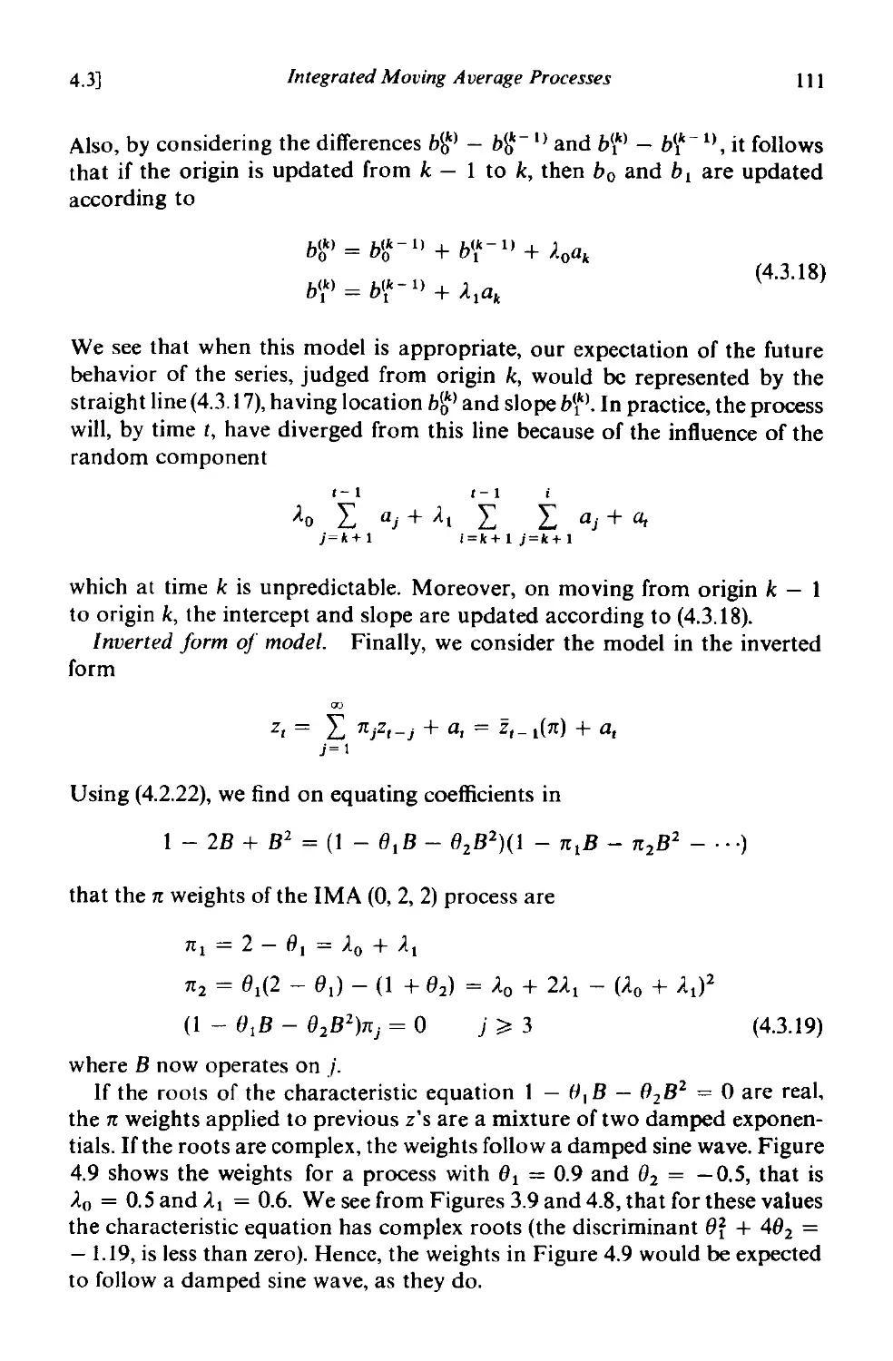


Author: Box G.E.P.
Tags: mathematics statistics math's statistics textbook mathematical statistics statistical hypothesis testing holden day series
Year: 1976


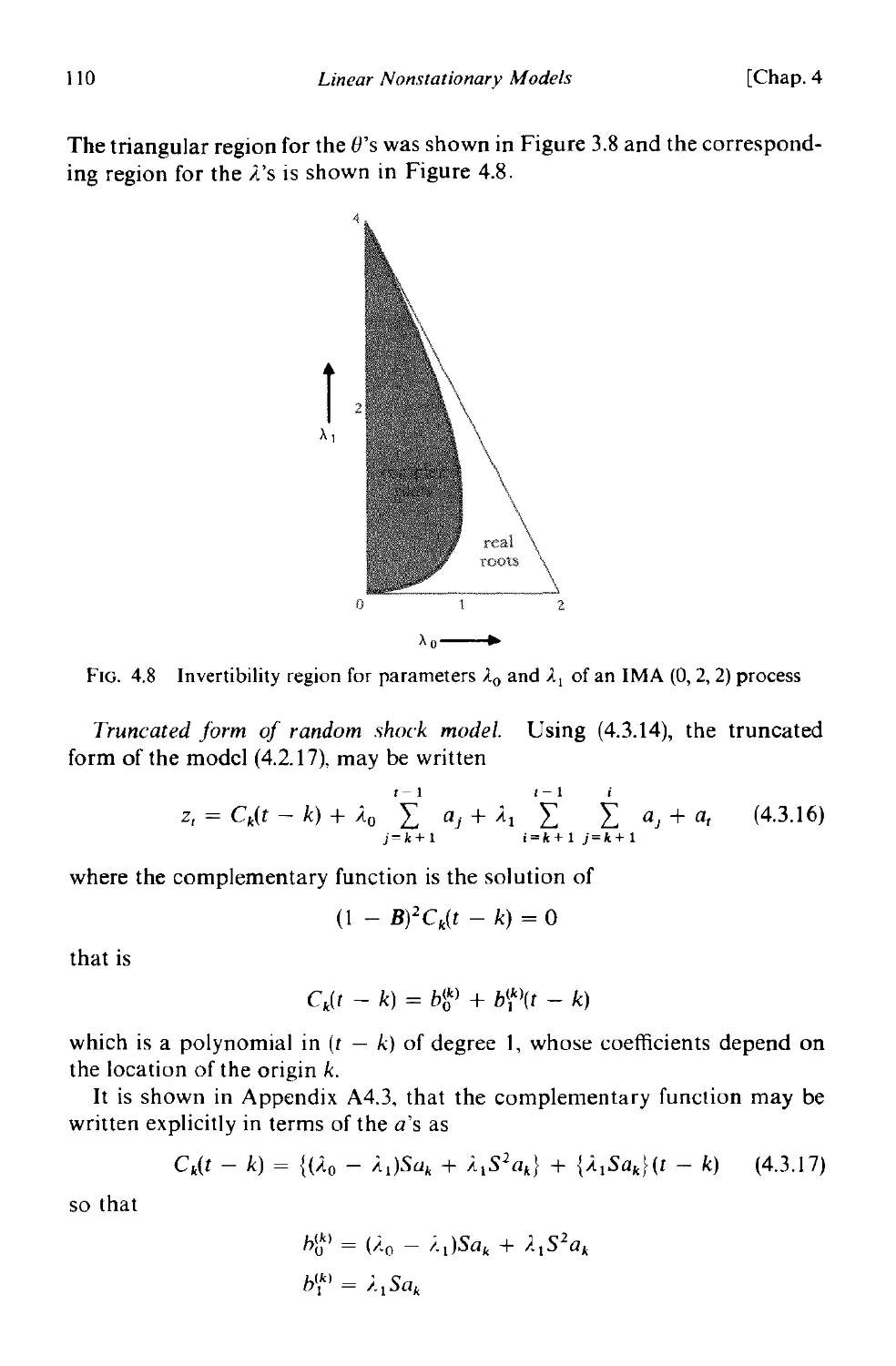
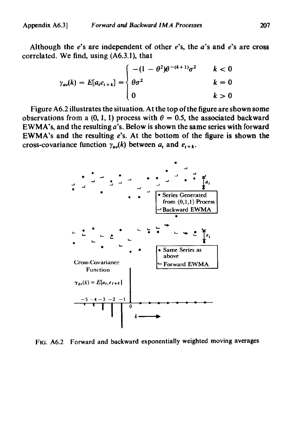
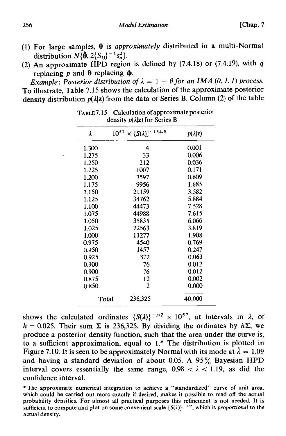
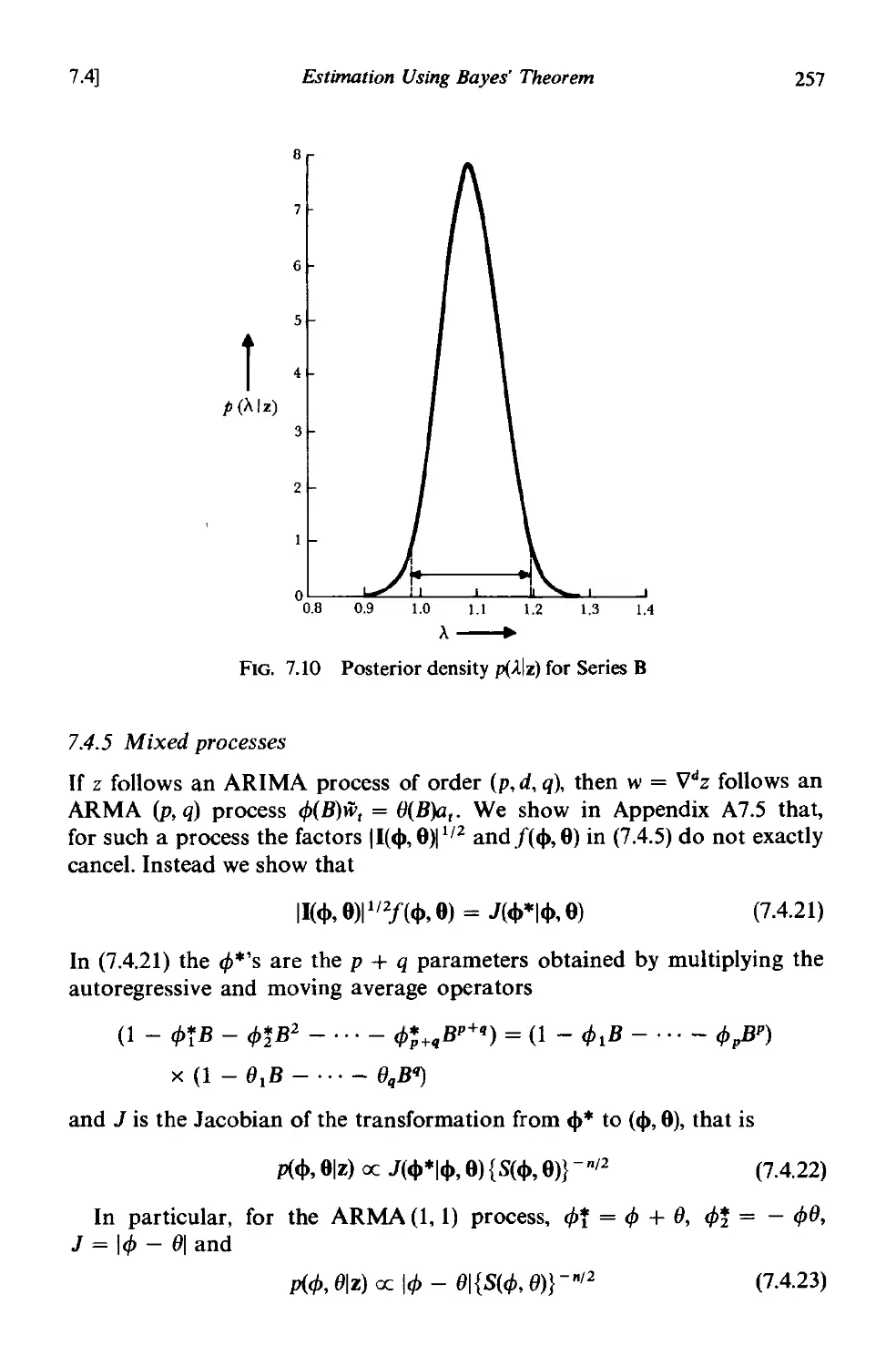
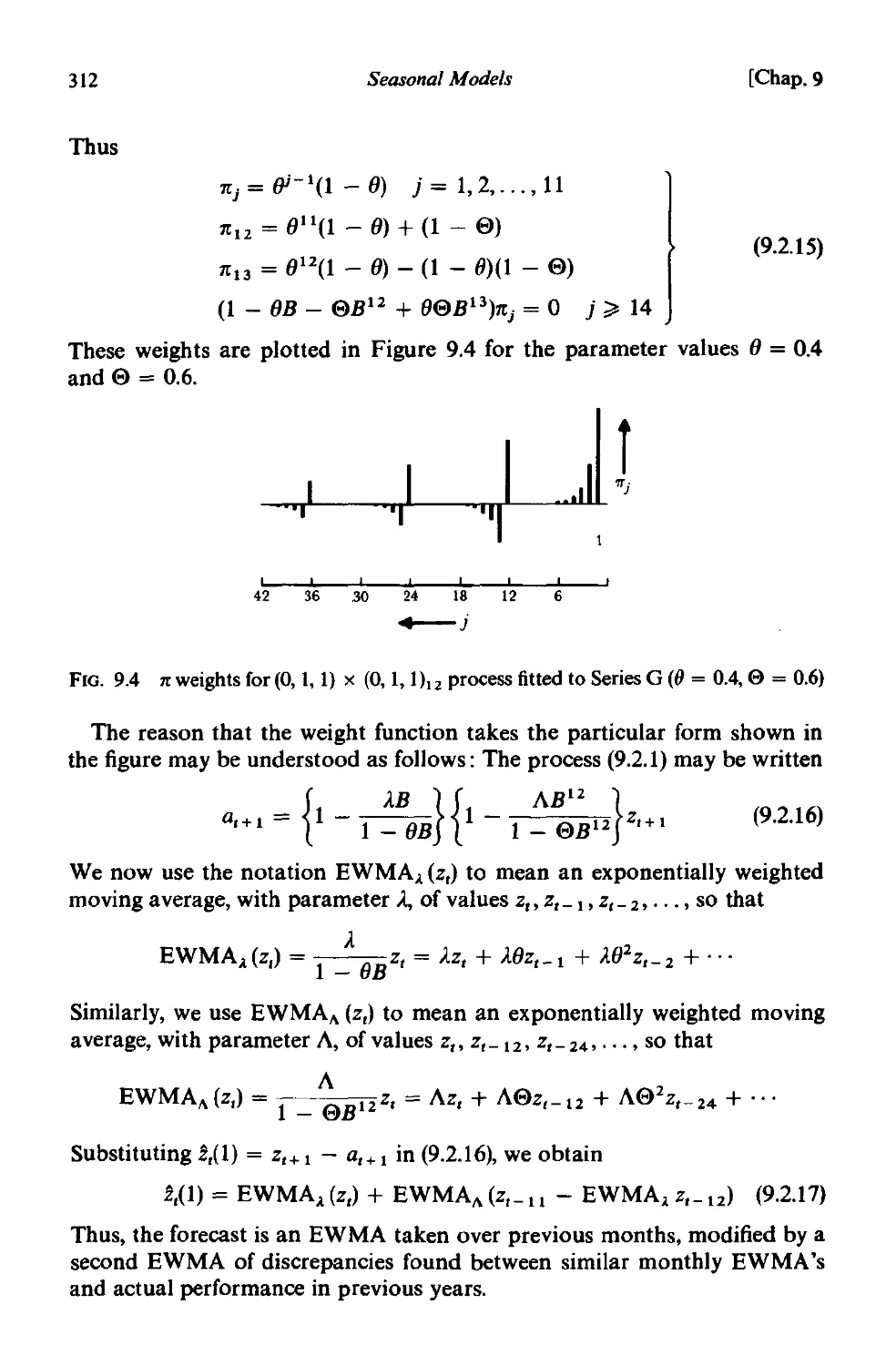
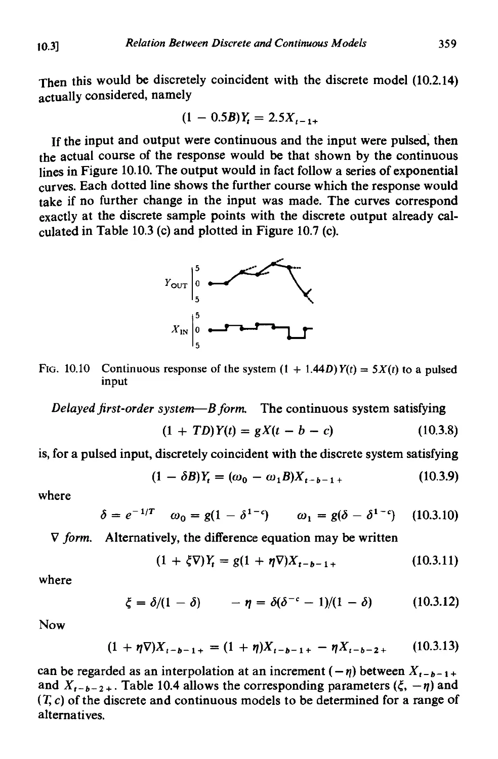
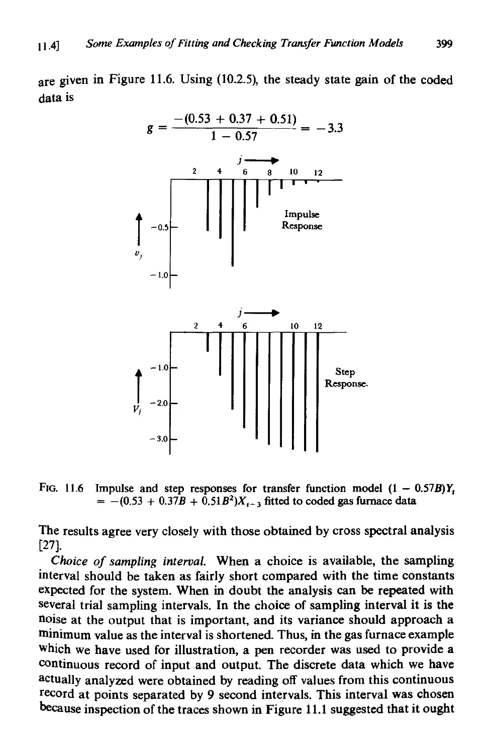
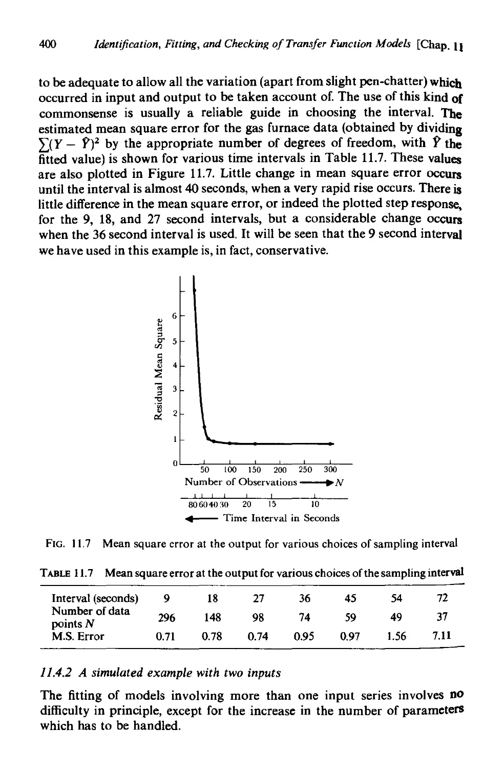
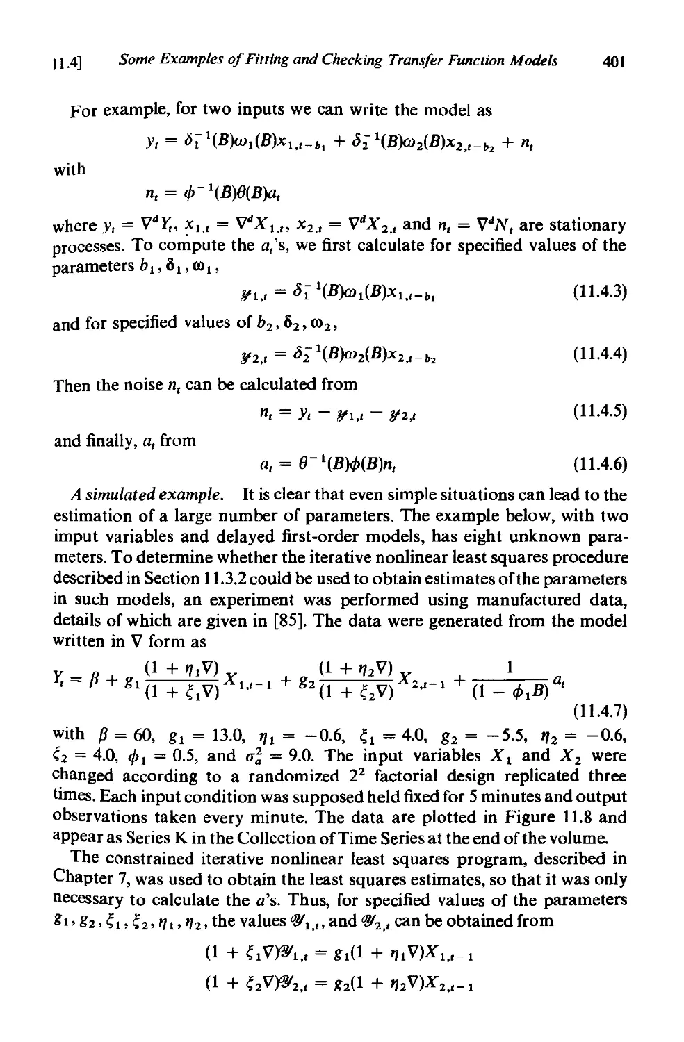
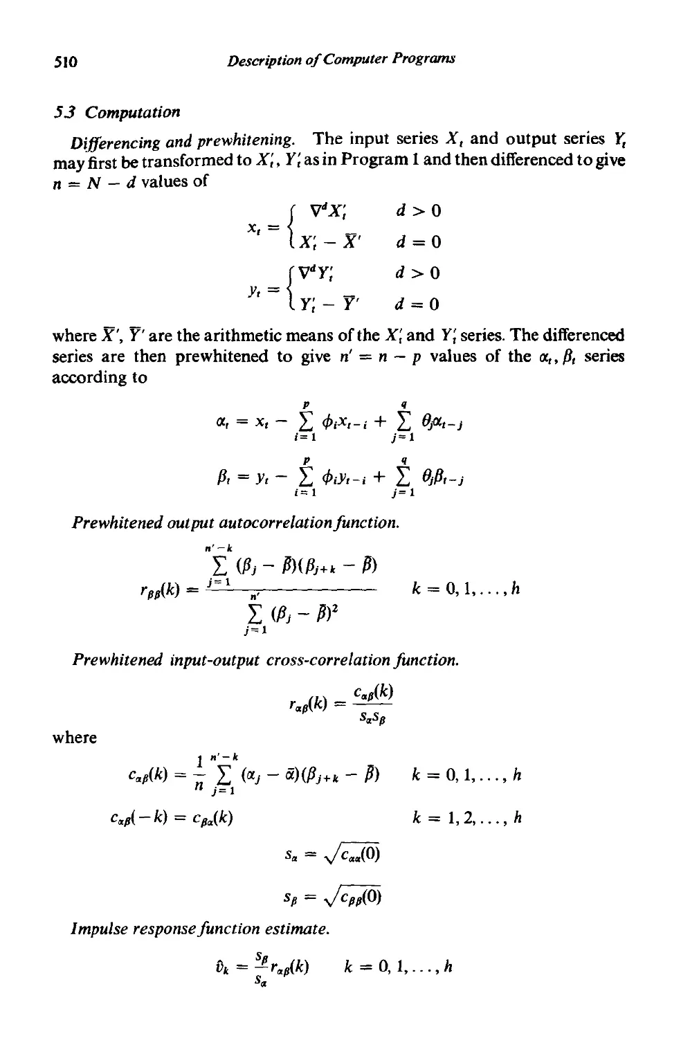
Text
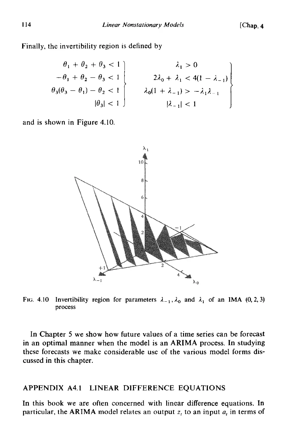
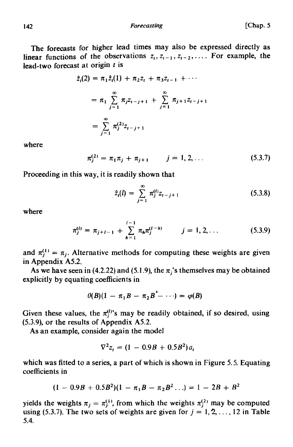
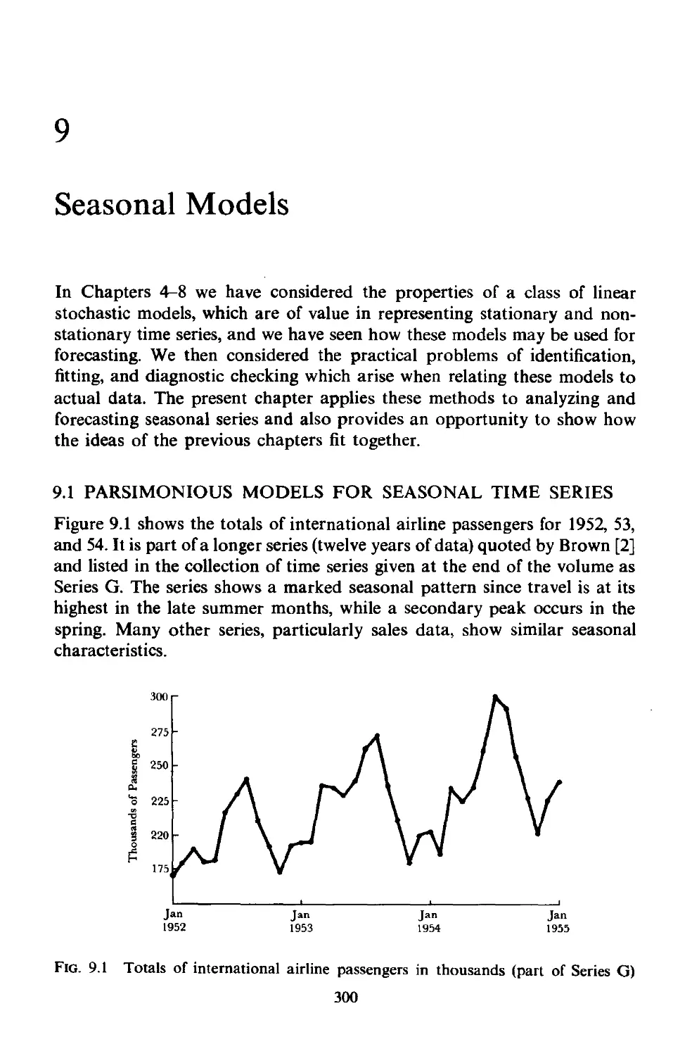
TIME SERIES
ANALYSIS
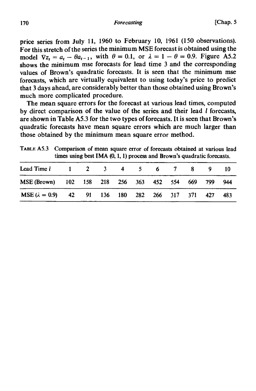
forecasting
and
control
Revised Edition
GEORGE E. P. BOX
University of Wisconsin, U.S.A.
and
GWILYM M. JENKINS
University of Lancaster, U.K.
HOLDEN-DAY
Oakland, California
@copyFight 1976 by HOLDEN-DAY. INC.
4432 Telegraph Avenue. Oakland. CaZifomia
AU Fights reserved. No pap/; of this book may be
reproduced. by mimeograph. 01' any other means.
without the permission in lJI'iting of the
publisher.
Library of Congress Catalog Card Number: 76-8713
Printed in the lhited States of AmeFica
ISB N 0-8162-1104-3
90 (H 54
To Joan and Meg
PREFACE TO THE REVISED EDITION
The subject is advancing rapidly and in this revised edition the opportunity
has been taken to update some material, to COrrect some earlier mistakes
and to clarify and amplify certain sections. A completely new section has
been added at the end of the book, containing exercises and problems for
the separate chapters. We hope that this new section will add to the value
of the book as a course text. We are indebted to Bovas Abraham, Gina
Chen, Johannes Ledolter and Greta Ljung for careful checking and proof-
reading.
G. E. P. Box, Madison, U.S.A.
G. M. Jenkins, Lancaster, U.K.
January, 1976
vii
Preface
Much of statistical methodology is concerned with models in which the
observations are assumed to vary independently. In many applications
dependence between the observations is regarded as a nuisance, and in
planned experiments, randomization of the experimental design is introduced
to validate analysis conducted as if the observations were independent.
However, a great deal of data in business, economics, engineering and the
natural sciences occur in the form of time series where observations are
dependent and where the nature of this dependence is of interest in itself.
The body of techniq ues available for the analysis of such series of dependent
observations is called time series analysis.
Spectral analysis, in the frequency-domain, comprises one class of
techniques for time series analysis, but we shall say very little here about
tha t important subject. This book is concerned with the building of stochastic
(statistical) models for discrete time series in the time-domain and the use
of such models in important areas of application. Our objective will be to
derive models possessing maximum simplicity and the minimum number of
parameters consonant with representational adequacy. The obtaining of
such models is important because:
(l) They may tell us something about the nature of the system generating
the time series;
(2) They can be used for obtaining optimal forecasts of future values of
the series;
(3) When two or more related time series are under study, the models can
be extended to represent dynamic relationships between the series and
hence 10 estimate transfer functions;
(4) They can be used to derive optimal control policies showing how a variable
under one's control should be manipulated so as to minimize distur-
bances in some dependent variable.
ix
x
Preface
The ability to forecast optimally, to understand dynamic relationships
between variables and to control optimally is of great practical importance.
For example, optimal sales forecasts are needed for business planning,
transfer function models are needed for improving the design and control
of process plant and optimal control policies are needed to regulate important
process variables, both manually and by the use of on-line computers.
Over the last ten years the authors have worked with real data arising in
economics and industry and, by trial and error, and by a long sequence of
interactions between theory and practice, have attempted to select, adapt,
and develop practical techniques to fulfill such needs. This book is the fruit
of these labors.
The approach adopted is, first, to discuss a class of models which are
sufficiently flexible to describe practical situations. In particular, time series
are often best represented by nonstationary models in which trends and other
psuedo-systematic characteristics which can change with time are treated
as statistical rather than as deterministic phenomena. Furthermore, econ-
omic and business time series often possess marked seasonal or periodic
components themselves capable of change and needing (possibly non-
stationary) seasonal statistical models for their description.
The process of model building, which is next discussed, is concerned with
relating such a class of statistical models to the data at hand and involves
much more than model fitting. Thus, identification techniques, designed to
suggest what particular kind of model might be worth considering, are
developed first and make use of the autocorrelation and partial autocor-
relation functions. The fitting of the identified model to a time series using
the likelihood function can then supply maximum likelihood estimates of
the parameters or, if one prefers, Bayesian posterior distributions. The
initially fitted model will not, necessarily, provide adequate representation.
Hence diagnostic checks are developed to detect model inadequacy, to
suggest appropriate modifications and thus, where necessary, to initiate a
further iterative cycle of identification, fitting and diagnostic checking.
When forecasts are the objective, the fitted statistical model is used
directly to generate optimal forecasts by simple recursive calculation. In
particular, this model completely determines whether the forecast projec-
tions should follow a straight line, an exponential curve, and so on. In
addition, the fitted model allows one to see exactly how the forecasts utilize
past data, to determine the variance of the forecast errors, and to calculate
limits within which a future value ofthe series will lie with a given probability.
When the models are extended to represent dynamic relationships, a
corresponding iterative cycle of identification, fitting and diagnostic check-
ing is developed to arrive at the appropriate transfer function-stochastic
model. In the final section of the book, the stochastic and transfer function
models developed earlier are employed in the construction of feedforward
and feedback control schemes.
Preface
XI
The applications given in this book are by no means exhaustive and it is
hoped that the examples presented will enable the reader to adapt the
techniques to his own problem. In particular the difference equations used
to represent transfer functions and stochastic phenomena may be employed
as building blocks which when appropriately fitted together can simulate a
wide variety of the systems occurring in engineering, business and economics.
Furthermore the principles of model building which are discussed and
illustrated have very general application.
AN OUTLINE OF THE BOOK
This book is set out in the following parts (from time to time, a vertical
line has been inserted in the left margin to indicate material which may be
omitted in the first reading):
Introduction and Summary (Chapter 1)
This chapter is an informal and highly condensed outline of topics dis-
cussed, defined and more fully explained in the main body of the text. It is
intended as a broad mapping of areas to be subsequently explored, a.nd the
student may wish to refer back to it as later chapters are read.
Part I Stochastic models and their forecasting (Chapters 2,3,4 and 5)
After some basic tools of time series analysis have been discussed in
Chapter 2, an important class of linear stochastic models is introduced in
Chapters 3 and 4 and their properties discussed. The immediate introduction
of forecasting in Chapter 5 takes advantage of the fact that the form of the
optimal forecasts follows at once from the structure of the stochastic models
discussed in Chapter 4.
Part II Stochastic model building (Chapters 6, 7,8 and 9)
Part II of the book describes an iterative model-building methodology
whereby' the stochastic models introduced in Part I, are related to actual
time series data. Chapters 6,7 and 8 describe, in turn, the processes of model
identification, model estimation, and model diagnostic checking. Chapter 9
illustrates the whole model building process by showing how all these ideas
may be brought together to build seasonal models and how these models
may be used to forecast seasonal time series.
Part III Transfer function model building (Chapters 10 and 11)
In Chapter 10 transfer function models are introduced for relating a
system output to one or more system inputs. Chapter 11 discusses methods
for transfer function-noise model identification, estimation and diagnostic
checking. The chapter ends with a description of how such models may be
used in forecasting.
xii
Preface
Part IV Design of discrete control schemes (Chapters J 2 and J 3)
In these two chapters we show how the stochastic models and transfer
function models previously introduced may be brought together in the
design of simple feed forward and feedback control schemes.
A first draft of the book was produced in 1965 and subsequently was
issued in 1966 and 1967 as Technical Reports Nos. 72,77,79,94,95,99,103,
104,116,121 and 122 of the Department of Statistics, University ofWiscon-
sin, and Nos. 1,2, 3,4,6, 7, 8, 9, 10, 11, 13 of the Department of Systems
Engineering, University of Lancaster. The work has involved a great deal of
research, which has been partially supported by the Air Force Office of
Scientific Research, United States Air Force, under AFOSR Grants AF-
AFOSR-1158-66 and AF-49 (638) 1608 and also by the British Science
Research Council. We are grateful to Professor E. S. Pearson and the
Biometrika Trustees for permission to reprint condensed and adapted forms
of Tables 1,8 and 12 of Biometrika Tablesfor Statisticians, Vol. 1, edited by
E. S. Pearson and H. O. Hartley, and to Dr. Casimer Stralkowski for
permission to reproduce and adapt three figures from his doctoral thesis,
University of Wisconsin, 1968. The authors are indebted to George Tiao,
David Mayne, Emanuel Parzen, David Pierce, Granville Wilson and Donald
Watts for suggestions for improving the manuscript, to John Hampton,
Granville Wilson, Elaine Hodkinson and Patricia Blant for writing the
computer programs described at the end of the book and also to them and to
Dean Wichern, David Bacon and Paul Newbold for assistance with the
calculations. Finally, we are glad to record our thanks to Him Kanemasu.
Paul Newbold, Larry Haugh, John .MacGregor and Granville Wilson for
careful reading and checking of the manuscript, to Carole Leigh and Mary
Esser for their care and patience in typing the manuscript and to Meg Jenkins
for the initial draft of the diagrams.
G. E. P. Box, Madison, U.S.A.
G. M. Jenkins, Lancaster, U.K.
June 1969
Contents
PREFACE Vll
CHAPTER INTRODUCTION AND SUMMARY
1.1 Three important practical problems I
1.1.1 Fon casting time series I
1.1.2 Estimation of transfer functions 2
1.1.3 Design of discrete control systems 4
1.2 Stochastic and deterministic dynamic mathematical models 7
1.2.1 Stationary and nonstationary stochastic models for fore-
casting and control. 7
1.2.2 Transfer function models . 13
1.2.3 Models for discrete control systems 16
1.3 Basic ideas in model building . 17
1.3.1 Parsimony 17
1.3.2 Iterative stages in the selection of a model 1-8
PART I STOCHASTIC MODELS AND THEIR
FORECASTING
CHAPTER 2 THE AUTOCORRELATION FUNCTION AND
SPECTRUM
2.1 Autocorrelation properties of stationary models 23
2.1.1 Time series and stochastic processes . 23
2.1.2 Stationary stochastic processes 26
2.1.3 Positive definiteness and the autocovariance matrix 28
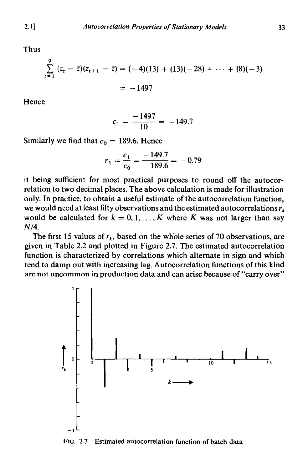
2.1.4 The autocovariance and autocorrelation functions . 30
2.1.5 Estimation ofautocovariance and autocorrelation functions 32
2.1.6 Standard errors of autocorrelation estimates 34
xiii
xiv
Contents
2.2 Spectral properties of stationary models 36
2.2.1 The periodogram 36
2.2.2 Analysis of variance 37
2.2.3 The spectrum and spectral density function. 39
2.2.4 Simple examples of autocorrelation and spectral density
functions 42
2.2.5 Advantages and disadvantages of the autocorrelation and
spectral density functions . 44
A2.l Link between the sample spectrum and autocovariance
function estimate 44
CHAPTER 3 LINEAR STATIONARY MODELS
3.1 The general linear process . 46
3.1.1 Two equivalent forms for the linear process 46
3.1.2 Autocovariance generating function of a linear process 48
3.1.3 Stationarity and invertibility conditions for a linear process 49
3.1.4 Autoregressive and moving average processes . 51
3.2 Autoregressive processes 53
3.2.1 Stationarity conditions for autoregressive processes 53
3.2.2 Autocorrelation function and spectrum of autoregressive
processes 54
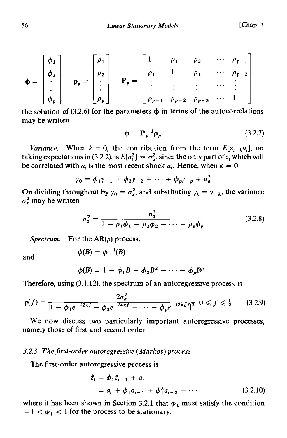
3.2.3 The first order autoregressive (Markov) process 56
3.2.4 The second order autoregressive process 58
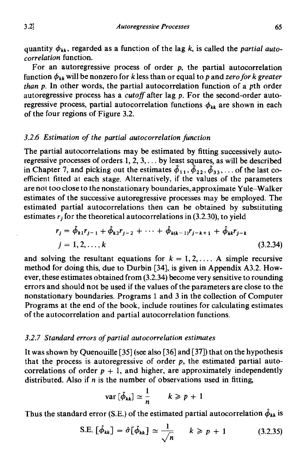
3.2.5 The partial autocorrelation function 64
3.2.6 Estimation of the partial autocorrelation function 65
3.2.7 Standard errors of partial autocorrelation estimates 65
3.3 Moving average processes . 67
3.3.1 Invertibility conditions for moving average processes 67
3.3.2 Autocorrelation function and spectrum of moving average
processes 68
3.3.3 The first-order moving average process . 69
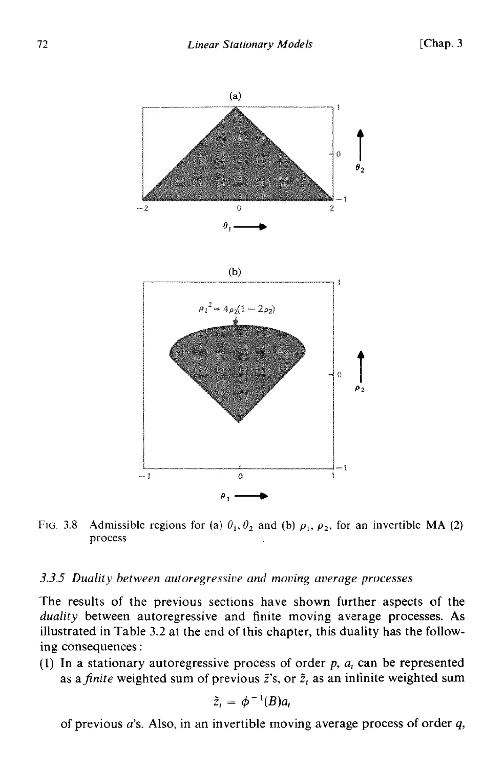
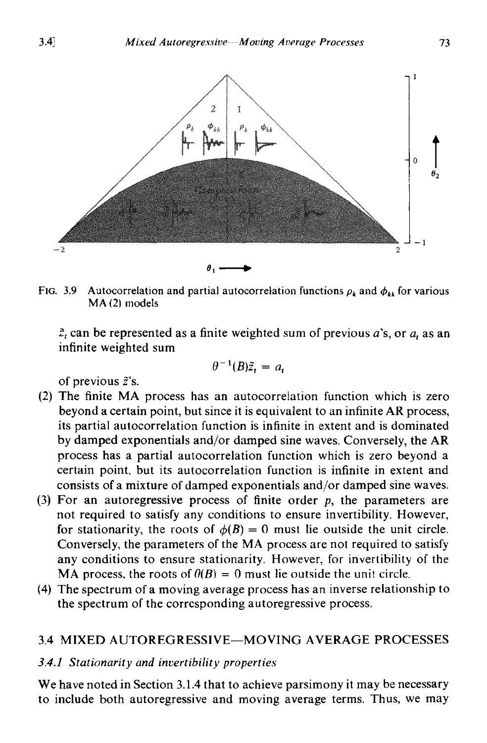
3.3.4 The second-order moving average process
3.3.5 Duality between autoregressive and moving average pro-
cesses 72
3.4 Mixed autoregressive-moving average processes 73
3.4.1 Stationarity and invertibility properties . 73
3.4.2 Autocorrelation function and spectrum of mixed processes 74
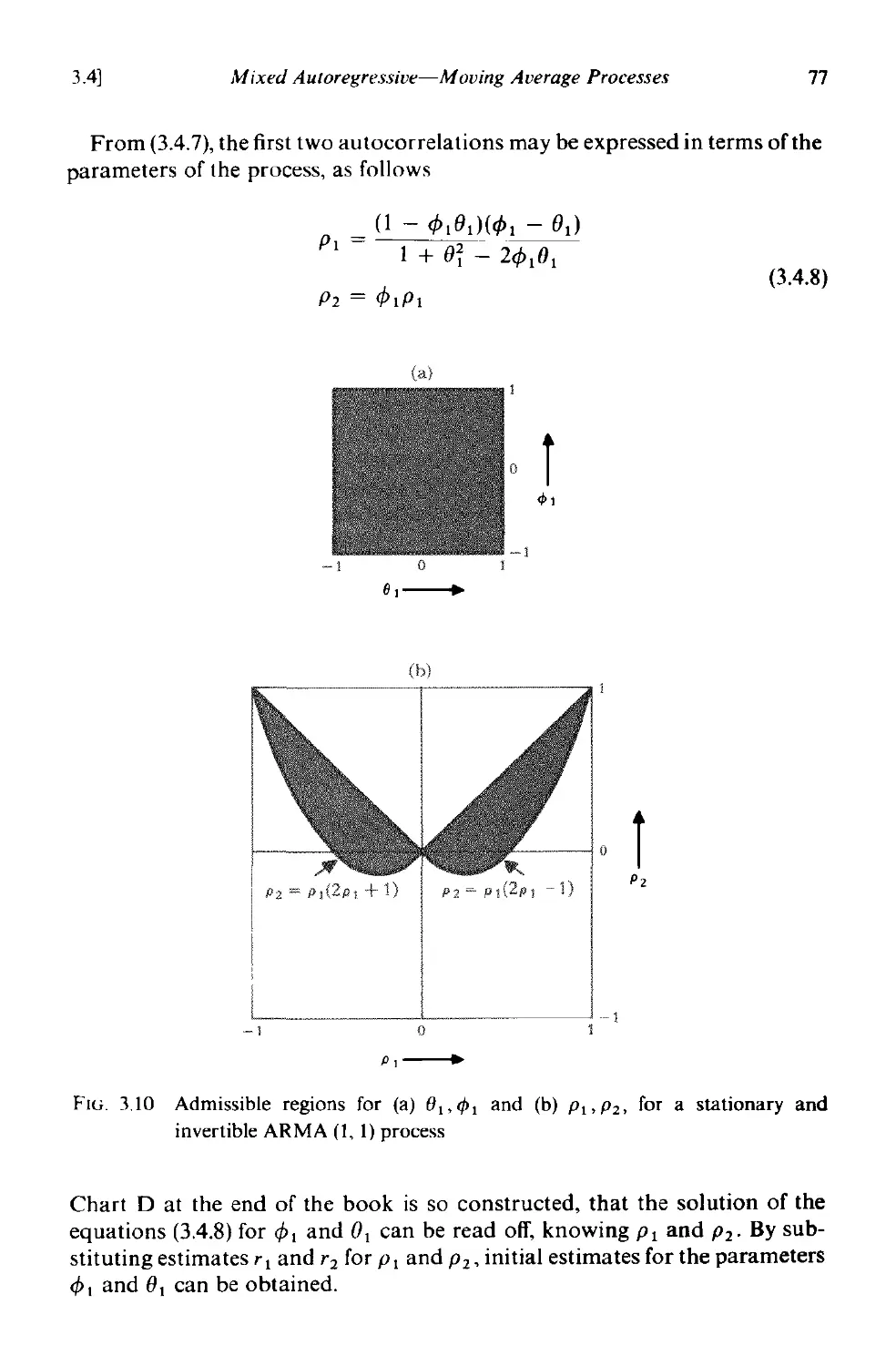
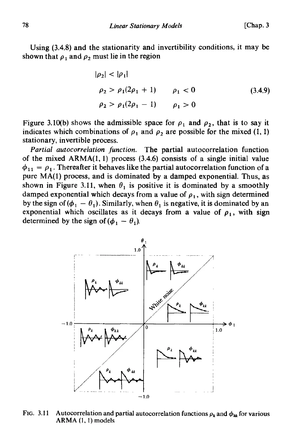
3.4.3 The first-order autoregressive-first order moving average
process . 76
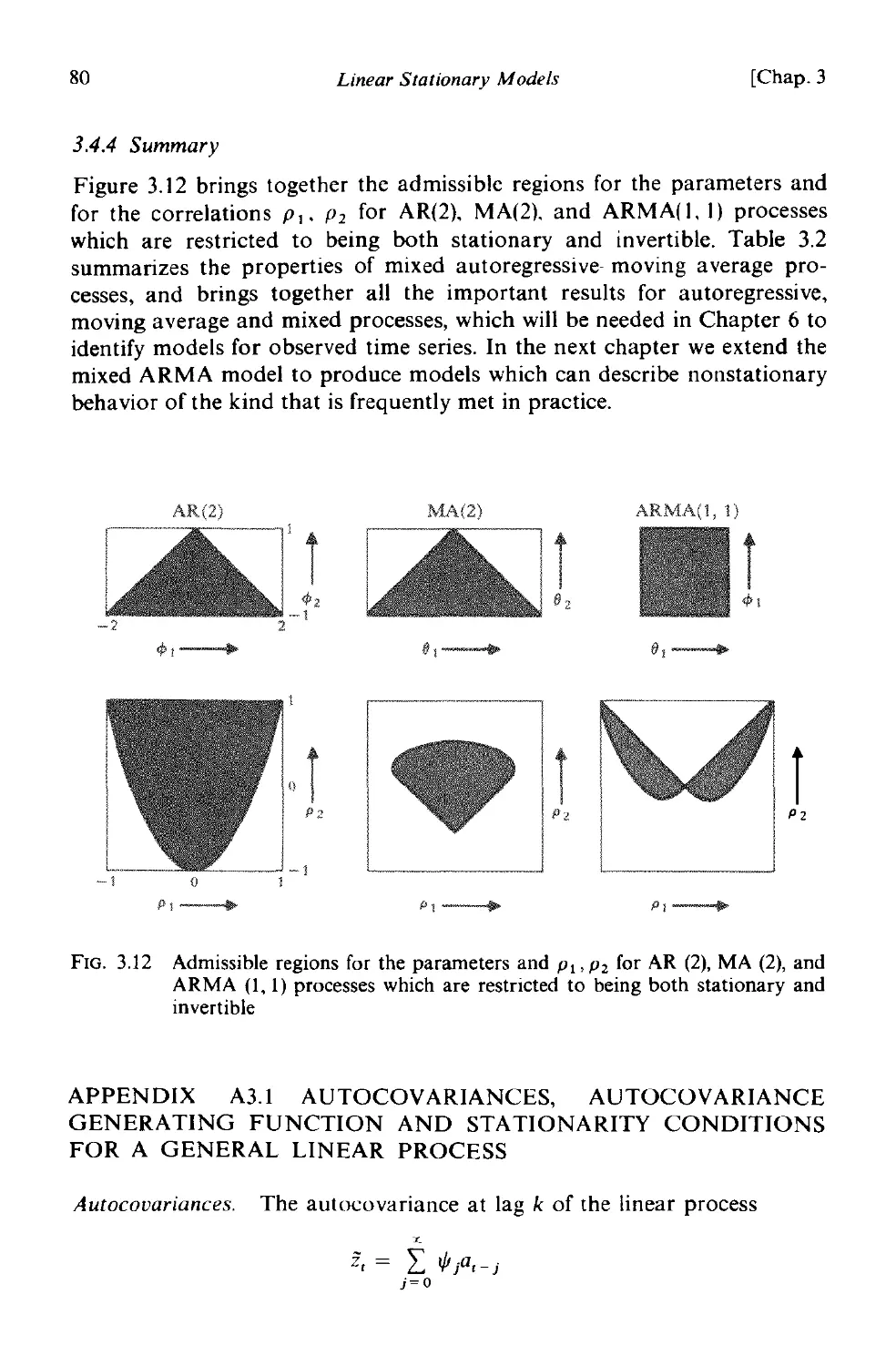
3.4.4 Summary 80
A3.l Autocovariances. autocovariance generating functions and
stationarity conditions for a general linear process 80
Contents xv
A3.2 A recursive method for calculating autoregressive para-
meters 82
CHAPTER 4 LINEAR NONSTATIONARY MODELS
4.1 Autoregressive integrated moving average processes 85
4.1.1 The nonstationary first order autoregressive process 85
4.1.2 A general model for a nonstationary process exhibiting
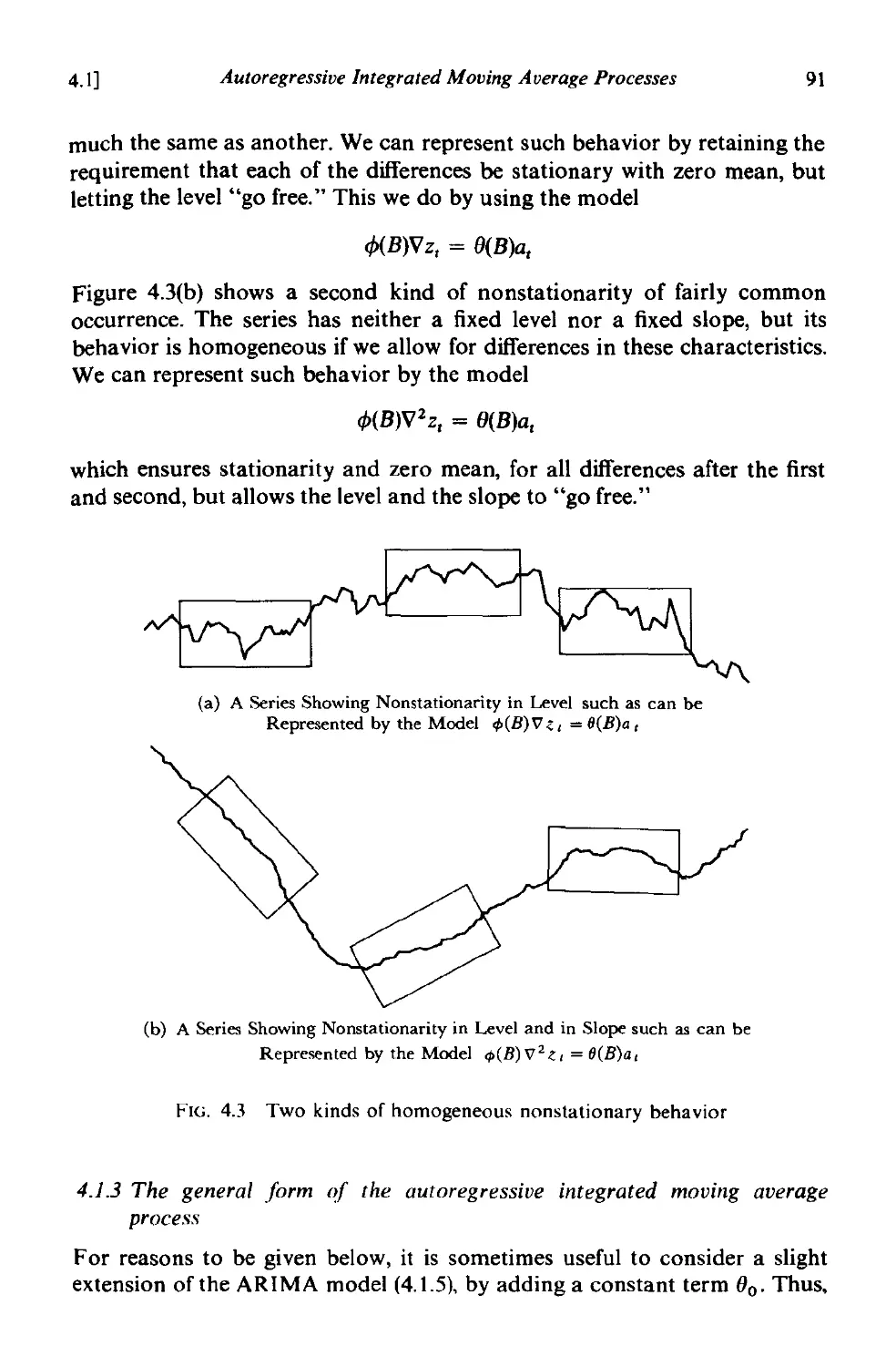
homogeneity 81
4.1.3 The general form of the autoregressive integrated moving
average process 9 I
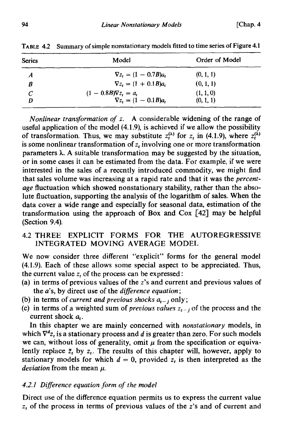
4.2 Three explicit forms for the autoregressive integrated moving
average model . 94
4.2.1 Difference equation form of the model 94
4.2.2 Random shock form of the model 95
4.2.3 Inverted form of the model 101
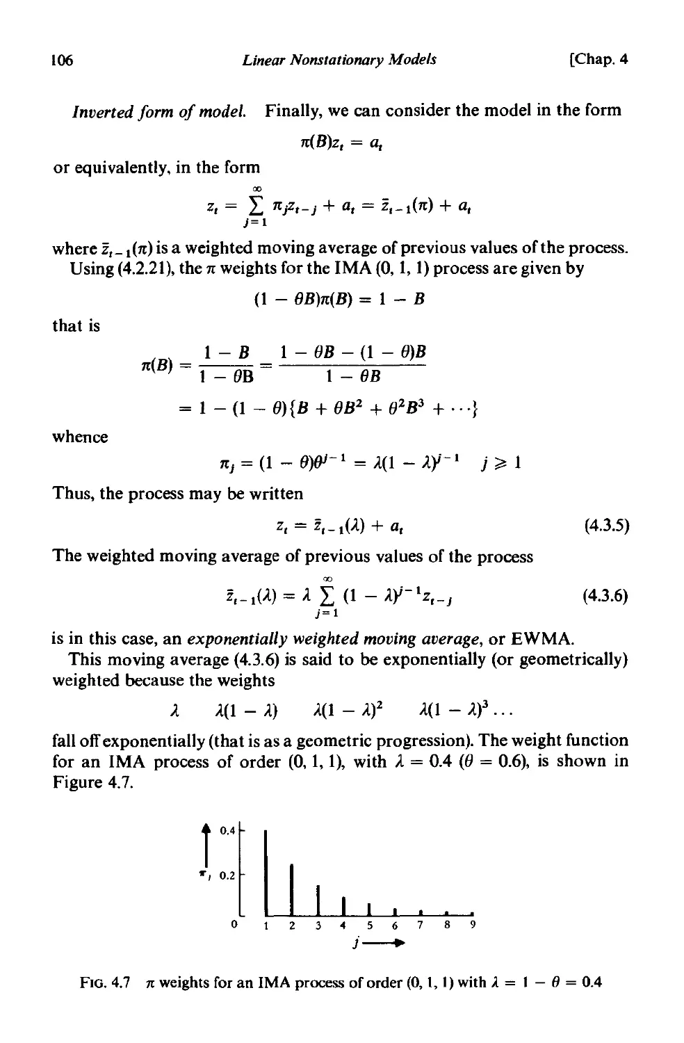
4.3 Integrated moving average processes . 103
4.3.1 The integrated moving average process of order (0, 1, 1) 105
4.3.2 The integrated moving average process of order (0, 2, 2) 108
4.3.3 The general integrated moving average process of order
(0, d, q) . 112
A4.1 Linear difference equations . 114
A4.2 The IMA (0, 1, 1) process with deterministic drift. 119
A4.3 Properties of the finite summation operator 120
A4.4 ARIMA processes with added noise 121
A4.4.1 The sum of two independent moving average processes 121
A4.4.2 Effect of added noise on the general model 121
A4.4.3 Example for an IMA (0, 1, 1) process with added white
noise . 122
A4.4.4 Relation between the IMA (0, I, 1) process and a random
walk 123
A4.4.5 Autocovariance function of the general model with added
correlated noise . 124
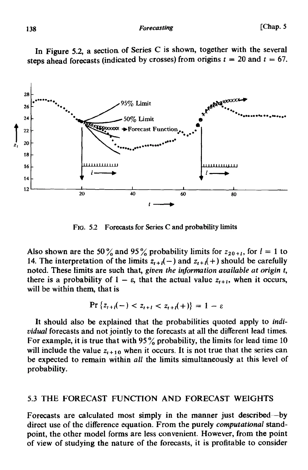
CHAPTER 5 FORECASTING
5.1 Minimum mean square;' error forecasts and their properties 126
5.1.1 Derivation of the minimum mean square error forecasts 127
5.1.2 Three basic forms for the forecast 129
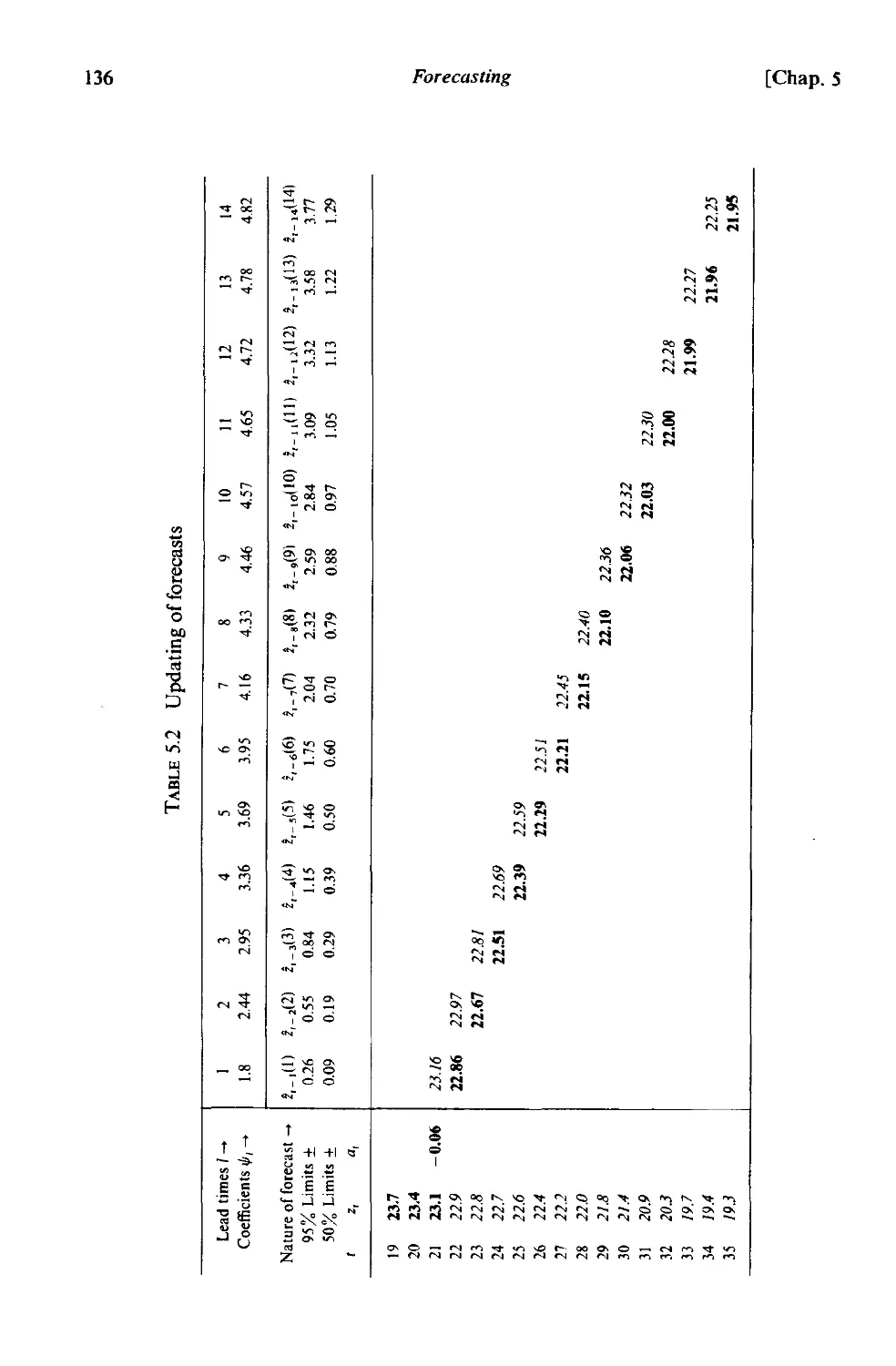
5.2 Calculating and updating forecasts 132
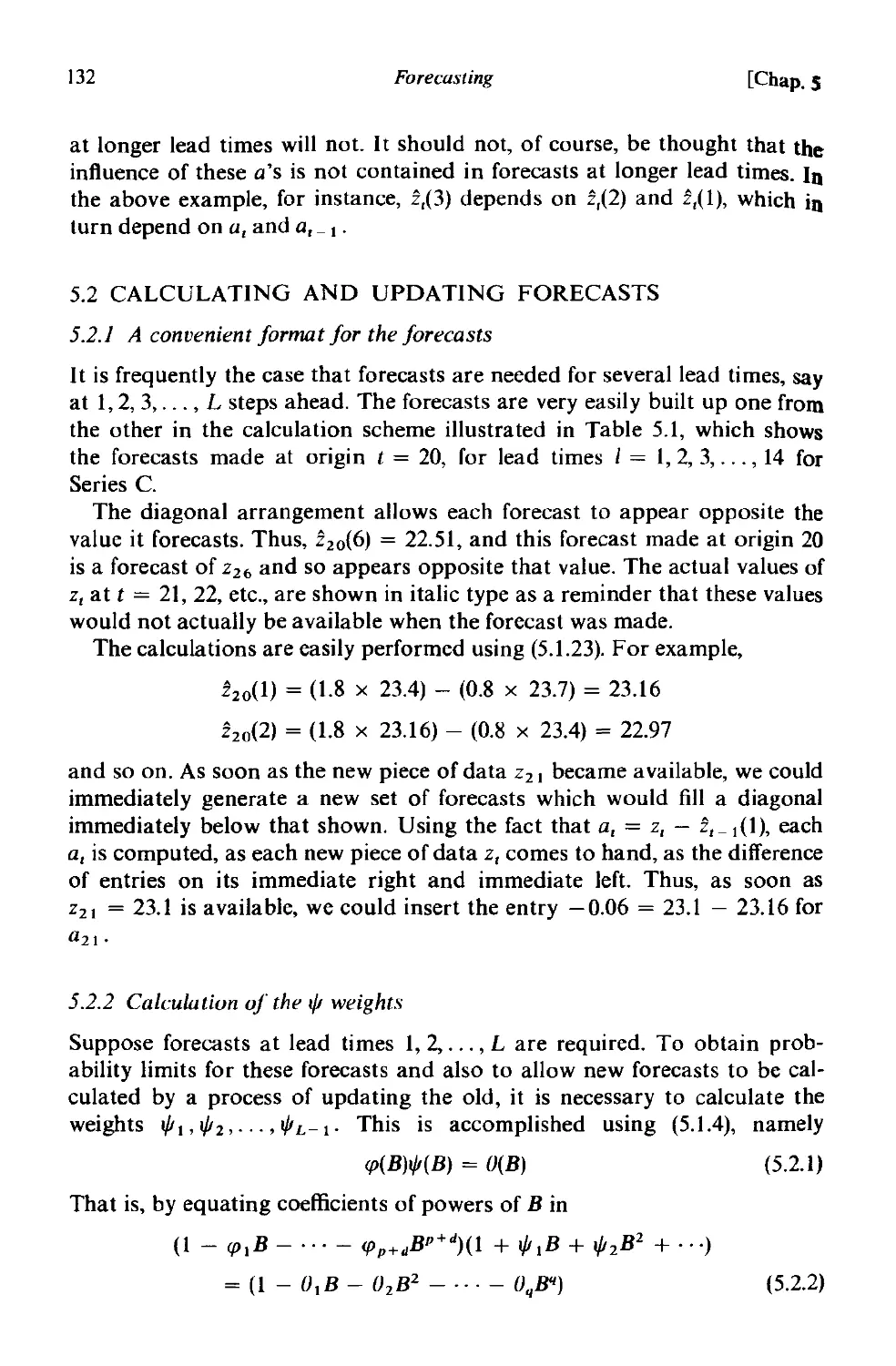
5.2.1 A convenient format for the forecasts 132
5.2.2 Calculation of the '" weights . 132
5.2.3 Use of the'" weights in updating the forecasts 134
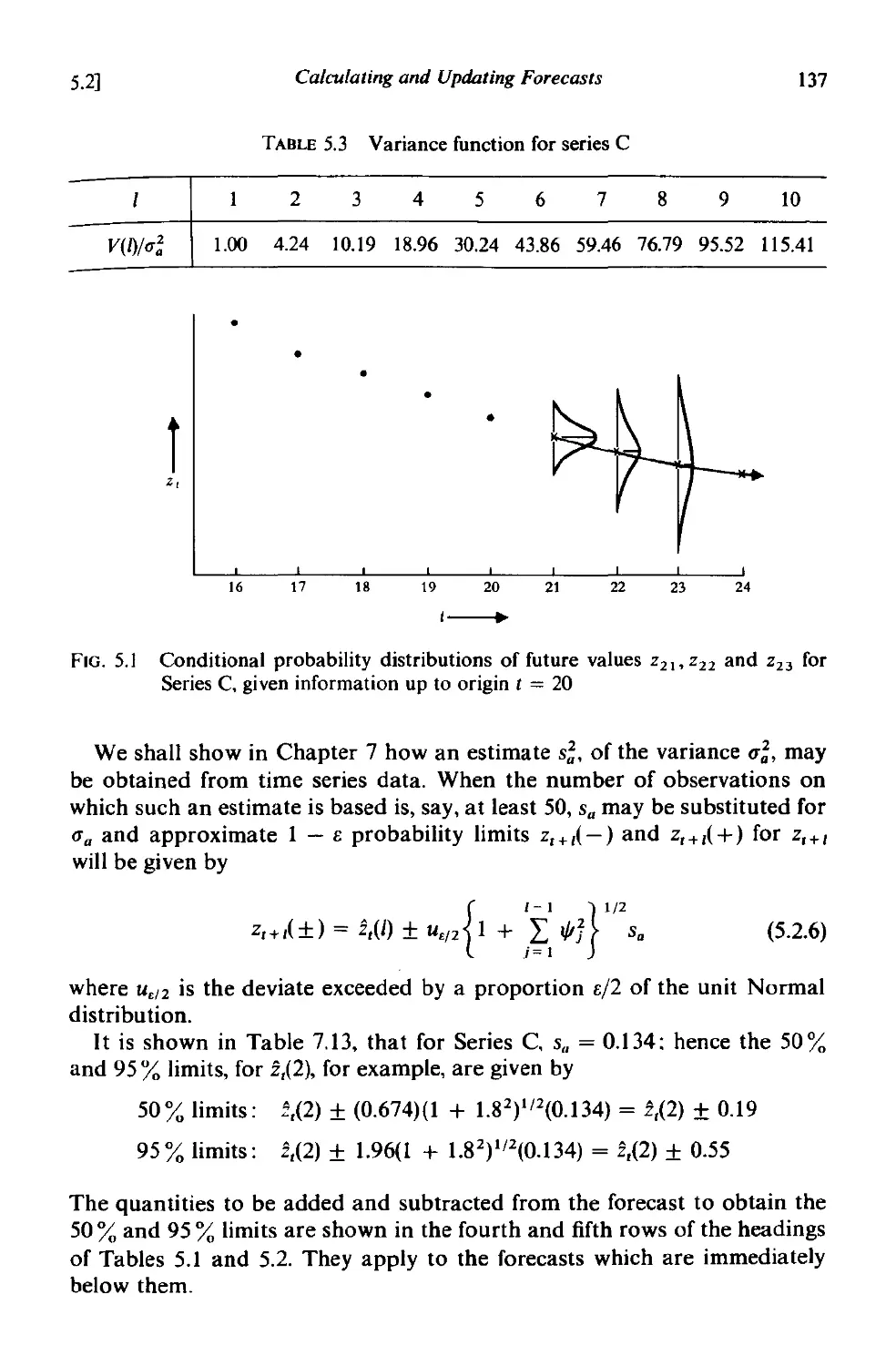
5.2.4 Calculation of the probability limits of the forecasts at any
lead time 135
xvi
Contents
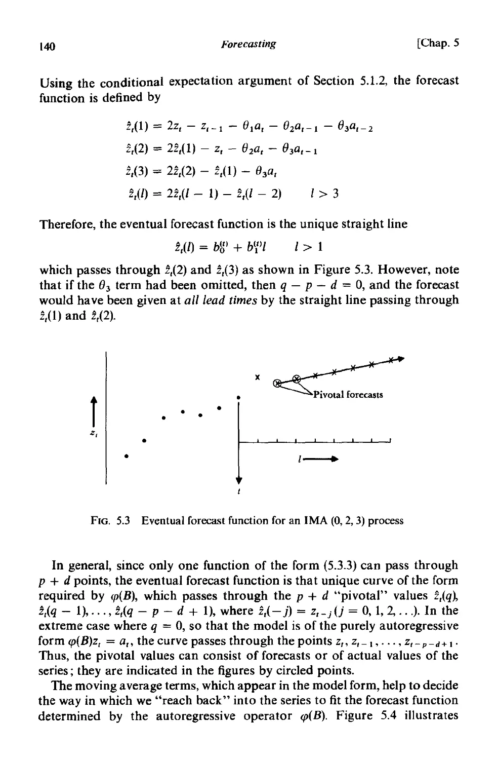
5.3 The forecast function and forecast weights 138
5.3.1 The eventual forecast function determined by the auto-
regressive operator. 139
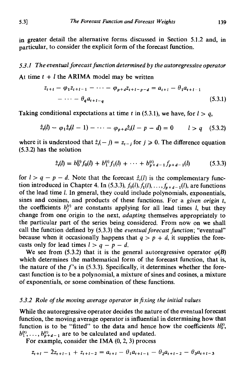
5.3.2 Role of the moving average operator in fixing the initial
values 139
5.3.3 The lead-l forecast weights 141
5.4 Examples of forecast functions and their updating 144
5.4.1 Forecasting an IMA (0, I, I) process 144
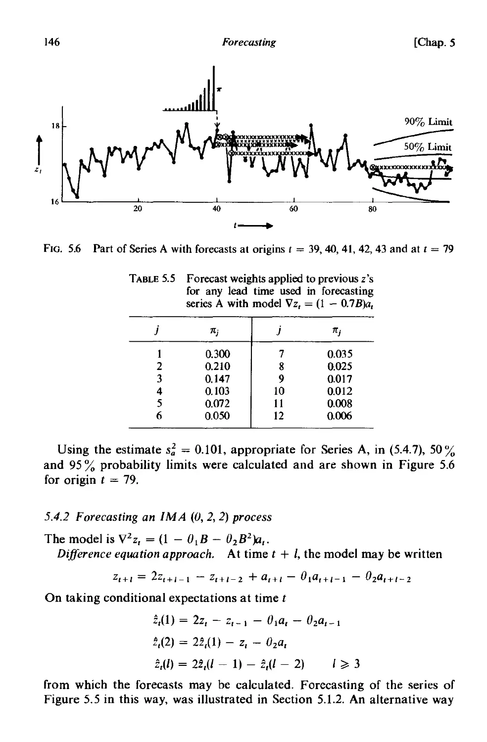
5.4.2 Forecasting an IMA (0, 2, 2) process 146
5.4.3 Forecasting a general IMA (0, d, q) process 149
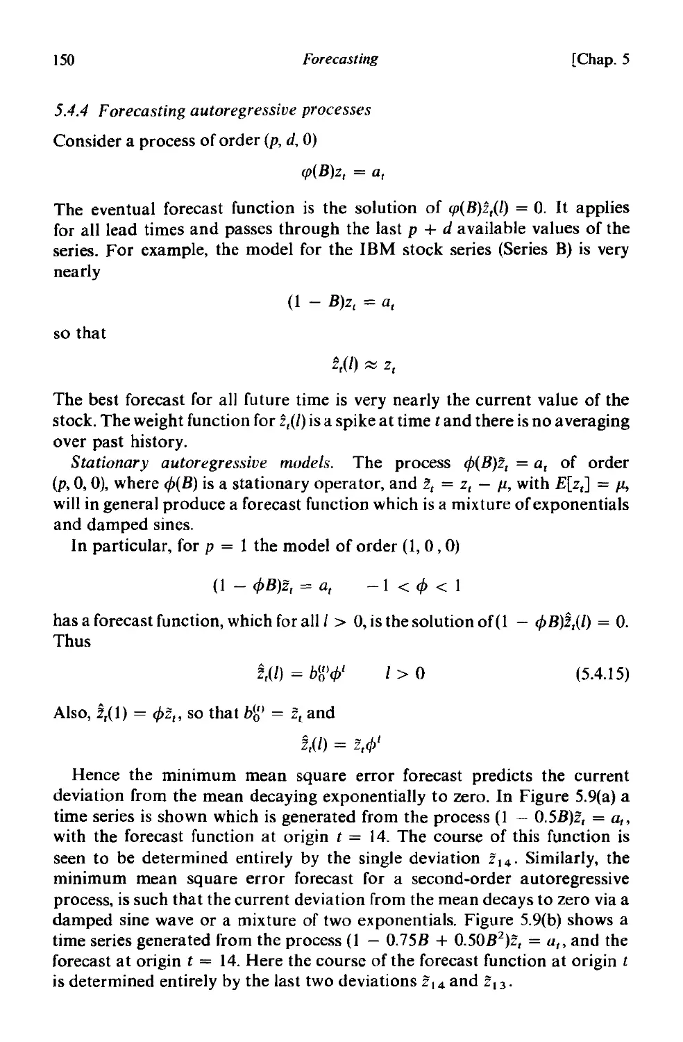
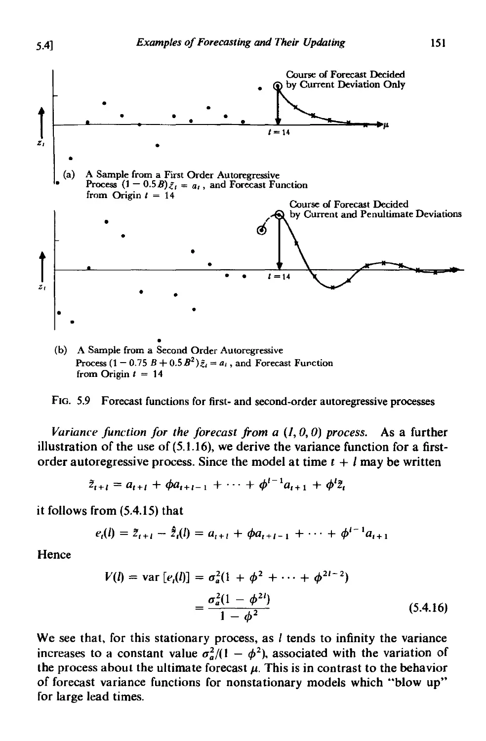
5.4.4 Forecasting autoregressive processes 150
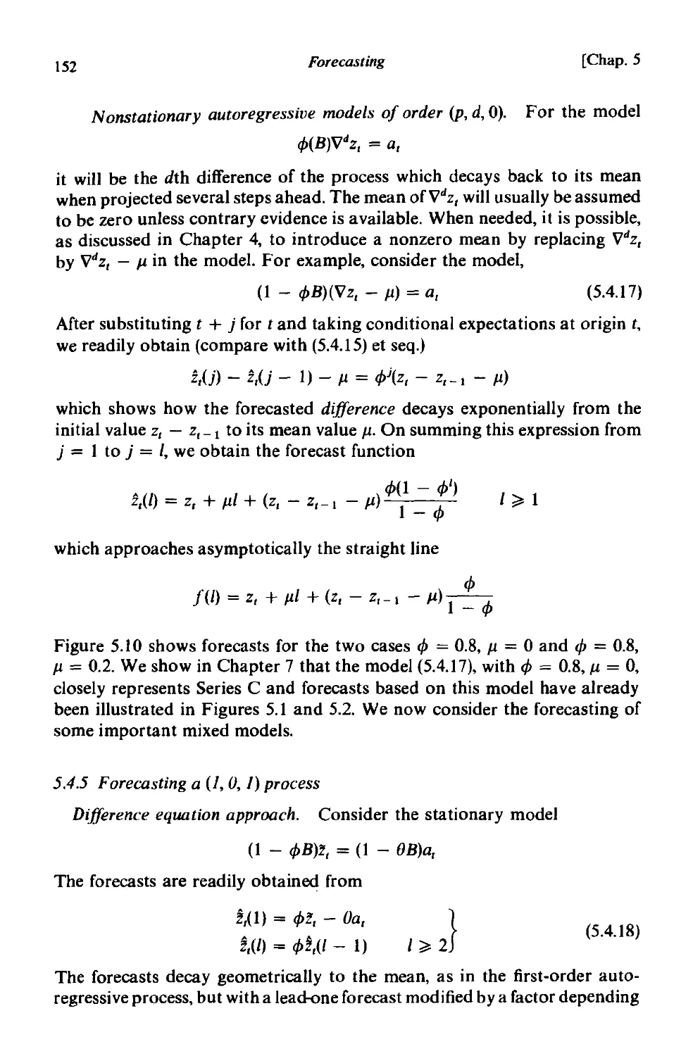
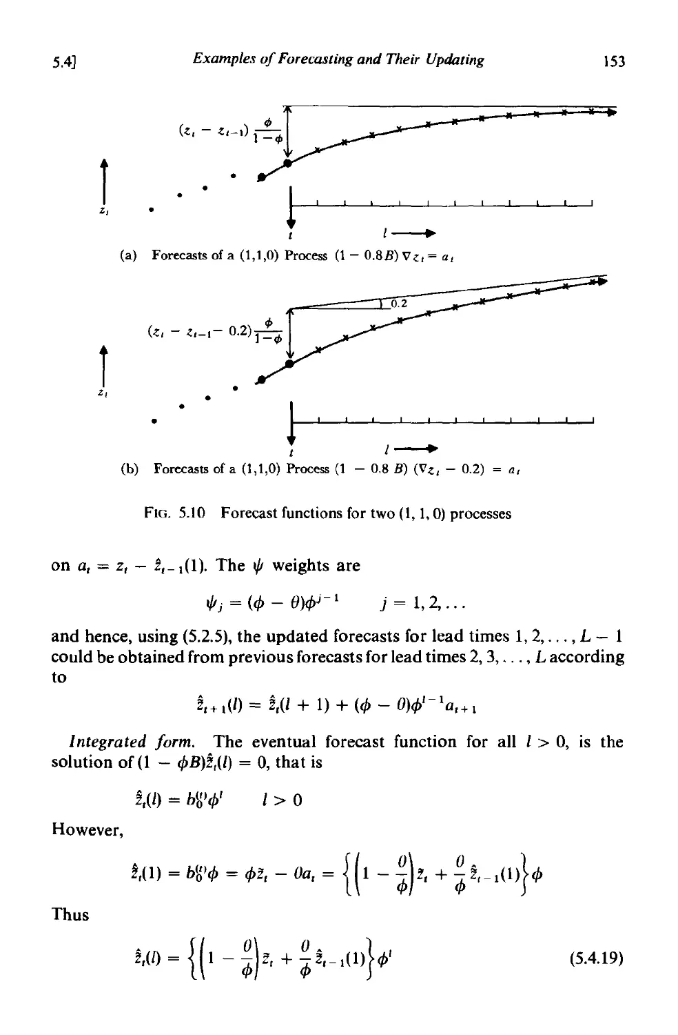
5 .4.5 Forecasting a (I, 0, I) process 152
5.4.6 Forecasting a (I, I, I) process 154
5.5 Summary 155
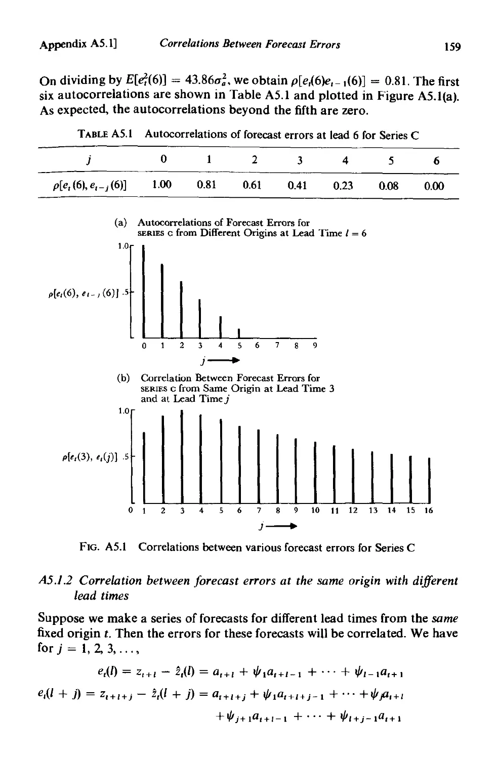
A5.l Correlations between forecast errors 158
A5.l.l Autocorrelation function of forecast errors at different
origins. 158
A5.1.2 Correlation between forecast errors at the same origin
with different lead times. 159
A5.2 Forecast weights for any lead time . 160
A5.3 Forecasting in terms of the general integrated form 162
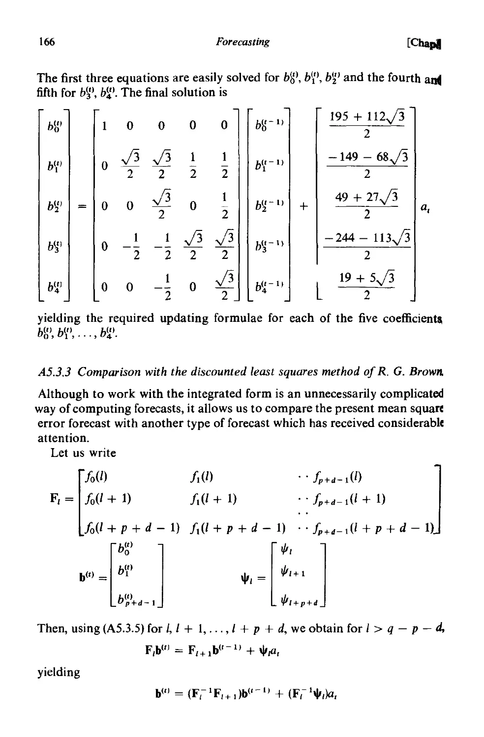
A5.3.l A general method of obtaining the integrated form 162
A5.3.2 Updating the general integrated form . 164
A5.3.3 Comparison with the discounted least squares method
of R. G. Brown . 166
PART II STOCHASTIC MODEL BUILDING
CHAPTER 6 MODEL IDENTIFICA nON
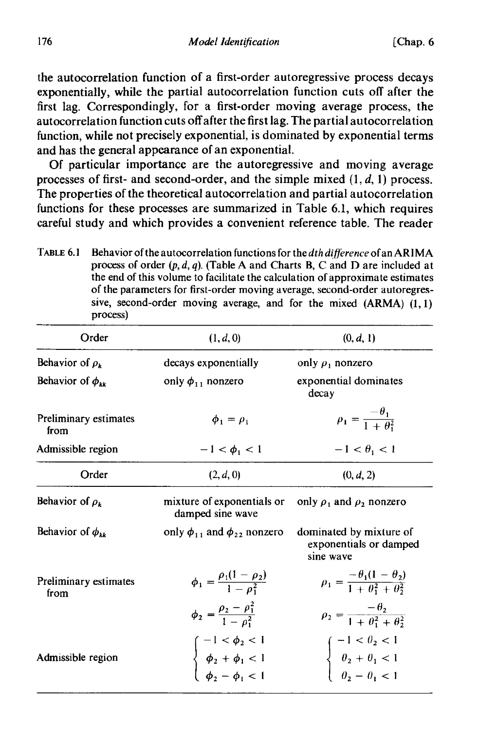
6.1 Objectives of identification 173
6.1.1 Stages in the identification procedure 173
6.2 Identification techniques 174
6.2.1 Use of the autocorrelation and partial autocorrelation
functions in identification 174
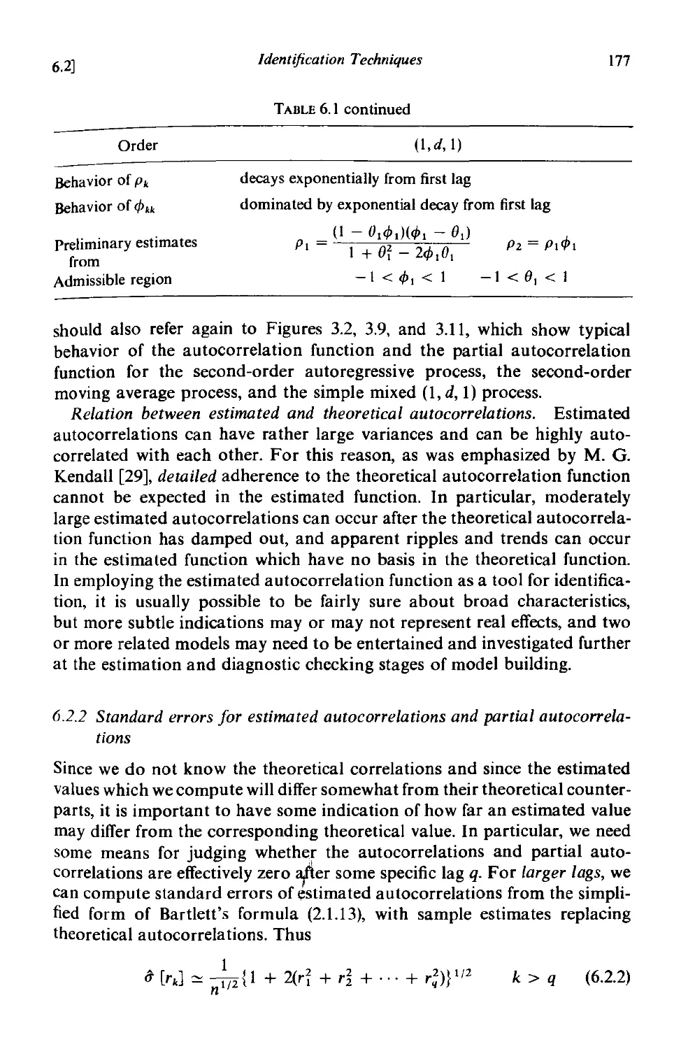
6.2.2 Standard errors for estimated autocorrelations and partial
autocorrelations 177
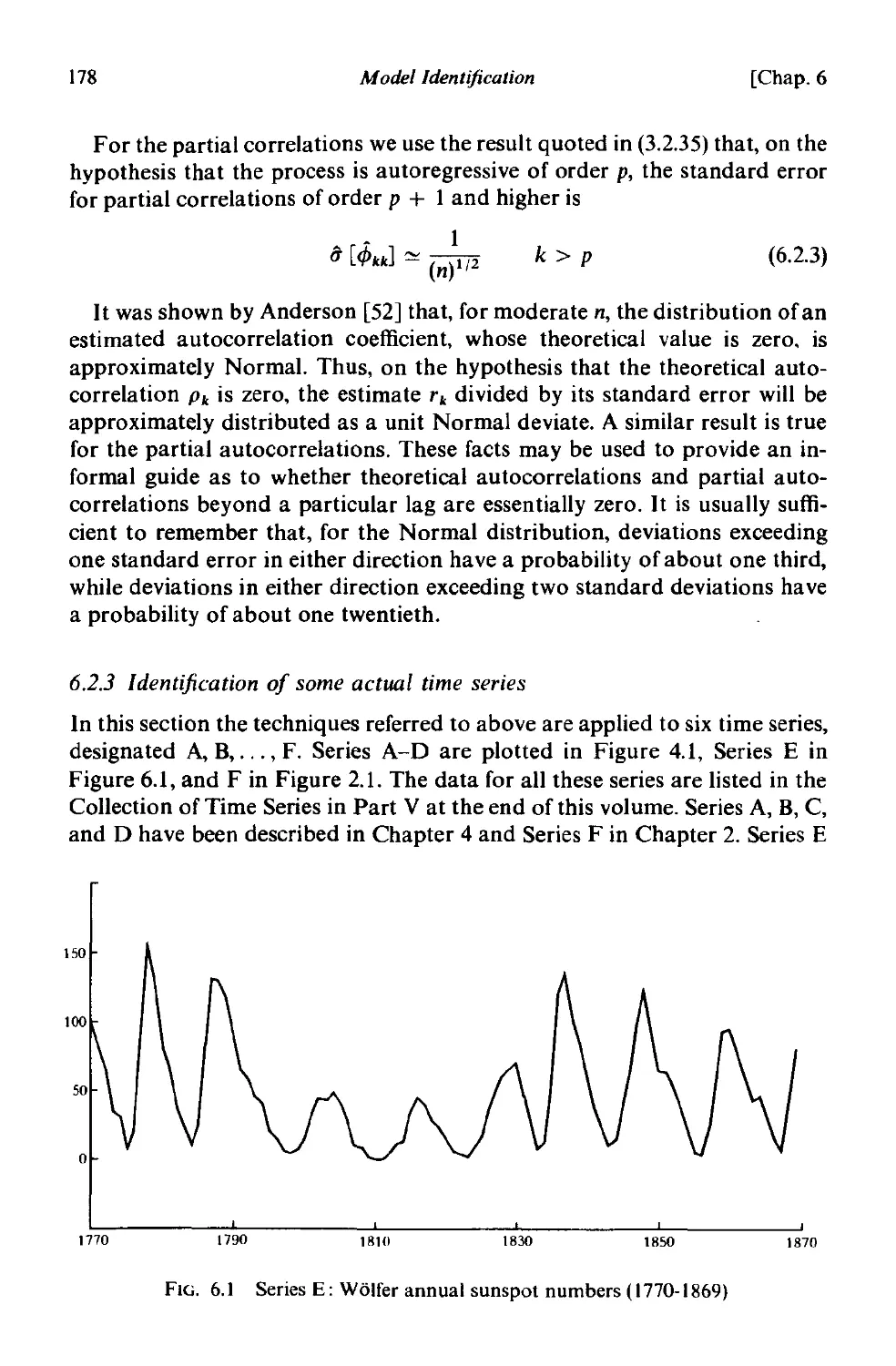
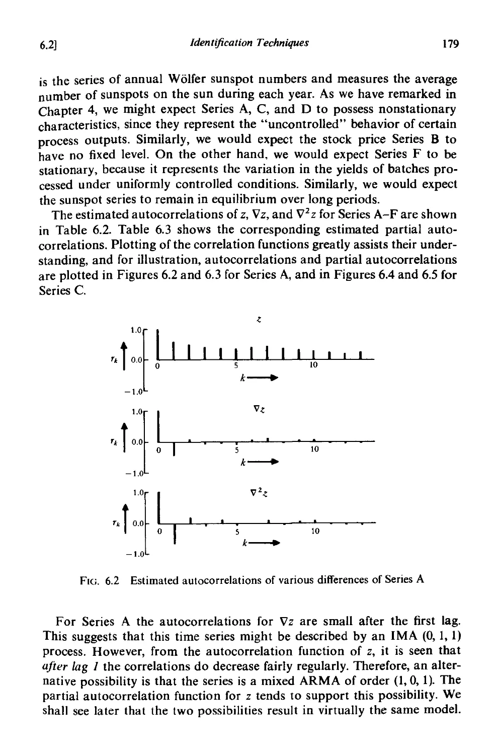
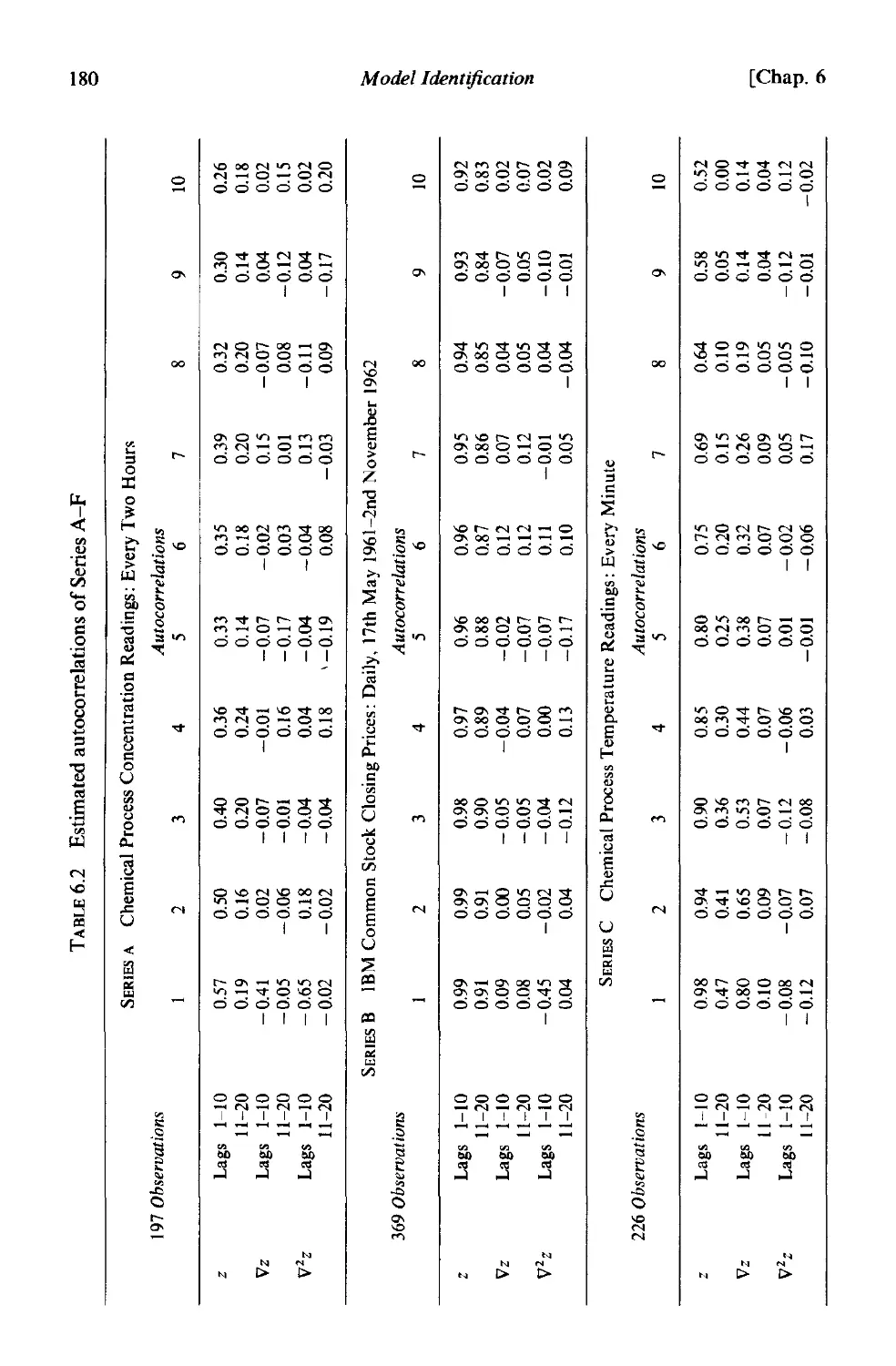
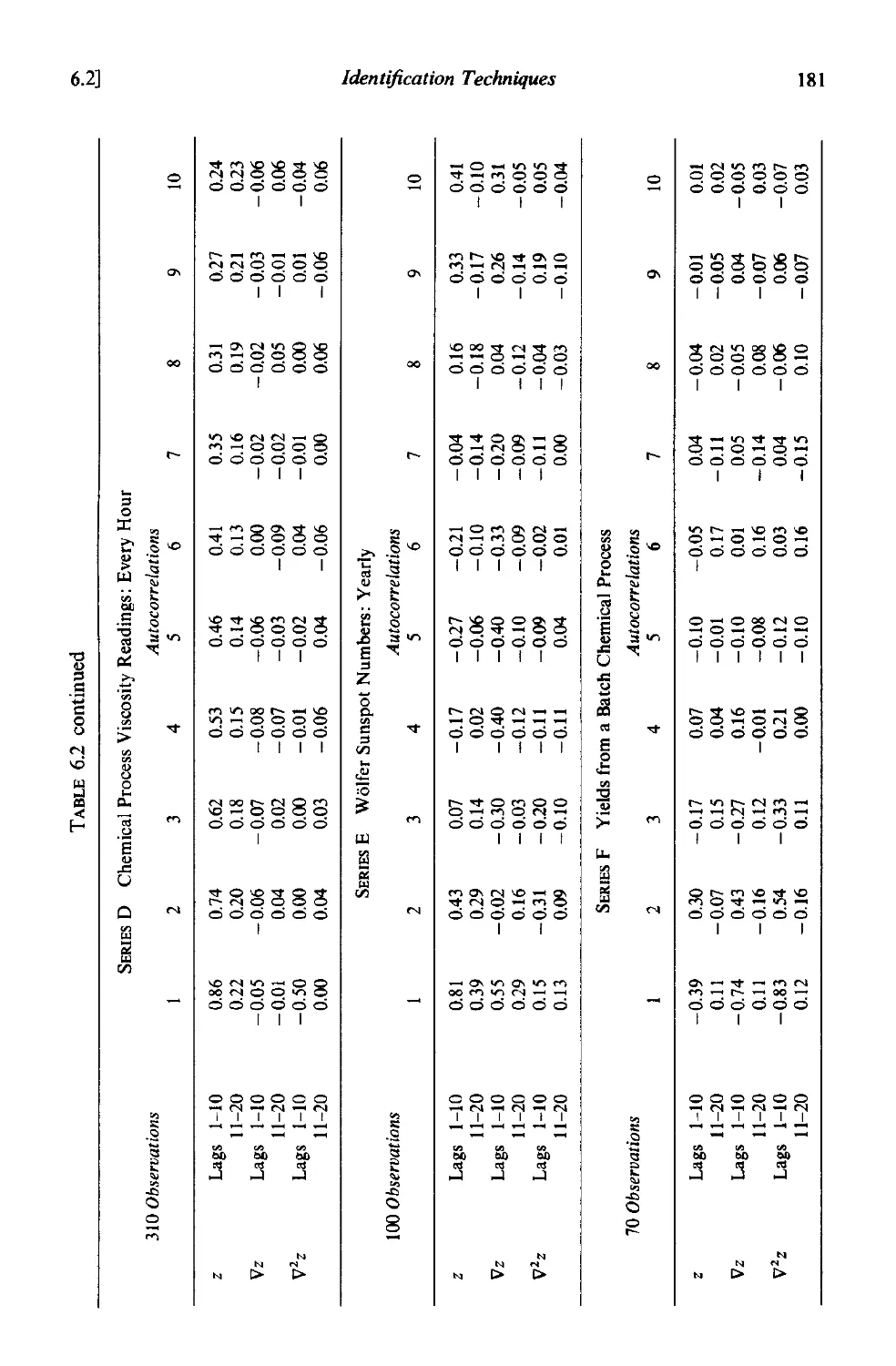
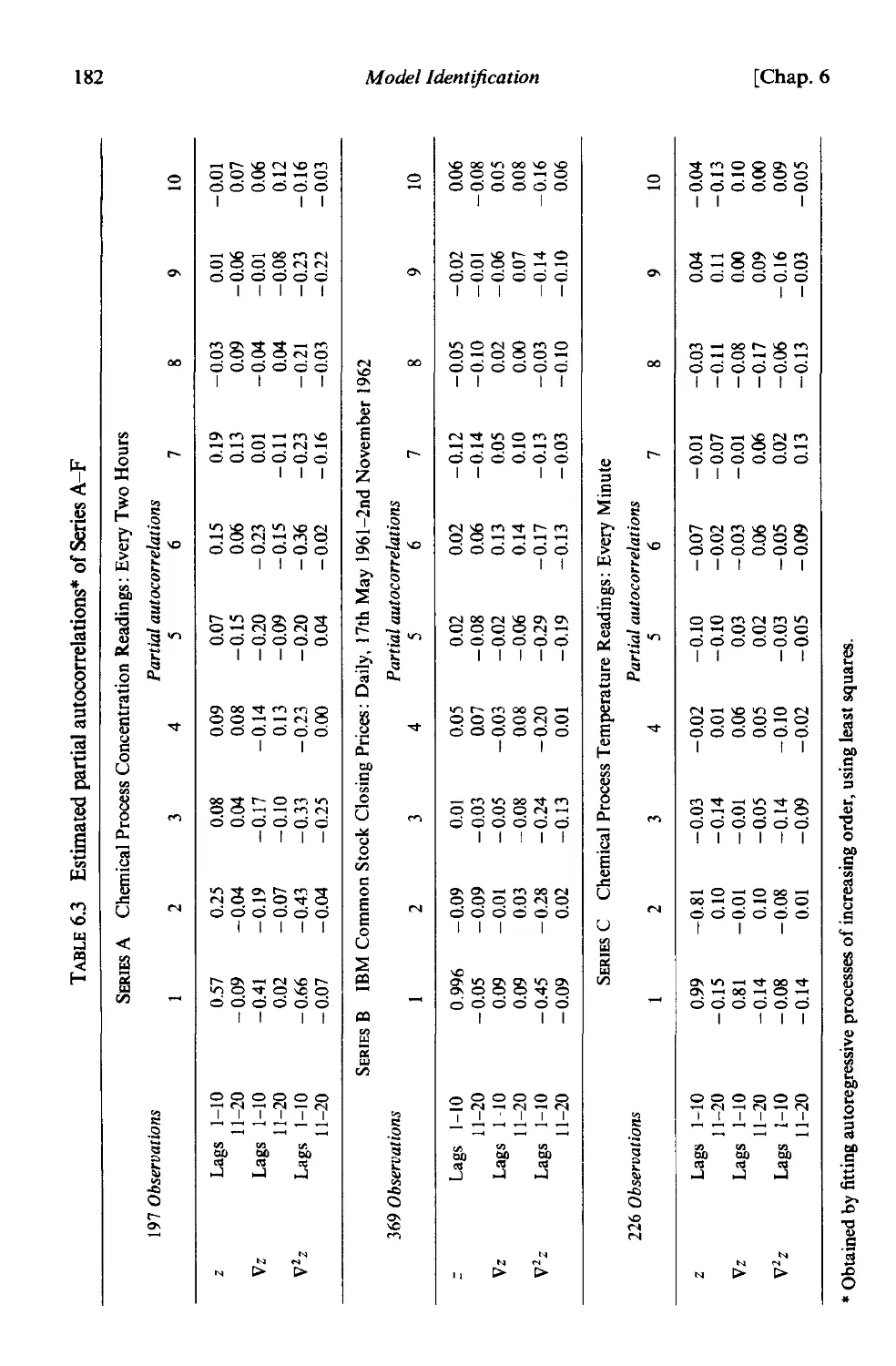
6.2.3 Identification of some actual time series 178
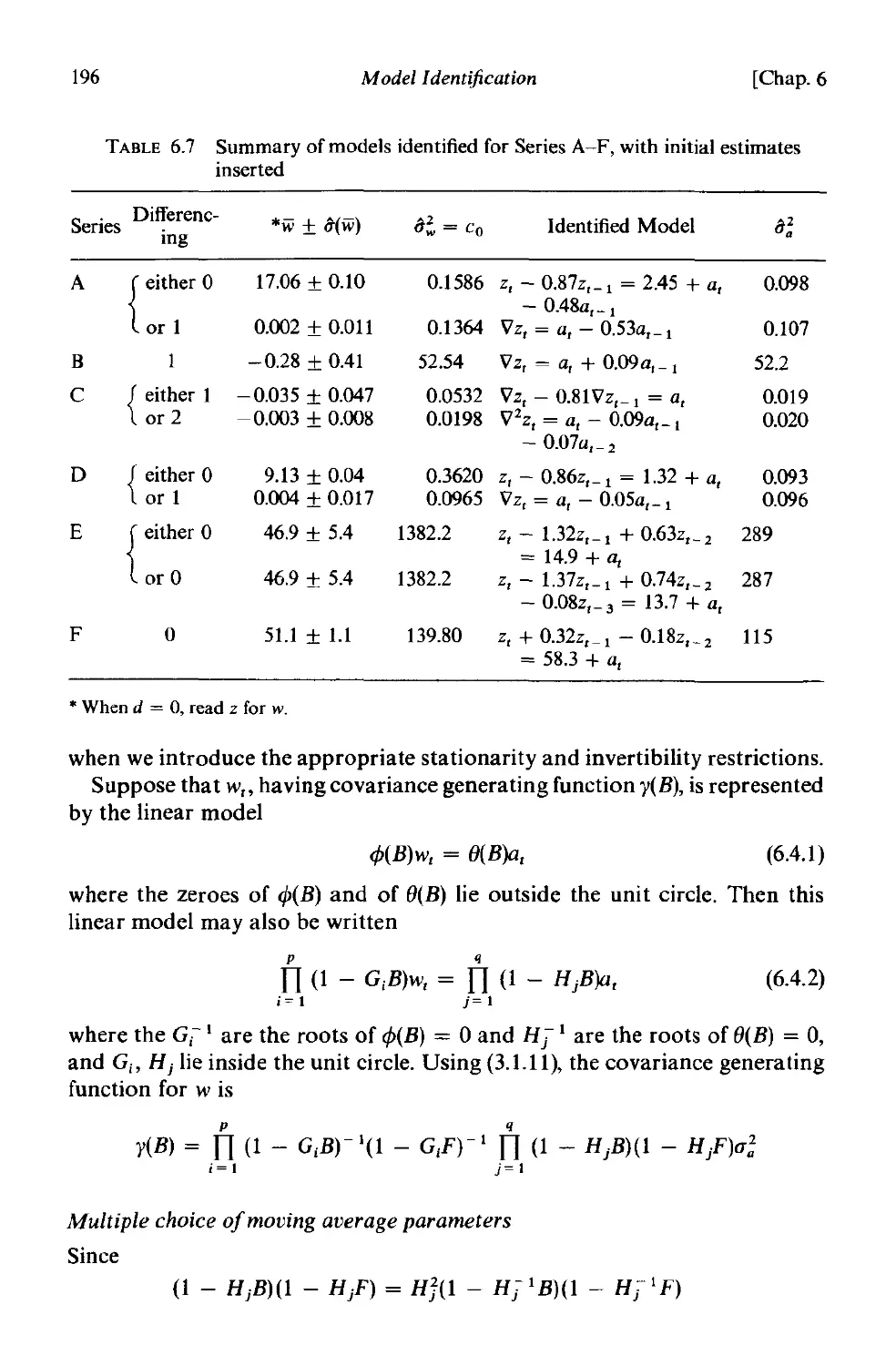
6.3 Initial estimates for the parameters 187
6.3.1 Uniqueness of estimates obtained from the autocovariance
function 187
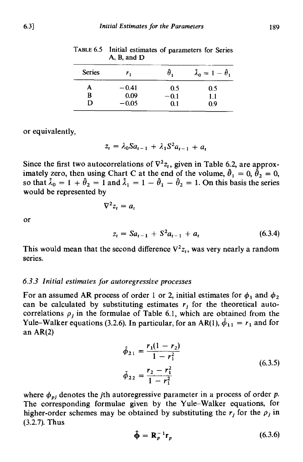
6.3.2 Initial estimates for moving average processes 187
6.3.3 Initial estimates for autoregressive processes 189
Contents xvii
6.3.4 Initial estimates for mixed autoregressive-moving average
processes 190
6.3.5 Choice between stationary and nonstationary models in
doubtful cases . 192
6.3.6 Initial estimate of residual variance . 193
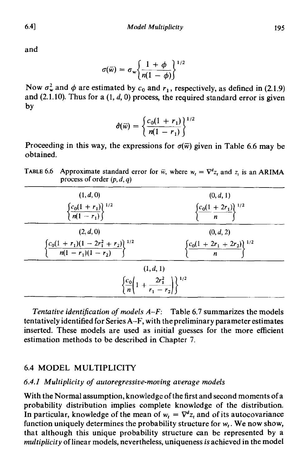
6.3.7 An approximate standard error for w 193
6.4 Model multiplicity . 195
6.4.1 Multiplicity of autoregressive-moving average models 195
6.4.2 Multiple moment solutions for moving average parameters. 198
6.4.3 Use of the backward process to determine starting values. 199
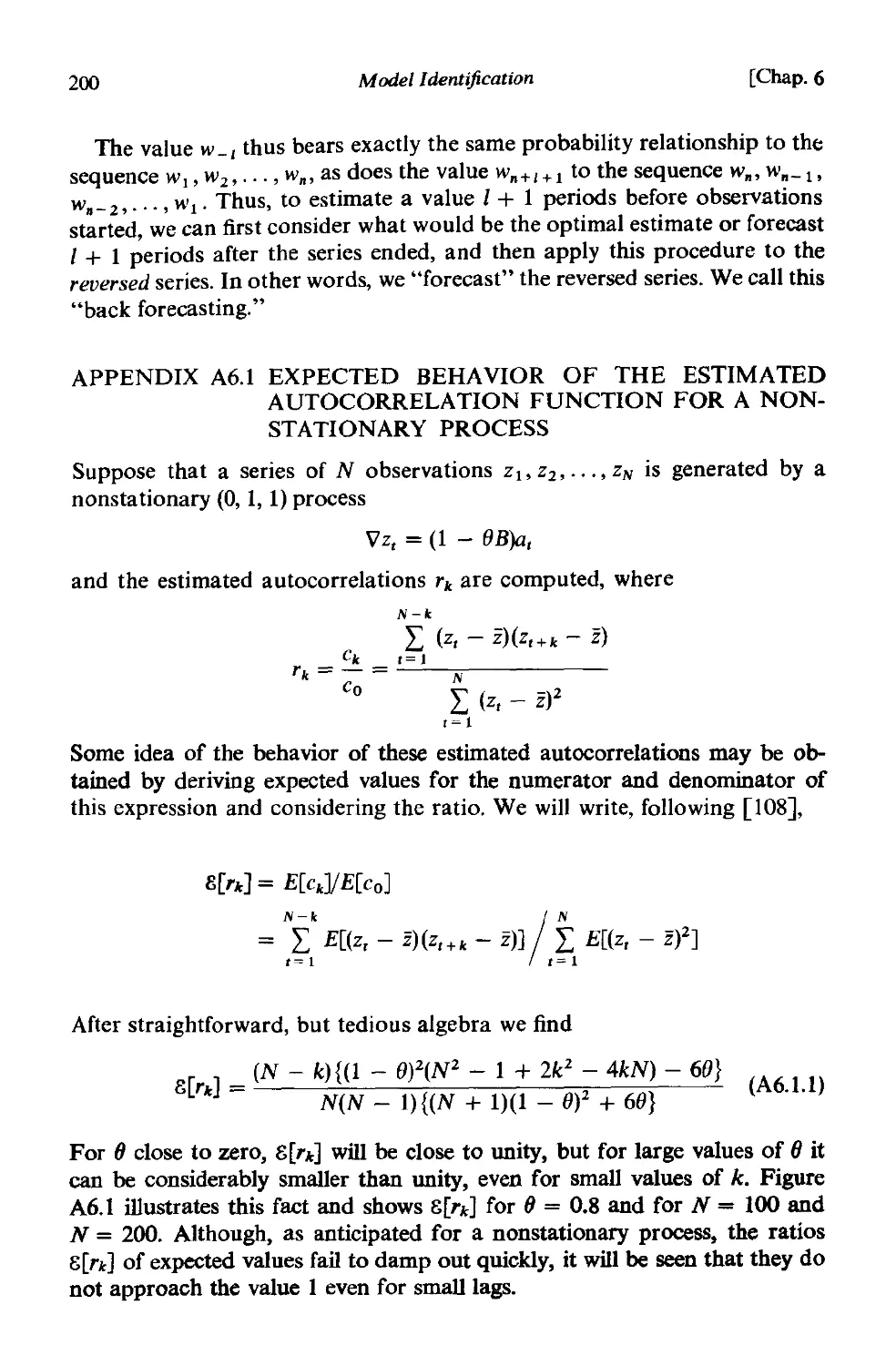
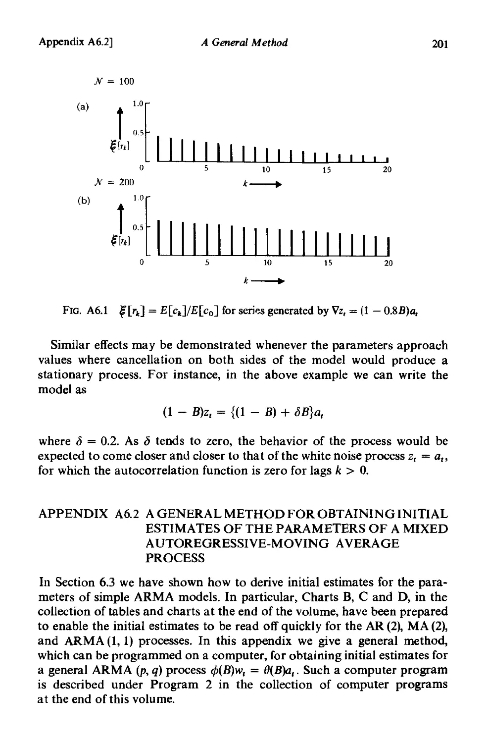
A6.1 Expected behaviour of the estimated autocorrelation function
for a non stationary process . 200
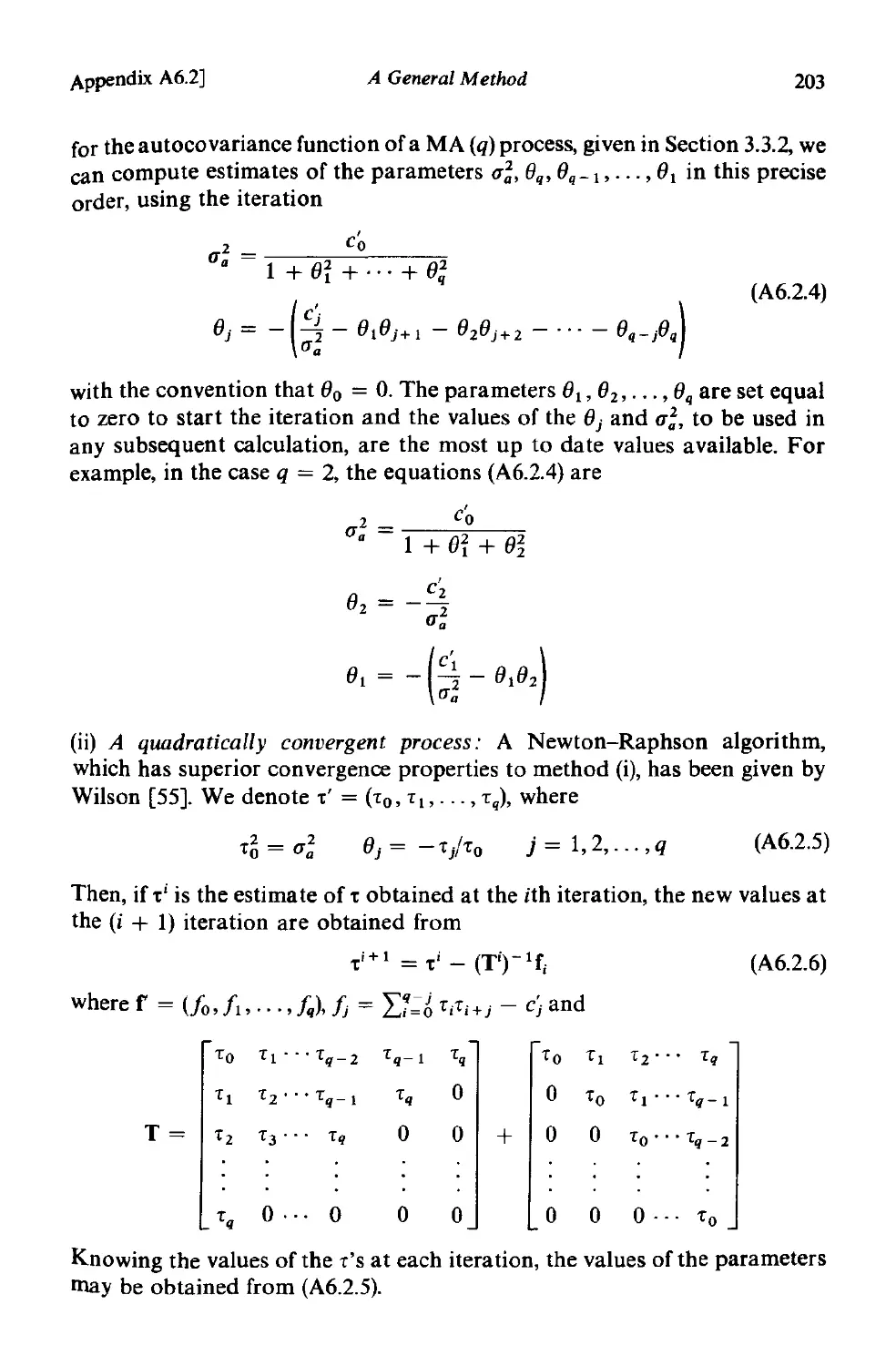
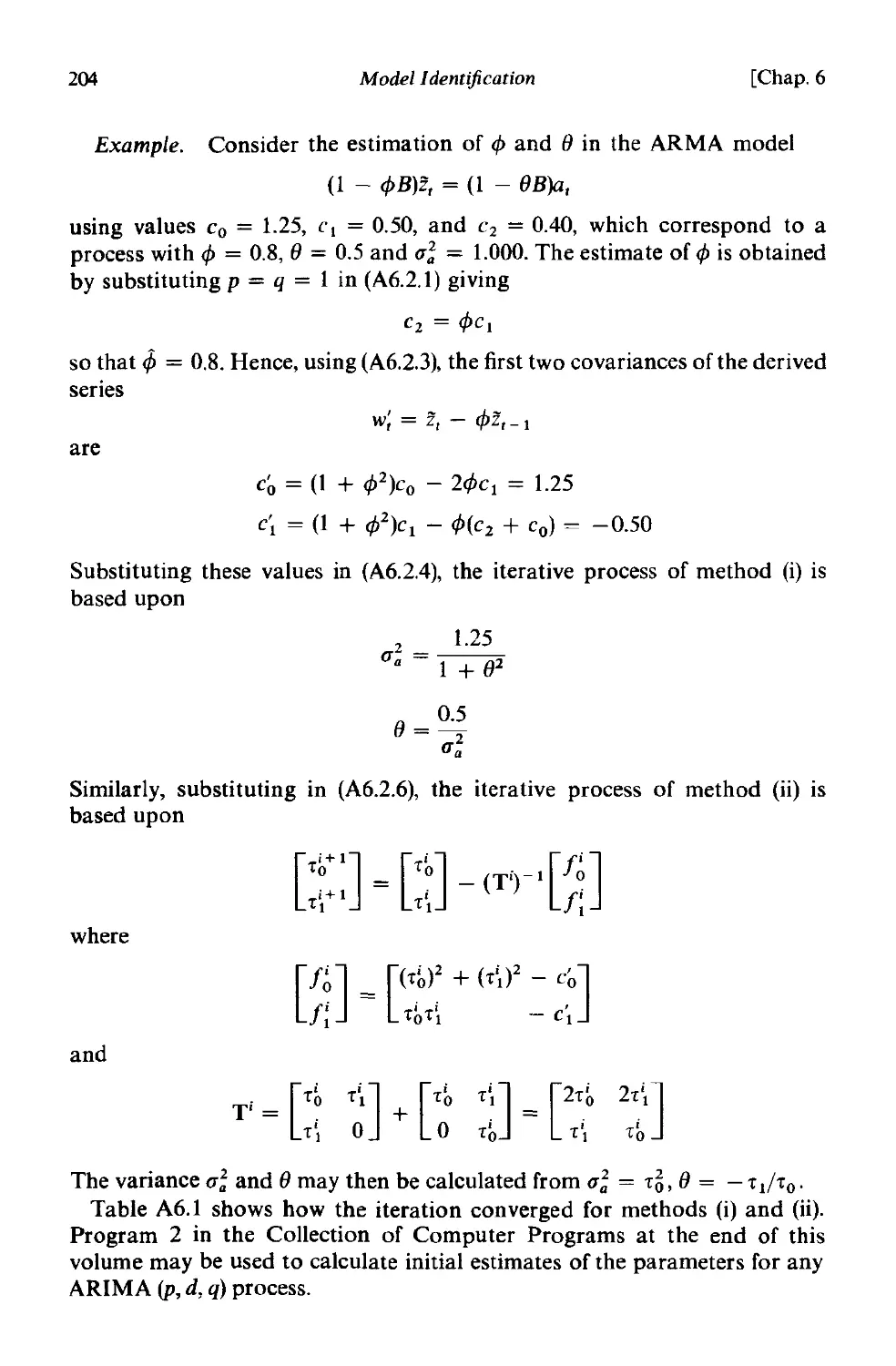
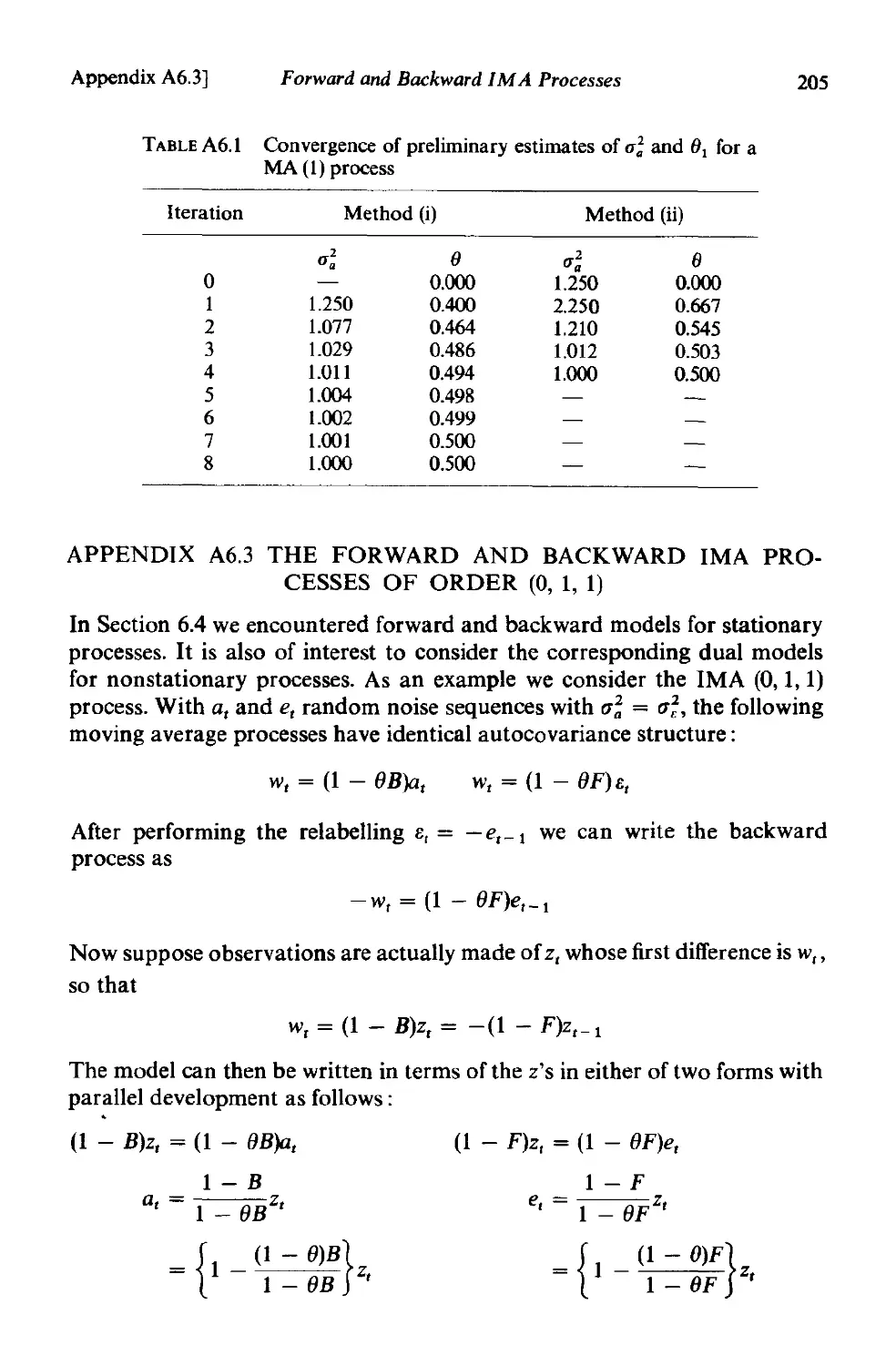
A6.2 A general method for obtaining initial estimates of the para-
meters of a mixed autoregressive-moving average process 201
A6.3 The forward and backward IMA processes of order (0, 1, I). 205
CHAPTER 7 MODEL ESTIMATION
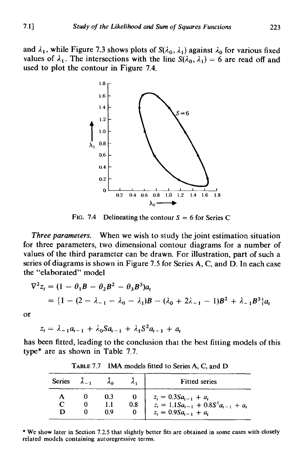
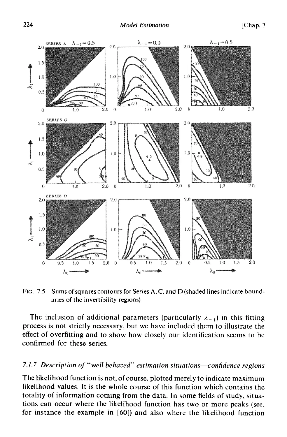
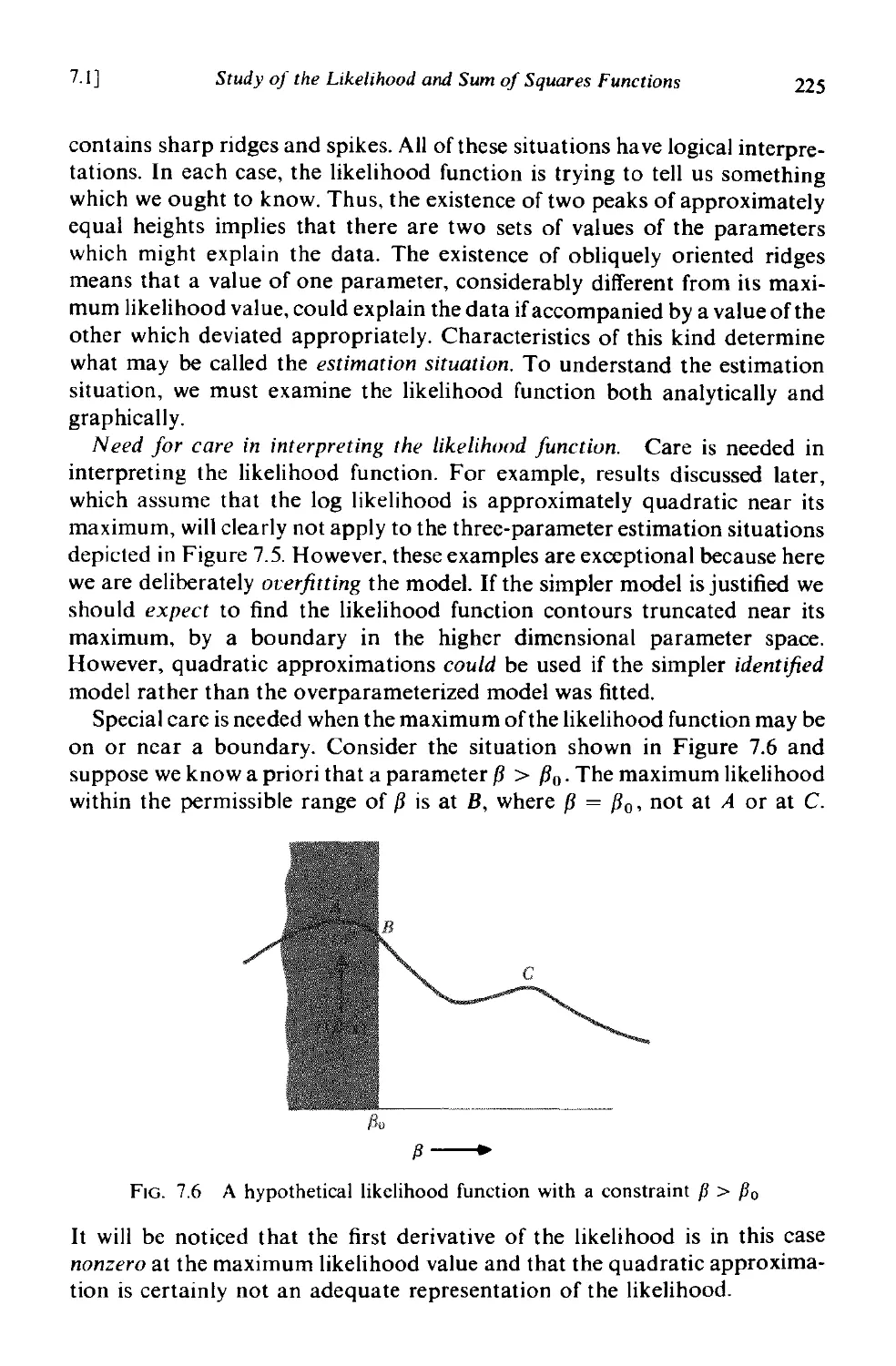
7.1 Study of the likelihood and sum of squares functions 208
7.1.1 The likelihood function 208
7.1.2 The conditional likelihood for an ARIMA process 209
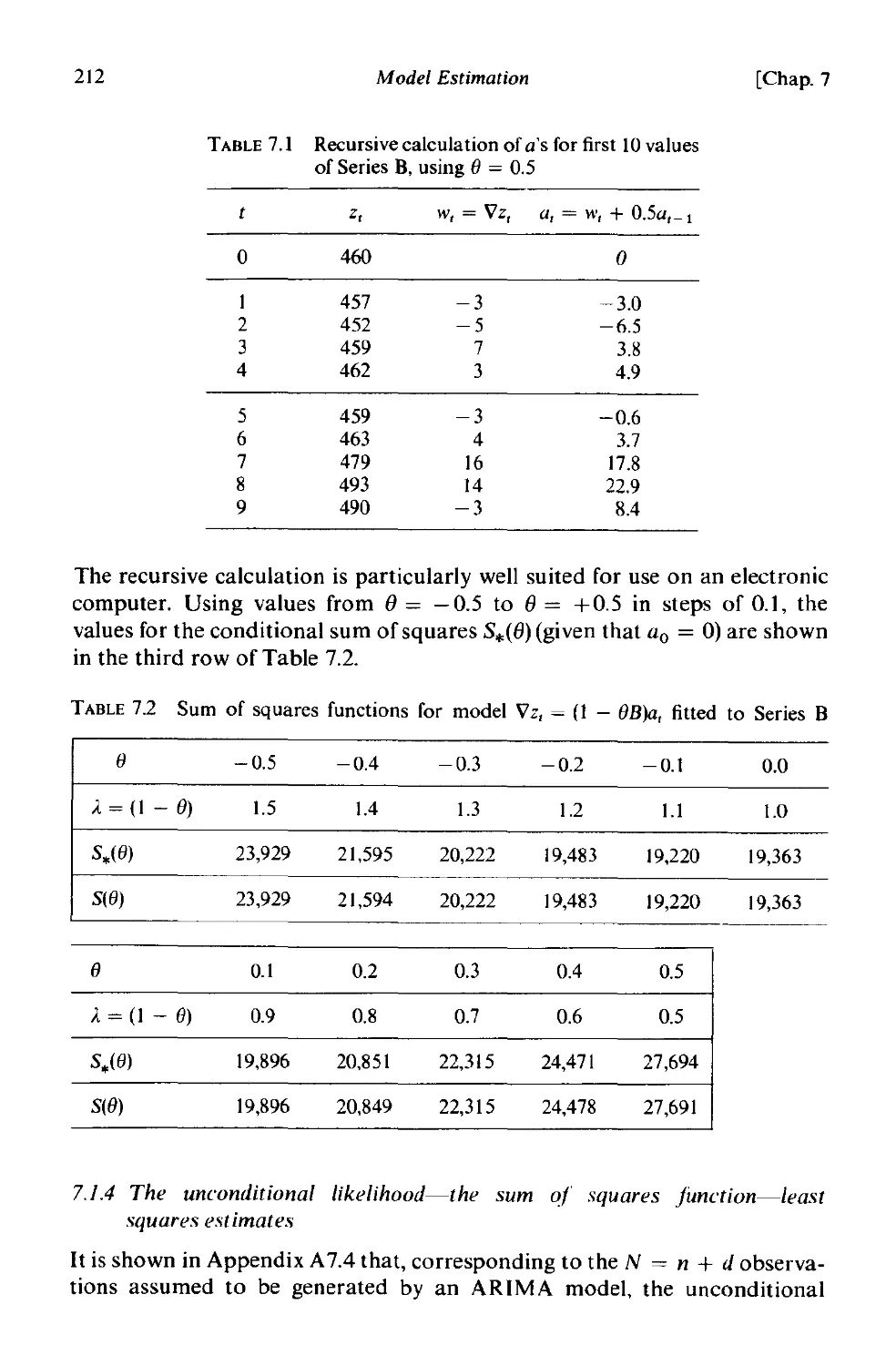
7.1.3 Choice of starting values for conditional calculation 210
7.1.4 The unconditional likelihood-the sum of squares function
-least squares estimates . 212
7.1.5 General procedure for calculating the unconditional sum
of squares 215
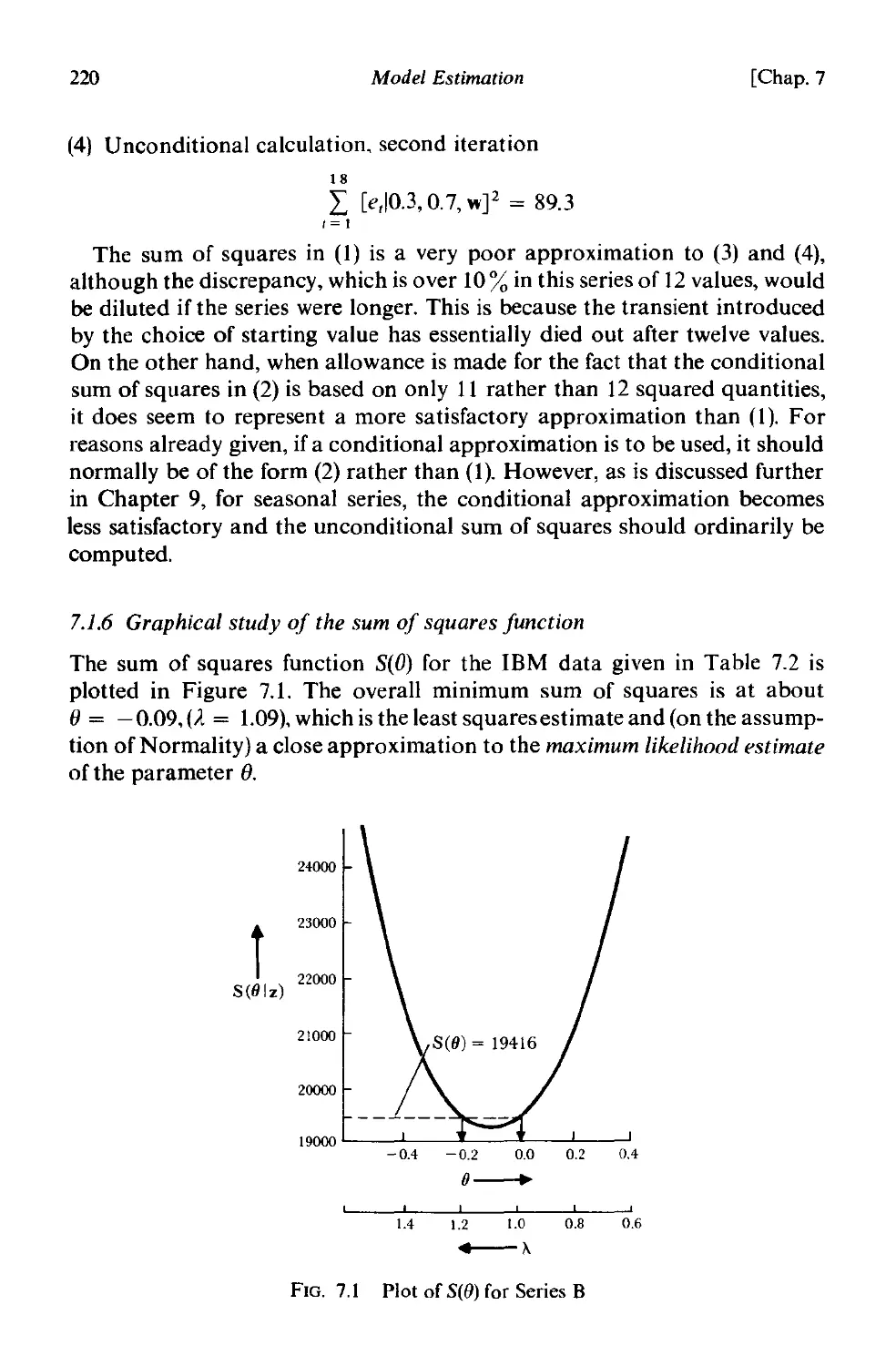
7.1.6 Graphical study of the sum of squares function . 220
7.1. 7 Description of "well-behaved" estimation situations-
confidence regions . 224
7.2 Nonlinear estimation 231
7.2.1 General method of approach 231
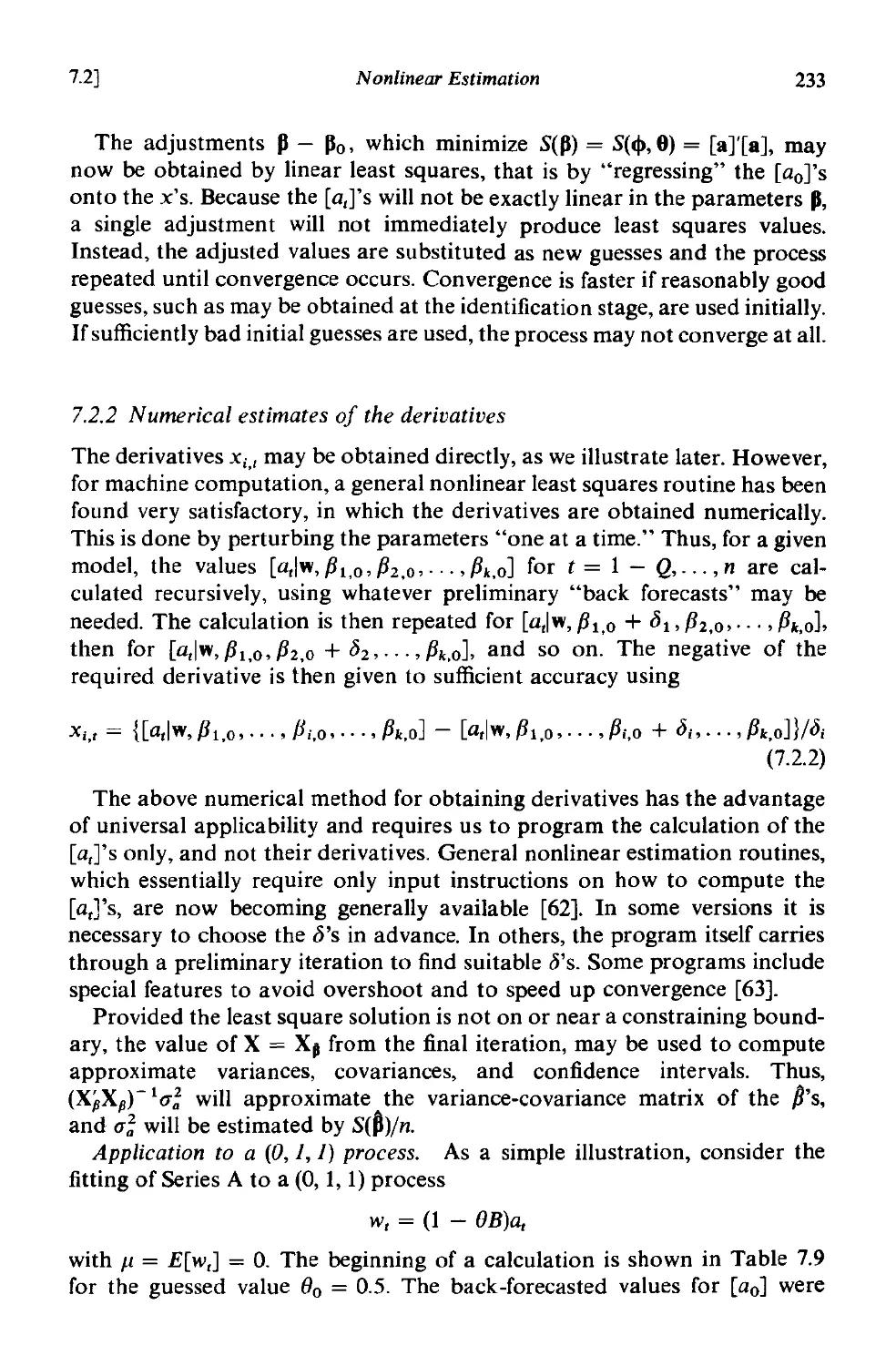
7.2.2 Numerical estimates ofthe derivatives 233
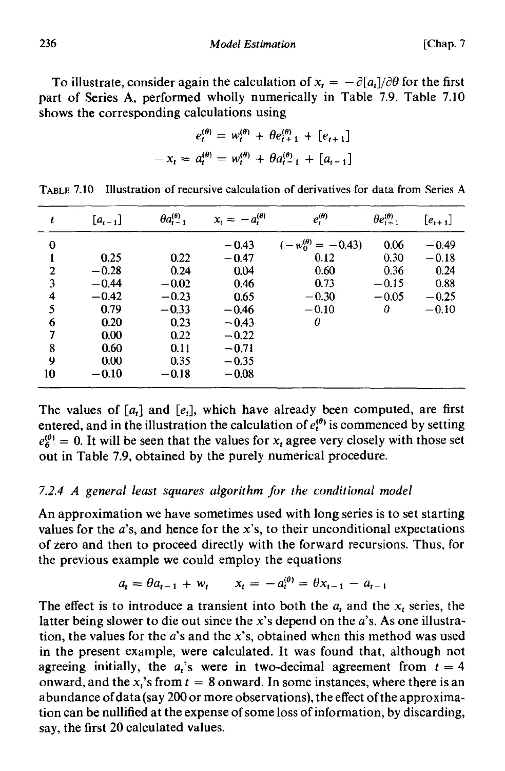
7.2.3 Direct evaluation of the derivatives . 235
7.2.4 A general least squares algorithm for the conditional model 236
7.2.5 Summary of models fitted to Series A-F 238
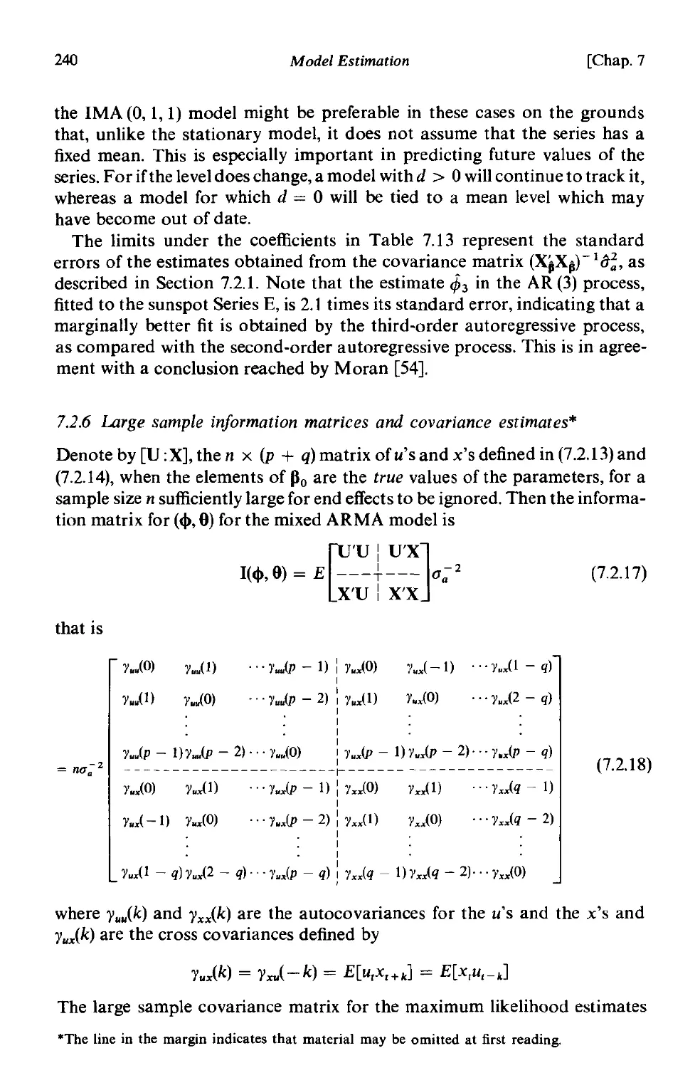
7.2.6 Large sample information matrices and covariance estim-
ates . 240
7.3 Some estimation results for specific models 243
7.3.1 ,Autoregressive processes . 243
7.3.2 Moving average processes 245
7.3.3 Mixed processes 245
7.3.4 Separation of linear and nonlinear components in estim-
ation 6
xviii
Contents
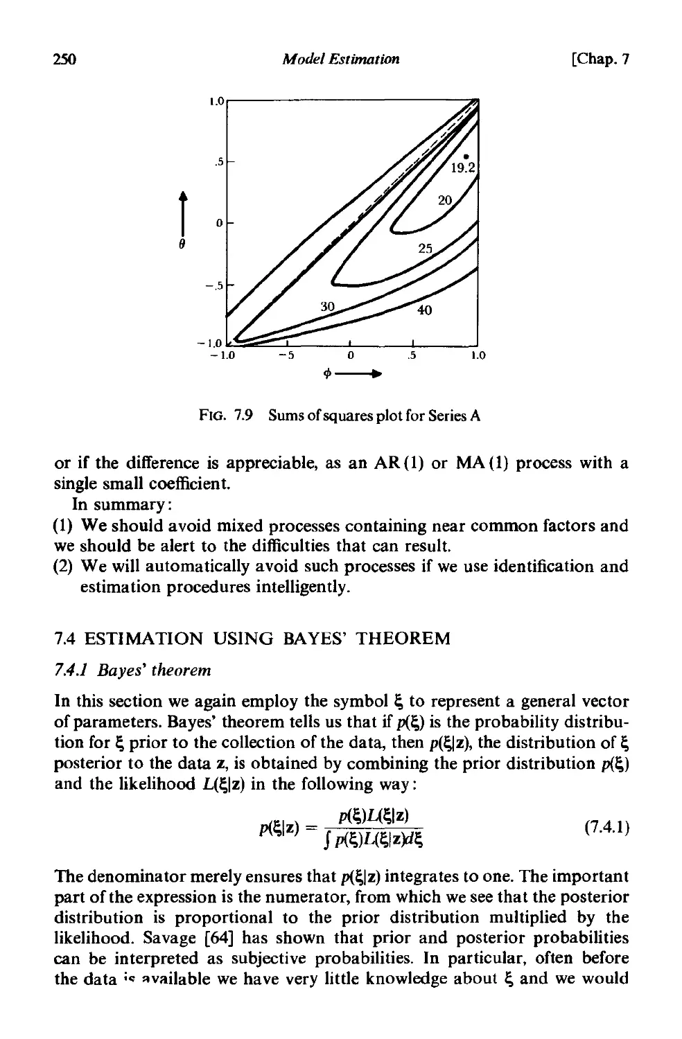
7.3.5 Parameter redundancy 248
7.4 Estimation using Bayes' theorem 250
7.4.1 Bayes' theorem 250
7.4.2 Bayesian estimation of parameters 252
7.4.3 Autoregressive processes . 253
7.4.4 Moving average processes 255
7.4.5 Mixed processes 257
A 1.1 Review of normal distribution theory 258
A 1.2 A review of linear least squares theory . 265
A 1.3 Examples of the effect of parameter estimation errors on
probability limits for forecasts . 267
A7.4 The exact likelihood function for a moving average process 269
A7.5 The exact likelihood function for an autoregressive process 274
A 1.6 Special note on estimation of moving average parameters 284
CHAPTER 8 MODEL DIAGNOSTIC CHECKING
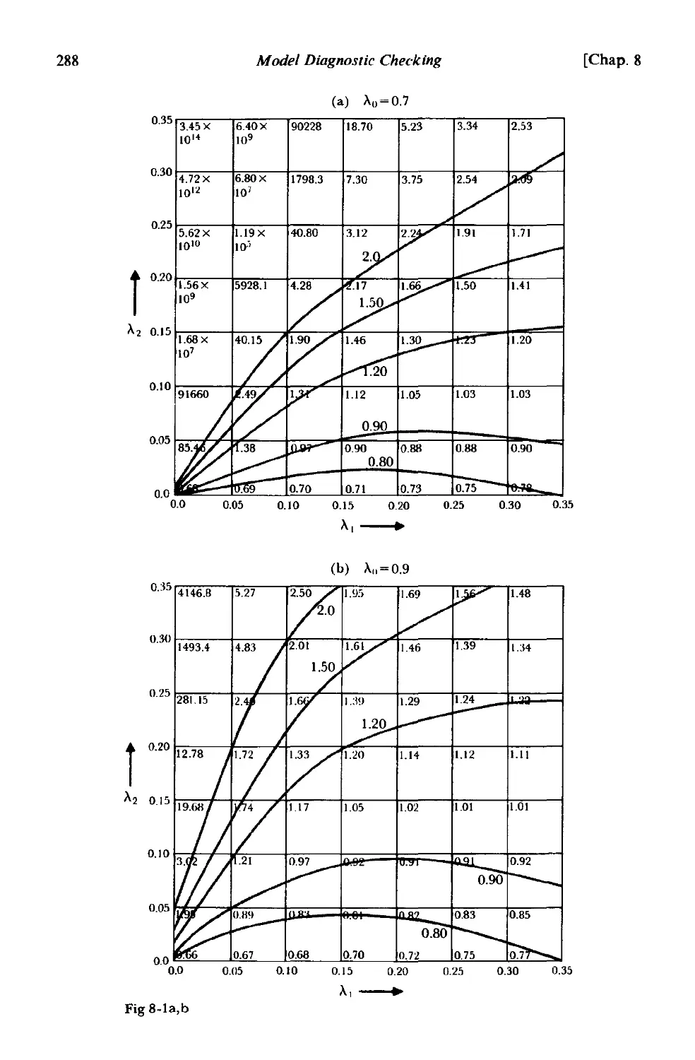
8.1 Checking the stochastic model. 285
8.1.1 General philosophy 285
8.1.2 Overfitting . 286
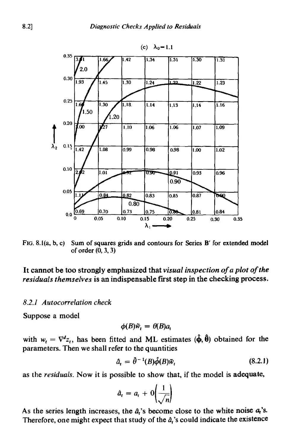
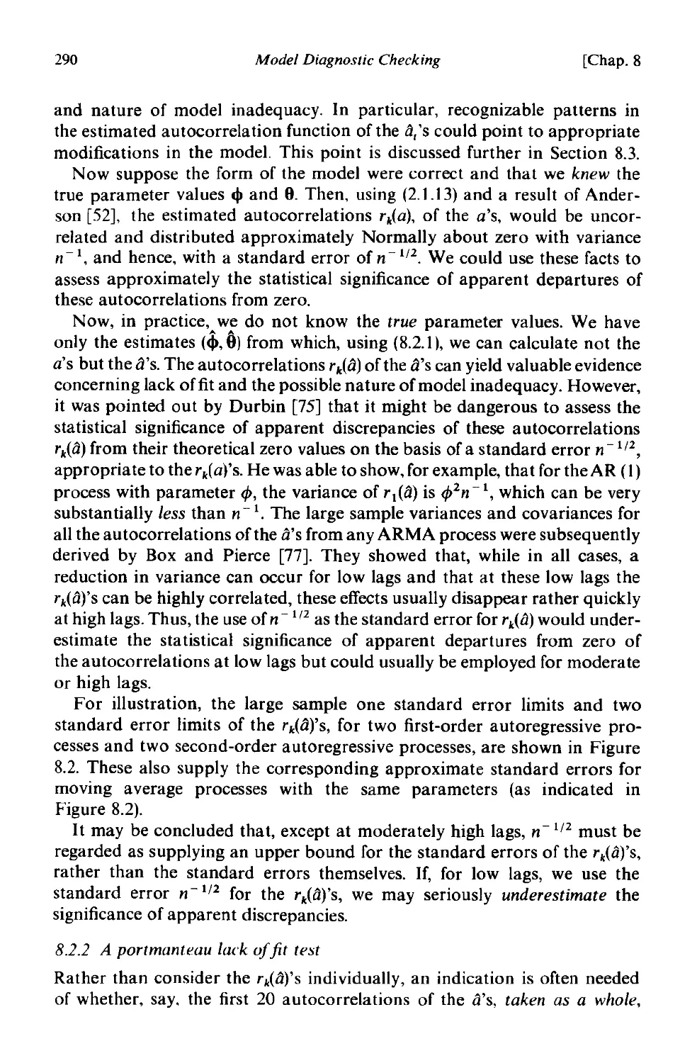
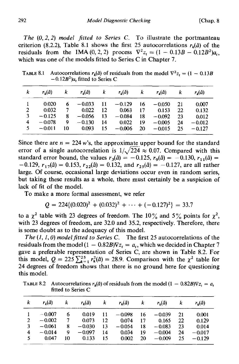
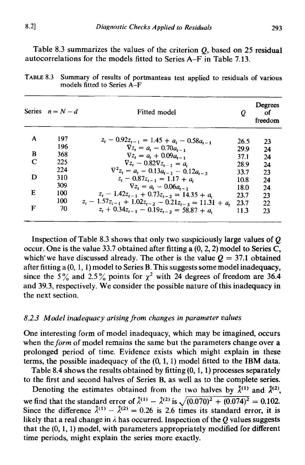
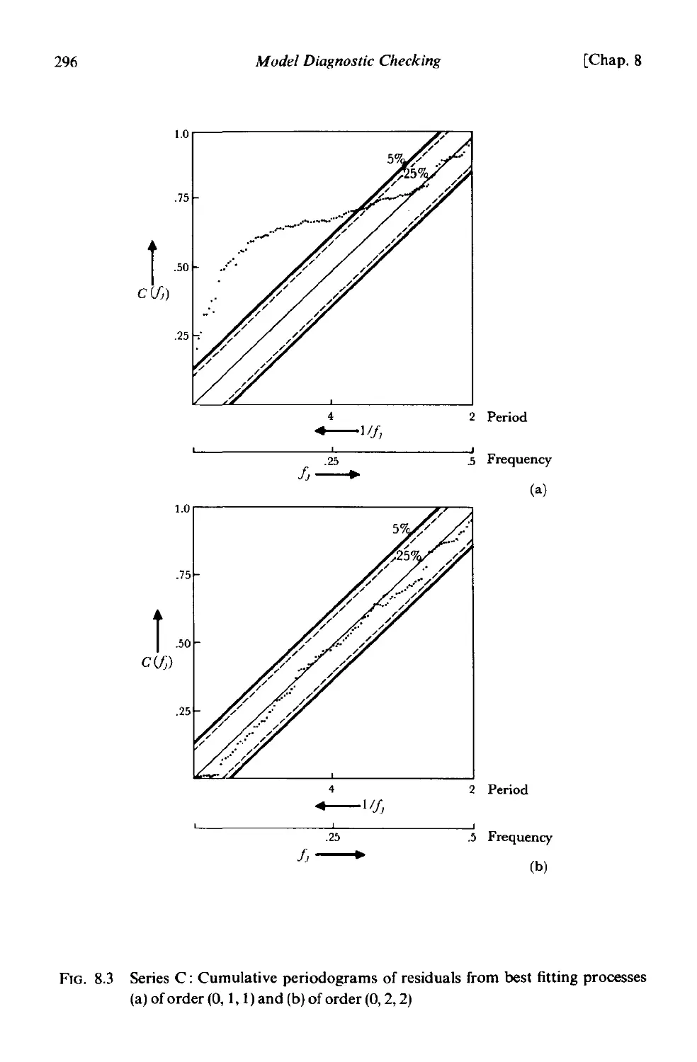
8.2 Diagnostic checks applied to residuals 281
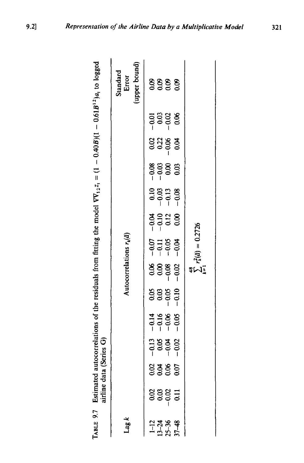
8.2.1 Autocorrelation check 289
8.2.2 A portmanteau lack of fit test 290
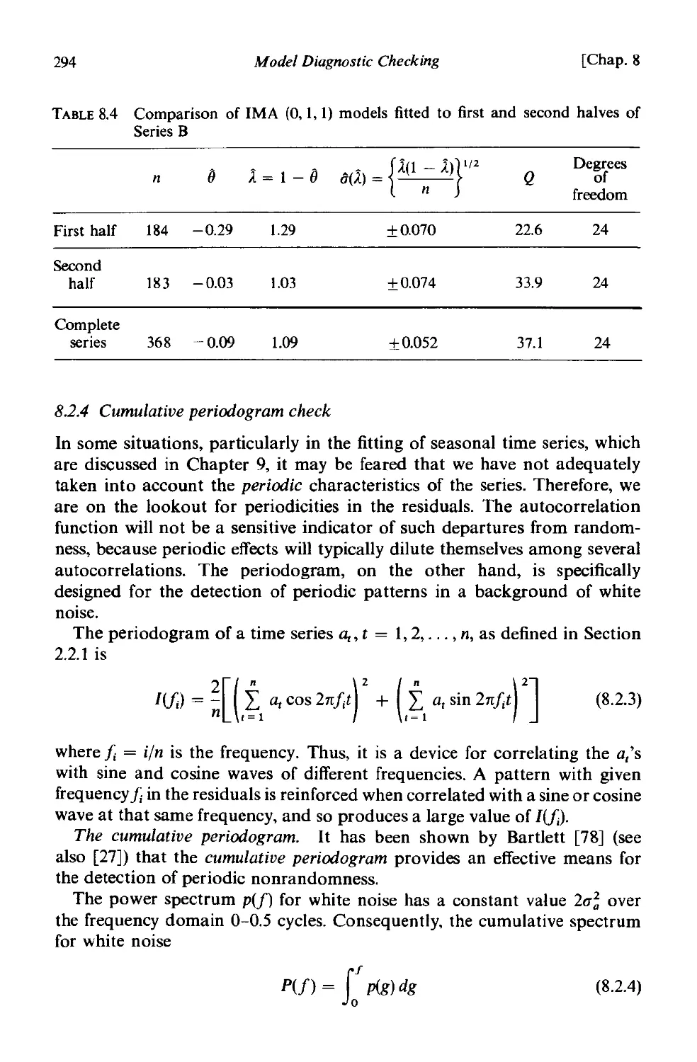
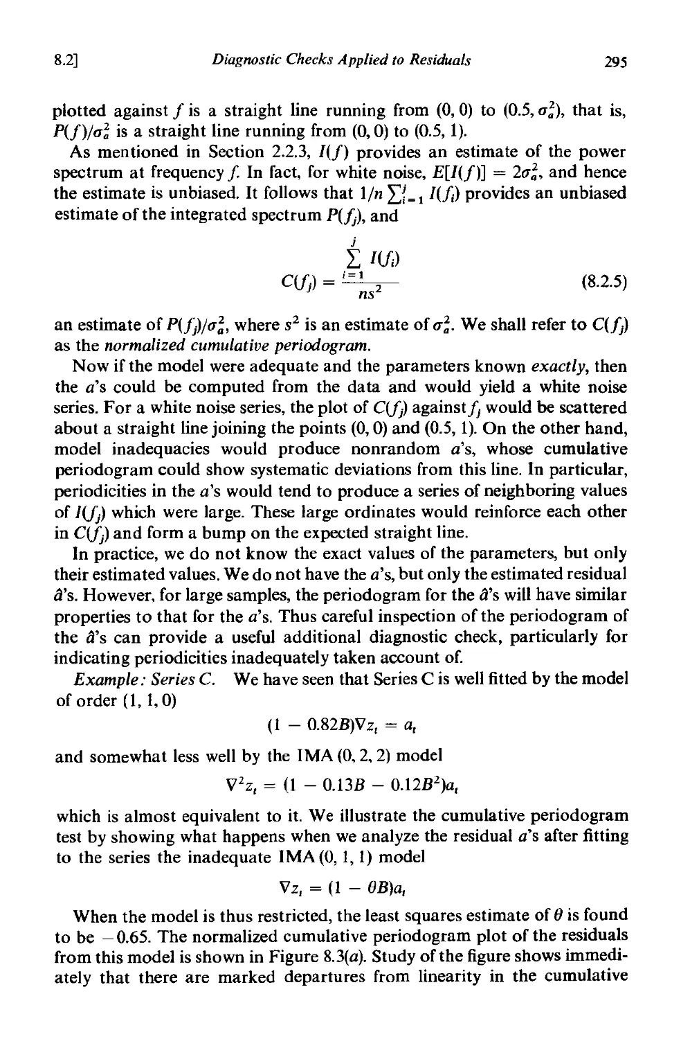
8.2.3 Model inadequacy arising from changes in parameter values 293
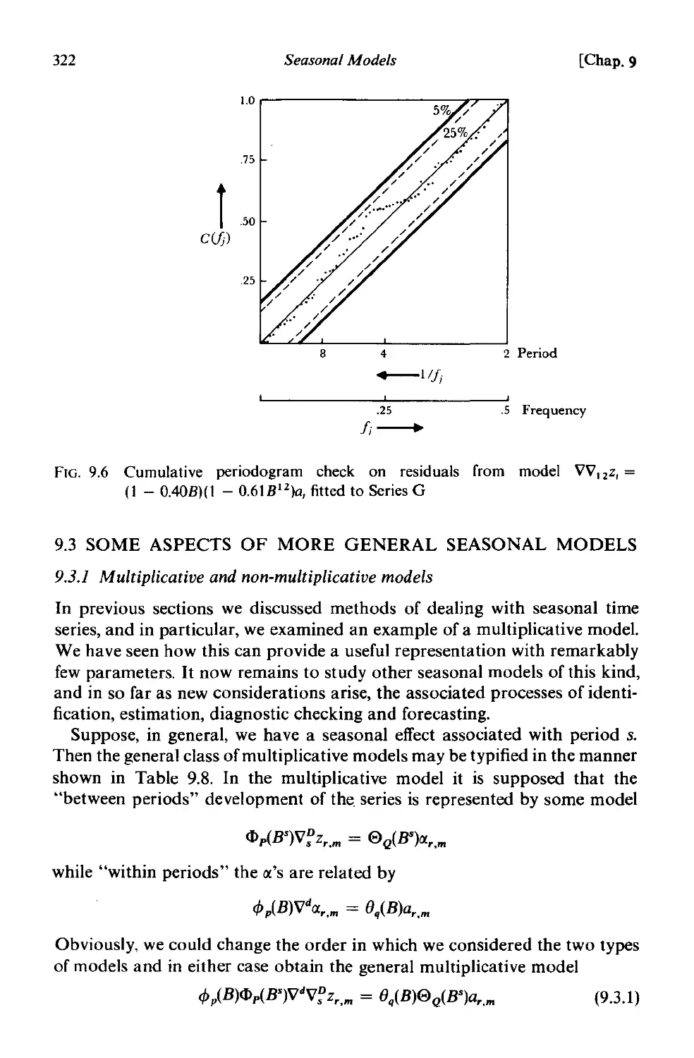
8.2.4 Cumulative periodogram check . 294
8.3 Use of residuals to modify the model 298
8.3.1 Nature of the correlations in the residuals when an incorrect
model is used 298
8.3.2 Use of residuals to modify the model 299
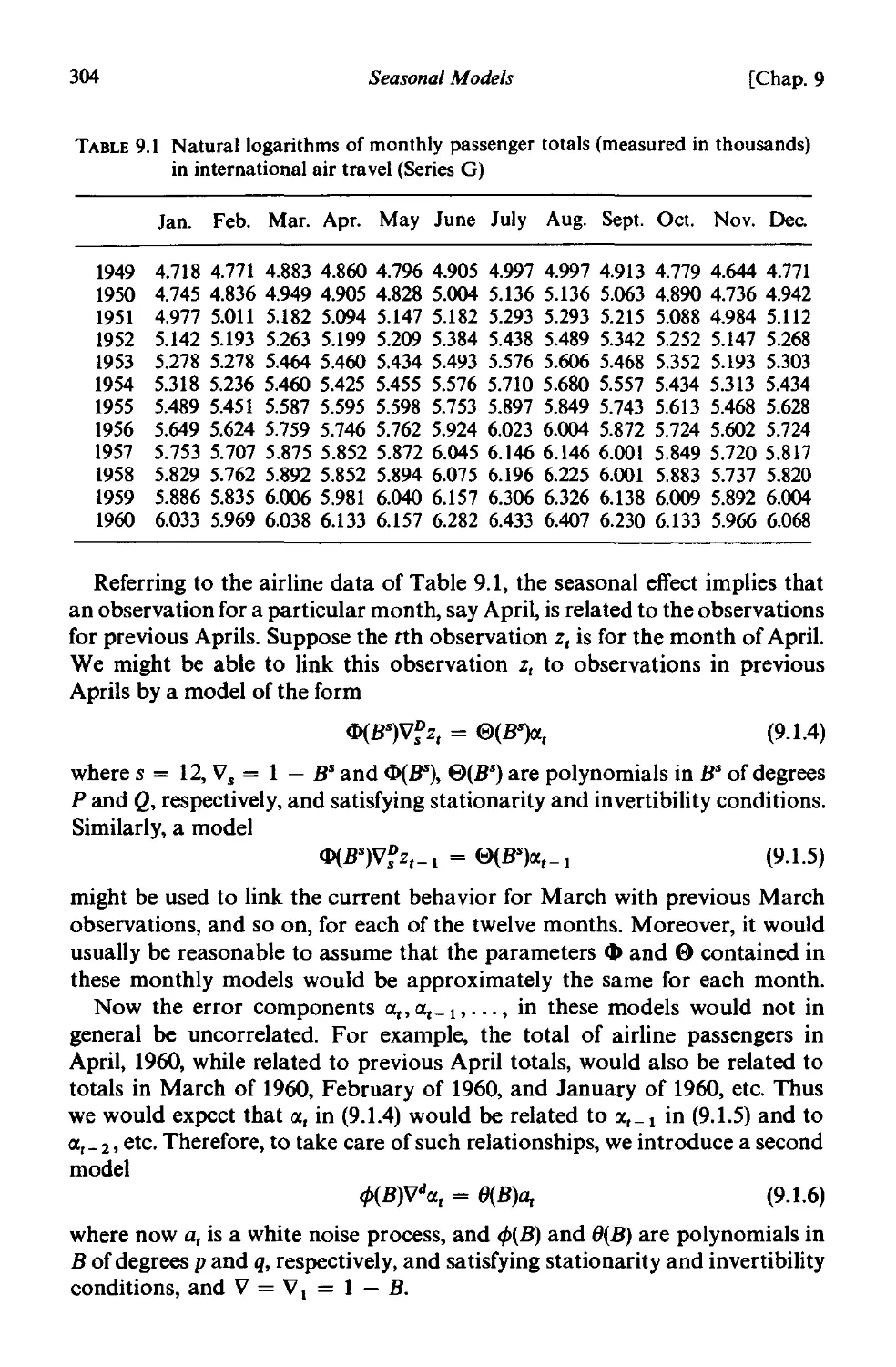
CHAPTER 9 SEASONAL MODELS
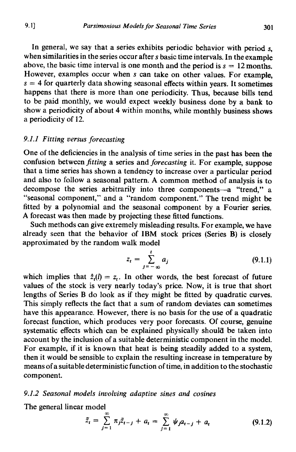
9.1 Parsimonious models for seasonal time series 300
9.1.1 Pitting versus forecasting 301
9.1.2 Seasonal models involving adaptive sines and cosines 30 I
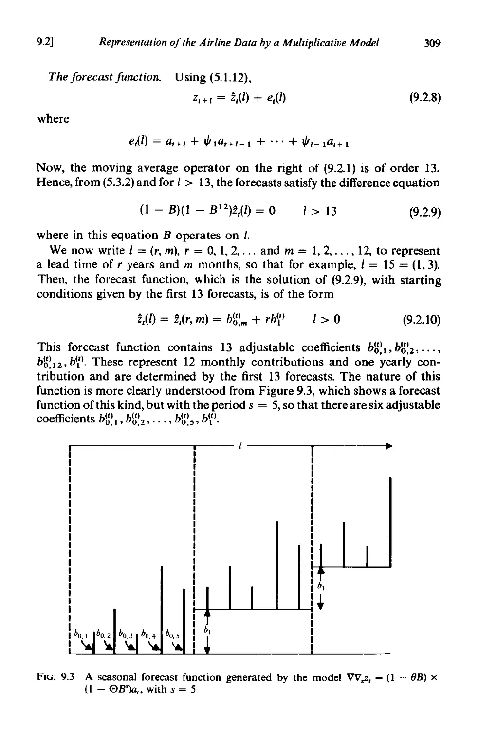
9.1.3 The general multiplicative seasonal model . 303
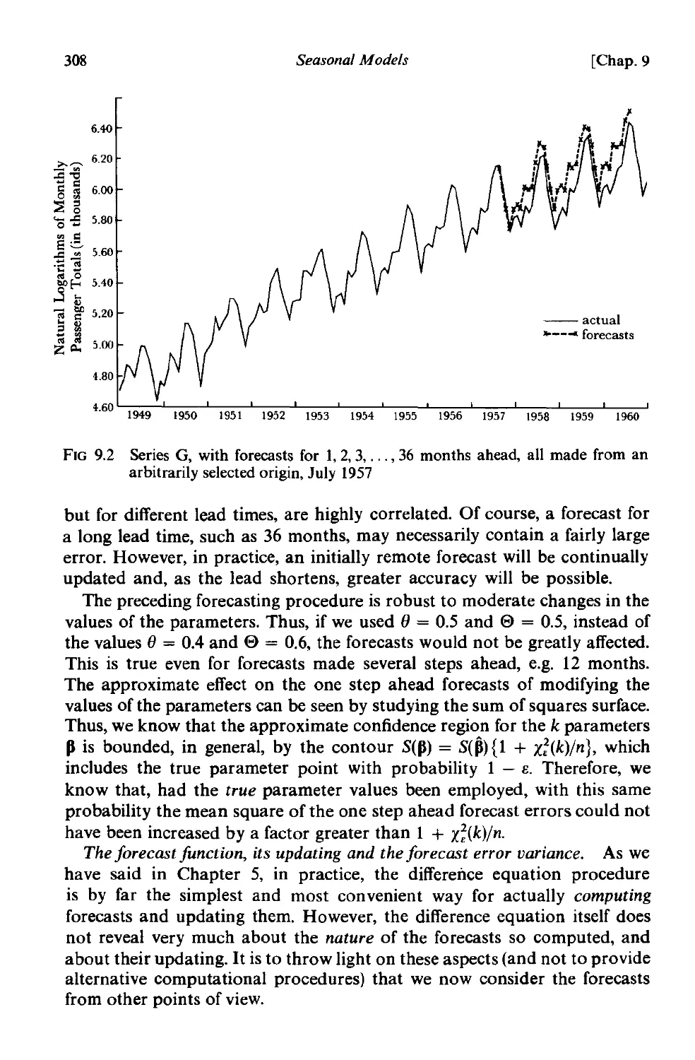
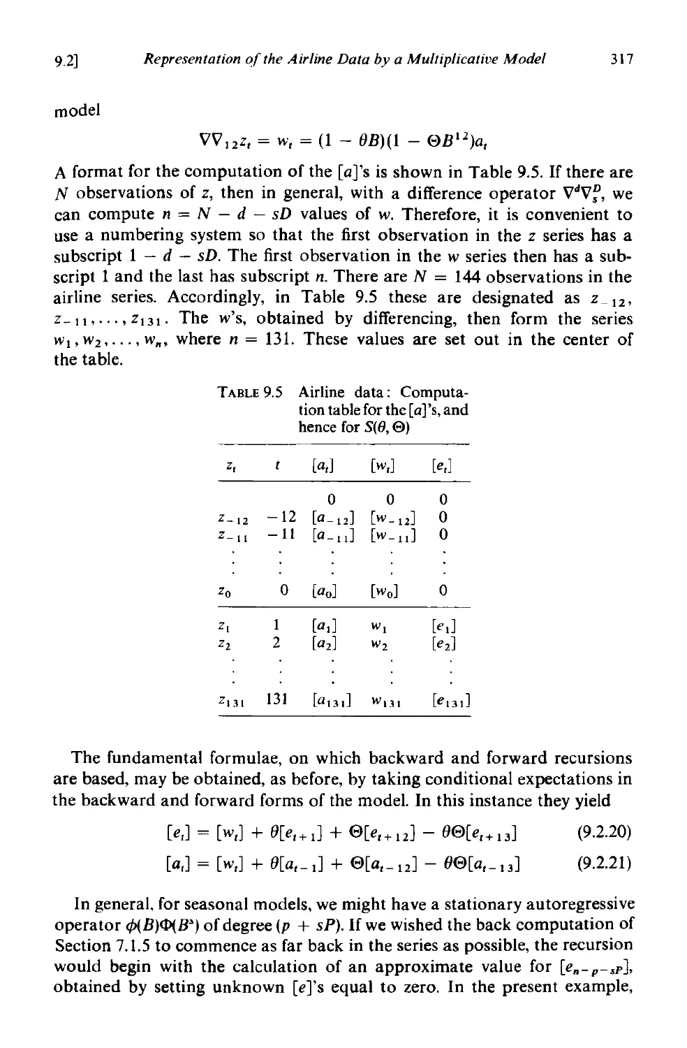
9.2 Representation of the airline data by a multiplicative (0, I, I) x
(0, I, 1)12 seasonal model . 305
9.2.1 The multiplicative (0, I, I) x (0, I, l)12 model 305
9.2.2 Forecasting. 306
9.2.3 Identification 313
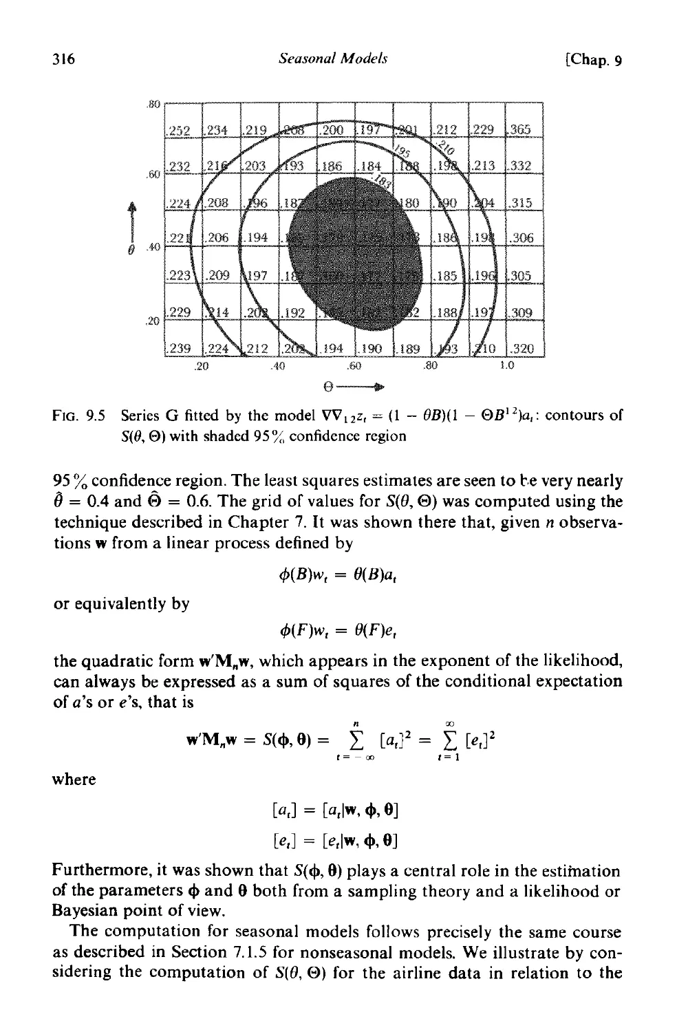
9.2.4 Estimation . 315
9.2.5 Diagnostic checking 320
9.3 Some aspects of more general seasonal models 322
9.3.1 Multiplicative and non multiplicative models 322
Contents xix
9.3.2 Identification 324
9.3.3 Estimation . 325
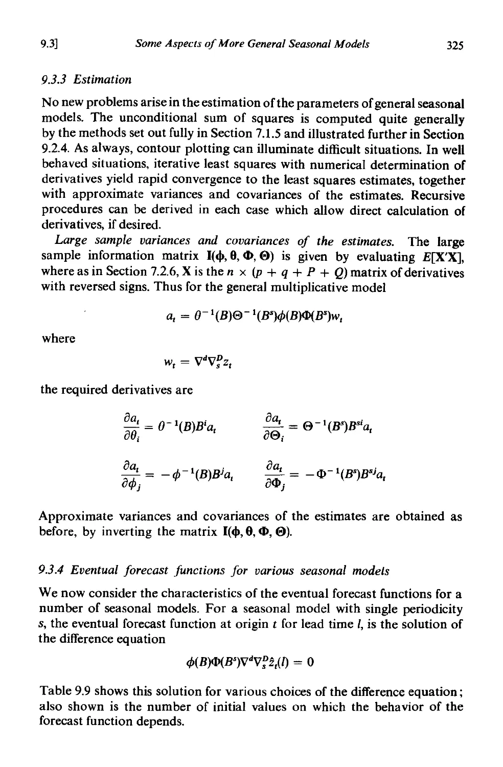
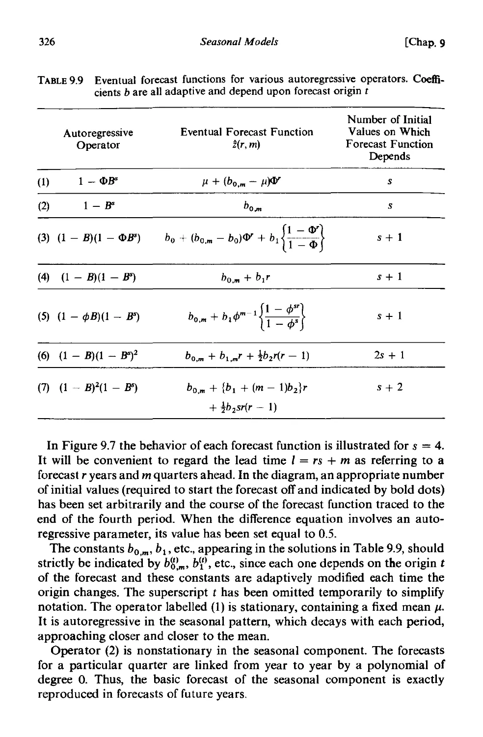
9.3.4 Eventual forecast functions for various seasonal models 325
9.3.5 Choice of transformation . 328
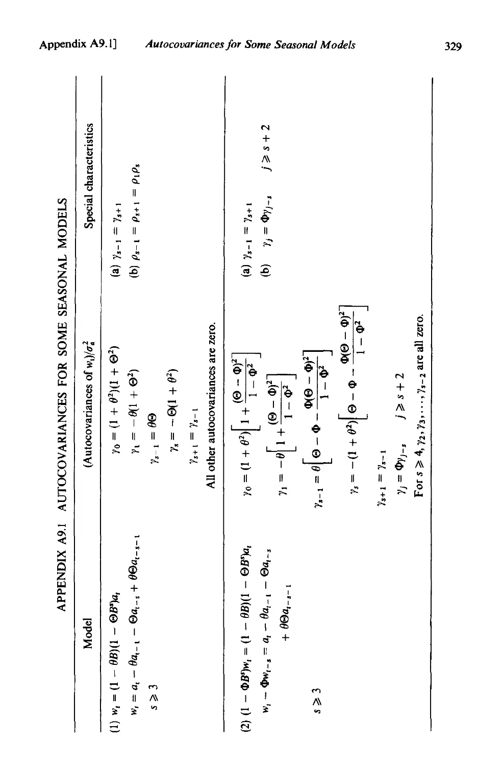
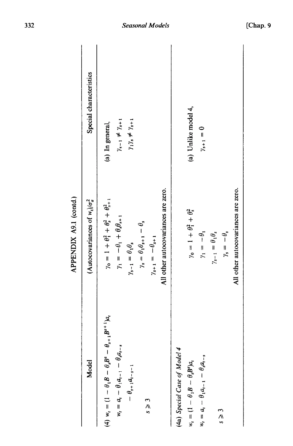
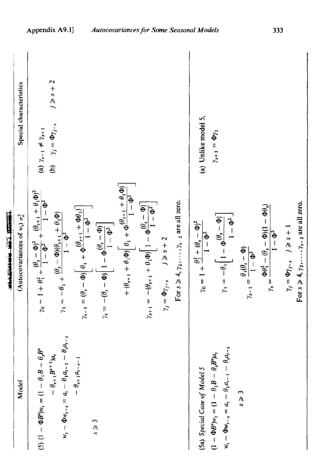
A9.l Autocovariances for some seasonal models 329
PART III TRANSFER FUNCTION MODEL BUILDING
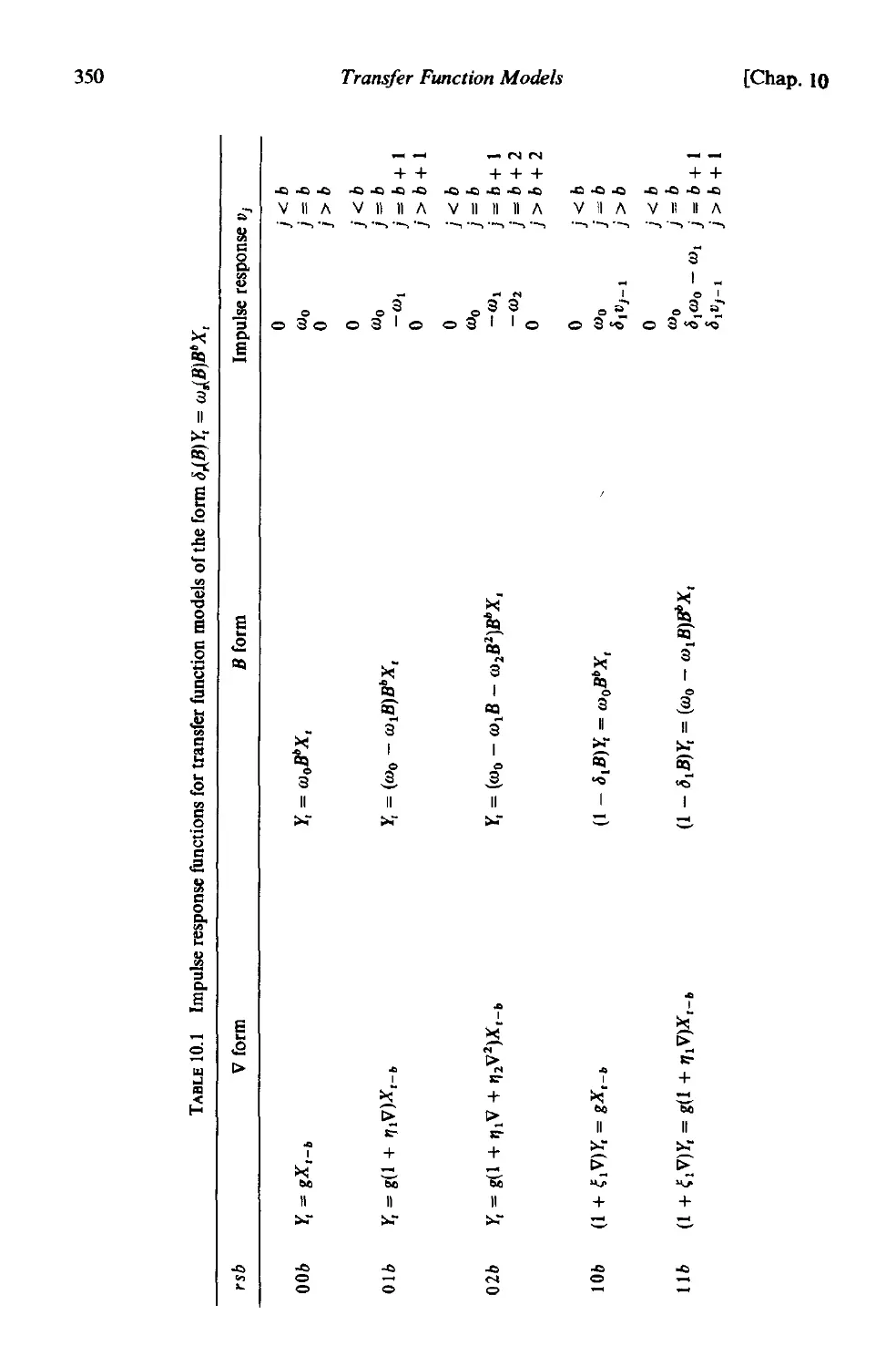
CHAPTER 10 TRANSFER FUNCTION MODELS
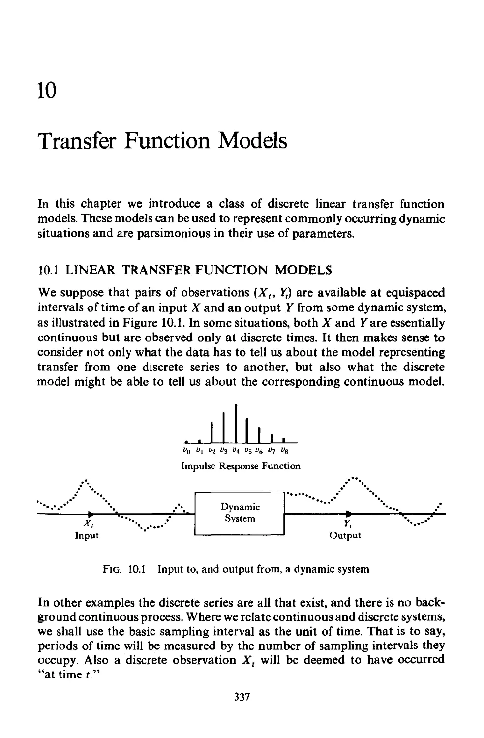
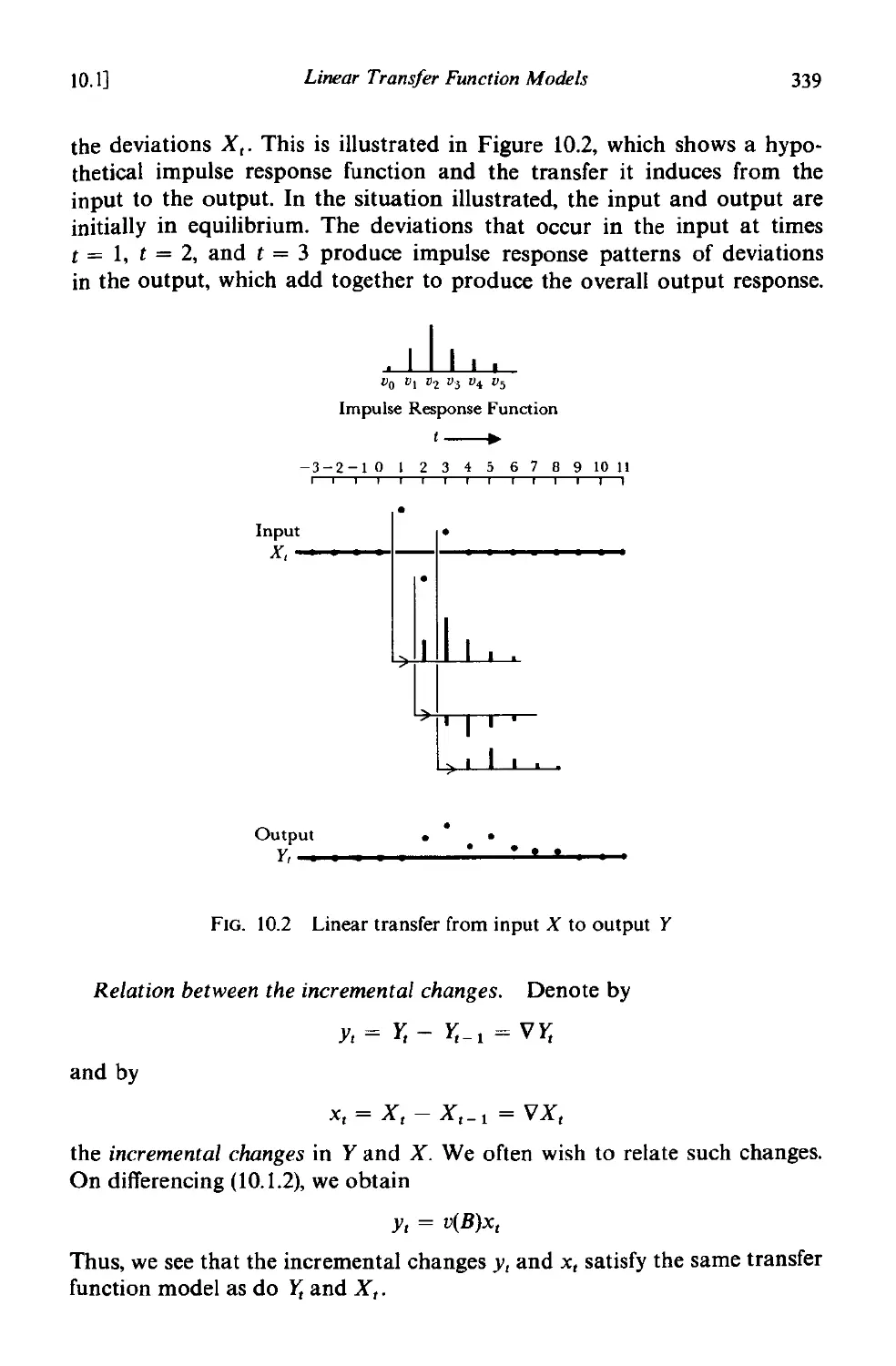
10.1 Linear transfer function models 337
10.1.1 The discrete transfer function 338
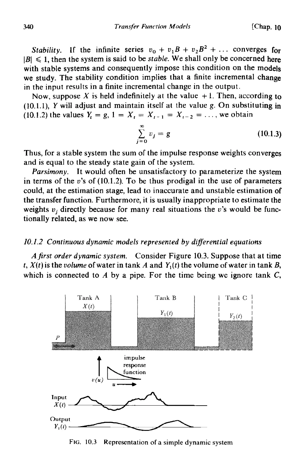
10.1.2 Continuous dynamic models represented by differential
equations . 340
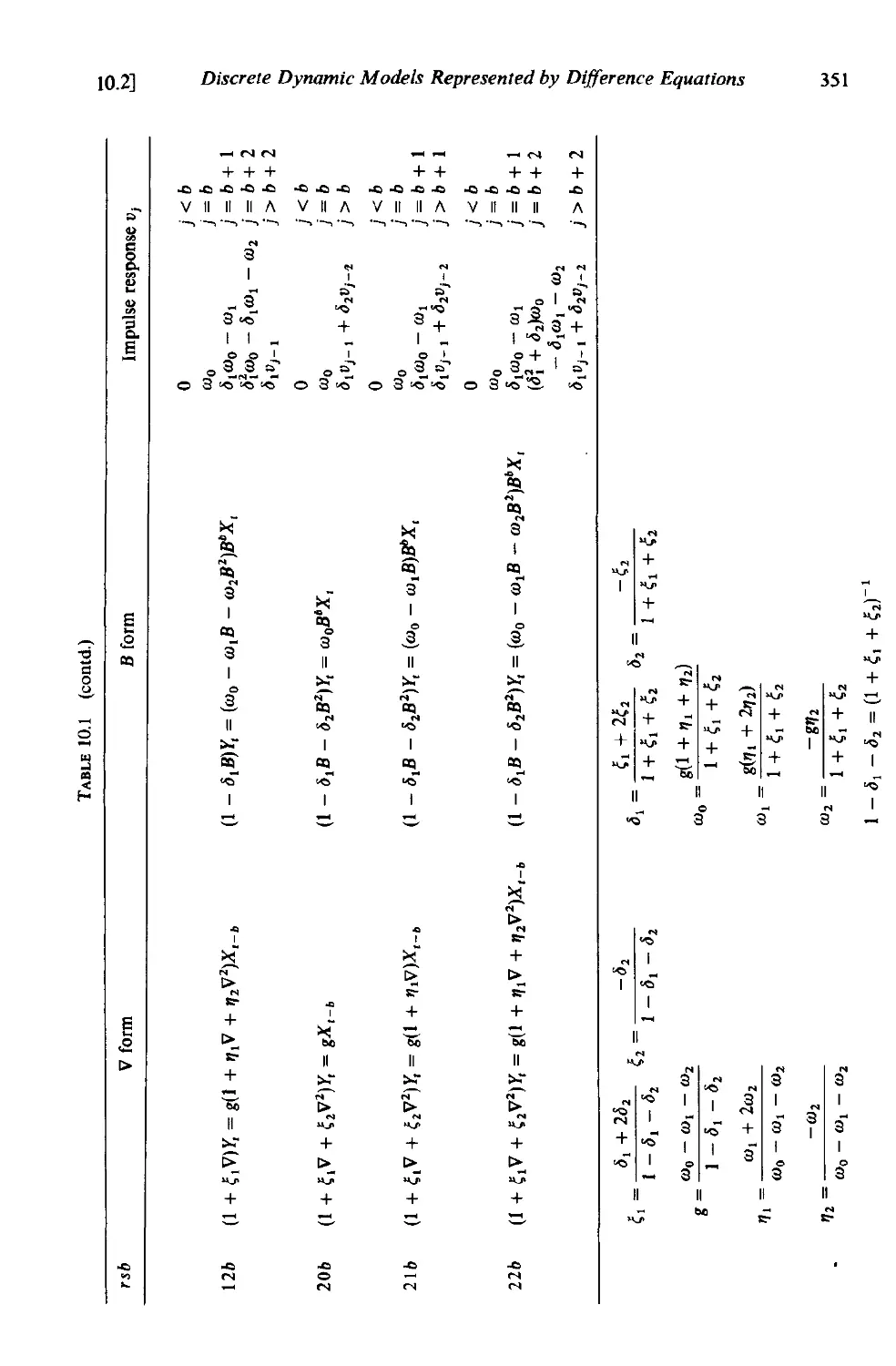
10.2 Discrete dynamic models represented by difference equations 345
10.2.1 The general form of the difference equation 345
to.2.2 Nature of the transfer function . 346
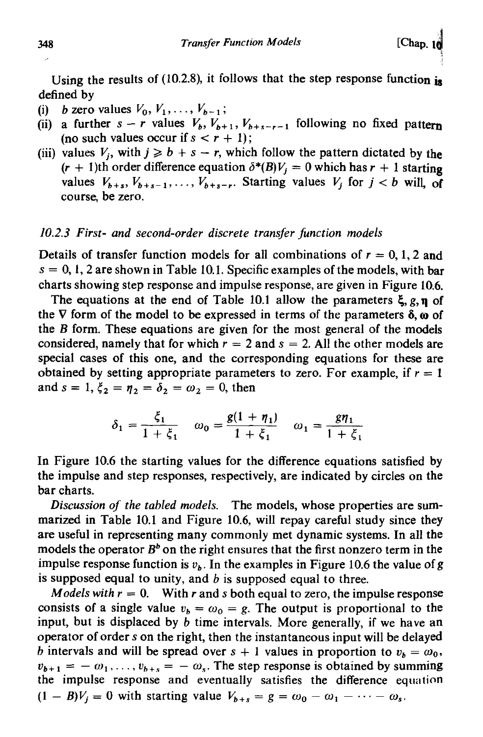
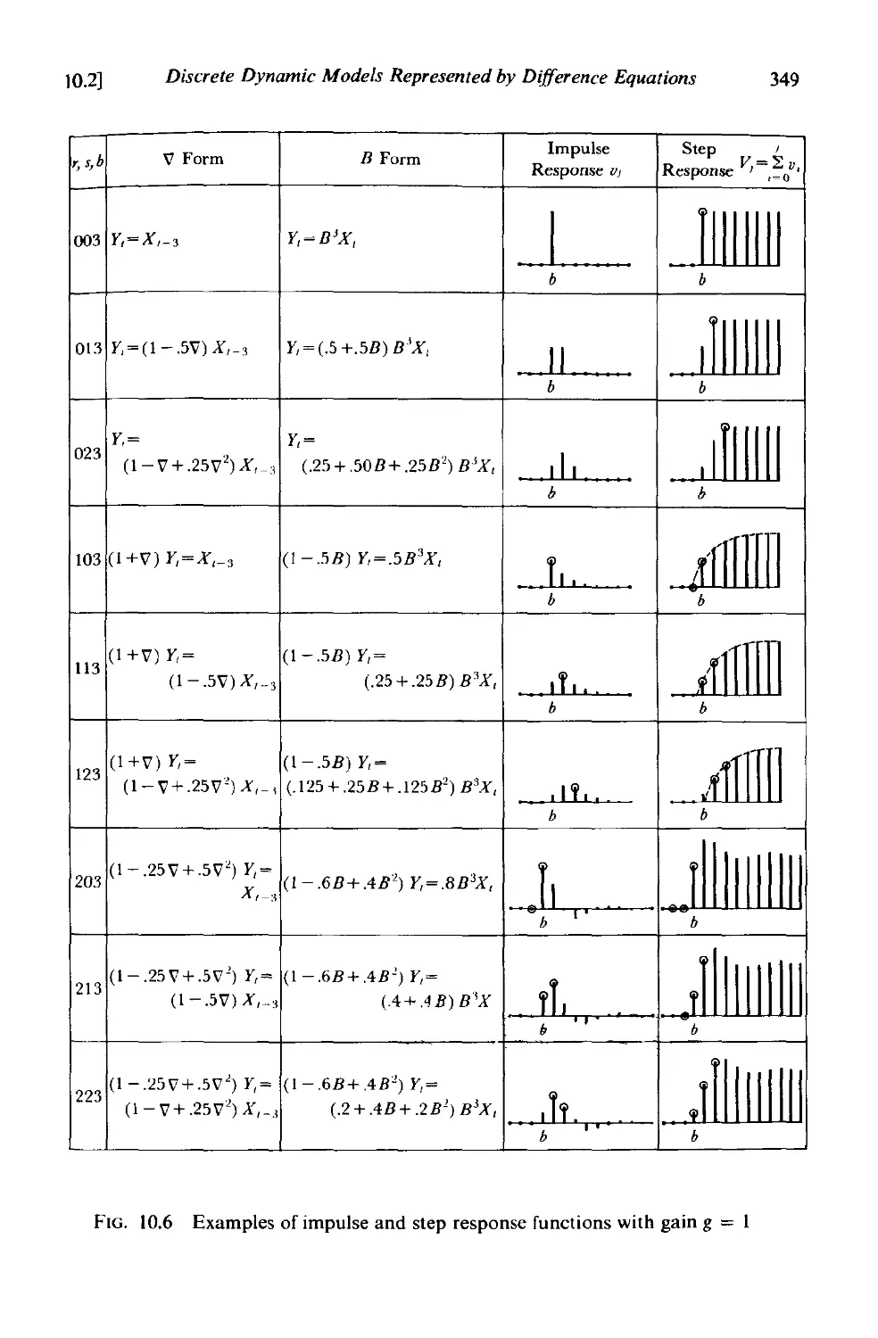
to.2.3 First and second order discrete transfer function models. 348
10.2.4 Recursive computation of output for any input 353
10.3 Relation between discrete and continuous models 355
10.3.1 Response to a pulsed input . 356
10.3.2 Relationships for first and second order coincident
systems 358
to.3.3 Approximating general continuous models by discrete
models . 361
to.3.4 Transfer function models with added noise 362
A 10.1 Continuous models with pulsed inputs 363
AIO.2 Nonlinear transfer functions and linearization 367
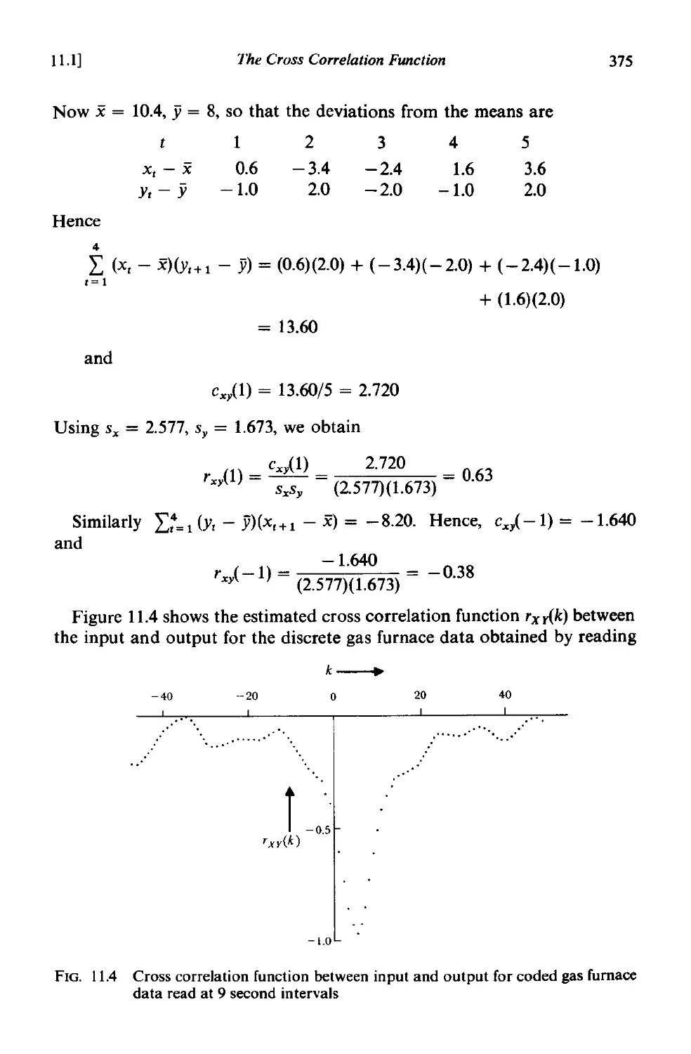
CHAPTER II IDENTIFICATION, FITTING, AND CHECKING
OF TRANSFER FUNCTION MODELS
11.1 The cross correlation function 371
11.1.1 Properties of the cross covariance and cross correlation
functions 371
11.1.2 Estimation of the cross covariance and cross correlation
fuoctiom 3N
11.1.3 Approximate standard errors of cross correlation estimates 376
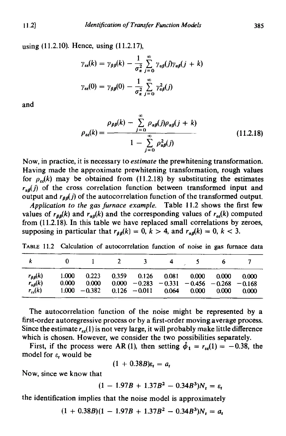
11.2 Identification of transfer function models 377
11.2.1 Identification of transfer function models by prewhitening
the input 379
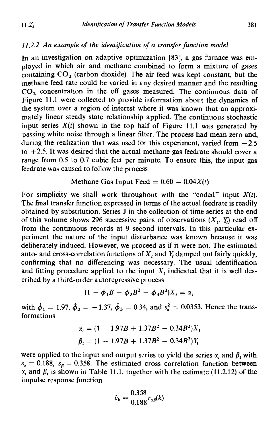
11.2.2 An example of the identification of a transfer function
model . 381
11.2.3 Identification of the noise model 383
11.2.4 Some general considerations in identifying transfer
function models 386
xx
Contents
11.3 Fitting and checking transfer function models 388
11.3.1 The conditional sum of squares function 388
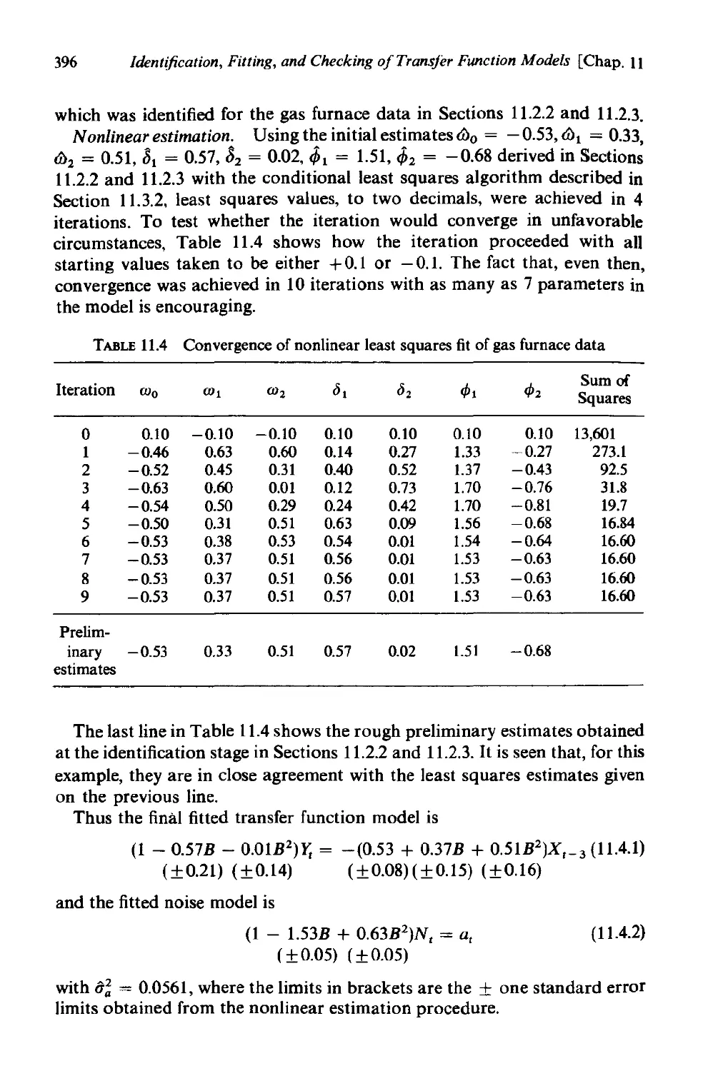
11.3.2 Nonlinear estimation 390
11.3.3 Use of residuals for diagnostic checking 392
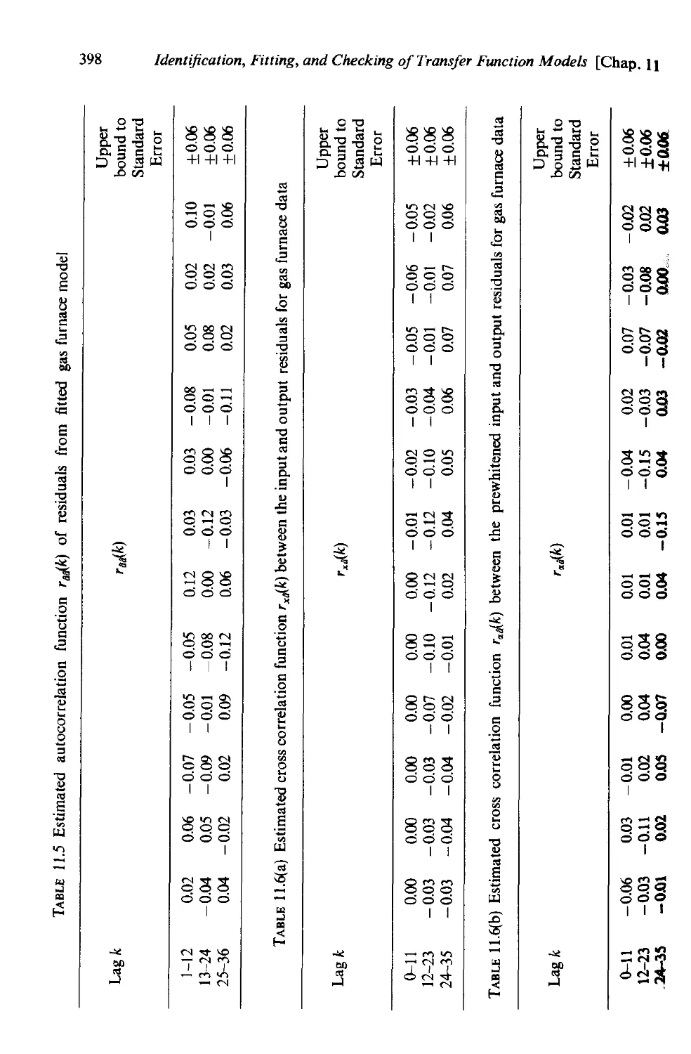
11.3.4 Specific checks applied to the residuals 393
11.4 Some examples of fitting and checking transfer function
models . 395
11.4.1 Fitting and checking of the gas furnace model 395
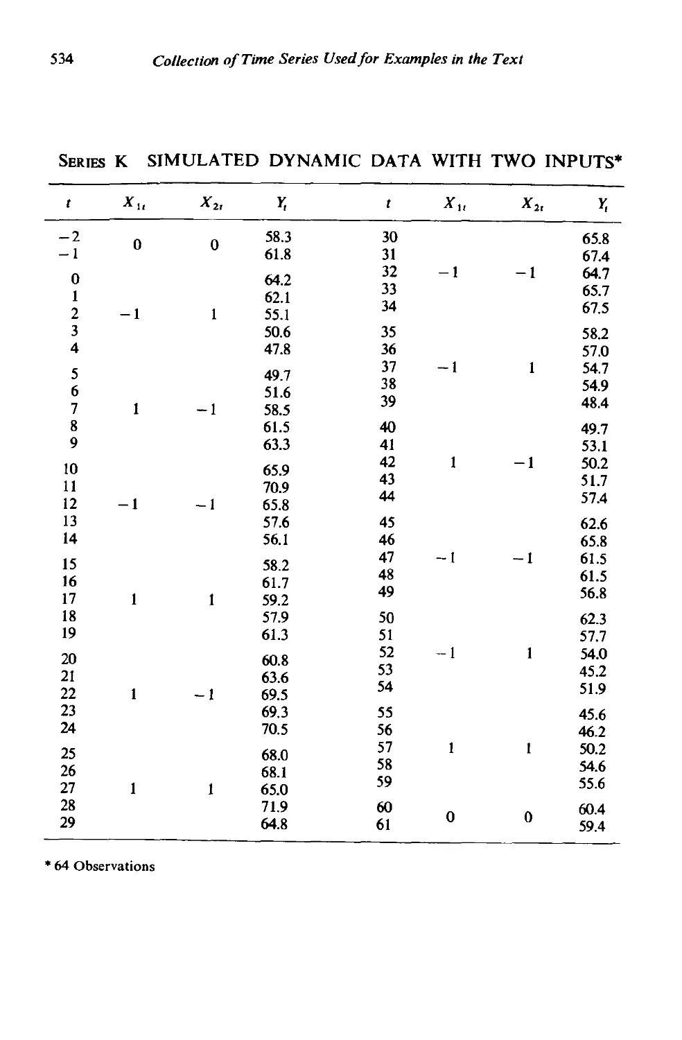
11.4.2 A simulated example with two inputs 400
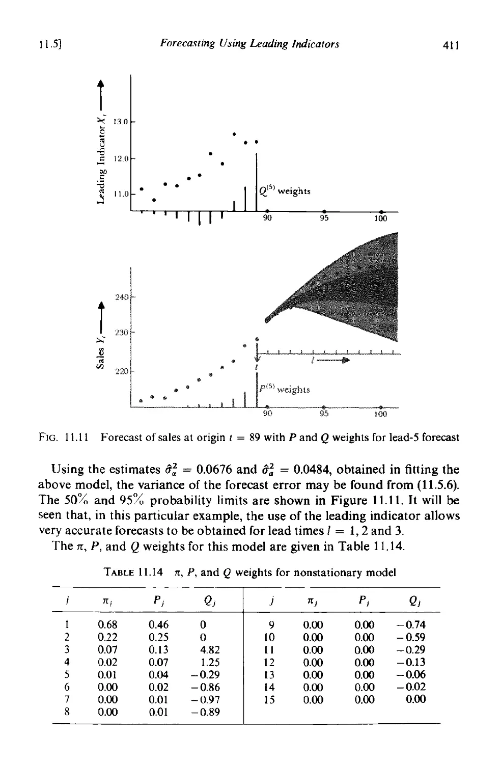
11.5 Forecasting using leading indicators 402
11.5.1 The minimum square error forecast 404
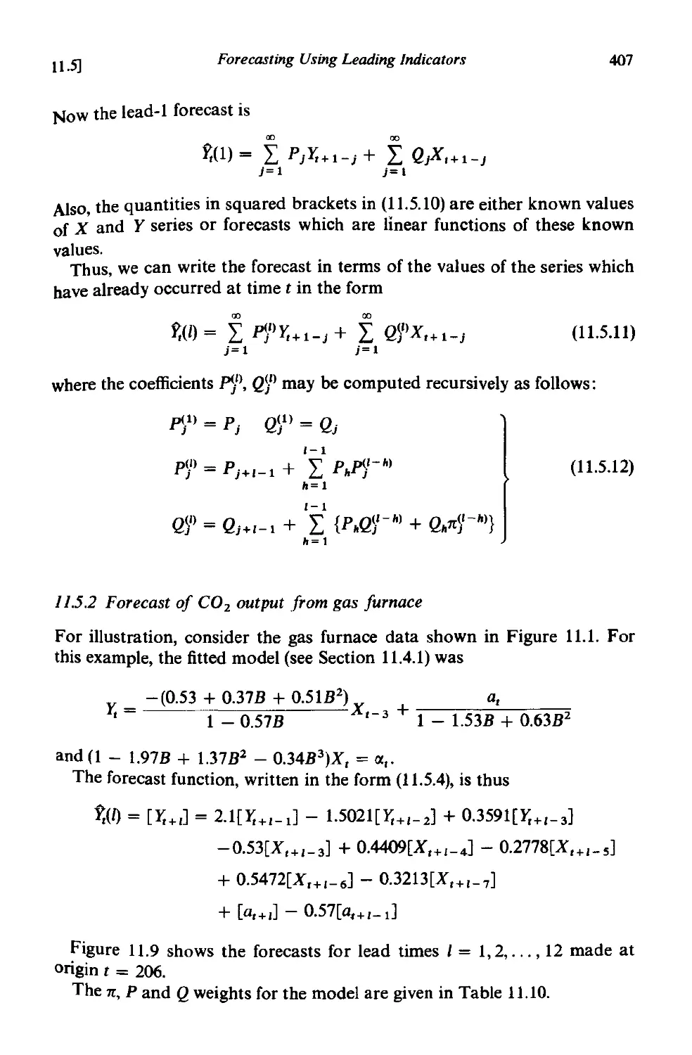
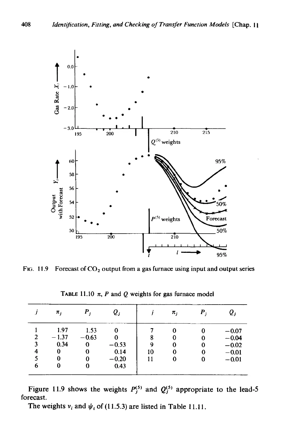
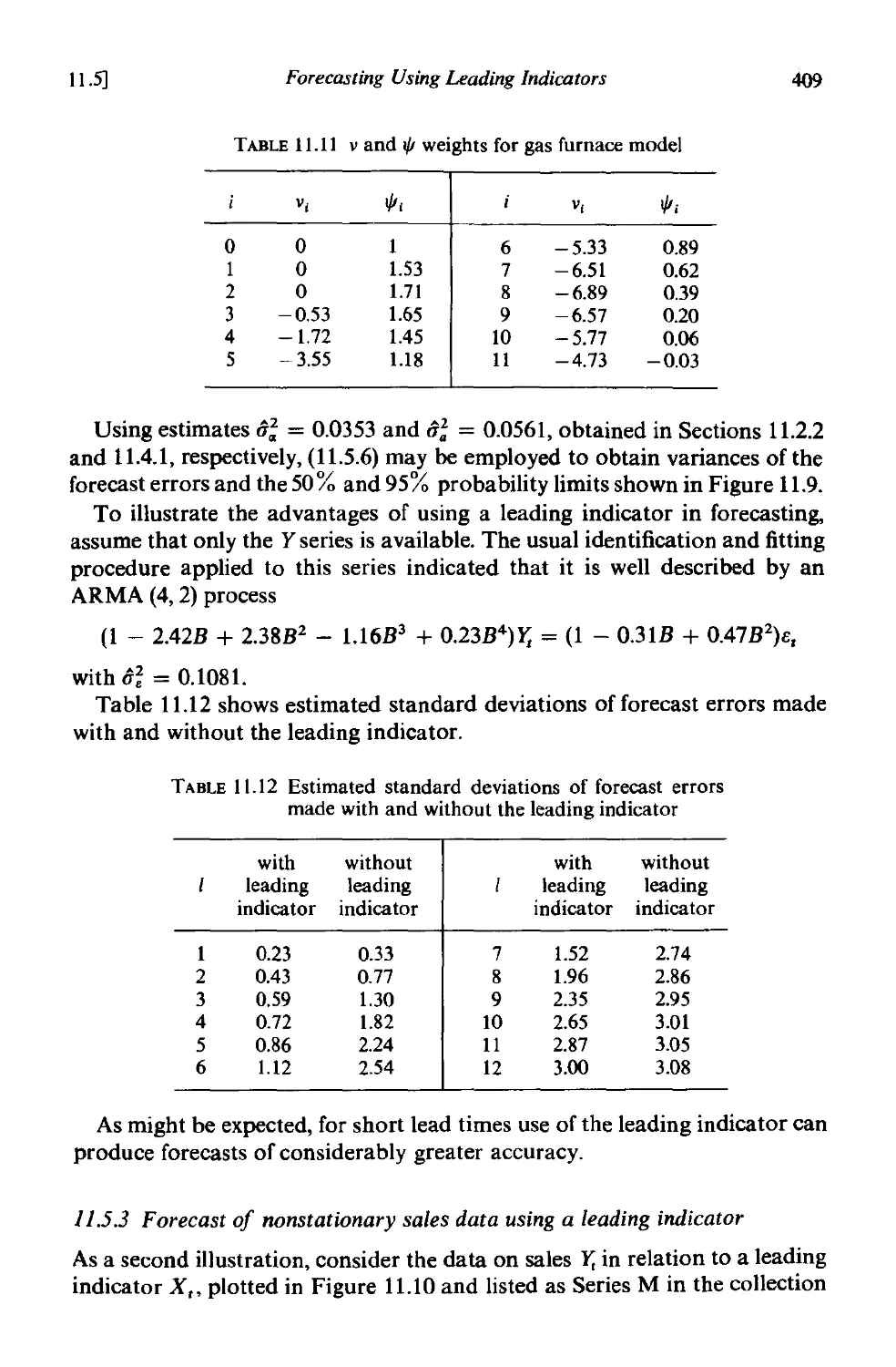
11.5.2 Forecast of CO 2 output from gas furnace 407
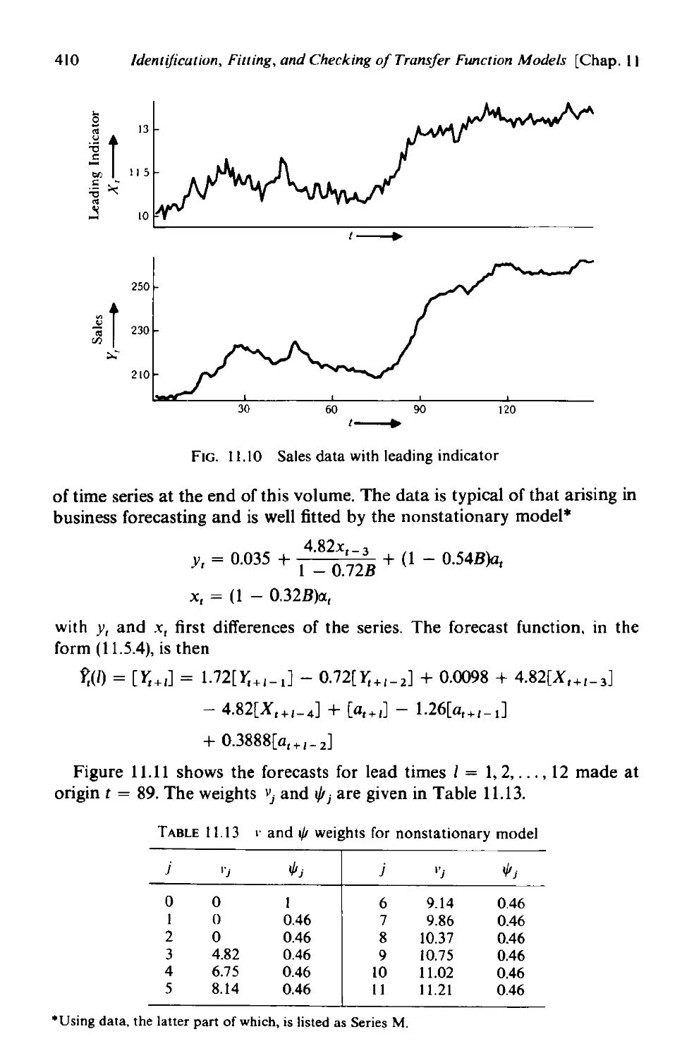
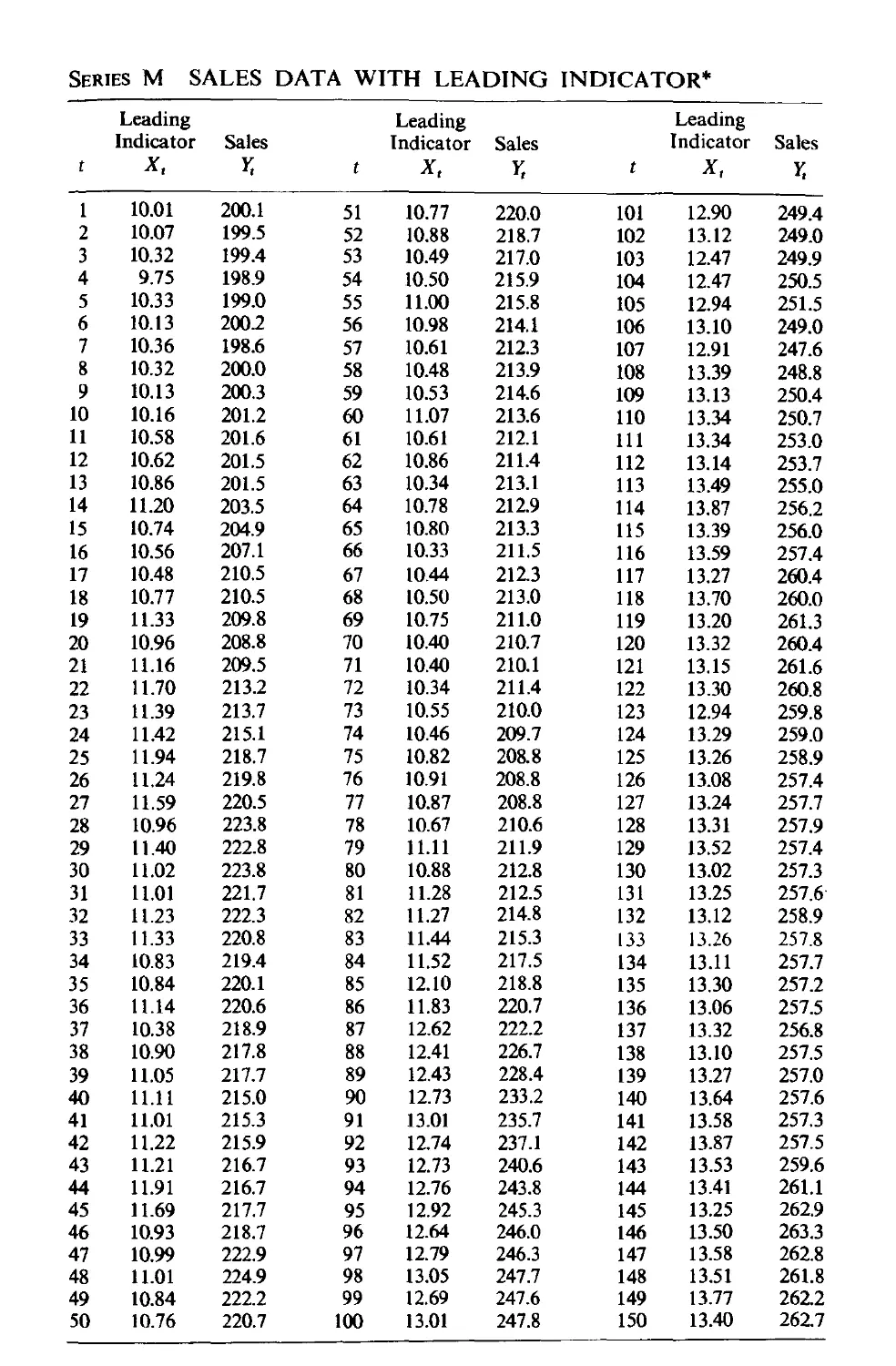
11.5.3 Forecast of non stationary sales data using a leading
indicator 409
11.6 Some aspects ofthe design of experiments to estimate transfer
functions 412
A 11.1 Use of cross spectral analysis for transfer function model
identification. 413
A 11.1.1 Identification of single input transfer function models. 413
A 11.1.2 Identification of multiple input transfer function models. 415
A 11.2 Choice of input to provide optimal parameter estimates 416
A 11.2.1 Design of optimal input for a simple system. 416
Al1.2.2 A numerical example . 418
PART IV DESIGN OF DISCRETE CONTROL SCHEMES
CHAPTER 12 DESIGN OF FEED FORWARD AND FEEDBACK
CONTROL SCHEMES
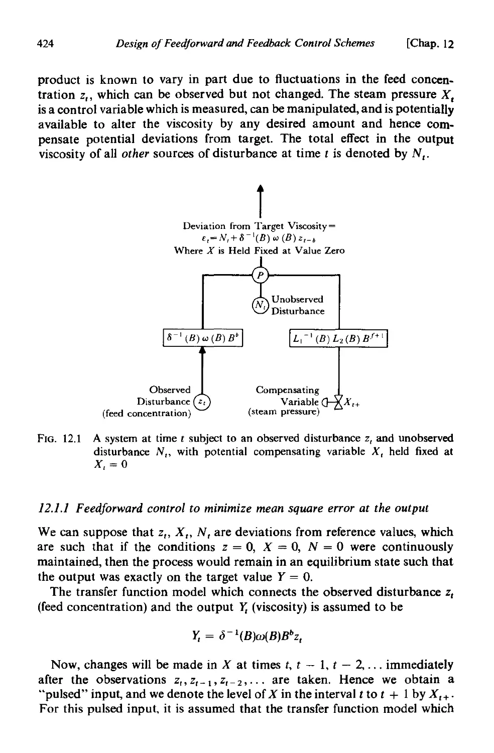
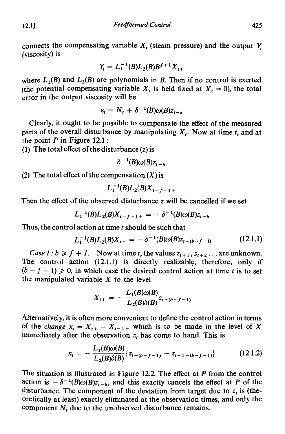
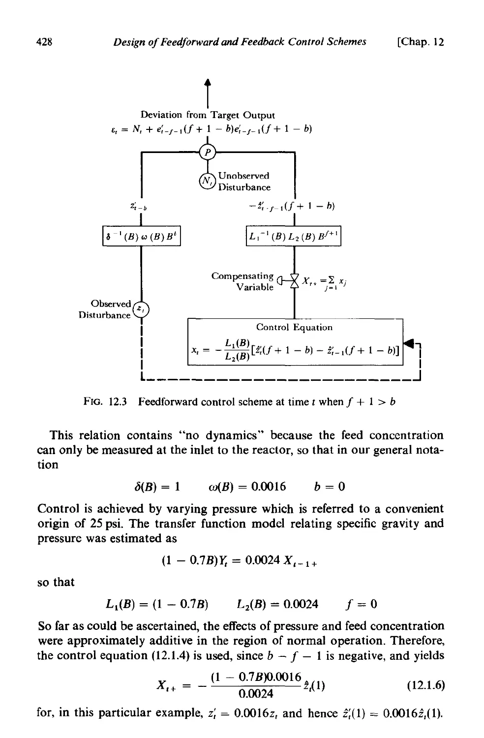
12.1 Feedforward control . 423
12.1.1 Feedforward control to minimize mean square error at
the output . 424
12.1.2 An example-control of specific gravity of an intermediate
product 427
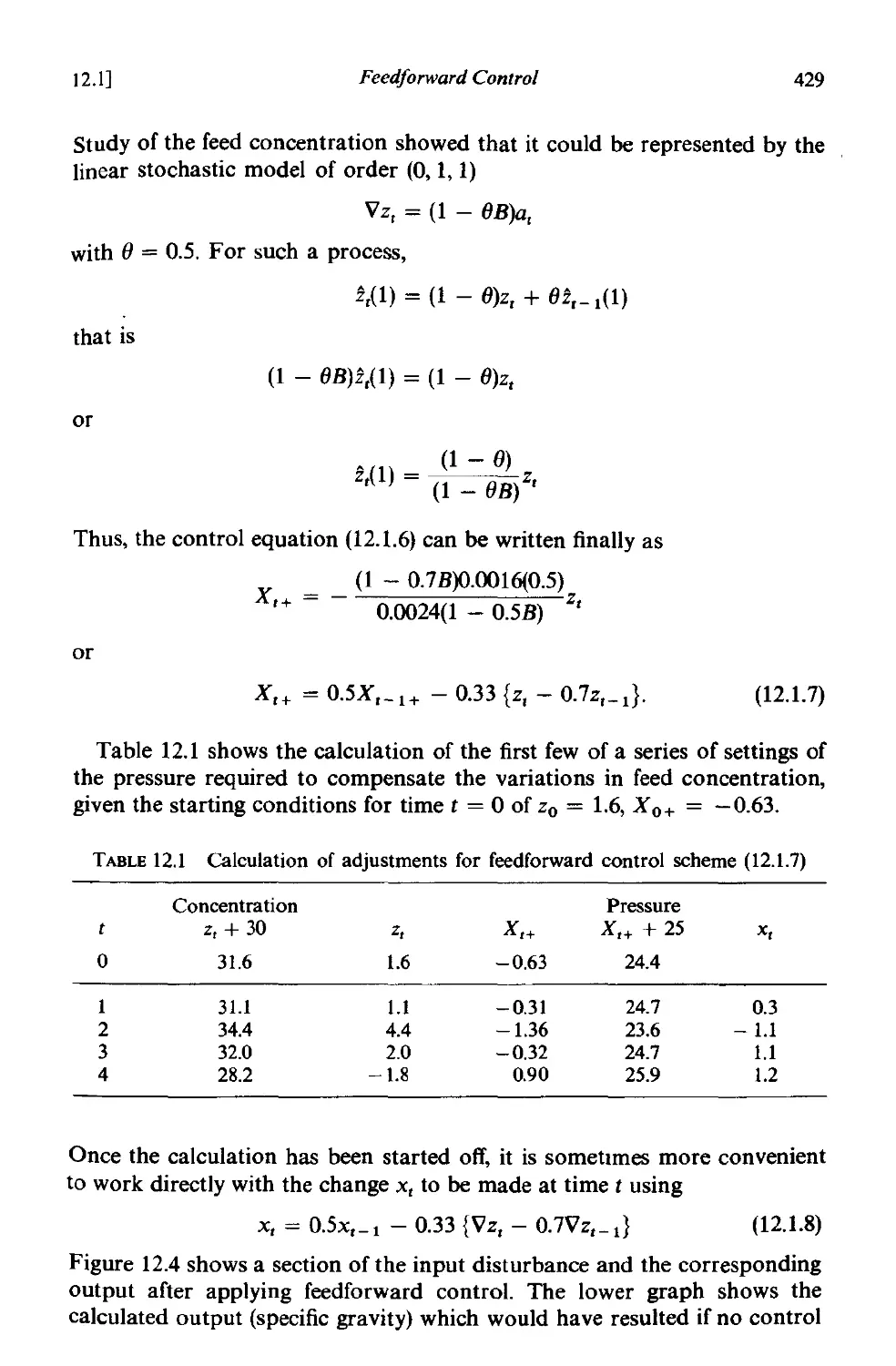
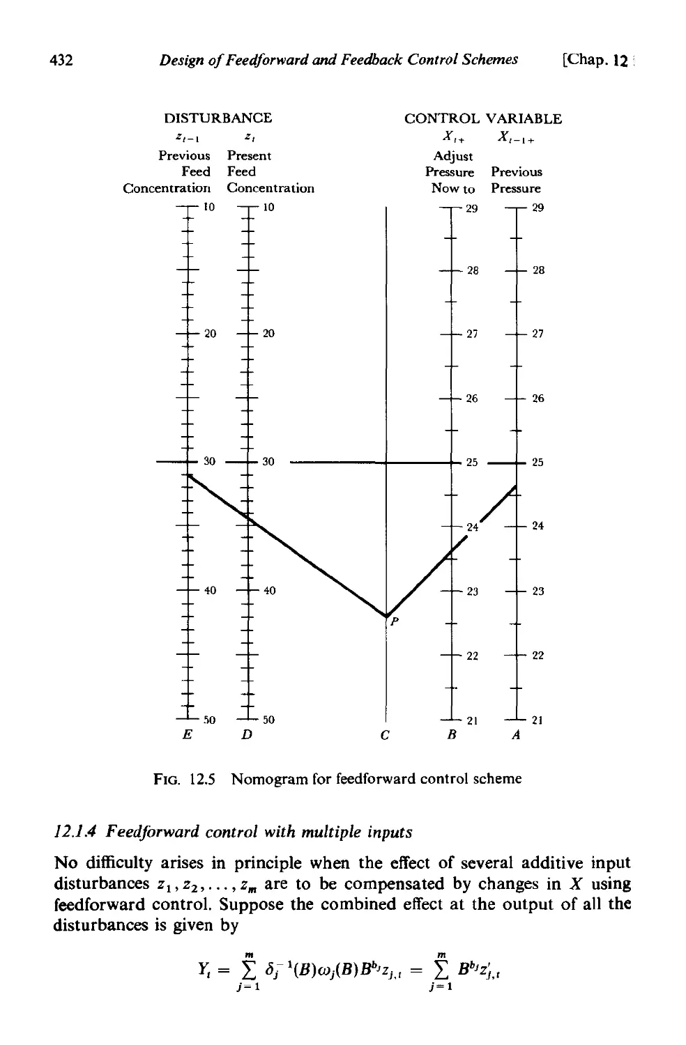
12.1.3 A nomogram for feed forward control . 430
12.1.4 Feedforward control with multiple inputs 432
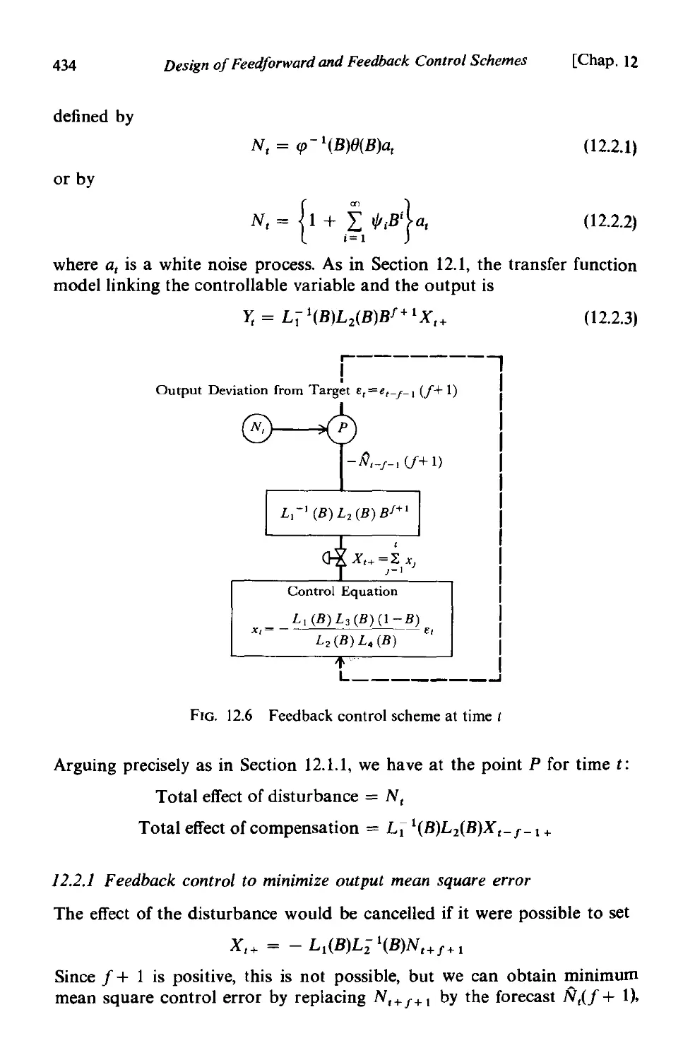
12.2 Feedback control . 433
12.2.1 Feedback control to minimize output mean square error 434
12.2.2 Application of the control equation: relation with three-
term controller 436
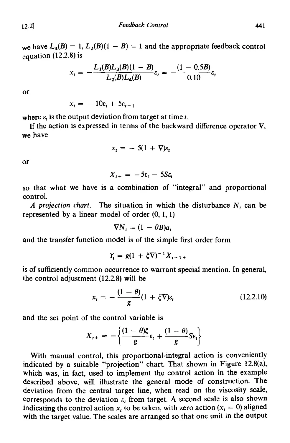
12.2.3 Examples of discrete feedback control 437
Contents xxi
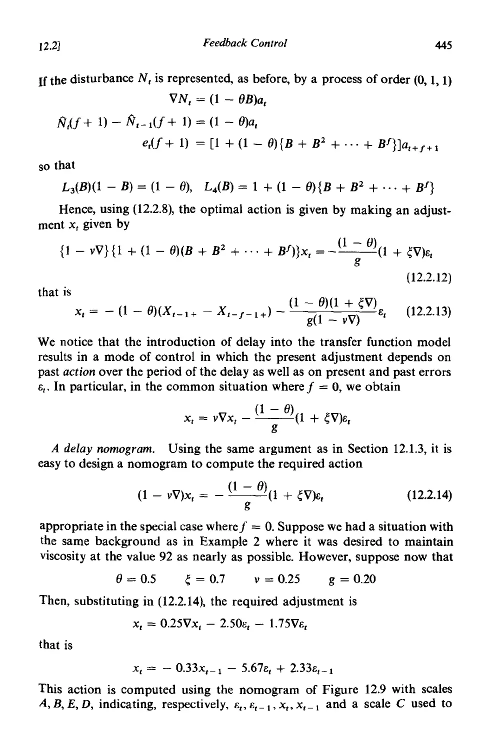
]2.3 Feedforward-feedback control 446
]2.3.1 Feedforward-feedback control to minimize output mean
square error 448
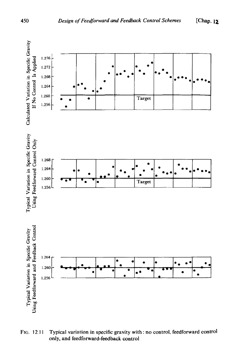
12.3.2 An example of feedforward-feedback control. 448
12.3.3 Advantages and disadvantages of feedforward and feed-
back control 449
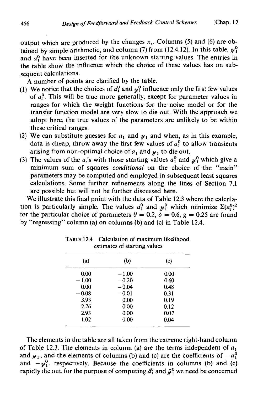
12.4 Fitting transfer function-noise models using operating data 451
] 2.4.1 Iterative model building 451
12.4.2 Estimation from operating data 451
12.4.3 An example 453
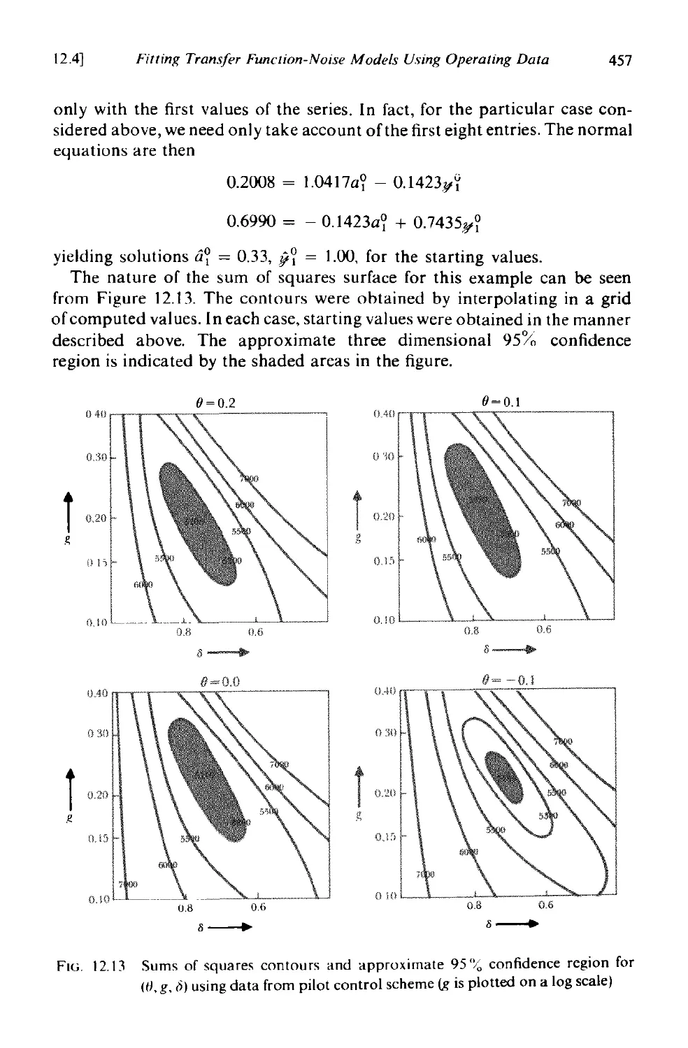
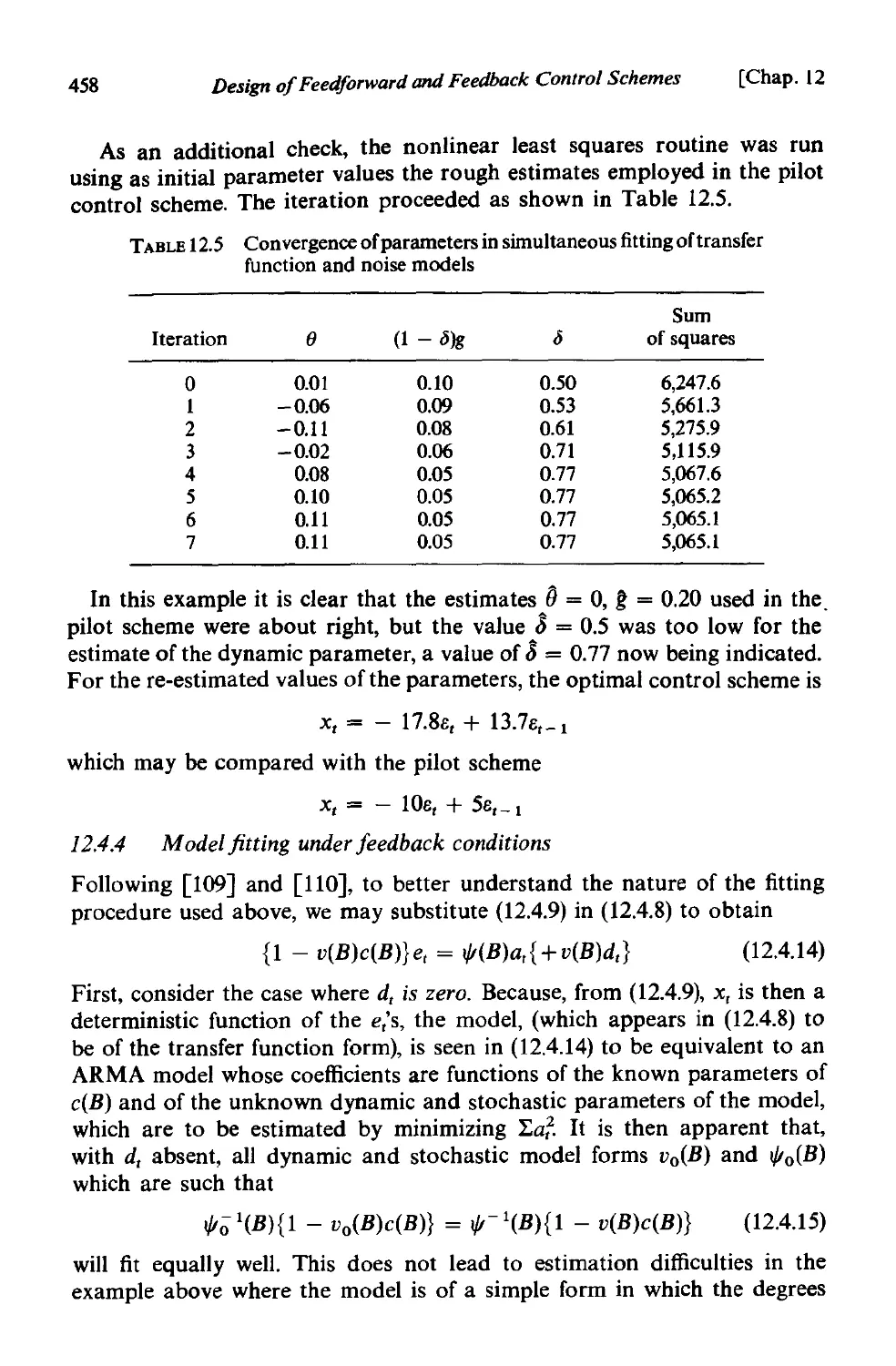
]2.4.4 Model titting under feedback conditions 458
CHAPTER 13 SOME FURTHER PROBLEMS IN CONTROL
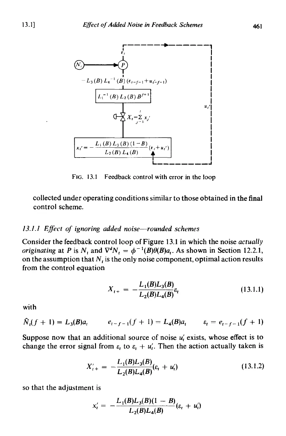
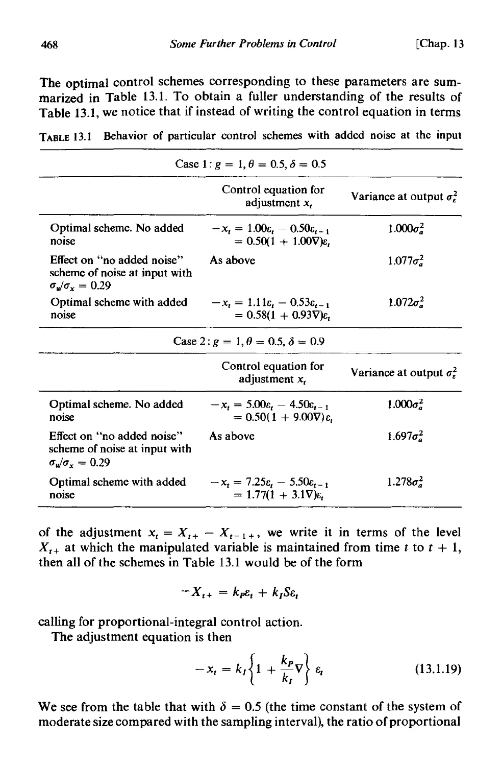
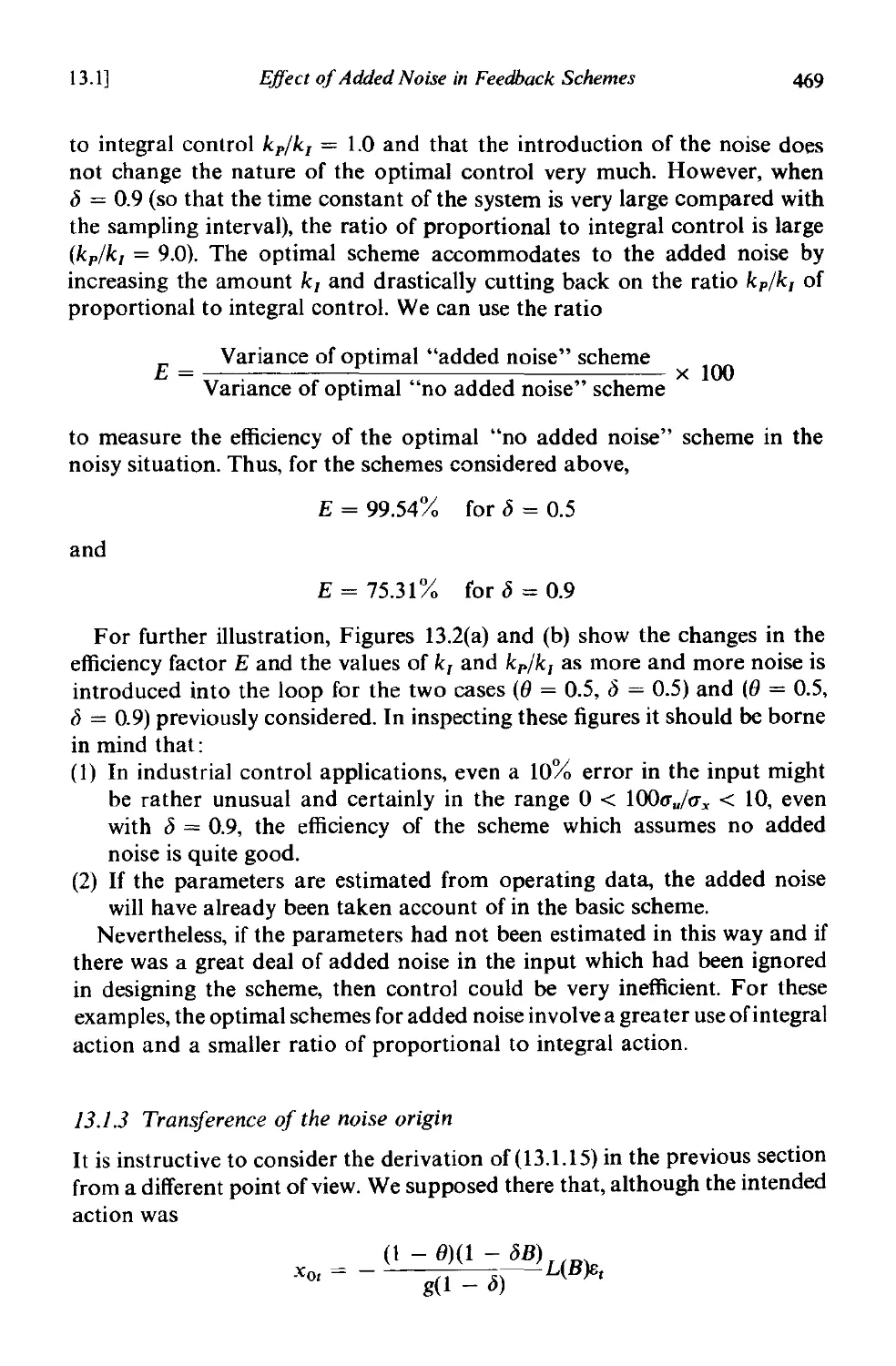
13.] Effect of added noise in feedback schemes . 460
13.1.1 Effect of ignoring added noise-rounded schemes 461
13.1.2 Optimal action when there are observational errors in the
adjustments x t 465
13.1.3 Transference of the noise origin 469
13.2 Feedback control schemes where the adjustment variance is
restricted 472
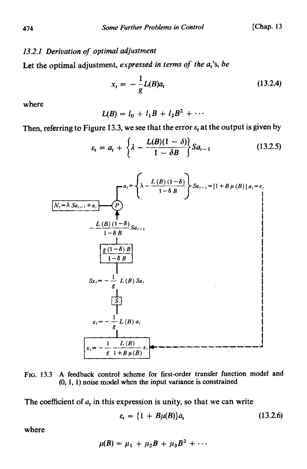
13.2.] Derivation of optimal adjustment 474
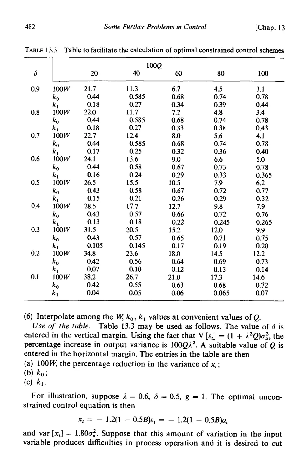
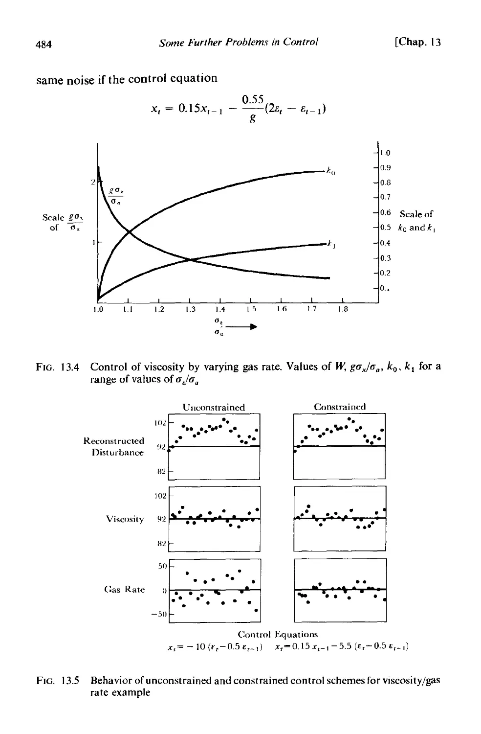
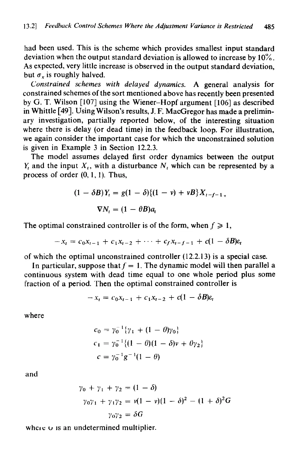
] 3.2.2 A constrained scheme for the viscosity/gas rate example 483
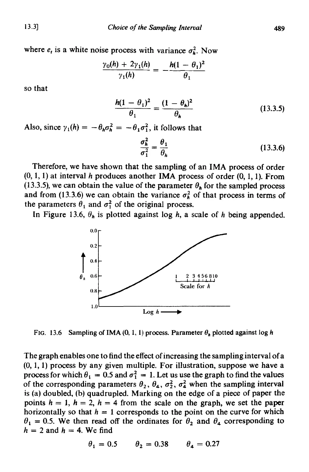
13.3 Choice of the sampling interval . 486
13.3.1 An illustration of the effect of reducing sampling frequency 487
13.3.2 Sampling an IMA (0, I, 1) process . 488
PART V
Description of computer programs
Collection of tables and charts .
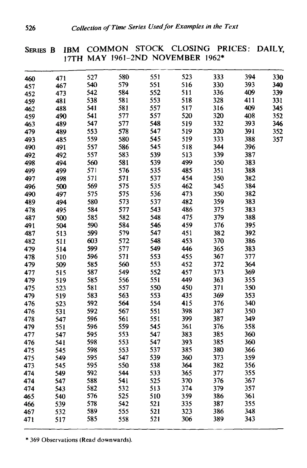
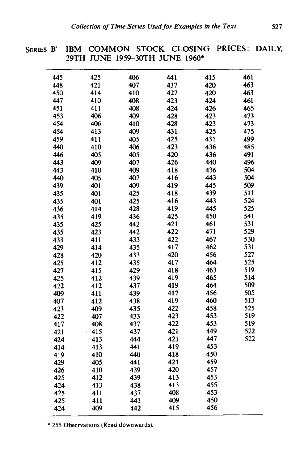
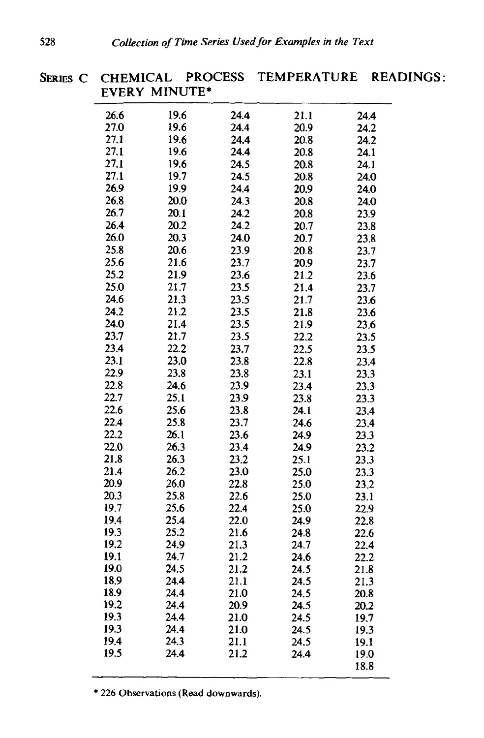
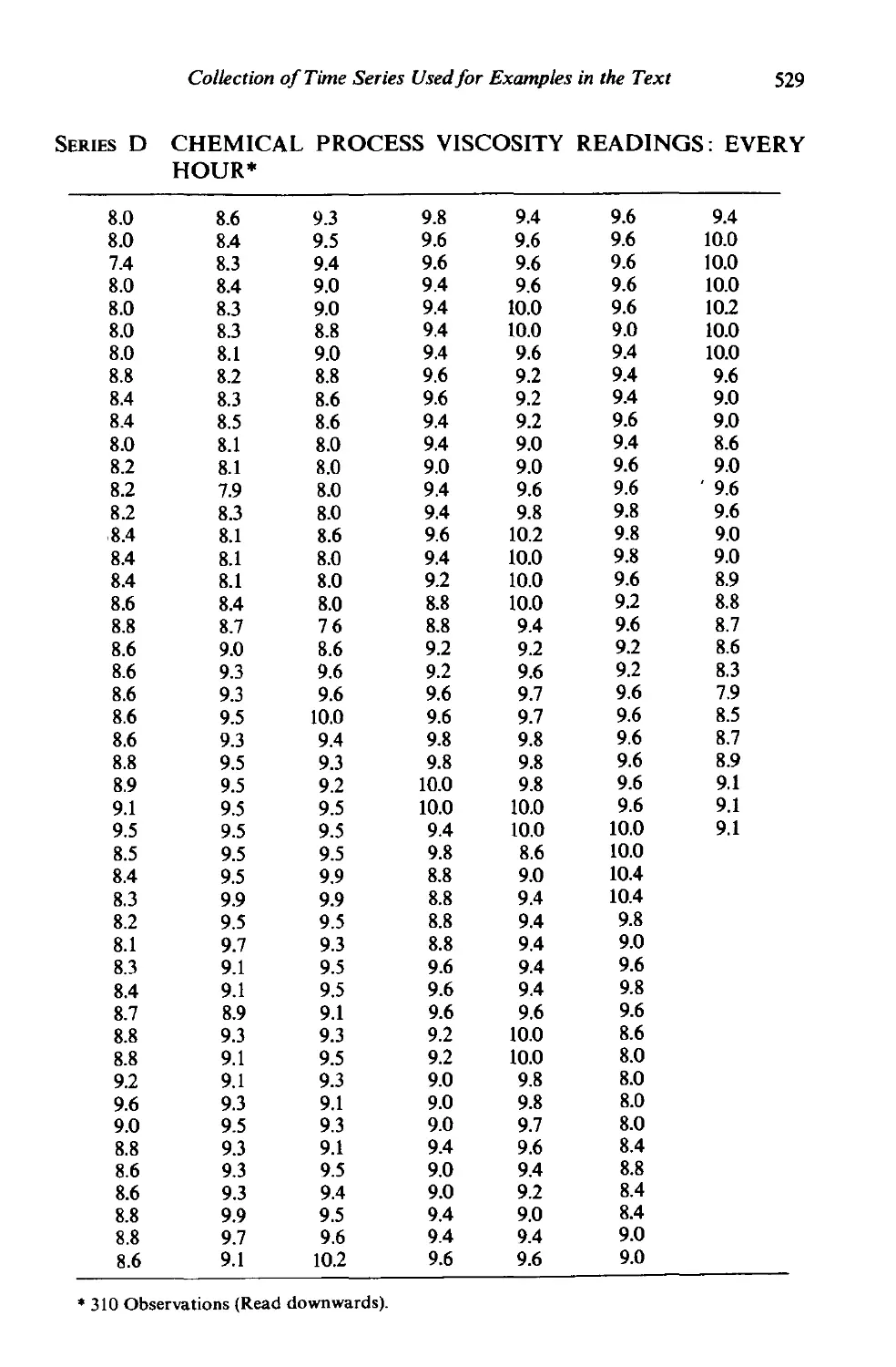
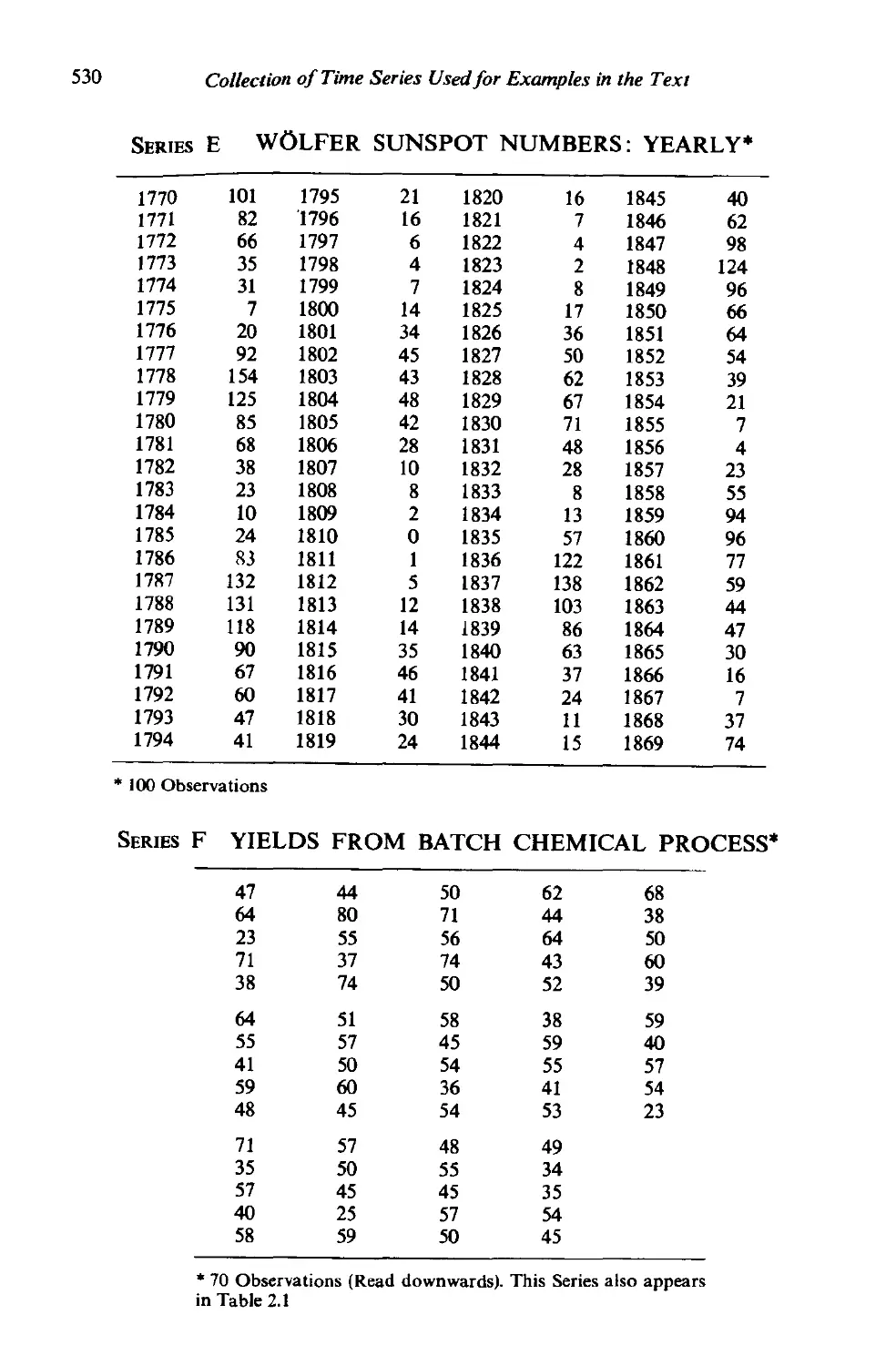
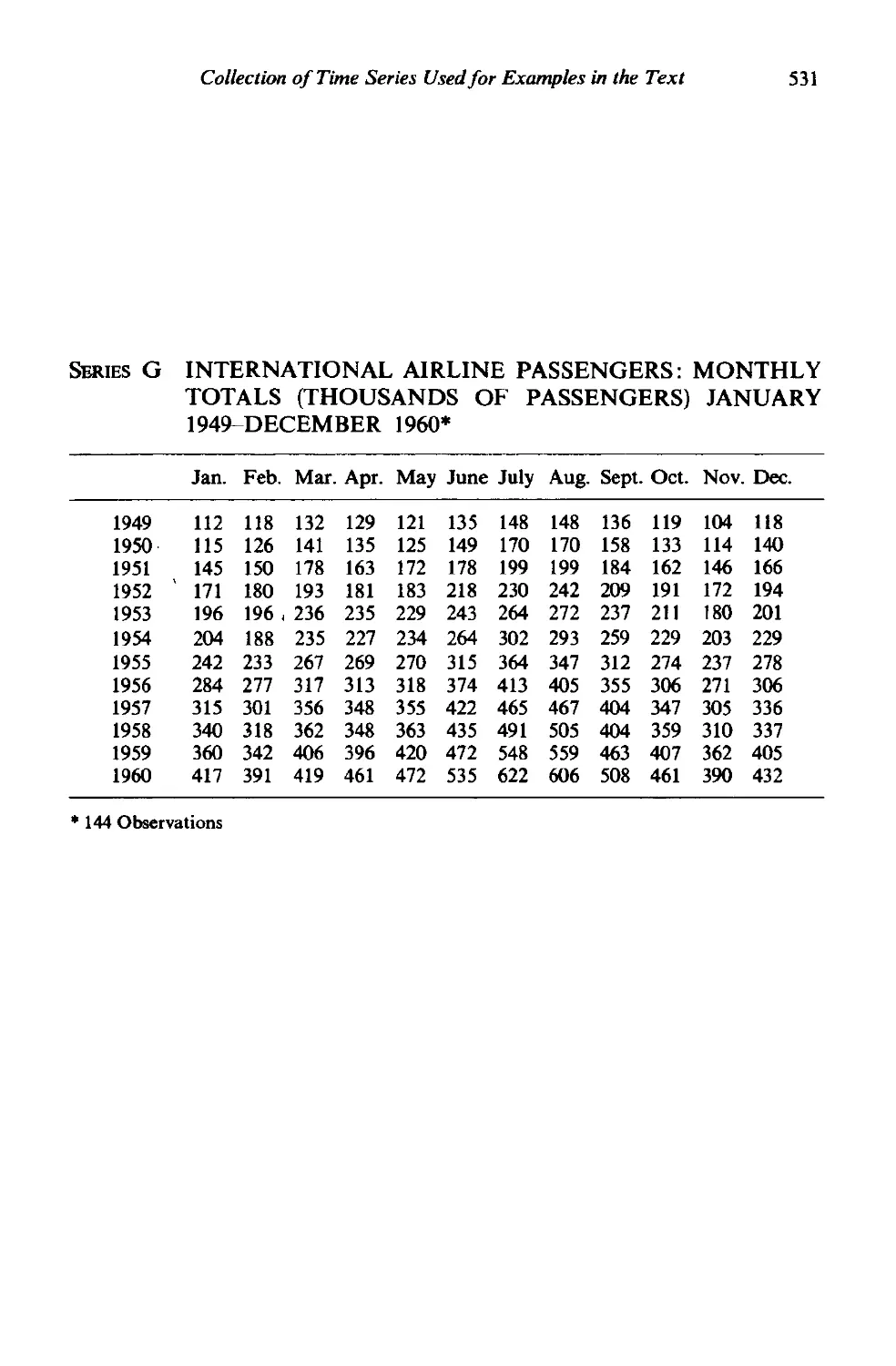
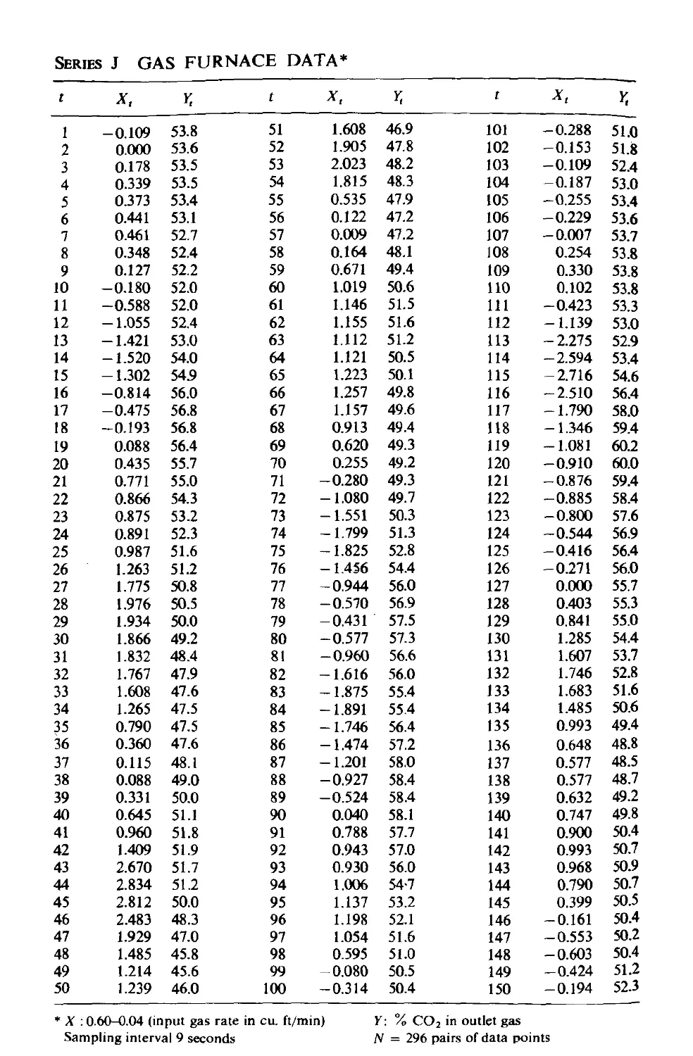
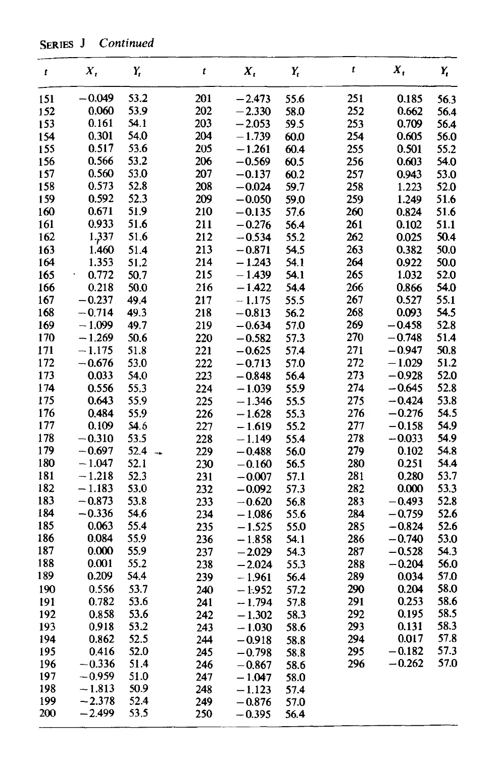
Collection of time series used for examples in the text
References .
Index
495
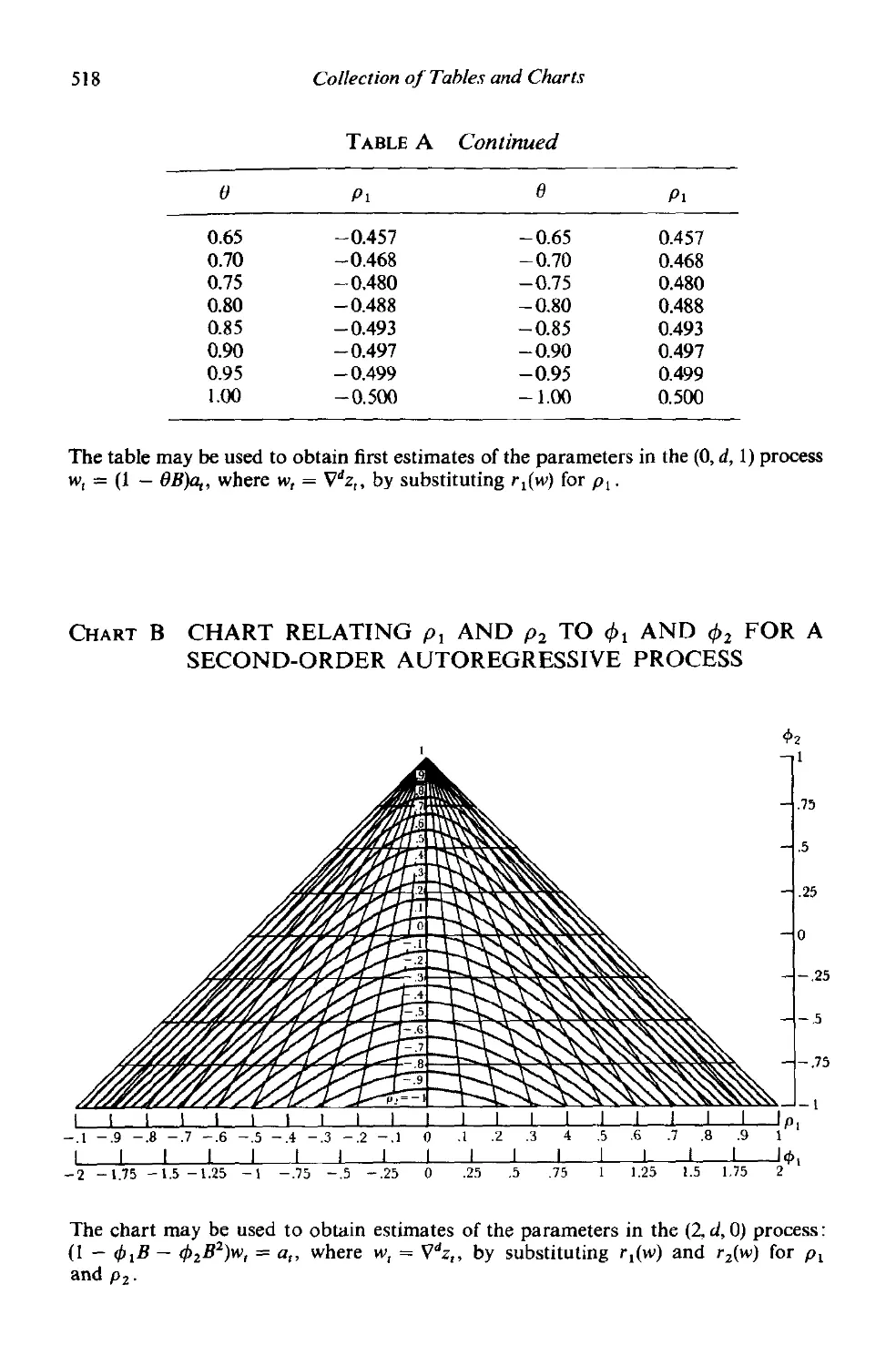
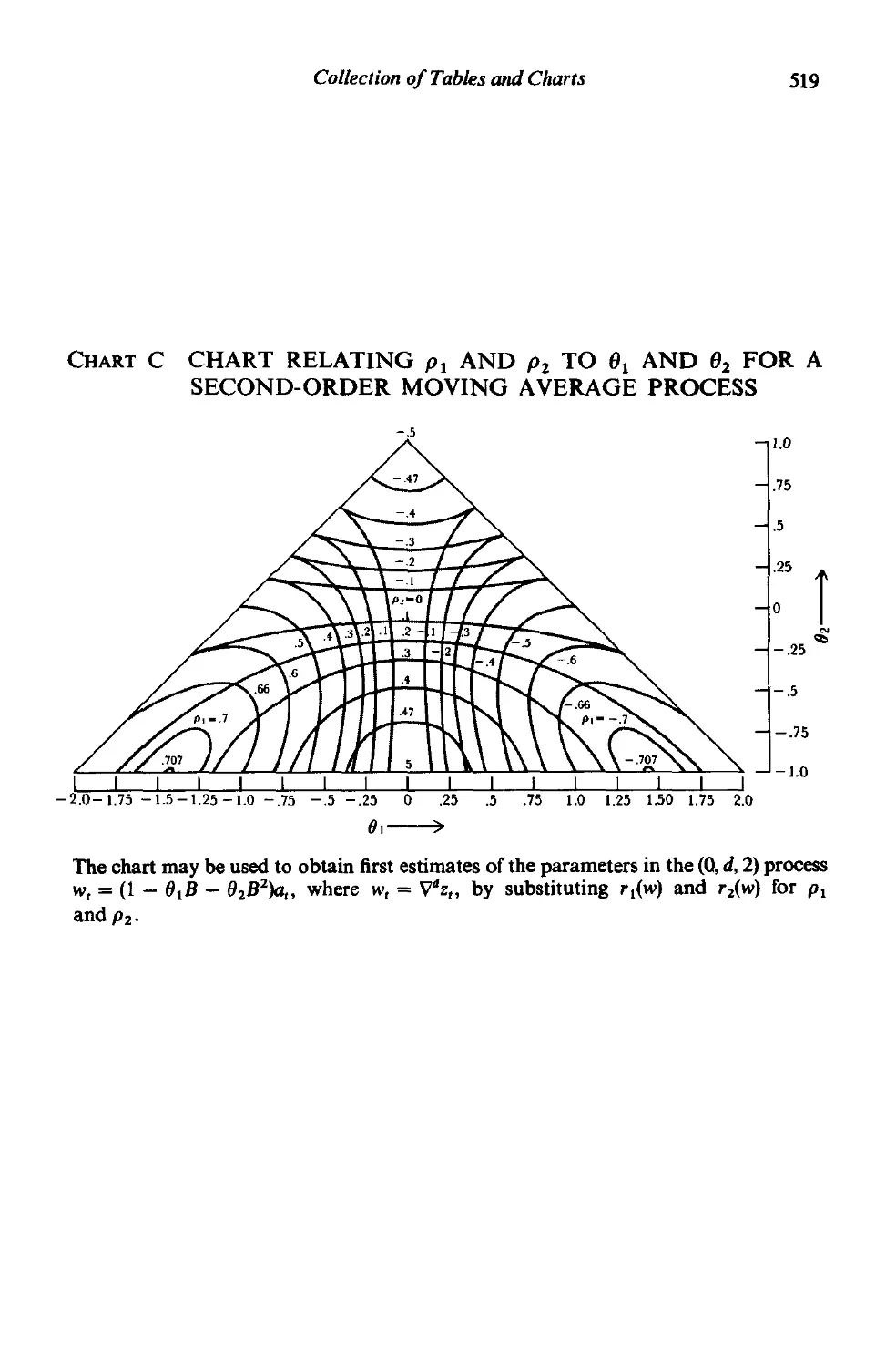
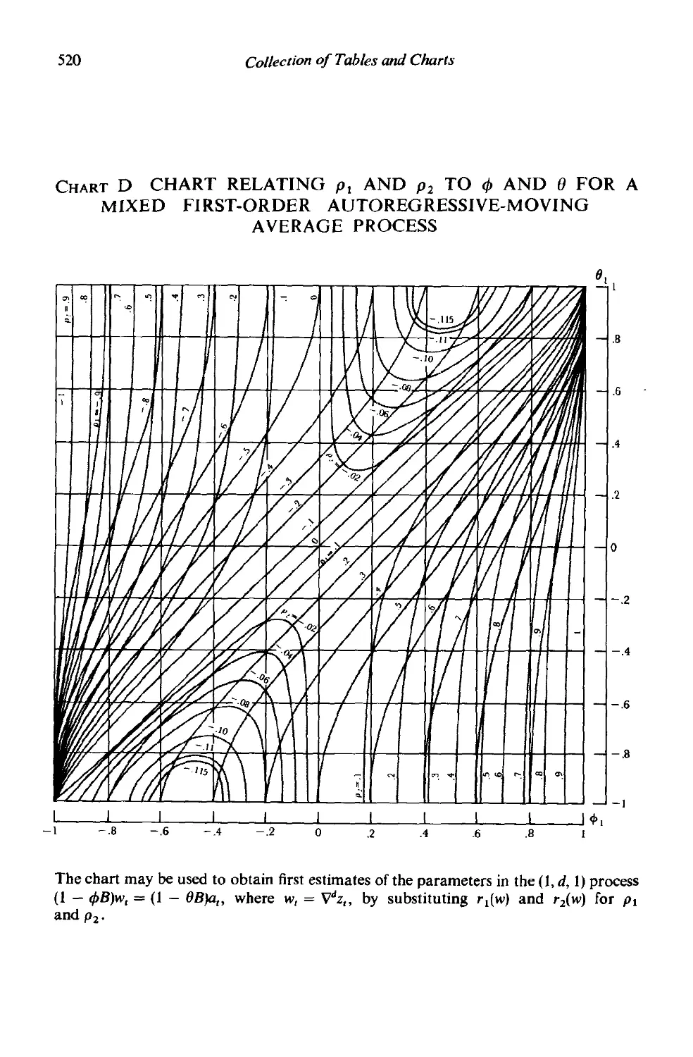
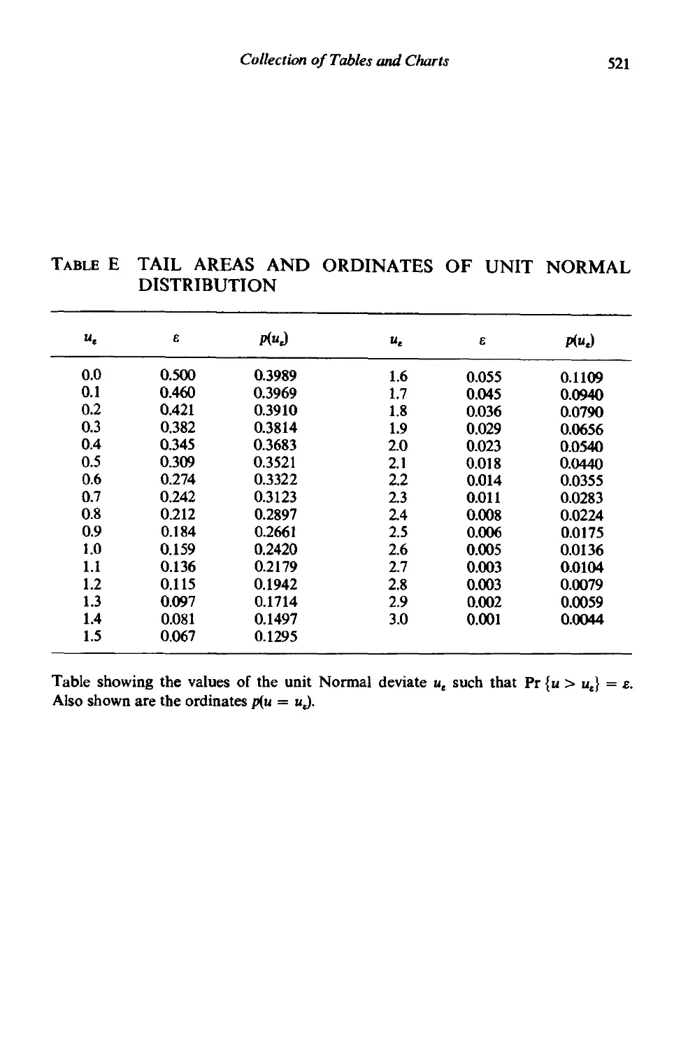
517
524
538
543
PART VI
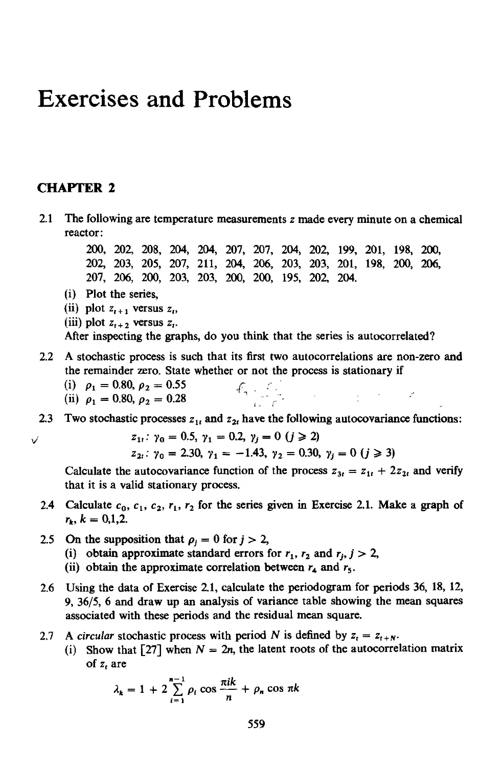
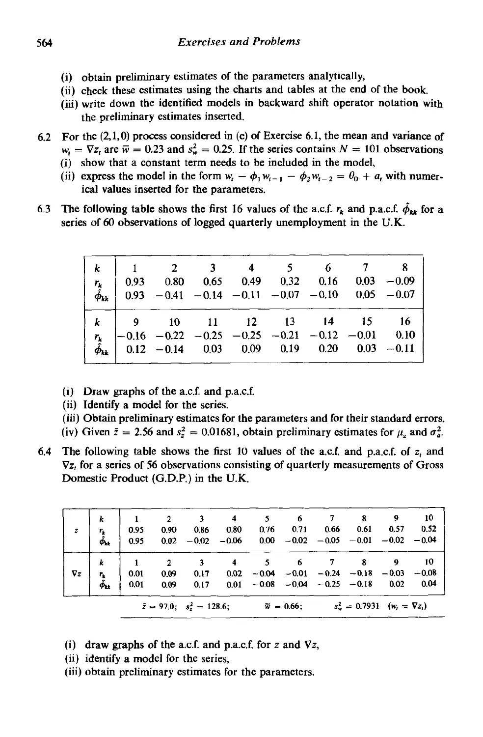
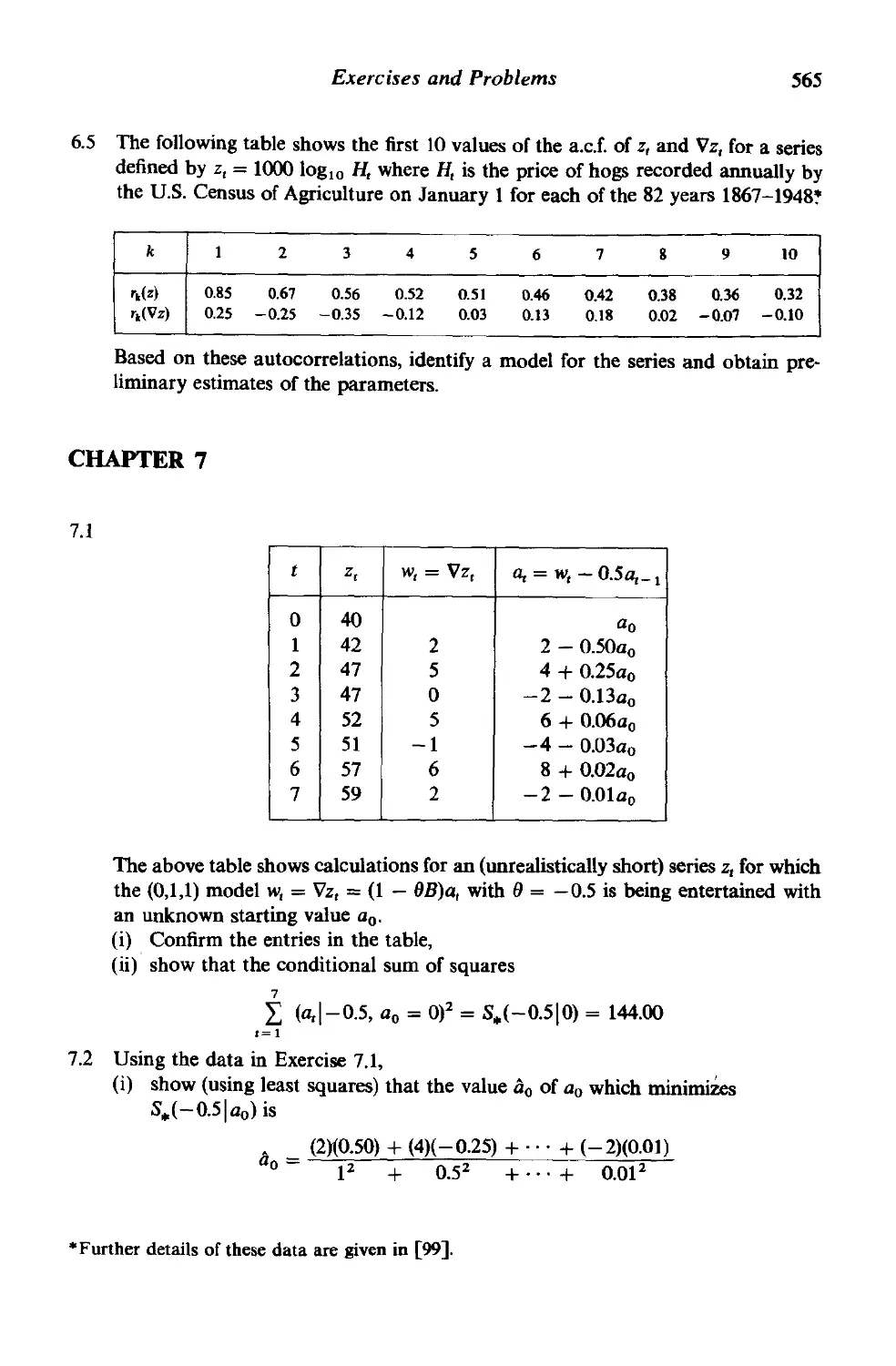
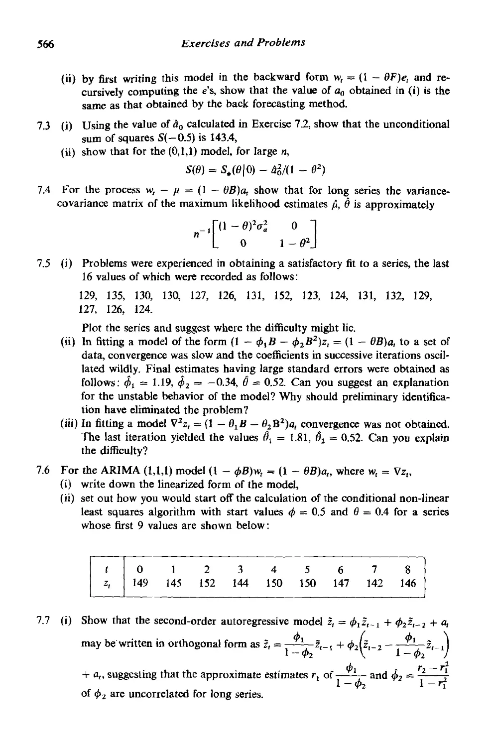
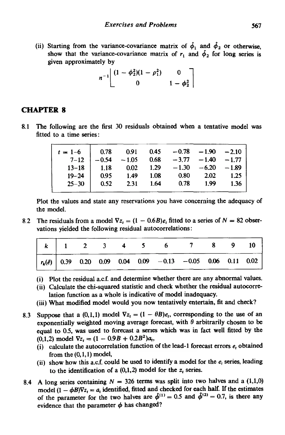
Exercises and Problems
559
TIME SERIES
ANAL YSIS
forecasting
and
control
1
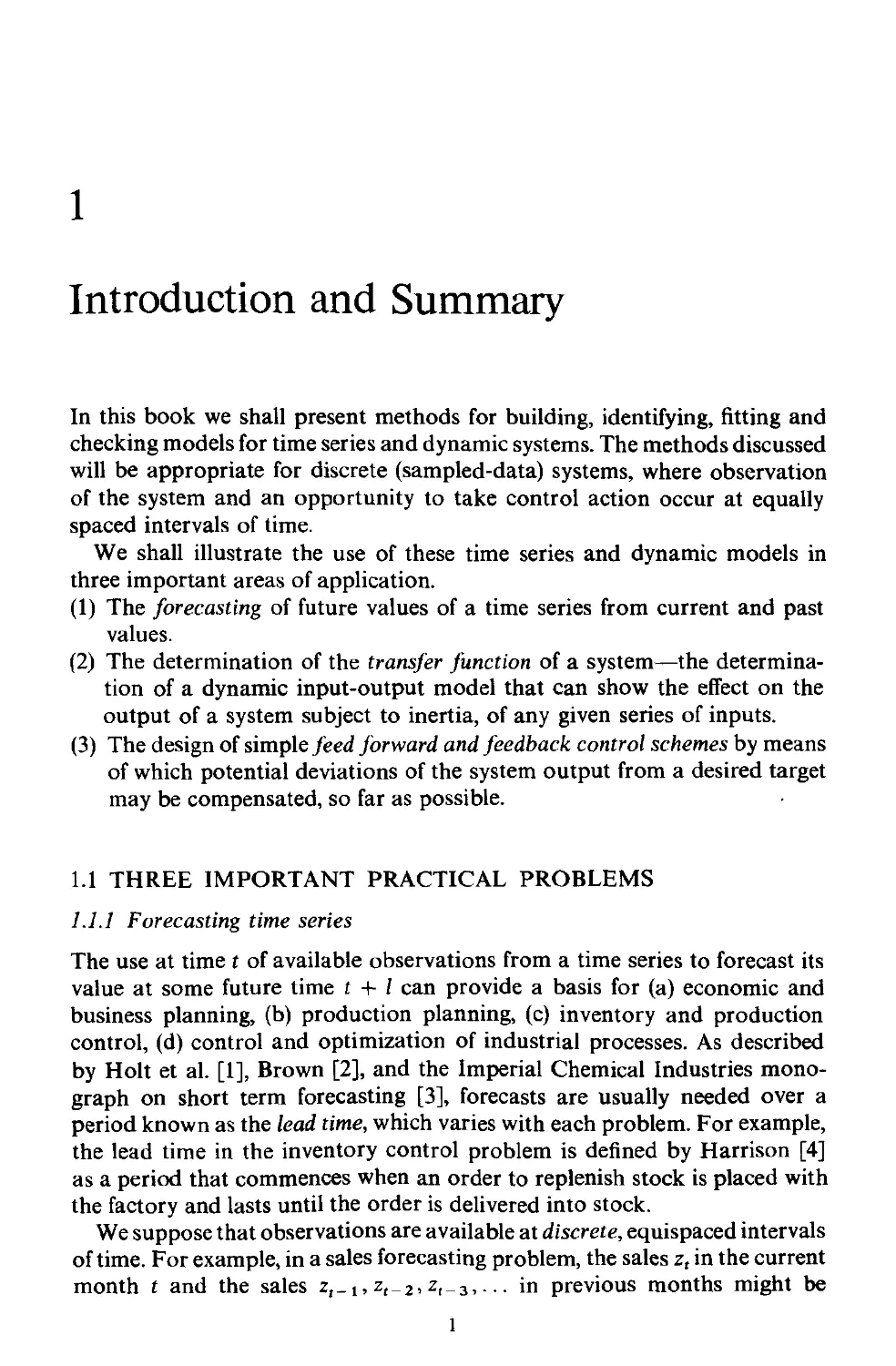
Introduction and Summary
In this book we shall present methods for building, identifying, fitting and
checking models for time series and dynamic systems. The methods discussed
will be appropriate for discrete (sampled-data) systems, where observation
of the system and an opportunity to take control action occur at equally
spaced intervals of time.
We shall illustrate the use of these time series and dynamic models in
three important areas of application.
(1) The forecasting of future values of a time series from current and past
values.
(2) The determination of the transfer function of a system-the determina-
tion of a dynamic input-output model that can show the effect on the
output of a system subject to inertia, of any given series of inputs.
(3) The design of simple feed forward and feedback control schemes by means
of which potential deviations of the system output from a desired target
may be compensated, so far as possible.
1.1 THREE IMPORTANT PRACTICAL PROBLEMS
1.1.1 Forecasting time series
The use at time t of available observations from a time series to forecast its
value at some future time t + I can provide a basis for (a) economic and
business planning, (b) production planning, (c) inventory and production
control, (d) control and optimization of industrial processes. As described
by Holt et al. [1], Brown [2], and the Imperial Chemical Industries mono-
graph on short term forecasting [3], forecasts are usually needed over a
period known as the lead time, which varies with each problem. For example,
the lead time in the inventory control problem is defined by Harrison [4]
as a period that commences when an order to replenish stock is placed with
the factory and lasts until the order is delivered into stock.
We suppose that observations are available at discrete, equispaced intervals
of time. For example, in a sales forecasting problem, the sales z, in the current
month t and the sales z, _ l' Zt - 2 , Z, - 3 , . .. in previous months might be
2
Introduction and Summary
(Chap. J
used to forecast sales for lead times I = 1, 2, 3, . .. 12 months ahead. Denote
by Zt(l) the forecast made at origin t of the sales Z'+I at some future time
t + I, that is at lead time I. The function Zt(l), I = 1,2,... that provides the
forecasts at origin t for all future lead times will be called the forecast function
at origin t. Our objective is to obtain a forecast function which is such that
the mean square of the deviations Zt+! - Zt(l) between the actual and fore-
casted values is as small as possible for each lead time I.
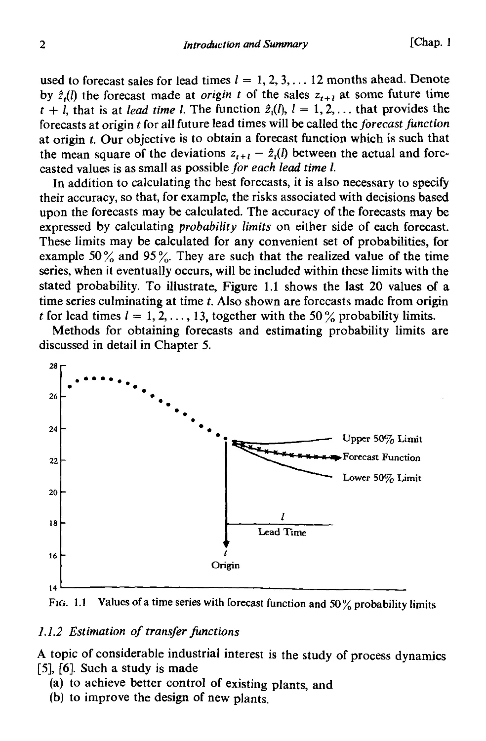
In addition to calculating the best forecasts, it is also necessary to specify
their accuracy, so that, for example, the risks associated with decisions based
upon the forecasts may be calculated. The accuracy of the forecasts may be
expressed by calculating probability limits on either side of each forecast.
These limits may be calculated for any convenient set of probabilities, for
example 50 % and 95 %. They are such that the realized value of the time
series, when it eventually occurs, will be included within these limits with the
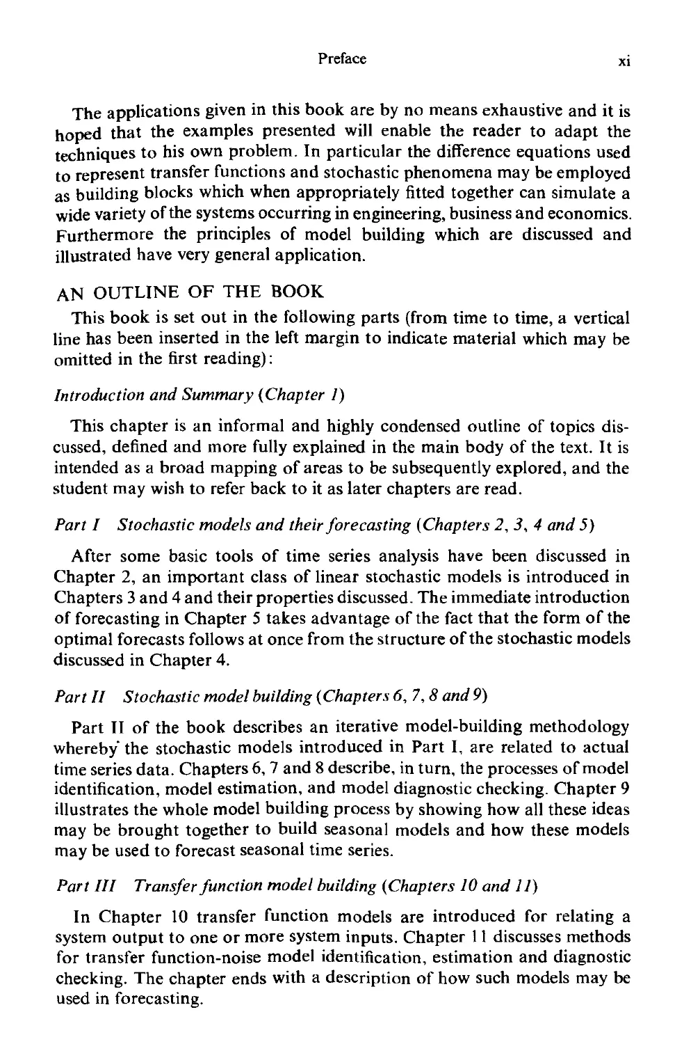
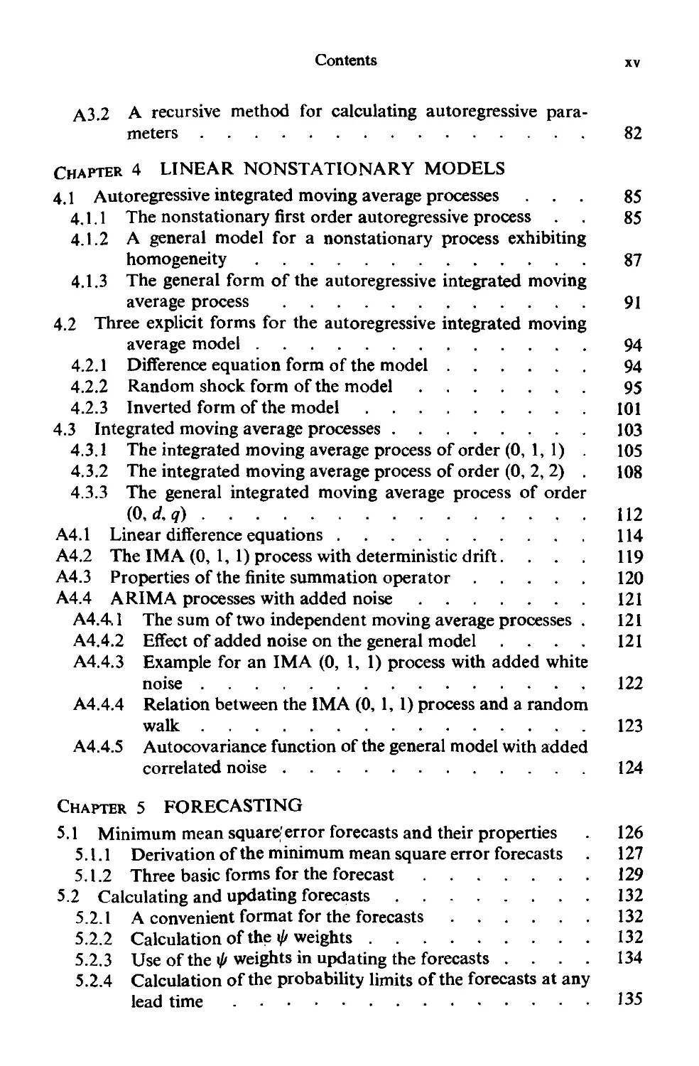
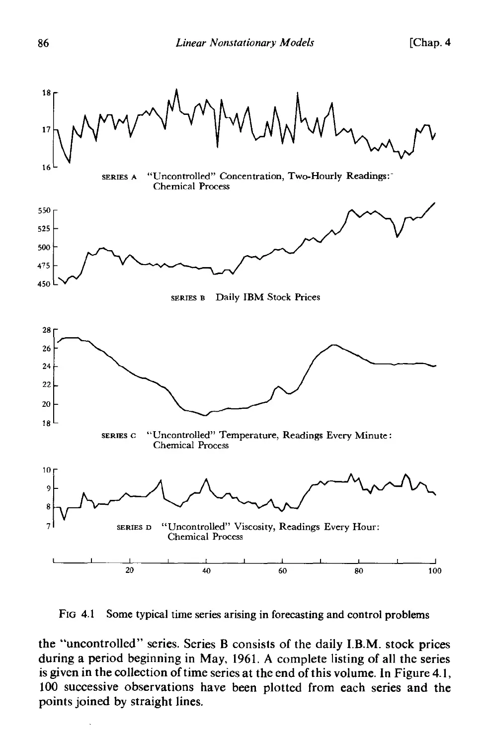
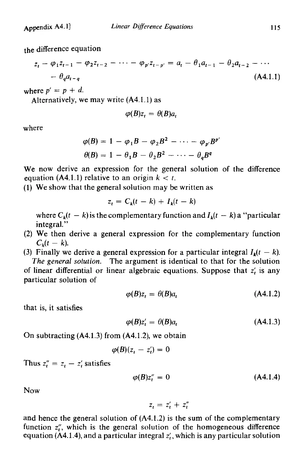
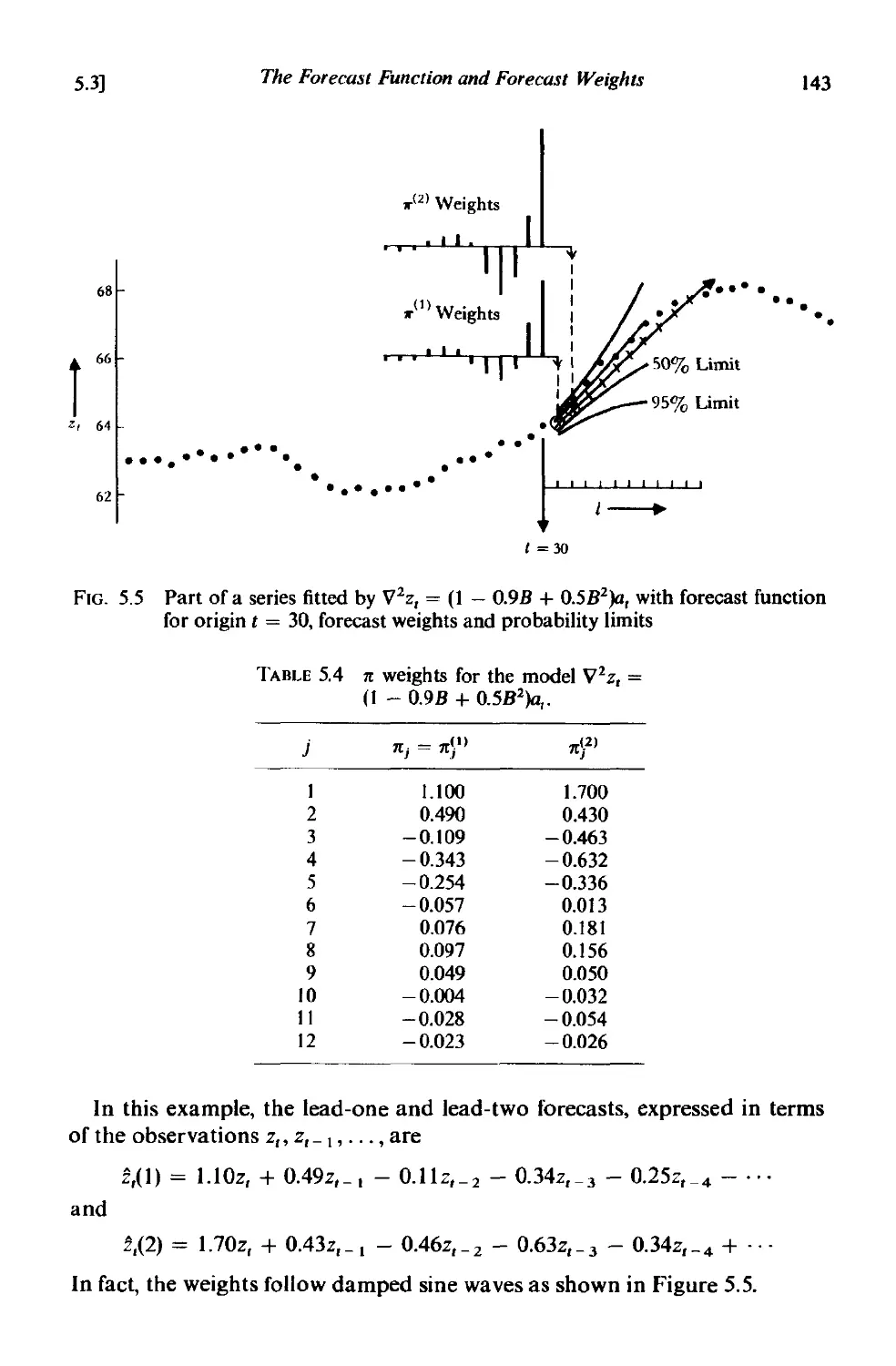
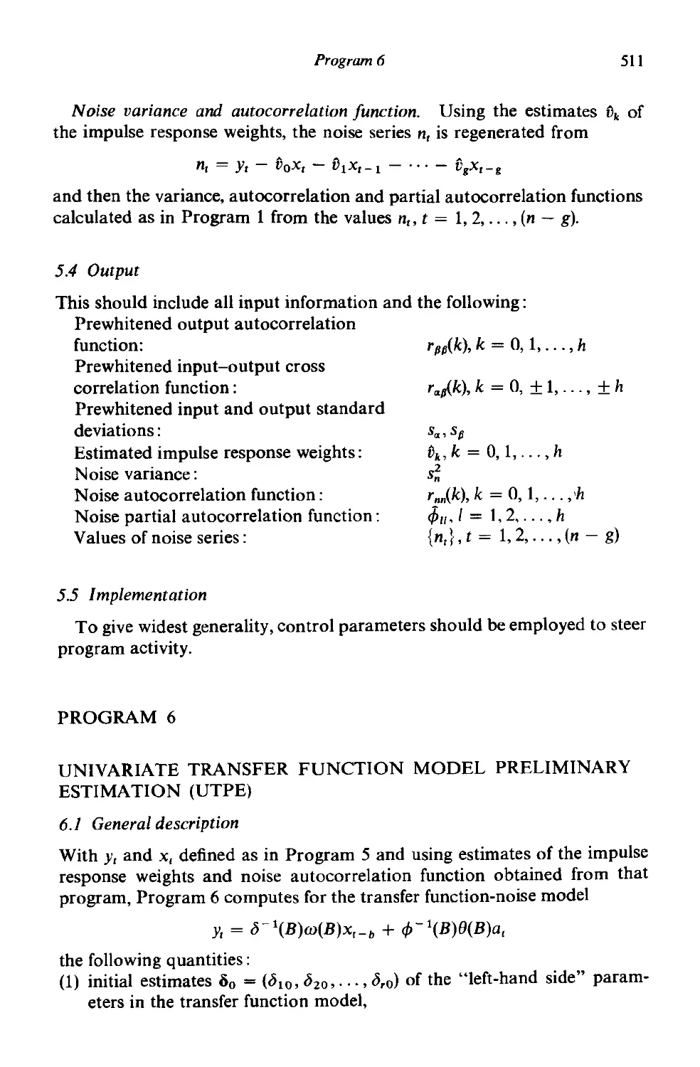
stated probability. To illustrate, Figure 1.l shows the last 20 values of a
time series culminating at time t. Also shown are forecasts made from origin
t for lead times 1 = 1,2,..., 13, together with the 50 % probability limits.
Methods for obtaining forecasts and estimating probability limits are
discussed in detail in Chapter 5.
28
26
.........
.
.
.
. .
24
.
.
.. UP!'" 50% U,.;,
.. Forecast Function
Lower 50% Limit
22
20
18
Lead Time
16
14
FIG. 1.1
I
Origin
Values ofa time series with forecast function and 50% probability limits
1.1.2 Estimation of transfer functions
A topic of considerable industrial interest is the study of process dynamics
[5J, [6]. Such a study is made
(a) to achieve better control of existing plants, and
(b) to improve the design of new plants.
1.1]
Three Important Practical Problems
3
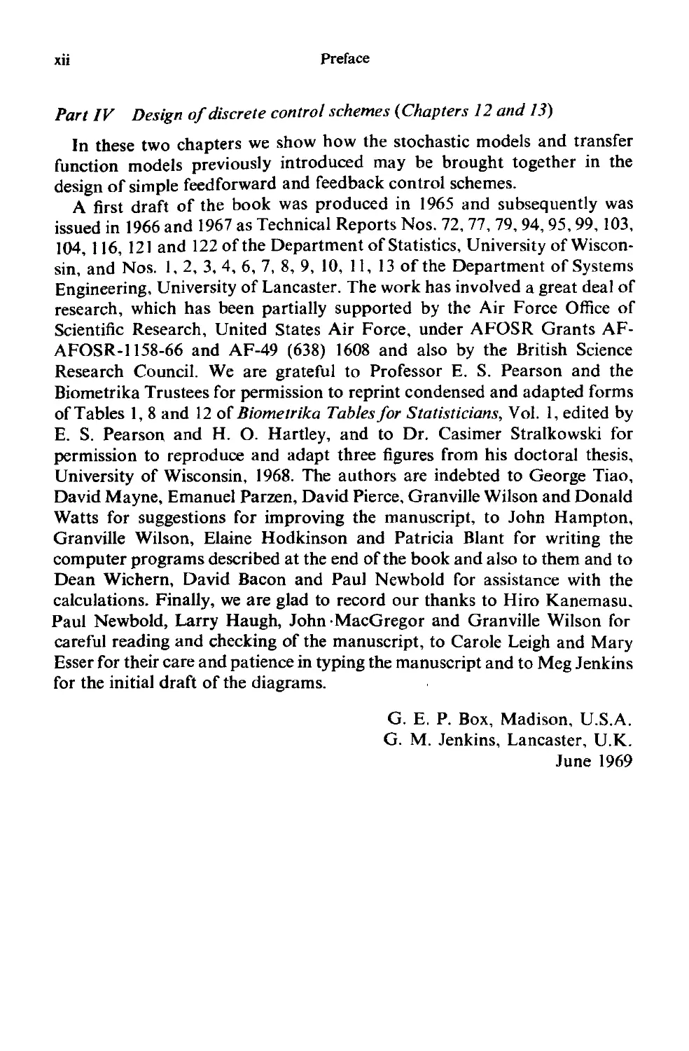
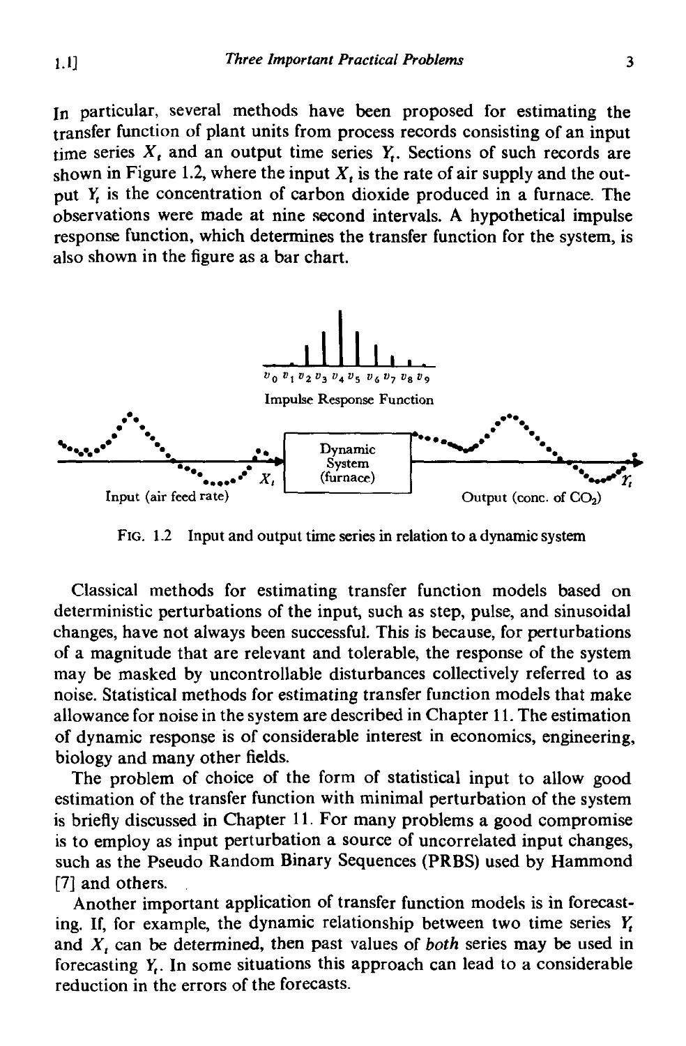
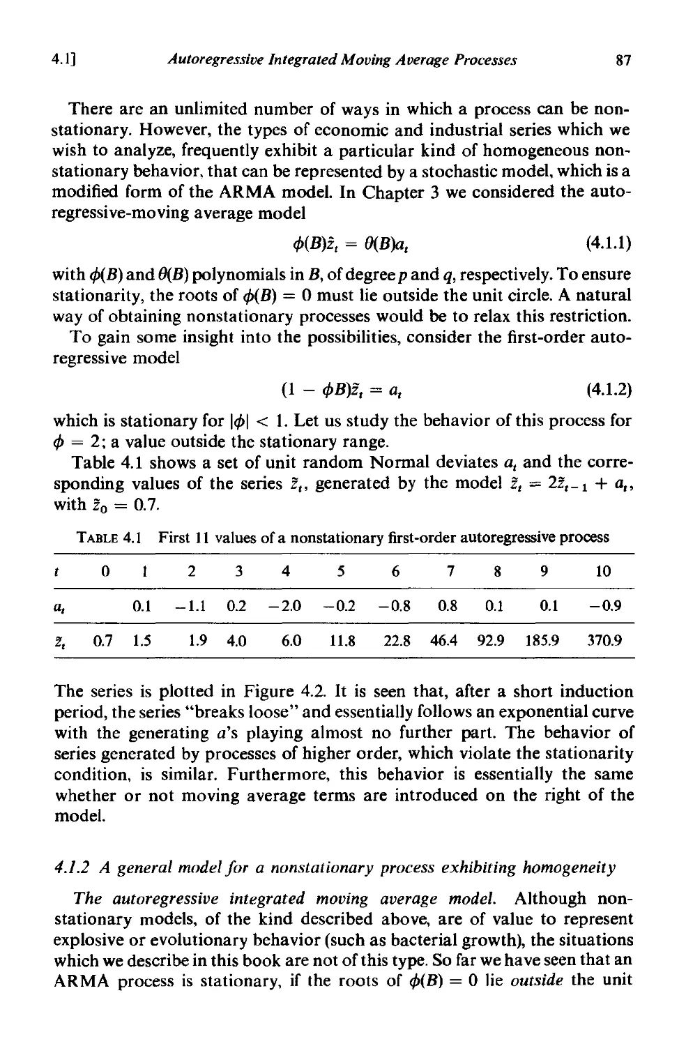
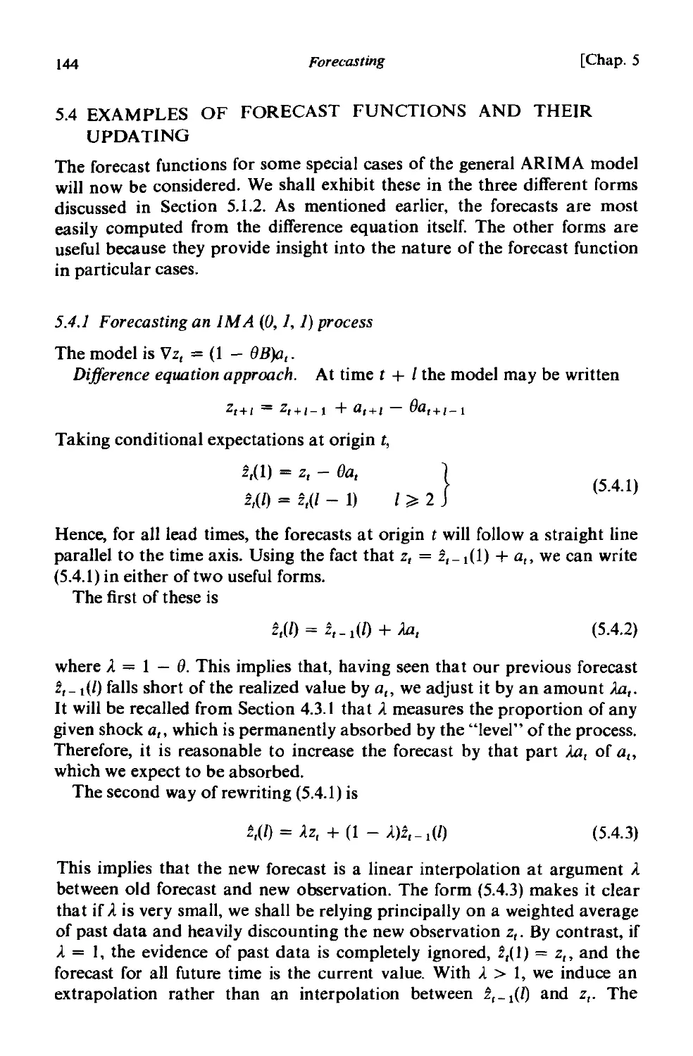
In particular, several methods have been proposed for estimating the
transfer function of plant units from process records consisting of an input
time series Xt and an output time series Y,. Sections of such records are
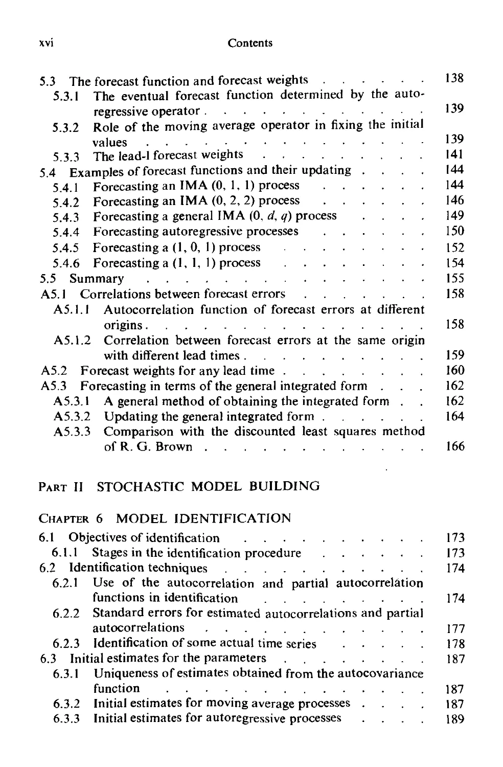
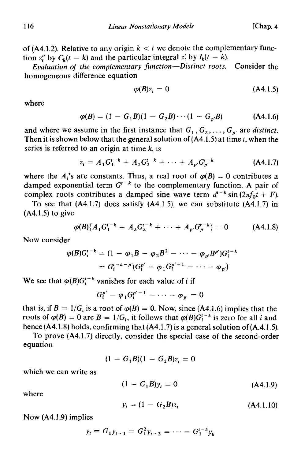
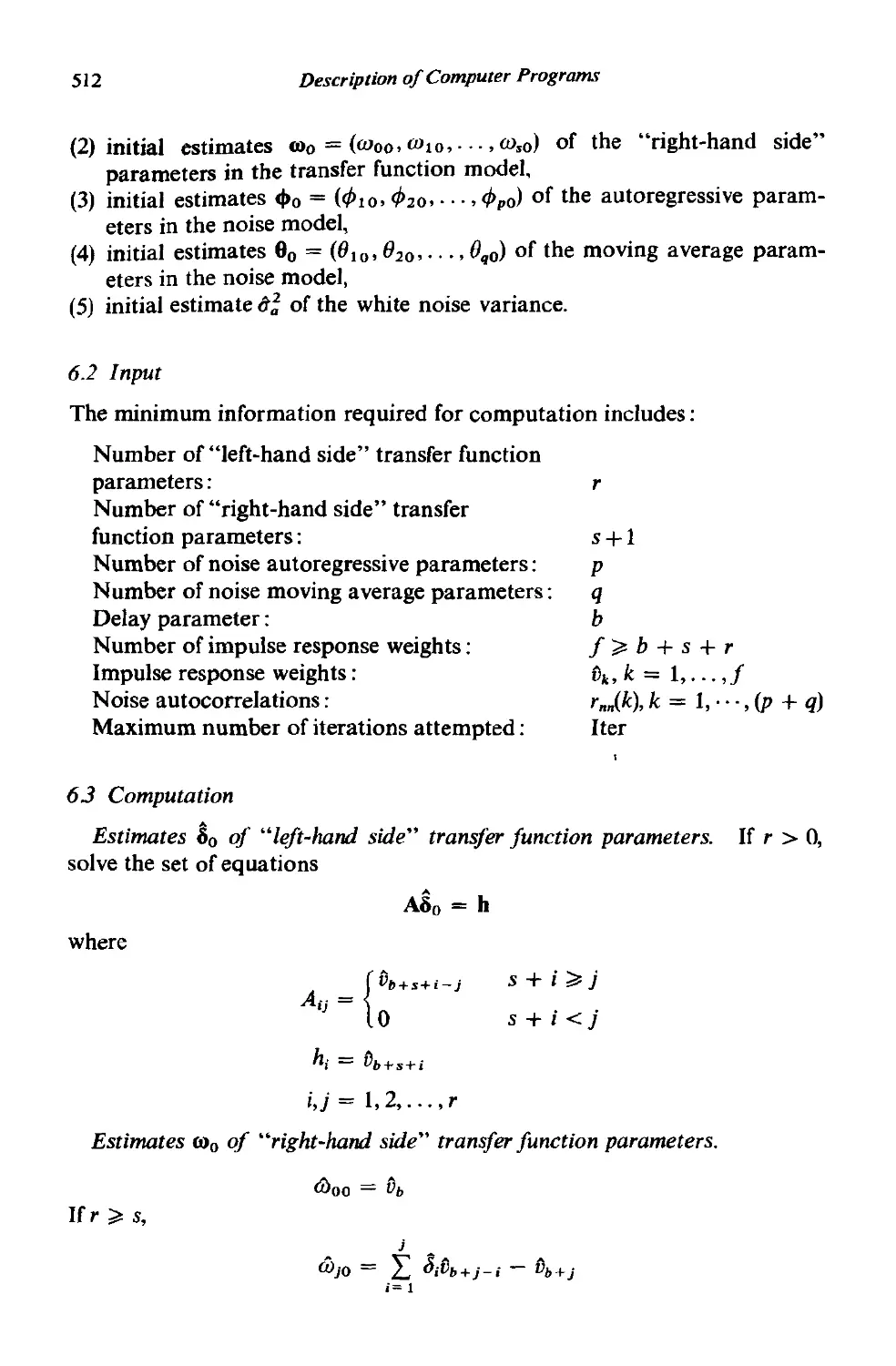
shown in Figure 1.2, where the input Xt is the rate of air supply and the out-
put 1; is the concentration of carbon dioxide produced in a fUrnace. The
observations were made at nine second intervals. A hypothetical impulse
response function, which determines the transfer function for the system, is
also shown in the figure as a bar chart.
V o V t V2 V 3 V 4 V s V6 V 7 Va V9
Impulse Response Function
...
. .
. ..
.......... -.. ....
.... ..-
..... Xt
Input (air feed rate)
Dynamic
System
(furnace)
...
.- -..
-.... .. -.
....., e.
ee._ _....
-r,
Output (cone. of CO 2 )
FIG. 1.2 Input and output time series in relation to a dynamic system
Classical methods for estimating transfer function models based on
deterministic perturbations of the input, such as step, pulse, and sinusoidal
changes, have not always been successful. This is because, for perturbations
of a magnitude that are relevant and tolerable, the response of the system
may be masked by uncontrollable disturbances collectively referred to as
noise. Statistical methods for estimating transfer function models that make
allowance for noise in the system are described in Chapter 11. The estimation
of dynamic response is of considerable interest in economics, engineering,
biology and many other fields.
The problem of choice of the form of statistical input to allow good
estimation of the transfer function with minimal perturbation of the system
is briefly discussed in Chapter 11. For many problems a good compromise
is to employ as input perturbation a source of uncorrelated input changes,
such as the Pseudo Random Binary Sequences (PRBS) used by Hammond
[7] and others.
Another important application of transfer function models is in forecast-
ing. If, for example, the dynamic relationship between two time series Y,
and X, can be determined, then past values of both series may be used in
forecasting 1;. In some situations this approach can lead to a considerable
reduction in the errors of the forecasts.
4
Introduction and Summary
[Chap. I
1.1.3 Design of discrete control systems
In the past, the word "control," to the statistician, has usually meant the
quality control techniques developed originally by Shewhart [8] in the United
States and by Dudding and Jennet [9] in Great Britain. Recently, the sequen-
tial aspects of quality control have been emphasized, leading to the introduc-
tion of cumulative sum charts by Page [10J, [llJ and Barnard [12J and the
geometric moving average charts of Roberts [13].
The word "control" has a different meaning, however, to the control
engineer. He thinks in terms of feed forward and feedback control loops, of
the dynamics and stability of the system, and usually of particular types of
hardware to carry out the control action. These control devices are automatic
in the sense that information is fed to them automatically from instruments
on the process and from them automatically to adjust the inputs to the
process.
In this book we describe a statistical approach to forecasting time series
and to the design of feed forward and feedback control schemes developed
in previous papers [14J, [15], [16J, [17J, [18], [19J and [20]. The control
techniques discussed are closer to those of the control engineer than the
standard quality control procedures developed by statisticians. This does
not mean we believe that the traditional quality control chart is unimportant
but rather that it performs a different function from that with which we are
here concerned. An important function of standard quality control charts
is to supply a continuous screening mechanism for detecting assignable
causes of variation. Appropriate display of plant data ensures that changes
that occur are quickly brought to the attention of those responsible for
running the process. Knowing the answer to the question "when did a change
of this particular kind occur?" we can then ask "why did it occur?" Hence,
a continuous incentive for process improvement, often leading to new
thinking about the process, can be achieved.
In contrast, the control schemes we discuss in this book are appropriate
for the periodic, optimal adjustment of a manipulated variable, whose
effect on some output quality characteristic is already known, so as to
minimize the variation of that quality characteristic about some target
value.
The reason control is necessary is that there are inherent disturbances or
noise in the process. When we can measure these disturbances, it may be
possible to make appropriate compensatory changcs in some other variable.
This is referred to as fee4forward control. Alternatively, or in addition, we
may be able to use the deviation from target or "error signal" of the output
characteristic itself to calculate appropriate compensatory changes. This is
called feedback control. Unlike feedforward control, this mode of correction
can be employed even when the source of the disturbances is not accurately
1.1]
Three Important Practical Problems
5
known or the magnitude of the disturbances is not measured. More generally,
it may be desirable to use a mixture of feedforward and feedback control;
feedforward control can be used to compensate for those disturbances that
can be measured and feedback control for those disturbances that cannot
be measured.
The approach to control adopted here is to typify the disturbance by a
suitable time series or stochastic model and the inertial characteristics ofthe
system by a suitable transfer function model. It is then possible to calculate
the optimal control equation. This is an equation that allows the action which
should be taken at any given time to be calculated given the present and
previous states of the system. "Optimal" action is interpreted as that which
produces the smallest mean square error at the output.
Execution of the control action called for by the control equation can be
achieved in various ways corresponding to various levels of technological
sophistication. The question of what means should be employed to meet a
given situation is not an appropriate subject for this text. However, we may
mention that at one extreme of sophistication we have so-called computer
control where the action called for by the control equation is calculated by
computer and is automatically effected by suitable transducers that appropri-
ately open and close valves to adjust process variables, such as temperatures,
pressures and flow rates. At an intermediate level we find automatic con-
trollers that employ various pneumatic and electrical devices to carry out
the control action. At the other extreme the action called for by the control
equation may be embodied in a suitable nomogram or chart. Periodically
the plant operator may make one or more readings, measurements, or
determinations, consult the nomogram to calculate the action called for
and then manually make the appropriate modifications.
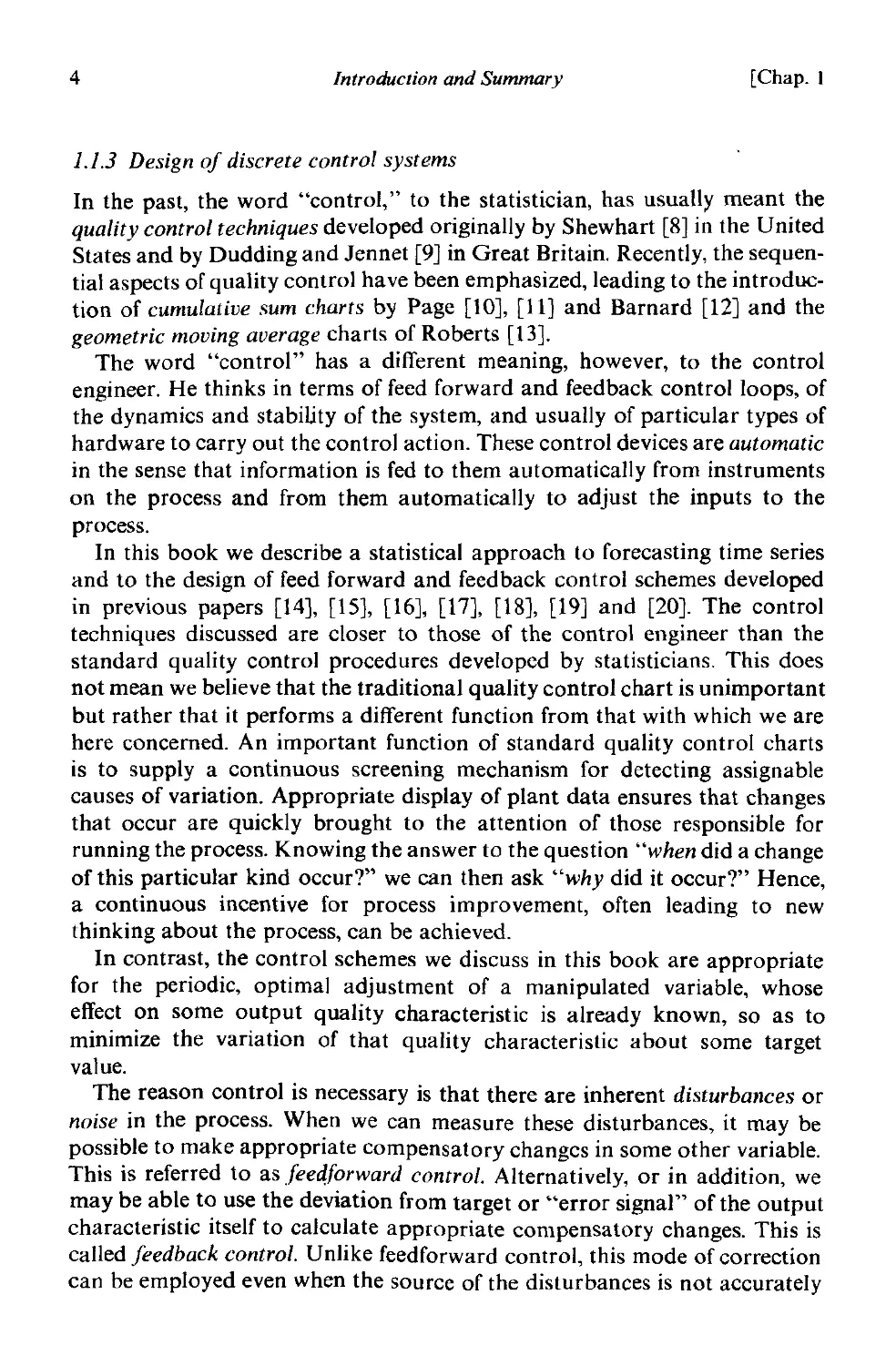
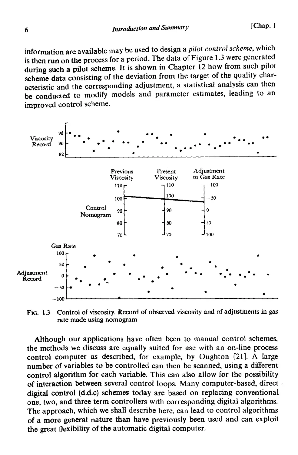
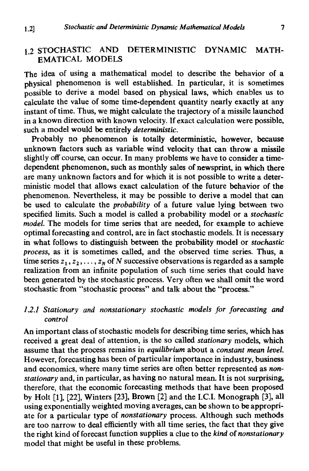
Even in modern industry there are many situations where manual control
is employed and could be improved. Chapter 12 discusses briefly the
preparation of charts and nomograms that can indicate optimal control
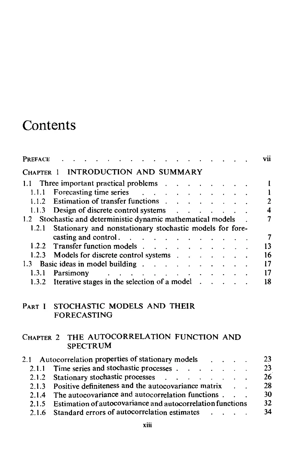
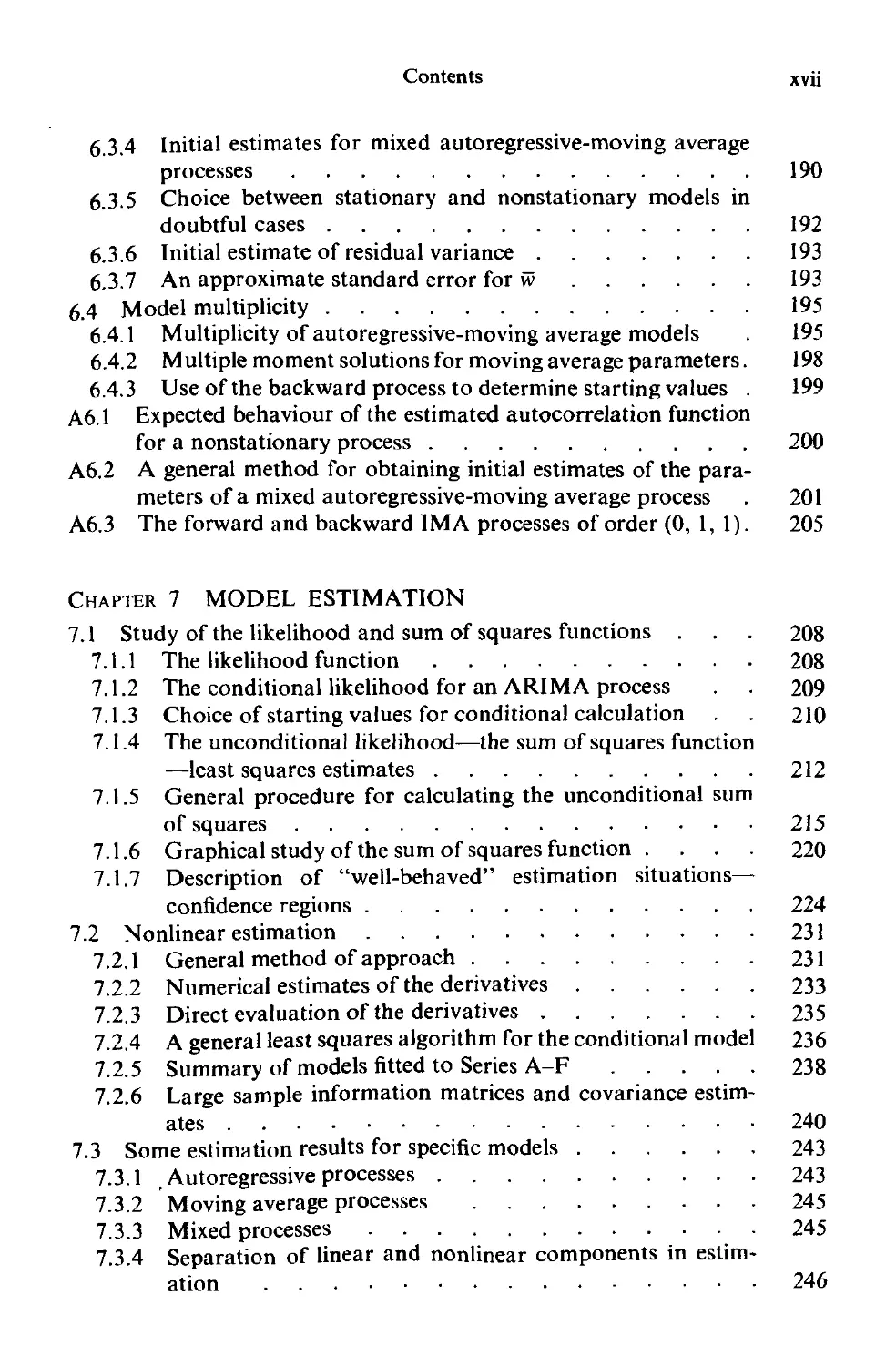
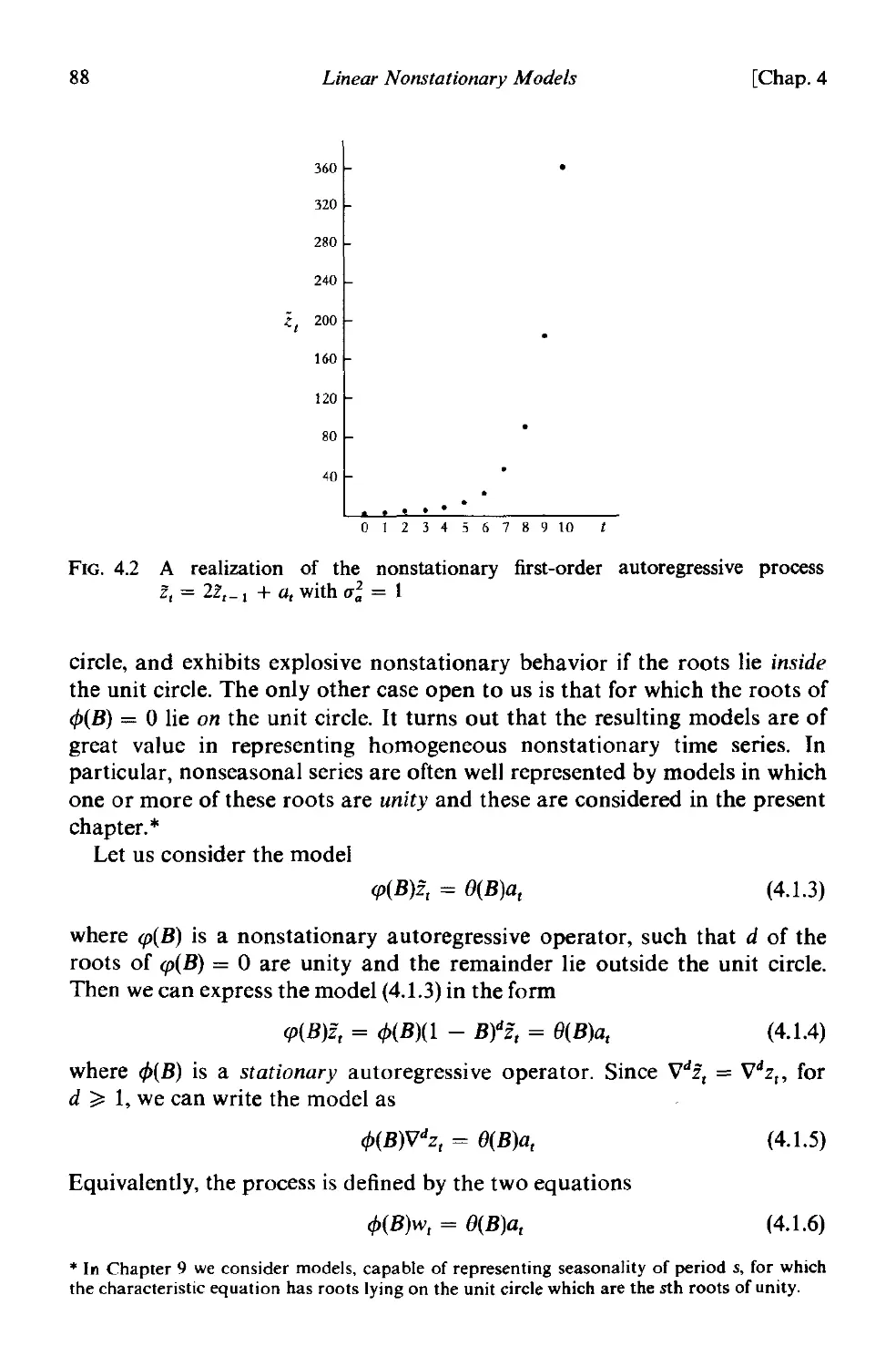
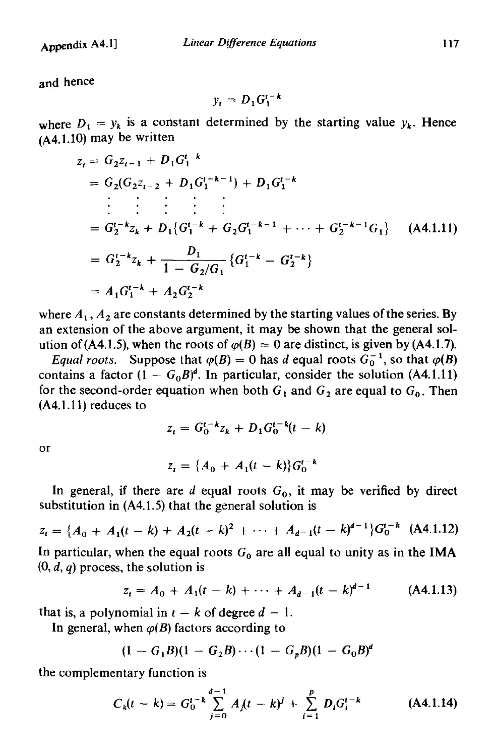
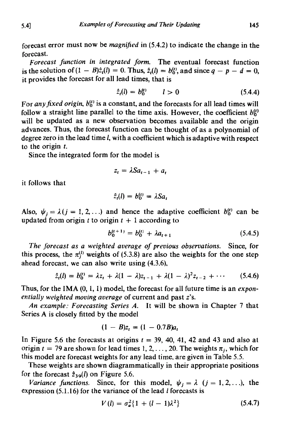
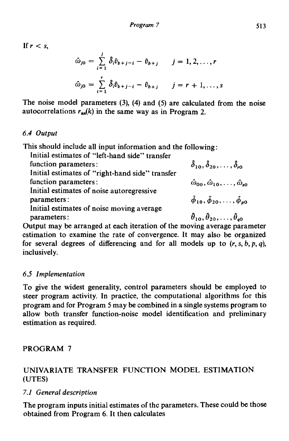
action in simple cases. For example, the upper chart of Figure 1.3 shows
hourly measurements of the viscosity of a polymer made over a period of
42 hours. The viscosity is to be controlled about a target value of 90 units.
As each viscosity measurement comes to hand, the process operator uses the
nomogram shown in the middle of the figure to compute the optimal adjust-
ment to be made in the manipulated variable (gas rate). The lower chart of
Figure 1.3 shows the adjustments made in accordance with the nomogram.
In practice, the precise nature of the stochastic and transfer function
models which are appropriate in any given situation and which are needed
to design the optimal control scheme will not usually be known. Further-
more, the appropriate numerical values for the parameters contained in
these models will be unknown. Therefore, as is almost always true in model
building, we have to proceed iteratively. Whatever records and background
6
Introduction and Summary
[Chap. 1
information are available may be used to design a pilot control scheme, which
is then run on the process for a period. The data of Figure 1.3 were generated
during such a pilot scheme. It is shown in Chapter 12 how from s ch pilot
scheme data consisting of the deviation from the target of the qualIty char-
acteristic and the corresponding adjustment, a statistical analysis can then
be conducted to modify models and parameter estimates, leading to an
improved control scheme.
98 0 00
Viscosity
Record 90 0 0 0
82
00
.. . .
00
100
Control 90
Nomogram
Present Adjustment
Viscosity to Gas Rate
110 -100
100 50
90 0
80 50
70 100
Previous
Viscosity
110
80
70
Gas Rate
100 0
50
Adjustment 0 0
Record 0 0
-50 0
-100
o
o
o o.
o 0
o
o 0 .
.
.
FIG. 1.3 Control of viscosity. Record of observed viscosity and of adjustments in gas
rate made using nomogram
Although our applications have often been to manual control schemes,
the methods we discuss are equally suited for use with an on-line process
control computer as described, for example, by Oughton [21]. A large
number of variables to be controlled can then be scanned, using a different
control algorithm for each variable. This can also allow for the possibility
of interaction between several control loops. Many computer-based, direct.
digital control (d.d.c) schemes today are based on replacing conventional
one, two, and three term controllers with corresponding digital algorithms.
The approach, which we shall describe here, can lead to control algorithms
of a more general nature than have previously been used and can exploit
the great flexibility of the automatic digital computer.
1.2]
Stochastic and Deterministic Dynamic Mathematical Motkls
7
1.2 STOCHASTIC AND DETERMINISTIC DYNAMIC MATH-
EMATICAL MODELS
The idea of using a mathematical model to describe the behavior of a
physical phenomenon is well established. In particular, it is sometimes
possible to derive a model based on physical laws, which enables us to
calculate the value of some time-dependent quantity nearly exactly at any
instant of time. Thus, we might calculate the trajectory of a missile launched
in a known direction with known velocity. If exact calculation were possible,
such a model would be entirely deterministic.
Probably no phenomenon is totally deterministic, however, because
unknown factors such as variable wind velocity that can throw a missile
slightly off course, can occur. In many problems we have to consider a time-
dependent phenomenon, such as monthly sales of newsprint, in which there
are many unknown factors and for which it is not possible to write a deter-
ministic model that allows exact calculation of the future behavior of the
phenomenon. Nevertheless, it may be possible to derive a model that can
be used to calculate the probability of a future value lying between two
specified limits. Such a model is called a probability model or a stochastic
model. The models for time series that are needed, for example to achieve
optimal forecasting and control, are in fact stochastic models. It is necessary
in what follows to distinguish between the probability model or stochastic
process, as it is sometimes called, and the observed time series. Thus, a
time series Zl' Zz,..., ZN of N successive observations is regarded as a sample
realization from an infinite population of such time series that could have
been generated by the stochastic process. Very often we shall omit the word
stochastic from "stochastic process" and talk about the "process."
1.2.1 Stationary and nonstationary stochastic models for forecasting and
control
An important class of stochastic models for describing time series, which has
received a great deal of attention, is the so called stationary models, which
assume that the process remains in equilibrium about a constant mean level.
However, forecasting has been of particular importance in industry, business
and economics, where many time series are often better represented as non-
stationary and, in particular, as having no natural mean. It is not surprising,
therefore, that the economic forecasting methods that have been proposed
by Holt [1], [22], Winters [23], Brown [2] and the I.C.!. Monograph [3], all
using exponentially weighted moving averages, can be shown to be appropri-
ate for a particular type of nonstationary process. Although such methods
are too narrow to deal efficiently with all time series, the fact that they give
the right kind offorecast function supplies a clue to the kind ofnonstationary
model that might be useful in these problems.
8
Introduction and Summary
[Chap. I
The stochastic model for which the exponentially weighted moving
average forecast is optimal is a member of a class of nonstationary processes
called autoregressive-integrated moving average processes (ARIMA proc-
esses), which are discussed in Chapter 4. This wider class of processes
provides a-riinge of models, stationary and non-stationary, that adequately
represent many of the time series met in practice. Our approach to forecast-
ing has been first to derive an adequate stochastic model for the particular
times series under study. As shown in Chapter 5, once an appropriate model
has been determined for the series, the optimal forecasting procedure
follows immediately. These forecasting procedures include the exponentially
weighted moving average forecast as a special case.
Some simple operators. We shall employ extensively the backward shift
operator B which is defined by BZt = Z'-I; hence B"'z, = Z,-m' The inverse
operation is performed by the forward shift operator F = B- 1 given by
Fz, = Z,+I; hence F"'Zt = Z,+.... Another important operator is the backward
difference operator V which can be written in terms of B, since
VZ t = Zt - Zt-l = (1 - B)z,
In turn, V has for its inverse the summation operator S given by
CJ)
V-IZ t = SZt = L Z'_j
j=O
= Zt + Z'-1 + Z'-2 + .,.
= (1 + B + B 2 + .. . )Zt
= (1 - B)-I Z ,
Linear filter model. The stochastic models we employ are based on the
idea, (Yule [24]), that a time series in which successive values are highly
dependent can be usefully regarded as generated from a series of independent
"shocks" at. These shocks are random drawings from a fixed distribution,
usually assumed Normal and having mean zero and variance (1;. Such a
sequence of random variables tlr, a,_ l' a,_ z,. .. is called a white noise
process by engineers.
The white noise process at is supposed transformed to the process z, by
what is called a linear filter, as shown in Figure l.4(a). The linear filtering
Whi: ,NOise
"'(B)
Linear
Filter
z,
.
FIG. l.4(a) Representation of a time series as the output from a linear filter
1.2]
Stochastic and Deterministic Dynamic Mathematical Models
9
operation simply takes a weighted sum of previous observations, so that
Z, = J1. + a, + t/11a'-1 + I/12a'-2 + ...
= J1. + I/1(B)a,
(1.2.1)
In general, J1. is a parameter that determines the "level" of the process, and
I/1(B) = 1 + I/11B + I/12B2 +...
is the linear operator that transforms at into z, and is called the transfer
function of the filter.
The sequence 1/11> 1/12' .,. formed by the weights may, theoretically, be
finite or infinite. If this sequence is finite, or infinite and convergent, the
filter is said to be stable and the process Zt to be stationary. The parameter J1.
is then the mean about which the process varies. Otherwise, Zt is non-
stationary and J1. has no specific meaning except as a reference point for the
level of the process.
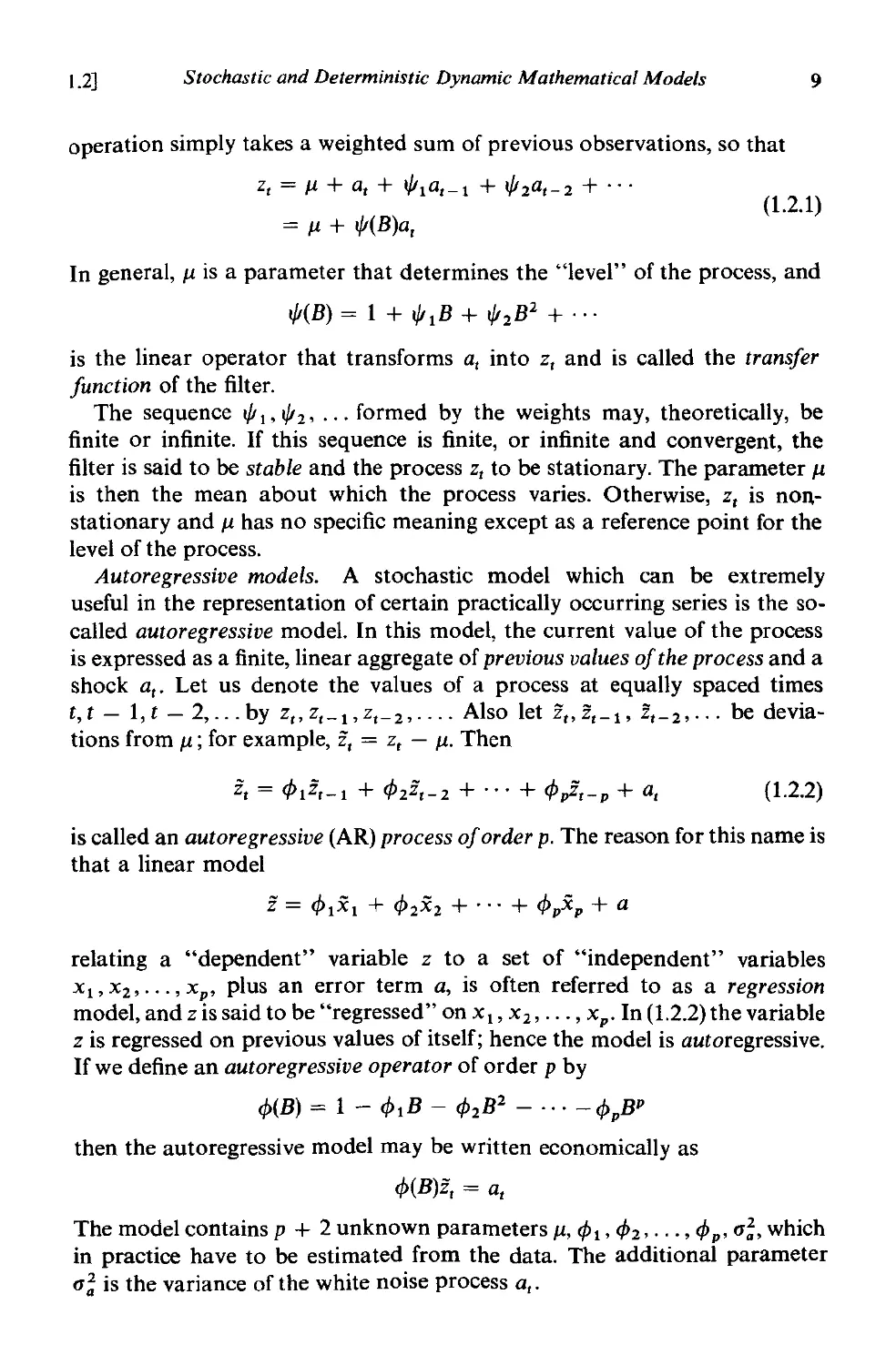
Autoregressive models. A stochastic model which can be extremely
useful in the representation of certain practically occurring series is the so-
called autoregressive model. In this model, the current value of the process
is expressed as a finite, linear aggregate of previous values of the process and a
shock at. Let us denote the values of a process at equally spaced times
t, t - 1, t - 2,.. . by Zp Z'-l' Z'-2" . .. Also let Zt, Zt-l, Z'-2" .. be devia-
tions from J1. ; for example, Zt = Zt - J1.. Then
Zt = <P1 Z t-l + CP2Zt-2 + '" + cPpz,_p + a,
( 1.2.2)
is called an autoregressive (AR) process of order p. The reason for this name is
that a linear model
Z = CPIXI + CP2X2 + . .. + CPpx p + a
relating a "dependent" variable Z to a set of "independent" variables
XI' X2,' . . , xp' plus an error term a, is often referred to as a regression
model, and zis said to be "regressed" on XI' X2'..., xp' In (1.2.2) the variable
Z is regressed on previous values of itself; hence the model is autoregressive.
If we define an autoregressive operator of order p by
cp(B) = 1 - CPIB - CP2B2 - .. . - CPpBP
then the autoregressive model may be written economically as
cp(B)zt = at
The model contains p + 2 unknown parameters J1., CPl' CP2' . . ., CPp, (1;, which
in practice have to be estimated from the data. The additional parameter
(1; is the variance of the white noise process a,.
10
Introduction and Summary
[Chap. I
It is not difficult to see that the autoregressive model is a special case of
the linear filter model of (1.2.1). For example, we can eliminate Zt-l from
the right-hand side of (1.2.2) by substituting
Zt-l = 4>l Z t-2 + 4>2 Z '-3 + ... + 4>"zt-p-l + a t -l
We can likewise substitute for Z'-2' and so on, to yield eventually an infinite
series in the a's.
Symbolically, we have
4>(B)Zt = at
is equivalent to
Zt = t/t(B)a t
with
t/t(B) = 4> -l(B)
Autoregressive processes can be stationary or nonstationary. For the
process to be stationary, the 4>'s must be chosen so that the weights
t/tl't/t2'... in t/t(B) = 4>-l(B) form a convergent series. We discuss these
models in greater detail in Chapters 3 and 4.
Moving average models. The autoregressive model (1.2.2) expresses the
deviation Zt of the process as a finite weighted sum of p previous deviations
Zr-l,Zt-2,...,Zt-" of the process, plus a random shock at. Equivalently,
as we have just seen, it expresses zr as an infinite weighted sum of a's.
Another kind of model, of great practical importance in the representa-
tion of observed time series, is the so-called finite moving average process.
Here we make Zt linearly dependent on a finite number q of previous a's.
Thus
Zt = at - (Jlat-l - (J2at-2 - ... - (Jqa t _ q
(1.2.3)
is called a moving average (MA) process of order q. The name "moving
average" is somewhat misleading because the weights 1, -(JI, -(J2,""
-(Jq, which multiply the a's, need not total unity nor need they be positive.
However, this nomenclature is in common use, and therefore we employ it.
If we define a moving average operator of order q by
()(B) = I - (JIB - (J2B2 - ... - 8iJ"
then the moving average model may be written economically as
Zt = lJ( B)at
It contains q + 2 unknown parameters J.I., (Jl'...' 8q, 0';, which in practice
have to be estimated from the data.
1.2]
Stochastic and Deterministic Dynamic Mathematical Models
11
Mixed autoregressive-moving average models. To achieve greater flex-
ibility in fitting of actual time series, it is sometimes advantageous to include
both autoregressive and moving average terms in the model. This leads to
the mixed autoregressive-moving average model
Zt = ifJ1 Z t-l + ... + ifJpz,-p + llr - (Jta,-t - ... - (Jqa t _ q (1.2.4)
or
ifJ(B)Zt = O(B)a t
which employs p + q + 2 unknown parameters J1.; ifJl,' . . , ifJp; (Jt,. . . , Oq;
0';, that are estimated from the data.
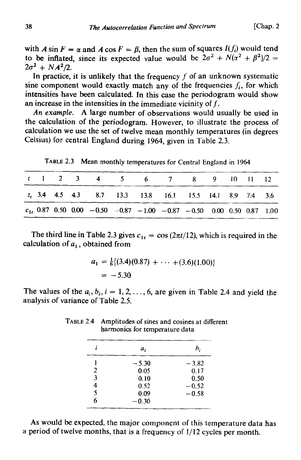
In practice, it is frequently true that adequate representation of actually
occurring stationary time series can be obtained with autoregressive, moving
average, or mixed models, in which p and q are not greater than 2 and often
less than 2.
Nonstationary models. Many series actually encountered in industry or
business (for example, stock prices) exhibit nonstationary behavior and in
particular do not vary about a fixed mean. Such series may nevertheless
exhibit homogeneous behavior of a kind. In particular, although the general
level about which fluctuations are occurring may be different at different
times, the broad behavior of the series, when differences in level are allowed
for, may be similar. We show in Chapter 4 that such behavior may be repre-
sented by a generalized autoregressive operator ep(B), in which one or more of
the zeroes of the polynomial ep(B) (that is one or more of the roots of the
equation ep(B) = 0) is unity. Thus the operator ep(B) can be written
ep(B) = cf>(B)(l - B)d
where cf>(B) is a stationary operator. Thus a general model, which can repre-
sent homogeneous nonstationary behavior, is of the form
ep(B)z, = cJ>(B)(l - B)d Z , = (J(B)a t
that is
cJ>(B)w t = 8(B)a,
( 1.2.5)
where
w, = Vdz t
(1.2.6)
Homogeneous nonstationary behavior can therefore be represented by a
model which calls for the d'th difference of the process to be stationary. In
practice d is usually 0, 1, or at most 2.
The process defined by (1.2.5) and (1.2.6) provides a powerful model for
describing stationary and nonstationary time series and is called an auto-
regressive integrated moving average (ARI MA) process, of order (p, d, q).
12
Introduction and Summary
[Chap. I
The process is defined by
w, = 4JIW'-1 +... + 4Jpw,-p + a, - 0la,-1 -... -Oqa,_q (1.2.7)
with w, = Vdz,. Note that if we replace w, by z, - p., when d = 0, the model
(1.2.7) includes the stationary mixed model (1.2.4), as a special case, and also
the pure autoregressive model (1.2.2) and the pure moving average model
(1.2.3).
The reason for the inclusion of the word "integrated" (which should
perhaps more appropriately be "summed") in the ARIMA title, is as follows.
The relationship which is inverse to (1.2.6) is
z, = Sd W ,
( 1.2.8)
where it will be recalled that S is the summation operator defined by
00
Sw, = I W'_j = w, + W'-1 + W'-2 + '"
j=O
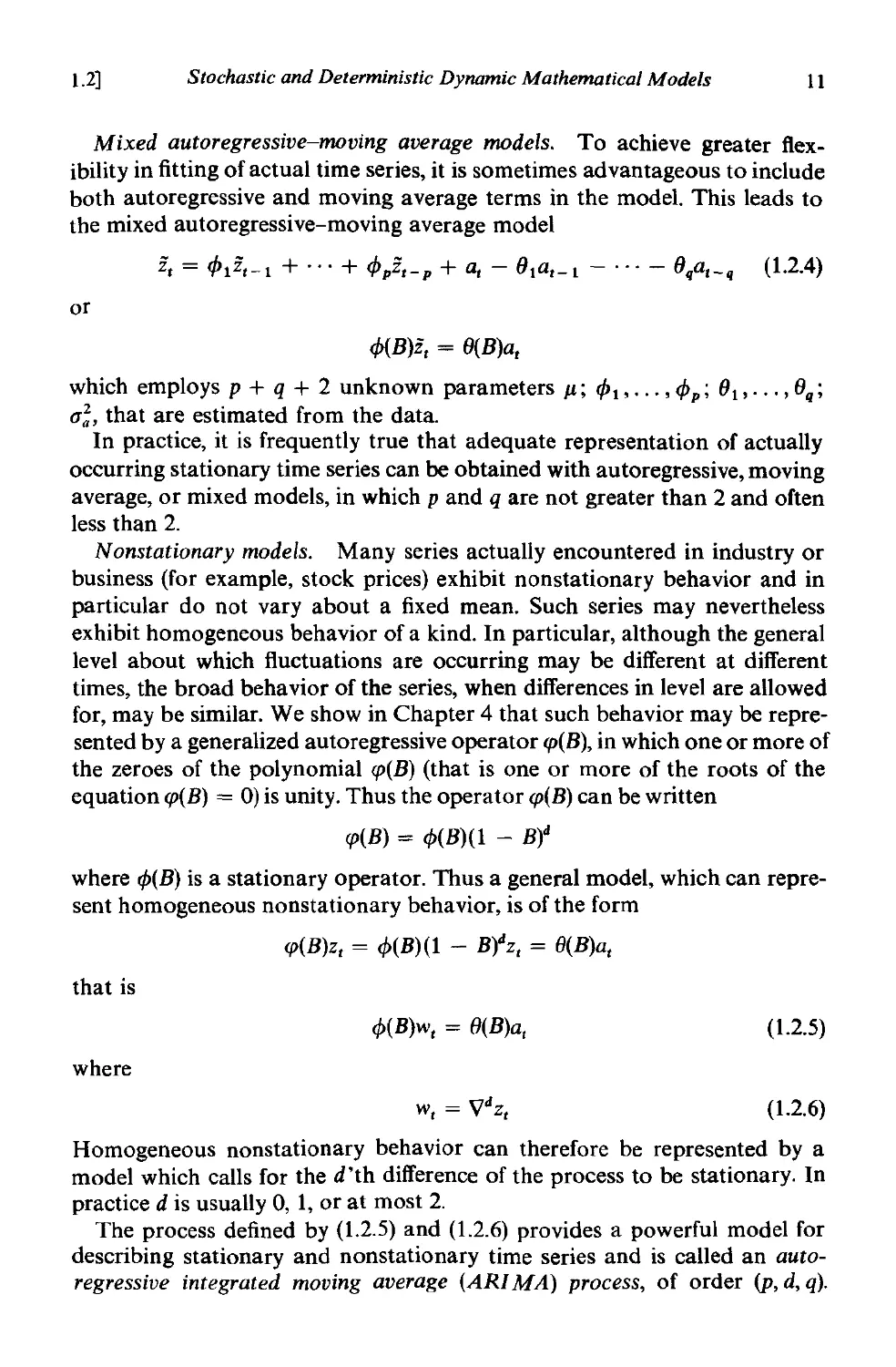
Thus, the general autoregressive integrated moving average (ARIMA)
process may be generated from white noise a, by means of three filtering
operations, as indicated -by the block diagram of Figure 1.4(b). The first
filter has input a" transfer function O(B), and output e" where
e, = a, - 0la,-1 - ... - (}qa,_q
= (}(B)a,
( 1.2.9)
White Noise
Time Series
a,
<:,
FIG. 1.4(b) Block diagram for autoregressive integrated moving average model
The second filter has input e,. transfer function 4J -1(B), and output WI'
according to
w, = 4JIW'-1 +... + 4Jpw,_p + e,
= 4J- I (B)e,
(1.2.10)
Finally, the third filter has input w, and output z" according to (1.2.8), and
has transfer function Sd.
As described in Chapter 9, a special form of the model (1.2.7) can be
employed to represent seasonal time series.
1.2]
Stochastic and Deterministic Dynamic Mathematical Models
13
1.2.2 Transfer function models
An important type of dynamic relationship between a continuous input and
a continuous output, for which many physical examples can be found, is that
in which the deviations of input X and of output Y, from appropriate mean
values, are related by a linear differential equation of the form
(1 + E 1 D + ... + E R DR)Y(t) = (Ho + H tD + ... + HsDS)X(t - t) (1.2.11)
where D is the differential operator d/dt, the E's and H's are unknown
parameters, and t is a parameter which measures the dead-time or pure delay
between input and output. The simplest example of (1.2.11) would be a
system where the rate of change in the output was proportional to the
difference between input and output, so that
dY
E-;tt=X-Y
and hence
(1 + ED)Y= X
In a similar way, for discrete data, in Chapter 10 we represent the transfer
between an output Yand an input X, each measured at equispaced times,
by the difference equation
(1 + tV + ... + .vr)y, = (110 + 11tV + ... + ".vS)X t _ b (1.2.12)
in which the differential operator D is replaced by the difference operator V.
An expression of the fonn (1.2.12), containing only a few parameters
(r 2, s 2), may often be used as an approximation to a dynamic relation-
ship, whose true nature is more complex.
The linear model (1.2.12) may be written equivalently in terms of past
values of the input and output by substituting B = 1 - V in (1.2.12), that is
(1 - biB - . .. - b,Br)y; = (wo - WtB - ... - wsBS)X t _ b (1.2.13)
= (wOB b - WtBb+l - ... - wsBb+s)X t
or
(B)Y, = w(B)BbX t
= Q(B)X t
Alternatively, we can say that the output Y, and input Xt are linked by a
linear filter
y, = VOXt + v 1 X,-t + v 2 X t - 2 +...
= v(B)X t
(1.2.14)
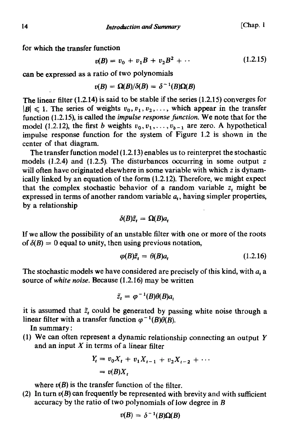
14
Introduction and Summary
[Chap. 1
for which the transfer function
v(B) = Vo + vtB + v 2 B 2 + .,
can be expressed as a ratio of two polynomials
v(B) = O(B)/ (B) = r 1 (B)O(B)
The linear filter (1.2.14) is said to be stable if the series (1.2.15) converges for
IBI 1. The series of weights Vo, .V l , V2, . . ., which appear in the transfer
function (1.2.15), is called the impulse response function. We note that for the
model (1.2.12), the first b weights vo, Vb' .., Vb-l are zero. A hypothetical
impulse response function for the system of Figure 1.2 is shown in the
center of that diagram.
The transfer function model (1.2.13) enables us to reinterpret the stochastic
models (1.2.4) and (1.2.5). The disturbances occurring in some output z
will often have originated elsewhere in some variable with which z is dynam-
ically linked by an equation of the form (1.2.12). Therefore, we might expect
that the complex stochastic behavior of a random variable z, might be
expressed in terms of another random variable ar, having simpler properties,
by a relationship
(1.2.15)
b(B)z, = Q(B)a,
If we allow the possibility of an unstable filter with one or more of the roots
of c5(B) = 0 equal to unity, then using previous notation,
cp(B)z, = O(B)a,
(1.2.16)
The stochastic models we have considered are precisely of this kind, with a, a
source of white noise. Because (1.2.16) may be written
z, = cp - t(B)(J(B)a,
it is assumed that Zt could be generated by passing white noise through a
linear filter with a transfer function cp -1(B)O(B).
In summary:
(1) We can often represent a dynamic relationship connecting an output Y
and an input X in terms of a linear filter
y, = voX, + V 1 X,_1 + V2X,-2 + . . .
= v(B)X t
where v(B) is the transfer function of the filter.
(2) In turn v(B) can frequently be represented with brevity and with sufficient
accuracy by the ratio of two polynomials of low degree in B
v(B) = b - I(B)O(B)
1.2]
Stochastic and Deterministic Dynamic Mathematical Models
15
so that the dynamic input-output equation may be written
<5(B)1'; = Q(B)X t
(3) It is postulated that a series z" in which successive values are highly
dependent, can be represented as the result of passing white noise a,
through such a dynamic system in which certain of the roots of <5(B) = 0
could be unity. The notion yields the autoregressive integrated moving
average model
<(J(B)z, = 8(B)at
Models with superimposed noise. We have seen that the problem of
estimating an appropriate model, linking an output Y, and an input X"
is equivalent to estimating the transfer function v(B) = (j -1(B)O(B). However,
this problem is complicated in practice by the presence of noise Nt> which
we assume corrupts the true relationship between input and output accord-
ing to
1'; = v(B)X t + Nt
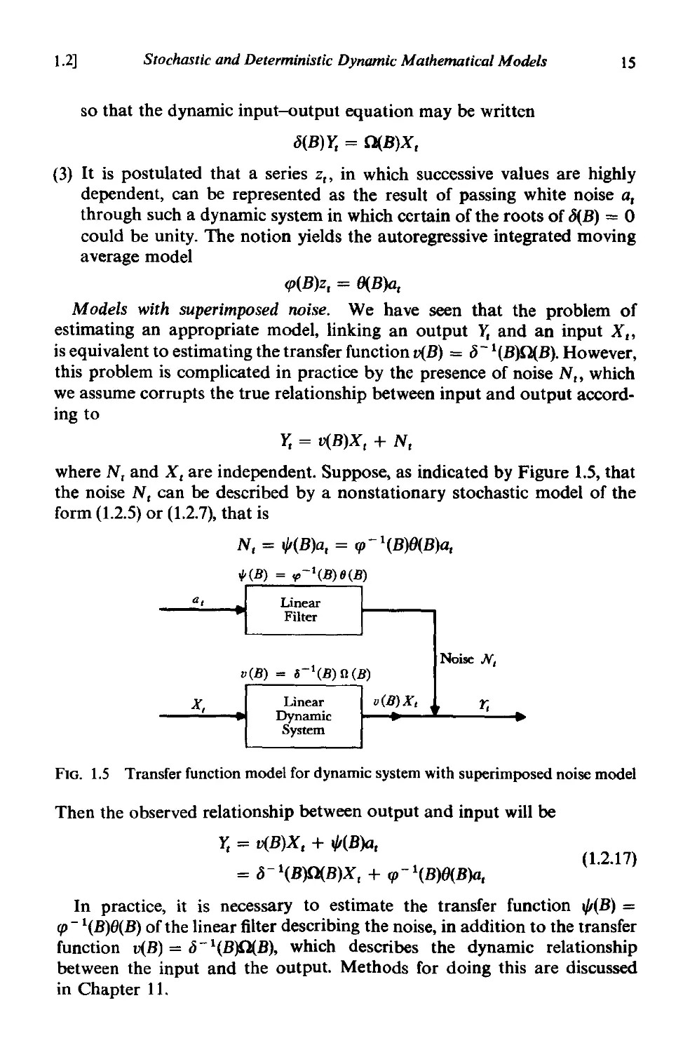
where Nt and Xt are independent. Suppose, as indicated by Figure 1.5, that
the noise Nt can be described by a nonstationary stochastic model of the
form (1.2.5) or (1.2.7), that is
Nt = "'(B)a t = qJ -1(B)O(B)a t
HB) = ",-I(B)8(B)
a,
Linear
Filter
v(B) = r l (B) {! (B)
Noise N,
X,
Linear
Dynamic
System
v (B) X,
r,
FIG. 1.5 Transfer function model for dynamic system with superimposed noise model
Then the observed relationship between output and input will be
1'; = v(B)X, + "'(B)at
= (j-l(B)Q(B)X t + qJ-l(B)O(B)at
In practice, it is necessary to estimate the transfer function "'(B) =
qJ - I(B)O(B) of the linear filter describing the noise, in addition to the transfer
function v(B) = (j -1(B)O(B), which describes the dynamic relationship
between the input and the output. Methods for doing this are discussed
in Chapter 11.
(1.2.17)
16
Introduction and Summary
[Chap. I
1.2.3 Modelsfor discrete control systems
As stated in Section 1.1.3, control is an attempt to compensate for disturb-
ances which infect a system. Some of these disturbances are measureable;
others are not measurable and only manifest themselves as unexplained
deviations from the target of the characteristic to be controlled.
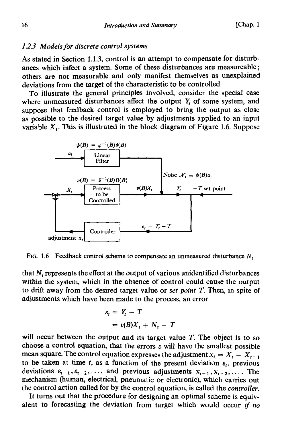
To illustrate the general principles involved, consider the special case
where unmeasured disturbances affect the output Y, of some system, and
suppose that feedback control is employed to bring the output as close
as possible to the desired target value by adjustments applied to an input
variable X,. This is illustrated in the block diagram of Figure 1.6. Suppose
1/t(B) = tp-I(B)8(B)
a,
x,
Noise A', = I/J(B)a,
v(B)X,
1;
- T set point
adjustment X,
" = 1'; - T
FIG. 1.6 Feedback control scheme to compensate an unmeasured disturbance N,
that N, represents the effect at the output of various unidentified disturbances
within the system, which in the absence of control could cause the output
to drift away from the desired target value or set point T. Then, in spite of
adjustments which have been made to the process, an error
8,=Y,-T
= v(B)X, + N, - T
will occur between the output and its target value T. The object is to so
choose a control equation, that the errors 8 will have the smallest possible
mean square. The control equation expresses the adjustment Xt = X, - X, - I
to be taken at time t, as a function of the present deviation 8" previous
deviations 8,-1'8,-20...' and previous adjustments X'-I'X'-2,.... The
mechanism (human, electrical, pneumatic or electronic), which carries out
the control action called for by the control equation, is called the controller.
It turns out that the procedure for designing an optimal scheme is equiv-
alent to forecasting the deviation from target which would occur if no
1.3]
Basic Ideas in Model Building
17
control were applied, and then calculating the adjustment that would be
necessary to cancel out this deviation. It follows that the forecasting and
control problems are closely linked. To forecast the deviation from target
that could occur ifno control were applied, it is necessary to build a model
N , = 1/I(B)a, = tp-1(B)lJ(B)a ,
for the disturbance. Calculation of the adjustment X, which needs to be
applied to the input variable at time t to cancel out a predicted change at the
output requires the building of a dynamic model with transfer function
v(B) = b- 1 (B)O(B)
which links the input and output. The resulting adjustment X, will consist, in
general, of a linear aggregate of previous adjustments, and current and
previous control errors. Thus the control equation will be of the form
X, = (1X , - 1 + (2X,-2 + ... + XOB, + X1 B ,-l + X2B,-2 + '" (1.2.18)
where (1' (2' . . . , Xo, XI' X2, . " are constants. These ideas are discussed in
Chapter 12.
1.3. BASIC IDEAS IN MODEL BUILDING
1.3.1 Parsimony
We have seen that the mathematical models, which we need to employ,
contain certain constants or parameters whose values must be estimated
from the data. It is important, in practice, that we employ the smallest
possible number of parameters for adequate representation. The central
role played by this principle of parsimony [25] in the use of parameters will
become clearer as we proceed. As a preliminary illustration, we consider
the following simple example.
Suppose we fitted a dynamic model (1.2.12) ofthe form
y, = ('10 + '11 V + '12 V2 + ... + '1.V S )X , (1.3.1)
when dealing with a system which was adequately represented by
(1 + V)Y, = X,
(1.3.2)
The model (1.3.2) contains only one parameter but, for s sufficiently large,
could be represented approximately by the model (1.3.1). Because of exper-
imental error, we could easily fail to recognize the relationship between the
coefficients in the fitted equation. Thus, we might needlessly fit a relationship
like (1.3.1), containing s parameters, where the much simpler form (1.3.2),
containing only one, would have been adequate. This could, for example,
lead to unnecessarily poor estimation of the output Y, for given values of
the input X" X'_I' . .. .
18
Introduction and Summary
[Chap. I
Our objective, then, must be to obtain adequate but parsimonious models.
Forecasting and control procedures could be seriously deficient if these
models were either inadequate or unnecessarily prodigal in the use of
parameters. Care and effort is needed in selecting the model. The process
of selection is necessarily iterative, that is to say, it is a process of evolution,
adaptation, or trial and error.
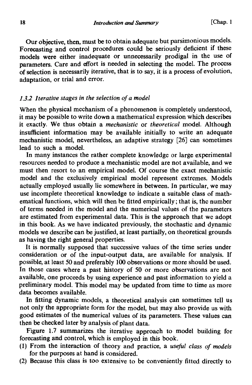
1.3.2 Iterative stages in the selection of a model
When the physical mechanism of a phenomenon is completely understood,
it may be possible to write down a mathematical expression which describes
it exactly. We thus obtain a mechanistic or theoretical model. Although
insufficient information may be available initially to write an adequate
mechanistic model, nevertheless, an adaptive strategy [26] can sometimes
lead to such a model.
In many instances the rather complete knowledge or large experimental
resources needed to produce a mechanistic model are not available, and we
must then resort to an empirical model. Of course the exact mechanistic
model and the exclusively empirical model represent extremes. Models
actually employed usually lie somewhere in between. In particular, we may
use incomplete theoretical knowledge to indicate a suitable class of math-
ematical functions, which will then be fitted empirically; that is, the number
of terms needed in the model and the numerical values of the parameters
are estimated from experimental data. This is the approach that we adopt
in this book. As we have indicated previously, the stochastic and dynamic
models we describe can be justified, at least partially, on theoretical grounds
as having the right general properties.
It is normally supposed that successive values of the time series under
consideration or of the input-output data, are available for analysis. If
possible, at least 50 and preferably 100 observations or more should be used.
In those cases where a past history of 50 or more observations are not
available, one proceeds by using experience and past information to yield a
preliminary model. This model may be updated from time to time as more
data becomes available.
In fitting dynamic models, a theoretical analysis can sometimes tell us
not only the appropriate form for the model, but may also provide us with
good estimates of the numerical values of its parameters. These values can
then be checked later by analysis of plant data.
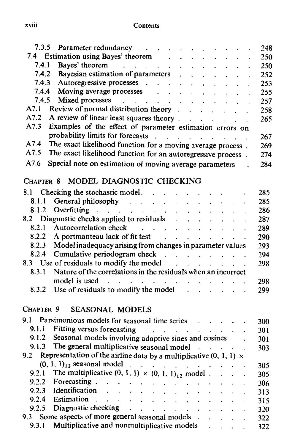
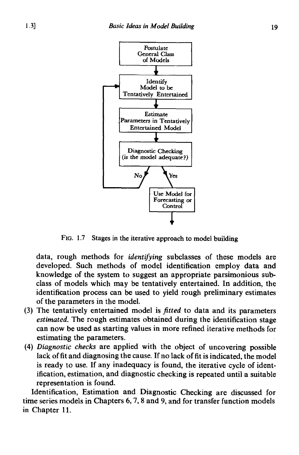
Figure 1.7 summarizes the iterative approach to model building for
forecasting and control, which is employed in this book.
(1) From the interaction of theory and practice, a useful class of models
for the purposes at hand is considered.
(2) Because this class is too extensive to be conveniently fitted directly to
1.3)
Basic Ideas in Model Building
19
Identify
Model to be
Tentatively Entertained
Estimate
Parameters in Tentatively
Entertained Model
Diagnostic Checking
(is the model adequate?)
Use Model for
Forecasting or
Control
FIG. 1.7 Stages in the iterative approach to model building
data, rough methods for identifying subclasses of these models are
developed. Such methods of model identification employ data and
knowledge of the system to suggest an appropriate parsimonious sub-
class of models which may be tentatively entertained. In addition, the
identification process can be used to yield rough preliminary estimates
of the parameters in the model.
(3) The tentatively entertained model is fitted to data and its parameters
estimated. The rough estimates obtained during the identification stage
can now be used as starting values in more refined iterative methods for
estimating the parameters.
(4) Diagnostic checks are applied with the object of uncovering possible
lack of fit and diagnosing the cause. If no lack of fit is indicated, the model
is ready to use. If any inadequacy is found, the iterative cycle of ident-
ification, estimation, and diagnostic checking is repeated until a suitable
representation is found.
Identification, Estimation and Diagnostic Checking are discussed for
time series models in Chapters 6, 7, 8 and 9, and for transfer function models
in Chapter 11.
Part I
Stochastic Models and their Forecasting
In the first part of this book, which includes Chapters 2, 3,4 and 5, a valuable
class of stochastic models is described and its use in forecasting discussed.
A model which describes the probability structure of a sequence of
observations is called a stochastic process. A time series of N successive
observations z' = (ZI' Z2,' .., ZN) is regarded as a sample realization, from
an. infinite population of such samples, which could have been generated
by the process. A major objective of statistical investigation is to infer
properties of the population from those of the sample. For example, to make
a forecast is to infer the probability distribution of a future observation
from the population, given a sample z of past values. To do this we need
ways of describing stochastic processes and time series, and we also need
classes of stocnastic models which are capable of describing practically
occurring situations. An important class of stochastic processes discussed in
Chapter 2 is the stationary processes. They are assumed to be in a specific
form of statistical equilibrium, and in particular, vary about a fixed mean.
Useful devices for describing the behavior of stationary processes are the
autocorrelation function and the spectrum.
Particular stationary stochastic processes of value in modelling time
series are the autoregressive, moving average, and mixed autoregressive
moving average processes. The properties of these processes, and in part-
icular their correlation structures are described in Chapter 3.
Because many practically occurring time series (for example stock prices
and sales figures) have nonstationary characteristics, the stationary models
introduced in Chapter 3 are further developed in Chapter 4 to give a useful
class of non stationary processes called autoregressive integrated moving
average (ARIMA) models. The use of all these models in forecasting time
series is discussed in Chapter 5 and is illustrated with examples.
21
2
The Autocorrelation Function and
Spectrum
A central feature in the development of time series models is an assumption
of some form of statistical equilibrium. A particular assumption of this kind
(an unduly restrictive one as we shall see later) is that of stationarity. Usually
a stationary time series can be usefully described by its mean, variance, and
autocorrelation function, or equivalently by its mean, variance, and spectral
density function. In this chapter we consider the properties of these functions
and, in particular, the properties of the autocorrelation function which is
used extensively in the chapters that follow.
2.1 AUTOCORRELATION PROPERTIES OF STATIONARY
MODELS
2.1.1 Time series and stochastic processes
Time series. A time series is a set of observations generated sequentially
in time. If the set is continuous, the time series is said to be continuous. If the
set is discrete, the time series is said to be discrete. Thus, the observations
from a discrete time series made at times 't1,1: 2 ,...,1:"...,'tN may be
denoted by z(-r 1), z(-r 2), . . . , z( 1:,), . . . , z(T N)' In this book we consider only
discrete time series where observations are made at some fixed interval h.
When we have N successive values of such a series available for analysis, we
write z 1, Z2,' . . , z". . . , ZN to denote observations made at equidistant time
intervals 'to + h, 'to + 2h,. .. ,'to + th,..., 'to + Nh. For many purposes the
values of 'to and h an; unimportant, but if the observation times need to be
defined exactly, these two values can be specified. If we adopt 'to as the origin
and h as the unit of time, we can regard Zt as the observation at time t.
Discrete time series may arise in two ways.
(1) By sampling a continuous time series; for example, in the situation
shown in Figure 1.2, where the continuous input and output from a gas
furnace was sampled at intervals of nine seconds.
(2) By accumulating a variable Over a period of time; examples are rainfall,
which is usually accumulated over a period such as a day or a month,
23
24
The Autocorrelation Function and Spectrum
[Chap. 2
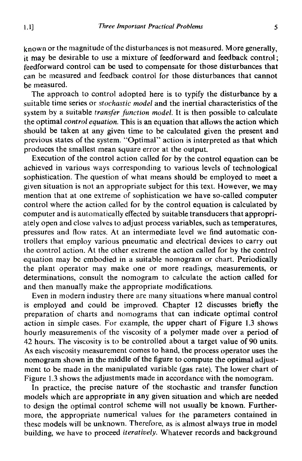
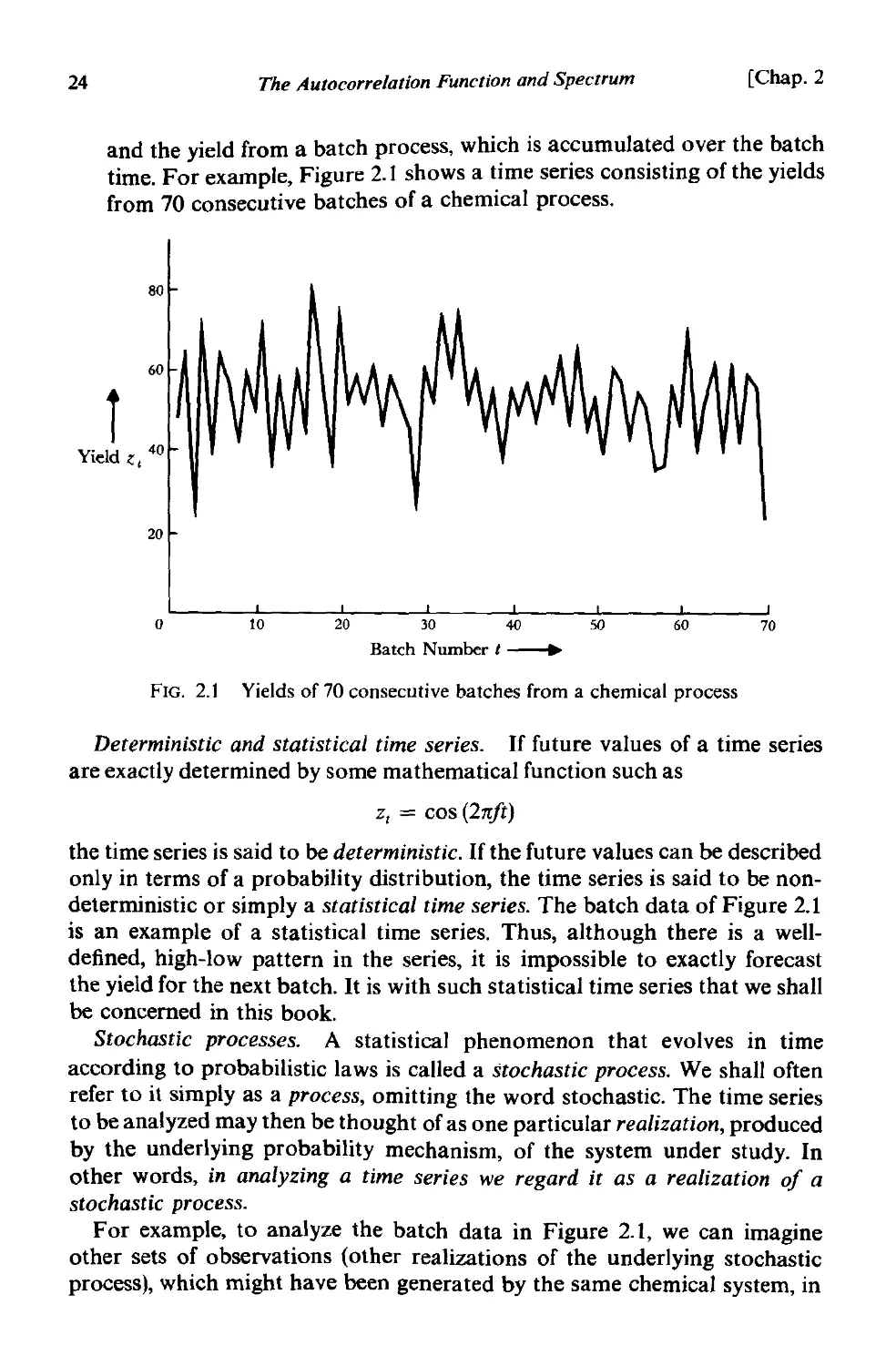
and the yield from a batch process, which is accumulated over the batch
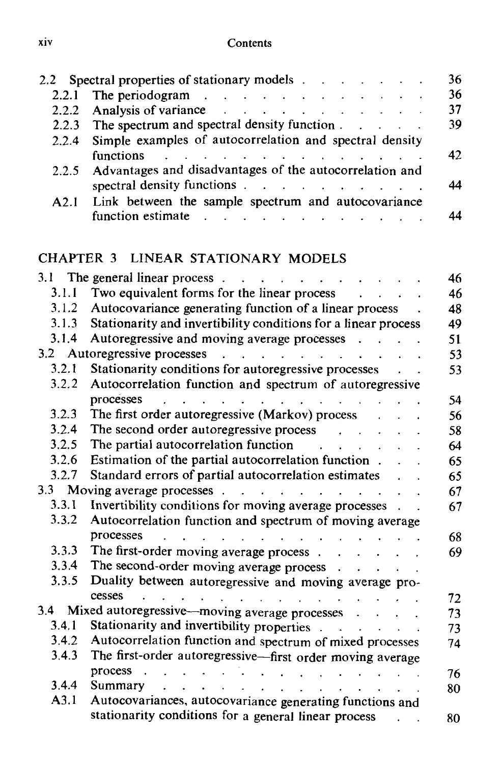
time. For example, Figure 2.1 shows a time series consisting of the yields
from 70 consecutive batches of a chemical process.
80
i
Yield ;;, 40
20
o
10
20 30 40 50
Batch Number t ----+
60
70
FIG. 2.1 Yields of 70 consecutive batches from a chemical process
Deterministic and statistical time series. If future values of a time series
are exactly determined by some mathematical function such as
z, = cos (27tft)
the time series is said to be deterministic. If the future values can be described
only in terms of a probability distribution, the time series is said to be non-
deterministic or simply a statistical time series. The batch data of Figure 2.1
is an example of a statistical time series. Thus, although there is a well-
defined, high-low pattern in the series, it is impossible to exactly forecast
the yield for the next batch. It is with such statistical time series that we shall
be concerned in this book.
Stochastic processes. A statistical phenomenon that evolves in time
according to probabilistic laws is called a stochastic process. We shall often
refer to it simply as a process, omitting the word stochastic. The time series
to be analyzed may then be thought of as one particular realization, produced
by the underlying probability mechanism, of the system under study. In
other words, in analyzing a time series we regard it as a realization of a
stochastic process.
For example, to analyze the batch data in Figure 2.1, we can imagine
other sets of observations (other realizations of the underlying stochastic
process), which might have been generated by the same chemical system, in
2.1]
Autocorrelation Properties of Stationary Models
25
the same n = 70 batches. Thus, Figure 2.2 shows the yields from batches
t = 21 to t = 30 (thick line), together with other time series which might
have been obtained from the population of time series defined by the under-
lying stochastic process. It follows that we can regard the observation z,
at a given time t, say t = 25, as a realization of a random variable z, with
probability density function p(z,). Similarly, the observations at any two
times, say t 1 = 25 and t 2 = 27, may be regarded as realizations oftwo random
variables Z'I and Zt2 with joint probability density function P(Z'I' z,z>, For
example, Figure 2.3 shows contours of constant density for such a joint
distribution, together with the marginal distribution at time t 1. In general,
the observations making up an equispaced time series can be described by an
N dimensional, random variable (ZI, Z2," ., ZN) with probability distri-
bution P(ZI, Z2'..., ZN)'
I
21
I
23
I I
25 27
t--+
I
31
FIG. 2.2 An observed time series (thick line) with other time series representing
realizations of the same stochastic process
t
Z'2
contours of bivariate distribution
P(Z'I' Z'2)
Z11
FIG. 2.3 Contours of constant density ofa bivariate probability distribution describing
a stochastic process at two times t l , t 2 , together with the marginal distribu-
tion at time t 1
26
The Autocorrelation Function and Spectrum
[Chap. 2
2.1.2 Stationary stochastic processes
A very special class of stochastic processes, called stationary processes, is
based on the assumption that the process is in a particular state of statistical
equilibrium. A stochastic process is said to be strictly stationary if its proper-
ties are unaffected by a change of time origin; that is, if the joint probability
distribution associated with m observations Zr" zr" .. ., z,.., made at any
set of times t I' t 2 ,. . ., t m , is the same as that associated with m observations
zrl+ k ,z'2+",...,z'rn+'" made at times t 1 + k,t z + k,...,t m + k. Thus for a
discrete process to be strictly stationary, the joint distribution of any set
of observations must be unaffected by shifting aU the times of observation
forward or backward by any integer amount k.
Mean and variance of a stationary process. When m = 1, the stationarity
assumption implies that the probability distribution p(z,) is the same for
all times t and may be written p(z). Hence, the stochastic process has a
constant mean
J.l = E[zrJ = f°-x, zp(z) dz
(2.1.1)
which defines the level about which it fluctuates, and a constant variance
0'; = E[(zr - J.l)zJ = f<XJ oo (z - J.l)2P(Z) dz
which measures its spread about this level. Since the probability distri-
bution p(z) is the same for all times t, its shape can be inferred by forming
the histogram of the observations Z I , Z 2' . . . , ZN, making up the observed
time series. In addition, the mean J.l ofthe stochastic process can be estimated
by the mean
(2.1.2)
1 N
Z = N L Zr (2.1.3)
r= I
of the time series, and the variance O' , of the stochastic process, can be
estimated by the variance
fJ 2 1;' - 2
. = - .L. (Zt - z)
Nr=1
(2.1.4)
of the time series.
Autocovariance and autocorrelation coefficients. The stationarity assump-
tion also implies that the joint probability distribution P(Zt1' Z'2) is the same
for all times t I' t 2 , which are a constant interval apart. It follows that the
nature of this joint distribution can be inferred by plotting a scatter diagram
using pairs of values (z" Zt+k), of the time series, separated by a constant
2.1]
Autocorrelation Properties of Stationary Models
27
interval or lag k. For the batch data, Figure 2.4(a) is a scatter diagram for
lag k = I, obtained by plotting z, + 1 versus z" and Figure 2.4(b) a scatter
diagram for lag k = 2, obtained by plotting Z'+2 versus z,. We see that
neigh boring values of the time series are correlated; the correlation between
.
i
<'+1
z/--+
(a)
i
.
.
<H2
<,--'
(b)
FIG. 2.4 Scattcr diagrams at lags I and 2 for the batch data of Figure 2.1
z, and z,+ 1 appearing to be negative and the correlation between z, and
Z'+2 positive. The covariance between z, and its value Z'H' separated by k
intervals of time, is called the autocovariance at lag k and is defined by
Yk = cov [z" Z'H] = E[(z, - Jl)(Z'H - Jl)]
(2.1.5)
28
The Autocorrelation Function and Spectrum
[Chap. 2
Similarly the autocorrelation at lag k is
E[(z, - J,l)(Z'H - J,l)]
Pk = .j E[(z, _ Jl)2]E[(Z'H _ Jl)2]
E[(z, - Jl)(Z'H - Jl)]
(1;
since, for a stationary process, the variance u; = Yo is the same at time t +k
as at time t.
Thus, the autocorrelation at lag k is
Yk
Pk =-
Yo
(2.1.6)
which implies that Po = 1.
2.1.3 Positive definiteness and the autocovariance matrix
The covariance matrix associated with a stationary process for observations
(z 1, Z2, . . . , z.), made at n successive times is
Yo YI 1'2 1'.-1
1'1 Yo 1'1 1'.-2
r = 1'2 Yl Yo 'Yn- 3
.
Y.-I 1'.- 2 Y.-3 Yo
PI P2 P.-l
PI PI P.-2
= 0-; P2 PI P.-3 = a;P. (2.1.7)
P.-I P.-2 P.-3
A covariance matrix r. of this form, which is symmetric with constant
elements on any diagonal, will be called an autocovariance matrix and the
corresponding correlation matrix p., will be called an autocorrelation
matrix. Now consider any linear function of the random variables z"
z,_ 1 , . . . , z, -. + 1
L, = liZ, + l2Z'_1 + . . . + lnz'-n + t
(2.1.8)
2.1]
Autocorrelation Properties of Stationary Models
29
Since cov [Zj, z J = YIj _ il for a stationary process, the variance of Lt is
" "
var [L,] = z:: L IJj Yij-il
i= 1 j= 1
which is necessarily greater than zero if the l's are not all zero. It follows that
both an autocovariance matrix and an autocorrelation matrix are positive-
definite for any stationary process.
Conditions satisfied by the autocorrelations of a stationary process. The
positive definiteness of the autocorrelation matrix (2.1.7) implies that its
determinant and all principal minors are greater than zero. In particular
for n = 2
1 1 PI \ > 0
PI 1
so that
1 - pi > 0
and hence
-1 < PI < 1
Similarly, for n = 3, we must have
I 1 1 I> 0, I 2 21 > 0
1 PI P2
PI PI >0
P2 PI
which implies
-1 < PI < 1
- 1 < P2 < I
2
_ 1 < P2 - <
1 - pi
and so on. Since p" must be positive definite for all values of n, the autocor-
relations of a stationary process must satisfy a very large number of condi-
tions. As will be shown in Section 2.2.3, all of these conditions can be brought
together in the definition of the spectrum.
Stationarity of linear functions. It follows from the definition of station-
arity, that the process L" obtained by performing the linear operation
(2.1.8) on a stationary process Z,. is also stationary. In particular, the first
30
The Autocorrelation Function and Spectrum
[Chap. 2
difference Vz, = Z, - Z'-1 and higher differences V.z" are stationary. This
result is of particular importance to the discussion of nonstationary time
series presented in Chapter 4.
Gaussian processes. If the probability distribution associated with any
set of times is a multivariate Normal distribution, the process is called a
Normal or Gaussian process. Since the multivariate Normal distribution is
fully characterized by its moments of first and second order, the existence of a
fixed mean J.I and an autocovariance matrix r n for all n, would be sufficient
to ensure the stationarity of a Gaussian process.
Weak stationarity. We have seen that for a process to be strictly station-
ary, the whole probability structure must depend only on time differences.
A less restrictive requirement, called weak stationarity of order f, is that the
moments up to some order f depend only on time differences. For example,
the existence ofa mean J.I and an autocovariance matrix r n ofthe form (2.1.7)
is sufficient to ensure stationarity up to second order. Thus, second order
stationarity, plus an assumption of Normality, is sufficient to produce strict
stationarity.
2.1.4 The autocovariance and autocorrelation functions
It was seen in Section 2.1.2 that the autocovariance coefficient Yk, at lag k,
measures the covariance between two values Zt and Zt+k> a distance k apart.
The plot of Yk versus the lag k, is called the autocovariance function {Yk}
of the stochastic process. Similarly, the plot of the autocorrelation coefficient
Pk as a function of the lag k, is called the autocorrelation function {pd of the
process. Note that the autocorrelation function is dimensionless; that is,
independent of the scale of measurement of the time series. Since ')Ik = Pk(1;
knowledge of the autocorrelation function {Pk} and of the variance (1; is
equivalent to knowledge of the autocovariance function {Yk}'
The autocorrelation function, shown in Figure 2.5 as a plot ofthe diagonals
of the autocorrelation matrix, reveals how the correlation between any two
values of the series changes as their separation changes. Since Pk = P _ k' the
autocorrelation function is necessarily symmetric about zero, and in prac-
tice it is only necessary to plot the positive half of the function. Figure 2.6
shows the positive half of the autocorrelation function given in Figure 2.5.
Henceforth, when we speak of the autocorrelation function, we shall often
mean the positive half. In the past, the autocorrelation function has some-
times been called the correlogram.
From what has been previously shown, a Normal stationary process z,
is completely characterized by its mean J.I and its autocovariance function
{yd, or equivalently by its mean J.I, variance (1;, and autocorrelation function
{Pk}'
2.1)
Autocorrelation Properties of Stationary Models
\.0 0.8 0.4 0.2 -0.1 0.1 ,
,
" ,
0.8 1.0 0.8 0.4 0.2 -0.1 '" ",
, , ,
, " , ,
0.4 0.8 1.0 0.8 0.4 0.2 ,
, , " ,
, , "-
, , , ,
0.2 0.4 0.8 1.0 0.8 0.4 , , , ,
, , , , ,
, , , ,
, " , , ,
, , , ,
-0.1 0.2 0.4 0.8 1.0 0.8 , , , ...,
, , ,
, ... " , ,
, ,
0.1 -0.1 0.2 0.4 , " , , "
, ,
, , \ ',\ , , , , , "
", , , , , "
" " , , ... ,
, , " , , ,
" , , " '\
" \ , , "
, , ,
, , , ,
, , , ,
, , \ \
, , , ,
, , , ,
, , , "
, ,
, , ,
, \ , ,
, , "
, ,
, , "
...'" , ,
, , ,
, " '.
..
...'"
/
FIG. 2.5 An autocorrelation matrix and the resulting autocorrelation function
1.0
r
PI/.- 1
0.0
o
k--+
FIG. 2.6 Positive half of the autocorrelation function of Figure 2.5
32
The Autocorrelation Function and Spectrum
[Chap. 2
2.1.5 Estimation of autocovariance and autocorrelation functions
Up to now we have only considered the theoretical autocorrelation function
which describes a conceptual stochastic process. In practice, we have a
finite time series ZI, Z2'...' ZN, of N observations, from which we can only
obtain estimates of the autocorrelations.
A number of estimates of the autocorrelation function have been sug-
gested by statisticians and their properties are discussed in particular in
[27]. It is concluded that the most satisfactory estimate of the kth lag auto-
correlation Pk is
Ck
r k =-
Co
(2.1.9)
where
I N-k
C k = N L (z, - z)(z'+k - z),
, 1
k = 0,1,2,..., K (2.1.10)
is the estimate of the autocovariance ')!k> and Z is the mean of the time series.
We now illustrate (2.UO) by calculating r I for the first 10 values ofthe batch
data of Figure 2.1, given in Table 2.1. The mean z of the first ten values in
the table is 51 and so the deviations about the mean are - 4, 13, - 28, 20,
-13, 13,4, -10,8, -3.
TABLE 2.1 A series of 70 consecutive yields from a batch
chemical process. This series also appears as
Series F in the Collection of Time Series at the end
of this volume
1-15 16--30 31-45 46--60 6\-70
47 44 50 62 68
64 80 71 44 38
23 55 56 64 50
71 37 74 43 60
38 74 50 52 39
64 5\ 58 38 59
55 57 45 59 40
41 50 54 55 57
59 60 36 41 54
48 45 54 53 23
71 57 48 49
35 50 55 34
57 45 45 35
40 25 57 54
58 59 50 45
2.1]
Autocorrelation Properties of Stationary Models
33
Thus
9
L (Zt - Z)(Z, + I - Z) = (-4)(13) + (13)( - 28) + .. . + (8)( - 3)
t= 1
= -1497
Hence
-1497
C 1 = --w- = -149.7
Similarly we find that Co = 189.6. Hence
C l
rl = - =
Co
- 149.7
189.6
-0.79
it being sufficient for most practical purposes to round off the autocor-
relation to two decimal places. The above calculation is made for illustration
only. In practice, to obtain a useful estimate of the autocorrelation function,
we would need at least fifty observations and the estimated autocorrelations rk
would be calculated for k = 0, 1,.. ., K where K was not larger than say
N/4.
The first 15 values of rb based on the whole series of 70 observations, are
given in Table 2.2 and plotted in Figure 2.7. The estimated autocorrelation
function is characterized by correlations which alternate in sign and which
tend to damp out with increasing lag. Autocorrelation functions of this kind
are not uncommon in production data and can arise because of "carryover"
i 0
10
15
o
'.
k ---+
-I
FIG. 2.7 Estimated autocorrelation function of batch data
34 The Autocorrelation Function and Spectrum [Chap. 2
TABLE 2.2 Estimated autocorrelation function of batch data
k rt k rt k rt
1 -0.39 6 -0.05 11 0.11
2 0.30 7 0.04 12 -0.07
3 -0.17 8 -0.04 13 0.15
4 0.07 9 -0.01 14 0.04
5 0.1O 10 0.01 15 -0.01
effects. In this particular example, a high yielding batch tended to produce
tarry residues which were not entirely removed from the vessel and ad-
versely affected the yield of the next batch.
A computer program for calculating estimates of the autocovariance
function and autocorrelation function is described under Program I, in the
collection of computer programs at the end of the volume.
2.].6 Standa rd e _ rror of autocorrelation estimates
- .
To identify a model for a time series, using methods to be described in
Chapter 6, it is necessary to have a crude check on whether Pk is effectively
zero beyond a certain lag. For this purpose, use can be made of the following
approximate expression for the variance of the estimated autocorrelation
coefficient of a stationary Normal process given by Bartlett [28].
1 +00
var [rk] N L {p + Pv+kPv-k - 4PkPvPv-k + 2p;pf}
v= - co
(2.1.11)
For example, if Pk = <jJlkl, (-1 < <jJ < 1), that is the autocorrelation function
damps out exponentially, (2.1.11) gives
var [rd == [ (1 + <jJ2)(1 - <jJ2k) _ 2k"l,.2k J
N 1 - <jJ2 'P
(2.1.12)
and in particular
var [r l ] == i (1 - <jJ2)
N
For any process for which all the autocorrelations Pv are zero for v > q,
aU terms except the first appearing on the right-hand side of (2.1.11) are
zero when k > q. Thus for the variance of the estimated autocorrelations rk,
2.1]
Autocorrelation Properties of Stationary Models
35
at lags k greater than some value q beyond which the theoretical autocorrela-
tionfunction may be deemed to have "died out," Bartlett's approximation gives
var [rkJ { I + 2 vt p;},
k>q
(2.1.13)
For example, as k is increased, and provided <P is not close to unity,
(2.1.12) tends quickly to its limiting form
. , 1 ( 1 + c/J2 )
hm var [rkJ -
k-x> N 1 - c/J
also given by (2.1.13).
To use (2.1.13) in practice, the estimated autocorrelations rk (k =1,2, . . . , q)
are substituted for the theoretical autocorrelations Pk and when this is done
we shall refer to the square root of (2.1.13) as the large-lag standard error.
On the assumption that the theoretical autocorrelations Pk are all essentially
zero beyond some hypothesized lag k = q, the large lag standard error
approximates the standard deviation of rk for suitably large lags (k > q).
Similar approximate expressions for the covariance between the estimated
correlations r k and rk+s at two different lags k and k + s have been given by
Bartlett [28J. In particular, the large-lag approximation reduces to
1 00
Cov[rk,rk+sJ N L PvPv+s
v=-oo
(2.1.14)
Bartlett's result (2.1.14) shows that care is required in the interpretation of
individual auto correlations because large covariances can exist between
neighboring values. This effect can sometimes distort the visual appearance
of the autocorrelation function which may fail to damp out according to
expectation [27J, [29].
An example. The following estimated autocorrelations were obtained
from a time series of length N = 200 observations, generated from a stoch-
astic process for which it was known that P 1 = - 0.4 and Pk = 0 for k 2:
k
1
-0.38
6
0.00
2
-0.08
7
0.00
3
0.11
8
0.00
4
-0.08
9
0.07
5
0.02
10
-0.08
r k
k
r k
On the assumption that the series is completely random, we have that q = O.
Then, for all lags, (2.1.13) yields
1 1
var [ r J - = - = 0 005
k N 200 .
36
The Autocorrelation Function and Spectrum
[Chap. 2
The corresponding standard error is 0.07 = (0.005)1/2. Since the value of
-0.38 for rl is over five times this standard error, it can be concluded that PI
is nonzero. Moreover, the estimated autocorrelations for lags greater than
one are small. Therefore it might be reasonable to ask next whether the series
was compatible with a hypothesis (whose relevance will be discussed later)
whereby PI was non-zero but Pk = 0 (k 2). Using (2.1.13) with q = 1 and
substituting rl for PI' the estimated large-lag variance under this assump-
tion is
1
var[rkJ 200 {1 + 2( -0.38)2} = 0.0064,
k> 1
yielding a standard error of 0.08. Since the estimated autocorrelations for
lags greater than one are small compared with this standard error, there is
no reason to doubt the adequacy of the model PI #- 0, Pk = 0 (k 2).
2.2. SPECTRAL PROPERTIES OF STATIONARY MODELS
2.2.1 The periodogram
Another way of analyzing a time series is based on the assumption that it is
made up of sine and cosine waves with different frequencies. A device which
uses this idea, first introduced by Schuster [30] in 1898, is the periodogram
(see also [31]).
The periodogram was originally'used to detect and estimate the amplitude
of a sine component, of known frequency, buried in noise. We shall use it
later to provide a check on the randomness of a series (usually a series of
residuals after fitting a particular model), where we consider the possibility
that periodic components of unknown frequency may still remain in the
series.
To illustrate the calculation of the periodogram, suppose that the number
of observations N = 2q + 1 is odd. If we fit the Fourier series model
q
Zt = rJ.o + L (CXiC it + PiSit) + e,
i 1
(2.2.1 )
where C ir = cos 2nD, Si' = sin 2nfit, and h = ilN is the ith harmonic of the
fundamental frequency IIN, then the least squares estimates ofthe coefficients
rJ.o and (rJ.i,PJ will be
a o = z
(2.2.2)
2 N )
a i = N L z,c ir
t 1
i = 1, 2, . . . , q
2 N
b i = N L z,sir
, 1
(2.2.3)
(2.2.4)
2.2J
Spectral Properties of Stationary Models
37
The periodogram then consists of the q = (N - 1)/2 values
N 2 2
1(fi) = 2 (a i + b i ),
i = 1,2,. ..,q
(2.2.5)
where l(fi) is called the intensity at frequency fi.
When N is even, we set N = 2q and (2.2.2), (2.2.3), (2.2.4), and (2.2.5), apply
for i = 1,2,.. . , (q - 1) but
1 N
a q = - I (-I)t z ,
N t=1
b q = 0
and
1([q) = 1(0.5) = Na
Note that the highest frequency is 0.5 cycles per time intervaJ because the
smallest period is 2 intervals.
2.2.2 Analysis of variance
In an analysis of variance table associated with the fitted regression (2.2.1),
when N is odd, we can isolate (N - 1)/2 pairs of degrees of freedom, after
eliminating the mean. These are associated with the pairs of coefficients
(a1,bd, (a2,b 2 ),...,(a q ,b q ), and hence with the frequencies I/N,2/N,...,
q/N. The periodogram l(fi) = (N/2)(a'f + b'f) is seen to be simply the "sum
of squares" associated with the pair of coefficients (ai' b;), and hence with the
frequency fi = i/N. Thus
N q
L (z, - Z)2 = I l(fi)
t= 1 i= 1
(2.2.6)
When N is even, there are (N - 2)/2 pairs of degrees of freedom, and a
further single degree of freedom associated with the coefficient aq.
If the series were truly random, containing no systematic sinusoidal
component, that is
Zt = (Xo + e t
with (Xo the fixed mean, and the e's independent and Normal, with mean zero
and variance u 2 , then each component 1(/;) wo ld have expectation 2u 2
and would be distributed. as ( 2 )(2(2), independently of all the other compon-
ents. By contrast, if the series contained a systematic sine component having
frequency /;, amplitude A, and phase angle F, so that
z, = (Xo + (X cos (2n/;t) + p sin (2nfit) + e t
* It is 10 be understood that x 2 (m) refers to a random variable having a chi-square distribution
with m degrees offreedom. defined explicitly, for example, in Appendix A.7.l.
38
The Autocorrelation Function and Spectrum
[Chap. 2
with A sin F = IX and A cos F = fJ, then the sum of squares I(};) would tend
to be inflated, since its expected value would be 2a 2 + N(C(2 + fJ2)/2 =
2a 2 + NA 2 /2.
In practice, it is unlikely that the frequency f of an unknown systematic
sine component would exactly match any of the frequencies 1;, for which
intensities have been calculated. In this case the periodogram would show
an increase in the intensities in the immediate vicinity off.
An example. A large number of observations would usually be used in
the calculation of the periodogram. However, to illustrate the process of
calculation we use the set of twelve mean monthly temperatures (in degrees
Celsius) for central England during 1964, given in Table 2.3.
TABLE 2.3 Mean monthly temperatures for Central England in 1964
2 3 4 5 6 7 8 9 10 11 12
z, 3.4 4.5 4.3 8.7 13.3 13.8 16.1 15.5 14.1 8.9 7.4 3.6
Cl' 0.87 0.50 0.00 -0.50 -0.87 - 1.00 -0.87 -0.50 0.00 0.50 0.87 1.00
The third line in Table 2.3 gives C Ir = cos (21ttI12), which is required in the
calculation of ai, obtained from
a l = H(3.4)(0.87) + '" +(3.6)(1.00)}
= -5.30
The values of the ai' b i , i = 1,2,...,6, are given in Table 2.4 and yield the
analysis of variance of Table 2.5.
TABLE 2.4 Amplitudes of sines and cosines at different
harmonics for temperature data
a; hi
I -5.30 -3.82
2 0.05 0.17
3 0.10 0.50
4 0.52 -0.52
5 0.09 -0.58
6 -0.30
As would be expected, the major component of this temperature data has
a period of twelve months, that is a frequency of 1/12 cycles per month.
2.2] Spectral Properties of Stationary Models 39
TABLE 2.5 Analysis of variance table for temperature series
Frequency Period Periodogram Degrees of Mean
fi I(h) freedom square
I 1/12 12 254.96 2 127.48
2 1/6 6 0.19 2 0.10
3 1/4 4 1.56 2 0.78
4 1/3 3 3.22 2 1.61
5 5/12 12/5 2.09 2 1.05
6 1/2 2 1.08 1 1.08
Total 263.10, 11 23.92
2.2.3 The spectrum and spectral density function
For completeness, we add here a brief discussion of the spectrum and
spectral density function. The use of these important tools is described
more fully in [27]. We do not apply them to the analysis of time series in this
book, and this section can be omitted on first reading.
The sample spectrum. The definition (2.2.5) of the periodogram assumes
that the frequencies fi = ilN are harmonics of the fundamental frequency
tiN. By way of introduction to the spectrum, we relax this assumption and
allow the frequency f to vary continuously in the range 0-0.5 cycles. The
definition (2.2.5) of the periodogram may be modified to
2'\ 2 2
l(f) = N (af + b f ),
O..;;f..;;!
(2.2.7)
and l(f) is then referred to as the sample spectrum [27]. Like the periodogram,
it can be used to detect and estimate the amplitude of a sinusoidal component
of unknown frequency f buried in noise and is, indeed, a more appropriate
tool for this purpose if it is known that the frequency f is not harmonically
related to the length of the series. Moreover, it provides a starting point for
the theory of spectral analysis, using a result given in Appendix A2.1. This
result shows that the sample spectrum l(f) and the estimate Cl; of the auto-
covariance function are linked by the important relation
l(f) = 2{C O + 2 :t: C t cos 27tfk}, 0 ..;; f ..;; ! (2.2.8)
That is, the sample spectrum is the Fourier cosine transform of the estimate of
the autocovariance function.
The spectrum. The periodogram and sample spectrum are appropriate
tools for analyzing time series made up of mixtures of sine and cosine waves,
at fixed frequencies buried in noise. However, stationary time series of the
40
The Autocorrelation Function and Spectrum
[Chap. 2
kind described in Section 2.1, are characterized by random changes of
frequency, amplitude, and phase. For this type of series, the sample spectrum
I(f) fluctuates wildly and is not capable of any meaningful interpretation
[27].
However, suppose that the sample spectrum was calculated for a time
series of N observations, which is a realization of a stationary Normal
process. As we have said above, such a process would not have any cosine
or sine deterministic components, but we could formally carry through the
Fourier analysis and obtain values of (af, b f ), for any given frequency f.
If repeated realizations of N observations were taken from the stochastic
process, we could build up a population of values for af' b f and I(f). Thus,
we could calculate the mean value of I(f) in repeated realizations of size N,
namely
E[I(!)] = 2f[c o J + 2 :t: E[CkJ cos 2n f k}
For large N it may be shown, for example in [27J, that the average value of
the estimate of the autocovariance coefficient Ck in repeated realizations tends
to the theoretical autocovariance Yk' that is
(2.2.9)
lim E[Ck] = Yk
N-oo
On taking the limit of (2.2.9) as N tends to infinity, the power spectrum
P(!) is defined by
p(!) = J E[I(!)] = 2{ Yo + 2 Jl Yk cos 2nfk}, 0 f 1 (2.2.10)
We note that since
lP(f)1 2{IYol + 2 k 1 IYkllcos 21tfl( }
= 2 Yol + 2 k 1 IYkl}
(2.2.11)
a sufficient condition for the spectrum to converge is that Yk damps out
rapidly enough for the series (2.2.11) to converge. Since the power spectrum
is the Fourier cosine transform of the autocovariance function, knowledge
of the autocovariance function is mathematically equivalent to knowledge
of the spectrum and vice versa. From now on we shall refer to the power
spectrum as the spectrum.
On integrating (2.2.10) between the limits 0 and 1, the variance of the
process z, IS
r l / 2
Yo = u; = J o P(!)df
(2.2.12)
2.2]
Spectral Properties of Stationary Models
41
Hence, in the same way that the periodogram 1(f) shows how the variance
(2.2.6) of a series, consisting of mixtures of sines and cosines, is distributed
between the various distinct harmonic frequencies, the spectrum P(f) shows
how the variance of a stochastic process is distributed between a continuous
range of frequencies. One can interpret P(f) df as measuring approximately
the variance of the process in the frequency range f to f + df
The- spectral density function. It is sometimes more convenient to base
the definition (2.2.10) of the spectrum on the autocorrelations Pk, rather than
the autocovariances Yk' The resulting function
g(f) = p(f)/u;
= 2{1 + 2 ktl PkCOS21tfk}, 0 f t
is called the spectral density function. Using (2.2.12). it is seen that the spectral
density function has the property
(2.2.13)
f. 1/2
o g(f)df = 1
Since g(f) is also positive, it has the same properties as an ordinary prob-
ability density function. This analogy extends to the estimation properties
of these two functions, as we shall now discuss.
Estimation of the spectrum. One would expect that an estimate of the
spectrum could be obtained from (2.2.10), by replacing the theoretical
autocovariances Yk with their estimates Ck' Because of (2.2.8), this corresponds
to taking the sample spectrum as an estimate of P(f). However, it may be
shown (see [27]) that the sample spectrum of a stationary time series fluctuates
violently about the theoretical spectrum. An intuitive explanation of this
fact is that the sample spectrum corresponds to using an interval, in the
frequency domain, whose width is too small. This is analogous to using too
small a group interval for the histogram when estimating an ordinary
probability distribution. By using a modified or smoothed estimate
{ N-1 }
fJ(f) = 2 Co + 2 k l AkCk cos 21tfk
(2.2.14)
where the Ak are suitably chosen weights called a lag window, it is possible
to increase the "bandwidth" of the estimate and to obtain a smoother
estimate of the spectrum.
Figure 2.8 shows an estimate of the spectrum of the batch data. It is seen
that most of the variance of the series is concentrated at high frequencies.
This is due to the rapid oscillations in the original series, to be seen in
Figure 2.1.
42
The Autocorrelation Function and Spectrum
[Chap. 2
r
.25
.5
log
PUJ
f--+
FIG. 2.8 Estimated power spectrum of batch data
2.2.4 Simple examples of autocorrelation and spectral density functions
For illustration, we show below equivalent representations of two simple
stochastic processes by :
(i) their theoretical models,
(ii) their theoretical autocorrelation functions, and
(iii) their theoretical spectra.
Consider the two processes
Zt = 10 + at + at-I Z, = 10 + at - a,-I
where a" at-I'" . , are a sequence of un correlated, random Normal variables
with mean zero and variance 1, that is, white noise. Using the definition
(2.1.5)
Yk = cov [Z,. Zt+kJ = E[(zt - Jl)(Zt+k - Jl)J
where E[ztJ = E[Zt+kJ = Jl = 10, the autocovariances of these two stochastic
processes are
1 2.0, k = °
Yk = 1.0, k = 1
O,k 2
1 2.0, k = 0
Yk = - 1.0, k = 1
0, k ?: 2
Thus the theoretical autocorrelation functions are
{ 0.5, k = 1 { -O.5, k = 1
Pk = Pk =
0.0, k ?: 2 0.0, k ?: 2
and using (2.2.13), the theoretical spectral density functions are
g(f) = 2( 1 + cos 21tf),
g(f) = 2( 1 - cos 21tf)
The autocorrelation functions and spectral density functions are plotted in
Figure 2.9, together with a sample time series from each process.
2.2]
Spectral Properties of Stationary Models
43
... A." AI\.. .1\1'\ J V1 AA ,... Apftll'
r 'v''fvvvV'' ' 'Y \JV "'/ v VV r' '''' YV'
Mcxlel (1) z, = 10 + a, + a I-I Mood (2) z, = 10 + a, - a'-1
r
II
I
10
10
Pk
-I
k ---+
Mood (1)
k--+
Mcxlel (2)
Theoretical Autocorrelation Funclions
g(f)
g(f)
Ys!4%)
Ys !4 % J1
f--+
Mood (1)
f--+
Mood (2)
Theoretical Spectral Density Functions
FIG. 2.9 Two simple stochastic models with their corresponding theoretical auto-
correlation functions and spectral density functions
(1) It should be noted that, for these two stationary processes, knowledge
of either the autocorrelation function or the spectral density function,
with the mean and variance of the process, is equivalent to knowledge
of the model (given the Normality assumption).
(2) It will be seen that the autocorrelation function reflects one aspect of
the behavior of the series. The comparatively smooth nature of the first
series is accounted for by the positive association between successive
values. The alternating tendency of the second series, in which positive
deviations usually follow negative ones, is accounted for by the negative
association between successive values.
(3) The spectral density throws light on a different, but equivalent aspect.
The predominance of low frequencies in the first series and high fre-
quencies in the second is shown up by the spectra.
44
The Autocorrelation Function and Spectrum
[Chap. 2
2.2.5 Advantages and disadvantages of the autocorrelation and spectral
density functions
Because the autocorrelation function and the spectrum are transforms of
each other, they are mathematically equivalent and therefore any discussion
of their advantages and disadvantages turns not on mathematical questions,
but on their representational value. Because, as we have seen, each sheds
light on a different aspect of the data, they should be regarded not as rivals
but, as allies. Each contributes something to an understanding of the stoch-
astic process in question.
The obtaining of sample estimates of the autocorrelation function and
of the spectrum are non-structural approaches, analogous to the repre-
sentation of an empirical distribution function by a histogram. They are
both ways of letting data from stationary series "speak for themselves"
and provide a first step in the analysis of time series, just as a histogram can
provide a first step in the distributional analysis of data, pointing the way to
some parametric model on which subsequent analysis will be based.
Parametric time series models, such as those of Section 2.2.4, are not
necessarily associated with a simple autocorrelation function or a simple
spectrum. Working with either of these non-structural methods, we may be
involved in the estimation of many lag correlations and many spectral
ordinates, even when a parametric model containing only one or two para-
meters could represent the data. Each correlation and each spectral ordinate
is a parameter to be estimated, so that these non-structural approaches
might be very prodigal with parameters, when the approach via the model
could be parsimonious. On the other hand, initially, we probably do not
know what type of model may be appropriate and initial use of one or other
of these non-structural approaches is necessary to identify the type of model
which is needed. (In the same way that plotting a histogram helps to indicate
which family of distributions may be appropriate). The choice between the
spectrum and the autocorrelation function as a tool in model building
depends upon the nature of the models which turn out to be practically
useful. The models which we have found useful and which we consider in
later chapters of this book are simply described in terms of the autocorrela-
tion function and it is this tool which we employ for identification of series.
APPENDIX A2.1 LINK BETWEEN THE SAMPLE SPECTRUM AND
AUTOCOV ARIANCE FUNCTION ESTIMATE
Here we derive the result (2.2.8)
{ N-l }
I(f) = 2 Co + 2 k 1 c k cos 2nfk ,
O f t
Appendix A2.l]
Link Between the Sample Spectrum
45
which links the sample spectrum I(!) and the estimate C k of the auto-
covariance function. Suppose that the least squares estimates af and b f
of the cosine and sine components, at frequency f, in a series are combined
according to d f = af - ib f , where i = .j=l, then
N
I(f) = 2 (af - ibf)(af + ib f )
= N d f dJ
2
where d; is the complex conjugate of d f . Then, using (2.2.3) and (2.2.4),
d f = 2 I. z,(cos 21tft - i sin 21tft)
N '=1
(A2.1.1)
2 N .
= - L z,e-'21t f t
Nt=1
2 N .
= - L (z, - z)e-'21t f '
N 1=1
(A2.1.2)
Substituting (A.2.1.2) in (A2.1.1),
2 N N ..
I(f) = - L L (z, - z)(z,. - z)e-'21t f (t-t)
N t=II'=1
(A2.1.3)
Since
1 N-k
Ck = - L (z, - Z)(ZtH - z)
N ,=1
the transformation k = t - t' transforms (A2.1.3) into
N-l
I(f) = 2 L cke-i2xfk
k= -N+ 1
{ N-l }
= 2 Co + 2 k1;1 C k cos 21tfk ,
which is the required result.
O f t
3
Linear Stationary Models
A general linear stochastic model is described, which supposes a time series
to be generated by a linear aggregation of random shocks. For practical
representation, it is desirable to employ models which use parameters
parsimoniously. Parsimony may often be achieved by representation of the
linear process in terms of a small number of autoregressive and moving
average terms. The properties of the resulting autoregressive-moving
average (ARMA) models are discussed in preparation for their use in model
building.
3.1. THE GENERAL LINEAR PROCESS
3.1.1 Two equivalent forms for the linear process
In Section 1.2.1 we discussed the representation of a stochastic process as the
ouput from a linear filter, whose input is white noise a" that is
t l f Ie' '-41} r :t' Z, = a, + t/11 a, _ 1 + t/12a, _ 2 + . .. 'i
00
= a, + L t/1J.(J'-j
j= 1
(3.1.1)
where Z, = Zt - J1. is the deviation of the process from some origin, or from its
mean, if the process is stationary. The general linear process (3.1.1) allows us
to represent Zt as a weighted sum of present and past values of the "white
noise" process a,. Important references in the development of linear sto-
chastic models are: [24], [28], [29], [32], [44], [92], [97], [98], [99], [100], [102]
and [103]. The white noise process a, may be regarded as a series of shocks
which drive the system. It consists of a sequence of uncorrelated random
variables with mean zero and constant variance, that is
E[a,] = 0 var [a,] = u
Since the random variables at are uncorrelated, it follows that their auto-
covariance function is
Yk = E[atarH] = {
46
k=O
k:;eO
(3.1.2)
3.1]
The General Linear Process
47
Thus, the autocorrelation function of white noise has the particularly simple
form
Pk = {
k=O
k'i'O
(3.1.3)
The model (3.1.1) implies that, under suitable conditions, Zt is a weighted
sum of past values of the z's, plus an added shock a" that is
Zt = 1t 1 Z t - l + 1t z Z r - z + ... + a r
<J)
= L 1tit-j + at
j= 1
The alternative form (3.1.4) may be thought of as one where the current
deviation Zt, from the level J.l, is "regressed" on past deviations Zt -1' Zt - 2' . . .
of the process.
Relationships between the '" weights and 1t weights. The relationships
between the'" weights and 1t weights may be obtained using the previously
defined backward shift operator
(3.1.4)
BZt = Z'-1
BjZt = Zt- J
Later we shall also need to use the forward shift operator F = B- 1, such that
Fz, = Z'+1
FJ Zt = Zt+ J
As an example of the use of the operator B, consider the model
Z, = at - Oar-I = (I - OB)at
in which '" 1 = - 0, "'J = 0 for j > 1. Expressing at in terms of the z's, we
obtain
(1 - OB)-1 Zt = at
Hence, for 101 < 1,
(I + OB + 02B 2 + 03B 3 + ...) Zt = at
and the deviation Zt expressed in terms of previous deviations, as in (3.1.4),
is
Zt = - OZr_ 1 - 0 2 Z, - 2 - 0 3 Zr - 3 - . " + a r
so that for this model1tj = -tY.
In general, (3.1.1) may be written
Zt = ( I + I t/ljBj ) a r
J= 1
or
Zr = "'(B)a,
(3.1.5)
48
Linear Stationary Models
[Chap. 3
where
00 00
I/I(B) = 1 + L I/IjBj = L I/IjBj
j= 1 j =0
with 1/10 = 1. As has been mentioned in Section 1.2.1, I/I(B) is called the
transfer function of the linear filter relating Zt to a,. It can also be regarded
as the generating function of the 1/1 weights, with B now treated simply as a
dummy variable whosejth power is the coefficient of I/Ij.
Similarly, (3.1.4) may be written
( 1 - .f njBj ) Z, = at
J= 1
or
n(B)z, = a,
(3.1.6)
Thus
00
n(B) = 1 - L njBj
j=1
is the generating function of the n weights. After operating on both sides of
(3.1.6) by I/I(B), we obtain
I/I(B)n(B)zt = I/I(B)a t = Zt
Hence
I/I(B)n(B) = 1
that is
n(B) = l/I- l (B)
(3.1.7)
The relationship (3.1.7) may be used to derive the n weights, knowing the 1/1
weights, and vice versa.
3.1.2 Autocovariance generating function of a linear process
A basic data analysis tool for identifying models in Chapter 6 will be the
autocorrelation function. Therefore, it is important to know the auto-
correlation function of a linear process. It is shown in Appendix A3.1
that the autocovariance function of the linear process (3.1.1) is given by
00
I'k = u L I/Ijl/lj+k
j=O
(3.1.8)
3.1]
The General Linear Process
49
In particular, by setting k = 0 in (3.1.8), we find that its variance is
00
)10 = 0'; = 0'; L I/IJ
1=0
It follows, that if the process is to have a finite variance, the weights 1/1 1
must decrease fast enough for the series on the right of (3.1.9) to converge.
A more convenient way of obtaining the autocovariances of a linear
process is often via the autocovariance generating function
(3.1.9)
00
)I(B) = L )lk Bk
k= - 00
(3.1.10)
in which it is noted that Yo, the variance of the process, is the coefficient of
B O = 1, while Yk, the autocovariance of lag k, is the coefficient of both B1
and of B- 1 = Fl. It is shown in Appendix A3.1 that
y(B) = O';I/I(B)I/I(B- l ) = O';I/I(B)r/J(F)
(3.1.11)
For example, suppose
it = at - Oa t -l = (1 - OB)a,
so that I/I(B) = 1 - OR. Then, substituting in (3.1.11),
y(B) = u;(1 - OB)(I - (]B-1)
= 0'; { _(]B-1 + (1 + ( 2 ) - OB}
Comparing with (3.1.10), the autocovariances are
Yo = (1 + ( 2 )0';
)II = -00';
Yk = 0
k';32
In the development that follows, when treated as a dummy variable in a
generating function, B will be supposed capable of taking complex values.
In particular, it will often be necessary to consider the different situations
occurring when IBI < 1, IBI = 1, or IBI > 1, that is, when the complex
number B lies inside, on or outside the unit circle.
3.1.3 Stationarity and invertibility conditions for a linear process
Stationarity. The convergence of the series (3.1.9) ensures that the process
has a finite variance. Also, we have seen in Section 2.1.3, that the auto-
covariances and autocorrelations must satisfy a set of conditions to ensure
stationarity. For a linear process these conditions can be embodied in the
single condition that the series I/I(B), which is the generating function of
50
Linear Stationary Models
[Chap. 3
the I/J weights, must converge for lEI 1. That is, on or within the unit circle.
This result is discussed in Appendix A3.1.
Spectrum of a linear stationary process. It is shown in Appendix A3.1
that if we substitute B = e- i2fCf , where i = , in the autocovariance
generating function (3.1.11), we obtain one half of the power spectrum.
Thus the spectrum of a linear process is
p(f) = 2u l/I(e-i2fCf)I/J(ei2fCf)
= 2u ll/I(e-i2JCfW 0 f i (3.1.12)
In fact, (3.1.12) is the well known expression [27], which relates the spectrum
P(f) of the output from a linear system, to the uniform spectrum 2u of a white
noise input by multiplying by the squared gain G 2 (f) = 1I/J(e-iZfCf)12 of the
system.
Invertibility. We have seen above, that the 1/1 weights of a linear process
must satisfy the condition that I/I(B) converges on or within the unit circle, if
the process is to be stationary. We now consider a restriction applied to the 1t
weights to ensure what is called "invertibility." The invertibility condition
is independent of the stationarity condition and is applicable also to the non-
stationary linear models, which we introduce in Chapter 4.
To illustrate the basic idea of invertibility, consider again the model
Z, = (1 - OB)a, (3.1.13)
Expressing the a's in terms of the z's, (3.1.13) becomes
a, = (l - 8B)-lz, = (l + (JB + (J2B2 + ... + (JkBk)(1 - 8k+JBk+1)-JZ,
that is
2, = -(JZ,_1 - 8 2 z'_2 - ... - (JkZ,-k + a, - 8k+ 1 a,-k_l (3.1.14)
and, if 181 < 1, on letting k tend to infinity, we obtain the infinite series
Z, = -82'_1 - (J2z'_2 - ... + a, (3.1.15)
and the 1t weights of the model in the form of (3.1.4), are 1t j = - oj. Whatever
the value offJ, (3.1.13) defines a perfectly proper stationary process. However,
if 181 1, the current deviation Z, in (3.1.14) depends on Z'_I, Z'_2, . . . , Z,-k,
with weights which increase as k increases. We avoid this situation by requir-
ing that I(JI < 1. We shall then say that the series is invertible. We see that
this condition is satisfied if the series
00
1t(B) = (1 - OB)-I = L fJ'B)
j O
converges for alllBI 1, that is, on or within the unit circle.
3.1]
The General Linear Process
51
In Chapter 6, where we consider questions of uniqueness of these models,
we shall see that a convergent expansion for a, is possible when 181 1, but
only in terms of Zt, Zt+ l' Zt+ 2' . .. (that is in terms of present and future
values of the process). The requirement of invertibility is needed if we are
interested in associating present events with past happenings in a sensible
manner.
In general, the linear process
1[(B)Zt = at
is invertible if the weights 1[j are such that the series 1[(B) converges on, or
within the unit circle.
To sum up, a linear process is stationary if I/I(B) converges on, or within the
unit circle and is invertible if 1[(B) converges on, or within the unit circle.
3.1.4 Autoregressive and moving average processes
The representations (3.1.1) and (3.1.4) of the general linear process would not
be very useful in practice, if they contained an infinite num her of parameters
I/Ij and 1[j' We now consider how to introduce parsimony and yet retain
models which are representationally useful.
Autoregressive processes. Consider the special case of (3.1.4), in which
only the first p of the weights are nonzero. This model may be written
Z, = <PIZt-1 + <P2Zt-2 + ... + <PpZt-p + at
(3.1.16)
where we now use the symbols <PI' <P2'...' <p p for the finite set of weight
parameters. The process defined by (3.1.16) is called an autoregressive process
of order p, or more succinctly, an AR(p) process. In particular, the auto-
regressive processes of first order (p = 1), and of second order (p = 2),
Z, = <P I Z, - 1 + a,
Z, = <PIZ,-1 + <P2Z,-2 + a,
are of considerable practical importance.
Now we can write (3.1.16) in the equivalent form
(1 - <PIB - <P2B2 - . .. - <ppBP)Zt = at
or
<p(B)Zt = a,
(3.1.17)
Since (3.1.17) implies
1
Z, = <P(B) at = <P - I(B)a,
52
Linear Stationary Models
[Chap. 3
the autoregressive process can be thought of as the output z, from a linear
filter with transfer function <p -1(B), when the input is white noise a,.
Moving average processes. Consider the special case of (3.1.1) when only
the first q of the'" weights are non-zero. The process
it = at - (JIU,-1 - (J2 a ,_2 - .. . - (Jqu,-q
(3.1.18)
where we now use the symbols - (}1, - O 2 ,, . . , - (Jq for the finite set of weight
parameters. The process defined by (3.1.18) is called a moving average process*
of order q, which we sometimes abbreviate to MA(q). In particular, the
processes of first order (q = 1), and second order (q = 2),
Zt = at - (}la,-1
it = at - (Jla,-l - (J2 a t-2
are particularly important in practice.
We can also write (3.1.18) in the equivalent form
it = (I - (JIB - (J2B2 - . .. - (JqBq)a t
or
, = (J(B)a t
(3.1.19)
Hence, the moving average process can be thought of as the output i, from
a linear filter with transfer function (J(B), when the input is white noise at.
Mixed autoregressive-moving average processes. We have seen in
Section 3.1.1 that the finite moving average process
Z, = a, - (Jla'-1 = (I - (J1B)a,
can be written as an infinite autoregressive process
Z, = - (J 1 Z, _ 1 - (Ji z, - 2 - .. . + a,
I (Jd < 1
Hence, if the process were really MA(I), we would obtain a nonparsimonious
representation in terms of an autoregressive model. Conversely, an AR(I)
could not be parsimoniously represented using a moving average process. In
practice, to obtain a parsimonious parameterization, it will sometimes be
necessary to include both autoregressive and moving average terms in the
model. Thus
Zt = <P1 Z t-l + ... + <PpZt-p + a, - (Jla t -l - ... - (Jqa t _ q
or
<p(B)z, = (J(B)a,
(3.1.20)
* As we remarked in Chapter I. the term "moving average.. is somewhat misleading, since the
weights do not sum to unity. However, this nomenclature is now well established and we shall
use it.
3.2]
Autoregressive Processes
53
is called the mixed autoregressive-moving average process of order (p, q),
which we sometimes abbreviate to ARMA (p, q). For example, the ARMA
(1, 1) process is
Zt - ljJ1 Z t-l = at - (J1at-1
Since (3.1.20) may be written
Zt = ljJ -1(B)(J(B)a,
(J(B) 1 - (JIB - . " - () Bq
=-a t = q a
ljJ(B) 1 -ljJI B -... -ljJpBP t
the mixed autoregressive-moving average process can be thought of as the
output Z, from a linear filter, whose transfer function is the ratio of two
polynominals (J(B) and ljJ(B), when the input is white noise at.
In the following sections we discuss important characteristics of auto-
regressive, moving average, and mixed models. We study their variances,
autocorrelation functions, spectra, and the stationarity and invertibility
conditions which must be imposed upon their parameters.
3.2. AUTOREGRESSIVE PROCESSES
3.2.1 Stationarity conditions for autoregressive processes
The set of adjustable parameters ljJ 1 ,ljJ2' . . . ,ljJ p of an AR(p) process
Z, = ljJIZ'-1 + ... + ljJpz,_p + a,
or
(l - ljJI B - . .. - ljJpBP)z, = ljJ(B)i t = a,
must satisfy certain conditions for the process to be stationary.
For illustration, the first-order autoregressive process
(1 - ljJIB)Zt = a,
may be written
00
z, = (1 - ljJI B )- la t = L <j>{a t - J
j=O
Hence
I/I(B) = (1 - cPI B )-l = L cP{Bj
j=O
We have seen in Section 3.1.3 that for stationarity, 1/1(B) must converge for
IBI 1. From (3.2.1) we see that this implies that the parameter cP1, of an
AR(I) process, must satisfy the condition IljJll < I to ensure stationarity.
(3.2.1)
54
Linear Stationary Models
[Chap. 3
Since the root of 1 - <PIB = 0 is B = <Pl1, this condition is equivalent to
saying that the root of 1 - <P 1 B = 0 must lie outside the unit circle.
For the general AR(P) process z, = <p -1(B)a t , we obtain,
<p(B) = (1 - G I B)(1 - G 2 B)... (1 - GpB)
and expanding in partial fractions,
p K-
Zt = <p - l(B)a, = i l (1 _ iB) a,
Hence, if "'(B) = <p - I(B) is to be a convergent series for IBI .;:; 1, then we
must have IGil < 1, where i = 1,2,..., p. Equivalently, the roots of <p(B) = 0
must lie outside the unit circle. The roots of the equation <p(B) = 0 may be
referred to as the zeroes of the polynomial <p(B). Thus, the stationarity condi-
tion may be expressed by saying that the zeroes of <p(B) must lie outside the
unit circle. A similar argument may be applied when the zeroes of <p(B) are not
all distinct. The equation <p(B) = 0 is called the characteristic equation
for the process.
Since the series
n(B) = <p(B) = 1 - <PIB - <P2B2 - . .. - <PpBP
is finite, no restrictions are required on the parameters of an autoregressive
process to ensure invertibility.
3.2.2 Autocorrelation function and spectrum of autoregressive processes
Autocorrelation function. An important recurrence relation for the auto-
correlation function of a stationary autoregressive process is found by
multiplying throughout in
Zt = <PlZ,-1 + <P2 Z t-2 + '" + <PpZt-p + at
by Z'-k' to obtain
Zt-k Z , = <PI Z t-k Z ,-l + <P2Zt-ki,-2 + ... + <PpZ'-kZ,-P + Zt-ka, (3.2.2)
On taking expected values in (3.2.2), we obtain the difference equation
Yk = <PIYk-l + <P2Yk-2 +... + <PpYk-p
k>O
(3.2.3)
Note that the expectation E[Z'_ka,] vanishes when k > 0, since Z'_k can only
involve the shocks a j up to time t - k, which are uncorrelated with a,.
On dividing throughout in (3.2.3) by Yo, it is seen that the autocorrelation
function satisfies the same form of difference equation
Pk = <PIPk- 1 + <P2Pk- 2 + . .. + <PpPk- P k > 0 (3.2.4)
3.2]
Autoregressive Processes
55
We note that this is analogous to the difference equation satisfied by the
process zr itself.
Now suppose that (3.2.4) is written
ljJ(B)Pk = 0
where ljJ(B) = 1 - <PIB - ... - ljJpBP and B now operates on k and not t.
Then, writing
p
<p(B) = f1 (I - GjB)
j= 1
the general solution of (3.2.4) is
Pk = AIG + A2G + ... + ApG
where G 1 1 , Gil, . . ., G; 1 are the roots of the characteristic equation
ljJ(B) = 1 - <PIB - <P282 - .. . - ljJpBP = 0
For stationarity we require that IGjl < 1. Thus, two situations can arise
in practice if we assume that the roots G j are distinct.
(I) A root G j is real, in which case a term AiG in (3.2.5) geometrically decays
to zero as k increases. We shall frequently refer to this as a damped expon-
ential.
(2) A pair of roots G;, G j is complex, in which case they contribute a term
(3.2.5)
d k sin (21tf k + F)
to the autocorrelation function (3.2.5), which follows a damped sine
wave.
In general, the autocorrelation function of a stationary autoregressive
process will consist of a mixture of damped exponentials and damped sine
wa ves.
Autoregressive parameters in terms of the autocorrelations-Yule-Walker
equations. If we substitute k = 1, 2, . . . , pin (3.2.4), we obtain a set of linear
equations for <Pl'ljJ2'...' <Pp in terms of Pl,P2," "PP' that is
PI = <PI
P2 = <PIPI
+ <P2Pl
+ ljJ2
+ . . . + <PpPp-l
+ '" + <PpPp-2
(3.2.6)
P p = <PIP P -l + <P2P p -2 + " . + <P p
These are usually called the Yule-Walker equations [24], [32]. We obtain
Yule-Walker estimates of the parameters, by replacing the theoretical auto-
correlations Pk by the estimated autocorrelations rk. Note that if we write
56
Linear Stationary Models
[Chap. 3
l/Jl
l/J2
PI
P2
PI
P2
PI
Pp-I
P p -2
PI
«1»=
Pp =
p =
p
cfJ p P p Pp-l P p -2 P p -3
the solution of (3.2.6) for the parameters «I» in terms of the autocorrelations
may be written
«I» = P; Ipp
(3.2.7)
Variance. When k = 0, the contribution from the term E[z'_ka,], on
taking expectations in (3.2.2), is E[a;] = 0';, since the only part of Zt which will
be correlated with at is the most recent shock a,. Hence, when k = 0
Yo = <PIY-l + <P2Y-2 +... + l/JpY- p + 0';
On dividing throughout by Yo = 0';, and substituting Yk = Y -k' the variance
0'; may be written
Spectrum.
0'2
(12 = ·
Z 1- PI <PI - P2<P2 - .,. - Ppl/Jp
For the AR(p) process,
"'(B) = <P - I(B)
(3.2.8)
and
<p(B) = 1 - <PIB - <P2B2 - ." - <PpBP
Therefore, using (3.1.12), the spectrum of an autoregressive process is
P(f) - 2(1; 1
- 11 A.. -i2fr1 A.. -i4"1 A.. -i2"pF I 2 0 f "2
-'I'l e -'I'2e -"'-'I'pe
(3.2.9)
We now discuss two particularly important autoregressive processes,
namely those of first and second order.
3.2.3 The first-order autoregressive (Markov) process
The first-order autoregressive process is
z, = <PIZ,-1 + a,
= at + <Pla,-1 + <pia'-2 + ...
(3.2.10)
where it has been shown in Section 3.2.1 that <PI must satisfy the condition
- I < <PI < I for the process to be stationary.
3.2]
Autoregressive Processes
57
Autocorrelation function. Using (3.2.4), the autocorrelation function
satisfies the first-order difference equation
Pk = 4>IPk-1 k > 0 (3.2.11)
which, with Po = I, has the solution
Pk = 4> k 0 (3.2.12)
As shown in Figure 3.1, the autocorrelatIOn function decays exponentially
to zero when 4>1 is positive, but decays exponentially to zero and oscillates
\ IIA
· V'G
, = O.8 '-1 +a,
1 0
10
Pk
k-..
-1
, ALvr "VJ" .AA ,
'-' 'V' vvvy r V'VV
z, = -O.8z'_1 + at
1 0
10
P,
Theoretical Autocorrelation Functions
-1
log
g(j)
log
g(j)
o
Theoretical Log Spectral Density Funclions
FIG. 3.1 Realizations from first-order autoregressive processes and their correspond-
ing theoretical autocorrelation functions and spectral density functions
58
Linear Stationary Models
[Chap. 3
in sign when <PI is negative. In particular, it will be noted that
PI = <PI
Variance. Using (3.2.8), the variance of the process is
U 2
(12 = a _
z I-Pl<Pl
(3.2.13)
(12
- a
- 1 - <P
(3.2.14)
on substituting PI = <PI'
Spectrum. Finally, using (3.2.9), the spectrum is
2u 2
P(f) = It - <P I e a _ i2"f1 2
2(12
_ a
- 1 + <P - 2<PI cos 21TI
O f !
(3.2.15)
Figure 3.1 shows realizations from processes with <PI = 0.8, <PI = -0.8,
and the corresponding theoretical autocorrelation functions and spectra.
Thus, when the parameter has the large positive value <PI = 0.8, neighboring
values in the series are similar and the series exhibits marked trends. This is
reflected in the autocorrelation function, which slowly decays exponentially
to zero, and in the spectrum which is dominated by low frequencies. When,
on the other hand, the parameter has the large negative value <PI = -0.8,
the series tends to oscillate rapidly and this is reflected in the autocorrelation
function, which alternates in sign as it decays to zero, and in the spectrum
which is dominated by high frequencies.
3.2.4 The second-order autoregressive process
Stationarity condition. The second-order autoregressive process may be
written
Z, = <PIZt- I + <P2 Z t- 2 + at
Far stationarity, the roots of
<p(8) = I - <PIB - <P2B2 = 0
(3.2.16)
(3.2.17)
must lie outside the unit circle, which implies that the parameters <PI and
<P2 must lie in the triangular region
<P2 + <PI < 1
<P2 - <PI < 1
(3.2.18)
- I < <P2 < t
3.2]
Autoregressive Processes
59
o
r
</>2
-1
-2
z
<1>1---+
FIG. 3.2 Typical autocorrelation and partial autocorrelation functions Pt and tPldc for
various stationary AR(2) models
shown in Figure 3.2.
Autocorrelation function. Using (3.2.4), the autocorrelation function
satisfies the second-order difference equation
Pk = <PIPt-l + <P2Pt-Z
k>O
(3.2.19)
with starting values Po = 1 and PI = <PI/O - <P2)' From (3.2.5), the general
solution of the difference equation (3.2.19) is
Pk = AIG + A2G
G IO - GDG - G 2 (1 - Gi>G
(G 1 - G z )(1 + G t G 2 )
(3.2.20)
where G l l and Gi I are the roots of the characteristic equation (3.2.17). When
the roots are real, the autocorrelation function consists of a mixture of
damped exponentials. This occurs when <pi + 4<P2 0 and corresponds
to regions 1 and 2, which lie above the parabolic boundary in Figure 3.2
(taken from Stralkowski [33]). Specifically, in region 1, the autocorrelation
function remains positive as it damps out, corresponding to a positive
dominant root in (3.2.20). In region 2, the autocorrelation function alternates
in sign as it damps out, corresponding to a negative dominant root.
If the roots Gland G 2 are complex (<PI + 4<P2 < 0), a second-order auto-
regressive process displays pseudo periodic hehaz'ior. This behavior is reflected
in the autocorrelation function, for on substituting G l = dei2nJo and G 2 =
de - i21tf o in (3.2.20), we obtain
{sgn (<PIW d k sin (21tf o k + F)
Pk = sin F (3.2.21)
60
Linear Stationary Models
[Chap. 3
where sgn (cP d is + 1 if cP 1 is positive and - 1 if cP I is negative. In either case,
we refer to (3.2.21) as a damped sine wave with damping factor d,frequency
fo, and phase F. These factors are related to the process parameters as follows:
d = .J - cPz (3.2.22)
where the positive square root is taken,
cos 2nfo = I cPll
2
(3.2.23)
1 + d 2
tan F = . - - tan 2n'
1 - d 2 10
(3.2.24)
Again referring to Figure 3.2, the autocorrelation function is a damped
sine wave in regions 3 and 4; the phase angle F being less than 90° in region
4 and lying between 90° and 180° in region 3. This means that the auto-
correlation function starts with a positive value throughout region 4, but
always switches sign from lag zero to lag 1 in region 3.
Yule-Walker equations. Substituting p = 2 in (3.2.6), the Yule-Walker
equations are
PI = cP1 + cP2Pl
P2 = cPlPI + cP2
which, when solved for cPI and cP2, give
cP - Pl(1 - P2)
1 - I - pf
2
A.. _ P2 - PI
'V2 - 1 - pi
Chart B in the collection of Tables and Charts at the end of the volume,
allows values of cP 1 and cP2 to be read off for any given values of P 1 and P2'
The chart is used in Chapters 6 and 7 to obtain estimates of the cP's from
values of the estimated autocorrelations r 1 and r 2'
Equations (3.2.25) may also be solved to express PI and P2 in terms of cPI
and cP2' to give
(3.2.25)
(3.2.26)
cPl
PI = 1 - cP2
cPi
P2 = cP2 + 1 - cP2
which explains the starting values for (3.2.19) quoted above. The forms
(3.2.20) and (3.2.21) for the autocorrelation function are useful for explaining
the different types which may arise in practice. However, for computing the
(3.2.27)
3.2]
Autoregressive Processes
61
autocorrelations of an AR(2) process, with given values of 4>1 and 4>2'
it is simplest to make direct use of the difference equation (3.2.19).
Using the stationarity conditions (3.2.18) and the expressions (3.2.27)
for PI and P2, it is found that the admissible values of PI and P2, for a station-
ary AR(2) process, must lie in the region
/ I < PI <
I
-I < P2 <
PT < P2 + 1)
Figure 3.3(a) shows the admissible region for the parameters 4>1 and 4>2'
and Figure 3.3(b) shows the corresponding admissible region for PI and P2'
(a)
i
4>2
-2
4> ,----+
(b)
0 i
P,
1.
-1 0 1
P,--+
FIG. 3.3 Admissible regions for (a) <PI' <P2 and (b) PI' P2, for a stationary AR(2) process
62
Linear Stationary Models
[Chap. 3
Variance. From (3.2.8), the variance of the process is
2 0';
(1 =
z 1 - PI4>1 - P24>2
( 1 - 4>2 ) (1;
= 1 + 4>2 {(I - 4>2)2 - 4>TJ
Spectrum. From (3.2.9), the spectrum is
2(12
P(f) = 11 4> -i2"f a 4> -i4"fI 2
- Ie - 2e
(3.2.28)
20';
{l + 4> + 4> - 24>1(1 - <1>2) COS 2nf - 2<1>2 cos 4nf}
o f t (3.2.29)
The spectrum also reflects the pseudo-periodic behavior which the series
exhibits when the roots of the characteristic equation are complex. For
illustration, Figure 3.4 shows seventy terms of a series generated by the
second-order autoregressive model
Zt = O.75z t _ l - 0.50z t _ 2 + at
obtained by setting <1>1 = 0.75 and <1>2 = -0.50 in (3.2.16). Figure 3.5 shows
,
r
10
20
30
t--+
40
50
60
FIG. 3.4 A time series generated from a second-order autoregressive process
2, = 0.752'_1 - 0.502,_2 + a,
3.2)
Autoregressive Processes
63
f 0.5
Pi 0
0 to
-0.5 k -...
FIG. 3.5 Theoretical autocorrelation function of second-order autoregressive process
!, = 0.75 2'-1 - 0.50 !,_ 2 + a,
the corresponding theoretical autocorrelation function calculated from
(3.2.19), with starting values of Po = I and PI = 0.75j{ I - (-0.5)} = 0.5.
The roots of the characteristic equation
1 - 0.75B + 0.5B 2 = 0
are complex, so that pseudo-periodic behavior which may be observed in
the series is to be expected. We clearly see this behavior reflected in the
theoretical autocorrelation function of Figure 3.5; the average apparent
period being about 6.
The damping factor d and frequency fo, from (3.2.22) and (3.2.23), are
cos- t 0.5303 1
d = JO.50 = 0.71 fo = 2n = 6.2
Thus, the fundamental period of the autocorrelation function is 6.2.
Finally, the theoretical spectral density function in Figure 3.6, obtained
from (3.2.29), shows that a large proportion of the variance of the series is
accounted for by frequencies in the neighborhood of fo.
r
g(j)
8 4 2.6 2
1/1 = period +--
I I I
.125 .25 .375 .5
1 = frequency-...
FIG. 3.6 Theoretical spectral density function of second-order autoregressive process
Z, = 0.75 Z'_I - 0.50 2'-2 + a,
64
Linear Stationary Models
[Chap. 3
3.2.5 The partial autocorrelation function
Initially, we may not know which order of autoregressive process to fit
to an observed time series. This problem is analogous to deciding on the
number of independent variables to be included in a multiple regression.
The partial autocorrelation function is a device which exploits the fact
that whereas an AR(P) process has an autocorrelation function which is
infinite in extent, it can by its very nature be described in terms of p non-zero
fttnctions of the autocorrelations. Denote by 4>hj' the jth coefficient in an
autoregressive process of order k, so that 4>hh is the last coefficient. From
(3.2.4), the 4>kj satisfy the set of equations
Pj = 4>k1Pj-1 + . . . + 4>k(h-1)Pj-U i + 4>kkPj-k
j = 1,2,.. . , k (3.2.30)
leading to the Yule-Walker equations (3.2.6), which may be written
1 Pi P2 Ph-l 4>k1 Pi
PI Pi Pk-2 4>kZ P2 (3.2.31)
Pk-i Ph-2 Pk-3 1 4>kk Pk
or
PkcPk = Pk (3.2.32)
Solving these equations for k = 1,2,3,.. ., successively, we obtain
4>11 = PI
1:1 Pll
4>22 = P2 P2 - P
= 1 - P
1:1 11
1 (3.2.33)
Pi PI
PI Pz
4>33 = P2 PI P3
1 Pi P2
P1 1 PI
P2 Pi
In general, for 4>kk, the determinant in the numerator has the same elements
as that in the denominator, but with the last column replaced by Ph' The
3.2]
Autoregressive Processes
65
quantity <Pkb regarded as a function of the lag k, is called the partial auto-
correlation function.
For an autoregressive process of order p, the partial autocorrelation
function <Pkk will be nonzero for k less than or equal to p and zero for k greater
than p. In other words, the partial autocorrelation function of a pth order
autoregressive process has a cutoff after lag p. For the second-order auto-
regressive process, partial autocorrelation functions <Pkk are shown in each
of the four regions of Figure 3.2.
3.2.6 Estimation of the partial autocorrelation function
The partial autocorrelations may be estimated by fitting successively auto-
regressive processes of orders 1,2,3, . . . by least squares, as will be described
in Chapter 7, and picking out the estimates cP 11' cP 22 , cP33' . . . of the last co-
efficient fitted at each stage. Alternatively, if the values of the parameters
are not too close to the nonstationary boundaries, approximate Y ule- Walker
estimates of the successive autoregressive processes may be employed. The
estimated partial autocorrelations then can be obtained by substituting
estimates rj for the theoretical autocorrelations in (3.2.30), to yield
r j = cPUrj-l + cPkZrj-Z + ... + cPk(k-l{j-k+ 1 + 4>kk r j-k
j = 1,2,. .. , k
(3.2.34)
and solving the resultant equations for k = 1,2,.... A simple recursive
method for doing this, due to Durbin [34], is given in Appendix A3.2. How-
ever, these estimates obtained from (3.2.34) become very sensitive to rounding
errors and should not be used if the values of the parameters are close to the
nonstationary boundaries. Programs 1 and 3 in the collection of Computer
Programs at the end of the book, include routines for calculating estimates
of the autocorrelation and partial autocorrelation functions.
3.2.7 Standard errors of partial autocorrelation estimates
It was shown by Quenouille [35] (see also [36] and [37]) that on the hypothesis
that the process is autoregressive of order p, the estimated partial auto-
correlations of order p + 1, and higher, are approximately independently
distributed. Also if n is the number of observations used in fitting,
1
var [<Pkk] :::: - k p + 1
n
Thus the standard error (S.E.) of the estimated partial autocorrelation 4>kk is
S.E. [4>kk] = U[4>kk] :::: )n
k p+l
(3.2.35)
66
Linear Stationary Models
[Chap. 3
Table 3.1 shows the first 15 estimated partial autocorrelations for the
batch data of Table 2.1, obtained by direct fitting* of autoregressive processes
of increasing order. These partial autocorrelations are plotted in Figure 3.7
1.0
0.8
0.6
0.4
f 0.2
0
u -0.2
-004
-0.6
-0.8
-1.0
20 Limits {z, AR(l) I
15
k--+
FIG. 3.7 Estimated partial autocorrelation function for batch data of Figure 2.1,
together with two standard error limits calculated on the assumption that
the model is AR(I)
and may be compared with the autocorrelations of Figure 2.7. The behavior
of these functions resembles that associated with an AR(I) process with a
neg,tive value of CPt (see Figure 3.1), or possibly an AR(2) process with a
dOIpinant negative root (see region 2 of !igu e 3.2). Also shown in Figure 3.7
by ofted lines are the 2 S.E. limits for CP22, CP33,. . . , calculated from (3.2.35)
on the assumption that the process is AR(I). Since 4)22 is the second biggest
partial autocorrelation of those considered, the possibility that the process is
AR(2) ought to be kept in mind.
TABLE 3.1 Estimated partial autocorrelation function for batch data
of Table 2.1.
k cP/cIc k cPu k cP/cIc
1 -0.40 6 -0.15 11 0.18
2 0.19 7 0.05 12 -0.05
3 0.Q1 8 0.00 13 0.09
4 - 0.Q7 9 -0.10 14 0.18
5 -0.07 10 0.05 15 0.Q1
The use of the partial autocorrelation function for identifying models
is discussed more fully in Chapter 6.
· Approximate values agreeing to the first decimal may be obtained by solving equations 3.2.34.
3.3]
Moving Average Processes
67
3.3 MOVING AVERAGE PROCESSES
3.3.1 Invertibility conditions for moving average processes
We now derive the conditions which the parameters 0 1 , O 2 , . . ., Oq must
satisfy to ensure the invertibility of the MA(q) process
Zt = at - 0la t - l - . . . - Oqa t _ q
= (1 - OlB - .,. - OqBq)a t
= O(B)a t
(3.3.1)
We have already seen in Section 3.1.3 that the first-order moving average
process
Z, = (1 - 01B)a,
is invertible if 10d < 1, that is,
00
n(B) = (1 - 0IB)-1 = L O{Bj
j=O
converges on, or within the unit circle. However, this is equivalent to saying
that the root, B = Oil of (1 - OlB) = 0, lies outside the unit circle.
The invertibility condition for higher order MA processes may be obtained
by writing (3.3.1) as
a, = 0-I(B)z,
Hence, if
q
O(B) = Il (1 - HjB)
j= 1
then, on expanding in partial fractions,
q M
n(B) = 0-I(B) = .L (1 _ . )
J= 1 JB
which converges if IHjl < 1, when j = 1,2,..., q. Since the roots of O(B) = 0
are Hi 1, it follows that the invertibility condition for a MA(q) process is
that the roots of the characteristic equation
O(B) = 1 - OlB - 02B2 - . .. - OqBq = 0
lie outside the unit circle.
Note, since the series
(3.3.2)
I/I(B) = O(B) = 1 - 01B - 02B2 - .. . - OqB9
is finite, no restrictions are needed on the parameters of the moving average
process to ensure stationarity.
68
Linear Stationary Models
[Chap. 3
3.3.2 Autocorrelation function and spectrum of moving average processes
Autocorrelation function. Using (3.3.1), the autocovariance function of a
MA(q) process is
'Yk = E[(a t - 0l a t-l - .., - Oqa,_q)(a'_k - (}l a ,-k-l - ... - Oqa t - k - q )]
Hence, the variance of the process is
'Yo = (1 + Oi + {} + .. . + {};)u;
(3.3.3)
and
{ ( -{}k + {}1 0 k+ 1 + {}2{}H2 + ... + (}q-k 8 q)IT;
'Yk = 0
k = 1, 2, . . . , q
k>q
Thus, the autocorrelation function is
! -8k + 01 0 k+ 1 + ... + 8q_k 8 q
Pk = 1 + 8i + . .. + {};
0,
k = 1,2,..., q
(3.3.4)
k>q
We see that the autocorrelation function of a MA(q) process is zero, beyond
the order q. of the process. Tn other words. the autocorrelation function of a
moving average process has a cut-off at lag q.
Moving average parameters in terms oj' the autocorrelations. If PI'
P2'...' Pq are known, the q equations (3.3.4) may be solved for the para-
meters 0 1 , 8 z ,..., 8q. However, unlike the Yule-Walker equations (3.2.6)
for an autoregressive process, which are linear, the equations (3.3.4) are
nonlinear. Hence, except in the simple case where q = 1, which is discussed
shortly, these equations have to be solved iteratively as described in Appendix
A6.2. By substituting estimates r k for Pk in (3.3.4) and solving the resulting
equations, initial estimates of the moving average parameters may be
obtained. Unlike the corresponding autoregressive estimates, obtained by a
corresponding substitution in the Yule-Walker equations, the resulting
estimates may not have high statistical efficiency. However, they can provide
useful rough estimates at the identification stage discussed in Chapter 6.
Furthermore, they provide useful starting values for an iterative procedure,
discussed in Chapter 7, which converges to the efficient maximum likelihood
estimates.
Spectrum. For the MA(q) process,
1jJ( B) = (}(8)
and
O(B) = I - 8 1 B - 02Bz - . . . - {}qBq
3.3]
Moving Average Processes
69
Therefore, using (3.1.12), the spectrum of a MA(q) process is
P(f) = 2u;ll - 81e i21tf - (}2e-i41tf -... - 8qe-i21tqfI2 0:;:;;; f:;:;;; t
(3.3.5)
We now discuss in greater detail the moving average processes of first and
second order, which are of considerable practical importance.
3.3.3 Thefirst-order moving average process
We have already met this process in the form
z, = at - 0la t - l
= (I - (}IB)at
and it has been shown in Section 3.1.3 that 0 1 must lie in the range -1 <
e l < 1 for the process to be invertible. However, the process is of course
stationary for all values of (}1'
Autocorrelation function. Using (3.3.3), the variance of the process is
Yo = (I + ei)O';
and using (3.3.4), the autocorrelation function is
{ -01
Pk = + ei
k = I
k 2
(3.3.6)
From (3.3.6), with k = 1, we find
e
ei + --.!. + 1 = 0
PI
Since the product of the roots is unity, we see that if ° I is a solution, then so
is ell. Furthermore, if e l satisfies the invertibility condition lOt! < I, the
other root 8 1 1 will be greater than unity and will not satisfy the condition.
For example, if PI = -0.4, (3.3.7) has two solutions, e l = 0.5 and e l = 2.0.
However, only the solution e l = 0.5 corresponds to an invertible process.
Table A, in the collection of Tables and Charts at the end of this volume,
allows such solutions for e 1 to be read off over the whole range of possible
values -0.5 < PI < 0.5.
Spectrum. Using (3.3.5), the spectrum is
P(f) = 20';11 - 81e-i27tfI2
= 20';(1 + ei - 2e l cos 2nf) 0 :;:;;; f :;:;;; t (3.3.8)
(3.3.7)
70
Linear Stationary Models
[Chap. 3
In general when 8 1 is negative, P1 is positive, and the spectrum is dominated
by low frequencies. Conversely, when 8 1 is positive, P1 is negative, and the
spectrum is dominated by high frequencies.
Partial autocorrelation function. Using (3.2.31) with P1 = -8d(1 + 81}
and Pk = 0, for k > I, we obtain after some algebraic manipulation
<Pkk = -B'!{I - OI}/{I - O (k+ 1)}
Thus, l<Pkkl < B'1, and the partial autocorrelation function is dominated by a
damped exponential. If P1 is positive, so that 8 1 is negative, the partial auto-
correlations alternate in sign. If, however, P1 is negative, so that 8 1 is positive,
the partial autocorrelations are negative.
We now note a duality between the AR(I) and MA(I) processes. Thus,
whereas the autocorrelation function of a MA(I) process has a cutoff after
lag I, the autocorrelation function of an AR(I) process tails off exponentially.
Conversely, whereas the partial autocorrelation function of a MA(I) process
tails off and is dominated by a damped exponential, the partial auto-
correlation function of an AR(I) process has a cutoff after lag 1. It turns out
that a corresponding approximate duality of this kind occurs in general.
3.3.4 The second-order moving average process
Invertibility conditions. The second-order moving average process is
defined by
Z, = a, - 0la,-t - 02a,-2
and is stationary for all values of8 1 and O 2 , However, it is invertible only if
the roots of the characteristic equation
1 - OIB - 02B2 = 0
(3.3.9)
lie outside the unit circle, that is
O 2 + 0 1 < 1
O 2 - 0 1 < 1
-I < O 2 < 1
(3.3.10)
These are parallel to the conditions (3.2.18) required for the stationarity
of an AR(2) process.
4utocorrelation function. Using (3.3.3), the variance of the process is
Yo = 0';(1 + 8 + e )
3.3]
Moving Average Processes
71
and using (3.3.4), the autocorrelation function is
-0 1 (1 - Oz)
P 1 = 1 + Oi + O
-9Z
PZ = I + of + O
Pk = 0 k 3
Thus the autocorrelation function has a cut-off after lag 2.
It follows from (3.3.10) and (3.3.11) that the first two autocorrelations of an
invertible MA(2) process must lie within the area bounded by segments of
the curves
(3.3.11)
pz + P1 = -0.5
pz - P1 = -0.5 (3.3.12)
pf = 4pz(l - 2pz)
The invertibility region (3.3.10) for the parameters is shown in Figure
3.8(a) and the corresponding region (3.3.12) for the autocorrelations in
Figure 3.8(b). The latter shows whether a given pair of autocorrelations
P I and pz is consistent with the hypothesis that the model is a MA(2) process.
If they are consistent, the values of the parameters 0 1 and 9z can be obtained
by solving the nonlinear equations (3.3.11). To facilitate this calculation,
Chart C at the end of the book has been prepared so that the values of 0 1 and
02 can be read off directly, given PI and Pz.
Spectrum. Using (3.3.5), the spectrum is
P(f) = 20';\1 - 01e-iZ"f - 0ze- i4 "fl z
= 20';{l + Oi + O - 20 1 (1 - (2) cos 21[1 - 20 2 cos 4 n
o 1 ! (3.3.13)
and is the reciprocal of the spectrum of a second-order autoregressive
process (3.2.29), apart from the constant 20';.
Partial autocorrelation function. The exact expression for the partial
autocorrelation function of an MA(2) process is complicated, but it is
dominated by the sum of two exponentials, if the roots of the characteristic
equation (3.3.9) are real, and by a damped sine wave, if the roots of (3.3.9)
are complex. Thus, it behaves like the autocorrelation of an AR(2) process.
The autocorrelation functions (left-hand curves) and partial autocorrelation
functions (right-hand curves) for various values of the parameters within the
invertible region are shown in Figure 3.9, which is taken from Stralkowski
[33]. Comparison of Figure 3.9 with Figure 3.2, which shows the correspond-
ing autocorrelations and partial autocorrelations for an AR(2) process,
illustrates the duality between the MA(2) and the AR(2) processes.
72
Linear Stationary Models
[Chap. 3
(a)
r
O 2
0, ----+
(b)
o
r
P2
o
P, ----+
FIG. 3.8 Admissible regions for (a) 0 1 , O 2 and (b) Plo P2' for an invertible MA (2)
process
3.3.5 Duality between autoregressive and moving average prucesses
The results of the previous sections have shown further aspects of the
duality between autoregressive and finite moving average processes. As
illustrated in Table 3.2 at the end of this chapter, this duality has the follow-
ing consequences:
(1) In a stationary autoregressive process of order p, a, can be represented
as a finite weighted sum of previous z's, or 2, as an infinite weighted sum
2, = 4> - l(B)a,
of previous a's. Also, in an invertible moving average process of order q,
3.4J
Mixed Autoregressive-Moving Average Processes
73
r
B 2
-1
8 1 --+
FIG. 3.9 Autocorrelation and partial autocorrelation functions Pk and tPkk for various
MA (2) models
z, can be represented as a finite weighted sum of previous a's, or a, as an
infinite weighted sum
rr I(B)z, = a,
of previous z's.
(2) The finite MA process has an autocorrelation function which is zero
beyond a certain point, but since it is equivalent to an infinite AR process,
its partial autocorrelation function is infinite in extent and is dominated
by damped exponentials and/or damped sine waves. Conversely, the AR
process has a partial autocorrelation function which is zero beyond a
certain point, but its autocorrelation function is infinite in extent and
consists of a mixture of damped exponentials and/or damped sine waves.
(3) For an autoregressive process of finite order p, the parameters are
not required to satisfy any conditions to ensure invertibility. However,
for stationarity, the roots of 4>(B) = 0 must lie outside the unit circle.
Conversely, the parameters of the MA process are not required to satisfy
any conditions to ensure stationarity. However, for invertibility of the
MA process. the roots of O( B) = 0 must lie outside the unit circle.
(4) The spectrum of a moving average process has an inverse relationship to
the spectrum of the corrcsponding autoregressive process.
3.4 MIXED AUTOREGRESSIVE-MOVING AVERAGE PROCESSES
3.4.1 Stationarity and invertibility properties
We have noted in Section 3.1.4 that to achieve parsimony it may be necessary
to include both autoregressive and moving average terms. Thus, we may
74
Linear Stationary Models
[Chap. 3
need to employ the mixed autoregressive-moving average (ARMA) model
Zt = cPIZt-l + ... + cP"zt-p + at - 0t a t-l - ... - Oqa t _ q (3.4.1)
that is
(1 - cPIB - cP2B2 - . .. - cPpBP)Zt = (1 - OIB - 8 2 B 2 .. . - Oq1J'I)a t
or
cP(B)Zt = O(B)at
where cP(B) and O(B) are polynomials of degree p and q, in B.
We subsequently refer to this process as an ARMA(p, q) process. It may
be thought of in two ways. Namely,
(a) as a pth order autoregressive process
cP(B)Zt = e t
with e t following the qth order moving average process
e t = O(B)a t
(b) as a qth order moving average process
Zt = O(B)b t
with b t following the pth order autoregressive process
cP(B)b t = a,
so that
cP(B)Zt = 6(B)cP(B)b t = 6(B)at
It is obvious that moving average terms on the right of (3.4.1) will not
affect the argument of Section 3.2.1, which establishes conditions for station-
arity of an autoregressive process. Thus, cP(B)Zt = O(B)at will define a station-
ary process, provided that the characteristic equation cP(B) = 0 has all its
roots lying outside the unit circle. Similarly, the roots of 6(B) = 0 must lie
outside the unit circle if the process is to be invertible.
3.4.2 Autocorrelation function and spectrum of mixed processes
Autocorrelation function. The autocorrelation function of the mixed
process may be derived by a similar method to that used for autoregressive
processes in Section 3.2.2. On multiplying throughout in (3.4.1) by Zt-k
and taking expectations, we see that the autocovariance function satisfies
the difference equation
1'k = cPl1'k-l + ... + rP P 1'k-p + Yza(k) - ()IYza(k - 1) - ...
- 6qYzafk - q)
(3.4.2)
3.4]
Mixed Autoregressive-Moving Average Processes
75
where Yzik) is the cross covariance function between z and a, and is defined
by Yza(k) = E[Zt-kUrJ. Since Z,-k depends only on shocks which have occurred
up to time t - k, it follows that
Yzik) = 0
Yza(k) ¥- 0
k>O
k O
We see that (3.4.2) implies
Yk = rPIYk-l + rP2Yk-2 + ... + rPpYk-p
and hence
Pk = rPIPk-1 + rP2Pk-2 + ... + rPPPk-P
k q+l
k q+l
(3.4.3)
or
rP(B)Pk = 0
k q+l
Thus, for the ARMA(p, q) process, there will be q autocorrelations Pq,
Pq_I'" ., PI whose valqes depend directly, through (3.4.2), on the choice
of the q moving average parameters 9, as well as on the p autoregressive
parameters «1>. Also, the p values Pq, Pq-l"'" Pq_p+ 1 provide the necessary
starting values for the difference equation rP(B)Pk = 0, where k q + 1,
which then entirely determines the autocorrelations at higher lags. If
q - p < 0, the whole autocorrelation function Pj' for j = 0,1,2,... , will
consist of a mixture of damped exponentials and/or damped sine waves,
whose nature is dictated by the polynomial rP(B) and the starting values. If,
however, q - p 0 there will be q - p + 1 initial values Po, PI," . , Pq-p,
which do not follow this general pattern. These facts are useful in identifying
mixed series.
Variance. When k = 0, we have
Yo = rPIYl +... + rPPY P + a; - OIYza(-I) - ... - 0qYzi-q) (3.4.4)
which has to be solved along with the p equations (3.4.2) for k = 1,2,..., p
to obtain Yo, Yl'...' Yp-
Spectrum. Using (3.1.12), the spectrum of a mixed process is
2 IO(e-i21tf)12
P(f) = 2a a IrP(e-i21tf)12
11 - 0le- iZ1tf - '" - 0 e-iZ1tqfI2
= 2a 2 --- q
a 11 _ rPle-i21tf _'.. _ rPpe-i21tPfI2
O f !
(3.4.5)
Partial autocorrelation function. The process (3.4.1) may be written
a, = (}-I(B)<fJ(B)z,
and (}-I(B) is an infinite series in B. Hence, the partial autocorrelation
76
Linear Stationary Models
[Chap. 3
function of a mixed process is infinite in extent. It behaves eventually like
the partial autocorrelation function of a pure moving average process,
being dominated by a mixture of damped exponentials and/or damped
sine waves, depending on the order of the moving average and the values
of the parameters it contains.
3.4.3 The first-order autoregressive-first-order moving average process
A mixed process of considerable practical importance is the first-order
autoregressive-first-order moving average ARMA(I, 1) process
z, - 4> I Z'-1 = at - 8 1 a,_1
(3.4.6)
that is
(I - 4>IB)Z, = (I - 8 1 B)a,
We now derive some of its more important properties.
Stationarity and invertibility conditions. First, we note that the process is
stationary if -1 < 4>1 < 1, and invertible if -1 < 8 1 < 1. Hence, the
admissible parameter space is the square shown in Figure 3. to(a).
Autocorrelationfunction. From (3.4.2) and (3.4.4) we obtain
1'0 = 4>1'1'1 + O' - 8 1 I'za(-t)
1'1 = 4>11'0 - 810'
I'k = 4>lYk-1
k 2
On multiplying throughout (3.4.6) by a'-l' and taking expectations, we
obtain
Yz.( - t) = (4)1 - 8dO'
Hence, the autocovariance function of the process is
_ I + 8i - 24> 1 8 1 2
1'0 - t _ 4>i 0'.
" _ (1 - 4>1 8 d(4)1 - 8d 2
(1 - t _ 4>i O'a
Yk = 4>IYk-1 k 2
Thus, the autocorrelation function decays exponentially from the starting
value PI' which depends on 8 1 as well as on 4>1*' As shown in Figure 3.11,
this exponential decay is smooth if 4>1 is positive and alternates if 4>1 is
negative. Furthermore, the sign of PI is determined by the sign of (4)1 - lJ I )
and dictates from which side of zero the exponential decay takes place.
(3.4.7)
· By contrast the autocorrelalion funclion for the AR(l) process decays exponentially from the
starling value Po = 1.
3.4]
J\.fixed Autoregressive-Moving Average Processes
77
From (3.4.7), the first two autocorrelations may be expressed in terms of the
parameters of the process, as follows
(1 - <Pl 0 d (<P1 - Od
1 + 0i - 2
P2 = <PIP1
PI
(3.4.8)
o
i
<1>1
-1
6,--+
(b)
f
Pz
p,--+
FIG. 3.10 Admissible regions for (a) 01> CP1 and (b) PI' P2, for a stationary and
invertible ARMA (I, 1) process
Chart 0 at the end of the book is so constructed, that the solution of the
equations (3.4.8) for <P, and 0 , can be read off, knowing PI and P2' By sub-
stituting estimates rl and r2 for PI and P2' initial estimates for the parameters
<P I and ° I can be obtained.
78
Linear Stationary Models
[Chap. 3
Using (3.4.8) and the stationarity and invertibility conditions, it may be
shown that P I and P2 must lie in the region
Ip21 < Iptl
P2 > PI(2PI + I)
P2 > Pl(2pl - 1)
PI < 0
PI > 0
(3.4.9)
Figure 3.10(b) shows the admissible space for PI and P2, that is to say it
indicates which combinations of PI and P2 are possible for the mixed (1, 1)
stationary, invertible process.
Partial autocorrelation function. The partial autocorrelation function
of the mixed ARMA(1, I) process (3.4.6) consists of a single initial value
<Pll = PI' Thereafter it behaves like the partial autocorrelation function of a
pure MA(I) process, and is dominated by a damped exponential. Thus, as
shown in Figure 3.11, when (JI is positive it is dominated by a smoothly
damped exponential which decays from a value of PI' with sign determined
by the sign of (<PI - (Jd. Similarly, when (JI is negative, it is dominated by an
exponential which oscillates as it decays from a value of PI' with sign
determined by the sign of (<PI - (JI)'
II,
1.0
-1.0
P- /
k A. qlk .#'/
P" o/
/
o/.
/
/
<1>,
, 1.0
qlkI;
-1.0
FIG. 3.11 Autocorrelation and partial autocorrelation functions Pk and tPkk for various
ARMA (1, 1) models
3.4]
'"
'"
'"
o
S.
-<:
et:
-<:
""
'"
><
's
""
s::
'"
,;
OJ)
'"
...
'"
;>
'"
OJ)
s::
';>
o
e
,;
.
!;j,
o
'5
01
'0
'"
.
...
'"
.r:>.
o
...
r:>.
'-
o
1:-
'"
5
5
=
"-'
'"
....;
w
....
'"
Mixed Autoregressive-Moving Average Processes
'"
'"
...
0.
""
'"
><
'"
'"
'"
'"
'"
...
0.
'"
OJ)
'"
t
;>
'"
OJ)
s::
';>
o
'"
'"
'"
'"
'"
2
0.
'"
;>
.;;;
'"
'"
...
OJ)
o
'5
-<:
",-
II
g
I
""
,;
II
....-
g
I
""'
,;
II
'"
ft-..
'"
=
o
';>
'"
S.
'0
.5
;:;
""
o
-si:
2S'
I
"$.
II
....
-si:
<b
II
....
",'
I
"$.
II
....-
'"
'",
'"
=
o
.;;:
'"
...
0.
'0
'"
e
...
.5
;:;
-g
'"
'"
'C
'"
'"
'c
<r::
.5
'"
"
.;::
'"
'"
'c
<r::
.5
'"
.
'"
'"
.!!
'c
<r::
'"
.E
OJ)
'u
'"
'"
"
'C
'"
'"
'c
<r::
.5
'"
.
'"
'"
'c
to
'"
'"
.;::
'"
'"
B
'c
to
.5
'"
.E
OJ)
'u
'"
-5
'"
'5
o
o
11
2
'u
0_
'a
o =
o
...
'"
...
'"
s::
.
'"
'"
'"
'"
t;j
'"
-5
'"
'5
o
o
II
-u
"$..:
'- '"
0_
'E
g ;>
...
s::
.g
:<;
s::
o
u
:;>
.;::
'"
s::
.
<;j
v.;
-
'c
;>
'"
'5
o
o
II
<b
O.!!
.
o u
o
...
'" '"
]
5
88'i
r:>.._ 01
x"'-
"'I""
15
.g -.;
:E-s
u__... ==
'E1 0
r::;=tI:S..!3
.5 'S
';:
=
'"
"0
.;;;
'5
o
o
II
<b
... '"
"E
0'0
o
...
.!!
';:
to
'"
...
'"
;>
.5
'"
'"
'"
t;j
"'
- '"
01 '"
.- >
;
s:: '"
o c
r:>.._
x '"
"""
""8.
8.5
5 '"
"'''''
"" ...
-0
"'.......
'S]
to 01
.5
s::
.g
:<;
s::
o
'"
.s
c
.
y
c
..2
c
.
'"
"E
...
o
'"
o
E
-<:
79
'"
OJ)
.... '"
0-
:gT
:: ""
>. c; u;
. Js
B
edo
.5 co
5 '"
0"" ;>
8.;
. e
cS or;;
.5 's
'=
o
'"
E
u
...
o
:a-
c
'"
'"
",t;j
..0'';:;
]g
01 0
s:: 0._
's r;
.g-g
-Q, '=
. 0
"O'r;; II)
.5 .
'=
o
B
';:
to
'=
o
'"
'5
'"
.
c
.
y
s::
.2
c
.
<;j
'E
....
o
E
'"
....
'"
1:1.
80
Linear Stationary Models
[Chap. 3
3.4.4 Summary
Figure 3.12 brings together the admissible regions for the parameters and
for the correlations P l' P2 for AR(2), MA(2). and ARMA( I, I) processes
which are restricted to being both stationary and invertible. Table 3.2
summarizes the properties of mixed autoregressive- moving average pro-
cesses, and brings together all the important results for autoregressive,
moving average and mixed processes, which will be needed in Chapter 6 to
identify models for observed time series. In the next chapter we extend the
mixed ARMA model to produce models which can describe nonstationary
behavior of the kind that is frequently met in practice.
MA(2) ARMA(1, 1)
i t
6 2 <1>1
<I> 1 -----+ -----+ ----!II-
r
i
Pz
pz
1 -----+
----!II-
FIG. 3.12 Admissible regions for the parameters and PI' P2 for AR (2), MA (2), and
ARMA (1,1) processes which are restricted to being both stationary and
invertible
APPENDIX A3.l AUTOCOVARIANCES, AUTOCOVARIANCE
GENERATING FUNCTION AND STATIONARITY CONDITIONS
FOR A GENERAL LINEAR PROCESS
Autocovariances. The autocovariance at lag k of the linear process
x
z, = L I/JP'-j
j O
Appendix A3.1]
Autocovariances- Linear Process
81
with t/lo = 1, is clearly
1'k = E[i,i'+kJ
= E[Jo h O t/ljt/lh a ,- J.Q'+k-hJ
rc
= 0'; I t/ljt/lj+k
j=O
(A3.1.1)
using the property (3.1.2) for the autocovariance function of white noise.
Autocovariance generating junction. The result (A3.1.!) may be sub-
stituted in the autocovariance generating function
00
1'(B) = I 1'k Bk
k=-oo
(A3.1.2)
to give
ex;
1'(B) = 0'; I I t/ljt/lj+k Bk
k=-cnj=O
00
= 0'; I I t/ljt/lj+k Bk
j=O k=-j
since t/lh = 0 for h < O. Writing j + k = h, so that k = h - j,
00 00
1'(B) = 0'; I I t/ljt/lh Bh - j
j= 0 h= 0
= 0'; I t/lh Bh I t/ljB- j
h=O j=O
that is
1'(B) = O';t/I(B)t/I(B - I) = O';t/I(B)t/I(F)
(A3.1.3)
which is the result (3.1.11) quoted in the text.
Stationarity conditions. If we substitute B = e- i2 "f, and F = B- 1 =
e i2 "f, in the autocovariance generating function (A 3. 1.2), we obtain half the
power spectrum. Hence, the power spectrum of a linear process is
p(f) = 20';t/I(e i2"f)t/I(e ihf )
= 2a;lt/I(e- ihf )[2 0 f !
(A3.1.4)
It follows that the variance of the process is
f l 12 f l/2
0'; = 0 p(f)df = 20'; 0 t/I(e-ihf)t/I(eihf)df
(A3.1.5)
82
Linear Stationary Models
[Chap. 3
Now if the integral (A3.1.5) is to converge, it may be shown [98] that the
infinite series t/J(B) must converge for B on or within the unit circle.
APPENDIX A3.2 A RECURSIVE METHOD FOR CALCULATING
ESTIMATES OF AUTOREGRESSIVE PARAMETERS
We now show how Yule-Walker estimates for the parameters of an AR(p + 1)
process may be obtained when the estimates for an AR(P) process, fitted to
the same time series, are known. This recursive method of calculation can be
used to approximate the partial autocorrelation function, as described in
Section 3.2.6.
To illustrate the recursion, consider the equations (3.2.34). Yule-Walker
estimates are obtained for k = 2, 3, from
'2 = $21 r l + $22
r 1 = $21 + $22 r l
(A3.2.1 )
and
r3 = $31 r 2 + $32 r l + $33
r2 = $31 r l + $32 + $33 r l
rl = $31 + $32 r l + $33'2
The coefficients $31 and $32 may be expressed in terms of $33' using the last
two equations of (A3.2.2). The solution may be written in matrix form
(A3.2.2)
( $31 ) _ R- 1 ( r 2 - $33 r l )
$32 - 2 rl - $33r2
(A3.2.3)
where
R 2 = [;1 r: J
Now (A3.2.3) may be rewritten
[ 31 ] = R;I [ r2 ]
cP32 rl
A I [ r1 ]
- cP33 R ; r2
(A3.2.4)
U sing the fact that (A3.2.1) may be rewritten
[ 21 ] = R2"I [ r2 ]
cP22 rl
Appendix A3.2]
A Recursive Method
83
it follows that (A3.2.4) becomes
[ 31 J = [ 21 J - 4>33 [ 22 J
f/132 f/122 f/121
that is
4>31 = 4>21 - 4>334>22
4>32 = 4>22 - 4>334>21
To complete the calculation of 4>31 and 4>32' we need an expression for 4>33'
On substituting (A3.2.5) in the first of the equations (A3.2.2), we obtain
(A3.2.5)
4>33 = r3 -1 21r2 -1 22r1
1 - f/121rl - f/122r2
Thus, the partial autocorrelation 4>33' is first calculated from 4>21 and 4>22'
using (A3.2.6), and then the other two coefficients, 4>31 and 4>32, may be
obtained from (A3.2.5).
In general, the recursive formulae, which are due to Durbin [34], are
4>p+ 1,j = 4>pj - 4>p+ l,p+ 1 4>p,p- j+ 1 j = 1,2,..., p (A3.2.7)
(A3.2,6)
P
r p+ 1 - L 4>pjr p+ 1- j
j=l
f/1p+ 1,p+ I = p
1 - L 4>ph
j= 1
Example. As an illustration, consider the calculations of the estimates
4>31,4>32' and 4>33' of the parameters of an AR(3) process, fitted to Wolfer's
sunspot numbers. The estimated autocorrelations to three decimal accuracy
are r 1 = 0.806, r2 = 0.428, r 3 = 0.070. Then
4>21 = rl(1 - r2) = 1.316
1 - ri
(A3.2.8)
r 2 - ri
f/122 = - = -0.632
1 - rr
Using (A3.2.6), we obtain
4> = 0.070 - (1.316)(0.428) + (0.632)(0.806) = 0077
33 1 - (1.316)(0.806) + (0.632)(0.428) .
On substituting the values for 4>21,4>22,4>33 in (A3.2.5),
cP31 = 1.316 + (0.077)(0.632) = 1.365
cP32 = -0.632 - (0.077)(1.316) = -0.733
84
Linear Stationary Models
[Chap. 3
We remind the reader that these estimates of the partial autocorrelations
differ somewhat from the maximum likelihood values obtained by fitting
autoregressive processes of successively higher order. They are very sensitive
to rounding errors particularly when the process approaches nonstationarity.
4
Linear N onstationary Models
Many empirical time series (for example, stock prices) behave as though they
had no fixed mean. Even so, they exhibit homogeneity in the sense that,
apart from local level, or perhaps local level and trend, one part of the series
behaves much like any other part. Models which describe such homogeneous
nonstationary behavior can be obtained by supposing some suitable differ-
ence of the process to be stationary. We now consider the properties of the
important class of models for which the dth difference is a stationary mixed
autoregressive-moving average process. These models are called auto-
regressive integrated moving average (ARIMA) processes.
4.1 AUTOREGRESSIVE INTEGRATED MOVING AVERAGE PRO-
CESSES
4.1.1 The nonstationary first-order autoregressive process
Figure 4.1 shows sections of four time series encountered in practice. These
series have arisen in forecasting and control problems, and all of them
exhibit behavior suggestive of nonstationarity. Series A, C, and D represent
"uncontrolled" outputs (concentration, temperature and viscosity, respec-
tively) from three different chemical processes. These series were collected
to show the effect on these outputs of uncontrolled and unmeasured distur-
bances such as variations in feed stock and ambient temperature. The temper-
ature series C was obtained by temporarily disconnecting the controllers
on the pilot plant involved, and recording the subsequent temperature
fluctuations. Both A and D were collected on full scale processes where it was
necessary to maintain some output quality characteristic as close as possible
to a fixed level. To achieve this control, another variable had been manip-
ulated to approximately cancel out variations in the output. However,
the effect of these manipulations on the output was in each case accurately
known, so that it was possible to compensate numerically for the control
action. That is to say, it was possible to calculate very nearly, the values of
the series that would have been obtained if no corrective action been taken.
It is these compensated values which are recorded here and referred to as
85
86
Linear Nonstationary Models
[Chap. 4
16
SERIES A "Uncontrolled" Concentration, Two-Hourly Readings:-
Chemical Process
550 t
525
500
475
450
SERIES B Daily IBM Stock Prices
28
18
SERms c "Uncontrolled" Temperature, Readings Every Minute:
Chemical Process
SERIES D "Uncontrolled" Viscosity, Readings Every Hour:
Chemical Process
20
40
60
80
100
FIG 4.1 Some typical time series arising in forecasting and control problems
the "uncontrolled" series. Series B consists of the daily I.B.M. stock prices
during a period beginning in May, 1961. A complete listing of all the series
is given in the collection of time series at the end of this volume. In Figure 4.1,
100 successive observations have been plotted from each series and the
points joined by straight lines.
4.1]
Autoregressive Integrated Moving Average Processes
87
There are an unlimited number of ways in which a process can be non-
stationary. However, the types of economic and industrial series which we
wish to analyze, frequently exhibit a particular kind of homogeneous non-
stationary behavior, that can be represented by a stochastic model, which is a
modified form of the ARMA model In Chapter 3 we considered the auto-
regressive-moving average model
4>(B)z, = (J(B)a,
(4,Ll)
with 4>(B) and fJ(B) polynomials in B, of degree p and q, respectively. To ensure
stationarity, the roots of 4>(B) = 0 must lie outside the unit circle. A natural
way of obtaining nonstationary processes would be to relax this restriction.
To gain some insight into the possibilities, consider the first-order auto-
regressive model
(1 - 4>B)zt = at
(4.1.2)
which is stationary for 14>1 < I. Let us study the behavior of this process for
4> = 2; a value outside the stationary range.
Table 4.1 shows a set of unit random Normal deviates a, and the corre-
sponding values of the series 2" generated by the model 2, = 22 t - 1 + at>
with 20 = 0.7.
TABLE 4.1 First 11 values of a nonstationary first-order autoregressive process
0
a, 0.1
2, 0.7 1.5
2 3 4 5 6 7 8 9 10
-1.1 0.2 -2.0 -0.2 -0.8 0.8 0.1 0.1 -0.9
1.9 4.0 6.0 11.8 22.8 46.4 92.9 185.9 370.9
The series is plotted in Figure 4.2. It is seen that, after a short induction
period, the series "breaks loose" and essentially follows an exponential curve
with the generating a's playing almost no further part. The behavior of
series generated by processes of higher order, which violate the stationarity
condition, is similar. Furthermore, this behavior is essentially the same
whether or not moving average terms are introduced on the right of the
model.
4.1.2 A general model for a nonstationary process exhibiting homogeneity
The autoregressive integrated moving average model. Although non-
stationary models, of the kind described above, are of value to represent
explosive or evolutionary behavior (such as bacterial growth), the situations
which we describe in this book are not ofthis type. So far we have seen that an
ARMA process is stationary, if the roots of 4>(8) = 0 lie outside the unit
88
Linear Nonstationary Models
[Chap. 4
360
320
280
240
.t, 200
160
120
80
40
. .
01234678910
FIG. 4.2 A realization of the nonstationary first-order autoregressive process
2, = 22'-1 + a, with u; = 1
circle, and exhibits explosive nonstationary behavior if the roots lie inside
the unit circle. The only other case open to us is that for which the roots of
cP(B) = 0 lie on the unit circle. It turns out that the resulting models are of
great value in representing homogeneous nonstationary time series. In
particular, nonseasonal series are often well represented by models in which
one or more of these roots are unity and these are considered in the present
chapter. *
Let us consider the model
cp(B)z, = O(B)a r
(4.1.3)
where cp(B) is a nonstationary autoregressive operator, such that d of the
roots of cp(B) = 0 are unity and the remainder lie outside the unit circle.
Then we can express the model (4.1.3) in the form
cp(B)z, = cP(B)(1 - B)di, = O(B)a,
(4.1.4)
where cP(B) is a stationary autoregressive operator. Since Vdz r = Vdz p for
d ;;:: 1, we can write the model as
cP(B)Vdz r = O(B)a,
Equivalently, the process is defined by the two equations
cP(B)w, = O(B)a,
(4.1.5)
(4.1.6)
* In Chapler 9 we consider models. capable of representing seasonality of period s, for which
the characteristic equation has roots lying on the unit circle which are the sth roots of unity.
4.1]
Autoregressive Integrated Moving Average Processes
89
and
w, = VdZ,
(4.1.7)
Thus, we see that the model corresponds to assuming that the dth difference
of the series can be represented by a stationary, invertible ARM A process.
An alternative way oflooking at the process for d I results from inverting
(4.1.7) to give
Zt = Sd W ,
(4.1.8)
where S is the infinite summation operator defined by
,
SX t = L X h = {I + B + B 2 + .. ')Xt
h= - 00
= {I - B)-IX, = V-IX,
Thus
S = (1 - B) - 1 = V-I
The operator S2Xt is similarly defined as
S2Xt = SX t + SX t - l + SX t - 2 + ...
t i
L L X h
i==-ooh=-oo
Also
t
S3 x, = L
j
L
L Xh
j=-ooi=-ooh=-oo
and so on.
Equation (4.1.8) implies that the process (4.1.5) can be obtained by sum-
ming (or "integrating") the stationary process (4.1.6) d times. Therefore,
we call the process (4.1.5), an autoregressive integrated moving average
(ARI M A) process. The ARIMA models for nonstationary time series, which
have also been considered by Yaglom [38], are offundamental importance to
problems of forecasting and control [14], [15], [16], [17], [18], [19], [20].
For a further discussion of nonstationary processes, see also Zadeh and
Ragazzini [39], and Kalman [40], [41]. An earlier procedure for time series
analysis which empl yed differencing was the "variate difference method."
(See Tintner [90], [91].) However, the motivation, methods and objectives
of this procedure were quite different from those discussed here.
As mentioned in Chapter 1, the model (4.1.5) is equivalent to represent-
ing the process z, as the output from a linear filter (unless d = 0 this is an
unstable linear filter), whose input is white noise a,. Alternatively, we can
90
Linear Nonslalionary Models
[Chap. 4
regard it as a device for transforming the highly dependent, and possibly
nonstationary process z" to a sequence of uncorrelated random variables at;
that is, for transforming the process to white noise.
If in (4.1.5), the autoregressive operator <p(B) is of order p, the dth difference
is taken, and the moving average operator O(B) is of order q, then we say we
have an ARIMA model of order (p, d, q), or simply an ARIMA (p, d, q) process.
Two interpretations of the ARI M A model. We now show that (4.1.5) is
an intuitively reasonable model for the time series we wish to describe in
practice. First, we note that a basic characteristic of the first-order auto-
regressive process (4.1.2), for 1<p1 < I and for 1<p1 > 1, is that the local behavior
of a series generated from the model is heavily dependent upon the level of
Zt. This is to be contrasted with the behavior of series such as those in Figure
4.1, where the local behavior of the series appears to be independent of its
level.
If we are to use models for which the behavior of the process is independ-
ent of its level, then we must choose the autoregressive operator cp(B) such
that
cp(B)(Zt + c) = cp(B)Zt
where c is any constant. Thus, cp(B) must be of the form
cp(B) = <PI(B)(I - B) = <Pl(B)V
Therefore, a class of processes having the desired property will be of the form
<P1(B)w, = 9(B)a,
where W t = VZ t = Vz,. Required homogeneity excludes the possibility that
W t should increase explosively. This means that either <PI (B) is a stationary
autoregressive operator, or <PI (B) = <P2(B)(I - B) so that <P2(B)w, = O(B)a"
where now w, = V 2 z,. In the latter case the same argument can be applied
to the second difference, and so on.
Eventually we arrive at the conclusion that, for the representation of
time series which are nonstationary, but nevertheless exhibit homogeneity,
the operator on the left of (4.1.3) should be of the form <p(B)V d , where <p(B)
is a stationary autoregressive operator. Thus, we are led back to the model
(4.1.5).
To approach the model from a somewhat different viewpoint, consider
the situation where d = 0 in (4.1.4), so that <p(B)z, = O(B)a t . The requirement
that the zeroes of <p(B) lie outside the unit circle would ensure, not only that
the process Z, was stationary with mean zero, but also that Vz" V 2 z" V 3 z". . .
etc., were each stationary with mean zero. Figure 4.3(a) shows one kind of
nonstationary series we would like to represent. This series is homogeneous
except in level, in that, except for a vertical translation, one part of it looks
4.1]
Autoregressive Integrated Moving Average Processes
91
much the same as another. We can represent such behavior by retaining the
requirement that each of the differences be stationary with zero mean, but
letting the level "go free. .. This we do by using the model
<I>(B)Vz t = 9(B)at
Figure 4.3(b) shows a second kind of nonstationarity of fairly common
occurrence. The series has neither a fixed level nor a fixed slope, but its
behavior is homogeneous if we allow for differences in these characteristics.
We can represent such behavior by the model
cP(B)V 2 z t = O(B)a,
which ensures stationarity and zero mean, for all differences after the first
and second, but allows the level and the slope to "go free."
(a) A Series Showing Nonstationarity in Level such as can be
Represented by the Model <I> (B) V Z I = 8(B)a ,
(b) A Series Showing Nonstationarity in Level and in Slope such as can be
Represented by the Model <I>(B)V 2 z t = 8(B)a,
FIG. 4.3 Two kinds of homogeneous nonstationary behavior
4.1.3 The general form (}f the autoregressive integrated moving average
process
For reasons to be given below, it is sometimes useful to consider a slight
extension of the ARIMA model (4.1.5), by adding a constant term (Jo. Thus,
92
Linear Nonstationary Models
[Chap. 4
a rather general form of the model which we shall use to describe time
series, is the autoregressive integrated moving average process
({J(B)z, = </>(B)Vd zr = 8 0 + 8(B)a,
(4.1.9)
where
</>(B) = I - </>IB - </>2B2... - </>pBP
8(B) = I - (JIB - (J2B2... - 0iJq
In what follows:
(1) </>(B) will be called the autoregressive operator; it is assumed to be
stationary, that is the roots of </>(B) = 0 lie outside the unit circle.
(2) cp(B) = Vd</>(B) will be called the generalized autoregressive operator;
it is a non stationary operator with d of the roots of ((J(B) = 0 equal to
unity.
(3) ()(B) will be called the moving average operator; it is assumed to be
invertible, that is, the roots of (J(B) = 0 lie outside the unit circle.
When d = 0, the model (4.1.9) represents a stationary process. The require-
ments of stationarity and invertibility apply independently, and in general,
the operators </>(B) and (J(B) will not be of the same order. Examples of the
stationarity regions for the simple cases of p = 1,2, and the identical invert-
ibility regions for q = 1,2 have been given in Chapter 3.
Stochastic and deterministic trends. We have seen in Section 4.1.2, that
when the constant term (Jo is omitted, the model (4.1.9) is capable of rep-
resenting series which have stochastic trends, as typified for example, by
random changes in the level and slope of the series. In general, however,
we may wish to include a deterministic function of timef(t) in the model. In
particular, automatic allowance for a deterministic polynomial trend, of
degree d, can be made by permitting (Jo to be nonzero. For example, when
d = 1, we may use the model with (Jo f= 0 to estimate a possible deterministic
linear trend in the presence of nonstationary noise. Since to allow eo to be
nonzero is equivalent to permitting
E[w,J = E[Vdz,] = J.lw = 8 0 /0 - </>1 - 4>2 - . . . - </>p)
to be nonzero, an alternative way of expressing this more general model
(4.1.9), is in the form of a stationary invertible ARMA process in w, = w, - J.lw'
That is
</>(B)w, = (J(B)a,
(4.1.10)
In many applications, where no physical reason for a deterministic
component exists, the mean of w can be assumed to be zero unless such an
assumption proves contrary to facts presented by the data. It is clear that,
for many applications, the assumption of a stochastic trend is often more
4.1J
Autoregressive Integrated Moving Average Processes
93
realistic than the assumption of a deterministic trend. This is of special
importance in forecasting a time series, since a stochastic trend does not
necessitate the series to follow the identical pattern which it has developed
in the past. In what follows, when d > 0, we shall often assume that J.l.w = 0,
or equivalently that eo = 0, unless it is clear from the data or from the nature
of the problem that a nonzero mean, or more generally a deterministic
component of known form, is needed.
Some important special cases of the ARIMA model. In Chapter 3 we
have become acquainted with some important special cases of the model
(4.1.9), corresponding to the stationary situation, d = O. The following
models represent some special cases of the non stationary model (d 1),
which seem to be of frequent occurrence.
(1) The (0,1,1) process.
\7Zt = at - (Jlat_1
= (1 - (JIB)a,
corresponding to p = 0, d = 1, q = 1, <I>(B) = 1, (J(B) = 1 - (JIB.
(2) The (0,2,2) process.
VZZ, = a, - (Jlat-I - (Jza l - z
= (1 - (JIB - (J2B2)a,
corresponding to p = 0, d = 2, q = 2, <I>(B) = 1, B(B) = 1 - {JIB - (J2B2.
(3) The (1, I, I) process.
\7z 1 - <l>1\7Z'-t = a, - (Jla,-1
or
(1 - <l>I B )\7Z, = (1 - B I B)a,
corresponding to p = 1, d = 1, q = 1, <I>(B) = 1 - <l>IB, (J(B) = 1 - (JtB.
For the representation of nonseasonal time series (seasonal models are
considered in Chapter 9), we rarely seem to meet situations for which either
p, d, or q need be greater than two. Frequently, values of zero or unity will
be appropriate for one or more of these coefficients. For example, we show
later that Series A, B, C, 0, given in Figure 4.1, are reasonably well fitted.
by the simple models shown in Table 4.2.
· As is discussed more fully later, there are certain advantages in using a nonstationary rather
than a stationary model in cases of doubt. In particular, none of the fitted models above assume
that z, has a fixed mean. However, we show in Chapter 7 that it is possible in certain cases to
obtain stationary models of slightly better fit.
94
Linear Nonstationary Models
[Chap. 4
TABLE 4.2 Summary of simple nonstationary models fitted to time series of Figure 4.1
Series
Model
Order of Model
A
B
C
D
Vz, = (1 - 0.7B)a,
Vz, = (1 + O.IB)a,
(1 - 0.8B)Vz, = a,
Vz, = (1 - O.1B)a,
(0, 1, 1)
(0,1,1)
(1,1,0)
(0, 1, 1)
Nonlinear transformation of z. A considerable widening of the range of
useful application of the model (4.1.9), is achieved if we allow the possibility
of transformation. Thus, we may substitute z ..) for z, in (4.1.9), where z ..)
is some nonlinear transformation of Zt involving one or more transformation
parameters J.... A suitable transformation may be suggested by the situation,
or in some cases it can be estimated from the data. For example, if we were
interested in the sales of a recently introduced commodity, we might find
that sales volume was increasing at a rapid rate and that it was the percent-
age fluctuation which showed non stationary stability, rather than the abso-
lute fluctuation, supporting the analysis of the logarithm of sales. When the
data cover a wide range and especially for seasonal data, estimation of the
transformation using the approach of Box and Cox [42] may be helpful
(Section 9.4).
4.2 THREE EXPLICIT FORMS FOR THE AUTOREGRESSIVE
INTEGRATED MOVING AVERAGE MODEL
We now consider three different "explicit" forms for the general model
(4.1.9). Each of these allows some special aspect to be appreciated. Thus,
the current value z, of the process can be expressed:
(a) in terms of previous values of the z's and current and previous values of
the a's, by direct use of the difference equation;
(b) in terms of current and previous shocks a,_ j only;
(c) in terms of a weighted sum of previous values z, _ j of the process and the
current shock a,.
In this chapter we are mainly concerned with nonstationary models, in
which Vdz, is a stationary process and d is greater than zero. For such models
we can, without loss of generality, omit J.l from the specification or equiva-
lently replace z, by Z,. The results of this chapter will, however, apply to
stationary models for which d = 0, provided z, is then interpreted as the
deviation from the mean J.l.
4.2.1 Difference equation form of the model
Direct use of the difference equation permits us to express the current value
z, of the process in terms of previous values of the z's and of Current and
4.2] Three Explicit Forms/or Autoregressive Integrated Moving Average Model 95
previous values of the a's. Thus, if
lp(B) = 4>(B)(1 - B)d = 1 - lplB - lp2B2 . . . - lpP+dBP+d
the general model (4.1.9), with 0 0 = 0, may be written
Zt = lplZt-l + ... + lpp+dZt-p-d - 0la,-l'" - Oqa t - q + a, (4.2.1)
For example consider the process represented by the model of order (1, 1,1)
(1 - 4>B)(1 - B)Zt = (1 - OB)a t
where for convenience we drop the suffix 1 on 4>1 and 0 1 . Then this process
may be written
{1 (1 + 4»B + 4>B2}Z, = (1 - OB)a,
that is
Zt = (1 + 4»Zt-1 - 4>Zt-2 + at - Oa,_l
(4.2.2)
For many purposes, and in particular for calculating the forecasts in Chapter
5, the difference equation (4.2. t) is the most convenient form to employ.
4.2.2 Random shock form of the model
The model in terms of current and previous shocks. We have seen in
Section 3.1.1 that a linear model can be written as the output z, from the
linear filter
Zt = at + t/11 a '-1 + t/12at 2 + ...
00
= at + L t/1l 1 t-j
j= 1
= t/1(B)a t
(4.2.3)
whose input is white noise, or a sequence of uncorrelated shocks at. It is
sometimes useful to express the ARIMA model in the form (4.2.3), and in
particular, the t/1 weights will be needed in Chapter 5 to calculate the variance
of the forecasts. We now show that the t/1 weights for an ARIMA process
may be obtained directly from the difference equation form of the model.
General expressionfor the t/1 weights. If we operate on both sides of(4.2.3)
with the generalized autoregressive operator lp(B), we obtain
lp(B)Zt = lp(B)I/f(B)a t
However, since
lp(B)Zt = O(B)a,
it follows that
lp(B)t/1(B) = O(B)
(4.2.4)
96
Linear Nonstationary Models
[Chap. 4
Therefore, the 1/1 weights may be obtained by equating coefficients of B in the
expansion
(1 - rplB - .., - rpp+4 BP +d)(1 + 1/11B + 1/12 B2 + ...)
= (1 - 0 1 B - . .. - OqIJ'I)
(4.2.5)
We note that for j greater than the larger of p + d - 1 and q, that is
j > p + d - 1 if p + d - 1 ;;. q
j>q if p+d-1<q
the 1/1 weights satisfy the difference equation defined by the generalized
autoregressive operator, that is
rp(B)l/1j = cP(B)(l - B)dl/1j = 0
(4.2.6)
where B now operates on the subscript j. Thus, for sufficiently large j, the
weights t/Jj are represented by a mixture of polynomials, damped expon-
entials, and damped sinusoids in the argument j.
Example. To illustrate the use of (4.2.5), consider the (1,1,1) process
(4.2.2) for which
rp(B) = (1 - cPB)(l - B)
= 1 - (1 + cP)B + cPB2
and
O(B) = 1 - OB
Substituting in (4.2.5) gives
{1 - (1 + cP)B + cPB2}(1 + 1/11B + 1/12B2 + ...) = 1 - OB
and hence
1/10 = 1
1/11 = Ao + A l cP
1/12 = Ao + A l cP 2
t/Jj = Ao + AlcP j
(4.2.7)
where
1 - 0
Ao=-
1-cP
O-cP
A l =-
1-cP
4.2] Three Explicit Formsfor Autoregressive Integrated Moving Average Model 97
and 1/10 = Ao + AI = 1. Thus, we can express the model (4.2.2) in the
equivalent form
00
Zt = L (Ao + A1</>j)at_j
j=O
(4.2.8)
Since 1</>1 < 1, the weights I/Ij tend to Ao for large j, so that shocks a t - j, which
entered in the remote past, receive a constant weight Ao.
Truncated form of the random shock model. For some purposes it is
convenient to consider the model in a slightly different form from (4.2.3).
Suppose we wish to express the current value Zt of the process in terms of the
t - k shocks a" at-I' . . . , aH I' which have entered the system since some
time origin k < t. This time origin k might, for example, be the time at which
the process was first observed.
The general model
lp(B)Zt = O(B)at
(4.2.9)
is a difference equation with the solution
Zt = Ck(t - k) + Ik(t - k)
(4.2.10)
A short discussion of linear difference equations is given in Appendix A4.1.
We remind the reader that the solution of such equations closely parallels the
solution of linear differential equations. The complementary function
Ck(t - k), is the general solution of the difference equation
lp(B)Ck(t - k) = 0
(4.2.11)
In general, this solution will consist of a linear combination of certain func-
tions of time. These functions are powers t j , real geometric (exponential)
terms G', and complex geometric (exponential) terms d' sin (2xf o t + F),
where the constants G, fo, F, are functions of the parameters (cf»,9) of the
model. The particular integral Ik(t - k) is any function which satisfies
lp(B)Ik(t - k) = O(B)at
(4.2.12)
It should be carefully noted that in this expression B operates on t and
not on k. It is shown in Appendix A4.1, that this equation is satisfied for
t - k > q by
[ 0, s k
I k(S - k) =
t t/ts-jaj = as + t/tIQs-l + ... + I/Is-k-1 Q k+l
j=k+l
s>k
(4.2.13)
98
Linear Nonstationary Models
[Chap. 4
For illustration, consider Figure 4.4. The above discussion implies that
any observation Zt can be considered in relation to any previous time k and
can be divided up into two additive parts. The first part Ck(t - k) is the
component of Zt, already determined at time k, and indicates what the observa-
tions prior to time k + I had to tell us about the value of the series at time t.
C!(t-k).
It(t - k)
...
i
z
. .
t
z,
k
FIG. 4.4 Role of the complementary function Ck(t - k) and of the particular integral
I k(t - k) in describing the behavior of a time series
It represents the course which the process would take, if at time k, the source
of shocks a, had been "switched off." The second part Ik(t - k) represents
an additional component, unpredictable at time k, which embodies the
entire effect of shocks entering the system after time k.
Example. For illustration, consider again the example
(1 - cPB)(1 - B)z, = (1 - OB)a t
The complementary function is the solution of the difference equation
(1 - cPB)(1 - B)Ck(t - k) = 0
tha t is
Ck(t - k) = b ) + b\k)cP t - k
where b ), b\k) are coefficients which depend on the past history of the process
and, it will be noted, change with the origin k.
Making use of the t/I weights (4.2.7), a particular integral (4.2.13) is
,
Ik(t - k) = I (Ao + AlcP,-j)aj
j k+1
4.2] Three Explicit Formsfor Autoregressive Integrated Moving Average Model 99
so that finally we can write the model (4.2.8) in the equivalent form
,
z, = b ( o ) + b ( l k).A,.'- + '" (A + A .A,.t j )
'I' £.. 0 1'1'-'a j
j=k+l
(4.2.14)
Link between the truncated and nontruncated forms of the random shock
model. Returning to the general case, we can always think of the process
with reference to some infinitely remote origin, at which the complementary
function C _ oo(t) can, without loss of generality, be taken to be zero. In that
case
t
Zt = L t/lt-l1j = t/I(B)a t = I -oo(t)
(4.2.15)
j= -ryJ
which is the nontruncated form (4.2.3) of the model.
The complementary function C (t - k) can also be expressed in terms of
the t/I weights, for on subtracting (4.2.10) from (4.2.15), we obtain for
t-k>q
k
C (t-k)=Loo(t)-I (t-k)= L t/I,-llj
j= - 00
(4.2.16)
It may be verified that the form (4.2.16) for the complementary function does
satisfy (4.2.11) since
cp(B){Loo(t) - Ik(t - k)} = {O(B) - O(B)}a t = 0
In summary then, for the general model (4.2.9):
(1) We can express the value Zt of the process as an infinite weighted sum of
current and previous shocks a j' according to
, 00
Zt = L t/lt-lJj = L t/llJt-j = t/I(B)a,
j=-oo j=O
(2) For t - k > q, the value of z, can be expressed as a weighted finite sum
of the t - k current and previous shocks occurring after some origin k,
plus a complementary function C (t - k). This finite sum consists of the
first t - k terms ofthe infinite sum, so that
t
Zt = Cit - k) + L t/I'-j.Qj
j=k+l
(4.2.17)
Finally, the complementary function Ck(t - k) can be taken to be equal to the
truncated infinite sum, so that
k
Ck(t - k) = L t/lt- j.Qj
j= - OC)
(4.2.18)
100
Linear Nonstationary Models
[Chap. 4
For illustration, consider once more the model
(1 - cPB)(1 - B)z, = (1 - OB)a t
We can write z, either as an infinite weighted sum of the a/s
,
Zt = L (Ao + A l cP,-j)a j
j= - 00
or in terms of the weighted finite sum as
,
Zt = Ck(t - k) + L (Ao + A l cP t - j )aj
j=k+l
Furthermore, the complementary function is the truncated sum
k
Ck(t - k) = L (Ao + A l cP t - j )a j
j= - 00
which can be written
Ck(t - k) = b ) + b )cP'-k
where
b (k) _ _ 1 - 0
o - Ao L... a j - - L... a j
j=-co l-cPj=-co
b ) = Al i cP k - ja j = 0 - cP i cP k - ja j
j=-co 1 - cP j=-co
Complementary function as a conditional expectation. One consequence
of the relationship (4.2.18) is that for m > 0
Ck(t - k) = Ck-m(t - k + m) + t/!t-kak + t/!t-H Ja k - l + . ..
+ t/!t-k+m-Iak-m+J
(4.2.19)
which shows how the complementary function changes as the origin k is
changed. Now denote by f[Zt], the conditional expectation of z, at time k.
That is the expectation given complete historical knowledge up to, but not
beyond time k. To calculate this expectation, note that
{ o j>k
E[a.] =
k J a j j k
That is to say, standing at time k, the expected values of a's that have yet to
happen is zero and the expectation of those which have happ<:ned already
is the value they have actually realized.
By taking conditional expectations at time k on both sides of (4.2.17),
we obtain E[zt] = Ck(t - k). Thus, for (t - k) > q, the complementary
k
4.2] Three Explicit Forms/or Autoregressive Integrated Moving Average Model 101
function provides the expected value of the future value z, of the process,
viewed from time k and based on knowledge of the past. The particular
integral shows how that expectation is modified by subsequent events
represented by the shocks au 1, ak + 2, . . . , a,. In the problem offorecasting,
which we discuss in Chapter 5, it will turn out that Ck(t - k) is the minimum
mean square error forecast of z, made at time k. Equation (4.2.19) may be
used in "updating" this forecast.
4.2.3 Inverted form of the model
The model in terms of previous z's and the current shock a,. We have seen
in Section 3.1.1 that the model
z, = IjJ(B)a,
may also be written in the inverted form
",-I(B)z, = a,
or
n(B)z, = ( 1 - .f njBj ) Zt = at
J= 1
(4.2.20)
Thus Zt is an infinite weighted sum of previous values of z, plus a random
shock
Zt = nl Z t-l + n2 Z t-2 + ... + at
Because of the invertibility condition, the n weights in (4.2.20) must form a
convergent series, that is, 1t(B) must converge on or within the unit circle.
General expression for the n weights. To derive the n weights for the
general ARIMA model, we can substitute (4.2.20) in
qJ(B)zt = lJ(B)a t
to obtain
qJ(B)z, = lJ(B)1t(B)z,
Hence, the n weights can be obtained explicitly by equating coefficients of B
In
qJ( B) = lJ( B)n( B)
(4.2.21)
that is
(1 - qJI B - ... - qJp+dBP+ = (1 - (JIB - ... - lJlllJ'l)
x (1 - niB -1t 2 B 2 - ...)
(4.2.22)
102
Linear Nonstationary Models
[Chap. 4
It will be noted that for j greater than the larger of p + d and q, that is for
j > p + d if p + d q
j>q
if p + d < q
the 1t weights satisfy the difference equation defined by the moving average
operator
O(B)1t j = 0
where B now operates on j. Hence, for sufficiently large j, the 1t weights will
behave like the autocorrelation function (3.2.5) of an autoregressive process,
that is, they follow a mixture of damped exponentials and damped sine waves.
Another interesting fact is that if d 1, the 1t weights in (4.2.20) sum to
unity. This may be verified by substituting B = 1 in (4.2.21). Thus, qJ(B) =
<p(B)(1 - B)d is zero when B = 1 and 0(1) '# 0, because the roots ofO(B) = 0
lie outside the unit circle. Hence, it follows from (4.2.21) that 1t(I) = 0, that is
00
L: 1t j = 1
j= 1
(4.2.23)
Therefore, if d 1, the process may be written in the form
z, = z, 1(1t) + a,
(4.2.24)
where
00
Zt- 1 (1t) = L: 1tj Z t_ j
j=1
is a weighted average of previous values of the process.
Example. We again consider, for illustration, the ARIMA (1, 1, 1) process
(1 - 4>B)(1 - B)z, = (1 - OB)a t
Then, using (4.2.21),
1t(B) = qJ(B)O-I(B) = {I - (1 + 4»B + 4>B2}(1 + OB + 0 2 B 2 + . 00)
so that
1tl = <p + (1 - 0), 1t2 = (0 - 4>)(1 - 0), 1tj = (0 - 4>}(1 - 0)8j-2 j 3
For example, the first seven 1t weights corresponding to <p = -0.3 and
o = 0.5, are given in Table 4.3.
TABLE 4.3 First seven It weights for an ARIMA (1, 1,1) process with tP = -0.3,
(J = 0.5
jj '
Itj 0.2
2
3
4
5
6
7
0.4
0.2
0.1
0.05
0.025
0.0125
4.3]
Integrated Moving Average Processes
103
Thus, the tth value of the process would be generated by a weighted average
of previous values, plus an additional shock, according to
Z, = (0.2Z'_1 + 0.4Z'_2 + 0.2Z'_3 + 0.1Z'_4 + ...) + a,
We notice in particular that the 1t weights die out as more and more remote
values of Z,_ j are involved. This is the property that results from requiring
that the series be invertible (in this case by requiring that -1 < (J < 1).
We mention in passing that, for statistical models representing practically
occurring time series, the convergent 1t weights usually die out rather quickly.
Thus, although z, may be theoretically dependent on the remote past, the
representation
00
z,= L1tjz,-j+a,
j=l
will usually show that z, is dependent to an important extent only on recent
past values z, -1 of the time series. This is still true even though, for non-
stationary models with d > 0, the rjJ weights in the "weighted shock"
representation
00
Z, = L rjJja'_j
j=O
do not converge. What happens, of course, is that all the information which
remote values of the shocks a, _ j supply about z, is contained in recent values
z,_ 1, z,_ 2, . . . of the series. In particular the expectation £[z,], in theory
conditional on complete historical knowledge up to time k,k can usually be
computed to sufficient accuracy from recent values of the time series. This
fact is particularly important in forecasting applications.
4.3 INTEGRATED MOVING AVERAGE PROCESSES
A nonstationary model which is useful in representing some commonly
occurring series is the (0,1,1) process
Vz, = a, - (Ja'_l
The model contains only two parameters, (J and IT;. Figure 4.5 shows two
time series generated by this model from the same sequence of random
Normal deviates a,. For the first series, (J = 0.6 and for the second, (J = O.
Models of this kind have often been found useful in inventory control
problems, in representing certain kinds of disturbance occurring in industrial
processes and in econometrics. As we have noted in Section 4.1.3, it will
be shown in Chapter 7 that this simple process can, with suitable parameter
values, supply useful representations of Series A, B, and D shown in Figure
104
Linear Nonstationary Models
[Chap. 4
- 0=O.6(X=0.4)
----- 0 = O.O( X = 1.0)
r
t,
,
I
, p.
I \ I
,1 I
\' .J
t
FIG 4.5 Two time series generated from an IMA (0,1,1) process
4.1. Another valuable model is the (0, 2, 2) process
V 2 z, = a, - 0tat-I - 02at-2
which contains three parameters, namely, 0 1 , O 2 , and 0';. Figure 4.6 shows
two series generated from the model using the same set of Normal deviates.
J
,
{ (01, O 2 )=(0, 0)
(>'0, ><1) = (1, 1)
t
FIG. 4.6 Two time series generated from an IMA (0,2,2) process
For the first series the parameters (01' (2) = (0,0) and for the second
(0 1 , (2) = (1.5, -0.8). The series tend to be much smoother than those
generated by the (0, 1, 1) process. The (0,2,2) models are usefulin representing
disturbances (such as Series C) in systems with a large degree of inertia.
Both the (0, 1, 1) and (0, 2, 2) models are special cases of the class
Vdz, = O(B)a t (4.3.1)
We call such models as (4.3.1) integrated moving average (IMA) processes, of
order (0, d, q) and consider their properties in the following section.
4.3]
Integrated Moving Average Processes
105
4.3.1 The integrated moving average process of order (0,1, 1)
Difference equation form. The (0, 1, 1) process
Vz, = (1 - (JB)a, -1 < (J < 1
possesses useful representational capability and we now study its properties
in more detail. The model can be written in terms of the z's and the a's in
the form
Zt = Zt-1 + at - (Ja t - l
(4.3.2)
Random shock form of model. Alternatively, we can obtain Zt in terms of
the a's alone by summing on both sides of (4.3.2). Before doing this, there is
some advantage in expressing the right-hand operator in terms of V rather
than B. Thus we can write
1 - (JB = (1 - (J)B + (1 - B) = (1 - O)B + V = AB + V
where A = 1 - (J, and the invertibility region in terms of ). is defined by
o < A < 2. Hence
VZ, = ).a t -1 + Va,
and on summation, this yields
Zt = ASa t _ l + at
(4.3.3)
whence, in z, = L.I=o I/tJ-at-j, the weights are I/to = l,l/tj = A. for j 1.
If we express the model in terms of a's entering the system after the time
origin k, we obtain, as in (4.2.17)
,-1
Z, = btt J + A L a j + a,
j=k+1
(4.3.4)
where the complementary function Ck(t - k) = btt J (a constant b o for each
k) is the solution of the difference equation (1 - B)Ck(t - k) = O. Moreover,
since
t-1
Sat-I L aj + Sak
j=k+l
we can write
k
btt J = ).Sa k =). L a j
j= - 00
For this model then, the complementary function is simply a constant (i.e. a
polynomial in t of degree zero) representing the current "level" of the process
and associated with the particular origin of reference k. If the origin is
changed from k - 1 to k, then b o is "updated" according to
b J = b -IJ + Aak
106
Linear Nonstationary Models
[Chap. 4
Inverted form of model. Finally, we can consider the model in the form
1t(B)z, = a,
or equivalently, in the form
00
z,= L 1tj Z t_j+ at = Z,_l(1t) + at
)=1
where Z'-l (1t) is a weighted moving average of previous values of the process.
Using (4.2.21), the 1t weights for the IMA (0, 1, 1) process are given by
(1 - BB)1t(B) = 1 - B
that is
1 - B 1 - OB - (1 - O)B
1t(B) = 1 _ OB = 1 - BB
= 1 - (1 - O){B + OB 2 + 02B 3 + ...}
whence
1tj = (1 - O)(}i- 1 = ..1.(1 - ..1.)i-l j 1
Thus, the process may be written
Zt = Zt-l(..1.) + at
The weighted moving average of previous values of the process
(4.3.5)
00
Z'_l(..1.) =..1. L (1 - ..1.)i-1 Zt _)
)= 1
(4.3.6)
is in this case, an exponentially weighted moving average, or EWMA.
This moving average (4.3.6) is said to be exponentially (or geometrically)
weighted because the weights
A.
..1.(1 - A.)
..1.(1 - ..1.)2
..1.(1 - ..1.)3 . ..
fall off exponentially (that is as a geometric progression). The weight function
for an IMA process of order (0, 1, 1), with A. = 0.4 (0 = 0.6), is shown in
Figure 4.7.
r:l lu
o
I
3 4 5 6
i--+
.
8
FIG. 4.7 1t weights for an IMA process of order (0, I, I) with A = 1 - (J = 0.4
4.3]
Integrated Moving Average Processes
107
Although the invertibility condition is satisfied for 0 < A. < 2, we are in
practice most often concerned with values of A. between zero and one.
We note that if A. had a value equal to 1, then the weight function would
consist of a single spike (1t1 = 1,1t j = 0 for j > 1). As the value..1. approaches
zero, the exponenti l weights die out more and more slowly and the EWMA
stretches back further into the process. Finally, with A. = 0 and (J = 1,
the model (1 - B)z, = (l - B)a, is equivalent to z, = (Jo + a" with (Jo being
given by the mean of all past values.
On comparing (4.3.3) and (4.3.5), it is evident that
Z,_I(..1.) = ..1.Sa'_1 (4.3.7)
It follows in particular, that for this process, the complementary function
b . = Ck(t - k) in (4.3.4) is
b ) = zk(il)
an exponentially weighted average of values up to the origin k. In fact, (4.3.4)
may be written
'-1
Z, = Zk(..1.) +..1. L a j + a,
j=k+ 1
We have seen that the complementary function CJ..t - k) can be thought
of as telling us what is known of the future value of the process at time t,
based on knowledge of the past when we are standing at time k. For the IMA
(0, 1, 1) process, this takes the form of information about the "level" or
location of the process b ) = Zk(..1.). At time k, our knowledge of the future
behavior of the process is that it will diverge from this level in accordance
with the "random walk" represented by..1. L -;; + 1 a j + a" whose expectation
is zero and whose behavior we cannot predict. As soon as a new observation
is available, that is, as soon as we move our origin to time k + 1, the level
will be updated to b + I) = ZH 1(..1.).
I mportant properties of the 1M A (0, J, J) process. Since the process is non-
stationary, it possesses no mean. However, the exponentially weighted
moving average z,(il), can be regarded as measuring the location or "level"
of the process at time t. From its definition (4.3.6), we obtain the well-known
recursion formula for the EWMA.
z,(..1.) = AZ, + (1 - A)Z'_I(A)
(4.3.8)
This expression shows that for the IMA (0,1,1) model, each new level is
arrived at by interpolating between the new observation and the previous
level. If A is equal to unity, Z,(A) = z" which would ignore all evidence con-
cerning location coming from previous observations. On the other hand, if A.
had some value close to zero, 2,(A) would rely heavily on the previous value
z'-I(il), which would have weight 1 - A.. Only the small weight A would be
given to the new observation.
108
Linear Nonslalionary Models
[Chap. 4
Now consider the two equations
Z, = Z'_I(..1.) + a,
(4.3.9)
Z,(..1.) = Z, 1(..1.) + ..1.a,
the latter being obtained by substituting (4.3.5) in (4.3.8) and is also directly
derivable from (4.3.7).
It has been pointed out by Muth [43] that these two equations (4.3.9),
provide a useful way of thinking about the generation of the process. The
first equation shows how, with the "level" of the system at 2,-1(..1.), a shock
a, is added at time t and produces the value Zt. However, the second equation
shows that only a proportion A. of the shock is actually absorbed into the
level and has a lasting influence; the remaining proportion (J = 1 - A. of
the shock being dissipated. Now a new level 2,(..1.) having been established by
the absorption of a" a new shock a,+! enters the system at time t + 1. The
equations (4.3.9), with subscripts increased by unity, will then show how this
shock produces Zt+ 1 and how a proportion..1. of it is absorbed into the system
to produce the new level Zt+ 1(..1.), and so on.
The manner in which this updating occurs is also exemplified by writing
the pair of equations (4.3.9) in terms of infinite sums of the a's, when they
become
Z, = ..1.Sa'_1 + a,
..1.Sa r = ..1.Sa, - 1 + ..1.a,
(4.3.10)
The properties of the IMA (0,1,1) process with deterministic drift
Vz, = (Jo + (1 - e l B)a t
are discussed in Appendix A4.2.
4.3.2 The integrated moving average process oj order (0,2,2)
Difference equation form. The process
V 2 z t = (1 - (JIB - (J2B2)at
(4.3.11)
possesses representational possibilities for series possessing stochastic
trends (for example, see Figure 4.6) and we now study its general properties
within the invertibility region
-1 < e 2 < 1
(J2 + e l < 1
(J2 - e l < 1
Proceeding as before, z, can be written explicitly in terms of z's and a's as
Z, = 2z t - l - Zt-2 + a, - (Jlat_1 - (J2a,-2
4.3J
Integrated Moving Average Processes
109
Random shock Jorm oj model. Alternatively, to obtain z, in terms of the
a's, we first rewrite the right hand operator in terms of differences
1 - 8lB - 8zBl = (Ao'1 + A l )B + '1 2
and on equating coefficients, we find expressions for the 8's in terms of the
):s, and vice versa, as follows
8 1 =2-A O -A l } ..1.0=1+81 }
fJz = Ao - 1 Al = 1 - 8 1 - 8z
The model (4.3.11) may then be rewritten
'11z, = (Ao V + Ada t - l + V1a,
On summing (4.3.13) twice, we find
z, = AoSa'_1 + A1S1a' 1 + at
so, for this process, the 1/1 weights are
(4.3.12)
(4.3.13)
(4.3.14)
1/10 = 1,1/11 = (Ao + AI)" .. , I/1j = (Ao + jAI)' . ..
There is an important advantage in using the forms (4.3.13) or (4.3.14)
of the model, as compared with (4.3.11). This stems from the fact that if we
set AI = 0 in (4.3.13), we obtain
'1z, = {I - (1 - Ao)B}a,
which corresponds to a (0,1,1) process, with fJ = 1 - Ao. However, if we set
8z = 0 in (4.3.11), we obtain
V1z, = (1 - 8 l B)a t
It is shown later in Chapter 5, that for a series generated by the (0, 2, 2)
process, the optimal forecasts lie along a straight line, the level and slope
of which are continually updated as new data becomes available. By contrast,
a series generated by a (0, I, 1) process can supply no information about slope,
but only about a continually updated level. It can be an important question
whether a linear trend, as well as the level, can be forecasted and updated.
When thc choice is between these two models, this question turns on whether
or not AI in (4.3.14) is zero.
The invertibility region for an IMA (0,2,2) process is the same as that
given for a MA(2) process in Chapter 3. It may be written in terms of the (J's
and A'S as follows:
(}l + at < I }
8 1 - 8 1 < 1
-1 < fJz < 1
o < 2Ao + Al < 4 }
..1. 1 > 0
Ao > 0
(4.3.15)
110
Linear Nonstationary Models
[Chap. 4
The triangular region for the 8's was shown in Figure 3.8 and the correspond-
ing region for the A's is shown in Figure 4.8.
r
A1
2
AO
FIG. 4.8 Invertibility region for parameters Ao and Al of an IMA (0,2,2) process
Truncated form of random shock model. Using (4.3.14), the truncated
form of the model (4.2.17), may be written
,-I
z, = Ck(t - k) + 20 L a j + AI
j k+l
t-l i
L L a J + a,
i=k+lj=k+l
(4.3.16)
where the complementary function is the solution of
(1 - B)2C k (t - k) = 0
that is
Ck(t - k) = b ) + b\k)(t - k)
which is a polynomial in (t - k) of degree 1, whose coefficients depend on
the location of the origin k.
It is shown in Appendix A4.3, that the complementary function may be
written explicitly in terms of the a's as
Cit - k) = {(Ao - AdSUk + A 1 S2ad + {A1Sad(t - k) (4.3.17)
so that
hg<) = Vo - i.dSak + }'IS 2 a k
b\kJ = ;-1 Sak
4.3]
Integrated Moving Average Processes
III
Also, by considering the differences bg.) - bg.- I) and b k) - b k-l), it follows
that if the origin is updated from k - 1 to k, then b o and b l are updated
according to
b ) = b -I) + b k-l) + Aoa k
b\k) = b\k-l) + A 1 a k
(4.3.18)
We see that when this model is appropriate, our expectation of the future
behavior of the series, judged from origin k, would be represented by the
straight line (4.3.17), having location b ) and slope b\k). In practice, the process
will, by time t, have diverged from this line because of the influence of the
random component
1-1 1-1
Ao L a j + Al L L aj + a,
j k+l i=k+lj=k+l
which at time k is unpredictable. Moreover, on moving from origin k - 1
to origin k, the intercept and slope are updated according to (4.3.18).
Inverted form of model. Finally, we consider the model in the inverted
form
00
z, = L 1t j Z I _ j + a, = ZI_I(1t) + a,
j 1
Using (4.2.22), we find on equating coefficients in
1 - 2B + B 2 = (1 - 81B - 82B2)(1 - 1t I B - 1t2B2 - ...)
that the 1t weights of the IMA (0, 2, 2) process are
1t I = 2 - 8 I = Ao + AI
1t2 = 8 1 (2 - ( 1 ) - (l + ( 2 ) = Ao + 2Al - (Ao + Ad 2
(1 - OIB - 82B2)1t j = 0 j 3
(4.3.19)
where B now operates on j.
If the roots of the characteristic equation 1 - HI B - (}2B2 = 0 are real,
the 1t weights applied to previous z's are a mixture of two damped exponen-
tials. If the roots are complex, the weights follow a damped sine wave. Figure
4.9 shows the weights for a process with 8 1 = 0.9 and 8 2 = -0.5, that is
Ao = 0.5 and AI = 0.6. We see from Figures 3.9 and 4.8, tha t for these values
the characteristic equation has complex roots (the discriminant Of + 48 2 =
- 1.19, is less than zero). Hence, the weights in Figure 4.9 would be expected
to follow a damped sine wave, as they do.
112
Linear Nonstationary Models
[Chap. 4
1.2
1.0
0.8
i 0.6
0.4
...
J 0.2
0
-0.2
-0.4
FIG. 4.9 11: weights for an IMA process of order (0, 2, 2) with Ao = 0.5, A, = 0.6
4.3.3 The general integrated moving average process of order (0, d, q)
Difference equation form. The general integrated moving average process
of order (0, d, q) is
Vdz, 0= (1 - 8 1 B - 8 2 B 2 - . . . - 8 q Bq)a, = 8(B)a, (4.3.20)
where the zeros of 8(B) must tie outside the unit circle for the process to be
invertible. The model (4.3.20) may be written explicitly in terms of past z's
and a's in the form
z, = dZ'-1 - id(d - l)z'-2 +... + (-I)d+ IZ'_d + a, - 8 1 a'-1 -'" - 8 q a,_q
Random shock form of model. To obtain z, in terms of the a's, we write
the right-hand operator in (4.3.20) in terms of V = 1 - B. In this way we
obtain
(1- 8 1 B -... - 8qBq) = (A d _ q Vq-l +... + A.OV d - 1 +... + Ad-l)B + V d
(4.3.21)
where, as before, the A'S may be written explicitly in terms of the (J's, by
equating coefficients of B.
On substituting (4.3.21) in (4.3.20) and summing d times, we obtain
z, = (A.d_qVq-d-1 + . . . + A.oS + . .. + A d _ 1 S d )a,_1 + a, (4.3.22)
From (4.3.22), if q > d, we notice that in addition to the d sums, we pick up
q - d additional terms Vq-d-la,_1 etc., involving a'-I,a'-2,'" ,a'+d-q.
If we write this solution in terms of finite sums of a's entering the system
after some origin k, we obtain the same form of equation, but with an added
complementary function which is the solution of
VdCk(t - k) = 0
4.3]
Integrated Moving Average Processes
113
that is the polynomial
Ck(t - k) = b ) + b )(t - k) + blf)(t - k)Z + ... + b k 1(t - k)d-l
As before, the complementary function Ck(t - k) represents that aspect of
the finite behavior of the process, which is predictable at time k. Similarly,
the coefficients b k) may be expressed in terms of the infinite sums up to
origin k, that is, Sab SZak, . . . , Sd ak . Accordingly, we can discover how the
coefficients b k) change as the origin is changed, from k - 1 to k.
Inverted form of model. Finally, the model can be expressed in the
inverted form
1I:(B)z, = a,
or
z, = Zt-l(n) + at
The n weights may be obtained by equating coefficients in (4.2.22), that is
(1 - B)d = (1 - 81B - 8 2 B 2 - ... - 8 q Bq)(1 - n 1 B - n2B2 - ...) (4.3.23)
For a given model, they are best obtained by substituting numerical values in
(4.3.23), rather than by deriving a general formula. We note that (4.3.23)
implies that, for j greater than the larger of d and q, the 11: weights satisfy
the difference equation
8(B)n j = 0
defined by the moving average operator. Hence, for sufficiently large j, the
weights 11:} follow a mixture of damped exponentials and sine waves.
I M A process of order (0, 2, 3). One final special case of sufficient interest
to merit comment is the IMA process of order (0,2, 3)
V 2 z, = (1 - 8 1 B - 8 2 B z - 8 3 B 3 )a,
Proceeding as before, this can be written in the integrated form as
z, = A.-Iat-I + A. O Sa'_1 + A.1S2at_1 + at
where the relations between the l's and 8's are
8 1 = 2 - L I - Ao - ,1,1 1
8 2 = ,1,0 - I + 2L 1
8 3 = -1_ 1
A. : : ;:3 82 + 28 3 1
AI = 1 - e l - e 2 - 8 3
Alternatively, it can be written in the truncated form as
t-l t-l i
z, = b ) + b\k)(t - k) + L l a,-1 + A.o L a j + AI L L a j + a,
j=k+ 1 i=k+ 1 J=k+ I
114
Linear Nonstationary Models
[Chap. 4
Finally, the invertibility region is defined by
8t + 8 2 + (J3 < I I
-0 1 + (J2 - (J3 < 1
(J3(8 3 - (Jd - (J2 < I
18 3 1 < 1
AI> 0 !
2Ao + A I < 4( I - L d
"'o(l + L d > -AIA- 1
IL l l < 1
and is shown in Figure 4.10.
A-I
AO
FIG. 4.10 Invertibility region for parameters ,L l' Ao and A. 1 of an IMA (0,2,3)
process
In Chapter 5 we show how future values of a time series can be forecast
in an optimal manner when the model is an ARIMA process. In studying
these forecasts we make considerable use of the various model forms dis-
cussed in this chapter.
APPENDIX A4.1 LINEAR DIFFERENCE EQUATIONS
In this book we are often concerned with linear difference equations. In
particular, the ARIMA model relates an output Zt to an input at in terms of
Appendix A4.l]
Linear Difference Equations
115
the difference equation
z, - CPI Z ,-I - CP2 Z ,-Z - '" - cpp.z'_p' = a, - 8 1 a/_ 1 - 8 Z a/_ 2 - ...
- 8 q a,_q
where p' = p + d.
Alternatively, we may write (A4.1.1) as
cp(B)z, = 8(B)a,
(A4.1.1)
where
cp(B) = 1 - CPIB - cpzB2 - '" - CPp,W'
8(B) = 1 - 8lB - 8 2 B z -... - 8qBq
We now derive an expression for the general solution of the difference
equation (A4.1.1) relative to an origin k < t.
(1) We show that the general solution may be written as
z/ = Ck(t - k) + lk(t - k)
where Ck(t - k) is the complementary function and I k(t - k) a "particular
integral. ..
(2) We then derive a general expression for the complementary function
Ck(t - k).
(3) Finally we derive a general expression for a particular integral lit - k).
The general solution. The argument is identical to that for the solution
of linear differential or linear algebraic equations. Suppose that z; is any
particular solution of
cp(B)z/ = 8(B)a,
(A4.1.2)
that is, it satisfies
cp(B)z; = O(B)a,
On subtracting (A4.1.3) from (A4.1.2), we obtain
cp(B)(z, - z;) = 0
(A4.1.3)
Thus z;' = z, - z; satisfies
cp(B)z;' = 0
(A4.1.4)
Now
Ze == z; + z;'
and hence the general solution of (A4.1.2) is the sum of the complementary
function z;', which is the general solution of the homogeneous difference
equation (A4.1.4), and a particular integral z;, which is any particular solution
116
Linear Nonstationary Models
[Chap. 4
of(A4.1.2). Relative to any origin k < t we denote the complementary func-
tion z;' by Ck(t - k) and the particular integral z; by ldt - k).
Evaluation oj the complementary junction-Distinct roots. Consider the
homogeneous difference equation
qJ(B)z, = 0
(A4.1.5)
where
qJ(B) = (l - G I B)(1 - G 2 B)..,(l - Gp,B)
(A4.1.6)
and where we assume in the first instance that G 1 , G z ,..., G p ' are distinct.
Then it is shown below that the general solution of(A4.1.5) at time t, when the
series is referred to an origin at time k, is
z, = A1G'I- k + A2G -k + ... + Ap.G k
(A4.1.7)
where the A;'s are constants. Thus, a real root of qJ(B) = 0 contributes a
damped exponential term G,-k to the complementary function. A pair of
complex roots contributes a damped sine wave term d t - k sin (2nj o t + F).
To see that (A4.1.7) does satisfy (A4.1.5), we can substitute (A4.1.7) in
(A4.1.5) to give
qJ(B){A1G'I- k + AzG -k + ... + Ap.G k} = 0 (A4.1.8)
Now consider
qJ(B)G -k = (l - qJtB - qJZB2 - ... - qJp,BP')G:- k
= G:-k-P'(G( - qJI G (-1 - ... - qJp')
We see that qJ(B)G:- k vanishes for each value of i if
G( - qJ 1 G( - 1 - . ., - qJ p' = 0
that is, if B = l/G i is a root of qJ(B) = O. Now, since (A4.1.6) implies that the
roots of qJ(B) = 0 are B = l/G i , it follows that qJ(B)G:-k is zero for all i and
hence (A4.1.8) holds, confirming that (A4.1. 7) is a general solution of (AA.I. 5).
To prove (A4.1.7) directly, consider the special case of the second-order
equation
(l - G1B)(1 - G 2 B)z, = 0
which we can write as
(l - GIB)y, = 0
(A4.1.9)
where
y, = (1 - G 2 B)z,
(A4.1.l0)
Now (A4.1.9) implies
y, = G 1 Y,-1 = G YI-2 = ... = G'I-kYk
Appendix A4.1]
Linear Difference Equations
117
and hence
y, = D I G'I- k
where D l = Yk is a constant determined by the starting value Yk' Hence
(A4.1.10) may be written
z, = G 2 z,_ I + Dl Gt\-k
= G 2 (G 2 z,-2 + D I G t \-k-l) + D I G'I- k
= G -kZk + DdG'1-k + G 2 G'I- k -l + ... + G -k-\Gd (A4.1.11)
D
= G'-k Z + I { G'-k _ Gt-k }
2 k 1 _ G 2 /G I 1 2
= A I G t l - k + A2G -k
where AI' A 2 are constants determined by the starting values ofthe series. By
an extension of the above argument, it may be shown that the general sol-
ution of (A4.1.5), when the roots of <p(B) = 0 are distinct, is given by (A4.1.7).
Equal roots. Suppose that <p(B) = 0 has d equal roots Go 1, so that <p(B)
contains a factor (l - GoBt In particular, consider the solution (A4.1.11)
for the second-order equation when both Gland G 2 are equal to Go. Then
(A4.1.11) reduces to
z, = G -kZk + DIG -k(t - k)
or
z, = {Ao + A 1 (t - k)}G -k
In general, if there are d equal roots Go, it may be verified by direct
substitution in (A4.1.5) that the general solution is
z, = {Ao + A l (t - k) + A 2 (t - k)2 + ... + A d - l (t - k)d-l }G -k (A4.1.12)
In particular, when the equal roots Go are all equal to unity as in the IMA
(0, d, q) process, the solution is
z, = Ao + A l (t - k) + ". + Ad-l(t - k)d-l (A4. 1. 13)
that is, a polynomial in t - k of degree d - 1.
In general, when <p(B) factors according to
(1 - G I B)(1 - G 2 B)... (1 - G p B)(1 - GoB)d
the complementary function is
d-l p
Ck(t - k) = G -k L AJ{t - k}i + L DiG:- k
j;O i;\
(A4.1.14)
118
Linear Nonstationary Models
[Chap. 4
Thus, in general, the complementary function consists of a mixture of damped
exponential terms G'-k, polynomial terms (t - k)i, damped sine wave terms
d'-k sin (2nf o t + F), and combinations of these functions.
Evaluation of the "Particular Integral." We now show that a particular
integral Ik(s - k), satisfying
cp(B)Ik(t - k) = 8(B)a" t - k > q
is a function defined as follows
lb - k) = 0, s k
Ik(1) = ak+ I
I k(2) = a k + 2 + 1/11 ak+ 1
(A4. 1.1 5)
(A4.1.16)
Ik(t - k) = a, + I/Ila' 1 + 1/12at-2 +... + I/It-k-lak+l' t> k
where the 1/1 weights are those appearing in the form (4.2.3) of the model.
Thus, the 1/1 weights satisfy
cp(B)I/I(B)a, = (J(B)a,
(A4.1.17)
Now the terms on the left-hand side of (A4.1.17) may be set out as follows:
at + I/Il a t-I + I/Iza,-z + ... + I/It-k-l a H I
-CPI(
-CP2(
a, - 1 + 1/11 a, - 2 + .. . + 1/1, - k - 2 a k+ I
+I/It-kak + ...
+ I/I,-k-Iak + . ..
- cP p'(
a,_p' + ... + 1/I,-k-p'-lak+1
+I/It-k-p.a k + ...
(A4. 1. 18)
Since the right-hand side of (A4.l.l7) is
at - 8 1 a'_1 -... - 8 q a,_q
it follows that the first q + 1 columns in this array sum to a" - 8 1 a,-I,
..., - 8 q a,_q. Now the left hand term in (A4.1.15), where Ik(s - k) is given
by (A4.1.16), is equal to the sum of the terms in the first (t - k) columns of the
array, that is, those to the left of the vertical line. Therefore, if t - k > q,
that is, the vertical line is drawn after q + 1 columns, the sum of all terms up
to the vertical line is equal to 8(B)a,. This shows that (A4.l.l6) is a "particular
integral" of the difference equation.
Example. Consider the IMA (0, 1 , 1) process
Z, - Z'-1 = a, - 8a'_1
(A4.1.19)
Appendix A4.2] The IMA (0,1,1) Process With Deterministic Drift
119
for which 1/Jj = 1 - (J for j ;;:: 1. Then
I k(O) = 0 )
Ik(l) = ak+ I
Ik(t-:k)=a:+(1-(J) ti l aj t-k>t
j=k+1
Now, if z, = l,,(t - k) is a solution of (A4.L19) then
lk(t - k) - lk(t - k - 1) = at - (Ja t _ 1
and, as is easily verified, while this is not satisfied by (A4.1.20) for t - k = 1,
it is satisfied by (A4.1.20) for t - k > 1, that is, for t - k > q.
(A4.1.20)
APPENDIX A4.2 THE IMA (0, t, t) PROCESS WITH DETERMINISTIC
DRIFT
The general model <I>(B)Vdz t = (Jo + O(B)at can also be written
<I>(B)Vdz t = 9(B)Et
with the shocks Bt having a nonzero mean ; = 0 0 /(1 - 0 1 - '" - Oq).
For example, the IMA (0,1,1) model is then
VZ t = (1 - OB)t:t
with E[Bt] = ; = Oo/(l - 0). In this form, z, could represent, for example,
the outlet temperature from a reactor when heat was being supplied from a
heating element at a fixed rate. Now if
8t = ; + at (A4.2.1)
where at is white noise with zero mean, then with reference to a time origin k,
the integrated form for the model is
t-I
Z - b lk) + A " 8 + B
,- 0 L... j I
j=k+ 1
(A4.22)
with A = 1 - O. Substituting for (A4.2.l) in (A4.2.2), the model written in
terms of the a's is
I-I
Z, = b ) + AW - k - 1) + ; + A L a j + at
J=k+1
Thus, we see that Zt contains a deterministic slope or drift due to the term
A;(t - k - I). Moreover, if we denote the "level" of the process at time
t - t by It _ I' where
(A4.2.3)
Z, = 1'-1 + at
120
Linear Nonstationary Models
[Chap. 4
we see that the level is changed from time t - 1 to time t, according to
I, = I, _ I + A + AU,
The change in the level thus contains a deterministic component A , as
well as a stochastic component AU,.
APPENDIX A4.3 PROPERTIES OF THE FINITE SUMMA nON
OPERA TOR
Relation between finite and infinite sums. It may be verified directly,
in the following simple cases, that the relation between the infinite and
the finite sum with first term having subscript k + 1, where t k + 1, is
Sx, - I Xh + SXk }
h=k+ I
(A4.3.1)
S2 X , = I I Xh + S2 Xk + (t - k)SXk
i=k+l h=k+l
Now, for example, the last equality may be written
, i
S2 X , = L L X h + b ) + b\k)(t - k)
i=k+l h=k+l
In general, the d-fold multiple infinite sum will be equal to the d-fold finite
sum, plus a polynomial of degree (d - 1) in t,
b\:') + b )(t - k) + b ) (t - + I) + ... + b k 1 r - - 2)
Application to the 1M A (0,2,2) process. The integrated form (4.3.14) of
the 1M A (0, 2,2) process is
z, = A o Sa'-l + A 1 S 2 a,_1 + a,
which, on using (A4.3.1), may be written
Z, = AO ( 'Ii ah + sak } + Al { 'II i ah + S2 ak + (t - k - l)sa k } + a,
h=k+l i=k+lh=k+l
= {(Ao - AdSak + A1S2ak} + A1Sak(t - k)
,-1 '-1
+ Ao L ah + Ai L L ah + a,
h=k+l i=k+lh=k+l
(A4.3.2)
Now the truncated form (4.3.16), of the random shock model is
,-1 '-1 i
z, = Ck(t - k) + Ao L ah + Ai L L a h + a, (A4.3.3)
h=k+l i=k+lh=k+l
Appendix A4.4]
ARIMA Processes With Added Noise
121
so that on equating (A4.3.2) and (A4.3.3), the complementary function can be
regarded as a function of infinite sums of random shocks as follows:
Ck(t - k) = {(A.o - AdSak + A1S2ak} + {A1Sad(t - k)
which is the result (4.3.17) quoted in the text.
APPENDIX A4.4 ARIMA PROCESSES WITH ADDED NOISE
In this appendix, we consider the effect of adding noise (for example
measurement error) to a general ARIMA (p, d, q) process.
A4.4.J The sum of two independent moving average processes
As a necessary preliminary to what follows, consider a stochastic process
w" which is the sum of two independent moving average processes of orders
q, and q2 respectively. That is
w, = 6 1 (B)a, + 6 2 (B)b,
(A4.4.1)
where 6, (B) and 6 2 (B) are polynomials in B, of order q, and q2' and the white
noise processes Ilr and b , have zero means, and are mutually independent.
Suppose q = max (q" q2); then it is clear that the autocovariance function
Yj for w, must be zero for j > q. It follows that there exists a representation
of w, as a single moving average process of order q
W, = 6 3 (B)u t
(A4.4.2)
where U , is a white noise process with mean zero.
Thus, the sum of two independent moving average processes is another
moving average process, whose order is the same as that of the component
process of higher order.
A4.4.2 Effect of added noise on the general model
Correlated noise. Consider the general nonstationary model of order
(p, d, q)
cjJ(B)Vdz, = O(B)a,
(A4.4.3)
Suppose that we cannot observe z, itself, but only Z, = z, + b" where b,
represents some extraneous noise (for example measurement error) and may
be correlated. We wish to determine the nature of the observed process Z,.
In general we have
cjJ(B)VdZ, = 6(B)a, + cjJ(B)Vdb,
122
Linear Nonslalionary Models
[Chap. 4
If the noise follows a stationary ARMA process of order (PI, 0, ql)
4J,(B)b, = 9 1 (B)a,
(A4.4.4)
where IX, is a white noise process independent of the a, process, then
4JI(B)4>(B)V d Z, = 4JI(B)lJ(B)a, + qA.,B)9 1 (B) Vd r:x.r
'-------v-----' '---v----' '-------v-----' (A4.4.5)
PI + P + d PI + q P + ql + d
where the numbers below the brackets indicate the degrees of the various
polynomials in B. Now the right-hand side of (A4.4.5) is of the form (A4.4.1).
Let P = PI + P and Q be equal to whichever of (PI + q) and (P + ql + d)
is the larger. Then we can write
4J2(B)V d Z, = 9 2 (B)u,
with u" a white noise process, and the Z, process is seen to be of order
(P, d, Q).
Added white noise. If, as might be true in some applications, the added
noise is white, then 4JI(B) = 9 1 (B) = 1 in (A4.4.4), and we obtain
4J(B)V d Z, = 9 2 (B)u, (A4.4.6)
with
9 2 (B)u, = 9(B)a, + 4J(B)V d b,
which is of order (P, d, Q), where Q is the larger of q and (P + d). If P + d q,
then the order of the process with error is the same as that of the original
process. The only effect ofthe added white noise, is to change the values ofthe
9's (but not the 4J's).
Effect of added white noise on an integrated moving average process. In
particular, an IMA process of order (0, d, q), with white noise added, remains
an IMA of order (0, d, q) if d q; otherwise it becomes an IMA of order
(0, d, d). In either case, the parameters of the process are changed by the
addition of noise. The nature of these changes can be determined by equating
the autocovariances of the process, with added noise, to those of a simple
IMA process. The procedure will now be illustrated with an example.
A4.4.3 Examplefor an 1M A (0, I, I) process with added white noise
Consider the properties of the process Z, = z, + b, when
00
z, = A L a,_j + a,
j= I
(A4.4.7)
and the b, and a, are mutually independent white noise processes. The Z,
process has first difference Iv, = Z, - Z'_I> given by
Iv, = {I - (1 - A)B}a, + (1 - B)b,
(A4.4.8)
Appendix A4.4]
ARI M A Processes With Added Noise
123
The autocovariances for the first differences W; are
Yo = 0';{1 + (1 - l)2} + 20' }
YI = -0';(1 - l) - O'
Yj = 0 j 2
The fact that the Yj are zero beyond the first, confirms that the process with
added noise is, as expected, an IMA process of order (0,1,1). To obtain
explicitly the parameters of the IMA which represents the noise process, we
suppose it can be written
(A4.4.9)
00
Z, = A L U t - j + U t
J; I
(A4.4.1O)
with U t a white noise process. The process (A4.4.10) has autocovariances
Yo = a;{1 + (1 - A)2} }
Yl = -0';(1 - A) (A4.4.11)
Yj = 0 j 2
Equating (A4.4.9) and (A4.4.11), we can solve for A and for a; explicitly. Thus
A 2 .il 2
1 - A -I - .il + O' /a;
.il 2
...2 _...2
V u - va A 2
(A4.4.12)
Suppose, for example, that the original series has .il = 0.5 and O' = 0';, then
A = 0.33 and 0'; = 2.250';.
A4.4.4 Relation between the 1M A (0, 1, 1) process and a random walk
The process
00 00
Zt = L a,_ j = L a,_ j + a,
j; 0 j; I
(A4.4.13)
which is an IMA (0, 1, 1) process, with .il = 1, is sometimes called a random
walk. If the at are steps taken forward or backwards at time t, then Zt will
represent the position of the walker at time t.
Any IMA (0,1,1) process can be thought of as a random walk buried
in white noise b" uncorrelated with the shocks at associated with the random
walk process. If the noisy process is Zt = z, + b" where z, is defined by
(A4.4.13), then using (A4.4.l2)
00
Z, = A L U, _ j + U,
j; 1
124
Linear Nonstationary Models
[Chap. 4
with
A 2 u;
1 - A - u
2 u;
uu = A 2
(A4.4.14)
A4.4.5 Autocovariance function of the general model with added correlated
noise
Suppose the basic process is an ARIMA process of order (p, d, q)
<jJ(B)Vdz, = O(B)a t
and that Zt = Zt + b t is observed, where the stationary b, process, which has
autocovariance function "lib), is independent of the at process, and hence of
Zt. Suppose that "l,{w) is the autocovariance function for w, = Vdz, =
<jJ-l(B)O(B)a t and that W; = VdZ t . We require the autocovariance function
for W;. Now
Vd(Zt - b t ) = <jJ - I(B)O(B)a,
W; = w, + v t
where
VI = Vdb t = (1 - B)db t
Hence
"lJ{W) = "ljw) + "ljv)
"lJ{v) = (1 - B)d(1 - F)d"ljb)
= (-I)d(1 - B)2d "lj +i b )
and
"ljW) = "ljw) + (-I)d(1 - B)2d"lj+ib)
(A4.4.15)
For example, suppose correlated noise b, is added to an IMA (0,1,1)
process defined by w, = Vz, = (1 - OB)a,. Then the autocovariances of the
first difference W; of the "noisy" process will be
"lo(W) = 0';(1 + (J2) + 2{"lo(b) - Yl(b)}
"lI(W) = -0';0 + {2Yl(b) - Yo(b) - Y2(b)}
yjW) = {2YJ{b) - "lj-l(b) - Yj+ l(b)} j 2
Appendix A4.4]
ARIMA Processes With Added Noise
125
In particular, if b, was first-order autoregressive, so that
b, = 4>b'-1 + OC,
Yo(W) = 0';(1 + (J2) + 2aW - 4»
Yt(W) = -0';8 - aW - 4»2
yJ{W) = -a;4>j-l(I - 4»2 j 2
In fact, from (A4.4.5), the resulting noisy process Z, = Zt + b, is in this case
defined by
(1 - 4>B)VZ t = (1 - 4>B)(1 - 8B)a t + (1 - B)oc t
which is of order (1, 1,2).
5
Forecasting
Having considered in Chapter 4 some of the properties of ARIMA models,
we now show how they may be used to forecast future values of an observed
time series. In Part II of the book we consider the problem of fitting the
model to actual data. For the present however, we proceed as if the model
were known exactly, bearing in mind that estimation errors in the parameters
will not seriously affect the forecasts unless the number of data points, used
to fit the model, is small.
In this chapter we consider nonseasonal time series. The forecasting of
seasonal time series is described in Chapter 9. We show how minimum mean
square error forecasts may be generated directly from the difference equation
form of the model. A further recursive calculation yields the probability
limits for the forecasts. It is to be emphasized that, for practical computation
of the forecasts, this approach via the difference equation is the simplest
and most elegant. However, to provide insight into the nature of the forecasts,
we also consider them from other viewpoints.
5.1 MINIMUM MEAN SQUARE ERROR FORECASTS AND THEIR
PROPERTIES
In Section 4.2 we discussed three explicit forms for the general ARIMA
model
<p(B)Zt = £J(B)a,
(5.1.1)
where <p(B) = 4J(B)V d . We begin by recalling these three forms, since each
one throws light on a different aspect of the forecasting problem.
We shall be concerned with forecasting a value Zt+l, I 1, when we are
currently standing at time t. This forecast is said to be made at origin t for
lead time I. We now summarize the results of Section 4.2, but writing t + I
for t and t for k.
The three explicit forms for the model. An observation Z'+l generated by
the process (5.1.1) may be expressed:
126
5.1]
Minimum Mean Square Error Forecasts and Their Properties
127
(1) Directly in terms of the difference equation by
Zt+l = CPIZt+l-l + ... + CPp+dZt+l-p-d - (}l a t+l-l - '"
- (},pt+l-q + at+l
(2) As an infinite weighted sum of Current and previous shocks U j,
(5.1.2)
,+1 <X)
Zt+1 = j <X) .pt+l-ja j = j O .pja,+l-j j
where.po = 1 and, as in (4.2.5), the.p weights may be obtained by equat-
ing coefficients in
(5.1.3)
cp(B)(1 + .plB + .p2B2 + ...) = £J(B)
(5.1.4)
Equivalently, for positive I > q, the model may be written in the trun-
cated form
Z,+I = Clf) + a t + 1 + .plat+I-1 + ... + .p,-Iat+l
(5.1.5)
where the complementary function C,(l) is equal to the truncated
infinite sum
t <X)
Ct(f) = L .pt+l-ju j = L .p,+ja,_j
j -oo j O
(5.1.6)
(3) As an infinite weighted sum of previous observations, plus a random
shock
00
Z'+I = I 1tj Z t+l_ j + at+1
J 1
(5.1.7)
Also, if d 1
00
Z,+I_l(n) = I 1t j Z, + 1_ j
j 1
(5.1.8)
will be a weighted average, since then L; 1 1tj = 1.
As in (4.2.22), the 1t weights may be obtained from
cp(B) = (1 - 1tlB - 1t2B2 - . . .)O(B)
(5.1.9)
5.1.1 Derivation of the minimum mean square error forecasts
Now suppose, standing at origin t, we are to make a forecast 2,(1) of Z,+I
which is to be a linear function of current and previous observations Zt,
Z,_ b Z,-2' .., . Then it will also be a linear function of current and previous
shocks a" a,-l' a'-2" . . .
Suppose then, that the best forecast is
2,(1) = .pia, + .pi+la'-I + .pi+2 a ,-2 +...
128
Forecasting
[Chap. 5
where the weights 1/11, 1/11+ 1>' .. are to be determined. Then, using (5.1.3),
the mean square error of the forecast is
E[z'+1 - Z,(1)]2 = (1 + l/1i + . . . + I/1t- 1)0'; + I {1/11+ j - 1/11+ yO'; (5.1.10)
j=O
which is minimized by setting 1/11+ j = 1/1,+ i' a conclusion which is a special
case of more general results in prediction theory due to Wold [44], Kol-
mogoroff [45], [46], [47], Wiener [48] and Whittle [49]. We have then
Z'+l = (a'+1 + 1/11 a '+I-l + ... + 1/1,-1 a ,+d + (l/1, a , + 1/11+1a'-1 + ...)
= e,(1) + z,(1)
(5.1.11)
(5.1.12)
where e,(l) is the error of the forecast z,(1) at lead time [.
Certain important facts emerge. As before denote E[z'+llz" Z'-I," .], the
conditional expectation of Z'+I given knowledge of all the z's up to time t, by
E[z'+I]. Then
,
(1)
z,(l) = l/1,a, + 1/1,+ la'-l + . . . = E[z'+I]
,
(5.1.13)
Thus, the minimum mean square error forecast at origin t, for lead
time I, is the conditional expectation of Z,+I, at time t. When z,(1) is
regarded as a function of [ for fixed t, it will be called the forecast function
for origin t.
(2) The forecast error for lead time I is
e t (/) =a'+1 + 1/11 a ,+I-l +... + 1/1,-1 a ,+1
(5.1.14)
Since
E[e,(/)] = 0
,
(5.1.15)
the forecast is unbiased. Also, the variance of the forecast error is
V(I) = var [e,(l)] = (1 + l/1i + 1/1 + ... + I/1t-I)O';
(5.1.16)
(3) It is readily shown that, not only is z,(/) the minimum mean square error
forecast of Zt+ z, but that any linear function L = 1 w1z,(I), of the forecasts,
is a minimum mean square error forecast of the corresponding linear
function I = 1 W,Zt+1 of the future observations. For example, suppose
that using (5.1.13) we ha ve obtained, from monthly data, minimum mean
square error forecasts z,(I), z,(2), and z,(3) of the sales of a product, one,
two, and three months ahead. Then it is true that z,(1) + z,(2) + 2,(3)
is the minimum mean square error forecast of the sales Z'+1 + Z'+2 +
z,+ 3, during the next quarter.
5.1]
Minimum Mean Square Error Forecasts and Their Properties
129
(4) The residuals as one step ahead forecast errors. Using (5.1.14), the one
step ahead forecast error is
e,(1) = Z,+ I - 2,(1) = a t + I (5.1.17)
Hence, the residuals at which generate the process, and which so far we
have introduced merely as a set of independent random variables or
shocks, turn out to be the one step ahead forecast errors.
It follows that, for a minimum mean square error forecast, the one
step ahead forecast errors must be uncorrelated. This is eminently
sensible, for if one step ahead errors were correlated, then the forecast
error a,+ 1 could, to some extent, be predicted from available forecast
errors a" a,_I, a t -2,.... If the prediction so obtained was 8,+ 1, then
i,(l) + 8,+ I would be a better forecast of Zt+1 than was zi1).
(5) Correlation between the forecast errors. Although the optimal forecast
errors at lead time 1 will be un correlated, the forecast errors for longer
lead times in general will be correlated. In Section A5.1.1 we derive a
general expression for the correlation between the forecast errors et(l)
and e t - il1 made at the same lead time I from different origins t and t - j.
Now it is also true that the forecast errors eil) and eil + j), made at
different lead times from the same origin t, are correlated. One conse-
quence of this is that there will often be a tendency for the forecast
function to lie either wholly above or below the values of the series
when they eventually come to hand. In Section A5.1.2, we give a general
expression for the correlation between the forecast errors e,(l) and
et(l + j), made from the same origin.
5.1.2 Three basic forms for the forecast
We have seen that the minimum mean square error forecast Zt(l) for lead
time I is the conditional expectation E[z'+I]' of Z,+!, at origin t.
t
Using this fact, we can write down expressions for the forecast in anyone
of three different ways, corresponding to the three ways of expressing
the model, summarized earlier in this section. For simplicity in notation, we
will temporarily adopt the convention that squared brackets imply that the
conditional expectation, at time t, is to be taken. Thus
[a'+I] = E[a,+!J
,
[z,+/J = E[zt+IJ
,
For I > 0, the three different ways of expressing the forecasts are:
Forecasts from difference equation. Taking conditional expectations at
time tin (5.1.2), we obtain
[Z'+IJ = iil) = <Pl[Z,+I-IJ + ... + <PP+d[Z,+I-p-d] - 8 1 [a t + I - I ]...
- 8q[a'+I_q] + [a,+/J (5.1.18)
130
Forecasting
[Chap. 5
Forecasts in integrated form. Using (5.1.3),
[Z'+IJ = z,(1) = .pl[a,+1-1J + .., + .p,-I[a'H] + .p,[a,]
+ .p,+l[a,-l] + ... + [a,+l] (5.1.19)
yielding the form (5.1.1 3) that we have met already. Alternatively, using the
truncated form of the model (5.1.5), for positive I > q
[Z,+I] = 2,(1) = C,(l) + [a'+I] + .pl[a,+I-d +... + .p'-l[a,+l] (5.1.20)
where C,(l) is the complementary function at origin t.
Forecasts as a weighted average of previous observations and forecasts
made at previous lead times from the same origin. Finally, taking conditional
expectations in (5.1.7),
00
[Z,+I] = Zt(l) = L 7tiZt+I-j] + [a,+I] (5.1.21)
j= 1
It is to be noted that the minimum mean square error forecast is defined in
terms of the conditional expectation
[z'+I] = E[z'+I] = E[z'+llz" Z'-l'...]
,
which theoretically requires knowledge of the z's stretching back into the
infinite past. However, the requirement of invertibility, which we have
imposed on the general ARIMA model, ensures that the 7t weights in (5.1.21)
form a convergent series. Hence, for the computation of a forecast to a
given degree of accuracy, for some k, the dependence on z, _ j for j > k can be
ignored. In practice, the 1£ weights usually decay rather quickly, so that
whatever form of the model is employed in the computation, only a moderate
length of series Z"Z'-l'...'Z'-k is needed to calculate the forecasts to
sufficient accuracy.
To calculate the conditional expectations which occur in the expressions
(5.1.18) to (5.1.21), we note that if j is a nonnegative integer,
[z,_j] = E[z,_j] = Z,_j j = 0,1,2,...
,
[z,+J = E[z,+j] = z,(j) j = 1,2,...
,
[a'_j] = f[a,-J = a'_j = Z,_j - Z,_j-l(l) j = 0, 1,2,...
[a,+j] = E[a,+j] = 0 j = 1,2,...
,
(5.1.22)
Therefore, to obtain the forecast z,(l), One writes down the model for Z'+I in
anyone of the above three explicit forms and treats the terms on the right
according to the following rules:
The z, _ j (j = 0, 1, 2, . . .), which have already happened at origin t, are left
unchanged.
5.1]
Minimum Mean Square Error Forecasts and Their Properties
131
The Z,+ j (j = 1,2,... which have not yet happened, are replaced by their
forecasts 2,(j) at origin t.
The a, _ j (j = 0, 1, 2, . . .), which have happened, are available from
Z,_j - 2,_j-l(I).
The a,+ j (j = 1,2,.. .), which have not yet happened, are replaced by
zeroes. For routine calculation it is by far the simplest to work directly with
the difference equation form (5.1.18).
Example: Forecasting using the difference equation form. It will be
shown in Chapter 7 that Series C is closely represented by the model
(1 - 0.8B)(1 - B)z'+I = a'+1
that is
(1 - 1.8B + 0.8B 2 )z'+1 = a'+1
or
Z'+I = 1.8ZI+I_l - 0.8Z'+1_2 + a,+1
The forecasts at origin t are given by
2,(1) = 1.8z, - 0.8z, - 1
2,(2) = 1.82,(1) - 0.8z,
2,(1) = 1.82,(1 - 1) - 0.82,(1 - 2)
I 3, 4, 5, ... !
(5.1.23)
It is seen that the forecasts are readily generated recursively in the order
2,(1), 2,(2), . . . .
In the above example, there happen to be no moving average terms in the
model; such terms produce no added difficulties. Thus, we consider later in
this chapter, a series arising in a control problem, for which the model at
time t + I is
V 2 Z'+1 = (1 - 0.9B + 0.5B 2 )a,+/
Then
Z'+I = 2Z'+I-l - Z,+/-2 + a,+1 - 0.9a,+1-1 + 0.5a,+1-2
2,(1) = 2z, - Z,_ I - 0.9a, + 0.5a'-1
2,(2) = 2z,(I) - z, + 0.5a,
z,(I) = 2z,(I - 1) - 2,(1 - 2) I = 3,4, .. .
In these expressions we remember that a, = z, - 2,-1(1), a'-1 = Z'-1 -
z'-2(1), and the forecasting process may be started off initially by setting
unknown a's equal to their unconditional expected values of zero.
In general, if the moving average operator O(B) is of degree q, the forecast
equations for z,( 1), =,(2), . . ., z,(q) will depend directly on the a's but forecasts
132
Forecasting
[Chap. 5
at longer lead times will not. It should not, of course, be thought that the
influence of these a's is not contained in forecasts at longer lead times. In
the above example, for instance, 2,(3) depends on 2,(2) and 2,(1), which in
turn depend on a, and a, - I .
5.2 CALCULATING AND UPDATING FORECASTS
5.2.1 A convenient format for the forecasts
It is frequently the case that forecasts are needed for several lead times, say
at 1,2,3,. . . , L steps ahead. The forecasts are very easily built up one from
the other in the calculation scheme illustrated in Table 5.1, which shows
the forecasts made at origin t = 20, for lead times I = 1,2, 3, . . . , 14 for
Series C.
The diagonal arrangement allows each forecast to appear opposite the
value it forecasts. Thus, 220(6) = 22.51, and this forecast made at origin 20
is a forecast of Z26 and so appears opposite that value. The actual values of
z, at t = 21,22, etc., are shown in italic type as a reminder that these values
would not actually be available when the forecast was made.
The calculations are easily performed using (5.1.23). For example,
2 20 (1) = (1.8 x 23.4) - (0.8 x 23.7) = 23.16
2 20 (2) = (1.8 x 23.16) - (0.8 x 23.4) = 22.97
and so on. As soon as the new piece of data Z21 became available, we could
immediately generate a new set of forecasts which would fill a diagonal
immediately below that shown. Using the fact that a, = Z, - 2'-1(1), each
a, is computed, as each new piece of data z, comes to hand, as the difference
of entries on its immediate right and immediate left. Thus, as soon as
Z21 = 23.1 is available, we could insert the entry -0.06 = 23.1 - 23.16 for
a21'
5.2.2 Calculatiun uf the .p weights
Suppose forecasts at lead times 1,2,..., L are required. To obtain prob-
ability limits for these forecasts and also to allow new forecasts to be cal-
culated by a process of updating the old, it is necessary to calculate the
weights .p1'.p2,..., .pL-1' This is accomplished using (5.1.4), namely
(!J(B).p(B) = O(B)
That is, by equating coefficients of powers of B in
(1 - (!JIB - ... - CPP+dBP+d)(1 + .p IB + .p2 B2 + ...)
= (1 - OIB - 02B2 - ... - OqJj'l)
(5.2.1)
( 5.2.2)
5.2]
Calculating and Updating Forecasts
133
N :! r-- '"
:! 00 r-- <"!
-.i , ..; ::I
'N
M ....
00 00 !
r-- or> ....
-.i - ..; ....
, ....
'N-
N 5 N '" ..
::::! r-- '" ....
-.i ..; - ....
<t.!l. ....
or> a- '"
:: -0 <=> q
-.i - ..; ....
, ....
'N-
.:!J <> ....
r-- ... r--
'" ;:: or> 0 00 a- ..,
-.i N 0 ....
'-' , ...
0) 'N
...
S
0) -0 a- 00
-5 a- ... or> 00 ....
-.i , N 0 ...
... ....
S
j '" g::
00 '" ....
-.i , N 0 ...
... 'N
S ."
i:: <=> .
r-- r-- ....
0) -.i , N 0 ...
'2 'N-
O)
-
'" '" '" <=> ."
0 -0 a- r-, -0 ....
'-' M , 0 ....
-<: ....-
a- or> <=>
.n '" -0 , '" ....
... ..; 0 ....
,..j ....-
=
..;
f-o '"
... ,
M , 0
,...-
or> a- ;;
a- N ....
N , 0 0 ....
,,,,-
...
... a-
... ....
N , 0 0 ...
<=> -0 g;
"'1 - N ..;
, 0 0 ...
-
g
,,- C
+1 +1 I
"
- U '" '" ... . 0- 00 "- '00 .... '" C '" "'> "- 'I: "'1
"' oq 'I:
C 'S 'S .; ..; ...; '" '" '" '" ;:::; - ;;j C 0; 2: 2:
.g .g ... '" '" '" '" '" '" '" -
. '0 ;;:i ;;:i
15 - :::: <=> ;:: N '" ... '" -0 r-- 00 '" <=> ;;:; N '"
"Q ... N N N N N N N N N '" '" '"
... <=>
0 " C
,..j U ;; '" :
z a
134
Forecasting
[Chap.,
Knowing the values of the cp's and the O's, the l/1's may be obtained by
equating coefficients of B as follows:
1/11 = (fJ, - 0, I
1/12 = (fJl1/11 + (fJ2 - O 2 (5.23)
J = 'I/1J-1 l...l (fJp+dI/1J-P-d - OJ
where 1/10 = 1,I/1j = 0 for j < 0 and OJ = 0 for j > q. If K is the greater of the
integers p + d - 1 and q, then for j > K the l/1's satisfy the difference
equation
I/1j = (fJll/1j-, + (fJ2I/1j-2 + '" +- (fJp+dl/1j-p-d (5.2.4)
Thus the l/1's are easily calculated recursively. For example, for the model
(1 - 1.8B + 0.8B 2 )z, = a" appropriate to Series C, we have
(1 - 1.8B + 0.8B 2 )(1 + 1/1 1 B + 1/12B2 + ...) = 1
Either by directly equating coefficients of Bj or by using (5.2.3) and (5.2.4)
with (fJ, = 1.8 and (fJ2 = -0.8, we obtain
1/10 = 1
1/1, = 1.8
I/1j = 1.81/1j-l - 0.8I/1j-2
j = 2, 3,4, .. .
Thus
1/12 = (1.8 x 1.8) - (0.8 x 1.0) = 2.44
1/13 = (1.8 x 2.44) - (0.8 x 1.8) = 2.95
and so on. The l/1's for this example are displayed in the second row of
Table 5.1.
5.2.3 Use of the 1/1 weights in updating the forecasts
It is interesting to consider yet another way of generating the forecasts.
Using (5.1.13), we can express the forecasts z, +, (I) and z,(1 + 1), of the
future observation Z,+I+ I, made at origins t + 1 and t, as
Z,+ .(1) = l/1/a, + , + 1/1,+ ,a, + 1/1/+2a'-1 + ."
2,(1 + 1) =
On subtraction, it follows that
z,+ 1(1) = z,(l + 1) + 1/1,a,+ 1
1/1,+ la, + 1/1,+2 a ,-1 + ...
( 5.2.5)
5.2)
Calc.u/ating and Updating Forecasts
135
Explicitly, the t-origin forecast of Zt+1+ 1 can be updated to become the t + 1
rig in forecast of the same z, + 1 + 1 , by adding a constant multiple of the one
:tep ahead forecast error at + 1 , with multiplier "'I'
This leads to a rather remarkable conclusion. Suppose that we currently
have forecasts at origin t for lead times 1, 2, . . . , L. Then, as soon as Zt + 1
becomes available, we can calculate a t + 1 = Z,+ 1 - 2,(1) and proportionally
update to obtain forecasts 2,+1(1) = 2,(1 + I) + "',at + 1 at origin t + 1,
for lead times 1, 2,..., L - 1. The new forecast 2,+ I(L), for lead time L,
cannot be calculated by this means, but is easily obtained from the forecasts
at shorter lead times, using the difference equation.
Referring once more to the forecasting of Series C, in Table 5.2, the
forecasts at origin t = 21 have been added to those previously shown in
Table 5.1. These can either be obtained directly, as was done to obtain the
forecasts at origin t = 20, or we can employ the updating equation (5.2.5).
The values of the ""s are located in the second row of the table so that this
can be done conveniently.
Specifically, as soon as we know Z21 = 23.1,wecancalculatea21 = 23.1 -
23.16 = - 0.06. Then
2 21 (1) = 22.86 = 22.97 + (1.8)( - 0.06)
2 H (2) = 22.67 = 22.81 + (2.44)( -0.06)
2 21 (3) = 22.51 = 22.69 + (2.95)(-0.06)
and so on.
5.2.4. Calculation of'the probability limits of the forecasts at any lead time
The expression (5.1.16) shows that, in general, the variance of the I steps
ahead forecast error for any origin t is the expected value of
e (I) = {Z'+I - 2,(/W
and is given by
V(l) = {I + :t: "'J}a;
For example, using the weights given in Table 5.1, the function V(/)/a; for
Series C is shown in Table 5.3.
Assuming that the a's are Normal, it follows that, given information up
to time I, the conditional probability distribution p(z, + liz" z, _ I' . ..) of a
future value z, + 1 of the process will be Normal with mean 2,(1) and standard
d viation {l + I';: "'J}I!laa. Figure 5.1 shows the conditional probability
distributions of future values Z21 ,Z22' Z23 for Series C, given information
up to origin t = 20.
136
Forecasting
[Chap. 5
;;;: :q
N - r-- g)
:! oc: """";;t:
... 7'" '" ;:;
'"
...-
00 '" N "- ...
- 00
:::: r-- -;;;"'1 N '"
... 7'" ....; '"
'" ...
...-
N N
N 00
r-- '"": '"
... 7'" ....;
...
...-
on ::;;g; V> "" g
'<> q ""'
... -....; ....
.....!. ...
,... 0 '" a
r--
on "" ""'
... -N 0 '" ....
, '" ...
!J ...-
'" '<> 00 ...
'"
u '" " 00 Q
... 0 '" f:i
,N '"
..2 '...
'- ;::: "" '"
0 ,... ....
bI) ... ri 0 ::i ...
.5 ...
"R 0 .... on
r-- ...
::J '" ,N 0 '" ...
",- , ...
N on 0
vi '<> "" o.c "> ...
....; 0 '" ....
,- N ....
...J
=
'" <:> '"
on '" V> ": ....
....; <"-11. ..... 0 ;::j
'" ;;;:on '" '"
" ..., .-: '" '0 ..,
....; 0 '" ...
<N!. ..... '" ....
on ;;;" '" - Wi
'" "" -;;jot? N 00
N 0 ....
,0 ....
,,,,-
:t B '" .....
N '" ...
N 70 0 '" ....
,,,,- '" ....
::;'" '" ...
"'< -N 0 00
76 0 ....
...- ...
t
t -i> +1 +1 ",- Q
- 1
'"
. = .2 e e
" ;J ;J ,.., ... - '" 00 '" '0 ..,. , "" 00 ..,. '" ""' '" ..,. ""'
"" 'D 0 ... .., ,.; ;:j '" '" '" '" '" :::j ...; ...; I<i ci
" tE ... .... '" '" '" N '" '" '" '"
" "
...J 0 =>">0
U - '" on
" '" 0 N N ..., " on ,... 00 '" ;;: ;;; .... ;; on
Z - N N N N N N N N .... ...,
5.2] Calculating and Updating Forecasts 137
TABLE 5.3 Variance function for series C
2 3 4 5 6 7 8 9 10
V(l)//1; 1.00 4.24 10.19 18.96 30.24 43.86 59.46 76.79 95.52 115.41
.
i
z,
.
16
17
18
19
20
21
22
23
24
1--+
FIG. 5.1 Conditional probability distributions of future values Z21, Z22 and Z23 for
Series C, given information up to origin I = 20
We shall show in Chapter 7 how an estimate s;, of the variance <1;, may
be obtained from time series data. When the number of observations on
which such an estimate is based is, say, at least 50, Sa may be substituted for
U a and approximate 1 - e probability limits z, + ,( - ) and z, + ,( +) for z, +,
will be given by
z/+,(:!:) = 2/(/) :!: U£/2{ 1 + :t: t/JJ f/\.
where U.12 is the deviate exceeded by a proportion el2 of the unit Normal
distribu tion.
It is shown in Table 7.13, that for Series C, s" = 0.134: hence the 50 %
and 95 % limits, for 2,(2), for example, are given by
(5.2.6)
50 % limits: 2,(2)::!: (0.674)(1 + 1.8 2 )1/2(0.134) = 2,(2) :!: 0.19
95 % limits: 2,(2)::!: 1.96(1 + 1.8 2 )1/2(0.134) = 2,(2) :!: 0.55
The quantities to be added and subtracted from the forecast to obtain the
50 % and 95 % limits are shown in the fourth and fifth rows of the headings
of Tables 5.1 and 5.2. They apply to the forecasts which are immediately
below them.
138
Forecasting
[Chap. 5
In Figure 5.2, a section, of Series C is shown, together with the several
steps ahead forecasts (indicated by crosses) from origins t = 20 and t = 67.
28
..........
26 '. .
'.
. .
24
r 22
z, 20
18
16
1---+
14
12
20
95% Limit
1---.
40
60
80
/ ----.
FIG. 5.2 Forecasts for Series C and probability limits
Also shown are the 50% and 95% probability limits for Zzo+" for I = 1 to
14. The interpretation of the limits Zt+/( -) and z,+,( +) should be carefully
noted. These limits are such that, given the information available at origin t,
there is a probability of 1 - s, that the actual value Zt+/, when it occurs,
will be within them, that is
Pr{z,+,(-) < z,+, < z,+/(+)} = 1 - e
It should also be explained that the probabilities quoted apply to indi-
vidual forecasts and not jointly to the forecasts at all the different lead times.
For example, it is true that with 95 % probability, the limits for lead time 10
will include the value z, + I 0 when it occurs. It is not true that the series can
be expected to remain within all the limits simultaneously at this level of
probability.
5.3 THE FORECAST FUNCTION AND FORECAST WEIGHTS
Forecasts are calculated most simply in the manner just described-by
direct use of the difference equation. From the purely computational stand-
point, the other model forms are less convenient. However, from the point
of view of studying the nature of the forecasts, it is profitable to consider
5.3]
The Forecast Function and Forecast Weights
139
in greater detail the alternative forms discussed in Section 5.1.2 and, in
particular, to consider the explicit form of the forecast function.
5.3.1 The eventual forecast function determined by the autoregressive operator
At time t + I the ARIMA model may be written
Z/+I - CPIZ/+I-l - ... - CPp+dZ,+I-p-d = a/+l - (Jl a ,+I-l
- . . . - (Jqa,+I_q
(5.3.1)
Taking conditional expectations at time tin (5.3.1), we have, for I > q,
z,(1) - CP1Z,(l - 1) - " . - CPp+dZ,(l - p - d) = 0
I > q (5.3.2)
where it is understood that =,( - j) = Z, _ j for j O. The difference equation
(5.3.2) has the solution
=/(1) = bg)fo(l) + b )fl(1) + ... + bg d-dp+d-l(l)
(5.3.3)
for I > q - p - d. Note that the forecast 2/(1) is the complementary func-
tion introduced in Chapter 4. In (5.3.3), Jo(l),ft(I),... ,J +d-l(l), are functions
of the lead time I. In general, they could include polynomials, exponentials,
sines and cosines, and products of these functions. For a given origin t,
the coefficients bY) are constants applying for all lead times I, but they
change from one origin to the next, adapting themselves appropriately to
the particular part of the series being considered. From now on we shall
call the function defined by (5.3.3) the eventual forecast function; "eventual"
because when it occasionally happens that q > p + d, it supplies the fore-
casts only for lead times I > q - p - d.
We see from (5.3.2) that it is the general autoregressive operator cp(B)
which determines the mathematical form of the forecast function, that is,
the nature of the I's in (5.3.3). Specifically, it determines whether the fore-
cast function is to be a polynomial, a mixture of sines and cosines, a mixture
of exponentials, or some combination of these functions.
5.3.2 Role of the moving average operator in fixing the initial values
While the autoregressive operator decides the nature of the eventual forecast
function, the moving average operator is influential in determining how that
function is to be "fitted" to the data and hence how the coefficients bW,
b J,. .., bg d-l are to be calculated and updated.
For example, consider the IMA (0, 2,3) process
Z'+I - 2Z,+I-l + Z,+1-2 = a,+1 - (}l a '+I-1 - (}za,+I-z - 8 3 a,+1-3
140
Forecasting
[Chap. 5
Using the conditional expectation argument of Section 5.1.2, the forecast
function is defined by
2,(1) = 2z, - Z'-1 - Gla, - G 2 a'-1 - G 3 a,-2
z,(2) = 22,(1) - z, - 8 2 a, - 8 3 a'-1
2,(3) = 22,(2) - z,(I) - 8 3 a,
2,(l) = 2z,(l - 1) - 2,(l - 2) I > 3
Therefore, the eventual forecast function is the unique straight line
2,(1) = bg' + b Jl I > 1
which passes through 2,(2) and 2,(3) as shown in Figure 5.3. However, note
that if the G 3 term had been omitted, then q - p - d = 0, and the forecast
would have been given at all lead times by the straight line passing through
2,(1) and 2,(2).
f
.
.
z,
.
.
1--+
FIG. 5.3 Eventual forecast function for an IMA (0, 2, 3) process
In general, since only one function of the form (5.3.3) can pass through
p + d points, the eventual forecast function is that unique curve of the form
required by IfJ(B), which passes through the p + d "pivotal" values z,(q),
2,(q - 1),...,z,(q - P - d + I), where z,(-j) = Z'_j(j = 0,1,2,...). In the
extreme case where q = 0, so that the model is of the purely autoregressive
form IfJ(B)z, = a" the curve passes through the points z" z, - 1 , . . . , Z, - P -d+ 1 .
Thus, the pivotal values can consist of forecasts or of actual values of the
series; they are indicated in the figures by circled points.
The moving a verage terms, which appear in the model form, help to decide
the way in which we "reach back" into the series to fit the forecast function
determined by the autoregressive operator IfJ(B). Figure 5.4 illustrates
5.3]
The Forecast Function and Forecast Weights
141
the situation for the model of order (1, 1,3) given by (1 - tj>B)Vz, =
(1 - OIB - 02B2 - 03B3)a,. The (hypothetical) weight functions indicate
the linear functional dependence of the three forecasts Zt(1), z.(2) and zt(3)
on z" z,_ I , Z, - 2, . . ... Since the forecast function contains p + d = 2 co-
efficients, it is uniquely determined by the forecasts zt(3) and z,(2), that is by
z,(q) and z,(q - 1). We next consider how the forecast weight functions,
referred to above, are determined.
Weight
Functions
for
Forecasts
2,(2) I
' '''
-- ----.Forecast function passes
Ll ,_'+'-2
I Pivotal values i,(q) and
".(2) I £I.. q- 1), where q = 3
I
Ll '-' -
ni-
X
i,(3) .
£,(1) .
.
.
1---+
FIG. 5.4 Dependence of forecast function on observations for (I, 1,3) process
(1 - tPB)Vz, = (1 - (}IB - 02B2 - 03B3)a,
5.3.3 The lead-l forecast weights
The fact that the general model may also be written in inverted form
a, = 1[(B)z, = (1 - 1[ I B - 1[2B2 - 1[3B3 - .. .)z, (5.3.4)
results in our being able to write the forecast as in (5.1.21).
On substituting for the conditional expectations in (5.1.211 we obtain
0()
zt(l) = L 1[j z t(1 - j)
j= 1
(5.3.5)
where, as before, Zt( -h) = Zt-h for h = 0,1,2,.... Thus, in general,
z,(1) = 1[IZ,(I- 1) +... + 1[1-12,(1) + 1[,Z, + 1[I+IZ'-1 +... (5.3.6)
and in particular,
z,(1) = 1[IZt + 1[2Zt-1 + 1[3Z'-2 + ...
142
Forecasting
[Chap. 5
The forecasts for higher lead times may also be expressed directly as
linear functions of the observations Z"Zt-I'Z'-2'.... For example, the
lead-two forecast at origin t is
z,(2) = 1tlz,(I) + 1t2Zt + 1t3Z'-1 + . . .
00 00
= 1tl L 1t j Z,_j+1 + L 1tj+I Z t-j+l
j= I j= I
00
" (2)
L., 1t j Z,-j+l
j= I
where
1t 2J = 1t,1tj + 1tj+ I
j = 1,2,...
(5.3.7)
Proceeding in this way, it is readily shown that
00
A (l) ,,(II
Zt = L., 1tj Z,_j+ 1
j= 1
(5.3.8)
where
I-I
rry'J = 1tj+l-l + L 1thrry'-hJ
h=1
j = 1,2,...
(5.3.9)
and 1t 1J = 1tj' Alternative methods for computing these weights are given
in Appendix A5.2.
As we have seen in (4.2.22) and (5.1.9), the 1t/s themselves may be obtained
explicitly by equating coefficients in
O(B)(1 - 1tlB - 1t2B>- ...) = <p(B)
Given these values, the 1tY"s may be readily obtained, if so desired, using
(5.3.9), or the results of Appendix A5.2.
As an example, consider again the model
V 2 Z t = (I - 0.9B + 0.5B 2 )a,
which was fitted to a series, a part of which is shown in Figure 5.5. Equating
coefficients in
(1 - 0.9B + 0.5B 2 )(1 - 1tIB - 1t2B2...) = I - 28 + 8 2
yields the weights 1tj = 1t IJ, from which the weights 1t 2) may be computed
using (5.3.7). The two sets of weights are given for j = 1,2,...,12 in Table
5.4.
5.3]
The Forecast Function and Forecast Weights
143
68
r 66
Z, 64
...(2) Weights
...
.
.
.
... oo.
... ..... ..-
o . .
. . .
......
1---+
62
1=30
FIG. 5.5 Part of a series fitted by V 2 z, = (1 - 0.9B + 0.5B 2 )a, with forecast function
for origin t = 30, forecast weights and probability limits
TABLE 5.4 1[ weights for the model V 2 z, =
(1 - 0.9B + 0.5B 2 )a,.
j
I
2
3
4
5
6
7
8
9
10
11
12
1[j = 1[ I)
1.100
0.490
-0.109
- 0.343
- 0.254
- 0.057
0.076
0.097
0.049
-0.004
-0.028
- 0.023
1[(2)
)
1.700
0.430
- 0.463
- 0.632
-0.336
0.013
0.181
0.156
0.050
- 0.032
- 0.054
- 0.026
In this example, the lead-one and lead-two forecasts, expressed in terms
of the observations z" Z'-I, . .., are
and
2,(1) = 1.10z, + 0.49z'_1 - 0.l1z'_2 - 0.34z'_3 - 0.25z'_4 - ...
2,(2) = 1.70z, + 0.43z'_1 - 0.46Z'_2 - 0.63z'-3 - 0.34z'_4 + ..,
In fact, the weights follow damped sine waves as shown in Figure 5.5.
144
Forecasting
[Chap. 5
5.4 EXAMPLES OF FORECAST FUNCTIONS AND THEIR
UPDA TING
The forecast functions for some special cases of the general ARIMA model
will now be considered. We shall exhibit these in the three different forms
discussed in Section 5.1.2. As mentioned earlier, the forecasts are most
easily computed from the difference equation itself. The other forms are
useful because they provide insight into the nature of the forecast function
in particular cases.
5.4.1 Forecasting an 1MA (0, J, J) process
The model is Vz, = (1 - 8B)a,.
Difference equation approach. At time t + 1 the model may be written
Z'+I = Z,+/_I + a,+1 - (}a,+I_1
Taking conditional expectations at origin t,
2,(1) = Z, - (}a,
2,(1) = 2,(1 - 1)
1 2}
(5.4.1)
Hence, for all lead times, the forecasts at origin t will follow a straight line
parallel to the time axis. Using the fact that z, = 2'-1(1) + a" we can write
(5.4.1) in either of two useful forms.
The first of these is
2,(1) = 2, - 1 (I) + la,
( 5.4.2)
where A = 1 - e. This implies that, having seen that our previous forecast
2,- dl) falls short of the realized value by a" we adjust it by an amount la,.
It will be recalled from Section 4.3.1 that A. measures the proportion of any
given shock a" which is permanently absorbed by the "level" of the process.
Therefore, it is reasonable to increase the forecast by that part la, of a o
which we expect to be absorbed.
The second way of rewriting (5.4.1) is
2,(1) = A.Z, + (1 - A)2, - 1 (I)
(5.4.3)
This implies that the new forecast is a linear interpolation at argument A
between old forecast and new observation. The form (5.4.3) makes it clear
that if A is very small, we shall be relying principally on a weighted average
of past data and heavily discounting the new observation z,. By contrast, if
A = I, the evidence of past data is completely ignored, 2,(1) = z" and the
forecast for all future time is the current value. With A > 1, we induce an
extrapolation rather than an interpolation between 2'-1(1) and z,. The
5.4]
Examples of Forecasting and Their Updating
145
forecast error must now be magnified in (5.4.2) to indicate the change in the
forecast.
Forecast function in integrated form. The eventual forecast function
is the solution of (1 - B)2 1 (1) = O. Thus, 2,(1) = bg', and since q - p - d = 0,
it provides the forecast for all lead times, that is
2,(1) = bg) I > 0 (5.4.4)
For any fixed origin, b ' is a constant, and the forecasts for all lead times will
follow a straight line parallel to the time axis. However, the coefficient bg>
will be updated as a new observation becomes available and the origin
advances. Thus, the forecast function can be thought of as a polynomial of
degree zero in the lead time I, with a coefficient which is adaptive with respect
to the origin t.
Since the integrated form for the model is
z, = ,1,Sa,_1 + a,
it follows that
2,(1) = bW = A.Sa,
Also, .pj = ,1,(j = 1, 2,...) and hence the adaptive coefficient b ) can be
updated from origin t to origin t + 1 according to
b + 1) = bW + Aa l + 1
(5.4.5)
The forecast as a weighted average of previous observations. Since, for
this process, the nY' weights of (5.3.8) are also the weights for the one step
ahead forecast, we can also write using (4.3.6),
z,(l) = bg) = A.Z, + ,1,(1 - ,1,)Z'-1 + ,1,(1 - ,1,fZ'-2 +... (5.4.6)
Thus, for the IMA (0,1,1) model, the forecast for all future time is an expon-
entially weighted moving average of current and past z's.
An example : Forecasting Series A. It will be shown in Chapter 7 that
Series A is closely titted by the model
(1 - B)z, = (l - 0.7 B)a,
In Figure 5.6 the forecasts at origins t = 39, 40, 41, 42 and 43 and also at
origin t = 79 are shown for lead times 1,2,. ..,20. The weights nj, which for
this model are forecast weights for any lead time. are given in Table 5.5.
These weights are shown diagrammatically in their appropriate positions
for the forecast 239(/) on Figure 5.6.
Variance functions. Since, for this model, .pj = A. (j = 1,2,.. .), the
expression (5.1.16) for the variance of the lead I forecasts is
V(1) = u;{1 + (1- lW}
(5.4.7)
146 Forecasting [Chap. 5
.
, 90% Limit
i
z,
16
60 80
1----+
FIG. 5.6 Part of Series A with forecasts at origins t = 39,40,41,42,43 and at t = 79
TABLE 5.5 Forecast weights applied to previous z's
for any lead time used in forecasting
series A with model V z, = (I - 0.7 B)a,
j 1t. j 1tj
J
1 0.300 7 0.035
2 0.210 8 0.025
3 0.147 9 0.017
4 0.103 10 0.012
5 0.072 II 0.008
6 0.050 12 0.006
Using the estimate s; = 0.101, appropriate for Series A, in (5.4.7),50%
and 95 % probability limits were calculated and are shown in Figure 5.6
for origin t = 79.
5.4.2 Forecasting an IMA (0,2,2) process
The model is VZz, = (1 - 01B - OzBz}a,.
Difference equation approach. At time t + l, the model may be written
Z,+I = 2Z,+1_1 - Z,+/-2 + a,+1 - 0l a ,+/-1 - 02 a ,+1-2
On taking conditional expectations at time t
=,(1) = 2z, - Z'-1 - 01a, - Oza'-I
2,(2) = 2z,(I) - z, - 02a,
=,(1) = 2z,(I 1) - z,(l - 2) I 3
from which the forecasts may be calculated. Forecasting of the series of
Figure 5.5 in this way, was illustrated in Section 5.1.2. An alternative way
5.4]
Examples of Forecasting and Their Updating
147
of generating the first L - 1 of L forecasts, is via the updating formula
(5.2.5
z,+ 1(1) = z,(l + 1) + rjJjlJ,+ I
(5.4.8)
The integrated model is
z, = AoSa'-1 + il l S 2 a'_1 + a,
AO = I + O 2
AI = 1 - 0 1 - O 2
(5.4.9)
so that rjJj = Ao + jill(j = 1,2... .). Therefore, the updating function for this
model is
Z,+I(/) = z,(/ + 1) + (Ao + lilda, + 1
(5.4.10)
Forecast in integrated form. The eventual forecast function is the solution
of (1 - B)22,(I) = 0, that is, z,(I) = bg) + bW Since q - p - d = 0, the
eventual forecast function provides the forecast for all lead times, that is
;' \ z,(I) = bg J + b )l I > 0 (5.4.11)
Thus, the forecast function is a linear function of the lead time I, with co-
efficients which are adaptive with respect to the origin t. The stochastic
model in integrated form is
Zt+f = a,+1 + il O Sa'+I-l + A I S 2 a,+I_1
and taking expectations at origin t
z,(I) = {iloSa, + il l S 2 a t _d + {ilISa,}1
The adaptive constants may thus be identified as
bg' = iloSa, + A I S 2a '_I }
b ) = il l Sa,
whence their updating formulae are
bg) = bg - 1) + bV - 1, + A.oat }
b ) = b -I) + Ala,
The additional slope term b -l), which occurs in the updating formula for
bg J , is an adjustment to change the location parameter b o to a value appro-
priate to the new origin.
It will be noticed also, that Ao and A. I are the fractions of the shock a"
which are transmitted to the location parameter and the slope respectively.
Forecasts as a weighted average of previous observations. For this model
then, the forecast function is the straight line that passes through the forecasts
2,(1) and 2,(2). This is illustrated for the series in Figure 5.5 which shows the
forecasts made at origin t = 30, with appropriate weight functions. It will be
(5.4.12)
(5.4.13)
148
Forecasting
[Chap. 5
seen how dependence of the whole forecast function on previous z's in the
series is a reflection of the dependence of 2,(1) and 2,(2) on these values.
The weight functions for 2,(1) and z,(2), plotted in the figure, have been given
in Table 5.4.
The example illustrates once more, that while the AR operator qJ(B) deter-
mines the form of function to be used (a straight line in this case), the MA
operator is of importance in determining the way in which that function is
"fitted" to previous data.
Dependence of the adaptive coefficients in the forecast function on previous
z's. Since, for the general model, the values of the adaptive coefficients in
the forecast function are determined by Zt(q), Zt(q - 1), . . . , Zt(q - p - d + 1),
which can be expressed as functions of the observations, it follows that the
adaptive coefficients themselves may be so expressed.
For instance, in the case of the model V 2 z t = (1 - 0.9B + 0.5B 2 )at of
Figure 5.5,
00
Zt(1) = bg' + bV' = L nS I 'zt-j+1
i 1
ao
Z ( 2 ) = b(" + 2b(" = "n<.2Iz .
, 0 1 L..) ,-)+1
j= 1
so that
ao
bg' = 2z,(I) - z,(2) = L {2njl' - nj2'}z'_i+1
j= 1
and
00
bV' = z,(2) - z,(I) = L {nj2) - njl)}z,_j+1
j= 1
These weight functions are plotted in Figure 5.7.
Weights for Location Parameter b o (I)
FIG 5.7 Weights applied to previous z's determining location and slope for the model
V 2 z, = (I - 0.9B + 0.5B 2 )a,
5.4]
Examples of Forecasting and Their Updating
149
The variance of the forecast error. Using (5.1.16), and the fact that y,J =
10 + P'1 , the variance of the lead-I forecast is
V(I) = a;{l + (I - 1)A. + i1(1 - 1)(21 - 1)..1.i + ..1.0..1.1/(1 - In (5.4.14)
Using the estimate s; = 0.032, ..1.0 = 0.5, and ..1. 1 = 0.6, the 50 % and 95 %
limits are shown in Figure 5.5 for the forecast at origin t = 30.
5.4.3. Forecasting a general 1 M A (0, d, q) process
As an example, consider the process of order (0,1,3)
(1 - B)z,+/ = (1 - 8tB - 8 2 B 2 - e 3 B 3 )a'+1
Taking conditional expectations at time t, we obtain
z,(I) - z, = -eta, - (J2a,-1 - e 3 a,-2
z,(2) - z,(1) = -fJ 2 a, - (J3a,-t
z,(3) - z,(2) = - (J3a,
z,(I) - z,(I - 1) = 0
1 = 4, 5, 6, . . .
Hence, z,(I) = z,(3) = bY' for all 1 > 2, as expected, since q - p - d = 2.
As shown in Figure 5.8, the forecast function makes two initial "jumps,"
depending on previous a's, before levelling out to the eventual forecast
function.
J x x v
1)
,
2 6 7
1--+
FIG. 5.8 Forecast function for an IMA (0, 1,3) process
For the IMA (0, d, q) process, the eventual forecast function satisfies
(I - B)dz,(I) = 0, and has for its solution, a polynomial in 1 of degree d - 1,
z,(1) = bY) + bV'1 + b }12 + ... + b 11d-t
This will provide the forecasts z,(/) for 1 > q - d. The coefficients bY', bV',
. . ., b 1, must be progressively updated as the origin advances. The forecast
for origin t will make q - d initial "jumps," which depend upon a" a,-I,
. . . , a, _ q + I and after this, will follow the above polynomial.
150
Forecasting
[Chap. 5
5.4.4 Forecasting autoregressive processes
Consider a process of order (p, d, 0)
qJ(B)z, = a,
The eventual forecast function is the solution of qJ(B)2,(/) = O. It applies
for all lead times and passes through the last p + d available values of the
series. For example, the model for the IBM stock series (Series B) is very
nearly
(1 - B)z, = a,
sO that
2,(1) z,
The best forecast for all future time is very nearly the current value of the
stock. The weight function for i,(/) is a spike at time t and there is no averaging
over past history.
Stationary autoregressive models. The process cp(B)'i, = a, of order
(p, 0, 0), where cp(B) is a stationary operator, and 'it = z, - p, with E[zt] = p,
will in general produce a forecast function which is a mixture of exponentials
and damped sines.
In particular, for p = 1 the model of order (1, 0,0)
(1 - cpB)z, = at
-1<cp<1
has a forecast function, which for aliI> 0, is the solution of (1 - cpB)2,(I) = O.
Thus
2,(1) = bg'q/
I> 0
(5.4.15)
Also, ,( 1) = cp'it, so that bg' = 'i/ and
2,(1) = 'i,cpl
Hence the mllllmum mean square error forecast predicts the current
deviation from the mean decaying exponentially to zero. In Figure 5.9(a) a
time series is shown which is generated from the process (I - O.5B)'i, = at,
with the forecast function at origin t = 14. The course of this function is
seen to be determined entirely by the single deviation 'i 14' Similarly, the
minimum mean square error forecast for a second-order autoregressive
process, is such that the current deviation from the mean decays to zero via a
damped sine wave or a mixture of two exponentials. Figure 5.9(b) shows a
time series generated from the process (1 - 0.75B + 0.50B 2 )'i, = at, and the
forecast at origin t = 14. Here the course of the forecast function at origin t
is determined entirely by the last two deviations 'i 14 and 'i 13'
5.4]
Examples of Forecasting and Their Updating
151
Course of Forecast Decided
by Current Deviation Only
t
z,
.
.
.
t= 14
(a) A Sample from a First Order Autoregressive
Process (1 - O.5B),e, = a, , and Forecast Function
from Origin t = 14
.
ct
Course of Forecast Decided
by Current and Penultimate Deviations
t
.
.
t -14
z,
.
.
.
.
(b) A Sample from a Second Order Autoregressive
Process (1- 0.75 B + 0.5B 2 )z, = a, , and Forecast Function
from Origin t = 14
FIG. 5.9 Forecast functions for first- and second-order autoregressive processes
Variam'e function for the forecast from a (1,0,0) process. As a further
illustration of the use of (5.1.16), we derive the variance function for a first-
order autoregressive process. Since the model at time t + I may be written
2/+ 1 = a/+I + cPar+l- 1 + . .. + cjJ'-l a ,+ 1 + cjJ'!,
it follows from (5.4.15) that
e,(l) = 2'+1 - ,(l) = a,+1 + cPa,+I-1 +... + 4>'-l a ,+1
Hence
V(l) = var [e,(l)] = 0';(1 + 4>2 + ... + cjJ21-2)
0';(1 - 4>21)
1 - 4>2
(5.4.16)
We see that, for this stationary process, as I tends to infinity the variance
increases to a constant value 0';/(1 - 4>2), associated with the variation of
the process about the ultimate forecast Jl. This is in contrast to the behavior
of forecast variance functions for nonstationary models which "blow up"
for large lead times.
152
Forecasting
[Chap. 5
Nonstationary autoregressive models of order (p, d, 0). For the model
4>(B)V d z, = a/
it will be the dth difference of the process which decays back to its mean
when projected several steps ahead. The mean ofVdz, will usually be assumed
to be zero unless contrary evidence is available. When needed, it is possible,
as discussed in Chapter 4, to introduce a nonzero mean by replacing Vdz,
by Vdz/ - p, in the model. For example, consider the model,
(1 - 4>B)(Vz, - p,) = a,
(5.4.17)
After substituting t + j for t and taking conditional expectations at origin t,
we readily obtain (compare with (5.4.15) et seq.)
z,(j) - z/(j - 1) - p, = 4>j(z, - Z,_I - p,)
which shows how the forecasted difference decays exponentially from the
initial value z, - Zr - 1 to its mean value p,. On summing this expression from
j = 1 to j = I, we obtain the forecast function
. 4>(1 - 4>1)
z,(l) = z, + p,l + (z, - Z/_I - p,) 1 _ 4> I 1
which approaches asymptotically the straight line
4>
f(l) = z, + p,l + (z, - z, - I - p,) I - 4>
Figure 5.1 0 shows forecasts for the two cases 4> = 0.8, p, = 0 and q, = 0.8,
p, = 0.2. We show in Chapter 7 that the model (5.4.17), with q, = 0.8, p, = 0,
closely represents Series C and forecasts based on this model have already
been illustrated in Figures 5.1 and 5.2. We now consider the forecasting of
some important mixed models.
5.4.5 Forecasting a (1,0,1) process
Difference equation approach. Consider the stationary model
(1 - 4>B)i, = (1 - OB)a/
The forecasts are readily obtained from
/(1) = 4>2, - Oa,
,(l) = 4> ,(l - 1)
I 2}
(5.4.18)
The forecasts decay geometrically to the mean, as in the fi.rst-order auto-
regressive process, but with a lead-one forecast modified by a factor depending
5.4]
Examples of Forecasting and Their Updating
153
r
"
("-".') I - - --
!
..
..
.. ..
z,
1---.
r
z,
(a) Forecasts of a (1,1,0) Process (1- 0.8B) V (:, = a,
("-"_'-O'2)
.
1
I /---+
(b) Forecasts of a (1,1,0) Process (1 - 0.8 B) (Vz, - 0.2) = a,
FIG. 5.10 Forecast functions for two (1,1,0) processes
on a, = z, - Z'-I(1). The I./J weights are
I./Jj = (cP - 8)cP J - 1
j = 1,2,...
and hence, using (5.2.5), the updated forecasts for lead times 1,2,. . . , L - 1
could be obtained from previous forecasts for lead times 2, 3, . . . , L according
to
2,+1(1) = 2,(1 + 1) + (cP - 0W-la,+1
Integrated form. The eventual forecast function for all 1 > 0, is the
solution of (1 - cPB) ,(l) = 0, that is
,(I) = bgW
I> 0
However,
,(1) = bg)cP = cPz, - Va, = {(I - *)z, + *2'-I(I)}cP
Thus
. {( V ) V A } I
z,(/) = 1-4> z, + 4>z,-I(I) cP
(5.4.19)
154
Forecasting
[Chap. 5
Hence, the forecasted deviation at lead l decays exponentially from an initial
value, which is a linear interpolation between the previous lead-l forecasted
deviation and the current deviation. When 4> is equal to unity, the forecast
for all lead times becomes the familiar exponentially weighted moving
average and (5.4.19) becomes equal to (5.4.3).
Weights applied to previous observations. The 1t weights, and hence the
weights applied to previous observations to obtain the lead one forecasts, are
1tj = (4) - (J)8i-l
j = 1,2,...
Note that the weights for this stationary process sum to (4) - (J)/(1 - (J)
and not to unity. If 4> were equal to 1, the process would become a non-
stationary IMA (0, 1, 1) process, the weights would then sum to unity, and
the behavior of the generated series would be independent of the level of z,.
For example, Series A is later fitted to a (1,0, 1) process with 4> = 0.9
and 0 = 0.6, and hence the weights are 1t) = 0.30, 1t2 = 0.18, 11:3 = 0.11,
1to!- = 0.07, " ., which sum to 0.75. The forecasts (5.4.19) decay very slowly to
the mean, and for short lead times, are practically indistinguishable from the
forecasts obtained from the alternative IMA (0,1,1) model Vz, = a, -
O.7a,-l' for which the weights are 1t1 = 0.30,1t2 = 0.21, 1t3 = 0.15, 1t4 = 0.10,
etc and sum to unity. The latter model has the advantage that it does not
tie the process to a fixed mean.
Variance function. Since the .p weights are given by
.pj = (4) - O)cjJ-l
j = 1,2,...
it follows that the variance function is
V(I) = U;{ 1 + (4) _ (J)2( I 1 - !;:2 )}
which increases asymptotically to the value u;(1 - 24>0 + (J2)/(l - 4>2).
(5.4.20)
5.4.6 Forecasting a (1,1,1) process
Another important mixed model is the nonstationary (1, 1, 1) process
(1 - 4>B)Vz, = (1 - OB)a,
Difference eqUlltion approach. At time t + l, the model may be written
Z,+I = (1 + 4»Z,+I-I - 4>Z,+1-2 + a'+1 - Oa,+I-l
On taking conditional expectations,
2,(1) = (1 + 4»z, - 4>Z'-1 - (Ja,
2,(1) = (1 + 4»2,(1 - 1) - 4>2,(l - 2)
l> J
(5.4.21)
5.5]
Summary
155
Integrated form. Since q < p + d, the eventual forecast function for all
I> 0 is the solution of (1 - c/JB)(1 - B)z,(l) = 0, which is
z,(l) = bW + b )<I>'
Substituting for 2,(1) and z,(2) in (5.4.21), we find explicitly that
b It) _ c/J ( ) (J
o - z, + 1 _ c/J Z, - Z, -I - '
bIt) _ (Ja, - c/J(z, - z, - d
1- l-c/J
Thus finally
. (l - c/J') (1 - c/J')
z,(l) = z, + <P 1 _ c/J (z, - z, - d - 8 1 _ c/J a,
(5.4.22)
Evidently for large I, the forecast tends to b ).
Weights applied to previous observations. Eliminating a, from (5.4.22),
we obtain the alternative form for the forecast in terms of previous z's
. I) { (J - c/J I } { (J - c/J I } -
z,( = 1 - 1 _ c/J (1 - c/J) z, + 1 _ c/J (1 - c/J) Z,_I«(J) (5.4.23)
where Z,_I«(J) is an exponentially weighted moving average with parameter
(J, that is, z,_ 1«(J) = (1 - (J) I J = 1 (Jj-l Z, _ j. Thus the 1t weights for the process
consist of a "spike" at time t and an EWMA starting at time t - 1. If we
refer to (1 - IX)X + IXY as a linear interpolation between x and y at argument
IX, then the forecast (5.4.23) is a linear interpolation between z, and Z'-I«(J).
The argument for lead time one is e - c/J, but as the lead time is increased, the
argument approaches (8 - c/J)/(1 - c/J). For example, when (J = 0.9 and
c/J = 0.5, the lead-l forecast is
2,(1) = 0.6z, + 0.4Z'_I«(J)
and for long lead times, the forecast approaches
z,{oo) = 0.2z, + 0.8Z'_I«(J)
5.5 SUMMARY
The results of this chapter may be summarized as follows: Let z, be the
deviation of an observed time series from any known deterministic function
of time f(t). In particular, for a stationary series, f(t) could be equal to p.,
the mean of the series, or it could be equal to zero, so that z, was the observed
series. Then consider the general ARIMA model
c/J(B)Vdz, = 8(B)a,
156
Forecasting
[Chap. 5
or
qJ(B)i, = ()(B)a,
Minimum mean square error forecast. Given knowledge of the series up
to some origin t, the minimum mean square error forecast 2,(1) (I > 0) of
Z,+I, is the conditional expectation
2,(l) = [2,+1] = £[2,+,li,,2,-I,...]
Lead.] forecast errors. A necessary consequence is that the lead-l
forecast errors are the generating a's in the model, and are uncorrelated.
Calculation of the forecasts. It is usually simplest in practice to compute
the forecasts directly from the difference equation to give
!,(I) = qJI[2,+I-l] + ... + qJp+d[Z,+I-p-d] + [a,+I] - ()l[a,+I-d
- . .. - 8q[a'+I_q] (5.5.1)
The conditional expectations in (5.5.1) are evaluated by inserting actual z's
when these are known, forecasted z's for future values, actual a's when
these are known, and zeroes for future a's. The forecasting process may be
initiated by approximating unknown a's by zeroes and, in practice, the
appropriate form for the model and suitable estimates for the parameters are
obtained by methods set out in Chapters 6, 7, and 8.
Probability limits for forecasts. These may be obtained
(a) by first calculating the 1/1 weights from
1/10 = 1
1/11 = qJl - 8 1
1/12 = qJll/1\ + qJ2 - 8 2
(5.5.2)
1/1 j = qJ \1/1 j - 1 + . .. + qJ p + dl/l j - p - d - e j
where,8 j = O,j > q
(b) for each desired level of probability e, and for each lead time I, substituting
in
i,+I(i:) = 2,(I)::!:: U£/2(1 t: I/I j r 2 0'a
where in practice O'a is replaced by an estimate Sa' of the standard deviation
of the white noise process a" and U£/2 is the deviate exceeded by a proportion
8/2 of the unit Normal distribution.
Updating the forecasts. When a new deviation z,+ 1 comes to hand, the
forecasts may be updated to origin t + 1, by calculating the new forecast
(5.5.3)
5.5]
Summary
157
error a,+1 = 2'+1 - ,(1) and using the difference equation (5.5.1) with
t + 1 replacing t. However, an alternative method is to use the forecasts
2,(1), ,(2),..., ,(L) at origin t, to obtain the first L - 1 forecasts '+1(1),
,+ 1(2),..., ,+ I(L - 1) at origin t + 1, from
'+I(l) = ,(l + 1) + 1/I,a,+1
(5.5.4)
and then generate the last forecast t+ I(L) using the difference equation
(5.5.1).
Other ways of expressing the forecasts. The above is all that is needed
for practical utilization of the forecasts. However, the following alternative
forms provide theoretical insight into the nature of the forecasts generated
by different models:
(I) Forecasts in integratedform: For I > q - p - d, the forecasts lie on the
unique curve
,(l) = bgJfo(l) + b )fl(l) + ... + b >:rd- tf P+d-l(l)
(5.5.5)
determined by the "pivotal" values 2t(q 2,(q - 1), . . ., ,(q - p - d + 1),
where 2,( - j} = Zt _ j(j = 0, 1, 2, . . .). If q > p + d, the first q - p - d
forecasts do not lie on this curve. In general, the stationary autoregressive
operator contributes damped exponential and damped sine wave terms
to (5.5.5) and the nonstationary operator V d polynomial terms.
The adaptive coefficients bY) in (5.5.5) may be updated from origin t to
t + I by amounts depending on the last lead-l forecast error a t + l'
according to the general formula
b(,+IJ = L'b(rJ + ga'+1
(5.5.6)
given in Appendix A5.3.
(2) Forecasts as a weighted sum of past observations: It is instructive from
a theoretical point of view to express the forecasts as a weighted sum of
past observations. Thus, if the model is written in inverted form
a, = 11:(B)2, = (1 - niB - nzB2 - .. ')z,
the lead-l forecast is
2,(1) = n12, + 11:z2'-1 + ...
and the forecasts for longer lead times may be obtained from
2,(1) = 11: 1 [=,+1-1] + 11: 2 [2,+1-2] + ...
(5.5.7)
(5.5.8)
where the conditional expectations in (5.5.8) are evaluated by replacing
z's by actual values, when known, and forecasted values when unknown.
158
Forecasting
[Chap. 5
Alternatively, the forecast for any lead time may be written as a linear
function of the available observations. Thus
00
A (l _ (/)
Zt ) - t... nj i,+j-t
j; 1
where the nY' are functions of the n/s.
APPENDIX A5.1 CORRELATIONS BETWEEN FORECAST ERRORS
A5.i.i Autocorrelation function of forecast errors at different origins
While it is true that, for an optimal forecast, the forecast errors for lead time 1
will be uncorrelated, this will not generally be true of forecasts at longer
lead times. Consider forecasts for lead times I, made at origins t and t - j
respectively, wherej is a positive integer. Then, ifj = 1,1 + 1,1 + 2,..., the
forecast errors will contain no common component, but for j = 1, 2,...,
I - 1, certain of the a's will be included in both forecast errors. Specifically,
e,(l) = Zt+1 - Zt(l) = at+/ + I/Il a ,+I-l + ... + I/II-l a ,+ 1
e,_j(l) = Z,+I_j - Z'-j(l} = a'_j+1 + I/Il a ,-j+l-t +... + I/I,-ta,-j+t
and for j < I, the lag j autocovariance of the forecast errors for lead time I
IS
1-1
E[e,(I)e,-i l )] = a L I/Iil/li-j
i=j
(A5.!.!)
where 1/10 = 1. The corresponding autocorrelations are
p[e,(l), e, - il)J =
1-1
L I/Iil/li-j
i=j
1-1
I. I/It
i=O
O j<l
(A5.1.2)
o j I
We show in Chapter 7 that Series C of Figure 4.1 is well fitted by the (1,1, 0)
model (1 - 0.8B)Vz, = a,. To illustrate (A5.1.2), we calculate the auto-
correlation function of the forecast errors at lead time 6 for this model.
It is shown in Section 5.2.2 that the 1/1 weights 1/1\'1/12'... ,1/15 for this model,
are 1.80, 2.44, 2.95, 3.36, 3.69. Thus, for example, the lag 1 autocovariance is,
E[e,(6)e, -1 (6)] = a:{(1.80 x 1.00) + (2.44 x 1.80) + . . . + (3.69 x 3.36)}
= 35.70u;
Appendix A5.1]
Correlations Between Forecast Errors
159
On dividing by E[t1,(6)] = 43.860';. we obtain p[e,(6)e,- 1(6)J = 0.81. The first
six autocorrelations are shown in Table A5.l and plotted in Figure A5.l(a).
As expected, the autocorrelations beyond the fifth are zero.
TABLE A5.! Autocorrelations of forecast errors at lead 6 for Series C
j 0 2 3 4 5 6
pre, (6), e,_ j (6)] 1.00 0.81 0.61 0.41 0.23 0.08 0.00
(a) Autocorrelations of Forecast Errors for
SERIES C from Different Origins at Lead Time / = 6
1.0
p[e,(6), e,_/ (6)J .5
o
2
6
9
j ----+
(b) Correlation Between Forecast Errors for
SERIES c from Same Origin at Lead Time 3
and at Lead Timej
1.0
4
6 7
j ----+
10 11 12 13 14 15 16
p[e,(3), e,(i)] .5
o 1 2
FIG. A5.! Correlations between various forecast errors for Series C
A5./.2 Correlation between forecast errors at the same origin with different
lead times
Suppose we make a series of forecasts for different lead times from the same
fixed origin t. Then the errors for these forecasts will be correlated. We have
for j = 1, 2, 3. .. ..
e,(l) = Z'+I - 2,(/) = a,+1 + I/Ila,+I-l + ... + 1/1,- la,+ 1
e,(1 + j) = zr+l+j - 2,(1 + j) = a,+l+j + I/Ila,+I+j-l +... +I/IP'+1
+I/Jj+la,+I-1 +... + I/J,+j-l a ,+1
160
Forecasting
[Chap. 5
so that the covariance between the t-origin forecasts at lead times t and t + j is
0'; L:: .pit/lj+i, where .po = 1.
Thus the correlation coefficient between the t-origin forecast errors at
lead times t and t + j is
1-1
L t/Ji.pj+i
p[e t (l1e,(l + j)] = { I-I i=OI+j_1 } 1/2
L t/J L .p;
h=O g=O
To illustrate (A5.I.3), we compute, for forecasts made from the same
origin, the correlation between the forecast error at lead time 3 and the
forecast errors at lead times j = 1, 2, 3, 4, .. .,16 for Series C. For example,
using (A5.I.3) and the t/J weights given in Section 5.2.2,
E[e t (3)e t (5)] = O';{(1.00 x 2.44) + (1.80 x 2.95) + (2.44 x 3.36)}
(A5.1.3)
= 15.940';
The correlations for lead times j = 1,2,.. ., 16 are shown in Table A5.2
and plotted in Figure A5.l(b).
TABLE A5.2 Correlation between forecast errors at lag 3 and at lag j made from a
fixed origin (Series C)
j 2 3 4 5 6 7 8
p[e,(3), e,WJ 0.76 0.94 1.00 0.96 0.91 0.85 0.80 0.75
j 9 10 11 12 13 14 15 16
p[e,(3), e,(j)] 0.71 0.67 0.63 0.60 0.57 0.54 0.52 0.50
As is to be expected, forecasts made from the same origin at different lead
times are highly correlated.
APPENDIX A5.2 FORECAST WEIGHTS FOR ANY LEAD TIME
In this appendix we consider an alternative procedure for calculating the
forecast weights /) applied to previous z's for any lead time t. To derive this
result, we make use of the identity (3.1. 7), namely
(1 + t/JIB + .p2B2 + ...)(1 - 1l1B - 1l2B2 - ...) = I
from which the 7t weights may be obtained in terms of the t/J weights and vice
versa.
Appendix A5.2]
Forecast Weights for any Lead Time
161
On equating coefficients, we find, for j 1,
j
.pj = L .pj-i7[i
i= 1
(.po = 1)
(A5.2.l)
Thus, for example,
.pI = 7[1
.p2 = .p17[1 + 7[2
7[1 = .pI
7[2 = .p2 - .p17[1
.p3 = .p27[1 + .p17[2 + 7[3
7[3 = .p3 - .p2'1t1 - .p1'1t2
Now from (5.3.6)
z,(I) = 7[I Z t(l - 1) + 7[2 Z t(l - 2) + . .. + '1t1- l z,(l) + '1tlZ, + '1t,+ IZt-1 + ...
(A5.2.2)
Since each of the forecasts in (A5.2.2) is itself a function of the observations
Z" Z'_I> Z'-2'...' we can write
z,(1) = '1t )z, + '1t )Zt-l + '1t )Z'_2 + '"
where the lead I forecast weights may be calculated from the lead one forecast
weights 7[ 1) = '1tj. We now show that the weights '1t ') can be obtained using
the identity
I
(l) = "./.
'.J £... V'l-i'.i+j-l
i=l
(A5.2.3)
For example, the weights for the forecast at lead time 3 are
'1t\3) = 7[3 + .p17[2 + .p27[1
'1t 3) = '1t4 + .pl'1t3 + .p27[2
7[ 3) = '1t5 + .p 1'1t4 + .p 2'1t3
and so on. To derive (A5.2.3), we write
z,(I) =
.p,ot + .p l+ 1 at - 1 + . . .
2,+1-1(1) = .pla,+I-l +... + .p,a,+ .p,+la t -l +...
On subtraction
2,(1) = Z'+I-l(l) - .plat+l-l - .p2 a ,+I-2 -... - I/I,-la,+1
162
Forecasting
[Chap. 5
Hence
z,(1) = 7[IZ,+/-1 + 1t2Z,+/-2 +... + 7[1-I Z '+1 + 7[IZ, + 7[I+IZ/-l + ...
+ "'1{ -Z,+/-1 + 7[I Z ,+1-2 + '" + 7[1-2 Z ,+1 + 7[/-I Z / + 7[IZ'-1 +...}
+ "'2{ - Z, +1- 2 + . . . + 7[/_ 3 Z , + I + 7[,- 2 Z , + 7[,- I Z, - 1 + . . .}
+ ...
+ "'I-d -Z'+I + 1[I Z , + 7[2 Z '-1 + ...}
Using the relations (A5.2.1), each one of the coefficients of Z,+I_ 1" . . , Z, + 1
is seen to vanish, as they should, and on collecting terms, we obtain the
required result (A5.2.3). Alternatively, we may use the formula in the recur-
sive form
7[ 1) = 1t I; 11) + "'1- 17[j
(A5.2.4)
Using the model V 2 z, = (1 - 0.9B + 0.5B 2 )a, for illustration, we calculate
the weights for lead time 2. Equation (A5.2.4) gives
'1t 2) = 7[j+ 1 + "'11tj
and using the weights in Table 5.4 with'" 1 = 1.1 we have, for example,
7[\2) = 1t 2 + "'17[1 = 0.490 + (1.1)(1.1) = 1.700
7[ 2) = 713 + '" 11t2 = - 0.109 + (1.1)(0.49) = 0.430
and so on. The first 12 weights have been given in Table 5.4.
APPENDIX A5.3 FORECASTING IN TERMS OF THE GENERAL
INTEGRA TED FORM
A5.3.1 A general method of obtaining the integratedform
We emphasize once more that, for practical computation of the forecasts,
the difference equation procedure is by far the simplest. The following
general treatment of the integrated form is given only to elaborate further on
the forecasts obtained. In this treatment, rather than solve explicitly for
the forecast function as we did in the examples given in Section 5.4. it will
be appropriate to write down the general form of the eventual forecast
function involving p + d adaptive coefficients. We then show how the
eventual forecast function needs to be modified to deal with the first
q - p - d forecasts if q > p + d. Finally, we show how to update the
adaptive coefficients from origin t to origin t + 1.
If it is understood that z,( - j) = Z,_ j for j = 0, 1,2,. . ., then using the
conditional expectation argument of Section 5.1.2, the forecasts satisfy the
Appendix A5.3] Forecasting in Terms of the General Integrated Form
163
difference equation
z,(1) - <PI z,(O) - . ..
z,(2) - C{J1 Z ,(1) - .. .
- C{Jp+d z ,(1 - P - d) = - (Jl a , - .. . - (J,p,_q+ 1
- C{Jp+d z ,(2 - P - d) = -(J2 a , - ... - (Jr/l,-q+2
(A5.3.1)
z,(q) - C{Jl z,(q - 1) - .. . - C{JP+dZ,(q - p - d) = - (Jr/ll
z,(/) - C{JIZ,(l - 1)... - C{Jp+dZ,(l - p - d) = 0 [ > q
The eventual forecast function is the solution of the last equation, and may
be written
p+d-l
Zl(l) = bg)fo(l) + Wfl(/) + ... + b )+d- dp+d-l(l) = L b!I)J;(l)
i=O
[>q-p-d
(A5.3.2)
When q is less than, or equal to p + d, the eventual forecast function will
provide forecasts ZI(1), zl(2), z,(3), .. . for all lead times [ ;;::: 1.
As an example of such a model with q p + d, suppose
(1 - B)(1 - .J3B + B2)2Z1 = (1 - O.5B)a l
so that p + d = 5 and q = 1. Then
(1 - B)(1 - .J3B + B2)2Z,(l) = 0
[ = 2, 3, 4, . . . ,
where B now operates on [ and not on t. Solution of this difference equation
yields the forecast function
21[[ 21[[ . 2nl 21[[
= + -+ -+ -+ -
12 12 12 12
[ = 1,2,...,
If q is greater than p + d, then for lead times [ ,,;; q - p - d, the forecast
function will have additional terms containing a's. Thus
P +d - 1 j
z,(l) = L b!'>J;(l) + L d/ia'-i
i=O i=O
l q-p-d
(A5.3.3)
where j = q - p - d - [ and the d's may be obtained explicitly by sub-
stituting (A5.3.3) in (A5.3.1). For example, consider the stochastic model
V 2 z, = (1 - 0.8B + 0.5B 2 - 0.4B 3 + O.I )a,
in which p + d = 2, q = 4, q - p - d = 2 and C{J1 = 2, C{J2 = -1, (JI = 0.8,
8 2 = -0.5, 8 3 = 0.4 and 8 4 = -0.1. Using the reCUrrence relation (5.2.3),
164
Forecasting
[Chap. 5
we obtain "'1 = 1.2, "'2 = 1.9, "'3 = 2.2, "'4 = 2.6. Now, from (A5.3.3),
2,(1) = bg) + b ) + d10a, + d l1 a'-l j
2,(2) = bg) + 2b ) + d 20 a, (A5.3A)
2,(1) = bg) + b >l 1 > 2
Using (A5.3.1) gives
2,(4) - 22,(3) + 2,(2) = O.1a,
so that from (A5.3.4)
d 20 a, = O.1a,
and hence d 20 = 0.1. Similarly, from (A5.3.1)
2,(3) - 22,(2) + 2,(1) = -O.4a, + O.la'_l
and hence, using (A5.3A)
-O.2a, + d 10 a, + d 11 a'-1 = -OAa, + O.la'_1
yielding
d lO = -0.2
Hence the forecast function is
2,(1) = bg) + b > - 0.2a, + O.la'_l
i,(2) = bg> + 2b ) + O.la,
2,(1) = hg> + hi'>l I > 2
d 11 = 0.1
A5.3.2 Updating the general integrated form
Updating formulae for the coefficients may be obtained using the identity
(5.2.5) with t + 1 replaced by t
2,(1) = 2'-1(/ + 1) + "'la,
Then, for I > q - p - d,
p+d-l
L b!'1;(1) =
i=O
p+d-l
L W- l 1;(l + 1) + "'la,
j:=Q
(A5.3.5)
By solving p + d such equations for different values of I, we obtain the
required updating formula for the individual coefficients, in the form
p+d-l
W) = I gijbY-l) + via,
j=O
Appendix A5.3] Forecasting in Terms of the General Integrated Form
165
Note that the updating of each of the coefficients of the forecast function
depends only on the lead one forecast error a, = z, - 2 t -l(I). As an example,
consider again the stochastic model
(1 - B)(1 - .)3B + B2)2Zt = (1 - O.5B)a t
We showed in Section AS.3.! that the forecast function for this example is
21[1 . 21[1
Z ( I ) = b(') + ( b(r) + Ib(t» ) cos - + ( b(t) + Ib(t» ) sm -
, 0 1 2 12 3 4 12
It is convenient to use the updating identity (AS.3.5) for the particular values
1 = 6, 12, 24, 3, 9. Using the recurrence relations (S.2.3), the'" weights cor-
responding to these values are "'6 = 25 + 9.)3, "'12 = 317 + 184J3,
"'24 = 611 + 346-,/3, "'3 = 4 + 7-,/3, "'9 = 134 + 90-,/3. Hence, using
(AS.3.5), we obtain the matrix equation
-1
1
1
-6
12
24
o
o
-1
_ J3 _ 7J3 1
2 2 2
o
o
.)3
2
J3
2
13.)3
2
2SJ3
2
1
2
-2
1
2
o
o
o
-9
1
2
1
2
.)3 2J3
2
_ J3 -SJ3
2
5
o
bW
o
bV)
o
b )
3
b )
b )
7
2
13
2
25
2
b('-I)
o
2S + 9)3
b(t-l)
1
317 + 184)3
b -I) + 611 + 346)3 a,
b('-I)
3
4 + 7)3
b('-I)
4
134 + 90)3
166 Forecasting [ChaPI
The first three equations are easily solved for bg), b ), b 1 and the fourth ant
fifth for b I, b ). The final solution is
bg' 0 0 0 0 bH - 1) 195 + 112,j3
2
b\" ,j3 ,j3 1 1 bV - 1) - 149 - 68,j3
0 -
2 2 2 2 2
b ) J3 1 b -I) 49 + 27,j3
0 0 0 + a,
2 2 2
b } 1 1 ,j3 J3 b -I) -244 - 113J3
0 --
2 2 2 2 2
b ) 0 1 0 ,j3 b -I) L 19 + 5J3
0 2 2 2
yielding the required updating formulae for each of the five coefficient.
bg), bV), . . . , b ).
A5.3.3 Comparison with the discounted least squares method of R. G. Brown.
Although to work with the integrated form is an unnecessarily complicated
way of computing forecasts, it allows us to compare the present mean square
error forecast with another type of forecast which has received considerable
attention.
Let us write
[ fO(l)
F, = fo(l + 1)
10(1 + p + d - 1)
[ b(') ]
b(') = b )
b )+d- 1
"J;,+d-l(l) ]
- . J;,+d-l(l + 1)
fl(l+p+d-1) --J;,+d-I(/+p+d-1)
[ "'I ]
\jI _ "'1+1
1- ""+p+d
fl(l)
fl(l + 1)
Then, using (A5.3.5) for I, I + 1,..., 1 + P + d, we obtain for 1 > q - p - d,
F,b(l) = Fl+l bU - 1 ) + \jI,a,
yielding
bIt) = (F/-IF1+dbl,-I) + (F,-I W, )a,
Appddix AS.3] Forecasting in Terms of the General Integrated Form
167
or
b(t) = L'b(' - 11 + ga,
(A5.3.6)
(A5.3.6) is of the same algebraic form as the updating function given by
the "discounted least squares" procedure of Brown [2], [50). For comparison,
if we denote the forecast error given by that method by e " then Brown's
updating formula may be written
P(t) = L'P(I-l) + bet (A5.3.7)
where ,(1) is his vector of adaptive coefficients. The same matrix L appears
in (A5.3.6) and (A5.3.7). This is inevitable, for this first factor merely allows
for changes in the coefficients arising from translation to the new origin and
would have to occur in any such formula. For example, consider the straight
line forecast function
Zt-dl) = bg- l / + bV-I/1
where bg- l / is the ordinate at time t - 1, the origin of the forecast. This can
equally well be written
Zt-l(l) = (bg- 1 / + bV- l ) + bV- 1 /(I- 1)
where now (bg- 1 / + bV- 1 /) is the ordinate at time t. Obviously, if we update
the forecast to origin t, the coefficient b o must be suitably adjusted even if the
forecast function were to remain unchanged.
In general, the matrix L does not change the forecast function, it merely
re-Iocates it. The actual updating is done by the vector of coefficients g
and h. We shall see that the coefficients g, which yield the minimum mean
square error forecasts, and the coefficients h given by Brown are in general
completely different.
Brown's method of forecasting.
(1) A forecast function is selected from the general class of linear combina-
tions and products of polynomials, exponentials, sines and cosines.
(2) The selected forecast function is fitted to past values by a "discounted
least squares" procedure. In this procedure, the coefficients are estimated
and updated so that the sum of squares of weighted discrepancies
00
SOl = L Wj{z,_j - ,(_j)}2
j=O
(A5.3.8)
between past values of the series and the value given by the forecast function
at the corresponding past time are minimized. The weight function Wj is
chosen arbitrarily to fall off geometrically, so that Wj = (1 - ex}!, where the
Constant ex, usually called the smoothing constant, is (again arbitrarily)
Set equal to a value in the range 0.1-0.3.
168
Forecasting
[Chap. 5
Difference between the minimum mean square error forecasts and those of
Brown.
To illustrate these comments, consider the forecasting ofIBM stock prices,
discussed by Brown [2, page 141]. In this study he used a quadratic model
which would be, in the present notation,
2,(1) = 116' + {N'I + tf!Jl12
With this model he employed his method of discounted least squares to
forecast stock prices three days ahead. The results obtained from this method
are shown for a section of the IBM series in Fig. A5.2, where they are com-
pared with the minimum mean square error forecasts.
The discounted least squares method can be criticized on the following
grounds:
(1) The nature of the forecast function ought to be decided by the auto-
regressive operator q>(B) in the stochastic model, and not arbitrarily.
In particular, it cannot be safely chosen by visual inspection of the time
series itself. For example, consider the IBM stock prices plotted in
Figure A5.2. It will be seen that a quadratic function might well be
used to fit short pieces of this series to values already available. If
such fitting were relevant to forecasting, we might conclude, as did
Brown, that a polynomial forecast function of degree 2 was indicated.
600
Price
Brown's Quadratic Forecast
4\0
600
data
lead 3 forecasts ......
Price
Minimum Mean Square Error Forecast
450
July 11 July 22 Aug. 5 Aug. 19 Sept.2 Sept. 16 Sept.30 Oct. 14 Oct. 28 Nov. 14
FIG. A5.2 IBM stock price series with comparison of lead 3 forecasts obtained from
best IMA (0,1,1) process and Brown's quadratic forecast for a period
beginning July 11, 1960
Appendix A5.3] Forecasting in Terms of the General Integrated Form
169
The most general linear process for which a quadratic function would
produce minimum mean square error forecasts at every lead time
1 = 1,2,.. . is defined by the (0,3,3) model
V 3 z, = (1 - (JtB - ()2B2 - (J3B3)tlr
which, arguing as in Section 4.3.3., can be written
V 3 z, = V 3 a, + .A. o V 2 a,_t + .A.IVa,-t + .A.2 a ,-1
However, we shall show in Chapter 7 that, if this model is correctly fitted,
the least square estimates of the parametersare.A.l = .1. 2 = O,and.A.o 1.0.
Thus, V Zt = (1 - (J B)a t , with () = 1 - .A.o close to zero, is the appropriate
stochastic model, and the appropriate forecasting polynomial is
2,(1) = P<JI, which is of degree zero in 1 and not of degree two.
(2) The choice of the weight function Wj in (A5.3.8) must correspondingly
be decided by the stochastic model, and not arbitrarily. The use of the
discounted least squares fitting procedure would produce minimum
mean square error forecasts in the very restricted case where:
(a) the process was of order (0, 1, 1), so that Vz, = (1 - (JB)a,;
(b) a polynomial of degree zero was fitted;
(c) the smoothing constant IX was set equal to our .A. = 1 - (J.
In the present example, even if the correct polynomial model of degree
zero had been chosen, the value ex = A. = 0.1, actually used by Brown,
would have been quite inappropriate. The correct value A. for this series
is close to unity.
(3) The exponentially discounted weighted least squares procedure forces
all the p + d coefficients in the updating vector h to be functions of the
single smoothing parameter ex. In fact they should be functions of the
p + q independent parameters (cP,O).
Thus, the differences between the two methods are not trivial, and it is
interesting to compare their performances on the IBM data. The minimum
mean square error forecast is 2,(1) = bg', with updating bg' = b -11 + Ail"
where A. 1.0. If A. is taken to be exactly equal to unity, this is equivalent to
using
2,(1) = z,
which implies that the best forecast of the stock price for all future time
is the present price.. The suggestion that stock prices behave in this way is
of course not new and goes back to Bachelier [51]. Since z, = Sa, when.A. = 1,
this implies that z, is a random walk.
To compare the minimum mean square error (MSE) forecast with Brown's
quadratic forecasts, a direct comparison was made using the IBM stock
· This result is approximately true supposing that no relevant information except past values
of the series itself is available and that fairly short forecasting periods are being considered.
For longer periods. growth and inflationary factors would become important.
170
Forecasting
[Chap. 5
price series from July 11, 1960 to February 10, 1961 (150 observations).
For this stretch ofthe series the minimum MSE forecast is obtained using the
model Vz, = a, - (}a,-I, with () = 0.1, or A. = 1 - () = 0.9. Figure A5.2
shows the minimum mse forecasts for lead time 3 and the corresponding
values of Brown's quadratic forecasts. It is seen that the minimum mse
forecasts, which are virtually equivalent to using today's price to predict
that 3 days ahead, are considerably better than those obtained using Brown's
much more complicated procedure.
The mean square errors for the forecast at various lead times, computed
by direct comparison of the value of the series and their lead I forecasts.
are shown in Table AS.3 for the two types offorecasts. It is seen that Brown's
quadratic forecasts have mean square errors which are much larger than
those obtained by the minimum mean square error method.
TABLE A5.3 Comparison of mean square error of forecasts obtained at various lead
times using best IMA (0, 1, 1) process and Brown's quadratic forecasts.
Lead Time I 2 3 4 5 6 7 8 9 10
MSE (Brown) 102 158 218 256 363 452 554 669 799 944
MSE (). = 0.9) 42 91 136 180 282 266 317 371 427 483
Part II
Stochastic Model Building
We have seen that an ARIMA process of order (p, d, q) provides a class of
models capable of representing time series which, although not necessarily
stationary, are homogeneous and in statistical equilibrium.
The ARIMA process is defined by the equation
cfJ(B)(l - B)d Z , = 0 0 + O(B)a,
where cfJ(B) and O(B) are operators in B of degree p and q, respectively, whose
zeroes lie outside the unit circle.
We have noted that the model is very general, subsuming autoregressive
models, moving average models, mixed autoregressive-moving average
models, and the integrated forms of all three.
Iterative approach to model building
The relating of a model of this kind to data is usually best achieved by a
three stage iterative procedure based on identification, estimation, and
diagnostic checking.
By identification we mean the use of the data, and of any information on
how the series was generated, to suggest a subclass of parsimonious
models worthy to be entertained.
By estimation we mean efficient use of the data to make inferences about
parameters conditional on the adequacy of the entertained model.
By diagnostic checking we mean checking the fitted model in its relation
to the data with intent to reveal model inadequacies and so to achieve
model improvement.
In Chapter 6, which follows, we discuss identification, in Chapter 7 estimation,
and in Chapter 8 diagnostic checking. In Chapter 9 all these techniques are
illustrated by applying them to modelling seasonal time series.
171
6
Model Identification
In this chapter we discuss methods for identifying non-seasonal time series
models. Identification methods are rough procedures applied to a set of
data to indicate the kind of representational model which is worthy of
further investigation. The specific aim here is to obtain some idea of the
values of p, d, and q needed in the general linear ARIMA model and to
obtain initial guesses for the parameters. The tentative model so obtained
provides a starting point for the application of the more formal and efficient
estimation methods described in Chapter 7.
6.1 OBJECTIVES OF IDENTIFICATION
6.1.1 Stages in the identification procedure
It should first be said that identification and estimation necessarily overlap.
Thus, we may estimate the parameters in a model, which is more elaborate
than that which we expect to find, so as to decide at what point simplification
is possible. Here we employ the estimation procedure to carry out part of the
identification. It should also be explained that identification is necessarily
inexact. It is inexact because the question of what types of models occur in
practice and in what circumstances, is a property of the behavior of the
physical world and cannot, therefore, be decided by purely mathematical
argument. Furthermore, because at the identification stage no precise
formulation of the problem is available, statistically "inefficient" methods
must necessarily be used. It is a stage at which graphical methods are par-
ticularly useful and judgment must be exercised. However, it should be borne
in mind that preliminary identification commits us to nothing except to
tentatively entertaining a class of models which will later be efficiently
fitted and checked.
Our task then, is to identify an appropriate subclass of models from the
general ARIMA family
tjJ(B)Vdz t = 0 0 + O(B)at
(6.1.1)
which may be used to represent a given time series. Our approach will be
173
174
Model identification
[Chap. 6
(a) to difference z, as many times as is needed to produce stationarity,
hopefully reducing the process under study to the mixed autoregressive-
moving average process
cP(B)w, = 0 0 + 8(B)a,
where
w, = (l - B)d Z , = Vdz,
(b) to identify the resulting ARMA process. Our principal tools for putting
(a) and (b) into effect will be the autocorrelation function and the partial
autocorrelation function. They are used not only to help guess the form
ofthe model, but also to obtain approximate estimates of the parameters.
Such approximations are often useful at the estimation stage to provide
starting values for iterative procedures employed at that stage.
6.2 IDENTIFICATION TECHNIQUES
6.2.1 Use of the autocorrelation and partial autocorrelation functions in
identification
Identifying the degree of differencing. We have seen in Section 3.4.2 that,
for a stationary mixed autoregressive-moving average process of order
(p,O, q), tjJ(B)z, = 8(B)a" the autocorrelation function satisfies the difference
equation
cP(B)Pk = 0 k > q
Also, if tjJ(B) = n 1(1 - GjB), then the solution of this difference equation
for the kth autocorrelation is, assuming distinct roots, of the form
Pk = AIG + A2G +... + ApG k> q - p (6.2.1)
The stationarity requirement that the zeroes of tjJ(B) lie outside the unit circle,
implies that the roots G I , G 2 , ., ., G p lie inside the unit circle.
Inspection of(6.2.1) shows that, in the case of a stationary model in which
none of the roots lie close to the boundary of the unit circle, the autocor-
relation function will quickly "die out" for moderate and large k. Suppose
now that a single real root, say G 1 , approaches unity, so that
G l = I - b
where b is some small positive quantity. Then, since for k large
Pk At(l - k(5)
the autocorrelation function will not die out quickly and will fall off slowly
and very nearly linearly. A similar argument may be applied if more than
one of the roots approaches unity. -
6.2]
Identification Techniques
175
Therefore, a tendency for the autocorrelation function not to die out
quickly is taken as an indication that a root close to unity may exist. The
estimated autocorrelation function tends to follow the behavior of the
theoretical autocorrelation function. Therefore, failure of the estimated
autocorrelation function to die out rapidly might logically suggest that we
should treat the underlying stochastic process as nonstationary in z" but
possibly as stationary in Vz" or in some higher difference.
It turns out that it is failure of the estimated autocorrelation function to
die out rapidly that suggests nonstationarity. It need not happen that the
estimated correlations are extremely high even at low lags. This is illustrated
in Appendix A.6.I, where the expected behavior of the estimated autocor-
relation function is considered for the non stationary (0, I, I) process Vz, =
(1 - 8B)a,. The ratio E[ck]/E[c o ] of expected values falls off only slowly,
but initially depends on the value of () and on the number of observations
in the series, and need not be close to unity if (J is close to one. We shall
ilIustrate this point again in Section 6.3.4 for Series A of Figure 4.1.
For the reasons given, it is assumed that the degree of differencing d,
necessary to achieve stationarity, has been reached when the autocorrelation
function of W, = Vdz, dies out fairly quickly. In practice d is normally either
0, 1, or 2 and it is usually sufficient to inspect the first 20 or so estimated
autocorrelations of the original series and of its first and second differences.
Identification of resultant stationary ARM A process. Having tentatively
decided what d should be, we next study the general appearance of the
estimated autocorrelation and partial autocorrelation functions of the
appropriately differenced series, to provide clues about the choice of the
orders p and q for the autoregressive and moving average operators. In
doing so, we recall the characteristic behavior of the theoretical autocorrela-
tion function and of the theoretical partial autocorrelation function for
moving average, autoregressive, and mixed processes, discussed in Chapter 3.
Briefly, whereas the autocorrelation function of an autoregressive process
of order p tails off, its partial autocorrelation function has a cutoff after lag p.
Conversely, the autocorrelation function of a moving average process of
order q has a cutoff after lag q, while its partial autocorrelation tails off.
If both the autocorrelations and partial autocorrelations tail off, a mixed
process is suggested. Furthermore, the autocorrelation function for a mixed
process, containing a pth order autoregressive component and a qth order
moving average component, is a mixture of exponentials and damped sine
waves after the first q - p lags. Conversely, the partial autocorrelation func-
tion for a mixed process is dominated by a mixture of exponentials and
damped sine waves after the first p - q lags (see Table 3.2).
In general, autoregressive (moving average) behavior, as measured by the
autocorrelation function, tends to mimic moving average (autoregressive)
behavior as measured by the partial autocorrelation function. For example,
176
Model Identification
[Chap. 6
the autocorrelation function of a first-order autoregressive process decays
exponentially, while the partial autocorrelation function cuts off after the
first lag. Correspondingly, for a first-order moving average process, the
autocorrelation function cuts off after the first lag. The partial autocorrelation
function, while not precisely exponential, is dominated by exponential terms
and has the general appearance of an exponential.
Of particular importance are the autoregressive and moving average
processes of first- and second-order, and the simple mixed (1, d, 1) process.
The properties of the theoretical autocorrelation and partial autocorrelation
functions for these processes are summarized in Table 6.1, which requires
careful study and which provides a convenient reference table. The reader
TABLE 6.1 Behavior ofthe autocorrelation functions for the dth difference of an ARI MA
process of order (p, d, q). (Table A and Charts B, C and D are included at
the end of this volume to facilitate the calculation of approximate estimates
of the parameters for first-order moving average, second-order autoregres-
sive, second-order moving average, and for the mixed (ARMA) (1,1)
process)
Order
(0, d, I)
(I,d, 0)
Behavior of Pk
Behavior of tPkk
Preliminary estimates
from
Admissible region
decays exponentially
only tP11 nonzero
4>1 = PI
-I < tPl < 1
only PI nonzero
exponential dominates
decay
-0 1
PI = I + Of
-I < 0 1 < I
Order
(O,d,2)
(2,d, 0)
Behavior of Pk
Behavior of 4>kk
Preliminary estimates
from
Admissible region
mixture of exponentials or
damped sine wave
only tPll and tP22 nonzero
A. _ Pl(1 - P2)
'1'1 - 1- pf
2
4> = P2 - PI
2 1 - pf
{ -I < 4>2 < 1
tP2 + 4>1 < I
tP2 - 4>1 < I
only PI and P2 nonzero
dominated by mixture of
exponentials or damped
sine wave
91(l - ( 2 )
PI = ] + Of + (J
-0 2
P2 = I + Of + O
{ -] < (J2 < I
O 2 + 0 1 < I
(J2 - (JI <]
6.2J
Identification Techniques
177
TABLE 6.1 continued
Order
(I,d, I)
Behavior of Pk
Behavior of 4>kk
decays exponentially from first lag
dominated by exponential decay from first lag
(1 - 014>d(4)1 - Od
PI = 1 + O _ 2tPI O I P2 = PI4>1
-I < 4>1 < 1 -1 < OJ < 1
Preliminary estimates
from
Admissible region
should also refer again to Figures 3.2, 3.9, and 3.11, which show typical
behavior of the autocorrelation function and the partial autocorrelation
function for the second-order autoregressive process, the second-order
moving average process, and the simple mixed (I, d,l) process.
Relation between estimated and theoretical autocorrelations. Estimated
autocorrelations can have rather large variances and can be highly auto-
correlated with each other. For this reason, as was emphasized by M. G.
Kendall [29], detailed adherence to the theoretical autocorrelation function
cannot be expected in the estimated function. In particular, moderately
large estimated autocorrelations can occur after the theoretical autocorrela-
tion function has damped out, and apparent ripples and trends can occur
in the estimated function which have no basis in the theoretical function.
In employing the estimated autocorrelation function as a tool for identifica-
tion, it is usually possible to be fairly sure about broad characteristics,
but more subtle indications mayor may not represent real effects, and two
or more related models may need to be entertained and investigated further
at the estimation and diagnostic checking stages of model building.
6.2.2 Standard errors for estimated autocorrelations and partial autocorrela-
tions
Since we do not know the theoretical correlations and since the estimated
values which we compute will differ somewhat from their theoretical counter-
parts, it is important to have some indication of how far an estimated value
may differ from the corresponding theoretical value. In particular, we need
some means for judging whether the autocorrelations and partial auto-
correlations are effectively zero after some specific lag q. For larger lags, we
can compute standard errors of estimated autocorrelations from the simpli-
fied form of Bartlett's formula (2.1.13), with sample estimates replacing
theoretical autocorrelations. Thus
(j hJ /2 {1 + 2(d + d +... + r W12
n
k>q
(6.2.2)
178
Model Identification
[Chap. 6
For the partial correlations we use the result quoted in (3.2.35) that, on the
hypothesis that the process is autoregressive of order p, the standard error
for partial correlations of order p + 1 and higher is
1
& [cPkk] (n)I/2
k>p
(6.2.3)
It was shown by Anderson [52] that, for moderate n, the distribution of an
estimated autocorrelation coefficient, whose theoretical value is zero, is
approximately Normal. Thus, on the hypothesis that the theoretical auto-
correlation Pk is zero, the estimate rk divided by its standard error will be
approximately distributed as a unit Normal deviate. A similar result is true
for the partial autocorrelations. These facts may be used to provide an in-
formal guide as to whether theoretical autocorrelations and partial auto-
correlations beyond a particular lag are essentially zero. It is usually suffi-
cient to remember that, for the Normal distribution, deviations exceeding
one standard error in either direction have a probability of about one third,
while deviations in either direction exceeding two standard deviations have
a probability of about one twentieth.
6.2.3 Identification of some actual time series
In this section the techniques referred to above are applied to six time series,
designated A, B,. . ., F. Series A-D are plotted in Figure 4.1, Series E in
Figure 6.1, and F in Figure 2.1. The data for all these series are listed in the
Collection of Time Series in Part V at the end of this volume. Series A, B, C,
and D have been described in Chapter 4 and Series F in Chapter 2. Series E
150
1770
1790
1810
1830
1850
1870
FIG. 6.1 Series E: Wolfer annual sunspot numbers (1770-1869)
6.2]
Identification Techniques
179
is the series of annual Wolfer sunspot numbers and measures the average
number of sunspots on the sun during each year. As we have remarked in
Chapter 4, we might expect Series A, C, and D to possess nonstationary
characteristics, since they represent the "uncontrolled" behavior of certain
process outputs. Similarly, we would expect the stock price Series B to
have no fixed level. On the other hand, we would expect Series F to be
stationary, because it represents the variation in the yields of batches pro-
cessed under uniformly controlled conditions. Similarly, we would expect
the sunspot series to remain in equilibrium over long periods.
The estimated autocorrelations of z, Vz, and V 2 z for Series A-F are shown
in Table 6.2. Table 6.3 shows the corresponding estimated partial auto-
correlations. Plotting of the correlation functions greatly assists their under-
standing, and for illustration, autocorrelations and partial autocorrelations
are plotted in Figures 6.2 and 6.3 for Series A, and in Figures 6.4 and 6.5 for
Series C.
'. t ::r !-u
-1.0
'. t:{ ! I
-1.0
'T h
"t], I.
z
I I I
5
k--+
I
10
Vz
. .
.
5
k--+
10
V 2 z
.
5
k--+
10
FIG. 6.2 Estimated autocorrelations of various differences of Series A
For Series A the autocorrelations for VZ are small after the first lag.
This suggests that this time series might be described by an IMA (0,1, 1)
process. However, from the autocorrelation function of z, it is seen that
afier lag J the correlations do decrease fairly regularly. Therefore, an alter-
native possibility is that the series is a mixed ARMA of order (1,0, 1). The
partial autocorrelation function for z tends to support this possibility. We
shall see later that the two possibilities result in virtually the same model.
180 Model Identificatio/l [Chap. 6
\OOONViNO NMNt-NO\ NO'l::t"::t"NN
8 N-O-ON 8 0-..000000 8 tnO-O-O
000000 000000 000000
I
g:!8s:J8 f"")vt-I.r'JO_ OOV)vvN_
'" 0\0000-0 '" V)o_o_o
'" ooooc;c;; 000000 000000
I I I I I I I
NO£-oo-O'\ ;;\;2<5:288 :b 0 "''''''' °
00 f"')NOO-O N 00 00 --00-
000000 "" 000000 000000
I I I I I
...
"
.D
"- O'IOIr)_f"")("") E 1O\Ot:-M-V') O'III)\QO'IlrIt-
("f")N-O-O " 0'\000-00 ...o-NOO-
... r- 000000 ;> r- 000000 r- 000000
:::s 0 "
0 I ;Z I :;
:I: c
0
c
J: N
..... 88 I '" \Ot-NN-O >. arlONt-N\O
'" 0'\00____ ... '" £-N("'t")OOO
'" >. . \0 . \0 " .9
<1) .... 000000 000000 ;> 000000
'r:: ., u.J
;> <; I I <; I I
<1) u.J -.: >. ..S! .. -.:
tn oj
'- ... ...
'" ... ... c ...
0 bO C C C
'" .S <.J bS:; .s <.J \OOONr--r-r-- :.a <.J Otr'loor---_
C C oj c
I: =V> r- ='" 0-.00000- " = V'> OONMOOO
.9 '" 000000 000000 000000
., --.: --.: --.:
'i;j I I I I .i:- I I I I I
] c .0; ::I
... .9 0
0 0;
(,) .... \Ov-\O'IIf'oo '" gj 88=: " O r--\Of")
0 ;:; NO-O- " '<T 0- oo("'t") ooo
'=' '<T 000000 .:0 000000 E '<T 000000
'"
u I I " I
'" I: .....
"0 0 OJ) '"
<1) U c '"
'i;j .;;; "
'" 15
. '" 8o<58 0 :B ;; O'-O t-NOO
., 0 ... O'\MV)O-O
U ...., 000000 ...., 000000 Po. M 000000
0
'" I I I I "" I I I I 0; I I
... u
0 .S<
0; rJ5 e
N u "
..0 's c ..c
O'-ON\COON 0 g;;;8:2tj8 u -V)0'Ir-.r-
'" ., tr'I-OO-O E O'Iv\Oooo
..J ..c N 000000 N 000000 N 000000
<= U I I E I U I
« 0
E- U '"
«: OJ
i2 ;:
OJ
;: [--O'I-V)V)N ::: o::g; [/) OOt'-OOOON
OJ '-rJ_vo-..oo 0''''::1"00_0_
[/) dooooo 000000 oooood
I I I I e:c I I I
i2
;:
OJ
[/)
000000 000000 000000
'" _N_N_N '" -N-N-N '" -N-N_N
I I I I I I ...L .1...!...!. J...!.J. ..!....:.
'" ------ '" '"
.9 - - - .9 - - - .9 - - -
<; '" '" " '" '" <; '" '" '"
00 OJ) bO 01) OJ) OJ) 00
i: oj oj '" ;:;, '" oj '" ;:;, oj oj oj
... ...
;;; '"" '"" '"" '" '"" '"" '"" ;;; '"" '"" '""
'"
..c ..c ..c
0 0 0
r- '" ""
'" "" N
...., N
'" '" .., '" "
'i> " 'i> 'i>
'" I> I> I>
6.2] Identification Techniques 181
;:!; 88 8 :;;;;;::g:g;; _NV)f1ir-f"f")
S S S 000000
dddddd dddddd dddddd
I I I I I I I
808 ("<")r-\OvO\o 8:g 888
a. a. M-N___ a-
dddddd dddddd dddddd
I I I I I I I I I I
00 ;;:; 8:g88 00 ;£ ;g 8 8:2 8S
dddddd dddddd 00 dddddd
I I I I , I I I
V) '-0 NN,.....,j 0 S:::8 ::;q
r- t""')-oooo r- r-
dddddd dddddd 000000
I I I I I I I I I I I
S
0
::r: '" :;::8 8 '" ;::::;S S88 '" '" V)t-_'\Of"4")'.C
t:' . \0 . '-0 '" . '.C 0-0-0-
dddddd .... dddddd B dddddd
" I I 'i: I I I I I 0 ] I
-.; oj -.; ...
" 0.. '"
... >- !:: ...
'" ... ...
OIJ " " u C
I: " '" "
" :!;888 ... .':1 :::;8 SS 's O-OooNO
:e '::I", '::I", -0_0__
'" dddddd ",,,, dddddd " dddddd
"0 " "'<: I I I E "'<: I I I I I ..: "'<: I I I I I I
g '" U
. Z ..:
I: u
..;;; '0 i
I: f1j\r)oor-_1"Q p. r-NON__ 8 ;£8;::::;8
0 \r)_Oooo '" v -O"l:t-__ '" v
u ;> v dddddd I: dddddd dddddd
I I I I '" I I I I I E I
N '" en
\Ci '" ... 0
" <.2 J::
u
0 ;0 '"
... :!2
11:I 0.. 8888 r-'II':f"O("<")oo " t-V)r-r".If1i-
-< O-f""'iON- >= --N-f""'I-
f-o ..., dddddd ..., dddddd ..., 000000
u I I I I I I I I
's '" ...
" '" '"
..c ;:
U '"
'" ;:
;:t 8;g8 en 8 ;: Ot-I"'1\Cv\C
'" ("<")O -V)-
0 N dddddd N dddddd en N dddddd
'" I I I I I I
'"
;:
'"
en
:3o 8 -o-..V)O"IV) O'\- -f1jN
OOMV)N-_ M-t--OO-
dddddd dddddd dddddd
I I I I I I
000000 000000 000000
_N_N_N _N_C'l_N _C'l_N_N
'" ...!. '" l JJJ.!. '" JJJJJ
" " "
.9 - - - .9 - - - .9 - - -
'" '" '" '" '" '" <i '" '" '"
"" "" "" eo OJ) OJ) 00 00 ""
" oj oj oj " j j oj '" oj j '"
... ...
:;; ....:I ....:I ....:I :;; ....:I ... ....:I ....:I
..0 ..0 ..0
C C C
0 :3 0
..., r-
N N N N
N C. N C. C.
N I> N I> N I>
182
'"
OJ
]
'"
...
6 .....
:I:
o
::!
E- .g
1:' ..s! '"
..
::
..
'" '->
CIJ ..
c:: ';j
'I
d) ]on
=' ..
.g
5 '<t
u
c::
o
U
.....
o
*
'"
.
...
'"
]
g
...
::s
'"
t;j
'€
g,
'"
.g
'"
'"
8
o ""
...
..
u
.
o '"
r<')
>0
E-
<
!3
fij
en
s
_f'-\CN\C("f"')
000--0
000000
I I I
0-
_\"C)_OO("f"')N
OOOONN
000000
I I I I I
00
8g N8
000000
I I I I
O'\("f")__("f"'j\O
--O-N_
000000
I I I
8 8
000000
I I I I
8 ?'1g
000000
I I I I
g; 8
000000
I I
8
000000
I I I I
8
000000
I I I I I
r-O\_t"-t\Or-
lr) o-.::t 0\00
000000
I I I I
'"
.,
.9
"
'"
'"
-C>
<:;)
.....
0-
000000
-N-t"-t-N
...!....!....!....!....!....!.
-
'" '" "'
CIJ CIJ ""
'" '" '"
"'" "'" "'"
N
t>
Model Identification
'"
'"
0-
...
"
8
o
Z
-0
c:: '"
'" .,
...!. .g
.!:! \C
;>, ..
'" ..
:E g
';j
..c:: 'I
.- ]'"
:£. a
'" Q,.
o
u
.;::
""
.
o
[)
-"
u
o
,;;;
c::
o
8
8
o
u
:E
ES
i:Q
'"
to
;;:
to
en
s
\C QQ V) 00 \Q \0
0000-0
000000
I I
0-
N-\Q r--oo::t °
0000--
000000
I I I I I
00
S888S
000000
I I I I
.....
N"I:f'I.I')O("f"jt'f""J
--0--0
000000
I I I I
8
000000
I I
8 8
000000
I I I I I
.....
'" r-- M 00 0......
0000<"'10
000000
I I
""
_t"')l.I')oo-.:;f"ff")
OOOON-
000000
I I I I I
'"
0-, O\-("'ti OON
0000<"'10
000000
I I I I
'"
0"\ 1.1') 0'\ 0'\ 1.0 0\-
"'ooo'<to
000000
I I I
'"
.,
.9
"
'"
..
..
'"
-C>
<:;)
0-
'"
""
000000
_t"-t-N-N
I I ' I I I
-:::-:::-:::
"'
CIJ
'"
....J
"' "'
CIJ ""
'" '"
"'" "'"
"
N
d)
:;
c::
1:1
1:' .
]\0
t
'" "
CIJ g
c:: ';j
'I
] VI
..
B
e
d)
c:>..
8
d)
E-
d)
u
o
..
u
's
'"
..c::
U
U
'"
to
02
to
en
[Chap. 6
s
:::S8g;g
000000
I I I
0-
:::8g 8
000000
I I
00
8:::gg 8:::
000000
I I I I I I
.....
o8088
000000
I I I
8 88(9
000000
I I I I I
00 ("f')N rrlV)
--0000
000000
I I I I
!1
...
'"
::s
i'
j
CIJ
.5
'"
'"
....
"
"E
o
CIJ
.5
...
u
.5
'-
o
d)
u
o
...
Co
"
>
.;;;
"'
CIJ
o
00
.g
.j:!
»
-0
"
c::
'3
o
.....
N-'\O 1.1") ON
0000-0
000000
I I I
""
8 o:g:!g
000000
I I I I I I
'"
-0-000-
00-0-00
000000
I I I
O'\I.I')_o::t"ooo::t
0'.-00_0_
000000
I I I I
'"
.,
.9
"
"
..
-C>
<:;)
'"
'"
'"
000000
_<"'1_N_N
l...!....!....!....!.
-
"' "' "'
CIJ CIJ CIJ
j j j
N
6.2]
"0
C1>
;:s
.5
'8
u
.....
>0
'"
....
=
-<
E-<
..
;::s
o
:I: .
,]1-0
..
'" <.>
1:10 S
C ::!
:a <:I
'" :- _ !! or>
.£
:>
'"
'"
v
u
o
..
c.
'5
'13
v
.c
U
o
gJ
i
CJ:>
Identification Teclmiques
8
o @8 8
dddddd
I I I
a..
88:g 8::
dddddd
I I I I
00
o8:g8:::
dddddd
I I I I
......
NO O'\VN
0-00__
dddddd
I I I I I
8 8 b
dddddd
I I I I
Mr-OOr-N_
0000""0
dddddd
I I I I
o8g 8
dddddd
I I I I I
<')
8C58o 8
dddddd
I I I I I
""
8o o
dddddd
I I I I
\0 1.1') V") 1.1') 0 V")
000001./')_
dddddd
I I I I
'"
.,
.g
<:I
..
...
..
'"
-C>
C
o
<')
000000
-N-("'.4_t"-t
...L ..L
- - -
'" '" '"
OIl OIl OIl
j j j
...
...
c..
OJ
.
..S!'D
;>, ..
;:: ...
'" ...
v 8
>- S
'" a
.B ]or>
e ...
;::s <:I
Z Q"
'0
p.
;::s
CJ:>
..
;0
u.:I
;:
'"
CJ:>
8
8 "'\0 \0 ff") 00
O-Of'f")O
dddddd
I I I I
a..
eH
000000
I I I I
00
8 8
dddddd
I I I I
......
b 8
dddddd
I I I
O"d" \0 Nr-I"I")
--NO--
dddddd
I I I I
OOONN\OO
-ON---
dddddd
I I I I
8 8
dddddd
I I I I
'"
S
dddddd
I I I I
""
-'COOV)IIjr<"")
I:"---.::t"_t'f'i_
dddddd
I I I I I I
-"I:t'r-fI"':IV)N
00-'-'1--0
dddddd
I
'"
.,
.g
<:I
"
...
..
'"
..Q
C
000000
-N-N-M
..L..l..l..l...L
- - -
'" '" '"
1:10 OIl co
j j j
...
...
.
'D
C. "
-;
u ;;
'13 <:I
] V)
to
I:Q
to
e
o
J::
'"
"0
d)
>: <')
!fi
ffi
CJ:> ""
183
:::
V)ooooo::t_o
O-NNff")M
dddddd
I I I I
a..
9::: g
dddddd
I I I I I
00
8;:!; ;!;:g
dddddd
I I I I I
......
V')-V')M\Ot-
OO--MO
dddddd
I I I
I.r)fI"':Ioq-N.qoO'l
-"I:t'NONM
dddddd
I I I I I
8o@;
dddddd
I I I I I
8 8
dddddd
I I I I
og
dddddd
I I I I
dddddd
I I I I I
OOOI",CNMN
"I:t'-r-Ooo-
dddddd
I I I I I
'"
.,
.
"
"
..
..
'"
..Q
C
o
......
s
...L...L.l...1...L...L
- - -
j
...
...
184
r :: [
4>..
-1.0
r : [
<i>..
-1.0
i :: [
$kk
-1.0
Model Identification
[Chap. 6
=.= =: =": .: ::' ':. -=- - -----======== 7 =.- =------- == :
5 10
--- 2ii limits I;:, AR(2)}
k---+
Vz
=-== = = -::::=:======== ===== == ==::;
5 10/
h_ U limits {V z, AR(2) I
k----+
V 2 z
r I t - + - -- t -- . -- " -- " -- - i - - +- ---
n_ 2iT limits IV 2 ;:, AR(2) I
k ----+
FIG. 6.3 Estimated partial autocorrelations of various differences of Series A
z
r L"[
0.0 0 10
Tk
k
-1.0
''[ Liu Vz
r 0.0 0 10
Tk k
-1.0
L"[ I v 2 z
r 0.0
Tk 0 10
-1.0 k ---+
FIG. 6.4 Estimated autocorrelations of various differences of Series C
6.2]
Identification Techniques
185
r :: [ h
4>u
-1.0
_:.. _ _.:.- -___ ___ _.:.. ____.::_ _L__ :_-1.___
5 10/
---2iT limits { , AR(2)}
k ---.
.l :J !
v
==== = ; = == == =:=== = == ===
---2iT limits IV , AR(2)}
k--+
i 1.0 [
0.0
t/>u
-1.0
V2
= == = == == == ==== ===
5 10/
--- 2iT limits I V 2 , AR(2)}
k--.
FIG. 6.5 Estimated partial autocorrelations of various differences of Series C
The autocorrelations of Series C, shown in Figure 6.4, suggest that at least
one differencing is necessary. The roughly exponential fall-off in the correla-
tions for the first difference suggests a process of order (I, 1,0), with an auto-
regressive parameter 4> of about 0.8. Alternatively, it will be noticed that the
autocorrelations of V 2 z are small, suggesting an IMA (0, 2, 0) process. The
same conclusions are reached by considering the partial autocorrelation
function. That for z points to a generalized autoregressive operator of
degree 2. That for Vz points to a first order autoregressive process in Vz"
with 4> equal to about 0.8, and that for V 2 z, to uncorrelated noise. Thus the
possibilities are
(1 - 0.8B)(1 - B)z, = Or
(1 - B)2Z, = a,
The second model is very similar to the first, differing only in the choice of
0.8 rather than 1 for one of the autoregressive coefficients.
In assessing the estimated correlation functions, it is very helpful to plot
"control" lines about zero at :t a or :t 28. An indication of the hypothesis
in mind should accompany the limits. Thus, in Figure 6.5, the annotation
"28 limits {z, AR (2)}" on the limit lines indicates that the value & employed,
is approximately correct on the hypothesis that the process is second-order
autoregressive. Tentative identification for each of the Series A-F is given in
Table 6.4.
186 Model Identification [Chap. 6
TABLE 6.4 Tentative identification of models for Series A-F
Series Degree of Apparent nature of Identification
Differencing differenced series for z,
{ either 0 mixed first-order AR (1,0,1)
A with first-order MA
or first-order MA (0, I, 1)
B first-order MA (0, I, 1)
C { either I first-order AR (I, 1,0)
or 2 uncorrelated noise (0,2,2)*
D { either 0 first-order AR (1,0,0)
or I uncorrelated noise (0, I, 1)*
E { either 0 second-order AR (2, 0, 0)
or 0 third-order AR (3, 0, 0)
F 0 second-order AR (2,0,0)
* The order of the moving average operator appears to be zero, but the more general form is
retained for subsequent consideration.
Three other points concerning this identification procedure need to be
mentioned:
(1) Simple differencing ofthe kind we have used will not produce stationarity
in series containing seasonal components. In Chapter 9 we discuss the
appropriate modifications for such seasonal time series.
(2) As discussed in Chapter 4, a nonzero value for 8 0 in (6.1.1) implies the
existence of a systematic polynomial trend of degree d. For the non-
stationary models in Table 6.4, a value of 8 0 = 0 can perfectly well
account for the behavior of the series. Occasionally, however, there will
be some real physical phenomenon requiring the provision of such a
component. In other cases it might be uncertain whether such a provision
should be made or not. Some indication of the evidence supplied by the
data, for the inclusion of8 0 in the model, can be obtained at the identifica-
tion stage by comparing the mean w of W, = Vdz , with its approximate
standard error, using 0'2(W) = n- to";(1 + 2rt(w) + 2r2(W) + ., .).
(3) It was noted in Section 3.4.2 that, for any ARMA (p, q) process with
p - q > 0, the whole positive half of the autocorrelation function will be
a mixture of damped sine waves and exponentials. This does not, of
course, prevent us from tentatively identifying q, because: (a) the partial
autocorrelation function will show p - q "anomalous" values before
6.3]
Initial Estimates for the Parameters
187
behaving like that of an MA(q) process; (b) q must be such that the
autocorrelation function could take, as starting values following the
general pattern, Pq back to p-(P-q-l)'
6.3 INITIAL ESTIMATES FOR THE PARAMETERS
6.3.1 Uniqueness of estimates obtained from the autocovariance function
While it is true that a given ARMA model has a unique covariance structure,
the converse is not true. At first sight this would seem to rule out the use of
the estimated autocovariances as a means of identification. We show later in
Section 6.4 that the estimated autocovariance function may be so used.
The reason is that, although there exists a multiplicity of ARMA models
possessing the same autocovariance function, there exists only one which
expresses the current value of Vdz t = W t , exclusively in terms of previous
history and in stationary invertible form.
6.3.2 Initial estimates for moving average processes
It has been shown (3.3.4) that the first q autocorrelations of a MA (q) process
are nonzero and can be written in terms of the parameters of the model as
-Ok + 0IOH I + 020k+2 + .., + Oq-k(}q
Pk = (I + Of + O + ...- + 0;) k = 1,2,...,q (6.3.1)
The expression (6.3.1) for PI' P2,..., Pq, in terms of (}b (}2,..., (}q, supplies
q equations in q unknowns. Preliminary estimates of the (}'s can be obtained
by substituting the estimates rk for Pk in (6.3.1) and solving the resulting non-
linear equations. A preliminary estimate of 0'; may then be obtained from
Yo = 0' (1 + (}f + . .. + ():)
by substituting the preliminary estimates of the (}'s and replacing Yo = 0'2
by its estimate co.
Preliminary estimates for a (0, d, 1) process. Table A, at the end of the
volume, relates PI to (}1, and by substituting r l (w) for PI' can be used to
provide initial estimates for any (0, d, 1) process w, = (1 - (JIB)a" where
w, = Vdz,.
Preliminary estimates for a (0, d, 2) process. Chart C, at the end of the
volume, relates PI and P2 to (Jl and (J2, and by substituting rl(w) and r2(w)
for P I and P2, can be used to provide initial estimates for any (0, d, 2) process.
In obtaining preliminary estimates in this way, the following points should
be borne in mind:
(1) The autocovariances are second moments of the joint distribution of
the w's. Thus, the parameter estimates are obtained by equating sample
188
Mode/identification
[Chap. 6
moments to their theoretical values. It is well known that the method of
moments is not necessarily efficient, and it can be demonstrated that it
lacks efficiency in these particular cases. However, the rough estimates
obtained can be useful in obtaining fully efficient estimates, because they
supply an approximate idea of "where in the parameter space to look"
for the most efficient estimates.
(2) In general, the equations (6.3.1), obtained by equating moments, will
have multiple solutions. For instance, when q = 1
-e l
PI = 1 + ei
( 6.3.2)
and hence both
e l = - 2 1 + { (2: 1 )2 - I} 1(2
and
e 1 =
1
---
2Pl
{ I } 1(2
(2pd 2 - 1
( 6.3.3)
are possible solutions. Thus, from Table 6.2, the first lag autocorrelation,
of the first difference of Series A, is about -0.4. Substitution in (6.3.3)
yields the pair of solutions e l 0.5 and e'l 2.0. However, the chosen
value e l 0.5 is the only value that lies within the invertibility interval
-1 < e 1 < 1. In fact, it is shown in Section 6.4.1, that it is always true
that only one of the multiple solutions can satisfy the invertibility
condition.
Examples. Series A, B, and D have all been identified in Table 6.4 as
possible IMA processes of order (0, 1, 1). We have seen in Section 4.3.1
that this model may be written in the alternative forms
Vz, = (1 - e l B)a,
z, = AoSa, - 1 + at
(AO = I - ed
00
z, = Ao L (1 - Aoy-1 Z '_j + a,
j= 1
Using Table A at the end of this volume, the approximate estimates of the
parameters shown in Table 6.5 were obtained.
Series C has been tentatively identified in Table 6.4 as an IMA (0, 2, 2)
process
V 2 z, = (1 - BIB - e 2 B 2 )a,
6.3]
Initial Estimates for the Parameters
189
TABLE 6.5 Initial estimates of parameters for Series
A, B, and D
Series r 1 e l 10 = 1 - e l
A -0.41 0.5 0.5
B 0.09 -0.1 1.1
D -0.05 0.1 0.9
or equivalently,
z, = AoSa'_1 + A1S2a,_1 + a,
Since the first two autocorrelations of V 2 z t , given in Table 6.2, are approx-
imately zero, then using Chart C at the end of the volume, {)1 = 0, {)2 = 0,
so that Xo = I + {)2 = 1 and XI = 1 - {)I - ()2 = 1. On this basis the series
would be represented by
V 2 z, = a,
or
z, = Sa'_1 + S2 a '_1 + a,
(6.3.4)
This would mean that the second difference V 2 z" was very nearly a random
series.
6.3.3 Initial estimntes for autoregressive processes
For an assumed AR process of order I or 2, initial estimates for 4>1 and 4>2
can be calculated by substituting estimates rj for the theoretical auto-
correlations Pj in the formulae of Table 6.1, which are obtained from the
Yule-Walker equations (3.2.6). In particular, for an AR(I), (fill = rl and for
an AR(2)
(fi21
rt(1 - '2)
1- d
(6.3.5)
2
(fi - r2 - r l
22 - I - d
where 4>pj denotes the jth autoregressive parameter in a process of order p.
The corresponding formulae given by the Yule-Walker equations, for
higher-order schemes may be obtained by substituting the rj for the P j in
(3.2.7). Thus
A -1
«j) = Rp rp
( 6.3.6)
190
Model Identification
[Chap. 6
where Rp is an estimate of the p x p matrix of correlations up to order p - I,
and r; is the vector (rl, rz,..., r p ). For example, if p = 3, (6.3.6) becomes
[ ::: ] = [ rl1 rl : j -t [ j (6.3.7)
4>33 r z r l 1 r 3
A recursive method of obtaining the estimates for an AR(p) from those of
an AR(p - 1) has been given in Appendix A3.2.
It will be shown in Chapter 7 that, by contrast to the situation for MA
processes, the autoregressive parameters obtained from (6.3.6) approximate
the fully efficient maximum likelihood estimates.
Example. Series E behaves in its undifferenced form like* an auto-
regressive process of second-order
(1 - 4>tB - 4>2B2)z, = a,
Substituting the estimates r l = 0.81 and rz = 0.43, obtained from Table
6.2, in (6.3.5) we have rPI = 1.32 and rPz = -0.63.
As a second example, consider again Series C identified as either of order
(1, 1,0), or possibly (0, 2, 2). The first possibility would give
(1 - 4>IB)VZ, = a,
with rPt = 0.8, since rt for Vz is 0.81.
This example is especially interesting, because it makes clear that the two
alternative models which have been identified for this series are closely
related. On the supposition that the series is of order (0,2,2), we have
suggested a model
(1 - B)(1 - B)z, = a,
(6.3.8)
The alternative
(1 - 0.8B)(1 - B)z, = a,
(6.3.9)
is very similar.
6.3.4 Initial estimates for mixed autoregressive-moving average processes
It will often be found, either initially or after suitable differencing, that
w, = Vdz, is most economically represented by a mixed ARMA process
4>(B)w, = (J(B)a,
* The sunspot series has been the subject of much investigation (see, for example, Schuster [53J.
Yule [24]. and Moran [54]). The series is almost certainly not adequately fitted by a second-
order autoregressive process. A model related to the actual mechanism at work would, of
course, be the most satisfactory. Recent unpublished work has suggested that empirically, a
second-order autoregressive model would provide a better fit if a suitable transformation were
first applied to z.
6.3]
Initial Estimates for the Parameters
191
It was noted in Section 6.2.1 that, a mixed process is indicated if both the
autocorrelation and partial autocorrelation functions tail off. Another fact
(3.4.3) of help in identifying the mixed process, is that after lag q - p the
theoretical autocorrelations of the mixed process behave like the autocor-
relations of the pure autoregressive process lj>(B)w, = a,. In particular, if
the autocorrelation function of the dth difference appeared to be falling off
exponentially from an aberrant first value r l we would suspect that we had
a process of order (1, d, 1), that is
(1 - cP1B)W, = (1 - 01B)a,
(6.3.10)
where W, = Vdz,.
Approximate values for the parameters ofthe process (6.3.10) are obtained
by substituting the estimates rl(W) and r2(w) for PI and P2 in the expressions
(3.4.8) and also given in Table 6.1. Thus
(1 - 0lcPd(cPl - Od
rl = 1 + Of - 2 cP J'J 1
r2 = r 1 cjjl
Chart D at the end of the volume relates PI and P2 to cPl and 0 1 , and can be
used to provide initial estimates of the parameters for any (1, d, 1) process.
For example, using Fig. 6.2, Series A was identified as of order (0, 1, 1),
with 0 1 about 0.5. Looking at the autocorrelation function of z" rather
than that of w, = Vz" we see that from r 1 onwards the autocorrelations
decay roughly exponentially, although slowly. Thus, an alternative identifica-
tion of Series A is that it is generated by a stationary process of order (1, 0, 1).
The estimated autocorrelations and the corresponding initial estimates of
the parameters are then
rl = 0.57
r2 = 0.50
cPl 0.87
0 1 0.48
This identification yields the approximate model of order (1, 0, 1)
(1 - 0.9B)z, = (1 - O.5B)a,
whereas the previously identified model of order (0, 1,1), given in Table 6.5,
is
(1 - B)z, = (1 - 0.5B)a,
Again we see that the "alternative" models are nearly the same.
A more general method for obtaining initial estimates of the parameters for
a mixed autoregressive-moving average process is given in Appendix A6.2.
Compensation between autoregressive and moving average operators. The
alternative models identified above are even more alike than they appear.
This is because small changes in the autoregressive operator of a mixed
192
Model Identification
[Chap. 6
model can be nearly compensated by corresponding changes in the moving
average operator. In particular, if we have a model
{l - (I - (5)B}z, = (1 - OB)a,
where i5 is small and positive, then we can write
(1 - B)z, = {I - (I - (5)B} -1(1 - B)(1 - OB)a,
= [1 - (5B{1 + (1 - b)B + (1 - c5)2B 2 + .. .}](1 - (JB)a,
= {I - «(J + (5)B }a t + terms in a, - 2, a, _ 3, . . . of order (j
6.3.5 Choice between stationary and nonstationary models in doubtful cases
The apparent ambiguity displayed in Table 6.4 in identifying models A, C.
and D is, of course, more apparent than real. It arises whenever the roots of
cP(B) = 0 approach unity. When this happens it becomes less and less import-
ant whether a root near unity is included in cP(B), or an additional difference
is included corresponding to a unit root. A more precise evaluation is possible
using the estimation procedures discussed in Chapter 7, but the following
should be borne in mind:
(1) From time series which are necessarily of finite length, it is not possible
to ever prove that a zero of the autoregressive operator is exactly equal
to unity.
(2) There is, of course, no sudden transition from stationary behavior to
nonstationary behavior. This can be understood by considering the
beha vior of the simple mixed model
(1 - <PIB)(z, - J1) = (1 - (J1 B )a,
Series generated by such a model behave in a more and more nonstationary
manner as <PI increases toward unity. For example, a series with <PI = 0.99
can wander away from its mean J1 and not return for very long periods.
It is as if the attraction which the mean exerts in the series becomes less and
less as <PI approaches unity, and finally, when <PI is equal to unity, the behavior
of the series is completely independent of J1.
In doubtful cases there may be advantage in employing the nonstationary
model rather than the stationary alternative (for example, in treating a <PI'
whose estimate is close to unity, as being equal to unity). This is particularly
true in forecasting and control problems. Where <P I is close to unity, we do
not really know whether the mean of the series has meaning or not. There-
fore, it may be advantageous to employ the nonstationary model which does
not include a mean J1. If we use such a model, forecasts of future behavior.
will not in any way depend on an estimated mean, calculated from a previous
period, which may have no relevance to the future level of the series.
6.3]
Initial Estimates for the Parameters
193
For comparison with the more efficient methods of estimation to be
described in Chapter 7, it is interesting to see how much additional informa-
tion about the model can be extracted at the identification stage. We have
already shown how to obtain initial estimates of the parameters (+,8) in the
ARMA model, identified for an appropriate difference w, = Vdz t ofthe series.
To complete the picture, we now show how to obtain preliminary estimates
of the residual variance a; and an approximate standard error for the mean
of the appropriately differenced series.
6.3.6 lnitial estimate of residual variance
An initial estimate of the residual variance may be obtained by substituting
an estimate Co in the expressions for the variance Yo given in Chapter 3.
Thus, substituting in (3.2.8), an initial estimate of u; for an AR process may
be obtained from
A2 - -
au = co(l - cPl r l - cP2 r 2 - .. . - cfv p) (6.3.11)
Similarly, from (3.3.3), an initial estimate for a MA process may be obtained
from
.2 Co
U a = .2 .2
1 + (}1 + .. . + (}q
The form of the estimate for a mixed process is more complicated and is
most casily obtaincd as dcscribcd in Appcndix A6.2. For the important
ARMA (1, 1) process, it takes thc form (see 3.4.7)
-2
8; = 2- cPl. . Co (6.3.13)
1 + (}t - 2cPt(}t
(6.3.12)
For example, consider the (1,0, 1) modcl idcntified for Series A. Using
(6.3.13) with $1 = 0.87,0 1 = 0.48 and Co = 0.1586, we obtain the estimate
&; =
1 - (0.87)2 0 1586 = 0.098
+ (0.48)2 - 2(0.87)(0.48) .
6.3.7 An approximate standard error for W
The gcncral ARIMA, for which thc mean I1w of w, = Vdz, is not nccessarily
zero, may bc written in any onc ofthc thrcc forms
4>(B)( w, - I1w) = O(B)a,
cP(B)w, = eo + e(B)a,
cP(B)w, = 8(B)(a, + )
(6.3.14)
(6.3.15)
(6.3.16)
194
Model Identification
[Chap. 6
where
0 0
/lw = 1 - cPI - cP2 - .. . - cPP
(1 - 8 1 - 8 2 - . . . - 8q)
1 - 1 - cP2 - . . . - cP p
Hence, if 1 - cPl - cP2 -... - cPP of. 0 and 1 - 0 1 - {}2 -... - (}q of. 0,
/lw = 0 implies that 0 0 = 0 and that = O. Now, in general, when d = 0,
/l: will not be zero. However, consider the eventual forecast function associ-
ated with the general model (6.3.14) when d > O. With /lw = 0, this forecast
function already contains an adaptive polynomial component of degree
d - 1. The effect of allowing f.l.w to be nonzero, is to introduce afixed poly-
nomial term into this function, of degree d. For example, if d = 2 and f.l.w is
nonzero, then the forecast function 2,(1) includes a quadratic component in I,
in which the coefficient of the quadratic term is fixed and does not adapt to the
series. Because models of this kind are often inapplicable when d > 0, the
hypothesis that f.l.w = 0 will frequently not be contradicted by the data.
Indeed, as we have indicated, we usually assume that /lw = 0 unless evidence
to the contrary presents itself.
At this, the identification stage of model building, an indication of whether
or not a nonzero value for f.l.w is needed, may be obtained by comparison of
w = "Lwfn with its approximate standard error. With n = N - d differences
available,
+00 +00
a 2 (w) = n- 1 yo I Pi = n- 1 I Yj
-00
-00
that is
u 2 (w) = n - ly(1)
(6.3.17)
where y(B) is the autocovariance generating function defined in (3.1.10) and
y(l) is its value when B = B- 1 = 1 is substituted.
For illustration, consider the process of order (1, d,O)
(1 - cPB)(w, - f.l.w) = a,
with w, = Vdz,. From (3.1.11), we obtain
2
( B ) _ U a
y - (1 - cPB)(l - cPF)
so that
a 2 (w) = n- l (l - cP)-2a;
But a; = a (1 - cP 2 ), so that
2 _ a 1 - cP 2 = a 1 + cP
U (w) = --; (1 _ (W n 1 - cP
6.4]
Model Multiplicity
195
and
_ { I + </1 } 1/2
a(w) = a w n(1 - </1)
Now a; and </1 are estimated by Co and rl' respectively, as defined in (2.1.9)
and (2.1.10). Thus for a (1, d, 0) process, the required standard error is given
by
8(w) = { coO + rd } 1/2
n(1 - r l )
Proceeding in this way, the expressions for a(w) given in Table 6.6 may be
obtained.
TABLE 6.6 Approximate standard error for w, where w, = Vdz, and z, is an ARIMA
process of order (p, d, q)
(l,d,O)
{ c o (1 + r l ) } 1/2
n(1 rd
(0, d, 1)
f0(1 : 2r l ) } 1/2
(2,d,0)
{ co(1 + r l )(1 - 2ri + r 2 ) } 1/2
n(1 - r l )(1 - r 2 )
(0, d, 2)
{ co(1 + 2 1 + 2r 2 ) } 1/2
(1, d, 1)
{ co ( 2r} ) } 1/2
- 1 + ---
n r l - r 2
Tentative identification of models A-F: Table 6.7 summarizes the models
tentatively identified for Series A-F, with the preliminary parameter estimates
inserted. These models are used as initial guesses for the more efficient
estimation methods to be described in Chapter 7.
6.4 MODEL MULTIPLICITY
6.4.1 Multiplicity of autoregressive-moving average models
With the Normal assumption, knowledge ofthe first and second moments of a
probability distribution implies complete knowledge of the distribution.
In particular, knowledge of the mean of w, = Vdz, and of its autocovariance
function uniquely determines the probability structure for w,. We now show,
that although this unique probability structure can be represented by a
multiplicity of linear models, nevertheless, uniqueness is achieved in the model
196 Model Identification [Chap. 6
TABLE 6.7 Summary of models identified for Series A F, with initial estimates
inserted
Series Differenc- *w :t 8-(w) 8-; = Co Identified Model 8- 2
ing a
A { either 0 17.06 ::!:: 0.10 0.1586 z, - 0.87z,_ 1 = 2.45 + a, 0.098
- 0.48a'_1
or 1 0.002 :t 0.011 0.1364 Vz, = a, - 0.53a'_1 0.107
B -0.28 :t 0.41 52.54 Vz, = a, + 0.09a,_t 52.2
C { either 1 -0.035 ::!:: 0.047 0.0532 Vz, - 0.81Vz' 1 = a, 0.019
or 2 -0.003 :t 0.008 0.0198 V 2 z, = a, - O.09a'_1 0.020
- 0.07a'_2
D { either 0 9.13 :t 0.04 0.3620 z, - 0.86z'_1 = 1.32 + a, 0.093
or 1 0.004 :t 0.017 0.0965 Vz, = a, - 0.05a'_1 0.096
E { either 0 46.9 ::!:: 5.4 1382.2 z, - 1.32z'_1 + 0.63z,_ 2 289
= 14.9 + a,
or 0 46.9 :t 5.4 1382.2 z, - 1.37z'_1 + 0.74z,_ 2 287
- 0.08z,_ 3 = 13.7 + a,
F 0 51.1 :t 1.1 139.80 z, + 0.32z'_1 - 0.18z,_ 2 115
= 58.3 + a,
· When d = 0, read z for w.
when we introduce the appropriate stationarity and invertibility restrictions.
Suppose that w" having covariance generating function y(B), is represented
by the linear model
<jJ(B)w, = 8(B)a,
(6.4.1 )
where the zeroes of cjJ(B) and of O(B) lie outside the unit circle. Then this
linear model may also be written
p q
TI (1 - G;B)w, = TI (1 - HjB)a,
j 1 j= 1
(6.4.2)
where the G j - I are the roots of cjJ(B) = 0 and Hj-l are the roots of O(B) = 0,
and G;. Hj lie inside the unit circle. Using (3.1.11), the covariance generating
function for w is
p q
y(B) = TI (1 - G j B)-I(l - GjF)-t n (1 - HjB)(l - HjF)a
j 1 j=1
Multiple choice of moving average parameters
Since
(1 - H j B)(l - Hf) = HJ(l - H j - l B)(l - Hj 1 F)
6.4]
Model Multiplicity
197
it follows that anyone of the stochastic models
P q
.n (1 - GjB)w, = n (1 - Hl' I B)ka l
I = I j= I
can have the same covariance generating function, if the constant k is
appropriately chosen. In the above, it is understood that for complex roots,
reciprocals of both members of the congugate pair will be taken. However,
if a real root H is inside the unit circle, H-I will lie outside, or if a complex
pair, say HI and H 2, are inside, then the pair H 1 1 and Hi! will lie outside.
It follows that there will be only one stationary invertible model of the form
(6.4.2), which has a given au to covariance function.
Backward representations
Now y(B) also remains unchanged if in (6.4.2) we replace 1 - GjB by
1 - GjF Or 1 - HjB by I - HjF. Thus, all the stochastic models
p q
f1 (1 - GiB:il)W, = f1 (1 - HjB:t1)a,
i= I j= 1
have identical covariance structure. However, representations containing
the operator B- 1 = F refer to future w's and/or future a's, so that although
stationary and invertible representations exist in which WI is expanded in
terms of future w's and a's, only one such representation, (6.4.2), exists
which relates w, entirely to past history.
A model form which, somewhat surprisingly, is of practical interest is that
in which all B's are replaced by F's in (6.4.1), so that
</> (F)w t = (}(F)e,
where e, is a sequence of independently distributed random variables
having mean zero and variance a; = a;. This then is a stationary invertible
representation in which w, is expressed entirely in terms of future w's and e's.
We refer to it as the backward form of the process, or more simply as the
backward process.
Equation (6.4.2) is not the most general form of stationary invertible linear
model having the covariance generating function y(B). For example, the
model (6.4.2) may be multiplied on both sides by any factor 1 - QB. Thus
the process
p q
(1 - QB) f1 (1 - GjB)w t = (1 - QB) f1 (1 - HjB)a,
i= 1 j= 1
has the same covariance structure as (6.4.2). This fact will present no particular
difficulty where identification is concerned, since we will be naturally led to
choose the simplest representation. However, we shall find in Chapter 7 that
198
Model Identification
[Chap. 6
we will need to be alert to the possibility of factoring of the operators when
fitting the process.
Finally, we reach the conclusion then that a stationary-invertible model,
in which a current value w, is expressed in terms only of previous history,
and which contains no common factors, is uniquely determined by the
covariance structure.
Proper understanding of model multiplicity is of importance for a number
of reasons:
(1) We are reassured by the above argument that the covariance function
can logically be used to identify a linear stationary-invertible model which
expresses w, in terms of previous history.
(2) The nature of the multiple solutions for moving average parameters
obtained by equating moments is clarified.
(3) The backward process
cP(F)w, = O(F)e,
obtained by replacing B by F in the linear model, is useful in estimating
values of the series which have occurred before the first observation was
made.
Now we consider (2) and (3) in greater detail.
6.4.2 Multiple moment solutionsfor moving average parameters
In estimating the q parameters 0 1 , O 2 , .. ., Oq in the MA model by equating
covariances, we have seen in Section 3.3 that multiple solutions are obtained.
To each combination of roots there will correspond a linear representation,
but to only one such combination will there be an invertible representation
in terms of past history.
For example, consider the MA(I) process in WI
WI = (1 - OIB)a,
and suppose Yo(w) and YI(W) are known and we want to deduce the values
of 0 I and a . Since
Yo = (1 + Oi)a
YI = -Ola
Yk = 0
k > 1
(6.4.3)
then
_ Yo = OIl + 0 1
YI
and if(OI = 0, a = a 2 ) is a solution for given Yo and Yl' then so is (0 1 = 0- 1 ,
a = 02a 2 ). Apparently then, for given values of Yo and Yl, there are a pair
of possible processes
WI = (1 - OB)a,
6.4]
Model Multiplicity
199
and
W, = (1 - 0 - 1 B)a, (6.4.4)
withO'; = 0'202.If-1 < 0 < 1,then(6.4.4)isnotaninvertiblerepresentation.
However, this model may be written
w, = {(1 - 0- 1 B)( - OF)} { - 0- 1 Bcx,}
Thus after setting
e, = -a,_ dO
the model becomes
W, = (1 - OF)e t
(6.4.5)
where e, has the same variance as a,. Thus (6.4.5) is simply the "backward"
process, which is dual to the forward process
W, = (1 - OB)a,
(6.4.6)
Just as the shock a, in (6.4.6) is expressible as a convergent sum of current
and previous values of W
a, = w, + OW'_1 + 02 W '_2 + ...
so the shock e, in (6.4.5) is expressible as a convergent sum of current and
future values of W
e, = w, + OW'+1 + 02W'+2 + .,.
Thus the root 0- 1 does produce an invertible process, but only if a representa-
tion of the shock e, in terms of future values of W is permissible.
The invertibility regions shown in Table 6.1 delimit acceptable values of the
parameters, given that we express the shock in terms of previous history.
6.4.3 Use of the backward process to determine starting values
Suppose a time series w 1 , w 2 , . . . , W n , is available from a process
c/J(B)w, = O(B)a,
(6.4.7)
In Chapter 7, problems arise where we need to estimate the values wo, w -1 ,
W _ 2, etc., of the series which occurred before the first observation was made.
This happens because "starting values" are needed for certain basic recursive
calculations used for estimating the parameters in the model. Now, suppose
we require to estimate w _I, given Wi>' . ., W n . The discussion of Section 6.4.1
shows that the probability structure of WI' . . . , W n is equally explained by the
forward model (6.4.7), or by the backward model
c/J(F)w, = O(F)e,
(6.4.8)
200
Mode/Identification
[Chap. 6
The value W_I thus bears exactly the same probability relationship to tht:
sequence WI' W 2 ,. . . , W., as does the value Wn+l + I to the sequence W., w.- 1 ,
W.- 2 ,..., WI' Thus, to estimate a value 1 + 1 periods before observations
started, we can first consider what would be the optimal estimate or forecast
1 + 1 periods after the series ended, and then apply this procedure to the
reversed series. In other words, we "forecast" the reversed series. We call this
"back forecasting."
APPENDIX A6.1 EXPECTED BEHAVIOR OF THE ESTIMATED
AUTOCORRELATION FUNCTION FOR A NON-
STATIONARY PROCESS
Suppose that a series of N observations Zb Z2,...' ZN is generated by a
nonstationary (0, 1, 1) process
VZ, = (1 - OB)at
and the estimated autocorrelations rk are computed, where
N-k
L (z, - z){z'+k - z)
_ Ck _ ,= I
rk - - -
Co
N
L (z, - Z)2
, 1
Some idea of the behavior of these estimated autocorrelations may be ob-
tained by deriving expected values for the numerator and denominator of
this expression and considering the ratio. We will write, following [108],
8[7k] = E[Ck]/E[co]
N-k / N
= ' 1 E[(z, - Z){Zt+k - z)] ' 1 E[(z, - Z)2]
After straightforward, but tedious algebra we find
Q [ r ] = (N - k){(1 - O)2(N 2 - 1 + 2k 2 - 4kN) - 60}
<> k N(N _ 1){(N + 1){1 _ 0)2 + 60} (A6.1.1)
For (J close to zero, 8[7k] will be close to unity, but for large values of 8 it
can be considerably smaller than unity, even for small values of k. Figure
A6.1 illustrates this fact and shows 8[7k] for (J = 0.8 and for N = 100 and
N = 200. Although, as anticipated for a nonstationary process, the ratios
8[71] of expected values fail to damp out quickly, it will be seen that they do
not approach the value 1 even for small lags.
Appendix A6.2]
A General Method
201
.N = 100
(a) "f
t 05
[TI]
0
.N = 200
(b) 'Of
i 0.5
[Tk]
0
10
Ie--+
15
20
Ie ---+
FIG. A6.1 nrt] = E[ct]/E[co] for seri s generated by Vz, = (1 - 0.8B)a,
Similar effects may be demonstrated whenever the parameters approach
values where cancellation on both sides of the model would produce a
stationary process. For instance, in the above example we can write the
model as
(1 - B)z, = {(I - B) + I5B}a,
where 15 = 0.2. As () tends to zero, the behavior of the process would be
expected to come closer and closer to that of the white noise process z, = at,
for which the autocorrelation function is zero for lags k > O.
APPENDIX A6.2 A GENERAL METHOD FOR OBTAINING INITIAL
ESTIMATES OF THE PARAMETERS OF A MIXED
AUTOREGRESSIVE-MOVING AVERAGE
PROCESS
In Section 6.3 we have shown how to derive initial estimates for the para-
meters of simple ARMA models. In particular, Charts B, C and D, in the
collection of tables and charts at the end of the volume, have been prepared
to enable the initial estimates to be read off quickly for the AR (2), MA (2),
and ARMA (1,1) processes. In this appendix we give a general method,
which can be programmed on a computer, for obtaining initial estimates for
a general ARMA (p, q) process <jJ(B)w, = O(B)at. Such a computer program
is described under Program 2 in the collection of computer programs
a t the end of this volume.
202
Mode/Identification
[Chap. 60
In the general case, the calculation of the initial estimates of an ARMA (p, q)
process is based on the first p + q + 1 autocovariances C j [j = 0, 1, . . . ,
(p + q)] of w, = V"z" and proceeds in three stages.
(1) The autoregressive parameters <PI' <P2,' .., <P p are estimated from the
autocovariances c q _ p+ l' . . . ,C q + l' C q + 2 , . . . , C q + P'
(2) Using the estimates c1» obtained in (1), the first q + I autocovariances
cjU = 0, 1, . . ., q) of the derived series
w; = w, - 4>IW'-1 -... - 4> p w,-p
are calculated.
(3) Finally, the autocovariances Co, Cfl" .., c are used in an iterative
calculation to compute initial estimates of the moving average para-
meters 0 1 , O 2 , . . . , Oq and of the residual variance 0';.
Initial estimates of autoregressive parameters. Making use of the result
(3.4.3), initial estimates of the autoregressive parameters may be obtained
by solving the p linear equations
Cq+l = <P1 C q + 4>2 C q-1 + '" + <P p C q - P +l
C q +2 = 4>IC q +l + 4>2 C q +... + <P p C q - p +2
c q + p = 4>I C q+P-l + <P2 C q+P-2 + ... + 4> p c q
(A6.2.1)
Autocovariances of derived moving average process. We now write
w; = <jJ(B)w" and then treat the process as a moving average process
w; = O(B)a,
(A6.2.2)
First, we need to express the autocovariances cj of w; in terms of the auto-
covariances C j of w,. It may be shown that
p p
cj = L <pfcj + L (<PO<Pi + <Pl<Pi+l + ... + <pp-i<pp)d j (A6.2.3)
i=O i= I
where
j = 0, 1, . . . , q
d j = Cj+i + Cj-i
<Po = - 1
Initial estimates of the moving average parameters. Using the auto-
variance estimates cj, we can obtain initial estimates of the moving average
parameters in the derived process (A6.2.2) by one of two iterative processes.
(i) Linearly convergent process: Using the expressions
Yo = (1 + Oi + .. . + 0:)0';
Yk = (-Ok + OIOHI + ... + Oq_kOq)O'; k 1
Appendix A6.2]
A General Method
203
for the autocovariance function of a MA (q) process, given in Section 3.3.2, we
can compute estimates of the parameters (1 , 8q, 8q-l'...' 8 1 in this precise
order, using the iteration
Co
(1 =
1 + (}f + . . . + ();
(}j = -( ; - (}l(}j+l - (}2(}j+2 -... - (}q-j(}q)
with the convention that (}o = O. The parameters (}b (}2,' .., (}q are set equal
to zero to start the iteration and the values of the (}j and (1;, to be used in
any subsequent calculation, are the most up to date values available. For
example, in the case q = 2, the equations (A6.2.4) are
(A6.2.4)
2 Co
(1 =
a 1 + Of + ()
C2
(}2 = - (12
a
(}I = -( :1 - 01(2)
(ii) A quadratically convergent process.' A Newton-Raphson algorithm,
which has superior convergence properties to method (i), has been given by
Wilson [55]. We denote t' = (TO, TI'...' T q ), where
t = (1
(}j = -tito
j = 1,2,..., q
(A6.2.5)
Then, if t j is the estimate of t obtained at the ith iteration, the new values at
the (i + 1) iteration are obtained from
t i + l = t i _ (Ti)-lfj (A6.2.6)
where f = (fo,fl> 00 ., J'q), jj = l) Tj'j+ j - cj and
TO T 1 . . . Tq - 2 Tq-l Tq '0 'I T2' .. Tq
T l T2°o.Tq_l Tq 0 0 '0 '1 . . . 'q - 1
T= '2 T3 . . . Tq 0 0 + 0 0 TO . . . Tq - 2
t q o ... 0 0 0 0 0 0.. . to
Knowing the values of the ,'s at each iteration, the values of the parameters
may be obtained from (A6.2.5).
204
Model Idel1lification
[Chap. 6
Example. Consider the estimation of 4J and (J in the ARMA model
(I - 4JB)z, = (1 - (JB)a,
using values Co = 1.25, C I = 0.50, and C2 = 0.40, which correspond to a
process with 4J = 0.8, (J == 0.5 and O' == 1.000. The estimate of 4J is obtained
by substituting p == q = 1 in (A6.2.1) giving
C2 = 4JCl
so that $ = 0.8. Hence, using (A6.2.3), the first two covariances of the derived
series
w; = z, - 4Jz, _ t
are
C == (I + 4J2)C O - 2c/1ct == 1.25
c == (I + c/12)C I - 4J(C2 + co) == -0.50
Substituting these values in (A6.2.4), the iterative process of method (i) is
based upon
2 1.25
U a == 1 + (J2
L) _ 0.5
0- 2
O'a
Similarly, substituting in (A6.2.6), the iterative process of method (ii) is
based upon
[ "i+ I J [ "i J [I i J
== 0 _ (Ti) -1 0
"1+ 1 "'1 I;
where
[ / J == [ ("i ) + ("id 2 - c, J
11 "0"1 - Cl
and
T i == [ ,, "il J + [ ,, "it J == [ 2" 2"il J
"'I 0 0 "0 "'1 '0
The variance u; and (J may then be calculated from 0'; == , , (J == -" tI"o'
Table A6.1 shows how the iteration converged for methods (i) and (ii).
Program 2 in the Collection of Computer Programs at the end of this
volume may be used to calculate initial estimates of the parameters for any
ARIMA (p, d, q) process.
Appendix A6.3]
Forward and Backward IMA Processes
205
TABLE A6.1 Convergence of preliminary estimates of u; and 8 1 for a
MA (1) process
Iteration Method (i) Method (ii)
u 2 (} u 2 8
. .
0 0.000 1.250 0.000
1 1.250 0.400 2.250 0.667
2 1.077 0.464 1.210 0.545
3 1.029 0.486 1.012 0.503
4 1.011 0.494 1.000 0.500
5 1.004 0.498
6 1.002 0.499
7 1.001 0.500
8 1.000 0.500
APPENDIX A6.3 THE FORWARD AND BACKWARD IMA PRO-
CESSES OF ORDER (0, 1, 1)
In Section 6.4 we encountered forward and backward models for stationary
processes. It is also of interest to consider the corresponding dual models
for non stationary processes. As an example we consider the IMA (0,1,1)
process. With a, and e t random noise sequences with u; = u;, the following
moving average processes have identical autocovariance structure:
w, = (1 - (JB)at
w, = (1 - (JF)I;,
After performing the relabelling &, = -e'_1 we can write the backward
process as
- w, = (1 - (JF)et-l
Now suppose observations are actually made of z, whose first difference is w"
so that
w, = (1 - B)z, = -(1 - F)Z'_l
The model can then be written in terms of the z's in either of two forms with
parallel development as follows:
(1 - B)z, = (1 - (JB)a,
I-B
a, = 1 _ (JB z ,
(1 - F)z, = (1 - (JF)e,
I-F
e, = 1 _ (JF Zt
_ { (1 - (J)B }
- 1 - 1 _ (JB z,
_ { (1 - O)F }
- 1 - 1 _ OF Zt
206
Model Identification
[Chap. 6
a, = Z, - (1 - O)(Z,_ 1
+ OZ'-2 + 02 Z '_3 + ...)
J
= Z, - Zt- 1
where £, _ 1 is the backward exponen-
tially weighted average, using values
of Z before time t. Hence
£'-1 - £t-2 = (1 - O)a'-I
it-I = (1 - O)Z'_I + oi'-2
e, = z, - (1 - O)(Z, + I
+ OZ,+2 + 02Z'+3 + ...)
L
= Z, - Z, + 1
where i, + 1 is the forward exponen-
tially weighted average using values
of Z after time t. Hence
i'+1 - i'+2 = (1 - O)e, + 1
2'+1 = (1 - O)Z, + 1 + Oi'+2
Suppose that we have values of Z extending on either side of the current
time t, the covariances of whose differences satisfy (6.4.3). From this series
we can construct two sets of random deviates,
... a,-2, at-I' a" a,+ l' a t + 2 ,... and ... e t - 2 , e'-I' e" e,+I' e,+2...'
where, for example, a, is the difference between z, and i, _ 1, the backward
EWMA computed from the previous values Z,_I' Z'-2' Zt-3...' whereas e t is
the difference between z, and i, + I, the forward EWMA computed from
Z,+ 1, Z, + 2, Z,+ 3 . . . .
Relation between the a's and e's. To obtain the relationship between the
a's and the e's, we can write
(0 - B)
a, = I _ eB e ,
(1 - O)B
= Oe, - (1 + 0) 1 _ OB e,
= Oe, - (1 + O) , I
Conversely
(0 - F)
e, = I _ OF a ,
(A6.3.l)
L
= Oa, - (l + O)ii, + 1
(A6.3.2)
where i, and , are exponentially weighted moving averages (EWMA's)
as previously defined.
It is easily confirmed that if, for example, the a's are a sequence of inde-
pendent random variables with mean zero and variance (12, then so are the
e's generated from them by (A6.3.2).
Appendix A6.3]
Forward and Backward 1M A Processes
207
Although the e's are independent of other e's, the a's and e's are cross
correlated. We find, using (A6.3.l), that
\ -(1 - (2)8-(k+1I(]'2 k < 0
Yae(k) = E[a,e'H] = 0 0 (]'2 k = 0
k>O
Figure A6.2 illustrates the situation. At the top ofthe figure are shown some
observations from a (0, 1, 1) process with 0 = 0.5, the associated backward
EWMA's, and the resulting a's. Below is shown the same series with forward
EWMA's and the resulting e's. At the bottom of the figure is shown the
cross-covariance function l'u.,(k) between a, and e,H'
.
. .
. fa,
...J
...J
.
.
...J
. .
. Series Generated
from (0,1,1) Process
--' Backward EWMA
.
..
.
...
L ...
. .
.. It,
... .
L
.
.
. Same Series as
above
..... Forward EWMA
Cross-Covariance
Function
oy.,(k) = E[a"e'HI
-5 -4 -3 -2 -I
o
k---+
FIG. A6.2 Forward and backward exponentially weighted moving averages
7
Model Estimation
The identification process having led to a tentative formulation for the model,
we then need to obtain efficient estimates of the parameters. After tbe param-
eters have been estimated, the fitted model wiII be subjected to diagnostic
checks and tests of goodness of fit. As pointed out by R. A. Fisher, for tests
of goodness of fit to be relevant, it is necessary that efficient use of the data
should have been made in the fitting process. If this is not so, inadequacy of
fit may simply arise because of the inefficient fitting and not because the
form of the model is inadequate. This chapter contains a general account of
likelihood and Bayesian methods for estimation of the parameters in the
stochastic model. Throughout the chapter, bold type is used to denote
vectors and matrices. Thus X = {XiJ is a matrix with Xij an element in the
ith row and jth column and X' is the transpose of the matrix.
7.1 STUDY OF THE LIKELIHOOD AND SUM OF SQUARES
FUNCTIONS
7.1.1 The likelihood function
Suppose we have a sample of N observations z with which we associate an
N -dimensional random variable, whose known probability distribution
p(zll;) depends on some unknown parameters 1;. We use the vector I; to
denote a general set of parameters and, in particular, it could refer to the
p + q + I parameters (<j», 9, 0") of the ARIMA model.
Before the data are available, p(zll;) will associate a density with each dif-
ferent outcome z, of the experiment, for fixed . After the data have come to
hand, we are led to contemplate the various values of which might have
given rise to the fixed set of observations z, actually obtained. The appropriate
function for this purpose is the likelihood junction L( lz), which is of the
same form as p(zll;), but in which z is now fixed, but I; is variable. It is only
the relative value of L( lz) which is of interest, so that the likelihood function
is usually regarded as containing an arbitrary multiplicative constant.
It is often convenient to work with the log likelihood function In L(l;lz) =
/(l;lz), which contains an arbitrary additive constant. One reason that the
likelihood function is of fundamental importance in estimation theory, is
208
7.IJ
Study afthe Likelihood and Sum afSquares Functions
209
because of the "likelihood principle," urged on somewhat different grounds
by Fisher [56], Barnard [57], and Birnbaum [58]. This principle says that
(given that the assumed model is correct) all that the data has to tell us about
the parameters is contained in the likelihood function, all other aspects of
the data being irrelevant. From a Bayesian point of view, the likelihood
function is equally important, sinc ' it is the component in the posterior
distribution of the parameters which comes from the data.
For a complete understanding of the estimation situation, it is necessary
to make a thorough analytical and graphical study ofthe likelihood function,
or in the Bayesian framework, the posterior distribution of the parameters
which, in the situations we consider, is dominated by the likelihood. In
many examples, for moderate and large samples, the log-likelihood function
will be unimodal and can be adequately approximated over a sufficiently
extensive region near the maximum by a quadratic function. In such cases,
the log-likelihood function can be described by its maximum and its second
derivatives at the maximum. The values of the parameters which maximize
the likelihood function, or equivalently the log-likelihood function, are called
maximum likelihood (M L) estimates. The second derivatives of the log
likelihood function provide measures of "spread" of the likelihood function
and can be used to calculate approximate standard errors for the estimates.
The limiting properties of Maximum Likelihood estimates are usually
established for independent observations [59]. But, as was shown by Whittle
[87], they may be extended to cover stationary time series.
In what follows, we shall assume that the reader is familiar with certain
basic ideas in estimation theory. Appendices A7.1 and A7.2 summarize some
important results in Normal distribution theory and linear least squares,
which are needed for this chapter. Some of the important earlier work on
estimation ofthe parameters oftime series models will be found in references
[34], [78], [88], [89], [93], [94], [95], [97], [98], [99], [100] and [101].
7./.2 The conditional likelihood for an ARI M A process
Let us suppose that the N = n + d original observations z, form a time series
which we denote by Ld+ 1" . . , Zo, ZI' Z2,' .. , Z.. We assume that this series
is generated by an ARIMA model of order (p, d, q). From these observations
we can generate a series w of n = N - d differences WI, W2 , . . . , W., where
w, = Vdz,. Thus the general problem of fitting the parameters q, and 9 of
the ARIMA model (6.1.1) is equivalent to fitting to the w's, the stationary,
invertible* ARMA (p,q) model which may be written
a, = w, - 4>1 W'-1 - 4>2 W '-2 - .,. - 4> p w,-p + (}l a ,-1 + (}2 a ,-2 + ..,
+ 0qa,_q
where w, = Vdz , and W, = w, - J! with E[w,] = /J..
.Special care is needed to ensure that estimates lie in the invertible region. See Appendix A 7.6.
(7.1.1)
210
Model Estimation
[Chap. 7
For d > 0 it would often be appropriate to assume that J-I. = 0 (see the
discussion in Sections 4.1.3, 6.2.3, 6.3.5, and 6.3.7). When this is not ap-
propriate, we suppose that w = I = I wtln is substituted for J-I.. For the
sample sizes normally considered in time series analysis, this approximation
will be adequate. However, if desired, J-I. may be included as an additional
parameter to be estimated. The procedures we describe may then be used for
simultaneous estimation of J-I., along with the other parameters.
The w's cannot be substituted immediately in (7.1.1) to calculate the a's,
because of the difficulty of starting up the difference equation. However,
suppose that the p values w* of the w's and the q values 8* ofthe a's prior to
the commencement of the w series were given. Then the values of ai, a2, . . . ,
an, conditional on this choice, could be calculated in turn from (7.1.1).
Thus, for any given choice of parameters (<<1»,9) and of the starting values
(W*,8*), we could calculate successively a set of values at(<<I», 91w*, 8*, w),
t = 1,2,..., n. Now, assuming that the a's are Normally distributed,
p(a l , a2,' .. , an) 00 tJ;n exp { - ttl at 1 2U ;)}
Given a particular set of data w, the log likelihood associated with the param-
eter values (<<1»,9, u a ), conditional on the choice of (w*, 8*), would then be
S*(<<I»,9)
1*(<<I»,9,u a ) = -nlnu a - 2
20'.
(7.1.2)
where, following the previous discussion, no additive constant term need
be included, and
n
S*(<<I»,9) = I a;(<<I»,9I w *,8*,W)
t= 1
(7.1.3)
In the above, star subscripts, on the likelihood and sum of squares functions,
are used to emphasize that they are conditional on the choice of the starting
values. We notice that the conditional likelihood '* involves the data only
through the conditional sum of squares function. It follows that contours of
1* for any fixed value of U a in the space of (<<1»,9, u a ) are contours of S*, that
these maximum likelihood estimates are the same as the least squares
estimates, and that in general we can, on the Normal assumption, study the
behavior of the conditional likelihood by studying the conditional sum of
squares function. In particular for any fixed ua,l* is a linear function of S*.
7.1.3 Choice of starting values for conditional calculation
We shall discuss shortly the calculation of the unconditional likelihood,
which, strictly, is what we need for parameter estimation.
7.1]
Study of the Likelihood and Sum of Squares Functions
211
For some purposes, when n is moderate or large, a sufficient approximation
to the unconditional likelihood is obtained by using the conditional like-
lihood with suitable values substituted for the elements of w* and 8* in
(7.1.3). One procedure is to set the elements of w* and of 8* equal to their
unconditional expectations. The unconditional expectations of the elements
of a* are zero, and if the model contains no deterministic part, and in
particular if J-I. = 0, the unconditional expectations of the elements of w *
will also be zero.* However, this approximation can be poor if some of the
roots of c/>(B) = 0 are close to the boundary of the unit circle, so that the
process approaches nonstationarity. In this case, the initial data value WI
could deviate considerably from its unconditional expectation, and the in-
troduction of starting values of this sort could introduce a large transient,
which would be slow to die out. In fitting a model of order (p, d, q), a more
reliable approximation procedure, and one we shall employ sometimes, is to
use (7.1.1) to calculate the a's from a p + I onwards, setting previous a's equal
to zero. Thus, actually occurring values are used for the w's throughout.
Using this method, we can sum the squares of only n - p = N .:.... p - d
values of a" but the slight loss of information will be unimportant for long
series. In cases where there are no autoregressive terms the two procedures
are equivalent. For seasonal series, discussed in Chapter 9, the conditional
approximation is not very satisfactory and the unconditional calculation
becomes even more necessary.
We now illustrate the recursive calculation of the conditional sum of
squares S* with a simple example.
Calculation of'the conditional sum of squares for a(O, 1,1) process. Series B
has been tentatively-identified in Table 6.4 as an IMA (0, 1, 1) process:
Vz, = (1 - (JB)a,
-1<(J<1
(7.1.4)
that is
a, = w, + (Ja t - I
where w, = Vz, and E[w,] = O. It will be recalled that in Chapter 6 a pre-
liminary moment estimate (Table 6.5) was obtained which suggested that,
for this data, (} was close to zero.
The calculation of the first few a's is set out in Table 7.1 for the particular
parameter value (J = 0.5. The a's are calculated recursively from
a, = w, + 0.5a'-I' to single decimal accuracy. In accordance with the above
discussion, to start up the process, a o is set equal to zero. This value is shown
in italic type. Proceeding in this way we find that
368
S*(0.5) = I a;(8 = 0.51ao = 0) = 27,694
, I
· If the assumption E[w,] = Jl oft 0 is appropriate. we can substitute w for each of the elements
ofw..
212 Model Estimation [Chap. 7
TABLE 7.1 Recursive calculation of a's for first 10 values
of Series B, using B = 0.5
z, w, = VZ r a r = w, + 0.5a,_ 1
0 460 0
I 457 -3 -3.0
2 452 -5 -6.5
3 459 7 3.8
4 462 3 4.9
5 459 -3 -0.6
6 463 4 3.7
7 479 16 17.8
8 493 14 22.9
9 490 -3 8.4
The recursive calculation is particularly well suited for use on an electronic
computer. Using values from e = -0.5 to 8 = +0.5 in steps of 0.1, the
values for the conditional sum of squares 3*(8) (given that a o = 0) are shown
in the third row of Table 7.2.
TABLE 7.2 Sum of squares functions for model Vz, = (I - BBjar fitted to Series B
IJ -0.5 -0.4 -0.3 -0.2 -0.1 0.0
A=(I-B) 1.5 1.4 1.3 1.2 1.1 1.0
S*(IJ) 23,929 21,595 20,222 19,483 19,220 19,363
S(IJ) 23,929 21,594 20,222 19,483 19,220 19,363
IJ 0.1 0.2 0.3 0.4 0.5
). = (I - IJ) 0.9 0.8 0.7 0.6 0.5
S*(IJ) 19,896 20,851 22,315 24,471 27,694
S(B) 19,896 20,849 22,315 24,478 27,691
7.1.4 The unconditional likelihood-the sum of squares function-least
squares estimates
It is shown in Appendix A 7.4 that, corresponding to the N = n + d observa-
tions assumed to be generated by an ARIMA model, the unconditional
7.1J
Study of the Likelihood and Sum of Squares Functions
213
log-likelihood is given by
S( cp, 9)
l(cp, 9, O'a) = f(cp,9) - n In O'a - _ 2 2
(fa
(7.1.5)
where f(cp,9) is a function of cp and 9. The unconditional sum of squares
function is given by
n
S(cp, 9) = L [a,lcp, 9, W]2
t= -00
(7.1.6)
where [a,lcp, 9, w] = E[atlcp, 9, wJ denotes the expectation of at conditional
on cp,9 and w. When the meaning is clear from the context we shall further
abbreviate this conditional expectation to [a,].
Usually, f(cp, 9) is of importance only for small n. For moderate and large
values of n, (7.1.5) is dominated by S(cp,9)/20'; and thus the contours of the
unconditional sum of squares function in the space of the parameters (<<1»,9)
are very nearly contours of likelihood and of log likelihood. It follows, in
particular, that the parameter estimates obtained by minimizing the sum of
squares (7.1.6), which we call least squares estimates, will usually provide
very close approximations to the maximum likelihood estimates. From a
Bayesian viewpoint, on assumptions discussed in Section 7.4, for all AR (p)
and MA (q), essentially the posterior density is a function only of S(<<I», 9).
Hence, very nearly the least squares estimates are those with maximum
posterior density. In the remainder of this section, and in Section 7.1.5, our
main emphasis will be on the calculation, study, and use of the unconditional
sum of squares function S(<<I», 9), as defined in (7.1.6), and on calculating least
squares estimates.
In the calculation of the unconditional sum of squares, the Cars are
computed recursively by taking conditional expectations in (7.1.1). A
preliminary back-calculation provides the values [w_jJ, j = 0,1,2,... (i.e.,
the back-forecasts) needed to start off the forward recursion.
Calculation of the unconditional sum of squares for a moving average process.
For illustration, we reconsider the IBM stock price example, again using
the first ten* values of the series given in Table 7.1. With w, = Vz" we have
seen in Section 6.4.3 that the model of order (0,1,1) we have fitted, may be
written in either the forward or backward forms
W, = (1 - OB)a,
W, = (1 - 8F)e,
and where again J1 = E[w t ] is assumed equal to zero. Hence we can write
[e,J = [w,] + O[e,+ lJ
[a,J = [w,J + 8[a,_ IJ
(7.1.7)
(7.1.8)
where [w,] = w, for t = 1,2,..., n and is the back forecast of w, for t O.
· In praclice, of course, useful parameter estimates could not be obtained from as few as ten
observations. We utilize this data subsel merely to illustrate the calculations.
214 Model Estimation [Chap. 7
These are the two basic equations we need in the computations. A convenient
format for the calculations is shown in Table 7.3.
TABLE 7.3 Calculation of the Ears from the first 10 values of Series B, using (} = 0.5
z, [a,] 0.5[a'_I] [w,] 0.5[e,+ 1] [e,]
-1 [458.4] 0 0 0 0 0
0 460 1.6 0 1.6 -1.6 0
1 457 -2.2 0.8 -3.0 -0.1 -3.1
2 452 -6.1 -1.1 -5.0 4.8 -0.2
3 459 4.0 -3.0 7.0 2.6 9.6
4 462 5.0 2.0 3.0 2.3 5.3
5 459 -0.5 2.5 -3.0 7.6 4.6
6 463 3.8 -0.2 4.0 11.1 15.1
7 479 17.9 1.9 16.0 6.2 22.2
8 493 23.0 9.0 14.0 -1.5 12.5
9 490 8.5 11.5 -3.0 0 -3.0
We commence by entering in the table what we know. These are:
(a) the data values ;O'ZI'...'Z9' from which we can calculate the first
differences WI' W2,' " , W9;
(b) the values [eoJ, [e -IJ,. . . which are zero, since eo, e_ l ,. . . are distributed
independently of w;
(c) the values [a_1J, [a_ 2 J,... which are zero, because for any MA (q)
process, a_ q , a- q - 1 , . . . are distributed independently of w. However,
note that in general [aoJ, [a_1J,. . ., [a_ q + IJ will be nonzero and are
obtained by back forecasting. Thus, in the present example, [ao] is so
obtained.
Beginning at the end of the series, (7.1.7) is now used to compute the [e,)'s
for t = 9, 8, 7,. .. ,1. We start this backward process by making the same
approximation as was described previously for the calculation of the con-
ditional sum of squares. In the present instance, this amounts to setting
[eloJ = O. In general, the effect of this approximation will be to introduce a
transient into the system which, because (B) and 8(B) are stationary oper-
ators, will for series of moderate length, almost certainly be negligible by the
time the beginning ofthe series is reached and thus will not affect the calcula-
tion of the a's. As we see later, if desired, the adequacy ofthis approximation
can be checked in any given case by pcrforming a second iterative cycle.
Thus, to start the recursion in Table 7.3, in the row corresponding to t = 9,
we enter a zero (shown in. italic type) in column 6 for the unknown value
7.1]
Study of the Likelihood and Sum of Squares Functions
215
O.5[e lO J. Then, using (7.1.7), we obtain
[e9] = [W9] + O.5[elO]
= W 9 + 0 = -3
and so 0.5[e 9 ] = -1.5 can be entered in the line t = 8, which enables us to
compute [e 8 ] and so on. Finally we obtain
[eo] = Cwo] + 8[e l ]
that is
o = [w o ] - 1.6
which gives [w o ] = 1.6, and thereafter [w- h ] = 0, h = 1,2,3,....
Using (7.1.8) with t = 0, we obtain
[a o ] = [w o ] + 8[a_ I] = 1.6 + (0.5)(0) = 1.6
and we can then continue the forward calculations of the remaining [a]'s.
Comparison ofthe values of a, given in Tables 7.1 and 7.3 shows that, in this
particular example, the transient introduced by the change in the starting
value has little effect for t > 5. Proceeding in this way with the whole series,
we find for the unconditional sum of squares
368
5(0.5) = I [a,10.5, W]2 = 27,691
'=0
which for this particular example is very close to the conditional value
5*(0.5) = 27,694.
The unconditional sums of squares 5(8), for values of 8 between -0.5 and
+0.5, are given in the bottom row of Table 7.2 and are very close to the
conditional values 5*(8) for this particular example.
7.1.5 General procedure for calculating the unconditional sum of squares
In the above example, w, was a first order moving average process, with
zero mean. It followed that all forecasts for lead times greater than I were
zero and consequently that, only one preliminary value (the back forecast
[w o ] = 1.6) was required to start the recursive calculation. For a qth order
moving average process, q nonzero preliminary. values [w o ]. [w-t].....
[w l _ q ] would be needed. Special procedures, which we discuss later in
Section 7.3.1, are available for estimating autoregressive parameters. How-
ever, we show in Appendix A 7.4 that, the procedure described in this section
can supply the unconditional sum of squares to any desired degree of
approximation, for any ARIMA model.
216
Model Estimation
[Chap. 7
Specifically, suppose the w,'s are assumed to be generated by the stationary
forward model
cP(B)w, = 8(B)a,
(7.1.9)
where Vdz l = WI and WI = W, - JL Then they could equally well have been
generated by the backward model
cP(F)w , = £J(F)e,
(7.1.10)
As before, we first employ (7.1.10) to supply back forecasts [w_ ) , 9, w].
Theoretically, the presence of the autoregressive operator ensures a series of
such estimates which is infinite in extent. However, because of the stationary
character of this operator, in practice, the estimates [w,] at and beyond some
point t = - Q with Q of moderate size, become essentially equal to zero.
Thus, to a sufficient approximation we can write
00 Q
W, = cP- 1 (B)£J(B)a, = L t/1P'-j L t/1 j a'_j
j= 0 j= 0
This means that the original mixed process can be replaced by a moving
average process of order Q and the procedure for moving averages already
outlined in Section 7.1.4 may be used.
Thus, in general, the dual set of equations for generating the conditional
expectations [a,I , 9, w] is obtained by taking conditional expectations in
(7.1.10) and (7.1.9), that is
cP(F)[wtJ = £J(F)[e,]
(7.1.11)
is first used to generate the backward forecasts and then
cP(B)[w/J = £J(B)[a,]
(7.1.12)
is used to generate the [a,]'s. If we find that the forecasts are negligible in
magnitude beyond some lead time Q, then the recursive calculation goes
forward with
[e_jl ,9, w] = 0
[a_) ,9, w] = 0
j = 0, 1, 2, . . .
j>Q-l
(7.1.13)
Calculation of the unconditional sum of squares for a mixed autoregressive-
moving average process. For illustration, consider the following n = 12
successive values of w, = Vdz,
2
3
4
5
6
7
8
9
10 II
12
w, 2.0 0.8 -0.3 -0.3 -1.9 0.3 3.2 1.6 -0.7 3.0 4.3 1.1
7.1J
Study of the Likelihood and Sum of Squares Functions
217
Suppose we wish to compute the unconditional sum of squares S(cj),9)
associated with the ARIMA (1, d, 1) process
(1 - rPB)wt = (I - eB)a,
with Vdz, = w" or equivalently, with the backward process
(1 - rPF)w, = (1 - eF)e,
it being assumed that the w's have mean zero.
Of course, estimates based on twelve observations would be almost
valueless, but nevertheless, this short series serves to explain the nature of the
calculation. We illustrate with the parameter values rP = 0.3, e = 0.7. Then
(7.1.11) and (7.1.12) may be written
[e,] = [w t ] - 0.3[w,+ 1] + 0.7[e,+ 1]
[at] = [w,] - 0.3[w,_ 1] + 0.7[a,_ 1]
(7.1.14)
(7.1.15)
where [w,] = w, (t = 1,2,..., n).
The layout of the calculation is shown in Table 7.4. The data are first
entered in the center column and then the known zero values for [eo],
[L 1], [e _ 2]'... are entered in the last column. The backward equation
(7.1.14), is now started off in precisely the manner described in Section 7.1.3
for the conditional calculation. Thus, because we have a first-order auto-
regressive operator in the model, we commence one step from the end of the
series and substitute 0 in line t = 11 for the unknown value of O.7[e 12 J.
The recursive calculation now goes ahead using (7.1.14). In Tables 7.4 and 7.5
the data are given to one decimal and the calculations are taken to two
decimals. The back forecasts [w _ j] (j = 0,1,2,. . .) die out quickly and to the
accuracy with which we are working are equal to zero for j > 4. Using (7.1.13),
the estimates [a_ j] are taken as being equal to zero for j > 4. The forward
recursion is now begun using (7.1.15) and the [a,] computed.
The unconditional sum of squares S(rP, e) is obtained by summing the
squares of all the calculated [a,]'s. Thus
12
S(0.3, 0.7) = L [a,]2 = 89.2
,= -4
In practice, a second iterative cycle would almost never be needed. How-
ever, to show the rapidity of convergence of this process, even for this im-
practically short series of 12 observations, a second cycle of the iteration is
performed in Table 7.5. Here the value for a l 2 of 3.99, computed in the
previous iteration, is used to start off a new iteration to calculate the forward
forecasts of the w's using (7.1.15). These may then be substituted in the back-
ward equations (7.1.14) to eventually obtain new back forecasts [wo},
218 Model Estimation [Chap. 7
TABLE 7.4 Calculation of [a)'s and of S(0.3,0.7) from 12 values of a series assumed to be
generated by the process (I - 0.3B)w, = (l - 0.7B)a,
[a,] 0.7[a,_,] -0.3[w,_,] [wJ -0.3[w,+ .] O. 7[e, + 1] [e,]
-4 -0.01 0.00 0.00 -0.01 0.01 0 0
-3 -0.04 -0.01 0.00 -0.03 0.03 0 0
-2 -0.11 -0.03 0.01 -0.09 0.09 0 0
-I -0.36 -0.08 0.03 -0.31 0.31 0 0
0 - 1.20 -0.25 0.09 -1.04 -0.60 1.64 0
I 1.47 -0.84 0.31 2.0 -0.24 0.58 2.34
2 1.23 1.03 -0.60 0.8 0.09 -0.06 0.83
3 0.32 0.86 -0.24 -0.3 0.09 0.13 -0.08
4 0.02 0.23 0.09 -0.3 0.57 -0.09 0.18
5 -1.80 om 0.09 -1.9 -0.09 1.86 -0.13
6 -0.39 - 1.26 0.57 0.3 -0.96 3.32 2.66
7 2.84 -0.27 -0.09 3.2 - 0.48 2.02 4.74
8 2.63 1.99 -0.96 1.6 0.21 1.08 2.89
9 0.66 1.84 -0.48 -0.7 -0.90 3.14 1.54
10 3.67 0.46 0.21 3.0 - 1.29 2.78 4.49
11 5.97 2.57 -0.90 4.3 -0.33 0 3.97
12 3.99 4.18 -1.29 1.1
12
S(0.3, 0.7) = L [a,]2 = 89.2
t=-4
TABLE 7.5 A second iteration of the calculation commenced in Table 7.4
[a,] 0.7[a'_IJ -0.3[W'_IJ [w,] 0.3[w'+IJ 0.7[e,+ 1J [e,J
0 -1.04 -0.60 1.64 0
I 2.0 -0.24 0.58 2.34
2 0.8 0.09 -0.06 0.83
3 -0.3 0.09 0.12 -0.09
4 -0.3 0.57 -0.10 0.17
5 -1.9 -0.09 1.85 -0.14
6 0.3 -0.96 3.30 2.64
7 3.2 -0.48 2.00 4.72
8 1.6 0.21 1.05 2.86
9 -0.7 -0.90 3.09 1.49
10 3.0 - 1.29 2.71 4.42
II 4.3 -0.33 - 0.1 0 3.87
12 3.99 1.1 0.74 - 1.98 -0.14
13 0 2.79 -0.33 -2.46 0.22 -0.60 -2.84
14 0 0 0.74 -0.74 0.07 -0.18 -0.85
15 0 0 0.22 -0.22 0.02 -0.06 -0.26
16 0 0 0.Q7 -0.07 0.01 -0.02 -0.08
17 0 0 0.02 -0.02 0.00 -0.01 -0.03
18 0 0 0.01 -0.01 0.00 -0.01
I.
S(0.3, 0.7) = L [e,F = 89.3
r= 1
7.1]
Study of the Likelihood and Sum of Squares Functions
219
[W _ 1]" . . . In general, for the second cycle of calculations, we use the relations
[an+il«jJ, 8, w] = 0 i = 1,2,...
[en+il«jJ, 8, w] = 0 i> Q'
where Q' is chosen so that [w n + i ] is negligible for i > Q'. Table 7.5 shows
how the second cycle eventually leads to Cwo] = -1.04, which is the value
obtained in the first cycle. Thus a further calculation for the a's would
yield the same results as before.
Further, as follows from Appendix A 7.4, S(<<jJ,9Iw) can be equally well
computed from the sum of squares of the [etTs. Using this fact, we find from
Table 7.5 that
(7.1.16)
18
5(0.3,0.7) = L [etf = 89.3
,=1
which agrees very closely with the value 89.2 found from the a/so
We sa w that, in the fitting of a process of order (0, 1, 1) to the IBM Series B,
the conditional sums of squares provided a very close approximation to the
unconditional value. That this is not always so can be seen from the present
example.
We have previously mentioned, in Section 7.1.3, two conditional sums
of squares which might be used as approximations to the unconditional
values. These were obtained
(I) by starting off the recursion at the first available observation, setting all
unknown a's or e's to zero and all the w's equal to their unconditional
expectations;
(2) by starting off the recursion at the pth observation using only observed
values for the w's and zeroes for unknown a's or e's.
Two such conditional sums of squares and the two unconditional sums of
squares
(3) obtained from the [atTs
(4) obtained from the [e,Ts
are compared below:
(1) Unknown w's and e's set equal to zero
12
L (e t I0.3,O.7,w I3 = O,e13 = O,W)2 = 101.0
,= 1
(2) Unknown e's set equal to zero
12
L (e,10.3,O.7,w I2 = 1.1,e 1 2 = o,wf = 82.4
'=2
(3) Unconditional calculation, first iteration
12
L [a,10.3, 0.7, WJ2 = 89.2
,= -4
220
Model Estimation
[Chap. 7
(4) Unconditional calculation, second iteration
18
I [e,10.3, 0.7, WJ2 = 89.3
,= I
The sum of squares in (I) is a very poor approximation to (3) and (4),
although the discrepancy, which is over 10% in this series of 12 values, would
be diluted if the series were longer. This is because the transient introduced
by the choice of starting value has essentially died out after twelve values.
On the other hand, when allowance is made for the fact that the conditional
sum of squares in (2) is based on only 11 rather than 12 squared quantities,
it does seem to represent a more satisfactory approximation than (l ). For
reasons already given, if a conditional approximation is to be used, it should
normally be of the form (2) rather than (1). However, as is discussed further
in Chapter 9, for seasonal series, the conditional approximation becomes
less satisfactory and the unconditional sum of squares should ordinarily be
computed.
7.1.6 Graphical study of the sum of squares function
The sum of squares function S(O) for the IBM data given in Table 7.2 is
plotted in Figure 7.1. The overall minimum sum of squares is at about
8 = -0.09, (). = 1.09), which is the least squares estimate and (on the assump-
tion of Normality) a close approximation to the maximum likelihood estimate
of the parameter 8.
24000
i 23000
22000
S(6Iz)
21000
2 ססoo
19000
-0.4 -0.2 0.0 0.2 0.4
6-+
I I I I I
1.4 1.2 1.0 0.8 0.6
A
FIG. 7.1 Plot of S(B) for Series B
7.1]
Study of the Likelihood and Sum of Squares Functions
221
The graphical study of the sum of squares functions is readily extended to
two parameters by evaluating the sum of squares over a suitable grid of
parameter values and plotting contours. As we have discussed in Section
7.1.4, on the assumption of Normality, the contours are very nearly likelihood
contours. F or most practical purposes, rough contours drawn in by eye on the
computer output grid are adequate. Figure 7.2 shows a grid of S()'o, Ad
values for Series B fitted with the IMA (0, 2, 2) process
V 2 z, = (1 - (JIB - (J2B2)a,
= {I - (2 - ,1,0 - AdB - (,1,0 - 1)B 2 }a, (7.1.17)
or in integrated form
z, = A o Sa r - l + A 1 S 2 a r _ l + a,
The minimum sum of squares in Figure 7.2 is at about Xo = 1.09, XI = 0.0.
The plot thus confirms that the preferred model in this case is an IMA (0,1,1)
process. The device illustrated here, of fitting a model somewhat more elab-
orate than that expected to be needed, can provide a useful confirmation of the
original identification. The elaboration of the model should be made, of
course, in the direction "feared" to be necessary.
1.4 ,66 ,0, 569 4,2 455 482 54, 690 1099 3843
1.3 044 458 633 1024 3595
1.2 ,62 452 526 743 1550 33084
1.1 589 456
1.0 620 467 38 349
0.9 641 472 86 341 3118
t 0.8 626 470 83 333 1397
0.7 590 857
,\,\ 0.6 564
0.5 540
0.4
0.3
0.2
0.1
0
0.3 0.4 0.5 0.6 0.7 0.8 0.9 1.0 1.1 1.2 1.3 1.4 1.5
Ao ---+
FIG. 7.2 Values of SV.o, A. 1 ) x 10- 2 for Series B on a grid of (A.o, AI) values and
approximate contours
222
Model Estimation
[Chap. 7
Plotting contours. Devices for automatic plotting from computer output
are becoming increasingly common. Using these, the plotting of contours
from grid values is readily arranged. If it is desired to prepare precise contour
plots by hand, a series of graphs of S(Ao, Ad against Ao may be made for
various values of AI' Horizontal lines are then drawn at chosen values of S
for which contours are required and the points of intersection transferred
to the grid. If necessary, more detail may be obtained by repeating the process
with S plotted against A] for various fixed values of Ao. The process is il-
lustrated in Table 7.6 and in Figures 7.3 and 7.4 for an IMA (0, 2, 2) process
fitted to the data of Series C. Table 7.6 shows a sum of squares grid for ,1,0
15
r
8(Aol A,)
5=8
Al = 1.4
Al = 1.0
AI=0.6
AI=0.2
10
S 6
IJ
0.2 0.4 0.6 0.8 1.0 1.2 1.4 1.6 1.8 2.0
An --+
FIG. 7.3 Graphs of 5(..1. o ,..1.d versus..1. o for fixed values of ..1. 1 , used in the preparation of
a contour plot for Series C
TABLE 7.6 Sum of squares grid for Series C on the tentative assumption that the model is of
order (0,2,2). Values are shown within the invertible region
..1. 1 ..1.0
0.0 0.2 0.4 0.6 0.8 1.0 1.2 1.4 1.6 1.8 2.0
2.0 11.5 7.55 6.60 9.00
1.8 11.1 7.08 5.87 6.51 14.0
1.6 12.3 6.92 5.52 5.40 7.45
1.4 13.8 7.24 5.41 4.89 5.56 12.1
1.2 15.9 7.94 5.56 4.72 4.75 6.55
1.0 20.3 9.02 5.99 4.79 4.44 5.03 11.0
0.8 19.7 10.1 6.61 5.09 4.44 4.47 6.05
0.6 23.3 11.4 7.48 5.65 4.72 4.40 4.87 10.3
0.4 26.8 13.6 8.97 6.67 5.39 4.73 4.66 6.00
0.2 41.3 19.7 12.5 8.91 6.90 5.74 5.18 5.40 10.2
0.0 160 55.5 28.6 17.7 12.2 9.19 7.42 6.58 7.30
7.1]
Study of the Likelihood and Sum of Squares Functions
223
and ,1,1' while Figure 7.3 shows plots of 8(,1,0' A.d against "'0 for various fixed
values of A,I' The intersections with the line 8(,1,0' A.d = 6 are read off and
used to plot the contour in Figure 7.4.
1.8
1.6
1.4
1.2
t 1.0
Al 0.8
0.6
U.4
0.2
o
0.2 0.4 0.6 0.8 1.0 1.2 1.4 1.6 1.8
Ao ---+
FIG. 7.4 Delineating the contour S = 6 for Series C
Three parameters. When we wish to study the joint estimation situation
for three parameters, two dimensional contour diagrams for a number of
values of the third parameter can be drawn. For illustration, part of such a
series of diagrams is shown in Figure 7.5 for Series A, C, and D. In each case
the "elaborated" model
V 2 z t = (1 - (JIB - (J2B2 - (J3B3)at
= {I - (2 - LI - ,1,0 - A.dB - (Ao + 2;._1 - 1)B 2 + A._IB3}a,
or
Z, = ,1,-1£1,-1 + "'08£1,-1 + ,1,18 2 £1,_1 + a,
has been fitted, leading to the conclusion that the best fitting models of this
type* are as shown in Table 7.7.
TABLE 7.7 lMA models fitted to Series A, C, and D
Series LI o 1 Fitted series
A 0 0.3 0 z, = 0.3Sa'_1 + a,
C 0 1.1 0.8 z, = I.ISa'-1 + 0.8S 2 a'_1 + at
D 0 0.9 0 z, = 0.9Sa,_ I + a,
· We show laler in Seclion 7.2.5 thai slightly better fits are obtained in some cases with closely
related models containing autoregressive terms.
224
Model Estimation
[Chap. 7
r
-<
i
i
.<
1.0 --IIi>
FIG. 7.5 Sums of squares contours for Series A. C, and D (shaded lines indicate bound-
aries of the invertibility regions)
The inclusion of additional parameters (particularly )._ 1) in this fitting
process is not strictly necessary, but we have included them to illustrate the
effect of overfitting and to show how closely our identification seems to be
confirmed for these series.
7.1.7 Description of "well behaved" estimation situations-confidence rE'gions
The likelihood function is not, of course, plotted merely to indicate maximum
likelihood values. It is the whole course of this function which contains the
totality of information coming from the data. In some fields of study, situa-
tions can occur where the likelihood function has two or more peaks (see,
for instance the example in [60]) and also where the likelihood function
7.IJ
Study of the Likelihood and Sum of Squares Functions
225
contains sharp ridges and spikes. All of these situations ha ve logical interpre-
tations. In each case, the likelihood function is trying to tell us something
which we ought to know. Thus, the existence of two peaks of approximately
equal heights implies that there are two sets of values of the parameters
which might explain the data. The existence of obliquely oriented ridges
means that a value of one parameter, considerably different from its maxi-
mum likelihood value, could explain the data if accompanied by a value ofthe
other which deviated appropriately. Characteristics of this kind determine
what may be called the estimation situation. To understand the estimation
situation, we must examine the likelihood function both analytically and
graphically.
Need for care in interpreting the likelihood function. Care is needed in
interpreting the likelihood function. For example, results discussed later,
which assume that the log likelihood is approximately quadratic near its
maximum, will clearly not apply to the three-parameter estimation situations
depicted in Figure 7.5. However, these examples are exceptional because here
we are deliberately over fitting the model. If the simpler model is justified we
should expect to find the likelihood function contours truncated near its
maximum, by a boundary in the higher dimensional parameter space.
However, quadratic approximations could be used if the simpler identified
model rather than the overparameterized model was fitted.
Special care is needed when the maximum of the likelihood function may be
on or near a boundary. Consider the situation shown in Figure 7.6 and
suppose we know a priori that a parameter P > Po. The maximum likelihood
within the permissible range of P is at B, where P = Po, not at A or at C.
p ---+
FIG. 7.6 A hypothetical likclihood function with a constraint P > Po
It will be noticed that the first derivative of the likelihood is in this case
nonzero at the maximum likelihood value and that the quadratic approxima-
tion is certainly not an adequate representation of the likelihood.
226
Model Estimation
[Chap. 7
The treatment afforded the likelihood method has, in the past, often left
much to be desired and ineptness in the practitioner has sometimes been
mistaken for deficiency in the method. The treatment has often consisted of
(i) differentiating the log likelihood and setting first derivatives to zero to
obtain the maximum likelihood (ML) estimates;
(ii) deriving approximate variances and co variances of these estimates from
the second derivatives of the log likelihood or from the expected values
of the second derivatives.
Mechanical application of the above can, of course, produce nonsensical
answers. This is so, first, because ofthe elementary fact that setting derivatives
to zero does not necessarily produce maxima, and second, because the
information which the likelihood function contains is only fully expressed
by the ML estimates and by the second derivatives of the log likelihood,
if the quadratic approximation is adequate over the region of interest.
To know whether this is so for a new estimation problem, a careful analytical
and graphical investigation is usually required.
When a class of estimation problems (such as those arising from the estima-
tion of parameters in ARM A models) is initially being investigated, it is
important to plot the likelihood function rather extensively. After the
behavior of a particular class of models is well understood, and knowledge
of the situation indicates that it is safe to do so, we may take certain short
cuts which we now consider. These results are described in greater detail in
the Appendices A 7.4 and A 7.5. We begin by considering expressions for the
variances and co variances of maximum likelihood estimates, appropriate
when the log likelihood is approximately quadratic and the sample size is
moderately large.
In what follows, it is convenient to define a vector II whose k = p + q
elements are the autoregressive and moving average parameters cI> and 9.
Thus the complete set of p + q + 1 = k + 1 parameters of the ARMA
process may be written as cI>, 0, 0' a; or as p, 0' a; or simply as .
Variances and covariances of ML estimates. For the appropriately
parameterized ARM A model, it will often happen that over the relevant*
region of the parameter space, the log likelihood will be approximately
quadratic in the elements of p (that is of cI> and 9), so that
A 1 k k A
1(1;) = I(P,O'a) ::oe I(P,O'a) + 2 1 1 j l lij(f3i - Pi)(f3j - p)
where, to the approximation considered, the derivatives
I = 02/(P,O'.)
'J OPiOpj
are constant.
* Say over a 95 % confidence region.
(7.1.18)
(7.1.19)
7.1]
Study of the Likelilwod and Sum of Squares Functions
227
For large n, the influence of the term f(q., 9), or equivalently, f(lJ) in (7.1.5)
can be ignored in most cases. Hence, I(IJ, (J.) will be essentially quadratic in
IJ, if S(IJ) is. Alternatively, I(P, (J.) will be essentially quadratic in P if the
conditional expectations [a,IP, w] in (7.1.6) are approximately locally linear
in the elements of IJ.
For moderate and large samples, when the local quadratic approximation.
(7.1.18) is adequate, useful approximations to the variances and co variances
of the estimates and approximate confidence regions may be obtained.
The information matrix for the parameters p. The (k x k) matrix
- E[/jj] = I(IJ) is referred to [56], [87] as the information matrix for the
parameters IJ, where the expectation is taken over the distribution of w.
For a given value of (Ja, the variance-covariance matrix V(P) for the ML
estimates P is, for large samples, given by the inverse of this information
matrix, that is
A _I
V(IJ) { - E[/ij]}
(7.1.20)
For example, if k = 2, the large sample variance-covariance matrix is
V(P) = [ V dA COV(P A I,P2) J _ [ E[III] E[l12] J -1
COV(Pl,P2) V(P2) E[1 12 ] E[l22]
Now, using (7.1.5)
Sij
Ii } ' 2
- 2eT a
(7.1.21)
where
0 2 S(Plw)
Sij = OPiOpj
Furthermore, if for large samples, we approximate the expected values
of I jj or of Sij by the values actually observed, then, using (7.1.20),
V(P) {-E[/jj]} -I 2eT {E[Sij]} -1 2(J {Sij} -1 (7.1.22)
Thus, for k = 2,
[ 0 2 S(P)
A oPi
V '" 2(J2
(IJ) - a 0 2 S(IJ)
iJPI 0 P2
02 S (P) ] _1
OPI 0 P2
02S(P)
l)P
If S(IJ) were exactly quadratic in IJ over the relevant region of the parameter
space, then, all the derivatives Sij would be constant over this region. In
practice, the Sjj will vary somewhat, and we shall usually suppose these
228
Model Estimation
[Chap. 7
derivatives to be determined at or near the point . Now it is shown in the
Appendices A 7.4 and A 7.5 that an estimate* of a; is provided by
&; = S(p)/n (7.1.23)
and that for large samples, &; and are uncorrelated. Finally, the elements of
(7.1.22) may be estimated from
cov (Pi' p) 2ft;Sij (7.1.24)
where the matrix {SU} is given by
{Si j } = {Sij}-1
and the expression (7.1.24) is understood to define the variance V(Pi) when
j = i.
Approximate confidence regions for the parameters. In particular, these
results allow us to obtain the approximate variances of our estimates. By
taking the square root of these variances, we obtain approximate standard
deviations, which are usually called the standard errors of the estimates.
The standard error of an estimate Pi is denoted by SE [pa. When we have to
consider several parameters simultaneously, we need some means of judging
the precision of the estimates jointly. One means of doing this is to determine
a confidence region. It may be shown (see for example [61]) that a 1 - e
confidence region has the property that, if repeated samples of size n are
imagined to be drawn from the same population and a confidence region
constructed from each such sample, then a proportion 1 - e of these regions
will include the true parameter point.
If, for given aa,l(JJ, aa) is approximately quadratic in P in the neighborhood
of P, then, using (7.1.20), (see also Appendix A 7.1), an approximate 1 - e
confidence region will be defined by
- L E[lij]([3i - Pi)(f1j - p j ) < X;(k)
i,j
(7.1.25)
where X;(k) is the significance point exceeded by a proportion e of the X2
distribution, having k degrees of freedom.
Alternatively, using the approximation (7.1.22) and substituting the
estimate of (7.1.23) for a;, the approximate confidence region is given byt
L SiJ{[3i - Pi)([3j p j ) < 2ft;X;(k)
i,j
(7.1.26)
* Arguments can be advanced for using the divisor n - k = n - p - q rather than n in (7.1.23),
but for moderate sample sizes, this modification makes little difference.
t A somewhat closer approximation based on the F distribution, which takes account of the
sampling distribution of Ii', may be employed. For moderate sample sizes this refinement makes
little practical difference.
7.1]
Study of the Likelihood and Sum of Squares Functions
229
However, for a quadratic S(I}) surface
S(P) - S( ) = i L Sii!3i - Pi)(!3j - Pj)
i.j
(7.1.27)
Thus, using (7.1.23) and (7.1.26), we finally obtain the result that the approx-
imate 1 - e confidence region is bounded by the contour on the sum of
squares surface, for which
S(I}) = S( ){ 1 + X; k) } (7.1.28)
Examples of the calculation of approximate confidence intervals and
regions.
(1) SERIES B: For Series B, values of S(A.) and of its differences are shown in
Table 7.8. The second difference of S(A) is not constant and thus S(A.) is not
TABLE 7.8 S(.J.) and its first and second differences for
various values of.J. for Series B
A.=1-8
V 2 (S)
S(.J.)
V(S)
1.5
1.4
1.3
1.2
1.1
1.0
0.9
0.8
0.7
0.6
0.5
23,929
21,595
20,222
19,483
19,220
19,363
19,896
20,851
22,315
24,471
27,694
2,334
1,373
739
263
-143
-533
-955
- 1,464
-2,156
- 3,223
961
634
476
406
390
422
509
692
1067
strictly quadratic. However, in the range from A. = 0.85 to A. = 1.35, V 2 (S)
does not change greatly, so that (7.1.28) can be expected to provide a reason-
ably close approximation. With a minimum value S( ) = 19,216, the critical
value S(A.), defining an approximate 95 % confidence interval, is then given by
S(A.) = 19,216 { 1 + 3.84 } = 19,416
368
Reading off the values of A. corresponding to S(A.) = 19,416 in Figure 7.1,
we obtain an approximate confidence interval 0.98 < A. < 1.19.
Alternatively, we can employ (7.1.26). Using the second difference at
)c = 1.1, given in Table 7.8, to approximate the derivative, We obtain
a 2 S 390
Sll = ai,2 ,.." (0.1)2
230
Model Estimation
[Chap. 7
Also, using (7.1.23), a- 19,216/368 = 52.2. Thus, the 95 % confidence
interval, defined by (7.1.26), is
( . 2 (). - 1.09)2 < 2 x 52.2 x 3.84
that is
I)" - 1.091 < 0.10
Thus, the interval is 0.99 < ), < 1.19, which agrees closely with the previous
calculation.
In this example, where there is only a single parameter I" the use of(7.1.25)
and (7.1.26) is equivalent to using an interval
1 :t u</2&(1)
where U</2 is the deviate which excludes a proportion el2 in the uppe r tail of
the Normal distribution. An approximate standard error &(1) = J 2ff;SJ}
is obtained from (7.1.24). In the present example,
V ( l ) = 2 '2S-1 = 2 x 52.2 X 0.1 2 = 000268
a a 11 390 .
and the approximate standard error of 1 is
&(1) = Jvar (1) = 0.052
Thus the approximate confidence interval is
1 :t 1.96&(1) = 1.09 :t 0.1 0
as before.
Finally, we show later in Section 7.2 that it is possible to evaluate (7.1.20)
analytically, for large samples from a MA (I) process, yielding
0 ) 1-(2 - ).)
V(il
n
For the present example, substituting J. = 1.09 for I" we find
V(l) 0.00269
which agrees closely with the previous estimate and so yields the same
standard error of 0.052, and the same confidence interval.
(2) SERIES C: In the identification of Series C, one model which was
entertained was a (0,2,2) process. To illustrate the application of (7.1.28)
for more than one parameter, Figure 7.7 shows an approximate 95 % con-
fidence region (shaded) for ,,1,0 and Al of Series C. For this example S(i) = 4.20,
7.2]
Nonlinear Estimation
231
n = 224, and X .o5(2) = 5.99, so that the approximate 95 % confidence
region is bounded by the contour for which
S(Ao, ).\) = 4.20{ 1 + . : } = 4.31
i
A,
FIG. 7.7 Sum of squares contours with shaded approximate 95 % confidence region
for Series C, assuming a model of order (0, 2, 2)
7.2 NONLINEAR ESTIMATION
7.2./ General method of approach
The plotting of the sum of squares function is of particular importance in
the study of new estimation problems, because it ensures that any peculiarities
in the estimation situation are shown up. When we are satisfied that anomalies
are unlikely, other methods may be used.
We have seen that for most situations, the maximum likelihood estimates
are closely approximated by the least squares estimates which make
n n
S(cfJ, 0) = L [a,lcfJ, 0, WJ2 = L [a,F
r= -:X)
t= - 00
a minimum, and in practict;,the infinite sum can be replaced by a manageable
finite sum L = I-Q [a,F.
In general, considerable simplification occurs in the minimization with
respect to II, of a sum of squares L = 1 {f,(Il)] 2, if each f,(Il), (t = 1,2,..., n)
is a linear function of the parameters II. We now show that the linearity
232
Model Estimation
[Chap. 7
status of [at] is somewhat different in relation to the autoregressive param-
eters cp and to the moving average parameters 9.
For the purely autoregressive process, [a,] = cP(B)[w,] and
ora,] = _ [ _ _ . ] + ,/, ( B ) o[w,]
OcPi W" 'f' ocPj
Now for u > 0, [w u ] = W u and o[Wu]jOcPi = 0, while for u :,,;; 0, [w u ] and
o[Wu]jOcPi are both functions of cpo Thus, except for the effect of "starting
values", [a,] is linear in the cP's. By contrast, for the pure moving average
process
[a,] = 0-I(B)[w,]
o[a,] = 0-2 ( B )[ - . ] + 0-I ( B ) 0[w,]
00. -J 08.
J J
so that the [aIrs are always nonlinear functions of the parameters.
We shall see in Section 7.3 that special simplifications occur in obtaining
least squares and maximum likelihood estimates for the autoregressive
process. We show in the present section how, by the iterative application of
linear least squares, estimates may be obtained for any ARMA model.
Linearization of the model. In what follows, we continue to use p as a
general symbol for the k = p + q parameters (cp,9). We need, then, to
mtmmlze
n
I [a,lw, pf =
,= I-Q
n
I [a,f
,= l-Q
Expanding [at] in a Taylor series about its value corresponding to some
guessed set of parameter values p = ({31,O, {32,O,..., {3k.O), we have ap-
proximately
k
[a,] = [a,.o] - I ({3i - {3i,O)Xi.,
i= 1
(7.2.1)
where
[a"o] = [a,lw, Po]
and
Xi.' = - O 'i] 111= 110
Now, if X is the (n + Q) x k matrix {Xi.t}, the n + Q equations (7.2.1) may
be expressed as
[ao] = X(P - Po) + [a]
where [ao] and [a] are column vectors with n + Q elements.
7.2J
Nonlinear Estimation
233
The adjustments P - Po, which minimize S(P) = S(<<j),9) = [a]'[a], may
now be obtained by linear least squares, that is by "regressing" the [ao]'s
onto the x's. Because the [a,]'s will not be exactly linear in the parameters P,
a single adjustment will not immediately produce least squares values.
Instead, the adjusted values are substituted as new guesses and the process
repeated until convergence occurs. Convergence is faster if reasonably good
guesses, such as may be obtained at the identification stage, are used initially.
If sufficiently bad initial guesses are used, the process may not converge at all.
7.2.2 Numerical estimates of the derivatives
The derivatives Xi" may be obtained directly, as we illustrate later. However,
for machine computation, a general nonlinear least squares routine has been
found very satisfactory, in which the derivatives are obtained numerically.
This is done by perturbing the parameters "one at a time." Thus, for a given
model, the values [a,lw, /31,0, /32.0'...' /3k.O] for t = 1 - Q,..., n are cal-
culated recursively, using whatever preliminary "back forecasts" may be
needed. The calculation is then repeated for [atlw, /31.0 + 15 1 , /32,0", . , /3k,O]'
then for [a,lw, /31.0, /32.0 + D 2 ,.. ., /3k,O]' and so on. The negative of the
required derivative is then given to sufficient accuracy using
Xi.' = {[a t lw,/3t.O,...,Pi.O,...,/3k.O] - [a,lw,/31.0,...,/3i.O + Dj,...,/3k.O]}/Di
(7.2.2)
The above numerical method for obtaining derivatives has the advantage
of universal applicability and requires us to program the calculation of the
[a,]'s only, and not their derivatives. General nonlinear estimation routines,
which essentially require only input instructions on how to compute the
[atJ's, are now becoming generally available [62]. In some versions it is
necessary to choose the D'S in advance. In others, the program itself carries
through a preliminary iteration to find suitable D'S. Some programs include
special features to avoid overshoot and to speed up convergence [63].
Provided the least square solution is not on or near a constraining bound-
ary, the value of X = X_ from the final iteration, may be used to compute
approximate variances, covariances, and confidence intervals. Thus,
(X p X p )-IO'; will approximate the variance-covariance matrix of the $'s,
and 0'; will be estimated by S( )/n.
Application to a (0,1,1) process. As a simple illustration, consider the
fitting of Series A to a (0,1,1) process
w, = (1 - OB)a,
with 11 = E[w,] = O. The beginning of a calculation is shown in Table 7.9
for the guessed value eo = 0.5. The back-forecasted values for [ao] were
234
Model Estimation
[Chap. 7
actually obtained by setting [e7] = 0, and using the back recursion ee,] =
[w,] + O[e ' +1]' Greater accuracy would be achieved by beginning the back
recursion further on in the series. Values of [a,] obtained by successive use of
[a,] = O[a'_I] + [w,], for 8 = 0.50 and for () = 0.51, are shown in the fourth
and fifth columns, together with values X" for the negative of the derivative,
obtained using (7.2.2). To obtain a first adjustment for (), we compute
.
L [a"o]x,
o - ()o = '=0.
LX;
,=0
TABLE 7.9 lllustration of numerical calculation of derivatives for data from Series A
z,
0 17.0
1 16.6
2 16.3
3 16.1
4 17.1
5 16.9
6 16.8
7 17.4
8 17.1
9 17.0
10 16.7
w,
-0.40
-0.30
-0.20
1.00
-0.20
-0.10
0.60
-0.30
-0.10
-0.30
[a,.o] = [a,IO.50] [a,j0.51] x, = l00{[a,10.50]
- [a,10.51])
0.2453 0.2496 -0.43
- 0.2773 - 0.2727 -0.46
- 0.4387 -0.4391 0.04
-0.4193 - 0.4239 0.46
0.7903 0.7838 0.65
0.1952 0.1997 -0.45
- 0.0024 0.0019 - 0.43
0.5988 0.6010 -0.22
- 0.0006 0.0065 -0.71
-0.1003 - 0.0967 - 0.36
-0.3502 -0.3493 -0.09
In this example, using the whole series of 197 observations, convergence
was obtained after four iterations. The Course of the calculation was as
follows:
Iteration 0
o 0.50
1 0.63
2 0.68
3 0.69
4 0.70
5 0.70
In general, values t"j) and 9 which minimize S(cp, 9), can normally be found
by this method to any degree of accuracy required. The method is especially
attractive because, by its use, we do not need to program derivatives, and
other than in the calculation of the [a,]'s, no special provision need be made
for end effects.
7.2]
Nonlinear Estimation
235
Program 3, which is described in the collection of Computer Programs in
Part V ofthis volume, evaluates the derivatives numerically and incorporates
the back forecasting feature. It can be used to calculate the least squares
estimates for the parameters of any (p, d, q) process.
We now show that it is also possible to obtain derivatives directly, but
additional recursive calculations are needed.
7.2.3 Direct evaluation of the derivatives
To illustrate the method, it will be sufficient to consider an ARMA (1,1)
process, which can be written in either of the forms
e, = w, - <f>W'+1 + ()e,+1
a, = w, - <f>w, - 1 + ()a, - 1
We have seen in Section 7.1.4 how the two versions of the model may be used
in alternation; one providing initial values with which to start off a recursion
with the other. We assume that a first computation has already been made
yielding values of [e t ], of [atJ, and of [woJ, [w - IJ, . . . , [w 1- Q], as in Section
7.1.5, and that [w_ QJ, [w _Q_ d, . . . and hence [a_ Q], [a_Q_I], . . . are negligible.
We now show that a similar dual calculation may be used in calculating
derivatives.
Using the notation ai4» to denote the partial derivative a[a,J/acp, we obtain
{e (4)) - W (4)) - A-w(4)) + () e(4» - [ w ]
, -, <p ,+ 1 ,+ 1 ,+ I
a:4» = w:4» - <f>W:!>1 + ()a:!>1 - [W'-IJ
{ e: O ) = w: O ) - <f>w: I + ()e: 1 + [e t + d
a:O) = w O) - <f>w: I + ()a: 1 + [a,_ d
(7.2.3)
(7.2.4)
(7.2.5)
(7.2.6)
Now
[w,J = w, }
w:4» = w: O ) = 0
t = 1, 2, . . . , n
(7.2.7)
and
[e-jJ=O
j = 0, 1,. . . , n
(7.2.8)
Consider equations (7.2.3) and (7.2.4). By setting e 4>J 1 = 0 in (7.2.3), we
can commence a back recursion, which using (7.2.7) and (7.2.8) eventually
allows us to compute w<.'!')j for j = 0,1,. .. , Q - 1. Since d'!'b, a<.'!'b-l'" . can
be taken to be zero, we can now use (7.2.4) to compute recursively the required
derivatives a:4». In a similar way, (7.2.5) and (7.2.6) can be used to calculate the
derivatives a: O ).
236
Model Estimation
[Chap. 7
To illustrate, consider again the calculation of x, == - c[a,]/ao for the first
part of Series A, performed wholly numerically in Table 7.9. Table 7.10
shows the corresponding calculations using
e 9) == W 9) + Oe 1iJ. 1 + [e,+ 1]
-x, == a 9) == W 9) + Oa 1 + [a,-t]
TABLE 7.10 Illustration of recursive calculation of derivatives for data from Series A
[a'-I] (} 1 x, == - aj9) e(6) (}e 6J. 1 [e,+ 1]
t
0 -0.43 (-wg) = -0.43) 0.06 - 0.49
1 0.25 0.22 -0.47 0.12 0.30 -0.18
2 -0.28 0.24 0.04 0.60 0.36 0.24
3 -0.44 -0.D2 0.46 0.73 - 0.15 0.88
4 -0.42 -0.23 0.65 -0.30 -0.05 -0.25
5 0.79 -0.33 - 0.46 -0.10 0 -0.10
6 0.20 0.23 -0.43 0
7 0.00 0.22 -0.22
8 0.60 0.11 -0.71
9 0.00 0.35 -0.35
10 -0.10 - 0.18 -0.08
The values of [a,] and [e,], which have already been computed, are first
entered, and in the illustration the calculation of e 9) is commenced by setting
e ) == O. It will be seen that the values for x, agree very closely with those set
out in Table 7.9, obtained by the purely numerical procedure.
7.2.4 A general least squares algorithm for the conditional model
An approximation we have sometimes used with long series is to set starting
values for the a's, and hence for the x's, to their unconditional expectations
of zero and then to proceed directly with the forward recursions. Thus, for
the previous example we could employ the equations
a, = Oa,-t + w,
x, == _a 9) == 8X'-1 - a'_1
The effect is to introduce a transient into both the a, and the x, series, the
latter being slower to die out since the x's depend on the a's. As one illustra-
tion, the values for the a's and the x's, obtained when this method was used
in the present example, were calculated. It was found that, although not
agreeing initially, the a,'s were in two-decimal agreement from t == 4
onward, and the x,'s from t == 8 onward. In some instances, where there is an
abundance of data (say 200 or more observations), the effect of the approxima-
tion can be nullified at the expense of some loss of information, by discarding,
say, the first 20 calculated values.
7.2]
Nonlinear Estimation
237
If we adopt the approximation, an interesting general algorithm for this
conditional model results. The general model may be written
a, = (J- l(B)4>(B)w,
where w, = Vdz" W, = w, - J1 and
(J(B) = I - (JIB -... - OrBr - ... - (JqBq
cf>(B) = 1 - cf>lB - ... - cf>jBj - ... - cf>pBP
If the first guesses for the parameters P = (<j),O) are Po = (<j)o, 0 0 ), then
a,.o = O o l (B)cf>o(B)w,
and
oar I = Uj" = U,_ j
acf>j 1\0
- ::: IPo = Xi,' = X'-i
where
u, = (Jo l(B)w r = cf>o I(B)a,.o
x, = - (Jo 2(B)cf>0(B)}v, = - 0 0 I(B)a,.o
(7.2.9)
(7.2.1 0)
The a's, x's, and u's may be calculated recursively, with starting values for
a's, x's, and u's set equal to zero, as follows
a"o = w r - cf>l,O W'-1 - ... - cf>p,o w'_P + 0 1 ,0 ar-l,O + ... + (Jq,O at-q,o
(7.2.11)
U, = 0 1 ,0 U r -l + . . . + (Jq,O U r - q + W, (7.2.12)
= 4>1,OU'-l +... + cf>p,ou,-p + a"o (7.2.13)
x, = 0 1 ,0 X'-l + . . . + Oq,O X'_q - a"o (7.2.14)
Corresponding to (7.2.1), the approximate linear regression equation
becomes
P q
a,.o = L (cf>j - cf>j.o)U'-j + L (Or - 0i.O)X,-i + a,
j I i 1
(7.2.15)
The adjustments are then the regression coefficients of a,.o on the U,_ j
and on X'-i' By adding the adjustments to the first guesses (<j)o, 9 0 ), a set of
"second guesses" are formed and these now take the place of (<j)o, 00) in a
second iteration, in which new values of a"o, x" and u, are computed until
convergence eventually occurs.
An alternativeformfor the algorithm. The approximate linear expansion
(7.2.15) can be written in the form
P q
a,.o = L (cf>j - cf>j.o)Bjcf>o I(B)a t . o - L (Oi - Or,o)BiO o I(B)a,.o + a,
j= 1 i 1
= - {cf>(B) - <Po(B)}cf>o I(B)a t .o + {(J(B) - Oo(B)}(Jo I(B)a,.o + a,
238
Model Estimation
[Chap. 7
that is,
at.O = -cP(B){cP(jl(B)a,.o} + O(B){O(jl(B)a"o} + a,
(7.2.16)
which presents the algorithm in an interesting form.
Application to an IMA (0, 2, 2) process. To illustrate the calculation with
the conditional approximation, consider the estimation ofleast squares values
8 1 ,8 2 for Series C, using the model of order (0, 2, 2)
w, = (1 - OIB - 02B2)a,
with
w, = V 2 z t
a"O = W, + 01,0a,-1,0 + 02,Oa,- 2,0
x, = -a"o + 0I,OX'-1 + 02,OX t -i
The calculations for initial values 0 1 ,0 = 0,1 and 02,0 = 0.1 are set out in
Table 7.11.
TABLE 7.11 Nonlinear estimation of 0 1 and O 2 for an IMA (0, 2, 2) process
z, Vz, V 2 z, = w, a"o Xt l X'-2
1 26.6 0 0 0
2 27.0 0.4 0 0 0
3 27.1 0.1 -0.3 -0.300 0 0
4 27.2 0.1 0.0 - 0.030 0.300 0
5 27.3 0.1 0.0 -0.033 0.060 0.300
6 26.9 -0.4 -0.5 - 0.533 0.069 0.060
7 26.4 -0.5 -0.1 -0.156 0.546 0.069
8 26.0 -0.4 0.1 0.039 0.218 0.546
9 25.8 -0.2 0.2 0.189 0.038 0.218
The first adjustments to 0 1 ,0 and ()2,0 are then found by "regressing"
a"o on X'-1 and X'-2' and the process is repeated until convergence occurs.
The iteration proceeded as shown in Table 7.12, using starting values
0 1 ,0 = 0.1,02,0 = 0.1.
7.2.5 Summary of models fitted to Series A-F
In Table 7.13 we summarize the models fitted by the iterative least squares
procedure of Sections 7.2.1 and 7.2.2 to Series A-F. The models fitted were
identified in Chapter 6 and have been summarized in Table 6.4. We see from
Table 7.13 that, in the case of Series A, C, and D, two possible models were
identified and subsequently fitted. For Series A and D the alternative models
involve the use of a stationary autoregressive operator (1 - cPB), instead of a
7.2] Nonlinear Estimation 239
TABLE 7.12 Convergence of iterates of 0 1 and O 2
Iteration (}1 O 2
0 0.1000 0.1000
1 0.1247 0.1055
2 0.1266 0.1126
3 0.1286 0.1141
4 0.1290 0.1149
5 0.1292 0.1151
6 0.1293 0.1152
7 0.1293 0.1153
8 0.1293 0.1153
nonstationary operator (1 - B). Examination of Table 7.13 shows that in
both cases the autoregressive model results in a slightly smaller residual
variance, although, as has already been pointed out, the models are very
similar. Even though a slightly better fit is possible with a stationary model,
TABLE 7.13 Summary of models fitted to Series A-F (the values (:t) under each estimate
denote the standard errors of those estimates)
Series No. of Fitted models Residual.
observations variance
A 197 z, - O.92Z'_1 = 1.45 + a, - 0.58a'_1 0.097
(:to.04) (:to.08)
Vz, = a, - 0.70a'_1 0.101
(:to.05)
B 369 Vz, = a, + O.09a'_1 52.2
(:to.05)
C 226 Vz, - 0.82Vz'_1 = a, 0.018
CtO.04)
V 2 z, = a, - O.13a'_1 - 0.12a'_2 0.019
(:to.07) ( :t 0.07)
D 310 z, - 0.87z'_1 = 1.17 + a, 0.090
(:t 0.03)
Vz, = a, - 0.06a,-1 0.096
(:t 0.06)
E 100 z, = 14.35 + 1.42z'_1 - 0.73z'_2 + a, 228
(:to.07) ( HW7)
z, = 11.31 + 1.57z'_1 - 1.02Z'_2 + 0.21z'_3 + a, 218
(:to.lO) ( :to.15) 1:t0.1O)
F 70 z, = 58.87 - 0.34z'_1 + 0.19z'_2 + a, 113
(:to.12) ( :to.12)
· Obtained Crom SIc{., &)/n.
240
Model Estimation
[Chap. 7
the IMA (0,1,1) model might be preferable in these cases on the grounds
that, unlike the stationary model, it does not assume that the series has a
fixed mean. This is especially important in predicting future values of the
series. For if the level does change, a model with d > 0 will continue to track it,
whereas a model for which d = 0 will be tied to a mean level which may
have become out of date.
The limits under the coefficients in Table 7.13 represent the standard
errors of the estimates obtained from the covariance matrix (X X )-Ia-;, as
described in Section 7.2.1. Note that the estimate cj)3 in the AR (3) process,
fitted to the sunspot Series E, is 2.1 times its standard error, indicating that a
marginally better fit is obtained by the third-order autoregressive process,
as compared with the second-order autoregressive process. This is in agree-
ment with a conclusion reached by Moran [54].
7.2.6 Large sample information matrices and covariance estimates*
Denote by [U :X], the n x (p + q) matrix ofu's and x's defined in (7.2.13) and
(7.2.14), when the elements of f}o are the true values of the parameters, for a
sample size n sufficiently large for end effects to be ignored. Then the informa-
tion matrix for ( , 9) for the mixed ARMA model is
[ U'U I U'X ]
I(<<j),9) = E ---+ --- a;; 2
X'U I x'x
(7.2.17)
that is
y..(O) y (l) . . . y (p - 1) : Y.x(O) Y.x( -1) ... Y.x(1 - q)
I
y..(1) y..(O) . . . Y..(P - 2) : Y.x(l) Y.x(O) . .. Y.x(2 - q)
I
I
I. .
Y..(p - l)Y..(P - 2)... Y..(O) : Y.x(P - 1) Y.x(P - 2)... Yu(P - q)
I
----------------------,---------------------
Y.x(O) Y.x(l) ... Y.x(P - 1) Yu(O) Yu(l) ... YxJq - I)
(7.2.18)
= nG a - 2
Y.x( -1) y....(O)
.., y.)J> - 2) yu(1)
Y xX<O)
. .. yu(q - 2)
Y.x(1 - q) Y.x(2 - q)... Y.x(p - q) : Yxx(q - I) yxx<q - 2)... Yxx(O)
where y..(k) and YxxCk) are the autocovariances for the u's and the x's and
yux(k) are the cross co variances defined by
yux(k) = Yx.( -k) = E[urx'+k] = E[X,U'-k]
The large sample covariance matrix for the maximum likelihood estimates
"The line in the margin indicates that material may be omitted at first reading.
7.2]
Nonlinear Estimation
241
may be obtained using
A A_I
V(<<j), 8) I (<<j),8)
Estimates of I(<<j), 9) and hence of V( , 9) may be obtained by evaluating
the u's and x's with Po = and omitting the expectation sign in (7.2.17), or
substituting standard sample estimates of the autocorrelations and cross
correlations in (7.2.18). Theoretical large sample results can be obtained by
noticing that, with the elements of Po equal to the true values of the param-
eters, equations (7.2.13) and (7.2.14) imply that the derived series u, and
x, follow autoregressive processes defined by
cjJ(B)u, = a,
O(B)x, = -a,
It follows that the autocovariances which appear in (7.2.18) are those for
pure autoregressive processes, and the cross covariances are the negative
of those between two such processes generated by the same a's.
We illustrate the use of this result with a few examples.
Covariance matrix of parameter estimates for AR (p) and M A (q) processes.
Let rp(<<j) be the p x p autocovariance matrix of p successive observations
from an AR (p) process with parameters <1>' = (cjJI' 4>*,. . . ,4>p)' Then using
(7.2.18), the p x p covariance matrix of the estimates <I> is given by
V( ) n-lu r; 1(<1»
(7.2.19)
Let ri9) be the q x q autocovariance matrix of q successive observations
from an AR (q) process with parameters 8' = (0 1 , O 2 ". . . ,Oq). Then, using
(7.2.18), the q x q covariance matrix of the estimates" is
V({}) n-Iu r; 1(9)
(7.2.20)
It is occasionally useful to parameterize an ARMA process in terms of the
zeroes of 4>(B) and O(B). In this case a particularly simple form is obtained
for the covariance matrix of the parameter estimates.
Covariances for the zeroes of an ARM A process. Consider the ARMA
(p, q) process parameterized in terms of its zeroes (assumed to be real), so
that
p q
Il (I - GiB)w, = Il (1 - HjB)a,
i 1 j= 1
or
p q
a, = Il (1 - GiB) Il (1 - HjB)-I(j:',
i= 1 j= 1
242
Model Estimation
[Chap. 7
The derivatives of the a's are then such that
oar -1
U i " = - aGo = (1 - GiB) a'-l
,
iJa, _ 1
X j " = - aH. = -(1 - HjB) a'-l
J
Hence, using (7.2.18), for large samples, the information matrix for the roots
is such that n- 1 I(G, H) =
(1 - on-I (1 - G,G 2 )-1 (1 - G 1 G.)-' 1-(1 - G 1 H d- ' ... -(1 - G I H.)-l
I
I
I
(1- GIG.)-I (1- G 2 G.)-1 (1- G;)-I 1-(1- G.Hd- ' ... -(1 - G.H.)-1
--------------------------------1- - - - - - - - - - -
-(1 - GIHI)-I -(1 - G 2 H I )-I... -(1 - G.Hd-11 (1 - Hfj-' (1 - H1H.)-1
I
I
I
-(1 - GIH.)-I -(1 - G 2 H.)-1 ... -(1 - G.H.)-I: (1 - H,H.)-I (1 - Hi)-'
(7.2.21)
AR (2). In particular therefore, for a second-order autoregressive process
(1 - G 1 B)(1 - G 2 B)w, = a r
_ [ ( 1 - G 2 ) -1 ( 1 - G G ) -I J -l
V(G G) _ -I 1 1 2
I' 2 - n (1 _ G 1 G 2 )-1 (1 _ G )-I
=! 1 - G I G 2 [ (1 - G1)(1 - G 1 G 2 ) -(1 - G1)(1 - G ) J
n (G 1 - G 2 )2 -(1 - G1)(1 - GD (1 - G )(1 - G 1 G 2 ) (7.2.22)
Exactly parallel results will be obtained for a second-order moving average
process.
ARMA (1,1). Similarly, for the ARMA (1, 1) process
(1 - cjJB)w r = (1 - lJB)a r
on setting cjJ = Gland lJ = H I in (7.2.21). we obtain
[ ( 1 - A..2 ) -1 _ ( 1 - A..lJ ) -I J -l
V(<b 0) n- 1 'I' 'I'
, -(1 - cjJlJ)-1 (1 - lJ2)-1
1 1 - cjJlJ [ (1 - cjJ2)(1 - cjJlJ) (1 - cjJ2)(1 - (2) J
= n (cjJ - lJ)2 (1 - cjJ2)(1 - ( 2 ) (1 - ( 2 )(1 - cjJlJ)
(7.2.23)
The results for these two processes illustrate a duality property discussed
in Appendix A7.5.
7.3J
Some Estimation Results for Specific Models
243
7.3 SOME ESTIMATION RESULTS FOR SPECIFIC MODELS
In Appendices A 7.4 and A 7.5, some estimation results for special cases are
derived. These, and results obtained earlier in this chapter, are summarized
here for reference.
73.1 Autoregressive processes
It is possible to obtain estimates of the parameters of a purely autoregressive
process by solving certain linear equations. We show in Appendix A7.5:
(1) How exact least squares estimates may be obtained by solving a linear
system of equations (see also Section (7.4.3».
(2) How, by slight modification of the coefficients in these equations, a
close approximation to the exact maximum likelihood equations may
be obtained.
(3) How estimates which are approximations to the least squares estimates
and to the maximum likelihood estimates may be obtained using the
estimated autocorrelations as coefficients in the linear "Yule-Walker"
equations.
The estimates obtained in (1) are, of course, identical with those given
by direct minimization of S(<j», as described in general terms in Section 7.2.
The estimates (3) are the well known approximations due to Yule and
Walker. They are useful as first estimates for use at the identification stage,
but can differ appreciably from the estimates (1) and (2) in some situations.
To illustrate, we now compare the estimates (3), obtained from the Yule-
Walker equations, with the least squares estimates (1), which have been
summarized in Table 7.13.
Yule-Walker estimates. The Yule-Walker estimates (6.3.6) are
= R - 1r
where
r l r p -l rl
r l 1 r p -2 r2
R= r= (7.3.1 )
r p -l r p -2 1 rp
In particular, the estimates for first- and second-order autoregressive pro-
cesses are
AR (1): $1 = r l
):.. _ r1(1 - r 2 )
AR(2): '1'1 - 1 - rf
2
):.. _ r 2 - r1
'1'2 - 1 - d
(7.3.2)
244
Model Estimation
[Chap. 7
It is shown in Appendix A7.5 that an approximation to S(cf» is provided by
n
S(cf» = L w {1 - r'cf>}
t 1
(7.3.3)
whence
& = S(cf»/n = c o (1 - r'cf»
(7.3.4)
where Co is the variance of the w's. A parallel expression relates u and 1'0'
the theoretical variance of the w's, see (3.2.8), namely
u = Yo(1 - p'cf»
where the elements of p and of cf> are the theoretical values. Thus, from
(7.2.19), the covariance matrix for the estimates cf> is
V{cf» n-l(j;r-l = n- I (1 - p'cf»p-l (7.3.5)
where rand p are the autocovariance and autocorrelation matrices of p
successive values of the AR (P) process, as defined in (2.1.7).
In particular, for first- and second-order autoregressive processes, we find
AR(1): V($) n- l (1 - cP 2 )
V($I,$2) n- 1 [ 1 - cP -cPI(1 +2 cP2 ) ]
-cPI(1 + cP2) 1 - cP2
(7.3.6)
AR (2) :
(7.3.7)
Estimates of the variances and co variances are obtained by substituting
estimates for the parameters in (7.3.5). Thus
',<cf» = n- I {1 - r'cf»R- l (7.3.8)
Examples. For Series C, 0, E and F, which have been identified as
possibly autoregressive (or in the case of Series C, autoregressive in the
first difference), the lag 1 and lag 2 autocorrelations are shown below.
Series Tentative Degree of Relevant estimated
identification differencing autocorrelations n
C (1, 1,0) 1 r 1 = 0.805 225
D (1,0,0) 0 r1 = 0.861 310
E (2, 0, 0) 0 r 1 = 0.806, r 2 = 0.428 100
F (2,0,0) 0 r 1 = - 0.390, r 2 = 0.304 70
Using (7.3.2) we obtain the Yule-Walker estimates shown in Table 7.14,
together with their standard errors calculated from (7.3.6) and (7.3.7).
Using (7.3.7), the correlation coefficient between the estimates of the two
parameters of a second-order autoregressive process is given by
( ); ); ) _ cov($t> $2) _ _ -<Pt _
P'fJl,'fJ2- - --Pl -rl
J V{$I) V{$2) 1 - cP2
7.3]
Some Estimation Results for Specific Models
245
TABLE 7.14. Yule-Walker estimates for Series C-F
Series
Estimates with standard errors
Correlation
coefficien ts
between estimates
C
D
<PI = 0.81
<PI = 0.86
{ 1 = 1.32
tP2 = -0.63
{ 1 = -0.32
tP2 = 0.18
E
F
:to.04
:tom
:to.08
:to.OS
:to.l2
:to.12
-0.81
0.39
We notice that in the case of Series E, there is a high negative correlation
between the estimates. This indicates that the confidence region for $1 and
$2 will be attenuated along a NW to SE diagonal. This implies that the
estimates are rather unstable and explains the relatively larger discrepancy
between the least squares estimates of Table 7.13 and the Yule-Walker
estimates of Table 7.14 for this particular series.
7.3.2 Moving average processes
Maximum likelihood estimates (J for moving average processes may, in
simple cases, be obtained graphically, as illustrated in Section 7.1.6, or
more generally, by the iterative calculation described in Section 7.2.1.
From (7.2.20), it follows that for moderate and large samples, the covariance
matrix for the estimates of the parameters of a qth order moving average
process is of the same form as the corresponding matrix for an autoregressive
process of the same order.
Thus, for first- and second-order moving average processes, we find,
corresponding to (7.3.6) and (7.3.7)
MA (1): V(O)::= n -1(1 _ (}2)
(7.3.9)
-(}1(1 + (}2) ]
1 - ()
_ 1 [ 1 - O
MA(2): V(9 1 ,8 2 )::= n
-0 1 (1 + (}2)
(7.3.10)
7.3.3 Mixed processes
Maximum likelihood estimates (cj), (J) for mixed processes, as for moving
average processes, may be obtained graphically in simple cases, and more
generally, by iterative calculation. For moderate and large samples, the
246
Model Estimation
[Chap. 7
covariance matrix may be obtained by evaluating and inverting the informa-
tion matrix (7.2.18). In the important special case of the ARMA (1,1) process
(1 - ljJB)w, = (1 - OB)a,
we obtain, as in (7.2.23),
t 1 - ljJO [ (1 - ljJ2)(1 - ljJO) (1 - ljJ2)(1 - 02) J
V(ljJ 0) - n-
, - (ljJ - 0)2 (I - ljJ2)(1 - 0 2 ) (1 - 0 2 )(1 - ljJO)
It will be noted that when ljJ = 0, the variances of cf> and {} are infinite.
This is to be expected, for in this case the factor (1 - ljJB) = (1 - OB) cancels
on both sides of the model, which becomes
(7.3.11)
w t = at
This is a particular case of parameter redundancy which we discuss more
fully in Section 7.3.5.
7.3.4 Separation of linear and nonlinear components in estimation
It is occasionally of interest to make an analysis in which the estimation of
the parameters of the mixed model is separated into its basic linear and
nonlinear parts. Consider the general mixed model, which we write as
at = ljJ(B)O-I(B)w t
or
at = ljJ(B)(etIO)
(7.3.12)
where
(1',10) = O-I(B)w t
that is
w t = O(B)(e,IO)
(7.3.13)
For any given set of O's, the e's may be calculated recursively from (7.3.13),
which may be written
1', = w, + 8 1 1',-1 + 8 2 6,-2 + ... + 8 q il t _ q
The recursion may be started by setting unknown il'S equal to zero. Having
calculated the e's, the conditional estimates c\.o may be readily obtained.
These are the estimated autoregressive parameters in the linear model
(7.3.12), which may be written
a, = e, - ljJte'-1 - ljJ2e'-2 - ... - ljJpe,_p
(7.3.14)
7.3]
Some Estimation Results for Specific Models
247
As we have explained in Section 7.3.1, the least squares estimates of the
autoregressive parameters may be found by direct solution of a simple set
of linear equations and approximated by the use of the Yule-Walker equa-
tions. In simple cases, we can examine the behavior of S(", 9) as well as
obtain the absolute minimum sum of squares, by computing it on a grid of9
values and plotting contours.
An example using series C. According to one tentative identification for
Series C, given in Table 6.4, it was possibly generated by a model of order
(1, 1,0)
(1 - 4>B)w, = a,
with w, = Vz, and E[w,J = O. It was decided to examine the estimation
situation for this data in relation to the somewhat more elaborate model
(1 - 4>B)w, = (1 - (J1B - (J2B2)tlr
Following the argument given above, the process may be thought of as
resulting from a combination of the nonlinear model
1:, = w, + (J1I:'-1 + (J21:'-2
and the linear model
a, = 1:, - 4>1:r-1
For each choice of the nonlinear parameters 9 = (0 1 , ( 2 ) within the
invertibility region, a set of I:'S was calculated recursively. Using the Yule-
Walker approximation, an estimate <Po = r1(1:) could now be obtained
together with
n
8($0, 9) L 1:; { I - d(I:)}
,= I
This sum of squares was plotted for a grid of values of 0 1 and O 2 and its
contours are shown in Figure 7.8. We see that a minimum close toOl = O 2 = 0
o r
8 2
-2 -1 0 2
8,--+
FIG. 7.8 Contours of S({Je, 9) plotted over the admissible parameter space for the
(}'s.
248
Model Estimation
[Chap. 7
is indicated, at which point rl(e) = 0.805. Thus, within the whole class of
models of order (1,1,2), the simple (1, 1,0) model,
(1 - 0.8B)V z, = at
is confirmed as providing an adequate representation.
73.5 Parameter redundancy
The model
cp(B)w, = 8(B)a,
is identical with the model
(1 - rxB)cp(B)w, = (1 - IXB)(}(B)a,
in which both autoregressive and moving average operators are multi-
plied by the same factor (1 - IXB). Serious difficulties in the estimation
procedure will arise if a model is fitted which contains a redundant factor.
Therefore, some care is needed in avoiding the situation where redundant
or near-redundant factors occur. It is to be noted that the existence of
redundancy is not necessarily obvious. For example, one can see the common
factor in the ARMA (2, 1) model
(1 - UB + 0.4B 2 )w, = (1 - 0.5B)a,
only after factoring the left hand side to obtain
(I - 0.5B)(1 - 0.8B)"', = (1 - 0.5B)u,
that is,
(1 - 0.8B)w, = a,
In practice, it is not just exact cancellation which causes difficulties, but
also near-cancellation. For example, suppose the true model was
(1 - 0.4B)(1 - 0.8B)w, = (1 - 0.5B)a,
(7.3.15)
If an attempt was made to fit this model, extreme instability in the parameter
estimates could be expected, because of near-cancellation of the factors
(1 - O.4B) and (I - 0.5B), on the left and right sides. In this situation,
combinations of parameter values yielding similar [aJ's and so similar
likelihoods can be found, and a change of parameter value on the left can
be nearly compensated by a suitable change on the right. The sum of squares
contour surfaces in the three dimensional parameter space, will thus approach
obliquely oriented cylinders and a line of "near least squares" solutions,
rather than a clearly defined point minimum will be found.
7.3]
Some Estimation &sultsfor Specific Models
249
From a slightly different viewpoint, we can write the model (7.3.15) in
terms of an infinite autoregressive operator. Making the necessary ex-
pansion, we find
(1 - 0.700B - O.030B 2 - 0.015B 3 - O.008B 4 - " .)w, = a,
Thus, very nearly, the model is
(1 - 0.7B)w, = a, (7.3.16)
The instability ofthe estimates, obtained by attempting to fit an ARMA (2,1)
model, would occur because we would be trying to fit three parameters
in a situation that could almost be represented by one.
Preliminary identification as a means of avoiding parameter redundancy. A
principal reason for going through the identification procedure prior to
fitting the model, is to avoid difficulties arising from parameter redundancy,
or, to be more positive, to achieve parsimony in parameterization. Thus, in
the example just considered, for a time series of only a few hundred observa-
tions, the estimated autocorrelation function from data generated by
(7.3.15) would be indistinguishable from that from data generated by the
simple autoregressive process (7.3.16).
Thus we should be led to the fitting of the AR (1) process, which would
normally be entirely adequate. Only with time series of several thousand
observations would the need for a more elaborate model be detected and
in these same circumstances, enough information would be available to
obtain reasonably good estimates of the additional parameters.
Redundancy in the ARMA (1, I) process. The simplest process where
the possibility occurs of direct cancellation of factors is the ARMA (1, 1)
process
(1 - c/JB)w r = (1 - 8B)a,
In particular, if c/J = fJ, then whatever common value they have,
w, = a,
and the model implies that w is generated by a white noise process. The data
then cannot supply information about the common parameter, and, using
(7.3.11), rb and e have infinite variances. Furthermore, whatever the values
of c/J and fJ, S(c/J, 8) must be constant on the line c/J = fJ, as it is for example in
Figure 7.9 which shows a sum of squares plot for the data of Series A. For
this data the least squares values rb = 0.92, e = 0.58 correspond to a point
which is not particuhvly close to the line c/J = fJ, and no difficulties occur in
the estimation of these parameters.
In practice, if the identification technique we have recommended is
adopted, these difficulties will be avoided. An ARMA (1,1) process in
which c/J is very nearly equal to fJ, will normally be identified as wliite noise,
250
Model Estimation
[Chap. 7
f
9
-5 0 .5 1.0
'" ----+
FIG. 7.9 Sums of squares plot for Series A
or if the difference is appreciable, as an AR (1) or MA (1) process with a
single small coefficient.
In summary:
(1) We should avoid mixed processes containing near common factors and
we should be alert to the difficulties that can result.
(2) We will automatically avoid such processes if we use identification and
estimation procedures intelligently.
7.4 ESTIMATION USING BAYES' THEOREM
7.4.1 Bayes' theorem
In this section we again employ the symbol I; to represent a general vector
of parameters. Bayes' theorem tells us that if P(I;) is the probability distribu-
tion for I; prior to the collection of the data, then p(l;lz), the distribution of I;
posterior to the data z, is obtained by combining the prior distribution P(I;)
and the likelihood L(l;lz) in the following way:
P(1;)L(l;lz)
P(l;lz) = J P(1;)L(l;lz)d1;
(7.4.1 )
The denominator merely ensures that P(l;lz) integrates to one. The important
part ofthe expression is the numerator, from which we see that the posterior
distribution is proportional to the prior distribution multiplied by the
likelihood. Savage [64] has shown that prior and posterior probabilities
can be interpreted as subjective probabilities. In particular, often before
the data ;" ::Ivailable we have very little knowledge about I; and we would
7.4]
Estimation Using Bayes' Theorem
251
be prepared to agree that, over the relevant region, it would have appeared
a priori just as likely that it had one value as another. In this case P( ) could
be taken as locally uniform, and hence P(l;lz) would be proportional to the
likelihood.
It should be noted that for this argument to hold, it is not necessary a priori
for to be uniform over its entire range (which for some parameters could
be infinite). By requiring that it be locally uniform we mean that it be approxi-
mately uniform in the region in which the likelihood is appreciable and
that it does not take an overwhelmingly large value outside that region.
Thus, if was the weight of a chair, we could certainly say a priori that it
weighed more than an ounce and less than a ton. It is also likely that when
we obtained an observation z by weighing the chair on a weighing machine,
which had an error standard deviation u, then we could honestly say that
we would have been equally happy with a priori values in the range z :t 3u.
The exception would be if the weighing machine said that an apparently
heavy chair weighed, say, 10 ounces. In this case the likelihood and the
prior would be incompatible and we should not, of course, use Bayes'
theorem to combine them, but would check the weighing machine and, if
this turned out to be accurate, inspect the chair more closely.
There is, of course, some arbitrariness in this idea. Suppose we assumed
the prior distribution of to be locally uniform. Then this implies that the
distribution of any linear function of is also locally uniform. However
the prior distribution of some nonlinear transformation, IX = IX( ), (such
as IX = log ) could not be exactly locally uniform. This arbitrariness will
usually have very little effect if we are able to obtain fairly precise estimates
of . We will then be considering only over a small range, and over such a
range the transformation from to, say, log would often be very nearly
linear.
Jeffreys [65] has argued that it is best to choose the metric IX( ) so that
Fisher's measure of information /" = -E[o21IoIX 2 ] is independent of the
value of IX, and hence of . This is equivalent to choosing IX( ) so that the
limiting variance of its maximum likelihood estimate is independent of
and is achieved by choosing the prior distribution of to be proportional
to JI;.
Jeffreys justified this choice of prior on the basis of its in variance to the
parameterization employed. Specifically, with this choice, the posterior
distributions for IX(':) and for , where IX( ) and are connected by a 1: 1
transformation, are such that P( lz) = P(lXlz)dlXld . The same result may
be obtained [66] by the following argument. If for large samples, the expected
likelihood function for IX( ) approaches a Normal curve, then the mean
and variance of the curve summarize the information to be expected from
the data. Suppose, now, a transformation IX( ) can be found in which the
approximating Normal curve has nearly constant variance whatever the
252
Model Estimation
[Chap. 7
true values of the parameter. Then, in this parameterization, the only
information in prospect from the data is conveyed by the location of the
expected likelihood function. To say we know essentially nothing a priori,
relative to this prospective observational information, is to say that we
regard different locations of IX as equally likely a priori. Equivalently we say
that IX should be taken as locally uniform.
The generalization of Jeffreys' rule to deal with several parameters, is
that the joint prior distribution of parameters be taken proportional to
IId i / 2 = I-E{ a:i J ll/2
It has been urged [67] that the likelihood itself is best considered and plotted
in that metric IX for which Ia is independent of IX. If this is done, it will be noted
that the likelihood function and the posterior density function with uniform
prior are proportional.
(7.4.2 )
7.4.2 Bayesian estimation of parameters
We now consider the estimation of the parameters in an ARIMA model
from a Bayesian point of view.
It is shown in Appendix A7.4 that, the exact likelihood of a time series z
of length N = n + d from an ARIMA (p, d, q) process is of the form
L(cI>, Olz) = I1Q nf(cI>, 0) exp {- S ,t2 }
(7.4.3)
where
n
S(cp,O) = L [a,lz, cI>, f})Z = L [a,lw, cp, OF
(7.4.4)
t= - 00
t= - 00
If we have no prior information about l1a, cp, or 0, and since information
about I1 Q would supply no information about cp and 0, it is sensible, following
Jeffreys, to employ a prior distribution for cp,O, and U Q of the form
p(cp,O, I1 Q ) oc II(cp, 0)1 1 / 2 11;; 1
It follows that the posterior distribution is
p(cp, 0, ualz) oc 11;(n+ 1)11(cp, 0)l l / 2 f(cp, 0) exp {- s t) }
(7.4.5)
If we now integrate (7.4.5) from zero to infinity with respect to I1 Q , we obtain
the exact joint posterior distribution of the parameters cI> and 0 as
P(cp,Olz) oc II(cp, 0)l l / 2 f(cI>, O){ 8(cp, O)} -n/2
(7.4.6)
7.4J
Estimation Using Bayes' Theorem
253
7.4.3 Autoregressive processes
If z, follows a process of order (p,d, 0), then w, = Vdz, follows a pure auto-
regressive process of order p. It is shown in Appendix A7.5 that, for such a
process, the factors II( )11/2 and f(cp), which in any case are dominated by
the term in 8(cp), essentially cancel. This yields the remarkably simple result
that, given the assumptions, the parameters cp of the AR (p) process in w
have the posterior distribution
P(cplz) ex {s( )} -n12
(7.4.7)
On this argument then, the sum of squares contours which are approximate
likelihood contours are, when nothing is known a prior also contours
of posterior probability.
The joint distribution of the autoregressive parameters. It is shown in
Appendix A7.5 that for the pure AR process, the least squares estimates of
the cP's which minimize S(cp) = cp D a are given by
cf> = D;ld (7.4.8)
where
D 12 Dn D Z3 D 2 ,p+ 1
DJ3 DB D33 D 3 ,p+ 1
CPa = [- -J d= D =
P
D 1 ,p+l D Z ,p+l D 3 ,p+l D p + l,p+ 1
D = [ _E +_=- - J
-d I Dp
(7.4.9)
and
D ij = D ji = WiW j + W i +1 W j+1 +... + W n +l-jW n +1-i
(7.4.10)
It follows that
8(cp) = vs; + (cp - cf>)'Dp(cp - cf»
(7.4.11 )
where
s; = S(cf>)jv
v=n-p
(7.4.12)
and
"" A A A A. 1
S( ) = cp D a = D 11 - 'Dpcp = D 11 - d'D; d
Thus we can write
(7.4.13)
{ ( - cf>YD (cp - cf» } -n I 2
p(cI>Iz) ex 1 + ;
vs u
(7.4.14)
254
Model Estimation
[Chap. 7
Equivalently,
{ 1 } -nI2
2: L. L. Sikpi - 4Ji)(4J j - 4Jj)
P(cplz) ex 1 + ') 2
VS a
(7.4.15)
where
Sij = iJ2S(cp)/iJ4JJJ4Jj = 2D i + l,j+ I
It follows that, a posteriori, the parameters of an autoregressive process
have a multiple t-distribution (A7.1.13), with v = n - p degrees of freedom.
In particular, for the special case p = 1, (4J - cb)/s<b is distributed exactly
in a Student t-distribution with n - 1 degrees of freedom where, using the
general results given above, (b and s<b are given by
(b = D 12 /D 22 S'" [ 1 D { I D2 }] 1/2 (7.4.16)
. = (n-l) D:: - Dll 22
The quantity s<b, for large samples, tends to {(I - 4J2)/n}1/2 and in the
sampling theory framework is identical with the large sample "standard
error" for (b. However, it is to be remembered, when using this and similar
expressions within the Bayesian framework, that it is the parameters (4J in
this case) which are random variables. Quantities such as (b and s<b, which
are functions of data that have already occurred, are regarded as fixed.
Normal approximation. For samples of size n > 50, in which we are
usually interested, the Normal approximation to the t-distribution is
adequate. Thus, very nearly, cp has a joint p-variate Normal distribution
N { , D; 1 s;} having mean cT> and variance-covariance matrix D; 1 s;.
Bayesian regions of highest probability density. In summarizing what
the posterior distribution has to tell us about the probability of various cp
values, it is useful to indicate a region of highest probability density, called
for short [104] an HPD region. A Bayesian 1 - e HPD region has the pro-
perties :
(1) Any parameter point inside the region has higher probability density
than any point outside.
(2) The total posterior probability mass within the region is 1 - 8.
Since <I> has a multiple t-distribution, it follows, using the result (A7.1.4)
that,
Prob {(cp - )'Dp(cp - ) < ps;F. (p, v)} = 1 - 8
(7.4.17)
defines the exact 1 - 8 HPD region for cp. Now, for v = n - p > 100,
pF.(p, v) X;(p)
Also,
(cp - )'Dp(cp - ) = L Sii4Ji - c{J;)(4Jj - (bj)
i,j
7.4]
Estimation Using Bayes' Theorem
255
Thus, approximately, the HPD region defined in (7.4.17) is such that
" A A 22
L. 8 ij (cPi - cPi)(4)j - cP) < 2s a X. (P)
i,j
(7.4.18)
which, if we set It; = s;, is dentical with the confidence region defined by
(7.1.26).
Although these approximate regions are identical, it will be remembered
that their interpretation is different. From a sampling theory viewpoint, we
say that if a confidence region is computed according to (7.1.26), then for
each of a set of repeated samples, a proportion 1 - B of these regions will
include the true parameter point. From the Bayesian viewpoint, we are
concerned only with the single sample z which has actually been observed.
Assuming the relevance of the non-informative prior distribution which
we have taken, the HPD region includes that proportion 1 - B of the
resulting probability distribution of cp, given z, which has the highest density.
In other words, the probability that the value of cp, which gave rise to the
data z, lies in the HPD region is 1 - B.
Using (7.4.11), (7.4.12) and (7.4.18), for large samples, the approximate
Bayesian HPD region is bounded by a contour for which
8(cp) = 8(ci»{I + x; ) }
(7.4.19)
which corresponds exactly with the confidence region defined by (7.1.28).
7.4.4 Moving average processes
If z follows an integrated moving average process of order (0, d, q), then
w = Vdz follows a pure moving average process of order q. It is shown in
Appendix A7.5, that in this case the factors 11(0)1 112 andf(O) in (7.4.6), which
in any case are dominated by 8(0), cancel for large samples. Thus, corres-
ponding to (7.4.7), we find that the parameters 0, of the MA (q) process in w,
have the posterior distribution
p(Olz) oc {8(0)} -n12 (7.4.20)
Again the sum of squares contours are, for moderate samples, essentially
exact contours of posterior density. However, because [a,] is not a linear
function of the 8's, 8(0) will not be exactly quadratic in 8, though for large
samples it will often be nearly so within the relevant ranges. In that case, we
have approximately
8(0) = vs; + t L 8ii 8 i - i)(8j - )
i,1
where vs = 8(f) and v = n - q. It follows, after substituting for 8(0) in
(7.4.20) and using the exponential approximation, that:
256
Model Estimation
[Chap. 7
(1) For large samples, 9 is approximately distributed in a multi-Normal
distribution N {O, 2{ Sjj} - 1 s;}.
(2) An approximate HPD region is defined by (7.4.18) or (7.4.19), with q
replacing p and 9 replacing .
Example: Posterior distribution of...l = 1 - e for an IMA (0, 1,1) process.
To illustrate, Table 7.15 shows the calculation of the approximate posterior
density distribution P(...llz) from the data of Series B. Column (2) of the table
TABLE7.15 Calculation of approximate posterior
density P(.1.lz) for Series B
.1. 10 57 X [S(.1.W 184.5 P(.1.lz)
1.300 4 0.001
1.275 33 0.006
1.250 212 0.036
1.225 1007 0.171
1.200 3597 0.609
1.175 9956 1.685
1.150 21159 3.582
1.125 34762 5.884
1.100 44473 7.528
1.075 44988 7.615
1.050 35835 6.066
1.025 22563 3.819
1.000 11277 1.908
0.975 4540 0.769
0.950 1457 0.247
0.925 372 0.063
0.900 76 0.012
0.900 76 0.012
0.875 12 0.002
0.850 2 0.000
Total 236,325 40.000
shows the calculated ordinates {S(A.)} - n/2 X 10 57 , at intervals in A., of
h = 0.025. Their sum 1: is 236,325. By dividing the ordinates by h1:, we
produce a posterior density function, such that the area under the curve is,
to a sufficient approximation, equal to 1.* The distribution is plotted in
Figure 7.10. It is seen to be approximately Normal with its mode at X = 1.09
and having a standard deviation of about 0.05. A 95 % Bayesian HPD
interval covers essentially the same range, 0.98 < ...l < 1.19, as did the
confidence interval.
* The approximate numerical integration to achieve a "standardized" curve of unit area,
which could be carried out more exactly if desired, makes it possible to read off the actual
probability densities. For almost all practical purposes this refinement is not needed. It is
sufficient to compute and plot on some convenient scale {S(l)} n / 2, which is proportional to the
actual density.
7.4]
Estimation Using Bayes' Theorem
257
8
6
5
f
4
P (A I z)
3
o
0.8 0.9 1.0 1.1 1.2 1.3 1.4
>.--+
FIG. 7.10 Posterior density p(llz) for Series B
7.4.5 Mixed processes
If z follows an ARIMA process of order (p, d, q), then w = Vdz follows an
ARMA (p, q) process cfJ(B)w t = 8(B)at. We show in Appendix A7.5 that,
for such a process the factors 11(<<1>, O 1/2 and f(cp, 0) in (7.4.5) do not exactly
cancel. Instead we show that
11(<<1>, 0)1 1 / 2 f(cp, 0) = J(<<I>*lcp,O)
(7.4.21)
In (7.4.21) the cfJ*'s are the p + q parameters obtained by multiplying the
autoregressive and moving average operators
(1 - cfJ!B - cfJ B2 - . . . - cfJ:+ q BP + q ) = (1 - cfJI B - . .. - cfJpBP)
x (1 - 01B - .. . - OqB")
and J is the Jacobian of the transformation from «1>* to (cp,O), that is
P(<<I>,8Iz) oc J(<<I>*lcp, O){S(cp, O)} -n/2
(7.4.22)
In particular, for the ARMA (1, 1) process, cfJ! = cfJ + 0, cfJ = - cfJO,
J = IcfJ - 01 and
p(cfJ, Olz) oc IcfJ - 01 {S(cfJ, O)} - n/2
(7.4.23)
258
Model Estimation
[Chap. 7
In this case we see that the Jacobian will dominate in a region close to the
line cP = e, and will produce zero density on the line. This is sensible because
the sum of squares S(cP, e) will take the finite value L = -1 W for any cP = e,
and corresponds to our entertaining the possibility that WI is white noise.
However, in our derivation, we have not constrained the range of the
parameters. The possibility that cP = e is thus associated with unlimited
ranges for the (equal) parameters. The effect of limiting the parameter
space by, for example, introducing the requirements for stationarity and
invertibility (-1 < cP < 1, -1 < e < 1) would be to produce a small
positive value for the density, but this refinement seems scarcely worthwhile.
The Bayesian analysis reinforces the point made earlier in Section 7.3.5,
that estimation difficulties will be encountered with the mixed model, and
in particular with iterative solutions, when there is near redundancy in the
parameters. We have already seen that the use of preliminary identification
will usually ensure that these situations are avoided.
APPENDIX A7.1 REVIEW OF NORMAL DISTRIBUTION THEORY
A7.1.1 Partitioning of a positive definite quadratic form
Consider the positive definite quadratic form Qp = x'1:- 1 x. Suppose the
P x 1 vector x is partitioned after the PI th element, so that x' = (X'l : X2) =
(XI' X2,..., x p1 ' : X PI + 1'...' X p ), and suppose that the P x P matrix 1: is
also partitioned after the PI th row and column so that
1: = [ . .l< . : . J
1: 12 : 1: 22
Then, since
x'1: - IX = (xl : X2)
[ I :-1:1/1:12 J [ 1:1/1 0 ] [ 1 :O J ( Xl )
x Or--I--- -O-r(i ---il i: r ) l -=- ;ii-liI . x;.
Qp = x'1: -IX can always be written as a sum of two quadratic forms Qp,
and QPl' containing Pl and P2 elements, respectively, where
Qp = QPI + QPl j
Qp, = X'I1: 1 lx l
QPl = (X2 - 1:l21:1lxl)'(1:22 - 1:'121: 1 /1: 12 ) -1(X2 - 1:'121: 1 /x l )
(A 7.1.1)
We may also write for the determinant of 1:
11:1 = 11: 11 111: 22 - 1:121:1/1:121
(A7.1.2)
Appendix A7.1]
Review of Normal Distribution Theory
259
A7.1.2 Two useful integrals
Let z'Cz be a positive definite quadratic form in z, which has q elements,
so that z' = (ZI> Z2'..., Zq), where - 00 < Zi < 00, i = 1,2,..., q, and let
a, b, and m be positive real numbers. Then it may be shown that
f { z'cz } -(m+q)/2 (bn)q/2r(m/2)
a+- dz=
R b a"'/21C1 1 / 2 r{(m + q)/2}
(A7.1.3)
where the q-fold integral extends over the whole z space Rand
f { z'cz } -(m+q)/2
1 +- dz
"7J: + }-(.+.'" dz L: p(flq,m)dF (A7.1A)
where the function p(Flq, m) is called the F distribution with q and m degrees
of freedom and is defined by
(q/m)q/2r{(m + q)/2} ( q ) -(m+q)/2
p(Flq m) = F(q-2)/2 1 + -F
, r(q/2)r(m/2) m
If m tends to infinity, then
{ z'cz } -(m+q)/2
1 + - tends to e - (z'Cz)/2
m
and writing qF = X 2 , we obtain from (A 7.1.4) that
(A 7.1.5)
f e-(z'Cz)/2 dz
z'Cz> X5 = LX) P(x 2 Iq) dX 2 (A 7.1.6)
fR e-(z'Cz)/2 dz X5
where the function P(x 2 Iq) is called the X 2 distribution with q degrees of
freedom, and is defined by
p(x 2 Iq) = 2q/2 (q/2) (x2)(q- 2)/2 e - x2/2 (A 7.1.7)
Here and elsewhere p(x) is used as a general notation to denote a probability
density function for a random variable x.
A7.1.3 The Normal Distribution
The random variable x is said to be Normally distributed with mean J.l and
standard deviation a, or to have a distribution N(J.l, ( 2 ), if its probability
density is
P(x) = (2n)-1/2(u 2 )-1/2 e-(x-p)2/ 2 ,,2.
(A 7.1.8)
260
Model Estimation
[Chap_ 7
Thus, the unit Normal deviate u = (x - J.1.)/u has a distribution N(O,1).
Table E at the end of the book shows ordinates p(u = u,) and values u, such
that Pr{ u > u,} = e for chosen values of c.
Multi-Normal distribution. The vector of random variables x' = (Xl,
X2, . . . , x p ) is said to have a joint p-variate Normal distribution N {Ji, I:} if
its probability density function is
p(x) = (2n)- p/21I:I- I / 2 e-(x-l1n; -I (x-I1)/2
(A 7.1.9)
The probability density contours are ellipsoids defined by (x - p)'I: - I(X - p)
= const. For illustration, the elliptical contours for a bivariate Normal
distribution are shown in Figure A 7.1.
Conlours of Bivariate Distribulion P (XI x2)
/
t 2
III
X I ----+
Xz
FIG. A 7.1 Contours of a bivariate Normal distribution showing the marginal distribu-
tion p(xd and the conditional distribution p(x 2 Ix lO ) at XI = XlO
At the point x = p, the multivariate distribution has its maximum density
max pIx) = p(p) = (2n)- P/21I:I- l / 2
The X 2 distrihution as the prohahility mass outside a density contour of
the multivariate Normal. For the p-variate Normal distribution, tA 7.1.9), the
probability mass outside the density contour defined by
(x - p)'1: I(X - p) = X6
Appendix A7.1]
Review of Normal Distribution Theory
is given by the X 2 integral with p degrees of freedom
f oo p(X2Ip)dX2
Xb
where the X 2 density function is defined as in (A7.1.7). Table F at the end of
the book shows values of x; (p), such that Pr{x 2 > X;(p)} = e for chosen
values of e.
Marginal and conditional distributions for the multivariate Normal distribu-
tion. Suppose the vector of P = PI + P2 random variables is partitioned
after the first PI elements, so that
x' = (xl:x2) = (Xl,X2,...,X p ,:X p ,+I,...,X p ,+p)
and that the variance-covariance matrix is
E [::::::]
Then using (A 7.1.1) and (A 7.1.2), we can write the multivariate Normal dis-
tribution for the P = PI + P2 variates as the marginal distribution of Xl
multiplied by tbe conditional distribution of x 2 given Xl' that is,
p(x) = p(x l , x 2 ) = P(Xl)P(x 2 Ixd
= (2n)- P, /2 11: 11 1- 112 exp{ - (XI - Jld'1: 1 l(xl - Jll)/2}
X (2n)-p2/2j1:22.111-1/2 exp{ -(X2 - Jl2.d'1: 2 }ll(X2 - Jl2.1)/2}
(A7.l.l0)
where
1: 22 . 11 = 1: 22 - 1: 21:1l1:12
(A7.1.11)
and 112.1 = Jl2 + 1J2.1(X I - Ill) = E(X2Ixt) define regression hyperplanes in
PI + pz dimensional space, tracing the loci of the means ofthe pz elements of
X2 as the PI elements of XI vary. The P2 x PI matrix ofregression coefficients
is given by 1J2.1 = 1:'121: 1 {
Both marginal and conditional distributions for the multivariate Normal
are therefore multivariate Normal distributions. It is seen that for the multi-
variate Normal distribution, the conditional distribution p(x2lxd is, except for
location, identical whatever the value of x I'
Univariate marginals. In particular, the marginal density for a single
element Xi (i = 1,2,..., p) is N(J.I.;. aD, a univariate Normal with mean equal
to the ith element of 11 and variance equal to the ith diagonal element of 1:.
Bivariate Normal. For illustration, the marginal and conditional dis-
tributions for a bivariate Normal are shown in Figure A 7.1. In this case, the
262
Model Estimation
[Chap. 7
marginal distribution of XI is N(PI, un, while the conditional distribution of
X2 given XI is
{ U2 2 2 }
N J12 + P Ul (XI - J1d,u2(1 - p )
where p = (Ut!U2){32.1 is the correlation coefficient between Xl and X2'
A7.1.4 Student's t distribution
The random variable X is said to be distributed in a scaled t distribution
t(J1, S2, v), with mean J1 and scale parameter s and with v degrees of freedom if
( ) -1/2 ( + 1 ) ( ){ ( ) 2 } -(V+l)/2
p(x) = (2n)-1/2(s2)-1/2 r T r- l 1 + Xv /
(A7.1.12)
Thus the standardized t deviate t = (x - J1)/s has distribution t(O, 1, v).
Table G at the end of the book shows values t, such that Pr(t > tJ = E
for chosen values of E.
Approach to Normal distribution. For large v, the product
( rI/2r( v; l )r-I(0
tends to unity, while the right-hand bracket in (A 7.1.12) tends to e - (1/2. 2 )(:<- 1')2.
Thus, if for large v we write S2 = (12, the t distribution tends to the Normal
distribution (A 7.1.8).
Multiple t distribution. Let JI' be a p x 1 vector (J1I' J12, . . . , J1 p ) and S
a p x p positive definite matrix. Then the vector random variable x is said
[68], [69] to have a scaled t distribution t(p, S, v) with means JI, scaling matrix
S, and v degrees of freedom if
p(x) = (21t)-PI2ISI-1/2( ) -p12 r( v ; p )r-I( )
{ (x - JI)'S-I(X - JI) } -(v+ p)/2
x 1+
v
(A 7.1.13)
The probability contours of the multiple t distribution are ellipsoids defined
by (x - JI)'S -1(X - JI) = const.
Approach to the multi-Normalform. For large v, the product
( ) - PI2 r( v; P )r-l( )
Appendix A 7.1]
Review of Normal Distribution Theory
263
tends to unity; also the right-hand bracket in (A 7.1.13) tends to
e- 1x - II )'S-1(x- II )/2. Thus, if for large v we write S = , the multiple t tends to
the multivariate Normal distribution (A7.1.9).
The F distribution as the probability mass outside a density contour of the
multiple t distribution. Using (A7.1.4), the probability mass outside the
density contour of the p-variate t distribution t(p, S, v), defined by
(x - fl)'S-I(X - p) = pFo
is given by the F integral with P and v degrees of freedom
(00 P(Flp, v) dF
J Fo
where the density function for F is defined by (A7.1.5). For large v, Pr{F >
F.(P, v)} = Pr{x Z > X;(P)} with pF = XZ. Hence, as would be expected, the
mass outside a density contour of the multiple t is, for large v, equal to the
mass outside the corresponding density contour of the multivariate Normal
distribution, which the multiple t distribution approaches.
Marginal t distribution. If the p = PI + PZ dimensional vector x, dis-
tributed as in equation (A 7.1.13), is partitioned after the PI th element so
that x' = (X'I: Xl), then with S similarly partitioned, we obtain
S = [ .I.I.I. ]
S 2 : S22
Writing
S22.11 = S22 - S 2S1?SI2
fl2.1 = P2 + 112.1(X 1 - PI), IIZ.1 = S 2S1?
then
( ) - (p 1 + pz)/2
P(X 1 ,X 2 ) = (2n)-(PI+Pz)/2ISIII-I/2IS22.111-1/2
x r( v + p + P2 )r-l( )
x {I + (XI - PI)'S /(Xl - pd + (X2 - fl2.d'Si;I. 11 (X2 - P2.d rIV+PI+P2//2
Now, using the preliminary result (A 7.1.3), with
1 (Xl - flIY S l/(XI - PI)
a= +
v
264
Model Estimation
[Chap. 7
b = v, m = v + PI' q = P2, C = S;l.II' we obtain
p(xd = (2n)- p,/2IS11I-I/2 ( r P1I2r( v PI ) r- I ( )
X {I + (XI - PdS v l/(X I - PI) } -(V+Pd/ 2
(A7.1.14)
Thus, if a P dimensional vector X has the multiple t distribution of equation
(A7.L13), the marginal distribution of any PI variables XI is the PI-variate t
distribution t(PI, Sl1, v).
Univariate Marginals. In particular, the marginal distribution for a
single element xi(i = 1,2,..., p) is t(Ji;. Sii, v a univariate t with mean equal
to the ith element of P and scaling factor equal to the positive square root of
the ith diagonal element of S, and having v degrees of freedom.
Conditional t distributions. The conditional distribution p(x2IxI) can be
obtained from the ratio of the joint distribution P(XI, X2) and the marginal
distribution p(xd; thus
p( I x ) - p(xlo, x 2 )
X2 10 - ( )
P XIO
Making the division, we have
{ ( ) ' { ( )8 -1 }( ) } -(V+Pl+P2)/2
p( I ) - t 1 + X2 - P2.1 C XIO 22.11 X2 - P2.1
X 2 X IO - cons
v + PI
(A7.1.15)
where C(XIO) (which is a fixed constant for given x I0 ) is given by
v + PI
C(X IO ) = ( )'S-I(
v + XIO - PI 11 x lO - pd
Thus the distribution ofx2, for given XI = XIO, is the multiple t distribution
(A 7.1.16)
t{P2 + P2.1(x IO - PI), C- l (XIO)S22.11, v + pd
where P2.! = S 2S1r
Bivariate t distribution. As before, some insight into the general multi-
variate situation can be gained by studying the bivariate distribution
t(p, S, v). A diagrammatic representation, parallel to Figure A 7.1, is at first
sight similar to the bivariate Normal. However, the marginal distributions
are univariate t distributions having v degrees of freedom while the con-
ditional distributions are t distributions with v + 1 degrees of freedom.
Furthermore, the scale factor for the conditional distribution p(x2IxlO)' for
example, would depend on XI0' This is to be contrasted with the conditional
distribution for the Normal case which has the same variance irrespective
of XIO.
Appendix A 7 .2]
A Review of Linear Least Squares Theory
265
APPENDIX A 7.2 A REVIEW OF LINEAR LEAST SQUARES
THEORY
A7.2.1 The normal equations
The model is assumed to be
Wi = Plxn + P2 X i2 + .. . + PkXik + ei
(A7.2.1)
where the Wi (i = 1,2,..., n) are observations obtained from an experiment
in which the independent variables Xi!, Xi2, . . . , Xii< take on known fixed
values, the Pi are unknown parameters to be estimated from the data, and
the e; are uncorrelated errors having zero means and the same variance (f2.
The relations (A7.2.1) may be assembled into a matrix relation
[ :: ] = [ ::: ::: ::: ] [ :: ] + [ :.: ]
W n Xnl x n2 Xnk Pk en
or
w = XII + e
(A 7.2.2)
where X is assumed to be of full rank k. Gauss's Theorem of Least Squares
may be stated [70] in the following form: the estimates p' = (ftl, ft2' . . . , ftk)
ofthe parameters II, which are linear in the observations and which minimize
the mean square error of any linear function A,tPI + A,2P2 + .. . + A.,J3k of
the parameters, are obtained by minimizing the sum of squares.
S(II) = e'e = (w - XII),(w - XII)
(A7.2.3)
To establish the minimum of S(II), we note that the vector w - XII may
be decomposed into two vectors w - Xp and X(II - p) according to
w - XII = w - XjJ - X(II - jJ) (A7.2.4)
Hence, provided we choose
(X'X)p = X'w
(A 7.2.5)
it follows that
S(lI) = S(p) + (II - jJ)'X'X(1I - jJ)
(A 7.2.6)
and the vectors w - XjJ and X(II - P) are orthogonal. Since the second term
on the right of (A7.2.6) is a positive definite quadratic form, it follows that the
minimum is attained when II = jJ, where II is given by the normal equations
(A 7.2.5).
266
Model Estimation
[Chap. 7
A7.2.2 Estimation of residual variance
Using (A 7.2.3) and (A 7 .2.5 the sum of squares at the minimum is
8(P) = w'w - P'X'XP (A 7.2.7)
Furthermore, if we define
2 8(P)
s =
n-k
(A 7.2.8)
it may be shown [71] that E[s2) = q2, and hence S2 provides an unbiased
estima te of q2.
A7.2.3 Covariance matrix of estimates
This is defined by
V(P) = cov [P, P']
= cov [(X'X)-lX'W, w'X(X'X)-I]
= (X'X)-lq2
(A7.2.9)
since cov (w, w') = Iq2.
A7.2.4 Confidence regions
Assuming normality [71], the quadratic forms 8(P) and (p - P)'X'X(P - P)
in (A 7.2.6) are independently distributed as chi-squared random variables
with n - k and k degrees of freedom, respectively. Hence
(IS - P)'X'X(IS - P) n - k
S( p ) ---;:-
is distributed as F(k, n - k). Using (A 7.2.8), it follows that
(P - P)'(X'X)(P - P) ks 2 F.(k, n - k)
(A7.2.10)
defines a 1 - 8 confidence region for p.
A7.2.5 Correlated errors
Suppose that the errors have a known covariance matrix V, where V-I =
Pp'/q2. Then (A7.2.2) may be rewritten
P'w = P'Xp + p'e
or
w* = X*p + e*
(A 7.2.11)
Appendix A7.3] Examples of the Effect of Parameter Estimation Errors 267
The covariance matrix of e* = p'e is
cov [P'e, e'P] = P'VP = 10'2
Hence, we may apply ordinary least squares theory with V = 10'2 to the
transformed model (A7.2.1l), in which w is replaced by w* = p'w and
X by X* = P'X.
APPENDIX A7.3 EXAMPLES OF THE EFFECT OF PARAMETER
ESTIMATION ERRORS ON PROBABILITY
LIMITS FOR FORECASTS
The variances and probability limits for the forecasts given in Section 5.2.4
are based on the assumption that the parameters (<<I», 9) in the ARIMA model
are known exactly. In practice, it is necessary to replace these by their esti-
mates (cf», ). To gain some insight into the effect of estimation errors on the
variance of the forecast errors, we consider the special cases of the nonsta-
tionary IMA (0, 1, 1) and the stationary first-order autoregressive processes.
It is shown that, for these processes and for parameter estimates based on
series of moderate length, the effect of such estimation errors is small.
I M A (0, 1, 1) processes. Writing the model V z, = at - lJa t -l for t + I,
t + 1 - 1,..., t + 1, and summing, we obtain
Zt+l - Z, = at+l + (1 -lJ)(a'+I_l + ... + a,+I) -lJat
Denote by z,(lllJ) the lead I forecast when the parameter lJ is known exactly.
On taking conditional expectations at time t, for I = 1,2,..., we obtain
z,(lllJ) = z, - lJa,
z,(lllJ) = i,(lllJ) 1 2
Hence the lead 1 forecast error is
e,(lIO) = Z'+I - z,(lllJ)
= a,+1 + (1 -lJ)(a'+I-l + '" + a,+I)
and the variance of the forecast error at lead time 1 is
V(l) = E[e?(lllJ)] = 0' {1 + (l - 1),..12}
,
(A7.3.1)
where .Ie = I - lJ.
However, if 0 is replaced by its estimate e, obtained from a time series
consisting of n values of w, = Vz" then
z,(lle) = z, - ed,
2,(/18) = 2,(118) I ? 2
268
Model Estimation
[Chap. 7
where tJ, = z, - 2'_1(110). Hence the lead 1 forecast error using {} is
et(lle) = Z'+I - 2,(110)
= Zt+1 - z, + etJ,
= e,(lIO) - (Oa, - OtJ,)
Since VZ t = (1 - OB)a t = (1 - eB)fi" it follows that
( 1 - OB )
£1, = 1 _ OB at
(A 7.3.2)
and on eliminating tJ, from (A7.3.2), we obtain
(O-{})
e,(IIO) = e,( O) - t=eBa,
Now
° - {} _ ° - {} { (0 _ {})B } - 1
t=eB ilt - 1 _ OB 1 + 1 _ OB a,
0 - {} { I _ (0 - {})B } a,
1 - OB 1 - OB
= (0 - (})( a, + Oat _ I + 0 2 a, - 2 + .. . )
- (0 - (})2(a'_1 + 2{Ja'_2 + 3{J2a t _3 +...)
(A 7.3.3)
On the assumption that the forecast and the estimate e are based on
essentially nonoverlapping data, {} and a" a'-l" .. are independent. Also,
{} will be approximately Normally distributed about 0 with variance (1 - {J2)/n,
for moderate sized samples. On these assumptions the variance ofthe expres-
sion in (A 7.3.3) may be shown to be
0'; { 3 1 + (}2 }
- 1+--
n n 1 - 0 2
Thus, provided 101 is not close to unity,
,
A 0'-
var [et( O)] O';{l + (l - 1).A. 2 } +
n
(A7.3.4)
Clearly, the proportional change in the variance will be greatest for 1 = 1,
when the exact forecast error reduces to 0';. In this case, for parameter esti-
mates based on a series of moderate length, the probability limits will be
increased by a factor (n + 1)/n.
Appendix A 7.4]
The Exact Likelihood Function
269
First-order autoregressive processes. Writing the model 2, = 4>2'-1 + a,
at time t + 1 and taking conditional expectations at time t, the lead 1 fore-
cast, given the true value of the parameter, is
2t( 4» = 4>2,(1 - 114» = 4>'2,
Similarly,
2,( $) = $2,(1 - 11$) = $'2,
and hence
e,( $) = e,( 4» + <4>' - $/)2,
It follows that
E[e;(lI$)] = E[e;(lI4»] + z; E[(4)' - $'f]
t , t
so that on the average
2(1 - 4>2/) 2 E [(4)' - $'fJ
var [e,(/I4»] (fa (1 _ 4>2) + (fa 1 _ 4>2
using (5.4.16). When 1 = 1,
2 ( (f; ) ( 1 - 4>2 )
var [e,(II4»] (fa + 1 _ 4>2 -----;;-
(A7.3.5)
=(f;(I+M
(A 7.3.6)
For 1 > 1, we have
4>1 - $1 = 4>1 - {4> - (4) - $)}' = 4>1 - 4>1{I - 4> ; $ f 14>'-1(4) - $)
Thus, on the average,
1 2 4>2(/-0
var [e,(lI4»] var [e,(lI4»] + (f;
n
and the discrepancy is again of order n - 1.
APPENDIX A7.4 THE EXACT LIKELIHOOD FUNCTION FOR A
MOVING AVERAGE PROCESS
To obtain the required likelihood function, we have to derive the probability
density function for a series w = (w 1 , W2'...' w.), assumed to be generated
by an invertible moving average model of order q
IV, = a, - (fta'-1 - (}2a,-2 - ... - fJqa,_q
(A7.4.I)
270
Model Estimation
[Chap. 7
where Hi, = w, - J1., J1. = E[w,J. Under the assumption that the a's and
hence the Hi's are Normally distributed, the joint density may be written
{ -\VM(O,q)W }
p(w n I9,O'.,J1.) = (27t0';)-n/2IM O,q)ll/2 exp n 20'} n (A 7.4.2)
with (M(P.q) -10'2 the n x n covariance matrix of the w's for an ARMA (p,q)
process. · When 'w, = Vdz" d > 0, it can sometimes be assumed that J1. = 0,
in which case Hi, = w t . When this is not assumed and E[w t ] is unknown,
then J1. may simply be regarded as an additional parameter to be estimated
and included in the vector 9. We now consider a convenient way of evaluating
wnM O,q)wn' and for simplicity, we suppose that J1. = 0, so that w, = w t .
Using the model (A 7.4.1), we can write down the n + q equations
ai-q = al-q
a_I = a_I
ao = ao
al = WI + 81ao + 02a-1 +... + 8 q al-q
az = W z + 0la l + 82ao +... + 8 q az- q
an = w n + 8 1 a n -1 + 02an-2 + ., . + Oqa n - q
After substituting the expression for al in that for a2, the expressions for
al and a2 in that for a 3 , etc., we can write the n + q dimensional vector
a/ = (al-q, a2-q'..., an) in terms of the n dimensional vector w =
(Wi, W2, . . . , w n ) and the q dimensional vector of preliminary values
a = (al-q,aZ- q ,...,ao). Thus
a = Lw n + Xa*
where L is an (n + q) x n matrix and X is an (n + q) x q matrix whose
elements are functions of the elements of 9, temporarily regarded as fixed.
Now the joint distribution of the n + q values which are the elements ofa is
{ a/a }
p(aIO'.) = (27tO';)-(n+ q )/Z exp - 20';
Noting that the transformation has unit Jacobian, the joint distribution
ofw n and a* is
p(w n , a*19, a.) = (27tO';)-(n+ q )/Z exp {_ S( ;*)}
Appendix A7.4]
The Exact Like/ihood Function
271
where
S(O, a.) = (Lw n + Xa.)'(Lw n + Xa.)
(A 7.4.3)
Now, let i. be the vector of values which minimize S(O, a.). Then, using the
result (A 7.2.6)
S(O, a.) = S(O) + (a. - i.YX'X(a. - i.)
where
S(9) = (Lw n + Xi.)'(Lw n + Xi.)
(A 7.4.4)
is a function of the observations W n , but not of the preliminary values a..
Thus
P(W n , a.19, O'u)
= (27tO' )-(n+q)/2 exp [ - 2 ; {S(9) + (a. - i.)'X'X(a. - i.)} ]
However, since
P(W n , a*19, O'u) = p(w n l9, O'a)p(a.lw n , 0, O'u)
it follows that
p(a.lw n , 9, O'a) = (27t0':)-q/2IX'XI 1 / 2 exp {_ (a. - i.Y (a. - ,.) }
(A 7.4.5)
S(9)
p(wJ9, O'a) = (27t0';)-n/2IX'XI- I / 2 exp - 20'2
a
(A7.4.6)
We can now deduce the following:
(1) From (A 7.4.5), we see that '* is the conditional expectation of a. given
w. and 9. Thus, using the notation introduced in Section 7.1.4,
i* = [a.lw n ,9] = [a.]
whence [a] = LW n + X[a.], and using (A7.4.4)
n
S(9) = L [a,F
,= l-q
(A7.4.7)
Now, although '* can be obtained by direct use of least squares, in
practice, it is much more easily computed by using the fact that i* = [a.]
and obtaining [a*] by the "back-forecasting" technique of Sections 7.1.4
and 7.1.5.
(2) By comparing (A7.4.6) and (A7.4.2), we have
IX'XI- t = IM o.q)1
272
Model Estimation
[Chap. 7
and
S(9) = w M o.q)wo
(3) To compute
o
S(9) = L [a,] 2
,=t-q
the quantities [a,] = [a,lw o ,8] may be obtained by using the estimates
[a*J' = ([at-q], [a2 -q],.. ., [ao]) obtained by back-forecasting for pre-
liminary values, and computing the elements [at], [a 2 ], . . . , [aJ re-
cursively from
[at] = [w,] + 8t[a' I] + 8 2 [a,-2] +... + 8q[a,_q]
where [Wt] = w" (t = 1,2,..., n).
(4) Finally, using (A7.4.6) and (A7.4.7), the unconditional likelihood is
given exactly by
L(8, O'alwo) = (0';)-0/2IX'XI- t / 2 exp {- 2 ;
o
L
t= l-q
[at] 2 }
(A7.4.8)
For example, if q = 1, it is readily shown that X consists of an (n + 1)
dimensional column vector whose elements are 1, e, 8 2 ,..., eo. Thus
X'X = {I - e 2 (0+ t)}/(1 - e 2 ). For n > 50, the term e 2 (0+ 1) would ordinarily
be negligible, and we should have the essentially exact result
L(9,O'al"'0) = (0';)-0/2(1 - 8 2 )1/2 exp {- 2 ; ,t [a,r}
(A7.4.9)
Extension to autoregressive and mixed processes. The method outlined
above may be readily extended to provide the unconditional likelihood for
the general mixed model
q,(B)w, = e(B)a,
(A7.4.l0)
which, with W t = Vdz" defines the general ARIMA process. We first notice
that this model may be written as an infinite moving average
W, = (1 + t/11B + t/12B2 + .. ')a, (A7.4.1l)
Now, for processes of common interest, the weights t/1 t. t/1 2. . .. die out
rather quickly, so that we can approximate (A7.4.11) to any desired accuracy
by afinite moving average of some order Q
w, = (1 + t/11B + t/12B2 + ... + t/1 Q IJIl)at
A suitable value of Q can be chosen using the fact that, for a finite moving
average of order Q, observations Q + 1 intervals apart are uncorrelated,
Appendix A 7.4]
The Exact Likelihood Function
273
and hence forecasts [wJ for lead times greater than Q will be zero. In the
course of the calculations described in Section 7.1.5, back-forecasts are
obtained for times 0, - 1, - 2, . . . , - Q + 1, and Q is chosen as the point
beyond which the forecasted values [wJ have become essentially zero. Thus,
in practice, we do not need to actually compute the I/I's, since the recursive
calculations are made directly in terms of the general model (A7.4.10). An
example of the calculation is given in Section 7.1.5.
Therefore, in general, the likelihood associated with a series z of n + d
values generated by any ARIMA process, is given by
L(cp, 9, u.lz) = (2n:u )-nI2IM ,q)1 1/2 exp { - S :t) } (A 7.4.12)
where
n
S(cp,9) = L [a,lz, cp, 9J2
t= - 00
(A7.4.13)
and in practice the values [atlz, cp, 9J = [a,lw n , cp, 9J can be computed re-
cursively with the summation proceeding from some point t = 1 - Q,
beyond which the [atJ's are negligible.
To illustrate, consider the first-order autoregressive process in w,
w, - ljJW'-l = a,
(A 7.4.14)
where w, might be the dth difference Vdz, of the actual observations and a
series Z oflength n + d observations is available. To compute the likelihood
(A7.4.12), we require
n 1 n
S(ljJ) = L [a t lw n ,ljJJ2 = L [a,lw n , ljJJ2 + L (w t - ljJw t -lf
[=-00 [=-00 ,=2
The required conditional expectations (back forecasts) are
[wjlwn,ljJJ = ljJl- j W l
j = 0, - 1, - 2, . . .
whence
[a,lwn,ljJJ = ljJ -,+ 1(1 - ljJ2)W l
t = 1,0, -1,. . .
Hence
n
S(4)) = (1 - ljJ2)WI + L (W, - 4>w,- d 2
,= 2
(A 7.4.15)
a result which may be obtained more directly by methods discussed in
Appendix A 7.5.
274
Model Estimation
[Chap. 7
APPENDIX A7.5 THE EXACT LIKELIHOOD FUNCTION FOR AN
AUTOREGRESSIVE PROCESS
We now suppose that a given series w = (WI, W2, . . ., w n ) is generated by
the pth-order stationary autoregressive model
w, - cPIW'-1 - cP2 W t-2 - ... - cPpWt-p = at
where, temporarily the w's are assumed to have mean Jl = 0, but, as before,
the argument can be extended to the case where J1. #- O. Assuming Normality
for the a's and hence for the w's, the joint probability density function of
the w's is,
{ W'M(P,O)W }
P(Wnlcp, 0'.) = (27t0' )-n/2IM ,O)II/2exp - "2: n (A7.5.1)
and because of the reversible character of the general process, the n x n
matrix M 'O) is symmetric about both of its principal diagonals. We shall say
that such a matrix is doubly symmetric. Now
p(wnlcp,O'.) = p(w p + I' w p + 2 "'" wnlw p , cp, O'.)p(wplcp, 0'.)
where w = (WI' W2," ., w p ). The first factor on the right may be obtained
by making use of the distribution
{ In }
p( ) - (2 2 ) -(n-p)/2 " 2 (A752)
a p + I" . ., a" - 7t0'. exp - _ 2 2 L.. a, . .
O'.t=p+1
For fixed w p , (a p + I'... , an) and (w p +1,..., w n ) are related by the trans-
formation
a p + 1 = Wp+1 - cPI W p - ... - cPpWI
an = W n - cPlWn-1 - ... - cPpw,,-p
which has unit Jacobian. Thus we obtain
P(W p + I" . . , w"lw p' cp, 0'.)
_ (2 2 ) -(n-p)/2 { 1 ( A.. A.. ) 2 }
- 7t0'. exp - _ 2 2 L... W, - 'l'IWt-1 - ... - 'l'pW,-p
O'.t=p+l
Also
p(wplcp,O'.) = (27t0';)- p/2IM:;"O)ll/2 exp {- 2 W M 'O)Wp}
Thus
{ -S(CP) }
p(wnlcp,O'.) = (27tC1;)-n/2I M :;'.O)l l / 2 exp 20';
(A7.5.3)
Appendix A7.5]
The Exact Likelihood Function
275
where
p p
S("') = L L m!f)wiwj +
i = 1 j= 1
n
L (w, - 4>1Wt-1 -... - 4> p W,_p)2
t=p+ 1
(A7.5.4)
Also,
[ : ::::: :: : ] -12
M 'O) = {m\f)} = {Yli-jl} -10' = :: O'a (A7.5.5)
Yp-1 Y p -2'" Yo
where Yo, Y 1, . . . , y p- 1 are the theoretical autocovariances of the process
and IM .O)I = IM .O)I.
Now let n = p + 1, so that
p p
. M (p,O) w - '" '" m (p) w W
W p +1 p+l p+1- L... L... ij i j
i= 1 j= 1
+ (W p + 1 - 4>1 W p - 4>2 W p-l - . .. - 4> p w d 2
Then
M 1 =
: 0 4>; 4>P4>p-l i - 4>p
I A.. 2 1-4>
I 0 'l'P4>P-1 4>P-l I p-I
I I
I + I
I " I
I " 1-4>1
-------------- -- -------------- -----
o 0 ! 0 - 4>p - 4>p-l ...! 1
and the elements of M ) = M 'O) can now be deduced from the considera-
tion that both Mg') and Mn 1 are doubly symmetric. Thus, for example,
M 1) = [ mW + 4>i -4>I J = [ 1 -4>1 J
-4>1 1 -4>1 mW + 4>i
and after equating elements in the two matrices, we have
M(p)
p
M I) = mW = 1 - 4>
Proceeding in this way. we find for processes of orders 1 and 2
M I) = 1 - 4>i IM I)1 = I - 4>i
M 2) = [ 1 - 4> -4>1(1 + 4>2) J
-4>1(1+4>2) 1-4>
IM 2)1 = (1 + 4>2)2{ (1 - 4>2f - 4>i}
276
Model Estimation
[Chap. 7
For example, when p = 1,
p(w n l4>, (To)
= (21UT.;)-n / 2(1 - 4>2)1/2 exp [ - _ 2 1 2 { (I - 4>2)wI + I (w, - 4>w,- t>2 }]
U o 1=2
which checks with the result obtained in (A 7.4.15). The above process of
generation must lead to matrices M:r), whose elements are quadratic in the
</J's.
Thus, it is clear from (A 7.5.4) that, not only is S(cp) = w M )wn a quadratic
form in the w's, but it is also quadratic in the parameters cpo Writing
cp = (1, 4>1'4>2'...' 4>p), it is clearly true that, for some (p + 1) x (p + 1)
matrix D whose elements are quadratic functions of the w's,
w M )wn = cp Dcpu
Now write
D ll -D 12 -D 13 -D 1 ,p+l
-D 12 D 22 D 23 Dz,p+ 1 (A 7.5.6)
D=
- D l ,p+ 1 D 2 ,p+ 1 D 3 ,p+l Dp+ l,p+ 1
Inspection of (A 7.5.4) shows that the elements Dij are "symmetric" sums
of squares and lagged products, defined by
D ij = D ji = WiWj + Wi+lWj+l +... + W n +l- j W n +l-i
(A7.5.7)
where the sum Di} contains n - (i - 1) - (j - 1) terms.
Finally, we can write the exact probability density, and hence the exact
likelihood, as
p(wnlcp, u o ) = L(cp, uolw.) = (2n:u.;)-n/2IM:r111/2 ex p { -2 jCP) }
(A7.5.8)
where
n
S(cp) = w M:r)wp + I (w, - 4>lW'-l -... - 4> p w'_p)2 = cp Dcpu
'=p+ 1
(A 7.5.9)
and the log likelihood is
l(cp, U Iw ) = - In u 2 + lnlM( PI I _ S(cp)
o n 2 0 2 p 2u.;
(A 7 .5.1 0)
Appendix A7.5]
The Exact Likelihood Function
277
Maximum likelihood estimates. Differentiating with respect to (fa and
each of the ljJ's in (A7.5.10), we obtain
al n S(<<p)
-- --+-
O(fa - (fa (f:
(A7.5.1l)
of _ 2
oljJj = M j + U a {D l ,j+l -ljJt D 2.j+1 -... -ljJpD p +1,j+d
j = 1,2,..., p
(A7.5.12)
where
M. = oH InIM )1}
J aljJj
Whence maximum likelihood estimates may be obtained by equating these
expressions to zero and solving the resultant equations.
We have at once from (A 7.5.11)
&2 = S(cI»)
a
n
(A 7.5.13)
Estimates of «p. A difficulty occurs in dealing with the equations (A 7.5.12)
since, in general, the quantities MjU = 1,2,..., p) are complicated functions
of the ljJ's. We consider briefly three alternative approximations.
(1) Least squares estimates:
Whereas the expected value of S(<<p) is proportional to n, the value of
I M:!)I is independent of n and for moderate or large samples, (A 7.5.8) is
dominated by the term in S(cJ») and the term in IM:!)I is, by comparison,
small.
If we ignore the influence of this term, then
n 2 S(<<p)
1(cJ», (falwn) - 2 1n <1a - 2<1
(A7.5.14)
and the estimates cI» of «p obtained by maximization of (A 7.5.14) are the
least squares estimates obtained by minimizing S(cJ»). Now, from (A7.5.9),
S(<<p) = «p D«pu' where D is a (p + 1) x (p + 1) matrix of symmetric sums
of squares and products, defined in (A 7.5.7). Thus, on differentiating,
the minimizing values are
D 12 = $ID22 + $2D23 + '" + $pD 2 . P +1 !
D13 = $ID23 + $2 D 33 + ... + $pD 3 . p + t
D l ,p+ 1 = $I D 2.p+ 1 + $2 D 3,p+ 1 + ... + $pDp+ l.p+ 1
which, in an obvious matrix notation, can be written
(A7.5.15)
d = Dpe/.
278
Model Estimation
[Chap. 7
so that
cT» = D;ld
These least squares estimates maximize the posterior density (7.4.15).
(2) Approximate maximum likelihood estimates:
We now recall an earlier result (3.2.3) which may be written
Yj - l/J1Yj-1 - l/J2Yj-2 - ... - l/JPYj-p = 0 j> 0 (A7.5.16)
Also, on taking expectations in (A 7.5.12) and using the fact that
E[0l/8l/Jj] = 0, we obtain
Mp + (n - j)YJ - (n - j - I)l/JIYJ-l - (n - j - 2)l/J21'j-2 -'"
-(n - j - p)l/JPYj-p = 0
(A7.5.17)
After multiplying (A 7.5.16) by n and subtracting the result from (A7.5.l7),
we obtain
Mp; = jYj - (j + l)l/JIYj-l - ... - (j + p)l/JpYj-p
Therefore, on using D i + l ,j+t!(n - j - i) as an estimate of Yil-il, a
natural estimate of Mp; is
j Dl,j+.l _ (j + l)l/Jl D2'!+1 _... _ (j + p)l/Jp Dp+ ,j+l
n-J n-J-l n-J-p
Substituting this esti'mate in (A7.5.12) yields
.!!.!..- n(J'-2 { !)I'J+l _l/J D2,j+l -...-l/J Dp+l,j+l }
ol/Jj a n-j In-j-l Pn-j-p
(j= l,2,...,p) (A7.5.l8)
leading to a set of linear equations of the form (A7.5.l5), but now with
Dt = nDo/{n - (i - 1) - (j - I)}
replacing Dij.
(3) Yule-Walker estimates:
Finally, if n is moderate or large, as an approximation, we may replace
the symmetric sums of squares and products in (A7.5.15) by n times the
appropriate autocovariance estimate. For example, DiJ, where Ii - jl = k,
would be replaced by nCk = L W,W'H' On dividing throughout in
the equations that result, by nco, we obtain the following relations ex-
Appendix A7.5]
The Exact Likelihood Function
279
pressed in terms of the estimated autocorrelations rk = cJc o :
rl = cl>l + cl>2 r l +
r2 = cl>l r l + cl>2 +
+ cl>"r ,,-1
+ cl>"r,,-2
" = cl>1;,,-1 + cl>2;,,-2 + + cl>"
These are the well known Yule-Walker equations.
In the matrix notation (7.3.1) they can be written r = Ref», so that
ef» = R- 1 r (A7.5.19)
which corresponds to the equations (3.2.7), with r substituted for P"
and R for P".
To illustrate the differences among the three estimates, take the case p = 1.
Then MICT; = -Yl and, corresponding to (A7.5.12), the exact maximum
likelihood estimate of ljJ is the solution of
n n-1
-Yl + L W,W'_1 - ljJ I w; = 0
'=2 '=2
Approximation (1) corresponds to ignoring the term Yl altogether, yielding
J.. = L:=2 W,W'_1 = D 12
'f' n- 1 2 D
£..., = 2 W, 22
(2) corresponds to substituting the estimateL:=2 w,w,_ d(n - 1) for 1'1'
yielding
cl> = L:=2 w,w,_d(n - 1) = n - 2 D 12
L:';;- w;;(n - 2) n - 1 D 22
(3) replaces numerator and denominator by standard autocovariance
estimates (2.1.10), yielding
J.. _ L:=2 W,W'_1 _ Cl _ _ D 12
'f' - 2 - - - rl - -
L-:= 1 w, Co Dll
Usually, as in this example, for moderate and large samples, the differences
between the estimates given by the various approximations will be small.
We normally use the least squares estimates given by (1). These estimates
can of course be computed directly from (A7.5.15). However, assuming an
electronic computer to be available, it is scarcely worthwhile to treat auto-
regressive processes separately, and we have found it simplest, even when
the fitted process is autoregressive, to employ the general iterative algorithm
described in Section 7.2.1, which computes least squares estimates for any
ARMA process.
280
Model Estimation
[Chap. 7
Estimate of a;. Using approximation (3) with (A7.5.9) and (A7.5.13),
2 S(eI)) . A, [ 1 : - r' ] ( 1 )
U a = --;- = c o (1 : ) -=- -:-R-- - -
On multiplying out the right-hand side and recalling that r - Rei) = 0, we
find
u; = co(1 - r' ) = co(1 - r'R-Ir) = c o (1 - 'ReI) (A7.5.20a)
It is readily shown that 0'; can be similarly written in terms of the theoretical
correlations
0'; = Yo(1 - p' ) = Yo(1 - p'P; Ip) = Yo(1 - 'Pp ) (A7.5.20b)
agreeing with the result (3.2.8).
Parallel expressions for u; may be obtained for approximations (l)and (2).
The information matrix. Differentiating for a second time in (A 7.5.11)
and (A7.5.18), we obtain
02[ n 3S( )
--= --+-
00'; 0'; a
(A7.5.21a)
02[ -I o[
- -(fa -
oaa0c/>j Oc/>j
0 2 1 n { Di+l,j+l }
- Oc/>/lc/>j 0'; n - i - j
(A7.5.21b)
(A7.5.21c)
Now, since
E [ J = 0
Oc/>j
it follows that, for moderate or large samples,
[ 02[ ]
E -- O
oaaoc/>j
and
II( , aa)1 II( )II(aa)
where
[(aa) = E [ - J = 2n
au; 0';
Now, using (A7.5.21c)
[ 021 j
I(cP) = -E -
Oc/>iOc/>j
r = nyo P = n(M(P»-1
0'; p 0'; P P
(A 7.5.22)
Appendix A7.5]
The Exact Likelihood Function
281
Hence
II(cJ», Cia) I 2n: + 1 1 M ,o)I-1
Variances and covariances of estimates of autoregressive parameters. Now,
in circumstances fully discussed in [87], the inverse of the information matrix
supplies the asymptotic variance-covariance matrix of the maximum
likelihood (ML) estimates. Moreover if the log-likelihood is approximately
quadratic and the maximum is not close to a boundary, even if the sample
size is only moderate, the elements of this matrix will normally provide
adequate approximations to the variances and covariances of the estimates.
Thus, using (A7.5.22) and (A7.5.20b),
V( ) = rl( ) n-IM ) = n- 1 Ci;r;1 ]
= -1 ( 1 _ 'p-I ) P-I
n p p p p
= n- l (1 - cJ»'ppcJ»)P;1 = n- l (l - p'cJ»)P;1
In particular, for autoregressive processes of first and second order
(A 7.5.23)
V(<J;) n- l (1 _ ljJ2)
V( .l..l. 1 [ 1 - ljJ
'1'10 '1'2) n-
-ljJl(1 + ljJ2)
-ljJl(l + ljJ2) ]
I - ljJ
(A 7.5.24)
Estimates of the variances and covariances may be obtained by substituting
estimates for the parameters in (A7.5.24). For example, we may substitute
r's for p's and for cJ» in (A7.5.23) to obtain
V( ) = n- 1 (1- r' )R-l (A7.5.25)
Extension of the autoregressive results to more general processes. There
is an interesting relationship which allows us to extend the estimation results
obtained for autoregressive models to more general models. Suppose
observations are generated by the ARMA model of order (p, q)
ljJ(B)w, = 8(B)a t
(A 7.5.26)
where w, = Vdz,. We can write the model in the form
p q
f1 (1 - G;B)w, = f1 (1 - HjB)a,
i= 1 j= 1
(A 7.5.27)
Now, let H?, H , . . ., H be values of the moving average parameters
differing slightly from HI' H 2' . . . , H q, and suppose we make a transformation
q
f1 (1 - HJB)2X, = w,
j=1
(A 7.5.28)
282
Model Estimation
[Chap. 7
By approximating unknown preliminary values by zeroes, we can use this
expression to generate a corresponding series x for each time series w
of n observations, generated by the model (A7.5.27). Denote the trans-
formation by T-Ix = w, so that x = Tw and since T -I is a triangular
matrix with diagonal elements all equal to unity, IT! = 1. Now write
HI = H? + 15 1 , Hz = H + b 2 ,...,Hq = H + tJ q . Then the likelihood
function associated with parameter values (G, H), that is with values
(G, HO + ), is
L{ G, H O + 0, u;lw, (p, q)}
This choice of parameters implies that the w, are generated from the ARMA
(p, q) model
p q
n (1 - GiB)w t = n {I - (H? + bj)B}a t
i= I j= I
and hence that the Xt are generated by the model
p q q
n (1 - GiB) n (1 - H?Bfxt = n {l - (H? + tJj)B}a,
i=l j=1 j=1
or, for small values of 15, very nearly by the AR (p + q) model
p q
n (1 - GjB) n {I - (HJ - bj)B}x, = at
j= I j= I
The corresponding likelihood will be written as
L{G, HO - 0, u;!x, (p + q,O)}
Now, for moderate or large samples, the end approximation ansmg in
transforming sample values, will have little effect and also the likelihood
will be small for large values of , so that only small deviations will be of
importance. Thus it follows that
L{G, HO + 0, u;lw, (p, q)} L{ G, HO - 0, u;!x, (p + q,O)}
These results follow immediately:
(1) Suppose the information matrix for parameters (G, H) associated with
the ARMA (p, q) model
(A7.5.29)
P q
n (1 - GiB)w, = n (1 - HjB)a t
i=1 j=1
is I{G, HI(p, q)}. Suppose, correspondingly, that the information matrix for
the parameters (G, H) in the pure AR (p + q) model
p q
n (1 - GiB) n (1 - HjB)w, = a,
i= 1 j= 1
Appendix A7.5]
The Exact Likelihood Function
283
is
{ } l IGG: 1 GB ]
I G,HI(P + q,O) = -'--1---
I GH I I HH
where the matrix is partitioned after the pth row and column. Then, for
moderate and large samples
[ I GG : - IGH ]
I{G, HI(P, q)} I{G, -HI(P + q,O)} = -=-- 1 7 - T -- I --
GH I HH
(2) It follows, to the degree of approximation considered, that the deter-
minants of the information matrices for the ARMA (p, q) process and
the AR (p + q) process are identical.
(A 7.5.30)
(3) Since, for moderate and large samples, the reciprocal of the information
matrix provides a close approximation to the covariance matrix V(G, H)
of the parameters, we have correspondingly
V{G,HI(p,q)} V{G, -HI(p + q,O)}
(4) Now, suppose we write
p q
TI (1 - GiB) TI (I - HjB) = 1 - <l>IB - <I>!B2 - .., - <I>:+qBp+q
i= 1 j= I
(A 7.5.31)
Then, using (A7.5.22),
II(cp*)1 np+qIM ++qq,O)I-I = np+qIM .q)I-I
(A 7.5.32)
Also
II(G, H)I = II(cp*)IJ2(cp*IG, H)
(A7.5.33)
where
I ocp* I
J(cp*IG, H) = o(G, H)
is the Jacobian of the transformation.
Moving average processes-variances and covariances of M L estimates.
It follows immediately that, for large samples, the covariance matrix for the
ML estimates from a pure moving average is precisely the same as that for
a pure autoregressive process of the same order. Thus, for moving average
processes of orders I and 2, we have corresponding to (A 7.5.24)
(A7.5.34)
V(O) n- l (1 _ (J2)
1 [ 1 - (J
V«(Jb(J2) n-
-(Jl(1 + (J2)
- (Jl (1 + (J2) ]
I - (J
Mixed moving average-autoregressive processes-variances and covariances
ofML estimates. To illustrate the use of(A7.5.31), consider the ARMA (1,1)
process
(1 - <l>B)w, = (I - ()B)a,
284
Model Estimation
[Chap. 7
which we relate to the AR (2) process
(1 - </>B)(1 - 8B)x, = a,
(A 7.5.35)
The variance-covariance matrix for <b and e in the autoregressive model
(A7.5.35) is, using (7.2.22),
_ 1 1 - </>8 [ (1 - </>2)(1 - </>0)
V{</>, 81(2, O)} n (</> _ 8)2 -(1 _ </>2)(1 _ ( 2 )
-(1 - </>2)(1 - ( 2 ) J
(1 - ( 2 )(1 - </>8)
Hence, the corresponding variances and co variances for the ARMA (1, 1)
process are
- - I 1 - </>8 [ (1 - </>2)(1 - </>0) (1 - </>2)(1 - (J2) J
V{</>, 01(1, I)} n- (</> _ W (1 _ </>2)(1 _ ( 2 ) (1 _ (2)(1 _ </>0)
APPENDIX A7.6 SPECIAL NOTE ON ESTIMATION OF MOVING
AVERAGE PARAMETERS
If the least squares iteration is allowed to stray outside the invertibility region,
parameter values can readily be found that apparently provide sums of
squares smaller than the true minimum. However, these do not provide
appropriate estimates and are quite meaningless. To illustrate, suppose a
series has been generated by the first-order moving average model w, =
(l - OB)a, with -1 < () < 1. Then the series could equally well have been
generated by the corresponding backward process w, = (l - 9F)e, with
a; = a . Now the latter process can also be written as w, = (l - 8- 1 B)a,
where now 8- 1 is outside the invertibility region. However, in this represen-
tation (T = (T 02 and is itself a function of 9. Therefore, a valid estimate of
8- 1 will not be provided by minimizing L a? = 0 2 L a'f. Indeed this has its
minimum at 8- 1 = 00.
The difficulty may be avoided
(a) by using as starting values rough preliminary estimates within the
invertibility region obtained at the identification stage,
(b) by checking that all moving average estimates, obtained after convergence
has apparently occurred, lie within the invertibility region.
It is also possible to write least squares programs such that estimates are
constrained to lie within the invertibility region.
8
Model Diagnostic Checking
The model having been identified and the parameters estimated, diagnostic
checks are then applied to the fitted model. One useful method of checking
a model is to over fit, that is, to estimate the parameters in a model somewhat
more general than that which we believe to be true. This method assumes
that we can guess the direction in which the model is likely to be inadequate.
Therefore, it is necessary to supplement this approach by less specific
checks applied to the residuals from the fitted model. These allow the data
themselves to suggest modifications to the model. We shall describe two
such checks which employ (1) the autocorrelation function of the residuals
and (2) the cumulative periodogram of the residuals.
8.1 CHECKING THE STOCHASTIC MODEL
8.1.1 General philosophy
Suppose that, using a particular time series, the model has been identified
and the parameters estimated using the methods described in Chapters 6
and 7. The question remains of deciding whether this model is adequate.
If there should be evidence of serious inadequacy, we shall need to know
how the model' should be modified in the next iterative cycle. What we are
doing is only partially described by the words, "testing goodness of fit."
We need to discover in what way a model is inadequate, so as to suggest
appropriate modification. To illustrate, by reference to familiar procedures
outside time series analysis, the scrutiny of residuals for the Analysis of
Variance, described by Anscombe and Tukey [72J, [73J, and the criticism
of factorial experiments, leading to Normal plotting and other methods due
to Daniel [74J, would be called diagnostic checks.
No model form ever represents the truth absolutely. It follows that, given
sufficient data, statistical tests can discredit models which could nevertheless
be entirely adequate for the purpose at hand. Alternatively, tests can fail to
indicate serious departures from assumptions because these tests are in-
sensitive to the types of discrepancies that occur. The best policy is to devise
the most sensitive statistical procedures possible but be prepared, for
285
286
Model Diagnostic Checking
[Chap. 8
sufficient reason, to employ models which exhibit slight lack of fit. Know
the facts as clearly as they can be known-then use judgement.
Clearly, diagnostic checks must be such that they place the model in
jeopardy. That is to say, they must be sensitive to discrepancies which are
likely to happen. No system of diagnostic checks can ever be comprehensive,
since it is always possible that characteristics in the data of an unexpected
kind could be overlooked. However, if diagnostic checks, which have been
thoughtfully devised, are applied to a model fitted to a reasonably large
body of data and fail to show serious discrepancies, then we shall rightly
feel more comfortable about using that model.
8.1.2 Overfitting
One technique which can be used for diagnostic checking is over fitting.
Having identified what is believed to be a correct model, we actually fit a
more elaborate one. This puts the identified model in jeopardy, because the
more elaborate model contains additional parameters covering feared
directions of discrepancy. Careful thought should be given to the question
of how the model should be augmented. In particular, in accordance with
the discussion on model redundancy in Section 7.3.5, it would be foolish
to add factors simultaneously to both sides of the ARM A model. If the
analysis fails to show that the additions are needed, we shall not, of course,
have proved that our model is COrrect. A model is only capable of being
"proved" in the biblical sense of being put to the test. As was recommended
by Saint Paul in his first epistle to the Thessalonians, what we can do is to
"Prove all things; hold fast to that which is good."
An example of overfitting. As an example, we consider again some IBM
stock price data. For this analysis, data was employed which is listed as
Series B f , in the collection oftime series at the end of this volume. This series
consists of IBM stock prices for the period* June 29, 1959-June 30, 1960.
The (0, 1, 1) model
V'z, = (1 - 8B)a t
with o = 1 - () = 0.90, was identified and fitted to the 255 available
observations.
The (0, 1, 1) model can equally well be expressed in the integrated form
(4.3.3) as
z, = A o Sa'_1 + at
* The IBM stock data previously considered. and referred to as Series B, covers a differeni
period, namely, May 17. 1961-November 2.1962.
8.2]
Diagnostic Checks Applied to Residuals
287
The extended model which was considered in the overfitting procedure was
the (0, 3, 3) process
V 3 z, = (1 - BIB - £J 2 B 2 - £J 3 B 3 )a,
or in integrated form
z, = A. O Sa'-l + A.1SZat_l + A.2S3a,_1 + at
The immediate motivation for extending the model in this particular way,
was to test a suggestion made by Brown [2] that the series should be forecasted
by an adaptive quadratic forecast function. Now, it was shown in Chapter 5,
that an IMA (0, q, q) process has for its optimal forecasting function, an
adaptive polynomial of degree q - 1. Thus, for the above extended (0,3,3)
model the optimal, lead - I, forecast function is the quadratic polynomial in I
2,(1) = bg J + b JI + b J[2
where the coefficients bg J , b ) and bg J are adjusted as each new piece of data
becomes available.
However, the model we have identified is an IMA (0,1,1) process, yielding
a forecast function
2,(1) = bg J
(8.1.1 )
This is "a polynomial in I" of degree zero. Hence, the model implies that
the forecast 2t(l) is independent of I; that is, the forecast at any particular
time t is the same for one step ahead, two steps ahead, and so on. In other
words, the series contains information only on the future level of the series,
and nothing about slope or curvature. At first sight this is somewhat sur-
prising because, using hindsight, quite definite linear and curvilinear trends
appear to be present in the series. Therefore, it is worthwhile to check
whether nonzero values of ..1. 1 and A. z , which would produce predictable
trends, actually occur. Sum of squares grids for S(A. I , A.zIA.o) are shown for
..1.0 = 0.7, 0.9, and 1.1, in Figure 8.1, from which it can be seen that the
minimum is close to 10 = 0.9, 1 1 = 0, and 1 2 = O. It is also clear that values
of Al > 0 and ..1. 2 > 0 lead to higher sums of squares and, therefore, depart-
ures from the identified IMA (0,1,1) model in these directions are counter-
indicated. This implies, in particular, that a quadratic forecast function
would give worse instead of better forecasts, than those obtained from
(8.1.1), as was indeed shown to be the case in Section A5.3.3.
8.2 DIAGNOSTIC CHECKS APPLIED TO RESIDUALS
The method of overfitting, by extending the model in a particular direction,
assumes that we know what kind of discrepancies are to be feared. Procedures
less dependent upon such knowledge are based on the analysis of residuals.
288 Model Diagnostic Checking [Chap. 8
(a) '\,,=0.7
0.35 3.45 x 6.40X 90228 18.70 5.23 3.34 2.53
10" 10 9
0.30 4.72 x 6.80 x 1798.3 7.30 3.75
10 12 10)
0.25 5.62 x 1.19 x 40.80 3.12
10 10 10'-'
r 0.20 1.56 x 5928.1
10 9
'\2 0.15 1.68 x 1.20
10 7
1.05 1.03 1.03
0.90
0.90 0.88 0.88 0.90
0.80
0.0 0.71 0.73 0.75
0.0 0.15 0.20 0.25 0.30 0.35
'\, ---+
(b) '\,,=0.9
0.:15 4146.8 5.27 1,48
0.30
1493.4 1.:\4
0.25 281.15
i 0.20 12.78 1.12 1.11
'\2 1.02 1.01 1.01
0.68 0.70
0.10 0.15 0.20
,\ 1 ---+
Fig 8-ta,b
8.2] Diagnostic Checks Applied to Residuals
(c) '\0-1.1
1.42 1.34 1.31 1.30 1.31
1.22 1.23
0.25
1.14 1.13 1.14 \.16
f 0.20
1.10 1.06 1.06 1.07 1.09
.\2 0.99 0.98 098 1.00 1.02
0.96
0.05
0.70 0.73 0.81 0.84
0.05 0.10 0.25 0.30 0.35
FIG. 8.1(a, b, c) Sum of squares grids and contours for Series B' for extended model
of order (0, 3, 3)
It cannot be too strongly emphasized that visual inspection of a plot of the
residuals themselves is an indispensable IITst step in the checking process.
8.2.1 Autocorrelation check
Suppose a model
<I>(B)w t = (J(B)a,
with W t = 'ijrJ z " has been fitted and ML estimates (<<I'dh obtained for the
parameters. Then we shall refer to the quantities
fit = {j- I(B)cP(B)w,
(8.2.1 )
as the residuals. Now it is possible to show that, if the model is adequate,
fi, = a, + o( )
As the series length increases, the a,'s become close to the white noise a,'s.
Therefore, one might expect that study of the lit's could indicate the existence
290
Model Diagnostic Checking
[Chap. 8
and nature of model inadequacy. In particular, recognizable patterns in
the estimated autocorrelation function of the a, 's could point to appropriate
modifications in the model. This point is discussed further in Section 8.3.
Now suppose the form of the model were correct and that we knew the
true parameter values q. and 9. Then, using (2.1.13) and a result of Ander-
son [52J, the estimated autocorrelations rk(a), of the a's, would be uncor-
related and distributed approximately Normally about zero with variance
n -1, and hence, with a standard error of n - 1/2. We could use these facts to
assess approximately the statistical significance of apparent departures of
these autocorrelations from zero.
Now, in practice, we do not know the true parameter values. We have
only the estimates (ct.,8) from which, using (8.2.1), we can calculate not the
a's but the a's. The autocorrelations rk(a) of the a's can yield valuable evidence
concerning lack of fit and the possible nature of model inadequacy. However,
it was pointed out by Durbin [75J that it might be dangerous to assess the
statistical significance of apparent discrepancies of these autocorrelations
rk(a) from their theoretical zero values on the basis of a standard error n -1/2,
appropriate to therk(a)'s. He was able to show, for example, that for theAR (I)
process with parameter <1>, the variance of rl (a) is <l> 2 n -1, which can be very
substantially less than n - 1. The large sample variances and covariances for
all the autocorrelations of the a's from any ARMA process were subsequently
derived by Box and Pierce [77]. They showed that, while in all cases, a
reduction in variance can occur for low lags and that at these low lags the
rk(a)'s can be highly correlated, these effects usually disappear rather quickly
at high lags. Thus, the use of n - 1/2 as the standard error for rk(a) would under-
estimate the statistical significance of apparent departures from zero of
the autocorrelations at low lags but could usually be employed for moderate
or high lags.
For illustration, the large sample one standard error limits and two
standard error limits of the rk(a)'S, for two first-order autoregressive pro-
cesses and two second-order autoregressive processes, are shown in Figure
8.2. These also supply the corresponding approximate standard errors for
moving average processes with the same parameters (as indicated in
Figure 8.2).
It may be concluded that, except at moderately high lags, n- 1/2 must be
regarded as supplying an upper bound for the standard errors of the rk(iI)'s,
rather than the standard errors themselves. If, for low lags, we use the
standard error n - 1/2 for the rk(a)'s, we may seriously underestimate the
significance of apparent discrepancies.
8.2.2 A portmanteau lack of fit teM
Rather than consider the rk(a)'s individually, an indication is often needed
of whether, say. the first 20 autocorrelations of the a's, taken as a whole,
H.2]
Diagnostic Checks Applied to Re,\'idual
291
indicate inadequacy of the model. Suppose that we have the first K auto-
correlations* rk(il) (k = 1,2,... , K) from any ARIMA (p, d, q) process, then
it is possible to show [77J that. if the fitted model is appropriate.
K
Q = n L: rf(a)
k 1
A ----too
(8.2.2)
A ----too
(d)
FIG. 8.2 Standard crror limits for residual aUlocorrelations r k (6)
is approximately distributed as X 2 (K - p - q), where n = N - d is the
number of w's used to fit the model. On the other hand, if the model is
inappropriate, the average values of Q will be inflated. Therefore, an approxi-
mate, general, or "portmanteau" test of the hypothesis of model adequacy,
designed to take account of the difficulties discussed above, may be made
by referring an observed value of Q to a table of the percentage points of X2
(such as Table F at the end of this volume).
· It is assumed here that K is taken sufficiently large so that the weights IjJJ in the model. written
in the form
"', = 4> '(8)0(8)", = 1jJ(8)",
will be negligibly small after j = K.
292
Model Diagnostic Checking
[Chap. 8
The (0,2,2) model fitted to Series C. To illustrate the portmanteau
criterion (8.2.2), Table 8.1 shows the first 25 autocorrelations rk(a) of the
residuals from the IMA (0,2,2) process V1z, = (1 - O.13B - 0.12B 2 )a"
which was one of the models fitted to Series C in Chapter 7.
TABLE 8.1 Autocorrelations rk(a) of residuals from the model V 2 z, = (1 - O.13B
-0. 12B2)a, fitted to Series C
k rk(a) k rM) k rk(a) k rk(a) k rM)
1 0.020 6 - 0.033 11 -0.129 16 - 0.050 21 0.007
2 0.032 7 0.022 12 0.063 17 0.153 22 0.132
3 - 0.125 8 -0.056 13 - 0.084 18 - 0.092 23 0.012
4 - 0.078 9 -0.130 14 0.022 19 - 0.005 24 -0.012
5 -0.011 10 0.093 15 - 0.006 20 - 0.015 25 -0.127
Since there are n = 224 w's. the approximate upper bound for the standard
error of a single autocorrelation is 1/.)224:::::: 0.07. Compared with this
standard error bound, the values r3(a) = -0.125, r 9 (a) = 0.130, ru(a) =
-0.129, r17(a) = 0.153, r 22 (a) = 0.132, and r2S(a) = -0.127, are all rather
large. Of course, occasional large deviations occur even in random series,
but taking these results as a whole, there must certainly be a suspicion of
lack of fit of the model.
To make a more formal assessment, we refer
Q = 224{(O.020)2 + (0.032)2 + '" + (-0.127V} = 33.7
to a X 2 table with 23 degrees of freedom. The 10 % and 5 % points for X2,
with 23 degrees of freedom, are 32.0 and 35.2, respectively. Therefore, there
is some doubt as to the adequacy of this model.
The (1, 1,0) model fitted to Series C. The first 25 autocorrelations of the
residuals from the model (1 - 0.82B)Vz, = a" which we decided in Chapter 7
gave a preferable representation of Series C, are shown in Table 8.2. For
this model, Q = 225 L:;: 1 ri(a) = 28.9. Comparison with the X2 table for
24 degrees of freedom shows that there is no ground here for questioning
this model.
TABLE 8.2 Autocorrelations rk(a) of residuals from the model (I - 0.82B)Vz, = a,
fitted to Series C
k rk(a) k rk(a) k rk(a) k ria) k ria)
1 - 0.007 6 0.019 11 - 0.098 16 - 0.039 21 0.001
2 - 0.002 7 0.073 12 0.074 17 0.165 22 0.129
3 -0.061 8 - 0.030 13 - 0.054 18 - 0.083 23 0.014
4 -0.014 9 - 0.097 14 0.034 19 - 0.004 24 -0.017
5 0.047 10 0.133 15 0.002 20 - 0.009 25 -0.129
8.2]
DiaKnostic Checks Applied 10 Residuals
293
Table 8.3 summarizes the values of the criterion Q, based on 25 residual
autocorrelations for the models fitted to Series A-F in Table 7.13.
TABLE 8.3 Summary of results of portmanteau test applied to residuals of various
models fitted to Series A-F
Series Degrees
n=N-d Fitted model Q of
freedom
A 197 z, - 0.92z'_1 = 1.45 + a, - 0.58a'_1 26.5 23
196 V'z, = a, - 0.70a'_1 29.9 24
B 368 Vz, = a, + O.09a'_1 37.1 24
C 225 Vz, - 0.82Vz'_1 = a, 28.9 24
224 V 2 z, = a, - 0.13a,-1 - 0.12a'_2 33.7 23
D 310 z, - 0.87z'_1 = 1.17 + a, 10.8 24
309 Vz, = a, - 0.06a,_1 18.0 24
E 100 z, - 1.42z'_1 + 0.73z'_2 = 14.35 + at 23.7 23
100 z, - 1.57z'_1 + 1.02z'_2 - 0.21z'_3 = 11.31 + a, 23.7 22
F 70 z, + 0.34Z'_1 - 0.19z,_ 2 = 58.87 + a, 11.3 23
Inspection of Table 8.3 shows that only two suspiciously large values of Q
occur. One is the value 33.7 obtained after fitting a (0,2,2) model to Series C,
which"we have discussed already. The other is the value Q = 37.1 obtained
after fitting a (0, 1, 1) model to Series B. This suggests some model inadequacy,
since the 5 % and 2.5 % points for l with 24 degrees of freedom are 36.4
and 39.3, respectively. We consider the possible nature of this inadequacy in
the next section.
8.2.3 Model inadequacy arising from changes in parameter values
One interesting form of model inadequacy, which may be imagined, occurs
when the form of model remains the same but the parameters change over a
prolonged period of time. Evidence exists which might explain in these
terms, the possible inadequacy of the (0, 1, 1) model fitted to the IBM data.
Table 8.4 shows the results obtained by fitting (0, 1, 1) processes separately
to the first and second halves of Series B, as well as to the complete series.
Denoting the estimates obtained from the t wo halves by 2(1) and (2),
we find that the standard error of X(l) - X(2) is -/ (0.070)2 + (0.074)2 = 0.102.
Since the difference X(l) - X(2) = 0.26 is 2.6 times its standard error, it is
likely that a real change in A has occurred. Inspection of the Q values suggests
that the (0, 1, 1) model, with parameters appropriately modified for different
time periods, might explain the series more exactly.
294
Model Diagnostic Checking
[Chap. 8
TABLE 8.4 Comparison of IMA (0,1,1) models fitted to first and second halves of
Series B
r -r 2 Degrees
n 0 X=I-0 a(X) = ),(1; ).) Q of
freedom
First half 184 -0.29 1.29 ::I: 0.070 22.6 24
Second
half 183 - 0.Q3 1.03 ::1:0.074 33.9 24
Complete
series 368 -0.09 1.09 ::1:0.052 37.1 24
8.2.4 Cumulative periodogram check
In some situations, particularly in the fitting of seasonal time series, which
are discussed in Chapter 9, it may be feared that we have not adequately
taken into account the periodic characteristics of the series. Therefore, we
are on the lookout for periodicities in the residuals. The autocorrelation
function will not be a sensitive indicator of such departures from random-
ness, because periodic effects will typically dilute themselves among several
autocorrelations. The periodogram, on the other hand, is specifically
designed for the detection of periodic patterns in a background of white
noise.
The periodogram of a time series a" t = 1, 2, . . . , n, as defined in Section
2.2.1 is
1([;) = [(,tl at cos 2nlit r + (,tl a, sin 2nlitrJ
(8.2.3)
where Ii = i/n is the frequency. Thus, it is a device for correlating the a,'s
with sine and cosine waves of different frequencies. A pattern with given
frequency Ii in the residuals is reinforced when correlated with a sine or cosine
wave at that same frequency, and so produces a large value of 1([;).
The cumulative periodogram. It has been shown by Bartlett [78] (see
also [27]) that the cumulative periodogram provides an effective means for
the detection of periodic nonrandomness.
The power spectrum p(f) for white noise has a constant value 20'; over
the frequency domain 0-0.5 cycles. Consequently, the cumulative spectrum
for white noise
P(f) = f: p(g) dg
(8.2.4)
8.2]
Diagnostic Checks Applied to Residuals
295
plotted against f is a straight line running from (0, 0) to (0.5, a;), that is,
P(f)/a; is a straight line running from (0,0) to (0.5, 1).
As mentioned in Section 2.2.3, l(f) provides an estimate of the power
spectrum at frequency f In fact, for white noise, E[I(f)] = 2a;, and hence
the estimate is unbiased. It follows that l/n r,{=II(Ji) 'provides an unbiased
estimate of the integrated spectrum P(jj), and
j
L I (f;)
C(jJ = i=1
J ns2
(8.2.5)
an estimate of P(jj)/a;, where S2 is an estimate of a;. We shall refer to C(jj)
as the normalized cumulative periodogram.
Now if the model were adequate and the parameters known exactly, then
the a's could be computed from the data and would yield a white noise
series. For a white noise series, the plot of C(fj) againstjj would be scattered
about a straight line joining the points (0,0) and (0.5, 1). On the other hand,
model inadequacies would produce nonrandom a's, whose cumulative
periodogram could show systematic deviations from this line. In particular,
periodicities in the a's would tend to produce a series of neighboring values
of IUj) which were large. These large ordinates would reinforce each other
in C(fj) and form a bump on the expected straight line.
In practice, we do not know the exact values of the parameters, but only
their estimated values. We do not have the a's, but only the estimated residual
a's. However, for large samples, the periodogram for the a's will have similar
properties to that for the a's. Thus careful inspection ofthe periodogram of
the a's can provide a useful additional diagnostic check, particularly for
indicating periodicities inadequately taken account of.
Example: Series C. We have seen that Series C is well fitted by the model
of order (1, 1,0)
(1 - 0.82B)V Zt = a,
and somewhat less well by the IMA (0, 2, 2) model
V 2 z, = (1 - O.13B - 0.12B 2 )a,
which is almost equivalent to it. We illustrate the cumulative periodogram
test by showing what happens when we analyze the residual a's after fitting
to the series the inadequate IMA (0,1,1) model
Vz, = (1 - (JB)a,
When the model is thus restricted, the least squares estimate of (J is found
to be - 0.65. The normalized cumulative periodogram plot of the residuals
from this model is shown in Figure 8.3(a). Study ofthe figure shows immedi-
ately that there are marked departures from linearity in the cumulative
296
Madel Diagnostic Checking
[Chap. 8
i
c(h)
4
+--1/1;
Period
.25
1; --+
.5 Frequency
(a)
i .50
C(h)
.75
1.0
4
+--1/1;
2 Period
.25
f,
.5 Frequency
(b)
FIG. 8.3 Series C: Cumulative periodograms of residuals from best fitting processes
(a) of order (0,1,1) and (b) of order (0, 2, 2)
8.2]
Diagnostic Checks Applied to Residuals
297
periodogram. These departures are very pronounced at low frequencies
and are what might be expected if, for example, there were insufficient
differencing. Figure 8.3(b) shows the corresponding plot for the best fitting
IMA (0,2,2) process. The points of the cumulative periodogram now cluster
more closely about the expected line, although, as we have seen in Table 8.3,
other evidence points to the inadequacy of this modeL
It is wise to indicate on the diagram the period as well as the frequency.
This makes for easy identification of the bumps which occur when residuals
contain periodicities. For example, in monthly sales data, bumps near
periods 12,24,36, etc., might indicate that seasonal effects were inadequately
accounted for.
The probability relationship between the cumulative periodogram and
the integrated spectrum is precisely the same as that between the empirical
cumulative frequency function and the cumulative distribution function.
For this reason we can assess deviations of the periodogram from that
expected if the a's were white noise, by use of the Kolmogorov-Smirnov
test [79]. Using this test, we can place limit lines about the theoretical line.
The limit lines are such that if the a, series were white noise, then the cumu-
lative periodogram would deviate from the straight line sufficiently to cross
these limits only with the stated probability. Now, because the Irs are fitted
values and not the true a's, we know that even when the model is correct
they will not precisely follow a white noise process. Thus, as a test for model
inadequacy, application of the Kolmogorov-Smirnov limits will indicate
only approximate probabilities. However, it is worthwhile to show these
limits on the cumulative periodogram to provide a rough guide as to what
deviations to regard with scepticism and what to take more note of.
The limit lines are such that, for a truly random series, they would be
crossed a proportion I: of the time. They are drawn at distances :1.KJjq
above and below the theoretical line, where q = (n - 2)/2 for n even and
(n - 1);2 for n odd. Approximate values for K. are given in Table 8.5.
TABLE 8.5 Coefficients for calculating approximate pro-
bability limits for cumulative periodogram test
Ii
K.
0.01
1.63
0.05
1.36
0.10
1.22
0.25
1.02
For Series C, q = (224-2)/2 = 111, and the 5 % limit lines inserted on
Figure 8.3 deviate from the theoretical line by amounts :1. J.36/jJT1 =
:1.0.13. Similarly, the 25% limit lines deviate by :1. 1.02/.jil1 = :1.0.10.
Conclusion. Each of the checking procedures mentioned above has
essential advantages and disadvantages. Checks based on the study of the
estimated autocorrelation function and the cumulative periodogram,
298
M ode/ Diagnostic Checking
[Chap. 8
although they can point out unsuspected peculiarities of the series, may not
be particularly sensitive. Tests for specific departures by overfitting are
more sensitive, but may fail to warn of trouble other than that specifically
anticipated.
8.3 USE OF RESIDUALS TO MODIFY THE MODEL
83.1 Nature of the correlations in the residuals when an incorrect model is used
When the autocorrelation function of the residuals from some fitted model
has indicated model inadequacy, it becomes necessary to consider in what
way the model ought to be modified. In Section 8.3.2 we show how the auto-
correlations of the residuals can be used to suggest such modifications.
By way of introduction, we consider the effect of fitting an incorrect model
on the autocorrelation function of the residuals.
Suppose the correct model is
4>(B)w, = O(B)a,
but that an incorrect model
4>o(B)w, = Oo(B)b,
is used. Then the residuals b" in the incorrect model, will be correlated and
since
b, = 0 0 I (B)8(B)4>o(B)4> - I(B)a,
(8.3.1 )
the autocovariance generating function of the b's will be
u;{ 0 0 l(B)Oo I (F)O(B)O(F)4>o(B)4>o(F)</J - 1 (B)4> -l(F)}
(8.3.2)
For example, suppose in an IMA(O, 1, 1) process that, instead of the
correct value 0, we use some other value 0 0 , Then the residuals b, would
follow the mixed process of order (1,0,1)
(1 - OoB)b, = (1 - OB)a t
and using (3.4.8)
(1 - (0 0 )(0 0 - 0)
Pl = 1 + 0 2 - 200 0
P j = P 1 &b - I j = 2, 3, . ..
For example, suppose that in the lMA (0, 1, 1) process
Vz, = (1 - OB)a t
8.3)
Use of Residuals to Modify the Model
299
we took eo = 0.8 when the correct value was e = O. Then
eo = 0.8 e = 0.0
PI = 0.8 Pj = 0.8 i
Thus the b's would be highly correlated and would follow the autoregressive
process
(1 - 0.8B)b, = a,
83.2 Use of residuals to modify the model
Suppose that the residuals b, from the model
O(B)VdOZt = Oo(B)b,
(8.3.3)
appear to be nonrandom. Using the autocorrelation function of b" the
methods of Chapter 6 may now be applied to identify a model
(B)Vdb, = B(B)a,
(8.3.4)
for the b, series. On eliminating b, between (8.3.3) and (8.3.4), we arrive at a
new model
o(B) (B)VdOVdZ, = fJo(B)B(BJar
(8.3.5)
which can now be fitted and diagnostically checked.
For example, suppose that a series had been wrongly identified as an
IMA (0,1,1) process and fitted to give the model
Vz, = (1 + 0.6B)b, (8.3.6)
Suppose also that a model
Vb, = (1 - 0.8B)a,
(8.3.7)
was identified for this residual series. Then on eliminating b t between
(8.3.6) and (8.3.7), we would obtain
V 2 z, = (1 - 0.2B - 0.48B 2 )a,
which would suggest that an IMA (0, 2, 2) process should now be entertained.
9
Seasonal Models
In Chapters 4-8 we have considered the properties of a class of linear
stochastic models, which are of value in representing stationary and non-
stationary time series, and we have seen how these models may be used for
forecasting. We then considered the practical problems of identification,
fitting, and diagnostic checking which arise when relating these models to
actual data. The present chapter applies these methods to analyzing and
forecasting seasonal series and also provides an opportunity to show how
the ideas of the previous chapters fit together.
9.1 PARSIMONIOUS MODELS FOR SEASONAL TIME SERIES
Figure 9.1 shows the totals of international airline passengers for 1952, 53,
and 54. It is part of a longer series (twelve years of data) quoted by Brown [2]
and listed in the collection of time series given at the end of the volume as
Series G. The series shows a marked seasonal pattern since travel is at its
highest in the late summer months, while a secondary peak occurs in the
spring. Many other series, particularly sales data, show similar seasonal
characteristics.
!;\,
c
:q
0.,
....
o
c
o
o
..c
f-
Jan
1952
Jan
1953
Jan
1954
Jan
1955
FIG. 9.1 Totals of international airline passengers in thousands (part of Series G)
300
9.1]
Parsimonious Modelsfor Seasonal Time Series
301
In general, we say that a series exhibits periodic behavior with period s,
when similarities in the series occur after s basic time intervals. In the example
above, the basic time interval is one month and the period is s = 12 months.
However, examples occur when s can take on other values. For example,
s = 4 for quarterly data showing seasonal effects within years. It sometimes
happens that there is more than one periodicity. Thus, because bills tend
to be paid monthly, we would expect weekly business done by a bank to
show a periodicity of about 4 within months, while monthly business shows
a periodicity of 12.
9.1.1 Fitting versus forecasting
One of the deficiencies in the analysis of time series in the past has been the
confusion between fitting a series and forecasting it. For example, suppose
that a time series has shown a tendency to increase over a particular period
and also to follow a seasonal pattern. A common method of analysis is to
decompose the series arbitrarily into three components-a "trend," a
"seasonal component," and a "random component." The trend might be
fitted by a polynomial and the seasonal component by a Fourier series.
A forecast was then made by projecting these fitted functions.
Such methods can give extremely misleading results. For example, we have
already seen that the behavior of IBM stock prices (Series B) is closely
approximated by the random walk model
t
Z, = L aj
j= - co
(9.1.1)
which implies that 2,(/) = Zt. In other words, the best forecast of future
values of the stock is very nearly today's price. Now, it is true that short
lengths of Series B do look as if they might be fitted by quadratic curves.
This simply reflects the fact that a sum of random deviates can sometimes
have this appearance. However, there is no basis for the use of a quadratic
forecast function, which produces very poor forecasts. Of course, genuine
systematic effects which can be explained physically should be taken into
account by the inclusion of a suitable deterministic component in the model.
For example, if it is known that heat is being steadily added to a system,
then it would be sensible to explain the resulting increase in temperature by
means of a suitable deterministic function of time, in addition to the stochastic
component.
9.1.2 Seasonal models involving adaptive sines and cosines
The general linear model
<XJ
2, = L nit - j + a, =
j= 1
<XJ
I I{JJ<l'-j + a,
j= 1
(9.1.2)
302
Seasonal Models
[Chap. 9
with suitable values for the coefficients 11: j and '" j, is entirely adequate to
describe many seasonal time series. The problem is to choose a suitable
system of parsimonious parameterization for such models. As we have said
before, this is not a mathematical problem, but is a question of finding
out how the world tends to behave. To do this one can only proceed by
trying out ideas on actual time series and developing those concepts which
seem fruitful.
We have seen that, for nonseasonal series, it is usually possible to obtain a
useful and parsimonious representation in the form
cp( B)z, = 8( B)at
(9.1.3)
Moreover, the generalized autoregressive operator <p(B) determines the
eventual forecast function, which is the solution of the difference equation
<p(B)2,(l) = 0
where B is understood to operate on 1. In representing seasonal behavior,
we shall want the forecast function to trace out a periodic pattern. Our first
thought might be that <p(B) should produce a forecast function consisting of
a mixture of sines and cosines, and possibly mixed with polynomial terms,
to allow for changes in the level of the series and changes in the seasonal
pattern. Such a forecast function could arise perfectly naturally within the
structure of the general model (9.1.3). For example, with monthly data, a
forecast function which is a sine wave with a twelve-month period, adaptive
in phase and amplitude, will satisfy the difference equation
(1 - ..fiB + B2)Zt(l) = 0
where B is understood to operate on I. However, it is not true that periodic
behavior is necessarily represented economically by mixtures of sines and
cosines. Many sine-cosine components would, for example, be needed to
represent sales data affected by Christmas, Easter, and other seasonal buying.
To take an extreme case, sales of fireworks in Britain are largely confined
to the weeks immediately prior to November 5, when the abortive attempt
of Guy Fawkes to blow up the Houses of Parliament is celebrated. An attempt
to represent the "single spike" of fireworks sales data directly by sines and
cosines might be unprofitable. It is clear that a more careful consideration of
the problem is needed.
Now, in our previous analysis, we have not necessarily estimated all the
components of <p(B). Where differencing d times was needed to induce
stationarity, we have written <p(B) = </J(B)(1 - B)d, which is equivalent to
setting d roots of the equation <p(B) = 0, equal to unity. When such a
representation proved adequate, we could proceed with the simpler analysis
of w, = Vdz,. Thus we have used V = 1 - B as a simplifying operator. In
other problems, different types of simplifying operators might be appropriate.
9.1]
Parsimonious Models for Seasonal Time Series
303
For example, the consumption of fuel oil for heat is highly dependent on
ambient temperature which, because the earth rotates around the sun, is
known to follow approximately a sine wave with period 12 months. In
analyzing sales offuel oil, it might then be sensible to introduce 1 - .j3B + B 2
as a simplifying operator, constituting one of the contributing components of
the generalized autoregressive operator q>(B). If such a representation proved
useful, we could then proceed with the simpler analysis ofw, = (1 - j3B +
B 2 )z,. This operator, it maybe noted, is of the homogeneous non stationary
variety, having zeroes e:!:(ih/12) on the unit circle.
9.1.3 The general multiplicative seasonal model
The simplifying operator 1 - B S . The fundamental fact about seasonal
time series with period s, is that observations which are s intervals apart
are similar. Therefore, one might expect that the operation B"Zt = Zt-s
would playa particularly important role in the analysis of seasonal series,
and furthermore, since nonstationarity is to be expected in the series Zt,
Z,-s' Zt-2s'" . , the simplifying operation Vsz r = (I - BS)zt = Zt - Zt-s might
be useful. This stable non stationary operator 1 - B" has s zeroes e i (2"k/.)
(k = 0, 1,.. ., s - 1) evenly spaced on the unit circle. Furthermore, the
eventual forecast function satisfies (1 - B S )2,(l) = 0 and so may (but need
not) be represented by a full complement of sines and cosines
'" (1) b (r) [ ] {b (t) ( 27tjl ) b (t). ( 27t j l )}
4, = 0 + L.- Ij COS - + 2j sm -
j= I S S
where the b's are adaptive coefficients, and where [s/2] = is if s is even
and [s/2] = !(s - 1) if s is odd.
The multiplicative model. When we have a series exhibiting seasonal
behavior with known periodicity s, it is of value to set down the data in the
form of a table containing s columns, such as Table 9.1, which shows the
logarithms of the airline data. For seasonal data special care is needed in
selecting an appropriate transformation. In this example (see Section 9.3.5)
data analysis supports the use of the logarithm.
The arrangement of Table 9.1 emphasizes the fact that, in periodic data,
there are not one but two time intervals of importance. For this example,
these intervals correspond to months and to years. Specifically, we expect
relationships to occur (a) between observations for successive months in a
particular year and (b) between the observations for the same month in
successive years. The situation is somewhat like that in a two-way analysis
of variance model, where similarities can be expected between observations
in the same column and between observations in the same row.
304
Seasonal Models
[Chap. 9
TABLE 9.1 Natural logarithms of monthly passenger totals (measured in thousands)
in international air travel (Series G)
Jan. Feb. Mar. Apr. May June July Aug. Sept. Oct. Nov. Dee.
1949 4.718 4.771 4.883 4.860 4.796 4.905 4.997 4.997 4.913 4.779 4.644 4.771
1950 4.745 4.836 4.949 4.905 4.828 5.004 5.136 5.136 5.063 4.890 4.736 4.942
1951 4.977 5.011 5.182 5.094 5.147 5.182 5.293 5.293 5.215 5.088 4.984 5.112
1952 5.142 5.193 5.263 5.199 5.209 5.384 5.438 5.489 5.342 5.252 5.147 5.268
1953 5.278 5.278 5.464 5.460 5.434 5.493 5.576 5.606 5.468 5.352 5.193 5.303
1954 5.318 5.236 5.460 5.425 5.455 5.576 5.710 5.680 5.557 5.434 5.313 5.434
1955 5.489 5.451 5.587 5.595 5.598 5.753 5.897 5.849 5.743 5.613 5.468 5.628
1956 5.649 5.624 5.759 5.746 5.762 5.924 6.023 6.004 5.872 5.724 5.602 5.724
1957 5.753 5.707 5.875 5.852 5.872 6.045 6.146 6.146 6.001 5.8495.7205.817
1958 5.829 5.762 5.892 5.852 5.894 6.075 6.196 6.225 6.001 5.883 5.737 5.820
1959 5.886 5.835 6.006 5.981 6.040 6.157 6.306 6.326 6.138 6.009 5.892 6.004
1960 6.033 5.969 6.038 6.133 6.157 6.282 6.433 6.407 6.230 6.133 5.966 6.068
Referring to the airline data of Table 9.1, the seasonal effect implies that
an observation for a particular month, say April, is related to the observations
for previous Aprils. Suppose the tth observation z, is for the month of April.
We might be able to link this observation z, to observations in previous
Aprils by a model of the form
<1>(BS)V z, = 0(B s )a, (9.1.4)
where s = 12, V s = 1 - B S and <1>(B S ), 0(B S ) are polynomials in B S of degrees
P and Q, respectively, and satisfying stationarity and invertibility conditions.
Similarly, a model
<1>(BS)V Z'_l = 0(BS)C1:,_ 1
(9.1.5)
might be used to link the current behavior for March with previous March
observations, and so on, for each of the twelve months. Moreover, it would
usually be reasonable to assume that the parameters Cb and (0) contained in
these monthly models would be approximately the same for each month.
Now the error components C1:,. C1:,_ 1 , . . ., in these models would not in
general be uncorrelated. For example, the total of airline passengers in
April, 1960, while related to previous April totals, would also be related to
totals in March of 1960, February of 1960, and January of 1960, etc. Thus
we would expect that C1:, in (9.1.4) would be related to C1:'-1 in (9.1.5) and to
OCt _ 2, etc. Therefore, to take care of such relationships, we introduce a second
model
4>(B)V d C1:, = e(B)a,
(9.1.6)
where now a, is a white noise process, and 4>(B) and e(B) are polynomials in
B of degrees p and q, respectively, and satisfying stationarity and invertibility
conditions, and V = VI = 1 - B.
9.2]
Representation of the Airline Data by a Multiplicative Model
305
Substituting (9.1.6) in (9.1.4), we finally obtain a general multiplicative
model
<pp(B)<I»p(B')VdV:>Zt = 8iB)E>Q(B')a, (9.1.7)
where for this particular example, S = 12. Also, in (9.1.7) the subscripts
p, P, q, Q have been added to remind the reader of the orders of the various
operators. The resulting multiplicative process will be said to be of order
(p, d, q) x (P, D, Q)s. A similar argument can be used to obtain models with
three or more periodic components to take care of multiple seasonalities.
9.2 REPRESENTATION OF THE AIRLINE DATA BY A
MULTIPLICATIVE (0, 1, 1) x (0, 1, 1)12 MODEL
In the remainder of this chapter, we consider the basic forms for seasonal
models of the kind just introduced and their potential for forecasting. We
also consider the problems of identification, estimation and diagnostic
checking which arise in relating such models to data. No new principles are
needed to do this, but merely an application of the procedures and ideas
we have already discussed in detail in Chapters 6-8. We proceed in this
Section 9.2 by discussing a particular example in considerable detail. In
Section 9.3 we discuss those aspects of the general seasonal model which call
for special mention.
The detailed illustration in this section will consist of the relating of a
model of order (0, I, 1) x (0,1,1)12 to the airline data ofSeriesG. We consider
in Section 9.2.1 the model itself; in Section 9.2.2 its forecasting; in Section
9.2.3 its identification; in Section 9.2.4 its fitting; and finally in Section 9.2.5
its diagnostic checking.
9.2.1 The multiplicative (0,1,1) x (0,1,1)12 model
We have already seen that a simple and widely applicable stochastic model
for the analysis of nonstationary time series, which contains no seasonal
component, is the IMA (0, 1, 1) process. Suppose, following the argument of
Section 9.1.3 that we employed such a model
V 12Z, = (1 - E>B I2 )CX t
for linking z's one year apart. Suppose further that we employed a similar
model
Va, = (1 - (}B)a,
for linking iX's one month apart, where in general () and E> will have different
306
Seasonal M ode/s
[Chap. 9
values. Then, on combining these expressions, we would obtain the seasonal
multiplicative model
VV 12Z, = (1 - 8B)(1 - eB l2 )a,
of order (0, I, 1) x (0, 1, 1)12' The model written explicitly is
(9.2.1)
Zt - Z'-1 - Zt 12 + Zt-13 = at -, 8a'_1 - ea'-12 + 8ea t -13
(9.2.2)
The invertibility region for this model, required by the condition that the
roots of (1 - 8B)(1 - eB 12 ) = 0 lie outside the unit circle, is defined by the
inequalities
-1<8<1
-1<e<1
Note that the moving average operator (1 - 8B)(1 - eB 12 ) = 1 - 8B -
eB 12 + 8eB 13 , on the right of (9.2.1), is of order q + sQ = 1 + 12(1) = 13.
We shall show in Sections 9.2.3, 9.2.4, and 9.2.5 that the logged airline
data is well fitted by a model of the form (9.2.1), where to a sufficient approx-
imation, {j = 0.4, 8 = 0.6, and 17; = 1.34 X 10- 3 . It is convenient as a
preliminary to consider how, using this model and with these parameter
values inserted, future values of the series may be forecast.
9.2.2 Forecasting
In Chapter 4 we saw that there are three basically different ways of con-
sidering the general model, each giving rise in Chapter 5 to a different way of
viewing the forecast. We consider now these three approaches for the fore-
casting of the seasonal model (9.2.1).
Difference equation approach. Forecasts are best computed directly from
the difference equation itself. Thus, since
Zt+1 = Z,+I-l + Z'+1-12 - Z,+1-13 + at+1 - 8a,+I_l
- ea t +I-12 + 8ea t + I - 1 3
(9.2.3)
after setting 8 = 0.4, e = 0.6, the minimum mean square error forecast at
lead time.l and origin t is given immediately by
2,(1) = [Zt+l-l + Zt+I-12 - Z,+1-13 + a'+1 - 0.4a t + I - 1
- 0.6a,+I_12 + 0.24a,+I_13]
As in chapter 5, we refer to
(9.2.4)
[Z,+I] = E[z, +118, e, z" Z,_ 1>" .]
as the conditional expectation of Z'+I taken at origin t. In this expression the
parameters are supposed exactly known and knowledge of the series Zt,
Z,_\,.. . is supposed to extend into the remote past.
9.2]
Representation of the Airline Data by a Multiplicative Model
307
Practical application depends upon the facts that
(a) invertible models fitted to actual data usually yield forecasts which
depend appreciably only on recent values of the series
(b) the forecasts are insensitive to small changes in parameter values
such as are introduced by estimation errors.
Now
{Zt+ j j O (9.2.5)
[z,+j] = 2,(j) j>O
{a t + j j O (9.2.6)
[a t + j ] = 0 j>O
Thus, to obtain the forecasts, as in Chapter 5, we simply replace unknown z's
by forecasts, and unknown a's by zeroes. The known a's are, of course, the
one-step ahead forecast errors already computed, that is, at = z, - zt-1(1).
For example, to obtain the three months ahead forecast, we have
Z'+3 = Z'+2 + Z,-9 - Z'-10 + a,+3 - 0.4a'+2 - 0.6a t - 9 + 0.24a t - 10
Taking conditional expectations at the origin t,
z,(3) = z,(2) + Zt-9 - Z'-10 - 0.6a'_9 + 0.24a'_10
that is
Zt(3) = z,(2) + Z/-9 - Zt-l0 - 0.6{Z'_9 - zt-10(1)}
+ 0.24{Zt_l0 - Z'-l1(1)}
Hence
2t(3) = z,(2) + 0.4z t - 9 - 0.76z t - 10 + 0.6Z'_1O(1) - 0.24z t - 11 (1)
(9.2.7)
which expresses the forecast in terms of previous z's and previous forecasts
of z's. Although separate expressions for each lead time may readily be
written down, computation of the forecasts is best carried out by using the
single expression (9.2.4) directly; the elements of its right-hand side being
defined by (9.2.5) and (9.2.6).
Figure 9.2 shows the forecasts for lead times up to 36 months, all made at
the arbitrarily selected origin, July 1957. We see that the simple model,
containing only two parameters, faithfully reproduces the seasonal pattern
and supplies excellent forecasts. It is to be remembered, of course, that like
all predictions obtained from the general linear stochastic model, the
forecast function is adaptive. When changes occur in the seasonal pattern,
these will be appropriately projected into the forecast. It will be noticed that
when the one month ahead forecast is too high, there is a tendency for all
future forecasts from the point to be high. This is to be expected because, as
has been noted in Appendix A5.I, forecast errors from the same origin,
308
Seasonal Models
[Chap. 9
6.40
- actual
..---« forecasts
>- 6.20
:2
6.00
::?: g
1; -= 5.80
'" <::
] S-- 5.60
.E '3
'" 0
.r: 5.40
"
.. 5.20
3 1;!
10
z
4.60 1949 1950 1951 1952 1953 1954 1955 1956 1957 1958 1959
1960
FIG 9.2 Series G, with forecasts for 1,2,3,...,36 months ahead, all made from an
arbitrarily selected origin, July 1957
but for different lead times, are highly correlated. Of course, a forecast for
a long lead time, such as 36 months, may necessarily contain a fairly large
error. However, in practice, an initially remote forecast will be continually
updated and, as the lead shortens, greater accuracy will be possible.
The preceding forecasting procedure is robust to moderate changes in the
values of the parameters. Thus, if we used (J = 0.5 and e = 0.5, instead of
the values (J = 0.4 and e = 0.6, the forecasts would not be greatly affected.
This is true even for forecasts made several steps ahead, e.g. 12 months.
The approximate effect on the one step ahead forecasts of modifying the
values of the parameters can be seen by studying the sum of squares surface.
Thus, we know that the approximate confidence region for the k parameters
II is bounded, in general, by the contour 8(11) = 8( ) {I + X;(k)/n}, which
includes the true parameter point with probability 1 - 8. Therefore, we
know that, had the true parameter values been employed, with this same
probability the mean square of the one step ahead forecast errors could not
have been increased by a factor greater than 1 + x;(k)/n.
The forecast function, its updating and the forecast error variance. As we
have said in Chapter 5, in practice, the difference equation procedure
is by far the simplest and most convenient way for actually computing
forecasts and updating them. However, the difference equation itself does
not reveal very much about the nature of the forecasts so computed, and
about their updating. It is to throw light on these aspects (and not to provide
alternative computational procedures) that we now consider the forecasts
from other points of view.
9.2]
Representation of the Airline Data by a Multiplicative Motkl
309
The forecast function. Using (5.1.12),
Z, + I = z,(I) + e,(I)
(9.2.8)
where
e,(l) = a'+1 + t/!la,+I-l + ... + t/!I-la t + 1
Now, the moving average operator on the right of (9.2.1) is of order 13.
Hence, from (5.3.2) and for 1 > 13, the forecasts satisfy the difference equation
(1 - B)(1 - B 12 )Z,(l) = 0
I> 13
(9.2.9)
where in this equation B operates on 1.
We now write 1 = (r, m), r = 0, 1,2, . .. and m = 1,2,...,12, to represent
a lead time of r years and m months, so that for example, 1 = 15 = (1,3).
Then, the forecast function, which is the solution of (9.2.9), with starting
conditions given by the first 13 forecasts, is of the form
z,(I) = z,(r, m) = bg m + rb )
I> 0
(9.2.10)
This forecast function contains 13 adjustable coefficients bg l' bg 2' . . .,
bg 12' b ). These represent 12 monthly contributions and one yearly con-
tribution and are determined by the first 13 forecasts. The nature of this
function is more clearly understood from Figure 9.3, which shows a forecast
function of this kind, but with the period s = 5, so that there are six adjustable
coefficients bg ] , bg 2' . . ., bg 5' bV).
.
hI
.
FIG. 9.3 A seasonal forecast function generated by the model VV"z, = (1 - lJB) x
(1 - 0B s )a" with s = 5
310
Seasonal Models
[Chap. 9
The t/J weights. To determine updating formulae and to obtain the
variance of the forecast error et(l), we need the t/J weights in the fonn
Zt = L o t/JJ.(Jt-j of the model. We can write the moving average operator
in (9.2.1) in the form
q - 8B)(1 - eB 12 ) = (V + ..1.B)(V 12 + AB12)
where..1. = 1 - e, A = 1 - e, V 12 = 1 - B 12 . Hence, the model (9.2.1) may
be written
VV 12 z, = (V + 2B)(V 12 + AB 12 )a t
On summing, we obtain
Zt = 2Sa t -l + AS 12 a t -12 + ..1.ASS 12 a r -13 + at
where S12 = 1 + B 12 + B 24 + .. . . Thus the t/J weights for this process are
t/Jo = 1
t/Jl = t/J2 =... = t/J11 = 2
t/J13 = t/J14 = .,. = t/J23 = ..1.(1 + A)
t/J25 = t/J26 =... = t/J35 = 2(1 + 2A)
t/J12 = A + A
t/J24 = 2(1 + A) + A
t/J36 = ..1.(1 + 2A) + A
and so on. Writing t/Jj as t/Jr,m, where r = 0,1,2,. . . and m = 1,2,3,...,12,
refer respectively to years and months, we obtain
t/Jr,m = 2(1 + rA) + oA
(9.2.11)
where
{ I, when m = 12
0-
0, when m #- 12
Updating. The general updating formula (5.2.5) is
zt+l(l) = z,(l + 1) + t/J,a, + 1
Thus, if m #- s = 12,
bg. I) + rb + 1) = bg m+ 1 + rb ) + (A. + r..1.A)a t + 1
and on equating coefficients of r, the updating formulae are
{ bg. l) = bg m+l + ..1.0,+1
b(t+ 1) - b(') + ' Aa
1 - 1 It t+ 1
(9.2.12)
Alternatively, if m = s = 12,
bg:jJ) + rb + 1) = bg 1 + (r + I)W + (A + A + r..1.A)a'+1
9.2]
Representation of the Airline Data by a Multiplicative Model
311
and in this case,
{ b g .- U ) = bg 1 + b ) + (A. + A)a t + 1
b + 1) = b ) + A.Aa t + 1
In studying these relations, it should be remembered that bg.. I) will be
the updated version of bg ",+ l' Thus, if the origin t was January of a par-
ticular year, then bg 2 would be the coefficient for March. After a month had
elapsed we should move the forecast origin to February, and the updated
version for the March coefficient would now be bgi 1).
The forecast error variance. Knowledge of th t/I weights enables us to
calculate the variance of the forecast errors at any lead time I, using the
result (5.1.16), namely
V(I) = {1 + t/li + ... + t/lt- du; (9.2.14)
Setting A. = 0.6, A = 0.4, u; = 1.34 x 10- 3 in (9.2.11) and (9.2.14), the
estimated standard deviations &(1) of the log forecast errors of the airline
data for lead times 1 to 36 are shown in Table 9.2.
(9.2.13)
TABLE 9.2 Estimated standard deviations of forecast errors for logarithms of airline
series at various lead times
Forecast lead times 1 2 3 4 5 6 7 8 9 10 11 12
17(1) x 10- 2 3.7 4.3 4.8 5.3 5.8 6.2 6.6 6.9 7.2 7.6 8.0 8.2
Forecast lead times 13 14 15 16 17 18 19 20 21 22 23 24
11(/) x 10- 2 9.0 9.5 10.0 10.5 10.9 11.4 11.7 12.1 12.6 13.0 13.3 13.6
Forecast lead times 25 26 27 28 29 30 31 32 33 34 35 36
17(1) x 10- 2 14.4 15.0 15.5 16.0 16.4 17.0 17.4 17.8 18.3 18.7 19.2 19.6
The forecasts as a weighted mean of previous observations. If we write
the model in the form
<X)
Zt = L 1tj Z t-j + at
j= 1
the one step ahead forecast is
co
£,(1) = L 1tjZ'+ 1- j
J= 1
The 1t weights may be obtained by equating coefficients in
(1 - B)(1 - B12) = (1 - OB)(1 - eB 12 )(1 - 1tlB - 1t2B2 - .. . )
312
Seasonal Models
[Chap. 9
Thus
7Cj = Oi- l (1 - 0) j = 1,2,..., 11
7C12 = 0 11 (1 - 0) + (1 - E»
7C13 = 0 12 (1 - 0) - (1 - 0)(1 - E»
(1 - OB - E>B 12 + 0E>B 13 )1t j = 0 j 14
These weights are plotted in Figure 9.4 for the parameter values 0 = 0.4
and E> = 0.6.
(9.2.15)
I
'I
I
"
"' ,,' !
I I I J I I I
42 36 30 24 18 12 6
+--j
FIG. 9.4 It weights for (0, 1, 1) x (0, 1, 1)12 process fitted to Series G (8 = 0.4,0 = 0.6)
The reason that the weight function takes the particular form shown in
the figure may be understood as follows: The process (9.2.1) may be written
a,+ I = {I - 1 BOB } {I - 1 :12 }Z,+ 1 (9.2.16)
We now use the notation EWMA). (z,) to mean an exponentially weighted
moving average, with parameter A., of values z" Z,-I, Z,-2,' . ., so that
A 2
EWMA). (z,) = 1 _ OB z , = AZ, + AOZ,_l + AO Z,_ 2 + . ..
Similarly, we use EWMA" (z,) to mean an exponentially weighted moving
average, with parameter A, of values z" Z,-12, z,_ 24, . .., so that
A 2
EWMA" (z,) = 1 _ E>B 12 Z , = Az, + AE>Z/-12 + AE> Z/-24 + ..,
Substituting 2,(1) = Zt+ 1 - ar+ 1 in (9.2.16), we obtain
2/(1) = EWMA). (z,) + EWMA,dzr-l1 - EWMA). Z/-12) (9.2.17)
Thus, the forecast is an EWMA taken over previous months, modified by a
second EWMA of discrepancies found between similar monthly EWMA's
and actual performance in previous years.
9.2]
Representation of the Airline Data by a Multiplicative Mode.
313
For example, suppose we were attempting to predict December sales for
a department store. These sales would include a heavy component from
Christmas buying. The first term on the right of (9.2.17) would be an EWMA
taken over previous months up to November. However, we know this will
be an underestimate, so we correct it by taking a second EWMA Over
previous years of the discrepancies between actual December sales and the
corresponding monthly EWMA's taken over previous months in those years.
The forecasts for lead times I > 1 can be generated from the 1t weights by
substituting forecasts of shorter lead time for unknown values. Thus
Zt(2) = 1t1z,(I) + 1t2Zt + 1t3Zt-1 + . . .
Alternatively, explicit values for the weights applied directly to z" Zt-I>
Zt-2,... may be computed, for example, from (5.3.9) or from (A5.2.3).
9.2.3 Identification
The identification of the nonseasonal IMA (0,1,1) process depends upon the
fact that, after taking first differences, the autocorrelations for all lags beyond
the first are zero. For the multiplicative (0, 1, 1) x (0, 1, 1)12 process (9.2.1), the
only nonzero autocorrelations of VV 12Zt are those at lags 1, 11, 12, and 13.
In fact, the autocovariances are
Yo = (1 + ( 2 )(1 + 0 2 )a;
Yl = - 8(1 + 0 2 )a;
Y 11 = 80a;
Y12 = -0(1 + ( 2 )a;
YI3 = 80a;
(9.2.18)
Table 9.3 shows the estimated autocorrelations of the logged airline data
for:
(a) the original logged series, Zt;
(b) the logged series differenced with respect to months only, V Z,;
(c) the logged series differenced with respect to years only, V 12 z,;
(d) the logged series differenced with respect to months and years, VV I2 Z t .
The autocorrelations for z are large and fail to die out at higher lags.
While simple differencing reduces the correlations in general, a very heavy
periodic component remains. This is evidenced particularly by very large
correlations at lags 12, 24, 36 and 48. Simple differencing with respect to
period twelve results in correlations which are first persistently positive and
then persistently negative. By contrast, the differencing VV 12 markedly
reduces correlation throughout.
314
s
'0
II)
.5
-;::
.;
.sa
II)
oS
...
o
8
c::
II)
Jj
:a
'"
;:I
.
...
...
o
'"
c::
.
]
...
8
o
g
'0
II)
.
'"
M
0\
«
E-<
Seasonal Models
cn;: :: 8o
0000000000000000
I I I I I I I
;;: 8 ::::
0000000000000000
I I I
&; ::: ::: c;8 o 8 c;
0000000000000000
I I I I I I I I I I
=::::: :::
oooooooooooooood
I I I I I I I I
9 ;;!;;;!; :=:: 9 8 8
0000 ddoo 0000 dddo
I I I I I I I
'"
c::
.
...
Q)
...
...
8
o
'5
-<
::: :::= ::: o
dood dddd oddo oood
I I I I I I I I I I
ItoON......N t"f"')-N...... N......-ION f"I""INI.nO
......"'......... 0000 .........NO 000.....
oddd dodo dooo dOoo
I I I
;;!;;;!; 88 9:=:: 8888
ddod ddod odod dddd
I I I I I I I I I
OC; !:: N S S
dddd dddd ddod ddo
I I I I I I I I I
N 9 9 8
dddd oodd oddo 0000
I I I I I I I I I I
:::8 8
dddd dddd dodo dddd
I I I I I I I I
"'N 00 0\ ONOO\ ..... Ooo "'O",
O\t'-- N NNN...... 1:'-......-4........_ ('f")--O
dddd dddd dooo dodd
I I I I I
'"
00
....J
N \Ooo N \Ooo N \Ooo N '-Ooo
7"t"i'1 7"t71 7"t71 7"t71
-("f"')V)t'- ......r"'jl.r)t'-- -('f")"'r- -M"'r-
......N("f"') _Nr"'i -('"'..1M -NM
N
'"
'"
'"
t>
t>
t>
t>
:?
e:
[Chap. 9
9.2]
Representation of the Airline Data by a Multiplicative Model
315
On the assumption that the model is of the form (9.2.1), the variances for
the estimated higher lag autocorrelations are approximated by Bartlett's
formula (2.1.13) which in this case becomes
[ ] 1 + 2(pi + pil + pi2 + P13)
var rk
n
k> 13
(9.2.19)
Substituting estimated correlations for the p's and setting n = 144 - 13 =
131 in (9.2.19), where n = 131 is the number of differences VV 12Z" we obtain
a standard error 8(r) 0.11.
In Table 9.4 observed frequencies of the 35 autocorrelations rk, k > 13,
are compared with those for a Normal distribution having mean zero and
standard deviation 0.11. This rough check suggests that the model is worthy
of further investigation. -
TABLE 9.4 Comparison of observed and expected frequencies for
autocorrelations of VV 12Z, at lags greater than 13
Expected from Normal distribution
mean zero and std. dev. 0.11 Observed*
o < Irl < 0.11
0.11 < Irl < 0.22
0.22 < Irl
23.9
9.5
1.6
27.5
7.0
0.5
35.0
35.0
* Observations on the cell boundary are allocated half to each adjacent cell.
Preliminary estimates. As with the nonseasonal model, by equating
observed correlations to their expected values, approximate values can be
obtained for the parameters (J and e. On substituting the sample estimates
r 1 = - 0.34 and r 12 = - 0.39 in the expressions
-(J -e
PI = 1 + (J2 P12 = 1 + e 2
we obtain rough estimates {) 0.39 and (;) 0.48. A table summarizing the
behavior of the autocorrelation function for some specimen seasonal models,
useful in identification and in obtaining preliminary estimates of the param-
eters, is given in Appendix A9.1.
9.2.4 Estimation
Contours of the sum of squares function S«(J, e) for the airline data fitted
to the model (9.2.1) are shown in Figure 9.5, together with the appropriate
316
Seasonal Models
[Chap. 9
i
(J
9--.
FIG. 9.5 Series G fitted by the model VV 122, = (l - 8B)(1 - 0B I2 )a,: contours of
S(O, 0) with shaded 95 'X, confidence region
95 % confidence region. The least squares estimates are seen to be very nearly
{} = 0.4 and e = 0.6. The grid of values for S(B, 8) was computed using the
technique described in Chapter 7. It was shown there that, given n observa-
tions w from a linear process defined by
q,(B)w, = B(B)a,
or equivalently by
q,(F)w, = B(F)e,
the quadratic form w'M.w, which appears in the exponent of the likelihood,
can always be expressed as a sum of squares of the conditional expectation
of a's or e's, that is
. 00
w'M.w = S(cp,9) = L [a,]2 = L [e,]2
t=-oo t=1
where
[a,J = [a,lw, cp, 9J
[e,J = [e,lw, cp, 9J
Furthermore, it was shown that S(<I>, 9) plays a central role in the estimation
of the parameters <I> and 9 both from a sampling theory and a likelihood or
Bayesian point of view.
The computation for seasonal models foHows precisely the same course
as described in Section 7.1.5 for nonseasonal models. We illustrate by con-
sidering the computation of S((}, 8) for the airline data in relation to the
92]
Representation of the Airline Data by a Multiplicative Model
317
model
VV 12=' = W, = (1 - OB)(1 - 0B 12 )a,
A format for the computation of the [aJ's is shown in Table 9.5. If there are
N observations of z, then in general, with a difference operator VdV , we
can compute n = N - d - sD values of w. Therefore, it is convenient to
use a numbering system so that the first observation in the z series has a
subscript 1 - d - sD. The first observation in the w series then has a sub-
script 1 and the last has subscript n. There are N = 144 observations in the
airline series. Accordingly, in Table 9.5 these are designated as L 12,
Z- 1\ , . . . , Z \31. The w's, obtained by differencing, then form the series
WI' W2," ., W n , where n = 131. These values are set out in the center of
the table.
TABLE 9.5 Airline data: Computa-
tion table for the [ars, and
hence for 5(0,0)
Z, [a,] [w,] [e,]
0 0 0
Z-12 -12 [a- 12 ] [w _ 12] 0
Z-ll -11 [a-II] [w- Il ] 0
Zo 0 [a o ] [w o ] 0
Zl 1 [a 1 ] WI [e 1 ]
Z2 2 [a2] W2 [e2]
ZI31 131 [a13l] W 1 31 [e131]
The fundamental formulae, on which backward and forward recursions
are based, may be obtained, as before, by taking conditional expectations in
the backward and forward forms of the model. In this instance they yield
[e,] = [WI] + O[e l + \] + 0[e l + 12] - 00[e,+ 13]
[a,] = [w,] + O[a,_ \] + 0[a,_ 12] - 00[a'_13]
(9.2.20)
(9.2.21)
In general. for seasonal models, we might have a stationary autoregressive
operator <fJ(B)<t>(B') of degree (p + sP). If we wished the back computation of
Section 7.1.5 to commence as far back in the series as possible, the recursion
would begin with the calculation of an approximate value for [e n - r' p ],
obtained by setting unknown [eJ's equal to zero. In the present example,
318
Seasonal Models
[Chap. 9
p = P = 0 and hence, using (9.2.20), we can begin with
[e I 31] = W 131 + {O x O} + {e x O} - {oe x O}
[e I3 0] = W\30 + {O x Cent]} + {e x O} - {oe x O}
and so on until el is obtained. Recalling that [L j] = 0 when j 0, we can
now use (9.2.20) to compute the back forecasts Cwo], [w- 1 ],..., [w- 12 ].
Furthermore, values of [w _ j] for j > 12 are all zero, and since each [a,] is a
function of previously occurring [w]'s, it follows (and otherwise is obvious
directly from the form of the model) that [a_ J = 0, j > 12. Thus, (9.2.21)
may now be used directly to compute the [a]'s, and hence to calculate
S(O, e) = I"l,;: 12 [a,]2. In almost all cases of interest, the transients intro-
duced by the approximation at the beginning of the back recursion will have
negligible effect on the calculation of the preliminary [wJ's, so that S(O, e)
computed in this way will be virtually exact. However, it is possible, as
indicated in Section 7.1.5, to continue the "up and down" iteration. The next
iteration would involve recomputing the [ers, starting off the iteration using
forecasts [w.+ 1 ]'[W.+2]'...'[W.+13J obtained from the Cars already calcu-
lated.
Iterative calculation of least squares estimates 8, e. As discussed in
Section 7.2, while it is essential to plot sums of squares surfaces in a new
situation, or whenever difficulties arise, an iterative linearization technique
may be used in straightforward situations to supply the least squares esti-
mates and their approximate standard errors. The procedure has been set
out in Section 7.2.1, and no new difficulties arise in estimating the parameters
of seasonal models.
For the present example, we can write approximately
a"o = (0 - OO)XI" + (e - e O )X2" + a,
where
oa, I
XI.' = - 00 8 0 .90
oa, I
X2' = --
. 8e 80,90
and where 0 0 and eo are guessed values and a,.o = [a,IOo, eo]. As explained
and illustrated in Section 7.2.2, the derivatives are most easily computed
numerically. Proceeding in this way. and using as starting values the pre-
liminary estimates 8 = 0.39, E> = 0.48 obtained in Section 9.2.3 from the
estimated autocorrelations, the iteration proceeded as in Table 9.6.
Thus, values of the parameters correct to two decimals, which is the most
that would be needed in practice, are available in three iterations. The
estimated variance of the residuals is a; = 1.34 x 10- 3 . From the inverse
of the matrix of sums of squares and products of the x's on the last iteration,
9.2]
Representation of the Airline Data by a Multiplicative Model
319
the standard errors ofthe estimates may now be calculated. The least squares
estimates followed by their standard errors are then:
() = 0.40 :f:: 0.08
0= 0.61 :f:: 0.07
agreeing closely with the values obtained from the sum of squares plot.
TABLE 9.6 Iterative estimation of (J
and 0 for the logged air-
line data
Iteration (} 0
Starting Values 0.390 0.480
1 0.404 0.640
2 0.395 0.612
3 0.396 0.614
4 0.396 0.614
The estimation procedure can be curtailed as follows. Given moderately
good estimates for the parameters obtained from the autocorrelations, we
compute back forecasts for the w's as before. These same starting values are
then used for all iterations until the process converges. At this point one
further iteration, using revised estimates of the back forecasts, will usually
bring final convergence. However, with a fast computer, refinements of this
sort are hardly worthwhile. Alternatively, proceeding as in Section 7.2.3,
the derivatives may be obtained to any degree of required accuracy by
recursive calculation.
Large sample variances and covariances for the estimates. As in Section
7.2.6, large sample formulae for the variances and co variances of the param-
eter estimates may be obtained. In this case,
Xu - (1 - (JB)-Ia'_l =
OJ
L. (JiBia'_1
j 0
m
X - - ( 1 - S B I2 ) -l a = - " Q i B I2i a
2,'- ,-12 '<=J '-12
i O
Therefore, for large samples, the information matrix is
[ (1 - ( 2 )-1
IBS=n
(,) (JII(I-B I2 S)-1
8 11 (1 - 8 12 S)-I J
(1 - 0 2 )-1
320
Seasonal Models
[Chap. 9
Provided /91 is not close to unity, the off-diagonal term is negligible and
approximate values for the variances and covariances of jj and e are
V(jj) n- l (1 - ( 2 )
v(e) n- 1 (1 - 0 2 )
cov(jj, e) 0
(9.2.22)
In the present example, substituting the values jj = 0.40, e = 0.61, and
n = 131, we obtain
V(jj) 0.0064
v(e) 0.0048
and
a(jj) 0.08
a(0) 0.07
which, to this accuracy, are identical with the values obtained directly from
the iteration. It is also interesting to note that the parameter estimates jj and
e, associated with months and with years respectively, are virtually uncor-
related.
9.2.5 Diagnostic checking
Before proceeding further, we check the adequacy of fit of the model by
examining the residuals from the fitted process.
Autocorrelation check. The estimated autocorrelations of the residuals
ii, = VV I 2Z, + O.40il l _ t + 0.61il l _ t 2 - 0.24il l _ t 3 are shown in Table 9.7.
A number of individual correlations appear rather large compared with
the upper bound 0.09 of their standard error, and the value r23 = 0.22,
which is about 2.5 times this upper bound, is particularly discrepant. How-
ever, among 48 random deviates one would expect some large deviations.
An overall check is provided by the quantity Q = n I: 1 rf(il), which
(see Section 8.2.2) is approximately distributed as X 2 with 46 degrees of
freedom, since two parameters have been fitted. The observed value of Q
is 131 x 0.2726 = 35.7, and on the hypothesis of adequacy of the model,
deviations greater than this would be expected in about 86 % of cases. The
check does not provide any evidence of inadequacy in the model.
Periodogram check. The cumulative periodogram (see Section 8.2.4) for
the residuals is shown in Figure 9.6. The Kolmogrov-Smirnoff 5 % and 25 %
probability limits which, as we have seen in Section 8.2.4, supply a very
rough guide to the significance of apparent deviations, fail in this instance
to indicate any significant departure from the assumed model.
9.2]
Representation of the Airline Data by a Multiplicative Model
321
:0-
=
t>O .. ..
..2 '" 0
'Q 0 .J:J
..
.9 = .. .. 0000
;g 8-
tn Po.
.... 2-
- -MN 8
\C
0 000
000 0
I I I
8 8
000 0
0 I
I 88 <"'>
0
000 0
I I
..
'" S8 00
t> 0
000 0
t> I I I
U
'Q 8
0
8 0000
cu I I
-5 r-
S N
t>O r- _ If'> 0
-E ..'" 0-0 II
., 000 0
cC = I I I I S
.9
8 ......
..
0 'E N H
..=: 0
.. 000 0
'" 0 I I
o;j <J
0
:;a "5 If'> <"\ If'> 0
'" <C 000 -
cu 000 0
..
0) I I
-5
'- If'>
0 0
., 000 0
= I I I I
.9
-;;j- a N
'E CI 0
.. '" 000 0
g.!: I I I
o cu
....en 8 8 r-
=
«S '" 0
«S 000 0
....'Q
«S 0)
8 = N<"\N -
.- .- 000 -
....-
. 000 0
I
r-
0\ ..:.:
'" t>O N""'IC j
-N<"\
....j «S I I I I
<= ..J _MIf'>
_N M
322
Seasonal Models
[Chap. 9
1.0
4
+--l/fj
.75
t 50
c(fj)
.25
,
.25
Ii --+
.5 Frequency
FIG. 9.6 Cumulative periodogram check on residuals from model VV I2 Z, =
(1 - 0.4OB)(t - 0.61B I2 )a, fitted to Series G
9.3 SOME ASPECTS OF MORE GENERAL SEASONAL MODELS
9.3.1 Multiplicative and non-multiplicative models
In previous sections we discussed methods of dealing with seasonal time
series, and in particular, we examined an example of a multiplicative model.
We have seen how this can provide a useful representation with remarkably
few parameters. It now remains to study other seasonal models of this kind,
and in so far as new considerations arise, the associated processes of identi-
fication, estimation, diagnostic checking and forecasting.
Suppose, in general, we have a seasonal effect associated with period s.
Then the general class of multiplicative models may be typified in the manner
shown in Table 9.8. In the multiplicative model it is supposed that the
"between periods" development of the series is represented by some model
<l>p(BS)V zr.m = E>Q(BS)O(r,m
while "within periods" the O('s are related by
cPp(B)VdO(r.m = (Jq(B)a r . m
Obviously, we could change the order in which we considered the two types
of models and in either case obtain the general multiplicative model
cPp(B)<I>p(Bs)VdV zr,m = (Jq(B)E>Q(BS)a r . m (9.3.1)
9.3]
Some Aspects of More General Seasonal Models
323
TABLE 9.8 Two way table for multiplicative seasonal model
Within periods
V d
Moving average parameters «(}1' 9 2 , . . . , (}q)
Autoregressive parameters (tPl, tP2, . . . , tP p )
Between
periods
v D
s
Moving average
parameters
(° 1 ,° 2 ,... ,0 Q )
ZI.1 ZI.2 zl.m
Z2.1 Z2.2 z2.m
..,@
.,.
Autoregressive
parameters
(<<1>1' «1>2' . . . ,«1>/.)
where a,.,m is a white noise process with zero mean. In practice, the usefulness
of models such as (9.3.1) depends on how far it is possible to parameterize
actual time series parsimoniously in these terms. In fact, this has been
possible for a variety of seasonal time series coming from widely different
sources [80].
It is not possible to obtain a completely adequate fit with multiplicative
models for all series. One modification which is sometimes useful allows the
mixed moving average operator to be non-multiplicative. By this is meant
that we replace the operator Oq(B)0 Q (BS) on the right-hand side of (9.3.1) by a
more general moving average operator O:.(B). Alternatively, or in addition,
it may be necessary to replace the autoregressive operator l/Jp(B)<I>p(B S ) on
the left by a more general autoregressive operator l/J;.(B). Some specimens
of non-multiplicative models are given in Appendix A9.1. These are num-
bered 4, 4a, 5 and 5a.
In those cases where a non-multiplicative model is found necessary,
experience suggests that the best fitting multiplicative model can provide a
good starting point from which to construct a better non-multiplicative
model. The situation is reminiscent of the problems encountered in analyzing
two-way analysis of variance tables, where additivity of row and column
constants mayor may not be an adequate assumption, but may provide a
good point of departure.
Our general strategy for relating multiplicative or non-multiplicative
models to data is that which we have already discussed and illustrated in
some detail in Section 9.2. Using the autocorrelation function for guidance:
(1) The series is differenced with respect to V and V.. so as to produce
stationarity.
(2) By inspection of the autocorrelation function of the suitably differenced
series, a tentative model is selected.
(3) From the values of appropriate autocorrelations of the differenced
324
Seasonal Models
[Chap. 9
series, preliminary estimates of the parameters are obtained. These can
be used as starting values in the search for the least squares estimates.
(4) After fitting, the diagnostic checking process applied to the residuals
either may lead to the acceptance of the tentative model or, alternatively,
may suggest ways in which it can be improved, leading to refitting and
repetition of the diagnostic checks.
9.3.2 Identification
A useful aid in model identification is the list in Appendix A9.1, giving the
covariance structure of WI = VdV for a number of simple seasonal models.
This list makes no claim to be comprehensive. However, it is believed that it
does include some of the frequently encountered models, and the reader
should have no difficulty in discovering the characteristics of others that
seem representationally useful. It should be emphasized that rather simple
models (such as models 1 and 2 in Appendix A9.1) have provided adequate
representations for many seasonal series.
A fact of considerably utility in deriving the autocovariances of a multi-
plicative process is that, for such a process, the autocovariance generating
function (3.1.11) is the product of the generating functions of the components.
Thus in (9.3.1) if the component processes
<pp(B)Vdz l = ()q(B)lX t II>P(B')V IXI = eQ(B')a l
have autocovariance generating function y(B) and r(B'1 then the auto-
covariance generating function for z in (9.3.1) is
y(B)r(B S )
Another point to be remembered is that it may be useful to parametrize
more general models in terms of their departures from related multiplicative
forms in a manner now illustrated.
The three parameter non-multiplicative operator
1 - OIB - ()12BI2 - OI3B13 (9.3.2)
employed in models 4 and 5 may be written
(1 - 01B)(1 - 012 B12 ) _ I(B 13
where
I( = ()1()12 - (-()13)
An estimate of I( which was large compared with its standard error would
indicate the need for a non-multiplicative model in which the value of 0 13
is not tied to the values of ()1 and ()12' On the other hand, if I( is small, then
on writing 0 1 = (), 0 12 = e, the model approximates the multiplicative
(0,1,1) x (0,1,1)12 model.
9.3]
Some Aspects of More General Seasonal Models
325
9.3.3 Estimation
No new problems arise in the estimation ofthe parameters of general seasonal
models. The unconditional sum of squares is computed quite generally
by the methods set out fully in Section 7.1.5 and illustrated further in Section
9.2.4. As always, contour plotting can illuminate difficult situations. In well
behaved situations, iterative least squares with numerical determination of
derivatives yield rapid convergence to the least squares estimates, together
with approximate variances and covariances of the estimates. Recursive
procedures can be derived in each case which allow direct calculation of
derivatives, if desired.
Large sample variances and covariances of the estimates. The large
sample information matrix I(cfJ, 8, cJ), 0) is given by evaluating E[X'X],
where as in Section 7.2.6, X is the n x (p + q + P + Q) matrix of derivatives
with reversed signs. Thus for the general multiplicative model
a, = (r '(B)8- '(B s )4>(B)<J>(B S )w,
where
W t = VdV Zt
the required derivatives are
8a, = 0- '(B)Bia,
80 i
8a, = 8- 1 (B S )B Si a
88 i '
8a t
8cpj
- cp - '(B)Bja,
8a t
8<1> j
-1I>-'(BS)Bsja t
Approximate variances and covariances of the estimates are obtained as
before, by inverting the matrix I(cfJ, 8, cJ), 0).
9.3.4 Eventual forecast functions for various seasonal models
We now consider the characteristics of the eventual forecast functions for a
number of seasonal models. For a seasonal model with single periodicity
s, the eventual forecast function at origin t for lead time I, is the solution of
the difference equation
cp(B)<J>(BS)VdV Zt(l) = 0
Table 9.9 shows this solution for various choices of the difference equation;
also shown is the number of initial values on which the behavior of the
forecast function depends.
326
Seasonal Models
[Chap. 9
TABLE 9.9 Eventual forecast functions for various autoregressive operators. Coeffi-
cients b are all adaptive and depend upon forecast origin t
Number of Initial
Autoregressive Eventual Forecast Function Values on Which
Operator z(r, m) Forecast Function
Depends
(1) 1 - <DB' JI + (b o . m - JI'fJf s
(2) 1 - B' b o .... s
r - }
(3) (1 - B)(1 - <DB') b o + (b o . m - bo) + b l 1 _ <D 5 + 1
(4) (1 - B)(1 - B') b o . m + b l r s + 1
(5) (1 - tPB)(1 - B') r - rb sr } 5 + 1
b o . m + b l tP m - 1 1 _ rb s
(6) (1 - B)(1 - B'f b o . m + b l . m r + tb 2 r(r - 1) 25 + 1
(7) (1 B)2(1 - B') b o . m + {b l + (m - l)b 2 }r s+2
+ tb 2 sr(r - 1)
In Figure 9.7 the behavior of each forecast function is illustrated for s = 4.
It will be convenient to regard the lead time 1 = rs + m as referring to a
forecast r years and m quarters ahead. In the diagram, an appropriate number
of initial values (required to start the forecast off and indicated by bold dots)
has been set arbitrarily and the course of the forecast function traced to the
end of the fourth period. When the difference equation involves an auto-
regressive parameter, its value has been set equal to OS
The constants b o . m , b j , etc., appearing in the solutions in Table 9.9, should
strictly be indicated by bg m' b ), etc., since each one depends on the origin t
of the forecast and these constants are adaptively modified each time the
origin changes. The superscript t has been omitted temporarily to simplify
notation. The operator labelled (1) is stationary, containing a fixed mean J1..
It is autoregressive in the seasonal pattern, which decays with each period,
approaching closer and closer to the mean.
Operator (2) is nonstationary in the seasonal component. The forecasts
for a particular quarter are linked from year to year by a polynomial of
degree O. Thus, the basic forecast of the seasonal component is exactly
reproduced in forecasts of future years.
9.3]
Some Aspects of More General Seasonal Models
327
Autoregressive
Operator
(1) 1-0.5B'
(2) 1-B'
(3) (I-B)(I-0.5B')
(4) (I-B)(I-B')
(5) (1-0.5 B) (I-B')
(6) (I-B)(I-B')2
(7) (I-B/(1-B')
...
FIG. 9.7 Behavior of the seasonal forecast function for various choices of the general
seasonal autoregressive operator
Operator (3) is nonstationary with respect to the basic interval but
stationary in the seasonal component. Figure 9.7 (3) shows the general level
of the forecast approaching asymptotically the new level
b o + bd(1 - 11»
where, at the same time, the superimposed predictable component of the
stationary seasonal effect dies out exponentially.
Operator (4) is the limiting case of the operator (3) as 11> approaches unity.
The operator is nonstationary with respect to both the basic interval and the
periodic component. The basic initial forecast pattern is reproduced, as is
the incremental yearly increase. This is the type of forecast function given by
the multiplicative (0, 1, 1) x (0, 1, Ih 2 process fitted to the airline date.
328
Seasonal Models
[Chap. 9
Operator (5) is nonstationary in the seasonal pattern but stationary with
respect to the basic interval. The pattern approaches exponentially an
asymptotic basic pattern
2,(00, m) = bo,m + b1<pm-I/(1 - <p S )
Operator (6) is nonstationary in both the basic interval and the seasonal
component. An overall quadratic trend occurs over years, and a particular
kind of modification occurs in the seasonal pattern. Individual quarters not
only have their own level bo,m but also their own rate of change oflevel b 1 "...
Therefore, when this kind of forecast function is appropriate, we can have a
situation where, for example, as the lead time is increased, the difference in
summer over spring sales can be forecast to increase from one year to the
next, while at the same time the difference in autumn over summer sales can
be forecast to decrease.
Operator (7) is again nonstationary in both basic interval and in the
seasonal component, and there is again a quadratic tendency over years
with the incremental changes in the forecasts from one quarter to the next
changing linearly. However, in this case they are restricted to have a common
rate of change.
9.3.5 Choice of Transformation
It is particularly true for seasonal models that the weighted averages of
previous data values, which comprise the forecasts, may extend far back
into the series. Care is therefore needed in choosing a transformation in
terms of which a parsimonious linear model will closely apply over a suffi-
cient stretch of the series. Simple graphical analysis can often suggest such
a transformation. Thus an appropriate transformation may be suggested by
determining in what metric the amplitude of the seasonal component is
roughly independent of the level of the series. To illustrate how a data
based transformation may be chosen more exactly denote the untransformed
airline data by x, and let us assume that some power transformation (z = x).
for A. 1= 0, z = In x for A = 0) may be needed to make the model (9.2.1)
appropriate. Then, as suggested in Section 4.1.3 the approach of Box and
Cox [42] may be followed, and the maximum likelihood value obtained
by fitting the model to x().) = (x). - l)/AX).-1 for various values of A., and
choosing A. which results in the smallest residual sum of squares S).. In this
expression x is the geometric mean of the series, and it is easily shown
that x(O) = xln x.
For the airline data we find
A. -0.4 -0.3 -0.2 -0.1 0 0.1 0.2 0.3 0.4
Sl 13825.5 12794.6 12046.0 11627.2 11458.1 11554.3 11784.3 12180.0 12633.2
The maximum likelihood value is thus close to A = 0 confirming for this
particular example the appropriateness of the logarithmic transformation.
Appendix A9.1]
Autocovariancesfor Some Seasonal Models
329
'" N
.3 +
. '"
o.
Q) 11\
'...,
o.
.<::
<.> II
-;
en - I
.J 'g + + + i
Q.,
0 en II II
0
- - .
I I "...
.J "...
-< e: e:
z
0
en
r---l
en N 0
8 e e o.
I
0 ....a I ';j
.... ,.--, .....
en r---l .... e Q)
N e- o.
IX: '" e N e I
0 '5 + 8 eo
.... N ,.--, N ....
LL. <:!:> c:: I I N I I eo + I
'" e e
Q) + + @,
en <.> N 'C ..... ..... I '" .
Iii <:!:> ..... I I e 11\
U + - +
'C I 0 @, ..... I '...,
Z ..... I I <.> ..... .:;
-< <:!:> 0 eo .... ?-
0 '5 + <:!:>
Q2 <.> II II II .... I
0 <:!:> ..... + ?-
-< '5 0 - o. L--.J i
;> "... I + Q) + ;' i
$ .<:: L....-..J 11\
0 '0 ..... I
<:!:>
U II II '"
0 <: II o.
0 ,:: - i:: 0
5 "... I to.
< C>-
0\ -
-<
:><: I I
is <:i i!Q 0::1-
CD CD
Z
LIJ + I I
0.. ..... -
0.. 1 1 I
-< i!Q 0::1- 0::1- 0::1-
CD CD
I I
"0 I I
0 ..... 0::1- +
.....
I II II
<:i -
I
I I :;-- t
tQ
..... <:i ...., eo
....,
II II 11\ I I 11\
- - '" ..... - '"
..... E
330
Seasonal Models
'"
.
.
....
Q)
t>
os
....
os
..c::
<.>
-; ... ...
"13 + + t t
... ...
8.. ;>.. ;>..
CI)
... ...
I I I I
... "
;>.. ;>..
e:
-..
...... -.. -.. 0
...... ...
-.. .... +
-d ... + -.. I Q)
... ... ....
= ... -
0 i -.. os
...... -.. -..
+ ...... ...... '"
... + CD I <:!> <:!> Q)
..... 0 - <.>
0\ '" - + :=: + + =
-.. .
< Q) ...... ... ... ... ... ...-
<.> "
; <:!> ... <:!> <:!> <:!> <:!> os
:><: <:!> ;>
- 'C + I + I I + I + 8
0 os ... - ..... - ..... 0
;> <:!> - -
ffi 0 ... ... ... ... E
<.> + ... CD CD ... CD CD I
<:!> <:!> I I os
0 - I I ... I ... I ... ... ....
E <:!> ;>.. <:!> ;>. ;>. Q)
..c::
< $ II II II II II II II II '0
0 ,;: ... ... N ... . ...
;>. ;>.. I I t + " t + <
;>..
,,:: ;>.. ,,:: ... ... ... ...
;>.. ;>. ;>. ;>.
i
...
I
0 .
I I
"f
:;-- I ...
... ... CD I
!:Q I N <:i'
... <:!> ...
NCD ... +
<> !:Q I <:!> ...
... I I
'0 <:!> I +
0 ...
I I I . I
!:QCD ... <:1-
<:I- I i)
I <:I- V'>
I - I i) ...
<:c A\
:;:.X <:1- + I + '"
II II
i $-
C
[Chap. 9
Appendix A9.l]
Autocovariancesfor Some Seasonal Models
331
'"
.
'"
'C
Q)
<:>
os
.....
os
..c::
<.>
:i .... t t
+ + ....
g ,:: ,:: .... ....
p.,
rn
....
I I
,:: "" ....
....
e e:
0 0
..... .....
........
.... CD .... 1:!
CD 'CD Q) CD Q)
'E ..... ..... + .....
+ os ........ I
+ ........ CD os
c:: <b '" 75 '"
0 '.t.- ..... Q) ..... Q)
2- + <.> + <.>
..... ........ .... .ffi + .... .... .... .ffi
0 .... CD .... .... .... CD <b <b
..... '" <b <:J:> <:J:> ..... CD
+ ..... + + .....
Q) I + + os I os
<.> :> + :>
c:: .... 0 .... ..... .....
<b ..... ..... - - <b - 8
:x: os CD CD <.> ..... ....
'C + <i: CD .... 0 + <:5' CD i' .... CD 0
- os <:J:> I :; CD CD :;
Q :> - I I .... I ..... I I I N
Z 0 "" os <b .... os
<.> II II II II ..... II II II II II II !:>
... 0 Q)
Cl. :; 0 ,:: .... N ,:: N ..c:: 0 . - oS
Cl. .... .... I I t + -0 ?- .... I + I .... t
<: $- . . . "" 0
"... "" ?- N N
:;;:: "... "... :;;::
I
!- I
I <:!
<:f ....
N CD
CD ,.,., <b
CD I I I
....., + .
I <::I- N
-.; .... CD -.; I . I
"'I- I "g I <::1-
c <::I- N <::I- N
Qj i; <i: + ::E - CD
"Q "",CD
0 <i: I I I +
:; '" I
'" I I . "'- .
d I o I N
<::1- <:$- U I
<:f <:f
"'5<b 0; CD V) "'5<b r£ r<">
'<:j I <:J:> A\ 'u I A\
'" '"
<:>...... 0- + '" <:>.- <:$- I
t;' II II II II
'.t.- .D _ '.t.-
C. '.t.- '.t.
332
Seasonal Models
'"
.3
'"
'C
2
u
<IS
....
<IS
.r:: -<i'
u
0; "0
';:) "0
... e + + 0
p. e 0
(I) ru "t\.. "t\.. ru II
!:i
ru .
0.0 I <-- i3 +
!:i <--
....
ci <:)
.... ....
ru ...
-0 "'. N N
+ ru ...
15 .... .... ....
0 'it o:s .... o:s
+ '" '"
'- ru ...
- 0 .... + . u + u
q; !:i !:i
0; '" o:s ..." o:s
... + .
<r: u I "C <:i: cr:," "
!:i ..." + o:s + cr:,.
. cr:, > I I >
+ + 0 cr:, 0
a .... + <:i: q;,. q;,. q;,. u u
<IS 0 II II 0
> I <:i: <:i: I
Z 0 "5 c "5
u II II II II o:s <-- ,,:: I o:s
0
"5 ... ....
0 ,,:: ... ...
<-- I + .r:: .r::
<r: '0 '0
:i.
+
+
. .
I I "'"
<:i -.:
"0 q;," "':! I
<:) <:3- <::f
"0 q;,. I .
0 I
I I I q;," I
<::f <::f <u I
cr:, '" I
q;, + <:3
I cr:," \.)
I <:; q;, q;,
::::;. <:3- '" I
II II 11\ <u
"" ...... <:3-
'it 'it '"
II II A\
':? .,,- .,,-
[Chap. 9
Appendix A9.l]
Autocovariancesfor Some Seasonal Models
333
'" N
() +
.
...
.:!J '"
...
11\
() .....,
od
....
od
..: '"
() <>
Od I
'(3 + . "0
'" 0 (i
" 09 S
p..
(/J "tl- II <> II
- .;::
I "a t.
;:J ;>..
e:
'" 'e I
e -",
-.... e ,---, 8 0
':to 09 + I
ele ':to ..
+ <> <>
I +- N r---; 09 N
NQ - I I -
to + ..... 09.... I (;j ele I (;j
+09 r---; ....
ele 09 - ru e I I - <>
+ I 09 a ..
'- + .... + I .... e e + o:s
0 - 09 +- I I I N .... 09 ., ....
'" .... + I 09 I
ee I - + I I 11\
L--...J - e.... '"
s::; - 09 09 L---....J '" + - I - .....,
.$ I I + 09 09
.... I 09 11\ N I
od q;,- ....., I i
> '" o:, ....
q;, - + '" + .... .
0 + L--...J L--...J + "-::- (i '"
u e e -<i' I 09 .£
0 -
;; .... + + + 11\ II II II II
I I .!., 11\
$ + ., 0 - . '"
'" .. ?o- ,:: I '" ?o-
I + 09 ..
0 0
II I II L>., L>.,
0 ;::. II .
'" I + '"
;>..
I
'3
I
q;, :i I :i ci'
I + I I ."
'3- .. I
+ + "'<:! I
'0 c <:3-
" I <£
0 - I ':to M
<:3- 'c>
II .. 11\
'" - <:3 '"
£ i <:3
V II II
-;r- a £
09 M
09 'C t
I I 11\ ..
c..
-;r-
t;' I I
-;r
-
Part III
Transfer Function Model Building
Suppose X measures the level of an input to a system. For example, X might
be the concentration of some constituent in the feed to a chemical process.
Suppose that the level of X influences the level of a system output Y. For
example, Y might be the yield of product from the chemical process. It
wiII usuaIly be the case that, because of the inertia of the system, a change in
X from one level to another will have no immediate effect on the output but,
instead, wiH produce delayed response with YeventuaIly coming to equili-
brium at a new level. We refer to such a change as a dynamic response. A
model which describes this dynamic response is caIled a transfer function
model. We shaIl suppose that observations of input and output are made at
equispaced intervals of time. The associated transfer function model wiIl
then be caIled a discrete transfer function model.
Models of this kind can describe not only the behavior of industrial
processes but also that of economic and business systems. Transfer function
model building is important because it is only when the dynamic character-
istics of a system are understood that intelligent direction, manipulation and
control of the system is possible.
Even under carefuIly controIled conditions, influences other than X wiH
affect Y. We refer to the combined effect on Y of such influences as the
disturbance or the noise. A model such as can be related to real data must
take account not only of the dynamic relationship associating X and Y but
also of the noise infecting the system. Such joint models are obtained by
combining a deterministic transfer function model with a stochastic noise
model.
In Chapter 10 foIl owing we introduce a class of linear transfer function
models capable of representing many of the dynamic relationships commonly
met in practice. Chapter 11 shows how, taking account of corrupting noise,
they may be related to data. This relating of model to data is accomplished
by processes of identification, estimation and diagnostic checking, which
closely paraIlel those already described.
335
10
Transfer Function Models
In this chapter we introduce a class of discrete linear transfer function
models. These models can be used to represent commonly occurring dynamic
situations and are parsimonious in their use of parameters.
10.1 LINEAR TRANSFER FUNCTION MODELS
We suppose that pairs of observations (X" Y;) are available at equispaced
intervals of time of an input X and an output Y from some dynamic system,
as illustrated in Figure 10.1. In some situations, both X and Yare essentially
continuous but are observed only at discrete times. It then makes sense to
consider not only what the data has to tell us about the model representing
transfer from one discrete series to another, but also what the discrete
model might be able to tell us about the corresponding continuous model.
00 VI V'l. V3 V4 Us V6 V7 Vs
Impulse Response Function
Dynamic
System
r ' .... ...............
........ ....
I! -..
Yt
Output
.. .........
"
. .
'. ...... ...... . I
...... '. .'
.. a .. .
X, ...............
InpUI .
FIG. 10.1 Input to, and output from, a dynamic system
In other examples the discrete series are all that exist, and there is no back-
ground continuous process. Where we relate continuous and discrete systems,
we shall use the basic sampling interval as the unit of time. That is to say,
periods of time will be measured by the number of sampling intervals they
occupy. Also a discrete observation X, will be deemed to have occurred
"at time t."
337
338
Transfer Function Models
[Chap. 10
When we consider the value of a continuous variable, say Y at time t,
we denote it by Y(t). If t happens to be a time at which a discrete variable y
is observed, then its value is denoted by 1';. When we wish to emphasize the
dependence of a discrete output Y, not only on time but also on the level of
the input X, we write Y;(X).
10.1.1 The discrete transfer function
With suitable inputs and outputs, which are left to the imagination of the
reader, the dynamic system of Figure 10.1 might represent an industrial
process, the economy of a country, or the behavior of a particular corpora-
tion or government department.
From time to time, we shall refer to the steady state level of the output
obtained when the input is held at some fixed value. By this we mean the
value Y",,(X) at which the discrete output from a stable system eventually
comes to equilibrium when the input is held at the fixed level X. Very often,
over the range of interest, the relationship between Y",(X) and X will be
approximately linear. Hence, if we use Y and X to denote deviations from
convenient origins situated on the line, we can write the steady state re-
lationship as
Y", =gX
(10.1.1)
where g is called the steady state gain, and it is understood that 1':70 is a func-
tion of X.
Now, suppose the level of the input is being varied and that X, and 1';
represent deviations at time t from equilibrium. Then it frequently happens
that, to an adequate approximation, the inertia of the system can be rep-
resented by a linear filter of the form
Y; = VoXt + VIX t _ 1 + V2 X ,-2 + .,.
= (v o + v l B + V2B2 + .. . )X,
= v(B)X,
in which the output deviation at some time t is represented as a linear aggre-
gate of input deviations at times t, t - 1,... . The operator v(B) is called the
transfer function of the filter.
The impulse response function. The weights Vo, VI' V2, . .. in (10.1.2) are
called the impulse response function of the system. The impulse response
function is shown in Figure 10.1 in the form of a bar chart. When there is no
immediate response, one or more of the initial v's, say Vo, Vb" . , Vb-I, will
be equal to zero.
According to (10.1.2), the output deviation can be regarded as a linear
aggregate of a series of superimposed impulse response functions scaled by
(10.1.2)
10.1]
Linear Transfer Function Models
339
the deviations Xt. This is illustrated in Figure 10.2, which shows a hypo-
thetical impulse response function and the transfer it induces from the
input to the output. In the situation illustrated, the input and output are
initially in equilibrium. The deviations that occur in the input at times
t = 1, t = 2, and t = 3 produce impulse response patterns of deviations
in the output, which add together to produce the overall output response.
Vo Vt v'2 V3 V4 Vs
Impulse Response Function
t---+
- 3-2-10
, I I I
4 5 6 8 9 10 11
I I I I I I I
Input
X,
.
lJ.m-
I) I I I .
Output
Y,
. . .
FIG. 10.2 Linear transfer from input X to output Y
Relation between the incremental changes. Denote by
y, = Y, - Y, - 1 = V Y,
and by
X,=X,-X'_1 =VX t
the incremental changes in Yand X. We often wish to relate such changes.
On differencing (10.1.2), we obtain
Yt = v(B)x t
Thus, we see that the incremental changes y, and x, satisfy the same transfer
function model as do Y, and X,.
340
Transfer Function Models
[Chap. 10
Stability. If the infinite series Vo + v l B + VZB2 + . .. converges for
IBI 1, then the system is said to be stable. We shall only be concerned here
with stable systems and consequently impose this condition on the models
we study. The stability condition implies that a finite incremental change
in the input results in a finite incremental change in the output.
Now, suppose X is held indefinitely at the value + 1. Then, according to
(10.1.1), Y will adjust and maintain itself at the value g. On substituting in
(10.1.2) the values y. = g, 1 = X, = X,_ I = X,-z = ..., we obtain
00
I V j = g
j=O
(10.1.3)
Thus, for a stable system the sum of the impulse response weights converges
and is equal to the steady state gain of the system.
Parsimony. It would often be unsatisfactory to parameterize the system
in terms of the v's of (10.1.2). To be thus prodigal in the use of parameters
could, at the estimation stage, lead to inaccurate and unstable estimation of
the transfer function. Furthermore, it is usually inappropriate to estimate the
weights Vj directly because for many real situations the v's would be func-
tionally related, as we now see.
10.1.2 Continuous dynamic models represented by differential equations
Afirst order dynamic system. Consider Figure 10.3. Suppose that at time
t, X(t) is the volume of water in tank A and Y\(t) the volume of water in tank B,
which is connected to A by a pipe. For the time being we ignore tank C,
r impulse
response
on
v(u)
u ----+
Input
%(/)
"""'--'"
Output
Y,(I)
-----
--
FIG. 10.3 Representation of a simple dynamic system
10.1]
Linear Transfer Function Models
341
shown by dotted lines. Now suppose that water can be forced in or out of A
through pipe P and that mechanical devices are available which make it
possible to force the level and hence the volume X in A to follow any desired
pattern irrespective of what happens in B.
Now if the volume X in the first tank is held at some fixed level, water will
flow from one tank to the other until the levels are equal. If we now reset the
volume X to some other value, again a flow between the tanks will occur
until equilibrium is reached. The volume in B at equilibrium as a function
of the fixed volume in A yields the steady state relationship
Y l "" = gl X
(10.1.4)
In this case the steady state gain g 1 physically represents the ratio of the cross-
sectional areas of the two tanks. If the levels are not in equilibrium at some
time t, it is to be noted that the difference in the water level between the
tanks is proportional to gtX(t) - Yt(t).
Suppose now that, by forcing liquid in and out of pipe P, the volume X(t) is
made to follow a pattern like that labelled "Input X(t)" in Figure 10.3. Then
the volume Y l (t) in B will correspondingly change in some pattern such as
that labelled on the figure as "Output Yl(t)." In general the function X(t)
which is responsible for driving the system is called the forcing function.
To relate output and input we note that to a close approximation, the
rate of flow through the pipe will be proportional to the difference in head.
That is,
dY I I )
dt = Tt {gI X (t) - Y l (t)(
where T l is a constant. The differential equation (10.1.5) may be rewritten
in the form
(10.1.5)
(1 + T 1 D)Y l (t) = gIX(t)
(10.1.6)
where D = dldt. The dynamic system so represented by a first order dif-
ferential equation is often referred to as a first order dynamic system. The
constant TI is called the time constant of the system. The same first order
model can approximately represent the behavior of many simple systems.
For example, Y l (t) might be the outlet temperature of water from a water
heater, and X(t) the flow rate of water into the heater.
It is possible to show, see for example [27J, that the solution of a linear
differential equation such as (10.1.6) can be written in the form
Yt(t) = L oo v(u)X(t - u) du
( 10.1.7)
where in general v(u) is the (continuous) impulse response function. We
see that Yt(t) is generated from X(t) as a continuously weighted aggregate,
342
Transfer Function Models
[Chap. 10
just as 1'; is generated from X, as a discretely weighted aggregate in (10.1.2).
Furthermore, we see that the role of weight function played by v(u) in the
continuous case is precisely parallel to that played by Vj in the discrete
situation. For the particular first-order system defined by (10.1.6),
v(u) = gl Tlle- ulTt
Thus, the impulse response in this case undergoes simple exponential decay,
as indicated in Figure 10.3.
In the continuous case, determination of the output for a completely
arbitrary forcing function, such as shown in Figure 10.3, is normally ac-
complished by simulation on an analog computer, or by using numerical
procedures on a digital machine. Solutions are available analytically only
for special forcing functions. Suppose, for example, that with the hydraulic
system empty, X(t) was suddenly raised to a level X(t) = 1 and maintained
at that value. Then we shall refer to the forcing function, which was at a
steady level of zero and changed instantaneously to a steady level of unity,
as a (unit) step function. The response of the system to such a function, called
the step response of the system, is derived by solving the differential equation
(10.1.6) with a unit step input, to obtain
Y1(t) = gl(1 - e-'IT t ) (10.1.8)
Thus, the level in tank B rises exponentially in the manner shown in Figure
10.4. Now, when t = T l , Y l {t) = g,(l - e-') = 0.632 g,. Thus, the time
constant T, is the time required after the initiation of a step input for the
first-order system (10.1.6) to reach 63.2 % of its final equilibrium level.
g ---------------- ----
1
Y t (t)
4 6 8 10
t--+
FIG. 10.4 Response of a first-order system to a unit step change
Sometimes there is an initial period of pure delay or dead time before the
response to a given input change begins to take effect. For example, if there
were a long length of pipe between A and B in Figure 10.3, a sudden change
in level in A could not begin to take effect until liquid had flowed down the
pipe. Suppose the delay thus introduced occupIes" units of time. Then the
10.1]
Linear Tranifer Function Models
343
response of the delayed system would be represented by a differential
equation like (10.1.6), but with t - . replacing t on the right-hand side, so that
(1 + TID)YI(t) = glX(t - .) (10.1.9)
The corresponding impulse and step response functions for this system would
be of precisely the same shape as for the undelayed system, but the functions
would be translated along the horizontal axis a distance ..
A second-order dynamic system. Consider Figure 10J once more. Imagine
a three tank system in which a pipe leads from tank B to a third tank C, the
volume of liquid in which is denoted by Y 2 (t). Let T 2 be the time constant
for the additional system and g2 its steady state gain. Then Y 2 (t) and Y l (t) are
related by the differential equation
(1 + T 2 D)Yit) = g2 Y,(t)
After substitution in (10.1.6), we obtain a second-order differential equation
linking the output from the third tank and the input to the first
{I + (T, + T 2 )D + TI T2D2} Y 2 (t) = gX(t)
(10.1.10)
where g = glg2' For such a system the impulse response function is a
mixture of exponentials
v(u) = g(e- UIT , - e- uIT2 )/(TI - T 2 )
and the response to a unit step is given by
{ Tie-tIT, - T2e-tIT2 }
Yit) = g 1 - T, T-
I - 2
(10.1.11)
(10.1.12)
The continuous curve R in Figure 10.5 shows the response to a unit step
for the system
(1 + 3D + 2D 2 )Y 2 (t) = 5X(t)
for which TI = 1, T 2 = 2, g = 5. Note that, unlike the first-order system,
the second-order system has a step response which has zero slope initially.
A more general second-order system is defined by
(1 + E,D + E2D2)Y(t) = gX(t)
(10.1.13)
where
EI = TI + T 2
E 2 = TI T 2
(10.1.14)
and the constants T l and T 2 may be complex. If we write
1 I}.
T l = -e
,
1 -I}.
T 2 = -e
,
(10.1.15)
344
Transfer Function Models
[Chap. 10
c
R
l}
,
2
Out
-2 -1 0
8,---+
In
FIG. 10.5 Step responses of coincident, discrete and continuous second-order systems
having characteristic equations with real roots (Curve R) and complex
roots (Curve C)
then (10.1.13) becomes
( 1 + 2 c s ..1. D + (\ ) Y(t) = gX(t)
The impulse response function (10.1.11) then reduces to
(e-'UCOSA. sin «(u sin..1.)
v(u) = g . ..1.
sm
(10.1.16)
(10.1.17)
and the response (10.1.12) to a unit step, to
{ e-"cos A. sin «(t sin ..1. + A.) }
Y(t) = g 1 - . ..1.
sm
The continuous curve C in Figure 10.5 shows the response to a unit step
for the system
(10.1.18)
(1 + ./iD + 2D 2 )Y(t) = 5X(t)
for which ..1. = 60° and ( = ./i12. It will be noticed that the response over-
shoots the value g = 5 and then comes to equilibrium as a damped sine
wave. This behavior is typical of underdamped systems, as they are called.
In general a second-order system is said to be overdamped, critically damped
or underdamped depending on whether the constants and 12 are real,
real and equal, or complex. The overdamped system has a step response
which is a mixture of ex ponentia Is, given by (10.1.12), and will always remain
below the asymptote Y(oo) = g. As with the first-order system, the response
10.2]
Discrete Dynamic Models Represented by Difference Equat;nns
345
can be made subject to a period of dead time by replacing t on the right-
hand side of (10.1.13) by t - or. Many quite complicated dynamic systems
can be closely approximated by such second-order systems with delay.
More elaborate linear dynamic systems can be represented by allowing
not only the level of the forcing function X(t) but also its rate of change
dX Idt and higher derivatives to influence the behavior of the system. Thus,
a general model for representing (continuous) dynamic systems is the linear
differential equation
(1 + E 1 D + '" + ERDR)Y(t) = g(1 + H 1 D + '" + HsDS)X(t - or)
(10.1.19)
10.2 DISCRETE DYNAMIC MODELS REPRESENTED BY
DIFFERENCE EQUA nONS
10.2.1 The general form of the difference equation
Corresponding to the continuous representation (10.1.19), discrete dynamic
systems are often parsimoniously represented by the general linear dif-
ference equation
(1 + 1 V + . .. + ,V')1'; = g(1 + '11 V + . .. + '1sVS)X'_b (10.2.1)
which we refer to as a transfer function model of order (r, s). The difference
equation (10.2.1) may also be written in terms of the backward shift operator
B=I-Vas
(1 - <5 1 B - . . . - <5,8')1'; = (wo - w 1 B - . .. - wsBS)X t _ b (10.2.2)
or as
o(B)Y, = w(B)X t - b
Equivalently, writing O(B) = w(B)B b , the model becomes
<5(B)1'; = Q(B)X,
(10.2.3)
Comparing (10.2.3) with (10.1.2) we see that the transfer function for this
model is
v(B) = r I(B)Q(B)
(10.2.4)
Thus the transfer function is represented by the ratio of two polynomials
in B.
Dynamics of ARIMA stochastic models The ARIMA model
cp(B)z, = O(B)a,
used for the representation of a time series {z,} relates Zt and a, by the linear
filtering operation
Zt "" cp - I(B)O(B)a,
346
Transfer Function Models
[Chap. 10
where at is white noise. Thus the ARIMA model postulates that a time series
can be usefully represented as an output from a dynamic system to which
the input is white noise and for which the transfer function can be parsi-
moniously expressed as the ratio of two polynomials in B.
Stability of the discrete models. The requirement of stability for the
discrete transfer function models exactly parallels that of stationarity for
the ARMA stochastic models. In general, for stability we require that the
roots of the characteristic equation
b(B) = 0
with B regarded as a variable, lie outside the unit circle. In particular, this
implies that, for the first-order model, the parameter 15\ satisfies
-1 < 15 1 < 1
and for the second-order model (see for example Figure 10.5), the parameters
15 1 ,15 2 satisfy
15 2 + 15 1 < 1
15 2 - 15 1 < 1
- 1 < 15 2 < 1
On writing (10.2.2) in full as
1'; = 15 1 1';-1 + ... + 15,1';_, + WOX t - b - W\X,_b_\ - ... - wsX t - b - s
we see that if X, is held indefinitely at a value + 1, 1'; will eventually reach
the value
g = Wo - WI - .. . - w.
I - 15\ - '" - 15,
( 10.2.5)
which expresses the steady state gain in terms ofthe parameters of the model.
10.2.2 Nature of the transfer function
If we employ a transfer function model defined by the difference equation
(10.2.2), then substituting
Y, = v(B)X,
(10.2.6)
in (10.2.2), we obtain the identity
(1 - biB - b 2 B 2 - ., . - b,B')(vo + V1B + V2B2 + . . . )
=(wo - w\B - ., . - wsB')B b
(10.2.7)
10.2]
Discrete Dynamic Models Represented by Difference Equations
347
On equating coefficients of B, we find
Vj = 0
Vj = t5 I V j - 1 + t5 2 v j -2 + '" + t5,v j _, + W o
Vj = t5 1 V j - l + t5 2 Vj-2 + ... + t5,v j _, - w j - b
Vj = t5 1 V j -l + t5 2 Vj_ 2 + '. . + tJ,Vj_,
j<b !
: : + 1, b + 2,. . . , b + s
j>b+s
(10.2.8)
The weights Vb+ so Vb+ s -1, . . . , Vb+, - r+ 1 supply r starting values for the dif-
ference equation
t5(B)Vj = 0
j>b+s
The solution
V j = f«(), co,j)
ofthis difference equation applies to all values Vj for whichj b + s - r + 1.
Thus, in general, the impulse response weights vi consist of
(i) b zero values vo, Vi,..., Vb-l;
(ii) a further s - r + 1 values Vb' Vb+ I' .. . , Vb+' _, following no fixed pattern
(no such values occur if s < r);
(iii) values vi with j b + s - r + 1 following the pattern dictated by
the rth order difference equation which has r starting values vb+so
vb+, _ 1 , . . . , vb+' _ r+ 1 . Starting values Vi for j < b will, of course, be zero.
The step response. We now write V(B) for the generating function of the
step response weights J-j. Thus
V(B) = V o + V I B + V 2 B 2 + . . . = Vo + (vo + vdB
+ (v o + VI + v2)B 2 + . .. (10.2.9)
and
v(B) = (1 - B)V(B) (10.2.10)
Substitution of (10.2.10) in (10.2.7) yields the identity
(1 - t5TB - t5 B2 - ... - t5 +1B'+1)(Vo + V I B + V 2 B 2 + ...)
= (w o - WtB - .,. - wsB')Bb (10.2.11)
with
(1 - t5TB - t5!B2 -". - t5 +lB'+l) = (1 - B)(1 - t5 1 B - ... - t5,B')
(10.2.12)
The identity (to.2.11) for the step response weights J-j exactly parallels the
identity (10.2.7) for the impulse response weights, except that the left-hand
operator t5*(B) is of order r + 1 instead of r.
348
Transfer Function Models
[Chap. Ii
Using the results of (10.2.8), it follows that the step response function is
defined by
(i) b zero values V o , VI' . . ., Vb-I;
(ii) a further s - r values Job, Job + 1, Vb+s-r-l following no fixed pattern
(no such values occur if s < r + 1);
(iii) values JIj, with j ;?: b + s - r, which follow the pattern dictated by the
(r + l)th order difference equation o*(B)JIj = 0 which has r + 1 starting
values Job+so Job+s-l' .. ., Job+s-r' Starting values JIj for j < b will, of
course, be zero.
10.2.3 First- and second-order discrete transfer function models
Details of transfer function models for all combinations of r = 0,1,2 and
s = 0, 1,2 are shown in Table 10.1. Specific examples of the models, with bar
charts showing step response and impulse response, are given in Figure 10.6.
The equations at the end of Table 10.1 allow the parameters ;, g, 11 of
the V form of the model to be expressed in terms of the parameters , (0 of
the B form. These equations are given for the most general of the models
considered, namely that for which r = 2 and s = 2. All the other models are
special cases of this one, and the corresponding equations for these are
obtained by setting appropriate parameters to zero. For example, if r = 1
and s = 1, 2 = '12 = O 2 = W2 = 0, then
1
01 = 1 + 1
g(1 + '1tJ
Wo = 1 + I
gll1
wl= l+ 1
In Figure 10.6 the starting values for the difference equations satisfied by
the impulse and step responses, respectively, are indicated by circles on the
bar charts.
Discussion of the tabled models. The models, whose properties are sum-
marized in Table 10.1 and Figure 10.6, will repay careful study since they
are useful in representing many commonly met dynamic systems. In all the
models the operator B b on the right ensures that the first nonzero term in the
impulse response function is Vb' In the examples in Figure 10.6 the value of g
is supposed equal to unity, and b is supposed equal to three.
Models with r = O. With rand s both equal to zero, the impulse response
consists of a single value Vb = Wo = g. The output is proportional to the
input, but is displaced by b time intervals. More generally, if we have an
operator of order s on the right, then the instantaneous input will be delayed
b intervals and will be spread over s + I values in proportion to Vb = WO,
Vb+ 1 = - Wt, . . ., Vh+., = - w s ' The step response is obtained by summing
the impulse response and eventually satisfies the difference eq ua lion
(I - B)I-j = 0 with starting value v,,+s = g = Wo - WI - ... - W s .
10.2]
Discrete Dynamic Models Represented by Difference Equations
349
1', s,b 'iJ Form B Form Impulse Step J
Response VJ Response VJ=, ov,
003 Y,=X'-3 Y,=BJX, J --
b b
013 Y,=(I- .5'iJ) X,-3 Y, (.5+.5B)BJX, --1L-
b b
Y,= Y,=
023 (1- 'iJ + .25'iJ') X'_3 (.25 + .50B+ .25B') BIX,
b b
103 (1+'iJ) Y,=X'-3 (1-.5B) Y,=.5B 3 X, --11,. JillIill
b b
113 (1+'iJ) Y,= (1-.5B) Y, J11II[]]
(1-.5'iJ)X'_3 (.25 + .25B) B 3 X, If I.
b b
123 (1+'iJ) Y, (1-.5B) Y,=
(1-'iJ+.25'iJ')X,_, (.125 + .25B+.125B') B 3 X, II , .
b b
203 (1-.25'iJ+.5'iJ') Y,= (I - .6B+ .48') Y,= .8B 3 X, JI -
X'-3
b I' b
213 (1-.25'iJ+.5'\7') Y,= (1-.6B+.48') Y,= -11. -1lliillill
(1- .5'iJ) X'-3 (.4+.4B) B'X
I'
b b
223 (1-.25'\7+.5'\7') Y,= (1- .6B+ .4B') Y,= ---.J f .
(1-'iJ+.25'iJ')X'_1 (.2+ .4B+ .2B') BIX,
I.
b b
FIG. 10.6 Examples of impulse and step response functions with gain g = I
350
><:-
-..
a
II
:...-
'-(
"'"
E
.2
<I>
-5
.....
o
'"
Q)
""
.
g
.E!
J1
'"
=
!:
....
.2
'"
=
.9
u
=
.E!
1,]
=
o
e
1,]
"3
Q.
.s
;:j
'"
..
'"
<
I-<
i:'
..,. ..,. ..,.
V II "
Transfer Function Models
'-, --., "-' '-. '-., '-., '-.
++
...Q..Q..Q ...Q
V II 11 "
1,]
=
8-
'"
e
1;!
"3
0.
e
-
o oe
08008 1 0
e
....
.2
CQ
e
....
.2
I>
oC>
.,
...
-
o
8
II
:...-
...
I
><:-
..
11
;...-
..,.
o
o
_NN
+++
...Q..Q..c..Q ..Q
V 11 II II "
......, '....,.-.,.......-..,
08 S
o:a I I 0
:..:-
e
I
o
II
>--
:..:-
I!Q
S
I
CQ
8
I
i-
II
;...-
...
I
:..:-
JOo
...
I
P.
'"
;:-
+
P:.
;:-
+
II
;...-
+
..
II
>--
oC>
o
..c
N
<:>
""oC>oC>
V II "
'-..,'-.." .....,
.1.,
o 8
++
..Q..Q oQ..Q
V II II "
....., '-. '-, '-.
e
I
o I
os..,.....
o:a
:..:-
o
:a
II
>--
"'"
:..:-
:a
I
o
2.-
II
:...-
fXi'
=-
....
..
I
:..:-
..
II
;...-
>v
+
...
I
I>
r:.
+
....
..
II
;...-
"V
+
=-
=-
..c
o
....
oC>
....
....
[Chap. 10
10.2] Discrete Dynamic Models Represented by Difference Equations 351
_NN -N N
+++ ++ ++ +
..Q..Q..Q..Q..Q oQ .." oQ ..Q..Q..c ..c oQ..Q..Q..Q .."
"' V II II II 1\ V II 1\ V II II 1\ V 11 II 11 1\
<I> --.,"-.,"-.,'--,'--, '--"'--,'--, .--.,.-...,.--..--. '"",,--,,'--,'-., --,
cg ...
0 a
I .. ... s ...
<I> 1 1 1
... s "' 01 "'
<I> ... ...
'" "'" ..... a a
'3 a"", + a+
C1. I I I I "'"
S ..... -
ss",!" I 0 I o 8" I
0'" oa -'
:3 -N- ... a"", a"",,,,,, a "'" -
0 ""''''''''''' 0 0 0 ..... "'"
><
><- ><- S ...
I ""
... +
'V
S a s I ..:;: I
I ><- I I + ...
E ""
0 0
0 +
..8 a
-0 a 11 II II ... ..:;:
a "'"
I ... ... +
0 ;:..,- ;:..,- ;:..,- ....
0 N' N' ... "" ... ...
... "" + ... "" "" :=,
... + A
"" + ... +
- ... N + ,;. ....
S II "'" ..... "'" ..:;: + ..:;: .. ..:;: ...
;:..,- I I I + ..:;: + + I "'"
.. ..:;: + - ,; + + I
"" 'O(j
.. "'" "'" "'" "'"
«
f-o I I 11 II
0 ... I
:=, :=, :=, :=, a a a
...
I
...
I>
.. .. ... ...
I 1 .... .....
:><:- + ... I
I> "'" ..;;
... ,;. ,; I
.... ... + + I
+ I
E i - -
... 1>- 'O(j 'O(j
..8
.... 11 II II ...
I> 'V
+ S ... ...
;:..,- ;:..,- ;:..,- ... a a
- ..;; "'" s
'O(j ... I I I I
..... I N S
II "" 'V 'V N a ..;; + a a
+ ..;; I
;:.., + + + I I I I
I> 1>- ..;; I 0 a 0 0
"" "" "" 'V a a a
+ + + + 11 II II
:::::, ..:;: .. ,; ...
:=, :=, :=, ....
o.Q o.Q o.Q o.Q o.Q
'" N <:> N
... - N N N
352
Transfer Function Models
[Chap. 10
Models with r = 1. With s = 0, the impulse response tails off exponen-
tially (geometrically) from the initial starting value Vb = Wo = g/( 1 + I) =
g(1 - 15 1 ), The step response increases exponentially till it attains the value
g = 1. If the exponential step response is extrapolated backwards as indi-
cated by the dotted line it cuts the time axis at time b - 1. This corresponds
to the fact that v,,-1 = 0 as well as v" = Vb are starting values for the ap-
propriate difference equation (1 - t5B)(1 - B)J-j = O.
With s = 1, there is an initial value Vb = Wo = g(1 + '11)/(1 + l) of
the impulse response which does not follow a pattern. The exponential
pattern induced by the difference equation v j = t5 1 Vj-l associated with tbe
left-hand operator begins with the starting value vb+ 1 = (t51wo - wd =
g( 1 - '1d/(1 + 1)2.
The step response function follows an exponential curve, determined by
the difference equation (I - t5B)(1 - B)Vj = 0, which approaches g asymp-
totically from the starting value v" = Vb and v" + 1 = Vb + Vb+ l' An expo-
nential curve projected by the dotted line backwards through the points will,
in general, cut the time axis at some intermediate point in the time interval.
We show in Section 10.3 that certain discrete models, which approximate
continuous first-order systems having fractional periods of delay, may in
fact be represented by a first-order difference equation with an operator of
order s = 1 on the right.
With s = 2, there are two values Vb and vb+ 1 for the impulse response
which do not follow a pattern, followed by exponential fall off beginning with
Vb+ 2. Correspondingly, there is a single preliminary value v" in the step
response which does not coincide with the exponential curve projected by
the dotted line. This curve is, as before, determined by the difference equation
(I - t5B)(1 - B)I/.i = 0 but with starting values Vb+ 1 and v,,+2'
Models with r = 2. The flexibility of the model with s = 0 is limited
because the first starting value of the impulse response is fixed to be zero.
More useful models are obtained for s = 1 and s = 2. The use of these models
in approximating continuous second-order systems is discussed in Section
10.3 and in Appendix AIO.1.
The behavior of the dynamic weights v j , which eventually satisfy
v j - t5 1 Vj-l - t5 2 Vj- 2 = 0 j > b + s (10.2.13)
depends on the nature of the roots S1 1 and S2 1 , ofthe characteristic equation
(I - biB - t5 2 B 2 ) = (1 - SIB)(1 - S2B) = 0
This dependence is shown in Table 10.2. As in the continuous case, the model
may be overdamped, critically damped or underdamped, depending on the
nature of the roots of the characteristic equation.
,When the roots are complex, the solution of (10.2.13) will follow a damped
sine wave, as in the examples of second-order systems in Figure 10.6. When
10.2]
Discrete Dynamic Models Represented by Difference Equations
353
the roots are real the solution will be the sum of two exponentials. As in the
continuous case considered in Section 10.1.2, the system can then be thought
of as equivalent to two discrete first-order systems arranged in series and
having parameters 8 1 and 8 2 ,
TABLE 10.2 Dependence of nature of second order system on
the roots of (1 - IB - 2B2) = 0
Roots (S,', S2 1 )
Condition
Damping
Real
Real and equal
Complex
I + 4 2 > 0
I + 4h 2 = 0
I + 4 2 < 0
Overdamped
Critically damped
Underdamped
The weights J-j for the step response eventually satisfy a difference equation
(J.j - g) - b 1 (J.j-1 - g) - b 2 (J.j- 2 - g) = 0
which is of the same form as (10.2.13). Thus the behavior of the step response
J-j about its asymptotic value g parallels the behavior of the impulse response
about the time axis. In the situation where there are complex roots the step
response "overshoots" the value g and then oscillates about this value until it
reaches equilibrium. When the roots are real and positive, the step response,
which is the sum of two exponential terms, approaches its asymptote g
without crossing it. However, if there are negative real roots, the step response
may overshoot and oscillate as it settles down to its equilibrium value.
In Figure 10.5 the dots indicate two discrete step responses, labelled Rand
C, respectively, in relation to a discrete step input indicated by dots at the
bottom of the figure. The difference equation models. corresponding to R
and Care:
R: (1 - 0.97 B + 0.22B 2 )),; = 5(0.15 + 0.09B)X,_ 1
C: (1 - 1.15B + 0.49B 2 )1'; = 5(0.19 + 0.15B)X'_1
Also shown in Figure 10.5 is a diagram ofthe stability region with the param-
eter points (b 1 , b 2 ) marked for each of the two models. Note that the
system described by model R, which has real positive roots, has no overshoot
while that for model C, which has complex roots, does have overshoot.
10.2.4 Recursive computation of output for any input
It would be extremely tedious if it were necessary to use the impulse response
form (10.1.2) of the model to compute the output for a given input. For-
* The parameters in these models were in fact selected, in a manner to be discussed in Section
10.3.2, so that at the discrete points, the step respopses exactly matched those of the continuous
systems introduced in Section 10.1.2.
354
Transfer Function Models
[Chap. 10
tunately this is not necessary. Instead we may employ the difference equation
model directly. In this way it is a simple matter to compute the output
recursively for any input whatsoever. For example, consider the model
with r = 1, s = 0, b = 1 and with = 1 and g = 5. Thus
(1 + V)Yr = 5X'-1
or equivalently,
(1 - 0.5B)Yr = 2.5X t - 1
(10.2.14)
Table 10.3 shows the calculation of Yr when the input X, is (a) a unit pulse
input; (b) a unit step input; (c) a "general" input. In all cases it is assumed
that the output has the initial value Yo = O. To perform the recursive calcula-
tion, the difference equation is written out with Yr on the left. Thus
Yr = 0.5Yr-1 + 2.5X t - 1
and, for example, in the case of the "general" input
Y I = (0.5) x (0) + (2.5) x (0) = 0
Y 2 = (0.5) x (0) + (2.5) x (1.5) = 3.75
and so on.
TABLE 10.3 Calculation of output from discrete first-order system for
impulse, step and general input
(a) (b) (c)
X, y, X, Y, X, Y,
Impulse Output Step Output General Output
input input input
0 0 0 0 0 0 0
1 1 0 1 0 1.5 0
2 0 2.50 1 2.50 0.5 3.75
3 0 1.25 1 3.75 2.0 3.12
4 0 0.62 1 4.38 1.0 6.56
5 0 0.31 1 4.69 -2.5 5.78
6 0 0.16 1 4.84 0.5 -3.36
These inputs and outputs are plotted in Figure 10.7 (a), (b) and (c).
In general, we see that having written the transfer function model in the
form
Yr = ()1 Yr-1 + ... + ()rYr-r + WOX'-b - W 1 X,-b-l - ... - W.X,_b_.
it is an easy matter to compute the discrete output for any discrete input.
To start off the recursion we need to know certain initial values. This need
10.3]
Relation Between Discrete and Continuous Motkls
355
is not of course a shortcoming of the method of calculation but comes about
because, with a transfer function model, the initial values of Y will depend
on values of X which occurred before observation was begun. In practice,
when the necessary initial values are not known, we can substitute mean
values for unknown Y's and X's (zero's if these quantities are considered as
deviations from their means). The early calculated values will then depend
upon this choice of the starting values. However for a stable system, the
effect of this choice will be negligible after a period sufficient for the impulse
response to become negligible. If this period is Po time intervals, then an
alternative procedure is to compute Y po ' Y po + l' ... directly from the impulse
response until enough values are available to set the recursion going.
5
. .
Y OUT 1 0 .
-5
(a) Impulse
X IN I . . . .
-5
t 0 I 2 3 4 5 6
Y OUT I · . . .
.
(b) -5 Step
X IN 1 .
-5
......
Y OUT I . . .
. .
-5
(c) General
X'N I 5 ' . . .
FIG. 10.7 Response of a first-order system to an impulse, a step and a "general"
input
10.3 RELATION BETWEEN DISCRETE AND CONTINUOUS
MODELS
The discrete dynamic model, defined by a linear difference equation, is of
importance in its own right. It provides a sensible class of transfer functions
and needs no other justification. In many examples no question will arise of
attempting to relate the discrete model to a supposed underlying continuous
one because no underlying continuous series properly exists. However, in
356
Transfer Function Models
[Chap. 10
some cases, for example where instantaneous observations are taken period-
ically on a chemical reactor, the discrete record can be used to tell us
something about the continuous system. In particular, control engineers are
used to thinking in terms of the time constants and dead times of continuous
systems and may best understand the results of the discrete analysis when
so expressed.
As before, we denote a continuous output and input at time t by Y(t) and
X(t), respectively. Suppose the output and input are related by the linear
filtering operation
y(t) = IX> v(u)X(t - u) du
Suppose now that only discrete observations (X t , 1';), (X t - l , 1';-1)'... of
output and input are available at equispaced intervals of time t, t - 1,...
and that the discrete output and input are related by the discrete linear
filter
""
Y, = L VjX t - j
j=O
Then, for certain special cases, and with appropriate assumptions, useful
relationships may be established between the discrete and continuous
models.
10.3.1 Response to a pulsed input
A special case, which is of importance in the design of the discrete control
schemes discussed in Part IV of this book, arises when the opportunity for
adjustment of the process occurs immediately after observation of the
output, so that the input variable is allowed to remain at the same level
between observations. The typical appearance of the resulting square wave,
or pulsed input as we shall call it, is shown in Figure 10.8. We denote the
fixed level at which the input is held during the period t - 1 < t < t by
X t - l + .
Consider a continuous linear system which has b whole periods of delay
plus a fractional period c of further delay. Thus, in terms of previous nota-
tion, b + C = t. Then we can represent the output from the system as
Y(t) = 1"" v(u)x(t - u) du
where the impulse response function v(u) is zero for u < b + c. Now for a
pulsed input, as is seen from Figure 10.9, the output at time t will be given
10.3]
Relation Between Discrete and Continuous Models
357
exactly by
Y(t) = {S::c l V(U)dU}X t - b -1+ + {S::1 2 V(U)dU}X,-b-2+ +...
Xt+
I
I
X,_I+
,
(-I
Time --+
,
t+1
FIG. 10.8 An example of a pulsed input
Thus
Y(t) = 1'; = Vb X ,-b-1+ + Vb+ l X t-b-2 + + . ..
Therefore, for a pulsed input, there exists a discrete linear filter which is
such that, at times t, t - 1, t - 2, . . ., the continuous output Y(t) exactly
equals the discrete output.
y(t)
Y(t-b)
,
....... "
,....-",
--
-----------b + 2 b + I b + c b
+--u
X t - b - I +
X 1 - b - 2 + X t - h +
t-b-3
,
l-b-2
I-b-I
,
I-b
FIG. 10.9 Transfer to output from a pulsed input
358
Transfer Function Models
[Chap. 11
Given a pulsed input, consider the output Y; from a discrete model
(V) Y; = '1(V)X t - b - 1 +
( 10.3.11
of order (r, r) in relation to the continuous output from the Rth order model
(1 + '2ID + '2 2 D 2 + ... + '2 R D R )Y(t) = X(t - b - c)
(10.3.2)
subject to the same input. It is shown in Appendix AIO.1 that, for suitably
chosen values of the parameters (E:, c), the outputs will coincide exactly iI
R = r. Furthermore, if c = 0, the output from the continuous model (10.3.2)
will be identical at the discrete times with that of a discrete model (10.3.1)
of order (r, r - 1). We refer to the related continuous and discrete models as
discretely coincident systems. If, then, a discrete model of the form (10.3.1)
of order (r, r) has been obtained, then on the assumption that the continuous
model would be represented by the rth order differential equation (10.3.2),
the parameters, and in particular the time constants for the discretely
coincident continuous system, may be written explicitly in terms of the
parameters of the discrete model.
The parameter relationships for a delayed second-order system have been
derived in Appendix A 10. 1. From these the corresponding relationships for
simpler systems may be obtained by setting appropriate constants equal to
zero, as we shall now discuss.
10.3.2 Relationships for first- and second-order coincident systems
Undelayed first-order system-B form. The continuous system satisfying
(1 + TjD)Y(t) = gX(t)
( 10.3.3)
is, for a pulsed input, discretely coincident with the discrete system satisfying
(1 - DB) Y; = WoXt- I + (10.3.4)
where
0= e- l / T T = (-lno)-l
Wo = g(1 - 0)
(10.3.5)
V form. Alternatively, the difference equation may be written
(1 + V)Y; = gX'-1+
( 10.3.6)
where
= 0/(1 - 0)
(10.3.7)
To illustrate, we reconsider the example of Section 10.2.4 for the "general"
input. The output for this case is calculated in Table 10.3 (c) and plotted in
Figure 10.7 (c). Suppose that, in fact, we had a continuous system
(1 + l.44D)Y(t) = 5X(t)
10.3]
Relation Between Discrete and Continuous Models
359
Then this would be discretely coincident with the discrete model (10.2.14)
actually considered, namely
(1 - 0.5B)Y, = 2.5X'_1+
If the input and output were continuous and the input were pulsed then
the actual course of the response would be that shown by the continuous
lines in Figure 10.10. The output would in fact follow a series of exponential
curves. Each dotted line shows the further course which the response would
take if no further change in the input was made. The curves correspond
exactly at the discrete sample points with the discrete output already cal-
culated in Table 10.3 (c) and plotted in Figure 10.7 (c).
Y OUT I
...
XINI
FIG. 10.10 Continuous response of the system (1 + l.44D) Y(t) = 5X(t) to a pulsed
input
Delayed first-order syste B form. The continuous system satisfying
(1 + TD)Y(t) = gX(t - b - c)
(10.3.8)
is, for a pulsed input, discretely coincident with the discrete system satisfying
(1 - oB)Y, = (wo - WIB)Xt-b-1+
(10.3.9)
where
0= e- 1 / T Wo = g(1 - 0 1 -')
WI = g(o - 0 1 -') (10.3.10)
'V form. Alternatively, the difference equation may be written
(1 + 'V)Y, = g(1 + '1'V)X t - b - 1 +
(10.3.11)
where
= t5/(1 - 0)
- '1 = b(b-' - 1)/(1 - b)
(10.3.12)
Now
(1 + '1'V)X,-b-l+ = (1 + '1)X t - b -1+ - '1X,-b-2+
(10.3.13)
can be regarded as an interpolation at an increment (-'0 between X t - b - 1 +
and X t - b -2+' Table lOA allows the corresponding parameters ( , -11) and
(T, c) of the discrete and continuous models to be determined for a range of
alternatives.
360
Transfer Function Models
[Chap. 10
TABLE lOA Values of -11 for various values of T and c for a first-order system with
delay. Also shown are corresponding values of'; and b.
Value Value Value c = 0.9 c = 0.7 c = 0.5 c = 0.3 c = 0.1
ofb of .; ofT
0.9 9.00 9.49 0.90 0.69 0.49 0.29 0.10
0.8 4.00 4.48 0.89 0.68 0.47 0.28 0.09
0.7 2.33 2.80 0.88 0.66 0.46 0.26 0.09
0.6 1.50 1.95 0.88 0.64 0.44 0.25 0.08
0.5 1.00 1.44 0.87 0.62 0.41 0.23 0.07
0.4 0.67 1.09 0.85 0.60 0.39 0.21 0.06
0.3 0.43 0.83 0.84 0.57 0.35 0.19 0.05
0.2 0.25 0.62 0.82 0.52 0.31 0.15 0.04
0.1 0.11 0.43 0.77 0.45 0.24 0.11 0.03
Undelayed second-order system-B form. The continuous system satisfy-
ing
(1 + T I D)(1 + T 2 D)Y(t) = gX(t)
(10.3.14)
is, for a pulsed input, discretely coincident with the system
(1 - <5IB - <5zB2)y, = (wo - WIB)Xt-l+
or equivalently, with the system
(1 - SIB)(1 - SzB)Y, = (wo - w 1 B)X t -1+
(10.3.15)
(10.3.16)
where
Wo = g(T I - TZ)-I{Tl(1 - S11 - Tz(1 - Sz)} 1
WI = g(T I - T 2 )-I{T 1 S 2 (1 - Sd - T 2 S 1 (1 - S2)}
SI = e- l / T1 S2 = e- l / T2
(10.3.17)
V form. Alternatively, the difference equation may be written
(I + lV + ZV2)Y, = g(1 + I'/tV)X t -1+
(10.3.18)
where
-1''/1 = (1 - Sd- l (1 - Sz)-I(TI - T Z )-I{T 2 S 1 (1 - Sz) - T 1 Sz(1 - Sd}
(10.3.19)
may be regarded as the increment of an interpolation between X'-1 + and
X,_ 2+ . Values for 1 and z in terms of the !5's can be obtained directly using
the results given in Table 10.1.
As a specific example, Figure 10.5 shows the step response for two discrete
systems we have considered before, together with the corresponding con-
tinuous responses from the discretely coincident systems.
10.3]
klation Between Discrete and Continuous Motk/s
361
The pairs of models are
Curve C Continuous: (1 + lAW + 2D2) Y(t) = 5X(t)
Discrete: (1 - 1.15B + OA9B 2 )1'; = 5(0.19 + 0.15B)X t _ l +
Curve R Continuous: (1 + 2D)(1 + D) Y(t) = 5X(t)
Discrete: (1 - 0.97B + 0.22B 2 )1'; = 5(0.15 + O.09B)X t _ L +
The continuous curves were drawn using (10.1.18) and (10.1.12), which give
the continuous step responses for second-order systems having respectively
complex and real roots.
The discrete representation of the response of a second-order continuous
system with delay to a pulsed input is given in Appendix AlO.l.
10.3.3 Approximating general continuous models by discrete models
Perhaps we should emphasize once more that the discrete transfer function
models do not need to be justified in terms of, or related to, continuous
systems. They are of importance in their own right in allowing a discrete
output to be calculated from a discrete input. However, in some instances,
such relationships are of interest.
For continuous systems the pulsed input arises of itself in control problems
when the convenient way to operate is to make an observation on the output
Yand then immediately to make any adjustment that may be needed on the
input variable X. Thus the input variable stays at a fixed level between obser-
vations, and we have a pulsed input. The relationships established in the
previous sections may then be applied immediately. In particular, these
relationships indicate that, with the notation we have used, the undelayed
discrete system is represented by
(V) 1'; = '1(V)X, -I +
in which the subscript t - 1 + on X is one step behind the subscript t
on Y.
Use of discrete models when continuous records are available. Even
though we have a continuous record of input and output, it may be convenient
to determine the dynamic characteristics of the system by discrete methods,
as we shall describe in Chapter 11. Thus, if pairs of values are read off with a
sufficiently short sampling interval, then very little is lost by replacing the
continuous record by the discrete one.
One way in which the discrete results may then be used to approximate the
continuous transfer function is to treat the input as though it were pulsed,
that is to treat the input record as if the discrete input observed at time j
extended from just after j - ! to j + !, as in Figure 10.11. Thus X(t) = X j ,
(j - ! < t j + !). We can then relate the discrete result to that of the
362
Transfer Function Models
[Chap. 10
continuous record by using the pulsed input equations with X, replacing X....
and with b + c - ! replacing b + c, that is with one half a time period
subtracted from the delay. The continuous record will normally be read at a
sufficiently small sampling interval so that sudden changes do not OCCur
between the sampled points. In this case the approximation will be very
close.
Y(l)
FIG. 10.11 Replacement of continuous input by pulsed input
10.3.4 Transfer function models with trdded noise
In practice, the output Y could not be expected to follow exactly the pattern
determined by the transfer function model, even if that model were entirely
adequate. Disturbances of various kinds other than X normally corrupt the
system. A disturbance might originate at any point in the system. but it is
often convenient to consider it in terms of its net effect on the output Y. as
indicated in Figure 1.5. If we assume that the disturbance, or noise Nt> is
independent of the level of X and is additive with respect to the influence of X,
then we can write
y. = b- l (B)w(B)X t _ b + Nt
(10.3.20)
If the noise model can be represented by an ARIMA (p, d, q) process
N, = cp - I(B)O(B)a,
where at is white noise, the model (10.3.20) can be written finally as
1'; = b- 1 (B)w(B)X'_b + cp-l(B)lJ(B)a,
(10.3.21 )
In the next chapter we describe methods for identifying, fitting and checking
combined transfer-function noise models of the form (10.3.21).
Appendix A 10.1]
Continuous Models with Pulsed Inputs
363
APPENDIX AlO.I CONTINUOUS MODELS WITH PULSED
INPUTS
We showed in Section lO.3.1 (see also Figure 10.9) that, for a pulsed input,
the output from any delayed continuous linear system
Y(t) = LX) v(u)X(t - u) du
where v(u) = 0, u < b + c, is exactly given at the discrete times t, t - 1,
t - 2,... by the discrete linear filter
1'; = v(B)X'_1 +
where the weights vo, v" . . . , Vb-I are zero and the weights Vb' Vb+ I' . .. are
given by
f. b+ I
Vb = v(u) du
b+c
(A 10. 1.1)
f. b+ j+ 1
Vb+j= v(u)du
b+j
j 1
(A 10. 1.2)
Now suppose the dynamics of the continuous system is represented by
the Rth order linear differential equation
8(D) Y(t) = gX(t - b - c)
which may be written in the form
(AI0.1.3)
R
TI (1 + T"D)Y(t) = gX(t - b - c)
h 1
where T l , T 2 , . . ., T R may be real or complex. We now show that, for a pulsed
input, the output from this continuous system is discretely coincident with
that from a discrete difference equation model of order (r, r), or of order
(r, r - 1) if c = O. Now v(u) is zero for u < b + c and for u b + c is in
general nonzero and satisfies the differential equation
R
TI (1 + T,.D)v(u - b - c) = 0
h 1
u b+c
Thus
v(u) = 0
u<b+c
V(u) = OCI e-(u-b-c)/T, + OC2 e-(u-b-c)/T2 + . . . + OCR e-(u-b-c)/TR I! b + c
whence, using (AlO.l.l) and (A1O.1.2),
R
Vb = L OCh T,.{ 1 - e-(I-C)/Th}
h 1
(AIO.1.4)
364
Transfer Function Models
[Chap. 10
R
Vb+j = L IXhT,,(I - e-I/Th)e<IThe-jITh
h= 1
j I
(A 10.1.5)
It will be noted that, in the particular case when c = 0, the weights V b + j
are given by (A 10.1.2) for j = 0 as well as for j > O.
Now consider the difference equation model of order (r, s)
c5(B) Y, = w(B)B b X, _ I +
(A 10. 1.6)
If we write
Q(B) = w(B)B b
the discrete transfer function v(B) for this model satisfies
c5(B)v(B) = Q(B)
(A 10.1.7)
As we have observed in (10.2.8), by equating coefficients in (AlO.1.7) we
obtain b zero weights Vo, VI>..., Vb-I' and, if s r, a further s - r + I values
Vb' Vb+ 1'" ., V b + s - r which do not follow a pattern. The weights v j eventually
sa tisf y
c5(B)v j = 0
j>b+s
(A 10. 1.8)
with Vb+.. Vb+s-I'...' Vb+s-r+ 1 supplying the required r starting values.
Now write
r
c5(B) = Il (I - Sh B )
h=1
where Si l , S2 I, . . ., S; t are the roots of the equation c5(B) = O. Then the
solution of (AIO.l.8) is of the form
Vj = At(ro)S{ + A2(ro)S + .. . + Ar(ro)St
j>b+s-r
(A 10. 1.9)
where the coefficients Ah(ro) are suitably chosen so that the solutions of
(AlO.l.9) for j = s - r + I, s - r + 2,.. ., s generate the starting values
Vb+s-r+ I" .., Vb+s and the notation Ah(ro) is used as a reminder that the
A's are functions of Wo, WI,' . . , w.,. Thus, if we set s = r, for given parameters
(ro,o) in (A 10. 1.6), and hence for given parameters (ro, S), there will be a
corresponding set of values Ah(ro) (h = 1,2,..., r) which produce the
appropriate r starting values Vb+ l' V b + 2 '...' V bH . Furthermore, we know
that Vb = Wo. Thus
Vb = Wo
(AIO.1.10)
r
Vb+j = L Ah(ro)Sl
h=1
(AIO.l.1l)
Appendix A 10.1]
Continuous Models with Pulsed Inputs
365
and we can equate the values of the weights in (AI0.1.4) and (A1O.1.5),
which come from the differential equation, to those in (A 10. 1.10) and
(A1O.1.11), which come from the difference equation. To do this we must set
R = r Sh = e- I/Th
and the remaining r + 1 equations
r
Wo= L cchT,.(I-S -C)
h= I
Ah(m) = CC h T,.(I - Sh)S;;C
determine c, IX I , 1X2, . . . , cc, in terms of the S's and w's.
When c = 0, we set s = r - 1, and for given parameters (00, S) in the dif-
ference equation, there will then be a set of r values Ah(m) which are functions
of Wo, WI", ., W,-I' which produce the r starting values Vb' Vb+ 1>' ..,
V b +,-1 and which can be equated to the values given by (A1O.1.5) for j = 0,
1,. .., r - 1. To do this we set
R = r
Sh = e- l/Th
and the remaining r equations
Ah(m) = iX h T,.(l - Sh)
determine CC I , 1X 2 , . . . , cc, in terms of the S's and w's.
It follows, in general, that for a pulsed input the output at times t, t - 1,...
from the continuous rth order dynamic system defined by
3(D) Y(t) = gX(t - b - c)
(AIO.1.12)
is identical to the output from a discrete model
(V)Y; = g17(V)X,-h-1+
(AI0.1.13)
of order (r, r) with the parameters suitably chosen. Furthermore, if c = 0,
the output from the continuous model (A1O.1.12) is identical at the discrete
times to that of a model (A 10.1.13) of order (r, r - 1).
We now derive the discrete model corresponding to the second-order
system with delay, from which the results given in Section 10.3.2 may be
obtained as special cases.
Second-order system with delay. Suppose the differential equation
relating input and output for a continuous system is given by
(1 + TI D)(I + T 2 D) Yet) = gX(t - b - c)
Then the continuous impulse response function is
(A to. 1.14)
v(u) = g(T 1 - T 2 )- l(e-(u-b-c)/T, _ e-(u-b-C)/T,)
u>b+c
(AIO.1.15)
366
Transfer Function Models
[Chap. 10
For a pulsed input, the output at discrete times t, t - 1, t - 2,... will
be related to the input by the difference equation
(1 + IV + 2V2)y, = g(1 + '11V + '11V2)X,_b_1+ (A10.1.16)
with suitably chosen values of the parameters. This difference equation can
also be written
(1 - biB - b 1 B2)y, = (wo - W1B - w 1 B 1 )X,_b_l+
or
(1 - SIB)(1 - SlB)Y, = (wo - WIB - w 1 B 1 )X t _ b _1+
(A 10. 1.17)
Using (AlO.l.l) and (AlO.1.2) and writing
Sl=e- l/T ,
Sl = e- l/T2
we obtain
f. b+ 1
Vb = v(u)du = g(T l - T 1 )-I{T l (1 - st- C ) - T 1 (1 - S1- c n
b+c
f. b+ j +l
Vb+j = v(u)du = g(T l - T 1 )-1{T 1 S 1 C (1 - SI)Sjl - T 2 Si C (1 - Sl)S }
b+j
j 1
Thus
(T l - T1)V(B) = gB b T l {1 - S -< + S1«1 - Sd(1 - SIB)-lS1B}
- gB b T 1 {1 - S1 -c + Si«1 - Sl)(1 - SlB)-IS 1 B}
But from (AlO.1.17),
( ) Bb(WO - WIB - w1B2)
vB =
(1 - SlB)(1 - SlB)
whence we obtain
Wo = g(T l - T 2 )-I{T l (1 - st -C) - T 1 (1 - s1 -cn
WI = g(T I - T 1 )-1{(SI + S2)(T l - T 2 ) + T 1 Si- C (1 + Sd
- T1S -«1 + S2)}
W1 = gSIS1(Tl - T 1 )-I{T 2 (1 - SiC) - T I (1 - S1 C )}
and
(A 10. 1.18)
b l = SI + S2 = e- 1 / T , + e- l / T2
b 1 = -SI S 2 = _e-(li T ,j-(I!T2J
(A 10.1.19)
Appendix AlO.2] Nonlinear Transfer Functions and Linearization
367
Complex roots. If T l and T 2 are complex, corresponding expressions are
obtained by substituting
Tl = Cle i )' T 2 = C 1 e- i ). (i2 = -1)
yielding
{ e-W-c)cos).sin {W - c) sin A. + A.} }
Wo = g 1 - .
Sin A.
{ e;c cos). sin ( - (c sin A. + A.) }
Wz = gc5 2 1 - .
SIn A.
Wl = W o - Wz - (1 - 15 1 - c5 2 )g
(A10.1.20)
where
c5 l = 2e-; cos). cos «( sin A.)
(A10.1.21)
c5 2 = _e-z;cos).
APPENDIX A 10.2 NONLINEAR TRANSFER FUNCTIONS AND
LlNEARIZA TION
The linearity (or additivity) of the transfer function models we have con-
sidered implies that the overall response to the sum of a number of individual
inputs will be the sum ofthe individual responses to those inputs. Specifically,
that if YP) is the response at time t to an input history {XP)} and y: 2 ) is the
response at time t to an input history {X: 2 )}, then the response at time t to
an input history {XP) + X Z)} would be y l) + y:Z), and similarly for
continuous inputs and outputs. In particular, if the input level is multiplied
by some constant, the output level is multiplied by this same constant. In
practice this assumption is probably never quite true, but it supplies a
useful approximation for many practical situations.
Models for nonlinear systems may sometimes be obtained by allowing
the parameters to depend upon the level of the input in some prescribed
manner. For example, suppose that a system were being studied over a
range where Y had a maximum ,." and for any X the steady state relation
could be approximated by the quadratic expression
Y"" = ,., - !k(Jl - X)Z
where Yand X are, as before, deviations from a convenient origin. Then
dY oo
g(X) = dX = k(Jl - X)
and the dynamic behavior of the system might then be capable of represent a-
tion by the fi.rst-order difference equation (10.3.4) but with variable gain
368
Transfer Function Models
[Chap. 10
proportional to kiJI. - X). Thus
Y, = c; Y,-1 + k(J-I. - XI-I +)(1 - c;)X'-1+
(AID.2.1)
Dynamics of a simple chemical reactor. It sometimes happens that we
can make a theoretical analysis of a physical problem which will yield the
appropriate form for the transfer function. In particular this allows us to
see very specifically what is involved in the linearized approximation.
As an example, suppose that a pure chemical A is continuously fed through
a stirred tank reactor, and in the presence of a catalyst a certain proportion
of it is changed to a product B, with no change of overall volume; hence
the material continuously leaving the reactor consists of a mixture of B
and unchanged A.
Suppose that initially the system is in equilibrium and that with quantities
measured in suitable units
(1) J-I. is the rate at which A is fed to the reactor (and consequently is also the
rate at which the mixture of A and B leaves the reactor).
(2) 11 is the proportion of unchanged A at the outlet, so that 1 - 11 is the
proportion of the product B at the outlet.
(3) V is the volume of the reactor.
(4) k is a constant determining the rate at which the product B is formed.
Suppose that the reaction is "first-order" with respect to A which means
that the rate at which B is formed and A is used up is proportional to the
amount of A present. Then the rate of formation of B is k VI1, but the rate
at which B is leaving the outlet is Jl(I - ,.,), and since the system is in equili-
brium,
J-I.(l - 11) = kVI1
(AID.2.2)
Now, suppose the equilibrium of the system is disturbed, the rate of feed
to the reactor at time t being J-I. + X(t) and the corresponding concentration
of A in the outlet being 11 + Yet). Now the rate of chemical formation of B,
which now equals kV(,., + Yet» , will in general no longer exactly balance
the rate at which B is flowing out of the system, which now equals
(Jl + X(t)][(l - 11 - Y(t»). The difference in these two quantities is the rate
of increase in the amount of B within the reactor, which equals - V[dY(t)/dt].
Thus
dY(t)
- V dt = kV[11 + Yet)] - [J-I. + X(t)][l - ,., - Yet)] (AIO.2.3)
Using (AIO.2.2) and rearranging, (AIO.2.3) may be written
(kV + Jl + VD)Y(t) = X(t)[l - ,., - yet)]
Appendix AlO.2] Nonlinear Transfer Functions and Linearization
369
or
(1 + TD)Y(t) = g ( 1 _ Y(t) ) X(t)
1 - '1
(A 10.2.4)
where
T = V
kV + J.l
(1 - '1)
g = kV + J.l
(A 10.2.5)
Now (A1O.2.4) is a nonlinear differential equation, since it contains a term
X(t) multiplied by Y(t). However, in some practical circumstances, it could
be adequately approximated by a linear differential equation, as we now
show.
Processes operate under a wide range of conditions, but certainly a not
unusual situation might be one where 100(1 - '1), the percentage conversion
of feed A to product B, was say 80 %, and 100Y(t), the percentage fluctua-
tion that was of practical interest, was say 4 %. In this case the factor
1 - Y(t)/(l - '1) would vary from 0.95 to 1.05 and, to a good approximation,
could be replaced by unity. The nonlinear differential equation (A1O.2.4)
could then be replaced by the linear first-order differential equation
(1 + TD)Y(t) = gX(t)
where T and g are as defined in Section 10.1.2. If the system were observed at
discrete intervals of time, this equation could be approximated by a linear
difference equation.
Situations can obviously occur when nonlinearities are of importance.
This is particularly true of optimization studies, where the range of variation
for the variables may be large. A device which is sometimes useful when the
linear assumption is not adequate is to represent the dynamics by a set of
linear models applicable over different ranges of the input variables. How-
ever, for discrete systems it is often less clumsy to work directly with a
nonlinear difference equation which can be "solved" recursively rather than
analytically. For example, we might replace the nonlinear differential
equation (A10.2.4) by the nonlinear difference equation
(1 + IV)Y, = g(l + '712Y,-I)X t - 1
11
Identification, Fitting, and Checking of
Transfer Function Models
In Chapter 10 a parsimonious class of discrete linear transfer function
models was introduced
Yr - ()l Yr-l - ... - (),Yr-, = WOX'-b - W 1 X,-b-l - ... - WsX t - b - s
or
Yr = ()-I(B)w(B)X'_b
In these models Xt and Yr were deviations from equilibrium of the system
input and output. In practice the system will be infected by disturbances,
or noise, whose net effect is to corrupt the output predicted by the transfer
function model by an amount Nt. The combined transfer function-noise
model may then be written as
Yr = ()-I(B)w(B)X'_b + Nt
In this chapter, methods are described for identifying, fitting, and checking
transfer function-noise models when simultaneous pairs of observations
(Xl' Yd, (X 2 , Y 2 ),...,(XN, Y N ) of the input and output are available at
discrete equispaced times 1, 2, . . . , N.
Engineering methods for estimating transfer functions are usually based
on the choice of special inputs to the system, for example, step and sine wave
inputs [81] and "pulse" inputs [82]. These methods have been useful when
the system is affected by small amounts of noise, but are less satisfactory
otherwise. In the presence of appreciable noise, it is necessary to use statistical
methods for estimating the transfer function. Two previous approaches
which have been tried for this problem are direct estimation of the impulse
response in the time domain, and direct estimation of the gain and phase
characteristics in the frequency domain, as described, for example, in [6],
[7], and [27]. These methods are often unsatisfactory because they involve
the estimation of too many parameters. For example, to determine the
gain and phase characteristics, it is necessary to estimate two parameters
at each frequency. The approach adopted in this chapter is to estimate the
370
ll.l]
The Cross Correlation Function
371
parameters in parsimonious difference equation models. Throughout most
of the chapter we assume that the input XI is itself a stochastic process.
Models of the kind discussed are useful in representing and forecasting
certain multiple time series.
11.1 THE CROSS CORRELATION FUNCTION
In the same way that the autocorrelation function was used to identify
stochastic models, the data analysis tool employed for the identification of
transfer function models is the cross correlation function between the input
and output. In this section we describe the basic properties of the cross
correlation function and in the next section show how it can be used to
identify transfer function models.
11.1.1 Properties of the cross covariance and cross correlation functions
Bivariate stochastic processes. We have seen in Chapter 2 that, to analyze
a statistical time series, it is useful to regard it as a realization of a hypothetical
population of time series called a stochastic process.
Now, suppose that we wish to describe an input time series XI and the
corresponding output time series from some physical system. For example,
Figure 11.1 shows continuous data representing the (coded) input gas feed
rate and corresponding output CO 2 concentration, from a gas furnace.
2.5
i
Coded Input
Gas Rate
-2.5
0
i 60
55
Output 50
Concentration
(% CO» 45
0
Sampling intervals
U1lI1lli1llJ 9 seconds
WlllJ 18 seconds
LJ..lJ 36 seconds
5
10
15
20
25
t (min) ----.
10
15
20
25
t (min) ----+
FIG. 11.1 Input gas rate and output CO 2 concentration from a gas furnace
372 Identification, Fitting, and Checking of Transfer Function Models [Chap. II
Then we can regard this pair of time series as realizations of a hypothetical
population of pairs of time series, called a bivariate stochastic process
(X" Y,). We shall assume that the data are read off at equispaced times
yielding a pair of discrete time series, generated by a discrete bivariate
process, and that values of the time series at times to + h, to + 2h, . . . ,
to + Nh are denoted by (XI' Yd, (X 2' Y 2 ),..., (X N , Y N ).
In this chapter, extensive illustrative use is made of the gas furnace data
read at intervals of nine seconds (see Figure 11.1). The values (X" Y,) so
obtained are listed as Series J in the Collection of Time Series in Part V at
the end of this volume.
The cross covariance and cross correlation junctions. We have seen in
Chapter 2 that a stationary Gaussian stochastic process can be described by
its mean Jl and autocovariance function Yb or equivalently by its mean Jl,
variance (12, and autocorrelation function Pk' Moreover, since Yk = Y _ k and
Pk = P-k, the autocovariance and autocorrelation functions need only be
plotted for nonnegative values of the lag k = 0, 1,2,. . "
In general, a bivariate stochastic process (X" Y,) need not be stationary.
However, as in Chapter 4, we assume that the appropriately differenced
process (x"y,), where x, = VdX"y, = VdY" is stationary. The stationarity
assumption implies in particular that the constituent processes x, and y,
have constant means Jlx and Jl v and constant variances (1; and u;. If, in
addition, it is assumed that the bivariate process is Gaussian, or Normal,
then it is uniquely characterized by its means Jlx, Jl. and its covariance
matrix. Figure 11.2 shows the different kinds of co variances that need to be
considered.
t-k
t+k
I J I
I . I
. . . . . xx(k)--
Y,y(-k)=Yyx(k) Y.y(k)
. . /. . . ._yyy(
. . . .x
. . . .Y
FIG. 11.2 Autocovariances and cross covariances of a bivariate stochastic process
The autocovariance coefficients of each constituent series at lag k are
defined by the usual formula
Yxx(k) = E[(x, - Jlx)(x'+k - Jlx)] = E[(x, - Jlx)(X'-k - Jlx)]
Y.i k ) = E[(y, - Jl)(Y'+k - Jly)] = E[(y, - JlY)(Y' k - Jly)]
I J.l]
The Cross Correlation Function
373
where we now use the extended notation yxx(k) and Yy,(k) for the auto-
covariances of the x and Y series. The only other co variances which can
appear in the covariance matrix are the cross covariance coefficients between
x and Y at lag + k
Yx,(k) = E[(x, - Jlx)(Yt+k - Jl y )]
k = 0, 1, 2, . . .
(11.1.1)
and the cross covariance coefficients between Y and x at lag + k
Yyx(k) = E[(yt - Jly)(X'+k - Jlx)) k = 0, 1,2,... . (11.1.2)
Note that, in general, Yx,(k) will not be the same as Yyx(k). However, since
Yxy(k) = E[(Xt-k - Jlx)(Yt - Jly)] = E[(Yt - Jly)(X'-k - Jlx)] = Yyx( - k)
we need only define one function Yx,(k) for k = 0, I: 1, I: 2, :i:.... The
function yx,(k), defined for k = 0, I: 1, :t2, :!: . .. , is called the cross co-
variance function of the bivariate process. Similarly the dimensionless
quantity
( k ) = Yx,(k)
Pxy
uxu y
k = 0, :tl, :t2, I: ...
(11.1.3)
is called the cross correlation coefficient at lag k, and the function Px,(k),
defined for k = 0, :I: 1, :t2, :t..., the cross correlation function of the
bivariate process.
Since Px,(k) is not in general equal to PXy( - k), the cross correlation function,
in contrast to the autocorrelation function, is not symmetric about k = O.
In fact it will often happen that the cross correlation function is zero over
some range - 00 to i or i to + 00. For example, consider the cross covariance
function between a and z for the "delayed" first-order autoregressive process
(1 - </JB)Zt = a t - b
where a, has zero mean. Then since
-1<</J<1 b>O
Z'+k = at+k-b + </Ja t + k - b -l + </J2at+k-b-2 + ..,
the cross covariance function between a and z is
{ </Jk - b U 2
Ya.(k) = E[a,z'+k] = 0 a
k b
k<b
Hence for the delayed autoregressive process, the cross correlation function
is
{ </Jk-b Ua = </Jk-b(1 _ </J2)112
Pa.(k) = U.
o
k b
k<b
Figure 11.3 shows this cross correlation function when b = 2 and </J = 0.6.
374 Identification, Fitting, and Checking of Transfer Function Models [Chap. II
1.0
0.8
r 06
p", (k) 0.4
8 -6 -4 -2 0 2
k--+
8
0.2
FIG. 11.3 Cross correlation function between a and z for delayed autoregressive
process 2, - 0.62'-1 = a'-2
11.1.2 Estimation qf the cross covariance and cross correlation functions
We assume that, after differencing, the original input and output time series
d times, there are n = N - d pairs of values (XI' yd, (X2, Y2),... , (xn, Yn)
available for analysis. Then it is shown, for example in [27], that an estimate
cxik) of the cross covariance coefficient at lag k is provided by
f 1 n-k
- I (x, - X)(Y'H - y) k = 0,1,2,...
n'=1
cxy(k) =
1 n+k
- I (y, - y)(X'-k - x) k = 0, -1, -2,...
n'=1
(11.1.4)
where x, yare the means of the x series and y series, respectively. Similarly,
the estimate rxy(k) of the' cross correlation coefficient Pxy(k) at lag k may be
obtained by substituting in (11.1.3) the estimates cxy(k) for Yxy(k), Sx = J cxx(O)
for U x and Sy = JCyiO) for u y , yielding
rxy(k) = cxy(k)
SxSy
k = 0, :t 1, :t 2, :t .. ..
(11.1.5)
An example. In practice we would need at least 50 pairs of observations
to obtain a useful estimate of the cross correlation function. However, to
illustrate the formulae (11.1.4) and (11.1.5), we compute an estimate of the
cross correlation function at lags + 1 and - I for the following series of
5 pairs of observations
x,
y,
1
11
7
2
7
10
3
8
6
4
12
7
5
14
10
11.1]
The Cross Correlation Function
375
Now x = 10.4, ji = 8, so that the deviations from the means are
1 2 3 4 5
x, - x 0.6 -3.4 -2.4 1.6 3.6
y, - y -1.0 2.0 -2.0 -1.0 2.0
Hence
4
L (x, - X)(Yt+ 1 - y) = (0.6)(2.0) + ( - 3.4)( - 2.0) + (- 2.4)( -1.0)
,=1
+ (1.6)(2.0)
= 13.60
and
cxy(l) = 13.60/5 = 2.720
Using Sx = 2.577, 8y = 1.673, we obtain
c xy (l) 2.720
rx,(l) = SxSy = (2.577)(1.673) = 0.63
Similarly Li= 1 (Yr - ji)(x, + 1 - x) = - 8.20. Hence, C Xy ( - 1) = -1.640
and
r _ = - 1.640 = - 0
Xy( 1) (2.577)(1.673) .38
Figure 11.4 shows the estimated cross correlation function rxy(k) between
the input and output for the discrete gas furnace data obtained by reading
k--+
-40
-20
o
20
40
....
'.
r -o.
r X y(k)
-1.0
FIG. 11.4 Cross correlation function between input and output for coded gas furnace
data read at 9 second intervals
376 Identification, Fitting, and Checking of Transfer Function Models [Chap. II
the continuous data of Figure 11.1 at intervals of 9 seconds. Note that the
cross correlation function is not symmetrical about zero and has a well
defined peak at k = + 5, indicating that the output lags behind the input.
The cross correlations are negative. This is to be expected since (see
Figure 11.1) an increase in the coded input produces a decrease in the output.
11.1.3 Approximate standard errors of cross correlation estimates
A crude check as to whether certain values of the cross correlation function
Pxy(k) could be effectively zero may be made by comparing the corresponding
cross correlation estimates with their approximate standard errors obtained
from a formula by Bartlett [78]. He shows that the covariance between two
cross correlation estimates rxy(k) and rxy(k + l) is, on the Normal assumption,
and k 0, given by
COy [rx,(k), rx,{k + l)]
+00
=:: (n - k)-l L [Pxx(v)pyy(v + l) + Px,{-v)PXy(v + 2k + l)
v== - 00
+ Px,{k)Pxy(k + l){p y(v) + tP x(v) + tP;y(v)}
- Pxik){pxx(v)px,{v + k + l) + PXy(-v)pyy(v + k + l)}
- Pxy(k + l){pxx(v)px,{v + k) + Px,{ - v)Py,{v + k)}]
(11.1.6)
In particular, setting I = 0,
+00
var [rxy(k)] =:: (n - k)-1 L [Pxx(v)pyy(v) + Pxy(k + v)Pxy(k - v)
v= - 00
+ p ,(k){p y(v) + ip x(v) + ip;y(v)}
- 2Px,{k){pxx(v)px,{v + k) + PXy( - v)Py,(v + k)}]
(11.1.7)
As noted by Bartlett, formulae which apply to important special cases
are derivable from these general expressions. For example, if it is supposed
that x, == y" it becomes appropriate to set
Pxx(v) = pyy(v) = PXy(v) = Px,{ - v)
On making this substitution in (11.1.6) and (11.1. 7) one obtains an expression
for the covariance between two autocorrelation estimates and more parti-
cularly the expression for the variance of an autocorrelation estimate given
in (2.1.1 1).
It is often the case that two processes are appreciably cross correlated
only over some rather narrow range of lags. Suppose it is postulated that
11.2]
Identification of Transfer Function Models
377
Px,(v) is nonzero only over some range Ql v Q2' Then
(a) if neither k, k + I nor k + il are included in this range, then all terms in
(11.1.6) except the first are zero, and
00
cov [rx,(k), rxy(k + I)] (n - k)-l L Pxlv)py,(v + I). (11.1.8)
V=-(JJ
(b) if k is not included in this range, then in a similar way (11.1.7) reduces to
00
var [rxy(k)] (n - k)-l L Pxx(v)py)'(v)
(11.1.9)
v;::; -00
In particular, on the hypothesis that the two processes have no cross
correlation, it follows that the simple formulae (11.1.8) and (11.1.9) apply
for all lags k and k + I.
Another special case of some interest occurs when two processes are not
cross correlated and one is white noise. Suppose Yt = a, is generated by a
white noise process but x, is autocorrelated, then from (11.1.8)
COy [rxa(k), rxa(k + l)] (n - k)-lpxx(1)
var [rxa(k)] (n - k)-l
(11.1.10)
(11.1.11)
Whence it follows that
p[rxik), r xik + I)] Pxx(l).
(11.1.12)
Thus in this case the cross correlations have the same autocorrelation
function as the process generating Xt. Thus even though a, and x, are not
cross correlated, the cross correlation function can be expected to vary about
zero with standard deviation (n - k)-1/2 in a systematic pattern typical of
the behaviour of the autocorrelation function Pxx(l).
Finally if two processes are both white noise and are not cross correlated
then the covariance between cross correlations will be zero.
11.2 IDENTIFICATION OF TRANSFER FUNCTION MODELS
We now show how to identify a combined transfer function-noise model
Y; = o-t(B)w(B)X'_b + Nt
for a linear system corrupted by noise N, at the output and assumed to be
generated by an ARIMA process which is statistically independent. of the
input X,. Specifically, the objective at this stage is to obtain some idea of
the orders rand s of the left-hand and right-hand operators in the transfer
· When the input is at our choice, we can guarantee that it is independent of N, by generating X,
according to some random process.
378 Identification, Fitting, and Checking of Transfer Function Models [Chap. II
function model and to derive initial guesses for the parameters , 0>, and the
delay parameter b. In addition we aim to make rough guesses of the param-
eters p, d, q of the ARIMA process describing the noise at the output and
to obtain initial estimates of the parameters CP and 8 in that model. The
tentative transfer function and noise models so obtained can then be used
as a starting point for more efficient estimation methods described in
Section 11.3.
An outline of the identification procedure. Suppose that the transfer
function model
1'; = v(B)X, + N ,
(11.2.1)
may be parsimoniously parametrized in the form
1'; = c5- 1 (B)w(B)X'_b + N,
(11.2.2)
where c5(B) = 1 - c5 1 B - D 2 B 2 - . .. - c5 r lJ" and w(B) = 010 - wlB - . . .
wsB s . The identification procedure consists of
(1) deriving rough estimates Vj of the impulse response weights v j in (11.2.1);
(2) using the estimates v J so obtained to make guesses of the orders rand s
of the right-hand and left-hand operators in (11.2.2), and of the delay
parameter b ;
(3) substituting the estimates Dj in the equations (to.2.8) with values of r, s,
and b obtained from (2) to obtain initial estimates of the parameters
and co in (11.2.2).
Knowing the Dj, values of b, r, and s may be guessed using the following
facts established in Section 10.2.2. For a model of the form of (11.2.2) the
impulse response weights Vj consist of
(i) b zero values vo, Vb" ., Vb-I;
(ii) a further s - r + 1 values Vb' Vb+ 1,' . . , Vb+s-r following no fixed pattern
(no such values occur if s < r);
(iii) values v j with j b + s - r + 1 which follow the pattern dictated by
an rth order difference equation which has r starting values Vb+s'.' .,
V b + s - r + l' Starting values Vj for j < b will, of course, be zero.
Differencing of the input and output. The basic tool which is employed
here in the identification process is the cross correlation function between
input and output. When the processes are nonstationary it is assumed that
stationarity can be induced by suitable differencing. Nonstationary behavior
is suspected if the estimated auto- and cross-correlation functions of the
(X" 1';) series fail to damp out quickly. We assume that a degree of differencing*
d necessary to induce stationarity has been achieved when the estimated
auto- and cross-correlations r",,(k), ryy(k), and r ,,)..k) of x, = V d X, and
y, = VdY, damp out quickly. In practice, d is usually 0, 1, or 2.
*The procedures outlined can equally well be used when different degrees of differencing are
......._I....."....A ...... :__u. _...a _ ._n"
11.2]
Identification of Transfer Function Models
379
Identification of the impulse response function without prewhitening.
Suppose that, after differencing d times, the model (11.2.1) can be written
in the form
y, = VOX, + V I X t - l + V2Xt- 2 + .. . + n, (11.2.3)
where y, = Vdy" X, = VdX" and n, = VdN, are stationary processes with
zero means. Then, on multiplying throughout in (11.2.3) by X t - k for k 0,
we obtain
Xt-kY, = VoXt-kX, + VI X '-k X '-1 +... + Xt-knt
( 11.2.4)
If we make the further assumption that X'-k is uncorrelated with n, for all k,
taking expectations in (11.2.4) yields the set of equations
Yxy(k) = voYxx(k) + v l Yxx(k - 1) + '" k = 0,1,2... (11.2.5)
Suppose that the weights v j are effectively zero beyond k = K. Then the
first K + 1 of the equations (11.2.5) can be written
Y Xy = rxxv (11.2.6)
where
Y Xy(O) Y xx(O) Yxil) Yxx(K) V o
Yxi 1 ) Y xx(1 ) Y xAO) Yxx(K. - 1) VI
Yxy = r xx = v=
Yxy(K) yxx(K) Yxx(K 1) Yxx(O) V K
Substituting estimates r xx(k) of the autocorrelation function of the input
and estimates r xik) of the cross correlation function between the input and
output, (11.2.6) provides K + 1 linear equations for the first K + 1 weights.
However, these equations which do not in general provide efficient estimates
are cumbersome to solve and in any case require knowledge of the point K
beyond which v j is effectively zero.
11.2.1 Identification of transfer function models by prewhitening the input
Considerable simplification in the identification process would occur if
the input to the system were white noise. Indeed, as is discussed in more
detail in Section 11.6, when the choice of the input is at our disposal, there
is much to recommend such an input. When the original input follows some
other stochastic process, simplification is possible by "prewhitening."
Suppose the suitably differenced input process Xt is stationary and is
capable of representation by some member of the general linear class of
llti"'\rp.(J'rp(;!C;:!1VP_n\r\V1no VprAOP m{)rlpl Thpn 0'1v n::l s.et of data. we can
380 Identification, Fitting, and Checking of Transfer Function Models [Chap. 11
carry out our usual identification and estimation methods to obtain a model
for the Xt process
cPx(B)O; l(B)x t = IX,
( 11.2.7)
which, to a close approximation, transforms the correlated input series Xt
to the uncorrelated white noise series IX,. At the same time, we can obtain an
estimate s; of u; from the sum of squares of the iI's. If we now apply this
same transformation to y, to obtain
Pt = cPx(B)O; l(B)y,
then the model (11.2.3) may be written
Pt = v(B}IX, + e,
where e, is the transformed noise series defined by
e t = cP,JB)O; I(B)n t
( 11.2.8)
(11.2.9)
On multiplying (11.2.8) on both sides by (t.'-k and taking expectations, we
obtain
Y p(k) = VkU; (11.2.10)
where Y p(k) = E[lXt-kpt] is the cross covariance at lag + k between IX and p.
Thus
v _ Y p(k)
k - -----r-
U
or in terms of the cross correlations,
p p(k)u P
Vk =
u.
k = 0, 1, 2, . . .
(11.2.11)
Hence, after "prewhitening" the input, the cross correlation function
between the prewhitened input and correspondingly transformed output is
directly proportional to the impulse response function. We note that the
effect of prewhitening is to convert the nonorthogonal set of equations
(11.2.6) into the orthogonal set (11.2.10).
In practice, we do not know the theoretical cross correlation function
p P(k), so we must substitute estimates in (11.2.11) to give
" k = r.p(k)sp
u k = 0, 1, 2, . . .
s
( 11.2.12)
The preliminary estimates Vk so obtained are again, in general, statistically
inefficient but can provide a rough basis for selecting suitable operators
J(B) and w(B) in the transfer function model. We now illustrate this identifi-
cation and preliminary estimation procedure with an actual example.
11.2]
Identification of Transfer Function Models
381
11.2.2 An example of the identification of a transfer function model
In an investigation on adaptive optimization [83J, a gas furnace was em-
ployed in which air and methane combined to form a mixture of gases
containing CO 2 (carbon dioxide). The air feed was kept constant, but the
methane feed rate could be varied in any desired manner and the resulting
CO 2 concentration in the off gases measured. The continuous data of
Figure 11.1 were collected to provide information about the dynamics of
the system over a region of interest where it was known that an approxi-
mately linear steady state relationship applied. The continuous stochastic
input series X(t) shown in the top half of Figure 11.1 was generated by
passing white noise through a linear filter. The process had mean zero and,
during the realization that was used for this experiment, varied from - 2.5
to + 2.5. It was desired that the actual methane gas feedrate should cover a
range from 0.5 to 0.7 cubic feet per minute. To ensure this, the input gas
feed rate was caused to follow the process
Methane Gas Input Feed = 0.60 - O.04X(t)
For simplicity we shall work throughout with the "coded" input X(t).
The final transfer function expressed in terms of the actual feed rate is readily
obtained by substitution. Series J in the collection of time series at the end
of this volume shows 296 successive pairs of observations (X" Y,) read off
from the continuous records at 9 second intervals. In this particular ex-
periment the nature of the input disturbance was known because it was
deliberately induced. However, we proceed as if it were not. The estimated
auto- and cross-correlation functions of X, and Y, damped out fairly quickly,
confirming that no differencing was necessary. The usual identification
and fitting procedure applied to the input X, indicated that it is well des-
cribed by a third-order autoregressive process
(1 - 4> l B - 4>2B2 - 4>3B3)X, = IX,
with 1 = 1.97, 2 = -1.37, 3 = 0.34, and s; = 0.0353. Hence the trans-
formations
IX, = (1 - 1.97B + 1.37B 2 - 0.34B 3 )X,
{3, = (1 - 1.97B + 1.37B 2 - 0.34B 3 )Y,
were applied to the input and output series to yield the series IX, and {3, with
Sa = 0.188, sp = 0.358. The estimated cross correlation function between
IX, and {3, is shown in Table 11.1, together with the estimate (11.2.12) of the
impulse response function
A 0.358
Vk = 0.188 ra p(k)
382
TABLE 11.1
k 0
Identification, Fitting, and Checking of Transfer Function Models [Chap. II
Estimated cross correlation function after prewhitening and approximate impulse
response function for gas furnace data
2
3
4
5
6
7
8
9
10
r,Ik) -0.01
8(r) 0.06
0. - 0.02
0.05 -0.03 -0.28 -0.33 -0.46 -0.27 -0.17 -0.03
0.06 0.06 0.05 0.06 0.05 0.06 0.06 0.06
0.10 -0.06 -0.53 -0.63 -0.88 -0.52 -0.32 -0.06
0.03 - 0.05
0.06 0.06
0.06 -0.10
The approximate standard errors for the cross correlations r"p(k) shown in
Table 11.1 are the square roots of the variances obtained from (11.1.7):-
(a) with cross correlations up to lag + 2 and from lag + 8 onwards assumed
equal to zero
(b) with autocorrelations r"..(k) assumed zero for k > 0
(c) with autocorrelations rpp(k) assumed zero for k > 4
(d) with estimated correlations from Table 11.1 replacing theoretical
values.
The estimated cross correlations together with one and two standard error
limits centered on zero are plotted in Figure 11.5. For this example the
standard errors differ very little from the approximate values n- t = 0.06
appropriate to the hypothesis that the series are uncorrelated.
o
8
-.2
r -.4
------0
----- 20
r"l1 (k) -.6
-.8
-1.0
FIG. 11.5 Estimated cross correlation function for coded gas furnace data after
prewhitening
The values vo, VI' and V2 are small compared with their standard errors
suggesting that b = 3 (that there are two whole periods of delay). Using the
results of Section 11.2.1 the subsequent pattern of the V's might be accounted
for by a model with (r, s, b) either equal to (1,2,3) or to (2,2,3). The first
model would imply that V3 and V 4 were preliminary values following no
fixed pattern and that Vs provided the starting value for an exponential decay
determined by the difference equation v j - bVj-l = 0, j > 5. The second
model would imply that V3 was a single preliminary value and that V 4 and Vs
provided the starting values for a pattern of double exponential decay
determined by the difference equation Vj - b l Vj-l - b 2 V j -2 = 0, j > 5.
11.2]
Identification of Transfer Function Models
383
Thus the preliminary identification suggests a transfer function model
(1 - biB - c5 2 B 2 )Y, = (Wo - wlB - W2B2)X'_b (11.2.13)
or some simplification of it, probably with b = 3.
Preliminary estimates. Assuming the model (11.2.13) with b = 3, the
equations (10.2.8) for the impulse response function are
Vj = 0
j < 3
V3 = Wo
V 4 = c5 I V 3 - WI
Vs = c51V4 + c52v3 - W2
V6 = 15 1 Vs + c5 2 v 4
V7 = c5 1 V6 + c5 2 v s
Substituting the estimates {)k from Table 11.1 in the last two ofthese equations,
we obtain
(11.2.14)
-0.88<>1 -0.63<>2 = -0.52
-0.52<5 1 -0.88<5 2 = -0.32
which give preliminary estimates <5 1 = 0.57, <5 2 = 0.02. Ifthese values are now
substituted in the second, third, and fourth of the equations (11.2.14), we
obtain
Wo = {)3 = -0.53
WI = <5 1 t'J 3 - ()4 = (0.57)( -0.53) + 0.63 = 0.33
W2 = <>1{)4 + <5 2 {)3 - {)s = (0.57)(-0.63) + (0.02)(-0.53) + 0.88 = 0.51
Thus, the preliminary identification suggests a tentative transfer function
model
(1 - 0.57B - 0.02B 2 )l'; = -(0.53 + 0.33B + 0.51B 2 )X'_3
The estimates so obtained can be used as starting values for the more
efficient iterative estimation methods which will be described in Section 11.3.
Note that the estimate <5 2 is very small and suggests that this parameter
may be omitted, but we shall retain it for the time being.
11.2.3 Identification of the noise model
Reverting to the general case, suppose that (where necessary, after suitable
differencing) the model could be written
Yr = v(B)x r + n r
384 Identification, Fitting, and Checking of Transfer Function Models [Chap. 11
where
n, = VdN t
Given that a preliminary estimate D(B) of the transfer function has been
obtained in the manner discussed in the last section, then an estimate of the
noise series is provided by
fI, = Yt - O(B)x,
that is
fit = y, - DoXt - D l x,_1 - D 2 x t - 2 - . "
Alternatively, O(B) may be replaced by the tentative transfer function model
lJ- 1 (B)6>(B)B b determined by preliminary identification. Thus
fi, = Yt - lJ-1(B)w(B)x t _ b
and fit may be computed from
fit = Yt + &I(fi t - I - Yt-t) + . .. + &lfi t -, - y,-,) - WOXt-b
+ W1Xt-b-1 + ... + wsx l - b - S
In either case, study of the estimated autocorrelation function of fit can lead to
identification of the noise model.
It is also possible to identify the noise using the correlation functions for
the input and output, after prewhitening, as follows:
Suppose that the input could be exactly prewhitened to give
p, = v(B)cx, + e, (11.2.15)
where the known relationship
13t = cp,,(B)8; I(B)n,
( 11.2.16)
would link e t and n,. If a stochastic model could be found for e" then, using
(11.2.16), a model could be deduced for n, and hence for N,. If we now write
v(B)cx t = Up so that Pt = U, + e" and provided our independence assumption
concerning XI and n" and hence concerning U t and 13" is justified, then we
can write
Ypp(k) = y.ik) + y..(k)
(11.2.17)
Since CXt is white noise, y..(k) may be obtained using the result (3.1.8) which
gives the autocorrelation function of a linear process.
Thus
00
y..(k) = 0'; I V jVj+k
j=O
1 00
= 2 I y"p(j)Y.pU + k)
0'. j= 0
11.2]
Identification of Transfer Function Models
385
using (11.2.10). Hence, using (11.2.17),
1 <X)
y..(k) = Ypp(k) - 2 L YapU)Yap(j + k)
(J a j= 0
1 <X)
y..(O) = Ypp(O) - 2 L y;p(j)
(Ja j=O
and
<X)
ppp(k) - L Pap(j)Pap(j + k)
p.,(k) = j=O <X)
1 - L p;p(j)
j=O
(11.2.18)
Now, in practice, it is necessary to estimate the prewhitening transformation.
Having made the approximate prewhitening transformation, rough values
for p..(k) may be obtained from (11.2.18) by substituting the estimates
raPU) of the cross correlation function between transformed input and
output and rpp(j) of the autocorrelation function of the transformed output.
Application to the gas furnace example. Table 11.2 shows the first few
values of rpp(k) and r"p(k) and the corresponding values of r..(k) computed
from (11.2.18). In this table we have replaced small correlations by zeroes,
supposing in particular that rpp(k) = 0, k > 4, and r"p(k) = 0, k < 3.
TABLE 11.2 Calculation of autocorrelation function of noise in gas furnace data
k 0 2 3 4 5 6 7
rpp(k) 1.000 0.223 0.359 0.126 0.081 0.000 0.000 0.000
r apC.k) 0.000 0.000 0.000 - 0.283 - 0.331 - 0.456 - 0.268 -0.168
r,,(k) 1.000 -0.382 0.126 -0.011 0.064 0.000 0.000 0.000
The autocorrelation function of the noise might be represented by a
first-order autoregressive process or by a first-order moving average process.
Since the estimate r,.(I) is not very large, it will probably make little difference
which is chosen. However, we consider the two possibilities separately.
First, if the process were AR (1), then setting cl>1 = r..(I) = -0.38, the
model for 6, would be
(1 + 0.38B)t:, = a,
Now, since we know that
(1 - 1.97 B + 1.37 B 2 - 0.34B 3 )N, = 6,
the identification implies that the noise model is approximately
(1 + 0.38B)(1 - 1.97B + l.37B 2 - 0.34B 3 )N, = a,
386 Identification, Fitting, and Checking of Transfer Function Models [Chap. 11
or
(1 - 1.59B + O.62B 2 + O.18B 3 - 0.13B 4 )N t = a,
(11.2.19)
Since the last two coefficients are small, it seems sensible to suppose ten-
tatively that N, might be represented by a second-order autoregressive
process which is approximately (1 - 1.6B + 0.6B 2 )N t = a,.
Alternatively, assuming that &t follows the MA (1) process &, = (1 - fJB ,
then entering Table A in the collection of tables and charts at the end of the
book with a value of r l = -0.38, we obtain a rough estimate 0.46 for 9.
Hence the model for Nt would be
..
(1 - 1.97B + 1.37B 2 - 0.34B 3 )N t = (1 - 0.46B)a t
On dividing by (1 - 0.46B), we obtain very nearly
(1 - 1.51B + 0.68B 2 )N, = a,
which is very similar to the model previously suggested.
Thus, the analysis of this Section and Section 11.2.2 suggests the identifi-
cation
(Wo - w 1 B - W2B2) 1
1'; = 1 _ (jlB _ (j2 B2 X t - 3 + 1 - <P1 B _ <P2 B2 at
for the gas furnace model. Furthermore, the initial estimates Wo = - 0.53,
W1 = 0.33, W2 = 0.51, 8 1 = 0.57, 8 2 = 0.02, cl>l = 1.51, cl>2 = -0.68 can
be used as rough starting values for the nonlinear estimation procedures to
be described in Section 11.3.
(11.2.20)
11.2.4 Some general considerations in identifying transfer function models
Some general remarks can now be made concerning the procedures for
identifying transfer function and noise models which we have just described.
(1) For many practical situations, when the effect of noise is appreciable, a
delayed first- or second-order system such as that given by (11.2.13), or
some simplification of it, would often provide as elaborate a model as
could be justified for the data.
(2) Efficient estimation is only possible assuming the model form to be
known. The estimates Dk given by (11.2.12) are in general necessarily
inefficient therefore. They are employed at the identification stage
because they are easily computed and can indicate a form of model
worthy to be fitted by more elaborate means.
(3) Even if these were efficient estimates, the number of D's required to fully
trace out the impulse response function would usually be considerably
larger than the number of parameters in a transfer function model. In
cases where the (j's and w's in an adequate transfer function model could
11.2]
Identification of Transfer Function Models
387
be estimated accurately, nevertheless, the estimates of the corresponding
v's could have large variances and be highly correlated.
(4) The variance of
k Sa
raP( ) = (\-
sp
is of order 1/n. Thus, we can expect that the estimates rap(k), and hence
the {)k, will be buried in noise unless (1a is reasonably large compared
with the residual noise, or unless n is large. Thus the identification
procedure requires that the variation in the input X shall be reasonably
large compared with the variation due to the noise and/or that a large
volume of data is available. These requirements are satisfied by the gas
furnace data for which, as we show in Section 11.3, the initial identifi-
cation is remarkably good. When these requirements are not satisfied, the
identification procedure may fail. Usually, this will mean that only very
rough estimates are possible with the available data. However, some kind
of rudimentary modelling may be possible by postulating a plausible
but simple transfer function/noise model, fitting directly by the least
squares procedures of the next section, and applying diagnostic checks
leading to elaboration of the model when this proves necessary.
Lack of uniqueness of the model. Suppose a particular dynamic system is
represented by the model
1; = b- l (B)w(B)X'_b + ep-l(B)(J(B)a,
Then it could equally well be represented by
L(B)1; = L(B)c5- 1 (B)w(B)X t _ b + L(B)ep-I(B)(J(B)at
Again, if the arbitrary operator L(B) were set equal to ep(B), we would have
L(B)1; = L(B)c5- 1 (B)w(B)X t _ b + O(B)a,
The chance that we may iterate towards a model of unnecessarily complicated
form is reduced if we base our strategy on the following considerations:
(1) Since rather simple transfer function models of first or second order,
with or without delay, are often adequate, iterative model building
should begin with a fairly simple model, looking for further simplification
if this is possible, and reverting to more complicated models only as
the need is demonstrated.
(2) One should be always on the look out for the possibility of removing a
factor common to two or more of the operators on 1;, X" and at. We
have illustrated such a factorization on the noise model identification
in Section 11.2.3. In practice, we shall be dealing with estimated coeffi-
cients, which may be subject to rather large errors, so that only approxi-
mate factorization can be expected, and considerable imagination may
388 Identification, Fitting, and Checking of Transfer Function Models [Chap. II
need to be exerted to spot a possible factorization. The factored model
may be refitted and checked to show whether the simplification can be
justified.
(3) When simplification by factorization is possible, but is overlooked, the
least squares estimation procedure may become extremely unstable
since the minimum will tend to lie on a line or surface in the parameter
space rather than at a point. Conversely, instability in the solution can
point to the possibility of simplification of the model. As previously
emphasized, one reason for carrying out the identification procedure
before fitting the model is to avoid redundancy or, conversely, to achieve
parsimony in parameterization.
An alternative method of identifying transfer function models, which is
capable of ready generalization to deal with multiple inputs, is given in
Appendix A11.1.
11.3 FITTING AND CHECKING TRANSFER FUNCTION MODELS
11.3.1 The conditional sum of squares junction
We now consider the problem of efficiently and simultaneously estimating
the parameters b, 0, OJ, .p, and 9 in the tentatively identified model
y, = b- l (B)w(B)x'_b + n,
(11.3.1)
where y, = Vdy', x, = VdX" n, = VdN, are all stationary processes and
nt = <P - l(B)O(B)a,
( 11.3.2)
It is assumed that n = N - d pairs of values are available for the analysis
and that Y, and X" (y, and x, if d > 0), denote deviations from expected
values. These expected values may be estimated along with the other param-
eters, but for the lengths of time series normally worth analyzing it will
usually be sufficient to use the sample means as estimates. When d > 0 it
will frequently be true that expected values for y, and x, are zero.
If starting values Xo, Yo, and 30 prior to the commencement of the series
were available, then given the data, for any choice of the parameters (b, b,
OJ, .p, 9) and of the starting values (xo , Yo, 3 0 ), we could calculate, successively,
values of a, = a,(b, 0, OJ, cj», 91xo, Yo, 3 0 ) for t = 1,2,..., n. Under the Normal
assumption for the a's, a close approximation to the maximum likelihood
estimates of the parameters can be obtained by minimizing the conditional
sum of squares function
n
Sorb, 0, OJ, cI», 0) = I a;(b, 0, OJ, cI», Olxo, Yo, 30)
t= 1
(11.3.3)
11.3]
Fitting and Checking Transfer Function Models
389
Three stage procedure for calculating the a's. Given appropriate starting
values, the generation of the a's for any particular choice of the parameter
values may be accomplished using the following three stage procedure.
First, the output lh from the transfer function model may be computed
from
1/, = b- l (B)w(B)x l _,
that is from
b(B)lIl = w(B)x l _ b
or from
y, - b lY '-1 - .. . - brY,-r = WOX'-b - WI X I-b-l - . .. - W.xl-b-s
( 11.3.4)
Having calculated the 111 series, then using (11.3.1), the noise series n l
can be obtained from
n l = YI - 1/,
(11.3.5)
Finally, the a's can be obtained from (11.3.2) written in the form
a, = fr l(B)cf>(B)n l
that is
a, = 8 1 a'-1 + .., + 8 q a , _ q + n l - cf>ln'-1 - '" - cf>pn l - p (11.3.6)
Starting values. As discussed in Section 7.1.3 for stochastic model
estimation, the effect oftransients can be minimized if the difference equations
are started off from a value of t for which all previous x's and y's are known.
Thus 111 in (11.3.4) is calculated from t = u + 1 onwards, where u is the
larger of rand s + b. This means that n l will be available from nu+ 1 on-
wards; hence, if unknown a's are set equal to their unconditional expected
values of zero, the a's may be calculated from a u + p + 1 onwards. Thus, the
conditional sum of squares function is
n
So(b, 0,0), cI», 0) = L a (b, 0, 0), cj), Olx o , Yo, 80)
'=u+p+l
(11.3.7)
Example using the gas furnace data. For this data the model (11.2.20),
namely
Wo - w l B - w 2 B 2 1
y. = 1 - biB - b 2 B 2 X'-3 + 1 - cf>I B - cf>2 B2 a,
390 Identification, Fitting, and Checking of Transfer Function Models [Chap. tI..
has been identified. Equations (11.3.4), (11.3.5), and (11.3.6) then become
ilJI, = c5 1 ilJ1 t - l + c5 2 ilJ1 t - 2 + W O X'-3 - WI X t-4 - W2 X ,-5 (11.3.8)
Nt = Y, - ilJI, (11.3.9)
a, = N, - <PIN'-1 - <PzN,-z (11.3.10)
Thus, (11.3.8) can be used to generate ilJI, from t = 6 onwards and (11.3.10)
to generate a, from t = 8 onwards. The slight loss of information which results
will not be important for a sufficiently long length of series. For example,
since N = 296 for the gas furnace data, the loss of seven values at the
beginning of the series is of little practical consequence. For illustration,
Table 11. 3 shows the calculation of the first few values of a, for the coded
gas furnace data with
b = 3 c5 1 = 0.1 15 2 = 0.1 Wo = 0.1 WI = -0.1 W z = -0.1
<PI = 0.1 <Pz = 0.1
The X, and Y, values in columns 2 and 4 were obtained by subtracting
the means X = -0.057 and Y = 53.51 from the values of the series given in
the Collection of Time Series at the end of this volume.
In the above we have assumed b = 3. To estimate b, the values of 0,0), cI»,
and 9, which minimize the conditional sum of squares, can be calculated
for each value of b in the likely range and the overall minimum with respect
to b, 0, 0), cp, and 9 obtained.
TABLE 11.3 Calculation of first few values a, for gas furnace data when
b = 3, (II = 0.1, (12 = 0.1, Wo = 0.1, WI = -0.1, W2 = -0.1,
tPl = 0.1, tP2 = 0.1
x,
OJI,
1';
N,
a,
I - 0.052
2 0.057
3 0.235
4 0.396
5 0.430
6 0.498
7 0.518
8 0.405
9 0.184
10 -0.123
0.024
0.071
0.116
0.151
0.171
0.29
0.09
- 0.01
- 0.01
- 0.11
-0.41
-0.81
-1.11
-1.31
-1.51
- 0.434
-0.881
- 1.226
- 1.461
-1.681
- 1.094
- 1.250
- 1.412
11.3.2 Nonlinear estimation
A nonlinear least squares algorithm, analogous to that given for fitting the
stochastic model in Section 7.2.4, can be used to obtain the least squares
11.3]
Fitting and Checking Transfer Function Models
391
estimates and their approximate standard errors. The algorithm will behave
well when the sum of squares function is very roughly quadratic. However,
the procedure can sometimes run into trouble, in particular if the param-
eters are very highly correlated (if, for example, the model approaches
singularity due to near-factorization), or in some cases, if estimates are
near a boundary of the permissible parameter space. In difficult cases the
estimation situation may be clarified by plotting sums of squares contours
for selected two-dimensional sections of the parameter space.
The algorithm may be derived as follows: At any stage of the iteration,
and for some fixed value of the delay parameter b,let the best guesses available
for the remaining parameters be denoted by
P = (<>1,0'..., (jr,o;Wo,o,.. .,W.,O;4>I,O'..., 4>p,o;fJ 1 ,o,..., (Jq,o)
Now let at,o be that value computed from the model, as in Section 11.3.1,
for the guessed parameter values Po and denote the negative of the deriva-
tives of at with respect to the parameters as follows:
,1,6) = _ oat I
I,t o<>j ,10
tf.. w ) = _ oat I
},t OWj 110
tf:q,) = _ oat ' I
g,t o4>g Po
£48) = _ oat I
,t O(Jh 110
(11.3.11)
Then a Taylor series expansion of at = at(p) about parameter values P = Po
can be rearranged in the form
r s
a"o L (<>j - (jj,o)d! l + L (Wj - Wj,o)dY:'1
i= 1 j=o
P q
+ L (4)g - 4>g.o)cfg 1 + L ((Jh - (Jh,oM + at
g=t h=1
(11.3.12)
We proceed as in Section 7.2 to obtain adjustments (jj - (jj,O, w j - Wj,O,
etc. by fitting this linearized equation by standard linear least squares. By
adding the adjustments to the first guesses Po, a set of second guesses can
be formed and the process repeated until convergence is reached.
As with stochastic models (see Chapter 7 and especially Section 7.2.3)
the derivatives may be computed recursively. However it seems simplest to
work with a standard nonlinear least squares computer program in which
derivatives are determined numerically and an option is available of "con-
strained iteration" to prevent instability (see Chapter 7). It is then only
necessary to program the computation of at itself.
The covariance matrix ofthe estimates may be obtained from the converged
value of the matrix (Xaxa>- l o-; as described in Section 7.2.2. If b, which is
an integer, needs to be estimated, then the iteration may be run to con-
vergence for a series of values of b and that value of b giving the minimum
sum of squares, selected.
392 Identification, Fitting, and Checking of Transfer Function Models [Chap. II
11.3.3 Use of residuals for diagnostic checking
Serious model inadequacy can usually be detected by examining
(a) the autocorrelation function r aJ...k) of the residuals at = a,(b, 3, ro,., 6)
from the fitted model, and
(b) certain cross correlation functions involving input and residuals: in
particular the cross correlation function r J..k) between prewhitened
input IX, and the residuals fi,.
Suppose, if necessary after suitable differencing, that the model can be written
y, = b- 1 (B)w(B)x t _ b + cf>-I(B)O(B)a t
= v(B)x, + I/I(B)a t
( 11.3.13)
Now, suppose that we select an incorrect model leading to residuals Clo"
where
Yt = vo(B)x t + I/Io(B)ao,
Then
aO t = I/Io 1 (B){v(B) - vo(B)}xt + I/Io 1 (B)I/I(B)at (11.3.14)
whence it is apparent in general that, if a wrong model is selected, the ao,'s
will be autocorrelated and the ao,'s will be cross correlated with the x,'s
and hence with the IX,'S which generate the x,'s.
Now consider what happens in the two special cases
(a) when the transfer function model is correct, but the noise model is
incorrect;
(b) when the transfer function model is incorrect.
Transfer function model correct noise model incorrect. If vo(B) = v(B)
but I/Io(B) =F I/I(B), then (11.3.14) becomes
a Ot = 1/10 1 (B)I/I(B)at (11.3.15)
Therefore, the ao,'s would not be cross correlated with x,'s or with IXr'S.
However, the aO t process would be autocorrelated, and the form of the auto-
correlation function could indicate appropriate modification of the noise
structure.
Transfer function model incorrect. From (11.3.14) it is apparent that,
if the transfer function model were incorrect, not only would the ao,'s be
cross correlated with the x,'s (and IX,'S), but also the aor's would be auto-
correlated. This would be true even if the noise model were correct, for then
(11.3.14) would become
ao, = I/I- 1 (B){v(B) - vo(B)}xt + at (11.3.16)
Whether or not the noise model was correct, a cross correlation analysis
could indicate the modifications needed in the transfer function model.
This aspect is clarified by considering the model after prewhitening. If the
11.3]
Fitting and Checking Transfer Function Models
393
output and the inpu are assumed to be t ansformed so that the input is
white noise, then, as In (11.2.8), we may wnte the model as
Pt = v(B)cx, + Et
where p, = rPx(B)8; l(B)y" E, = rPx(B)8; I(B)n,. Now, consider the quantities
EOt = Pt - vo(B)cxt
Since Eo, = {v(B) - vo(B) }lXt + E,. arguing as in Section 11.2.1, the cross
correlations between the Eo,'S and the IX,'S measure the discrepancy between
the correct and incorrect impulse functions. Specifically, as in (11.2.11),
pa.&o(k)u. o
Vk - VOk =
u«
k = 0, 1, 2, . . .
(11.3.17)
Il.3.4 Specific checks applied to the residuals
In practice, we do not know the process parameters exactly but must apply
our checks to residuals at computed after least squares fitting. Even if the
functional form of the fitted model were adequate, the parameter estimates
would differ somewhat from the true values and the distribution of the
correlations of the residual ar's would also differ to some extent from that of
the autocorrelations of the at's. Therefore, some caution is necessary in
using the results of the previous sections to suggest the behavior of residual
correlations. The brief discussion which follows is based on a more detailed
study given in [84].
Autocorrelation checks. Suppose that, a transfer function-noise model
having been fitted by least squares and the residual £1,'s calculated by
substituting least squares estimates for the parameters, the estimated auto-
correlation function raJ...k) of these residuals is computed. Then, as we have
seen
(a) if the autocorrelation function r aJ...k) shows marked correlation patterns,
this suggests model inadequacy;
(b) if the cross correlation checks do not indicate inadequacy of the transfer
function model, the inadequacy is probably in the fitted noise model
nt = t/lo(B)a,.
In the latter case, identification of a subsidiary model
aO l = T(B)at
to represent the correlation of the residuals from the primary model can,
in accordance with (11.3.15), indicate roughly the form
nt = t/lo(B)T(B)at
to take for the modified noise model. However, in making assessments of
Whether an apparent discrepancy of estimated autocorrelations from zero is,
394 Identification, Fitting, and Checking of Transfer Function Models [Chap. 11
or is not, likely to point to a nonzero theoretical value, certain facts must
be borne in mind analagous to those discussed in Section 8.2.1.
Suppose that, after allowing for starting values, m = n - u - p values of
the at's are actually available for this computation. Then if the model was
correct in functional form and the true parameter values were substituted,
the residuals would be white noise and the estimated autocorrelations would
be distributed mutually independently about zero with variance 11m. When
estimates are substituted for the parameter values, the distributional
properties of the correlations at low lag are affected. In particular, the variance
of these estimated low lag correlations can be considerably less than 11m,
and the values can be highly correlated. Thus, with k small, comparison of
an estimated autocorrelation ratf..k) with a "standard error" II:';; could
greatly underestimate its significance. Also, ripples in the estimated auto-
correlation function at low lags can arise simply because of the high induced
correlation between these estimates. If the amplitude of such low lag ripples
is small compared with I/jrn, they could have arisen by chance alone and
need not be indicative of some real pattern in the theoretical autocorrelations.
A helpful overall check, which takes account of these distributional effects
produced by fitting, is as follows. Consider the first K estimated auto-
correlations ratf..l), . . ., ratf..K) and let K be taken sufficiently large so that, if
the model is written as y, = v(B)x, + I{/(B)a" the weights I{/j can be expected
to be negligible for j > K. Then, if the functional form of the model is
adequate, the quantity
K
Q = m L r tf..k)
k=l
(11.3.18)
is approximately distributed as X 2 with K - P - q degrees of freedom.
Note that the degrees of freedom in X2 depends on the number of parameters
in the noise model but not on the number of parameters in the transfer
function model. By referring Q to a table of percentage points of X2, we can
obtain an approximate test of the hypothesis of model adequacy.
Cross correlation check. As we have seen in the last section:
(1) A pattern of markedly nonzero cross correlations r"tf..k) suggests inad-
equacy of the transfer function model.
(2) A somewhat different cross correlation analysis can suggest the type of
modification needed. Specifically, if the fitted transfer function is vo(B)
and we consider the cross correlations between quantities o, = p, - vo(B)oc,
and IX" then rough estimates of the discrepancies Vk - VOk are given by
r o(k)s o
s
Suppose the model were of the correct functional form and true parameter
values had been substituted. The residuals would be white noise uncorrelated
with the n's and, using (11.1.11), the variance of the rxa(k) for an effective
11.4]
Some Examples of Fitting and Checking Transfer Function Models
395
length of series m would be approximately 11m. However, unlike the auto-
correlations raa(k), these cross correlations will not be approximately
uncorrelated. In general, if the x's are autocorrelated, then so are the cross
correlations rxa(k). In fact as has been seen in (11.1.12), on the assumption
that the x's and the a's have no cross correlation, the correlation coefficient
between r xa(k) and r xa(k + 1) is
p[rxik), rxa(k + 1)] Pxx(l) (11.3.19)
That is, approximately, the cross correlations have the same autocorrelation
function as does the original input series XI' Thus, when the x,'s are auto-
correlated, a perfectly adequate transfer function model will give rise to
cross correlations rxl..k) which although small in magnitude may show
pronounced patterns. This effect is eliminated ifthe check is made by comput-
ing cross correlations r ai..k) with the prewhitened input IX,.
As with the auto correlations, when estimates are substituted for parameter
values, the distributional properties of the auto correlations are affected.
However, a rough overall test of the hypothesis of model adequacy, similar
to the autocorrelation test, can be obtained based on the sizes of the cross
correlations. To employ the check, the cross correlations ratf...k) for
k = 0, 1,2, . . . , K between the input IXt in prewhitened form and the residuals
Ii, are estimated, and K is chosen sufficiently large so that the weights v j and
t/ij in (11.3.13) can be expected to be negligible forj > K. The effects resulting
from the use of estimated parameters in calculating residuals are, as before,
principally confined to correlations of low order whose variances are con-
siderably less than m- 1 and which may be highly correlated even when the
input is white noise.
However, it is true [84] that
K
S = m L r;l..k)
k O
is approximately distributed as X 2 with K + 1 - (r + s + 1) degrees of
freedom, where (r + s + 1) is the number of parameters fitted in the transfer
function model. Note that the number of degrees of freedom is independent
of the number of parameters fitted in the noise model.
(11.3.20)
11.4 SOME EXAMPLES OF FIITING AND CHECKING
TRANSFER FUNCTION MODELS
11.4.1 Fitting and checking of the gas furnace model
We now illustrate the approach described in Section 11.3 to the fitting of
the model
_ Wo - W1 B - W2 B2 X 1
1"; - 1 _ 0IB _ 02B2 t-3 + 1 - lfJI B _ lfJ2B2at
396 Identification, Fitting, and Checking of Transjer Function Models [Chap. II
which was identified for the gas furnace data in Sections 11.2.2 and 11.2.3.
Nonlinear estimation. Using the initial estimates 6)0 = - 0.53, 6)1 = 0.33
6)2 = 0.51, J 1 = 0.57,3 2 = 0.02, <PI = 1.51, <P2 = -0.68 derived in Section
11.2.2 and 11.2.3 with the conditional least squares algorithm described in
Section 11.3.2, least squares values, to two decimals, were achieved in 4
iterations. To test whether the iteration would converge in unfavorable
circumstances, Table 11.4 shows how the iteration proceeded with all
starting values taken to be either +0.1 or -0.1. The fact that, even then,
convergence was achieved in 10 iterations with as many as 7 parameters in
the model is encouraging.
TABLE 11.4 Convergence of nonlinear least squares fit of gas furnace data
Iteration <>1 <>2 tPl tP2 Sum of
Wo WI W2 Squares
0 0.10 -0.10 -0.10 0.10 0.10 0.10 0.10 13,601
1 -0.46 0.63 0.60 0.14 0.27 1.33 -0.27 273.1
2 -0.52 0.45 0.31 0.40 0.52 1.37 -0.43 92.5
3 -0.63 0.60 0.01 0.12 0.73 1.70 -0.76 31.8
4 -0.54 0.50 0.29 0.24 0.42 1.70 -0.81 19.7
5 - 0.50 0.31 0.51 0.63 0.09 1.56 -0.68 16.84
6 -0.53 0.38 0.53 0.54 0.01 1.54 -0.64 16.60
7 -0.53 0.37 0.51 0.56 0.01 1.53 -0.63 16.60
8 -0.53 0.37 0.51 0.56 0.01 1.53 -0.63 16.60
9 -0.53 0.37 0.51 0.57 0.01 1.53 -0.63 16.60
Prelim-
inary -0.53 0.33 0.51 0.57 0.02 1.51 -0.68
estimates
The last line in Table 11.4 shows the rough preliminary estimates obtained
at the identification stage in Sections 11.2.2 and 11.2.3. It is seen that, for this
example, they are in close agreement with the least squares estimates given
on the previous line.
Thus the final fitted transfer function model is
(1 - 0.57B - 0.0IB 2 )Y, = -(0.53 + 0.37B + 0.51B 2 )X t _ 3 (11.4.1)
(:to.21) (:to.14) (:to.08)(:t0.15) (:to.16)
and the fitted noise model is
(1 - 1.53B + 0.63B 2 )N, = a,
( :t 0.05) (:t 0.05)
( 11.4.2)
with 8 = 0.0561, where the limits in brackets are the :t one standard error
limits obtained from the nonlinear estimation procedure.
11.4]
Some Examples of Fitting and Checking Transfer Function Models
397
Diagnostic checking. Before accepting the above model as an adequate
representation of the system, autocorrelation and cross correlation checks
should be applied, as described in Section 11.3.4. The first 36 lags of the
residual autocorrelations are tabulated in Table 11.5, together with the
upper bound 1/';;' for their standard errors (m = 289) assuming that the
model is adequate. There seems to be no evidence of model inadequacy
from the behavior of individual autocorrelations. This is confirmed by
calculating the Q criterion (11.3.18) which is
36
Q = 289 L ri,(k) = 41.7
k=l
Comparison of Q with the X 2 table for K - P - q = 36 - 2 - 0 = 34
degrees of freedom provides no grounds for questioning model adequacy.
The first 36 lags of the cross correlation function rxl..k) between the input
and estimated residuals are given in Table 11.6(a), together with the upper
bound 1/';;' for their standard errors. It will be seen that, although the cross
correlations r xl..k) are not especially large compared with the upper bound of
their standard errors, they are themselves highly autocorrelated. This is to be
expected because, as indicated by (11.3.19), the cross correlations follow the
same stochastic process as does the input Xt and, as we have already seen,
for this example the input was highly autocorrelated.
The corresponding cross correlations between at and the prewhitened
input IX, are given in Table 11.6(b).
The criterion (11.3.20) yields
35
S = 289 L r;l..k) = 29.4
k=O
Comparison of S with the X2 table for K + 1 - (r + s + 1) = 36 - 5 = 31
degrees of freedom again provides no evidence that the model is inadequate.
Step and impulse responses. The estimate b 2 = 0.01 in (11.4.1) is very
small when compared with its standard error :to.14, and the parameter lJ 2
can in fact be omitted from the model without affecting the estimates of the
remaining parameters to the accuracy considered. The final form of the
combined transfer function-noise model for the gas furnace data is
Y. _ -(0.53 + 0.37B + 0.51B 2 ) X 1
, - 1 - 0.57B t-3 + 1 - 1.53B + 0.63B 2at
The step and impulse response functions corresponding to the transfer
function model
(1 - 0.57B)Y, = -(0.53 + 0.37B + 0.51B 2 )X'_3
398 Identification, Fitting, and Checking of Transfer Function Models [Chap. 11
0"0
... .... ...
8."O 0
p., I': = I::
:::Jg.5
.Den
-.:;
"0
o
E
OJ
u
'"
=
...
.z
'"
'"
bO
]
<E
8
o
..:::
'"
0;
::s
"0
.;;;
......
o
'1i
...
"1!
...
=
.g
U
=
.z
=
.12
'E
...
o
u
o
'5
'"
"0
£
C'(j
.
'"
'"
:::
/OJ
""
-'C
bO
'"
...J
888
000
+1+1+1
o
000
1
""
000
000
II)OO
000
000
00 __
00-
000
1 1 1
888
ood
1
M ""
0_0
000
I 1
8
dod
II) 00
00....
odo
I I 1
II) _ 0'\
000
000
1 1
888
ddd
1 1
\OII)
000
ddd
1
8
ddd
I
\O
- ""
I I I
-Mil)
-
0"0
';aO
Co 1':"0 ...
Co;:j = ...
:::Jo.5
.Den
'"
';
"0
2$
'"
=
...
.z
'"
'"
co
....
..!2
'"
0;
::I
"0
.
'5
p.,
'5
o
"0
=
'"
'5
p.,
.5
OJ
-=
=
OJ
OJ
ti
.D
"'6
..."
=
.2
'0
=
.E
I':
.12
';
'E
....
o
(J
'"
'"
o
....
(J
"0
II>
';
.
'"
....
....
'"
""
=
'"
"
...
-'C
co
'"
...J
888
ddd
+1+1+1
II) \0
000
ddd
1 1
\O-r-
000
ddd
1 1
II) - r-
000
ddd
1 1
8 8
doo
1 1
Oll)
0-0
ddd
I 1
o
ddd
1 1
8
-0
ddd
1
8 0-
-0
ddd
1 I
8 r-
00
doo
I 1
88
ddd
1 1
88
odd
1 1
8 MM
00
ddd
1 I
-M'I')
- M
-
'"
"0
=
...
.E
'"
'"
bO
...
..8
'"
0;
::s
:'9
'"
OJ
....
'5
p.,
'5
o
"0
=
'"
8.
.5
is
=
E
:.a
OJ
...
p.,
OJ
-=
0"0
a.....- .....
8."O 0
p.,= = I::
:::Jg.5
.Dcn
=
OJ
OJ
OJ
.D
...
'"
...
I':
.12
'0
=
.E
=
.12
-.:;
....
....
o
u
'"
'"
o
....
u
"0
OJ
';
.
'"
:E
-
-
-'C
bO
'"
...J
'"
""
g
oO d
+1 +t ii
8('o.1
oga
1
q
oOd
1 I
r-r-
00
00
I I
('1....,-
qqQ
OOd
I
!
odo
1 I
--.,..
00_
000
I
oo!
doo
oC58
000
s.
000
I
oa
000
1
8:::a
000
I
\0........
00<:/
00 0
I I I
_.....on
-'N "'"
6,.!.
-'
11.4]
Some Examples of Fitting and Checking Transfer Function Motkls
399
are given in Figure 11.6. Using (10.2.5), the steady state gain of the coded
data is
g= -(0.53 + 0.37 + 0.51) = - 3.3
1 - 0.57
j ---+
4 6 8 10 12
f Impulse
-0.5 Response
oJ
-1.0
j ---+
4 6 10 12
f -1.0
-2.0
Vj
-3.0
I
Ste
Res
I-
p
ponse.
FIG. 11.6 Impulse and step responses for transfer function model (1 - 0.57B)Y,
= -(0.53 + 0.37B + 0.51B 2 )X'_J fitted to coded gas furnace data
The results agree very closely with those obtained by cross spectral analysis
[27].
Choice of sampling interval. When a choice is available, the sampling
interval should be taken as fairly short compared with the time constants
expected for the system. When in doubt the analysis can be repeated with
several trial sampling intervals. In the choice of sampling interval it is the
noise at the output that is important, and its variance should approach a
minimum value as the interval is shortened Thus, in the gas furnace example
which we have used for illustration, a pen recorder was used to provide a
continuous record of input and output. The discrete data which we have
actually analyzed were obtained by reading off values from this continuous
record at points separated by 9 second intervals. This interval was chosen
because inspection of the traces shown in Figure 11.1 suggested that it ought
400 Identification, Fitting, and Checking of Transfer Function Models [Chap. II
to be adequate to allow all the variation (apart from slight pen-chatter) which
occurred in input and output to be taken account of. The use of this kind of
commonsense is usually a reliable guide in choosing the interval. The
estimated mean square error for the gas furnace data (obtained by dividing
L(Y - y)2 by the appropriate number of degrees of freedom, with Y the
fitted value) is shown for various time intervals in Table 11.7. These values
are also plotted in Figure 11.7. Little change in mean square error occurs
until the interval is almost 40 seconds, when a very rapid rise occurs. There is
little difference in the mean square error, or indeed the plotted step response,
for the 9, 18, and 27 second intervals, but a considerable change occurs
when the 36 second interval is used. It will be seen that the 9 second interval
we have used in this example is, in fact, conservative.
!:: 6
"
"
$ 5
<::
!J 4
3
.;;
2
o
50 100 150 200 250 300
Number of Observations --+ N
I I I J I I I
80604030 20 15 10
+-- Time Inlerval in Seconds
FIG. 11.7 Mean square error at the output for various choices of sampling interval
TABLE 11.7 Mean square error at the output for various choices of the sampling interval
Interval (seconds)
Number of data
points N
M.S. Error
9
296
0.71
18
148
0.78
27
98
0.74
36
74
0.95
45
59
0.97
54
49
1.56
72
37
7.11
11.4.2 A simulated example with two inputs
The fitting of models involving more than one input series involves no
difficulty in principle, except for the increase in the number of parameters
which has to be handled.
11.4]
Some Examples of Fitting and Checking Transfer Function Models
401
For example, for two inputs we can write the model as
y, = b 1 1 (B)wl(B)Xl,,_b , + .5 2 1 (B)w2(B)X2,'_b2 + nt
with
n, = cP - I(B)8(B)a,
where y, = vdy;, Xu = V d X 1 . t , x 2 ., = V d X 2 ., and nt = VdN t are stationary
processes. To compute the a,'s, we first calculate for specified values of the
parameters b 1 , 1 , co 1 ,
&'1" = .5 1 1 (B)wl(B)Xl,'_bl
and for specified values of b 2 , 2' co 2 ,
&'2,t = b 2 1 (B)w2(B)X2,t-b2
Then the noise nt can be calculated from
nt = Yt - &'1,t - &'2,t
(11.4.3)
(11.4.4)
( 11.4.5)
and finally, at from
a, = {J-1(B)cP(B)n t
(11.4.6)
A simulated example. It is clear that even simple situations can lead to the
estimation of a large number of parameters. The example below, with two
imput variables and delayed first-order models, has eight unknown para-
meters. To determine whether the iterative nonlinear least squares procedure
described in Section 11.3.2 could be used to obtain estimates ofthe parameters
in such models, an experiment was performed using manufactured data,
details of which are given in [85]. The data were generated from the model
written in V form as
y'-fl (l+I7tV) (1 + 'hV) X 1
,- p + gl (l + IV) Xl,t-1 + g2 (1 + 2V) 2.t-1 + (1- cPI B ) at
(11.4.7)
with /3 = 60, gl = 13.0, 'II = -0.6, 1 = 4.0, g2 = -5.5, '12 = -0.6,
2 = 4.0, cPI = 0.5, and u; = 9.0. The input variables XI and X 2 were
changed according to a randomized 2 2 factorial design replicated three
times. Each input condition was supposed held fixed for 5 minutes and output
observations taken every minute. The data are plotted in Figure 11.8 and
appear as Series K in the Collection of Time Series at the end of the volume.
The constrained iterative nonlinear least squares program, described in
Chapter 7, was used to obtain the least squares estimates, so that it was only
necessary to calculate the a's. Thus, for specified values of the parameters
glo g2, 1' 2' 'II' '12' the values o//l.t, and 0// 2 " can be obtained from
(1 + IV)o/Jl.' = gl(1 + 'IIV)XI,,-1
(1 + 2V)o/J2" = g2(1 + 'I2V)X2,t-l
402 Identification, Fitting, and Checking of Transfer Function Models [Chap. II
80
J : :....."
40
C-D
X,I 0 I
A-B
X,
X,L1E
x 2 { bE
-I
Conditions 0 I C I B I A I D I BID I A I C I B I A I C I D 10
o 5 10 15 20 25 30 35 40 45 ')0 ')') 60
Time in Minutes
FIG. 11.8 Data for simulated two-input example (Series K)
and can be used to calculate
Nt = 1'; - If!II,t -If!Iz,t
Finally, for specified values of l!JI, at can be calculated from
a, = Nt -l!JIN t - 1
It was assumed that the process inputs had been maintained at their center
conditions for some time before the start of the experiment, so that If!II,I>
If!I z ", and hence Nt> may be computed from t = 0 onwards and at from t = 1.
Two runs were made of the nonlinear least squares procedure using two
different sets of initial values. In the first the parameters were chosen as
representing what a person reasonably familiar with the process might guess
for initial values. In the second, the starting value for fJ was chosen to be the
mean Y of all observations and all other starting values were set equal to 0.1.
Thus, the second run represents a much more extreme situation than would
normally arise in practice. Table 11.8 shows that, with the first set of initial
values, convergence occurs after 5 iterations. and Table 11.9 shows that
convergence with the second set occurs after 9 iterations. These results
suggest that, in realistic circumstances, multiple inputs can be handled
without serious estimation difficulties.
11.5 FORECASTING USING LEADING INDICATORS
Frequently, forecasts of a time series 1';, 1';- 1,' .. may be considerably
improved by using information coming from some associated series
11.5] Forecasting Using Leading Indicators 403
TABLE 11.8 Convergence of nonlinear least squares procedure for two inputs using guessed
initial estimates
Itera- p ';1 ';2 t/J. Sum of
tion gl g2 "1 "2 squares
0 59.19 10.00 -7.00 -0.50 -0.50 1.00 1.00 0.10 2,046.8
1 59.20 9.07 -6.37 -0.58 -0.56 1.33 1.31 0.24 1,085.4
2 59.24 8.38 -5.35 -0.70 -0.59 2.03 1.75 0.39 621.5
3 59.35 9.24 -3.98 -0.75 -0.55 3.45 1.95 0.36 503.5
4 59.41 11.90 -3.40 -0.75 -0.56 5.21 1.66 0.22 463.7
5 59.39 12.03 -3.52 -0.80 -0.57 4.99 1.76 0.21 461.8
6 59.39 12.08 -3.53 -0.79 -0.56 5.03 1.77 0.21 461.8
7 59.39 12.07 -3.53 -0.79 -0.56 5.03 1.77 0.21 461.8
8 59.39 12.07 - 3.53 -0.79 -0;56 5.03 1.77 0.21 461.8
TABLE 11.9 Convergence of nonlinear least squares procedure for two inputs using extreme
initial values
Itera- p Sum of
tion g. g2 ", "2 .;. ';2 tPl sq uares
0 59.19 0.10 0.10 0.10 0.10 0.10 0.10 0.10 2,496.4
1 59.19 0.24 -0.07 - 1.57 0.48 1.77 -0.28 0.15 2,190.5
2 59.22 1.62 -0.29 -2.09 -2.24 -0.07 0.26 0.29 1,473.6
3 59.21 1.80 -0.77 -1.75 0.58 0.20 -0.10 0.56 1,016.8
4 59.21 3.01 -1.31 -1.15 -0.83 0.91 0.22 0.72 743.1
5 59.31 6.17 -2.82 -0.93 -0.65 3.03 1.20 0.67 611.4
6 59.61 15.83 -3.25 -0.70 -0.66 8.88 1.64 0.26 534.2
7 59.47 10.31 -3.48 -0.74 -0.56 3.52 1.63 0.23 501.9
8 59.41 11.89 -3.41 -0.74 -0.58 5.01 1.65 0.20 462.8
9 59.39 12.07 -3.52 -0.79 - 0.57 5.04 1.76 0.21 461.8
10 59.39 12.07 - 3.53 -0.79 -0.56 5.03 1.77 0.21 461.8
II 59.39 12.Q7 -3.53 -0.79 -0.56 5.03 1.77 0.21 461.8
X" X, -1, . . . . This is particularly true if changes in Y tend to be anticipated
by changes in X, in which case economists call X a "leading indicator" for Y.
In order to obtain an optimal forecast using information from both Yand
X, we first build a transfer function-noise model connecting Yand X in the
manner already outlined.
Suppose, using previous notations, an adequate model is
y, = c5- 1 (B)w(B)X'_b + cp-l(B)8(B)a,
b O
(11.5.1)
In general, the noise component ofthis model, which is assumed statistically
independent of the input X" is nonstationary with
qJ(B) = c/J(B)Vd
404 Identification, Fitting, and Checking of Transfer Function Models [Chap. II
so that if
V d 1'; = y, and VdX, = X,
y, = f5-I(B)w(B)x'_b + </J-l(B)(}(B)a,
Also, we shall assume that an adequate stochastic model for the leading
series is
x, = (j); l(B)(}x(B)rx,
(11.5.2)
so that with
(j)x(B) = </Jx(B)V d
X, = </J; I(B)(}x(B)rx,
11.5.1 The minimum mean square error forecast
Now (11.5.1) may be written
1'; = v(B)rx, + t/!(B)a,
(11.5.3)
with the a's and the rx's statistically independent. Arguing as in Section 5.1.1,
suppose the forecast (1) of 1';+1 made at origin t is of the form
00 00
,"0 ,"0
1';(1) = L.. VI+ p.,- j + L.. t/!I+ 11,- j
j;O j;O
Then
1-1
1';+1 - (l) = I (VilX,+I-i + t/!ia,+I-i)
i=O
+ I {(VI+ j - v?d lX ,- j + (t/!I+ j - t/!?+ j)a,_ j}
j;O
and
E{ 1';+1 - (1)}2 = (V5 + VI + .. . + vf- du + (1 + t/!I + ... + t/!f-I)U;
00
+ I {(Vl+j - V?+j)2U; + (t/!I+j - t/!Y+)2 U ;}
j;O
which is minimizl:d only if v?+ j = VI+ j and t/!?+j = t/!I+j' Thus the minimum
mean square error forecast (1) of 1';+1 at origin t is given by the conditional
expectation of 1';+1 at time t. Theoretically, this expectation is conditional on
knowledge of the series from the infinite past up to the present origin t.
<\s in Chapter 5 such results are of practical use because, usually, the fore-
'asts depend appreciably only on recent past values of X and Y.
11.5]
Forecasting Using Leading Indicators
405
Computation of the forecast. Now (11.5.1) may be written
cp(B)c5(B) Yr = cp(B)w(B)X t - b + c5(B)O(B)a"
which we shall write as
(j*(B)Yr = w*(B)X t - b + O*(B)at
Then, using square brackets to denote conditional expectations at time t,
and writing p* = p + d, we have for the lead-l forecast
y'(l) = [Yr+/J = c5![Yr+I-IJ +... +c5;'+,[Yr+l- p '-'] + W [Xt+l-b]
-... - w:.+.[X,+I-b-p'-'] + [a,+I] - Of[a t + l - I ]
- ... - O:+,[a t + l _ q _,]
(11.5.4)
where
{ Yr+j
[Yr+ j] = YrU)
{ Xt+ j
[Xtd = X,(j)
[a,+.J = { a'+j
J 0 j>O
and a, is calculated from (11.5.1), or if b 1, from
a, = Yr - Yr-l(1)
j O
j>O
j O
j>O
(11.5.5)
j O
Thus, by appropriate substitutions, the minimum square error forecast is
readily computed directly using (11.5.4) and (11.5.5). The forecasts XtU) are
obtained in the usual way (see Section 5.2) utilizing the model (11.5.2).
The variance of the forecast. The v weights and the t/I weights of (11.5.3)
may be obtained explicitly by equating coefficients in
c5(B)CPx(B)v(B) = w(B)Ox(B)B b
and in
cp(B)t/I(B) = O(B)
The variance of the lead-l forecast error is then given by
1-1 I-I
VO) = E{ Yr+ I - f.(lW = (1; L vf + (1; L t/lJ
j=b j= 0
(11.5.6)
Forecasts as a weighted aggregate of previous observations. It is instruc-
tive to consider, for any given example, precisely how the forecasts of future
values of Y utilize the previous values of the X and Y series.
406 Identification, Fitting, and Checking of Transfer Function Models [Chap. 11
We have seen in Section 5.3.3 how the forecasts may be written as linear
aggregates of previous values of the series. Thus, for forecasts of the leading
indicator, we could write
00
X,(l) = L Tt I)X,_j+1
j=1
(11.5.7)
The weights Tt I) = Tt j arise when the model (11.5.2) is written in the form
0(, = X, - TtIX,_1 - TtZX,-Z - '"
and may thus be obtained by explicitly equating coefficients in
qJx(B) = (1 - Tt I B - Tt2B2 - ... )8 x (B)
Also, using (5.3.9),
1-1
(I) _ ." (I-h)
Ttj - Ttj+I_1 + 1..- TthTtj
h=1
(11.5.8)
In a similar way, we can write the transfer function model (11.5.1) in the
form
00 00
a, = Yr - L PjYr- j - L QjX t - j b > 0
j= 1 j= 1
( 11.5.9)
(It should be noted that if the transfer function between the leading
indicator X and the output Y is such that Vj = 0 for j < b, then QI, Qz,. ..,
Qb- 1 in (11.5.9) will be zero.)
Now (11.5.9) may be written
at = ( 1 - .I: PjBj ) Yr - .I: QjBiX,
}=I )=1 .
Comparison with (11.5.1) shows that the P and Q weights may be obtained
by equating coefficients in the expressions
O(B) ( 1 - Jl PjBj) = cp(B)
00
8(B)(j(B) L QjBj = cp(B)w(B)F'
j=1
On substituting t + I for tin (11.5.9), and taking conditional expectations at
origin t, we have the lead I forecast in the form
00 00
'P.(l) = L PJYr+I- j ] + L QJX t + l - j ]
J= 1 j= 1
(11.5.10)
n.5]
Forecasting Using Leading Indicators
407
Now the lead-l forecast is
00 00
f,(l) = L P j Y,+l-j + L Q j X,+l-j
j=l j=l
Also, the quantities in squared brackets in (11.5.10) are either known values
of X and Y series or forecasts which are linear functions of these known
values.
Thus, we can write the forecast in terms of the values of the series which
have already occurred at time t in the form
00 00
f,(l) = L PPY,+l-j + L Q /)X'+l-j
j=l j=l
(11.5.11)
where the coefficients PJ>, QY) may be computed recursively as follows:
I11) = Pj Q l) = Qj
1-1
P (I) _ P + " P p<,'-h)
j - j+l-l h J
h= I
I-I
QY) = Qj+l-l + L {PhQY- h ) + Qh 1t Y-h)}
h=l
(11.5.12)
11.5.2 Forecast of CO 2 output from gas furnace
For illustration, consider the gas furnace data shown in Figure 11.1. For
this example, the fitted model (see Section 11.4.1) was
y. _ -(0.53 + 0.37B + 0.51B 2 ) X at
, - 1 - 0.57B '-3 + 1 - 1.53B + 0.63B 2
and (1 - 1.97B + 1.37B 2 - O.34B 3 )X, = 0(,.
The forecast function, written in the form (11.5.4), is thus
f,(l) = [Y,+I] = 2.1[Y,+I-l] - 1.5021[Y,+1-2] + 0,3591[1';+1-3]
-0.53[X'+1_3] + 0.4409[X'+1-4] - 0.2778[Xr+I_s]
+ O.5472[X'+1_6] - 0.3213[X,+1_7]
+ [ar+l] - 0.57[ar+l_ d
Figure 11.9 shows the forecasts for lead times I = 1,2,...,12 made at
origin t = 206.
The n, P and Q weights for the model are given in Table 11.10.
408 Identification, Fitting, and Checking of Transfer Function Models [Chap. II
r 0.0
-1.0
" .
OJ
IX
-2.0 .
"
-3.0
195 200 210 215
Q ( 5) weights
. .
r 60 .
58
;.;
'" 56
os
;; ij
c..... 54
;;
0-5
. 52 . pi') weights
. .
50
195 200 210
I ----+ 95%
FIG. 11.9 Forecast of CO 2 output from a gas furnace using input and output series
TABLE 11.10 1t, P and Q weights for gas furnace model
j 1tj p. Qj 1tj p. Qj
} }
1 1.97 1.53 0 7 0 0 -0.07
2 - 1.37 -0.63 0 8 0 0 -0.04
3 0.34 0 -0.53 9 0 0 -0.02
4 0 0 0.14 10 0 0 -0.D1
5 0 0 -0.20 11 0 0 -0.01
6 0 0 0.43
Figure 11.9 shows the weights 5) and Q}5) appropriate to the lead-5
forecast.
The weights Vi and t/Ji of (11.5.3) are listed in Table 11.11.
11.5] Forecasting Using Leading Indicators 409
TABLE 11.11 v and I/J weights for gas furnace model
Vi I/Ji Vi I/Ji
0 0 1 6 -5.33 0.89
1 0 1.53 7 - 6.51 0.62
2 0 1.71 8 -6.89 0.39
3 -0.53 1.65 9 -6.57 0.20
4 -1.72 1.45 10 -5.77 0.06
5 -3.55 1.18 11 -4.73 -0.03
Using estimates u; = 0.0353 and u; = 0.0561, obtained in Sections 11.2.2
and 11.4.1, respectively, (11.5.6) may be employed to obtain variances of the
forecast errors and the 50 % and 95% probability limits shown in Figure 11.9.
To illustrate the advantages of using a leading indicator in forecasting,
assume that only the Y series is available. The usual identification and fitting
procedure applied to this series indicated that it is well described by an
ARMA (4, 2) process
(1 - 2.42B + 2.38B 2 - 1.16B 3 + 0.23B 4 )1'; = (1 - 0.31B + 0.47B 2 )8,
with u; = 0.1081.
Table 11.12 shows estimated standard deviations of forecast errors made
with and without the leading indicator.
TABLE 11.12 Estimated standard deviations of forecast errors
made with and without the leading indicator
with without with without
leading leading leading leading
indicator indicator indicator indicator
1 0.23 0.33 7 1.52 2.74
2 0.43 0.77 8 1.96 2.86
3 0.59 1.30 9 2.35 2.95
4 0.72 1.82 10 2.65 3.01
5 0.86 2.24 11 2.87 3.05
6 1.12 2.54 12 3.00 3.08
As might be expected, for short lead times use of the leading indicator can
produce forecasts of considerably greater accuracy.
ll.5.3 Forecast of nonstationary sales data using a leading indicator
As a second illustration, consider the data on sales 1'; in relation to a leading
indicator X" plotted in Figure 11.10 and listed as Series M in the collection
410 Identification, Fitting, and Checking of Transfer Function Models [Chap. II
is
!i
" -
'<i
'"
250
i 230
;...-
210
t--+
FIG. Il.l 0 Sales data with leading indicator
of time series at the end of this volume. The data is typical of that arising in
business forecasting and is well fitted by the nonstationary model.
4.82x, - 3
y, = 0.Q35 + 1 _ O.72B + (1 - 0.54B)a,
x, = (1 - O.32B)O:t
with y, and x, first differences of the series. The forecast function, in the
form (11.5.4), is then
f,(l) = [1-;+1] = 1.72[1';+1-1] - 0.72[1';+1-2] + 0.0098 + 4.82[X t + I _ 3 ]
- 4.82[X'+1_4] + [a'+IJ - 1.26[a'+I_']
+ 0.3888[ a, + 1- 2]
Figure 11.11 shows the forecasts for lead times I = 1, 2, .. . , 12 made at
origin t = 89. The weights v j and t/1 j are given in Table 11.13.
TABLE 11.l3 \. and I/J weights for nonstationary model
j I" I/Jj j I'. I/J j
J J
0 0 1 6 9.14 0.46
I 0 0.46 7 9.86 0.46
2 0 0.46 8 10.37 0.46
3 4.82 0.46 9 10.75 0.46
4 6.75 0.46 10 11.02 0.46
5 8.14 0.46 II 11.21 0.46
.Using data, the latter part of which, is listed as Series M.
11.5]
Forecasting Using Leading Indicators
411
i
:..:- 13.0
B
"
u
:.a
..:: 120
bJ)
"
:;
3 11.0
. .
. .
r
Q(5) weighls
90
95
100
>.-
i'J
-;
'"
FIG. 11.11 Forecast of sales at origin I = 89 with P and Q weights for lead-5 forecast
Using the estimates 8; = 0.0676 and 8 = 0.0484, obtained in fitting the
above model, the variance of the forecast error may be found from (11.5.6).
The 50% and 95% probability limits are shown in Figure 11.11. It will be
seen that, in this particular example, the use of the leading indicator allows
very accurate forecasts to be obtained for lead times I = 1,2 and 3.
The IT, P, and Q weights for this model are given in Table 11.14.
TABLE 11.14 It, P, and Q weights for nonstationary model
It; p. Qj j 7t j Pj Qj
}
1 0.68 0.46 0 9 0.00 0.00 -0.74
2 0.22 0.25 0 10 0.00 0.00 -0.59
3 0.07 0.13 4.82 11 0.00 0.00 -0.29
4 0.02 0.07 1.25 12 0.00 0.00 -0.13
5 0.01 0.04 -0.29 13 0.00 0.00 -0.06
6 0.00 0.02 -0.86 14 0.00 0.00 -0.02
7 0.00 0.01 -0.97 15 0.00 0.00 0.00
8 0.00 0.01 -0.89
412 Identification, Fitting, and Checking of Transfer Function Models [Chap. 11
The weights 5) and Q 5) appropriate to the lead-5 forecasts are shown
in Figure 11.11.
11.6 SOME ASPECTS OF THE DESIGN OF EXPERIMENTS TO
ESTIMA TE TRANSFER FUNCTIONS
In some engineering applications the form of the input X, can be deliberately
chosen so as to obtain good estimates of the parameters in the transfer
function-noise model
y, = {)-I(B)w(B)X t _ b + Nt
The estimation of the transfer function is equivalent to estimation of a
dynamic "regression" model and the methods which can be used are very
similar to those used in ordinary non-dynamic regression. As might be
expected, the same problems [86] face us.
As with static regression, it is very important to be clear on the objective
of the investigation. In some situations we want to answer the question
"If the input X is merely observed (but not interfered with) what
can this tell us of the present and future behavior of the output Y
under normal conditions of process operation?"
In other situations the appropriate question is
"If the input X is changed in some specific way. what change will be
induced in the present and future behavior of the output Y?"
The types of data we need to answer these two questions are different.
To answer the first question unambiguously, we must use data, obtained
by observing, but not interfering with, the normal operation of the system.
By contrast, the second question can only be answered unambiguously
from data in which deliberate changes have been induced into the input of
the system, that is the data must be specially generated by a designed experi-
ment.
Clearly, if X is to be used as a control variable, that is a variable which
may be used to manipulate the output, then we need to answer the second
question. To understand how we can design experiments to obtain valid
estimates of the parameters of a cause and effect relationship, it is necessary
to examine the assumptions of the analysis.
A critical assumption is that the X,'s are distributed independently of the
N,'s. When this assumption is violated:
(I) The estimates we obtain are, in general, not even consistent. Specifically,
as the sample size is made large, the estimates converge not on the true
values but on other values differing from the true values by an unknown
amount.
Appendix All.lJ
Use of Cross Spectral Analysis
413
(2) The violation of this assumption is not detectable by examining the data.
Therefore, the possibility that in any particular situation the independence
assumption may not be true is a particularly disturbing one. The only
way it is possible to guarantee its truth is by deliberately designing the
experiment rather than using data which have simply "happened."
Specifically, we must deliberately generate and feed into the process a
disturbance XI> which we know to be uncorrelated with Nt because we
have generated it by some external random process.
The disturbance X, can, of course, be autocorrelated; it is necessary only
that it should not be cross-correlated with Nt. To satisfy this requirement,
we could, for example, draw a set of random deviates 0(, and use them to
generate any desired input process Xt = t/lX<B)a.,.
Alternatively, we can choose a fixed "design," for example the factorial
design used in Section 11.4.2, and randomize the order in which the runs are
made. Appendix Al 1.2 contains a preliminary discussion of some elementary
design problems, and it is sufficient to expose some of the difficulties in the
practical selection of an "optimal" stochastic input. In particular, as is true
in a wider context:
(I) It is difficult to decide what is a sensible criterion for optimality.
(2) The choice of "optimal" input depends on the values of the unknown
parameters which are to be optimally estimated.
In general, a white noise input has distinct advantages in simplifying identifi-
cation, and if nothing very definite were known about the system under
study, would provide a sensible initial choice of input.
APPENDIX AI1.l USE OF CROSS SPECTRAL ANALYSIS FOR
TRANSFER FUNCTION MODEL
IDENTIFICATION
In this Appendix we show that an alternative method for identifying transfer
function models, which does not require prewhitening of the input, can be
based on spectral analysis. Furthermore, it is easily generalized to multiple
inputs.
All.].] Identification of single input transfer function models
Suppose the transfer function v(B) is defined so as to allow the possibility
of non-zero impulse response weights v j for j a negative integer, so that
00
v(B) = L Vk Bk
k= - 00
Then if, corresponding to (11.2.3), the transfer function-noise model is
y, = v(B)x, + n,
414 Identification, Fitting, and Checking of Transfer Function Models [Chap. 11
the equations (11.2.5) become
00
Yxy(k) = I vjYxx(k - j)
j= - 00
k = 0, :t 1, :t 2, .. .
(AI 1.1.1)
We now define a cross covariance generating function
00
yXY(B) = I Yxy(k)B'
k=-oo
(AI 1.1.2)
which is analogous to the autocovariance generating function (3.1.10).
On multiplying throughout in (All.l.l) by B' and summing, we obtain
yXY(B) = v(B)yXX(B)
(AI 1.1.3)
If we now substitute B = e- i2rrf in (AI 1.1.2), we obtain the cross spectrum
Px)..f) between input and output. Making the same substitution in (AI 1.1.3)
yields
( - i2 rr f ) PXy(f)
ve =-
p xx(f)
-! f < !
(AI 1.1.4)
where
00
v(e- i2rrf ) = G(f)e i2rr 4>(f) = L Vk e-i2rrfk
k=-oo
(AI 1.1.5)
is called the frequency response function of the system and is the Fourier
transform of the impulse response function. Since v(e- i2rrf ) is complex, we
write it as a product involving a gain jUnction G(f) and a phase jUnction
4J(f). (All.1.4) shows that the frequency response function is the ratio of
the cross spectrum to the input spectrum. Methods for estimating the
frequency response function v(e- i2rrf ) are described in [27]. Knowing
v(e- i2nf ), the impulse response function Vk can then be obtained from
f l/2
Vk= v(e- i2rrf ) ei2rrfk df
-1/2
(AI 1.1.6)
Using a similar approach, the autocovariance generating function of the
noise nt is
Y M ( B ) = YY ( B ) _ yXY(B)yxY(F) (All 1 7)
y yXX(B) . .
On substituting B = e- i2nf in (AI 1.1.7), we obtain the expression
Pnn(f) = pyy(f)[l - K';y(f)]
for the spectrum of the noise, where
K y(f) = IPxy(f)1 2
Pxx(f)pyyU)
(AI 1.1.8)
Appendix All.l]
Use of Cross Spectral Analysis
415
and "xif), the coherency spectrum, behaves like a correlation coefficient at
each frequency f Knowing the noise spectrum, the noise autocovariance
function Ynn(k) may then be obtained from
f l / Z
y",,(k) = 2 0 Pnn(f) cos 21tf k df
By substituting estimates of the spectra such as are described in [27], estimates
of the impulse response weights Vk and noise autocorrelation function are
obtained. These can be used to identify the transfer function model and noise
model as described in Sections 11.2.1 and 6.2.1.
All.l.2 Identification of multiple input transfer function models
We now generalize the model
1'; = v(B)X t - b + Nt
= <5- I (B)w(B)X'_b + Nt
to allow for several inputs X l,t' Xz,,,..., Xm,t. Thus
Y, = vl(B)X 1,t + ... + vm(B)X m . t + Nt (A11.1.9)
= <5i 1 (B)W 1 (B)X l,t-b1 + ... + t5;;,I(B)w m (B)X m ,'_b m + N,
(Al1.1.10)
where vJ{B) is the generating function of the impulse response weights
relating X j . t to the output. We assume, as before, that after differencing,
(Al1.1.9) may be written
Yt = vl(B)Xl.' + .. . + vm(B)x m . t + nt
Multiplying throughout by X 1 ,t-k, XZ,t-k, .. ., Xm,t-k in turn, taking expecta-
tions and forming the generating functions, we obtain
yX1Y(B) = vI(B)yX1Xl(B) + v2(B) y X 1X2(B) + . .. + v m (B)y X 1 X m(B)
y X 2Y(B) = v 1 (B)yX2 X l(B) + vZ(B) y X 2 X 2(B) + ... + v m (B)yX2 X m(B) (Al1.1.ll)
yXmY(B) = vl(B)yX m X l(B) + vz(B)y X m X 2(B) + . .. + vm(B)yXmXm(B)
On substituting B = e - iZ1<f, the spectral equations are obtained. For example,
with m = 2
PXlif) = H 1(f)P X 1 X l(f) + H Z (f)PX1X2(f)
PX2if) = H l (f)PX2X,(f) + Hz{f)P x 2 X .(f)
416 Identification, Fitting, and Checking of Transfer Function Models [Chap. 11
and the frequency response functions H 1 (f) = VI (e - i2"/), H 2(f) =
V2(e- i2 "f) can be calculated as described in [27].
The impulse response weights can then be obtained using the inverse
transformation (Al1.1.6).
APPENDIX Al1.2 CHOICE OF INPUT TO PROVIDE OPTIMAL
PARAMETER ESTIMATES
Suppose the input to a dynamic system can be made to follow an imposed
stochastic process which is at choice. For example, it might be an auto-
regressive process, a moving average process, or white noise. To illustrate
the problems involved in the optimal selection of this stochastic process, it is
sufficient to consider an elementary example.
All.2.1 Design of optimal inputs for a simple system
Suppose a system is under study for which the transfer function-noise model
is assumed to be
1'; = P11';-1 + P2 X ,-1 + at
IPII < 1
(Al1.2.1)
where at is white noise. It is supposed also that the input and output processes
are stationary and that X" 1'; denote deviations of these processes from their
respective means. For large samples, and associated with any fixed pro-
bability, the approximate area of the Bayesian HPD region for PI and P2,
and also of the corresponding confidence region, is proportional to A -1 / 2,
where
I E[yn
A-
E[1';X,]
E[1';X,] I
E[X;J
We shall proceed by attempting to find the design minimizing the area of the
region and thus maximizing A. Now
2 2 2 2 (1 + 2q) 11;
E[Y,] = l1y = I1XP2 1 _ fJ1 + 1 - Pi
E[1';X,] = I1k : q
E[X;] = I1k
(Al1.2.2)
where
00
q = L P Pi
i= 1
I1kPi = E[XtX,-J
Appendix All.2] Choice of Input to Provide Optimal Parameter Estimates 417
The value of the determinant may be written in terms of o'k as
2 2 P 2 4 4 p 2 { P 2 } 2
A = UXUa + 2 a X _ ax 2 _ ( A 112 3)
1 - Pi (1 - PD 2 pi q 1 - Pi . .
Thus, as might be expected, the area of the region can be made small by
making ai large (that is, by varying the input variable over a wide range).
In practice, there may be limits to the amount of variation that can be
allowed in X. Let us proceed by first supposing that ai is to be held fixed
at some specified value.
The solution with a fixed. With (1 - pD > 0, and for any fixed ai, we
see from (A 11.2.3) that A is maximized by setting
Pi
q= l-pf
that is
PtPt + Pip2 + pip3 + ... = Pi + fJ1 + M + ..,
There are an infinity of ways in which, for given P l' this equality could be
achieved. One solution is
Pi = pit
Thus one way to maximize A, for fixed ai, would be to force the input to
follow the autoregressive process
(1 - PtB)X, = 8,
where 8, is a white noise process with variance u; = ai(1 - MJ.
T he solution with a fixed. So far we have supposed that u is unrestricted.
In some cases we might wish to avoid too great a variation in the output
rather than in the input. Suppose that u is held equal to some fixed accept-
able value but that ui is unrestricted. Then the value of the determinant
A can be written in terms of u as
A = u { (a - a ) _ Pi ( ) 2 }
Ll 2 2 2 (Al1.2.4)
P2 ay s 1 + 2q
where
pit
s-
- (1 + Pit)
(Al1.2.5)
and
a 2
t - y
- (a - a;)
(Al1.2.6)
418 Identification, Fitting, and Checking of Transfer Function Models [Chap. 11
The maximum is achieved by setting
q = - s = - Mtl(1 + Pit)
(Al1.2.7)
that is
PIPI + PIPz + P P3 + ... = - PIt + Mt 2 - P7t 3 + ...
There are again an infinity of ways of satisfying this equality. In particular
we can make
Pi = (-Plt)i
(Al1.2.8)
by forcing the input to follow the autoregressive process
(1 + PltB)Xt = 8r
(Al1.2.9)
where 8t is a white noise process with variance u; = ui(1 - Mt Z ). Since t is
essentially positive, the sign of the parameter Pit of this autoregressive
process is opposite to that obtained for the optimal input with ui fixed.
The solution with u} x ui fixed. In practice it might happen that exces-
sive variations in input and output were both to be avoided. Ifit were true that
a given percentage decrease in the variance of X was equally as desirable as
the same percentage decrease in the variance of Y, then it would be sensible
to maximize .1 subject to a fixed value of the product ui x u . The deter-
minant is
.1 = uiu - (UkP qZ 1M) (Al1.2.1O)
which is maximized for fixed uiu only if q = O. Once again there is an
infinity of solutions. However, by using a white noise input, .1 is maximized
whatever the value of PI' For such an input, using (Al1.2.2), ui is the positive
root of
UkP + uiu; - k(1 - P1> = 0
(Al1.2.11)
where k = uiu .
All.2.2 A numerical example
Suppose we were studying the first-order dynamic system (Al1.2.1) with
PI = 0.50, pz = 1.00, so that
y, = 0.50 Y,-1 + l.OOX t _ l + a,
where u; = 0.2.
ui fixed, u unrestricted. Suppose at first that the design is chosen to
maximize .1 with ui = 1.0. Then one optimal choice for the input X, will
be the autoregressive process
(1 - O.5B)X, = 8,
Appendix All.2] Choice of Input to Provide Optimal Parameter Estimates 419
where the white noise process 8, would have variance 0'; = O'i(1 - Pi) = 0.75.
Using (Al1.2.2), the variance u¥ of the output would be 2.49, and the scheme
will achieve a Bayesian region for fh and P2 whose area is proportional to
/1-1/2 = 0.70.
O'¥ fixed, ui unrestricted. The above scheme is optimal under the assump-
tion that the input variance is ui = 1 and the output variance is unrestricted.
This output variance then turns out to be 0': = 2.49. If, instead, the input
variance were unrestricted, then with a fixed output variance of 2.49, we
could, of course, do considerably better. In fact, using (Al1.2.6), t = 1.087,
so that from (Al1.2.9), one optimal choice for the unrestricted input would
be the autoregressive process
(1 + 0.54B)X, = 8t
where in this case 8, is a white noise process with 0'; = 2.05. The variance
O'i of the input would now be increased to 2.91, and /1-1/2, which measures
the area of the Bayesian region, would be reduced to /1-1/2 = 0.42.
Product u¥ x O'i fixed. Finally, we consider a scheme which attempts to
control both u: and ui by minimizing /1 with O'¥ x O'i fixed. In the previous
example in which 0': was fixed, we found that /1-1/2 = 0.42 with O'i = 2.91
and 0': = 2.49, so that the product 2.91 x 2.49 = 7.25. If our objective had
been to minimize /1-1/2 while keeping this product equal to 7.25 we could
have made an optimal choice without knowledge of PI by choosing a white
noise input Xt = 8,. Using (Al1.2.11), ui = 0'; = 2.29, u¥ = 3.16 and in
this case, as expected, /1-1/2 = 0.37 is slightly smaller than in the previous
example.
It is worth considering this example in terms of spectral ideas. To optimize
with ui fixed we have used an autoregressive input with <p positive which
has high power at low frequencies. Since the gain of the system is high at low
frequencies, this achieves maximum transfer from X to Y and so induces
large variations in Y. When O'¥ is fixed, we have introduced an input which
is an autoregressive process with <p negative. This has high power at high
frequencies. Since there is minimum transfer from X to Yat high frequencies,
the disturbance in X must now be made large at these frequencies. When
the product O'i x 0': is fixed, the "compromise" input white noise is indicated
and does not require knowledge of PI' This final maximization is equivalent
to minimizing the correlation between the estimates PI and P2, and in fact
the correlation between these estimates is zero when a white noise input
is used.
Conclusions. This investigation shows
(1) The optimal choice of design rests heavily on how we define "optima!."
(2) Both in the case where O'i is held fixed and in that where 0': is held fixed,
the optimal choices require specific stochastic processes whose param-
eters are functions of the unknown dynamic parameters. Thus, we are in
420 Identification, Fitting, and Checking of Transfer Function Models [Chap. II
the familiar paradoxical situation where we can do a better job of data
gathering only to the extent that we already know something about the
answer we seek. A sequential approach, where we improve the design
as we find out more about the parameters, is a possibility worth further
investigation. In particular, a pilot investigation using a possibly non-
optimal input disturbance, say white noise, could be used to generate
data from which preliminary estimates of the dynamic parameters could
be obtained. These estimates could then be used to specify a further input
disturbance using one of our previous criteria.
(3) The use of white noise is shown, for the simple case investigated, to be
optimal for a sensible criterion of optimality, and its use as an input
requires no prior knowledge of the parameters.
Part IV
Design of Discrete Control Schemes
In earlier chapters we studied the modelling of discrete time series and
dynamic systems. We saw how, once adequate models have been obtained,
they may be put to use to yield forecasts of time series and to characterize
the transfer function of a dynamic system. However, the models and the
methods for their manipulation are of much wider importance than even
these applications indicated. The ideas we have outlined are of importance
in the analysis of a wide class of stochastic-dynamic systems occurring for
example, in economics, engineering, commerce and in organizational
studies.
It is obviously impossible to illustrate every application. Rather, it is hoped
that the theory and examples of this book may help the reader to adapt
the general methods to his own particular problems. In doing this, the
dynamic and stochastic models we have discussed will often act as building
blocks which can be linked together to represent the particular system under
study. Also, techniques of identification, estimation and diagnostic checking,
similar to those we have illustrated, will be needed to establish the model.
Finally, recursive calculations and the ideas considered under the general
heading of forecasting will have wider application in working out the con-
sequences of a model once it has been fitted.
We shall conclude this book by illustrating these possibilities in one
further application-the design of optimal feedforward and feedback control
schemes. In working through the following chapters, it is the exercise of
bringing together the previously discussed ideas in a fresh application,
quite as much as the detailed results, which we hope will be of value.
421
12
Design of Feedforward and Feedback
Control Schemes
A common control problem is how to maintain some output variable as
close as possible to a target value in a !Oystem subject to disturbances. We
now consider this problem using the previously discussed stochastic and
transfer function models to describe disturbances and system dynamics.
We shall continue to assume that data is available at discrete equispaced
time intervals, when opportunity can also be taken to make adjustments.
It is assumed also that no appreciable extra cost is associated with corrective
action. This is the case for many industrial processes subject to manual or
automatic control. It is sensible then to seek control schemes which minimize
some overall measure of error at the output. The overall error measure we
use is the mean square error.
In some instances, one or more sources of disturbance may be measured
and these measurements used to compensate potential deviations in the
output. Such action is called feedforward control. In other situations, the
only evidence we have of the existence of the disturbance is the deviation
from target it produces in the output. When this deviation itself is used as a
basis for adjustment, this action is feedback control. In some instances, a
combination of the two modes of control is desirable, and this is referred to
as feedforward1eedback control.
In this chapter we first show how one can design control schemes of the
various types described above to yield minimum square error at the output.
Finally we show how process data and, in particular, data collected during
the operation of a pilot control scheme may be used to obtain better
estimates of the model and its parameters. This allows us to employ an
iterative approach in arriving at an optimal control scheme.
12.1 FEEDFORWARD CONTROL
We now consider the design of discrete feedforward control schemes which
give minimum mean square error at the output. A situation arising in the
manufacture ofa polymer is illustrated in Figure 12.1. The viscosity Y, ofthe
423
424
Design of Feedforward and Feedback Control Schemes
[Chap. 12
product is known to vary in part due to fluctuations in the feed concen-
tration z" which can be observed but not changed. The steam pressure X,
is a control variable which is measured, can be manipulated, and is potentially
available to alter the viscosity by any desired amount and hence com-
pensate potential deviations from target. The total effect in the output
viscosity of all other sources of disturbance at time t is denoted by Nt.
r
Deviation from Target Viscosity=
',= N, +" -1(B) w (B) Z'-b
Where X is Held Fixed al Value Zero
N Unobserved
, Disturbance
8- I (B)w(B)B'
L,-I (B) L 2 (B)Bf+'
Observed
Disturbance z,
(feed concentration)
Compensating
Variable
(steam pressure)
Xt+
FIG. 12.1 A system at time t subject to an observed disturbance z, and unobserved
disturbance No with potential compensating variable X, held fixed at
X, =0
12.1.1 Feedforward control to minimize mean square error at the output
We can suppose that z" X" N, are deviations from reference values, which
are such that if the conditions z = 0, X = 0, N = 0 were continuously
maintained, then the process would remain in an equilibrium state such that
the output was exactly on the target value Y = O.
The transfer function model which connects the observed disturbance z,
(feed concentration) and the output Y, (viscosity) is assumed to be
Y, = b - I(B)w(B)B b z t
Now, changes will be made in X at times t, t - 1, t - 2,... immediately
after the observations z" z, _ 1 , Z, _ 2, . .. are taken. Hence we obtain a
"pulsed" input, and we denote the level of X in the interval t to t + I by X,+.
For this pulsed input, it is assumed that the transfer function model which
12.1]
Feedforward Control
425
connects the compensating variable X, (steam pressure) and the output Y,
(viscosity) is
Y, = Li 1 (B)L 2 (B)BI+ 1 X t +
where L l (B) and L 2 (B) are polynomials in B. Then if no control is exerted
(the potential compensating variable Xt is held fixed at Xt = 0), the total
error in the output viscosity will be
e, = Nt + (j-1(B)w(B)Zt_b
Clearly, it ought to be possible to compensate the effect of the measured
parts of the overall disturbance by manipulating Xt. Now at time t, and at
the point P in Figure 12.1:
(1) The total effect ofthe disturbance (z) is
b -l(B)w(B)Zt_b
(2) The total effect ofthe compensation (X) is
Li 1 (B)L 2 (B)X t _ 1-1 +
Then the effect of the observed disturbance z will be cancelled if we set
Li 1 (B)L 2 (B)X t - I _1+ = -b- 1 (B)w(B)z'_b
Thus, the control action at time t should be such that
Li l (B)L 2 (B)X t + = -(j-1(B)w{B)z'_(b_I_1)
(12.1.1)
Case 1 : b f + 1. Now at time t, the values Zt+ 1, Zt+ 2' . . are unknown.
The control action (12.1.1) is directly realizabl , therefore, only if
(b - f - 1) 0, in which case the desired control action at time t is to set
the manipulated variable X to the level
X _ _ L 1 (B)w(B)
t+ - L 2 (B)b(B) Z'-(b- I-I)
Alternatively, it is often more convenient to define the control action in terms
of the change x, = X t + - X t - l + which is to be made in the level of X
immediately after the observation Zt has come to hand. This is
L l (B)w{B)
Xt = - Lz(B)b(B) {Zt-(b- I-I) - Zt-l-(b- I-I)}
(12.1.2)
The situation is illustrated in Figure 12.2. The effect at P from the control
action is - c5 -l(B)w(B)z, _ b, and this exactly cancels the effect at P of the
disturbance. The component of the deviation from target due to Zt is (the-
oretically at least) exactly eliminated at the observation times, and only the
component Nt due to the unobserved disturbance remains.
426
Design of Feedforward and Feedback Control Schemes
[Chap. 12
i
Deviation from Target Output E,=N,
Unobserved
Disturbance
_[/1-1 (B) OJ (B) z/-b]
Control Equalion
Observed L I (8) OJ (B) .,
Disturbance z, x,= - L 2 (8)/I (8) [Z'-Ib-J-I)-Z,-I-Ib-J I,] I
I I
L______________________J
FIG. 12.2 Feedforward control scheme at time t when b .r + 1
Case 2: (b - f - 1) negative. It can happen that f + 1 > b. This means
that an observed disturbance reaches the output before it is possible for
compensating action to become effective. In this case the action
X t + = -L I (B)L'2 1 (B)w(B)I5- 1 (B)zt+f+ l _b
(12.1.3)
is not realizable because at time t, when the action is to be taken, the relevant
value Zt+(f+ I-b) of the disturbance is not yet available. One would usually
avoid this situation if one could (if some quicker acting compensating variable
could be used instead of X), but sometimes such an alternative is not avail-
able.
Now with z; = w(B)I5- 1 (B)zt represented by the linear model [117]
Z; = { I + .f t/JiB1 } a,
1=1
where, as before, at is a white noise process with mean zero and variance
0';, then
Z;+f+ l -b = z;(f + 1 - b) + e;(f + 1 - b)
In this expression
e;(f + 1 - b) = a t +/+ I-b + t/Jl a ,+/-b + ... + t/Jf-b a ,+ 1
12.1]
Feedforward Control
427
is the forecast error. Then we can write the right-hand side of (12.1.3) in the
form
-L l (B)L 2 1 (B)z;(f+ 1- b) - L l (B)L 2 1 (B)e;(f+ 1- b)
Now, e;(f + 1 - b) is a function of the uncorrelated random deviates
a,+h (h 1) which have not yet occurred at time t and which are uncorrelated
with any variable known at time t (and are therefore unforecastable). It
follows that the optimal action is achieved by setting
L l (B) AI
X,+ = - L 2 (B) z,(f+ 1- b)
(12.1.4)
that is by making the change in the compensating variable at time t equal to
Xt = - : {£;(f + I - b) - 2;-I(f + 1 - b)}
(12.1.5)
This results in an additional component in the deviation 8, from the target,
which now becomes
8, = N, + e;-/-l(f + 1 - b)
If the disturbance model is rp(B)zt = O(B)a" then that for z; can be written
(fJ'(B)z; = (}'(B)a" with (fJ'(B) = rp(B)<5(B) and (}'(B) = O(B)(1)(B). The needed
forecast £;(f + 1 - b), obtained as in Chapter 5, can then be written con-
veniently in terms of previous z's and a's obtainable from the z series itself.
12.1.2 An Example-Control of the specific gravity of an intermediate product
In the manufacture of an intermediate product, used for the production of a
synthetic resin, the specific gravity 1'; of the product had to be maintained
as close as possible to the value 1.260. This was actually achieved by a mixed
scheme of feedforward and feedback control. We consider the complete
scheme later and discuss here only the feedforward part. The process has
rather slow dynamics, and also the disturbance is known to change slowly,
so that observations and adjustments are made at two-hourly intervals. The
uncontrolled disturbance which is fed forward is the feed concentration z"
which is measured from an origin of 30 grams per liter. The relation between
specific gravity and feed concentration over the range of normal operation is
1'; = 0.0016 z,
where 1'; is measured from the target value 1.260.
428
Design of Feedforward and Feedback Control Schemes
[Chap. 12
i
Deviation from Target Output
1:, = N, + e;_/_,(.f+ I - b)e;_/_l(.f+ 1 - b)
Unobserved
Dislurbance
Z;-b
-i;/-l(.f + 1 - b)
Observed z
Disturbance I
I Control Equation
I x, = - :::i [i;(.f + 1 - b) - i;_,(.f + 1 - b)] 1
I I
l_______________________J
FIG. 12.3 Feedforward control scheme at time t when f + I > b
This relation contains "no dynamics" because the feed concentration
can only be measured at the inlet to the reactor, so that in our general nota-
tion
15(B) = 1
w(B) = 0.0016
b=O
Control is achieved by varying pressure which is referred to a convenient
origin of 25 psi. The transfer function model relating specific gravity and
pressure was estimated as
(1 - 0.7B)1'; = 0.0024 X'-1+
so that
L l (B) = (1 - 0.7B)
L 2 (B) = 0.0024
1=0
So far as could be ascertained, the effects of pressure and feed concentration
were approximately additive in the region of normal operation. Therefore,
the control equation (12.1.4) is used, since b - 1 - 1 is negative, and yields
X - (1-0.7B)O.0016. ( 6)
,+ - - 0.0024 z, 1) (12.1.
for, in this particular example, z; = 0.0016z, and hence 2;(1) = 0.00162,(1).
12.1]
Feedforward Control
429
Study of the feed concentration showed that it could be represented by the
linear stochastic model of order (0, 1, 1)
Vz, = (1 - 8B)a,
with (J = 0.5. For such a process,
z,(I) = (1 - 8)z, + 8Z'_1(1)
that is
(1 - 8B)z,(I) = (1 - 8)z,
or
A (1 - (J)
z,(I) = (1 _ (JB)z,
Thus, the control equation (12.1.6) can be written finally as
(1 - 0.7 B)O,(X)16(O.5)
X,+ = - 0.0024(1 _ O.5B) z,
or
X,+ = O.5X,_l+ - 0.33 {z, - 0.7z,_d.
(12.1.7)
Table 12.1 shows the calculation of the first few of a series of settings of
the pressure required to compensate the variations in feed concentration,
given the starting conditions for time t = 0 of Zo = 1.6, X 0 + = - 0.63.
TABLE 12.1 Calculation of adjustments for feedforward control scheme (12.1.7)
Concentration Pressure
z, + 30 z, X,+ X,+ + 25 x,
0 31.6 1.6 -0.63 24.4
1 31.1 1.1 -0.31 24.7 0.3
2 34.4 4.4 - 1.36 23.6 -1.1
3 32.0 2.0 -0.32 24.7 1.1
4 28.2 -1.8 0.90 25.9 1.2
Once the calculation has been started off, it is sometImes more convenient
to work directly with the change x, to be made at time t using
x, = O.5X'_1 - 0.33 {Vz, - 0.7Vz,_d
(12.1.8)
Figure 12.4 shows a section of the input disturbance and the corresponding
output after applying feedforward control. The lower graph shows the
calculated output (specific gravity) which would have resulted if no control
430
Design of Feedforward and Feedback Control Schemes
[Chap. 12
Feed
Concentration
(measured
disturbance Z I)
Specific Gravity
(output after
feed forward
control)
1.268 r
1.264
1.260
1.256
1.276
1.272
Calculated
Specific Gravily
(if no control
had been applied)
1.268
1.264
1.260
1.256
40r
30r
. .
. .. . . . .
. .
. . . .
. . . . . . . . . .... . . .
. .
.
. . .
. .
. . . . . . . . . ....
. . . . . . .
. -. . . . .
. . . Target
. . ,
. .
. . . . . .
. .' . .
. . .. .
. . . . . . .
. . .
. .
.
. .
. . Target
FIG. 12.4 Measured disturbance and output from feedforward control scheme
had been applied. These values 1'; are, of course, not directly available but
may be obtained in general from the values Y; which actually occurred using
1'; = Y; + z;-/-I(f + 1 - b).
For this example then
that is
Y. , = Y' + 0.OOO8z t - l
r 1 - 0.5B
1'; = 0.51';-1 + Y; - 0.5Y;_1 + 0.OOO8Z'_1
As a result of feedforward control, the root mean square error deviation of
the output from the target value over the sample record shown is 0.003.
Over the same period the root mean square error of the uncorrected series
would have been 0.008. The improvement is marked and extremely worth-
while. However, it appears that other unidentified sources of disturbance
exist in the process, as evidenced by the drift away from target. This kind of
tendency is frequently met in pure feedforward schemes but may be com-
pensated by the addition of feedback control, as discussed in Section 12.2.
12.1.3 A nomogram for feedforward control
Control action is effected in whatever manner is most suited to the situation.
If changes are made infrequently, and if the control equation is fairly simple,
12.1]
Feedforward Control
431
the theory we have outlined may be used to obtain optimal manual control.
It is then convenient to use some form of control chart or nomogram which
can be easily understood by the process operator.
For illustration, we design a nomogram to indicate the appropriate
feedforward control action for the previous example. The control equa-
tion (12.1.7) is
(1 - O.5B)X t + = -0.33(1 - 0.7B)z,
and since
(1 - bB) = (1 - b) ( 1 + V )
1 - (j
this may be written in difference notation as
(1 + V)X t + = -0.20(1 + 2.33V)z,
(12.1.9)
To design a nomogram which allows us to compute the value of
rt = (1 + V)Xt+ = X t + + (Xt+ - X t - 1 +)
we construct three vertical scales to accommodate X t - 1 +, X,+ and r t ,
like the scales A, B, and C in Figure 12.5, and mark them off in units of X,
and space them so that BC/ AB = . Then, by simple geometry, it is evident
that the value of r, may be obtained by projecting a line through the points
corresponding to X t - 1 + and X t + on the A and B scales onto the C scale---
the scale of rt.
To achieve the control action of equation (12.1.9), we must equate two
expressions of this type, and hence we need five scales as shown in Figure 12.5.
Four of these, namely A, B, D, and E, are to accommodate X t -1+, X t +, z"
and Zt-1, respectively, and a further scale C allows the right side of the
equation to be equated to the left. The scales are arranged so that
(1) The origins, pressure = 25 psi: feed concentration = 30 grams per
liter, are in the same horizontal line, and so that 1 unit of Zt equals -0.2
units of Xt
( 2 ) BC = 1 CD = 2 33
AB ' DE ..
The data of Table 12.1 may be used to show the calculation of the action
appropriate at time t = 2. We project onto the C scale at P the line joining
the previous feed concentration (ZI + 30) = 31.1 on the E scale and the
present feed concentration (Z2 + 30) = 34.4 on the D scale. We then join
this projected point P to the points marking the previous pressure
X 1+ + 25 = 24.7 on the A scale and read off on scale B the value
X 2 + + 25 = 23.6 to which the pressure must now be adjusted and held for
the next two hours.
432 Design of Feedforward and Feedback Control Schemes [Chap. 12
DISTURBANCE CONTROL VARIABLE
Zt-l Z, X,,. X 1 - 1 +
Previous Present Adjust
Feed Feed Pressure Previous
Concentration Concentration Now to Pressure
10 10 29 29
28 28
20 20 27 27
26 26
30 30 25 25
24
23
P
22 22
50 50 21 21
E D C B A
FIG. 12.5 Nomogram for feedforward control scheme
12.1.4 Feedforward control with multiple inputs
No difficulty arises in principle when the effect of several additive input
disturbances z l' Z2, . . . , Z", are to be compensated by changes in X using
feedforward control. Suppose the combined effect at the output of all the
disturbances is given by
m
Yr = L lJ j - l(B)wi B )B b )zj.,
j= 1
m
" Bbjz'
L.... j,'
j=1
12.2]
Feedback Control
433
and, as before, the transfer function model for the compensating variable is
given by
y, = L 1 1 (B)L 2 (B)B/+ I X,+
Then, proceeding precisely as before, the required control action is to change
X at time t by an amount
m
X, = -L l (B)Li l (B) L [zj,'+/+1-bj - zj,'+/-bJ
j= I
(12.1.10)
where
[zj.t+/+ I-bj - zj,'+/-bJ
{ Zj.'+/+I-b j - zj.'+/-bj f + 1 - h j 0
= ij.,(f + 1 - h j ) - ij,'-I(f + 1 - h j ) f + 1 - h j > 0
If, as before, N, is an unmeasurable disturbance, then the error at the output
wi1l be
(12.1.11)
m
G, = Nt + L ej,,-/-I(f + 1 - h j )
j= 1
(12.1.12)
where ej,,-/-I(f + 1 - h j ) = 0 iff + 1 - h j O.
On the one hand, feedforward control allows us to take prompt action to
cancel the effect of disturbance variables, and if f + 1 - h j 0, to anticipate
completely such disturbances, at least in theory. On the other hand, to use
this type of control we must be able to measure the disturbing variables
and possess complete knowledge-or at least a good estimate-of the
relationship between each disturbance variable and the output. In practice,
we could never measure all of the disturbances that affected the system.
The remaining disturbances, which we have denoted by Nt, and which are
not affected by feedforward control, could of course increase the variance
at the output or cause the process to wander off target, as in fact occurred
in the example discussed in Section 12.1.2.
Clearly, we should be able to prevent this from happening by using the
error G, itself to indicate an appropriate adjustment, that is, by using feed-
back control.
12.2 FEEDBACK CONTROL
Consider the feedback scheme shown in Figure 12.6. Here Nt measures the
joint effect at the output of unobserved disturbances and is defined as the
deviation from target that would occur in the output at time t if no control
action were taken. It is assumed to follow some linear stochastic process
434
Design oj FeedJorward and Feedback Control Schemes
[Chap. 12
defined by
Nt = q> - I(B){J(B)a,
(12.2.1)
or by
Nt = { 1 +I t/li Bi } at
,=1
(12.2.2)
where at is a white noise process. As in Section 12.1, the transfer function
model linking the controllable variable and the output is
1'; = Lt I(B)L 2 (B)Bf+ 1 X,+ (12.2.3)
r--------,
Output Deviation from Targ t E,=e'-f-l (J+ 1)
Control Equation
Ll (B) L3 (B) (I-B)
X(= - fl
L 2 (B) L. (B)
L_______..J
FIG. 12.6 Feedback control scheme at time t
Arguing precisely as in Section 12.1.1, we have at the point P for time t:
Total effect of disturbance = Nt
Total effect of compensation = Li 1 (B)L 2 (B)X t _ f-l +
12.2.1 Feedback control to minimize output mean square error
The effect of the disturbance would be cancelled if it were possible to set
X,+ = - L l (B)Li l (B)Nt+f+ 1
Since f + 1 is positive, this is not possible, but we can obtain minimum
mean square control error by replacing N,+ f+ I by the forecast N,(f + 1),
12.2]
Feedback Control
435
that is, by taking the control action
X t + = - L\(B)L 2 1 (B)R,(f + 1)
(12.2.4)
Thus, the change or adjustment to be made in the manipulated variable is
Xt = - L l (B)L 2 1 (B){R,(f + I) - Rt-l(f + 1)}
( 12.2.5)
in which case the error at the output at time t will be the forecast error at
lead time! + 1 for the Nt process, that is
8t = Nt - N t - r - l (! + 1) = e t - r -l(f + 1)
Now R,(f + 1) - N,-l(f + 1) is not known directly but it can nevertheless
be deduced from the error sequence f: t , F., _ \, F., _ 2' ... which is observed.
This follows from the fact that
N t + r+ 1 = {1 + i 1 t/JiBi}a t + r+ 1
= {at + r + \ + i{I\ at + r + . .. + i{I r a , + d + {i{I r + 1 a, + i{I r+ 2 a, - \ + . . .}
= et(f + 1) + N,(f + 1)
Now both et(f + 1) and Nt(f + 1) are linear functions of the a's, so that we
can write the preceding equation as
N t +f+l = L 4 (B)a t + r +1 + L 3 (B)a,
Knowing the model Nt = ip-l(B)IJ(B)a t = i{I(B)a, for the stochastic process,
we can deduce the operators L 3 (B) and L 4 (B) in the relations
e,_ r-l(f + 1) = L 4 (B)a t R,(f + 1) = L 3 (B)a, (12.2.6)
and hence the relations
L 3 (B) L 3 (B)
N,(f+ 1) = L4(B) e,-r-l(f+ 1) = L 4 (B) 8,
Finally then, the feedback control equation (12.2.4) resulting in smallest
mean square error at the output may be written
x _ L l (B)L 3 (B)
,+ - - LAB)L 4 (B) 8,
(12.2.7)
Alternatively, if as is frequently convenient, we define the control action in
terms of the adjustment x, = X t + - X t - l + to be made at time t, then
L I (B)L 3 (B)(1 - B)
x, = - L 2 (B)L 4 (B) 8,
(12.2.8)
436
Design of Feedforward and Feedback Control Schemes
[Chap. 12
In practice, the nature of L 3 (B)(1 - B) is often best deduced by noting that
this is the operator which occurs in the updating formula,
R,(f + 1) - R,_ df + 1) = L 3 (B)(1 - B)a,
(12.2.9)
1222 Application of the control equation: relation with three-term controller
In this book we are concerned principally with the derivation of the optimal
control equation which indicates how the manipulated variable should be
changed to maintain the controlled variable close to some target value.
In practice, the actual measuring, and the computing and carrying out of the
required action, can be done in a number of ways. At one end of the scale of
sophistication, one may have electrical measuring instruments, the results
from which are fed to a computer which calculates the required control
action and directly activates transducers which carry it into effect. At the
other end of this scale, one may have a plant operator who periodically
takes a measurement, reads off the required action from a simple chart or
nomogram and carries it out by hand. The theory which we have described
has been used successfully in both kinds of situations. We go to some pains
to describe in detail some of the manual applications because we feel that
the use of elementary control ideas to assist the plant operator to do his job
well has been somewhat neglected in the past. Although, undisputably, more
and more schemes of automatic control are coming into use, there is still a
great deal of manual operation, and this is likely to continue for a long period
of time.
Three-term controller. A type of automatic control device which has
been in use for many years is the "three-term controller." Controllers of
this kind may operate through either mechanical, pneumatic, hydraulic, or
electrical means, and their operation is based on continuous rather than
discrete measurement and adjustment. If B, is the error at the output at time t,
control action may be made proportional to B itself, its integral with respect
to time or its derivative with respect to time. A three-term controller uses a
linear combination of all of these, so that if X, indicates the level of the
manipulated variable at time t, the control equation is of the form
k dc, J
X, = D dt + kpl;, + k] B, dt
where k D , k p , and k] are constants.
In some situations, only one or two ofthese three modes of action are used.
Thus, we find instances of simple proportional control (k D = 0, k r = 0), of
simple integral control (k D = 0, k p = 0), of proportional-integral control
(k D = 0), and of proportional-derivative control (k] = 0).
12.2]
Feedback Control
437
The discrete analogue of this continuous control equation is
X t + = kDVB, + kpBt + k}Se,
or in terms* of the adjustments to be made,
x, = k D V 2 B, + kpVB, + klB,
We shall find that many of the simple situations which we meet do lead to
control equations containing terms of these types. For example, if the noise
can be represented by a(O, 1,1) process VN, = (1 - 8B)a" while the dynamics
can be represented by the first-order system (1 + V)Y, = gX t - 1 +, (12.2.7)
reduces to
X,+ = _ (1 - O) Bt _ (1 - 0) Set
g g
Thus the action called for is the discrete analogue of proportional-integral
control.
However, it is clear that not all control actions that might be called for
by (12.2.7) could be produced by a three-term controller, and rather simple
examples occur where other modes of control are required. We now consider
some specific examples.
12.2.3 Examples of discrete feedback control
Example 1. In a scheme to control the viscosity Y of a polymer employed
in the manufacture of a synthetic fiber, the controlled variable, viscosity,
was checked every hour and adjusted by manipulating the catalyst formula-
tion X. The desired target value for viscosity was 47 units. The transfer func-
tion model between X and Y was adequately described by the simple first-
order system
(1 - £5B)¥, = (1 - (5)gX t - 1 +
Furthermore, the time constant of the system was short compared with the
sampling interval. Specifically, £5 0.04, so that an estimated 96 % of the
eventual change occurred in the sampling interval of one hour. Therefore, to
a sufficient approximation, we can set £5 = O. Furthermore, catalyst formula-
tion changes were, by custom, scaled in terms of the effect they were expected
to produce. Thus, one unit offormulation increase was such as would decrease
viscosity by one unit. Hence g = -1, and the transfer function model was
· In previous publications [14], [15], we have used a different nomenclature. For example an
adjustment x, = kIf., was there referred to as proportional control. This control action is equi-
valent to x,. = klSE" that is to integral action in the level set-point X of the manipulated
variable. It is this latter nomenclature which has been used traditionally by control engineers
and which we adopt here,
438
Design of Feedforward and Feedback Control Schemes
[Chap. 12
taken to be
1';=gX'-I+
with g = -I, or in terms of the general model (12.2.3),
L 1 (B) = 1
L 2 (B) = g = -I
f=O
The disturbance Nt at the output, which it will be recalled is defined as the
variation in viscosity if no control were exerted, was adequately described
by the stochastic process of order (0, I, I)
VN, = (I - 8B)a,
with 8 = 0.53, A = (I - (}) = 0.47, so that
N,(I) - N,-I(1) = Aa,
whence using (12.2.9), L 3 (B)(1 - B) = ...1. = 0.47. Furthermore, SInce B, =
e t -f-l(f + I) = e,-t(l) = a" then, using (12.2.6),
L 4 (B) = I
Finally then, the adjustment called for at time l is
X,=
L t (B)L 3 (B)(1 - B) A
- L 2 (B)L 4 (B) 10, = - !ie,
that is,
x, = 0.4710, or X,+ = 0.47St:,
In this situation then, where the time constant of the system is small com-
pared with the sampling interval, optimal control requires the discrete
analogue of simple integral control action. We can derive the required control
action for this type of example somewhat more directly as follows:
Predicted change at the output = N t (1) - N,-I(1) = Aa,
Effect of adjustment = gx,
Therefore, the adjustment required to compensate is such that gx, = -...1.a,.
But with this adjustment, the error at the output is B, = a,. Thus the optimal
feedback control equation is x, = - (...1./g)f.,.
The efficiency of control action of this kind is insensitive to moderate
changes in parameter values and, to a sufficient approximation, we can take
x, = 0.510,
A convenient chart for use when, as in this example, manual control action
is employed, is shown in Figure l2.7(a). On this chart the output (viscosity)
scale and the action scale are arranged so that the output target is aligned
with zero action, and so that one unit of output is matched by -...1./g units
12.2]
Feedback Control
439
of action. To employ the chart, the plant operator simply plots the latest
output (viscosity) value and reads off the appropriate adjustment on the
action scale.
'" Action Viscosity
>-
OJ 2.5- 52
...
U 2.0- 51
.S: 1.5-50
"
M 1.0- 49
c
oS
oJ:: 0.5 - 48
U
c 0.0- 47
.S:
... -0.5- 46
:; -1.0- 45
E
0 -1.)- 44
..... -2.0- 43
0
:!J -2.5- 42
'2
;:J
(a) An Integral Action Chart
AClion Viscosily
.. - 52
... +2
U
.S: - 50
"
M +1
C
oS - 48
oJ::
U
c 0
.S: - 16
...
:; -1
E - 44
0
..... -2
0
'" - 42
'2
;:J
(b) A Rounded Integral Action Chari
FIG. 12.7 Fccdback charts for integral control action
On this particular process, control had previously been carried out using
a chart based somewhat arbitrarily on a sequential significance testing
scheme. It had turned out in this connection that it was convenient to add
or subtract from the catalyst formulation in standard steps. Possible actions
were: no action, ::!::: one step, or :f:: two steps of catalyst formulation.
Significance testing procedures have little relevance in the present context.
However, the previous scheme did have the advantages (i) that it had not
been necessary to make changes every time and (ii) when changes were
called for they were of one of five definite types, making the procedure easy
to apply and supervise. However, these features can easily be included in the
440
Design of Feedforward and Feedback Control Schemes
[Chap. 12
present control scheme, with very little increase in the error, by using a
"rounded" action chart.
Rounded charts. A rounded chart is easily constructed from the original
chart by dividing the action scale into bands. The adjustment made when
an observation falls within the band is that appropriate to the middle point
of the band on an ordinary chart. Figure 12.7(b) shows a rounded chart in
which possible action is limited to - 2, -1, 0, 1, or 2 catalyst formulation
changes. Figures 12.7(a) and (b) have been constructed by back calculating
the values of a r from a set of operating data and reconstructing the charts
that would have resulted from using an unrounded and a rounded scheme.
The increase in mean square error Oess than 5 % for this example), which
results from using the rounded scheme, is often outweighed by the con-
venience of working with a smalt number of standard adjustments. The effect
of rounding is discussed in more detail in Section 13.1.1.
Example 2. At a later stage of manufacture ofthe polymer, the objective
was to maintain the output viscosity Yas close as possible to a target value
of92 by adjusting the gas rate. Hourly determinations of viscosity were used
for making regular adjustments to the gas rate every hour. We shall discuss
here the planning of the pilot control scheme for this process. It will be
described later how the data collected during the running of this preliminary
pilot study was used to re-estimate parameters and to arrive thereby at an
improved control scheme.
At this stage of the investigation some data were available which showed
the variation which occurred in viscosity when no control was applied (that
is when the gas rate was held fixed). These data came from a previous period
of operation, during which compensations for variations in viscosity were
made at a later stage. These data are in fact the 310 observations of Series D,
listed in the Collection of Time Series at the end of the volume. We have
shown in Chapter 6 and 7 that this series could be described fairly well by
the IMA of order (0,1,1), VN, = (1 - 9B)ar, with e close to zero (that is
A = 1 - e close to unity). There was good evidence that, over the range of
operation, the steady state relation between gas rate and viscosity was linear
aud that a unit change in gas rate produced 0.20 units of change in viscosity,
so that the steady state gain was taken to be g = 0.20. Experimental evidence
of questioned reliability indicated simple exponential dynamics with no
dead time such that about half of the eventual change occurred in one hour.
Thus we have, tentatively, for the transfer function model connecting
viscosity Yand gas rate X,
(1 - 0.5B)Y, = 0.lOX r - 1 +
so that L 1 (B) = 1 - 0.5B, L 2 (B) = 0.10./ = O. Also, using the disturbance
model
VN, = a,
12.2]
Feedback Control
441
we have L 4 (B) = 1, £3(B)(1 - B) = 1 and the appropriate feedback control
equation (12.2.8) is
X , =
L l (B)L 3 (B)(1 - B)
I> -
L 2 (B)L 4 (B) I -
(1 - 0.5B)
0.10 1>,
or
X, = - 101>, + 51>,_ 1
where 1>, is the output deviation from target at time t.
If the action is expressed in terms of the backward difference operator V,
we have
X, = - 5(1 + V)I>,
or
X , + = - 51>, - 5Ser
so that what we have is a combination of "integral" and proportional
control.
A projection chart. The situation in which the disturbance N, can be
represented by a linear model of order (0, 1, 1)
VN t = (1 - eB)a,
and the transfer function model is of the simple first order form
1'; = g(1 + V)- 1 X , _ 1 +
is of sufficiently common occurrence to warrant special mention. In general,
the control adjustment (12.2.8) will be
(1 - e)
x, = - -(1 + V)6,
g
(12.2.10)
and the set point of the control variable is
X _ _ { (I - e) (1 - (J) S }
1+ - 6 , + - 6 ,
g g
With manual control, this proportional-integral action is conveniently
indicated by a suitable "projection" chart. That shown in Figure 12.8(a),
which was, in fact, used to implement the control action in the example
described above, will illustrate the general mode of construction. The
deviation from the central target line, when read on the viscosity scale,
corresponds to the deviation 6, from target. A second scale is also shown
indicating the control action x, to be taken, with zero action (x, = 0) aligned
with the target value. The scales are arranged so that one unit in the output
442
Design of Feedforward and Feedback COn/rol Schemes
[Chap. 12
viscosity (6,) scale corresponds to - [( I - 8)/g] units on the control action
scale.
The appropriate action at time t can be read off by projecting time units
ahead a line through 6, and 6,-1 (or equivalently through the last two vis-
cosity measurements). For the present pilot scheme, = 1, so we must
project one time unit ahead. The control action at time l = 2, for example,
is found by joining the viscosity values at time t = 1 and t = 2 by a line
projecting one step ahead and reading off the value - 30 on the action scale.
Action Viscosity
-50- 102
"
"
u
::s
."
"
-40- 100
-30- 98
-20- 96
-10- 94
0- 92
10- 90
20- 88
30- 86
40- 84
I
/
\ IJ
/r.. I
\ \
\
<I
"
...
'"
Ii
..
t; ';0- 82
..s 1 2 3 4 5 6 7 8 910 1112 13141516 171819
t
(a) A Proportional-Integral Action Chart
.
o
Ii
>
(b) A Rounded Proportional-Integral AClion Chart
FIG. 12.8 Feedback charts for proportional-integral action
122J
Feedback Control
443
This indicates that the gas rate should be decreased by 30 units and held
at the new value until further information becomes available at time t = 3.
A rounded chart. As we have mentioned earlier in this Section, exception
is sometimes taken to control schemes based on charts like the one above
because they require that action be taken after each observation. It may be
felt that action ought to be taken "only when it is necessary." Two different
kinds of reasoning may underlie this feeling, one having a more valid basis
than the other.
(1) The practitioner who is familiar with statistical significance tests and
standard quality control charts may be persuaded that he ought to have
real evidence that "the process has deviated from target" before any
action is taken. When, as in the mass production metal working in-
dustries (where standard quality control procedures have traditionally
been used), an additional cost is incurred every time a change is made,
it is possible to agree with the consequences of this thinking if not its
customary justification [15]. However, within the process industries,
the process operator (or the controlling computer) is usually going to
be on duty anyway to check the process periodically, so that there is no
additional cost in making a change. In this latter case, it is appropriate
simply to minimize some measure of deviation from target such as the
mean square error, and this is what we do here.
(2) A second and more sensible argument might be that, in any industrial
operation, it is always advantageous to simplify as much as possible the
actions that the plant operator is expected to take. If a chart could be
devised which, without much loss, required him to take one of a small
number of distinct actions, this would be an advantage.
As we have seen before, this objective is easily gained by the use of a
"rounded" chart. A suitable "rounded" chart for the present example is
shown in Figure 12.8(b). In this chart the action scale has been divided into
5 bands, each 30 gas rate units in width. The bands correspond to the 5
actions: reduce gas rate by 60, reduce gas rate by 30, no action, increase gas
rate by 30, increase gas rate by 60. The viscosity is plotted and the points
projected exactly as before, but the action is "rounded" and corresponds
to the central value of the band in which the projected point falls. The chance
of a projected point falling outside an outer band is small, and such points
are treated as having fallen within the appropriate outer band. In other
words, the outer bands are extended to stretch to plus and minus infinity.
Of course, the result of using a rounded chart is to increase somewhat
the variance of the output viscosity about target. However, even with such
severe rounding, as is illustrated here, the increase is usually not very great.
In Section 13.1.1 we discuss the general question of the effect of added noise
in the input of the process. Using the derivation given there, it turns out
that the increase in the standard deviation of viscosity about the target,
444
DesiKn of Feedforward and Feedback Control Schemes
[Chap. 11
produced by the rounding illustrated in Figure 12.8(b), is about 7%. The
points which have been placed on the rounded chart in Figure 12.8(b) fOI
illustration were, in fact, back calculated assuming that the same dis-
turbance is present as for the unrounded chart in Figure 12.8(a). It is shown
in Chapter 13 that, provided tJ is not too close to I, (that is, provided the
time constant of the system is not too long compared with the sampling
interval) a rounding interval as wide as one standard deviation of x may be
used without causing a large increase in the variance of the output. The
approximate effect of such rounding, applied to the control equation (12.2.10),
is now considered.
Let the rounding interval be denoted by Ru x ' Then for the particular
choice R = I, and assuming a Normal distribution, we would have the
following distribution of actions for a chart such as 12.8(b)
{ -00 - 1.5a x -0.5ax; 0.50' x 1.5u x
Zone
- 1.5u -0.50'x 0.50' x 1.5u x 00
"Central" value
of zone - 2u x -Ux; 0 u x 2u x
Probability (%)
of falling in zone 6.7 24.2 38.3 24.2 6.7
Strictly speaking, the theoretical results of Section 13.1.1 concerning the
increase in output variance, due to rounding, assume that there are also
zones centered on 3u x ' - 3u x , 4u", - 4u", and so on. However, the total
probability of a point falling into these outer zones would be only 1.24%,
and the effect of combining them all into the :t 2u x zones is assumed small.
Specifically, it can be shown that with these assumptions the standard
deviation of the output is increased by the factor F, where
F 2 ,...,. R 2 (I + 8tJ)(1 - 0)(1 + {)Z)
- 1 + 12 (1 _ 8tJ)(1 + 8)(1 _ tJ2)
For the chart in Figure 12.8(b), 8 = 0, b = 0.5, R 1, so that F 1.07.
Example 3. For further illustration, we consider the slightly more com-
plicated situation which occurs when the transfer function model may be
represented by a first-order system with dead time (delay). Thus, with
(12.2.11 )
VY, = g(1 + V)-1 {(I - v)Xt- f-l + VX,_ f-Z}
then in terms of the general model (12.2.3),
L 1 (B)jL 2 (B) = (1 + V) {g(1 - VV)}-1
12.2)
Feedback Control
445
If the disturbance N, is represented, as before, by a process of order (0,1,1)
V N, = (1 - (JB)at
N,(f + 1) - N t - l (f + 1) = (1 - (J)a t
e,(f + 1) = [1 + (1 - O){B + B 2 +... + Bf}]a r + f +1
so that
L 3 (B)(1 - B) = (1 - (J), L 4 (B) = 1 + (1- (J){B + B 2 + '" + Bf}
Hence, using (12.2.8), the optimal action is given by making an adjust-
ment Xt given by
{I - vV}{1 + (1 - O)(B + B 2 + '" + Bf)}x, = - (1 - (J) (1 + V)6,
g
(12.2.12)
that is
(1 - (J)(1 + V)
Xt = - (1 - O)(X'_1+ - X,_ f-1 +) - g(1 _ vV) 6t (12.2.13)
We notice that the introduction of delay into the transfer function model
results in a mode of control in which the present adjustment depends on
past action over the period of the delay as well as on present and past errors
6,. In particular, in the common situation where f = 0, we obtain
x, = vVx, _ (1 - (J) (1 + V)6,
g
A delay nomogram. Using the same argument as in Section 12.1.3, it is
easy to design a nomogram to compute the required action
(1 - vV)x, = - (1 - 0) (1 + ,V)et
g
appropriate in the special case wheref = O. Suppose we had a situation with
the same background as in Example 2 where it was desired to maintain
viscosity at the value 92 as nearly as possible. However, suppose now that
(12.2.14)
(J = 0.5
, = 0.7
v = 0.25
g = 0.20
Then, substituting in (12.2.14), the required adjustment is
Xt = 0.25Vx t - 2.506, - 1.75Ve,
that is
x, = - 0.33X'_1 - 5.67e, + 2.33e'_1
This action is computed using the nomogram of Figure 12.9 with scales
A, B, E, D, indicating, respectively, f." f.'-I' x" X'-1 and a scale C used to
446
Design of Feeq{orward and Feedhack Control Schemes
[Chap. I:
equate the two sides of the control equation. The scales are arranged so that:
(I) Zero action and target value are aligned.
(2) One unit on the viscosity scale is equal to -(1 - f)/g = -2.5 units il
the gas rate scale.
(3) The distances between the scales are such that AC/AB = .; = 0.7,
CE/DE = v = 0.25.
On the nomogram shown in Figure 12.9, a value of 92 for the viscosity
has just come to hand. A straight line joining this to the previous viscosity
reading of96 is projected to cut the C scale at a point marked P. A line drawn
through P and the value - 32, corresponding to the previous adjustment,
cuts the action scale at 20. This tells us that the present optimal adjustment
is to increase the gas rate by 20 units.
96+',-1 X t _ 1 96+" x,
Previous Previous Present
Viscosity Adjustment Viscosity Action
108 -40 108 -40
104 -30 Reduce
100 Gas
96 96 Rate
92 92
88 + 10 88 Increase
84 +20 84 Gas
80 +30 80 +30 Rale
76 +40 76 +40
B D , C E
n
FIG. 12.9 Control nomogram for a simple delayed system
Note that, in this particular example. the current value of viscosity is on
target. Nevertheless, taking into account the previous behavior of the
process and its dynamic-stochastic characteristics, corrective action is still
necessary. The plant operator must increase the gas rate by 20 units if he is
to follow a policy which will minimize the mean square deviation from target
viscosity.
As before, if it were desired to simplify the control action, a "rounded"
nomogram with the action scale divided up into a suitable number of zones
could be used.
12.3 FEEDFORW ARD-FEEDBACK CONTROL
A combined feedforward-feedback scheme provides for the elimination of
identifiable disturbances by feedforward control and for the reduction of
the remaining disturbance by feedback control. Figure 12.10 shows part ora
12.3]
Feedforward-Feedback Control
447
combined feedforward-feedback scheme in which m identifiable disturbances
ZI' Z2" .., Zm are fed forward. It is supposed that N; is a further unidentified
disturbance and that the augmented noise Nt is made up of N; plus that part
of the feedforward disturbance that cannot be predicted at time t. Thus,
using (12.1.12),
m
N, = N; + L ej"-f-l(f + 1 - b j )
j= 1
with ej.l-f-1 (! + 1 - h j ) = 0 if! + 1 - h j 0, and includes any further
contributions from errors in forecasting the identifiable inputs. It is assumed
that N , can be represented by a linear stochastic process so that, as in
(12.2.9), the relationship between the forecasts of this noise process and the
forecast errors may be written
L 3 (B)(1 - B) -
L 4 (B) B, = N , (! + 1) - N , - 1 (f + 1)
where B, = e,_ f-I(! + 1).
r------------------------
OutpUI Deviation from Target ',="_/_1 (f+ I)
N, = N; + f. ej"-f-,(f + 1 - b)
j=l
-N,_/_, (f+ I)
Z2.1-b2
Z't,l-h l
m
- L zJ.t-bj
j=1
11 2 - 1 (B) W 2 (B) B'2
L 1 - 1 (B)L 2 (B)B J + 1
X,= x)
j=1
Conlrol equation
Z2.t
Z),t
x = _ L, (B) { m _ '
, L 2 (B) j ' [Zj.'+f+1-bj Zj.l+f-bj] +
LdB)(I-B) ., }
L.(B)
I
I
I I
L__J
------------- I
-------------------------j
FIG. 12.10 Mixed feedforward-feedback control scheme at time t
448
Design of Feedforward and Feedback Control Schemes
[Chap. II
12.3.1 Feedforward-feedback control to minimize output mean square error
Arguing as in (12.1.10) and (12.2.8), the optimal control action is
LI(B) { m , I L 3 (B)(I- B) }
x, = - L 2 (B) j 1 [Zj.'+f+ l-bj - Zj,'+f-bJ + L 4 (B) e,
(12.3.1)
where
Zi,,+/+I-bj - Zi,,+/-bj
f + 1 - b j 0
f + 1 - b j > 0
(12.3.2)
The first term in the control equation (12.3.1) is the same as (12.1.10) and
compensates for changes in the feedforward variables. The second term in
(12.3.1) is the same as (12.2.8) and compensates for that part N; of the aug-
mented noise which can be predicted at time t. In Figure 12.10, the output
from the right-hand box is split into two parts only for diagrammatic
convenience.
{Zi.,+f+l-bj - zj"+f-b J
= ii,,(f + 1 - b) - ii,t-l(f + 1 - b)
12.3.2 An example of feedforward-feedback control
We illustrate by discussing further the example used in Section 12.1.2, where
it was desired to control specific gravity as close as possible to a target value
1.260. Study of the deviations from target occurring after feedforward control
showed that they could be represented by the IMA (0, I, 1) process
VN, = (1 - 0.5B)a t
where at is a white noise process. Thus
LiB)(1 - B)
at = N,(1) - 1V t - I (1) = O.5a,
LiB)
and
e t = e t -I(1) = at
As in Section 12.1.2, the remaining parameters are
c5- 1 (B)w(B) = 0.0016
L - 1 ( B ) L ( B ) = (1 - 0.7B)
2 1 0.0024
b=O
f=O
and
2,(1) - 2,-1(1) = 0.5 (z, - Z,-I)
I - O.5B
12.3]
Feedforward-Feedback Control
449
Using (12.3.1), the optimal adjustment incorporating feedforward and
feedback control is
(1 - O.7B) [ (O.OO16)(O.5) ]
Xt = - 0.0024 1 _ 0.5B (z, - Zt-l) + 0.56,
(12.3.3)
that is
x, = 0.5X t -l - 0.33(1 - 0.7B)(zt - Z,-I) - 208(1 - 0.7B)(1 - 0.5B)Et
or
x, = O.5X'-l - 0.33z, + 0.56z'_1 - 0.23z t _ 2 - 2086 t + 2506 t _ l - 736 t -2
(12.3.4)
Figure 12.11 shows the section of record previously given in Figure 12.4,
when only feed forward control was employed, and the corresponding
calculated variation that would have occurred if no control had been applied.
This is now compared with a record from a scheme using both feedforward
and feedback control. The introduction of feedback control resulted in a
further substantial reduction in mean square error and corrected the tendency
to drift from target which was experienced with the feedforward scheme.
Note that with a feedback scheme, the correction employs a forecast
having lead time f + 1, whereas with a feedforward scheme the forecast
has lead time f + 1 - b and no forecasting is involved iff + 1 - b is zero
or negative. Thus, feedforward control gains in the immediacy of possible
adjustment whenever b is greater than zero.
The example we have quoted is exceptional in that b = 0, and conse-
quently no advantage of immediacy is, in this case, gained by feedforward
control. It might be true in this case that equally good control could have
been obtained by feedback alone. In practice, possibly because of error
transmission problems, the mixed scheme did rather better than the pure
feedback system.
12.3.3 Advantages and disadvantages of feedforward and feedback control
With feedback control it is the total disturbance, as evidenced by the error
at the output, that actuates compensation. Therefore, it is not necessary to be
able to identify and measure the sources of disturbance. All that is needed is
that we characterize the disturbance Nt at the output by an appropriate sto-
chastic process. Because we are not relying on "dead reckoning," unexpected
disturbances and moderate errors in estimating the system's characteristics
will normally result only in greater variation about the target value and not
(as may occur with feedforward control) in a consistent drift away from the
target value. On the other hand, especially if the delay f + 1 is large, the
450
.:;:
'"'
u]
:g
'"
.5 -
5e
.
. 8
'"
> 0
]
...-
'3
u
..
U
1.276
1.272
1.268
1.264
1.260
1.256
Design of Feedforward and Feedback Control Schemes
[Chap. 11
'S: >-
f""2
,",0
g
[
<nU
.5 'E
c '"
.g
",..s
. ]
>
.5
'0. ::J
1. 268 r
1.264
1.260
1.256
.
. . .
. . .
. .. . . .. .
. . ... .
. ......
..
. . .
. .
. . . Target
.
. . .
. .
. . .. ...
. . .. . ... . . ..
. ... .
. .
.. .. .. - . Target
. . . . ..
... . .... . .. ..
. . . . .. . .. . .
. .. .
FIG. 12.11 Typical variation in specific gravity with: no control, feedforward control
only, and feedforward-feedback control
g
.- c
> 0
u
'"'.:.:
u u
<J: '"
.- .<>
iJ-o
0.."
<n
.5 -0
@
:; ]
1;;
>..s
--0
'" "
.
s
::J
1.264 [
1.260[
1.256
12.4]
Fitting Transfer Function-Noise Models Using Operating Data
451
errors about the target (since they are then the errors of a remote forecast)
may be large although they have zero mean. Clearly, if identifiable sources
of disturbance can be partially or wholly eliminated by feedforward control,
then this should be done. Then, only the unidentifiable error has to be dealt
with by feedback control.
In summary, although we can design a feedback scheme which is optimal,
in the sense that it is the best possible feedback scheme, it will not usually
be as good as a combined feedforward-feedback scheme in which sources
of error which can be, are, eliminated before the feedback loop.
12.4 FITIING TRANSFER FUNCTION-NOISE MODELS USING
OPERATING DATA
12.4.1 Iterative model building
It is desirable that the parameters of a control system be estimated from data
collected under as nearly as possible the conditions which will apply when
the control scheme is in actual operation. The calculated control action,
using estimates so obtained, properly takes account of noise in the system,
which will be characterized as if it entered at the point provided for in the
model (see Section 13.1.3). This being so, it is desirable to proceed iteratively
in the development of a control scheme. Using technical knowledge of the
process, together with whatever can be gleaned from past operating data,
preliminary transfer function and noise models are postulated and used to
design a pilot control scheme. The operation of this pilot scheme can then
be used to supply further data, which may be analyzed to give improved
estimates of the transfer function and noise models, and then used to plan
an improved scheme.
12.4.2 Estimationfrom operating data
It will be sufficient to consider a feed forward-feedback scheme with a single
feedforward input.
b - f - 1 nonnegative. If we suppose that b - f - 1 is nonnegative,
then, whatever the inputs Zt and X t +, it will be true that the error is given by
Bt = c)-l(B)w(B)z'_b + L 1 1 (B)L 2 (B)X t _ j-1+ + N, (12.4.1)
We see that (12.4.1) is of similar form to the open loop models considered
in Section 11.4.2 and contains two inputs z, and X,+. The model (12.4.1)
can thus be fitted exactly as described in Chapter 11.
If it is assumed, as in Chapter 11, that the noise may be described by an
ARIMA (p, d, q) model
N, = rP - I(B)V- d 8(B)a,
452
Desi/{n of Feedforward and Feedback Control Schemes
[Chap. 12:
the model (12.4.1) may be rewritten
V d €, = J/l.' + J/2.. + n,
(12.4.2)
where
J/l.' = b -1(B)w(B)V d z'_b
J/2.' = Li l (B)L 2 (B)V d X,_ f-l +
n, = VdN, = r/J - I(B)8(B)a,
(12.4.3)
(12.4.4)
(12.4.5)
It is supposed that data is available, in the form of simultaneous series for
8" z" and X t +, during a fairly long period of actual plant operation. Usually,
although not necessarily, this would be a period during which some pre-
liminary pilot control scheme was being operated. Then, proceeding as in
Chapter 11, for specified values of the parameters, J/l.' can be generated
from z, and J/2.t from X,+. Then the differenced noise nt can be calculated
from
nt = V d €, - J/l.' - J/2.'
(12.4.6)
and finally a, from
at = (r 1 (B)r/J(B)n,
(12.4.7)
Equation (12.4.7) allows the ar's to be calculated for any chosen values
of the parameters. To estimate these parameters, we need only program the
recursive calculation of the a,'s and insert this subroutine into the general
nonlinear estimation program which computes the derivatives numericalIy
and which automaticalIy proceeds with the iteration, as already described
in Chapters 7 and 11.
Feedback Control. Consider now a pure feedback system which, with
e t = V d €" Xt = VdX" and n, = VdN, = t{1(B)a" may be represented in the
form
e, = v(B)x, + t{1(B)a,
X, = c(B)e, [+d,]
(12.4.8)
(12.4.9)
where c(B) is the transfer function of the controller, not necessarily optimal,
and d, is either a mistake representing the diffcrcnce between c(B)e t . the
calculated adjustment, and X, the adjustment known to have actually been
applied, or an added "dither" signal (see Section 12.4.4) which has been
deliberately introduced. The curly brackets in (12.4.9) emphasize that the
added term mayor may not be present. In either case, in the fitting process,
equation (12.4.8) may be used to compute the a/'s for any given values of
12.4]
Fitting Transfer Function-Noise Models Using Operating Data
453
the parameters of v(B) = L I(B)L 2 (B)Bf+ I and I/1(B) = (J(B)jcp(B) as is
done in the example which folIows.
12.4.3 An example
In the second feedback control example in Section 12.2.3, the objective
was to maintain the viscosity of a polymer as close as possible to the target
value of 92 by hourly readings of viscosity and adjustment of the gas mte.
The previous discussion was concerned with the design of a pilot control
scheme based on information of questionable accuracy. Essentially the
pilot scheme assumed that the noise and transfer-function models were
VN, = (1 - (JB)at
(1 - c5B) Y. = g(1 - c5)X t - 1 +
with (J = 0, b = 0.5, g = 0.20.
These models led to the control equation x, = - lOE, + 58,_] as defining
the optimal adjustment at time t. Part of the actual operating record using
this pilot scheme is shown in Figure 12.12. The changes in gas rate Xt and
the corresponding deviations from target E, now supply the data from
which new estimates may be obtained. We proceed on the assumption
that the form of model is adequate but that the estimates of the parameters
(J, b, and g may be in error. In this case, equations (12.4.4), (12.4.6) and
(12.4.7) become, respectively,
Jj, = bJj'-1 + g(1 - c5)x t - l
(12.4.10)
where Xt = VX,+,
n, = V E, - Jj,
at = (Ja, - 1 + n,
= (Ja,_ 1 + VE, - Jj,
(12.4.11)
For illustration, a set of eight pairs of values of Xt and E, are given in Table 12.2.
These are the initial values of a series of 312 observations made during
13 days of running of the pilot scheme and fully listed as Series L, "Pilot
Scheme Data" in the list of series and data at the end of this volume.
TABLE 12.2 Eight pairs of values of (x" Ii,) series from pilot scheme
2 3 4 5 6 7 8
x, 30 0 -10 0 -40 0 -10 10
8, -4 -2 0 0 4 2 2 0
454
,,
5
'" -'"
s:::
'" 0
" .;::
u
,S
E -50
1:
..:::: 0 -100
U
s::: c
.3 .
.
;; 10
'" -
b£) 0
.S ;
E-< -10
E
.g
" s:::
> "
",-",
:z::
:Q s:::
::> "
o "
I'Q
"0
- '"
:z::
f-< s:::
>- .9
.
u
-
.- 0
> b
s::: s:::
8
i
"0'-
,,""
-"0
'" "
;:;.=:
a
'" "
u
Design of Feed(orward and Feedback Control Schemes
[Chap. 12
100
50
o
50
40
30
20
10
o
FIG. 12.12 Pilot scheme for control of viscosity' part of the operating record with
reconstructed disturbance
Table 12.3 shows the beginning of the recursive calculation of d; for the
parameter values () = 0.2, b = 0.6, g = 0.25. For these values, equations
(12.4.11) and (12.4.10) become
a = O.2a _ 1 + Vs, - y
y = 0.6Y _1 + O.IX/_ l
( 12.4.12)
( 12.4.13)
The data are given in columns (1), (2), and (3) of Table 12.3. The entries in
column (4) are obtained using (12.4.13) and represent the changes at the
12.4]
Fitting Transfer Function-Noise Models Using Operating Data
'"
N
o
II
bI)
\lS
o
II
<0<;:>
N
o
II
<t>
'"
II.)
:s
'a
>
II.)
....
&
....
.9
'5
'"
...
..sa
'6,
8
o
J::
"0
....
.9
o
<::
'-
o
s::
.S
<;;
"3
u
13
II.)
.
'"
....
:s
I¥
455
o
I
0_ 0... 0_ 0... 0- 0_ 0'"
.Jo
-_OO
0000000
I I I I I I I
.;
+
0... 0.... 0_ 0_
<:s 8.2
N O
000
+ + +
88
-'0
I
o
t!:I
o
II
0_
<::
OO("f"\I.O("f"\N
g :::i 5
I
o
I
0_ 0.... 0_ 0...-1 0'" 0- 0.-1
1' .J:>
N-OOO
0000000
I I I I I I I
8 gg b;
....;OOM NO
I
.;
t>
t!
NNO...,.NON
I I
I
-
o
+
8 gg
r...-i-.4dOMNN
+ + + + I I I
0- 0.... 0.... 0_ 0_ 0.... 0- Q....
J'.J:>
N-OOO
0000000
oJ.
o
II
o
"'
...,.NOO...,.NNO
I I
...
'"
!::i! o o o
E-< I
('f"'j'll:ttr)\O 1'-00
456
Design of Feedforward and Feedback Control Schemes
[Chap. 12
output which are produced by the changes x,. Columns (5) and (6) are ob-
tained by simple arithmetic, and column (7) from (12.4.12). In this table, y?
and a? have been inserted for the unknown starting values. The entries in
the table show the influence which the choice of these values has on sub-
sequent calculations.
A number of points are clarified by the table.
(1) We notice that the choices of a? and y? influence only the first few values
of a . This will be true more generally, except for parameter values in
ranges for which the weight functions for the noise model or for the
transfer function model are very slow to die out. With the approach we
adopt here, the true values of the parameters are unlikely to be within
these critical ranges.
(2) We can substitute guesses for at and Yt and when, as in this example,
data is cheap, throwaway the first few values of a to allow transients
arising from non-optimal choice of a I and Y t to die out.
(3) The values of the a,'s with those starting values a? and y? which give a
minimum sum of squares conditional on the choice of the "main"
parameters may be computed and employed in subsequent least squares
calculations. Some further refinements along the lines of Section 7.1
are possible but will not be further discussed here.
We illustrate this final point with the data of Table 12.3 where the calcula-
tion is particularly simple. The values a? and y? which minimize (aJ)2
for the particular choice of parameters () = 0.2, lJ = 0.6, g = 0.25 are found
by "regressing" column (a) on columns (b) and (c) in Table 12.4.
TABLE 12.4 Calculation of maximum likelihood
estimates of starting values
(a) (b) (c)
0.00 - 1.00 0.00
-1.00 -0.20 0.60
0.00 -0.04 0.48
-0.08 -0.01 0.31
3.93 0.00 0.19
2.76 0.00 0.12
2.93 0.00 0.07
1.02 0.00 0.04
The elements in the table are all taken from the extreme right-hand column
of Table 12.3. The elements in column (a) are the terms independent of at
and Yt, and the elements of columns (b) and (c) are the coefficients of -a?
and - y?, respectively. Because the coefficients in columns (b) and (c)
rapidly die out, for the purpose of computing d? and p? we need be concerned
12.4]
Fitting Transfer Function-Noise Models Using Operating Data
457
only with the first values of the series. In fact, for the particular case con-
sidered above, we need only take account of the first eight entries. The normal
equations are then
0.2008 = 1.0417a? - 0.I423. ¥
0.6990 = - 0.1423a? + O.7435y?
yielding solutions a? = 0.33, y? = 1.00, for the starting values.
The nature of the sum of squares surface for this example can be seen
from Figure 12.13. The contours were obtained by interpolating in a grid
of computed values. In each case, starting values were obtained in the manner
described above. The approximate three dimensional 95 o confidence
region is indicated by the shaded areas in the figure.
() 0.2
040
0.:10
i i
.
0
{UO
---II>
0=0.0
i
s--+
()-O.l
8--+
FIG. 12.13 Sums of squares contours and approximate 95 '%, confidence region for
(Ii, g, 6) using data from pilot control scheme (g is plotted on a log scale)
458
Design of Feedforward and Feedback Control Schemes
[Chap. 12
As an additional check, the nonlinear least squares routine was run
using as initial parameter values the rough estimates employed in the pilot
control scheme. The iteration proceeded as shown in Table 12.5.
TABLE 12.5 Convergence of parameters in simultaneous fitting of transfer
function and noise models
Sum
Iteration (J (1 - b)g b of squares
0 0.Q1 0.10 0.50 6,247.6
1 -0.06 0.09 0.53 5,661.3
2 -0.11 0.08 0.61 5,275.9
3 -0.02 0.06 0.71 5,115.9
4 0.08 0.05 0.77 5,067.6
5 0.10 0.05 0.77 5,065.2
6 0.11 0.05 0.77 5,065.1
7 0.11 0.05 0.77 5,065.1
In this example it is clear that the estimates {j = 0, = 0.20 used in the.
pilot scheme were about right, but the value 3 = 0.5 was too low for the
estimate of the dynamic parameter, a value of 3 = 0.77 now being indicated.
For the re-estimated values ofthe parameters, the optimal control scheme is
Xt = - 17.88 t + 13.78 t _l
which may be compared with the pilot scheme
x, = - 108 t + 58, - 1
12.4.4 Model fitting under feedback conditions
Following [109] and [110], to better understand the nature of the fitting
procedure used above, we may substitute (12.4.9) in (12.4.8) to obtain
{I - v(B)c(B)}e t = ift(B)a,{ + v(B)d,}
(12.4.14)
First, consider the case where d, is zero. Because, from (12.4.9), Xl is then a
deterministic function of the e,'s, the model, (which appears in (12.4.8) to
be of the transfer function form), is seen in (12.4.14) to be equivalent to an
ARMA model whose coefficients are functions of the known parameters of
c(B) and of the unknown dynamic and stochastic parameters of the model,
which are to be estimated by minimizing r.a It is then apparent that,
with d, absent, all dynamic and stochastic model forms vo(B) and ifto(B)
which are such that
ifto l (B){1 - vo(B)c(B)} = ift-l(B){1 - v(B)c(B)}
(12.4.15)
will fit equally well. This does not lead to estimation difficulties in the
example above where the model is of a simple form in which the degrees
l2.4J
Fitting Transfer Fwtction-Noise Models Using Operating Data
459
of each of the polynomials in the rational functions v(B) and I./t(B) are known
and the pilot controller is not very close to optimality in the sense of mini-
mizing mean square errors. More generally however difficulties can arise.
In particular, consider the case where the dynamic and stochastic models
are of the form v(B) = w(B)Bjc5(B), I./t(B) = (J(B)/4J(B). Then it may be
shown [111], that as the pilot controller used during the generation of the
data approaches near-optimality, then near-singularities occur in the sum
of squares surface in the r + s + 1 + p + q dimensional space of 6, ro, 4>, 9.
The individual parameters may then be estimated only very imprecisely or
in the limit will be non-estimable. However, in these circumstances, accurate
estimates of those functions of the parameters which are the constants of
the control equation may be obtainable. Thus while data collected under
feedback conditions may be inadequate for estimating the individual dy-
namic and stochastic parameters of the system, it may nevertheless be used
for updating the estimates of the constants of a control equation whose
mathematical form is assumed known. The situation can be much improved
by the deliberate introduction during data generation of a random signal d,
as in (12.4.9). To achieve this the action c(B)e, is first computed according
to the control equation and then d, is added on. The added signal can, for
example, be a random Normal deviate or a random binary digit and should
have mean zero and variance sufficiently small so as not to unduly upset
the process. The computations of the a,'s needed in the fitting may be carried
through using equation (12.4.8) exactly as before. We see, however, from
(12.4.14) that with d, present this procedure now employs a genuine transfer
model form in which e, depends on the random input d, as well as on the
shocks a,. Thus with d, present the fitting procedure tacitly employs, not
only information arising from the autocorrelation of the e's, but also addi-
tional information associated with the cross correlations of the e's and the d's.
Identification under feedback conditions. In the example above, data from
a pilot scheme was used to reestimate parameters with the model form
already identified from open loop data and from previous knowledge of the
system. Considerable care is needed in using closed loop data in the identi-
fication process itself. In the first place, if d, is absent, it is apparent from
(12.4.9) that cross correlation of the 'output' e, and the 'input' Xl with or
without prewhitening will tell us (what we already know) about c(B) and
not, as might appear if (12.4.8) were treated as defining an open loop system,
about v(B). Furthermore, since the autocorrelations of the e,'s wiIl be the
same for all model forms satisfying (12.4.15) unique identification is not
possible if nothing is known about the form of either I./t(B) or v(B). On the
other hand if either of I./t(B) or v(B) is known the autocorrelation function
can be used for the identification of the other. With d, present, the form of
(12.4.14) is that of the transfer function model considered in Chapter 11 and
corresponding methods may be used for identification.
13
Some Further Problems in Control
In this chapter we consider three further problems which arise in the design
of discrete control schemes. First, we consider the effect of additional noise
on the design of a control scheme (a) by calculating the extent to which the
performance of the control scheme is lowered if the added noise is ignored
and (b) by computing the optimal action when the effect of the noise is allowed
for. Second, we show how to construct optimal schemes when the adjustment
variance of the control variable is restricted by practical considerations.
Finally, we show how the choice of sampling interval affects the degree of
control that is possible.
13.1 EFFECT OF ADDED NOISE IN FEEDBACK SCHEMES
In Chapter 12 we emphasized the importance of estimating the parameters
of the system under, as nearly as possible, the actual control conditions which
will obtain in the final scheme. The main reason for this is to ensure that all
sources of noise are taken account of. If we estimate the system parameters
under working control conditions, then automatically we shall estimate the
noise as if it all originated at the source provided for it in the model. The
effect of this will be that parameter estimates will be obtained which will
give near optimal control action under actual working conditions.
By contrast, suppose the stochastic and transfer function models were
estimated "piecemeal." For example, we might use records which indicated
the noise actually originating at P in Figure 13.1 to estimate the noise model
for N,. Provided the amount of additional noise was not excessive, the
control scheme obtained using this estimate might still be reasonably good.
However, the ignoring of large additional noise sources could lead to
inefficient control action.
In the sections that follow, we investigate, for a feedback scheme, the
following problems:
(1) The effect of ignoring added noise.
(2) "Rounding" the control action as a source of added noise.
(3) Differences in optimal action produced by added noise.
(4) Effective transference of the noise origin which occurs when data are
460
13.1]
Effect of Added Noise in Feedback Schemes
461
r------+------,
f, I
!
I
I
I
I
I
U(I
I
I
I
I
I
L,(B)L 3 (B)(I-B) I
x,'= - (f,+U,')
1.2 (B) I.. (B) . I
I I
L.________..J
- 1.3 (B) L. -, (B') (f , _/_, +u''-j_')
1.,-1 (8) 1.2 (B) B/+'
I
X,=L x/
;-'
FIG. 13.1 Feedback control with error in the loop
collected under operating conditions similar to those obtained in the final
control scheme.
13.1.1 Effect of ignoring added noise-rounded schemes
Consider the feedback control loop of Figure 13.1 in which the noise actually
originating at Pis N, and VdN, = cP -1(B)O(B)a,. As shown in Section 12.2.1,
on the assumption that N, is the only noise component, optimal action results
from the control equation
L 1 (B)L 3 (B)
X 1 + = - 8
L 2 (B)L 4 (B) 1
(13.1.1 )
with
N,U + I) = L 3 (B)a,
e'-f-l(f + 1) = L 4 (B)a ,
8 1 = e r - f-l(/ + 1)
Suppose now that an additional source of noise u; exists, whose effect is to
change the error signal from 8, to 8, + u;. Then the action actually taken is
x;+ =
L I (B)L 3 (B) ,
L 2 (B)L 4 (B) (8, + u,)
( 13.1.2)
so that the adjustment is
L l (B)L 3 (B)(1 - B) ' )
x; = - L 2 (B)L 4 (B) (8, + u,
462
Some Further Problems in Control
[Chap. 13
Then at P in Figure 13.1,
e, = Nt - L 3 (B)L 4 1 (B)Bf+ l(e, + u;)
or
L 3 (B)L 4 1 (B)u;- f- l - N, = - {L 3 (B)L 4 1 (B)Bf+1 + l}e, (13.1.3)
However, using the results of Section 12.2.1,
Nt = N'-f l(f + 1) + e,-j-l(f + 1)
and
N,_ f-l(f + 1) = L 3 (B)L 4 1 (B)Bf+ 1e t _ f- l (f + 1)
Hence
N, = {L 3 (B)L 4 1 (B)Bf+ 1 + 1}e t - f -l(f + 1) (13.1.4)
Adding (13.1.3) and (13.1.4), we obtain
L 3 (B)Li 1 (B)u;_f_l = {L 3 (B)Li l (B)Bf+ 1 + 1}(e t -f-l(f + 1) - e,) (13.1.5)
Now, since
VdN t = 4> -1(B)O(B)a,
= 4> -1(B)O(B)L 4 1 (B)e t _ f-l(f + 1)
substituting (13.1.4) in (13.1.6) gives
Vd(L3(B)L41(B)Bf+l + 1) = 4>-I(B)O(B)L 4 1 (B)
(13.1.6)
It follows that (13.1.5) may be rewritten
L3(B)L4 I(B)V d u;_ f-I = 4> -1(B)O(B)L 4 1 (B){ e t - f-I(f + 1) - e t }
so that
e, = e'-f-l(f + 1) - L 3 (B)4>(B)O-I(B)V d u;_f_l
( 13.1.7)
Now
et-f-I(f + 1) = L4(B)a t = at + t/llllr-l + ... + t/lfa'-f
is statistically uncorrelated with u;_ f- 1 provided only that the cross co-
variances YU'a(k) are zero for k I. In what follows, we assume this condition
to be satisfied.
If the additional noise u; is represented by the stochastic process
4>1(B)V d1 u; = 8 1 (B)b;
13.1]
Effect of Added Noise in Feedback Schemes
463
with b; a white noise process, then (13.1.7) becomes
Bt = L 4 (B)a, - L 3 (B)cjJ(B)8- 1 (B)cjJl 1 (B)8 1 (B)Vd-d'b;_ J-l (13.1.8)
and provided d d l' Bt will be a stationary process. For any choice of the
parametric models for the noise at P, the additional noise in the system, and
the transfer function, the variance of B, at the output can now be calculated.
Errors in x,, If we wish to think of the ignored error as occurring in the
adjustments x" we can write the control equation as
X, =
L 1 (B) L 3 (B)(1 - B)
- L 2 (B) L 4 (B) &, + u,
where
u, =
L l (B)L 3 (B)(1 - B) ,
L 2 (B)LiB) u,
Equation (13.1.7) then becomes
&, = e'-J-1(f + 1) + Ll1(B)L2(B)L4(B)cjJ(B)8-1(B)Vd-1UI_i_l (13.1.9)
and if the errors in x, follow a stochastic process
cjJ2(B)Vd 2 U , = 8 2 (B)b t (13.1.10)
then, on substituting (13.1.10) in (13.1.9) and writing e t - J 1(f + I) = L4(B)a t ,
we obtain
&, = L 4 (B)a t + Ll1(B)L2(B)L4(B)cjJ(B)8-1(B)cjJz 1(B)lJ2(B)V d - d 2 -1b,_ i-1
(13.1.11)
Provided then that d > d 2 , &t will follow a stationary process, and its variance
may be calculated for any given choice of the parameters.
Ignoring observational errors in Xt for a simple control scheme. For
illustration, we now study the effect of ignoring observational errors in X,
for an important but simple control scheme of the type considered before in
Section 12.2. The noise and the transfer function are defined, respectively, by
VN, = (1 - 8B)a t
and
(I - 15)
Vr; = g(1 _ <5B)X'-1
and the optimal control adjustment (12.2.8), assuming no errors in the loop,
is
x, =
_ (1 - B) (1 _ <5B)&,
(1 - (j)g
464
Some Further Problems in Control
[Chap. 13
with [;, = at. We suppose that the adjustment actually made is
x; = x, + u,
with the adjustment errors u" u, _ l' u t - 2' .. uncorrelated and having variance
(T:. Then L I (B)Li 1 (B) = (1 - t5B)/(1 - t5)g, f = 0, L 3 (B)(1 - B) = (1 - 0),
L 4 (B) = I, 4> - l(B)O(B) = 1 - OB, 4>;1(B)02(B) = 1, d = 1, d 2 = O. Sub-
stituting these values in (13.1.11), we obtain
g( 1 - 0)
[;, = a, + (l _ oB)(1 _ OB)U'-l
2 2 g2(1 - 0)2(1 + (0) 2
(T. = (T. + (1 _ (0)(1 _ 0 2 )(1 _ 15 2 (.
To make comparison simpler, it is convenient to express (T. as a multiple
k(Tx of the standard deviation (Tx of x when no additional noise is present.
Then
2 _ k 2 2 _ k 2 (1 - 0)2( 1 + 15 2 ) 2
(T. - (Tx - g2(1 _ 15)2 (T.
(13.1.12)
Finally, if the additional noise in x raises the variance to (l + k 2 )(T;, then
the variance of the deviation from target output is increased according to
2 _ 2 { 1 k2 (1 + 015)(1 - 0)(1 + t5 2 ) }
(T. - (T. + (1 _ 015)(1 + 0)(1 _ 15 2 )
(13.1.13)
Rounding error in the adjustment. In particular, (13.1.13) allows us to
obtain, approximately, the effect of "rounding" the adjustments Xl as is
done, for example, in the chart of Figure l2.8(b). Suppose that the rounding
interval is R(Tx' Very approximately we can represent the effect of rounding
by adding an error u, to Xl which is uniformly distributed over the interval
R(Tx' Moreover, although there wiII be some autocorrelation among the
u,'s, for most practically occurring cases this will be slight and so we assume
them to be uncorrelated. With these approximations,
(T2 = (T2 { t R2 (I + 015)(1 - 0)(1 + t5 2 ) }
E · + 12 (I - 015)(1 + 0)(1 - 15 2 )
which gives the formula (12.2.12) previously quoted. Thus, for the chart of
l2.8(b), 0 = 0, 15 = 0.5, R I, so that
(T; (T; {l + 3'0 )
(T. 1.067(T.
13.1]
Effect of Added Noise in Feedback Schemes
465
13.1.2 Optimal action when there are observational errors in the adjustments x,
Equation (13.1.11) makes it possible to calculate the effect of added noise
in Xt when the optimal scheme which assumes no added noise is used. It is
of interest also to derive the optimal scheme for specified added noise and to
see how it differs from the scheme which assumes no added noise. We use for
illustration the example considered in Section 13.1.1.
Suppose the control action actually taken is
(I - lJ)(1 - bB)
x, = g(1 _ b) L(B)e t + u,
where again u" u, _ I' . . . are uncorrelated with variance 11 and that the noise
N, can be represented by an IMA process of order (0, I, I). We wish to choose
L(B) so as to minimize 11;.
Considering, as before, the situation at the point P in the feedback loop,
we obtain
Vet = g(1 - b)(1 - i5B)-'x,_, + VN,
whence
(I - B)E, = -(I - O)L(B)r.'_1 + (I - OB)a, + g(l - b)(1 - oB)-'U'_1
that is
(I - oB){ 1 - B + (I - O)BL(B)]r., = (I - oB)(I - OB)a, + g(l - O)U,-1
(13.1.14)
Now the right-hand side of (13.1.14) is a representation of a second-order
moving average process with added white noise and can therefore (see
Section A4.4.I) be represented by another second-order moving average
process
(I - 7r.,B - 7r.2B2)h,
where b, is a white noise process. Therefore, the problem is reduced to that of
choosing L(B) so that var [r.,] is minimized, where
(I - <5B){1 - B + (I - O)BL(B)]E, = (I - 7r.,B - 7r.2 B2 )b,
Alternatively, we can write this equality in the form
f., = (I + t/1IB + t/12B2 + ...)b,
so that
11; = (I + t/1i + t/1 + .. ')11
and u; is minimized only if 0 = t/11 = t/12 = t/13 = .... We require then that
(I - i5B) [I - B + (I - O)BL(B): = 1 - niB - 7r.2B2 (13.1.15)
466
Some Further Problems in Control
[Chap. 13
that is
) _ (1 + 8 - 7f.) - (8 + 7f 2 )B
L(B - (I - 0)(1 - 8B)
Therefore, the optimal adjustment is
{ (I + 8 - 7f.) - (8 + 7f 2 )B }
X 01 = - g( 1 _ 8) GI
(13.1.16)
Now, substituting (13.1.15) in (13.1.14), we obtain
(I - 7f l B - 7f2B2)G, = (1 - M)(l - OB)a, + g(1 - 8)u r - l
whence 7ft and 7r2 may be found by equating covariances of lags 0, 1,2.
Writingr = (1;/(1;', we obtain
(12 }
(1 + nf + 7f )r = 1 + (8 + (J)2 + (8(Jf + g2(l - 8f---1-
(fa
7fl(l - 7f2)r = (8 + (J)(1 + 8(J) (13. l.l 7)
- 7r2r = 8(J
Optimal rounded control scheme. For illustration, consider again the
rounded chart of Figure 12.8(b). Making the same approximations as before,
we consider what would have been the optimal control scheme given that
the additional rounding error is to be taken account of.
Suppose, as in the earlier discussion at the end of Section 13.1.1, that
g = 0.2, 0 = 0, {) = 0.5, R = 1, and hence that
(1; _ (1 - (J)2(l + ( 2 )
(1; - 12 g2(1 - 8f
125
12
Then using (13.1.17)
7f2 = 0
0.5
7f, =-
r
r + 0}5 = 1 + 0.52 + \ 5 = 1.3542
Hence
r = 1.134 7f l = 0.43 7f2 = 0
Substituting these values in (13.1.16), we now find that the optimal control
adjustment is
XO, = - 10.681:, + 5.00 ;, _ I
13.1]
Etlect olAdded Noise in Feedback Schemes
467
with a. = 1.065a a . This may be compared with the scheme
x, = - 10.00/:, + 5.00/:, - 1
with u. = 1.067a a , which was actually used and which is optimal on the
assumption that there is no added error. Clearly, in this case, the choice of
optimal control equation is not much effected by the added noise.
Changes in the optimal adjustment induced by noise in the input. If, as
before, we write
2 _ k2 2 _ k 2 0 - 0)2(1 + (j2) 2
au - ax - g2(l _ b)2 aa
then, from equations (13.l.l7), we obtain
bO
7[2 = --
r
( 13.l.l8a)
((j + 0)(1 + bO)
r + (j0
r{l + «(j +(:):( /0)2 + ( O r} = I + «(j + 0)2 + (bO)2
+ k 2 (1 _ 0)2(1 + (j2)
(13.l.l8c)
where, as before, r = a;/a;,. In practice, when relating r to P, it is easiest to
solve o 3. l.l8c) in terms of k 2 for a series of suitably chosen values of rand
then obtain the corresponding values of 7[1 and 7[2 by substituting in
03.l.l8a) and (l3.l.l8b).
In this example then, a moderate amount of additional noise (due to
severe rounding) did not greatly increase a;, nor was the optimal scheme
which took account of the added noise much better than the scheme which
ignored it. This kind of conclusion applies for moderate added noise levels
over wide ranges of the parameters. However, it does not apply when b
approaches unity (the system has a time constant which is large compared
with the sampling interval) and for very large components of added noise in
the loop. To shed some further light on these questions, we consider some
examples. In each case we take k 2 = R 2 /12, with R = I, so that aJu x = 0.29.
Then this corresponds to adding noise u with standard deviation au the same
as that of the rounding error, with the rounding interval equal to a x (where
a x is the standard deviation of x for the no noise case).
We now consider two cases.
7[1
(l3.l.l8b)
Casel: g=l
Case 2: g = 1
0=0.5
() = 0.5
(j = 0.5
b = 0.9
468
Some Further Problems in Control
[Chap. 13
The optimal control schemes corresponding to these parameters are sum-
marized in Table 13.1. To obtain a fuller understanding of the results of
Table 13.1, we notice that if instead of writing the control equation in terms
TABLE 13.1 Behavior of particular control schemes with added noise at the input
Case 1 : g = 1, 6 = 0.5, b = 0.5
Control equation for
adjustment x,
Variance at output u;
Optimal scheme. No added
noise
Effect on "no added noise"
scheme of noise at input with
u.!u x = 0.29
Optimal scheme with added
noise
- x, = 1.006, - 0.506, - 1
= 0.50(1 + I.00V)e,
As above
-x, = 1.116, - 0.536,_1
= 0.58(1 + 0.93V)e,
l.000u;
1.077u;
1.072u;
Case 2: g = 1, (} = 0.5, b = 0.9
Control equation for
adjustment x,
Variance at output u;
Optimal scheme. No added
noise
1.0000-;
Effect on "no added noise"
scheme of noise at input with
u.!u x = 0.29
Optimal scheme with added
noise
- x, = 5.006, - 4.501>,_ I
= 0.50(1 + 9.00V)6,
As above
-x, = 7.256, - 5.5Oc'_1
= 1.77(1 + 3.1VjG,
1.697u;
1.278u;
of the adjustment Xt = X,+ - X t - l +, we write It In terms of the level
X t + at which the manipulated variable is maintained from time t to t + 1,
then all of the schemes in Table 13.1 would be of the form
- X,+ = kpe, + krSe,
calling for proportional-integral control action.
The adjustment equation is then
-x, = kr{ 1 + : v} 6,
(13.1.19)
We see from the table that with = 0.5 (the time constant of the system of
moderate size compared with the sampling interval), the ratio of proportional
13.1]
Effect of Added Noise in Feedback Schemes
469
to integral control kplk[ = 1.0 and that the introduction of the noise does
not change the nature of the optimal control very much. However, when
= 0.9 (so that the time constant of the system is very large compared with
the sampling interval), the ratio of proportional to integral control is large
(kplk, = 9.0). The optimal scheme accommodates to the added noise by
increasing the amount k[ and drastically cutting back on the ratio kplk[ of
proportional to integral control. We can use the ratio
E _ Variance of optimal "added noise" scheme
- Variance of optimal "no added noise" scheme x 100
to measure the efficiency of the optimal "no added noise" scheme in the
noisy situation. Thus, for the schemes considered above,
E = 99.54% for = 0.5
and
E = 75.31% for = 0.9
For further illustration, Figures 13.2(a) and (b) show the changes in the
efficiency factor E and the values of k[ and kplk, as more and more noise is
introduced into the loop for the two cases (0 = 0.5, 8 = 0.5) and (0 = 0.5,
b = 0.9) previously considered. In inspecting these figures it should be borne
in mind that:
(1) In industrial control applications, even a 10% error in the input might
be rather unusual and certainly in the range 0 < l00u u /o"x < 10, even
with b = 0.9, the efficiency of the scheme which assumes no added
noise is quite good.
(2) If the parameters are estimated from operating data, the added noise
will have already been taken account of in the basic scheme.
Nevertheless, if the parameters had not been estimated in this way and if
there was a great deal of added noise in the input which had been ignored
in designing the scheme, then control could be very inefficient. For these
examples, the optimal schemes for added noise involve a greater use ofintegral
action and a smaller ratio of proportional to integral action.
13.1.3 Traniference of the noise origin
It is instructive to consider the derivation of(13.1.15) in the previous section
from a different point of view. We supposed there that, although the intended
action was
Xo, =
_ (I - 0)(1 - bB) L(B)Bt
g(1 - b)
470
Some Further Problems in Control
[Chap. I
E%
100
(a):O=0.5, 6=0.5 k r k p / k /
5 10
8
3 6
80
60
40
20
kp/k/
k/
0 I I I I I I I I I I I
0 10 20 30 40 50 60 70 80 90 100
1000,/0,--+-
(b): 0=0.5, o 0.9
k r kpik/
5 10
4
60
6
40
o I J I I I I I I I I
o 10 20 30 40 50 60 70 80 90 100
1000,/0, -----+
FIG. 13.2 Characteristics of control schemes for various proportions of added noise
at the input
because of the error Up the action actually taken was
(1 - 8)(1 - I5B)
XI = - g(l _ 15) L(B)e, + u,
The appropriate operator L(B) to give optimal control was derived in these
circumstances.
Now the effect of the additional noise u, is that after being acted upon by
the dynamics of the process, an additional component is produced at Pin
Figure 12.6. We could equally well regard this component as part of the
13.1]
Effect of Added Noise in Feedback Schemes
471
noise source at P. In fact, the situation is as if the noise entering at P was
such that
, g(1 - b)
VN, = VN, + 1 _ bB U,-l
In that case
, g(1 - b)
VN , = (1 - OB)a , + 1 _ bB U'-l
(1 - bB)VN; = (1 - bB)(1 - OB)a , + g(1 - b)U'_l
= (1 - 1tlB - 1t2B2)bl
where 1t 1> 1t2, and h, are defined precisely as before. We can now apply the
general equation (12.2.8) for optimal adjustment
L 1 (B)L 3 (B)
XI = - L 2 (B)L 4 (B) (1 - B)£,
with = e, _ f - 1 (f + 1). The total noise at P is now represented by the
process of order (1, 1,2)
VN' _ (1 - 1tlB - 1t 2 B 2 ) b
'+1 - I-bB 1+1
so that
ft ( l ) _ N' _ ( 1 ) = { (1 - niB - 1t2B2) - ( 1 - B )} b
I I 1 1 _ bB 1+ I
= { (1 + (j - nl) - (15 + 1t2)B } b = L 3 (B)(1 - B) b
1 - bB I L 4 (B) I
and f = 0, so that e, = b,. Also L 1 (B)/L 2 (B) = (1 - bB)/g(1 - b).
Thus, optimal adjustment is obtained, as before, by setting
_ { (1 + b - 1td - «(j + 1t 2 )B }
XO I - - g(1 _ b) £1
This device of transference of the noise origin can be applied more generally
to obtain optimal control action with additional noise entering the system
at any point.
Implications for estimation of transfer function-noise model. The fact
that the noise origin can be transferred in the manner described above has a
very important practical implication which has already been referred to.
Provided the model parameters are estimated from actual operating records
when closed loop control is being applied, the estimates will automatically
472
Some Further Problems in Control
[Chap. 13
take account of added noise, and a control scheme based on these param-
eters will be optimal for the actual situation in which added noise OccurS.
On the other hand, a scheme based on estimating the actual noise N, which
really originates at the point P in Figure 12.6 could fail to give optimal
control. For example, consider again the simple scheme with added noise
in the input x discussed in Section 13.1.3. In practice, to use such a scheme,
we would need to know the form of the appropriate noise and transfer
function models and to have estimates of the parameters. Specifically, if
we were successful in characterizing the actual noise at P by, for example,
performing an experiment in which the process was run with the manip-
ulated variable X held fixed, we would be led to the noise model V N, =
(1 - OB)a,. If, under normal operating conditions, there was really a great
deal of additional noise entering the system from observational errors in x
which were not present under the conditions of the experiment, then the
scheme ignoring this additional noise could be rather inefficient. On the
other hand, if data collected during the actual running of a closed loop con trol
scheme, necessarily not optimal, were used to estimate parameters, added
white noise U, in the adjustments x, would lead to the noise at P being
represented by
VN; = (1 - i5B)-I(1 - nIB - n z B2)b,
and could lead to the design of an optimal scheme.
13.2 FEEDBACK CONTROL SCHEMES WHERE THE
ADJUSTMENT VARIANCE IS RESTRICTED
The discrete feedback control schemes previously discussed were designed
to produce minimum mean square error at the output. It was tacitly supposed
that there was no restriction in the amount of adjustment x, that could be
tolerated to achieve this. It sometimes happens that we are not able to
employ these schemes because the amount of variation which can be allowed
in x, is restricted by practical limitations. Therefore, we consider how a
particular class of feedback control schemes would need to be modified if a
constraint was placed on var [x,], supposing x, to be a stationary process.
We consider again the important case in which the disturbance N, at
the output can be represented by a model
VN, = (1 - eB)a,
-1<e<1
(13.2.1)
of order (0, I, I), whilc the output and input are related by a first-order
transfer function model, such that
(1 - i5B)
I _ 15 y, = gx, - I
( 13.2.2)
13.2] Feedback Control Schemes Where the Adjustment Variance is Restricted 473
where V Y, = y,. It will be recalled that I - b may be interpreted as the pro-
portion of the total response to a step input that occurs in the first time
interval. As we have seen in Section 12.2.3. the control equation yielding
minimum output variance is
A (1 - c5B)
x, = - g 1 _ c5 1>,
where A = 1 - (J and 1:/ = a,.
If c5 is negligibly small, optimal control is obtained from x, = - (A/g)et
and in that case, let us write var [x,] = (A2/g2)a :::: k. It follows that when b
is not negligible, var [x,] :::: k[(1 + c5 2 )/(1 - c5)2]. If i5 is near its upper limit
of unity, var [x,] can become very large. For example, if c5 = 0.9 (so that only
one tenth of the eventual change produced by a step input is experienced in
the first interval), then var [x,] :::: 181 k. In fact, as b approaches unity, the
control action
(13.2.3)
A
x, = - g(1 _ 1>) (1), - 1>I>,_d
takes on more and more of an "alternating" character, the adjustment made
at time t reversing a substantial portion of the adjustment made at time
t - I. Now a value of 1> = 0.9 corresponds to a time constant for the system
of over nine sampling intervals (sce for example Table lOA). The occurrence
of such a value would immediately raise the question as to whether the
sampling interval was being taken too short; whether in fact, the inertia of
the process was so large that little would be lost by less frequent surveillance.
Now, (see Section 13.3) the question of the choice of sampling interval must
depend on the nature of the noise which infects the system. Because the
properties of the noise usually reflect system inertia as well, in many cases
it would be concluded that the sampling interval should be increased.
Nevertheless, cases have occurred in practice [105] where a sensible sampling
interval has been used and yet the excessive size of var [x,] has rendered a
scheme which minimizes output variance impossible to operate.
Consider now the situation where the models for the noise and system
dynamics are again given by (13.2.1) and (13.2.2), but some restriction of the
input variance var [x,] is necessary. The unrestricted optimal scheme has the
property that the errors in the output <-1'1>,- 1 , 1:,- 2' . . . are the un correlated
random variables a" a, _ 1 , a, _ 2 ' . . . and the variance of the output u; has
the minimum possible value a;. With the restricted schemes, the variance
a; will necessarily be greater than u;, and the errors e" 1>'-1 ,1:'-2,... at
the output will be correlated.
We shall pose our problem in the following form: Given that u; be allowed
to increase to some value a; = (1 + c)u;, where c is a positive constant, to
find that control scheme which produces the minimum value for var [x,].
474
Some Further Problems in Control
[Chap. 13
13.2.1 Derivation of optimal adjustment
Let the optimal adjustment, expressed in terms of the a,'s, be
1
Xt = - -L(B)a,
g
(13.2.4)
where
L(B) = 10 + lIB + 1 2 B 2 + ...
Then, referring to Figure 13.3, we see that the error f:t at the output is given by
{ L(B)(1 - 15) }
f:t = at + ,t - 1 _ JB Sat-l
(13.2.5)
f L(B)(l- ) }
a,+ )0.- Sa'_I=[1 +Bp(B))a,=c,
1-6B
N,=)o.Sa,_,+a,
_ L (B) (l- ) Sa,_1
l- B
1
Sx,= -- L(B)Sa,
1
x,= - -L (B) a,
g
I
I
---------- --_....
FIG. 13.3 A feedback control scheme for first-order transfer function model and
(0, 1, 1) noise model when the input variance is constrained
The coefficient of at in this expression is unity, so that we can write
e, = {1 + BJl(B)}a t
(13.2.6)
where
Jl(B) = Jll + Jl2B + Jl3 B2 + . . .
13.2J Feedback Control Schemes Where the A4justment Variance is Restricted 475
Furthermore, in practice, control would need to be exerted in terms of the
observed output errors 1>, rather than in terms of the a,'s, so that the control
equation actually used would be of the form
1 L(B)
x, = - g 1 + BJl(B)l>t
Equating (13.2.5) and (13.2.6), we obtain
(1 - c3)L(B) = P. - (1 - B)J1(B)}(l - c3B)
(13.2.7)
( 13.2.8)
Since b, g, and a; are constants, we can proceed conveniently by finding an
unrestricted minimum of
(1 - c3)2g2V [xtJ + V { V [I>,J _ (1 + C) }
a (]'
(13.2.9)
where, for example,
V[x,J = var [x,J
Equivalently, using covariance generating functions, we require an un-
restricted minimum of the coefficient of B O = 1 in the expression
G(B) = (1 - c3)2L(B)L(F) + v{1 + BJl(B)}{1 + FJl(F)}
that is, in
G(B) = (1 - bB)(1 - c3F){A - (1 - B)J1(B)} P. - (1 - F)Il(F)}
+ v{1 + BIl(B)}{1 + FJl(F)} (13.2.10)
where F = B- 1 . This we can obtain by differentiating G(B) with respect to
each Ili (i = 1,2,.. .), selecting the coefficients of BO = 1 in the resulting
expression. equating them to zero and solving the resulting equations. Thus
0;00 G(B) = (1 - c3B)(1 - bF)[ - A{ (1 - B)B i - 1 + (1 - F)F i - 1 }
Ulli
+ (1 - B)(I- F){Il(B)F i - 1 + Il(F)B i - 1 }J (13.2.11)
+ V[Bi + F i + B i - l Jl(F) + F i - l Jl(B)J
After selecting the coefficients of BO = 1 for i = 1, 2, 3, . . . and setting each
of these equal to zero, we obtain the following equations
(i = I): - ,1(1 + c3 + c3 2 ) + 2(1 + c3 + c3 2 )111 - (1 + c3)21l2
+ c31l3 + Vlli = 0
(i = 2): Ac3 - (1 + c3)21l1 + 2(1 + b + c3 2 )112 - (1 + c3)21l3
+ bll 4 + vIl2 = 0
(13.2.12)
(13.2.13)
476
Some Further Problems in Control
[Chap. 13
(i> 2): {bB 2 - (1 + (j)2B + 2(1 + {) + {)2) - (1 + {»2F
+ bF 2 + V}lli = 0
( 13.2.14)
The case where {) is negligible. Consider first the simpler case where {)
is negligibly small and can be set equal to zero. Then the above equations
can be written
(i = 1):
(i > 1):
- (A - Ild + (Ill - 112) + vlll = 0
{B - (2 + v) + F}llj = 0
( 13.2.15)
(13.2.16)
These difference equations have a solution of the form
Ili = A I Ki l + A 2 K1
where K I and K 2 are the roots of the characteristic equation
B 2 - (2 + v)B + 1 = 0
(13.2.17)
that is, of
B + B- 1 = 2 + v
Evidently, if K is a root, then so is K- I . Thus the solution is of the form
Iii = A1Ki + A 2 K- i . Now if K has modulus less than or equal to 1, then
/(-1 has modulus greater than or equal to I, and since e, = {l + Bj1(B)}u t
must have finite variance, A 2 must be zero with IKI < 1. By substituting the
solution Ili = A I K i in (13.2.15), we find that AI = I..
Finally, then, Iii = I.K i and since Ili and ). must be real, then so must the
root K. Hence
AK
Il(B) = 1 - KB
0< K < 1 (13.2.18)
AKB 1 - eKB
1 + BIl(B) = 1 + 1 _ KB = 1 _ KB
(13.2.19)
where e = I - A.. Thus
I - el(B
e, = I _ KB a,
so that
V [e,J .1. 2 1(2
-=1+-
u; I - K 2
( 13.2.20)
13.2J Feedback Control Schemes Where the Adjustment Variance is Restricted 477
Also, using (13.2.8) with lJ = 0,
L(B) = 2 _ (1 - B).:1.K = 2(1 - K)
1 - KB 1 - KB
(13.2.21)
Thus
2 (1 - K)
Xt= -- -a
g 1 - KB '
and
v eXt] _ 2 2 (1 - K)2 _ 2 2 (1 - K)
- g2 1 - K 2 - g2 (1 + K)
(13.2.22)
Using (13.2.7) with (13.2.19) and (13.2.21), we now find that the optimal
control action, in terms of the observed output error e" is
1 2(1 - K)
X, = - e,
g 1 - (}KB
that is
1
x, = (1 - A)KX'_1 - -).(1 - K)e,
g
(13.2.23)
Note that the constrained control equation differs from the unconstrained
one in two respects:
(1) A new factor (1 - 2)KX t - 1 is introduced, thus making present action
depend partly on previous action.
(2) The constant determining the amount of integral control is reduced by a
factor I - K.
We have supposed that the output variance is allowed to increase to some
value u (1 + c). It follows from (13.2.20) that
2 2 K 2
C = 1 _ K2
that is
K= J 2 2: C
where the positive square root is to be taken. It is convenient to write
Q = c/ A 2 . Then Q = K 2 /0 - K2) and K 2 = Q/(1 + Q) and the output variance
becomes (J (1 + 2 2 Q).
478
Some Further Problems in Control
[Chap. 13
In summary, supposing we are prepared to tolerate an increase in variance
in the output to some value 0';(1 + A. 2Q), then
(1) We compute K = J 1 ; Q
(2) Optimal control will be achieved by taking action
I
x, = (1 - A.)KXt_1 - -l(1 - K)i;,
g
(3) The variance of the input will be reduced to
l2 I - K
V [x,] = --'2 _ I 0';
g + K
that is, it will reduce to a value that is W% of that for the unconstrained
scheme, where
W = lOO ( ) .
I+K
Table 13.2 shows K and W for values of Q between 0.1 and 1.0.
TABLE 13.2 Values of parameters for a simple constrained control scheme
c
J:2=Q 0.10 0.20 Oe30 0.40 0.50 0.60 0.70 0.80 0.90 1.00
K 0.302 0.408 0.480 0.535 0.577 0.612 0.641 0.667 0.688 0.707
W 53.7 42.0 35.1 30.3 26.8 24.0 21.9 20.0 18.5 17.2
For illustration, suppose A. = 0.4. Then the optimal unconstrained scheme
will employ the control action
0.4
x, = - -e,
g
with e, = a,. The variance of x, would be Vex,] = (0';/g2)<)'16. Suppose it
was desired to reduce this by a factor of four to the value (0';/g2)O.04. Thus.
we require W to be 25 'x, . Table 13.2 shows that a reduction of the input
variance to 24% of its unconstrained value is possible with Q = 0.60 and
/( = 0.612. If we use this scheme, the output variance will be
(J, = 0'';(1 + 0.16 x 0.60} = 1.100';
Thus, by the use of the control action
I
x, = O.37x, I - --0.16/;,
g
13.2] Feedback Control Schemes Where the Adiustment Variance is Restricted 479
instead of
0.4
x, = --B
g ,
the variance of the input is reduced to about a quarter of its previous value,
while the variance of the output is increased by only tOY.).
Case where {) is not negligible. Consider now the more general situation
where {) is not negligible and the system dynamics must be taken account of.
The difference equation (13.2.14) is of the form
(cxB- 2 + fJB- I + Y + fJB + cxB 2 )Jli = 0
and if" is a root of the characteristic equation, then so is ,,-I. Suppose the
roots are "I, "2' "II, "i l and suppose that "I and /(2 are a pair of roots
with modulus < 1. Then in the solution
It i = AI"il + A2" + A3"li + A4"ii
A3 and A4 must be zero, because H, is required to have a finite variance.
Hence the solution is of the form
It i = AI"il + A2"
1"11 < 1 1"21 < 1
The A's satisfying the initial conditions, defined by (13.2.12) and (13.2.13),
are obtained by substitution to give
A" 1 (1 - '(2)
AI = - -.-_. _.
"I - "2
A 2 =
A"2(1 - "I)
"I - "2
If we write ko = "I + "2 - "1"2' k 1 = "1"2, then
{ k() - k I B }
Jl(B) = A C-= (k o - + kdB + k l B2
(13.2.24)
and
I - klB - (I - A)(koB - k 1 B2)
1 + BIL(B) = - u ------ ------y--
I - (k o + k.)B + kt B
Now substituting (13.2.24) in (13.2.8),
( 13.2.25)
A(l - (5B)(1 - ko)
L(B) = -- _ - - ----- --r
(I - (5)[1 - (k o + k.)B + k l B ]
( 13.2.26)
and
L(B) A(I - (5B)(1 - ko)
1+ BIL(B) = (I - 6)(1 - k;B- (1--':i)( B --':k)i 2 -)}
480
Some Further Problems in Control
[Chap. 13
Therefore, using (13.2.7) we find that the optimal control action in terms of
the error E, is
2 (1 - bB)(1 - ko)
x, = - g (1 _ D){1 _ k,B - (1 _ )')(koB _ klB2)} E,
(13.2.27)
or
2(1 - ko)(1 - DB)
x, = (k l + (1 - )')ko)x'_1 - (1 - A)k l x'_2 - B,
g(1 - b)
(13.2.28)
Thus the modified control scheme makes x, depend on both X,_I and X,-2
(only on X,_I if A = 1) and reduces the standard integral and proportional
action by a factor 1 - ko.
The variances of output and input. The actual variances for the output
and input are readily found since
(ko - k l B)
G, = a, + A l _ (ko + k.)B + klB2 a'-1
The second term on the right defines a mixed autoregressive-moving average
process of order (2,0,1), the variance for which is readily obtained to give
v [:,J = 1 + A2 { (ko + k.)2(1 - k.)2 - 2k,(k o - n } = I + ).2Q
(Ta (1 - k l ){(1 + k.) - (ko + k.) }
(13.2.29)
Also,
V [x,J 2 2 (1 - k o ){(1 + 15 2 )(1 + k.) - 2b(k o + k l )}
To g2(1 - b)2 (1 + ko + 2k.)(1 - k.)
(13.2.30)
Computation of ko and k l . Returning to the difference equations (13.2.14),
the characteristic equation may be written
B 4 - M B 3 + N B 2 - M B + 1 = 0
where M = (1 + 15)2/15 and N = {(1 + b)2 + (1 + 15 2 ) + vi/b. It may also
be written in the form
(B 2 - TB + P)(B 2 - P-'TB + p-I) = 0
where
T = K l + K2 and P = KIK2
13.2] Feedback Control Schemes Where the A4justment Variance is Restricted 481
Equating coefficients of B,
T+ P- 1 T= M
that is
PM
T= I+P
p+p- l +P-'T 2 =N
Thus P + p- l + PM 2 /(l + p)2 = N, that is
(P + 2 + p-l)(p + p-l) + M 2 = N(P + 2 + p-I)
(P + P- 1)2 + (2 _ N)(P + P-') + M 2 - 2N = 0
For suitable values of v, this quadratic equation will have two real roots
U I = "1"2 + "1 1 "2 1
U2 = KIK21 + K11K2
the root UI being the larger. The required quantity P is now the smaller root
of the quadratic equation
p2 _ u,P + 1 = 0
and T is given by
T = {P(U2 + 2)}'/2
Table of optimal values for constrained schemes-Construction of the
table. Table 13.3 is provided to facilitate the selection of an optimal
control scheme. The tabled values were obtained as follows for each chosen
value of the parameter I> in the transfer function model:
(1 + 1»2 (1 + 15)2 + (1 + (5 2 ) + v .
(1) Compute M = and N = for a senes of
<5 <5
values of v chosen to provide a suitable range for Q.
(2) Compute U l = (N _ 2) + {( N 2 )2 + 2N _ M2} 1/2
and U2 = (N _ 2) _ {( N ; 2 r + 2N _ M2} 1/2
(3) Compute k l = P = Ul {( Ul r - I} 1/2
and ko = T - P = {k l (U2 + 2)}'/2 - k,
(ko + k l )2(1 - kd - 2k l (k o - k )
( 4 ) Com p ute Q
= (1 - kd{(1 + kd 2 - (ko + kd 2 }
( 5 ) C _ (1 - ko){(1 + (5 2 )(1 + kd - 2<5(k o + kd}
ompute W - (1 + ko + 2kd(1 - kd(1 + (5 2 )
482
Some Further Problems in Control
[Chap. 13
TABLE 13.3 Table to facilitate the calculation of optimal constrained control schemes
l00Q
J 20 40 60 80 100
0.9 l00W 21.7 11.3 6.7 4.5 3.1
ko 0.44 0.585 0.68 0.74 0.78
k 1 0.18 0.27 0.34 0.39 0.44
0.8 l00W 22.0 11.7 7.2 4.8 3.4
ko 0.44 0.585 0.68 0.74 0.78
k 1 0.18 0.27 0.33 0.38 0.43
0.7 lOOW 22.7 12.4 8.0 5.6 4.1
ko 0.44 0.585 0.68 0.74 0.78
k 1 0.17 0.25 0.32 0.36 0.40
0.6 lOOW 24.1 13.6 9.0 6.6 5.0
ko 0.44 0.58 0.67 0.73 0.78
k 1 0.16 0.24 0.29 0.33 0.365
0.5 l00W 26.5 15.5 10.5 7.9 6.2
ko 0.43 0.58 0.67 0.72 0.77
k l 0.15 0.21 0.26 0.29 0.32
0.4 l00W 28.5 17.7 12.7 9.8 7.9
ko 0.43 0.57 0.66 0.72 0.76
k l 0.13 0.18 0.22 0.245 0.265
0.3 l00W 31.5 20.5 15.2 12.0 9.9
ko 0.43 0.57 0.65 0.71 0.75
k l 0.105 0.145 0.17 0.19 0.20
0.2 l00W 34.8 23.6 18.0 14.5 12.2
ko 0.42 0.56 0.64 0.69 0.73
k l 0.Q7 0.10 0.12 0.13 0.14
0.1 l00W 38.2 26.7 21.0 17.3 14.6
ko 0.42 0.55 0.63 0.68 0.72
k l 0.04 0.05 0.06 0.065 0.07
(6) Interpolate among the Jv, ko, k 1 values at convenient values of Q.
Use of the table. Table 13.3 may be used as follows. The value of (j is
entered in the vertical margin. Using the fact that V [8t] = (1 + A. 2Q)0',;, the
percentage increase in output variance is l00Ql2. A suitable value of Q is
entered in the horizontal margin. The entries in the table are then
(a) lOOW; the percentage reduction in the variance of x,;
(b) ko;
(c) k l .
For illustration, suppose A. = 0.6, (j = 0.5, g = 1. The optimal uncon-
strained control equation is then
Xt = - 1.2(1 - 0.5B)8, = - 1.2(1 - O.5B)u.
and var [x,] = 1.800'';. Suppose that this amount of variation in the input
variable produces difficulties in process operation and it is desired to cut
13.2] Feedback Control Schemes Where the Adjustment Variance is Restricted 483
var [x,] to about 0.500';, that is, to about 28% of the value for the uncon-
strained scheme. Inspection of Table 13.3 in the column labelled {) = 0.5
shows that a reduction to 26.5% can be achieved by using a control scheme
with constants ko = 0.43, k] = 0.15, that is, by employing the control equa-
tion (13.2.28) to give
Xt = 0.32x'_1 - 0.06x t _ 2 - (0.57 x 1.2)(1 - O.5B)B t
This solution corresponds to a value Q = 0.20. Therefore, the variance at
the output will be increased by a factor of 1 + A.2Q = 1 + 0.6 2 (0.2) = 1.072,
that is by about 7/0.
13.2.2 A constrained scheme for the viscosity/gas rate example
In the second example in Section 12.2.3, we considered a chemical process in
which viscosity was controlled to a target value of 92 by varying the gas rate.
For the pilot control scheme, A. = 1.0, «(J = 0), [) = 0.5, so that the optimal
control action was
1
x, = - -(2B, - B,-d
g
with Bt = a,. We later showed (Section 12.4.3) that this model was somewhat
in error. However, for the purposes of the present illustration we suppose it
correct. The variance of x, would then be
2 1 2
U x = 2 5 0'a
g
that is
U x /C
g - = y' 5 = 2.24
O'a
Figure 13.4 shows the reduction in g(O'x/aa) possible for various values of
aJaa, together with the accompanying optimal control parameters. We
see, in particular, that for a 10% increase in the standard deviation of the
output, the standard deviation of the input can be halved.
Figure 13.5 illustrates this point further. A set of twenty-four successive
observations showing the values of inputs (g<lS rate) and outputs (viscosity)
are reproduced in the left-hand diagrams as they were actually recorded
using the optimal unrestricted scheme x, = -(I/g)(2B, - B,_ d with g = 0.2.
Also shown is the reconstructed noise. Supposing the scheme to be initially
on target, this reconstructed noise is the (computed) drift away from target
that would have occurred if no control action had been taken. The right-hand
diagrams show the calculated behavior that would have occurred with the
484
Some Further Problems in Control
[Chap. 13
same noise if the control equation
x, = 0.15x'_1
0.55
-(21', - I',-d
g
1.0
kG 09
08
0.7
Scale go, 0.6 Scale of
of 0. 0.5 ko and *,
*, 0.4
0.3
0.2
0..
0,
- ------.
0.
1.7 1.8
FIG. 13.4 Control of viscosity by varying gas rate. Values of Iv, guxfu a , ko, k l for a
range of values of u Ju a
Reconstructed
Disturbance
U nconslrained
102 -.
-.. ... .....- .
. . . -.
92 . -.
8
102
.
. .
Viscosity 9 ..
. .
8
:)0
. . . .. .
C;as Rate 0 .
. . . ..
.. . . . .
.
-:)()
Constrained
..
e.. ._......_ .
. . . e.
. ..
.
.- . .
. ..-
... -.. .
Control Equalions
x,= - 10 (F, - 0.5 Er-,) x,= 0.15 x,_, - 5.5 (E,- 0.5 ',_ ,)
FIG. 13.5 Behavior of unconstrained and constrained control schemes for viscosity/gas
rate example
13.2J Feedback Control Schemes Where the Adjustment Variance is Restricted 485
had been used. This is the scheme which provides smallest input standard
deviation when the output standard deviation is allowed to increase by 10%.
As expected, very little increase is observed in the output standard deviation,
but (]' x is roughly halved.
Constrained schemes with delayed dynamics. A general analysis for
constrained schemes ofthe sort mentioned above has recently been presented
by G. T. Wilson [107] using the Wiener-Hopf argument [106] as described
in Whittle [49]. Using Wilson's results, 1. F. MacGregor has made a prelimin-
ary investigation, partially reported below, of the interesting situation
where there is delay (or dead time) in the feedback loop. For illustration,
we again consider the important case for which the unconstrained solution
is given in Example 3 in Section 12.2.3.
The model assumes delayed first order dynamics between the output
1'; and the input X" with a disturbance Nt which can be represented by a
process of order (0, I, 1). Thus,
(1 - <5B)Y, = g(l - <5){(1 - v) + vB}X'_/_I+
VN, = (1 - OB)a,
The optimal constrained controller is of the form, when f 1,
-x, = COX'-1 + CIX,-2 + ... + c[X'_[_1 + c(1 - <5B)e t
of which the optimal unconstrained controller (12.2.13) is a special case.
In particular, suppose thatf = 1. The dynamic model will then parallel a
continuous system with dead time equal to one whole period plus some
fraction of a period. Then the optimal constrained controller is
-x, = COX'_I + CIX'-2 + c(1 - <5B)e,
where
Co = Yo I(YI + (I - O)YoJ
('I = Yo 1((1 - 0)(1 - <5)v + 0Y2]
c = Yolg-I(l - 0)
and
Yo + Y 1 + Y2 = (1 - <5)
Yo}' I + YIY2 = v(1 - v)(1 - (5)2 - (1 + (jfG
YO)'2 = t5G
whel t: lJ IS an undetermined multiplier.
486
Some Further Problems in Control
[Chap. 13
Also, the variance of x, and e, are given by
V(x,) (1 - O)2{(yo + Y2)(1 + b 2 ) + 2y l b]
0'; = (Yo - Y2){(Yo + Y2)2 - yi}
V(e,) (1 - (W{(yo + Y2)[Y + (v - vb - Y2)2] - 2YOYI(V - vb - Y2»)
----z = 1 + ( ) f ( ) 2 2)
O'a Yo - }'2 l Yo + Y2 - )'11
The case in which the system is delayed is of special interest, because
unconstrained minimum mean square error schemes often call for im-
practically large alternating adjustments. To illustrate the dramatic reduc-
tions possible in the adjustment variance V(x,) when schemes of this kind
are used, calculations were made for the case g = 1, f = I, v = 0.4, 0 = 0.6
(a) with b = 0.5 and (b) with fJ = 0.9.
The characteristics of the unconstrained schemes are as follows. For
b = 0.5,
-x, = 1.07X'-1 + 0.27x'_2 + 1.33(e, - 0.5e,_ d
V(e,) = 1 1 6
2 .
0'.
V( ,) = 6.13
O'a
and for b = 0.9,
-x, = 1.07X'-1 + 0.27x'_2 + 1.33(£, - 0.ge,-d
V( r) = 1.16
O'a
V( ,) = 9.63
(Ta
Various optimal constrained schemes are shown in Table 13.4.
13.3 CHOICE OF THE SAMPLING INTERVAL
By comparison with continuous systems, discrete systems of control, such
as are discussed here, can be very efficient provided that the sampling
interval is suitably chosen. Roughly speaking, we want the interval to be
such that not too much change can occur during the sampling interval.
Usually, the behavior of the disturbance which has to pass through all or
part of the system reflects the inertia or dynamic properties of the system,
so that the sampling interval will often be chosen tacitly or explicitly to be
proportional to the time constant or constants of the system. In chemical
processes involving reaction and mixing of liquids, where time constants of
2 or 3 hours are common, rather infrequent sampling, say at hourly intervals
and possibly with operator surveillance and manual adjustment, will be
sufficient. By contrast, where reactions between gases are involved, a suitable
sampling interval may be measured in seconds and automatic monitoring
and adjustment may be essential.
13.3]
Choice of the Sampling Interval
487
TABLE 13.4 Comparison of constrained and unconstrained feedback schemes
() % increase % decrease Controller Parameters
in V(6,)/U; in V(x,)/u; Co c) c
(unconstrained scheme)
0 0 1.07 0.27 1.33
0.2 49.1 0.88 0.24 1.19
0.5
0.7 69.8 0.69 0.23 1.06
2.8 90.0 0.24 0.20 0.74
(unconstrained scheme)
0 0 1.07 0.27 1.33
0.1 40.5 0.93 0.25 1.23
0.9
0.7 71.7 0.68 0.23 1.05
2.4 89.4 0.29 0.21 0.78
It will be noticed that, for example, with {) = 0.9, an 89 % reduction in varIx,) to a value 1.020;
is obtained with an accompanying increase of only 2.4 % in var(&,).
In some cases, experimentation may be needed to arrive at a satisfactory
sampling interval, and in others rather simple calculations wi\1 show how the
choice of sampling interval wi\1 affect the degree of control that is possible.
13.3.1 An illustration of the effect of reducing sampling frequency
To illustrate the kind of calculation that is helpful, suppose again that we
have a simple system in which, using a particular sampling interval, the noise
is represented by a (0, I, 1) process V N, = (1 - eB)a, and the transfer
function model by the first-order system (I - bB)y, = g( I - (j)x, _ I .
In this case, if we employ the optimal adjustment
(1 - 8)
x, = - g(1 _ (5) (1 - oB)e,
(13.3.1)
then the deviation from target is e, = a, and has variance a = at say.
In practice, the question has often arisen: How much worse off would we
be if we took samples less frequently? To answer this question, we must
consider the effect of sampling the stochastic process involved.
488
Some Further Problems in Control
[Chap. 13
13.3.2 Sampling an 1M A (0,1,1) process
Suppose that, with observations being made at some "unit" interval, we
have a noise model
VN, = (1 - OtB)a,
with var [a,] = u; = ui, where the subscript 1 is used in this context to de-
note the choice of sampling interval. Then, for the differences V N" the
autocovariances Yk are given by
Yo = (1 + 8i)ui
Yl = - 8 1 ui
( 13.3.2)
Yj = 0
j 2
Writing' = (Yo + 2Yt)!Yl, we obtain
, = - (1 - 8d 2 !Ot
so that, given Yo and Yl, the parameter A. of the IMA process may be obtained
by solving the quadratic equation
(1 - Od 2 - W - ( 1 ) + , = 0
selecting that root for which - 1 < 8t < 1. Also
ui = -yt/ 8 t
(13.3.3)
Suppose now that the process Nt is observed at intervals of h units (where
h is a positive integer) and the resulting process is denoted by M,. Then
VM, = N, - N t - h = (a, + at-I + .., + at-h+ I)
- 8 1 (a'-1 + a t -2 + ... + a' h)
VM'_h = N'-h - N t - 2h = (a'-h + a t - h - I + ... + a'-2h+ d
- 8 1 (a,-h-l + ... + a,-2h)
and so on. Then, for the differences V M" the autocovariances Yk(h) are
Yo(h) = {(I + ei) + (h - 1)(1 - (1)2}ui
Ydh) = - 8tO'I
(13.3.4)
Yih) = 0
j 2
It follows that the process M, is also an IMA process of order (0,1,1),
V M, = (I - 8hB)e,
13.3]
Choice of the Sampling Interval
489
where e, is a white noise process with variance O' . Now
Yo (h) + 2YI(h)
YI(h)
h(1 - 8d 2
8 1
so that
h(1 - ( 1 )2 (1 - 6h)2
8 I ()h
Also, since Yl(h) = -()hO' = -()10'i, it follows that
O' 6 1
0'1 - ()h
Therefore, we have shown that the sampling of an IMA process of order
(0,1,1) at interval h produces another IMA process of order (0, 1, 1). From
(13.3.5), we can obtain the value of the parameter 6h for the sampled process
and from (13.3.6) we can obtain the variance O' of that process in terms of
the parameters () 1 and 0'1 of the original process.
In Figure 13.6, (}h is plotted against log h, a scale of h being appended.
(13.3.5)
(13.3.6)
0.0
0.2
2 3456810
I I I II I I
f 0.4
(J. 0.6
Scale for h
1.0
Logh
FIG. 13.6 Sampling of IMA (0, 1, 1) process. Parameter Oh plotted against log h
The graph enables one to find the effect of increasing the sampling interval of a
(0,1,1) process by any given multiple. For illustration, suppose we have a
process for which () 1 = 0.5 and 0'1 = 1. Let us use the graph to find the values
of the corresponding parameters 6 2 , 8 4 , O' , O' when the sampling interval
is (a) doubled. (b) quadrupled. Marking on the edge of a piece of paper the
points h = 1, h = 2, h = 4 from the scale on the graph, we set the paper
horizontally so that h = 1 corresponds to the point on the curve for which
()1 = 0.5. We then read off the ordinates for ()2 and ()4 corresponding to
h = 2 and h = 4. We find
(Jl = 0.5
6 2 = 0.38
6 4 = 0.27
490
Some Further Problems in Control
[Chap. 13
Using (13.3.6), the variances are in inverse proportion to the values of 0,
so that
O'f = 1.00
O' = 1.32
O' = 2.11
Suppose now that, for the original scheme with unit interval, the dynamic
constant was <5 1 (again we shall use the subscript to denote the sampling
interval). Then, since in real time the same fixed time constant T = - h/ln <5
applies to all the schemes, we have
O 2 = of 0 4 = 01
The scheme giving minimum mean square error for a particular sampling
interval h would be
(1 - ()h) h
x,(h) = - gO _ o ) (1 - oIB)e,(h)
or
(1 - ()h) { O }
x,(h) = - 1 + V e,(h)
g I - UI
Suppose, for example, with ()I = 0.5 as above, 0 1 = 0.8, so that 02 = 0.64,
0 4 = 0.41. Then the optimal schemes would be
(13.3.7)
0.5
h = 1 :x,(l) = --(1 + 4V)e,(I)
g
0.62
h = 2 :x,(2) = --(1 + 1.78'11)6,(2)
g
0.13
h = 4 :x,(4) = --(I + 0.69V)e,(4)
g
0': = 1.00
g2q; = 10.25
q: = 1.32
g2q; = 5.50
q: = 2.11
g20'; = 3.84
In accordance with expectation, as the sampling interval is increased and the
dynamics of the system have relatively less importance, the amount of
"integral" control is increased and the ratio of proportional to integral
control is markedly reduced. We have noted earlier that in some cases an
excessively large adjustment variance 0'; would be a disadvantage. The
values of g2u; are indicated to show how the schemes differ in this respect.
The smaller value for u; would not of itself, of course, justify the choice h = 4.
Using an optimal constrained scheme, such as is described in Section 13.2
with h = 1 a very large reduction in 0'" would be produced with only a small
increase in the output variance. For example, entering Table 13.3 with
o = 0.8, 100Q = 20, we find that, for a 5 % increase of output variance to the
value (l + A.2Q)uf = 1.05uL the input variance for the scheme with h = I
could be reduced to 22% of its unconstrained value, so that
13.3]
Choice of the Sampling Interval
49\
g2(J = 10.25 x 0.22 = 2.26. Using (13.2.28), we obtain for the constrained
scheme with h = 1,
x, = O.40X'_1 - 0.09X'_2 - 0.56{ O 5 (1 + 4V)}f t (1)
(J'; = 1.05 1{20' = 2.26
In practice, various alternative schemes could be set out with their accom-
panying characteristics and an economic choice made to suit the particular
problem. In general, the increase in output variance which comes with
the larger interval would have to be balanced off against the economic
advantage, if any, of less frequent surveillance.
Part V
This part of the book is a collection of auxiliary material useful in the
analysis of time series. This includes a description of computer programs
needed for time series analysis, tables and charts for obtaining preliminary
estimates of autoregressive-moving average models, together with the usual
tail-area tables of the Normal, X 2 and t distributions. This is followed by a
complete listing of all the Time Series analyzed in the book.
493
Description of Computer Programs
Program]
Program 2
Program 3
Program 4
Program 5
Program 6
Univariate Stochastic Model Identification (USID)
Univariate Stochastic Model Preliminary Estimation (USPE)
Univariate Stochastic Model Estimation (USES)
Univariate Stochastic Model Forecasting (USFO)
Univariate Transfer Function Model Identification (UTlD)
Univariate Transfer Function Model Preliminary Estimation
(UTPE)
Univariate Transfer Function Model Estimation (UTES)
Program 7
USE OF THE COMPUTER IN MODEL BUILDING
The computer has great speed and precision, compared with which the
human mind is slow and inaccurate. However, the mind has powers of
critical and inductive reasoning, relative to which, those of the present-day
computer are minuscule. This makes possible a happy division of labor
in which mind and machine each contributes what it does better. Models
built entirely automatically by the computer without the intervention of
intellectual imagination and restraint are unlikely to be very good, and
could be very bad. Programs such as those outlined below are not intended
to provide automatic model-building. Rather, when properly used, they
allow the investigator great freedom to experiment with his data, and can
spark the ideas necessary to creative iteration. Once the form of the tentative
model has been decided, it is often possible to obtain remarkably rapid
convergence using the iterative nonlinear estimation routine, even when rather
remote initial parameter values are employed. It may therefore be possible
to dispense with the preliminary estimation phase embodied in Programs
2 or 6. In suitable cases, after tentative identification of the model form
with Programs 1 or 5, the investigator may proceed directly with the est-
imation Programs 3 or 7.
ACKNOWLEDGMENT
Programs described below were written in ALGOL at the University of
Lancaster by John Hampton, Granville Wilson, Elaine Hodgkinson and
495
496
Description of Computer Programs
Patricia Blant. They are presented here in the form of computational al-
gorithms. Although necessary input and desirable output is fully specified,
no discussion of program organization is attempted since this will generally
depend upon local conditions and the requirements of indivIdual users.
PROGRAM 1
UNIVARIATE STOCHASTIC MODEL IDENTIFICATION (USIO)
1.1 General description
The program inputs a time series, appropriately transforms each observation,
applies a differencing operation and then calculates the following quantities:
(I) Mean wand variance s;.
(2) Autocovariance function (acvf) Ck'
(3) Autocorrelation function (acf) rk'
(4) Partial autocorrelation function (pac!) (fill'
1.2 Input
The minimum information required for computation includes:
Time series values: {Zt}, t = 1,2,..., N
Number of observations: N
Degree of nonseasonal differencing: d a
Degree of seasonal differencing: D 0
Period of seasonality: s 1 N - d - sD > 1
Maximum lag of acvf, acf: K
Maximum lag of pacf: L K
Transformation parameters: ;.., m
1.3 Computation
Transforming and differencing. For each set of values (d, D, A, m), the
time series is transformed as follows:
{ (Zt + m)J. A oF 0
z; = 10& (Zt + m) A = 0
where, if A oF 0, the parameter m is chosen so that z, + m is positive for all t
and, if A = 1, m is set equal to zero so that the z's remain unchanged.
The series is then differenced so that
w, = VdV Z;
t = 1,2,. . . , n
Program 1
497
where
VW, = W, - W,_I
V.W, = W, - W'-s
n = N - d - sD
Then the following quantities are calculated:
Mean and variance.
1 ·
w = - L w,
n,=1
s = Co
where Co is defined below.
Autocovariance function.
1.-k
Ck = - L (w, - w)(w'+k - w)
n,=l
where k = 0,1,..., K.
Autocorrelation jUnction.
Ck
r k =-
Co
where k = 0, 1, . . ., K.
Partial autocorrelation jUnction.
r1
1= 1
I-I
c/JII = r, - L cl>,-l.j r ,-j
j= 1
1-1
1- L c/J,-l.jrj
j= 1
I = 2, 3, . . . , L
where
c/J1j = c/J,-1.j - c/J1lc/J,-1.I-j
j = 1,2,..., I - 1
Alternatively, the partial autocorrelation function may be evaluated more
precisely, using Program 3 (USES), by calculating the least squares estimate
of the last autoregressive parameter c/JII in successive AR(l) process, I = 1,2,...
fitted to the data.
1.4 Output
This should include all input information and
Transformation parameters: A., m
498
Description of Computer Programs
Values of differenced and transformed series:
Number of W t values:
Mean of W series:
Variance of W series:
acvf of w series:
acf of w series:
pacf of w series:
{w,},t = 1,2,...,n
n
W
s;,
Ck, k = 0,1,..., K
r k , k = 0, 1,. . . , K
$11,1 = 1,2,..., L
1.5 Implementation
To give widest generality, control parameters should be employed to steer
program activity.
PROGRAM 2
UNIVARIATE STOCHASTIC MODEL PRELIMINARY
ESTIMATION (USPE)
2.1 General description
Using the auto co variances, calculated using Program 1, this program com-
putes for the nonseasonal model
W t = rpl W '-1 +... + rppw t - p + (}o + a, - 8 1 a t -1 - ... - (},pt-q
identified for the suitably differenced and transformed series, the following
quantities:
(1) Initial estimates cf>o = ($10' $20, " ., $po) of the nonseasonal autore-
gressive parameters.
(2) Initial estimates 0 0 = (8 10 , e 20 ,..., Oqo) of the nonseasonal moving
average parameters.
(3) Initial estimate 8 00 of the overall constant term.
(4) Initial estimate &; of the white noise variance.
2.2 Input
The minimum information for input includes:
Number of autoregressive parameters:
Number of moving average parameters:
Mean of w, series:
Autocovariances of w, series:
p O
q 0, p + q > 0
W
ck,k = 0, 1,.. .,K
K p+q
where wand Ck are computed as in Program 1.
Program 2
499
2.3 Computation
Estimates cf> of autoregressive parameters. If p > 0, solve the set of p
linear equations
AcPo = x
where
Aij = Clq+i-jl
Xi = Cq+i
i,j = 1,2,...,p
Estimates A of moving average parameters. (1) Using the autocovariances
C k of the W, series, the following modified covariance sequence c J is calculated:
cj = l itO kto cl>iOcl>kOCU+i-kl p > 0 ($00 = -1)
Cj P = 0
where j = 0,1,... ,q.
(2) Then the Newton-Raphson algorithm
1: i + 1 = 1: i - h
where
Tih =f
is used to calculate the vector 1: i + 1 at the (i + l)st iteration from its value 1: i at
the ith iteration, where
1: = ('to,'tt>...,'t q )
q-j
f . = " 't.'t. + . - c ' .
1 L. J) J
i=O
r = (fo,ft>... ,/q)
'to 'tl.......
't q
'to 't 1
't q
't I 't2 . . . . . . 't q
'to 'tl
't q - 1
T=
+
o
o
'q
'0
with starting values 'to = , '1 = '2 = ... = 'q = O.
(3) When Ifj I < G,j = 0, 1,.. ., q, for some prescribed v lue G, the proce s is
considered to have converged and the parameter estimates are obtamed
soo
Description of Computer Programs
from the final 'r values according to
8 jo = - 'rj/'ro
Estimate 800 of overall constant.
j = 1,2,..., q
8 _ j W ( 1 - f t$iO )
00 - 1= 1
W p=O
Estimate u; of white noise variance.
j 'r 5
u 2 - p
· - Co - L t$ICj
i=l
where oro is calculated as in (2) above.
p>O
q>O
q=O
2.4 Output
This should include all input information and
Initial estimates of nonseasonal
autoregressive parameters: cl»o = (1$10,1$20' .. ., t/Jpo)
Initial estimates of nonseasonal
moving average parameters: Do = (0 10 ,8 20 ,..., (}qo)
Initial estimate of overall constant term: 0 00
Initial estimate of white noise variance: 6';
The computation and output may be organized for several degrees of differ-
encing and for all models (p, q) from (1, 0) and (0,1) up to (p, q) inclusive.
2.5 Implementation
To give the widest generality, control parameters should be employed to
steer program activity. In practice, the computational algorithms for this
program and for Program 1 may be combined in a single systems program to
allow both stochastic model identification and preliminary estimation as
desired.
PROGRAM 3
UNIV ARIA TE STOCHASTIC MODEL ESTIMATION (USES)
3.1 General description
The program inputs initial estimates ofthe parameters. These could be those
from Program 2 if the model is nonseasonal and as described in Chapter 9 if
Program 3
SOl
the model is seasonal. It then calculates
(1) The least squares estimates of the parameters p., cj),..., 9, 8 and q; in the
seasonal model
(B)<I>(B')(Wt - p) = 6(B)0(B')at
where w, = VdV Z;,
z; is the transformed time series as defined in Program I,
p is the mean value of the w series
(2) The standard errors of the estimates and an estimate of their correlation
matrix.
(3) The autocorrelation function of the residuals corresponding to the least
squares estimates and the associated chi-square statistic.
3.2 Input parameters
The minimum information required for computation includes
{Zt}, N, d, D, s, K, -t, m: as defined in Program 1
p, q : as defined in Program 2
Number of seasonal autoregressive
parameters:
Number of seasonal moving average
parameters:
Control parameter for mean p:
Initial estimate of p :
Initial estimates of nonseasonal
autoregressive parameters:
Initial estimates of seasonal auto-
regressive parameters:
Initial estimates of nonseasonal
moving average parameters:
Initial estimates of seasonal moving
average parameters:
Maximum number of iterations to be
attempted:
p o
Q O,P+Q>O
M = 1 (p included)
M = 0 (p omitted)
wifM = l;zeroifM = 0
. = ($lo,cb2o,...,4>po)
& = ( 1O' 20".. , po)
A = (e 10 , h 20 ,. .., e qo )
= ( 10' 20'''.' ao)
it
3.3 Computation
Calculation of residual sum of squares. (1) Having backforecast initial
w's, the residuals for a specified set of values of the parameters are calculated
502
Description of Computer Programs
by the two stage process:
p q
IX, = (w, - Ii) - L cP;(W'-i - Ii) + L (}jlX'_j
i= 1 j= I
P Q
a, = IX, - L eII i OC'-is + L 0j a,_ js
i= I j= 1
where we here employ the shortened notation a r for [arlp., cp, CP, 8, 0, w],
Ii only appears if M = 1,
t = Q', Q' + 1,..., nand
Q' is a negative origin for t beyond which the back forecasts are negligible.
(2) For starting the forward recursion in (1), a procedure from Program 4 is
used to back-forecastthe values wo, w _ (,..., the process being terminated
when w, - fi becomes negligibly small.
(3) For given values of the parameters (p., cp, CP, 8, 0), the residual sum of
squares is calculated from
n
S(p., cp, CP, 8, 0) = L af
r=Q'
Calculation of least squares estimates. The values of the parameters
which minimize the residual sum of squares are obtained by a constrained
optimization method, proposed by Marquardt [63], which is described at
the end of this program. The input parameter "it" defines the maximum
number of such iterations to be attempted.
Standard errors and correlation matrix. The estimate of the residual
variance is obtained from the value of the sum of squares function at con-
vergence usmg
2 1 AA_AA
= P Q M
n-p-q- - -
and the covariance matrix V of the estimates from
V = {ViA = (X'X)-Ib;
where X is the regression matrix in the linearised model, calculated at the
last iteration of the Marquardt procedure.
The standard errors are
s= IV:
I V"'ii
i = 1, 2, . . . , p + q + P + Q + M
and the elements Rij of the correlation matrix are obtained from
R.. = V . / y"V-V,.
I) I} U JJ'
Finally an estimate () 0 of the overall constant term is
{)o = fiG
Program 3
where
503
G= ( 1-.f $; )( 1-.f <D j )
'=1 J= I
Diagnostic checks. Using the residuals a, corresponding to the least
square estimates, the residual autocorrelations are obtained from
where
raa(k) = caa (k)/c aa (0)
l,.-k
caik) = - L (a, - a)(a, +k - a)
n,=1
1 ,.
a=-La,
n,=1
and
k = 0, 1, . . . , K
Finally, the chi-square statistic is calculated from
K
x 2 = n L da(k)
k=1
and is compared with a chi-square distribution with
v=K-M-p-q-P-Q
degrees of freedom.
3.4 Output
This should include all input information and:
{l, cr., ci», , e, S({l, cr., ci», " 8)
at each iteration and the following information at the final iteration (that
is, following convergence, failure of the search routine, or when convergence
is not obtained after the maximum number, "it", of iterations)
Residuals corresponding to least
squares estimates:
Residual (white noise) variance
estimate:
Covariance matrix of estimates:
Standard errors of estimates:
Correlation matrix of estimates:
Overall constant estimate:
Residual autocorrelations:
Chi-square statistic:
{a,}
t = 1,2,..., n
{12
a
V
S = (SI, S2'...' -\l+p+q+P+Q)
R
0 0
raa(k)
X 2
k = 1, 2, . . . , K
S04
Description of Computer Programs
3.5 Implementation
To give widest generality, control par et rs Ashould be employed to steer
program activity. Tabulations of S({l, «1>, CIt, 9,9) around the minimum may
be included by computing this function on a grid centred on the least squares
values.
MARQUARDT ALGORITHM FOR NONLINEAR LEAST SQUARES.
J. Supplied Quantities
Denoting by II = (PI, f12, . . . , Pk) all the parameters in the model, that is
II = (P,., cD, 8,8), starting values 110 are specified together with parameters
7t and F 2 , which constrain the search, and a convergence parameter &.
During the search, the values at = [atlll, w] and the derivatives
oa,
Xi,t = - OPi
need to be evaluated at each stage of the iterative process.
2. Calculation of derivatives
Using the residuals, calculated as described in Section 3.3 of Program 3, the
derivatives are obtained from
Xi.' = {a,{pt,O'...'Pi.O'...,Pk.O) - a,(pt,O,...,Pi.O + b;,...,Pk.O}}/b,
3. The Iteration
STAGE (1). With a" Xi" supplied from the current parameter values, the
following quantities are formed:
(I) The k x k matrix
A = {Aij}
where
n
Ai) = I Xi.,Xj.'
' Q'
(2) The vector g with elements g 1, g2, . . . , gk, where
n
gi = I xi.,a,
x Q'
(3) The scaling quantities D i = V'A:
.Slightly modified by G. T. Wilson.
Program 4
505
STAGE (2). The modified (scaled and constrained) linearized equations
A.h. = g.
are constructed according to
A = Aij/D;Dj i ¥- j
A = I + 1[
gt= gt/D/
The equations are solved for h., which is scaled back to give the parameter
corrections h j , where
h j = hll D j
Then the new parameter values are constructed from
P = Po + h
and the sum of squares of residuals S(IJ) evaluated.
STAGE (3). (1) If S(IJ) < S(lJo), the parameter corrections h are tested.
If all are smaller than e, convergence is assumed and the k x k matrix A-I
is used to calculate the covariance matrix of the estimates as described in
Program 3; otherwise, 1J0 is reset to the value P, 1t is reduced by a factor F 2
and computation returns to Stage (1).
(2) If S(IJ) > S(lJo), the constraint parameter 1[ is increased by a factor F 2 and
computation resumed at Stage (2). In all but exceptional cases, a reduced
sum of squares will eventually be found. However, an upper bound is placed
on 1t, and if this bound is exceeded, the search is terminated.
When convergence has occurred, either according to the criterion in (1) of
Stage (3), or it is assumed to have taken place after a specified number of
iterations, the residual variance and the covariance matrix of the estimates
are calculated as described in Program 3.
PROGRAM 4
UNIVARIATE STOCHASTIC MODEL FORECASTING (USFO)
4.1 General description
The program inputs the least squares estimates (0 0 , cI», cD, , 0) of the param-
eters in the general model, fitted using Program 2, together with the values
of the time series and computes
(1) The forecast functionzN-b(l),/ = 1,2,..., L for each origin b = 0,1,. .., B
time units before the end of the series. The forecasts are first formed for
506
Description of Computer ProgramJ
the transformed series z; and then converted into forecasts for the
original time series z/ .
(2) Upper and lower probability limits z,( -), z,( +} such that probability
P{z,( -) < z, < Zt( +)} of some future value z, of the time series lying
between these limits is equal to a specified value IX.
4.2 Input parameters
The minimum information for computation includes:
{Zt}, N, d, D, s, K: as defined in Program 1
p, P, q, Q: as defined in Program 3
Control parameter for constant
term:
Maximum lead time of forecast:
Maximum value of backward origin:
Least squares estimate of constant
term:
Least squares estimates of non-
seasonal autoregressive parameters:
Least squares estimates of
seasonal autoregressive parameters:
Least squares estimates of non-
seasonal moving average
parameters:
Least squares estimates of seasonal
moving average parameters:
Least squares estimate of residual
varIance:
M = 1 (constant term included)
M = 0 (constant term omitted)
L
B
0 0
tPI' tP2," ., c/Jp
cl>1 , cl>2, . . . , cl>p
Ot. 8 2 ..... Oq
01'02'....E>Q
6';
4.3 Computation
Unscrambling the operators. For forecasting purposes, the seasonal model
is written in the form
z, = <l>tz'-1 + ... + <I>;'z,_p' + 8 0 + a, - 8!a'_1 - .,. - 8 .a'_Q.
where in practice estimates are substituted for unknown parameters. To
generate the <1>;, first the parameters <1>'1, . . ., <I> . in the operator
<I>'(B) = <I>(W)cP(B) = 1 - <1>'1 B - .. . - <I> .BP'
are derived, where p' = p + sP, using
<1>;' = - I I <l>ifjJj
i j
j+si=k
Program 4
507
the double sum being evaluated by ranging over allj = 0,. . ., p; i = 0,. . ., P
and accumulating the products <l>icPj appropriately. The constants o
and cPo are both taken as - I. Second, the parameters <l>r,. . . , <1>:. in the
operator
<I>*(B) = VdV <I>'(B) = 1 - <1>1 B - .. . - <I>;.BP'
with p* = p' + d + sD, are obtained by the following three stage procedure:
(I)
{ <I>" O::::;j<s
<ItJ ..; '"' -, H' j "d
-<I>j-s p' <j ::::; p' + s
(2) Apply (I) repeatedly D times, replacing <l>j with <l>j, p' with p" = p' + s
at each iteration to obtain the coefficients in V <I>'(B).
(3) Similarly, continue by applying (1), with s = 1, repeatedly d times to the
values obtained from (2) to obtain eventually the coefficients <l>r, . . . , <1>;'.
The moving average parameters e: are obtained in the same way as the <1>'
parameters using
er = - I I ejO j
I j
j+si k
where i = 0, 1,..., Q, j = 0, 1,. . . , q, with eo = - 1, 0 0 = -1.
Generatiun of forecasts. (1) For the transformed series z;, the forecasts
ZN-b(l) are obtained from
p+sP+d+sD q+SQ
ZN-b(l) = eo + I <l>t[ZN-b-i+l] - I ef[aN-b-j+l]
i= 1 j= 1
where
{ zN-b(1 - i)
[ZN -b- j+l] = ,
ZN-b-i+l
{ o
[aN-b-j+l] =
ZN-b-j+l - ZN-b-j+I-1(1)
I> i
I ::::; i
l>j
l::::;j
with I = 1, 2, . . . , Land z; as defined in Program 1. The forecasts are obtained
for each backward origin b = 0,1,. .., B.
(2) Then the forecasts ZN-b(f) for the original series are obtained from
j ':N-b(l)
zN-b(l) = {ZN-b(l)} 1/;. - m
exp {ZN-b(l)} - m
A = 1
A#O
A=O
508
Description of Computer Programs
Accuracy of forecasts. (1) For the transformed forecasts, the upper and
lower probability limits are:
ZN-b+l(:t) = ZN-b(l) :t u JV(l)
where u = 0.68, 1.65, 1.96 or 2.58 depending on whether the probability that
a future value lies in the interval is 0.50, 0.90, 0.95 or 0.99, respectively. The
variance function is
1-1
V(l) = a; L I/tJ
j=O
where
1 1 j=O
I/tj = j
L tl/tj-i - 01 j 1
i= I
for j = 1, 2, . . . , Land
r = 0 i > p + sP + d + sD
0j = 0 j > q + sQ
(2) For the transformed forecasts, the upper and lower limits are
1 z;'" - b+ I(::!::)
ZN-b+I(:t) = {ZN-b+I(:tW/J. - m
exp {ZN-b+l(:t)} - m
A. = 1
A.#O
.A. = 0
4.4 Output
This should include all input information and:
Parameters in generalized autoregressive operator:
Parameters in generalized moving average operator:
I/t weights:
For a given probability level, forecasts and their
upper and lower probability limits:
<D*
0*
I/tj,j = 1,2,...,L
ZN-b+/( +)
ZN-b(l)
ZN-b+I( -)
for 1= 1,2,.. . , L, and for selected origins decided by choice of b = 0,1, . . ., B.
4.5 Implementation
To give widest generality, control parameters should be employed to steer
program activity. In practice, the forecasts should appear in the outnut :H
Program 5
509
suitably displayed matrix so that every element in each column corresponds
to the z, it forecasts.
PROGRAM 5
UNIVARIATE TRANSFER FUNCTION MODEL IDENTIFICATION
(UTID)
5.1 General description
The program inputs a pair of time series, differences each series, applies a
prewhitening transformation to each series to produce another pair of time
series (IX" P,) and then calculates the following:
(1) The autocorrelation function raa(k) and the cross correlation function
(eef) r ap(k) of the prewhitened series.
(2) Estimates Vk of the impulse response weights in the model
y, = VOX, + VIX,-\ + .,. + VhX,-h + n,
where n, is the noise component.
(3) The noise variance s;, autocorrelation function r..(k) and partial auto-
correlation function <PII'
5.2 Input
The minimum information required for computation includes:
"Input" time series values: {X,}, t = 1,2,. . ., N
"Output" time series values: {Y,}, t = 1, 2, . . . , N
Number of observations in each series: N
Degree of differencing:. d
Number of parameters in autoregressive
prewhitening operator: p
Number of parameters in moving average
prewhitening operator: q
Parameter values for autoregressive
operator: cI> = (<p\, <P2' . . . ,<pp)
Parameter values for moving average
operator: 9 = (8\,8 2 , . .., li q )
Number of Vk weights to be estimated: h
Number of Vk weights for generating noise
series n,: g
Transformation parameters: A. x , A.y, m x , my
. More recent versions of programs , b. and 7 allow for different degrees of differencing in
the X and Y series.
SIO
Description of Computer Programs
53 Computation
Differencing and prewhitening. The input series X, and output series Y,
may first be transformed to X;, Y; as in Program 1 and then differenced to give
n = N - d values of
x, = { VdX;_
X;-X'
{ VdY;
y, =
Y; - ¥'
d>O
d=O
d>O
d=O
where X', ¥' are the arithmetic means of the X; and Y; series. The differenced
series are then prewhitened to give n' = n - p values of the (1", p, series
according to
p q
(1" = x, - L <PiX'-i + I <X.'_j
i= 1 j= 1
p q
P, = y, - L <PiY,-i + I 8.iP,-j
i= 1 j= 1
Prewhitened output autocorrelation function.
n'-k
L (fJj - j3)(P j +k - 11)
j= 1
rpp(k) =
n'
I (Pj - fJ)2
j= I
k = 0, 1, . . . , h
Pre whitened input-output cross-correlation function.
(k) _ c p(k)
r p --
s sp
where
1 n'-k
c p(k) = - L (lXj - ii)(pj+k - fJ)
n j= 1
C p( - k) = cp (k)
Sa = J caiO)
sp = J cpP(O)
Impulse responsefunction estimate.
sp
Vk = -rap(k)
sa
k = 0, 1, . . . , h
k = 1,2,..., h
k = 0, 1, . . . , h
Program 6
51]
Noise variance and autocorrelation function. Using the estimates v k of
the impulse response weights, the noise series n, is regenerated from
n, = y, - iJox, - VIX t -l - ... - VgX,_g
and then the variance, autocorrelation and partial autocorrelation functions
calculated as in Program 1 from the values n" t = 1,2,..., (n - g).
This should include all input information and the following:
Prewhitened output autocorrelation
function:
Prewhitened input-output cross
correlation function:
Prewhitened input and output standard
deviations:
Estimated impulse response weights:
Noise variance:
Noise autocorrelation function:
Noise partial autocorrelation function:
Values of noise series:
5.4 Output
rpp(k), k = 0, 1, .. ., h
r",p(k),k = 0, II,..., Ih
s"" sp
iJ k , k = 0, 1, . . . , h
S2
n
rnn(k),k =O,I,..."h
cl>1I' 1= 1,2,..., h
{n,},t = 1,2,...,(n - g)
5.5 Implementation
To give widest generality, control parameters should be employed to steer
program activity.
PROGRAM 6
UNIVARIATE TRANSFER FUNCTION MODEL PRELIMINARY
ESTIMATION (UTPE)
6.1 General description
With Yt and x, defined as in Program 5 and using estimates of the impulse
response weights and noise autocorrelation function obtained from that
program, Program 6 computes for the transfer function-noise model
Y, = i5 -1(B)w(B)x'_b + c/> -l(B)8(B)a,
the following quantities:
(1) initial estimates o = (i5 10 , i5 20 , . . . , i5,o) of the "left-hand side" param-
eters in the transfer function model,
512
Description of Computer Programs
(2) initial estimates 0)0 = (woo, WIO,' .. , w'o) of the "right-hand side"
parameters in the transfer function model,
(3) initial estimates cPo = (qho, <P20,' . ., <ppo) of the autoregressive param-
eters in the noise model,
(4) initial estimates 9 0 = (8 10 , (}20,' . ., (}qo) of the moving average param-
eters in the noise model,
(5) initial estimate a; of the white noise variance.
6.2 Input
The minimum information required for computation includes:
Number of "left-hand side" transfer function
parameters:
Number of "right-hand side" transfer
function parameters:
Number of noise autoregressive parameters:
Number of noise moving average parameters:
Delay parameter:
Number of impulse response weights:
Impulse response weights:
Noise autocorrelations :
Maximum number of iterations attempted:
r
s+1
p
q
b
f b+s+r
i\, k = 1,...,f
rnn(k), k = 1,..., (p + q)
Iter
63 Computation
Estimates 3 0 of "left-hand side" transfer function parameters. If r > 0,
solve the set of equations
A80 = h
where
{ Vb+'+i- j
A..=
') 0
s+i j
s+i<j
hi = Vb+'+i
i,j = 1,2,..., r
Woo = Vb
Estimates 0)0 of "right-hand side" transfer function parameters.
If r s,
j
WjO = L J;i)b+j-i - Vb+j
i= 1
Program 7
513
If r < s,
j
WjO = L $;iJb+ j-i - Vb+ j
i= I
j = 1, 2, . . . , r
,
A A A
WjO = L (;iVb+ j-i - Vb+ j
i= 1
j = r + 1,. . . , s
The noise model parameters (3), (4) and (5) are calculated from the noise
autocorrelations rnn(k) in the same way as in Program 2.
6.4 Output
This should include all input information and the following:
Initial estimates of "left-hand side" transfer
function parameters: $10, $20' . . . , $'0
Initial estimates of "right-hand side" transfer
function parameters: Woo, WlO,..., W. O
Initial estimates of noise autoregressive
parameters: cfilo, cfi20,..., cfipo
Initial estimates of noise moving average
parameters: 01O,020,...,OqO
Output may be arranged at each iteration of the moving average parameter
estimation to examine the rate of convergence. It may also be organized
for several degrees of differencing and for all models up to (r, s, b, p, q),
inclusively.
6.5 Implementation
To give the widest generality, control parameters should be employed to
steer program activity. In practice, the computational algorithms for this
program and for Program 5 may be combined in a single systems program to
allow both transfer function-noise model identification and preliminary
estimation as required.
PROGRAM 7
UNIVARIATE TRANSFER FUNCTION MODEL ESTIMATION
(UTES)
7.1 General description
The program inputs initial estimates of the parameters. These could be those
obtained from Program 6. It then calculates
514
Description of Computer Programs
(I) The least squares estimates of the parameters 0, co, «fI, 9 and a; in the
transfer function-noise model defined in Program 6.
(2) The standard errors of the estimates and an estimate of their correlation
matrix.
(3) The autocorrelation of the residuals a, corresponding to the least squares
estimates and the associated chi-square statistic.
(4) The cross correlation function between the residuals a, and the pre-
whitened input and the associated chi-square statistic.
7.2 Input parameters
The minimum information required for input includes:
{ X t }, {Y,}, N, d, A. x , A.y, m x , my :
r, s, b, p, q :
Maximum lag of aef and ccf:
Initial estimates of "left-hand side" transfer
function parameters:
Initial estimates of "right-hand side" transfer
function parameters:
Initial estimates of noise autoregressive
parameters:
Initial estimates of noise moving average
parameters:
In addition, the following parameters
(p', d', q')
CPl , .. . , cP '
0 1 , .. . , O ,
as defined in Program 5
as defined in Program 6
K
8 10 ,8 20 ,...,8,0
Woo, WI0'..., wso
rPlO, rP20,..., <bpo
{)10, {)20,..., OqO
specify an estimated noise model for the input series {x,}.
7.3 Computation
Calculation of residual sum of squares. Given the x, and y, series, for given
values of the parameters (0, co, «fI, 9), the residuals a, are calculated by the
three stage process
(a) y, = bty,- I + '" + {),y,-, + WOX'-b - WtX'-b-l - ., . - WsX'-b-s
for t b + s + 1, and values of Yr previous to this point set equal to zerO.
= -
(c) a, = n, - CPln'-1 - .., - cppn,_p + 0la'-1 + ... + Oqa,_q
Program 7
515
for t s + b + p + 1, and values of a, previous to this point, set equal to
zero.
Calculation of least squares estimates. As described in Program 3.
Standard errors and correlation matrix. The estimate of the residual
variance is obtained from the value of the sum of squares function at
convergence usmg
8; = 2 2 S(A, 00, , 6)
n-r- s- - p-q-l
Then the covariance and correlation matrix of the estimates are obtained
as described in the "Standard Errors and Correlation Matrix" in Program 3.
Autocorrelation diagnostic check. Using the residuals corresponding to
the least squares estimates, the residual autocorrelations are obtained from
rliJ,k) = cliJ..k)/CiiJ...o)
k = 0,1,..., K
where
n-k
(n - s - b - p - 1) cliJ..k) = L (at - d)(atH - d)
'=s+b+p+ 1
The chi-square statistic is calculated from
K
P = (n - s - b - p) L r a<k)
k=1
and is compared with a chi-square distribution with K - p - q degrees of
freedom.
Cross correlation diagnostic check. The cross correlations between the
prewhitened input series ext obtained from
ex, = x, - <pix'-I - .., - <p;,x,-p' + Oiex'-1 + lJ;'ex'-2 + .., + O;,a,_q'
for t p' + 1, with values of ex, previous to this point set to zero, and the
residuals a, are calculated from
r J,k) = c J..k)/ .j CiiJ..O)C a(O)
k = 0, I, .. . , K
where
1 n-k
C 1i = - L (11, - Ii)(a'+k - 8)
n - v ,= v+ 1
1 n
caa(O) = -----; L (ext - 1i)2
n - P , p'+1
v = max (s + b + p, p')
516
Description of Computer Programs
The chi-square statistic is calculated from
K
Q = (n - v) I r;,J..k)
k O
and is compared with a chi-square distribution with K - r - s degrees
of freedom.
7.4 Output
This should include all input information and:
, wAdi
S( , 10, cf», 0)
and the following information at convergence (see Program 3):
A2
(1a
V
Residual variance estimate:
Covariance matrix of estimates:
Standard errors of estimates:
Correlation matrix of estimates:
Residuals corresponding to least squares
estimates:
Residual autocorrelations:
Chi-square statistic :
Degrees of freedom:
Prewhitened input-residual cross
correlations:
Chi-square statistic:
Degrees of freedom:
S = (SI,S2,... ,sr+s+p+q+d.
R
{at},t = s + b + p + l,...,n
r{jJ..k), .k = 1,2, .. ., K
p
K-p-q
r",J..k), k = 0, 1, ., . , K
Q
K-r-s
7.5 Implementation
To give widest generality, control parameters should be employed to steer
program activity. Tabulations of 8(0, ro, cfI, 0) around the minimum may
be induded by computing this function on a grid centred on the least squares
values. The program is readily extended to make provision for the simul-
taneous estimation of a constant term Bo.
Collection of Tables and Charts
Table E
Table F
Table G
Table relating P I to (J for a first-order moving average process.
Chart relating PI and P2 to cPl and cP2 for a second-order auto-
regressive process.
Chart relating Pi and P2 to (Ji and (}2 for a second-order moving
average process.
Chart relating PI and P2 to cP and () for a mixed fint-order auto-
regressive-moving average process.
Tail areas and ordinates of unit Normal distribution.
Tail areas of the chi-square distribution.
Tail areas of the t-distribution.
Table A
Chart B
Chart C
Chart D
Charts B, C and D are adapted and reproduced by permission of the author
from reference [33]. Tables E, F and G are condensed and adapted from
Biometrika Tables for Statisticians Volume I, with permission from the
trustees of Biometrika.
TABLE A TABLE RELATING Pi TO () FOR A FIRST-ORDER
MOVING AVERAGE PROCESS
(J PI (J PI
0.00 0.000 0.00 0.000
0.05 - 0.050 -0.05 0.050
0.10 - 0.099 -0.10 0.099
0.15 -0.147 -0.15 0.147
0.20 -0.192 -0.20 0.192
0.25 -0.235 -0.25 0.235
0.30 -0.275 -0.30 0.275
0.35 -0.315 -0.35 0.315
0.40 -0.349 -0.40 0.349
0.45 -0.374 -0.45 0.374
0.50 -0.400 -0.50 0.400
0.55 -0.422 -0.55 0.422
0.60 -0.441 -0.60 0.441
517
518 Collection of Tables and Charts
TABLE A Continued
() PI e PI
0.65 -0.457 -0.65 0.457
0.70 -0.468 -0.70 0.468
0.75 - 0.480 -0.75 0.480
0.80 - 0.488 -0.80 0.488
0.85 - 0.493 -0.85 0.493
0.90 - 0.497 -0.90 0.497
0.95 - 0.499 -0.95 0.499
1.00 -0.500 -1.00 0.500
The table may be used to obtain first estimates of the parameters in the (0, d, 1) process
w, = (1 - (}B)a" where w, = Vdz" by substituting r 1 (w) for Pl'
CHART B CHART RELATING PI AND P2 TO cPt AND cP2 FOR A
SECOND-ORDER AUTOREGRESSIVE PROCESS
4>2
t
.75
.5
.25
o
-.25
-.5
-.75
I I I I I
-.8 -.7 -.6 -.5 -.4 -.3
I I I I I I I I
-2 -1.75 -1.5 -1.25 -1 -.75 -.5 -.25
I
.9
I I
1.5 1.75
The chart may be used to obtain estimates of the parameters in the (2, d, 0) process:
(1 - tP1B - c/J2 B2 )w, = a" where w, = Vdz" by substituting r 1 (w) and r 2 (w) for Pi
and P2'
Collection o/Tables and Charts
519
CHART C CHART RELATING PI AND pz TO (JI AND (Jz FOR A
SECOND-ORDER MOVING AVERAGE PROCESS
-.5
1.0
.75
.5
.25 i
0
qo
-.25
-.5
-.75
5 -1.0
I I
0 .25 2.0
(J,
The chart may be used to obtain first estimates of the parameters in the (0, d, 2) process
w, = (1 - 9 1 B - 9 2 B 2 )a" where w, = Vdz" by substituting rl(w) and rz(w) for PI
and pz .
520
Collection of Tables and Charts
CHART D CHART RELATING PI AND P2 TO <b AND () FOR A
MIXED FIRST-ORDER AUTOREGRESSIVE-MOVING
AVERAGE PROCESS
I
-.8
I
-.6
I
-.4
I
-.2
I
o
I
.2
I
.4
I
.6
.8
.6
.4
.2
0
-.2
-.4
-.6
-.8
-]
1 <1>,
I
I
-I
I
.8
The chart may be used to obtain first estimates of the parameters in the (1, d, I) process
(1 - tPB)W, = (1 - OB)a" where W, = Vdz" by substituting rl(w) and r2(w) for PI
and P2 .
Collection of Tables and Charts
521
TABLE E TAIL AREAS AND ORDINATES OF UNIT NORMAL
DISTRIBUTION
u. E p(uJ U. E p(u.)
0.0 0.500 0.3989 1.6 0.055 0.1109
0.1 0.460 0.3969 1.7 0.045 0.0940
0.2 0.421 0.3910 1.8 0.036 0.0790
0.3 0.382 0.3814 1.9 0.029 0.0656
0.4 0.345 0.3683 2.0 0.023 0.0540
0.5 0.309 0.3521 2.1 Om8 0.0440
0.6 0.274 0.3322 2.2 0.014 0.0355
0.7 0.242 0.3123 2.3 0.011 0.0283
0.8 0.212 0.2897 2.4 0.008 0.0224
0.9 0.184 0.2661 2.5 0.006 0.0175
1.0 0.159 0.2420 2.6 0.005 0.0136
1.1 0.136 0.2179 2.7 0.003 0.0104
1.2 0.115 0.1942 2.8 0.003 0.0079
1.3 0.097 0.1714 2.9 0.002 0.0059
1.4 0.081 0.1497 3.0 0.001 0.0044
1.5 0.067 0.1295
Table showing the values or the unit Normal deviate u. such that Pr {u > u.} = .e.
Also shown are the ordinates p(u = u.).
522 Collection of Tables and Charts
"" _NC"'"1-.:t V"')...cr-OOC7\ =:= :!; !::22 O-Nf"") :n N
NNNNN
8 QOQO(""")V) .V)V)r1_CJ\ \Ot""'IO\I.I'\_ r-t""'IOOt'fiOO f""i 00 C"'"1 r"'-- N \Q-V"I0'\t""it---
0 ON<o:i-.or' "'-:N 1oCi ;;:; N.oq:....-)..coOo\
NNNNN Nf"f"'It""it""it""i ............V)......V)V\
.,.,
8 00 "1f¥)q O'VOON\O O\t""'I...oO('f"!,r--.
oc ...c 00 0'\ NOOMOOt""i OOt""ir"'--N-.o
0 r--:g :! ?'n::j;::j ..n..c 00 c\-:; N .nr--:oO :; :t ocio' N"";
NNNNt""i t'f"')t""it""'lt""i t""i V\'t"'IV")
Z c: .....-
0 10 N t"I"i t'fi _OOV)_r- Nr"'--Nr-_ \OO OON \COIM...cO f""i\OOt""'l...cQ'\
- 0 ..co\::: ",'-CioOo""'; ON ...c :; :t"'r'ocio' 0
f-o ---NN t""i t"f"It""it""'l t""i -.::I"":t"":t"":t"tI'\
::::I .,.,
= '" '" 00.,.,
- 0 Ot""'lt""'l- OC!'<I;C!""!C! V)0\t""ir"'--_ 't"'IOONV\C7\ NV')OO-<o:T \OCJ'\N.......r-o
0 't"'ir--:o-:.......: :! !:: r'oci 0""; r-.i "' OO'" :; :t j
f-o NNt""'It"")f"") t""'It""i t""i t""i f"")
tn
- .,., 0<1
0 0 "1 t""'Ir"'--O r--. o t""i \00\_ r; f'! r-CJ'\_t""i\Coo
0 t""'I V) f"'-. C7\ = oOQ\-=N ..Qr--:oOO -Nt""'IV) \0 'tt
--NNN NNNNf"") ("f')("f')f""i t""'I t""'I J
-< - -...... 00 ..,.
::::I r-\ONt- N\CO<o:t"r- Ot""iV)QO_ t""'II.I')OOON "I:t'tQOOON ":t"...or-O\-f""")
0 N \Or' o\ \cir'oOa.:,.....; N r' gig
CI ----N NNNNN 'a
tn
I f
- .,., Nr--.-O\ ;;1;S",..,.
:I: '" t""'It---_t""'I V)r"'--ooo_ "1\oC! oqO':C! f"'i "1 oq
U 0 .....;N v) ..0 r'o' s:: ::t 00 0\ 0 -q..... M \Or-OO ;;:;
--NNN NNNNN
'"
:I: "... oJ
V) 0\ f"'oo. ...0 V)V\'t"'I ;;1;...................
f-o "... "'I:T t""'I t""'I t""'I Mt""'It""'It""'It""'I t""'It""'It')t""'I t""'I("f')Mt"")("f') "'1f'\'1 f'\'1
0 O......:N v) r--:oo o\O""';NM Q\O.....iN ;;:(n N .It
t.. ---- -NNNN 11\0
0 "... '" .,., ;q8 j
Or"'---N ; '"
tn .... ,,)f"! C: r--: V)t""'IN-O O'IOOr"'--r"'--IoO't"'I
-< 0 00-- N 't"'i't"'i r--:oOQ\5:! ::= :t
of
::;;1;8 .
-< -Ot""'lO\r"'-- .,.,- -.
0\ C!f'!"'1 . oq V)t""'I_O\("-o. <o:t"NOOOr--- V)t""'I_O\OO\Q
0 000_ -NNt""'I <o:t"V)\Qf"'oo.r"'-- oOo\s5:!:: :!:i 1i:
......
.,., ...."'- A
0.,.,- !:: <o:t"r"'--t""'IO'Ir"'--
0\ -.... .... "'! "'! \C!f'\'1 \O<o:t"NO'If"'oo.V) 'it
0 000 .....:;.....;NN t""'I<o:t"V')V')\O r---r---oo0'\8 9::: :!
t..
"... ;;:; ;;1; ;:;:: O\ooo It
'"" .... q \Q-\Qt""'I_ 0\
= 0\ 0"''''' 00 N I"C) _ r--- f'! "1f"! "'! C! -00 \0 t""'I 0 00
0 000 O""';-iNN t""'It""'I V)V) \0 \0 r---oo 00 O'\ == :! :::: J
o on.... .".'" 1
'" - 0\ :R g ::; t""'I--_t""'I :;!;N""
0_", 't"'INO'\\OMO
0 000 o 0"';""'; N NMt""'I"d""d" V)V)\Qr"'--r"'-- oOcxio\g -iNN rf")<o:f ""
------ 1i1
"... 0"''''' "'''''''' 13
-""0 - f"'oo. 00 "d" t""'I &)q ::6..,.0""..,. q
qq"! "d"IoOO\t""'Ir"'-- - r" N 00 V)NOOV)-QO '8
0 000 ooo "': NNt""'I("f') V v)"'; ..o r"'--CX)OOO\O'I O.....;.....;N ,....;
------ J
"" -Nt""'I<o:t" V)loOf"'oo.OOO\ = ::!: !::; N:;:j;::j;; V)\Qr"'--OOO\O
NNNNNM
Collection of Tables and Charts 523
TABLE G TAIL AREAS OF THE t-DISTRIBUTION
E
v
0.25 0.10 0.05 0.025 0.01 0.005
1 1.00 3.08 6.31 12.71 31.82 63.66
2 0.82 1.89 2.92 4.30 6.96 9.92
3 0.76 1.64 2.35 3.18 4.54 5.84
4 0.74 1.53 2.13 2.78 3.75 4.60
5 0.73 1.48 2.02 2.57 3.36 4.03
6 0.72 1.44 1.94 2.45 3.14 3.71
7 0.71 1.42 1.90 2.36 3.00 3.50
8 0.71 1.40 1.86 2.31 2.90 3.36
9 0.70 1.38 1.83 2.26 2.82 3.25
10 0.70 1.37 1.81 2.23 2.76 3.17
11 0.70 1.36 1.80 2.20 2.72 3.11
12 0.70 1.36 1.78 2.18 2.68 3.06
13 0.69 1.35 1.77 2.16 2.65 3.01
14 0.69 1.34 1.76 2.14 2.62 3.00
15 0.69 1.34 1.75 2.13 2.60 2.95
16 0.69 1.34 1.75 2.12 2.58 2.92
17 0.69 1.33 1.74 2.11 2.57 2.90
18 0.69 1.33 1.73 2.10 2.55 2.88
19 0.69 1.33 1.73 2.09 2.54 2.86
20 0.69 1.33 1.72 209 2.53 2.84
30 0.68 1.31 1.70 2.04 2.46 2.75
40 0.68 1.30 1.68 2.02 2.42 2.70
60 0.68 1.30 1.67 2.00 2.39 2.66
120 0.68 1.29 1.66 1.98 2.36 2.62
00 0.67 1.28 1.64 1.96 2.33 2.58
Table of t.(v) such that Pr {t(v) > t.(v)} = E, where v is the number of degrees offreedom
Collection of Time Series Used for
Examples in the Text
Series A
Series B
Series B'
Series C
Series D
Series E
Series F
Series G
Series J
Series K
Series L
Series M
Chemical process concentration readings: every two hours.
IBM common stock closing prices: Daily, 17th May 1961-2nd
November 1962.
IBM common stock closing prices: Daily, 29th June 1959-30th
June 1960.
Chemical process temperature readings; every minute.
Chemical process viscosity readings: every hour.
Wolfer sunspot numbers: yearly.
Series of 70 consecutive yields from a batch chemical process
(tabulated in Table 2.1 in the text).
International airline passengers: Monthly totals (thousands of
passengers) January 1949-December 1960.
Gas furnace data.
Simulated dynamic data with two inputs.
Pilot scheme data.
Sales data with leading indicator.
524
Collection of Time Series Used for Examples in the Text 525
SERIES A CHEMICAL PROCESS CONCENTRA nON READINGS:
EVERY TWO HOURS.
1 17.0 41 17.6 81 16.8 121 16.9 161 17.1
2 16.6 42 17.5 82 16.7 122 17.1 162 17.1
3 16.3 43 16.5 83 16.4 123 16.8 163 17.1
4 16.1 44 17.8 84 16.5 124 17.0 164 17.4
5 17.1 45 17.3 85 16.4 125 17.2 165 17.2
6 16.9 46 17.3 86 16.6 126 17.3 166 16.9
7 16.8 47 17.1 87 16.5 127 17.2 167 16.9
8 17.4 48 17.4 88 16.7 128 17.3 168 17.0
9 17.1 49 16.9 89 16.4 129 17.2 169 16.7
10 17.0 50 17.3 90 16.4 130 17.2 170 16.9
11 16.7 51 17.6 91 16.2 131 17.5 171 17.3
12 17.4 52 16.9 92 16.4 132 16.9 172 17.8
13 17.2 53 16.7 93 16.3 133 16.9 173 17.8
14 17.4 54 16.8 94 16.4 134 16.9 174 17.6
15 17.4 55 16.8 95 17.0 135 17.0 175 17.5
16 17.0 56 17.2 96 16.9 136 16.5 176 17.0
17 17.3 57 16.8 97 17.1 137 16.7 177 16.9
18 17.2 58 17.6 98 17.1 138 16.8 178 17.1
19 17.4 59 17.2 99 16.7 139 16.7 179 17.2
20 16.8 60 16.6 100 16.9 140 16.7 180 17.4
21 17.1 61 17.1 101 16.5 141 16.6 181 17.5
22 17.4 62 16.9 102 17.2 142 16.5 182 17.9
23 17.4 63 16.6 103 16.4 143 17.0 183 17.0
24 17.5 64 18.0 104 17.0 144 16.7 184 17.0
25 17.4 65 17.2 105 17.0 145 16.7 185 17.0
26 17.6 66 17.3 106 16.7 146 16.9 186 17.2
27 17.4 67 17.0 107 16.2 147 17.4 187 17.3
28 17.3 68 16.9 108 16.6 148 17.1 188 17.4
29 17.0 69 17.3 109 16.9 149 17.0 189 17.4
30 17.8 70 16.8 110 16.5 150 16.8 190 17.0
31 17.5 71 17.3 111 16.6 151 17.2 191 18.0
32 18.1 72 17.4 112 16.6 152 17.2 192 18.2
33 17.5 73 17.7 113 17.0 153 17.4 193 17.6
34 17.4 74 16.8 114 17.1 154 17.2 194 17.8
35 17.4 75 16.9 115 17.1 155 16.9 195 17.7
36 17.1 76 17.0 116 16.7 156 16.8 196 17.2
37 17.6 77 16.9 117 16.8 157 17.0 197 17.4
38 17.7 78 17.0 118 16.3 158 17.4
39 17.4 79 16.6 119 16.6 159 17.2
40 17.8 80 16.7 120 16.8 160 17.2
* 197 Observations
526 Collection of Time Series Used for Examples in the Text
SERIES B IBM COMMON STOCK CLOSING PRICES: DAILY,
17TH MAY 1961-2ND NOVEMBER 1962*
460 471 527 580 551 523 333 394 330
457 467 540 579 551 516 330 393 340
452 473 542 584 552 511 336 409 339
459 481 538 581 553 518 328 411 331
462 488 541 581 557 517 316 409 345
459 490 541 577 557 520 320 408 352
463 489 547 577 548 519 332 393 346
479 489 553 578 547 519 320 391 352
493 485 559 580 545 519 333 388 357
490 491 557 586 545 518 344 396
492 49;2 557 583 539 513 339 387
498 494 560 581 539 499 350 383
499 499 571 576 535 485 351 388
497 498 571 571 537 454 350 382
496 500 569 575 535 462 345 384
490 497 575 575 536 473 350 382
489 494 580 573 537 482 359 383
478 495 584 577 543 486 375 383
487 500 585 582 548 475 379 388
491 504 590 584 546 459 376 395
487 513 599 579 547 451 382 392
482 511 603 572 548 453 370 386
479 514 599 577 549 446 365 383
478 510 596 571 553 455 367 377
479 509 585 560 553 452 372 364
477 515 587 549 552 457 373 369
479 519 585 556 551 449 363 355
475 523 581 557 550 450 371 350
479 519 583 563 553 435 369 353
476 523 592 564 554 415 376 340
476 531 592 567 551 398 387 350
478 547 596 561 551 399 387 349
479 551 596 559 545 361 376 358
477 547 595 553 547 383 385 360
476 541 598 553 547 393 385 360
475 545 598 553 537 385 380 366
475 549 595 547 539 360 373 359
473 545 595 550 538 364 382 356
474 549 592 544 533 365 377 355
474 547 588 541 525 370 376 367
474 543 582 532 513 374 379 357
465 540 576 525 510 359 386 361
466 539 578 542 521 335 387 355
467 532 589 555 521 323 386 348
471 517 585 558 521 306 389 343
* 369 Observations (Read downwards).
Collection of Time Series Usedfor Examples in the Text 527
SERIES B' IBM COMMON STOCK CLOSING PRICES: DAIL Y,
29TH JUNE 1959-30TH JUNE 1960*
445 425 406 441 415 461
448 421 407 437 420 463
450 414 410 427 420 463
447 410 408 423 424 461
451 411 408 424 426 465
453 406 409 428 423 473
454 406 410 428 423 473
454 413 409 431 425 475
459 411 405 425 431 499
440 410 406 423 436 485
446 405 405 420 436 491
443 409 407 426 440 496
443 410 409 418 436 504
440 405 407 416 443 504
439 401 409 419 445 509
435 401 425 418 439 511
435 401 425 416 443 524
436 414 428 419 445 525
435 419 436 425 450 541
435 425 442 421 461 531
435 423 442 422 471 529
433 411 433 422 467 530
429 414 435 417 462 531
428 420 433 420 456 527
425 412 435 417 464 525
427 415 429 418 463 519
425 412 439 419 465 514
422 412 437 419 464 509
409 411 439 417 456 505
407 412 438 419 460 513
423 409 435 422 458 525
422 407 433 423 453 519
417 408 437 422 453 519
421 415 437 421 449 522
424 413 444 421 447 522
414 413 441 419 453
419 410 440 418 450
429 405 441 421 459
426 410 439 420 457
425 412 439 413 453
424 413 438 413 455
425 411 437 408 453
425 411 441 409 450
424 409 442 415 456
· 255 Observations (Read downwards).
528 Collection afTime Series Used for Examples in the Text
SERIES C CHEMICAL PROCESS TEMPERA TURE READINGS:
EVERY MINUTE*
26.6 19.6 24.4 21.1 24.4
27.0 19.6 24.4 20.9 24.2
27.1 19.6 24.4 20.8 24.2
27.1 19.6 24.4 20.8 24.1
27.1 19.6 24.5 20.8 24.1
27.1 19.7 24.5 20.8 24.0
26.9 19.9 24.4 20.9 24.0
26.8 20.0 24.3 20.8 24.0
26.7 20.1 24.2 20.8 23.9
26.4 20.2 24.2 20.7 23.8
26.0 20.3 24.0 20.7 23.8
25.8 20.6 23.9 20.8 23.7
25.6 21.6 23.7 20.9 23.7
25.2 21.9 23.6 21.2 23.6
25.0 21.7 23.5 21.4 23.7
24.6 21.3 23.5 21.7 23.6
24.2 21.2 23.5 21.8 23.6
24.0 21.4 23.5 21.9 23.6
23.7 21.7 23.5 22.2 23.5
23.4 22.2 23.7 22.5 23.5
23.1 23.0 23.8 22.8 23.4
22.9 23.8 23.8 23.1 23.3
22.8 24.6 23.9 23.4 23.3
22.7 25.1 23.9 23.8 23.3
22.6 25.6 23.8 24.1 23.4
22.4 25.8 23.7 24.6 23.4
22.2 26.1 23.6 24.9 23.3
22.0 26.3 23.4 24.9 23.2
21.8 26.3 23.2 25.1 23.3
21.4 26.2 23.0 25.0 23.3
20.9 26.0 22.8 25.0 23.2
20.3 25.8 22.6 25.0 23.1
19.7 25.6 22.4 25.0 22.9
19.4 25.4 22.0 24.9 22.8
19.3 25.2 21.6 24.8 22.6
19.2 24.9 21.3 24.7 22.4
19.1 24.7 21.2 24.6 22.2
19.0 24.5 21.2 24.5 21.8
18.9 24.4 21.1 24.5 21.3
18.9 24.4 21.0 24.5 20.8
19.2 24.4 20.9 24.5 20.2
19.3 24.4 21.0 24.5 19.7
19.3 24.4 21.0 24.5 19.3
19.4 24.3 21.1 24.5 19.1
19.5 24.4 21.2 24.4 19.0
18.8
· 226 Observations (Read downwards).
Collection of Time Series Usedfor Examples in the Text 529
SERIES D CHEMICAL PROCESS VISCOSITY READINGS: EVERY
HOUR.
8.0 8.6 9.3 9.8 9.4 9.6 9.4
8.0 8.4 9.5 9.6 9.6 9.6 10.0
7.4 8.3 9.4 9.6 9.6 9.6 10.0
8.0 8.4 9.0 9.4 9.6 9.6 10.0
8.0 8.3 9.0 9.4 10.0 9.6 10.2
8.0 8.3 8.8 9.4 10.0 9.0 10.0
8.0 8.1 9.0 9.4 9.6 9.4 10.0
8.8 8.2 8.8 9.6 9.2 9.4 9.6
8.4 8.3 8.6 9.6 9.2 9.4 9.0
8.4 8.5 8.6 9.4 9.2 9.6 9.0
8.0 8.1 8.0 9.4 9.0 9.4 8.6
8.2 8.1 8.0 9.0 9.0 9.6 9.0
8.2 7.9 8.0 9.4 9.6 9.6 ' 9.6
8.2 8.3 8.0 9.4 9.8 9.8 9.6
,8.4 8.1 8.6 9.6 10.2 9.8 9.0
8.4 8.1 8.0 9.4 10.0 9.8 9.0
8.4 8.1 8.0 9.2 10.0 9.6 8.9
8.6 8.4 8.0 8.8 10.0 9.2 8.8
8.8 8.7 76 8.8 9.4 9.6 8.7
8.6 9.0 8.6 9.2 9.2 9.2 8.6
8.6 9.3 9.6 9.2 9.6 9.2 8.3
8.6 9.3 9.6 9.6 9.7 9.6 7.9
8.6 9.5 10.0 9.6 9.7 9.6 8.5
8.6 9.3 9.4 9.8 9.8 9.6 8.7
8.8 9.5 9.3 9.8 9.8 9.6 8.9
8.9 9.5 9.2 10.0 9.8 9.6 9.1
9.1 9.5 9.5 10.0 10.0 9.6 9.1
9.5 9.5 9.5 9.4 10.0 10.0 9.1
8.5 9.5 9.5 9.8 8.6 10.0
8.4 9.5 9.9 8.8 9.0 10.4
8.3 9.9 9.9 8.8 9.4 10.4
8.2 9.5 9.5 8.8 9.4 9.8
8.1 9.7 9.3 8.8 9.4 9.0
8.3 9.1 9.5 9.6 9.4 9.6
8.4 9.1 9.5 9.6 9.4 9.8
8.7 8.9 9.1 9.6 9.6 9.6
8.8 9.3 9.3 9.2 10.0 8.6
8.8 9.1 9.5 9.2 10.0 8.0
9.2 9.1 9.3 9.0 9.8 8.0
9.6 9.3 9.1 9.0 9.8 8.0
9.0 9.5 9.3 9.0 9.7 8.0
8.8 9.3 9.1 9.4 9.6 8.4
8.6 9.3 9.5 9.0 9.4 8.8
8.6 9.3 9.4 9.0 9.2 8.4
8.8 9.9 9.5 9.4 9.0 8.4
8.8 9.7 9.6 9.4 9.4 9.0
8.6 9.1 10.2 9.6 9.6 9.0
· 310 Observations (Read downwards).
530 Collection o/Time Series Used/or Examples in the Text
SERIES E WOLFER SUNSPOT NUMBERS: YEARLY.
1770 101 1795 21 1820 16 1845 40
1771 82 '1796 16 1821 7 1846 62
1772 66 1797 6 1822 4 1847 98
1773 35 1798 4 1823 2 1848 124
1774 31 1799 7 1824 8 1849 96
1775 7 1800 14 1825 17 1850 66
1776 20 1801 34 1826 36 1851 64
1777 92 1802 45 1827 50 1852 54
1778 154 1803 43 1828 62 1853 39
1779 125 1804 48 1829 67 1854 21
1780 85 1805 42 1830 71 1855 7
1781 68 1806 28 1831 48 1856 4
1782 38 1807 10 1832 28 1857 23
1783 23 1808 8 1833 8 1858 55
1784 10 1809 2 1834 13 1859 94
1785 24 1810 0 1835 57 1860 96
1786 R3 1811 1 1836 122 1861 77
17R7 132 1812 5 1837 138 1862 59
1788 131 1813 12 1838 103 1863 44
1789 118 1814 14 1839 86 1864 47
1790 90 1815 35 1840 63 1865 30
1791 67 1816 46 1841 37 1866 16
1792 60 1817 41 1842 24 1867 7
1793 47 1818 30 1843 11 1868 37
1794 41 1819 24 1844 15 1869 74
* 100 Observations
SERIES F YIELDS FROM BATCH CHEMICAL PROCESS.
47 44 50 62 68
64 80 71 44 38
23 55 56 64 50
71 37 74 43 60
38 74 50 52 39
64 51 58 38 59
55 57 45 59 40
41 50 54 55 57
59 60 36 41 54
48 45 54 53 23
71 57 48 49
35 50 55 34
57 45 45 35
40 25 57 54
58 59 50 45
* 70 Observations (Read downwards). This Series also appears
in Table 2.1
Collection of Time Series Used for Examples in the Text 531
SERIES G INTERNATIONAL AIRLINE PASSENGERS: MONTHLY
TOTALS (THOUSANDS OF PASSENGERS) JANUARY
1949-DECEMBER 1960*
Jan. Feb. Mar. Apr. May June July Aug. Sept. Oct. Nov. Dec.
1949 112 118 132 129 121 135 148 148 136 119 104 118
1950. 115 126 141 135 125 149 170 170 158 133 114 140
1951 145 150 178 163 172 178 199 199 184 162 146 166
1952 171 180 193 181 183 218 230 242 209 191 172 194
1953 196 196 , 236 235 229 243 264 272 237 211 180 201
1954 204 188 235 227 234 264 302 293 259 229 203 229
1955 242 233 267 269 270 315 364 347 312 274 237 278
1956 284 277 317 313 318 374 413 405 355 306 271 306
1957 315 301 356 348 355 422 465 467 404 347 305 336
1958 340 318 362 348 363 435 491 505 404 359 310 337
1959 360 342 406 396 420 472 548 559 463 407 362 405
1960 417 391 419 461 472 535 622 606 508 461 390 432
· 144 Observations
SERIES J GAS FURNACE DATA *
X, Y, x, y, X, Y,
1 -0.109 53.8 51 1.608 46.9 101 - 0.288 51.0
2 0.000 53.6 52 1.905 47.8 102 -0.153 51.8
3 0.178 53.5 53 2.023 48.2 103 -0.109 52.4
4 0.339 53.5 54 1.815 48.3 104 -0.187 53.0
5 0.373 53.4 55 0.535 47.9 105 -0.255 53.4
6 0.441 53.1 56 0.122 47.2 106 - 0.229 53.6
7 0.461 52.7 57 0.009 47.2 107 - 0.007 53.7
8 0.348 52.4 58 0.164 48.1 108 0.254 53.8
9 0.127 52.2 59 0.671 49.4 109 0.330 53.8
10 -0.180 52.0 60 1.019 50.6 110 0.102 53.8
11 -0.588 52.0 61 1.146 51.5 111 -0.423 53.3
12 - 1.055 52.4 62 1.155 51.6 112 -1.139 53.0
13 -1.421 53.0 63 1.112 51.2 113 - 2.275 52.9
14 - 1.520 54.0 64 1.121 50.5 114 - 2.594 53.4
15 - 1.302 54.9 65 1.223 SO. 1 115 - 2.716 54.6
16 -0.814 56.0 66 1.257 49.8 116 -2.510 56.4
17 -0.475 56.8 67 1.157 49.6 117 - 1.790 58.0
18 -0.193 56.8 68 0.913 49.4 118 - 1.346 59.4
19 0.088 56.4 69 0.620 49.3 119 -1.081 60.2
20 0.435 55.7 70 0.255 49.2 120 -0.910 60.0
21 0.771 55.0 71 - 0.280 49.3 121 -0.876 59.4
22 0.866 54.3 72 - 1.080 49.7 122 -0.885 58.4
23 0.875 53.2 73 - 1.551 50.3 123 -0.800 57.6
24 0.891 52.3 74 - 1. 799 51.3 124 - 0.544 56.9
25 0.987 51.6 75 - 1.825 52.8 125 -0.416 56.4
26 1. 263 51.2 76 - 1.4}6 54.4 126 -0.271 56.0
27 1.775 50.8 77 -0.944 56.0 127 0.000 55.7
28 1.976 50.5 78 -0.570 56.9 128 0.403 55.3
29 1.934 50.0 79 -0.431 . 57.5 129 0.841 55.0
30 1.866 49.2 80 -0.577 57.3 130 1.285 54.4
31 1.832 48.4 81 -0.960 56.6 131 1.607 53.7
32 1. 767 47.9 82 -1.616 56.0 132 1.746 52.8
33 1.608 47.6 83 - 1.875 55.4 133 1.683 51.6
34 1.265 47.5 84 - 1.891 55.4 134 1.485 50.6
35 0.790 47.5 85 -1.746 56.4 135 0.993 49.4
36 0.360 47.6 86 -1.474 57.2 136 0.648 48.8
37 0.115 48.1 87 - 1.201 58.0 137 0.577 48.5
38 0.088 49.0 88 -0.927 58.4 138 0.577 48.7
39 0.331 50.0 89 -0.524 58.4 139 0.632 49.2
40 0.645 5Ll 90 0.040 58.1 140 0.747 49.8
41 0.960 51.8 91 0.788 57.7 141 0.900 50.4
42 1.409 51.9 92 0.943 57.0 142 0.993 50.7
43 2.670 51.7 93 0.930 56.0 143 0.968 50.9
44 2.834 51.2 94 1.006 54,7 144 0.790 50.7
45 2.812 50.0 95 1.137 53.2 145 0.399 50.5
46 2.483 48.3 96 1.198 52.1 146 -0.161 50.4
47 1.929 47.0 97 1.054 51.6 147 -0.553 50.2
48 1.485 45.8 98 0.595 51.0 148 - 0.603 50.4
49 1.214 45.6 99 - 0.080 50.5 149 -0.424 51.2
50 1.239 46.0 100 -0.314 50.4 150 -0.194 52.3
* X : O.6O-{).04 (input gas rate in cu. ft/min) Y: % CO 2 in outlet gas
Sampling interval 9 seconds N = 296 pairs of data points
SERIES J Continued
x, y, X, Y, X, Y,
151 - 0.049 53.2 201 -2.473 55.6 251 0.185 56.3
152 0.060 53.9 202 - 2.330 58.0 252 0.662 56.4
153 0.161 54.1 203 - 2.053 59.5 253 0.709 56.4
154 0.301 54.0 204 -1.739 60.0 254 0.605 56.0
155 0.517 53.6 205 -1.261 60.4 255 0.501 55.2
156 0.566 53.2 206 -0.569 60.5 256 0.603 54.0
157 0.560 53.0 207 -0.137 60.2 257 0.943 53.0
158 0.573 52.8 208 -0.024 59.7 258 1.223 52.0
159 0.592 52.3 209 -0.050 59.0 259 1.249 51.6
160 0.671 51.9 210 -0.135 57.6 260 0.824 51.6
161 0.933 51.6 211 -0.276 56.4 261 0.102 51.1
162 1}37 51.6 212 -0.534 55.2 262 0.025 50.4
163 1.460 51.4 213 -0.871 54.5 263 0.382 50.0
164 1.353 51.2 214 - 1.243 54.1 264 0.922 50.0
165 0.772 50.7 215 - 1.439 54.1 265 1.032 52.0
166 0.218 50.0 216 - 1.422 54.4 266 0.866 54.0
167 -0.237 49.4 217 1.175 55.5 267 0.527 55.1
168 -0.714 49.3 218 -0.813 56.2 268 0.093 54.5
169 - 1.099 49.7 219 -0.634 57.0 269 - 0.458 52.8
170 - 1.269 50.6 220 - 0.582 57.3 270 -0.748 51.4
171 -1.175 51.8 221 - 0.625 57.4 271 -0.947 50.8
172 - 0.676 53.0 222 -0.713 57.0 272 - 1.029 51.2
173 0.033 54.0 223 - 0.848 56.4 273 - 0.928 52.0
174 0.556 55.3 224 - 1.039 55.9 274 -0.645 52.8
175 0.643 55.9 225 - 1.346 55.5 275 - 0.424 53.8
176 0.484 55.9 226 - 1.628 55.3 276 -0.276 54.5
177 0.109 54.6 227 -1.619 55.2 277 -0.158 54.9
178 -0.310 53.5 228 1.149 55.4 278 -0.033 54.9
179 -0.697 52.4 _ 229 - 0.488 56.0 279 0.102 54.8
180 -1.047 52.1 230 -0.160 56.5 280 0.251 54.4
181 - 1.218 52.3 231 - 0.007 57.1 281 0.280 53.7
182 - 1.183 53.0 232 - 0.092 57.3 282 0.000 53.3
183 - 0.873 53.8 233 -0.620 56.8 283 -0.493 52.8
184 -0.336 54.6 234 - 1.086 55.6 284 -0.759 52.6
185 0.063 55.4 235 - 1.525 55.0 285 -0,824 52.6
186 0.084 55.9 236 - 1.858 54.1 286 -0.740 53.0
187 0.000 55.9 237 - 2.029 54.3 287 -0,528 54.3
188 0.001 55.2 238 - 2.024 55.3 288 - 0,204 56.0
189 0.209 54.4 239 -1.961 56.4 289 0.034 57.0
190 0.556 53.7 240 -1-.952 57.2 290 0.204 58.0
191 0.782 53.6 241 - 1. 794 57.8 291 0.253 58.6
192 0.858 53.6 242 - 1.302 58.3 292 0,195 58.5
193 0.918 53.2 243 - 1.030 58.6 293 0.131 58.3
194 0.862 52.5 244 -0.918 58.8 294 O.ot7 57.8
195 0.416 52.0 245 - 0.798 58.8 295 -0.182 57.3
196 -0.336 51.4 246 -0.867 58.6 296 - 0.262 57.0
197 - 0.959 51.0 247 -1.047 58.0
198 -1.813 50.9 248 - 1.123 57.4
199 -2.378 52.4 249 - 0.876 57.0
200 - 2.499 53.5 250 - 0.395 56.4
534 Collection of Time Series Usedfor Examples in the Text
SERIES K SIMULA TED DYNAMIC DATA WITH TWO INPUTS.
XI' X 2 , Y, XII X 2 , Y,
-2 0 0 58.3 30 65.8
-1 61.8 31 67.4
0 64.2 32 -1 -1 64.7
1 62.1 33 65.7
2 -1 55.1 34 67.5
3 50.6 35 58.2
4 47.8 36 57.0
5 49.7 37 -1 54.7
6 51.6 38 54.9
7 -1 58.5 39 48.4
8 61.5 40 49.7
9 63.3 41 53.1
10 65.9 42 -1 50.2
11 70.9 43 51.7
12 -1 -1 65.8 44 57.4
13 57.6 45 62.6
14 56.1 46 65.8
15 58.2 47 -1 -1 61.5
16 61.7 48 61.5
17 59.2 49 56.8
18 57.9 50 62.3
19 61.3 51 57.7
20 60.8 52 -I 54.0
21 63.6 53 45.2
22 -1 69.5 54 51.9
23 69.3 55 45.6
24 70.5 56 46.2
25 68.0 57 50.2
26 68.1 58 54.6
27 65.0 59 55.6
28 71.9 60 60.4
29 64.8 61 0 0 59.4
* 64 Observations
SERIES L PILOT SCHEME DATA*
x, Ii, X, Ii, X, £,
I 30 -4 53 -60 6 105 55 -4
2 0 -2 54 50 -2 106 0 2
3 -10 0 55 -10 0 107 -90 8
4 0 0 56 40 -4 108 40 0
5 -40 4 57 40 -6 109 0 0
6 0 2 58 -30 0 110 80 -8
7 -10 2 59 20 -2 111 -20 -2
8 10 0 60 -30 2 112 -10 0
9 20 -2 61 10 0 113 -70 6
10 50 -6 62 -20 2 114 -30 6
11 -10 -2 63 30 -2 115 -10 4
12 -55 4 64 -50 4 116 30 -1
13 0 2 65 10 -2 117 -5 0
14 10 0 66 10 -2 118 -60 6
15 0 -2 67 10 -'1. 119 70 -4
16 10 -2 68 -30 0 120 40 -6
17 -70 6 69 0 0 121 10 -4
18 30 0 70 -10 2 122 20 -4
19 -20 2 71 -10 3 123 10 -3
20 10 0 72 15 0 124 0 -2
21 0 0 73 20 -2 125 -70 6
22 0 0 74 -50 4 126 50 -2
23 20 -2 75 20 0 127 30 -4
24 30 -4 76 0 0 128 0 -2
25 0 -2 77 0 0 129 -10 0
26 -10 0 78 0 0 130 0 0
27 -20 2 79 0 0 131 -40 4
28 -30 4 80 -40 4 132 0 2
29 0 2 81 -100 12 133 -10 2
30 10 0 82 0 8 134 10 0
31 20 -2 83 0 -12 135 0 0
32 -10 0 84 50 -15 136 80 -8
33 0 0 85 85 -15 137 -80 4
34 20 -2 86 5 -12 138 20 4
35 10 -2 87 40 -14 139 20 0
36 -10 0 88 10 -8 140 -10 2
37 0 0 89 -60 2 141 10 0
38 0 0 90 -50 6 142 0 0
39 0 0 91 -50 8 143 -20 2
40 0 0 92 40 0 144 20 -1
41 0 0 93 0 0 145 55 -6
42 0 0 94 0 .0 146 0 -3
43 20 -2 95 -20 2 147 25 -4
44 -50 4 96 -30 4 148 20 -4
45 20 0 97 -60 8 149 -60 4
46 0 0 98 -20 6 150 -40 6
47 0 0 99 -30 6 151 10 4
48 40 -4 100 30 0 152 20 0
49 0 -2 101 -40 4 153 60 -6
50 50 -6 102 80 -6 154 -50 2
51 -40 0 103 -40 0 155 -10 2
52 -50 3 104 -20 2 156 -30 4
SERIES L Continued
x, £, x, E, .x:, e,
157 20 0 209 -40 4 261 -25 4
158 0 0 210 40 -2 262 35 -2
159 20 -2 211 -90 8 263 70 8
160 10 -2 212 40 0 264 -10 -5
161 10 -2 213 0 0 265 100 -20
162 10 -22 214 0 0 266 -20 -8
163 50 -6 215 0 0 267 -40 0
164 -30 0 216 20 -2 268 -20 2
165 -30 6 217 90 -10 269 10 0
166 -90 12 218 30 -8 270 0 0
167 60 0 219 20 -6 271 0 0
168 -40 4 220 30 -6 272 -20 2
169 20 0 221 30 -6 273 -50 6
170 0 0 222 30 -6 274 50 -2
171 20 -2 223 30 -6 275 30 -4
172 10 -2 224 -90 6 276 60 -8
173 -30 2 225 10 2 277 -40 0
174 -30 4 226 10 2 278 -20 2
175 0 2 227 -30 4 279 -10 2
176 50 -4 228 -20 4 280 10 0
177 -60 4 229 40 -2 281 -110 13
178 20 0 230 10 -2 282 15 4
179 0 0 231 10 -2 283 30 -2
180 40 -8 232 10 -2 284 0 -1
181 80 -12 233 -100 12 285 25 -3
182 20 -8 234 10 6 286 -5 -1
183 -100 6 235 45 -2 287 -15 1
184 -30 6 236 30 -4 288 45 -4
185 30 0 237 30 -5 289 40 -6
186 -20 2 238 -15 -1 290 -50 2
187 -30 4 239 -5 0 291 -10 2
188 20 0 240 10 -1 292 -SO 6
189 60 -6 241 -85 8 293 20 1
190 -10 -2 242 0 4 294 5 0
191 30 -4 243 0 0 295 -40 4
192 -40 2 244 60 -4 296 0 6
193 30 -2 245 40 -6 297 -60 8
194 -20 1 246 -30 0 298 40 0
195 5 0 247 -40 4 299 -20 2
196 -20 2 248 -40 6 300 130 -12
197 -30 4 249 50 -2 301 -20 -4
198 20 0 250 10 -2 302 0 -2
199 10 -1 251 30 -4 303 30 -4
200 -15 1 252 -40 2 304 -20 0
201 -75 8 253 10 0 305 60 6
202 -40 8 254 -40 4 306 10 -4
203 -40 6 255 40 -2 307 -10 1
204 90 -6 256 -30 2 308 -25 2
205 90 -12 257 -50 6 309 0 1
206 80 -14 258 0 3 310 15 -1
207 -45 -2 259 -45 6 311 -5 0
208 -10 0 260 -20 5 312 0 0
SERIES M SALES DATA WITH LEADING INDICA TOR'"
Leading Leading Leading
Indicator Sales Indicator Sales Indicator Sales
X, y, X, Y, X, Y,
1 1O.Q1 200.1 51 10.77 220.0 101 12.90 249.4
2 10.07 199.5 52 10.88 218.7 102 13.12 249.0
3 10.32 199.4 53 10.49 217.0 103 12.47 249.9
4 9.75 198.9 54 10.50 215.9 104 12.47 250.5
5 10.33 199.0 55 11.00 215.8 105 12.94 251.5
6 10.13 200.2 56 10.98 214.1 106 13.10 249.0
7 10.36 198.6 57 10.61 212.3 107 12.91 247.6
8 10.32 200.0 58 10.48 213.9 108 13.39 248.8
9 10.13 200.3 59 10.53 214.6 109 13.13 250.4
10 10.16 201.2 60 11.07 213.6 110 13.34 250.7
11 10.58 201.6 61 10.61 212.1 111 13.34 253.0
12 10.62 201.5 62 10.86 211.4 112 13.14 253.7
13 10.86 201.5 63 10.34 213.1 113 13.49 255.0
14 11.20 203.5 64 10.78 212.9 114 13.87 256.2
15 10.74 204.9 65 10.80 213.3 115 13.39 256.0
16 10.56 207.1 66 10.33 211.5 116 13.59 257.4
17 10.48 210.5 67 10.44 212.3 117 13.27 260.4
18 10.77 210.5 68 10.50 213.0 118 13.70 260.0
19 11.33 209.8 69 10.75 211.0 119 13.20 261.3
20 10.96 208.8 70 10.40 210.7 120 13.32 260.4
21 11.16 209.5 71 10.40 210.1 121 13.15 261.6
22 11.70 213.2 72 10.34 211.4 122 13.30 260.8
23 11.39 213.7 73 10.55 210.0 123 12.94 259.8
24 11.42 215.1 74 10.46 209.7 124 13.29 259.0
25 11.94 218.7 75 10.82 208.8 125 13.26 258.9
26 11.24 219.8 76 10.91 208.8 126 13.08 257.4
27 11.59 220.5 77 10.87 208.8 127 13.24 257.7
28 10.96 223.8 78 10.67 210.6 128 13.31 257.9
29 11.40 222.8 79 11.11 211.9 129 13.52 257.4
30 11.02 223.8 80 10.88 212.8 130 13.02 257.3
31 11.01 221. 7 81 11.28 212.5 131 13.25 257.6
32 11.23 222.3 82 11.27 214.8 132 13.12 258.9
33 11.33 220.8 83 11.44 215.3 133 13.26 257.8
34 10.83 219.4 84 11.52 217.5 134 13.11 257.7
35 10.84 220.1 85 12.10 218.8 135 13.30 257.2
36 11.14 220.6 86 11.83 220.7 136 13.06 257.5
37 10.38 218.9 87 12.62 222.2 137 13.32 256.8
38 10.90 217.8 88 12.41 226.7 138 13.10 257.5
39 11.05 217.7 89 12.43 228.4 139 13.27 257.0
40 11.11 215.0 90 12.73 233.2 140 13.64 257.6
41 11.01 215.3 91 13.01 235.7 141 13.58 257.3
42 11.22 215.9 92 12.74 237.1 142 13.87 257.5
43 11.21 216.7 93 12.73 240.6 143 13.53 259.6
44 11.91 216.7 94 12.76 243.8 144 13.41 261.1
45 11.69 217.7 95 12.92 245.3 145 13.25 262.9
46 10.93 218.7 96 12.64 246.0 146 13.50 263.3
47 10.99 222.9 97 12.79 246.3 147 13.58 262.8
48 11.01 224.9 98 13.05 247.7 148 13.51 261.8
49 10.84 222.2 99 12.69 247.6 149 13.77 2622
50 10.76 220.7 100 13.01 247.8 150 13.40 262.7
References
[I] C. C. Holt, F. Modigliani, J. F. Muth and H. A. Simon, Planning Produ£'tion,
Inventories and Work Force, Prentice-Hall, New Jersey, 1963.
[2] R. G. Brown, Smoothing, Forecasting and Prediction of Discrete Time Series,
Prentice-Hall, New Jersey, 1962.
[3] Short Term Forecasting, I.c.I. Monograph No.2, Oliver and Boyd, Edinburgh,
1964.
[4] P. J. Harrison, "Short-term sales forecasting," Applied Stat., 14, 102, 1965.
[5] K. J. Astrom, "Numerical identification of linear dynamic systems from normal
operating records," Theory of Self-adaptive Control Systems, 96, Plenum
Press, 1966.
[6] A. W. Hutchinson and R. J. Shelton, "Measurement of dynamic characteristics
of full-scale plant using random perturbing signals: an application to a
refinery distillation column," Trans. Inst. Chem. EnK., 45,334, 1967.
[7] P. A. N. Briggs, P. H. Hammond, M. T. G. Hughes and G. O. Plumb, "Corre-
lation analysis of process dynamics using pseudo-random binary test pertur-
bations," Inst. Mech. Eng., Advances in Automatic Control, Paper 7,
Nottingham, U.K., April 1965.
[8] W. A. Shewhart, The Economic control of'the Quality f' Manufactured Product,
Macmillan, New York, 1931.
[9] B. P. Dudding and W. J. Jennet, "Quality control charts," British Standard
600R, 1942.
[10] E. S. Page, "On problems in which a change in a parameter occurs at an unknown
point," Biometrika, 44, 249, 1957.
[II] E. S. Page, "Cumulative sum charts," Technometrics, 3, I, 1961.
[12] G. A. Barnard, "Control charts and stochastic processes," Jour. Royal Stat. Soc.,
821,239, 1959.
[13] S. W. Roberts, "Control chart tests based on geometric moving averages,"
Technometrics, I, 239, 1959.
[14] G. E. P. Box and G. M. Jenkins, "Some statistical aspects of adaptive optimiza-
tion and control," Jour. Royal Stat. Soc., 824, 297, 1962.
[15] G. E. P. Box and G. M. Jenkins, "Further contributions to adaptive quality
control: simultaneous estimation of dynamics: non-zero costs," Bull. Int[.
Stat. Inst., 34th Session, 943, Ottawa, Canada, 1963.
[16] G. E. P. Box and G. M. Jenkins, "Mathematical models for adaptive control
and optimization," A.J.Ch.E.-I.Chem.E. Symp. Series, 4.61, 1965.
538
References
539
[17] G. E. P. Box, G. M. Jenkins and D. W. Bacon, "Models for forecasting seasonal
and non-seasonal time series," Advanced Seminar on Spectral Analysis of
Time Series, ed. B. Harris, 271, John Wiley, New York, 1967.
[18] G. E. P. Box and G. M. Jenkins, "Discrete models for feedback and feedforward
control," The Future of Statistics, ed. D. G. Watts, 201, Academic Press,
New York, 1968.
[19] G. E. P. Box and G. M. Jenkins, "Some recent advances in forecasting and
control, I," Applied Stat., 17,91, 1968.
[20] G. E. P. Box and G. M. Jenkins, "Discrete models for forecasting and control,"
Encyclopedia of Linguistics, Information and Control, 162, Pergamon Press,
1969.
[21] K. D. Oughton, "Digital computer controls paper machine," Ind. Electron.,
5, 358, 1965.
[22] C. C. Holt, "Forecasting trends and seasonals by exponentially weighted moving
averages," O.N.R. Memorandum, No. 52, Carnegie Institute of Technology,
1957.
[23] P. R. Winters, "Forecasting Sales by exponentially weighted moving averages,"
Management Sci., 6,324, 1960.
[24] G. U. Yule, "On a method of investigating periodicities in disturbed series, with
special reference to WOlfer's sunspot numbers," Phil. Trans., A226, 267,
1927.
[25] J. W. Tukey, "Discussion emphasizing the connection between analysis of
variance and spectrum analysis," Technometrics, 3, 191, 1961.
[26] G. E. P. Box and W. G. Hunter, "The experimental study of physical mecha-
nisms," Technometrics, 7, 23, 1965.
[27] G. M. Jenkins and D. G. Watts, Spectral Analysis and Its Applications, Holden-
Day, San Francisco, 1968.
[28] M. S. Bartlett, "On the theoretical specification of sampling properties of auto-
correlated time series," Jour. Royal Stat. Soc., 88, 27,1946.
[29] M. G. Kendall, "On the analysis of oscillatory time series," Jour. Royal Stat.
Soc., 108, 93, 1945.
[30] A. Schuster, "On the investigation of hidden periodicities," Terr. Mag., 3, 13,
1898.
[31] 'G. C. Stokes, "Note on searching for periodicities," Proc. Royal Soc., 29, 122,
1879.
[321 G. Walker, "On periodicity in series of related terms," Proc. Royal Soc., AI31,
518,1931.
[33J C. M. Stralkowski, "Lower order autoregressive-moving average stochastic
models and their use for the characterization of abrasive cutting tools,"
Ph.D. Thesis, University of Wisconsin, 1968.
[34J J. Durbin, "The fitting of time series models." Rev.lnt.lnst. Stat., 28, 233,1960.
[35] M. H. Quenouille, "Approximate tests of correlation in time series," Jour.
Royal Stat. Soc., 811, 68, 1949.
[36] G. M. Jenkins, "Tests of hypotheses in the linear autoregressive model," I.
Biometrika, 41, 405, 1954; 11. Biometrika, 43, 186, 1956.
[37] H. E. Daniels, "The approximate distribution of serial correlation coefficients,"
Biometrika, 43, 169, 1956.
540 References
[38J A. M. Yaglom, "The correlation theory of processes whose nth difference
constitute a stationary process," Matem. Sb., 37 (79),141,1955.
[39J L. A. Zadeh and J. R. Ragazzini, "An extension of Wiener's theory of pre-
diction," Jour. of App. Phys., 21, 645, 1950.
[4OJ R. E. Kalman, "A new approach to linear filtering and prediction problems,"
Jour. of Basic Eng., Series D82, 35, 1960.
[41J R. E. Kalman and R. S. Bucy, "New results in linear filtering and prediction
theory," Jour. of Basic Eng., Series D83, 5,1961.
[42J G. E. P. Box and D. R. Cox, "An analysis of transformations," Jour. Royal
Stat. Soc., B26, 211, 1964.
[43J J. F. Muth, "Optimal properties of exponentially weighted forecasts of time
series with permanent and transitory components," Jour. Amer. Stat. Assoc.,
55, 299, 1960.
[44J H. O. Wold, A Study in The Analysis of Stationary Time Series, Almquist and
Wicksell, Uppsala, 1938 (2nd. ed. 1954).
[45J A. Kolmogoroff, "Sur l'interpolation et l'extrapolation des suites stationnaires,"
C. R. Acad. Sci. Paris, 208, 2043, 1939.
[46] A. Kolmogoroff, "Stationary sequences in Hilbert space," Bull. Math. Univ.
Moscow 2, No.6, 1941.
[47] A. Kolmogoroff, "Interpolation und Extrapolation von stationaren zufalligen
folgen," Bull. Acad. Sci. (Nauk) U.S.S.R., Ser. Math., 5,3,1941.
[48J N. Wiener, Extrapolation, Interpolation and Smoothing of Stationary Time
Series, John Wiley, New York, 1949.
[49J P. Whittle, Prediction and Regulation by Linear Lea. t-Squares Methods, English
Universities Press, London, 1963.
[50J R. G. Brown and R. F. Meyer, "The fundamental theorem of exponential
smoothing," Operations Res., 9, 673, 1961.
[5lJ L. Bachelier, "Theorie de la speculation," Ann. Sci. Ec. norm. sup., Paris,
Series 3, 17, 21, 1900.
[52J R. L. Anderson, "Distribution of the serial correlation coefficient," Ann. Math.
Stat., 13, I, 1942.
[53J A. Schuster, "On the periodicities of sunspots," Phil. Trans. Royal Soc., A206,
69, 1906.
[54J P. A. P. Moran, "Some experiments in the prediction of sunspot numbers,"
Jour. Royal Stat. Soc., B16, 112, 1954.
[55] G. T. Wilson, "Factorization of the generating function ofa pure moving average
process," SIAM Jour. Num. Analysis, 6, 1, 1969.
[56] R. A. Fisher, Statistical Methods and Scientific Inference, Oliver and Boyd,
Edinburgh, 1956.
[57] G. A. Barnard, "Statistical inference," Jour. Royal Stat. Soc., B11, 116, 1949.
[58J A. Birnbaum, "On the foundations of statistical inference," Jour. Amer. Stat.
Assoc., 57, 269, 1962.
[59J C. R. Rao, Linear Statistical Inference and Its Applications, John Wiley, New
York, 1965.
[60J G. E. P. Box and N. R. Draper, "The Bayesian estimation of common param-
eters from several responses," Biometrika, 52,355, 1965.
[61] S. S. Wilks, Mathematical Statistics, John Wiley, New York, 1962.
References
541
:62] G. W. Booth and T. I. Peterson, "Non-linear estimation," IBM Share Program.
Pa. No. 687 WL NL/, 1958.
[63] D. W. Marquardt, "An algorithm for least squares estimation of non-linear
parameters," Jour. Soc. Ind. Appl. Math., 11,431,1963.
[64J L. J. Savage, The Foundations of StatisticalIliference, Methuen, London, 1962.
[65] H. Jeffreys, Theory of Probability, 3rd. ed., Clarendon Press, Oxford, 1961.
[66J G. E. P. Box and G. C. Tiao, Bayesian Inference, Addison-Wesley, Reading, 1973.
[67] G. M. Jenkins, contribution to the discussion of the paper "Relationships
between Bayesian and confidence limits for predictors" by A. R. Thatcher,
Jour. Royal Statist. Soc., B26, 176, 1964.
[68J E. A. Cornish, "The multivariate t-distribution associated with a set of normal
sample deviates," Aust. Jour. Phys., 7, 531, 1954.
[69J c. W. Dunnett and M. Sobel, "A bivariate generalization of Student's t-distribu-
tion, with tables for special cases," Biometrika, 31, 153, 1954.
[70J G. A. Barnard, "The logic of least squares," Jour. Royal Stat. Soc., B25, 124,
1963.
[7lJ R. L. Plackett, Principles of Regression Analysis, Clarendon Press, Oxford, 1960.
[72J F. J. Anscombe, "Examination of residuals," Proc. 4th Berkeley Symp., 1, I,
1961.
[73J F. J. Anscombe and J. W. Tukey, "The examination and analysis ofresiduals,"
Technometrics, 5, 141, 1963.
[74J C. Daniel, "Use of half normal plots in interpreting factorial experiments,"
Technometrics, 1, 311, 1959.
[75] J. Durbin, "Testing for serial correlation in least-squares regression when some
of the regressors are lagged dependent variables;' Econometrica, 38, 410, 1970.
[76J J. Durbin. "An alternative to the bounds test for testing serial correlation in
least squares regression," Econometrica, 38, 422, 1970.
[77] G. E. P. Box and D. A. Pierce, "Distribution of residual autocorrelations in ;,
autoregressive-integrated moving average time series models," Jour. Amer.
Stat. Assoc., 64, 1509. 1970.
[78J M. S. Bartlett, Stochastic Processes, Cambridge University Press, Cambridge,
1955.
[79] A. Hald. Statistical Theory with Engineering Applications, John Wiley, New
York, 1952.
[80] D. W. Bacon, "Seasonal time series," Ph.D. Thesis, University of Wisconsin,
Madison, 1965.
[81] A. J. Young, An Introduction 10 Process Control Systems Design, Longman
Green, New York, 1955.
[82J J. O. Hougen, Experience and Experiments with Process Dynamics, Chemical
Engineering Progress Monograph Series, 60, No.4, 1964.
[83J K. D. Kotnour, G. E. P. Box and R. J. Altpeter, "A discrete predictor-controller
applied to sinusoidal perturbation adaptive optimization," Instr. Soc. Amer.
Trans., 5, 225, 1966.
[84] D. A. Pierce, "Distribution of residual correlations in dynamic/stochastic time
series models." University of Wisconsin Tech. Rep. 173, August 1968.
542 References
[85] G. E. P. Box, G. M. Jenkins and D. W. Wichern, "Least squares analysis with a
dynamic model," University of Wisconsin Technical Report 105, 1967.
[86] G. E. P. Box, "Use and abuse of regression," Technornetrics, 8, 625, 1966.
[87] P. Whittle, "Estimation and Information in Stationary time series," Arkiv
fur Mathematik, 2, 423, 1953.
[88] G. A. Barnard, G. M. Jenkins and C. B. Winsten, "Likelihood inference and
time series," Jour. Royal Stat. Soc., Al25, 321, 1962.
[89] M. G. Kendall and A. Stuart, The Advanced Theory of Statistics, Vol. 3, Griffin,
London, 1966.
[90] G. Tintner, The Variate Difference Method, Principia Press, Bloomington,
Indiana. ]940.
[91] G. Tintner and J. N. K. Rao, "On the variate difference method," Australian
Journal of Statistics, 5, 106, 1963.
[92] E. Slutsky, "The summation of random causes as the source of cyclic processes"
(Russian), Problems of Economic Conditions, 3, 1, 1927; English trans. in
Econometrica, 5, 105, 1937.
[93] H. B. Mann and A. Wald, "On the statistical treatment of linear stochastic
difference equations." Econometrica, 11, 173, 1943.
[94] T. C. Koopmans, "Serial correlation and quadratic forms in normal variables,"
Ann. Math. Stat., 13, 14, 1942.
[95] T. C. Koopmans (ed.), Statistical Inference in Dynamic Economic Models, John
Wiley, New York, 1950.
[96] D. R. Cox, "Prediction by exponentially weighted moving averages and related
methods." Jour. Royal Stat. Soc., 823,414, 1961.
[97] E. J. Hannan, Time Series Analysis, Methuen, London, 1960.
[98] U. Grenander and M. Rosenblatt, Statistical Analysis of Stationary Time Series,
John Wiley, New York, 1957.
[99] M. H. Quenouille, Analysis of Multiple Time Series, Hafner, New York, 1957.
[100] M. H. Quenouille, Associated Measurements, Butterworth, London, 1952.
[101] P. Whittle, Hypothesis Testing in Time Series Analysis, University of Uppsala
publication, 1951.
[102] J. L. Doob, Stochastic Processes, John Wiley. New York, 1953.
[103] E. A. Robinson, Multichannel Time Series Analysis, Holden-Day, San Francisco,
1967.
[104] G. E. P. Box and G. C. Tiao, "Multiparameter problems from a Bayesian point
of view," Ann. Math. Statist. 36,1468,1968.
[105] P. M. Reilly, Personal Communication, 1967.
[106] B. Noble, Methods Based on the Wiener-Hopf Technique for the Solution of
Partial Differential Equations, Pergamon Press, New York, 1958.
[]07] G. T. Wilson, "Optimal Control-A General Method of Obtaining the Fccdback
Scheme which Minimizes the Output Variance, Subject to a Constraint
on the Variability of the Control Variable," Technical Repon No. 20,
Dept. of Systems Engineering, University of Lancaster.
[108] D. W. Wichern, "The behaviour of the sample autocorrelation function for an
integrated moving average process," Biometrika, 60, 235, 1973.
References
543
[109] J. F. MacGregor, "Topics in the control of linear processes with stochastic
disturbances," Ph.D. Thesis, University of Wisconsin, Madison, 1972.
[110] G. E. P. Box and J. F. MacGregor, "The analysis of closed-loop dynamic
stochastic systems," Technometrics, 16, 391, 1974.
[111] G. E. P. Box and J. F. MacGregor, "Parameter estimation for dynamic-stochastic
models using closed-loop operating data," Proceedings of Sixth Triennial
World Congress LF.A.C. Boston, Sept., 1975, also Technometrics, 18, 1976.
[112] G. C. Tiao, G. E. P. Box and W. J. Hamming, "Analysis of Los Angeles photo-
chemical smog data: a statistical overview," Jour. Air Pollution Control
Assoc., 25, 260, 1975.
[113] H. E. Thompson and G. C. Tiao, "Analysis of telephone data: a case study of
forecasting seasonal time series," Bell. Journ. of Econ. and Man. Sci., 2, 515,
1971.
[114] G. E. P. Box and G. C. Tiao, "Intervention analysis with applications to eco-
nomic and environmental problems," Jour. Amer. Stat. Assoc., 70, 70, 1975.
[115] G. M. Jenkins, "The interaction between the muskrat and mink cycles in North
Canada," Proceedings of the 8th International Biometric Conference, Editura
Academiei Republicii Socialiste Romania, 1975, pp. 55-71.
[116] G. E. P. Box and G. C. Tiao, "Comparison of forecast and actuality," Applied
Stat., 25, 1976.
[117] G. E. P. Box, G. M. Jenkins and J. F. MacGregor, "Some recent advances in
forecasting and control, II," Applied Stat., 23, 158, 1974.
Indexes
Author Index
Alpeter, R.J., 541
Anderson, R.L., 178, 290, 540
Anscombe, F.J.. 285, 541
Astrom, K.J., 538
Bachelier, L., 540
Bacon, D.W., 539, 541
Barnard, G.A., 4,209,538,540,541,
542
Bartlett, M.S., 34, 35,177,298,315.
376,539,541
Birnbaum, A., 209, 540
Booth, G.W.. 541
Box, G.E.P., 94, 290, 328, 538, 539,540,
541. 542. 543
Briggs, P.A.N., 538
Brown, R.G., 1,7, 166, 167, 168, 169,
287,300,538,540
Bucy, R.S., 540
Cornish, E.A., 541
Cox, D.R., 94, 328, 540, 542
Daniel, C., 285,541
Daniels, H.E., 539
Doob, J., 542
Draper, N.R., 540
Dudding, B.P., 4,538
Dunnett, C.W., 541
Durbin, J., 65, 83, 290,539,541
Fisher, R.A., 209, 2?1, 540
Grenander, U., 542
Hald, A., 541
Hamming, W.J., 543
Hammond, P.H., 3, 538
Hannan, E.J., 542
Harrison, P.J., 1,538
Holt, c.c., 1, 7, 538, 539
Hopf, E., 485
Hougen, J.D., 541
Hughes, M.T.G., 538
Hunter, W.G., 539
Hutchinson, A.W., 538
Jeffreys, H., 251, 252, 541
Jenkins, G.M 538, 539, 541, 542, 543
Jennet, W.J., 4, 538
Kalman, R.E., 89, 540
Kendall, M.G., 177,539,542
Kolmogoroff, A., 128,297,540
Koopmans, T.e., 542
Kotnour, K.D., 541
Mann, H.B., 542
Marquardt, D.W., 502, 541
MacGregor,J. F., 485, 543
Meyer, R.F., 540
Modigliani, F., 538
Moran, P.A.P., 190,240.540
Muth, J.F., 108, 538, 540
Noble, B., 542
547
548
Oughton, K.D., 6, 539
Page, E.S., 4, 538
Peterson, TI., 541
Pierce, D.A, 290, 541
Plackett, R.L., 541
Plumb, G.O., 538
Quenouille, M.H., 65, 539, 542
Ragazzini, J.R., 89, 540
Rao, C.R., 540
Rao, J.N.K., 542
Reilly, P.M., 542
Roberts, S.W., 4, 538
Robinson, E.A, 542
Rosenblatt, M., 542
Savage, L.J., 250, 541
Schuster, A., 36, 190,539,540
Shelton, R.J., 538
Shewhart, W.A., 4, 538
Simon, H.A., 538
Slutsky, E., 542
Sobel, M., 541
Index
Stokes, G.c., 539
Stralkowski, C.M., 59, 71
Stuart, A, 542
Thompson, H.E., 543,569
Tiao, G.c., 541, 542, 543, 569
Tintner, G., 89, 542
Tukey, J.W., 285,539,541
Wald, A., 542
Walker, G., 55, 60, 64, 68, 82, 189,
243,278,539
Watts, D.G., 539
Whittle, P., 128, 485, 540, 542
Wichern, D.W., 542
Wiener, N., 128, 485, 540
Wilks, S.S., 540
Wilson, G.T., 203,485,504,540,542
Winsten, C.B., 542
Winters, P.R., 7, 539
Wold, H.O., 128,540
Yaglom, AM., 89, 540
Young, A.I., 541
Yule, G.D., 8, 55,60,64,68,82,189,
190,243,279,539
Zadeh, L.A., 89, 540
Subject Index
Adaptive sines and cosines, 301-303
Analysis of variance, 37-39
Autocorrelation check for residuals,
289-293, 393-394
Autocorrelation function, 28, 30-31
advantages and disadvantages, 44
estimation of, 32-33,497
examples of, 42-43
expected value for nonstationary
processes, 200-20 I
of ARM A process, 74-75
of ARMA (1,1) process, 76-78,
177
of autoregressive process, 54-56
of first-order AR process, 57
of first-order MA process, 69
of second-order AR process, 59-60
of second-order MA process, 70-71
standard error of, 34-36, 177
summary of properties, 176-177
use for identification, 44
Autocorrelation matrix, 28-29
Autocovariancc function, 26-27,
30-31
estimation of, 32-33
for seasonal models, 329-333
Autoregressive-integrated moving
average process (model), 8,
11-12,73-78,87-103,171
Bayesian estimation, 252, 257-258
conditional likelihood, 209-212
covariance matrix of estimates,
240,245
difference equation form, 94-95,
127
effect of added noise, 121-125
estimation of, 500-505
exact likelihood function, 281-284
initial estimates of, 190-192,
201-205,498-500,520
inverted form, 101-103, 127
multiplicity of, 195-197
random shock form, 95-101, 127
special cases, 93-94
truncated form, 97-101
unconditional likelihood, 212-213
Autoregressive-moving average
process (model), 11, 52
ARMA (1,1) process, 76-78
autocorrelation function, 74-75
partial autocorrelation function,
75-76
spectrum, 75
summary of properties, 79
Autoregressive process (model),
9-10,51-52
autocorrelation function, 54-56
Bayesian estimation, 253
covariance matrix of estimates,
241,281
estimation of parameters, 243-245
first-order, 56-58
information matrix, 280
initial estimates of, 189-190, 518
second-order, 58-63
spectrum, 56, 58, 62
549
550
stationarity, 53-54
summary of properties, 79
Backward difference operator, 8
Backward processes, 197-198,
205-207
use to determine starting values,
199-200
Backward shift operator, 8
Bayes theorem, 250-252
Bayesian HPD regions, 254-255
Bivariate Normal distribution,
261-262
Bivariate stochastic process, 371- 372
Characteristic equation, 55, 59, 63
Charts, collection of, 517-521
Chi-square distribution, 260-261,522
Complementary function, 97, 101
as a conditional expectation, 100
of linear difference equation,
115-118
of (0,1,1 ) process, 105
of (0,2,2) process, 110-112
of (O,d,q) process, 113
Computer programs, collection of,
495-515
Conditional ex pectation, 100, 128
Conditional sum of squares function,
210,388
choice of starting values for,
210-212,389
graphical study of, 220-224
Confidence regions, 228-231
Continuous systems, 340-345
Continuous time series, 23 .
relation with discrete systems,
355-362
with pulsed inputs, 363--367
Contour plotting, 222-223
Control systems
automatic, 5-6
design of, 4-6
effect of added noise, 460-472
feedback, 4, 433-446
feedforward, 4, 423-433
feedforward-feedback, 446-449
manual, 5
models for, 16-17
nomograms for, 5,430-432,
445-446
pilot, 6, 453-459
Index
three term, 6,436-437
when adjustment variance
restricted,472-486
Covariance matrix of estimates,
227-228,266
for ARMA processes, 240, 245
for autoregressive processes, 241,
281
for moving average processes, 241,
245, 283
Cross correlation check for residuals,
394-395, 397
Cross covariance, correlation
function, 371-374
estimation of, 374-376
standard error of, 376-377
Cross covariance generating function,
414
Cross spectral analysis, 4 13-416
Cumulative periodogram, 294-295,
322
Data "-
Series A. 85, 94, 145 , 154,
178-184, 188-189, t9.J., 193,
196, 223, 239, 250, 29J 25
Series 8,85-86,94, 168-170, "
178-183,188-189,196,
211-212,220-221,223,
229-230,239,256-257,
293-294,526
Series B', 286-289, 527
Series C, 85, 94, 131-138, 158-160,
178-185,188-190,196,222,
223, 239, 244, 247, 292, 293,
295-298, 528
Series D, 85, 94, 178-183,
188-189,196,223,239,244,
293,440,529
Series E, 83, 178-183, 196,239,
244,293,530
Series F, 24, 27, 32-34, 66,
178-183, 196,239,244,293,
530
Series G, 303-322, 531
Serics J, 371-372, 375, 381-383,
385-386, 390, 395-400,
407-409,532-533
Series K, 401-403,534
Series L, 453-459, 535-536
Series M, 409-412,537
Delay, 342, 359-361,363-367
Design of experiments, 412-413,
416-420
Diagnostic checking, 19, 171
of stochastic model, 285-299
of transfer function models,
392-395,397-399,515-516
Difference equations (see Linear
difference equations)
Difference operator (see Backward
difference operator)
Differential equations (see Linear
differential equations)
Discounted least squares, 166-167
Discrete systems, 338-340, 345-346,
348-353, 358-361
Discrete time series. 23-24
Duality between AR and MA
processes, 72-73
Estimation, 19, 171
Bayesian, 250-258
least squares, 265-267
likelihood, 208-213
mixed ARMA processes, 245-246,
257-258,281-284
moving-average processes, 245,
255-256,269-273
nonlinear (see Nonlinear
estimation)
of autoregressive processes,
243-245,253-255,274-281
parameter redundancy, 248-250
separation of linear and nonlinear
components, 246-248
well behaved situations, 224-231
Exponentially weighted moving
average, 106
forecasts, 145, 155,312-313
forward and backward, 206-207
F-distribution, 263-264
Feedback control, 4, 433-436
Feedforward control, 4, 423-433
Feedforward- feedback control,
446-449
First-order autoregressive processes,
56-58
First-order moving average processes,
69-70
Index
551
First-order systems, 340-343,
348-352, 358-360
Forcing function, 341
Forecast errors, 128
autocorrelation function at
different lead times, 160
autocorrelation function at
different origins, 158-159
correlation between, 129
variance of (see Variance of
forecast errors)
Forecast function, 1-2, 138-143
eventual, 139
examples of, 144-155
fixing initial values for, 139-141
Forecast weights, 141-143,160-162
Forecasting, 1-2
a multiplicative (0,1,1) X (0,1,1)"
process, 306-313
a (1,0,0) process, 150-151
a (1 ,0,1) process, 152-154
a (1,1,0) process, 152
a (1,1,1,) process, 154-155
an IMA (0,1,1) process, 144-146
an IMA (0,2,2) process, 146-149
an IMA (O,d,q) process, 149
using leading indicators, 402-412
Forecasts, minimum mean square
error, 127-129, 156,404
as conditional expectation, 128
calculation of, 132, 156, 505-509
comparison with R. G. Brown's
method,I66-170
difference equation form, 129, 144,
146, 152, 154
effect of estimation errors on,
267-269
integrated form, 130, 145, 147,
153,155,157,162-170
probability limits for, 2, 135-138,
156
updating integrated form, 164-166
updating of, 134-135
weighted average of past
observations, 131, 145,
147-148,154, 155,157,
311-313
Frequency response function, 414
Gain (see Steady state gain)
Gain function, 414
552
Identification, 19, 171
as a means of avoiding parameter
redundancy, 249-250
of ARMA process, 175-177
of degree of differencing, 174-175,
378
of gas furnace data, 381-383,
385-388
of multiplicative process, 313-315
of Series A-F, 178-187
of transfer function-noise models,
377-388
stages in, 173-174
use of autocorrelation function in,
174-177
use of partial autocorrelation
function in, 174-177
Impulse response function, 3, 14
continuous, 341
discrete, 338
identification, 379-380
of general discrete model, 346-347
relationship between discrete and
continuous, 356
Information matrix, 227, 240-242,
280
Initial estimates, 187-195
of ARMA parameters, 190-192,
201-205,498-500
of autoregressive parameters,
189-190
of moving average parameters
187-189
of multiplicative process, 315
of residual variance, 193
of transfer function parameters,
383,511-513
Integral control charts, 439-440
Integrated moving average models.
103-114
difference equation form, 105, 108.
112
inverted form, 106-107, Ill, 113
of order (0,1,1),105-108,123-124
of order (0,2,2),108-113
of order (0,2,3), 113-114
of order (O,d,q), 112-114
random shock form, 105-107,
109-113
with deterministic drift, 108,
119-120
Index
Invertibility,50-51
of first-order moving average
process, 69
of general moving average
processes, 67
of second-order moving average
process, 70
Joint probability distribution, 26, 260
Lag, 27, 30
Lead time, 2, 128
Leading indicators, 402-412
Least squares estimates, 265-267
for ARIMA process, 213
for autoregressive processes,
277-278
Likelihood function, 208-209
care in interpretation of, 225-226
conditional, 209-210
for autoregressive-moving average
process, 281-284
for autoregressive process, 274-281
for moving average process,
269-273
Likelihood principle, 209
Linear difference equations, 13,
114-119,345
Linear differential equations, 13
Linear filter model, 8-9, 13-14,46-48
autocovariance generating function
of, 48. 80-81
invertibility, 50-51
spectrum of, 50
stationarity, 49-51,81-82
Linearization of model, 232, 367-369
Maximum likelihood estimates, 209
for autoregressive processes, 277
standard errors, 228
variances and covariances of,
226-227
Mean, 26
standard error of, 193-195
Minimum mean square error
forecasts, 127-129, 156,404
Model building
iterative nature of, 5-6, 18-19, 171,
451
parsimony, 17-18,302,340
Model diagnostic checking (see
Diagnostic checking)
Model inadequacy, 293-294
Model multiplicity, 195-200
Moving average model (process), 10.
52
autocorrelation function, 68
Bayesian estimation, 255-257
covariance matrix of estimates,
241,245,283
exact likelihood function, 269-273
first-order, 69-70
initial estimates of, 187-189,
517-518,519
invertibility, 67
multiple solutions for parameters,
198-199
second-order, 70-72
spectrum, 68-69
summary of properties of, 79
Multiple solutions for moving average
parameters, 198-199
Multiplicative seasonal models,
303-306, 322-324, 329-333
diagnostic checking, 320-322
estimation, 315-320, 325
forecasting, 307-313. 325-328
identification, 313-315, 324
Multivariate Normal distribution,
260,261
Noise, 4
effect in control schemes, 460-472
identification of, 383-386
Nomograms, 5, 430-432, 445-446
Nonlinear estimation, 231-242,
318-319,390-391
Nonmultiplicative seasonal models.
323, 324, 332-333
Nonstationary AR process, 85-87
Nonstationary models, 7-8,11-12,
192-193
expected value of estimated
autocorrelations, 200-20 I
Normal distribution, 259-260, 521
Normal distribution theory, 258-264
Overfitting, 286-287
Parsimony (see Model building)
Index
553
Partial autocorrelation function,
64-65
estimation of, 65, 497
of ARMA process, 75-76
of ARMA (1,1) process, 78
of first-order MA process, 70
of second-order MA process, 71-72
standard error of, 65-66, 178
summary of properties of, 176-177
Particular integral, 97-99
of linear difference equation,
11 8-119
Periodogram, 36-37
analysis of variance of, 37-39
cumulative, 294-295, 322
standard error of, 65
Pi-weights, 48, 101-103
Prewhitening, 379-380
Probability distributions, 259
bivariate Normal, 261-262
chi-square, 260-261, 522
F-distribution, 263-264
multivariate and marginal Normal
distributions, 259-260
multivariate and marginal ,-
distributions, 262-264
Normal distribution, 259-260, 521
student's (-distribution, 262, 523
Probability limits of forecasts, 2,
135-138,156
Projection control charts, 441-446
Psi-weights, 47,95-97,132-133
use for updating forecasts, 134-135
Pulsed input, 356
response of continuous system to,
356-358, 363-367
Quadratic likelihood functions,
225-226
Quality control charts, 4
Random walk, 123-124
Redundancy in parameterization,
248-250
Residual variance estimate', 233, 253,
266,277
Residuals
as one step ahead forecast errors,
129, 156
diagnostic checks applied to,
287-298, 392-393
554
use to modify model, 298-299
Restricted control schemes, 472-485
Roots of characteristic equation, 55,
59-61,343-344,353
Rounded control charts, 440-441 ,
443-445,464,466-467
Sample spectrum, 39
link with autocovariance function,
44-45
Sampling interval, choice of, 399-400,
486-491
Seasonal component, 301
Seasonal models, 300-333
Second-order autoregressive
processes, 58-63
Second-order moving average
processes, 70-72
Second-order systems, 343-345,
352-353,360-361
Spectral density function, 41
advantages and disadvantages, 44
examples of, 42-43
of autoregressive process, 56, 58, 62
of moving average process, 68-69
Spectrum, 39-41
estimation of, 41-42
of linear process, 50
Stability, 9, 14,340, 346
Starting values, 199
determination from backward
process, 199-200
for conditional calculation,
210-212
Stationarity, 9
of ARMA process, 75
of autoregressive process, 53-54
of first-order AR process, 53-54,
56
of first-order MA process, 69-70
of linear functions, 29-30
of linear process, 49-50
of second-order AR process, 58
of second-order MA process, 71
weak, 30
Stationary models, 7, 46-83,192-193
Steady state gain, 338, 346
Step response, 342
of general discrete model, 347-348
Index
Stochastic models, 5, 7-12
Stochastic process, 7, 24-25
bivariate, 371-372
Gaussian (Normal), 30
stationary, 26-31
Student's t- distribution, 262-264,523
Sum of squares function (see
Conditional sum of squares
function and Unconditional sum
of squares function)
Sum oftwo moving average processes,
121
Summation operator, 8, 12, 89, 120
Tables, collection of, 5 I 7-521
Three term controllers, 6, 436-437
Time constant, 341-342
Time series, 23-24
collection of, 524-537
mean and variance, 26
Transfer function, 9, 338
estimation of, 2-3
Transfer function models, 3,5,13-15,
335-369
computation of output, 353-355
discrete, 338-340, 345-346
first-order continuous, 340-343
first-order discrete, 348-352,
358-360
lack of uniqueness, 387-388
nonlinear models, 367-369
relation between discrete and
continuous, 355-356,361-362
second-order continuous, 343-345
second-order discrete, 352-353,
360-361
Transfer function-noise models, 15,
362
design of experiments to estimate,
412-413,416-420
diagnostic checking, 392-395,
397-399,515-516
estimation, 388-391, 395-396,
451-459,513-515
identification, 377-388,413-416,
509-511
multiple inputs, 400-402, 415-416
preliminary estimates, 383,
511-513
Trend, 92, 301
Unconditional sum of squares
function, 215-220
Unit circle, 50, 54, 67
Variance, 26
of ARMA process, 75
of autoregressive process, 56, 58,
62
of maximum likelihood estimates,
226-227
of moving average process, 68, 69,
70
Variance of forecast errors
linear process, 128
Index
555
(0,1, I) process, 145-146
(0,2,2) process, 149
(1,0,0) process, 151
(1,0,1) process, 152
Weak stationarity, 30
Weights (see Pi-weight and Psi-
weight)
White noise (model), 8, 46-47
effect on ARMA model, 122-123
Wolfer's sunspot numbers, 83, 178,
179,181,530
Yule-Walker equations (estimates),
55,60,64,68,189,243,278-279
recursive calculation of, 82-84,
497
Part VI
This part of the book is a collection of Exercises and Problems for the
separate chapters. We hope that these will further enhance the value of the
book when used as a course text and also assist private study. A number
of examples point to extensions of the ideas and act as a first introduction
to methods such as Intervention Analysis.
557
Exercises and Problems
CHAPTER 2
2.1 The following are temperature measurements Z made every minute on a chemical
reactor:
200, 202, 208, 204, 204, 207, 207, 204, 202, 199, 201, 198, 200,
202, 203, 205, 207, 211, 204, 206, 203, 203, 201, 198, 200, 206,
207, 206, 200, 203, 203, 200, 200, 195, 202, 204.
(i) Plot the series,
(ii) plot Z'+1 versus z"
(iii) plot Z'+2 versus z,.
After inspecting the graphs, do you think that the series is autocorrelated'!
2.2 A stochastic process is such that its first two autocorrelations are non-zero and
the remainder zero. State whether or not the process is stationary if
(i) PI = 0.80, P2 = 0.55
(ii) PI = 0.80, P2 = 0.28
.(0
iF "
2.3 Two stochastic processes Zit and Z2' have the following autocovariance functions:
1/ ZI': ')'0 = 0.5, ')'1 = 0.2, '/j = 0 (j 2)
Z2r: ')'0 = 2.30, ')'1 = -1.43, 1'2 = 0.30, ')'j = 0 (j 3)
Calculate the autocovariance function of the process Z3' = ZI' + 2z 2 , and verify
that it is a valid stationary process.
2.4 Calculate Co, Cl, C2' r!, r2 for the series given in Exercise 2.1. Make a graph of
rto k = 0,1,2.
2.5 On the supposition that Pj = 0 for j > 2,
(i) obtain approximate standard errors for rh '2 and rj, j > 2,
(ii) obtain the approximate correlation between r4 and rs.
2.6 Using the data of Exercise 2.1, calculate the periodogram for periods 36, 18, 12,
9, 36/5, 6 and draw up an analysis of variance table showing the mean squares
associated with these periods and the residual mean square.
2.7 A circular stochastic process with period N is defined by z, = Z'+N'
(i) Show that [27] when N = 2n, the latent roots of the autocorrelation matrix
of z, are
.- 1 nik
A. k = 1 + 2 L Pi COS - + P. cos nk
i=1 n
559
560
Exercises and Problems
k = 1,2, . . . , N and that the latent vectors corresponding to
ilk' )."'-k are
I ' _ ( cos 7r:k cos 27r:k 2 k)
k- , ,...,COS 1t
n n
/' _ ( sin 7r:k sin 27r:k . 2 k )
N-k - n ' n ' . . . ,SIn 1[
(ii) Verify that as N tends to infinity, ilk tends to 2g(k/n), where g(f) is the
spectral density function, showing that in the limit the latent roots of the
autocorrelation matrix trace out the spectral curve.
CHAPTER 3
3.1 Write the following models in B notation:
(a) i, - 0.5z'_1 = a,
(b) i, = a, - 1.3a'_1 + 0.4a'_2
(c) Z, - 0.5i'_1 = a, - 1.3a,_1 + 0.4a'_2
3.2 For each of the models in Exercise 3.1, obtain
(i) the first four'" weights,
(ii) the first four 'It weights,
(iii) the covariance generating function,
(iv) the first four autocorrelations,
(v) the variance of z, assuming u: = 1.0.
3.3 For each of the models of Exercise 3.1 and also for the following models:
(d) z, - 1.5i'_1 + 0.5i,_ 2 = a,
(e) Z, - Z'_I = a, - 0.5a'_1
(f) Z, - Z'-1 = a, - 1.3a'_1 + 0.3a,-2
state whether it is (i) stationary, (ii) invertible.
3.4 Classify each of the four models (a)-(d) in Exercises 3.1 and 3.3 as a member of
the class of ARM A (p,q) processes.
3.5 (i) Write down the Yule-Walker equations for models (a) and (d).
(ii) Solve these equations to obtain PI and P2 for the two models.
(iii) Obtain the partial autocorrelation function for the two models.
3.6 For the AR(2) process Z, - 1.0i'_1 + 0.5Z'-2 = a"
(i) Calculate PI'
(ii) using Po and PI as starting values and the difference equation form for the
autocorrelation function, calculate the values of Pk for k = 2, . . ., 15,
(iii) use the plotted function to estimate the period and damping factor of the
autocorrelation function,
(iv) check the values in (iii) by direct calculation using the values of tPl and 4>2'
3.7 (i) Plot the power spectrum g(f) of the autoregressive process of Exercise 3.6
Exercises and Problems
561
(ii)
3.8 (i)
(ii)
and show that it has a peak at a period which is close to the period in the
autocorrelation function.
Graphically, or otherwise, estimate the proportion of the variance of the
series in the frequency band between f = 0.0 and f = 0.2 cyclC[ per data
interval.
Why is it important to factorize the autoregressive and moving average and
autoregressive operators after fitting a model to an observed series?
It is shown in [115J that the number of mink skins z, traded annually between
1848-1909 in North Canada is adequately represented by the AR(4) model
(1 - 0.82B + 0.22B 2 + O.28'w) In z, = a,
Factorize the autoregressive operator and explain what the factors reveal
about the autocorrelation function and the underlying nature of the mink
series.
CHAFfER 4
4.1 For each of the models
(a) (1 - B)z, = (1 - 0.5B)a,
(b) (1 - B)z, = (1 - 0.2B)a,
(c) (1:"" B)(1 - 0.5B)z, = at
(d) (1 - B)(1 - O.2B)z, = a,
(e) (1 - B)(1 - O.2B)z, = (1 - O.5B)a"
(i) obtain the first seven'" weights,
(ii) obtain the first seven 11: weights,
(iii) classify as a member of the class of ARIMA (p,d,q) process.
4.2 For the five models of Exercise 4.1, and using where appropriate the results
there obtained,
(i) write each model in random shock form,
(H) write each model as a complementary function plus a particular integral in
relation to an origin k = t - 3,
(iii) write each model in inverted form.
4.3
t 0 1 2 3 4 6 7 8 9 10 11 12 13 14
a, -0.3 0.6 0.9 0.2 0.1 -0.6 1.7 -0.9 -1.3 -0.6 -0.4 0.9 0.0 -1.4 -0.6
Given the series of random shocks a, shown above and given that Zo = 20, L 1 = 19,
(i) use the difference equation form of the model to obtain z.. Z2' . . . , Z14 for
each of the five models in Exercise 4.1,
(ii) plot the derived series.
4.4 Using the inverted forms of each of the models in Exercise 4.1, obtain Zu, Z13
and Z14' using only the values ZI' Z2, . . . , Zu derived in Exercise 4.3 and au,
au and a14' Confirm that the values agree with those obtained in Exercise 4.3.
562 Exercises and Problems
4.5 If z, = f 'lt J Z,-j+1, then for the models (a) and (b) of Exercise 4.1, which are of
the fooit= (1 - B)z, = (1 - OB)a" Z, is an exponentially weighted moving average.
For these two models, by actual calculation confirm that zu, Z12 and Z13 satisfy
the relations
z, = Zt-1 + a, (See Exercise 4.4)
Zt = Z'-1 + (1 - (})a,
Z, = (1 - O)z, + OZ'_I
4.6 If Wit = (1 - 01B)alr and W 2 , = (1 - 02B)a2U show that W3' = Wit + W 2 , may be
written as W3' = (1 - 03B)a3' and derive an expression for 0 3 and u a in terms
of the parameters of the other two processes. State your assumptions.
4.7 Suppose that Z, = z, + b , where z, is a first-order autoregressive process (1 - tPB)z,
= a, and b, is a white noise process with variance C1t. What process does Z, follow'!
State your assumptions.
CHAPTER 5
5.1 For the models
(a) Z, - 0.5:'_1 = a,
(b) Vz, = a, - 0.5a'_1
(c) (1 - O.6B)Vz, = a,
generate forecasts for lead times I = 1 and I = 2
(i) from the difference equation,
(ii) in integrated form (using the "'-weights),
(iii) as a weighted average of previous observations.
5.2 The following observations represent the values Z91, Z92, . . . , Z100 from a series
fitted by the model Vz, = a, - 1.1a'_1 + 0.28a'_2
166, 172, 172, 169, 164, 168, 171, 167, 168, 172.
(i) generate the forecasts f lOo (l) for 1= 1,2, . . . , 12 and draw a graph of the
series values and the forecasts, (assume a90 = 0, a91 = 0),
(H) with : = 1.103, calculate the estimated standard deviations (l) of the fore-
cast errors and use them to calculate 80% probability limits for the forecasts.
Insert these probability limits on the, graph, on either side of the forecasts.
5.3 Suppose that the data of Exercise 5.2 represent monthly sales,
(i) calculate the minimum mean square error forecasts for quarterly sales for
1, 2, 3, 4 quarters ahead, using the data up to t = 100,
(H) calculate 80% probability limits for these forecasts.
5.4 Using the data and forecasts of Exercise 5.2, and given the further observation
Z101 = 174,
(i) calculate the forecasts z 101 (I) for I = 1, 2, . . ., 11 using the updating formula
z,+ I (I) = i,(1 + 1) + ""ar+ I
(ii) verify these forecasts using the difference equation directly.
Exercises and Problems
563
5.5 For the model Vz, = a, - l.la'_1 + 0.28a'_2 of Exercise 5.2,
(i) write down expressions for the forecast errors e,(I), e,(2), . . . , e,(6), from the
same origin t,
(ii) calculate and plot the autocorrelations of the series of forecast errors e,(3)
(iii) calculate and plot the correlations between the forecast errors e,(2) and e,(j)
for j = 1, 2, . . . , 6.
5.6 Let the vector e' = (eb e2, . . . , ed have for its elements the forecast errors made 1,
2, . . . , L steps ahead, all from the same origin t. Then if a' = (ar+ 10 a, + 2, . . . , a, + d
are the corresponding uncorrelated shocks
[ 1 0
1/1 1 1
e = Ma, where M = 1/12 1/11
I/IL-l I/IL-2 I/IL-3
Show [112, 116] I:., the covariance matrix of the e's, is I:. = MM'u; and hence
that a test that a set of subsequently realized values Z,+I, Z,+2, . . . , Z'+L of the
series do not jointly differ significantly from the forecasts made at origin t is
obtained by referring
o
o
1
:J
'+L
e'I:;le = e'(MM')-le/u; = a'a/u; = L aj/u;
j='+1
to a chi-squared distribution with L degrees of freedom. (Note that a'+j is the
one step ahead forecast error calculated from z'+j - £,+)-1(1».
5.7 It was found that a quarterly economic time series was well represented by the
model
VZ, = 0.5 + (1 - LOB + 0.5B 2 )a,
with u; = 0.04,
(i) given Z48 = 130, a47 = -0.3, a48 = 0.2, calculate and plot the forecasts 2 48 (1)
for I = 1, 2, . . . , 12,
(ii) insert the 80% probability limits on the graph,
(iii) express the series and forecasts in integrated form.
6.1 Given the identified models and the values of the estimated autoco[relations of
w, = Vdz, in the following table:
I dentijied Model
pdq
110
o 1 1
101
022
210
CHAPTER 6
(a)
(b)
(c)
(d)
(e)
Estimated Autocorrelations
r 1 = 0.72
r1 = -0.41
r l = 0.40, r 2 = 0.32
r 1 = 0.62, r2 = 0.13
r 1 = 0.93, r 2 = 0.81
564 Exercises and Problems
(i) obtain preliminary estimates of the parameters analytically,
(ii) check these estimates using the charts and tables at the end of the book.
(ijj) write down the identified models in backward shift operator notation with
the preliminary estimates inserted.
6.2 For the (2,1,0) process considered in (e) of Exercise 6.1, the mean and variance of
w, = Vz, are w = 0.23 and s = 0.25. If the series contains N = 101 observations
(i) show that a constant term needs to be included in the model,
(ii) express the model in the form w, - tPl W'_I - tP2W,-2 = eo + a, with numer-
ical values inserted for the parameters.
6.3 The following table shows the first 16 values of the a.d. r k and p.a.c.f. tP/ck for a
series of 60 observations of logged quarterly unemployment in the U.K.
k 1 2 3 4 5 6 7 8
rk 0.93 0.80 0.65 0.49 0.32 0.16 0.03 -0.09
tPkk 0.93 -0.41 -0.14 -0.11 -0.07 -0.10 0.05 -0.07
k 9 10 11 12 13 14 15 16
rk -0.16 -0.22 -0.25 -0.25 -0.21 -0.12 -0.01 0.10
tP/ck 0.12 -0.14 0.03 0.09 0.19 0.20 0.03 -0.11
(i) Draw graphs of the a.c.f. and p.a.c.f.
(ii) Identify a model for the series.
(iii) Obtain preliminary estimates for the parameters and for their standard errors.
(iv) Given z = 2.56 and s; = 0.01681, obtain preliminary estimates for flz and u;.
6.4 The following table shows the first 10 values of the a.d. and p.a.d. of z, and
Vz, for a series of 56 observations consisting of quarterly measurements of Gross
Domestic Product (G.D.P.) in the u.K.
k 1 2 3 4 5 6 7 8 9 10 I
z r. 0.95 0.90 0.86 0.80 0.76 0.71 0.66 0.61 0.57 0.52
r$.. 0.95 0.02 -0.02 -0.06 0.00 -0.02 -0.05 -0.01 -0.02 -0.04
k 1 2 3 4 5 6 7 8 9 10
Vz r. 0.Q1 0.09 0.17 0.02 -0.04 -0.01 -0.24 -0.18 -0.03 -0.08
r$.. 0.01 0.09 0.17 0.01 -0.08 -0.04 -0.25 -0.18 0.02 0.04
z = 97.0; s; = 128.6;
w = 0.66;
s; = 0.7931 (w, = Vz,)
(i) draw graphs of the a.c.f. and p.a.d. for z and Vz,
(ii) identify a model for the series,
(iii) obtain preliminary estimates for the parameters.
Exercises and Problems
565
6.5 The following table shows the first 10 values of the a.d. of z, and Vz, for a series
defined by z, = 1000 loglo H, where H, is the price of hogs recorded annually by
the U.S. Census of Agriculture on January 1 for each of the 82 years 1867-1948!
k 1 2 3 4 5 6 7 8 9 10
,.(z) 0.85 0.67 0.56 0.52 0.51 0.46 0.42 0.38 0.36 0.32
,.(Vz) 0.25 -0.25 -0.35 -0.12 0.03 0.13 0.18 0.02 -0.07 -0.10
Based on these autocorrelations, identify a model for the series and obtain pre-
liminary estimates of the parameters.
CHAPTER 7
7.1
t z, w, = Vz, a, = w, - O.5a,-1
0 40 ao
1 42 2 2 - 0.50ao
2 47 5 4 + 0.25ao
3 47 0 -2 - O.13ao
4 52 5 6 + O.06ao
5 51 -1 - 4 - 0.03ao
6 57 6 8 + 0.02ao
7 59 2 -2 - O.Olav
The above table shows calculations for an (unrealistically short) series z, for which
the (0,1,1) model w, = Vz, = (1 - OB)a, with 0 = -0.5 is being entertained with
an unknown starting value ao.
(i) Confirm the entries in the table,
(ii) show that the conditional sum of squares
7
L (a,1-0.5, a o = 0)2 = 8.(-0.510) = 144.00
t=l
7.2 Using the data in Exercise 7.1,
(i) show (using least squares) that the value av of ao which minimiZes
S.(-O.5lao) is
. (2)(0.50) + (4)(-0.25) + . . . + (- 2)(0.01)
ao = 12 + 0.52 + . . . + 0.01 2
* Further details of these data are given in [99].
566
(ii)
7.3 (i)
(ii)
Exercises and Problems
by first writing this model in the backward form w, = (1 - OP)e, and re-
cursively computing the e's, show that the value of ao obtained in (i) is the
same as that obtained by the back forecasting method.
Using the value of 17 0 calculated in Exercise 7.2, show that the unconditional
sum of squares S( -0.5) is 143.4,
show that for the (0,1,1) model, for large n,
S(O) = S,.(O/O) - aU(1 - (}2)
7.4 For the process w, - Jl = (1 - BB)a, show that for long series the variance-
covariance matrix of the maximum likelihood estimates /1, {) is approximately
n-I [ (1 - o Wu; 0 ]
1 _ (}2
7.5 (i) Problems were experienced in obtaining a satisfactory fit to a series, the last
16 values of which were recorded as follows:
129, 135, 130, 130, 127, 126, 131, 152, 123, 124, 131, 132, 129,
127, 126, 124.
Plot the series and suggest where the difficulty might lie.
(ii) In fitting a model of the form (1 - tPIB - tP2B2)z, = (1 - OB)a, to a set of
data, convergence was slow and the coefficients in successive iterations oscil-
lated wildly. Final estimates having large standard errors were obtained as
follows: <PI = 1.19, <P2 = -0.34, (j = 0.52. Can you suggest an explanation
for the unstable behavior of the model? Why should preliminary identifica-
tion have eliminated the problem?
(iii) In fitting a model V 2 z, = (1 - BIB - B2B2)a, convergence was not obtained.
The last iteration yielded the values (}1 = 1.81, (J2 = 0.52. Can you explain
the difficulty?
7.6 For the ARIMA (1,1,1) model (1 - tPB)w, = (1 - BB)a" where w, = Vz"
(i) write down the linearized form of the model,
(ii) set out how you would start off the calculation of the conditional non-linear
least squares algorithm with start values tP = 0.5 and 0 = 0.4 for a series
whose first 9 values are shown below:
1
145
2
152
3
144
4
150
5
150
6
147
7
142
8
146
7.7 (i) Show that the second-order autoregressive model z, = cP 1 Z,-1 + tP2Z,-2 + a,
be " . tt . th al c - CPl - ..I. - tPI - )
may wn en III or ogon lorm as Z, = -Z'_I + '1'2 z'-2 - -Z'_I
I-tP2 I-tP2
. h h " tPl - r2 - r?
+ a" suggestmg t at t e approximate estimates r 1 of - and tP2 =
1 - tP2 1 - r l
of tP2 are uncorrelated for long series.
Exercises and Problems
567
(ii) Starting from the variance-covariance matrix of rfi1 and rfi2 or otherwise,
show that the variance-covariance matrix of r 1 and rfi2 for long series is
given approximately by
n-11 (1 - tjJn o (1 - pf) 0 l
L 1- tjJ
CHAPTER 8
8.1 The following are the first 30 residuals obtained when a tentative model was
fitted to a time series:
t = 1-6 0.78 0.91 0.45 -0.78 -1.90 -2.10
7-12 -0.54 - 1.05 0.68 -3.77 - 1.40 -1.77
13-18 1.18 0.02 1.29 - 1.30 -6.20 - 1.89
19-24 0.95 1.49 1.08 0.80 2.02 1.25
25-30 0.52 2.31 1.64 0.78 1.99 1.36
Plot the values and state any reservations you have concerning the adequacy of
the model.
82 The residuals from a model Vz, = (1 - 0.6B)e, fitted to a series of N = 82 obser-
vations yielded the following residual autocorrelations:
k 1 2 3 4 5 6 7 8 9 10
rt( ) 0.39 0.20 0.09 0.04 0.09 -0.13 -0.05 0.06 0.11 0.02
(i) Plot the residual a.d. and determine whether there are any abnormal values.
(ii) Calculate the chi-squared statistic and check whether the residual autocorre-
lation function as a whole is indicative of model inadequacy.
(iii) What modified model would you now tentatively entertain, fit and check'!
8.3 Suppose that a (0,1,1) model Vz, = (1 - 6B)e" corresponding to the use of an
exponentially weighted moving average forecast, with 9 arbitrarily chosen to be
equal to 0.5, was used to forecast a senes which was in fact well fitted by the
(0,1,2) model Vz, = (1 - 0.9B + 0.2B 2 )a"
(i) calculate the autocorrelation function ofthe lead-l forecast errors e, obtained
from the (0,1,1) model,
(ii) show how this a.c.f. could be used to identify a model for the e, series, leading
to the identification of a (0,1,2) model for the z, series.
8.4 A long series containing N = 326 terms was split into two halves and a (1,1,0)
model (1 - tjJB)Vz, = a, identified, fitted and checked for each half. If the estimates
of the parameter for the two halves are q,(l) = 0.5 and $(2) = 0.7, is there any
evidence that the parameter tjJ has changed?
568
Exercises and Problems
8.5 (i) Show that the variance of the mean of n observations from a stationary
AR(I) process (I - tjJB)z, = a, is given by
(12
var[z] . 2
n(l - tjJ)
(ii) The yields from consecutive batches of a chemical process obtained under
fairly uniform conditions of process control were shown to follow a stationary
AR(I) process (1 + 0.5B)z, = a,. A technical innovation is made at a given
point in time leading to 85 data points with mean Zl = 41.0 and residual
variance si. = 0.1012 before the innovation is made and 60 data points with
Z2 = 43.5, s . = 0.0895 after the innovation. Is there any evidence that the
innovation has improved the yield?
CHAPTER 9
9.1 Show that the seasonal difference operator 1 - B 12 , often useful in the analysis
of monthly data, may be factorized as follows:
(I - B12) = (1 + B)(1 - .J3B + B 2 )(1 .- B + B 2 )(1 + B2)(1 + B + B2)
x (I + .J3B + B 2 )(1 - B)
Plot the zeros of this expression in the unit circle and show by actual numerical
calculation and plotting ofthe results that the factors in the order given above cor-
respond to sinusoids with frequencies (in cycles per year) of 6, 5, 4, 3, 2, I, together
with a constant term. (For example, the difference equation (1 - B + B 2 )x, = 0
with arbitrary starting values XI = 0, X 2 = I yields X3 = I, Xi4 = 0, Xs = -1 etc.,
generating a sine wave of frequency 2 cycles per year).
9.2 A method which has sometimes been used for "deseasonalizing" monthly time
series employs an equally weighted 12 month moving average
Z, = {z, + Z'_I +... + z,-,d.
12
(i) Using the decomposition (I - B I2 )/(1 - B) = I + B + B 2 + ... + B 11 , show
that 12(z, - z, .) = (I - B I2 )z,.
(ii) The exceedance for a given month over the previous moving average may
be computed as z, - z, _ I. A quantity u, may then be calculated which com-
pares the current exceedance with the average of similar monthly exceedances
experienced over the last k years. Show that u, may be written as
u = { I _ !!.- (1 - B I2 ) }{ 1 _ B I2 (1 - B I2k ) } Z
, 12 (I - B) k (1 _ B12) ,
9.3 It has been shown [112] that monthly averages for the (smog producing) oxidant
level in Azusa, California, may be represented by a model
(I - BI2)Z, = (1 + 0.2B)(1 - 0.9B I2 )a" (1; = 1.0
(i) Compute and plot the'" weights.
(ii) Compute and plot the n weights.
Exercises and Problems
569
(iii) Calculate the standard deviation of the forecast three months and 12 months
ahead.
(iv) Obtain the eventual forecast function.
9.4 The monthly oxidant averages in parts per hundred million in Azusa from Jan-
uary 1969-December 1972 were as follows:
J F M A M J J A S 0 N D
1969 2.1 2.6 4.1 3.9 6.7 5.1 7.8 9.3 7.5 4.1 2.9 2.6
1970 2.0 3.2 3.7 4.5 6.1 6.5 8.7 9.1 8.1 4.9 3.6 2.0
1971 2.4 3.3 3.3 4.0 3.6 6.2 7.7 6.8 5.8 4.1 3.0 1.6
1972 1.9 3.0 4.5 4.2 4.8 5.7 7.1 4.8 4.2 2.3 2.1 1.6
Using the model of Exercise 9.3, compute the forecasts for the next 24 months.
(Approximate unknown a's by zeros.)
9.5 Thompson and Tiao [113] have shown that the outward station movements of
telephones (logged data) in Wisconsin are well represented by the model
(1 - 0.5B 3 )(1 - B I2 )Z, = (1 - 0.2B 9 - 0.3B 12 - 0.2B 13 )O,
Obtain and plot the autocorrelation function for w, = (1 - BI2)Z, for lags 1,
2,...,24.
96 The following table shows the first 12 autocorrelations of various differences of
a series of N = 41 observations consisting of quarterly deposits in a bank.
k I 2 3 4 5 6 1 8 9 10 II 12 w s;
't(z} 0.88 0.83 0.72 0.61 0.56 0.53 0.42 0.41 0.32 0.29 0.21 0.18 152.0 876.16
'j(Vz) -0.83 0.68 -0.10 0.10 -0.65 0.62 -0.10 0.69 -0.60 0.55 -0.60 0.62 2.46 91.12
,...(V...z) 0.21 0.06 0.15 -0.34 -0.10 0.03 -0.18 -0.13 0.02 -0.04 0.10 0.22 10.38 25.76
r,(VV...z) -0.33 -0.06 0.36 -0.45 0.08 0.22 -0.10 -0.05 0.14 -0.12 -0.05 0.28 0.42 38.19
Plot these autocorrelation functions and identify a model (or models) for the
series. Calculate preliminary estimates for the parameters and for u;.
9.7 In the analysis of a series consisting of the logarithms of the sales of a seasonal
product, it was found that differencing of the form w, = VV 12 In z, was needed
to induce stationarity with respect to both monthly and seasonal variation. The
following table shows the first 48 autocorrelations of the w, series which con-
tained n = 102 monthly observations:
w = 0.241 s; = 106.38
Lags 1-12 -0.39 -0.24 0.17 0.21 -0.27 -o.oJ 0.26 -0.10 -0.20 0.07 0.44 -0.58
Lags 13-24 0.!19 0.17 0.01 -0.24 0.16 0.04 -0.12 -QOI 0.11 0.08 -0.33 0.28
Lag. 25-36 0.01 -0.14 -0.02 O./g -0.13 0.04 -0.01 0.10 -0.13 -0.09 0.27 -0.22
Lags 37-48 0.00 0.09 0.02 -0.18 0.17 -O.os 0.00 -0.06 0.06 0.06 -0.13 0.11
Identify a suitable model (or models) for the series and obtain preliminary esti-
mates of the parameters.
570
Exercises and Problems
CHAFfER 10
to. 1 In the following transfer-function models, X, is the methane gas feedrate to a
gas furnace, measured in cubic feet per minute and Y, the % carbon dioxide
in the outlet gas:
25
(a) Y, = 10 + 0 X'_I
1 - .7B
22 - 12.5B
(b) Y, = to + 1 _ 0.85B X'-2
( ) 10 20 - 8.5B X
c y, = + 1 _ 1.2B + 0.4B2 ,- 3
(i) Verify that the models are stable.
(H) Calculate the steady state gain g, expressing it in the appropriate units.
10.2 For each ofthe models (a), (b), and (c) of Exercise 10.1, calculate from the differ-
ence equation and plot tbe responses to:
(i) a unit impulse (0,1,0,0,0,0,...) applied at time t = 0
(ii) a unit step (0,1,1,1,1,1,. 00) applied at time t = 0
(iii) a ramp input (0,1,2,3,4,5,...) applied at time t = 0
(iv) a periodic input (0,1,0,-1,0,1, 00') applied at time t = 0
Estimate the period and damping factor of the step response to model (c).
10.3 Use equations (10.2.8) to obtain the impulse weights Vj of models (a), (b), and (c)
of Exercise 10.1, and check that they are the same as the impulse response
obtained in (i) of Exercise 102.
10.4 Express models (a), (b), and (c) of Exercise 10.1 in V form.
10.5 (i) Calculate and plot the response of the two-input system
6 8
Y, = 10 + 1 _ 0.7B XI .'-1 + 1 _ 0.5B X2 .'-2
to the orthogonal and randomized input sequences shown below:
t 0 1 2 3 4 5 6 7 8
XI' 0 -1 1 -1 1 1 1 -1 -1
X 2 , 0 1 -1 -1 1 -1 1 -1 1
(ii) Calculate the gains gl and g2 of Y with respect to XI and Xz respectively
and express the model in V form.
Exercises and Problems
571
CHAPTER 11
11.1 If two series may be represented in "'-weight form as
y, = "',(B) a, x, = "'x(B)a,
(i) Show that the cross-covariance generating function
'"
y"(B) = L ')Ixy(k)Ir
A:=-
is given by "',(B)"',,(F)u;
(ii) Use the above result to obtain the cross covariance function between y,
and x, when
y, = (1 - (}B)a, x, = (1 - 9;,B - O B2)a,
11.2 After estimating a Drewhitening transformation tjJx(B)(J; I(B)x, = ex, for an in-
put series x, and then computing the transformed output {1, = tjJ,,(B)O; l(B)y"
cross correlations r.p(k) were obtained as follows:
k 0 1 2 3 4 5 6 7 8 9
r.p(k) 0.05 0.31 0.52 0.43 0.29 0.24 0.07 -0.03 0.10 0.07
with a. = 1.26, a p = 2.73, n = 187.
(i) Obtain approximate standard errors for the cross correlations,
(ii) calculate rough estimates for the impulse response weights Vj'
(iii) suggest a model form for the transfer function with rough estimates of its
parameters.
11.3 It is frequently the case that the user of an estimated transfer function model
y, = w(B)(j-I(B)Bbx, will want to establish whether the steady state gain
g = w(l)(j-I(I) makes sense.
(i) For the first -order system
W o
y, = 1 - ()B X,-I
show that an approximate standard error a(g) of the estimate g = wo/l - S
is given by
8- 2 (g) var[wo] var[J] 2cov[6.Io,8]
g2 -+ + 6.1 0 (1- $ )
Calculate g and an approximate value for a(g) when 6.1 0 = 5.2, S = 0.65,
a(wo) = 0.5, <1(.5) = 0.1, cov[wo,t] = 0.025.
11.4 Consider the model
(ii)
y, = {11X1., + {12X2" + N,
where N, is a non-stationary error term and V N, = a, - Oa, _ l' Show that the
572
Exercises and Problems
model may be rewritten in the form
Y, - Y,-I = f31(X 1 ., - XI.'_I) + f32(X 2 . 1 - X 2 ,,-t) + a,
where f.-I' XI.'-l' X 2 .'-1 are exponentially weighted averages so that for
example :
Y,-1 = (I - O)(Y,-I + 0Y,-2 + 02Y,_3 +...)
It will be seen that the fitting of this non-stationary model by maximum likeli-
hood is equivalent to fitting the deviations of the independent and dependent
variables from local updated exponentially weighted moving averages by ordinary
least squares.
11.5 In an analysis [II4J of monthly data y, on smog-producing oxidant, allowance
was made for two possible "interventions" II and 1 2 as follows:
II: In early 1960, diversion of traffic from the opening of the Golden State
Freeway and the coming into effect of a law reducing reactive hydrocarbons
in locally sold gasoline,
1 2 : In 1966, the coming into effect of a law requiring all new cars to have
modified engine design. In the case of this intervention, allowance was made
for the well known fact that the smog phenomenon is different in summer
and winter months.
In a pilot analysis of the data the following intervention model was used:
W2 2 (1)3 (I - (}B)(1 - 0B12)
y, = WI'I' + 1- BI2 '2' + 1 _ BI2 ';3' + 1_8 12 a,
where
): _ { O, t < Jan. 1966
"2' -
I, t Jan. 1966
(summer months)
(i) Show that the model allows for
(a) a possible step change in Jan. 1960 of size WI' possibly produced by II'
(b) a "staircase function" of annual step size (1)2 to allow for possible sum-
mCr effect of cumulative influx of cars with new engine design,
(c) a "staircase function" of annual size w) to allow for possible winter
effect of cumulative influx of cars with new engine design.
(ii) Describe what steps you would take to check the representational adequacy
of the model.
(iii) Assuming you were satisfied after (ii), what conclusions would you draw
from the following results (estimates are shown with their standard errors
below in parentheses)
(VI = -1.09, (V 2 = -0.25, (V) = -0.07,
(:to.! 3) C:t0.07) (:to.06)
{ O, t < Jan. 1960
(I' =
. 1, t Jan. 1960
J: _ { O, t < Jan. 1966
3t -
1, t Jan. 1966
(winter months)
(j = - 0.24,
(:t 0.03)
E> = 0.55
(:!::O.04
) 1.6 A general transfer function model of the form
k
y, = L wj(B)oj-I(B)';j, + H(B)tjJ -'(B)a,
)==1
Exercises and Problems
573
can include input variables ';j which are themselves time series and other in-
puts ';i which are indicator variables. The latter can estimate (and eliminate)
the effects of interventions of the kind described in Exercise 11.5 and, in par-
ticular, are often useful in the analysis of sales data.
Let .; T) be an indicator variable which takes the form of a unit pulse at
time T, that is
.;(T) = { O, t + T
, 1, t = T
For illustration, consider the models
wlB
(a) y, = I _ bE .; T) (with WI = 1.00, () = 0.50)
( b ) _ { wlB w 2 B } ):(T)
y, - 1 _ bB + 0", (with WI = 1.00, b = 0.50, W2 = 0.30)
{ wlB W2 B } IT)
(c) y, = Wo + I _ bB + I-B .;,
(with Wo = 1.50, WI = -1.00, b = 0.50, W 2 = -0.50)
Compute recursively the response y, for each of these models at times t = T,
T + I, T + 2, .. . and comment on their possible usefulness in the estimation
and/or elimination of effects due to such phenomena as advertising campaigns,
promotions and price changes.
CHAPTER 12
12.1 In the chemical process described in Example 2 on page 440, 30 successive
values of viscosity N, which occurred during a period when the control variable
(gas rate) X, was held fixed at its standard reference origin, were recorded as
follows:
1-10 92 92
11-20 98 88
21-30 90 94
96 96
88 88
90 90
96 98 98
96 96 92
94 94 96
100
92
96
100 94
90 90
96 96
Reconstruct and plot the error sequence 6, and adjustments x, which would
have occurred if the optimal feedback control scheme
x, = -101:, + 56,_1 (I)
had been applied during this period. It is given that the dynamic model is
qy, = 0.5 qy, -1 + 0.10x, _ 1 (2)
and that the error signal may be obtained from
6, = 6,_\ + VN, + ty, (3)
574 Exercises and Problems
Your calculation sequence should proceed in the order (2), (3), and (1) and
initially you should assume that 61 = 0, <1Ih = 0, Xl = O. Can you devise a more
direct way to compute e, from N, '!
12.2 Given the following combinations of disturbance and transfer-function models
(a) VN, = (1 - 0.7B)a,
(1 - 0.4B)Y, = 5.0X'_1+
(b) VN, = (1 - O.5B)a,
(1 - 1.2B + 0.4B 2 ) Y, = (20 - 8.5B)X H +
(c) V 2 N, = (1 - 0.9B + 0.5B 2 )a,
(1 - 0.7B)Y, = 3X'_I+
(d) VN, = (1 - 0.7B)a,
(1 - 0.4B)Y, = 5.0X'_H
(i) Design the minimum mean square error feedback control schemes associ-
ated with each combination of disturbance and transfer-function model.
(ii) For case (d), derive an expression for the error Er and for its variance in
terms of u;.
(Hi) For case (d), design a nomogram suitable for carrying out the control action
manually by a process operator.
12.3 In a treatment plant for industrial waste, the strength z, of the influent is mea-
sured every 30 minutes and can be represented by the model Vz, = (1 - 0.5B)a,.
In the absence of control the strength of the effluent Y, is related to that of the
influent z, by
Y. _ 0.3B -
, - 1 _ 0.2B z,
An increase in strength in the waste may be compensated by an increase in the
flow u, of a chemical to the plant according to the model
Y. 21.6B 2 _
, = 1 _ 0.7B u,
Show that minimum mean square error control is obtained with the control
equation
Ii = _ 0.3 { (D.7 - 0.2B)(1 - O.7B) } i
I 21.6 (1 - 0.2B)(1 - 0.5B) ,
that is", = 0.714,_1 - 0.lU'_2 - 0.0139(0.7i, - 0.69i'_1 + 0.14z'_2)'
12.4 A pilot feedback control scheme, based on the following disturbance and transfer-
function models:
VN, = a,
(1 - bB)'!!/, = W o X'-1+ - W 1 X'-H
was operated, leading to a series of adjustments x, and errors Ii,. It was believed
that the noise model was reasonably accurate but that the parameters of the
transfer function model were of questionable accuracy.
(i) Given the first 10 values of the X" E, series shown below
Exercises and Problems
575
t 1 2 3 4 5 6 7 8 9 10
X, 25 42 3 20 5 -30 -25 -25 20 40
E, -7 -7 -6 -7 -4 1 3 4 0 -3
set out the calculation of the residuals a,(t = 2,3, . . . , 10) for b = 0.5, W o = 0.3,
WI = 0.2 and for arbitrary staning values 'Y and x8.
(ii) Calculate the values I' o of 'Y and x8 which minimize the sum of squares
10
L (a, I b = 0.5, Wo = 0.3, 0h = 0.2, 'Y , X8)2 and the value of this minimum
t=2
sum of squares.
12.5 Consider [111] a system like that illustrated in Figure 12.6 for which the process
transfer function is gB and the noise model is (1 - B)N, = (1 - OB)a, so that
the error E, at the output is given by
(1 - B)E, = g(1 - B)X , - 1 + + (1 - OB)a,
Suppose the system is controlled by a known discrete 'integral' controller
(1 - B)X,+ = -ce.
(i) Show that the errors E, at the output will follow the ARMA(I,I) process
(1 - tjJB)e. = (1 - OB)a" tjJ = 1 - gc
and hence that the problem of estimating g and (J using data from a pilot
control scheme is equivalent to that of estimating the parameters in this
model.
(ii) Show also that the optimal scheme is such that c = Co = (1 - (})/g and hence
that if the pilot scheme used in collecting the data happens to be optimal
already, then 1 - (J and g cannot be separately estimated.