/


Text
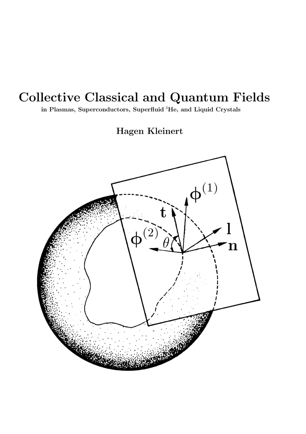
Collective Classical and Quantum Fields
in Plasmas, Superconductors, Superfluid 3 He, and Liquid Crystals
Hagen Kleinert
Collective Classical and
Quantum Fields
in Plasmas, Superconductors,
Superfluid 3He, and Liquid Crystals
Hagen Kleinert
Professor of Physics
Freie Universität Berlin
To Annemarie and Hagen II
Preface
Strongly interacting many-body systems behave often like a system of weakly interacting collective excitations. When this happens, it is theoretically advantageous
to replace the original action involving the fundamental fields (electrons, nucleons,
3
He, 4 He atoms, quarks etc.) by another action in which only certain collective excitations appear as independent quantum fields. Mathematically, such replacements
can be performed in many different ways without changing the physical content of
the initial theory. Experimental understanding of the important processes involved
can help theorists to identify the dominant collective excitations. If they possess
only weak residual interactions, these can be treated perturbatively. The associated
collective field theory greatly simplifies the approximate description of the physical
system.
It is the purpose of this book to discuss some basic techniques for deriving such
collective field theories. They are based on Feynman’s functional integral formulation of quantum field theory. In this formulation, the transformation to collective
fields amounts to mere changes of integration variables in functional integrals.
Systems of charged particles may show excitations of a type whose quanta are
called plasmons. For their description, a real field depending on one space and one
time variable is most convenient. If the particles form bound states, a complex field
depending on two spacetime coordinates renders the most economic description.
Such fields are bilocal , and are referred to as pair fields. If the attractive potential
is of short range, the bilocal field simplifies to a local field. This has led to the field
theory of superconductivity by Ginzburg and Landau. A bilocal theory of this type
has been used in elementary-particle physics to explain the observable properties of
strongly interacting mesons.
The change of integration variables in path integrals will be shown to correspond
to an exact resummation of the perturbation series, thereby accounting for phenomena which cannot be described perturbatively in terms of fundamental particles.
The path formulation has the great advantage of translating all quantum effects
among the fundamental particles completely into the field language of collective excitations. All fluctuation corrections may be computed using only propagators and
interaction vertices of the collective fields.
The method becomes unreliable if several collective effects compete with each
other. An example is a gas of electrons and protons at low density where the attractive forces can produce hydrogen atoms. They are absent in a description involving
a plasmon field. A mixture of plasmon and pair effects is needed to describe these.
vii
viii
Another example is superfluid 3 He, where pairing forces are necessary to produce
the superfluid phase transition. Here plasma-like magnetic excitations called paramagnons provide strong corrections. In particular, they are necessary to obtain
the pairing in the first place. If we want to tackle such mixed phenomena, another
technique must be used called variational perturbation theory.
In Chapter 1, I explain the mathematical method of changing from one field
description to another by going over to collective fields representing the dominant
collective excitations. In Chapters 2 and 3, I illustrate this method by discussing
simple systems such as an electron gas or a superconductor. At the end of Chapter
3, I had good help from my collaborator S.-S. Xue, with whom I wrote the basic
strong-coupling paper (arxiv:cond-mat/1708.04023), that is cited as Ref. [89] on
page 143. In Chapter 4, I apply the technique to superfluid 3 He. In Chapter 5, I
use the field theoretic methods to study physically observable phenomena in liquid
crystals. In Chapter 6, finally, I illustrate the working of the theory by treating
some simple solvable models.
I want to thank my wife Dr. Annemarie Kleinert for her great patience with
me while writing this book. Although her field of interest is French Literature and
History (her homepage https://a.klnrt.de), and thus completely different from mine,
her careful reading detected many errors. Without her permanent reminding me of
the still missing explanations of certain questions I could never have completed this
work. My son Michael, who just received his PhD in experimental physics, deserves
the credit of asking many relevant questions and making me improve my sometimes
too formal manuscript.
Berlin, December, 2017
H. Kleinert
Contents
1 Functional Integral Techniques
1.1 Nonrelativistic Fields . . . . . . . . . . . . . . . . . . . .
1.1.1
Quantization of Free Fields . . . . . . . . . . . .
1.1.2
Fluctuating Free Fields . . . . . . . . . . . . . .
1.1.3
Interactions . . . . . . . . . . . . . . . . . . . . .
1.1.4
Normal Products . . . . . . . . . . . . . . . . . .
1.1.5
Functional Formulation . . . . . . . . . . . . . .
1.1.6
Equivalence of Functional and Operator Methods
1.1.7
Grand-Canonical Ensembles at Zero Temperature
1.2 Relativistic Fields . . . . . . . . . . . . . . . . . . . . . .
1.2.1
Lorentz and Poincaré Invariance . . . . . . . . .
1.2.2
Relativistic Free Scalar Fields . . . . . . . . . . .
1.2.3
Electromagnetic Fields . . . . . . . . . . . . . . .
1.2.4
Relativistic Free Fermi Fields . . . . . . . . . . .
1.2.5
Perturbation Theory of Relativistic Fields . . . .
Notes and References . . . . . . . . . . . . . . . . . . . . . . . .
2 Plasma Oscillations
2.1 General Formalism . . . . . . . . . . . . .
2.2 Physical Consequences . . . . . . . . . .
2.2.1
Zero Temperature . . . . . . . .
2.2.2
Short-Range Potential . . . . . .
Appendix 2A Fluctuations around the Plasmon
Notes and References . . . . . . . . . . . . . . .
.
.
.
.
.
.
.
.
.
.
.
.
.
.
.
.
.
.
.
.
.
.
.
.
.
.
.
.
.
.
.
.
.
.
.
.
.
.
.
.
.
.
.
.
.
.
.
.
.
.
.
.
.
.
.
.
.
.
.
.
.
.
.
.
.
.
.
.
.
.
.
.
.
.
.
.
.
.
.
.
.
.
.
.
.
.
.
.
.
.
.
.
.
.
.
.
.
.
.
.
.
.
.
.
.
.
.
.
.
.
.
.
.
.
.
.
.
.
.
.
.
.
.
.
.
.
.
.
.
.
.
.
.
.
.
.
.
.
.
.
.
.
.
.
.
.
.
.
.
.
.
.
.
.
.
.
.
.
.
.
.
.
.
.
.
.
.
.
.
.
.
.
.
.
1
2
2
4
8
10
14
15
16
22
22
27
31
34
37
39
.
.
.
.
.
.
41
41
45
46
47
48
49
3 Superconductors
3.1 General Formulation . . . . . . . . . . . . . . . . . . . . . . . . . . .
3.2 Local Interaction and Ginzburg-Landau Equations . . . . . . . . . .
3.2.1
Inclusion of Electromagnetic Fields into the Pair Field Theory
3.3 Far below the Critical Temperature . . . . . . . . . . . . . . . . . .
3.3.1
The Gap . . . . . . . . . . . . . . . . . . . . . . . . . . . .
3.3.2
The Free Pair Field . . . . . . . . . . . . . . . . . . . . . .
3.4 From BCS to Strong-Coupling Superconductivity . . . . . . . . . . .
3.5 Strong-Coupling Calculation of the Pair Field . . . . . . . . . . . . .
ix
50
52
59
69
72
73
77
91
92
x
3.6
From BCS Superconductivity near Tc to the onset of pseudogap
behavior . . . . . . . . . . . . . . . . . . . . . . . . . . . . . . . .
3.7 Phase Fluctuations in Two Dimensions and Kosterlitz-Thouless
Transition . . . . . . . . . . . . . . . . . . . . . . . . . . . . . . .
3.8 Phase Fluctuations in Three Dimensions . . . . . . . . . . . . . .
3.9 Collective Classical Fields . . . . . . . . . . . . . . . . . . . . . . .
3.9.1
Superconducting Electrons . . . . . . . . . . . . . . . . .
3.10 Strong-Coupling Limit of Pair Formation . . . . . . . . . . . . . .
3.11 Composite Bosons . . . . . . . . . . . . . . . . . . . . . . . . . . .
3.12 Composite Fermions . . . . . . . . . . . . . . . . . . . . . . . . . .
3.13 Conclusion and Remarks . . . . . . . . . . . . . . . . . . . . . . .
Appendix 3A Auxiliary Strong-Coupling Calculations . . . . . . . . . . .
Appendix 3B Propagator of the Bilocal Pair Field . . . . . . . . . . . . .
Appendix 3C Fluctuations Around the Composite Field . . . . . . . . .
Notes and References . . . . . . . . . . . . . . . . . . . . . . . . . . . . .
. 100
.
.
.
.
.
.
.
.
.
.
.
.
105
111
112
115
117
122
127
129
131
133
135
138
4 Superfluid 3 He
145
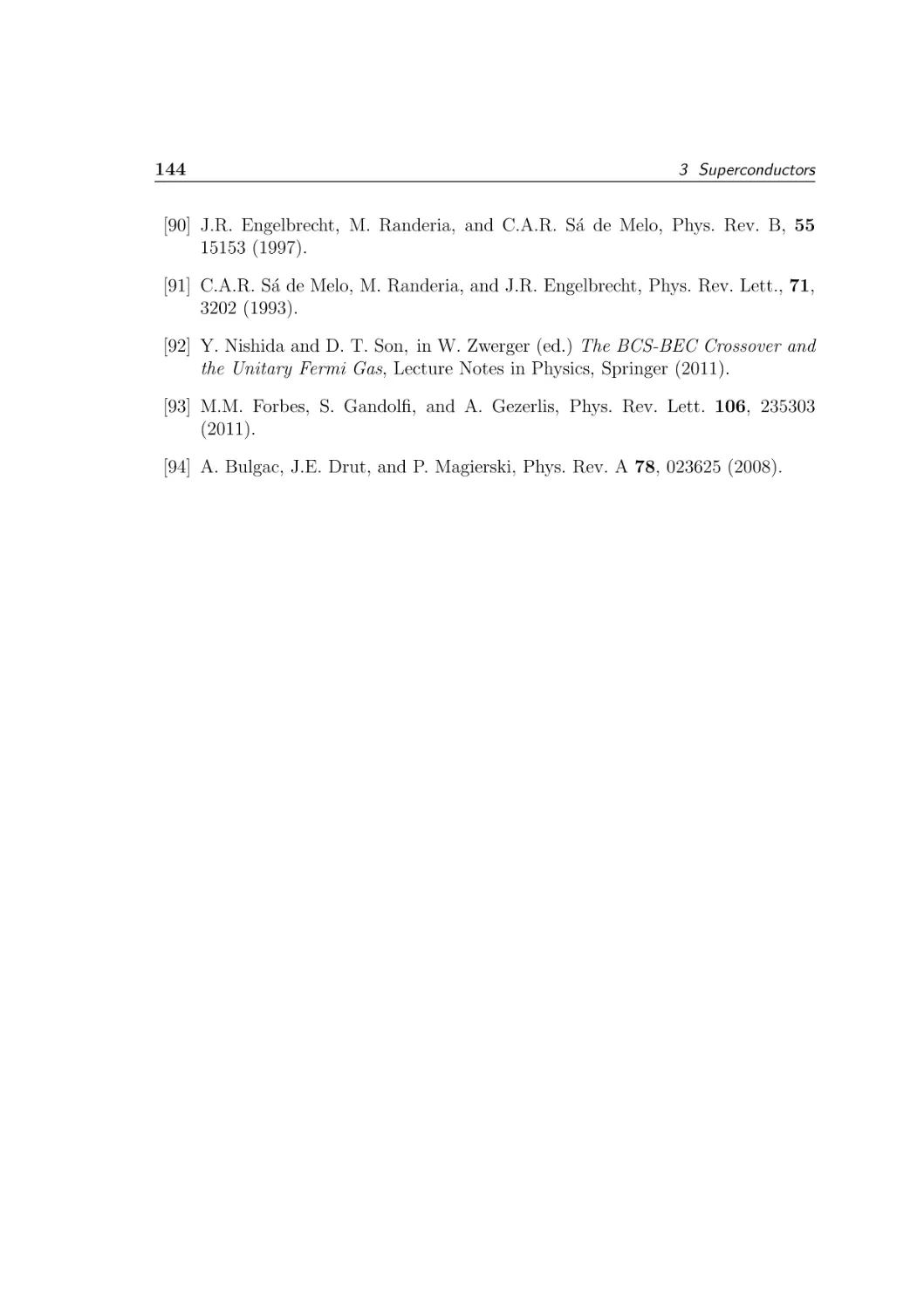
4.1 Interatomic Potential . . . . . . . . . . . . . . . . . . . . . . . . . . 145
4.2 Phase Diagram . . . . . . . . . . . . . . . . . . . . . . . . . . . . . . 147
4.3 Preparation of Functional Integral . . . . . . . . . . . . . . . . . . . 149
4.3.1
Action of the System . . . . . . . . . . . . . . . . . . . . . . 149
4.3.2
Dipole Interaction . . . . . . . . . . . . . . . . . . . . . . . 149
4.3.3
Euclidean Action . . . . . . . . . . . . . . . . . . . . . . . . 150
4.3.4
From Particles to Quasiparticles . . . . . . . . . . . . . . . 151
4.3.5
Approximate Quasiparticle Action . . . . . . . . . . . . . . 152
4.3.6
Effective Interaction . . . . . . . . . . . . . . . . . . . . . . 155
4.3.7
Pairing Interaction . . . . . . . . . . . . . . . . . . . . . . . 158
4.4 Transformation from Fundamental to Collective Fields . . . . . . . . 159
4.5 General Properties of a Collective Action . . . . . . . . . . . . . . . 164
4.6 Comparison with O(3)-Symmetric Linear σ-Model . . . . . . . . . . 169
4.7 Hydrodynamic Properties Close to Tc . . . . . . . . . . . . . . . . . 170
4.8 Bending the Superfluid 3 He-A . . . . . . . . . . . . . . . . . . . . . 178
4.8.1
Monopoles . . . . . . . . . . . . . . . . . . . . . . . . . . . 179
4.8.2
Line Singularities . . . . . . . . . . . . . . . . . . . . . . . . 182
4.8.3
Solitons . . . . . . . . . . . . . . . . . . . . . . . . . . . . . 184
4.8.4
Localized Lumps . . . . . . . . . . . . . . . . . . . . . . . . 187
4.8.5
Use of Topology in the A-Phase . . . . . . . . . . . . . . . . 188
4.8.6
Topology in the B-Phase . . . . . . . . . . . . . . . . . . . . 190
4.9 Hydrodynamic Properties at All Temperatures T ≤ Tc . . . . . . . . 193
4.9.1
Derivation of Gap Equation . . . . . . . . . . . . . . . . . . 194
4.9.2
Ground State Properties . . . . . . . . . . . . . . . . . . . . 199
4.9.3
Bending Energies . . . . . . . . . . . . . . . . . . . . . . . . 208
4.9.4
Fermi-Liquid Corrections . . . . . . . . . . . . . . . . . . . 218
4.10 Large Currents and Magnetic Fields in the Ginzburg-Landau Regime 227
xi
4.10.1 B-Phase . . . . . . . . . . . . . . . . . . . . . . . . . . . .
4.10.2 A-Phase . . . . . . . . . . . . . . . . . . . . . . . . . . . .
4.10.3 Critical Current in Other Phases for T ∼ Tc . . . . . . . .
4.11 Is 3 He-A a Superfluid? . . . . . . . . . . . . . . . . . . . . . . . . .
4.11.1 Magnetic Field and Transition between A- and B-Phases .
4.12 Large Currents at Any Temperature T ≤ Tc . . . . . . . . . . . . .
4.12.1 Energy at Nonzero Velocities . . . . . . . . . . . . . . . .
4.12.2 Gap Equations . . . . . . . . . . . . . . . . . . . . . . . .
4.12.3 Superfluid Densities and Currents . . . . . . . . . . . . . .
4.12.4 Critical Currents . . . . . . . . . . . . . . . . . . . . . . .
4.12.5 Ground State Energy at Large Velocities . . . . . . . . . .
4.12.6 Fermi Liquid Corrections . . . . . . . . . . . . . . . . . .
4.13 Collective Modes in the Presence of Current at all Temperatures
T ≤ Tc . . . . . . . . . . . . . . . . . . . . . . . . . . . . . . . . .
4.13.1 Quadratic Fluctuations . . . . . . . . . . . . . . . . . . .
4.13.2 Time-Dependent Fluctuations at Infinite Wavelength . . .
4.13.3 Normal Modes . . . . . . . . . . . . . . . . . . . . . . . .
4.13.4 Simple Limiting Results at Zero Gap Deformation . . . .
4.13.5 Static Stability . . . . . . . . . . . . . . . . . . . . . . . .
4.14 Fluctuation Coefficients . . . . . . . . . . . . . . . . . . . . . . . .
4.15 Stability of Superflow in the B-Phase under Small Fluctuations for
T ∼ Tc . . . . . . . . . . . . . . . . . . . . . . . . . . . . . . . . .
Appendix 4A Hydrodynamic Coefficients for T ≈ Tc . . . . . . . . . . . .
Appendix 4B Hydrodynamic Coefficients for All T ≤ Tc . . . . . . . . .
Appendix 4C Generalized Ginzburg-Landau Energy . . . . . . . . . . . .
Notes and References . . . . . . . . . . . . . . . . . . . . . . . . . . . . .
5 Liquid Crystals
5.1 Maier-Saupe Model and Generalizations . . . . . . . . . .
5.1.1
General Properties . . . . . . . . . . . . . . . . .
5.1.2
Landau Expansion . . . . . . . . . . . . . . . . .
5.1.3
Tensor Form of Landau-de Gennes Expansion . .
5.2 Landau-de Gennes Description of Nematic Phase . . . . .
5.3 Bending Energy . . . . . . . . . . . . . . . . . . . . . . .
5.4 Light Scattering . . . . . . . . . . . . . . . . . . . . . . .
5.5 Interfacial Tension between Nematic and Isotropic Phases
5.6 Cholesteric Liquid Crystals . . . . . . . . . . . . . . . . .
5.6.1
Small Fluctuations above T1 . . . . . . . . . . . .
5.6.2
Some Experimental Facts . . . . . . . . . . . . .
5.6.3
Mean-Field Description of Cholesteric Phase . . .
5.7 Other Phases . . . . . . . . . . . . . . . . . . . . . . . . .
Appendix 5A Biaxial Maier-Saupe Model . . . . . . . . . . . . .
Notes and References . . . . . . . . . . . . . . . . . . . . . . . .
.
.
.
.
.
.
.
.
.
.
.
.
.
.
.
.
.
.
.
.
.
.
.
.
.
.
.
.
.
.
.
.
.
.
.
.
.
.
.
.
.
.
.
.
.
.
.
.
.
.
.
.
.
.
.
.
.
.
.
.
.
.
.
.
.
.
.
.
.
.
.
.
.
.
.
.
.
.
.
.
.
.
.
.
.
.
.
228
239
240
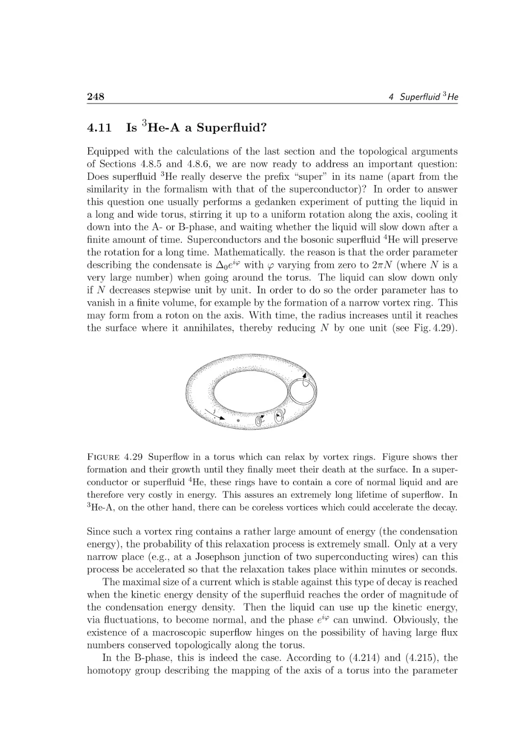
248
272
274
274
275
283
285
289
289
.
.
.
.
.
.
.
292
292
295
298
301
303
304
.
.
.
.
.
307
312
315
319
319
323
. 324
. 324
. 326
. 327
. 328
. 336
. 338
. 347
. 351
. 354
. 355
. 357
. 362
. 365
. 368
xii
6 Exactly Solvable Field-Theoretic Models
6.1 Pet Model in Zero Plus One Time Dimensions . . . . . . .
6.1.1
The Generalized BCS Model in a Degenerate Shell
6.1.2
The Hilbert Space of the Generalized BCS Model .
6.2 Thirring Model in 1+1 Dimensions . . . . . . . . . . . . . .
6.3 Supersymmetry in Nuclear Physics . . . . . . . . . . . . . .
Notes and References . . . . . . . . . . . . . . . . . . . . . . . . .
Index
.
.
.
.
.
.
.
.
.
.
.
.
.
.
.
.
.
.
.
.
.
.
.
.
.
.
.
.
.
.
371
371
379
390
393
397
397
399
List of Figures
1.1
Contour C in the complex z-plane . . . . . . . . . . . . . . . . . . . 19
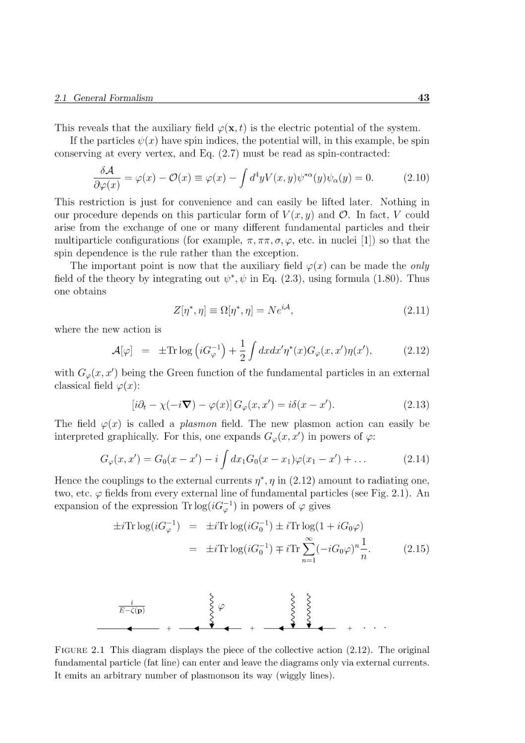
2.1
2.2
2.3
The pure current piece of the collective action . . . . . . . . . . . . 43
The non-polynomial self-interaction terms of plasmons . . . . . . . 44
Free plasmon propagator . . . . . . . . . . . . . . . . . . . . . . . . 44
3.1
3.2
3.3
3.4
3.5
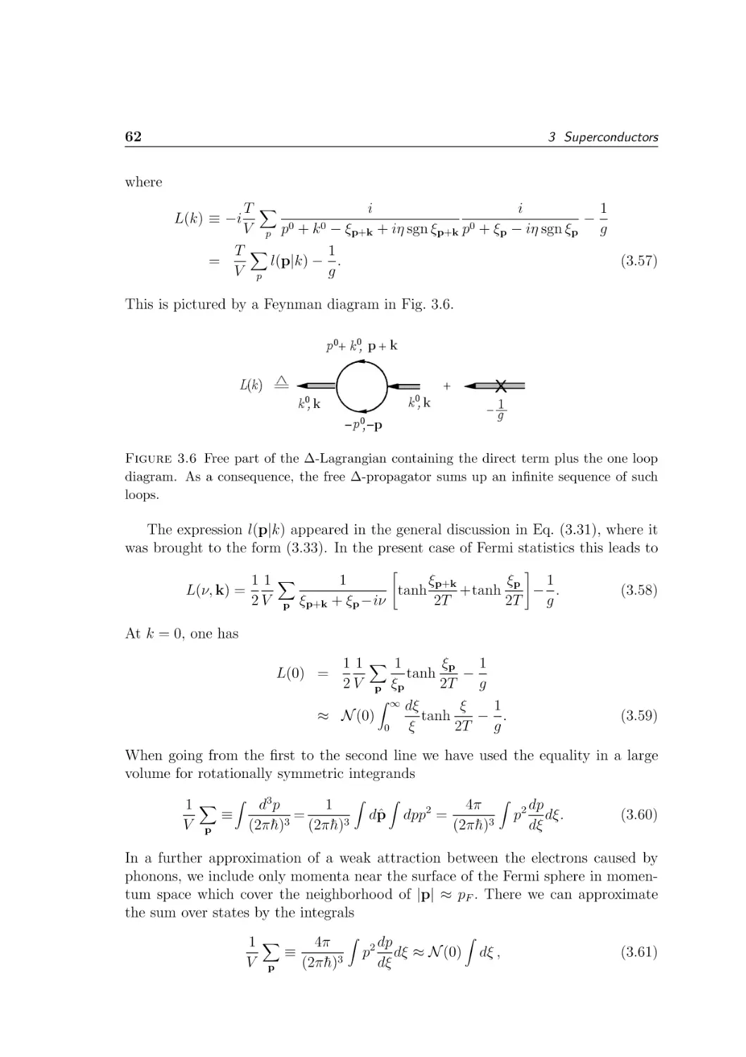
3.6
3.7
3.8
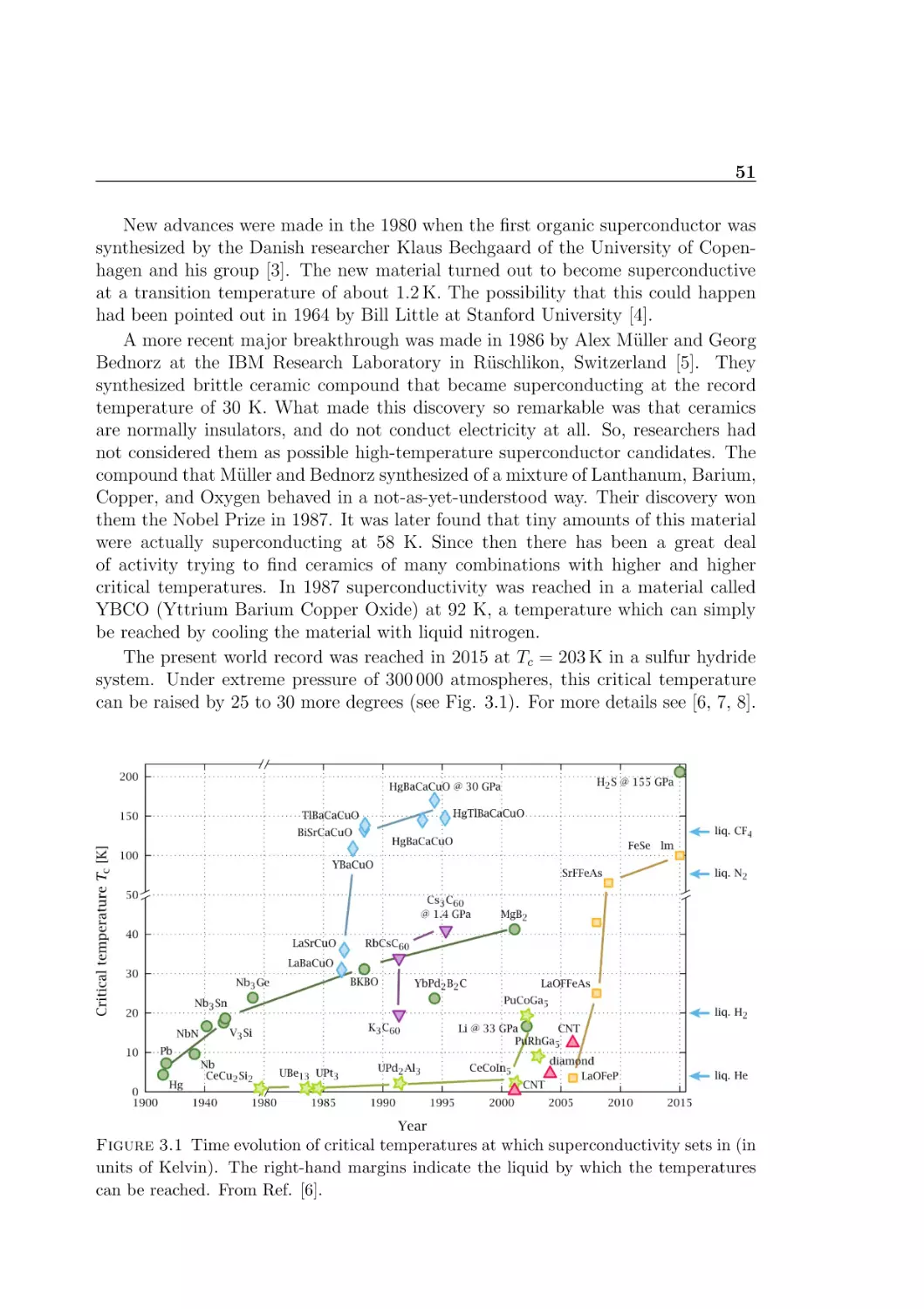
Time evolution of critical temperatures of superconductivity . . . . .
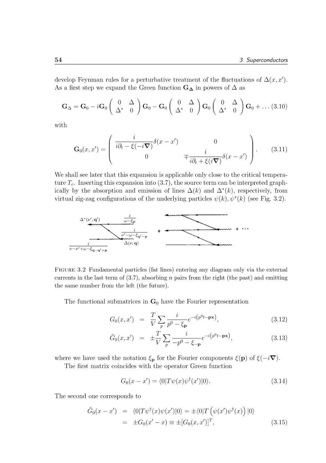
Fundamental particles entering any diagram . . . . . . . . . . . . .
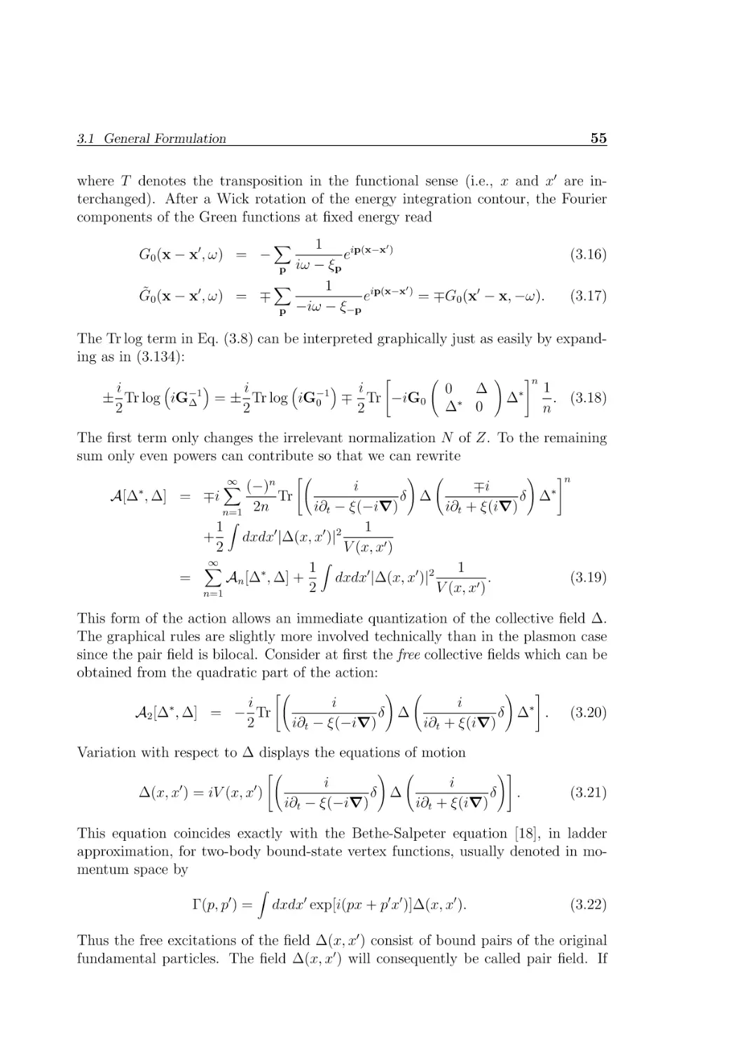
Free pair field following the Bethe-Salpeter equation . . . . . . . . .
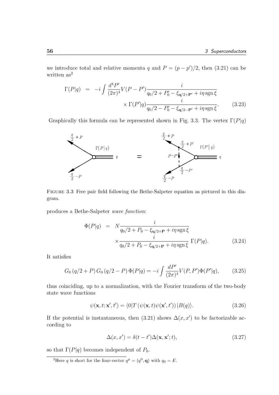
Free pair propagator . . . . . . . . . . . . . . . . . . . . . . . . . .
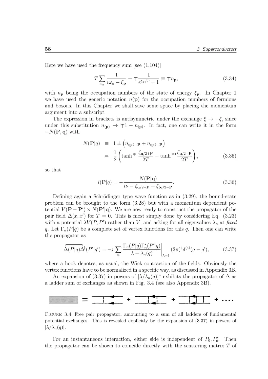
Self-interaction terms of the non-polynomial pair Lagrangian . . . .
Free part of pair field ∆ Lagrangian . . . . . . . . . . . . . . . . . .
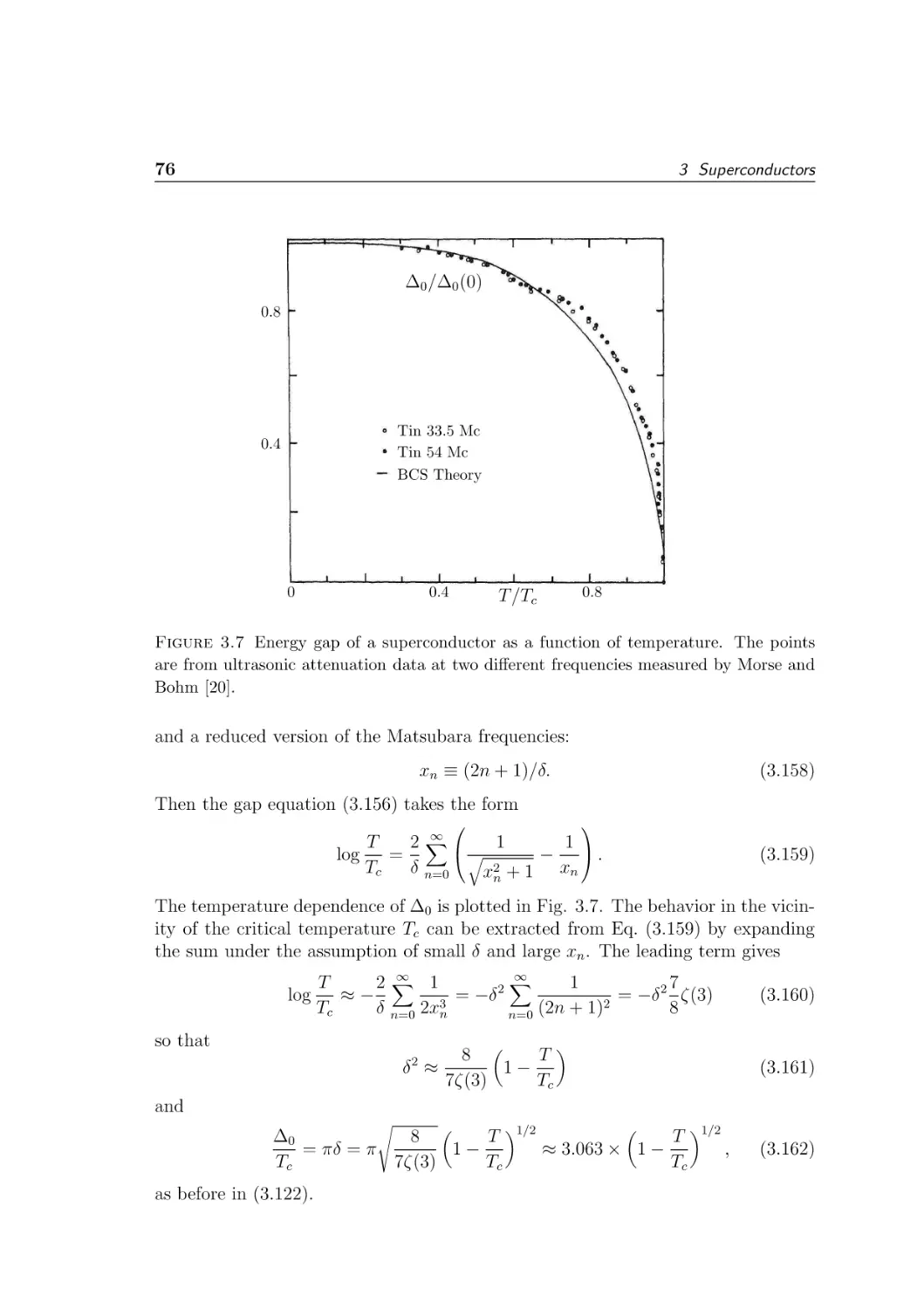
Energy gap of a superconductor as a function of temperature . . . .
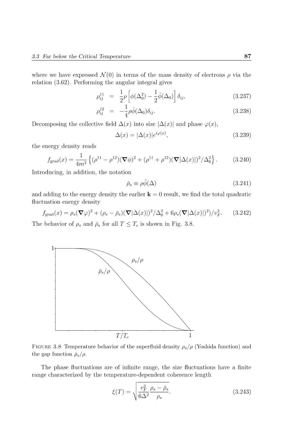
Temperature behavior of the superfluid density ρs /ρ (Yoshida function) and the gap function ρ̄s /ρ . . . . . . . . . . . . . . . . . . . .
Temperature behavior of the inverse square coherence length ξ −2(T )
Gap function ∆ and chemical potential µ at zero temperature as
functions of the crossover parameter µ̂ . . . . . . . . . . . . . . . . .
Temperature dependence of the gap function in three (a) and two
(b) dimensions . . . . . . . . . . . . . . . . . . . . . . . . . . . . . .
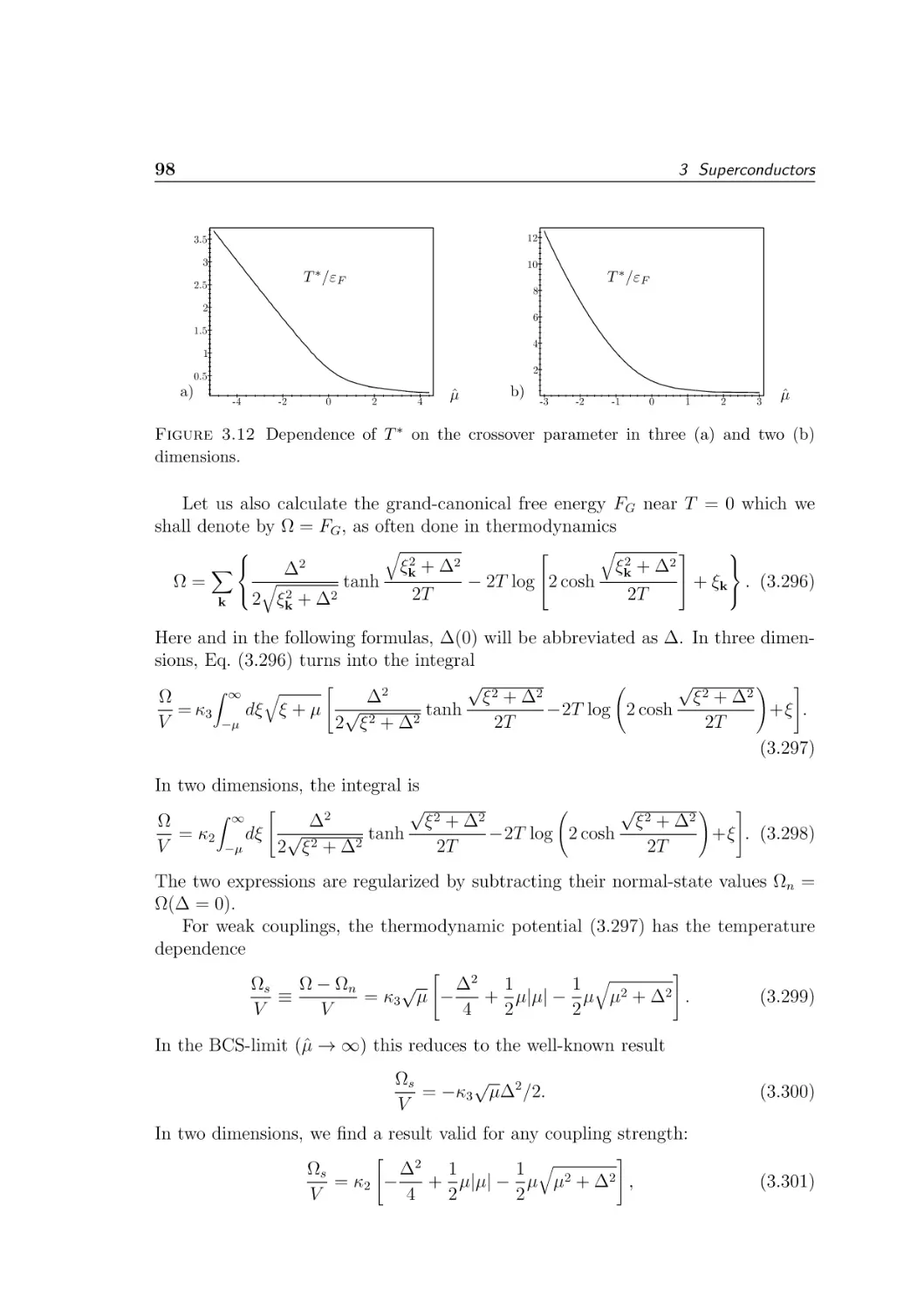
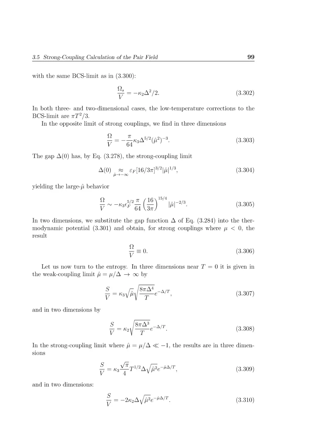
Dependence of T ∗ on the crossover parameter in three (a) and two
(b) dimensions . . . . . . . . . . . . . . . . . . . . . . . . . . . . . .
Dependence of the pair-formation temperature T ∗ on the chemical
potential . . . . . . . . . . . . . . . . . . . . . . . . . . . . . . . . .
Qualitative phase diagram of the BCS-BEC crossover as a function
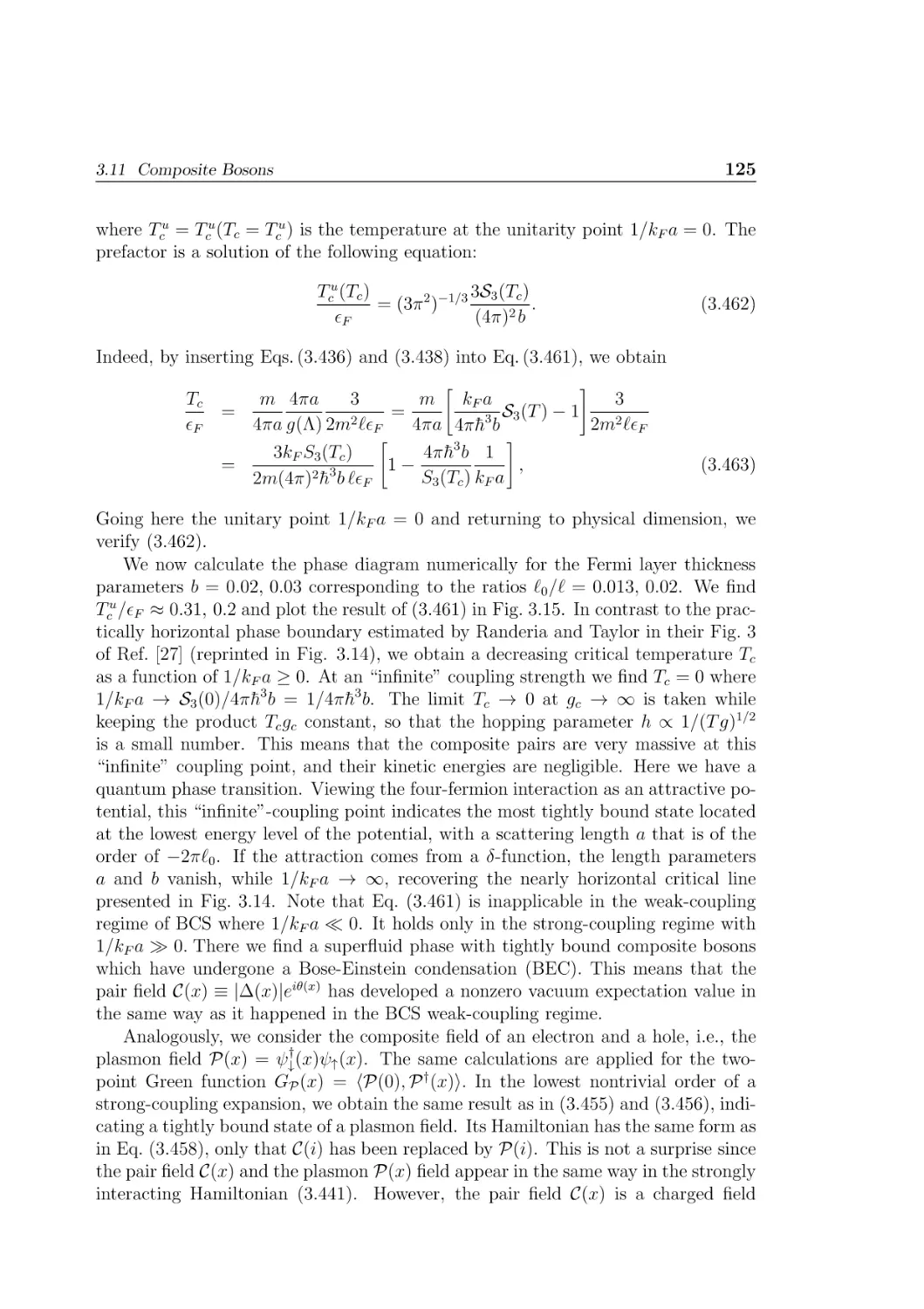
of temperature T /ǫF and coupling 1/kF a . . . . . . . . . . . . . . .
Qualitative phase diagram in the unitarity limit . . . . . . . . . . .
3.9
3.10
3.11
3.12
3.13
3.14
3.15
4.1
4.2
4.3
4.4
Interatomic potential between 3 He atoms as a function of the distance r . . . . . . . . . . . . . . . . . . . . . . . . . . . . . . . . .
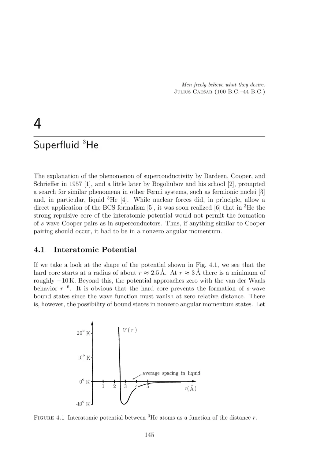
Imaginary part of the susceptibility caused by repeated exchange of
spin fluctuations . . . . . . . . . . . . . . . . . . . . . . . . . . . .
Phase diagram of 3 He plotted against temperature, pressure, and
magnetic field . . . . . . . . . . . . . . . . . . . . . . . . . . . . .
Three fundamental planar textures, splay, bend, and twist of the
director field in liquid crystals . . . . . . . . . . . . . . . . . . . .
xiii
51
54
56
58
59
62
76
87
88
96
97
98
109
118
126
. 145
. 146
. 148
. 172
xiv
4.5
4.6
4.7
4.8
4.9
4.10
4.11
4.12
4.13
4.14
4.15
4.16
4.17
4.18
4.19
4.20
4.21
4.22
4.23
4.24
4.25
4.26
4.27
4.28
4.29
4.30
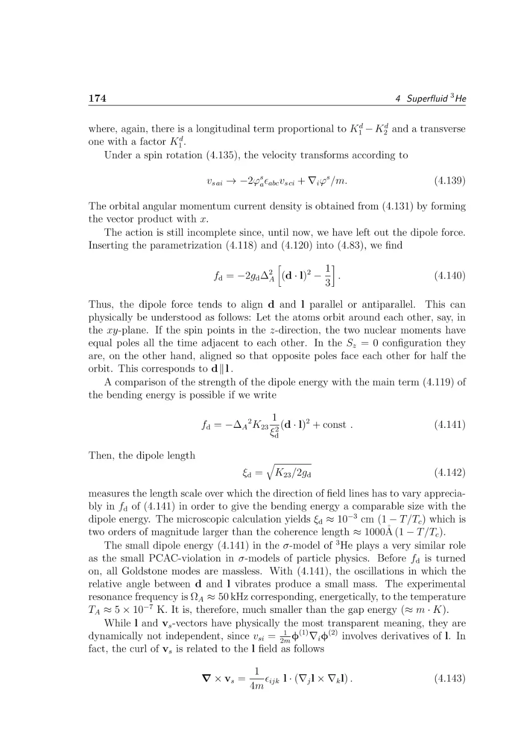
Sphere with one, two, or no handles and their Euler characteristics
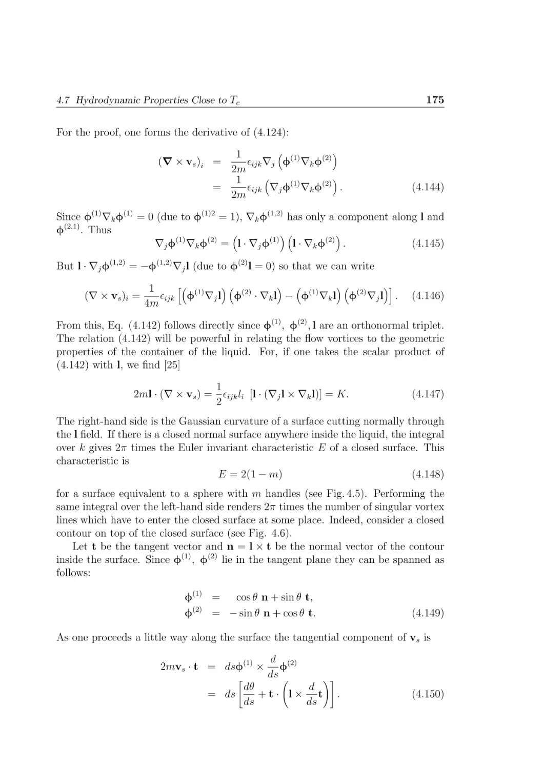
Local tangential coordinate system n, t, i for an arbitrary curve on
the surface of a sphere . . . . . . . . . . . . . . . . . . . . . . . . .
The lkd-field lines in a spherical container . . . . . . . . . . . . . .
Two possible parametrizations of a sphere . . . . . . . . . . . . . .
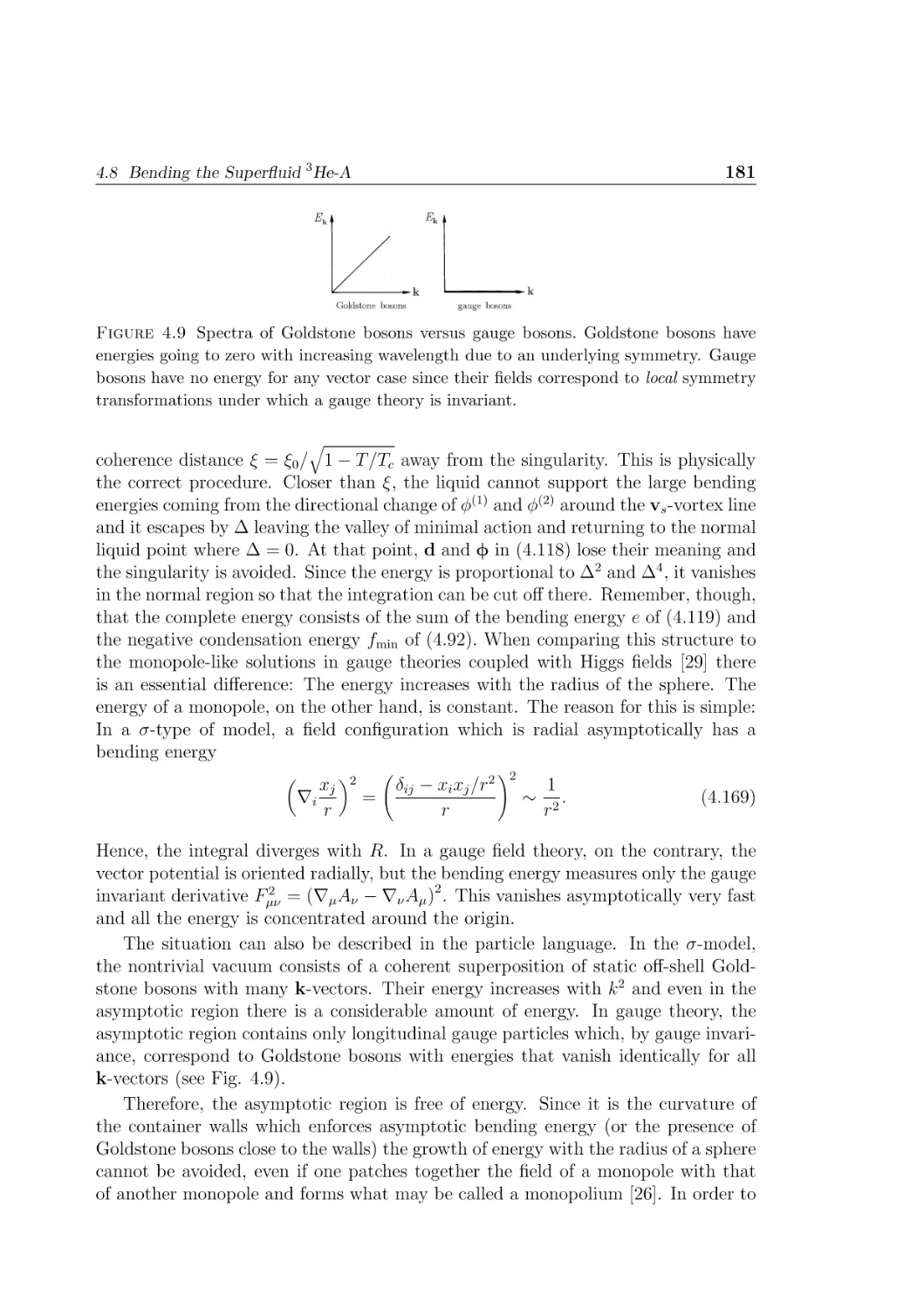
Spectra of Goldstone bosons versus gauge bosons . . . . . . . . . .
Cylindrical container with the l k d-field lines spreading outwards
when moving upwards . . . . . . . . . . . . . . . . . . . . . . . . .
Field vectors in a composite soliton . . . . . . . . . . . . . . . . .
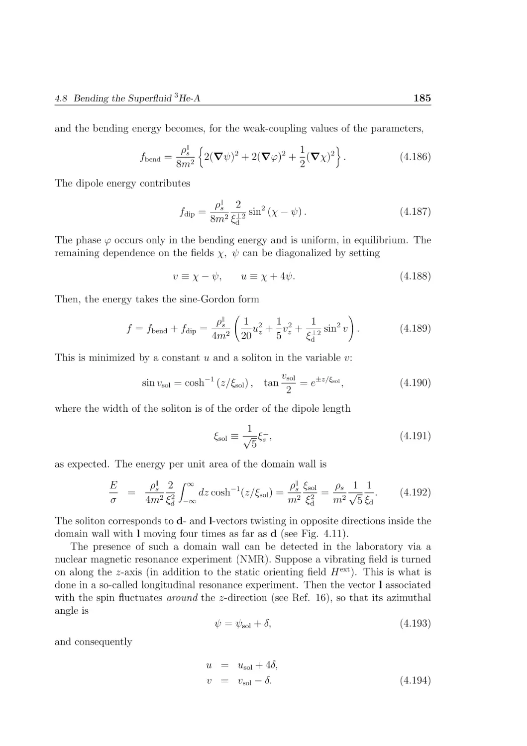
Nuclear magnetic resonance frequencies of a superfluid 3 He-A sample
in an external magnetic field . . . . . . . . . . . . . . . . . . . . .
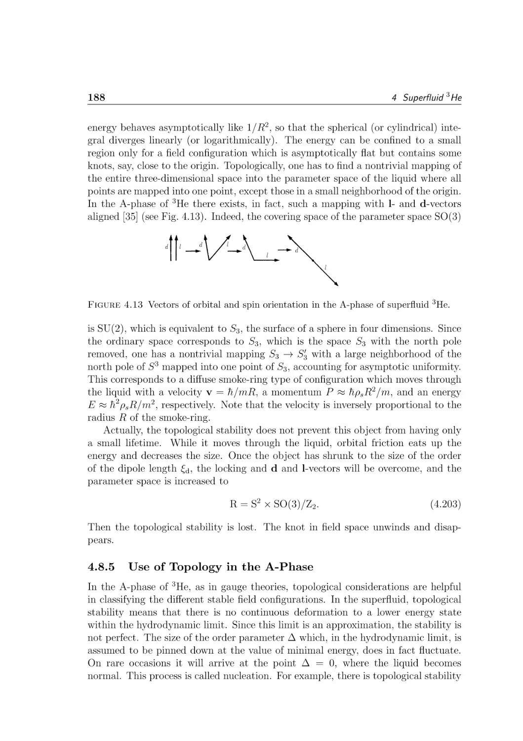
Vectors of orbital and spin orientation in the A-phase of superfluid
3
He . . . . . . . . . . . . . . . . . . . . . . . . . . . . . . . . . . .
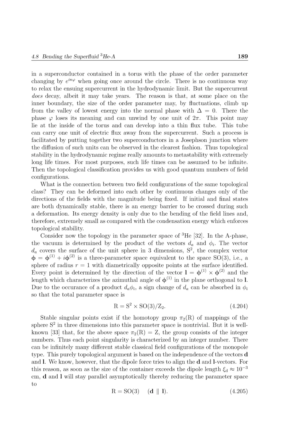
Parameter space of 3 He-B containing the parameter space of the
rotation group . . . . . . . . . . . . . . . . . . . . . . . . . . . . .
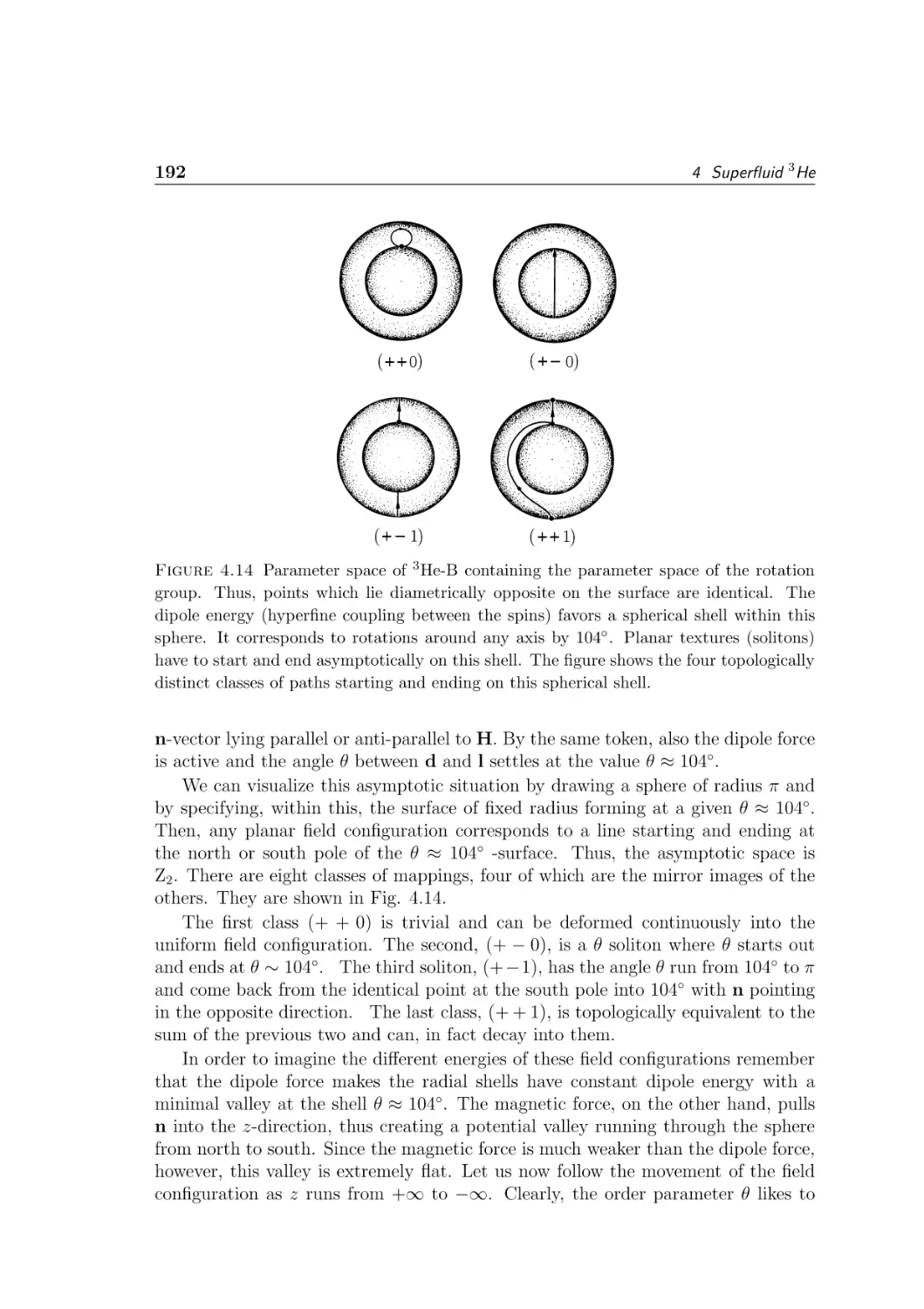
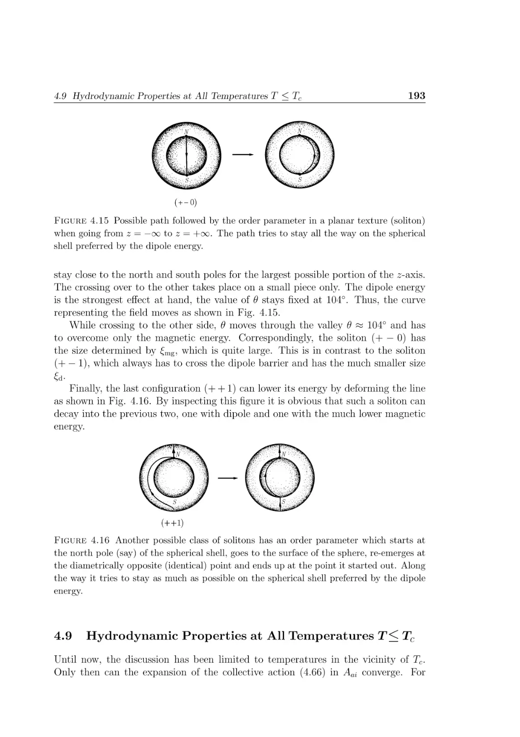
Possible path followed by the order parameter in a planar texture
(soliton) when going from z = −∞ to z = +∞ . . . . . . . . . . .
Another possible class of solitons . . . . . . . . . . . . . . . . . .
Fundamental hydrodynamic quantities of superfluid 3 He-B and -A,
shown as a function of temperature . . . . . . . . . . . . . . . . .
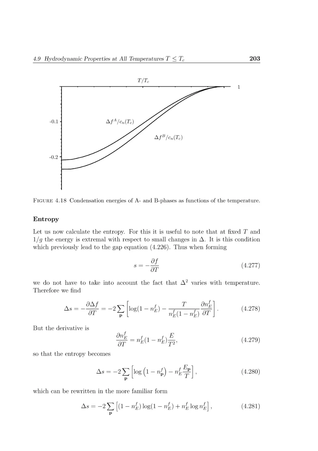
Condensation energies of A- and B-phases as functions of the temperature . . . . . . . . . . . . . . . . . . . . . . . . . . . . . . . .
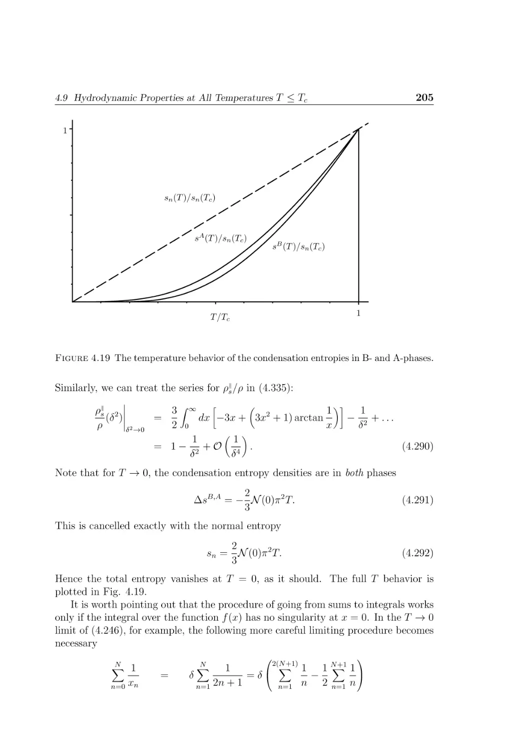
The temperature behavior of the condensation entropies in B- and
A-phases . . . . . . . . . . . . . . . . . . . . . . . . . . . . . . . .
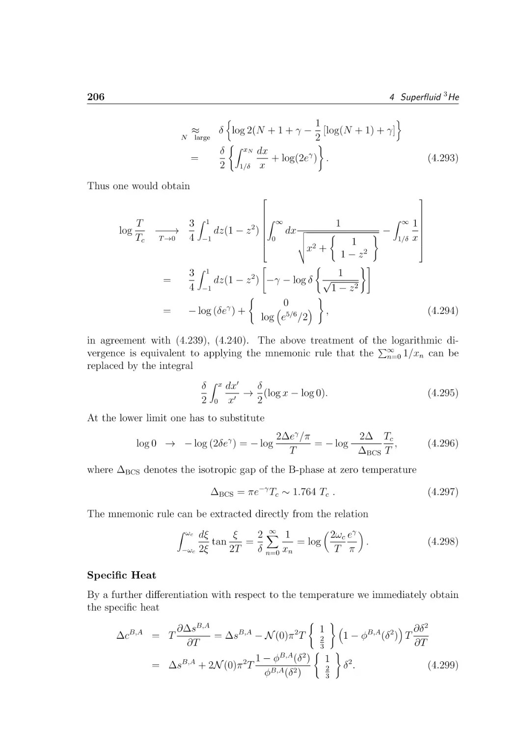
Specific heat of A- and B-phases as a function of temperature . . .
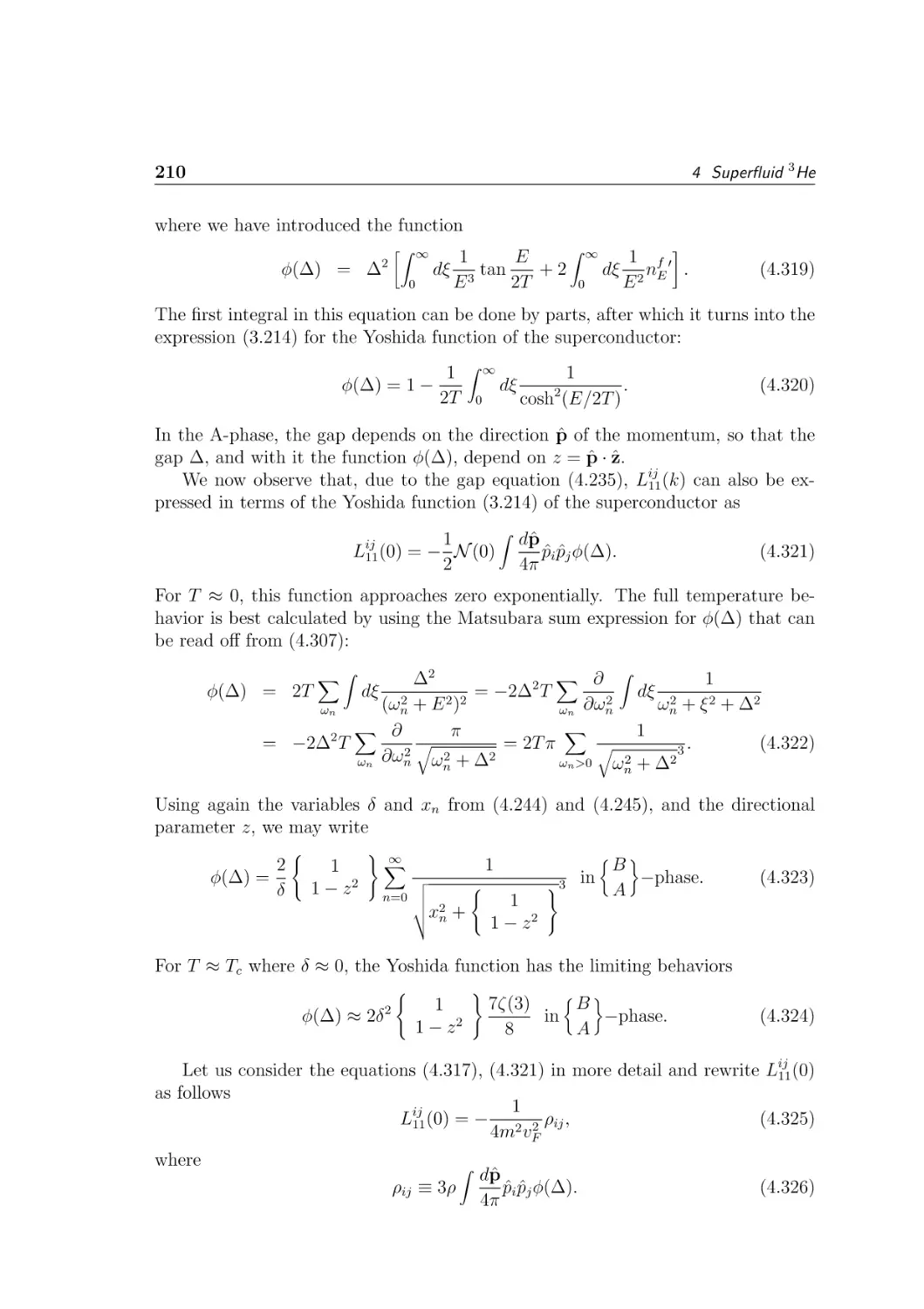
Temperature behavior of the reduced superfluid densities in the Band in the A-phase of superfluid 4 He . . . . . . . . . . . . . . . . .
Superfluid stiffness functions Kt , Kb , Ks of the A-phase as functions
of the temperature . . . . . . . . . . . . . . . . . . . . . . . . . . .
Superfluid densities of B- and A-phase after applying Fermi liquid
corrections . . . . . . . . . . . . . . . . . . . . . . . . . . . . . . .
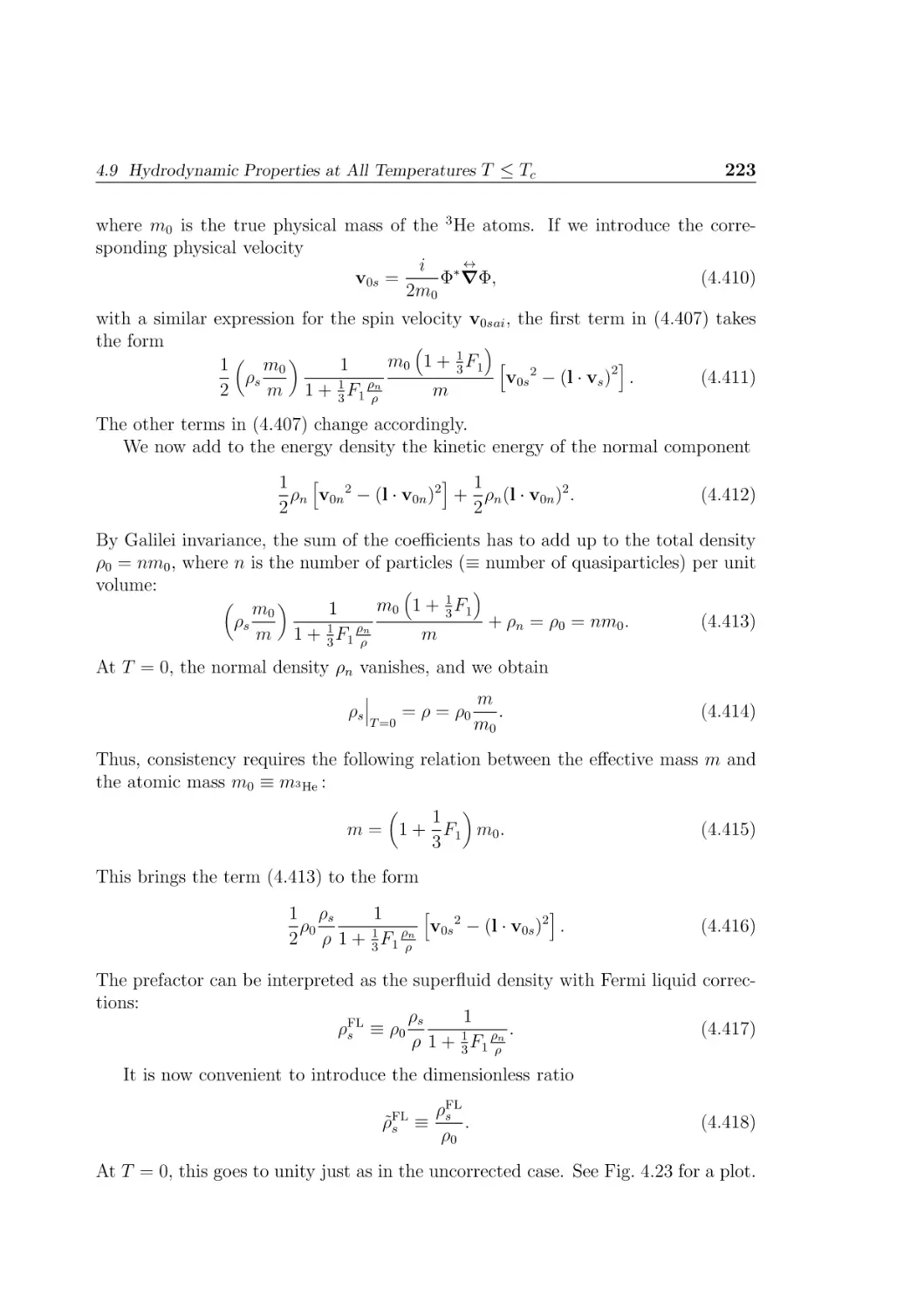
Coefficients c = ck and their Fermi liquid corrected values in the
A-phase as a function of temperature . . . . . . . . . . . . . . . .
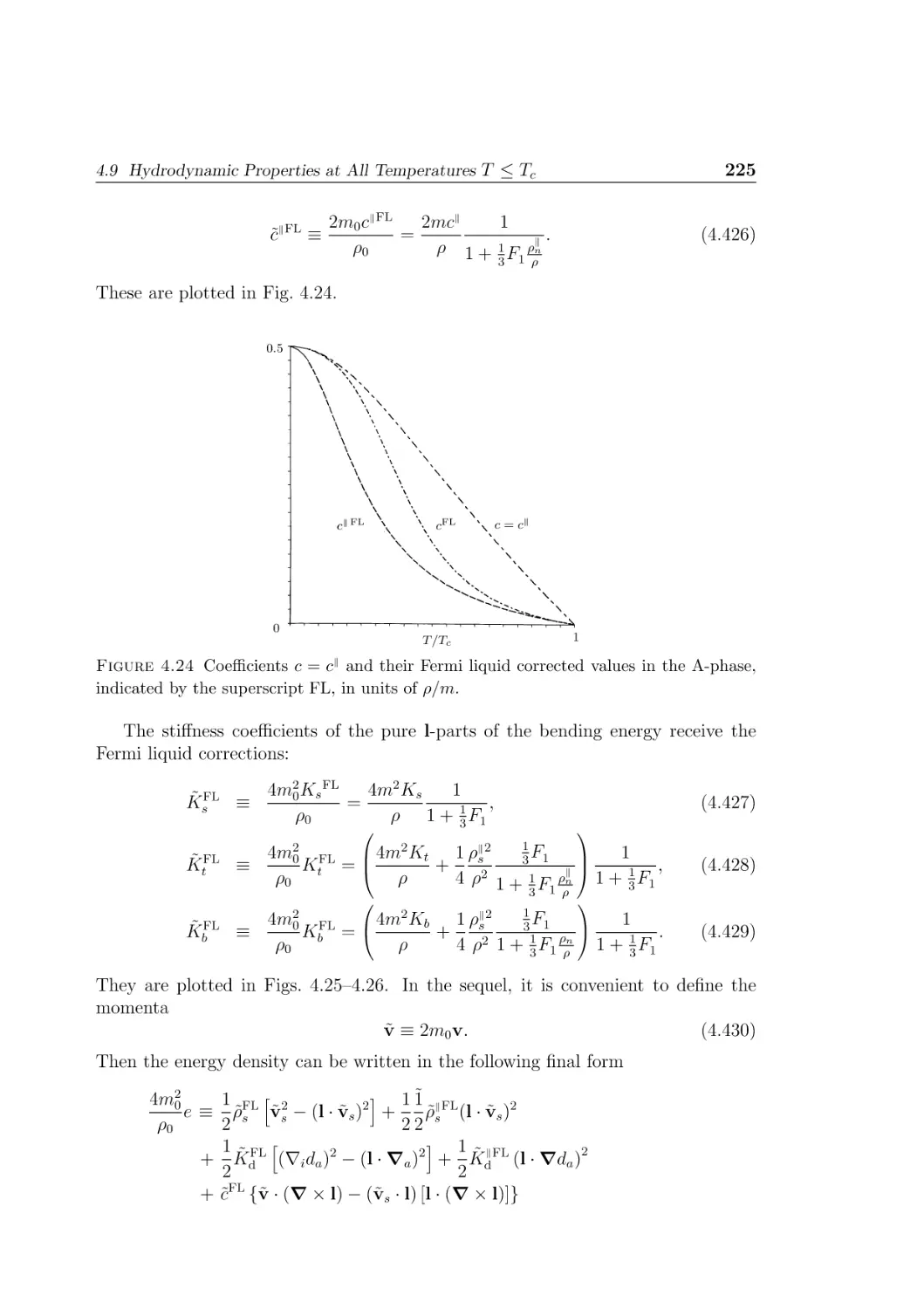
Coefficient Ks for splay deformations of the fields, and its Fermi
liquid corrected values in the A-phase as a function of temperature
Remaining hydrodynamic parameters for twist and bend deformations of superfluid 3 He-A . . . . . . . . . . . . . . . . . . . . . . .
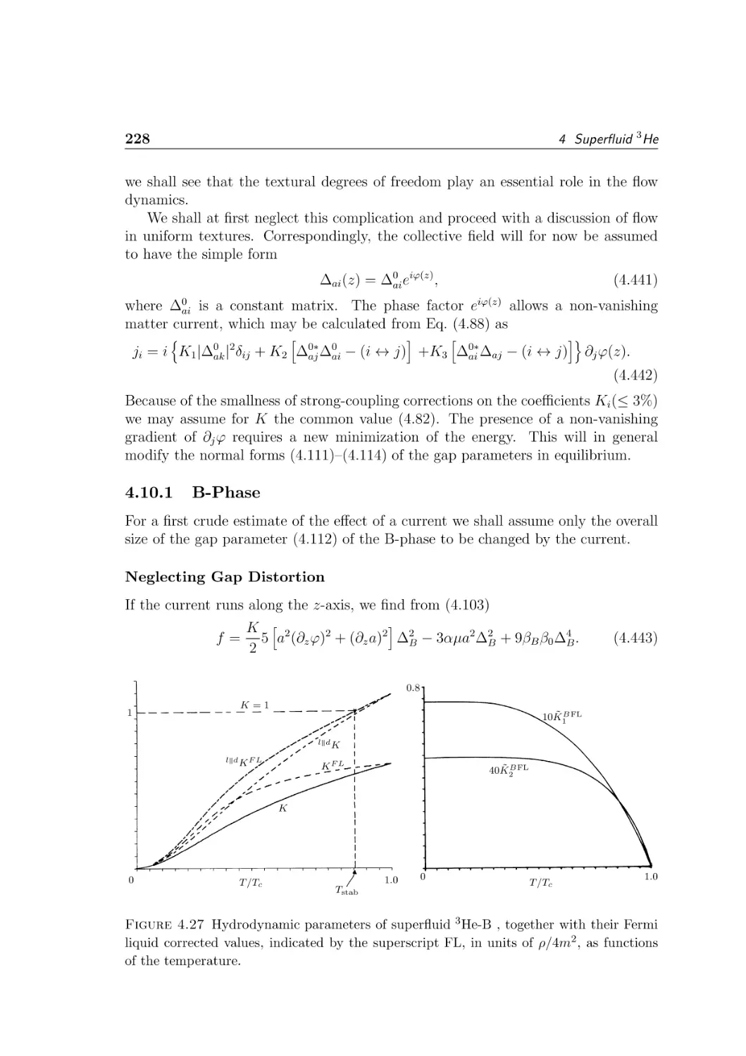
Hydrodynamic parameters of superfluid 3 He-B together with their
Fermi liquid corrected values, as functions of the temperature . .
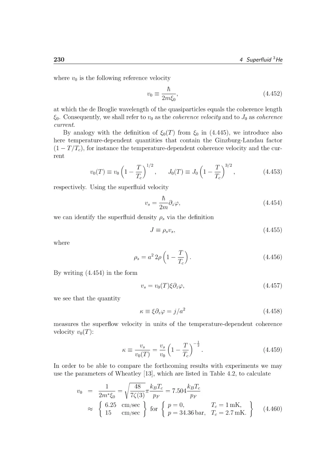
Shape of potential determining stability of superflow . . . . . . .
Superflow in a torus . . . . . . . . . . . . . . . . . . . . . . . . . .
In the presence of a superflow in 3 He-A, the l-vector is attracted to
the direction of flow . . . . . . . . . . . . . . . . . . . . . . . . .
176
.
.
.
.
176
179
180
181
. 183
. 186
. 187
. 188
. 192
. 193
. 193
. 198
. 203
. 205
. 207
. 211
. 218
. 224
. 225
. 226
. 227
. 228
. 231
. 248
. 254
4.31 Doubly connected parameter space of the rotation group corresponding to integer and half-integer spin representations . . . . . . . . .
4.32 Helical texture in the presence of a supercurrent . . . . . . . . . .
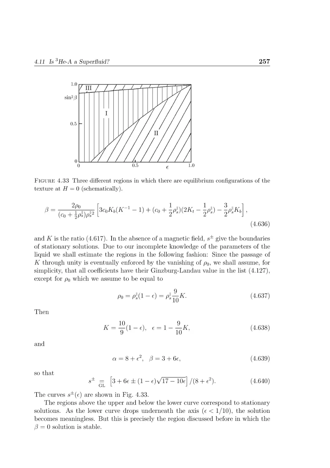
4.33 Three different regions of equilibrium configurations of the texture
at H = 0 (schematically) . . . . . . . . . . . . . . . . . . . . . . .
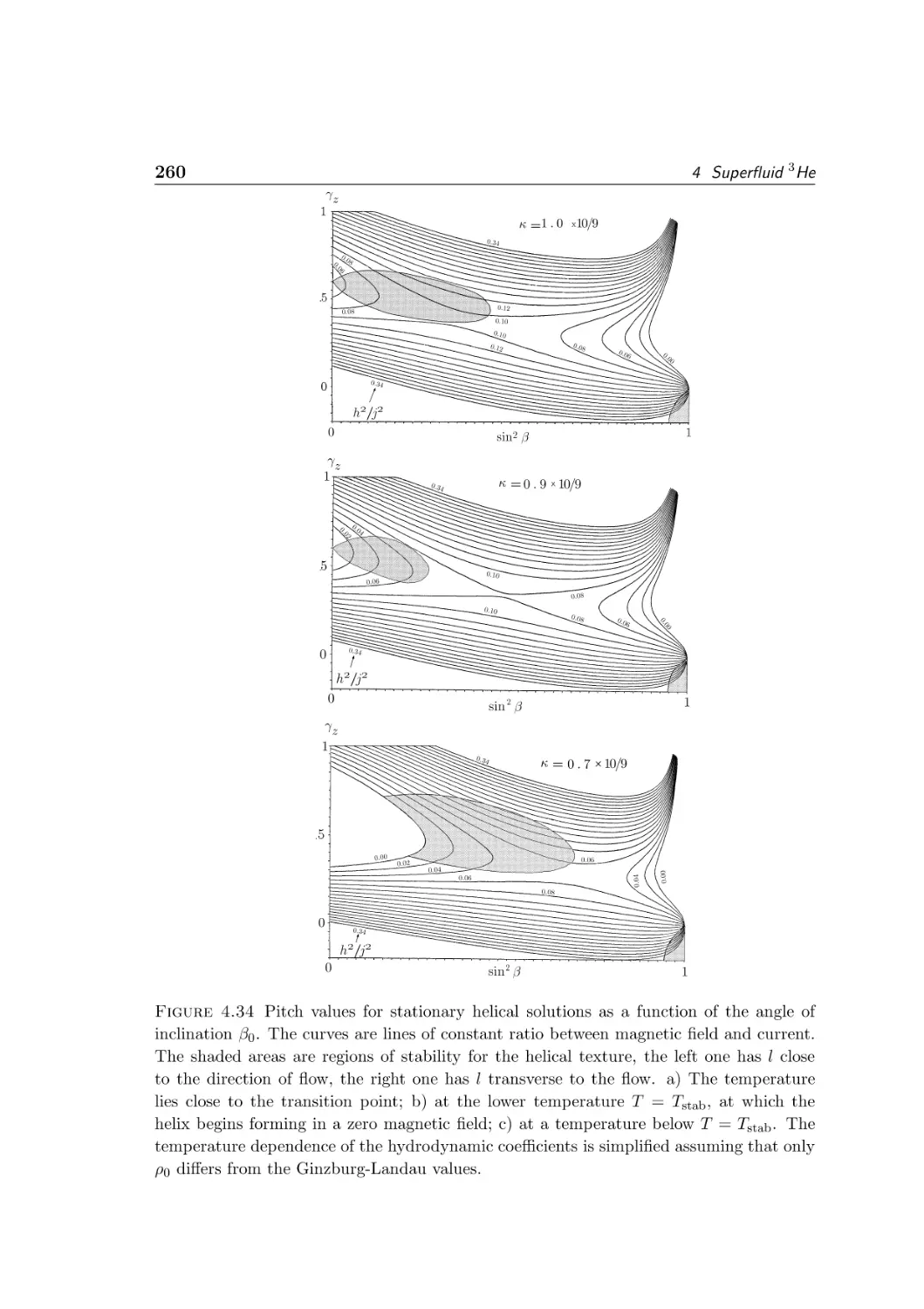
4.34 Pitch values for stationary helical solutions as a function of the angle
of inclination β0 . . . . . . . . . . . . . . . . . . . . . . . . . . . .
4.35 Regions of stable helical texture, II- and II+ . . . . . . . . . . . .
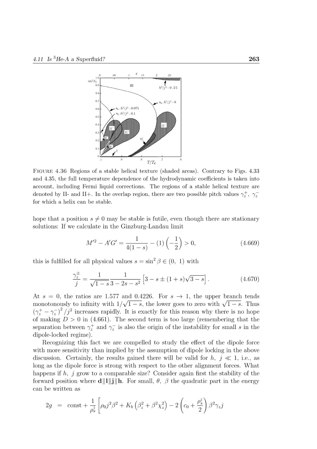
4.36 Regions of stable helical texture (shaded areas) . . . . . . . . . .
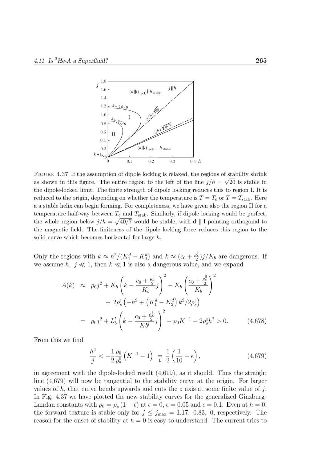
4.37 Shrinking of the regions of stability when dipole locking is relaxed
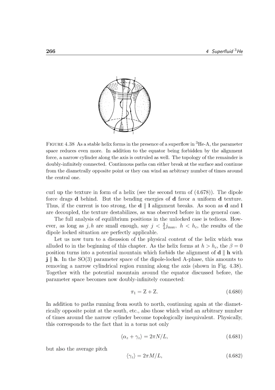
4.38 As a stable helix forms in the presence of superflow in 3 He-A . . .
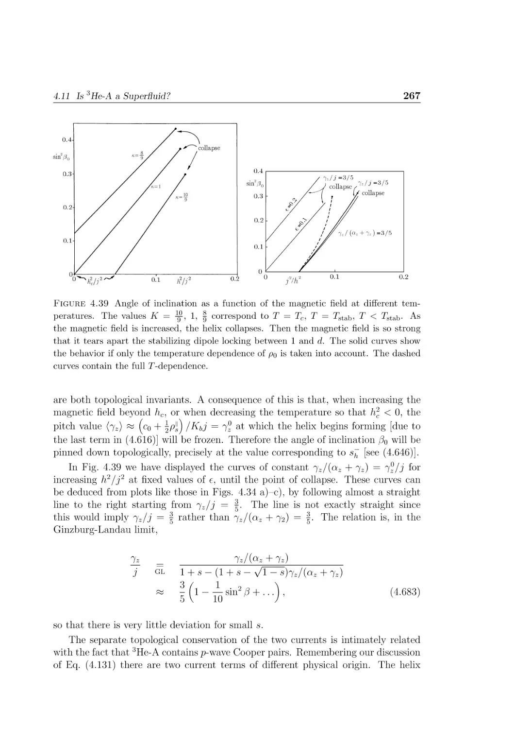
4.39 Angle of inclination as a function of the magnetic field at different
temperatures . . . . . . . . . . . . . . . . . . . . . . . . . . . . .
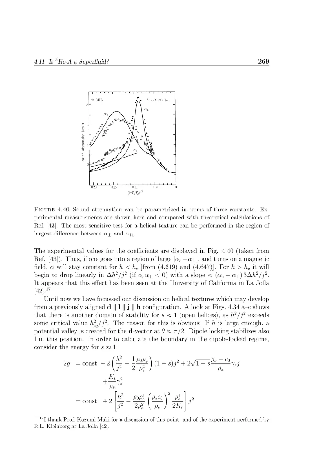
4.40 Sound attenuation parametrized in terms of three constants . . . .
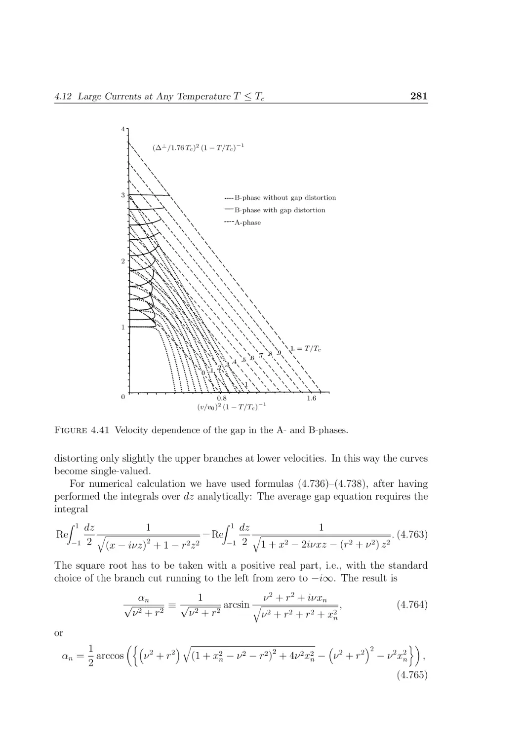
4.41 Velocity dependence of the gap in the A- and B-phases . . . . . .
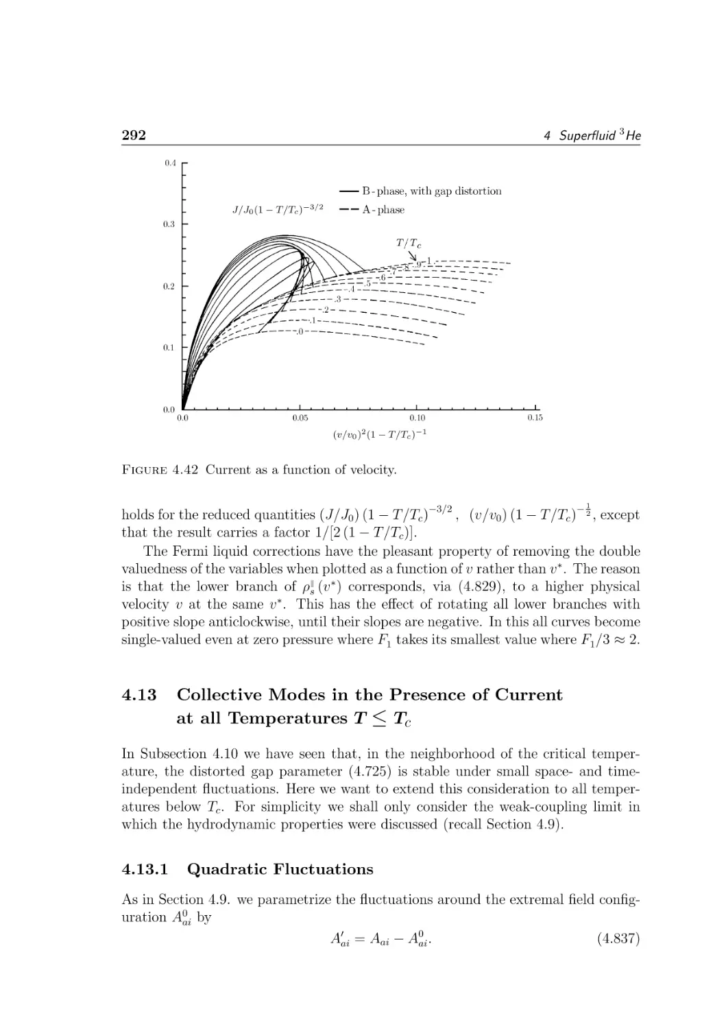
4.42 Current as a function of velocity . . . . . . . . . . . . . . . . . . .
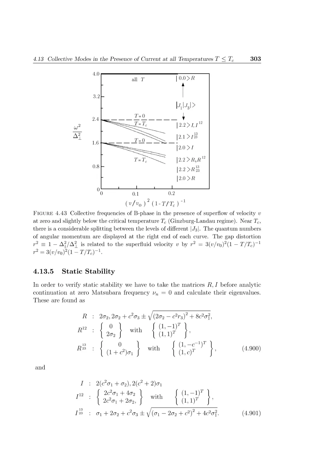
4.43 Collective frequencies of B-phase in the presence of superflow of
velocity v . . . . . . . . . . . . . . . . . . . . . . . . . . . . . . . .
5.1
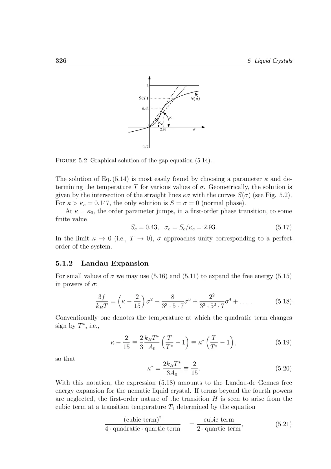
5.2
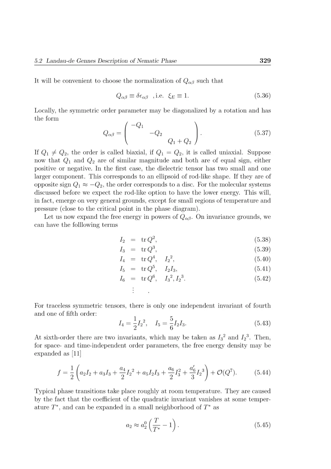
5.3
5.4
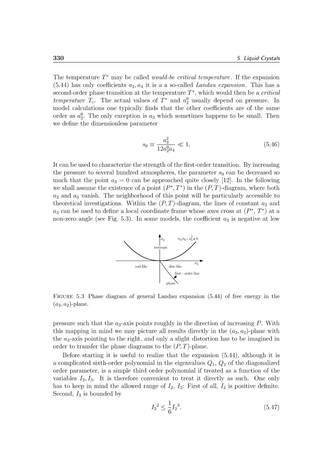
5.5
5.6
5.7
5.8
5.9
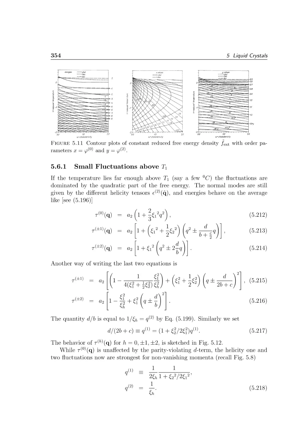
5.10
5.11
5.12
5.13
5.14
5.15
5.16
5.17
5.18
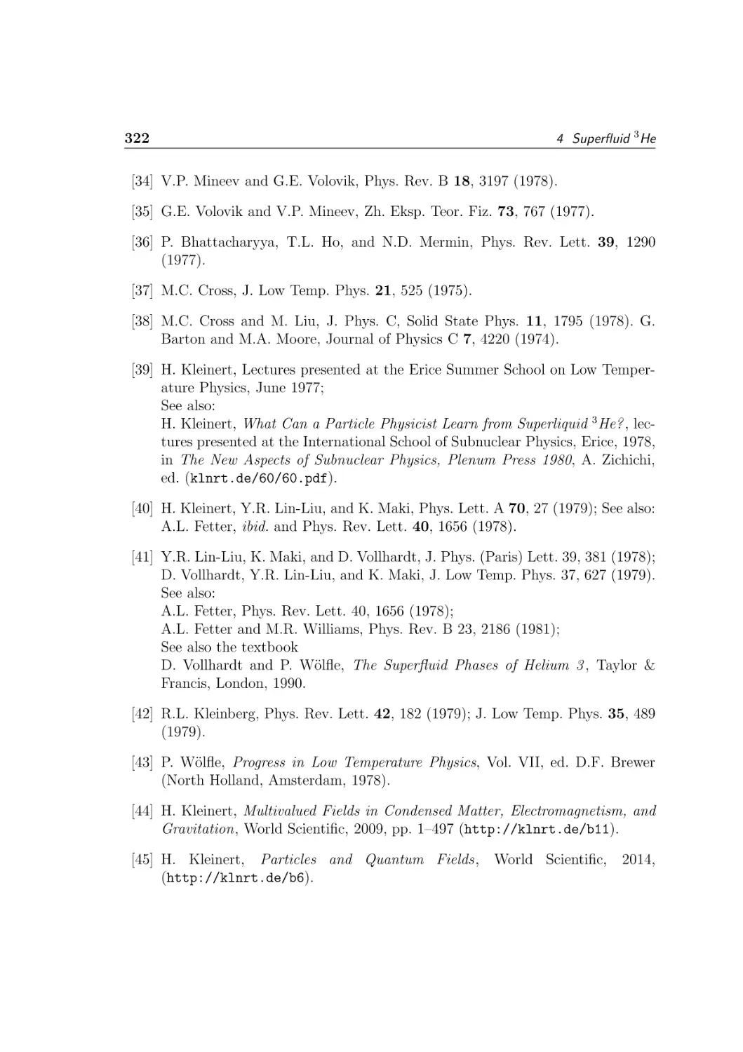
Molecular structure of PAA . . . . . . . . . . . . . . . . . . . . . .
Graphical solution of the gap equation . . . . . . . . . . . . . . . .
Phase diagram of general Landau expansion in the (a3 , a2 )-plane .
Biaxial regime in the phase diagram of general Landau expansion of
free energy in the (a3 , a2 )-plane . . . . . . . . . . . . . . . . . . . .
Jump of the order parameter ϕ from zero to a nonzero value ϕ> in
a first-order phase transition at T = T1 . . . . . . . . . . . . . . .
Different configurations of textures in liquid crystals . . . . . . . .
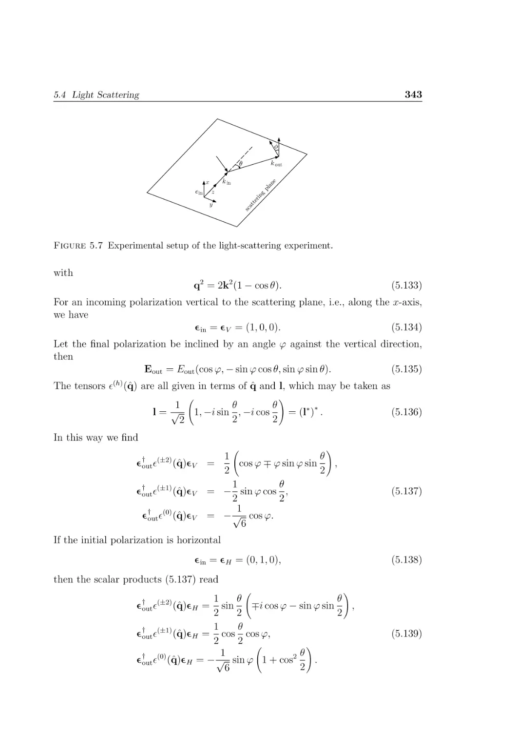
Experimental setup of the light-scattering experiment . . . . . . .
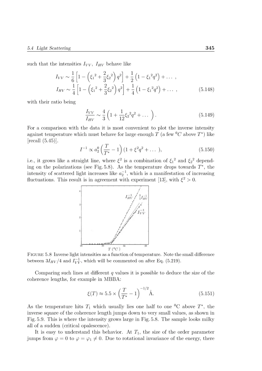
Inverse light intensities as a function of temperature . . . . . . . .
Behavior of coherence length as a function of temperature . . . . .
Relevant vectors of the director fluctuation . . . . . . . . . . . . .
Contour plots of constant reduced free energy f˜ext . . . . . . . . .
Momentum dependence of the gradient coefficients . . . . . . . . .
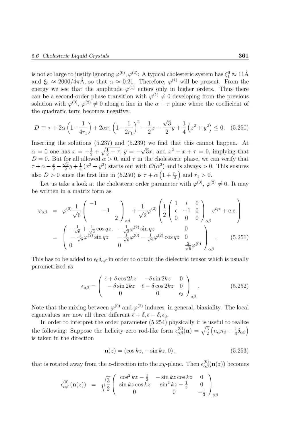
Momenta and polarization vectors of a body-centered cubic phase
of a cholesteric liquid crystal . . . . . . . . . . . . . . . . . . . . .
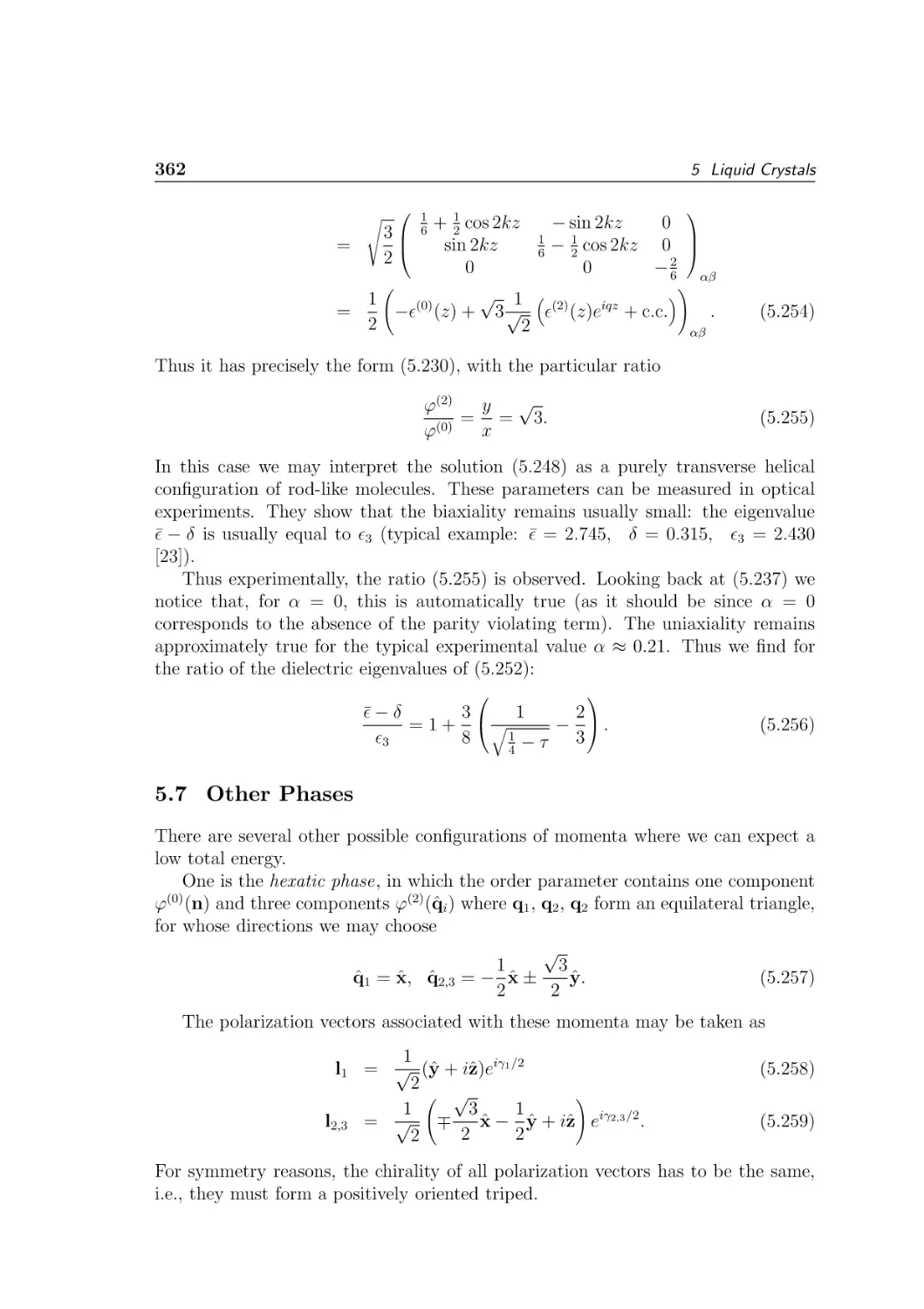
Regimes in the plane of α, τ , where the phases, cholesteric, hexatic,
or bcc are lowest . . . . . . . . . . . . . . . . . . . . . . . . . . . .
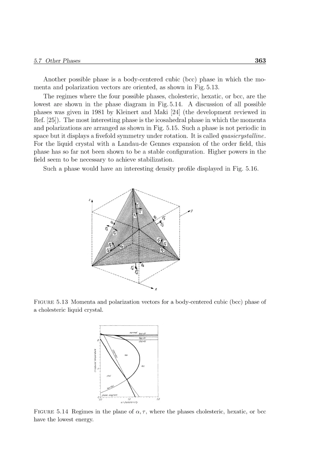
Momenta and polarization vectors for an icosahedral phase of a
cholesteric liquid crystal . . . . . . . . . . . . . . . . . . . . . . . .
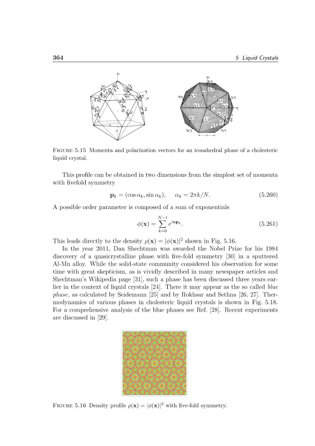
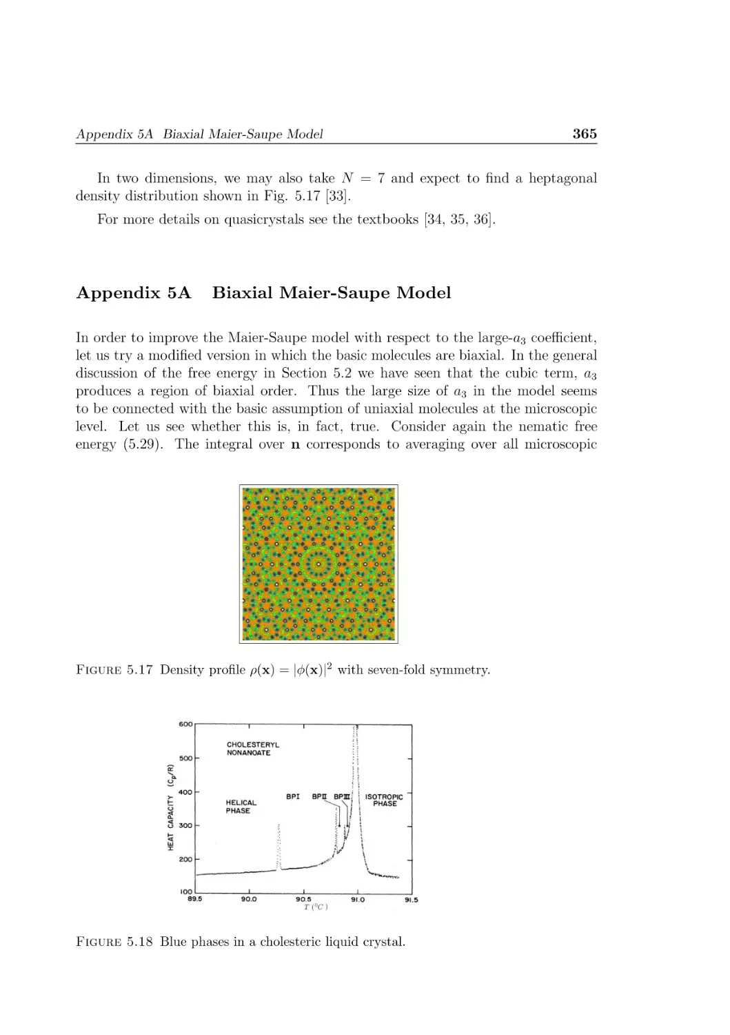
Density profile with five-fold symmetry . . . . . . . . . . . . . . .
Density profile with seven-fold symmetry . . . . . . . . . . . . . .
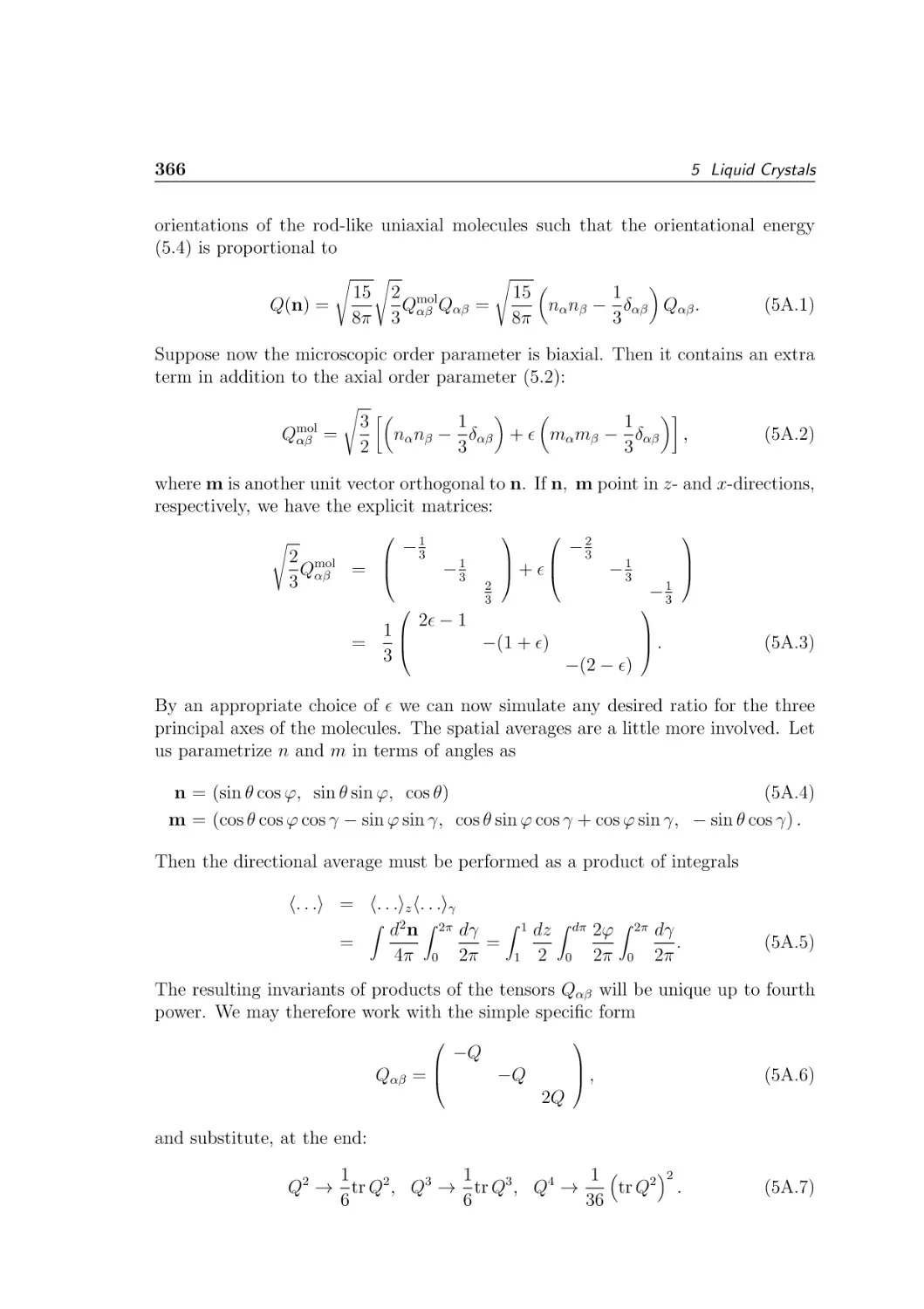
Blue phases in a cholesteric liquid crystal . . . . . . . . . . . . . .
xv
. 254
. 255
. 257
.
.
.
.
.
260
262
263
265
266
.
.
.
.
267
269
281
292
. 303
. 323
. 326
. 330
. 331
.
.
.
.
.
.
.
.
333
337
343
345
346
347
354
355
. 363
. 363
.
.
.
.
364
364
365
365
xvi
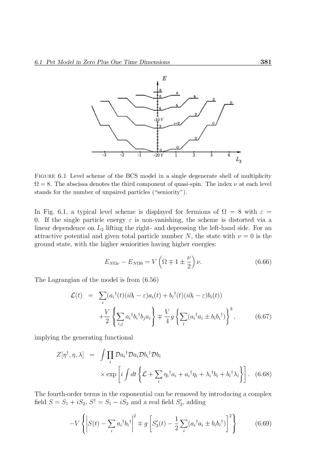
6.1
Level scheme of the BCS model in a single degenerate shell of multiplicity Ω = 8 . . . . . . . . . . . . . . . . . . . . . . . . . . . . . . 381
List of Tables
4.1 A factor of roughly 1000 separates the characteristic length scales of
superconductors and 3 He . . . . . . . . . . . . . . . . . . . . . . . . . 148
4.2 Pressure dependence of Landau parameters F1 , F0 , and F0S of 3 He
together with the molar volume v and the effective mass ratio m∗ /m 153
4.3 Parameters of the critical currents in all theoretically known phases . 243
Reality is nothing more
than a collective hunch.
Jane Wagner (1935-)
1
Functional Integral Techniques
An important goal of many-body physics is the study of collective phenomena in
systems of many bosons or fermions. The interactions are typically caused by twobody forces. In their field-theoretic description, such forces emerge in a perturbation
theory from the exchange of virtual particles, such as photons or phonons. More
complicated forces can also be generated by the exchange of virtual particles carried
by higher tensor fields. So far, all forces in nature between particles can be reduced
to such exchange processes. Depending on the detailed properties of forces and
thermodynamic parameters such as density, pressure, and temperature, bosons or
fermions may exhibit different collective behaviors. In an electron gas, for example,
one may observe density fluctuations or pair condensation. The first type is found
if the exchanged particles couple strongly to other particles or holes. Examples
are plasma oscillations in a degenerate electron gas. The second type of behavior
is found if the forces favor the formation of bound states between pairs of particles. This is usually observed below a certain critical temperature Tc . Examples are
excitons in a semiconductor or Cooper pairs in a superconductor.
For systems showing plasma type of excitations, real fields depending on space
and time are most convenient to describe the physical phenomena. To describe
pair condensation, complex fields render the most economic description of such
phenomena. They contain the two spatial arguments of the constituents and their
common time coordinates. Such fields will be called bilocal . In relativistic systems,
also the time coordinates of the constituents may be different. If the potential
has a sufficiently short range, the bilocal field degenerates into a local field. The
most important example for the latter case is the collective pair-field theory of
superconducting electrons which is known as the Ginzburg-Landau theory.
A bilocal field theory is useful in elementary particle physics where it allows to
study the transition from inobservable quark fields to observable meson fields (see
[1] or Chapter 26 in the textbook [2]). The new basic field quanta of the converted
theory are no longer the fundamental particles but the set of all quark-antiquark
meson bound states which are obtained by solving a Bethe-Salpeter bound-state
equation in the so-called ladder approximation. They are called bare mesons. Such a
formulation can also be given to quantum electrodynamics of electrons and positrons,
where the bare mesons are positronium atoms [1].
1
2
1.1
1 Functional Integral Techniques
Nonrelativistic Fields
Let us begin with the description of functional methods that can be used for the
study of many-body physics of relativistic particles. We shall follow the historic
development.
1.1.1
Quantization of Free Fields
Consider free nonrelativistic particles, whose energy ε depends on the momentum
p by some function ε(p). In free space, this has the form ε(p) = p2 /2m. For
a particle moving in a periodic solid, the momentum dependence is usually more
complicated. However, for many purposes it can be approximated by the same
quadratic behavior, provided that we exchange the mass m by an effective mass
parameter m∗ 6= m called the effective mass. The action of a free nonrelativistic
field describing an ensemble of these particles reads
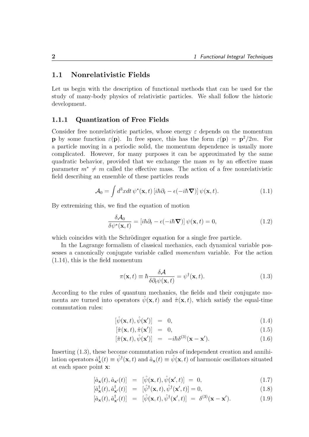
A0 =
Z
d3 xdt ψ ∗ (x, t) [ih̄∂t − ǫ(−ih̄∇)] ψ(x, t).
(1.1)
By extremizing this, we find the equation of motion
δA0
= [ih̄∂t − ǫ(−ih̄∇)] ψ(x, t) = 0,
δψ ∗ (x, t)
(1.2)
which coincides with the Schrödinger equation for a single free particle.
In the Lagrange formalism of classical mechanics, each dynamical variable possesses a canonically conjugate variable called momentum variable. For the action
(1.14), this is the field momentum
π(x, t) ≡ h̄
δA
= ψ † (x, t).
δ∂t ψ(x, t)
(1.3)
According to the rules of quantum mechanics, the fields and their conjugate momenta are turned into operators ψ̂(x, t) and π̂(x, t), which satisfy the equal-time
commutation rules:
[ψ̂(x, t), ψ̂(x′ )] = 0,
[π̂(x, t), π̂(x′ )] = 0,
[π̂(x, t), ψ̂(x′ )] = −ih̄δ (3) (x − x′ ).
(1.4)
(1.5)
(1.6)
Inserting (1.3), these become commutation rules of independent creation and annihilation operators â†x (t) ≡ ψ̂ † (x, t) and âx (t) ≡ ψ̂(x, t) of harmonic oscillators situated
at each space point x:
[âx (t), âx′ (t)] = [ψ̂(x, t), ψ̂(x′ , t)] = 0,
[â†x (t), â†x′ (t)] = [ψ̂ † (x, t), ψ̂ † (x′ , t)] = 0,
(1.7)
(1.8)
[âx (t), â†x′ (t)] = [ψ̂(x, t), ψ̂ † (x′ , t)] = δ (3) (x − x′ ).
(1.9)
3
1.1 Nonrelativistic Fields
For each oscillator, there exists a ground state |0ix defined by the condition
ψ̂(x, t)|0i = 0. The excited states are obtained by multiplying |0ix with nx creation operators ψ̂ † (x, t). They are denoted by (a† )nxx |0ix = [ψ̂ † (x, t)]nx |0ix , where
nx are integer quantum numbers nx = 0, 1, 2, 3, . . . . These are interpreted as the
numbers of particles at point x.
Thus, by quantizing the field and converting it to a field operator , the singleparticle Schrödinger theory changes into a theory of arbitrarily many identical oscillators at all space point x. The ground state of the system is the direct product of
Q
the ground states of all these oscillators: |0i ≡ x |0ix . The resulting many-particle
Hilbert space is called the Fock space, and the procedure of field quantization is
called second quantization. The usual quantization is ensured by the correspondence rule p → −ih̄∇ in the single-particle Schrödinger equation (1.14) and the
action (1.1).
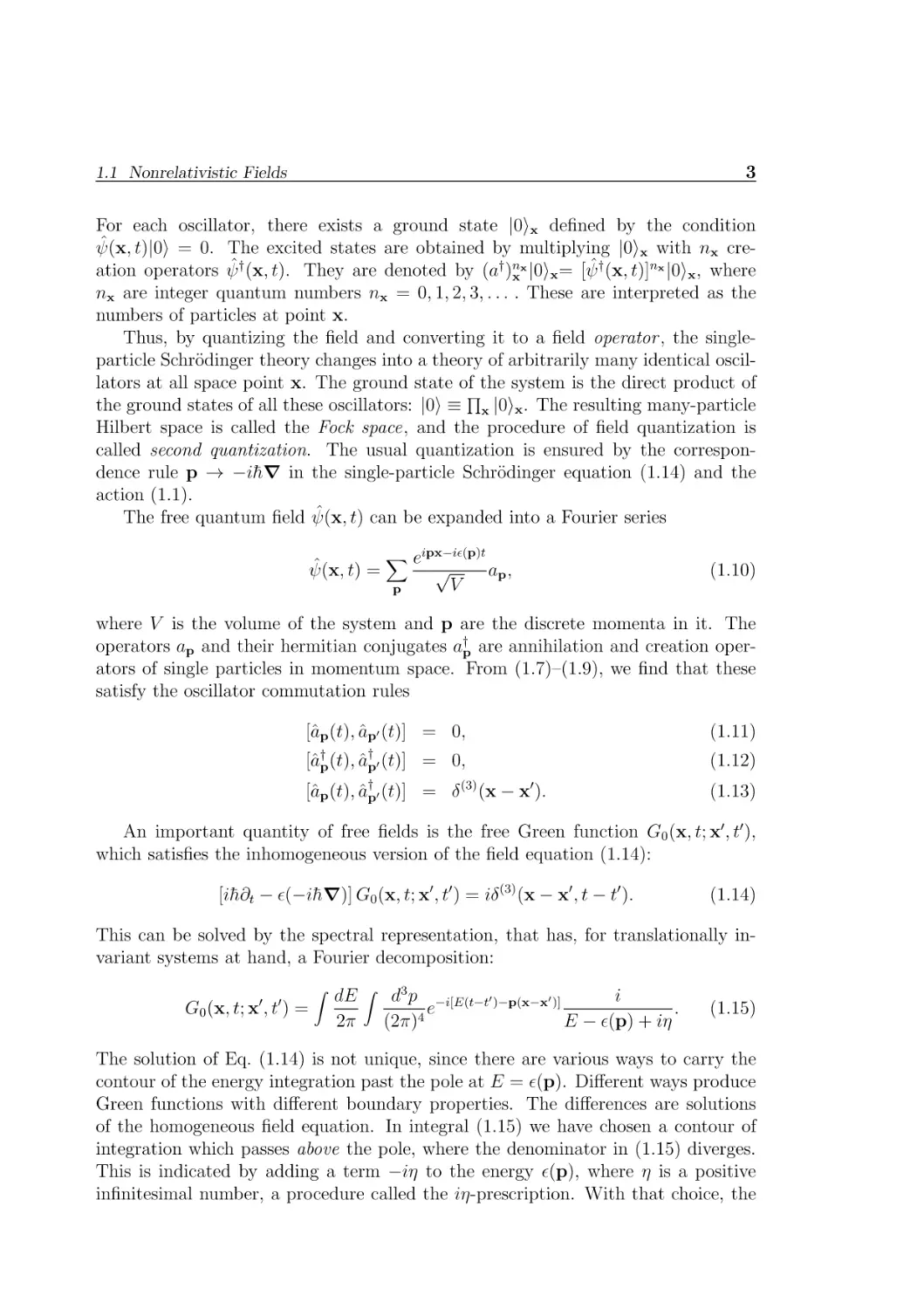
The free quantum field ψ̂(x, t) can be expanded into a Fourier series
ψ̂(x, t) =
X
p
eipx−iǫ(p)t
√
ap ,
V
(1.10)
where V is the volume of the system and p are the discrete momenta in it. The
operators ap and their hermitian conjugates a†p are annihilation and creation operators of single particles in momentum space. From (1.7)–(1.9), we find that these
satisfy the oscillator commutation rules
[âp (t), âp′ (t)] = 0,
[â†p (t), â†p′ (t)]
[âp (t), â†p′ (t)]
(1.11)
= 0,
(3)
(1.12)
′
= δ (x − x ).
(1.13)
An important quantity of free fields is the free Green function G0 (x, t; x′ , t′ ),
which satisfies the inhomogeneous version of the field equation (1.14):
[ih̄∂t − ǫ(−ih̄∇)] G0 (x, t; x′ , t′ ) = iδ (3) (x − x′ , t − t′ ).
(1.14)
This can be solved by the spectral representation, that has, for translationally invariant systems at hand, a Fourier decomposition:
′
′
G0 (x, t; x , t ) =
Z
dE
2π
Z
i
d3 p −i[E(t−t′ )−p(x−x′ )]
e
.
4
(2π)
E − ǫ(p) + iη
(1.15)
The solution of Eq. (1.14) is not unique, since there are various ways to carry the
contour of the energy integration past the pole at E = ǫ(p). Different ways produce
Green functions with different boundary properties. The differences are solutions
of the homogeneous field equation. In integral (1.15) we have chosen a contour of
integration which passes above the pole, where the denominator in (1.15) diverges.
This is indicated by adding a term −iη to the energy ǫ(p), where η is a positive
infinitesimal number, a procedure called the iη-prescription. With that choice, the
4
1 Functional Integral Techniques
Green function (1.15) coincides with the vacuum expectation value of the timeordered product of field operators (1.10):
G0 (x, t; x′ , t′ ) = h0|T̂ ψ̂(x, t)ψ̂ † (x′ , t′ )|0i.
(1.16)
The time-ordering operator T̂ is defined to change the position of the operators
behind it in such a way that fields with later time arguments stand to the left
of those with earlier time arguments. The expectation value on the right-hand
side is also called the free propagator of the quantum field ψ̂(x, t). By inserting the
expansion (1.10) into (1.16) it is easy to verify that the evaluation of the expectation
value (1.16) gives exactly the expression (1.15).
1.1.2
Fluctuating Free Fields
There exists an equivalent approach to second quantization where the thermodynamic partition of the above system is expressed as a functional integral over all
possible fluctuating fields [4, 5]. For free fields, we define a partition function
Z0 = N
Z
Dψ ∗ (x, t)Dψ(x, t) exp {iA0 [ψ ∗ , ψ]} ,
(1.17)
where N is some constant which will play no role in all subsequent discussions. From
here on we shall work with natural units in which h̄ = 1.
The functional formulation was found by Richard Feynman. He observed that
the amplitudes of diffraction phenomena of light are obtained by summing over
the individual amplitudes for all paths which the light could possibly have taken.
Each path is associated with a pure phase depending only on the action of the light
particle along the path. For fields, this principle leads to Formula (1.17) for the
partition function.
The functional integral may conveniently be defined by grating the spacetime
into a finer and finer cubic lattice of spacing δ with corners at (xi1 , yi2 , zi3 , ti4 ) =
(i1 , i2 , i3 , i4 ) δ. The fields are characterized by their values at the nearest lattice
point:
√ 4
(1.18)
ψi1 i2 i3 i4 ≡ ψ (xi1 , yi2 , zi3 , ti4 ) δ .
The measure in the functional integral in (1.17) is then defined by the product of
all integrals over the cubus around each lattice point:
Z
∗
Dψ (x, t)Dψ(x, t) ≡
Y
i1 i2 i3 i4
i′ i′ i′ i′
1 2 3 4
The double integral over complex variables
Z
∞
−∞
Z Z
RR
dψi†1 i2 i3 i4 dψi′1 i′2 i′3 i′4
√ √
.
2πi 2πi
dψ ∗ dψ symbolizes the real integrals
ψ − ψ∗
ψ + ψ∗
√
√
d
.
d
−∞
2
2i
Z
∞
!
(1.19)
!
(1.20)
5
1.1 Nonrelativistic Fields
This naive definition of path integration is straightforward for Bose fields. If
we want to use the functional technique to describe also the statistical properties
of fermions, some modifications are necessary. Then the fields must be taken to be
anticommuting c-numbers. In mathematics, such objects form a Grassmann algebra.
If ξ, ξ ′ are any two real elements in this algebra, they satisfy the anticommutation
relation
{ξ, ξ ′} ≡ ξξ ′ + ξ ′ ξ = 0.
(1.21)
A trivial consequence of this condition is that the square of each Grassmann element
vanishes, i.e., ξ 2 = 0. If ξ = ξ1 + iξ2 is a complex Grassmann variable, then
ξ 2 = −ξ ∗ ξ = −2iξ1 ξ2 is nonzero, but (ξ ∗ ξ)2 = (ξξ)2 = 0.
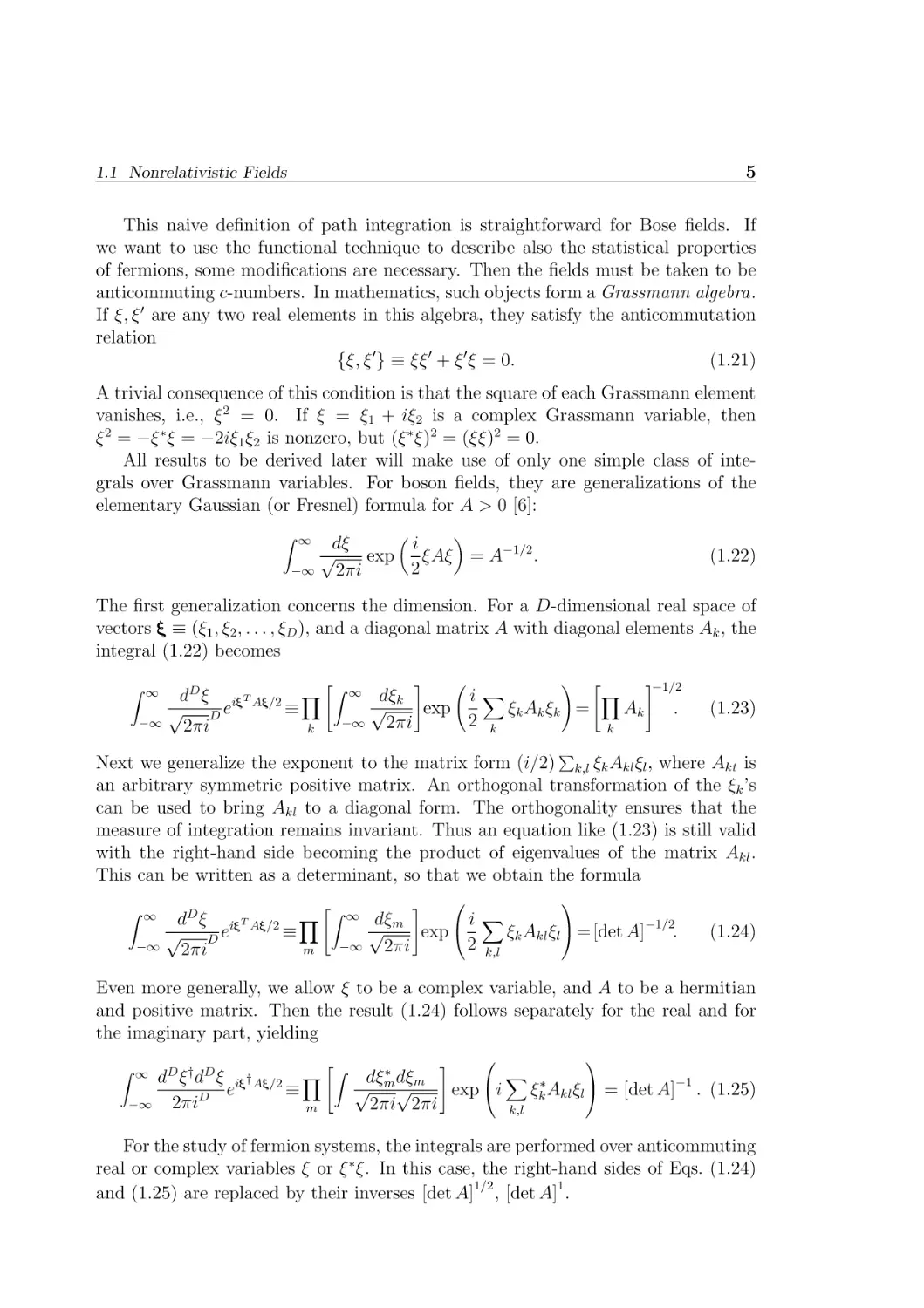
All results to be derived later will make use of only one simple class of integrals over Grassmann variables. For boson fields, they are generalizations of the
elementary Gaussian (or Fresnel) formula for A > 0 [6]:
Z
∞
−∞
dξ
i
√
exp ξAξ = A−1/2 .
2
2πi
(1.22)
The first generalization concerns the dimension. For a D-dimensional real space of
vectors ≡ (ξ1 , ξ2 , . . . , ξD ), and a diagonal matrix A with diagonal elements Ak , the
integral (1.22) becomes
Z
∞
−∞
dD ξ iT A/2 Y
≡
√ De
2πi
k
"Z
∞
−∞
!
#
"
Y
dξ
iX
√ k exp
ξk Ak ξk =
Ak
2 k
2πi
k
#−1/2
.
(1.23)
Next we generalize the exponent to the matrix form (i/2) k,l ξk Akl ξl , where Akt is
an arbitrary symmetric positive matrix. An orthogonal transformation of the ξk ’s
can be used to bring Akl to a diagonal form. The orthogonality ensures that the
measure of integration remains invariant. Thus an equation like (1.23) is still valid
with the right-hand side becoming the product of eigenvalues of the matrix Akl .
This can be written as a determinant, so that we obtain the formula
P
Z
∞
−∞
dD ξ iT A/2 Y
≡
√ De
m
2πi
"Z
∞
−∞
#
dξ
iX
√ m exp
ξk Akl ξl = [det A]−1/2.
2
2πi
k,l
(1.24)
Even more generally, we allow ξ to be a complex variable, and A to be a hermitian
and positive matrix. Then the result (1.24) follows separately for the real and for
the imaginary part, yielding
Z
∞
−∞
dD ξ † dD ξ i† A/2 Y
e
≡
2πiD
m
"Z
X
dξ ∗ dξ
√ m √ m exp i
ξk∗ Akl ξl = [det A]−1 . (1.25)
2πi 2πi
k,l
#
For the study of fermion systems, the integrals are performed over anticommuting
real or complex variables ξ or ξ ∗ ξ. In this case, the right-hand sides of Eqs. (1.24)
and (1.25) are replaced by their inverses [det A]1/2 , [det A]1 .
6
1 Functional Integral Techniques
Let us prove this for complex variables. After bringing the matrix Akl to a
diagonal form via a unitary transformation, the integral reads
Z Y"
m
X
Y
dξ ∗ dξ
√ m √ m exp i
ξn∗ An ξn =
2πi 2πi
n
m
#
!
Z
dξ ∗ dξ
∗
√ m √ m exp (iξm
Am ξm ) .
2πi 2πi
(1.26)
Expanding the exponentials into a power series leaves only the first two terms, since
∗
(ξm
ξm )2 = 0. Thus the integral becomes
YZ
m
dξ ∗ dξ
∗
√ m√ m (1 + iξm
Am ξm ).
2πi 2πi
(1.27)
Each of these integrals can be performed trivially by defining two basic integrals
over the Grassmann variables, from which all the others follow using the linearity
of integrals. For real Grassmann variables, these rules are
Z
dξ
√
= 0,
2πi
Z
dξ
√
ξ = 1.
2πi
(1.28)
The integrals over higher powers vanish trivially due to the anticommutation property (1.21):
Z
dξ n
√
ξ = 0,
2πi
n > 1.
(1.29)
The two rules (1.28) and (1.29) determine the integrals over any function F (ξ) of
a real Grassmann variable ξ. They ensure that such a function is determined by
only two parameters: the zeroth- and the first-order Taylor coefficients. Indeed,
due to the property ξ 2 = 0, the Taylor series can only possess the first two terms
F (ξ) = F0 + F ′ ξ, where F0 = F (0) and
F ′ ≡ dF (ξ)/dξ.
(1.30)
But according to (1.28), the integral yields also F ′ :
Z
dξ
√
F (ξ) = F ′ .
2πi
(1.31)
Remarkably, this property makes the linear operation of integration over Grassmann
variables in (1.28) identical to the linear operation of differentiation. As a consequence, a linear change of Grassmann integration variables multiplies the integral by
the inverse of the Jacobian. For example, going from a real ξ to another Grassmann
variable ξ ′ = aξ, the integrals over ξ ′ have again the properties (1.28):
Z
dξ ′
√
= 0,
2πi
Z
dξ ′ ′
√
ξ = 1.
2πi
(1.32)
7
1.1 Nonrelativistic Fields
In order to be compatible with (1.28), the measure must change as follows:
Z
dξ ′
1
√
=
a
2πi
Z
dξ
√
.
2πi
(1.33)
This is in contrast to ordinary integrals where the factor on the right-hand side
would be a.
From the real rules (1.28), we derive the integrals involving complex Grassmann
variables:
Z
Z
Z
dξ ∗ dξ
dξ ∗ dξ
dξ
∗
√
√
√
√
√
= 0,
iξ ξ = 1,
(ξ ∗ξ)n = 0, n > 1. (1.34)
2πi
2πi 2πi
2πi 2πi
The integration rules (1.28) imply that the right-hand side of (1.27) becomes the
product of eigenvalues Am :
Y
Am = det A,
(1.35)
m
which is exactly the inverse of the bosonic result (1.25), thus proving the statement
after Eq. (1.25).
For real Fermi fields, the proof is slightly more involved, since now the hermitian
matrix Akl can no longer be diagonalized by a unitary
transformation, so that the
√
Q
invariance of the measure of integration m (dξm/ 2πi) is no longer automatically
guaranteed. However, the integral can be done after all by observing that Akl may
always be assumed to be antisymmetric. If there is any symmetric part, it cancels
P
in the quadratic form kl ξk Akl ξl due to the anticommutativity of the Grassmann
variables. Now, an antisymmetric hermitian matrix can always be written as A =
−iAR , where AR is real and antisymmetric. Such a matrix is standard in symplectic
spaces. It can be brought to a canonical form C which is zero everywhere except
for 2 × 2 matrices,
!
0 1
2
c = iσ =
,
(1.36)
−1 0
along the diagonal. Here σ 2 is the second Pauli matrix. Then A can be written as
A = −iT T CT
(1.37)
where the hermitian matrix −iC contains only σ 2 -matrices along the diagonal. This
matrix has a unit determinant so that det T = det 1/2 (A). Thus, under a linear
transformation of Grassmann variables ξk′ ≡ Tk ξl , the measure of integration changes
according to
Y
Y
dξk = (det T ) dξk′ ,
(1.38)
k
k
as a direct consequence of the integration rule (1.33). With the help of the rules
(1.28) and (1.29), the Grassmann version of the functional integral (1.24) can now
be evaluated as follows:
"
Y Z
m
#
X
dξ
√ m exp i
ξk Akl ξl
2πi
k,l
8
1 Functional Integral Techniques
X
dξ ′
√ m exp −
ξk′ Ckl ξl′
= (det T )
2πi
m
kl
"
#
∞ Z
′
′
Y
dξ
dξ
′
′
√ 2n √2n+1 1 + ξ2n+1
= (det A)1/2
ξ2n
= (det A)1/2 .
2πi
2πi
n
#
"
Y Z
!
(1.39)
Thus the right-hand side is the inverse of the bosonic result (1.24), as announced
after Eq. (1.25).
In order to apply these formulas to fields ψ(x, t) defined on a continuous spacetime, both formulas have to be written for the lattice field (1.18) in such a way that
the limit of infinitely fine lattice spacing δ → 0 can be performed without problem.
For this we recall the useful matrix identity
[det A]∓1 = exp[i(±iTr log A)],
(1.40)
where log A may be expanded in the standard fashion as
log A = log [1 + (A − 1)] = −
∞
X
1
[−(A − 1)]n .
n
n=1
(1.41)
This formula reduces the calculation of the determinant to a series of matrix multiplications. In each of these, the limit δ → 0 can easily be taken. One simply replaces
all sums over lattice indices by integrals over d3 xdt, for instance
trA2 =
X
kl
Akl Alk −
−
−→ TrA2 =
Z
d3 xdtd3 x′ dt′ A(x, t; x′ , t′ )A(x′ , t′ , x, t). (1.42)
With this in mind, the field versions of (1.24) and (1.25) amount to the following
functional formulas for boson and fermion fields:
Z
Z
i
3
3 ′ ′
′ ′
′ ′
Dϕ(x, t) exp
d xdtd x dt ϕ(x, t)A(x, t; x , t )ϕ(x , t )
2
(
) !#
"
i
1
A ,
(1.43)
= exp i ± Tr log
i
2
Z
Z
Dψ ∗ (x, t)Dψ(x, t) exp i
d3 xdtd3 x′ dt′ ψ ∗ (x, t)A(x, t; x′ , t′ )ψ(x′ , t′ )
= exp [i(±iTr log A)] .
(1.44)
Here ϕ, ψ are arbitrary real and complex fields, with the upper sign holding for
bosons, the lower for fermions. The same result is of course true if ϕ and ψ have
several components (describing, for example, spin) and A is a matrix in the corresponding space.
1.1.3
Interactions
Consider now a many-particle system described by an action of the form (in natural
units with h̄ = 1):
A ≡ A0 + Aint =
−
Z
1
2
d3 xdtψ ∗ (x, t) [i∂t − ǫ(−i∇)] ψ(x, t)
Z
(1.45)
d3 xdtd3 x′ dt′ ψ ∗ (x′ , t′ )ψ ∗ (x, t)V (x, t; x′ , t′ )ψ(x, t)ψ(x′ , t′ ).
9
1.1 Nonrelativistic Fields
The fundamental field ψ(x) may describe bosons or fermions. The interaction potential is usually translationally invariant in space and time:
V (x, t; x′ , t′ ) = V (x − x′ , t − t′ ).
(1.46)
In nonrelativistic many-body systems, the potential is often instantaneous in time:
V (x, t; x′ , t′ ) = δ(t − t′ )V (x − x′ ).
(1.47)
This property simplifies many calculations. It is in general fulfilled only approximately.
For instance, the attraction between electrons in a low-temperature superconductor is caused by phonon exchange which contains retardation effects due to the
finite speed of sound.
The complete information on the physical properties of the system resides in its
Green functions. In the field operator language, one uses the so-called Heisenberg
picture, where the Green functions are given by the expectation values of the timeordered products of the field operators
G (x1 , t1 , . . . , xn , tn ; xn′ , tn′ , . . . , x1′ , t1′ )
(1.48)
†
†
= h0|T̂ ψ̂H (x1 , t1 ) · · · ψ̂H (xn , tn )ψ̂H
(x1′ , t1′ ) |0i,
(xn′ , tn′ ) · · · ψ̂H
where ψ̂H (x, t) are the Heisenberg operators of the interacting field. The timeordering operator T̂ changes the position of the operators behind it in such a way
that fields with later time arguments stand to the left of those with earlier time
arguments. To achieve this order, a number of field transmutations are necessary. If
F denotes the number of transmutations of Fermi fields, the final product receives
a sign factor (−1)F .
It is convenient to view all Green functions (1.48) as derivatives of the generating
functional
∗
Z
Z[η , η] = h0|T̂ exp i
3
d xdt
h
†
ψ̂H
(x, t)η(x, t)
∗
+ η (x, t)ψ̂H (x, t)
i
|0i,
(1.49)
namely
G (x1 , t1 , . . . , xn , tn ; xn′ , tn′ , . . . , x1′ , t1′ )
′
δ n+n Z[η ∗ , η]
′
= (−i)n+n ∗
δη (x1 , t1 ) · · · δη ∗ (xn , tn )δη(xn′ , tn′ ) · · · δη(x1′ , tn′ )
(1.50)
.
η=η∗ ≡0
Physically, the generating functional describes the amplitude that the vacuum remains a vacuum in spite of the presence of external perturbations.
The calculation of this Green functional is usually performed in the interaction
picture which can be summarized by the operator formulation for Z[η ∗ , η]:
Z[η ∗ , η] = Nh0|T̂ exp iAint [ψ̂ † , ψ̂] + i
Z
h
d3 xdt ψ̂ † (x, t)η(x, t) + h.c.
i
|0i. (1.51)
10
1 Functional Integral Techniques
In the interaction picture, the field operators ψ̂(x, t) move according to the free-field
equation of motion (1.14). The time-ordered product of two of these field operators
coincide with the free-field propagator calculated before in (1.16).
The normalization constant N is determined by the condition [which is trivially
true for (1.49)]:
Z[0, 0] = 1.
(1.52)
The calculation may now proceed perturbatively. One expands the exponential
exp{iAint } in (1.51) in a power series and obtains
Z[η ∗ , η] = N
∞
X
1
Zn [η ∗ , η],
n!
n=0
(1.53)
where the contribution of order n is given by
Zn [η ∗ , η] ≡ Nh0|T̂
n
iAint [ψ̂ † , ψ̂]
Z
exp i
h
d3 xdt ψ̂ † (x, t)η(x, t) + h.c.
i
|0i. (1.54)
This expression is further expanded in powers of η ∗ and η. The resulting vacuum
expectation values of time-ordered products of field operators can be expanded in
products of Green functions of the free field operators. The rules for doing this is
provided by Wick’s theorem [5, 6, 7]. This theorem states that any time ordered
product of free field operators ψ(x, t) and its hermitian conjugate ψ † (x, t) can be
expanded into a sum of normal products with all possible contractions taken via
Feynman propagators.
1.1.4
Normal Products
Given an arbitrary set of n free field operators φ1 (x1 ) · · · φn (xn ), each of them consists of a creation and an annihilation part:
φi (xi ) = φci (xi ) + φai (xi ).
(1.55)
Some φi may be commuting Bose fields, some anticommuting Fermi fields. The
normally ordered product or normal product of n of these field operators will be
denoted by N̂ (φ1 (x)φ(x2 ) · · · φ(xn )). In the present context, a function symbol is
more convenient than the earlier double-dot notation. The normal product is a
function of a product of field operators which has the following two properties:
i) Linearity: The normal product is a linear function of all its n arguments, i.e.,
it satisfies
N̂ ((αφ1 + βφ′1 )φ2 φ3 · · · φn ) = αN̂(φ1 φ2 φ3 · · · φn ) + β N̂(φ′1 φ2 φ3 · · · φn ). (1.56)
If every φi is replaced by φci + φai , it can be expanded into a linear combination
of terms which are all pure products of creation and annihilation operators.
11
1.1 Nonrelativistic Fields
ii) Normal Ordering: The normal product reorders all products arising from
a complete linear expansion of all fields according to i) in such a way that
all annihilators stand to the right of all creators. If the operators φi describe
fermions, the definition requires a factor −1 to be inserted for every transmutation of the order of two operators.
For example, let φ1 , φ2 , φ3 be scalar fields, then with two field operators normal
ordering produces:
N̂(φc1 φc2 )
N̂ (φc1 φa2 )
N̂ (φa1 φc2 )
N̂ (φa1 φa2 )
=
=
=
=
φc1 φc2 = φc2 φc1 ,
φc1 φa2 ,
φc2 φa1 ,
φa1 φa2 = φa2 φa1 ,
(1.57)
and with three field operators:
N̂ (φc1 φc2 φa3 ) = φc1 φc2 φa3 = φc2 φc1 φa3 ,
N̂ (φc1 φa2 φc3 ) = φc1 φc3 φa2 = φc3 φc1 φa2 ,
N̂ (φa1 φc2 φc3 ) = φc2 φc3 φa1 = φc3 φc2 φa1 .
(1.58)
If the operators φi are fermions, the effect is
N̂(φc1 φc2 )
N̂(φc1 φa2 )
N̂(φa1 φc2 )
N̂(φa1 φa2 )
=
≡
=
=
φc1 φc2 = −φc2 φc1 ,
φc1 φa2 ,
−φc2 φa1 ,
φa1 φa2 = −φa2 φa1 ,
(1.59)
and
N̂(φc1 φc2 φa3 ) = φc1 φc2 φa3 = −φc2 φc1 φa3 ,
N̂(φc1 φa2 φc3 ) = −φc1 φc3 φa2 = φc3 φc1 φa2 ,
N̂(φa1 φc2 φc3 ) = φc2 φc3 φa1 = −φc3 φc2 φa1 .
(1.60)
The normal product is uniquely defined. The remaining order of creation or annihilation parts among themselves is irrelevant, since these commute or anticommute
with each other by virtue of the canonical free-field commutation rules. In the following, the fields φ may be Bose or Fermi fields and the sign of the Fermi case is
recorded underneath the Bose sign.
The advantage of defining normal products is their important property that
they have no vacuum expectation values. There is always an annihilator on the
right-hand side or a creator on the left-hand side which produce 0 when matched
between vacuum states. The method of calculating all n-point functions consists
in expanding all time ordered products of n field operators completely into normal
products. Then only the terms with no operators survive between vacuum states.
This is the desired value of the n-point function.
12
1 Functional Integral Techniques
Let us see how this works for the simplest case of a time-ordered product of two
identical field operators
T̂ (φ(x1 )φ(x2 )) ≡ Θ(x01 − x02 )φ(x1 )φ(x2 ) ± Θ(x02 − x01 )φ(x2 )φ(x1 ).
(1.61)
The basic expansion formula is
T̂ (φ(x1 )φ(x2 )) = N̂ (φ(x1 )φ(x2 )) + h0|T̂ (φ(x1 )φ(x2 ))|0i.
(1.62)
For brevity, we shall denote the propagator of two fields as follows:
h0|T (φ(x1)φ(x2 ))|0i = φ(x1 )φ(x2 ) = G(x1 − x2 ).
(1.63)
The hook which connects the two fields on the top are referred to as a contraction
of the fields.
We shall prove the basic expansion formula (1.62) by considering it separately
for the creation and annihilation parts φc and φa . This will be sufficient since the
time ordered product is linear in each field just as the normal product. Now, in
>
both cases x01 < x02 we have
c
c
T̂ (φ (x1 )φ (x2 )) =
(
φc (x1 )φc (x2 )
± φc (x2 )φc (x1 )
)
(
φc (x1 )φc (x2 )
= φc (x1 )φc (x2 ) + h0|
± φc (x2 )φc (x1 )
)
|0i,
(1.64)
which is true since φc (x1 )φc (x2 ) commute or anticommute with each other, and
annihilate the vacuum state |0i. The same equation holds for φa (x1 )φa (x2 ). The
only nontrivial cases are those with a time-ordered product of φc (x1 )φa (x2 ) and
>
φa (x1 )φc (x2 ). The first becomes for x01 < x02 :
T (φc (x1 )φa (x2 )) =
(
φc (x1 )φa (x2 )
± φa (x2 )φc (x1 )
)
(
φc (x1 )φa (x2 )
= φ (x1 )φ (x2 ) + h0|
± φa (x2 )φc (x1 )
c
a
)
|0i.
(1.65)
For x01 > x02 , this equation is obviously true. For x01 < x02 , the normal ordering
produces an additional term
±(φa (x2 )φc (x1 ) ∓ φc (x1 )φa (x2 )) = ±[φa (x2 ), φc (x1 )]∓ .
(1.66)
As the commutator or anticommutator of free fields is a c-number, they may equally
well be evaluated between vacuum states, so that we may replace (1.66) by
±h0| [φa (x2 ), φc (x1 )]∓ |0i.
(1.67)
Moreover, since φa annihilates the vacuum, this reduces to
±h0|φa (x2 ), φc (x1 )|0i.
(1.68)
13
1.1 Nonrelativistic Fields
The oppositely ordered operators φa (x1 )φc (x2 ) can be processed by complete analogy.
We shall now generalize this basic result to an arbitrary number of field operators.
In order to abbreviate the expressions let us define the concept of a contraction inside
a normal product
N̂ φ1 · · · φi−1 φi φi+1 · · · φj−1φj φj+1 · · · φn
!
≡ η φi φj N̂ (φ1 · · · φi−1 φi+1 · · · φj−1φj+1 · · · φn ) .
(1.69)
Here η = 1 for bosons and η = (−1)j−i−1 for fermions, each minus-sign counting
the number of fermion transmutations which is necessary to reach the final order.
A normal product with several contractions is defined by the successive execution
of each of them. If only one field is left inside the normal ordering symbol, it is
automatically normally ordered so that
N̂ (φ) = φ.
(1.70)
Similarly, if all fields inside a normal product are contracted, the result is no longer an
operator and the symbol N̂ may be dropped using linearity and the trivial property
N̂ (1) ≡ 1.
(1.71)
The fully contracted normal product is the relevant one in determining the n-particle
propagator. With these preliminaries we are now ready to prove Wick’s theorem for
the expansion of a time-ordered product in terms of normally ordered products.1
The formula for an arbitrary functional of free fields ψ, ψ ∗ is
R
∗
T F [ψ , ψ] = e
d3 xdtd3 x′ dt′
δ
δ
G (x,t;x′ ,t′ ) δψ ∗ (x,t
′)
δψ(x,t) 0
N̂ (F [ψ ∗ , ψ]).
(1.72)
Applying this to
Z
∗
∗
h0|T F [ψ , ψ]|0i = h0|T exp i
∗
dxdt(ψ η + η ψ) |0i
(1.73)
one finds:
∗
Z0 [η , η] = exp −
Z
′
′
∗
′
′
′
′
dxdtdx dt η (x, t)G0 (x, t; x , t )η(x , t )
Z
× h0|N̂ exp i
∗
∗
dxdt(ψ η + η ψ)
|0i.
(1.74)
Each term can be pictured graphically by so-called Feynman diagrams. They have
the physical interpretation as a virtual process.
The perturbation expansion of (1.51) may be used to define an interacting theory. In praxis, however, it can only be carried up to a certain finite order in n.
1
G.C. Wick, Phys. Rev. 80 , 268 (1950); F. Dyson, Phys. Rev. 82 , 428 (1951).
14
1 Functional Integral Techniques
As such it is unable to describe many important physical phenomena. Examples
are bound states living in the vacuum, or collective excitations of many-body systems. These require the summation of infinite subsets of Feynman diagrams to all
orders. In many situations it is well known which subsets have to be taken if we
want to account approximately for a specific effect. What is not clear is how such
approximations can be improved in a systematic manner. The point is that, as soon
as a selective summation of Feynman diagrams is performed, the original coupling
constant has lost its meaning as an organizer of the expansion and there is need for
a new systematics of diagrams. Such a systematic approach will be presented in
what follows.
As soon as bound states or other collective excitations are formed, it is suggestive
to construct a quantum field theory for these and continue working with the new
fields rather than the original fundamental fields ψ(x, t). The goal would then to
rewrite the expression (1.51) for Z[η ∗ , η] in terms of new fields whose unperturbed
propagator has the free energy spectrum of the bound states or of the other collective
excitations. It would also display their mutual interactions. In the operator form
(1.51), such changes of fields are not so easy to achieve.
The ideal theoretical framework for describing the generating functional Z[η ∗ , η]
of a physical system in terms of the new quantum fields is offered by the aboveintroduced functional integral techniques [4, 5, 6]. In these, changes of fields amount
to changes of integration variables, as we shall see in the sequel.
1.1.5
Functional Formulation
In the functional integral approach, the generating functional (1.49) is given by
∗
Z[η , η] = N
Z
∗
∗
Z
3
∗
Dψ (x, t)Dψ(x, t) exp iA[ψ , ψ]+i d xdt [ψ (x, t)η(x, t) + c.c.] .
(1.75)
Note that in contrast to the expression (1.49), the field ψ(x, t) is now a complexvalued field, not an operator. All quantum effects are accounted for by the fluctuations in the functional integral. This does not only include the classical field
configurations, but all possible field configurations, also those which are classically
forbidden, i.e., all those which do not run through the valley of extremal actions in
the exponent.
In order to evaluate functional integrals of the type (1.75) involving source terms,
we must extend the Gaussian formulas (1.24), (1.25) and (1.43), (1.44) to include
linear terms. This complicates the integrals only slightly. We simply eliminate the
linear terms by a quadratic completion. If this is done in (1.24) and (1.25), we
obtain for both bosons and fermions (dropping product and summation symbols):
Z
∞
−∞
dξ
1
√
exp ξAξ + ijξ
2
2πi
Z ∞
i −1
dξ
i
−1
−1
√
A ξ + A j − jA j ,
ξ + jA
=
exp
2
2
−∞
2πi
(1.76)
15
1.1 Nonrelativistic Fields
Z
√
dξ ∗dξ
√
exp(iξ ∗ Aξ + ij ∗ ξ + iξ ∗ j)
2πi 2πi
Z
i
h
dξ ∗ dξ
√
√
=
exp i ξ ∗ + j ∗ A−1 A ξ + A−1 j − ij ∗ A−1 j .
2πi 2πi
(1.77)
The shift in the integral ξ → ξ + A−1 ξ gives no change due to the infinite range of
integration. Hence
Z
∞
−∞
Z
∞
−∞
)
(
dξ
i
i
1
√
exp ξAξ + ijξ =
A∓1/2 exp − jA−1 j ,
1/2
i
2
2
2πi
∗
dξ dξ
√ √
exp(iξ ∗ Aξ + ij ∗ ξ + iξ ∗ j) = A∓1 exp(−ij ∗ A−1 j).
2πi 2πi
(1.78)
A corresponding operation on the functional formulas (1.43) and (1.44) leads to the
so-called Hubbard-Stratonovich transformations:
Z
i
Dϕ(x, t)e 2
R
d3 xdtd3 x′ dt′ [ϕ(x,t)A(x,t;x′ ,t′ )ϕ(x′ ,t′ )+2j(x,t)ϕ(x,t)δ3 (x−x′ ,t)δ(t−t′ )]
n o
i(± 2i Trlog 1i A)− 2i
=e
R
d3 xdtd3 x′ dt′ j(x,t)A−1 (x,t;x′ ,t′ )j(x′ ,t′ )
,
(1.79)
or
Z
Dψ ∗ (x, t)Dψ(x, t)ei
R
d3 xdtd3 x′ dt′ {ψ∗ (x,t)A(x,t;x′ ,t′ )ψ(x,t′ )+[η∗ (x,t)ψ(x)δ3 (x−x′ )δ(t−t′ )+c.c.]}
= ei(±iTrlogA)−i
R
d3 xdtd3 x′ dtη∗ (x,t)A−1 (x,t;x′ ,t′ )η(x′ ,t′ )
.
(1.80)
These integration formulas will be needed repeatedly in the remainder of this text.
They have been applied frequently in many-body theory, ever since the work of
Hubbard and Stratonovic [10], and for this reason they have been named in many
publications after these authors. They are the basis for the treatment of any interacting quantum field theory in terms of collective quantum fields.
Although this transformation is mathematically exact, it may be of little use in
applications in which various collective effects compete with each other. This can be
understood only after treating a few important phenomena using this tranformation.
A way out of the difficulties will be shown in Section 3.9. The improved treatment
will allow us to study competing mechanisms in terms of collective classical fields.
1.1.6
Equivalence of Functional and Operator Methods
As an exercise we shall apply (1.79) and (1.80) and demonstrate the equivalence
betweeen the operator expression (1.51) for the generating functional Z[η ∗ , η] with
Feynman’s functional integral formula (1.75).
First we note that the interaction can be taken outside the integral or the vacuum
expectation value in either formula as
∗
(
Z[η , η] = exp iAint
"
1 δ 1 δ
,
i δη i δη ∗
#)
Z0 [η ∗ , η],
(1.81)
16
1 Functional Integral Techniques
where Z0 [η ∗ , η] is the generating functional for the free fields. Thus Eq. (1.75)
contains only A0 of (1.45) in the exponent, i.e.
A0 [ψ ∗ , ψ] =
Z
dxdtψ ∗ (x, t) [i∂t − ǫ(−i∇)] ψ(x, t).
(1.82)
The functional integral in Z0 [η ∗ , η] is of the type (1.80), where A(x, t; x′ , t′ ) is the
functional matrix
A(x, t; x′ , t′ ) = [i∂t − ǫ(−i∇)] δ (3) (x − x′ )δ(t − t′ ).
(1.83)
The inverse of this functional matrix yields the so-called propagator of the free
particle:
G0 (x, t; x′ , t′ ) = iA−1 (x, t; x′ , t′ ).
(1.84)
It can be calculated explicitly in the spectral representation which, for translationally
invariant operators, is a Fourier representation:
′
′
G0 (x, t; x , t ) =
dE
2π
Z
i
d3 p −i[E(t−t′ )−p(x−x′ )]
e
.
4
(2π)
E − ǫ(p) + iη
Z
(1.85)
Inserting this into (1.80), we see that
∗
Z0 [η , η] = N exp i
±iTr log iG−1
0
Z
3
3 ′
′
∗
′
′
′
′
− d xdtd x dt η (x, t)G0 (x , t )η(x , t ) . (1.86)
We now fix the normalization constant N to satisfy the condition (1.52):
N = exp [i (±iTr log iG0 )] ,
(1.87)
and arrive at
∗
Z0 [η , η] = exp −
Z
3
3 ′
′
∗
′
′
′
′
d xdtd x dt η (x, t)G0 (x, t; x , t )η(x , t ) .
(1.88)
This coincides exactly with what would have been obtained from the operator expression (1.51) for Z0 [η ∗ , η] (i.e., without Aint ).
1.1.7
Grand-Canonical Ensembles at Zero Temperature
All these results are easily generalized from vacuum expectation values to thermodynamic averages at fixed temperatures T and chemical potential µ. The change at
T = 0 is trivial: The single particle energies in the action (1.45) have to be replaced
by
ξ(−i∇) = ǫ(−i∇) − µ,
(1.89)
17
1.1 Nonrelativistic Fields
and new boundary conditions have to be imposed upon all Green functions via an
appropriate iǫ prescription in G0 (x, t; x′ , t′ ) of (1.85) [see [5, 8]]:
T =0
′
′
G0 (x, t; x , t ) =
Z
i
dEd3 p −iE(t−t′ )+ip(x−x′ )
e
.
(2π)4
E − ξ(p) + iη sgn ξ(p)
(1.90)
As a consequence of the chemical potential, fermions with ξ < 0 inside the Fermi
sea propagate backwards in time. Bosons, on the other hand, have in general ξ > 0
and, hence, always propagate forward in time.
In order to simplify the notation we shall often use the four-vectors p = (p0 , p)
and write the measure of integration in (1.90) as
Z
dEd3 p
=
(2π)4
Z
d4 p
.
(2π)4
(1.91)
Note that in a solid, the momentum integration is really restricted to a Brillouin
zone. If the solid has a finite volume V , the integral over spacial momenta becomes
a sum over momentum vectors,
Z
d3 p
1 X
=
,
(2π)3
V p
(1.92)
and the Green function (1.90) reads
T =0
G0 (x, t; x′ , t′ ) ≡
Z
i
dE 1 X −ip(x−x′ )
.
e
0
2π V p
p − ξ(p) + iη sgn ξ(p)
(1.93)
The resulting formulas for T =0 Z[η ∗ , η] can be brought to a conventional form by
performing a Wick rotation in the complex energy plane in all energy integrals
(1.90), implied by formulas (1.51) and (1.74). For this, one sets E = p0 ≡ iω and
replaces
Z ∞
Z ∞
dE
dω
→i
.
(1.94)
−∞ 2π
−∞ 2π
Then the Green function (1.90) becomes
T =0
G0 (x, t; x′ , t′ ) = −
Z
dω d3 p ω(t−t′ )+ip(x−x′ )
1
e
.
2π (2π)3
iω − ξ(p)
(1.95)
Note that with formulas (1.88) and (1.81), the generating functional T =0 Z[η ∗ , η] is
the grand-canonical partition function in the presence of sources [8].
Finally, we have to introduce arbitrary temperatures T . According to the standard rules of quantum field theory (for an elementary introduction see Chapter 2 in
Ref. [5]), we must continue all times to imaginary values t = iτ , restrict the imaginary time interval to the inverse temperature2 β ≡ 1/T , and impose periodic or
2
Throughout this chapter we use natural units so that kB = 1, h̄ = 1.
18
1 Functional Integral Techniques
antiperiodic boundary conditions upon the fields ψ(x, −iτ ) of bosons and fermions,
respectively [5, 8]:
ψ(x, −iτ ) = ±ψ(x, −i(τ + 1/T )).
(1.96)
When there is no danger of confusion, we shall usually drop the factor −i in front
of the imaginary times in all field arguments, for brevity. The same thing will be
done in the Green functions.
By virtue of (1.81) and (1.88), also the Green functions satisfy these boundary
conditions, implying that
T
T
G0 (x, τ + 1/T ; x′ , τ ′ ) ≡ ± G0 (x, −iτ ; x′ , −iτ ′ ).
(1.97)
This property is enforced automatically by replacing the energy integrations
−∞ dω/2π in (1.95) by a summation over the discrete Matsubara frequencies [in
analogy to the momentum sum (1.92), the temporal “volume” being β = 1/T ]:
R∞
Z
∞
−∞
X
dω
,
→T
2π
ωn
(1.98)
which are even or odd multiples of πT
ωn =
(
2n
2n + 1
)
πT for
(
bosons
fermions
)
.
(1.99)
The prefactor T of the sum over the discrete Matsubara frequencies accounts for the
density of these frequencies yielding the correct T → 0-limit.
Thus, for the imaginary-time Green function of a free nonrelativistic field at finite
temperature (the so-called free thermal Green function), we obtain the following
expression:
T
G0 (x, τ, x′ , τ ′ ) = − T
XZ
ωn
1
d3 p −iωn (τ −τ ′ )+ip(x−x′ )
e
.
(2π)3
iωn − ξ(p)
(1.100)
Incorporating the Wick rotation in the sum notation we may write
T
X
p0
= −iT
X
ωn
= −iT
X
,
(1.101)
p4
where p4 = −ip0 = ω. If both temperature and volume are finite, the Green function
is written as
T
G0 (x, τ, x′ , τ ′ ) = −
T X X −iωn (τ −τ ′ )+ip(x−x′ )
1
.
e
V p0 p
iωn − ξ(p)
(1.102)
At equal space points and equal imaginary times, the sum can easily be evaluated.
One must, however, specify the order in which τ → τ ′ . Let η denote an infinitesimal
positive number and consider the case τ ′ = τ + η, i.e., the Green function
T
G0 (x, τ, x, τ + η) = − T
XZ
ωn
1
d3 p iωn η
e
.
3
(2π)
iωn − ξ(p)
19
1.1 Nonrelativistic Fields
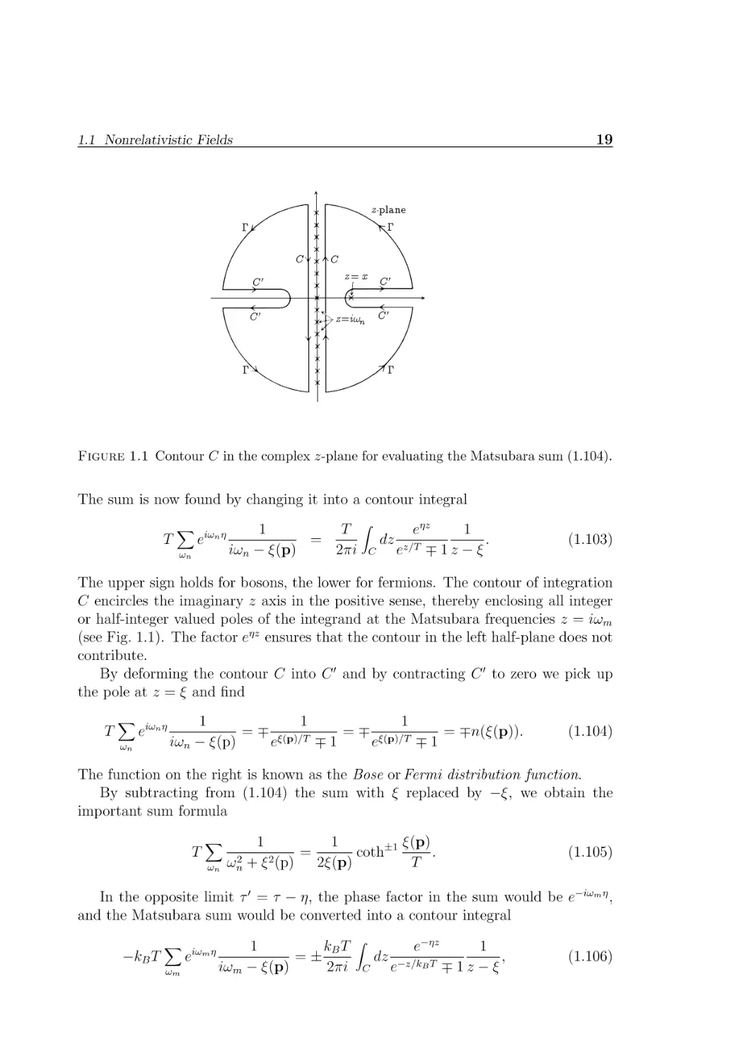
Figure 1.1 Contour C in the complex z-plane for evaluating the Matsubara sum (1.104).
The sum is now found by changing it into a contour integral
T
X
eiωn η
ωn
1
T
=
iωn − ξ(p)
2πi
Z
C
dz
1
eηz
.
ez/T ∓ 1 z − ξ
(1.103)
The upper sign holds for bosons, the lower for fermions. The contour of integration
C encircles the imaginary z axis in the positive sense, thereby enclosing all integer
or half-integer valued poles of the integrand at the Matsubara frequencies z = iωm
(see Fig. 1.1). The factor eηz ensures that the contour in the left half-plane does not
contribute.
By deforming the contour C into C ′ and by contracting C ′ to zero we pick up
the pole at z = ξ and find
T
X
eiωn η
ωn
1
1
1
= ∓ ξ(p)/T
= ∓ ξ(p)/T
= ∓n(ξ(p)).
iωn − ξ(p)
e
∓1
e
∓1
(1.104)
The function on the right is known as the Bose or Fermi distribution function.
By subtracting from (1.104) the sum with ξ replaced by −ξ, we obtain the
important sum formula
T
X
ωn
1
1
±1 ξ(p)
=
coth
.
ωn2 + ξ 2 (p)
2ξ(p)
T
(1.105)
In the opposite limit τ ′ = τ − η, the phase factor in the sum would be e−iωm η ,
and the Matsubara sum would be converted into a contour integral
−kB T
X
ωm
eiωm η
kB T Z
1
e−ηz
1
=±
,
dz −z/k T
B
iωm − ξ(p)
2πi C e
∓1z −ξ
(1.106)
20
1 Functional Integral Techniques
yielding 1 ± nξ(p) .
In the operator language, these limits correspond to the expectation values
T
†
†
G (x, τ ; x, τ + η) = h0|T̂ ψ̂H (x, τ )ψ̂H
(x, τ + η) |0i=±h0|ψ̂H
(x, τ )ψ̂H (x, τ )|0i,
T
†
†
G (x, τ ; x, τ − η) = h0|T̂ ψ̂H (x, τ )ψ̂H
(x, τ − η) |0i=h0|ψ̂H (x, τ )ψ̂H
(x, τ )|0i
†
= 1 ± h0|ψ̂H
(x, τ )ψ̂H (x, τ ∓ η)|0i.
The function n(ξ(p)) is the thermal expectation value of the number operator
†
(x, τ )ψ̂H (x, τ ).
N̂ = ψ̂H
(1.107)
It is useful to employ a four-vector notation also in T 6= 0 -ensembles. The
four-vector
pE ≡ (p4 , p) = (ω, p)
(1.108)
is called the Euclidean four-momentum. Correspondingly, we define the Euclidean
spacetime coordinate
xE ≡ (−τ, x).
(1.109)
The exponential in (1.100) can be written as
pE xE = −ωτ + px.
(1.110)
Collecting integral and sum in a single four-summation symbol, we shall write (1.100)
as
T
G0 (xE − x′ ) ≡ −
1
T X
.
exp [−ipE (xE − x′E )]
V pE
ip4 − ξ(p)
(1.111)
It is quite straightforward to derive the general T 6= 0 Green function from a
path integral formulation analogous to (1.75). For this we consider classical fields
ψ(x, τ ) with the periodicity or anti-periodicity
ψ(x, τ ) = ±ψ (x, τ + 1/T ) .
(1.112)
They can be Fourier-decomposed as
ψ(x, τ ) =
T X X −iωn τ +ipx
T X −ipE xE
e
a(pE ),
e
a(ωn , p) ≡
V ωn p
V pE
(1.113)
with a sum over even or odd Matsubara frequencies ωn . If now a free action is
defined as
∗
A0 [ψ , ψ] = −i
Z
1/2T
−1/2T
dτ
Z
d3 xψ ∗ (x, τ ) [−∂τ − ξ (−i∇)] ψ(x, τ ),
(1.114)
21
1.1 Nonrelativistic Fields
Eq. (1.80) renders [4, 10]
T
∓Tr log A+
∗
Z0 [η , η] = e
R R 1/2T
dτ dτ ′
−1/2T
R
d3 xd3 x′ η∗ (x,τ )A−1 (x,τ,x′ ,τ ′ )η(x′ ,τ ′ )
,
(1.115)
with
A(x, τ ; x′ , τ ′ ) = [∂τ + ξ (−i∇)] δ (3) (x − x′ )δ(τ − τ ′ ).
(1.116)
Henceforth A−1 is equal to the propagator (1.100). The Matsubara frequencies arise
from the finite τ interval of Euclidean space together with the periodic boundary
condition (1.112).
Again, interactions are taken care of by multiplying TZ0 [η ∗ η] with the factor
(1.81). In terms of the fields ψ(x, τ ), the exponent has the form
1 Z Z 1/2T
dτ dτ ′
2
−1/2T
Aint =
×
Z
d3 xd3 x′ ψ ∗ (x, τ )ψ ∗ (x′ , τ ′ )ψ(x′ , τ ′ )ψ(x, τ )V (x, −iτ ; x′ , −iτ ′ ). (1.117)
In the case of a potential of type (1.47), which becomes instantaneous in τ :
V (x, −iτ ; x′ , −iτ ′ ) = V (x − x′ ) iδ(τ − τ ′ ).
(1.118)
Then Aint can be written in terms of the interaction Hamiltonian as
Aint = i
Z
1/2T
−1/2T
dτ Hint (τ ).
(1.119)
Thus the grand canonical partition function in the presence of external sources may
be calculated from the path integral [10]:
T
∗
Z[η , η] =
Z
T
i A+
∗
Dψ (x, τ )Dψ(x, τ )e
R 1/2T
−1/2T
dτ
R
d3 x[ψ∗ (x,τ )η(x,τ )+c.c.]
,
(1.120)
where the grand-canonical action is
T
∗
i A[ψ , ψ] = −
+
i
2
Z
1/2T
−1/2T
Z
1/2T
−1/2T
dτ
Z
d3 xψ ∗ (x, τ ) [∂τ + ξ(−i∇)] ψ(x, τ )
(1.121)
Z
dτ dτ ′ d3 xd3 x′ ψ ∗ (x, τ )ψ ∗ (x′ , τ ′ )ψ(x, τ ′ )ψ(x, τ )V (x, −iτ ; x, −iτ ′ ).
The Green functions are obtained from the functional derivatives
G (x1 , τ1 , . . . , xn , τn ; xn′ , τn′ , . . . , x1′ , τ1′ )
′
δ n+n Z[η ∗ , η]
n+n′
= (−i)
δη ∗ (x1 , τ1 ) · · · δη ∗ (xn , τn )δη(xn′ , τn′ ) · · · δη(x1′ , τn′ )
(1.122)
.
η=η∗ ≡0
22
1 Functional Integral Techniques
The right-hand side consists of the functional integrals
Z
N Dψ ∗ (x, t)Dψ(x, t) ψ̂(x1 , τ1 ) · · · ψ̂(xn , τn )ψ̂ ∗ (xn′ , τn′ ) · · · ψ̂ ∗ (x1′ , τ1′ )eiA[ψ
∗ ,ψ]
.(1.123)
In the sequel, we shall always assume the normalization factor to be chosen in such
a way that Z[0, 0] is normalized to unity. Then the functional integrals (1.123) are
obviously the correlation functions of the fields, commonly written in the form
hψ̂(x1 , τ1 ) · · · ψ̂(xn , τn )ψ̂ ∗ (xn′ , τn′ ) · · · ψ̂ ∗ (x1′ , τ1′ )i.
(1.124)
In contrast to Section 1.2, the bra and ket symbols denote now a thermal average
of the classical fields.
The functional integral expression (1.120) for the generating functional offers the
advantageous flexibility with respect to changes in the field variables.
Summarizing we have seen that the functional (1.120) defines the most general
type of theory involving two-body forces. It contains all information on the physical
system in the vacuum as well as in thermodynamic ensembles. The vacuum theory
is obtained by setting T = 0, µ = 0, and continuing the result back from T to
physical times. Conversely, the functional (1.75) in the vacuum can be generalized to
ensembles in the straightforward manner by first continuing the times t to imaginary
values −iτ via a Wick rotation in all energy integrals and then going to periodic
functions in τ .
There is a complete correspondence between the real-time generating functional
(1.75) and the thermodynamic imaginary-time expression (1.120). For this reason
it is sufficient to exhibit all techniques only in one version for which we shall choose
(1.75). Note, however, that due to the singular nature of the propagators (1.85) in
real energy-momentum, the thermodynamic formulation specifies the way how to
avoid singularities.
1.2
Relativistic Fields
We shall also study collective phenomena in relativistic fermion systems. For this
we shall need fields describing relativistic particles of spin zero, 1/2, and 1. Their
properties will now be briefly reviewed.
1.2.1
Lorentz and Poincaré Invariance
For relativistic particles, the relation between the physical laws in two coordinate
frames which move with a constant velocity with respect to each other are different
from the nonrelativistic case. Suppose a frame moves with velocity v into the −zdirection of another fixed frame. Then in the moving frame, the z-momentum of
the particle will be increased. The particle appears boosted in the z-direction with
respect to the original observer. The momenta in x- and y-directions are unaffected.
Now, the total four momentum still satisfies the energy momentum relation
E(p) =
q
p2 + M 2 .
(1.125)
23
1.2 Relativistic Fields
Introducing the four-vector notation
pµ ≡ (p0 , pi ) with p0 ≡ (p)/c,
(1.126)
we see that the four-vector satisfies the mass shell condition
2
p0 − p2 = M 2 .
(1.127)
2
2
For the particle moving in the z-direction, the combination p0 − p3 remains invariant. This implies that there must be a hyperbolic transformation mixing p0 and p3 ,
which may be parametrized by a hyperbolic angle ζ called rapidity:
p′0 = cosh ζ p0 + sinh ζ p3 ,
p′3 = sinh ζ p0 + cosh ζ p3 .
(1.128)
This is called a pure Lorentz transformation. We may write it in a 4 × 4 matrix form
as
p′µ =
cosh ζ
0
0
sinh ζ
0
1
0
0
0 sinh ζ
0
0
1
0
0 cosh ζ
µ
pν ≡ B3 (ζ)µν pν .
(1.129)
ν
The subscript 3 of B3 indicates that the particle is boosted into the z-direction. A
similar matrix can be written down for x and y-directions. In an arbitrary direction
p̂, the matrix elements are
Bp̂ (ζ) =
p̂i sinh ζ
cosh ζ
p̂i sinh ζ δ ij + p̂i p̂j (cosh ζ − 1)
.
(1.130)
By combining rotations and boosts one obtains a 6-parameter manifold of matrices
Λ = Bp̂ (ζ)R'ˆ (ϕ),
(1.131)
called proper Lorentz transformations. For all these
2
2
p′0 − p′2 = p0 − p2 = M 2 c2
(1.132)
is an invariant. These matrices form a group, the proper Lorentz group. We can
easily see that the Lorentz group allows reaching every momentum pµ on the mass
shell by applying an appropriate group element to some fixed reference momentum
pµR . For example, if the particle has a mass M we may choose for pµR the so-called
rest momentum
pµR = (M, 0, 0, 0),
(1.133)
and apply the boost in the p̂ direction
Λ = Bp̂ (ζ),
(1.134)
24
1 Functional Integral Techniques
with the rapidity given by
cosh ζ =
p0
,
M
sinh ζ =
|p|
.
M
(1.135)
But we may also choose Λ(p) = Bp̂ (ζ)R'ˆ (ϕ) where R'ˆ is an arbitrary rotation,
since any of these leaves the rest momentum pµR invariant. In fact, the rotations
form the largest subgroup of the group of all proper Lorentz transformations, which
leaves the rest momentum pµR invariant. It is referred to as the little group or Wigner
group of a massive particle. It has an important physical significance since it serves
to specify the intrinsic rotational degrees of freedom of the particle. If the particle
is at rest it carries no orbital angular momentum. If its quantum mechanical state
remains completely invariant under any member R'ˆ of the little group, the particle
must also have zero intrinsic angular momentum or zero spin. Besides this trivial
representation, the little group being a rotation group can have representations of
any angular momentum s = 21 , 1, 32 , . . . . In these cases, the state at rest has 2s + 1
components which are mixed with each other upon rotations.
The situation is quite different in the case of massless particles. They move with
the speed of light and pµ cannot be brought by a Lorentz transformation from the
light cone to a rest frame. There is, however, another standard reference momentum
from which one can generate all other momenta on the light cone. It is given by
pµR = (1, 0, 0, 1)p,
(1.136)
and it remains invariant under a different little group, which is again a threeparameter subgroup of the Lorentz group. This will be discussed later.
It is useful to write the invariant expression (1.132) as a square of a four vector
µ
p formed with the metric
gµν =
namely
1
−1
−1
−1
,
p2 = gµν pµ pν .
(1.137)
(1.138)
In general, we define a scalar product between any two vectors as
pp′ ≡ gµν pµ p′ν = p0 p′0 − pp′ .
(1.139)
A space with this scalar product is called Minkowski space. . It is useful to introduce
the covariant components of any vector v µ as
vµ ≡ gµν v ν .
(1.140)
Then the scalar product can also be written as
pp′ = pµ p′µ .
(1.141)
25
1.2 Relativistic Fields
With this notation the mass shell condition for a particle before and after a Lorentz
transformation reads simply
2
p ′ = p 2 = M 2 c2 .
(1.142)
Note that, apart from the minus signs in the metric (1.137), the mass shell con2
2
2
2
dition p2 = p0 − p1 − p2 − p3 = M 2 c2 , left invariant by the Lorentz group, is
2
2
2
2
completely analogous to the spherical condition p4 + p1 + p2 + p3 = M 2 c2 which
is left invariant by the rotation group in a four-dimensional euclidean space. Both
groups are parametrized by six parameters which are associated with linear transformations in the six planes 12, 23, 31; 10, 20, 30 or 12, 23, 31; 14, 24, 34, respectively.
In the case of the four-dimensional euclidean space these are all rotations which
form the group of special orthogonal matrices called O(4). The letter S indicates
the property special . A group is called special if all its transformation matrices have
a unit determinant. In the case of the proper Lorentz group one uses by analogy
the notation SO(1,3). The numbers indicate the fact that in the metric (1.137), one
diagonal element is equal to +1 and three are equal to −1.
The fact that all group elements are special follows from a direct calculation of
the determinant of (1.130), (1.131).
How do we have to describe the quantum mechanics of a free relativistic particle
in Minkowski space? The energy and momenta p0 , p must be related to the time
and space derivatives of particle waves in the usual way
∂
∂
ǫ
= ih̄
≡ ih̄ 0 ,
c
∂ct
∂x
∂
= −ih̄ i .
∂x
p0 =
pi
(1.143)
They satisfy the canonical commutation rules
[pµ , pν ] = 0,
[xµ , xν ] = 0,
[pµ , xν ] = −ih̄g µν .
(1.144)
We expect that associated with the pure momentum state p there will be some wave
function
fp (x) = e−i(p
0 x0 −pi xi )/h̄
≡ e−ipx/h̄ .
(1.145)
At this point we do not yet know the proper scalar product necessary to extract
physical information from such wave functions.
We have stated previously that permissible energy momentum states of a free
particle can be realized by considering one and the same particle in different coordinate frames connected by the transformation Λ(p). Suppose that we change the
coordinates of the same space time point as follows:
x → x′ = Λx.
(1.146)
26
1 Functional Integral Techniques
Under this transformation the scalar product of any two vectors remains invariant:
x′ y ′ = xy.
(1.147)
This holds also for scalar products between momentum and coordinate vectors
p′ x′ = px.
(1.148)
For the transformation matrix Λ, it implies that
(Λp)(Λx) = px.
(1.149)
If the scalar products are written out explicitly in terms of the metric gµν this
amounts to
gµν Λµ λ pλ Λν κ xκ = gλκ pλ xκ ,
(1.150)
for all p, x. The Lorentz matrices Λ satisfy therefore the identity
gµν Λµ λ Λν κ = gλκ ,
(1.151)
ΛT gΛ = g.
(1.152)
or, written without indices,
If the metric is Euclidean, this would be the definition of orthogonal matrices. In
fact, in the notation of scalar products in which the metric is suppressed as in
(1.153), there is no difference between the manipulation of orthogonal and Lorentz
matrices. In both cases one has
(Λp)(Λx) = pΛ−1 Λx = px.
(1.153)
When changing the coordinates, the same particle wave in space behaves like
−1 ′
fp (x) = e−ipΛ x /h̄
′
= e−i(Λp)x /h̄ = fΛp (x′ ) = fp′ (x′ ).
(1.154)
This shows that, in the new coordinates, the same particle appears with different
momentum components
p′ = Λp.
(1.155)
Consider a wave ψ(x) which is an arbitrary superposition of different momentum
states. After a coordinate transformation it will still have the same value at the
same space time point. Thus ψ ′ (x′ ), as seen in the new frame, must be equal to
ψ(x) in the old frame
ψ ′ (x′ ) = ψ(x).
(1.156)
At this place one defines the substantial change under the Lorentz transformation
Λ as the change at the same values of the coordinates x (which corresponds to a
transformed point in space)
Λ
ψ(x) −
−−→ ψΛ′ (x) = ψ(Λ−1x).
(1.157)
27
1.2 Relativistic Fields
We have marked by a subscript the transformation under which ψ ′ (x) arises. Clearly,
this transformation property is valid only if the particle does not possess any intrinsic
orientational degree of freedom, i.e., no spin. A field with this property is called a
scalar field or, for historical reasons, a Klein-Gordon field .
If a particle has spin degrees of freedom, the situation is quite different. Then
the wave function has several components to account for the spin orientations. The
transformation law must be such that the spin orientation in space remains unchanged at the same space point. This implies that the field components which
specify the orientation with respect to the different coordinate axes will have to
be transformed by certain matrices. It is well-known how this is done in the case
of electromagnetic and gravitational fields, whose vector and tensor transformation
properties follow standard rules. In the next sections these will be recalled. Afterwards it will be easy to generalize everything to the case of arbitrary spin.
Before coming to this, however, let us conclude this section by mentioning that
there are other space transformations which leave the scalar products pµ xµ invariant
but which are not contained in the group SO(1,3): Most importantly there is the
space inversion, also called mirror reflection or parity transformation:
1
−1
P =
−1
−1
,
(1.158)
which reverses the direction of the spatial vectors, x → −x. There is further the
time inversion
−1
1
T =
1
1
,
(1.159)
which changes the sign of x0 . If P and T are incorporated into the special Lorentz
group SO(1,3), one deals with the full Lorentz group.
Note that the determinants of both (1.158) and (1.159) are negative, so that
the full Lorentz group no longer deserves the letter S in its name. It is then called
O(1,3).
1.2.2
Relativistic Free Scalar Fields
From all this it is obvious how the non-relativistic free field action
A=
Z
∂x 2
ψ(x, t)
dtdxψ (x, t) ih̄∂t + h̄
2M
∗
"
2
#
(1.160)
must be modified to describe relativistic n-particle states. In order to accommodate
the kinematic features, discussed in the last section, we require the action to be
28
1 Functional Integral Techniques
invariant under Lorentz transformations. Depending on the possible internal spin
degrees of freedom there are different ways of making the action relativistic. These
will now be discussed separately.
Scalar Fields
If the field ψ(x, t) carries no spin degree of freedom which varies under space rotations, the spatial derivative ∂x always has to appear squared in the action to
guarantee rotational invariance. With the Lorentz symmetry between ∂0 and ∂x we
are led to a classical action
A=
Z
dx0 L =
Z
dx0 d3 xψ ∗ (x, t) [c1 ∂ µ ∂µ + c2 ] ψ(x, t),
(1.161)
where c1 , c2 are two arbitrary real constants. It is now easy to see that this action is
indeed Lorentz invariant: Under the transformation (1.146), the four-volume element
does not change
dx0 d3 x ≡ d4 x → d4 x′ = d4 x.
(1.162)
If we therefore take the action in the new frame
A=
Z
h
i
(1.163)
i
(1.164)
d4 x′ ψ ∗′ (x′ ) c1 ∂ ′µ ∂µ′ + c2 ψ ′ (x′ ),
we can use (1.161) and (1.156) to rewrite
A=
Z
h
d4 xψ ∗ (x) c1 ∂ ′µ ∂µ′ + c2 ψ(x).
But since
∂µ′ = Λµ ν ∂ν ,
∂ µ′ = Λµ ν ∂ ν
(1.165)
with Λµ ν ≡ gµλ g νκ Λλ κ , we see that
∂ ′2 = ∂ 2 ,
(1.166)
and the transformed action becomes
A=
Z
dx0 d3 xψ ∗ (x, t) [c1 ∂ µ ∂µ + c2 ] ψ(x, t),
(1.167)
which is the same as (1.161).
It is useful to introduce the integrand of the action as the so-called Lagrangian
density
h
i
2
L(x, t) = ψ ∗ (x, t) c1 (∂ 0 − ∂x 2 ) + c2 ψ(x, t).
(1.168)
Then the invariance of the action under Lorentz transformation is a direct consequence of the Lagrangian density being a scalar field, satisfying the transformation
law (1.156),
L′ (x′ ) = L(x),
(1.169)
29
1.2 Relativistic Fields
as implied by (1.163), (1.164), and (1.166).
The free-field equations of motion are derived from (1.161) as follows. We write
A=
Z
0
dx L =
Z
0
dx
Z
h
2
i
d3 xψ ∗ (x, t) c1 (∂ 0 − ∂x 2 ) + c2 ψ(x, t),
(1.170)
and vary this independently with respect to the fields ψ(x) and ψ ∗ (x). The independence of these variables is expressed by the functional differentiation rules
δψ(x)
= δ (4) (x − x′ ),
δψ(x′ )
δψ(x)
= 0,
δψ ∗ (x′ )
δψ ∗ (x)
= δ (4) (x − x′ ),
δψ ∗ (x′ )
δψ ∗ (x)
= 0.
δψ(x′ )
(1.171)
Applying these rules to (1.170) we obtain directly
δA
=
d4 x′ δ (4) (x′ − x)(c1 ∂ 2 + c2 )ψ(x)
∗
δψ (x)
= (c1 ∂ 2 + c2 )ψ(x) = 0.
Z
(1.172)
Similarly,
Z
δA
=
d4 x′ ψ ∗ (x′ )(c1 ∂ 2 + c2 )δ(x′ − x)
δψ(x)
←
= ψ ∗ (x)(c1 ∂ 2 +c2 ),
(1.173)
where the arrow on top of the last derivative indicates that it acts on the field to the
left. The second equation is just the complex conjugate of the previous one. Then
the functional derivative with respect to ψ ∗ (x) is simple. In terms of the Lagrangian
density, the extremality condition can be expanded in terms of partial derivatives
with respect to increasing partial derivatives of all fields in L,
δA
∂L(x)
∂L(x)
∂L(x)
=
− ∂µ
+ ∂µ ∂ν
+ ... ,
δψ(x)
∂ψ(x)
∂∂µ ψ(x)
∂∂µ ∂ν ψ(x)
(1.174)
with the same equation for ψ ∗ (x). This follows directly from the defining relations
in (1.171). The field equation for ψ(x) is particularly simple:
δA
∂L(x)
=
.
∗
δψ (x)
∂ψ ∗ (x)
(1.175)
For ψ ∗ (x), on the other hand, all derivatives written out in (1.174) have to be
evaluated.
Both field equations (1.172) and (1.173) are solved by the quantum mechanical
plane wave (1.145),
fp (x) = e−ipx/h̄ ,
(1.176)
30
1 Functional Integral Techniques
if the momentum satisfies the condition
−c1 pµ pµ + c2 = 0.
(1.177)
This has precisely the form of the mass shell relation (1.142) if we choose
c2h̄2 /c1 = M 2 c2 .
(1.178)
It is customary to normalize c1 to
c1 = −h̄2 .
(1.179)
The sign is necessary to have stable field fluctuations. The size can be brought
to this value by a multiplicative renormalization of the field. Then the mass shell
condition fixes the free field action to the standard form
A=
Z
h
i
dx0 d3 xψ ∗ (x, t) −h̄2 ∂ µ ∂µ − M 2 c2 ψ(x, t).
(1.180)
The appearance of the constants h̄ and c in all future formulas can be avoided
if we agree to work with natural units l0 , m0 , t0 , E0 different from the ordinary cgs
units. They are chosen to give h̄ and c the value 1. Expressed in terms of the
conventional length, time, mass, and energy, these new natural units are given by
h̄
h̄
h̄
c,
t0 =
=
,
Mc
E0
Mc2
= M, E0 = Mc2 .
l0 =
m0
(1.181)
(1.182)
If, for example, the particle is a proton with mass mp , these units are
l0 = 2.103138 × 10⁻¹¹ cm
= Compton wavelength of proton,
(1.183)
t0 = l0 /c = 7.0153141 × 10⁻²² sec
= time taken by light running along Compton wavelength,
(1.184)
m0 = mp = 1.6726141 × 10⁻²⁴ g,
E0 = 938.2592 MeV.
(1.185)
(1.186)
For any other mass, they can easily be rescaled.
With these natural units we can drop c and h̄ in all formulas and write the action
simply as
Z
Z
A = d4 xL(x) = d4 xψ ∗ (x)(−∂ 2 − M 2 )ψ(x).
(1.187)
Actually, since we are dealing with relativistic particles there is no fundamental
reason to assume ψ(x) to be a complex field. In the non-relativistic theory this was
necessary in order to construct a term linear in the time derivative
Z
dtψ ∗ i∂t ψ.
(1.188)
31
1.2 Relativistic Fields
For a real field ψ(x) this would have been a pure surface term that does not influence
the dynamics of the system. For second-order time derivatives as in (1.187) this is
no longer necessary.
Thus we shall also study the real scalar field with an action
A=
Z
1
d xL(x) =
2
4
Z
d4 xφ(x)(−∂ 2 − M 2 )φ(x).
(1.189)
In this case, a prefactor 21 is the normalization convention for the field. We have
also here used the letter φ(x) to denote the real field, as is commonly done.
1.2.3
Electromagnetic Fields
Electromagnetic fields move with light velocity and have no mass term.3 The fields
have two polarization degrees of freedom (right and left polarized) and are described
by the usual electromagnetic action. Historically, this was the very first example of
a relativistic classical field theory. Thus it could also have served as a guideline for
the previous construction of the action of the scalar field φ(x).
The action may be given in terms of a real auxiliary four-vector potential Aµ (x)
from which the physical electric and magnetic fields can be derived as follows
E i = −(∂ 0 Ai − ∂ i A0 ) = −∂t Ai − ∂i A0 ,
1
1
H i = − ǫijk (∂ i Ak − ∂ k Ai ) = ǫijk (∂j Ak − ∂k Aj ).
2
2
(1.190)
(1.191)
Here ǫijk is the completely antisymmetric Levi-Cività tensor with ǫ123 = 1. It is
useful to introduce the so-called four-curl of the vector potential
Fµν = ∂µ Aν − ∂ν Aµ .
(1.192)
Its six components are directly the field strengths
E i = −F 0i = F0i ,
H i = −F jk = −Fjk ;
ijk = cyclic.
(1.193)
For this reason Fµν is also called the field tensor. The electromagnetic action reads
A=
Z
4
d xL(x) =
Z
1 2
1Z 4
2
d x (H − E ) = −
d xFµν 2 .
2
4
4
(1.194)
The four-curl Fµν satisfies the so-called Bianchi identity for any smooth Aµ [which
satisfies the Schwartz integrability condition (∂λ ∂κ − ∂κ ∂λ )Aµ = 0]:
∂µ F̃ µν = 0,
(1.195)
3
The best upper limit for the mass of the electromagnetic field Mγ deduced under terrestrial
conditions, from the shape of the earth’s magnetic field, is Mγ < 4 · 10−48 g corresponding to a
Compton wavelength λγ = h̄/Mγ c > 1010 cm (= larger than the diameter of the sun). Astrophysical
considerations (“whisps” in the crab nebula) give λγ > 1016 cm. If metagalactic magnetic fields
are discovered, the Compton wavelength would be larger than 1024 − 1025 cm, quite close to the
ultimate limit set by the horizon of the universe = c× age of the universe ∼ 1028 cm. See G.V.
Chibisov, Sov. Phys. Usp. 19 , 624 (1976).
32
1 Functional Integral Techniques
where
F̃ µν = ǫµνλκ Fλκ
(1.196)
is the so called dual field tensor , with ǫµνλκ being the four-dimensional Levi-Cività
tensor with ǫ0123 = 1.
The equations of motion which extremize the action are
∂L(x)
δA
= −∂µ
= ∂µ F µν (x) = 0.
µ
δA (x)
∂µ Aν (x)
(1.197)
Separating the equations (1.196) and (1.197) into space and time components they
are seen to coincide with Maxwell’s equation in empty space
∂µ F µν = 0 :
∂µ F̃ µν = 0 :
∇ · E = 0,
∇ · B = 0,
∇ × B − ∂t E = 0,
∇ × E + ∂t B = 0.
(1.198)
(1.199)
The field tensor is invariant under local gauge transformations
Aµ (x) −
−−→ Aµ (x) + ∂µ Λ(x),
(1.200)
where Λ(x) is any smooth field which satisfies the integrability condition (∂µ ∂ν −
∂ν ∂µ )Λ = 0. In terms of the vector field Aµ , the action reads explicitly
A=
Z
1
d xL(x) = −
d4 x[∂ µ Aν (x)∂µ Aν (x) − ∂ ν Aν (x)∂ µ Aµ (x)]
2Z
1
dxAµ (x)(g µν ∂ 2 − ∂ µ ∂ ν )Aν (x).
(1.201)
=
2
4
Z
The latter form is very similar to the scalar action (1.160). The first piece is the
same as (1.161) for each of the spatial components A1 , A2 , A3 . The time component
A0 , however, appears with an opposite sign. A field with this property is called a
ghost field . When trying to quantize such a field, the associated particle states turn
out to have a negative norm. In order for the theory to be physically consistent it
will be necessary to make sure that such states can never appear in any scattering
process. The second piece in the action ∂ ν Aν ∂ µ Aµ is novel with respect to the scalar
case. It exists here as an additional Lorentz invariant since Aµ is a vector field under
Lorentz transformation.
In order to see the Lorentz transformation properties, let us remember that in
electrodynamics the Lorentz forces on a moving particle carrying a charge and a
classical magnetic pole are obtained from the field transformation
E|| ′ = E|| ,
B|| ′ = B|| ,
E⊥ ′ = γ(E⊥ + v × B),
B⊥ ′ = γ(B⊥ − v × E),
q
(1.202)
(1.203)
with v being the velocity of the particle and γ ≡ 1 − v2 /c2 . Here E and B are
the fields in the laboratory, whereas E′ and B′ are the corresponding fields in the
33
1.2 Relativistic Fields
frame of the moving particle. They exert electric and magnetic forces eE′ + gB′.
The subscripts || and ⊥ denote the components parallel and orthogonal to v.
From this experimental fact we can derive the transformation law of the vector
field Aµ under Lorentz transformations. The frame in which the moving particle is
at rest is related to the laboratory frame by
x′ = Bv̂ (ζ)x,
(1.204)
where Bv̂ (ζ) is a boost in the v-direction with the rapidity
cosh ζ = γ,
v
sinh ζ = γ ,
c
v
tanh ζ = .
c
(1.205)
The transformation law (1.202) is equivalent to
A′µ (x′ ) = Bv̂ (ζ)µ ν Aν (x).
(1.206)
An analogous transformation law holds for rotations so that we can write, in general,
A′µ (x′ ) = Λµ ν Aν (x).
(1.207)
This transformation law differs from that of a scalar field (1.156) in the way envisaged above for particles with non-zero intrinsic angular momentum. The field
has several components. It points in the same spatial direction before and after the
coordination change. This is ensured by its components changing in the same way
as the coordination of the point xµ . Notice that as a consequence, ∂ µ Aµ (x) is a
scalar field in the sense defined in (1.156). Indeed
∂ ′µ A′µ (x′ ) = (Λµ ν ∂ ν )Λµ λ Aλ (x) = ∂ ν Aν (x).
(1.208)
For this reason the second term in the action (1.218) is Lorentz invariant, just as
the mass term in (1.189). The invariance of the first term is shown similarly
A′ν (x′ )∂ ′2 A′ν (x′ ) = Λν λ Aν (x)∂ ′2 Λν κ Aκ (x′ )
= Aν (x)∂ ′2 Aν (x) = Aν (x)∂ 2 Aν (x).
(1.209)
Hence the action (1.218) does not change under Lorentz transformations, as it
should.
Just as the scalar action, also the electromagnetic action (1.194) is invariant
under a Lorentz group extended by translations (the so-called Poincaré group):
A′µ (x′ ) = Aµ (x)
(1.210)
x′µ = Λµ ν xν + aµ .
(1.211)
where
Similarly, we have under parity
P
Aµ −
−−→ A′ µP (x) = õ (x̃),
(1.212)
34
1 Functional Integral Techniques
and under time reversal,
T
A−
−−→ A′ µT (x) = õ (xT )
(1.213)
where the tilde inverts the spacial components
õ = (A0 , −Ai ).
(1.214)
In principle, there would have been the possibility of a parity transformation
P
Aµ −
−−→ AµP (x) = ηP õ (x̃),
(1.215)
with ηP = ±1, and in the case ηP = −1 the field Aµ would have been called an axial
vector field . The electromagnetic gauge field Aµ , however, is definitely a vector field.
This follows from the vector nature of the electric and the axial vector nature of
the magnetic field, which are observed in the laboratory. Similarly, the phase under
time reversal of Aµ , which in principle could have been
T
Aµ −
−−→ A′ µT (x) = ηT õ (xT )
(1.216)
with ηT = ±1, is given by (1.213). This is due to time reversal, under which all
currents change their direction. This reverses the direction of the B-field but has
no influence on the E-field.
It is also possible to perform the operation of charge conjugation by exchanging
the sign of all charges without changing their direction of flow. Then E and B
change directions. Hence
C
Aµ −
−−→ A′ µC (x) = −Aµ (x).
(1.217)
In general, the vector field could have been transformed as
C
Aµ −
−−→ A′ µC (x) = ηC Aµ (x)
(1.218)
with ηC = ±1. The phase factor ηC = −1 expresses the experimental fact that the
electromagnetic field is odd under charge conjugation.
1.2.4
Relativistic Free Fermi Fields
For Fermi fields, the situation is technically more involved. Experimentally, fermions
always have an even number of spin degrees of freedom. In order to describe these we
give the field ψ a spin index α running through (2s+1) components. Under rotations,
these spin components are mixed with each other as observed experimentally in
the Stern-Gerlach experiment. Lorentz transformations lead to certain well defined
mixtures of different spin components.
The question arises whether we can construct a Lorentz invariant action involving
(2s + 1) spinor field components. To see the basic construction principle we use the
35
1.2 Relativistic Fields
known transformation law (1.207) for the 4-vector field Aµ as a guide. For an
arbitrary spinor field we postulate the transformation law
Λ
ψ(x)α −
−−→ψα′ (x′ ) = Dα β (Λ)ψβ (x),
(1.219)
with an appropriate (2s + 1) × (2s + 1) spinor transformation matrix Dα β (Λ) which
we have to construct. This can be done by purely mathematical arguments. The
construction is the subject of the so-called group representation theory. First of all,
we perform two successive Lorentz transformations,
x′′ = Λx = Λ2 x′ = Λ2 Λ1 x.
(1.220)
Since the Lorentz transformations Λ1 , Λ2 are elements of a group, the product Λ ≡
Λ2 Λ1 is again a Lorentz transformation. Under the individual factors Λ2 and Λ1 ,
the field transforms as
Λ1
Ψ(x) −
−−→ Ψ′ (x′ ) = D(Λ1)Ψ(x),
(1.221)
Ψ′ (x) −
−−→ Ψ′′ (x′′ ) = D(Λ2 )Ψ′ (x′ ),
(1.222)
Λ2
so that under Λ = Λ2 Λ1 ,
Λ2 Λ1
Ψ(x) −
−−→ Ψ′′ (x′′ ) = D(Λ2 )D(Λ1 )Ψ(x).
(1.223)
But for Λ itself, the transformation matrix is D(Λ) and
Ψ′′ (x′′ ) = D(Λ2 Λ1 )Ψ(x).
(1.224)
Comparison of this with (1.223) shows that the matrices D(Λ) which mix the spinor
field components under the Lorentz group must follow a group multiplication law
which has to be compatible with that of the group itself. The mapping
Λ−
−−→ D(Λ)
(1.225)
is a homomorphism and the D(Λ)’s form a matrix representation of the group.
Notice that the transformation law (1.207) for Aµ follows the same rule, with
D(Λ) ≡ Λ
(1.226)
being the defining 4 × 4 representation of the Lorentz group.
The group laws for Λ and D(Λ) are sufficiently stringent to allow only a countable
set of fundamental4 finite dimensional transformation laws D(Λ). They are characterized by two quantum numbers, s1 and s2 , with either one taking the possible
half-integer or integer values 0, 12 , 1, 32 , . . . .
4
Mathematically, “fundamental” means that the representation is irreducible. Any arbitrary
representation is equivalent to a direct sum of irreducible ones.
36
1 Functional Integral Techniques
A representation D (s1 ,s2 ) (Λ) will turn out to harbor particles of spin |s1 − s2 |
to s1 + s2 . Hence, particles with a single fixed spin s can only follow the D (s,0) (Λ)
or D (0,s) (Λ) transformation laws. For spin 1/2, the relativistic free-field which is
invariant under parity has four components and is called the Dirac field. It is
described by the action
A=
Z
d4 xL(x) =
Z
d4 xψ̄(x) (iγ µ ∂µ − M) ψ(x),
(1.227)
where M is the mass of the spin-1/2 -particles described by ψ(x). The quantities
γ µ are the Dirac matrices. , defined by defined by
µ
γ =
0 σµ
σ̃ µ 0
!
,
(1.228)
where σ µ is a four-vector formed from the 2×2-dimensional Pauli matrices as follows:
σ µ ≡ (1, σ i ),
(1.229)
σ̃ µ ≡ (1, −σ i ).
(1.230)
ψ̄ ≡ ψ † γ 0 .
(1.231)
and
The symbol ψ̄(x) is short for
As a historical note we mention that Dirac did not find his equation by invoking
group-theoretic arguments. Instead, he was searching for an alternative solution to
the relativistic time-independent Schrödinger equation of an electron
Ĥψ(x) =
q
p̂2 + M 2 ψ(x) = Eψ(x).
(1.232)
He observed that a square root linear in the momentum operator exists if the equation is considered as a matrix equation acting on several components of ψ(x, t).
These would indeed be necessary to represent the spin degrees of freedom of the
electron. So he made the ansatz
ĤD ψ(x) = (−iαi p̂i + βM)ψ(x) = Eψ(x),
(1.233)
with unknown matrices αi , β. Being the square root of Ĥ, the operator ĤD has
2
to fulfill the equation ĤD
= p̂2 + M 2 . This implies that the matrices satisfy the
algebraic relations:
{αi , αj } = δij ,
{αi , β} = 0,
β 2 = 1.
(1.234)
By multiplying Eq. (1.235) with β and going over to a time-dependent equation by
replacing E by i∂x0 , he obtained the Dirac equation
(iγ µ p̂µ − M)ψ(x) = 0,
(1.235)
37
1.2 Relativistic Fields
with the matrices
γ 0 ≡ β,
γ i ≡ βαi .
(1.236)
These satisfy the anticommutation rules
{γ µ , γ ν } = 2g µν ,
(1.237)
which are indeed solved by the Dirac matrices (1.228).
It has become customary to abbreviate the contraction of γ µ with any vector v µ
by
v/ ≡ γ µ vµ ,
(1.238)
and write the Dirac equation as
(/
p − M)ψ(x) = 0,
(1.239)
(i/
∂ − M)ψ(x) = 0.
(1.240)
or
1.2.5
Perturbation Theory of Relativistic Fields
If interactions are present, the Lagrangian consists of a sum
L ψ, ψ̄, ϕ = L0 + Lint .
(1.241)
As in the case of nonrelativistic fields, all time ordered Green’s functions can be
obtained from the derivatives with respect to the external sources of the generating
functional
i
Z [η, η̄, j] = const × h0|T e
R
dx(Lint +η̄ψ+ψ̄η+jϕ)
|0i.
(1.242)
The fields in the exponent follow free equations of motion and |0i is the free-field
vacuum. The constant is conventionally chosen to make Z [0, 0, 0] = 1, i. e.
i
const = h0|T e
R
dxLint (ψ,ψ̄,ϕ)
|0i
−1
.
(1.243)
This normalization may always be enforced at the very end of any calculation such
that Z [η, η̄, j] is only interesting as far as its functional dependence is concerned,
modulo the irrelevant constant in front.
It is then straightforward to show that Z [η, η̄, j] can alternatively be computed
via the Feynman path integral formula
Z [η, η̄, j] = const ×
Z
DψD ψ̄Dϕei
R
dx[L0 (ψ,ψ̄,ϕ)+Lint +η̄ψ+ψ̄η+jϕ]
.
(1.244)
Here the fields are no more operators but classical functions (with the mental reservation that classical Fermi fields are anticommuting objects). Notice that contrary
to the operator formula (1.242) the full action appears in the exponent.
38
1 Functional Integral Techniques
For simplicity, we demonstrate the equivalence only for one real scalar field ϕ(x).
The extension to other fields is immediate [1, 3]. First note that it is sufficient to
give the proof for the free field case, i. e.,
Z0 [j] = h0|T ei
R
dxj(x)ϕ(x)
= const ×
Z
i
Dϕe
|0i
R
dx[ 21 ϕ(x)(−✷x −µ2 )ϕ(x)+j(x)ϕ(x)]
.
(1.245)
Indeed, if it holds there, a simple multiplication on both sides of (1.245) by the
differential operator
ei
R
dxLint ( 1i
δ
δj(x)
)
(1.246)
would extend it to the interacting functionals (1.242) or (1.244). Equation (1.245)
follows directly from Wick’s theorem according to which any time ordered product
of a free field can be expanded into a sum of normal products with all possible time
ordered contractions. This statement can be summarized in an operator form valid
for any functional F [ϕ] of a free field ϕ(x):
1
T F [ϕ] = e 2
R
δ
δ
dxdy δϕ(x)
D(x−y) δϕ(y)
N̂(F [ϕ]),
(1.247)
where D(x − y) is the free-field propagator
D(x − y) =
i
δ(x − y) =
−✷x − µ2 + iǫ
i
d4 q −iq(x−y)
e
.
4
2
(2π)
q − µ2 + iǫ
Z
(1.248)
Applying this to (1.247) gives
1
Z0 = e 2
R
δ
δ
dxdy δϕ̂(x)
D(x−y) δϕ̂(y)
R
1
= e− 2
R
1
−2
= e
dxdyj(x)D(x−y)j(y)
dxdyj(x)D(x−y)j(y)
.
h0|N̂(ei
h0|N̂(ei
R
R
dxj(x)ϕ̂(x)
dxj(x)ϕ̂(x)
)|0i
)|0i
(1.249)
The last part of the equation follows from the vanishing of all normal products of
ϕ(x) between vacuum states.
Exactly the same result is obtained by performing the functional integral in
(1.245) and using the functional integral formula (1.79). The matrix A is equal to
A(x, y) = (−✷x − µ2 ) δ(x − y), and its inverse yields the propagator D(x − y):
A−1 (x, y) =
1
δ(x − y) = −iD(x − y)
−✷x − µ2 + iǫ
(1.250)
thus reproducing once more (1.249).
For the generating functional of a free Dirac field theory
Z0 [η, η̄] = h0|T ei
R
ˆ
(η̄ ψ̂+ψ̄η)dx
= const ×
Z
|0i
DψD ψ̄ei
R
dx[L0 (ψ,ψ̄ )+η̄ψ+ψ̄η]
,
(1.251)
39
Notes and References
with the free-field Lagrangian
L0 (x) = ψ̄(x) (iγ µ ∂µ − M) ψ(x),
(1.252)
we obtain, similarly,
Z0 [η̄, η] = e
1
2
R
− 21
= e
Now,
R
R
1
−2
= e
δ
δ
dxdy δψ(x)
G0 (x−y) δψ̄(y)
dxdy η̄(x)G0 (x−y)η(y)
dxdy η̄(x)G0 (x−y)η(y)
.
h0|N̂(ei
h0|N̂(ei
R
R
ˆ
dx(η̄ ψ̂+ψ̄η)
ˆ
dx(η̄ ψ̂+ψ̄η)
A(x, y) = (iγ µ ∂µ − M) δ(x − y),
)|0i
)|0i
(1.253)
(1.254)
and its inverse yields the fermion propagator G0 (x − y):
A−1 (x, y) =
iγ µ ∂µ
1
δ(x − y) = −iG0 (x − y).
− M + iǫ
(1.255)
Note that it is Wick’s expansion which supplies the free part of the Lagrangian
when going from the operator form (1.247) to the functional version (1.244).
Notes and References
[1] For the introduction of collective bilocal fields in particle physics and applications see:
H. Kleinert, On the Hadronization of Quark Theories, Erice Lectures 1976,
publ. in Understanding the Fundamental Constituents of Matter , Plenum
Press, 1978, (ed. by A. Zichichi).
See also:
H. Kleinert, Phys. Letters B 62, 429 (1976), B 59, 163 (1975).
[2] H. Kleinert, Particles and Quantum Fields, World Scientific, Singapore, 2016
(klnrt.de/b6).
[3] H.E. Stanley, Phase Transitions and Critical Phenomena, Clarendon Press,
Oxford, 1971; F.J. Wegner, Phase Transitions and Critical Phenomena, ed. by
C. Domb and M. S. Green, Academic Press, 1976, p. 7; E. Brézin, J. C. Le Guillou, and J. Zinn-Justin, ibid., p. 125, see also L. Kadanoff, Rev. Mod. Phys. 49,
267 (1977).
[4] R.P. Feynman, Rev. Mod. Phys. 20, 367 (1948);
R.P. Feynman and A.R. Hibbs, Path Integrals and Quantum Mechanics,
McGraw-Hill, New York (1968).
[5] H. Kleinert, Path Integrals in Quantum Mechanics, Statistics, Polymer
Physics, and Financial Markets, 5th ed., World Scientific, Singapore, 2006,
pp. 1-1547 (klnrt.de/b5).
40
1 Functional Integral Techniques
[6] J. Rzewuski, Quantum Field Theory II, Hefner, New York (1968).
[7] S. Coleman, Erice Lectures 1974, in Laws of Hadronic Matter, ed. by A.
Zichichi, p. 172.
[8] See for example:
A.A. Abrikosov, L.P. Gorkov, and I.E. Dzyaloshinski, Methods of Quantum
Field Theory in Statistical Physics, Dover, New York (1975);
L.P. Kadanoff, G. Baym, Quantum Statistical Mechanics, Benjamin, New York
(1962);
A.L. Fetter and J.D. Walecka, Quantum Theory of Many-Particle Systems,
McGraw-Hill, New York (1971).
[9] The first authors to employ such identities were
P.T. Mathews and A. Salam, Nuovo Cimento 12, 563 (1954); 2, 120 (1955).
[10] R.L. Stratonovich, Sov. Phys. Dokl. 2, 416 (1958);
J. Hubbard, Phys. Rev. Letters 3, 77 (1959);
B. Muehlschlegel, J. Math. Phys. 3, 522 (1962);
J. Langer, Phys. Rev. A 134, 553 (1964);
T.M. Rice, Phys. Rev. A 140, 1889 (1965); J. Math. Phys. 8, 1581 (1967);
A.V. Svidzinskij, Teor. Mat. Fiz. 9, 273 (1971);
D. Sherrington, J. Phys. C 4 401 (1971).
Our observation of nature must be diligent,
our reflection profound, and our experiments exact.
Denis Diderot (1713–1784)
2
Plasma Oscillations
In this chapter we develop a collective quantum field theory for a gas of many
electrons which interact only via long-range Coulomb forces. The Coulomb forces
give rise to collective modes called plasmons.
2.1
General Formalism
The simplest application of the functional method transforms the grand-canonicel
partition function (1.120) from the defining formulation in terms of a fundamental
field to a re-formulation in terms of a collective quantum field. The new formulation
describes the phenomeana directly by means of its fundamental excitations called
plasmons. For this, we make use of the Hubbard-Stratonovich transformation in
the form (1.79) and observe that a two-body interaction (1.45) in the generating
functional can be created by a fluctuating auxiliary field ϕ(x) as follows:
i
exp −
2
Z
′
∗
∗
′
′
′
dxdx ψ (x)ψ (x )ψ(x)ψ(x )V (x, x )
= const ×
Z
i
Dϕ
2
Z
′
h
dxdx ϕ(x)V
−1
′
(2.1)
′
∗
′
(x, x )ϕ(x )−2ϕ(x)ψ (x)ψ(x)δ(x − x )
i
.
To abbreviate the notation, we have used a four-vector notation with
x ≡ (x, t),
dx ≡ d3 xdt,
δ(x) ≡ δ 3 (x)δ(t).
The symbol V −1 (x, x′ ) denotes the functional inverse of the matrix V (x, x′ ), which
is the solution of the equation
Z
dx′ V −1 (x, x′ )V (x′ , x′′ ) = δ(x − x′′ ).
(2.2)
The constant prefactor in (2.1) is [det V ]−1/2 . Absorbing this in the always omitted normalization factor N of the functional integral, the grand-canonical partition
function Ω = Z becomes
Z[η ∗ , η] =
Z
Dψ ∗ DψDϕ exp iA + i
Z
41
dx (η ∗ (x)ψ(x) + ψ ∗ (x)η(x)) ,
(2.3)
42
2 Plasma Oscillations
where the new action is
∗
A[ψ , ψ, ϕ] =
+
Z
dxdx ψ ∗ (x) [i∂t − ξ(−i∇) − ϕ(x)] δ(x − x′ )ψ(x′ )
′
(2.4)
1
ϕ(x)V −1 (x, x′ )ϕ(x′ ) .
2
Note that the effect of using formula (1.79) in the generating functional amounts to
the addition of the complete square involving the field ϕ in the exponent:
1
dxdx′ ϕ(x)− dyV (x, y)ψ ∗(y)ψ(y) V −1 (x, x′ ) ϕ(x′ )− dy ′V (x′ , y ′)ψ ∗ (y ′)ψ(y ′) ,
2
(2.5)
followed by a functional integration over ϕ(x). The addition of (2.5) to the action
(2.12) can be generated from a source term
Z
AI =
Z
Z
1
DI(x) e− 2
R
dxI(x)V (x.x′ )I(x′ )+I(x)[ϕ(x)−
Z
R
dy V (x,y) ψ∗ (y)ψ(y)]
.
(2.6)
The generating functional Z remains unchanged by the two successive manipulations
as follows from the observation that the integral Dϕ produces the irrelevant constant
[det V ]1/2 , which is precisely cancelled by the functional over I(x). This procedure
of going from (1.45) to (2.4) is probably simpler mnemonically than formula (1.79).
The physical significance of the new field ϕ(x) is easy to understand: ϕ(x) is
directly related to the particle density. At the classical level this is seen immediately
by extremizing the action (2.4) with respect to variations δϕ(x), which yield:
δA
= ϕ(x) −
δϕ(x)
Z
dy V (x, y) ψ ∗(y)ψ(y) = 0.
(2.7)
Quantum mechanically, there are fluctuations around the field configuration ϕ(x)
that is determined by Eq.
(2.7). These make the field ϕ(x) different from the comR
posite operator O(x) ≡ dyV (x, y)ψ ∗ (y)ψ(y). But due to the Gaussian nature of
the functional integral over ϕ(x), the fluctuations are rather trivial. Thus we can
easily see that the propagators of the two fields ϕ(x) and O(x) differ only by the
direct interaction, i.e.,
hT (ϕ(x)ϕ(x′ ))i = V (x − x′ ) + hT (O(x)O(x′ ))i .
Note that if a potential V (x, y) is dominantly caused by a single fundamentalparticle exchange, the field ϕ(x) coincides with the field of this particle: If, for
example, V (x, y) represents the Coulomb interaction
e2
δ(t − t′ ),
|x − x′ |
(2.8)
4πe2 ∗
ψ (x, t)ψ(x, t).
∇2
(2.9)
V (x, x′ ) =
then Eq. (2.7) amounts to
ϕ(x, t) = −
43
2.1 General Formalism
This reveals that the auxiliary field ϕ(x, t) is the electric potential of the system.
If the particles ψ(x) have spin indices, the potential will, in this example, be spin
conserving at every vertex, and Eq. (2.7) must be read as spin-contracted:
δA
= ϕ(x) − O(x) ≡ ϕ(x) −
∂ϕ(x)
Z
d4 yV (x, y)ψ ∗α (y)ψα (y) = 0.
(2.10)
This restriction is just for convenience and can easily be lifted later. Nothing in
our procedure depends on this particular form of V (x, y) and O. In fact, V could
arise from the exchange of one or many different fundamental particles and their
multiparticle configurations (for example, π, ππ, σ, ϕ, etc. in nuclei [1]) so that the
spin dependence is the rule rather than the exception.
The important point is now that the auxiliary field ϕ(x) can be made the only
field of the theory by integrating out ψ ∗ , ψ in Eq. (2.3), using formula (1.80). Thus
one obtains
Z[η ∗ , η] ≡ Ω[η ∗ , η] = NeiA ,
(2.11)
where the new action is
1
dxdx′ η ∗ (x)Gϕ (x, x′ )η(x′ ),
(2.12)
A[ϕ] = ±Tr log
+
2
with Gϕ (x, x′ ) being the Green function of the fundamental particles in an external
classical field ϕ(x):
iG−1
ϕ
Z
[i∂t − χ(−i∇) − ϕ(x)] Gϕ (x, x′ ) = iδ(x − x′ ).
(2.13)
The field ϕ(x) is called a plasmon field. The new plasmon action can easily be
interpreted graphically. For this, one expands Gϕ (x, x′ ) in powers of ϕ:
Gϕ (x, x′ ) = G0 (x − x′ ) − i
Z
dx1 G0 (x − x1 )ϕ(x1 − x′ ) + . . .
(2.14)
Hence the couplings to the external currents η ∗ , η in (2.12) amount to radiating one,
two, etc. ϕ fields from every external line of fundamental particles (see Fig. 2.1). An
expansion of the expression Tr log(iG−1
ϕ ) in powers of ϕ gives
−1
±iTr log(iG−1
ϕ ) = ±iTr log(iG0 ) ± iTr log(1 + iG0 ϕ)
∞
X
1
(−iG0 ϕ)n .
= ±iTr log(iG−1
)
∓
iTr
0
n
n=1
i
E−ζ(p)
(2.15)
ϕ
Figure 2.1 This diagram displays the piece of the collective action (2.12). The original
fundamental particle (fat line) can enter and leave the diagrams only via external currents.
It emits an arbitrary number of plasmonson its way (wiggly lines).
44
2 Plasma Oscillations
The nth term corresponds to a loop of the original fundamental particle emitting
nϕ lines (see Fig. 2.2).
Figure 2.2 The non-polynomial self-interaction terms of plasmons arising from the Tr log
in (2.12) are equal to the single loop diagrams emitting n plasmons.
Let us now use the action (2.12) to construct a quantum field theory of plasmons.
For this we may include the quadratic term
±iTr(G0 ϕ)2
1
2
(2.16)
into the free part of ϕ in (2.12) and treat the remainder perturbatively. The free
propagator of the plasmon becomes
{0|T ϕ(x)ϕ(x′ )|0} ≡ (2s + 1)G0 (x′ , x).
(2.17)
This corresponds to an inclusion of all ring graphs into the V -propagator (see Fig.
2.3).
Figure 2.3 Free plasmon propagator containing an infinite sequence of single loop corrections (“bubblewise summation”)
It is worth pointing out that the propagator in momentum space Gpl (k) contains
actually two important physical informations. From the derivation at fixed temperature it appears in the transformed action (2.12) as a function of discrete Euclidean
frequencies νn = 2πnT only. In this way it serves for the time-independent description of the system at fixed T . However, the calculation of the correlation function
(2.17) makes use of the Fourier representation in the entire complex energy plane. A
suitable analytic continuation of this Fourier representation can be used to calculate
also the time-dependent collective phenomena for real times [2].
With the propagator (2.17) and the interactions given by (2.15), the original theory of fundamental fields ψ ∗ , ψ has been transformed into a theory of ϕ-fields whose
bare propagator accounts for the original potential which has absorbed ringwise an
infinite sequence of fundamental loops.
45
2.2 Physical Consequences
This transformation is exact. Nothing in our procedure depends on the statistics
of the fundamental particles nor on the shape of the potential. Such properties
are important when it comes to solving the theory perturbatively. Only under
appropriate physical circumstances will the field ϕ represent important collective
excitations with weak residual interactions. Then the new formulation is of great
use in understanding the dynamics of the system. As an illustration consider a dilute
fermion gas of very low temperature. Then the function ξ(−i∇) is ǫ(−i∇) − µ with
ǫ(−i∇) = −∇2 /2m.
2.2
Physical Consequences
Let the potential be translationally invariant and instantaneous:
V (x, x′ ) = δ(t − t′ )V (x − x′ ).
(2.18)
Then the plasmon propagator (2.17) reads in momentum space
Gpl (ν, k) = V (k)
1
,
1 − V (k)π(ν, k)
(2.19)
where the single electron loop symbolizes the analytic expression1
π(ν, k) = 2
T X
1
1
.
V p iω − p2 /2m + µ i(ω + ν) − (p + k)2 /2m + µ
(2.20)
The frequencies ω and ν are odd and even multiples of πT , respectively. In order
to calculate the sum we introduce a convergence-enforcing factor eiωη , and rewrite
(2.20) as [3]
1
d3 p
3
(2π) ξ(p + k) − ξ(p) − iν
"
#
X
1
1
iωn η
e
×T
.
−
i(ωn + ν) − ξ(p + k) iωn − ξ(p)
ωn
π(ν, k) = 2
Z
(2.21)
Using the summation formula (1.104), this becomes
π(ν, k) = 2
Z
d3 p n(p + k) − n(p)
,
(2π)3 ǫ(p + k) − ǫ(p) − iν
(2.22)
or, after some rearrangement,
π(ν, k) = −2
1
Z
1
1
d3 p
. (2.23)
n(p)
+
3
(2π)
ǫ(p + k) − ǫ(p) − iν ǫ(p − k) − ǫ(p) + iν
"
The factor 2 stems from the trace over the electron spin.
#
46
2 Plasma Oscillations
Let us study this function for real physical frequencies ω = iν where we rewrite it
as
1
1
d3 p
,
n(p)
+
π(ω, k) = −2
3
(2π)
ǫ(p+k)−ǫ(p) − ω ǫ(p−k)−ǫ(p) + ω
#
"
Z
(2.24)
which can be brought to the form
k2
π(ω, k) = 2
mω 2
Z
1
d3 p
n(p)
.
3
(2π)
(ω − p · k/m + iη)2 − (k 2 /2M)2
(2.25)
For |ω| > pF k/m + k 2 /2m, the integrand is real and we can expand
2
k
π(ω, k) = 2
mω 2
Z
3
p·k
dp
2p · k
n(p) 1 +
+3
3
(2π)
mω
mω
p·k
+
mω
2.2.1
!3
!2
80(p · k)4 + m2 ω 2 k 4
+ . . . . (2.26)
+
16m2 ω 4
Zero Temperature
For zero temperature, the chemical potential µ is equal to the Fermi energy εF =
p2F /2m, and all states below the Fermi momentum pF are occupied so that the
occupation number is given by a Heaviside function n(p) = Θ(p − pF ). Then the
integral in (2.26) can be performed trivially as
N
=n=2
V
p3F
d3 p
n
(p)
=
,
T =0
(2π)3
3π 2
Z
(2.27)
and we obtain the expansion
k2 n
3
π(ω, k) = 2 1 +
ω m
5
pF k
mω
!2
1
+
5
pF k
mω
!4
1 k4
+ . . . .
+
16 m2 ω 2
(2.28)
Inserting this into (2.19) we find, for long wavelengths, the Green function
#−1
"
V (k) n
+ ...
G (ν, k) ≈ V (k) 1 −
ω2 m
pl
.
(2.29)
Thus the original propagator is modified by a factor
ǫ(ω, k) = 1 −
4πe2 n
+ ... .
ω2 m
(2.30)
The dielectric constant vanishes at the frequency
ω = ωpl =
s
4πe2
,
m
(2.31)
47
2.2 Physical Consequences
which is the famous plasma frequency of the electron gas. At this frequency, the
plasma propagator (2.19) has a pole on the real-ω axis, implying the existence of an
undamped excitation of the system.
For an electron gas, we insert the Coulomb interaction (2.9) and obtain
#−1
4πe2
4πe2
n+ ...
G (ν, k) ≈ 2 1 −
k
mω 2
"
pl
.
(2.32)
Thus the original Coulomb propagator is modified by a factor
ǫ(ω, k) = 1 −
4πe2
n + ...,
mω 2
(2.33)
which is simply the dielectric constant.
The zero temperature limit can also be calculated exactly starting from the
expression (2.26), written in the form
d3 p
1
π(ω, k) = −2
Θ(p
−
p
)
+ (ω → −ω) .
F
(2π)3
p · k + k 2 /2m − ω
"
Z
#
(2.34)
Performing the integral yields
!2
1 2
k mω
k 2 + 2mω − 2kpF
mpF
pF −
+
+ p2F log 2
π(ω, k) = − 2 1 −
2π
2kpF
2
k
k + 2mω + 2kpF
+ (ω → −ω).
(2.35)
The lowest terms of a Taylor expansion in powers of k agree with (2.28).
2.2.2
Short-Range Potential
Let us also find the real poles of Gpl (ν, k) for a short-range potential where the
singularity at k = 0 is absent. Then a rotationally invariant [V (k)]−1 has the longwavelength expansion
[V (k)]−1 = [V (0)]−1 + ak2 + . . . ,
(2.36)
as long as [V (0)]−1 is finite and positive, i.e., for a well behaved overall repulsive
R
potential satisfying V (0) = d3 xV (x) > 0. Then the Green function (2.19) becomes
n
3
Gpl (ω, k) = ω 2 ω 2 [V (0)]−1 + aω 2 k 2 − k 2 1 +
m
5
There is a pole at ω = ±c0 k, where
c0 = V (0)
n
m
pF k
mω
!2
−1
+ . . . .
(2.37)
(2.38)
48
2 Plasma Oscillations
is the velocity of zero sound.
In the neighborhood of the positive-energy pole, the propagator has the form
Gpl (k0 , k) ≈ V (0) ×
|k|
.
ω − c0 |k|
(2.39)
More details can be studied in the textbook [4].
Appendix 2A
Fluctuations around the Plasmon Field
Here we derive the quantum mechanical fluctuations around the classical equation
of motion [recall (2.7)]
ϕ(x) =
Z
dy V (x, y) ψ †(y)ψ(y).
(2A.1)
They are quite simple to calculate. Let us compare the Green function of ϕ(x) with
that of the composite operators on the right-hand side ofR Eq. (2A.1). The Green
functions of ϕ are generated by adding external currents dxϕ(x)I(x) to the final
action (2.12) respectively, and by forming functional derivatives δ/δI. The Green
functions of the composite operators, on the other hand, are obtained by adding
Z
dx
Z
dyV (x, y)ψ † (y)ψ(y) K(x)
to the original actions (2.4) and by forming functional derivatives δ/δK. It is obvious
that the sources K(x) can be included in the final action (2.12) by simply replacing:
ϕ(x) → ϕ′ (x) = ϕ(x) −
Z
dx′ K(x′ )V (x′ , x).
If one now shifts the functional integrations to these new translated variables and
drops the irrelevant superscript “prime”, the actions can be rewritten as
A[ϕ] = ±iTr log(iG−1
ϕ )+
1
2
Z
Z
dxdx′ ϕ(x)V −1 (x, x′ )ϕ(x′ )+i dxdx′ η † (x)Gϕ (x, x′ )η(x)
1
dxdx′ I(x)V (x, x′ )I(x′ ).
(2A.2)
2
In this form, the action display clearly the fact that derivatives of the partition
function with respect to the source I(x) coincide exactly with the the right-hand
side of (2.1).
Thus the propagators of the plasmon field ϕ(x) and of the composite
R
operator dyV (x, y)ψ †(y)ψ(y) are related by
+
Z
dxϕ(x)I(x) −
ϕ(x)ϕ(x′ ) = −
=V
−1
′
Z
δ (2) Z
δ (2) Z
−1
′
=
V
(x,
x
)
−
δI(x)δI(x′ )
δK(x)δK(x′ )
(x, x ) + h0|T̂
Z
†
dyV (x, y)ψ (y)ψ(y)
where T̂ is the time-ordering operator.
Z
′
′
(2A.3)
′
†
′
′
dy V (x , y )ψ (y )ψ(y ) |0i,
Notes and References
49
Notes and References
[1] H. Kleinert, Particles and Quantum Fields, World Scientific, Singapore, 2016.
[2] L.P. Kadanoff and G. Baym, Quantum Statistical Mechanics, Benjamin, New
York (1962);
and the review papers
G. Baym and N.D. Mermin, J. Math. Phys. 2, 232 (1961);
L.P. Kadanoff, Rev. Mod. Phys. 49, 267 (1977);
and Chapter 14 of the textbook [1].
[3] A.A. Abrikosov, L.P. Gorkov, and I.E. Dzyaloshinski, Methods of Quantum
Field Theory in Statistical Physics, Dover, New York (1975);
A. Fetter and J.D. Walecka, Quantum Theory of Many-Particle Systems,
McGraw-Hill, New York (1971). See in particular Chapter 9.
[4] H.L. Pècseli, Waves and Oscillations in Plasmas, CRC Press, New York, 2013.
What we wish, we readily believe,
and what we ourselves think, we imagine others think also.
Julius Caesar (100 B.C.–44 B.C.)
3
Superconductors
Superconductors are made from materials which do not pose any resistance to the
flow of electricity. The phenomenon was first observed in 1911 by the Dutch physicist
Heike Kamerlingh Onnes at Leiden University. When he cooled mercury down to
the temperature of liquid helium, which appears at about 4 degree Kelvin (1 degree
Kelvin −273.15 ◦ C), its resistance suddenly disappeared. For this discovery, Onnes
won the Nobel Prize in physics in 1913.
Superconductors have an important property, which distinguishes them from ordinary conductors of extremely low resistance: They are perfect diamagnets. This
implies that they do not tolerate, in their inside, any magnetic fields. This is the
so-called Meissner-Ochsenfeld effect discovered in 1933. This effect causes superconductive materials to hover over a sufficiently strong magnetic field. They are lifted
as soon as they are cooled below the critical temperature (levitation). A perfect
conductor would only hover above the magnet if brought in from the outside due to
induction, generating a current with a magnetic moment opposite to the external
field.
For the purpose of energy conservation, it is a challenge to find superconductive
materials which can transport high currents without loss at room temperature. Since
1941, the record was held for a long time by niobium-nitride, which becomes superconductive at 16 K, surpassed in 1953 by vanadium-silicon with a critical temperature of 17.5 K. In 1962, a first commercial superconducting wire was manufactured
from an alloy of niobium and titanium. First applications were made in 1987 in
the Fermilab high-energy particle-accelerator Tevatron where the necessary strong
magnetic fields were produced by supercurrents in copper-clad niobium-titanium.
The magnets had been developed in 1960 at the Rutherford Appleton Laboratory
in the UK.
The first satisfactory theory of superconductivity was developed in 1957 by J.
Bardeen, L.N. Cooper, and J.R. Schrieffer [1], now called BCS theory, which won
them the Nobel prize in 1972. The theory made essential use of a fermionic version
of a canonical transformation that had been invented ten years earlier for bosons
by N.N. Bogoliubov, to expain the phenomenon of superfluidity in a dilute gas of
bosons [2]. The BCS theory explains the early forms of superconductivity observed
for elements and simple alloys at temperatures close to absolute zero.
50
51
New advances were made in the 1980 when the first organic superconductor was
synthesized by the Danish researcher Klaus Bechgaard of the University of Copenhagen and his group [3]. The new material turned out to become superconductive
at a transition temperature of about 1.2 K. The possibility that this could happen
had been pointed out in 1964 by Bill Little at Stanford University [4].
A more recent major breakthrough was made in 1986 by Alex Müller and Georg
Bednorz at the IBM Research Laboratory in Rüschlikon, Switzerland [5]. They
synthesized brittle ceramic compound that became superconducting at the record
temperature of 30 K. What made this discovery so remarkable was that ceramics
are normally insulators, and do not conduct electricity at all. So, researchers had
not considered them as possible high-temperature superconductor candidates. The
compound that Müller and Bednorz synthesized of a mixture of Lanthanum, Barium,
Copper, and Oxygen behaved in a not-as-yet-understood way. Their discovery won
them the Nobel Prize in 1987. It was later found that tiny amounts of this material
were actually superconducting at 58 K. Since then there has been a great deal
of activity trying to find ceramics of many combinations with higher and higher
critical temperatures. In 1987 superconductivity was reached in a material called
YBCO (Yttrium Barium Copper Oxide) at 92 K, a temperature which can simply
be reached by cooling the material with liquid nitrogen.
The present world record was reached in 2015 at Tc = 203 K in a sulfur hydride
system. Under extreme pressure of 300 000 atmospheres, this critical temperature
can be raised by 25 to 30 more degrees (see Fig. 3.1). For more details see [6, 7, 8].
Figure 3.1 Time evolution of critical temperatures at which superconductivity sets in (in
units of Kelvin). The right-hand margins indicate the liquid by which the temperatures
can be reached. From Ref. [6].
52
3 Superconductors
3.1
General Formulation
The theoretical description of low-temperature superconductivity is based on a collective field complementary to the plasmon field. The complementary field is a pair
field which describes the dominant low-energy collective systems such as the superconductors to be discussed in this Chapter. The pair field is in general bilocal
and will be denoted by ∆(x t; x′ t′ ), with two space and two time arguments. It
is introduced into the generating functional by performing a Hubbard-Stratonovich
transformation of the type (1.80), according to which one rewrites the exponential
of the interaction term in (2.1) in the partition function (1.75) as [9, 10]:
i
exp −
2
"
i
×exp
2
Z
Z
′
∗
(
dxdx
′
′
′
Z
dxdx ψ (x)ψ (x )ψ(x )ψ(x)V (x, x ) = const × D∆(x, x′ )D∆∗ (x, x′ )
′
∗
)#
1
|∆(x, x )|
− ∆∗ (x, x′ )ψ(x)ψ(x′ )− ψ ∗ (x)ψ ∗ (x′ )∆(x, x′ ) .
′
V (x, x )
(3.1)
′
2
In contrast to the similar-looking plasmon expression (2.1), the inverse 1/V (x, x′ ) in
(3.1) is understood as a numeric division for each x, y, not as a functional inversion.
Hence the grand-canonical potential becomes
Z
Z[η, η ∗] =
Dψ ∗ DψD∆∗ D∆ eiA[ψ
∗ ,ψ,∆∗ ,∆]+i
R
dx(ψ∗ (x)η(x)+c.c.)
,
(3.2)
with the action
A[ψ ∗ , ψ, ∆∗ , ∆] =
Z
(
dxdx′ ψ ∗ (x) [i∂t − ξ(−i∇)] δ(x − x′ )ψ(x′ )
)
1
1
1
1
− ∆∗ (x, x′ )ψ(x)ψ(x′ ) − ψ ∗ (x)ψ ∗ (x′ )∆(x, x′ ) + |∆(x, x′ )|2
, (3.3)
2
2
2
V (x, x′ )
where ξp ≡ εp − µ is the grand-canonical single particle energy (recall Subsection 1.1.7). This new action arises from the original one in (1.75) by adding to it
the complete square
i
2
Z
dxdx′ |∆(x, x) − V (x′ , x)ψ(x′ )ψ(x)|2
1
,
V (x, x′ )
which removes
the fourth-order interaction term and gives, upon functional integraR
tion over D∆∗ D∆, merely an irrelevant constant factor to the generating functional.
At the classical level, the field ∆(x, x′ ) is nothing but a convenient abbreviation
for the composite field V (x, x′ )ψ(x)ψ(x′ ). This follows from the equation of motion
obtained by extremizing the new action with respect to δ∆∗ (x, x′ ). This yields
δA
δ∆∗ (x, x′ )
=
1
[∆(x, x′ ) − V (x, x′ )ψ(x)ψ(x′ )] ≡ 0.
′
2V (x, x )
(3.4)
53
3.1 General Formulation
Quantum mechanically, there are Gaussian fluctuations around this solution which
are discussed in Appendix 3C.
Expression (3.3) is quadratic in the fundamental fields ψ(x) and can be rewritten
in a matrix form as
1 ∗
f (x)A(x, x′ )f (x′ )
2
!
1 †
[i∂t − ξ(−i∇)] δ(x − x′ )
−∆(x, x′ )
= f (x)
f (x′ ), (3.5)
− ∆∗ (x, x′ )
∓ [i∂t + ξ(i∇)] δ(x − x′ )
2
!
ψ(x)
where f (x) denotes the fundamental field doublets f (x) =
and f † ≡ f ∗T .
ψ ∗ (x)
The field f ∗ (x) is not independent of f (x). Indeed, there is an identity
†
f Af = f
T
0 1
1 0
!
Af.
(3.6)
Therefore, the real-field formula (1.79) must be used to evaluate the functional
integral for the generating functional
∗
Z[η , η] =
Z
D∆∗ D∆ eiA[∆
∗ ,∆]− 1
2
R
dx
R
dx′ j † (x)G∆ (x,x′ )j(x′ )
,
(3.7)
where j(x)
! collects the external source η(x) and its complex conjugate, j(x) ≡
η(x)
. Then the collective action reads
η ∗ (x)
h
i
i
1
1Z
−1
′
A[∆ , ∆] = ± Tr log iG∆ (x, x ) +
dxdx′ |∆(x, x′ )|2
.
2
2
V (x, x′ )
∗
(3.8)
The 2 × 2 matrix G∆ denotes the propagator iA−1 which satisfies the functional
equation
Z
′′
dx
!
[i∂t − ξ(−i∇)] δ(x−x′′ )
−∆(x, x′′ )
G∆ (x′′ , x′ ) = iδ(x−x′ ).
− ∆∗ (x, x′′ )
∓ [i∂t + ξ(i∇)] δ(x−x′′ )
(3.9)
!
G G∆
Writing G∆ as a matrix
, the mean-field equations associated with this
G†∆ G̃
action are precisely the equations used by Gorkov to study the behavior of type II
superconductors.1 With Z[η ∗ , η] being the full partition function of the system,
the fluctuations of the collective field ∆(x, x′ ) can now be incorporated, at least in
principle, thereby yielding corrections to these equations.
Let us set the sources in the generating functional Z[η ∗ , η] equal to zero and
investigate the behavior of the collective quantum field ∆. In particular, we want to
1
As an example see p. 444 in Ref. [11].
54
3 Superconductors
develop Feynman rules for a perturbative treatment of the fluctuations of ∆(x, x′ ).
As a first step we expand the Green function G∆ in powers of ∆ as
0 ∆
∆∗ 0
G∆ = G0 − iG0
!
G0 − G0
0 ∆
∆∗ 0
!
0 ∆
∆∗ 0
G0
!
G0 + . . . (3.10)
with
i
δ(x − x′ )
i∂t − ξ(−i∇)
G0 (x, x′ ) =
0
0
i
δ(x − x′ )
∓
i∂t + ξ(i∇)
.
(3.11)
We shall see later that this expansion is applicable only close to the critical temperature Tc . Inserting this expansion into (3.7), the source term can be interpreted graphically by the absorption and emission of lines ∆(k) and ∆∗ (k), respectively, from
virtual zig-zag configurations of the underlying particles ψ(k), ψ ∗ (k) (see Fig. 3.2).
∆∗ (ν ′ , q′ )
i
ω−ξp
i
ν ′ −ω−ξq′ −p
i
ν−ν ′ +ω−ξq−q′ +p
∆(ν, q)
Figure 3.2 Fundamental particles (fat lines) entering any diagram only via the external
currents in the last term of (3.7), absorbing n pairs from the right (the past) and emitting
the same number from the left (the future).
The functional submatrices in G0 have the Fourier representation
T X
0
i
e−i(p t−px) ,
0
V p p − ξp
0
i
T X
e−i(p t−px) ,
G̃0 (x, x′ ) = ±
0
V p −p − ξ−p
G0 (x, x′ ) =
(3.12)
(3.13)
where we have used the notation ξp for the Fourier components ξ(p) of ξ(−i∇).
The first matrix coincides with the operator Green function
G0 (x − x′ ) = h0|T ψ(x)ψ † (x′ )|0i.
(3.14)
The second one corresponds to
G̃0 (x − x′ ) = h0|T ψ †(x)ψ(x′ )|0i = ±h0|T ψ(x′ )ψ † (x) |0i
= ±G0 (x′ − x) ≡ ±[G0 (x, x′ )]T ,
(3.15)
55
3.1 General Formulation
where T denotes the transposition in the functional sense (i.e., x and x′ are interchanged). After a Wick rotation of the energy integration contour, the Fourier
components of the Green functions at fixed energy read
1
′
eip(x−x )
p iω − ξp
X
1
′
eip(x−x ) = ∓G0 (x′ − x, −ω).
G̃0 (x − x′ , ω) = ∓
p −iω − ξ−p
G0 (x − x′ , ω) = −
X
(3.16)
(3.17)
The Tr log term in Eq. (3.8) can be interpreted graphically just as easily by expanding as in (3.134):
"
i
i
i
−1
± Tr log iG−1
=
±
∓ Tr −iG0
Tr
log
iG
∆
0
2
2
2
0
∆
∗
∆ 0
!
∗
∆
#n
1
. (3.18)
n
The first term only changes the irrelevant normalization N of Z. To the remaining
sum only even powers can contribute so that we can rewrite
∞
X
#n
(−)n
i
∓i
A[∆∗ , ∆] = ∓i
Tr
δ ∆
δ ∆∗
2n
i∂
−
ξ(−i∇)
i∂
+
ξ(i∇)
t
t
n=1
1Z
1
+
dxdx′ |∆(x, x′ )|2
2
V (x, x′ )
Z
∞
X
1
1
An [∆∗ , ∆] +
dxdx′ |∆(x, x′ )|2
=
.
(3.19)
2
V (x, x′ )
n=1
"
!
!
This form of the action allows an immediate quantization of the collective field ∆.
The graphical rules are slightly more involved technically than in the plasmon case
since the pair field is bilocal. Consider at first the free collective fields which can be
obtained from the quadratic part of the action:
"
i
A2 [∆ , ∆] = − Tr
2
∗
!
#
!
i
i
δ ∆
δ ∆∗ .
i∂t − ξ(−i∇)
i∂t + ξ(i∇)
(3.20)
Variation with respect to ∆ displays the equations of motion
′
′
∆(x, x ) = iV (x, x )
"
!
i
i
δ ∆
δ
i∂t − ξ(−i∇)
i∂t + ξ(i∇)
!#
.
(3.21)
This equation coincides exactly with the Bethe-Salpeter equation [18], in ladder
approximation, for two-body bound-state vertex functions, usually denoted in momentum space by
′
Γ(p, p ) =
Z
dxdx′ exp[i(px + p′ x′ )]∆(x, x′ ).
(3.22)
Thus the free excitations of the field ∆(x, x′ ) consist of bound pairs of the original
fundamental particles. The field ∆(x, x′ ) will consequently be called pair field. If
56
3 Superconductors
we introduce total and relative momenta q and P = (p − p′ )/2, then (3.21) can be
written as2
Γ(P |q) = −i
Z
i
d4 P ′
V (P − P ′ )
′
4
(2π)
q0 /2 + P0 − ξq/2+P′ + iη sgn ξ
i
.
× Γ(P ′ |q)
′
q0 /2 − P0 − ξq/2−P′ + iη sgn ξ
(3.23)
Graphically this formula can be represented shown in Fig. 3.3. The vertex Γ(P |q)
Figure 3.3 Free pair field following the Bethe-Salpeter equation as pictured in this diagram.
produces a Bethe-Salpeter wave function:
Φ(P |q) = N
i
q0 /2 + P0 − ξq/2+P + iη sgn ξ
i
Γ(P |q).
×
q0 /2 + P0 − ξq/2+P + iη sgn ξ
(3.24)
It satisfies
G0 (q/2 + P ) G0 (q/2 − P ) Φ(P |q) = −i
Z
dP ′
V (P, P ′)Φ(P ′ |q),
(2π)4
(3.25)
thus coinciding, up to a normalization, with the Fourier transform of the two-body
state wave functions
ψ(x, t; x′ , t′ ) = h0|T (ψ(x, t)ψ(x′ , t′ )) |B(q)i.
(3.26)
If the potential is instantaneous, then (3.21) shows ∆(x, x′ ) to be factorizable according to
∆(x, x′ ) = δ(t − t′ )∆(x, x′ ; t),
so that Γ(P |q) becomes independent of P0 .
2
Here q is short for the four-vector q µ = (q 0 , q) with q0 = E.
(3.27)
57
3.1 General Formulation
Consider now the system at T = 0 in the vacuum. Then µ = 0 and ξp = εp > 0.
One can perform the P0 integral in (3.23) with the result
Γ(P|q) =
1
d3 P ′
V (P − P′ )
Γ(P′|q).
4
′
′
(2π)
q0 − εq/2+P − εq/2−P + iη
Z
(3.28)
Now the equal-time Bethe-Salpeter wave function
Z
′
ψ(x, x ; t) ≡ N
d3 Pdq0 d3 q
x + x′
exp
−i
q
t
−
q
·
− P · (x − x′ )
0
(2π)7
2
1
×
q0 − εq/2+P − εq/2−P + iη
"
!#
(3.29)
satisfies
i
h
i∂t − ǫ(−i∇) − ǫ(−i∇′ ) ψ(x, x′ ; t) = V (x − x)ψ(x, x′ ; t),
(3.30)
which is simply the Schrödinger equation of the two-body system. Thus, in the
instantaneous case, the free collective excitations in ∆(x, x′ ) are the bound states
derived from the Schrödinger equation.
In a thermal ensemble, the continuous integrals over the energies P ′0 in (3.23) are
restricted to sums over the Matsubara frequencies. First, we write the Schrödinger
equation as
Γ(P|q) = −
Z
d3 P′
V (P − P′ )l(P′ |q)Γ(P′|q)
3
(2π)
(3.31)
with
l(P|q) = −i
X
G0 (q/2 + P ) G̃0 (P − q/2)
= −i
X
q0 /2+P0 −ξq/2+P +iη sgn ξ q0 /2 − P0 −ξq/2−P +iη sgn ξ
P0
P0
i
i
. (3.32)
After a Wick rotation and setting q0 ≡ iν, the replacement of the energy integration
by a Matsubara sum leads to
1
1
ωn i (ωn + ν/2) − ξq/2+P i (ωn − ν/2) + ξq/2−P
X
1
= T
ωn iν − ξq/2+P − ξq/2−P
l(P|q) = −T
X
"
1
1
×
−
i(ωn + ν/2) − ξq/2+P i(ωn − ν/2) + ξq/2−P
= −
h
± nq/2+P + nq/2−P
i
iν − ξq/2+P − ξq/2−P
.
#
(3.33)
58
3 Superconductors
Here we have used the frequency sum [see (1.104)]
T
X
ωn
1
1
= ∓ ξp /T
≡ ∓np ,
iωn − ξp
e
∓1
(3.34)
with np being the occupation numbers of the state of energy ξp . In Chapter 1
we have used the generic notation n(p) for the occupation numbers of fermions
and bosons. In this Chapter we shall save some space by placing the momentum
argument into a subscript.
The expression in brackets is antisymmetric under the exchange ξ → −ξ, since
under this substitution n(p) → ∓1 − n(p) . In fact, one can write it in the form
−N(P, q) with
N(P|q) ≡ 1 ± nq/2+P + nq/2−P
!
ξq/2+P
ξq/2−P
1
tanh ∓1
,
+ tanh ∓1
=
2
2T
2T
(3.35)
so that
l(P|q) = −
N(P|q)
.
iν − ξq/2+P − ξ(q/2−P
(3.36)
Defining again a Schrödinger type wave function as in (3.29), the bound-state
problem can be brought to the form (3.28) but with a momentum dependent potential V (P − P′ ) × N(P′ |q). We are now ready to construct the propagator of the
pair field ∆(x, x′ ) for T = 0. This is most simply done by considering Eq. (3.23)
with a potential λV (P, P ′) rather than V , and asking for all eigenvalues λn at fixed
q. Let Γn (P |q) be a complete set of vertex functions for this q. Then one can write
the propagator as
∆(P |q)∆† (P ′ |q ′ ) = −i
X
n
Γn (P |q)Γ∗n (P ′ |q)
λ − λn (q)
λ=1
(2π)4 δ (4) (q − q ′ ),
(3.37)
where a hook denotes, as usual, the Wick contraction of the fields. Obviously the
vertex functions have to be normalized in a specific way, as discussed in Appendix 3B.
An expansion of (3.37) in powers of [λ/λn (q)]n exhibits the propagator of ∆ as
a ladder sum of exchanges as shown in Fig. 3.4 (see also Appendix 3B).
Figure 3.4 Free pair propagator, amounting to a sum of all ladders of fundamental
potential exchanges. This is revealed explicitly by the expansion of (3.37) in powers of
[λ/λn (q)].
For an instantaneous interaction, either side is independent of P0 , P0′ . Then
the propagator can be shown to coincide directly with the scattering matrix T of
3.2 Local Interaction and Ginzburg-Landau Equations
59
the Schrödinger equation (3.30) and the associated integral equation in momentum
space (3.28) [see Eq. (3B.13)].
∆∆† = iT ≡ iV + iV
1
V.
E−H
(3.38)
Consider now the higher interactions An , n ≥ 3 of Eq. (3.19). They correspond to
zig-zag loops shown in Fig. 3.5. These have to be calculated with every possible
Γn (P |q), Γ∗m(P |q) entering or leaving, respectively.
Figure 3.5 Self-interaction terms of the non-polynomial pair Lagrangian amounting to
the calculation of all single zig-zag loop diagrams absorbing and emitting n pair fields.
Due to the P dependence at every vertex, the loop integrals become very involved. A slight simplification arises for an instantaneous potential where at least
the frequency sums can be performed immediately. Only in the special case of a
completely local action the full P -dependence disappears and the integrals can be
calculated at least approximately. This will be done in the following section.
3.2
Local Interaction and Ginzburg-Landau Equations
Let us study the case of a completely local potential in detail. For the electrons in
a crystal, such a local potential is only an approximation which, however, happens
to be quite reliable. In a crystal, the interaction between the electrons is mediated
by phonon exchange. An electron moving through the lattice attracts the positive
ions in its neighborhood and thus creates a cloud of positive charge around its path.
This cloud, in turn, attracts other electrons and this is the origin of pair formation.
The size of the cloud is of the order of the lattice spacing, i.e., a few Å. Although
this can hardly be called local, it is effectively so, as far as the formation of bound
states is concerned. The reason is that the strength of the interaction is quite small.
This leads to a rather wide bound-state wave function. Its radius will be seen to
extend over many lattice spacings. Thus, as far as the bound-states are concerned,
the potential may just as well be considered as local. This is what justifies the
theoretical treatment to be developed in the sequel.
We assume the fundamental action to be a sum
A = A0 + Aint ,
(3.39)
60
3 Superconductors
with a free-particle term
A0 =
Z
d3 xdtψβ∗ (x, t)[i∂t − ξ(−i∇)]ψβ (x, t),
(3.40)
and a δ-function interaction
g XZ 3
d xdtψα∗ (x, t)ψβ∗ (x, t)ψβ (x, t)ψα (x, t),
Aint =
2 α,β
(3.41)
with g > 0, for an attractive potential. Following the general arguments leading to
formula (3.1), we rewrite the exponential of this interaction as3
exp
i
g
2 α,β
XZ
d
3
Z
x dt ψα∗ (x, t)ψβ∗ (x, t)ψβ (x, t)ψα (x, t)= const×
i
×exp−
2
Z
d3 xdt
X
αβ
D∆(x, t)D∆∗ (x, t)
!
|∆αβ |2
− ψβ ∆∗βα ψα − ψα∗ ∆αβ ψβ∗ , (3.42)
g
where the new auxiliary field is a (2s + 1) × (2s + 1) non-hermitian matrix which
satisfies the equation of constraint:
∆αβ (x, t) = gψα (x, t)ψβ (x, t).
(3.43)
Observe the hermiticity property
∆αβ (x, t)∗ = ∆∗βα (x, t).
(3.44)
The free part of the action is now written in a 2 × 2 matrix form analogous to that
in (3.5):
A0 =
Z
d3 x dt d3 x′ dt′ f ∗ (x)A(x, t; x′ , t′ )f (x′ ),
(3.45)
where f T (x) denotes here the doubled fundamental field
f T (x) = ψα (x), ψβ∗ (x) ,
and A(x, t; x′ , t′ ) is the functional matrix
′
′
A(x, t; x , t ) =
(3.46)
[i∂t − ξ(−i∇)] δ(x − x′ )δαβ −∆αβ (x)δ(x − x′ )
− ∆∗αβ (x)δ(x − x′ )
∓ [i∂t + ξ(i∇)] δ(x − x′ )δαβ
!
.
(3.47)
Then the action (3.19) becomes
∞
X
(−)n
A [∆ , ∆] = ∓i
Tr trspin
n=1 2n
∗
3
"
!
!
#n
i
∓i
δ (∆ δ)
δ (∆∗ δ) ,
i∂t − ξ(−i∇)
i∂t + ξ(i∇)
(3.48)
Note that the hermitian adjoint ∆∗↑,↓ (x) comprises transposition of the spin indices, i.e.,
∗
= [∆↓,↑ (x)] .
∆∗↑,↓ (x)
61
3.2 Local Interaction and Ginzburg-Landau Equations
where trspin indicates the trace over the spin indices, and Tr refers to the trace in the
functional matrix space. The different terms on the right-hand side will be denoted
by An [∆∗ , ∆].
Consider fermions of spin 1/2 close to a critical region, i.e., for T ≈ Tc . There
only long-range properties of the system dominate. As far as such questions are
concerned, the expansion
∗
A[∆ , ∆] =
∞
X
2
An [∆∗ , ∆]
(3.49)
may be truncated after the fourth term without much loss of information. The
dimensions of the neglected terms are so high that they become irrelevant at long
distances. The free part of the action A2 [∆∗ , ∆] is given by
"
!
!
#
i
∓i
A2 [∆ , ∆] = ±iTr trspin
δ (∆δ)
δ (∆∗ δ)
i∂t − ξ(−i∇)
i∂t + ξ(i∇)
Z
1
1
(3.50)
− trspin dx∆∗ (x)∆(x) .
2
g
∗
The spin traces can be performed by noting that due to Fermi statistics, the square
of the field at a point vanishes, ψ↓2 (x) = 0, ψ↑2 (x) = 0, so that there is really only
one independent pair field:
∆(x) ≡ ∆↓↑ (x) = gψ↓ (x)ψ↑ (x) = −∆↑↓ (x).
(3.51)
Thus A2 becomes:
∗
A2 [∆ ∆] = −i
Z
1Z
dx|∆(x)|2 .
dxdx G0 (x, x )G̃0 (x , x)∆ (x)∆(x ) −
g
′
′
′
∗
′
(3.52)
Let us expand the pair field into its Fourier components
∆(τ, x) = T
XZ
νn
d3 k −i(τ νn −kx)
e
∆(νn , k),
(2π)3
(3.53)
with the bosonic Matsubara frequencies
νn = 2nπT.
(3.54)
Using the short notation
T
XZ
νn
X
d3 k
f
(ν
,
k)
=
T
f (k),
n
(2π)3
k
(3.55)
the quadratic action A2 [∆∗ ∆] can be written in momentum space as
A2 [∆∗ , ∆] =
T X ∗
∆ (k)L(k)∆(k),
V k
(3.56)
62
3 Superconductors
where
T X
i
i
1
−
0
0
0
V p p + k − ξp+k + iη sgn ξp+k p + ξp − iη sgn ξp g
1
T X
(3.57)
l(p|k) − .
=
V p
g
L(k) ≡ −i
This is pictured by a Feynman diagram in Fig. 3.6.
Figure 3.6 Free part of the ∆-Lagrangian containing the direct term plus the one loop
diagram. As a consequence, the free ∆-propagator sums up an infinite sequence of such
loops.
The expression l(p|k) appeared in the general discussion in Eq. (3.31), where it
was brought to the form (3.33). In the present case of Fermi statistics this leads to
"
#
ξp+k
1
11 X
1
ξp
L(ν, k) =
tanh
− .
+tanh
2 V p ξp+k + ξp −iν
2T
2T
g
(3.58)
At k = 0, one has
11 X 1
ξp
1
tanh
−
2 V p ξp
2T
g
Z ∞
ξ
1
dξ
tanh
− .
≈ N (0)
ξ
2T
g
0
L(0) =
(3.59)
When going from the first to the second line we have used the equality in a large
volume for rotationally symmetric integrands
Z
Z
Z
Z
1 X
1
4π
dp
d3 p
2
dp̂ dpp =
p2 dξ.
=
≡
3
3
3
V p
(2πh̄)
(2πh̄)
(2πh̄)
dξ
(3.60)
In a further approximation of a weak attraction between the electrons caused by
phonons, we include only momenta near the surface of the Fermi sphere in momentum space which cover the neighborhood of |p| ≈ pF . There we can approximate
the sum over states by the integrals
Z
Z
1 X
4π
2 dp
p
dξ ≈ N (0) dξ ,
≡
V p
(2πh̄)3
dξ
(3.61)
63
3.2 Local Interaction and Ginzburg-Landau Equations
where
N (0) =
3 ρ
mpF
=
3
2π 2h̄
4h̄3 p2F
(3.62)
is the density of states on the Fermi surface at zero temperature. Here ρ is the mass
density which is related to the particle density N/V by
ρ=m
N
.
V
(3.63)
In (3.62), we have expressed the Fermi momentum of free spin-1/2 particles in terms
of ρ by
pF = 3π 2
1/3
ρ1/3 h̄ ≈ g × 10−20 g cm/sec.
(3.64)
It is only slightly pressure dependent. The associated Fermi temperature defined by
TF ≡ (1/kB )p2F /2m corresponds in most materials to around 10 000 times the Fermi
momentum of free spin-1/2 particles.
The ξ-integral in (3.59) is logarithmically divergent. This is a consequence of
the local approximation to the attractive interaction between the electrons assumed
in Eq. (3.41). As explained earlier, the attraction between electrons is caused by
phonon exchange. Phonons, however, have frequencies which are at most of the order
of the Debye frequency ωD . This may be used as a cutoff to all energy integrals of the
R
type dξ, which will be restricted to the interval ξ ∈ (−ωD , ωD ). The associated
Debye temperature TD ≡ h̄ωD /kB is of the order of 1000 K and thus quite large
compared to the characteristic temperature Tc where superconductivity sets in, the
so-called critical temperature.
The Debye temperature TD , although being much larger than Tc , is an order of
magnitude smaller than TF . As a consequence, the attraction between electrons is
active only between states within a thin layer in the neighborhood of the surface of
the Fermi sphere. Using the cutoff energy h̄ωD in Eq. (3.59) yields (from now on in
natural units with h̄ = kB = 1)
L(0) ≈ N (0)
Z
0
ωD
dξ
ξ
1
ωD 2eγ
tanh
− = N (0) log
ξ
2T
g
T π
1
− ,
g
(3.65)
where γ is Euler’s constant
γ = −Γ′ (1)/Γ(1) ≈ 0.577,
(3.66)
implying that eγ /π ≈ 1.13.
The integral in (3.65) is evaluated as follows: First there is an integration by
parts, yielding
Z
0
ωD
ξ
ξ
ξ
dξ
tanh
= log tanh
ξ
2T
T
2T
ωD
0
1
−
2
Z
0
∞
d
ξ
ξ
log
T
T
1
cosh2
ξ
2T
.
(3.67)
64
3 Superconductors
Since ωD /πT ≫ 1, the first term is equal to log(ωD /2T ), with exponentially small
corrections which can be ignored. In the second integral, we have taken the upper
limit of integration to infinity since it converges. We may use the integral formula4
Z
∞
0
dx
4
xµ−1
2−µ
=
Γ(µ)ζ(µ − 1),
1
−
2
(2a)µ
cosh2 (ax)
(3.68)
set µ = 1 + δ, expand the formula to order δ, and insert the special values
1
Γ′ (1) = −γ, ζ ′ (0) = − log(2π) log(4eγ /π),
2
(3.69)
to find from the linear terms in δ:
Z
∞
0
dx
log x
= −2 log(2eγ /π).
cosh2 (x/2)
(3.70)
Hence we obtain
Z
0
ωD
ξ
ωD 2eγ
dξ
.
tanh
= log
ξ
2T
T π
(3.71)
The value L(0) of Eq. (3.65) vanishes at a critical temperature determined by
Tc ≡
2eγ
ωD e−1/N (0)g .
π
(3.72)
Using this, we can rewrite Eq. (3.65) as
L(0) = N (0) log
Tc
T
.
≈ N (0) 1 −
T
Tc
(3.73)
The constant L(0) obviously plays the role of the chemical potential of the pair field.
Its vanishing at T = Tc implies that, at this temperature, the field propagates over a
long range (with a power law) in the system. Critical phenomena are observed [19].
For T < Tc , the chemical potential becomes positive indicating the appearance of a
Bose condensate. If ν 6= 0 and k = 0, one can write (3.52) in the subtracted form
#
"
ξp
1
T X
1
tanh
−
L(ν, 0) − L(0, 0) =
V p 2ξp − iν 2ξ(p)
2T
Z ωD
dξ
ξ
1
≈ iνN (0)
tanh
.
2T
−ωD 2ξ − iν 2ξ
(3.74)
(3.75)
Since the subtracted integral converges fast it can be performed over the entire
ξ-axis with the small error of relative order T /ωD ≪ 1. For ν < 0, the contour
may be closed above, picking up poles exactly at the Matsubara frequencies ξ =
i(2n + 1)πT = iωn . Hence
L(ν, 0) − L(0, 0) ≈ νN (0)πT
4
1
1
.
ωn >0 ωn − ν/2 ωn
X
See, for instance, I.S. Gradshteyn and I.M. Ryzhik, op. cit., Formula 3.527.3.
(3.76)
65
3.2 Local Interaction and Ginzburg-Landau Equations
The sum can be expressed in terms of Digamma functions: For |ν| ≪ T , one expands
ν 1
ν2 1
1
+
+
+ ... ,
ωn2
2 ωn3
4 ωn4
#
(3.77)
1
1
= k k [1 − 2−k ]ζ(k),
k
π T
ωn >0 ωn
(3.78)
X
ωn >0
"
and applies the formula
X
to express everything in terms of the Riemann zeta function
ζ(z) =
∞
X
n−z .
(3.79)
n=1
Some of its values are
π2
,
6
π4
ζ(4) = ,
90
..
.
,
ζ(2) =
ζ(3) = 1.202057,
ζ(5) = 1.036928,
(3.80)
implying the Matsubara sums
1 3 π2
1
1
=
=
,
2
2
2
π T 4 6
8T 2
ωn >0 ωn
X 1
1 7
ζ(3),
=
3
3
π T3 8
ωn >0 ωn
X
(3.81)
(3.82)
1 15 π 4
1
1
=
=
,
4
4
4
π T 16 90
96T 4
ωn >0 ωn
..
.
.
X
(3.83)
(3.84)
Using the power series for the Digamma function
ψ(1 − x) = −γ −
∞
X
ζ(k)xk−1,
(3.85)
k=2
the sum is
2
ν
−
ψ 1−
νπT
2πT
ν
−ψ 1−
4πT
1
1
1
ν
/2 + γ/2 =
ψ
−ψ
−
νπT
2
2 4πT
,
with the first term
1 7
ν2
1
+
ν
ζ(3)
+
+ ... .
8T 2
2π 3 T 3 8
4 · 96T 4
(3.86)
66
3 Superconductors
For ν > 0, the integration contour is closed in the lower half-plane, and the same
result is obtained with ν replaced by −ν. Thus one finds
!#
"
1
|ν|
1
−ψ
+
L(ν, 0) − L(0, 0) = N (0) ψ
2
2 4πT
1 7
π
≈ −N (0)
|ν| − ν 2 2 2 ζ(3) + . . . .
8T
2π T 8
The k-dependence at ν = 0 is obtained by expanding directly
L(0, k) =
T X
1
1
1
−
V ω,p iω − ξ(p + k) −iω − ξ(p) g
∞
X
k2
pk
+
m
2m
1
1 X
= T
n+1
n=0 V ω,p [iω − ξ(p)]
!n
(3.87)
1
1
− .
−iω − ξ(p) g
(3.88)
The sum over p may be split into radial and angular integrals [compare (3.62)]:
Z
Z
dp̂
1 X Z d3 p
≈ N (0) dξ
,
3
V p
(2π)
4π
(3.89)
where the second integral runs over all unit vectors p̂ as follows:
1 d cos θ
π dφ
dp̂
=
.
(3.90)
4π
2
−π 2π −1
Here θ and φ are the spherical angles of the momenta p̂.
The momentum integrals in (3.88) receive only contributions from a thin shell
around the Fermi sphere, where |p| ≈ pF , and there are only small corrections of
the order O(TD /TF ) ≈ 10−3 . Introducing now the Fermi velocity vF ≡ pF /m, for
convenience, and performing the ξ-integrals in the form
Z
1
π
1
dξ
= (−i sgn ω)n n n+1 ,
(3.91)
n+1
(iω − ξ)
−iω − ξ
2 |ω|
Z
Z
Z
we find
∞
X
π
(−i) n n+1
L(0, k) ≈ 2N (0)Re
2 |ω|
n=0
n
Z
k2
dp̂
vF p̂k +
4π
2m
!n
1
− .
g
(3.92)
For k = 0, we recover the logarithmically divergent sum
X π
1
− .
L(0, 0) = N (0)
g
ω |ω|
(3.93)
This is just another representation of the energy integral (3.65). It can therefore be
made finite by the same cutoff and subtraction procedure as before.
The higher powers can be summed via formula (3.78) with the result
∞
X
(−i)n
L(0, k) = L(0, k) + 2 N (0)Re
(1−2−(n+1) )ζ(n + 1)
n
n
n
n=1 2 π T
= L(0, 0) + N (0) Re
Z
Z
k2
dp̂
vF p̂k +
4π
2m
1
1
k2
dp̂
ψ
−ψ
−i vF p̂k +
4π
2
2
2m
"
!
1
4πT
!#
!n
. (3.94)
67
3.2 Local Interaction and Ginzburg-Landau Equations
Comparing this with Eq. (3.87), we see that the full k- and ν-dependence is obtained
by adding |ν|/4πT to the arguments of the second Digamma function. This can also
be checked by a direct calculation. In the long-wavelength limit in which kυF /T ≪ 1,
one has also
k kvF
kvF
k 2 /2m
≈
≪
,
(3.95)
T
pF T
T
and one may truncate the sum after the quadratic term as follows:
L(0, k) = L(0, 0) +
where
X
Λkl (0)kk kl ,
1 7
Λkl (0) = −2N (0) 2 2 ζ(3)vF2
4π T 8
Z
(3.96)
dp̂
p̂k p̂l .
4π
(3.97)
The angular integration yields
Z
dp̂
1
p̂k p̂l = δkl ,
4π
3
(3.98)
so the lowest terms in the expansion of L(ν, k) are, for kvF ≪ T and ν ≪ T ,
L(ν, k) ≈ L(0, 0) − N (0)
π
1 7
|ν| + 2 2 ζ(3)vF2 k2 .
8T
6π T 8
(3.99)
The second term in (3.97) may also be conveniently calculated in x-space. For large
x ≫ 1/pF , the Green function behaves like
#
"
|ω|
m
|x| ,
exp ipF |x| sgn ω −
G0 (x, ω) ≈ −
2π|x|
vF
(3.100)
so that the second spatial derivatives of ∆(x) contribute to the expansion (3.52) a
term
Z
" Z
1
dx
2
d3 x′ T
X
ωn
#
G0 (x − x′ , ωn )G0 (x − x′ , −ωn )(x−x′ )i (x−x′ )j ∆∗ (x)∇i ∇j ∆(x).
(3.101)
The expression in parentheses becomes
1
2
Z
3
d zT
X
ωn
m
2π|z|
1
= δij T
24
Z
!2
d3 z
!
|ωn |
|z| zi zj
exp −2
vF
1
7ζ(3)
v2
= δij
N (0) 2F 2 ,
sinh2π|z|T /vF
48
π T
which makes (3.101) agree with (3.96).
(3.102)
68
3 Superconductors
In many formulas to come it is useful to introduce the characteristic length
parameter
ξ0 ≡
s
7ζ(3) vF
.
48 πTc
(3.103)
In proper physical units, the right-hand side carries a factor h̄/kB . Inserting ζ(3) ≈
1.202057 from (3.81), this becomes
ξ0 ≈ 0.4187 ×
vF
.
πTc
(3.104)
Using TF ≡ µ ≡ p2F /2m, the right-hand side of (3.103) can also be written as
ξ0 =
s
7ζ(3) 2TF p−1
TF −1
F
≈ 0.25 ×
p .
48
πTc
Tc F
(3.105)
In most superconductors, Tc is of the order of one degree Kelvin, about 1/1000 of
the Fermi temperature TF . The length parameter ξ0 is of the order of 1000 Å.
The low-frequency and long-wavelength result (3.99) corresponds, in the collective action (3.56), to a term5
A2 [∆∗ , ∆] ≈ −iN (0)T
X
∆∗ (ν, k)
ν≪T,k
1−
π
T
− ξ02k2 −
|ν| ∆(ν, k). (3.106)
Tc
8T
This implies that for T ≤ Tc , the field ∆ has a correlation function
−1
π
1
T
1
2 2
− |νn | + 1−
− ξ0 k .
∆ (νn , k)∆(νm , k ) = −(2π) δ (k − k ) δnm
T
N (0)
8T
Tc
(3.107)
∗
′
3 (3)
′
The spectrum of collective excitations can be extracted from this expression by
continuing the energy back to real values from the upper half of the complex plane:
8
8T
k0 = −i (T − Tc ) − i ξ02k2 .
π
π
(3.108)
These excitations are purely dissipative.
If the system is close enough to the critical temperature, all interaction terms
except A4 [∆∗ , ∆] become irrelevant because of their high dimensions. And in A4
only the momentum-independent contributions are of interest, again because they
have the lowest dimension.
5
Note that only the Matsubara frequency ν0 = 0 satisfies the condition ν ≪ T . The neighborhood of ν0 = 0 with the linear behavior |ν| becomes visible only after analytic continuation of
(3.107) to the retarded Green function which amounts to replacing |νn | → −ik0 .
69
3.2 Local Interaction and Ginzburg-Landau Equations
Its calculation is standard, applying the procedure in Eq. (3.101) to the higher
terms in the expansion (3.49):
"
!
!
#2
i
i
i
∆δ
δ ∆∗ δ
A4 [∆∗ ∆] = Tr Trspin
4
i∂t − ξ(−i∇)
i∂t + ξ(i∇)
Z
i
=−
dx1 dx2 dx3 dx4 G0 (x1 x2 )G̃0 (x2 x3 )G0 (x3 x4 )G̃0 (x4 x1 )∆∗ (x1 )∆(x2 )∆∗ (x3 )∆(x4 )
2Z
Z
1
4
d3 x2 d3 x3 d3 x4
dx |∆(x)|
≈−
2
X
[G0 (x − x2 , ωn )G0 (x3 − x2 , −ωn )G0 (x3 − x4 , ωn )G0 (x − x4 , −ωn )]
× T
ωn
≡−
β
dx|∆(x)|4 .
2
Z
(3.109)
The coefficient β is computed as follows:
β=T
X
1
≈ N (0)T
2
2
2
ωn
ωn p (ωn + ξp )
X
= N (0)
7ζ(3)
ξ02
=
6
N
(0)
=
8(πTc )2
vF2
Z
dξ
1
π X 1
= N (0) T
2 ωn |ωn |3
(ωn2 + ξ 2 )2
ρ ξ2
p3
9 2 40 ≈ 10−3 F 2 .
m vF
TF Tc
(3.110)
In proper physical units, the right-hand side carries a factor 1/h̄2 . The timeindependent part of this action at the classical level has been derived long time
ago by Gorkov on the basis of Green function techniques [11, 12]. His technical
manipulations are exactly the same as presented here. The difference lies only in
the theoretical foundation [15, 16, 17, 19] and the ensuing prescriptions on how to
improve the approximations. Our action of (3.8) is the exact translation of the fundamental theory into pair fields. These fields can be turned into quantum fields in
the standard fashion, by going from functional formalism to the operator language.
The result is a perturbation theory of ∆-fields with (3.107) as a free propagator
and An , n > 2 treated as perturbations. The higher terms A6 , A8 , . . . are very weak
residual interactions as far as long distance questions are concerned. In fact, for the
calculation of the critical indices, A2 and A4 contain the whole relevant information
about the system.
3.2.1
Inclusion of Electromagnetic Fields into
the Pair Field Theory
The original action A in (3.3) can be made invariant under general spacetimedependent gauge transformations
ψ(x, T ) → exp[−iΛ(x, t)]ψ(x, t).
(3.111)
Such transformations can be absorbed into an electromagnetic vector potential
A = (ϕ, A)
(3.112)
70
3 Superconductors
by letting it transform via the addition of a pure derivative
c
Ai → Ai + ∇i Λ.
e
1
ϕ → ϕ − ∂t Λ,
e
(3.113)
Then the action with the well-known minimal replacement
A[ψ ∗ , ψ]
(3.114)
i∂t →i∂t + 1e ϕ,−∇i →−i∇i + ec Ai
is invariant under (3.111) and (3.113). Adding to this the action of the electromagnetic field itself in the Coulomb gauge, ∇A = 0, we arrive at the complete action
of the superconductor:
1 Z
1
Asc = A[ψ , ψ]
+
dx −ϕ∇2 ϕ + 2 A2 + A∇2 A .
i∂t →i∂t + 1e ϕ,−∇i →−i∇i + ec Ai 8π
c
(3.115)
∗
Since the final pair action (3.8) describes the same system as the initial action (1.45),
it certainly has to possess the same invariance after inclusion of electromagnetism.
From the constraint equation (3.4) we see
∆(x, x′ ) → exp {−i[Λ(x) + Λ(x′ )]} ∆(x, x′ ).
(3.116)
For the local pair field appearing in (3.42) this gives
∆(x) → exp [−2iΛ(x)] ∆(x).
(3.117)
Near the critial temperature, we approximate the electron pair action in (6.75) by
a sum of the quadratic action A2 in Eq. (3.106) and a fourth-order term A4 of
Eq. (3.109). The first is made gauge invariant by the minimal substitution
i∂t → i∂t + 2eϕ,
k0 → k0 + 2eϕ,
e
− i∇i → −i∇i + 2 Ai ,
c
e
ki → ki + 2 Ai .
c
(3.118)
This leads to the full time-dependent Lagrangian close to the critical point:
N (0)π ∗
T
L =
∆∗ ∆
∆ (x)(−∂t + 2ieϕ)∆(x) + N (0) 1 −
8T
Tc
e
e
−N (0)ξ02 ∇i − 2i Ai ∆∗ (x) ∇i + 2i Ai ∆(x)
c
c
2
1
1 2
ξ0
2
2
4
−ϕ∇ ϕ + 2 Ȧ + A∇ A .
−3N (0) 2 |∆(x)| +
vF
8π
c
(3.119)
The discussion of this Lagrangian is standard. At the classical level there are, above
Tc , doubly charged pair states that possess a chemical potential
µpair
T
= L(0) = N (0) 1 −
Tc
3 ρ 1
=
2 m2 p2F
T
1−
Tc
< 0;
T > Tc .
(3.120)
71
3.2 Local Interaction and Ginzburg-Landau Equations
In proper physical units, the right-hand side carries a factor 1/h̄3 .
Below Tc the chemical potential becomes positive causing an instability which
settles, due to the stabilizing fourth-order term, at a nonzero field value (the “gap”)
∆0 (T ) =
s
µpair
=
β
s
T
8
πTc 1 −
7ζ(3)
Tc
1/2
.
(3.121)
Inserting ζ(3) ≈ 1.202057, this is approximately
∆0 (T ) ≈ 3.063 × Tc 1 −
T
Tc
1/2
.
(3.122)
The new vacuum obviously breaks gauge invariance spontaneously: the field ∆ will
now fluctuate in size with a chemical potential
µpair
T
= −2N (0) 1 −
Tc
< 0; T < Tc .
(3.123)
For static spatially constant pair fields, the energy density in the Landau expansion
up to |∆|4 is given by the minimum of
f = µpair |∆|2 +
β
|∆|4 .
2
(3.124)
The minimum lies at the gap (3.154) where it has the value
f
min
µ2pair
T
ρ
µpair
|∆|2 = −
=− 2 1−
=
2
2β
m
Tc
1
h̄2
× .
2
2ξ0
4
(3.125)
Its negative value is the so-called condensation energy density fc = −f min .
Due to the gradient terms in (3.119), spatial changes of the absolute size of the
field ∆ can take place over a length scale
ξc (T ) ≡
v
u
u coefficient
t
of |∇∆|2
T
= ξ0 1 −
|µpair |
Tc
−1/2
,
(3.126)
called the temperature-dependent coherence length [11, 12]. The azimuthal fluctuations experience a different fate in the absence of electromagnetism; they have a
vanishing chemical potential due to the invariance of L under phase rotations. As
an electromagnetic field is turned on, the new center of oscillations (3.121) is seen
in (3.119) to generate a mass term 1/8πµ2A A2 for the photon. The vector potential
acquires a mass
µ2A = 8π coefficient of A2 in |∇∆|2 −term = 8ω
4e2
N (0)ξ02∆20 .
c2
(3.127)
72
3 Superconductors
This mass limits the penetration of the magnetic fields into a superconductor. The
penetration depth is defined as [11, 12]:
λ(T ) ≡
µ−1
A
=
s
3
c
πN (0) 4evF
=
s
3π
8
s
c
vF α
T
1−
Tc
p−1
F
−1/2
T
1−
Tc
−1/2
.
(3.128)
Here we have introduced the fine-structure constant
α=
e2
1
≈
.
h̄c
137
(3.129)
The ratio
v
u
λ(T ) u
9π 3
=t
κ(T ) ≡
ξ(T )
14ζ(3)
s
c Tc
≈ 4.1 ×
vF α TF
s
c Tc
vF α TF
(3.130)
is the Ginzburg-Landau parameter that decides whether it is energetically√preferable
for the superconductor to have flux lines invading it or not. For κ >√1/ 2 they do
invade, and the superconductor is said to be of type II, for κ < 1/ 2 they don’t,
and the superconductor is of type I.
3.3
Far below the Critical Temperature
We have seen in the last section that for T smaller than Tc the chemical potential of
the pair field becomes positive, causing oscillations around a new minimum which
is the gap value ∆0 given by (3.121). That formula was based on the expansion
(3.134) of the pair action and can be valid only as long as ∆ ≪ Tc , i.e., T ≈ Tc .
If T drops far below Tc , one must account for ∆0 non-perturbatively by inserting
it as an open parameter into G∆ of the collective action (3.8) and by extremizing
A[∆∗ , ∆]. If the extremum lies at ∆0 (x, x′ ), we insert
∆(x, x′ ) = ∆0 (x − x′ ) + ∆′ (x, x′ )
(3.131)
into the collective action (3.8)
i
h
i
1
′
A[∆ , ∆] = ± Tr log iG−1
∆0 +∆′ (x, x ) +
2
2
∗
Z
dxdx′ |∆0 + ∆′ (x, x′ )|2
1
,
V (x, x′ )
(3.132)
and expand everything in powers of ∆′ (x, x′ ). The Green function of the pair field
is expanded around
′
G∆0 (x, x ) = i
[i∂t − ξ(−i∇)]δ
−∆0
†
− ∆0
∓i[∂t − ξ(i∇)]δ
!−1
(x, x′ )
(3.133)
73
3.3 Far below the Critical Temperature
as follows:
G∆ = G∆0 − iG∆0
!
!
0 ∆′
0 ∆′
G∆0
G∆0 − G∆0
′∗
∆′∗ 0
∆
0
!
0 ∆′
G∆0 + . . . .
∆′∗ 0
(3.134)
This replaces the expansion (3.134).
3.3.1
The Gap
In the underlying theory of fields ψ ∗ , ψ, the matrix G∆0 collects the bare one-particle
Green functions:
G∆0 (x, x′ ) =
†
′
′
ψ(x)ψ (x )
ψ(x)ψ(x )
ψ † (x)ψ † (x′ ) ψ † (x)ψ(x′ )
.
(3.135)
The off-diagonal (also called anomalous) Green functions are nonvanishing. This
signalizes that for T < Tc , a condensate is present in the vacuum. The presence of
∆0 causes a linear dependence of the action (3.132) on ∆′ (x, x′ ):
′∗
"
′
0
∆′
′∗
∆ 0
A1 [∆ , ∆ ] = ±Tr G∆0
1
+
2
Z
′
dxdx
"
∆∗0 (x
!#
#
1
+ c.c. .
− x )∆ (x, x )
V (x, x′ )
′
′
′
(3.136)
The gap function may now be determined optimally by minimizing the action with
respect to δ∆′ at ∆′ = 0 which amounts to the elimination of A1 [∆′∗ , ∆′ ]. Taking
the functional derivative of (3.136) gives the gap,equation
′
′
∆0 (x − x ) = ±V (x − x ) tr2×2
"
τ−
G∆0 (x, x )
,
2
′
#
(3.137)
!
0 0
where τ /2 is the matrix
in the 2 × 2 dimensional matrix space of (3.9).
1 0
If the potential is instantaneous, the gap has a factor δ(t − t′ ), i.e.,
−
∆0 (x − x′ ) ≡ δ(t − t′ ) × ∆0 (x − x′ ),
(3.138)
and the Fourier transform of the spatial part satisfies
τ−
T X
.
V (p − p′ ) tr2×2 G∆0 (ω, p′ )
∆0 (p) = ±
V ω,p′
2
"
#
(3.139)
Inverting (3.133) renders the propagator:
G∆0 (τ, x) =
T X
1
∓
exp [−i(ωτ − px)] 2
2
V ω,p
ω + ξ (p) ∓ |∆0 (p)|2
(3.140)
!
∓ [iω + ξ(p)]
∆0 (p)
,
∆∗0 (p)
[iω − ξ(p)]
74
3 Superconductors
so that the gap equation (3.139) takes the explicit form
∆0 (p) = −
∆0 (p′ )
T X
.
V (p − p′ ) 2
V ω,p′
ω + ξp2 ′ ∓ |∆0 (p′ )|2
(3.141)
Performing the frequency sum yields
∆0 (p) = −
Ep′
∆0 (p′ )
1 X
tanh ∓1
,
V (p − p′ )
V p′
2Ep′
2T
(3.142)
where
Ep =
q
ξp2 ∓ |∆0 (p)|2 .
(3.143)
For the case of the superconductor with an attractive local potential
V (x − x′ ) = −gδ (3) (x − x′ )δ(t − t′ )
(3.144)
this becomes
#
"
T X
Ep
1 X 1
∆0
tanh
∆0 .
∆0 = g
=
g
V ω,p ω 2 + ξp2 + |∆0 |2
V p 2Ep
2T
(3.145)
There is a nonzero gap if
1 X 1
Ep
1
tanh
= .
V p 2Ep
2T
g
(3.146)
Let T = Tc denote the critical temperature at which the gap vanishes. At that
temperature, the gap vanishes and Ep = ξp , so that Eq. (3.145) determines the
same Tc as the previous Eq. (3.72) which were derived for T ≈ Tc in a different
fashion. The result (3.145) holds for any temperature.
The full temperature dependence of the gap cannot be obtained in closed form
from (3.146). For T ≈ Tc one may expand directly (3.145) in powers of ∆0 :
1 = g
T
V
X
ω,p
ω2
1
1
− ∆20 h
i2 + . . .
2
+ ξp
ω2 + ξ2
p
(3.147)
The first sum on the right-hand side yields the same integral as in (3.65), and we
obtain
ωD eγ
7ζ(3)
1 = gN (0) log
2 − ∆20 2 2 + . . .
T π
8π T
#
"
T
2 7ζ(3)
− ∆0 2 2 + . . . .
= 1 + N (0) 1 −
Tc
8π T
"
#
(3.148)
75
3.3 Far below the Critical Temperature
From this we find
∆20 (T )
T
8
,
π 2 Tc2 1 −
≈
7ζ(3)
Tc
(3.149)
in agreement with (3.121). For very small temperatures, on the other hand,
Eq. (3.145) can be written as
1 = gN (0)
Z
dξ
ωD
q
q
1 − 2 exp(− ξ 2 + ∆20 /T ) − . . .
ξ 2 + ∆20
2ωD
= gN (0) log
− 2K0 (∆0 /T ) + . . . .
∆0
0
(3.150)
For small T , the function 2K0 (∆0 /T ) vanishes exponentially fast like
2K0
∆0
T
→
1 q
2πT ∆0 e−∆0 /T .
∆0
(3.151)
At T = 0 we find the gap
∆0 (0) = 2ωD e−1/gN (0) .
(3.152)
Using Eq. (3.72), this is related to the critical temperature Tc by
∆0 (0) = πe−γ Tc ≈ 1.76 × Tc .
(3.153)
This value is approached by the the temperature-dependent gap ∆0 (T ) exponentially
fast for T → 0, since from (3.150)
log
∆0 (T )
1 q
∆0 (T )
≈
−1≈−
2πT ∆0 (0)e−∆0 (0)/T .
∆0 (0)
∆0 (0)
∆0 (0)
(3.154)
For arbitrary T , the calculation of (3.268) is conveniently done via the expansion
into Matsubara frequencies
X
E
1 X
1
1
1
1
=T
tanh
=
T
−
.
2
2
2
2E
2T
2E ωn iωn + E iωn − E
ωn ωn + ξ + ∆0
(3.155)
This can be integrated over ξ and we find
X
T
1
1
q
log
= 2πT
.
−
Tc
ωn2 + ∆20 ωn
ωn >0
(3.156)
Here it is convenient to introduce the auxiliary dimensionless quantity
δ=
∆0
,
πT
(3.157)
76
3 Superconductors
∆0 /∆0 (0)
0.8
Tin 33.5 Mc
Tin 54 Mc
BCS Theory
0.4
0
0.4
0.8
T /Tc
Figure 3.7 Energy gap of a superconductor as a function of temperature. The points
are from ultrasonic attenuation data at two different frequencies measured by Morse and
Bohm [20].
and a reduced version of the Matsubara frequencies:
xn ≡ (2n + 1)/δ.
(3.158)
Then the gap equation (3.156) takes the form
∞
T
1
2X
1
q
log
− .
=
Tc
δ n=0
x2n + 1 xn
(3.159)
The temperature dependence of ∆0 is plotted in Fig. 3.7. The behavior in the vicinity of the critical temperature Tc can be extracted from Eq. (3.159) by expanding
the sum under the assumption of small δ and large xn . The leading term gives
log
∞
∞
X
1
2X
1
T
2
27
=
−δ
≈−
=
−δ
ζ(3)
2
Tc
δ n=0 2x3n
8
n=0 (2n + 1)
so that
T
8
1−
δ ≈
7ζ(3)
Tc
2
(3.160)
(3.161)
and
s
∆0
T
8
1−
= πδ = π
Tc
7ζ(3)
Tc
as before in (3.122).
1/2
≈ 3.063 × 1 −
T
Tc
1/2
,
(3.162)
77
3.3 Far below the Critical Temperature
3.3.2
The Free Pair Field
The quadratic part of the action (3.132) in the pair fields ∆′ reads
!
"
i
0
∆′
0
∆′
G∆0
A2 [∆′∗ , ∆′ ] = ± Tr G∆0
′∗
′∗
∆ 0
∆ 0
4
Z
1
1
+
dxdx′ |∆(x, x′ )|2
,
2
V (x, x′ )
!#
(3.163)
with an equation of motion
∆′ (x, x′ )
∆′∗ (x, x′ )
!
"
i
= ∓ V (x, x′ )tr2×2 G∆0
2
0
∆′
′∗
∆ 0
!
G∆0
0
∆′
′∗
∆ 0
!
τ±
(x, x′ ),
2
(3.164)
#
rather than (3.21). Inserting the momentum space representation (3.140) of G∆0 ,
this renders the two equations
∆′ (P |q) = −
∆′∗ (P |q) = −
T X
V (P − P ′ ) [l11 (P ′|q)∆′ (P ′ |q) + l12 (P ′ |q)∆′∗ (P ′ |q)] , (3.165)
V p′
T X
V (P − P ′ ) [l11 (P ′|q)∆′∗ (P ′|q) + l12 (P ′|q)∆′ (P ′ |q)] , (3.166)
V p′
where (with P0 ≡ iω)
ω 2 − ν 2 /4 + ξq/2+P ξq/2−P
i,
ih
l11 (P |q) = h
2
2
(ω − ν/2)2 + Eq/2−sP
(ω + ν/2)2 + Eq/2+P
(3.167)
∆20 (q/2 + P)
i.
ih
l12 (P |q) = ± h
2
2
(ω − ν/2)2 + Eq/2−sP
(ω + ν/2)2 + Eq/2+P
(3.168)
Thus for T ≪ Tc the simple bound-state problem (3.31) takes quite a different form
due to the presence of the off-diagonal terms in the propagator (3.140).
Note that the parenthesis on the right-hand side of Eqs. (3.165) and (3.166)
contain precisely the Bethe-Salpeter wave function of the bound state (compare
(3.24), (3.26) in the gapless case)
"
i
q
0
∆′ (P |q)
ψ(P |q) ≡ ± tr2×2 G∆0
+P
∆′∗ (P |q)
0
2
2
′
′
′∗
= l11 (P |q)∆ (P |q)l12(P |q)∆ (P |q).
!
G∆0
q τ∗
P−
2 2
(3.169)
#
Not much is known on the general properties of the solutions of equations (3.166).
Even for the simple case of a δ (4) (x−x′ ) function potential, only the long wavelength
spectrum has been studied. There is, however, one important solution which always
occurs for T < Tc due to symmetry considerations: The original action (1.45) is
symmetric under phase transformations
ψ → e−iα ψ,
(3.170)
78
3 Superconductors
guaranteeing the conservation of the particle number. If the pair fields oscillate
around a nonzero value ∆0 (x − x′ ), this symmetry is spontaneously broken (since
the complex c-number does not take part in such a phase transformation). As a consequence, there must now be an excitation of the system related to the infinitesimal
symmetry transformation. This is known as the Goldstone theorem. If the whole
system is transformed at once, we are dealing with momentum q = 0. The symmetry ensures that this state has also a vanishing energy q0 = 0. Indeed, suppose the
gap equation would has a non-trivial solution ∆0 (P ) ≡ 0. Then we can easily see
that a solution of the bound-state equations (3.165) and (3.166) at q = 0 would be
∆′ (P |q = 0) ≡ i∆0 (P ).
(3.171)
Take
l11 (P |q = 0) =
2
ω 2 + ξP
,
ω 2 + EP2
(3.172)
and insert (3.171) into (3.166). The associated gap is
(
)
i
h
T X
1
′ 2
2
2
∆0 (P ) =
V (P − P ′)
∓
|∆
(P
)|
ω
+
ξ
0
P′
2
V P′
(ω ′2 + EP2 ′ )
∆0 (P ′ )
T X
,
V (P − P ′ ) ′2
= −
V P′
ω + EP2 ′
(3.173)
i.e., the bound-state equation at q = 0 reduces to the gap equation. Moreover, due
to (3.169), the expression
ψ0 (P |q = 0) ≡
ω2
1
∆0 (P )
+ EP2
(3.174)
is the Bethe-Salpeter wave function of the bound state with q = 0. If the potential
is instantaneous, it is possible to calculate the equal-time amplitude ψ0 (x − x′ , τ ) ≡
ψ(x, τ ; x′ τ ). Doing the sum over ω in (3.173) we find
′
d3 P iP(x−x′ ) X
e
T
ψ0 (P|q = 0)
(2π)3
ω
Z
EP ∆0 (P)
d3 P iP(x−x′ )
e
tanh ∓1
.
=
3
(2π)
2T 2EP
ψ0 (x − x , τ ) =
Z
(3.175)
Note that the time-dependence of this amplitude happens to be trivial since the
bound state has no energy. The q = 0 -bound state described by the wave function
ψ0 (x − x′ , τ ) = ψ0 (x − x′ , 0) is called a Cooper pair.
In configuration space, (3.173) amounts to a Schrödinger type of equation:
−2E(−i∇) ψ0 (x) = V (x)ψ(x).
(3.176)
79
3.3 Far below the Critical Temperature
This may be interpreted as the q = 0 -bound state of two quasi-particles whose
energies are
EP =
q
ξ 2 (P) ∓ |∆0 (P)|2.
(3.177)
Note that Eq. (3.176) is non-linear since ∆0 (P) in EP is a functional of ψ0 (x). In
order to establish contact with the standard discussion of pairing effects via canonical
transformations (see Ref. [11]), a few comments may be useful. Let us restrict
the discussion to instantaneous potentials. From equation (3.140) one sees that
the propagator G∆ can be diagonalized by means of an ω-independent Bogoliubov
transformation
u∗p ∓vp∗
− vp
up
Bp =
!
,
(3.178)
where
"
#
ξp
1
1+
,
|up | =
2
Ep
2
"
#
1
ξp
|v p| = ∓ 1 −
,
2
Ep
2
2up vp∗ =
∆0 (p)
.
Ep
(3.179)
Since
|up|2 ∓ |vp |2 = 1,
(3.180)
one finds
Bp−1 =
up ±vp∗
vp
u∗p
!
(
=
σ3 Bp† σ3 for bosons
Bp†
for fermions
)
.
(3.181)
Thus Bp is a unitary spin rotation in the Fermi case, and a non-unitary element of
the non-compact group SU(1, 1) [21]. After the transformation, the propagator is
diagonal:
Gd∆0 (ω, p) = Bp G∆0 (ω, p)Bp†
(iω − Ep )−1
= −
±(iω + Ep )−1
!
.
(3.182)
The poles in the complex ω-plane may be interpreted as quasi-particles of energy
Ep =
q
ξp2 ∓ |∆0 (p)|2 .
(3.183)
In fact, we can introduce new creation and annihilation operators
αp (τ )
†
(τ )
β−p
!
= Bp
ap (τ )
†
a−p (τ )
!
.
(3.184)
80
3 Superconductors
Their propagators would be
Gd∆0 (τ − τ ′ , p) ≡
= T
αp (τ )αp† (τ ′ )
′
αp (τ )β−p (τ )
β †−p (τ )αp† (τ ′ ) β †−p (τ )β−p (τ ′ )
X
ω
′
e−iω(τ −τ ) Gd∆0 (ω, p) .
(3.185)
At equal “times”, where τ ′ = τ + ǫ, the frequency sums may be performed with the
!
result
X
±npb,f
0
d
G∆0 (ω, p) =
,
(3.186)
0
±1 + nb,f
p
ω
where nb,f
p are the usual Bose and Fermi occupation factors for the quasi-particle
energy (3.177):
1
.
(3.187)
nb,f
p = Ep /T
e
∓1
The corresponding frequency sum for the original propagator becomes
T
X
G∆0 (ω, p) = T
ω
X
Bp−1 Gd∆0 (ω, p)Bp−1 †
(3.188)
ω
Ep
∓1 Ep
2
± nb,f
up υp∗ tanh ∓1
p
±|vp | tanh
2T
2T
.
=
∓1 Ep
±1 Ep
b,f
2
∗
±|up | tanh
− np
upvp tanh
2T
2T
(3.189)
The off-diagonal elements of G∆0 describe, according to Eq. (3.135), the anomalous
vacuum expectation values
d3 p ipx
∓1 Ep
∗
e
u
v
tanh
p
p
(2π)3
2T
Z
3
Ep
d p ipx ∆0 (p)
e
tanh ∓1 .
=
3
(2π)
2Ep
2T
hψ(x, τ )ψ(x, τ )i =
Z
According to Eq. (3.175), this coincides with the Schrödinger type of wave function
of the bound state hψ(x, τ )ψ(x, τ )|B(q)i at q = 0.
After this general discussion let us now return to the superconductor. The quadratic part (3.163) of the action (3.132) in the pair fields ∆′ reads, with the local
interaction [generalizing (3.50) to T < Tc ],
"
i
A2 [∆ , ∆ ] = − Tr G∆0
2
′∗
′
0
∆′
∆′∗ 0
!
G∆0
0
∆′
∆′∗ 0
!#
−
1
g
Z
dx|∆′ (x)|2 . (3.190)
This action can be written in momentum space in a form that generalizes (3.56):
A2 [∆′∗ , ∆′ ] =
1 T X ′∗
[∆ (k)L11 (k)∆′ (k) + ∆′ (−k)L22 (k)∆′ (−k)
2V k
+ ∆′∗ (k)L12 (k)∆′∗ (−k) + ∆′ (−k)L21 (k)∆′ (k)] .
(3.191)
81
3.3 Far below the Critical Temperature
The Lagrangian matrix elements Lij (k) are obtained by inserting the Fermi form of
the propagator (3.140) into (3.190) [compare (3.166), (3.168)]. Setting ν = ik0 one
has:
A2 [∆′∗ , ∆′ ] = −
1
1
1T X
2
2
2 V ω,p ω + ν + E 2 k ω − ν + E 2 k
2
2
p+
p−
2
× Tr
×
i ω+
ν
2
i ω−
ν
2
∆0
+ ξp+ k
2
∆∗0
2
∆∗0
− ξp+ k
− ξp− k
ν
2
ν
2
i ω+
+ ξp− k
2
i ω−
2
∆0
2
0
∆′ (k)
′∗
∆ (k)
0
0
∆′ (−k)
′∗
∆ (k)
0
!
1 X ′∗
−
∆ (k)∆′ (k).
g k
!
(3.192)
This is equal to
("
# "
#)−1
2
2
X
T
ν
ν
1
2
2
+ Ep+
+ Ep−
ω+
ω−
A2 [∆′∗ , ∆′ ] =
k
k
2
2
2 V ωn ,p
2
2
ν2
+ ξp+ k ξp− k [∆′∗ (k)∆′ (k) + ∆′ (−k)∆′∗ (−k)]
× ω −
2
2
4
)
1 X ′∗
2
′∗
′∗
′
′
− |∆0 | [∆ (k)∆ (−k) + ∆ (k)∆ (−k)] −
∆ (k)∆′ (k). (3.193)
g k
("
#
2
From this, we read off the coefficients in (3.191):
L11 (k) = L22 (k) =
=
T X
l11 (p|k)
V ω,p
ωn2 − ν 2 /4 + ξ+ ξ−
1
d3 p X
− ,
T
2
2
3
(2π)
g
ωn
ωn + ν2 + E+2
ωn − ν2 + E−2
Z
(3.194)
and
L12 (k) = [L21 (k)]∗ =
= −
Z
T X
l12 (p|k)
V ω,p
X
d3 p
1
2
. (3.195)
|∆
|
T
0
2
2
(2π)3
ν
ν
2
2
ωn
ωn + 2 + E+
ωn − 2 + E−
Here ξ± ≡ ξp± k and E± ≡ Ep± k , so that with v ≡ p/m we get
2
(
E+
E−
)
2
=
v(
u
u
t
2
ξ+
2
ξ−
)
1
ξ
1
|∆0 |2
+ |∆0 |2 ≈ E ± vk + (vk)2 3 + . . . ,
2 E 8
E
(3.196)
82
3 Superconductors
(
ξ+
ξ−
)
≡
p2
1
k2
1
(p ± k/2)2
=
± vk +
≈ ξ ± vk + . . . ,
2m
2m 2
8m
2
(3.197)
q
with ξ and E = ξ 2 + |∆0 |2 . The integral over d3 p can be split into a size and a
directional integral, according to (3.89), and we can approximate v ≡ F /m ≈ vF p̂.
We now rearrange the terms in the sum in such a way that we obtain combinations
of single sums of the type
X
1
,
(3.198)
T
ωn iωn − E+
which lead to the Fermi distribution function
T
X
ωn
1
1
= nfE ≡ E/T
iωn − E
e
+1
(3.199)
with the property
nfE = 1 − nf−E .
(3.200)
In contrast to (1.104) and (3.34), we label here the occupation numbers with the
energies as subscripts. If we introduce the notation ω± ≡ ω ± ν/2, the first term in
the sum (3.195) for L12 (k) can be decomposed as follows:
1
2
(ω+
+
2
E+2 ) (ω−
+ E−2 )
!
1
1
1
1
−
−
=
4E+ E− iω+ + E+ iω+ − E+
iω− + E− iω− − E−
(
!
1
1
1
1
=
−
−
4E+ E−
E+ + E− − iν iω+ − E+ iω− − E−
!
1
1
1
−
+
E+ + E− + iν iω+ + E+ iω− + E−
!
1
1
1
−
−
E+ − E− + iν iω+ + E+ iω− + E−
!)
1
1
1
−
.
+
E+ − E− − iν iω+ − E+ iω− − E−
1
!
(3.201)
We now use the summation formula (1.104) and the fact that the frequency shifts ν
in ω± do not appear in the final result. They amount to a mere discrete translation
in the infinite sum (3.199). Collecting the different terms we find
L12 (k) = [L21 (k)]∗ = −
(
Z
d3 p
1
|∆0 |2
3
(2π)
2E− E+
(3.202)
)
E+ − E−
E+ + E−
f
f
f
f
×
+
.
1
−
n
−
n
n
−
n
E
E
E
E
+
−
+
−
(E+ + E− )2 + ν 2
(E+ − E− )2 + ν 2
83
3.3 Far below the Critical Temperature
In Eq. (3.194) for L11 (k), we decompose
1
1
1
ωn2 − ν 2 /4 + ξ+ ξ−
+ 2
=
2
2
2
2
2
2
(ω+ + E+ ) (ω− + E− )
2 ω+ + E+ ω− + E−2
−
(E+2
+
E−2
1
. (3.203)
+ ν − 2ξ+ ξ− ) 2
2
2
(ω+ + E+ ) (ω−
+ E−2 )
2
When summing the first two terms, we use the formula
T
X
ω
ω2
1 f
1
E
1
=
(n−E − nfE ) =
tanh
.
2
+E
2E
2E
2T
(3.204)
In the last term, the right-hand factor is easily evaluated as before: Replacing the
factor E−2 + E+2 + ν 2 , once by (E− + E+ )2 + ν 2 − 2E− E+ and once by (E− − E+ )2 +
ν 2 + 2E− E+ , we obtain immediately
L11 (k) = L22 =
d3 p E+ E− + ξ+ ξ−
E+ + E−
f
f
−
n
1
−
n
E−
E+
(2π)3
2E+ E−
(E+ + E− )2 + ν 2
)
1
E+ − E−
E+ E− − ξ+ ξ−
f
f
− . (3.205)
n
−
n
−
E
E
+
−
2
2
2E+ E−
(E+ − E− ) + ν
g
(
Z
Let us study in more detail the static case and consider only the long-wavelength
limit of small k. Hence, we shall take ν = 0 and study only the lowest orders in k.
At k = 0 we find from (3.202)
L12 (0) = −N (0)|∆0 |2
Inserting E =
∞
Z
−∞
dξ
1
1 f′
f
1
−
2n
n
.
E +
3
4E
2E 2 E
(3.206)
q
ξ 2 + ∆20 , this can be rewritten as
1
L12 (0) = − N (0)φ(∆0).
2
(3.207)
Here we have introduced the so-called Yoshida function
∞
∆20
Z
ξ f
n
∆20 E E
!
φ(∆0 ) ≡
0
1
2 f′
f
dξ
1 − 2nE + 2 n E .
E3
E
(3.208)
Now we observe that
∂ξ
!
1
1
1
= 3 nfE +
− 2 nf ′E ,
2
E
∆0 E
(3.209)
so that we can bring (3.208) to the form
φ(∆0 ) ≡ |∆0 |
2
Z
0
∞
(
2 f′
ξ f
1
+
n
−
2∂
n
dξ
ξ
E
2
E 3 ∆0
∆20 E E
!)
.
(3.210)
84
3 Superconductors
The surface term vanishes, and the first integral in Eq. (3.210) can be done to arrive
at the more convenient expression
Z
φ(∆0 ) = 1 + 2
∞
0
dξ
nf ′E
1
=1−
2T
Z
∞
0
dξ
1
.
cosh (E/2T )
(3.211)
2
We now turn to Eq. (3.205) which reads at ν = 0, k = 0:
1
L11 (0) = N (0)
2
Z
∞
0
E2 + ξ2
∆20 f ′
1
f
dξ
.
−
2
1
−
2n
n E−
E
3
2
E
E
g
(
)
(3.212)
Here we observe that due to the gap equation (3.141), L11 (k) can also be expressed
in terms of the Yoshida function φ(∆0 ) as
1
L11 (0) = − N (0)φ(∆0 ).
2
(3.213)
For T ≈ 0, this function approaches zero exponentially fast. The full temperature
behavior is best calculated by using the Matsubara sum (3.204) to write
X ∂ Z
1
∆20
2
dξ 2
= −2∆0 T
dξ 2
φ(∆0 ) = 2T
2
2
2
(ωn + E )
ωn + ξ 2 + ∆20
ωn ∂ωn
ωn
X ∂
X
π
1
q
= −2∆20 T
= 2T π
(3.214)
q
3.
2
2
2
ωn ∂ωn
ω 2 + ∆20
ωn >0
ω +∆
XZ
n
n
0
Using again the variables δ and xn from (3.157) and (3.158), this becomes
φ(∆0 ) =
For T → Tc and small δ we have
∞
1
2X
.
q
δ n=0 x2 + 13
n
∞
X
(3.215)
1
T
2 7ζ(3)
.
φ(∆0 ) ≈ 2δ
=
2δ
≈
2
1
−
3
8
Tc
n=0 (2n + 1)
2
(3.216)
In the limit T → 0, the sum turns into an integral. Using the formula
Z
0
∞
xµ−1
1
dx 2
= B(µ/2, ν − µ/2)
ν
(x + 1)
2
(3.217)
with B(x, y) = Γ(x)Γ(y)/Γ(x + y), we see that
φ(∆0 ) = 1.
T =0
(3.218)
Note that we can also write L11 (0) as
L11 (0) = −
3
ρs
4M 2 vF2
(3.219)
85
3.3 Far below the Critical Temperature
with
ρs ≡ ρ φ(∆0 ).
(3.220)
The function ρs is the superfluid mass density. To justify this, let us calculate the
bending energies of the collective field ∆(x). For this, we expand L11 (ε, k) and
L12 (ε, k) at ν = 0 into powers of the momentum k up to k2 . Let us denote the
zero-frequency parts of L11 (k) and L12 (k) by L11 (k) and L11 (k), respectively, with
the explicit form
L11 (k) =
1
ω 2 + ξ+ ξ−
T X
− ,
2
2
2
2
V ωn ,p (ω + E+ ) (ω + E− ) g
L12 (k) = −
T X
∆20
.
V ωn ,p (ω 2 + E+2 ) (ω 2 + E−2 )
(3.221)
(3.222)
Inserting the expansions
1
(vk)2 + . . . ,
4
)
1
= E 2 ± ξvk + (vk)2 + . . . ,
2
ξ+ ξ− = ξ 2 −
(
E+2
E−2
(3.223)
we have
L11 (k) − L12 (k) ≈
Z
=
Z
ω 2 + ∆20 + ξ 2 − 14 (vk)2
1
d3 p X
i − + ...
h
T
2 −ξ 2 +∆2
3
ω
2
1
0
(2π)
g
ω (ω 2 + E 2 ) 1 + (vk)2
2
(ω 2 +E 2 )2
d3 p
(2π)3
(
!
1
1
T
−
2
2
g
ω ω +E
)
#
"
X 1
ω 2 + ∆20
1
2
(vk) + . . . . (3.224)
− 2
+T
2
2 2
(ω + E 2 )3
ωn 4 (ω + E )
X
Due to the gap equation, the first parentheses vanish so that we are left with
!2
dp̂ pk
L11 (k) − L12 (k) ≈ N (0)
4π m
"
#
Z ∞
1
ω 2 + ∆20
1
×
dξ
.
−
4 (ω 2 + ξ + ∆20 )2 (ω 2 + ξ 2 + ∆20 )3
−∞
Z
(3.225)
Similarly, we obtain
L12 (k) ≈ −N (0)
Z
∆20
dp̂ Z ∞
dξ
2
4π −∞
(ω 2 + ξ 2 + ∆20 )
"
#)
ω 2 + ∆20
1
2 1
. (3.226)
+(vk)
−
2 (ω 2 + ξ 2 + ∆20 )3 (ω 2 + ξ 2 + ∆20 )4
(
86
3 Superconductors
Using the integrals
∞
π
1 3 5
1
, ,
dξ
q
3,5,7 ,
2,3,4 =
2
2
2
2 8 16
−∞
(ω + ξ + ∆0 )
ω 2 + ∆20
Z
(3.227)
we find
N (0) (vk)2 dp̂
φ(∆0 ),
4
∆20
4π
Z
N (0)
N (0)
dp̂
L12 (k) ≈ −
φ(∆0 ) +
(vk)2
φ̄(∆0 ),
2
8
4π
Z
L11 (k) − L12 (k) ≈ −
(3.228)
(3.229)
where φ(∆0 ) is again the Yoshida function (3.215), while φ̄(∆0 ) is a further gap
function:
φ̄(∆0 ) =
2∆40 πT
X
ωn >0
1
q
ωn2 + ∆20
5
∞
2X
1
.
≡
q
δ n=0 x2 + 15
(3.230)
n
For T ≈ Tc , this behaves like
φ̄(∆0 ) ≈ 2δ 4
∞
X
1
31ζ(5)
= δ4
,
5
16
n=0 (2n + 1)
(3.231)
and thus, by (3.161), the temperature behavior is
T
φ̄(∆0 ) ≈ 21.8144 × 1 −
Tc
2
.
(3.232)
In the limit T → 0, on the other hand, the sum turns into an integral whose value
is, by formula (3.217),
2
(3.233)
φ̄(∆20 ) = .
T =0 3
Altogether, we find for the energy density the gradient terms
fgrad (x) =
i
1 h 11
∗
2
12
∗
∗
2
ρ
∇
∆
(x)∇
∆(x)/∆
+
Re
ρ
∇
∆
(x)∇
∆
(x)/∆
i
j
i
j
0
ij
0 . (3.234)
4m2 ij
Here we have dropped the primes on the field gradients, since the additional constant
∆0 does not matter. The first coefficient is given by
ρ11
ij
3ρ
=
2
Z
dp̂
1
p̂i p̂j φ(∆0 ) − φ̄(∆0 ) ,
4π
2
(3.235)
the second by
ρ12
ij = −
3ρ
2
Z
1
dp̂
p̂i p̂j φ̄(∆0 ),
4π
2
(3.236)
87
3.3 Far below the Critical Temperature
where we have expressed N (0) in terms of the mass density of electrons ρ via the
relation (3.62). Performing the angular integral gives
1
1
ρ φ(∆20 ) − φ̄(∆0 ) δij ,
=
2
2
1
ρ12
= − ρφ̄(∆0 )δij .
ij
4
Decomposing the collective field ∆(x) into size |∆(x)| and phase ϕ(x),
ρ11
ij
∆(x) = |∆(x)|eiϕ(x) ,
(3.237)
(3.238)
(3.239)
the energy density reads
o
1 n 11
12
2
11
12
2
2
fgrad (x) =
(ρ
−
ρ
)(∇φ)
+
(ρ
+
ρ
)(∇|∆(x)|)
/∆
.
0
4m2
Introducing, in addition, the notation
ρ̄s ≡ ρφ̄(∆)
(3.240)
(3.241)
and adding to the energy density the earlier k = 0 result, we find the total quadratic
fluctuation energy density
fgrad (x) = ρs (∇ϕ)2 + (ρs − ρ̄s )(∇|∆(x)|)2 /∆20 + 6ρs (∇|∆(x)|)2 )/vF2 .
(3.242)
The behavior of ρs and ρ̄s for all T ≤ Tc is shown in Fig. 3.8.
1
ρs /ρ
ρ̄s /ρ
1
T /Tc
Figure 3.8 Temperature behavior of the superfluid density ρs /ρ (Yoshida function) and
the gap function ρ̄s /ρ.
The phase fluctuations are of infinite range, the size fluctuations have a finite
range characterized by the temperature-dependent coherence length
ξ(T ) =
v
u
u
t
vF2 ρs − ρ̄s
.
6∆2 ρs
(3.243)
88
3 Superconductors
For T close to Tc , the second ratio tends towards unity, while ∆2 goes to zero according to Eq. (3.121). Thus we recover the previous result (3.105) for the coherence
length:
T
,
(3.244)
ξ(T ) ≈ ξ0 1 −
Tc
with
s
7ζ(3) vF
vF
ξ0 =
≈ 0.419 ×
.
(3.245)
48 πTc
πTc
For T → 0, ξ(T ) tends exponentially fast against
ξ(0) =
eγ vF
vF
≈ 0.591 ×
≈ 1.4179 × ξ0 .
3 πT
πT
(3.246)
The behavior of ξ02 /ξ 2 (T ) is displayed in Fig. 3.9.
0.5
ξ02 /ξ 2 (T )
1
T /Tc
Figure 3.9 Temperature behavior of the inverse square coherence length ξ −2 (T ).
At low temperatures we can ignore the size fluctuations of the collective field
parameter ∆(x). This is called the hydrodynamic limit or London limit. Thus we
approximate
∆(x) ≈ ∆0 eiφ(x) .
(3.247)
In this limit, the bending energy is simply
fgrad (x) =
1
ρs [∂i φ(x)]2 .
4m2
(3.248)
By studying the behavior of this expression under Galilei transformations we identify
the superfluid velocity of the condensate
vs =
1
∇φ.
2m
(3.249)
89
3.3 Far below the Critical Temperature
In terms of this, the energy density takes the form
1
fgrad (x) = ρs vs2 .
2
(3.250)
This shows that ρs is the superfluid density of the condensate.
For temperatures close to zero, the sum over Matsubara frequencies T
X
may
ω
also be performed as an integral
L11 (k) = L22 (k) =
R
dω/2π, and the result is [recall (3.221), (3.222)]
T X
1 X E+ E− + ξ+ ξ−
E+ + E−
1
1
− ,
l11 (p|k) − =
2
2
V ω,p
g
V p
2E+ E−
(E+ + E− ) + ν
g
(3.251)
L12 (k) = L21 (k) =
1
E+ + E−
1 X
T X
. (3.252)
l12 (p|k) = −|∆0 |2
V ω,p
V p 2E+ E− (E+ + E− )2 + ν 2
We now express 1/g in terms of the gap equation (3.268) at T = 0,
1 X 1
=
,
g
p 2E(p)
(3.253)
so that the last term in L11 (k) provides us with a subtraction of the sum.
The energies of fundamental excitations are obtained by diagonalizing the action
A2 [∆′∗ , ∆′ ], and by searching for zero eigenvalues of the matrix L(k) via
L11 (k)L22 (k) − L212 (k) = 0.
(3.254)
Since L11 (k) = L22 (k), this amounts to the two equations
L11 (k) = L12 (k),
(3.255)
L11 (k) = −L12 (k).
(3.256)
and
These equations can be solved for small k. Expanding them to fourth order in ν
and k [22], and using once more the gap equation (3.253) at T = 0, one finds
M 2 vF
L11 (k) = −
4π 2
M 2 vF
L12 (k) = −
4π 2
ν2
vF2 k2 vF2 ν 2 k2
ν4
vF4 k4
1+
+
−
−
−
+ . . . , (3.257)
3∆20
9∆20
30∆40
20∆40 100∆40
!
ν2
vF2 k2
vF2 ν 2 k2
ν4
vF4 k4
1−
−
+
+
+
+ . . . . (3.258)
6∆20 18∆20
45∆40
30∆40 150∆40
!
We have ignored terms such as k4 /M 2 ∆2 compared to vF2 k4 /∆4 since the Fermi
energy is much larger than the gap in a superconductor, i.e., MvF2 /2 ≪ ∆. With
these expansions, the Eq. (3.255) has the solution with small k0 = −iν:
k0 = ±c|k|(1 − γk2 ),
vF
c≡ √ ,
3
γ=
vF2
.
45∆20
(3.259)
90
3 Superconductors
The Eq. (3.256) can be solved directly for small k and k0 = −iν. Using (3.252) and
(3.253) one can write −L11 (k) − L12 (k) = 0 as6
(∆20 − EE ′ − ξξ ′)(E + E ′ )
1 X 1
= 0.
+
V p 2E
2EE ′ [(E + E ′ )2 + ν 2 ]
"
#
(3.260)
For small k, this leads to the energies [22]
(n)
k0
= 2∆0 + ∆0
vF k
2∆0
!2
zn ,
(3.261)
with zn being the solutions of the integral equation
x2 − z
= 0.
dx
dy 2
x + y2 − z
−1
−∞
√
√
1 − z + 1 / 1 − z − 1 this is equivalent to
Setting et =
Z
1
Z
∞
sinh t + t = 0,
(3.262)
(3.263)
which has infinitely many solutions tn , starting with
t1 = 2.251 + i4.212,
(3.264)
and tending asymptotically to
tn ≈ log[π(4n − 1)] + i 2πn −
π
.
2
(3.265)
The excitation energies are
(n)
k0 = 2∆0 −
1
vF2 2
.
k
2
4∆0 sinh tn /2
(3.266)
(1)
Of these, only the first one at k0 ≈ 2∆0 + (.24 − .30i)vF2 /4∆20 k2 lies on the second
sheet and may have observable consequences, while the others are hiding under
lower and lower sheets of the two-particle branch cut from 2∆0 to ∞. The cut is
logarithmic due to the dimensionality of the surface of the Fermi sea at T = 0.
The basic strength of the Hubbard-Stratonovich transformation is that the two
ways of eliminating the four-particle interaction via formula (3.1) and (2.4) yield
both a complete description of the system, once in terms of a bilocal pair field
∆(x, x′ ), and once in terms of the local scalar field ϕ(x). In practice, however,
this is an important weakness. In either description the effects of the other can
be recovered by summing an infinity of diagrams formed with the other collective
6
For T 6= 0, each result appears with a factor
1
2
E′
E
+ tanh 2T
tanh 2T
, to which we must add
once more the entire expression with E ′ replaced by −E ′ .
3.4 From BCS to Strong-Coupling Superconductivity
91
quantum field. Such an infinite set of diagrams can unfortunately never be calculated
and summed. The only way out of this dilemma is to go to classical collective fields
∆(x, x′ ) and ϕ(x).
The way how to do this has been shown for simple systems in the textbook
[23], and for large-order effects in general quantum field theory in the textbook
[24]. Here we shall present the method for the example of the superconducting local
four-particle interaction (3.41).
3.4
From BCS to Strong-Coupling Superconductivity
The above calculations were valid only for weak coupling since they were based on
the assumption that, in momentum space, only a small layer of electrons in the
neighborhood of the Fermi sphere is subject to the phonon-induced attraction. This
was implied by the approximation (3.61) which was used to simplify the evaluation of
the gap function in (3.59). This approximation explained the phenomena observed
in all old-fashioned superconductors known until 1986 (recall Fig. 3.1).
As described in the beginning of this chapter, this was the year that superconductivity was discovered in a completely new class of material by Johannes Georg
Bednorz and Karl Alexander Müller [5]. A first attempt to explain this phenomenon
was to free the BCS-theory from the weak-coupling assumption, by allowing the
phonon attraction to extend beyond the thin shell around the Fermi surface in momentum space. For strong coupling g, the attraction can lead to the formation of
tightly bound bosons rather than loosely bound Cooper pairs. These can undergo
Bose-Einstein condensation, and all calculations have to be reconsidered. Initially,
this was done in Refs. [25, 47]. More recently the same mechanism has come under renewed investigation with the hope that it might explain experimental data of
high-Tc superconductivity in underdoped cuprate samples [26, 53]. These materials
show an anomalous behavior in the normal phase well above the superconductive
transition Tc . In particular, they exhibit an anomalous temperature dependence in
resistivity, specific heat, spin susceptibility, and similar properties. Angle Resolved
Photoemission Spectroscopy (ARPES) indicates the existence of a pseudogap in the
single-particle excitation spectrum [30, 56]. This manifests itself in a significant
suppression of low-frequency spectral weight. This suppression is in contrast to the
complete suppression in the presence of an ordinary gap.
Thus we study what happens if we increase the coupling strength g. We shall
be able to explain a few of the features of high-Tc superconductors, although many
of them will remain unexplained. In particular one cannot explain the fact that
the physical system undergoes merely a crossover from the pseudogap-regime to the
normal phase, rather than performing a proper phase transition of the model.
In an exactly solvable field theoretic model, a strong attraction leads to two
phase transitions: first a second order one in which tightly bound bosonic bound
states are formed, and a second one of the Berezinskii-Kosterlitz-Thouless type [31],
in which these undergo a Bose-Einstein condensation [34]. This has been discussed
in Chapter 23 of the textbook Ref. [35].
92
3 Superconductors
There is a possible connection between the presence of a pseudogap and the
existence of an anomalous normal state above Tc in underdoped cuprates, as was
pointed out experimentally in [36, 37]. ARPES experiments have shown that the
superconducting gap below Tc in both underdoped and optimally doped materials
have the same magnitude and wave vector dependence as a pseudogap well above
Tc . Further experimental facts display the pseudogap behavior above Tc :
1. Experiments on YBCO [38, 39] observe a significant suppression of in-plane
conductivity σab (ω) at frequencies below 500 cm−1 . They begin at temperatures much above Tc . The temperature T ∗ , where the suppression starts,
increases with decreasing doping. This is confirmed by recent experiments
[37, 40] on underdoped samples which show clearly the increase of resistivity
for decreasing temperature if T drops below a certain value.
2. Specific heat experiments [41] also clearly display a pseudogap behavior much
above Tc .
3. Nuclear Magnetic Resonance (NMR) and some neutron scattering observations
[42, 43] show that, below a temperature T ∗ which lies much higher than Tc ,
magnetic response starts decreasing. Within the model to be studied the connection of pseudogap and loss of magnetic response was studied theoretically
in [44].
4. Experiments reviewed in Ref. [26] on optical conductivity [45, 46] and on
tunneling exhibit the opening of a pseudogap in underdoped and optimally
doped cuprates.
The model to be presented here was investigated in various ways in a number of
papers [47, 48]. We shall describe now the superconductive phase at small but finite
temperature and the pseudogaped normal phase where mean-field methods should
also be reliable [44, 50]. Indeed, the paramagnetic susceptibility was studied in the
anomalous phase in Ref. [44], and the experiments exhibit the pseudogap behavior.
Some years ago, analytic results were obtained within the same model for the
entire crossover region at T = 0 in a three-dimensional system [51]. For the twodimensional system, similar results were obtained earlier at T = 0 in [52].
In this chapter we shall begin by reproducing the results of Refs. [51, 52] for ∆(0).
Then we extend the results to find the temperature behavior of gap and pseudogap
as well as of thermodynamic functions.
3.5
Strong-Coupling Calculation of the Pair Field
We work with the same action as before in (3.39), but make two important changes
with respect to the earlier weak-coupling calculations. First, the gap equation (3.268)
is evaluated without the approximation of Eq. (3.65), which led to the simple results
(3.147) and (3.150). Second, the chemical potential is no longer close to its zerotemperature limit εF , but has a pronounced temperature behavior. To find it, we
93
3.5 Strong-Coupling Calculation of the Pair Field
have to evaluate an extra equation obtained from the derivative of the Euclidean
action with respect to the chemical potential. This yields the equation for the
particle densiy:
!
X
ξp
Ep
1 X
N
1−
tanh
.
=
ρp =
ρ =
V
V p
Ep
2T
p
(3.267)
Taking the gap equation (3.146) and converting the momentum sum into an integral
over ξ and an integral over the directions p̂, as in (3.60), we arrive at the threedimensional gap equation
√ 2
√ 2
Z ∞
1
ξ +µ
ξ + ∆2
1 X 1
Ep
tanh
dξ √ 2
=
tanh
= κ3
,
(3.268)
g
V p 2Ep
2T
2T
2 ξ + ∆2
−µ
√
where the constant is κ3 = m3/2 / 2π 2 .
Instead of the coupling constant one can parametrize the attractive δ-function
attraction by the renormalized coupling constant
1
1 X 1
1
= −
.
gR
g V p ǫp
(3.269)
and express the renormalized coupling constant in terms of the exprimentally measurable s-wave scattering length a:
m 1
1
=−
.
gR
4πh̄3 a
(3.270)
The factor denominator 4π instead of 2π accounts for the fact that two equal masses
have a reduced mass m/2, and the negative sign is there since an attractive positive g
refers to a negative s-wave phase shift. The explanation of all this is in the textbook
[35] in Chapter 9 Eqs. (9.264)–(9.266).
Thus we can write the gap equation (3.268) also as:
!
m 1
1
1 X
Ep
1
1
−
.
=
=
tanh
−
3
gR
V p 2Ep
2T
2ǫp
4πh̄ a
(3.271)
In two-dimensions, the density of states is constant, and the gap equation becomes
√ 2
Z ∞
1
ξ + ∆2
1
tanh
dξ √ 2
= κ2
,
(3.272)
g
2T
2 ξ + ∆2
−µ
with a constant κ2 = m/2π. The particle number density in Eq. (3.267) can be
integrated with the result
(
!#)
"
√ 2
µ + ∆2
m q 2
2
,
(3.273)
µ + ∆ + µ + 2T log 1 + exp −
ρ=
2π
T
the right-hand side being a function ρ(µ, T, ∆).
94
3 Superconductors
The δ-function potential produces a divergence similar to that in (3.65), which
requires regularization. Since the momentum sum is running over the entire momentum space rather than merely over the vicinity of the Fermi sphere, the divergence
is the same as in the calculation of the scattering amplitude for the δ-function potential. It can therefore be removed by a subtraction, based on going from g to the
renormalized coupling gR via Eq. (3.269).
For the temperature of pair dissociation we obtain the estimate:
Tdissoc ≃ εB / log(εB /εF )3/2 .
(3.274)
This shows that, at strong couplings, T ∗ is indeed related to pair formation [50]
which lies above the temperature of phase coherence [26, 47].
The gap in the spectrum of single-particle excitations has a special feature at
the point where the chemical potential changes its sign [25, 57, 58]. The sign change
occurs at the minimum of the Bogoliubov quasiparticle energy Ek where this energy
defines the gap energy in the quasiparticle spectrum:
Egap = min[ξk2 + ∆2 ]1/2 .
(3.275)
Thus, for a positive chemical potential, the gap energy is given directly by the gap
function ∆, whereas for a negative chemical potential, it is larger:
(
Egap =
∆
(µ2 + ∆2 )1/2
for µ > 0,
for µ < 0.
(3.276)
In three dimensions at T = 0, equations (3.267) and (3.268) were solved analytically
in the entire crossover region in [51] to obtain ∆ and µ as functions of the reduced
chemical potential
µ̂ ≡ µ/∆.
(3.277)
This will be referred to as crossover parameter. The results for ∆ and µ are:
1
,
[µ̂I1 (µ̂) + I2 (µ̂)]2/3
∆
µ̂
= µ̂
=
,
εF
[µ̂I1 (µ̂) + I2 (µ̂)]2/3
∆
εF
µ
εF
=
(3.278)
(3.279)
where µ̂ is related to the s-wave scattering length by
1
kF a
= −
4 µ̂I2 (µ̂) − I1 (µ̂)
.
π [µ̂I1 (µ̂) + I2 (µ̂)]1/3
Here we have introduced the functions
I1 (z) ≡
x2
dx 2
[(x − z)2 + 1]3/2
0
Z
∞
(3.280)
95
3.5 Strong-Coupling Calculation of the Pair Field
= (1 + z 2 )1/4 E(π/2, y) −
I2 (z) ≡
=
1
2
Z
∞
0
dx
4z12 (1
1
F (π/2, z),
+ z 2 )1/4
(3.281)
1
[(x2 − z)2 + 1]1/2
1
F (π/2, y),
2(1 + z 2 )1/4
(3.282)
where
x2 ≡
k2 1
,
2M ∆
y2 ≡
1 √
z1 ≡ ( 1 + z 2 + z),
2
z12
,
(1 + z 2 )1/2
(3.283)
and E(π/2, x) and F (π/2, x) are the standard elliptic integrals.
The calculations for D = 2 are similar. They were obtained in Ref. [52] and need
not be presented here. The results are
∆
εF
=
2
√
,
µ̂ + 1 + µ̂2
(3.284)
=
µ ∆
2µ̂
√
,
=
∆ εF
µ̂ + 1 + µ̂2
(3.285)
from (3.278), and
µ
εF
from (3.278). The first equation relates the gap ∆ to µ by
∆
εF
2
µ
+
εF
2
= 2,
(3.286)
√
which shows that the gap disappears at the critical value µ = µc ≡ 2εF . Combining
this with Eq. (3.273), we find that at µc , the particle number density has the critical
value
ρ = ρc ≡
m
µc .
π
(3.287)
If the number density exceeds this critical value, the gap disappears, and the superconductor becomes a normal metal. In Fig. 3.10, we plot the three- and twodimensional quantities ∆ and µ as a function of the ratio µ̂ = µ/δ.
Let us also calculate the pair binding energy εB from the bound-state equation
1
1 X
mZ∞
1
1
dz
=
.
− =
g
V k k2 /m + εB
2π −µ̂ 2z + εB /∆ + 2µ̂
(3.288)
After performing the elementary integrals, we find
εB q
= 1 + µ̂2 − µ̂.
∆
(3.289)
96
3 Superconductors
0
0
∆/ǫF
∆/ǫF
-5
-100
-10
-15
-20
-200
µ/ǫF
-25
-30
-5
µ/ǫF
-300
0
5
10
µ̂
-400
-10
-5
0
5
10
µ̂
Figure 3.10 Gap function ∆ and chemical potential µ at zero temperature as functions
of the crossover parameter µ̂ in D = 3 (left-hand plot) and D = 2 (right-hand plot).
By combining (3.289) with (3.284) we find the dependence of the ratio ǫ0 /ǫF on the
crossover parameter µ̂:
√
1 + µ̂2 − µ̂
εB
= 2√
.
(3.290)
εF
1 + µ̂2 + µ̂
These relations can easily be extended to non-zero temperature. In the ensuing
analysis of the gap or pseudogap function at fixed coupling strength we no longer
consider the carrier density as fixed, but rather assume the system to be in contact
with a reservoir of a fixed chemical potential µ = µ(1/kF as ). This will be most
convenient for deriving simple analytic results for the finite-temperature behavior
of the system.7
The idea of the present discussion is to produce, at strong couplings and zero
temperature, a large mean-field gap ∆eiγ(x) with a rather rigid phase factor γ(x) ≡ γ.
As the temperature is raised, the phase fluctuations increase, depending on the
stiffness. At a certain temperature to be identified with Tc , the stiffness becomes so
small that the phase fluctuations become decoherent. The gap is still there, but the
fluctuations are so violent that order is destroyed. This is the pseudogap regime.
As the temperature is raised further, it reaches some value T ∗ where the mean-field
gap is completely destroyed.
Let us now turn to the region near zero temperature, where we can derive exact
results for the gap. From (3.278) we extract the asymptotic behavior in the threedimensional case for µ̂ > 1. In this region one can assume density of states to be
roughly constant, since the integrand of (3.268) is peaked in the narrow region near
ξ = 0. The small-T behavior is
r s
π
∆(T ) = ∆(0)−∆(0)
2
7
" √
T −∆(0)/T
e
1 + erf
∆(0)
µ̂2 + 1 − 1
T /∆(0)
#1/2
,
(3.291)
In Ref. [44], the temperature dependence of the chemical potential was calculated numerically
within a ”fixed carrier density model”, where it turned out to be very weak in comparison with
the strong dependence on the coupling strength.
97
3.5 Strong-Coupling Calculation of the Pair Field
where erf(x) is the error function. Since the density of states is nearly constant in
this limit, the same equation holds in two-dimensions — apart from a modified gap
∆(0) given by (3.284).
In the weak-coupling limit, µ̂ = µ/∆(0) tends to infinity, and the expression
above approaches exponentially fast the well-known BCS-result:
∆(T ) = ∆(0) − [2π∆(0)T ]1/2 e−∆(0)/T .
(3.292)
For strong couplings with µ̂ < −1, where the three-dimensional momentum integrals
are no longer peaked on a thin shell around the Fermi surface, the gap is given by
8 q
∆(0)
∆(T ) = ∆(0) − √
−µ̂
π
T
!3/2
e−
√
µ̂2 +1 ∆(0)/T
.
(3.293)
Near T = 0, the gap ∆(T ) tends exponentially fast to ∆(0).
1
1
0.8
0.8
0.6
a)
0.6
∆(T )/∆(0)
0.4
0.4
0.2
0.2
0
0.2
0.4
T /T
0.6
∗
0.8
1
b)
0
∆(T )/∆(0)
0.2
0.4
0.6
0.8
1
T /T ∗
Figure 3.11 Temperature dependence of the gap function in three (a) and two (b) dimensions. The solid line corresponds to the crossover parameter µ̂ = 10 (which lies in the
BCS regime), crosses represent µ̂ = 0 (i.e., the intermediate regime), and lines with boxes
and circles represent µ̂ = −2 and µ̂ = −5, respectively, and the dashed line represents
µ̂ = −10 (i.e., the strong-coupling regime).
In two dimensions, the behavior is similar:
q
∆(0)
2
µ̂ + 1 ∆(0)/T ,
∆(T ) = ∆(0) −
E1
2
where E1 is the exponential integral E1 (z) =
this becomes:
∆(T ) = ∆(0) −
R∞
z
(3.294)
e−t /t dt. For very strong couplings,
√
∆(0) T
1
2
√ 2
e− µ̂ +1 ∆(0)/T .
2 ∆(0) µ̂ + 1
(3.295)
For a plot of the temperature dependence of the gaps and the associated transition
temperatures T ∗ , see Figs. 3.11 and Figs. 3.12.
98
3 Superconductors
12
3.5
3
10
T ∗ /εF
2.5
T ∗ /εF
8
2
6
1.5
4
1
2
0.5
a)
-2
-4
0
2
µ̂
4
b)
-3
-2
-1
0
1
2
3
µ̂
Figure 3.12 Dependence of T ∗ on the crossover parameter in three (a) and two (b)
dimensions.
Let us also calculate the grand-canonical free energy FG near T = 0 which we
shall denote by Ω = FG , as often done in thermodynamics
Ω=
X
k
2
∆
2
q
ξk2
+
∆2
tanh
q
ξk2 + ∆2
2T
− 2T log 2 cosh
q
ξk2 + ∆2
2T
+ ξk
. (3.296)
Here and in the following formulas, ∆(0) will be abbreviated as ∆. In three dimensions, Eq. (3.296) turns into the integral
!
#
"
√ 2
√ 2
Z ∞ q
Ω
ξ + ∆2
ξ + ∆2
∆2
+ξ .
= κ3
−2T log 2 cosh
dξ ξ + µ √ 2
tanh
V
2T
2T
2 ξ + ∆2
−µ
(3.297)
In two dimensions, the integral is
!
#
√ 2
√ 2
Z ∞ "
Ω
ξ + ∆2
ξ + ∆2
∆2
+ξ . (3.298)
= κ2
−2T log 2 cosh
dξ √ 2
tanh
V
2T
2T
2 ξ + ∆2
−µ
The two expressions are regularized by subtracting their normal-state values Ωn =
Ω(∆ = 0).
For weak couplings, the thermodynamic potential (3.297) has the temperature
dependence
Ω − Ωn
√
1 q 2
Ωs
∆2 1
≡
= κ3 µ −
+ µ|µ| − µ µ + ∆2 .
V
V
4
2
2
"
#
(3.299)
In the BCS-limit (µ̂ → ∞) this reduces to the well-known result
Ωs
√
= −κ3 µ∆2 /2.
V
(3.300)
In two dimensions, we find a result valid for any coupling strength:
∆2 1
1 q
Ωs
= κ2 −
+ µ|µ| − µ µ2 + ∆2 ,
V
4
2
2
"
#
(3.301)
99
3.5 Strong-Coupling Calculation of the Pair Field
with the same BCS-limit as in (3.300):
Ωs
= −κ2 ∆2 /2.
V
(3.302)
In both three- and two-dimensional cases, the low-temperature corrections to the
BCS-limit are πT 2 /3.
In the opposite limit of strong couplings, we find in three dimensions
Ω
π
= − κ3 ∆5/2 (µ̂2 )−3 .
V
64
(3.303)
The gap ∆(0) has, by Eq. (3.278), the strong-coupling limit
∆(0)
≈ εF [16/3π]3/2 |µ̂|1/3 ,
µ̂→−∞
(3.304)
yielding the large-µ̂ behavior
Ω
16
5/2 π
∼ −κ3 ǫF
V
64 3π
15/4
|µ̂|−2/3 .
(3.305)
In two dimensions, we substitute the gap function ∆ of Eq. (3.284) into the thermodynamic potential (3.301) and obtain, for strong couplings where µ < 0, the
result
Ω
≡ 0.
V
(3.306)
Let us now turn to the entropy. In three dimensions near T = 0 it is given in
the weak-coupling limit µ̂ = µ/∆ → ∞ by
s
q
8π∆4 −∆/T
S
= κ3 µ̂
e
,
V
T
(3.307)
and in two dimensions by
s
8π∆3 −∆/T
S
= κ2
e
.
V
T
(3.308)
In the strong-coupling limit where µ̂ = µ/∆ ≪ −1, the results are in three dimensions
√
π 1/2 q 2 −µ̂∆/T
S
= κ3
T ∆ µ̂ e
,
(3.309)
V
4
and in two dimensions:
q
S
= −2κ2 ∆ µ̂2 e−µ̂∆/T .
V
(3.310)
100
3 Superconductors
From the entropy, we easily derive the heat capacity at a constant volume cV . In
three dimensions and near T = 0, it becomes near T = 0:
q 2∆
√
cV = κ3 2π∆4 µ̂ 3/2 e−∆/T ,
T
(3.311)
and in two dimensions:
cV = κ3
√
π −1/2 2 2 −µ̂∆/T
T
∆ µ̂ e
.
4
(3.312)
The strong-coupling behavior is in three dimensions
√
π −1/2 2 2 −√µ̂2 ∆/T
cV = κ3
T
∆ µ̂ e
,
4
(3.313)
and in two dimensions
∆2 2 −√µ̂2 ∆/T
cV = 2κ2 µ̂ e
.
T
3.6
(3.314)
From BCS Superconductivity Near Tc
to the Onset of Pseudogap Behavior
We now turn to the region near T ∗ , for which we derive the asymptotic behavior
of the ratios ∆(T )/T ∗ and ∆(T )/∆(0), as well as other thermodynamic quantities.
In doing so, we shall consider ∆(T )/T as a small parameter of the problem. In our
calculations near T ∗ it is convenient to use the reduced chemical potential µ̃ ≡ µ/2T ∗
rather than µ̂ = µ/∆ as a crossover parameter (which also tends to ∞ in the weak-,
and to −∞ in the strong-coupling limit). In three dimensions, we find for weak
couplings
"
∆(T )
2T ∗
#2
T
µ̃
1 + tanh
∗
T #
2
= "
2
.
1 1
2
2
1
µ̃
µ̃
+
1+ arctan
−
tanh
4 µ̃/2 (µ̃/2)2
2
π
π
π
1−
(3.315)
In the limit µ̃ → ∞ this tends to the BCS-result
s
T
∆(T )
≃3 1− .
Tc
Tc
(3.316)
In the opposite limit of strong couplings, both T ∗ and ∆(0) approach infinity. The
ratio ∆(T )/T near T ∗ goes to zero exponentially as a function of the crossover
parameter µ̃:
"
∆(T )
2T ∗
#2
T
16
1− ∗
=√
T
2π
−
µ̃
2
3/2
eµ̃ .
(3.317)
3.6 From BCS Superconductivity near Tc to the onset of pseudogap behavior
101
In two-dimensions the same near-T ∗ formula (3.315) is applicable. In the weakcoupling limit, it reproduces once more the BCS-result (3.316). In the strongcoupling limit, we find once more that the ratio ∆(T )/T tends to zero exponentially
and behaves now on the crossover parameter µ̃ like
"
∆(T )
2T ∗
#2
2 #−1
"
µ̃
2
2
1
−
=2
4
π
1−
T
eµ̃ .
T∗
(3.318)
Let us calculate the dependence of T ∗ on the crossover parameter µ̃ in the strongcoupling limit. In three dimensions, we obtain from Eq. (3.268) the relation
T∗
1
=
εF
3
2/3
e−2µ̃/3 .
(3.319)
This is solved for T ∗ (up to a logarithm) by
2
T ∗ ≃ − µ log−1 (−µ/εF )
3
(3.320)
As a function of the crossover parameter µ̂, we obtain
1 16
T∗
≃
εF
2 3π
2/3
|µ̂|
4/3
log
−1
q
16/π|µ̂| .
(3.321)
In two dimensions we find from (3.272)
T∗
1
= e−µ̃ ,
εF
2
(3.322)
T ∗ ≃ −µ log−1 (−µ/εF ) .
(3.323)
and thus
As a function of µ̂, this implies
√
T∗
= 2µ̂2 log−1 2 2|µ̂| .
εF
(3.324)
Let us also derive the dependence of the ratio ∆(0)/T ∗ on the crossover parameter
in the strong-coupling region, which in three dimensions reads
4
∆(0)
√
=
(−µ̃)1/4 eµ̃/2 ,
T∗
π
(3.325)
√
∆(0)
=
2
2 (−µ̃)1/2 eµ̃/2 .
T∗
(3.326)
and in two dimensions
102
3 Superconductors
In the weak-coupling regime, the results are in both three and two dimensions
∆2 (0)
π
∆(0)
1
−
=
T∗
eγ
4µ2
"
#−1/2
π
= γ
e
1
1− 2
4µ̂
!−1/2
π
≃ γ
e
!
1
1+ 2 .
8µ̂
(3.327)
In the weak-coupling regime of three- and two dimensional systems, the temperature
T ∗ is the following function of µ̂:
T∗
eγ
≃
ǫF
π
!
1
3
− 3 .
µ̂ 8µ̂
(3.328)
Using this, we can also calculate the asymptotic behavior of the ratio ∆(T )/∆(0)
near T ∗ . In three dimensions, the strong-coupling limit is
#2
"
√
µ̃
T
∆(T )
π
−
1− ∗ ,
(3.329)
=
∆(0)
2
2
T
and in two dimensions:
"
∆(T )
∆(0)
#2
1
1 4
−
=
2
8 π
4
−1
T
1− ∗ .
T
(3.330)
At weak couplings, both the three- and two-dimensional gap functions behave like
"
∆(T )
∆(0)
#2
T
µ̃
1
+
tanh
2
4π
T∗ #
2
= 2γ "
2
.
e 1 1
2
1
µ̃
µ̃
2
+
1 + arctan
−
tanh
4 µ̃/2 (µ̃/2)2
2
π
π
π
1−
(3.331)
In order to calculate the thermodynamic potential near T ∗ , we expand the general
expression (3.296) in powers of ∆(T )/∆(0) and, keeping only terms of the lowest
order, we get
Ωs
ξ
(T ∗ − T )∆2
dD p
≃ −
cosh−2
∗
D
V
4T
(2π)
2T ∗
!
Z
∆4
1
ξ
dD p 1
1
−2 ξ
−
cosh
− tanh ∗ ,
8
(2π)D ξ 2 2T ∗
2T ∗ ξ
2T
Z
(3.332)
where D is the space dimension. Recall again that we consider here the temperature
behavior of the system at a fixed chemical potential µ(T, 1/kF as ) ≈ µ(0, 1/kF as ),
and regularize Ω by subtracting Ωn = Ω(∆ = 0). Then we obtain in three dimensions
at weak-couplings near T ∗ the thermodynamic potential:
q √
(T ∗ − T )∆2
Ωs
µ̃
+
(3.333)
1 + tanh
= −κ3 µ̃ T ∗
∗
V
2T
2
! 2
"
#)
2
1
1
µ̃
2
µ̃
1
∆4 1
+
1 + arctan
.
−
tanh
+
4 (2T ∗ )2 4 µ̃/2 (µ̃/2)2
2
π
π
π
(
3.6 From BCS Superconductivity near Tc to the onset of pseudogap behavior
103
In the BCS-limit, this reduces to the well-known formula:
q √
T
1 ∆2
Ωs
− 2 2 .
= −κ3 µ̃ T ∗ ∆2 1 −
V
Tc 2π Tc
!
(3.334)
)
√
√
T
µ̃
2 π
∗
T e .
+ 1− ∗ ∆
T
2
(3.335)
In the strong-coupling limit we have
(
Ωs
µ̃
π 4
= −κ3
∆ (2T ∗ )−3/2 −
V
64
2
−3/2
Using the asymptotic estimates derived above for the strong-coupling limit, and the
fact that in this limit
µ
µ
≃ −const × log(|µ̂|),
(3.336)
≃ − log −
T∗
εF
we find near T ∗ the difference between the thermodynamic potential of the gapless
and pseudogaped normal states:
Ωs
T
≃ −const 1 − ∗
V
T
2
|µ̂|−3/2 .
(3.337)
In two dimensions near T = T ∗ , the thermodynamic potential of the gas of bound
pairs is given by the formula
µ̃
(T ∗ − T )∆2
Ωs
+
(3.338)
1
+
tanh
= −κ2
V
2T ∗
2
! 2
"
#)
∆4 1
2
1
1
µ̃
2
µ̃
1
+
+
1 + arctan
,
−
tanh
4 (2T ∗ )2 4 µ̃/2 (µ̃/2)2
2
π
π
π
(
which holds in the crossover region, where it can be approximated by
T
1 ∆2
Ωs
= −κ2 ∆2 1 − ∗ − 2 ∗ 2 .
V
T
2π T
!
(3.339)
In the strong-coupling limit it reads
Ωs
= −κ2
V
T
∆4 1
1 − ∗ ∆2 eµ̃ +
T
4 (2T ∗ )2
(
"
4
1
− 2
4 π
1
µ̃/2
#)
.
(3.340)
Using the earlier-derived asymptotic behavior, plus the limiting equation (3.336)
which also holds in two dimensions, we derive the µ̂-behavior of the thermodynamic
potential
T
Ωs
≃ −const × 1 − ∗
V
T
2
log |µ̂|.
(3.341)
The entropy behaves in three dimensions in the weak-coupling regime near T ∗ like
q √
∆2
Ss
S − Sn
µ̃
,
≡
= −κ3 µ̃ T ∗
1
+
tanh
∗
V
V
2T
2
(3.342)
104
3 Superconductors
with the BCS-limit
Ss
√ ∆2
= −κ3 µ .
V
Tc
(3.343)
The strong-coupling limit in three dimensions yields
√
Ss
π ∆2 µ̃
√ e .
= −κ3
V
2 T∗
(3.344)
Inserting in the above asymptotic formulas the quantities ∆, µ, and T ∗ , we find
Ss
T
≃ −const × 1 − ∗ |µ̂|−5/3 .
V
T
(3.345)
In two dimensions, the entropy is given in the entire crossover region by
∆2
µ̃
Ss
.
= −κ2 ∗ 1 + tanh
V
2T
2
(3.346)
In the BCS-limit, the behavior is
Ss
∆2
= −κ2 ∗ ,
V
T
(3.347)
Ss
∆2
= −κ2 ∗ eµ̃ .
V
T
(3.348)
and in the strong-coupling limit:
Using corresponding asymptotic formulas for ∆, µ and T ∗ in two dimensions, this
depends on µ̂ as
Ss
T
= −const × 1 − ∗ µ̂−2 .
V
T
(3.349)
Let us now derive the specific heat. From the derivative with respect to the
temperature we find, in three dimensions and at weak-couplings near T ∗ :
Cs
= 2T κ3
V
µ̃ 2
√
# 2 2
µ̃ T ∗ "
, (3.350)
1 1
2
1
µ̃
2
µ̃
+
1 + arctan
−
tanh
4 µ̃/2 (µ̃/2)2
2
π
π
π
1 + tanh
q
which has the well-known BCS-limit
q √
Cs
≃ κ3 µ̃ T ∗ π 2 Tc .
V
(3.351)
In the strong-coupling limit, the result is
√
µ̃
Cs
= κ3 16 2T ∗ 3/2 −
V
2
3/2
e2µ̃ .
(3.352)
3.7 Phase Fluctuations in Two Dimensions and Kosterlitz-Thouless Transition
105
Inserting earlier- derived asymptotic formulas we see that Cs tends to zero in the
strong-coupling limit as
Cs
∼ const × |µ̂|−2 .
V
(3.353)
In two dimensions, the result for the entire crossover region is
µ̃ 2
1
+
tanh
Cs
# 2 2
= 2T ∗ κ2 "
.
V
1 1
2
1
µ̃
2
µ̃
+
1 + arctan
−
tanh
4 µ̃/2 (µ̃/2)2
2
π
π
π
(3.354)
In the BCS-limit, this becomes
Cs
≃ κ2 π 2 T ∗ ,
V
(3.355)
q √
Cs
4 −1 2µ̃
1
∗
= 4κ2 µ̃ T
−
e .
V
4 π2
(3.356)
and in the strong-coupling limit
As a function of µ̂, the result is
Cs
∼ const × µ̂−2 .
V
(3.357)
From the above calculation near T ∗ we see that both quantities Ss and Cs tend
rapidly to zero with growing coupling strength in the pseudogaped regime (like a
power of the crossover parameter µ̂ or with an exponential dependence on µ̂).
in the strong-coupling regime, the modified gap function
√ 2Note 2 that,
√
µ + ∆ = µ̂2 + 1 ∆ of Eq. (3.276) enters the expressions for thermodynamic
quantities below T ∗ in the same way as the ordinary gap ∆ in the BCS-limits
(3.309), (3.310), (3.313), and (3.314).
3.7
Phase Fluctuations in Two Dimensions and
Kosterlitz-Thouless Transition
In the previous sections we have calculated the properties of the theory in the meanfield approximation. One of the results is the bending energy of the complex gap
function ∆(x) = |∆(x)|eiθ(x) . Most important are the stiffness fluctuations of the
phase angle θ(x). These determine the superfluid density ρs . As the temperature
increases, the stiffness decreases just like in an ordinary solid. In two dimensions,
the defects in the phase angle field are observable as vortices and antivortices. These
attract each other with logarithmic potentials, thus behaving like a two-dimensional
gas of electric charges. When the softening of the stiffness proceeds, one reaches a
temperature TBKT , where the vortex pairs separate. This so-called pair unbinding
106
3 Superconductors
transition was discovered by Berezinskii and developed further by Kosterlitz and
Thouless, and named after them [54]. At the transition, the stiffness collapses in the
same way as in the melting process of a crystal, where the elastic constants collapse.
We shall now present a calculation of the stiffness, first in the two-dimensional
system. There the phase fluctuations are quite violent so that the Mermin-WagnerHohenberg-Coleman theorem [55] forbids the existence of a strict long-range order.
It rather leads to a power behavior of correlation functions for all temperatures
below TBKT .
The crossover of the Kosterlitz-Thouless transition from weak to strong coupling
was first considered in the 1990s by [48, 49]. It was also studied by means of an
XY-model, whose stiffness of phase fluctuations was derived from a fixed nonvanishing modulus of the order parameter ∆ [44]. Writing the spacetime-dependent order
parameter as ∆(x)eiθ(x) , the partition function may be expressed as a functional
integral
Z
e
Z(µ, T ) = ∆ D∆ Dθ e−A∆ .
(3.358)
The exponent contains a Euclidean collective action Ae∆ = −iA[∆∗ , ∆]:
Ae∆
1
=
g
Z
β
0
dτ
Z
dx ∆2 (x) − Tr log (Ge∆ )−1 + Tr log (Ge∆0 )−1 .
(3.359)
This can be extracted from (3.8) by a Wick rotation of the time t to imaginary
values −iτ . The right-hand side contains the inverse Euclidean Green functions of
the fermions in the collective pair field. These can be read off the Wick-rotated
version of Eq. (3.47), which reads for fermions
(Ge∆ )−1 =
[−∂τ − ξ(−i∇)] δ(x−x′′ )
∆(x, x′′ )
∗
′′
∆ (x, x )
[i∂τ + ξ(i∇)] δ(x−x′′ )
!
. (3.360)
This may also be written in a matrix notation as
(Ge∆ )−1
ˆ τ + τ3
= −I∂
∇2
+ µ + τ1 ∆(τ, x),
2M
!
(3.361)
where Iˆ = τ0 , τ1 , τ3 are Pauli matrices.
We want to study the action as a functional of the phase fluctuations of ∆(x). For
this we can in principle proceed as in Eq. (3.132). In the present context, however,
we shall be interested mainly in the bending energy of the phase fluctuations. Then
it is more convenient to absorb the phase factor of ∆ = eiθ(x) ∆0 into the external
fermions before integrating them out in the functional integral. Then the inverse
Green function has the matrix form
(Ge∆ )−1
≡
(Ge∆0 )−1
ˆ τ + τ3
− Σ = −I∂
∇2
+ µ + τ1 ∆0 − Σ,
2M
!
(3.362)
where
Σ ≡ τ3 Σ3 + τ0 Σ0 ≡ τ3
"
i∇2 θ i∇θ(τ, x)∇
i∂τ θ (∇θ)2
− Iˆ
.
+
+
2
8M
4M
2M
#
"
#
(3.363)
3.7 Phase Fluctuations in Two Dimensions and Kosterlitz-Thouless Transition
107
By expanding the collective action (3.359) in powers of Σ, we derive the gradient
expansion
Ae∆ = Ae,pot
+ Ae,grad
,
∆
∆
(3.364)
∞
X
(3.365)
where
Ae,grad
= Tr
∆
1 e
(G∆0 Σ)n .
n
n=1
From now on we shall neglect the subscript of ∆0 as being superfluous because we
work only at the extremal value of ∆, and study only phase modulations. The first
term in the expansion (3.365) is
e(1)
A∆
=
Z
β
0
dτ
Z
∞ Z
X
D
d x
D
d k
tr[Ge∆ (iωn , k)τ3 ]
n=−∞
with
Ge∆ (iωn , k) = −
"
i∂τ θ (∇θ)2
,
+
2
8m
#
iωn Iˆ + τ3 ξk − τ1 ∆
.
ωn2 + ξk2 + ∆2
(3.366)
(3.367)
After summing over the Matsubara frequencies and integrating over k, we obtain
e(1)
A∆
=
Z
0
β
dτ
Z
i∂τ θ (∇θ)2
d x ρ(µ, T, ∆)
,
+
2
8m
D
"
#
(3.368)
with ρ(µ, T, ∆) given by (3.267).
For the second expansion term we obtain two contributions. The first is
1Z β Z D
i∂τ θ (∇θ)2
=−
dτ d x K(µ, T, ∆)
+
2 0
2
8M
"
e(2,1)
A∆
#2
,
(3.369)
!
(3.370)
where K(µ, T, ∆) is the integral
M
µ
K(µ, T, ∆) =
1+ √ 2
tanh
8π
µ + ∆2
√
µ2 + ∆2
.
2T
The second term is
(2,2)
A∆
=−
Z
0
β
dτ
Z
Z
k2
1
D
q
d
k
d x
(∇θ)2 .
2
2
2
32π 2 M 2
cosh [ ξ + ∆ /2T ]
D
(3.371)
k
Combining (3.368), (3.369), and (3.371), we obtain
Ae∆grad
1Z β Z D
=
dτ d x [ρ(µ, T, ∆)i∂τ θ
2 0
i
+ J(µ, T, ∆(µ, T ))(∇θ)2 + K(µ, T, ∆(µ, T ))(∂τ θ)2 , (3.372)
108
3 Superconductors
where J(µ, T, ∆) is the stiffness coefficient
J(µ, T, ∆) =
1
T
ρ(µ, T, ∆) −
4M
4π
Z
∞
−µ/2T
dx
x + µ/2T
cosh2
q
x2 + ∆2 /4T 2
.
(3.373)
At the temperature T ∗ where the modulus of ∆ vanishes, also the stiffness disappears. The gradient energy corresponds to an XY-model with a Hamiltonian [54, 33]:
J
H=
2
Z
dx[∇θ(x)]2 .
(3.374)
The only difference with reprect to the standard XY-model lies in the dependence
of the stiffness constant J on the temperature. Here this is determined from the
solutions of gap- and number-equations (3.268) and (3.267). Clearly, in this model
the Berezinskii-Kosterlitz-Thouless transition always takes place below T ∗ . In the
XY-model with vortices of a high fugacity, the temperature of the phase transition
is determined by a simple formula [33, 59]:
TBKT =
π
J.
2
(3.375)
The transition point is found from the divergence of the average square distance
of the vortex-antivortex pair. The two attract each other by a Coulomb potential
v(r) = 2πJ log(r/r0 ), and the average square distance is
hr 2 i ∝
Z
∞
r0
d2 x r 2 e−(2πJ/T ) log(r/r0 ) ∝
1
.
4 − 2πJ/T
(3.376)
This diverges indeed at the temperature (3.375). In our case, TBKT is determined
self-consistently from the equation
TBKT =
π
J(µ, TBKT , ∆(µ, TBKT )).
2
(3.377)
Using Eqs. (3.373) and (3.375), we can easily see that TBKT tends to zero when
the pair attraction vanishes. In general, the behavior of TBKT for strong and weak
couplings is found by the following considerations. We observe that the particle number n does not vary appreciably if the temperature lies in the interval 0 < T < T ∗ ,
so that weak-coupling estimates for TBKT derived within the model under the assumption of a temperature-independent chemical potential practically coincide with
those derived from a fixed fermion density. Further it is immediately realized that
in the weak-coupling limit, ∆(TBKT , µ)/TBKT is a small parameter. At zero coupling, the stiffness J(µ, TBKT , ∆(µ, TBKT )) vanishes identically, so that an estimate
of J at weak couplings requires calculating a lowest-order correction to the second
term of Eq. (3.373) which is a term proportional to ∆(TBKT , µ)/TBKT . Thus the
weak-coupling approximation expression to the stiffness reads:
J(T ) ≃
7ζ(3) ∆2 (T )
εF
.
16π 3
T ∗2
(3.378)
109
3.7 Phase Fluctuations in Two Dimensions and Kosterlitz-Thouless Transition
Inserting here the BCS value (3.316), and equating J with the critical stiffness
(3.375), we obtain the weak-coupling equation for TBKT :
TBKT
εF
1−
,
(3.379)
TBKT ≃
4
T∗
where εF = (π/M)ρ is the Fermi energy of free fermions in two dimensions.
It is useful to introduce the reduced dimensionless temperatures T̃KT ≡ TKT /εF
and T̃ ∗ = T ∗ /εF , which are both small in the weak-coupling limit. Then we rewrite
Eq. (3.379) as
1
1
T̃KT ≃
.
(3.380)
4 1 + 1/4T̃ ∗
For small T̃ ∗ , we may expand
T̃KT ≈ T̃ ∗ − 4T̃ ∗2 .
(3.381)
This equation shows explicitly how TBKT merges with T ∗ for decreasing coupling
strength.
For weak coupling, TBKT behaves like
eγ
(3.382)
TBKT ≈ ∆(0).
π
The merging of the two temperatures in the weak-coupling regime is displayed in
Fig. 3.13.
0.3
0.1
0.25
0.08
0.2
T∗
0.06
0.15
0.04
0.1
Tc
Tc
0.02
0
T∗
10
0.05
20
30
40
50
60
0
70
4
6
8
10
12
14
16
18
20
µ/∆(0)
µ/∆(0)
Figure 3.13 Dependence of the pair-formation temperature T ∗ on the chemical potential.
Dashed lines represent the pair condensation temperature Tc . The left figure is for D = 2
dimensions, where Tc = TBKT , the right for D = 3.
Consider now the opposite limit of strong couplings. There we see, using Eqs.
(3.377), (3.267), (3.268), and (3.373) for TBKT , ρ(T, µ), and ∆(T, µ), that TBKT tends
to a constant value. We further observe that in the strong-coupling limit, ∆(TBKT )
is always situated close to the zero-temperature value of ∆(TBKT , µ) ≈ ∆(T = 0, µ).
Taking this into account, we derive an estimate for the second term in (3.373), thus
obtaining the strong-coupling equation for TBKT :
TBKT ≃
TBKT
π ρ
−
exp −
8 M
π
q
µ2 + ∆2 (TBKT , µ)
TBKT
.
(3.383)
110
3 Superconductors
With the approximation ∆(TBKT , µ) ≈ ∆(T = 0, µ), we find that the first term in the
exponent tends, in the strong-coupling limit, to a constant ∆2 (TBKT , µ)/2µTBKT →
−4. The first term in brackets tends to −∞. Hence Eq. (3.383) has the limiting
form
TBKT
1
2µ
π ρ
1 − exp
−4
≃
8m
8
εF
.
(3.384)
Thus for increasing coupling strength, the phase-decoherence temperature TBKT
tends rapidly towards a constant:
TBKT ≃
π ρ
.
8m
(3.385)
In this limit we know, from Eq. (3.267), that the difference in the carrier density
at zero temperature, ρ(T = 0), becomes equal to ρ(T = TKT ), so that our limiting
result coincides with that obtained in the “fixed carrier density model”:
TBKT =
εF (n0 )
π
=
ǫ0 ,
8
8m
(3.386)
where we have inserted εF (n) = (π/m)ρ for the Fermi energy of free fermions at the
carrier density ρ0 = ρ(T = 0).
From the above asymptotic formulas for weak- and strong-coupling limits we
observe that the temperature of the Berezinskii-Kosterlitz-Thouless transition is a
monotonous function of coupling strength and carrier density. The crossover takes
place in a narrow region where µ/∆(0) ∈ (−1, 1). It is also observed in the behavior
of the three-dimensional condensation temperature Tc of a gas of tightly bound,
almost freely moving, composite bosons. In Refs. [47, 50] which include only quadratic fluctuations around the mean field (corresponding to ladder diagrams), Tc
was shown to tend to a constant free Bose gas value Tc = [ρ/2ζ(3/2)]2/3 π/M, with
no dependence on the internal structure of the boson.
Here we find a similar result in two dimensions, where TKT tends to a constant,
depending only on the mass 2M and the density ρ/2 of the pairs. No dependence
on the coupling strength remains. The only difference with respect to the threedimensional case is that here the transition temperature Tc = TKT is linear in the
carrier density n, while growing like ρ2/3 in three dimensions. Our limiting result
(3.386) agrees with Refs. [48] and [44]. There exists a corresponding equation for
the temperature T ∗ in the strong-coupling limit ε0 ≫ εF :
T∗ ≃
ε0
1
.
2 log ε0 /εF
(3.387)
111
3.8 Phase Fluctuations in Three Dimensions
3.8
Phase Fluctuations in Three Dimensions
In this section we discuss, in a completely analogous way, the fluctuations in three
dimensions. For small temperatures, where ∆(T ) is close to ∆(0), we obtain from
(3.373):
√
Z
2M 1 ∞
(ξ + µ)3/2
1
√
,
(3.388)
dξ
ρ(µ, T, ∆) −
J3D (µ, T, ∆) =
4m
16π 2 T −µ cosh2 ( ξ 2 + ∆2 /2T )
governing the phase fluctuations via an effective XY-model
H=
J3D Z 3
d x[∇θ(x)]2 .
2
(3.389)
The temperature of the phase transition in this model can reasonably be estimated
using mean-field methods for the lattice 3D XY-model [33]:
MF
T3D
≃ 3J3D a .
(3.390)
1/3
Then the lattice spacing of the theory [33] is a = 1/nb , where nb denotes the
number of vortex-antivortex pairs.
In the weak-coupling limit, the stiffness coefficient becomes, approximating Tc
by T ∗ ,
p3F ∆2
7
ζ(3)
.
(3.391)
J3D ≈
48π 4
M T ∗2
This is precisely the coefficient of the gradient term in the Ginzburg-Landau expansion. In the weak-coupling limit, the two temperatures merge according to the
formula
T̃c = T̃ ∗ − αT̃ ∗5/2 ,
(3.392)
which contains a larger power of T̃ ∗ in the second term, as well as a smaller prefactor
α = (2π 2 )2/3 /2 ≈ 3.65. Formula (3.392) is compared with the two-dimensional
expression in (3.381). The merging behavior of the two T ∗ -curves is displayed in
Fig. 3.13.
In the strong-coupling limit of the theory, there exist tightly bound composite
bosons, and the phase stiffness tends asymptotically to
√
ρ
3 2πm 3/2 −√µ2 +∆2 /T
J=
−
T e
.
(3.393)
4m
16π 2
For small T this goes rapidly to
JBE =
ρ
.
4m
(3.394)
An estimate for the critical temperature, obtained via the mean-field treatment of
the 3D XY-model on the lattice, reads in this limit:
#
"
√
ρ 2/3
1
1
3
3/2 3/2 − µ2 +∆2 /Tc
.
(3.395)
− 1/3 7/6 3/2 Tc m e
Tc =
2m 2
ρ 2 π
112
3 Superconductors
This quickly tends from below to the value:
Tc3D XY =
3
3ρ2/3
= εF
≃ 0.2εF .
5/3
2 m
(6π 2 )2/3
(3.396)
The result is very close to the temperature of the condensation of bosons of mass
2M and density ρ/2, which was obtained after including the effect of Gaussian
fluctuations on the mean-field equation for the particle number [47, 50] (as discussed
above), yielding
TcBosons = [ρ/2ζ(3/2)]2/3π/m = 0.218εF .
(3.397)
Let us remark that the separation of T ∗ and Tc has an analogy in ferroelectrics
and magnets. These also contain two separate characteristic temperatures, for example in the latter case — the Stoner- and the Curie-temperature. It also can be
studied more precisely in a simple field theoretic model in 2+ε dimensions with an
O(n) symmetry for large n. In such a model, the existence of two small parameters
ε and 1/n has permitted us to prove the existence of two transitions, and to exhibit
clearly their different physical origins [34].
3.9
Collective Classical Fields
The introduction of a fluctuating pair field ∆αβ via the Hubbard-Stratonovich transformations (1.79) and (1.80), together with the identity (3.42), is an exact procedure.
It allows to re-express the interaction in the partitian function in the form (3.42)
which contains the fundamental field only quadratically. However, since our calculations of the physical properties will eventually be merely approximate, the exactness
of the transformation is not a virtue, but turns out to be a handicap. A better approximation is more useful than an exact expression in the wrong environment.
We have seen in Chapter 2 that there exists another possibility of eliminating the
fourth-order interaction term with the help of a completely different real density field
ϕ. That procedure led also to an exact reformulation of the theory in terms of a fluctuating collective quantum field. The question as to which of the two formulations
is better depends on the phenomena which one wants to study. The phenomena
emerging in one formulation from a low-order approximation may require, in the
other formulation, the summation of infinitely many diagrams. Usually, this is a
hard task, so we need a procedure where the collective effects in each possible channel emerge from a low-order calculation. The way out is found by giving up the
attempt of rewriting the functional integral of the theory in terms of a fluctuating collective quantum field . Instead, we must resort to a non-fluctuating collective
classical field . Such a theory was developed in the context of quantum mechanics
under the name of Variational Perturbation Theory (VPT) [23]. This theory has
been shown to produce exponentially fast converging results which contain the effects of all possible collective phenomena. They are based on the introduction and
subsequent optimization of a variety of collective classical fields. The theory has
been extended to QFT in the textbook [24].
113
3.9 Collective Classical Fields
Following the classical collective field approach we modify the classical action
in a trivial way, rather than applying the functional integral identity (3.42) in the
partition function (3.1). Initially, the classical action consists of a sum
A = A0 + Aint ,
(3.398)
with a free term
A0 =
Z
d3 x dt ψα† (x, t)[i∂t − ξ(−i∇)]ψα (x, t),
(3.399)
and an interaction term
Aint =
gX
2 α,β
Z
d3 xdtψα∗ (x, t)ψβ∗ (x, t)ψβ (x, t)ψα (x, t).
(3.400)
To this we add and subtract a dummy term which has the form of a simple spacetimedependent mass term:
AM
1
=−
2
Z Z
d3 x dtf † (x, t)M(x, t)f (x, t).
(3.401)
It contains in a mass matrix
Mαβ ≡
Σαβ ∆αβ
∆∗αβ ±Σαβ
!
,
(3.402)
which depends an as yet undetermined off-diagonal trial field ∆αβ (x) and a diagonal
field Σαβ (x). Explicitly, the mass term (3.401) reads
AM = −
Z
d3 xdt ±ψα∗ Σαβ ψβ +
1 ∗
±ψα Σαβ ψβ + ψβ ∆∗βα ψα + ψα∗ ∆αβ ψβ∗ . (3.403)
2
After adding and subtracting AM , we reorganize the action (3.398): We change the
free part A0 to Anew
≡ A0 + AM , and the interaction to the new subtracted inter0
action Anew
≡
A
−
AM . In terms of the four-components fields f (x) introduced
int
int
in Eq. (3.46), the new free action may be written in a 4 × 4-matrix form analogous
to (3.47):
Anew
=
0
Z
d4 x f ∗ (x)Anew
Σ,∆ f (x),
(3.404)
where Anew
Σ,∆ is the same functional matrix as before in (3.78), except that it contains,
in addition to the pair field ∆αβ , the density field Σαβ in the form
Anew
Σ,∆ =
!
[i∂t − ξ(−i∇)] δαβ − Σαβ (x)
−∆αβ (x)
δ(x−x′ ),
∗
− ∆αβ (x)
∓ [i∂t + ξ(i∇)] δαβ ∓ Σαβ (x)
with Σαβ and ∆αβ being matrices in spin space.
(3.405)
114
3 Superconductors
An important difference with respect to the earlier treatment is that Σαβ and
∆αβ are now nonfluctuating classical fields. They will be determined at the end of
the calculation by an optimization process. The new interaction Anew
int ≡ Aint − AM
reads explicitly
Anew
=
int
+
gX
2 α,β
Z
Z
3
d3 xdt ψα∗ (x, t)ψβ∗ (x, t)ψβ (x, t)ψα (x, t)
d xdt
±ψα∗ Σαβ ψβ
1
+
ψβ ∆∗βα ψα + ψα∗ ∆αβ ψβ∗ .
2
(3.406)
We now calculate the partition function of the action A = Anew
+ Anew
0
int in
perturbation theory. To zeroth order, the quadratic terms produce the collective
action
h
i
i
′
A0 [∆, Σ] = ± Tr log iG−1
∆,Σ (x, x ) ,
2
(3.407)
where the 4 × 4-matrix G∆,Σ denotes the propagator which satisfies the functional
equation
!
[i∂t − ξ(−i∇)] δαβ − Σαβ (x)
−∆αβ (x)
G (x, x′ )= iδ(x−x′ ).(3.408)
− ∆∗αβ (x)
∓ [i∂t + ξ(i∇)] δαβ ∓ Σαβ (x) ∆.Σ
To first order in perturbation theory we calculate the expectation value of the
interaction (3.42) using Wick’s theorem. First we have
hψα∗ (x, t)ψβ∗ (x, t)ψβ (x, t)ψα (x, t)i = hψα∗ (x, t)ψα (x, t)ihψβ∗ (x, t)ψβ (x, t)i
± hψα∗ (x, t)ψβ (x, t)ihψβ∗ (x, t)ψα (x, t)i
+ hψα∗ (x, t)ψβ∗ (x, t)ihψβ (x, t)ψα (x, t)i. (3.409)
We now introduce the expectation values8
∗
∗
G∆∗
αβ (x, t) ≡ hψα (x, t)ψβ (x, t)i,
∗
GΣ
αβ (x, t) ≡ hψα (x, t)ψβ (x, t)i,
G∆
αβ (x, t) ≡ hψβ (x, t)ψα (x, t)i,
∗
GΣ∗
αβ (x, t) ≡ hψβ (x, t)ψα (x, t)i.
(3.410)
(3.411)
Then we can rewrite the interaction as
hAinti = (1/2g)
− (1/2g)
hAint i = (g/2)
− (1/2)
8
Z
Z
Z
Z
˜∗ ∆
˜
d3 xdt (Σ̃αα Σ̃ββ ± Σ̃αβ Σ̃βα + ∆
βα βα
˜ βα ∆∗βα + ∆
˜ ∗αβ ∆βα ),
d3 xdt (±2Σ̃αβ Σαβ + ∆
(3.412)
Σ
Σ
Σ
∆∗ ∆
d3 xdt (GΣ
αα Gββ ± Gαβ Gβα + G̃βα G̃βα
∆
∗
∆∗
d3 xdt (±2GΣ
αβ Σαβ + Gβα ∆βα + Gαβ ∆βα ).
(3.413)
As in Eq. (3.44), the hermitian adjoint ∆∗↑↓ (x) comprises transposition in the spin indices, i.e.,
∗
= [∆↓↑ (x)] .
∆∗↑↓ (x)
115
3.9 Collective Classical Fields
The total action is then
A1 [∆, Σ] = A0 [∆, Σ] + (g/2)
− (1/2)
Z
Z
Σ
Σ
Σ
∆∗ ∆
d3 xdt (GΣ
αα Gββ ± Gαβ Gβα + G̃βα G̃βα
∆
∗
∆∗
d3 xdt (±2GΣ
αβ Σαβ + Gβα ∆βα + Gαβ ∆βα ). (3.414)
Now we observe that
1
δ
A0[∆, Σ] = G∆
,
∗
δ∆αβ
2 αβ
δ
A0 [∆, Σ] = GΣ
αβ .
δΣαβ
(3.415)
This shows that the first-order collective action
A1 [∆, Σ] = A0 [∆, Σ] + hAint i
(3.416)
is automatically extremal in the variational parameters Σαβ and ∆αβ , and that their
extremal values are
∆
Σαβ = gGΣ
αβ , ∆αβ = gGαβ .
(3.417)
Moreover, if we insert the extremal solutions (3.417) into the first-order collective
action A1 [∆, Σ], it becomes
h
i
gZ 3
i
Σ
Σ
Σ
∆∗ ∆
′
d xdt (−GΣ
(x,
x
)
−
A1 [∆, Σ] = ± Tr log iG−1
αα Gββ ± Gαβ Gβα + G̃βα G̃βα ),
∆,Σ
2
2
(3.418)
or
h
i
i
2
′
A1 [∆, Σ] = ± Tr log iG−1
∆,Σ (x, x ) −
2
g
3.9.1
Z
d3 xdt (−Σαα Σββ ± Σαβ Σβα + ∆∗βα ∆βα ).
(3.419)
Superconducting Electrons
We now focus attention upon electrons of spin 1/2 where the interaction (3.420) is
simply9
Aint = g
Z
d3 xdt ψ↑∗ (x, t)ψ↓∗ (x, t)ψ↓ (x, t)ψ↑ (x, t),
(3.420)
and the Wick contractions (3.409) are
hψ↑∗ (x, t)ψ↓∗ (x, t)ψ↓ (x, t)ψ↑ (x, t)i = hψ↑∗ (x, t)ψ↑ (x, t)ihψ↓∗ (x, t)ψ↓ (x, t)i
± hψ↑∗ (x, t)ψ↓ (x, t)ihψ↓∗ (x, t)ψ↑ (x, t)i
+ hψ↑∗ (x, t)ψ↓∗ (x, t)ihψ↓ (x, t)ψ↑ (x, t)i.
9
Note that g > 0 is the attractive case.
(3.421)
116
3 Superconductors
In the absence of a magnetic field we expect that
∆
G∆
↓↑ (x, t) ≡ G (x, t),
∆∗
G∆∗
↑↓ (x, t) ≡ G (x, t),
Σ
Σ
GΣ
↑↑ (x, t) ≡ G (x, t) = G↓↓ (x, t),
Σ
GΣ
↑↓ (x, t) ≡ G↓↑ (x, t) ≡ 0.
(3.422)
(3.423)
Then the interaction (3.413) becomes
1
˜ 2 ) − (2GΣ Σ + G∆∗ ∆ + G∆ ∆∗ ).
hAint i = (Σ̃2 + |∆|
g
(3.424)
Now the action at the extremum (3.419) reads
A1 [∆, Σ] = A0 [∆, Σ] −
1 2
(Σ + |∆|2 ).
g
(3.425)
If the interactions are strong and the attraction is not confined to a narrow layer
around the Fermi sphere, the present quantum field theory needs subtractions of
the same type as encountered before. We must add a mass counterterm to the
interaction (3.406)
Adiv = −gGdiv
∆
1Z 3
d xdt (ψα ψα + ψα∗ ψα∗ ) ,
2
(3.426)
with a divergent integral Gdiv
∆ . Then all equations become finite if we replace the
inverse coupling constant g by the renormalized one gR .
Note that if we assume that Σ vanishes identically, the extremum of the oneloop action A1 [∆, Σ] gives the same result as the one obtained from the meanfield collective quantum field action (3.8), which reads for the present δ-function
attraction
1
A1 [∆, 0] = A0 [∆, 0] − |∆|2 .
g
(3.427)
On the other hand, if we extremize the action (3.425) at ∆ = 0, we find the extremum
from the expression
1
A1 [0, Σ] = A0 [0, Σ] − Σ2 .
g
(3.428)
The essential difference between the collective quantum field theory and the collective classical field theory is only manifest at higher orders. In the collective
quantum field theory based on the Hubbard-Stratonovich transformation where a
functional integral remains over the fluctuating pair field ∆αβ (x), there are higherorder diagrams to be calculated with the help of the propagators of the collective
field. These are extremely complicated quantities, and this makes all higher diagrams formed with them practically impossible to integrate. Moreover, and most
importantly, they contain infinities which cannot be removed by counter terms.
117
3.10 Strong-Coupling Limit of Pair Formation
There exists so far no technique that would allow a renormalization of the field
theory based on the fluctuating collective field ∆αβ (x).
In contrast to that, the higher-order diagrams in the present theory can all be
calculated with ordinary free-particle propagators G∆ and GΣ of Eqs. (3.410) and
(3.411), using the interaction (3.420). Even that can become tedious for higher
orders in g. But all encountered infinities can be compensated by divergent counter
terms. These have all the same form as the terms which are already present in the
original action (3.398). They are either diagonal or off-diagonal mass terms which
are quadratic in the original fields, or their gradients, or they are interaction terms.
Moreover, there is a simple rule to find the higher terms of the theory [33].
One calculates the diagrams with only the four-particle interaction, and collects
the contributions to order g n in a term An [∆, Σ]. Then one replaces An [∆, Σ] by
An [∆ − εg∆, Σ − εgΣ] and re-expands all results up to the order g n , forming an
P
n
10
expression N
If the result of these
n=0 ε Ãn [∆, Σ]. Finally onePsets ε equal to 1/g.
N
operations up to order N is denoted by n=0 Ãn [∆, Σ], we arrive at the final action
by an expression like (3.425):
A1 [∆, Σ] = A0 [∆, Σ] +
N
X
n=1
Ãn [∆, Σ] −
1 2
(Σ + |∆|2 ).
g
(3.429)
Note that this action must be merely extremized, as any action in a classical treatment. There are no more quantum fluctuations in the classical collective fields ∆, Σ.
At the extremum, the action (3.429) is directly the grand-canonical potential.
3.10
Strong-Coupling Limit of Pair Formation
Our goal is to understand the phenomena arising in a Fermi liquid at low temperature in an external magnetic field. In order to set up a theory at strong couplings,
we shall work in a four-dimensional “world crystal” discussed in the textbook [83].
The forth dimension represents the inverse temperature of the system. We shall
treat the electrons and holes with the help of relativistic fields. After the calculation
we can go back to the non-relativistic limit. In that limit, the Klein-Gordon wave
mc2 t
function reduces to the Schrödinger field multiplied with a phase factor ei h̄ , just as
in Schrödinger’s original derivation of his time-displacement operator HS = k2 /2m:
−i
i kx
h̄
e
e
√
k2 +m2 c2 ct
h̄
ei
mc2 t
h̄
kx
k2
kx
t
≈ ei h̄ e−i 2mh̄ t = ei h̄ e−iHS h̄ .
(3.430)
The attraction between any two particles can be tuned as a function of an external magnetic field. Ultimately it can be made so strong that the coupling constant
reaches the unitary limit of infinite s-wave scattering length by means of a so-called
Feshbach resonance. This phenomenon is discussed in detail in Subsection 9.2.8 of
the textbook [35] and more recently in the review [84]. At that point, the Cooper
10
The alert reader will recognize here the so-called square-root trick of Chapter 5 in the textbook
Ref. [23].
118
3 Superconductors
pairs which form in the weak-coupling limit at low temperature and make the system
a BCS superconductor, become so strongly bound that they behave like elementary
bosonic particles. These form a Bose-Einstein condensate (BEC). At low temperature, the condensate behaves like a superconductor in which vortices can form
behaving like bosonic quasi-particles. We study what happens with this condensate
in the neighborhood of the unitarity limit.
By setting up strong-coupling equations for the fermions moving in a BoseEinstein condensate we find that in 2+ǫ dimensions they couple to the gas of boson
pairs encircling them, thus forming new fermionic quasi-particles. These can bind,
in their own right, to bosonic pairs which condense at low enough temperature
and form a new type of condensate. That condensation happens at a much higher
temperature than the first condensation process, so that it may be at the origin of
high-Tc superconductivity.
The problem of understanding the behavior of a Fermi gas as a function of
temperature has been investigated with reasonable success in a review paper by
Randeria and Taylor [27], which is discussed in great detail in [28]. The results are
summarized in Figure 3 of their paper which we reprint in Fig. 3.14. The abcissa
shows the inverse of the s-wave scattering length which is infinite at 1/kF a = 0.
Near the origin, the figure has a weak-coupling regime where pairs form, and the
Fermi liquid is dominated by the physics of these Cooper pairs. The right-hand part
of the figure is denoted as “Normal Bose Liquid”.
Figure 3.14 Qualitative phase diagram of the BCS-BEC crossover as a function of temperature T /ǫF and coupling 1/kF a, where kF is the Fermi momentum and a the scattering length. The picture shows schematically the evolution from the BCS limit with
large Cooper pairs to the BEC limit with tightly bound molecules. Unitarity (1/kF a = 0)
corresponds to strongly interacting pairs with size comparable to kF−1 . The pair-formation
crossover scale T ∗ diverges away from the transition temperature Tc , below which a condensate exists and the system is superfluid, as the attraction increases. Reproduced from
Figure 3 of Randeria and Taylor in Ref. [27].
119
3.10 Strong-Coupling Limit of Pair Formation
In Ref. [85] it has been argued that their Randeria-Taylor-results should be improved as follows. The region to the right of the vertical dashed line is still dominated
by strongly interacting fermions. In addressing the many-body problem at finite
temperature we can incorporate the relevant s-wave scattering physics via a “zerorange” contact potential in the Hamiltonian for spinor wave functions, ψσ = ψ↓ (x)
for σ = −1 and ψσ = ψ↑ (x) for σ = +1, and start with
βH =
Z
β
0
dτ
Z
h
i
dx H0 − gψ↑† (x)ψ↓† (x)ψ↓ (x)ψ↑ (x) ,
(3.431)
where x = (x, τ ), and β = 1/T is the inverse temperature. The kinetic energy of
fermions with mass m and chemical potential µ is collected in
H0 =
X
σ
ψσ† (x)[∂τ − ∇2 /2m − µ]ψσ (x).
(3.432)
It will eventually be necessary to include, in addition to the two-body interaction,
also three-body interactions [61, 62].
Let an attractive interaction be parametrized by a positive coupling constant
g(Λ), where Λ = πℓ−1
0 represents the inverse range of the four-fermion interaction
(3.431). The distance ℓ0 is usually much smaller than the lattice spacing ℓ of the
mean separation between two atoms (ℓ0 ≪ ℓ). The bare coupling constant determines the gap size by the gap equation (3.268) or its renormalized version (3.271):
1 X 1
Ek
1
=
tanh
,
g(Λ)
V |k|<Λ 2Ek
2T
!
1
1 X
Ek
1
1
,
=
tanh
−
gR
V |k|<Λ 2Ek
2T
ǫk
(3.433)
where Ek denotes the quasipaticle energy, and the symbol ωn ,|k|<Λ contains the
phase-space integral plus the sum over the Matsubara frequencies ωn = 2πT n for
n = 0, ±1, ±2, · · · . Let us go to the regime of large enough temperature where
we the system is in the nomal phase and the gap vanishes. Then we are dealing
with free fermions which will participate in the strong-coupling expansion, and the
unrenormalized coupling constant fulfills the equation
P
1
1 X 1
ǫk
=
tanh
.
g(Λ)
V |k|<Λ 2ǫk
2T
(3.434)
If we now allow for scattering between the fermions with an s-wave scattering length
a, that satisfies the equation [compare with Eq. (3.271)]:
1
1 X 1
ǫk
m
=−
+
tanh
.
4πa
g(Λ) V |k|<Λ 2ǫk
2T
(3.435)
In d = 3 dimension, this can be written as
4πa
kF a
=
S3 (T ) − 1,
mg(Λ)
4πh̄3 b
(3.436)
120
3 Superconductors
where
S3 (T ) ≡
Z
0
1
ǫF π 2 t2
dt tanh
T 8b2
"
#
(3.437)
is the reduced temperature-dependent phase-space sum in (3.433). Although we
shall work eventally with a continuum model, we may adopt a “world-crystal” lattice
language and define an effective lattice spacing ℓ by setting the Fermi wave number
equal to
(3π 2 )1/3
kF ≈
.
(3.438)
ℓ
The so-called half-filling electron density is simply n ≈ 1/ℓ3 ≈ kF3 /(3π 2). Moreover, we have introduced the dimensionless length parameter b = ℓ0 kF /2 =
2−1 (3π 2 )1/3 ℓ0 /ℓ ≪ 1 as the relative width of the electron density around the surface
of their Fermi sphere (its “thickness”). The definition of b ensures the normalization
S3 (0) = 1. For low temperatures and small a, Eq. (3.433) reduces properly to its
well-known BCS expressions [72, 74]. In the opposite limit of strong-coupling where
1/kF a = 0, we arrive at the so-called unitary fermion gas.
In the weak-coupling region, one is confronted with spontaneous symmetry breaking and Cooper-pair formation in the Bardeen-Cooper-Schrieffer (BCS) model of
superconductivity. There the standard collective quantum field treatment is to introduce C(x) = ψ↓ (x)ψ↑ (x) = ∆(x)eiθ(x) and to express Eq. (3.431) in terms of
quadratic fermion fields. After integrating out the fermion fields one obtains the
collective quantum field action [72, 74]:
1
A[∆ , ∆] =
2
∗
Z
0
β
dτ
Z
|∆(x)|2
i
,
dx − Tr ln (iG−1
∆ )+
2
g
)
(
(3.439)
where G−1
∆ is the inverse operator of quadratic fermion fields, which is a functional of
∆(x) and its spacetime derivatives. After performing a regularization of the coupling
strength via the experimental s-wave scattering length a in (3.433), we adopt the
approximation of a uniform static saddle point C(x) ≈ hC(0)i = ∆ that satisfies the
saddle-point condition δA/δ∆ = 0, as well as the fermion number N = −δA/δ∆.
Then the renormalized gap and number equations are obtained from (3.268) and
(3.267) [72, 74, 75]:
"
#
m
1 X 1
tanh(βEk /2)
,
=
−
4πa V k 2ǫk
2Ek
q
"
1 X
βEk
ξk
n=
tanh
1−
V k
Ek
2
!#
. (3.440)
Here Ek = ξk2 + ∆2 with ξk = ǫk − µ. In the weak-coupling limit where 1/kF a →
−∞ and the temperature is a small T /µ ≪ 1, the chemical potential is close to the
Fermi energy µ ≈ ǫF = h̄2 kF2 /2m = h̄2 (3π 2 n)2/3 /2m and one obtains the BCS results
[75]: There the critical temperature is Tc = 1.1ǫF exp(−π/2kF |a|), and the energy
gap is ∆0 ≡ ∆(T = Tc ) = 1.76Tc . The Cooper-pair size ξpair is much larger than
the lattice spacing ξpair ∼ kF−1 exp(π/2kF |a|) ≫ kF−1 . This implies that the Cooper
121
3.10 Strong-Coupling Limit of Pair Formation
pair C(x) = ψ↓ (x)ψ↑ (x) is a loosely bound pair of spin-up electron and spin-down
electron. In the domain of the infrared-stable fixed point, the Cooper-pair size ξpair
sets the physical scale for scaling laws. The critical temperature Tc is scaled by the
gap value ∆0 as ∆(T )/∆0 = 1.74 (1 − T /Tc )1/2 .
As the four-fermion attractive coupling g or 1/kF a increases, it is expected that
the Cooper pairs become tightly bound states of bosons. They form a superfluid
Bose liquid, provided the temperature T is less than the crossover temperature T ∗
of Cooper-pair formation (T < T ∗ ). Otherwise, the Cooper pairs dissociate into two
fermions and form a normal Fermi liquid of unpaired fermions (T > T ∗ ). It was
qualitatively shown that the crossover temperature T ∗ of Cooper-pair formations
diverges away from the transition temperature Tc as the four-fermion attraction
increases. They approach each other in the weak-coupling 1/kF a → −∞ regime of
BCS [74].
The crossover from the weak-coupling BCS pairing to strong-coupling BEC of
tightly-bound pairs, as a function of the attractive interaction (3.431), has long
been of interest to theoretical physicists. For that it is important to study the
pair-formation crossover temperature T ∗ , and the transition temperature Tc , as well
as the phase diagram of T /ǫF versus 1/kF a, in particular the infrared (IR) scaling
domain 1/kF a → −∞ for the BCS-limit and the ultra-violate (UV) scaling domain
1/kF a → 0± in the unitarity limit.
Inspired by strong-coupling quantum field theories [76, 77], we calculate the
two-point Green functions of the composite boson and fermion fields. We use a
strong-coupling expansion to diagonalize the Hamiltonian into a bilinear form of the
composite fields. This produces composite-particle spectra in the strong-coupling
phase. We find that the Fermi liquid of composite fermions coexists with the Bose
liquid of composite bosons in the pseudogap region (Tc < T < T ∗ ) as well as in the
BEC region (T < Tc ). The lattice representation of the Hamiltonian (3.431), for
one-electron per cubic lattice site (half filling), reads
βH = β
X
h
i
(ℓd )ψσ† (i) −∇2 /2mℓ2 −µ ψσ (i)−gβ
i,σ=↑,↓
X
i
(ℓd )ψ↑† (i)ψ↓† (i)ψ↓ (i)ψ↑ (i). (3.441)
Here each fermion field is defined at a lattice site “i” as ψ↑ (i) = ψ↑ (x) or ψ↓ (i) =
ψ↓ (x), the parameter d is the spatial dimension, and the index i runs over all lattice
sites. The fermion field ψσ has a length dimension [ℓ−d/2 ], and the four-fermion
coupling g has a dimension [ℓd−1 ]. The Laplace operator ∇2 is defined in d spacetime
dimensions as
∇2 ψσ (i) ≡
Xh
ℓ̂
i
ψσ (i + ℓ̂) + ψσ (i − ℓ̂) − 2ψσ (i) ⇒ 2
2 2
≈ −k ℓ ψσ (k).
hX
ℓ̂
i
cos(k ℓ̂) − 1 ψσ (k)
(3.442)
The vectors ℓ̂ for l = 1, . . . , d indicate the orientated lattice space vectors to the
nearest neighbors, and ψσ (k) are the Fourier components of ψσ (i) in momentumspace. In the last line we assume that k 2 ℓ2 ≪ 1. The chemical potential µ controls
the density of free fermions with a dispersion ǫk = k2 /2m.
122
3 Superconductors
Following the framework of chiral gauge field theories [77], we calculate the expansion in the strong-coupling limit. Here we relabel βℓd → β and 2mℓ2 → 2m,
so the lattice spacing ℓ is effectively set equal to unity; this rescales ψσ (i) →
(βg)1/4 ψσ (i) and ψσ† (i) → (βg)1/4 ψσ† (i). The Hamiltonian (3.441) can thereP
fore be written as βH = i [hH0 (i) + Hint (i)], where the hopping parameter is
h ≡ β/(βg)1/2, and
H0 (i) =
X
σ=↑,↓
H0σ (i) ≡
X
σ=↑,↓
ψσ† (i)(−∇2 /2m − µ)ψσ (i),
Hint (i) ≡ −ψ↑† (i)ψ↓† (i)ψ↓ (i)ψ↑ (i).
(3.443)
(3.444)
The partition function is given by
Z = Πi,σ
Z
dψσ (i)dψσ† (i) exp(−βH),
h· · ·i = Z −1 Πi,σ
Z
dψσ (i)dψσ† (i)(· · ·) exp(−βH).
(3.445)
(3.446)
Fermion fields ψ↑ and ψ↓ are one-component Grassman variables, ψσ (i)ψσ′ (j) =
−ψσ′ (j)ψσ (i) and
Z
dψσ (i)ψσ′ (j) = δσ,σ′ δij ,
Z
dψσ† (i)ψσ† ′ (j) = δσ,σ′ δij ,
(3.447)
and all others vanish.
In the strong-coupling limit h → 0 for g → ∞ and finite T , the kinetic terms
(3.443) are neglected, and the partition function (3.445) becomes the one-site integral at the spatial point “i”
Πi
Z Z
i↓
i↑
exp
ψ↑† (i)ψ↓† (i)ψ↓ (i)ψ↑ (i)
= −Πi
Z
i↓
ψ↓ (i)† ψ↓ (i) = (1)N ,
(3.448)
where N is the total number of lattice sites, i↑ ≡ [dψ↑† (i)dψ↑ (i)] and i↓ ≡
R
[dψ↓† (i)dψ↓ (i)]. The strong-coupling expansion can now be performed in powers
of the hopping parameter h, so that it is a hopping expansion.
R
3.11
R
R
Composite Bosons
In the strong-coupling phase, we first consider a composite bosonic pair field C(x) =
ψ↓ (x)ψ↑ (x). We want to study its two-point function
G(x) = hψ↓ (0)ψ↑ ((0), ψ↑† (x)ψ↓† (x)i = hC(0), C † (x)i.
(3.449)
Here the fermion fields are not re-scaled by (βg)1/4 , and x stands for the point at
the nearest lattice site labeled by “i”. The leading strong-coupling approximation
to (3.449) is
G(x) =
δ (d) (x)
.
βg
(3.450)
123
3.11 Composite Bosons
The first correction is obtained by using the one-site partition function Z(i) and the
integral
hψ↑ ψ↓ i ≡
1 Z Z
ψ↑ (i)ψ↓ (i)e−hH0 (i)−βHint (i) ,
Z(i) i↓ i↑
2
= h
ave
X
ℓ̂
ψ↑ (i; ℓ̂)
ave
X
ℓ̂′
′
2
ψ↓ (i; ℓ̂ ) ≈ h
ave
X
ℓ̂
ψ↑ (i; ℓ̂)ψ↓ (i; ℓ̂),
(3.451)
where the non-trivial result needs ψ↑† (i) and ψ↓† (i) fields in the hopping expansion
i
P
P h
of e−hH0 (i) , and ave
ψ
(i;
ℓ̂)
≡
ψ
(i
+
ℓ̂)
+
ψ
(i
−
ℓ̂)
. When integrating over
σ
σ
σ
ℓ̂
ℓ̂
fields ψ↑,↓ (i) at the site “i” in the expansion of (3.449), the first corrected (3.449)
reads:
1
δ (d) (x)
+
G(x) =
βg
βg
β
2m
!2
Xh
i
Gnb (x + ℓ̂) + Gnb (x − ℓ̂) .
ℓ̂
(3.452)
Here δ (d) (x) is a spatial δ-function and Gnb (x ± ℓ̂) is the Green function (3.449)
without integration over the fields ψσ at the neighbor site x. Note that the nontrivial
contributions come only from kinetic hopping terms ∝ (h/2m)2 = (1/βg)(β/2m)2.
The chemical potential term µψσ† (i)ψσ (i) in the Hamiltonian H0 (3.443) does not
contribute to the hopping.
Replacing Gnb (x± ℓ̂) by G(x± ℓ̂) converts Eq. (3.452) into a recursion relation for
G(x), which actually takes into account all high-hopping corrections in the strongcoupling expansion. Going to momentum space we obtain
1
2
G(q) =
+
βg βg
β
2m
!2
G(q)
X
cos(q ℓ̂).
(3.453)
,
(3.454)
ℓ̂
This equation is solved by
G(q) =
(2m/βℓ)2
4ℓ
P
−2
ℓ̂
sin2 (q ℓ̂/2) + MB2
where we have returned to the original lattice spacing ℓ by replacing back β → βℓ3
and 2m → 2mℓ2 . This implies that in the strong-coupling effective Hamiltonian,
the two-fermion field C = ψ↓ ψ↑ possesses a massive composite boson mode, i.e., a
bosonic bound state with a propagator
gG(q) =
2
2
gRB
/2MB
gRB
,
=
(q 2 /2MB ) + MB /2
q 2 + MB2
(qℓ ≪ 1).
(3.455)
2
RB
= (2m/βℓ)2 .
(3.456)
2
This has a pole at the mass MB with a residue gRB
:
h
i
MB2 = g(2m)2 (ℓ/β) − 2d ℓ−2 > 0,
124
3 Superconductors
The condition MB2 = 0 determines a critical curve that satisfies in d = 3 dimensions
T−
1 3
= 0.
g 2m2 ℓ
(3.457)
The strong-coupling effective Hamiltonian of the composite boson field C associated
with the propagator (3.455) can be written as
B
βHeff
= β
X
i
h
i
(ℓ3 )ZB−1 C † (i) − ∇2 /2MB ℓ2 − µB C(i),
(3.458)
2
where µB = −MB /2 is the chemical potential and ZB = gRB
/2MB the wavefunction renormalization constant. As long as ZB is finite, we renormalize the elementary fermion field and the composite boson field as
2 −1/4
ψ → (gRB
)
ψ,
and C → (2MB )1/2 C.
(3.459)
Now the composite boson field C behaves like a quasi particle in Eq. (3.458). Contrary to a loosely-packed bound state of two electrons in a Cooper pair formed at
a small s-wave scattering length (kF a)−1 ≪ 0 in the weak-coupling region, this is a
tightly-packed bound pair, i.e., the proper bound state of a Feshbach resonance for
(kF a)−1 ≫ 0 in the strong-coupling region.
At weak coupling, the bound states are composed of two constituent fermions
ψ↓ (k1 ) and ψ↑ (k2 ) around the Fermi surface, k1 ≈ k2 ≈ kF and k2 − k1 = q ≪
kF . The form factor or wave-function renormalization ZB ∝ gT 2 (3.455) relates
to the bound-state size ξboson . As gT 2 → 0, ZB decreases and C(x) decribes a
loosely-bound Cooper pair. The vanishing wave function renormalization constant
indicates the fact that the bosonic bound state pole dissolves into two fermionic
constituent cuts [78]. At this dissociation scale, i.e., at the crossover temperature
T ∗ , the phase transition takes place which leads to a normal Fermi liquid of unpaired
fermions. Limited by the validity of strong-coupling expansion, we have not been
able to quantitatively obtain the dissociation scale T ∗ as it results from the inverse
scattering length 1/a. At the unitary point 1/kF a = 0, we can estimate the crossover
temperature as T ∗ ≈ ǫB / log(ǫB /ǫF )3/2 [74, 27], and the binding energy ǫB from
(3.290) as
√
ǫB
1 + µ̂2 − µ̂
= 2√
.
(3.460)
ǫF
1 + µ̂2 − µ̂
Inserting here the crossover parameter µ̂ = µB /MB = −1/2, obtained from taking
MB as the mass gap at the unitary point 1/kF a=0, we find ǫB /ǫF = 5.24 and
T ∗ /ǫF = 4.86.
Note that the mass term MB2 CC † (x) changes its sign from MB2 > 0 to MB2 < 0
and the pole MB in (3.455) becomes imaginary, implying the second-order phase
transition from the symmetric phase to the condensed phase [77]. The vanishing
boson mass MB2 = 0 gives rise to the critical curve (3.457), which can also be
written as
"
#
Tcu (Tc )
4πh̄3 b 1
Tc
=
1−
,
(3.461)
ǫF
ǫF
S3 (Tc ) akF
125
3.11 Composite Bosons
where Tcu = Tcu (Tc = Tcu ) is the temperature at the unitarity point 1/kF a = 0. The
prefactor is a solution of the following equation:
Tcu (Tc )
3S3 (Tc )
= (3π 2 )−1/3
.
ǫF
(4π)2 b
(3.462)
Indeed, by inserting Eqs. (3.436) and (3.438) into Eq. (3.461), we obtain
Tc
ǫF
"
#
m 4πa
m kF a
3
3
=
=
3 S3 (T ) − 1
2
4πa g(Λ) 2m ℓǫF
4πa 4πh̄ b
2m2 ℓǫF
"
#
3kF S3 (Tc )
4πh̄3 b 1
=
1
−
,
S3 (Tc ) kF a
2m(4π)2h̄3 b ℓǫF
(3.463)
Going here the unitary point 1/kF a = 0 and returning to physical dimension, we
verify (3.462).
We now calculate the phase diagram numerically for the Fermi layer thickness
parameters b = 0.02, 0.03 corresponding to the ratios ℓ0 /ℓ = 0.013, 0.02. We find
Tcu /ǫF ≈ 0.31, 0.2 and plot the result of (3.461) in Fig. 3.15. In contrast to the practically horizontal phase boundary estimated by Randeria and Taylor in their Fig. 3
of Ref. [27] (reprinted in Fig. 3.14), we obtain a decreasing critical temperature Tc
as a function of 1/kF a ≥ 0. At an “infinite” coupling strength we find Tc = 0 where
1/kF a → S3 (0)/4πh̄3 b = 1/4πh̄3 b. The limit Tc → 0 at gc → ∞ is taken while
keeping the product Tc gc constant, so that the hopping parameter h ∝ 1/(T g)1/2
is a small number. This means that the composite pairs are very massive at this
“infinite” coupling point, and their kinetic energies are negligible. Here we have a
quantum phase transition. Viewing the four-fermion interaction as an attractive potential, this “infinite”-coupling point indicates the most tightly bound state located
at the lowest energy level of the potential, with a scattering length a that is of the
order of −2πℓ0 . If the attraction comes from a δ-function, the length parameters
a and b vanish, while 1/kF a → ∞, recovering the nearly horizontal critical line
presented in Fig. 3.14. Note that Eq. (3.461) is inapplicable in the weak-coupling
regime of BCS where 1/kF a ≪ 0. It holds only in the strong-coupling regime with
1/kF a ≫ 0. There we find a superfluid phase with tightly bound composite bosons
which have undergone a Bose-Einstein condensation (BEC). This means that the
pair field C(x) ≡ |∆(x)|eiθ(x) has developed a nonzero vacuum expectation value in
the same way as it happened in the BCS weak-coupling regime.
Analogously, we consider the composite field of an electron and a hole, i.e., the
plasmon field P(x) = ψ↓† (x)ψ↑ (x). The same calculations are applied for the twopoint Green function GP (x) = hP(0), P † (x)i. In the lowest nontrivial order of a
strong-coupling expansion, we obtain the same result as in (3.455) and (3.456), indicating a tightly bound state of a plasmon field. Its Hamiltonian has the same form as
in Eq. (3.458), only that C(i) has been replaced by P(i). This is not a surprise since
the pair field C(x) and the plasmon P(x) field appear in the same way in the strongly
interacting Hamiltonian (3.441). However, the pair field C(x) is a charged field
126
3 Superconductors
Figure 3.15 Qualitative phase diagram in the unitarity limit. Solving Eq. (3.438),
the transition temperature Tc /ǫF is plotted as a function of 1/kF a ≥ 0 for the selected
parameters b = 0.02, 0.03. The “infinite”-coupling points are shown to lie at one of the
corresponding zeros (1/kF a)Tc =0 = 4.0, 2.7. These are points of quantum phase transition.
Above the critical line is a normal liquid consisting of massive composite bosons and
fermions. Below the critical line lies a superfluid phase with a new type of BEC, that
involves composite massive fermions.
whereas the plasmon field P(x) is neutral, so that they can be different up to a relative phase θ(x). We select the relative phase such that h|P(x)|i = h|C(x)|i = ∆(x).
In the weak-coupling regime 1/kF a → −∞ we go into the super-fluid phase
of BCS, where the ground state is parametrized by the minimum of the vacuum
expectation value. Here the Cooper field C(x) has the expectation value hC(x)i ≡
∆ 6= 0, rather than forming a condensate of the plasmon field P(x). This makes
the difference between the charged Cooper pair and the neutral plasmon pair of an
electron and a hole, which does not contribute to low-temperature superconductivity
in the BCS-limit.
In the strong-coupling limit, we also consider the two-point Green function of
the Cooper field C(x) with a plasmon field P(x):
GM (x) = hP(0), C † (x)i = hψ↓† (0)ψ↑ (0)ψ↑† (x)ψ↓† (x)i.
(3.464)
From it we shall see their correlations and mixing. The same calculations up to the
lowest nontrivial order of the strong-coupling expansion lead to
1
GM (x) =
βg
β
2m
!2
Xh
ℓ̂
i
GM (x + ℓ̂) + GM (x − ℓ̂) .
(3.465)
Going to Fourier space, this is solved to be identically vanishing, as one field is
charged while the other is neutral.
127
3.12 Composite Fermions
3.12
Composite Fermions
To exhibit the presence of composite fermions in the strong-coupling effective Hamiltonian H of Eqs. (3.443) and (3.444), we use the Cooper field C(x) = ψ↓ (x)ψ↑ (x)
and calculate the two-point Green functions:
SLL (x) ≡ hψ↑ (0), ψ↑† (x)i,
(3.466)
SM L (x) ≡ hψ↑ (0), C (x)ψ↓ (x)i = hψ↑ (0), [ψ↑† (x)ψ↓† (x)]ψ↓ (x)i,
†
†
†
†
†
SM
L (x) ≡ hψ↓ (0)C(0), ψ↑ (x)i = hψ↓ (0)[ψ↓ (0)ψ↑ (0)], ψ↑ (x)i,
SM M (x) ≡ hψ↓† (0)C(0), C † (x)ψ↓ (x)i = hψ↓† (0)[ψ↓ (0)ψ↑ (0)], [ψ↑† (x)ψ↓† (x)]ψ↓ (x)i.
†
(3.467)
(3.468)
(3.469)
Here the fermion fields are not re-scaled by (βg)1/4 . Using the following fermionic
integrals:
ave
X
1
≡
Z(i)
Z Z
ψ↑† (i)e−hH0 (i)−βHint (i) ≈ h3
hψ↑† ψ↓ ψ↓† i ≡
1
Z(i)
Z Z
ψ↑† (i)ψ↓ (i)ψ↓† (i)e−hH0 (i)−Hint (i) = h
hψ↑ ψ↑† ψ↓ ψ↓† i ≡
1
Z(i)
Z Z
ψ↑ (i)ψ↑† (i)ψ↓ (i)ψ↓† (i)e−hH0 (i)−Hint (i)
hψ↑† i
i↓
i↓
i↓
i↑
i↑
i↑
ℓ̂
ψ↑† (i; ℓ̂)ψ↓ (i; ℓ̂)ψ↓† (i; ℓ̂),(3.470)
ave
X
ℓ̂
ψ↑† (x; ℓ̂),
= 1,
(3.471)
(3.472)
we obtain, by analogy with (3.449)–(3.452), for the composite-fermion Green functions (3.466)–(3.469) the recursion relations
1
SLL (x) =
βg
β
2m
!3
X
ℓ̂
1
δ (d) (x)
+
SM L (x) =
βg
βg
SM M (x) =
1
βg
β
2m
!
!
β X
[SLL (x + ℓ̂) + SLL (x − ℓ̂)],
2m
X
ℓ̂
[SM L (x + ℓ̂) + SM L (x − ℓ̂)],
(3.473)
(3.474)
ℓ̂
†
†
[SM
L (x + ℓ̂) + SM L (x − ℓ̂)].
(3.475)
Transforming these three two-point functions to momentum space SX (p) =
−ipx
SX (x) where X stands for the symbol-pairs LL, ML, MM, respectively,
xe
we obtain the recursion relations
P
1
SLL (p) =
βg
β
2m
!3
1
1
SM L (p) =
+
βg βg
SM M (p) =
1
βg
β
2m
!
h X
2
i
cos(pℓ̂) SM L (p),
ℓ̂
!
i
β h X
2
cos(pℓ̂) SLL (p),
2m
h X
2
ℓ̂
(3.476)
(3.477)
ℓ̂
i
†
cos(pℓ̂) SM
L (p).
(3.478)
128
3 Superconductors
They are solved by
SM L (p) =
(1/βg)
h P
1 − (1/βg)2(β/2m)4 2
ℓ̂
cos(pℓ̂)
i2 .
(3.479)
From this SLL (p) is found via (3.476) and SM M (p) via (3.478). By analogy with
Eqs. (3.454) and (3.455) for the composite boson, we find
−1
−2
−3
S(p) = RB
SLL (p) + 2RB
SM L (p) + RB
SM M (p)
2
2
=
⇒
, (p ℓ ≪ 1),
P
2
2
p + MF2
4ℓ−2 ℓ̂ sin (pℓ̂/2) + MF2
(3.480)
where RB and MF2 = MB2 are given by (3.456) in the lowest order calculation.
We have returned to the original lattice spacing ℓ by re-substituting β → βℓ3 and
2m → 2mℓ2 . Equation (3.480) represents a composite fermion consisting of the
elementary fermion ψ↑ and the three-fermion state C(x)ψ↓† (x),
−1/2
Ψ↑ (x) = RB
−3/2
ψ↑ (x) + RB
C(x)ψ↓† (x) ⇒ g 1/4 ψ↑ (x) + g 3/4 C(x)ψ↓† (x). (3.481)
The three-fermion state C(x)ψ↓† (x) is made of a hole ψ↓† (x) that is “dressed” by a
cloud of Cooper pairs. The associated two-point Green function satisfies
hΨ↑ (0), Ψ†↑ (x)i = hψ↑ (0), ψ↑† (x)i + hψ↑ (0), C † (x)ψ↓ (x)i
+ hC(0)ψ↓† (0), ψ↑† (x)i + hC(0)ψ↓† (0), C † (x)ψ↓ (x)i, (3.482)
and its momentum transform is given by Eq. (3.480). A similar result holds for the
−1/2
−3/2
spin-down composite fermion field Ψ↓ (x) = RB ψ↓ (x) + RB C(x)ψ↑† (x).
Defining the quantity gS(p) as the propagator of the composite fermion
SFermion (p), the composite fermion can be described by the strong-coupling effective Hamiltonian:
F
βHeff
= β
X
i,σ=↑,↓
h
i
(ℓ3 )ZF−1 Ψ†σ (i) − ∇2 /2MF ℓ2 − µF Ψσ (i).
(3.483)
Its chemical potential is µF = −MF /2 and its wave function renormalization constant is ZF = g/MF . Following the renormalization (3.459) of elementary fermion
fields, we renormalize the composite fermion field Ψ↑,↓ ⇒ (ZF )−1/2 Ψ↑,↓ , which behaves like a quasi-particle in Eq. (3.483), analogously to the composite boson (3.458).
The negatively charged (e) three-fermion state is a combination of a twice negatively
charged (2e) Cooper field C(x) = ψ↓ (x)ψ↑ of two electrons with a once positively
charged hole in ψ↓ (x). Similarly, positively charged (−e) composite fermion fields
Ψ†↑ (x) or Ψ†↓ (x) are composed of two-hole states C † ψ↑† ψ↓† combined with a single hole
state ψ↑† or ψ↓† . Suppose that two constituent electrons ψ↓ (k1 ) and ψ↑ (k2 ) of the
Cooper pair field are combined with a constituent hole ψ↑ (k3 ) lying close to the
Fermi surface k1 ≈ k2 ≈ k3 ≈ kF , then the Cooper bound state q = k2 − k1 ≪ kF
129
3.13 Conclusion and Remarks
and the three-fermion bound state p = k1 − k2 + k3 ≈ k3 ≈ kF lie also around the
Fermi surface. As a result, the composite fermion bound states Ψ↑,↓ live around the
Fermi surface as well.
Due to the Cooper field C(x) and the plasmon field P(x) appearing in an equivalent way in the interacting Hamiltonian (3.441), the same results (3.480)–(3.483) are
obtained for the case of a plasmon field P(x) = ψ↓† (x)ψ↑ (x) combined with another
electron or hole. The associated composite fermion field is given by
−1/2
ΨP↑ (x) = RB
−3/2
ψ↑ (x) + RB
P(x)ψ↓ (x) ⇒ g 1/4 ψ↑ (x) + g 3/4 P(x)ψ↓ (x), (3.484)
whose two-point Green function reads:
†
† †
hΨP↑ (0), ΨP†
↑ (x)i = hψ↑ (0), ψ↑ (x)i + hψ↑ (0), P ψ↓ (x)i
+ hPψ↓ (0), ψ↑† (x)i + hPψ↓ (0), P † ψ↓† (x)i.
−1/2
(3.485)
−3/2
For the spin-down field we find similarly ΨP↓ (x) = RB ψ↓ (x) + RB P(x)ψ↑ (x).
The composite fermions can be represented in the strong-coupling effective Hamiltonian of Eq. (3.483) with Ψσ (i) → ΨPσ (i), following the renormalization (3.459) of
elementary fermion fields, and a renormalization ΨP↑,↓ ⇒ (ZF )−1/2 ΨP↑,↓ . The charged
†
three-fermion states Pψ↑,↓ or P † ψ↑,↓
are composed of one electron or one hole combined with a neutral plasmon field P(x) = ψ↓† (x)ψ↑ (x) or P † (x) = ψ↑† (x)ψ↓ (x) of
an electron and a hole. The composite fermion fields ΨP↑,↓ (x) are composed of a
three-fermion state Pψ↑,↓ that consists of a plasmon in combination with a further
elementary fermion ψ↑ or ψ↓ .
The same thing is true for its charge-conjugate state. Suppose that a constituent
electron ψ↓ (k1 ) and a hole ψ↓† (k2 ) are combined with another constituent electron
ψ↑ (k3 ), and suppose that all momenta lie around the Fermi surface k1 ≈ k2 ≈ k3 ≈
kF . Let the plasmon have the momentum q = k2 − k1 ≪ kF , and the composite
fermion bound state have momenta p = k1 − k2 + k3 ≈ k3 ≈ kF near the Fermi
surface. We can consider a three-fermion state C(x)ψ↓† (x) in Eq. (3.481). It can be
written as
C(x)ψ↓† (x) = ψ↓ (x)ψ↑ (x)ψ↓† (x) = −ψ↓† (x)ψ↑ (x)ψ↓ (x) = −P(x)ψ↓ (x).
(3.486)
This implies that the three-fermion state C(x)ψ↓† (x) is the same as the three-fermion
state P(x)ψ↓ (x) up to a definite phase factor eiπ . As a result, the composite fermion
field Ψσ (x) in (3.481) is the same as the composite fermion ΨPσ (x) in (3.484), up to
a definite phase factor.
3.13
Conclusion and Remarks
In the weak-coupling limit, as the running energy scale becomes smaller corresponding to an increase of the lattice spacing ℓ, the limit 1/kF a → −∞ produces an
IR-stable fixed point. Its scaling domain is described by an effective Hamiltonian of
130
3 Superconductors
BCS physics. The temperature region T ∼ Tc is characterized by the energy scale
∆0 = ∆(Tc ). In elementary particle physics, this is analogous to the IR-stable fixed
point and scaling domain of an effective Lagrangian of the Standard Model (SM).
The physics at this electroweak scale is recapitulated in Ref. [86, 71].
As the running energy scale becomes larger, which happens when the lattice spacing ℓ becomes smaller, the coupling g becomes stronger and 1/kF a becomes finite,
crossing over to the region where the Cooper pairs are getting tightly bound. Their
size becomes smaller and smaller and the width of the Feshbach resonance becomes
sharper and sharper. At negative 1/kF a → 0, the fermion system approaches the
unitarity limit, where the Feshbach resonance turns into a tightly bound composite
boson which behaves like an elementary scalar particle.
In Ref. [87], it is shown that at zero temperature and for d > 2, the unitarity
limit of negative 1/kF a → 0− and positive 1/kF a → 0+ represents an UV-stable
fixed point of large coupling. The couplings g > gUV and g < gUV approach gUV , as
the running energy scale becomes larger (which happens when the lattice spacing ℓ
becomes smaller). In the scaling domain of this UV-stable fixed point in the unitarity limit 1/kF a → 0± , where T ∗ > T → Tc , an effective Hamiltonian of composite
bosons and fermions is realized with characteristic scales MB,F (T ). These considerations apply to the dimension d = 2 + ǫ > 0 case. In elementary particle physics,
this is analogous to the fixed point in the UV-regime with its scaling domain, where
an effective Lagrangian of composite particles is realized with the characteristic
scale probably in TeV range. The effective Lagrangian preservers SM chiral gauge
symmetries and composite particles are made of SM elementary fermions [89].
We have shown here that the effective Hamiltonians (3.458) and (3.483) exist
for composite bosons and fermions if 1/kF a ≥ 0 at different values of temperature
T . In the first regime T ∈ (T ∗ , Tc ), one finds a mixed liquid of composite bosons
and fermions with the pseudogap MF,B (T ). It is expected to dissolve to a normal
unpaired Fermi gas at the crossover temperature T ∗ . These composite quasi particles
are either charged or neutral. They behave like superfluids up to a relatively high
crossover temperature T ∗ . In a second regime T < Tc , the superfluid phase of
composite bosons undergoes BEC and one finds in the ground state the coexistence of
BEC and semi-degenerate fermions Ψ↑ (x) and Ψ↓ (x). The latter couple to the BEC
background to form massive quasi-particles of fermion type, moreover they form
tightly bound states Ψ↑ Ψ↓ or Ψ†↑ Ψ↓ , which are new bosonic quasi-particles producing
a new condensate of the Bose-Einstein type. In both cases, whenever the Coulomb
repulsion between electrons can be compensated by “phonons” in an analogous
way to either composite bosons via a Feshbach resonance, or new bosonic quasiparticles via a composite-fermion pair state, this would result in superconductivity
and superfluity at high temperature Tc ∝ O(ǫF ). The scale of that is the result
of a large coherent mass gap MF,B (T ), being much larger than the BCS gap. The
coherent supercurrents consist of composite fermions and bosons. These features,
which we have discussed for 1/kF a ≥ 0, are expected to be also true in 1/kF a ≪
0, only with a much smaller scale MF,B (T ). Due to the presence of composite
fermions in addition to composite bosons, we expect a further suppression of the low-
131
Appendix 3A Auxiliary Strong-Coupling Calculations
energy spectral weight for single-particle excitations and for the material following a
harder equation of state. Its observable consequences include a further T -dependent
suppression of heat capacity and gap-like dispersion in the density-of-states and spin
susceptibility. Moreover, we discuss the quantum critical point and speculate upon
the phase of complex quasi-particles involved. It is known that the limit 1/kF a ≪ 0
produces an IR-stable fixed point, and its scaling domain is described by an effective
∗
Hamiltonian of BCS physics with the gap scale ∆0 = ∆(Tc ) in T ∼ Tc <
∼ T . This is
analogous to the IR-stable fixed point and scaling domain of an effective Lagrangian
of the Standard Model (SM), which contains up to the electroweak scale all relevant
fields of elementary particle physics [71, 86].
The unitarity limit 1/kF a → 0± representing a scale invariant point [88] was
formulated in a renormalization group framework [87], implying an UV-stable fixed
point of large coupling. The couplings g > gUV and g < gUV approach gUV , as the
running energy scale becomes larger. In the scaling domain of this UV-stabe fixed
point 1/kF a → 0± and T → Tcu , an effective Hamiltonian of composite bosons and
fermions is realized with a characteristic scale
T − Tcu
Tcu
MB,F (T ) =
ν/2
(2d)1/2
kF ,
(3π 2 )1/d
> T u,
T∼
c
(3.487)
where ν = 1 is the critical exponent derived from the β-function which determines
the scaling laws. Equation (3.487) shows that the relevant cutoff are the Fermi
−1
momentum kF and the physical correlation length ξ ∝ MB,F
. The last characterizes
−1
the size of composite particles via their form factor ZB,F ∝ MB,F
(3.458) and (3.483).
This domain should be better explored experimentally. The analogy was discussed
in elementary particle physics with anticipations of the UV-scaling domain at TeV
scales and an effective Lagrangian of composite particles made by SM elementary
fermions including those of Majorana type [89].
Appendix 3A
Auxiliary Strong-Coupling Calculations
Here we present the following one-site functional integrals over fermion fields that
are useful for obtaining the recursion relations of two-point Green functions of composite boson and fermion fields. The integral of one field ψ↑ (i) at the point “i” is
defined as,
Z Z
1
hψ↑† (x)i ≡
ψ † (i)e−hH0 (i)−βHint (i) ,
(3A.1)
Z(i) i↓ i↑ ↑
where i↓ ≡ [dψ↓† (i)dψ↓ (i)] and i↑ ≡ [dψ↑† (i)dψ↑ (i)]. To have a non-vanishing
R
↑
integral i↑ , it needs a ψ↑ (x)-field in the expansion of e−hH0 (x) ,
R
R
R
hψ↑ (i)i =
ave
h X
ψ↑† (i; ℓ̂)
Z(i)
= −
ℓ̂
h
Z(i)
ave
X
ℓ̂
R
Z
↓
e−hH0 (i)
i↓
ψ↑† (i; ℓ̂)
Z
i↓
↓
Z
i↑
e−hH0 (i)
ψ↑ (i)ψ↑† (i)e−Hint (i) ,
(3A.2)
132
where
3 Superconductors
Pave
ℓ̂
P h
ψ↑† (i; ℓ̂) =
ℓ̂
Z
i↑
i
ψ↑† (i, ℓ̂) + ψ↑† (i, −ℓ̂) and
ψ↑ (i)ψ↑† (i)e−Hint (i) =
R
using Eq. (3.448). The integral
i↓
↓
of e−hH0 (i) ,
hψ↑ (i)i =
1
ψ↓† (i)ψ↓ (i)
= −1,
needs to have ψ↓ (i) and ψ↓† (i) fields in expansion
ave
ave
ave
X
X
h3 X
ψ↓† (i; ℓ̂′′ )
ψ↓ (i; ℓ̂′ )
ψ↑† (i; ℓ̂)
Z(i)
′′
′
≈ h3
ℓ̂
ℓ̂
ℓ̂
ℓ̂
ave
X
(3A.3)
Z
i↓
ψ↓ (i)ψ↓† (i),
ψ↑† (i; ℓ̂)ψ↓ (i; ℓ̂)ψ↓† (i; ℓ̂),
(3A.4)
where the three fields ψ↑† , ψ↓ and ψ↓† are approximately at the same point i + ℓ̂ for
the lowest non-trivial contribution.
The integral of two fields ψ↑ (i)ψ↓ (i) at “i” is defined as
1
hψ↑ (i)ψ↓ (i)i ≡
Z(i)
Z Z
i↓
i↑
ψ↑ (i)ψ↓ (i)e−hH0 (i)−βHint (i) .
(3A.5)
To have a non-trivial result, it needs ψ↑† (i) and ψ↓† (i) fields in the expansion of
e−hH0 (i) ,
hψ↑ (i)ψ↓ (i)i = h2
ave
X
ℓ̂
ψ↑ (i; ℓ̂)
ave
X
ℓ̂′
ψ↓ (i; ℓ̂′ ) ≈ h2
ave
X
ℓ̂
[ψ↑ (i; ℓ̂)ψ↓ (i; ℓ̂)]. (3A.6)
The integral of three fields at the site “i” is defined as
hψ↑† (i)ψ↓ (i)ψ↓† (i)i
1 Z Z †
≡
ψ↑ (i)ψ↓ (i)ψ↓† (i)e−hH0 (i)−Hint (i)
Z(i) i↓ i↑
Z Z
ave
↓
h X
†
=
ψ↑ (x; ℓ̂)
ψ↑ (i)ψ↑† (i)ψ↓ (i)ψ↓† (i)e−hH0 (i)−Hint (i)
Z(i)
i↓ i↑
ℓ̂
= h
ave
X
ℓ̂
ψ↑† (x; ℓ̂),
(3A.7)
↑
where a ψ↑ (i) field comes from the expansion of e−hH0 (i) .
The integral of the four fermion fields at site “i” reads:
hψ↑ (i)ψ↑† (i)ψ↓ (i)ψ↓† (i)i
1
≡
Z(i)
Z Z
i↓
i↑
ψ↑ (i)ψ↑† (i)ψ↓ (i)ψ↓† (i)e−hH0 (i)−Hint (i) = 1. (3A.8)
133
Appendix 3B Propagator of the Bilocal Pair Field
Appendix 3B
Propagator of the Bilocal Pair Field
Consider the Bethe-Salpeter equation (3.23) with a potential λV instead of V
Γ = −iλV G0 G0 Γ.
(3B.1)
Take this as an eigenvalue problem in λ at fixed energy-momentum q = (q 0 , q)=
(E, q) of the bound states. Let Γn (P |q) be all solutions, with eigenvalues λn (q).
Then the convenient normalization of Γn is:
−i
q
q
d4 P †
Γn (P |q) G0
+ P G0
− P Γn′ (P |q) = δnn′ .
4
(2π)
2
2
Z
(3B.2)
If all solutions are known, there is a corresponding completeness relation (the sum
may comprise an integral over a continuous part of the spectrum)
−i
X
G0
n
q
q
+ P G0
− P Γn (P |q)Γ†n(P ′ |q) = (2π)4 δ (4) (P − P ′ ).
2
2
(3B.3)
This completeness relation makes the object given in (3.37) the correct propagator
of ∆. In order to see this, write the free ∆ action A2 [∆† ∆] as
1
1
+ iG0 × G0 ∆,
A2 = Ơ
2
λV
(3B.4)
where we have used λV instead of V . The propagator of ∆ would have to satisfy
1
+ iG0 × G0 ∆∆† = i.
λV
(3B.5)
Performing this calculation on (3.29), one has indeed for Γn and λn , by virtue of
(3B.1), the equation
X Γn Γ†n
1
+ iG0 × G0 × −iλ
λV
n λ − λn (q)
1
X
Γ Γ† + iG0 × G0 Γn Γ†n
λV n n
= −iλ
λ − λn (q)
n
= iλ
)
(
X
n
= i −i
− λnλ(q) + 1
(−iG0 × G0 Γn Γ†n )
λ − λn (q)
X
i
G0 ×
G0 Γn Γ†n
!
= i.
(3B.6)
Note that the expansion of the propagator in powers of λ, namely
†
∆∆ = i
X
k
X
n
λ
λn (q)
!k
Γn Γ†n ,
(3B.7)
134
3 Superconductors
corresponds to the graphical sum over one, two, three, etc. exchanges of the potential
λV . For n = 1 this is immediately obvious due to (3B.1):
i
X
n
X λ
λ
Γn Γ†n =
λn (q)V G0 × G0 Γn Γ†n = iλV.
λn (q)
λn (q)
(3B.8)
For n = 2 one can rewrite, using the orthogonality relation,
i
X
n
λ
λn (q)
!2
Γn Γ†n =
λ
λ
= λV G0 × G0 λV, (3B.9)
Γn Γ†n G0 × G0 Γn′ Γ†n′
λn (q)
λn′ (q)
X
nn′
which displays the exchange of two λV terms with particles propagating in between.
The same procedure applies at any order in λ. Thus the propagator has the expansion
∆∆† = iλV − iλV G0 × G0 iλV + . . . .
If the potential is instantaneous, the intermediate
placing
G0 × G0 →
R
(3B.10)
dP0 /2π can be performed re-
i
,
E − E0 (P|q)
(3B.11)
where
E0 (P|q) = ξ
q
q
+P +ξ
−P
2
2
is the free particle energy which may be considered as the eigenvalue of an operator
H0 . In this case the expansion (3B.10) reads
∆∆† = i λV + λV
E − H0
1
λV + . . . = iλV
.
E − H0
E − H0 − λV
(3B.12)
We see it related to the resolvent of the complete Hamiltonian as
∆∆† = iλV (RλV + 1),
(3B.13)
X ψn ψn†
1
=
,
E − H0 − λV
n E − En
(3B.14)
where
R≡
with ψn being the Schrödinger amplitudes in standard normalization. We can now
easily determine the normalization factor N in the connection between Γn and the
Schrödinger amplitude ψn . In the instantaneous case, Eq. (3B.2) gives
Z
1
d3 P †
Γn (P|q)
Γn′ (P|q) = δnn′ .
3
(2π)
E − H0
(3B.15)
Appendix 3C Fluctuations Around the Composite Field
135
Inserting ψ from (3.29) renders the orthogonality relation
1
N2
Z
d3 P †
ψ (E − H0 )ψn′ (P|q) = δnn′ .
(2π) n
(3B.16)
But since
(E − H0 )ψ = λV ψ,
(3B.17)
the orthogonality relation reads also
1
N2
Z
d3 P †
ψ (P|q) λV ψn′ (P|q) = δnn′ .
(2π)3 n
(3B.18)
For wave functions ψn in standard normalization, the integral expresses the differential
λ
dE
.
dλ
For a typical calculation of a resolvent, the reader is referred to Schwinger’s treatment of the Coulomb problem [60]. His result may directly be used for a propagator
of electron hole pairs bound to excitons.
Appendix 3C
Fluctuations Around the Composite Field
Here we show that the quantum mechanical fluctuations around the classical equations of motion
∆(x, y) = V (x − y)ψ(x)ψ(y)
(3C.1)
are quite simple to calculate. This will be compared with the collective plasmon
field in equation
ϕ(x) =
Z
dyV (x, y)ψ † (y)ψ(y).
(3C.2)
For this let us compare the Green functions of ∆(x, y) [or ϕ(x)] or with those of
the composite operators on the right-hand side of Eqs. (3C.1) or (3C.2). The Green
functions of ∆ [or ϕ] are generated byR adding to the original actions (3.3)
[or (2.4)],
R
†
respectivly, the external currents 1/2 dxdy(∆(y, x)I (x, y)+c.c.) [or dx ϕ(x)I(x)]
to the final actions (3.8) [or (2.12)], respectively, and by forming functional derivatives δ/δK [or δ/δI]. The Green functions of the composite operators ψ(x)ψ(y) [or
ψ † (x) ψ(x)], on the other hand, are obtained by adding to the original actions (3.3)
[or (2.4)] the source terms
1
2
Z
dx
Z
dy [V (x − y)ψ(x)ψ(y)K †(x, y) + c.c.
(3C.3)
136
3 Superconductors
[or
Z
dx
Z
†
dyV (x, y)ψ (y)ψ(y) I(x) ],
(3C.4)
and by forming functional derivatives δ/δK [or δ/δI]. To do this most simply we
observe that the source K can be included in the final actions by replacing in (3.8)
∆(x, y) → ∆′ (x, y) = ∆(x, y) − K(x, y),
(3C.5)
[or in (2.12)
′
ϕ(x) → ϕ (x) = ϕ(x) −
Z
dx′ I(x′ )V (x′ , x) ].
(3C.6)
If one now shifts the functional integrations to the new translated variables and
drops the irrelevant superscript “prime”, the combined action can be rewritten as
1
i
1
+
A[∆ , ∆] = ± Tr log iG−1
dxdx′ |∆(x, x′ )|2
∆
2
2
V (x, x′ )
Z
1
i
dxdx′ j † (x)G∆ (x, x′ )j(x′ )
(3C.7)
+
2
V (x, x′ )
n
o
1Z
1Z
†
′
dxdx ∆(y, x)K (x, y) + h.c. +
dxdx′ |K(x, x′ )|2 V (x, x′ ),
+
2
2
Z
∗
[or
Z
1Z
dxdx′ ϕ(x)V −1 (x, x′ )ϕ(x′ )+i dxdx′ η † (x)Gϕ (x, x′ )η(x)
2 Z
Z
1
dxdx′ I(x)V (x, x′ )I(x′ ) ].
(3C.8)
+ dxϕ(x)I(x) +
2
A[ϕ] = ±iTr log(iG−1
ϕ )+
In this form the actions display clearly the fact that derivatives with respect to
the sources K or I coincide exactly, except for all possible insertions of the direct
interaction V . For example,
the propagators of the plasmon field ϕ(x) and of the
R
composite operator dyV (x, y)ψ † (y)ψ(y) are related by
ϕ(x)ϕ(x′ ) = −
δ (2) Z
δ (2) Z
−1
′
=
V
(x,
x
)
−
δI(x)δI(x′ )
δK(x)δK(x′ )
= V −1 (x, x′ ) + h0|T̂
Z
dyV (x, y)ψ † (y)ψ(ϕ)
Z
(3C.9)
dy ′V (x′ y ′ )ψ † (y ′)ψ † (y ′)ψ(y ′) |0i,
where T̂ is the time-ordering operator. Similarly, one finds for the pair fields:
∆(x, x′ )[∆(y, y ′)] † = δ(x − y)δ(x′ − y ′ )iV (x − x′ )
+ h0|T̂ V (x′ , x)ψ(x′ )ψ(x) V (y ′ , y)ψ †(y)ψ † (y ′) |0i.
(3C.10)
Appendix 3C Fluctuations Around the Composite Field
137
Note that the latter relation is manifestly displayed in the representation (3B.10) of
the propagator ∆. Since
∆∆† = iV G(4) V,
one has from (3C.10)
h0|T̂ [V (ψψ)(ψ † ψ † V )]|0i = V G(4) V,
(3C.11)
which is certainly true, since G(4) is the full four-point Green function. In the equaltime situation in the presence of an instantaneous potential, G(4) is replaced by the
resolvent R.
138
3 Superconductors
Notes and References
[1] J. Bardeen, L.N. Cooper, and J.R. Schrieffer, Phys. Rev. 108, 1175 (1957).
See also the little textbook from the Russian school:
N.N. Bogoliubov, E.A. Tolkachev, and D.V. Shirkov, A New Method in the
Theory of Superconductivity, Consultants Bureau, New York, 1959.
[2] N.N. Bogoliubov, Sov. Phys. JETP 7, 41 (1957).
[3] D. Jerome, A. Mazaud, M. Ribault, and K. Bechgaard, Journal de Physique
Lettres 41, 4 (1980);
See also the textbook
A.G. Lebed (ed.), The Physics of Organic Superconductors and Conductors,
Springer Series in Material Science, 110, (2008).
[4] See the historic paper on the web under http://www.superconductors.org/
history.htm.
[5] J.G. Bednorz and K.A. Müller, Z. Physik, B 64 189 (1986).
[6] From the MS-thesis of
P.J. Ray, Niels Bohr Institute, Copenhagen, Denmark, November 2015,
DOI:10.6084/m9.figshare.2075680.v2.
[7] See the www addresses:
http://superconductors.org/type2.htm;
http://www.users.qwest.net/˜csconductor/Experiment Guide/History of Superconductivity.htm.
[8] See the article in Nature:
http://www.nature.com/nature/journal/v525/n7567/abs/nature14964.html.
[9] For the introduction and use of such bilocal fields in particle physics see
H. Kleinert, Erice Lectures 1976 on Particle Physics (ed. by A. Zichichi);
Phys. Letters B 62, 429 (1976); B 59, 163 (1975).
[10] H. Kleinert, Fortschr. Phys. 26, 565 (1978).
[11] See for example:
A.A. Abrikosov, L.P. Gorkov, and I.E. Dzyaloshinski, Methods of Quantum
Field Theory in Statistical Physics, Dover, New York (1975);
L.P. Kadanoff, and G. Baym, Quantum Statistical Mechanics, Benjamin, New
York (1962);
A.L. Fetter and J.D. Walecka, Quantum Theory of Many-Particle Systems,
McGraw-Hill, New York (1971).
Notes and References
139
[12] See the last of Ref. [11] or
D. Saint-James, G. Sarma, and E.J. Thomas, Type II Superconductivity, Pergamon Press, New York (1969).
[13] See Eq. (9.266) in the textbook:
H. Kleinert, Particles and Quantum Fields, World Scientific, Singapore, 2016.
[14] M. Randeria, W. Zwerger, and M.W. Zwierlein, In W. Zwerger, editor, The
BCS-BEC Crossover and the Unitary Fermi Gas, Lecture Notes in Physics.
Springer, 2012.
[15] J. Hubbard, Phys. Rev. Letters 3, 77 (1959);
B. Mühlschlegel, J. Math. Phys. 3, 522 (1962);
J. Langer, Phys. Rev. 134, A 553 (1964);
T.M. Rice, Phys. Rev. 140, A 1889 (1965); J. Math. Phys. 8, 1581 (1967);
A.V. Svidzinskij, Teor. Mat. Fiz. 9, 273 (1971);
D. Sherrington, J. Phys. C4, 401 (1971).
[16] F.W. Wiegel, Phys. Reports C16 57 (1975);
V.N. Popov, Kontinual’nye Integraly v Kvantovoj Teorii Polja i Statisticheskoj Fizike, Atomizdat, Moscow (1976); Engl. translation by J. Niederle and
L. Hlavatŷ in Functional Integrals in Quantum Field Theory and Statistical
Physics (Mathematical Physics and Applied Mathematics).
[17] The first authors to employ such identities were
P.T. Mathews and A. Salam, Nuovo Cimento 12, 563 (1954); 2, 120 (1955).
[18] An excellent review on this equation is given by
N. Nakanishi, Progr. Theor. Phys. Suppl. 43, 1 (1969).
[19] H.E. Stanley, Phase Transitions and Critical Phenomena, Clarendon Press,
Oxford, 1971;
F.J. Wegner, in Phase Transitions and Critical Phenomena, ed. by C. Domb
and M.S. Green, Academic Press 1976, p. 7;
E. Brézin, J.C. Le Guillou, and J. Zinn-Justin, ibid., p. 125.
See also
L. Kadanoff, Rev. Mod. Phys. 49, 267 (1977).
[20] R.W. Morse and H.V. Bohm, Phys. Rev. 108, 1094 (1957).
[21] J.G. Valatin and D. Butler, Nuovo Cimento X, 37 (1958);
R.W. Richardson, J. Math. Phys. 9, 1327 (1968).
[22] V.A. Adrianov and V.N. Popov, Theor. Math. Fiz. 28, 340 (1976).
[23] H. Kleinert, Path Integrals in Quantum Mechanics, Statistics, Polymer Physics, and Financial Markets, World Scientific, Singapore, 2009
(klnrt.de/b5).
140
3 Superconductors
[24] H. Kleinert and V. Schulte-Frohlinde, Critical Properties of φ4 -Theories,
World Scientific, Singapore 2001, pp. 1–489 (klnrt.de/b8).
[25] A.J. Leggett, in Modern Trends in the Theory of Condensed Matter, edited
by A. Pekalski and J. Przystawa, Lecture Notes in Physics, Vol. 115 (SpringerVerlag, Berlin, 1980), p. 13.
[26] M. Randeria. Precursor Pairing Correlations and Pseudogaps, in G. Iadonisi,
J. R. Schrieffer, and M. L. Chiafalo, editors, Proceedings of the International
School of Physics Enrico Fermi, Course CXXXVI on High Temperature Superconductors, pages 53-75. IOS Press, 1998 (cond-mat/9710223).
[27] M. Randeria and E. Taylor, Annual Review of Condensed Matter Physics, 5,
209 (2014).
[28] M. Randeria, W. Zwerger and M. Zwierlein, In W. Zwerger, editor, The BCSBEC Crossover and the Unitary Fermi Gas, Lecture Notes in Physics. Springer,
2012.
[29] J.R. Engelbrecht, A. Nazarenko, M. Randeria, and E. Dagotto, Phys. Rev. B
57, 13406 (1997) (cond-mat/9705166).
[30] H. Ding et al., Nature 382, 51 (1996).
[31] J.V. José, 40 Years of Berezinskii-Kosterlitz-Thouless Theory, World Scientific, Singapore, 2013. The last two authors have received the Nobel prize in
2016, together with
F.D.M. Haldane [32]. See also the textbooks cited in Ref. [33].
[32] F.D.M. Haldane, Phys. Rev. B 15, 2477 (1977), Phys. Rev. Letters 61, 1988
(2015).
[33] H. Kleinert, Gauge Fields in Condensed Matter, Vol. 1: Superflow and Vortex
Lines (Disorder Fields, Phase Transitions); Vol. 2: Stresses and Defects (Differential Geometry, Crystal Melting), World Scientific, Singapore, 1989.
D.J. Thouless, Topological Quantum Numbers in Nonrelativistic Physics.
World Scientific, Singapore, 1998.
[34] H. Kleinert and E. Babaev, Phys. Lett. B 438, 311 (1998.)
[35] H. Kleinert, Particles and Quantum Fields, World Scientific, Singapore, 2016.
[36] J.M. Harris et al., Phys. Rev. Lett. 79, 143 (1997).
[37] T. Ito et al., Phys. Rev. Lett. 70, 3995 (1993);
[38] L.D. Rotter et al., Phys. Rev. Lett. 67, 2741 (1991).
[39] J. Orenstein et al., Phys. Rev. B 42, 6342 (1990).
Notes and References
141
[40] B. Bucher et al., Phys. Rev. Lett. 70, 2012 (1993).
[41] J. Loram et al., Phys. Rev. Lett. 71, 1740 (1993) and Physica C 235-240, 134
(1994).
[42] Y.J. Uemura, in Proceedings of the Workshop in Polarons and Bipolarons in
High-Tc Superconductors and Related Materials, Cambridge, 1994, ed. by E.
Salje et al. (Cambridge Univ. Press, 1995), pp. 453-460.
[43] Y.J. Uemura, in Proceedings of the CCAST Symposium on High-Tc Superconductivity and the C60 Family, Beijing, China, 1994, ed. by S. Feng and H.C.
Ren (Gordon and Breach, New York, 1995), pp. 113.
[44] V.P. Gusynin, V.M. Loktev, and S.G. Sharapov, JETP Lett. 65 182 (1997);
JETP 88, 685 (1999) (cond-mat/9709034);
V.M. Loktev, S.G. Sharapov, Cond. Matter Physics (Lviv) 11, 131 (1997)
(cond-mat/9706285);
V.M. Loktev, R.M. Quick, and S.G. Sharapov, Physica C 314, 233 (1999)
(cond-mat/9804026).
[45] A. Puchkov, D. Basov, and T. Timusk, J. Phys. Condensed Matter 8, 10049
(1996).
[46] C.C. Homes et al., Phys. Rev. Lett. 71, 1645 (1993).
[47] P. Nozières and S. Schmitt-Rink, J. Low. Temp. Phys. 59, 195 (1985).
[48] M. Drechsler and W. Zwerger, Ann. Phys. (Germany) 1, 15 (1992).
[49] V.J. Emery and S.A. Kivelson, Nature 374, 434 (1995).
[50] J.R. Engelbrecht, M. Randeria, and C.A.R. Sá de Melo, Phys. Rev. B 55,
15153 (1997).
[51] M. Marini, F. Pistolesi, and G.C. Strinati, Eur. Phys. J. 1, 151 (1998) (condmat/9703160).
[52] M. Randeria, J.-M. Duan, and L. Shieh, Phys. Rev. B 41, 327 (1990).
[53] Y. J. Uemura et al., Phys. Rev. Lett. 66, 2665 (1991); Nature (London) 352,
605 (1991).
[54] V.L. Berezinskii, Zh. Eksp. Teor. Fiz. 59, 907 (1971);
J.M. Kosterlitz and D.J. Thouless. J. Phys. C 6, 1181 (1973).
[55] N.D. Mermin and H. Wagner, Phys. Rev. Lett. 17, 1113 (1966);
P.C. Hohenberg, Phys. Rev. 158, 383 (1967);
S. Coleman, Comm. Math. Phys. 31, 259 (1973).
142
3 Superconductors
[56] D.S. Marshall et al., Phys. Rev. Lett. 76, 4841 (1996).
[57] M. Randeria, in Bose-Einstein Condensation, edited by A. Griffin, D.W. Snoke
and S. Stringari, New York, Cambridge University Press, 1995, p. 355.
[58] D.M. Eagles, Phys. Rev. 186, 456 (1969).
[59] P. Minnhagen, Rev. Mod. Phys. 59, 1001 (1987).
[60] J. Schwinger, J. Math. Phys. 5, 1606 (1964).
[61] R.J. Fletcher, R. Lopes, J. Man, N. Navon, R.P. Smith, M.W. Zwierlein, Z.
Hadzibabic, Science 355, 377 (2017).
[62] A. Gammal, T. Frederico, L. Tomio, and P. Chomaz. J. Phys. B (At. Mol.
Opt. Phys.) 33, 4053 (2000).
[63] Y. Nambu and G. Jona-Lasinio, Phys. Rev. 122, 345 (1961).
[64] M. Tinkham, Superconductivity, Dover, London, 2012.
[65] F. Englert and R. Brout, Phys. Rev. Lett. 13, 321 (1964).
[66] P.W. Higgs, Phys. Lett. 12, 132 (1964); Phys. Rev. Lett. 13, 508 (1964); Phys.
Rev. 145 1156 (1966).
[67] G.S. Guralnik, C.R. Hagen, and T.W.B. Kibble, Phys. Rev. Lett. 13 (1964)
585.
[68] T.W.B. Kibble, Phys. Rev. 155, 1554 (1967).
[69] S. Coleman and E. Weinberg, Phys. Rev. D 7, 1888 (1973).
[70] E. Weinberg, Radiative Corrections as the Origin of Spontaneous Symmetry
Breaking, Harvard University, Cambridge, Massachusetts, 1973.
[71] See also the application to the Standard model of electroweak interactions by
M. Fiolhais and H. Kleinert, Physics Letters A 377, 2195 (2013)
(http://klnrt.de/402).
S.-S. Xue, Phys. Lett. B 737, 172 (2014).
[72] H. Kleinert, Fortschr. Physik 26, 565 (1978) (http://klnrt.de/55).
[73] See Eq, (9.264) to (9.266) of the textbook [35].
[74] C.A.R. Sá de Melo, M. Randeria, and J.R. Engelbrecht, Phys. Rev. Lett. 71,
3202 (1993).
[75] J.R. Engelbrecht, M. Randeria, and C.A.R. Sá de Melo, Phys. Rev. B 55,
15153, 1997.
Notes and References
143
[76] C.M. Bender, F. Cooper, G.S. Guralnik, D.H. Sharp, Phys. Rev. D 19, 1865
(1979);
C.M. Bender, F. Cooper, G.S. Guralnik, P. Roskies, D.H. Sharp,
Phys. Rev. Lett. 43, 537 (1979); Phys. Rev. D 23, 2999 (1981);
E. Eichten and J. Preskill, Nucl. Phys. B 268, 176 (1986);
M. Creutz and C. Rebbi, M. Tytgat, and S.-S. Xue, Phys. Lett. B 402, 341
(1997).
[77] S.-S. Xue, Phys. Lett. B 381, 277 (1996); Nucl. Phys. B 486, 282 (1997);
Phys. Rev. D 64, 094504 (2001)
[78] This is reminiscent of the discussion whether helium nuclei are elementary or
composite particles, based on the vanishing form-factors and binding energy
of composite particles. See the articles by
S. Weinberg, Phys. Rev. 130, 776 (1963), 131, 440 (1963), 133, B232 (1963),
137, B672 (1965).
[79] Y. Nishida and D.T. Son, Phys. Rev. Lett. 97, 050403 (2006).
[80] Y. Nishida and D.T. Son, Phys. Rev. A 75, 063617 (2007).
[81] M. Randeria, J.M. Duan, and L.Y. Shieh, Phys. Rev. Lett. 62, 981 (1989).
[82] C.A.R. Sá de Melo, M. Randeria, and J. R. Engelbrecht, Phys. Rev. Lett. 71,
3202 (1993).
[83] H. Kleinert, Multivalued Fields in Condensed Matter, Electromagnetism, and
Gravitation, World Scientific, Singapore 2009 (http://klnrt.de/b11).
[84] W. Zwerger, Proceedings of the International School of Physics ”Enrico Fermi”
- Course 191 ”Quantum Matter at Ultralow Temperatures” edited by M. Inguscio, W. Ketterle, S. Stringari. and G. Roati, IOS Press, Amsterdam, and
SIF Bologna, 2016, pp. 63-142 (https://arxiv.org/abs/1608.00457).
[85] S.-S. Xue and H. Kleinert, Composite Fermions and their Pair States in a
Strongly-Coupled Fermi Liquid. (http://klnrt.de/415) (arXiv:1708.04023).
[86] S.-S. Xue, Phys. Lett. B 721, 347 (2013), ibid 727, 308 (2013); 744, 88 (2015).
JHEP 11, 027 (2016) (arXiv:1605.01266).
[87] see for example, the papers by
P. Nikolić and S. Sachdev, Phys. Rev. A 75, 033608 (2007) (arXiv:condmat/0609106).
[88] T.-L. Ho. Phys. Rev. Lett. 92, 090402 (2004).
[89] S.-S. Xue, Phys. Lett. B 737, 172 (2014) and JHEP 05, 146 (2017)
(arXiv:1601.06845).
144
3 Superconductors
[90] J.R. Engelbrecht, M. Randeria, and C.A.R. Sá de Melo, Phys. Rev. B, 55
15153 (1997).
[91] C.A.R. Sá de Melo, M. Randeria, and J.R. Engelbrecht, Phys. Rev. Lett., 71,
3202 (1993).
[92] Y. Nishida and D. T. Son, in W. Zwerger (ed.) The BCS-BEC Crossover and
the Unitary Fermi Gas, Lecture Notes in Physics, Springer (2011).
[93] M.M. Forbes, S. Gandolfi, and A. Gezerlis, Phys. Rev. Lett. 106, 235303
(2011).
[94] A. Bulgac, J.E. Drut, and P. Magierski, Phys. Rev. A 78, 023625 (2008).
Men freely believe what they desire.
Julius Caesar (100 B.C.–44 B.C.)
4
Superfluid 3He
The explanation of the phenomenon of superconductivity by Bardeen, Cooper, and
Schrieffer in 1957 [1], and a little later by Bogoliubov and his school [2], prompted
a search for similar phenomena in other Fermi systems, such as fermionic nuclei [3]
and, in particular, liquid 3 He [4]. While nuclear forces did, in principle, allow a
direct application of the BCS formalism [5], it was soon realized [6] that in 3 He the
strong repulsive core of the interatomic potential would not permit the formation
of s-wave Cooper pairs as in superconductors. Thus, if anything similar to Cooper
pairing should occur, it had to be in a nonzero angular momentum.
4.1
Interatomic Potential
If we take a look at the shape of the potential shown in Fig. 4.1, we see that the
hard core starts at a radius of about r ≈ 2.5 Å. At r ≈ 3 Å there is a minimum of
roughly −10 K. Beyond this, the potential approaches zero with the van der Waals
behavior r −6 . It is obvious that the hard core prevents the formation of s-wave
bound states since the wave function must vanish at zero relative distance. There
is, however, the possibility of bound states in nonzero angular momentum states. Let
Figure 4.1 Interatomic potential between 3 He atoms as a function of the distance r.
145
4 Superfluid 3 He
146
us estimate its probable magnitude. As in superconductors, only the fermions close
to the surface of the Fermi sphere in momentum space are capable of substantial
interactions. They move with a momentum p ≈ pF ≈ 8 × 10⁻¹⁹ g cm/sec. For
angular momenta l = 0, h̄, 2h̄, 3h̄, the impact parameter, i.e., the distance at which
the particles pass one another, is of the order of l/pF ≈ 0, 1.25Å, 2.5 Å, 3.75 Å, . . . .
With the repulsive core rising at r ≤ 2.5 Å, it was estimated that the lowest partial
wave having a chance of showing a bound state would be the d-wave. In fact, the
first quantitative analyses indeed suggested that d-wave pairs do form a superfluid
condensate, and a first extension of the entire BCS formalism was undertaken for
this case [8].
The situation is, however, more complicated than in superconductors. There are
strong many-body effects which have been neglected in these first considerations.
The strong-coupling effects lead to a screening of the fundamental interatomic potential, so that the partial wave estimates had to be modified. Moreover, the hard core
together with the Pauli exclusion principle generate strong spin-spin correlations.
As a consequence, there is a pronounced resonance in the dynamic susceptibility (see
Fig. 4.2), which is usually referred to as a paramagnon excitation. The exchange
Im Γ(q, ω)
Im χ(q, ω)
ω
ωPar (q)
Figure 4.2 Imaginary part of the susceptibility caused by repeated exchange of spin
fluctuations, as a function of energy ω. There is a pronounced peak whose sharpness
increases with decreasing q. Thus, for small q, there are long-lived excitations in the
system which are called paramagnons. The straight line shows the imaginary part of the
susceptibility for a free Fermi system.
of these particle-like states between two atoms gives rise to an additional attraction
between parallel spins, and this enhances the bound states of odd angular momenta.
It would clearly be desirable to calculate these effects quantitatively from first
principles, i.e., from an n-body Hamiltonian of 3 He-atoms with the fundamental
interaction V (r) shown in Fig. 4.1. However, the strength of this interaction makes
the calculation an extremely hard task. Therefore we decide to take the evidence
from experiment showing that Cooper pairs form at a lower angular momentum
than expected, namely at l = 1. Apparently, the screening effects weaken somewhat
the hard core, and the paramagnons provide sufficient additional attraction between
parallel spins to cause binding in the p-wave with its rather small impact parameter.
By statistics, an l = 1 -state must be symmetric in the spin wave function, so that
its total spin is necessarily S = 1 (spin triplet) [9, 10, 11].
4.2 Phase Diagram
147
Given the difficulties in calculating which orbital wave is the leading one in
binding the Cooper pairs, also the estimates for the transition temperature Tc were
initially quite inaccurate. Early estimates started as high as Tc ≈ 0.1 K. They were
lowered successively when a phase transition was not yet seen.
Experimentally, the transition was discovered in 1972 [7] at 2.7 mK, when cooling
liquid 3 He down along the melting curve. A second transition was found at 2.1 mK.
Since then, the superfluid phases of 3 He have attracted increasing experimental and
theoretical attention. On the one hand, these pose the practical challenge of achieving and maintaining ultra-low temperatures. On the other hand, the observed phenomena show macroscopic system in anisotropic quantum statea passessing rather
interesting collection excitations. Many surprising properties have been found and
are probably waiting for their discovery. They form a beautiful field of applications with many theoretical methods still being developed for different branches of
physics.
At the microscopic level, they are based on converting the fundamental action
involving 3 He atoms to an alternative, equivalent form in which collective excitations can be studied most directly. This was done by generalizing the treatment of
superconductors to superfluid 3 He.
4.2
Phase Diagram
The reason why measurements were first performed along the melting curve lies
in the simplicity of the cooling technique and of the temperature control via the
so-called Pomeranchuk effect. It is useful to keep in mind how temperatures in the
milli-Kelvin range can be reached and maintained: First, the system is pre-cooled
to roughly 77 K by working inside a Dewar container filled with liquid nitrogen.
Embedded in this is another container filled with liquid 4 He which maintains, at
atmospheric pressure, a temperature of 4 K. Enclosed in this lies a dilution refrigerator. This exploits the fact that liquid 3 He, when brought into contact with 4 He,
forms a well-defined interface. Across it, diffusion takes place in the same way as in
the evaporation process across a water surface. This lowers the temperature. The
process can be made cyclic just like in an ordinary evaporation refrigerator. Temperatures of a few mK were easily reached. In the beginning, the dilution cooling
was used only down to around 100 mK. From there on, the Pomeranchuk effect was
exploited. This is based on the observation that according to the Clausius-Clapeyron
equation,
dP
Sliquid − Ssolid
=
,
(4.1)
dT
Vliquid − Vsolid
the temperature is lowered by increasing the pressure, since the entropy of the liquid
becomes smaller than that of the solid in spite of its larger volume. Thus, in order
to cool the system, one just has to compress it.
If one wants to measure the phase diagram away from the melting curve, adiabatic demagnetization may be used in addition to the Pomeranchuk effect. The best
4 Superfluid 3 He
148
magnetic materials for this purpose are either CMN (cereous magnesium nitrate) or
copper. In the first material, the magnetic moments of the electrons are demagnetized, in the second, the demagnetization is done on the nuclei. There for copper,
temperatures of a few mK can be maintained for several days.
With such techniques, the phase diagram has been measured for very low pressures (see Fig. 4.3). The two phases originally discovered along the melting curve are
Figure 4.3 Phase diagram of 3 He plotted against temperature, pressure, and magnetic
field H. At H = 0 there are two phases, A and B. For increasing magnetic fields, a
widening phase A1 develops. At pressures above the melting plane, the liquid solidifies.
called A and B. For large magnetic fields, there is another phase, called A1 , which
forms between the A-phase and the normal liquid. In order to improve visibility in
Fig. 4.3, we have exaggerated the corresponding temperature interval.
Many properties of these three phases have meanwhile been investigated experimentally, and they are all in best agreement with the theoretical description via
p-wave spin triplet Cooper pairs.
While it was hard to predict the precise value of the transition temperature,
the finally observed value Tc = 2.7 mK is in perfect scale with respect to that of
low-temperature superconductors (see Table 4.1).
Table 4.1 A factor of roughly 1000 separates the characteristic length scales of superconductors and 3 He.
Superconductor
3
He
TF
1000 K
1K
mass
1 melectron
1000 melectron
Tc
2.7 K
2.7 mK
149
4.3 Preparation of Functional Integral
4.3
Preparation of Functional Integral
4.3.1
Action of the System
It will be convenient to consider the system as a grand canonical ensemble in which
the particle number can fluctuate while its average remains fixed (recall Subsection 1.1.7). Then, instead of the Hamiltonian H, the time evolution is driven by the
grand-canonical energy HG = H − µN where H is the Hamiltonian, and N counts
the particle number:
Z
N = d3 x ψ ∗ (x, t)ψ(x, t).
(4.2)
The Lagrangian multiplyer µ is the chemical potential, as usual. Then the total field
action reads for free fields
A0 =
Z
d4 x ψ ∗ (x)ih̄∂t ψ(x) −
where H0 is the free Hamiltonian, so that
Z
3
Z
dt (H0 − µN),
2∇
†
2
(4.3)
!
− µ ψ(x),
(4.4)
d4 xd4 x′ ψ ∗ (x)ψ ∗ (x′ )V (x′ , x)ψ(x′ )ψ(x).
(4.5)
H0 − µN =
d x ψ (x) −h̄
2m
The interaction contains the pairing term
Aint ≡ −
1
2
Z
As in the previous Chapter 3, we shall use a four-vector notation for spacetime.
The italic symbol x indicates space and time with the four components xµ ≡ (x0 , x).
We shall also write d4 x ≡ dtd3 x = dtdx1 dx2 dx2 dx3 . The potential V (x, x′ ) may be
approximated by an instantaneous and time-independent function of the distance
between x and x′ :
V (x′ , x) = δ(t′ − t)V (x′ − x).
(4.6)
The dominant part of V (x′ − x) consists in the van der Waals molecular potential
thet was displayed in Fig. 4.1.
4.3.2
Dipole Interaction
In contrast to electrons in a superconductor, the 3 He-atoms are electrically neutral,
so that there are no Coulomb forces at atomic distances. There is, however, a weak
nuclear magnetic moment γ ≈ 2.04 × 10⁴ (gauss sec)−1 causing an additional small
spin-spin dipole interaction
Hdd = γ 2
Z
d3 x′ d3 x vab (|x′ − x|) ψ ∗ (x′ , t)
σa
σb
ψ(x′ , t)ψ ∗ (x, t) ψ(x, t),
2
2
(4.7)
with the dipole potential
"
#
(x′ − x)a (x − x)b 1
1
.
vab (|x − x|) = −∂a ∂b = δab − 3
r
|x′ − x|2
r3
′
(4.8)
4 Superfluid 3 He
150
Due to its smallness, this interaction is negligible in the normal Fermi liquid. In the
highly sensitive superfluid phase, however, it has interesting consequences, causing
a variety of domain structures. There the Hamiltonian (4.4) with the dipole interaction Hdd is sufficient to explain quantitatively most of the properties of the normal
and superfluid 3 He. As stated in the beginning of this chapter, the condensate of
Cooper pairs is a very sensitive system. We shall see that many of its interesting
phenomena are a direct manifestation of the very small dipole coupling (even though
this is merely a hyperfine interaction).
4.3.3
Euclidean Action
As shown in the previous Chapter 3, the thermodynamic action governing the statistical mechanics of the fluid is obtained by analytic continuation to imaginary time
τ:
−iA → AT =
Z
h̄β
0
dτ d3 x ψ ∗ (x)h̄∂τ ψ(x) +
Z
0
h̄β
dτ (H − µN + Hdd ) ,
(4.9)
with ψ(x) in this Euclidean expression standing for ψ(x, τ ), and β ≡ 1/kB T as usual.
In the partition function, the path integral extends over all fields ψ(x) = ψ(x, τ )
which are antiperiodic under the replacement τ → τ + h̄β:
ψ(x, τ ) = −ψ (x, τ + h̄β) .
(4.10)
Faced with the action (4.9) it appears, at first sight, quite hopeless to attempt
any perturbative treatment. First of all, the potential V (r) has a strongly repulsive
core. Moreover, from the experimental density we can estimate the average distance
between the atoms in the liquid to be about 3.5 Å, where the potential is still of
considerable strength. The salvation from this difficulty is provided by Landau’s
observation that many features of this strongly interacting Fermi liquid will obey
the same laws as in a free Fermi system:
1. The specific heat behaves like CV ∼ T .
2. The susceptibility behaves like χ ∼ const.
3. The compressibility behaves, for small T but in the normal liquid, like κ ∼
const.
In fact, all free Fermi liquid laws for these quantities are valid, provided we replace
the atomic mass m3 He by an effective mass meff which is a few times larger than the
true mass m3 He . The factor ranges from 3 to 6, depending on whether one works
close to zero or close to the melting pressure (∼ 35 bar). Apart from that, there
is a simple multiplicative renormalization by a factor which can be attributed to
molecular field effects, similar to what happens in Weiss’ theory of ferromagnetism.
Landau’s interpretation of this phenomenon is the following: By restricting
one’s attention to low-energy and momentum properties of a system, the stronginteraction problems simplify considerably. The rapid fluctuations cause an almost
151
4.3 Preparation of Functional Integral
instantaneous re-adjustment of the particle distribution. For this reason, if slow and
long-wavelength disturbances are applied to the system, several 3 He atoms that are
in their mutual range of interaction will respond simultaneously as a cluster, called
quasiparticle, with an effective mass larger than the atomic mass. The residual interaction between these quasiparticles is very smooth and weak since any potential
hole, which could appear as a result of a small displacement in the liquid, is immediately filled up and screened away by a rapid redistribution of the atoms. It
is this screening effect, mentioned in the introduction, which makes quantitative
calculations managable at least at the level of quasiparticles. Apparently, the fast
fluctuations generate a new effective action of approximately the same form as (4.3),
except that ψ(x) has to be read as a quasiparticle field, m as the effective mass meff
which is a few times larger than the true mass m3 He .
The potential V (x − x′ ) in (4.5) is the residual effective potential between the
quasiparticles. The energy range of integrations in the Fourier decomposition of the
fields is, however, limited to some cutoff frequency ωcutoff beyond which the effective
action becomes invalid. Using the path integral formulation of the partition function
we shall quite easily be able to rewrite the fundamental expression A in terms of
quasiparticle fields, at least in principle.
4.3.4
From Particles to Quasiparticles
It was argued that fluctuations cause a significant screening of the potential. The
screened lumps of particles move almost freely but with a larger effective mass. In
order to formulate this situation we first need a precise distinction between fast and
slow fluctuations. For this we expand the field in a Fourier series
X
1
ψ(x, t) = q
e−iωn t+ikx ,
(4.11)
(tb − ta )V ωn ,k
where V is the spatial volume of the system and ωn are the Matsubara frequencies
2π (n + 1/2)
ωn ≡
,
(4.12)
tb − ta
which enforce the anti-periodic boundary condition (4.10). Apparently, there are
natural energy and momentum scales ωs and ks , so that a separation of the field
into slow and long-wavelength and fast and short-wavelength makes sense:
ψ(x, t) ≡ ψs (x, t) + ψh (x, t)
(4.13)
X
X
1
e−iωn t+ikx ψ(ωn , k)
e−iωn t+ikx ψ(ωn , k) +
=q
.
|ωn |≥ωs
(tb − ta )V |ωn |<ωs
|k|<ks
|k|>ks
This can be used to simplify the path integral. The two terms are referred to as
soft and hard components of the field ψ(x, t). When written in energy momentum
space, the functional integral measure may be separated accordingly:
Z
DψDψ ∗ =
Z
Dψs Dψs∗
Z
Dψh Dψh∗
4 Superfluid 3 He
152
≡
Y
|ω|<ωs ,|k|<ks
Y
dψ(ωn , k)dψ ∗ (ωn , k))
dψ(ωn , k)dψ ∗ (ωn , k)
. (4.14)
2πi
2πi
|ω|≥ωs ,|k|≥ks
If we now perform the path integral over the hard components we remain with a
partition function
Z=
Z
∗
Dψs Dψs∗ eiAs [ψs ,ψs ] ,
(4.15)
where As [ψs∗ , ψs ] is a functional of only the soft components. The point of Landau’s
argument is now that due to the high quality of the free Fermi gas laws there seems
to exist an optimal choice for ωs and ks so that the action looks like the action of the
initial 3 He particles, except that the new fields ψs (x, t) have a larger effective mass
m∗ and that the interactions are much weaker than in the original fundamental form
(4.3).
Certainly, the actual calculation of the path integral over the fast components
is extremely difficult due to the strength of the interactions. We shall therefore
accept Landau’s argument on phenomenological grounds and see its justification in
the successful derivation of the physical properties of the liquid.
At first sight, the precise choice of ωs and ks seems to be a rather ad hoc matter
and one might fear that all results derived from the partition function (4.14) depend
strongly on which values are taken. It is gratifying to note, however, that this is
not really true. Only the prediction as to the size of the transition temperature Tc
varies strongly with ωs , ks . But in all final results ωs , ks can be eliminated in favor
of the observable temperature Tc . In this way, any arbitrariness is removed. This is
completely analogous to the independence of all physical amplitudes on the cutoff
in renormalizable field theory.
For the phenomena of superfluidity, the optimal choice of ωs , ks will be so that
ωs is about ten times larger than the transition temperature Tc while ks comprises
approximately ten atomic distances (i.e., ks ≈ 2π/10Å). In this way quasiparticle
fields are well enough localized in space and time to describe excitations with frequencies between zero and one MHz, corresponding roughly to 1 kB Tc in 3 He, and
wavelengths of up to about 100 Å.
4.3.5
Approximate Quasiparticle Action
We are thus confronted with a simplified problem of calculating the partition function over soft field components ψs . For brevity, the subscripts will be dropped. The
soft field quanta are precisely what Landau introduced as quasiparticles. Since we
are not able to calculate As explicitly, we have to deduce its structure from experimental facts. As argued above, the action must account for the free-particle-like
behavior of the specific heat and of the susceptibility with a characteristic transition
temperature Tc modified by a simple renormalization factor.
153
4.3 Preparation of Functional Integral
Table 4.2 Pressure dependence of Landau parameters F1 , F0 , and F0S of 3 He, together
with the molar volume v and the effective mass ratio m∗ /m. The values of v, m∗ /m and
F1 are from Greywall [12], whereas F0 , F0S are from Wheatley [13], except for corrections
using more recent values of m∗ /m. The values at P = 34.39 bar are from Wheatley [13].
v(cm3 ) m∗ /m
36.84
2.80
33.95
3.16
32.03
3.48
30.71
3.77
29.71
4.03
28.89
4.28
28.18
4.53
27.55
4.78
27.01
5.02
26.56
5.26
26.17
5.50
25.75
5.74
25.50
5.85
P (bar)
0
3
6
9
12
15
18
21
24
27
30
33
34.39
F1
5.39
6.49
7.45
8.32
9.09
9.85
10.60
11.34
12.07
12.79
13.50
14.21
14.56
F0
9.30
15.99
22.49
29.00
35.42
41.73
48.46
55.20
62.16
69.43
77.02
84.79
88.47
F0S
−0.695
−0.723
−0.733
−0.742
−0.747
−0.753
−0.757
−0.755
−0.756
−0.755
−0.754
−0.755
−0.753
Let us briefly take a look at the experimental situation: For a free Fermi gas
with g spin states in a volume V , the total density of states per unit energy at the
Fermi surface for the two spin-1/2 states is 2N (0), and
N (0) =
mpF
3 ρ
3 =
2
2π h̄
4h̄3 p2F
(4.16)
is the density of states at the surface of the Fermi sea [recall Eq. (3.62)], where
ρ = MN/V is the particle density. As before in Eq. (3.64), the quantity
pF = 3π
2 1/3
N
V
1/3
h̄ ≈ g × 10−20 g cm/sec
(4.17)
is the Fermi momentum of free spin-1/2 particles. The associated Fermi velocity
vF ≡ pF /m varies from 5.5 · 103 cm/sec at zero pressure to about 3 · 103 cm/sec at
melting pressure (see Table 4.2 above).
From this it is easy to calculate the three quantities specific heat, magnetic
susceptibility, and compressibility:1
CV
1
= N
mpF
kB T,
3h̄3
(4.18)
The standard derivation is omitted at this point since it will appear anyhow later. Note that
we keep the physical constants h̄ and kB explicit in these formulas.
4 Superfluid 3 He
154
γ 2 mpF 1
,
4 π 2 h̄
m pF
= 2 2 3.
ρ π h̄
χN =
(4.19)
κT
(4.20)
The parameter γ = 2µ/h̄ is the gyromagnetic ratio of the 3 He nucleus, and µ is the
nuclear magnetic moment.
Experimentally one finds the linear behavior of cV below 20 mK to be enhanced
by a factor 6 to 14 for pressures ranging from atmospheric to 35 bar (melting pressure). This enhancement may be attributed to a change in the effective mass from
m to a larger value m∗ . The effective mass is defined so that the energy of quasiparticles starts for small momentum as p2 /2m∗ + O(p4 ). Let Σ(ω, p) be the self-energy
of the fermions after all interactions are taken into account. Then the fermion Green
may be written as [generalizing (1.95)]
′
′
G(x, t; x , t ) = −
Z
dω d3 p ω(t−t′ )+ip(x−x′ )
1
e
.
3
2π (2π)
iω − ξ ∗ (ω, p)
(4.21)
where
ξ ∗ (ω, p) ≡ ξ(p) + Σ(ω, p).
(4.22)
Expanding this in powers of ω and p2 , the chemical potential is shifted from µ to
the renormalized value µ+Σ(0, 0), and the effective mass is found from the equation
1 − i∂iω ξ ∗ (ω, p)
m∗
=
m
2m ∂ξ ∗ (ω, p)/∂p2
=
ω=0,p2 =p2F
1 − i∂iω Σ(ω, p)
1 + 2m ∂Σ(ω, p)/∂p2
.
(4.23)
ω=0,p2 =p2F
It is customary to introduce the parameter F1 so that this equation reads
m∗
F
= 1 + 1.
m
3
(4.24)
The precise values of F1 can be seen in Table 4.2.
The spin susceptibility is found to be independent of temperature below 40 mK.
If one inserts the effective mass m∗ into the free-fermion formula (4.19) one finds
a value about four times too small. This is attributed to molecular field effects. If
the atomic magnetic moments are partially oriented, the magnetic field seen by an
individual atom consists of the external field plus that of the other moments in the
liquid. The enhancement factor is usually denoted as
1
1
,
≡
S
1 + F0
1 + Z0 /4
(4.25)
with F0S ≡ Z0 /4 being roughly −3 up to the melting pressure of ≈ 35 bar (see Table
4.2).
155
4.3 Preparation of Functional Integral
The compressibility κT , finally, is determined my measuring the velocity of sound.
Inserting m∗ into Eq. (4.20), we obtain it from
vF
1
F
= √ 1+ 1
c= √
ρκT
3
3
1/2
,
(4.26)
where
pF
(4.27)
m∗
is the Fermi velocity for the effective mass m∗ , which ranges from 5 to 3×103 cm/sec
(see Table 4.2). Experimentally, formula (4.26) turns out to fail by a factor 3 to 10,
a failure which is again attributed to molecular field effects upon the density field
ρ. Thereby the sound velocity is multiplied by a correction factor 1/(1 + F0 ), and
becomes
1/2
F
vF
1 + 1 (1 + F0 )
c= √
,
(4.28)
3
3
vF =
with F0 ranging from 10 to 100 (Table 4.2). Thus the compressibiliy κT = 1/c2 ρ is
modified by a factor 1/(1 + F0 ).
4.3.6
Effective Interaction
What an action can we set up to explain these low-frequency and small-momentum
features of liquid 3 He observed in a wide range above the superfluid transition temperature? It appears simple to include the effective mass. All we have to do is
choose a free-particle Hamiltonian
H0 =
Z
!
∇2
ψ(x),
d x ψ (x) i∂t +
2m∗
∗
3
(4.29)
where we have used natural units with h̄ = 1, kB = 1. This naive approximation
would indeed lead to the specific heat (4.18) with the mass m replaced by m∗ ,
provided the number of quasiparticles is taken to be equal to the true particle
number, so that also the Fermi momentum pF . Recall that according to Eq. (4.17),
this depends simply on the particle density N/V .
If one would set the system into motion by displacing all particle velocities
v=
p
m∗
(4.30)
by a certain amount ∆v, the total momentum P of the system would change by
∆P = ∆v Nm∗
(4.31)
rather than by the bare expression
∆P = ∆v Nm.
(4.32)
4 Superfluid 3 He
156
This can only be corrected by introducing an additional interaction which, however,
must not modify the previous calculation of the specific heat. Such interactions are
well known in molecular field theories. We simply add to the free Hamiltonian a
current interaction
Hcurr−curr
↔
→
1 F
= ∗ 1
2ρ 3
Z
i↔
i↔
d3 xψ ∗ (x) ∇ψ(x)ψ ∗ (x) ∇ψ(x),
2
2
(4.33)
←
where ∇ ≡ ∇ − ∇ is the right-minus-left derivative, the constant F1 denotes the
coupling strength, and
m∗ N
V
ρ∗ =
(4.34)
is the mass density of quasi-particles. Then the kinematic properties of single quasiparticle states are automatically correct. Indeed, such a state has an energy
p2
F
E=
1+ 1 ,
∗
2m
3
so that the velocity is
(4.35)
F
p
∂E
= ∗ 1+ 1 ,
v=
∂p
m
3
and the total momentum changes, upon a change ∆v in the velocity, by
∆P =
∆vNm∗
,
1 + F1 /3
(4.36)
(4.37)
as it should, due to Eq. (4.32), if we use the relation (4.24).
The renormalization factors for susceptibility and compressibility have to be
inferred in a similar manner.
It is nontrivial to see that the interaction (4.33) really leaves the specific heat
in the form (4.18), only that m is replaced by m∗ . When going from one Galilean
frame of reference to another one that moves with velocity v, the energy changes by
∆Hv = −
Z
↔
∇
d xψ (x) ψ(x) ∆v.
2
3
∗
(4.38)
When turning on a magnetic field, the energy changes by
∆HH =
Z
d3 x ψ ∗ (x)
σa
ψ(x) γHa ,
2
(4.39)
due to the interaction with the spin magnetic moments.
Finally, if a chemical potential is introduced by contact with a particle reservoir,
the energy is modified by
∆Hµ = −
Z
d3 x ψ ∗ (x)ψ(x) µ .
(4.40)
157
4.3 Preparation of Functional Integral
Thus, the current density
1 ↔
j ≡ ψ ∗ ∇ψ,
2
(4.41)
σa
ψ,
2
(4.42)
the spin density
sa ≡ ψ ∗
and the particle density
n ≡ ψ ∗ ψ,
(4.43)
all appear on the same footing.
We have seen that the quadratic current density coupling brings changes in the
kinetic energy to the correct form
p
1
F
1
pdp → ∗ 1 + 1 pdp = dp.
∗
m
m
3
m
(4.44)
Thus we expect quadratic spin density and particle density couplings
Hdd
Hsd
1 F0 Z 3 ∗
=
d x ψ (x)ψ(x)ψ ∗ (x)ψ(x),
∗
2ρ
1 F1S Z 3 ∗
=
d x ψ (x) ψ(x)ψ ∗ (x) ψ(x),
2 ρ∗
2
2
(4.45)
(4.46)
to produce corresponding correction factors for changes in the magnetic and chemical
energy density
χ HdH → χ (1 + F0 ) HdH,
κ µdµ → κ 1 + F0S µdµ.
(4.47)
(4.48)
These are needed to obtain agreement with experiment.
The above simple couplings are just the leading terms in the more complete
multipole expansion
Hint
∞ Z
Fl
1 X
d3 x
ψ ∗ (x)∂lm ψ(x)ψ ∗ (x)∂lm ψ(x)
=
∗
2ρ l=0
2l + 1
∞ Z
1 X
σa
FlS ∗ σ a
∗
3
√
+
ψ
(x)
∂
ψ
(x)
d
x
∂lm ψ(x).
lm
2ρ∗ l=0
2l + 1
2
2
(4.49)
The parameters Fl can depend also on the momentum transfer, i.e., the momentum of the composite field which is given by −il times the spherical derivative of the
angular momentum l with z-component m, to be denoted by ψ ∗ ∂lm ψ. Such a dependence characterizes the form factor of the quasiparticles. The spherical derivative
∂lm is a short notation for the product of l spatial derivatives which are combined to
be traceless. In this way one projects out a definite angular momentum, for instance
1
∂2m ∝ ∂i ∂j − δij ∂ 2 ,
3
1
δij ∂ 2 ∂k + 2 cyclic permutations .
∂3m ∝ ∂i ∂j ∂k −
5
(4.50)
(4.51)
4 Superfluid 3 He
158
We shall choose the proportionality factor to comply with the spherical momentum
definition in terms of spherical harmonics Ylm (k̂):
klm =
s
4π
Ylm (k̂)|k|l .
2l + 1
(4.52)
∗
Since the labels m refer to a spherical basis, we must distinguish klm and klm
=
m
(−1) kl −m . If one wants to form rotationally invariant objects, the labels must be
∗
∂lm = (−1)m ∂lm ∂l −m .
contracted accordingly, for instance ∂lm
It will turn out that many phenomena depend only on the values of Fl at zero
momentum transfer. Moreover, only the parameters which appear in Eq. (4.28) are
easily accessible to experimental measurement.
4.3.7
Pairing Interaction
With the couplings introduced so far, the properties of the degenerate Fermi liquid
can be explained within very simple approximations as long as the temperature
is above the critical value Tc . As explained in the introduction, the superfluid
properties below Tc require the formation of p-wave spin triplet Cooper pairs. This
can only happen due to an additional attractive interaction which must consist of one
screened version of the original potential V . Its accurate shape is unknown. This,
however, turns out to be no handicap. The reason is the following: The attractive
force is extremely weak. Therefore the Cooper pairs are only barely bound, as
manifested by the fact that the critical temperature Tc is much smaller than the
characteristic temperature unit of the system which is TF = p2F /2m (which is the
Fermi energy of the system of the order of ≈ 1 K). This makes the radius of the
bound-state wave functions much larger than 1/pF ≈ 1 Å. Its size will turn out to
be a few hundred Å. For this reason, it does not matter what the detailed shape of
V (x′ − x) in Eq. (4.6) really is, and it can be chosen to be point-like with a range
of a few Å. That has only a single bound state. It must only bind in a p-wave spin
triplet state, we may directly write
Hpair = −
3g
4p2F
Z
d3 x ψ ∗ (x)
σa † ↔ ∗
σa ↔
c ∇ ψ (x) ψ(x)c ∇ ψ(x).
2
2
The matrix c is
2
c = iσ =
0 1
−1 0
!
,
(4.53)
(4.54)
which ensures that ψcσa ψ transforms in the same way as ψ ∗ σ a ψ, i.e., like a vector,
due to the equivalence of the 2 × 2 rotation matrix U to its complex conjugate by
U ∗ = cUc−1 .
4.4 Transformation from Fundamental to Collective Fields
4.4
159
Transformation from Fundamental to
Collective Fields
While fundamental fields provide the theoretically most satisfactory way of defining
the action of a theory, they are quite ineconomic as far as the description of lowenergy and long-wavelength phenomena of systems like 3 He and superconductors is
concerned. The reason is basically the following: Below the transition temperature
Tc at which the superfluid phase arises, the binding between the fundamental particles in Cooper pairs results in an energy gap ∆ of the single particle spectrum. This
becomes
q
(4.55)
E(p) = ξ 2 (p) + ∆2 .
For 3 He, the size of the gap is of the order of mK, while for most superconductors
∆ lies in the K-regime. As a consequence, the propagator
h0|T (ψ(x)ψ ∗ (y))|0i
(4.56)
has no singularities in the energy plane below E = ∆. A description of the rich set of
physical phenomena with energies much smaller than ∆2 such as zero-sound waves,
spin waves etc. is quite complicated when employing the fundamental field ψ(x).
An infinite set of Feynman graphs is necessary even for a lowest order understanding
of these phenomena. On the other hand, there are Green functions which directly
display excitations of this type in the complex energy plane, for example those of
the composite field operators
h0|T (ψ ∗ (x)ψ(x)ψ ∗ (y)ψ(y))|0i,
h0|T ψ ∗ (x)
σa
σb
ψ(x)ψ ∗ (y) ψ(y) |0i.
2
2
(4.57)
(4.58)
Singularities which appear in such composite Green functions but not in (4.56) are
called collective excitations. One may expect that the most economic description
of the associated physical phenomena can be obtained by first transforming the
full theory to the appropriate composite fields. Such transformations have, in fact,
been studied long time ago in many-body theory at the quasiclassical level. For
superconductors [14] and 3 He, the result is the so-called Ginzburg-Landau equation
[15]. This equation has been extremely successful in explaining many low-energy
properties of the system. The approximate methods leading to this equation have
been described in general in Chapter 1. They have been applied to plasmons in
Chapter 2 and to superconductors in Chapter 3. Following this method we add here
to the sum of a free action (4.3) and the pair interaction (4.53):
Aint =
2
Z
dt Hpair
These will often be called “infrared” phenomena, for brevity.
(4.59)
4 Superfluid 3 He
160
a complete square involving an auxiliary collective field Aai (x):
∆A = −
1
3g 2
Z
2
d4 x Aai (x) −
↔ σa
3g
ψi (x)∇i c ψ(x) .
2pF
2
(4.60)
This does not change the theory. Up to this point, Aai (x) is a nondynamical field,
since its time derivative ∂t Aai (x) does not appear in the action. Such a field can be
eliminated from the action by solving the Euler-Lagrange equation δA/δAai (x) = 0
which yields the relation
Aai (x) = Aψψ
ai (x) ≡
↔ σa
3g
ψ(x)i∇i c ψ(x).
2pF
2
(4.61)
At the classical level, Aai coincides with the composite field of a pair of 3 He atoms
in a p-wave spin triplet configuration. Since it serves to describe the collective
phenomena it will, from now on, be called the collective pair field of liquid 3 He.
Reinserting (4.61) into (4.60) gives ∆A = 0 so that, at the classical level, the
addition of ∆A really leaves the action unchanged.
As before in Chapter 3 for the case of superconductors, this remains true at the
full quantum level. By analogy with that chapter, we consider the partition function
of the theory
Z
Z = Dψ ∗ DψDA∗a DAai ei(A0 +Aint +∆A) .
(4.62)
The integral over the auxiliary field DAai is of the Gaussian type. It peaks for
each spacetime point x when Aai is equal to Aψψ
ai (x). Since the integral runs at each
point from −∞ to +∞, the finite shift is irrelevant and the integral renders the
same irrelevant constant for each x. The merit of choosing (4.60) for ∆A lies in its
eliminating the fourth-order term in the action in (4.62), so that the combination
A = A0 + Aint + ∆A
=
Z
4
∗
d x ψ (x) [i∂t − ξ(−i∇)] ψ(x) +
˜ i c σa ψ
A∗ai (x)ψi∇
2
(4.63)
1
+ c.c. − A∗ai Aai
3g
R
is quadratic in the fields ψ(x). For this reason, the functional integral Dψ ∗ Dψ
can be performed in (4.62), and the result is a quantum field theory formulated
entirely in terms of the pair field Aai . In (4.63) we have gone over to a dimensionless
right-minus-left derivative
↔
˜ ≡ 1 ∇,
(4.64)
∇
2pF
for convenience.
We now bring the path integral over Fermi fields to the standard form by rewriting the action as in Eq. (3.405), with the help of the four-component field which
combines the ψ(x) and ψ ∗ (x) components into a single quadruplet
f=
ψ
cψ ∗
!
.
(4.65)
161
4.4 Transformation from Fundamental to Collective Fields
Then (4.63) can be rewritten as
A=
Z
"
1
d x f ∗ (x)
2
4
˜ i σa Aai
i∂t − ξ(−i∇) i∇
∗
˜
i∇i σa Aai
i∂t + ξ(i∇)
!
#
1
f (x) − A∗ai Aai .
3g
(4.66)
˜ i are meant to act only on f ∗ (x), f (x) but not on the collective
The derivatives ∇
R
field Aai (x). Performing now the functional integral Df ∗ Df with the help of the
fermionic Gaussian functional formula (1.80), written as
Z
1
Df ∗Df ei 2 f
we obtain
Z=
Z
∗M f
1
= e 2 Tr log M ,
DA∗ai DAai eiAcoll [A
∗,
A]
(4.67)
.
(4.68)
The exponent contains the collective action
i
Acoll [A∗ , A] = − Tr log
2
˜ i σa Aai
i∂t − ξ(−i∇) i∇
˜ i σa A∗
i∇
i∂t + ξ(i∇i )
ai
!
1
−
3g
Z
d4 xA∗ai (x)Aai (x).
(4.69)
The functional integral (4.68) over the fluctuating Aai -field promotes this field from
a collective classical field to a collective quantum field [17].
The Trace log part is treated as in the case of a superconductor [recall (3.9)–
(3.19)]. It is rewritten as
!
i
− Tr log
2
i∂t − ξ(−i∇)
0
0
i∂t + ξ(i∇)
i
"
i
i∂ − ξ(−i∇)
− Tr log 1 − i t
i
2
0
i∂t + ξ(i∇)
(4.70)
˜ i σa Aai
0
i∇
∗
˜ i σa A
i∇
0
ai
!#
,
and the first term can immediately be calculated, yielding the lowest contribution
to iAcoll [A∗ , A] /h̄:
Tr log [(i∂t − ξ)δαβ ] = 2
Z
i
h
d3 p
−ξ(p)/T
≡ −F0 /T,
log
1
+
e
(2π)3
(4.71)
where F0 is the free energy of a free fermion system.
The second term can be expanded in powers of Aai as follows:
∞
X
"
↔
↔
(−i)2n
i
i
i
Tr
i∇i σa Aai
i∇j σa A∗bj
2n
i∂t − ξ(−i∇)
i∂t + ξ(i∇)
n=1
#n
.
(4.72)
The lowest terms of this expansion correspond to the loop diagrams shown in
Fig. 3.2. The free part of the collective action is given by the term in (4.72) with
4 Superfluid 3 He
162
n = 1, plus the last term in (4.69). By Fourer-decomposing the field in space and
imaginary time
X
1
1 X
Aai (k)e−ikx ≡ q
Aai (ωn , k)e−i(ωn τ −kx) ,
Aai (x) = q
V /T k
V /T ωn ,k
(4.73)
we find the action for static collective fields in which all Aai (ωn , k) with ωn 6= 0 are
equal to zero, and only the ωn = 0 component Aai (0, k) ≡ Aai (k) is present,
A0 [A∗ , A] ≈
Z
X
N (0)
dt
A∗ai (k)
3
k
Here
ξ0 =
1−
s
3
T
δ ij − ξ02 k2 δ ij + 2k i k i Aaj (k). (4.74)
Tc
5
7ζ(3) vF
≈ 120Å
48π 2 Tc
(4.75)
is the basic coherence length of the superfluid3 , and Tc is the critical temperature.
Its value is obtained by solving the gap equation [compare (3.65)–(3.71)]
Z
d3 p
ξ(p) 1
1
0 =
tanh
− ≈ N (0)
3
(2π) 2ξ(p)
2T
g
γ
1
2 ωcutoff
− ,
= N (0) log 2
π T
g
Z
ωcutoff
−ωcutoff
ξ
1
dξ
tanh
−
2ξ
2T
g
(4.76)
where N (0) is the density of states at the surface of the Fermi sea in Eq. (3.62).
The critical temperature is therefore determined by the equation [compare (3.72)]
Tc ≡ ωcutoff 2
eγ −1/gN (0)
e
.
π
(4.77)
Close to Tc , the right-hand side of Eq. (4.76) is approximately equal to
N (0) (1 − T /Tc ), and this leads to the first term of Eq. (4.74).
The lowest-order interaction in the collective action is fourth order in the Aai (x)fields. It becomes in the static case for long-wavelengths
Aint [A∗ , A] = −
Z
d4 x
h
β1 A∗ai Abj A∗ai Abj + β2 (A∗ai Aai )2
(4.78)
i
+β3 A∗ai Aaj A∗bi Abj + β4 A∗ai Abi A∗bj Aaj + β5 A∗ai Abi A∗aj Abj .
The coefficients βi are found from the loop integral for n = 2 in the same way as in
the case of the superconductor [recall (3.110)]:4
−2β1 = β2 = β3 = β4 = −β5 =
2
3 ρ ξ02
ξ0 2
.
N (0) 2 2 =
5
5 m2 vF4 h̄2
vF h̄
(4.79)
P∞
The constant is ζ(3) ≡ n=1 1/n3 ≈ 1.202 . See Eq. (3.82).
4
The coefficient β2 is related to the coefficient β of the superconductor β = 6 N (0)ξ0 2 /vF 2 h̄2
in Eq. (3.110) by β2 = β/15 (assuming that we take account of the different mass parameters).
3
163
4.4 Transformation from Fundamental to Collective Fields
The full interaction contains infinite powers of the collective field Aai (x). If
one restricts the consideration to temperatures close to the critical point (T ≈ Tc ),
where µA is very small, the fields Aai (x) undergo large long-range fluctuations. As
far as long-wavelength properties are concerned, higher and higher powers in Aai (x)
become more and more irrelevant, due to the fact that the dimension of Aai (x) is
1/length. This type of discussion is standard in the renormalization group treatment
of critical phenomena [18].
In x-space, the free part of the action can be written as
Z
K2
K3
K1
∂i A∗aj ∂j Aai −
∂i A∗ai ∂j Aaj ,
A0 [A , A] = d x
− ∂i A∗aj ∂i Aaj −
2
2
2
(4.80)
with the temperature dependence residing all in
∗
4
µA A∗ai Aai
1
T
µA = N (0) 1 −
3
Tc
=
1 ρ 1
2 m2 vF2
1−
T
,
Tc
(4.81)
which is related to the chemical potential in the superconductor calculation by a
factor 1/3. The stiffness constants satisfy
3 ρ ξ02
2
,
K1 = N (0)ξ02 = vF2 h̄2 β2 =
5
5 m2 υF 2
K2 + K3 = 2K1 .
(4.82)
The static long-wavelength action consisting of the free part (4.80) and the interactions (4.78) is referred to as the “weak-coupling” Ginzburg-Landau action of 3 He.
The functional integral (4.68) with this action defines a fluctuating field theory of
the superfluid in the neighborhood of the critical temperature. From this, all universal critical properties can be calculated with great accuracy. The general procedure
for doing this is amply described in the literature [18].
If fluctuation corrections are calculated, they do not change the general form
of (4.78) and (4.80) for small and smooth fields Aai (x). Only the numerical values
of the coefficients are modified, and will no longer satisfy the relations (4.79) and
(4.82) obtained from the expansion (4.72). This is actually a consequence of the
symmetry properties of the original action (4.56), which is invariant under separate
rotations of spin, orbits, and phase of the fermion fields ψ → eiα ψ. The collective
action derived from the original action displays the same invariance. In the static
long-wavelength limit with T ≈ Tc , this leaves only the form (4.78) plus (4.80).
On the same symmetry grounds it is obvious that the dipole action (4.60) cannot
be included by a mere change of the coefficients: The action contracts spatial with
spin indices and is no longer invariant under separate spin and orbital rotations.
It can be shown [19] that the collective form of the dipole action gives rise to an
additional mass term for the Aab field:
A d = gd
Z
4
d x
A∗aa Abb
+
A∗ab Aba
2
− A∗ab Aab .
3
(4.83)
The coupling of spatial and spin degrees results in the most interesting observable
phenomena of the superfluid phase.
4 Superfluid 3 He
164
At the mean-field level, the integrand of the collective action yields the GinzburgLandau free energy to be used in the sequel:
f = f0 + fint + fd
K2
K3
K1
∂i A∗aj ∂i Aaj +
∂i A∗aj ∂j Aai +
∂i A∗ai ∂j Aaj
2
2
2
+β1 A∗ai Abj A∗ai Abj + β2 (A∗ai Aai )2
+β3 A∗ai Aaj A∗bi Abj + β4 A∗ai Abi A∗bj Aaj + β5 A∗ai Abi A∗aj Abj .
2 ∗
∗
∗
−gd Aaa Abb + Aab Aba − Aab Aab .
(4.84)
3
= −µA A∗ai Aai +
The terms proportional to K1 , K2 , K3 constitute the so-called gradient energy
fgrad ≡
4.5
K2
K3
K1
∂i A∗aj ∂i Aaj +
∂i A∗aj ∂j Aai +
∂i A∗ai ∂j Aaj .
2
2
2
(4.85)
General Properties of a Collective Action
The static action (4.78) with (4.80) describes the 3 He-liquid in terms of a complex
3 × 3 -matrix, i.e., an 18-component field called the order field . If the dipole interaction is left out, the action is invariant under global SU(2) × SU(2) × U(1) transformations:
Aai → Rab (
=
o −2iϕ
's)R
ij (' )e
e−i'
s
ab
e−i2 '
o
ij
e−2iϕ Abj ,
(4.86)
where (ǫa )bc ≡ −iǫabc are the 3 × 3 matrix generators of the three-dimensional rotation group and the angular vectors s , o denote the associated rotation parameters.
Remembering the classical equality
' '
Aai (x) =
↔ σa
3g
ψ(x)i∇i c ψ(x)
2pF
2
(4.87)
we see that the first transformation corresponds to pure spin, the second to pure
orbital rotations to the original field ψ. The last phase is associated with particle
number conservation and is doubled because of the two fields occurring in (4.87).
Accordingly, there are three conserved Noether currents which are obtained by
functional derivatives with respect to infinitesimal x-dependent symmetry transformations:
First there is the particle current density:
ji ≡
δA
δ∂i ϕ
(4.88)
↔
↔
↔
↔
↔
= i K1 A∗aj ∇i Aaj + K2 A∗aj ∇j Aai −A∗ai ∇j Aaj + K3 A∗ai ∇j Aaj −A∗ai ∇j Aai
.
165
4.5 General Properties of a Collective Action
This current density ji coincides also with 1/m times the components T 0i of the
energy momentum tensor. Indeed, under an infinitesimal Galilei transformation
ψ(x) → e−imv·x ψ(x),
(4.89)
the collective field changes as follows:
Aai (x) → e−2imv·x Aai (x),
(4.90)
so that the energy changes by
δE = m
Z
d3 x j(x) · v.
(4.91)
Similarly, we derive, from an infinitesimal spin rotation, the conserved spin current
density:
spin
jai
↔
↔
δA
∗
∗
K
A
=
ǫ
A
+
A
≡
∇
∇
abc
1
i
cj
i Abj
bj
cj
δ∂i ϕsa
↔
↔
(4.92)
↔
↔
+ K2 A∗bj ∇j Acj + A∗cj ∇j Abj + K3 A∗bi ∇j Acj + A∗cj ∇j Abi
.
The orbital current density can be written as
m jiorb = ǫijk xj T 0k − xk T 0i .
(4.93)
jorb ≡ x × j,
(4.94)
This is equal to
since angular momentum density is the vector product of x with the momentum
density m j. Both orbital and spin currents have zero divergence:
∇ · jorb = 0,
∇ · j = 0,
(4.95)
if the fields satisfy the Euler-Lagrange equation. The two currents follow from
Noether’s theorem and the invariance under spatially independent symmetry
transformations.5
As a consequence of ∇ · jorb = 0, the integral over (4.94), which is the total
angular momentum
Z
L = d3 x x × jorb ,
(4.96)
is a time-independent quantity.
Since the invariance of the collective action under (4.86) is a direct consequence
of the original fundamental action being invariant under separate phase, spin, and
orbital rotations defined as
ψ → e−iϕ ψ,
−i's ·
ψ → e
(4.97)
ψ,
−'o ·(x×∇)
ψ → e
5
(4.98)
ψ,
See Chapter 3 in the textbook [44] or Chapter 8 in the textbook [45].
(4.99)
4 Superfluid 3 He
166
the currents (4.88), (4.92), and (4.94) are simply the collective versions of the fundamental Noether currents following from the continuous symmetries under the
transformations (4.97)–(4.99):6
1 ∗↔
ψ ∇i ψ,
2mi
1 ∗ ↔
ψ σa ∇i ψ,
≡
2mi
ji ≡
jai
jorb ≡ x × j.
(4.100)
Because of the invariance under (4.97)–(4.99) and the fourth-order form of
the collective action, the theory at hand is what is called a 3 + 1 dimensional
SU(2) × SU(2) × U(1) -symmetric linear σ-model. It is of the same type as the
O(3)-symmetric Landau model of ferromagnetism.
When confronted with such a model, the discussion usually starts with the stability analysis of all possible vacuum states. One examines small oscillations of the
field Aai around its static ground state configurations. There the action A can be
expressed in terms of the energy as
A=−
Z
dtE = −
Z
dtd3 x f
(4.101)
A glance at Eq. (4.84) shows that small oscillations of Aai around zero are stable as
long as
N (0)
T
µA =
1−
< 0,
i.e., T > Tc .
(4.102)
3
Tc
As the temperature drops below the critical value Tc , the quadratic potential becomes unstable and the fourth-order term is needed to control the fluctuations.
The field Aai settles at some new minimum away from zero. Unfortunately, no full
mathematical analysis is available on the minima for all possible configurations of
the coefficients βi . Among the many minima discussed in the literature [21], there
are three which apparently have been found in the laboratory associated with the
phases which were shown in Fig. 4.3. Each of these is non-unique due to a residual
degeneracy and can be parametrized as follows:
A-phase
A0ai = ∆A da φ(1) + iφ(2) .
Here d,
i
(4.103)
(1),
(2) are arbitrary real unit vectors with
(1)⊥
(2) .
B-phase
A0ai = ∆B Rai (n̂, θ)eiϕ .
6
Recall Subsec. 3.5.3 in the textbook [44].
(4.104)
167
4.5 General Properties of a Collective Action
Here Rai is an arbitrary rotation around an axis n̂ by an angle θ with ϕ being some
phase angles.
A1 -phase
Aai = ∆A1 d(1) + id(2)
a
φ(1) + iφ(2)
i
.
(4.105)
Here d(1) , d(2) ; (1) , (2) are unit vectors with d(1) ⊥ d(2) and (1) ⊥ (2) . The magnitudes of ∆ are controlled by the free energy. In the three cases, this becomes:
fA = −2µA ∆2A + (β2 + β4 + β5 ) 4∆4A ,
fB = −3µA ∆2B + (β1 + β2 ) 9∆4B + (β3 + β4 + β5 ) 3∆4B ,
fA1 = −4µA ∆2A1 + 16 (β2 + β4 ) ∆4A1 .
(4.106)
For µA < 0, the minima lie at the nonzero values
∆A =
∆B =
∆A1 =
s
s
s
s
s
µA
10
T
1− ,
= πTc
4β245
7ζ(3)
Tc
s
s
µA
8
T
1− ,
= πTc
6β12 + 2β345
7ζ(3)
Tc
s
s
µA
10
T
1− ,
= πTc
8β24
7ζ(3)
Tc
(4.107)
where βij , βijk , . . . are short for βi + βj , βi + βj + βk , . . . . The minimal values are
fAmin
fBmin
fAmin
1
T h̄2
5
ρ
× ,
=
=− 2 1−
2
m
Tc 2ξ0
24
2
3
T h̄
1
ρ
= − µA ∆2A = − 2 1 −
× ,
2
2
m
Tc 2ξ0
4
2
T h̄
5
ρ
× ,
= −2µA ∆2A1 = − 2 1 −
2
m
Tc 2ξ0
48
µA ∆2A
(4.108)
respectively. Note that in the B-phase, the expression for the gap and for the energy
(4.108) are the same as for the superconductor in Eqs. (3.154) and (3.125) (apart
from the different mass values).
It is useful to introduce the various relevant β-values in the different phases,
−1
= 56 β2−1
1) B:
βB−1 = β12 + 31 β345
2) A:
βA−1 = ( 23 β245 )−1 = 1 β2−1
3) A1 :
βA−11 = (2β24 )−1 = 31 β2−1
so that the gap is given by
∆=
s
µA
,
6β
(4.109)
4 Superfluid 3 He
168
and the minimal energy is the negative of the condensation energy
f min = −fc = −
T
5 ρ
µ2A
1−
=−
2
4β
24 m
Tc
β2
h̄2
× .
2
2ξ0
β
(4.110)
The fluctuations around the new minima can be separated according to massive
and massless ones. The massive ones all occur with a mass of the same order of
magnitude as is found for the oscillations of ∆ at the new minimum. This can be
calculated as follows: Introducing
∆ → ∆ + ∆′ ,
(4.111)
f = f min + δ 2 f,
(4.112)
we find for ∆′ -oscillations
with a mass term twice the opposite of that in (4.106):
δ 2 f = 4µA ∆′2 .
(4.113)
The massive oscillations in directions other than ∆ have the same type of mass
term except that it is accompanied by a numerical factor (determined by a ClebschGordon coefficient). The massless oscillations arise for small displacements of the
and the phase ϕ characterizing the minima. They are
direction vectors d and
called Goldstone bosons.
Group-theoretically, the following considerations are useful. The action is invariant under the global transformations of the group SU(2) × SU(2) × U(1). The
infinitesimal transformations consist of those which change the directions of the
minima and a subgroup leaving them invariant. The first ones coincide with the
long-wavelength limit of Goldstone bosons oscillating around the new minimum.
The mass of these oscillations is zero, since the action is invariant in the limit of
infinite wavelength in which the small displacements become uniform rotations of
d, , ϕ. The subgroup of symmetry transformations which leave the directions at
the minima invariant, but they mix the Goldstone modes with each other. These
transformations describe the residual symmetry left for the physics of the Goldstone
modes.
The collective field Aai has 18 parameters while the above Aai have only 6, 5,
or 7 parameters in A, B, and A1 -phases, respectively. The above parametrizations
of the vacuum, therefore, does not allow to describe all massive oscillations (only
those of the size parameter ∆ are included).
In field theoretic considerations a particular direction di0 is usually chosen as a
vacuum of the theory. The freedom of taking an arbitrary direction corresponds to
an infinite degeneracy of the possible vacua. In 3 He physics such a uniform choice is
usually not possible since, as we shall see, boundary effects do not permit the ground
state to settle in a uniform direction of the A0ai field. The “vacua” are nontrivial. In
addition to boundaries, also external fields7 , currents8 , and topology may serve to
7
8
For a general discussion and references see Ref. [17].
Non-trivial helix-like textures in the presence of currents have first been found in Ref. [40].
4.6 Comparison with O(3)-Symmetric Linear σ -Model
169
stabilize different non-uniform field configurations. The latter fact establishes links
with discussions of topologically interesting vacua in field theory.
As we have stressed repeatedly, we shall analyze the quantum liquid only with
respect to those phenomena which take place at energies much smaller than the
gap energy ∆. In this limit, all massive oscillations become unimportant (since
their energy lies in the ∆ regime). We can therefore assume ∆ to be pinned down
tightly at one of the degenerate extremal values (4.114) and allow only fluctuations
of the direction of A0ai . This approximation, in which only the Goldstone modes
are studied, is called the hydrodynamic or the London limit of the theory. In σmodels of field theory, this corresponds to letting the mass of the σ-particle (the
σ-oscillations) go to infinity. This limit leaves only the pion as a dynamical field in
what is called a nonlinear σ-model. In the following, we shall restrict our discussions
to this hydrodynamic limit.
4.6
Comparison with O(3)-Symmetric Linear σ -Model
For comparison, we briefly recall the symmetry-breakdown in the simple O(3)symmetric σ-model, also known as the classical Heisenberg model of ferromagnetism.
There the free-energy density reads, for constant fields,
f=
2
λ 2
µ2 2
π1 + π22 + π32 +
π1 + π22 + π32 .
2
4
(4.114)
For µ2 < 0, this has the following set of degenerate minima:
πi0
≡
∆0 d0i
0
with
∆ =
s
−
µ2
,
λ
(4.115)
where d0i is an arbitrary unit vector in three-space. The oscillations of πi ≡ ∆di
around πi0 consist of massive radial oscillations in ∆ controlled by
f =−
µ4
+ (−µ2 )(∆ − ∆0 )2
4λ
(4.116)
and massless oscillations of di around the direction of d0i . If d0i points along the
3−axis, these oscillations can be parametrized as
π′
di = i ,
∆
s
′2 .
1−
∆2
(4.117)
The energy depends only on ∆. Rotations leaving d0i invariant transform the fluctuationg fields π1′ and π2′ among each other and correspond to the residual O(2)
symmetry after spontaneous symmetry breakdown of the original O(3). The situation here is simpler than that for 3 He since the parametrization πi = ∆di of the
ground state can be used to cover the entire three-dimensional field space.
4 Superfluid 3 He
170
4.7
Hydrodynamic Properties Close to Tc
In the hydrodynamic limit the only degrees of freedom of the liquid consist in ground
state configurations A0ai with slow spatial variations of the directional vectors. In
the A-phase, in which
A0ai = ∆A da φi
(1)
(2)
φi ≡ φi + iφi ,
(1)
(4.118)
(2)
where φi and φi are orthogonal unit vectors, the magnitude ∆A is pinned down
at the potential minimum (4.108) with a value (4.107). The unit vectors da and
(1)
(2)
φi , φi vary in space. It is useful to visualize the physical meaning of these directions. Remembering the relation (4.87) expressing the collective field Aai in terms
of the pair of fundamental fields, the vector da indicates the direction along which
the spin has the wave function √12 (↑↓ + ↓↑), along which the third spin component
vanishes.9 The plane in which the Cooper pair moves is given by the plane spanned
by the unit vectors (1) and (2) . It has become customary to introduce a vector
l≡
(1) ×
(2),
(4.119)
which denotes the direction of the intrinsic orbital angular momentum of the Cooper
pairs in the condensate. For the completeness of the description, one has to specify,
in addition, the azimuthal angle α of φ(1) in the plane orthogonal to 1. This specification can be made unique, for example, by the following choice of parametrization:
(1)
≡
+ i (2)
(4.120)
−iα
= e {(− sin γ, cos γ, 0) + i(− cos β cos γ, − cos β sin γ, sin β)} ,
l ≡ (sin β cos γ, sin β sin γ, cos β) .
(4.121)
Consider now the gradient energy density (4.85) in the hydrodynamic limit.
Inserting the above parametrization of the order field, it becomes
n
h
i
1
fgrad = ∆2A K1 |∇i φj |2 + K2 ∇i φ†j ∇j φi − φ†i ∇j φj + K23 |∇i φi |2
2
o
+ K23 | · ∇da |2 + 2K1 (∇i da )2 ,
(4.122)
with the notation K12 ≡ K2 + K3 . The last term is a pure divergence and can
be neglected in most discussions. Since the magnitude of all directional vectors
is unity, the mass term in (4.80) and the fourth-order term (4.78) add up to the
minimal values given in (4.108). Since ∆ is tightly pinned down at that minimal
value, any deviation of the energy from this minimum is completely determined by
the derivative terms (4.122) of the Ginzburg-Landau expansion (4.84). These vanish
9
To verify this, let da = (0, 0, 1)a so that da (cσ a )αβ = − (↑α ↓β + ↓α ↑β ) , where ↑α , ↓β are the
spin- 12 two-spinors with spin up and down, respectively.
4.7 Hydrodynamic Properties Close to Tc
171
for uniform field configurations and grow with increasing bending of the field lines.
For this reason, the gradient-energy (4.122) is often referred to as bending energy.
The prefactor 12 ∆2A can be brought to a physically more transparent form: Using
(4.76) and (4.107), we find in the weak-coupling limit:
1 2
1 µA
11
1
∆A =
=
N (0) 8
2
2 4β245
23
N (0)ξ02/vF2
5
T
1
ρ
1
−
,
=
2
16m
Tc K1
T
5 vF2
=
1−
Tc
48 ξ02
T
1−
Tc
(4.123)
where ρ is the mass density of 3 He particles per unit volume. Now, if a collective
excitation of wave vector k runs through the liquid, its energy density per particle
is of the order (k2 /2m) (1 − T /Tc ). It grows with decreasing temperature due to the
increasing condensation energy.
Instead of the complex vector , one may express the energy density in a somewhat more intuitive fashion by using the more physical vector l of (4.121). To this
end we define a gradient vector called the macroscopic superfluid velocity:
vs i =
1
2m
i †
(1)∇i
(2) = 4m
∇ i
,
(4.124)
where the vectors (1) and (2) are those introduced in Eq. (4.103). Then the gradient part (4.85) of the free energy density takes the form (see Appendix 4A)
fgrad =
1
1
ρs vs2 − ρ0 (l · vs )2 + cvs · (∇ × l) − c0 (l · vs ) [l · (∇ × l)]
2
2
1
1
1
+ Ks (∇ · l)2 + Kt [l · (∇ × l)]2 + Kb [l × (∇ × l)]2
2
2
2
1
1 d
2
(4.125)
+ K1 (∇i da )2 − K2d (l · ∇da ) ,
2
2
with the coefficients
ρs
c
Ks
K1d
=
=
=
=
∆2A (K1 + 12 K23 ) 4m2 , ρ0 = ∆2A K23 4m2 ,
∆2A K3 2m,
c0 = ρ0 /2m,
Kt = ∆2A K1 ,
Kb = ∆2A (K1 + K23 ),
ρs /4m2 ,
K2d = ρ0 /4m2 .
(4.126)
In the weak-coupling limit (4.84) these expressions simplify to
ρs
= ρ0 = 2mc0 = 4mc
2
2
= (2m)2 2Ks = (2m)2 2Kt = (2m)2 Kb
3
1
= (2m)2 K1d = (2m2 )K2d .
2
(4.127)
4 Superfluid 3 He
172
The material constants Ks,b,t parametrize the stiffness for the various fundamental
deformations of the l-field which are illustrated in Fig. 4.4. They have been defined
in the theory of liquid crystals to be discussed in Chapter 5 as splay, bend and twist
deformations [22] (see Section 5.3 of Chapter 5). It is easily verified that in these
three configurations the terms with Ks , Kb , and Kt give the dominant contributions.
Indeed, if the spatial changes of the l field take place only in the z-direction, one
can write the relevant part in gradient energy (4.125) as
1
1
1
Ks (∇ · l)2 + Kt [l · (∇ × l)]2 + Kb [l × (∇ × l)]2
(4.128)
2
2
2
i
1
1 h
1
Ks sin2 β βz2 + Kt sin4 β γz2 + Kb cos2 β (sin2 β γz2 + βz2 ) .
=
2
2
2
fgrad stb ≈
In the twist texture, l changes in the xy-plane from the x- to the −x-direction.
Hence β ≡ π/2 is a constant, and only γz contributes to the gradient energy
1
fgrad t = Kt γz2 .
2
(4.129)
The other two textures are not that clearly separated: In both, γ ≡ 0 is constant,
so that
1
1
(4.130)
fgrad sb = Ks sin2 β βz2 + Kb cos2 β βz2 .
2
2
In the splay case, l turns in the xz-plane from z to −z-direction. In the middle
of the texture, i.e., in the place of largest βz where angle β is π/2, the first term
dominates. In the bend case, l turns in the xz-plane from x- to −x-direction. Thus,
for the largest βz where β ≈ π, the second term dominates.
Figure 4.4 Three fundamental planar textures: splay (a), bend (b), and twist (c). The
left-hand side of the figure shows field configurations with a singular plane where the fields
reverse direction. Since the superfluid would have to be normal in this plane, it prefers
the right-hand configuration in which the direction changes smoothly through a domain
wall of finite size. The thickness ξd is determined by the competition of the dipole and
bending energy.
4.7 Hydrodynamic Properties Close to Tc
173
The currents can now be calculated by inserting (4.118) into (4.87) and (4.88).
For the mass current density we find
ji = ρs ij vsj + cij (∇ × l)j ,
(4.131)
ρs ij ≡ ρs δij − ρ0 li lj ,
cij = cδij − c0 li lj .
(4.132)
with the matrices
Note, that this result also follows directly from an infinitesimal Galilean transformation. If one multiplies A by e2imvx , this leaves l invariant while changing the
superfluid velocity (4.123) as follows
vs → vs + v.
(4.133)
This shows that vs transforms indeed like any velocity (thus justifying its name).
Using this transformation together with (4.91) on (4.125) yields again the current
density (4.131). This current density describes the superflow of Cooper pairs in the
rest frame of the normal liquid. The superfluid density is a tensor with a component
longitudinal to l, ρks = ρs − ρ0 , and a transverse one, ρs⊥ = ρs .
We now turn to the “orbital current”. It describes the collective motion of the
atoms within the Cooper pairs. It is similar to the current density ∇ × M which
appears in magnetostatics in the presence of magnetizable matter [23] in the Maxwell
equation
∇ × B = 4π (j + ∇ × M) .
(4.134)
The second current term describes the electronic current density flowing within the
molecular orbits of the matter. In complete analogy to this, there is a local matter
current associated with the rotation of 3 He atoms inside the Cooper pairs. This
current contributes to the total superflow.
The spin current density can be derived similarly to the matter current density
s
via the appropriate symmetry transformation which brings A → e−2' A and da →
da + δda with
δdb = −2ϕsa ǫabc dc .
(4.135)
spin
Since the spin current density is defined by jai
≡ −∂e/∂i ϕsa we find directly, from
the hydrodynamic energy (4.128):
jai = 2 K1d δij − K2d li lj ǫabc db ∇j dc .
(4.136)
In order to keep as much analogy as possible with the superfluid velocity we may
define a superspin velocity
1
vs ai ≡
ǫabc db ∇i dc ,
(4.137)
2m
in terms of which the current density becomes
jai = 4m K1d δij , −K2d li lj vsaj
(4.138)
4 Superfluid 3 He
174
where, again, there is a longitudinal term proportional to K1d − K2d and a transverse
one with a factor K1d .
Under a spin rotation (4.135), the velocity transforms according to
vs ai → −2ϕsa ǫabc vs ci + ∇i ϕs /m.
(4.139)
The orbital angular momentum current density is obtained from (4.131) by forming
the vector product with x.
The action is still incomplete since, until now, we have left out the dipole force.
Inserting the parametrization (4.118) and (4.120) into (4.83), we find
fd =
−2gd ∆2A
1
.
(d · l) −
3
2
(4.140)
Thus, the dipole force tends to align d and l parallel or antiparallel. This can
physically be understood as follows: Let the atoms orbit around each other, say, in
the xy-plane. If the spin points in the z-direction, the two nuclear moments have
equal poles all the time adjacent to each other. In the Sz = 0 configuration they
are, on the other hand, aligned so that opposite poles face each other for half the
orbit. This corresponds to d k l .
A comparison of the strength of the dipole energy with the main term (4.119) of
the bending energy is possible if we write
fd = −∆A 2 K23
Then, the dipole length
ξd =
1
(d · l)2 + const .
ξd2
q
K23 /2gd
(4.141)
(4.142)
measures the length scale over which the direction of field lines has to vary appreciably in fd of (4.141) in order to give the bending energy a comparable size with the
dipole energy. The microscopic calculation yields ξd ≈ 10−3 cm (1 − T /Tc ) which is
two orders of magnitude larger than the coherence length ≈ 1000Å (1 − T /Tc ).
The small dipole energy (4.141) in the σ-model of 3 He plays a very similar role
as the small PCAC-violation in σ-models of particle physics. Before fd is turned
on, all Goldstone modes are massless. With (4.141), the oscillations in which the
relative angle between d and l vibrates produce a small mass. The experimental
resonance frequency is ΩA ≈ 50 kHz corresponding, energetically, to the temperature
TA ≈ 5 × 10⁻⁷ K. It is, therefore, much smaller than the gap energy (≈ m · K).
While l and vs -vectors have physically the most transparent meaning, they are
(1)
1
dynamically not independent, since vsi = 2m
∇i (2) involves derivatives of l. In
fact, the curl of vs is related to the l field as follows
∇ × vs =
1
ǫijk l · (∇j l × ∇k l) .
4m
(4.143)
4.7 Hydrodynamic Properties Close to Tc
175
For the proof, one forms the derivative of (4.124):
Since (1) ∇k
(2,1)
. Thus
(1) ∇k
(2)
(1) ∇k
(2) .
(4.144)
(1) = 0 (due to
(1)2 = 1), ∇k
(1,2) has only a component along l and
∇j
But l · ∇j
1
ǫijk ∇j
2m
1
ǫijk ∇j
=
2m
(∇ × vs )i =
(1) ∇k
(2) =
l · ∇j
(1)
l · ∇k
(2)
.
(4.145)
(1,2) = −
(1,2)∇j l (due to
(2)l = 0) so that we can write
(∇ × vs )i =
h
1
ǫijk
4m
(1)∇j l
(2) · ∇k l
−
i
(1) ∇k l
(2) ∇j l
.
(4.146)
From this, Eq. (4.142) follows directly since (1) , (2) , l are an orthonormal triplet.
The relation (4.142) will be powerful in relating the flow vortices to the geometric
properties of the container of the liquid. For, if one takes the scalar product of
(4.142) with l, we find [25]
1
2ml · (∇ × vs ) = ǫijk li [l · (∇j l × ∇k l)] = K.
2
(4.147)
The right-hand side is the Gaussian curvature of a surface cutting normally through
the l field. If there is a closed normal surface anywhere inside the liquid, the integral
over k gives 2π times the Euler invariant characteristic E of a closed surface. This
characteristic is
E = 2(1 − m)
(4.148)
for a surface equivalent to a sphere with m handles (see Fig. 4.5). Performing the
same integral over the left-hand side renders 2π times the number of singular vortex
lines which have to enter the closed surface at some place. Indeed, consider a closed
contour on top of the closed surface (see Fig. 4.6).
Let t be the tangent vector and n = l × t be the normal vector of the contour
inside the surface. Since (1) , (2) lie in the tangent plane they can be spanned as
follows:
(1)
(2)
= cos θ n + sin θ t,
= − sin θ n + cos θ t.
(4.149)
As one proceeds a little way along the surface the tangential component of vs is
2mvs · t = ds
(1) × dsd
(2)
"
d
dθ
+t· l× t
= ds
ds
ds
!#
.
(4.150)
4 Superfluid 3 He
176
+
Figure 4.5 Sphere with one, two, or no handles, and their respective Euler characteristics
E = 0, = 2, or 2.
Figure 4.6 Local tangential coordinate system n, t, i for an arbitrary curve on the surface
of a sphere.
The second term
d
γ = t· l× t
ds
!
(4.151)
is called the geodesic curvature since it describes the rate of change of t away from
the t direction (it is zero on the equator of a sphere). If we now convert the integral
over the left-hand side of (4.147) into a contour integral and increase the contour
throughout the surface leaving out all singular points, the result is
XI
i
"
dθ
+γ
ds
ds
#
(4.152)
4.7 Hydrodynamic Properties Close to Tc
177
with the sum over all enclosed singularities. If the circles are infinitesimal, the
surface can be considered as a plane and the integral over the geodesic curvature
renders
I
ds γ = 2π.
(4.153)
The integral over dθ/ds, on the other hand, depends on the vertex strength Ni at
the point i as
2π(Ni − 1).
(4.154)
For, if there is no vortex, the vectors φ(1) , φ(2) stay fixed in space along the contour.
Thus, the intrinsic coordinate θ of (4.149) changes by −2π. If, on the other hand,
there is a vortex with φ(1) , φ(2) rotating Ni times around l in the positive sense,
when going around the contour, there will be an additional change of 2π · Ni . Thus
the Euler characteristic determines the number of vortex lines passing through any
closed surface normal to the l-field inside the liquid. This theorem will be useful for
the discussion to follow.
In the B-phase, in which
A0ai = ∆B Rai (θ) eiϕ ,
(4.155)
the magnitude of ∆B is pinned down at the potential minimum (4.108) with a value
(4.107). Only the angles θ and ϕ are allowed to vary. Due to (4.80), the gradient
energy becomes
fgrad =
1
1 2
∆B K1 δij δkl + K23 (δil δjk + δik δjl ) ∇k Rai (θ)e−iϕ ∇l Raj (θ)eiϕ .
2
2
(4.156)
The derivative factor can be rewritten as
∇k ϕ∇l ϕ + ∇k Rai ∇l Raj + . . . ,
(4.157)
with mixed terms ∇R∇ϕ vanishing in the contraction with the tensor (4.152), for
symmetry reasons. If we parametrize small oscillations in θ as
Rai (θ) = Raj (θ0 )Rji (θ),
(4.158)
the energy becomes
fgrad =
i
1 2 n h
∆B K1 3(∇ϕ)2 + 2(∇i θ̃j )2
2
1
1
+K23 (∇ϕ)2 + (∇i θ̃j )2 − (∇θ̃)2 − (∇i θ̃j ∇j θ̃i ) .
2
2
(4.159)
Using the result of Eq. (4.107) together with (4.123), we have
8 1 2
8 1
T
1 2
∆B =
∆A =
ρ 1−
2
2
10 2
10 16m
Tc
1
,
K1
(4.160)
4 Superfluid 3 He
178
which can be used to bring the energy to the form
fgrad
1 1 B 3
2
=
ρs
(∇ϕ)2 + (∇i θ̃j )2
2
4m 2
5
5
2
1
1
K23 2
(∇ϕ)2 + (∇i θ̃j )2 − (∇θ̃)2 − ∇i θ̃j ∇j θ̂i .
+
2K1 5
5
5
5
(4.161)
Here, we have introduced the quantity
ρB
s
T
,
≡ 2ρ 1 −
Tc
(4.162)
which for T ≈ Tc is the superfluid density of the rmB-phase. The current density
can be obtained either by inserting (4.158) into (4.88), or by performing ϕ → ϕ+2δϕ
in (4.161):
1 1
(3 + K23 /K1 )∇i ϕ.
(4.163)
ji = ρB
s
2m2 5
The spin current density may be obtained by inserting (4.158) into (4.92), from
which we find
jai = Raa′ ( 0 )j̃a′ i ,
1
K23
1 K23
2
j̃ai = − 2 ρs
1+
∇i θ̂a −
∇a θ̃i + δia ∇ · ˜ .
2m
5
2K1
5 2K1
4.8
(4.164)
Bending the Superfluid 3 He-A
The experimental interest lies in the possibility of preparing many nontrivial field
configurations by gaining control over the directions of l- and d-vectors. Their
presence can be detected by magnetic and sonic resonances. The principal means
of enforcing certain field directions are the following:
1. External Magnetic Fields
These try to enforce d⊥H with a strength comparable to the dipole energy if
H ≈ 35 Oe. The energy is proportional to (d · H)2 . The microscopic reason
for this collective effect is clear. The field H becomes the quantization axis
so that the direction d (that specifies the direction along which the magnetic
quantum number vanishes, S3 = 0) is orthogonal to H.
2. Walls
Since l denotes the direction of the orbital angular momentum of the Cooper
pairs, one expects l to stand orthogonal to the walls of the container since a
plane of orbital motion parallel to the walls should energetically be favored
over the orthogonal configuration. This expectation is verified by calculations.
4.8 Bending the Superfluid 3 He-A
179
Figure 4.7 The lkd-field lines in a spherical container. There are necessarily two flux
quanta associated with a singular point either in the form of two vortex lines (a) or of
one with double circulation (b). Since vortex lines store condensation energy, they act
approximately like a rubber band and draw the point to the wall (c), thereby generating
a flower-like texture called a boojum [24, 25].
Apart from this, currents and probably also electric fields act as directional agents
upon l.
Let us now discuss what is called an open system. It is defined by a liquid in
a container which is large compared to the dipole length ξd (i.e., much bigger than
103 cm) and with no magnetic field being present. In order to avoid the pile-up of
dipole energy, d and l-vectors will stay aligned over most of the volume. Only in the
neighborhood with a radius ξd around the line-like singularities, where the bending
energies become comparable with a dipole energy, alignment may be destroyed. Such
singularities will be present in any sample prepared carelessly. Moreover, even with
the most delicate cooling into the superfluid phase, the geometry of most containers
will enforce the existence of some singularities. This will now be discussed separately.
4.8.1
Monopoles
If a sphere is cooled smoothly through the transition region, the field lines of l(x)
will be planted uniformly orthogonal to the walls and develop towards the inside
like the spines of a hedgehog. At some place there has to be a point-like singularity.
Moreover, since the Euler characteristic of the sphere is E = 2, any closed surface
orthogonal to the l-field inside the liquid has to be passed by two vortex quanta.
Possible field configurations are shown in Fig. 4.7. In the first case, two separate
vortex lines of strength one emerge from the singularity, one running to the north,
the other to the south pole. In the second¡ case, there is, instead, one single line of
vortex strength two at the north pole. In the third case the singularity has settled
at the boundary forming a flower-like structure, a texture called a boojum [25]. The
last case is apparently favored energetically since there is considerable condensation
energy stored in the vortex line inside of which the liquid is normal. The vortex
line acts like a rubber band (compare the next section on vortex lines) pulling the
singularity to the boundary. The first situation corresponds to the field lines of (1)
and (2) running along the lines of equal longitude or latitude like on a globe, the
l-vector pointing, of course, radially outward. North and south poles are singular.
4 Superfluid 3 He
180
Figure 4.8 Two possible parametrizations of a sphere, either with two singularities, as
the standard geographic coordinate frame on the globe, or with one singularity, as shown
in the right-hand figure. The geographic parametrization corresponds to liquid 3 He having
two singular vortex lines, one emerging at the north pole and one at the south pole. The
vectors (1) × (2) are tangential to the coordinates. The vector l = (1) × (2) points
radially outwards. The lower parametrization corresponds to one vortex line with double
circulation emerging at the north pole. The south pole is a regular point.
The two other situations correspond to a parametrization of the globe with only one
singularity at the north pole (see Fig. 4.8).
In order to estimate the energies let us parametrize the field lines as10
l = er ,
= (eθ + ieϕ ) eiχ .
(4.165)
Then the superfluid velocity is:
1
cot θ
vs =
∇χ −
eϕ
2m
r
!
(4.166)
with a vorticity
1
er .
(4.167)
r2
Integrating this over a spherical closed surface gives 4π = 2 × 2π, corresponding
to the passing of two vortex units. Choosing χ ≡ 0 we see vs to be singular at
θ = 0 and π, so that two vortices of one quantum run from the center upwards or
downwards [see Fig. 4.7a)], respectively. If χ is chosen to be χ = ϕ, the singularity
on the north (south) pole is cancelled with the other one being doubled [see Fig.
4.7(b)]. Inserting these configurations into the energy (4.126) with 2K1 ∼ K23 = 2K
one has [26]
!
ρs π
2R 5
(4.168)
E = 2 R log
−
m 4
ξ
2
2m (∇ × vs ) =
in the first case. Recall that ρs ≈ 2ρ (1 − T /Tc ).
The energy of the second case is obtained by replacing log (2p/ξ − 5/2) by the
larger value 2 log (2R/ξ − 7/4). The volume integration has to be cut off at the
10
We neglect, for simplicity, all energy terms involving the d-vector.
4.8 Bending the Superfluid 3 He-A
181
Figure 4.9 Spectra of Goldstone bosons versus gauge bosons. Goldstone bosons have
energies going to zero with increasing wavelength due to an underlying symmetry. Gauge
bosons have no energy for any vector case since their fields correspond to local symmetry
transformations under which a gauge theory is invariant.
q
coherence distance ξ = ξ0 / 1 − T /Tc away from the singularity. This is physically
the correct procedure. Closer than ξ, the liquid cannot support the large bending
energies coming from the directional change of φ(1) and φ(2) around the vs -vortex line
and it escapes by ∆ leaving the valley of minimal action and returning to the normal
liquid point where ∆ = 0. At that point, d and in (4.118) lose their meaning and
the singularity is avoided. Since the energy is proportional to ∆2 and ∆4 , it vanishes
in the normal region so that the integration can be cut off there. Remember, though,
that the complete energy consists of the sum of the bending energy e of (4.119) and
the negative condensation energy fmin of (4.92). When comparing this structure to
the monopole-like solutions in gauge theories coupled with Higgs fields [29] there
is an essential difference: The energy increases with the radius of the sphere. The
energy of a monopole, on the other hand, is constant. The reason for this is simple:
In a σ-type of model, a field configuration which is radial asymptotically has a
bending energy
xj
∇i
r
2
=
δij − xi xj /r 2
r
!2
∼
1
.
r2
(4.169)
Hence, the integral diverges with R. In a gauge field theory, on the contrary, the
vector potential is oriented radially, but the bending energy measures only the gauge
2
invariant derivative Fµν
= (∇µ Aν − ∇ν Aµ )2 . This vanishes asymptotically very fast
and all the energy is concentrated around the origin.
The situation can also be described in the particle language. In the σ-model,
the nontrivial vacuum consists of a coherent superposition of static off-shell Goldstone bosons with many k-vectors. Their energy increases with k 2 and even in the
asymptotic region there is a considerable amount of energy. In gauge theory, the
asymptotic region contains only longitudinal gauge particles which, by gauge invariance, correspond to Goldstone bosons with energies that vanish identically for all
k-vectors (see Fig. 4.9).
Therefore, the asymptotic region is free of energy. Since it is the curvature of
the container walls which enforces asymptotic bending energy (or the presence of
Goldstone bosons close to the walls) the growth of energy with the radius of a sphere
cannot be avoided, even if one patches together the field of a monopole with that
of another monopole and forms what may be called a monopolium [26]. In order to
4 Superfluid 3 He
182
study the situation, the point singularities sit at (0, 0, C) and (0, 0, −C). Then an
ansatz
r2 + C 2
r2 − C 2
cos θ er +
sin θ eθ
(4.170)
l=
λ
λ
with
2
2 2
2 2
2
λ≡ r −C
+ 4C r sin θ
(4.171)
can be used to construct a vector field φ so that the superfluid velocity is
1
vs =
2M
(
)
r 2 cos2 θ − C 2
∇χ −
eθ .
λr sin θ
(4.172)
The energy becomes
"
56 ρs
π ρs
2C
9 3π 2
E = π 2R +
C
ln
−
+
24 m
2 m2
ξ
4
32
!#
(4.173)
within a sphere of radius R. Thus, in addition to the energy proportional to R enforced by the spherical container, there is a linear binding energy with a logarithmic
correction which stems from the bending energy in the neighborhood of the vortex
line. The vortex line pulls the point singularities together according to an almost
constant force.
Note, that apart from the first term in the energy caused by geometry, there is
an essential difference of this σ-model result with what one expects for string like
solutions of pure gauge theories. There, color is supposed to be screened completely
in the vacuum so that the color field does not leave the vortex line. This is the
reason why the force is purely linear! The monopolium state can be stabilized by
placing ions of equal charge at both ends.
4.8.2
Line Singularities
If a cylindrical container is cooled, the l-lines will develop radially inwards. One
therefore expects a singular line along the axis. At this line, the liquid would have
to be in its normal state since the l-vectors are undefined. This amounts to the
accumulation of a large condensation energy, which can be avoided by the l-lines
flaring upwards like in a chimney [26] (see Fig. 4.10). Then the entire liquid can
remain superfluid and contain only bending energies.
Quantitatively, the energy can be minimized by an l-field
l = ez cos β + eρ sin β,
(4.174)
with
π
.
(4.175)
2
There are many complex vectors φ which can be constructed with this l, for example:
β(ρ = 0) = 0, β(ρ = R) =
φ = eimϕ [− sin β ez + cos β eρ + ieϕ ] .
(4.176)
4.8 Bending the Superfluid 3 He-A
183
Figure 4.10 Cylindrical container with the l k d field lines spreading outwards when
moving upwards. The line singularity on the left stores condensation energy. The curved
configuration on the right contains only bending energy, which is preferable in a large
container. Small containers and magnetic fields, on the other hand, may give preference
to the singular line.
They lead to a superfluid velocity
vs =
1
(m − cos β) eρ .
2Mρ
(4.177)
At m = 1, there is no vortex line along the axis. This situation is favored energetically. Inserting vs and l into the energy (4.125) and extremizing with respect to
δβ(ρ), one finds the solution for β(ρ) from the integral:
(
Z T /2
ρ
Ks cos2 β + Kb sin2 β
= exp
2
ρs
R
β(ρ)
Ks sin2 β + 4m
2 (1 − cos β)
)1/2
dβ .
(4.178)
The total energy of this configuration is
E ≈ 1.145π
ρs
L,
m2
(4.179)
where L is the length of the cylinder. Here, the weak coupling equalities (4.120)
have been used.
Note that from (4.177) there is an azimuthal current flowing in this field configuration, which therefore may have a nonvanishing orbital angular momentum. In
order to calculate this, consider the second, convective, part of the current
∇ × l = (l · ∇) βeϕ = −(cos β)′eϕ .
(4.180)
This part also circulates around the axis but with a different radial dependence.
The total angular momentum is then, due to (4.94),
L=
Z
d3 x (x × j) .
(4.181)
4 Superfluid 3 He
184
It is directed along the z-axis with a value
Lz
Z
"
∂
ρs
(1 − cos β) − c (cos β)
= 2π dzdρρ
2Mρ
∂ρ
Z
ρs
(1 − cos β) + c cos β
= 2π dzdρ
2M
ρs
1
2
≈ R2
1 − + 2 L.
2m
π π
#
(4.182)
For the last equation, we have again inserted the weak-coupling value c = ρs /4.
During the phase transition, the angular momentum must manifest itself in a recoil imparted upon the container. It would be interesting to detect this effect
experimentally.11
There is also a way to prepare the singular vortex line. For this, a magnetic field
has to be turned on along the z- axis which drives the d-vectors into the xy-plane.
This enforces a singularity in the d-field lines along the axis causing the liquid to
be normal there. Once the condensation energy is spent, the weak dipole force is
sufficient to pull also the l-field into the radial direction [30].
4.8.3
Solitons
Let us now turn to planar textures in an open geometry [26, 28]. A direction may
be defined by magnetic field pointing, say, along the z-axis. Then, the d-vectors will
be forced to lie in the xy-plane:
d = sin ψ x̂ + cos ψ ŷ.
(4.183)
The bending energy is minimized by a constant ψ in space. The dipole force pulls
the l vector in the same or in the opposite directions. Since this force is very weak,
there will be some regions where l is parallel and others where l is anti-parallel to d.
The wall separating the different domains is stabilized by the competition between
bending and dipole energy. If the thickness of the domain wall, a, shrinks, the
bending energy density grows like mρs2 a12 × a, while the corresponding dipole term
falls off like mρs2 ξd12 × a. Conversely, a large domain accumulates an overwhelming
dipole energy. Equilibrium is reached at a ≈ ξd2 . If one studies, for simplicity, only
configurations with a pure z-dependence and with l in the xy-plane
l = sin χ x̂ + cos χ ŷ,
the most general
11
-vector is
= eiϕ (− cos χ x̂ + sin χ ŷ + iẑ) ,
(4.184)
(4.185)
Also, the boojum in a sphere has an angular momentum which would set the sphere into
rotation when cooling through the transition point.
4.8 Bending the Superfluid 3 He-A
185
and the bending energy becomes, for the weak-coupling values of the parameters,
fbend
1
ρks
2(∇ψ)2 + 2(∇ϕ)2 + (∇χ)2 .
=
2
8m
2
(4.186)
The dipole energy contributes
fdip =
ρks 2
sin2 (χ − ψ) .
8m2 ξd⊥2
(4.187)
The phase ϕ occurs only in the bending energy and is uniform, in equilibrium. The
remaining dependence on the fields χ, ψ can be diagonalized by setting
v ≡ χ − ψ,
u ≡ χ + 4ψ.
(4.188)
Then, the energy takes the sine-Gordon form
f = fbend + fdip
ρk
= s2
4m
!
1
1 2 1 2
uz + vz + ⊥2 sin2 v .
20
5
ξd
(4.189)
This is minimized by a constant u and a soliton in the variable v:
sin vsol = cosh−1 (z/ξsol ) , tan
vsol
= e±z/ξsol ,
2
(4.190)
where the width of the soliton is of the order of the dipole length
1
ξsol ≡ √ ξs⊥ ,
5
(4.191)
as expected. The energy per unit area of the domain wall is
ρks 2
E
=
σ
4m2 ξd2
Z
∞
−∞
dz cosh−1 (z/ξsol ) =
ρks ξsol
ρs 1 1
√
=
.
2
m2 ξd
m2 5 ξd
(4.192)
The soliton corresponds to d- and l-vectors twisting in opposite directions inside the
domain wall with l moving four times as far as d (see Fig. 4.11).
The presence of such a domain wall can be detected in the laboratory via a
nuclear magnetic resonance experiment (NMR). Suppose a vibrating field is turned
on along the z-axis (in addition to the static orienting field H ext ). This is what is
done in a so-called longitudinal resonance experiment. Then the vector l associated
with the spin fluctuates around the z-direction (see Ref. 16), so that its azimuthal
angle is
ψ = ψsol + δ,
(4.193)
and consequently
u = usol + 4δ,
v = vsol − δ.
(4.194)
4 Superfluid 3 He
186
Figure 4.11 Field vectors in a composite soliton. At z = +∞, l and d are parallel, at
z = −∞ they are antiparallel. Inside the domain wall of size ξd the vectors change their
direction, l four times as much as d.
This gives an additional vibrational energy
!
"
#
2
1
ρk
δ2 .
δ f = s 2 × δz2 + ⊥ 2 1 −
2
4m
ξd
cosh (z/ξsol )
2
(4.195)
The extrema of this energy correspond to the bound states of the Schrödinger
equation12
"
!#
1
2
2
−∇z + ⊥ 2 1 −
δ(z) = λδ(z).
(4.196)
ξd
cosh2 (z/ξsol )
This is a standard soluble problem (see the textbook on quantum mechanics by
Landau-Lifshitz, ch. 23). The ground state is
δ(z) ∝
1
,
cosh (z/ξsol )
(4.197)
2
with
"
1
−1 +
s≡
2
s
1+4
2
ξd⊥ 2
2
ξsol
#
1
= −1 +
2
s
2
1 + 4 ≈ 0.306.
5
(4.198)
Since s ≤ 1 there is only one bound state. This bound state has an energy
λ=
12
1
1 √
65 − 7 ⊥ 2 .
2
ξd
(4.199)
The time driving term can be shown to go as 12 δ 2 , so that λ corresponds to a frequency square.
4.8 Bending the Superfluid 3 He-A
187
f 2 (109 Hz2 )
L
Absorbed energy
Figure 4.12 Nuclear magnetic resonance frequencies in a superfluid 3 He-A sample in
an external magnetic field, as measured in Ref. [27]. The large peak corresponds to the
main absorption line, the small peak to the right is a satellite frequency line attributed
to the trapping of spin waves in planar domain walls. The lower part of the figure shows
the position of these lines for different external frequencies of the longitudinal magnetic
field. The ratio of the satellite frequency to the main frequency agrees with the theoretical
calculation.
The continuum has a spectrum
λ = k2 +
1
ξd⊥ 2
.
(4.200)
Experimentally, the vibrating field is homogeneous so that in the continuum only
the k = 0 value is excited. This leads to the main NMR resonance absorption
line. If now a soliton is present, this is the only observed signal. The bound state
trapped by
has the effect of creating a line whose frequency lies by a
√ the soliton
1
factor 2
65 − 7 ≈ (0.728)2 below the main line. Such a “satellite” frequency has
indeed been observed experimentally (see Fig. 4.12).
Note that the satellite line provides a good test for the weak-coupling values of
the coefficients K1,2,3 in the bending energies. If κ denotes the ratio
κ ≡ 2K1 /(K2 + K3 ),
(4.201)
the frequency should be found at
1 q
(3κ + 2)(κ + 2) − (5κ + 2) ,
2κ
(4.202)
instead of (0.728)2. The experimental value (0.74)2 implies that κ is close to 1, in
agreement with the weak-coupling result.
If the parameter s had been a positive number, there would have been more
bound states, one for each n = 0, 1, 2, . . . , s.
4.8.4
Localized Lumps
We have argued before that the energies of point- and line-like singularities are
necessarily not localized. In a hedgehog-like field structure, the σ-model bending
4 Superfluid 3 He
188
energy behaves asymptotically like 1/R2 , so that the spherical (or cylindrical) integral diverges linearly (or logarithmically). The energy can be confined to a small
region only for a field configuration which is asymptotically flat but contains some
knots, say, close to the origin. Topologically, one has to find a nontrivial mapping of
the entire three-dimensional space into the parameter space of the liquid where all
points are mapped into one point, except those in a small neighborhood of the origin.
In the A-phase of 3 He there exists, in fact, such a mapping with l- and d-vectors
aligned [35] (see Fig. 4.13). Indeed, the covering space of the parameter space SO(3)
Figure 4.13 Vectors of orbital and spin orientation in the A-phase of superfluid 3 He.
is SU(2), which is equivalent to S3 , the surface of a sphere in four dimensions. Since
the ordinary space corresponds to S3 , which is the space S3 with the north pole
removed, one has a nontrivial mapping S3 → S3′ with a large neighborhood of the
north pole of S 3 mapped into one point of S3 , accounting for asymptotic uniformity.
This corresponds to a diffuse smoke-ring type of configuration which moves through
the liquid with a velocity v = h̄/mR, a momentum P ≈ h̄ρs R2 /m, and an energy
E ≈ h̄2 ρs R/m2 , respectively. Note that the velocity is inversely proportional to the
radius R of the smoke-ring.
Actually, the topological stability does not prevent this object from having only
a small lifetime. While it moves through the liquid, orbital friction eats up the
energy and decreases the size. Once the object has shrunk to the size of the order
of the dipole length ξd , the locking and d and l-vectors will be overcome, and the
parameter space is increased to
R = S2 × SO(3)/Z2 .
(4.203)
Then the topological stability is lost. The knot in field space unwinds and disappears.
4.8.5
Use of Topology in the A-Phase
In the A-phase of 3 He, as in gauge theories, topological considerations are helpful
in classifying the different stable field configurations. In the superfluid, topological
stability means that there is no continuous deformation to a lower energy state
within the hydrodynamic limit. Since this limit is an approximation, the stability is
not perfect. The size of the order parameter ∆ which, in the hydrodynamic limit, is
assumed to be pinned down at the value of minimal energy, does in fact fluctuate.
On rare occasions it will arrive at the point ∆ = 0, where the liquid becomes
normal. This process is called nucleation. For example, there is topological stability
4.8 Bending the Superfluid 3 He-A
189
in a superconductor contained in a torus with the phase of the order parameter
changing by einϕ when going once around the circle. There is no continuous way
to relax the ensuing supercurrent in the hydrodynamic limit. But the supercurrent
does decay, albeit it may take years. The reason is that, at some place on the
inner boundary, the size of the order parameter may, by fluctuations, climb up
from the valley of lowest energy into the normal phase with ∆ = 0. There the
phase ϕ loses its meaning and can unwind by one unit of 2π. This point may
lie at the inside of the torus and can develop into a thin flux tube. This tube
can carry one unit of electric flux away from the supercurrent. Such a process is
facilitated by putting together two superconductors in a Josephson junction where
the diffusion of such units can be observed in the clearest fashion. Thus topological
stability in the hydrodynamic regime really amounts to metastability with extremely
long life times. For most purposes, such life times can be assumed to be infinite.
Then the topological classification provides us with good quantum numbers of field
configurations.
What is the connection between two field configurations of the same topological
class? They can be deformed into each other by continuous changes only of the
directions of the fields with the magnitude being fixed. If initial and final states
are both dynamically stable, there is an energy barrier to be crossed during such
a deformation. Its energy density is only due to the bending of the field lines and,
therefore, extremely small as compared with the condensation energy which enforces
topological stability.
Consider now the topology in the parameter space of 3 He [32]. In the A-phase,
the vacuum is determined by the product of the vectors da and φi . The vector
da covers the surface of the unit sphere in 3 dimensions, S2 , the complex vector
= (1) + i (2) is a three-parameter space equivalent to the space SO(3), i.e., a
sphere of radius r = 1 with diametrically opposite points at the surface identified.
Every point is determined by the direction of the vector l = (1) × (2) and the
length which characterizes the azimuthal angle of (1) in the plane orthogonal to l.
Due to the occurance of a product da φi , a sign change of da can be absorbed in φi
so that the total parameter space is
R = S2 × SO(3)/Z2.
(4.204)
Stable singular points exist if the homotopy group π2 (R) of mappings of the
sphere S2 in three dimensions into this parameter space is nontrivial. But it is wellknown [33] that, for the above space π2 (R) = Z, the group consists of the integer
numbers. Thus each point singularity is characterized by an integer number. There
can be infinitely many different stable classical field configurations of the monopole
type. This purely topological argument is based on the independence of the vectors d
and l. We know, however, that the dipole force tries to align the d and l-vectors. For
this reason, as soon as the size of the container exceeds the dipole length ξd ≈ 10−3
cm, d and l will stay parallel asymptotically thereby reducing the parameter space
to
R = SO(3) (d k l).
(4.205)
4 Superfluid 3 He
190
Then the homotopy group is π2 (R) = 0 and there are no monopoles.
Thus monopoles could be created only in very small regions (r << 10−3 cm)
of the liquid. Their d and l field lines are non-aligned. As a consequence, their
neighborhood contains considerable dipole energy. If the volume of the neighborhood becomes much larger than the dipole length, fluctuations in the liquid cause
nucleation to the normal phase with the monopole vanishing in favor of a d k l
alignment and no dipole energy. Quantitatively, the transition point to the configuration with d k l is determined by the competition of the small dipole energy
density fd ∼ (ρ/m2 )(1/ξd2 ), stored in a finite volume, with the large condensation
energy density fc ∼ (ρ/m2 )(1/ξ 2), stored in the immediate neighborhood vlume ξ 3
of the singularity of size ξ(≈ 1000 Å) . The relaxation occurs at
or
R>
R3
ξ3
>
,
ξd2
ξ2
(4.206)
q
(4.207)
3
ξξd2 ≈ 10−4 cm.
For line singularities we have to consider π1 (R). If d and l are independent of each
other, this homotopy group is
π1 (R) = Z4 .
(4.208)
Hence there are four types of line singularities which can be labelled by their vortex
strengths s = ± 12 , ±1. Examples:
1
:
2
±1 :
±
= e±iξ/2 (ex + iey ) ,
= (ez + ieϕ ) ,
d = ex cos
d = eρ ,
γ
γ
∓ ey sin , l = ez
2
2
l = eρ .
(4.209)
(4.210)
As the volume increases, R ≫ ξd , the dipole force leads again to alignment of d and
l, reducing the parameter space to
π1 (R) = Z2
(l k d).
(4.211)
Thus only two types of singular lines survive and one sees from (4.209) that it is the
±1 vortex lines which survive.
4.8.6
Topology in the B-Phase
The discussion of the hydrodynamic limit can be extended to the B-phase. Consider
the parametrization (4.104) of the degenerate ground state
Aai = ∆B Rai (n, θ) eiϕ
(4.212)
with ∆B pinned at the point (4.107) of minimal energy density (4.107). The matrix
R may be written explicitly as
Rai (n, θ) = cos θδai + (1 − cos θ) na ni + sin θǫaik nk .
(4.213)
4.8 Bending the Superfluid 3 He-A
191
Inserting this into the collective action (4.78), (4.80) the energy becomes the sum
of bending energies involving gradients of θ, n and ϕ.
The parameter space of (4.212) consists of the direct product of a phase (which is
isomorphic to the circle S1 ) and the group space SO(3). As the dipole force is turned
on, the angle θ is pined at the value θ ≈104◦ and the space SO(3) is narrowed down
to the different directions of n only, covering the surface of a sphere S2 . The pointand line-like singularities are classified by considering the homotopy groups π2 (R)
and π(R) of the parameter spaces R=S2 × SO(3) for small configurations, r ≪ ξd ,
and R = S2 × S2 for large ones.
In the first case one has
π2 (R) = 0, π1 (R) = Z + Z2 .
(4.214)
Thus, there are no topologically stable point singularities while there are two types
of vortex lines: One set has its origin in the pure phase eiφ of the parametrization
and is characterized by an arbitrary integer N. These vortex lines are of exactly
the same type as those of superfluid 4 He. In addition, there are singular lines in the
n, θ parameter space, two of which can annihilate each other (due to Z2 ). For large
samples where θ = 104◦ , the homotopy groups are
π2 (R) = Z,
π1 (R) = Z.
(4.215)
Thus, there are stable point like solutions of arbitrary integer charge, the simplest
being a hedgehog with the n-vector pointing radially. The line singularities are all
due to the phase eiϕ and therefore again of the same nature as in superfluid bosonic
helium.
The B-phase possesses also interesting planar structures. In order to classify
them one has to map the line z ∈ (−∞, ∞) into the parameter space SO(3). In
an open geometry any such mapping can be deformed into the identity. Stable
configurations arise if a magnetic field is turned on along the z-direction which
aligns the n vector parallel or anti-parallel. Note, however, that, contrary to the Aphase, the directional energy of the magnetic field is quite weak: Since the B-phase
corresponds to J = 0 -Cooper pairs, only the small distortion of the wave function
caused by the dipole coupling which leads to a net magnetic energy of the order of
fmg (H) ∼ gd
γ
∆
2
(n · H)2
(4.216)
Thus, the characteristic length over which bending and magnetic energies are comparable is much larger than ξd , namely
ξmg (H) ∼
∆
ξd .
γH
(4.217)
With ∆ ∼ 1 m0 K and γH ∼ 0.156 × 10³ m0 K/gauss, this is, at 100 gauss, of the
order of one mm. At large distances, however, this weak-coupling does result in the
192
4 Superfluid 3 He
Figure 4.14 Parameter space of 3 He-B containing the parameter space of the rotation
group. Thus, points which lie diametrically opposite on the surface are identical. The
dipole energy (hyperfine coupling between the spins) favors a spherical shell within this
sphere. It corresponds to rotations around any axis by 104◦ . Planar textures (solitons)
have to start and end asymptotically on this shell. The figure shows the four topologically
distinct classes of paths starting and ending on this spherical shell.
n-vector lying parallel or anti-parallel to H. By the same token, also the dipole force
is active and the angle θ between d and l settles at the value θ ≈ 104◦ .
We can visualize this asymptotic situation by drawing a sphere of radius π and
by specifying, within this, the surface of fixed radius forming at a given θ ≈ 104◦ .
Then, any planar field configuration corresponds to a line starting and ending at
the north or south pole of the θ ≈ 104◦ -surface. Thus, the asymptotic space is
Z2 . There are eight classes of mappings, four of which are the mirror images of the
others. They are shown in Fig. 4.14.
The first class (+ + 0) is trivial and can be deformed continuously into the
uniform field configuration. The second, (+ − 0), is a θ soliton where θ starts out
and ends at θ ∼ 104◦ . The third soliton, (+−1), has the angle θ run from 104◦ to π
and come back from the identical point at the south pole into 104◦ with n pointing
in the opposite direction. The last class, (+ + 1), is topologically equivalent to the
sum of the previous two and can, in fact decay into them.
In order to imagine the different energies of these field configurations remember
that the dipole force makes the radial shells have constant dipole energy with a
minimal valley at the shell θ ≈ 104◦ . The magnetic force, on the other hand, pulls
n into the z-direction, thus creating a potential valley running through the sphere
from north to south. Since the magnetic force is much weaker than the dipole force,
however, this valley is extremely flat. Let us now follow the movement of the field
configuration as z runs from +∞ to −∞. Clearly, the order parameter θ likes to
4.9 Hydrodynamic Properties at All Temperatures T ≤ Tc
193
Figure 4.15 Possible path followed by the order parameter in a planar texture (soliton)
when going from z = −∞ to z = +∞. The path tries to stay all the way on the spherical
shell preferred by the dipole energy.
stay close to the north and south poles for the largest possible portion of the z-axis.
The crossing over to the other takes place on a small piece only. The dipole energy
is the strongest effect at hand, the value of θ stays fixed at 104◦ . Thus, the curve
representing the field moves as shown in Fig. 4.15.
While crossing to the other side, θ moves through the valley θ ≈ 104◦ and has
to overcome only the magnetic energy. Correspondingly, the soliton (+ − 0) has
the size determined by ξmg , which is quite large. This is in contrast to the soliton
(+ − 1), which always has to cross the dipole barrier and has the much smaller size
ξd .
Finally, the last configuration (+ + 1) can lower its energy by deforming the line
as shown in Fig. 4.16. By inspecting this figure it is obvious that such a soliton can
decay into the previous two, one with dipole and one with the much lower magnetic
energy.
Figure 4.16 Another possible class of solitons has an order parameter which starts at
the north pole (say) of the spherical shell, goes to the surface of the sphere, re-emerges at
the diametrically opposite (identical) point and ends up at the point it started out. Along
the way it tries to stay as much as possible on the spherical shell preferred by the dipole
energy.
4.9
Hydrodynamic Properties at All Temperatures T ≤ Tc
Until now, the discussion has been limited to temperatures in the vicinity of Tc .
Only then can the expansion of the collective action (4.66) in Aai converge. For
4 Superfluid 3 He
194
T ≪ Tc the field Aai can no longer be assumed to be small since it fluctuates around
a finite average value A0ai whose size increases as the temperature decreases. For
T ≈ Tc , such a behavior is described by formula (4.107). Here we shall extend the
results to all temperatures.
4.9.1
Derivation of Gap Equation
We separate the collective field Aai in the collective action (4.66) into a constant
background field A0ai , plus fluctuations A′ai around it, by setting
Aai ≡ A0ai + A′ai .
(4.218)
Then the collective action becomes a functional of A′ai :
!
˜ i σa (A0 + A′ )
i∂t − ξ(−i∇)
i∇
ai
ai
˜ i σa (A0∗ + A′ ∗ ) i∂t + ξ(i∇)
i∇
ai
ai
Z
Z
Z
1
1
1
0
4
0∗ ′
−
d4 xA0∗
A
−
d
x
A
A
+
c.c.
−
d4 xA′ai∗ A′ai . (4.219)
ai ai
ai ai
3g
3g
3g
Acoll [A′ai ]
i
= − Tr log
2
Here we have introduced the dimensionless derivative
↔
˜ i ≡ 1 ∇i .
∇
2pF
(4.220)
The trace log part can be rewritten by analogy with (4.70) as
!
Z
˜ i σa A0
1
i∂t − ξ(−i∇) i∇
0
ai
d4 xA0∗
−
ai Aai
0∗
˜
i∇i σa Aai
i∂t + ξ
3g
!)
(
˜ i σa A′
i
0
i∇
ai
− Tr log 1 − iGA0
˜ i σa A′ ∗ 0
i∇
2
i
Acoll [A′ai ] = − Tr log
2
1
−
3g
Z
ai
1
d4 x A0ai∗ A′ai + c.c. −
3g
where
GA 0 ≡ i
Z
d4 x|A′ai |2 ,
(4.221)
!−1
(4.222)
˜ i σa A0
i∂t − ξ(−i∇) i∇
ai
˜ i σa A0∗
i∇
i∂
+
ξ(i∇)
t
ai
is the propagator in the presence of the constant A0 field.
The first two terms can be dropped since they are an irrelevant constant due to
their lack of depending on the fluctuating field A′ . Expanding in powers of A′ , we
have
∞
Acoll [A′ai ] =
with a linear term
A1 [A′ai ]
X
n=1
+
1
˜ i σa A′ τ
= Tr GA0 i∇
ai
2
2
!
An [A′ai ]
−
1
3g
Z
′
d4 xA0∗
ai Aai + c.c.
(4.223)
(4.224)
4.9 Hydrodynamic Properties at All Temperatures T ≤ Tc
+
+
where τ /2 is the same 2 × 2-matrix as σ /2 =
0 1
0 0
195
!
but acting on the two field
components of (4.65). The quadratic term is
A2 [A′ai ]
"
i
= Tr GA0
4
˜ i σa A′
0
i∇
ai
˜ i σa A′ ∗ 0
i∇
ai
!#2
1
−
3g
Z
d4 xA′ai∗ A′ai .
(4.225)
The linear term is eliminated by the requirement that A is stationary under fluctuations in A′ai . This condition yields the gap equation:
A0ai
−
3g
˜ i GA0 (x, y) τ
= Tr σa i∇
2
2
!
.
(4.226)
x=y−ǫ
The propagator (4.222) can be calculated most easily for the case of a unitary
matrix
∆αβ (p̃) ≡ p̃i (σa )αβ Aai ,
(4.227)
where p̃ denotes the dimensionless vector p/pF . Then
1
∆αβ ∆†βγ = Tr(∆∆† )δαγ .
2
(4.228)
The condition is satisfied if A0ai has the form (4.103) in the A-phase or (4.104) in the
B-phase [not, however, for the A1 -phase (4.105)]. In A- and B-phases the right-hand
side becomes
)
(
∆2A sin2 θ
p̃2 ≡ ∆2 p̃2 ,
(4.229)
∆2B
where θ is the angle between l and the momentum vector p̃. In momentum space,
the propagator is
1
GA0 (ω, p) = 2
2
ω + ξ (p) + ∆2A sin2 θ p̃2
(iω + ξ(p))δαβ −∆αβ (p̃)
− ∆†αβ (p̃)
(iω − ξ(p))δαβ
!
(4.230)
for the A-phase, with ∆2A sin2 θ replaced by ∆2B in the B-phase. This matrix can
be diagonalized via a so-called Bogoliubov-transformation. This is a 2×2-matrix in
which the diagonal values display pure propagators of the energy
E(p) =
v
u
u
±tξ(p)2
+
(
∆2A sin2 θ
∆2B
)
.
(4.231)
The energies show a gap ∆2A sin2 θ or ∆2B . In the B-phase, the gap is isotropic just
as in a superconductor. In the A-phase, on the other hand, there is an anisotropy
along the l-axis with the gap vanishing for momenta along l.
4 Superfluid 3 He
196
The size of the gap is found by solving the gap equation (4.226). Inserting
(4.230), this takes the form
A0ai = 3g
X
X
T
ωn ,p
j
= 3g
XX
p̃i p̃j
p
j
p̃i p̃j
ωn2
1
A0
+ E 2 (p) aj
1
E(p) 0
tan
A ,
2E(p)
2T aj
(4.232)
or
X
E(p)
δij
1
=
tan
.
p̃i p̃j
3g
2E(p)
2T
p
(4.233)
The momentum integration can be split into size and direction [recall (3.61)]
Z
d3 p
≈ N (0)
(2π)3
Z
dp̂
4π
Z
dξ,
(4.234)
where N (0) is the density of states (3.62) at the surface of the Fermi sea. Since
1
the integration over dξ is cut off at a value ωcutoff ≈ 10
TF , the momenta stay sufficiently close to the Fermi sphere forcing the dimensionless vectors p̃ ≡ p/pF to be
approximately equal to the unit vectors p̂ ≡ p/|p|. Then (4.233) becomes
Z
1
g
X
dp̂
p̂i p̂j ≈ N (0)
4π
j
Z
dp̂
p̂i p̂j
4π
Z
E
1
tan
dξ
2E
2T
−ωcutoff
ωcutoff
.
(4.235)
We may eliminate the coupling constant g in favor of the critical temperature Tc by
using (4.76). This gives
√ 2
Z ωcutoff
Z
Z ωcutoff
1
ξ + ∆2
1
3 1
ξ
2
dξ tan
dξ √ 2
=
dz 1 − z
.
tan
2ξ
2Tc 4 −1
2T
2 ξ + ∆2
−ωcutoff
ωcutoff
(4.236)
In order to extract the finite content, one may subtract
Z
ωcutoff
ωcutoff
dξ
ξ
1
tan
2ξ
2T
on both sides. Then ξ-integral converges and we can remove the cutoff which leads
to
T
3
log
=
Tc
4
Z
1
−1
dz 1 − z
2
#
q
ξ
1
1
.
tan
ξ 2 + ∆2 /2T −
dξ √ 2
tan
2ξ
2T
2 ξ + ∆2
−∞
(4.237)
Z
∞
"
From this we may calculate T /Tc as a function of ∆AB /Tc as follows:
4.9 Hydrodynamic Properties at All Temperatures T ≤ Tc
197
For small T , the integral increases as log T due to the small-ξ
√ behavior of the
second term. The finite term is determined by setting tan ξ 2 + ∆2 /2T ≈ 1
(which is good to fit experimental data, except in the A-phase for z ≈ ±1) and
integrating the first while partially integrating the second term:
)
! Z
(
√ 2
Z
∞
ξ + ∆2 + ξ
3 1
ξ
ξ
log x
T
2
≈
+
− log
tan
dz(1 − z ) log
dx
log
Tc
4 −1
2T
2T
2T
0
cosh2 x
Z
3 1
4T
4eγ
=
dz(1 − z 2 ) log
− log
4 −1
∆
π
Z 1
∆2
3
T
2
.
(4.238)
dz(1
−
z
)
log
−
= log
∆max eγ /π 8 −1
∆2max
In the B-phase, ∆ ≡ ∆max = ∆B , and
∆B /Tc = πe−γ ≈ 1.76,
T ≈ 0.
(4.239)
In the A-phase, ∆ = ∆A sin Θ, and the integral becomes
−
3Z 1
5
dz(1 − z 2 ) log(1 − z 2 ) = − log 2 ≈ log 1.15,
8 −1
6
so that
∆A /Tc = πe−γ
e5/6
≈ 2.03 .
2
(4.240)
(4.241)
For small T , this value is approached exponentially fast ∼ e−∆B /T for the B-phase
and with a power law T 4 for the A-phase (due to the vanishing of ∆A sin θ along the
anisotropy axis l).
For arbitrary T , the calculation of (4.237) is done (as in the case of superconductivity in Chapter 3) by using the expansion into Matsubara frequencies
X
1
1
E
1 X
1
1
=T
tan
=
T
−
.
2
2
2
2E
2T
2E ωn iωn + E iωn − E
ωn ω + ξ + ∆
(4.242)
This can be integrated over ξ to find, for the gap equation (4.237):
X
1
1
T
3Z 1
q
−
dz(1 − z 2 ) T
log
= 2π
.
Tc
4 −1
ωn2 + ∆2 ωn
ωn >0
(4.243)
At this place we introduce the auxiliary dimensionless quantity
δ=
∆
,
πT
(4.244)
and a reduced version of the Matsubara frequencies:
xn ≡ (2n + 1)/δ.
(4.245)
4 Superfluid 3 He
198
2
∆A /Tc
∆B /Tc
1
1
T /Tc
Figure 4.17 Fundamental hydrodynamic quantities of superfluid 3 He-B and -A, shown as
a function of temperature. The superscript FL denotes the Fermi liquid corrected values.
Then the gap equation (4.237) takes the form
T
2 3
log
=
Tc
δ 4
Z
1
−1
dz(1 − z 2 )
X
∞
n=0
,v
u
u
1 tx2
n
+
(
1
1 − z2
)
− 1/xn
(4.246)
in the B- and in the A-phase, respectively. In the B-phase, the angular integral of
the parentheses gives a factor 1, so that
B:
∞
T
1
2X
1
q
log
− .
=
Tc
δ n=0
x2n + 1 xn
(4.247)
In the A-phase it leads to
A:
log
∞
1
T
2X
3
1
(1 − x2n ) arctan
.
=
+ xn −
Tc
8 n=0 4
xn
xn
(4.248)
The curves ∆A,B /Tc are plotted in Fig. 4.17.
The T ≈ Tc behavior can be extracted from (4.246) by expanding the sum for
large xn . The leading term is
(
1
1 − z2
)
∞
X
1
=
3
n=0 2xn
(
1
1 − z2
)
∞
δ3 X
1
=
2 n=0 (2n + 1)2
(
1
1 − z2
)
δ3 7
ζ(3),
28
(4.249)
4.9 Hydrodynamic Properties at All Temperatures T ≤ Tc
199
so that
s
8
T
1−
∆B /Tc = πδ = π
7ζ(3)
Tc
s
T
10
1−
∆A /Tc = πδ = π
7ζ(3)
Tc
1/2
1/2
T
≈ 3.063 1 −
Tc
1/2
,
,
(4.250)
in agreement with the determination (4.107).
4.9.2
Ground State Properties
The superfluid densities do not only characterize the hydrodynamic bending energies. They also appear in the description of the thermodynamic quantities of the
ground state. Close to the critical temperature Tc , these can be extracted directly
from the Ginzburg-Landau free energies (4.108). These limiting results can be used
to cross-check the general properties to be calculated now.
Free Energy
Since the ground state field A0ai is constant in space and time the first two terms
in Eq. (4.221) can be calculated explicitly. In energy momentum space the matrix
inside the trace log is diagonal
ǫ − ξ(p) p̃i σa A0ai
p̃i σa A0∗
ǫ + ξ(p)
ai
!
(4.251)
in the functional indices ǫ, p. In the 4 × 4 matrix space this can be diagonalized via
a Bogoliubov transformation with the result
(ǫ − E(p))
0
1
0
0
1
0
(ǫ + E(p))
1
0
0
1
(4.252)
where E(p) are the quasi-particle energies (4.231). Thus the first trace log term in
the expression (4.221) can be written as
−i(tb − ta )V
Z
dǫ d3 p
log (ǫ − E(p)) (ǫ + E(p)) .
2π (2π)3
(4.253)
The second term contributes simply
1
−
3g
(
3∆2B
2∆2A
)
(tb − ta )V.
(4.254)
After a Wick rotation which replaces A → iE/T, tb −ta → −i/T,
this corresponds to the free-energy density
f =−
XX
ωn
p
1
log[(iωn − E(p))(iωn + E(p))] +
g
(
∆2B
2 2
∆
3 A
)
R∞
−∞
dǫ → iT
+ const .
P
ωn ,
(4.255)
4 Superfluid 3 He
200
The constant accounts for the unspecified normalization of the functional integration. It is removed by subtracting the free fermion system with ∆ = 0, g = 0 [note
that ∆2 ∼ e−1/gN (0) → 0 for g → 0 due to (4.77), (4.239), (4.241)]. Since the energy
of the free fermion system is well-known
f0 = −2T
X
log 1 − eξ(p)/T ,
p
(4.256)
it is sufficient to study only
X
1
iωn − E(p)
+ (E → −E, ξ → −ξ) +
∆f = f −f0 = −T
log
iωn − ξ(p)
g
ωn ,p
(
)
∆2B
. (4.257)
2 2
∆
3 A
This energy difference is the condensation energy associated with the transition into
the superfluid phase.
The sum over Matsubara frequency can be performed, by analogy with the treatment of the propagator in Eq. (1.103), using Cauchy’s formula:
X
T
ωn
log 1 −
E
iωn
=−
1
2πi
Z
dz
E
,
log 1 −
z/T
e +1
z
(4.258)
where the contour C encircles all poles along the imaginary axis at z = iωn in the
positive sense but passes the logarithmic cut from z = 0 to E on the left if E > 0
(see Fig. 1.1). By deforming the contour C into C ′ the integral becomes
−
Z
Since
E
0
dz
=
ez/T + 1
Z
E
0
dE nfE .
(4.259)
∂nfE
= −nfE (1 − nfE )/T,
∂E
(4.260)
this can be calculated as
−
Z
E
0
dEnfE = T
Z
nfE
1/2
df ′
1
= −T log[2(1 − nfE )].
1 − f′
(4.261)
Therefore the expression (4.257) becomes
∆f = T
Xh
p
log(1 −
nfE )nfE
− log(1 −
nfξ )nfξ
i
1
+
g
(
∆2B
2 2
∆
3 A
)
,
(4.262)
where nfξ denotes the free-fermion distribution. Alternatively, we may write
∆f = 2T
Xn
p
log(1 −
nfE ))
o
1
− (E − ξ) +
g
(
∆2B
2 2
∆
3 A
)
− 2T
X
p
log(1 − nfξ ).
(4.263)
4.9 Hydrodynamic Properties at All Temperatures T ≤ Tc
201
The first two terms give the energy of the superfluid ground state, while the last
term is the negative of the energy of the free system.
The explicit calculation can be conveniently done by studying ∆f of (4.263) at
fixed T as a function of g. At g = 0, ∆AB = 0 and ∆f = 0. As g is increased to
its physical value, the gap increases to ∆AB . Now, since ∆f is extremal in changes
of ∆ at fixed g and T , all g-dependence comes from the variation of the factor 1/g,
i.e.,
(
)
∆2B
∂∆f
= 2 2 .
(4.264)
∆
∂g T
3 A
We can therefore calculate ∆f by simply performing the integral
∆f = −
Z
∞
1/g
′
d (1/g )
(
∆2B (1/g ′)
2 2
∆
3 A
(1/g ′)
)
.
(4.265)
The 1/g-dependence of the gap is obtained directly from (4.227), (4.246) as
1
eγ ωc
− log 2
gN (0)
π T
=
3
4
Z
+
(
1
−1
dz(1 − z 2 )A(δ 2 , z),
(4.266)
with the angle-dependent function
,v
u
u
tx2
∞
1X
1
A(δ 2 , z) ≡
δ n=0
n
1
1 − z2
)
− 1/xn .
(4.267)
Differentiating this with respect to δ 2 at fixed T yields
∂
∂δ 2
1
gN (0)
!
T
1 3
= −
2δ 4
Z
1
−1
dz(1 − z 2 )A(δ 2 , z)
1
1
= − 2 φB,A (δ 2 ) = − 2
2δ
2δ
(
ρB
s /ρ
ρs /ρ
)
,
(4.268)
A
where ρB
s and ρS are the superfluid densities of B- and A-phases, respectively. Using
these we can change variables of integration in (4.265) from g ′ to δ using (4.266),
and write
2
∆f = N (0)π T
21
2
Z
0
δ2
dδ
′2
(
φB (δ ′ 2 )
2 A ′2
φ (δ )
3
)
.
(4.269)
Inserting φB from the upper part of equation (4.323), we can perform the integral
with the result:
1
δ2
Z
δ2
0
q
∞
1
4X
2
2
− q
dδ ′ φB (δ ′ ) =
+2
x2n + 1 − xn .
8 n=0
x2n + 1
(4.270)
4 Superfluid 3 He
202
B
We shall denote this angular average by φ̃B . By analogy with the relation φB
s = ρs /ρ
B
B
[see (4.268)], we shall also write φ̃ ≡ ρ̃s /ρ, and state the result (4.270) in the form
q
∞
1
4X
ρ̃B
s
2
−q
≡
xn + 1 − xn .
+2
2
ρ
δ n=0
xn + 1
(4.271)
When plotted against temperature, this function starts out like 1 − T /Tc for T ∼ Tc ,
and is equal to unity at T = 0.
Similarly, we may integrate the lower part of Eq. (4.269). The integral
1
δ2
Z
δ
0
2
2
dδ ′ φA (δ ′ )
produces a further gap function, that will be encountered later in the discussion of
the superfluid density as the ratio ρks /ρ in Eq. (4.335).
The condensation energy can therefore be written in the simple form
2
∆f = −N (0)π T
2
(
1 B
ρ̃ /ρ
2 s
1 k
ρ /ρ
3 s
)
δ2.
(4.272)
k
2
For T → Tc , both ρ̃B
s and ρs behave like (1 − T /Tc ) , so that
21
T
∆e ≈ −N π T
1−
2
Tc
2
2
8
7ζ(3)
(
1
5
6
)
,
(4.273)
in agreement with our previous calculation (4.108) in the Ginzburg-Landau regime
for T ∼ Tc .
For T → 0, both ρ̃B and ρks tend to ρ, with the approach to that limit like
2 2
2
δ π T →
(
3.111
4.118
)
Tc2 .
(4.274)
Thus the condensation energies become at zero temperature
∆f |T =0 = −
(
0.236
0.209
)
cn (Tc ).
(4.275)
The right-hand part of the equation has been normalized with respect to the specific
heat of the liquid just above the critical temperature
2
cn (Tc ) = − π 2 N (0)Tc .
3
The full temperature dependence of ∆e is shown in Fig. 4.18.
(4.276)
4.9 Hydrodynamic Properties at All Temperatures T ≤ Tc
203
T /Tc
1
∆f A /cn (Tc )
-0.1
∆f B /cn (Tc )
-0.2
Figure 4.18 Condensation energies of A- and B-phases as functions of the temperature.
Entropy
Let us now calculate the entropy. For this it is useful to note that at fixed T and
1/g the energy is extremal with respect to small changes in ∆. It is this condition
which previously lead to the gap equation (4.226). Thus when forming
s=−
∂f
∂T
(4.277)
we do not have to take into account the fact that ∆2 varies with temperature.
Therefore we find
#
"
X
T
∂nfE
∂∆f
.
= −2
log(1 − nfE ) − f
∆s = −
∂T
nE (1 − nfE ) ∂T
p
But the derivative is
∂nfE
E
= nfE (1 − nfE ) 2 ,
∂T
T
(4.278)
(4.279)
so that the entropy becomes
∆s = −2
X
p
log 1 −
nfp
−
Ep
nfE
T
,
(4.280)
which can be rewritten in the more familiar form
∆s = −2
Xh
p
i
(1 − nfE ) log(1 − nfE ) + nfE log nfE ,
(4.281)
4 Superfluid 3 He
204
after having inserted the identity
1 − nfE
E
.
= log
T
nfE
(4.282)
For an explicit calculation, we differentiate (4.269) with respect to the temperature
and find
∂∆f
∆s = −
∂T
Z
2
= N (0)π T
δ2
0
dδ
′2
(
φB
2 A
φ
3
)
2
+ N (0)π T
21
2
(
φB
2 A
φ
3
)
∂δ 2
.
∂T
(4.283)
From Eq. (4.246) we know log(T /Tc ) as a function of δ 2 . Differentiating it leads to
1 3
1 dT
=− 2
2
T dδ
2δ 4
Z
1
−1
dz(1 − z 2 )φ(δ, z) = −
1 B,A
φ ,
2δ 2
(4.284)
i
(4.285)
so that the condensation entropy density is simply
∆s
B,A
2
= −N (0)π T
(
)Z
1
2
3
δ2
0
h
dδ ′2 1 − φB,A (δ ′2 ) .
If we normalize this again with the help of cn (Tc ), it can be written as
∆s
B,A
/cn (Tc ) = −
(
2
3
For T → Tc this behaves like
∆s
A,B
3
/cn (Tc ) ≈ −
T ≈Tc
2
(
(1 − ρ̃B /ρ)
(1 − ρks /ρ)
1
5
6
)
)
T
1−
Tc
δ2.
(4.286)
8
.
7ζ(3)
(4.287)
In order to calculate the T → 0 limit we consider the expansion (4.269). For T → 0,
δ → ∞ so that the spacings of xn = (2n + 1)/δ become infinitely narrow and the
sum converges towards an integral according to the rule13
∞
X
δ
f (xn ) =
2
n=0
+
"
Z
dxf (x) −
1
2! · 3
2
1
(f ′ (∞) − f ′ (0))
2! · 3δ 2
#
1
1 ′′′
−
(f (∞) − f ′′′ (0)) + . . . .
4
4! · 5 δ
(4.288)
For ρ̃B this implies
ρ̃B 2
= 2
(δ )
ρ
δ2 →0
Z
0
= 1−
13
∞
"
dx − √
1
x2
2
+ ... .
3δ 2
+1
+2
√
x2 + 1 − x
#
−
2
+ ...
3δ 2
Note that this Euler-MacLaurin expansion misses exponential approaches e−δ .
(4.289)
4.9 Hydrodynamic Properties at All Temperatures T ≤ Tc
205
1
sn (T )/sn (Tc )
sA (T )/sn (Tc )
sB (T )/sn (Tc )
1
T /Tc
Figure 4.19 The temperature behavior of the condensation entropies in B- and A-phases.
Similarly, we can treat the series for ρks /ρ in (4.335):
1
3Z ∞
ρks 2
dx −3x + 3x2 + 1) arctan
=
(δ )
ρ
2 0
x
δ2 →0
1
1
= 1− 2 +O 4 .
δ
δ
−
1
+ ...
δ2
(4.290)
Note that for T → 0, the condensation entropy densities are in both phases
2
∆sB,A = − N (0)π 2 T.
3
(4.291)
This is cancelled exactly with the normal entropy
2
sn = N (0)π 2 T.
3
(4.292)
Hence the total entropy vanishes at T = 0, as it should. The full T behavior is
plotted in Fig. 4.19.
It is worth pointing out that the procedure of going from sums to integrals works
only if the integral over the function f (x) has no singularity at x = 0. In the T → 0
limit of (4.246), for example, the following more careful limiting procedure becomes
necessary
N
X
1
n=0 xn
=
2(N +1)
+1
X 1
1
1 NX
1
δ
=δ
−
2 n=1 n
n=1 2n + 1
n=1 n
N
X
4 Superfluid 3 He
206
≈
N
1
δ log 2(N + 1 + γ − [log(N + 1) + γ]
2
(
)
δ Z xN dx
γ
+ log(2e ) .
2 1/δ x
large
=
(4.293)
Thus one would obtain
Z
∞
T
3Z 1
dx v
dz(1 − z 2 )
log
−
−−→
u
Tc T →0 4 −1
0
u
Z
"
1
tx2
+
(
(
1
1 − z2
1
dz(1 − z ) −γ − log δ √
−1
1 − z2
(
)
0
,
− log (δeγ ) +
log e5/6 /2
3
4
=
=
1
2
)#
)
−
Z
∞
1/δ
1
x
(4.294)
in agreement with (4.239), (4.240). The above treatment of the logarithmic diP
vergence is equivalent to applying the mnemonic rule that the ∞
n=0 1/xn can be
replaced by the integral
δ
2
Z
0
x
dx′
δ
→ (log x − log 0).
′
x
2
(4.295)
At the lower limit one has to substitute
log 0 → − log (2δeγ ) = − log
2∆eγ /π
2∆ Tc
= − log
,
T
∆BCS T
(4.296)
where ∆BCS denotes the isotropic gap of the B-phase at zero temperature
∆BCS = πe−γ Tc ∼ 1.764 Tc .
(4.297)
The mnemonic rule can be extracted directly from the relation
Z
ωc
−ωc
∞
ξ
2X
2ωc eγ
1
dξ
= log
.
tan
=
2ξ
2T
δ n=0 xn
T π
(4.298)
Specific Heat
By a further differentiation with respect to the temperature we immediately obtain
the specific heat
∆c
B,A
(
)
∂δ 2
∂∆sB,A
1
= T
1 − φB,A (δ 2 ) T
= ∆sB,A − N (0)π 2 T 2
∂T
∂T
3
(
)
B,A 2
1 − φ (δ ) 1
δ2.
(4.299)
= ∆sB,A + 2N (0)π 2T
2
φB,A (δ 2 )
3
4.9 Hydrodynamic Properties at All Temperatures T ≤ Tc
207
cB (T )/cn (Tc )
2
cA (T )/cn (Tc )
1
1
T /Tc
Figure 4.20 Specific heat of A- and B-phases as a function of temperature. The dashed
line is the contribution of the normal Fermi liquid.
This can be rewritten in terms of the superfluid density function as
T
3
2
∆c /cn (Tc ) =
− 1 − ρ̃B
/ρ
+ 3(ρ/ρB
s
s − 1) δ ,
Tc
2
T
∆cA /cn (Tc ) =
[− (1 − ρks /ρ) + 2(ρ/ρs − 1)] δ 2 .
Tc
B
(4.300)
(4.301)
At T = Tc there are finite discontinuities
3 8
= 1.43,
2 7ζ(3)
10
= 1.19,
∆cA /cn (Tc ) =
7ζ(3)
∆cB /cn (Tc ) =
(4.302)
(4.303)
which can also be derived directly from Ginzburg-Landau expressions in Eqs. (3.20).
For the full specific heat one has to add the normal contribution of the normal Fermi
liquid to both equations (4.296), which is simply equal to T /Tc .
For T → 0 we use the results (4.289), (4.290) to find
∆cB,A /cn (Tc ) = −T /Tc .
(4.304)
This is exactly the opposite of the specific heat of the normal liquid so that the
curves for the total cA,B /cn (Tc ) start out very flat at the origin [exponentially flat
for the B-phase due to the nonzero gap (i.e., a finite activation energy) and powerlike for the A-phase since the gap vanishes along l]. The full temperature behavior
of the specific heat is shown in Fig. 4.20.
Certainly, all these results need strong-coupling corrections which are presently
only known in the Ginzburg-Landau regime T → Tc .
4 Superfluid 3 He
208
4.9.3
Bending Energies
Consider now the free-field part A2 [A′ai ] of the collective action in Eq. (4.225). In
momentum space, with the imaginary zeroth component k0 = −iν, it can be written
in the form
A2 =
1 Xn ′
ij
′
′
′
∗
Aai (k)∗ Lij
11 (k)Aaj (k) + Aai (−k)L22 (k)Aaj (−k)
2 k
o
ij,ab
′
∗
′
′
+ A′ai (k)∗ Lij,ab
12 (k)Abj (−k) + Aai (−k)L21 (k)Abi (k) ,
where
ij
Lij
11 (k) = L22 (k) =
Z
(4.305)
X
d3 p
ωn2 − ν 2 /4 + ξ+ ξ−
δij
−
p̃
p̃
T
,
i j
2
2
3
(2π)
g
ωn
ωn − ν2 + E+2
ωn + ν2 + E−2
(4.306)
and
h
ij,ab
Lij,ab
12 (k) = L21 (k)
=−
Z
3
i∗
(4.307)
X
d p
1
0∗
0
,
′ p̃j ′ A ′ ′ A ′ ta′ b′ ,ab T
p̃
p̃
p̃
2
2
i
j
i
b
j
a
i
3
(2π)
ν
ν
2
2
ωn
ωn − 2 + E+
ωn + 2 + E−
with the tensor
1
ta′ b ′ ab ≡ tr(σa′ σb′ σa σb ) = δa′ a δb′ b + δa′ b δb′ a − δa′ b′ δab ,
2
(4.308)
and the energies (containing the abbreviation v ≡ p/m):
(
(
ξ+
ξ−
E+
E−
)
)
≡
=
(p ± k/2)2
p2
1
k2
1
+ ... =
± v·k+
≈ ξ ± v · k+ ... ,
2m
2m 2
8m
2
v(
u
u
t
2
ξ+
2
ξ−
)
ξ
1
∆2
1
+ ∆2 ≈ E ± v · k + (v · k)2 3 + . . . .
2
E 8
Ē
(4.309)
√
Here ξ and E = ξ 2 + ∆2 denote the energy values of ξ+ , ξ− and E+ , E− . As usual,
the integral over d3 p can be split into size and directional integral, and we can
approximate v ≈ vF p̂, as in (4.76). Compare also with (3.221) and (3.222).
We now rearrange the terms in the sum in such a way that we obtain combinations of single sums of the type
T
X
ωn
1
,
iωn − E
(4.310)
which lead to the Fermi distribution function [recall (3.199)]
T
X
ωn
1
1
= nfE ≡ E/T
,
iωn − E
e
+1
(4.311)
4.9 Hydrodynamic Properties at All Temperatures T ≤ Tc
with the property
209
nfE = 1 − nf−E .
(4.312)
If we introduce the notation ω± ≡ ω ± ν/2, the decomposition of the different terms
Lijab
12 (k) can be done as in Eq. (3.201). After that we use formula (4.311), and the
fact that the frequency shifts ν in ω± do not appear at the end, since they amount
to a mere translation in the infinite sum. Collecting the different terms we find
h
i∗
Z
ta′ b′ ,ab
d3 p
p̃i p̃j p̃i′ p̃j ′ A0a′ i′ A0∗
(4.313)
b′ j ′
3
(2π)
2E− E+
(
)
E+ + E−
E+ − E−
f
f
f
f
×
1 − nE+ − nE− +
n − nE− .
(E+ + E− )2 + ν 2
(E+ − E− )2 + ν 2 E+
ij,ab
Lij,ab
12 (k) = L21 (k)
=−
In the first expression we decompose
ωn2 − ν 2 /4 + ξ+ ξ−
1
1
1
=
+ 2
2
2
2
2
2
2
[ω+ + E+ ] [ω− + E− ]
2 ω+ + E+ ω− + E−2
−(E+2 + E−2 + ν 2 − 2ξ+ ξ− )
1
.
2
2
2
(ω+ + E+ ) (ω−
+ E−2 )
(4.314)
For summing up the first two terms we use the formula
T
X
ω
ω2
1
1 f
1
E
=
(n−E − nfE ) =
tanh
.
2
+E
2E
2E
2T
(4.315)
In the last term of (4.314), the right-hand factor is treated as before in (3.201).
Replacing its factor E−2 + E+2 + ν 2 once by (E− + E+ )2 + ν 2 − 2E− E+ and once by
(E− − E+ )2 + ν 2 + 2E− E+ , and proceeding as in the derivation of Eq. (3.205), we
obtain
Z
d3 p
p̃i p̃i
(2π)3
(
E+ + E−
E+ E− + ξ+ ξ−
f
f
1
−
n
−
n
×
E
E
+
−
2E+ E−
(E+ + E− )2 + ν 2
)
E+ E− − ξ+ ξ−
δij
E+ − E−
f
f
−
− .
n
−
n
E+
E−
2
2
2E+ E−
(E+ − E− ) + ν
g
ij
Lij
11 (k) = L22 (k) =
(4.316)
For the remainder of this chapter we shall specialize on the static case with k0 = 0.
We consider only the long-wavelength limit of small k. At k = 0 we find from
(4.316) and (4.313)
Lij
11 (0)
and
= N (0)
Z
dp̂
p̂i p̂j
4π
Z
)
(4.317)
dp̂
φ(∆)
p̂i p̂j p̂′i p̂′j 2 A0a′ i′ A0∗
b′ j ′ ta′ b ′ ab ,
4π
∆
(4.318)
(
1
E
E2 + ξ2
,
tan
dξ
+ 2nfE ′ −
3
4E
2T
g
1
Lij,ab
12 (0) = − N (0)
2
Z
4 Superfluid 3 He
210
where we have introduced the function
2
φ(∆) = ∆
Z
∞
0
E
1
+2
dξ 3 tan
E
2T
Z
∞
0
1
dξ 2 nfE ′ .
E
(4.319)
The first integral in this equation can be done by parts, after which it turns into the
expression (3.214) for the Yoshida function of the superconductor:
φ(∆) = 1 −
1
2T
Z
∞
0
dξ
1
.
cosh (E/2T )
(4.320)
2
In the A-phase, the gap depends on the direction p̂ of the momentum, so that the
gap ∆, and with it the function φ(∆), depend on z = p̂ · ẑ.
We now observe that, due to the gap equation (4.235), Lij
11 (k) can also be expressed in terms of the Yoshida function (3.214) of the superconductor as
1
Lij
11 (0) = − N (0)
2
Z
dp̂
p̂i p̂j φ(∆).
4π
(4.321)
For T ≈ 0, this function approaches zero exponentially. The full temperature behavior is best calculated by using the Matsubara sum expression for φ(∆) that can
be read off from (4.307):
XZ
Z
X ∂
∆2
1
2
dξ 2
φ(∆) = 2T
dξ 2
=
−2∆
T
2
2
2
(ωn + E )
ωn + ξ 2 + ∆2
ωn
ωn ∂ωn
X ∂
X
1
π
q
= −2∆2 T
=
2T
π
(4.322)
q
3.
2
ωn ∂ωn
ωn2 + ∆2
ωn >0
ω 2 + ∆2
n
Using again the variables δ and xn from (4.244) and (4.245), and the directional
parameter z, we may write
2
φ(∆) =
δ
(
1
1 − z2
)
∞
X
n=0
v
u
u
tx2
n
1
+
(
1
1 − z2
)3
in
B
−phase.
A
(4.323)
For T ≈ Tc where δ ≈ 0, the Yoshida function has the limiting behaviors
φ(∆) ≈ 2δ
2
(
1
1 − z2
)
B
7ζ(3)
−phase.
in
8
A
(4.324)
Let us consider the equations (4.317), (4.321) in more detail and rewrite Lij
11 (0)
as follows
1
Lij
ρij ,
(4.325)
11 (0) = −
4m2 vF2
where
ρij ≡ 3ρ
Z
dp̂
p̂i p̂j φ(∆).
4π
(4.326)
4.9 Hydrodynamic Properties at All Temperatures T ≤ Tc
211
In the B-phase, the angular integral in (4.321) is trivial and yields
2 2 2
B
ρB
ij = vF m N (0)φ(∆)δij = ρφ(∆)δij ≡ ρs δij
3
(4.327)
where φB (∆) is the upper of the functions (4.323) (the isotropic Yoshida function).
The invariant ρB
s is called the superfluid density of the B-phase. For T ≈ Tc , we
use the expression (4.322) to see that
ρB
s ≈ 2ρ 1 −
T
.
Tc
(4.328)
For T = 0, on the other hand, we better use (4.319) to deduce that φ = 1, which
implies that in this limit
ρB
T = 0.
(4.329)
s = ρ,
The full T -dependence of the reduced superfluid density ρ̃B ≡ ρB /ρ is plotted in
Fig. 4.21.
1
ρB
s
ρs
k
ρs
T /Tc
1
Figure 4.21 Temperature behavior of the reduced superfluid densities in the B- and in
the A-phase of superfluid 4 He.
The figure contains also the corresponding quantities of the A-phase. They are
found from the integral
Z
dp̂
ρA
≡
3ρ
p̂i p̂j φ(∆),
(4.330)
ij
4π
after expanding it into covariants as
k
ρA
ij = ρs (δij − li lj ) + ρs li lj ,
(4.331)
4 Superfluid 3 He
212
whose coefficients are the superfluid densities of the A-phase
Z
dp̂ 2
ρs
≡
p φ(∆) =
3ρ
4π x
Z
ρks
dp̂ 2
≡
p φ(∆) =
3ρ
4π z
Z
1 1 dz
1
(1 − z 2 )φ(∆) ≡ φA (∆),
2 −1 2
2
Z 1
1
dz
(1 − z 2 )φ(∆).
2 −1 2
(4.332)
The second function is the same ratio that occurred in the lower expression (4.272)
for the free energy.
The spatially averaged φ function in the first line will appear repeatedly in the
further description of the A-phase and has therefore been given an extra name
φA (∆). Using the integrals
Z
Z
Z
1
−1
1
dz q
1
x2n + 1 − z 2
3
z2
dz q
3
−1
x2n + 1 − z 2
1
−1
dz q
1
x2n + 1 − z 2
3
=
2
xn (x2n
+ 1)
=
2
2
− 5 + ... ,
3
xn xn
1
1
− arctan
=2
xn
xn
= xn + 2
=
2 1
2 1
−
+ ... ,
3
3 xn 5 x5n
(4.333)
6 1
x2n + 1
1
2 1
−
+ ... ,
−3(1 + x2n ) arctan
=
3
xn
xn
5 xn 35 x5n
these densities are seen to have the expansions
"
∞
ρs
2xn
1
1 X
3xn − 2
=
+ 1 − 3x2n arctan
3ρ
2δ n=0
xn + 1
xn
!
#
∞
∞
9X
1
1
8 1 X
−
+ ... ,
=
3
15 δ n=0 xn 7 n=0 x5n
∞
ρks
1
1X
−3xn − (3x2n + 1) arctan
=
3ρ
δ n=0
xn
(4.334)
!
∞
∞
6X
1
1
4 1 X
−
+ ... .
=
3
15 δ n=0 xn 7 n=0 x5n
For T ≈ Tc :
(4.335)
10
T
δ≈
1−
→ 0.
7ζ(3)
Tc
The first two sums in each expression can be done with the results:
8
ρs ≈ c3 δ 2 1 −
5
4
ρs k ≈ c3 δ 2 1 −
5
9 c5 2
T
+ ... ,
δ + ... ≈ 2 1 −
7 c3
Tc
6 c5 2
T
+ ... ,
δ + ... ≈
1−
7 c3
Tc
where the coefficients
ck =
2k − 1
ζ(k)
2k
(4.336)
(4.337)
(4.338)
(4.339)
4.9 Hydrodynamic Properties at All Temperatures T ≤ Tc
213
P
−k
are the results of the sums ∞
(c3 ≈ 1.0518, c5 ≈ 1.0045). The higher
n=0 (2n + 1)
terms are omitted on the right-hand sides, although they will be of use later.
For T = 0, we have again φ(∆) = 1, and from Eqs. (4.332) and (4.333) we find
that
ρs = ρks = ρ, T = 0.
The full temperature behavior of the superfluid densities was shown above in
Fig. 4.21.
Consider now the function Lij,ab
12 (0). Here it is useful to introduce a tensor
3
ρijkl ≡ ρ
2
Z
dp̂
p̂i p̂j p̂k p̂l φ(∆)/∆2 ,
4π
(4.340)
in terms of which Lij,ab
12 (0) can be written as
Lijab
12 (0) = −
1
ρijkl A0a′ k A0∗
b′ l ta′ b ′ ab ,
2mvF2
(4.341)
with the tensor ta′ b ′ ab of Eq. (4.308). In the B-phase, where the gap is isotropic, the
angular integration is trivial and we find from (4.340):
ρijkl =
1
(δij δkl + δil δkj + δik δjl ) ρB .
10
(4.342)
In the A-phase, this tensor can be expressed in terms of the three covariants
Âijkl = δij δkl + δil δkj + δik δjl ,
B̂ijkl = δij lk ll + δik lj ll + δil lj lk + δjk li ll + δjl li lk + δkl li lj ,
Ĉijkl = li lj lk ll ,
(4.343)
as follows:
ρijkl = AÂijkl + B B̂ijkl + C Ĉijkl.
(4.344)
Contracting this with δij δkl and δij lk ll , we find that the coefficients A and B are
given by the following combinations of ρs and ρks :
1
A = ρs ,
8
1
A + B = ρks .
4
(4.345)
The third covariant leads to another function of the gap parameter γ(∆) defined by:
3A + 6B + C =
3
γ(∆)
8
(4.346)
where γ(∆) is calculated from the angular integral
γ(∆) ≡ 4ρ
Z
∆2
dp̂ 4
p̂z φ(∆) A2 .
4π
∆
(4.347)
4 Superfluid 3 He
214
Inserting (4.323) and performing the angular integrals, we find the series representation
∞
2
4X
1
γ
3xn +
.
(4.348)
=
− 3(x2n + 1) arctan
ρ
δ n=0
xn
xn
By comparing this series with (4.248) and (4.334), we see that γ(∆) is not a new
gap function. In fact, by adding and subtracting the series for 4 log(T /Tc ), we find
T
ρks
γ
≡ −4 log
−2 .
ρ
Tc
ρ
(4.349)
For T ≈ Tc , γ starts out like
γ ≈2 1−
T
,
Tc
(4.350)
just as ρs /ρ. As T approaches zero, however, there is a logarithmic divergence which
is due to the zeros in the gap along the l direction [see Eq. (4.347)].
Let us now turn to the bending energies. For this, we expand L11 (k) and L12 (k)
to lowest order in the momentum k and find
fgrad
1 11
A
∗
2
12
∗
∗
=
−phase. (4.351)
ρijkl ∂k Aai ∂l Aaj /∆A,B + Re ρijkl,ab∂k Aai ∂l Abj in
2
B
4m
Here we have dropped in the primes on the fields, since in the presence of derivatives,
the additional constant A0ai does not matter. The tensor coefficients are found by
performing similar calculations as in Eqs. (3.194) and (3.195) for the superconductor,
except that we must now include directional integrations in momentum space:
ρ11
ijkl
ρ12
ijkl,ab
2
Z
∆A,B
3ρ dp̂
1
=
p̂i p̂j p̂k p̂l φ(∆) − φ̄(∆)
,
2
4π
2
∆2
Z
∆2
3ρ dp̂
1
= −
p̂i p̂j p̂k p̂l p̂m p̂n φ̄(∆) A,B
A0a′ m A0b′ n ta′ b ′ ab ,
4
2
4π
2
∆
(4.352)
(4.353)
where φ(∆) is the same as in (4.320) and (4.322), whereas φ̄(∆) denotes another
function of the gap:
φ̄(∆) ≡ 2πT ∆4
X
ωn>0
√
1
ω 2 + ∆2
5
∞
X
1
2
= (1 − z 2 )2
v
)5 .
(
u
δ
2
n=0 u
1−z
tx2 +
n
1
(4.354)
In the superconductor, this function does not appear in the hydrodynamic limit. We
therefore expect a similar cancellation in the B-phase, where the gap is isotropic. In
fact, by assuming that
Aai = ∆B eiϕ Rai (θ),
(4.355)
4.9 Hydrodynamic Properties at All Temperatures T ≤ Tc
215
we find that the second term in (4.351) becomes
−iϕ
Re ρ12
Rai (θ)∂l eiϕ Rbj (ϕ)
ijklab ∂b e
Z
3ρ
=−
2
Z
3ρ
=−
2
1
∆2
dp̂
p̂i p̂j p̂k p̂l φ̄(∆) B2 p̂m p̂n Ra′ m Rb′ n ta′ b ′ ab (−∂k ϕ∂l ϕRai Rbj + ∂k Rai ∂l Rbj )
4π
2
∆
1
∆2B
dp̂
p̂k p̂l φ̄(∆) 2 (−∂k ϕ∂l ϕ − p̂k p̂l ∂k Rai ∂l Raj ) .
(4.356)
4π
2
∆
−iϕ
And this coincides exactly with the φ̄ content in ρ11
Rai ∂l eiϕ Raj .
ijkl ∂k e
Note that the two terms change sign for different reasons: ∂k ϕ∂l ϕ does, because of
the equality of the phases eiϕ , and ∂k Rai ∂l Rbj does, because of symmetry properties
of the tensor ta′ b ′ ab . Thus, for the B-phase, the result is simply
fgrad =
1
ρijkl ∂k A∗ai ∂l Aaj /∆2B ,
4m2
(4.357)
with ρijkl being the tensor discussed before in (4.340). This result is exactly the same
as for a superconductor except for two additional direction vectors p̂i p̂j inserted into
the spatial average which are contracted with the vector indices of the fields A∗ai Aaj .
Inserting the decomposition (4.342) we find the energy (see Appendix 4B for details)
fgrad
4
1
1
1 ρB
s
(∇ϕ)2 + (∂i θ̃j )2 − (∇θ̃)2 − ∂i θ̃j ∂j θ̃i .
=
2
4m 2
5
5
5
(4.358)
For T ≈ Tc , we insert (4.328) and reobtain the previous Ginzburg-Landau result
(4.159), if we use the fact that close to Tc :
K23 ≈ 2K1 .
(4.359)
T ≈Tc
The superfluid density ρB
s was shown before in Fig. 4.21.
In the A-phase, matters are considerably more complicated. This is due to the
fact that the gap size varies which prevents the φ̄(∆) function to cancel. Consider
the field dependent parts of the ρ12 contribution:
Re Aa′ m 0 Ab′ n 0 ta′ b ′ ab ∂k A∗ai ∂l A∗bj /∆2A =
(4.360)
∆A 2 Re da′ db′ φm φn ta′ b ′ ab ∂k da ∂l db φ†i φ†j + da db ∂b φb φ†i ∂l φ†j .
Contracting now the indices a′ and b′ , we see that the gradients of d appear
with opposite signs in the form
−Re ∆A 2 ∂k da ∂e db φm φn φ†i φ†j
(4.361)
whereas the derivatives ∂φ keep their sign
∆2A Re φm ∂k φ∗i ∂l φ†j .
(4.362)
4 Superfluid 3 He
216
Using Formula (4A.5) of Appendix 4A, the expression (4.360) can be cast in the
form
∆2A {(∂k lm )li (∂l ln )lj
(4.363)
− [(ǫmpr lr ∂k lp li − 2mvsk (δmi − lm li )) × (ǫnqs ls ∂q lq lj − 2mvsl (δnj − ln lj ))]} .
The calculation is simplified considerably by observing that an expression
∆2A Re Φ∗m ∂k Φi Φn ∂e Φ†j ,
(4.364)
instead of (4.362), would give exactly the same result as that in (4.363), except with
a plus sign in front of the bracket instead of a minus sign. Thus (4.362) can be
written as
2∆2A (∂k lm ) li (∂e ln ) lj − ∆2A Re Φ∗m ∂k Φi Φn ∂e Φ†j .
(4.365)
Now, the second term together with (4.353) corresponds to an energy
∆f
(2)
1 3ρ
=− 2
4m 2
Z
1
∆2
dp̂
p̂i p̂j p̂k p̂l φ̄(∆) A2
4π
2
∆
!
1
∆2A
p̂m A∗b p̂n Abn ∂k A∗ai ∂l Aaj 2 ,(4.366)
2
∆
∆A
which again cancels the φ̄-part in the ρ11 -term. Hence, this part of the energy f has
again the form (4.357), thus simply doubling it.
Let us now study the contribution of the first term in (4.365) to the energy:
1 3ρ Z dp̂
∆4A
∆f = − 2
p̂l p̂j p̂k p̂l p̂n φ̄(∆) 4 (∂k lm ) li (∂l ln ) lj .
4m 2
4π
∆
(4.367)
Since p̂ · l = z, we can introduce the tensor
ρ̄ijkl =
3ρ
2
Z
z2
∆2A
dp̂
p̂i p̂j p̂k p̂l
φ̄(∆)
,
4π
1 − z2
∆2
(4.368)
so that the additional energy (4.367) can be written as
∆f = −
1
ρ̄ijkl ∂k li ∂l lj .
4m2
(4.369)
Decomposing ρ̄ijkl in the same way as ρijkl in (4.346), we find the coefficients
1
ρ̄s ,
8
1 k
Ā + B̄ =
ρ̄ ,
4 s
Ā =
(4.370)
where ρ̄s , ρ̄ks are auxiliary quantities defined as
ρ̄ks
Z
1
∆2
3
dz(1 − z 2 )φ̄(∆) A2 ,
ρ
4 −1
∆
Z 1
2
∆
3
ρ
dzz 4 φ̄(∆) A2 .
≡
2 −1
∆
ρ̄s ≡
(4.371)
4.9 Hydrodynamic Properties at All Temperatures T ≤ Tc
217
Inserting the explicit form (4.354) for φ̄(∆), we can partially integrate Eq. (4.371)
and find
ρ̄s
∞
X
1
3 Z1
2 2 22
ρ
dz(1 − z ) z
=
q
4 −1
δ n=0 x2 + 1 − z 2 5
n
ρ̄ks
Z
1
3
5
φ(∆)
1
= − ρ
dz
− 2z 2 + z 4
,
4 −1
3
3
(1 − z 2 )
Z 1
∞
X
3
1
4 2
2 2
=
ρ
dz(z ) (1 − z )
q
4 −1
δ n=0 x2 + 1 − z 2 5
3
= − ρ
4
Z
n
5
φ(∆)
dz z 2 + z 4
.
3
(1 − z 2 )
−1
1
(4.372)
(4.373)
The auxiliary quantities are therefore expressible in terms of the superfluid densities
as follows:
2 k 1
ρ − ρs ,
3 s 3
1
= −ρks + γ.
2
ρ̄s =
ρ̄ks
(4.374)
If we now perform the contractions of the covariants in (4.357) and (4.369), we find
the energy in the form given in (4.125), but now with coefficients (see Appendix 4B
for details):
2mc = 21 ρks , 2c0 m = ρks ,
4m2 K1d = ρs , 4m2 K2d = ρ0 = ρs − ρks ,
(4.375)
2
2
k
2
k
4m Ks = ρs /4, 4m Kt = (ρs + 4ρs )/12, 4m Kb = (ρs + γ)/2.
Their temperature dependence is known for all T down to T = 0 (see Fig. 4.22).
The twist, bend, and splay bending constants are displayed in Fig. 4.22. There
is no need to plot K1d , K2d since K1d is equal to ρs /4m2 , which was plotted in Fig.
4.21. Similarly, the coefficients c, c0 need no extra plot, since they are proportional
to ρks of Fig. 4.21. To see what K2d looks like we introduce, by analogy with ρks , the
longitudinal quantity
Kkd ≡ K1 − K2 ,
(4.376)
which is equal to ρks /4m2 .
If d is locked to l, the bending constants K1d , K2d change Kt , Kb , Ks into
Ksl = Ks + ρs = 5ρs /4,
Ktl = Kt + ρs = (13ρs + 4ρks )/12,
Kb = Kb + Kkd = (3ρks + γ)/2.
(4.377)
4 Superfluid 3 He
218
2
Kb
KbFL
KtFL
KsFL
1
Kt
Ks
1
T /Tc
Figure 4.22 Superfluid stiffness functions Kt , Kb , Ks of the A-phase, in units of ρ/4m2 ,
as functions of the temperature, once without and once with Fermi liquid corrections,
indicated by the superscript FL.
4.9.4
Fermi-Liquid Corrections
In order to compare the above results with experiment at all temperatures below
Tc , the pair interaction turns out not to be sufficient. The more T drops below
Tc , the more other interactions become important. Here we shall discuss the most
relevant of these which is due to a current-current coupling between particle and
spin currents.
In Landau’s theory of the normal Fermi liquid, these interactions are
parametrized with coupling constants F1 , F1S as follows:
Acurr−curr
1
=−
2
Z
"
#
S
F1
˜ i ψψ ∗ ∇
˜ i ψ + F1 ψ ∗ i∇
˜ i σa ψψ ∗ i∇
˜ i σaψ .
dx
ψ ∗ i∇
2N (0)
2N (0)
4
(4.378)
Using the particle and spin currents of Eq. (4.100) and the relation 2N (0)p2F = 3ρ,
this can be written compactly as
Acurr−curr = −
1 Z 4 m2
dx
2
ρ
1
1
2
.
F1 ji2 + F1S jai
3
3
(4.379)
As in the case of the pair interaction, these fourth order expressions in the fundamental fields ψ ∗ , ψ can be eliminated in favor of quadratic ones by introducing
collective fields ϕi , ϕai and by adding, to the action, the complete squares
1
2
Z
m2 1
ρ 1
dx
F1 ji + 2 ϕi
ρ 3
m F1
4
!2
ρ 1
1
+ F1S jai + 2 S ϕai
3
m F1
!2
,
(4.380)
4.9 Hydrodynamic Properties at All Temperatures T ≤ Tc
219
by analogy with (4.60). Then the current-current interaction becomes
Acurr−curr =
Z
"
1 ρ
d x ji ϕi + jai ϕai +
2 m2
4
1
1 2
ϕi + 1 S ϕ2ai
1
F
F
3 1
3 1
!#
.
(4.381)
After integrating out the Fermi fields, the first term in (4.69) is changed to −i/2
times Tr log of the matrix
i ˜
i∂t − ξ(−i∇) + 2m
∇i ϕ i +
˜ i σa A∗
i∇
ai
i ˜
∇σ ϕ
2m i a ai
˜ i σa Aai
i∇
i ˜
∇i ϕ i +
i∂t + ξ(−i∇) + 2m
i ˜
∇σ ϕ
2m i a ai
!
, (4.382)
depending on ϕi , ϕai .
In the hydrodynamic limit, where only quadratic field dependencies are considered, there is a simple method to find this dependence without going again through
loop calculations. For this we observe that a term in the action
Z
d4 x (ji ϕi + jai ϕai )
(4.383)
is equivalent to adding velocity source terms to the energy density, thereby forming
quantity that looks like an enthalpy density, except that the roles of pressure and
volume are played by momenta and velocities, i.e.,
f → fent = f − pi Vi − pai Vai .
(4.384)
Here pi ≡ mji , pai ≡ mjai are the momentum densities of particle and spin flow.
We call e → fent the flow enthalpy. The minimum of this quantity determines
the equilibrium properties of the system at externally enforced velocities Vi , Vai of
particles and spins:
Vi ≡ ϕi /m,
Vai ≡ ϕai /m.
(4.385)
Consider now the energy (4.125) in a planar texture which has all l-vectors
parallel. If we want to take into account the effect of the current-current interactions
we must extend this expression. Recall that the earlier calculations were all done in
a frame in which the normal part of the liquid was at rest. When studying nonzero
velocities of the system, as we now do, we must add to the energy density the kinetic
contribution of the normal particle and spin flows
ρn ⊥2
ρk
2
vni + vn⊥ai + n vnk i 2 + vnk ai 2 ,
2
2
(4.386)
where v⊥ and vk are defined by
v⊥ = v − vk ,
vk = l (l · v),
(4.387)
with similar definitions for the spin velocities. The corresponding currents are
p = mj = ρs vs + ρn vn ,
pa = mja = ρs vsa + ρn vna .
(4.388)
(4.389)
4 Superfluid 3 He
220
The additional terms (4.386) are necessary to guarantee the correct Galilei transformation properties of the energy density f .
We now study the equilibrium properties of the liquid. First we minimize the flow
enthalpy (4.389). If topology does not enforce a nonzero superflow, both velocities
vn and vs are equal to a single velocity v. Thus, in equilibrium, we may rewrite the
flow enthalpy density also as
ρ 2
2
− pi Vi − pai Vai .
vi + vai
2
fent =
(4.390)
This expression is minimal at
vi = Vi , vai = Vai ,
(4.391)
where it has the equilibrium value
fent
eq
=−
ρ 2
Vi + Vai2 .
2
(4.392)
Let us compare this with the calculation of the flow enthalpy from the trace log
term of the collective action. The enthalpy density is
i∂t − ξ(p) + pi Vi + pi σa Vai
p̃i σa A′ai
p̃i σa A′ai ∗
i∂t + ξ(p) − pi Vi − pi σa Vai
fent = − log
!
.
(4.393)
The quadratic term in the fluctuating field A′ai around the extremum has been
calculated before. It has led to the hydrodynamic-limit result
f=
ρs ⊥2
ρks k 2
2
k 2
.
+
v
vs i + vs ⊥
v
+
s ai
ai
2
2 si
(4.394)
In addition, there are now linear terms
∆1 f = −ρs vsi Vi + vs⊥ ai Vai − ρks (vsk i Vi + vsk ai Vai ) .
(4.395)
We would like to find quadratic terms in Vi , Vai . They certainly have the form
∆2 f = −
a ⊥2
ak k 2
Vi + Vai⊥ 2 −
Vi + Vaik 2 .
2
2
(4.396)
⊥,k
⊥,k
In order to determine a and ak , we simply minimize the enthalpy in vsi
and vsai
,
which become equal at Vi⊥,k and Vai⊥,k , respectively. At these velocities,
fent
eq
=−
ρk + ak k 2
ρs + a ⊥ 2
Vi + Vai⊥ 2 − s
Vi + Vaik 2 .
2
2
(4.397)
Comparing this with (4.390), we see that
a = ρn = ρ − ρs ,
ak = ρkn = ρ − ρks ,
(4.398)
4.9 Hydrodynamic Properties at All Temperatures T ≤ Tc
221
implying that the coefficients in (4.396) are simply the normal-liquid densities. Thus,
the hydrodynamic limit of the collective energy density is given by
f=
ρk k 2
ρs ⊥ 2
+ vsk ai 2 − ji ϕi − jai ϕai
vs i + vs⊥ ai 2 + s vsi
2
2
"
!
!
1
1
1 m2
ρkn
ρn
⊥2
ϕi + 1 +
ϕki 2
−
1 s +
2 ρ
ρ
ρ
F
F
3 i
3 1
+
!
1
ρn
2
ϕ⊥
ai +
1 S +
ρ
F
3 1
#
!
1
ρkn
ϕkai 2 .
+
1 S
ρ
F
3 1
(4.399)
k
We now complete the squares in the fields ϕ⊥
ai and ϕai , and obtain
1
ρk
f = ρs vs⊥ i 2 + vs⊥ ai 2 + s vsk i 2 + vsk ai 2
2
2
2
+
1m
2 s 1
−
1 s
F
3 a
j ⊥2
1
+ 3 F1 ρρn i
1 ρ
2 m2
+
1
1
F
3 1
1
1 S
F
3 1
+
+
+
1
1 a
F
⊥2
3 a
1 S ρn jai
+ 3 F1 ρ
!
ρn ⊥
ϕ
i
ρ
!
−
1
ρn ⊥
ϕai −
ρ
1
+
1
1
F
k2
3 1
k ji
1 s ρn
+ 3 Fa ρ
+
2
1 s
F
⊥
3 a
ρn ji
1
+ 3 F1 ρ
2
1 S
F
⊥
3 1
1 S ρn jai
+ 3 F1 ρ
1
1 S
F
k 2
3 1
k jai
1 S ρn
+ 3 F1 ρ
+ (⊥ → k)
.
(4.400)
The path integrals over the fields ϕi , ϕai can then be performed, and this makes
the harmonic terms in brackets disappear.
Finally, we allow l to vary in space. This produces Fermi liquid corrections to
the stiffness constants Ks,t,b [recall (4.126)], which are plotted in Fig. 4.22.
In the presence of a nontrivial l texture, the currents acquire additional terms.
The particle current density ji becomes
mj⊥ = ρs vs + c (∇ × l)⊥ ,
mjk = ρks vsk − ck (∇ × l)k ,
ρks
,
2
ρk
2mck = s ,
2
2mc =
(4.401)
where we have separated ∇ × l into transverse and longitudinal parts:
(∇ × l)⊥ = (∇ × l) − l [l · (∇ × l)] ,
(∇ × l)k = l [l · (∇ × l)] ,
respectively. The squares of the currents are
(4.402)
4 Superfluid 3 He
222
i
1 ρs ρks ⊥
1 ρks 2 h
2
2
+
(∇
×
l)
−
(l
·
(∇
×
l))
v (∇ × l)⊥
4m2 4
2m 2
i
h
1 ρ2s
= ρ2s v2 − (l · v)2 +
[l × (∇ × l)]2
4m2 4
1 ρs ρks
[v · (∇ × l) − (v · l)(∇ × l)] ,
(4.403)
+
2m 2
1 ρks 2
1 ρks 2
2
[l
·
(∇
×
l)]
−
(v · l)(∇ × l),
(4.404)
m2 jik 2 = ρks 2 (l · v)2 +
4m2 4
2m 2
ρ2
⊥2
⊥2
m2 jai
= ρ2s vai
= s 2 {ǫabc db [∇i − li (l · ∇)] dc }2
4m
2 h
i
ρs
2
2
,
(4.405)
(∇
d
)
−
(l
·
∇d
)
=
i
a
a
4m2
ρk 2
k 2
k 2
m2 jai
= ρks 2 vai
= s 2 [li ǫabc db (l · ∇)dc ]2
4m
k2
ρs
(l · ∇da )2 .
(4.406)
=
2
4m
Using these, we find the energy density
m2 ji⊥ 2 = ρ2s v⊥2 +
i
1 + 13 F1 h 2
1 k 1 + 31 F1
1
2
+
v
−
(l
·
v
)
(l · vs )2
f = ρs
ρ
s
2 1 + 31 F1 ρρn s
2 s 1 + 1 F ρkn
3 1 ρ
i
1 + 31 F1S 1 h
1
1 k 1 + 31 F1S
2
2
2
+ ρs
(∇
d
)
−
(l
·
∇d
)
)
+
ρs
i a
a
k (l · ∇da )
1 S ρn
2
ρ
1
2 1 + 3 F1 ρ 4m
2 1 + FS n
3 1 ρ
ρks 1 + 13 Fas 1
{vs · (∇ × l) − (l · vs ) [l · (∇ × l)]}
+
2 1 + 13 F1 ρρn 2m
ρks 1 1 + 13 F1
(l · vs ) [l · (∇ × l)]
−
2 2m 1 + 1 F ρkn
3
1 ρ
k2
1 ρs
1
1
+ Ks (∇ · l)2 + Kt +
2
2
4m2 4ρ2 1
1 3
F
3 1
k
+ 31 F1 ρρn
2
[l · (∇ × l)]
1
F
1 ρks 2
1
3 1
[l × (∇ × l)]2 .
Kb +
+
ρn
1
2
2
2
4m 4ρ 1 + 3 F1 ρ
(4.407)
As discussed in the beginning, the mass parameter m in these expressions is the
effective mass of the screened quasiparticles in the Fermi liquid. As a consequence,
the velocity
1 ∗↔
vs =
Φ ∇Φ
(4.408)
2m
is not really the correct parameter of Galilean transformations. To play this role,
the phase change in the original fundamental fields would have to be
ψ → eim0 v·x ψ,
(4.409)
4.9 Hydrodynamic Properties at All Temperatures T ≤ Tc
223
where m0 is the true physical mass of the 3 He atoms. If we introduce the corresponding physical velocity
↔
i
Φ∗ ∇Φ,
(4.410)
v0s =
2m0
with a similar expression for the spin velocity v0sai , the first term in (4.407) takes
the form
i
m0 1 + 31 F1 h 2
m0
1
1
2
.
(4.411)
ρs
v
−
(l
·
v
)
0s
s
2
m 1 + 31 F1 ρρn
m
The other terms in (4.407) change accordingly.
We now add to the energy density the kinetic energy of the normal component
i
1 h 2
1
ρn v0n − (l · v0n )2 + ρn (l · v0n )2 .
2
2
(4.412)
By Galilei invariance, the sum of the coefficients has to add up to the total density
ρ0 = nm0 , where n is the number of particles (≡ number of quasiparticles) per unit
volume:
m0 1 + 13 F1
1
m0
+ ρn = ρ0 = nm0 .
(4.413)
ρs
m 1 + 31 F1 ρρn
m
At T = 0, the normal density ρn vanishes, and we obtain
ρs
T =0
= ρ = ρ0
m
.
m0
(4.414)
Thus, consistency requires the following relation between the effective mass m and
the atomic mass m0 ≡ m3 He :
1
m = 1 + F1 m0 .
3
(4.415)
This brings the term (4.413) to the form
i
h
1
1 ρs
2
2
.
v
−
(l
·
v
)
ρ0
0s
0s
2 ρ 1 + 31 F1 ρρn
(4.416)
The prefactor can be interpreted as the superfluid density with Fermi liquid corrections:
ρs
1
ρFL
.
(4.417)
s ≡ ρ0
1
ρ 1 + 3 F1 ρρn
It is now convenient to introduce the dimensionless ratio
ρ̃FL
s ≡
ρFL
s
.
ρ0
(4.418)
At T = 0, this goes to unity just as in the uncorrected case. See Fig. 4.23 for a plot.
4 Superfluid 3 He
224
FL
ρ̃B
s
ρ̃sFL
ρ̃ks FL
T /Tc
Figure 4.23 Superfluid densities of B- and A-phase after applying Fermi liquid corrections, indicated by the superscript FL.
For T ≈ Tc , however, it receives a strong reduction by a factor
1
m0
,
=
1
1 + 3 F1
m
(4.419)
so that
ρs m0
.
(4.420)
T ≈0
ρ m
Thus near Tc the number of particles in the normal component is equal to the
true particle density if it is multiplied by the quasiparticle mass m instead of the
atomic mass m0 . Specific-heat experiments [13] determine the effective mass ratios
m/m0 mentioned in the beginning. Inserted into Eq. (4.419), these ratios yield the
parameters
1
F = (2.01, 3.09, 3.93, 4.63, 5.22)
(4.421)
3 1
at pressures
p = (0, 9, 18, 27, 34.36) bar.
(4.422)
ρ̃FL
s
≈
Similarly, we may go through the Fermi liquid corrections of the spin currents and
obtain
K̃dFL
k FL
K̃d
KdFL
ρs 1 + 13 F1S
1
≡
=
,
1 S ρn
ρ0
ρ 1 + 3 F1 ρ 1 + 31 F1
(4.423)
1
ρks 1 + 13 F1S
Kdk FL
,
=
≡
k
ρ0
ρ 1 + 1 F S ρn 1 + 13 F1
1
3
ρ
(4.424)
while the coefficients c and ck satisfy
c̃FL ≡
2m0 cFL
2mc
1
,
=
1
ρ0
ρ 1 + 3 F1 ρρn
(4.425)
4.9 Hydrodynamic Properties at All Temperatures T ≤ Tc
c̃k FL ≡
225
2mck
1
2m0 ck FL
.
=
ρ0
ρ 1 + 1 F ρkn
3 1 ρ
(4.426)
These are plotted in Fig. 4.24.
0.5
ck FL
cFL
0
c = ck
1
T /Tc
k
Figure 4.24 Coefficients c = c and their Fermi liquid corrected values in the A-phase,
indicated by the superscript FL, in units of ρ/m.
The stiffness coefficients of the pure l-parts of the bending energy receive the
Fermi liquid corrections:
K̃sFL ≡
K̃tFL
4m2 Ks
1
4m20 Ks FL
=
,
ρ0
ρ 1 + 31 F1
(4.427)
1
F
4m20 FL 4m2 Kt 1 ρks 2
3 1
≡
Kt =
+
ρ0
ρ
4 ρ2 1 + 1 F
K̃bFL ≡
4m20
ρ0
KbFL
3
2
k2
4m Kb 1 ρs
=
+
ρ
4 ρ2 1
k
ρn
1 ρ
1
F
3 1
1
+ 3 F1 ρρn
1
,
1 + 13 F1
(4.428)
1
.
1 + 13 F1
(4.429)
They are plotted in Figs. 4.25–4.26. In the sequel, it is convenient to define the
momenta
ṽ ≡ 2m0 v.
(4.430)
Then the energy density can be written in the following final form
h
i
1
1 1̃ k FL
4m20
2
2
e ≡ ρ̃FL
ρ̃ (l · ṽs )2
+
ṽ
−
(l
·
ṽ
)
s
s
s
ρ0
2
22 s
i
h
1
1
+ K̃dFL (∇i da )2 − (l · ∇a )2 + K̃dk FL (l · ∇da )2
2
2
+ c̃FL {ṽ · (∇ × l) − (ṽs · l) [l · (∇ × l)]}
4 Superfluid 3 He
226
− c̃k FL (ṽs · l) [l · (∇ × l)]
1
1
1
+ K̃sFL (∇ · l)2 + K̃tFL [l · (∇ × l)]2 + K̃bFL [l × (∇ × l)]2 . (4.431)
2
2
2
In large containers, where l and d are locked to each other, the K̃dFL , K̃dk FL terms
FL
can be absorbed into K̃s,t,b
which then take the dipole-locked values
K̃sFL |lock = K̃sFL + K̃dFL ,
K̃tFL |lock = K̃tFL + K̃dFL ,
K̃bFL |lock = K̃tFL + K̃dFL .
(4.432)
(4.433)
(4.434)
The temperature dependence of all these quantities is shown in Figs. 4.25 and 4.26
for the experimental Fermi liquid parameters 31 F1 = 5.22 and 31 F1S = −.22.
The Fermi liquid corrections in the B-phase can be applied in completely analogous manner. There the energy becomes
4m20
1 FL
f = ρ̃B
(∇ϕ)2 + λ(4 + δ)(∇i θj )2 − (1 + δ)∇i θj ∇j θi − (∇i θi )2 ,
s
ρ0
2
(4.435)
with the dimensionless parameters
FL
ρ̃B
=
s
λ =
1
ρB
s
,
1
ρ 1 + F1 ρBn
3
ρ
(4.436)
1 + 31 F1S
1 + 31 F1S
ρB
n
ρ
2
+ 13 F1S 15
ρB
s
ρ
1
,
1 + 13 F1
(4.437)
1
lk d K
s
Ks
lkd K FL
s
KsFL
0
T /Tc
1
Figure 4.25 Coefficient Ks for splay deformations of the fields, and its Fermi liquid
corrected values, indicated by the superscript FL, in the A-phase in units of ρ/4m2 as
functions of the temperature.
4.10 Large Currents and Magnetic Fields in the Ginzburg-Landau Regime
227
4
lkd K
2
1
lk d K
t
t
Kb
KtFL
0
Kt
lkd K FL
t
lkd K FL
b
KbFL
0
1
T /Tc
T /Tc
1
Figure 4.26 Remaining hydrodynamic parameters for twist and bend deformations of
superfluid 3 He-A, together with their Fermi liquid corrected values, indicated by the superscript FL, in units of ρ/4m2 , as functions of the temperature.
δ =
1
1 S ρB
F s
3 1 ρ
B
+ 31 F1S ρρn
.
(4.438)
the first being plotted in Fig. 4.23. The combinations
K̃1B FL = ρB
s λ(4 + δ)/5,
K̃2B FL = ρB
s λ(1 + δ)/5,
(4.439)
(4.440)
are plotted in Fig. 4.27.
Certainly, all these results need strong-coupling corrections which are presently
only known in the Ginzburg-Landau regime T → Tc .
4.10
Large Currents and Magnetic Fields in the
Ginzburg-Landau Regime
The properties of superflow are most easily calculated close to the critical temperature. In this regime, thermodynamic fluctuations are governed by the GinzburgLandau form of the energy. There the depairing critical currents have been derived
quite some time ago. For the sake of a better understanding of our general results
to follow later, we find it useful to review the well-known results.
Suppose a uniform current is set up in a container along the z direction. Since
the bending energies tend to straighten out textural field lines it may be expected
that, in equilibrium, and in uniform currents, also the textures are uniform. It
will be shown later in a detailed study of local stability in Section 4.13, that this
assumption is indeed justified in the B-phase. In the A-phase, on the other hand,
4 Superfluid 3 He
228
we shall see that the textural degrees of freedom play an essential role in the flow
dynamics.
We shall at first neglect this complication and proceed with a discussion of flow
in uniform textures. Correspondingly, the collective field will for now be assumed
to have the simple form
∆ai (z) = ∆0ai eiϕ(z) ,
(4.441)
where ∆0ai is a constant matrix. The phase factor eiϕ(z) allows a non-vanishing
matter current, which may be calculated from Eq. (4.88) as
n
h
i
h
0
0∗
ji = i K1 |∆0ak |2 δij + K2 ∆0∗
aj ∆ai − (i ↔ j) +K3 ∆ai ∆aj − (i ↔ j)
io
∂j ϕ(z).
(4.442)
Because of the smallness of strong-coupling corrections on the coefficients Ki (≤ 3%)
we may assume for K the common value (4.82). The presence of a non-vanishing
gradient of ∂j ϕ requires a new minimization of the energy. This will in general
modify the normal forms (4.111)–(4.114) of the gap parameters in equilibrium.
4.10.1
B-Phase
For a first crude estimate of the effect of a current we shall assume only the overall
size of the gap parameter (4.112) of the B-phase to be changed by the current.
Neglecting Gap Distortion
If the current runs along the z-axis, we find from (4.103)
f=
i
K h 2
5 a (∂z ϕ)2 + (∂z a)2 ∆2B − 3αµa2∆2B + 9βB β0 ∆4B .
2
(4.443)
0.8
1
K=1
10K̃1B FL
lk d K
lkd K F L
KF L
40K̃2B FL
K
0
T /Tc
Tstab
1.0
0
T /Tc
1.0
Figure 4.27 Hydrodynamic parameters of superfluid 3 He-B , together with their Fermi
liquid corrected values, indicated by the superscript FL, in units of ρ/4m2 , as functions
of the temperature.
4.10 Large Currents and Magnetic Fields in the Ginzburg-Landau Regime
229
For the discussions to follow, it is convenient to measure the energy densities in
terms of the condensation energy of the B-phase in the weak-coupling limit. In the
Ginzburg-Landau regime this is
fc = fcB =
T
ρ
1
−
2
4m2 ξ0
Tc
2
.
(4.444)
By using the definition (4.105) and the temperature-dependent coherence length
ξ0
ξ(T ) = q
,
1 − T /Tc
(4.445)
with ξ0 from (4.75), we find the simple form
i
h
1 6
f
= a2 ξ 2 (∂z ϕ)2 + (∂z a)2 − αa2 +
βB a4 .
2fc
2 5
(4.446)
If one wants to study the system in the presence of a non-vanishing current, one may
eliminate the cyclic variable ϕ in favor of the canonical momentum-like variable
j≡
1 ∂ f
= a2 ξ∂z ϕ.
2ξ ∂∂z ϕ 2fc
(4.447)
This has the virtue of being z-independent, as follows from the equation of motion
for ϕ.
The associated Legendre transformed energy
g=
f
− 2ξj∂z ϕ
2fc
(4.448)
can then be used to study the remaining problem in only one variable a(z)
g = (∂z a)2 − αa2 +
j2
1 6
βB a4 − 2 .
2 5
a
(4.449)
By comparing (4.446) and (4.442) we see that the physical current j3 ≡ J is determined in terms of the dimensionless quantity j up to a factor two:
∂f
= 10∆2B K∂z ϕ
∂∂z ϕ
T 3/2
h̄
T 3/2
ρ2 1 −
= j
≡ j J0 1 −
.
2mξ0
Tc
Tc
J = 2
(4.450)
Thus the quantity j measures the physical mass current in units of
J0
T
1−
Tc
3/2
= v0
T
1−
Tc
1/2
T
,
2ρ 1 −
Tc
(4.451)
4 Superfluid 3 He
230
where v0 is the following reference velocity
v0 ≡
h̄
,
2mξ0
(4.452)
at which the de Broglie wavelength of the quasiparticles equals the coherence length
ξ0 . Consequently, we shall refer to v0 as the coherence velocity and to J0 as coherence
current.
By analogy with the definition of ξ0 (T ) from ξ0 in (4.445), we introduce also
here temperature-dependent quantities that contain the Ginzburg-Landau factor
(1 − T /Tc ), for instance the temperature-dependent coherence velocity and the current
v0 (T ) ≡ v0 1 −
T
Tc
1/2
J0 (T ) ≡ J0 1 −
,
T
Tc
3/2
,
(4.453)
respectively. Using the superfluid velocity
vs =
h̄
∂z ϕ,
2m
(4.454)
we can identify the superfluid density ρs via the definition
J ≡ ρs vs ,
(4.455)
where
T
.
ρs = a 2ρ 1 −
Tc
2
(4.456)
By writing (4.454) in the form
vs = v0 (T )ξ∂z ϕ,
(4.457)
κ ≡ ξ∂z ϕ = j/a2
(4.458)
we see that the quantity
measures the superflow velocity in units of the temperature-dependent coherence
velocity v0 (T ):
vs
T
vs
κ≡
1−
=
v0 (T )
v0
Tc
− 21
.
(4.459)
In order to be able to compare the forthcoming results with experiments we may
use the parameters of Wheatley [13], which are listed in Table 4.2, to calculate
v0
1
=
=
2m∗ ξ0
≈
(
s
48 kB Tc
kB Tc
π
= 7.504
7ζ(3) pF
pF
6.25 cm/sec
15
cm/sec
)
for
(
p = 0,
Tc = 1 mK,
p = 34.36 bar, Tc = 2.7 mK.
)
(4.460)
4.10 Large Currents and Magnetic Fields in the Ginzburg-Landau Regime
231
Figure 4.28 Shape of potential determining stability of superflow.
It is now quite simple to study the equilibrium gap configuration for a given
current density j. According to (4.449) the energy looks like the Lagrangian of a
mass point at position a moving as a function of “time” z in a potential which is
turned upside down:
j2
1 5
βB a4 − 2 .
−V (a) = −αa +
2 6
a
2
(4.461)
The shape of this potential is displayed in Fig. 4.28. For a small enough current,
there is a constant solution satisfying ∂V /∂a = 0:
a(z) ≡ a0
(4.462)
This amounts to a current density
2
j =
a40
6
α−
βB a20 .
5
(4.463)
Obviously, this solution can exist only as long as j stays below the maximal value
allowed by (4.463). By differentiation we find
a2c =
2 α
,
3 65 βB
(4.464)
4 Superfluid 3 He
232
with the maximal j equal to
jc =
2 1 α3/2
√
≡ a20 κc .
3 3 65 βB
(4.465)
This value determines the depairing critical current density
Jc = J0 (T )jc .
(4.466)
At zero pressure, this becomes numerically
cm
T
Jc = 12.5 ρ 1 −
sec
Tc
3/2
α3/2
.
6
β
5 B
(4.467)
With the values of α and βB listed previously we find that the strong-coupling
corrections cause an increase of the critical current by a factor of about 30%.
For completeness, let us insert (4.463) into (4.449), and evaluate the total energy
2
g = −αa +
5
β
6 B
a4 − a2 α − βB a2 ,
2
3 6
βB a4 .
= −2αa +
2 5
2
(4.468)
It is cumbersome to express this analytically as a function of j since this would
involve solving the cubic equation (4.449). However, if we do not try to express it
in terms of the current density j but, instead, in terms of the parameter κ, i.e., the
superfluid velocity in natural units, we have [see (4.447), (4.448), (4.449)]
κ2 = α − βB a2 ,
(4.469)
and the current dependence of the energy is written explicitly as:
g=−
1
α − κ2 α + 3κ2 .
2βB
(4.470)
Note that the free energy itself is simply
2
1
f
α − κ2 .
=−
2fc
2βB
(4.471)
Including a Magnetic Field
The critical currents in the B-phase depend sensitively on external magnetic fields.
In order to see this consider the additional field energy
fmg = gz |Ha ∆ai |2 ,
(4.472)
where gz was calculated microscopically to be
3 ρ ξ02 2
Z0
gz =
γ 1+
2 2
2 pF vF
4
−2
,
(4.473)
233
4.10 Large Currents and Magnetic Fields in the Ginzburg-Landau Regime
with γ being the magnetic dipole moment of the 3 He atoms
γ ≈ 2.04 × 10⁴
1
,
gauss sec
(4.474)
and Z0 = F0S is the Fermi liquid parameter of the spin density coupling.
According to Table 4.2 its value is, at zero pressure, −Z0 ≈ 2.69. It will be useful
to rewrite fmg in a dimensionless form as
fmg
= h2 |Ĥa ∆ai /∆B |2 ,
2fc
(4.475)
where Ĥ is the unit vector in the direction of the field and h ≡ H/H0 (T ) measures
the magnetic field in terms of the following natural units
v
u3 2 s
u ρp
t2 F 1−
H0 (T ) ≡
gz
≡ H0
s
Z0
T
= 1+
Tc
4
s
s
vF
T
1−
ξ0 γ
Tc
T
T
≈ 16.4K gauss 1 − .
1−
Tc
Tc
(4.476)
For the undistorted gap parameter (4.441), the additional magnetic energy is simply
fmg
= h2 a2 .
2fc
(4.477)
This enters into the expression for the equilibrium current (4.463) in the form
2
j =
a40
6
α−
βB a20 − h2 ,
5
(4.478)
so that the current is now maximal at
a20 =
2 1
2
,
α
−
h
3 56 βB
(4.479)
with values jc , κc :
jc =
3/2
2 1 1
√ 5
α − h2
,
3 3 6 βB
1 1 √
κc = √ 5
α − h2 .
β
36 B
(4.480)
Thus, at higher magnetic fields, the liquid supports less superflow. For
hc 2 = α,
(4.481)
the liquid becomes normal. Note that this result is independent of the direction of
H with respect to the texture of the B-phase.
Let us also calculate the changes in the total energies. With (4.447) and (4.458)
we have now
6
κ2 = α − βB a0 2 − h2 ,
5
(4.482)
4 Superfluid 3 He
234
and
or
1
g B = − 6 α − κ2 − h2 α + 3κ2 + 3h2 ,
2 5 βB
1
fB
= − 6 α − κ2 − h2 2.
2fc
2 βB
(4.483)
(4.484)
5
Allowing Gap Distortion
Certainly, the assumption of a purely multiplicative modification of the gap was an
over-simplification. For, if we look at the energy for a general gap parameter
∆0ai = ∆B aai eiϕ(z) ,
(4.485)
we find from the energy (4.84) (neglecting the gd -terms)
1
f
= (a∗ai aai + 2a∗az aaz )(∂z ϕ)2 +β1 a∗ai abj a∗ai abj + β2 (a∗ai aai )2
2fc
5
+β3 a∗ai aaj a∗bi abj + β4 a∗ai abi a∗bj aaj + β5 a∗ai abi a∗aj abj . (4.486)
In the absence of magnetic field and current, the energy is invariant under the full
group of independent rotations on spin and orbital indices (apart from a phase
invariance aai → eiϕ aai ).
As a field and a current are turned on, two specific directions in these spaces are
singled out. Due to the original invariance, however, the energy at the extremum
cannot depend on which directions are chosen. Therefore we may pick for both,
H and the current J, the z-direction. Given the solution for the order parameter
aai in this particular case, the general result is obtained by simply performing an
appropriate SO(3)spin ×SO(3)orbit rotation relevant for the actual directions of H and
J.
We shall now determine the functional direction in which the deformation of
the gap parameter has to take place. Consider at first a small current density j.
Then the gap parameter can be assumed to be close to the equilibrium value in the
B-phase:
aai = a0 δai + a′ai ≡ a0 δai + rai + i iai
(4.487)
s
(4.488)
with
a0 =
α
.
6
β
5 B
4.10 Large Currents and Magnetic Fields in the Ginzburg-Landau Regime
235
Inserting this into (4.444) we can pick up all terms up to quadratic order and find:
δ2f
2fc
=
o
1 n ′ 2
|aai | + 2|a′az |2 + 2a0 (r11 + r22 + 3r33 ) (∂3 ϕ)2
5
1 α n
2 (2β124 + β35 ) R1 + 4β12 R3 + 2β345 R5
+ 6
15 5 βB
o
−8β1 I ′ + 8β1 I 3 − 6β1 I 5 − 2 (3β1 + β35 − β4 ) I 6 .
Here R1,3,5,6 represent the following quadratic forms
2
2
2
R1 ≡ r11
+ r22
+ r33
,
3
R ≡ 2 (r11 r22 + r22 r33 + r33 r11 ) ,
R5,6 ≡ (r12 ± r21 )2 + (r23 ± r32 )2 + (r31 ± r13 )2 ,
(4.489)
(4.490)
with I 1,3,5,6 being the same expressions in terms of the imaginary parts iai .
Now, the linear term involves only the real diagonal elements r11 , r22 and r33 .
Thus only these will develop new equilibrium values. Moreover, since r11 and r22
enter symmetrically, their new values are equal. For small currents we are just led
to a new gap parameter
∆ai = ∆B
a
a
c
iϕ(z)
.
e
(4.491)
We shall now assume that this form of the distortion is also present in stronger
currents, up to its critical value Jc .
In order to ensure this, we have to examine the stability of this form under small
oscillations for any current. This will be done in Sections 4.13.5 and 4.15, where
local stability of the form (4.491) will indeed be found (up to Jc ). As a side result,
the analyses will provide us with the energies of all collection excitations in the
presence of superflow.
In order to study the problem with a distorted gap (4.491) let us, at first, neglect
the strong-coupling corrections. Then the energy (4.446) takes the simple form
i
f
1 2 h 2
2a + 3c2 (∂z ϕ)2 + 2a2z + 3c2z
=
ξ
2fc
5
1 2
1
3 4
2
4
2 2
− 2a + c +
4a + 2a c + c + h2 c2 ,
3
15
2
(4.492)
where we have included the magnetic field. The current density is now
j=
2a2 + 3c2
1 2
2a + 3c2 ξ∂z ϕ =
κ,
5
5
(4.493)
so that the superfluid density becomes
T
1 2
2a + 3c2 2ρ 1 −
.
ρs =
5
Tc
k
(4.494)
4 Superfluid 3 He
236
Note that this is valid only parallel to the flow, which is why we have added a
superscript k to ρs . Since a and c are different, an additional small gradient of ϕ
orthogonal to the flow would be associated with a different current density
j=
1 2
4a + c2 ξ∂z ϕ,
5
(4.495)
i.e., the transverse superfluid density would rather be
ρ⊥
s
1 2
T
=
4a + c2 2ρ 1 −
.
5
Tc
(4.496)
The Legendre transformed energy reads
1 2 2
1 2
2a + c2
ξ 2az + 3c2z −
5
3
3 4
5j 2
1
4
2 2
4a + 2a c + c − 2
+ h2 c2 .
+
2
15
2
2a + 3c
g =
(4.497)
Minimizing this with respect to a and c we find two equations
2
− +
3
1
− +
3
i
10j 2
1 h 2
= 0,
2 2a + c2 + 4a2 +
15
(2a2 + 3c2 )2
i
j2
1 h 2
2
2
2
2a + c + 2c + 15 2
2 + h = 0.
2
15
(2a + 3c )
(4.498)
(4.499)
They are solved by
3
a20 = 1 + h2 ,
2
2 1
1
j2 =
2 + 3c20 + 3h2
1 − c20 + 6j 2 .
25
3
(4.500)
(4.501)
Thus, in the absence of a magnetic field, the gap parameter orthogonal to the flow
is not distorted after all,
∆⊥ ≡ ∆B a0 = ∆B ,
(4.502)
whereas the gap parallel to the flow is reduced to
∆k ≡ ∆B c0 ,
(4.503)
with c0 satisfying (4.502).
The current has a maximal size for
c2c =
4 h2
− ,
9 13
(4.504)
where jc , κc take the values
2
jc =
9
s
3/2
5
1 − 3h2
,
3
1
κc =
3
s
1/2
5
1 − 3h2
.
3
(4.505)
237
4.10 Large Currents and Magnetic Fields in the Ginzburg-Landau Regime
The critical current is smaller than the previously calculated value by a factor of
about 3/4.
The energy can be expressed most simply as a function of κ. From (4.493) and
(4.502) we identify
κ2 =
1
1 − c2 − 6h2 .
3
(4.506)
Inserting this into (4.492), which in terms of κ reads
f
1 2
=
2a + 3c2 κ2
2fc
5
1 2
1
3 4
2
4
2 2
−
2a + c +
4a + 2a c + c + h2 c2 ,
3
15
2
(4.507)
we may evaluate only half of the quadratic terms according to the general rule that
in equilibrium, the fourth-order part is half the opposite of the quadratic one. In
this way we easily find
2
f
5 2 2 2
1
h + κ
= − 1 − κ2 − h2 −
2fc
2
2
5
2
,
(4.508)
so that
f
− 2jκ
2fc
2
1
9
= − 1 − κ2 − h2 − 2κ2 1 − 3h2 − κ2 .
2
5
g =
(4.509)
Let us now see how strong-coupling corrections modify this result. It is straightforward to calculate that then the free energy reads
g =
2
1
1 2
1 2
2az + 3c2z −
2a + c2 +
β12 2a2 + c2 + β345 2a4 + c4
5
3
15
2
5j
+ h2 c2 .
(4.510)
− 2
2a + 3c2
The local minimum is given by the extrema in a and c:
i
j2
2
4 h 2
2
2
β12 2a + c + β345 a − 10 2
− +
= 0,
3 15
(2a + 3c2 )2
i
1
j2
2 h 2
− +
β12 2a + c2 + β345 c2 − 15 2
+ h2 = 0,
3 15
(2a + 3c2 )2
(4.511)
(4.512)
so that c and a are now related by
3
(4β12 + 3β345 ) a2 + (2β12 − β345 ) c2 = 5 1 + h2 .
2
(4.513)
4 Superfluid 3 He
238
From this we find
!
5β345
6
2β12 + β345 2
25j 2
α − βB c2 −
3h ,
κ2 =
2 =
2
2
3 (β12 + 3β345 )
5
β345
(2a + 3c )
(4.514)
and obtain the longitudinal gap parameter
"
∆k 2
9
1
2
α
−
=
c
=
6
∆B 2
5
β
5 B
!
#
!
2β12
4β12
κ2 − 1 +
3h2 .
3β345
β345
(4.515)
Similarly, we find for the transversal direction
"
∆⊥2
3β12 2
2β12
1
α+
h − 1−
= a2 = 6
2
β
∆B
β345
β345
5 B
!
#
(4.516)
!
(4.517)
3 2
κ .
5
The current is now maximal at
4β12 + 3β345 2
5β345
5
α−
3h ,
=
9 8β12 + 11β345
5β345
κ2c
where jc , κc become
jc =
κc =
√ s
!3/2
1 2 5
4β12 + 3β345 2
5β345
α−
3h
,
6
8β12 + 11β345
5β345
β 9
5 B
s s
5
9
5β345
4β12 + 3β345 2
α−
3h
8β12 + 11β345
5β345
!1/2
.
(4.518)
The free energy density is found by the same method as before
(
)
f
2 2 2
5
1
2
2 2 1
2
α−κ −h
h + κ
+
.
=−
6
2fc
2
β345
5
β
5 B
(4.519)
This result is rather simple since some of the strong-coupling corrections cancel in
the first quadratic term of (4.508)
2a2 + c2 =
3
2
2
.
α
−
κ
−
h
6
β
5 B
(4.520)
The free energy density g, on the other hand, looks more complicated because of
the awkward form of the longitudinal superfluid density
ρks
2ρ 1 −
T
Tc
1 2
1
=
2a + 3c2 = 6
5
β
5 B
(
4β12 + 3β345 2 8β12 + 11β345 3 2
α−
3h −
κ
5β345
5β345
5
)
(4.521)
entering the additional term
−2jκ = −2κ2
2a2 + 3c2
.
5
(4.522)
4.10 Large Currents and Magnetic Fields in the Ginzburg-Landau Regime
4.10.2
239
A-Phase
Before discussing the result in the B-phase further, it is useful to compare them
with the A-phase. As before, we shall first assume a uniform texture
∆ai = ∆0ai eiϕ(z) .
(4.523)
Later we shall see that this ansatz is stable only for very small currents. Still, it is
instructive to go through the same calculation as in the B-phase.
The kinetic energy has the form
f=
κ 2 0 2
ξ |∆ai | + 2|∆0a3 |2 κ2 .
2
(4.524)
If we suppose again that the gap parameter suffers only from a change of size, we
may write
ˆ ai = ∆ a ∆
ˆ ai ,
∆0ai = ∆A ∆
B
(4.525)
ˆ ai the standard form up to spin and orbital rotation. From
and we assume for ∆
ˆ a3 is chosen to vanish implying
(4.524) we see that the bending energy is minimal if ∆
that the field l(x) points in the direction of flow. Then the total energy has the form
f=
κ 2 2
∆B 2a (∂ϕ)2 − 3αµa2 ∆2B + 4β0 βA a4 ∆4B .
2
The current has now the form
J = 4mκ∆2B a2 ξ∂z ϕ.
(4.526)
In order to compare with the previously derived results for the B-phase it is useful
to measure again all energies in units of 2fc of the B-phase. Then we obtain14
f
2
2
26
= a2 (∂z ϕ)2 − αa2 +
βA a4 ,
2fc
5
3
95
(4.527)
for which the dimensionless current density is now
2
2
j = a2 ξ∂z ϕ = a2 κ.
5
5
(4.528)
Therefore the Legendre transformed energy
2
5j 2 2
f
αa2 − βA a4
− 2jκ = − 2 −
g=
2fc
2a
3
5
14
(4.529)
This result agrees, of course, with energy (4.492) of the distorted B-phase if one inserts c = 0
and takes α = βA , i.e., the weak-coupling limit, since the planar phase and the A-phase are
energetically the same.
4 Superfluid 3 He
240
is extremal at
4
4
j = a4 α − a2 βA .
15
5
2
(4.530)
By comparison with (4.525) we find the gap parameter as a function of the velocity
κ as
5
3
a =
α − κ2 ,
4βA
5
2
(4.531)
from which we may calculate
∆A 2 = ∆B 2 a2 .
(4.532)
The current has a maximum at a2 = 5α/6β with the critical values
√ 3/2
5α
,
jc =
9 βA
√
5 1/2
κc =
α .
3
(4.533)
In terms of κ the energies take the simple explicit forms:
2
1
3
f
= −6
α − κ2 ,
2fc
5
β
5 A
1
3 2
f
−
α − κ κ.
g =
2fc βA
5
(4.534)
It is important to realize that all these results are true, irrespective of the presence
of a magnetic field: The d-texture can always lower its energy by orienting itself
orthogonal to H, because of the absence of magnetic energy.
4.10.3
Critical Current in Other Phases for T ∼ Tc
For completeness let us analyze the energies of the Ginzburg-Landau expansion in
the presence of superflow in all the above possible phases. It could happen that the
presence of superflow induces a transition into a phase with zero current which is
unphysical because of its high energy. In order to eliminate this possibility we shall
carry out an analysis for all known phases found in the analysis of the GinzburgLandau energy by Barton and Moore [21]. For each of these the order parameter
may be written as
ˆ ai ,
Aai = ∆∆
(4.535)
where Âai is sometimes normalized to unity
tr Âai Âai = 1.
(4.536)
4.10 Large Currents and Magnetic Fields in the Ginzburg-Landau Regime
241
The energy is
f = −µ∆2 + β β̂∆4 ,
(4.537)
where β is a combination of various βi ’s for the phase under consideration. This is
minimal at
µ
,
(4.538)
∆20 =
2β0 β̂
with f = −fc and the condensation energy density
fc =
µ2 1
.
4β0 β
(4.539)
Now let there be an equilibrium current flowing through a uniform texture. The
order parameter may be normalized as
Aai = ∆Âai eiϕ ,
(4.540)
so that the bending energies are
f=
i
K 2h
∆ (∂i ϕ)2 + 2(∂x ϕ)2 (Aax )2 + 2(∂y ϕ)2 (Aay )2 + 2(∂z ϕ)2 (Aaz )2 .
2
(4.541)
In the presence of the velocity (∂i ϕ)/2m, the energy does not minimize any longer
a gap value (4.538), but it is minimal at a new modified order
∆ = ∆0 a,
(4.542)
so that the energy can be written as
i
K 2 2h
∆0 a (∂i ϕ)2 + 2(∂x ϕ)2 + 2(∂x ϕ)2 (Aax )2 + 2(∂y ϕ)2 (Aay )2 + 2(∂z ϕ)2 (Aaz )2
2
−µ∆0 2 a2 + β0 βa4 ∆0 4 .
(4.543)
f =−
It is again convenient to divide out the condensation energy of the phase in the
absence of a current by substituting
µ∆0 2 = 2fc ,
β̂β0 ∆0 4 = fc .
(4.544)
In addition, we have from (4.82)
K∆0 2
3
1
6
= N (0)µ
ξ0 2 = fc .
2
5
2β0β
5
(4.545)
Therefore the energy has the generic reduced form
6
f
= a2 ξ0 2 (∂ϕ)2 − 2a2 + a4 ,
fc
5
(4.546)
4 Superfluid 3 He
242
with
α = 1 + 2|Âai ĵ|2
(4.547)
and ĵ being the direction of the current. The physical current is
6
J = fc 4m a2 ξ0 2 (∂ϕ)α
5
T 7/2 1 1 2
= ρ 1−
a ζ(∂ϕ)
Tc
ξ0 m2 2β
= jJ0 .
(4.548)
Here J0 is the same quantity as introduced in (4.451), and j is the dimensionless
reduced current density
j=
1 2
a ξ(∂ϕ).
2β
(4.549)
At a fixed j, we have to minimize
f − 24
j(∂ϕ)
g
5
=
fc
fc
24 j 2 β 2
= −
− 2a2 + a4 .
2
5 a α
(4.550)
The equilibrium value of a lies at
j 2 = Ra4 1 − a2 ,
where R is the quantity
R=
5 α
.
12 β 2
(4.551)
(4.552)
Since β and α are independent of a, the current is maximal for a2 = 2/3, where it
is given by
j2 =
14
R.
39
(4.553)
Let us now calculate the parameters α and R for each of the different superfluid
phases. The results are displayed in Table 4.3. Since α depends on the direction of
the current with respect to the texture, the energy has to be minimized for each of
the standard forms Aai listed in [21]. In the second column we have therefore marked
the possible directions of the equilibrium current. Clearly, in the presence of strongcoupling corrections, R is modified by a suitable factor. The last column contains
the condensation energy as compared to that of the B-phase. At the critical current,
the energy −g is lower than −fcB by a factor 43 . Thus it might, in principle, happen
243
4.10 Large Currents and Magnetic Fields in the Ginzburg-Landau Regime
Table 4.3 Parameters of the critical currents in all theoretically known phases
β
βGL
RGL
fc /fc B
gc /fc B
β12 + 13 β345
β12 + 12 β345
β12 + β345
β2 + 13 β345
5
6
1
1
1
5
3
direction of
current
x, y, z
z
y, z
x, y, z
5
9
5
12
5
27
5
6
5
9
5
18
1
1
1
1
z
z
y, z
z
β2 + 12 β345
β245
β234
β124
5
8
5
12
5
108
5
48
5
9
5
6
6
15
5
12
− 34
− 10
9
− 20
27
10
− 27
Phases
α
B
planar
polar
α
5
3
1
1
bipolar
axial
β
γ
3
2
4
3
3
2
1
3
2
2
− 20
27
− 10
9
8
− 15
− 95
that one of the higher-lying phases drops underneath a lower one when increasing
the current. It can be checked, however, that such a crossover does not take place.
For this we compare g at the critical currents
4
g = −4a + 3a = −
3
2
4
fc
fcB
!
fcB .
(4.554)
for the different phases. Starting out with the B-phase, the energy drops from −1
. This value is
to − 34 . In the A-phase it starts out at − 65 and drops down to − 10
9
underneath −1 so that there is, in principle, the possibility of a crossover, but we
can check that the energy of the B-phase drops fast enough to avoid a collision.
Similar arguments can be applied to any other pair of phases. In order to study this
behavior in detail one has to plot the energy g as a function of the current density
j. As a function of a, the energy g is most easily determined by solving the cubic
equation (4.551) in a geometric way, writing
a2 =
1 1
2
1
2
+ cos ϕ − √ sin ϕ,
3 3
3
3
3
(4.555)
where
cos ϕ =
3√ j
3√ .
2
R
(4.556)
At j = 0 and j = jc , the angle φ and the size a are given by
π
j = 0, ϕ = , a2 = 1,
2
2
j = jc , ϕ = 0, a2 = .
(4.557)
3
Consider now the non-inert phases. Then the coefficients α and β contain one
more parameter, for instance an angle θ. In addition to
∂g
=0
∂a
(4.558)
4 Superfluid 3 He
244
which leads, as before, to
j2
= a4 1 − a2 .
R
(4.559)
Now we have to minimize g also with respect to θ :
∂g
≡ g ′ = 0.
∂θ
(4.560)
Therefore we also have
!
j2 1
R j2
−2 2 − 2a2 + a4 fc′ + 2 2 fc = 0,
a R
R a
(4.561)
where, according to (4.944), the θ-dependence is ruled by the differential equation
!
R′
β′ γ′
.
=− 2 −
R
β
γ
(4.562)
From (4.932) we see that fc depends on θ only via 1/β(θ). Hence
fc′ = −
β′
fc ,
β
(4.563)
so that (4.561) becomes
j2
a2
= a4 1 −
R
2
!
1
,
1−τ
(4.564)
where we have abbreviated
βα′
τ≡ ′ .
βα
(4.565)
By equating (4.564) and (4.559) we find
a2 =
τ
,
τ − 21
(4.566)
and the relation between current density and angle θ becomes
j2 =
1
τ 2 (θ)
R(θ).
2 [τ (0) − 1/2]3
(4.567)
This current density is maximal if θ solves the equation
α′ β ′
+
α
β
!
α′′ β ′′
− ′
α′
β
!
!
α′ 5 β ′
α′
2 −
.
=
α
α
2β
(4.568)
245
4.10 Large Currents and Magnetic Fields in the Ginzburg-Landau Regime
If α′′ = 0, this can also be written in the more convenient form
1
5
−2β α β + α′ β ′′ = β ′ α β ′′ α − α′ β ′ .
2
2
′2 ′
(4.569)
As an example consider the ζ-phase with
sin θ cos φ −i sin θ sin φ
0
∆
Aai = √ i sin θ sin φ sin θ cos φ √ 0
.
s
2 cos θ
0
0
(4.570)
Actually, this parametrization interpolates between several phases:
polar
:
all φ, θ = 0,
Aai = ∆
all φ, θ = π2 ,
planar :
B
: φ = 0, sin θ =
√
0
0 √
,
2
1
Aai = ∆
1
0
1
,
0
(4.571)
∆
1
23, Aai = √
,
3 0
1
and, certainly, the non-inert phase ζ itself. The potential energy is
fp = −µ∆2 + ∆4 β0 βζ ,
(4.572)
where
βζ = β1 4 1 − 2 sin2 φ sin2 θ
h
2
+ β2 4
i
h
+β35 2 sin4 θ 1 − sin2 2φ + ϕ cos4 θ + β4 2 sin4 θ 1 + sin2 2φ + ϕ cos ϕθ
= (4β1 + 2β345 ) sin4 θ + (4β1 + 4β345 ) cos4 θ + 4β2
+ (β4 − β35 − 2β1 ) 2 sin4 θ sin2 2φ + 8β1 sin2 θ cos2 θ cos2 φ.
i
(4.573)
Minimizing this with respect to φ gives either
tan2 θ cos2 φ = T ≡
2β1
β4 − β135 − β1
(4.574)
or the trivial solution
φ = 0, π.
(4.575)
In the latter case, Aai interpolates only between the three phases (4.571). In particular, the previously discussed distorted B-phase is contained in it.
In either case, the function β becomes:
βζ = β4 sin4 θ + (β1345 + β1 T ) cos4 θ + β2 ,
(4.576)
4 Superfluid 3 He
246
1
βζφ=0 = β12 + β345 sin4 θ + 2 cos4 θ .
2
(4.577)
Consider now the bending energy. Inserting (4.571) into (4.80) gives
fbend =
i
K 2h
∆ (∂i ϕ)2 (1 + sin2 θ) + (∂z ϕ)2 (2 − 3 sin2 θ) .
2
(4.578)
The orientation of the current with respect to the texture depends on the equilibrium
value of θ. If
2
sin2 θ <
> 3,
(4.579)
the current points in the x, y-plane, or in the z-direction, respectively. In these two
cases the bending energies are
fbend
K
= ∆2 (∂i ϕ)2
2
(
1 + sin2 θ
3 − 2 sin2 θ
)
.
(4.580)
< 2/3,
> 2/3.
(4.581)
Therefore we identify
α=
1 + sin2 θ
3 − 2 sin θ
!
, sin2 θ
In the absence of a current the extremal value for θ is given by
tan2 θ =
T β1 + β1345
.
β4
(4.582)
In the Ginzburg-Landau domain we find
1
3
3
T = − , tan2 θ = , sin2 θ = .
2
4
7
(4.583)
At the value where sin θ = 2/3, both equations are solved at equal θ. Setting more
generally sin2 θ = x, we can easily calculate the critical current. For simplicity we
use only the weak-coupling values of βi and have
α = 1 + x, α′ = 1, α′′ = 0,
7 2 6
3
x − x+1 ,
β = x2 + (1 − x)2 + 1 =
4
4
7
6
7
7
2x −
,
β ′′ = · 2.
β′ =
4
7
4
(4.584)
With these values, our equation (4.569) becomes linear and is solved by
1
x= .
4
(4.585)
4.10 Large Currents and Magnetic Fields in the Ginzburg-Landau Regime
247
At that point, the parameter τ = βα′/β ′ α is equal to
τ=
19
,
10
(4.586)
implying via Eq. (4.566) the equilibrium value of a
a2 =
19
.
24
(4.587)
The corresponding critical current density is then from (4.567):
jc =
s
5
.
6 · 27
(4.588)
Note
that this current density is smaller than that of the B-phase by a factor
q
5/24 ∼ 1/2.
For consistency, we convince ourselves that at critical current the value of x is
smaller than at j = 0 so that the direction of the current with respect to the texture,
and therefore the choice of the bending energy with α = 1 + x, remains valid for all
equilibrium currents.
As a cross check of this method let us confirm the critical current of the B-phase
with gap distortion by using the parametrization (4.577) in the weak-coupling limit:
β φ=0 =
i
3
3
1h
1 + x2 + 2(1 − x)2 = x2 − 2x + .
2
2
2
(4.589)
Here we start out with the B-phase where
2
x = sin2 θ = .
3
(4.590)
From our previous calculation we know that c ≤ a, which says that in all currents
the value of θ stays above the value implied by (4.590). Then we have to use the
bending energy with
x = 3 − 2x.
(4.591)
Inserting β, γ, β ′, γ ′ , β ′′ γ ′′ into (4.569), we find the linear equation
x = sin2 θ =
9
11
(4.592)
which is indeed larger than (4.590). The associated values of τ,
42 28
113
− 15
, 33 , and 4·(21)
2 , so that the critical current density becomes
j 2 = R a4 1 − a2 =
as obtained before.
20 1
,
3 81
a2 , and R are
(4.593)
4 Superfluid 3 He
248
4.11
Is 3 He-A a Superfluid?
Equipped with the calculations of the last section and the topological arguments
of Sections 4.8.5 and 4.8.6, we are now ready to address an important question:
Does superfluid 3 He really deserve the prefix “super” in its name (apart from the
similarity in the formalism with that of the superconductor)? In order to answer
this question one usually performs a gedanken experiment of putting the liquid in
a long and wide torus, stirring it up to a uniform rotation along the axis, cooling it
down into the A- or B-phase, and waiting whether the liquid will slow down after a
finite amount of time. Superconductors and the bosonic superfluid 4 He will preserve
the rotation for a long time. Mathematically. the reason is that the order parameter
describing the condensate is ∆0 eiϕ with ϕ varying from zero to 2πN (where N is a
very large number) when going around the torus. The liquid can slow down only
if N decreases stepwise unit by unit. In order to do so the order parameter has to
vanish in a finite volume, for example by the formation of a narrow vortex ring. This
may form from a roton on the axis. With time, the radius increases until it reaches
the surface where it annihilates, thereby reducing N by one unit (see Fig. 4.29).
Figure 4.29 Superflow in a torus which can relax by vortex rings. Figure shows ther
formation and their growth until they finally meet their death at the surface. In a superconductor or superfluid 4 He, these rings have to contain a core of normal liquid and are
therefore very costly in energy. This assures an extremely long lifetime of superflow. In
3 He-A, on the other hand, there can be coreless vortices which could accelerate the decay.
Since such a vortex ring contains a rather large amount of energy (the condensation
energy), the probability of this relaxation process is extremely small. Only at a very
narrow place (e.g., at a Josephson junction of two superconducting wires) can this
process be accelerated so that the relaxation takes place within minutes or seconds.
The maximal size of a current which is stable against this type of decay is reached
when the kinetic energy density of the superfluid reaches the order of magnitude of
the condensation energy density. Then the liquid can use up the kinetic energy,
via fluctuations, to become normal, and the phase eiϕ can unwind. Obviously, the
existence of a macroscopic superflow hinges on the possibility of having large flux
numbers conserved topologically along the torus.
In the B-phase, this is indeed the case. According to (4.214) and (4.215), the
homotopy group describing the mapping of the axis of a torus into the parameter
4.11 Is 3 He-A a Superfluid?
249
space of the B-phase contains the group of integer numbers Z which can pile up a
macroscopic superflow. In the A-phase, on the other hand, one has in a large torus
π1 = Z2 [see (4.211)]. Hence, there is only one nontrivial mapping. The associated
flux is of unit strength and therefore necessarily microscopic. Thus it appears as if
the liquid 3 He is not really “super” at all in comparison with superconductors and
superfluid 4 He.
We shall now show that this is, fortunately, not completely true. Although in
a much weaker sense, i.e., with much smaller critical currents and shorter lifetimes,
3
He-A does support a stable superflow. Moreover, as the temperature drops below
a certain value, say Tstab , there are even two separate supercurrents, which both
are topologically conserved [39]. Thus in the weaker sense, 3 He-A is really a double
superfluid .
In order to understand this, one has to observe that in the bulk it is not really
necessary to have an overwhelming potential barrier of condensation energy guaranteeing the stability at a macroscopic time scale. A barrier with a moderately large
energy density, say ρs /m2 ξb2 , can also prevent a state from decaying, and the length
scale characterizing the size of the barrier ξb can be quite a bit larger than the coherence length ξ0 . This can make a phase metastable, if the volume is sufficiently large.
As argued above, such a decay can only proceed via the nucleation of a vortex tube
of length L and diameter d with the energy (ρs /m2 ξb2 ) · d2 L (for a potential barrier of
the order of the dipole force ξd ∼ 1000ξ0, this energy corresponds to ≈ 10−6 mK per
Cooper pair). The diameter d will adapt itself to the characteristic length scale of
the potential barrier, i.e., d ≈ ξb . Thus the energy of the vortex tube is (ρs /M2 ) L.
It is this number that enters the exponent in the Boltzmann factor dominating the
decay rate
(
!
)
1
1
ρs 1
2L
− fcurr ξb
,
(4.594)
∼ exp −
τ
τ0
m2 ξb2
T
where fcurr is the energy density of the current flow, and τ0 is the characteristic
time of vortex motion. This parameter varies for the decay mechanism associated
with different barriers, but not by many orders of magnitude. The main effect
of the smaller barrier energy lies in the significant reduction of the critical energy
density which can be accumulated in the current (note that the barrier strength
parameter 1/ξb can be small enough to be cancelled by the energy density fcurr in
the exponential). As a consequence, if we are satisfied with a rather small critical
current, the potential barrier does not need to be completely unsurmountable to
allow the use of topological arguments to classify stable flow configurations.
The important property of 3 He-A is that a current, once established, attracts
the l-vector into its direction via the second term in the energy (4.125):
−ρ0 (l · vs )2 .
(4.595)
It is this term which creates a potential barrier permitting a supercurrent to accumulate. In order to simplify the discussion we shall assume the torus to be sufficiently
long and wide to neglect its curvature and boundaries. Thus, the fields in the energy
4 Superfluid 3 He
250
(4.125) can be assumed to depend only on the variable z (if we assume the z-axis
to coincide with the axis of the torus). In order to avoid the use of constraints
for respecting the curl condition (4.147) it is convenient to work directly with the
parametrization of l and in terms of Euler angles (4.120), (4.121), so that vs of
Eq. (4.124) becomes
1
vs = −
(∇α + cos β ∇γ) .
(4.596)
2m
We shall also express d in terms of directional angles as
d = (sin θ cos ϕ, sin θ sin ϕ, cos θ) .
(4.597)
For pure z-variations of the fields we calculate the derivatives
∇ · l = − sin β βz ;
l · (∇ × l) = − sin2 β γz ;
(∇i da )2 = θz2 + sin2 θφ2z ;
∇ × l = −γz l⊥ − cos β βz
ez × l
,
|ez × l|
[l × (∇ × l)]2 = cos2 β βz2 + sin2 β γz2 ,
(4.598)
(l · ∇da )2 = cos2 β θz2 + sin2 θ φ2z ,
and find the energy density
2f = A(s)αz2 + G(s)γz2 + 2M(s)αz γz + B(s)βz2 + T (s) θz2 + sφ2z + 2
i
ρks h
2
,
1
−
(l
·
d)
ξd⊥2
(4.599)
where the coefficients are the following functions of s ≡ sin2 β:
A(s)
B(s)
G(s)
M(s)
T (s)
≡
≡
≡
≡
≡
ρks + ρ0 s; ρks ≡ ρs − ρ0 ,
Kb + (Ks − Kb )s,
ρks + (Kb − 2c0 + ρ0 − ρks ) s + (Kt − Kb + 2c0 − ρ0 ) s2 ,
√
[ρks + (ρ0 − c0 ) s] 1 − s,
K1d − K2d + K2D s.
(4.600)
Here we have dropped several factors 2m by going to time units t0 in which 2m ≡ 1,
i.e., where
vF
1
t0 =
=
2pF
2m
is a unit of time. The energy possesses two mass currents
1 ∂f
1
=−
[A(s)αz + M(s)γz ] ,
(4.601)
2m ∂αz
2m
1
∂f
1
=−
[G(s)γz + M(s)αz + T (β)sφz ] , (4.602)
≡ −
2m ∂[(α + γ)z /2]
2m
J1 ≡ −
J2
which are separately conserved:
∂z J1 = ∂2 J2 = 0.
4.11 Is 3 He-A a Superfluid?
251
Note that such a conservation law is certainly not enough to stabilize a superflow
since small dissipative effects neglected in (4.599) will ruin the time independence
and swallow up momentum and energy. To make the following discussion as transparent as possible, let us go to units which are most natural for the problem at
hand: We shall measure all lengths in units of ld ≡ ξd , the energy in units of
fd ≡ ρks /(4m2 ξd2 ), and the current density as multipoles of Jd ≡ ρks /(2mξd ), respectively. Physically, the fd is the energy density which the system would have if all d
and l-vectors were orthogonal, contrary to the dipole alignment force. The second
current component in (4.602 ) is the current which flows if the Bose condensate
moves with “dipole velocity” vd ≡ 1/2mξd parallel to l. Now, the energy 2f has
again the form (4.599) except that all coefficients are divided by ρks and there is no
ρks /ξd2 in front of the dipole coupling. In the Ginzburg-Landau regime, in which the
parameters of the liquid satisfy the identities (4.127), the coefficients simplify to
1
1
A(s) = 1 + s, B(s) = (3 − 2s), G(s) = 1 − s,
2
2
√
M(s) = 1 − s, T (s) = 1 + s.
(4.603)
Since we are interested in the system at a fixed current we study the energy
2g ≡ 2(f − jγz )
= Ag j 2 + Gg γz2 + 2Mgγz j + Bβz2 + T θz2 + sφ2z + 2 (1 − [l · d)2 ], (4.604)
where
Ag ≡ −A−1 , Mg ≡ M/A, Gg ≡ G − M 2 /A ≡ ∆(s)/A,
(4.605)
and
∆(s) ≡ GA − M 2
h
i
h
i o
s n
= k 2 ρks Kb + ρks (Kt − Kb ) + (ρ0 Kb − c20 ) s + ρ0 (Kt Kb ) + c20 s2
ρs
≡ s ∆0 + ∆1 s + ∆2 s2 .
(4.606)
In the Ginzburg-Landau regime, this becomes simply (see Appendix 4C)
∆(s) =
GL
s
(3 − s).
2
(4.607)
In order to gain as much experimental flexibility as possible let us also add a magnetic
field
g → g + gz (d · H)2 .
(4.608)
It is convenient to bring this to a form in which it can be compared most easily with
the dipole energy. Let Hdd be the magnetic field (Hdd ≈ 300 O
/ ) at which
2
gz Hdd
= ρks /4m2 ξd2 .
(4.609)
4 Superfluid 3 He
252
If we measure H in terms of these units, say via the dimensionless quantity
we have
h ≡ H/Hdd ,
(4.610)
ρks
(d · h)2 ,
f=
2
2
4m ξd
(4.611)
which for the energy (4.604) amounts to simply adding
2g → 2g − 2h2 s.
(4.612)
In order to obtain a first estimate of the stability properties let us assume j and h
to be much smaller than one (i.e., current and field energies are much smaller than
the characteristic dipole values). Then the d k l alignment force causes a complete
locking of these two vectors and we may set τ ≡ β, φ ≡ γ. Now the energy 2g reads
2g l = Ag j 2 + Glg γz2 + 2Mg γz j + B l βz2 − 2h2 s
(4.613)
where Glg , B l have the same form as those in (4.605), but with Ks , Kt , Kb replaced
by
Ksl ≡ Ks + K1d ,
Ktl ≡ Kt + K1d ,
Kbl ≡ Kb + K1d − K2d ,
(4.614)
as shown in Appendix 4A. In the Ginzburg-Landau regime, their values are, if we
divide out the factor ρks :
1
5
+2= ,
2
2
5
1
+2= ,
=
2
2
5
3
+2−1= .
=
2
2
Ksl =
Ktl
Kbl
(4.615)
Consider now the problem of stability of the d k l k j k h configuration with s = 0.
Expanding the energy up to the first power in s gives15
!
c0 + 12 ρks
Kb
Kb
ρ0
2g = j + 2jγz + k βz2 + k j 2 − 2h2 s + k sγz2 − 2
sγz j
gs
ρs
ρs
ρks
2
ρ
Kb
0
= j 2 + 2jγz + k βz2 + k
ρs
ρs
15
1−
k
c0 + ρ2s
ρ0 Kb
2
2
j
− 2h2 s +
(4.616)
k
2
c0 + ρ2s
Kb
j .
s γz −
Kb
ρks
Here we omit the superscript l, and understand all K ′ s as locked values (4.614).
4.11 Is 3 He-A a Superfluid?
253
Note that the term linear in γz is a pure surface term and does not influence the
stability. Let us introduce the quantity
ρ0 Kb
K≡
2 .
k
ρs
c0 + 2
(4.617)
For small β, the term proportional to β 2 is
"
#
1 ρ0
h2 2 2
−1
2
−
1
−
K
β j .
2 ρks
j2
(4.618)
Hence the position at β = 0 is stable if and only if
h2c
1 ρ0
h2
−1
≤
≡
).
k (1 − K
2
2
j
j
2 ρs
(4.619)
In the absence of a magnetic field, stability implies [36]
K > 1.
In the Ginzburg-Landau regime, this is barely satisfied:
K =
GL
10
.
9
(4.620)
For decreasing temperature, however, ρ0 is known to vanish. Hence we expect K
to cross eventually the line K = 1. If one uses the energy parameters (4.126), but
with the Fermi liquid corrections of Subsection 4.9.4 [37], one can argue that this
will happen well within the A-phase at a temperature [38]
Tstab ≡ T (K = 1) ≈ 0.86 Tc .
(4.621)
Thus we can conclude: For T ∈ (Tstab , Tc ), the presence of a superflow acts selfstabilizing. It creates its own potential well, which prevents the free motion of d k l
away from the direction of the current. In the parameter space SO(3) of the d k l phase, this corresponds to a potential mountain around the equatorial region (see
Fig. 4.30). This mountain is sufficient to prevent the deformation of contours to the
two basic ones (corresponding to integer and half-integer spin representation). For
these deformations, the passage of the equator would have to be unhindered (see
Fig. 4.31).
It is easy to convince oneself that the SO3 -sphere with forbidden equatorial
regions allows an infinity of inequivalent paths: The allowed type within the SO(3)
sphere has its upper face coinciding with the lower one (except for a reflection on the
axis). The parameter space becomes equivalent to a torus and π1 = Z. Therefore
there are again large quantum numbers which are conserved topologically in the
weaker sense discussed above. Thus there exists indeed superflow in 3 He-A.
4 Superfluid 3 He
254
Figure 4.30 In the presence of a superflow in 3 He-A, the l-vector is attracted to the
direction of flow. In the parameter space of 3 He-A this force corresponds to forbidding
the equator of the sphere, thereby favoring a conical section. Since diametrally opposite
points are identical, the topology is infinitely connected. The figure shows an example of
a closed curve with two breaks.
Figure 4.31 Doubly connected parameter space of the rotation group corresponding to
integer and half-integer spin representations. Note that the continuous deformation of
arbitrary contours to the two fundamental ones (either a point or a line running from a
point at the surface to the diametrally opposite point) always has to pass via the equator
of the sphere. An alignment force between l and the current which forbids the equator of
the sphere therefore changes drastically the topology to being infinitely connected.
Note that in the dipole-locked regime with β0 = 0 both currents (4.602) and
(4.601) coincide and are equal to
j1 ≡ J1 /Jd = j2 ≡ J2 /Jd = − (αz + γz ) .
(4.622)
4.11 Is 3 He-A a Superfluid?
255
Figure 4.32 Helical texture in the presence of a supercurrent. The vectors show the
directions of l which rotate around the axis of superflow when preceding along the z-axis.
The angle of inclination has a constant value β0 . The pitch of the helix is constant with
a ratio γz /j ≈ (c0 + ρks ) /Kb ≈ 35 .
Topological conservation in a torus implies that hαz + γz i is pinned down at 2π/L
times an integer number, say N, when going once around the axis. Hence both
currents are topologically stable at a value
j1 = j2 = 2πN/L,
(4.623)
where L is the length of the torus.
What happens when the temperature drops below Tstab ? Then the quadratic
term becomes negative and β starts moving away from the forward direction. We
can then show that the higher orders in β stop this motion at a value β0 6= 0. In
this case the coefficient of the last term in (4.616) becomes finite so that γz will be
driven to an average value
k
hγz i ≈
γz0
c0 + ρ2s
3
≡
j = j.
GL 5
Kb
(4.624)
A texture with fixed angle of inclination β0 and γz = γz0 looks like a helix with
constant pitch γz0 (see Fig. 4.32).
It is in this helical texture that the two currents (4.601) and (4.602) no longer
coincide and, moreover, become both conserved topologically [39].
4 Superfluid 3 He
256
In order to prove the dynamic stability of the helix we first consider all stationary
solutions. Since 2g does not depend on γ, a solution at s ≡ s0 is stationary if and
only if16
2g ′ = A′g j 2 + 2Mg′ γz j + G′g γz2 − 2h2 = 0.
(4.625)
For every s0 there are two values of γz at which this happens:
γz±
=
j
Mg′
− ′
Gg
v
u
u
±t
Mg′
G′g
!2
−
A′g
h2 1
+
2
.
G′g
j 2 G′g
(4.626)
Since M and G are simpler expressions than Mg and Gg , we use
M ′ A − AM ′
1
Mg′ =
,
= − √
2
GL
A
2 1−s
G′g = G′ − 2MM ′ /A + M 2 A′ /A2 =
GL
which satisfy
Mg′ 2 − G′g A′g =
(4.627)
5 + 6s + 9s2 + 4s3 /4(1 + s)2 ,
M ′2 − G′ A′ /A2 ,
(4.628)
(4.629)
to write [see (4.605) and the forthcoming Appendix 4C]
γz±
j
=
×
=
GL
×
h
A2 G′ − 2MM ′ A + M 2 A′
q
−1
(4.630)
−(M ′ A − MA′ ) ± A M ′2 − G′ A′ + A2 G′g 2 h2 /j 2
i−1
h√
1 − s 5 + 6s + 9s2 + 4s3
3−s±
q
(3 −
s)2
− 2[1 − (1 +
s)2 2h2 /j 2 ](5
i
+ 6s +
(4.631)
9s2
+
4s3 )(1
− s) .
This equation has two solutions if
M ′2 − G′ A′ − A2 G′g 2h2 /j 2 > 0.
(4.632)
Consider at first the case h = 0. After a somewhat tedious calculation one can write
M ′2 − G′ A′ = α(s − s+ )(s − s− )/4(1 − s),
(4.633)
(4.634)
with
q
β
s ≡
1 ± 1 + 4αKb ρ0 (1 − K −1 )/βρks 2 ,
α
±
where
h
i
α ≡ ρ20 2ρ0 c0 + gc20 + 8(Kt − Kb )ρ0 /ρks 2 = 8,
16
GL
(4.635)
As we noted after Eq. (4.616), a linear term in γz does not influence the field equation of the
system since it is a pure surface term. It is a mere constant after integration over z.
4.11 Is 3 He-A a Superfluid?
257
Figure 4.33 Three different regions in which there are equilibrium configurations of the
texture at H = 0 (schematically).
1
2ρ0
1
3
−1
− 1) + (c0 + ρks )(2Kt − ρks ) − ρks Kb ,
β=
1 k k 2 3c0 Kb (K
2
2
2
(c0 + 2 ρs )ρs
(4.636)
and K is the ratio (4.617). In the absence of a magnetic field, s± give the boundaries
of stationary solutions. Due to our incomplete knowledge of the parameters of the
liquid we shall estimate the regions in the following fashion: Since the passage of
K through unity is eventually enforced by the vanishing of ρ0 , we shall assume, for
simplicity, that all coefficients have their Ginzburg-Landau value in the list (4.127),
except for ρ0 which we assume to be equal to
ρ0 = ρks (1 − ǫ) = ρks
9
K.
10
(4.637)
Then
K=
10
9
(1 − ǫ), ǫ = 1 − K,
9
10
(4.638)
and
so that
s± =
GL
α = 8 + ǫ2 , β = 3 + 6ǫ,
(4.639)
i
√
3 + 6ǫ ± (1 − ǫ) 17 − 10ǫ /(8 + ǫ2 ).
(4.640)
h
The curves s± (ǫ) are shown in Fig. 4.33.
The regions above the upper and below the lower curve correspond to stationary
solutions. As the lower curve drops underneath the axis (ǫ < 1/10), the solution
becomes meaningless. But this is precisely the region discussed before in which the
β = 0 solution is stable.
4 Superfluid 3 He
258
In the following we shall try to keep the discussion as general as possible but
find it useful to indicate a size and temperature dependence of more complicated
expressions by exhibiting their generalized Ginzburg-Landau form in which only ρ0
deviates from the values (4.127) via (4.637). This limit will be indicated with a
symbol =
and be referred to as L-limit. The Ginzburg-Landau case (4.127) will be
L
= , as before.
exhibited with an equality sign GL
Let us now include the magnetic field. Then the boundaries of stationary solutions are
!
"
#
ρ0
8h2
ρ0
α(s − s† )(s − s− ) + 2 ∆0 + 2∆1 s + 3∆2 + k ∆1 s2 + 2 k ∆2 s3 (1 − s)
j
ρs
ρs
2
h
= 8s2 − 6s − 1 + 4 2 5 + 6s + 9s2 (1 − s) ≥ 0.
(4.641)
GL
j
This equation is no longer quadratic in s and its solution is complicated. It is
gratifying to note that the physically interesting regions can easily be studied with
a good approximation. First observe that at s ≥ 0 there are stationary solutions if
the magnetic field is larger than the value given by
αs† s− + 8
h2c
∆0 = 0.
j2
(4.642)
This implies [see (4.233)]:
αs† s− k
h2c
ρ.
=
−
j2
8Kb s
(4.643)
But from (4.634) one has
αs† s= − 4
Kb ρ0
1 − K −1 ,
k2
ρs
(4.644)
so that the value of hc from (4.643) coincides with the critical value determined
previously from the stability of the texture with β = 0 (see (4.619). Thus as h
exceeds hc , the aligned solution destabilizes in favor of a new extremal solution.
The new equilibrium position can be calculated to lowest order in ∆h2 ≡ h2 h2c by
expanding formula (4.641):
"
#
h2
∆h2
8 2c (2∆1 − ∆0 ) − (s† + s− )α s + 8 2 > 0,
j
j
(4.645)
which amounts to
s < s−
h ≡
∆j 2
.
2
β − 4 hj 2c (2∆1 − ∆c ) j 2
4
(4.646)
Using the limiting value
h2c
= (1 − 10ǫ) /20,
j2 L
(4.647)
4.11 Is 3 He-A a Superfluid?
259
we estimate the prefactor to be
4
β−4
h2c
j2
(2∆1 − ∆0 )
=
L
=
10
3 + 6ǫ − (1 − 10ǫ)2 /10
(
100/29
100/36
(4.648)
ǫ = 0,
T = Tc ,
ǫ = 1/10, T = Tstab ,
for
(4.649)
which is therefore ≈ 1/3 for all temperatures between Tc and Tstab .
Within this small-s region we can now solve (4.626) for γa± . Since γz goes with
2
the square root of s −s−
h , sh , it is sufficient to keep, for small ∆h , only the constants
in the other terms and we find
c0 + 12 ρks
γz±
ρks q
†
−
±
≈
α(s − s−
h )(sh − sh )
j
Kb
2Kb
c0 + 12 ρks
ρk
=
± s
Kb
Kb
s
(4.650)
"
#1/4 q
β
α 4Kb ρ0
1 + 2 k 2 1 − K −1
2
β ρs
s−
h − s.
If we choose, in addition, also K ≈ 1, we have
γz
γ0
ρk
≈ z +± s
j
j
Kb
s
βq −
s − s,
2 h
(4.651)
which in the L-limit reads explicitly
v
u
"
#
u 5 20 h2
γz
3
≈ 1 ± t
− (K − 1) − s .
j L 5
4 9 j2
(4.652)
As the magnetic field increases one can solve this equation for the external positions
only numerically. The results are shown in Figs. 4.34 a)–c) for three different values
of ǫ : ǫ = 0, ǫ = 0.1, ǫ = 0.2. Note that the small-s regions coincide if the magnetic
field lines are labelled by ∆h2 /j 2 rather than h2 /j 2 . Let us now find out which of
these positions correspond to stable extrema. The energy density can be written in
the form
2g = B̄s2z + V (s, γz ).
(4.653)
The stationary points were determined from
∂V
s0 , γz± = 0.
∂s
(4.654)
If we now assume linear oscillations around this value we have
∂V
(s0 , γz± )(δγz )
∂γz
∂2V
∂2V
∂2V
(s0 , γz± ) +
(s0 , γz± ).
+ 2 (s0 , γz± ) + 2
∂s
∂s∂γz
∂γz
2δ 2 g = B̄(δsz )2 +
(4.655)
260
4 Superfluid 3 He
Figure 4.34 Pitch values for stationary helical solutions as a function of the angle of
inclination β0 . The curves are lines of constant ratio between magnetic field and current.
The shaded areas are regions of stability for the helical texture, the left one has l close
to the direction of flow, the right one has l transverse to the flow. a) The temperature
lies close to the transition point; b) at the lower temperature T = Tstab , at which the
helix begins forming in a zero magnetic field; c) at a temperature below T = Tstab . The
temperature dependence of the hydrodynamic coefficients is simplified assuming that only
ρ0 differs from the Ginzburg-Landau values.
4.11 Is 3 He-A a Superfluid?
261
The second term is a pure surface term and can be ignored. The equations of motion
of (4.655) are linear. Therefore the superposition principle holds and we can test
stability separately by using plane waves of an arbitrary wave vector k. With such
an ansatz 2δ 2 g becomes
2δ 2 g = V ′ + B̄k 2 (δs)2 + 2V̇ ′ k(δs)/(δγ) + V̈ k 2 (δγ)2 .
(4.656)
This is positive-definite for all k if
∂2V
> 0,
∂γz2
(4.657)
V ′′ V̈ − V̇ ′2 > 0.
(4.658)
V̈ ≡
and
In terms of the functions defined in (4.605), these conditions read
Gg > 0,
(4.659)
2 G′′g γz± 2 + 2Mg′′ jγz± + A′′g j 2 Gg − 4 G′g + Mg′ jγz±
2
> 0.
(4.660)
Using (4.626), the second condition takes the alternative form
D ± = G′′g γz± 2 + 2Mg′′ jγz± + A′′g j 2
Gg
(γz+ − γz− )2
−
> 0.
2G′g 2
4j 2
(4.661)
Now it is easy to see that Gg > 0 for all s, and only (4.661) remains to be tested.
Analytically, the small-s region is simple to study. Since
Gg
ρks
≈
s,
2G′g 2
2Kb
(4.662)
we have to satisfy
(
ρk
ρ2
ρ0 c0
ρks
−2 k02 + c0 − s + 2 k
2Kb
4
ρs
ρs
"
!
1 c0 + 12 ρks
ρks Kb
(c0 + 21 ρks )2
ρs
+ 2 (Kt − Kb ) + 2c0 +
−2
2
ρks
k
#
c0 + 21 ρks
Kb
s
!2
α 4Kb ρ0
ρk 2 β
1 + 2 k 2 (1 − K −1 )(s−
> s2
h − s).
Kb 2
β ρs
s
(4.663)
For K ≈ 1, we can keep only terms linear in K − 1, s−
h , s. Using the generalized
Ginzburg-Landau values for the parameters gives
"
1 1 36 1 9
+
5 2 25 4 10
2
#
(K − 1) s >
36 −
(s − s).
125 h
(4.664)
4 Superfluid 3 He
262
Figure 4.35 Regions of stable helical texture, II- and II+. In the region of overlap there
are two possible pitch values γz+ , γz− for which a helix can be stable.
But on the left-hand side, K − 1 can be neglected since it contributes higher orders
in s. Thus we find that the extremal solutions, which exist for
s < s−
h,
(4.665)
are stable if
2
s > s−
.
3 h
Using (4.652), this result can also be phrased in the form
γz − γz0
γz0
!2
1
< (1 − K).
3
(4.666)
(4.667)
In Fig. 4.35, this statement amounts to the upper third portion underneath the curve
s−
h to be stable at s ≈ 0. In general, the stability can be decided only numerically.
In Figs. 4.34 a–c we have encircled the stable regions with a dashed line. Note that
for fixed h2 , the instability sets in as γz+ and γz− become separated. Looking at the
expression (4.661) the reason is clear: The second derivative V ′ is positive but not
very large. If the branches separate too much, the positivity cannot be maintained.
We see that as h2 increases, the helix is stable only up to s ≈ 0.3 −0.45. Beyond this
it collapses. For completeness, we have also indicated the stable regions in Fig. 4.36.
Note that the existence of the dipole force is essential for stability. First of all,
the position s = 0 is never stable if the vectors d and l are not coupled at all. To
see this remember that the constant K of (4.617) would be, in the Ginzburg-Landau
region [compare (4.614)], considerably smaller than unity:
K=
Kb ρ0
2
< 1.
1 k 2 =
3
(c0 + 2 ρs )
(4.668)
There is no hope that this situation reverses for smaller temperatures (since ρ0 → 0
for small T ). The magnetic field does not help since it couples only to d. Also the
4.11 Is 3 He-A a Superfluid?
263
Figure 4.36 Regions of a stable helical texture (shaded areas). Contrary to Figs. 4.33
and 4.35, the full temperature dependence of the hydrodynamic coefficients is taken into
account, including Fermi liquid corrections. The regions of a stable helical texture are
denoted by II- and II+. In the overlap region, there are two possible pitch values γz+ , γz−
for which a helix can be stable.
hope that a position s 6= 0 may be stable is futile, even though there are stationary
solutions: If we calculate in the Ginzburg-Landau limit
M ′2 − A′ G′ =
1
1
> 0,
− (1) −
4(1 − s)
2
(4.669)
this is fulfilled for all physical values s = sin2 β ∈ (0, 1) with
i
h
√
1
γz±
1
3
−
s
.
=√
3
−
s
±
(1
+
s)
j
1 − s 3 − 2s − s2
(4.670)
At s = 0, the ratios are 1.577 and
branch tends
√ 0.4226. For s → 1, the upper √
monotonously to infinity with 1/ 1 − s, the lower goes to zero with 1 − s. Thus
2
(γz+ − γz− ) /j 2 increases rapidly. It is exactly for this reason why there is no hope
of making D > 0 in (4.661). The second term is too large (remembering that the
separation between γz+ and γz− is also the origin of the instability for small s in the
dipole-locked regime).
Recognizing this fact we are compelled to study the effect of the dipole force
with more sensitivity than implied by the assumption of dipole locking in the above
discussion. Certainly, the results gained there will be valid for h, j ≪ 1, i.e., as
long as the dipole force is strong with respect to the other alignment forces. What
happens if h, j grow to a comparable size? Consider again first the stability of the
forward position where dklkjkh. For small, θ, β the quadratic part in the energy
can be written as
"
!
1
ρk
2g = const + k ρ0 j 2 β 2 + Kb βz2 + β 2 χ2z − 2 c0 + s β 2 γz j
2
ρs
4 Superfluid 3 He
264
i
(4.671)
v̄ = θ sin φ,
(4.672)
√
√
γz = (uvz − vuz ) / u2 + v 2 ; φz = (ūv̄z − v̄ūz ) / ū2 + v̄ 2 ,
(4.673)
+ K1d − K2d
θz2 + β 2 φ2z + 2 θ2 + β 2 − 2θβω(γ − φ) − 2h2 β 2 .
Introducing coordinates which are regular at the origin
u = β cos γ,
so that
v = β sin γ,
ū = θ cos φ,
the energy becomes
(
!
ρk
1
2g = k ρ0 j 2 u2 + v 2 + Kb u2z + vz2 − 2 c0 + s (uvz − vuz ) j
2
ρs
+ K1d − K2d
ūz 2 + v̄z2 + 2 (u − ū)2 + (v − v̄)2 − 2h2 ū2 + v̄ 2
o
.
Since the corresponding equations of motion are linear, we can again test the stability
of all plane waves
u, ū ∼ sin kx;
v, v̄ ∼ cos kx,
each of which gives
1
ρk
2g = k ρ0 j 2 + Kb k 2 − 2kj c0 + s
2
ρs
×
+
h
K1d − K2d k 2 − 2 h2 − 1 ρks
ρ
1 2
ρ0 j + Kb k 2 − 2kj c0 + s
2
ρks
!
× u2 + v 2
h
k
!
k
+ 2ρs
i
!
u2 + v 2
ū2 + v̄ 2
−
K1d
−
K2d
K1d − K2d k 2 − 2(h2 − 1)ρks
i
(4.674)
k2
4ρs
k2
−
2
2ρs
u + (u →
× ū −
K1d − K2d k 2 − 2(h2 − 1)ρks
k
2(h2
k
− 1)ρs
v) .
Since K1d − K2d > 0, the second term is positive definite for all k if:
h2 < 1.
+ 2ρks
(4.675)
(4.676)
Thus we remain with deciding the region in the h, p-plane for which
ρk
A(k) = ρ0 j + Kb k + 2ρ − 2kj c0 + s
2
2
2
k
k
2
!
4ρks 2
−
K1d − K2d k 2 − 2(h2 − 1)ρks
k
2
c0 + ρ2s
c0 + ρ2s
= ρ0 j 2 + Kb k −
j − Kb
Kb
Kb
2ρks
2ρk
> 0.
1−
+
s
K1d − K2d k 2 − 2 (h2 − 1) ρks
(4.677)
4.11 Is 3 He-A a Superfluid?
265
Figure 4.37 If the assumption of dipole locking is relaxed, the regions of stability shrink
√
as shown in this figure. The entire region to the left of the line j/h = 20 is stable in
the dipole-locked limit. The finite strength of dipole locking reduces this to region I. It is
reduced to the origin, depending on whether the temperature is T = Tc or T = Tstab . Here
a a stable helix can begin forming. For completeness, we have given also the region II for a
temperature half-way between Tc and Tstab . Similarly, if dipole locking would be perfect,
p
the whole region below j/h = 40/7 would be stable, with d k l pointing orthogonal to
the magnetic field. The finiteness of the dipole locking force reduces this region to the
solid curve which becomes horizontal for large h.
k
Only the regions with k ≈ h2 /(K1d − K2d ) and k ≈ (c0 + ρ2s )j/Kb are dangerous. If
we assume h, j ≪ 1, then k ≪ 1 is also a dangerous value, and we expand
k
2
k
2
c0 + ρ2s
c0 + ρ2s
j − Kb
A(k) ≈ ρ0 j + Kb k −
Kb
Kb
2
+ 2ρks −h2 + K1d − K2d k 2 /2ρks
k
2
c0 + ρ2s
= ρ0 j 2 + Llb k −
j − ρ0 K −1 − 2ρks h2 > 0.
Kbl
(4.678)
From this we find
1 ρ0 −1
1 1
h2
<− k K −1 =
−ǫ ,
L 2 10
j
2 ρs
(4.679)
in agreement with the dipole-locked result (4.619), as it should. Thus the straight
line (4.679) will now be tangential to the stability curve at the origin. For larger
values of h, that curve bends upwards and cuts the z axis at some finite value of j.
In Fig. 4.37 we have plotted the new stability curves for the generalized GinzburgLandau constants with ρ0 = ρks (1 − ǫ) at ǫ = 0, ǫ = 0.05 and ǫ = 0.1. Even at h = 0,
the forward texture is stable only for j ≤ jmax = 1.17, 0.83, 0, respectively. The
reason for the onset of stability at h = 0 is easy to understand: The current tries to
4 Superfluid 3 He
266
Figure 4.38 As a stable helix forms in the presence of a superflow in 3 He-A, the parameter
space reduces even more. In addition to the equator being forbidden by the alignment
force, a narrow cylinder along the axis is outruled as well. The topology of the remainder is
doubly-infinitely connected. Continuous paths can either break at the surface and continue
from the diametrally opposite point or they can wind an arbitrary number of times around
the central one.
curl up the texture in form of a helix (see the second term of (4.678)). The dipole
force drags d behind. But the bending energies of d favor a uniform d texture.
Thus, if the current is too strong, the d k l alignment breaks. As soon as d and l
are decoupled, the texture destabilizes, as was observed before in the general case.
The full analysis of equilibrium positions in the unlocked case is tedious. However, as long as j, h are small enough, say j < 34 jmax , h < hc , the results of the
dipole locked situation are perfectly applicable.
Let us now turn to a disussion of the physical content of the helix which was
alluded to in the beginning of this chapter. As the helix forms at h > hc , the β = 0
position turns into a potential mountain which forbids the alignment of d k h with
j k h. In the SO(3) parameter space of the dipole-locked A-phase, this amounts to
removing a narrow cylindrical region running along the axis (shown in Fig. 4.38).
Together with the potential mountain around the equator discussed before, the
parameter space becomes now doubly-infinitely connected:
π1 = Z + Z.
(4.680)
In addition to paths running from south to north, continuing again at the diametrically opposite point at the south, etc., also those which wind an arbitrary number
of times around the narrow cylinder become topologically inequivalent. Physically,
this corresponds to the fact that in a torus not only
hαz + γz i = 2πN/L,
(4.681)
hγz i = 2πM/L,
(4.682)
but also the average pitch
4.11 Is 3 He-A a Superfluid?
267
Figure 4.39 Angle of inclination as a function of the magnetic field at different tem8
peratures. The values K = 10
9 , 1, 9 correspond to T = Tc , T = Tstab , T < Tstab . As
the magnetic field is increased, the helix collapses. Then the magnetic field is so strong
that it tears apart the stabilizing dipole locking between 1 and d. The solid curves show
the behavior if only the temperature dependence of ρ0 is taken into account. The dashed
curves contain the full T -dependence.
are both topological invariants. A consequence of this is that, when increasing the
2
magnetic field beyond
hc , orwhen decreasing the temperature so that hc < 0, the
pitch value hγz i ≈ c0 + 12 ρks /Kb j = γz0 at which the helix begins forming [due to
the last term in (4.616)] will be frozen. Therefore the angle of inclination β0 will be
pinned down topologically, precisely at the value corresponding to s−
h [see (4.646)].
In Fig. 4.39 we have displayed the curves of constant γz /(αz + γz ) = γz0 /j for
increasing h2 /j 2 at fixed values of ǫ, until the point of collapse. These curves can
be deduced from plots like those in Figs. 4.34 a)–c), by following almost a straight
line to the right starting from γz /j = 35 . The line is not exactly straight since
this would imply γz /j = 35 rather than γz /(αz + γ2 ) = 35 . The relation is, in the
Ginzburg-Landau limit,
γz
j
=
GL
≈
γz /(αz + γz )
√
1 + s − (1 + s − 1 − s)γz /(αz + γz )
1
3
1−
sin2 β + . . . ,
5
10
(4.683)
so that there is very little deviation for small s.
The separate topological conservation of the two currents is intimately related
with the fact that 3 He-A contains p-wave Cooper pairs. Remembering our discussion
of Eq. (4.131) there are two current terms of different physical origin. The helix
4 Superfluid 3 He
268
stabilizes both currents topologically and provides, in addition, the perfect tool for
measuring their ratio. The pair current
J pair = ρs vs − ρ0 l(l · vs )
(4.684)
is a sum of two terms
1
1
(αz + cos βγz ) ez + ρ0 l⊥ cos β
(αz + cos βγz )
2m
2m
1
1
=−
A (αz + cos βγz ) ez + ρ0 l⊥ cos β
(αz + cos βγz ) ,
(4.685)
2m
2m
J pair = − ρs − ρ0 cos2 β
of which the first flows in the z-direction, while the second forms stratified layers of
currents whose direction changes with l⊥ when proceeding along the helix.
The orbital current
J orb = c (∇ × l) − c0 l [l · (∇ × l)]
= c0 cos β sin2 βγz ez − c − c0 sin2 γz l⊥ + c cos ββz eϕ ,
(4.686)
on the other hand, is the sum of three terms, the last of which points into the
azimuthal direction
eϕ ≡ (ez × l) /|ez × l|,
and vanishes in equilibrium where βz = 0. With β = β0 and αz , γz frozen topologically, both currents are determined. In particular, the ratio of their z-components
is
γz
Jzorb
2
.
pair = 2mc0 sin β0 cos β0
2
(ρs − ρ0 cos β0 ) (dz + cos β0 γz )
Jz
(4.687)
There is a simple way to measure sin2 β0 . As is well-known, sound attenuation is
sensitive to the angle between the l-vector and the direction of propagation of the
sound [43]. In fact, if δ denotes this angle, the attenuation constant is given by
α ≡ α⊥ cos4 δ + 2αc sin2 5 cos2 δ + α⊥ sin4 δ,
= (α11 − 2αc + α⊥ ) cos4 δ + 2 (αc α⊥ ) cos2 δ + α⊥ .
(4.688)
If the helix is probed with a transverse signal, the angle δ becomes
cos δ = sin β cos γ.
(4.689)
Therefore one has the averages
hcos2 δi = sin2 β0 hcos2 γi =
1 2
sin β,
2
hcos4 δi = sin4 β0 hcos4 γi =
3 4
sin β, (4.690)
8
so that
α = α⊥ + (αc − α⊥ ) sin2 β0 +
3 4
sin β.
8
(4.691)
4.11 Is 3 He-A a Superfluid?
269
Figure 4.40 Sound attenuation can be parametrized in terms of three constants. Experimental measurements are shown here and compared with theoretical calculations of
Ref. [43]. The most sensitive test for a helical texture can be performed in the region of
largest difference between α⊥ and α11 .
The experimental values for the coefficients are displayed in Fig. 4.40 (taken from
Ref. [43]). Thus, if one goes into a region of large |αc −α⊥ |, and turns on a magnetic
field, α will stay constant for h < hc [from (4.619) and (4.647)]. For h > hc it will
begin to drop linearly in ∆h2 /j 2 (if αc α⊥ < 0) with a slope ≈ (αc − α⊥ ) 3∆h2 /j 2 .
It appears that this effect has been seen at the University of California in La Jolla
[42].17
Until now we have focussed our discussion on helical textures which may develop
from a previously aligned d k l k j k h configuration. A look at Figs. 4.34 a–c shows
that there is another domain of stability for s ≈ 1 (open helices), as h2 /j 2 exceeds
some critical value h2c2 /j 2 . The reason for this is obvious: If h is large enough, a
potential valley is created for the d-vector at θ ≈ π/2. Dipole locking stabilizes also
l in this position. In order to calculate the boundary in the dipole-locked regime,
consider the energy for s ≈ 1:
!
√
h2 1 ρ0 ρks
ρs − c0
2g = const + 2 2 −
(1 − s)j 2 + 2 1 − s
γz j
2
j
2 ρs
ρs
Kt
+ k γz2
ρs
17
h2 ρ0 ρks
= const + 2 2 −
j
2ρ2s
ρs c0
ρs
!2
ρks 2
j
2Kt
I thank Prof. Kazumi Maki for a discussion of this point, and of the experiment performed by
R.L. Kleinberg at La Jolla [42].
4 Superfluid 3 He
270
"
√
Kt
ρs − c0
+ k γz + 1s
ρs
ρs
!
ρks
Kt
#2
.
Thus the β ≈ π/2 -position is stable as long as
"
h2c2
(ρs − c0 )2
ρks
h2
ρ
+
>
=
0
j2
j2
2ρ2s
Kt
=
L
(4.692)
#
2
7 (1 − ǫ) 1 − 7 ǫ
.
40 (1 − ǫ/2)2
(4.693)
This boundary was shown in Fig. 4.37 for T ≈ Tc (i.e., ǫ ≈ 0). It is important to
realize that for h > hc2 , not only the angle β = π/2, but also an entire neighborhood
√
of it is stable. This can easily be shown: Since Mg′ is diverging for s ≈ 1 as 1/ 1 − s,
the solution of (4.630) becomes simply
"
"
#
#
γz−
h2
2 − ǫ√
1 h2 A′g
1−ǫ
1
−
s
=
−
2
,
≈
−
−
j
Mg′ j 2
2 s≈1 L
1−ǫ
j2
8(1 − ǫ/2)2
M′
1−ǫ
γz+
1
,
(4.694)
≈ −2 ′g
= √
j
Gg s≈1 L
1 − s 6 − 25 ǫ
which can be compared with Fig. 4.34 a)–c).
Now the first stability criterion (4.659) is fulfilled trivially:
Gg |s=1 =
Kt
> 0.
ρks
(4.695)
The second criterion on the determinant in Eq. (4.661) is, on the other hand, dominated by the singularity in Mg′′ where
2Mg′′ jγz±
Gg
γz+ 2
>
.
2G′g 2 ≈ 4j 2
(4.696)
Inserting (4.694) we see that only the negative values of γz− on the lower branch can
satisfy this under the condition:
Mg′ 2 1
h2 A′g
.
−
>
j2
2
Mg′′ Gg
(4.697)
Inserting the parameters of the liquid, this becomes exactly the same condition
as (4.693), but now it guarantees stability of all positions in the neighborhood of
s ≈ 1. Note that, contrary to s = 0, where s = 0 and s 6= 0 correspond to two
different parameter manifolds, the point s = 1 is in no way special as compared to
its neighborhood.
4.11 Is 3 He-A a Superfluid?
271
If dipole locking is relaxed, the straight boundary (4.693) in the j, h plane will
curve for larger values of j (see Fig. 4.37), and will eventually approach an asymptotic line j = jmax . In order to find jmax , consider the terms of the energy quadratic
in β̃ ≡ β − π/2, θ̃ ≡ θ − π/2, γ, φ:
!
ρs c0
ρ0 ρks 2 2
h2
β̃ j + Ks β̃z2 + 2β̃
γz j
2g = const + 2 2 θ̃ −
2
j
2ρs
ρs
2
Kt
Kd
+ k γz2 + k1 θz2 + φ2z + 2 θ̃ − β̃ + 2 (γ − φ)2 ,
ρs
ρs
(4.698)
1
where now Ks , Kt are the unlocked values (Ks = Kt =
also K1d = 2). For a
GL
GL 2
GL
plane wave ansatz this becomes
2g = const +B̃ β̃ 2 + T̃ θ̃2 − 4θ̃β̃ + G̃γ 2 + 2Mjk β̃γ + F̃ φ2 − 4γφ,
(4.699)
with
B̃ = Ks k 2 −
ρ0 ρks 2
j + 2,
ρ2s
Kt 2
k + 2,
ρks
K1d 2
k + 2h2 + 2,
T̃ =
ρks
K1d 2
F̃ =
k + 2.
ρs
G̃ =
(4.700)
After a few quadratic completions one finds
2g = const + B̄ β̃ 2 + T̃ θ̄2 + Ḡγ̄ 2 + F̃ φ̄2 ,
(4.701)
with
Kl
Kt K1d 2
Ḡ ≡ G̃ − 4/F̃ = kt k 2 1 +
k
ρs
2Ktl ρks
B̄ = B̃ − M̃ 2 /Ḡj 2 − 4/T̃
=
Ks 2 ρ0 ρks 2
ρs − c0
j +2−
k k −
2
ρs
ρs
ρs
!,
!2
!
1 K1d 2
1+
k ,
2 ρks
(4.702)
k2 2
j −
G
2
K1d
k
2ρs
k 2 + h2 + 1
,
and new angles
θ̄ = θ̃ − β̃/T̃ ,
γ̄ = γ − Mjk/Ḡ β,
φ̄ = φ − γ/F̃ .
(4.703)
4 Superfluid 3 He
272
We now observe that F̃ ≥ 0, T̃ ≥ 0, Ḡ ≥ 0, and that the quadratic form (4.701)
is positive-definite for all k if
B̄(k) > 0.
(4.704)
For small h2 , j 2 , we can expand in h2 , j 2 , and k 2 and recover the dipole-locked result
(4.693). As h increases, the stability curve approaches the line j = jmax determined
by the h = ∞ version of (4.704) which renders
2
jmax
−
2ρ20 /ρks
ρ0 +
(ρs −c0 )2
Ktl
=
GL
40
.
7
(4.705)
In fact, if the coefficients are close enough to their Ginzburg-Landau values, the
value B̄(k = 0) is the most dangerous one, yielding the boundary curve,
j2 ≤
1
h2
2ρ2s
,
2
ρks ρ0 + (ρs −cl 0 ) h2 + 1
(4.706)
Kt
which starts out as (4.693) and becomes horizontal for h ≫ 1 (see Fig. 4.37).
A final remark concerns the possibility that the stability discussion presented here
becomes invalid due to transverse oscillations which we have neglected. Certainly,
these oscillations must be included to believe the above stability criteria. This
makes the discussion of the energy much more tedious. Until now, only oscillations
with very small transverse momentum have been tested. Fortunately it turns out
that at least for this limit the transverse oscillations have higher energies than the
longitudinal ones, so that the instabilities are always triggered along the z-direction.
Since the discussion of this point is very technical, the reader is referred to Ref. [40].
A similar helical texture exists in an external magnetic field, as was found soon
after the above discovery of the helix in a flowing superfluid [41].
4.11.1
Magnetic Field and Transition between A- and B-Phases
At zero flow we can observe a transition between A- and B-phases at a magnetic
field which satisfies
α
α
5 4
2 2
α
−
h
h = 6 .
+
6
β345
β
β
5 B
5 A
(4.707)
β345
α
[1 − f (β)] ,
3 2β12 + β345
(4.708)
The solution is
h2AB =
where
f (β) ≡
s
3βB q
2β13 − β345 .
βA β345
(4.709)
4.11 Is 3 He-A a Superfluid?
273
In the weak-coupling limit, the result is
1
h2AB = .
6
(4.710)
Recalling the definition of h in Eq. (4.476), this translates into the relation between
the physical magnetic field H, and the temperature between A- and B-phase:
TAB
1
H2
1−
,
=
2
H0
6
Tc
(4.711)
from which we see that the transition temperature is shifted downwards quadratically with an increasing magnetic field. At the polycritical pressure ppc one has
βA = βB ,
(4.712)
and
3β13 = 2β345 ,
f (β) = 1,
(4.713)
so that the transition occurs at zero magnetic field, as it should.
0
Let TAB
be the temperature of the transition in the absence of a magnetic field.
We may expand the right-hand side of Eq. (4.708) around this temperature by
setting
1 − f (β) = f
′
0
TAB
T0
1 − AB
T
!
.
(4.714)
Inserting this into (4.708) we find that a magnetic field shifts the transition from
0
h
TAB
to TAB
according to the approximate formula
h2AB =
α
β345
f′
3 2β12 + β345
0
TAB
0
h
TAB
− TAB
,
(4.715)
or in terms of physical magnetic fields:
2
HAB
α
β345
=
f′
2
H0
3 2β12 + β345
0
TAB
0
TAB
−
h
TAB
0
0
h
TAB
TAB
− TAB
1−
+
Tc
Tc
!
.
(4.716)
Thus we see that far away from the polycritical pressure ppc there is a quadratic
h
response of TAB
to H. Close to ppc , on the other hand, the response is linear. This
explains why the experimental curve of phase transition shows the most significant
dependence on H in the neighborhood of the polycritical pressure ppc .
It should be noted that, in the absence of strong-coupling corrections, the order
parameter of the B-phase is distorted continuously into that of the A-phase as H
reaches HAB . There the order parameters a2 = 1 + 23 h2 , c2 = 1 − 6h2 become
a2 = 45 , c2 = 0.
Thus the transition is of second order. Since it is sometimes believed that strongcoupling corrections become small for p → 0, this amounts to a decreasing latent
heat.
4 Superfluid 3 He
274
4.12
Large Currents at Any Temperature T
4.12.1
≤ Tc
Energy at Nonzero Velocities
For general temperatures T ≤ Tc we shall confine our discussion to the weak-coupling
regime. Fermi liquid correction will be included at a later stage.
Adding the external source
i↔
vJ = −vψ ∗ (x) ∇ψ(x)
2
(4.717)
to the action (4.75) gives rise, in the 2 × 2 matrix M of (4.80), to the additional
entries
vp 0
0 vp
!
.
(4.718)
Therefore, the final collective action (4.83) becomes simply
↔
i
1
i∂ − ξ(p) + vp
Aai σa ∇i /2
Av = − Tr log t ai∗ ↔
−
2
3g
A σa ∇i /2
i∂t + ξ(p) + vp
Z
d3 x|Aai |2 . (4.719)
For constant field configurations, Aai ≡ A0ai , this results in the free energy density
at velocity v:
T
g v ≡ − Av
V
= −T
X
ωn ,p
(4.720)
[log (iωn + vp − E(p)) + (E − E)] +
1 0 2
|A | + const ,
3g ai
with
E(p) =
q
ξ 2 (p) + ∆2⊥ + (1 − r 2 z 2 ).
(4.721)
As usual in such expressions, it is convenient to subtract from this the free energy
of the free Fermi liquid, now with the external source vp. Then
g0v = −T
X
ωn ,p
[log (iωn + vp − ξ(p)) + (ξ → −ξ)] + const.
(4.722)
For v = 0 this quantity was calculated earlier [recall Eq. (4.264)]. For v 6= 0 we
observe that we may perform a quadratic completion
∓vp − ξ(p) = −
m
(p ± mv)2
+ µ + v2 .
2m
2
(4.723)
4.12 Large Currents at Any Temperature T ≤ Tc
275
The first term gives the same g0 as the v = 0 formula since the integration over p is
merely shifted by mv. As far as the additional kinetic energy mv2 /2 is concerned
we may assume it to be very much smaller than p2F /2m so that we can expand
g0v
e−iωn µ
eiωn µ
−
=
+T
iωn + ξ(p)
ωn ,p iωn − ξ(p)
X
m
= g00 −
n(ξ) v2
2
p
g
= g00 − v2 ,
2
X
g00
!
m 2
v
2
(4.724)
thus arriving at the usual form of a Galilean transformed energy.
4.12.2
Gap Equations
We shall now allow for anisotropic gaps (4.104) of the same distorted form (4.491)
as discussed previously in the Ginzburg-Landau limit, i.e.,
A0ai = ∆0
a
a
c
=
∆⊥
∆⊥
,
∆k
(4.725)
where ∆⊥ and ∆k are the gaps orthogonal and parallel to the flow. Introducing the
gap distortion parameter
∆2k
r ≡1− 2 ,
∆⊥
(4.726)
and the directional cosine z of the quasiparticle momentum with respect to the
preferred axis, which lies parallel to the current for symmetry reasons, we may write
the anisotropic gap as
|A0ai p̂i |2 = ∆2 (z) = ∆2⊥ 1 − z 2 + ∆2k z 2 ≡ ∆2⊥ 1 − r 2 z 2 .
(4.727)
This paramerization of the gap permits a simultaneous discussion of B-, A-, planar,
and polar phases. With the form (4.725) the last term in the free energy g v becomes
!
1
1
r2
1
2∆⊥ 2 + ∆k 2 = ∆2⊥ 1 −
.
|Aai |2 =
3g
3g
g
3
(4.728)
Minimizing g v with respect to ∆k 2 and ∆⊥ 2 we find the two conditions:
"
"
#
X
1
1
∆k = 0,
−T
3z 2
g
(ωn − ipF z)2 + E 2 (p)
ωn ,p
#
X 3
1
1
∆⊥ = 0.
1 − z2
−T
g
(ωn − ivpF z)2 + E 2 (p)
ωn ,p 2
(4.729)
(4.730)
4 Superfluid 3 He
276
If we assume both gaps ∆k and ∆⊥ to be nonzero, there are two nontrivial gap
equations. Sometimes it is useful to compare the general result with the hypothetical
case of a gap that is free of distortion, ∆k = ∆⊥ or r = 0. Then only the average
gap equation [ 31 (longitudinal +2 transverse )] survives with no directional factor z
in the integration and with r = 0 inserted. Moreover, since the polar phase in
which ∆⊥ vanishes (corresponding to r → −∞) is physically rather uninteresting,
due to its small condensation energy, we shall henceforth work with the average gap
equation together with the transverse one (4.730). From the latter we shall often
draw comparison with the A-phase by inserting r = 1.
In the two gap equations, the sums over Matsubara frequencies may be performed
in the standard fashion using Formula (4.242) to find
X
!
1
1
−
T
iωn + vpF z − E(p) iωn + vpF z + E(p)
ωn
1
E − vpF z
=
tanh
+ (v → −v) .
4E
2T
Decomposing the integral over momenta according to direction and size
1
2E
Z
d3 p
≈ N (0)
(2π)3
Z
1
−1
dz
2
Z
∞
−∞
dξ,
(4.731)
(4.732)
the average and the transverse gap equations become
Z 1
1
=
gN (0)
−1
Z 1
1
=
gN (0)
−1
dz
γ(z),
2
dz 3
1 − z 2 γ(z),
2 2
(4.733)
where γ(z) denotes the function
XZ
∞
1
(ωn − vpF z)2 + E 2 (p)
ωn −∞
Z ∞
1
E − vpF z
=
dξ
tanh
+ (v → −v) ,
(4.734)
4E
2T
−∞
which is logarithmically divergent. It may be renormalized via the critical temperature which satisfies
Z ∞
ξ
ωc −γ
1
1
= log
2e /π
=
dξ tanh
gN (0)
2ξ
2Tc
Tc
−∞
Z ∞
T
ξ
1
= log
+
.
(4.735)
dξ tanh
Tc
2ξ
2T
−∞
γ(z) ≡ T
dξ
Subtracting this expression on both sides the gap equations take the form
Z
1
T
=
Tc
−1
Z 1
T
=
log
Tc
−1
log
dz
γ(z),
2
dz 3
(1 − z 2 )γ(z),
2 2
(4.736)
(4.737)
4.12 Large Currents at Any Temperature T ≤ Tc
277
with the subtracted finite function
Z
(
E − vpF z
1
ξ
1
tanh
+ (v → −v) −
tanh
γ(z) =
dξ
4E
2T
2ξ
2T
−∞
∞
)
.
(4.738)
For calculations it is more convenient to return to the Matsubara sum forms (4.729)
and (4.730). Then the integrals over d can be performed and with the above renormalization procedure, and we find the simple expression
γ(z) = π
X
ωn
1
q
−
(ωn − ivpF z)2 + ∆2⊥ (1 − r 2 z 2 ) ωn
1
∞
1 X
1
1
q
=
− .
δ n=−∞
(xn − iνz)2 + (1 − r 2 z 2 ) xn
(4.739)
In this and many formulas to come we have introduced the following dimensionless
variables:
∆⊥
,
πT
vpF
ν =
,
∆⊥
ωc
xn =
.
∆⊥
δ =
(4.740)
In order to check the gap equations we first re-derive the previous Ginzburg-Landau
results by going to the limit T → Tc . Then the variables xn become very large and
we may approximate the two equations (4.736) and (4.737) for log T /TC ≈ 1 − T /Tc
as
T
2
1−
≈
Tc
δ
= δ
2
Z
1
−1
"
dz
2
1+
(
(
1
3
1
5
1
3
(1 − z 2 )
2
)
2
)
2ν − r
2
∞ h
X
n=0
#
i
1 + 2ν 2 − r 2 z 2 − 2iνz xn /2x3n
7ζ(3)
.
8
(4.741)
Combining the two equations we see that near Tc , the gap distortion grows with the
square of the velocity:
r2 = 1 −
∆2k
c2
=
1
−
= 2ν 2 .
∆2⊥
a2
(4.742)
Inserting this into (4.741), the transverse gap behaves like
∆2⊥
8
T
=π T δ ≈
π 2 Tc2 1 −
7ζ(3)
Tc
2
2 2
≈ 3.063
2
T
1−
,
Tc
(4.743)
i.e., it is independent of the current velocity. Note that it follows the same nearTc -equation as the gap in a superconductor [compare (3.121)]. Inserting this into
4 Superfluid 3 He
278
Eq. (4.740), we find an equation for the reduced current velocity κ ≡ v/v0 [see
(4.459)]:
v 2 p2F
v 2 p2F
=
∆2⊥
ν2 =
8
T
π 2 Tc 2 1 −
7ζ(3)
Tc
2
3
v
3
1
3 v2
= κ2 .
=
=
!2
2
T
2
2 v0 (T )
2
1
1−
Tc
2mξ0
(4.744)
Via the gap distortion (4.742), this determines the ratio of logitudinal versus
trasverse gap as a function of κ:
∆k 2
c2
=
= 1 − 3κ2 .
∆⊥ 2
a2
(4.745)
These results agree with the Ginzburg-Landau formulas (4.515) and (4.516), if we
insert the appropriate expansion coefficients βi of the corresponding state.
In the opposite limit of zero temperature the distance between neighboring values
xn goes to zero so that we may replace the sum over xn in (4.739) by an integral
according to the rule
X
xn
−
−−→
T →0
2Z
dxn .
δ
(4.746)
P
As in Chapter 3 and in Eq. (4.293), care is necessary to treat the last sum n 1/xn
in (4.739), since each term diverges at T = 0. As in the case of the superconductor
gap equation (3.159), leading to (3.161) and (3.162), the proper replacement is
∞
2X
1
→
δ n=0 xn
Z
xN
1/δ
dx
+ log(2eγ ).
x
(4.747)
Therefore we obtain
(
Z 1
dz
T
−−→ Re
log −
Tc T →0
−1 2
Z
×
∞
0
= −Re
Z
1
−1
dz
2
(
dx q
)
1
3
(1
− z2)
2
1
(x − iνz)2 + 1 − r 2 z 2
1
3
(1
− z2)
2
)
log
q
1−
(ν 2
Z
−
+
∞
1/δ
1
− log 2 − γ
x
r2) z2
(4.748)
− iǫz − iνz − log δ − γ.
Taking γ and log δ to the other side, the log T -divergence cancels and we find
Z
∆⊥ (T = 0)
log
= −Re
∆BCS
1
−1
dz
2
(
1
3
(1 − z 2 )
2
)
log
q
1 − (ν 2 + r 2 ) z 2 − iǫz − iνz ,
(4.749)
4.12 Large Currents at Any Temperature T ≤ Tc
279
where we have introduced the T = 0 gap of the BCS theory [compare (3.153)]
∆BCS = πTc e−γ ∼ 1.7638 Tc.
(4.750)
When calculating the logarithm, we have to be careful to use the correct square root.
Taking the branch cut, as usual, to the left, this is specified by the iǫ prescription.
As a cross check we see that for ν = 0, r = 0 (B-phase) the orthogonal gap
becomes ∆⊥ = ∆BCS , while for r = 1 (A-phase) the lower equation gives
∆⊥
log
=−
∆BCS
Z
1
−1
√
5
dz 3
1 − z 2 log 1 − z 2 = − log 2,
2 2
6
(4.751)
such that
∆⊥ = ∆BCS
e5/6
∼ 2.03Tc .
2
(4.752)
While the full solution of the gap equation (4.749) can only be found numerially,
we can see directly that at T = 0, the gap distortion parameter r vanishes for all
ν = vpF /∆⊥ ≤ 1, so that ∆⊥ = ∆BCS is a solution of both equations (4.748): in
fact, the real part of the logarithm vanishes identically for r = 0.
The full T -behavior of the gaps can be found from the average [i.e., 13 (longitudinal
+2 transverse)] between the two gap equations (4.736) and (4.737). Then there is
no dependence on z, and the result is
Z
∆⊥ (T = 0)
log
= −Re
∆BCS
1
−1
√
dz
log
1 − ν 2 z 2 − iǫz − iνz .
2
(4.753)
There exists a real part only for ν > 1, which is
Z
−
1
1/ν
dz log
√
ν 2 z 2 −1+νz
Z
=−
1
1/ν
i1
h
√
,
dz acosh νz = z acosh νz − 1/ν ν 2 z 2 −1
1/ν
(4.754)
which is why the T = 0 -gap without distortion (using a superscript u for “undistorted”) is given by18
1√ 2
∆uB (T = 0)
= −θ(ν − 1) acoshν −
ν −1 .
log
∆BCS
ν
(4.755)
The gap remains equal to ∆BCS up to ν = 1. From there on it drops rapidly
to zero. The place where it vanishes is found from (4.755) by inserting the limit
ν = v pF /∆B → ∞, which yields in this limit
− log ∆BCS = − log 2vpF + 1,
18
(4.756)
Carrying the Euler-Maclaurin expansion one step further, the right-hand side in (4.755) would
√
2 2
have an additional − 61 δ 2 ν ν 2 − 1, which in (4.757) would give a factor exp{− 61 (pπFTv)2 } ∼ 1 −
2 2(γ−1)
3
e
2
2
(T /Tc ) ∼ 1 − 0.29 (T /Tc ) .
4 Superfluid 3 He
280
or
e
vpF
= ≈ 1.359.
∆BCS
2
(4.757)
In physical units this amounts to
s
2pF 7ζ(3)
vpF
v
= v 2mξ0 = v
= −γ 2e−γ
v0
πTc
48
πe Tc
pF v
=
0.47 ≈ 0.64.
∆BCS
s
7ζ(3)
48
(4.758)
For comparison we see that in the A-phase
∆⊥ (T = 0)
= −Re
log
∆BCS
=−
Z
1
Z
−1
−2
Z
√
dz 3
1 − z 2 log
1 − z 2 − ν 2 z 2 − iǫz − iνz
−1 2 2
√
dz 3
1 − z 2 log 1 − z 2
2 2
1
1
√
1/ 1+ν 2
dz 3
1 − z 2 log
2 2
q
(1 + ν 2 ) z 2 − 1 + νz
√
, (4.759)
1 − z2
implying that19
Z
1
3
νz
∆⊥ (T = 0)
2
acosh √
1
−
z
=
−
log
√
5/6
2
∆BCS e /2
1/ 1+ν 2
1 − z2
1 ν2
1
2
.
=
−
log
1
+
ν
2 1 + ν2 2
(4.760)
Here the gap decreases smoothly and hits zero at
e5/6 √
vpF
=
e ≈ 1.897,
∆BCS
2
(4.761)
v
≈ 0.892.
v0
(4.762)
or
The full solution of the gap equations are shown in Fig. 4.41. For comparison we
also have displayed the solutions in the B-phase and the A-phase neglecting the gap
distortion [i.e., using r ≡ 0 or ∆⊥ ≡ ∆k , and either of the two equations (4.729),
(4.730)].
All curves as functions of v are double-valued. It will be seen later that this
behavior is an artifact of neglecting Fermi liquid corrections. Once included, these
will turn the lower branches anticlockwise into the region of higher velocities while
2
To next order in 1/δ, the Euler-Maclaurin expansion gives −ν 2 / 1 + ν 2 2δ 2 which enters in
2 2
2
2
2
(4.761) as a factor e−π T /2(pF ν) ≈ 1 − 2e8/3 +2γ (T /Tc ) ≈ 1 − 0.44 (T /Tc ) .
19
4.12 Large Currents at Any Temperature T ≤ Tc
281
4
(∆⊥ /1.76 Tc )2 (1 − T /Tc )−1
3
B-phase without gap distortion
B-phase with gap distortion
A-phase
2
1
= T /Tc
1
0
0.8
(v/v0 )2 (1 − T /Tc )−1
1.6
Figure 4.41 Velocity dependence of the gap in the A- and B-phases.
distorting only slightly the upper branches at lower velocities. In this way the curves
become single-valued.
For numerical calculation we have used formulas (4.736)–(4.738), after having
performed the integrals over dz analytically: The average gap equation requires the
integral
Z
Re
1
−1
Z
1 dz
dz
1
1
q
q
= Re
. (4.763)
2 (x − iνz)2 + 1 − r 2 z 2
−1 2
1 + x2 − 2iνxz − (r 2 + ν 2 ) z 2
The square root has to be taken with a positive real part, i.e., with the standard
choice of the branch cut running to the left from zero to −i∞. The result is
√
or
1
αn = arccos
2
αn
1
ν 2 + r 2 + iνxn
q
√
,
≡
arcsin
ν 2 + r2
ν 2 + r2
ν 2 + r 2 + r 2 + x2n
2
ν +r
2
q
(1 +
x2n
−
ν2
−
r 2 )2
+
4ν 2 x2n
2
− ν +r
(4.764)
2 2
−
ν 2 x2n
,
(4.765)
4 Superfluid 3 He
282
which lies in the interval (0, π/2), so that the average of the gap equations (4.748)
becomes
!
∞
2X
1
1
T
√
.
=
αn −
log
2
2
Tc
8 n=0
xn
ν +r
(4.766)
q
1
cos
(1 + x2n + ν 2 )2 − 4ν 2 − ν 2 − x2n ,
2
(4.767)
For r = 0, we have
αn =
and thus we recover the result of the B-phase, neglecting gap distortion. For the
transverse gap, we have to perform the integral (4.763) with an additional weight
factor 32 (1 − z 2 ) and find
2
∞
ν 2 − r2 2
T
32 X
α
1
1 −
√ n
log
=
+
x
n
2
2
2
Tc
2 δ n=0
2 (ν + r ) (ν 2 + r 2 )
ν 2 + r2
2 1
ν 2 + r 2 − 3iνxn q
2
2
(x
+Re
n − iν) + 1 − r −
2
3 xn
2 (ν 2 + r 2 )
)
. (4.768)
At r = 1, this is seen to reduce to the gap equation of the A-phase since
αn
r=1
= arctan
√
1 + ν2
,
xn
(4.769)
and
Re
1 − 2ν 2
ν 2 + 1 − 3iνxn
(x
−
iν)
=
.
n
2 (ν 2 + 1)
2 (ν 2 + 1)2
(4.770)
The second term in the sum may be evaluated explicitly by defining
3νxn
∈ (0, π/2) ,
ν 2 + r2
2νxn
≡ arctan
∈ (0, π) ,
2
1 + xn − ν 2 − r 2
γn ≡ arctan
βn
(4.771)
which brings it to the form
q
(ν 2 + r 2 )2 + 9ν 2 x2n
2 (ν 2 + r 2 )2
√
ν 2 + r 2 − 1 − x2n
2
+ 4ν 2 x2n
1
4
βn
cos γn +
2
!
2νxn
1
βn
1
√
.
cos
γ
+
=
n
2 (ν 2 + r 2 ) sin βn cos γn
2
!
(4.772)
4.12 Large Currents at Any Temperature T ≤ Tc
4.12.3
283
Superfluid Densities and Currents
By construction, the current density in the presence of the external source (4.717)
is
−
∂g v
.
∂v
(4.773)
This, however, is not the full current density of the system. In calculating g v we have
assumed the field A0ai to be a constant in space (and time). In this way the Cooper
pairs have been forced artificially to remain immobile. In full thermal equilibrium
also these follow the drag of the external source, and in the ground state the gap
A0ai acquires a phase modulation
e2imvx A0ai .
(4.774)
The gradient of this order parameter accounts for the flow of the condensate, i.e.,
the 3 He quasiparticles bound in Cooper pairs.
If calulated at an unmodulated gap A0ai , the gradient (4.773) accounts only for
the movement of the quasiparticles which are not bound in Cooper pairs. These
make up the normal component of the superfluid. If the current associated with
this flow is written with a subscript n it reads:
∂g v
Jn ≡ −
∂v
= const.
(4.775)
A0ai
From this we deduce the mass density of the normal component via the relation
Jn ≡ ρn v.
(4.776)
J = ρv,
(4.777)
Since the full current would be
we may attribute the difference entirely to the flow of Cooper pairs and write
Js ≡ J − Jn = (ρ − ρn ) v = ρs v.
(4.778)
This quantity defines the superfluid density ρs from the density of flowing pairs in
the liquid. Since J = ρv is obtained from −∂g0v /∂v, Js is obtained directly from the
derivative of the condensation energy
Js =
∂g v ∂g0v
∂g v
∂gcv
≡
−
=
− (∆ = 0) .
∂v
∂v
∂v
∂v
(4.779)
Using (4.722) we perform the differentiation and find
Js
X
!
1
= −T
+ (E → −E) − (∆ = 0)
pF z
iωn + vpF − E
ωn ,p
Z
Z ∞
3 1 dz
E − vpF z
=
2N (0)
− (v → −v) − [∆ = 0] ,
dξ tanh
2 −1 2
2T
−∞
(4.780)
4 Superfluid 3 He
284
where we have replaced the momentum sum as in (4.732), and added a factor 2 for
the two spin orientations. For numerical evaluations it is more convenient to keep
the Matsubara sum (4.780), but perform analytically the integration over ξ. Then
we find
X
iωn + vpF z
3ρ Z 1 dz Z ∞
dξT
Js =
2
2
2 2
2
pF −1 2 −∞
ωn (ωn − ivpF z) + ∆⊥ (1 − r z ) + ξ
Z 1
X
3ρ
dz
iωn + vpF z
q
=
πT
zRe
pF
−1 2
ωn
(ωn − vpF z)2 + ∆2 (1 − r 2 z 2 )
6
=
δν
Z
⊥
1
−1
∞
X
dz
ixn + νz
ρv = ρk v ,
q
zRe
s
2
2
2
2
n=0
(xn − iνz) + 1 − r z
(4.781)
where we have inserted 2N (0) = 32 ρ/p2F from (4.16). Thus we can identify the
superfluid density parallel to the flow as:
Z 1
Z
ρks
dz ∞
E − vpF z
3 1
dξ tanh
=
− (v → −v) − [∆ = 0]
ρ
2 pF v −1 2 −∞
2T
Z
∞
X
ixn + νz
6 1 dz
q
.
(4.782)
=
z Re
δν −1 2
n=0
(xn − iν)2 + 1 − r 2 z 2
The integral over z yields
(
∞
ρks
ν
3ρ X
α
2
2
2 2
√ n
=
ν
+
r
+
3r
x
(4.783)
n
2
ρ
δν n=0 (ν 2 + r 2 )
ν 2 + r2
)
q
1
νxn
2
2
2
ixn + ν 1 − 3i 2
(xn − iν) + 1 − r .
−Re 2
(ν + r 2 )
2
ν + r2
If we neglect gap distortion by setting r = 1, we recover the result of previous
calculations
(
∞
1 h 2
ρks r≡0 3 X
2
2
2
2 2
√
α
−
=
ν
−
9x
1
−
ν
+
x
n
n
n − 12ν xn
ρ
δν 3 n=0
2
q
−9x2n ν 2 (1 + ν 2 + x2n )2 − 4ν 2
2
.
(4.784)
The last term becomes simply −3xn ν/ (ν 2 + 1) , so that ρks at r = 1 reduces to the
expression for the A-phase:
√
#
"
∞
√
X
1
ρks A−phase 3
ν2 + 1
2
2
2
− 3 ν + 1 xn . (4.785)
=
ν + 1 + 3xn arctan
3
ρ
δ (ν 2 + 1) 2 n=0
xn
For general r, the real part in (4.783) consists of two terms, of which the second
coincides with −2ν times the corresponding term in the transverse gap equation.
The first may be rewritten in terms of the angle β of (4.771) as
2ixn q
2ixn
2
2
2 2
2 + 1 − r 2 = −Re
−Re 2
(x
−
iν)
1+x
−ν
−r
+ 4ν 2 x2n
n
n
ν + r2
ν 2 + r2
2xn q
νxn tan βn /2.
= − 2
ν + r2
1
4
e−iβn /2
(4.786)
4.12 Large Currents at Any Temperature T ≤ Tc
285
Let us compare the result with our Ginzburg-Landau calculation in Section 4.10.2.
For T ∼ Tc , we may take the limit xn → ∞ and remain with
6
ρks
≈
ρ
δ
Z
1
−1
∞
X
dz 2
1
r2
2 1
=
6δ
z 1 − r2z2
−
3
2
3
5
n=0 xn
!
7ζ(3)
.
8
(4.787)
This coincides with our previous result if we insert (4.744):
ρks
3
=
ρ
ν
Z
3
=
ν
Z
dz
−1 2
1
Z
∞
0
ix + νz
dx q
(x − iνz)2 + 1 − r 2 z 2
q
dz
z νz − Re i 1 − (ν 2 + r 2 ) z 2 − iǫνz .
−1 2
1
(4.788)
The square root gives a contribution only for z 2 > 1/ν 2 + r 2 , implying that ρks
remains equal to ρ until ν 2 = 1 − r 2 .
Since the upper branch of the gap is isotropic up to ν = 1, there is also an upper
branch with ρks ≡ ρ up to ν = 1. On the lower branch one has ν 2 > 1 − r 2 and
ρks
ρ
=
T =0
=
3
1 − Re
ν
Z
1
1/(ν 2 +r 2 )
q
dzz (ν 2 + r 2 ) z 2 − 1
1 − Θ ν 2 + r2 − 1
ν2
√
3
1
ν 2 + r2 − 1 ,
2
+r )
(ν 2
(4.789)
where Θ(z) is the Heaviside function. This result agrees with those of B- and Aphases for r = 0 and 1, respectively.
4.12.4
Critical Currents
In the Ginzburg-Landau regime, the critical currents are known from Section 4.10.
These results agree with the present calculation since ρks of (4.788) is the same as
before. In the opposite limit T → 0, an exact calculation is difficult but the current
can be fixed to a high accuracy by the following consideration:
Due to the distortion of the gap, the current Js as a function of v must be below
the current calculated by neglecting distortion. Now, up to ν = 1, both currents are
identical since the gap distortion was derived to be zero for ν ≤ 1. Thus Js (v) is
known to reach the value
Js (v)
ν=1
= ρvν=1 = ρ
∆ν=1
.
pF
(4.790)
Since ∆ν=1 = ∆BCS also at T = 0 [see the text after (4.752)], we have the lower
bound on the critical current
Js (v) ≥ ρ
∆BCS
≈ 0.47J0 .
pF
(4.791)
4 Superfluid 3 He
286
As an upper bound we may use the maximum of JsBu (v) which can easily be calculated exactly. We shall see in a moment that the critical velocity is determined
by
1
≈ 1.036.
νc = q
2
1/3
1 − (2 − 1)
(4.792)
Inserting this into the superfluid density (4.789) at r = 0, we find
ρBu
s
ρ
νc
= 1 − 21/3 − 1
3
≈ 0.982.
(4.793)
This leads to a critical current
JcBu = ρ 1 − 21/3 − 1
3
∆Bu |νc
.
2
p
1/3
F
1 − (2 − 1)
1
q
(4.794)
But the gap at νc can be evaluated from (4.755), with the result
∆kB
log
∆BCS
= − log νc +
νc
q
νc2 − 1 +
h
s
= log νc + log 1 − 21/3 − 1
so that
∆B
1/3 −1
= ∆BCS e2
νc T =0
h
1−
1
νc2
i
+ 21/3 − 1 ,
(4.795)
i
νc .
(4.796)
1 − 21/3 − 1
Thus we find, altogether, a critical current
JcBu
=
1− 2
≈ 1.0112
1/3
−1
3
1/3
∆BCS
2−1/3 e(2 −1)
ρ
pF
∆BCS
ρ ≈ 0.486J0.
pF
(4.797)
This lies only slightly above the lower bound. Therefore the true critical current,
including the effect of gap distortion, is determined extremely well by the upper and
lower bounds
0.470J0 ≤ JcB ≤ 0.486J0 .
(4.798)
Note that the critical velocity in the B-phase is
1/3
∆BCS
∆ ∆BCS
= 21/3 e(2 −1)
∆BCS pF
pF
∆BCS
≈ 0.48 v0 ,
≈ 1.029
pF
vc = vc
(4.799)
4.12 Large Currents at Any Temperature T ≤ Tc
287
i.e., it is reached immediately above ν = 1. Thus the critical velocity vc lies between
0.47v0 and 0.48 v0 .
Let us now derive (4.792). Certainly, the maximum of the current is determined
by
d
d
Js = ρs (v) + ρs (v) = 0.
dv
dv
(4.800)
In general, ρs is a function of ν, δ, T, where ρ is itself a function of ν and T via gap
equation:
T
= γ(δ, ν).
Tc
log
(4.801)
We can therefore express the derivative at fixed T as
∂
∂ν
=
∂v
∂v
∂δ ∂
∂
+
∂ν ∂δ ∂ν
!
But since ν = vpF /∆⊥ we have
pF
∂ν
=
∂v
πT
1
1 ∂ν ∂δ
− 2
δ δ ∂v ∂ν
.
!
(4.802)
,
(4.803)
or
∂ν
ν
=
∂v
v
1
.
v ∂δ
1+
δ ∂ν
(4.804)
In this way, the extremal condition (4.802) may be written in terms of the natural
variables as
∂δ ∂
∂
+
∂ν ∂δ ∂ν
!
!
1 ∂δ
1
ρs +
ρs = 0.
+
δ ∂ν ν
(4.805)
The derivative ∂δ/∂ν may be taken from (4.804) as − (∂γ/∂ν) / (∂γ/∂δ). Let us
evaluate condition (4.805) at zero temperature. Then ρs becomes independent of δ,
and the first term in (4.805) is absent. The gap equation (4.804), on the other hand,
has the form
log
∆
= γ0 (ν),
∆BCS
(4.806)
1 ∂δ
∂γ0
=
.
δ ∂ν
∂ν
(4.807)
so that
The critical velocity at T = 0 is therefore obtained from the simple relation
"
! #
∂γv
∂ρs
+ v
+1 ρ
ν
∂ν
∂ν
νc
= 0.
(4.808)
4 Superfluid 3 He
288
For the B-phase, neglecting gap distortion, we see from (4.789)
3√
∂ρBu
s
= −θ(ν − 1) 4 ν 2 − 1.
∂ν
ν
(4.809)
The gap function γ0 is taken from (4.755), so that
√
v2 − 1
∂γ0
=−
θ(ν − 1).
∂ν
ν2
(4.810)
The condition (4.808) becomes
√
√
√
!
3
ν2 − 1
ν2 − 1
ν2 − 1
−3ν
+ 1−
1−
= 0.
ν4
ν
ν3
This awkward equation is solved by setting y ≡
q
1−
1
ν2
(4.811)
and rewriting
y 3 + 3y 2 + 3y − 1 = 0,
(4.812)
which has the only real solution
y = 21/3 − 1,
(4.813)
which verifies the critical current of the previous discussion (4.792)–(4.799).
For comparison we may use (4.808) to derive also the depairing critical current
for the A-phase. From (4.789) with r = 1 and (4.760) we see that
1
ρks
=
,
ρ
1 + ν2
log
(4.814)
∆⊥
ν2
e5/6 1
= γ0 (v) = log
− log 1 + ν 2 +
,
∆BCS
2
2
2 (1 + ν 2 )
(4.815)
which is inserted into (4.808) to give
!
1
ν4
2ν 2
+
= 0.
1
−
−
(1 + ν 2 )2 (1 + ν 2 )
(1 + ν 2 )2
√
This is solved by νc2 = 1/ 2. From this we obtain the critical current
ρks ∆⊥ ∆BCS
ρ
νc
ρ ∆BCS pF
√ !
!
r
√ √2−1 ∆
2
e5/6 √
1
BCS
√
ρ
=
2 − 1 2e 2
1/4
2
pF
2+1 2
3/2 √2−1 e5/6 ∆
√ √
BCS
=
ρ
2 2−1
e 2
2 pF
∆BCS
ρ ≈ 0.25J0,
≈ 0.534
pF
(4.816)
JcA =
(4.817)
4.12 Large Currents at Any Temperature T ≤ Tc
289
implying a critical velocity
q√
Jc
vc = k =
ρs
2 − 1e
≈ 0.911
4.12.5
√
2−1
2
e5/6 ∆BCS
2 pF
∆BCS
≈ 0.428v0.
pF
(4.818)
Ground State Energy at Large Velocities
Let us now consider the superfluid in motion. As before, we imagine bringing the
liquid adiabatically from v = 0 to its actual velocity. This will result in an additional
energy
gc(v)
= gc |v=0 +
Z
v
0
dv ′ ρks (v ′ )v ′ ,
(4.819)
where g|v=0 is the previously calculated condensation energy fc , and ρks is the superfluid density parallel to the flow. Alternatively, we may take the energy of the
freely moving fermions
ρ
g0 = f0 − v 2 ,
(4.820)
2
and form the total energy as a combination
g = f0 + fc −
Z
v
0
dv ′ ρkn (v ′ )v ′ ,
(4.821)
where
ρkn = ρ − ρks
(4.822)
is the density of the normal component of the liquid.
4.12.6
Fermi Liquid Corrections
With (4.821), the expression for the energy reaches a convenient form which permits
the inclusion of the quantitatively very important Fermi liquid corrections due to
the current-current coupling (4.379). In Eq. (4.393) we have seen that the associated
molecular fields ϕi enter the collective action on the same footing as the velocity v
of the liquid.
In equilibrium we expect a constant nonzero mean molecular field. For symmetry reasons, only the field parallel to the flow can contribute. Therefore we may
substitute simply v → v + ϕ in (4.821) and add, after this, the quadratic term as
in (4.392). Then the energy, corrected by the constant mean molecular field, may
be written as
∗
"
g = min f0 + fc −
ϕ
Z
0
v+'
#
1 1
ϕ2 .
dv ρn (v )v − ρ
2 F1 /3
′
k
′
′
(4.823)
4 Superfluid 3 He
290
Differentiating with respect to ϕ we see that the minimum lies at the mean field
ϕ=−
F1 ρn (v + ϕ)
(v + ϕ) .
3
ρ
(4.824)
Inserting this back into (4.823), the energy becomes an explicit function of the
quantity
v ∗ ≡ v + ϕ.
(4.825)
This may be interpreted as the local fluid velocity felt by the quasi-particles including
the effects of the molecular field. In terms of v ∗ it reads:
Z
v∗
1 F1 /3 k 2 ∗ ∗2
ρ (v )v
2 ρ n
0
Z v
1 F1 /3 2 ∗
J (v ).
= f0 + fc −
dv ′Jn (v ′ ) −
2 ρ n
0
g ∗ = f0 + fc −
dv ′ρkn (v ′ )v ′ −
(4.826)
Given an arbitrary physical velocity v, the quantity v ∗ may be found from
Eq. (4.824), which can be rewritten in the form
!
F1 ρn (v ∗ ) ∗
1+
v = v.
3
ρ
(4.827)
Expression (4.826) allows a calculation of the Fermi-liquid-corrected supercurrent
and superfluid density. By differentiation with respect to v we find
∂v ∗ F1 /3
∂Jn (v ∗ )
∂g ∗
= Jn (v ∗ )
+
Jn (v ∗ )
∂v
∂v
ρ
∂v
("
)
#
∗
F /3 ∂Jn ∂v
= Jn (v ∗ ) 1 + 1
.
ρ ∂v ∗ ∂v
Jn∗ (v) = −
(4.828)
By writing (4.827) in the form
v∗ +
F1 /3
Jn (v ∗ ) = v,
ρ
(4.829)
we see that the factor in curly brackets of (4.828) is unity. Hence the Fermi-liquidcorrected current equals the uncorrected one, except for its evaluation at the local
velocity v ∗ rather than the physical v:
Jn∗ (v) ≡ ρ∗n (v)v = Jn (v ∗ ) = ρn (v ∗ )v ∗ .
(4.830)
As in Section 4.9.4 we have found it convenient to introduce ρ∗n as the corrected
density of the normal component
ρ∗n (v) ≡ ρn (v ∗ )
ρn (v ∗ )
v∗
,
=
F
v
1 + 31 ρρn (v ∗ )
(4.831)
4.12 Large Currents at Any Temperature T ≤ Tc
291
which is reduced with respect to ρn by the ratio of v ∗ and v. The same reduction
appears in the superfluid density. Here we have to subtract the normal current from
the total one, ρv. In order to do so we have to remember that ρ contains the true
mass of the 3 He atoms m = m3 He , while all quantities derived from the original
action involve the effective mass m∗ = (1 + F1 /3) m.
Therefore the supercurrent is given by
Js∗ (v) = ρv − Jn∗ (v)
= ρv − ρn (v ∗ ) v ∗
v
m∗ ρn (v ∗ )
= ρv − ρ
F1 ρn (v∗ ) ,
m ρ 1+
3
(4.832)
ρ
which can further be brought to the form:
Js∗ (v) = ρv − 1 +
= ρv
F1
3
1
ρn (v ∗ )
1
F1 ρn (v∗ )
F1 ρn (v∗ )
ρ 1+
1+
3
ρ
3
∗
ρs (v )
1
F1 ρn (v∗ ) .
ρ 1+
3
ρ
ρ
(4.833)
The effect of Fermi-liquid corrections is to reduce the superfluid fraction ρs /ρ by a
∗)
F
factor 1/[1 + 31 ρn (v
], and to change the velocity coordinate from v to v ∗ :
ρ
ρFL
ρs (v ∗ )
1
s (v)
=
F1 ρn (v∗ ) .
ρ
ρ 1+
3
(4.834)
ρ
Note that for small velocities the integral in (4.826) may be performed, which brings
g ∗ to the simple form
1 ρs (v ∗ )
1
ρ
2
g ∗ = f0 + fc − v 2 + ρ
F1 ρn (v∗ ) v
2
2
ρ 1+
3
ρ∗ (v) 2
= f0 + fc − n
v .
2
ρ
(4.835)
As far as our Figure 4.41 is concerned we learn that in ∆, ∆k , ∆⊥ , the curves remain
the same except that the v axis has to be read as v ∗ . The same statement holds for
∗)
F
].
ρk and ρ⊥ which are, in addition, reduced by the factors 1/[1 + 31 ρn (v
ρ
Sometimes in an experiment, the velocity v is given, rather than the current. The
corresponding quantity v ∗ is easily extracted graphically from a plot of Js versus v ∗
(see Fig. 4.42). By rewriting Eq. (4.833) as
F
1 + 31 v ∗
v
Js (v ∗ )
=
−
ρ
F1 /3
F1 /3
(4.836)
we see that for any value of F1 /3, we may draw a straight line of unit slope and
intercept (1 − v)/(F1 /3). It intercepts the curves of Js /ρ at v ∗ . The same statement
4 Superfluid 3 He
292
J/J0 (1 − T /Tc )−3/2
(v/v0 )2 (1 − T /Tc )−1
Figure 4.42 Current as a function of velocity.
1
holds for the reduced quantities (J/J0 ) (1 − T /Tc )−3/2 , (v/v0 ) (1 − T /Tc )− 2 , except
that the result carries a factor 1/[2 (1 − T /Tc )].
The Fermi liquid corrections have the pleasant property of removing the double
valuedness of the variables when plotted as a function of v rather than v ∗ . The reason
is that the lower branch of ρks (v ∗ ) corresponds, via (4.829), to a higher physical
velocity v at the same v ∗ . This has the effect of rotating all lower branches with
positive slope anticlockwise, until their slopes are negative. In this all curves become
single-valued even at zero pressure where F1 takes its smallest value where F1 /3 ≈ 2.
4.13
Collective Modes in the Presence of Current
at all Temperatures T ≤ Tc
In Subsection 4.10 we have seen that, in the neighborhood of the critical temperature, the distorted gap parameter (4.725) is stable under small space- and timeindependent fluctuations. Here we want to extend this consideration to all temperatures below Tc . For simplicity we shall only consider the weak-coupling limit in
which the hydrodynamic properties were discussed (recall Section 4.9).
4.13.1
Quadratic Fluctuations
As in Section 4.9. we parametrize the fluctuations around the extremal field configuration A0ai by
A′ai = Aai − A0ai .
(4.837)
4.13 Collective Modes in the Presence of Current at all Temperatures T ≤ Tc
293
Inserting this into the collective action (4.221) and expanding in powers of A′ai up
to quadratic order, we find
!
"
˜i
˜i
i
0
A′ai σa i∇
0
A′ai σa i∇
v
δ A = − Tr Gv
G
˜i
˜i
A′ ai∗ σa i∇
0
A′ ai∗ σa i∇
0
4
Z
1
d4 x|A′ai |2 ,
−
3
v
where G is the generalization of the 4 × 4 matrix (4.222):
2
v
˜i
i∂t + v∇ − ξ
A0ai σa ∇
0 ∗
˜
Aai σa ∇i
i∂t + v · ∇ + ξ
v
G =i
!−1
.
!#
(4.838)
(4.839)
This contains the source term (4.717) to guarantee the velocity v of the fluid. as
in the collective action (4.719). Assuming that A0ai is extremal, i.e., that it satisfies
gap equations like (4.729), (4.730), there are no linear terms in A′ai .
The explicit form of the matrix Gv in energy-momentum space reads
ǫ + vp − ξ(p) −A0ai σa p̃i
0∗
− Aai
σa p̃i
ǫ + vp + ξ(p)
i
G (ǫ, p) =
−(ǫ + pv)2 + E 2
v
!
.
(4.840)
It is the propagator of the pair of Fermi field f = (ψ, cψ ∗ ) in the presence of a
velocity v and a constant pair field A0ai .
We now pass from quantum mechanics to quantum statistics at constant temperature T by replacing everywhere ǫ by iωn = i(2n + 1)πT , and integrals over energies
R
dǫ/2π by sums over Matsubara frequencies
Z
X
dǫ
.
→ iT
2π
ωn
(4.841)
Correspondingly, we decompose the fluctuations of the pair field as in (3.53):
A′ai (τ, x) = T
XZ
νn
d3 k −i(τ νn −kx) ′
e
Aai (νn , k),
(2π)3
(4.842)
νn = 2nπT.
(4.843)
with bosonic Matsubara frequencies
With the short notation (3.55),
T
XZ
νn
X
d3 k
f (νn , k) = T
f (k),
3
(2π)
k
(4.844)
the fluctuation action (4.838) may be written as
2
v
iδ A ≈ T
X
k
(
T
X
p
"
k
1
G p−
2
2
k
×G p+
2
!
!
0
A′ (−k)σa p̂−
i
A′ ∗ (k)σa p̂−
0
i
0
A′ (k)σa p̂+
i
A′ ∗ (−k)σa p̂+
0
i
!
!#
(4.845)
)
1
− |A′ai (k)|2 .
3g
4 Superfluid 3 He
294
Here we have collected again frequency νn and momentum k in a single four-vector
symbol k. Also, by restricting our consideration to long wavelengths with k ≪ pF
only, we have set (p g
± k) ≈ p̂∓
i . For small k compared to the Fermi energy εF and
momentum pF , this can be approximated by (p g
± k) ≈ p̂i . After a little matrix
algebra, the fluctuation action can be written as
1 X ′∗
A′ (k)
(A ai (k), A′ai (−k)) Lv ij,ab (k)(k)
iδ A ≈ − T
A′ ∗ (−k)
2 k
2
v
!
(4.846)
bj
with the matrix
v ij,ab
L
(k) ≡
Lv11ij (k)δ ab Lv12ij,ab (k)
Lv21ij,ab(k) Lv22ij (k)δ ab
!
(4.847)
whose coefficients Fαβ (k) involve the four 2 × 2 submatrices of Gv
Gv11 (k) Gv12 (k)
G21 (k) Gv22 (k)
Gv (k) =
!
(4.848)
as follows:
Lv11ij (k)δ ab
Lv22ij (k)δ ab
Lv12ij (k)δ ab
Lv21ij (k)δ ab
!
!
X
k
k
1
σa p̂i Gv11 p +
σb p̂j ,
tr T
Gv22 p −
≈
2 2×2 p
2
2
!
!
X
1
k
k
≈
σa p̂i Gv22 p +
σb p̂j ,
tr T
Gv11 p −
2 2×2 p
2
2
!
(4.849)
!
X
k
1
k
σa p̂i Gv12 p +
σb p̂j ,
≈
tr T
Gv12 p −
2 2×2 p
2
2
!
!
X
k
1
k
≈
σa p̂i Gv21 p +
σb p̂j .
tr T
Gv21 p −
2×2
2
2
2
p
Using (4.840) we find
Lv11ij (k) = T
X
p
(iω̃+ − ξ+ ) (iω̃− + ξ− )
1
p̂i p̂j + δij ,
2
2
2
2
(ω̃+ + E+ ) (ω̃− + E− )
3g
Lv22ij (k) = Lv11ij (−k),
Lv12ij,ab (k) = T
X
p
(4.851)
1
2
(ω̃+
(4.850)
+
2
E+2 ) (ω̃−
Lv21ij,ab (k) = Lv12ij,ak (−k)∗ .
+ E−2 )
p̂i p̂j p̂k p̂l taba′ b′ A0a′ k A0b′ l ,
(4.852)
(4.853)
with the tensor taba′ b′ being the trace
1 ′
′
′
taba′ b′ ≡ tr σ a σ a σ b σ b = δaa′ δbb′ + δab′ δba′ − δab δa′ b′ ,
2
(4.854)
4.13 Collective Modes in the Presence of Current at all Temperatures T ≤ Tc
295
and ξ± , ω̃ ± ,E± abbreviating
ξ± = ξ ± vF p̂k,
ω̃± ≡ ωn ± ν/2 − ivp̂pF ,
E± = E (p ± k/2) ≡
(4.855)
q
(ξ ± vF p̂k)2 + |Aai p̂i |2 .
If we split the energy-momentum summation into size and angular parts using the
density of states N (0) = 34 ρ/p2F , then Lv12ij,ab can be written as an angular average
Lv12ij,ab (k)
ρ
= 23
2pF
Z
1
−1
dp̂ v
L (k0 , p̂k)p̂i p̂j p̂k p̂l taba′ b′ A0a′ k A0∗
b′ l ,
4π
(4.856)
where Lv (k0 , p̂k) is the following function:
v
L (k0 , p̂k) = T
XZ
∞
−∞
ω
dξ
1
.
(ω̃ + 2 + E+2 ) (ω̃ − 2 + E−2 )
(4.857)
It is a generalization of the Yoshida function φ(∆) in Eq. (4.320) to the nonzero flow
situation. For v = 0, k = 0:
v
L (k0 , p̂k)
4.13.2
=
v=0,k=0
T
XZ
ω
∞
−∞
dξ
(ω 2
1
1
φ(∆2 ).
2 =
2
2∆2
+E )
(4.858)
Time-Dependent Fluctuations at Infinite Wavelength
Let us now specialize on those fluctuations which depend only on time and not on
space. Then the only preferred spatial direction is the anisotropy axis l and we may
decompose the tensor Lv11ij into components parallel and orthogonal to l, i.e.,
Lv11ij (ν) = (δij − li lj ) Lv11⊥ (ν) − li lj Lv k (ν).
(4.859)
Alternatively we shall decompose
v0
Lv11ij (ν) = δij Lv11⊥ (ν) − li lj F11
(ν).
(4.860)
Using the general decomposition formula for an integral
3
Z
dp̂
f (pl)p̂i p̂j =
4π
=
"Z
1
−1
"Z
1
−1
#
"Z
#
1 dz
dz 3
1−z 2 f (z) (δij − li lj ) +
3z 2 f (z) li lj
2 2
−1 2
#
#
"Z
1 dz 3
dz 3
2
2
1−3z f (z) li lj , (4.861)
(1−z )f (z) δij −
2 2
1 2 2
which may be verified by contraction with δij and li lj , we identify
Z
"
Z
#
1 dz 3
X ∞
(i ω̃+ − ξ+ )(i ω̃− + ξ− )
ρ
2
d′ ξ 2
(1
−
z
)
T
+γ ,
=
2
2
2pF −1 2 2
(ω̃+ + E+2 )(ω̃−
+ E−2 )
−∞
ω
"
#
XZ ∞
ρ Z 1 dz 3
v0
′ (i ω̃+ − ξ+ )(i ω̃− + ξ− )
2
L11 (ν) =
dξ 2
(1 − 3z ) T
+γ
2
2p2F −1 2 2
(ω̃+ + E+2 )(ω̃−
+ E−2 )
−∞
ω
Z 1
dz 3
ρ
(1 − 3z 2 )γ,
(4.862)
− 2
2pF −1 2 2
Lv11⊥ (ν)
4 Superfluid 3 He
296
where γ is the gap function introduced earlier in (4.734):
γ=T
XZ
ω
∞
−∞
dξ
1
.
(ω̃ 2 + E 2 )
(4.863)
Note that in L011 (ν), the function γ cancels out. To keep the expressions for both
coefficients as similar as possible, however, we have left γ in the equation. The
advantage of this is that the square bracket can be simplified, due to the fact that γ
may also be summed in terms of variables ω̃± and E± instead of ω̃, E, a replacement
that merely amounts to a translation of the infinite sum. Thus, taking the average
of both forms, we may write
γ=T
XZ
ω
∞
−∞
dξ
2
2
+ ω̃−
+ E+2 + E−2
1 ω̃+
.
2
2
2 (ω̃+
+ E+2 )(ω̃−
+ E−2 )
(4.864)
Now the numerators in (4.862) can be combined to
!
ν2
ρ
ρ Z 1 dz
2
∆ +
Lv (ν) ≡ 2 ϕv ⊥ (ν),
(4.865)
= 2
2pF −1 2
2
4pF
!
#
"
Z 1
ρ
ρ
ν2
dz 3
v0
v
2
2
L11 (ν) = 2
L (ν) − γ ≡ 2 ϕv 0 (ν), (4.866)
(1 − 3z ) ∆ +
2pF −1 2 2
2
4pF
Lv11⊥ (ν)
with the function Lv (k0 , p̂k) of Eq. (4.857). On the right-hand side of (4.865) we have
introduced convenient dimensionless quantities ϕv ⊥ , ϕv 0 associated with Lv11⊥ , Lv110 .
It is a pleasant feature of the B-phase that the γ term in (4.866) does not
contribute due to the simultaneous validity of the longitudinal and the transversal
gap equations (4.603) and (4.604). Thus the B-phase acts as if there is no gap
distortion at all. This is not so in the A-phase where only the transversal gap
equation is available and γ does contribute!
Let us now perform a tensorial decomposition of Lv12 . Generalizing (4.861), we
may decompose
3
Z
dp̂
F (pl) p̂i p̂j p̂k p̂l = A (δij δkl + δik δjl + δil δjk )
4π
+B (δij lk ll + δik lj lj + δil lj lk + δik li ll + δjl li lk + δkl li lj ) + Cli lj lk ll , (4.867)
where A, B, C are the following angular projections of F :
A =
B =
C =
=
3 Z 1 dz
(1 − z 2 )2 F (z),
8 −1 2
Z
3 1 dz
(1 − z 2 )(1 − 5z 2 )F (z),
−
8 −1 2
Z
3 1 dz
(3 − 30z 2 + 35z 4 )F (z),
8 −1 2
Z
3 1 dz
(1 − 3z 2 )F (z).
−7B −
8 −1 2
(4.868)
4.13 Collective Modes in the Presence of Current at all Temperatures T ≤ Tc
297
For the purpose of obtaining the final results in the simplest possible form it is
convenient to use the alternative dimensionless projections
σ1 (ν) ≡ 2(A + B)∆2⊥ =
Z
Z
1
−1
dz 2
3z (1 − z 2 )F v (ν)∆2⊥ ,
2
dz 3
(1 − z 2 )2 F v (ν)∆2⊥ ,
−1 2 2
Z 1
dz 4 v
σ3 (ν) ≡ 2(3A + 6B + C)∆2⊥ = 6
z F (ν)∆2⊥ .
−1 2
σ2 (ν) ≡ 4A∆2⊥ =
1
(4.869)
Note that due to (4.238), the functions A and B at ν = 0 contain the information
on the orthogonal superfluid density, since
ρ⊥
=
s
h
8A + 2c2 (A + B)
i
ν=0
∆2⊥ = 2σ2 (0) + c2 σ1 (0).
(4.870)
We now evaluate the full tensor Lv12ijab (ν) in terms of σ1,2,3 . Contracting (4.867) with
taba′ b′ of (4.854), we find
A {2 (δai δbj + δaj δbi − 3δab δij )
+(1 − c) [2(2la lb − δab ) + 2(δai lb lj + δbi la lj + (i ↔ j)) − 4δab li lj ]
+ (1 − c)2 [−(δab − 2la lb )(δij + 2li lj )]
o
+B {[(2la lb − δab )δij + 2(δai lb lj + δbi la lj + (i ↔ j)) − 5δab li lj ]
+(1 − c) [2(2la lb − δab )(3li lj + δij ) + 2(δai lb lj + δbi la lj + (i ↔ j)) − 4δab li lj ]
o
n
o
+(1 − c)2 [(2la lb − δab )δij + 5(2la lb − δab )li lj ] + C c2 (2la lb − δab )li lj .
Collecting terms of equal tensorial properties this becomes
h
i
h
(4.871)
i
2A[δai δbj + (i ↔ j)] + −2A − c2 (A + B) δab δij + −2A + 2c2 (A + B) la lb δij
h
i
+ 2A + c2 (A + B) − c2 (3A + 6B + C) δab li lj
+ [−2A + 2(A + B)] [δai lb lj + δai la lj + (i ↔ j)]
h
i
+ 4(1 − c)2 (A + B) − 6(1 − c2 )B + 2c2 C la lb li lj .
(4.872)
Multiplying Lv11 , Lv12 with the pair of fluctuating fields A′ai = ∆⊥ dai , and taking
account of the fact that the contributions from Lv22 , Lv21 are complex conjugate to
each other, leads to an action
Xn
∆2⊥ ρ
ϕ⊥ (νn ) tr d † d − ϕ0 (νn )|dd l|2
VT
2
4pF
νn
σ2
1
(daa dbb + dai dia + h.c.) − (c2 σi + σ2 )(dia dia + h.c.)
2
2
h
i
h
i
1
1 2
T
T
(2c σ1 − σ2 ) (l d )a (l d )a + h.c. + (σ1 + σ2 − c2 σ3 ) (lT d )a (lT d )a + h.c.
2
2
h
i
T
T
2(2σ1 − σ2 ) (dd l)a (l d )a + h.c.
h
io
3
−(1 + 4c + c2 )σ1 + σ2 + c2 σ3 (lT d l)(lT d l) + h.c. ,
(4.873)
2
iδ 2 Av = −
+
+
+
+
4 Superfluid 3 He
298
where d denotes the matrix whose matrix elements are dai . As a cross-check of
the result we verify that this expansion reduces in the static case νn = 0, and the
Ginzburg-Landau limit T ∼ Tc , to the previous expression (4.125). Indeed, if we
insert d(0) = d/T and iδ 2 A = −δ 2 f V /T , and express
1 p2F ρ
1
1
∆2⊥ ρ
≈
≈ 2fc
,
2
2
2
2
4pF
6 m ξ 4pF
6 1 − T /Tc
we observe that for T ∼ Tc :
v
L
(0)∆2⊥
(4.874)
1
T
≈ φ(∆2 ) ≈ 1 −
,
2
Tc
(4.875)
so that σ1,2,3 have the extremely simple Ginzburg-Landau limits
σi ≈ i ·
4.13.3
T
2
1−
.
5
Tc
(4.876)
Normal Modes
It is pleasant to realize that also the new formula (4.873), which is valid for all T ≤ Tc
and νn 6= 0, can be diagonalized on the same subspaces of real and imaginary parts
of dai (νn ) ≡ rai (νn ) + i iai (νn )
r11 , r22 , r33 ;
i11 , i22 , i33 ;
r12 , r21 ; r13 , r31 ;
i12 , i21 ; i13 , i31 ;
r23 , r32 ;
i23 , i32 .
(4.877)
On these two 3+2+2+2 -dimensional subspaces, the curly brackets in the energy
(4.873) can be written as a quadratic form
2
iδ A
v
X nh
∆2⊥ ρ
(r11 , r22 , r33 )R(r11 , r22 , r33 )T + (r12 , r21 )R12 (r12 , r21 )T
= − 2 VT
4pF
νn
+ (r13 , r31 )R13 (r13 , r31 )T + (r23 , r32 )R23 (r23 , r32 )T
+ (R → I, rai → iai ) ,
i
(4.878)
in which the real parts are a sum of three matrices
λ⊥ + c2 σ1 − σ2
−σ2
−2cσ1
⊥
2
− σ2
λ + c σ1 − σ2
−2cσ1
R =
,
− 2cσ1
−2cσ1
λ⊥ − λ0 + 2σ1 − c2 σ2
R
R
12
13
23
=
=
λ⊥ + c2 σ1 − σ2
σ2
⊥
σ2
λ + c2 σ1 − σ2
!
λ⊥ − λ0 − c2 σ3
2cσ1
2cσ1
λ⊥ + c2 σ1 − 2σ2
,
!
(4.879)
.
4.13 Collective Modes in the Presence of Current at all Temperatures T ≤ Tc
299
Similar matrices are found for the imaginary parts, except that the σ-terms appear
with reversed sign.
These matrices serve two purposes. On the one hand, we can now verify the
stability under static fluctuations for all temperatures T 6= Tc by finding the eigenvalues at νn = 0. On the other hand, the matrices contain information on the energy
of collective excitations at infinite wavelengths: By continuing analytically from the
discrete values νn to physical frequencies
νn → −i(ω + iǫ)
(4.880)
these energies are given by the frequency ω at which the matrices become singular. The corresponding eigenvectors are the normal modes of the order parameter
fluctuations dai (ω).
To embark on this calculation it is useful to express the functions ϕ⊥ , ϕ0 of
(4.865), (4.866) in terms of the functions σi as follows
ϕv ⊥ (νn ) =
Z
1
−1
ν2
dz 3
(1 − z 2 )(1 − r 2 z 2 )2F ∆2⊥ + n2
2 2
2∆⊥
Z
dz 3
1 − z 2 2F ∆2⊥ .
2 2
(4.881)
Using (4.869), this becomes
ϕv ⊥ (νn ) = c2 σ1 + 2σ2 + 2
νn2
(σ1 + 2σ2 ) .
4∆2⊥
(4.882)
Similarly, we find
ϕv k (νn ) = 2σ1 + σ3 + 2
νn2
(2σ1 + σ3 )
4∆2⊥
≡ ϕv k − ϕv 0 (νn ).
(4.883)
Inserting these relations into (4.879) we obtain
3σ2−2w 2 (σ1+2σ2 )
σ2
2cσ1
σ2
3σ2−2w 2 (σ1+2σ2 )
2cσ1
R=
,
2
2
2cσ1
2cσ1
2c σ3−2w (2σ1+σ3 )
R
R
12
13
23
=
=
σ2−2w 2 (σ1+2σ2 )
σ2
σ2
σ2−2w 2 (σ1+2σ2 )
!
,
2σ1−2w 2 (2σ1+σ3 )
2cσ1
2
2cσ1
2c σ1−2w 2 (σ1+2σ2 )
(4.884)
!
.
For the imaginary parts of dai the fluctuation matrices are
σ2+2c2 σ1−2w 2 (σ1+2σ2 )
−σ2
−2cσ1
2
2
−σ2
σ2+2c σ1−2w (σ1+2σ2 )
−2cσ1
I=
,
−2cσ
−2cσ1
4σ1−2w 2 (2σ1+σ3 )
4 Superfluid 3 He
300
I
I
12
13
23
=
=
3σ2+2c2 σ1−2w 2 (σ1+2σ2 )
−σ2
2
−σ2
3σ2+2c σ1−2w 2 (σ1+2σ2 )
2(σ1+c2 σ3 )−2w 2 (2σ1+σ3 )
−2cσ1
− 2cσ1
4σ2−2w 2 (σ1+2σ3 )
!
!
,
(4.885)
.
For brevity, we have introduced the dimensionless frequency variable
w2 ≡ −
νn2
(ω + iǫ)2
=
.
4∆2⊥
4∆2⊥
(4.886)
It is now straightforward to determine the places of vanishing determinants: For
R12 , I 12 we immediately find
2
w1 =
2
w 21 =
2
(
0
σ2
σ1 +2σ2
)
c2 σ1 +2σ2
σ1 +2σ2
c2 σ1 +σ2
σ1 +2σ2
with
with
(
(
(1, −1)T
(1, 1)T
(1, −1)T
(1, 1)T
)
)
,
,
(4.887)
respectively. Behind each eigenvalue we have written down the corresponding eigen13
vector. For R 23 , the eigenvalues are given
(
)
(
)
0
(1, −1/c)T
w1 =
with
(4.888)
σ1
2
2
[(2c + 1)σ1 +2σ2 +c σ3 ]
2
(σ1 +2σ2 , c(2σ1 +σ3 ))T .
(σ1 +2σ2 )(2σ1 +σ3 )
2
13
For I 23 the roots can no longer be written down explicitly. Here we find
w 21 =
2
σ1 + c2 σ3
1
σ2
+
±
σ1 + 2σ2 2(2σ1 + σ3 ) 2(σ1 + 2σ2 )(2σ1 + σ3 )
(4.889)
q
× [(2σ1 + σ3 )2σ2 − (σ1 + c2 σ3 )(σ1 + 2σ2 )] + 4c2 σ12 (2σ1 + σ3 )(σ1 + 2σ2 ).
In the 3×3 subspaces the eigenvalues look simple only for the imaginary components
of dai . First we observe that (1, 1, c)T is an eigenvector of I with eigenvalue
w12 = 0
(1, 1, c)T .
(4.890)
For c = 1, this is the pure phase oscillation of zero sound. By adding the second
and the last column times c to the first, the determinant of I can be written as
|I| = −2w 2 (σ1 + 2σ2 )
1
0
−2cσ1
2
2
−2cσ1
.
× 1 σ2 + 2c σ1 − 2w (σ1 + 2σ2 )
2
c
−2cσ1
4σ1 − 2w (2σ1 + σ3 )
(4.891)
The remaining determinant has the form
h
4(σ1 +2σ2 )(2σ1 +σ3 )w 4 −4w 2 (c2 σ1 +σ2 )(2σ1 +σ3 )+(2+c2)σ1 (σ1 + 12σ2 )
+ 4(c2 σ1 + σ2 )(2 + c2 )σ1 = 0,
i
(4.892)
4.13 Collective Modes in the Presence of Current at all Temperatures T ≤ Tc
301
so that the remaining two eigenvalues are
(2 + c2 )σ1
,
2σ1 + σ3
c2 σ1 + σ2
.
=
σ1 + 2σ2
w22 =
w32
(4.893)
For the real 3 × 3 matrix R, finally, we can find a trivial eigenvector (1, −1, 0)T with
eigenvalue
w12 =
σ2
.
σ1 + 2σ2
(4.894)
It is degenerate with the second of the eigenvalues of R12 . By subtracting in the
determinant of R the second from the first row we obtain
h
|R| = 2σ2 − 2W 2 (σ1 + 2σ2 )
×
i
1
−1
0
σ2 2σ2 − 2w 2(σ1 + 2σ2 )
2cσ1
,
2
2
2cσ1
2cσ1
2c σ3 − 2w (σ1 + σ3 )
so that the remaining two roots are found from the secular equation
h
w 4(σ1 + 2σ2 )(2σ1 + σ3 ) − w 2 (σ1 + 2σ2 )c2 σ3 + (2σ1 + σ3 )2σ2
+ 2c2 (σ2 σ3 − σ12 ) = 0,
i
(4.895)
which is solved by
w 22 =
3
×
1 c2 σ3
σ2
1
+
±
2 2σ1 + σ3 σ1 + 2σ2 2(σ1 + 2σ2 )(σ1 + σ3 )
(4.896)
q
[(σ1 + 2σ2 )c2 σ3 − (2σ1 + σ3 )2σ2 ]2 + 8c2 σ12 (σ1 + 2σ2 )(2σ1 + σ3 ).
All these equations are transcendental since the right-hand sides depend again on
w 2 . They can, however, be solved quite simply in an iterative fashion.
4.13.4
Simple Limiting Results at Zero Gap Deformation
Before attempting a numerical solution of these equations we may extract several
results right away: For small current the asymmetry parameter r vanishes at all
temperatures. As a consequence, σ1,2,3 becomes independent of z and we find immediately, from integrating (4.869), that the functions σ1 : σ2 : σ3 have a fixed ratio
4 Superfluid 3 He
302
1 : 2 : 3. As a result we obtain the well-known collective frequencies of the B phase,
at all temperatures:
R
R
12
:
13
23
:
and
I 12 :
I
I:
(
R:
13
23
(
:
(
(
0
2
5
0
2
5
2
5
1
2
5
1
3
5
1
3
5
3
5
3
5
0
)
)
)
)
2
, ω =
2
, ω =
2
, ω =
, ω2 =
2
, ω =
2
, ω =
(
0
8 2
∆
5 ⊥
(
(
(
0
8 2
∆
5 ⊥
8 2
∆
5 ⊥
4∆2⊥
8 2
∆
5 ⊥
4∆2⊥
12 2
∆⊥
5
4∆2⊥
12 2
∆⊥
5
12 2
∆⊥
5
12 2
∆⊥
5
0
)
)
with
with
(
(
(1, −1)T
(1, 1)T
(1, −1)T
(1, 1)T
)
)
,
,
T
(4.897)
(1, −1, 0)
,
(1, 1, 1)T
with
T
(1, 1, −2)
)
)
with
with
with
(
(
(1, −1)T
(1, 1)T
(1, −1)T
(1, 1)T
)
)
T
,
,
(4.898)
(1, −1, 0)
(1, 1, −2)T ,
(1, 1, 1)T
where the eigenvectors have again been recorded in each case. Moreover, since at
T = 0 there is no gap deformation for ν ≤ 1 these results remain true for all velocities
up to ≤ vn .
It is useful to classify this symmetric situation in terms of angular momentum.
The real and imaginary 3 × 3 matrices contain a J = 0, J = 1, and J = 2 tensor
with the correspondence
√1 (1, 1, 1)
3
√1 (1, −1, 0)
2
√1 (1, 1, −2)
6
√1 (1, −1)
2
√1 (1, 1)
2
√1 (1, −1)
2
√1 (1, 1)
2
√1 (1, −1)
2
√1 (1, 1)
2
= |00i,
= √12 (|2, 2i + |2, −2i) ,
= |2, 0i,
= |1, 0i,
= √12 (|2, 2i − |2, −2i) ,
= √12 (|1, 1i + |1, −1i) ,
= √12 (|2, 1i + |2, −1i) ,
= √12 (|1, 1i − |1, −1i) ,
= √12 (|2, 1i − |2, −1i) ,
R, I
R12 , I 12
R13 , I 13
(4.899)
R23 , I 23
explaining the degeneracies among the 5 real J = 2 modes, the three real ω 2 = 0
∆2⊥ , and
Goldstone modes with J = 1, the 5 imaginary J = 2 modes with ω 2 = 12
5
the 3 imaginary J = 1 modes with ω 2 = 4∆2⊥ .
Now, if a current is turned on, the levels of different |J3 | within each multiplet
split up. Using the explicit forms of analytically continued σi functions, to be
discussed in the next section, we find for T close to Tc the level structure displayed
in Fig. 4.43.
4.13 Collective Modes in the Presence of Current at all Temperatures T ≤ Tc
303
ω2
∆2⊥
Figure 4.43 Collective frequencies of B-phase in the presence of superflow of velocity v
at zero and slightly below the critical temperature Tc (Ginzburg-Landau regime). Near Tc ,
there is a considerable splitting between the levels of different |J3 |. The quantum numbers
of angular momentum are displayed at the right end of each curve. The gap distortion
r 2 ≡ 1 − ∆2k /∆2⊥ is related to the superfluid velocity v by r 2 = 3(v/v0 )2 (1 − T /Tc )−1
r 2 = 3(v/v0 )2 (1 − T /Tc )−1 .
4.13.5
Static Stability
In order to verify static stability we have to take the matrices R, I before analytic
continuation at zero Matsubara frequency νn = 0 and calculate their eigenvalues.
These are found as
R : 2σ2 , 2σ2 + c2 σ3 ±
R12 :
R
13
23
:
(
(
0
2σ2
)
q
(2σ2 − c2 r3 )2 + 8c2 σ12 ,
(
with
0
(1 + c2 )σ1
)
(1, −1)T
(1, 1)T
with
(
)
,
(1, −c−1 )T
(1, c)T
)
,
(4.900)
and
I : 2(c2 σ1 + σ2 ), 2(c2 + 2)σ1
(
)
2
2c
σ
+
4σ
1
2
I 12 :
with
2c2 σ1 + 2σ2 ,
13
I 23 : σ1 + 2σ2 + c2 σ3 ±
q
(
(1, −1)T
(1, 1)T
)
,
(σ1 − 2σ2 + c2 )2 + 4c2 σ12 .
(4.901)
4 Superfluid 3 He
304
The eigenvectors are marked explicitly if they are simple. We can now easily verify
that all nonzero values remain positive for all subcritical velocities thus guaranteeing
static stability.
4.14
Fluctuation Coefficients
We have seen in the last section that all properties of quadratic fluctuations at finite
wavelengths are expressible in terms of the functions σ1,2,3 (ω 2) which in turn are
angular projections of the function F v (iνn , p̂k) [recall (4.869)]
F v (iνn , p̂k) = T
XZ
∞
−∞
ω
dξ
1
2
(ω̃+
+
2
E+2 )(ω̃−
+ E−2 )
(4.902)
formed at |k| = 0. For the particular case of static fluctuations, F v (0, 0) reduces
directly to the standard Yoshida function
F v (0, 0) =
1 v
φ (0, 0).
2∆2⊥
(4.903)
It can then easily be checked that in this case the projection σi (0) are positive thus
guaranteeing the stability of static fluctuation frequencies (4.901): First close to Tc ,
all nonzero eigenvalues are positive since σi have the simple form (4.876). Moreover,
as the temperature reaches zero, the gap becomes uniform and
F v ∆2⊥ →
1
2
(4.904)
for subcritical velocities so that σi (0) are positive members with the same ratios
1 : 2 : 3. Inserting this together with c = 1 into (4.901) all eigenvalues become again
positive. By monotony of the gap distortion at fixed velocity (v 2 /ν02 ) (1 − T /Tc )−1
(see Fig. 4.41) as a function of temperature, we conclude that there is stability at
all temperatures T ≤ Tc and all subcritical velocities.
For dynamic fluctuations, let us continue F v analytically in the frequency −νn .
For this we decompose
F v (iνn , p̂k) = T
XZ
ω
∞
−∞
dξ
2
ω̃−
1
1
2
2
+ E− ω̃+ + E+2
(4.905)
as in (3.201), and use the summation formula (3.199) to find
1
E + vpF z
1
1
E − vpF z
1 X
1±
tanh
. (4.906)
T
=
+ tanh
2E ω iω̃± ± E
2E
2
2T
2T
Again we have made use of the fact that the frequency shift νn in ω± does not appear
in (4.906) since it amounts to a mere translation in the infinite sum. Collecting the
different terms we find
F v (iνn , p̂k) = T
Z
∞
−∞
dξ
305
4.14 Fluctuation Coefficients
(
E+ + vpF z
E+ +E−
1
tanh
+(v → −v) +(E+ ↔ E− ) (4.907)
×
2
2
4E+ E− (E+ +E− ) +νn 2
2T
)
E+ −E−
E+ + vpF z
1
−
tanh
+(v → −v) −(E+ ↔ E− ) .
(E+ −E− )2 +νn2 2
2T
1
with
E±2 = (ξ ± vF p̂k)2 + ∆2 .
(4.908)
At k = 0, and v = 0, we recover the Yoshida function in the presence of superflow
(4.903) that governs the superfluid densities:
Z
E2
1 X
T
E 2 ω (ω̃ 2 + E 2 )2
−∞
= φv (∆2 )/2∆2⊥ .
v
F (0, 0) =
∞
dξ
(4.909)
The expression (4.907) can readily be continued analytically to physical frequencies
ω by merely replacing
iνn → ω + iǫ,
(4.910)
which is independent of the direction p. Let us now turn to the calculation of the
functions. For this we consider the continued expression at infinite wavelength
F v (ω, 0) =
Z
∞
−∞
dξ
1
E + vpF z
1
tanh
+ (v → −v) .
2
2
E(4E − ω ) 2
2T
(4.911)
The temperature region close to Tc is explored most easily by inserting the expansion
(4.906). Then the integral over ξ can be done and we find by the same steps as from
Eq. (3.201) to (3.202):
1
4
Z
∞
X
1
2
2
−∞
ω (ωn − ivpF z) + ω /4
#
"
1
1
−
× 2
ξ + ∆2 − ω 2 /4 (ωn − ivpF z)2 + ξ 2 + ∆2
"
#
π
ω/2 + v
1
1
q
=
tanh
+ (v → −v)
(4.912)
4 ∆2 − ω 2 /4 ω
2T
F v (ω, 0) =
−
dξ T
ω2
1
1
πT X
q
+
.
2
4 ωm (ωm − ivpF z)
4 (ωn − ivpF z)2 + ∆2
Using the previously introduced dimensionless variables (4.886), this may be rewritten as
π
π
1
√
tanh
(w − νz)δ + (ν → −ν)
8 1 − r2 z2 − w2
2
∞
X
1
1
1
q
Re
,
−
2
2
2δ
(xn − ivz)2 + 1 − r 2 z 2
n=0 (xn − iνz) + w
F v (ω, 0)∆2⊥ =
(4.913)
4 Superfluid 3 He
306
where the square root has to be taken with a positive real part.
In the limit T → Tc , δ → 0 and the sum is suppressed by one power of δ as
compared with the first term so that we may use the simple expression
F v (ω, 0)∆2⊥
=
T →Tc
1
π2δ
√
.
8
1 − r2z2 − w2
(4.914)
For T → 0, the integral is found easily from (4.911) if the velocity v is satisfies
v < ∆BCS /pF ≈ vc . Then tanh[(E ± pF z)/2T ] = 1, and we have
1
F (ω, 0) =
4
v
Z
∞
1
1
dξ √ 2
.
2
2
2
ξ + ∆ ξ + ∆ (1 − w 2)
−∞
(4.915)
It is useful to remove the square root by an auxiliary integration, writing
1
F (ω, 0) =
4π
v
Z
∞
−∞
dξ
Z
∞
−∞ ξ 2
1
1
.
2
2
2
2
+ µ + ∆ ξ + ∆ (1 − w 2 )
(4.916)
Using Feynman’s formula
Z 1
1
s
=2
ds
AB
[sA + (1 − s2 )B]2
0
(4.917)
this becomes
F v (ω, 0) =
1
π
Z
1
0
ds
Z
∞
−∞
Z
∞
−∞
dξd(µs)
1
[ξ 2
+
s2 µ 2
+
∆2
− (1 − s2 )w 2 ]2
.
(4.918)
Due to rotational invariance in the (ξ, sµ)-plane this can be evaluated in polar
coordinates to give
2
Z
0
1
ds
Z
0
∞
dr
Z ∞
r
1
=
ds
.
(r 2 + ∆2 − (1 − s2 )w 2 )2
sA2 − (1 − s2 )w 2
0
(4.919)
Thus we arrive at the simple integral representation
F
v
(ω, 0)∆2⊥
1
1Z ∞
ds 2 2
=
,
2 0
s w + 1 − r2z2 − w2
(4.920)
ω
1
1
1
√
arcsin √
.
2
2
2
2 1−r z −w w
1 − r2z2
(4.921)
which can be integrated to
F v (ω1 , 0)∆2⊥ =
We can now proceed to calculate the σ1,2,3 functions. Consider first the limit
T → Tc . Straightforward integration yields, with the overall factor
α ≡ π 2 δ/4 = π∆⊥ /4T,
(4.922)
4.15 Stability of Superflow in the B-Phase under Small Fluctuations for T ∼ Tc
307
the expressions
Z
dz 2
1
(4.923)
z (1 − z 2 ) √
T →Tc
−1 2
1 − w2 − r2z2
#
"
3
r2 √
3
3
2 2
2
2
2
r 1 − w2r2 ,
= 5 − (1 − w ) + r (1 − w ) l + (1 − w ) −
4r
4
4
2
Z 1
dz
1
3
(1 − z 2 )2 √
σ2 (w 2)
= α
(4.924)
T →Tc
4 −1 2
1 − w2 − r2z2
i √
h
8 2
3 3
2 2
2
2
2
2
2
2
(1 − w ) − r (1 − w − r ) l + −(1 − w ) + 2r r 1 − w − r ,
= 5
4r 8
3
Z 1
1
dz
z4 √
σ3 (w 2)
= 3α
(4.925)
T →Tc
−1 2
1 − w2 − r2z2
#
"
3
r2 2 √
3
3
2 2
2
2
2
2
2
= 5 − (1 − w ) + r (1 − w ) l + (1 − w ) + r r 1 − w − r .
4r
4
4
2
σ1 (w 2)
=
α
3
2
1
Here l is the fundamental integral
l(w 2 ) ≡ r
Z
1
−1
1
r
dz
√
√
=
arcsin
.
2 1 − w2 − r2z2
1 − w2
(4.926)
This formula may be used as long as w 2 < 1 − r 2 . For w 2 between 1 − r 2 and l there
is an imaginary part whose sign is controlled by the iǫ prescription in ω:
π
i
l(w ) = + log
2 r
2
r+
q
w 2 − (1 − r 2 )
√
.
1 − w2
(4.927)
It may in principle give rise to a width of the collective excitation due to pair
breaking along directions where the gap is not maximal.
4.15
Stability of Superflow in the B-Phase under
Small Fluctuations for T ∼ T c
Let us finally investigate the important question whether the ansatz (4.763) for the
distorted order parameter is a local minimum of the free energy for all currents up
to Jc . Previously, we have shown this form to develop for infinitesimal currents. We
shall now study, for all currents up to the critical value Jc , the small fluctuations in
the 18 parameter field space Aai .
With the time driving term of the collective action being of the simple pure
damping form, it will be sufficient to consider only static fluctuations. It is a disadvantage of the Ginzburg-Landau regime that there are no properly oscillating
modes which could easily be detected experimentally. On the other hand, there is
the advantage of a simple parametrization of strong-coupling corrections.
Let us parametrize the static fluctuations in the form
Aai = ∆B [a (δai + rla li ) + dai ] ,
(4.928)
4 Superfluid 3 He
308
where
c
−1
(4.929)
a
and c and a are the equilibrium values of the gap parameters in the presence of a
current (we shall leave out the magnetic field, for simplicity). Inserting (4.928) into
the energy we obtain the potential terms for r = 0
r≡
2
δ f /2fc
pot
α 2
a2 h
(3β1 + β35 ) dai2 + d∗ai2
= − |dai | +
3
15
+ (6βB − 6β1 + 2β4 ) |dai2 | + (4β1 + 2β2 ) |t|2 + β2 t2 + t∗2
i
+2β35 |dai2 | + β4 (daj dja + h.c.) .
(4.930)
Here t denotes the trace of dai . The linear terms have been left out since they are
all of the form t + t∗ and cancel
at the extremum. Moreover, with the equilibrium
value of a2 being α/ 56 βB , the first term simply cancels the 6βB -term inside the
bracket.
Neglecting strong-coupling corrections, the expression simplifies to
3 2
a2
5|dai2 | + (daj dja + h.c.) + t2 + t∗2 −
dai + h.c. . (4.931)
pot
15
2
The term containing the gap distortion gives an additional
δ 2 f /2fc
=
i
a2 n h 2
β1 4r |d33 |2 + 4r (td∗33 + h.c.)
15
h
i
+β2 2r 2 |d33 |2 + 2r (td∗33 + h.c.) + 2r (2 + r) |d|2
h
+β3 2r 2 |d33 |2 + 2r (di3 d∗3i + h.c.) + 2r(2 + r)|da3 |2
h
+ β4 2r 2 |d3i |2 + 4r|d3i |2 + 2r(2 + r)|da3 |2
h
i
+ β5 2r 2 |d33 |2 + 2r (d3i d∗i3 + h.c.) + 2r(2 + r)|d3i |2
+ β1 r(2 + r) d2 + h.c.
h
+ β2 r 2 d233 + h.c. + 2r (ta33 + h.c.)
h
+ β3 r 2 d23i + h.c. + 2r d23i + h.c.
h
o
i
i
i
+ β4 r 2 d233 + h.c. + 2r (di3 d3i + h.c.)
β5 r(2 + r) d2a3 + h.c.
i
i
Without strong-coupling effects this simplifies considerably leaving only
1 n 2
2 c − 1 |d2ai | + 2|da3 |2
15
1
− c2 − 1 d2ai + h.c. + 2 (c − 1)2 d233 + h.c.
2
+2 (c − 1) (td33 + h.c.) + c2 − 1 d23i + h.c.
− c2 − 1
o
d2a3 + h.c.
(4.932)
(4.933)
4.15 Stability of Superflow in the B-Phase under Small Fluctuations for T ∼ Tc
309
where we have made use of a = 1 so that
r = c − 1.
(4.934)
The result can be written in matrix form
δ2f
= rai Rai,a′ i′ ra′ i′ + iai Iai,a′ i′ ia′ i′
2fc
15
(4.935)
where we have separated d into real and imaginary parts
dai = rai13.33 + i iai .
(4.936)
The matrix R may be decomposed as R× R12 × R13 × R23 where R is a 3 × 3
r11
submatrix acting only in the space r23 while R12 , R13 , R23 are 2 × 2 blocks in
r33
the subspaces
r12
r21
!
r13
r31
!
r23
r32
!
.
(4.937)
An analogous decomposition holds for I. Collecting the different contribution we
find
5 + c2
2
2c
2
5+c
2c
R = 2
,
2
2c
2c
9c − 3
R
R
12
13
23
!
=
c2 + 1
2
2
2
c +1
=
3c2 − 1
2c
2c
3c2 − 1
,
!
,
1 + 3c2
−2
−2c
2
−2c
I = − 2 1 + 3c
,
− 2c
−2c 1 + 3c2
I
I
12
13
23
3c2 + 5
−2
− 2 3c2 + 5
=
−1 + 9c2 −2c
−2c
7 + c2
=
!
,
!
.
(4.938)
In the absence of a current, we have c = 1 and can recover immediately the eigenvalues:
R
R :
:
I :
23
:
12,13,23
I 12,
13,
(10, 4, 4) ,
(0, 4) ,
(0, 6, 6) ,
(6, 10) .
(4.939)
4 Superfluid 3 He
310
We observe the occurrence of 4 Nambu-Goldstone modes corresponding to overall
phase oscillations (sound) and three vibrations of the order parameter θ, one for the
length and two for the direction.
These correspond to the residual part of the original SO(3)spin × SO(3)orbit ×
U(1)phase symmetry left unbroken by the isotropic parameter A0ai , of the B-phase.
The strong-coupling corrections change the eigenvalues only slightly. Since the
Nambu-Goldstone bosons are a consequence of the symmetry of the action and A0ai ,
their eigenvalues remain exactly zero. Collecting the different terms in (4.932) we
find the corrected matrices
β12345 β12
β12
α
β12345 β12
,
R = 4 β12
6
βB
5
β12
β12
β12345
R
12,13,23
= 2β345
1 1
1 1
!
α
,
6
β
B
5
2 −1 −1
α
I = −4β1 − 1 2 −1 6 ,
β
5 B
− 1 −1 2
I 12,13,23 = 2
with eigenvalues
(4.940)
−6β1 − β35 + β4
β35 − β4
β35 − β4
−6β1 − β35 + β4
R : (12βB , 4β345 , 4β345 )
α
β
5 B
!
α
,
6
β
5 B
α
,
6
β
5 B
R12,13,23 : β345 (0, 4) 6
I 12,13,23 : (−12β1 ,
Remember that
α
6
β
5 B
(4.941)
− 12β1 + 4 (β4 − β35 ))
α
.
6
β
5 B
∆B represents the corrected gap value in the B-phase.
Note that if β345 = 0, there would be two more zero-frequency modes in R.
This fact is associated with the accidental degeneracy of polar and planar phase
at β345 = 0: the two modes correspond to linear interpolations between these two
phases.
Let us now turn on the current. Then we have to add the fluctuations from the
term
5j 2
,
(4.942)
− 2
2
|
|dai | + |da3
which in equilibrium contributes inside the curly brackets of (4.932):
h
3κ2
2
2
2
2
2
|d
|
+
|d
|
+
3|d
|
2a
+
3c
a1
a2
a3
2a2 +3c2
2
2
+ r22
− 36c2 r33 2
−4a2 r11
i
−8r11 r22 a2 − 24ac (r11 + r22 ) r33 .
(4.943)
4.15 Stability of Superflow in the B-Phase under Small Fluctuations for T ∼ Tc
311
Without strong-coupling corrections a = 1 this adds directly
1 − c2
1
3c2 − 2
−4
−12c
1
2
1
− 4 3c − 2 −12c ,
,
2
2 + 3c
3
− 12c −12c 6 − 27c2
1
1
13
!
1
,
1
!
,
3 0
0 1
!
,
3 0
0 1
!)
(4.944)
13
to R, I, R12 , I 12 , R 23 , I 23 so that we obtain the new matrices:
22c2 + 8
2 (c2 + 4)
2c (9c2 − 4)
22c2 + 8
2c (9c2 − −4)
R = 2 (c2 + 4)
,
2c (9c2 − 4) 2c (9c2 − 4) 6c2 (9c2 − 4)
R
R
12
12
23
!
=
2 2
2 2
=
2 2c
2c 2c2
,
!
,
2 (1 + c2 )
−2
−2c
2
−2
2 (1 + c ) −2c
I =
,
− 2c
−2c
4
I
I
12
2c2 + 6
−2
− 2 2c2 + 6
=
6c2 + 2 −2c
− 2c
8
13
23
!
.
!
,
(4.945)
The eigenvalues are now
1 4
1q 2 4
3
2
2
2
2
2
R :
27c + 8 ±
(9c ) − 8 (9c ) − 48 (9c ) + 512 (9c ) + 576 , 4c ,
5
3
R12 : (0, 4) ,
13
R 23 :
0, 2 1 + c2
,
2
2
2 + c2 ,
2 + c2 ,
5
5
2
2
I : 2c + 4, 2c + 8
I :
I
13
23
0,
: 3c2 + 5±,
s
14
c4 − c2 + 1 .
9
(4.946)
For increasing current, c2 = 1 − 3κ2 decreases and with it also the eigenfrequencies.
At the critical current κ2c = 5/27 the value of c2 drops to 4/9 and the eigenvalues
become
16 16
,
R : 0, ,
3 9
4 Superfluid 3 He
312
R12 : (0, 4) ,
13
26
,
R 23 : 0,
9
44 44
I : 0, ,
,
45 45
44 62
I 12 :
,
,
9 9
13
I 23 : (4.2, 7.04) .
(4.947)
The zero eigenvalue in R signalizes the instability for decay into the planar (or A)
phase.
Summary
We have presented only a short introduction into the wide field of 3 He physics
which has been developed over the last forty years. The methods used in describing
the physical properties of the superfluid run hand in hand with those which are
popular nowadays in particle physics and field theory. For a particle physicist it
can be rewarding to study some of the phenomena and their explanations since it
may provide him with a more transparent understanding of the σ-type of models.
Also, the visualization of functional field spaces in the laboratory may lend a more
realistic appeal to topological considerations which have become a current tool in
the analysis of solutions of gauge field equations.
Finally, there may even be direct applications of superfluid 3 He in particle
physics. Since the condensate is characterized by two vectors L and S, there is
a vector L × S which is time-reversal invariant, but parity violating. If there are
neutral currents of this symmetry type in weak interactions they may build up a
small electric dipole moment in the Cooper pairs. This has to be aligned necessarily
with L × S. In the condensed phase of the superfluid, this very small dipole moment can pile up coherently and might result in an observable macroscopic dipole
moment. This could lead to a more sensitive test than those available right now.
Unfortunately, the uncertainty in the Cooper pair wave function is, at present, an
obstacle to a reliable estimate of the effect. Also, the detection of the resulting
macroscopic dipole moment may be hampered by competing orientational effects.
Appendix 4A
Hydrodynamic Coefficients for T ≈ Tc
Here we give a brief derivation of the hydrodynamic energy (4.125) as it follows from
the original form (4.85) which we rewrite as
o
n
1
fgrad = ∆2A K1 |∂i φj |2 + K2 ∂i φ∗j ∂j φi + K3 |∇ |2 + K23 | ∇da |2 + 2K1 (∂i da )2
2
(4A.1)
Appendix 4A Hydrodynamic Coefficients for T ≈ Tc
313
with the notation K12 ≡ K2 + K3 . First we process the pure φ parts. The first term
is decomposed as follows:
|∂i φj |2 = (∂i
(1))2 + (∂i
(2) )2.
(4A.2)
(1)
has only an l and a
(2) component, due to the
(1)
∂i
(1) = 0, we write
(4A.3)
∂i
(1) = l ∂i
(1) l +
(2) ∂i
(1)
(2) .
Observing that the vector ∂i
trivial orthogonality relation
In terms of the superfluid velocity
vsi =
1
2m
(1)∂i
(2)
(4A.4)
and using the further orthogonality relation l ∂i (1,2) = − (∂i l)
from the orthogonality between l and (1,2) , we have
∂i
(1,2) which follows
(1,2) = −(
(1,2)∂il)l ∓ 2mvsi
(2,1).
(4A.5)
By squaring this, we obtain
(1))2 = (
(1)∂i l)2 + 4m2vs2.
(4A.6)
Adding once more the same term with
(1) and
(2) interchanged we obtain
|∂i
|2 = (
(1) ∂i l)2 + (
(2) ∂i l)2 + 8m2 vs2
(∂i
= (∂i l)2 + 8m2 vs2 ,
(4A.7)
having dropped a trivially vanishing term − (l∂i l)2 . The first term can be decomposed into splay, twist, and bend terms as
(∂i l)2 = (∇ · l)2 + [l · (v × l)]2 + [l × (v × l)]2
(4A.8)
so that we find the final form
|∂i |2 = (∇ · l)2 + [l · (∇ × l)]2 + [l × (∇ × l)]2 + 8m2 vs2 .
(4A.9)
The third derivative term φ is treated as follows:
(1) 2
) + (∇
(2) )2
h
i
(2) 2
= (l∂i
(1) )li + (
(2) ∂i
(1) )φi
+ (1 ↔ 2)
(2)
= [−(
(1) ∂i l)li − 2mvsi φi ]2 + (1 ↔ 2, vs → −vs )
|∇ |2 = (∇
= (l∇l j )2 +
(2) (1)
4mvsk [φk φj
h
(4A.10)
− (1 ↔ 2)] (∂i lj ) li + 4m2 vs2 − (l · vs ]2 .
Here the first term is of the pure bend form
[l∇l j ]2 = [l × (∇ × l)]2 .
(4A.11)
4 Superfluid 3 He
314
The second term can be rewritten using
(2) (1)
(1) (2)
φk φj − φk φj = −ǫkjm lm
(4A.12)
as
−mvsk ǫkjmlm (∂i lj )li .
(4A.13)
li ǫkjm = lk ǫijm + lj ǫkim + lm ǫkji
(4A.14)
With the formula
it becomes
−4m (vs · l) [l · (∇ × l)] + 4mvs · (∇ × l).
(4A.15)
The second gradient term in (4A.1) becomes, finally, by a similar treatment:
∂i φ∗j ∂j φi = [l × (∇ × l)]2 + 4m2 [vs2 − (vs · l)2 ] − 4m(vs · l)[l · (∇ × l)]. (4A.16)
Hence, the pure φ part of the gradient energy is
1 2n 2
eφ =
∆ 4m (2K1 + K23 )vs2 − 4m2 K23 (l · vs )2
2 A
+4mK3 vs · (∇ × l) − 4mK23 (vs · l) [l · (∇ × l)]
2
2
+K1 (∇ · l) + K2 [l · (∇ × l)] + (K1 + K23 ) [l × (∇ × l)]
2
o
(4A.17)
.
If the d bending energies are neglected, we find the hydrodynamic energy (4.125)
with the coefficients
ρs
ρ0
c
c0
Ks
Kb
=
=
=
=
=
=
∆A (2K1 + K23 ) 4m2 ,
2mc0 = ∆2A K23 4m2 ,
∆2A K3 2m,
∆2A K23 2m,
Kt = ∆2A K1 ,
∆2A (K1 + K23 ).
(4A.18)
(4A.19)
(4A.20)
(4A.21)
(4A.22)
(4A.23)
Inserting the weak-coupling results (4.82) for K1 , 2, 3 , one has
T
ρs = 2ρ 1 −
Tc
(4A.24)
and the relations
ρ0 =
1
ρs = c0 2m = 2c 2m,
2
Ks = K t =
1 1
ρs ;
4m2 4
Kb =
1 3
ρs .
4m2 4
(4A.25)
(4A.26)
Appendix 4B Hydrodynamic Coefficients for All T ≤ Tc
315
The terms containing the d-vectors can be processed similarly. With
| ∇da |2 = ( (1) ∇da )2 + ( (2) ∇da )2
= (∂i da )2 − (l∇da )2
(4A.27)
we obtain
o
n
1
ed = ∆2A (2K1 + K23 )(∂i da )2 − K23 (l∇da )2
2
(4A.28)
amounting to the bending constants
K1d = ∆2A (2K1 + K23 ),
K2d = ∆2A K23 .
(4A.29)
In the case that d and l are locked to each other by the dipole energy, the general
bending energy of the da field
ed =
o
1n d
K1 (∂i da )2 − K2d (l∇da )2
2
(4A.30)
contributes to the l field an energy
d
flocked
=
o
1 dn
(K1 (∇ · l)2 + [l · (∇ × l)]2 + [l × (∇ × l)]2
2
− K2d [l × (∇ × l)]2 ).
(4A.31)
Adding this to (4.125) we obtain again the general form (4.125), now with the
coefficients
Ktl = Kt + K1d ,
Ksl = Ks + K1d ,
Kb = Kb + K1d − K2d .
(4A.32)
For the present case with the coefficients (4A.17) and (4A.28) this gives
Ks = Kt = Kb = ∆2A (3K1 + K23 ).
(4A.33)
In the weak-coupling limit these are related to the superfluid density by
Ks,t,b =
Appendix 4B
1 5
ρs .
4m2 4
(4A.34)
Hydrodynamic Coefficients for All T ≤ T
For arbitrary temperatures T ≤ Tc , the hydrodynamic limit is
1
1
1
ρ̄ ∂ l ∂ l
∗
2 ijkl k i l j
,
−
f=
ρ
∂
A
∂
A
4m
ijkl
k
l
aj
ai
4m2
∆2AB
0
(
A
B
)
c
phase
(4B.1)
with Aai having the forms (4.103), (4.104) but being permitted to contain smooth
spatial variations of the direction vectors. We now evaluate this further for the two
phases:
4 Superfluid 3 He
316
A-phase
Here, we have to contract the three covariants of (4.343),
Âijkl ≡ δij δkl + δil δjk + δik δjl ,
B̂ijkl ≡ δij lk ll + δik lj ll + δil lj lk + δkj li ll + δlj li lk + δkl li lj ,
Ĉijkl ≡ li lj lk ll
(4B.2)
with
∂k (da Φ∗i ) ∂l (da Φj ) = (∂k da ∂l da ) Φ∗i Φj + ∂k Φ∗i ∂l Φj .
(4B.3)
From  we find
|∂i Φj |2 + ∂i Φ∗j ∂j Φi + |∇ |2 + 2(∇da )2 + 2| ∇da |2 .
 :
(4B.4)
These gradient terms have been expanded in Appendix 4A in terms of the generic
hydrodynamic gradient terms in the energy (4.125). If we use the following short
notation for the various invariants in that energy
ρ̂ ≡ 4m2 vs2 , ρ̂0 ≡ −4m2 (l · vs )2 ,
ĉ ≡ 2mvs · (∇ × l) , ĉ0 ≡ −2m (l · vs ) [l · (∇ × l]) ,
ŝ ≡ (∇ · l)2 , t̂ ≡ [l · (∇ × l)]2 , b̂ ≡ [l × (∇ × l)]2 ,
k̂1d ≡ (∂i da )2 , k̂2d ≡ − (l · ∇da )2 ,
(4B.5)
the hydrodynamic expansion reads
1 ρs
̺0
c
c0
f=
ρ̂ +
̺ˆ0 +
ĉ +
ĉ0 + Ks ŝ + Kt t̂ + Kb b̂ + K1d k̂1d + K2d k̂2d .
2
2
2 4m
4m
2m
2m
(4B.6)
With the same invariants we can write (4B.4) as
ŝ + b̂ + t̂ + 2ρ̂ + b̂ + ρ̂ + ρ̂0 + ĉ0 + b̂ + ρ̂ + ρ̂0 + ĉ + ĉ0 + 4K̂1d + 2K̂2d ,
(4B.7)
where parentheses indicate the different terms in (4B.4).
The covariant B̂ijkl has a very simple contribution to the d bending energy
B̂ :
2 (l · ∇da )2 = −2K̂2d ,
(4B.8)
as follows immediately from l = 0. As far as the gradient terms of the
concerned we use (4A.5) to rewrite
∂k Φ∗i ∂l Φi =
+
nh
(1) ∂k l
(2)
li
(1) ∂l l
h
(1) (1)
field are
lj + (1 ↔ 2) − 4m2 vsk vsl φi φj + (1 ↔ 2)
i
2mvsl φj (φ(1) ∂k l)li + (k ↔ l, i ↔ j) − [1 ↔ 2]
o
i
(4B.9)
Appendix 4B Hydrodynamic Coefficients for All T ≤ Tc
317
and employ (4A.12) to bring the terms in curly brackets to the form
−2mvsl ǫjmn ln ∂k lm li + (k ↔ l, i ↔ j) .
(4B.10)
Contracting the pure l terms of (4B.9) with B̂ijkl we find
B̂ :
5[
(1) (l · ∇)l]2 + (
(1)∂k l)2 + (1 ↔ 2) = 5 (l · ∇li )2 + (∂k li)2
= 5b̂ + (ŝ + t̂ + b̂).
(4B.11)
The first v-terms in (4B.9), on the other hand, contribute
B̂ :
4m2 (lvs )2 = −2ρ̂0
(4B.12)
while the others extracted in (4B.10) add to this
B̂ :
− 2mvi ǫimn ln (l∇)lm − 2m(lvs )ǫimn ln ∂i lm
− 2m(lvs )ǫimn ln ∂i lm − 2mvi ǫimn ln (l∇)lm
= −4m(l · vs )[l · (∇ × l) + 4m[vs · (∇ × l)] − 4m(l · vs )[l · (∇ × l)]
= ĉ + 2ĉ0 .
(4B.13)
The contributions of the third covariant Ĉijkl , finally, are obtained by contracting
four l-vectors with (4B.8) giving
Ĉ :
2
[ ′ (l · ∇)l] + [1 → 2] = [(l · ∇)l]2 = [l · (∇ × l)]2 = b̂.
(4B.14)
Collecting all terms we obtain
(AÂ + B B̂ + C Ĉ)ijkl ∂k (da Φ∗i )∂l (da Φj ) = 4Aρ̂ + 2(A − B)ρ̂0 + 4AK̂1d + 2(A − B)K̂2d
+(A + B)Ĉ + 2(A + B)Ĉ0 + (A + B)ŝ + (A + B)t̂ + (3A + 6B + C)b̂. (4B.15)
Inserting (4.345)-(4.346) we obtain the energy (4.125) with the coefficients
2mC = 12 ρks ,
4m2 K1d = ρs ,
4m2 Ks = 4m2 Kt = 21 ρks ,
2mck = 2m(c0 − c) = 21 ρks ,
4m2 K2d = ρ0 ,
4m2 Kb = 43 γ.
We now turn to the ρ̄ijkl -term in the gradient energy (4B.1). This tensor has
once more the same expansion into covariants
ĀÂijkl + B̄ B̂ijkl + C̄ Ĉijk ,
(4B.16)
with the coefficients Ā and B̄ given by (4.370) while C̄ijkl does not contribute when
contracting it with ∂k li ∂l lj as required by (4.369). In fact, doing this contraction on
(4B.16) gives
Ā(3ŝ + t̂ + b̂) + B̄ b̂,
Ā = ρ̄s /8,
Ā + B̄ = ρ̄ks /4.
(4B.17)
4 Superfluid 3 He
318
This adds −3Ā, −Ā, −(Ā + B̄) to the bending constants 12 4m2 Ks,t,b , respectively,
which therefore become
4m2 Ks = ρs /4,
4m2 Kt = (ρs + 4ρks ) /12,
4m2 Kb = (ρks + γ)/2
(4B.18)
as stated in (4.375).
B-phase
Let the vacuum be given by
A0ai = ∆B Rai (θ0 )e−iϕ0 .
(4B.19)
We may parametrize the oscillators around this nonzero value by letting
Rai (θ) = Raj (θ0 )Rji (θ̃).
(4B.20)
Since the subscripts a of A′ai are always contracted, we may also use
Ãai ≡ R−1 (θ0 )aa′ Aa′ i
(4B.21)
as an order parameter without changing the energy. With this the derivative terms
of the field become simply
∂k Ãai = −iLcai ∂k θ̃c = −ǫcai ∂k θ̃c ,
(4B.22)
where Lcai are the 3 × 3 generating matrices of the rotation group Lcai = −iǫcai .
Consider now the expression (4B.1) with coefficient in the B-phase being:
3
1 1
ρijkl = ρbs 2
(δij δkl + δil δjk + δik δjl ) .
2 ∆B 15
(4B.23)
The derivatives are
∂k A∗ai ∂l Aaj = ∂k Ã∗ai ∂l Ãaj
= ∆2B ∂k ϕ∂l ϕδij + ∂k R̃ai ∂l R̃aj + mixed terms.
The mixed terms can be neglected since
∆2B i ∂k R̃ai R̃aj ∂l ϕ − R̃ai ∂l R̃aj ∂k ϕ
(4B.24)
(4B.25)
is antisymmetric under (i ↔ j, k ↔ l), while (4B.23) is symmetric. Contracting
this with the covariant in (4B.21) gives
h
∆2B (3 + 1 + 1)(∂i ϕ)2 + ∂k θ̃c ∂l θ̃d ǫcai ǫcaj (δij δkl + δil + δik δjl )
n
h
i
h
i
= ∆2B 5(∂i ϕ)2 + 2(∂i θ̃j )2 + (∂i θ̃j )2 − (∂i θ̃)2 + (∂i θ̃j )2 − ∂i θ̃j ∂j θ̃i
so that
ρB
4
1
1
4m f = s (∇ϕ)2 + (∂i θ̃j )2 − (∇θ̃)2 − (∂i θ̃j ∂j θ̃j ) ,
2
5
5
5
2
as given in (4.358).
io
, (4B.26)
(4B.27)
319
Appendix 4C Generalized Ginzburg-Landau Energy
Appendix 4C
Generalized Ginzburg-Landau Energy
If one assumes all temperature dependence to come from ρ0 = ρks (1 − ǫ) ≡ ρks α, the
coefficients of the energy are in the dipole-locked regime:
A = 1 + αs = 1 + s,
(4C.1)
GL
Ag = −A−1 ,
A′g = αA−2 =
GL
1
,
(1 + s)2
1
,
(1 + s)3
GL
√
√
1−s
,
= 1 − sA−1
1−s =
GL
1+s
A′′g = −2α2 A−3 = − 2
Mg
i √
h
3−s
1
Mg′ = − 1 + (2 − 3s)A−1 − 2(1 − s)αsA−3 /2 1 − s = − √
,
GL
2 1 − s (1 + s)2
h
i
Mg′′ = − 1 − (4 − 3s)A−1 − 4(3s2 − 5s + 2)A−2 + 8(1 − s)2 sαA−3 /4(1 − s)3/2
1
1
2
3
=
,
11
−
7s
−
15s
+
3s
GL 4(1 − s)3/2 (1 + s)4
c 5 + 3s + 2s2
s
5 − 2s(1 − s)A−1 =
,
Gg =
GL 2
2
1+s
i
h
5
1
G′g =
− s 2 − 3s − s(1 − s)A−1 A−1 =
(5 + 6s9s2 + 4s3 ),
2
GL
2
2(1 + s)
′′
−1
−2
2
Gg = 2(3s − 1)A − 2(3s − 2)sαA − 2s (1 − s)αA−3
2
=
(s3 + 3s2 + 3s − 1).
GL (1 + s)3
Notes and References
[1] J. Bardeen, L.N. Cooper, and J.R. Schrieffer, Phys. Rev. 108, 1175 (1957).
[2] See the little textbook from Bogoliubov’s school:
N.N. Bogoliubov, E.A. Tolkachev, and D.V. Shirkov, A New Method in the
Theory of Superconductivity, Consultants Bureau, New York, 1959.
[3] A. Bohr, B.R. Mottelson, and D. Pines, Phys. Rev. 110, 936 (1958).
B. Mottelson, The Many-Body Problem. Les Houches Lectures 1958, Dunod,
Paris, 1959.
[4] L.N. Cooper, R.L. Mills, and A.M. Sessler, Phys. Rev. 114, 1377 (1959).
[5] S.T. Belyaev, Mat. Fys. Medd. 31, 11 (1959).
See also the author’s 1964 M.S. thesis klnrt.de/0/0.pdf and recent papers;
E. Flowers, M. Ruderman, and P. Sutherland, Astrophys. J. 205, 541 (1976);
4 Superfluid 3 He
320
M. Baldo, O. Elgaroey, L. Engvik, M. Hjorth-Jensen, and H.J. Schulze, Phys.
Rev. C 58, 1921 (1998);
D.J. Dean and M. Hjorth-Jensen, Rev. Mod. Phys. 75, 607 (2003);
G. Baym, Lecture notes, www.conferences.uiuc.edu/bcs50/PDF/Baym.pdf.
[6] L.N. Pitaevski, Zh. Exp. Teor. Fiz. 37, 1794 (1959). (Sov. Phys. JETP 10,
1267 (1960).
K.A. Brueckner, T. Soda, P.W. Anderson, and P. Morel, Phys. Rev. 118, 1442
(1960).
V.J. Emery and A.M. Sessler, Phys. Rev. 119, 43 (1960).
[7] D.D. Osheroff, W.J. Gully, R.C. Richardson, and D.M. Lee, Phys. Rev. Lett.
29, 920 (1972).
See also:
Z.M. Galasiewicz, Phys. Cond. Matter 18, 141 (1974);
A.J. Leggett, Rev. Mod. Phys. 47, 331 (1975).
[8] P.W. Anderson and P. Morel, Phys. Rev. 123, 1911 (1960).
[9] R. Balian and N.R. Werthamer, Phys. Rev. 131, 1553 (1963).
[10] For a review see:
P.W. Anderson and W.F. Brinkmann, Lecture at the Fifteenth Scottish Universities Summer School, 1944, in The Helium Liquids, Edited by J.G.J. Armitage and I.W. Farquhar, Academic Press.
[11] N.F. Berk and J.R. Schrieffer, Phys. Rev. Lett. 17, 433 (1966);
A.J. Layzer and D. Fay, Proc. Int. Low Temp. Conf. (LT-11), 1968.
[12] D.S. Greywall, Phys. Rev. B 33, 7520 (1986).
[13] J.W. Wheatley, Rev. Mod. Phys. 47, 415 (1975).
[14] A.A. Abrikosov, L.P. Gorkov, and I.E. Dzyaloshinski, Methods of Quantum
Field Theory in Statistical Physics, Dover, New York (1975);
L.P. Kadanoff and G. Baym, Quantum Statistical Mechanics, Benjamin, New
York (1962);
A.L. Fetter and J.D. Walecka, Quantum Theory of Many-Particle Systems,
McGraw-Hill, New York (1971).
[15] V. Ambegaokar, P.G. de Gennes, and D. Rainer, Phys. Rev. A 9, 2676 (1974);
A 12, 245 (1975).
V. Ambegaokar, Lectures presented at the 1974 Canadian Summer School.
[16] P.T. Mathews and A. Salam, Nuovo Cimento 12, 563 (1954); 2, 120 (1955).
[17] H. Kleinert, Fortschr. Phys. 26, 397 (1978).
Notes and References
321
[18] H.E. Stanley, Phase Transitions and Critical Phenomena, Clarendon Press,
Oxford (1971).
See also:
L.P. Kadanoff, Rev. Mod. Phys. 49, 267 (1977);
F.J. Wegner, in Phase Transitions and Critical Phenomena, ed. by C. Domb
and M.S. Green, Academic Press, New York 1976, p. 7.
E. Brézin, J.C. Le Guillou, and J. Zinn-Justin, ibid, p. 125;
H. Kleinert and V. Schulte-Frohlinde, Critical Phenomena in φ4 -Theory,
World Scientific, 2001, pp. 1–487 (klnrt.de/b8).
[19] A.J. Leggett, Rev. Mod. Phys. 47, 331 (1975).
[20] H. Kleinert, Phys. Lett. B 69, 9 (1977); Lett. Nuovo Cimento 31, 521, (1981);
Phys. Lett. A 84, 199 (1981); Phys. Lett. A 84, 259, (1981).
[21] G. Barton and M.A. Moore, Journal of Physics C 7, 4220 (1974).
[22] P.G. de Gennes, The Physics of Liquid Crystals, Clarendon Press, Oxford
(1974).
[23] J.D. Jackson, Classical Electrodynamics, J. Wiley & Sons, New York (1967),
p. 152.
[24] N.D. Mermin, lectures presented at the Erice Summer School on Low Temperature Physics, June 1977.
[25] N.D. Mermin, remarks prepared for the Sanibel Symposium on Quantum Fluids and Solids, 1977 and Physica 90 B, 1 (1977).
[26] K. Maki and P. Kumar, Phys. Rev. Lett. 38, 557 (1977);
K. Maki, Nucl. Phys. B 90, 84 (1977).
[27] C.M. Gould and D.M. Lee, Phys. Rev. Lett. 37, 1223 (1976).
[28] S. Coleman, Phys. Rev. D 11, 2088 (1975);
[29] N.D. Mermin and T.L. Ho, Phys. Rev. Lett. 36, 594 (1976).
[30] G. ’t Hooft, Nucl. Phys. B 79, 276 (1974).
A.M. Polyakov, JETP Letters 20, 194 (1974).
[31] K. Maki and T. Tsuneto, J. Low Temp. Phys. 27, 635 (1976).
L.J. Buchholtz and A.L. Fetter, Phys. Rev. B 15, 5225 (1977).
[32] G.E. Volovik and V.P. Mineev, Pis’ma Zh. Exsp. Teor. Fiz. 24, 605 (1976).
[33] N. Steenrod, The Topology of Fiber Bundles, Princeton University Press,
Princeton, 1951.
322
4 Superfluid 3 He
[34] V.P. Mineev and G.E. Volovik, Phys. Rev. B 18, 3197 (1978).
[35] G.E. Volovik and V.P. Mineev, Zh. Eksp. Teor. Fiz. 73, 767 (1977).
[36] P. Bhattacharyya, T.L. Ho, and N.D. Mermin, Phys. Rev. Lett. 39, 1290
(1977).
[37] M.C. Cross, J. Low Temp. Phys. 21, 525 (1975).
[38] M.C. Cross and M. Liu, J. Phys. C, Solid State Phys. 11, 1795 (1978). G.
Barton and M.A. Moore, Journal of Physics C 7, 4220 (1974).
[39] H. Kleinert, Lectures presented at the Erice Summer School on Low Temperature Physics, June 1977;
See also:
H. Kleinert, What Can a Particle Physicist Learn from Superliquid 3 He? , lectures presented at the International School of Subnuclear Physics, Erice, 1978,
in The New Aspects of Subnuclear Physics, Plenum Press 1980, A. Zichichi,
ed. (klnrt.de/60/60.pdf).
[40] H. Kleinert, Y.R. Lin-Liu, and K. Maki, Phys. Lett. A 70, 27 (1979); See also:
A.L. Fetter, ibid. and Phys. Rev. Lett. 40, 1656 (1978).
[41] Y.R. Lin-Liu, K. Maki, and D. Vollhardt, J. Phys. (Paris) Lett. 39, 381 (1978);
D. Vollhardt, Y.R. Lin-Liu, and K. Maki, J. Low Temp. Phys. 37, 627 (1979).
See also:
A.L. Fetter, Phys. Rev. Lett. 40, 1656 (1978);
A.L. Fetter and M.R. Williams, Phys. Rev. B 23, 2186 (1981);
See also the textbook
D. Vollhardt and P. Wölfle, The Superfluid Phases of Helium 3 , Taylor &
Francis, London, 1990.
[42] R.L. Kleinberg, Phys. Rev. Lett. 42, 182 (1979); J. Low Temp. Phys. 35, 489
(1979).
[43] P. Wölfle, Progress in Low Temperature Physics, Vol. VII, ed. D.F. Brewer
(North Holland, Amsterdam, 1978).
[44] H. Kleinert, Multivalued Fields in Condensed Matter, Electromagnetism, and
Gravitation, World Scientific, 2009, pp. 1–497 (http://klnrt.de/b11).
[45] H. Kleinert, Particles and Quantum Fields, World Scientific,
(http://klnrt.de/b6).
2014,
The supreme misfortune is when theory outstrips performance.
Leonardo da Vinci (1452–1519)
5
Liquid Crystals
In 1888, Friedrich Reinitzer investigated the thermodynamic properties of crystals
of cholesteryl benzoate [1]. He observed that they melt at 145.5◦ C to form a cloudy
liquid. This was stable up to 178.5◦C, before it melted again to form a clear liquid.
The cloudy liquid is a new phase of matter intermediate between a crystal and a
liquid which is now referred to as a liquid crystal . A liquid crystal is a system of
rod-like or disk-like molecules which behave under translations in the same way as
the molecules in an ordinary liquid, while their molecular orientations can undergo
phase transitions into states of long-range order, a typical property of crystals.
In this part of the book we shall focus our attention on molecules whose shape
strongly deviates from spherical symmetry but which mechanically have no dipole
properties, i.e., a reversal of the direction of the principal axis remains energetically
negligible. Examples for such molecules are p, p′ -azoxyanisole shortly called PAA, or
p-methoxybenzylidene-p-n-butylaniline, usually abbreviated as MBBA. The chemical structure of the latter is shown in Fig. 5.1.
Figure 5.1 Molecular structure of PAA.
The long molecules in this and similar materials opened the way for the construction of all modern displays in watches and computers [2]. See the internet page
for a movie illustration on how they function.1 For some of these long molecules it
may happen that the atomic array exhibits a slight screw-like structure. This is
the case in many derivatives of steroids whose prime example is cholesterol. Such
molecules violate mirror reflection symmetry.
A satisfactory description of the long-range correlations in such systems can again
be given by means of a collective field theory. It is constructed by using the lowest
non-vanishing multipole moment of the molecules as a local field characterizing the
1
http://plc.cwru.edu/tutorial/enhanced/files/lcd/tn/tn.HTM.
323
324
5 Liquid Crystals
orientation of the molecules and expanding the free energy in a power series in
this field and its derivatives. The thermodynamic properties are then obtained by
calculating the partition function for all fluctuating field configurations:
Z=
e−Energy/kB T .
X
(5.1)
field
configurations
If the system is not extremely close to a critical point, where fluctuations become
important, the partition function can be approximated by the field configuration
which extremizes the energy (saddle point method). This is equivalent to considering
the collective field as a mean-field variable of the Landau type [3, 4, 5, 6].
For a theoretical description of the system we derive first a mean-field theory in
terms of a non-fluctuating order parameter [3], [4]. This is extended by derivative
terms to find a Ginzburg-Landau type of field theory [5] which describes the physical
properties resulting from the long-range fluctuations or the order field.
5.1
Maier-Saupe Model and Generalizations
The simplest microscopic model for the description of phase transitions in liquid
crystals was constructed by Maier and Saupe. It is based on the standard molecular
field approximation invented long time ago by Pierre Weiss [7] to explain ferromagnetism. By construction, the model is confined to nematic systems.
5.1.1
General Properties
The molecules are assumed to be non-polar, rod-like objects. If the direction of the
body axis is denoted by the unit vector n(x), the instantaneous orientation may be
characterized by the traceless tensor field
Qmol
αβ (x)
=
(0)
ǫαβ
(n(x)) =
s
1
3
nα (x)nβ (x) − δαβ .
2
3
(5.2)
In the normal phase, this field fluctuates around zero. Below the phase transition,
however, there is a non-vanishing average order
(0)
Qαβ = hQmol
αβ i = Sǫ (n̄) = S
s
3
1
n̄α n̄β − δαβ .
2
3
(5.3)
This is due to the intermolecular forces which tend to align the vector field nα (x) to a
common average value n̄α . The interaction may be approximated by an orientational
energy
Hor = −A0 Qmol
(5.4)
αβ Qαβ
with some coupling strength A0 . Inserting this into Boltzmann’s distribution law,
one finds the self-consistency relation
Qαβ = hQαβ i = Z −1
Z
d2 n mol −Hor /kB T
Q e
,
4π αβ
(5.5)
325
5.1 Maier-Saupe Model and Generalizations
where
Z =
Z
d2 n −Hor /kB T
e
.
4π
(5.6)
Orienting n̄ along the z-direction and setting n · n̄ ≡ z, we see that
1 3 A0 S (z 2 − 1 )/kB T
3
e2
dz z −
,
3
0
Z 1
3
2 1
Z =
dz e 2 A0 S (z − 3 )/kB T .
1 3
S =
Z 2
Z
1
2
0
(5.7)
(5.8)
Introducing σ ≡ S/κ and κ ≡ kB T / 23 A0 , this takes the form
1 3 1 d
κσ = − +
J(σ),
2 2 J(σ) dσ
where
J(σ) =
is related to Dawson’s integral
D(x) =
Z
x
0
2
ey dy = x +
by
Z
0
1
dz eσz
2
(5.9)
(5.10)
x5
x7
x3
+
+
+ ...
3 · 1! 5 · 2! 7 · 3!
√
1
J(σ) = √ D( σ).
σ
(5.11)
(5.12)
After a partial integration we see that
J(σ) = eσ − 2σ
d
J(σ),
dσ
(5.13)
so that Eq. (5.9) can be written as
eσ
1 21
1
√
√ −
κσ = S(σ) ≡ − +
2 32
σD( σ) σ
!
1 3 1
4
23
24
2
3
= − +
+ σ− 3
σ + 4 2 σ + ... .
2 2 3 45
3 ·5·7
3 ·5 ·7
!
(5.14)
This implicit equation is the extremum of the free energy density
kB T 2
1
κσ − 3 log Z ,
f = A0 S 2 − kB T log Z =
2
3
(5.15)
where Z is the partition function of (5.7)
Z=
Z
0
1
dzeσ(z
2− 1
3
) = e− 31 σ √1 D(√σ).
σ
(5.16)
326
5 Liquid Crystals
Figure 5.2 Graphical solution of the gap equation (5.14).
The solution of Eq. (5.14) is most easily found by choosing a parameter κ and determining the temperature T for various values of σ. Geometrically, the solution is
given by the intersection of the straight lines κσ with the curves S(σ) (see Fig. 5.2).
For κ > κc = 0.147, the only solution is S = σ = 0 (normal phase).
At κ = κ0 , the order parameter jumps, in a first-order phase transition, to some
finite value
Sc = 0.43, σc = Sc /κc = 2.93.
(5.17)
In the limit κ → 0 (i.e., T → 0), σ approaches unity corresponding to a perfect
order of the system.
5.1.2
Landau Expansion
For small values of σ we may use (5.16) and (5.11) to expand the free energy (5.15)
in powers of σ:
8
2
22
3f
σ2 − 3
= κ−
σ3 + 3 2 σ4 + . . . .
kB T
15
3 ·5·7
3 ·5 ·7
(5.18)
Conventionally one denotes the temperature at which the quadratic term changes
sign by T ∗ , i.e.,
2 kB T ∗
2
≡
κ−
15
3 A0
T
T
− 1 ≡ κ∗
−1 ,
∗
T
T∗
(5.19)
so that
2
2kB T ∗
≡ .
(5.20)
3A0
15
With this notation, the expression (5.18) amounts to the Landau-de Gennes free
energy expansion for the nematic liquid crystal. If terms beyond the fourth powers
are neglected, the first-order nature of the transition H is seen to arise from the
cubic term at a transition temperature T1 determined by the equation
κ∗ =
(cubic term)2
4 · quadratic · quartic term
=
cubic term
,
2 · quartic term
(5.21)
327
5.1 Maier-Saupe Model and Generalizations
from which we find
(8/33 · 5 · 7)2
10
T1
−
1
=
= ,
∗
3
2
T
4(2/15)(4/3 · 5 · 7)
63
(5.22)
or T1 /T ∗ = 73/63 ≈ 1.159. This lies quite a bit higher than the exact ratio T1 /T ∗ =
κc 15/2 ≈ 1.1 determined from the full gap equation (5.14). Experimentally, T1 lies
much closer to T ∗ (T1 /T ∗ ≈ 1.0025) which shows that the cubic coefficient of the
theory is somewhat too large with respect to fourth-order and quadratic coefficients
in order to justify the Landau expansion, a well-known weakness of the model.
The κ-value at the transition point is
κc = κ∗ (T1 /T ∗ ) = 2 · 73/15 · 63.
(5.23)
The order parameter σ jumps from zero to
σc = 5,
(5.24)
so that S jumps from zero to
Sc = κc σc = σc =
5.1.3
2 73
≈ 1.35.
3 63
(5.25)
Tensor Form of Landau-de Gennes Expansion
Let us rewrite the free energy density (5.15) in another form using the following
auxiliary field quantity:
s
15
nα nβ Qαβ ≡ Q(n).
(5.26)
8π
Then the free energy density (5.15) can be written as
f
4π
=
kB T
3κ
with a partition function
Z=
Z
Z
d2 n 2
Q − log Z,
4π
(5.27)
d2 n √ 4π 2 Q(n)/κ
e 53
.
4π
(5.28)
Expanding (5.27) in powers of Q(n) we obtain
f
kB T
2
1
κ−
4π
=
3κ
15
+
2
3κ
4 s
4
d2 n 2
2
Q −
4π
3κ
Z
4π 1
5
24
Z
d2 n 4 1
Q −
4π
8
3 s
Z
4π
5
3
Z
d2 n 2
Q
4π
d2 n 3
Q
4π
!2
+ ...
.
(5.29)
328
5 Liquid Crystals
The angular integrals yield
15 2
d2 n 2
Q =
Qαβ Qαβ ,
4π
8π 15
Z 2
dn 3
15 3/2 8
Q =
Qαβ Qβγ Qγα ,
4π
8π
105
Z 2
2
15 2 36
dn 4
Qαβ 2 ,
Q =
4π
8π 945
Z
(5.30)
so that (5.29) takes the tensor form
√
6
2
1
2 3
2
tr Q −
tr Q3
κ−
=
kB T
3κ2
15
3 · 5 · 7 3κ
1
2 4
+
(tr Q2 )2 + . . . .
(5.31)
700 3κ
√
3
Inserting here Qαβ = κσǫ(0) (m) with tr ǫ(0)2 = 1, tr ǫ(0) = 1/ 6, we recover (5.18).
In the sequel, we shall abbreviate the dimensionless reduced energy f /kB T by
˜
f.
f
5.2
Landau-de Gennes Description of Nematic Phase
The lowest non-vanishing multipole moment of the elongated molecules is of the
quadruple type. Thus a traceless symmetric tensor Qαβ is the appropriate order
parameter for a Landau expansion [3, 4]. To lowest approximation, any other physical property described by the same type of tensor must be a multiple of this order
parameter Qαβ . Examples are the deviations of the dielectric tensor ǫαβ or the
magnetic permeability µαβ from the isotropic value
δǫ = ǫαβ − ǫ0 δαβ ,
δµ = µαβ − µ0 δαβ .
(5.32)
If Qαβ vanishes, there can be no orientational preference. Thus δ αβ ǫ = 0 and δµ = 0.
For small Qαβ , one can expand
ǫ
δǫαβ = Mαβγδ
Qγδ + . . . ,
(5.33)
where, from symmetry arguments, Mαβγδ can only have the general form
b
(δαγ δβδ + δαδ δβγ ) .
(5.34)
2
But applied to a symmetric traceless tensor Qγδ , the a-term vanishes while the b-term
gives simply (b/2) Qαβ . Hence, the deviations of electric and magnetic permeability
are proportional to Qαβ . This makes all properties of the order parameter observable
via an interaction Hamiltonian
Z
1
Hint =
d3 x (ξE Qαβ Eα Eβ + ξM Qαβ Hα Hβ ) .
(5.35)
2
Mαβγδ = a δαβ δγδ +
329
5.2 Landau-de Gennes Description of Nematic Phase
It will be convenient to choose the normalization of Qαβ such that
Qαβ ≡ δǫαβ , i.e. ξE ≡ 1.
(5.36)
Locally, the symmetric order parameter may be diagonalized by a rotation and has
the form
−Q1
−Q2
(5.37)
Qαβ =
.
Q1 + Q2
If Q1 6= Q2 , the order is called biaxial, if Q1 = Q2 , it is called uniaxial. Suppose
now that Q1 and Q2 are of similar magnitude and both are of equal sign, either
positive or negative. In the first case, the dielectric tensor has two small and one
larger component. This corresponds to an ellipsoid of rod-like shape. If they are of
opposite sign Q1 ≈ −Q2 , the order corresponds to a disc. For the molecular systems
discussed before we expect the rod-like option to have the lower energy. This will,
in fact, emerge on very general grounds, except for small regions of temperature and
pressure (close to the critical point in the phase diagram).
Let us now expand the free energy in powers of Qαβ . On invariance grounds, we
can have the folllowing terms
I2
I3
I4
I5
I6
=
=
=
=
=
..
.
tr Q2 ,
tr Q3 ,
tr Q4 ,
tr Q5 ,
tr Q6 ,
(5.38)
(5.39)
(5.40)
(5.41)
(5.42)
I2 2 ,
I2 I3 ,
I3 2 , I2 3 .
.
For traceless symmetric tensors, there is only one independent invariant of fourth
and one of fifth order:
1
5
I4 = I2 2 , I5 = I2 I3 .
(5.43)
2
6
At sixth-order there are two invariants, which may be taken as I3 2 and I2 3 . Then,
for space- and time-independent order parameters, the free energy density may be
expanded as [11]
!
a4 2
a6 2 a′6 3
1
a2 I2 + a3 I3 + I2 + a5 I2 I3 + I3 + I2 + O(Q7 ).
f=
2
2
2
3
(5.44)
Typical phase transitions take place roughly at room temperature. They are caused
by the fact that the coefficient of the quadratic invariant vanishes at some temperature T ∗ , and can be expanded in a small neighborhood of T ∗ as
a2 ≈ a02
T
−1 .
T∗
(5.45)
330
5 Liquid Crystals
The temperature T ∗ may be called would-be critical temperature. If the expansion
(5.44) has only coefficients a2 , a4 it is a a so-called Landau expansion. This has a
second-order phase transition at the temperature T ∗ , which would then be a critical
temperature Tc . The actual values of T ∗ and a02 usually depend on pressure. In
model calculations one typically finds that the other coefficients are of the same
order as a02 . The only exception is a3 which sometimes happens to be small. Then
we define the dimensionless parameter
s0 ≡
a23
≪ 1.
12a02 a4
(5.46)
It can be used to characterize the strength of the first-order transition. By increasing
the pressure to several hundred atmospheres, the parameter s0 can be decreased so
much that the point a3 = 0 can be approached quite closely [12]. In the following
we shall assume the existence of a point (P ∗, T ∗ ) in the (P, T )-diagram, where both
a2 and a3 vanish. The neighborhood of this point will be particularly accessible to
theoretical investigations. Within the (P, T )-diagram, the lines of constant a2 and
a3 can be used to define a local coordinate frame whose axes cross at (P ∗ , T ∗ ) at a
non-zero angle (see Fig. 5.3). In some models, the coefficient a3 is negative at low
Figure 5.3 Phase diagram of general Landau expansion (5.44) of free energy in the
(a3 , a2 )-plane.
pressure such that the a3 -axis points roughly in the direction of increasing P . With
this mapping in mind we may picture all results directly in the (a3 , a2 )-plane with
the a3 -axis pointing to the right, and only a slight distortion has to be imagined in
order to transfer the phase diagrams to the (P, T )-plane.
Before starting it is useful to realize that the expansion (5.44), although it is
a complicated sixth-order polynomial in the eigenvalues Q1 , Q2 of the diagonalized
order parameter, is a simple third order polynomial if treated as a function of the
variables I2 , I3 . It is therefore convenient to treat it directly as such. One only
has to keep in mind the allowed range of I2 , I3 : First of all, I2 is positive definite.
Second, I3 is bounded by
1
(5.47)
I3 2 ≤ I2 3 .
6
331
5.2 Landau-de Gennes Description of Nematic Phase
The boundaries are reached for the uniaxial phase. This follows from the property
tr
−Q1
−Q1
2Q1
√
= ± 6
tr
−Q1
−Q1
2Q1
2 3/2
for
Q1 <
> 0. (5.48)
3/2 √
There is one boundary with I3 = I2 / 6 where the order is positive or rod-like, the
3/2 √
other has I3 = −I2 / 6 where the order is negative or disc-like. Only between these
boundaries are I2 , I3 independent corresponding to a biaxial phase. The domain is
shown in Fig. 5.4.
Figure 5.4 Biaxial regime in the phase diagram of the general Landau expansion (5.44)
of free energy in the (a3 , a2 )-plane.
In this simplified view of the expansion (5.44) let us, for a moment, consider the
expansion only up to the fourth power and look for the minimum in I2 and I3 . Since
∂f /∂I3 = a3 , there is no extremum in the allowed domain of Fig. 5.4, except for
a3 = 0. There the transition is of second order: For a2 > 0, T > T ∗ one has only
I2 = 0 and hence Qαβ = 0, which is the isotropic phase. For a2 < 0, T < T ∗ one
finds I2 = −a2 /a4 , and the system is ordered. Since I3 is not specified, the order
can be anywhere on the biaxial line in Fig. 5.4 between the rod-like and disc-like end
points. The energy is
2
2
a2 2
a0
T
f =−
=− 2
−
1
.
(5.49)
4a4
4a4 T ∗
The specific heat has the usual jump
2
1 1 a02
∂2f
=
−
,
∆c = −T
∂T 2
T ∗ 2 a4
(5.50)
when passing from T > T ∗ to T < T ∗ .
The situation is quite different in the presence of the cubic term a3 6= 0. Since
there cannot be any minimum for independent I2 and I3 , it must necessarily lie
at the uniaxial boundaries (there must exist a minimum since F is continuous in
332
5 Liquid Crystals
Q1 , Q2 and eventually F → ∞ for Q1 , Q2 → ∞). Let us insert the particular
uniaxial parametrization
Qαβ =
(0)
ϕ ǫαβ (n)
≡ϕ
s
3
1
nα nβ − δαβ ,
2
3
(5.51)
where n is an arbitrary unit vector, ϕ > 0 the order parameter, and ǫ(0) (n) the
traceless polarization tensor
(0)
ǫ (n) ≡
s
1
3
nα nβ − δαβ .
2
3
(5.52)
The order is rod-like for ϕ > 0, and
√ disc-like for ϕ < 0. Then we find, using the
traces tr (ǫ(0)2 ) = 1, tr (ǫ(0)3 ) = 1/ 6,
1
a4
1
f = a2 ϕ2 + √ a3 ϕ3 + ϕ4 .
2
4
2 6
(5.53)
This energy is minimal at ϕ = 0 with f = 0 and at
s
!
(5.54)
3
f = a2 + √ a3 ϕ + a4 ϕ2 ϕ = 0.
2 6
(5.55)
ϕ>
<
3a3
1±
=− √
4 6a4
96a2 a4
,
1−
9a3 2
which are the solutions of
!
′
Combining (5.55) with (5.53) we see that the energy at ϕ > is
<
!
1
a3
f = − ϕ3 √ + a4 ϕ .
4
6
(5.56)
The energy vanishes at a point ϕ 6= 0, if ϕ > satisfies
<
a3
ϕ = −√
.
6a4
(5.57)
From (5.54) we see that this happens at a temperature T1 at which
a2 = a02
i.e., at which
a3 2
T1
−
1
=
,
T∗
12a4
(5.58)
T1
− 1 = s0 .
(5.59)
T∗
At this point the potential has the usual symmetric double-well form entered around
ϕ> /2 (see Fig. 5.5).
333
5.2 Landau-de Gennes Description of Nematic Phase
Figure 5.5 Jump of the order parameter ϕ from zero to a nonzero value ϕ> in a first-order
phase transition at T = T1 .
The quantity (5.59) tells us how much earlier the first-order transition takes
place with respect to the would-be critical temperature. It will be referred to as
the precocity of the first-order transition due to the cubic term a3 6= 0 in the energy
expansion (5.44).
Once a0 is nonzero then, as T passes the temperature T1 which lies above T ∗ ,
the order jumps discontinuously from the old minimum at ϕ = 0 to the new one at
ϕ = ϕ> . At that point, the entropy changes by
∆s = − T
∂f
∂T
∂f
−
∂T
T =T1 +ǫ
giving a latent heat,
2
T =T1 −ǫ
!
=
1 T 0 2
1 a02 a2
a
ϕ
=
−
,
2
>
2 T∗
T ∗ a4
(5.60)
2
T1 a0 T1
a02
∆q = ∗ 2
s0 .
(5.61)
−
1
≈
T a4 T ∗
a4
It is proportional to the precocity s0 which may therefore also be viewed as the
strength of the first-order transition. From Eq. (5.54) it follows that, for a3 < 0, the
order is positive uniaxial, for a3 > 0 negative uniaxial.
Energetically, the higher powers of the free energy are negligible as long as ϕ>
is sufficiently small. From Eqs. (5.57) and (5.59) we see that, at the transition, the
order parameter has the value
ϕ> =
s
2a02
a4
s
T1
−1 .
T∗
(5.62)
Since a02 and aq
order of magnitude, the corrections in the energy
4 are of the same
∗
are of order O
T1 /T − 1 . Experimentally, the temperature precocity of the first
order transition T1 /T ∗ − 1 = s0 is extremely small, typically ≈ 1/400. First-order
transitions with this property is usually referred to as being weakly first-order . For
a2 > 0 and close to the critical point (P ∗ , T ∗ ), the higher orders are rather insignificant. They do become relevant for a2 < 0, in particular in some neighborhood of
the a3 = 0 line where the different phases are unspecified. In order to get a qualitative picture, let us neglect the a′6 -term which could give only slight quantitative
changes but which would make the following discussion much more clumsy. Varying
f independently with respect to I2 and I3 we find the extremality conditions
a2 + a4 I2 + a5 I3 = 0,
334
5 Liquid Crystals
a3 + a5 I2 + a6 I3 = 0.
(5.63)
a4 a6 − a5 2 > 0,
(5.64)
a4 a6 − a5 2 < 0,
(5.65)
For
or
this can be solved by
I2
I3
!
1
=
a4 a6 − a5 2
−a6
a5
a5 −a4
!
a2
a3
!
.
(5.66)
We shall exclude the accidental equality sign since a4 , a5 , a6 are rather invariable
material constants. The extremum is a minimum only under the condition (5.64).
We then have to see whether I2 and I3 remain inside the allowed domain I2 3 ≥ 6I3 2 .
For this we simply map the position of the boundaries into the (a3 , a2 )-plane. On
the rod-like and disc-like boundaries, we have
1 3/2
a2 = −a4 I2 ∓ a5 √ I2 ,
6
1 3/2
a3 = −a5 I2 ∓ a6 √ I2 .
6
(5.67)
We may form two combinations
1
a2 a5 − a3 a4 = ±(a4 a6 − a5 2 ) √ I2 3/2 ,
6
2
a2 a6 − a3 a5 = −(a4 a6 − a5 )I2 .
(5.68)
(5.69)
Eliminating I2 from these equations gives
a2 a5 − a3 a4 = ± a4 a6 − a5
2
"
1
a2 a6 − a3 a5
√
6 −(a4 a6 − a5 2 )
#3/2
If the right-hand side is absent, this yields a straight line
a4
a2 = a3
a5
.
(5.70)
(5.71)
in the (a3 , a2 )-plane. It is easy to see that the right-hand side of (5.70) gives only
a correction of order a2 3/2 to this result. Indeed, inserting the lowest-order approximation (5.71), the right-hand side of (5.70) becomes
1
a2
±(a4 a6 − a5 2 ) √ −
a4
6
3/2
,
(5.72)
so that, up to order a2 3/2 ,
a2
1
a2 a5 − a3 a4 = ±(a4 a6 − a5 ) √ −
a4
6
2
3/2
+ ... .
(5.73)
335
5.2 Landau-de Gennes Description of Nematic Phase
The two boundary curves are displayed in Fig. 5.4. Between these branches the
order is biaxial with a well determined ratio Q1 /Q2 . One may envisage the effect
of higher powers in the free energy expansion as having slightly rotated the vertical
degenerate line in Fig. 5.3, and opened it up into the two branches of Fig. 5.4, thereby
generating an entire domain for the biaxial phase. Since the order parameter moves
continuously towards the uniaxial boundary, the transition uniaxial to biaxial is of
second order.
If the determinant a4 a6 − a5 2 becomes smaller, the biaxial region shrinks. For
negative sign, it disappears and the two uniaxial regions overlap. Since only one
of them can have the lower energy, there must be a line at which the transition
takes place. This is found most easily by considering the uniaxial energy in the
parametrization (5.51) which reads
a5
a4
a6
a3
(5.74)
2f = a2 ϕ2 + √ ϕ3 + ϕ4 + √ ϕ5 + ϕ6 + . . . .
2
12
6
6
Here a6 /12 can be thought of as containing also a parameter a′6 /3 coming from the
last term in (5.44). In the Landau approximnation, only the terms a2 and a4 are
present.
The minimum lies at a nonzero field ϕ which satisfies the equation
!
(5.75)
!
(5.76)
3
5
a2 + √ a3 ϕ + a4 ϕ2 + √ ϕ3 + a6 ϕ4 ϕ = 0.
2 6
2 6
Keeping the coefficients up to a4 , this is solved by
ϕ>
<
3 a3
1±
=− √
4 6 a4
s
96a2 a4
.
1−
9a23
Only ϕ> gives a minimum, the other a maximum. As a5 , a6 are turned on, the
maximum may become a minimum. In order to see where this happens let us
assume a3 to be very small, as compared with a2 a4 . Then ϕ is given by
s
3
−a2
ϕ=±
1± √
a4
4 6
s
a23
+ . . . .
−a2 a4
(5.77)
Inserting this back into the energy we find that the two energies become equal at
a2 = a3
a4
1
+ √ a3 3/2 a5 −1/2 + O(a23 ).
a5
6
(5.78)
For small a5 this reduces back to the line a3 = 0. The latent heat is now
∆q = −
∂a3 1
a3 ∂a2
T
(a2 a5 − a3 a4 ).
−T
2a4 ∂T
∂T 2a5
(5.79)
Let us finally calculate the correction to the isotropic-uniaxial curve in Figs. 5.4 and
5.3. For small a3 we find
a2 =
1 a3 3 a5
1 a3 2
+
+ O(a3 4 ),
12 a4
36 a4 3
(5.80)
336
5 Liquid Crystals
which may be used to calculate a small correction to the latent heat (5.61).
All ordered phases described here are referred to as nematic. In the Landau
approximation, the minimum of the energy lies at ϕ2L = −a2 /a4 and has the value
fc,L = −
1 a22
4 a4
(5.81)
called the Landau condensation energy.
5.3
Bending Energy
The order parameters discussed in the last section were independent of space and
time. In the laboratory, such configurations are difficult to realize. External boundaries usually do not permit a uniform order but enforce spatial variations. The system tries, however, to keep the variations as smooth as possible. It exerts resistance
to local deformations. In order to parametrize the restoring forces one expands the
free energy in powers of the derivatives of the collective field Qαβ . If the fields bend
sufficiently smooth, the expansion may be terminated after the lowest derivative.
Due to rotational invariance, there can only be the following bending energies
fbend =
b
c1
c2
∇γ Qαβ ∇γ Qαβ + ∇α Qαγ ∇β Qβγ + ∇α Qβγ ∇β Qαγ .
2
2
2
(5.82)
As far as the total energy F = d3 xf is concerned, the latter two terms may be
collected by a partial integration into one, say the first, by substituting c1 → c1 +c2 ≡
c.
In the ordered phase which is usually of the rod-like type we may use the
parametrization (5.51) and split the gradient of Qαβ into variation of the size ϕ
and the direction n. In the bulk liquid the size of the order parameter ϕ is caught
in the potential minimum at ϕ> (see Fig. 5.5) and only the direction n will vary
from point to point. Then we can find from (5.82) the purely directional bending
energy:
R
fbend,dir =
3 2
ϕ [b∇γ (nα nβ )∇γ (nα nβ ) + c1 ∇α (nα nγ )∇β (nβ nγ )
4
+ c2 ∇α (nβ nγ )∇β (nα nγ )] .
(5.83)
Since nα 2 = 1, we may use the orthogonality property nα ∇γ nα = 0, and write
fbend,dir =
We now rewrite
i
h
3 2n
ϕ 2b n2α,β + c1 (∇·n)2 + (n · ∇nγ )2
4
io
h
+ c2 (∇α nβ )(∇β nα ) + (n · ∇nγ )2 .
n2α,β = (∇ · n)2 + [n · (∇ × n)]2 + [n × (∇ × n)]2 ,
(5.84)
(5.85)
337
5.3 Bending Energy
and
nα,γ nγ,α = (∇)2 + ∇α (nβ ∇β nα ) − ∇β (nβ ∇α nα ),
(5.86)
so that
fbend,dir =
3 2
ϕ
2
b+
c
c
(∇ · n)2 + b [n · (∇ × n)]2 + b +
[n × (∇ × n)]2
2
2
+ c2 [∇α (nβ ∇β nα ) − ∇β (nβ ∇α nα )] .
(5.87)
The last term is a pure surface term. The coefficients
c
ϕ2 ,
K1 ≡ Ks = 3 b +
2
K2 ≡ Kt = 3 b ϕ 2 ,
c
K3 ≡ Kb = 3 b +
ϕ2
2
(5.88)
are known as Frank constantsof textural bending. The subscripts s, t, b stand
for splay, twist, and bend and indicate that each term dominates a certain class of
distortions of the directional field. They are shown in Fig. 5.6. The experimental
Figure 5.6 Different configurations of textures in liquid crystals.
values of K1,2,3 are of the order of 5 to 10 × 10−7 dynes, for example [6]:
MBBA : T ≈ 220 C
PAA : T ≈ 1250 C
K1,2,3 = (5.3 ± 0.5 , 2.2 ± 0.7 , 7.45 ± 1.1) × 10−7 dynes,
K1,2,3 = (4.5 , 2.9 , 9.5) × 10−7 dynes.
(5.89)
For topological reasons, the field configurations may have singularities called defects.
In their neighborhood, also the size ϕ has spatial variations. This is also true near
boundaries or at the interface between two phases. The derivative terms for these
variations are found from (5.82) by calculating
∇γ Qαβ ∇γ Qαβ = (∇ϕ)2 + O(∇n)2
1
1
nα nβ + δαβ
∇α Qαγ ∇β Qβγ = ∇α ϕ∇β ϕ
2
3
(5.90)
(5.91)
1
+ 3 [(∇α nα )nγ + nα (∇α nγ )] nβ nγ − δβγ ∇β ϕ + O(∇n)2
3
338
5 Liquid Crystals
1
1
(n · ∇ϕ)2 + (∇ϕ)2 +2(n · ∇ϕ)∇n−(n · ∇nγ )∇γ ϕ + O(∇n)2 ,
2
6
1
1
(5.92)
= ∇α ϕ∇β ϕ (nα nβ + δαβ )
2
3
1
+ 3[(∇α nβ )nγ +nβ (∇α nγ )] nα nγ − δαγ ∇β ∇β ϕ+O(∇n)2
3
1
1
= (n · ∇ϕ)2 + (∇ϕ)2 +2(n · ∇nγ )∇γ ϕ−(n · ∇ϕ)∇n+O(∇n)2 ,
2
6
=
∇α Qβγ ∇β Qαγ
so that the combined bending energies are
fbend = fbend,dir +
+
5.4
c
c
1
b+
(∇ϕ)2 + (n · ∇ϕ)2
2
6
2
2c1 − c2
[ϕ (n · ∇ϕ) (∇ · n) + ϕ (n · ∇nα ) ∇α ϕ] .
2
(5.93)
Light Scattering
The bending energies determine the length scale at which local field fluctuations
take place. These in turn are directly observable in light scattering experiments.
Consider at first the region T > T1 . There the order parameter vanishes such
that the field Qααβ fluctuates around zero. If the temperature is sufficiently far
above T1 (precisely how far will soon be seen), the quadratic term in the energy
strongly confines such fluctuations and we can study their properties by considering
only the quadratic term in the free energy
fbend =
a2 2
b
c
Qαβ + (∇γ Qαβ ) + ∇α Qαγ ∇β Qβγ + surface terms.
2
2
2
(5.94)
Obviously, b/a2 and c/a2 have the dimension of a length square and it is useful to
define the squares of the coherence lengths for T > T ∗ :
−1
−1
b
b T
T
02
≡
= 0
−
1
−
1
≡
ξ
1
a2
a2 T ∗
T∗
−1
−1
c T
T
c
02
= 0
−
1
−
1
≡
ξ
ξ22 (T ) =
2
a2
a2 T ∗
T∗
ξ12 (T )
(5.95)
which increase as the temperature approaches T ∗ from above. These length scales
will turn out to control the range of local fluctuations.
Let us expand Qαβ in plane waves
1 X iq·x
Qαβ (x) = √
e Qαβ (q)
V q
(5.96)
where Qαβ ∗ (q) = Qαβ (−q). Then the total energy becomes
Fbend =
h
i
1X
Qαβ (−q) (a2 + b q2 )δαα′ + cqα qα′ Qα′ β (q).
2 q
(5.97)
339
5.4 Light Scattering
The spin orbit coupling term c can be diagonalized most easily on states of fixed
helicity. The spin matrix for the tensor field is
(Sγ Q)αβ = −i [ǫγαα′ Qα′ β + (α↔β)] .
(5.98)
The helicity is defined as the projection of S along q
H ≡ S · q̂.
(5.99)
We now calculate
[HQ(−q)]αβ [HQ(q)]αβ = [q̂γ ǫγαα′ Qα′ β (−q) + (α↔β)] [q̂δ ǫδαα′′ Qα′′ β (q) + (α↔β)]
= 4Qαβ (−q)Qαβ (q) − 6Qαβ (−q)q̂α q̂α′ Qα′ β (q), (5.100)
so that (5.97) can be rewritten as
Fbend
1X
=
2 q
c
2
a2 + b + c q 2 |Qαβ (q)|2 − |HQ(q)|2 .
3
6
(5.101)
This is obviously diagonal on eigenstates of helicity. These are easily constructed.
First those of unit angular momentum: For this one simply takes the spherical
combinations of unit vectors
1
(±) = ∓ √ (x̂ ± iŷ) ,
2
(0)
= ẑ,
(5.102)
which are eigenstates of S3 and S2 :
S3 ± = ± ± ,
2 ± ,
S2 ± =
S3 0 = 0,
S2 0 = 0.
(5.103)
(5.104)
We rotate them into the direction of q by a matrix
R(q̂) = e−iϕL3 e−iθL2
cos θ 0 sin θ
cos ϕ − sin ϕ 0
0
1
0
= sin ϕ cos ϕ 0
, (5.105)
− sin θ 0 cos θ
0
0
1
where ϕ and θ are the polar angles of q̂. This turns x̂, ŷ, ẑ into a local triped
l(1) , l(2) , q̂ of unit vectors,
l(1) = R(q̂)x̂, l(2) = R(q̂)ŷ, q(1) = R(q̂)ẑ.
(5.106)
From these we create the rotated polarization vectors (±,0) (q̂) ≡ R(q̂)(±,0) which
diagonalize H with eigenvalues ±1, 0:
(1)
(2)
(H (1,−1) )α = −iq̂γ ǫγαβ lβ ± ilβ
(H (0) )α = −iq̂γ ǫγαβ q̂β = 0.
= iq̂ × l(1) ± il(2)
α
= ±i l(1) ± il(2)
α
,
(5.107)
340
5 Liquid Crystals
Now we couple pairs of these vectors symmetrically to tensors and obtain the angular
momentum helicity tensors of spin 2 and helicities h = (−2, −1, 0, 1, 2):
(2)
(−2)∗
(q̂) = ˆlα ˆlβ = ǫ(2) (−q̂) ,
1
(1)
(−1)∗
ǫαβ (q̂) = −ǫαβ (q̂) = √ (lα q̂β + lβ q̂α ) = −ǫ(1) (−q̂) ,
2
s
3
1
(0)
q̂α q̂β − δαβ ≡ ǫ(0) (−q̂) ,
ǫαβ (q̂) =
2
3
ǫαβ (q̂) = ǫαβ
(5.108)
where we have introduced the unit vector l ≡ √12 l(1) + il(2) . Using its properties
l2 = 0, l · l∗ = 1, we verify directly the orthogonality
′
tr ǫ(h) (q̂)ǫ(h )∗ (q̂) = δhh′ .
(5.109)
The completeness relation is found to be
2
X
(h)
(h)
ǫαβ (q̂)ǫγδ (q̂) = Iαβ,γδ ,
(5.110)
h=−2
where
Iαβ,γδ ≡
1
1
(δαγ δβδ + δαδ δβγ ) − δαβ δγδ
2
3
(5.111)
is the projection into the space of symmetric traceless tensors of spin 2, as it should.2
(h)
The energy can now be diagonalized by expanding Qαβ (x) in terms of the ǫαβ (q)eigenmodes:
i
Xh
(h)
eiqx ǫαβ (q̂) ϕ(h) (q) + c.c. .
(5.112)
Qαβ (x) =
q,h
This yields
F =
Z
d3 xf =
X
f (h) (q) =
q,h
X
τ (h) (q)|ϕ(h) (q)|2 ,
(5.113)
q,h
with
3 h2
c q2
−
τ (h) (q) = a2 + b +
2
6
(
"
# )
!
2 h2
2
2
= a2 1 + ξ1 +
ξ2 q 2 .
−
3
6
! #
"
(5.114)
We can now calculate the correlation functions of the field. If we express the partition
function
X
Z=
e−F/kB T
(5.115)
Q
2
Compare with the gravitational polarization tensors in Subsection 4.10.6 of the textbook [5].
341
5.4 Light Scattering
in terms of the diagonalized modes, we have
Z =
1 X (h)
f (q)
dϕ(h) (q) exp −
kB T q,h
q
=
YZ
1 X (h)
dϕ(h) (q) exp −
τ (q)|ϕ(h) (q)|2 .
kB T
q,h
YZ
q
(5.116)
From the “equipartition theorem”3 , we deduce that the thermal expectation values
of the correlation functions are4
hϕ(h) (q)ϕ(h)∗ (q′ )i = δq,q′
kB T /2
.
τ (h) (q)
(5.117)
For the amplitude Qαβ , this implies the expectation values in q-space
hQαβ (q)[Qγδ (q′ )]∗ i = δq,q′
X
h
kB T (h) ′ (h)∗
ǫ (q̂ ) ǫγδ (q̂),
τ (h) (q) αβ
(5.118)
eiq(x−x) (h)
(h)
ǫαβ (q̂)ǫγδ (q̂)∗ .
(h)
τ (q)
(5.119)
so that in x-space,
hQαβ (x)Qγδ (x′ )i = kB T
X
q
The correlation function reads
(h)
Gγδ
αβ (q)
= kB T
X
h
(h)
εαβ (q)εγδ (q)
τ (h) (q)
∗
(5.120)
These can be rewritten as
τ (±1) = a2 1 −
τ (±2)
4(ξ12
1
+
ξ12
1 2
ξ ) ξh2
2 2
d
ξ2
= a2 1 − 12 + ξ12 q ∓
ξh
b
!
1
+ ξ12 + ξ22
2
q∓
d
2b + c
!2
.
!2
,
(5.121)
(5.122)
The correlations are observable in inelastic scattering of visible light. Recall that
we assumed in (5.33) that the deviations δǫαβ of the dielectric tensor from the
average isotropic value are equal to the order parameter fluctuations Qαβ , so that
the interaction energy of the liquid crystal with the vector potential is, under the
assumption (5.36), equal to
σHint =
3
4
1
2
Z
d3 xEα Qαβ Eβ .
See page 327 in the textbook [10].
The factor 12 is due to the dependence of ϕ and ϕ∗ , ϕ(h) (−q) = ϕ(h)∗ (q).
(5.123)
342
5 Liquid Crystals
Let Ein be the field of incoming light with momentum kin and frequency ω. For a
given fixed dielectric configuration ǫ(x), the polarization of the medium is given by
P (x)e−iωt =
1
[ǫ(x) − 1]Ein e−i(ωt−kin x) .
4π
(5.124)
Since P (x) may be considered as a density of radiating dipoles, these will emit light
in a spherical wave which, at a large distance R away from the sample, has an
electric field strength
ω2 1
(5.125)
Eout (x′ ) = 2 eikR P⊥ (x),
c R
where k = ω/c, R = |x′ − x|. We have accounted for the dipole nature of the
radiation by putting on the right-hand side P⊥ , which is the component of the
polarization transverse to the direction of the outgoing wave. We now expand R
around x = 0, so that kR ≈ kR0 − kout x, integrate over the entire sample, and
obtain the scattering amplitude A for incoming and outgoing polarization directions
in , out :
Z
ω2 ∗
3
−iqx
ǫ
d xe
[(x) − 1] in ,
(5.126)
A=
4πc2 out
where q ≡ kout − kin is the momentum transfer. See Fig. 5.7 for the experimental
setup. The outgoing electric field is given by
out · Eout (x′ ) =
Ein ikR0
e
A.
R0
(5.127)
The square of A gives the differential cross section per unit solid-angle:
dσ
= |A|2 .
dΩ
(5.128)
Eliminating the direct beam associated with the spatially constant part of the ǫαβ (x),
we may write
ih
i
dσ
ω4 h †
†
∗
δǫ(q)
δǫ
(q)
=
.
(5.129)
in
out
out
in
dΩ
(4πc2 )2
In the present case, the dielectric tensor has thermodynamic fluctuations and we
have to replace δǫ(q)δǫ∗ (q) by the correlation function (5.123). This gives
ω 4 kB T X 1
dσ
=
|† ǫ(h) (q)in |2 .
dΩ
(4πc2 )2 2 h τ (h) (q) out
(5.130)
Let the incoming beam run in the z-direction with the outgoing beam being rotated
by an angle θ towards the y-axis (see Fig. 5.7). Then
kin = k(0, 0, 1), kout = k(0, sin θ, cos θ),
(5.131)
and the momentum transfer is
!
θ
θ
,
q = q 0, cos , sin
2
2
(5.132)
343
5.4 Light Scattering
Figure 5.7 Experimental setup of the light-scattering experiment.
with
q2 = 2k2 (1 − cos θ).
(5.133)
For an incoming polarization vertical to the scattering plane, i.e., along the x-axis,
we have
in = V = (1, 0, 0).
(5.134)
Let the final polarization be inclined by an angle ϕ against the vertical direction,
then
Eout = Eout (cos ϕ, − sin ϕ cos θ, sin ϕ sin θ).
(5.135)
The tensors ǫ(h) (q̂) are all given in terms of q̂ and l, which may be taken as
1
θ
θ
l = √ 1, −i sin , −i cos
2
2
2
!
= (l∗ )∗ .
(5.136)
In this way we find
†out ǫ(±2) (q̂)V
†out ǫ(±1) (q̂)V
†out ǫ(0) (q̂)V
!
1
θ
=
cos ϕ ∓ ϕ sin ϕ sin
,
2
2
1
θ
= − sin ϕ cos ,
2
2
1
= − √ cos ϕ.
6
(5.137)
If the initial polarization is horizontal
in = H = (0, 1, 0),
(5.138)
then the scalar products (5.137) read
!
θ
θ
1
∓i cos ϕ − sin ϕ sin
,
= sin
2
2
2
θ
1
†out ǫ(±1) (q̂)H = cos cos ϕ,
2
2
!
1
†
(0)
2 θ
out ǫ (q̂)H = − √ sin ϕ 1 + cos
.
2
6
†out ǫ(±2) (q̂)H
(5.139)
344
5 Liquid Crystals
Inserting this into (5.130) we find the cross section for a vertical incidence:
dσV
dΩ
θ
ω 4 kB T
1
1
1
1
cos2 sin2 ϕ
=
cos2 ϕ +
+ (−1)
2
2
(0)
(1)
(4πc ) 2
6τ (q)
4 τ (q) τ
(a)
2
!
!#
θ
1
1
1
− sin2 sin2 ϕ .
+ (−2)
(5.140)
+
(2)
4 τ (q) τ
(q)
2
"
!
For the horizontal incidence it is
dσH
dΩ
1
ω 4 kB T
θ
=
sin2 ϕ 1 + cos2
2
2
(0)
(4πc ) 2
6τ (q)
2
!
θ
1
1
1
cos2 cos2 ϕ
+ (−1)
+
(1)
4 τ (q) τ
(a)
2
!
!#
1
1
1
2 θ
2
+
1 − cos sin ϕ .
+
4 τ (2) (q) τ (−2) (q)
2
"
!
(5.141)
The experimental results show very little q-dependence. In fact, for visible light of
long wavelength with
ξ1 q ≪ 1, ξ2 q ≪ 1,
(5.142)
i.e., for which the wavelength is much larger than both coherence lengths, we may
neglect ξ1 , ξ2 for a moment and see that
τ (0) ≈ τ (±1) ≈ τ (±2) .
(5.143)
Therefore the intensity of the scattered light goes like
"
θ
1
1
θ
1 1
1 − sin2 sin2 ϕ
cos2 ϕ + cos2 sin2 ϕ +
IV ∼
a2 6
2
2
2
2
!#
.
(5.144)
For final polarizations vertical or horizontal to the scattering plane at a scattering
angle = 900 , the result implies that
2
,
3a2
1
∼
,
2a2
IV V ∼
IHV
so that
(5.145)
4
IV V
∼ .
(5.146)
IHV
3
This ratio is approximately observed experimentally for T sufficiently above T ∗ [13].
As T approaches T ∗ , the coherence length grows larger, and the q-dependence has
a chance of becoming observable. Expanding 1/τ (h) (q) to lowest order in ξ 2 q 2 we
find
#
)
(
"
!
1
2 h2
1
2
2
2
(5.147)
1 − ξ1 +
ξ2 q + . . . ,
=
−
τ (h) (q)
a2
3
6
345
5.4 Light Scattering
such that the intensities IV V , IHV behave like
IV V
IHV
1
2
1
1 − ξ1 2 + ξ2 2 q 2 +
1 − ξ1 2 q 2 + . . . ,
∼
6
3
2
2
1
1
1 − ξ1 2 + ξ2 2 q 2 +
1 − ξ1 2 q 2 + . . . ,
∼
4
3
4
(5.148)
with their ratio being
IV V
4
1
∼
1 + ξ2 2 q 2 + . . .
IHV
3
12
.
(5.149)
For a comparison with the data it is most convenient to plot the inverse intensity
against temperature which must behave for large enough T (a few 0 C above T ∗ ) like
[recall (5.45)].
T
−
1
(1 + ξ 2 q 2 + . . . ),
(5.150)
I −1 ∝ a02
T∗
i.e., it grows like a straight line, where ξ 2 is a combination of ξ1 2 and ξ2 2 depending on the polarizations (see Fig. 5.8). As the temperature drops towards T ∗ , the
intensity of scattered light increases like a−1
2 , which is a manifestation of increasing
fluctuations. This result is in agreement with experiment [13], with ξ 2 > 0.
Figure 5.8 Inverse light intensities as a function of temperature. Note the small difference
between 3IHV /4 and IV−1V , which will be commented on after Eq. (5.219).
Comparing such lines at different q values it is possible to deduce the size of the
coherence lengths, for example in MBBA:
T
ξ(T ) ≈ 5.5 ×
−1
T∗
−1/2
Å.
(5.151)
As the temperature hits T1 which usually lies one half to one 0 C above T ∗ , the
inverse square of the coherence length jumps down to very small values, as shown in
Fig. 5.9. This is where the intensity grows large in Fig. 5.8. The sample looks milky
all of a sudden (critical opalescence).
It is easy to understand this behavior. At T1 , the size of the order parameter
jumps from ϕ = 0 to ϕ = ϕ1 6= 0. Due to rotational invariance of the energy, there
346
5 Liquid Crystals
Figure 5.9 Behavior of inverse square of coherence length as a function of temperature
near the weakly first-order phase transition in MBBA (see Ref. [13]).
is an infinite number of points in the Qαβ parameter space with the same energy,
namely all those which differ only by a rotation of the direction vector n. The
associated continuous degeneracy causes strong directional fluctuations, and these
result in strong fluctuations of the dielectric tensor that is proportional to Qαβ . The
latter can be observed by scattering light on the material.
Let us calculate the cross section of a small deviation δQαβ (x) of the order
parameter from the homogenous field configuration of the ground state. Expressing
this in terms of the deviations of the director nα (x) via Eq. (5.51), the cross section
is
dσ
ω4
3
(5.152)
=
kB T ϕ2 |†outβ (kout )δ[(nα nβ )(q)]inα (kin )|2 ,
2
2
2
dΩ
(4π c )
4
where q ≡ kout − kin is the momentum transfer. For unpolarized incoming light, or
if we do not measure the polarization of the outcoming light, the thermal average
of the right-hand side requires knowledge of the correlation function
hδ(nα nβ )δ(nα nβ )i = hδn∗α δnγ inβ nδ +hδnαδnδ inβ nγ +hδnβ δnγ inα nδ +hδnβ δnδ inα nγ .
(5.153)
To find hδnα δnβ i, we consider the bending energy (5.87) for the Fourier transformed
field
1 X iqx
δn(x) = √
e δn(q).
(5.154)
V q
It has the form
i
1 Xh
K1 qα qβ + K2 (n × q)α (n × q)β + K3 (n · q)2 δαβ δnα (−q)δnα (q).
2 q
(5.155)
In order to simplify the discussion suppose the system has an average orientation
nkẑ. Then
Fbend =
Fbend =
i
1 Xh
K1 qα qβ + K2 q⊥α q⊥β + K3 qz 2 δαβ δnα (−q)δnα (q),
2 q
(5.156)
5.5 Interfacial Tension between Nematic and Isotropic Phases
347
where q⊥ ≡ (−q2 , q1 , 0). The fluctuations can have only x- and y-components. This
follows from the trivial equation 21 δ (nα nα )2 = δnα nα = 0. We can diagonalize
this expression by introducing two orthogonal unit vectors e1 (q) = (q̂1 , q̂2 , 0) and
e2 (q) = q̂⊥ . If we decompose
δn(q) = e1 (q)δn1 (q) + e2 (q)δn2 (q),
(5.157)
as illustrated in Fig. 5.10, we find the diagonal form
F =
1 X
2
Ka q⊥
+ K3 qz2 |δna (q)|2 .
2 a=1,2
(5.158)
Thus the fluctuations of δn1 and δn2 diverge for q → 0. The liquid crystal becomes
opaque.
Figure 5.10 Relevant vectors of the director fluctuation (5.157).
In this fashion, the bending constants K1 , K2 , K3 can be measured with values
for which examples were quoted before.
5.5
Interfacial Tension between
Nematic and Isotropic Phases
At the different lines of first-order phase transition, the order parameter moves from
one value to another. Due to the derivative terms in the free energy, this change
cannot take place abruptly but must be distributed over a length scale of the order
of ξ in order to save gradient energies. It is a simple application of mean-field theory
to calculate the energy stored in the interface.
Experimentally this quantity can be measured in the form of a surface tension [16]. This may be deduced to light scattering experiments [17] or, more directly,
by looking at the curvature radius of a droplet of one phase embedded inside the
other [18]. In this way, the surface tension was found for MBBA to be
σ ≈ 2.3 × 10⁻² erg/cm2 ,
[17]
(5.159)
σ ≈ 1.6 × 10⁻² erg/cm2 . [18]
(5.160)
348
5 Liquid Crystals
For the calculation it is convenient to go to natural dimensionless quantities and
introduce a renormalized field
ϕαβ = −4
s
2 a4
Qαβ .
3 a3
(5.161)
We further measure the energy density in units of
f1 ≡
and find
9 a43
,
29 a34
(5.162)
f = f1 f˜.
(5.163)
Then the energy density consisting of the sum of the Landau expansion f of
Eq. (5.44) and the bending energy (5.94), ftot = fbend + f , corresponds to a dimensionless energy density [recall (5.95)]
f˜tot
ξ2 2
= 2τ0 ξ12 (∇γ ϕαβ ) + 2 ∇α ϕαγ ∇β ϕβγ
ξ1
√
2
6
1
+ τ ϕαβ 2 −
ϕαβ 2 + . . . ,
ϕαβ ϕβγ ϕγα +
3
8
"
#
2
(5.164)
where τ0 is a dimensionless parameter
τ0 ≡
4a4 a02
3a3 2
(5.165)
whose inverse s ≡ τ0−1 measures how strongly the phase transition is of first order. It
is useful to introduce the temperature-dependent dimensionless parameter
4a4 a2
4a4 a02 a2
T
τ=
≡
= τ0
−1 .
2
2
0
3a3
3a3 a2
T∗
(5.166)
Then we may write
f1 =
1
fc,L .
8τ 2
(5.167)
where fc,L is the the Landau condensation energy (5.81)
fc,L = −
1 a22
.
4 a4
(5.168)
The nematic phase with the order parameter
(0)
ϕαβ = ϕǫαβ (n)
(5.169)
has a dimensionless potential energy
1
1
f˜ = τ ϕ2 − ϕ3 + ϕ4 ,
3
8
(5.170)
349
5.5 Interfacial Tension between Nematic and Isotropic Phases
if it is measured in units of f1 of Eq. (5.162). This has a first-order transition at
τ1 =
2
(1/3)2
= ,
4(1/8)
9
(5.171)
where ϕ jumps from ϕ = 0 to
ϕ = ϕ1 =
1/3
4
= .
2(1/8)
3
(5.172)
Note that at that temperature
τ1 = τ0
2
T1
−1 = .
∗
T
9
(5.173)
The energy density (5.164) can be used to study a planar interface between the
nematic and the disordered phase in the xy-plane. Let the region z ≫ 0 be nematic
and z ≪ 0 be disordered. For symmetry reasons, we assume all gradients to point
along the z-axis, leading to a bending energy
f˜bend =
2τ0 ξ12
ξ2 2
(∇z ϕαβ ) + 2 ∇z ϕzγ ∇z ϕzγ .
ξ1
"
#
2
(5.174)
With the order parameter (5.169) and ϕ 6= 0, this is minimized by letting n point
orthogonal to the z-axis. Then (5.174) becomes
2τ0 ξ12
1 ξ2 2
(∇z ϕ)2 .
1+
6 ξ1 2
!
(5.175)
Therefore, the total energy density across the interface reads at T = T1 :
1
1
f˜ = ξtr2 (∇z ϕ)2 + τc ϕ2 − ϕ3 + ϕ4 ,
3
4
(5.176)
where we have introduced the transverse coherence length at T = T1 :
2
ξtr = 2τ0 ξ12
1 ξ2
1 + 22
6 ξ1
!
.
(5.177)
T =T1
If we adopt ξtr as our transverse length scale, we may rewrite
f˜ = (∇z ϕ)2 + V (ϕ)
= (∇z ϕ)2 + V0 ϕ2 (ϕ − ϕ1 )2 ,
(5.178)
where V0 = 1/8, ϕ1 = 4/3. The potential term has the standard form of a symmetric
double well, with minima at ϕ = 0 and ϕ1 = 4/3 (see Fig. 5.5). Inside the interface,
the order parameter moves from one value to the other while keeping the total
350
5 Liquid Crystals
interface energy minimal, i.e., satisfying the Euler-Lagrange differential equation
[10] which amounts here to
∇z 2 ϕ = V ′ (ϕ).
(5.179)
This is precisely the same as the equation of motion of a point particle at position
ϕ as a function of pseudotime z, but in the reversed potential: The solution corresponds to a mass point rolling “down” the hill from ϕ = 0 through the “valley” at
ϕ = ϕ1 /2 up to the other hill at ϕ = ϕ1 . The total pseudoenergy of this motion is
conserved, i.e.,
(∇z ϕ)2 − V (ϕ) = const.
(5.180)
Far away from the interface, the field tends against ϕ = 0 or ϕ = ϕ1 . Having there
the value V = 0, the constant is equal to zero, and we may integrate
z=
to
Z
dϕ′
ϕ
0
q
V (ϕ′ )
.
(5.181)
!
√
1
z V 0 ϕ1
ϕ(z) = ϕ1 1 + tanh
.
2
2
This is the same as
(5.182)
!
z
2
1 + tanh √ .
ϕ(z) =
3
3 2
(5.183)
The total free energy for this situation is found from the integral
f˜ =
Z
∞
h
2
i
Z
∞
dz (∇z ϕ) + V (ϕ) = 2
dzV (ϕ) = 2
0
√
q Z ϕ1
V0 3 16 √
= 2 V0
ϕ =
2.
dϕ ϕ(ϕ − ϕ1 ) =
3 1 81
0
−∞
Z
ϕ1
0
q
dϕ V (ϕ)
(5.184)
This is the surface tension which, back in physical units, reads
16 √
2 ξtr f1 .
(5.185)
σ=
81
The value of f1 involves a3 and a4 , which are both somewhat hard to determine
experimentally. But there is a simple experimental quantity which contains f1 rather
directly: the latent heat of the transition. In MBBA, for example, one measures
[19]:
J
erg
kJ
≈ 1.2 = 1.2 · 107
.
(5.186)
∆q = 0.3
mol
g
g
Within the present natural units, the latent heat is found from (5.170) as
∂τ
T
∆q = f1
∂T
= f1 τ0
∂ f˜
∂ f˜
−
∂τ ϕ=ϕ1 ∂τ ϕ=0
32 T1
T1 2 16 T1
ϕ1 = τ0 ∗ f1 =
∗
T
9 T
81 T ∗
T1
−1
T∗
−1
f1 .
(5.187)
351
5.6 Cholesteric Liquid Crystals
Comparing this with (5.185) we find the simple relation
σ=
√
T∗
2∆q ξtr
T1
T1
−1 .
T∗
(5.188)
For MBBA we may insert ∆q of (5.186) on the right-hand side and estimate
ξtr ≈ 150Å,
T1
1
−1 ≈
,
∗
T
400
(5.189)
so that σ ≈ 1.5 × 10⁻² erg/cm2 , in reasonable agreement with the experimental
values (5.159), (5.160).
5.6
Cholesteric Liquid Crystals
The collective field theory developed up to this point is able to describe an ensemble
of rod-like, disc-like or biaxial order. In the introduction it was mentioned that, in
cholesterol and similar compounds, the molecular build-up exhibits a slight screwlike distortion. This violates mirror reflection symmetry. In order to describe such
systems we have to add a parity violating piece to the energy. To lowest order there
exists the following quadratic term with this property:
fpv = −d ǫαβγ Qαβ ∇γ Qβγ .
(5.190)
This may be written alternatively in terms of the spin matrix (5.97) as
fpv = −i d Qαβ (S∇Q)αβ .
(5.191)
For the Fourier transformed field, we can write (with q ≡ |q|):
fpv = −d
X
q
Qαβ (−q)q (HQ(q))αβ .
(5.192)
In a notation slightly different from that in Subsection 5.1.3, this can also be written
as
Z
fpv = −id d2 n Q Ŝ · ∇Q,
(5.193)
where Ŝ is the operator
Ŝ = −in × ∇n .
(5.194)
The total free-energy density ftot = f + fbend ≡ f + fder + fpv describes the
cholesteric phase transition. Let us construct the cholesteric ground state. For this
we consider small fluctuations, and expand Q into normal modes as
Qαβ =
X X
q
h
(h)
ǫαβ (q̂)eiq·x S (h) (q)
!
+ c.c. ,
(5.195)
352
5 Liquid Crystals
where ǫ(±2) (q̂), ǫ(±1) (q̂), ǫ(0) (q̂) are the five polarization tensors of helicities h =
−2, . . . , 2 of Eq. (5.108). Inserting (5.195) into fbend = fder + fpv of (5.94) and
(5.190), the bending energy becomes
1 X (h)
fbend
=
f (q)
kB T
kB T q,h
=
X
q
+
1
2
(
1
2
a2 + b + c q 2 |S (0) (q)|2
2
3
a2
where
(5.196)
2
c
d
d
+ b +
−
q
∓
2
4 b + 2c
2 b+
d2
1
+ a2 −
2
b
!
d
+b q∓
b
!2
|S (±2) (q)|2
)
c
2
2
(±1)
(q)|2
|S
.
(5.197)
4 T
2
2
1
=
κ−
− 1 2.
(5.198)
2
∗
3κ
15
45 T
κ
From light scattering experiments we find S (2) and S (0) to be the modes of largest
fluctuations. The first has zero momentum q(0) = 0, the second has a non-vanishing
momentum q(0) pointing in an arbitrary direction, whose size is given by the minimum of the bending energy at
A=
q (2) =
d
1
= .
b
ξh
(5.199)
This gives rise to a normal reflection of circularly polarized light of wavelength
λR = 4πξh .
The cholesteric ground state may now be found from a superposition of the
dominant h = 2 and h = 0 modes
(0)
h
(2)
Qαβ = S (0) ǫαβ (q̂(2) ) + S (2) (q̂(2) ) ǫαβ ei(q
(2) ·x+δ)
i
+ c.c. ,
(5.200)
where δ is an arbitrary phase. If we set n·q(2) ≡ z, the quantity defined in Eq. (5.26)
becomes
s
4π 2
1
S (0) +
Q(n) = z 2 −
5 3
3
s
2
1 − z 2 S (2) cos q(2) · x + δ .
3
(5.201)
Averaging over all directions and a period along q̂(2) , and replacing S (h) by κσ (h) ,
this results in a free energy
f
kB T
1 (0)2 2
d2
σ (2)
=
κσ
+ κ 1−
3
3
κb
Z
Z 1
√
1 2π
z 2 − 31 )σ(0) + 23 (1−z 2 )σ(2) cos δ
(
(5.202)
−
dδ log
dz e
2π 0
0
!
Z
1 2π
d2
κ (0) 2 1 (0) 2
2
σ (2) −
σ
+ σ + κ 1−
=
dδ log J σ (0) , σ (2) , δ ,
3
3
3
κb
2π 0
!
353
5.6 Cholesteric Liquid Crystals
where
(0)
(2)
J σ , σ , δ ≡
Z
0
1
z 2 σ(0) −
dz e
√2
3
σ(2) cos δ
(5.203)
is the generalization of the previous integral (5.10). In equilibrium, we now have the
equations
κσ
2κ 1 −
(0)
d2
σ (2)
κb
!
1 2 1 2π 1 ∂
= − +
dδ
J,
2 3 2π 0
J ∂σ (0)
Z
3 1 2π 1 ∂
=
dδ
J.
2 2π 0
J ∂σ (2)
Z
(5.204)
(5.205)
The first equation can again be expressed inqthe same fashion as before in (5.14),
except that σ has to be replaced by σ (0) − 23 σ (2) cos δ, and an average has to be
taken over all δ:
Z
q
1 2π
dδ S σ (0) − 23 σ (2) cos δ .
κσ (0) =
(5.206)
2π 0
The other equation has an additional weight factor
d2
σ (2) =
2κ 1 −
κb
!
s
2 1
3 2π
Z
0
2π
q
2
3
cos δ, to be averaged as
dδ cos δ S σ (0) −
q
2
3
σ (2) .
(5.207)
Remember (5.14) for the definition of the function S(x).
In order to establish contact with the previous calculations of the cholesteric free
energy, it is useful to go to the natural variables to find
2
2
21 3 d2
≡
(τ + 2α) , 2α ≡
,
15
21
2 2 b
15 y
15
√ .
x , σ (2) ≡
σ (0) ≡
4
4 2
κ−
f
kB T
≡
25 ˜
f,
56
(5.208)
(5.209)
Then f˜ has the simple expansion
2
1 2
1
x + y2 + . . . ,
f˜ = (τ + 2α) x2 + τ y 2 − x3 + xy 2 +
3
8
(5.210)
and the field equations (5.206), (5.207) read
21 1 2π
7
x =
dδ S 154 x − √13 y cos δ ,
(τ + 2α) +
5
5 2π 0
√ 21 1 Z 2π
7
3
y =
dδ cos δ S 154 x − √13 y cos δ , (5.211)
2 τ+
5
5 2π 0
Z
which may be solved by iteration. The results for f˜, x, and y as functions of α and
τ are shown in Fig. 5.11 as contour plots.
The main defect of the Maier-Saupe model is that the size of the cubic term is
too large in comparison with the physical transition. In Appendix 5A we show how
this aspect can be improved by a biaxial version of the Maier-Saupe model.
354
5 Liquid Crystals
Figure 5.11 Contour plots of constant reduced free energy density f˜ext with order parameters x = ϕ(0) and y = ϕ(2) .
5.6.1
Small Fluctuations above T1
If the temperature lies far enough above T1 (say a few 0 C) the fluctuations are
dominated by the quadratic part of the free energy. The normal modes are still
given by the different helicity tensors ǫ(2) (q̂), and energies behave on the average
like [see (5.196)]
2
τ (q) = a2 1 + ξ1 2 q 2 ,
3
!#
"
d
1 2
2
(±1)
2
q ,
q ±
τ
(q) = a2 1 + ξ1 + ξ2
2
b + 2c
τ
(±2)
(0)
"
(q) = a2 1 + ξ1
d
q ±2 q
b
2
2
!#
(5.212)
(5.213)
.
(5.214)
Another way of writing the last two equations is
τ (±1)
τ (±2)
!
!2
1
ξ12
= a2 1 −
4(ξ12 + 21 ξ22 ) ξh2
ξ2
d
= a2 1 − 12 + ξ12 q ±
ξh
b
1
+ ξ12 + ξ22
2
.
d
q±
2b + c
!2
,
(5.215)
(5.216)
The quantity d/b is equal to 1/ξh = q (2) by Eq. (5.199). Similarly we set
d/(2b + c) ≡ q (1) = (1 + ξ22 /2ξ12)q (1) .
(5.217)
The behavior of τ (h) (q) for h = 0, ±1, ±2, is sketched in Fig. 5.12.
While τ (0) (q) is unaffected by the parity-violating d-term, the helicity one and
two fluctuations now are strongest for non-vanishing momenta (recall Fig. 5.8)
1
1
,
2ξh 1 + ξ2 2 /2ξ1 2
1
.
=
ξh
q (1) ≡
q (2)
(5.218)
355
5.6 Cholesteric Liquid Crystals
Figure 5.12 Momentum dependence of the gradient coefficients τ (h) (q) of the modes of
helicity h, as specified in Eqs. (5.212), (5.215), and (5.216).
This fact will be seen to give rise to a number of distinctive physical properties of
cholesteric systems.
5.6.2
Some Experimental Facts
As far as Rayleigh scattering far above T1 is concerned, the momentum transfers are
so small that the result of (5.148),
IV H −1
4
≈ ,
−1
IV V
3
(5.219)
is still expected to be true. Experimentally a slight deviation (1.448±.94) is observed
which has not yet been explained (see Fig. 5.8).
The most striking difference with respect to the nematic case, however, consists in
the following. The data points of I −1 no longer end at a precocious phase transition
at T1 > T ∗ . Instead, they turn off the straight line and can now be followed down
to below T ∗ (see Fig. 5.8) by half a degree Celsius, where they suddenly jump down
to small values as the ordered phase is reached. These values are, however, much
(≈ 10 times) larger than those in the nematic ordered phase, i.e., the scattered light
intensity is much smaller. This indicates a lower level of degeneracy of orientational
degrees of freedom as compared to the nematic phase. There is another characteristic
feature which was already observed by Reinitzer [1] in his first investigations of such
systems. The liquid appears in a bright blue color. For this reason, this temperature
regime is referred to as the blue phase [20].
When pressed into a thin layer between two glass plates, the liquid forms a great
number of domains, called plaquelets, some of them blue [21]. As the temperature
356
5 Liquid Crystals
is lowered by one more degree, the colors suddenly disappear and the intensity
of scattered light jumps up once more. Now the liquid shows the same degree
of opaqueness as nematic ordered phases. This temperature regime is called the
cholesteric phase.
If the liquid is subjected to more detailed optical investigations, it reveals several
important phenomena:
1. The refractive indices for ordinary and extraordinary light rays are equal in
the blue phase but differ by about one percent in the cholesteric phase [21, 22].
2. The cholesteric phase shows a single strong Bragg reflex of circularly polarized
light at normal incidence at barely UV wavelengths. Thus, the liquid is capable
of transferring a certain momentum5 ,
q = 2k0 =
4π
,
λR
(5.220)
upon the incoming light of momentum k0 and wavelength λR . The quantity
P = 4π/q is referred to as optical pitch.
3. For oblique incidence there are also reflexes of higher order 2q, 3q, at Bragg
angles θ:
P
(5.221)
λR = sin θ
m
(θ = 900 , normal incidence). But now the polarizations are elliptical.
4. Also the blue phase gives Bragg reflexes but with a larger pitch Pblue which
is about two times larger than that in the cholesteric phase (this is why the
color is blue rather than UV). Moreover, the plaquelets described above reflect
light at√wavelengths which are integer fractions of the above pitch Pblue and of
Pblue · 2. As a matter of fact, the directions of reflexes can be fitted by the
same Bragg condition as those in a bcc lattice:
sin θ
λR /Pb
!2
=
m1 2 + m2 2 + m3 2
,
2
(5.222)
where the Miller indices can take integer values with even numbers. The presence of lattice planes (1, 1, 0), (2, 0, 0), (2, 0, 0) has apparently been established
[22].
5. There is one more important observation [22]. The wave length of reflected
light remains constant for about half a degree Celsius. Then it has a jump to a
higher value and increases even more for another half degree before it falls back
to a low value as the cholesteric phase is reached. The jump is present only
for samples of shorter pitch. We shall now try to understand these properties
theoretically.
5
If the light is observed outside the medium, λR has to be replaced by λR /n.
357
5.6 Cholesteric Liquid Crystals
5.6.3
Mean-Field Description of Cholesteric Phase
In the presence of the parity violating term (5.191), the ground state is much harder
to determine than in nematics, even at the mean-field level. The reason is that a
constant field configuration can no longer give the lowest energy. For the following
discussion let us truncate the free energy after the quartic term, for simplicity. In
the natural energy units (5.162) introduced before we may write the free energy
density as
√
6
1 2 2
2
ϕ
ϕαβ ϕβγ ϕγα +
f˜ = (τ + 2α)ϕαβ −
3
4 #αβ
"
ξ2 2
+2αξh2 (∇γ ϕαβ )2 + 2 ∇α ϕαγ ∇β ϕβγ
ξ1
−4αξh ǫαβγ ϕαβ ∇γ ϕβδ .
(5.223)
Here we have introduced the additional dimensionless parameter
2 ξ12 (T1 )
4a4 b d2
,
(5.224)
=
2α ≡
3a3 2 b2
9 ξh2
√
where ξ1 (T1 ) = ξ1 (T1 /T ∗ − 1) = 6a4 b/a3 is the coherence length at the first-order
phase transition [recall (5.95)]. The cholesteric phase condenses when τ +2α becomes
negative. Recalling (5.170) and (5.171), we identify
4a4 b a02 T
2 ξ12 (T1 )
T
4a4 b a2
≡
−
1
=
τ
−
1
≡
.
(5.225)
0
3a23 b
3a3 2 b T ∗
T∗
9 ξ12(T )
q
√
The parameter α measures the coherence lenght ξ1 = b/a2 at T1 in units of the
cholesteric length scale ξh , apart from a trivial factor 1/3. For this reason we call α
the cholestericity of the liquid crystal. Obviously, the limit α → 0 which is reached
for d2 → 0, restores the nematic case [see (5.224)], in which case (5.225) coincides
with the previous definition (5.166), and 2αξh2 becomes 2τ0 ξ12 .
We have seen in the last chapter that, at the level of small fluctuations, the last
term in (5.223) gives a preference to the helicity-two (q ≈ q (2) ) mode with q ≈ q (2)
(see Fig. 5.12). Thus we may expect a lower energy for an ansatz:
τ + 2α ≡
1 (2)
ǫ (q̂)eiqx ϕ(2) + c.c. .
ϕαβ = √
2V
(5.226)
Inserting this into (5.223) we find
f˜ = τ ϕ
(2) 2
1
q
4
+ ϕ(2) + 2α (2) − 1
8
q
!2
2
ϕ(2) .
(5.227)
There is no cubic term since the product of three ǫ(2) (q), ǫ(2)∗ (q) tensors vanishes.
The energy is minimized by setting q = q (2) , where it becomes
1
4
f˜ = τ ϕ(2) + ϕ(2) .
8
(5.228)
358
5 Liquid Crystals
This is to be compared with the helicity-zero expression:
1
1
2
3
4
f˜ = (τ + 2α)ϕ(0) − ϕ(0) + ϕ(0)
3!
8
2
ξ
2
2
1
q 2 ϕ(0)
+2dξh2 1 +
2
3 ξ2
(5.229)
which is minimal at q = 0.
We now realize that for large enough α the energy (5.228) is always lower than
(5.229). For if 2α > 2/g, the energy (5.229) vanishes for τ > (2/g) − 2α while
(5.227) has a second-order phase transition at τ = 0 and starts being negative for
τ < 0. But this is by far not the lowest possible energy. In order to see this let us
combine both helicities linearly and take
ϕαβ
"
#
1
1
=√
ǫ(0) (n)ϕ(0) + √ ǫ(2) (q̂)eiqx ϕ(2) + c.c. ,
2
V
(5.230)
where q̂ points in an arbitrary direction and the direction vector n may be
parametrized as
n = (nx , ny , nz ) = sin θ(cos φ x̂ + sin φ ŷ) + cos θẑ.
(5.231)
Now the energy has the form
3
ϕ(0)
2
− ϕ(0) |ϕ(2) |2 3|l̂ · n̂|2 − 1
f˜ = (τ + 2α) ϕ(0) + τ |ϕ(2) |2 −
3
i
1 h (0) 2
+
(5.232)
ϕ
+ |ϕ(2) |2 + 6ϕ(0) |ϕ(2) |2 + O(|ϕ(0) |4 ).
8
The two modes are coupled at the cubic level. This gives rise to a linear asymmetry
for the ϕ(0) -amplitude such that it is pulled out of the equilibrium position to a new
minimum thereby reducing the remaining quartic potential for ϕ(2) . This effect is
strongest if the cubic term is maximal and the quartic term minimal, which happens
for
n̂ · l̂ = 0.
(5.233)
The associate energy density is
2
1 2
x3
x + y2 .
+ xy 2 +
f˜ = (τ + 2α)x2 + τ y 2 −
3
8
(5.234)
Here we have changed variables from ϕ(0) and ϕ(2) to x and y, for convenience. We
now minimize f˜ with respect to x and y and find
1
1
(τ + 2α) x − x2 + y 2 + x(x2 + y 2) = 0,
2
2
τ y + xy + y(x2 + y 2) = 0.
(5.235)
(5.236)
359
5.6 Cholesteric Liquid Crystals
From these two equations we obtain
y 2 = 3x2 − 4αx,
(5.237)
which, after inserting it back into (5.233), gives
x2 + (1 − α)x + τ = 0,
(5.238)
which has the two solutions
x1,2
1−α
±
= −
2
s
At the extrema, the energy is
(1 − α)2
− τ .
4
(5.239)
x3
− ατ x
f˜ext = 2 x2 +
3
!
1
4
= 2 −τ 2 + (1−α)τ −
3
3
!
s
(1−α)2
(1 − α)2
1−α
−τ
±
−τ ,(5.240)
4
2
4
and we see that the + sign corresponds to the lower value.
The phase transition takes place at τc = τc (α), where f˜ext vanishes. Instead of
solving f˜ext = 0 from (5.240) it is more convenient to combine f˜ext = 0 with (5.238)
to get two linear equations:
τ + α − α2
,
(5.241)
x=−
α + 31
and
x=
α+
1
3
τ
τ + (α − 1)/3
.
(5.242)
Using these we eliminate once the lowest and once the highest power of x in f˜ext = 0.
Combining the resulting equations we obtain
gτ 2 + 2(gα − 1)τ − 3α(1 − α)2 = 0,
(5.243)
which determines the curve in the (α, τ )-plane, where f˜ vanishes. For α < 0, this
happens first at a value τc > 0, which for α = 0 takes the nematic value 2/9, and
which decreases down to zero at α = 1. Above α = 1, the curve (5.241) does not
correspond to a minimum. In that region, the phase transition takes place at τ = 0
and is of second order, as can be seen directly from (5.240). Above α = 1, the energy
becomes for small τ ≤ 0:
f˜ext = −2τ 2 1 +
!
4
+ O(τ 3 ).
3(α − 1)
(5.244)
The full behaviour of f˜ext as a function of temperature τ and cholestericity α is
shown in the form of contour plots in Fig. 5.11.
360
5 Liquid Crystals
The order parameters x and y are also displayed in the contour plots of Fig. 5.11.
The lines of constant x are straight: ǫ = xα − (x2 + x). For α > 0 one winds up in
the cholesteric phase. Notice that for α → ∞, the helicity-zero component becomes
more and more suppressed, and only ϕ(2) = y survives.
What happens if also the helicity-one component is admitted? In order to study
this let us assume all fields to vary only along the z-axis. For symmetry reasons, we
may take l̂ = √12 (x̂ + iŷ). Then we have n = ẑ from (5.233), and we may expand
"
#
1 (1)
1
(0)
(2)
ǫαβ (ẑ)ϕ(0) (z) + √ ǫαβ (ẑ)ϕ(1) (z) + ǫαβ (ẑ)ϕ(2) (z) + c.c. , (5.245)
ϕαβ (z) = √
2
V
with a real field ϕ(0) (z) and two complex fields ϕ(1) (z), ϕ(2) (z). The energy density
bocomes using (5.232)
2
f˜ = (τ + 2α) ϕ(0) + |ϕ(1) |2 + |ϕ(2) |2
√
3 (2)∗ (1) 2
1 (0) 3 1 (0) (1) 2
(2) 2
|ϕ | − 2|ϕ | −
ϕ ϕ
+ c.c.
− ϕ
− ϕ
3
2
4
2
1 (0) 2
(1) 2
(2) 2
+ |ϕ | + |ϕ |
(5.246)
+ ϕ
8
+2αξh2 r0 ∇z ϕ(0)
−2αξh (ϕ
(1)∗ ∇z
2
ϕ
2
(1)
+ r1 |∇z ϕ(1) |2 + |∇z ϕ(2) |2
+ 2ϕ
(2)∗ ∇z
2
(2)
ϕ ) .
Here we have introduced the convenient abbreviations
2 c1 + c2
4r1 − 1
=
,
3 b
3
c1 + c2
c
r1 ≡ 1 +
=1+ .
2b
2b
r0 ≡ 1 +
(5.247)
Both are experimentally accessible in the ordered phase by measuring the ratio of
Frank constants
K3 + K − b
K 1 + K3
=
.
(5.248)
r1 ≡
2K2
2Kt
In momentum space, the quadratic terms can be rewritten after a quadratic completion as
f˜ =
X
q
τ + 2α + 2αr0 ξh2 q 2 |ϕ(0) (q)|2
1
1
+ τ + 2α 1 −
+ 2αr1 qξh ∓
4r1
2r1
+ τ + 2α (qξh ∓ 1)
2
|ϕ
(±2)
2
(q)| ,
2 !
|ϕ(±1) (q)|2
(5.249)
where q ≡ qz . For very large α, this is certainly minimal at the former solution with
q = 1/ξh , and no ϕ(0) , ϕ(2) components can be present. Experimentally, however, α
361
5.6 Cholesteric Liquid Crystals
is not so large to justify ignoring ϕ(0) , ϕ(2) : A typical cholesteric system has ξ10 ≈ 11Å
and ξh ≈ 2000/4π Å, so that α ≈ 0.21. Therefore, ϕ(1) will be present. From the
energy we see that the amplitude ϕ(1) enters only in higher orders. Thus there
can be a second-order phase transition with ϕ(1) 6= 0 developing from the previous
solution with ϕ(0) , ϕ(2) 6= 0 along a line in the α − τ plane where the coefficient of
the quadratic term becomes negative:
√
3
1 2 1
1 2
1
+ 2αr1 1−
x + y 2 ≤ 0. (5.250)
− x−
y+
D ≡ τ + 2α 1−
4r1
2r1
2
2
4
Inserting the solutions (5.237)
and (5.239) we find that this cannot happen. At
q
√
1
1
α = 0 one has x = − 2 + 2 − τ , y = − 3x, and x2 + x + τ = 0, implying that
D = 0. But √for all allowed α > 0, and τ in the cholesteric phase, we can verify that
τ + α − x2 − 23 y + 14 (x2 + y 2) starts out with O(α2 ) and is always > 0. This ensures
also D > 0 since the first line in (5.250) is τ + α 1 + r21 and r1 > 0.
Let us take a look at the cholesteric order parameter with ϕ(0) , ϕ(2) 6= 0. It may
be written in a matrix form as
1
ϕαβ = ϕ(0) √
6
=
−1
−1
2
− √16 + √12 cos qz,
− √12 ϕ(2) sin qz
0
1 i 0
1
1
iqz
ǫ −1 0
+ √ ϕ(2)
e + c.c.
2
2
0 0 0 αβ
αβ
− √12 ϕ(2)
− √16 ϕ(0)
0
sin qz
0
1
(2)
− √2 ϕ cos qz 0
√2 ϕ(0)
6
.
(5.251)
αβ
This has to be added to ǫ0 δαβ in order to obtain the dielectric tensor which is usually
parametrized as
ǫαβ
ǭ + δ cos 2kz −δ sin 2kz
0
= − δ sin 2kz ǭ − δ cos 2kz 0 .
0
0
ǫ3 αβ
(5.252)
Note that the mixing between ϕ(0) and ϕ(2) induces, in general, biaxiality. The local
eigenvalues are now all three different ǭ + δ, ǭ − δ, ǫ3 .
In order to interpret the order parameter (5.254) physically it q
is useful
to realize
(0)
3
the following: Suppose the helicity zero rod-like form ǫαβ (n) = 2 nα nβ − 13 δαβ
is taken in the direction
n(z) = (cos kz, − sin kz, 0) ,
(5.253)
(0)
that is rotated away from the z-direction into the xy-plane. Then ǫαβ (n(z)) becomes
(0)
ǫαβ (n(z)) =
s
cos2 kz − 31 − sin kz cos kz 0
3
sin2 kz − 13
0
sin kz cos kz
2
1
0
0
− 3 αβ
362
5 Liquid Crystals
1
6
+ 21 cos 2kz
− sin 2kz
0
3
1
1
sin 2kz
− 2 cos 2kz 0
=
6
2
0
0
− 62 αβ
!
√ 1 (2)
1
iqz
(0)
.
−ǫ (z) + 3 √ ǫ (z)e + c.c.
=
2
2
αβ
s
(5.254)
Thus it has precisely the form (5.230), with the particular ratio
ϕ(2)
y √
=
= 3.
ϕ(0)
x
(5.255)
In this case we may interpret the solution (5.248) as a purely transverse helical
configuration of rod-like molecules. These parameters can be measured in optical
experiments. They show that the biaxiality remains usually small: the eigenvalue
ǭ − δ is usually equal to ǫ3 (typical example: ǭ = 2.745, δ = 0.315, ǫ3 = 2.430
[23]).
Thus experimentally, the ratio (5.255) is observed. Looking back at (5.237) we
notice that, for α = 0, this is automatically true (as it should be since α = 0
corresponds to the absence of the parity violating term). The uniaxiality remains
approximately true for the typical experimental value α ≈ 0.21. Thus we find for
the ratio of the dielectric eigenvalues of (5.252):
ǭ − δ
2
3
1
− .
= 1 + q
1
ǫ3
8
3
−τ
4
(5.256)
5.7 Other Phases
There are several other possible configurations of momenta where we can expect a
low total energy.
One is the hexatic phase, in which the order parameter contains one component
(0)
ϕ (n) and three components ϕ(2) (q̂i ) where q1 , q2 , q2 form an equilateral triangle,
for whose directions we may choose
√
3
1
q̂1 = x̂, q̂2,3 = − x̂ ±
ŷ.
(5.257)
2
2
The polarization vectors associated with these momenta may be taken as
1
l1 = √ (ŷ + iẑ)eiγ1 /2
2
√
!
3
1
1
x̂ − ŷ + iẑ eiγ2,3 /2 .
l2,3 = √ ∓
2
2
2
(5.258)
(5.259)
For symmetry reasons, the chirality of all polarization vectors has to be the same,
i.e., they must form a positively oriented triped.
5.7 Other Phases
363
Another possible phase is a body-centered cubic (bcc) phase in which the momenta and polarization vectors are oriented, as shown in Fig. 5.13.
The regimes where the four possible phases, cholesteric, hexatic, or bcc, are the
lowest are shown in the phase diagram in Fig. 5.14. A discussion of all possible
phases was given in 1981 by Kleinert and Maki [24] (the development reviewed in
Ref. [25]). The most interesting phase is the icosahedral phase in which the momenta
and polarizations are arranged as shown in Fig. 5.15. Such a phase is not periodic in
space but it displays a fivefold symmetry under rotation. It is called quasicrystalline.
For the liquid crystal with a Landau-de Gennes expansion of the order field, this
phase has so far not been shown to be a stable configuration. Higher powers in the
field seem to be necessary to achieve stabilization.
Such a phase would have an interesting density profile displayed in Fig. 5.16.
Figure 5.13 Momenta and polarization vectors for a body-centered cubic (bcc) phase of
a cholesteric liquid crystal.
Figure 5.14 Regimes in the plane of α, τ , where the phases cholesteric, hexatic, or bcc
have the lowest energy.
364
5 Liquid Crystals
Figure 5.15 Momenta and polarization vectors for an icosahedral phase of a cholesteric
liquid crystal.
This profile can be obtained in two dimensions from the simplest set of momenta
with fivefold symmetry
pk = (cos αk , sin αk ),
αk = 2πk/N.
(5.260)
A possible order parameter is composed of a sum of exponentials
φ(x) =
N
−1
X
eixpk .
(5.261)
k=0
This leads directly to the density ρ(x) = |φ(x)|2 shown in Fig. 5.16.
In the year 2011, Dan Shechtman was awarded the Nobel Prize for his 1984
discovery of a quasicrystalline phase with five-fold symmetry [30] in a sputtered
Al-Mn alloy. While the solid-state community considered his observation for some
time with great skepticism, as is vividly described in many newspaper articles and
Shechtman’s Wikipedia page [31], such a phase has been discussed three years earlier in the context of liquid crystals [24]. There it may appear as the so called blue
phase, as calculated by Seidemann [25] and by Rokhsar and Sethna [26, 27]. Thermodynamics of various phases in cholesteric liquid crystals is shown in Fig. 5.18.
For a comprehensive analysis of the blue phases see Ref. [28]. Recent experiments
are discussed in [29].
Figure 5.16 Density profile ρ(x) = |φ(x)|2 with five-fold symmetry.
Appendix 5A Biaxial Maier-Saupe Model
365
In two dimensions, we may also take N = 7 and expect to find a heptagonal
density distribution shown in Fig. 5.17 [33].
For more details on quasicrystals see the textbooks [34, 35, 36].
Appendix 5A
Biaxial Maier-Saupe Model
In order to improve the Maier-Saupe model with respect to the large-a3 coefficient,
let us try a modified version in which the basic molecules are biaxial. In the general
discussion of the free energy in Section 5.2 we have seen that the cubic term, a3
produces a region of biaxial order. Thus the large size of a3 in the model seems
to be connected with the basic assumption of uniaxial molecules at the microscopic
level. Let us see whether this is, in fact, true. Consider again the nematic free
energy (5.29). The integral over n corresponds to averaging over all microscopic
Figure 5.17 Density profile ρ(x) = |φ(x)|2 with seven-fold symmetry.
Figure 5.18 Blue phases in a cholesteric liquid crystal.
366
5 Liquid Crystals
orientations of the rod-like uniaxial molecules such that the orientational energy
(5.4) is proportional to
Q(n) =
s
15
8π
s
2 mol
Q Qαβ =
3 αβ
s
15
1
nα nβ − δαβ Qαβ .
8π
3
(5A.1)
Suppose now the microscopic order parameter is biaxial. Then it contains an extra
term in addition to the axial order parameter (5.2):
Qmol
αβ =
s
3
2
1
1
nα nβ − δαβ + ǫ mα mβ − δαβ
3
3
,
(5A.2)
where m is another unit vector orthogonal to n. If n, m point in z- and x-directions,
respectively, we have the explicit matrices:
s
2 mol
Qαβ =
3
=
− 13
1
3
− 31
2ǫ − 1
2
3
+ ǫ
−(1 + ǫ)
− 32
− 31
−(2 − ǫ)
− 13
.
(5A.3)
By an appropriate choice of ǫ we can now simulate any desired ratio for the three
principal axes of the molecules. The spatial averages are a little more involved. Let
us parametrize n and m in terms of angles as
n = (sin θ cos ϕ, sin θ sin ϕ, cos θ)
(5A.4)
m = (cos θ cos ϕ cos γ − sin ϕ sin γ, cos θ sin ϕ cos γ + cos ϕ sin γ, − sin θ cos γ) .
Then the directional average must be performed as a product of integrals
h. . .i = h. . .iz h. . .iγ
Z 2 Z 2π
Z
Z
Z 1
d n
dγ
dz dπ 2ϕ 2π dγ
=
=
.
4π 0 2π
2π 0 2π
1 2 0
(5A.5)
The resulting invariants of products of the tensors Qαβ will be unique up to fourth
power. We may therefore work with the simple specific form
Qαβ =
−Q
−Q
2Q
,
(5A.6)
and substitute, at the end:
2
1
1
1
tr Q2 .
Q2 → tr Q2 , Q3 → tr Q3 , Q4 →
6
6
36
(5A.7)
367
Appendix 5A Biaxial Maier-Saupe Model
With (5A.6) we see that the source term Qmol
αβ Qαβ satisfies
s
i
h
2 mol
Qαβ Qαβ = Q −nx 2 − nγ 2 + 2nz + ǫ −mx2 − my 2 + 2mz 2
3
h
i
= Q 3nz 2 − 1 + ǫ 3mz 2 − 1
n
h
= Q 3z 2 − 1 + ǫ 3 cos2 α 1 − z 2 − 1
= Q 3z 2 a − b ,
where we have set
a ≡ 1 − ǫ cos2 γ ,
io
(5A.8)
b ≡ 1 − ǫ 3 cos2 γ − 1 .
The averages over z are now easily performed, yielding:
(5A.9)
15 tr Q2 9 2
a − 2ab + b2
Q (n) =
8π
6
5
γ
3/2
3
D
E
tr Q 27 3 27 2
15
3
2
3
Q (n) =
a − a b + 3ab − b
8π
6
7
5
γ
2
2 2
D
E
15
(tr Q ) 81 4 108 3
54
12
Q4 (n) =
a −
a b + a2 b2 − ab3 + b4 . (5A.10)
8π
36
9
7
5
3
γ
D
2
E
For ǫ = 0 one has a = b = 1, leading back to the previous results (5.30) for
nematic liquid crystals. For cholesteric liquid crystals, we must perform a remaining
nontrivial average over γ. This is easily done using the basic average formula
D
cos2n γ
E
γ
=
(2n − 1)!!
,
2n!!
(5A.11)
which yields explicitly the averages 1/2, 3/8, 5/16, 35/(8 · 16) for n = 1, 2, 3, 4. If
we write a = 1 − ǫα, b = 1 − ǫβ with α = cos2 γ, β = 3 cos2 γ − 1, we calculate
1
hαi = hβi = , hα2i =
2
5
hα3 i =
,
hα2βi =
16
35
,
hα3 βi =
hα4 i =
128
3
5
,
hαβi = ,
8
8
9
17
, hαβ 2 i = ,
16
16
65
123
, hα2 β 2 i =
,
128
128
11
,
8
29
hβ 3 i = ,
16
233
hαβ 3i =
,
128
hβ 2 i =
(5A.12)
hβ 4 i =
Hence we find
5
11
3
ha2 i = 1 − ǫ + ǫ2 habi = 1 − ǫ + ǫ2 hb2 i = 1 − ǫ + ǫ2 ,
8
8
8
9
5
3
ha3 i = 1 − ǫ + ǫ2 − ǫ3 ,
2
8
16
13
9
3
ha2 bi = 1 − ǫ + ǫ2 − ǫ3 ,
2
8
16
467
.
128
368
5 Liquid Crystals
3
hab2 i = 1 − ǫ +
2
3
3
hb i = 1 − ǫ +
2
ha4 i =
ha3 bi =
ha2 b2 i =
hab3 i =
hb4 i =
21 2 17 3
ǫ − ǫ,
8
16
33 2 29 3
ǫ − ǫ,
8
16
35 4
18 2 5 3
ǫ,
1 − 2ǫ + ǫ − ǫ +
8
4
128
65 4
1 − 2ǫ + 3ǫ2 − 2ǫ3 +
ǫ,
128
52
123 4
34
ǫ,
1 − 2ǫ + ǫ2 − ǫ3 +
8
16
8 · 16
233 4
80
ǫ,
1 − 2ǫ + 6ǫ2 − ǫ3 +
16
8 · 16
66
29
467 4
1 − 2ǫ + ǫ2 − ǫ3 +
ǫ.
8
4
8 · 16
(5A.13)
Combining these we obtain the following correction factors to the ǫ = 0 -terms of
(5A.10)
1 − ǫ + ǫ2 ,
3
3
3
1− ǫ− +ǫ ,
2
2
1 − 2ǫ + 3ǫ2 − 2ǫ3 + ǫ4
(5A.14)
=
1 − ǫ + ǫ2
2
.
Going back to (5.29) we see that the first two coefficients multiply directly the
coefficients in the Landau expansion (5.31) with ǫ = 0, while the quartic term
receives a combined correction factor produced by the third row of (5A.14):
a4 → a4
2
2
2
7
5
= a4 1 − ǫ + ǫ2 .
1 − ǫ + ǫ2 −
1 − ǫ + ǫ2
2
2
(5A.15)
Since the cubic factor may be written as ǫ − 12 (ǫ + 1) (ǫ − 2) we see that we can
indeed make it arbitrarily small, for example by choosing ǫ ≈ 21 . Note that the
values ǫ = 12 , ǫ = −1, ǫ = 2 correspond to
s
3 mol 1
Q =
2
2
0
−1
1
,
−1
0
1
,
1
−1
0
Notes and References
[1] F. Reinitzer, Monatsh. Chemie 9, 421 (1888).
[2] These are the so-called twisted nematic (TN) displays of
M. Schadt and W. Helfrich, App. Phys. Lett. 18, 127 (1971).
.
(5A.16)
Notes and References
369
[3] L. Landau, Phys. Z. Sovjetunion 11, 26, 545 (1937); and The Collected Papers
of L. Landau, ed. by D. ter Haar, Gordon and Breach, Pergamon, N.Y., 1965.
[4] P.G. de Gennes, Mol. Cryst. Liq. Cryst. 12, 193 (1971).
[5] H. Kleinert, Particles and Quantum Fields, World Scientific, 2016 (klnrt.de/b6).
[6] P.G. de Gennes, The Physics of Liquid Crystals, Clarendon Press, Oxford,
1974;
M.J. Stephen and J.P. Straley, Rev. Mod. 46, 617 (1974);
Hans Kelker and Volker Hatz, Handbook of Liquid Crystals, Verlag Chemie,
Weinheim, 1980.
[7] P. Weiss, J. Phys. Theor. Appl. 6, 661 (1907).
[8] H.E. Stanley, Introduction to Phase Transitions and Critical Phenomena,
Oxford University Press, Oxford, 2007.
[9] W. Maier and A. Saupe, Z. Naturforsch. A 13, 564 (1958), A 14, 882 (1959),
A15, 287 (1960). See also the reference on p. 623 of the second paper of these.
[10] See the general discussion in the textbook:
H. Kleinert, Path Integrals in Quantum Mechanics, Statistics, Polymer Physics, and Financial Markets, 5th ed., World Scientific, 2009
(klnrt.de/b8).
[11] P.B. Vigman, A.I. Larkin, and V.M. Filev, JETP 41, 944 (1975).
[12] V.Y. Paskakov, V.K. Semenchonko, and V.M. Byankin, JETP 39, 3a83 (1975).
[13] T.W. Stinson and J.D. Litster, Phys. Rev. Lett. 25, 503 (1970); 30, 688 (1973);
B. Chu, C.S. Bak, and F.L. Lin, Phys. Rev. Lett. 28, 1111 (1972).
[14] J.D. Litster, Critical Phenomena, McGraw-Hill, N.Y. (1971), p. 393.
[15] E. Gulari and B. Chu, J. Chem. Phys. 62, 798 (1975).
[16] K. Kahlweit and W. Ostner, Chem. Phys. Lett. 18, 589 (1973).
[17] D. Langevin and M.A. Bouchiat, Mol. Cryst. Liq. Cryst. 22, 317 (1973).
[18] R. Williams, ibid., 35, 349 (1976).
[19] T. Shinoda, Y. Maeda, and H. Enokido, J. Chem. Thermod. 6, 92 (1974).
[20] T. Harada and P.O. Crooker, Phys. Rev. Lett. 34, 1259 (1975).
[21] F. Porsch and H. Stegemeyer, Chem. Phys. Lett. 155, 620 (1989).
370
5 Liquid Crystals
[22] D.L. Johnson, H.H. Flack, and P.O. Crooker, Phys. Rev. Lett. 45, 641 (1980).
See also
S. Meiboom and M. Sammon, Phys. Rev. Lett. 44, 882 (1980).
[23] D.W. Berremann and T.J. Scheffer, Phys. Rev. Lett. 25, 577 (1970).
[24] H. Kleinert and K. Maki, Fortschr. Phys. 29, 219 (1981) (klnrt.de/75).
[25] T. Seideman, Rep. Prog. Phys. 59, 659 (1990).
[26] D.S. Rokhsar and J.P. Sethna, Phys. Rev. Lett. 56, 1727 (1986).
[27] For more details see http://klnrt.de/icosahedral.
[28] D.C. Wright and N.D. Mermin, Rev. Mod. Phys. 61, 385 (1989).
[29] O. Henrich, D. Marenduzzo, K. Stratford, and M. E. Cates, Phys. Rev. E 81,
031706 (2010).
[30] D. Shechtman, I. Blech, D. Gratias, and J. W. Cahn, Phys. Rev. Lett. 53,
1951 (1984).
[31] Here a short collection of comments by his colleagues:
• The head of the NBS group of researchers told him: “Dr. Shechtman, you
are embarrassing the group and I have to ask you to transfer to another
research group.”
• The editors of the Journal of Applied Physics wrote: “The paper will not
interest physicists. We recommend that you send it to a metallurgical
journal.”
• “Shechtman is talking nonsense”, at a scientific conference where Shechtman was sitting in the audience. “There are no such things as quasicrystals — there are only quasi-scientists.”
See http://www1.technion.ac.il/en/technion/scitech/111006-nobel.
[32] http://en.wikipedia.org/wiki/Dan Shechtman.
On this page he recounts his experience of “several years of hostility”.
[33] H. Kleinert, EJTP 8, 169 (2012) (klnrt.de/394).
[34] C. Junot, Quasicrystals, Oxford University Press, London, 1995.
[35] Z.M. Stadnik, Physical Properties of Quasicrystals, Springer Series in SolidState Sciences, Berlin, 1999.
[36] T. Fujuwara and Y. Ishii, Quasicrystals, Elsevier, Amsterdam, 2008.
Simplicity is the ultimate sophistication.
Leonardo da Vinci (1452–1519)
6
Exactly Solvable Field-Theoretic Models
The techniques developed in the previous chapters can be understood better by
observing how they work in some simple exactly solvable models whose physics is
well known on the basis of conventional techniques. This will be illustrated in this
chapter in several typical cases.
6.1
Pet Model in Zero Plus One Time Dimensions
Consider the extremely simple case of a fundamental theory with a Hamiltonian
H = (a† a)2 /2,
(6.1)
where a† and a denote the creation and annihilation operator of either¡ a boson or
a fermion. In the first case, the eigenstates are
1
|ni = √ (a† )n |0i,
n!
n = 0, 1, 2, . . . ,
(6.2)
with the energies
En =
n2
.
2
(6.3)
In the fermionic case, there are only two eigenstates
|0i,
|1i = a† |0i,
(6.4)
with the energy eigenvalues
E0 = 0,
1
E1 = .
2
(6.5)
The Lagrangian corresponding to H is
L(t) = a† (t)i∂t a(t) −
371
1
2
h
i2
a† (t)a(t) ,
(6.6)
372
6 Exactly Solvable Field-Theoretic Models
and the generating functional of all Green functions reads
Z
†
Z[η , η] = h0|T exp i
= N
Z
†
†
Z
dt(η a + a η) |0i
†
Da Da exp i
†
†
dt L + η a + a η
.
(6.7)
A collective field may be introduced via the formula
i
exp −
2
Z
†
2
dt[a a(t)]
=
Z
i
Dρ(t) exp
2
Z
h
2
†
dt ρ (t) − 2ρ(t)a a(t)
i
.
(6.8)
Equivalently we may add to the exponent of (6.7) a term
i
2
Z
i2
h
dt ρ(t) − a† (t)a(t) ,
and integrate the generating functional Z over the ρ-field [compare the HubbardStratonovich transformation in Eq. (1.79)].
The resulting Z can be rewritten as
Z[η † , η] = N
Z
Da† Da Dρ
ρ2 (t)
× exp dt a (t)i∂t a(t) − ρ(t)a (t)a(t) +
+ η † (t)a(t) + a† (t)η(t)
2
(
"
†
†
#)
. (6.9)
The collective field ρ(t) describes the particle density. Indeed, a functional derivative
of the Lagrangian density in the exponent of (6.9) displays the dependence
ρ(t) = a† (t)a(t)
(6.10)
which holds exactly at the classical level.
Integrating out the a† , a fields gives
†
Z[η , η] = N
Z
Dρ exp iA[ρ] −
Z
′ †
′
′
dtdt η (t)Gρ (t, t )η(t ) ,
(6.11)
with the collective field action [see once more (1.79)]
A[ρ] = ±iTrlog iG−1
+
ρ
Z
dt
ρ2 (t)
,
2
(6.12)
where Gρ denotes the propagator of the fundamental particles in a classical ρ(t) field
satisfying
[i∂t − ρ(t)] Gρ (t, t′ ) = iδ(t − t′ ).
(6.13)
The solution can be found by introducing an auxiliary field
ϕ(t) =
Z
t
ρ(t′ )dt′ ,
(6.14)
373
6.1 Pet Model in Zero Plus One Time Dimensions
in terms of which
′
Gρ (t, t′ ) = e−iϕ(t) eiϕ(t ) G0 (t − t′ ),
(6.15)
with G0 being the free-field propagator of the fundamental particles. At this point
one has to specify the boundary condition on G0 (t − t′ ). They have to be adapted
to the physical properties of the system. The generating functional is supposed to
describe the amplitude for vacuum to vacuum transitions in the presence of the
source fields η † , η. The propagation of the free particles must take place in the same
vacuum. If a†0 , a0 describes a free particle, their time ordered product in the free
vacuum is
G0 (t − t′ ) = h0|T a0 (t)a†0 (t′ ) |0i = Θ(t − t′ ).
(6.16)
Using (6.15), we find
′
Gρ (t, t′ ) = e−iϕ(t) eiϕ(t ) Θ(t − t′ ).
(6.17)
Equipped with this knowledge we can readily calculate the Trlog term in (6.12).
The functional derivative is certainly
o
δ n
±iTrlog(iG−1
)
= ∓Gρ (t, t′ )
= 0,
ρ
δρ(t)
t′ =t+ǫ
(6.18)
where the t′ → t limit is specified in such a way that the field ρ(t) in (6.9) couples
to
a† (t)a(t) = ±T a(t)a† (t′ )
t′ =t+ǫ
=
ˆ ± Gρ (t, t′ )
.
(6.19)
t′ =t+ǫ
Hence, the Θ-function in (6.17) makes the functional derivative vanish and the Trlog
becomes an irrelevant constant. The generating functional reduces to the simple
expression
Z[η † , η] = N
Z
Dϕ(t) exp
Z
iZ
′
dtϕ̇(t)2 − dtdt′ η † (t)η(t′ )e−iϕ(t) e−iϕ(t ) Θ(t − t′ ) ,
2
(6.20)
where we have used the relation
Dρ = Dϕ det δ̇(t − t′ ) = const · Dϕ.
(6.21)
Observe that it is the field ϕ(t) which becomes a convenient dynamical plasmon
variable, not ρ(t) itself.
The original theory has been transformed into a new one involving plasmons of
zero mass. At this point we take advantage of the equivalence between functional and
quantized operator formulation by considering the plasmon action in the exponent
374
6 Exactly Solvable Field-Theoretic Models
of (6.20) directly as a quantum field theory. The first term may be associated with
a Lagrangian
1
L0 (t) = ϕ̇(t)2 ,
2
(6.22)
describing free plasmons.
The Hilbert space of the corresponding Hamiltonian H = p2 /2 consists of plane
waves which are eigenstates of the functional momentum operator p = −i∂/∂ϕ:
1
{ϕ|p} = √ eipϕ ,
2π
(6.23)
normalized according to
Z
∞
−∞
dϕ {p|ϕ} {ϕ|p′ } = δ(p − p′ ).
(6.24)
In the operator version, the generating functional reads
1
0 T exp −
Z[η , η] =
{0|0}
†
Z
′ †
′
−iϕ(t) iϕ(t′ )
dtdt η (t)η(t )e
e
′
Θ(t − t ) 0 , (6.25)
where ϕ(t) are free field operators. Note that it is the zero functional momentum
states between which the operator is evaluated. Due to the norm (6.24) there is an
infinite normalization factor which has formally been taken out.
We can now verify the generation of all Green functions of fundamental particles
from the functional derivatives with respect to η † , η. First
δ (2) Z
δη † (t)δη(t′ ) η† ,η=0
1 n −iϕ(t) iϕ(t′ ) o
=
e
0 Θ(t − t′ ).
0 e
{0|0}
h0|T a(t)a† (t′ )|0i = −
(6.26)
Inserting the time translation operator
p2
eiHt = ei 2 t ,
(6.27)
the matrix element (6.26) becomes
p2 ′
p2
p2
1
1
′
′
2
0 e−ip 2e−iϕ(0) e−i 2 (t−t ) eiϕ(0) e−i 2 t 0 =
0 e−iϕ(0) e−i 2 (t−t ) eiϕ(0) 0 .(6.28)
{0|0}
{0|0}
But the state eiϕ(0) |0 } is an eigenstate of the functional momentum p with p = 1,
so that (6.28) equals
1
′
′
{1|1} e−i(t−t )/2 = e−i(t−t )/2 ,
{0|0}
(6.29)
375
6.1 Pet Model in Zero Plus One Time Dimensions
and the Green function (6.26) becomes
′
h0|T a(t)a† (t′ )|0i = e−i(t−t )/2 Θ(t − t′ ).
(6.30)
This coincides exactly with the result of a calculation within the fundamental field
operators a† (t), a(t):
†
i
2
† a)2 (t−t′ ) †
h0|T a(t)a† (t′ )|0i = Θ(t − t′ )h0|ei(a a) t/2 a(0)e− 2 (a
′
= Θ(t − t′ )e−i(t−t )/2 .
† a)2 t′ /2
a (0)e−i(a
|0i
(6.31)
Observe that nowhere in the calculation have Fermi- or Bose- statistics been used.
This becomes relevant only for higher Green functions. Expanding the exponent
(6.25) to nth order gives
Z
[n]
1 (−)n
η ,η =
{0|0} n!
h
†
i
n
Z
dt1 dt′1 · · · dtn dt′n η † (t1 )η(t′1 ) · · · η † (tn )η(t′n )
′
o
′
× 0 T e−iϕ(t1 ) eiϕ(t1 ) · · · e−iϕ(tn ) eiϕ(tn ) 0 Θ(t1 − t′1 ) · · · Θ(tn − t′n ). (6.32)
The Green function
h0|T a(t1 ) · · · · · a(tn )a† (t′n ) · · · · · a† (t′1 )|0i
(6.33)
is obtained by forming the derivative
(−i)2n δ (2n) Z[η † η]/δη † (t1 ) · · · · · δη † (tn )δη(t′n ) · · · · · δη(t).
There are (n!)2 contributions due to the product rule of differentiation, n! of them
being identical, thereby canceling the factor 1/n! in (6.32). The others correspond,
from the point of view of combinatorics, to all Wick contractions of (6.33), each
′
being associated with a factor e−iϕ(t) eiϕ(t ) . In addition, the Grassmann nature of
source fields η causes a minus sign to appear in all contractions which deviate from
the natural order 11′ , 22′, 33′ , . . . by an odd permutation. For example
h0|T a(t1 )a(t′2 )a† (t′2 )a† (t′1 )|0i
= h0|T (a(t1)a(t2 ) a(t′2 )a† (t′1 ) |0i ± h0|T (a(t1 )a(t2 ) a(t′2 )a† (t′1 ) |0i
o
1 n
′
′
=
0 T e−iϕ(t1 ) e−iϕ(t2 ) eiϕ(t2 ) eiϕ(t1 ) 0
{0|0}
= [Θ(t1 − t′1 )Θ(t2 − t′2 ) ± Θ(t1 − t′2 )Θ(t2 − t′1 )] ,
(6.34)
(6.35)
where the upper sign holds for bosons, the lower for fermions. The lower sign enforces
the Pauli exclusion principle: If t1 > t2 > t′2 > t′1 , the two contributions cancel,
reflecting the fact that no two fermions a† (t′2 )a† (t′1 ) can be created successively on
the particle vacuum. For bosons one
may insert again the time translation operator
R
(6.27) and complete sets of states dp|p }{ p| = 1, with the result:
1
{0|0}
Z
p2
p2
′
p2
′
′
dpdp′ {0|e−iϕ(0) e−i 2 (t1 −t2 ) e−iϕ(0) e−i 2 (t2 −t2 ) eiϕ(0) e−i 2 (t2 −t1 ) eiϕ(0) |0}
′
′
′
= e−i(t1 −t2 )/2 e−i2(t2 −t2 ) e−i(t2 −t1 )/2 .
(6.36)
376
6 Exactly Solvable Field-Theoretic Models
Here the expectation values {0|e−iϕ(0) |p} = δ(1 − p), {p|e−iϕ(0) |p′ } = δ(p + 1 − p′ )
have been used. The result agrees again with an operator calculation of the type
(6.31).
We now understand how the collective quantum field theory works in this model.
Its Hilbert space is very large consisting of states of all functional momenta |pi.
When it comes to calculating the Green functions of the fundamental fields, however,
only a small portion of this Hilbert space is used. A fermion can make plasmon transitions back and forth between the ground state |0} and the unit momentum state
|1} only, due to the anticommutativity of the fermion source fields η † , η. Bosons, on
the other hand, can connect states of any integer momentum |n}. No other states
can be reached. The collective basis is over-complete as far as the description of the
underlying system is concerned. Strong selection rules, p → p ± 1, together with
the source statistics make sure that only a small subspace becomes involved in the
dynamics of the fundamental system. The compatibility of such a projection with
unitarity is ensured by the conservation law a† a = const. In higher dimensions,
there have to be infinitely many conservation laws (one for every space point).
Actually, in the boson case, the overcompleteness can be removed by defining
the collective Lagrangian in (6.20) on a cyclic variable, i.e., one takes (6.22) on
ϕ ∈ [0, 2π) and extends it periodically. The path integral (6.20) is then integrated
accordingly. In this case, the Hilbert space would be grated containing only integer
momenta p = 0, ±1, ±2, . . . coinciding with the multi-boson states.
The following observations may be helpful in understanding the structure of the
collective theory: It may sometimes be convenient to build all Green functions not
on the vacuum state |0i but on some other reference state |Ri for which we may
choose the excited state |ni. In the operator language this amounts to a generating
functional
n
Z
†
Z[η , η] = hn|T exp i
h
†
†
dt η (t)a(t) + a (t)η(t)
i
|ni.
(6.37)
This would reflect itself in the boundary condition of G0 for bosons
n
G0 (t − t′ ) = hn|T a0 (t)a†0 (t′ ) |ni
= (n + 1)Θ(t − t′ ) + nΘ(t′ − t).
(6.38)
For fermions, only n = 1 would be an alternative, with
1
G0 (t − t′ ) = h1|T a0 (t)a†0 (t′ ) |1i = −Θ(t′ − t).
(6.39)
As a consequence of (6.38) or (6.39), formula (6.18) would become
o
δ n
±iTrlog iG−1
=−
ρ
δρ(t)
(
n
1
)
.
(6.40)
Integrating this functionally gives
±iTrlog
iG−1
ρ
=−
(
n
1
)Z
∞
−∞
ρ(t)dt ,
(6.41)
377
6.1 Pet Model in Zero Plus One Time Dimensions
so that the functional form of (6.37) reads, according to (6.12):
{ n1 } Z[η † , η] =
( Z
" Z
Z
Dϕ exp i
′ †
′
ϕ̇2
−
dt
2
−iϕ(t) iϕ/t′ )
× exp − dtdt η (t)η(t )e
e
(
) !
n
1
"(
#
ϕ̇ dt
)
n+1
Θ(t − t′ ) +
0
(
)
n
Θ(t′ − t)
−1
#)
. (6.42)
The collective Lagrangian of this model is
ϕ̇2
L(t) =
−
2
(
n
1
)
ϕ̇
1
ϕ̇ −
=
2
(
n
1
)!2
1
−
2
(
n2
1
)
.
(6.43)
With the help of the functional canonical field momentum
p = ϕ̇ −
(
n
1
)
(
n
1
)!
we find the Hamiltonian
H =
ϕ̇ −
ϕ̇2
=
=
2
p+
(
2
ϕ̇ − L
n
1
)!2
.
(6.44)
Thus the spectrum is the same as before, but the momenta are shifted by n (or 1)
units accounting for the fundamental particles contained in the reference state |Ri
of (6.37). In the collective quantum field theory, this reference state has a functional
momentum zero:
{ n1 } Z[η † , η] =
1
′
{0|T exp − dtdt′ η † (t)η(t′ )e−iϕ(t) eiϕ(t )
{0|0}
n
n
Θ(t′ − t) |0}.
Θ(t − t′ ) +
×
−1
−1
Z
(6.45)
In fact, the one-particle Green function becomes
δ (2)
{ n1 } Z[η † , η]
δη † (t)δη(t′ )
1
′
{0|T e−iϕ(t) eiϕ(t ) |0}
=
{0|0}
"(
)
(
)
#
n+1
n
′
′
×
Θ(t − t ) +
Θ(t − t) .
0
−1
{ n1 } G(t, t′ ) = −
(6.46)
378
6 Exactly Solvable Field-Theoretic Models
Inserting the times translation operator corresponding to (6.44) this yields, for t > t′ ,
"
{ n1 } G(t, t′ ) = exp −i
=
(
(
n + 1/2
3/2
)
′
(t − t )
#(
)
n+1
0
(n + 1) exp[−i(n + 1/2)(t − t′ )
0
)
,
(6.47)
and for t < t′
"
{ n1 } G(t, t′ ) = exp −i
(
=
(
n − 1/2
1/2
)
′
(t − t )
n exp[−i(n − 1/2)(t − t′ )
′
− e−i(t−t )/2
#(
)
n
−1
)
,
(6.48)
in agreement with a direct operator calculation.
The appearance of the additional derivative term ϕ̇ in the Lagrangian (6.43) can
be understood in an alternative fashion. The reference state |ni of nZ in (6.37) can
be generated in the original generating functional by applying successively derivatives −δ (2) /δη † (t)δη(t′ ), letting t′ → −∞, t → ∞ and absorbing the infinite phase
exp[−i∆E × (∞ − (−∞))] into the normalization constant where ∆E is the energy
difference between |ni and |0i:
n
Z[η † , η]|η† =η=0 ∝
δ (n)
δ (n)
0
.
Z[η † , η]
n
(δη † (+∞)) (δη(−∞))n
η† =η=0
(6.49)
Each such pair of derivatives brings down a Green function
−iϕ(t) iϕ(t′ )
e
e
′
Θ(t − t ) = exp −i
Z
t
t′
′′
′′
ϕ̇(t )dt
Θ(t − t′ ).
(6.50)
In the limits t′ → −∞, t → ∞ we obtain, for n such factors,
exp −in
Z
∞
−∞
ϕ̇(t)dt ,
(6.51)
in agreement with the derivative term in (6.42).
While the functional Schrödinger picture is useful in understanding what happens
in the Hilbert space of the collective field theory, it is quite awkward to apply to
more than one dimension, in particular to the relativistic situation where the time
does not play a special role. A more direct and easily generalizable method for the
evaluation of fermion propagators in the collective theory consists in the following
procedure: One brings the products of exponentials in (6.32) to normal order by
using Wick’s contraction formula in the functional form. Let the “charges” of the
incoming and outgoing fermions be qi = +1 and qi −1, respectively. Then the matrix
element to be calculated in (6.32) are
"
{0|T exp i
X
i
#
Z
qi ϕ(ti ) |0} = {0|T exp i
dtϕ(t)∂i qi (t − ti ) |0},
(6.52)
379
6.1 Pet Model in Zero Plus One Time Dimensions
where we have re-numbered the times in the exponents as t1 , t2 , t3 , t4 , . . . rather than
t1 , t′1 , t2 , t′2 , . . ., etc. Now, from Wick’s contraction rule one has
{0|T ei
1
q ϕ(ti )
i i
|0} = exp −
2
P
Z
dtdt′
X
i
" Z
×{0|T : exp i
qi δ(t − ti ) ϕ(t)ϕ(t′ )
dtϕ(t)
X
i
#
X
j
qj δ(t − tj )
qi δ(t′ − ti ) : |0}
1X
= exp −
qi qj ϕ(ti )ϕ(tj ) ,
2 ij
(6.53)
where a contraction denotes again the propagator of a ϕ-field. This is well defined
after introducing a small regulator mass κ:
i
dE
′
e−iE(t−t )
2
2
2π E − κ + iǫ
1 −κ|t−t′ |
1
i
=
e
=
− |t − t′ | + O(κ).
(6.54)
2κ
2κ 2
P
As κ → 0 this expression vanishes unless the sum of all charges is zero: i qi = 0.
Thus one finds the general result for (6.32):
Z
′
ϕ̇(t)ϕ̇(t ) =
"
{0|T exp i
X
qi
#
iX
qi qj |ti − tj | .
ϕ(ti ) |0} = δΣqi ,0 exp
2 i>j
(6.55)
In particular, the two-point function (6.26) agrees with the Schrödinger calculation
(6.30).
6.1.1
The Generalized BCS Model in a Degenerate Shell
A less trivial but completely transparent example is provided by the BCS degenerateshell model used in nuclear physics to describe the energy levels of some nuclei
in which pairing forces are dominant (for example Sn and Pb isotopes [31]). For
understanding the structure of the collective theory it is useful to consider at first
both bosons and fermions as well as a more general interaction, and impose the
restriction to fermions and to the particular BCS pairing force at a later stage. This
more general Hamiltonian reads
H = H0 + Hint = ǫ
Ω
X
i=1
V
± g
4
"
X
i
(ai † ai + bi † bi ) −
†
†
#
V X † †
ai bi bj aj
2 i,j
(ai ai + bi bi ) ± Ω ,
(6.56)
where g = 0 reduces to the actual BCS model in the case of fermions. The model
can be completely solved by introducing quasi-spin operators
L† =
Ω
X
i=1
ai † bi † ,
L− =
Ω
X
i=1
bi ai = (L† )† ,
(6.57)
380
6 Exactly Solvable Field-Theoretic Models
)
(
1X †
1
1 X †
(ai ai + bi † bi ) ± Ω =
ai ai ± bi bi † = [N ± Ω],
L3 =
2 i
2 i
2
where N counts the total number of particles. These operators generate the group
SU(1, 1) or SU(2) for bosons or fermions, respectively:
[L3 , L± ] = ±L± ,
[L+ , L− ] = ∓2L3 .
(6.58)
L+ L− = L2 ∓ L3 ± L3 2
(6.59)
H = 2εL3 ∓ ǫΩ − V (L2 ± L3 2 ∓ gL3 2 )
= 2εL3 − V [L2 ± (1 − g)L3 2 ] ∓ εΩ.
(6.60)
Using
we can write
Note that for g = 1, the interaction term is SU(1, 1)- or SU(2)-symmetric. The
irreducible representation of the algebra (6.58) consists of the states
|n[Ω, ν]i = Nn (L+ )n |0[Ω, ν]i,
(6.61)
where the seniority label ν denotes the presence of ν unpaired particles ai † or bj † , i.e.
those which are orthogonal to the configurations (L† )n |0i. For ν = 0 the spectrum
of L3 in an irreducible representation is
Ω
Ω Ω
± , ± + 1, ± , +2, . . . .
2
2
2
(6.62)
This continues ad infinitum for bosons due to the non-compact topology of SU(1, 1)
while it terminates for fermions at Ω/2 corresponding to a finite spin Ω/2. The
invariant Casimir operator
L2 ≡ L1 2 + L2 2 ∓ L3 2
(6.63)
characterizing the representation has the eigenvalue Ω/2(1 ∓ Ω/2) showing, in the
fermion case, again the quasi-spin Ω/2. If ν unpaired particles are added to a
vacuum, the eigenvalues start at ±(Ω + ν)/2. Thus the quasi-spin is reduced to
(Ω − ν/2). If ν = Ω unpaired fermions are present, the state is quasi-spin symmetric,
for example:
|0[Ω, Ω]i = b1 † b2 † · . . . · bΩ † |0i.
(6.64)
Due to the many choices of unpaired particles with the same total number, the
levels show considerable degeneracies and one actually needs another label for their
distinction. This has been dropped for brevity.
On the states |n[Ων]i, the energies are taken from (6.60) and become, after
inserting N = 2n + ν:
"
Ω±ν
Ω±ν
1∓
E = e(N ± Ω) − V
2
2
#
(1 − g)
±
(N ± Ω)2 ∓ εΩ.
4
(6.65)
381
6.1 Pet Model in Zero Plus One Time Dimensions
Figure 6.1 Level scheme of the BCS model in a single degenerate shell of multiplicity
Ω = 8. The abscissa denotes the third component of quasi-spin. The index ν at each level
stands for the number of unpaired particles (“seniority”).
In Fig. 6.1, a typical level scheme is displayed for fermions of Ω = 8 with ε =
0. If the single particle energy ε is non-vanishing, the scheme is distorted via a
linear dependence on L2 lifting the right- and depressing the left-hand side. For an
attractive potential and given total particle number N, the state with ν = 0 is the
ground state, with the higher seniorities having higher energies:
EN Ων − EN Ω0 = V Ω ∓ 1 ±
ν
ν.
2
(6.66)
The Lagrangian of the model is from (6.56)
L(t) =
X
i
(ai † (t)(i∂t − ε)ai (t) + bi † (t)(i∂t − ε)bi (t))
)3
(
X
V X † †
V
+
ai bi bj ai ∓ g
(ai † ai ± bi bi † ) ,
2 i,j
4
i
(6.67)
implying the generating functional
†
Z[η , η, λ] =
Z Y
i
Dai † Dai Dbi † Dbi
" Z
× exp i
(
dt L +
X
†
†
†
†
ηi ai + ai ηi + λi bi + bi λi
i
)#
. (6.68)
The fourth-order terms in the exponential can be removed by introducing a complex
field S = S1 + iS2 , S † = S1 − iS2 and a real field S3′ , adding
−V
2
S(t) −
X
i
"
ai † bi † ∓ g S3′ (t) −
1
2
X
i
(ai † ai ± bi bi † )
#2
(6.69)
382
6 Exactly Solvable Field-Theoretic Models
and integrating Z functionally over DS = DS1 DS2 DS3 . The addition of (6.69)
changes L to:
X
L(t) =
i
{ai † (i∂t − ε ∓ gV S3 ′ )ai ∓ bi (i∂t + ε ± gV S3 ′ )bi † }
+V S †
X
ai † bi † +
X
i
i
V bi ai S − V (|S|2 ∓ gS3 ′2 ) ± εΩ.
(6.70)
By using the more convenient two-spinor notation for fundamental fields and sources
fi ≡
ji ≡
!
ai
; fi † ≡ (ai † , bi )
bi †
!
ni
; ji † ≡ (ηi † , λi )
λi †
(6.71)
the generating functional can be rewritten as
†
Z[j , j] =
Z Y
i
Dfi† Dfi DS exp
" Z
i
(
dt L(S) +
X
(ji† fi
+
fi† ji )
i
)#
,
(6.72)
with
Ω
X
!
i∂t − ε ∓ gV S3 ′
V S†
f (t)
L(S) =
fi † (t)
VS
∓(i∂t + ε ± gV S3 ′ ) i
i=1
− V (|S|2 ∓ gS3 ′2 ) ± εΩ .
(6.73)
Now the fundamental fields fi † , fi can be integrated out in (6.72) yielding the collective action [32]
A[S] = ±iTr log(iGS −1 ) − V (S1 2 + S2 2 ∓ g − S3 ′2 ) ± εΩ ,
(6.74)
where GS is the matrix collecting the Green functions of the particles in the external
field S = (S1 , S2 , S3 ) = (S, S † , S3 ):
GS (t, t′ )ij =
ai (t)a†j (t′ )
′
ai (t)bj (t )
b†i (t)a†j (t′ ) b†i (t)bj (t′ )
The associated equation of motion of GS (t, t′ ) reads
i∂t − ε ∓ gV S3 ′
V S†
∓VS
i∂t + ǫ ± gV S3 ′
!
′
GS (t, t ) = i
(
.
σ3
1
)
(6.75)
δ(t − t′ ).
(6.76)
It may be solved by an ansatz
GS (t, t′ ) = U † (t)G0 (t, t′ )U(t′ ),
where G0 is a solution of (6.76) for S = 0, S3 ′ = 0, ε = 0.
(6.77)
383
6.1 Pet Model in Zero Plus One Time Dimensions
Before we proceed it is useful to absorb ε and g into S3 ′ , by defining the more
symmetric variable
ε
(6.78)
∓S3 = ∓gS3 ′ − .
V
Then Eq. (6.76) reads
σ3
iS1
δ(t − t′ ).
σ 2 ∓ V S3 σ 3 U † (t)G0 U(t′ ) = i
i∂t + V
1
−S2
(6.79)
This can be solved be parametrizing the matrix U(t) in terms of Euler angles as
−iS2
σ1 + V
S1
(
iα
U(t) = e
σ3
2
n
e
−β̃
iβ
o
σ2
2
σ3
)
eiγ 2 .
(6.80)
σ3
.
1
(6.81)
Then they satisfy the identity
σ3
U(t) =
U (t)
1
†
(
)
(
)
Thus they form a subgroup of the rotation group SU(2) in the fermion case, or of
the Lorentz group SU(1, 1) in the Bose case. The differential equation (6.79) can
be rewritten as
†
†
iU̇ (t)U (t)
−1
= −V
iS1
−iS2
σ 2 ∓ V S3 σ 3 .
σ1 +
S2
S1
(6.82)
In the Bose case, the left-hand side can be expressed as an exponential ei˜!· involving
˜ = (ω̃1 , ω̃2 , ω̃3 ) of SU(1, 1) matrices. They depend on the
the angular velocities !
Lorentz version of the Euler angles as
ω̃1 ≡ β̃ sin γ + α̇ sinh β̃ cos γ = 2V S1 ,
ω̃2 ≡ β̃ cos γ − α̇ sinh β̃ sin γ = 2V S2 ,
ω̃3 ≡ α̇ cosh β̃ + γ̇ = 2V S3 .
(6.83)
In the Fermi-case, where the matrices (6.80) are of the rotation group SU(2), the
time-derivatives U̇ † (t)U(t) can be expressed as exponentials ei!· involving the ordinary angular velocities ! = (ω1 , ω2 , ω3 ) depending on the standard Euler angles
as
ω1 ≡ −β̇ sin γ + α̇ sin β cos γ = −2V S2 ,
ω2 ≡ β̇ cos γ + α̇ sin β sin γ = −2V S2 ,
(6.84)
ω3 ≡ α̇ cos β + γ̇ = −2V S3 .
The upper equations in (6.82) follow from the lower ones by replacing in (6.80)
β → −iβ̃, and in (6.82) S1 → −iS2 , S2 → iS1 , S3 → −S3 . Since this transition
can be done at any later stage it is convenient to avoid the clumsy distinction of
different cases and focus attention upon the Fermi case only. Then Eq. (6.80) is
384
6 Exactly Solvable Field-Theoretic Models
1/2
unitary and coincides with the well-known representation matrix Dm′ m (αβγ) of the
rotation group1 . The formal solution of Eq. (6.82) is
U(t) = ei!· = T exp −i
Z
t
∞
2V S · dt′ .
(6.85)
Given this U(t)-matrix we can now proceed to evaluate the Trlog-term in (6.74).
By differentiation with respect to S we find:
X
δ
Tr(σ k GiiS (t, t′ )|t′ =t+ε .
[−iTr log(iG−1
S )] = V
δSk (t)
i
(6.86)
The right-hand side can be calculated in terms of Euler angles by inserting (6.80). In
addition one has to choose the reference state for Z[η † , η] by specifying the boundary
condition on G0 . Since G0 represents the same matrix of Green functions as (6.75),
except with free oscillators a†0 , b0 † of zero energy, this is easily done.
Let us choose as our reference state |Ri one of the quasi-spin symmetric states
of seniority ν = Ω, say (6.64). Then G0 has to have the form
ij
′
G0 (t, t ) =
Θ(t − t′ ) 0
0
Θ(t − t′ )
!
δ ij .
(6.87)
′
As a consequence Gij
= 0 such that also (6.86) vanishes and
0 (t, t )|t′ =t+ε
−1
−iTr log(iGS ) becomes an irrelevant constant.
Hence the generating functional in the quasi-spin symmetric reference state
(6.64) is
R
†
Z[j , j] =
Z
DS exp
"Z
2
dt V S(t) −
Z
′
′
dtdt Θ(t − t )
X
†
†
′
′
#
ji (t)U (t)U(t )ji (t ) .
i
(6.88)
As in the case of the trivial model it is now convenient to change variables and integrate directly over the Euler angles α, β, γ rather than the vectors S = (S1 , S2 , S3 ).
Using the derivatives
−
1 δSi (t)
≡ A(t)ij δ(t − t′ ) + B(t)ij δ̇(t − t′ )
2V δqj (t′ )
0 α̇ cos β cos γ −β̇ cos γ − α̇ sin β sin γ
= 0 α̇ cos β sin γ −β̇ sin γ + α̇ sin β cos γ
0 −α̇ sin β
0
ij
(6.89)
sin β cos βγ − sin γ 0
′
cos γ
0
×δ(t − t′ ) + sin β sin γ
δ(t − t ), (6.90)
cos β
0
1 ij
1
For conventions see: A.R. Edmonds, Angular Momentum in Quantum Mechanics, Princeton
University Press, 1960.
385
6.1 Pet Model in Zero Plus One Time Dimensions
one calculates the functional determinant as the determinant of the second matrix
B. This can be seen most easily by multiplication with the constant (functional)
R
matrix dt′ Θ(t′ − t′′ ) which diagonalizes the δ̇(t − t′ ) and brings the δ(t − t′ )-term
completely to the right of the functional diagonal: δΘ′ = Θ. The determinant of
such a matrix equals the determinant of the diagonal part only. Thus, up to an
irrelevant factor, one has
DS = const. × DαDβDγ sin β
(6.91)
corresponding to the standard measure of the rotation group. Inserting now (6.84)
into (6.88) we find
†
Z[j , j] =
Z
" Z
DαD cos βDγ exp i
" Z
× exp i
dtdt′ Θ(t − t′ )
"
(
#
)
1
1
ω1 2 + ω2 2 + (ω3 − 2ε)2 − εΩ
dt −
4V
g
X
#
ji † (t)U † (t)U(t′ )ji (t′ ) .
i
(6.92)
The collective Lagrangian becomes
1
ε
ε2
1
2
2
2
2
(β̇ + α̇ sin β) + (γ̇ + α̇ cos β) +
(γ̇ + α̇ cos β)−
−εΩ. (6.93)
L=−
4V
g
Vg
Vg
(
)
This has the standard form
1
L = q̇ i gij (q)q̇ j + ai (q)q̇ i − v(q),
2
(6.94)
with the metric
sin2 β + 1g cos2 β 0 g1 cos β
1
1 0
gij (q) = −
0
,
2V
1
1
cos β
0 g
g
1
g
(6.95)
0 − 1g cos β
g
1 0
g ij (q) ≡ (g −1 (q))ij = −2V
0
2
sin β
− g1 cos β 0 sin2 β + 1g cos2 β
of determinant
g ≡ det (gij ) = −
1 1 2
sin β,
8V 3 g
(6.96)
(6.97)
in the space labelled again by q i ≡ (α, β, γ).
In this curved space, the Hamiltonian is given by [33]
1
H = H1 + H2 + H3 + v(q) + ai ai (q),
2
(6.98)
386
6 Exactly Solvable Field-Theoretic Models
with the three terms
H1
H2
H3
!
1
∂
∂
= − g −1/2 i g 1/2 g ij j ,
2
∂q
∂q
!
i −1/2 ∂ 1/2 ij
g
g g aj (q) ,
=
2
∂q i
∂
= iai (q)g ij g ij i .
∂q
(6.99)
(6.100)
(6.101)
Here we find H1 as the standard asymmetric-top Hamiltonian,
∂2
∂
∂2
1 ∂2
cos β ∂ 2
H1 = V
. (6.102)
+
cot
β
+
(g
+
cot
β)
+
−
2
∂β 2
∂β
∂γ 2 sin2 β ∂α2
sin2 β ∂α∂γ
"
#
Since
ai =
ǫ
(cos β, 0, 1),
Vg
(6.103)
the second part, H2 , vanishes and the third part becomes
H3 = −2εi∂γ .
(6.104)
The resulting Hamiltonian is exactly the Schrödinger version of the quasi-spin form
(6.60) with
L± = e±iγ
"
#
i
±∂β + cot βi∂a − i
∂γ ,
sin β
L3 = −i∂γ .
(6.105)
The eigenfunctions of H coincide with the rotation matrices
j
iαm +γm) j
Dm
dm′ m (β).
′ m (α, β, γ) = e
′
(6.106)
The energy eigenvalues of H1 are well-known
1
Ejm
= −V [j(j + 1) − m2 (1 − g)],
(6.107)
such that the full energies are
Ejm = 2εm − V [j(j + 1) − (1 − g)m2] + εΩ.
(6.108)
This coincides with the fermion part of the spectrum (6.65) if m, j are set equal to
m = (N − Ω)/2, j =
Ω−ν
.
2
(6.109)
For g = 1, ε = 0 the spectrum is degenerate as the Lagrangian (6.93) is rotationally invariant. It may be worth mentioning that in this case the Lagrangian can also
387
6.1 Pet Model in Zero Plus One Time Dimensions
be written as a standard σ-model in the time dimension. In order to see this, we
use the identity iU̇ † (t)U(t) = −iU † (t)U̇ (t) = ωi (t)σi /2 to bring (6.85) to the form
L=−
1
1
(ωi 2 + ω2 2 + ω3 2 ) = − tr(U̇ † UU † U̇ ).
4V
2V
(6.110)
If we now define field σ(t) and π(t) by decomposing
U(t) = σ(t) + iπ(t) · σ,
(6.111)
where σ 2 (t) + π 2 (t) = 1 due to unitary of U(t), the Lagrangian takes the familiar
expression
1
L = − (σ̇ 2 + π 2 ).
(6.112)
V
It is instructive to exhibit the original quasi-spin operators and their algebra
within the collective Lagrangian. For this we add to the Hamiltonian (6.56) a
coupling to external currents:
∆H = −2V
Z
Li (t)li (t)dt,
(6.113)
where Li are the operators (6.57). In the Lagrangian (6.70), this amounts to
∆L(t) = 2V Li (t)li (t)dt,
(6.114)
which modifies (6.73) by adding the matrix
†
V f (t)
l3 l †
l l3
!
f (t).
(6.115)
This has the effect of replacing
Si → S̃i ≡ Si + li
(6.116)
in the Trlog term in (6.74).
Performing a shift in the integration DS → D S̃ = D(S + l) we can also write
A[S, l] =
+iTrlog(iG−1
S )
"
1
ε
− V (S1 − l1 ) + (S2 − l2 ) −
S 3 + − l3
g
V
2
2
2 #
.
(6.117)
The Green function involving angular momentum operators can now be generated
by differentiating
Z
Z[li ] = DS exp{iA[S, l]}
with respect to δli :
Li =
ˆ−
i δ
.
2V δli
(6.118)
388
6 Exactly Solvable Field-Theoretic Models
In the reference state |Ri in which the Trlog-term vanishes, the derivatives
(−i/2V )δ/δl 1 , −(i/2V )δ/δl3 generate the fields S1,2 − l1,2 , (S3 + ε/V − l3 )/g via the
2
source terms (6.114) in the functional integral.
In the fermion case, this implies for l = 0, using Eq. (6.80),
1
1
(ω1 ± iω2 ) = − (±iβ̇ + α̇ sin β)e±iγ ,
2V
2V
1
1
= −
(ω3 − 2ε) = −
(α̇ cos β + γ̇ − 2ε),
2V g
2V g
L± = −
(6.119)
L3
(6.120)
which are exactly the angular momenta of the Lagrangian (6.93) with moments of
inertia
1
1
I1,2 = − , I3 = −
.
(6.121)
2V
2V g
Inserting the canonical momenta of (6.93)
Pα =
=
Pβ =
Pγ =
"
#
1
1
α̇ sin2 β + (γ̇ + α̇ cos β − 2ε) cos β
−
2V
g
1
− α̇ sin2 β + cos βpγ = −i∂α ,
2V
i
1
− β̇ = −i sin−1/2 β∂β sin1/2 β = −i∂β − cot β,
2V
2
1
(γ̇ + α̇ cos β − 2ε) = −i∂γ ,
−
2Vg
(6.122)
(6.123)
we recover the differential operators (6.105).
The quasi-spin algebra can now be verified by applying the derivatives:
1
− 2
4V
!
δ
δ
δ
δ
δ
Z
−
−
δlj (t + ε) δli (t) δli (t) δli (t + ε) δlj (t)
=
t=0
1
δ
εijk Z
2V
δlk
.
l=0
(6.124)
What would have happened in this model if we had not chosen the symmetric
reference state |Ri to specify the boundary condition on G0 ? Consider for example
the vacuum state |0i. Then the Green function becomes, for S = 0,
′
Gij
0 (t, t )
=
Θ(t − t′ )
0
0
−Θ(t′ − t)
!
δ ij
(6.125)
rather than (6.87). In this case there is a contribution of −iTr log(iGS −1 ) since from
(6.86) and (6.77):
δ
−1 + σ 3
[−itr log(iGS −1 )] = −V Ωtr σ i U † (l)
U(t′ )
δSi
2
!
.
t′ =t
Now (6.80) implies
U † (t)σ 3 U(t) = cos βσ3 + sin β(cos γσ1 + sin γσ2 )
(6.126)
389
6.1 Pet Model in Zero Plus One Time Dimensions
yielding for the right-hand side of (6.126) the expression
n1
sin β cos γ
−V Ω n2 ≡ −V Ω sin β sin γ .
n3
cos β
(6.127)
Observe that due to the differential equations (6.84), the unit vector ni can be found
to satisfy the equation of motion
ṅ = 2V n × S.
(6.128)
We can now proceed and find −iTrlogiGS −1 by functionally integrating (6.126). We
shall do so in terms of the Euler variables αβγ. Using (6.126), (6.127), (6.90), and
the chain rule of differentiation
XZ
δSi (t) δ
δ
−1
[−iTrlogG
]
=
[−iTrlogiGS −1 ]
dt
S
′
′ ) δS (t)
δqj (t )
δq
(t
j
i
i
XZ
δSi (t)
= −V Ω
dtni (t)
,
δqj (t′ )
i
(6.129)
we find
Ω XZ
δ
dt (ni (t)Aij (t)δ(t − t′ ) + ni (t)Bij (t)δ(t − t′ ))
[−iTrlogiGS −1 ] =
δqi (t)
2 i
Z
Ω
′
=
[(0, 0, −β̇ sin β(t ))j + dt(1, 0, cos β(t))j δ(t − t′ )].
2
(6.130)
The second part in brackets yields upon a partial integration
′
(1, 0, cos β(t))δ(t − t′ )|t=∞
t=−∞ + (0, 0, β̇ sin β(t )).
(6.131)
With the boundary condition cos β(±∞) = 1, one has therefore
δ
Ω
[−iTrlogiGS −1 ] = (1, 0, 1)[δ(∞ − t) − δ(−∞ − t)].
δ(α, β, γ)(t)
2
(6.132)
This pure boundary contribution can immediately be functionally integrated with
the result
Z
Ω ∞
−1
[α̇(t) + γ̇(t)]dt.
(6.133)
−iTrlogiGS =
2 ∞
Hence the exponent of the generating functional Z[j † , j] on the reference state |0i
becomes
(
"
#
)
1
1
Ω
i dt −
ω1 2 + ω2 2 + (ω3 − 2ε)2 + [α̇ + γ̇] − εΩ
(6.134)
4V
g
2
(
)
Z
X
1 + σ3
1 − σ3
′
†
†
′
′
†
′
′
− dtdt
ji (t) U (t)
U(t )Θ(t − t )U (t)
U(t )Θ(t − t) ji (t′ ),
2
2
i
Z
390
6 Exactly Solvable Field-Theoretic Models
rather than (6.92). As in the case of the Pet model in the last section, the Hamiltonian changes rather trivially. The canonical momenta Pα, Pγ become
Pα
Pγ
"
#
cos β
Ω
1
α̇ sin2 β +
(γ̇ + α̇ cos β − 2ε) +
= −
2V
g
2
Ω
1
= − α̇ sin2 β + cos βpγ − (cos β − 1) = −i∂α ,
2V
2
1
Ω
= −
(γ̇ + α̇ cos β − 2ε) + = −i∂γ .
2V g
2
(6.135)
The additional term can be removed by multiplying all eigenfunctions belonging to
(6.136) by a phase exp[−iΩ/2(α+γ)] thereby reducing them to the previous case. In
the present context it is really superfluous to discuss such trivial surface terms. We
are doing this only because these terms become important at that moment where
the transition to the true BCS model is made by going to the weak-coupling limit
g → 0. This will be discussed in the next section.
6.1.2
The Hilbert Space of the Generalized BCS Model
Let us now study in which fashion the Hilbert space of all rotational wave functions
imbeds the fermion theory. For this consider the generation of Green functions by
functional derivation of R Z[j † , j], with the reference state |Ri being the quasi-spin
symmetric one (6.62), for simplicity.
The resulting one-particle Green function will have to coincide with
′
Gij
mm′ (t, t )
= h0|bΩ · . . . · b1
T ai (t)a†j (t′ ) T ai (t)bj (t′ )
T b†i (t)a†j (t′ ) T b†i (t)bj (t′ )
!
mm′
b1 † · . . . · bΩ † |0i. (6.136)
If we differentiate (6.92) accordingly, we find
′
Gij
mm′ (t, t )
=
Z
ij
†
′
′
DαD cos βDγδ (U (t)U(t )mm′ Θ(t − t ) exp[i
Z
dtL(t)].
(6.137)
This can be calculated most easily by going to the Schrödinger picture
′
Gij
mm′ (t, t ) =
X
k
1/2
1/2
{R|Dkm (αβγ(t))Dkm′ (αβγ(t′ ))|R}δ ij Θ(t − t′ ).
(6.138)
Since the reference state is symmetric,
it must be associated with the wave function
√
0
{αβγ(t)|R} = D00
(αβγ(t)) ≡ 1/ 8π 2
ER ≡ E0;0 = εΩ.
(6.139)
Inserting the time translation operator2
D(αβγ(t)) = eiHt D(αβγ(0))eiHt ,
2
(6.140)
The Schrödinger angles α, β, γ coincide with the time dependent angles α(t), β(t), γ(t) at t = 0.
391
6.1 Pet Model in Zero Plus One Time Dimensions
with H in the differential form (6.98) one finds a phase
′
ei∆E(t−t ) ,
(6.141)
where ∆E is the energy difference between the state |jmi = | 12 12 i and the reference
state |Ri = |0, 0i:
1 g
∆E = E 1 1 − E0,0 = ε − V
.
(6.142)
+
2 2
2 4
The orthogonality relation is
XZ
1/2∗
1/2
dαd cos βdγ{R|αβγ}Dkm (αβγ)Dkm′ (αβγ){αβγ|R} = δmm′ .
(6.143)
k
This coincides exactly with the result one would obtain from (6.136) by using the
original operator (6.56) and observing the energy spectrum (6.65).
Note that the orthogonality relation together with the Grassmann algebra ensure
the validity of the anticommutation rules among the operators. For higher Green
functions the functional derivatives amount again to the contractions as in (6.35),
except that here the contractions are associated with
1/2
†
′
f mi (t)fm
= Dmm′ (U † (t)U(t′ )Θ(t − t′ )δ ij
′ j (t )
=
X
k
1/2∗
1/2
Dkm (U † (t))Dkm′ (U(t))Θ(t − t′ )δ ij ,
(6.144)
where f1/2i , f−1/2i stands for (ai , bi † ).
We can now proceed and construct the full Hilbert space by piling up operators
†
ai or bj on the reference state |Ri = b1 † · . . . · bΩ † |0i. First we shall go to the true
vacuum state |0i of a† , b† which means that we calculate 0 Z[j † , j] in this state. For
this we obviously have to bring down successively into the main integral line of the
functional (6.92) the operators b1 † (∞) · . . . · bΩ (−∞)bΩ (−∞) · . . . · b1 (−∞). We do
this by forming the functional derivatives:
δ 2Ω
R
Z [0, 0] ∝
.
Z[j † , j]
†
δj−1/2,1 (∞) · . . . · δj−1/2,1 (−∞)
j=0
0
(6.145)
Of the resulting n! contractions, only one combination survives, since all indices i, j
are different and the Kronecker-δ ij permits only one set of contractions. The result
is
0
Z[0, 0] = N
Z
Z
DsαD cos βDγ exp i
1/2
dtL(t) [D−1/2−1/2 U † (∞)U(−∞))]Ω . (6.146)
But from the coupling rules of angular momenta and the group property one has:
1/2
Ω/2
[D−1/2−1/2 (U † (∞)U(−∞))]Ω = D−Ω/2−Ω/2 (U † (∞)U(−∞))
=
X
k
Ω/2∗
Dk−Ω/2 (U(∞))Dk−Ω/2 (U(−∞)). (6.147)
392
6 Exactly Solvable Field-Theoretic Models
Going to the Schrödinger picture and inserting the time translation operator (6.140)
one finds an infinite phase exp[i(ER − E0 )2∞] which can be absorbed in the normalization factor N. Here E0 = EΩ/2,−Ω/2 is the energy of the ground state |0i which
has |jmi = |Ω/2 − Ω/2i. The eigenfunctions D(α, β, γ) now appear both at t = 0.
The functional (6.146) in the Schrödinger picture becomes,
Ω/2
0
X
Z[0, 0] =
k=−Ω/2
Z
dαdβdγ sin γ{0k|αβγ}{αβγ|0k},
(6.148)
with the vacuum wave functions
Ω/2
Ω/2
{αβγ|0, k} = Dk,−Ω/2 (αβγ) = ei(kα−Ωγ/2) dk,−Ω/2 (β).
(6.149)
It is easy to verify, how an additional unpaired particle a† , added to the vacuum,
decreases Ω/2 → (Ω − 1)/2 and raises the third component of quasi-spin by 21 unit.
Differentiating (6.90) by −δ 2 /δj 1 1 (∞)δj †1 1 (−∞) in addition to (6.145) leads to a
2
2
different set of contractions. Picturing them within the original fermion language,
these are
hR|T (b1 † (+∞) · . . . · bΩ † (+∞)a1 (+∞)a1 † (−∞)bΩ (−∞) · . . . · b1 (−∞))|Ri
= hR|T (b1 † (∞) · . . . · bΩ † (∞) a1 (∞)a†1 (−∞) · . . . · bΩ (−∞) · . . . · b1 (−∞)) |Ri
..
.
+ < hR|T (b1 † (∞) · . . . · bΩ † (∞) a1 (∞)a†1 (−∞) · . . . · bΩ (−∞) · . . . · b1 (−∞)) |Ri.
Under the functional integral (6.146), they lead to:
1
1
[D−2 1 − 1 (U † (∞)U(−∞))]Ω D 12 1 (U † (∞)U(−∞))
2
2
1
2
2 2
− [D− 1
1
2 −2
1
†
1
(U (∞)U(−∞))]Ω−1 D−2 1 1 (U † (∞)U(−∞))D 12
2 2
2
1
Ω/2
− 21
(U † (∞)U(−∞))
= [D−Ω/2 −Ω/2 (U † (∞)U(−∞))]D 12 1 (U † (∞)U(−∞))
(6.150)
2 2
1
(Ω−1)/2
1
− D−(Ω−1)/2 −(Ω−1)/2 (U † (∞)U(−∞))D−2 1 1 (U † (∞)U(−∞))D 12
2 2
2
− 21
(U † (∞)U(−∞)).
Employing the explicit formulas
Ω/2
D−Ω/2−Ω/2 (αβγ)
−Ω(α+γ)/2
=e
β
cos
2
1
β
D 12 1 (αβγ) = e(α+γ)/2 cos ,
22
2
1
1
D−2 1 1 (αβγ)D 12 − 1 (αβγ) = − sin2
22
2
2
!Ω
,
(6.151)
β
,
2
393
6.2 Thirring Model in 1+1 Dimensions
the r.h.s. of (6.150) becomes
β
cos
2
−Ω(α+γ)/2
e
!Ω
(α+γ)/2
e
β
cos
2
−(Ω−1)(α+γ)/2
=e
β
β
cos + e−(Ω−1)(α+γ)/2 cos
2
2
!Ω−1
!Ω−1
sin2
β
2
(Ω−1)/2
= D−(Ω−1)/2,−(Ω−1)/2 (αβγ),
(6.152)
and therefore, by analogy with (6.146) and (6.148),
a†1 |0iZ[j † , j]
= N
j=0
Z
(Ω−1)/2
DαD cos βDγ D−(Ω−1)/2,−(Ω−1)/2 (αβγ) exp
(Ω−1)/2
X
=
k=−(Ω−1)/2
Z
i
h̄
dt dαd cos βdγ{a1 k|αβγ}{αβγ|a†1k},
Z
dtL
(6.153)
with the Schrödinger wave functions
(Ω−1)/2
{αβγ|a1 † k} ≡ Dk,−(Ω−1)/2 (αβγ).
(6.154)
In a similar fashion we may work our way through the whole Hilbert space!
The method has been applied to field theories of nuclear excitations where they
form the basis of a theory of supersymmetry in nuclei.3
6.2
Thirring Model in 1+1 Dimensions
Let us also study an example of a quantum field theory in two spacetime dimensions,
the Thirring model [3, 4]. It is a model of a self-interacting spin- 12 field with an action
A=
Z
g
d2 x ψ̄(x)ih̄γ µ ∂µ ψ(x) − [ψ̄(x)γ µ ψ(x)]2 .
2
(6.155)
In this model, the technique presented here leads to an exact translation from the
Fermi fields ψ to collective Bose fields ϕ(x), λ(x). Consider the partition function
of the model
Z=
Z
DψD ψ̄eiA/h̄ ,
(6.156)
and let us perform a Hubbard-Stratonovich transformation à la Eq. (1.79), by adding
to the action the complete square
g
∆A =
2
3
Z
h
i2
d2 x ψ̄(x)γ µ ψ(x) − Aµ .
(6.157)
See the web pages http://klnrt.de/55/1978 and http://klnrt.de/55/1978/1978-4.gif
where the theory is illustrated.
394
6 Exactly Solvable Field-Theoretic Models
This removes the four-fermion interaction term and makes the action quadratic in
the fermion fields. They can be integrated out to obtain the collective action as a
functional of the vector field Aµ :
Acoll [Aµ ] = −iTrlog (ih̄∂/ − gA
/) +
g
2
Z
d4 xA2µ (x).
(6.158)
Now one can make use of the fact that in two dimensions, a vector field Aµ has only
two components and can be expressed in terms of two scalar fields as
1
Aµ (x) = √ (∂ µ ϕ(x) − ǫµν ∂ν λ(x)) ,
g
(6.159)
so that
g 2
1
1
Aµ (x) = [∂µ ϕ(x)]2 − [∂µ λ(x)]2 .
(6.160)
2
2
2
The trace log term can be expanded as in (2.15), with only the n = 1 -term contributing. This is equal to
g2
2π
"
g
µν
∂µ∂ν
− 2
∂
!
Aν (x)
#2
.
(6.161)
Hence the collective action is simply
Acoll [ϕ, λ] =
Z
g
1
1
1+
(∂λ)2 .
d x (∂ϕ(x))2 −
2
2
π
4
(6.162)
Since this transformation from the ψ to the ϕ− and λ-field description is exact, one
can also calculate the Green functions of the original fermion fields ψ. For this, an
external source term
Z
h
i
d4 x ψ̄(x)η(x) + c.c.
(6.163)
is added in the exponent of the generating functional. After a quadratic completion
the source term leads to an additiaonal quadratic term in the collective action (6.162)
(setting h̄ = 1 from here on, for brevity)
Aext curr = i
Z
!
i
d xd y η̄(x)
(x, y)η(y).
i∂/ − gA
/
4
4
(6.164)
Using the decomposition (6.159), the Green function in this expression can also be
calculated exactly as follows:
i
i
(x, y) =
(x, y)
√
i∂/ − gA
/
i∂/ − g∂/(ϕ + γ5 λ)
√
√
i
= e−i gϕ(x)+γ5 λ(x) (x, y)ei g(ϕ(y)+γ5 λ(y)
i∂/
√
√
1
x
/ − y/
i g(ϕ)+γ5 λ(y))
= e−i g(ϕ(x)+γ5 λ(x))
ǫ
.
4πi (x − y)2 + iǫ
(6.165)
395
6.2 Thirring Model in 1+1 Dimensions
All Green functions of the theory can now be calculated by applying the functional
δ
δ
δ
δ
derivatives δη̄(x)
and δη̄(x)
to the generating functional
δη(y)
δη(y)
Z[η̄, η] = ei(A+Aext curr /h̄) .
(6.166)
In particular, the original one-particle Green function is obtained from the derivative
δ
δ
and reads
δη̄(x) δη(y)
G(x, y) =
√
√
1
x
/
−i g(ϕ(x)+γ5 λ(x))
i g(ϕ(0)+γ5 λ(0))
h0|:
e
:
:
e
:|0i.
4πi x2 + iǫ
(6.167)
We now apply the standard rule for calculating the exponential of free fields
x
/
1
2
h0|: e−iαϕ(x) : : eiαϕ(y):|0i = eα hϕ(x)ϕ(y)i ,
2
4πi x + iǫ
(6.168)
that follows directly from Wick’s theorem [see (1.253)], together with the use of the
expectation values of the two-dimensional massless scalar fields [2]
1
log(µ2 x2 ),
4π
1
1
log(µ2 x2 ).
h0|λ(x)λ(0)|0i =
1 + g/π 4π
h0|ϕ(x)ϕ(0)|0i = −
(6.169)
(6.170)
In this way we find for the vacuum expectation value in the Green function (6.167)
! −g+ g ) 1
1+g/π 4π
x2 (
=
µ2
x2
µ2
!−
g2
1
1+g/π 4π
.
(6.171)
Hence we find the exact Green function of the Thirring model
x
/
1
G(x, 0) =
4πi x2 + iǫ
x2
µ2
!−
g2
1
1+g/π 4π
.
(6.172)
The result is very interesting. It is scale-invariant and for this reason it contains an
arbitrary mass parameter µ that can be chosen freely. The physical reason for this
freedom is the absence of a mass term in the Thirring action (6.157). Such a mass
term would destroy the exact solvability of the theory. It would make it calculable
only approximately in perturbation theory, order by order in the coupling strength
g. In this case the above exact solution would be the result of a strong-coupling
limit [1]. This limit is of special interest in all quantum field theories. Take for
instance the Heisenberg model of ferromagnetism. In the classical limit it is a theory
of an N-component scalar field with O(N) rotational symmetry. That model can
be studied experimentally in the strong-coupling limit by going to a second-order
phase transition. Then the model possesses scale-invariant correlation functions
which have a pure power form and contain an arbitrary mass scale. The powers
396
6 Exactly Solvable Field-Theoretic Models
reflect a dynamically generated anomalous dimension of the field. This vanishes, of
course, in the free-field limit.
Note that a mass term in the original action mψ̄ψ could be obtained from the
generating functional (6.166) by a derivative
m
δ
δ
δµ(x) δ µ̄(x′ )
.
(6.173)
x=x′
Due to Eq. (6.165), this is equivalent to the replacement
√
mψ̄ψ = m (ψ1∗ ψ2 + ψ2∗ ψ1 ) → m ei2
gλ(x)
∗
ψ01
ψ02 + c.c. ,
(6.174)
where ψ0 are free fields. In the two-dimensional model world all matrix elements of
∗
∗
products of many Fermi fields ψ01
ψ02 , ψ02
ψ01 can also be calculated with the help
of exponentials of the massless Bose fields ϕ(x) and λ(x), for instance
∗
ψ01
ψ02 ≃ ei
√
4πϕ
.
(6.175)
Moreover, the matrix elements of
√
ei(2
√
gλ+ 4πϕ)
(6.176)
are, again due to (6.168), (6.169), (6.170), the same as those of
−i
e
q
4π
ϕ
1+g/π
.
(6.177)
Thanks to this, the mass term of the Thirring model can be expressed with the help
of the scalar field ϕ(x) as
mψ̄(x)ψ(x) ≃ 2m cos
s
!
4π
ϕ(x) .
1 + (g/π)
(6.178)
In this way we arrive at the well-known sine-Gordon bosonic description of the
massive Thirring model [4].
In a similar way, the Schwinger model can be treated exactly. It is a twodimensional version of QED with the action
A=
Z
1
d2 x ψ̄(x)ih̄ (∂µ − eAµ ) ψ(x) − Fµν F µν ,
4
(6.179)
where Fµν ≡ ∂µ Aν − ∂ν Aµ is the tensor collecting the electric and magnetic field
strengths. The partition function
Z=
Z
DψD ψ̄eiA/h̄
(6.180)
can be calculated by integrating out the Fermi fields, which leads to the new collective action
Z
1
Apl = −iTr log (ih̄∂/ − gA
/) −
d2 xFµν F µν .
(6.181)
4
397
6.3 Supersymmetry in Nuclear Physics
The subscript emphasizes the similarity of the new vector potential to the collective
plasmon field in Chapter 2. The trace log term can be evaluated exactly as before
and the action becomes
Apl =
Z
m2pl
1
Aµ Aµ ,
d x − Fµν F µν +
4
2
!
2
(6.182)
with
e2
.
π
It describes a single free plasmon Bose field of mass mpl (see also Section 14.12 in
the textbook [5]).
mpl =
6.3
Supersymmetry in Nuclear Physics
We may consider the algebra formed by the creation operators a†i , b†i and their annihilation operators ai , bi as well as the quasi-operators (6.70). Then the eigenstates
contain even and odd nuclei. They form a broken supersymmetry. The level scheme
looks like a generalization of Fig. 6.1 which includes half-integer nuclei. For more
details see Refs. [6, 7]. This model has been the answer to a question posed to Sergio Ferrara after his lecture on supersymmetry in elementary-particle physics by the
student Yuan K. Ha at the Erice summer school.4
Notes and References
[1] H. Kleinert and V. Schulte-Frohlinde, Critical Properties of φ4 -Theories,
World Scientific, 2001, pp. 1–489 (klnrt.de/b8).
[2] J.A. Swieca, Fortschr. Phys. 25, 303 (1977).
[3] W. Thirring, Annals of Physics 3, 91 (1958).
[4] B. Klaiber, The Thirring Model, published in his Boulder Lecture ed. by
A.O. Barut and W. Brittin, Lectures in Theoretical Physics, Gordon and
Breach, N.Y., 1968.
[5] H. Kleinert, Particles and Quantum Fields, World Scientific, 2016.
[6] H. Kleinert, Collective Quantum Fields,
Lectures presented at the First Erice Summer School on Low-Temperature
Physics, 1977, Fortschr. Physik 26, 565-671 (1978).
[7] F. Iachello and A. Arima, The Interacting Boson Model, Cambridge University
Press, Cambridge, 1987.
4
See the web pages http://klnrt.de/55/1978 and http://klnrt.de/55/1978/1978-4.gif
where the theory is illustrated.
398
H. Kleinert, COLLECTIVE FIELDS
H. Kleinert, COLLECTIVE FIELDS
October 15, 2017 ( /home/kleinert/kleinert/books/cqf/nachspan.tex)
Index
Abrikosov, A.A. . . . . . 40, 49, 138, 320
Adrianov, V.A. . . . . . . . . . . . . . . . . . . 139
Ambegaokar, V. . . . . . . . . . . . . . . . . . 320
Anderson, P.W. . . . . . . . . . . . . . . . . . . 320
Arima, A. . . . . . . . . . . . . . . . . . . . . . . . . . 397
axial vector field . . . . . . . . . . . . . . . . . . . . . 34
Bouchiat, M.A. . . . . . . . . . . . . . . . . . . 369
Brézin, E. . . . . . . . . . . . . . . . . . . . . 139, 321
Brewer, D.F. . . . . . . . . . . . . . . . . . . . . .322
Brinkmann, W.F. . . . . . . . . . . . . . . . . 320
Brittin, W. . . . . . . . . . . . . . . . . . . . . . . . 397
Brout, R. . . . . . . . . . . . . . . . . . . . . . . . . . 142
Brueckner, K.A. . . . . . . . . . . . . . . . . . 320
Bucher, B. . . . . . . . . . . . . . . . . . . . . . . . 141
Buchholtz, L.J. . . . . . . . . . . . . . . . . . . 321
Bulgac, A. . . . . . . . . . . . . . . . . . . . . . . . 144
Butler, D. . . . . . . . . . . . . . . . . . . . . . . . .139
Byankin, V.M. . . . . . . . . . . . . . . . . . . . .369
Babaev, E. . . . . . . . . . . . . . . . . . . . . . . . 140
Bak, C.S. . . . . . . . . . . . . . . . . . . . . . . . . . 369
Baldo, M. . . . . . . . . . . . . . . . . . . . . . . . . 320
Balian, R. . . . . . . . . . . . . . . . . . . . . . . . . 320
Bardeen, J. . . . . . . . . . . . . . . . . . . 138, 319
Barton, G. . . . . . . . . . . . . . . . . . . . . . . . 321
Barut, A.O. . . . . . . . . . . . . . . . . . . . . . . 397
Basov, D. . . . . . . . . . . . . . . . . . . . . . . . . . 141
Baym, G. . . . . . . . . . . . . . .40, 49, 138, 320
BCS
model, generalized . . . . . . . . . . . . . 379
theory . . . . . . . . . . . . . . . . . . 74–76, 145
Bechgaard, K. . . . . . . . . . . . . . . . . . . . 138
Bednorz, J.G. . . . . . . . . . . . . . . . . . . . . 138
Belyaev, S.T. . . . . . . . . . . . . . . . . . . . . 319
bend configuration . . . . . . . . . . . . . . . . . 337
Bender, C.M. . . . . . . . . . . . . . . . . . . . . 143
bending energy . . . . . . . . . . . . . . . . . . . . . 171
Berezinskii, V.L. . . . . . . . . . . . . . . . . . 141
Berk, N.F. . . . . . . . . . . . . . . . . . . . . . . . . 320
Bhattacharyya, P. . . . . . . . . . . . . . . 322
Bianchi identity . . . . . . . . . . . . . . . . . . . . . 31
bilocal . . . . . . . . . . . . . . . . . . . . . . . . . . . . . . . . 1
Blech, I. . . . . . . . . . . . . . . . . . . . . . . . . . . 370
Bogoliubov
theory . . . . . . . . . . . . . . . . . . . . . . . . . 145
transformation . . . . . . . . . . . . . 79, 195
Bogoliubov, N.N. . . . . . . . . . . . 138, 319
Bohm, H.V. . . . . . . . . . . . . . . . . . . . . . . . 139
Bohr, A. . . . . . . . . . . . . . . . . . . . . . . . . . . 319
boojum . . . . . . . . . . . . . . . . . . . . . . . . . . . . 179
Bose distribution . . . . . . . . . . . . . . . . . . . . 19
Cahn, J. W. . . . . . . . . . . . . . . . . . . . . . . 370
Cates, M. E. . . . . . . . . . . . . . . . . . . . . . 370
cholesteric
liquid crystals . . . . . . . . . . . . . . . . . . 351
phase . . . . . . . . . . . . . . . . . 351, 355, 356
Chomaz, P. . . . . . . . . . . . . . . . . . . . . . . . 142
Chu, B. . . . . . . . . . . . . . . . . . . . . . . . . . . . 369
classical
collective field . . . . . . . . . . . . . . . . . . 113
Heisenberg model . . . . . . . . . . . . . . 169
Clausius-Clapeyron equation . . . . . . . 147
coherence
current . . . . . . . . . . . . . . . . . . . . . . . . . 230
length . . . . . . . . . . . . . . . . . . . . . . 87, 162
velocity . . . . . . . . . . . . . . . . . . . . . . . . 230
Coleman, S. . . . . . . . . . 40, 141, 142, 321
collective
classical field . . . . . . . . . . . . . . . . . . . 113
pair field . . . . . . . . . . . . . . . . . . . . . . . 160
quantum field . . . . . . . . . . . . . . . . . . 112
components
hard . . . . . . . . . . . . . . . . . . . . . . . . . . . 151
soft . . . . . . . . . . . . . . . . . . . . . . . . . . . . 151
spherical field, higher l . . . . . . . . . 158
Composite Bosons . . . . . . . . . . . . . . . . . . 122
compound, MBAA . . . . . . . . . . . . . . . . . 323
399
400
compound, PAA . . . . . . . . . . . . . . . . . . . .323
condensation energy . . . . . . . . . . . . . 71, 88,
89, 109, 110, 118, 121, 125, 202,
241, 276, 283, 348
configuration
bend . . . . . . . . . . . . . . . . . . . . . . . . . . . 337
splay . . . . . . . . . . . . . . . . . . . . . . . . . . . 337
twist . . . . . . . . . . . . . . . . . . . . . . . . . . . 337
constant, dielectric . . . . . . . . . . . . . . . 46, 47
contraction . . . . . . . . . . . . . . . . . . . . . . . . . . 12
Cooper pair . . . . . . . . . . . . . . . . . . 1, 78, 145
p-wave . . . . . . . . . . . . . . . . . . . . . . . . . 146
Cooper, F. . . . . . . . . . . . . . . . . . . . . . . . 143
Cooper, L.N. . . . . . . . . . . . . . . . . 138, 319
correlation function . . . . . . . . . . . . . . . . . . 22
coupling, electromagnetic . . . . . . . . . . . . 69
Creutz, M. . . . . . . . . . . . . . . . . . . . . . . . 143
critical
point . . . . . . . . . . . . . . . . . . . . . . . . . . . 324
temperature . . . . . . . . . . . . . . . . 63, 330
temperature, would-be . . . . . . . . . 330
Cross, M.C. . . . . . . . . . . . . . . . . . . . . . . 322
crossover parameter . . . . . . . . . . . . . . . . . 94
crystal, liquid . . . . . . . . . . . . . . . . . . . . . . 323
Dagotto, E. . . . . . . . . . . . . . . . . . . . . . . 140
de Gennes, P.G. . . . . . . . . . . . . . 320, 321
Dean, D.J. . . . . . . . . . . . . . . . . . . . . . . . . 320
Debye
frequency . . . . . . . . . . . . . . . . . . . . . . . 63
temperature . . . . . . . . . . . . . . . . . . . . . 63
defects . . . . . . . . . . . . . . . . . . . . . . . . 105, 337
density, superfluid . . . . . . . . . . . . . . . . . . . 89
dielectric constant . . . . . . . . . . . . . . . 46, 47
Ding, H. . . . . . . . . . . . . . . . . . . . . . . . . . . 140
dipole-locked . . . . . . . . . . . . . . . . . . . . . . . 226
Dirac
equation . . . . . . . . . . . . . . . . . . . . . . . . 36
field . . . . . . . . . . . . . . . . . . . . . . . . . . . . . 36
matrices . . . . . . . . . . . . . . . . . . . . . . . . . 36
distribution
Bose . . . . . . . . . . . . . . . . . . . . . . . . . . . . 19
Fermi . . . . . . . . . . . . . . . . . . . . . . . . . . . 19
Domb, C. . . . . . . . . . . . . . . . . . . . . . . . . . .321
double superfluid . . . . . . . . . . . . . . . . . . . 249
Drechsler, M. . . . . . . . . . . . . . . . . . . . 141
Drut, J.E. . . . . . . . . . . . . . . . . . . . . . . . . 144
Index
dual field tensor . . . . . . . . . . . . . . . . . . . . . 32
Dyson, F. . . . . . . . . . . . . . . . . . . . . . . . . . . 13
Dzyaloshinski, I.E. . . 40, 49, 138, 320
Eagles, D.M. . . . . . . . . . . . . . . . . . . . . . 142
effective mass . . . . . . . . . . . . . . . . . . . . . . . . . 2
Eichten, E. . . . . . . . . . . . . . . . . . . . . . . . 143
electromagnetic coupling . . . . . . . . . . . . .69
Elgaroey, O. . . . . . . . . . . . . . . . . . . . . . 320
Emery, V.J. . . . . . . . . . . . . . . . . . . 141, 320
energy, condensation . . . . . . . . . . . . 71, 88,
89, 109, 110, 118, 121, 125, 202,
241, 276, 283, 348
Engelbrecht, J.R. . . . . . 140, 142, 144
Englert, F. . . . . . . . . . . . . . . . . . . . . . . .142
Engvik, L. . . . . . . . . . . . . . . . . . . . . . . . . 320
Enokido, H. . . . . . . . . . . . . . . . . . . . . . . 369
equal-time amplitude . . . . . . . . . . . . . . . . 78
equation
Dirac . . . . . . . . . . . . . . . . . . . . . . . . . . . . 36
equation, gap . . . . . . . . 162, 167, 194–198
Euclidean
four-momentum . . . . . . . . . . . . . . . . . 20
spacetime coordinate . . . . . . . . . . . . 20
expansion, hopping . . . . . . . . . . . . . . . . . 122
Fay, D. . . . . . . . . . . . . . . . . . . . . . . . . . . . . 320
Fermi
distribution . . . . . . . . . . . . . . . . . . . . . 19
momentum . . . . . . . . . . . . . . . . . 63, 153
temperature . . . . . . . . . . . . . . . . . . . . . 63
velocity . . . . . . . . . . . . . . . . . . . . . . . . . 66
Feshbach resonance . . . . . . . . . . . . . . . . . 117
Fetter, A.L. . . . . . . . . 40, 138, 320–322
Feynman, R.P. . . . . . . . . . . . . . . . . . . . . 39
field
collective classical . . . . . . . . . . . . . . 113
collective pair . . . . . . . . . . . . . . . . . . 160
collective quantum . . . . . . . . . . . . . 112
Dirac . . . . . . . . . . . . . . . . . . . . . . . . . . . . 36
momentum . . . . . . . . . . . . . . . . . . . . . . . 2
operator . . . . . . . . . . . . . . . . . . . . . . . . . . 3
pair . . . . . . . . . . . . . . . . . . . . . . . . . . . . . 52
tensor . . . . . . . . . . . . . . . . . . . . . . . . . . . 31
Filev, V.M. . . . . . . . . . . . . . . . . . . . . . . . 369
Fiolhais, M. . . . . . . . . . . . . . . . . . . . . . . 142
Fletcher, R.J. . . . . . . . . . . . . . . . . . . . 142
H. Kleinert, COLLECTIVE FIELDS
401
flow enthalpy . . . . . . . . . . . . . . . . . . . . . . . 219
Flowers, E. . . . . . . . . . . . . . . . . . . . . . . 319
Fock space . . . . . . . . . . . . . . . . . . . . . . . . . . . .3
Forbes, M.M. . . . . . . . . . . . . . . . . . . . . 144
four-curl . . . . . . . . . . . . . . . . . . . . . . . . . . . . . 31
four-momentum, Euclidean . . . . . . . . . . 20
Frank constants . . . . . . . . . . . . . . . . . . . . 337
Frederico, T. . . . . . . . . . . . . . . . . . . . . 142
Fujuwara, T. . . . . . . . . . . . . . . . . . . . . . 370
function
correlation . . . . . . . . . . . . . . . . . . . . . . 22
Riemann . . . . . . . . . . . . . . . . . . . . . . . . 65
Yoshida . . . . . . . . . . . . . . . . . 83, 86, 210
functional
methods . . . . . . . . . . . . . . . . . . . . . . . . . . 2
Helfrich, W. . . . . . . . . . . . . . . . . . . . . . 368
Henrich, O. . . . . . . . . . . . . . . . . . . . . . . 370
Hibbs, A.R. . . . . . . . . . . . . . . . . . . . . . . . . 39
Higgs, P.W. . . . . . . . . . . . . . . . . . . . . . . 142
Hjorth-Jensen, M. . . . . . . . . . . . . . . . 320
Ho, T.L. . . . . . . . . . . . . . . . . . . . . . .321, 322
Hohenberg, P.C. . . . . . . . . . . . . . . . . . 141
Homes, C.C. . . . . . . . . . . . . . . . . . . . . . . 141
hopping
expansion . . . . . . . . . . . . . . . . . . . . . . 122
parameter . . . . . . . . . . . . . . . . . . . . . . 122
Hubbard, J. . . . . . . . . . . . . . . . . . . . 40, 139
Hubbard-Stratonovich
transformation
15, 41, 90, 112, 116, 117
hydrodynamic limit . . . . . . . . . . . . . . . . . .88
Galasiewicz, Z.M. . . . . . . . . . . . . . . . 320
Gammal, A. . . . . . . . . . . . . . . . . . . . . . . .142
Gandolfi, S. . . . . . . . . . . . . . . . . . . . . . . 144
gap
equation . . . . . .73, 162, 167, 194–198
pseudo . . . . . . . . . . . . . . . . . . . . . . . . . . 91
Gezerlis, A. . . . . . . . . . . . . . . . . . . . . . . 144
ghost field . . . . . . . . . . . . . . . . . . . . . . . . . . . 32
Goldstone theorem . . . . . . . . . . . . . . . . . . 78
Gorkov, L.P. . . . . . . . . . 40, 49, 138, 320
Gould, C.M. . . . . . . . . . . . . . . . . . . . . . .321
Gradshteyn, I.S. . . . . . . . . . . . . . . . . . . 64
Gratias, D. . . . . . . . . . . . . . . . . . . . . . . . 370
Green function
thermal . . . . . . . . . . . . . . . . . . . . . . . . . 18
Green, M.S. . . . . . . . . . . . . . . . . . . . . . . 321
Greywall, D.S. . . . . . . . . . . . . . . . . . . 320
Griffin, A. . . . . . . . . . . . . . . . . . . . . . . . 142
group
Poincaré . . . . . . . . . . . . . . . . . . . . . . . . 33
representation theory . . . . . . . . . . . . 35
Gulari, E. . . . . . . . . . . . . . . . . . . . . . . . . 369
Gully, W.J. . . . . . . . . . . . . . . . . . . . . . . 320
Guralnik, G.S. . . . . . . . . . . . . . . 142, 143
Gusynin, V.P. . . . . . . . . . . . . . . . . . . . . 141
Iachello, F. . . . . . . . . . . . . . . . . . . . . . . 397
Inguscio, M. . . . . . . . . . . . . . . . . . . . . . . 143
integrability condition . . . . . . . . . . . 31, 32
intrinsic angular momentum . . . . . . . . . 24
Ishii, Y. . . . . . . . . . . . . . . . . . . . . . . . . . . . 370
Ito, T. . . . . . . . . . . . . . . . . . . . . . . . . . . . . 140
Hadzibabic, Z. . . . . . . . . . . . . . . . . . . . . 142
Hagen, C.R. . . . . . . . . . . . . . . . . . . . . . . 142
Haldane, F.D.M. . . . . . . . . . . . . . . . . . 140
hard components . . . . . . . . . . . . . . . . . . . 151
Harris, J.M. . . . . . . . . . . . . . . . . . . . . . . 140
Jackson, J.D. . . . . . . . . . . . . . . . . . . . . 321
Jérôme, D. . . . . . . . . . . . . . . . . . . . . . . . 138
José, J.V. . . . . . . . . . . . . . . . . . . . . . . . . . 140
Junot, C. . . . . . . . . . . . . . . . . . . . . . . . . . 370
Kadanoff, L.P. . 40, 49, 138, 320, 321
Kahlweit, K. . . . . . . . . . . . . . . . . . . . . . 369
Ketterle, W. . . . . . . . . . . . . . . . . . . . . 143
Kibble, T.W.B. . . . . . . . . . . . . . . . . . . .142
Kivelson, S.A. . . . . . . . . . . . . . . . . . . . 141
Klaiber, B. . . . . . . . . . . . . . . . . . . . . . . . 397
Kleinberg, R.L. . . . . . . . . . . . . . . . . . . 322
Kleinert, H. 39, 49, 138–140, 142, 143,
320–322, 369, 370, 397
Kosterlitz, J.M. . . . . . . . . . . . . . . . . . 141
Kumar, P. . . . . . . . . . . . . . . . . . . . . . . . . 321
Lagrangian density . . . . . . . . . . . . . . . . . . 28
Langer, J. . . . . . . . . . . . . . . . . . . . . 40, 139
Langevin, D. . . . . . . . . . . . . . . . . . . . . . 369
largest subgroup . . . . . . . . . . . . . . . . . . . . . 24
Larkin, A.I. . . . . . . . . . . . . . . . . . . . . . . 369
Layzer, A.J. . . . . . . . . . . . . . . . . . . . . . . 320
Le Guillou, J.C. . . . . . . . . . . . . 139, 321
Lebed, A.G. . . . . . . . . . . . . . . . . . . . . . . 138
402
Lee, D.M. . . . . . . . . . . . . . . . . . . . . 320, 321
Leggett, A.J. . . . . . . . . . . .140, 320, 321
Levi-Cività tensor . . . . . . . . . . . . . . . . . . . 31
Lin, F.L. . . . . . . . . . . . . . . . . . . . . . . . . . . 369
Lin-Liu, Y.R. . . . . . . . . . . . . . . . . . . . . . 322
liquid crystal . . . . . . . . . . . . . . . . . . . . . . . 323
Litster, J.D. . . . . . . . . . . . . . . . . . . . . . 369
little group . . . . . . . . . . . . . . . . . . . . . . . . . . 24
Liu, M. . . . . . . . . . . . . . . . . . . . . . . . . . . . . 322
Loktev, V.M. . . . . . . . . . . . . . . . . . . . . 141
London limit . . . . . . . . . . . . . . . . . . . . . . . . 88
Lopes, R. . . . . . . . . . . . . . . . . . . . . . . . . . 142
Loram, J. . . . . . . . . . . . . . . . . . . . . . . . . . 141
Lorentz group
full . . . . . . . . . . . . . . . . . . . . . . . . . . . . . . 27
proper . . . . . . . . . . . . . . . . . . . . . . . . . . 23
macroscopic superfluid velocity . . . . . 171
Maeda, Y. . . . . . . . . . . . . . . . . . . . . . . . . 369
Magierski, P. . . . . . . . . . . . . . . . . . . . . 144
Maier-Saupe Model . . . . . . . . . . . . . . . . .324
Maki, K. . . . . . . . . . . . . . . . . 321, 322, 370
Man, J. . . . . . . . . . . . . . . . . . . . . . . . . . . . 142
Marenduzzo, D. . . . . . . . . . . . . . . . . . .370
Marini, M. . . . . . . . . . . . . . . . . . . . . . . . . 141
Marshall, D.S. . . . . . . . . . . . . . . . . . . .142
mass
effective . . . . . . . . . . . . . . . . .2, 150, 222
matrix . . . . . . . . . . . . . . . . . . . . . . . . . 113
Mathews, P.T. . . . . . . . . . . . 40, 139, 320
matrices, Dirac . . . . . . . . . . . . . . . . . . . . . . 36
Mazaud, A. . . . . . . . . . . . . . . . . . . . . . . . 138
MBAA compound . . . . . . . . . . . . . . . . . . 323
Mermin, N.D. . . .49, 141, 321, 322, 370
meson . . . . . . . . . . . . . . . . . . . . . . . . . . . . . . . . 1
Mills, R.L. . . . . . . . . . . . . . . . . . . . . . . . 319
Mineev, V.P. . . . . . . . . . . . . . . . . 321, 322
minimal coupling . . . . . . . . . . . . . . . . . . . . 69
Minkowski
metric . . . . . . . . . . . . . . . . . . . . . . . . . . . 24
mirror reflection . . . . . . . . . . . . . . . . . . . . . 27
momentum
Fermi . . . . . . . . . . . . . . . . . . . . . . 63, 153
field . . . . . . . . . . . . . . . . . . . . . . . . . . . . . . 2
rest . . . . . . . . . . . . . . . . . . . . . . . . . . . . . 23
Moore, M.A. . . . . . . . . . . . . . . . . . . . . . 321
Morel, P. . . . . . . . . . . . . . . . . . . . . . . . . .320
Index
Morse, R.W. . . . . . . . . . . . . . . . . . . . . . 139
Mottelson, B.R. . . . . . . . . . . . . . . . . . 319
Mühlschlegel, B. . . . . . . . . . . . . 40, 139
Müller, K.A. . . . . . . . . . . . . . . . . . . . . .138
Nakanishi, N. . . . . . . . . . . . . . . . . . . . . .139
natural units . . . . . . . . . . . . . . . . . . . . . . . . 30
Navon, N. . . . . . . . . . . . . . . . . . . . . . . . . . 142
Nazarenko, A. . . . . . . . . . . . . . . . . . . . 140
nematic phase . . . . . . . . . . . . . . . . . . . . . . 336
Nikolić, P. . . . . . . . . . . . . . . . . . . . . . . . 143
Nishida, Y. . . . . . . . . . . . . . . . . . . . . . . . 143
Noether theorem . . . . . . . . . . . . . . . . . . . 165
non-inert phase . . . . . . . . . . . . . . . . . . . . .243
nonrelativistic particles . . . . . . . . . . . . . . . 2
normal product . . . . . . . . . . . . . . . . . . . . . . 10
Nozières, P. . . . . . . . . . . . . . . . . . . . . . . 141
order field . . . . . . . . . . . . . . . . . . . . . . . . . . 164
Orenstein, J. . . . . . . . . . . . . . . . . . . . . . 140
Osheroff, D.D. . . . . . . . . . . . . . . . . . . 320
Ostner, W. . . . . . . . . . . . . . . . . . . . . . . . 369
PAA compound . . . . . . . . . . . . . . . . . . . . 323
Pécseli, H.L. . . . . . . . . . . . . . . . . . . . . . . 49
pair field . . . . . . . . . . . . . . . . . . . . . . . . . 52, 56
paramagnon . . . . . . . . . . . . . . . . . . . . . . . . 146
parameter
crossover . . . . . . . . . . . . . . . . . . . . . . . . 94
hopping . . . . . . . . . . . . . . . . . . . . . . . . 122
parity transformation . . . . . . . . . . . . . . . . 27
Paskakov, V.Y. . . . . . . . . . . . . . . . . . . 369
phase
cholesteric . . . . . . . . . . . . . . . . . . . . . .351
nematic . . . . . . . . . . . . . . . . . . . . . . . . 336
non-inert . . . . . . . . . . . . . . . . . . . . . . . 243
Pines, D. . . . . . . . . . . . . . . . . . . . . . . . . . . 319
Pistolesi, F. . . . . . . . . . . . . . . . . . . . . . . 141
Pitaevski, L.N. . . . . . . . . . . . . . . . . . . . 320
plasma . . . . . . . . . . . . . . . . . . . . . . . . . . . . . . . 1
Poincaré group . . . . . . . . . . . . . . . . . . . . . . 33
point, critical . . . . . . . . . . . . . . . . . . . . . . . 324
Polyakov, A.M. . . . . . . . . . . . . . . . . . . 321
Pomeranchuk effect . . . . . . . . . . . . . . . . .147
Popov, V.N. . . . . . . . . . . . . . . . . . . . . . . 139
positronium . . . . . . . . . . . . . . . . . . . . . . . . . . 2
Preskill, J. . . . . . . . . . . . . . . . . . . . . . . .143
product, normal . . . . . . . . . . . . . . . . . . . . . 10
H. Kleinert, COLLECTIVE FIELDS
403
proper Lorentz transformations . . . . . . 23
pseudogap . . . . . . . . . . . . . . . . . . . . . . . . . . . 91
Puchkov, A. . . . . . . . . . . . . . . . . . . . . . . 141
quanta . . . . . . . . . . . . . . . . . . . . . . . . . . . . . 152
quantization, second . . . . . . . . . . . . . . . . . . 3
quantum, collective field . . . . . . . . . . . . 112
quasiparticle . . . . . . . . . . . . . . . . . . . . . . . 151
Randeria, M. . . . . . . 139, 140, 142, 144
rapidity . . . . . . . . . . . . . . . . . . . . . . . . . . . . . 23
Ray, P.J. . . . . . . . . . . . . . . . . . . . . . . . . . .138
Rebbi, C. . . . . . . . . . . . . . . . . . . . . . . . . . 143
reference momentum . . . . . . . . . . . . . . . . 23
Reinitzer, F. . . . . . . . . . . . . . . . . 323, 368
representation theory, group . . . . . . . . . 35
resonance, Feshbach . . . . . . . . . . . . . . . . 117
rest momentum . . . . . . . . . . . . . . . . . . . . . .24
Ribault, M. . . . . . . . . . . . . . . . . . . . . . . .138
Rice, T.M. . . . . . . . . . . . . . . . . . . . . 40, 139
Richardson, R.C. . . . . . . . . . . . . . . . . 320
Richardson, R.W. . . . . . . . . . . . . . . . 139
Riemann, zeta function . . . . . . . . . . . . . . 65
Roati, G. . . . . . . . . . . . . . . . . . . . . . . . . . 143
Rokhsar, D.S. . . . . . . . . . . . . . . . . . . . . 370
Roskies, P. . . . . . . . . . . . . . . . . . . . . . . . 143
Rotter, L.D. . . . . . . . . . . . . . . . . . . . . . 140
Ruderman, M. . . . . . . . . . . . . . . . . . . . . 319
Ryzhik, I.M. . . . . . . . . . . . . . . . . . . . . . . . 64
Rzewuski, J. . . . . . . . . . . . . . . . . . . . . . . . 40
Sá de Melo, C.A.R. . . . . 141, 142, 144
Sachdev, S. . . . . . . . . . . . . . . . . . . . . . . . 143
Saint-James, D. . . . . . . . . . . . . . . . . . . 139
Salam, A. . . . . . . . . . . . . . . . . 40, 139, 320
Sarma, G. . . . . . . . . . . . . . . . . . . . . . . . . .139
Schadt, M. . . . . . . . . . . . . . . . . . . . . . . . 368
Schmitt-Rink, S. . . . . . . . . . . . . . . . . . 141
Schrieffer, J.R. . . . . . . . . 138, 319, 320
Schulte-Frohlinde, V. .140, 321, 397
Schulze, H.J. . . . . . . . . . . . . . . . . . . . . . 320
Semenchonko, V.K. . . . . . . . . . . . . . . 369
semiconductor . . . . . . . . . . . . . . . . . . . . . . . . 1
Sessler, A.M. . . . . . . . . . . . . . . . .319, 320
Sethna, J.P. . . . . . . . . . . . . . . . . . . . . . . 370
Sharapov, S.G. . . . . . . . . . . . . . . . . . . . 141
Sharp, D.H. . . . . . . . . . . . . . . . . . . . . . . 143
Shechtman, D. . . . . . . . . . . . . . . . . . . . 370
Sherrington, D. . . . . . . . . . . . . . . 40, 139
Shinoda, T. . . . . . . . . . . . . . . . . . . . . . . . 369
Shirkov, D.V. . . . . . . . . . . . . . . . 138, 319
Smith, R.P. . . . . . . . . . . . . . . . . . . . . . . . 142
Snoke, D.W. . . . . . . . . . . . . . . . . . . . . . . 142
soft components . . . . . . . . . . . . . . . . . . . . 151
Son, D.T. . . . . . . . . . . . . . . . . . . . . . . . . . 143
space
Fock . . . . . . . . . . . . . . . . . . . . . . . . . . . . . 3
inversion . . . . . . . . . . . . . . . . . . . . . . . . 27
spacetime coordinate
Euclidean . . . . . . . . . . . . . . . . . . . . . . . 20
special orthogonal group . . . . . . . . . . . . . 25
spherical
components, higher l . . . . . . . . . . . 158
spin . . . . . . . . . . . . . . . . . . . . . . . . . . . . . . . . . 24
splay configuration . . . . . . . . . . . . . . . . . 337
Stadnik, Z.M. . . . . . . . . . . . . . . . . . . . . 370
Stanley, H.E. . . . . . . . 39, 139, 321, 369
Steenrod, N. . . . . . . . . . . . . . . . . . . . . . 321
Stern-Gerlach experiment . . . . . . . . . . . . 34
Stinson, T.W. . . . . . . . . . . . . . . . . . . . . 369
Stratford, K. . . . . . . . . . . . . . . . . . . . . 370
Stratonovich, R.L. . . . . . . . . . . . . . . . 40
Strinati, G.C. . . . . . . . . . . . . . . . . . . . . 141
Stringari, S. . . . . . . . . . . . . . . . . 142, 143
substantial change . . . . . . . . . . . . . . . . . . . 26
superconductor . . . . . . . . . . . . . . . . . . . . . . . 1
type I . . . . . . . . . . . . . . . . . . . . . . . . . . . 72
type II . . . . . . . . . . . . . . . . . . . . . . . . . . 72
superfluid
density . . . . . . . . . . . . . . . . 89, 211, 212
with Fermi liquid corrections . 223
double . . . . . . . . . . . . . . . . . . . . . . . . . 249
supersymmetry in nuclear physics . . 397
Sutherland, P. . . . . . . . . . . . . . . . . . . 319
Svidzinskij, A.V. . . . . . . . . . . . . . 40, 139
Swieca, J.A. . . . . . . . . . . . . . . . . . . . . . . 397
Taylor, E. . . . . . . . . . . . . . . . . . . . . . . . . 140
temperature
critical . . . . . . . . . . . . . . . . . . . . . 63, 330
critical, would-be . . . . . . . . . . . . . . . 330
Debye . . . . . . . . . . . . . . . . . . . . . . . . . . . 63
Fermi . . . . . . . . . . . . . . . . . . . . . . . . . . . 63
temperature-dependent coherence length
229
404
tensor, Levi-Cività . . . . . . . . . . . . . . . . . . .31
theorem, Wick . . . . . . . . . . . . . . . . . . . . . . .13
theory
Bardeen-Cooper-Schrieffer(BCS) 74–
76, 145
Bogoliubov . . . . . . . . . . . . . . . . . . . . . 145
Thirring model . . . . . . . . . . . . . . . . . . . . . 393
Thirring, W. . . . . . . . . . . . . . . . . . . . . . 397
Thomas, E.J. . . . . . . . . . . . . . . . . . . . . . 139
’t Hooft, G. . . . . . . . . . . . . . . . . . . . . . .321
Thouless, D.J. . . . . . . . . . . . . . . 140, 141
Timusk, T. . . . . . . . . . . . . . . . . . . . . . . . . 141
Tinkham, M. . . . . . . . . . . . . . . . . . . . . . . 142
Tolkachev, E.A. . . . . . . . . . . . . 138, 319
Tomio, L. . . . . . . . . . . . . . . . . . . . . . . . . . 142
transformation
Bogoliubov . . . . . . . . . . . . . . . . . 79, 195
Hubbard-Stratonovich . . . . . . . 15, 41
Tsuneto, T. . . . . . . . . . . . . . . . . . . . . . . 321
twist configuration . . . . . . . . . . . . . . . . . 337
Tytgat, M. . . . . . . . . . . . . . . . . . . . . . . . 143
Index
Xue, S.-S. . . . . . . . . . . . . . . . . . . . . 142, 143
Yoshida function . . . . . . . . . . . . 83, 86, 210
zeta function, Riemann . . . . . . . . . . . . . . 65
Zichichi, A. . . . . . . . . . . . . . . . . . . . . . . . 138
Zinn-Justin, J. . . . . . . . . . . . . . . . 139, 321
Zwerger, W. . . . . . . . . . . . 139, 141, 143
Zwierlein, M.W. . . . . . . . . . . . . 139, 142
Uemura, Y.J. . . . . . . . . . . . . . . . . . . . . . 141
Valatin, J.G. . . . . . . . . . . . . . . . . . . . . . 139
velocity, Fermi . . . . . . . . . . . . . . . . . . . . . . . 66
Vigman, P.B. . . . . . . . . . . . . . . . . . . . . . 369
Vollhardt, D. . . . . . . . . . . . . . . . . . . . 322
Volovik, G.E. . . . . . . . . . . . . . . . 321, 322
Wagner, H. . . . . . . . . . . . . . . . . . . . . . . . 141
Walecka, J.D. . . . . . . . . . . . 40, 138, 320
weakly first order . . . . . . . . . . . . . . . . . . . 333
Wegner, F.J. . . . . . . . . . . . . 39, 139, 321
Weinberg, E. . . . . . . . . . . . . . . . . . . . . . 142
Weinberg, S. . . . . . . . . . . . . . . . . . . . . . 143
Weiss, P. . . . . . . . . . . . . . . . . . . . . . . . . . 369
Werthamer, N.R. . . . . . . . . . . . . . . . . 320
Wheatley, J.W. . . . . . . . . . . . . . . . . . .320
Wick theorem . . . . . . . . . . . . . . . . . . . . . . . 13
Wick, G.C. . . . . . . . . . . . . . . . . . . . . . . . . 13
Wiegel, F.W. . . . . . . . . . . . . . . . . . . . . 139
Wigner group . . . . . . . . . . . . . . . . . . . . . . . 24
Williams, M.R. . . . . . . . . . . . . . . . . . . .322
would-be critical temperature . . . . . . 330
Wölfle, P. . . . . . . . . . . . . . . . . . . . . . . . 322
Wright, D.C. . . . . . . . . . . . . . . . . . . . . .370
H. Kleinert, COLLECTIVE FIELDS