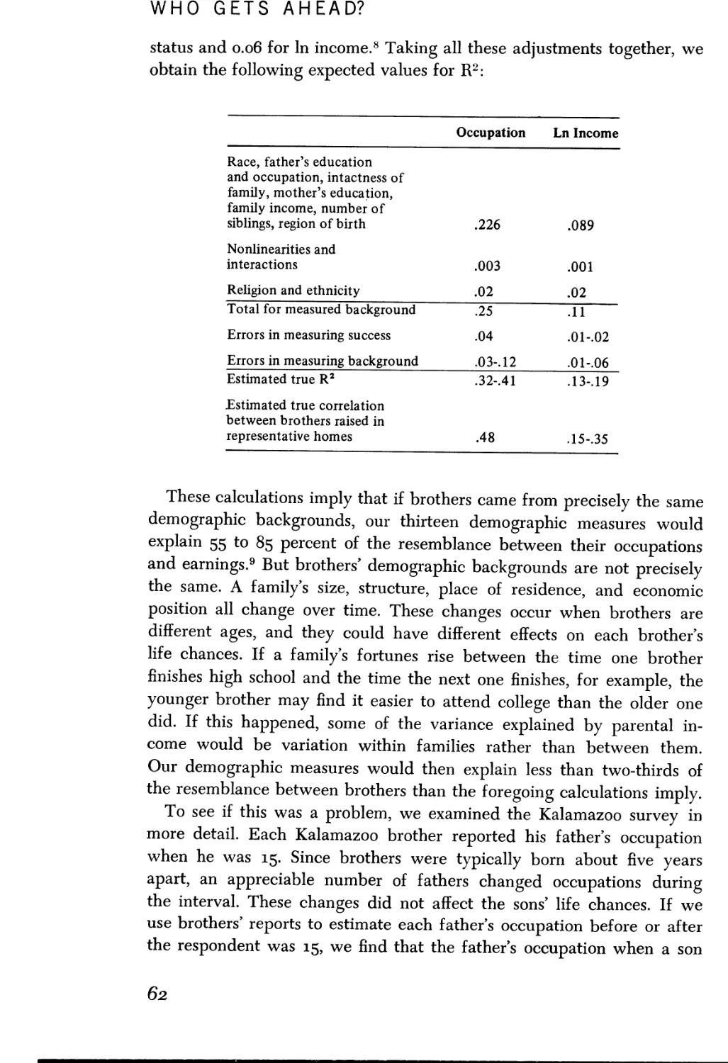
/


Text
characteristics, family
judgments about leader
ship ability, and, most
WHO GETS
AHEAD?
The Determinants of
Economic Success
in America
BY
CHRISTOPHER JENCKS
SUSAN BARTLETT - MARY CORCORAN
JAMES CROUSE - DAVID EAGLESFIELD
GREGORY JACKSON - KENT McCLELLAND
PETER MUESER - MICHAEL OLNECK
JOSEPH SCHWARTZ - SHERRY WARD
JILL WILLIAMS
=
Basic Books, Inc., Publishers New York
Library of Congress Cataloging in Publication Data
Jencks, Christopher.
Who gets ahead?
A revised version of The effects of family back-
ground, test scores, personality traits, and schooling
on economic success by C. Jencks and L. Rainwater
published by the National Technical Information Service,
1977.
Bibliography: p. 379
Includes index.
1. Success. 2. Education—Economic aspects—
United States. 3. Students’ Socio-economic status-—
United States. I. Title.
HF5386.]39 331.1 78—19809
ISBN: 0—465—09182-2
Copyright © 1979 by Basic Books, Inc.
Printed in the United States of America
DESIGNED BY VINCENT TORRE
10987654321
CONTENTS
LIST OF TABLES AND FIGURES oi
PREFACE xi
1. Introduction 3
2. Methods 17
3. The Efiects of Family Background 50
4 The Eflects of Academic Ability 85
5. The Eflects of Noncognitive Traits 122
6 The Eflects of Education 159
7 The Efiects of Race on Earnings 191
8 Who Gets Ahead: A Summary 213
9 Individual Earnings and Family Income 231
10. Do Difierent Surveys Yield Similar Results? 251
11. The Effects of Research Style 271
12. Who Gets Ahead? and Inequality: A Comparison 290
APPENDIX OF SUPPLEMENTARY TABLES 312
NOTES 365
BIBLIOGRAPHY 379
INDEX 389
1.1
2.1
3.1
3.2
3.3
4.1
4.2
4.3
4.4
4.5
4.6
4.7
4.8
5.1
5.2
5.3
vi
TABLES AND FIGURES
Characteristics of Subsamples from Eleven Surveys
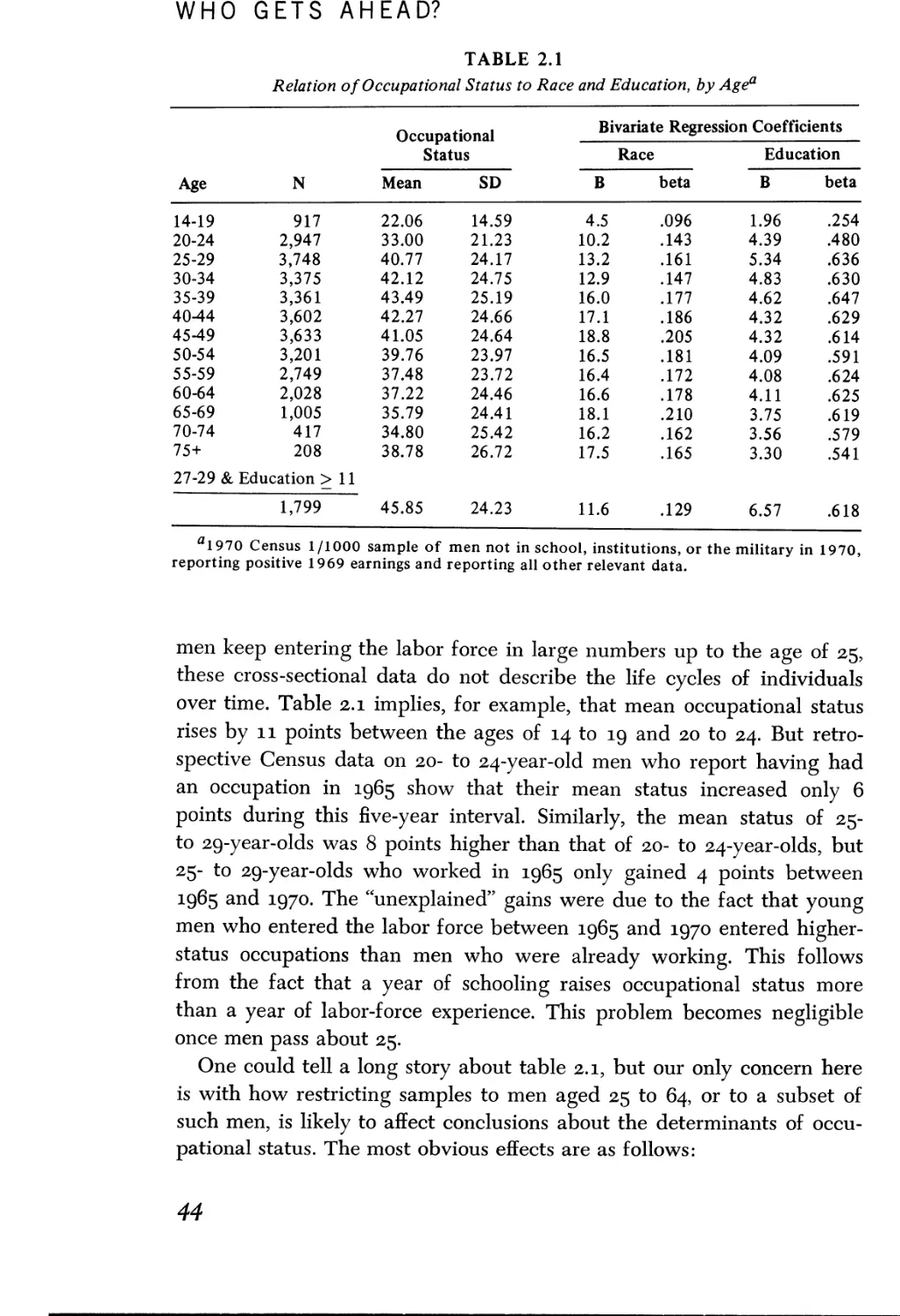
Relation of Occupational Status to Race and
Education, by Age
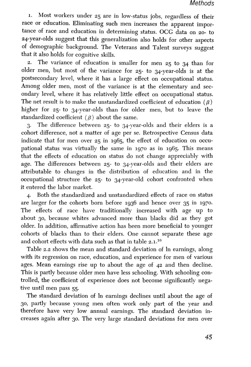
Relation of Ln Earnings to Race, Education, and
Experience, by Age
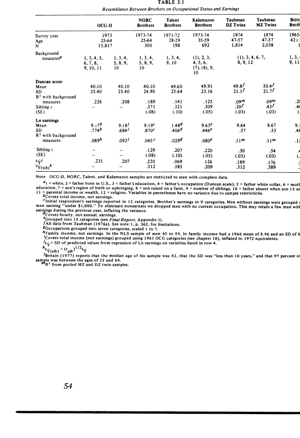
Resemblance Between Brothers on Occupational Status
and Earnings
Estimated Correlations Among Sets of Background
Characteristics Influencing Different Outcomes
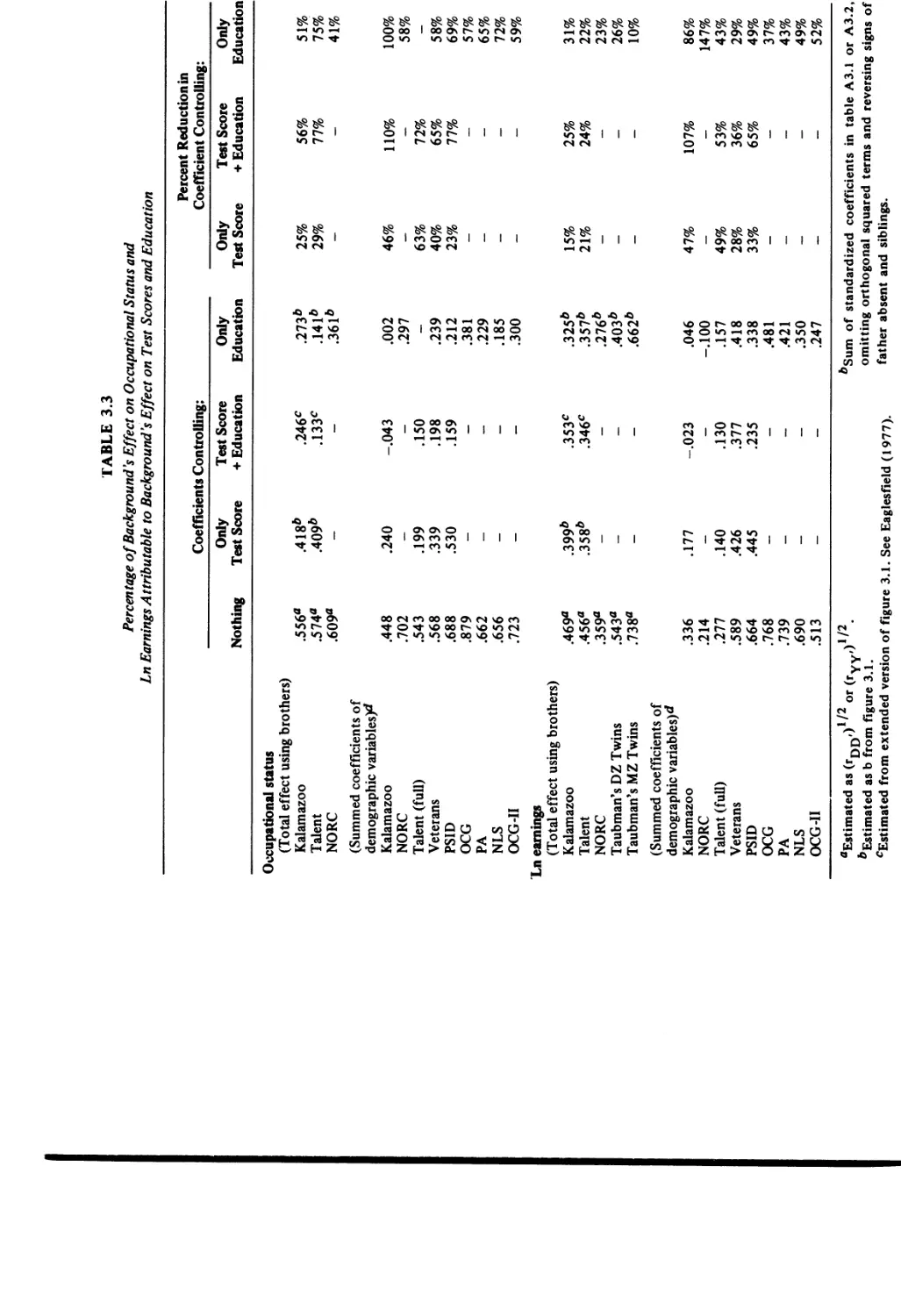
Percentage of Background’s Effect on Occupational
Status and Ln Earnings Attributable to Background’s
Effect on Test Scores and Education
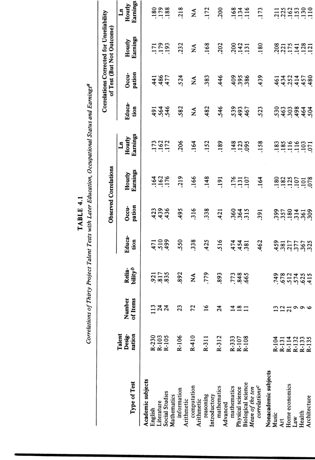
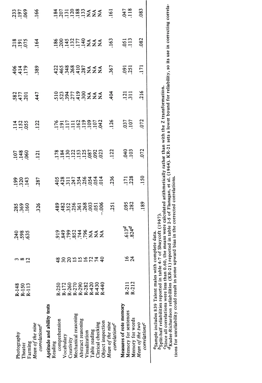
Correlations of Thirty Project Talent Tests with
Later Education, Occupational Status, and Earnings
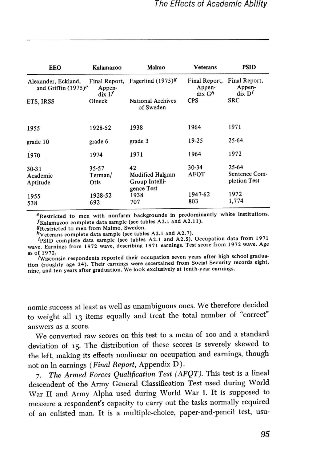
Characteristics of Longitudinal Surveys That
Collected Test Scores
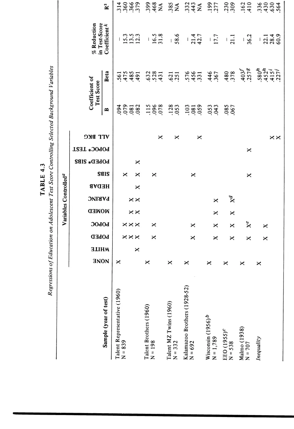
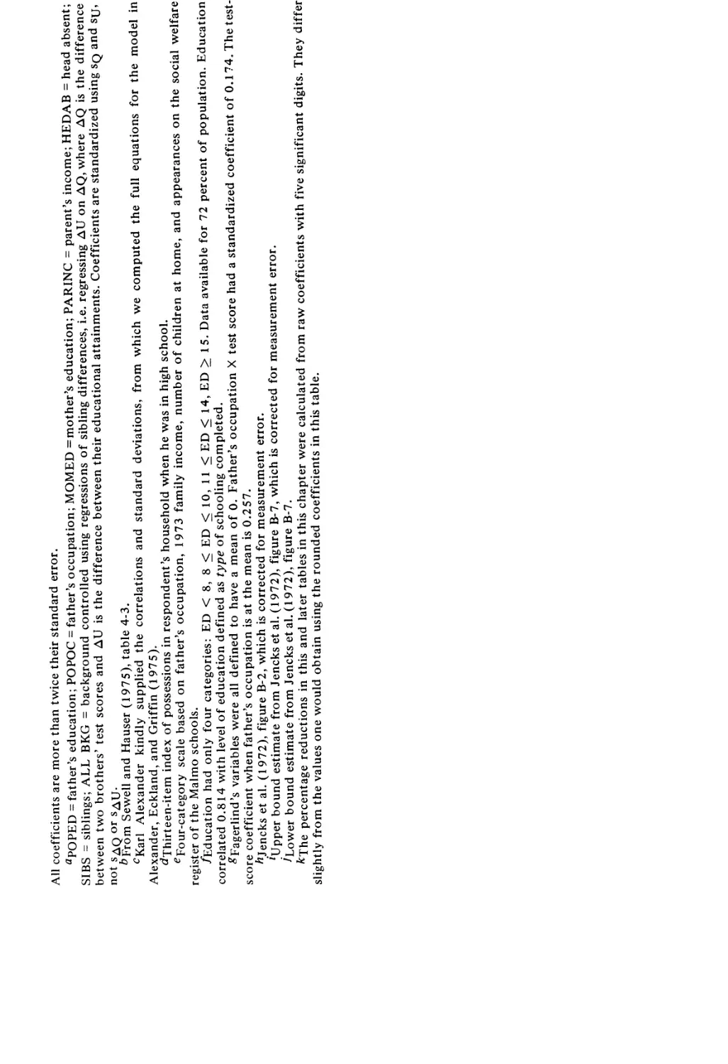
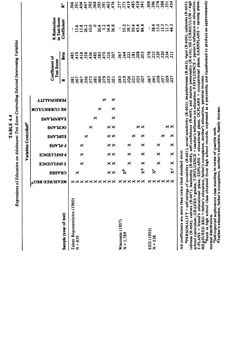
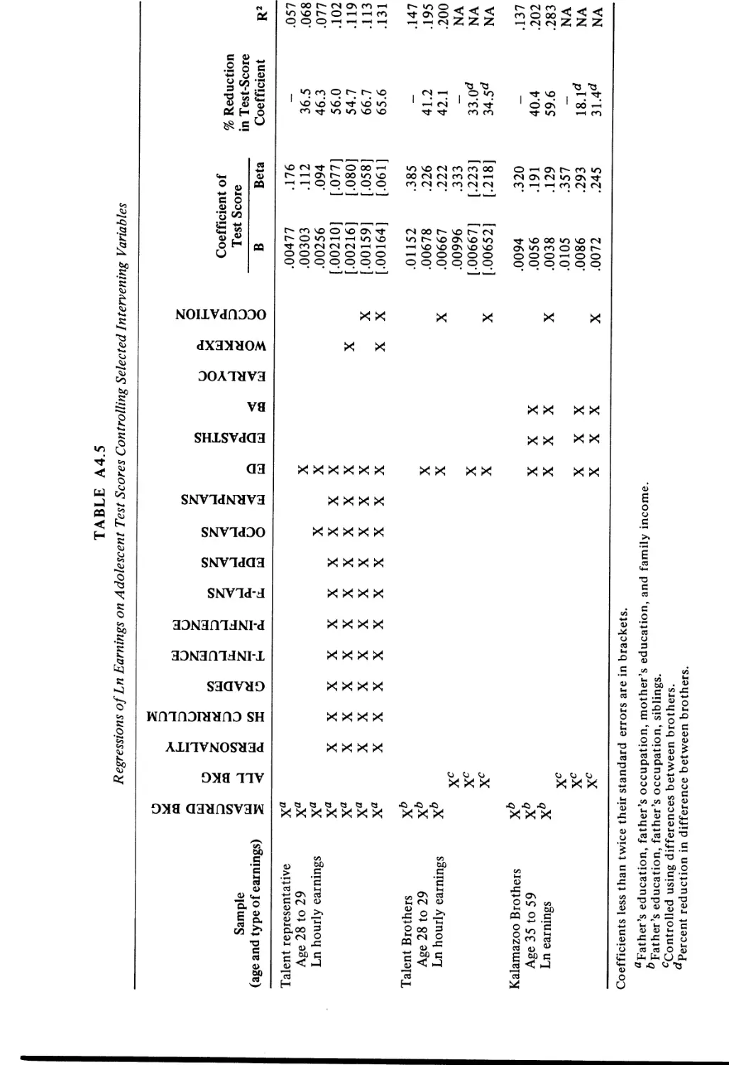
Regressions of Education on Adolescent Test Score
Controlling Selected Background Variables
Regressions of Education on Adolescent Test Score
Controlling Selected Intervening Variables
Regressions of Occupational Status on Adolescent Test
Score Controlling Selected Background Variables
Regressions of Occupational Status on Adolescent Test
Score Controlling Selected Intervening Variables
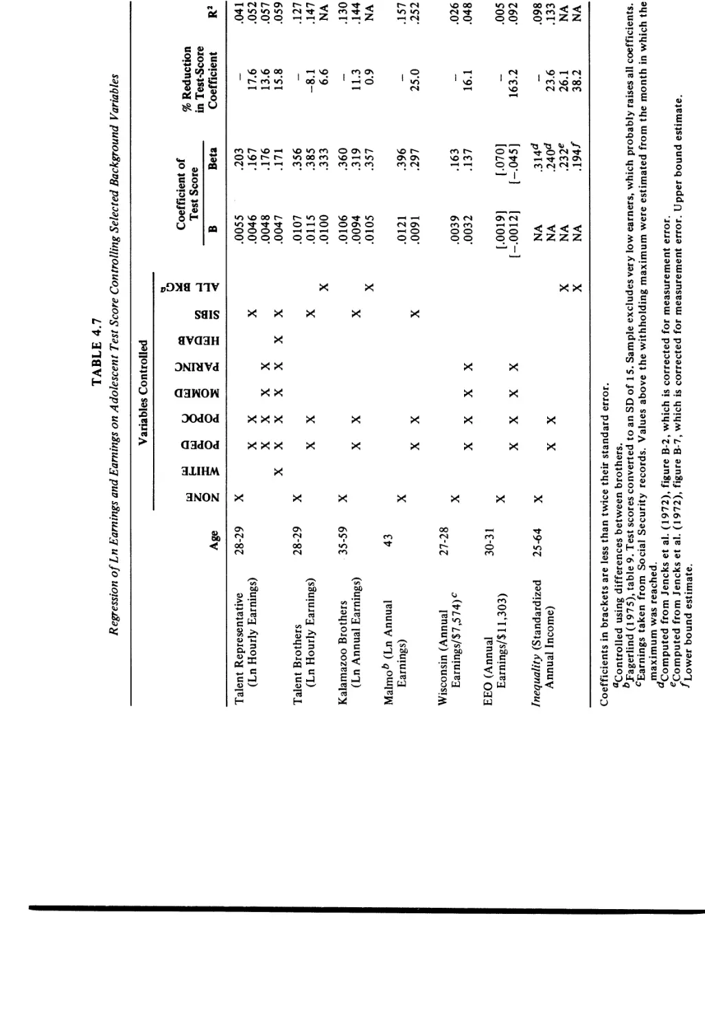
Regressions of Ln Earnings and Earnings on Adolescent
Test Score Controlling Selected Background Variables
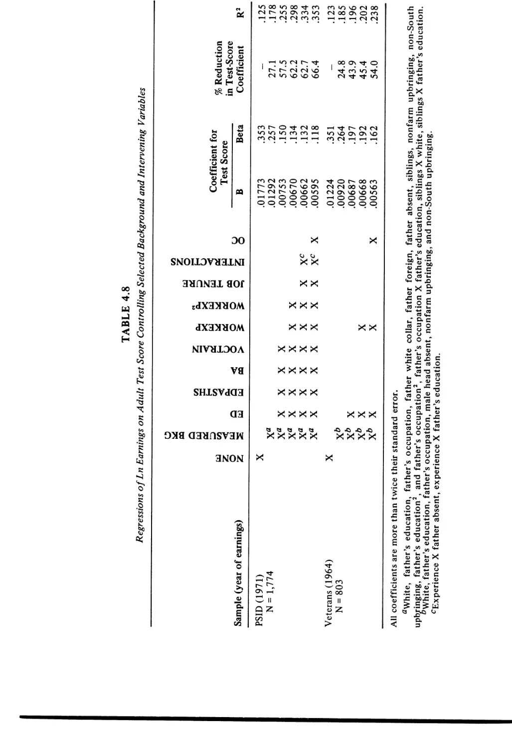
Regressions of Ln Earnings on Adult Test Score Con-
trolling Selected Background and Intervening Variables
Selected Questions from the Ten Talent Personality
Self-Assessment Scales
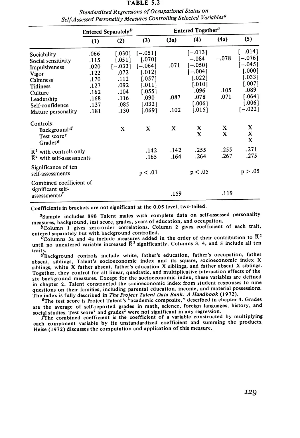
Standardized Regressions of Occupational Status on
Self-Assessed Personality Measures Controlling
Selected Variables
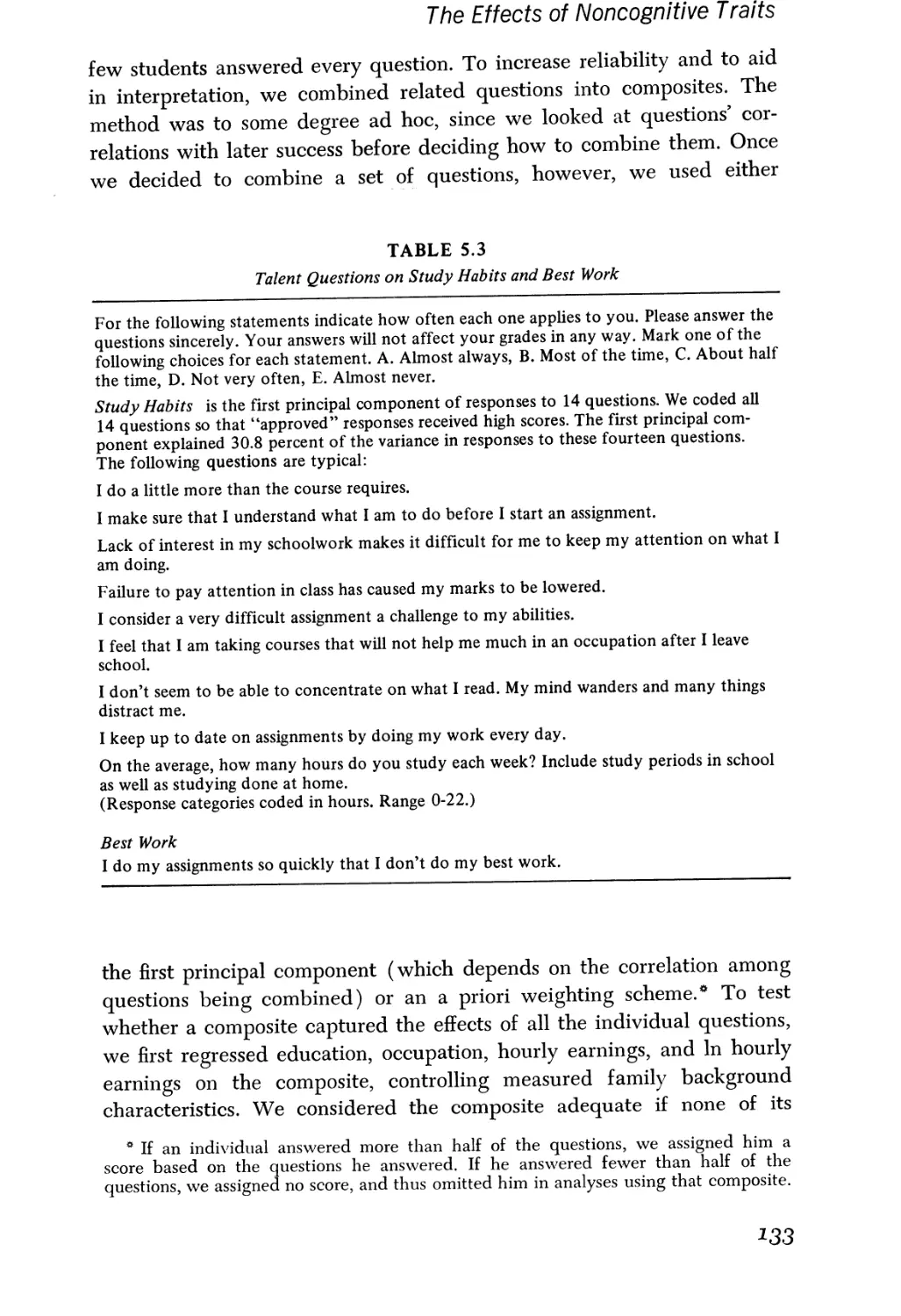
Talent Questions on Study Habits and Best Work
74
88
94
102
107
111
113
116
118
127
129
133
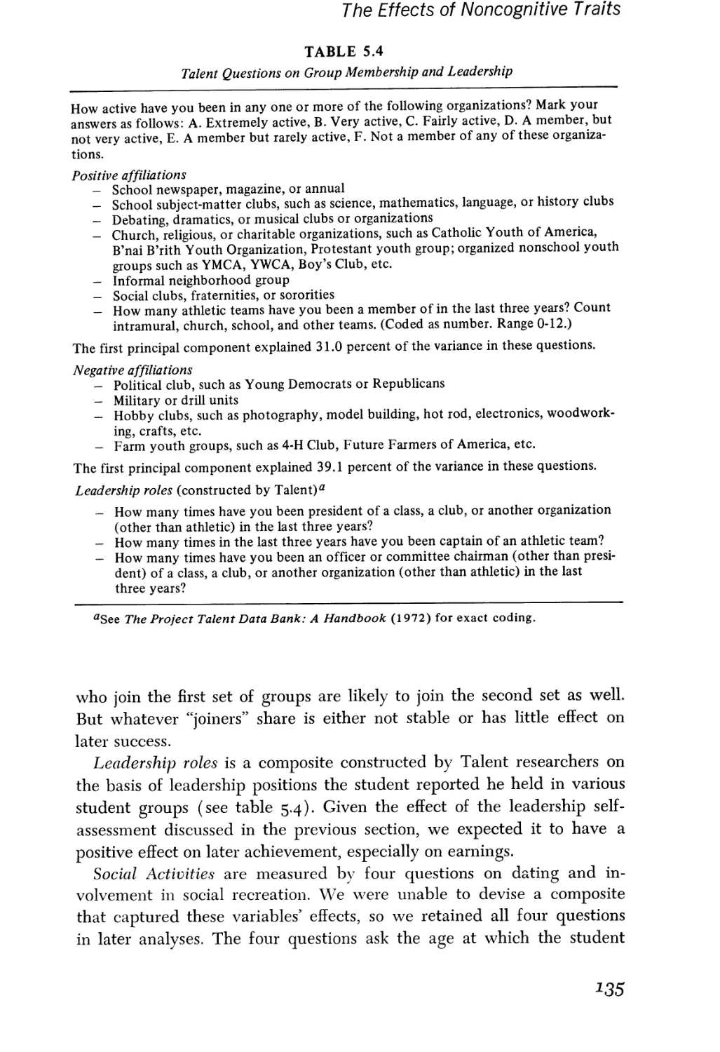
5.4 Talent Questions on Group Membership and Leadership
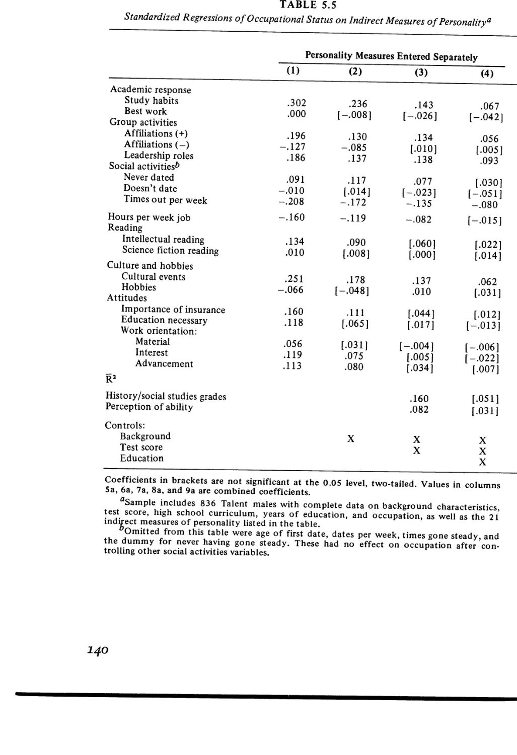
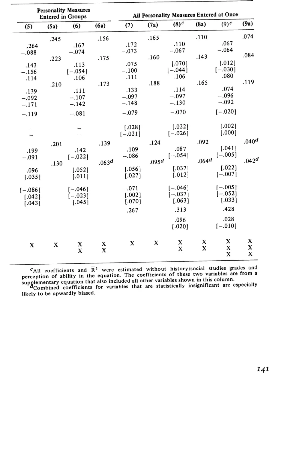
5.5
5.6
5.7
5.8
5.9
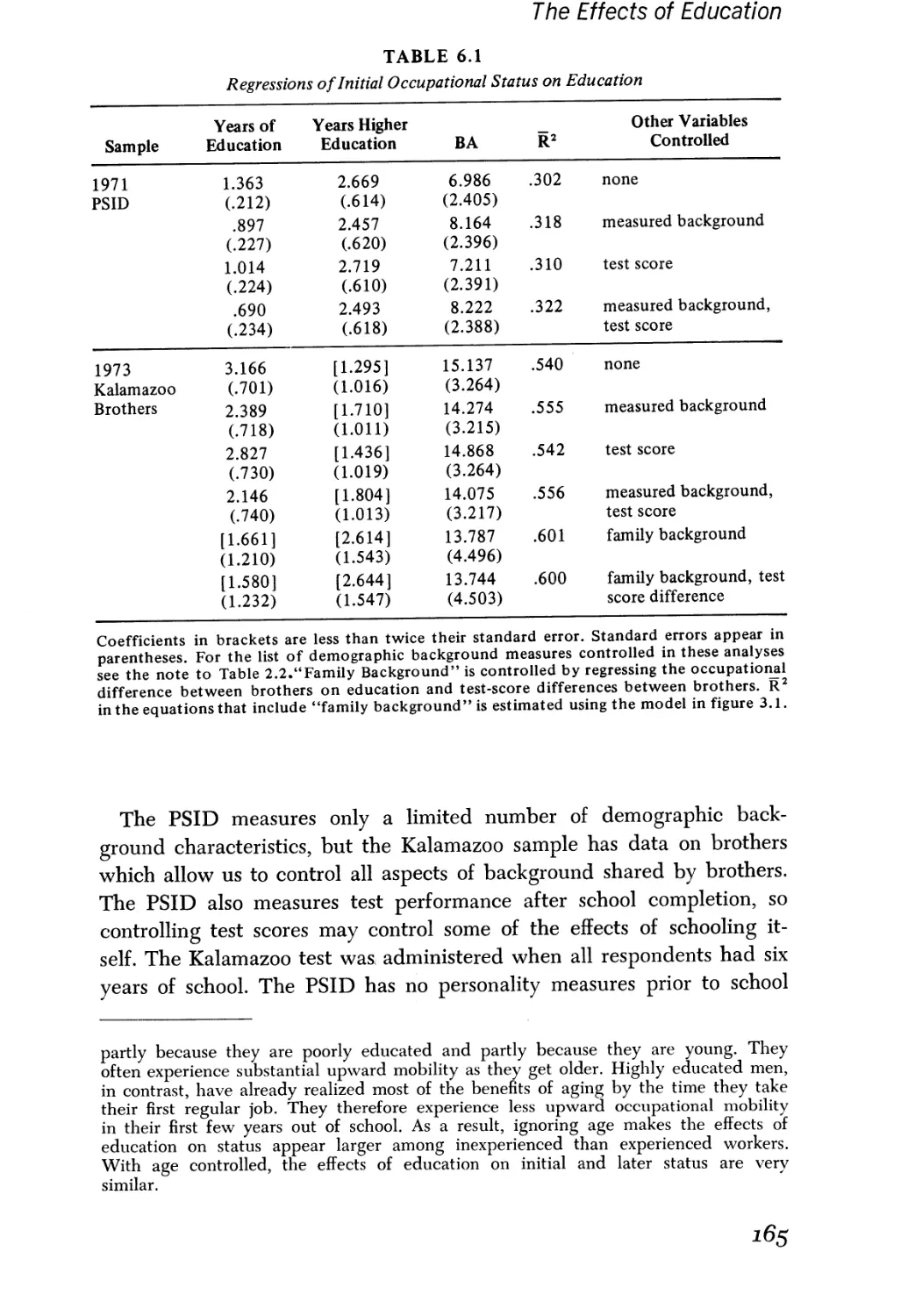
6.1
6.2
6.3
6.4
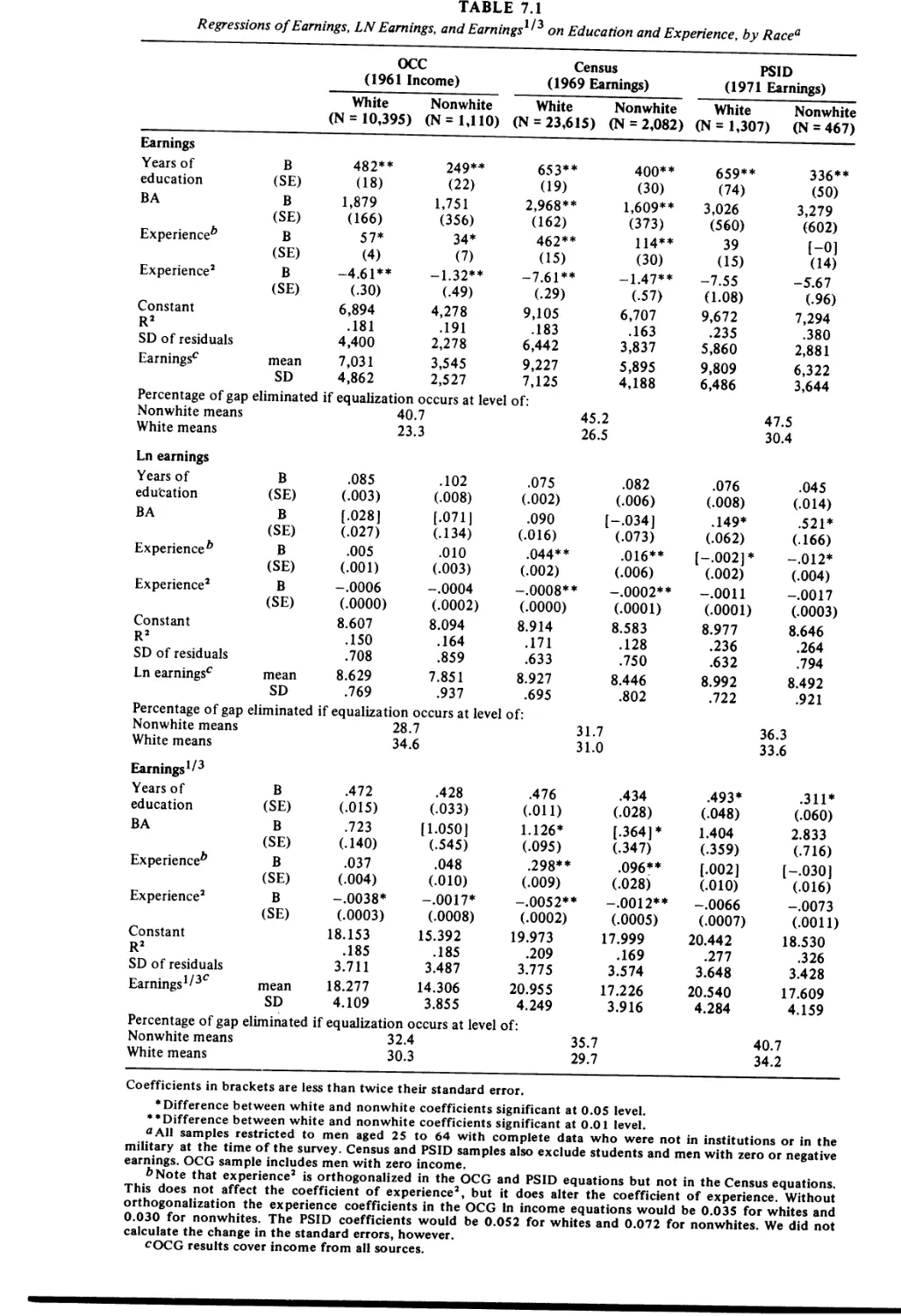
7.1
7.2
7.3
9.1
9.2
9.3
9.4
10.1
10.2
Tables and Figures
Standardized Regressions of Occupational Status on
Indirect Measures of Personality
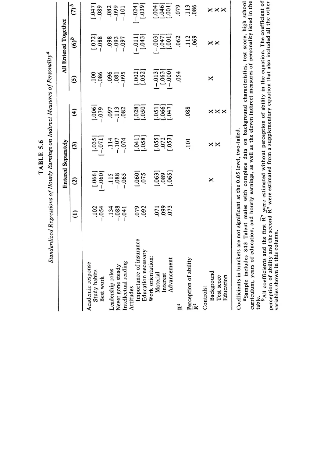
Standardized Regressions of Hourly Earnings on
Indirect Measures of Personality
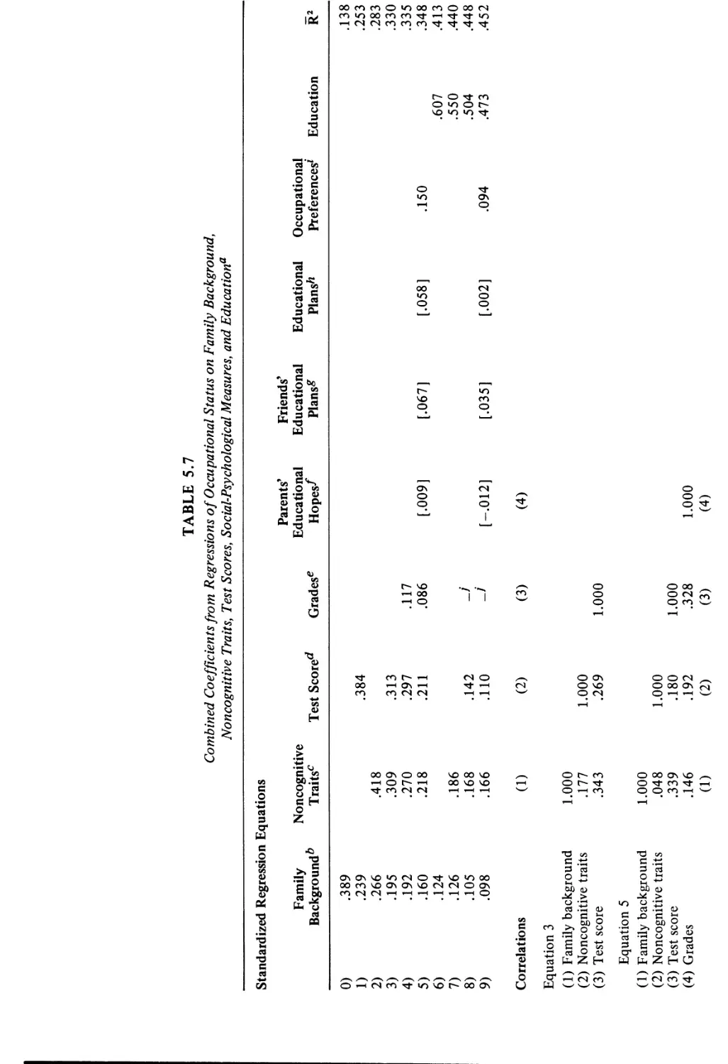
Combined Coefficients from Regressions of Occupational
Status on Family Background, Noncognitive Traits, Test
Scores, Social-Psychological Measures, and Education
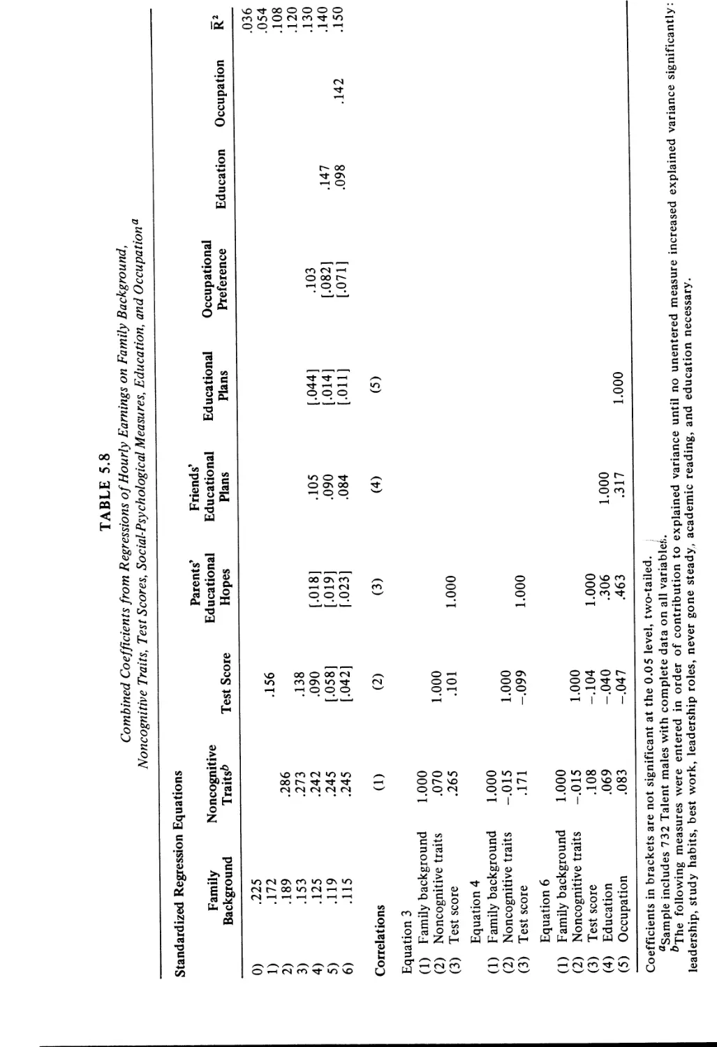
Combined Coefficients from Regressions of Hourly
Earnings on Family Background, Noncognitive Traits,
Test Scores, Social—Psychological Measures,
Education, and Occupation
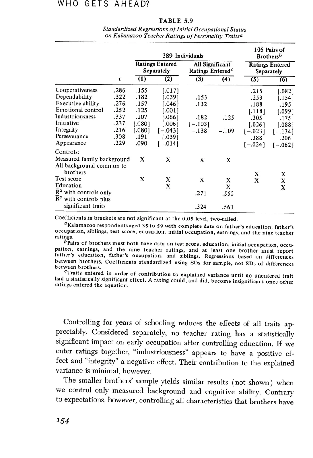
Standardized Regressions of Initial Occupational Status
on Kalamazoo Teacher Ratings of Personality Traits
Regressions of Initial Occupational Status on
Education
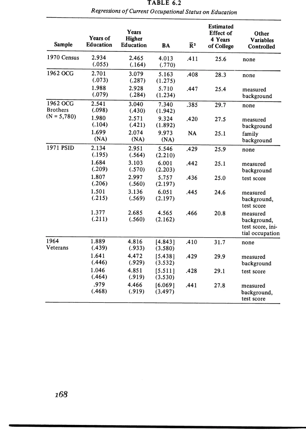
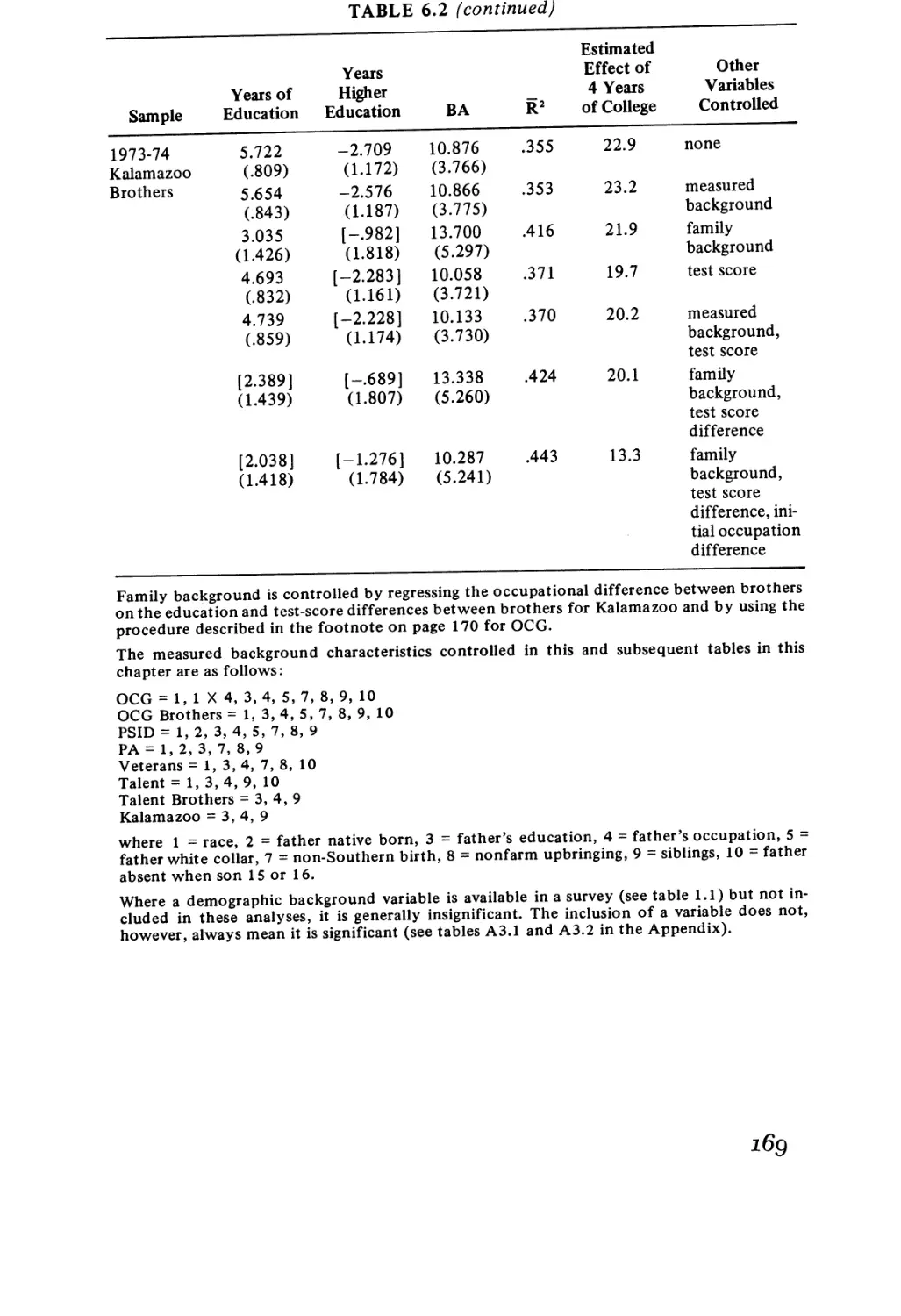
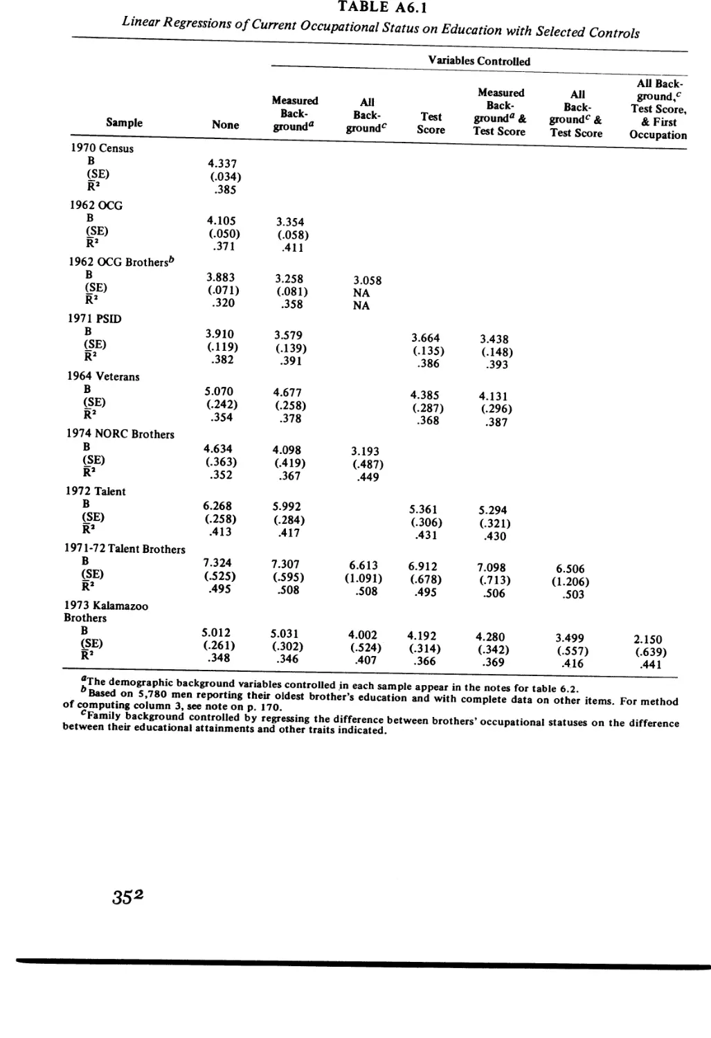
Regressions of Current Occupational Status on
Education
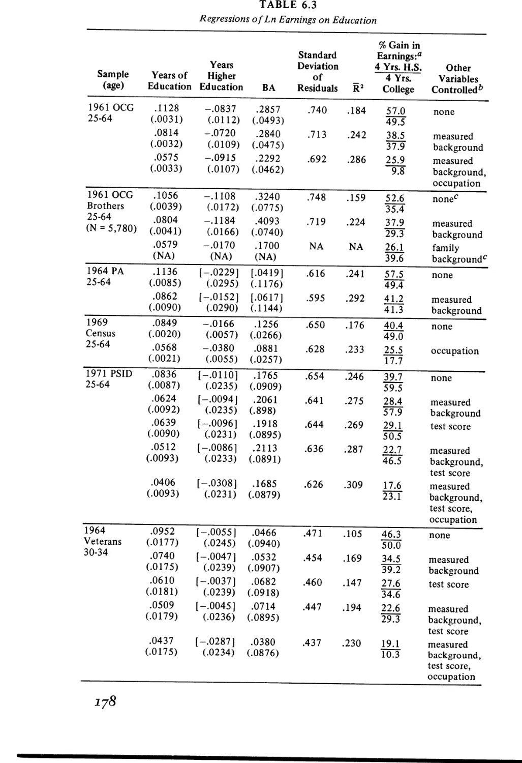
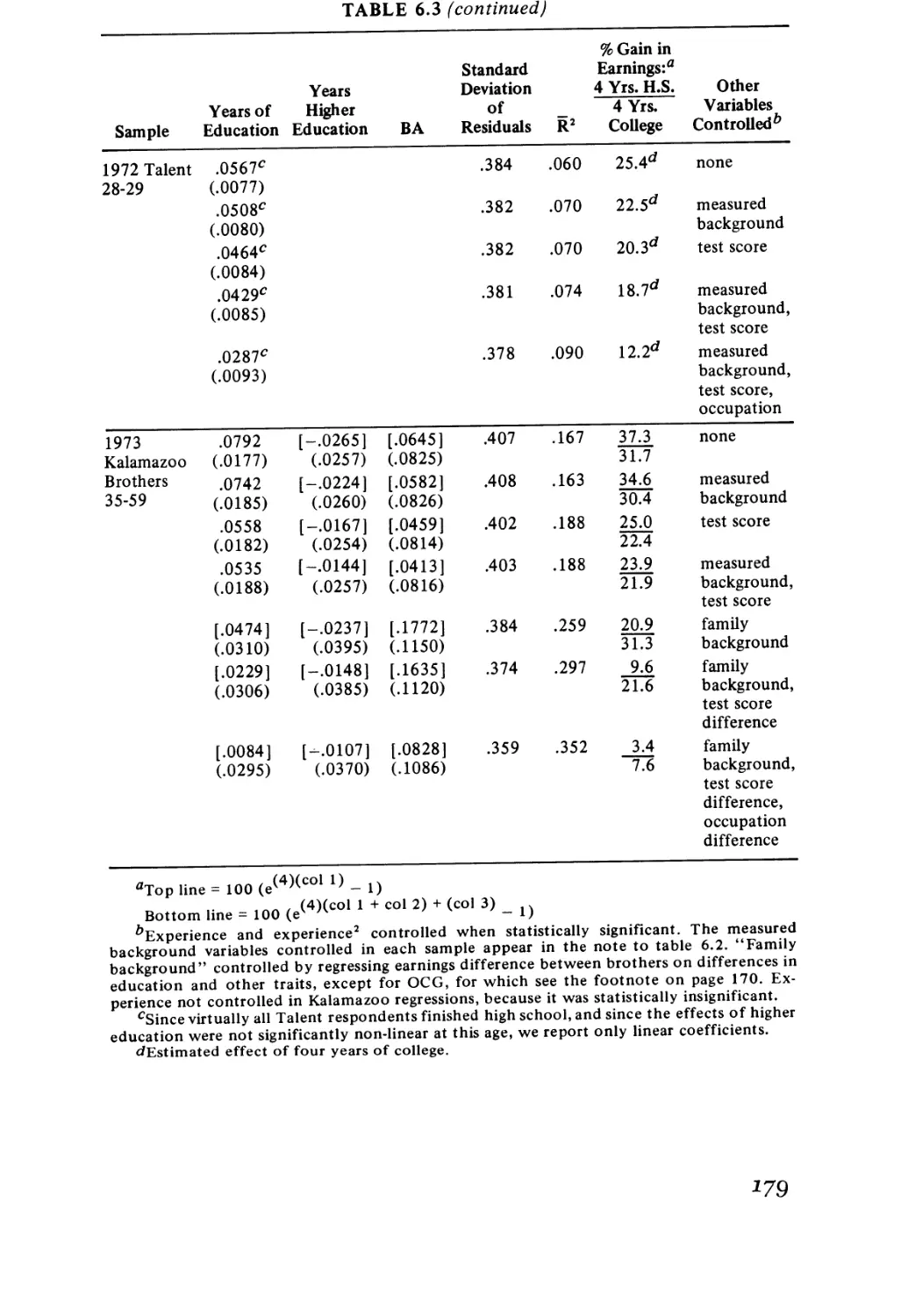
Regressions of Ln Earnings on Education
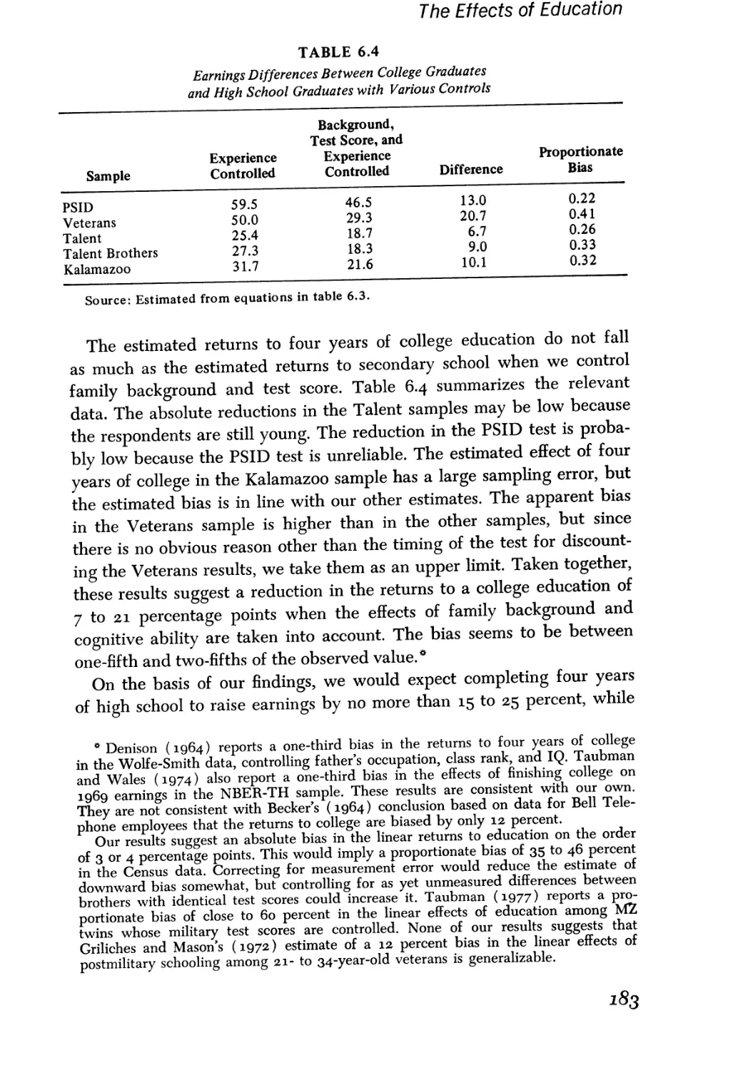
Earnings Differences Between College Graduates and
High School Graduates with Various Controls
Regressions of Earnings, Ln Earnings, and Earnings ”3
on Education and Experience, by Race
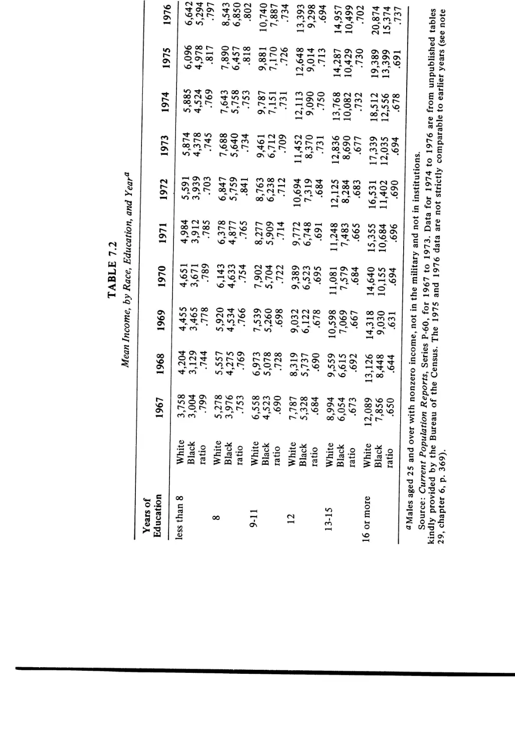
Mean Income, by Race, Education, and Year
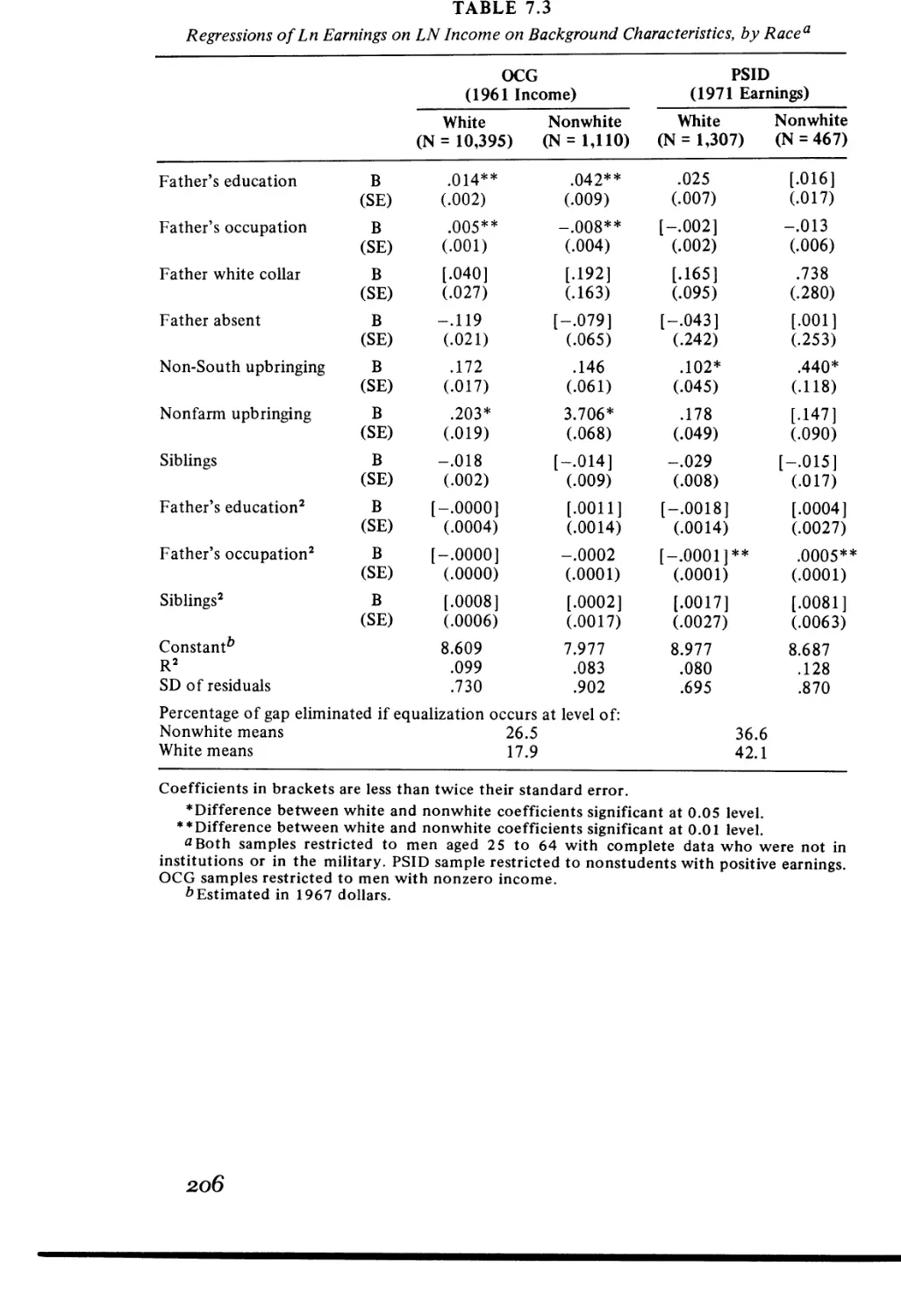
Regressions of Ln Earnings or Ln Income on
Background Characteristics, by Race
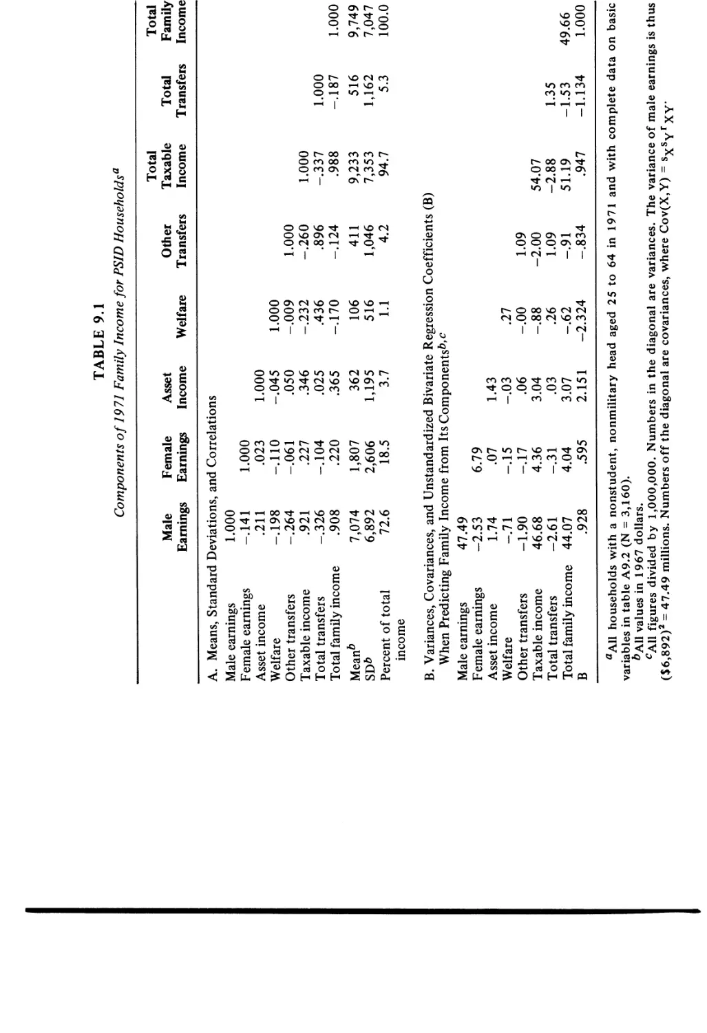
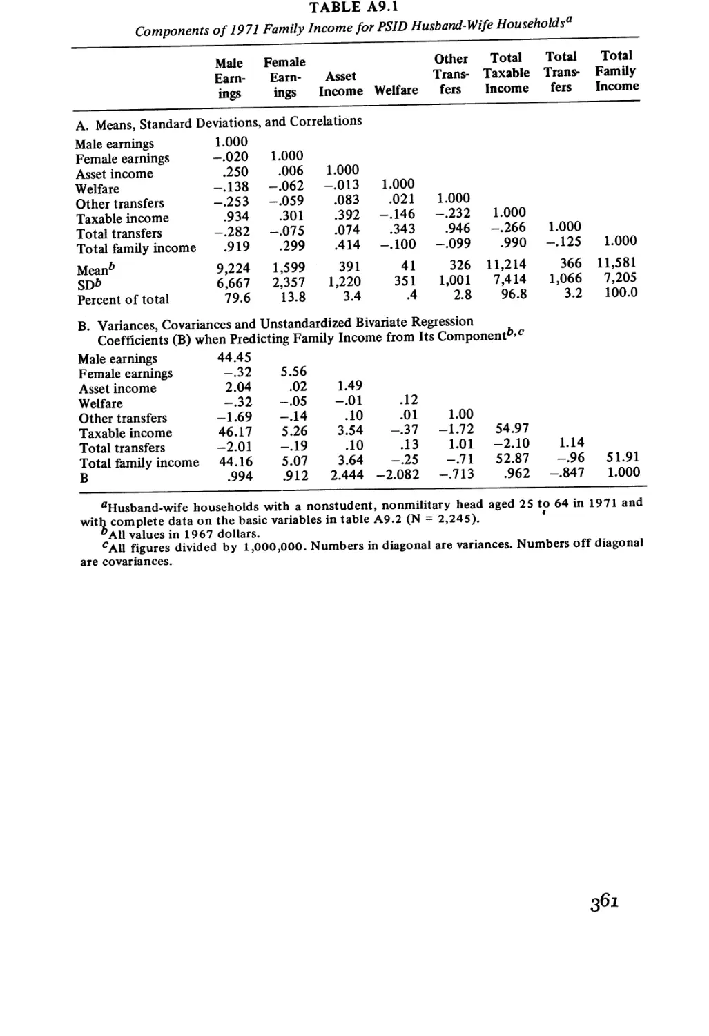
Components of 1971 Family Income for PSID
Households
Correlations Among PSID Husbands’ and Wives’
1971 Wages, Hours, and Earnings
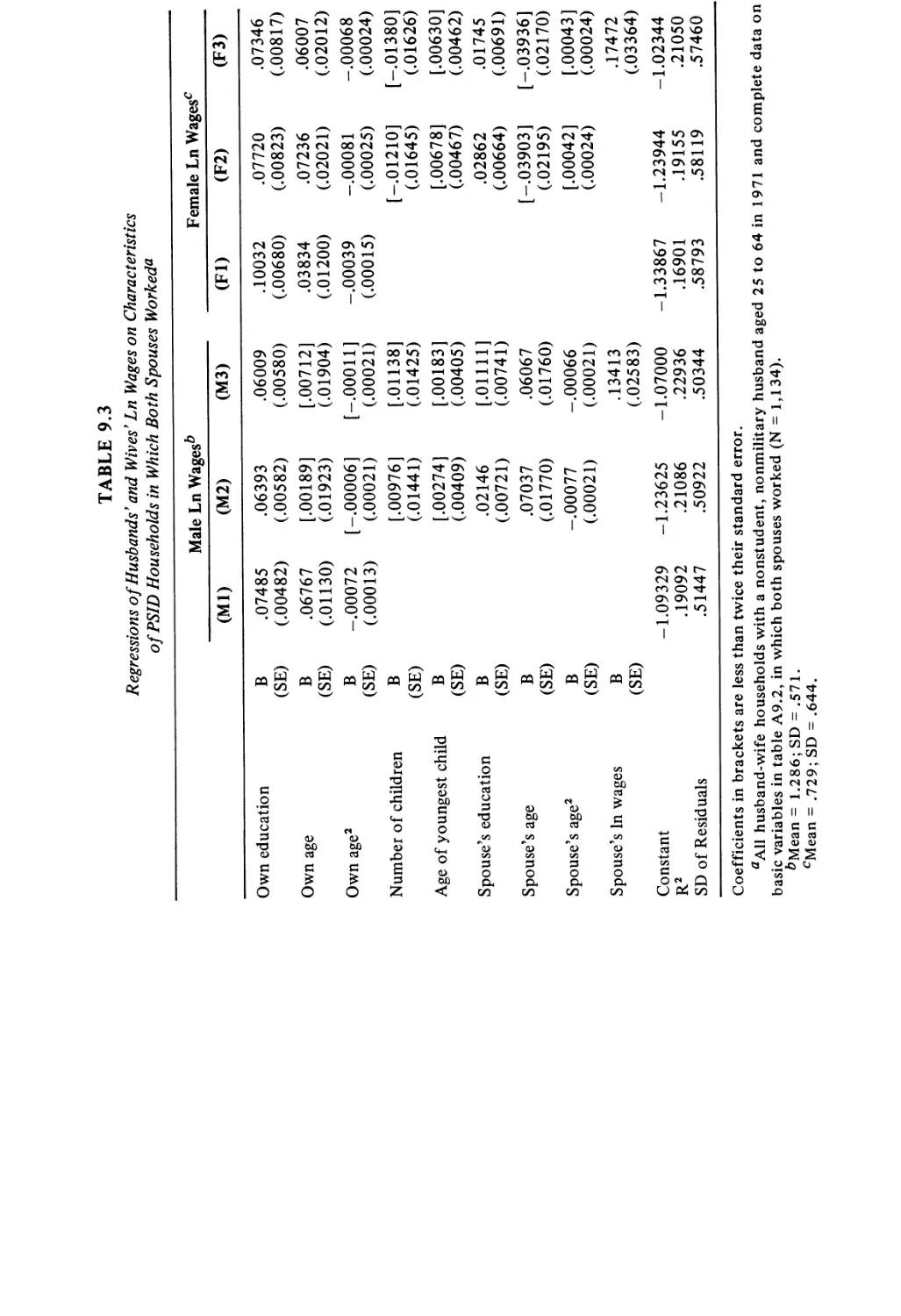
Regressions of Husbands’ and Wives’ Ln Wages on
Characteristics of PSID Households in Which Both
Spouses Worked
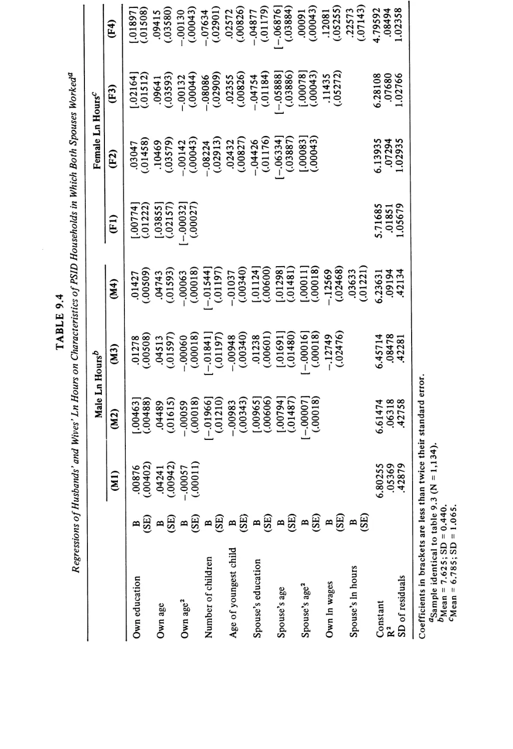
Regressions of Husbands’ and Wives’ Ln Hours on
Characteristics of PSID Households in Which Both
Spouses Worked
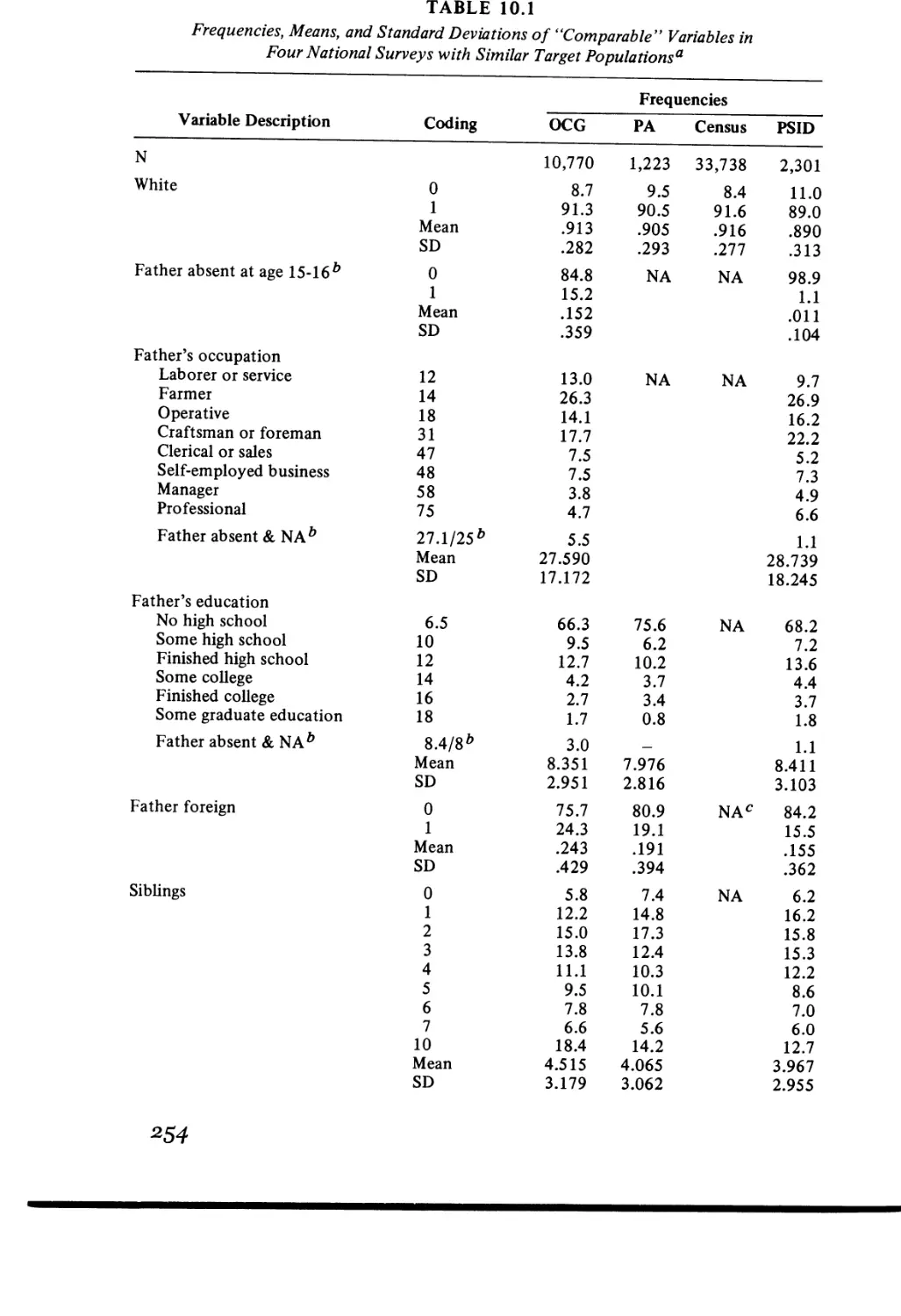
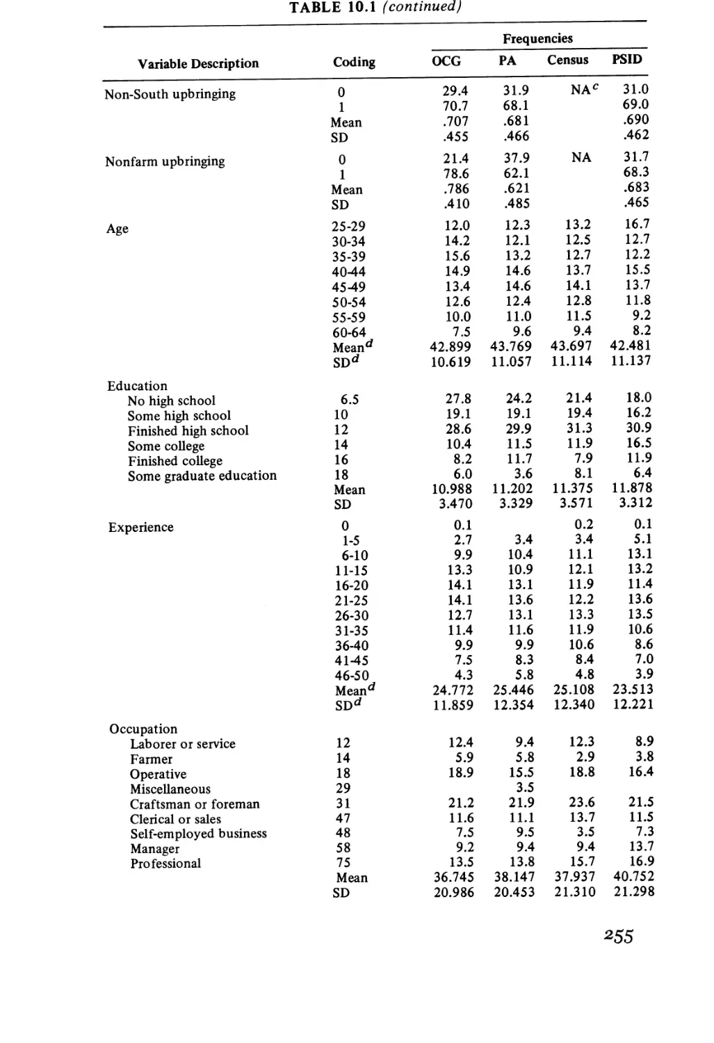
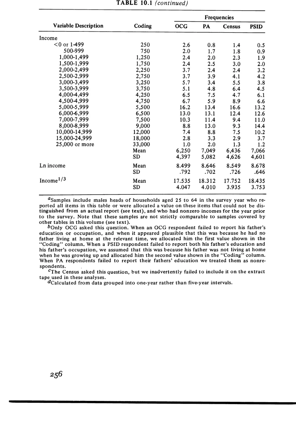
Frequencies, Means, and Standard Deviations of
“Comparable” Variables in Four National Surveys with
Similar Target Populations
Means and Standard Deviations of Education, Occupa-
tional Status, and Income, by Father’s Occupation
135
140
143
148
154
165
168
178
183
194
' zoo
206
234
238
241
243
254
262
vii
Tables and Figures
10.3
10.4
10.5
10.6
11.1
11.2
11.3
11.4
11.5
3.1
9.1
A2.1
A22
A23
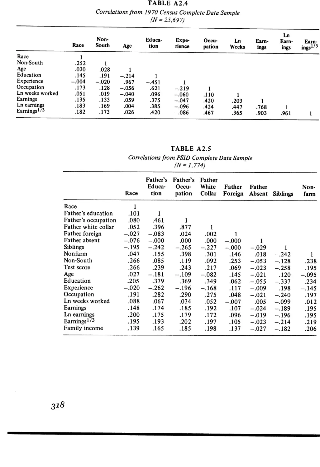
A24
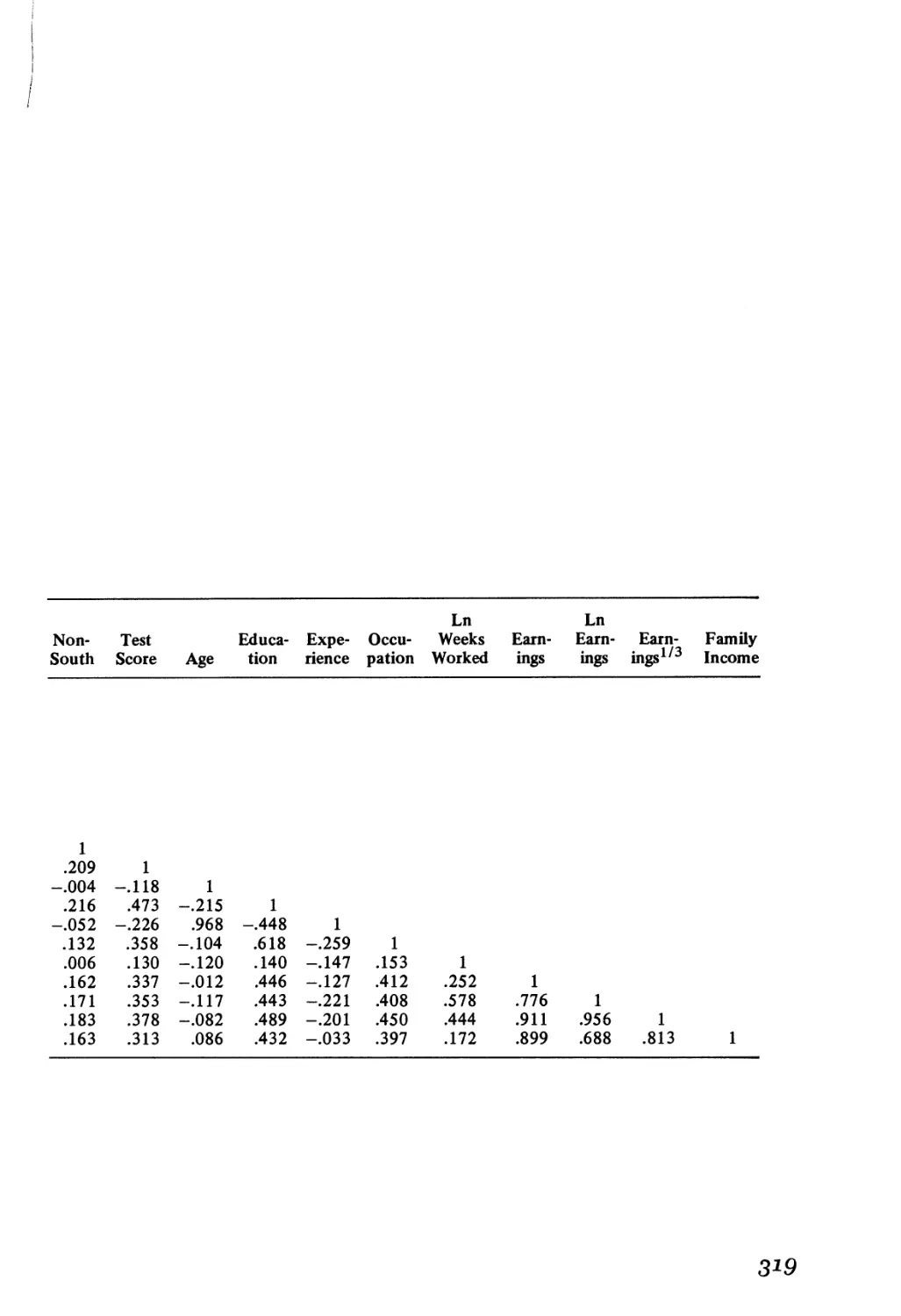
A25
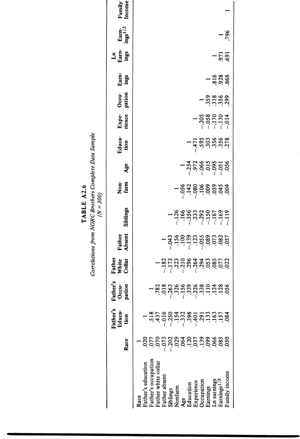
A26
viii
Means and Standard Deviations of Education, Occupa-
tional Status, and Income, by F ather’s Education
Means and Standard Deviations of Education, Occupa-
tional Status, and Income, by Number of Siblings
Means and Standard Deviations of Occupational Status
and Income, by Education
Means and Standard Deviations of Income (1961
Equivalent), by Occupation
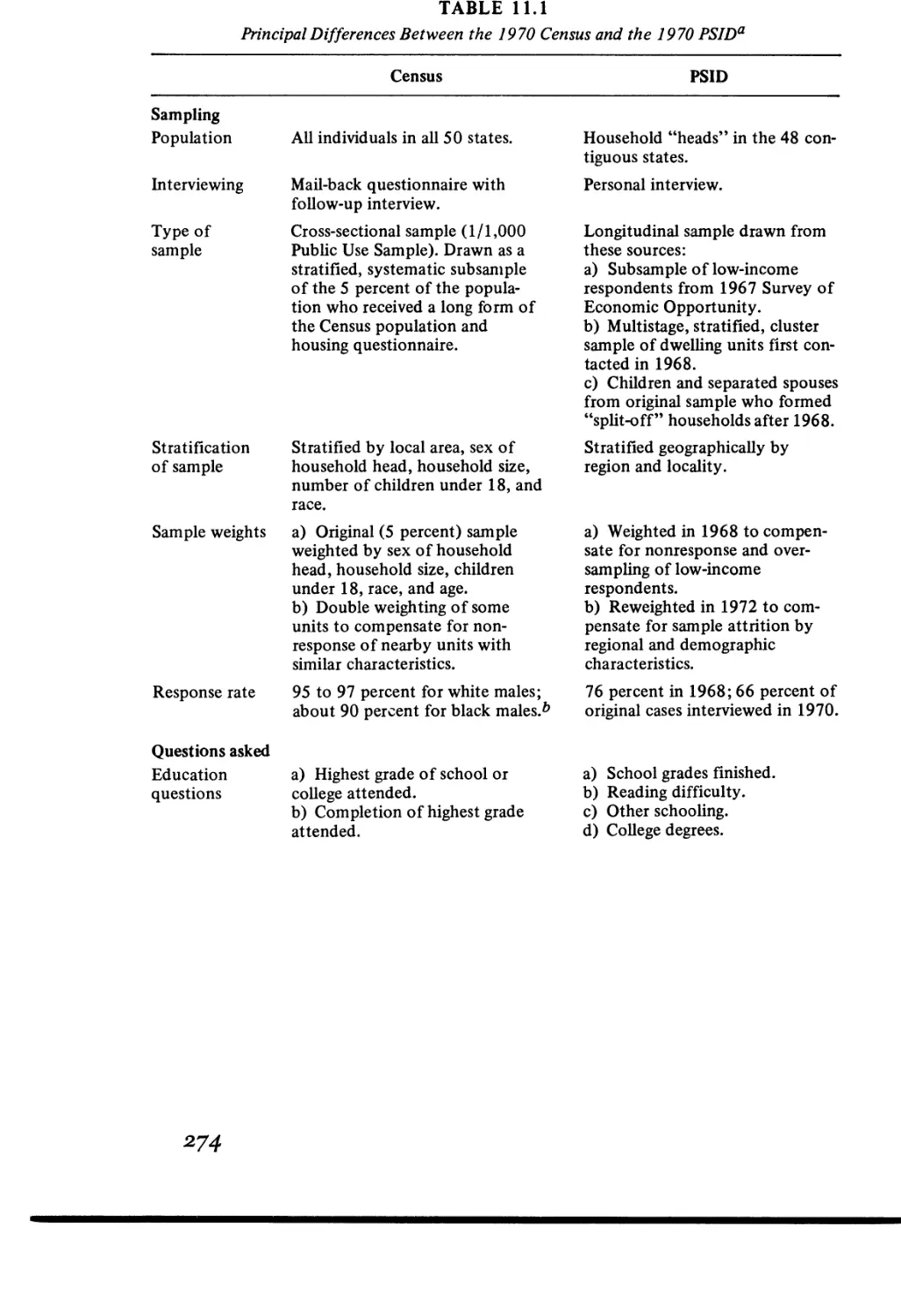
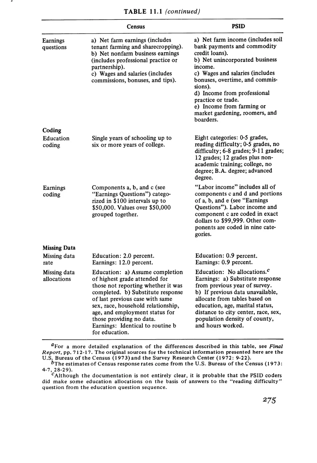
Principal Differences Between the 1970 Census and the
1970 PSID
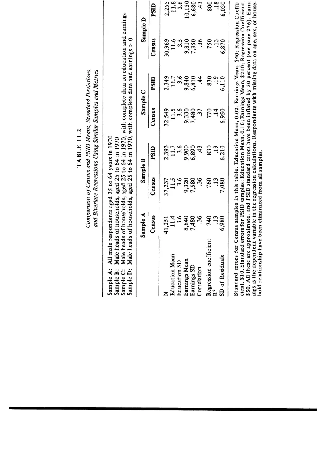
Comparison of Census and PSID Means, Standard
Deviations, and Bivariate Regressions, Using Similar
Samples and Metrics
Effects of Nonearners on Means, Standard Deviations,
and Bivariate Regressions of Ln Earnings on Years of
Education
Means, Standard Deviations, and Bivariate Regressions
of Earnings and of Grouped and Ungrouped Income on
Years of Education
Means, Standard Deviations, and Bivariate Regressions
of Ln Earnings and of Grouped and Ungrouped Ln
Income on Years of Education
FIGURES
Family Effects on Test Scores (Q) and Earnings (Y)
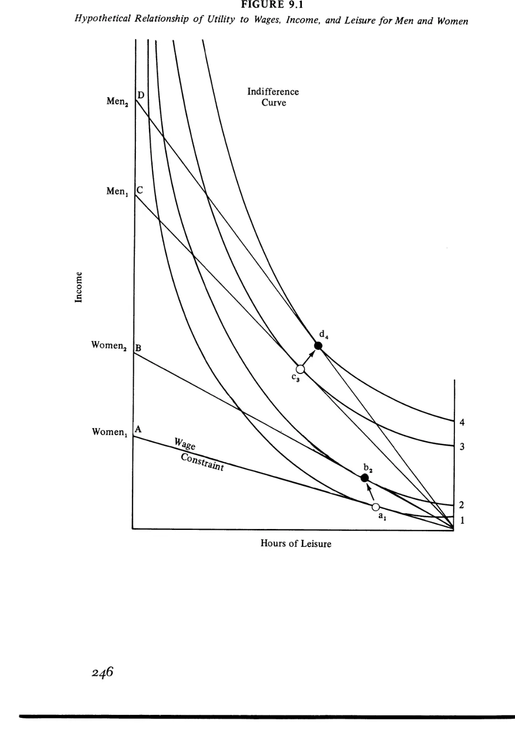
Hypothetical Relationship of Utility to Wages,
Income, and Leisure
APPENDIX TABLES
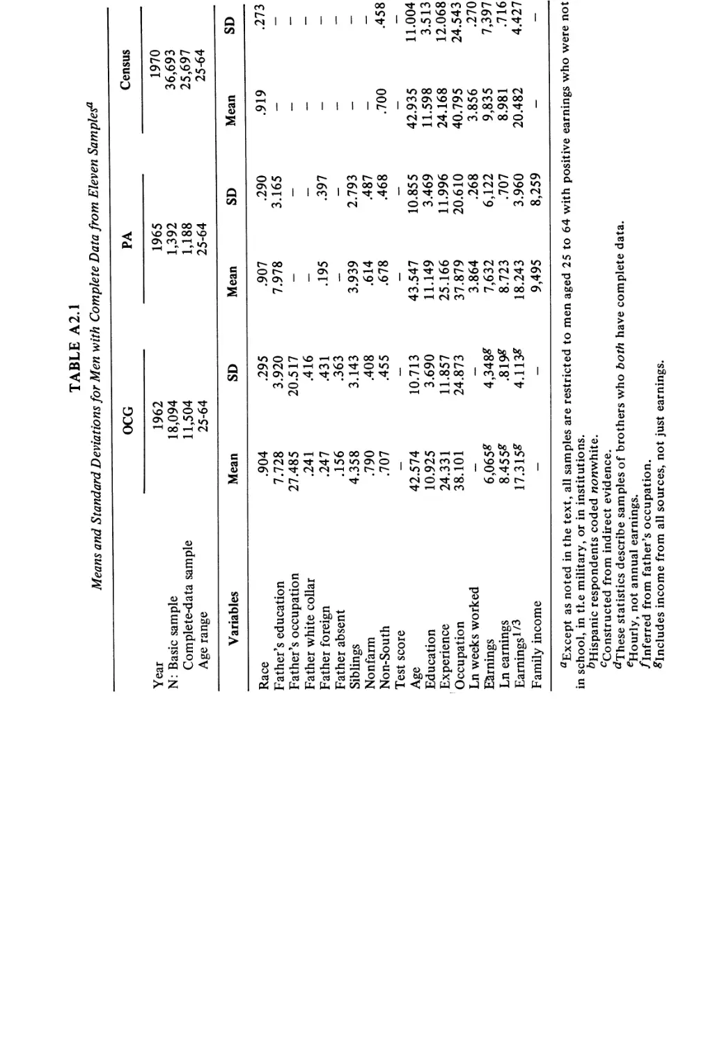
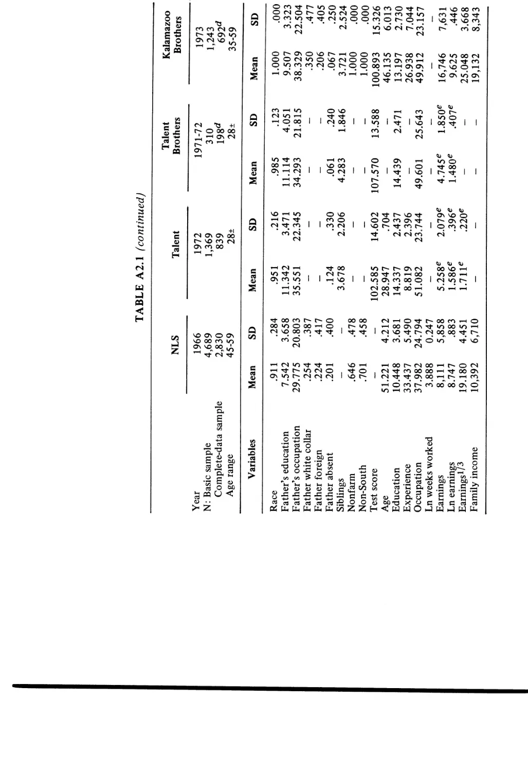
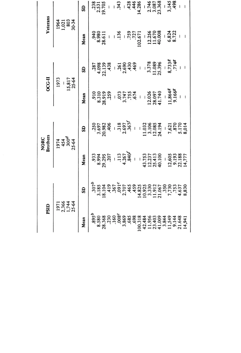
Means and Standard Deviations for Men with
Complete Data from Eleven Samples
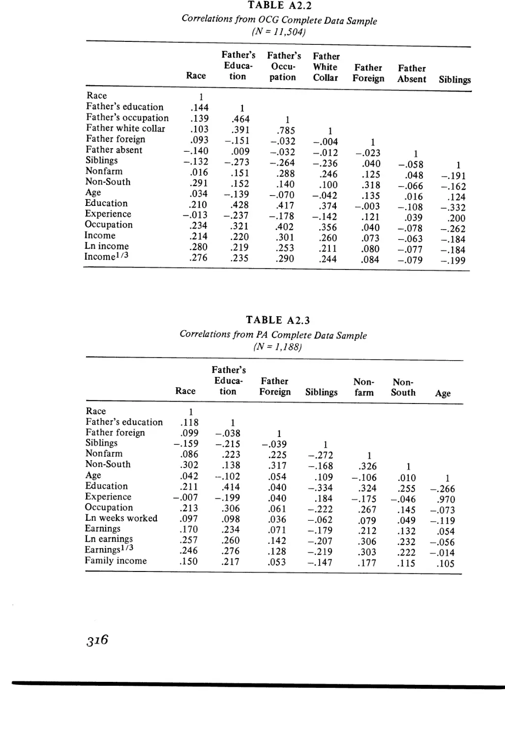
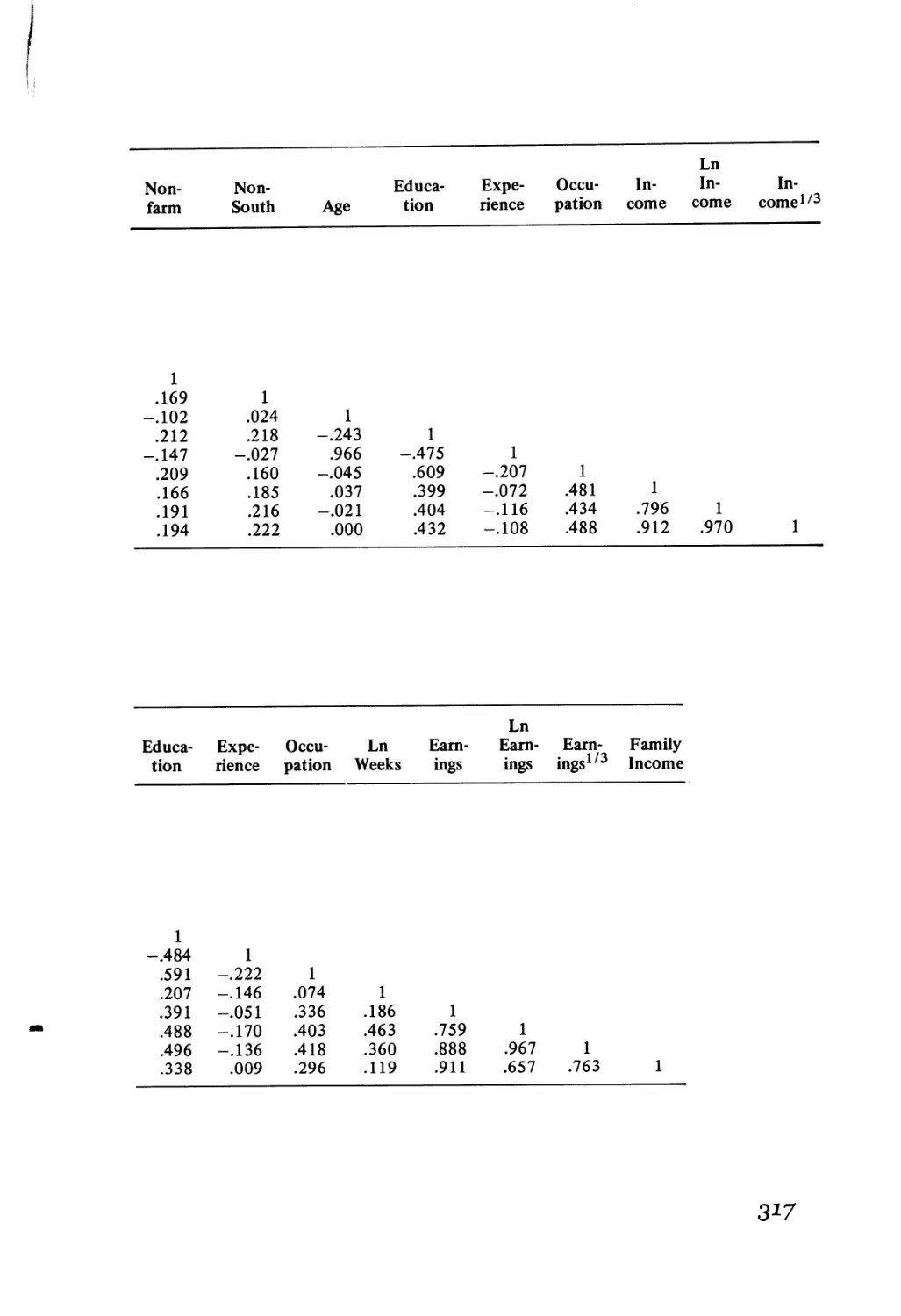
Correlations from OCG Complete Data Sample
Correlations from PA Complete Data Sample
Correlations from 1970 Census Complete Data Sample
Correlations from PSID Complete Data Sample
Correlations from NORC Brothers Complete Data
Sample
264
266
267
268
274
278
28';
L
285
286
72
246
312
Tables and Figures
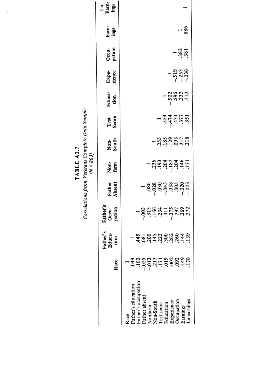
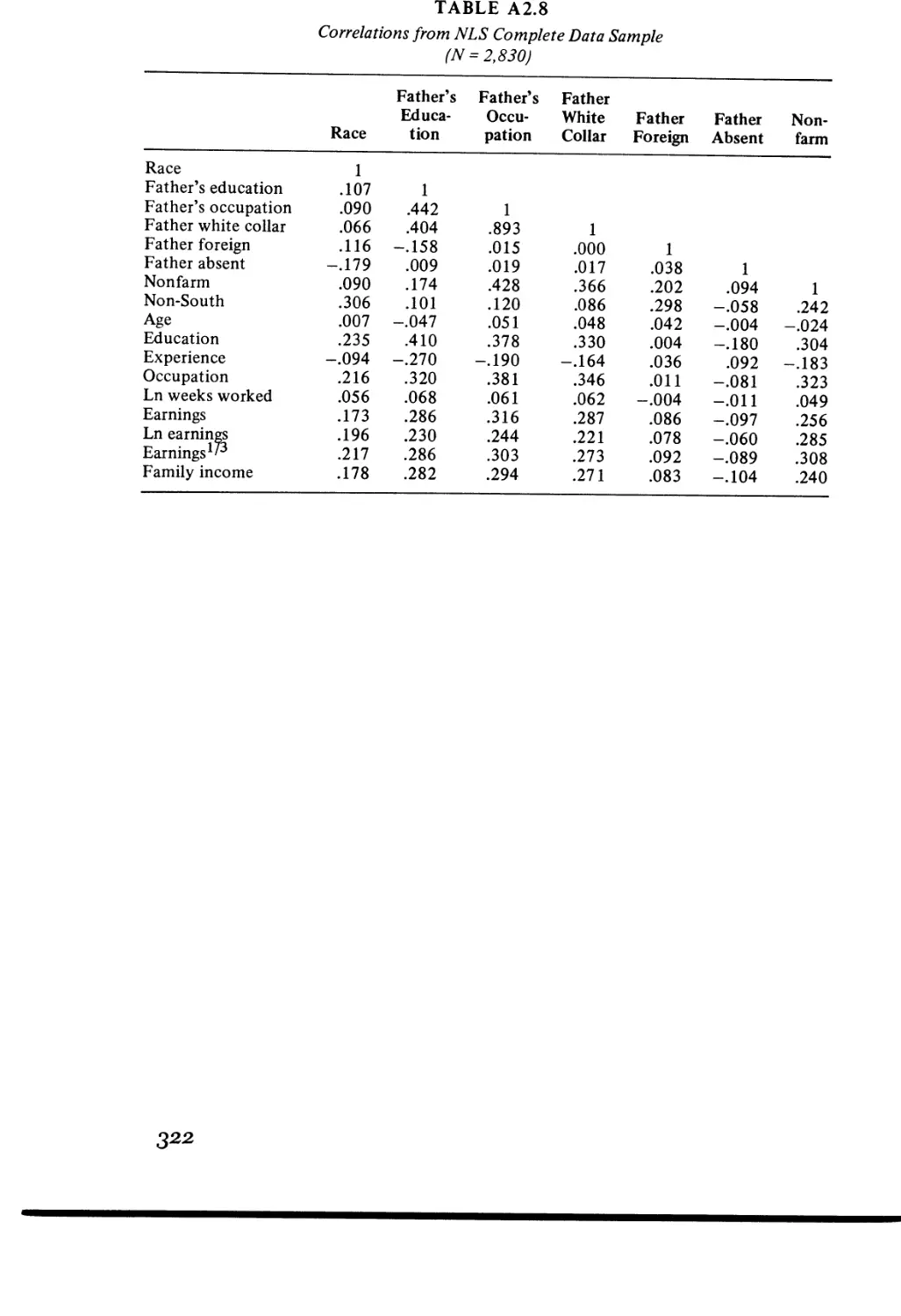
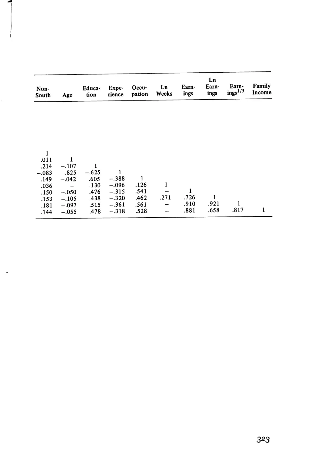
A2.7 Correlations from Veterans Complete Data Sample
A2.8 Correlations from NLS Complete Data Sample
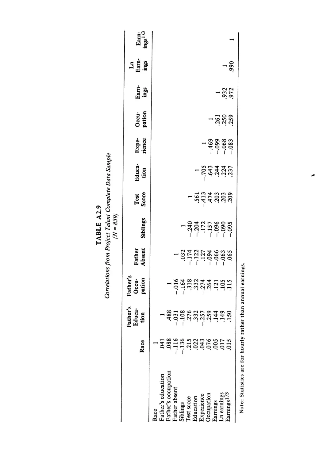
A2.9 Correlations from Project Talent Complete Data Sample
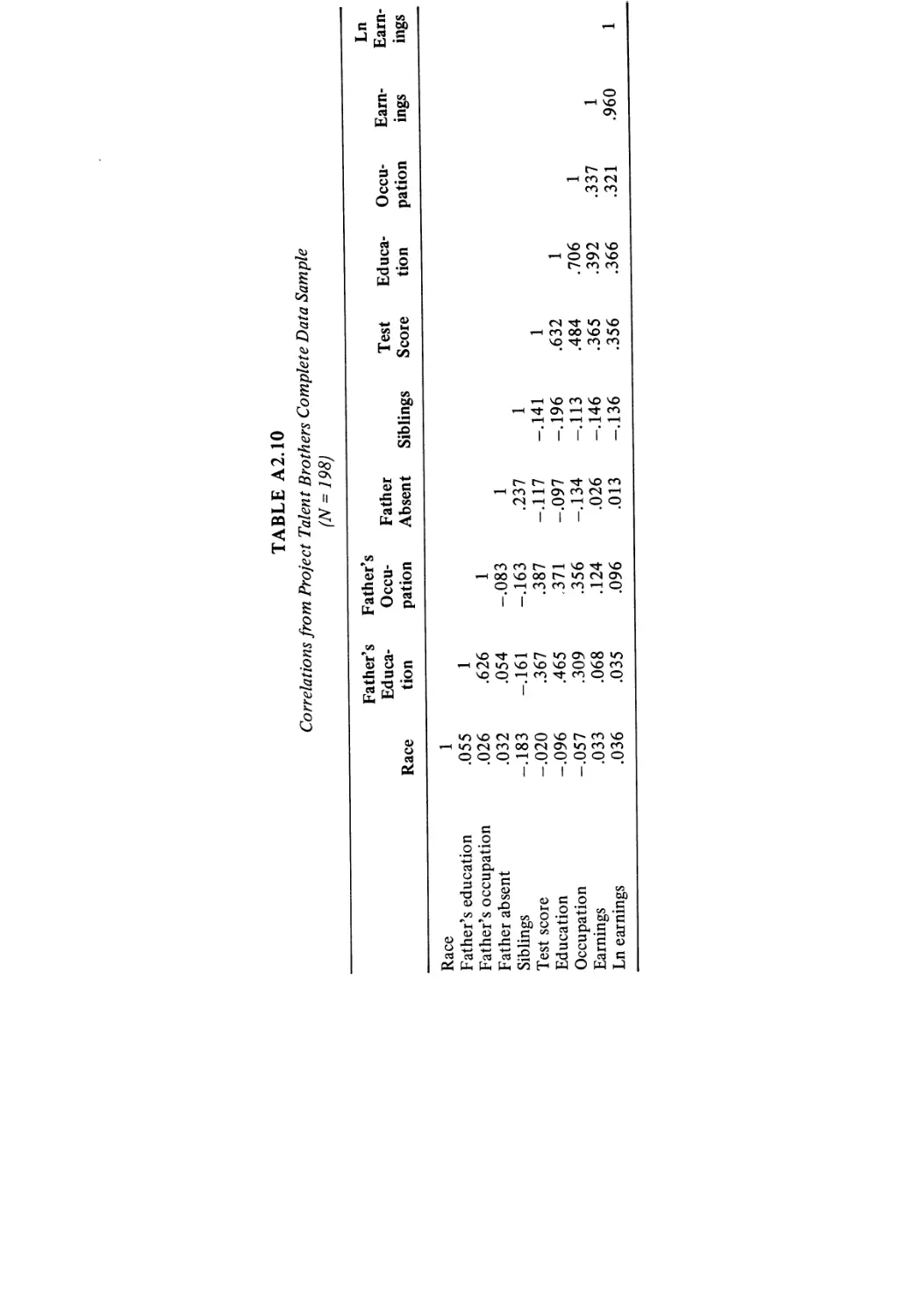
A2.10 Correlations from Project Talent Brothers Complete
Data Sample
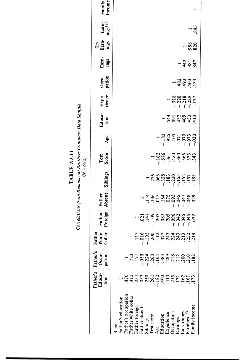
A2.11 Correlations from Kalamazoo Brothers Complete
Data Sample
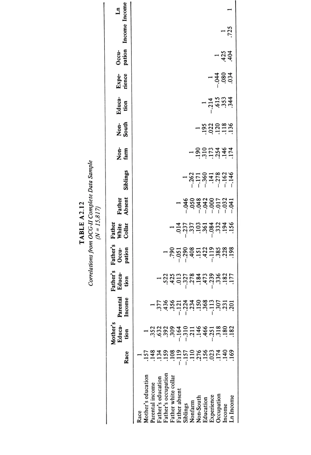
A2.12 Correlations from OCC-II Complete Data Sample
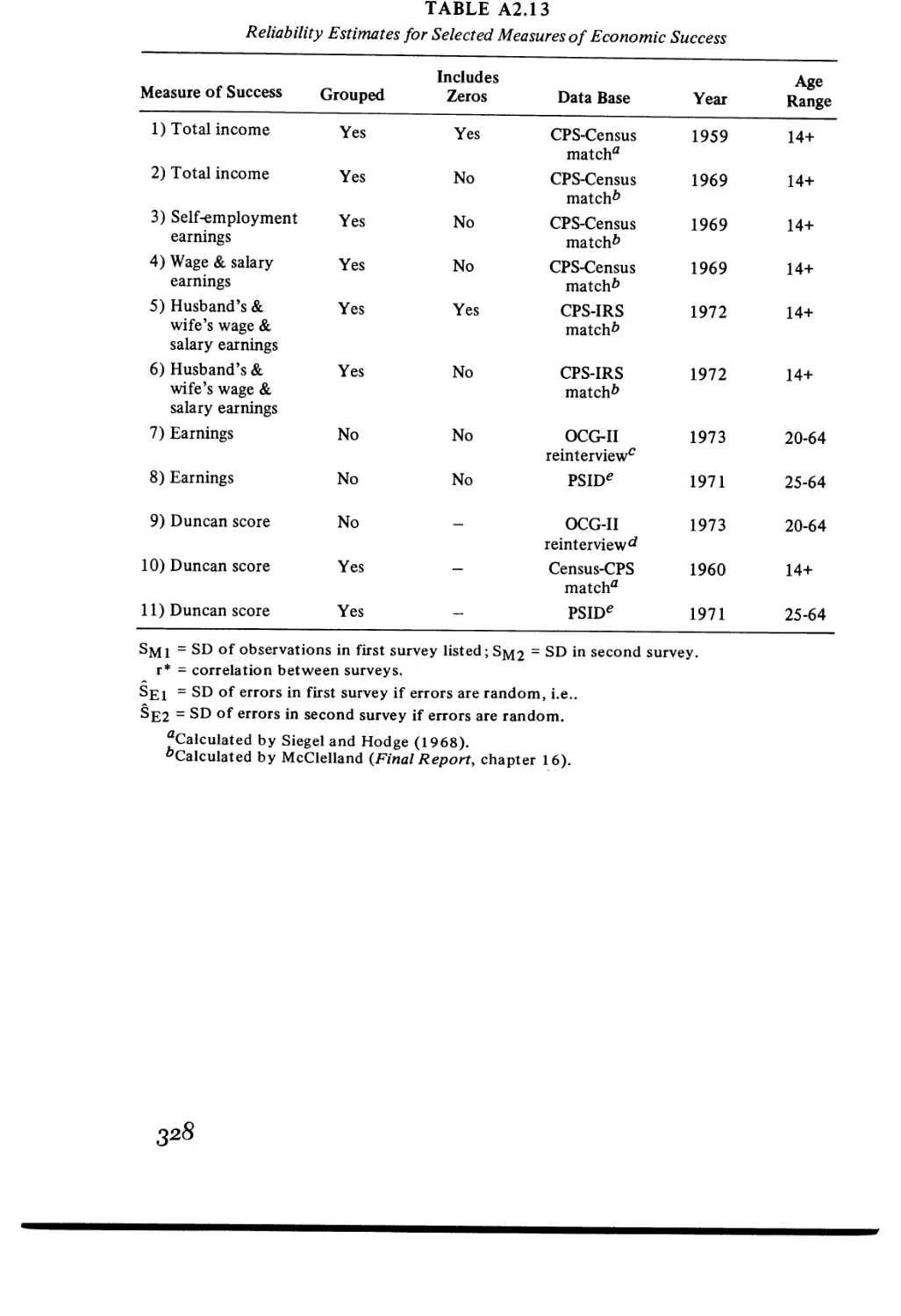
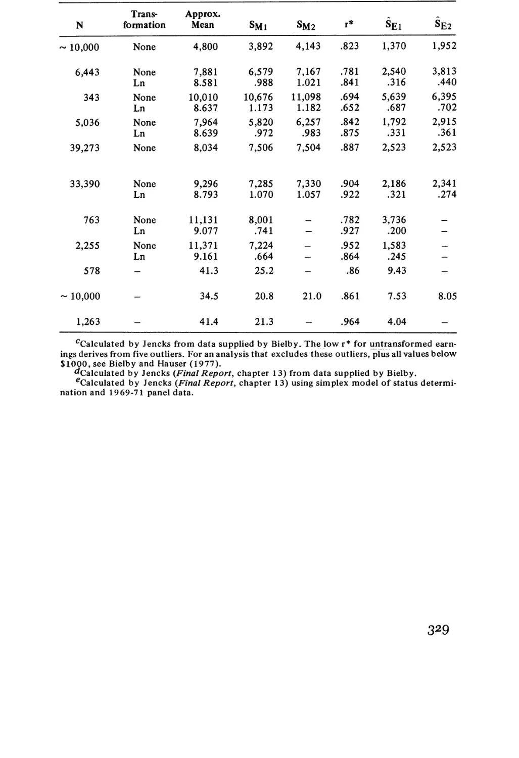
A2.13 Reliability Estimates for Selected Measures of
Economic Success
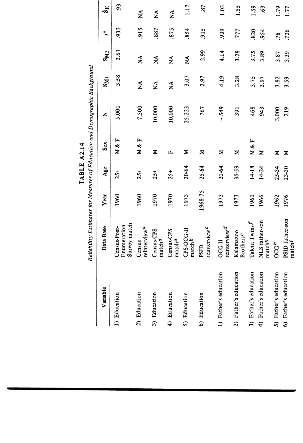
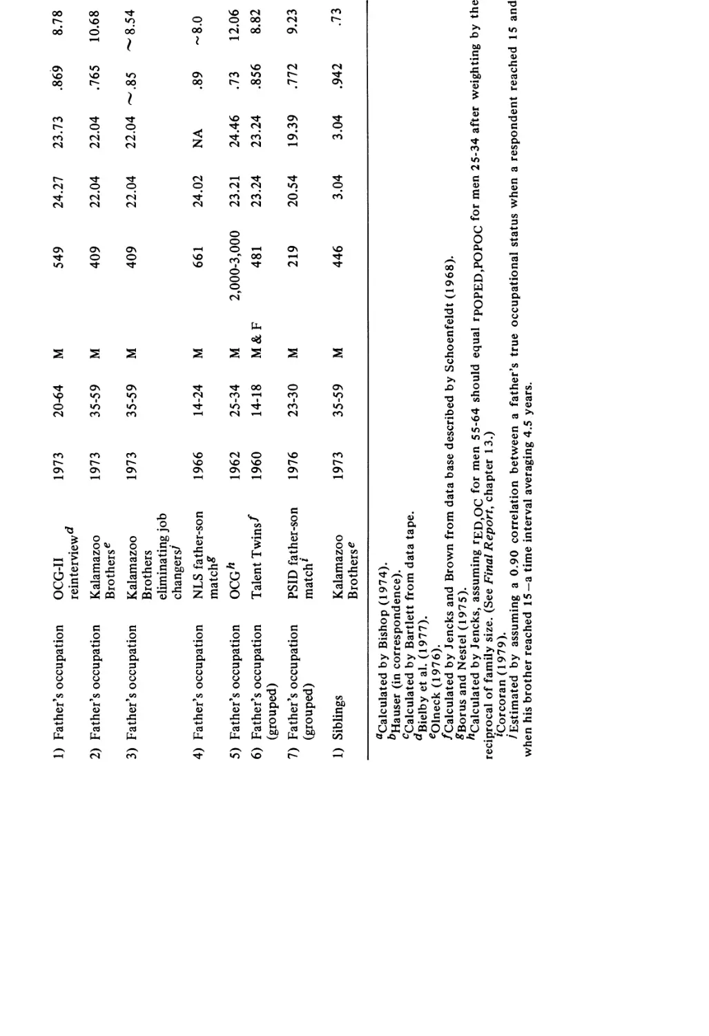
A2.14 Reliability Estimates for Measures of Education and
Demographic Background
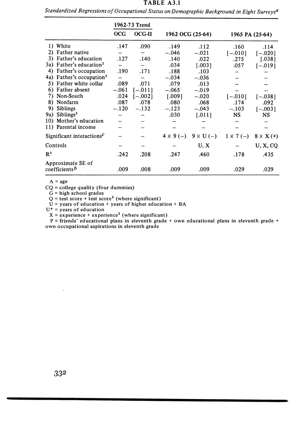
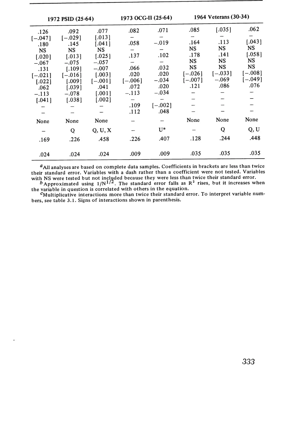
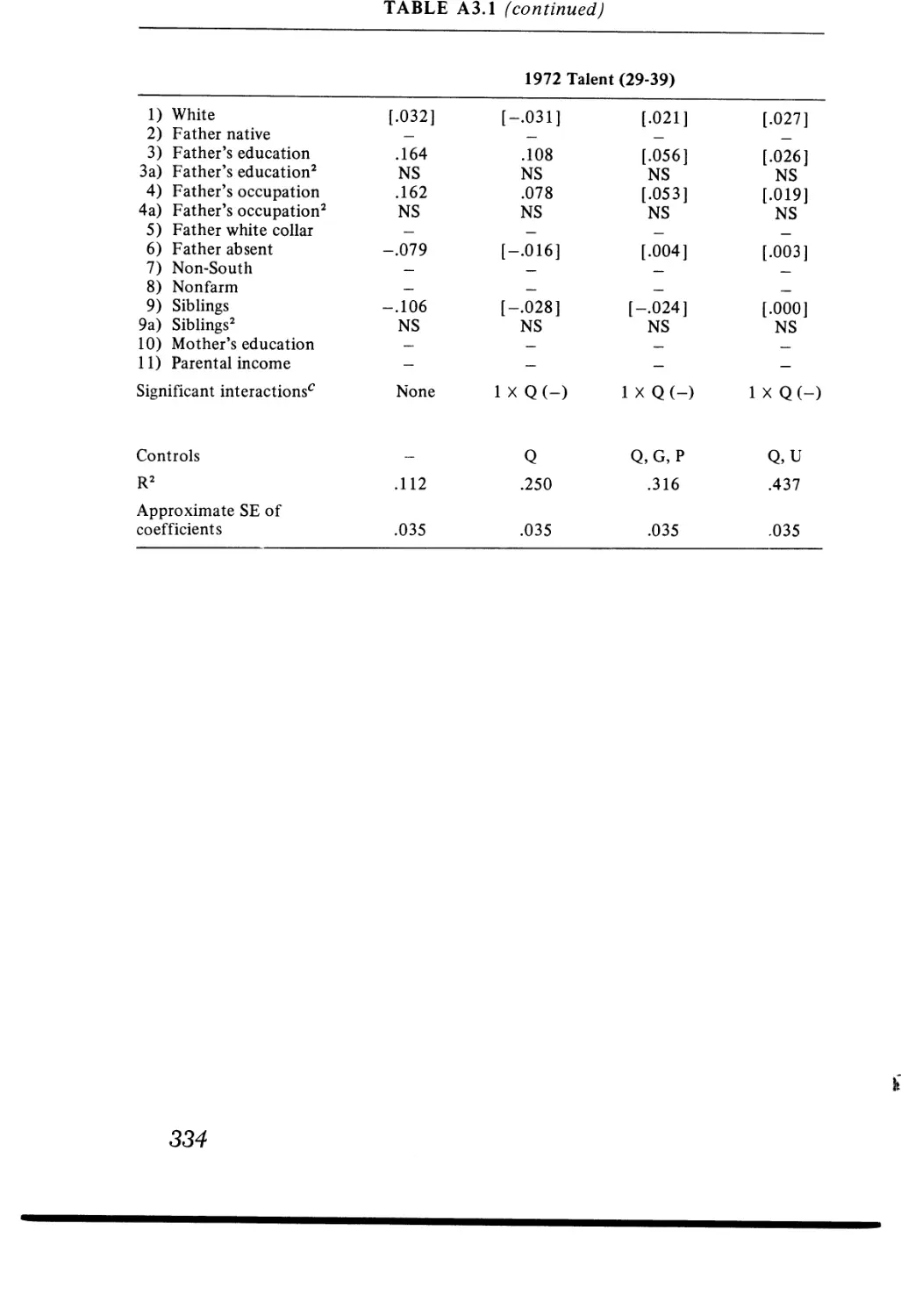
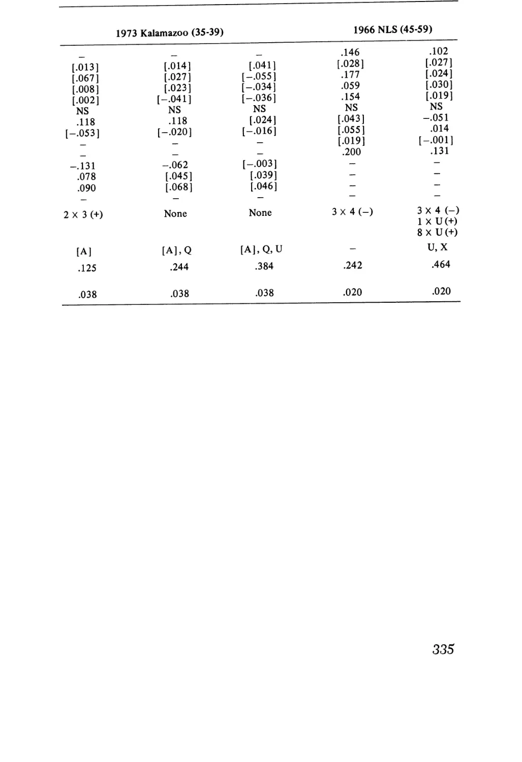
A3.l Standardized Regressions of Occupational Status on
Demographic Background in Eight Surveys
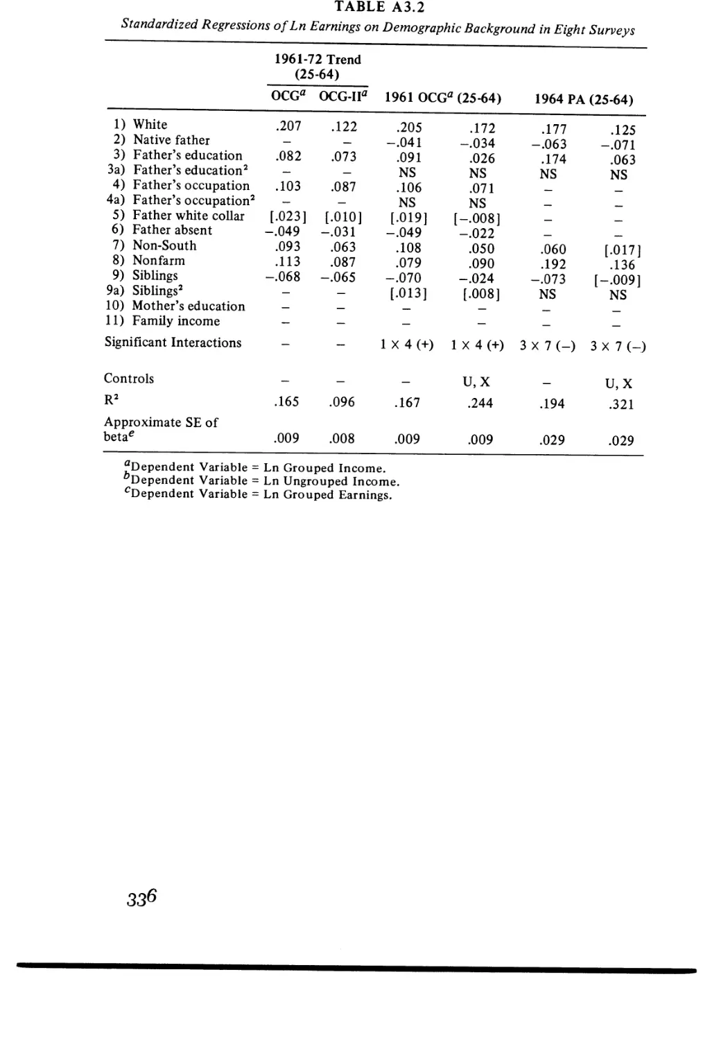
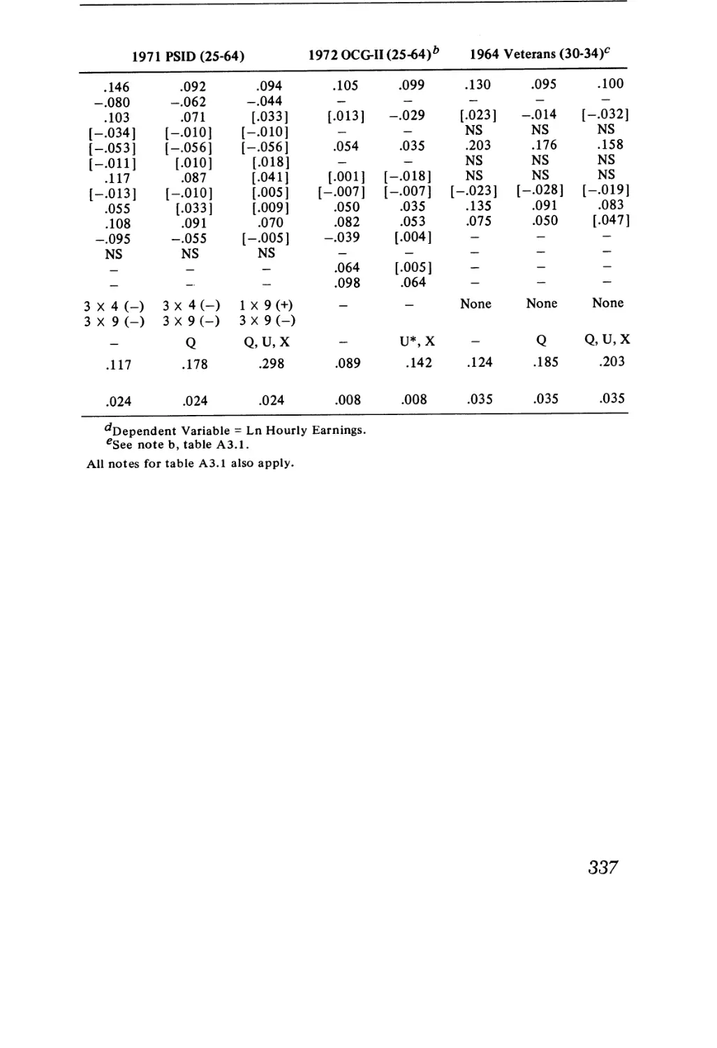
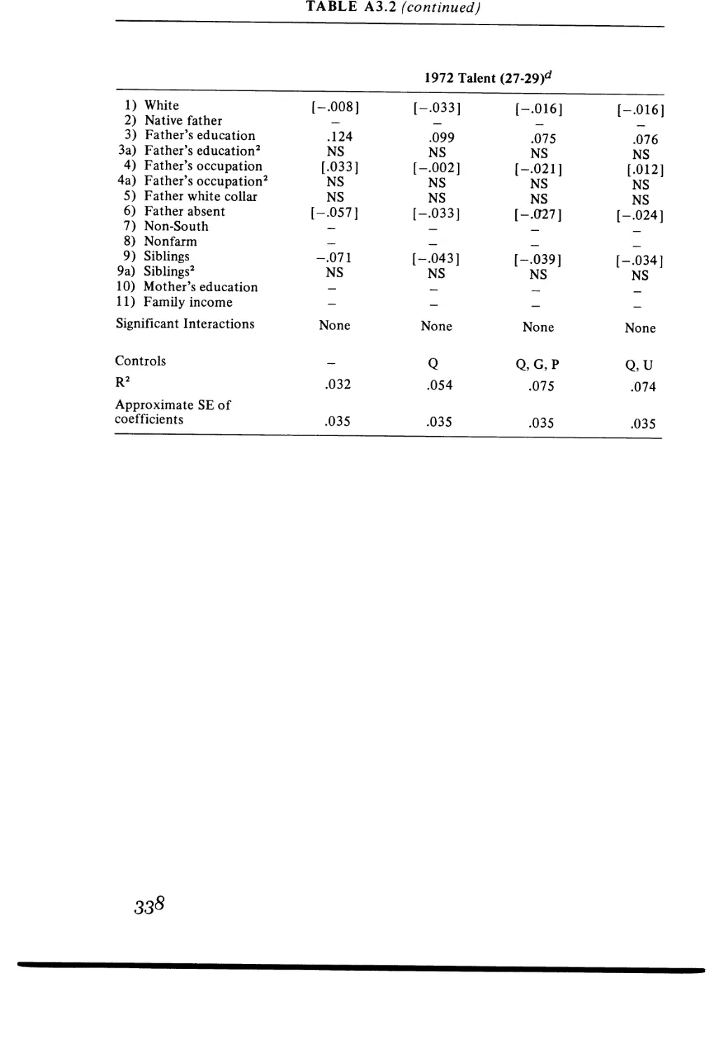
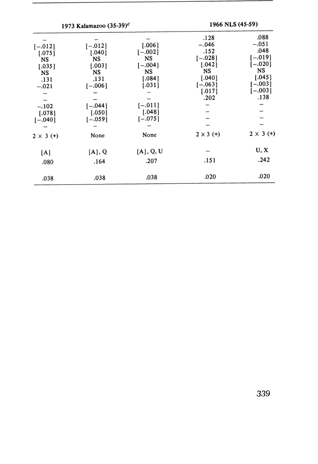
A3.2 Standardized Regressions of Ln Earnings on
Demographic Background in Eight Surveys
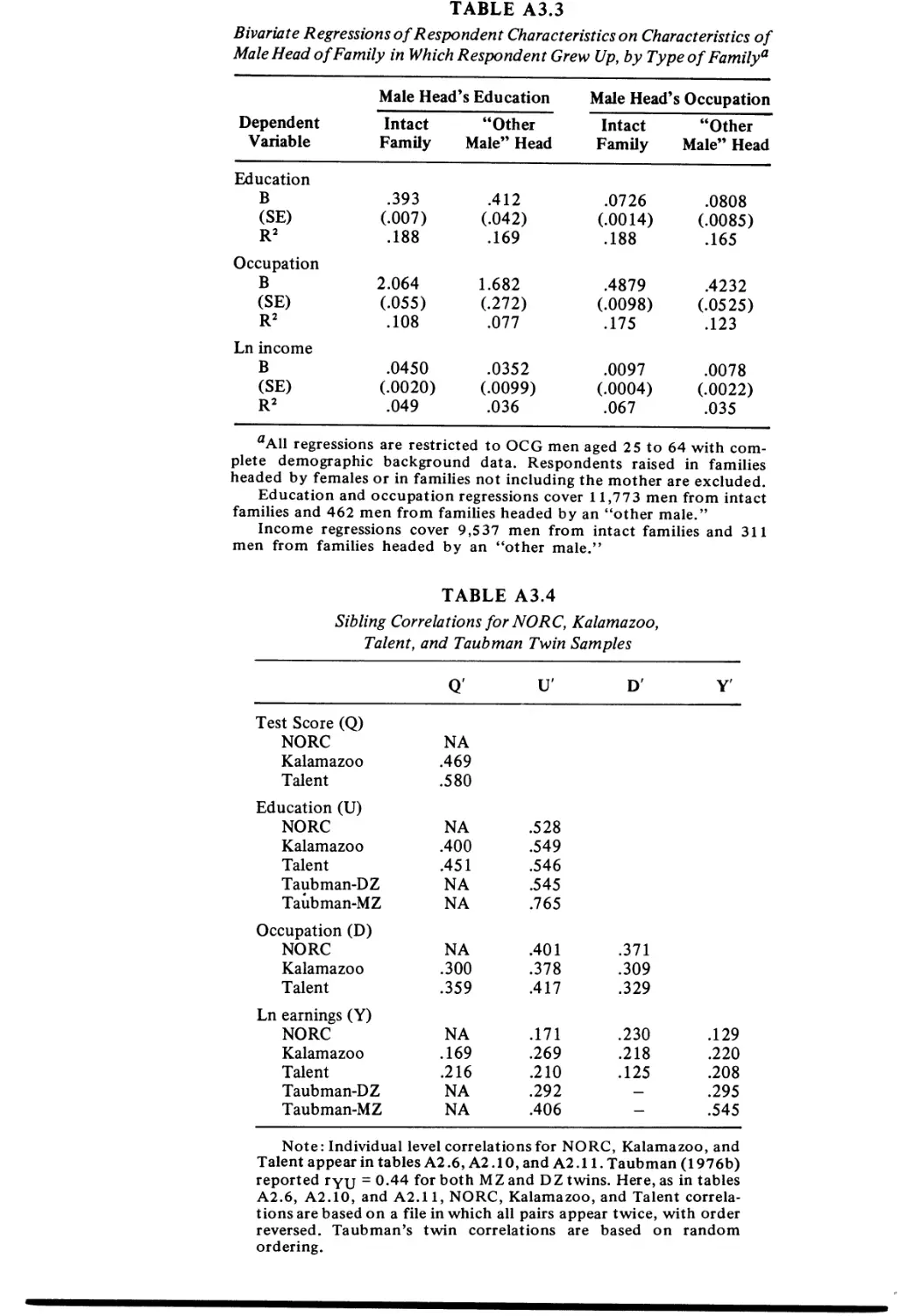
A33 Bivariate Regressions of Respondent Characteristics on
Characteristics of Male Head of Family in Which
Respondent Grew Up, by Type of Family
A3.4 Sibling Correlations for NORC, Kalamazoo, Talent, and
Taubman Twin Samples
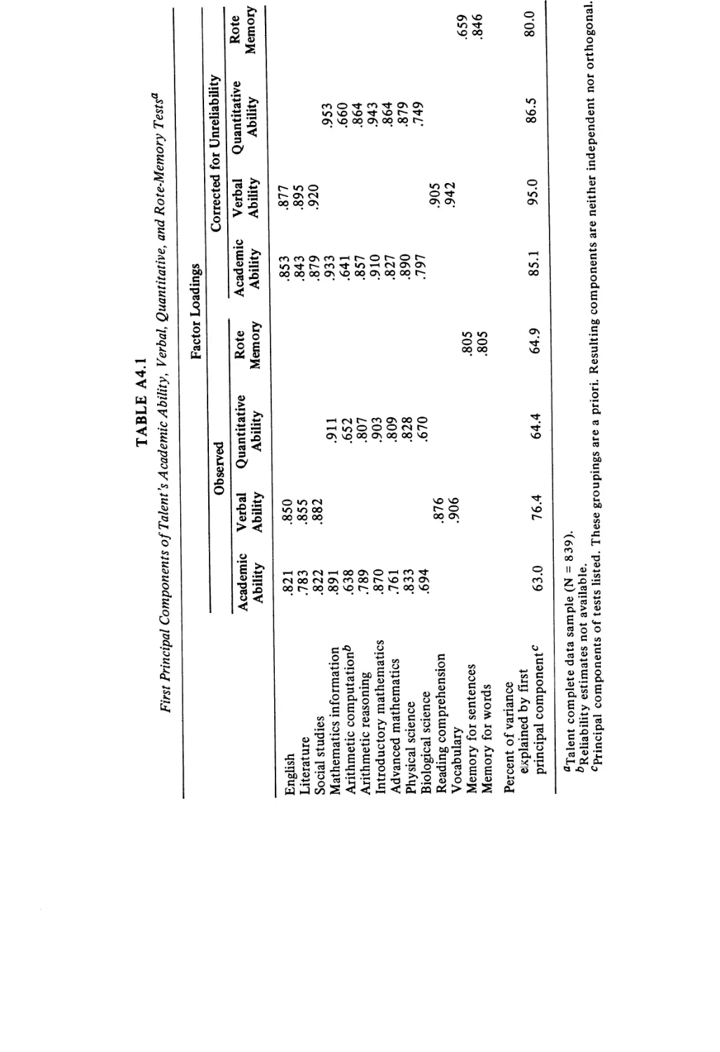
A4.l First Principal Components of Talent’s Academic
Ability, Verbal, Quantitative, and Rote-Memory Tests
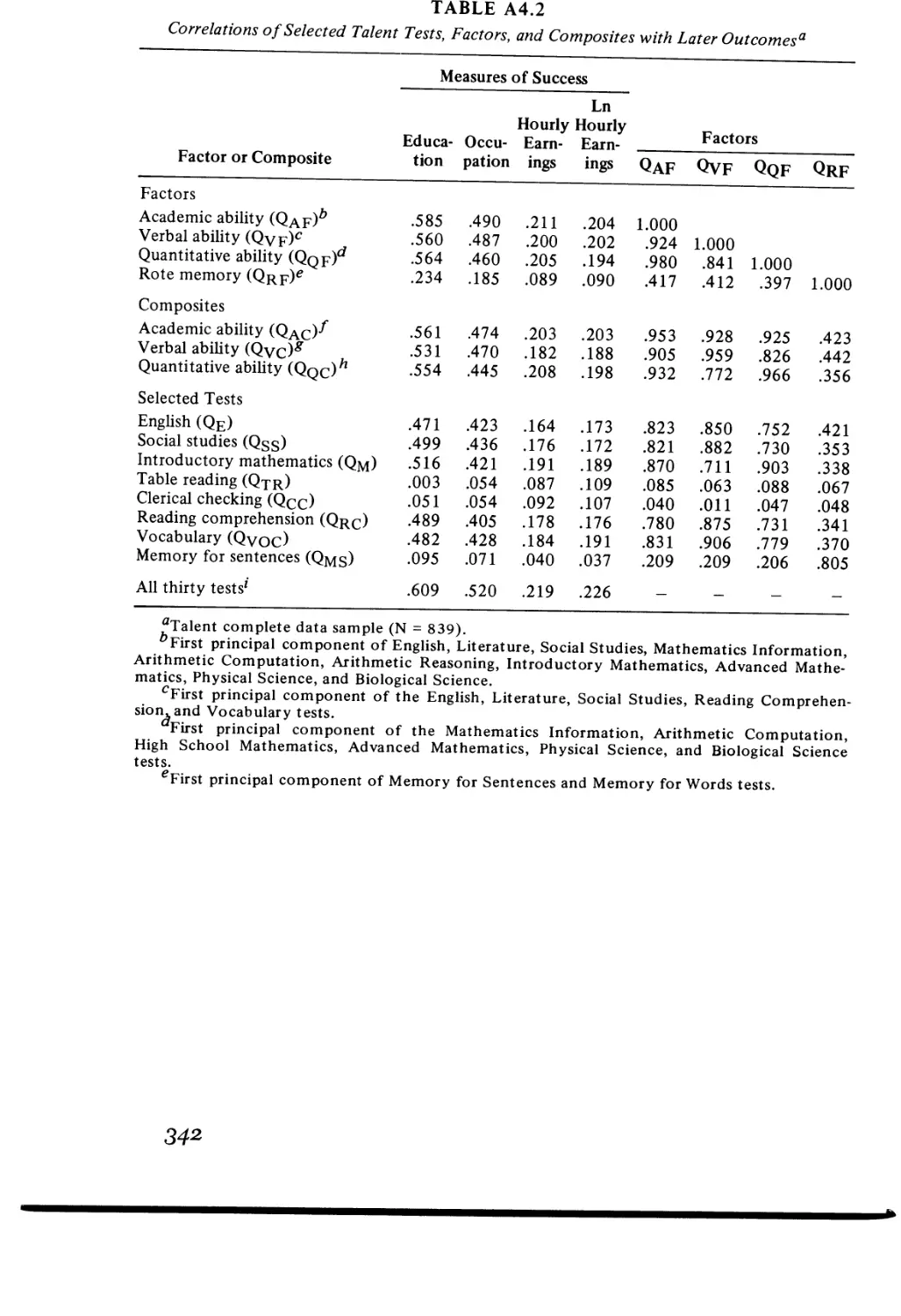
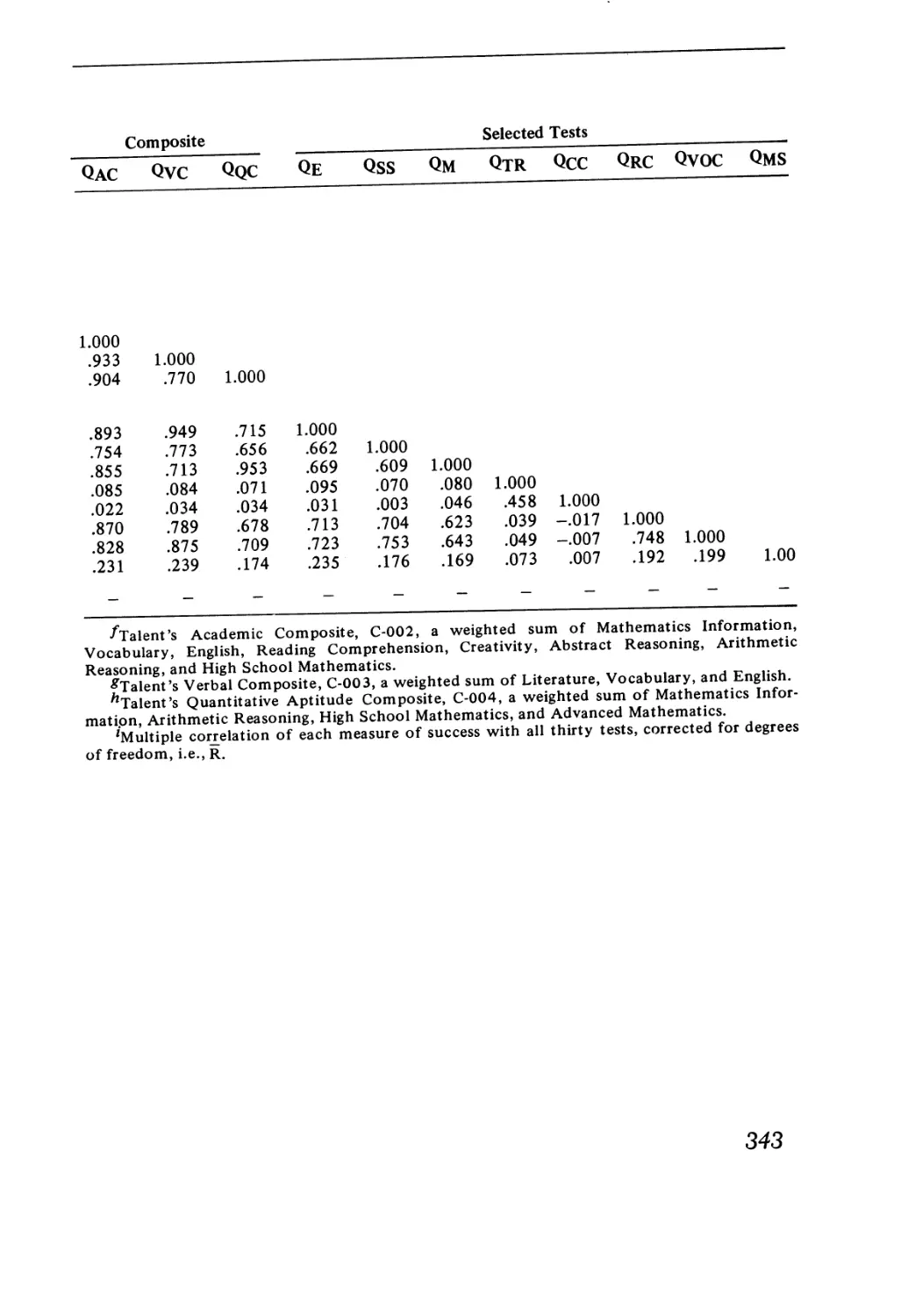
A4.2 Correlations of Selected Talent Tests, Factors, and
Composites with Later Outcomes
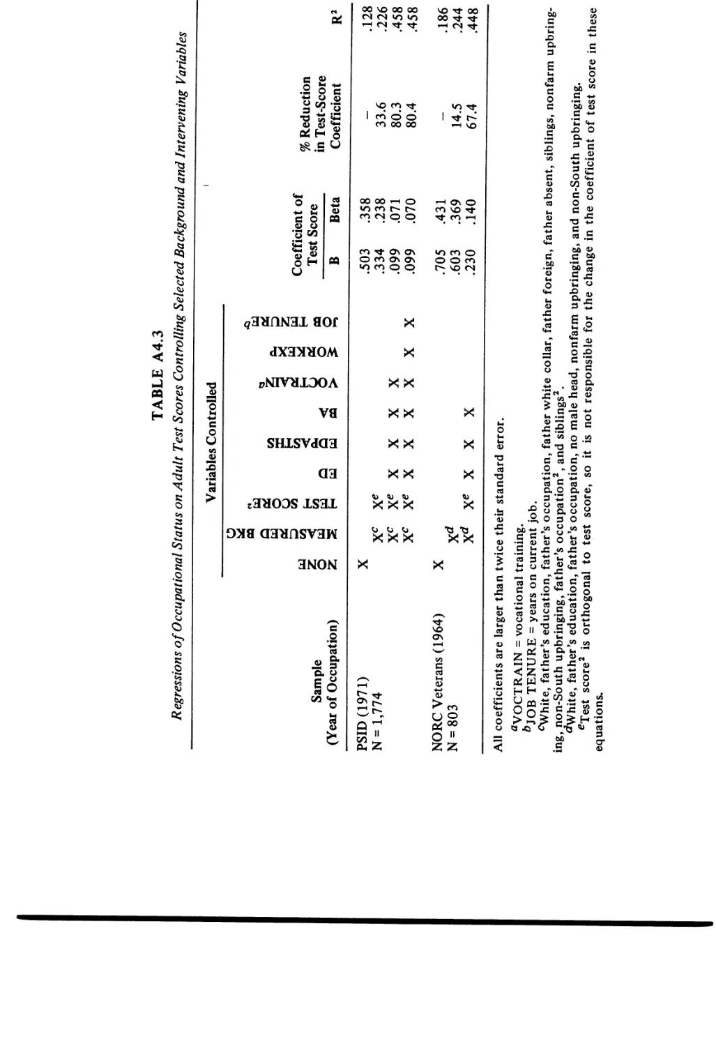
A43 Regressions of Occupational Status on Adult Test
Scores Controlling Selected Background and Intervening
Variables
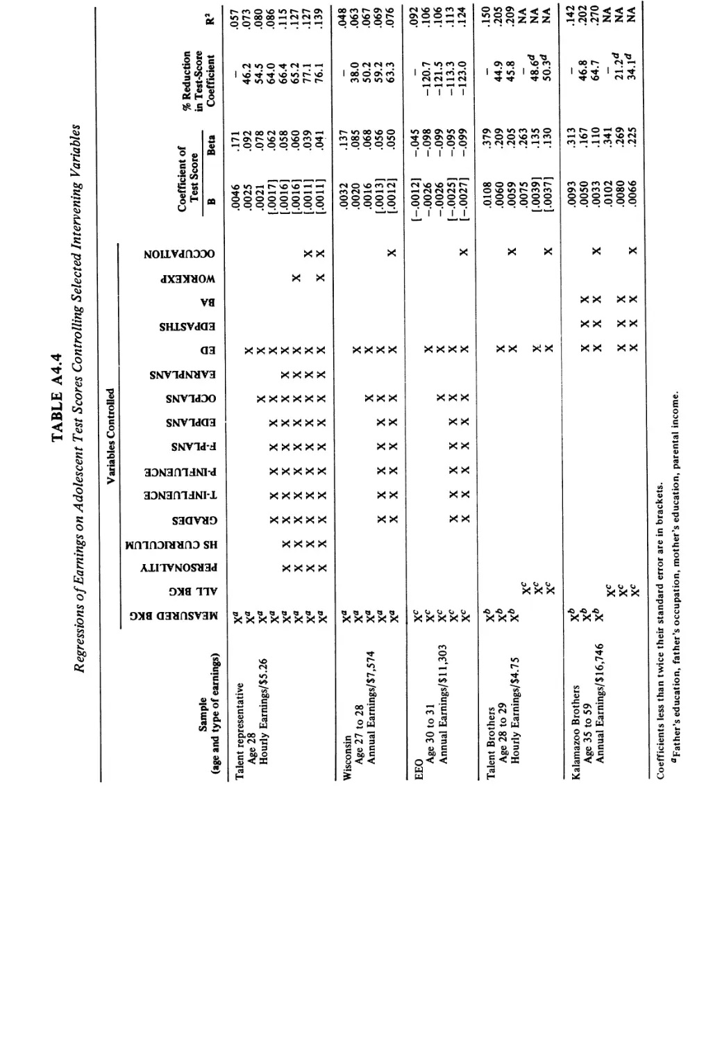
A44 Regressions of Earnings on Adolescent Test Scores "
Controlling Selected Intervening Variables
A45 Regressions of Ln Earnings on Adolescent Test
Scores Controlling Selected Intervening Variables
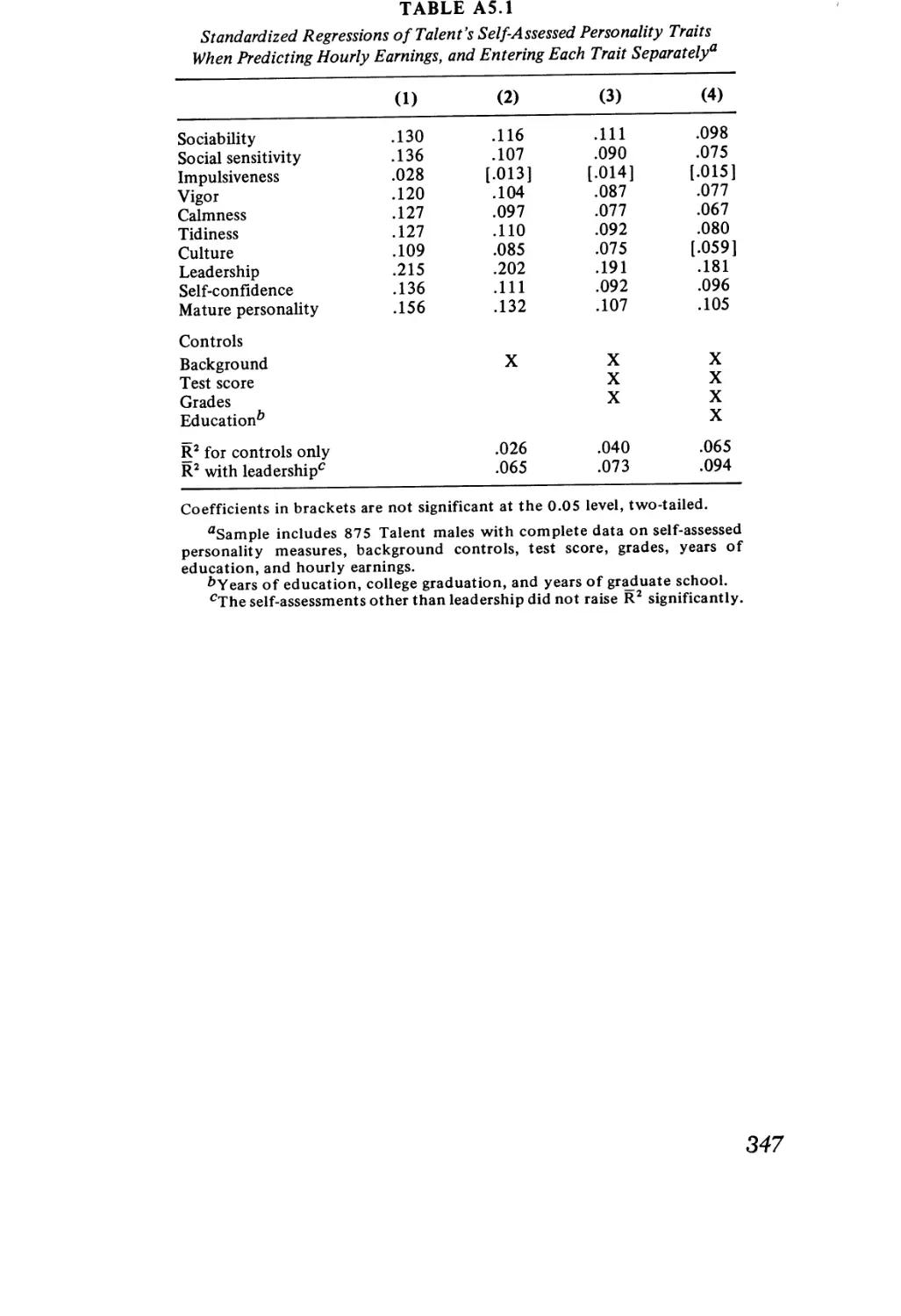
A5.1 Standardized Regressions of Talent’s Self-Assessed
Personality Traits When Predicting Hourly Earnings
and Entering Each Trait Separately
A5.2 Talent Questions Relating to Student Activities and
Attitudes
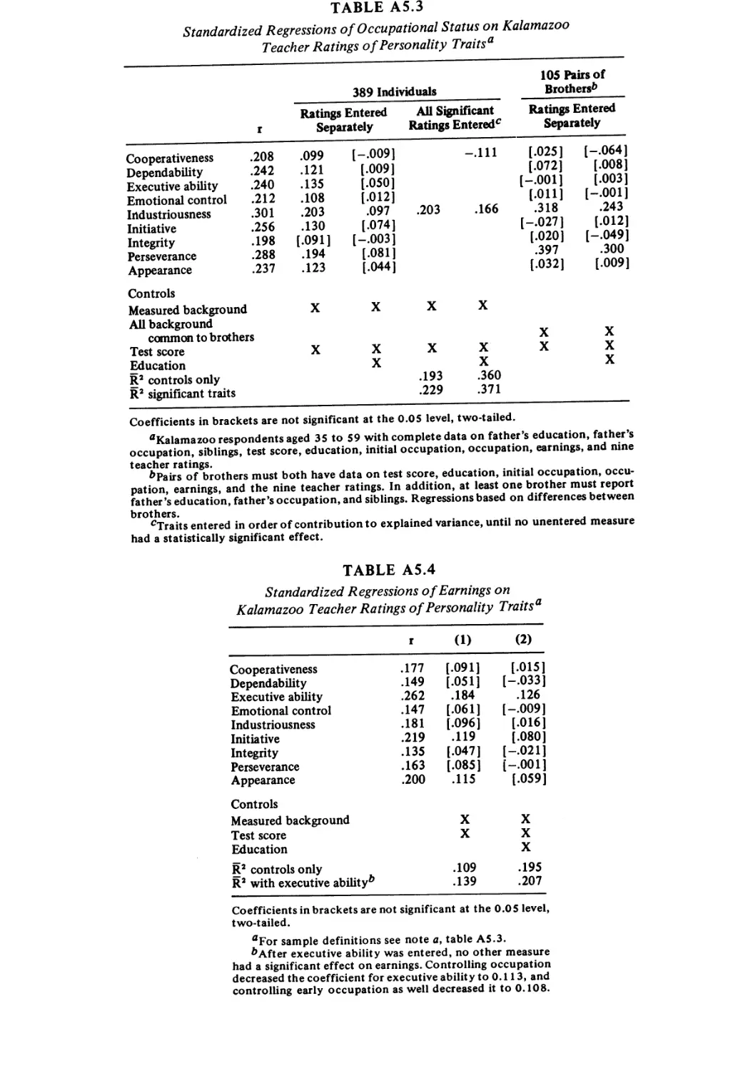
A53 Standardized Regressions of Occupational Status on
Kalamazoo Teacher Ratings of Personality Traits
A5.4 Standardized Regressions of Earnings on Kalamazoo
Teacher Ratings of Personality Traits
ix
Tables and Figures
A6.1
A6.2
A6.3
A6.4
A65
A66
A6.7
A7.1
A7.2
A9.1
A92
Linear Regressions of Current Occupational Status on
Education with Selected Controls
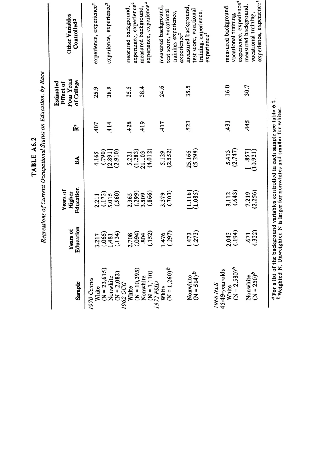
Regressions of Current Occupational Status on
Education, by Race
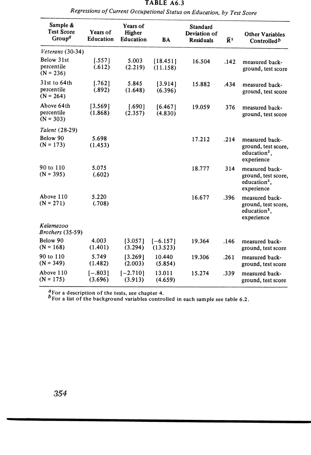
Regressions of Current Occupational Status on
Education, by Test Score
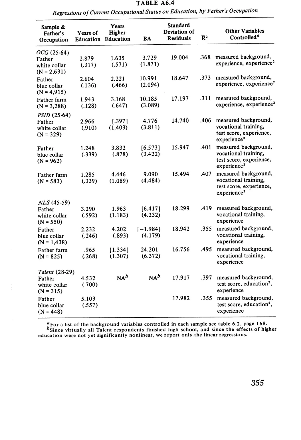
Regressions of Current Occupational Status on
Education, by Father’s Occupation
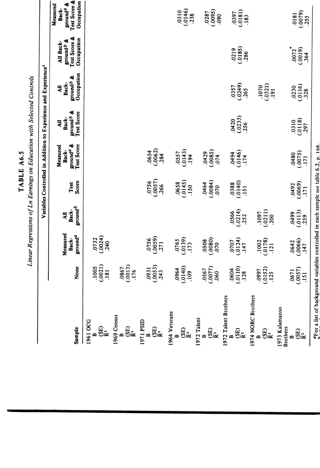
Linear Regressions of Ln Earnings on Education with
Selected Controls
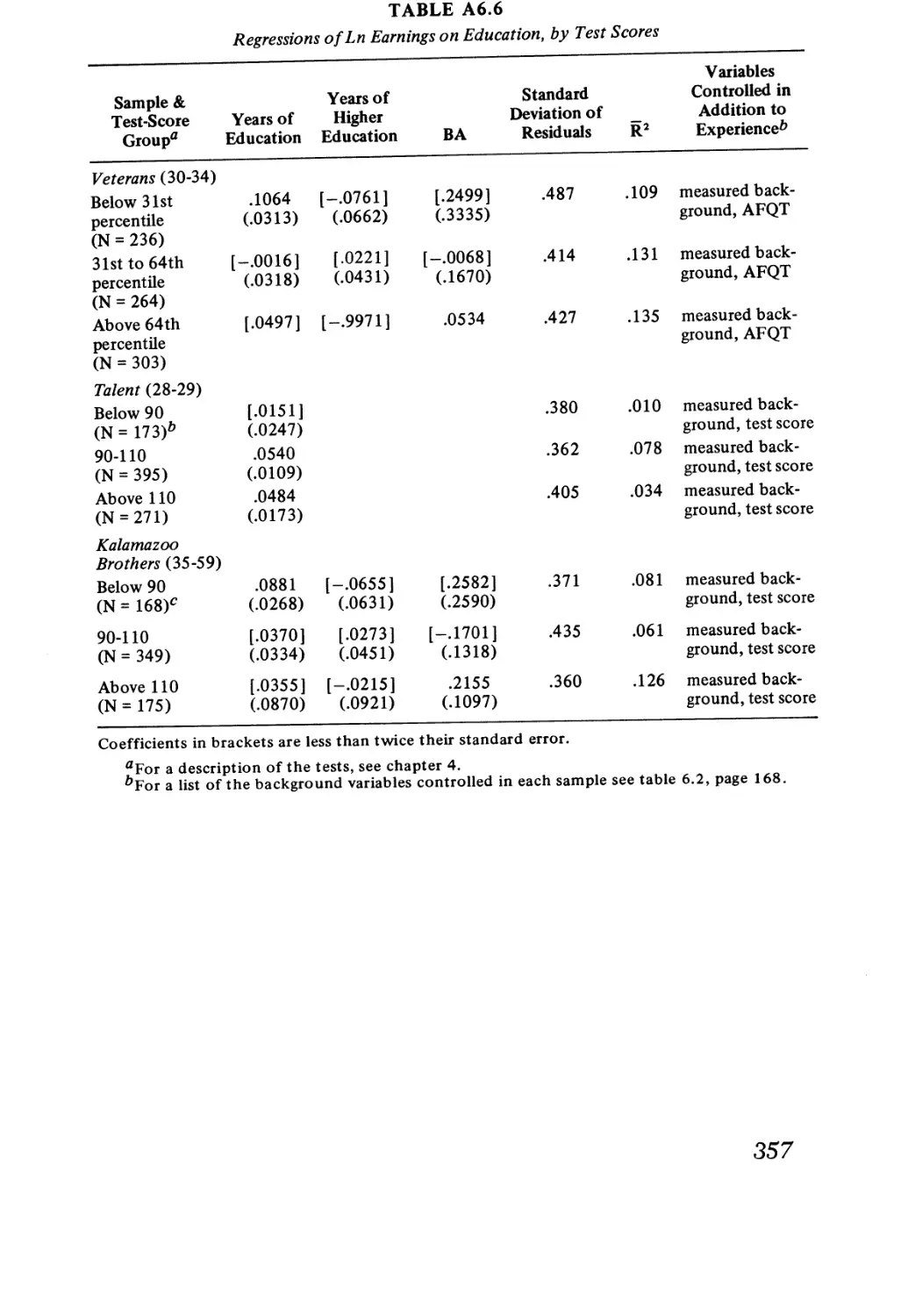
Regressions of Ln Earnings on Education, by
Test Scores
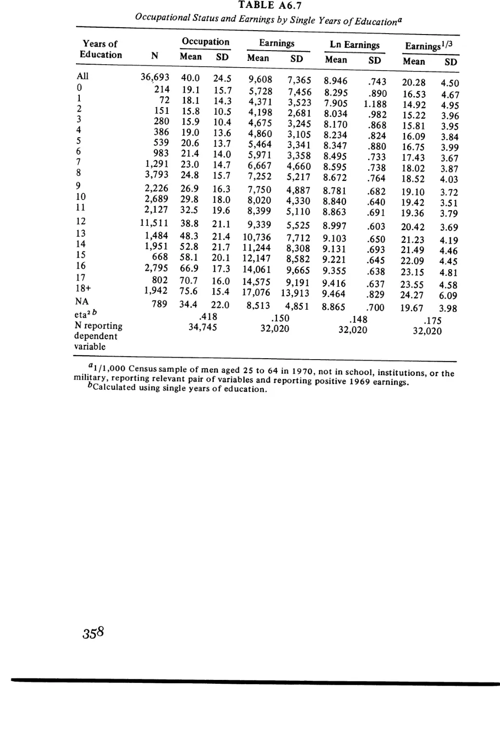
Occupational Status and Earnings by Single Years of
Education
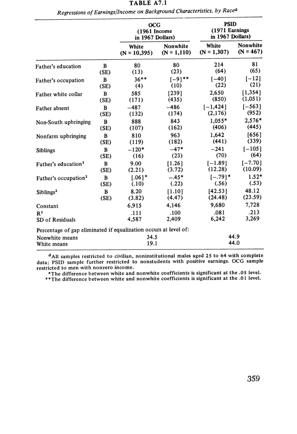
Regressions of Earnings / Income on Background
Characteristics, by Race
Regressions of Earnings“ 3 /Income“ 3 on Background
Characteristics, by Race
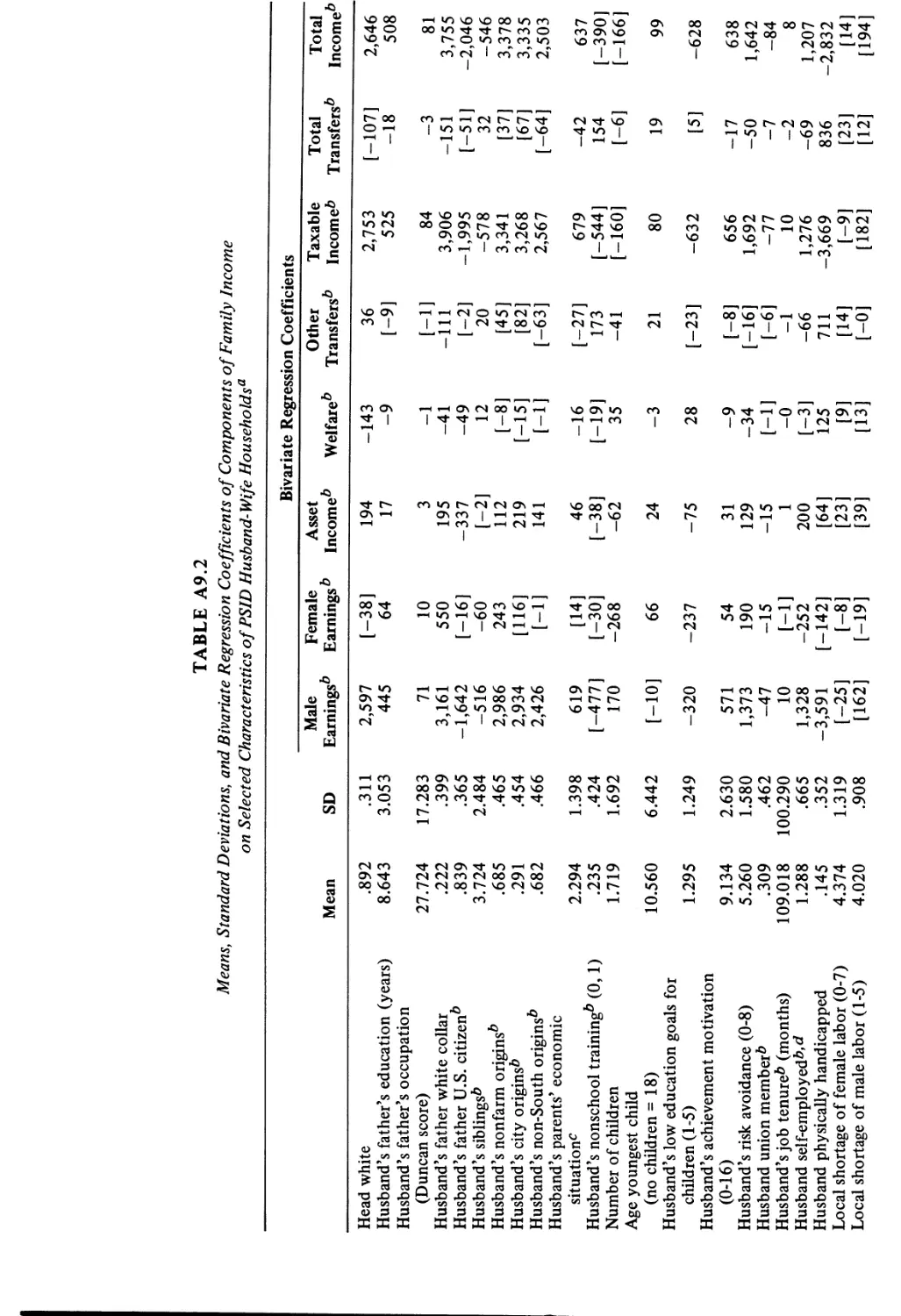
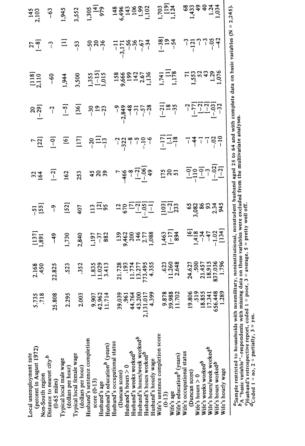
Components of 1971 Family Income for PSID
Husband-Wife Households
Means, Standard Deviations, and Bivariate Regression
Coefficients of Components of Family Income on
Selected Characteristics of PSID Husband-Wife
Households
PREFACE
This book grew out of the controversy that followed the publication of
Inequality: A Reassessment of the Efiect of Family and Schooling in
America in 1972. In that book Jencks and seven colleagues at Harvard’s
Center for Educational Policy Research investigated the relationships
among various kinds of inequality in America. They concluded, among
other things, that disparities in adult occupational status and earnings
were not primarily attributable to the fact that workers came from dif-
ferent family backgrounds, had different cognitive skills, and had spent
different amounts of time in school.
Inequality relied on what seemed to be the best evidence available
at the time, but it contained a number of potentially serious gaps. About
a year after its publication we initiated a systematic effort to close some
of these gaps. Who Gets Ahead? describes the fruits of that effort.
But because it involved a different group of investigators with different
backgrounds and interests, and because five years of data analysis al-
tered our thinking in many respects, Who Gets Ahead? is a very different
book from Inequality.
First, Who Gets Ahead? is primarily concerned with the determinants
of individual success within the existing economic system, not with the
determinants of the level of inequality in that system. Second, Who Gets
Ahead? presents the evidence on which it bases its conclusions in far
more detail than Inequality did. Third, Who Gets Ahead? does not devote
much space to problems of public policy. Its conclusions are largely de-
scriptive. Finally, Who Gets Ahead? is a more fully collaborative effort
than Inequality was. Each of the coauthors listed on the title page either
took primary responsibility for analyzing one of the surveys on which
this book is based or else took primary responsibility for writing one
or more of the chapters.
Who Gets Ahead? tries to assess the impact of family background,
cognitive skills, personality traits, years of schooling, and race on men’s
occupational status, earnings, and family income. To accomplish this, we
looked at eleven different surveys. Because each of these surveys had its
own peculiarities, and because our reading of previous research sug-
xi
Preface
gested that casual use of unfamiliar data had often led to disastrous
errors, every member of the project but Schwartz and Corcoran assumed
responsibility for learning as much as possible about one or more of the
surveys. Each of us eventually wrote a detailed comparison of “our”
sample with others of nominally similar character. We also produced
statistical tables describing each sample in a “standard” form that we had
jointly agreed upon in advance.
Every member of the project but Eaglesfield and Ward also took re-
sponsibility for preparing one or more chapters on a substantive prob-
lem. These chapters tried to synthesize all the evidence from the sample
descriptions that was relevant to a specific issue. Each chapter also
required additional analyses aimed at clarifying problems that had not
been apparent when we did our sample descriptions. Each chapter thus
rests partly on data analyzed by its author and partly on data analyzed
by others.
We completed drafts of these chapters in the winter of 1977 and cir-
culated them to a number of potential critics. After mulling over the
critics’ comments, we made some revisions and submitted both our sub-
stantive analyses and our sample descriptions to the funding agencies
that had supported our work. Our report, The Effects of Family
Background, Test Scores, Personality Traits, and Schooling on Economic
Success, is available from the National Technical Information Service,
Springfield, Virginia, 28151. We will refer to this publication simply as
the Final Report.
The present volume is a considerably revised version of the Final Re-
port. We have eliminated some of the obscurities and errors that mar
the Final Report, clarified a number of ambiguities by further analysis
of our data, and added a new conclusion comparing our findings to those
in Inequality. We have also cut out a substantial amount of material justi—
fying our methodological choices, although we have retained references
to this material for aficionados.
While this is a joint effort, we are not all equally responsible for every
word that appears here. Lest anyone be blamed for what he or she could
not prevent, it seems wise to record who worked on what.
Christopher jencks initiated, planned, and supervised the project. He
was thus largely responsible for deciding what each chapter would cover
and what it would ignore. He wrote chapters 1 and 2, which describe
our aims and methods, and chapter 12, which compares our findings to
those in Inequality. With Corcoran, he wrote chapter 3, which analyzes
the effects of family background on economic success. He was primarily
xii
Preface
responsible for analyzing the Veterans Survey, which he describes in
Appendix G of the Final Report. Finally, he edited the entire manu-
script, often heavily. He is therefore deeply implicated in whatever
stylistic and substantive deficiencies remain.
Susan Bartlett analyzed changes in the effects of education and ex-
perience on men’s income, using 1940, 1950, 1960, and 1970 Census data.
Her findings appear in the Summer 1978 issue of the Journal of Human
Resources, and we have not reprinted them here. Her description of the
1970 Census results, written jointly with jencks, constitutes Appendix A
of the Final Report.
Mary Corcoran shared responsibility with jencks and Eaglesfield for
investigating the effects of family background. She and jencks wrote chap-
ter 3. She also wrote chapter 8, which summarizes our findings about the
determinants of individual success.
James Crouse wrote chapter 4, which analyzes the relationship be-
tween test performance and economic success. He also took primary re-
sponsibility for analyzing our Project Talent data, except for that dealing
with personality traits. His description of the Talent samples appears in
Appendices H and I of the Final Report.
David Eaglesfield was responsible for analyzing the NORC Brothers
Survey. His description of this survey appears in Appendix E of the
Final Report. He also estimated a large number of alternative models of
the effects of family background. This work appears in his doctoral dis-
sertation, “Family Background and Occupational Achievement,” done
for the Harvard Department of Sociology in 1977. Chapter 3 relies on
these estimates at several points.
Gregory jackson wrote chapter 10, which examines the degree of com-
parability between our four major national surveys. He also took primary
responsibility for analyzing the Occupational Changes in a Generation
Survey. His description of this survey appears in Appendix B of the Final
Report.
Kent McClelland wrote chapter 11, which examines the effects of varia-
tion in individual research style on findings about the relationship be—
tween education and earnings. An earlier version of this chapter ap-
pears in his doctoral dissertation, “How Different Surveys Yield Different
Results: The Case of Education and Earnings,” done for the Harvard
Department of Sociology in 1976. He also analyzed the Productive
Americans Survey, which he describes in Appendix C of the Final Report.
Peter Mueser analyzed Project Talent’s data on personality traits and
wrote chapter 5, which summarizes the effects of adolescent personality
xiii
Preface
traits on later success in the Talent and Kalamazoo surveys. He also took
primary responsibility for analyzing the Panel Study of Income Dynam-
ics, which he describes in Appendix D of the Final Rep-mt.
Michael Olneck wrote chapter 6, which describes the effects of educa-
tional attainment on economic success. He was also responsible for con-
ducting the Kalamazoo Brothers Survey, which he describes in detail
in Appendix I of the Final Report and in his doctoral dissertation, “The
Determinants of Educational Attainment and Adult Status among Broth-
ers: The Kalamazoo Study,” done for the Harvard Graduate School of
Education in 1976.
Joseph Schwartz and Jill Williams wrote chapter 7, which compares
the determinants of earnings among whites and nonwhites. Schwartz also
wrote chapter 9, which analyzes the relationship between earnings and
family income.
Sherry Ward was primarily responsible for analyzing the National
Longitudinal Survey’s data on older men. Her description of her findings
appears in Appendix F of the Final Report.
Several other individuals played vital roles in the project. Jan Lennon
administered the project for the Center for the Study of Public Policy and
typed dozens of draft chapters and thousands of tables for us. Without
her, our work would have taken even longer than it did. Irene Coodsell
typed the final manuscript.
David Featherman and Robert Hauser provided us with a copy of
the 1962 Occupational Changes in a Generation data tape and gener-
ously authorized David Bills to make tabulations for us from the 1973
replication of that survey. The Survey Research Center at the University
of Michigan provided well-documented copies of' the Productive Ameri-
cans and Panel Study of Income Dynamics data. William Mason gave us a
copy of the US. Current Population Survey’s 1964 survey of veterans.
Project Talent gave us access to selected data from their files. Olneck
also shared his Kalamazoo data unstintingly.“
Susan Bartlett, Jill Williams, and Marianne Winslett did most of Jencks’s
computer work for him, leaving him free to send memos suggesting addi—
tional work for everyone else. Zvi Criliches, Andrew Kohen, and Paul
Taubman provided valuable criticisms of a draft of the Final Report
while Bill Bielby did the same for a draft of the book.
The National Institute of Education and the Employment and Train-
” In this connection we are especially grateful to Dr. David Bartz and Dr. William
Coapes of the Kalamazoo Public School System for permitting Olneck to use their
archives, and to Dr. Stanley Robbin of the Center for Sociological Research at Western
Michigan University for allowing Olneck to use the Center’s facilities while he was
resurveying the Kalamazoo respondents.
xiv
Preface
ing Administration of the US. Department of Labor supported our work
through a grant to Christopher Jencks and Lee Rainwater for work at
the Center for the Study of Public Policy, a nonprofit research organiza-
tion in Cambridge. The Department of Health, Education, and Welfare’s
Office of Income Security Policy also made a much larger grant to Lee
Rainwater at the MIT-Harvard Joint Center for Urban Studies. This
grant was primarily to support work on the relationship between differ-
ent sources of family income, but some of the funds were used to sup-
port our work on the determinants of male earnings.
Tradition usually dictates a discrete silence about the actual amount
of such support, since researchers rightly assume that readers will be
appalled by the expense involved in producing a single book. But such
reticence reinforces the illusion that one “should” be able to do large—
scale research on a shoestring. This is just not true.
The NORC Brothers and Kalamazoo Brothers surveys were financed
by Harvard’s Center for Educational Policy Research, using funds granted
by the Carnegie Corporation of New York. The NORC Survey cost about
$13,000. The Kalamazoo Survey cost about $25,000. Grants from the Na-
tional Institute of Education and the Department of Labor provided
about $100,000 for data analysis, while HEW’s Office of Income Security
Policy provided another $100,000. Crouse’s work on the effects of cogni-
tive skills was partially supported by the Graduate College at the Uni-
versity of Delaware and by National Science Foundation Grant G—OC—
7103704 to Donald T. Campbell. Olneck’s analysis of the Kalamazoo data
was supported by a doctoral fellowship from the US. Department of
Labor’s Employment and Training Administration and by a Ford Foun-
dation grant to Samuel Bowles and Herbert Gintis at the Harvard Center
for Educational Policy Research. The Institute for Research on Poverty at
the University of Wisconsin supported much of Olneck’s work on chapter
6. The Carnegie Corporation of New York supported Jencks during the
summer of 1977, when he was editing the final manuscript.
All told, we received about $300,000 for our work. In addition, the au-
thors all spent substantial amounts of time on the project for which they
were not paid. The true cost of our work, after allowing for this form
of self-exploitation, was probably at least $400,000.
xv
Who Gets Ahead?
CHAPTER 1
Introduction
This book investigates the relationship between personal characteristics
and economic success among American males aged 25 to 64. It does not
try to provide a complete picture of the determinants of individual suc-
cess. Rather, its aim is to assess the effects of a man’s characteristics
when he enters the labor market on his subsequent success. The book
focuses on four kinds of personal characteristics: family background,
cognitive skills, personality traits, and years of schooling?“
When we launched this project in 1973 we were concerned with three
major deficiencies in earlier work (including our own) on these issues:
1. Previous investigators had seldom had adequate measures of family back-
ground, cognitive skills, or personality traits for representative national
samples.
2. Previous investigators had often made simplifying assumptions about the
ways family background, cognitive skills, and educational attainment af-
fected success without testing these assumptions empirically.
3. Previous investigators had often reached contradictory conclusions, even
when asking apparently similar questions and using apparently similar data.
We set out to assemble better samples, to analyze these samples more
thoroughly, and to explain the discrepancies we found. We have not
achieved any of these objectives fully. We have, however, made some
progress in each area. This chapter summarizes what we have accom-
Christopher Jencks wrote this chapter.
"’ We did not investigate the effects of changes in these characteristics after men
enter the labor market. Nor did we analyze the effects of geogr:fphic mobility, marital
status, fertility, or on-the-job training, all of which can change ter entering the labor
market, partially as a result of prior economic success.
WHO GETS AHEAD?
plished. It begins by describing our samples and the measures we
derived from them. It also summarizes very briefly how these new mea-
sures changed our understanding of the determinants of economic suc-
cess. Then it briefly describes our statistical methods, again explaining
how they altered our understanding of the determinants of economic
success. Finally, it notes the major sources of noncomparability between
our findings and the findings of other investigators. With this background
readers should be able to read subsequent chapters in whatever order
they want, skipping chapters that are irrelevant to their interests.
The plan of the rest of the book is as follows. Chapter 2 describes
our methods in more detail. It also summarizes the effects of some of
our procedural decisions, such as restricting our sample to 25- to 64-year-
olds. Chapters 3 through 6 present our findings regarding the effects of
family background, cognitive skills, personality traits, and educational
attainment. Chapter 7 compares the effects of family background and
educational attainment on the earnings of whites to their effects on non-
whites. Chapter 8 summarizes our findings about the determinants of
individual economic success. Chapter 9 investigates the relationship be-
tween male earnings and family income. Chapter 10 assesses the de-
gree of comparability between our surveys, while chapter 11 looks at the
effects of different analytic techniques on results from the same survey.
Chapter 12 compares our results to results presented seven years ago in
Inequality.
1. THE CHARACTER OF THE EVIDENCE
The Surveys. We will look at five national surveys of 25- to 64-year-
Old men:
1. The 1962 Occupational Changes in a Generation (OCC) sample collected
by the US. Current Population Survey (CPS). This sample has been ex-
tensively analyzed by Blau and Duncan (1967); Duncan, Featherman,
and Duncan (1972); and Featherman and Hauser (1976a, 1976b, 1978).
2. The 1965 Productive Americans (PA) sample collected by the University
of Michigan Survey Research Center (SEC).
The 1970 Census of Population’s 1/1,ooo Public Use sample.
The 1971—72 wave of the Panel Study of Income Dynamics (PSID), col-
lected by SEC. This sample has been extensively analyzed by James
Morgan and his collaborators (1974-78).
{‘90
Introduction
5. The 1973 CPS replication of OCC. David Featherman and Robert Hauser
(1976a, 1976b, 1978) have analyzed this survey. The original data
were not available to other users until after we finished our work, but
Featherman and Hauser provided us with means, standard deviations,
and correlations among key variables for a sample similar to the one we
used from. the 1962 OCG.
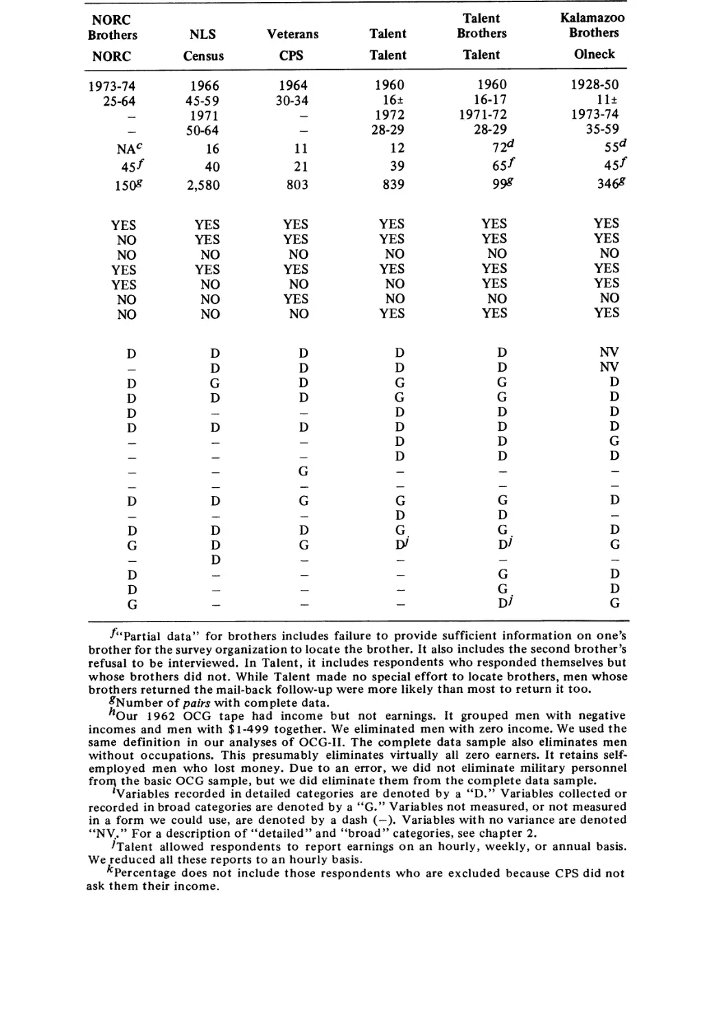
We will also look at six special-purpose samples that cover more
restricted populations but provide data not available in the five surveys
listed above:
6. The 1973—74 NORC Brothers sample. This survey was conducted at our
request and has not previously been analyzed in any detail.
7. The 1966—67 wave of the Census Bureau’s National Longitudinal Survey
of Older Men (NLS). Herbert Parnes of Ohio State University has been
the principal investigator concerned with these data.
8. The 1964 CPS Veterans sample. This sample is restricted to veterans
under the age of 35. It has been analyzed by Duncan (1968) and Criliches
and Mason (1972).
9. Project Talent’s 1960—72 representative subsample. This subsample from
the full Talent sample covers students who were in eleventh grade in
1960 and who were followed up intensively in 1972. It has not been
previously analyzed.
10. Project Talent’s 1960—72 brothers sample. This subsample includes pairs
of brothers enrolled in grades 11 and 12 in 1960 who returned a mail-
back questionnaire in 1971 or 1972. It has not been previously analyzed.
11. Michael Olneck’s 1928—74 Kalamazoo Brothers sample. This sample covers
men who were sixth graders in Kalamazoo, Michigan, between 1928 and
1950, who had brothers in these same schools, and whom Olneck followed
up in 1973—74.
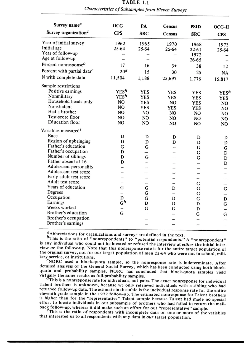
For reasons we will describe later, we tried to restrict all these sam-
ples to men who were not in school, in institutions, or in the military,
and who had positive earnings in the relevant year. Table 1.1 sum-
marizes each sample’s most salient characteristics. Taken together, they
provide a more complete picture of the relationship between men’s
characteristics in youth and their subsequent success than has pre—
viously been available.
Unfortunately, these surveys tell us far less about women than about
men. The Census and Project Talent were the only two of our surveys to
collect comparable data on both women and men—and the Census pro-
vides very limited information on its respondents, while Talent covers
only quite young respondents. In light of these data limitations we reluc-
tantly decided to restrict all our analyses to males. Fortunately, other in-
vestigators with more suitable data have done an excellent job of analyz-
ing the effects of sex on economic success (see e.g. Treiman and Terrell,
5
TABLE 1.1
Characteristics of S ubsamples from Eleven Surveys
“Mm
Survey name“ OCG PA Census PSID OCG-II
Survey organization“ CPS SRC Census SRC CPS
“—“M
Year ofinitial survey 1962 1965 1970 1968 1973
Initial age 25-64 25-64 25-64 22-61 25-64
Year of follow-up —— — -— 1972 ——
Age at follow-up — -— - 26-65 —
Percent nonresponseb 17 16 3+ 38 12
Percent with partial datae 20k 15 3O 25 NA
N with complete data 11,504 1,188 25,697 1,776 15,817
Sample restrictions
Positive earnings YES” YES YES YES YES”
Nonmilitary YESh YES YES YES YES
Household heads only NO YES NO YES NO
Nonstudent NO YES YES YES NO
Had a brother NO NO NO NO NO
Test-score floor NO NO NO NO NO
Education floor NO NO NO NO NO
Variables measured‘
Race D D D D D
Region of upbringing D D D D D
Father’s education G G — G G
Father’s occupation D — -— G D
Number of siblings D G — G D
Father absent at 16 D — —— — D
Adolescent personality — — — — —
Adolescent test score - — —— — —
Early adult test score — — — — —
Adult test score — — — G —
Years of education G G D G G
Degrees — G — G —
Occupation D G D G D
Earnings Gh D D D G
Weeks worked —- G G D —
Brother’s education G — -— G G
Brother’s occupation _ _
Brother’s earnings _ _. _
M—
aAbbreviations for organizations and surveys are defined in the text.
bThis is the ratio of “nonrespondents” to “potential respondents.” A “nonrespondent”
is any individual who could not be located or refused the interview at either the initial inter-
view or the follow-up. Note that this nonresponse rate is for the entire target population of
the original survey, not for our target population of men 25-64 who were not in school, mili-
tary service, or institutions.
CNORC used a block-quota sample, so the nonresponse rate is indeterminate. After
detailed analysis of the General Social Survey, which has been conducted using both block-
quota and probability samples, NORC has concluded that block-quota samples yield
virtgally the same results as full-probability samples.
This is a nonresponse rate for individuals, not pairs. The exact nonresponse for individual
Talent brothers is unknown, because we only retrieved individuals with a sibling who had
returned follow~up data. The estimate in the table is the individual response rate for the entire
eleventh-grade sample in the 1972 follow-up. The estimated nonresponse for Talent brothers
is higher than for the “representative” Talent sample because Talent had made no special
effort to locate individuals in our subsample of brothers who had failed to return the mail-
back follow-up, whereas it did make such an effort for our “representative” sample.
eThis is the ratio of respondents with incomplete data on one or more of the variables
that interested us to all respondents with any data in our target population.
I
I
NORC Talent Kalamazoo
Brothers NLS Veterans Talent Brothers Brothers
NORC Census CPS Talent Talent Olneck
1973-74 1966 1964 1960 1960 1928-50
25-64 45—59 30-34 16: 16-17 11:
— 1971 — 1972 1971-72 1973-74
— 50-64 — 28-29 28-29 35-59
NA6 16 1 1 12 7 2d 55"
45f 40 21 39 65f 45f
1509 2,580 803 839 99g 346g
YES YES YES YES YES YES
NO YES YES YES YES YES
NO NO NO NO NO NO
YES YES YES YES YES YES
YES NO NO NO YES YES
NO NO YES NO NO NO
NO NO NO YES YES YES
D D D D D NV
— D D D D NV
D G D G G D
D D D G G D
D — — D D D
D D D D D D
— — — D D G
-— — — D D D
_ _ G _ _ _
D D G G G D
_ - _ D D _
D D D G . G _ D
G D G D1 D1 G
_ D _ _ _ _
D —— — —— G D
D — — —— G . D
G — — — D1 G
fl‘Partial data” for brothers includes failure to provide sufficient information on one’s
brother for the survey organization to locate the brother. It also includes the second brother’s
refusal to be interviewed. In Talent, it includes respondents who responded themselves but
whose brothers did not. While Talent made no special effort to locate brothers, men whose
brothers returned the mail-back follow-up were more likely than most to return it too.
gNumber of pairs with complete data.
hOur 1962 OCG tape had income but not earnings. It grouped men with negative
incomes and men with $1-499 together. We eliminated men with zero income. We used the
same definition in our analyses of OCG-II. The complete data sample also eliminates men
without occupations. This presumably eliminates virtually all zero earners. It retains self-
employed men who lost money. Due to an error, we did not eliminate military personnel
from the basic OCG sample, but we did eliminate them from the complete data sample.
'Variables recorded in detailed categories are denoted by a “D.” Variables collected or
recorded in broad categories are denoted by a “G.” Variables not measured, or not measured
in a form we could use, are denoted by a dash (—). Variables with no variance are denoted
“NV.” For a description of “detailed” and “broad” categories, see chapter 2.
[Talent allowed respondents to report earnings on an hourly, weekly, or annual basis.
We reduced all these reports to an hourly basis.
kPercentage does not include those respondents who are excluded because CPS did not
ask them their income.
WHO GETS AHEAD?
1975). Nonetheless, this limitation is both serious and regrettable, since
sex is one of the most important single factors affecting earnings.
All of these surveys measured both the respondent’s occupation and
his earnings. Unlike most previous investigators, we did not concentrate
on one of these measures to the exclusion of the other. Instead, we
looked at both and tried to contrast results obtained using occupational
status to results obtained using earnings.
Occupational Status. We measured occupational status using Duncan’s
(1961) Socio-Economic Index. An occupation’s Duncan score depends
on the percentage of men working in the occupation who had com-
pleted high school and the percentage with incomes of $3,500 or more in
1950. F eatherman, Jones, and Hauser (1975) and F eatherman and
Hauser ( 1976c) have demonstrated that this scoring system captures both
inter- and intragenerational occupational stability better than any other
system in common use.
Since an occupation’s Duncan score depends on its educational re-
quirements, education inevitably influences a man’s score. This is not just
a methodological artifact; it reflects a real social phenomenon. The aver-
age education of men in a given line of work is closely related to the
cognitive complexity and desirability of the work. It affects not only the
social position of those who engage in the work (Duncan, 1961), but
their children’s life chances (Klatzky and Hodge, 1971), independent of
both the individual’s own education and his earnings from his work
( Sewell and Hauser, 1975; Bielby et al., 1977).
The Duncan scale runs from o to 96. To get some sense of the signifi-
cance of a one-point difference in Duncan scores, we looked at Rain-
water’s 1971—72 Boston Area Survey. Rainwater had asked respondents to
rank 120 hypothetical individuals in terms of their “general standing” in
their community. Each of these 120 hypothetical individuals had a differ-
ent combination of education, occupation, and income. A one-point
change in a man’s Duncan score had the same effect on his “general
standing” as a 1.3 percent change in his income.1
Earnings. Except in Project Talent, we measured earnings on an an—
nual, rather than a weekly or hourly, basis. We tried three different pro-
cedures for scaling earnings. First, we looked at actual earnings, mea-
sured in dollars. Second, we looked at the natural logarithm of earnings
(ln earnings). This allows us to estimate the percentage change in
earnings associated with a unit change in any other trait. Third, we
looked at the determinants of the cube root of earnings (earnings 1/3).
There is some evidence that subjective well-being (“utility”) is more
8
Introduction
nearly a linear function of earnings 1/3 than of either earnings or In
earnings.2 These three alternative measures of earnings yield essentially
similar results, though earnings 1/3 is slightly more predictable than either
earnings or In earnings.3 However, ln earnings has two advantages over
earnings and earnings 1/3. First, In earnings is especially sensitive to varia-
tions near the bottom of the earnings distribution. This coincides with
the emphasis of public policy since 1964, which has focused on altering
the bottom of the earnings distribution. Second, ln earnings yields co-
eflicients that are easier to compare across time. Most of our analyses
therefore concentrate on In earnings.
Economists usually think of annual earnings as depending on two fac-
tors: hourly wages and hours worked per year. Chapter 9 shows that the
determinants of wages are not the same as the determinants of hours,
although each may influence the other. Ideally, then, we should investi-
gate the determinants of wages and hours separately. Unfortunately,
many of our surveys did not collect information on hours (or even weeks)
worked during the previous year. The surveys that did collect such in-
formation often grouped it into broad categories. This means that we
could not estimate the respondent’s average hourly or weekly wage ac-
curately. We therefore decided not to try to disentangle the factors that
influence wages from those that influence hours in most of our analyses.
Chapter 9, however, does do this for the PSID data.
The reader may also wonder why we looked only at earnings, ignoring
other sources of income. The main reason is simplicity. Chapter 9 shows
that among families with a “head” 25- to 64-years-old, male earnings ex-
plain 82 percent of the variance in total family income. Some families
receive substantial income from female earnings, but since few females
have high earnings and many have none at all, female earnings con-
tribute far less than male earnings to the overall variance of family
income. A few families also receive substantial income from dividends,
interest, or rent, but such income also explains a relatively modest frac-
tion of the variance in total family income. Transfer payments, such as
welfare and social security, are even less important. The principal prob-
lem posed by concentrating on male earnings is that we completely ig-
nore families with no male earner at all. This problem is not as serious
as it seems, however, since we can predict family income quite ac—
curately if we know that the family in question has no male earner. Such
families’ total income is almost always low.
Family Background Measures. We define family background as
everything that makes men with one set of parents different from men
9
WHO GETS AHEAD?
with a different set of parents. Most previous investigators have measured
family background in terms of what we will call “demographic” advan-
tages. By this we mean such readily measurable background characteris-
tics as race, place of birth, father’s education, father’s occupation, num-
ber of siblings, and whether the respondent lived with both parents
while he was growing up.4 One can obviously augment this list by in-
cluding mother’s education, mother’s occupation, parental income, pa-
rental ethnicity, parental religion, and the like. But no such list is ever
complete. Thus while analyses of this kind can set a lower limit on the
overall impact of family background, they can never set an upper limit.
To get around this difficulty we have used an alternative measure of
familial influence, namely the degree of resemblance between brothers.
Such resemblance can be due to common genes, common environment,
or the influence of one brother on the other. But unless brothers deliber-
ately become unlike one another, resemblance between siblings sets an
upper limit on the explanatory power of their common environment and
common genes. ( Resemblance between siblings does not allow us to esti-
mate the effects of genes alone.)
Contrary to what Iencks et al. argued in Inequalitz , background char-
acteristics seem to exert appreciable effects on both occupational status
and earnings even among men with the same test scores and education.
The background characteristics that exert these effects are not primarily
the “standard” demographic measures of parental advantages, such as
father’s occupation and parental income. Rather, some set of as yet un-
measured background characteristics makes brothers more alike than
we would expect on the basis of their test scores and education. The
unmeasured background characteristics that affect economic success ap-
pear to be different in kind from the background characteristics that in-
fluence test scores and educational attainment. Taking account of these
unmeasured influences increases the apparent importance of growing up
in the “right” family. Chapter 3 explores these effects in detail.
Cognitive Measures. Almost all investigations of the effects of cogni-
tive skills on economic success have relied on a single cognitive test,
usually designed to measure academic “aptitude” or “intelligence.” 5
Project Talent, in contrast, administered cognitive tests covering 60 dif—
ferent areas to a national sample of high school students in 1960. In
1972 Talent recontacted a relatively representative subsample of former
eleventh graders, most of whom were then 28 or 29 years old, and ob-
tained data on their education, occupational status, and earnings. The
Talent data therefore allow us to explore the effects of different adoles-
10
Introduction
cent cognitive skills in far greater detail than previous investigations
have. Chapter 4 shows that tests of academic aptitude and skills predict
economic success better than did Talent’s other tests (e.g. “creativity,”
“clerical checking,” “abstract reasoning”). Within the academic domain
no one general area is clearly more important than others. The best
predictors are those that test a wide range of verbal and quantitative
skills.
Test performance in sixth grade seems to predict subsequent success
as accurately as test performance later in school or in adulthood. This
implies that changes in test performance after sixth grade have little
impact on adult success. If this is the case, it is the “aptitude” component
of test performance that affects success, not the “achievement” com—
ponent. The evidence for this interpretation is by no means conclusive,
however, and some Swedish data contradict it (Fagerlind, 1975). If
confirmed, this finding would imply that changing a student’s relative
test performance, at least after sixth grade, has little effect on his
life chances.
With the exception of Taubman and Wales (1974), most previous in—
vestigations of the relationship between adolescent cognitive skills and
later economic success have measured workers’ success when they were
still quite young. Our Talent respondents are also young, but Olneck’s
Kalamazoo sample is 35- to 59-years-old. Since Olneck’s data cover broth-
ers, they also allow us to distinguish the effects of cognitive skills from
the effects of family background more adequately than previous research.
Chapter 4 analyzes the effects of cognitive skills in detail.
Personality Measures. Most previous research on the effects of per-
sonality traits has relied on cross-sectional data. This makes it very diffi-
cult to say whether “favorable” personality traits cause economic success
or vice versa. The Talent and Kalamazoo surveys probably provide the
best longitudinal data on adolescent personality traits now available. The
Kalamazoo schools collected teacher ratings of tenth graders’ personal-
ity traits. Project Talent collected a wide range of self-assessments from its
high school respondents. It also asked respondents to describe their high
school behavior. Variations in such behavior presumably reflect personal-
ity differences to some extent.
No one personality measure predicts success in maturity as well as
test scores do. When we combine a number of different adolescent per-
sonality measures, however, their combined effects are as strong as the
combined effects of different adolescent cognitive tests. Furthermore,
personality traits affect earnings in ways that are largely independent of
11
WHO GETS AHEAD?
background, test scores, and educational attainment. Overall, then, our
data suggest that personality traits are considerably more important than
earlier data implied. The best predictor of economic success appears to be
what Talent labeled “leadership” and Kalamazoo teachers called “execu-
tive ability.” Chapter 5 analyzes the effects of these traits in more detail.
Education. Like most previous investigators we were primarily con-
cerned with estimating the economic effects of the amount of time re-
spondents had spent in school, but none of our surveys asked how many
years students had actually spent in school. Instead, our surveys asked the
respondent the highest grade of school or college he had completed. Like
time in school. Our estimates of the economic benefits of schooling do
not, then, differ from those of previous investigators because we measured
respondents’ educational experience differently but because we had more
measures of respondents’ characteristics before they were exposed to dif—
ferent amounts of schooling. Chapter 6 shows that improved measure-
ment of respondents’ initial characteristics somewhat reduces the appar-
ent benefits of school attendance. The reduction is larger for secondary
school than for higher education, and larger for earnings than for occu-
pational status.
While our primary concern was estimating the effects of time spent in
school (“quantity”), we also devoted some attention to differences in
respondents’ experiences while they were enrolled in school (“quality”).
The Talent and Veterans surveys asked respondents what kind of cur-
riculum they had pursued in high school and found that those who had
completed a college preparatory curriculum were somewhat better off
economically than those who had completed a nonacademic curriculum.
But as chapter 6 notes, this difference is entirely attributable to the fact
that enrolling in a college preparatory curriculum increases a student’s
chance of attending college. When we compared students who had the
same amount of schooling, we found no evidence that either the subject
matter or the attitudes acquired in a college preparatory curriculum were
more valuable economically than those acquired in other curricula.
Talent also collected data on the subjects its respondents had studied
in college and on the institutions they had attended, but we have not yet
analyzed these data. The only other survey we analyzed that recorded
data on college quality was the Productive Americans (PA) survey. The
PA survey reported the “selectivity” of the last college or graduate school
a respondent had attended and showed that respondents who had at-
tended selective institutions earned more than those who had attended
unselective ones. But since PA did not collect data on students’ abilities
12
Introduction
or aspirations before they entered college, it does not allow us to say how
much of the economic advantage enjoyed by the alumni of selective col-
leges is due to their college experiences per se.
2. STATISTICAL METHODS
In considering the association of workers’ characteristics with one an-
other, we asked three questions:
1. How strong is the observed relationship between any given worker
characteristic and economic success? We were not satisfied with merely
establishing the existence of a relationship. Rather, we tried to determine
the size of the relationship. The size of a given relationship depends on
the population one studies, the way in which one asks and codes ques-
tions, and the statistics one uses to describe the results. One must de-
vote considerable attention to technical details in order to make mean-
ingful statements about the size of relationships.
We did not assume that the relationships between worker characteris-
tics and economic success were necessarily linear. Chapter 2 describes
how we tested for nonlinearities. Nonlinearities proved unimportant
when estimating the effects of family background and test scores. But a
year of higher education raises occupational status by two or three
times as much as a year of elementary or secondary education. A year of
higher education also raises earnings by a larger dollar amount, though
not by a larger percentage, than a year of elementary or secondary edu-
cation. The first and last years of high school and college are associated
with larger percentage increases in earnings than the intervening years.
This could be due to institutional selection, self-selection, or “credential
effects.”
2. How much of a trait’s observed relationship to economic success is a
by-product of the fact that both the trait in question and economic suc-
cess depend on causally prior traits? If we want to assess the true “ef—
feet” on economic success of, say, staying in school rather than dropping
out, we must compare groups of respondents who had the same charac-
teristics in adolescence but who then got different amounts of school-
ing for some unknown reason. We use multiple regression equations to
make such comparisons. To assess the effect of schooling on occupational
status, for example, we regress occupational status on schooling while
13
WHO GETS AHEAD?
controlling all worker characteristics that are causally (i.e., temporally)
prior to leaving school. These traits include family background, adoles-
cent test scores, and adolescent personality traits.
We did not restrict ourselves to controlling causally prior variables that
we could measure directly. By looking at differences between brothers,
we were also able to control the unmeasured family background charac-
teristics that make brothers alike. This allowed us to isolate the effects
of cognitive skills and education more precisely than most previous
investigators.“ Furthermore, the fact that some of our surveys contained
measures of both adolescent test scores and adolescent personality traits
allowed us to estimate the extent to which ignoring these factors biases
other estimates of the economic benefits of schooling. Chapter 6 shows
that controlling all aspects of family background plus adolescent test
scores substantially reduces the estimated returns to schooling.
We retained nonlinear education measures throughout our analyses.
This turned out to be quite important. Chapter 6 shows that controlling
family background and cognitive skills lowers the estimated economic
benefits of elementary and secondary education more than it lowers the
estimated benefits of higher education.
We also investigated whether the effect of one worker characteristic
depended on the value of another. Chapter 2 describes our procedures
for detecting such interactions. In general, they did not appear to be very
important. Chapter 6 shows, for example, that returns to education do
not depend on initial ability. Similarly, chapter 7 shows that, contrary
to much previous research, percentage returns to education are not con-
sistently higher for whites than for nonwhites. It would be wrong, how-
ever, to say that interactions are never important. Chapter 7 shows that
race affects returns to different levels of education, with whites generally
receiving higher returns to the first 15 years of schooling and nonwhites
gaining more from the 16th year. Chapter 6 shows that men with white-
collar fathers obtain a greater occupational payoff from elementary and
secondary schooling than men with farm fathers, but the pattern is re-
versed for higher education. Such interactions are atypical, however.
3. What are the mechanisms by which a given characteristic exerts its
influence on economic success? To answer this question we augment our
regression equations by including worker characteristics that are causally
subsequent to the characteristic under study. Thus, if we want to say
how education affects economic success, we control test scores in ma-
turity, years of labor-force experience, or other traits that depend on
education.
As we add each of these “intervening” variables to our equation, the
14
Introduction
coefficient of education changes. If we could identify all the relevant in-
tervening variables and could measure them correctly, the coefficient of
education might fall to zero. If we cannot identify (or properly measure)
all the relevant intervening variables, the coefficient of education will
remain positive. The ratio of the coefficient after controlling an interven-
ing variable to the coefficient with only causally prior variables con-
trolled tells us how much of the effect of education depends on the fact
that education affects this intervening variable. According to sociological
convention, the effects of one variable on another that are not explained
by intervening variables are known as “direct” effects, while the ex—
plained effects are known as “indirect.” The magnitude of the “direct”
effects is, of course, a function of the investigator’s choice of “intervening”
variables.
3. RECONCILING DISCREPANT FINDINGS
One major advantage of our investigation was our simultaneous use of
many different surveys. These surveys often yielded apparently inconsis-
tent results. This made us unusually sensitive to the many sources of non-
comparability in social science research. It also led us to investigate
some of these sources of noncomparability in a systematic way.
Chapter 10 shows that even when we made a systematic effort to
eliminate all differences between our major national surveys, irreducible
“survey organization effects” remained. Specifically, we found that
Michigan’s Survey Research Center interviews fewer unskilled and semi-
skilled workers than the Census Bureau. SRC may also get higher qual-
ity income data from the people it interviews.
Chapter 11 shows how various “arbitrary” decisions that researchers
make in the course of analyzing their data affect the apparent distribu-
tion of both education and earnings in the 1970 Census and in the
1970 wave of the PSID. It also shows that with one major exception
these decisions do not appreciably alter the estimated value of an extra
year of school. The exception is the treatment of respondents without
earnings. Our work focused exclusively on individuals with positive earn—
ings. Some other investigators include respondents with zero earnings. If
one is predicting dollar earnings and is looking only at men aged 25 to
64, including nonearners makes little difference. But if one is predicting
15
WHO GETS AHEAD?
the logarithm of earnings, as economists usually do, one must assign men
without earnings some arbitrary value. Most economists choose $1. Even
when the overwhelming majority of respondents have earnings, this has
disastrous effects. Including nonearners and assigning them $1 dramati-
cally increases the apparent variance of earnings. It also means that one’s
equations primarily describe the determinants of labor-force participa—
tion, not the determinants of relative earnings among participants.
Studies that use this method cannot be compared to studies like ours that
do not.
Chapter 2 discusses several other issues that affect the comparability
of results from different studies. Age restrictions appear to be the most
important source of noncomparability. Samples that include men under
25 (e.g., Mincer, 1974) yield very different results from samples that
include only older men. Even samples of 25- to 34-year-olds differ in
important respects from samples of older men. This means that we
cannot generalize with much confidence from our Talent samples to all
men aged 25 to 64.
As the foregoing summary indicates, our research took us in a variety
of different directions. The result is a long book. In order to facilitate
selective reading, we tried to make each chapter as self-contained as
possible. This leads to a certain amount of repetition. To prevent such
repetition from becoming unbearable, we decided not to make each
chapter methodologically self-contained. Instead, we grouped almost all
our methodological material in chapter 2. Later chapters assume familiar-
ity with this material. Readers with limited time or trusting dispositions
can therefore skim chapter 2 and then turn to the substantive chapters
that particularly interest them.
16
CHAPTER 2
Methods
This chapter describes how we analyzed our eleven samples and provides
some of the technical information needed to assess the plausibility of our
results. Section 1 describes the questions different surveys asked and
how we coded the responses. Differences between surveys account for
some of the inconsistencies in our subsequent numerical estimates.
Section 2 discusses associations among pairs of variables. We begin
by discussing unstandardized linear coefficients (i.e., correlations). Then
we present the usual formula for estimating standardized linear coeffi-
cients (i.e., correlations). Then we discuss the interpretation of such
unstandardized coefficients when the dependent variable is the natural
logarithm of earnings. We conclude by discussing our procedures for
identifying nonlinear relationships (i.e., quadratic terms and comparison
of eta 2 with R 2) and for summarizing such nonlinearities in regression
equations (i.e., orthogonal quadratic terms, splines, and dummies).
Readers with economic training will find nothing new here, except per-
haps for our discussion of orthogonal nonlinear terms. Sociologically
trained readers should also peruse the discussion of semilog equations.
Readers who do not use statistics on a daily basis may want to read the
whole section.
Section. 3 discusses multivariate relationships. It begins by describing
how we estimated the “effect” of one trait on another, as distinct from
the association, by controlling causally prior traits. It also discusses how
Susan Bartlett, James Crouse, David Eaglesfield, Gregory Jackson, Christopher
Jencks, Kent McClelland, Peter Mueser, Michael Olneck, Joseph Schwartz, Sherry
Ward, and Jill Williams all contributed to this chapter. Jencks wrote the text.
17
WHO GETS AHEAD?
we controlled unmeasured background characteristics by estimating
“difference equations” for brothers. Then it discusses how we investi-
gated the mechanisms through which a trait affected economic success
by controlling “intervening” variables. It concludes by discussing our
search for nonadditive relationships, which we tried to identify both by
splitting each sample into subsamples and by including orthogonal multi-
plicative terms in our equations. Statistically sophisticated readers will
find nothing new here except for our discussions of difference equations
and orthogonal multiplicative terms.
Section 4 discusses measurement error. It presents evidence on the
likely size of such errors in various samples and gives simple formulas
for estimating the effect of random errors on bivariate associations.
Section 5 gives some rules of thumb for estimating the significance of
differences obtained from weighted samples and for calculating the sig-
nificance of differences between pairs of regression coefficients. Readers
familiar with these problems should skip this section.
Section 6 discusses the effects of eliminating students, soldiers, inmates,
and respondents with incomplete data. It also presents data on the ef-
fects of age restrictions. This discussion should help explain some of the
apparent discrepancies between samples discussed in later chapters. Sec-
tion 6 also discusses the biases introduced by estimating returns to school-
ing with experience rather than age controlled.
1. QUESTIONS AND CODING
We habitually describe the men who interest us as “respondents.” In a
number of instances, however, our information about these men comes
from someone else, whom we might call an “informant.” In OCG, for
example, information on the respondent’s education and occupation
came from a March 1962 CPS interview which was conducted with the
most knowledgeable adult who happened to be at home when the inter-
viewer reached a given household. OCG’s income data came from similar
interviews in February. Women are at home more often than men, so
most of these data probably come from wives. The PA and PSID tried
to get data from men whenever they could, but they did not always
succeed. The Census asked “the householder” to fill out the question-
naire for everyone in his or her household but did not say who the
18
Methods
householder was. The other surveys obtained virtually all their data di-
rectly from the respondents. Chapter 11 concludes that PSID wives’
estimates of their husband’s earnings were about as accurate as the hus-
bands’ estimates, but this may not hold for other surveys or traits.
Race. The Census Bureau and the Survey Research Center (SEC)
told interviewers to guess the informant’s race, using whatever visual or
verbal clues the interviewer thought appropriate. When the informant
was not the respondent, both the Census Bureau and SEC assumed that
the respondent was of the same race as the informant. The NOBC
Brothers Survey told interviewers who had any doubt about the respon—
dent’s race to ask the respondent, “What race do you consider yourself?”
The 1970 Census and Project Talent relied largely on mail questionnaires
and asked all respondents to report their race for themselves.
We assigned “white” respondents a score of 1 on this variable. We as-
signed all others 0. This variable’s coefficient therefore measures the
benefit of being white rather than nonwhite.*
Father Absent. The NLS, Veterans, and NORC Brothers surveys
asked, “With whom were you living when you were 15?” OCG and
Kalamazoo asked, “Were you living with both your parents most of the
time up to age 16?” Talent asked eleventh graders, “With whom are you
now living?” The PA, Census, and PSID did not ask this question. In
analyzing the PSID we assumed that respondents who reported neither
their father’s education nor his occupation had not grown up with
their fathers]t
Father’s Education. The Census did not ask about father’s educa-
tion. Talent asked “What is the highest grade of school or college your
father reached?” All other surveys substituted “completed” for “reached.”
All surveys but the PA and PSID asked respondents who were not living
with their father when they were 15 or 16 (or when they were “growing
up”) to report on the individual who “headed” their household. Between
7 and 20 percent of all respondents reported on someone other than
their father, with the percentage varying by age and geographic location.
The NLS, NORC Brothers, and Kalamazoo surveys recorded the exact
number of years completed. The OCG, PA, Veterans, PSID, and Talent
surveys grouped responses into categories like “some high school,” “high
” Tables A2.1 and A25 treat PSID’s “Spanish American” respondents as “non-
white.” Chapter 7 treats Spanish American respondents as white, in order to increase
comparability with our other surveys, which did not distinguish Spanish Americans
from other respondents.
i This coding procedure means that the coefficient of the PSID variable is not com-
parable to the coefficient of the father absent variable in other samples and should
not be given any substantive interpretation. Its only purpose is to avoid eliminating
men who knew nothing about their fathers.
19
WHO GETS AHEAD?
school graduate,” “some college,” and so forth. We used 1970 Census data
to estimate the mean number of years of school completed by men in
each category and assigned all respondents the estimated mean of their
category. Grouping makes the observed variance slightly less than the
true variance.
The PA and PSID surveys asked respondents who did not know their
father’s education whether he could read and assigned those who could
not read to the category “0 to 5 years of school.” Neither PA nor PSID
retained flags for these assigned values, so we could not eliminate
them. The PA and PSID did not ask how many years of school fathe1s
had completed beyond high school. Instead, they asked whethe1 the
father had attended college, whether he had earned a bachelor’s de—
gree, and whether he had earned a graduate degree. We estimated
years of school from these data.
There was a serious nonresponse problem among men who said their
father was not living at home when they were “growing up” or when
they were 16. We assigned such men the survey mean if they did not
report their father’s education and relied on the dummy variable for
father absent to capture differences in economic success between men
with no father at home and the rest of the sample.
Father’s Occupation. The OCC, Veterans, NLS, and Kalamazoo sur-
veys asked respondents what kind of work their fathers did when they
were about 15 or 16 years old. The NORC Brothers Survey asked what
the father “normally” did when the respondent was “growing up.” These
surveys also asked who the respondent’s father worked for, if anyone.
Thev classified the resulting replies using Census three- d—igit occupation
and industry codes and then assigned them Duncan scores
The PSID asked about the fathers “usual occupation” when the re-
spondent was “growing up” and coded replies into eight categories that
correspond roughly to broad Census occupational groups. Talent asked
its eleventh-grade respondents which of seventeen occupational cate-
gories “comes closest to describing your father’s work.” Talent provided a
minimal description and a few examples for each category. We assigned
the PSID and Talent categories an approximate Duncan score, based on
Duncan’s (1961) data on workers in the relevant category. Grouping
reduces the measured standard deviation of father’s occupation by
about a seventh in the PSID. There is no apparent reduction in Talent.
OCG, Veterans, NLS, Kalamazoo, and Talent asked respondents who
were not living with their fathers to report on the individual who
headed their household when they were 15 or 16. PSID did not ask
whether the father was absent. Nor did it ask for data on the person
20
Methods
who headed the household if the father was absent. The PA and Census
did not ask about the father’s occupation.
Father Foreign. The PA and PSID asked respondents where their
father grew up. The OCG, NLS, and Kalamazoo surveys asked where he
was born. The Census also asked where the father was born, but we
did not utilize this question in our Census analyses. The Veterans, Proj-
ect Talent, and NOBC Brothers surveys did not ask about the father’s
place of birth.
Siblings. The OCC, PA, PSID and NORC Brothers surveys asked
about the number of brothers and the number of sisters the respondent
had. OCC asked respondents to include stepsiblings, adopted siblings,
and siblings who had lived but were now deceased. PSID added that
foster siblings should not be included. NOBC said nothing about foster
siblings but qualified OCC’s list with “if you grew up with them.” Talent
asked how many living children the're were in the respondent’s family.
Kalamazoo asked separately the number of older and younger “children
[who] grew up in your family.” The Veterans, NLS, and Census surveys
did not ask about siblings.
Nonfarm Upbringing. NLS asked, “When you were 15 years old,
where were you living?” and included “rural farm” as a possible answer.
OCC asked a similar question but allowed respondents to answer, “The
same place I do now.” The Census Bureau coded OCC respondents who
gave this answer as having grown up on a farm if they were living
on a farm in 1962. There is no way to identify OCC respondents who
grew up on a farm, no longer lived on one in 1962, but still lived in the
same community.“ PA and PSID asked, “Where did you grow up? Was
that on a farm, in a city or what?” Veterans asked “In what kind of
place did you live most of the time up until you were 15?” NOBC
Brothers did not ask such a question, so we assumed that men whose
fathers were “normally” farmers or farm laborers grew up on farms. We
could have done this in Talent as well, but we did not. Kalamazoo
respondents all lived in the city of Kalamazoo when they were in sixth
grade, so the question seemed redundant. The Census did not collect any
information on whether the respondent grew up on a farm.
Non-South Upbringing. OCC, NLS, and Census asked where the re-
spondent was born. The Veterans Survey asked where the respondent
lived “most of the time” up to age 15. PA asked where he “grew up
“ We could have treated such respondents as having grown up on a farm if they
said their father worked in farming, but this is not quite the same thing. Some men
work on farms without living on one. Others live on farms while working primarily in
some other, more lucrative occupation.
21
WHO GETS AHEAD?
(from about ages 6—16).” PSID merely asked, “Where did you grow up?”
We defined the South as including all states south of the Mason-Dixon
line and the Ohio River, plus Arkansas, Louisiana, Oklahoma, and Texas.
We coded everyone else as nonsouthern. We did not code this informa—
tion in Talent. We did not collect it from NORC or Kalamazoo Brothers.
Test Score. Talent administered a large battery of tests to eleventh
graders. Kalamazoo administered the Terman or Otis Group IQ test in
sixth grade. The Veterans Survey retrieved men’s AFQT scores at the
time they entered military service. The PSID administered a thirteen-
item sentence-completion test in 1972. The other samples have no test-
score data. We scaled all these tests using an “”IQ metric, in which the
population mean is 100 and the standard deviation is 15.1
Age. PA, PSID, OCC, Census, Veterans, Talent, and NLS asked
respondents how old they were, with OCG and Census specifying “on
your last birthday.” The Census also asked for date of birth. NORC
Brothers asked, “In what year were you born?” Kalamazoo obtained the
birth year from school records. Since all Talent respondents were in
eleventh grade in 1960, variation in their age is mainly due to variation
in the age at which they started school and the number of grades they
skipped or repeated. With test score controlled, age did not affect suc-
cess in Talent, so we ignored it.
Education. OCC and Census asked for the highest grade the respon—
dent had attended and whether he had completed that grade. Veterans,
NLS, and Kalamazoo asked for the highest grade completed. PA and
PSID asked about grades attended through high school and whether high
school graduates had started or completed college or graduate school. In
addition, PSID asked whether respondents had any trouble reading.
Talent asked whether respondents had obtained a high school diploma
and how much college and graduate schooling they had completed.
NORC asked about both years of schooling and degrees obtained.
Census, NLS, Kalamazoo, and NOBC Brothers recorded the highest
grade in single years. OCC, Veterans, PA, and PSID recorded re-
sponses in broader categories. This reduces the standard deviation of
education slightly. The 1975 wave of the PSID, which became available
after our analyses were complete, asked respondents how many years
of education they had completed and recorded exact years. This mea-
sure correlated o.976 with the grouped PSID measure based on de-
grees. Neither education measure predicts economic success consis-
tently better than the other in PSID, so we ignore the distinction.
Experience. We defined “experience” as the number of years the re—
spondent had been out of school since the age of 14. For this purpose
22
Methods
we assumed that every respondent entered first grade when he was six
and advanced one grade per year. It follows that:
Experience = Age — (Education + 6) if Education 2 8
= Age — 14 if Education g 8
Of course not all men enter first grade when they are 6 years old,
and not all advance one grade per year.“ Furthermore, many of our
surveys did not ask exactly how many years of school respondents had
had, especially if they had attended graduate school. Our estimates of
experience therefore contain a fair amount of error.
Note that this variable does not measure experience since school com-
pletion. Many men leave school, work for a few years, and then return
to school. Our variable includes experience prior to reentering school.
Note, too, that our variable does not measure work experience. Many
respondents work while they are in school. Many others do not work even
while they are out of school. And finally, our variable does not measure
on-the-job training. We have no data regarding such training.
Occupation. OCG, Census, NORC, and Kalamazoo asked, “For whom
do you work?” “What kind of business or industry is this?” and “What
kind of work are you doing? (Please describe duties as specifically as
possible).” They coded responses into three-digit Census occupational
categories and then recoded to Duncan scores. Veterans and NLS
merely asked, “What kind of work are you doing?” and coded it simi-
larly. PA and PSID asked, “What is your main occupation?” and classi-
fied responses into broad Census categories, to which we assigned Dun-
can scores. Talent assigned respondents to one of 181 occupational cate-
gories. We tried to match these Talent categories with those used by the
Census Bureau and then estimated each category’s Duncan score.
Earnings. We defined earnings as income from wages, salaries, and
self-employment. OCG, PA, NLS, PSID, and the Census asked respon—
dents to report income from wages and salaries, nonfarm self-employ-
ment, and farming separately. Unfortunately, our OCG tape did not
record these separate responses. Instead, it recorded total income from
all sources, including assets and transfer payments. Most respondents un-
derreport their asset and transfer income to the Census Bureau, so the
distortion is not as serious as it might be. For Census respondents with
a current occupation, 95 percent of all reported income is from earnings.
Chapter 11 shows that substituting income for earnings raises the esti-
mated returns to schooling by about 1 percent in the Census but has
” OCG asked about age at school completion, but the responses contain so many
oddities that we did not try to use them.
23
WHO GETS AHEAD?
no effect in the PSID. The difference is smaller if one restricts the
analysis to men with a current occupation, as we do. We therefore treat
results for income and earnings as interchangeable.*
The OCG, PA, NLS, Census, and NORC Brothers surveys asked re-
spondents to report their earnings or income for the calendar year prior
to the survey. This means that the earning year does not coincide
with the survey year, and that some respondents reported a current oc-
cupation different from the occupation they engaged in when they
earned the amount reported]l PSID also asked respondents about their
earnings during the previous calendar year, but because the survey was
repeated at one-year intervals we were able to ascertain both occupa—
tional status and earnings for the same year (1971). Some Kalamazoo
Brothers were surveyed near the end of 1973 and were asked how much
they expected to earn during that year. The rest were surveyed in early
1974 and were asked how much they had actually earned in 1973.
Veterans were asked how much they expected to earn in 1964. Re-
sponses to this question appear to be about as accurate as responses to
questions about actual earnings for the previous calendar year. Talent
respondents were asked their hourly, weekly, or monthly earnings at
the time of the survey. We reduced all the Talent responses to an hourly
value, since we did not know how many hours respondents had worked
during the previous year.
The OCG, Veterans, NORC, and Kalamazoo surveys grouped re—
sponses into quite broad categories. This compresses the variance of
earnings. It also increases the correlation of earnings with other traits,
since the traits we measured did not explain much of the variation
within the top or bottom categories. As a result, grouping earnings
slightly increases standardized coeHicients while leaving unstandardized
coefficients almost unchanged (see chapter 11 ).
Family Income. We defined family income as the sum of the re-
spondent’s earnings, his income from assets and transfer payments, and
the income from all sources of all other family members. This measure
is available for the Veterans, PA, NLS, Census, PSID, Kalamazoo, and
” PSID did not record total self-employment income. Instead, it divided such in-
come into “labor” and “asset” income, and grouped the latter. We reconstructed the
approximate amount of PSID self-employment income using other data. For details on
this problem see Final Report, Appendix D and chapter 16.
f Tables dealing with occupational status ordinarily indicate the year of the survey,
while tables dealing with earnings indicate the earning year. This means that the
same survey is identified in different ways in different tables. When we refer to both
occupational status and earnings we often identify a survey as covering a two-year
interval: “the 1961—62 OCG data,” for example.
24
Methods
NORC Brothers samples, but we did not use it in our Veterans or Census
analyses.
As the foregoing discussion indicates, there is no professional con-
sensus on how best to measure standard “demographic” concepts. As
a result, every investigator feels free to “improve” previous investigators’
measures. In most cases these “improvements” have no effect. But there
is seldom any simple way to be sure of this, since those who improve
their predecessors’ measures rarely bother to try both approaches and
compare the results. Thus when we obtain different results from different
samples we rarely know precisely why. Furthermore, whether or not an
“improvement” actually “works” (e.g. by predicting an outcome of in-
terest more accurately than alternative measures), most investigators
give their new measures the same verbal label as older ones. This creates
the illusion of greater comparability than really exists. This is one reason
why knowledge in the social sciences is so seldom cumulative. We have
tried to be sensitive to this danger in our own analyses, but we have not
completely avoided it.
Table A2.1 in the Appendix shows the mean and standard deviation of
each variable for each sample of respondents with complete data. Table
10.1 in chapter 10 shows frequency distributions for OCC, PA, Census,
and PSID samples that have been modified slightly to make them more
nearly comparable to one another. Chapter 10 also discusses some of
the reasons for differences among our samples.
2. BIVARIATE RELATIONSHIPS
Unstandardized- Coefficients. One way to estimate the association be-
tween two worker characteristics is to write an equation relating them
to one another. Suppose, for example, that we want to relate education
(U) to earnings (Y). If we use the subscript i to designate any randomly
selected individual, the coefficient B0 to designate the expected earnings
of individuals with no schooling, and the coefficient B1 to designate
the average increase in earnings associated with the average year of
schooling, we can write:
25
WHO GETS AHEAD?
(1) Y¢= BO‘l‘BlUi'l‘Ei
where E,- is an error term, equal to the difference between the 2th in-
dividual’s actual earnings (Y1) and the value predicted on the basis of
the equation (Yi). This predicted value is simply B0 +B1U,-. If we esti-
mate B1 using conventional least squares regression, E will be uncorre-
lated with U. Taking the variance of both sides of equation 1 then yields:
(2) 52Y = B2152U + 52E
where s2y, s2U, and 52E are the variances of Y, U, and E respectively.
Since Y-= B0+B1U it follows that s2 y — —B2ls2U and equation 2 can be
reduced to:
(23) 52Y252Y+S2E
We designate s23? as the “explained” variance. It follows that s2 §/s2y is
the percentage of the total variance in Y “explained” by variation in U.
We designate this percentage as R2. (Since the observed value of R2
tends to be slightly higher than the true value, especially in small sam-
ples, we sometimes report a “corrected” value of R2, denoted as R2).
Standardized Coefficients. Measures like test scores and occupational
status have no “natural” metric. Even when a measure has a natural
metric, as education and earnings do, it is often convenient to “standard-
ize” it for comparability with other measures with different metrics. To
accomplish this we subtract 3 variable’s mean (Y or U) from all obser-
vations and then divide by the standard deviation (sy or 51;). Every
standardized variable’s mean is therefore zero, with a standard deviation
of 1.000. If we denote these standardized measures with lowercase let-
ters, we can show that:
(3) Yr = rYUui + 91'
where rm is the correlation between Y and U, and ei = Ei/ 51'. We can also
show that:
<4> B1: (5" >
SU
Squaring both sides and rearranging gives us:
B21321} 2 ’1}
(4a) 2 = T = r2YU
S Y 5 Y
The correlation coefficient therefore has a double meaning. Suppose,
for example, that rYU =o.4o, a fairly typical value. Equation 3 then
26
Methods
tells us that two individuals who differ by one standard deviation on
education can be expected to differ by 0.40 standard deviations on earn-
ings. Equation 4a tells us that the ratio of explained to total variance in
earnings is equal to r2UY =0.16. Tables A2.2—A2.12 in the Appendix
display the correlations among the principal variables in our complete
data samples. One can combine these correlations with the standard
deviations in table A21 to obtain unstandardized regression coefficients.
Logarithmic Coefficients. If we want to estimate the percentage in-
crease in earnings associated with an extra year of education, we use
the natural logarithm of earnings (i.e., the log to the base e, where
e ~ 2.71828) as the dependent variable. Then we estimate:
(5) lnYi = B0 + BlUi +Ei
Taking the antilogarithm of both sides, we have:
(5a) Y,- =eBo eBlUieEi
A one-year increase in education (U) thus multiplies earnings by 631.
Suppose, for example, that B1 = 0.10. Since e"-10 = 1.1052, each extra year
of school multiplies earnings by 1.1052, an increase of 10.52 percent. The
following table of equivalents is likely to be useful for interpreting log-
arithmic coefficients:
e-00 = 1.000 6'10 = 1.105 e'-10 = .905
em = 1.010 e20 = 1.221 6'20 = .819
e-05 = 1.051 e50 = 1.649 6"50 = .607
These calculations show that logarithmic coefficients between 0 and,o.10
approximate percentage effects quite closely. Even when the coefficient
is as large as 0.20, the upward bias can usually be neglected. For values
above 0.20, the percentage effect should be calculated directly by taking
the antilog of the coefficient and subtracting 1.000. Note that when the
logarithmic coefficient is negative, it underestimates the percentage re-
duction in the dependent variable associated with a one-unit change in
the independent variable. This discrepancy between the logarithmic c0-
echient and the percentage effect is larger if the independent variable
changes by more than one unit and smaller if it changes by less than one
unit. If, for example, lnY = 0.10X, a five-unit increase in X will multiply
Y by a factor of (1.105)5 = e‘WO-lo) = 1.649. Conversely, an 0.10 unit in-
crease in X will raise Y by a factor of (1.105)°-10 1.010. Thus, for suf-
ficiently small changes in X the logarithmic coefficient will always equal
27
WHO GETS AHEAD?
the percentage effect, while for large changes the logarithmic coefficient
will always underestimate the percentage effect?ah
Nonlinearities: Eta? The bivariate coefficients in tables A2.2—A2.12
measure the linear association of every trait with every other. The values
of B1 in equation 1 may, however, vary as U varies. In that case a plot
of 37- for various values of U will not be linear. To test this hypothesis
we divided each continuous worker characteristic into six to ten cate-
gories and calculated the percentage of the total variance in education,
occupational status, and earnings, attributable to variation in the means
of the categories. This percentage is known as eta2. Eta2 is equal to
the value of B2 we would obtain if we treated each category of the
independent variable as a dichotomous variable, assigned each respon-
dent a value of 1 if he fell in the category and o if he did not, and then
regressed economic success on these dummy variables. Since no associ-
ation is perfectly linear eta2 always exceeds the bivariate r2.’r The dis—
crepancy is usually too small to deserve attention, but when eta2 was
appreciably larger than r2, we looked for the simplest nonlinear specifi-
cation that would capture the deviations from linearity.
Orthogonal Quadratic Terms. Except in the case of education, we
found that we could capture virtually all significant deviations from
linearity by assuming that the regression slope was a parabola instead
of a straight line, i.e., that B1 in equation 1 was a linear function of U.
When we regressed our measures of economic success on test score and
test score2 or on father’s occupation and father’s occupation2, for exam—
ple, the value of R2 was extremely close to our “target” eta2. The as-
sumption that nonlinearities were parabolic allowed us to keep the total
number of independent variables relatively modest. In analyzing a
given sample we included the quadratic term only when its coefficient
was statistically significant.
Linear and quadratic terms tend to be highly correlated with one
another. Thus, when we add the quadratic term, the standard error
of the linear term rises sharply. This makes it hard to tell when the
linear coefficient differs significantly across samples. Furthermore, if the
’°‘ The logic of the semilog coefficients is analogous to that of compound interest.
The logarithmic coefficient estimates the implied return over an infinitely short period.
The longer the period over which these returns compound, the larger the discrepancy
between the implied rate of return and the ratio of total returns to initial investment.
1‘ When the independent variable had more than ten categories, we grouped it into
ten or fewer. Although this slightly reduces eta2, the reduction is never appreciable.
In such cases, however, I2 will exceed eta2 if the relationship is perfectly linear.
Tables 10.2—10.6 in chapter 10 show the means and standard deviations of educa-
tion, occupation, and income for each category of father’s education, father’s occupa-
tion, siblings, and education.
28
Methods
quadratic term is insignificant in only one of the two samples and is
therefore omitted from one but not the other, the two linear coefficients
are no longer at all comparable. To facilitate comparisons between sam-
ples we therefore wanted squared terms that captured only the devia-
tions from linearity. If the distribution of the trait (T) is symm_etrical
around the mean, the squared deviation from the mean (T— T)2,
uncorrelated with T and captures only deviations from the linear slopes.
But since distributions are seldom perfectly symmetrical, we had to de-
velop a more general procedure for isolating the nonlinear component of
the quadratic relationship. To eliminate the linear component of T2 we
first regressed T2 on T, obtaining:
(6) T21 = B0 + BtTrz + E1
where B0 is a constant, Bt is the increase in T2 associated with a unit in-
crease in T, and E is the usual error term. If we subtract BtT from both
sides, we obtain:
(7) T2, — BtT, = B0 + E,-
We call the left side of equation 7 the “orthogonal squared term” and
denote it as T20.
In order to see how the use of these orthogonal terms affects our re-
sults, consider what happens when we regress a measure of economic
success (Y) on T and T20.
We begin With:
(8) Y = B0 + B1T + 13sz0 + E
Substituting T2 — BtT for T0 gives us:
(9) Y = B0 + B1T + B2T2 _ 132m“ + E
= B0 + (B1 — BgBt)T + B2T2 + E
Since T20 is uncorrelated with T, the coefficient of T controlling T20 is the
same as the coefficient we would obtain if we regressed Y on T alone.
The coefficient of T2,, is the same as the coefficient of T2 controlling T.
The coefficient of T controlling T20 is not, however, the same as the coeffi-
cient we would obtain if we controlled T2. Substituting T2O for T2 reduces
the coefficient of T by BgBt (compare equations 8 and 9).
Orthogonalization has three important virtues and one important vice.
The first virtue is that it facilitates comparisons between samples, since
"linear coefficients from equations that do not control nonlinear effects
because they are statistically insignificant mean roughly the same thing
as linear coefficients from equations that do control such effects. The
second virtue is that since the orthogonal squared term is independent
29
WHO GETS AHEAD?
of the linear term, squaring the standardized coefficient of the orthogo-
nal term yields the percentage of the total variance explained by the
nonlinear quadratic effect. The third virtue is that orthogonal terms
reduce the danger of serious rounding errors—a nontrivial hazard in
most standard computing packages.
The major drawback of orthogonalized terms is that they make it
harder to estimate the marginal change in Y associated with a given
change in T. If we want to know the change in Y associated with an
increase of T from 6 to 7, for example, we must calculate the first
derivative of Y with respect to T when T = 6.5. Using equation 9, this is:
dY
(10) HT = ZBQT + B1 — BgBt
We cannot evaluate this unless we know the value of Bt used in con-
structing the orthogonal squared term.2
Splines and Dummies. Quadratic terms do not adequately capture
the nonlinear effects of education. Nor do they provide a theoretically
satisfying representation of the effects of different levels of education.
After much experimentation, we settled on three variables to represent
the effects of education. We called the first of these three variables
“years of education.” It is equal to the highest grade of school or col—
lege the respondent completed. We called the second “years of higher
education.” It is a “spline” variable and is equal to o for those with
twelve or fewer years of education and to years of education— 12 for
those with thirteen or more years of education. We called the third
“college graduation” or “BA.” It is a “dummy” variable and is equal to
1 if the respondent completed sixteen or more years of school, 0 if he did
not. When we include all three variables in a single equation, the co-
efficient of years of education measures the average change in the de-
pendent variable associated with an extra year of elementary or sec-
ondary education. The coefficient of years of higher education measures
the difference between the change associated with an extra year of
elementary or secondary education and the change associated with an
extra year of higher education. The overall effect of a year of higher
education is thus the sum of the coefficient of years of education and the
coefficient of years of higher education. The coefficient of college grad-
uation then represents the additional increment associated with com-
pleting the sixteenth year of school, over and above the increment pre-
dicted by summing the coefficients of years of education and years of
higher education. While this specification is not ideal, especially for
30
Methods
predicting occupational status, it works better than a simple linear spec-
ification. Chapter 6 discusses it in more detail.
3. MULTIVARIATE RELATIONSHIPS
Efleots vs. Associations. While we are sometimes concerned with the
observed association between pairs of worker characteristics, we are more
often concerned with the extent to which the association persists with
other traits controlled. To estimate these “partial” associations we esti-
mated multiple-regression equations. Suppose, for example, that we
wanted to know the association between education and earnings among
men from similar demographic backgrounds. If we had only one de-
mographic measure (X) we would estimate:
(11) Y=B0+B1X+B2X2+BUU+e
where U again represents education. If the effects of X were either
linear or quadratic, as this equation assumes, BU would represent the
average change in earnings associated with an extra year of education
among men with the same value of X. One can easily expand equation
11 to include more X3 or to include nonlinear measures of U.
When we have controlled all the measured worker characteristics that
influence both education and earnings, it becomes natural to think of
the remaining association as causal. Thus, when we have controlled all
available Xs we habitually interpret BU as the “effect” of a one-year
change in education attainment on an individual’s earnings. Experience
suggests, however, that the reader should treat such language with
extreme caution. Our equations never include all the potentially rele-
vant control variables. BU is therefore likely to be biased, usually
upward. This means that raising a random individual’s educational at-
tainment by one year is unlikely to change his earnings by an amount
equal to BU. This caveat probably applies with even greater force to
changing test scores, personality traits, or background characteristics.
Furthermore, even if our equations were perfectly specified, so that
changing a few random individuals’ test scores or education produced
the expected effect on their occupational status or earnings, it would be
rash to assume that changing all workers’ test scores or educational
31
WHO GETS AHEAD?
attainment would change their mean occupational status or earnings by
the expected amount. The mean level of economic success would only
change by the expected amount if changing individual characteristics
changed the overall occupational structure and national income by ex-
actly the same amount that it changed individuals’ relative positions.
This would only happen if macroeconomics were a branch of
microeconomics.
compare pairs of brothers. This will not control every conceivable fam-
ily influence, since families do not treat all their sons exactly alike. But
it will control more aspects of family background than merely controlling
demographic background. It will also control roughly half the influence
of genotype, since brothers share approximately half the genes that vary
among individuals.
In order to compare brothers, we estimate a “difference equation.” If
Y denotes the first brother’s earnings and Y’ the second brother’s earn-
ings, and if U denotes the first brother’s education and U’ the second
brother’s education, we define AY as Y — Y’ and AU as U — U’. We then
estimate:
(12) AY = BAFAU ‘l‘ EAT"
Comparing B AU to the value of BU in a simple bivariate equation tells
us how much of the association between education and earnings is due
to the effects of shared family background on both education and earn-
ings. We can easily extend this approach to take account of nonlineari-
ties and to include several independent variables.*
Intervem'ng Variables. Suppose we know that individuals who get an
extra year of education earn 5 percent more as a result. Our next ques-
’“ All pairs of brothers appear twice in our data files with their order reversed. This
is a constrained equivalent to ordering pairs randomly. It makes the correlations be-
tween brothers symmetric (i.e., rm, =rm’). When this is done, B _\.U = (sY/SU)(ryu—
l'YU')/(1 — ch'). This means that if one has the symmetrical matrices of correlations
among the traits of both individuals and their brothers, one can estimate the difference
equations without recourse to the raw data. The relevant data appear in tables A2.6,
A2.1o, A2.11, and A3.4. A derivation of the above equation appears in figure 3.1.
Note that the equation does not require rm]. Thus, if we have, say, education data
on both brothers but economic data on only one, as in OCG, we can still estimate BAU
if we are willing to assume that the observed matrix estimates the symmetrical matrix
obtained by entering all pairs twice with order reversed.
32
Methods
tion is likely to be why. We answer this question by controlling “inter-
vening” variables that depend on education.
One standard hypothesis, for example, is that education provides men
with useful cognitive skills. To test this claim we might measure such
skills after school completion and denote them as Q. We would then
estimate an equation that included not only causally prior X5 (X1,
X2, . . . , Xn) but also Q:
(13) Y = B0 + B1X1 + B2X12 + . . . + anng + BUU + BQQ + By
BU now estimates the difference in earnings between respondents who
differ by one year on education attainment, who have the same char-
acteristics prior to school completion (i.e., the same X5), and who have
the same cognitive skills after school completion. If BU remained the
same in equation 13 as in equation 11, we would conclude that educa-
tion did not pay off because it taught men cognitive skills. If, on the
other hand, BU were zero in this equation, we would conclude that
education paid off entirely because it provided general cognitive skills.
Once again, we can extend this logic to any number of intervening
variables.
Nonadditive Effects: Split Samples. Suppose that after controlling
adolescent test scores, a one-year increase in education is associated
with a 5 percent increase in earnings. Up to now we have talked as if
the earnings of men with high and low scores would both increase by
5 percent. This implies that the effects of test scores and education are
independent, and hence additive?“ In some cases, however, the effects
of one variable depend on the value of the other. When this is the case,
we say there are interactions. We tried to detect these interactions by
separating whites from nonwhites, by separating men with white-collar,
blue-collar, and farm fathers, and by separating men with high, medium,
and low test scores. We found no consistent differences between men
with high, medium, or low scores. The only consistent differences be-
tween men with white—collar, blue-collar, and farm fathers were in re—
turns to education (see chapter 6). Race had complex and changing
effects on the coefficients of background characteristics, education, and
experience (see chapter 7).
* The fact that effects are independent does not necessarily mean that the levels
are independent. Educational attainment, for example, clearly depends on test per-
formance. But the benefits of education do not increase as test scores increase.
When we predict ln earnings, the additive model assumes that the percentage ef—
fects of different traits are independent. This means that the dollar effects cannot be
independent. The semilog model does not, however, imply that the effects of the in-
dependent variables are multiplicative, as the double-log model does.
33
WHO GETS AHEAD?
Orthogonal Multiplicative Terms. Our second strategy for identifying
interactions was to multiply selected worker characteristics by one an-
other and enter the products in our regression equations. If the effect
of a characteristic changes in a consistent direction as another trait rises
or falls, the product terms will have significant coefficients even with
their linear components controlled. Because there were so many possible
product terms, we only included those that were statistically significant.
In order to maintain the comparability of results from samples where
the product terms entered with results from samples where the product
terms did not enter, we made the products orthogonal to their linear
components. To accomplish this we regressed the product term (Xng)
on its components, so that:
(14) X1X2 = B1X1 + BQXQ + E
Subtracting B1X1 + B2X2 from X1X2 leaves the orthogonal component of
the multiplicative interaction. Orthogonalization has precisely the same
virtues and vices here as it did with nonlinearities.
We found no multiplicative interactions that were consistently sig-
nificant in different surveys. Indeed, none had consistent signs in differ-
ent surveys. We will therefore spend very little time discussing these
results.3
4. MEASUREMENT ERROR
Measurement errors fall into three broad categories. The most serious
and intractable errors are conceptual. If we treat a short-term memory
test as an adequate proxy for a respondent’s other cognitive skills, for
example, we will systematically underestimate the importance of cogni-
tive skills in determining economic success. Likewise, if we assume that
the status of a father’s occupation is an adequate proxy for the family’s
overall economic position, we will underestimate the effect of economic
background on children’s life chances. The bias can, 'of course, also
work the other way. If we treat a vocabulary test as a measure of short-
term memory, for example, we will overestimate the importance of
memory. These problems have no easy solutions. Readers will have to
judge for themselves how well our measures correspond to the labels we
use to describe them.
34
Methods
A second type of error arises when respondents make consistent re-
porting errors. A respondent may, for example, always say that his
father was a factory manager, because that is the impression his father
gave him, even though the father was in fact a foreman. Or a boy’s
teachers may all report that he is unusually diligent in doing his home-
work, when in fact his parents do it for him. Conventional reliability
studies cannot detect errors of this type, because conventional methods
rely on inconsistency to detect error. If an error recurs over and over,
conventional methods will assume that it is the truth. We have no way
of knowing how important such errors are.
What we usually call “measurement error” arises when a respondent
describes his family background, educational attainment, or economic
position differently in different surveys; gets a different score on two
different cognitive tests that purport to measure the same thing; or
describes his aspirations in different ways on different days. Coders also
make random errors, both in transcribing clear-cut responses and in class—
ifying ambiguous ones. Available evidence suggests that errors of this
kind are independent of one another (Bielby et a1., 1977; Olneck, 1976).
The best evidence regarding the reliability of our measures of eco-
nomic success comes from matching respondents’ answers to different
surveys. Since different surveys seldom use the same methods, their
reliabilities are seldom the same. CPS, for example, uses face—to-face
interviews, mostly with wives, while the Census relies mainly on a
mail-back questionnaire. If errors were strictly random, we could assess
the relative quality of two matched surveys by comparing their variances.
But when we make this assumption, all kinds of anomalies appear. In
the case of income, for example, this assumption implies that CPS reports
contain less error than Census reports and no more than tax returns.4
We do not believe that CPS income data are really as accurate as tax
returns. Rather, we believe that CPS reports contain more error, but
that these errors are negatively correlated with true values, keeping the
measured variances the same. Presumably men overestimate their income
if it is low and underestimate it if it is high.5 Once we allow for such
patterns, we cannot estimate error variances with any confidence. We
can, however, make rough estimates of the “reliability” of different mea-
sures, i.e., the correlation between two independent estimates of the
same underlying trait.
Table A2.13 in the Appendix gives reliabilities of this kind for occu—
pational status and earnings from various surveys. If we eliminate men
without earnings and take logarithms, two independent measures of
income or earnings in the same year correlate between 0.93 and 0.84.
35'
WHO GETS AHEAD?
This suggests that between 7 and 16 percent of the measured variance
cannot possibly be explained by our independent variables. The anal-
ogous figures for occupational status are between 4 and 14 percent. Re-
porting errors of this sort lower the standardized regression coefficients
of independent variables as well as B2. To correct B2, one divides the
observed R2 by the estimated reliability. To correct the standardized
regression coefficients, one divides by the square root of the estimated
reliability. This will raise the standardized coefficients by 2 to 9 percent.
If errors in the dependent variable are completely random, they will
not affect the unstandardized regression coefficients. If errors are nega-
tively correlated with true values, they will lower the unstandardized
regression coefficients.
Table A2.14 in the Appendix gives estimated reliabilities for educa-
tion, father’s education, father’s occupation, and family size. Chapter 4
discusses the reliability of test scores. The reliability of a variable is a
function of the true variance as well as the amount of error. Thus,
the fact that education reports from the matched CPS—OCG-II sample
are less reliable (r= 0.85) than reports from the matched CPS—Census
sample (r = 0.89) does not imply that OCG-II respondents made larger
errors than Census respondents. The difference may be due to the fact
that the observed variance is larger in the Census sample. The ratio of
error variance to total variance would therefore be lower.
Yet even after correcting for differences in the measured variances, the
estimated error variances for father’s education and occupation depend
heavily upon the estimation procedure. OCG-II reinterviewed the same
respondent and obtained high reliabilities. Indeed, if one believes the
OCG-II data, sons’ reports on their fathers are more accurate than their
reports about themselves. This seems unlikely. Presumably, sons reinter-
viewed about their fathers tend to make the same errors as in the initial
interviews, whereas they change their reports about themselves.6 This
hypothesis is supported by the Kalamazoo results, which use brothers
to get two independent estimates of the father’s education. Our OCG
results, while more conjectural, also imply that there is more error in
reports of father’s education than in self-reports. The same holds for
father’s occupation. Corcoran’s (197g) PSID analysis, which uses both
fathers’ self reports and sons’ retrospective reports about their fathers, also
implies far more error in sons’ reports than Bielby et al. (1977) found.
Thus, despite Bielby’s findings, we are inclined to believe that sons’
retrospective reports about their fathers contain substantially more error
than fathers’ self-reports, with reliabilities of around 0.75 for representa—
tive samples.
36
Methods
The reader can in theory use the data in tables A2.13 and A2.14 to cor-
rect observed correlations. If rxy denotes the observed correlation between
two traits, rxy denotes the true correlation, rxx denotes the reliability of
X, and rm denotes the reliability of Y, one can show that:
(15) r = __iXY—
XY (rxxl'YY >1/2
Thus if we have plausible reliability estimates for two measures in a
particular sample, we can estimate their true correlation. We cannot es-
timate unstandardized regression coefficients unless we also know the
true standard deviations.
If we had reliability measures for all our independent variables, we
could take this logic a step further by correcting entire correlation
matrices. This would allow us to estimate the true standardized regres-
sion coefficients in multivariate equations. But we do not have all the
relevant reliabilities, and if we correct some variables but not others,
we can easily obtain more biased results than if we make no corrections
at all. The reader can, however, set an approximate upper bound on
the true coefficient of a given trait (X) when predicting Y by multi-
plying the observed coefficient by (1/rXXrYY)1/2. If the independent
variables are highly correlated with one another, as they often are, this
correction will often be too large. If the reliability of X is high while the
reliability of other measures that correlate with X is relatively low, the
true coefficient of X may actually be smaller than the observed coeffi-
cient. But when all variables have roughly equal reliabilities, as they
do in our data, corrections of this sort will suffice for virtually any prac-
tical purpose. Indeed, uncorrected data will suffice for most purposes,
and that is what we will usually present.
5. SAMPLING ERROR
Weighted Samples. In the Census 1/1,ooo sample, every individual
in the covered population has an equal chance of appearing. Self-weight-
ing samples of this kind are very expensive. OCG, Veterans, PA, NLS,
and PSID therefore used clustered samples that included several re-
spondents from the same neighborhood. Since people living in the same
neighborhood tend to have the same characteristics, measurements ob-
37
WHO GETS AHEAD?
tained in such samples are not completely independent. This makes the
sampling errors larger than they would be in a strict probability sample
of similar size.
Since there is more nonresponse in some neighborhoods than in others,
clustered samples also weight respondents in underrepresented areas
more heavily than respondents in overrepresented areas to make the
sample more representative of the target population. OCG, Veterans,
and PSID also weighted respondents unequally to compensate for dif-
ferential attrition after the first interview. These unequal weights further
inflate the standard errors of all estimates.
The PSID and NLS samples were also stratified so as to oversample
poor and black respondents. This kind of stratification yields more stable
estimates at one extreme of most distributions, lowering most standard
errors, but it provides slightly less stable estimates at the other end of
most distributions.
One can think of weighting as affecting the “efficiency” of a sample.
Thus, if there are 10,000 individuals in a truly random sample, the sam—
pling error of an observed mean will be (1/1o,000)1/2= 1 percent of
the standard deviation for all individuals in the covered population. If
the sample is weighted, the sampling error of the mean might rise by 50
percent. The observed sampling would thus be equivalent to what one
would expect in an unweighted sample 10,000/ ( 1. 50 )2 = 4,444 individuals.
The “efficiency” of this sample design is thus only 44 percent of that in
an unweighted design.
Unfortunately, samples seldom have a single, uniform efficiency for
all purposes. A sample may be 90 percent efficient for estimating the
percentage of blacks in the target population, but only 70 percent effi-
cient for estimating the returns to graduate education. Making efficiency
estimates is expensive and time consuming. We therefore adopted a less
precise approach. We calculated standard errors as if the sample were
unweighted, by making the mean weight 1.00. This underestimates most
standard errors. If a difference is more than twice its estimated standard
error using this procedure, we call it “significant.” A difference of this
size would arise by chance in about one random sample out of twenty.
It would be in the expected direction by chance in about one random
sample out of forty. In weighted samples like OCG, Veterans, PA, NLS,
and PSID, such differences are more common. As a rough rule of thumb,
the reader might expect 10 rather than 5 percent of all differences to
exceed twice their estimated standard error by chance in these samples.
About 5 percent of all such chance differences should also be in the
expected direction.
38
Methods
We did not weight our NORC Brothers, Kalamazoo, or Talent sam-
ples. The initial NORC Brothers sample was based on block quotas,
so there was no simple way of estimating the effects of nonresponse
among initial respondents. We could have weighted initial respondents
unequally to correct for differential response rates among these initial
respondents’ brothers, but we chose to investigate the effects of fraternal
nonresponse directly.7 Olneck made the same decision in his Kalamazoo
sample.8 The initial Talent sample was stratified by school size, but we
did not weight our final results to compensate for this.” Nor did we
weight our Talent samples to compensate for nonresponse, which was
low in the “representative” sample but high for the sample of brothers.
Difierenoes between Regression Coefiioients. The difference between
two regression coefficients from independent samples is likely to be
roughly normally distributed, with a sampling variance equal to the sum
of the separate sampling variances of the two coefficients. Thus if B1
and B2 are two coefficients from different samples and 5131 and 532
are the sampling errors of these coefficients, we can test the significance
of the difference between B1 and B2 for large samples by using:
B1-B2
= (S2131 + S232)1/2
For reasons indicated above, t-statistics from weighted samples should
be interpreted conservatively.
(16) t
6. SAMPLE RESTRICTIONS
Inmates. Inmates of institutions constituted 1.2 percent of all male
Census respondents aged 25 to 64 in March 1970. Of these, 20 percent
reported 1969 earnings to the Census. These individuals had worked an
average of 31.3 weeks during 1969. None of our other surveys covered
inmates. We excluded them from our target population partly to achieve
consistency, partly because we doubted the accuracy of data on inmates’
earnings for the previous year, and partly because we assumed that
most inmates had been institutionalized during at least part of 1969.
We saw no good way of estimating a man’s economic status during
weeks he was institutionalized.
* As a check, we compared the unweighted Talent correlation matrix to the weighted
matrix. The two were virtually identical.
39
WHO GETS AHEAD?
Soldiers. Members of the military constituted 2.0 percent of all male
Census respondents aged 25 to 64 in 1970. Of these, 94.9 percent re-
ported earnings for 1969, compared to 94.7 percent of all other 25- to
64-year-old men who were not inmates or students. Soldiers with 1969
earnings reported having worked an average of 49.6 weeks, whereas
men with earnings who were not soldiers, inmates, or students reported
having .worked 48.2 weeks. There is, then, no prima facie reason for
excluding soldiers, at least if they were serving voluntarily, as they
usually were if they were over 25. But our other surveys did not cover
soldiers living on bases. We therefore excluded soldiers from our target
population to achieve consistency. In addition, we felt that soldiers’
earnings could be misleading, since soldiers receive an unusually large
part of their compensation in kind rather than in cash.
Students. According to the Census, 2.4 percent of all men aged 25
to 64 were enrolled in school in March 1970. Of these, 91.5 percent
reported 1969 earnings. Students who had worked during 1969 reported
an average of 43.6 weeks of employment?“ Students often receive room,
board, tuition, or money from their parents, the college they attend,
or the government. In most cases this income is only available so long
as they remain students. From the student’s viewpoint, then, such in-
come is virtually equivalent to regular earnings. Our surveys did not
collect information on such income. As a result, they systematically un—
derestimate the economic status of studentsdl We eliminated full-time
students whenever we had the necessary information. When we could
not distinguish full-time from part-time students, we eliminated both.
In OCG we eliminated neither.
Missing Respondents. The Census Bureau claims to have located 98
percent of all males aged 25 to 64 living in the Unites States, and to
have obtained at least partial data from 97 percent. Our other surveys
did less well (see table 1.1). Olneck got data from only 45 percent of
the original Kalamazoo sample, and Talent got data from only about 28
percent of all brothers. Some surveys tried to compensate for missing
respondents by differential weighting of those who remained. Unfor-
’°‘ Not all these men were students throughout 1969, so it would be a mistake to
assume that students work as much while enrolled in school as these figures imply.
1‘ Another widely cited reason for eliminating students from analyses of this type is
that students’ current status underestimates their eventual status. This is true, but ir—
relevant. The coefficients from our equations estimate effects of specific traits averaged
over a specific forty-year age interval. These averages are depressed by all sorts of
individual decisions, from going to school to becoming a drunk (or a poet). While it
would be instructive to analyze a sample in which everyone was maximizing his cur-
rent occupational status or earnings, this is not feasible. But eliminating some non-
maximizers while retaining others yields estimates with no clear meaning.
4o
Methods
tunately, we can never be sure how well such weighting has worked.
One way to estimate the sensitivity of statistics to sample attrition is
to compare weighted to unweighted results. We did this for several
samples. Weighting did not affect regression coefficients in any consist-
ent way.
We also compared results from samples with high attrition rates to
results from samples with low attrition rates. Chapter 11 shows that the
1970 Census, which obtained data from 97 percent of its target popula-
tion, differs in several respects from the 1970 wave of the PSID, which
obtained data from only 62 percent of its target population. But chapter
10 shows similar differences between the 1962 OCC, in which 83 percent
of the target population is represented, and the 1964 PA, in which 84
percent is represented.“ Read together, chapters 10 and 11 suggest that
there are systematic differences between CPS and SEC sampling frames
or survey methods. They do not suggest that differential response rates
have any predictable effect.
Men with Partial Data. Even when respondents agree to be inter-
viewed and return their questionnaires, they seldom provide complete
data. Item nonresponse of 15 percent is quite common in our data, and
in some cases it is even higher.
The Census Bureau usually assigns nonrespondents the value reported
by the last previous respondent who resembles the nonrespondent on
some presumptively relevant set of traits, such as sex, race, age, and
the like. If the Bureau used all the respondent’s known characteristics
to allocate missing values, and if nonrespondents were like respondents
with similar measured characteristics, this procedure would reproduce
the multivariate distributions for the population as a whole. But it is
seldom possible to find another sample member who resembles the non—
respondent in every respect. The Census Bureau does not even try to do
this. As a result, retaining men with allocated values usually depresses
correlations slightly (see chapter 11). We eliminated men with allo-
cated values whenever we could.
Some investigators (e.g., Duncan et al., 1972) compute every statistic
for all individuals reporting the necessary data and then assume that
these individuals are representative of the entire sample. If this as-
sumption is correct, one can treat all the observed means, standard
deviations, and correlations as if they applied to the full sample and can
use them to compute regression equations for the full sample. If the
assumption is incorrect, one can easily get results that do not apply to
“ CPS may, however, have done better at weighting OCC to compensate for non-
response than SRC did with PA.
41
WHO GETS AHEAD?
any population. If, for example, poor people fail to report their occupa—
tions, while rich people fail to report their incomes, a “pairwise present”
correlation matrix involving education, occupation, and income will end
up using some data for the rich, some data for the poor, and some data
for both. The results are unpredictable.
Another strategy, which appears preferable in almost every respect to
the preceding one, is to use only individuals with complete data. These
individuals constitute our “complete data” samples. These samples typ-
ically exclude something like a third of the initial respondents. We
compared each univariate and bivariate statistic for the complete data
sample to the analogous statistic for everyone in the full sample with rele-
vant data to see if they differed to any appreciable degree.9 The com-
plete data sample yields essentially the same regression results as the full
sample in almost every case. The Veterans sample was the main excep-
tion. There, highly educated men were often missing AFQT scores, and
the pairwise sample overestimated the effect of controlling AFQT on the
coefficient of education when predicting earnings.
Age. We restricted our analyses to men between the ages of 25 and
64. We had two reasons for doing this. First, we were interested in the
effects of personal characteristics on individuals’ “potential” status or
earnings if and when they worked for pay. To make such estimates,
we must make some assumption about the potential status and earnings
of those who chose not to work for pay during the period under investi-
gation. Other things being equal (which they seldom are), individuals
with high potential status or earnings are more likely to work for pay
than individuals with low potential status or earnings. Looking only at
individuals who chose to work will therefore lead us to underestimate
the impact of personal characteristics on economic success, because it
will eliminate a disproportionate number of individuals whose personal
characteristics have had unusually large negative effects on their poten-
tial status or earnings. The simplest way to minimize this bias is to look
at a group in which labor-force participation is nearly universal. Since
our 1970 Census sample indicated that 95 percent of males aged 25
to 64 had worked for pay during 1969, compared to 65 percent of males
aged 14 to 24, 31 percent of males aged 65 to 99, and 49 percent of
females aged 14 to 99, we decided to concentrate on males between
25 and 64.”
” Techniques are now available for estimating the degree of bias introduced by
nonparticipation (Heckman, 1974). These techniques require assumptions that are
hard to test, however, and in any event they were not available when we chose our
target population.
42
Methods
Our second reason for concentrating on men between the ages of 25
and 64 was that such men are less likely than others to be trading status
or earnings for other objectives, such as leisure. We can see this most
clearly in the case of earnings. An individual’s standard of living de-
pends largely on his or her family’s total income, not on his or her
personal earnings. An individual whose family income depends largely
on his or her personal earnings is therefore under more pressure to
maximize such earnings than an individual whose family’s income comes
largely from other sources. Since women’s earnings are lower and less
variable than men’s, variation in wives’ earnings explains only 9 percent
of the variation in 25- to 64-year-old couples’ total family income. Var-
iation in husbands’ earnings explains more than 84 percent of the
variation in such couples’ total family income (see Table A9.1). We
have not calculated analogous statistics for men of other ages, but a
priori reasoning certainly suggests that the link between individual earn-
ings and family income is closer for men 25 to 64 than for younger or
older men. Young men often live with their parents, which means that
their standard of living depends to a significant extent on their parents’
income, not their own. Men over 65 often receive substantial pensions
and Social Security benefits, which again weakens the link between
their earnings and their standard of living. Of course even men between
25 and 64 usually have other goals in addition to maximizing their
earnings. This means that when we estimate the effect of a personal
characteristic like education on all 25- to 64—year—old men’s earnings, we
inevitably underestimate its effect on those 25- to 64-year-olds who are
most concerned with maximizing their earnings. We decided to concen-
trate on men between 25 and 64 simply because we assumed that this
problem would be less serious for them than for other groups.
Five of our samples cover only part of our target population of 25 to 64
year olds. Our two Talent samples cover men who were almost all 28
or 29. Our Veterans sample covers men between 30 and 34. The NLS
sample covers men between 45 and 59. The Kalamazoo sample covers men
between 35 and 59. We cannot assess all the consequences of such age
restrictions, since we do not have samples of 25- to 64-year-olds with all
the information that’these restricted samples provide. (If we did, we
would not use the restricted samples.) We can, however, Show how
age alters the economic benefits of race, region of birth, and education,
since the Census Bureau collects information on these three traits from
men of all ages.
Table 2.1 breaks down Census occupational statistics by age for men
who were not in school, in the military, or in institutions in 1970. Since
43
WHO GETS AHEAD?
TABLE 2.1
Relation of Occupational Status to Race and Education, by Age“
Bivariate Regression Coefficients
Occupational
Status Race Education
Age N Mean SD B beta B beta
14-19 917 22.06 14.59 4.5 .096 1.96 .254
20-24 2,947 33.00 21.23 10.2 .143 4.39 .480
25-29 3,748 40.77 24.17 13.2 .161 5.34 .636
30-34 3,375 42.12 24.75 12.9 .147 4.83 .630
35-39 3,361 43.49 25.19 16.0 .177 4.62 .647
40-44 3,602 42.27 24.66 17.1 .186 4.32 .629
45—49 3,633 41.05 24.64 18.8 .205 4.32 .614
50-54 3,201 39.76 23.97 16.5 .181 4.09 .591
55-59 2,749 37.48 23.72 16.4 .172 4.08 .624
6064 2,028 37.22 24.46 16.6 .178 4.11 .625
65-69 1,005 35.79 24.41 18.1 .210 3.75 .619
70-74 417 34.80 25.42 16.2 .162 3.56 .579
75+ 208 38.78 26.72 17.5 .165 3.30 .541
27-29 & Education 2 11
1,799 45.85 24.23 11.6 .129 6.57 .618
“1970 Census 1/1000 sample of men not in school, institutions, or the military in 1970,
reporting positive 1969 earnings and reporting all other relevant data.
men keep entering the labor force in large numbers up to the age of 25,
these cross-sectional data do not describe the life cycles of individuals
over time. Table 2.1 implies, for example, that mean occupational status
rises by 11 points between the ages of 14 to 19 and 20 to 24. But retro-
spective Census data on 20— to 24-year-old men who report having had
an occupation in 1965 show that their mean status increased only 6
points during this five-year interval. Similarly, the mean status of 25-
to 29—year-olds was 8 points higher than that of 20— to 24-year-olds, but
25- to 29-year-olds who worked in 1965 only gained 4 points between
1965 and 1970. The “unexplained” gains were due to the fact that young
men who entered the labor force between 1965 and 1970 entered higher-
status occupations than men who were already working. This follows
from the fact that a year of schooling raises occupational status more
than a year of labor-force experience. This problem becomes negligible
once men pass about 25.
One could tell a long story about table 2.1, but our only concern here
is with how restricting samples to men aged 25 to 64, or to a subset of
such men, is likely to affect conclusions about the determinants of occu-
pational status. The most obvious effects are as follows:
44
tance of race and education in determining status. OCG data on 20- to
24-year-olds suggest that this generalization also holds for other aspects
of demographic background. The Veterans and Talent surveys suggest
that it also holds for cognitive skills.
2. The variance of education is smaller for men 25 to 34 than for
older men, but most of the variance for 25- to 34-year-olds is at the
postsecondary level, where it has a large effect on occupational status.
Among older men, most of the variance is at the elementary and sec-
ondary level, where it has relatively little effect on occupational status.
The net result is to make the unstandardized coefficient of education ( ,8)
higher for 25- to 34—year—olds than for older men, but to leave the
standardized coefficient ( ,8) about the same.
3. The difference between 25- to 34-year-olds and their elders is a
cohort difference, not a matter of age per se. Retrospective Census data
indicate that for men over 25 in 1965, the effect of education on occu-
pational status was Virtually the same in 1970 as in 1965. This means
that the effects of education on status do not change appreciably with
age. The differences between 25— to 34-year-olds and their elders are
attributable to changes in the distribution of education and in the
occupational structure the 25— to 34-year-old cohort confronted when
it entered the labor market.
4. Both the standardized and unstandardized effects of race on status
are larger for the cohorts born before 1936 and hence over 35 in 1970.
The effects of race have traditionally increased with age up to
about 30, because whites advanced more than blacks did as they got
older. In addition, affirmative action has been more beneficial to younger
cohorts of blacks than to their elders. One cannot separate these age
and cohort effects with data such as that in table 2.1.10
Table 2.2 shows the mean and standard deviation of In earnings, along
with its regression on race, education, and experience for men of various
ages. Mean earnings rise up to about the age of 42 and then decline.
This is partly because older men have less schooling. With schooling con—
trolled, the coefficient of experience does not become significantly nega-
tive until men pass 55.
The standard deviation of In earnings declines until about the age of
30, partly because young men often work only part of the year and
therefore have very low annual earnings. The standard deviation in-
creases again after 30. The very large standard deviations for men over
45
WHO GETS AHEAD?
TABLE 2.2
Relation oan Earnings to Race, Education, and Experience, by Age“
Coefficient of Education
Coefficient Age Experience Coefficient 2f
Ln Earnings of Raceb Controlledc Controlledc Experience
Age Mean SE— B beta B beta B beta B beta
14-19 7.304 1.085 .248 .071 .044 .076 .252 .439 .375 .299
20-24 8.316 .831 .424 .152 —.003 —.007 .098 .273 .128 .322
25-29 8.807 .648 .345 .157 .040 .177 .072 .320 .035 .162
30-34 8.999 .616 .359 .165 .061 .322 .075 .394 .015 .080
35-39 9.070 .669 .501 .209 .075 .397 .077 .405 .002 .009
40-44 9.094 .693 .594 .230 .078 .404 .077 .399 —.001 —.005
45-49 9.068 .712 .620 .234 .080 .394 .076 .375 -—.004 —.021
50-54 9.005 .754 .474 .181 .089 .408 .089 .410 .001 .003
55-59 8.943 .762 .552 .181 .085 .403 .067 .321 —.020 —.092
60—64 8.786 .873 .408 .122 .084 .357 .048 .203 —-.043 —.173
65-69 8.148 1.194 .488 .116 .090 .304 —.002 —.007 —.116 —.353
70-74 7.778 1.326 .539 .103 .083 .257 .043 .133 —.052 —.141
27-29 and Education 2 11
Annual 8.923 .608 .213 .094 .027 .099 .050 .187 .023 .093
Hourlye 5.157 .632 .174 .074 .031 .113 .043 .155 .012 .045
al/IOOO Census sample of men not in schools, institutions, or the military in 1970,
reporting positive 1969 earnings and reporting all other relevant data.
No controls.
cRace, region of birth, and race X region also controlled.
Race, region of birth, race X region, and education controlled.
eEstimated hourly earnings. Estimate derived by dividing total 1969 earnings by weeks
worked in 1969 to get 1969 weekly earnings, and then dividing by hours worked in last
week of March 1970 to get mean hourly earnings in 1969. This introduces an unknown but
probably substantial amount of error.
60 are again partly due to increased variation in weeks worked. But
average weekly earnings also vary more for men under 25 and over 60
than for men aged 25 to 60.
The effects of race are larger for older men, though the increase is
not perfectly monotonic. Restricting samples to 25- to 64-year-olds there-
fore increases the estimated effect of race, regardless of whether one uses
standardized or unstandardized coefficients.
The effects of education also appear to vary with age. The apparent
direction of the change depends on whether, within a given age group,
one controls age itself or experience. Columns 6 and 7 show the coeffi-
cients of education with age controlled. These coefficients are larger for
older men, implying that an extra year of school is worth more to
older men. Columns 8 and 9 show the education coefficients with ex-
perience, rather than age, controlled. These coefficients decline as men
get older, implying that the value of schooling declines as men get older.
46
Methods
The most plausible explanation of this apparent contradiction is that the
effects of education are actually quite stable over the life cycle. Ac-
cording to this hypothesis, the changes in table 2.2 derive from the fact
that it controls either age or experience when it should control both.
For illustrative purposes, consider the way in which table 2.2 esti-
mates the value of the last year of high school. Ignoring nonlinearities
and interactions, the equation for 14- to 19-year-olds implies that a 19-
year-old with twelve years of school earns 4.4 percent more than a 19-
year—old with eleven years of school. But a 19-year-old with eleven years
of school is likely to have two years of labor-force experience, whereas
a 19-year-old high school graduate is only likely to have one year of
experience. Since the first few years of experience are worth a lot more
than later ones, the earnings differential at 19 will underestimate the
likely differential when the two men have, say, twenty-one and twenty-
two years of experience respectively. This explains the apparent increase
in returns to schooling as men get older. Mincer (1974) argues that the
right way to solve this problem is to control experience instead of age.
When we do this, we are in effect estimating the value of twelfth grade
by comparing the earnings of 19-year-old high school graduates with
those of 18-year-olds who finished eleven years of school. Again ignoring
nonlinearities and interactions, our equations imply that the earnings
differential between these two groups averages e0-252— 1 =29 percent.
They also imply that this differential declines to only 7 percent by the
time these men are 28 and 29 respectively. The most reasonable expla-
nation is that a large part of the difference between the 18- and 19-
year-olds was due to age, not education, and that the effects of age
diminish after men pass about 25.
We see the same problem in reverse when we look at men over 55.
If we control only age, returns to education look quite stable from 55
to 75. If we control experience, returns fall precipitously. When we
control experience, however, we are comparing 64-year-olds with eleven
years of school to 65—year-olds with twelve years of school. Because
physical aging reduces both weeks worked and weekly earnings after
the age of 55, such a comparison implies lower returns to schooling than
would a comparison of men who were the same age.
The inference we draw from these data is that age per se has impor-
tant effects on earnings up to about 25 and after 55. Experience, how-
ever, also has important effects on earnings. An ideal specification would
therefore control both age and experience.11 One can only do this,
however, if one has some good basis for distinguishing the two, which
we do not. We therefore decided to focus our analyses on a relatively
47
WHO GETS AHEAD?
homogeneous age group, where we thought physical aging would have
minimal effects. We chose 25- to 64-year-olds to maintain comparability
with earlier work and with published Census data. The data in table
2.2 suggest that 30— to 55-year-olds might have been a better choice,
but the differences are not great.
Within the 25— to 64-year-old group, the coefficient of education is
more stable with experience controlled than with age controlled. This
does not necessarily mean that experience has more effect on 25- to
64-year-olds’ earnings than age does. But if we want to estimate the
effect of education on lifetime earnings and we have only data on rela-
tively young men, as we often do, table 2.2 suggests that we may do
somewhat better with equations that control experience than with equa-
tions that control age. This generalization does not hold, however, for
men under 25 or over 55. Table 2.2 suggests that neither specification
is adequate for these men.
Finally, it is worth noting that since each extra year of education
means a year less experience, the net benefit of education at a given
age is equal to the coefficient of education minus the coefficient of
experience. But extra education is associated with higher labor-force
participation, longer life, and slightly later retirement, so highly edu-
cated men end up working as many years as poorly educated men. Thus
if one is concerned with lifetime earnings differentials, equations that
control experience are likely to yield better estimates than equations
that control age.12
Education Restrictions. The Kalamazoo sample includes only indi-
viduals who reached sixth grade. This restriction does not seem serious,
since almost all Kalamazoo children got at least six years of schooling
after World War I. The Veterans sample systematically undersamples
both highly educated and poorly educated men, as well as men who
scored below the tenth percentile on the AFQT. These restrictions
introduce all sorts of complex biases.13 The full Talent sample includes
only those who reached eleventh grade, and the Talent Brothers sample
includes only those who reached eleventh grade and had a brother
who reached twelfth grade (or vice versa). This restriction excludes
about 15 percent of the cohort.
Since the Talent data play a crucial role in our analyses of cognitive
skills and personality traits, we were quite concerned about the likely
effect of this restriction. Tables 2.1 and 2.2 provide some summary data
on the determinants of economic success among Census respondents
aged 27 to 29 with at least eleven years of school. Looking first at the
results for occupational status in table 2.1, we see that eliminating men
48
Methods
with less than eleven years of school lowers the standardized coefficient
of education but raises the unstandardized coefficient. This is what we
would expect, given the underlying nonlinearity of the association. The
effects of race also fall slightly. Turning to table 2.2, we see that elim-
inating men with less than eleven years of school substantially reduces
the estimated effects of both race and education on In earnings. This
is partly because returns to postsecondary education are usually lower
than returns to secondary education for young men. Table 2.2 also shows
coefficients when the dependent variable is hourly, rather than annual,
earnings. The Census results suggest that race, education, and experi-
ence generally have less effect on hourly earnings than on annual earn-
ings.* This is relevant because our Talent analyses predict hourly rather
than annual earnings.“
Conclusions about Sample Restrictions. Our data suggest that it
makes little difference whether we include or exclude individuals in
institutions, in the military, or in school when studying 25- to 64—year-old
males. Nor does nonresponse at the individual or item level appear to
affect our regression results. Samples selected on the basis of education,
test scores, or family background Will usually yield different results than
more representative samples, but we can predict the direction of these
differences with some confidence on a priori grounds. Samples selected
on the basis of age will also yield different results than samples without
age restrictions. We cannot predict the character of these differences
with confidence using a priori reasoning. We can predict some of them
using'existing data, but in other cases no relevant data exist. General-
izing from a narrow age range to a broader one is therefore quite risky.
* The Census asked about annual earnings in 1969. To estimate hours worked in
1969, we multiplied grouped data on weeks worked by the number of hours the re-
spondent was said to have worked in the last week of March 1970. This introduces
an unknown amount of random error. These errors should inflate the observed vari—
ance, lower B2, and lower the standardized coefficients. They should not affect un—
standardized coefficients. But there may also be some nonrandom errors. The estima-
tion procedure probably overestimates the 1969 hours of highly educated men who
left school during 1969. The unstandardized coefficient of education when predicting
ln hourly earnings may therefore be too low, while the unstandardized coefficient of
experience may be too high.
49
CHAPTER 3
The E fleets of Family
Background
This chapter assesses the effect of “family background” on men’s ex-
pected economic success. We define the effects of family background
as including all the potentially predictable consequences of having one
set of parents rather than another. To see what this means, imagine
two parents with an infinite number of sons. If their sons earned an
average of $16,000 while the average man earned $12,000, we would say
that having these particular parents was worth an average of $4,000.
This advantage would, of course, reflect not only the effects of the
parents themselves, but the effects of the neighborhood in which the
parents raised their sons, the schools to which they sent their sons, the
economic opportunities available to men in the parents’ community (to
which the sons would have an “irrational” attachment), the genes the
parents passed on to their sons, and many other “nonparental” influences.
Still, we could plausibly say that the overall effect, direct and indirect,
of being born to this pair of parents was to raise a man’s expected
earnings by $4,000.
This definition poses two major problems. The first is theoretical. It
is not clear what specific factors account for the influence of what we
label “family background.” It subsumes some but not all of the effects of
an individual’s genes, since brothers share about half the genes that ordi-
Mary Corcoran and Christopher Jencks wrote this chapter. Zvi Griliches and Paul
Taubman made helpful criticisms of an earlier draft.
5O
The Effects of Family Background
narily vary from one individual to another. It also includes some but not
all of the effects of environmental influences, since parents, teachers, and
neighbors treat brothers more alike than random individuals.
These theoretical difficulties are not, however, unique to our defini-
tion of family background. They are equally applicable to concepts like
“father’s occupation,” “socioeconomic status,” and “class origins,” all of
which affect life chances because they are proxies for many other un-
measured traits.
The second problem is practical. Families are not infinitely large.
Indeed, we usually sample only two sons from a given family. As a
result, we cannot determine the mean status or earnings of all conceiv-
able brothers raised in a given family. All we know is the mean for some
specific pair of brothers raised in the family. Fortunately, sampling the-
ory tells us how much these pair means are likely to deviate from the
hypothetical family mean if the family had an infinite number of sons.
If we subtract the variance of pair means due to sampling error from
the total variance of the pair means, we can estimate the likely variance
of family means if each family had an infinite number of sons. Compar—
ing this estimate to the total variance of individual success gives us the
percentage of the total variance attributable to what we call family
background. This percentage is equal to the correlation between pairs of
brothers.ink
This chapter is divided into three parts. First, we estimate the likely
degree of economic resemblance between brothers aged 25 to 64 who
have been raised in “representative” American homes. Then we try to
identify the characteristics that make brothers alike. Finally, we look at
the extent to which background affects economic success by affecting
cognitive skills, personality traits, occupational aspirations, and educa-
tional attainment.
* If we had an infinite number of pairs and arranged them randomly, the product-
moment correlation would estimate the variance ratio. In finite samples we can achieve
the same result by entering all pairs twice, with the order reversed. Product-moment
correlations for such samples are equal to intraclass correlations. For a more detailed
explanation, see Snedecor and Cochran (1967). Brittain (1977) also discusses the
relationship between variances and correlations, but we are unable to follow his
argument.
5'1
WHO GETS AHEAD?
1. ECONOMIC RESEMBLANCE BETWEEN BROTHERS
Data Quality. Four of the five brothers surveys discussed in this
chapter started with a list of known siblings and traced each individual.
Many members of the target population were not found. Since a re-
spondent’s estimate of his brother’s occupational status or earnings is
not very accurate,‘* one can only use pairs in which both members
were located. The proportion of pairs with usable data is thus even
smaller than the proportion of individuals. Because of high attrition,
these four samples underrepresent poor respondents. The five samples
we will examine are as follows:
1. Olneck’s Kalamazoo Brothers sample. This sample began with 2,782 brothers
from 1,224 families, all of whom had attended sixth grade in the Kalama-
zoo schools between 1928 and 1950. Out of 1,408 “independent” pairs of
brothers, Olneck obtained complete data on 346 independent pairs. This
means that 25 percent of all potential pairs were both interviewed.
2. The Talent Brothers sample. This sample includes 198 brothers from 99
families who were enrolled in grades 11 and 12 of Project Talent high
schools in 1960 and who returned complete follow-up data in 1971—72. We
do not know the exact number of potentially eligible pairs, but judging by
results for twins, we believe that about 20 percent of all eligible pairs re-
turned follow-up data. Of these, about a quarter provided incomplete data.
We therefore assume that our final sample includes about 15 percent of all
potentially eligible pairs.
3. John Brittain’s “Cleveland” sample. This sample includes 151 individuals
from 66 families in which one of the parents died in the Cleveland area in
1964-65. Brittain does not report the response rate for pairs. The response
rate for individuals was 60 percent, implying a response rate of at least 36
percent for pairs.
4. Paul Taubman’s Twin sample. This sample includes 1,926 pairs of M2 and
DZ twins born between 1917 and 1927. The sample includes only pairs
who both served in the armed forces, i.e., about 30 percent of all pairs
born in the relevant years. Taubman obtained usable data from about a
sixth of all living pairs with military records, i.e., about 5 percent of all
" Of the 279 NORC respondents aged 25 to 64 who reported having a 25- to 64-
year-old brother, 93 percent estimated his educational attainment, but only 77 percent
could describe his occupation, and only 67 percent were willing to estimate his earn-
ings. NORC was able to verify about two-thirds of these estimates by telephone or
mail. The correlation between the initial respondent’s estimate and his brother’s re-
port was 0.86 for education, 0.77 for occupational status, and 0.65 for earnings.
Olneck (1976a) reports similar results for the Kalamazoo sample. The education cor-
relation implies that respondents’ reports on their brothers are almost as reliable as
self-reports. The occupation and earnings correlations imply that a respondent’s esti-
mate of his brother’s economic position is far less reliable than a self-report (compare
table A213).
52
The Effects of Family Background
pairs born in the relevant years. Unfortunately, Taubman’s occupational
data are very peculiar, so we analyze only his earnings data.1
5. The NORC Brothers sample was created using a different method from the
other four samples. NORC screened its fall, 1973, Amalgam survey for
25- to 64-year-old men who reported having a 25- to 64-year-old brother.
NORC asked these men about their brother’s education, occupation, and
earnings. (If men had more than one brother, NORC asked about the
oldest.) NORC also asked respondents for their brother’s address and tele-
phone number. Some respondents were unwilling or unable to provide
NORC with enough data to locate their brother. Others had brothers who
refused to be interviewed. But 63 percent of all brothers were located and
interviewed. After eliminating another 9 percent of the original respondents
because they or their brother had incomplete data, we had complete data
on 54 percent of all potentially eligible pairs. In terms of both target popu-
lation and response rate, then, the NORC sample is likely to be more repre-
sentative of economically active 25— to 64-year-olds, than the other four
samples. But the NORC sample includes only 300 individuals from 150
families.2
One possible source of bias in all these sibling studies deserves com-
ment. Every survey but Talent relies at least in part on one brother to
help trace the other. One might plausibly expect brothers to stay in
closer touch with one another if they were economically similar than if
their fortunes had diverged. If this happens, our surveys will overesti-
mate the degree of resemblance between brothers in general. The NORC
Brothers Survey suggests that this problem is not serious with respect
to occupational status, but it may be of some importance for earnings?“
Table 3.1 compares our five sibling samples to one another and to the
1973 OCG—II survey of 25- to 64-year-old men. We present the OCG-II
baseline data in two forms. Column 1 uses the full list of OCG-II back-
ground measures and the most precise available coding of income.
Column 2 excludes background measures not available in the NORC
Survey and groups income in much the same way that the NORC and
Kalamazoo surveys group earnings. We will begin by discussing the
results for occupational status and then turn to income.
Occupational Resemblance. NORC and OCG-II respondents have
* The NORC Survey asked the initial respondent about his brother’s education, oc-
cupation, and earnings. The correlation between initial respondents’ occupations and
their estimate of their brother’s occupation was 0.35 for res ondents in our final
sample of brothers. It was 0.34 for respondents who did not en up in the final sam-
ple, either because NORC could not trace the brother or because of incomplete data.
For earnings, the correlations were 0.21 for men in the final sample vs. 0.06 for men
not in the final sample. While this difference is not statistically significant, it is not
trivial. It may mean that brothers who ended up in the final NORC sample are more
alike with respect to earnings than brothers who had lost touch with one another.
Alternatively, respondents who have lost touch with their brother may simply make
larger random errors in estimating his earnings. Many did not even try.
53
TABLE 3.1
Resemblance Between Brothers on Occupational Status and Earnings
NORC Talent Kalamazoo Taubman Taubman Britt:
OCG-II Brothers Brothers Brothers DZ Twins Ml Twins Broth
Surve ear 1973 1973-74 1971-72 1973-74 1974 1974 1965-
Age y y 25-64 25-64 28-29 35-59 47-57 47-57 42:]
N 15,817 300 198 692 1,814 2,038 1
Back round
mgeasuresa 1,3, 4, 5, l, 3,4, 1,39 4, 19 394) (1)9293; (1)9 3949 69 79 19 39‘
6,7,8, 5,8,9, 5,8, 9, 9,10 4,5,6, 8, 9, 12 9,11,
9,10, 11 10 10 (7), (8), 9,
10
Duncan score f f
Mean 40.10 40.10 40.10 49.60 49.91 49.8 50.4
51) 25.40 25.40 24.90 25.64 23.16 21.1f 21.7f
R2 with background
measures .226 .208 .189 .141 .125 .09’" .09’" .21
Sibling r — — .371 .321 .309 .20f .43f .4<
(SE) (.08) (.10) (.05) (.03) (.03) (.
Ln earnings .
Mean 9:17” 9.18{ 9.196 1.48d 9.63" 9.64 9.67 9.1
so .774b .684' .8700 .4064 .446 .57 .53 .42
R2 with background .
measures .089b .092' .045 c .029“ .0809 .11m .11m .1:
Sibling r - — .129 .207 .220 .30 .54 .4
(SE) — — (.08) (.10) (.05) (.03) (.03) (.
591' .231 .207 .220 .069 .126 .189 .176 .1
39mm]: — — .312 .185 .209 .312 .389 ‘
Note: OCG-11, NORC, Talent, and Kalamazoo samples are restricted to men with complete data.
“I = white, 2 = father born in U.S., 3 = father’s education, 4 = father’s occupation (Duncan scale), 5 = father white collar, 6 = mot}
education, 7 = son’s region of birth or upbringing, 8 = son raised on a farm, 9 = number of siblings, 10 = father absent when son 15 or
11 = parental income or wealth, 12 = religion. Variables in parentheses have no variance due to sample restrictions.
bCovers total income, not earnings.
clnitial respondent’s earnings reported in 12 categories. Brother’s earnings in 9 categories. Men without earnings were grouped i
men earning “under 81,000.” To eliminate nonearners we dropped men with no current occupation. This may retain a few men witl
earnings during the previous year, inflating the variance.
Covers hourly, not annual, earnings.
eGrouped into 15 categories (see FinaIReport, Appendix I).
fAll data from Taubman (1976a). See note 1, p. 362, for limitations.
30ccupations grouped into seven categories, sealed 1 to 7.
’{Family income, not earnings. 1n the NLS sample of men 45 to 59, In family income had a 1966 mean of 8.96 and an SD ofO
{Covers total income (not earnings) grouped using 1961 OCG categories (see chapter 10), inflated to 1972 equivalents.
IsY- = SD of predicted values from regression of Ln earnings on variables listed in row 4.
k _ l 2
sfusib) ‘('sib) I 5Y
[Britain (1977) reports that the median age of his sample was 42, that the SD was “less than 10 years,” and that 97 percent 01
sam le was between the ages of 25 and 64.
R2 from pooled MZ and D2 twin samples.
54
The Effects of Family Background
about the same mean status, since excluding men without brothers
reduces the NORC mean, while excluding men with untraceable broth-
ers increases it. The other four sibling surveys have higher means than
OCG-II or other representative samples because they undersampled poor
respondents. Setting aside Taubman’s twins, the variances are quite
similar.
Although each survey measured different demographic background
characteristics, the overlap among these characteristics is quite high. As
a result, R2 is not very sensitive to the inclusion or omission of any
specific background characteristic. When we restrict the list of back-
ground characteristics in OCC-II to those available in the NOBC survey
(see column 2), R2 is 0.208 in OCG-II vs. 0.189 for NORC Brothers.
As we shall see, this discrepancy is probably due to the fact that men
with brothers come from less varied backgrounds than men in general.
Apparently neither random sampling error nor sample bias has appre-
ciably distorted the NORC regression results for occupational status.
R2 in Kalamazoo is lower than in OCG-II, primarily because father’s
occupational status has a very modest effect in Kalamazoo. This difference
is too large to attribute solely to sampling error. E2 in Talent is also
lower than in OCG-II, probably because all the Talent respondents had
at least reached eleventh grade. R2 in Brittain’s sample is much higher
than in OCG—II, presumably because of random sampling error.3
Other things being equal, sibling correlations should be higher in
samples where demographic background explains a large percentage of
variance. The correlations between brothers’ occupational statuses fol-
low this pattern. The sibling correlations exceed the R2 obtained by
regressing occupational status on measured background by 0.18 in the
Talent, Kalamazoo, and NORC surveys and by 0.12 in the Brittain
Survey.
Judging both by the character of the target p0pulation and the explan-
atory power of demographic background, the NORC sample appears
likely to give us a relatively unbiased estimate of the correlation be-
tween the Duncan scores of all brothers aged 25 to 64. In what follows
we treat the NOBC correlation (0.37) as the best available estimate
of the correlation between 25- to 64-year-old brothers’ occupational
statuses.
Earnings Resemblance. What we call “earnings” is not really com-
parable from sample to sample, since each sample uses a different
measure (see table 3.1). When we compared the earnings distribution
for the NORC Brothers to the Census and PSID distributions, we found
55
WHO GETS AHEAD?
that there were too many NORC Brothers with earnings under $1,000.”
When we compared the distributions for the other four samples of
brothers to analogous Census and PSID distributions these four brothers
included too many high earners and too few in the lower brackets. As
a result, the standard deviation of In earnings is inflated in the NORC
Brothers sample and restricted in the other four brothers samples.
Table 3.1 shows that demographic background explains very different
percentages of the total variance in different samples. This is not be-
cause one sample measures hourly earnings, another measures annual
earnings, another measures annual personal income, and still another
measures annual family income.it It may, however, be partly because
some samples group the income data while others do not. Experiments
with OCG-II, the Census, and PSID indicate that grouping income or
earnings, as NORC and Kalamazoo did, typically raises R2 by a fifth to
a third, though grouping does not change the absolute amount of var-
iance explained. Sampling only older respondents, as Brittain, Taub-
man, and Kalamazoo did, increases both R2 and the absolute amount
of variance explained. Restricting the list of independent variables low-
ers R2. Finally, NORC’s oversampling of low earners is likely to lower
1:12.: All these sample differences are likely to affect correlations between
brothers in much the same way they affect R2.
The explanatory power of demographic background in our samples
is inversely related to the amount of variance to be explained. This
suggests that the absolute effects of demographic variation may be rela-
tively similar in different samples, even though the total variance of in—
come differs. The standard deviations of predicted annual earnings (5?)
range from 0.13 in the Kalamazoo sample, where there is the least varia—
tion in demographic background, to 0.23 in the OCG-II sample, where
” NORC did not distinguish men without earnings from men earning $1—999 or
men who lost money as a result of self-employment. We assigned all these men $500.
Since the earnings question covered the year in which NORC ascertained the re—
spondent’s occupation, we tried to eliminate men without earnings by restricting the
sample to men who re orted a current occupation. But 97.8 percent of all NORC’s
25—64 year old respondfmts reported a current occupation, whereas only 94.5 percent
of all Census res ondents reported 1969 earnings. We infer that some of those clas-
sified as earning ess than $1,000 may have reported an occupation from which they
currently received no money. Alternative explanations are (a) random sampling error
and (b) NORC’s use of a block quota sample, which overrespresents those who
happen to be at home and hence, perhaps those not in the labor force.
1‘ Neither chapters 2, 9, and 11 nor tables A2.2—A2.12 in the Appendix show con-
sistent differences in correlations as one moves from hourly earnings to annual earn-
ings to personal income to family income. Furthermore, the correlation between
brothers’ family incomes is ——0.02 in the NORC Brothers sample and 0.218 in the
Kalamazoo Brothers sample.
iEliminating NORC respondents who earned less than $1,000 raised the correla-
tion between brothersto 0.17.
56
The Effects of Family Background
both variation in background and the number of background measures
are largest. Unlike the discrepancies in R2, these discrepancies in sY
make intuitive sense. The much lower standard deviation of predicted
hourly earnings in the youthful Talent sample also makes sense. The
same pattern holds when we look at brothers. The standard deviations
of the predicted family means, assuming that each family had an infinite
number of sons (sigh), are 0.21 in Kalamazoo, 0.31 in the NORC sample,
0.31 for Taubman’s DZ twins, and 0.32 in Brittain’s “Cleveland” sample.
The low standard deviation for the Kalamazoo sample is what we would
expect if Kalamazoo families were more alike than American families
generally.
If the line of reasoning suggested above is correct, the standard devia-
tion of predicted family means for In earnings should also be about 0.31
in a large representative sample of 25- to 64-year-old brothers. The
standard deviation for individuals in such a sample is about 0.75 using
ungrouped data (see the Census and PSID results in table A21). The
implied correlation between brothers is thus about (0.31/0.75)2 = 0.17.
Grouping should raise the correlation slightly. Undersampling low earn-
ers should raise it substantially.
We do not have great faith in this estimate. We could, after all, have
made a good theoretical case for expecting the within-family variance
to remain constant across samples, while the between-family variance
differed. Correlations between brothers would then have been higher
in samples with large variances. The inverse relationship of correlations
to variances in our samples may just be an accident. In what follows we
will treat 0.17 as the best available point estimate of the correlation
between 25- to 64-year-old brothers, but we will assume that the value
could fall anywhere between 0.12 and 0.28. We regard 0.12 as a plausible
minimum because demographic background alone explains almost 12
percent of the variance in recent representative samples. We regard
0.28 as a plausible maximum because it is almost as large as the value
Taubman obtained for DZ twins, and the correlation between ordinary
brothers should be somewhat lower than that between DZ twins.
If these estimates were correct, if brothers were representative of all
men, if our measures of economic success were accurate, and if brothers
did not influence one another, we could conclude that family back-
ground explained about 37 percent of the variance in occupational
status and 12 to 28 percent of the variance in In earnings among 25— to
64-year-old men. But brothers are not typical of all men, and our data
are not entirely accurate, so further adjustments are necessary.
Brothers 08. Other Men. Family size is the only background charac-
57
WHO GETS AHEAD?
teristic likely to affect whether a respondent has a brother. This means
that restricting our samples to men with brothers is not likely to affect
the variance of unmeasured background characteristics that vary inde-
pendently of family size. Restricting our samples to men with brothers
is therefore likely to lower the explanatory power of family background
by the same amount that it lowers the explanatory power of demo-
graphic background. In OCG this reduction is from 24.2 to 20.4 percent
for occupational status and from 16.5 to 14.4 percent for In income.”
Thus if family background explains 37.1 percent of the variance in
25- to 64-year-old brothers’ occupational statuses, it should explain about
37.1 + (24.2—20.4) =40.9 percent of the variance for all men aged 25
to 64. Likewise, family background should explain 14 to 30 percent
of the variance in In earnings for all men aged 25 to 64 who work.
Reliability Corrections. Self-reports of occupational status appear to
have reliabilities of about 0.86. The value for In earnings appears to be
between 0.86 and 0.93. This implies that if we eliminated random error,
and if brothers did not influence each other, family background would
explain 0.409/o.86=48 percent of the variance in occupational status
and between 0.14/o.93= 15 and o.30/0.86=35 percent of the variance
in In earnings.
2. SOURCES OF RESEMBLANCE BETWEEN BROTHERS
The most obvious source of resemblance between brothers is the fact
that they come from the same demographic background. As we shall
see, however, this is not the whole story. In addition, brothers share
somewhat more than half the genes that ordinarily vary from one in-
dividual to another. This appears to be important. But unmeasured as-
pects of their home environment may also make brothers alike. Finally,
brothers may influence one another. We will consider these explanations
in turn.
Demographic Influences. We investigated the influence of thirteen
demographic characteristics on men’s occupational status and earnings.
These traits were:
’°‘ The explanatory power of some aspects of demographic background fell between
the time of the DOC and OCG-II surveys, but this was not true for family size.
The Effects of Family Background
Race (white/ nonwhite)
Father’s birthplace (U.S./ other)
Father’s education (highest grade completed)
F ather’s occupation (Duncan score)
Father white collar (yes/ no)
Mother’s education (highest grade completed)
Son’s region of birth ( South/ other)
Son raised on a farm (yes/n0)
Number of siblings
Father absent when son was fifteen or sixteen (yes/n0)
11. Parental income (1967 dollars)
12. Religion (Catholic/ Jewish/ Protestant)
13. Ethnicity (Irish/ Italian/ Polish/ F rench/ Cerman/ Slavic/ Spanish/ British/
Jewish/ Black / Other)
989.00.“ 9391+9°E°E
No one survey provides data on all thirteen of these traits. Tables A3.1'
and A3.2 in the Appendix present the standardized equations we ob-
tained when we regressed occupational status and earnings on the traits
that were available in our eight largest samples.4 These tables support
the following conclusions:
1. A comparison of OCG to OCC-II indicates that the effects of
demographic background on both occupational status and In income
declined between 1961-62 and 1972—73. This also holds for the un-
standardized equations.5 The same trend emerges when we compare
the 1964-65 SRC sample (PA) to the 1971 SRC sample (PSID), though
this trend is somewhat obscured by the fact that the 1971 equation in-
cludes more background measures than the 1964—65 equation.
2. Demographic background explained less of the variance in occupa-
tional status and more of the variance in In earnings in the Survey
Research Center samples (PA and PSID) than in the Census Bureau
samples surveyed at about the same time (OCG and OCC-II). The
depressed R2 for occupational status in the SRC surveys presumably
reflects the fact that SRC grouped occupations into broader categories
than the Census Bureau did. The inflated SRC R2 for earnings prob-
ably relates to the fact that SRC has fewer low earners, though SRC may
also get higher quality data from its respondents.
3. Demographic background explains more of the variance in occupa-
tional status than in earnings or income for every sample except the PA.
If we were to construct a single index of demographic advantages, its
correlation with occupational status would be between 0.4 and 0.5 in our
large national samples of 25- to 64-year-old men, whereas its correlation
with In earnings or In income would be between 0.3 and 0.4 in these
same samples.
59
WHO GETS AHEAD?
4. Being white, having a father or mother with a lot of schooling,
having a father with a high-status occupation, having parents with high
incomes, and coming from a small family all enhance a son’s economic
prospects.
5. Being raised outside the South increases a man’s expected earnings
but not his occupational status. OCG shows that men born in the North
only earn more if they remain there. Southerners who move to the North
are no worse off than native northerners once we control for other
advantages.6
6. Growing up on a farm lowers a man’s expected status and earnings
even more than one would expect on the basis of the fact that most
men who grew up on farms had fathers with low Duncan scores. This
disadvantage arises largely because men who grew up on farms continue
to live in smaller than average communities, where mean status and
earnings are below the national average. It Virtually disappears once we
control current community size in OCG.
7. Having a native—born father provides no occupational advantage
and is associated with slightly lower earnings. This disadvantage is re-
duced but does not quite disappear in OCG when we control for the
fact that men with native-born fathers are more likely to live in rural
areas and small towns.
8. Our principal surveys had no measures of parental ethnicity?“ We
therefore consulted Andrew Greeley, who has collected a large number
of national surveys that asked about both religion and ethnicity during
the 19605. Greeley assigned respondents to one of thirteen ethnic/reli-
gious groups: Blacks, Jews, French Catholics, German Catholics, German
Protestants, Irish Catholics, Irish Protestants, Italian Catholics, Polish
Catholics, Slavic Catholics, Hispanic Catholics, British Protestants, and
“American” Protestants. A simple white/nonwhite dichotomy accounted
for 5 percent of the variance in both occupational status and family
income in Greeley’s samplesf Ethnic/ religious differences among whites
explained another 3 percent of the variance in both occupational status
’°‘ PSID asked if the respondent was Catholic, Jewish, or Protestant. We did not
analyze this variable, but Greg Duncan found that after controlling most of our other
demographic measures, it raised R2 for In earnings by 0.017 for 25- to 54-year-old
PSID men. Most respondents probably belong to the same major religious group as
their parents, so this is probably a true “background” measure.
f Greeley’s surveys did not ask about individual earnings. Part of the ethnic varia-
tion in family income could be due to differences in savings rates and female labor-
force participation, rather than male earnings. Greeley also found appreciable variation
in status and income among Protestant denominations. But since the surveys all asked
about the respondent’s denomination rather than his parents’ denomination, and since
economically mobile Protestants often switch denominations, we cannot necessarily
impute these economic differences to differences in parental religion.
60
The Effects of Family Background
and family income with nothing but race controlled. Ethnicity pre-
sumably correlates with father’s and mother’s education, father’s occupa-
tion, parental income, and region of birth. We therefore doubt that
ethnicity and religion would boost R2 by more than 0.02 if we con-
trolled our other demographic background measures.
9. The nonlinear effects of our background measures are sometimes
significant but seldom large enough to be substantively interesting.ink
There is no evidence that men born at the very bottom of the distri-
bution are consistently worse off than a linear model implies. A few
multiplicative interactions are significant, but none is consistently sig—
nificant across samples or across different measures of economic success.
Indeed, none has a consistent sign in different samples. Positive inter-
actions do not outnumber negative interactions, so we cannot argue that
those with multiple handicaps are worse off than an additive model im-
plies.7 The linear, additive model therefore seems satisfactory for our
purposes.
Explanatory Power of Demographic Background. OCG-II is our most
recent sample and has the most extensive list of background measures.
Its ten measures explain 22.6 percent of the variance in occupational
status and 8.9 percent of the variance in In income. We could not
investigate nonlinearities 0r interactions in OCG-II, but quadratic non-
linearities and multiplicative interactions only raised R2 by 0.003 for
occupational status and 0.001 for In income in OCG. The increases in
R2 are similar in our other large samples, so we assume they would
be similar in OCG-II. Creeley’s data imply that measures of parental
ethnicity and religion would probably raise R2 by about 0.02 for both
occupational status and income. Eliminating errors in measuring occupa-
tional status should raise R2 by another 0.04, while eliminating errors in
measuring 1n income should raise its R2 by 0.01 or 0.02. If Bielby et al.’s
(1977) estimates of the accuracy of OCG-II respondents’ reports on
their parents’ characteristics are correct, eliminating this source of error
would probably raise R2 by about 0.03 for occupational status and 0.01
for In income. If one makes what we regard as more realistic assump-
tions about the accuracy of respondents’ reports on their parents’ char-
acteristics, the increase in R2 could be as large as 0.12 for occupational
"’ The squared terms in tables A3.1 and A3.2 are constructed so as to be orthogonal
to the analogous linear terms. This makes them virtually orthogonal to the other
linear terms as well. As a result, their contributions to R2 closely approximate the
squares of their coefficients. We included an orthogonal quadratic term in these equa-
tions if it had beenrsignificant in a bivariate regression that controlled only the linear
term. Quadratic terms that were tested but insignificant at the bivariate level are de-
noted with “NS.” Terms not tested are denoted with a dash. For more details on non-
linear effects, see chapter 10.
61
WHO GETS AHEAD?
status and 0.06 for In income.8 Taking all these adjustments together, we
obtain the following expected values for R2:
Occupation Ln Income
Race, father’s education
and occupation, intactness of
family, mother’s education,
family income, number of
siblings, region of birth .226 .089
Nonlinearities and
interactions .003 .001
Religion and ethnicity .02 .02
Total for measured background .25 .11
Errors in measuring success .04 01-02
Errors in measuring background .0 3-. 12 01-06
Estimated true R2 .32-.41 .13-.19
Estimated true correlation
between brothers raised in
representative homes .48 .15-.35
———__—___—_______
These calculations imply that if brothers came from precisely the same
demographic backgrounds, our thirteen demographic measures would
explain 55 to 85 percent of the resemblance between their occupations
and earnings.9 But brothers’ demographic backgrounds are not precisely
the same. A family’s size, structure, place of residence, and economic
position all change over time. These changes occur when brothers are
different ages, and they could have different effects on each brother’s
life chances. If a family’s fortunes rise between the time one brother
finishes high school and the time the next one finishes, for example, the
younger brother may find it easier to attend college than the older one
did. If this happened, some of the variance explained by parental in-
come would be variation within families rather than between them.
Our demographic measures would then explain less than two-thirds of
the resemblance between brothers than the foregoing calculations imply.
To see if this was a problem, we examined the Kalamazoo survey in
more detail. Each Kalamazoo brother reported his father’s occupation
when he was 15. Since brothers were typically born about five years
apart, an appreciable number of fathers changed occupations during
the interval. These changes did not affect the sons’ life chances. If we
use brothers’ reports to estimate each father’s occupation before or after
the respondent was 15, we find that the father’s occupation when a son
62
The Effects of Family Background
was older or younger than 15 predicts his life chances as well as the
father’s occupation when the son was 15.“
If changes in family characteristics while children are growing up do
not affect children’s life chances, we are probably underestimating the
effects of demographic background on life chances. Our Kalamazoo re-
sults imply, for example, that a son’s economic position depends on his
father’s average occupational status throughout the years when the son
is growing up, not on the father’s status at a single arbitrarily selected
point in time. If we calculated each father’s mean status from the time
his son was born until the son left home, this mean would probably
correlate no more than 0.90 with the father’s status when his son was
15. Thus, if the father’s status when his son is 15 correlates 0.36 with his
son’s status, the correlation between the father’s mean status and his
son’s status might be as high as o.36/o.90= 0.40. This same logic may
apply to other family characteristics that change over time. Nonetheless,
conventional demographic measures are unlikely to account for the en-
tire resemblance between brothers. We must therefore ask why brothers
might end up more alike than random individuals from the same demo-
graphic background.
Genetic Resemblance between Brothers. A mother passes along half
her genes to each of her children, but she does not necessarily pass on
the same half to any two children. The same holds for a father. Thus, if
parents married randomly, full brothers would share half the genes that
ordinarily vary from one individual to another. But parents do not marry
randomly. They tend to choose spouses who resemble them genetically—
* As a further test of the effects of demographic changes on brothers’ life chances,
we looked at the effects of birth order. Oldest children spend the first few years of
their lives in smaller families than younger children do. If unadulterated parental at-
tention is helpful in early childhood, oldest children should end up better off than
others. But youngest children typically spend their late adolescence in a smaller family
than their elders did. So if unadulterated parental attention were helpful in adoles-
cence, younger children should end up better off. (In addition, younger children often
enjoy economic advantages denied to their older siblings, partly because parents have
more money when they are older and partly because the older siblings cease to make
claims on the family’s resources.) Middle children should end up worse off than either
their elders or their juniors.
The OCG data support these expectations, but very modestly. The more older sib-
. lings men had, the worse off they were economically in 1962. But this relationship
virtually disappeared once we controlled overall family size. Within families of any
given size, men without older siblings scored only one point higher on the Duncan
scale than men with one older sibling. Men with two older siblings were also better
off than men with only one older sibling, but the advantage was less than half a
point on the Duncan scale. Each subsequent “demotion” in ordinal position raised
expected occupational status by another half point. These effects explain only 0.2 per-
cent of the variance in occupational status. The effects on income follow the same
pattern but are not statistically significant. Either birth order is not closely related to
changes in families’ demographic characteristics, or else demographic changes do not
explain much of the variation among men reared in the same home.
63
WHO GETS AHEAD?
except, of course, with respect to sex. Whites tend to marry whites, tall
women tend to marry tall men, and so forth. As a result, brothers share
more than half the genes that ordinarily vary from individual to
individual.
In discussing the effects of genetic resemblance between brothers, it
is important not to fall into the trap of trying to separate the effects
of heredity from the effects of environment. One of the primary mecha-
nisms by which heredity is likely to influence a man’s economic success
is by influencing his environment. To begin with, a man’s genes are
likely to influence the environments he selects for himself. Tall men are
more likely to try out for the basketball team, for example. This means
that tall men have a better than average chance of acquiring the skills
needed to become professional basketball players. In addition, a man’s
genes are likely to affect the environment others create for him. Basket-
ball coaches are likely to spend more time with tall players than with
short ones, for example. This means that we cannot separate resemblance
between brothers into “genetic” and “environmental” components. We
can, however, try to estimate the overall impact of genetic resemblance,
assuming that it may work either through the environment or in other
ways. We can then ask how much of the resemblance between brothers
remains unexplained. This nongenetic residual is the expected degree
of resemblance between pairs of genetically unrelated men reared in
the same home.
Our only direct quantitative evidence regarding genes’ contribution
to economic resemblance between brothers comes from Taubman’s twin
survey. His identical twins’ earnings correlate 0.54, while his fraternal
twins’ earnings correlate 0.30. The correlation for fraternal twins is thus
56 percent of the correlation for identical twins. We know from genetic
theory that fraternal twins and ordinary siblings share more than half
the genes that ordinarily vary from one individual to the next. Taub-
man’s results are therefore compatible with the hypothesis that genes
explain the entire resemblance between twins’ earnings and that common
home environment is of no importance.10
There are, however, several alternative explanations for Taubman’s
findings. First, the fact that identical twins have the same genes may
lead other people to treat them as a single social unit. Second, identical
twins may have more influence on one another than fraternal twins or
ordinary siblings. Third, interactions among genes, or between genes
and environment, may inflate the resemblance between identical twins.
In order to rule out these hypotheses, we would need additional data
of a kind not currently available.11
64
The Effects of Family Background
Indirect evidence does, however, raise serious doubt about the hy-
pothesis that genes explain the entire resemblance between brothers.
For this to be true, the effects of demographic background would also
have to be traceable to the fact that demographic background is corre-
lated with genotype. This is clearly true in some cases. Race, for example,
predicts economic success partly because it is correlated with skin color,
facial features, and other genetically determined traits. These genet-
ically determined traits affect the value many employers place on an
individual’s services. Other demographic characteristics may operate in
the same way.
It seems less likely, however, that traits like father’s and mother’s
education and occupational status are simply proxies for parental genes.
They may affect a son’s life chances partly because genes affect parental
success and parents pass on their genes to their children, but it is hard
to believe this is the whole story. In order to assess the extent to which
father’s education and father’s occupation affect a son’s life chances by
affecting the son’s genotype, we looked at OCG data on sons who were
raised in a family with a male head other than their natural father.
About 3 percent of all OCG respondents reported that their household
was headed by a male other than their natural father when they were
16 and also reported this head’s education and occupation. Some of these
nonpaternal heads were presumably uncles, grandfathers, or other rela-
tives who shared some genes with the respondent. Others were pre-
sumably stepfathers, who would also tend to have more genes in common
with the respondent than with random individuals because of assortative
mating. Nonetheless, if a household head’s education and occupation
affect a son’s life chances exclusively because they are proxies for geno-
type, the effects should be attenuated when the household head is not
the respondent’s natural father. Yet in our OCC sample, a nonpaternal
head’s Characteristics had about four—fifths as much effect on his son’s
occupational status and income as when the head was the respondent’s
natural father. This difference was not statistically significant. Further-
more, a nonpaternal head’s characteristics had slightly more effect on
a son’s educational attainment than a paternal head’s characteristics.
All in all, then, our OCG data do not support the view that parental
status affects a son’s life chances primarily because it is a proxy for
parental genotype.12
Our other demographic measures are even less likely to correlate with
genotype. Family size does not seem to depend on the parents’ genes,
but even if it did, not many of the genes affecting fertility are likely to
affect economic success. Region of birth is also unlikely to be a proxy
65
WHO GETS AHEAD?
for genotype. All things considered, we doubt that there is much overlap
between the variance attributable to demographic background and the
variance attributable to genes. If we are right about this, the fact that
demographic background explains at least two—thirds of the resemblance
between brothers implies that genes are unlikely to explain much more
than a third of such resemblance.
Other Unmeasured Background Characteristics. In order to get more
clues about common influences that make brothers alike, it is useful to
ask whether the same traits explain resemblance on different outcomes.
If the same background characteristics explain resemblance on test
scores, education, occupational status, and earnings, it is tempting to
think of these traits as proxies for global concepts like “socioeconomic
status” or “native ability.” If different background characteristics affect
different outcomes, we need a subtler vocabulary.
We began by asking whether the same demographic characteristics
affected different outcomes. To answer this question, we compared the
relative size of each trait’s coefficients when predicting test scores, ed-
ucation, occupational status, and earnings. We found a number of modest
differences. Race, for example, usually had a larger relative weight when
predicting test performance than when predicting educational attain-
ment. Parental income had a larger relative weight when predicting
earnings than when predicting educational attainment. Father’s educa-
tion had a larger weight when predicting a son’s education than when
predicting his occupation. But no demographic trait that helped con-
sistently in one area was consistently harmful in another. Thus when we
combined demographic measures into a single index of demographic
advantage, the index that best predicted one outcome correlated better
than 0.85 with the index that best predicted the other three outcomes. For
most purposes, then, it is reasonable to talk about demographic ad-
vantages as if they had uniform effects on all outcomes.
If we extend this logic to include all the other unmeasured factors that
produce resemblance between brothers, the picture changes. Imagine
regressing two different outcomes like test scores (Q) and education
(U) on a comprehensive set of background measures that includes all
relevant nonlinearities and interactions. If brothers have no effect on
one another, these common background measures must explain the en-
tire resemblance between brothers. Next, imagine an index of back-
ground characteristics in which each characteristic receives the same
weight it had in our hypothetical regression equation. Let us denote
the index for predicting test scores as FQ and the index for predicting
66
The Effects of Family Background
education as F U. The correlation between the index predicting test
performance and actual performance will then be:
(1) rFQ,Q = Tool/2
where rQQ' is the correlation between the two brothers’ test scores. We
can write analogous formulas for calculating the correlation between
any other outcome and the index predicting that outcome. We can also
calculate the correlation between the index that best predicts test scores
and the index that best predicts education:
I'QUI
2 r = ___.________
( ) FQ’FU (rQQ’rUU’)1/2
Where the primes again denote the second brother’s traits.13
TABLE 3.2
Estimated Correlations A mong Sets of Background Characteristics
Influencing Different Outcomes
____________________________——————
Background Characteristics Influencing:
Test Scores and Test Scores and Test Scores and
Education Occupation Ln Earnings
Kalamazoo Brothers“ .788 .788 .526
Talent Brothersb .801 .822 .623
Education and Education and Occupation and
Occupation Ln Earnings Ln Earnings
Kalamazoo Brothers“ .918 .774 .836
Talent Brothersb .983 .625 .479
NORC Brothersc .906 .655 1.051f
Taubman DZ Twinsd .882 .721 .776
Taubman MZ Twinsd .770 .624 .560
OCGe .970 .886 .925
“Derived from correlations in tables A2.11 and A3.4.
bDerived from correlations in tables A2.10 and A3.4.
cDerived from correlations in tables A26 and A3.4.
61Derived from correlations in Taubman (1976a).
eEstimates are for demographic measures only, and are derived by correlating values
predicted for education, occupation, and In earnings using independent variables listed in
tables A3.1 and A3.2.
fThe population value cannot exceed 1.00. The estimate can exceed 1.00, due to
sampling error.
Table 3.2 shows the correlations between the background characteris-
tics that affect different outcomes in each sample of brothers. These
correlations are almost all lower than the correlations between demo-
graphic background traits predicting the same outcomes in OCG. Not
surprisingly, the indices that predict highly correlated outcomes, like
67
WHO GETS AHEAD?
education and occupational status, are more highly correlated than the
indices that predict poorly correlated outcomes, like earnings and test
scores. Table 3.2 suggests that we will be seriously misled if we think
of the unmeasured family characteristics that make brothers alike as
being the same for all outcomes. We should not, for example, think that
the unmeasured “ability” factors affecting education and earnings are
exactly the same.14 Nor can we invoke a one-dimensional notion of class
background to explain resemblance between brothers.15 Rather, we need
to imagine genetic or nongenetic influences that affect some outcomes
without affecting others. A family’s values regarding the relative im-
portance of ideas, status, and money might, for example, operate in this
way.
Do Brothers Influence One Another? Another possible explanation
of resemblance between brothers is that they influence one another.
There is no general way to test this hypothesis without quasi-experi-
mental data. We can, however, ask whether the pattern of resemblance
between brothers is consistent with specific hypotheses about how broth-
ers might influence one another.
Our first hypothesis was that older brothers might serve as models for
their younger brothers, especially when the younger brother was decid-
ing whether to remain in school. If this hypothesis were correct, we
would also expect older brothers to partially displace fathers as role
models. (The more accessible models the respondent has, the less crucial
any one should be.) We assessed the father’s importance as a role model
by looking at the effect of his education on his son’s education and the
effect of his occupation on his son’s occupation with all other aspects
of demographic background controlled. When we made such compari—
sons for OCG men from intact families, we found no significant differ-
ences between oldest sons and younger sons. We also looked at the
effects of father’s education and occupation on men with different num-
bers of older brothers and sisters. Again, there was no significant reduc-
tion in the effects of the father’s characteristics as the number of alterna-
tive role models increased.”
’“ The multiplicative interactions of father’s education and occupation with both
the number of older brothers and the total number of older siblings never approached
significance in predicting either the respondent’s education or his occupation. The
multiplicative interaction between father’s education and number of younger sisters
was significant (t = 3.3) when predicting respondent’s education. Each younger sister
reduced the estimated effect of father’s education by about 5 percent. The multiplica-
tive interaction between father’s occupation and total number of siblings was signif-
icant (t = 2.6) when predicting respondent’s occupation. Again, each extra sibling
reduced the effect of father’s occupation by about 5 percent. If one allows for the
effects of weighting and the large number of interactions we tested, these results
might conceivably be due to chance. We certainly cannot explain them otherwise.
68
The Effects of Family Background
Our second hypothesis was that younger brothers might arbitrarily
select one older brother as a model, either because he was the most
successful or for other reasons, and that this might happen without
diminishing the father’s influence. If this were the case, the correlation
between the respondent’s characteristics and his oldest brother’s char-
acteristics should diminish as the number of older brothers increased.
Yet once we controlled other background characteristics, the partial cor-
relation between the respondent’s education and his oldest brother’s
education in OCG did not vary significantly with either the number of
older brothers or the total number of older siblings the respondent
reported?“
Our third hypothesis was that brothers might affect one another’s
cognitive skills or personality traits. If this were the case, we would
expect brothers born close together to influence one another’s develop—
ment more than brothers born many years apart, since brothers born
close together spend more time together. To test this hypothesis we
correlated the absolute age difference between brothers with the ab-
solute difference in their educational attainment, occupational status,
and earnings in the NORC, Kalamazoo, and Talent samples. The correla-
tion was both positive and significant for education in NORC and for
occupational status in Kalamazoo. It was positive but insignificant in
most other cases. It was never significantly negative.1L But even if broth-
ers born close together end up more alike, this need not mean that
brothers influence one another, since brothers born close together are
also treated more alike and are more likely to attend the same schools,
* There is a significant positive interaction (t=4.6) between brother’s education
and total number of older siblings until we add the interaction between brother’s edu—
cation and number of younger sisters. With the latter interaction included (t = 3.9),
the t-value for the former is only 0.25. We have no explanation for this finding.
1‘ In the NORC sample, a one-year increase in the absolute age difference is asso-
ciated with an 0.13-year increase in the absolute educational difference (t = 3.2). The
t-statistics for occupational status and In earnings are 0.5 and —0.2.
In Kalamazoo, Olneck (1976b) reports that brothers born within three years of one
another had Duncan scores that correlated 0.469, while those born more than three
years apart correlated only 0.181. The education correlation was insignificantly larger
for men born within three years of one another, while the earnings correlation was
insignificantly smaller.
Our Talent brothers were all born very close together, so for this purpose we used a
larger sample of Talent siblings in grades 9—12 followed up five years after high school
(Jencks and Brown, 1977). Age difference was not significantly related to education
difference in this sample (N = 817).
The number of intervening siblings is also a partial proxy for the age difference
between an OCG respondent and his oldest brother. Once other aspects of background
are controlled, the partial correlation between the respondent’s education and his old-
est brother’s education does not depend on the number of intervening siblings (see
previous footnote). This may, however, merely mean that intervening siblings are a
poor proxy for age differences.
69
WHO GETS AHEAD?
grow up in the same neighborhood, and enter the same labor market.
Since we found no support for our first two hypotheses about the
likely character of brothers’ influences on one another, and since broth-
ers born close together may end up more alike because they encounter
more similar environments, we cannot confidently attribute resemblance
between brothers to the fact that brothers influence one another. Yet
the fact that brothers born close together end up slightly more alike on
some outcomes means that we cannot rule out reciprocal influences
either. This is doubly true for reciprocal influences exerted after both
brothers enter the labor market. If brothers d0 influence one another,
our estimates of family background’s impact on economic success will
be too high.”ll If brothers influence one another more on some outcomes
than on others, our earlier conclusion that family background is multi-
dimensional may also be wrong.
3. MECHANISMS BY WHICH BACKGROUND
AFFECTS ECONOMIC SUCCESS
Family advantages seem to affect economic success in at least five con-
ceptually distinct ways:
1. Men from advantaged backgrounds have cognitive skills that employers
value.
2. Men from advantaged backgrounds have noncognitive traits that employers
value.
3. Among men with similar cognitive and noncognitive traits, those from ad-
vantaged families have more educational credentials. Employers appear
to value these credentials in their own right, even when they are not as-
sociated with measurable skills, attitudes, or behavior.
4. Among men with similar skills and credentials, those from advantaged
families seek jobs in higher-status occupations than those from disadvan-
taged families.
’°‘ Given our uncertainty about reciprocal influences, the reader may wonder why
we have not defined the problem out of existence by asserting that “family back-
ground” includes the influence of brothers as well as parents. The difficulty with this
definition is that it prevents us from using resemblance between brothers as a measure
of family background’s explanatory power. Let Y=one brother’s measured success,
Y’ = the other brother’s success, F = an optimally weighted sum of background char-
acteristics other than the brother’s success, and assume Y = aF + bY’+ er and Y' = aF
+ bY + ey'. If brothers do not affect one another, b = O and ru’ 2 a2. If we redefine F
to include Y’ for the first brother and Y for the second, a is indeterminate, unless we
know b, which we do not.
70
The Effects of Family Background
5. Even among men with similar skills and credentials who enter the same
occupation, employers seem to pay men from advantaged families slightly
more than men from disadvantaged families.
Researchers have traditionally investigated the relative importance of
these influences by measuring family advantages directly. They have
then asked whether the apparent effects of a given family advantage
(e.g., a highly educated mother) persisted when they controlled the
respondent’s own characteristics (e.g., his education). We will do this
too, but we will also extend the analysis by using our more compre-
hensive definition of family background, namely everything that makes
brothers alike. We label this “shared” or “common” background to dis-
tinguish it from the narrower concept of “demographic” background.
We then ask, in effect, how much of the resemblance between brothers
on our measures of economic success derives from the fact that brothers
have, say, similar cognitive skills or similar educational attainments.
Ideally, we would like to do this for personality traits and aspirations
as well, but the samples of brothers with relevant data were too small
to justify such analyses.
If we want to assess the extent to which shared background affects
earnings by affecting an intervening variable like test scores, we need
a model with two distinct indices of background characteristics. One
index (F Q) must explain resemblance between brothers’ test scores.
The other (HY) must explain resemblance between brothers’ earnings,
over and above the resemblance expected on the basis of their test
scores. The second of these indices (HY) will be somewhat different
in character from the index that explained overall resemblance of broth-
ers’ earnings (FY), since the relative importance of specific background
characteristics will change when we control test scores. A father’s cog-
nitive skills, for example, are likely to influence his son’s earnings largely
by influencing his son’s test performance. A father’s race will affect his
son’s earnings even with test scores controlled. Figure 3.1 displays such
a model visually and gives the equations for estimating its parameters.
Comparing the standardized coefficient of HY in figure 3.1 to the zero-
order correlation of F y with Y tells us how much of shared back-
ground’s overall effect on earnings operates independently of test
performance.
To estimate the extent to which strictly demographic advantages af-
fect earnings by affecting test scores, we calculated the economic ad-
vantage enjoyed by someone who was one standard deviation above
the mean on all the background characteristics measured in a given
survey. We then reestimated this advantage with test scores controlled.
71
WHO GETS AHEAD?
FIGURE 3.1
Family Effects on Test Scores (Q) and Earnings ( Y)
Standardized Structural Equations
1. Q = aFQ + eQ
2. Q, = aFQ + eQ'
3. Y=b(Hy)+cQ+eY
4. Y, = b (Hy) + CQ' + ey’
Normal Equations
5. TYQ = c + abd
rYQ’ = rQy’ = chQ’ + abd
6.
7. TQQ' = a2
8. ryy’ = c rYQ' + b2 + abcd
Solutions
9. a = (rQQ')1/2
10. c :M'
l — rQQ’
11. b = rY‘y’ — 2CI'YQ' + CQIQQ'
12_ d =_IY%.—_c
Note: For estimates of a and b, see table 3.3. For estimates of c, see chapter 4. For
estimates of c with schooling substituted for test scores, see chapter 6.
An individual who ranks one standard deviation above the mean on all
demographic measures is considerably more advantaged than an indi-
vidual who ranks one standard deviation above the mean on a composite
index of advantages, so we cannot compare the absolute effects of
demographic measures to the effects of the index that explains resem-
blance between brothers.‘ We can, however, ask how much controlling
test scores reduces the estimated benefits of demographic background,
‘°‘ In order to compare the two sets of results, we would need what Heise (1972)
calls a “sheaf” coefficient. Chapter 5 uses this coefficient. Our method here is cruder
but serviceable. We simply add the standardized regression coefficients in a given
equation, ignoring the covariances among background variables.
72
The Effects of Family Background
and we can compare these percentages to percentage reductions in the
estimated effect of all aspects of “shared” or “common” background.
Cognitive Skills. Conservatives have traditionally argued that dispro-
portionate numbers of men from privileged backgrounds end up in privi-
leged positions themselves because men from privileged backgrounds are
more likely to have personal characteristics that society needs and values.
Since World War II America has increasingly seen itself as a “meritoc-
racy” in which “intelligence” is the key to advancement. Conservatives
have therefore been increasingly inclined to argue that men from privi—
leged backgrounds end up in good jobs because they are smarter than
other people. In its “strong” variant, this theory claims that men from
privileged backgrounds inherit more than their share of the genes that
facilitate cognitive development. In its “weak” variant, the theory merely
claims that men from privileged backgrounds grow up in homes that
facilitate cognitive development, and that early experiences are so impor-
tant that these men’s initial advantage persists throughout their lives.
In principle, the PSID, Veterans, Kalamazoo, and Talent samples are
all suitable for testing this claim, since these four surveys all include a
measure of cognitive skill. The PSID test was administered long after most
men had entered the labor force, however, so a man’s score could be a
result of his labor market position as well as a cause of it. In addition,
the PSID test is not very reliable and may not measure the same skills as
most general purpose cognitive tests. The Veterans, Kalamazoo, and
Talent tests were all given before men had acquired any appreciable labor
force experience, and all appear to measure general cognitive skills quite
reliably. These three samples include fewer men over 35, men from dis—
advantaged backgrounds, men with low test scores, and men with low
educational attainment than our national samples of men aged 25 to 64.
As a result, the overall association of demographic background with eco-
nomic success is weaker in these three samples than in our national sam-
ples of 25- to 64-year-olds. Nonetheless, these three samples tell a rela-
tively consistent story. We are therefore inclined to believe that the same
story applies to all men aged 25 to 64.
Table 3.3 shows that 46 to 63 percent of demographic background’s
effect on Kalamazoo and Talent men’s occupational status and earnings
derives from its effect on their cognitive skills before they enter the labor
market. Among Veterans, the figures are only 40 percent for occupational
status and 28 percent for earnings. These results support the conservative
View that general cognitive skills play a significant role in the transmis-
sion of privilege from one generation to the next. They obviously say
73
.3537. E; 2.8% $58 .33: 23.83%. 8m .3 as»: he :22? 33.35 82. 83...:me
no mam.» 9:333 23 253 U325» .acaozto 95:80 ._.m 05»: Eat a an noun—Enamn
.u.m< 3 «at. 933 5 3:22:80 50393.33 .3 EsmAN .u\_A.>>b .5 «ITQDS as vows—tame
$3 I I SN. I I 2w. :-OUO
$3. I I own. I I coo. qu
$9. I I “NV. I I an». 4..—
$$m I I 3v. I I web. 000
$3 $3 $mm wmm. m2. 3%. v3. Ema
$2 $9” $m~ m3. Em. out awn. «5:52,
$3 $3 $3. >2. 9?. 03. EN. 2:: Eofih
$5: I I ogf I I EN. UMOZ
$om $52 $5“ 35. mnof 5:. mmm. 0325:3—
13328.» oEQSmoEou
mo 3:23:08 88:58
$3 I I anew. I I uwmfi «53H N2 Manchnsah
$3 I I amov. I I umVn. 858 NO 958938
$m~ I I comm. I I 33. UMOZ
$~N $3 $_ N 13. 93m. nwnm. sowv. “coir—l
$~ m $3 $2 nmnm. ummm. comm. uaow. SEER—ax
98:85 9%: Soto 30,5
«9:an .5.
$3 I I com. I I m2. $600
$2. I I m3. I I one. qu
$3 I I am. I I New. $—
$nm I I Sm. I I 2b. 600
$$ $: $3 an. an“. 9%. www. 9mm
$3 $3 $3. mmm. ma. mmm. awn. “5288»
$I $2. $3 I On fl. m3. new. :15. “co—uh
o am I I an. I I Nos. UMOZ
$2: $o: $3 moo. mvof ovN. wvw. Susan—ax
183mg; oEaEmoEov
.8 358508 coE—camv
$3. I I Atom. I I .58. umoz
$3 $t. $3 $1. ommfi, amov. ovum. “co—ah
$~ m $3 $3 nmhn. 93%. $31 comm. oonaEflS—
98505 was: Soto 30.5
“38¢ i=cwa=ouc
aozaoavm 533:3.— + 28m 30,—. cacao—.3— :ozaosvm + 28m «SH 9.232
2.5 28m =3. 2.5 2.5 28m .3 .35
"9.59280 «5.9530 35:05.80 3:28:30
5 330.63— 2.83.—
202855 33 83.9% a: 20 Subs M. uraogwauum S uESgrt—x amrmsum .3
.23 2:8». BrchumauuQ =0 BNQM a. b§a§§§hk¢ was §u§k
m.m m4m<h
The Effects of Family Background
nothing about whether men from privileged backgrounds do better on
standardized tests for genetic or for nongenetic reasons.
The picture looks somewhat different if we consider the overall effect
of family background rather than just the effect of demographic advan-
tages. Whereas sixth grade IQ scores accounted for 46 and 47 percent of
demographic background’s impact on occupational status and earnings in
Kalamazoo, they account for only 25 and 15 percent of family back-
ground’s overall impact. The unmeasured background characteristics that
affect Kalamazoo men’s life chances must, then, differ in some important
way from the demographic background characteristics measured in the
Kalamazoo survey, since they exert far less of their impact via cognitive
skills. The same holds in Talent. Thus if we are interested in all the ways
in which parents affect their children’s life chances, concentrating exclu-
sively on parents with demographic advantages will lead us to exaggerate
the importance of cognitive skills as an intervening variable. Most of us,
however, are primarily concerned with the mechanisms by which demo-
graphic advantages affect children’s life chances. The mechanisms by
which different families with the same demographic characteristics exert
different effects on their children are of far less political concern.
Personality Traits. “Intelligence” is not the only virtue that all mem-
bers of society value, though it has certainly been the most widely pub-
licized. When the Kalamazoo high school asked its tenth grade home-
room teachers to rate students’ noncognitive traits, it constructed a list
of virtues that almost all Kalamazoo parents probably wanted their chil-
dren to have: cooperativeness, dependability, executive ability, emotional
control, industriousness, initiative, integrity, and perseverance. The only
trait on the Kalamazoo list that might now seem problematic to a signifi-
cant number of people is “appearance.” While these ratings probably
have quite low reliabilities and validities, chapter 5 shows that they do
predict economic success to some extent.
Conservatives have often argued that one reason men from privileged
backgrounds are especially likely to succeed economically is that they are
more likely than men from less privileged backgrounds to display the
kinds of virtues measured in Kalamazoo. The Kalamazoo data offer little
support for this view. Demographic advantages explain only 2 to 7 per-
cent of the variance in teacher ratings on these nine traits, and the trait
most strongly related to earnings, namely “executive ability,” has the
weakest relationship to background. As a result, teacher ratings of these
traits explain a negligible fraction of the association between demographic
background and economic success among Kalamazoo men.
The Talent sample provides no teacher ratings, but it does provide both
75
WHO GETS AHEAD?
self-assessments and measures of students’ behavior in high school. Like
the Kalamazoo teacher assessments, Talent’s noncognitive measures have
a moderate effect on economic success (see chapter 5). But they account
for a negligible fraction of the association between demographic back-
ground and economic success. The “sheaf” coefficient of the demographic
background measures that best predict occupational status in the Talent
sample is 0.39 with no controls and 0.24 with eleventh grade test scores
controlled. Adding the Talent measures of noncognitive traits to this
equation only lowers the coefficient of background to 0.19. This means
that Talent’s measures of noncognitive traits explain only 0.05/ 0.39 = 13
percent of demographic background’s effect on occupational status. The
sheaf coefficient of demographic background when predicting hourly
earnings is 0.23 with no controls, 0.17 with test scores controlled, and 0.15
with test scores and noncognitive traits controlled. Talent’s noncognitive
measures thus explain even less of demographic background’s impact on
earnings than on occupational status. Again, these results do not provide
much support for the view that men from privileged backgrounds end up
in good jobs because their parents instill noncognitive virtues that either
employers or society as a whole value.
The idea that noncognitive traits play an important role in the trans-
mission of privilege from one generation to another is not, of course, con—
fined to conservative defenders of the status quo. Liberals and radicals
(Kohn, 1969; Bowles and Gintis, 1976) have also espoused such theories.
Their argument has been that work is organized hierarchically, and that
different positions in this hierarchy demand different attitudes towards
conformity and authority. According to this View, parents try to socialize
their children in ways that would ensure success at whatever level in the
job hierarchy the parents occupy. To the extent that parents succeed, they
increase their children’s chances of ending up in jobs like those the par-
ents held. Unfortunately, our data are not really suitable for testing this
theory. First, we have no good measure of parents’ place in the work
hierarchy, though the father’s occupational status is a crude proxy. Sec-
ond, and more crucial, our noncognitive measures do not really allow us
to distinguish students who have adopted a “working class” mode of con-
formity from students who have adopted a “middle class” mode of con-
formity. One could perhaps argue that students rated high on “coopera-
tiveness” and “dependability” were likely to fit into low level jobs more
easily than students rated high on “initiative” and “executive ability”, but
since ratings on all these traits correlate positively with one another and
with eventual economic success, this argument is difficult to sustain. A1-
ternatively, one could argue that all nine Kalamazoo ratings measure
76
The Effects of Family Background
virtues that are increasingly valuable as one moves up the job hierarchy.
This is consistent with the finding that students from middle-class back—
grounds rank somewhat higher on all nine measures, and that those who
rank high on these measures are somewhat more successful economically
when they grow up. Nonetheless, Kalamazoo teacher ratings account for
a negligible fraction of the association between a father’s occupational
status and either his son’s status or his son’s earnings. While we regard
this as evidence against Kohn’s hypothesis about the transmission of
privilege from generation to generation, we do not regard it as strong
evidence.“
Aspirations. If men from privileged backgrounds were more con-
cerned about maximizing their occupational status and earnings than
men with similar skills from less privileged backgrounds, this would
help explain why men from privileged backgrounds ended up better off.
Project Talent asked eleventh graders to rate the attractiveness of 112
different occupations on a five-point scale. We assigned each occupation
a Duncan score and used the respondent’s assessment of occupations
at various levels to estimate his level of aspiration. When we control
this index of occupational aspirations along with cognitive and noncog-
nitive traits, the “sheaf” coefficient of the family background measures
falls from 0.19 to 0.16 when predicting occupational status at age 28,
and from 0.15 to 0.13 when predicting hourly earnings at 28.16 This
suggests that differences in eleventh-grade aspirations play a very lim-
ited role in explaining demographic background’s effects on occupational
status and earnings.
We have no way of knowing what jobs our respondents actually ap-
plied for, or what promotions they sought, so we cannot rule out the
hypothesis that some of the unexplained economic advantage enjoyed
by men from advantaged backgrounds derives from differences in the
jobs they eventually seek.
* As a further test of Kohn’s hypothesis, we looked at the correlations between the
105 pairs of brothers who both had ratings on these traits. These correlations range
from a low of 0.24 for “executive ability” to a high of 0.47 for “perseverance.” This
suggests that family background as a whole plays a major role in determining such
traits, even though demographic advantages of the kind we measured are not very
important. This is consistent with Kohn’s View that the parents’ position in the work
hierarchy is critical. But the family background characteristics that promote the nine
noncognitive virtues measured in Kalamazoo are not the same as the family back-
ground characteristics that promote later economic success. The coefficient of the trait
with the largest effect on occupational status, namely “industriousness,” actually in-
creases when we control all aspects of family background by looking at differences
between brothers. Such an increase implies a negative correlation between the set of
background characteristics affecting “industriousness” and the set affecting occupa—
tional status with “industriousness” controlled (See equation 12, figure 3.1).
77
WHO GETS AHEAD?
Education. Men from advantaged families succeed economically
partly because they obtain more education than most people. This is
particularly true when we measure success in terms of occupational
status. For reasons discussed earlier, we believe that the NORC data
on brothers’ occupations are more representative than the Kalamazoo
0r Talent data. Controlling education explains 41 percent of shared
background’s effect on occupational status in the NORC sample. Back-
ground characteristics have less impact in Kalamazoo, and education ex-
plains slightly more of their effect. Among the handful of Talent broth-
ers, all of whom finished high school, education explains 75 percent of
background’s effect on status. Education and test scores together explain
little more of shared backgroxund’s effect in Talent and Kalamazoo than
education alone. Nor is the pattern very different when we look only at
demographic background than when we consider all aspects of shared
background.
Education explains only a quarter of shared background’s effect on
brothers’ earnings, compared to almost half its effect on occupational
status. Education explains 40 to 50 percent of demographic background’s
effect on earnings, compared to 60 to 70 percent of its effect on occu-
pational status. With education controlled, background’s effect on earn-
ings is about as large as its effect on occupational status.
The role of education in transmitting occupational status cannot be
fully explained by the fact that men who had more education had
unusual cognitive 0r noncognitive traits before they finished school. In
the Talent sample, for example, adding education to an equation that
controls cognitive and noncognitive traits plus occupational preferences
in eleventh grade lowers the coefficient of background from 0.16 to 0.10
in the occupation equations.
Education plays a far smaller role in helping advantaged parents
boost their sons’ earnings than in helping them boost their sons’ occupa-
tional status. The coefficient of background in the Talent hourly earnings
equations is 0.12 with test scores, noncognitive traits, and occupational
preferences controlled. It is still 0.12 with education also controlled. One
finds much the same pattern in the earnings equations from most other
samples. Except in PSID, controlling education as well as test scores
explains only a little more of backgrounds effect on earnings than con-
trolling test scores alone.
Discrimination. Race, ethnicity, father’s occupation, farm upbringing,
and southern birth affect economic success even with education con-
trolled in both OCG and OCG-II. The effects of farm upbringing and
78
The Effects of Family Background
southern birth derive largely from their influence on current place of
residence. The effects of race, ethnicity, and father’s occupation require
more careful scrutiny.
Race directly affects occupation and earnings in all our large national
surveys of 25- to 64-year-olds. This is also true in most of the surveys
that control test scores. Talent is the only survey where race has no
independent effect, perhaps because of the high nonresponse rate in
Talent’s nonwhite sample. Of course, none of these surveys controls
every worker characteristic that affects employers’ willingness to hire or
promote whites. These unmeasured worker characteristics could account
for at least part of the white/nonwhite difference. Our data only indi-
cate that economic differences between whites and nonwhites persist
even when they have the same amount of schooling and the same scores
on cognitive tests. Nonetheless, this creates a strong prima facie case
for assuming that on the average, and despite affirmative action, non-
whites suffer from discrimination based on skin color.
Our data do not allow us to analyze the effects of ethnicity in any
detail. Greeley (1977) found that Jews enjoyed occupational statuses
about a third of a standard deviation higher than those of other white
males with the same schooling and parental education, even after taking
account of the fact that they mostly live in the urban North. Among
gentiles in the urban North, white Anglo-Saxon Protestants and German
Catholics ranked about a sixth of a standard deviation above the level
expected on the basis of their demographic background and schooling,
while Italian and “French” (mostly French Canadian) Catholics and
Irish Protestants ranked about a sixth of a standard deviation lower. Most
Catholic ethnic groups earn 10 to 20 percent more than we would expect
on the basis of their background, education, and place of residence.
The same held for Jews.”
F ather’s occupation directly affects both occupation and income in
OCC and OCC-II, but its effects are insignificant and occasionally have
the wrong sign in NLS and PSID. The PSID result may reflect the cruder
measurement of the father’s occupation in that survey, but the NLS
measure is identical to OCC’s.
One way in which a father’s status could affect his son’s status inde-
pendent of the son’s schooling or ability would be if sons inherited
‘* Creeley’s occupational rankings are based on the NORC prestige scale. His in-
come data cover family income, not earnings, and his income equations either have
no controls or control both education and occupation. The statements in the text
are thus approximations.
79
WHO GETS AHEAD?
farms, small businesses, professional practices, or union memberships
directly from their fathers. To test this hypothesis we reestimated the
1962 OCG equation for a sample that included only sons who worked
in a different Census occupational category from their father. With edu-
cation controlled, this sample change lowered the standardized coeffi-
cient of the father’s occupational status from 0.103 to 0.061 in the oc-
cupation equation and from 0.071 to 0.068 in the income equation.
Direct inheritance of occupations is thus a small part of the story.
The OCG equations do not control test scores, personality traits,
aspirations, or such “skills” as having a middle-class accent.17 With test
scores and aspirations as well as education controlled, a father’s occu-
pational status has virtually no effect on either occupational status or
earnings at age 28 in the Talent sample. But father’s occupation is not
as well measured in Talent as in OCG, and its bivariate relationship
to economic success is weaker in Talent than in an OCG sample of the
same age.18 In the Veterans sample, where father’s occupation is better
measured, its effects persist with both test scores and education con-
trolled. The same is true in the Wisconsin sample (Sewell and Hauser,
1975). All in all, while test scores, personality traits, aspirations, and ed-
ucation may explain the apparent effects of father’s occupation, we can-
not rule out the possibility that employers discriminate on the basis of
parental status, or at least on the basis of traits that serve as proxies for
parental status, such as speech patterns.
Unmeasured family characteristics also exert substantial effects on
sons’ occupations and earnings with both test scores and education
controlled. This is true even in the NORC and Kalamazoo samples,
where demographic background has no effect on earnings with test
scores and education controlled. It is tempting to suppose that these
unmeasured characteristics are unmeasured aspects of socioeconomic
status. But the unmeasured family characteristics that affect a son’s
earnings with cognitive skills controlled are completely uncorrelated with
the family characteristics that affect cognitive skills.“ Likewise, the fam-
ily characteristics that affect earnings with education controlled are not
the same as the family characteristics that affect education itself. In-
deed, they are not even consistently correlated with the factors that
* In figure 3.1, rmny = —0.018 in Kalamazoo and —0.o85 in Talent. If we extend
figure 3.1 to include education as well as test scores, and redefine Hy as the weighted
sum of the family characteristics that influence earnin 8 independently of both test
scores and education, rmm = —0.213 in Kalamazoo an —o.016 in Talent. These low
correlations are not a methodological artifact. If, for example, one performs the same
calculations using occupational status rather than earnings as the dependent variable,
mom 2 0.575 and 0.602 for the two-variable model and 0.379 and 0.607 in the three-
variable model for Kalamazoo and Talent respectively.
80
The Effects of Family Background
make brothers alike 0n occupational status.“ Thus, while we cannot
identify the unmeasured family characteristics that affect sons’ earnings,
we can reject candidates that would affect a wide range of outcomes
rather than just affecting earnings.
CONCLUSIONS
We began this chapter by asking how much effect family background
had on economic success. After allowing for differences between men
with brothers and men in general, and after correcting for random
measurement error, we concluded that family background as a whole
explained about 48 percent of the variance in occupational status and
15 to 35 percent of the variance in earnings among men aged 25 to 64
in the early 19705. These estimates imply that those who do well eco-
nomically typically owe almost half of their occupational advantage and
55 to 85 percent of their earnings advantage to family background}
We investigated thirteen demographic characteristics that explained
at least two-thirds of the overall impact of family background on both
occupational status and earnings. Other unmeasured background char-
acteristics that vary among families with similar demographic profiles
seem to account for significant amounts of variance in occupational status
and earnings. These unmeasured characteristics differ from most conven—
tional measures of socioeconomic status in that we cannot classify them
as “advantages” or “disadvantages” for a wide range of purposes. Rather,
they seem to be “advantages” for one purpose (e. g., earnings) but not for
* If one substitutes education (U) for test scores (Q) in figure 3.1, rpumz = 0.409
in Kalamazoo, 0.085 in Talent, —0.179 in NORC, 0.382 for Taubman’s DZ twins, and
0.497 for Taubman’s MZ twins. For occupational status (D), the analogous values are
0.587 for Kalamazoo, 0.657 for Talent, and 0.701 for NORC. In the three-variable
model, mum: = 0.286 in Kalamazoo and — 0.097 in Talent, while mum) = 0.489 in
Kalamazoo and 0.522 in Talent. In a three-variable model that treats education and
occupational status as intervening variables between family background and earnings,
runny = 0.367 in Kalamazoo, -—0.685 in Talent, and 0.872 in NORC. These estimates
have very large sampling errors, so there is no necessary inconsistency between samples.
f If we express all values as deviations from the mean, the fraction of the average
individual’s earnings advantage or disadvantage attributable to family background is
the expected ratio of an individual’s actual advantage or disadvantage (Y) to the ad-
vantage 0r disadvantage expected on the basis of an individual’s background (T).
If Y explains 48 percent of the variance in Y, then {fr 2 Sy/S?= 0.481”: 0.69. The
expected value of Y for a given value of Y is equal to the regression coefficient of Y in
an equation predicting Y, i.e., (r?Y)(S?/Sy) = 0.48.
81
WHO GETS AHEAD?
others (e.g., test performance). These family characteristics could be
genetic. Alternatively, they could involve subtle differences in the habits
and values that parents inculcate in their children. Or they could involve
local differences in intellectual or economic opportunity. Or brothers
could influence each other on some outcomes but not others.
The fact that demographic background affects cognitive skills and
educational attainment explains more than half its effect on occupational
status and earnings in recent surveys (PSID and OCG-II). The un-
measured background characteristics that make brothers’ earnings more
alike than we would expect on the basis of their common demographic
background do not seem to exert as much of their influence via test
scores and education as demographic traits do. Only a quarter of the
overall impact of shared background on earnings is traceable to its impact
on test scores and education.
The fact that demographic background affects personality traits and
occupational aspirations in high school also explains some of its effect
on the economic success of Talent 28-year-olds. We could not assess the
contribution of such traits to economic resemblance between brothers.
Southern and farm upbringing depress a man’s chances of economic
success, largely because they often affect where he lives as an adult.
Father’s occupation usually affects economic success even with education
controlled. This effect is reduced but not eliminated when we eliminate
men who work in precisely the same occupation as their father. We
cannot say for sure whether it would persist with test scores, personality
traits, and aspirations controlled. Race has a large effect on both occupa-
tional status and earnings with everything else controlled.
If we define “equal opportunity” as a situation in which sons born
into different families have the same chances of success, our data show
that America comes nowhere near achieving it. If, for example, an om-
niscient social scientist were to predict the economic standing of sons
from different families, he would find that sons from the most favored
fifth of all families had predicted Duncan scores of about 64, while sons
from the least favored fifth of all families have predicted scores of about
16.‘ This is the difference between a social worker or the manager of a
hardware store (both 64) and a construction painter (16), a farmer
(14), or an auto mechanic (19). If we rerank families in terms of their
sons’ predicted earnings, the sons of the most advantaged fifth could
’“ If family background explains 48 percent of the true variance, Duncan scores
have a mean of 40 with an SD of 25, and the extreme quintiles average 1.4 SD’s from
the mean, their predicted scores are 40 i- (1.4)(25)(o.48)1’2= 40 i 24 points. This
calculation assumes that the predicted values are normally distributed. The observed
values are skewed, with a long tail to the right.
82
The Effects of Family Background
expect to earn 150 to 186 percent of the national average, while the
sons of the least advantaged fifth could expect to earn 56 to 67 percent
of the national average?“
But relatively few people seem to care whether sons born into differ-
ent families have different chances of success. This becomes an issue only
if the reasons for such differences are judged “unfair” or “unjust.” At
least in contemporary America, this means that inequality between fam-
ilies or individuals is acceptable so long as it derives from “merit” of
some sort. We doubt that merit runs in families to anything like the ex-
tent necessary to reconcile our results with “meritocracy.” But our data
do not speak to this issue directly.
We have shown, for example, that a nontrivial fraction of background’s
effect on success derives from the fact that background affects cognitive
skills. But it is not clear that cognitive skills are, or should be, synony-
mous with “merit.” A large vocabulary seems to help a man get through
school, and getting through school clearly helps him enter a high-status
occupation and earn more money than most men do. But this does not
prove that a man “needs” a large vocabulary in order to perform com-
petently in most highly paid jobs. Furthermore, even if such jobs d0
demand a large vocabulary, it does not follow that this is either tech-
nically inevitable or morally desirable. The same logic applies to edu-
cational attainment. Educational credentials are essential for obtaining .
some lucrative jobs. But it does not follow that educational credentials
ought to be essential for these jobs. If what we want is competence,
for example, we might be better off dispensing with academic creden—
tials and setting up on-the-job selection procedures for identifying in-
competents. We cannot draw any firm moral or political conclusions
about the legitimacy or inevitability of the processes by which parents
enhance or diminish their children’s life chances simply by knowing
that they depend on test scores or educational attainment.
We cannot even draw clear moral or political conclusions from the fact
that family background affects life chances independent of test scores
and education. Elitists have traditionally argued, for example, that family
background affects economic success partly because those who are “prop-
erly” brought up have the “right” attitudes and values for top jobs. Our
surveys do not measure these attitudes or values. But even if attitudes
and values were to explain the “direct” effects of family background on
” These estimates assume that the SD of In earnings is 0.75, that the top and bot-
tom quintiles average 1.4 SD’s from the mean, that family background explains 15 to
35 percent of the variance in In earnings, and that the distribution of predicted values
for In earnings is normal.
83
WHO GETS AHEAD?
economic success, what would we conclude? The answer would depend
on whether the attitudes or values that explained the success of men
from privileged backgrounds were ones that we thought essential to
maintaining the overall quality of life, or whether they were simply the
hallmarks of some clubby snobbery. Without evidence on this, our data
constitute neither an indictment nor an endorsement of the status quo.
CHAPTER 4
The Efiects of
Academic Ability
Men who score well on cognitive tests usually obtain higher-status jobs
and earn more money than lower—scoring men.1 Nonetheless, policy
analysts of different political persuasions interpret the relationship of
test performance to adult success quite differently.2 Liberal interpre-
tations stress that low test scores often result from poor schooling. They
also stress that the tests themselves measure assimilation of “middle-
class” culture and are therefore more difficult for children from working-
class or lower-class backgrounds. Conservative interpretations stress that
school failure may result from poor heredity, and that one cannot have
a technically advanced society without “middle-class” skills and values.
Our results do not speak directly to these interpretations, but they do
bear on the social and economic significance of test performance. In
brief, our findings are as follows:
1. Tests of academic ability predict economic success better than
other tests. Tests that do not correlate highly with academic ability cor-
relate poorly both with one another and with later educational and
economic success. Tests covering a wide range of academic abilities pre-
dict economic success better than tests covering a single ability.
2. Tests given as early as sixth grade appear to predict educational
James Crouse wrote this chapter. Lee Cronbach, Arthur Hoerl, Arthur Jensen, An-
drew Kohen, Jon Magoon, Victor Martuza, Robert Stump, and Paul Taubman made
critical comments on earlier drafts.
85
WHO GETS AHEAD?
attainment, occupational status, and earnings as well as tests given later.
This suggests that it is not cognitive skill per se that affects later suc-
cess. Rather, the stable motivations and aptitudes that lead to the de-
velopment of cognitive skills also affect later success. A test’s predictive
power appears to derive in large part from its relationship to these stable
underlying factors.
3. The correlation of test scores with educational attainment, occu—
pational status, and earnings appears to have remained fairly stable in
the United States since shortly after the turn of the century. If test
scores measure “merit,” our data offer no evidence that the US. has
grown more “meritocratic.”
4. The apparent economic benefits of ability exceed the actual bene-
fits. Adolescents with more ability are successful partly because they
possess family advantages that affect both their ability and their adult
success. Some of these advantages are probably genetic.
5. Adolescents with greater academic ability succeed economically
to a considerable degree because they are selectively encouraged to
have higher aspirations and to attend school longer. This may be because
they learn more in school, because they possess other characteristics that
lead to educational success, or because they benefit from irrational prej-
udices on the part of teachers and employers.
6. Even among men whose background, personality, and schooling
do not differ, those with high test scores are worth somewhat more to
employers who hire, fire, and pay them. This may be because they are
more productive or because employers prefer workers with high scores
for noneconomic reasons and are willing to pay modest amounts to in-
dulge this prejudice.
This chapter is divided into six sections. The first section describes
the relative importance of different cognitive abilities and skills and
describes the tests used in the later sections. Section 2 looks at changes
in the relationship between ability and adult success when ability is
measured at different ages, while section 3 examine-s historical trends in
the association between test scores and success. Section 4 estimates the
effect of adolescent cognitive skills on education with family background
controlled and analyzes some of the mechanisms by which cognitive
skills affect educational attainment. Sections 5 and 6 investigate the ef-
fects of adolescent cognitive skills on occupational status and earnings.
86
The Effects of Academic Ability
1. THE RELATIVE IMPORTANCE OF DIFFERENT SKILLS
Project Talent is the only national sample that provides data on the
relationship of many different adolescent abilities to subsequent edu-
cation, occupation, and earnings. Talent gave a two-day battery of 60
tests to high school students in 1960. The Talent tests covered a wide
range of information and skills. Our data come from 839 male Talent
students who were tested in eleventh grade. Talent ascertained their
education, occupation, and earnings in September 1972, when they were
about 28 years old.
One problem is how to classify these tests. One common approach is to
assume that if two tests are highly correlated they measure similar abil-
ities. But this is not necessarily so. Knowledge of Latin and knowledge of
geometry have no logical relationship to one another, for example, yet
because of the way American high schools are organized, students who
have studied Latin are also likely to have studied geometry. As a result,
knowledge of the two subjects is likely to be highly correlated, at least
among American high school seniors. Rather than grouping tests on the
basis of their intercorrelations, we therefore began by grouping them on
the basis of what they purported to measure.
We divided the tests into four a priori categories: academic subjects,
nonacademic subjects, aptitude and ability, and rote memory. The classi-
fication is based on the subject matter of the tests. It is not meant to
suggest that performance on the “academic subject matter” tests is in-
dependent of ability or rote memory, or even that the “aptitude and
ability” tests measure aptitude better than other tests. Nor is the “aptitude
and ability” label meant to imply that either of these tests measure stable
traits or that a student’s performance on these tests is unaffected by the
kind of school he attends or by kinds of formal instruction he gets. A test
of “reading comprehension,” for example, presumably measures a student’s
ability to read and understand English prose. Most students acquire this
ability in school and lose it if they do not use it. To call it an “ability” is
not to say that its development depends on factors that are fundamentally
different from the factors affecting, say, knowledge of English literature.
Table 4.1 shows correlations between thirty different Talent tests and
later success. Information in academic areas predicts success better than
information in nonacademic areas, but the differences are not large. The
differences disappear almost entirely when the correlations are corrected
87
oz. HS. 3?. wow. :0. who. acm. mum. 2v. 0 37m EBQSEB<
o2. wmfi. 3v. vow. m3. 2:. Gm. Sm. mmo. m mme :28:
m2. :2. EV. wav. 0:. 2:. Em. Em. Em. m «2.2 >23
$2. m2. «mm. mom. 0:. m3. o2. :m. mam. N 32.2 828808 080:
mam. Ham. v3. mow. mwfi. mwfi 3m. Sm. who. S 22.2 t<
SN. mom. 3v. omw. m3. 2:. mam. mmv. m3. 2 37m 0532
383.5 382.8232
22. owfi amv. mam. was v3. am. new. unsotufihou
:3 2% \o :83
0:. Hmfi. own. new. mac. 2:. 2m. 2mm. new. 2 onm 8:28 328205
34. m3. mam. mmv. mg. 22. vom. vmv. 3%. 3 87m 8:28 282352
wofi. com. mow. mmm. mi. o3. owm. Ev. min 3 mmmi 8:38:me
u8§>v<
com. mom. 03. 2%. $2. 23. av. 3m. mam. vm ”3-x mosafiofims
b33855
m2. m3. mwm. mwv. «2. mi. mmm. mmv. at. 3 23-x wfiaomaoa
ofioEfiE<
<2 <2 <2 <2 v3. 8:. 3 m. wmm. <2 Nu 3.3m 8:83:80
0308523
MIN. mmm. van. awn. com. SN. mmv. oww. Nam. mm 87% 533585
828:8:ng
m3. m2. iv. 3%. 32. 22. omv. mow. mmm. vm mon 863m 300m
32. at. wwv. van. m3. «3. mmv. Sm. :w. vm mon 83385
owfi. 2:. 3%. av. m5. «3. mmv. :2“. 2mm. m: Ommum fizwcm
$833 omfiouao<
meEam 355%— :oan .8: mwfifiam mwfifiam .8an :0: $323 3.3— no :23: 33. mo 093.
>55: >35: .38.... .mozum 2.50: base: 580 .833. .332 Hon—:52 ammon—
=A =4 Emu—ah
888.5 :2 38 Ed. 8
bani—2:3 H8 888.80 2832280
2236800 votomao
XMEEQM ~28 9.38% 3:923:89 .zotuuxbm 8.3% 5:: hams 2835 “88¢ 5.5:: k0 3823230
2v mdmdfiw
ducts—880 382.50 2: E 33 c.8325 228 E :38 2:8 3:53—98: 8.. 25:
-2828 mascots E was a: 0m $323ng 8.2 canon 532 m 33 :22 A<om$ .3 we dummy—«E .«o mé 293 5 23.893 Cm-va 33:32:: 282222-23:th
.cotmeuemcmt N 2: :23 :3: 858 2230308522 632338 825 2:68 05 .86 :9: 82 395 $5333qu =m 85mg
.33: 283% «o S“ 038 E 8:82 32:53.2 22-2392
.323 329:8 5:3 8:2: “:23. 0mm $6205 oEEmmu
moo. «mo. 2:. SN. who. «no. o2. $2. ugohsmwtou
95 2t \0 :83
M22. m2. #2... :m. 32. mofi. wmm. mom. Ego. <N ~32 2:95 So 25:52
So. So. So. 23. bmo. o<o. 2:. woo. 3mg. 3 :~-m $02328 So 30822
2.882: 88 «0 $5932
32. $2. Sm. <3. 82. «2. <2. 23. Eozsmts
m5: 2: <3 :8:
<2 <2 <2 <2 «3. Re. So. woof <2 3 332 5289.5 28.30
<2 <2 <2 <2 32. moo. <wo. 3o. <2 <2. om<.m $3820 28220
<2 <2 <2 <2 moH. boo. <mo. moo. <2 mm om<.m 9238 2an
m2. o3. mom. oom. m2 2. m2. 0mm. mom. can. 3 mwmi 20532335
$2. :2. o2<. m3. No2. m2. <mm. Sm. <3. 2 ommi $228on 32322
o3. m2. mom. Em. :2. NE. SN. own. N3. 3 onmi $228on 28:22:28:
22. m3. o<m. <3. .2 2. omH. 2m. mmm. mm». om oomfi 33:85
now. oom. mo<. mam. 2%. <3. w~<. Nw<. m<w. om N52 Em2=nmoo>
<w2. o3. ~m<. o3. o:. w:. mo<. mw<. m3. w< omm-m 2025:8an0
magnum
38. 3:5“ as 252:?
82. <3. 22. 3%. NS. 5. EN. 8m. QEQEMSS
m5: 82 kc =8:
moo. mno. m2. How. wmo. ooo. m3. of. now. N2 2 2.2 328me
32. 23. <H<. :<. N2. mi. omm. mom. mom. w omfii 288:...
mm. ”3. 8e. gm. :2. :2. m3. 3m. 03. m ”2.2 3&2222
WHO GETS AHEAD?
for unreliability.“ As we shall see, students who are informed in academic
areas tend to be informed in nonacademic ones as well. But the correla-
tion between academic and nonacademic performance is far from perfect.
The aptitude and ability tests differ considerably in their prediction
of success. The reading comprehension and vocabulary tests correlate as
highly with success as any academic subjects. But skills like table read-
ing, clerical checking, and object inspection, in which schools seem to
have little interest, have almost no correlation with success.
Tests like “memory for sentences” and “memory for words” have some-
times been considered measures of an individual’s “learning quotient.” 3
But rote memory does not predict later success at all well, even after
correction for attenuation. This suggests that a student’s “learning quo-
tient” is of little economic importance. Insofar as these tests measure
rote memory, the small correlations with educational attainment are also
hard to reconcile with critiques of schooling that claim schools only
reward rote memoryqt
In order to get a better sense of the relative importance of the Talent
tests, we factor analyzed the tests covering academic subjects and used
the first principal component as an index of academic ability. We did
the same thing for tests that had a “verbal” label, a “quantitative” label,
and a label stressing rote memory. The first principal components account
for between 63.0 and 76.4 percent of the variance in these four groups
of tests. Part of the variance that is not explained by the first principal
components is due to random measurement error. In order to estimate
the percent of stable nonerror variance explained by the factors, we
corrected the correlations for test reliability and recomputed each
factor analysis. When this is done, each of the four factors explains 80
to 95 percent of the stable nonerror variance in the tests used to construct
it. The four factors therefore seem to capture the skills measured by
these thirty tests quite adequately}?
The academic ability factor explains 34.2 percent of the variance in
“ Computed as r”..- : ins/(111.1)“, where rqm is the corrected correlation between test
performance and success, rqs is the observed correlation, and r.1Q is the estimate of re—
liability in table 4.1. We did not attempt to correct the measures of success for
measurement error.
1‘ “Memory for sentences” and “memory for words” together explain only 7.2 per-
cent of the variance in Talent respondents’ average grades in English, history and
social studies, math, science, and foreign language courses.
3 We corrected the correlations by assuming rqqu: rqlqg/ (rq].,11‘q2qg)1/2, where I'qltqfn
is the corrected correlation between the two tests, rqlqg is the observed correlation, and
rqlql and rqaqg are the reliabilities for the two tests. The reliabilities were taken from
table 4.1. We corrected the diagonal elements of each correlation matrix by inserting
the test reliabilities. This obviously introduces some random error, since the reliabilities
were not estimated from the present sample. Table A4.1 summarizes our results.
90
The Effects of Academic Ability
education. In a multiple regression equation that weights the thirty
separate tests so as to maximize their capacity to predict education, in-
stead of weighting them on the basis of their correlations with one
another, they explain 37.1 percent of the variance in education. This
suggests that the first principal component is a fairly good proxy for the
separate tests. The analogous figures are 24.0 vs. 27.0 percent for oc-
cupational status, 4.4 vs. 4.8 percent for hourly earnings, and 4.2 vs. 5.1
percent for In hourly earnings. No single test predicts success quite this
well. This suggests that the tests typically used in survey research some-
what underestimate the relationship between test performance and adult
status.
The academic ability factor predicts men’s education, occupation, and
earnings better than do any of the other tests, factors, or composites.
Verbal and quantitative factors are next in importance. There is no strik-
ing evidence that one is more important than the other.4 Rote-memory
tests are again the least important predictors of later success. Talent
also computed a priori academic, verbal, and quantitative composites.
The correlations of these composites with success are similar to the cor-
relations of the analogous factors with success.
The academic, verbal, and quantitative factors have an average inter-
correlation of 0.915. Rote memory correlates poorly with these abilities
and with later success. In general, tests that do not correlate well with
each other do not predict economic success very well. Such tests also
measure traits in which schools take little formal interests”) These results
suggest that academic, verbal, and quantitative ability predict educa-
tional and economic success better than other kinds of information or
cognitive skills. Academic, verbal, and quantitative skills are highly cor-
related. Common sense suggests, however, that they are quite different.
Having a large vocabulary is different from being able to solve quadratic
equations. The three kinds of tests presumably correlate because they
have common causes. They also seem to have similar effects, at least
on economic success. For studies of stratification, then, they are inter-
changeable.
Our findings suggest that academic ability is largely but not entirely
one-dimensional, at least for the purpose of predicting life chances.
“Nonacademic” tests seem to predict success only insofar as they corre-
late with academic tests. This does not mean that all academic skills are
the same, or that they all correlate equally well with all outcomes that
one might conceivably measure. It means only that their effects on
socioeconomic status are similar. This is probably because they share
common causes.
91
WHO GETS AHEAD?
We also investigated nonlinearities in the relationship of test scores
to success. We regressed education, occupation, hourly earnings, and
In hourly earnings on each of the thirty tests in table 4.1 and then added
a test score2 term to each regression. The test score2 term had different
signs with different tests and outcomes. It only increased B2 by more
than 0.02 for “table reading” and “clerical checking.” Unlike the other
twenty-eight tests, these two tests had seriously skewed distributions.
We conclude that test scores’ nonlinear effects on life chances are not
important so long as the original scores are more or less symmetrically
distributed. This conclusion could be wrong if the test score distributions
are truncated and mask nonlinearities at the very top or bottom of the
ability distribution. Since our Talent sample includes only those who
reached eleventh grade, it cannot tell us much about the effects of
very low scores. Eliminating such men led us to expect some positive
skew in the Talent distributions. However, about two-thirds of the tests
show both negative skewness and kurtosis. The degree of nonnormality
is seldom large, although it reaches statistical significance in some
instances.
The fact that two-thirds of the Talent tests have negatively skewed
distributions suggests that ceiling effects may have truncated the upper
end of some distributions. Very few individuals got every item right,
however. This suggests that ceiling effects were not produced by a ceil-
ing on the number of items students could possibly get correct. Rather,
the tests must have contained enough very difficult items to impose an
artificial ceiling above which even the most clever students seldom rose.
Jencks and Brown (1975) reached a similar conclusion from their exam-
ination of longitudinal changes between ninth and twelfth grade for
the Talent tests.
Deviations from normality therefore do not appear to be substantial
for most Talent tests and probably can be traced to the joint effects of
sample restrictions and ceiling effects. But because the range of all dis-
tributions is restricted at the lower end, and some may be restricted at
the upper end, the conclusion that nonlinearities are small must be
tentative.
In the analyses that follow we will use data from nine longitudinal
surveys to look at the effects of test performance. Table 4.2 describes
the surveys and some of their characteristics. The surveys used seven
tests, all but one of which were administered to groups rather than
individually. Five were administered to adolescents. Adolescents taking
a given test were all enrolled in the same grade. Two of the tests were
92
The Effects of Academic Ability
administered to adults with different amounts of formal education. The
tests are as follows.
1. The Project Talent Academic Composite. This measure is the un-
equally weighted sum of a respondent’s correct answers on tests of
“vocabulary,” “reading comprehension,” “mathematics,” “English,” “ab-
stract reasoning,” and “creativity.” Talent based its weighting scheme
on a priori reasoning, not factor analysis, and this lowered the com-
posite’s predictive power slightly.6 It would have been better to use
the principal component of the academic ability tests, but this was not
available when we initiated the analyses that follow. Since the a priori
composite and the principal component correlate 0.95, the difference is
minor. Scores on the Academic Composite have a roughly normal dis-
tribution. We rescaled them to a mean of 100 and a standard deviation
of 15 for those who reached eleventh grade. The Talent staff estimates
the reliability of this composite as greater than 0.97.
2. The Henmon—Nelson Test of Mental Ability. This test was given
to Wisconsin eleventh graders in Sewell and Hauser’s sample. The scores
are standardized to a mean of 100 and a standard deviation of 15 for
all Wisconsin high school juniors. Hauser estimates the reliability of this
test to be between 0.92 and 0.95.7
3. The EEO Test of Academic Aptitude. This twenty-item test gives
approximately equal weight to vocabulary and arithmetic reasoning.
The test was designed for maximum discrimination between the sixth
and eighth deciles of an unselected twelfth-grade population. Conse-
quently, the mean was only 7.81 for the tenth graders in the EEO sample.
Stice and Ekstrom ( 1964: 10) estimate the reliability at 0.82 for a twelfth-
grade sample. Unlike Alexander, Eckl-and, and Griffin (1975), we stan-
dardized the test to a mean of 100 and standard deviation of 15.
4. The Terman or Otis Intelligence Test. One or the other of these
tests is available for all Kalamazoo sixth graders. They are primarily
verbal rather than quantitative in character, and they consist of multiple-
choice items. The two tests were not standardized to the same mean and
variance. Olneck equalized the means, but not the variances, in his
Kalamazoo sample. The two tests’ correlations with other variables are
similar. Their reported reliabilities range from 0.85 to 0.97. Both tests
correlated 0.85 with overall scores on the Metropolitan Achievement
Test in tenth grade in the Kalamazoo sample (Olneck, 1976).
5. The Modified Hallgren Group Intelligence Test. This is a Swedish
test. Fagerlind describes it as a standardized mental ability test. It was
designed especially for the Malmo study.
93
WHO GETS AHEAD?
TABLE 4.2
Characteristics of Longitudinal Surveys that Collected Test Scores
Talent Talent
Talent 22- to 23- 28- to 29-
28- to 29- Year-Old Year-Old
Year-Olds Identical Twins Brothers Wisconsin
——_____—____________________
References Final Report, J encks and Brown Final Report, Sewell and Hauser
Appen- (1977)b Appen- (1975)d
dix Ha dix Kc
Survey organi- Talent Talent Talent U. of Wisconsin
zation plus Social
Security Ad-
ministration
Initial survey 1960 1960 1960 1957
year
Age when grade 11 grades 9-12 grades 11-12 grade 11
tested
Final survey 1972 1965-68 1972 1967
year .
Final age 28-29 22-23 28-29 24-281
Test Academic Academic Academic Henmon-Nelson
Composite Composite Composite
Year of test 1960 1960 1960 1956
Sample size 839 332 198 1,789
W
Note: All nonadult samples restricted to individuals who reached the grade shown in row
4. Twin and sibling samples restricted to those with a twin or sibling who also reached this
grade. All samples restricted to those with complete data.
“Talent complete data sample (see tables A2.1 and A2.9).
blncludes only pairs who were both enrolled in grades 9-12 of a Talent school. Includes
180 females.
clncludes only pairs who were both enrolled in grades 11 or 12 of a Talent school (see
tablgs A2.1 and A2.10).
Male Wisconsin high school graduates in 1957 with nonfarm background, not enrolled
in school and employed in civilian labor force in 1964, with nonzero earnings 1965-67.
6. The PSID Sentence Completion Test. SRC developed this test
from the Lorge-Thorndike “intelligence” test. It correlates 0.4 to 0.6 with
other IQ tests. It is the only one of our tests administered individually,
but this advantage is offset by the fact that the interviewers who ad-
ministered it had no psychometric training. Each item is a sentence with
a missing word. The respondent is asked which of five words that might
complete the sentence is “best, truest, most sensible.” Many items are
ambiguous. We dichotomized responses to each item into the one SBC
deemed “correct” and the four SRC deemed “incorrect.” “Correct” re-
sponses to some items predict economic success better than “correct” re-
sponses to others. But the differences between items are not statistically
significant. Ambiguous items predict educational attainment and eco-
94
The Effects of Academic Ability
EEO Kalamazoo Malmo Veterans PSID
Alexander, Eckland, Final Report, Fagerlind (1975)g Final Report, Final Report,
and Griffin (1975)e Appen- Appen- Appen-
dix If dix Gh dix D‘
ETS, IRSS Olneck National Archives CPS SRC
of Sweden
1955 1928-52 1938 1964 1971
grade 10 grade 6 grade 3 19-25 25-64
i970 . 1974 1971 1964 1972
30-31 35-57 42 30-34 25-64
Academic Terman/ Modified Halgran AFQT Sentence Com-
Aptitude Otis Group Intelli— pletion Test
gence Test
1955 1928-52 1938 1947-62 1972
538 692 707 803 1,774
_____________________.__———-——————————-
eRestricted to men with nonfarm backgrounds in predominantly white institutions.
fKalamazoo complete data sample (see tables A2.1 and A2.11).
gRestricted to men from Malmo, Sweden.
h,Veterans complete data sample (see tables A2.1 and A2.7).
'PSID complete data sample (see tables A2.1 and A2.5). Occupation data from 1971
wave. Earnings from 1972 wave, describing 1971 earnings. Test score from 1972 wave. Age
as of, 1972.
’Wisconsin respondents reported their occupation seven years after high school gradua-
tion (roughly age 24). Their earnings were ascertained from Social Security records eight,
nine, and ten years after graduation. We look exclusively at tenth-year earnings.
nomic success at least as well as unambiguous ones. We therefore decided
to weight all 13 items equally and treat the total number of “correct”
answers as a score.
We converted raw scores on this test to a mean of 100 and a standard
deviation of 15. The distribution of these scores is severely skewed to
the left, making its effects nonlinear on occupation and earnings, though
not on In earnings (Final Report, Appendix D).
7. The Armed Forces Qualification Test (AFQT). This test is a lineal
descendent of the Army General Classification Test used during World
War II and Army Alpha used during World War I. It is supposed to
measure a respondent’s capacity to carry out the tasks normally required
of an enlisted man. It is a multiple-choice, paper-and-pencil test, usu-
95
WHO GETS AHEAD?
ally administered to large groups under less than ideal conditions. Prior
to 1953, theAFQT consisted of thirty vocabulary items, thirty mathe-
matical items, and thirty spatial-relations items. These items were very
similar to those used in other group tests that purport to measure “aca-
demic aptitude” or “intelligence.” From 1953 on, the AFQT included
twenty-five items from each of the three original categories plus twenty-
five items on the use of tools. The tool items appear to have lowered
the correlation between AF QT score and educational attainment, while
raising the correlation between AFQT score and efficiency ratings within
the military (Final Report, Appendix G).
Our data tape did not include separate scores for the four AFQT
subtests. Neither did it include the exact number of right or wrong
answers. All we had were percentile scores, grouped in quite broad in-
tervals. The percentile scores are relative to men mobilized in 1944. We
rescaled these percentile ranks to a population mean of 100 and a
standard deviation of 15, on the assumption that the underlying distri-
bution was normal. When scaled in this way, the effects of test per-
formance on economic success are essentially linear.
We do not know how strongly these seven tests correlate with one
another. Other reliable tests of this kind typically correlate at the 0.65
to 0.85 level. Our analyses of the Talent tests show that if one extracts the
first principal component from a battery of heterogeneous tests, this
principal component explains almost as much of the variance in eco-
nomic success as the separate tests in a multiple regression. It therefore
seems reasonable to proceed on the assumption that the different tests
all correlate with economic success largely because they correlate with
the same underlying trait or traits, but that the different tests may not all
correlate equally well with these underlying traits.
2. AGE OF TESTING
One might expect tests given close to school completion to predict sub-
sequent success better than tests given earlier in life, but available evi-
dence offers only limited support for this hypothesis. Iencks and Brown
(1975) report, for example, that when Talent followed up a sample of
students tested in ninth grade and gave them the same tests again in
twelfth grade, students’ twelfth-grade scores did not predict their edu-
cational attainment five years later any more accurately than did their
96
The Effects of Academic Ability
ninth-grade scores. This same pattern holds in the smaller F els Institute
sample, which was tested repeatedly from age 3 through 18. IQ scores
obtained between the ages of 3 and 6 correlated only 0.1 to 0.2 with
eventual educational attainment, while IQ scores obtained between the
ages of 8 and 16 correlated 0.45 to 0.50 with eventual attainment. There
was no clear trend between the ages of 8 and 16, but education cor-
related more highly with IQ scores obtained at age 18 than with IQ
scores obtained between 8 and 16. This may be because some respon-
dents left school before the age of 18. The correlation between educa-
tional attainment and IQ at 18 may, in other words, reflect the fact that
educational attainment can affect IQ at 18 as well as vice versa.8
Our samples also suggest that tests given as early as sixth grade
have the same predictive validity as tests given later. Sixth-grade Terman
or Otis scores correlate 0.541 with education for Olneck’s 150 Kalamazoo
men born 1934—38. Eleventh-grade Academic Composite correlates 0.561
with education for Talent men born around 1944. Education five years
after high school correlated 0.567 with Talent’s Academic Composite
for ninth graders, 0.517 for tenth graders, 0.520 for eleventh graders,
and 0. 527 for twelfth graders.
The fact that tests given after sixth grade predict education no better
than sixth-grade tests suggests that while abilities may develop at differ-
ent rates in different individuals, the stable aptitudes measured by these
tests are the ones that affect educational attainment. Apparently, the
tests used in these surveys measure such stable aptitudes as well in the
sixth grade as they do in the twelfth grade.
Test scores in third grade also appear to predict an individual’s occu-
pational status about as well as tests given later in school.9 The same
holds for earnings.10 These findings are what we would expect if ability
influenced men’s occupations and earnings in large part by influencing
their education.
Adult 03. Adolescent Scores. It is not obvious whether adult tests
should predict economic success better or worse than adolescent tests.
Correlations between adolescent and adult test scores are typically at
least 0.80 (cf. Bloom, 1964). These correlations suggest that adult suc-
cess should show much the same relationship to adult tests as to adoles-
cent tests. However, measures of adult ability incorporate not only the
effects of early ability but the effects of unequal schooling. Thus we
might expect adult success to correlate higher with adult tests than
with earlier tests. But the tests used to measure ability before and after
school completion are seldom alike. Even when they have the same
content, the tests may measure different things for adolescents and
97
WHO GETS AHEAD?
adults. Adolescents who can be located as adults may also have environ—
ments which have changed less than those of adolescents who cannot
be located, so their adult success may be more predictable from early
tests than is the case for those who could not be located.
We have only one survey that measures adolescent ability, adult abil-
ity, and adult economic success for the same individuals, and it was
conducted in Malmo, Sweden. The Malmo study includes a measure
of ability at age 10, a military test of ability at age 20 (when almost
all respondents had finished their schooling), and measures of occupa-
tional status and earnings at the ages of 25, 30, 35, 40, and 43. The
two tests correlated 0.745, which is lower than in most American studies
of representative samples. Occupational status had an average correla-
tion of 0.351 with test scores at age 10 and 0.486 with test scores at
age 20. For income, the correlations averaged 0.274 vs. 0.333. The adult
test thus had somewhat higher correlations with both occupation and
income than did the earlier test. Furthermore, F agerlind (1975) reports
that those who attended a university had some of their formal education
after “adult” ability was measured. His data may therefore slightly
understate the difference between adolescent and adult tests. On the
other hand, his test for 1o-year-olds may simply have been less reliable
than that for 20-year-olds.
No American studies that have both adolescent and adult test scores
also follow up men’s economic success. There are, however, several
American surveys that measure only adult scores. The Veteran’s survey
includes AF QT scores for men tested between the ages of 19 and 25
who were followed up between the ages of 30 and 34. Some of these
men had additional schooling after their military service. The PSID
includes sentence-completion scores for men aged 25 to 64 who were no
longer in school. The Malmo results suggest that these posteducational
tests should explain more of the variance in economic success than do
adolescent tests from surveys like Talent and Kalamazoo. No such pat-
tern emerges, but this may be because of differences in sample cover-
age and test reliability.“ The PSID sentence-completion test is far less
reliable than the other three tests. The education distribution has been
artificially truncated in the Veterans and Talent samples, which is likely
to lower almost all correlations in those samples. The Talent respondents
are also younger than the respondents in other samples, which usually
" When we use test score to predict occupational status, eta2 is 0.143 for Veterans,
0.128 for PSID, 0.213 for Talent, and 0.154 for Kalamazoo. The bivariate regression
coefficient is 0.62 for Veterans, 0.50 for PSID, 0.77 for Talent, and 0.69 for Kalama-
zoo. When we predict earnings, eta2 is 0.081 for Veterans, 0.106 for PSID, 0.026 for
Talent, and 0.111 for Kalamazoo.
98
The Effects of Academic Ability
lowers correlations.ink Thus while adult tests do not seem to predict
occupational status or earnings any better than adolescent tests do in
our samples, adult tests may still have larger effects when one retests
the same individuals.
3. HISTORICAL CHANGES
Education. The mean level of educational attainment has increased
steadily in the United States since the turn of the century, but very
little is known about whether educational attainment has become more
dependent on test scores in elementary or secondary school. This is
somewhat surprising in light of claims that schools are becoming more
meritocratic, less meritocratic, or not changing. The topic has never been
investigated in a national survey, but some local data exist.
The Kalamazoo, Michigan, public school system has preserved the re-
sults of its ability-testing program since 1928. Olneck (1976, 1977) has
described these data in detail. The correlation between sixth-grade test
scores and educational attainment does not appear to have changed
much since the late 19203 for men raised in Kalamazoo. We examined
correlations between sixth-grade Terman or Otis scores and educational
attainment in cohorts of Kalamazoo men born in 1919—23, 1923—28,
1929—33, and 1934—38. There were about two hundred men in each
cohort. The correlations between test scores and years of education were
0.555, 0.472, 0.616, and 0.541. These changes are not significant and do
not move in any consistent direction. The lowest correlation is for men
whovfinished high school between 1940 and 1945, the highest for men
who finished between 1946 and 1950.1t
‘* In addition, the occupation metric in PSID and the earnings metric in Talent
differ from other samples. It is not clear what effect, if any, these differences have on
correlations.
{The standard deviation of education has decreased since 1919 in the United
States. It was smaller in Kalamazoo than in the United States in 1919, but it has not
fallen much in Kalamazoo since 1919. Thus, educational attainment has become more
homogeneous since 1919 in the United States, but has been relatively homogeneous
all along in Kalamazoo.
The standard deviations of education in Kalamazoo are 2.54, 2.55, 3.05, and 2.77
for the 1919—23, 1923-28, 1929—33, and 1934—38 cohorts. Roughly corresponding
Census values estimated by Jencks, et al. (1972) are 3.30, 3.21, 3.21, and 2.92. The
Kalamazoo test score standard deviations are 14.36, 16.69, 17.01, and 13.66. The un-
standardized coefficients are 0.0983, 0.0720, 0.1098, and 0.1096. The unstandardized
99
WHO GETS AHEAD?
Taubman and Wales (1972) argue that the relationship of test scores
to college entrance was higher in the 19505 than in earlier decades.
This might be because test scores had less effect on whether an indi-
vidual finished high school in the 19505, forcing college admissions offices
to stress test scores more in order to retain their traditional level of
selectivity. Alternatively, educators at all levels may have put more
emphasis on test scores in the 19505 than before. Taken in isolation, their
data are inconclusive.11
As a further check on whether the test score—education correlation
has changed, we compared Benson’s (1942) sample of Minneapolis sixth
graders who took the Haggerty Intelligence Examination in 1923 with
the Talent eleventh graders tested in 1960. Benson reports a correlation
of 0.57, which Duncan, F eatherman, and Duncan (1972) reestimate
at 0.542. The Talent correlation between Academic Composite and ed-
ucation reported earlier is 0.561. While these tests may differ in reliabil—
ity, the correlations are quite similar.
All in all, there is no evidence that the correlation between elementary
and secondary school test scores and eventual educational attainment
changed for men born after World War I. This suggests that schools
have put about the same weight on the skills these tests measure through-
out the twentieth century. No data seem to exist on whether the cor-
relation of the test performance with educational plans is changing.
The unstandardized regression coefficient of elementary school test scores
is probably declining, simply because the variance of educational at-
tainment is declining. This decline in the variance of educational at-
tainment need not, however, change the relative importance of test
scores in determining attainment.
Occupational Status. When we correlated sixth-grade Terman or Otis
IQ’s with first occupation for the four cohorts of Kalamazoo men who
were born between 1919—23, 1923—28, 1929-33, and 1934—38, the cor-
relations were 0.455, 0.371, 0.523, and 0.429. The unstandardized coef-
coeflicients rise slightly among younger men, although the differences are not signif-
icant. The education standard deviations for the older Kalamazoo cohorts are more
restricted compared to the Census. This implies that the Kalamazoo data may under-
estimate the national correlation more for the older cohorts than for the younger co-
horts. We have no evidence on the representativeness of the Kalamazoo test score
standard deviations. We corrected the correlations using the Census standard devia-
tions, assuming that:
”I? = [rte(SE/Se )l / [1 — r2te + rgte( SIC/Se)2]%
where rm and rte are the corrected and observed correlations and SE and Se are the
Census and Kalamazoo standard deviations (McNemar, 1962: 144). The corrected
correlations are 0.595, 0.526, 0.623, and 0.552. This suggests that there was little
change in the relationship between test scores and education for men born between
1919—38.
100
The Effects of Academic Ability
ficients were 0.706, 0.504, 0.775, and 0.825. These coefficients do not
differ significantly. Nor is there a consistent trend over time?“
We also correlated 1972 test scores with first occupation for PSID
respondents born in 1907 to 1916, 1917 to 1926, 1927 to 1936, and 1937
to 1946. These correlations were 0.340, 0.343, 0.261, and 0.256, suggest-
ing that test scores exerted more impact on initial status before World
War II than afterward. The trend is not statistically significant, how—
ever, and the data may be contaminated if occupational status affected
1972 test scores as well as the other way around.
Taken together, the Kalamazoo and PSID data offer little support for
the claim that occupational selection has become more dependent on
the skills measured by standardized tests over the past half century.
Unfortunately, no reliable data are available for earlier eras. Indeed,
even the data for the past half century are far from conclusive, so our
conclusion about trends in occupational selection must be provisional.
Earnings. Despite the importance of tests in American society, there
has never been a historical study of the relationship between adolescent
test scores and adult earnings. Our data show only that the correlation
does not vary systematically with age, at least after men pass the age
of 35. The correlations between sixth-grade IQ scores and 1n earnings
in adulthood for cohorts of Kalamazoo men aged 35—39, 40—44, 45—50,
and 50—54 were 0.337, 0.455, 0.339, and 0.324. The unstandardized co-
efficients show the same pattern. The coefficients do not differ sig-
nificantly from one another.
4. EFFECTS OF ADOLESCENT ACADEMIC ABILITY
ON EDUCATIONAL AT TAINMENT
This section looks at the effects of academic competence prior to high
school completion on the amount of education men get. We will try
to determine how much of the correlation between test scores and
‘“ We also correlated these same Kalamazoo men’s IQ scores with their occupational
status in 1973. The correlations were 0.342, 0.402, 0.488, and 0.491 for the four birth
cohorts listed in the text. The unstandardized regression coefficients were 0.545, 0.546,
0.678, and 0.837. Test scores thus had appreciably less impact on current than on
first occupation among men born between 1919 and 1923. (Most of these men prob-
ably entered the labor force before 1943, then served in the military, and then re-
turned to civilian life.) Because of the difference between first and current occupa-
tions in the oldest Kalamazoo cohort, there is a consistent increase in the apparent
effect of test scores on current occupation in more recent Kalamazoo cohorts. The
trend is not statistically significant, however, and is not found in PSID.
101
in;
vow. adv .Rmm. X
93. Twm N2? X
omv. fimm :mmv. X X
0mm. I :03. X «93:85
03. Nam wnmm. X X mX X 2K n 2
mg. I xmov. X $3: 0832
mom. HAN mum. 3o. EX X X X wmm n 2
0mm. I 2;. as. x 9833 0mm
Em. 5: Sm. mvo. X X X X 22.4 M Z
m3. I 8%. mmo. X 103: £208;
<2 5.? 2mm. mmo. X
3%. v.3 03. So. X X X I «mm H 2
Nmm. I cum. m3. X Amw-w~m3 £2:on 0053:23—
<2 o.ww 2mm. mmo. X Nmmuz
mwm. I So. mg. X 83: marsh N2 Ham—ah
<2 mam Hmv. m3. X
wow. 93 wmm. woo. X X X ma n 2
mam. I NS. 2 H. X 833 22:on HERE
mum. mdfi 3v. mmo. X X X X X X X X
3m. 92 3v. :3. X X X X
com. 02 mix m3. X X X mmw u 2
Em. I Sm. vmo. X Bead o>33¢omoaom 325%
III];
«m $565000 Sam M V M M E H W W M M M N 3on 20 39C 295m
282; s IlIlleam E n m m m m m m m. m m m
.5553. § .6 Eeatoou m w w W m m 3 a a a
9 M m
m m
25:05:00 weigh;
i
3333; «Ezoxmvtum hmgumEm «852309 38% “EN 2683wa :0 tobuuthxo wroammkmmm
m6 m4m<H
.030: 3:: 8: 3823,2000 606880: 0:: 00808 80::0 6:803 080 0030> 0:: 80:: 380:0
:0t:6 >0:H .0396 8030:8006 03: :83 08205000 30: 80:: 60:08200 0:03 380:0 m::: 8: 02:0: :30: 680 08: 8: 08030860: 038080: 0:8:
gnm 080:: A303 :0 :0 £080: 80:: 0:08:00 6880: 830::
80:80 808080008 :0: 60:00:00 0: :08? .0: 08:5 .3603 :0 :0 00.080: 80:: 0:08:00 6880: 8:03
8080 808080008 :0: 60:00:00 0: :08? .m-m 0:88.: A203 :0 :0 30806:
Emu: m: 8008 0:: :0 m: 8030:8000 0.80::0: 80:3 :80:0:::000 0:000
-:m0:0:H .32.: :0 :80:0:.::000 6086:0683: 0 60: 0:000 :00: x 8030:8000 9:050“: .o :0 8008 0 0>0: 0: 608::06 :0 0:03 02:06:; 0.68::0w0mm
60:03800 m8:00:0m .:0 09:: m0 608:06 88:00:60 :0 _0>0_ :23 65.: 60:20:00
3:82:00 85:32:00 :o E858 3 S: 030096 300 .m: N am .3 W mm W 2 .o: w 00 w 0 .0 v 0: 528088 So: 3:0 02 00:85:00:
0:00:00 08:02 0:: :0 8:080:
0:0:03 3:000 0:: 80 0008080090 680 .080: :0 83280 :0 8:838 .08008 3:80: mp0: 803008000 0.850: 80 6000: 0:000 800030088090
._00:00 :2: 8: 003 0: 80:3 6:0:0080: 0.8068030: 8: 080600000: :0 X068: 8088008.;6
.3603 8.320 680 68020”: .:0680x0_<
8: :0608 0:: :0: 08030860 :3: 0:: 6080800 03 :0::>> 80:: 58030306 6:06:03. 680 8050—0200 0:: 6029080 368:: :0680x0_< 20v:
.3“ 203 .33: :83: 2:0 2950 8800
.340 :0 O<m :08
.30 680 00 wEm: 6086806803 0:0 3830:3000 68088030 380300860 ::0:: 800250: 008083.36 0:: m: Dd 680 00:08 :00: .3058: 03: 80038:
008088.36 0:: m: O< 0:0:B.O< 80 Dd w8:mm0:m0: .0: .m0080:0.:.::6 m8:::m :0 80:000.:m0: m8? 60:03:00 68:08:00: H UMm Add: ”382:8: n mm:m
38030 600: H m<QmI M08008: 0.80:0: .I. 0233?: ”82:00:60 0.80508" QmEOS ”803003000 9:050: n 00:00 ”80:00:60 0.80::0: n QmEOmu
.:0::0 6:0680:m 80:: 00:3: 80:: 0:08 0:0 0:828:08 =<
WHO GETS AHEAD?
education is due to their both being affected by family background.
We will also try to show in some detail how ability exerts its effects.
High—scoring individuals have greater educational opportunities than
low scorers. Table 4.3 compares regression results from eight surveys.
A fifteen-point test-score advantage in elementary or secondary school
is associated with an educational advantage in adulthood of 0.8 to 1.9
years in these surveys, with the population value being about 1.4 years
in the 19603.“
Academic ability predicts educational attainment at least as well as
measured socioeconomic background in the United States. Yet test scores
alone never explain more than 40 percent of the variance in educational
attainment (see tables 4.3 and A42).12 This means that the standard
deviation of educational attainment among those who have the same test
scores averages at least 77 percent of the standard deviation for the sam—
ple as a whole. Bowles and Gintis (1976) argue that the educational
system fosters and reinforces the belief that economic success depends
essentially upon the possession of technical and cognitive skills. Yet edu-
cational inequality among those with the same test scores is three-quarters
that for the population as a whole.
Test scores correlate with education partly because both depend on
family background. The different surveys measured different background
characteristics, so controlling these characteristics does not always have
the same effect. Table 4.3 shows, however, that only 12 to 21 percent of
the bivariate relationship between test scores and education in the
United States results from higher-scoring individuals coming from fam-
ilies with demographic advantages.
No survey can measure all of the family characteristics that affect test
scores and education. We can control family background more fully
by analyzing pairs of brothers. Regressing the educational difference
between brothers 0n the test-score difference yields test-score coefficients
unbiased by factors that are uniform for the whole family. Table 4.3
suggests that unmeasured family characteristics explain another 15 to 20
percent of the correlation between test scores and education. These re-
sults imply that 57 to 68 percent of the observed correlation between test
scores and education is independent of family background}
* The estimate of 1.4 years is based on the Talent representative sample. The less
representative twin and sibling surveys show stronger relationships between test scores
and schooling. The weakest relationship, shown by the Wisconsin survey, probably
results in part from the fact that Sewell and Hauser excluded from their sample both
men who were still in school seven years after high school and men who did not
reach twelfth grade.
1‘ Jencks et al. (1972) estimated the range from 39 to 72 percent (see last two lines
of table 4.3).
104
The Effects of Academic Ability
What are the unmeasured family characteristics that affect test scores
and education? Father’s education, father’s occupation, and number of
siblings explain about 30 percent of thevariance in the weighted sum
of all the shared family characteristics that affect a man’s test scores
and about 47 percent of the variance in the weighted sum of all the
shared family characteristics that affect his education after test scores
are controlled in the Talent and Kalamazoo Brothers surveys.” Thus, a
family’s effects on its children’s ability and education vary considerably,
even within groups that have similar demographic advantages.
One possible explanation is that the unmeasured characteristics are
genetic, since siblings share roughly half the genes that ordinarily vary
from one individual to another. Unfortunately, there is at present no
way to identify most of the genes that affect test scores and education.
This means we cannot identify individuals who are alike only on relevant
genes. We can, of course, study identical twins, who have all their genes
in common, but such twins almost always grow up in the same families.
Separating the genetic and nongenetic components of the test score—
education relationship is therefore difficult.13
In theory, regressing the educational difference between pairs of MZ
twins 0n the test-score difference between the same pair of twins pro-
vides a coefficient that cannot be biased by either genes or other common
background characteristics. The Talent 22- to 23-year-old sample in
table 4.3 is the only one with both education and an early test score
for M2 twins. Comparison of regressions from this sample with regres—
sions from the Talent sample of 28- to 29-year-old siblings implies that
genes make an important contribution to the relationship of test scores
to education.
Controlling all genes and common environment reduces the coefficient
of test scores from 0.128 to 0.053. This 59 percent reduction for MZ
twins is considerably higher than the 32 percent reduction for Talent
Brothers, for whom we can control common environment, but only half
the relevant genes. It is also higher than the 43 percent reduction for
Kalamazoo Brothers. If we take the Talent MZ twin results at face value,
they suggest that controlling the half of all genes that siblings do not
have in common reduces the effect of test score on education by
59-32 = 27 percent. Controlling all genes must therefore reduce the
f F ather’s education, father’s occupation, and siblings have a multiple correlation
of 0.558 with the weighted sum of all family characteristics that brothers share that
affect test scores in Talent. The multi le correlation is 0.702 with the weighted sum
of shared family characteristics that affect education after test scores are controlled in
Talent. The corresponding values are 0.532 and 0.664 in the Kalamazoo Brothers
sample. Chapter 2 of the Final Report presents the models in more detail.
105
WHO GETS AHEAD?
coefficient by 54 percent. Controlling those aspects of twins or siblings’
common environment that act independently of genes can only reduce
the test-score coefficient by 59—54: 5 percent. This suggests that 54
percent of the effect of test performance on education arises because
tests are proxies for “native ability,” 5 percent arises because they are
proxies for home environment, and 41 percent arises because they are
proxies for other traits that vary even when individuals have the same
genes and the same parents (e.g., interest in schoolwork).
These inferences must, however, be treated with extreme caution.
After comparing these same MZ twins to a small sample of DZ twins
(instead of siblings), Jencks and Brown (1977) concluded that only a
small fraction of the relationship between tests and educational attain—
ment arose because the same genes affect test scores and education. If
this were true, parents who provided their offspring with a genotypic
advantage for test scores would not necessarily provide their offspring
with a genotypic advantage for education. Given the small samples and
large number of assumptions required to derive these results, they
should all be treated with special caution. This is particularly true be-
cause we cannot say how genotype affects test scores or educational at-
tainment. The Talent tests were given during high school. Genotype
could easily affect both tests and education by affecting a child’s home
or school environment. Both sex and skin color probably work this way
to some extent.
We turn now to explaining how ability exercises its influence on an
individual’s schooling. Higher-scoring individuals are treated differently
than lower-scoring individuals, especially in school. Adolescents with
high scores are more likely to be in a college curriculum, more likely
to receive high grades, more likely to report that their parents want
them to attend college, more likely to say their friends plan to attend
college, more likely to discuss college with teachers, and more likely to
have ambitious educational and occupational plans. It is not possible to
decompose the effects of test scores on educational attainment into
components uniquely associated with each of these consequences, since
their causal order is unknown. But it is possible to estimate the maximum
amount that ability could affect educational attainment by influencing
any one of these characteristics. Table 4.4 presents the relevant regres-
sion results from three surveys.
The skills measured by test scores influence educational attainment
partly because they affect a student’s success in high school. Controlling
high school grades reduces the coefficient for test scores 14 percent below
its level with only background controlled in the Talent Survey. The
106
.0802: 32:8 60:00:00 3850—: 602000000 «.353 60:00:00 9358:»
.35.. 0:330 «0 £53 5 mus—0:80 mun—0 0:050:00» 0020:2503
£033.53: .250:
235808.505 :a 00:00:: 3 36:03:20 0:: 65:00.8: 0 ma voumoaxo £3003 .005... it. 80...: 005300 9.20 30:3. cum: E 0.5%
.05005 30:93: 6033000 “.5508 60:00:30 3550.. £03800» 9.85.: n Ova Guy—3m m2
3:2: 9:53 u mz<qmzx<m 3:20 3:033:30 u 9.2.300 3:20 .3233? n mz<qmnm $.02: 3:033:00 $053 u 9.33:-..—
Eocaosuo :0 3:25.: 90:93: n moZmDAm 72.: ”:033000 :0 3:02.05 93:08: N MUZmDAmZVH 3008» u mun—«£0 "Sanctuso .005»
52 u 23003200 m: 220-5 3:283: 832: E; .3835 853.53.: .38»: 9:283. :83: 23:5 .9595 9.86:
A33: 32:53 .233: 8m; .3855 3202235 .383: 32:83 308 .203: 3:538 be $5.358 n >tq<20mmm3
coho 0.30:3» :2: 33$ :2: 30:. 03 3:32:03 =<
i‘ll‘lll'llllllll‘li
#3.. mi... :N. hmo. X X X X X 0X X
fimm. Nu: .vmm. ano. X X
wwm. mfia Cam. bmo. X X
mhm. o.m~ mNm. mmo. X X X X
wan. Tam mmw. :5. 0X X wmm N Z
mam. I mum. 500. X Anna: 0mm
30%. wéw mno. 500. X X X X X 0X X
wav. Wm». mom. wNo. X X
mwv. edm flwfi. amo. X X
mfiv. 5mm ~NN. eNo. X X X X
:h. N.mn veg. ago. QX X awn; u Z
E. » Sm. 95. x :8: 58803
0:... wdm mom. “no. X X X X X X X X X X
mow. wém wfim. mmo. X X X X X X X
mom. Nd Orv. aho. X X
mam. WON mwm. #00. X X
wwm. o. mmv. Hwo. X X
mam. odfi wmv. who. X X
51v. New wmm. wno. X X
3?. w.m~ wfiv. boo. X X X X
“an. 0.2 m3“. boo. X X amw N Z
8m. x 22.. So. x 88: 2:05:23: :83.
«a 2305000 30¢ a M W W m M M m H m M 630 :0 593 2:55
oncomémoh 5 200m «mob N m m M. H 1. d M G W
GOmHOn—BN— 05 mo HEOmOuMOOU m H mm W W W m m m n
W N W S S S 3 3 M
I 3 s m m a
u m a .. m
n 9
N P
$3.858 8§E>
33:35 «5:09:25 33020.: w§~0h=0b 200m. ups E8833. :0 20.2830m x 0 30.50:»0M
v6 mam—(nu.
WHO GETS AHEAD?
reduction is 38 percent in the EEO and 55 percent in Wisconsin.“ These
estimates of how much ability affects education by affecting grades are
inflated to the extent that grades depend on other high school charac-
teristics (like curriculum assignment) that themselves affect education.
Individuals with high test scores report more discussions with teach-
ers, more parental encouragement, and higher aspirations among their
peers than low-scoring individuals. This may be partly because high-
scoring individuals seek out persons who will provide encouragement,
but it may also be partly because high-scoring individuals receive more
encouragement than low-scoring individuals from the same people, or
at least feel that they receive more such encouragement. Our estimates
suggest that no more than 40 percent of the test-score effect, and per-
haps as little as 13 percent, can be explained by differences in the en-
couragement high school students feel they get from parents, teachers,
and friends.
The test-score effect among Wisconsin seniors, 26 percent for Talent
juniors, and 15 percent for EEO sophomores. Students’ plans conform to
their actual attainment more closely as they approach high school gradua-
tion. This is probably partly due to the selective encouragement they re-
ceivef As a result, while tenth grade educational plans explain only 15
percent of test score’s effect on actual attainment in EEO, eleventh grade
plans explain 26 percent of the effect in Talent, and twelfth grade plans
explain 51 percent of the Wisconsin sample.
About 21 percent of the effect of test scores depends on the fact that
the skills measured by test scores affect curriculum placement in the
Talent sample.14 This estimate is too high if curriculum placement also
affects test scores, but most evidence suggests that it does not.15 It is
also too high if encouragement, plans, and aspirations affect curriculum
placement.
Self-assessed personality characteristics explain little of the effect of
* The greater importance of grades in the Wisconsin sample could be due partly
to the fact that Wisconsin grades are school reports from twelfth grade, while Talent
and EEO have self-reports from the middle of eleventh and tenth grades respectively.
Grades were also measured by class standing in Wisconsin and EEO, whereas Talent
asked for letter grades.
{After controlling for prior variables, the standardized coefficient for educational
plans is 0.160 for EEO sophomores, 0.230 for Talent juniors, and 0.331 for Wisconsin
seniors. These coefficients suggest that plans for higher education become better pre-
dictors of actual attainment as men approach the transition from high school to col-
lege. This correlation probably ap roaches 1.00 as the time of decision approaches.
Occupational plans are somewhat ess important. Controlling for prior variables, the
standardized coefficients are 0.072 in the EEO survey, 0.069 in Talent, and 0.066 in
Wisconsin. The Talent and Wisconsin coefficients are significant, but the EEO c0-
eflicient is not.
108
The Effects of Academic Ability
test scores on education. Controlling them explains only 3 percent of
the test score effect in Talent. Better measures of personality charac-
teristics might explain more of the test score effect, but none of the
analyses in chapter 5 suggest that test scores are simply proxies for
personality characteristics.
We can also estimate how much of the effect of ability persists with
all of these characteristics controlled. Grades, encouragement from oth-
ers, and educational and occupational plans explain 44 percent of the
test score effect in EEO and 37 percent in Talent. Controlling high
school curriculum and personality as well as grades, encouragement,
and plans lowers the coefficient by another 2 percent in Talent. The
Talent and EEO values agree reasonably well. But these same inter-
vening variables explain 85 percent of test score’s effect on education
in the Wisconsin Survey. This could be due to the fact that the Wisconsin
Survey measured grades, plans, and influence of others in twelfth grade,
whereas Talent measured them in eleventh grade and EEO measured
them in tenth grade.
These results mean that adolescents with greater ability get more
education partly because they are treated differently in school. They
are more likely to be in the college curriculum. They also receive
higher grades, talk more with teachers, have more ambitious friends,
and develop more ambitious plans of their own. But we cannot say to
what extent these differences arise because schools favor abler students
and to what extent abler students seek out favorable environments
within a given school.
Adolescents with greater ability may receive more encouragement
because they learn more in school. Their higher grades suggest this.
But even if they do not learn more in school, they may possess other
characteristics, not measured in our surveys, that lead to selective en-
couragement. They may, for example, be “better” behaved or more
pleasant for teachers to work with.
It is'not clear that adolescents with greater ability must be selectively
favored, or even that they “merit” the preference shown them. Bloom
( 1976) argues that under very favorable conditions, a large proportion of
slow learners can learn as much as fast learners. When previously slow
learners do succeed in reaching the same level of achievement as fast
learners, he says, they appear to be able to learn equally complex sub-
sequent ideas, their retention is equally good, and their application of
newly learned ideas is equally competent. Previously slow learners’
interest and attitudes toward school do not differ from those of fast
109
WHO GETS AHEAD?
learners once their achievement is similar, and the previously Slow
learners cease to need extra time to master new tasks. If Bloom is
correct, the selective treatment given adolescents with greater ability
may be irrational or simply convenient.16 This suggests that the effects
of ability on educational attainment could fall if the relationship of
ability to grades, encouragement, and plans fell.17
We can summarize the findings in this section as follows:
First, high-scoring individuals have greater educational opportunity in
the United States than low scorers. As much as a fifth of their ad-
vantage results from their coming from families that are economically
more successful, more educated, smaller, and stabler. Another fifth seems
to be explained by family characteristics that are not measured in our
surveys. These characteristics may well involve ways of socializing
children. They may also involve genetic differences among families.
Second, after controlling for family background, more than half of
the observed correlation between academic ability and education re-
mains unexplained. Adolescents with greater ability get more education
partly because they are treated differently than adolescents with less
ability. They may also seek out more favorable environments. This is not
inevitable, and our data do not tell us whether it is desirable. Nor do
our data tell us whether the relationship of ability to educational at-
tainment conforms to meritocratic criteria. The relationship may arise
partly out of convenience or from causes that are “unfair” to adolescents
with low ability.
5. EFFECTS OF ACADEMIC ABILITY
ON OCCUPATIONAL STATUS
We have seen that a man’s adolescent ability substantially affects his
educational attainment. This section will Show that academic ability
also affects adult occupational status. Our evidence mostly comes from
the occupations of relatively young men. But tests given early in adoles-
cence seem to predict Kalamazoo men’s occupational attainment equally
110
gum 0.5m: .3003 Am 00 83:3 80.5 308300 .0559 003040
.0800 308025005 08 03000000 mm :03? .b-m ousmc A363 .3 00 30:3 80¢ 308300 0:309 Samba
.wde E; 300 as .70 235
Eat 603006 .0039 6300:005— 2; .0020 288050005 00.“ 6300200 02 £02.23 .~-m 0.3m: Amway .E 00 3.05:. :3: 0030000
35000 0.8985 :05 003$ :05 EOE 0.3 mgcomomtooo =<
<2 ohm 0mg. X
<2 w.mm gnaw. X
mwm. me 02m. X X
m3. I uovv. X 8303005
3:. 5% EN. Ev. x x x x E 8 om 0}.
m3. I 0mm. own. X 0mm
82. 0.: Sm. 30. x x x x mm 8 E om<
HE. I cum. mow. X £30023
<2 vém wwm. omv. X
Sm. 03 gm. How. X X X mm 8 mm 0w<
com. I mmv. mwo. X 305on OONwEEmX
<2 fiwm SN. mww. X
EN. 2: 0%. mi. x x x a 8 3 0?
21%. I vwv. m3. X $05on 0:23.
«mm. 0.2 mg. mum. X X X X X X X
«mm. m.: m3. omo. X X X X
wvm. wdfi Ev. mum. X X X mm 8 mm 0w<
mam. I iv. :5. X 0303:8832 0:202.
«m 0:22:80 Sam M. w m m w m m m m w 206%
oncoméou. w: 080m 30,—. M S W m M w H M W...
00:95:00 $S£E>
0033.3; ntzoxwfium 20800202 “05:92:09 0.80m. 30$ 3000033... :0 2:82 235208806 .8 020.5332
m6 mam—<8
WHO GETS AHEAD?
well throughout their lifetimes, so findings for young men can probably
be generalized to older men.“
Data on the overall effects of adolescent ability on occupation appear
in table 4.5. A fifteen-point difference in adolescent test performance
is associated with an occupational advantage of a third to half a standard
deviation. The advantage is larger in the Talent and Kalamazoo surveys
than in Wisconsin and EEO. Controlling most combinations of measured
background reduces the test-score coefficient between 12 and 25 percent.
Controlling all background (with sibling difference regressions) reduces
the test-score coefficient by 39 percent among Talent Brothers and 36
percent among Kalamazoo BrothersjL It follows that almost two-thirds
of the test-score effect arises from causes independent of family back-
ground. Unfortunately, we have no data on identical twins to check this
inference.
The most important reason why individuals with high scores end up
in occupations of higher status than individuals with low scores is that
they get more schooling. Table 4.6 shows that controlling education
alone reduces the test-score coefficient 62 percent in the Talent repre-
sentative sample. All of our other surveys also show substantial reduc-
tions in the test-score coefficient with only education controlled. These
results suggest that test scores affect a man’s occupational status pri-
marily by influencing his educational attainment.
High school students with higher ability also have more ambitious
occupational plans than students with less ability, even when they get
no more education. Our results suggest, however, that unless these stu-
dents get more schooling, they derive little occupational benefit from
their ability. Table 4.6 shows that controlling occupational plans reduces
the test-score coefficient only 1 to 9 percent after background and
education are controlled.
The findings are similar with regard to other characteristics measured
in high school. Curriculum placement, grades, encouragement, plans,
and personality explain why adolescents with higher ability get higher-
status jobs largely because they explain why adolescents with higher
ability go to school longer. After controlling education, these character-
istics explain very little of the effect of ability on occupation.
* Olneck reports that Terman or Otis IQ scores correlate 0.475 with first occupa-
tion and 0.453 with current occupation at age 35 to 59 in his Kalamazoo sample with
complete data. F agerlind (1975) reports that group IQ tests at age ten correlate
0.277, 0.350, 0.389, 0.386, and 0.352 with occupational status at age 25, 3o, 35, 40,
and 43 for his sample of Swedish men.
1‘ Jencks et al. (1972) estimated the range of likely values as 33 to 55 percent (see
last lines of table 4.5).
112
60:23.58 .00 28>»
400:3. .00 0030—0600 San :033300 $th
400:8 :mE 0:980 0038300 00 23>.»
.mwczflm 62303000 $358 £02833 $858 000 £05.00 380650
6802: 32:3 £038.60 @3508 £03333 902:8 6038300 @658 00» 303:8 $32050
.3335 E 03 Stu 030.33 :2: 83$ :2: 32 3.565000
'Illllllllllnlllllllllllllllllllllllllllll
2v. 3; :2: $3..
x x x x x x x ex
St Ex :33 38.. x x ex
8m. 0: 38.. :8; x ax : 8 On a?
a2. .. $0 Ev. ex 0mm
omv. m.mw fimo. .23. X X X X X X X 0X
3... ES 35. 02. x x ax _
m3. 0.8 2 fl. N2. x ax mm 2 «N a?
2:. 1 2m. 3w. ax £88m;
<2 md». mi. 02. X X X X X
<2 3v 2;. 02. x x x x
<2 I fix. 0?. x
2w. 0.3 1:. mg. x x x x ax
Sm. 3: m2. SA. x x x ax 3830?
SN. 1 am. So. ax 22:on oogesé
<2 QR 8o. 25. x x
<2 I mom. m3. x
an. Em Re. So. x ax mm 8 mm 93
SN. I 0mm. win 0X mHofioum “co—«H
Ev. 0.3 EH. SN. x x x x x x x x x x x ax
3v. 9% 52. SN. x x x x x x x x x x ax
8m. :0 a. «2. x x x x x x x ax
3.. 08 c2. EN. x x ax
93. GS m2. SN. x ax mm 8 w” a?
«2. 1 M: V. owe. ax oéscosaom :53
Illllllllllllllllllllllnlllllnlllllllllllllllllllllllll
a figs a; m m w w m m w. m m M H u o m a w m 2.5
$28.5 an an dd1NNWDH1v
.8533. «x 283:: x 1 v 3 w 1 1 d a a n s a S
. 3220580 3A mvumwmmmauwxn
X m H u S S S 3 3 S “a 9 W
S Ta. 3 n... H
a 1 IA 8
n X
W 9
lilll'lllllllilllllllllllllllll
830.53 mfixmfifis ©2033. 333.2209 200% ans Ntmomfiouv‘ :0 228% Ngouazuug \0 ESQEMGN
9v mumfih
WHO GETS AHEAD?
Olneck surveyed Kalamazoo men when they were older than Wiscon-
sin, Talent, and EEO men. In addition to asking their current occupation,
he also asked for their first occupation. Controlling first occupation as
well as education reduces the test-score coefficient only 1 to 3 percent
more than controlling education alone. Thus, the occupational advantage
of middle-aged men with high adolescent scores over men with the same
education but lower scores does not appear to depend on beginning their
career at a higher level.
The effects of ability on occupation are relatively small after control-
ling for education. In the EEO survey, the effect of test scores on adult
status does not reach significance once education is controlled. It is
significant in Talent, Wisconsin, and Kalamazoo (beta=o.11 to 0.16).
We found no significant interaction between test scores and education
in either the Talent or the Kalamazoo surveys?“ This suggests that at
least within the range of cognitive skills found in these two surveys, the
occupational payoff to education is no greater for bright students than
for slow learners who persist in school.
We also looked at the two samples tested after school completion,
namely PSID and Veterans. A fifteen-point difference in adult test
performance is associated with an occupational difference of 0.36 stan-
dard deviations among PSID men and 0.43 standard deviations among
Veterans. Controlling measured family background reduces the regres-
sion coefficient by 14 percent in the Veterans Survey and 34 percent
in the PSID. Controlling education reduces the test-score coefficient 80
percent in the PSID and 67 percent in the Veterans Survey.f These
results are quite similar to those in table 4.6 where the tests were
administered prior to school completion.
These findings lead to three general conclusions:
* We investigated twenty-eight interactions between the five background variables,
test scores, grades, and education in Talent. We would expect one or two of the
twenty-eight interactions to reach significance by chance alone. In fact, only two of
the twenty-eight had coefficients more than twice their standard errors. The test-score
coefficient also did not differ significantly in samples having blue—collar and white-
collar fathers in either Talent or Kalamazoo. See Hauser and Daymont (1977) for
similar evidence in the Wisconsin survey.
f The findings are shown in table A4.3. They are not modified by considering inter-
actions among the determinants of occupation. None of the multiplicative interactions
between race, father’s education, father’s occupation, father absent, siblings, test score,
education, and experience was significant in the PSID. Nor did the test-score co-
efficient differ significantly for subsamples based on the respondent’s race or on hav-
ing a white-collar, blue-collar, or farm father. The coefficient for AFQT is significantly
higher for men with white—collar fathers than for men with blue-collar fathers in the
Veterans sample. The AF QT coefficient for men with blue—collar fathers is, in turn,
larger than for men with farm fathers, but not significantly larger. Not much weight
should be put on these interactions for Veterans, since they do not appear in the
PSID, or for adolescent test scores.
114
The Effects of Academic Ability
First, a man’s ability in sixth to eleventh grade has important effects
on his later occupational status, but 60 to 80 percent of the effect is
explained by the amount of schooling he gets. Academic ability’s effect
on schooling can, in turn, be traced largely to its effects on curriculum
placement, grades, encouragement from others, and high school plans.
Men who fail to convert their ability advantage into additional schooling
do not have much of an occupational advantage over men with lower
scores. These results suggest that if instruction were changed in schools
so that the relationship of ability to educational attainment fell, adoles-
cents with differing abilities would have more equal occupational chances
as adults. This might occur if low-ability students were to learn more,
receive more encouragement, have higher aspirations, and therefore
attend school longer.
Second, if employers view cognitive skills as essential for high-status
occupations, they impose this requirement by the relatively inefficient
device of requiring educational credentials. Alternatively, employers
may not see cognitive ability as a prerequisite for high-status occupa-
tions. They may believe that credentialed individuals have more suitable
attitudes and values.
Third, the standard deviation of occupational status among men who
have identical test scores averages at least 88 percent of the standard
deviation among men in general. This suggests that the United States
cannot be considered a “meritocracy,” at least if “merit” is measured by
general cognitive skills. Our findings offer little support for Hermstein’s
(1973) arguments that the United States is rapidly approaching a hered-
itary merit'ocracy based upon the genetic transmission of IQ. Nor do
they offer much support for the part of Herrnstein’s syllogism which
assumes that ability is an important determinant of occupational success.
Thus even if test scores are entirely explained by genes, which they
almost certainly are not, the genes that affect test scores have rather
modest effects on occupational success.
6. EFFECTS OF ACADEMIC ABILITY ON EARNINGS
The first complication an investigator faces when analyzing the effects
of academic ability on earnings is that previous investigators have mea-
sured earnings in quite varied ways. Some have looked at earnings,
115
.oumESmo “Enos 830‘:
63833 6:309 .8an .820 3080530.: 8m 638:8 fl coma—3 Knm 83m: A253 .3 3 83:3. 50¢ 033an0
w
.558 3080530.: he 033:8 M: :03? .~-m 83w: A263 .3 8 3.28.. Eat coSQEoUu
.UOSONOH mu; 53::me
2: :02? 5 5:2: 2: 89¢ 32253.0 083 Ear—inch 9:20:55» 2: 30% mo:_m> .8303 22.53% .Eoom Soc :32: mmEEmmu
.mEBQESo =a momma.— 23305 :05? .3058 32 23> «.3230 29:3 .2 .3 Om :m 3 9552.8 853. “mob .o 298 Am; C uE—Smmhn
5.6505 525:5 80:30qu mafia 62—83003
.523 22:83 :2: 393 :2: $2 0.3 38389 E mucomomtuoo
<2 33 .33. <2 2
<2 28 K2. <2 2
m3. 9mm hcvm. <2 X X 3885 222:2
woo. I him. <2 X v0.3 wofiuumtcfimv A5338:
8o. 33 33.1. 328.1. x x x 2
8o. 1 83.. :83 2 so? Eaceam
3-8 325$ 0mm
”23. 2.2 52. 28. x x x 2
3o. 1 9:. 38. x lingassam
mmélm 3352: 530823
N2. 3N an. 88. x x 2
$2. : 8m. :8. 2 35:5
mv _m=::< cu: Q0832
<2 3 Sm. 88. x
3;. 0: am. 38. x x 2 35:5 32:2 ad
02. : Sm. 88. x 3-2. 2265 8.3523.
<2 3 mmm. 88. x
:2. ST 3m. 28. x x x 3:85 2:52 .5
:2. 1 e2. 88. x 2-3 22.85 :53
a8. 92 E. 2.8. x x x x x x 2
So. 32 9:. 38. x x x 2
So. 0.: $2. 3.8. x x x @553 3:5: E:
:5. 1 8m. . 28. x 3mm 2:383:32 :55
E 220380 38 m w m m. w w m m N om<
anaemia. 5 38m “no“. 1. mm. W m m M M W M
8:33. .R. .o 2.20580 m a m M a a
9
D
3.35.50 83ata>
$38.3: hzaokmxuum 3293mm. 2:39:89 28%. gawk 258.3th :0 mmaESM ES uMSEum =‘N .3 =95?me
5v mam—fir
The Effects of Academic Ability
others at In earnings. Some have looked at hourly earnings, others at
annual earnings. In order to minimize the effects of these differences, we
divided the coefficients in equations that predicted untransformed earn—
ings by the sample mean. The resulting coefficient expresses the effect
on earnings of a one-point change in test performance as a percentage
of the mean earnings of the entire sample. These transformed coeffi-
cients were almost identical to the coefficients we obtained when pre-
dicting ln earnings in the samples for which both were available, so
we will treat the two as if they were interchangeable}
A second complication is that the effects of adolescent academic ability
on earnings increase as men get older. The correlation between adoles-
cent academic ability and earnings increases steadily up to around the
age of 35f The standard deviation of In earnings increases steadily
. from the age of 25 to the age of 65, so the unstandardized coefficient
I of adolescent test performance continues to rise even after the stan-
dardized coefficient stabilizes.
Table 4.7 shows the effects of adolescent academic ability on earnings
in various samples. In general, the effects are larger for older samples.
With nothing else controlled, a one-point increase in test performance
is associated with a 0.4 percent increase in Wisconsin men’s earnings at
27 or 28, a 0.6 percent increase in Talent men’s earnings at 28 or 29,
a 1.1 percent increase in Kalamazoo men’s earnings between the ages of
35 and 59, and a 1.2 percent increase in Malmo men’s earnings at the
age of 43. The principal exception to the pattern is the EEO sample, in
which a one-point increase in test performance is associated with only
a 0.2 percent increase in earnings at the age of 30 or 31.
Table 4.8 shows parallel results for adult test scores. A one-point
’“ After dividing by the sample mean, the coefficients of test score in Kalamazoo
and Talent equations predicting earnings never differ by more than 0.0003 from the
analogous coefficients in equations predicting In earnings, and values of R2 never differ
by more than 0.003 in table 4.7. The differences are slightly larger with intervening
variables controlled (see tables A4.4 and A45).
f Sewell and Hauser (1975) report that Wisconsin men’s eleventh grade IQ scores
correlate 0.096 with their earnings eight years out of high school, 0.125 with their
earnings nine years out of high school, and 0.166 with their earnings ten years out of
high school. Hauser and Daymont (1977) indicate that the correlation continues to
rise for men eleven, twelve, thirteen, and fourteen years out of high school, although
they do not report the exact values.
Fagerlind (1975) reports that a group IQ test administered at the age of 10 cor—
related 0.082, 0.222, o.343, 0.333, and 0.396 with In earnings at the ages of 25, 3o,
35, 40, and 43 in the Malmo sample.
Cross-sectional results for the 1973 earnings of Kalamazoo men aged 35 to 54 show
no statistically significant age trend. The correlations are 0.319, 0.476, 0.338, and
0.283 for men aged 35 to 39, 40 to 44, 45 to 50, and 50 to 54 in 1973. The pattern
for the unstandardized coefficients and for In earnings is similar.
117
£05838 @853 X 8382898 .2838 .853 X 80853me
8:85.53. 5:0m-=o: “:8 .mcmmctnaz 5.23:0: .3838 E8: 23: £283.80 @853 5058568 9.853 .323
£05838 9853 X .8536 .323 X 8536 505838 M853 X cotquooo 3.853 .ucoflwnsooo M853 can (.558:an M853 .wfiwfimnq:
5:0m-:o: .m:_wESQ: 853:0: ,mwczfim Jcomom .853 £283 853 .858 8:55 .853 .comumasooo @853 605838 9853 .3338
£88 P8288 .85 33$ :85 858 88 3:88:88 =<
fIII.I.IIIIIIIIIIII..IIIllI|....IIlIIII.II..'In.Illlullll-I.lllnl.llulll.llllf
wmm. oéw mg. mwmoo. X X X QX
mom. vfiv m3. woooo. X X QX
o3. adv >3. bwwoo. X QX
wmfi. wém vow. ommoo. QX mow M Z
mg. I 3m. vmmfio. X $.me 2888>
mmm. véw wz. mmmoo. X 8X X X X X X X X 8X
va. fimw m2. Noooo. 9X X X X X X X X 8X
mam. mdc vmfi. onooc. X X X X X X 3X
mmm. mSm o2. mmnoo. X X X X 3X
m2. HEN 5mm. mmmfio. 3X 3.54 M Z
33. i mwm. mtg. X :33 mam
«m 5885800 Sam M. Ammficuao .«o 58.3 295m
oncoméoh 5 858m «89
€059.60”— ok no.“ HGOMOEMOOU
30
V8
(IE!
SNOILDVHHLNI
EQUINE“. 801‘
deEDIHOM
(IXEDIHOM
NIV‘JJDOA
SHLSVJGH
EDIE! GHHHSVHW
HNON
gill-Ill;
83$qu M58333 ~33 E==o§u~uum 888.8% «3:03:00 8.89m. .385 533‘. :0 8.328% :58 8:038?me
wé mum—«C.
The Effects of Academic Ability
increase in adult test scores is associated with a 1.2 percent increase in
earnings among 30- to 34-year-old veterans and a 1.8 percent increase
among PSID 25- to 64-year-olds. The larger coefficient in the PSID sam-
ple reflects the fact that the variance of earnings in PSID is not as
restricted as in the other surveys that collected a test score. The stan-
dardized coefficient of test score in PSID is quite similar to that in our
other surveys. We are therefore inclined to: treat the unstandardized
PSID coefficient as our best population estimate for both adolescent
and adult tests, even though it may be biased downward by the
unreliability of the PSID test.
The effects of controlling measured background on the test-score co-
efficient also vary from sample to sample. The coefficient becomes nega-
tive (but insignificant) in the EEO survey. The coefficient increases
slightly in the Talent Brothers sample. This could be due to sampling
error, since there are only ninety—nine pairs in this sample. The re-
maining samples show reductions in the test-score coefficient between
11 and 27 percent. This holds for the samples in which tests were ad-
ministered after school completion as well as those where they were
administered before.
The pattern is similar when one uses sibling differences to estimate
the effect of unmeasured as well as measured background characteris-
tics. The coefficients in the difference equations imply that background
accounts for 1 percent of the apparent effect of test performance on
earnings in the Kalamazoo Brothers sample and only 7 percent in the
Talent Brothers sample.18 The reduction with sibling controls is slightly
less than with measured background contrélled in the Kalamazoo Broth-
ers sample but more in the Talent Brothers sample.
The overall effect of test scores on earnings with all background
controlled appears to be substantively important. Each fifteen-point test-
score increase is associated with a 17 percent increase in Kalamazoo
Brothers’ annual earnings. In the PSID, where the test is given to adults
and the variance of earnings is much greater, a fifteen-point increase in
test performance is associated with a 21 percent increase in earnings. The
effects may be even larger than this, since the PSID test is likely to
underestimate the overall effect of the cognitive skills measured by a
battery of reliable tests. Nonetheless, there is still a great deal of vari-
ability in earnings among men with the same test scores.
The fact that academic ability affects educational attainment accounts
for between 36 and 47 percent of ability’s effect on subsequent earnings
in the Talent, Wisconsin, and Kalamazoo samples (see tables A4.4 and
A45 in the Appendix). Thus if an academically talented male fails to
119
WHO GETS AHEAD?
get more schooling than other men, he does not usually earn appreciably
more, at least not up to the age of 30. Among men from the same demo-
graphic background and with the same amount of schooling, a fifteen-
point advantage on a test of academic ability in adolescence is associated
with an earnings advantage of only 4.6 percent among Talent 28- and
29-year-olds and 3.0 percent among Wisconsin 27- and 28-year-olds.
Among EEO respondents from similar backgrounds and with the same
amount of schooling, a fifteen—point test score advantage is actually as-
sociated with a 3.8 percent earnings disadvantage. The impact of aca-
demic ability independent of background and schooling does, how-
ever, seem to increase with age. Among Kalamazoo Brothers with the
same amount of schooling, for example, a fifteen-point difference in
sixth-grade IQ scores is associated with a 14 percent difference in
annual earnings between the ages of 35 and 59. Results using adult test
scores in the Veterans sample of 30- to 34-year-olds and the PSID
sample of 25- to 64-year-olds are similar.”
Test scores continue to affect a man’s earnings even with occupation
controlled. Thus if Kalamazoo Brothers have the same education and the
same occupational status but have test scores that differ by fifteen
points, they differ by 11 percent in earnings. The PSID results are
roughly similarff
We found no significant interaction between test score and education
when predicting earnings in the Talent or Kalamazoo sample.19 If bright
students learn more in school, and if school learning were the basis
for higher earnings, we would expect a positive interaction.
These results suggest that even if men with high scores do not have
high aspirations or get more schooling than average, they are worth
somewhat more to employers who hire, fire, and pay them. There are
several reasons why this may be true. Men with higher ability may have
attitudes or personality characteristics not measured in our surveys that
employers value. Early proponents of testing believed, for example, that
ability affected “social character.” Social character may be important,
though probably not in the ways early proponents of testing claimed.20
Men with higher ability may be more productive on the job, but we
have no direct evidence for this. Men with higher ability may also
" Table 4.8 shows that in the PSID, using an unreliable adult score which may be
affected by education, the difference is 12 percent. In the Veterans sample, with a
more reliable test but a restricted variance for earnings, the difference is 11 percent.
Preliminary results from Taubman’s (1977) sample of M2 twins suggest that addi-
tional controls for all common background and genes may reduce the estimated effect
of adult test score below the values in the PSID and Veterans samples.
’r The relevant regressions appear in tables 4.8, A4.4, and A4.5.
120
The Effects of Academic Ability
search more effectively for lucrative jobs. Or employers may have an
economically irrational preference for workers with high scores and
may be willing to pay to indulge this preference.
Our findings with respect to earnings can be summarized as follows:
First, the apparent economic benefits of ability exceed the actual
benefits by about a quarter. But even controlling family background,
a fifteen-point test-score difference is associated with a 17 percent differ-
ence in Kalamazoo Brothers’ annual earnings.
Second, the effects of test performance on earnings increase with age.
Third, differences in education help explain why men with high test
scores earn more, but nearly two-thirds of the effect of test scores on
earnings is independent of men’s education. Differences in adolescent
plans and other measured adolescent characteristics do not explain the
effects of ability on earnings among men with the same amount of edu—
cation. A fifteen-point test-score difference between men with the same
amount of education is associated with as much as a 14 percent difference
in their annual earnings.
Fourth, the effects of test performance on earnings are not very large
relative to the overall earnings gap between the rich and the poor in
general. The best paid fifth of male earners earns about five times what
the worst paid fifth earn, and the disparity is even greater if one com—
pares, say, the top and bottom tenths. Our findings therefore do not
characterize the United States as a “meritocracy,” at least when merit is
measured by general cognitive skills.
121
CHAPTER 5
The Eflects 0f
Noncognitive Traits
teristics affect social and economic success. Most people assume, for
example, that individuals with “ambition,” “good attitudes,” “high aspira-
tions,” or “good judgment” are more likely to succeed than individuals
who lack these characteristics. Employers and college admissions com-
mittees reflect this belief when they seek personal interviews, letters of
recommendation, and other personal evaluations, even when test scores
and other measures of cognitive ability are available.
Past Research. Although most people assume that noncognitive char-
acteristics are important determinants of life success, few studies have
attempted to measure their importance.
Crockett (1962) found a positive relationship between socioeconomic
mobility and an individual’s “need for achievement” score on the The-
matic Apperception Test (TAT). When Duncan, F eatherman, and Dun-
can (1972) reanalyzed Crockett’s data, they found that need for
achievement had a small direct effect on occupational status (standard-
ized coefficient 0.12) after controlling father’s occupation and respon-
dent’s education. However, since the test was administered at the same
time occupation was measured, the respondent’s occupational status may
have affected his TAT responses, rather than the other way around.
Peter Mueser wrote this chapter.
122
The Effects of Noncognitive Traits
Elder (1968) used longitudinal data to consider the influence of high
school students’ noncognitive traits. He found that estimates of need for
achievement based on high school TAT responses had a negligible effect
on subsequent educational attainment and occupational status. But a mea-
sure of “motivation” based on observers’ ratings of students’ behavior
in high school had appreciable effects on both educational and occupa-
tional attainment (standardized coefficients 0.236 and 0.222, controlling
IQ and social class). Unfortunately, Elder’s sample was small (N = 65),
all white, and drawn entirely from Oakland, California, so it is unclear
whether his findings can be generalized.
F eatherman (1972) used longitudinal data to examine the effects of
“positive orientation to work,” “materialistic orientation,” and “percep-
tion of personal achievements” at the age of 30 on men’s occupational
and economic success three to ten years later. After controlling for
demographic background, education, occupational status, and income at
age 30, he found that “work orientation” at age 30 had a small effect
on occupational status at age 33 (standardized coeflicient 0.063) but no
other statistically significant effects. “Materialistic orientation” affected
income three and six to ten years later (standardized coefficients 0.052
and 0.071), as did “subjective achievement” (coefficients 0.157 and
0.083).
Sewell and Hauser (1975) analyzed the effects of several social-
psychological factors on Wisconsin high school seniors’ educational attain—
ment and occupational status at age 24 and earnings between the ages
of 25 and 28. After controlling for socioeconomic background character-
istics and academic ability, they found that students’ high school grades,
perceived influence from teachers, peers, and parents, and students’
own educational and occupational aspirations all influenced years of
education. These factors also affected occupational status and earnings,
although their effects on earnings were small. Sewell and Hauser sug-
gested that the encouragement a student receives and his level of aspira-
tions affect his educational attainment and economic success. It is pos-
sible, however, that such measures merely reflect the respondent’s own
underlying motivational characteristics.
Bowles and Gintis (1976) reported that measures of rule orientation,
dependability, and internalization based on sixteen. peer ratings by high
school students were related to grade-point ave-rage in high school after
controlling measures of cognitive ability. Similar traits, based on peer
ratings by Boston area workers, predicted the ratings that individuals
received from supervisors on their jobs. Bowles and Gintis argue that
individuals learn these noncognitive traits in high school and are later
123
WHO GETS AHEAD?
rewarded for them by employers. Unfortunately, since the data were
not longitudinal, the measures they use may simply reflect behavior pat-
terns developed in the particular setting, rather than stable personality
characteristics. Thus, individuals who respond in an “appropriate” fash-
ion in school may not be the same individuals who succeed on a job.
Andrisani and Nestel (1976) found that “internal control”—the extent
to which an individual believes success is determined by personal initia-
tive rather than external events—had a positive relationship to occupa-
tional status and earnings for NLS men over 45. They also found that
this measure predicted change in earnings over the two years following
the initial survey. This is consistent with theory, which suggests that
internal control should affect success (see Rotter, 1966). But the direc-
tion of causation is still unclear, even in this longitudinal data. Indi-
viduals may believe they can control their lives because they face
favorable circumstances, or because they possess other unmeasured char-
acteristics that facilitate success. Nonetheless, Andrisani and Nestel’s
findings suggest that some aspect of personality may influence earnings.
Numerous studies have examined the relationship between personality
and job success for individuals in restricted occupational groupings.1
However, since these studies are usually limited to a single occupational
grouping (e.g., salesmen, managers) and often to a single company, it is
difficult to determine whether relationships found in such self-selected
populations apply to representative samples. The personality measures
also differ across studies, so results for different occupational groupings
cannot easily be pieced together. Even if results were comparable
within a wide range of occupations, they would not tell us anything
about the effects of personality on occupational choice or selection. There-
fore, these studies are of little help in determining the extent to which
personality predicts success for the population in general.
Data and Methods. The Talent and Kalamazoo surveys provide more
comprehensive data on adolescents’ noncognitive traits and their subse-
quent economic success than any other surveys that we could find. The
Talent Survey asked students to assess their own personality traits, to
provide numerous details on their behavior in high school, to describe
other people’s attitudes toward them, and to describe their own aspira-
tions and plans. Talent measured educational attainment and economic
success twelve years after the initial survey.
Kalamazoo teachers rated tenth graders on a variety of character
traits. Olneck contacted these men when they were 35 to 59 to deter-
124
The Effects of Noncognitive Traits
mine their educational attainment and economic success. Both surveys
also measured demographic background and cognitive ability. Since
Olneck surveyed brothers, one can also control whatever unmeasured
family characteristics brothers have in common when analyzing this data.
Since previous empirical evidence has not supported any particular
theory in a consistent way, our analyses of these data are exploratory.
We examine a large number of noncognitive variables in an effort to
identify those which have predictive power. Our first concern is to an—
swer the global question of how important noncognitive traits are in the
status-attainment process, since most stratification research ignores such
variables entirely. We also hope to draw conclusions about the nature
of those traits that are important and thus to shed light on the mecha—
nisms by which individuals succeed or fail in our society. Since our
concern is with the possible causal role of noncognitive traits, our analyses
focus on these traits’ effects after controlling background characteristics.
It is worth noting that we seek to identify traits that have long-term,
consistent effects on individual success. We are not concerned with
traits that are valuable in one job or with one employer. A trait must
be valued by enough different employers so that demand exceeds supply
and men with the trait enjoy a general competitive advantage over
men who lack it. If, for example, some jobs demand docility while
others demand initiative, and if the frequency of the two sorts of jobs
is proportionate to the frequency of the two traits among relevant work-
ers, jobs requiring each trait will pay equally well and enjoy equal
status. Observers may still attribute an individual’s success or failure in
a given job to docility or to initiative, but on the average neither docility
nor initiative will influence status or earnings. Traits of this kind there-
fore have no value in predicting individuals’ economic standing.
This chapter is divided into four sections. Section 1 examines the im—
portance of ten self-assessed personality traits. Project Talent derived
these ten measures from students’ responses to the high school question-
naire. Since responses to individual questions are not available, the
validity of these analyses depends on the validity of Talent’s scales.
The second section considers more than 60 questions on the Talent
questionnaire relating to student activities, behavior, and attitudes. We
treat these as proxies for students’ noncognitive traits and use principal
component analysis to search for factors that have consistent effects on
later success.
In the third section, we consider the combined effects of all the non-
cognitive traits measured in Project Talent, using a model that includes
125
WHO GETS AHEAD?
students’ perceptions of encouragement from others as well as their
explicit preferences and plans. We also look for nonlinear and nonaddi-
tive effects of personality.
In the fourth section, we use the Kalamazoo Survey to determine the
importance of teacher ratings of student character for predicting students’
later success. Since Olneck followed up Kalamazoo respondents when
they were aged 35 to 59, his data allow us to investigate whether effects
found among 28-year-old Talent men persist in later years.
I. PERSONALITY SELF-ASSESSMENTS
Talent’s personality self-assessments are based on questions that require
respondents to make judgments concerning their own actions, prefer-
ences, or the way others view them. The Talent staff grouped together
statements which they thought described similar types of behavior,
summed scores on each group of items, and gave the resulting composite
a verbal label. Table 5.1 lists these composites and selected items from
each. The items differ in generality. The “sociability” items, for exam-
ple, range from “I am friendly” (weighted positively) to “I prefer reading
a good book to going out with friends” (weighted negatively). Most
items require the respondent to characterize his behavior as if it were
relatively stable over time and across situations. An individual who did
possesses a given set of traits.
With the possible exception of “impulsiveness,” the composites mea-
sure perceived conformity to socially acceptable patterns of behavior.
In a factor analysis using a Talent sample which differed from ours,
Lohnes (1966) found that all the composites, excluding “impulsiveness,”
loaded on a single factor. He suggested that these composites were
largely measuring an individual’s need to conform. We coded all these
composites so that the “approved” response led to a higher score than
the “deviant” response. The correlations among these nine composites
range from 0.28 to 0.62.
126
TABLE 5.1
Selected Questions from the Ten Talent Personality Self-A ssessment Scales“
____________________________________—————————-—————
Regarding the things I do and the way I do them, this statement describes me
A. extremely well
B. quite well
C. fairly well
D. slightly
E. not very well
An item is marked with a plus (+) when Talent scored options A or B as 1 and options C, D,
and E as 0. The item is marked with a minus (—) when Talent scored options D and E as 1
and A, B, and C as 0. Scores on a scale are found by summing the scores on the items includ-
ed in this scale. Thus scores range from 0 to the number of items in the scale.
Sociability (12 items)
(+) People seem to think I make new fiiends more quickly than most people do.
(—) I prefer reading a good book to going out with friends.
(+) I am friendly.
Social sensitivity (9 items)
(+) I seem to know how other people will feel about things.
(+) People consider me a sympathetic listener.
(+) I am sympathetic.
Impulsiveness (9 items)
(+) I like to do things on the spur of the moment.
(+) I am impulsive.
(-) It takes me quite a while to come to a decision.
Vigor (7 items)
(+) I can work or play outdoors for hours without getting tired.
(+) I am energetic.
Calmness (9 items)
(—) People seem to think I get angry easily.
(+) I am even-tempered.
(+) I am usually self-controlled.
Tidiness (11 items)
(+) I am never sloppy in my personal appearance.
(+) Before I start a task, I spend some time getting it organized.
(+) I am neat.
Culture (10 items)
(+) I enjoy beautiful things.
(+) I take part in the cultural activities in my community.
(+) I am refined.
Leadership (5 items)
(+) I am the leader in my group.
(+) I am influential.
(+) I have held a lot of elected offices.
(+) People naturally follow my lead.
(+) I like to make decisions.
Self-confidence (l 2 items)
(+) I am confident.
(+) I ’d enjoy speaking to a club group on a subject I know well.
(—) Being around strangers makes me ill-at-ease.
Mature personality (24 items)
(+) I make good use of all my time.
(+) I work fast and get a lot done.
(+) It bothers me to leave a task half done.
(+) I do my job, even when I don’t like it.
(+) I do things the best! know how, even if no one checks up on me.
(+) I am dependable.
(+) I am reliable.
“For a complete list of questions in the ten scales, see The Project Talent Data Bank:
A Handbook (1972), pp. 38-42.
WHO GETS AHEAD?
While “impulsiveness” is not usually considered a socially acceptable
trait, this label may not be entirely appropriate to the items included
under it. One might, for example, argue that the items in this scale
really measure “decisiveness” rather than “impulsiveness,” and that “de-
cisiveness” is a socially desirable characteristic. Whether for this or
other reasons, “impulsiveness” correlates positively with all the other
composites (r=o.11 to 0.25). It also correlates positively with later
success. We therefore retained the original coding rather than trans-
forming the scale into a measure of “nonimpulsiveness.”
Responses to the 108 separate questions were not available, so we
could not determine whether Talent had lost important information in
constructing the composites.
The ten self-assessments are not closely tied to measured family char-
acteristics. Fourteen measures of demographic background explained
less than 6 percent of the variance in “leadership” and less than 4
percent in the other nine measures.
Effects on Occupation. Table 5.2 presents zero-order correlations and
standardized coefficients of the self-assessments when they are used to
predict occupational status 12 years after the initial survey.“ Columns
3 to 4a indicate that when the measures are considered together, “lead-
ership,” “mature personality,” and “culture” have positive effects, while
“social sensitivity” and “impulsiveness” have negative effects. The nega-
tive effect for “social sensitivity” in this regression contrasts with its
positive coefficient when it is considered in isolation (column 2). If
these composites really measure what their labels imply, we might claim
that social sensitivity increases with leadership and cultural interest, but
that at any given level of leadership and cultural interest, the more
socially sensitive students enter lower-status occupations.
Comparisons of regressions before and after controlling test score indi-
cate that “mature personality” has much of its effect because it reflects
cognitive ability. In contrast, “culture” has most of its moderate effect
independent of cognitive ability.
In order to compare the relative importance of family background,
ability, and self-assessed personality, we created a variable that com-
bined all the significant composites into a single “sup-ercomposite.” We
” Our sample differs from the basic Talent sample described in chapter 2 in that it
does not exclude students or military personnel. Only two males with occupations or
earnings report being students, however, and only five report that they are in the
military, so the inclusion of such res ondents will not make much difference. In addi-
tion, each analysis in this chapter e iminates men with missing data on the variables
used in that analysis. This means that the sample changes from one analysis to the
next.
128
TABLE 5.2
Standardized Regressions of Occupational Status on
Self-A ssessed Personality Measures Controlling Selected Variables“
________________________________________———-——————————
Entered Separatelyb Entered Togetherc
_________________——————————
(1) (2) (3) (3a) (4) (4a) (5)
___________________________————————-——-
Sociability .066 [.030] [—.05 l] [—.013] [—.014]
Social sensitivity .115 [.051] [.070] —.084 —.078 [—.076]
Impulsiveness .020 [—.033] [—.064] —.071 [—.050] [——.045]
Vigor .122 .072 [.012] [——.004] [.000]
Calmness .170 .112 [.057] [.022] [.033]
Tidiness .127 .092 [.011] [.010] [.007]
Culture .162 .104 [.055] .096 .105 .089
Leadership .168 .116 .090 .087 .078 .071 [.064]
Self-confidence .137 .085 [.032] [.006] [.006]
Mature personality .181 .130 [.069] .102 [.015] [—.022]
Controls:
Backgroundd x x X x x X
Test scoree X X X
Gradese X
132 with controls only .142 .142 .255 .255 .271
R2 with self-assessments .165 .164 .264 .267 .275
Significance of ten
self-assessments p < .01 p < .05 p > .05
Combined coefficient of
significant self -
assessmentsf .159 .119
_____________________________———————————
Coefficients in brackets are not significant at the 0.05 level, two-tailed.
“Sample includes 898 Talent males with complete data on self-assessed personality
measures, background, test score, grades, years of education, and occupation.
bColumn 1 gives zero-order correlations. Column 2 gives coefficient of each trait,
entered separately but with background controlled. __
cColumns 3a and 43 include measures added in the order of their contribution to R2
until no unentered variable increased R2 significantly. Columns 3, 4, and 5 include all ten
traits.
dBackground controls include white, father’s education, father’s occupation, father
absent, siblings, Talent’s socioeconomic index and its square, socioeconomic index X
siblings, white X father absent, father’s education X siblings, and father absent X siblings.
Together, they control for all linear, quadratic, and multiplicative interaction effects of the
six background measures. Except for the socioeconomic index, these variables are defined
in chapter 2. Talent constructed the socioeconomic index from student responses to nine
questions on their families, including parental education, income, and material possessions.
The index is fully described in The Project Talent Data Bank: A Handbook (1972).
“The test score is Project Talent ’3 “academic composite,” described in chapter 4. Grades
are the average of self-reported grades in math, science, foreign languages, history, and
social studies. Test score2 and grades2 were not significant in any regression.
fThe combined coefficient is the coefficient of a variable constructed by multiplying
each component variable by its unstandardized coefficient and summing the products.
Heise (1972) discusses the computation and application of this measure.
129
WHO GETS AHEAD?
constructed this new variable by multiplying each significant trait by
its unstandardized coefficient and summing the products. Its coefficient
measures the effect of having the most desirable combination of non-
cognitive characteristics.2 The bottom row of table 5.2 shows this “com-
bined coefficient.” With only background controlled, the standardized
coefficient of this composite is 0.159. Controlling academic ability (equa-
tion 4a) reduces the coefficient to 0.119. Controlling high school grades
as well as academic ability reduces all but one personality self-assess-
ment to nonsignificance. The remaining effects are thus too small to
construct a meaningful combined coefficient in a sample of this size.
The importance of self-assessed personality traits in explaining occupa-
tional attainment thus depends on whether personality traits affect cog-
nitive skills and high school grades. If self-assessed personality traits
affect cognitive skills but not vice versa, the standardized coefficient of
0.159 is the best measure of personality traits’ combined effects. If cog—
nitive skills and grades affect self-assessments but not vice versa, or if
they all depend on the same unmeasured but causally prior traits, self-
assessed personality traits have insignificant effects.
The coefficient for test scores in equation 4 is 0.373, and the multiple
correlation between the demographic background measures and occupa-
tion is 0.391. These comparisons suggest that self-assessed personality is
far less important than either background or cognitive skills in deter—
mining eventual occupational status.
In regressions that control educational attainment, none of the self-
assessed measures of personality has a significant effect on occupational
status. This suggests that among men with the same amount of educa-
tion, prior personality self-assessments are not important in determining
who will enter a high-status occupation. These adolescent personality
traits affect occupational status largely if not exclusively by affecting
education.
Efiects on Earnings. When we looked at the effects of self-assessed
personality on hourly earnings, the “leadership” composite had the largest
effect (0.202)?“ With “leadership” controlled, none of the other self-
” Table A5.1 in the Appendix presents the relevant results. Talent asked respon-
dents to report wages on their present job as an hourly, weekly, or monthly figure. It
also asked how many hours they had worked that week and how many weeks they
had worked during the previous twelve months. This allows accurate calculation of
hourly earnings. It only allows accurate calculation of annual earnings if respondents
had had the same hours and wages for the previous twelve months. When we esti-
mated annual earnings on these assumptions, the results were similar to those usmg
hourly earnings, except that the equations explained a somewhat smaller proportion of
the variance.
130
The Effects of Noncognitive Traits
assessments had a statistically significant coefficient. Controlling for
academic ability and grades decreases the coefficient of “leadership”
less than 10 percent, implying that only a small portion of the effect
is due to its association with cognitive ability.
An increase of one standard deviation in the leadership measure ap-
pears to have increased a 28-year-old male’s hourly earnings by about
45 cents in 1972. This return may seem modest when we consider that
hourly earnings averaged $5.27, and that the standard deviation was
$2.24. Nonetheless, the coefficient of “leadership” with background con—
trolled (0.202) is larger than the combined coefficient of all the back-
ground variables with no controls (o.197). And the coefficient of “leader-
ship” with background, test scores, and grades controlled (0.191) is
nearly twice as large as the combined coefficient of test scores and
grades in the same equation (0.115).
Only a small part of “leadership’s” effect on earnings works through
education. Controlling years of schooling, college graduation, and years
in graduate school lowers the standardized coefficient for “leadership”
to 0.181. The combined coefficient for the three education variables in
this same equation is only 0.183 at this age.
The standardized effects of “leadership” on In hourly earnings are
about 30 percent smaller than are those on hourly earnings, although
effects of family background and cognitive ability are about the same.
This indicates that personality traits associated with leadership explain
less of the variation near the bottom of the earnings distribution than
near the top.“
Conclusions about Effects of Self-Assessed Personality Traits. If per-
sonality affects academic ability and high school grades but not vice
versa, the effects of self-assessed personality traits on occupational status
are about half as large as the effects of test scores and the effects of
background. If, more reasonably, we assume that personality is codeter-
mined with or depends on ability and grades, its effects are much
smaller. Self-assessed personality affects occupational status almost ex-
clusively by affecting educational attainment.
In contrast, self-assessed “leadership” has an appreciable effect on
hourly earnings at age 28, independent of cognitive ability and grades.
“Leadership” does not affect earnings primarily by influencing schooling
or occupational status.
‘“ Coefficients could also be lower because effects on In hourly earnings conformed
poorly to the linear model. However, this is unlikely, since effects of the self-assess-
ments were seldom significantly nonlinear in regressions predicting ln hourly earnings.
131
WHO GETS AHEAD?
Students who characterize themselves as vigorous, calm, or tidy enjoy
no subsequent advantage over those who do not characterize themselves
in these ways, once we control other self—assessments. Those who are
more socially oriented (as reflected in the “sociability” and “social sensi—
tivity” self-assessments) end up in lower-status occupations when we
control the other self-assessed traits. This is because they obtain less
schooling. This supports the notion that socially oriented individuals are
less interested than others in academic work. Despite their lower occu-
pational attainments, sociable students’ wages at age 28 are not ap-
preciably lower, perhaps reflecting the fact that many jobs require
social skills.
The effects of “culture” on occupational status also work through edu-
cation, but are largely independent of ability and high school grades. If
“culture” measures the extent to which the student identifies with a
group that values education, it may appear to influence education be-
cause it reflects the student’s values.
The leadership composite is the student’s perception of his peers’
judgment of him. It may reflect his ability to accomplish concrete goals
in a high school peer-group context. The personality factors that make
up this perceived ability must be somewhat stable, since leadership
exercises an appreciable effect on earnings twelve years later, even
when background and intervening factors are controlled. Apparently, it
measures social skills that are useful in a wide variety of circumstances.
2. INDIRECT MEASURES OF PERSONALITY
If eleventh graders have stable personality characteristics that affect later
success, students’ life styles and attitudes should reflect these charac—
teristics. We selected 60 questions from Talent’s high school questionnaire
that seemed to describe the way the student interacted with his en'-
vironment. These questions cover five broad areas: (1) study habits
and attitudes, (2) participation in group activities, (3) participation in
other activities, (4) attitudes, and (5) ability-related characteristics.“
We did not examine responses to all 60 questions at once, since very
“ We also examined students’ reports of height in order to test Deck’s ( 1968) claim
that height influenced salary. Height did not have a significant effect on occupation
or earnings. Nor did a measure of obesity based on weight and height.
132
The Effects of Noncognitive Traits
few students answered every question. To increase reliability and to aid
in interpretation, we combined related questions into composites. The
method was to some degree ad hoc, since we looked at questions’ cor-
relations with later success before deciding how to combine them. Once
we decided to combine a set ”of questions, however, we used either
TABLE 5.3
Talent Questions on Study Habits and Best Work
____________________.___________—————————————
For the following statements indicate how often each one applies to you. Please answer the
questions sincerely. Your answers will not affect your grades in any way. Mark one of the
following choices for each statement. A. Almost always, B. Most of the time, C. About half
the time, D. Not very often, E. Almost never.
Study Habits is the first principal component of responses to 14 questions. We coded all
14 questions so that “approved” responses received high scores. The first principal com-
ponent explained 30.8 percent of the variance in responses to these fourteen questions.
The following questions are typical:
I do a little more than the course requires.
I make sure that I understand what I am to do before I start an assignment.
Lack of interest in my schoolwork makes it difficult for me to keep my attention on what I
am doing.
Failure to pay attention in class has caused my marks to be lowered.
I consider a very difficult assignment a challenge to my abilities.
I feel that I am taking courses that will not help me much in an occupation after I leave
school.
I don’t seem to be able to concentrate on what I read. My mind wanders and many things
distract me.
I keep up to date on assignments by doing my work every day.
On the average, how many hours do you study each week? Include study periods in school
as well as studying done at home.
(Response categories coded in hours. Range 0-22.)
Best Work
I do my assignments so quickly that I don’t do my best work.
_________________________.___.————————
the first principal component (which depends on the correlation among
questions being combined) or an a priori weighting scheme.’m To test
whether a composite captured the effects of all the individual questions,
we first regressed education, occupation, hourly earnings, and ln hourly
earnings on the composite, controlling measured family background
characteristics. We considered the composite adequate if none of its
"* If an individual answered more than half of the questions, we assigned him a
score based on the questions he answered. If he answered fewer than half of the
questions, we assigned no score, and thus omitted him in analyses using that composite.
133
WHO GETS AHEAD?
components added appreciably to R2 after the composite was con-
trolled.‘ No composite adequately represented certain sets of questions,
so we kept these questions separate in our analyses.
We will begin by discussing the measures we constructed from the
behavioral and attitude questions. Although we cite those results that
bear on the validity of the measures, we will postpone a full discus-
sion of other results until after we discuss the measures themselves.
Study habits is the first principal component of 14 questions which
measure the extent to which a student says he accepts his teachers’
norms regarding academic work. Table 5.3 lists the questions. Students
receive a high score if they say they pay attention in class, keep up to
date on their assignments, do more work in a course than is required,
or spend many hours on homework. If such behavior persists when
students take a job, and if employers value it, high scorers should earn
more than low scorers ( Bowles and Gintis, 1976).
Best work is based on a fifteenth question about study habits, namely,
whether the student says he often does assignments “so quickly that I
don’t do my best work.” Teachers presumably prefer students who never
do assignments too quickly. Although this question correlated positively
with study habits, its effects on outcomes were different.)[
Positive afliliations and negative afiliatrions measure student partici-
pation in group activities (see table 5.4). Positive affiliations is the
principal component of responses to seven questions about participation
in groups that had positive effects on later success. These groups in-
cluded church groups, social clubs, and clubs dealing with school subject
matter. Negative affiliations is the principal component of responses to
four questions about membership in groups with negative effects on
later success. These groups include farm youth groups, political clubs,
military or drill units, and hobby clubs. We have no convincing expla-
nation for why the first set of group memberships aids later achievement
while the second set depresses it. The two types of group membership
are positively correlated with one another, suggesting that individuals
“ We also performed this test with test score controlled. In addition, we checked
for nonlinear effects after controlling the composite. Thus, if any question in a com-
posite had a substantively important linear or nonlinear effect that was not reflected
in the composite, we rejected the composite.
flncluding “best work” in the “study habits” composite led to a serious under-
estimate of the effects of these questions. This suggests that even when different
questions appear to measure the same personal trait, they may not do so. It also under-
lines the danger of using a priori composites without considering whether the items
all measure the same underlying traits. Factor analysis alone does not suffice to answer
this question. This caveat applies with special force to the analyses of self-assessed
traits in the previous section, since we were not able to test the adequacy of Talent’s
a priori grouping of these traits.
134
The Effects of Noncognitive Traits
TABLE 5.4
Talent Questions on Group Membership and Leadership
_________________________________—__———-—————
How active have you been in any one or more of the following organizations? Mark your
answers as follows: A. Extremely active, B. Very active, C. Fairly active, D. A member, but
not very active, E. A member but rarely active, F. Not a member of any of these organiza-
tions.
Positive affiliations
— School newspaper, magazine, or annual
— School subject-matter clubs, such as science, mathematics, language, or history clubs
— Debating, dramatics, or musical clubs or organizations
— Church, religious, or charitable organizations, such as Catholic Youth of America,
B’nai B’rith Youth Organization, Protestant youth group; organized nonschool youth
groups such as YMCA, YWCA, Boy’s Club, etc.
— Informal neighborhood group
— Social clubs, fraternities, or sororities
—- How many athletic teams have you been a member of in the last three years? Count
intramural, church, school, and other teams. (Coded as number. Range 0-12.)
The first principal component explained 31.0 percent of the variance in these questions.
Negative affiliations
— Political club, such as Young Democrats or Republicans
— Military or drill units
- Hobby clubs, such as photography, model building, hot rod, electronics, woodwork-
ing, crafts, etc.
—- Farm youth groups, such as 4-H Club, Future Farmers of America, etc.
The first principal component explained 39.1 percent of the variance in these questions.
Leadership roles (constructed by Talent)“
— How many times have you been president of a class, a club, or another organization
(other than athletic) in the last three years?
—— How many times in the last three years have you been captain of an athletic team?
— How many times have you been an officer or committee chairman (other than presi-
dent) of a class, a club, or another organization (other than athletic) in the last
three years?
“See The Project Talent Data Bank: A Handbook (1972) for exact coding.
who join the first set of groups are likely to join the second set as well.
But whatever “joiners” share is either not stable or has little effect on
later success.
Leadership roles is a composite constructed by Talent researchers on
the basis of leadership positions the student reported he held in various
student groups (see table 5.4). Given the effect of the leadership self-
assessment discussed in the previous section, we expected it to have a
positive effect on later achievement, especially on earnings.
Social Activities are measured by four questions on dating and in-
volvement in social recreation. We were unable to devise a composite
that captured these variables’ effects, so we retained all four questions
in later analyses. The four questions ask the age at which the student
135
WHO GETS AHEAD?
started dating, the number of dates he had per week, how often he
had gone steady, and how many times per week he went out for recrea-
tion.” We coded each variable in its natural metric (i.e., age or number
of times). For the three dating variables we also included a dummy to
identify individuals with no dating experience whatever. Coleman
(1961) argues that at least in the late 19505 social activity implied
involvement in an adolescent subculture that discouraged intellectualism.
If this were so, social activity should be negatively associated with
educational attainment. Socially involved individuals might also have
less taste for schoolwork. Alternatively, individuals who are less inter-
ested in school may become more involved in social activities. Later
achievements are also likely to require social skills, however, so socially
involved students may not suffer the same disadvantage in earnings as
in educational attainment.
measures of employment experience: the age at which the student first
began working, the number of summers he had worked, and the per-
centage of his spending money he said he got from a job. But after we
controlled hours worked, none of the other questions had a statistically
significant effect on later success, so we dropped them from later analyses.
Although we might expect individuals who had held down jobs to be
more oriented toward achievement, especially in nonacademic pursuits,
high school employment is actually negatively associated with both ed-
ucational and occupational attainment and has no effect on earnings,
even after family background is controlled. The fact that other employ-
ment experiences have no impact after controlling for hours worked
during the school year suggests that those who have held jobs before
eleventh grade do not differ in any consistent way from those who have
not held jobs. Hours worked during the school year may therefore lower
educational attainment and occupational status either because students
who are less concerned or interested in academic matters spend more
time working during the school year, or because the student’s job leaves
less time for schoolwork. Hours worked during the school year may also
reflect aspects of background not captured by our controls. Employment
in high school does not, however, seem to imply motives or talents that
facilitate later success.
Intellectual reading is the principal component of responses to four
questions on the nonrequired reading done by students. These include
a measure of the total number of books read, as well as measures of
’°‘ These and subsequent questions appear in table A5.2 in the Appendix.
136
The Effects of Noncognitive Traits
effects on occupational status and hourly earnings are not so easy to
predict. Since intellectuals prefer occupations requiring cognitive skills,
and since such occupations generally have high status, intellectualism
should be positively associated with status. However, intellectuals may
sacrifice earnings for intellectual challenge. If so, intellectualism may not
lead to high earnings.
Science fiction reading is positively associated with other nonrequired
reading, but negatively associated with educational attainment. It is
probably best thought of as an alternative to academic pursuits.
Student interest in high culture is ascertained from a question that
asks how often the student attended cultural events such as concerts,
lectures, plays, etc. Like the self—assessment for culture, we expected
this measure to affect occupation through educational attainment, but
to have little effect on earnings.
We used composites constructed by Talent researchers to measure
students’ interest in hobbies and their involvement in various sports.”
Since preliminary analyses indicated that participation in sports had no
statistically significant effects on later success after controlling family
background, we omitted it from later analyses.
Importance of insurance is the student’s response to a single question
on the importance of life insurance. Three other questions relating to
financial security (expected life insurance in terms of future salary; ex-
pected savings in terms of salary; expected investments in securities in
terms of salary) had insignificant effects after controlling importance of
insurance.
Education necessary is the student’s View of whether it is necessary to
have a college education to be a leader in the community. We also con-
sidered a question that asked students whether “girls should go to col—
lege only if they plan to use their education on a job,” but found boys’
answers to the question had no effect on their later success after con—
trolling assessments of whether education was necessary for leadership.
Materialistic orientation tries to measure the extent to which the stu-
dent views adult work in terms of monetary rewards. Interest orientation
tries to measure the importance of intrinsic rewards to work. Advance-
ment orientation tries to measure the value of continued promotions and
raises. Each question asks how likely the student would be to quit a job
* We used these two composites without testing whether they adequately reflected
the effects of their component questions. Effects of individual questions may therefore
be hidden.
137
WHO GETS AHEAD?
if it did not meet the particular standard. Correlations between these
items range from 0.6 to 0.7, perhaps reflecting the fact that for all
questions a positive answer implies taking purposive action.
Perception of ability is the principal component of six questions that
ask the student to judge his own academic skills, including his reading
and writing ability and his studying skills. This measure correlates only
0.38 with test scores, and it is of interest if it predicts success inde-
pendently of such scores.
Students’ grades in history and social studies courses had larger effects
on all outcomes than did grades in English, mathematics, foreign lan-
guage, or science courses. History and social studies grades also had a
greater effect on all outcomes than did average grades in all academic
subject areas.
None of the indirect measures of personality is well explained by
measured family background. Background controls explain 8 percent of
the variance in positive affiliations, 6 percent of the variance in cultural
events and perception of ability, and less than 5 percent of the variance
in the other noncognitive measures.
Eflects on Occupation. Table 5.5 shows the effects of these noncog-
nitive measures on occupational status with various controls. Column 1
shows the observed correlations. Columns 2 to 4 show each noncognitive
measure’s standardized coefficient when we control background, test
score, and education, but not the other noncognitive measures. Columns
5 and 6 show each noncognitive measure’s coefficient when we also con-
trol other similar noncognitive measures. Columns 5a and 6a show com-
bined coefficients for each group of noncognitive measures. Columns 7
to 9 show each noncognitive measure’s coefficient with all the other
noncognitive measures entered. Columns 7a to 9a show combined co-
efficients for each group of noncognitive measures with all the others
controlled.
Columns 5 and 6 allow us to consider the way that similar questions
relate to occupational status when they are entered together. We can
see that although “study habits” has a positive effect on occupational
status, the “best work” measure has a negative effect. Those who say they
often do assignments too quickly to do their best work thus have an
occupational advantage over those who say they are more conscientious.
Since those who say they do assignments too quickly get less schooling,
we might take this as an indication that the pragmatist has an advantage
over the perfectionist after he leaves school. Alternatively, individuals
138
The Effects of Noncognitive Traits
who say they never work too quickly to do their best work may have
lower personal standards, so the negative sign may indicate that those
who set high standards for themselves enter higher-status occupations,
even when they do not obtain more schooling.
The pattern of coefficients for the three work-orientation questions
confirms our expectation that individuals who are concerned only about
pay and not about whether a job provides interesting work or oppor-
tunity for advancement obtain lower-status jobs (coefficient —o.086).
The coefficients in columns 5 and 6 should, however, be viewed with
caution. The three social activities variables, for example, include reports
of past and present dating behavior. Since the two are logically related,
the standardized coefficient of one variable with the other held constant
has no meaningful interpretation. Similarly, while membership in one
set of groups is separable from membership in another, a person’s var-
ious affiliations are probably interrelated. It may not be possible to alter
an individual’s membership in one group without altering his social con-
tacts, and thus his memberships in other groups. Thus, we should not
necessarily attach causal importance to one affiliation measure’s coeffi-
cient while the other is controlled. The same caveat applies to the work
orientation and study habits Variables.
In order to provide more interpretable coefficients, we combined coef-
ficients for groups of variables that were similar. These coefficients ap-
pear in columns 5a and 6a. With just background characteristics con-
trolled, the three questions on dating and social behavior have a
combined effect of 0.210. This is the effect of the best linear combination
of the three variables.
The combined coefficients in columns 5a and 6a indicate the relative
importance of different classes of variables. These combined coefficients
are meaningful only if the different groups of variables measure distinct
traits. We have not tried to prove that they do. Nonetheless, we will
proceed as if each group label really identifies a conceptually distinct
trait. Thus, column 5a implies that having the “right” response to aca—
demic demands, having appropriate dating experience, or being affili-
ated with certain kinds of groups plus holding positions of leadership
predict eventual occupational status equally well. These traits’ effects
are not completely independent of one another. Column 7 shows, for
example, that holding down a job during the school year depresses
occupational attainment less when other noncognitive traits are con-
trolled, suggesting that the working student suffers partly because his
other noncognitive traits put him at a disadvantage.
139
TABLE 5.5
Standardized Regressions of Occupational Status on Indirect Measures of Personality“
\E
Personality Measures Entered Separately
“a
(1) (2) (3) (4)
xxx
Academic reSponse
Study habits .302 .236 .143 .067
Best work .000 [—.008] [—.026] [—.042]
Group activities
Affiliations (+) .196 .130 .134 .056
Affiliations (—) —. 127 —.085 [.010] [.005]
Leadership roles .186 .137 .138 .093
Social activitiesb
Never dated .091 .117 .077 [.030]
Doesn’t date ——.010 [.014] [—.023] [—.05 1]
Times out per week -—.208 ——.172 —.135 -.080
Hours pel- Week job '-.160 —.119 —.082 [—.015]
Reading
Intellectual reading .134 .090 [.060] [.022]
Science fiction reading .010 [.008] [.000] [.014]
Culture and hobbies
Cultural events .251 .178 .137 .062
Hobbies —.066 [—.048] .010 [.031]
Attitudes
Importance of insurance .160 .111 [.044] [.012]
Education necessary .118 [.065] [.017] {—013}
Work orientation:
Material .056 [.031] [—.004] {—0061
Interest .119 .075 [.005] [—.022]
Advancement .113 .080 [.034] [.007]
Ii”
History/social studies grades .160 [.051]
Perception of ability .082 [.031]
Controls:
Background X X X
Test score X X
Education X
ER
Coefficients in brackets are not significant at the 0.05 level, two-tailed. Values in columns
53, 6a, 7a, 8a, and 9a are combined coefficients.
“Sample includes 836 Talent males with complete data on background characteristics,
test score, high school curriculum, years of education, and occupation, as well as the 21
indigect measures of personality listed in the table.
140
___________________________________——————————-
Personality Measures
Entered in Groups All Personality Measures Entered at Once
(5) (5a) (5) (6a) (7) (7a) (8)0 (8a) (9)0 (9a)
___________________________________——————————————
.245 .156 .165 .110 .074
.264 .167 .172 .110 .067
—.088 —.074 —.073 ——.067 —.064
.223 .175 .160 .143 -034
.143 .113 .075 [.070] [.012]
—.156 [—.054] —.100 [—.044] [~.030]
.114 .106 .111 .106 .080
.210 .173 .188 .165 .119
.139 .111 .133 .114 .074
—.092 —.107 —.097 —.097 —.096
—.171 —.142 —.148 —.130 —.092
—.119 —.081 —.079 —.070 [—.020]
— — [.028] [.022] [.002]
— — [—.021] [——.026] [.000]
.201 .139 .124 .092 0400’
.199 .142 .109 .087 [.041]
——.091 [—.022] —.086 [——.054] [-.005]
.130 .063d .0956! .064d 0420'
.096 [.052] [.056] [.037] [.022]
[.035] [.011] [.027] [.012] [—.007]
[—.086] [—-.O46] —.071 [—.046] [—.005]
[.042] [—.023] [.002] [—.037] [—.052]
[.043] [.045] [.070] [.063] [.033]
.267 .313 .428
.096 .028
[.020] [—.010]
X X X X X X X X X X
X X X X X X
X X
________________________________________——————————
cAll coefficients and R2 were estimated without history/social studies grades and
perception of ability in the equation. The coefficients of these two variables are from a
supglementary equation that also included all other variables shown in this column.
Combined coefficients for variables that are statistically insignificant are especially
likely to be upwardly biased.
141
WHO GETS AHEAD?
The attitude questions have small and only occasionally significant
effects. If students who have appropriate attitudes are more successful
than others, our measures must not capture the relevant attitudes very
well. Extracurricular reading has a statistically insignificant effect after
other measures are controlled.
No single noncognitive characteristic appears central in determining
what kind of job an individual will obtain. Instead, many different
traits have small but distinct effects. Correlations between these mea-
sures are usually positive but sometimes negative.
Columns 3, 6, 6a, 8, and 8a present effects of these same noncognitive
measures under the assumption that they depend on academic ability
and that one should therefore assess their effects with ability con-
trolled. Controlling ability reduces combined coefficients by as much as
25 percent. The pattern of coefficients remains unchanged, however.
These columns also present the effects of history/ social studies grades
and perception of ability, since these measures depend on cognitive
ability. Column 8 indicates that once other noncognitive characteristics
are controlled, perception of ability does not affect occupational attain—
ment, while history and social studies grades do.
Controlling for education as well as ability (columns 4 and 9) reduces
the impact of all personality measures, implying that they affect occupa—
tion partly by influencing how much schooling an individual gets. The
positive effect of having good high school grades and attending cultural
events, and the negative effect of holding down a job during high
school, all decline by more than 50 percent. Similarly, the impact of
having the right study habits and attitudes and of belonging to the right
types of groups declines by more than 40 percent. However, measures of
leadership and social activities have less than 30 percent of their impact
on occupational status because they influence education. This is in sharp
contrast to self-assessed personality traits, which exert almost all their
influence on occupation by affecting education.
Background explained 12.7 percent of the variance in occupational
status. The noncognitive measures raise E2 to 26.7 percent. If we enter
the noncognitive measures after academic ability (column 7), E2 rises
from 0.241 to 0.318, and if we enter them after ability and education,
R2 rises from 0.408 to 0.428.
Efiects on Earnings. Table 5.6 presents regressions of hourly earnings
at age 28 on those noncognitive measures that had significant effects in
preliminary analyses. “Leadership roles” has the largest effect when we
142
£8300 £5 E :39? 0033:;
00:00 05 :0 600305 00—0 005 :030350 33.550395 0 80¢ 00008300 0003 «M 6:800 05 0:0 3:30 00 503900009
00 0:06:38 0—; £22500 05 E 3:30 00 :OSQ0000Q 305:5 00008300 000% «M 00.5 05 0:0 3.0232000 :<n
.033
05 E 00%: 3:20.33 mo 00.30008 «00:05 :0>0_0 05 mm :03 mm .mmEF—a0 3.50: can 60300300 00 0000» .8232050
30:00 :mE .0800 0000 .moflmtflofimco 25003009 :0 300 0003500 :2? 00:2: 0:01; 9% 006205 0380?»
60:00-95 ._0>0_ mod 05 «a EmocEwE «o: 000 300—005 5 0203300000
Illilllllllllllllllllllllll
X X :otmoscm
X X X X 088 gal
X X X X X X vasonv—omm
ӣ00300
23. So. «M
2 M. 3 H. wwo. 2:. 3:50 00 083000005“
m8. So. Ea. um
:03 :2: 38.; :2: $8.. :03 m8. 588$?
.02: :2: :03 303 So. as. go. 083::
:53 38.... 38.1. :2: :2: .83 :o. 35::
5033:0000 0.003
.33 :2: 53 32: :2: m8. So. $382 8:830
$8.1. :3... .83 $8.. :2: 303 m8. 8:835 .8 8:383:
SEEE
2:.1 So... 30.: $9: Ea.» 30.: So... 0:680 338235
3o.» .89: $0.: 2 H... 87 $5.: $3.1 $8: 8% 352
So. Mao. 08. 8o. EH. 2 0. 02. £2 03323
23.: £0... 08.1 39: :Sr. 38.; 03.1 fig 080
:2: ES 2:. .83 $8.. 303 NS. 352 35a
025%8 omE0wmo<
Illllllllllllllnllllllllllllllllll
it as 5 :0 5 5 :0
850on 00000.5 :4 3002000m 00002.1”—
ubzuzoflgxo 00.3000: 89505 :0 MMEEFN «£20058 utommmmhvm 303330205
9m mama;
WHO GETS AHEAD?
consider the composites one at a time (column 2), but the coefficient
is only 0.114. The other coefficients are even smaller. “Study habits”
has a positive effect, and the “best work” measure a negative effect,
as in equations predicting occupational status.
Never having gone steady has a negative coefficient, indicating that
students who had gone steady by the time they were in eleventh grade
are more successful economically 12 years later than students who had
not gone steady. Controlling cognitive ability increases the positive ef-
fect of having gone steady (column 5), as does controlling education.
It thus appears that students who have gone steady have slightly lower
academic ability and obtain slightly less education but possess other
characteristics that enhance their earnings despite these disadvantages.
They may have social skills that increase their earnings. Alternatively,
they may be more likely to marry young, have family responsibilities,
and therefore work steadily.
The negative coefficient of intellectual reading indicates that intel-
lectuals have lower earnings at age 28. This may be because intellectuals
are trading income for intellectual challenge. If so, their disadvantage
may only be temporary. Alternatively, high school intellectualism may
be negatively associated with later earnings because it reflects a rejec-
tion of the adolescent subculture. Following Coleman’s ( 1961) argument,
this may indicate a lack of concern for collectively pursued goals. In—
tellectuals may be less productive than others on jobs that require them
to adopt group goals and perform in a group context. This could depress
earnings later on as well?“
Doing nonrequired reading and never having gone steady both have
negative effects on earnings, despite the fact that they are both positively
related to socioeconomic background and academic ability. Individuals
from advantaged backgrounds and with high ability thus have certain
characteristics that depress their earnings, at least at the age of 28.
Comparing columns 5 and 6 indicates that noncognitive traits’ effects
on earnings are not generally tied to academic ability. The greatest
decline is for study habits, indicating that students with good study
habits have an advantage partly because they have greater academic
ability.
Controlling for educational attainment further reduces the impact of
study habits but has little effect on the other measures. These measures
* Lower earnings are not due to taking longer to complete a given level of educa-
tion and thus having less work experience. When we controlled for work experience,
the negative coefficient of intellectual reading declined less than 5 percent.
144
The Effects of Noncognitive Traits
apparently affect economic success independent of how much schooling
an individual obtains.
Entered together after background characteristics, noncognitive traits
raise the explained variance in hourly earnings from 0.022 to 0.054. If
we assume that academic ability precedes these measures, the contri-
bution to explained variance remains appreciable, with E2 increasing
from 0.032 to 0.0623“
Conclusions about Efiects of Indirect Measures of Personality. High
school behavior predicts occupational status and earnings at age twenty—
eight even with ability and family background controlled. Behavior pre-
dicts occupational status better than self-assessed personality traits do,
but it does no better in predicting earnings.
Habits and attitudes that teachers like (“study habits”) help students
get higher-status jobs by helping them to obtain more schooling, but
they do not raise earnings much. Similarly, at least at age 28, those who
have the “right” friends in high school, as indicated by group member-
ships, obtain more schooling but have little economic advantage inde-
pendent of their schooling.
Leadership behavior correlates only 0.37 with self-assessed leadership,
but the two measures predict economic success in much the same way.
Individuals who hold positions of leadership, like those who see them-
selves as leaders, obtain greater earnings even when they neither have a
lot of schooling nor enter high-status occupations.
Although those who have gone out for dates or other social recreation
enter lower-status occupations, those who have gone steady make more
money. While it is not clear what these measures mean, the pattern
suggests that different mechanisms determine what kind of occupation
an individual enters and how much money he makes once he enters it.
Attending cultural events correlates only 0.28 with the culture self-
assessment, but both influence occupational status, primarily through
education.
Although student attitudes toward financial security, education, and
jobs usually have the effects predicted by conventional wisdom, these
effects are small and decline further after controlling ability and behav—
ioral measures of personality. This suggests that student behavior pre-
dicts future success better than attitudes do.
"’ Regressions which predict ln hourly earnings are very similar to those predicting
hourly earnings. E2 with background controls is 0.003 less. 132 adding noncognitive
characteristics is 0.004 less. There are no important substantive differences.
145
WHO GETS AHEAD?
3. COMBINED EFFECTS OF DIFFERENT PERSONALITY TRAITS
While our evidence indicates that many loosely related noncognitive
traits affect individual achievement, it is also instructive to combine
them into a single measure. Tables 5.7 and 5.8 present standardized
coefficients for combined variables. The variable labeled “noncognitive
traits” is constructed from both self-assessed and behavioral personality
measures. The noncognitive characteristics embodied in this variable
to regression, though the changes are seldom large.
We have also entered several social-psychological variables similar to
those used by Sewell and Hauser (1975). These include parents’ edu—
cational hopes, friends’ educational plans, respondents’ educational plans,
and respondents’ occupational preferences.
Efiects on Occupation. About a third of family background’s effect
on occupational status derives from its effect on noncognitive traits,
either directly or indirectly via cognitive ability. With background
characteristics but not academic ability controlled, the noncognitive com-
posite has a sheaf coefficient of 0.418. Controlling for academic ability
reduces the coefficient to 0.309, implying that one-quarter of the effect
of noncognitive traits is due to their association with academic ability.
If academic ability is formed before these noncognitive traits, this pro-
portion should be considered spurious. If academic ability develops after
these noncognitive traits, one-quarter of their effect is traceable to the
fact that they influence ability. Whatever the causal ordering, individuals
with high academic ability tend to have personality traits that help them
obtain higher-status jobs, as indicated by a correlation of 0.269 between
the academic composite and the noncognitive traits that affect occupa-
tion. Noncognitive traits are as important overall as cognitive skills; both
have standardized coefficients of 0.31 with background controlled.
Table 5.7 also shows that even after controlling grades, the influ—
ence of parents and friends, and the student’s own occupational pref-
erences and educational plans, noncognitive traits still have a sizable
coefficient (0.218). Thus we may conclude that certain noncognitive
characteristics influence occupational status independent of family back-
146
The Effects of Noncognitive Traits
ground, academic ability, grades, peer group pressures, educational
plans, and occupational preferences in eleventh grade.
Indeed, noncognitive traits have an appreciable effect on occupational
status even with education controlled (see equations 7 to 9), with
standardized coefficients ranging from 0.166 to 0.186. The noncognitive
traits that affect occupational status independent of education are much
less closely tied to cognitive ability or family background than the non-
cognitive traits that work through educational attainment (correlations
0.120 and —o.001 vs. 0.269 and 0.177).
Of the social-psychological variables, only occupational preferences have
an effect on occupation after education is controlled. Almost none of the
posteducational influence of the other noncognitive traits on status at-
tainment is due to the fact that these traits correlate with occupational
preferences in high school. Over 20 percent of the posteducational impact
of cognitive ability is attributable to the fact that ability correlates with
high school occupational preferences (compare equations 8 and 9).
Effects on Hourly Earnings. Table 5.8 presents combined effects of
noncognitive traits on hourly earnings. Equations 0 and 2 indicate that
a sixth of the effect of background on earnings works through our mea-
sures of noncognitive traits. It appears, then, that at least among 28-year-
olds, the noncognitive traits we have measured are not critical in facili-
tating the conversion of parental advantages into earnings.
Adding test scores to the model indicates that noncognitive charac-
teristics do not work through academic ability either. The correlation
matrix for equation 3 indicates that students who have noncognitive
characteristics that boost earnings are not particularly likely to have high
test scores (r: 0.101) or to come from more advantaged backgrounds
(r=o.o7o). This conclusion is strengthened if we consider only those
noncognitive traits that exert effects independent of friends’ plans and
occupational preferences. The intercorrelations among the combined
measures in equation 4 indicate that individuals who rank above average
on these noncognitive characteristics score slightly below the sample
mean on the Talent tests. Indeed, most of these noncognitive character-
istics seem to affect wages at age 28 independent of schooling and occupa-
tional status. The total effect of noncognitive traits therefore remains
appreciable (0.245) even after controlling education and occupation.”
‘* When we add work experience to the earnings equations, the coefficients for the
noncognitive measures (considered one at a time) change less than 10 percent. The co-
efficients usually fall, suggesting that individuals with favorable personality traits have
slightly more labor—force experience at age 28 than others with the same education.
But this does little to explain why they make more money.
147
2; A8 A8 2V
83 m2. m2. 3;. 835 A3
83 2:. 9%. 203 :3 5
83 M30. as: oéewsqoz S
83 250302 38E 3
m 8%sz
83 SN. Sm. 258 E; 5
83 E. 33: 23:30:02 S
83 232308 38$ 3
m .8383.
C; Amv AS A: 8832880
N2. MS. :3. .83 .33 :SL 7 S H. 8H. Mac. 3
mg. 3m. .7 «2. SH. 2:. a
3%. omw. . 3:. as. :
2v. :5. v2. 6
8A. 02. $2: :2: 38.. as. 5. 2m. OS. 3
2m. E. EN. EN. N2. Q
omm. 2m. mom. a. a
ma. 2v. SN. 3
m8. 3;. a2. 2
m2. 3m. 8
am cot—858m Nmoocououofl £285 mass—m K880: mac—830 houoom «nah 83%;. 89839—25
3:23.580 3.83335 3:228:3— _a:o_§oscm 95:80:02 283m
.muzctn— .35an
28:83— :OEmoumoM 8368985
38.285ch 33 £3583 Nuuwmgofiaumfitom 888% :85 5.8er 2:38.882.
fitxotfiuum 3.58% =0 “58% 329:3:89 a8 88meme EEK 283589 823589
Nam mum—<8
8030300 033 8 000080 30: 0:000:05 0:0 8003830 330303030 307$
80300300 0080008 3008 03:00:30 05 :0 00000 0080008 00:30:08 .823
300.30 003008 0 00: 080008 00:. 0080:3000 0L0:0_>_08 05 >0 008303 0:000 :00::Q 08:03: 0:: 00 00:30:08 3:038:80 00000 0:0 80300300 03 000000
:0055 00308300 0088000 0>> .0303 0:3 00.: 0303 >05 :0:8 30: 8300308 0.000 3800.033 0 :0 0:038:80 a: 0038 350:5. "00:08:05 080300300~
.w T: ~
0w:mm .0:00> 8 00000 00:00.03: :08: 80> 0:080 020: 03 300008 :0> :0300:00 .30 8:080 30080:» 0.3 0_ :83: 80300:: 0:3 803 :33: 0:20 2803083;
.w T: 083: .080> 8 00000 00:0000m 2080300 03 0:882: 00:05 80> .30 3008 0.8 :0300:00 :88 30:: 80300:: 0.3 803 :0033 0:20 3:038:00 005305
.w T: H
083: .0:00> 8 00000 0080003: 20020: 03 :0> 803 0:80:03 :0 03:08: 80> 00 :0300:00 :0:8 301: 80300:: 0:: 803 :08: 0000: 8:038:00 .080Smk
00008 02030 .8000 0:0 >838: n 0000000
A: 803080 000v 2030000800 03800000: 808% 300.0050
00:00:08 .30 00:03:008_ 0:0 £0300: .03:0>0 88380 “000302, 0.80: £003 :0:
3:0 0083 .0300 35000 “00300 00>0: .020: 030.8000— Alv 0:030:38 xi 0:030:50 .0303 3000 .0350: >030 $358008: 08308 d_:0:0000_ 00080308083 .>:>3
40:00 0:03 00:00: 0080002 3:033:30 3000303030 00 03 0::0: 0:03 0:0 003003 0:03 :23 0080008 0>3_:w00:0: 00.3 80330000 0080800 M 0383 9038008020
.0::0:wv_000 >083 ,30 30098 0.33 008830830 830E000 033 60:83
.830 00 00200800 .000308 0003 00.80008 :0 00:5 And 033 000V 0::0uwx000 33:00 03 000: 003038, :0>0_0 00:: 803030000 0080800 H 0::08003000 33:0an
0030390 :0 :0 300 030—0800 505 0208 829w «mp 000208 0.0880
00:03.02: ._0>0_ 00.0 003 30 8003880 30: 0.8 030x080 8 08203300
{I}!!!
coo; 0mm. mmm. 2:. :0300:0m 20V
coo; 0m: wmfi. 0:000 300B AC
oooé Nvof 03.83 0>38w00:0z ANV
08.: 2380003 has: 3
m 830:3:
coo: nwm. omm. >2. :0300:0m CL
coo; om: 03. 0:000 300B Amv
coo; Hoof 0:03 0>38w00:0z A8
coo; 0080:3009 >085 :v
w 830:3.
3.0 A8 A8 A:
.5883: c2883 23 .883.— omfiogom 2.3838 28m .55: £20.— 35832 £83 Son .352 358 £33032
”388:8m8 8:33.» 35298 32885 @8938 3.8828 c: :8: count? @053qu 3 :ossflbcg 8 830 E 88:8 303 8832: 838:8 oar—é
8033:; =« so 38 329:8 53> 8:2: “co—«H «2. $622: 08883
6025-025 88— mod 2: pm ESEGME 8: 03 33395 E ficflfltooo
"
83 Sm. m8. $8.: $0. 88880 5
83 88. 88.1 88. 8:858 8
coo; vofil mg. 088 83. AC
83 28.: 82288882 5
83 252303 38$ 3
0:03.ch
83 88.: 3:. 8833B 5
83 28.1 883328882 5
83 88883 SEQ S
.383ch
83 83. mom. 283on 5
83 88. 88228882 8
83 88888 :88 E
msoflmscm
5 8 5 5 3 883:8
82. NE. 88. :2: :2: 38. $8.. .33 SN. 23. G
9:. 3. .83 $8.. 88. $2: 58.. m8. 3. G
82. 2:. $8.. 2:. $8.. 88. NE. a. Q
84. 3. m2. m2. 3
83. 88. 2:. a
88. 82. NS. 2
omo. WNN. Ac
Illllulllllllllllllllnllnllllllllllllllllllullllllllllll
«M :otaasooo .868st oocuuflofl 82m 285 mono: 080m 80,—. 838:. ucsouwxoam
l ficomwamsooc 1283835 Ecocaosum 1:838:3— u>§:m8:oz 288m
.m—Eotm .388“—
mcozascm :ommmouwom tongs—=35
1111‘!
38:83qu ES 50.2855 £35.82 338855.33th 888% aura 33¢ 88.58882
fizzoxmfium «£58k =0 mmfirxum 3:8me 38.58362 28¢ inflamfimob 833.5509
w.m mAm—afi—L
The Effects of Noncognitive Traits
It is hard to predict whether the effects of noncognitive traits will
increase or decrease as the sample ages.
Interactions and Nonlinearities. The analyses presented up to this
point have entered squared terms to account for nonlinearities in the
effects of background characteristics and cognitive ability and product
terms to account for interactions among background characteristics. In
contrast, we have treated the noncognitive traits as if their effects were
exclusively linear and additive. To see if there were important non-
linearities, we added squared terms to the linear equations. Several
were statistically significant, but none altered If: enough to be sub-
stantively interesting. Since the original scaling of the noncognitive
traits was arbitrary, the nonlinearities have no clear substantive interpre-
tation.
The scanty available evidence (Elder, 1968; Crockett, 1962) also indi-
cated that personality traits might not have additive effects. Although
these studies had serious flaws, they suggested that individual motivation
was more important for individuals from lower-status background. This
implies a negative multiplicative interaction between family background
and motivation. Gasson, Haller, and Sewell (1972), in contrast, suggested
that student educational plans and occupational aspirations might inter-
act positively with background and ability, since a student should have
less trouble realizing his aspirations or plans if his resources were greater.
Numerous other potential interactions suggest themselves. If any one
personality trait either accentuates or reduces the effect of another, for
example, we should find significant multiplicative interactions between
the relevant personality measures. Individuals with certain personality
characteristics may also realize greater returns to ability or education
than others.
To test such possibilities, we added product terms involving the per-
sonality measures to regressions that already controlled their additive
effects. We tested more than 100 potential interactions in this way,
including interactions of personality measures with background charac-
teristics, cognitive ability, and education, and interactions between dif-
ferent personality measures. Fewer than one in ten of the interaction
terms was statistically significant at the 0.05 level. The significant inter-
actions do not fit any pattern suggested by previous research. We were
not even able to find any convincing explanation for the observed ef-
fects, perhaps partly because more than half were due to sampling error
and we had no way of knowing which half.
In addition to testing single-interaction terms, we also performed
151
WHO GETS AHEAD?
numerous experiments with groups of interactions. Their explanatory
power was often greater than we would expect by chance, suggesting
that interaction effects exist. The explanatory power of the interactions
was invariably small, however, and their inclusion did not change the
coefficients of other variables. Our investigation does not, then, support
any of the obvious alternatives to a simple additive model. This does
not mean that the world is “really” additive. It is not, and any theory
that predicted the specific interactions we found would be far better
than our additive approach. But because we lack such a theory, and
because we found no empirical support for the a priori theories discussed
above, we must settle for additive approximations of reality.
4. PERSONALITY ASSESSMENTS BY OTHERS
Kalamazoo’s tenth-grade homeroom teachers rated their students on nine
character traits: “cooperativeness,” “dependability,” “executive ability,”
3, “o
“emotional control, 1ndustriousness,
3) (<-
1nitiative,
,, (‘0 ,9 “
mtegrity, persever-
ance,” and “appearance.” They rated students above average, average,
or below average on each trait. There is no way of ascertaining how
well teachers knew the students they rated. Homeroom teachers were in
charge of as many as eighty students. Although teachers had further con-
tact with some students in regular classes, teachers’ ratings of many
students must have been based on second-hand information or on the
student’s general reputation in the school. Not only are teachers likely to
have rated some students relatively inaccurately, but different teachers are
likely to have interpreted the nine traits differently. Nonetheless, these
ratings have the virtue of portraying students as others see them, not
just as they see themselves.
For each of the nine‘ traits, more than half the students received
ratings of average. The proportion of students rated above average
ranged from 32.1 percent for “cooperativeness” to 10.8 percent for execu-
tive ability. Teachers rated more students above average than below
average on every trait. We coded these responses as if they represented
an equal interval scale (below average = 1, average = 2, above aver-
age=3)."*
” We used dummies to test whether the equal-interval coding adequately repre-
sented the effects of the teacher ratings. Although deviations from linearity were con—
sistent and often statistically significant, they were not large enough to alter substan—
tive conclusions. We therefore retained the equal-interval coding in the analyses that
follow.
152
The Effects of Noncognitive Traits
Teacher ratings for different traits tend to be highly correlated, the
lowest correlation being 0.4. This may be because the underlying char-
acter traits tend to vary together, because teachers tend to rate indi-
viduals consistently without regard to the actual pattern of traits, or
because different ratings measure the same underlying trait. Correlations
of “dependability” with “cooperativeness” and of “perseverance” with
“industriousness” exceed 0.8, suggesting that these traits are perceived
as very similar. The correlations of the teacher ratings with IQ scores
are consistently smaller than the correlations among the ratings (0.2 to
0.3 vs. 0.4 to 0.8). If teachers are rating students largely on an under-
lying unitary trait, that trait is not closely associated with test
performance.
Father’s education, father’s occupation, and family size explain less
than 6 percent of the variance in any teacher rating. If these three
family characteristics captured all aspects of the family that made broth-
ers alike, the correlations between teachers’ ratings of brothers would
average less than 0.06. In fact, the correlations between teacher ratings
of brothers range from 0.24 to 0.46. Teachers may rate a student partly
on a basis of his brother’s behavior. Brothers may also affect one another’s
behavior, making them more alike than we would expect if all they
shared was a common background. It seems unlikely, however, that these
factors alone explain the large sibling correlations. Genetic or environ-
mental factors shared by brothers that operate independently of father’s
education, father’s occupation, and family size probably have appreciable
effects on students’ behavior and hence on teacher ratings.
Effects on Occupation. Table 5.9 indicates that positive ratings by
teachers are associated with higher-status first occupations, even after
family characteristics and cognitive ability are controlled.“ “Initiative”
and “integrity” have negative effects, however, once we control the other
significant ratings. Experiments with various forms of this regression indi-
cate that if we omit “dependability,” “integrity” no longer has an ap—
preciable negative effect. This suggests that individuals rated as dis-
playing integrity but not dependability suffer on the job market. This
negative effect is generally hidden, since individuals are usually rated
similarly on both traits. We found a similar relationship between
“executive ability” and “initiative,” suggesting that displaying initiative
is not in itself helpful, but that it appears helpful because those who take
initiative also have other virtues.
“ Since cognitive ability is measured by a test administered in the sixth grade, we
have assumed it is causally prior to tenth-grade teacher ratings.
153
WHO GETS AHEAD?
TABLE 5.9
Standardized R egressions of Initial Occupational Status
on Kalamazoo Teacher Ratings of Personali ty Traits“
105 Pairs of
389 Individuals Brothersb
Ratings Entered All Significant Ratings Entered
Separately Ratings Enteredc Separately
I (1) (2) (3) (4) (5) (6)
Cooperativeness .286 .155 [.017] .215 [.082]
Dependability .322 .182 [.039] .153 .253 [.154]
Executive ability .276 .157 [.046] .132 .188 .195
Emotional control .252 .125 [.001] [.118] [.099]
Industriousness .337 .207 [.066] .182 .125 .305 .175
Initiative .237 [.080] [.006] [—.103] [.026] [.088]
Integrity .216 [.080] [—.043] —.138 —-.109 [—.023] [—.134]
Perseverance .308 .191 [.039] .388 .206
Appearance .229 .090 [—.014] [—.024] [—.062]
Controls:
Measured family background X X X X
All background common to
brothers X X
Test score X X X X X X
Education X X X
R” with controls only .271 .552
R2 with controls plus
significant traits .324 .561
“M“—
Coefficients in brackets are not significant at the 0.05 level, two-tailed.
“Kalamazoo respondents aged 35 to 59 with complete data on father’s education, father’s
occupation, siblings, test score, education, initial occupation, earnings, and the nine teacher
ratings.
bPairs of brothers must both have data on test score, education, initial occupation, occu-
pation, earnings, and the nine teacher ratings, and at least one brother must report
father’s education, father’s occupation, and siblings. Regressions based on differences
between brothers. Coefficients standardized using SDs for sample, not SDs of differences
between brothers.
CTraits entered in order of contribution to explained variance until no unentered trait
had a statistically significant effect. A rating could, and did, become insignificant once other
ratings entered the equation.
Controlling for years of schooling reduces the effects of all traits ap-
preciably. Considered separately, no teacher rating has a statistically
significant impact on early occupation after controlling education. If we
enter ratings together, “industriousness” appears to have a positive ef-
fect and “integrity” a negative effect. Their contribution to the explained
variance is minimal, however.
The smaller brothers’ sample yields similar results (not shown) when
we control only measured background and cognitive ability. Contrary
to expectations, however, controlling all characteristics that brothers have
154
The Effects of Noncognitive Traits
in common (through difference equations) increases the apparent effects
of the ratings (columns 5 and 6). After we controlled all characteristics
brothers have in common, as well as cognitive ability and education,
three ratings had statistically significant effects on early occupational
status, whereas none had significant effects when we controlled measured
family characteristics, cognitive ability, and education in this same sam—
ple. Chapter 4 found a similar increase in the effect of cognitive skills
within Kalamazoo families.
Teacher ratings have less effect in maturity than they had on initial
status.“ But after controlling education, the ratings’ effects on mature
status are at least as great as on initial status. Furthermore, regressions
of mature occupational status in the smaller sample of brothers are very
much like those predicting early occupation. After controlling for differ-
ences in ability and schooling, personality differences between brothers
appear more important than personality differences between individuals
from similar demographic background.
The increase in the apparent effect of most personality traits when we
look at differences between brothers suggests that the unmeasured back-
ground characteristics that affect personality traits must be negatively
correlated with those that affect occupational status. This is rather
puzzling, since the measured family characteristics that affect teacher
ratings are much like those that affect adult success. In any event, these
findings suggest that the modest effects of teacher character ratings on
occupational achievement would not disappear if family environment
had been measured more carefully.
Since the effects of teacher ratings on initial occupational status are
similar to their effects on later status after ability and schooling are con-
trolled, these traits must have a continuing influence on status. The
sample is too small—especially in analyses that consider brothers—to
determine the relative importance of these traits, but it is clear that they
have some impact.
Efiects on Earnings. Teacher ratings also have positive effects on
earnings after we control measured family background and abilityql But
once we control education, “executive ability” is the only statistically
significant rating, with a coefficient of 0.126. Controlling for occupation
decreases the standardized coefficient of executive ability to 0.108. Re-
gressions with the smaller sample of brothers reveal little of interest. N0
* The relevant regressions appear in table A53 of the Appendix.
f The relevant regressions appear in table A5.4 0f the Appendix.
WHO GETS AHEAD?
teacher rating has a statistically significant effect on earnings in any
regression in this small sample. The regressions of In earnings on teacher
ratings do not differ appreciably from those of earnings.
Conclusions about Teacher Ratings. Given the circumstances under
which teachers rated students and the crude scale they used, all co-
efficients obtained from the Kalamazoo sample are likely to be biased
downward. Nonetheless, the effects of the traits teachers rated clearly
persist into middle age. Analyses using brothers indicate that these ef-
fects would persist even if family environment were measured in more
detail.
Negative coefficients for initiative, integrity, and cooperativeness in re-
gressions predicting occupational status suggest that the advantages we
normally associate with these traits may be spurious. Apparently, the
characteristics that lead to success are not captured in a simple way
by the traits teachers rated.
It appears likely, however, that teachers did recognize an important
aspect of personal competence or motivation when they rated students
on executive ability. Not only does this measure influence occupational
status, but it also affects earnings independent of status from 20 to 40
years later.
CONCLUSIONS
Our findings support the notion that individuals possess stable personal-
ity characteristics that influence their economic success. Measures of
personality based on high school students’ self-assessments, personal be-
havior, attitudes, and ratings by others are related to subsequent occupa—
tional status and earnings, even after we control for family background
and cognitive ability.
Since the personality measures we used almost certainly capture over-
lapping concepts, their coeflicients cannot be taken to show the impor-
tance of single, discrete traits. Our regressions are thus not rigorous
causal models. The regressions are useful, however, in that they allow
us to eliminate some‘models that might otherwise appear plausible. They
156
The Effects of Noncognitive Traits
help us to refine our intuitions about the nature and role of personality
traits critical to success.
Talent data suggest that the social skills or motivations which make a
student see himself as a leader and hold positions of leadership in high
school are critical to later achievement. They are particularly salient in
helping 28-year—olds get jobs with high wages.
Kalamazoo teacher ratings of executive ability may partially capture
these same characteristics. This trait influences earnings throughout an
individual’s working life.
Student interest in high culture, as measured by self-concept and
actual attendance at cultural events, has an appreciable influence on
education and hence on occupational status, but it has little effect on
earnings, at least at age 28. Intellectual reading habits in high school
also raise educational attainment, but they do not raise occupational
status and they actually depress earnings, at least at 28. Since such
reading habits are associated with high family status, this pattern re-
duces the benefits ordinarily associated with coming from a privileged
background.
Dating experience in eleventh grade is negatively related to family
status and appears a» reduce both educational attainment and occupa—
tional status. Nonetheless, dating experience increases hourly earnings
at age 28. These findings suggest that the social skills or preferences
associated with dating\\help an individual get a well-paid job within
most occupations, even though they do not help him acquire the creden-
tials needed to enter a high-status occupation. These data are the first
to support the widely held view that success prior to entering the job
market requires different personal characteristics than success after labor
market entry.
We found little support for the idea that any single personality trait
is of critical importance in determining individual success. Rather, each
trait that influences success seems to have a small and for the most part
separable effect. Only when the effects of numerous measures of per-
sonality are considered together do they explain even a moderate por-
tion of the observed variation in individual achievement. In general,
the personality characteristics that predict success are not closely tied
to family status or to cognitive ability.
The data on brothers indicate that living in the same family and
sharing the same parents make men’s personalities far more alike than
merely growing up in the same socioeconomic stratum of society. But
personality traits are not merely proxies for unmeasured family char-
157
WHO GETS AHEAD?
acteristics. They have an independent causal role in determining in-
dividual success.
Contrary to expectations, we failed to find any consistent or important
interaction effects involving personality traits. In the absence of any
compelling theory, all our conclusions about the influence of noncogni-
tive traits have been general and tentative. These analyses suggest, how-
ever, that noncognitive traits contribute more to individual achievement
than previous research had indicated.
158
CHAPTER 6
The Efiects of
Education
INTRODUCTION
Men with a lot of schooling tend both to work in much higher status
occupations and to earn more money than men with less schooling. Com-
monplaces such as, “If you want to get ahead, get an education,” reflect
popular faith that schooling is not only associated with economic success
but actually causes it. Public policy also reflects this view, emphasizing
education as a strategy both for promoting community- or nation-wide
economic growth and for helping the poor improve their economic posi-
tion relative to other Americans.1
American economists have also emphasized the economic benefits of
education, especially in the last twenty years. Theodore Schultz (1960)
and Edward Denison (1962) have argued, for example, that the spread
of formal education played a major role in boosting the aggregate produc-
tivity of American workers.2 Jacob Mincer (1958), Cary Becker (1964),
and others took the argument a step further, asserting that decisions about
whether or not to attend school could be seen as decisions about whether
or not to invest in one’s stock of skills, which they, like other economists,
call “human capital.” All these economists have also argued that dispar-
Michael Olneck wrote this chapter.
159
WHO GETS AHEAD?
ities in individual earnings are at least partly due to the fact that different
individuals invest different amounts in their human capital.3
In order either to calculate how much education has contributed to
economic growth or to assess the efficiency of public or private spending
on education, one must know the actual rate of return on “investment” in
schooling.4 If individuals who stayed in school were initially just like
those who dropped out, this calculation would be relatively easy, since
any observed difference between those with more schooling and those
with less would be attributable to the difference in school experience. In
practice, however, those who stay in school are likely to have more of the
skills that employers value even before they gain their educational advan-
tage. They are also likely to come from family backgrounds and have as-
pirations that would give them a certain economic advantage even if they
dropped out. All this means that only part of the observed economic dif-
ferential between those with more schooling and those with less is due to
school per se. Putting the point slightly differently, if public policy induces
individuals who would ordinarily have dropped out to stay in school an
extra year, these potential dropouts are not likely to be as successful
economically as the average individual who completes the same year of
school.
This chapter is concerned principally with estimating the extent to
which the apparent economic benefits of lengthier schooling are due to
the fact that better-educated men start out with characteristics that af-
fect both their educational attainment and their economic success.5 It is
also concerned with whether the advantages associated with additional
schooling vary by level of schooling. If public policy seeks to enhance
economic opportunity by extending educational opportunity, it is im-
portant to know if all increments in schooling promise the same benefits
or if there are levels of schooling whose effects are unusually large or
robust. Policies based on relationships estimated over the general pop-
ulation may also be misguided if they are directed toward atypical
populations. The chapter therefore devotes considerable attention to
whether the benefits of education vary by race, socioeconomic back-
ground, or initial ability.
Measuring Education. Our primary measure of school experience is
the highest grade of school or college the respondent had completed. Ec-
onomic estimates of “returns” to schooling should in theory use the num-
ber of years men attended, not the highest grade they completed.
Years of attendance will exceed the highest grade completed if the
respondent repeated one or more grades. Years of attendance will be
lower than the highest grade completed if the respondent skipped one
160
The Effects of Education
or more grades. Since repeaters are more common than skippers, our
data slightly overstate the benefit of the average year of attendance.
Since we were concerned with the possibility that different levels of
schooling confer different economic benefits, we explored the nonlinear
effects of education on occupational status and earnings in some detail.
As expected, different levels of schooling had significantly different effects
in all our large samples. But the pattern of nonlinearities was not the
same for occupational status as for earnings. Nor was the pattern for dol-
lar earnings the same as for In earnings. Furthermore, the nonlinearities
in the Census sample, which gave single years of schooling, were not the
same as in OCG, where educational attainment had been grouped. Nor
were they the same as in the two SRC samples, where educational at-
tainment beyond high school was initially measured in terms of creden-
tials rather than in terms of the highest grade completed.
Instead of selecting a different “ideal” specification for every sample
and every dependent variable, we decided to distinguish those levels of
education that seemed most likely to interest policy makers. To accom-
plish this, we used three education measures: years of education, years of
higher education, and college graduation (BA).6
Years of education represents the total number of years of schooling
the respondent completed. With years of higher education and BA con-
trolled, the regression coefficient of years of education measures the
average effect of an extra year of elementary or secondary school. The
coefficient of years of higher education measures the diflerence between
the effect of a year of college or graduate school and the effect of a year
of elementary or secondary school. Its standard error is the standard
error of this difference. The coefficient of BA measures the difference
between the actual earnings of men with four or more years of higher
education and the earnings predicted on the assumption that each year
of higher education has the same effect. (The BA variable does not
measure the difference between the effect of the last year of college and
the effect of the next to last year of college. It may either underesti-
mate or overestimate that difference, depending on the effects of other
years of college and other years of graduate school and on the propor—
tions of respondents with and without graduate training.)
We can illustrate the implications of our specification by considering
1970 Census data on differences in occupational status between 25- to
64-year-old college graduates (those with exactly 16 years of schooling),
high school graduates (those with exactly 12 years of schooling), and
elementary school graduates (those with exactly 8 years of schooling).
Table A6.7 shows that high school graduates outrank elementary school
161
WHO GETS AHEAD?
graduates by 13.9 points, whereas college graduates outrank high school
graduates by 28.1 points.’ll
Our table 6.2, which appears on page 168, implies that the typical year
of elementary or secondary education raises status by 2.934 points, and
hence that high school graduates outrank elementary school graduates
by (4)(2.934) = 11.6 points. It implies that a typical year of higher
education is worth 2.465 points more than a typical year of elementary
or secondary education, and that college graduation is worth an extra
4.013 points, so that college graduates outrank high school graduates
by a total of (4)(2.934+2.465)+4.o13=25.6 points. Table 6.2 thus
underestimates the actual payoff from four years of high school by
13.9—11.7=2.2 points. It underestimates the actual payoff from four
years of college by 28.1— 256:2.5 points. These discrepancies are due
partly to the simplifying assumptions required to capture effects of edu-
cation with only three variables and partly to the fact that table 6.2
estimates the effects of education on status from a sample of men with
complete data on other variables, whereas table A6.7 covers all men in
our target population who reported their education and occupation. F or-
tunately, the discrepancies between estimates that are derived using
our three variable specifications and estimates that are based on more
complete information are quite small, so we will not discuss them further}
It is tempting to interpret the coefficient of BA in these equations as
a measure of “credentialism,” but this interpretation is only legitimate
under rather stringent conditions. If we measure years of higher educa-
tion accurately, and if the effect of higher education on productivity
is linear, the BA dummy will measure the discrepancy between produc-
tivity and status or earnings for those with credentials. But our measures
of educational attainment are by no means perfect, and the association
between higher education and productivity may be truly nonlinear. Both
issues deserve comment.
The OCG, PA, PSID, and Veterans surveys group together all men
with “some college.” The PA and PSID also group men with a BA
together with men who have some graduate education but no degree.
OCG groups together all men with a year or more of graduate educa-
tion, regardless of whether they have degrees. If we misestimated the
* All tables preceded by the letter A appear in the Appendix.
1‘ A linear equation yields considerably worse estimates than our nonlinear alterna-
tive. Table A6.1 shows that when we treat the association between schooling and
status as if it were linear, a typical year of schooling is associated with a 4.377 point
increase in status. This implies that four years of either high school or college 1n-
crease a man’s status by 17.3 points. This estimate is 3.4 points too high for high
school and 10.8 points too low for college.
162
The Effects of Education
mean number of years of schooling for any of these groups, as we easily
could have, the association between years of higher education and eco-
nomic success would appear nonlinear, even though it was in fact per-
fectly linear. The Census and NLS, which measure education in single
years, therefore provide more reliable evidence than OCG, PA, and
PSID on the degree of linearity in the effects of higher education. The
Census and NLS show about the same “BA effect” on occupational status
as OCG, PA, and PSID, though they show a markedly smaller “BA
effect” on In earnings. This suggests that the apparent nonlinearities in
OCG, PA, and PSID are genuine, but we cannot be sure about this.
Even if all the apparent nonlinearities are genuine, we cannot be sure
that the BA coefficient measures the effects of “credentialism.” Creden-
tialism implies that employers reward men known to have BAs more
than they reward similar men who are not known to have BAs. If com-
pleting the last year of college is associated with a larger increase in
status or earnings than completing the previous three years, and if it is
also associated with a larger increase than completing an extra year of
graduate school, it is tempting to argue that this is because the last
year of college provides a diploma. But the association between years of
higher education and actual productivity may follow the same pattern,
and credentials per se may be of no economic consequence. It is hard to
believe that students learn more in their last year of college than in
other undergraduate or graduate years. But if the obstacles to com-
pleting college eliminate more undesirable employees than the obstacles
to entering college and continuing for a few years, future BAs may enter
college with traits that make them markedly more attractive employees
than men who end up with only three years of college. Likewise, if men
who go on to graduate school are short on the characteristics that em-
ployers value, and if they do not ordinarily acquire such characteristics
in graduate school, they may enjoy less of an economic advantage over
men with a BA than BAs enjoy over college dropouts. We have not mea—
sured most of the traits that make employers eager to hire men with a lot
of education. Thus we cannot rule out the possibility that those traits,
whatever they are, account for the apparent “BA effect.”
Our suspicion that the apparent effects of holding a BA may not
measure credentialism per se is strengthened by the fact that in the
Census sample, completing the first year of college, like completing the
last, is associated with larger effects than completing either of the two
intervening years. While employers may systematically favor individuals
who merely enter but do not complete more than one year of college,
it seems more likely that college entrants differ in relevant ways from
163
WHO GETS AHEAD?
nonentrants. The same may well be true for college graduates and non-
graduates. Since none of our large data sets with background and
ability also measured education in single years, we cannot explore this
reasoning directly. The coefficient of BA must, therefore, remain only
a suggestive indicator of the possible size of the “credential effect,” not
a strong test.
The following discussion considers the effects of years of education
on initial occupational status, current occupational status, and In earn-
ings. We then turn briefly to the effects of school and college “quality”
on these outcomes.
1. INITIAL OCCUPATIONAL STATUS
The OCC, PSID, and Kalamazoo surveys include information about the
occupations that respondents entered directly after finishing school. The
OCG item is flawed, however, and we ignore it here.7 Table 6.1 shows
the effects of education on initial occupational status in the PSID and
Kalamazoo samples. Since initial occupation is grouped in PSID but not
in Kalamazoo, the coefficients for the two samples are not comparable.
Years of higher education and BA have positive coefficients in both
samples. This means that a year of higher education raises initial status
more than a year of elementary or secondary education. Four years of
high school are associated with a 5-point advantage in initial status in
PSID, whereas four years of college are associated with a 23-point
advantage. The analogous figures in Kalamazoo are 13 vs. 33 points. The
“BA effect” is equal to about two years of higher education in the PSID
and four years in Kalamazoo. While the differences between the two
samples are partly due to the way in which they measure occupational
status, they are also partly due to peculiarities in the distribution of
the Kalamazoo respondents’ occupations.
In order to assess the extent to which education per se affects initial
occupational status, we ought to control family background, cognitive
skills prior to school completion, personality traits prior to school com-
pletion, and age at the time of taking one’s first job.“
’“ Controlling age is far more important when analyzing the determinants of men’s
initial occupational status than when analyzing the determinants of their current
status. This is because age exerts a substantial impact on status only among very
young men. Poorly educated men start their working lives in low status occupations
164
The Effects of Education
TABLE 6.1
Regressions 0 f Initial Occupational Status on Education
_________________.___._____———————————-——
Years of Years Higher _ Other Variables
Sample Education Education BA R2 Controlled
__________________________—————————
1971 1.363 2.669 6.986 .302 none
PSID (.212) (.614) (2.405)
.897 2.457 8.164 .318 measured background
(.227) (.620) (2.396)
1.014 2.719 7.211 .310 test score
(.224) (.610) (2.391)
.690 2.493 8.222 .322 measured background,
(.234) (.618) (2.388) test score
_____________________——————————
1973 3.166 [1.295] 15.137 .540 none
Kalamazoo (.701) (1.016) (3.264)
Brothers 2.389 [1.710] 14.274 .555 measured background
(.718) (1.011) (3.215)
2.827 [1.436] 14.868 .542 test score
(.730) (1.019) (3.264)
2.146 [1.804] 14.075 .556 measured background,
(.740) (1.013) (3.217) test score
[1.661] [2.614] 13.787 .601 family background
(1.210) (1.543) (4.496)
[1.580] [2.644] 13.744 .600 family background, test
(1.232) (1.547) (4.503) score difference
______________________——————————-———-————-
Coefficients in brackets are less than twice their standard error. Standard errors appear in
parentheses. For the list of demographic background measures controlled in these analyses
see the note to Table 2.2.“Fami1y Background” is controlled by regressing the occupational
difference between brothers on education and test-score differences between brothers. 1?
in the equations that include “family background” is estimated using the model in figure 3.1.
The PSID measures only a limited number of demographic back-
ground characteristics, but the Kalamazoo sample has data on brothers
which allow us to control all aspects of background shared by brothers.
The PSID also measures test performance after school completion, so
controlling test scores may control some of the effects of schooling it-
self. The Kalamazoo test was. administered when all respondents had six
years of school. The PSID has no personality measures prior to school
partly because they are poorly educated and partly because they are young. They
often experience substantial upward mobility as they get older. Highly educated men,
in contrast, have already realized most of the benefits of aging by the time they take
their first regular job. They therefore experience less upward occupational mobility
in their first few years out of school. As a result, ignoring age makes the effects of
education on status appear larger among inexperienced than experienced workers.
Witllr age controlled, the effects of education on initial and later status are very
51ml ar.
165
WHO GETS AHEAD?
completion, and the Kalamazoo measures explain Virtually none of the
effects of education on economic success, so we will ignore them. Neither
survey provides data on how old men were when they entered their first
occupation.
Controlling background and test performance lowers the estimated
effect of elementary and secondary education more than it lowers the
estimated effect of higher education. In the Kalamazoo sample, con-
trolling all aspects of background and sixth-grade test scores lowers the
estimated effect of finishing twelfth rather than eighth grade from 13 to
6 points, whereas it only lowers the estimated effect of four years of
college from 33 to 31 points. The pattern in the PSID is almost identical.
These results mean that 25- to 64-year-old men who completed high
school got better first jobs than men who dropped out largely because
they came from more advantaged homes and had higher initial ability.
If the same results were to hold for young men today, discouraging
male high school students from dropping out of school would not greatly
improve their occupational prospects unless they also went to college.
The large and persistent effect of completing college suggests that col-
lege augments initial status for reasons unrelated to family background
or cognitive skill. This could be because colleges actually help students
acquire characteristics employers value. Alternatively, employers may be
concerned with the background and skill differences between college
and noncollege men, but not with differences within the two groups.
Or employers may simply need some arbitrary device for distributing
high-status jobs and may feel that giving such jobs to men with higher
education causes less trouble than most other alternatives.
2. CURRENT OCCUPATIONAL STATUS
Even though men’s initial occupational status depends heavily on whether
they have higher education, it does not follow that the same pattern per-
sists later in their careers. While education is positively correlated with
age among men seeking their first job, this is not true for experienced
workers. Furthermore, the longer men’s work histories, the more relevant
information employers have about them. This means that, if they wish,
employers can base decisions about promotions, transfers, and dismissals
on job performance, rather than on education. Thus, if education were
166
The Effects of'Educaz‘ion
merely a “signal” that employers used in lieu of better information, we
would expect it to have its maximum effect on initial status. Its effect on
later occupational status would be smaller and would be more likely to
disappear when we controlled characteristics like test scores and motiva-
tion. On the other hand, if'workers with more schooling are designated
early for training and promotion, if they are more active and successful
in searching for better jobs, if they are more productive on the job, or if
later jobs depend primarily on initial jobs, we would expect education to
have relatively large and robust effects on occupational status throughout
life. Our data suggest that the effects of elementary and secondary edu-
cation on occupational status in maturity are small and mostly spurious,
while the effects of higher education are both large and robust.
Effects of Controlling Family Background. High-status families en-
sure that their sons will have greater than average chances for economic
success mainly by ensuring that their sons get a lot of schooling. How-
ever, measured family background is associated with occupational status
even among men with the same amount of education. Consequently, we
somewhat overestimate the effect of schooling on status if we ignore the
effects of measured background on both.
Our best information about the effects of education among men with
similar socioeconomic background comes from OCC.“ Table 6.2 shows
the nonlinear regressions.8 Among men with similar backgrounds in the
OCG samples, an extra year of elementary or secondary education is
associated with an advantage of 2.0 points on the Duncan scale. This
is 74 precent of the apparent effects without background controls. Four
years of college are associated with an increment of 25.4 points in oc-
cupational status among men from similar backgrounds, which is 90
percent of the increment without background controls. The apparent
effects of higher education on occupational status are thus only modestly
inflated by the dependence of both educational attainment and occupa-
tional status on socioeconomic background.
But socioeconomic variables do not measure family advantages very
precisely. If the unmeasured aspects of family background which affect
education are related to those which affect occupational status, the OCG
results may well overestimate the effects of education per se. To control
background more fully, we analyzed the relationship between sibling
* The OCG sample is large and the measures of background are good. The un-
controlled effects of education in the OC’G are quite close to the effects in the Census.
NLS gives results quite comparable to OCG, but the sample is restricted in age, so we
have relied on the OCG here. In the PA and PSID, occupation is grouped.
167
TABLE 6.2
Regressions of Current Occupational Status on Education
M“
Estimated
Years Effect of Other
Years of Higher _ 4 Years Variables
Sample Education Education BA R2 of College Controlled
H“
1970 Census 2.934 2.465 4.013 .411 25.6 none
(.055) (.164) (.770)
1962 OCG 2.701 3.079 5.163 .408 28.3 none
(.073) (.287) (1.275)
1.988 2.928 5.710 .447 25.4 measured
(.079) (.284) (1.234) background
M
1962 OCG 2.541 3.040 7.340 .385 29.7 none
Brothers (.098) (.430) (1.942)
(N = 5,7 80) 1.980 2.571 9.324 .420 27.5 measured
(.104) (.421) (1.892) background
1.699 2.074 9.973 NA 25.1 family
(NA) (NA) (NA) background
—————-——“—————_—_
1971 PSID 2.134 2.951 5.546 .429 25.9 none
(.195) (.564) (2.210)
1.684 3.103 6.001 .442 25.1 measured
(.209) (.570) (2.203) background
1.807 2.997 5.757 .436 25.0 test score
(.206) (.560) (2.197)
1.501 3.136 6.051 .445 24.6 measured
(.215) (.569) (2.197) background,
test score
1.377 2.685 4.565 .466 20.8 measured
(.211) (.560) (2.162) background,
test score, ini-
tial occupation
__________________________
1964 1.889 4.816 [4.843] .410 31.7 none
Veterans (.439) (.933) (3.580)
1.641 4.472 [5.438] .429 29.9 measured
(.446) (.929) (3.532) background
1.046 4.851 [5.511] .428 29.1 test score
(.464) (.919) (3.530)
.979 4.466 [6.069] .441 27.8 measured
(.468) (.919) (3.497) background,
test score
168
TABLE 6.2 (continued)
__________________________________—————————————
Estimated
Years Effect of Other
Years of Higher _ 4 Years Variables
Sample Education Education BA R2 of College Controlled
__________________________________———————————-—
1973-74 5.722 —2.709 10.876 .355 22.9 none
Kalamazoo (.809) (1.172) (3.766)
Brothers 5.654 —2.576 10.866 .353 23.2 measured
(.843) (1.187) (3.775) background
3.035 [—.982] 13.700 .416 21.9 family
(1.426) (1.818) (5.297) background
4.693 {—2.283} 10.058 .371 19.7 test score
(.832) (1.161) (3.721)
4.739 {—2.228} 10.133 .370 20.2 measured
(.859) (1.174) (3.730) background,
test score
[2.389] [—.689] 13.338 .424 20.1 family
(1.439) (1.807) (5.260) background,
test score
difference
[2.038] {—1.276] 10.287 .443 13.3 family
(1.418) (1.784) (5.241) background,
test score
difference, ini-
tial occupation
difference
________________________.__——————————-——-—-
Family background is controlled by regressing the occupational difference between brothers
on the education and test-score differences between brothers for Kalamazoo and by using the
procedure described in the footnote on page 170 for OCG.
The measured background characteristics controlled in this and subsequent tables in this
chapter are as follows:
OCG=1,1 X4,3,4,5
OCG Brothers = 1, 3, 4,
PSID = 1, 2, 3, 4, 5, 7, 8
PA=1,2,3,7, 8,9
Veterans =1, , , 7, 8,10
Talent =1, 3, 4, 9, 10
Talent Brothers = 3, 4, 9
Kalamazoo = 3, 4, 9
where 1 = race, 2 = father native born, 3 = father’s education, 4 = father’s occupation, 5 =
father white collar, 7 = non-Southern birth, 8 = nonfarm upbringing, 9 = siblings, 10 = father
absent when son 15 or 16.
Where a demographic background variable is available in a survey (see table 1.1) but not in-
cluded in these analyses, it is generally insignificant. The inclusion of a variable does not,
however, always mean it is significant (see tables A3.1 and A3.2 in the Appendix).
, 7, 8, 9,10
5, 7, 8, 9,10
9
\a
169
WHO GETS AHEAD?
the effect of four years of college by 7 percent, while controlling all
common family background factors reduces it by 16 percent. In the
Talent and Kalamazoo samples of brothers, controlling measured back-
ground has virtually no effect on the estimated effect of four years of
college, while controlling brothers’ common background reduces the es-
timate by only 4 to 10 percentf It seems safe to conclude that the
apparent effects of four years of college are not only larger but less
likely to be spurious than the effects of four years of high school.
i“ The OCC survey asked each respondent to report his eldest brother’s educational
attainment. If brothers’ characteristics do not directly affect one another and if re-
spondents’ reports of their brother’s education are nearly as reliable as self-reports, we
can use this information to calculate the effects of education within families. These
assumptions appear tenable (see chapter 3, and also Olneck, 1976).
Letting U denote respondent’s education, U’ denote brother’s education, and Y de-
note respondent’s occupation, the standardized coefficient (b) with shared background
controlled is:
b = (I‘YU — I‘YU') / (1- TL'U’)
Assuming Sr: 2 SU', the unstandardized coefficient is B = Sy(rw — rYU’) / Su(l —
I'UU'). For exposition of the model underlying this result, see chapters 2 and 3 of this
volume and Olneck (1976, p. 160). The logic of the solution is easily extended to a
model incorporating our spline variables. '
f Virtually all members of the Talent sample completed high school, so the linear
coefficient of schooling estimates the benefits of higher education. The linear coeffi-
cients for the Talent sample appear in table A6.1. Controlling measured background
reduces the linear effect of education on occupation by 16 percent in the OCG sub-
sample and 12 percent in the NORC Brothers sample and raises it by a negligible
amount in the Kalamazoo sample. Controlling brothers’ shared background reduces
the linear effect by 21 percent in OCG, 31 percent in NORC Brothers, and 20 percent
in Kalamazoo.
In an OCC-II sample of respondents aged 35 to 59 who reported their eldest
brother’s education, controlling measured background reduces the effect of education
on occupational status by 15 percent, while controlling shared background reduces it
by 23 percent. These results agree with those from our OCG—I subsample.
17o
The Effects of Education
Eflects of Controlling Measured Ability. Men from advantaged back—
grounds get more schooling and enter higher-status occupations in part
because they possess cognitive skills that are useful both at school and
at work. When we control family background, we are, to some extent,
controlling the effects of such ability. But men from the same socio-
economic stratum and, indeed, from the same families vary substan-
tially in their cognitive skills. We must hold these skills constant if we
want an unbiased estimate of the effects of schooling. But our data
show that such controls have very modest effects on the estimated ef-
fects of education on occupational status. In the two samples with
adolescent test scores, the estimated linear effect of an extra year of
education on the status of men with the same scores is five-sixths of the
estimated effect among men in general.“ The reduction is even less in
the two samples tested after school completion, suggesting that the ef-
fects of education on occupational status do not depend on improving
the general cognitive skills measured by our tests.
Effects of Controlling Both Measured Ability and Family Background.
Since background and cognitive ability both affect schooling and occu-
pational status, we need to ask what the effects of schooling are among
men who come from similar backgrounds and who also have the same
test scores. Because background and test scores are correlated, the an-
swer is not a simple combination of the results based on controlling
each separately.
We can estimate the effects of elementary and secondary education
with both test scores and background controlled from the Kalamazoo,
Veterans, and PSID samples, though the Veterans and PSID use tests
administered after school completion, so they may slightly underesti-
mate the overall effects of schooling. The estimated effects of elementary
and secondary schooling with no controls are appreciably larger in Kala-
mazoo, and appreciably smaller in PSID and Veterans, than in the more
satisfactory Census and OCG samples. The PSID coefficient is low
because occupations are grouped. The Veterans coefficient could be low
because of random sampling error, sample bias, or both. The Kalamazoo
coefficient exceeds the Census and OCC values by almost four times its
sampling error, so there must be some systematic reason for the differ-
ence. Controlling background and test score reduces the large coefficients
more than the small ones. Under these circumstances, we get more con-
“ Controlling test scores in the 1964 Wisconsin follow-up reduces the schooling co-
efficient from 8.501 to 7.750, which is consistent with our results. See Sewell and
Hauser ( 1975).
171
WHO GETS AHEAD?
different samples, rather than the absolute bias. Using this approach,
we can say that controlling background and test performance lowers the
coefficient of elementary and secondary education (primarily the latter)
by about half in the Kalamazoo and Veterans samples and by about a
best estimate of the bias is about 50 percent.
We can estimate the coefficient of higher education from the linear
coefficients for Talent and Talent Brothers (see table A61) and from
and differ substantially from one sample to another. The two coefficients
also seem to vary reciprocally, so that the Kalamazoo sample has a very
large coefficient for BA and a negative coeflicient for years of higher
reduces the coefficient more when the initial value is largest, so it seems
best to estimate the percentage change rather than the absolute change.
The percentage change ranges from a low of 5 percent in the PSID
to a high of 24 percent among Talent Brothers. If we discount the PSID
on the ground that the test is unreliable and the Talent Brothers on the
ground that the sample is small and unrepresentative, the estimated
bias is between 12 and 15 percent for the Kalamazoo, Veterans, and
representative Talent samples.
Applying these percentages to Census data, the most plausible con-
clusion seems to be that an extra year of elementary or secondary school
is associated with an increase of about 3 points in a man’s occupational
status, and that about half this advantage is really due to the fact that
highly educated men come from advantaged families and have high
initial test scores. Among men who do not get BAs, each year of college
is associated with a 5 or 6 point increase in occupational status, only 1
point of which is explained by family advantages and test scores. The
“BA bonus” is about 5 points, so the average value of each year of college
is increased by about 1 point among those who finish college.
Since the effects of higher education on occupational status cannot be
172
The Effects of Education
explained by differences in cognitive skills and family background among
men with different amounts of education, it is tempting to conclude that
employers favor men with higher education because of their noncogni-
tive skills. Men with more drive, perseverance, initiative, and other
characteristics generally thought to promote job performance may well
get more schooling than those whose personalities are less attractive to
employers. Brothers are certainly not identical on such characteristics,
so controlling family background will not adequately control their effects.
We can do somewhat better by controlling the direct measures of per-
sonality obtained in the Talent and Kalamazoo surveys. Controlling the
nine Kalamazoo teacher ratings leaves the estimated effect of education
virtually unchanged. Controlling all the Talent measures, including both
self-assessments and behavioral indices, has an equally trivial effect (see
chapter 5 ). This could mean that the specific characteristics rated in these
surveys are not the ones that make employers value workers with higher
education, that the connection between personality traits and educational
attainment is not as strong as conventional wisdom assumes, or that this
connection only develops after men have had different amounts of school—
ing, i.e., that schooling affects the traits employers value but it does not
depend on them.
If the jobs men hold in their later careers depend upon the jobs they
hold at the start of their careers, the occupational advantages of mature
men with higher education could be explained simply by their advantage
when they first entered the labor force. But even after controlling ini-
tial occupational status as well as family background and test scores,
the unexplained difference in current status between college graduates
and high school graduates is at least two-thirds of the observed difference.
This means that even among men from the same homes, with identical
test scores, and with similar initial occupations, college graduates end up
in substantially higher-status occupations than high school graduates.
Our data do not tell us why this is so.”
Racial Differences in the Effects of Education on Occupational Status.
One common assumption about the “cost of being black” in America is
that whites get greater rewards from a given amount of education than
* Part of the reason is definitional. The Duncan scale is a function of the proportion
of workers in an occupation with twelve or more years of schooling and the proportion
earning more than $3,500 in 1950. To the extent that college graduates are concen-
trated in educationally homogeneous occupations, their Duncan scores will be high.
But this logic also applies to secondary education, whose effects are far weaker. In
any event, occupational status scales that do not include education appear inferior on
other grounds (F eatherman, Jones, and Hauser, 1975).
173
WHO GETS AHEAD?
nonwhites. Usually, this assertion means only that whites work in higher-
status occupations than nonwhites with the same amount of education.
This is clearly true. Our concern here, however, is whether an extra year
of schooling raises a white man’s occupational status more than it raises
a nonwhite’s, i.e., with whether the gap between whites and nonwhites
is wider among the highly educated. We cannot answer this question
simply by comparing linear regression coefficients among whites and
nonwhites. As we have seen, the effects of schooling on occupational
status are distinctly nonlinear, with higher education providing greater
occupational rewards than elementary or secondary education. Since
variation in educational attainment is more likely to include variation
in higher education among whites than among nonwhites, the linear
coefficients for whites are likely to be larger than for nonwhites, even if
the rewards for any particular year of schooling are identical for both
groups.
We have four samples with appreciable numbers of nonwhites: the
Census, OCC, PSID, and NLS. In the Census, OCG, and NLS, the
estimated effect of an extra year of elementary or secondary schooling
on occupational status is significantly higher for whites than for non-
whites. In the PSID, the apparent effect is virtually identical, but this is
probably because SRC’s grouping of occupations reduces the true effect
for whites more than it does for nonwhites.9 Comparing OCG and
OCC—II, F eatherman and Hauser ( 1978: 345) show that returns to ele-
mentary and secondary school were still twice as great for whites as for
blacks, in 1973, though the gap had narrowed appreciably since 1962,
especially for men aged 25 to 34.
The pattern is quite different for nonwhites who attend college. The
expected status advantage of a college graduate over a high school
graduate is larger for nonwhites than for whites in all four of our samples
and also in F eatherman and Hauser’s OCC—II sample. This does not
mean that nonwhite BAs work in higher-status occupations than white
BAs. It simply means that nonwhites without college degrees are at even
more of a disadvantage relative to whites than nonwhites who finish col-
lege. As a result, college graduation is more valuable to nonwhites than
to whites, even though secondary schooling is less valuable.
Ability Difierences in the Occupational Effects of Education. One
plausible reason why schooling might affect occupational status even
with test scores controlled is that schools impart useful knowledge or
skills not measured by our tests. But if this theory were correct, we
174
The Effects of Education
would expect men with high initial test scores to realize larger occupa—
tional benefits from any given amount of schooling than men with low
initial scores. This is because our tests measure fairly basic skills, and
individuals with these skills should be able to learn more in a given
amount of time than individuals who lack these skills. Yet we found
no consistent evidence that the occupational benefits of additional school-
ing were larger for men with high test scores than for men with low
test scores. Perhaps low—scoring individuals acquire economically rele-
vant skills and knowledge from schooling as quickly as high-scoring
individuals. Or perhaps schools do not impart any economically relevant
skills, and employers value credentials for other reasons.10
Background Diflerences in the Effects of Education on Occupational
Status. More and better schooling is frequently proposed as a way to
improve the life chances of poor children. For that reason, it is im-
portant to ask whether the benefits of schooling are as great for men
from disadvantaged backgrounds as for the population in general. Un-
fortunately, none of our data sets includes good information on parental
income. As a substitute, we stratified our OCG, PSID, and NLS sam-
ples according to whether a respondent’s father held a white-collar, blue-
collar, or farm job. The effects of elementary and secondary education
were consistently higher for men with white-collar fathers than for men
with blue-collar fathers, but the difference was never statistically signifi-
cant, and in the largest sample (OCG) it was trivial in size. The effects
of elementary and secondary education on farm sons do, however, differ
appreciably from the effects on white-collar sons in all three samples,
and the difference is significant in the OCG and NLS.11 Farm sons in
these samples fail to convert elementary and secondary education into
occupational advantages, perhaps because farm sons who finish high
school are still quite likely to become farmers themselves.”
The benefits of higher education for white-collar sons are close to or
exceed the benefits for blue-collar sons. Farm sons gain appreciably
more by graduation from college than do white—collar sons. In this re-
spect, they are similar to nonwhites. Apparently, high school graduation
pays off primarily for men from advantaged backgrounds. Men from
disadvantaged backgrounds must attend college to reap large occupa-
tional benefits from their education.
’“ We could test this possibility directly by excluding respondents who are currently
farmers, but we only thought of this possibility after our funds were exhausted.
175
WHO GETS AHEAD?
3. EARNINGS
status.12 Certainly, economists’ theories about human capital are devoted
almost exclusively to explaining differences in earnings or wage rates.
While occupational status is correlated with income, the correlation is
less than 0.50. Furthermore, the factors affecting income are often dif-
ferent from those affecting occupational status. This section therefore
looks at the effects of schooling on earnings or income.”
If students’ earnings approximately equal the direct costs of their
schooling, if earnings profiles for those with different amounts of school-
ing remain parallel as they acquire experience, and if highly educated
men work as many years after school completion as less educated men,
the regression coefficients in equations predicting ln earnings are equiv-
alent to rates of return.13 More cautiously, we can simply say that such
coefficients measure the monetary benefits of education, and that the
costs are unknown}
Gaining more schooling requires foregoing experience in the labor
market. At least initially, labor-force experience, like schooling, has a
positive effect on earnings. If men with more schooling worked fewer
years than men who quit school earlier, the effects of schooling averaged
over the working life would be best estimated with experience ex-
cluded. In fact, however, men with more schooling appear to work as
many years as men with less schooling. Ignoring experience will there-
fore understate the average benefit of additional education over a work-
ing life.14 We therefore estimate the effects of education with experience
” The OCG survey measured respondents’ personal income, rather than their earn-
ings. Chapter 11 shows that this may raise the bivariate regression coefficient of edu-
cation, but the difference is slight, so we discuss OCG income as if it were inter-
changeable with earnings.
iWe used logarithmic equations for reasons discussed in chapter 2. These equa-
tions estimate the ratio of the geometric means for earners with different amounts of
schooling. Equations that predict earnings rather than ln earnings can also be con-
verted to percentage terms, but they then estimate the ratio of the arithmetic means for
the two schooling groups. The two ratios are not the same. Suppose, for example, that
two earners have eight years of school and earn $5,000 and $7,000 restectively. Two
others have twelve years of school and earn $5,000 and $10,000. An or inary earnings
equation will imply that high school raises earnings by a factor of $7,500/ $6,000 2
1.25. A In earnings equation will imply an increase of [(5,000)(10,000)]“2/
[(5,ooo)(7,ooo)]1/2: 1.20. The two equations will yield identical results only when
the shape of the distribution of earnings is the same at all levels of education.
176
The Effects of Education
controlled whenever the coefficient of experience or experience2 is
significant.15
Association between Education and Earnings. Table 6.3 displays the
nonlinear regressions of In earnings on education.16 While the non-
linearities are significant in the four large national samples of men
aged 25 to 64, they are not as important when predicting ln earnings
as they were when predicting occupational status. The average year of
higher education is associated with a slightly smaller percentage increase
in earnings than the average year of elementary or secondary educa-
tion. But a BA boosts earnings appreciably, especially in OCC. The
next to last column shows the estimated percentage increases in earn-
ings associated with four years of elementary or secondary schooling (top
row) and four years of college (bottom row).
It is tempting to infer trends in returns to schooling from these data,
but the temptation should be resisted. The two large national surveys
conducted early in the 19605 (OCC and PA), for example, imply higher
returns to elementary and secondary schooling than the two surveys con-
ducted around 1970 (Census and PSID). Yet when Smith and Welch
(1977) compared the much larger 1/ 100 samples from the 1960 and 1970
Censuses, they found no change in returns to elementary and secondary
education during the 19603. This means that the apparent trend in table
6.3 is almost certainly due to methodological diflerences between the
surveys. Similarly, comparison of OCC to the Census suggests that returns
to higher education were constant during the 19605, while comparison of
PA to PSID suggests that returns to higher education rose. Since Smith
and Welch’s data also indicate that returns to higher education rose be—
tween 1960 and 1970, we infer that the OCC-Census comparison is mis—
leading, perhaps because OCC’s use of income rather than earnings in-
creases the apparent returns to higher education (see chapter 11). The
only real “conclusion” one can draw from these comparisons is that esti-
mates of returns to schooling are as sensitive to methodological decisions
as to secular trends, so one should not draw conclusions about secular
trends unless methodological variations have been eliminated.
Controlling demographic background lowers the estimated benefits of
a year of elementary or secondary education somewhat more in the
early surveys, where the initial coefficient is large, than in the later
surveys, where the initial coefficient is smaller. This suggests that it is
wise to think of the bias caused by omitting background characteristics
as a percentage of the original coefficient rather than as an absolute
177
TABLE 6.3
Regressions of Ln Earnings on Education
N‘—
% Gain in
Standard Earnings:a
Years Deviation 4 Yrs. H.S. Other
Sample Years of Higher of 4 Yrs. Variables
(age) Education Education BA Residuals W College Controlledb
1961 OCG .1128 —.0837 .2857 .740 .184 L none
25-64 (.0031) (.0112) (.0493) 49.5
.0814 —.0720 .2840 .713 .242 .3_8_5 measured
(.0032) (.0109) (.0475) 37.9 background
.0575 —.O915 .2292 .692 .286 22 measured
(.0033) (.0107) (.0462) 9.8 background,
occupation
1961 OCG .1056 —.1108 .3240 .748 .159 52_._ none"
Brothers (.0039) (.0172) (.0775) 35.4
25-64 .0804 —.1184 .4093 .719 .224 37.9 measured
(N = 5,780) (.0041) (.0166) (.0740) 2—93 background
.0579 —.0170 .1700 NA NA _2_6_.1 family
(NA) (NA) (NA) 39.6 backgroundc
1964 PA .1136 {—0229} [.0419] .616 .241 5_7_.5 none
25-64 (.0085) (.0295) (.1176) 49.4
.0862 {—0152} [.0617] .595 .292 4__1;2_ measured
(.0090) (.0290) (.1144) 41.3 background
1969 .0849 —.0166 .1256 .650 .176 404 none
Census (.0020) (.0057) (.0266) 49.0
25-64 .0568 ——.0380 .0881 .628 .233 25 5 occupation
1...:
\l
\l
(.0021) (.0055) (.0257)
1971 PSID .0836 [—.0110] .1765 .654 .246 none
03
\O
\I
25-64 (.0087) (.0235) (.0909) '5—93
.0624 [—.0094] .2061 .641 .275 28.4 measured
(.0092) (.0235) (.898) 57.9 background
.0639 [-—.0096] .1918 .644 .269 29.1 test score
(.0090) (.0231) (.0895) 50.5
.0512 [-.0086] .2113 .636 .287 22.7 measured
(.0093) (.0233) (.0891) 46.5 background,
test score
.0406 [—.0308] .1685 .626 .309 17.6 measured
(.0093) (.0231) (.0879) 23.1 background,
test score,
occupation
mm—
1964 .0952 [—-.0055] .0466 .471 .105 46.3 none
Veterans (.0177) (.0245) (.0940) 50.0
30-34 .0740 {—0047} .0532 .454 .169 34.5 measured
(.0175) (.0239) (.0907) 39.2 background
.0610 [—.0037] .0682 .460 .147 27.6 test score
(.0181) (.0239) (.0918) 34.6
.0509 [—.0045] .0714 .447 .194 22.6 measured
(.0179) (.0236) (.0895) 29.3 background,
test score
.0437 [—.0287] .0380 .437 .230 19.1 measured
(.0175) (.0234) (.0876) 10.3 background,
test score,
occupation
—_______“__________
178
TABLE 6.3 (continued)
__________________________————————————
% Gain in
Standard Earningsza
Years Deviation 4 Yrs. H.S. Other
Years of Higher of 4 Yrs. Variables
Sample Education Education BA Residuals W College Controlledb
_____________________.___——————————————
1972 Talent .0567" .384 .060 25.4d none
28-29 (.0077)
.0508" .382 .070 22.5d measured
(.0080) background
.04640 .382 .070 2030’ test score
(.0084)
.04290 .381 .074 18.7(1 measured
(.0085) background,
test score
.02870 .378 .090 12.2d measured
(.0093) background,
test score,
occupation
__________________________——————————
1973 .0792 [—.0265] [.0645] .407 .167 37.3 none
Kalamazoo (.0177) (.0257) (.0825) 31 7
Brothers .0742 [—.0224] [.0582] .408 .163 34.6 measured
35-59 (.0185) (.0260) (.0826) 30.4 background
.0558 [—.0167] [.0459] .402 .188 25.0 test score
(.0182) (.0254) (.0814) 22 4
.0535 [~.0144] [.0413] .403 .188 23.9 measured
(.0188) (.0257) (.0816) 21.9 background,
test score
[.0474] [-—.0237] [.1772] .384 .259 20.9 family
(.0310) (.0395) (.1150) 31.3 background
[.0229] [—.0148] [.1635] .374 .297 9.6 family
(.0306) (.0385) (.1120) 21.6 background,
test score
difference
[.0084] [+0107] [.0828] .359 .352 3.4 family
(.0295) (.0370) (.1086) 7.6 background,
test score
difference,
occupation
difference
________________________————————————-—
“Top line = 100 (e(4)(C01 1) — 1)
Bottom line = 100 (e(4)(COI 1 + C012) +(CO1 3) - l)
bExperience and experience2 controlled when statistically significant. The measured
background variables controlled in each sample appear in the note to table 6.2. “Family
background” controlled by regressing earnings difference between brothers on differences in
education and other traits, except for OCG, for which see the footnote on page 170. Ex-
perience not controlled in Kalamazoo regressions, because it was statistically insignificant.
cSince virtually all Talent respondents finished high school, and since the effects of higher
education were not significantly non-linear at this age, we report only linear coefficients.
dEstimated effect of four years of college.
179
WHO GETS AHEAD?
returns to elementary and secondary schooling by 28 percent in OCG,
24 percent in PA, and 25 percent in PSID.
When we control all aspects of family background, instead of just
socioeconomic variables, the apparent effect of elementary or secondary
education on In earnings is further reduced. Among OCG brothers, for
example, controlling measured background reduces the estimated mone-
tary benefits of four years of high school by about a quarter, while
controlling all aspects of shared background reduces it by almost half.
The percentage reduction when we control all aspects of background is
almost as great in the Kalamazoo sample as in OCG, despite the fact that
measured background has less effect in Kalamazoo.
When we estimate the benefits of higher education, background con-
trols have less consistent effects. Controlling demographic background
lowers the estimated benefits of a year of higher education that does
not lead to a BA by 0.02 to 0.03 in our major samples of 25- to 64-year-
olds, regardless of the initial value, and has no consistent effect on the
estimated value of a BA per se. The percentage reduction ranges from a
quarter of the uncontrolled effect in OCG to an eighth in PSID. Con-
trolling all aspects of family background should further reduce the esti-
mated returns to higher education, but our results do not follow this
pattern in any consistent way. The “within family” effects of higher
education are actually stronger than the effects with only demographic
background controlled in the OCG and Kalamazoo samples of brothers.
The smaller Talent and NORC samples conform more closely to the
expected pattern, but the confidence intervals are so large that we cannot
draw any firm conclusions. It certainly seems premature to conclude
that ignoring unmeasured background inflates the apparent returns to
higher education.”
Efiects of Controlling Measured Ability. Economists have devoted
considerable attention to the possibility that the apparent returns to
schooling are inflated by a correlation between educational attainment
and initial ability. Unless one is able to identify and measure ability,
empirical research can never satisfactorily resolve this issue. Cognitive
tests measure only a subset of abilities. Getting through school and
‘* With the exception of the NORC Brothers sample, all our samples with data on
brothers suggest that controlling common family background reduces the linear effect
of education on In earnings by one-quarter to one-third. The samples vary in the ex-
tent to which the within-family coefficient differs from the coefficient controlling only
measured background. See Taubman (1976) and Brittain (1977) for analyses of other
brothers’ samples that yield similar results.
180
The Effects of Education
succeeding at work may require many abilities which are not measured
by such tests. But controlling the test scores available in our data should
eliminate at least part of the “ability bias” from our estimates.
In estimating the degree to which education is merely a proxy for
initial ability, we cannot legitimately control performance on a test ad-
ministered to students who have had different amounts of schooling,
since, if schooling affects performance on the test, controlling scores on
the test will underestimate the overall returns to schooling. This means
that we must treat the Veterans and PSID results with test score con-
trolled as overestimates of the effect of controlling initial ability, at least
as it would be measured by the Veterans and PSID tests. Talent and
Kalamazoo are our only samples with a test administered to students who
had had the same amount of schooling. The Talent results are for very
young men and are not likely to apply to older men.‘ The Kalamazoo
sample should therefore provide our most reliable evidence on the
consequences of ignoring ability when estimating returns to education
among mature men.
Looking first at the estimated benefits of elementary and secondary
education, we see that controlling test scores lowers the Kalamazoo co-
efficient from 0.079 to 0.056—a 30 percent reduction. Both the absolute
and relative reduction are somewhat greater than in the Veterans sam-
ple, which was tested after the respondents had had different amounts
of schooling. The reduction is slightly smaller in the PSID, which was
also tested after respondents had had different amounts of schooling,
but with an unreliable test. Talent tells us virtually nothing about returns
to secondary schools. Our evidence thus suggests that controlling initial
ability reduces the estimated returns to elementary and secondary edu-
cation by a quarter to a third, i.e., between two and three percentage
points.
Turning to higher education, the estimated advantage of college grad—
uates over high school graduates varies dramatically among the four
samples with test scores. The reduction in estimated benefits when we
control test score also varies substantially, and not in direct proportion
to the observed differentials. One can conjure up all sorts of plausible
explanations for these discrepancies, but the fact remains that they leave
’“ Hauser and Daymont (1977) show that bias in estimating the effects of higher
education without controlling test performance diminished from 20 percent when their
Wisconsin sample was aged 28 to 14 percent when it was aged 32. Taubman and
Wales (1974) found that the bias due to omitting test performance from estimates of
the benefits of four years of college in the NBER-TH sample fell from 20 percent to
14 percent between 1955 and 1969. Their findings mean that the effects of education
on earnings independent of ability increase more with age than the effects of ability.
181
WHO GETS AHEAD?
considerable room for disagreement about the likely degree to which
earnings differences between college graduates and high school grad-
uates reflect differences in initial ability. All we can say with confidence
is that controlling initial ability is not likely to lower the estimated
benefits of a college education by more than a third (the value in the
Veterans sample). Nor is the reduction likely to be much less than a
sixth. On the whole, the lower value appears more plausible?“ The earn-
ings differential between college graduates and high school graduates
seems to have fallen since most of these data were collected. It is not
clear how much returns to ability have changed, so it is not clear how
the effects of higher education with ability controlled are likely to have
changed.
Eflects 0f Controlling Both Measured Ability and Family Background.
Because variations in both family background and cognitive ability can
affect earnings among men with the same amount of schooling, it is
necessary to ask what the returns to education are with both background
and test score controlled. (In theory we should also control adolescent
personality traits, but chapter 5 shows that this would have virtually no
effect on the estimated returns to education in our samples.) Our results
suggest that the apparent effects of elementary and secondary schooling
arise in large measure because men with more schooling are already
advantaged, but that this is not true for higher education.
Controlling background and test score reduces the coefficients of ele-
mentary and secondary education from 0.08 to 0.05 in PSID, from 0.10
to 0.06 in the Veterans sample, and from 0.08 to 0.02 among Kalamazoo
Brothers, for whom we can control all aspects of background. Unrelia-
bility in the PSID test probably reduces the bias more than the timing
of the test inflates it. The ability bias in the Veterans sample could be
either overestimated or underestimated as a result of sample restrictions.
But the bias due to family background is probably underestimated be-
cause of the exclusion of unmeasured family factors. The Kalamazoo
sample may simply be atypical. But it still seems unlikely that if we had
data comparable to Kalamazoo for a large national sample, returns to
elementary and secondary schooling would exceed 5 percent, and 4 per-
cent seems more likely. This implies a proportionate bias of 40 to 60
percent.
” The Talent sample, like the Wisconsin sample, shows a bias of about 20 percent
for men aged 28. As noted above, this had fallen to 14 percent by the time Wisconsin
men reached 32. The PSID shows a bias of 15 percent. The PSID test is administered
after school completion, but it is not very reliable, so the two biases should offset one
another.
182
The Effects of Education
TABLE 6.4
Earnings Differences Between College Graduates
and High School Graduates with Various Controls
______________________________———————————-—————
Background,
Test Score, and
Experience Experience Proportionate
Sample Controlled Controlled Difference Bias
___________________________.__—————————————-—-
PSID 59.5 46.5 13.0 0.22
Veterans 50.0 29.3 20.7 0.41
Talent 25.4 18.7 6.7 0.26
Talent Brothers 27.3 18.3 9.0 0.33
Kalamazoo 31.7 21.6 10.1 0.32
________________________________————————————-
Source: Estimated from equations in table 6.3.
The estimated returns to four years of college education do not fall
as much as the estimated returns to secondary school when we control
family background and test score. Table 6.4 summarizes the relevant
data. The absolute reductions in the Talent samples may be low because
the respondents are still young. The reduction in the PSID test is proba-
bly low because the PSID test is unreliable. The estimated effect of four
years of college in the Kalamazoo sample has a large sampling error, but
the estimated bias is in line with our other estimates. The apparent bias
in the Veterans sample is higher than in the other samples, but since
there is no obvious reason other than the timing of the test for discount-
ing the Veterans results, we take them as an upper limit. Taken together,
these results suggest a reduction in the returns to a college education of
7 to 21 percentage points when the effects of family background and
cognitive ability are taken into account. The bias seems to be between
one-fifth and two-fifths of the observed value.“
On the basis of our findings, we would expect completing four years
of high school to raise earnings by no more than 15 to 25 percent, while
* Denison (1964) reports a one-third bias in the returns to four years of college
in the Wolfe-Smith data, controlling father’s occupation, class rank, and IQ. Taubman
and Wales (1974) also report a one-third bias in the effects of finishing college on
1969 earnings in the NBER-TH sample. These results are consistent with our own.
They are not consistent with Becker’s (1964) conclusion based on data for Bell Tele-
of 3 or 4 percentage points. This would imply a proportionate bias of 35 to 46 percent
in the Census data. Correcting for measurement error would reduce the estimate of
downward bias somewhat, but controlling for as yet unmeasured differences between
brothers with identical test scores could increase it. Taubman (1977) reports a pro-
portionate bias of close to 60 percent 1n the linear effects of education among M'Z
twins whose military test scores are controlled. None of our results suggests that
Griliches and Mason’s (1972) estimate of a 12 percent bias in the linear effects of
postmilitary schooling among 21- to 34-year-old veterans is generalizable.
183
WHO GETS AHEAD?
completing four years of college might raise earnings by as much as 40
percent, at least in labor markets like those that prevailed up to 1970.17
There are at least three possible explanations for this discrepancy between
the effects of high school and the effects of college:
1. College completion could be associated with larger unmeasured
differences in initial ability or motivation than high school completion.
Our data do not support this view. In the Kalamazoo, Veterans, and
PSID samples, the difference in test performance between high school
and elementary school graduates is quite similar to the difference be-
tion between schooling and productivity should be linear. Of course,
colleges may select more strongly on personality traits and motivation
than high schools do. But since this is not the case with respect to test
scores, there is no obvious reason why it should hold for persOnality
traits.
2. Colleges may enhance productivity more than high schools do. If
this were the case, we would expect the effect of an average year of
higher education to be larger than the effect of an average year of
secondary education. Yet once we control for holding a BA, the per-
centage effect of an extra year of college is consistently smaller than the
percentage effect of an extra year of high school.19
3. Employers may “overreward” men with BAs for reasons unrelated
to individual productivity. Taubman and Wales (1974) calculate that
almost half of the earnings difference between college graduates and
high school graduates can be explained by the exclusion of capable
high school graduates from higher-paying jobs?O Their estimates are
crude, but their conclusion appears consistent with our evidence. Since
it is hard to believe that the last year of college enhances individual
productivity more than the previous three, it seems likely that employers
favor college graduates even when they are quite similar to nongraduates.
Employers seem to do this principally by excluding nongraduates from
high-status occupations. Controlling occupational status reduces the re-
turns to four years of college by one-half to three-quarters in the PSID,
Census, and OCC samples. It reduces returns to elementary and sec-
ondary schooling by only one-quarter to one—third.
A Caveat on Measurement Error. We have emphasized omitted var-
iables as a source of upward bias in the observed effects of schooling.
We have ignored a well-known source of downward bias, namely mea-
1'84
The Effects of Education
surement error. If education measures include random errors, the effects
of education will be underestimated. Controlling measured ability and
family background to eliminate spurious effects can worsen the impact
of measurement error (Griliches, 1977). The remaining bias depends
upon the degree of measurement error, the relationship of errors in
measuring schooling to errors in other variables, the relationships among
errors and the true values of variables, and the effects of omitted
variables that affect both schooling and economic success.
We have ignored the effects of measurement errors because we did not
have the data needed to correct for such errors in most samples. The
evidence we do have suggests that ignoring measurement errors does
not seriously bias estimates of the effects of education. Bielby et a1.
(1977) indicate that correcting for measurement errors in both parental
socioeconomic status and schooling in the 1973 OCC—II data raises the
estimated effect of education on occupational status by only 0.52 points,
from 4.39 to 4.91. Bielby and Hauser (1978) obtain equally modest
effects for earnings.
Bishop (1976) has noted that the use of sibling data can exacerbate
the problem of measurement error and has argued that the within-
family effect of schooling on earnings is at a maximum only 83 percent
of the true effect. However, the accuracy of educational reports in the
Kalamazoo data appears somewhat higher than in the CPS data Bishop
analyzed.21 The Kalamazoo results suggest the observed within-family
coefficient of education could be close to 90 percent of the true coeffi-
cient?2 If these calculations are reasonable, our conclusions regarding
the effects of education would not be substantially altered by correc—
tions for measurement error.
Ability Difierences in the Efiects of Education on Ln Earnings. If
abler men learn more from a given educational experience than less
able men, and if the economic benefits of educational attainment depend
on learning, the benefits of schooling should be greater for men with
high initial test scores than for men with low scores. Certainly, econo-
mists have traditionally assumed that this was the case and have used
this “fact” to explain the greater likelihood of abler men remaining in
school (Renshaw, 1960; Becker and Chiswick, 1966; Weisbrod and Kar-
poff, 1968; Hause, 1972). Our data do not, however, support this expec-
tation. There are few significant differences between schooling coeffi—
cients across ability groups in our samples.23 Nor are the patterns of
observed differences consistent across samples. We also looked at ability
effects within educational levels in the Veterans, Talent, and Kalamazoo
185
WHO GETS AHEAD?
samples, respectively. We found no consistent and few significant
differences?4
This finding suggests that abler students do not remain in school
longer because they expect to reap proportionately greater economic
benefits from their education than less able students do. But abler stu-
dents presumably find schoolwork less onerous, so their persistence in
school is easy to explain in terms of lower psychological costs.
previous work. We found no consistent differences among men from
white-collar, blue-collar, or farm backgrounds.25 If white-collar children
go to better schools than blue-collar or farm children, this result suggests
that the returns to educational attainment do not depend upon educa—
tional quality.26
Efiects of Educational Quality. Individuals often try to attend a
“good” college because they believe that going to such a college will
help them get a better job and higher earnings. But individuals who
go to good colleges are usually also the “right kind of material.” Sorting
out the effects of school resources, characteristics of classmates, and
individual characteristics is difficult. Research on the effects of educa-
tional quality is plagued by the confounding of these factors, and our
data offer little that is useful with which to unravel the problem.
The Productive Americans Survey rated the college that each respon-
dent had attended as unaccredited, nonselective, selective, highly selec-
tive, or very highly selective. The index is based on the ratio of ac-
similar data?7
For men with similar backgrounds, differences in college selectivity
bear no significant relationship to occupational status. College selectivity
occupational status and weeks worked controlled. The earnings differ-
ences between men from colleges classified as “selective,” “highly se-
lective,” and “very highly selective” were statistically insignificant. Were
we able to control individual academic ability in the PA, the apparent
disadvantage of attending a “selective” college would presumably fall.28
The most important differences in the quality of educational exper-
186
The Effects of Education
iences may not be due to qualitative differences between schools or
colleges but rather to differences in the way a given school treats differ-
ent students. The most obvious differences derive from the curriculum.
The Talent and Veterans surveys asked respondents to classify their high
school curriculum as either college preparatory or of some other type.
While completing a college preparatory curriculum was associated with
higher educational attainment, it had no continuing effect on economic
success among men with the same amount of schooling. This suggests
either that men who eventually get the same amount of education learn
the same amount in high school regardless of program differences or that
learning more in high school does not pay off economically unless it
leads to still more education.
Curriculum differences at the college level are likely to have larger
effects, but we have not analyzed them.
CONCLUSIONS
The economic benefits of schooling depend on the level of schooling,
the measure of economic success, and the population studied. The esti-
mated benefits of schooling also depend on the range of causally prior
variables a researcher can control and on the amount of measurement
error.
Completing high school rather than elementary school is associated
with an occupational advantage of close to half a standard deviation
among men 25- to 64-years-old. Among men from the same homes and
with the same test scores, the expected advantage is only a quarter of
a standard deviation. The occupational benefits of secondary education
do not appear to vary systematically by cohort or test score. The bene—
fits are larger for whites than for nonwhites and larger for nonfarm sons
than for farm sons.
Completing college rather than high school is associated with an
occupational advantage of more than one standard deviation among
25- to 64-year-olds. The advantage is almost the same when family back-
ground and test score are controlled. Nonwhites and farmers’ sons appear
to benefit more than others if they complete college. The occupational
advantage of completing college does not vary systematically with test
scores. The advantage is larger among younger men in our samples.
187
WHO GETS AHEAD?
Four years of high school are associated with a 40 percent increase
in earnings among men with the same amount of experience in our most
representative recent national samples, namely the Census and PSID.
If we could control both family background and test score, we would
expect this advantage to fall to between 15 and 25 percent. Four years
of college are associated with a 49 percent earnings advantage among
Census respondents with the same amount of experience. We would
expect controlling family background and test scores to reduce this ad-
vantage to between 30 and 40 percent. The earnings advantage of
college graduates derives largely from the fact that they enter higher-
status occupations than other men. This is not so true of secondary
schooling. Unless employers are concerned only with average differences
in ability and personality between men with different amounts of school-
ing, our measures of these characteristics cannot explain the occupational
advantages of college graduates.“
The economic benefits of education may, of course, change in the years
ahead. Freeman ( 1976) argues, for example, that because of the dramatic
increase in college attendance during the 19603, a substantial BA “sur—
plus” developed during the 19705, which sharply reduced the economic
* There is a large overlap in test scores between men with high school diplomas
and men with college degrees. However, few college graduates have very low scores
and few high school graduates have very high scores. Employers who wish to bypass
low-scoring individuals and maximize their chances of hiring hi h-scoring individuals
would, in the absence of direct information, hire college gra uates. For test-score
distributions by educational levels in the Talent and Kalamazoo samples, see Olneck
and Crouse (1978). The Kalamazoo personality data also suggest that employers seek—
ing to maximize their chances of hiring men who are above average in dependability,
executive ability, or industriousness, or seeking not to hire men below average on
these characteristics, would hire college graduates.
According to the “screening hypothesis,” employers do in fact use educational cre-
dentials as a cheap and unobtrusive way of gathering information about job appli-
cants’ cognitive skills and personality traits. Because productivity is difficult to measure
directly, employers cannot adequately reward individuals whose productivity exceeds
the norms for their educational group, nor can they withhold benefits from individuals
whose productivity falls below the norm for their educational group. As a result, edu-
cation per se affects an individual’s economic success, even though employers value
such education exclusively as a proxy for other unmeasured traits.
The plausibility of this hypothesis depends on the claim that employers are un-
willing or unable to measure the traits they really value, and that they therefore rely
on education as a proxy for these traits. If employers really valued the cognitive skills
measured by IQ tests, it is difficult to see why they would not administer such tests
to job applicants and use the results in lieu of educational credentials. Likewise, if
employers were really interested in personality traits of the kind that Kalamazoo
teachers rated, it is difficult to see why they would not ask schools and colleges to
provide such ratings. Indeed, some employers do precisely this. To keep the “screen-
ing hypothesis” plausible, one must assume that employers really value traits too elu-
sive to measure. If this is the case, social scientists are also likely to experience dif-
ficulty measuring these traits. This suggests that the screening hypothesis may be
untestable in principle.
188
The Effects of Education
value of a degree. Freeman’s research shows dramatic declines in returns
to higher education among young men just entering the labor force. The
declines are much more modest if one looks at all men aged 25 to 64, as
we have tried to do. CPS surveys indicate, for example, that among men
aged 25 and over in 1967, those with BA’s enjoyed incomes 47 percent
higher than high school graduates. By 1968 the differential was 52 per-
cent. If one adjusts for the fact that CPS underestimated the incomes of
highly educated nonrespondents during these years, the differentials were
probably 53 percent in 1967 and 58 percent in 1968.29 By 1975, when CPS
was using an improved methodology to estimate missing data, college
graduates’ advantage had fallen to 43 percent. It was only marginally
higher (44 percent) in 1976—the most recent year for which CPS data
are currently available.
We cannot be sure how the BA “surplus” will affect returns to educa-
tion in the future. Young BAs are now entering lower status occupations
than in the past where earnings have not traditionally grown very fast as
men got older. Thus, one might plausibly expect the earnings differential
between college graduates and high school graduates aged 25 to 64 to
keep falling as older college graduates retire and younger, more numerous
cohorts of BAs compete for their jobs. At the same time, however, high
school graduates in lower status occupations are likely to find themselves
competing for promotions with college graduates to a greater extent than
in the past. If college graduation leads to promotion in these occupations,
returns to higher education may rise again as time goes on. In light of
all this, we cannot be sure whether today’s college graduates will get
substantially lower lifetime returns to their education than earlier gen-
erations of graduates did. But even if college graduates’ relative earnings
do decline, the value of the characteristics created by college attendance
is not likely to change much relative to the value of the personal charac—
teristics that lead to college attendance. Thus, the proportion of the ap-
parent returns to college attendance that persists after controlling back-
ground, initial ability, and motivation is not likely to change much.
Our findings place a number of widespread presumptions in doubt.
The most significant of these is that high school dropouts are economi-
cally disadvantaged largely because they fail to finish school. Our results
suggest that the apparent advantages enjoyed by high school graduates
derive to a significant extent from their prior characteristics, not from
their schooling. Unless high school attendance is followed by a college
education, its economic value appears quite modest.
Our findings imply that higher education is worth more than secondary
education, particularly for those whose primary concern is with occupa-
189
WHO GETS AHEAD?
tional status rather than earnings. This finding may help explain why the
equalization of men’s educational attainment during the twentieth cen—
tury has not been accompanied by much, if any, equalization in earnings.
Schooling as a whole has come to be more equally distributed because
almost everyone now finishes high school. The variance of elementary
and secondary schooling is therefore very small. But since elementary and
secondary education do not have much impact on earnings once we con-
trol family background and initial test scores, equalizing the distribution
of such education cannot be expected to have much effect on the distri-
bution of earnings. Furthermore, while the distribution of elementary
and secondary education has become considerably more equal, the dis-
tribution of higher education has become somewhat less equal. Since
higher education has more impact on earnings than elementary or sec-
ondary education, at least for those who complete college, the increasingly
unequal distribution of higher education may more than offset the effects
of equalizing the distribution of elementary and secondary education.30
By diversifying opportunities for higher education through programs
of unequal duration and by increasing the number of BAs without mak-
ing degrees universal, we may unwittingly have increased rather than
decreased the amount of economic inequality. Since our findings indicate
that individuals without the traditional attributes of college students
(e.g., higher test scores) still receive the traditional benefits from such
schooling (or did up to 1972), policies encouraging greater equality in
higher education could probably be pursued with no harm to economic
efficiency and with the possibility of reducing income inequality.
190
CHAPTER 7
TheEfiects of Race
on Earnings
This chapter will examine differences between whites and nonwhites,
focusing on differences in the way background characteristics and edu—
cation affect each group’s earnings. We will concentrate on the 1962
OCG, 1970 Census, and 1972 PSID surveys, since these are our only
surveys of 25- to 64-year-olds with substantial numbers of nonwhite
respondents. These three surveys differ in several potentially important
respects.” The reader who wants precise trend data should therefore con-
]oseph Schwartz and Jill Williams wrote this chapter.
"’ OCG includes students and men without earnings who had current occupations
and income from other sources. The Census and PSID exclude such men. The OCG
and Census include men who are not household heads, while the PSID excludes them.
OCG uses a grouped income measure, whereas the other surveys use ungrouped earn-
ings. PSID uses broad occupational groups, whereas OCG and the Census use detailed
groups. OCG groups years of education, while the Census does not (except at the
top). PSID does not distinguish men with graduate education but no degree from
men with BAs and assigns nonrespondents to one of the two lowest education cate-
gories on the basis of literacy. OCG assigns missing education values using the re—
spondent’s other characteristics, while the Census does not assign missing education
values. A more complete discussion of these differences a pears in the Final Report,
volume 1, pp. 398—406. Note that to maintain comparabi ity, the PSID analyses re-
ported here treat Hispanic respondents as “white,” while those elsewhere combine
Hispanic respondents with nonwhites.
One further difference deserves comment. To test for the possibility of spurious
trends, we compared the distributions of education and income (earnings) in OCG,
Census, and PSID to the published CPS distributions for the same ear. While there
is no strong evidence that any of our surveys find more highly e ucated or poorly
191
WHO GETS AHEAD?
sult other sources as well. Winsborough (1975) has analyzed CPS data
on the effects of education and race on earnings during the 19603. Smith
and Welch (1977) have performed a more detailed analysis using the
1960 and 1970 1/100 Census samples. F eatherman and Hauser (1978)
have compared the 1962 OCG to the 1973 replication (OCG-II). Our
analyses focus on different questions from theirs, but where we ask
similar questions we obtain much the same answers. This increases our
confidence that the apparent changes in the effects of race between 1961
and 1971 in our samples are not just methodological artifacts.
1. RACE DIFFERENCES IN RETURNS TO EDUCATION
On the average, nonwhites acquire less schooling than whites. This is a
frequently cited, if only partial, explanation of why whites earn more
than nonwhites. Others have suggested that the return to additional
years of schooling is less for nonwhites than for whites and that non-
whites may therefore be making an economically rational decision when
they acquire less education than whites. While we have no data on the
costs of education and therefore cannot calculate net returns to educa-
tion, we can compare gross returns for whites and nonwhites.
In this section we consider three ways of estimating such gross re-
turns. Each method uses the same independent variables: years of
schooling (Ed), completion of four years of college (BA), years of
experience (Exp), and years of experience squared (Exp2). The three
methods differ only with respect to the dependent variable, i.e., the
measure of “returns.” Our first model uses dollar earnings to measure
returns, our second model uses the log of earnings, and our third uses
and variable definitions, but chapters 10 and 11 show that PSID respondents regort
higher 1969 earnings than Census respondents even when sample restrictions are i en-
tical. Chapter 10 shows that more PSID than Census respondents hold white-collar
jobs. This means that one should not treat the entire change in earnings between the
1969 Census and 1971 PSID as genuine.
192
if
The Effects of Race on Earnings
earnings?” Chapter 6 shows that ignoring these questions leads to
overestimates of the monetary returns to schooling. With luck, however,
ignoring this bias will inflate estimated returns for whites and nonwhites
by roughly equal amounts.
Our simplest model assumes that actual earnings (Y) is an additive
function of the four independent variables:
Y = B0 + BlEd + B2BA + B3Exp + B4Exp2 ( 1)
The earnings equations in table 7.1 estimate this model for the white
and nonwhite subsamples of the OCC, Census, and PSID. In the regres-
sions presented in this chapter, we subtracted the total sample mean
from each independent variable. This has no effect on the coefficients
or their standard errors, but means that the regression constant is equal
to the expected value of the dependent variable for an individual who
is at the total sample mean on all the independent variables. The dif-
ference between the white and nonwhite constants is thus the expected
difference between a white and a nonwhite who are both at the sample
mean on all the independent variables. Although the earnings data for
different years have been converted to 1967 dollars (to control for infla-
tion), it is risky to compare coefficients for different years unless one
also takes account of changes in real income. There is, however, no
problem comparing whites to nonwhites in any given year.
Table 7.1 shows that whites receive considerably higher dollar returns
to education than nonwhites in all three survey years. In the Census,
whites also receive more for a BA than nonwhites, but this is not true
in OCC or PSID. While the race difference in returns to a BA is signifi-
cant by conventional standards in the Census sample (p < 0.001), we
nonetheless believe that it is due to sampling error. The mean earnings
of the 149 nonwhites with graduate education in our 1/1,000 Census
sample are considerably lower than the published mean for all such
men in the full 1/20 Census sample, and this discrepancy is sufficient
to explain the apparent difference between the white and nonwhite BA
coefficient in our 1/ 1,000 sample.
Our second variant of the human capital model assumes that earnings
change by a constant proportion for each unit change in an independent
variable. This implies that we should treat ln earnings as the dependent
variable in an additive model. Most economists prefer this semilog
model. It has the advantage that if pay increases are distributed in
proportion to initial earnings, the expected regression coefficients for
different years will be the same. The white coefficients for years of
education are similar in the three samples and indicate that each year
193
TABLE 7.1
Regressions of Earnings, LN Earnings, and Earnings”3 on Education and Experience, by Race“
\\
OCC Census PSID
(1961 Income) (1969 Earnings) (197 1 Earnings)
White N onwhite White N onwhite White N onwhite
(N = 10,395) (N = 1,110) (N = 23,615) (N = 2,082) (N = 1,307) (N = 467)
Earnings
Years of B 482** 249** 653** 400** 659** 336”
education (SE) (18) (22) (19) (30) (74) (50)
BA B 1,879 1,751 2,968** l,609** 3,026 3,279
(SE) (166) (356) (162) (373) (560) (602)
Experienceb B 57* 34* 462** 114** 39 {—0}
(SE) (4) (7) (15) (30) (15) (14)
Experience2 B —4.6l** —1.32** —7.61** —1.47** —7.55 -5.67
(SE) (.30) (.49) (.29) (.57) (1.08) (.96)
Constant 6,894 4,278 9,105 6,707 9,672 7,294
R2 .181 .191 .183 .163 .235 .380
SD of residuals 4,400 2,278 6,442 3,837 5,860 2,881
Earningsc mean 7,031 3,545 9,227 5,895 9,809 6,322
SD 4,862 2,527 7,125 4,188 6,486 3,644
Percentage of gap eliminated if equalization occurs at level of:
Nonwhite means 40.7 45.2 47.5
White means 23.3 26.5 30.4
Ln earnings
Years of B .085 .102 .075 .082 .076 .045
edu‘cation (SE) (.003) (.008) (.002) (.006) (.008) (.014)
BA B [.028] [.071] .090 [—.034] .149* .521*
(SE) (.027) (.134) (.016) (.073) (.062) (.166)
Experienceb B .005 .010 .044** .016** {—002} * —.012*
(SE) (.001) (.003) (.002) (.006) (.002) (.004)
Experience2 B —.0006 —.0004 —.0008** —.0002** —.0011 —.0017
(SE) (.0000) (.0002) (.0000) (.0001) (.0001) (.0003)
Constant 8.607 8.094 8.914 8.583 8.977 8.646
R2 .150 .164 .171 .128 .236 .264
SD of residuals .708 .859 .633 .750 .632 .794
Ln earningsc mean 8.629 7.851 8.927 8.446 8.992 8.492
SD .769 .937 .695 .802 .722 .921
Percentage of gap eliminated if equalization occurs at level of :
Nonwhite means 28.7 31.7 36.3
White means 34.6 31.0 33.6
Earnings”3
Years of B .472 .428 .476 .434 .493* .311*
education (SE) (.015) (.033) (.011) (.028) (.048) (.060)
BA B .723 [1.050] 1.126* [.364] * 1.404 2.833
(SE) (.140) (.545) (.095) (.347) (.359) (.716)
Experienceb B .037 .048 .298** .0961” [.002] {—030}
(SE) (.004) (.010) (.009) (.028) (.010) (.016)
Experience’ B —.0038* —.0017* —.0052** —.0012** —.0066 —.0073
(SE) (.0003) (.0008) (.0002) (.0005) (.0007) (.0011)
Constant 18.153 15.392 19.973 17.999 20.442 18.530
R2 .185 .185 .209 .169 .277 .326
SD of residuals 3.711 3.487 3.775 3.574 3.648 3.428
Earnings1/3c mean 18.277 14.306 20.955 17.226 20.540 17.609
SD 4.109 3.855 4.249 3.916 4.284 4.159
Percentage of gap eliminated if equalization occurs at level of:
Nonwhite means 32.4 35.7 40.7
White means 30.3 29 7 34 2
Coefficients in brackets are less than twice their standard error.
earnings. OCG sample includes men with zero income.
bNote that experience2 is orthogonalized in the OCG and PSID equations but not in the Census equations.
This does not affect the coefficient of experience”, but it does alter the coefficient of experience. Without
orthogonalization the experience coefficients in the OCG In income equations would be 0.035 for whites and
0.030 fOr nonwhites. The PSID coefficients would be 0.052 for whites and 0.072 for nonwhites. We did not
calculate the change in the standard errors, however.
COCG results cover income from all sources.
\
The Effects of Race on Earnings
of schooling increases earnings by about 8 percent. The nonwhite co-
efficients for years of education declined significantly between 1961
(OCG) and 1971 (PSID), indicating lower percentage returns to the
first fifteen years of schooling in 1971 than in 1961. Nonetheless, the
difference between the white and nonwhite coefficients for years of edu-
cation is not quite significant in either year, so we cannot be certain
that nonwhites had higher returns to the first fifteen years of school in
1961 or lower returns in 1971.
In stating that the proportional “returns” to education are not signifi-
cantly different for whites and nonwhites we do not wish to imply that
a year of education is worth the same for each group. Rather, the ratio
of nonwhite to white earnings is approximately the same at each level
of education. Since nonwhites generally earn less than whites, equal
percentage returns imply greater absolute returns for whites. Showing
that whites and nonwhites receive similar proportional returns to edu-
cation does not demonstrate that nonwhites have an equal incentive to
pursue additional education. This depends on how incentives actually
work.
The coefficient of BA represents the percentage increase in earnings
(over and above the average return to a year of education) for com-
pleting the fourth year of college. White OCG college graduates earned
about what one would expect if percentage returns to schooling were
uniform at all levels.“ In the Census and PSID, the last year of college
is worth two to three times as much for whites as other years of school-
ing. We are inclined to attribute this difference to a real increase in the
value of a BA during the sixties. Nonwhites’ percentage returns to a BA
do not differ significantly from whites’ in the OCG or Census but appear
to be very much higher in PSID.’r
Our third variant of the human capital model assumes that education
and experience have additive effects on “utility” rather than on earnings.
We do not, of course, have any direct measure of the subjective utility
of money to our respondents. Some argue that the marginal utility of
money declines in direct proportion to the amount of money one already
’“ Actually, returns are somewhat higher for BAs, but this is offset by low returns
for college dropouts and those with graduate education (see chapter 6).
’r One should not place too much emphasis on the PSID nonwhite BA coefficient,
since there were only nineteen nonwhites with a BA in the PSID sample. The weight
for nonwhites with a BA is also more than twice the nonwhite average. This means
that the standard error of the BA coefficient is really greater (after correcting for the
design effect) than that re orted in table 7.1. A modest increase in the standard error
would be sufficient to rencffer the white/nonwhite difference in returns to a BA statis-
tically insignificant. But as we show later in the chapter, CPS data also indicate that
black college graduates have improved their position relative to both white college
graduates and black nongraduates, so we doubt that the PSID results are misleading.
195
WHO GETS AHEAD?
has, i.e., that a 1 percent increase in income has the same utility regard-
less of the base. If this were the case, utility would be a linear function
of the logarithm of earnings, and our semilog equations would embody
our “utility” model. But subjective scaling experiments suggest that this
assumption is too extreme, i.e., that a $1,000 increase in income is worth
more to a man with $10,000 than a $200 increase is worth to a man
with $2,000. The $1,000 increase is not, however, worth five times as
much to the first man as the $200 increase is to the second.1 Experi-
mentation suggests that one can get a reasonable approximation of the
subjective value of money by assuming that utility is typically a linear
function of the cube root of income. If utility (or subjective well-being)
is substantively more important than actual earnings, then this cube-root
model may be the most relevant. The earnings“3 equations in table 7.1
show that if utility is a linear function of earningsl/3, then the utility
of a year of education for whites remained virtually constant from 1961
to 1971, while the utility of a BA increased?“
The marginal utility of years of education for nonwhites is not sig-
nificantly lower than for whites in the OCG and Census samples, but it
is significantly lower in the PSID sample. If we assume that utility is
a linear transformation of earningsl/3, and if we ignore the social and
economic costs of acquiring education and deferring earnings, we can
conclude that nonwhites had almost as much incentive as whites to ob-
tain additional education if they expected to confront economic condi-
tions like those of 1961 or 1969, but less incentive if they expected to
confront conditions like those of 19714l Race differences in the utility
of a BA are also inconsistent in the three samples. The coefficients are
about the same in the OCC, much higher for nonwhites in the PSID,
and somewhat lower for nonwhites in the Census. Because of the peculi-
arities of our 1/1,ooo Census sample alluded to above, we believe that
the apparent increase in the utility of a BA for nonwhites between the
time of the OCC and PSID surveys represents the real trend over this
decade.
Our main conclusions about the relationship between education and
earnings, based on three versions of a human capital model, are as
follows:
* Increases in productivity (mean constant dollar earnings) over time have con-
siderably less impact on earnings“3 than on earnings. The above conclusions would
prevail after any reasonable adjustment for changes in productivity; e.g., changing
utility by either a constant or proportionate amount.
f We present evidence later in the chapter that the low returns to years of educa-
tion and high returns to a BA for nonwhites may reflect the great impact of business
cycles on nonwhites.
196
The Effects of Race on Earnings
1. Whites receive higher dollar returns to years of education than. nonwhites.
The proportional returns and marginal utility of years of educatlon are 51m-
ilar for both groups and remained approximately constant from 1961 to
1971.
2. The returns to a BA (absolute, proportional, and utility) were similar for
whites and nonwhites in the OCG and probably also the Census (after ac-
counting for the sampling bias for nonwhites with graduate education).
These returns increased for both groups from 1961 to 1971.
3. The PSID nonwhite sample is somewhat inconsistent in that, for all three
models, the return to years of education is lower than we would expect,
while the marginal utility of and proportional return to a BA are higher.
How does one choose the “best” model? There are at least three pos-
sible criteria. The first is to opt for interpretability. This criterion is
partially imposed a priori because one rarely estimates equations before
thinking about how to interpret the likely results. We have discussed
the three human capital models in decreasing order of interpretability.
The second criterion is parsimony, primarily as it relates to invariant
parameters and the absence of significant interactions. Models which
show constant returns across time or between whites and nonwhites are
preferable by this standard.2 By this criterion, the semilog and utility
models perform better than the untransformed earnings model. The
third criterion relates to the “fit” of the model to the data and, in the
present situation, involves comparisons of explained variance. If we sim-
ply compare values of R2, the utility model looks somewhat better than
the untransformed model which is, in turn, better than the semilog
model.“ While it is difficult to weight the different criteria, we think
" There is a problem in comparing values of R2 from models with different de-
pendent variables: the variances being explained are not the same. One solution to
this problem is to estimate the expected values of individuals from one model, trans—
form these expected values into the scale (units) of the dependent variable from a
second model, compute residuals from the second dependent variable, and compare
their standard deviations. This technique is always biased in favor of the second
model, because the transformed expected values of the first model are not least—squares
estimates of the second dependent variable. Therefore, if the residuals from the trans—
formed expected values have a smaller standard deviation than the residuals of the
second model, the first model is clearly superior. Another technique, which is much
more difficult and costly, employs nonlinear least-squares regression to estimate the
first linear model after it has been translated into a nonlinear model with the same
dependent variable as the second model (Goldfeld and Quandt, 1972). We did not
try to compare our three models using any of these methods.
Heckman and Polachek (1974) have used maximum likelihood methods to in-
vestigate the functional form of the education—earnings relationship. They conclude
that an additive model with In earnings as the dependent variable and years of edu-
cation as the independent variable constitutes the best “simple” functional form.
These results show, however, that a model with earnings”3 as the dependent variable
would fit the data better. We understand their reluctance to consider the earnings"3
model “simple” but suggest that when interpreted as a utility model, it should not be
dismissed too quickly.
197
WHO GETS AHEAD?
, the utility model probably per-
forms the best. However, since the semilog model is more common and
yields much the same conclusions as the utility model, we will confine
our discussion for the most part to the semilog results.
2. CHANGES IN RETURNS TO EDUCATION
FOR NONWHITES SINCE 1967
returns to education between the 1969 Census and the 1971 PSID, we
took advantage of the longitudinal aspect of the PSID data. We com-
puted white and nonwhite PSID equations analogous to those in table
7.1 for each year from 1967 through 1971 for all nonstudent, nonmilitary
heads of households who were between the ages of 25 and 64 throughout
the interval. There are no significant differences among the white equa-
tions for the five years, nor are there significant differences between the
Census and the PSID equations for whites. This generalization holds
for all three transformations of earnings, indicating a high degree of
stability in returns to education for whites who were in the labor force
throughout this five-year period.3
In contrast, the nonwhite PSID equations show a marked change from
1967 to 1971. The coefficient of years of education in the nonwhite ln
age returns to years of education were thus halved over a five-year
period for the same nonwhite men. This result is also consistent with the
time trend in table 7.1. Partially offsetting the decline in percentage
returns to years of education was an equally remarkable increase in the
percentage returns to a BA—from 0.208 to 0.744 in 1971. In the equation
predicting nonwhites’ 1969 In earnings, the 95 percent confidence inter-
val of the BA coefficient (not correcting for design effects) runs from
0.168 to 0.616. In a tidy empirical world, the Census nonwhite returns
to a BA would fall in this interval. In fact, the analogous Census con-
fidence interval runs from —0.180 to 0.112. The significant difference
between these two surveys is largely attributable to the previously noted
bias in the mean earnings of nonwhites with graduate education in the
1/ 1,000 Census sample.4
The PSID results suggest that returns to a BA increased dramatically
over the short span of five years, while returns to other years of schooling
198
The Effects of Race on Earnings
decreased for nonwhites. The implication is clear: by 1971, a nonwhite
needed to have completed college in order to realize a substantial return
on his investment in education. The implied ratio of nonwhite to white
earnings fell as education increased from zero to fifteen years. But non—
white returns to a BA were so much higher than white returns that the
earnings of those with BAs were almost equal for the two groups.
F eatherman and Hauser (1978) have reached similar conclusions about
the relationship between education and both occupational status and
earnings; returns to education are lower for members of their black
sample until they acquire a BA, at which point they almost catch up with
comparable nonblacks. These results support the View that the 19605
helped create a new black elite (see e.g., Moynihan, 1972). The social,
political, and public policy implications of such a development, as well
as the role of past policies (including university recruitment of minority
students) in promoting it, deserve more attention than they have gotten.
Since the PSID longitudinal sample is quite small and could be un-
representative due to sample attrition, we also looked at cross-sectional
CPS data for the years 1967 through 1976. The comparison poses three
problems. First, CPS did not publish data on earnings by educational
level until 1977. Earlier CPS tabulations cover total personal income.
Second, CPS does not publish income data by race for men aged 25 to
64, but only for all men 25 and over. Neither of these discrepancies
would be serious in isolation, since most earners are 25 to 64 and most
income of 25- to 64-year-olds comes from earnings. But the two dis-
crepancies together lead to the inclusion of a significant number of men
over 64 without earnings. A third source of difficulty is that since 1967,
CPS has published income data for blacks, but not for all nonwhites.
The effects of these changes in coverage and definition can be sum-
marized as follows: 5
a. The shift from a nonwhite to a black subsample has little effect, except
that the ninety-one blacks with graduate education in the 1/1,ooo sample
earn more than the other fifty-eight nonwhites.
b. Since whites report more income from sources other than earnings than
blacks do, the change from earnings to total personal income reduces the
black/white ratio. This effect increases somewhat with increasing levels of
education. When one looks at earnings, the proportional return to the first
sixteen years of education is approximately equal for whites and blacks.
When one looks at total income, returns appear lower for blacks than
whites.6
c. The inclusion of men 65 and over increases the black/white income ratio
at lower levels of education. This accentuates the apparent difference be-
tween black and white returns to the first sixteen years of education.
199
3%.: Hmwnwfi mwmamm owe“: wfiméfi omfimfi mmqg 833 80553
Non. omn. mmn. :0. mwo. now. go. new. mmw. mum. 033
mafia mmvaofi Nwodfi omod vwm£ mva mnwK moo§ and v36 v—oflm
Em“: SQ: www.mfi 3&3 mafia wvmn: “we“: mama: mmmd vmmd 323 2-2
vmw. 25. own. Hmn. vwo. Haw. mom. who. omo. vwo. 0:8
wand Eofim omod onmd mHmK mid mmwd N26 nmnfi wmmfi xofim
mmmzmfi M393 m:.mfi Nam: vmodfi Sham mwmd mmod afiw Swan 32>» NH
3K. wmn. Hmn. mob. man. :5. man. man. www. com. 058
nwwfi on: fiwfin :56 wmwd momfi voufi owmfi wnofi mmwé gum—m
GER: Hmwam 3nd Sim mend :Naw NomK mmwK mad mwmnw 32>» :&
Now. mg. mwn. emu. 3%. won. vwn. own. m3. .065. 0:8
omwflo nwvd wmfim owed mwbfi Ewé mmwav meJq :NJ 036 xofim
mvwé ommK mvofi wmwK 3&6 wnmd mid ommfi nmmnw wnmfi 33>» w
5mm. 53. men. mg. mon. 35. awn. wt. v3. m3. 0:3
mvcno omofiw wwwfi Ewfi Hawam 336 S06 mmvnv vofiv awhm 333 w 52: 32
IX!
33 mg“ :3 «.53 ~53 :3 ova aea— $3 $3 cot—8.6m
«o 988»
;
The Effects of Race on Earnings
This summary suggests that one should be cautious in generalizing
from black/ white income ratios to nonwhite/ white earnings ratios. None-
theless, if earnings returns to a BA rose substantially for 25- to 64-year-
old nonwhites between 1967 and 1971, as the PSID data suggest, this
trend should also be apparent in the CPS income data on whites and
blacks 25 and over. Table 7.2 shows that the black/white income ratio
for those with a BA did indeed increase from about 0.64 to about 0.69
around 1970, which is consistent with our PSID results.7 While there is
some evidence that the black/ white income ratio increased slightly at
other educational levels during the mid-19703, the trends are far less
clear. The CPS results are consistent with our analysis of Census data in
suggesting that the first sixteen years of education raise blacks’ incomes
(as distinct from earnings) by a smaller percentage than they raise
whites’ incomes.
3. COMPARABILITY WITH PREVIOUS FINDINGS
It is not as easy as it should be to compare these results to earlier
research on returns to education for whites and nonwhites. Thurow
(1969), Link (1975), and Weiss and Williamson (1975) all regressed
ln earnings on In education rather than education. Their coefficients
represent elasticities, while our semilog coefficients represent the per-
centage increase associated with an extra year of schooling. While per-
centage returns to education seem to decline at higher levels of educa-
tion, they do not decline nearly so quickly as the double-log model
implies. As a result, 32 is consistently lower in their double-log models
than in our semilog models. Because of this we have more confidence
in our conclusions than in theirs.8
The recent study by Smith and Welch (1977) is by far the most
thorough contribution to the literature on black/ white differences in the
returns to education. They use the 1960 and 1970 Censuses to estimate
the benefits of education for blacks and whites. Their approach is
similar to ours in many respects, but there are several important
differences. First, they exclude the self-employed. Second, they also
control geographic region, metropolitan or central city residence, and
whether an individual is employed by federal, state, or local government
201
WHO GETS AHEAD?
or an industry which is somehow dependent on the federal government.
Since education is causally prior to these variables, these controls are not
appropriate when estimating individual returns to schooling. Third, they
analyze men with zero to forty years of imputed work experience, while
we analyze men aged 25 to 64. Men with less than ten years of ex-
perience are often under 25. Fortunately, Smith and Welch present
separate results for men with varying amounts of experience. Men with
less than ten years of experience have unusually large educational co-
efficients in both 1959 and 1969. This is probably because age per se is
important for men under 25 and is not controlled.9 Fourth, their de-
pendent variable is the log of weekly rather than annual earnings.
Weekly earnings should be less affected by the fact that the 1959 and
1969 surveys were conducted at different points in the business cycle.
But since one benefit of education is to reduce the likelihood of involun-
tary unemployment, this procedure again lowers estimated returns to
schooling.
Smith and Welch found that the percentage return to a year of ele-
mentary or secondary schooling was higher for whites than blacks in 1959.
There was no change for either race between 1959 and 1969. Percentage
returns to years of college were the same for both groups in 1959 and
increased equally for both groups during the 1960s.
Smith and Welch thus confirm our finding that returns to elementary
and secondary schooling were constant (or decreased by an insignificant
amount) during the 19605 for whites, while returns to higher education
increased. They also confirm our finding that minority returns to college
were roughly equal for whites and nonwhites during the sixties, although
our PSID and CPS data suggest that returns to a BA per se may have
been greater for nonwhites than for whites after 1969. The primary differ-
ence between their results and ours is that they find that blacks receive
lower returns to elementary and secondary schooling than whites and
that the gap between these returns was the same in 1969 as it had been
in 1959. In our 1961 OCG and 1969 Census samples, percentage returns
to the first fifteen years of education were at least as large for nonwhites
as for whites. This was also true for nonwhites in the first two years of the
PSID (1967 and 1968).
This difference could have several explanations. First, we analyzed
nonwhites, while Smith and Welch analyzed blacks. Second, by con-
trolling for place of residence, type of employment, and weeks worked,
Smith and Welch eliminate several potential sources of disparity be-
tween black and white returns to schooling. It is quite possible that
more of the total effect of education on wages or earnings is mediated
202
The Effects of Race on Earnings
through these variables for blacks than for whites, leaving a smaller
direct effect.“ Third, they estimated returns to the first twelve years of
schooling, while we estimated returns to the first fifteen years.
4. EFFECTS OF EQUALIZING EDUCATION AND EXPERIENCE
One popular proposal for reducing the racial gap in earnings is to elim-
inate racial differences in educational attainment. Accomplishing this
quickly requires increasing the education of nonwhite adults. Past experi-
ences with adult education and job training programs suggest that this
type of policy can be quite expensive and, while benefitting certain
individuals, is unlikely to have a large effect on the mean earnings of
nonwhites. If society is willing to proceed at a more leisurely pace, it
can concentrate on encouraging young nonwhites to obtain more edu-
cation. If the nonwhite educational distribution were eventually to ap-
proximate the white distribution and if pay differentials between whites
and nonwhites with the same education remained unaltered, table 7.1
shows that between 25 and 30 percent of the present earnings difference
between whites and nonwhites would disappear. This estimate must
obviously be treated cautiously. First, a large increase in the supply of
educated nonwhite workers might lead to a decline in their relative
wages. Then, too, unless the entire effect of education on earnings is
due to the fact that extra education raises productivity, increasing mean
nonwhite education will not increase GNP enough to cover the expected
increase in earnings. The only way to finance the increase in earnings
for highly educated nonwhites would be to reduce the real wages of
whites. (This could be done by wage cuts or through general inflation.)
Finally, part of the apparent effect of schooling is really due to causally
prior traits like parental status and ability. Unless the means for these
traits increased along with education, the benefits of education would
be less than our equations imply. The estimates in table 7.1 therefore
constitute an upper limit on the likely effects of reducing the education
gap between whites and nonwhitesf Even if we ignore (as we have)
’“ To the extent that current location is correlated with where one was raised, the
causal order of education and location is ambiguous.
f Differences in experience explain less than 1 percent of the white/nonwhite earn-
ings differential.
203
WHO GETS AHEAD?
the possible development of new or alternative forms of discrimination,
changing nonwhite educational attainment is likely to have less effect
than table 7.1 indicates.
An alternative policy is to ensure that whites and nonwhites with
equal levels of education and experience receive equal pay. We can
estimate the effect of this change by substituting the nonwhite means
on education and experience into the white equations. The result would
be a 55 to 70 percent reduction in the gap between white and nonwhite
earnings.“ Public policies which ensure that nonwhites earn as much as
whites with similar education have several advantages over policies that
increase nonwhite educational attainment, though both are clearly de-
sirable. First, the benefits are likely to be felt sooner, since changing
mean education is a gradual process and would be of little value to
older workers. Second, the estimated effect of equalizing white and
nonwhite earnings within educational levels is generally greater than the
estimated effect of equalizing the distribution of education. Furthermore,
our analysis probably overestimates the actual effect of equalizing the
distribution of education. This implies that we probably underestimate
the effect of equalizing earnings for equally educated whites and
nonwhites.10
During the ten years between the OCC and PSID surveys, the aver-
age earnings of both whites and nonwhites rose considerably, even after
controlling for inflation. Since the earnings of both groups increased
by about the same absolute amount, the ratio of nonwhite to white earn-
ings also increased. It seems useful to ask to what extent these increases
reflect changes in the average education and experience of the two
groups.
Let us begin with whites. The average (geometric mean) earnings of
PSID whites were 43.8 percent greater than the average earnings of
’“ Let fw and fn denote the regression equations for whites and nonwhites respec-
tively. Let xw and xn denote the vectors of means for whites and nonwhites respectively.
Let fw(xw) denote the value obtained by substituting the white means in the white
equations, and so forth. Assuming equal pay for equal credentials, the expected in-
come of nonwhites is fw<Xn). This is the same as the hypothetical white average in-
come, assuming that white means on the independent variables equal nonwhite means.
However, in the first case we are asking how much this change moves nonwhites
toward whites, i.e., [fw(xn) — fn(xn)]/[fw(xw) — fn(x,.)] : 55 to 70 percent, and we
therefore compare the hypothetical nonwhite average to the observed nonwhite aver-
age. In the latter situation, we ask how different (as a percentage of the total white/
nonwhite gap) the hypothetical white average income is from the observed white
average income [fw(xw) — fw(xn)]/[fw(xw) — fn(xn)] = 30 to 45 percent. These two
cases split the total white/nonwhite gap into two pieces. It follows that the sum of
the two pieces will always equal 100 percent of the gap:
fw(Xw) —fw(x.,) fw(xn) —fn(xn) fw<Xw) —fn(xn)
fw(Xw) —fn(xn) +f...(x...) —f.,(x..) "f...(x...) —fn(xn)
204
The Effects of Race on Earnings
OCG whites. If we insert the 1971 white means on education and
experience in the 1961 In earnings equation, we find that changes in
these characteristics account for 20.7 percent of the ten-year increase
in real In earnings. (As we pointed out previously, this figure should be
interpreted as a maximum.) This implies that almost 80 percent of the
white increase was due to other factors. Changes in the regression
coefficients were small. Most of the increase in the white mean is thus
due to an increase in the constant. This means that most of the increase
in white earnings was an across-the-board increase for everyone in the
labor force. If we reverse the process by substituting 1961 white means
in the 1971 In earnings equation, the picture is almost identical. This
is also true when we look at earnings and earnings”. Results for non-
whites are similar to those for whites, with education and experience
gains accounting for 18 percent of the income gain between 1961 and
1971.
5. DEMOGRAPHIC BACKGROUND AND EARNINGS
Background characteristics influence earnings in much the same way
among nonwhites as among whites. In table 7.3 we regress ln earnings
on demographic background among whites and among nonwhites. Of the
twenty pairs of comparable coefficients, only five differ significantly by
race.11 Growing up on a farm is a greater disadvantage for nonwhites
than for whites in the OCC, while growing up in the South constitutes
a greater disadvantage for nonwhites than for whites in the PSID. This
may reflect nonwhite migration during the sixties from southern farms
to cities in both the South and North.
Controlling for other background variables, father’s occupation has a
significant positive effect for OCG whites, but not for nonwhites. Suc-
cessful white parents were able to pass on more of their advantages
to their children than were nonwhite parents. The negative coefficient
of father’s occupation among nonwhites more than compensates for the
fact that father’s education has a larger coefficient among nonwhites. In
the PSID, father’s occupation does not have a large net effect for either
whites or nonwhites. However, nonwhites with fathers at both extremes
of the Duncan scale had higher-than-expected earnings, thus making
the coefficient of father’s occupation2 significant.
205
TABLE 7.3
Regressions of Ln Earnings on LN Income on Background Characteristics, by Race“
OCG PSID
(1961 Income) (1971 Earnings)
White Nonwhite White Nonwhite
(N = 10,395) (N = 1,110) (N = 1,307) (N = 467)
Father’s education B .014** .042** .025 [.016]
(SE) (.002) (.009) (.007) (.017)
Father’s occupation B .005** —.008** [——.OO2] —.013
(SE) (.001) (.004) (.002) (.006)
Father white collar B [.040] [.192] [.165] .738
(SE) (.027) (.163) (.095) (.280)
Father absent B ——.1 19 [—.079] [—.043] [.001]
(SE) (.021) (.065) (.242) (.253)
Non-South upbringing B .172 .146 .102* .440*
(SE) (.017) (.061) (.045) (.118)
Nonfarm upbringing B .203* 3.706* .178 [.147]
(SE) (.019) (.068) (.049) (.090)
Siblings B —.018 [—.Ol4] ——.029 [—.015]
(SE) (.002) (.009) (.008) (.017)
Father’s education2 B [~—.0000] [.0011] [-—.0018] [.0004]
(SE) (.0004) (.0014) (.0014) (.0027)
Father’s occupation2 B [—.0000] —.0002 [—.0001]** .0005**
(SE) (.0000) (.0001) (.0001) (.0001)
Siblings2 B [.0008] [.0002] [.0017] [.0081]
(SE) (.0006) (.0017) (.0027) (.0063)
Constantb 8.609 7.977 8.977 8.687
R2 .099 .083 .080 .128
SD of residuals .730 .902 .695 .870
Percentage of gap eliminated if equalization occurs at level of:
Nonwhite means 26.5 36.6
White means 17.9 42.1
Coefficients in brackets are less than twice their standard error.
*Difference between white and nonwhite coefficients significant at 0.05 level.
“Difference between white and nonwhite coefficients significant at 0.01 level.
“Both samples restricted to men aged 25 to 64 with complete data who were not in
institutions or in the military. PSID sample restricted to nonstudents with positive earnings.
OCG samples restricted to men with nonzero income.
bEstimated in 1967 dollars.
206
The Effects of Race on Earnings
For men at the nonwhite mean on the background variables in 1961,
the earnings gap between whites and nonwhites was 27 percent less than
the gap between whites and nonwhites generally. For men at the white
mean on the background variables, the gap was only 18 percent less than
that between whites and nonwhites generally. This implies that the earn-
ings gap between whites and nonwhites widens among those from more
advantaged backgrounds.12 The more recent PSID equations tell a some-
what different story, indicating that by 1971 the gap between whites and
nonwhites was marginally smaller among men from advantaged back-
grounds.13
Table 7.3 also shows that background accounted for more of the gap
in 1971 than in 1961. Since the overall gap decreased during this period
(the ratio of nonwhite to white earnings increased from 0.504 to 0.645),
the gap between those from similar backgrounds decreased dramatically.
OCG and PSID equations not shown here indicate that between 35
and 65 percent of the white/nonwhite difference in earnings is as-
sociated with differences in background, education, and occupation. This
leaves 65 to 35 percent of the gap due to differences in earnings between
whites and nonwhites with equivalent background, education, and oc-
cupations. The portion of the gap attributable to differences between
“equivalent” whites and nonwhites decreased more between 1961 and
1971 than did the portion attributable to white/nonwhite differences
in background, education, and occupation. In other words, the determi-
nants of economic attainment among nonwhites became more like those
for whites during the 19603.14
CONCLUSIONS
Much of the debate about white/nonwhite (or black/ white) differences
in earnings (or wages or income) has centered around two principal
issues:
1. How much of the earnings differential is attributable to white/nonwhite
differences in personal characteristics that affect earnings regardless of race
(“human capital”)?
2. How much of the earnings differential is due to white/nonwhite differences
in returns to personal characteristics, i.e., to differences between white and
nonwhite regression coefficients?
207
WHO GETS AHEAD?
The answer to the first question depends on one’s answer to a counter-
factual question: how large would the earnings gap be if whites did
not differ from nonwhites on traits such as education and experience?
This is a legitimate question. Those who ask the question sometimes
seem, however, to make the implicit assumption that each individual can
control or change (and is therefore responsible for) the traits he pos-
sesses. This is obviously false in relation to demographic background
characteristics. It is also questionable with respect to education. While
it is true that once individuals pass the age of compulsory schooling
they choose for themselves whether to stay in school or drop out, not
all individuals face the same constraints when making these choices.
Most sociologists agree, for example, that the economic and psycholog-
ical costs of remaining in school tend to bear more heavily on non-
whites than on whites. Thus even if the benefits of schooling were equal
for whites and nonwhites, we would expect whites to end up with more
schooling than nonwhites.
Furthermore, while we cannot blame discrimination by current em-
ployers for the portion of the earnings gap attributable to white/non-
white differences in personal characteristics, neither can we simply dis-
miss the possibility that this portion of the gap is due to discrimination.
To the extent that discrimination in education causes white/nonwhite
differences in educational attainment, or past discrimination by employ-
ers causes white/nonwhite differences in social background, discrimina-
tion is an indirect cause of the entire earnings differential.
Whether whites receive higher returns to schooling than nonwhites is
a very different question. We concluded that there is not much difference
in their percentage (or utility) returns. Since nonwhites start from a
lower base than whites, this implied significant differences in actual
dollar returns. Others have claimed that whites also have higher per-
centage returns. This is an important issue, but not because higher
returns to whites would explain a substantial portion of the earnings
gap. Rather, it is important because the desire for higher earnings has
been a major reason for seeking education in modern societies. We
cannot measure the nonmonetary costs or benefits of continuing educa-
tion for either whites or nonwhites. In the absence of such information,
we must assume that lower monetary benefits mean lower overall returns
and, hence, lower incentives to continue one’s education. The issue of
differential returns to education is also important because different re-
turns can violate our notions of justice and equity.
Our findings suggest, however, that the main difference between the
white and nonwhite earnings equations is the difference between the
208
The Effects of Race on Earnings
constants. There is a tendency in regression analyses not to interpret
the constants, which usually seem arbitrary. A regression constant rep-
resents the expected value of the dependent variable for a (hypothetical)
individual with a value of zero on every independent variable. This is
usually a person with zero education, zero experience (or age), zero
occupational status, and so forth. Such a person’s expected earnings are
not of much interest. But if, as in this chapter, we redefine the indepen-
dent variables relative to the average individual, the constants are not
only interpretable but very informative?“
The fact that the nonwhite regression constants in our equations are
always much lower than those of whites tells us that when whites and
nonwhites have identical values on each of the independent variables
and these values are equal to the population means, nonwhites have
much lower earnings than whites. The similarity of the regression co-
efficients of the independent variables for whites and nonwhites tells
us that if we compare the earnings of “equivalent” whites and nonwhites
throughout the distributions of the independent variables, this gap will
not change much.
How should we interpret the differences in constants (the equivalent
of a race coefficient)? In particular, what does it tell us about discrim-
ination? There are two extreme interpretations, both of which can be
misleading. The first is that this difference measures the effect of earnings
discrimination, i.e., the effect on earnings of nonwhite skin. But if dis-
crimination is defined as the difference between the expected earnings
of whites and nonwhites who are alike on selected measures, errors in
specification and measurement will, tend to create evidence of discrim—
ination. This is not a satisfactory method for estimating the actual
importance of discrimination.
The second alternative is to assume that the difference between the
constants embodies the effects of white/nonwhite differences on other
determinants of earnings, such as ability and ambition, that have not
been included in the model. If these traits were all incorporated into
the earnings model, the argument goes, no differences would remain
between the white and nonwhite constants. This interpretation is, in
principle, testable. Its implication is that we should spend our time
collecting better data and generating better earnings models, instead
of worrying about white/nonwhite differences in earnings. Some carry
* While our hypothetical reference person is “statistically” representative, he would
not in fact exist since he simultaneously has a fraction of a BA and fewer than
twelve years of education. The constant might be slightly more interpretable if our
reference person were in the modal category of each independent variable.
209
WHO GETS AHEAD?
this argument one step further by assuming that if the constants are equal,
there is no discrimination. We discussed this fallacy earlier. While equal
constants show that employers are not discriminating on the basis of skin
color, they do not prove that discrimination plays no part in creating the
other differences between whites and nonwhites that result in unequal
earnings.
Nonetheless, there is surely an element of truth in both interpreta-
tions. Direct earnings discrimination does occur in our society. Our mod-
els also omit many variables, the inclusion of which would probably help
explain part of the earnings gap between whites and nonwhites. When
the difference between constants changes over time, however, the change
is likely to reflect a change in the amount of discrimination. Our regres-
sions of earnings on social background, education, experience, and occu-
pation indicate that 60 percent of the income gap in the 1961 OCG
was due to different constants. In the 1971 PSID this was 35 to 45 per-
cent, depending on the earnings measure. We believe that this change
reflects a sharp decrease in direct earnings discrimination, but that a
significant portion of the remaining difference in constants is still due to
such discrimination.
We conclude this chapter with a conjecture evolved from the “missing
variables” interpretation. This interpretation assumes that our models
have not considered enough of the traits that affect a worker’s produc—
tivity and, hence, his potential value to his employer. This omission
reflects the difficulty of obtaining data on other traits. OCG, Census,
and PSID do not, for example, have reliable data on IQ or ability.
But how much information does an employer have about a prospective
employee? He knows what is contained in a job application—the em-
ployee’s name, address, sex, education, age, marital status, and previous
two or three jobs—and perhaps something about his ability based on oral
or written recommendations. The employer does not often know or wish
to know the employee’s father’s education or occupation, or how many
siblings the employee has (the sociologist’s cherished background var-
iables); nor does he usually test the employee’s IQ. In assessing the
qualifications of a candidate, the employer also uses his own expectations
concerning the relationship between known characteristics and unknown
abilities and characteristics, such as initiative or punctuality.15 If an
employer believes that race is associated with these unmeasured traits,
he will use race as a source of easily and cheaply gathered information
about an applicant’s abilities. He will be reluctant to hire nonwhites if
there are whites available with the same measured characteristics unless
he can pay the nonwhites a lower wage.
210
The Effects of Race on Earnings
Arrow (1972a, 1972b) outlines a model based on these assumptions
and shows that the result may be consistently lower wages for non-
whites. Furthermore, if individuals incur costs in acquiring skills, quali-
fications, and/ or good work habits, then lower nonwhite wages imply
lower incentives for nonwhites to acquire such skills. The result—fewer
skilled nonwhites—may cause employers to readjust their expectations,
pushing nonwhite wages even lower. In such a situation, nonwhites
would be better off if employers had access to more reliable and objective
information on which to base their judgments.
Spence (1975) has developed a related model which suggests that
the difference between white and nonwhite wages could be completely
arbitrary, bearing no relation to differences in productivity. His assump-
tions include the following:
1. The monetary and psychic cost of acquiring education and other skills is
negatively correlated with an individual’s “native” ability or productivity.
2. Individuals know both the costs and expected benefits of acquiring dif-
ferent amounts of education and will attempt to maximize their net return.
3. The costs of hiring, training, and firing a potential employee make it de-
sirable for the employer to estimate the job applicant’s productivity (not
initially observable) from other information about the applicant.
4. The employer can and does measure the productivity of his labor force. If
necessary, employers adjust their expectations about the relationship be-
tween productivity and the measurable characteristics of job applicants.
They also adjust the wages they offer job applicants so that these wages
correspond to applicants’ expected productivity.
Based on these assumptions, Spence shows that if employers initially
assume that the relationship between education and productivity is dif-
ferent for whites and nonwhites, an equilibrium can result in which
whites and nonwhites with the same amount of education are offered
different wages.“ The average wage of each group (but not the distribu-
tion of wages within a group) will be arbitrary. An average difference
between groups can thus arise even if whites and nonwhites have the
same abilities. If it is true that earnings differentials are arbitrary or are
caused by employers’ mistaken beliefs about the relationship between
race and unobserved traits, it should be relatively easy to reduce them.
The resulting situation is a nonoptimal equilibrium from the perspective
of both employers and employees. Both groups would benefit if the
artificial pressures holding down wages and productivity could be broken,
yet an external force, such as government or public pressure against
discrimination, may be needed in order to initiate such a change.
‘* This initial assumption may be attributable to prejudice, historical differences,
or anything else. Its source need not be rational and is irrelevant to the model.
211
WHO GETS AHEAD?
As nonwhites’ education—and presumably their skills—approach those
of whites, it is not clear how quickly employers will respond. If em-
ployers’ expectations lag behind reality, the closing of the gap between
white and nonwhite earnings will be unnecessarily retarded. Thus, models
which suggest that discrimination on the part of employers is a rational
response to imperfect information should not, in any sense, be seen as a
justification of discriminatory practices.
212
CHAPTER 8
Who Gets Ahead:
A Summary
To what extent do the most desirable jobs go to the brightest, to the
most educated, to the most ambitious, or to the sons and daughters of
the rich? Previous chapters have looked at the effects of each of these
factors separately. This chapter summarizes and synthesizes our findings.
It begins by discussing the effects of family background, then takes up
cognitive skills and personality traits, and concludes by discussing the
effects of education.
1. FAMILY BACKGROUND
Association of Background with Status. We found no convincing evi-
dence that brothers influenced one another’s life chances, so we used the
degree of resemblance between brothers to assess the overall impact of
family background. After correcting first for the fact that pairs of brothers
are concentrated in large families and then for the effects of random
measurement error, we concluded that all aspects of family background
Mary Corcoran wrote this chapter.
213
WHO GETS AHEAD?
explained about 48 percent of the variance in mature men’s occupa-
tional statuses. The reader can interpret this statistic in either of two
equally correct ways. The first interpretation uses it to explain observed
differences in status among sons. If, for example, we pick a sample of
doctors—whose Duncan scores are about 53 points above the national
average—our data imply that their brothers’ scores will typically be
about (o.48)(53) =25 points above the national average. The typical
doctor thus owes about 48 percent of his occupational advantage to
family background and 52 percent to factors that operate independent
of background, differentiating him from his brothers. The second inter-
pretation asks how much parents can influence their sons. If we could
measure all aspects of family background and construct a properly
weighted composite index of family advantages, our data imply that this
index would correlate 0.481/2=o.69 with a son’s occupational status.
Thus if parents were two standard deviations above the mean on our
composite index of advantages, they could expect their sons to be 1.4
standard deviations above the mean. This is a strong association—almost
as strong as the association between education and occupational status.
The most important single measured background characteristic affect-
ing a son’s occupational status is his father’s occupational status, but
father’s ocupation accounts for only a third of the resemblance between
brothers. If we also consider other demographic characteristics, such as
father’s and mother’s education, parental income, family size, race, eth-
nicity, religion, and region of birth, we can account for at least another
third of the resemblance between brothers. The remaining third is pre-
sumably due to unmeasured social, psychological, or genetic factors that
vary within demographic groups.
The influence of most measured background characteristics on occu-
pational status declined slightly between the early 19605 and the early
19705. The effects of race fell quite markedly. Unfortunately, we do not
have trend data on occupational resemblance between brothers, so we
cannot say whether the effects of unmeasured background changed dur-
ing those years.
Mechanisms by Which Background Affects Status. Men from advan-
taged backgrounds have higher test scores than men from disadvantaged
backgrounds, but this does not explain most of their occupational ad-
vantage. This is partly because the background characteristics that affect
test scores are somewhat different from those that affect status (F: 0.80).
Test performance accounts for 40 to 60 percent of demographic back-
ground’s effect in three samples with reliable scores. But when we also
214
Who Gets Ahead: A Summary
take account of all the unmeasured background characteristics that make
brothers alike, controlling test scores only accounts for a quarter of these
shared background characteristics’ eventual impact on occupational status.
Controlling education as well as test scores accounts for 65 to 92
percent of the effect of measured background on status and 56 to 77
percent of family background’s overall effect. Five background charac-
teristics consistently influenced occupational status independent of edu-
cational attainment: race, ethnicity, religion, father’s occupational status,
and farm background.
The effects of race persist no matter what we control, at least among
men over 30. This could mean that there are unmeasured behavioral
differences between blacks and whites with similar backgrounds, test
scores, and education; that employers hire or promote on the basis of
racial identity per se; or both.
Ethnicity also appears to have modest effects on occupational status
even after one controls educational attainment. Jews work in occupations
that rank about a third of a standard deviation above the level one
would expect on the basis of their schooling and place of residence.
White Anglo—Saxon Protestants and German Catholics enjoy a more mod—
est advantage. Italian and French Catholics and Irish Protestants are
about a sixth of a standard deviation below the expected level.
A father’s occupational status exerts a modest effect on his son’s oc-
cupational status in OCC and OCC-II, even after we control the son’s
educational attainment. This could be due to unmeasured behavioral
differences between men from different backgrounds with the same
amount of education. Speech patterns differ by background, for example,
even among men with the same amount of schooling, and employers
may prefer to hire or promote men who talk as if they were brought
up in middle-class homes. But if this were the explanation, father’s
education, mother’s education, and family income should capture these
effects about as well as father’s occupation. The peculiar potency of
father’s occupational status relative to other measures of a family’s posi-
tion suggests that we are not dealing with the general effects of priv-
ileged upbringing but with something specific to occupations. Direct
transmission of specific jobs may be part of the story, but even after
we eliminate sons in the same detailed occupational category as their
father, the father’s occupational status has a small direct effect on his
son’s status in OCC. Perhaps this is because the father’s status affects
his son’s willingness to accept a job in a low-status occupation.
The negative effects of farm upbringing are hard to distinguish from
the negative effects of having a father who was a farmer. Insofar as the
215
WHO GETS AHEAD?
two are distinguishable, the effects of farm upbringing seem to disappear
once we control the size of the community in which the respondent
lives as an adult. This suggests that men reared on farms work in low-
status occupations partly because they often remain in small towns
where job opportunities are limited.
Since brothers end up more alike in terms of occupational status than
we would expect on the basis of their common demographic background
and educational and cognitive resemblance, there must also be other
background characteristics that have a direct influence on a son’s occu-
pational status. Parental attitudes and values may be important, but we
have little direct evidence for this. We know, for example, that brothers
end up more alike on Talent’s noncognitive measures than we would
expect on the basis of the fact that they come from the same demo-
graphic background. If these noncognitive measures also explained a
substantial fraction of the variance in occupational status with test scores
and education controlled, we could infer that noncognitive traits ex-
plained the remaining occupational resemblance between brothers. This
would strongly imply that parental noncognitive traits were also in-
volved. In fact, however, Talent’s noncognitive measures explain only
1.5 percent of the variance in occupational status after test scores and
education have been controlled. Thus, even if brothers were completely
alike on these noncognitive measures, which they are not, such resem-
blance could not account for much of their occupational resemblance.
The fact that brothers share roughly half their genes could also help
explain part of their occupational resemblance, but our data certainly do
not prove this. Still less do our data explain how genes might exert
such effects. We know, for example, that genes affect test performance.
But if test performance were the only source of occupational resem-
blance between brothers, the correlation between brothers’ statuses
would be less than 0.15. For genes to explain the rest of the resemblance
between brothers, they would have to affect status independent of test
scores. This is quite possible. Physical and mental health, physical stam-
ina, and appearance (including skin color) all depend partly on geno-
type and probably all affect occupational status. Unfortunately, we
cannot assess their quantitative importance with our data. We would,
however, be astonished if such traits accounted for most of the unex-
plained occupational resemblance between brothers.
Given the difficulty of identifying background characteristics that ex-
plain the full resemblance between brothers, we cannot reject the hy-
pothesis that brothers affect one another. If they do, we have over-
estimated the impact of shared background.
216
Who Gets Ahead: A Summary
Association of Background with Earnings. After correcting for the
unrepresentativeness of our samples of brothers and random measure—
ment error, we concluded that family background might explain any-
where from 15 to 35 percent of the variance in 25- to 64-year-old men’s
earnings. This means that 15 to 35 percent of a mature man’s advantage
or disadvantage in earnings typically derives from characteristics he
shares with his brothers. The best paid fifth of all male earners aged 25 to
64 in the Census, for example, earned 2.01 times the mean for such men.
Even if the correlation between brothers were as high as 0.35, the brothers
of men earning twice the cohort average could only be expected to earn
1.35 times the cohort average. If the correlation were as low as 0.15, the
brothers of the best paid fifth could be expected to earn only 1.15 times
the cohort average.
Another interpretation of these results, which makes family background
sound considerably more important, involves ranking parents according
to their ability to enhance their sons’ earnings, ignoring all their other
advantages and disadvantages. When we rank parents in this way, their
rank correlates 0.39 to 0.59 with specific sons’ earnings. This correlation
is somewhat stronger than that between education and earnings. If the
correlation were as high as 0.59, and if families’ only objective were to
increase their sons’ earnings, the most “successful” fifth of all families
could expect their sons to earn nearly 80 percent more than the national
average. If the correlation were as low as 0.39, the most “successful” fifth
of all families could still expect their sons to earn at least 45 percent more
than the average man?“
Parental income only seems to account for about 4 percent of the
variance in incomes. If one also takes account of race, ethnicity, father’s
occupation, father’s and mother’s education, region of birth, whether the
family remained intact while the sons were growing up, errors in mea-
suring these traits, and errors in measuring income, one can explain
13 to 19 percent of the variance. This leaves much of the resemblance
between brothers unexplained.
The effects of demographic background on earnings, like their effects
on occupational status, declined between the early 19605 and early 19705.
The decline was particularly marked for race. Again, we have no trend
data on the effects of unmeasured background characteristics.
* These estimates assume that the distribution of predicted values is normal, and
that parents in the top fifth of the distribution therefore average 1.4 standard devia-
tions above the mean. If the standard deviation of In earnings for sons is 0.70, and
the correlation between parents and sons is between 0.39 and 0.59, the expected ratio
of sons in the top fifth to all sons will be between e‘1‘4"°‘39"°'70’ and e‘1‘4"°'59"°'7°’, i.e.,
between 1.47 and 1.78.
217
WHO GETS AHEAD?
Mechanisms by Which Background Affects Earnings. Background af-
fects earnings partly by affecting the cognitive skills measured on stan-
dard tests, but this is not the primary mechanism involved. The fact
that demographic background affects test performance accounts for be-
tween 25 and 50 percent of demographic background’s impact on earnings
in the four samples with test scores. Test scores account for 15 to 21
percent of the overall effect of common background characteristics on
earnings in the two samples of brothers with relevant data.
Education and test scores together explain somewhat more of the effect
of demographic background, reducing the demographic measures’ co-
efficients by 36 to 107 percent in the four samples with test-score data.
But when we include the unmeasured background characteristics that
make brothers alike, education and test scores explain only a quarter of
backgrounds effect.
Thus, while family background has less overall impact on ln earnings
than on occupational status, its “direct” effects on earnings, once we
control test scores and educational attainment, are at least as large as
its direct effects on status. This holds true both when we look at the
overall effects of background in our small samples of brothers and when
we look at the effects of measured background in larger and more
representative samples.
We were not able to identify most of the background characteristics
that affect earnings independent of cognitive skills and education. The
only demographic characteristics with such effects are race, religion,
region of birth, father’s occupation, and whether the respondent grew
up on a farm. Farm origins and southern birth affect earnings only insofar
as they affect where the respondent is likely to live as an adult. Father’s
occupation affects earnings primarily by affecting occupational status,
though this is not quite the whole story. Race has large effects with
everything controlled. This could be because nonwhites do not seek jobs
that pay as well as the jobs whites seek, because employers are less in-
clined to hire nonwhites than whites with similar qualifications, or be-
cause nonwhites are less likely to get raises once they have been hired. If
nonwhites earn less because they get fewer raises, this could either imply
that the two groups perform differently on the job or that employers
discriminate. Catholics and Jews also seem to enjoy higher incomes than
Protestants with similar demographic backgrounds and schooling, but
again we cannot say why.
218
Who Gets Ahead: A Summary
2. EFFECTS OF COGNITIVE SKILLS
Association between Cognitive Skills and Adult Occupational Status.
The Talent, Kalamazoo, Wisconsin, and EEO surveys include a cognitive
test score obtained before students finished school, while the Veterans
and PSID surveys include scores obtained after school completion. The
association between test scores and occupational status in our samples
does not depend on the age at which an individual is tested. Nor does it
depend on the age at which we ascertain occupation. These six surveys
imply that men whose test scores differ by fifteen points (one standard
deviation) can expect to work in occupations whose status differs by one-
third to one-half a standard deviation.
Efiects of Cognitive Skills on Adult Status with Background Con-
trolled. Part of the association between test performance and occupa»
tional status derives from the fact that they both depend on family
background. In the Kalamazoo Brothers sample, controlling demographic
background reduces the estimated effect of test performance on adult
occupational status by one-eighth, while controlling all aspects of family
background reduces the estimated effect by three-eighths. The same
pattern holds among Talent Brothers. With all aspects of family back-
ground controlled, a one standard-deviation difference in adolescent test
performance is associated with an occupational difference of one-quarter
to one-third of a standard deviation in all our samples. These results do
not support Bowles and Gintis’s (1973) argument that IQ tests are
merely proxies for family background. The skills that these tests mea-
sure vary substantially even within families, and these variations have
appreciable effects on economic success.
Mechanisms by Which Adolescent Cognitive Skills Affect Adult Status.
From 60 to 80 percent of the effect of adolescent cognitive skills on
adult occupational status derives from the fact that adolescent cognitive
skills affect educational attainment. Among men with the same amount
of schooling, a one standard-deviation difference in adolescent test per-
formance is associated with a difference of only 0.16 standard deviations
in occupational status in the Talent and Kalamazoo samples. The dif-
ference is even smaller in the Wisconsin and EEO samples.
Test scores have virtually no effect on first occupation in the Kalama-
zoo or PSID samples once we control education. This suggests that
adolescent cognitive skills affect adult occupational status in two distinct
219
WHO GETS AHEAD?
ways. First, they affect how much education men get, which then in-
fluences their initial occupation. Later, cognitive skills seem to exert a
modest influence on occupational mobility, so that men with high test
scores have a slightly greater chance of improving their initial position
than men with low scores. Most of this improvement seems to take place
fairly soon after men enter the labor force, since there is no evidence that
the effect of test performance increases appreciably after the age of 25 or
30. Contrary to what one might expect, high test scores do not increase
the percentage value of an extra year of high school or college.
Association of Cognitive Skills with Earnings. A fifteen-point increase
in adolescent test scores was associated with a 17 percent increase in
earnings for Kalamazoo men aged 35 to 59 and with a 9 percent increase
in earnings for Talent 28-year—olds. This discrepancy is likely to be
caused by the age difference between the two samples. The effects of
adolescent cognitive skills would probably look even larger if we had
data on representative national samples, since earnings would be more
varied in such samples.
The correlation of adult test scores with earnings does not increase
consistently as PSID men get older, but since the variance of earnings
increases, the earnings differential between men with different scores
grows wider. On average, a fifteen-point difference in test performance
is associated with a 30 percent difference in earnings among PSID 25-
to 64-year-olds. The difference would probably be close to 40 percent
if the PSID test were more reliable.
Efiects of Cognitive Skills on Earnings with Background Controlled.
Less than a quarter of the relationship between test scores and earnings
arises because men with high test scores come from families with demo-
graphic advantages. Controlling all aspects of background by looking at
brothers does not alter the estimated effect in Kalamazoo and reduces it
only trivially in Talent.
The effects of test scores did not vary consistently with background,
age, education, or experience. This suggests that one cannot account for
the modest size of the correlation between test scores and earnings by
saying that high scores are a necessary but not sufficient condition for
high earnings. High scores are neither necessary nor sufficient. They are
merely helpful.
Mechanisms by Which Adolescent Cognitive Skills Aflect Earnings.
Cognitive skills affect earnings partly because men with high adolescent
scores tend to get more schooling and enter higher-status occupations
220
Who Gets Ahead: A Summary
than men with low scores, but that is not the whole story. In Kalamazoo,
a fifteen-point difference in Kalamazoo brothers’ test scores is associ-
ated with a 17 percent difference in earnings. The expected difference
is still 14 percent if the brothers have the same amount of schooling.
Indeed, it is an 11 percent difference if they have the same occupational
status as well as the same amount of schooling. Results for Talent broth-
ers are similar. The full Talent sample shows much weaker test-score
effects, but schooling and occupational status play a comparable role as
intervening variables. This means that while test scores are not as strongly
correlated with earnings as with occupational status, their standardized
direct effect with education controlled is equally large. The PSID and
Veterans samples show roughly comparable effects for adult test scores
with education controlled.
Adult Scores. The Veterans and PSID surveys measure test scores
after school completion. If cognitive skills affect job performance di-
rectly, adult scores should predict performance more accurately than
adolescent scores do. Fagerlind’s Swedish study, which is the only one
that has test scores both before and after school completion for the same
individuals, yields this result. Our samples do not. This may be because
the PSID test is unreliable and the Veterans sample underrepresents
high— and low-scoring men. Yet even after correcting for unreliability,
the PSID correlations are no higher than those obtained using tests
administered before school completion. This suggests that both adoles-
cent and adult tests may predict economic success largely because they
are proxies for stable underlying aptitudes, not because they measure
skills that are themselves directly useful. If so, school-induced changes
in test performance may not have much effect on economic success. Bet-
ter data on this problem are badly needed.
3. ADOLESCENT PERSONALITY TBAITS
We used four different kinds of measures of adolescent personality:
teacher ratings, self-assessments, attitude measures, and reports of actual
behavior. Most previous research in this area had relied primarily on
attitude measures and had obtained largely negative results. We found
that teacher ratings and actual behavior predicted later success some-
221
WHO GETS AHEAD?
what better than either attitudes or self-assessments. This suggests that
adolescent personality traits play a larger role than previous research
had indicated. While no single, well-defined trait emerged as a decisive
determinant of economic success, the combined effects of many different
measures were typically as strong as the combined effects of the different
items that we used to measure cognitive skills.
Adolescent Personality and Occupational Status. Of the nine teacher
ratings collected in Kalamazoo, ratings of “industriousness” proved to be
the best predictors of occupational status in maturity (r = 0.30). About
a third of this association is traceable to the fact that both “industrious-
ness” and adult status depend on family background and sixth-grade
test scores. Another third is explained by the fact that “industriousness”
affects educational attainment. None of the other ratings had significant
effects with background controlled. The label “industriousness” may not
prove much, however, since teacher ratings of students’ “cooperative-
ness,” “dependability,” and “emotional control” correlated 0.6 to 0.7 with
their ratings of “industriousness.”
Among the Talent measures, no one stands out as crucial. Nonetheless,
even if we ignore occupational aspirations and focus on high school
self-assessments and behavior, these measures have as much impact on
occupational status as the Talent test-score battery. With background
and test performance controlled, a one standard-deviation advantage
on our combined measure of personality traits is associated with one-
third of a standard-deviation advantage in occupational status twelve
years later. About half this advantage is attributable to the fact that
personality traits affect educational attainment.
Adolescent Personality and Earnings. The personality traits that affect
earnings do not appear to be the same as those that affect occupational
status. In Kalamazoo, for example, teacher ratings of tenth graders’ execu-
tive ability predicted adult earnings more accurately (r = 0.26) than did
teacher ratings of industriousness (r=o.18). About a third of this as-
sociation derives from the fact that both executive ability and earnings
depend on background and sixth-grade test scores. A third of the re-
mainder is explained by the fact that executive ability affects educa-
tional attainment.
The personality measures that affect Talent 28-year-olds’ earnings are
also quite different from those that affect their occupational status. Again,
no one trait is decisive, but measures of “leadership” are more important
than any other single self-assessment or behavioral measure. All per-
222
Who Gets Ahead: A Summary
sonality traits together have a combined standardized coefficient of 0.29
with background characteristics controlled. Less than a sixth of this
effect works through test scores, education, or occupation.
4. EDUCATIONAL ATTAINMENT
Association of Education with Occupational Status. When an in-
dividual first enters the labor market, the highest grade of school or
college he has completed is the best single predictor of his eventual
occupational status. Four years of secondary schooling are associated
with an increase in status of almost half a standard deviation. Four years
of college are associated with an increase of more than one standard
deviation. If one allows for measurement error, education explains about
half the variance in occupational status.
The last year of high school, the first year of college, and the last
year of college have larger effects on occupational status than other
years of high school or college. The first and last years of college also
have larger effects on status than the first year of graduate school. The
“bumpiness” of the relationship could mean that initial ability, personal-
ity, or family background characteristics have more effect on decisions
to complete high school, enter college, or complete college than on
decisions to continue in school or college for one more year. Alterna-
tively, the bumpiness of the relationship could reflect certification effects.
Employers may see workers as high school dropouts, high school grad-
uates, college dropouts, or college graduates without knowing exactly
how much schooling either high school or college dropouts got. This
would yield the observed result. The peculiar potency of the first year
of college could also mean that students change more during their first
year of college than later, perhaps by acquiring a stronger preference
for white—collar rather than blue-collar or farm work.
Efiects of Education on Status with Background, Test Scores, and
Personality Controlled. Both education and status depend on family
background, adolescent ability, and adolescent personality traits, so it is
essential that we control these factors when estimating the actual effect
of an extra year of schooling on an individual’s occupational status. Past
research has generally concluded that schooling has almost as much
223
WHO GETS AHEAD?
impact on occupational status among men from similar demographic
backgrounds as among men in general (Griffin, 1976). Our analyses con-
firm this. If we take a weighted average of the OCC, NLS, PA, and
PSID results, the estimated occupational difference between men with
twelve rather than eight years of school is 11 points on the Duncan
scale. This difference drops to 8 points when we control demographic
background. The expected difference between college graduates and
high school graduates falls from 28 to 25 points once we control demo-
graphic background. This pattern does not change much when we con-
trol all aspects of background that brothers share.
When we also control test scores prior to school completion, the
difference between elementary and secondary schooling and higher ed-
ucation is even more apparent. Controlling both family background and
adolescent test scores reduces the apparent effects of high school by
nearly 60 percent for Kalamazoo men. These controls only reduce the
estimated benefits of four years of college by 12 percent in Kalamazoo
and 22 percent among Talent Brothers.
An extra year of elementary or secondary schooling still raises whites’
occupational status twice as much as nonwhites’. But a BA is worth
more to nonwhites than to whites. This reflects the low status of non—
whites who do not finish college, not the high status of nonwhite BAs.
Racial differences in returns to the first fifteen years of schooling could
conceivably result from differences in the average quality of such school-
ing (Welch, 1974; Freeman, 1973), though this does not seem likely.
Alternatively, there may have been more discrimination against non-
whites seeking middle-level jobs than against nonwhite BAs who sought
to enter the professions. Whatever the reason, nonwhites have less in-
centive to complete high school than do whites. But among those who
complete high school, the occupational incentives to get a BA are higher
for nonwhites than for whites.
Men with white—collar fathers also obtain a greater occupational ad-
vantage from elementary and secondary schooling than men with blue-
collar fathers, though the difference is not significant in any one sample.
Men from farm backgrounds gain significantly more by graduating from
college than other men do.
Mechanisms by Which Education Afiects Occupational Status.
Schooling could affect occupational status by teaching cognitive skills
that employers value. But controlling adult test scores in the PSID and
Veterans surveys reduced the apparent occupational value of education
by 7 percent or less. This suggests that schooling does not enhance men’s
224
Who Gets Ahead: A Summary
chances of entering a high-status occupation primarily by improving their
general cognitive skills. Of course, schools may impart specific skills or
knowledge which enable men to enter and remain in high-status occu-
pations. For example, those who hire attorneys want applicants to know
something about law, and such knowledge presumably depends to some
extent on attending law school. Schools that teach such specific skills
usually assume, however, that an applicant with high scores on general
tests of the kind we used will learn more than applicants with low
scores. It follows that men with high test scores should get greater occu-
pational benefits from a year of schooling than men with low test scores.
They do not. Furthermore, if grades measure how well one has acquired
economically useful specific skills, the “cognitive” theory implies that
high school grades should influence occupational status independent of
years of schooling. Again, they do not. Moreover, a number of studies
suggest that college and graduate school grades are minimally related
to worker performance within specific occupations (Jencks et al., 1972,
p. 187). Also, if schooling increases work-related cognitive skills, one
would expect that within a given occupation, educational attainment
would be positively related to measures of worker performance. Berg
(1970) reports a number of studies which imply that this is not the
case. Of course, less-educated men may have to have other compensating
skills to get into a given occupation.
Building on evidence of this kind, Bowles and Gintis (1976) argue
that spending time in school must impart attitudes, values, and behavior
patterns that employers value. If this were true, controlling measures of
adult attitudes and behavior should considerably reduce the apparent
impact of educational attainment on occupation. So far as we know,
no investigator has ever found a set of attitude measures that explained
a significant fraction of the relationship between education and occupa-
tional status. But since attitudes are seldom a good proxy for behavior,
negative evidence of this kind is not sufficient to refute Bowles and
Gintis’s argument. Our behavioral measures from high school also explain
a negligible fraction of the association between education and status,
but the measures are not well suited to testing Bowles and Gintis’s
theory, and they tell us nothing about the effects of subsequent
education on attitudes or behavior.
Indirect evidence suggests that schooling may affect aspirations. Both
Sewell and Hauser’s Wisconsin sample and the Talent sample provide
data on the status of occupations to which students aspired in high
school and on their actual status seven or eleven years after high school.
Those who finished college tend to be working in occupations of slightly
225
WHO GETS AHEAD?
higher status than the occupations to which they aspired in high school.
Those who did not attend college tend to be working in occupations
of appreciably lower status than the ones to which they aspired in high
school. Leaving school could, of course, be a result of declining aspira-
tions. But we cannot dismiss the possibility that education actually af-
fects aspirations, increasing workers’ aversion to low-status occupations
and thereby increasing their willingness to do whatever an employer
demands in order to get and keep a job in a high-status occupation.
Another possibility is that schooling simply serves as an arbitrary oc-
cupational rationing system. Berg argues, for instance, that educational
attainment is Virtually unrelated to job performance and that school
attendance is valuable only because it leads to formal credentials. Yet, if
schooling were valuable only because it led to formal credentials, at-
tending high school, college, or graduate school would be of no economic
value unless one finished. Census data suggest that the last year of high
school has twice as much effect on occupational status as previous years
have. The first and last years of college also have twice as much effect
as other years of college or graduate school.1 But the “extra” effects of
the last year of school and the first and last years of college account
for only a quarter of the overall difference in status between men with
eight and eighteen years of education. Thus even if these “extra” effects
were entirely due to credentialism rather than selectivity, such creden-
tialism would only account for a quarter of the overall association be-
tween schooling and status. Of course, one could argue that an extra
year of school constitutes a “credential” even if it does not result in a
diploma, and that this credential provides access to high-status occupa-
tions even with background, test scores, and personality traits controlled.
Our data are consistent with this View in the limited sense that they
provide no solid alternative explanation for the effect of education on
occupational status. But we have not measured behavior at work or
aspirations after school completion, so we can hardly claim to have
tested the importance of credentials rigorously.
College Quality. The PA ranked colleges according to selectivity.
Differences in college quality had no impact on occupational status once
schooling was controlled.
Association of Schooling with Earnings. Years of education correlated
0.38 to 0.49 with In earnings in our four large national surveys of 25-
to 64-year—olds. The variation is probably caused by sampling and
measurement differences. The percentage increase in earnings associated
with an extra year of schooling does not vary much by level of education,
226
Who Gets Ahead: A Summary
at least up through college graduation. In the 1970 Census, for example,
the geometric mean of 25— to 64-year-old male college graduates’ earnings
was 1.43 times that for high school graduates. The geometric mean for
high school graduates was, in turn, 1.38 times that for elementary school
graduates (i.e., those with eight years of school).
Efiects of Education on Earnings with Background, Test Scores, and
Personality Controlled. Controlling demographic background reduces
the 11 percent income advantage associated with an extra year of ele-
mentary or secondary schooling to 8 percent.2 Data on brothers’ edu-
cational attainments suggest that controlling all aspects of background
reduces the returns still further. When we control not only the back-
ground characteristics shared by brothers but also sixth-grade test
scores, the apparent payoff to a year of secondary schooling falls from
6.8 to 2.3 percent in Kalamazoo.
The apparent returns to higher education are more robust. Controlling
demographic background lowers the apparent benefits of four years of
college from 51 to 41 percent in our four large national samples. OCG
data on brothers suggest a slightly larger reduction when one controls
all aspects of background. Controlling both test scores and all aspects
of family background reduces the estimated benefits of four years of
college from 32 to 22 percent for Kalamazoo Brothers and from 27 to 18
percent for Talent Brothers. This suggests that if we had test-score and
sibling data for a representative national sample, we would still find
that at least two-thirds of the apparent effect of college persisted with
everything controlled.
The first and last years of both high school and college raise earnings
twice as much as the intervening years. The unusual potency of the
last year of high school and college suggests that employers reward
credentials per se. But the almost equal potency of the first year of
high school or college raises questions about this interpretation. Employ-
ers may, of course, favor individuals who have attended high school or
college, even if they have not completed it, and they may do this re-
gardless of whether an individual stayed one, two, or three years. Those
who decide to enter high school or college may also differ in important
ways from those who do not enter, and employers may be paying pre-
mium wages for these traits. The Kalamazoo Survey provides some modest
support for this view, since it shows that the apparent effects of college
entrance disappear once one controls sixth-grade IQ scores. The effects
of college graduation, in contrast, persist with all available controls.
Nonetheless, our data do not suggest that the economic benefits of
227
WHO GETS AHEAD?
education depend primarily on certification effects. Any year of school-
ing raises earnings to some extent.
Controlling noncognitive measures obtained in tenth or eleventh grade
does not appreciably alter the monetary benefits of subsequent education.
If we calculate the benefits of education solely in terms of earnings, our
data suggest that an extra year of elementary or secondary education
raises earnings by only 4 or 5 percent, while an extra year of college
raises earnings by 7 to 9 percent. The reader should bear in mind, how-
ever, that these estimates are for the 19608 and early 19703. Returns to
higher education may have fallen since, especially for younger men
(Freeman, 1976).
Annual percentage returns to formal education did not vary in any
consistent way between whites and nonwhites; men with white-collar,
blue-collar, and farm fathers; men with high, medium, and low test
scores; or men aged 25 to 34, 35 to 44, 45 to 54 and 55 to 64. This implies,
of course, that absolute dollar benefits were higher for whites, for men
with white-collar fathers, for men with high test scores, and for men
over 353“
Mechanisms by Which Education Aflects Earnings. Many people as-
sume that education influences men’s earnings because it provides intel-
lectual skills that employers value. F agerlind’s Swedish data support this
hypothesis only to a limited extent. Our American data are less satis-
factory. In our samples, controlling test scores after school completion
does not lower the estimated benefits of education any more than con-
trolling test scores before school completion. This suggests that the eco-
nomic benefits of extra education do not derive from increases in test
scores, but this inference might not hold up if we had better data.
If schools increase men’s earnings by improving skills, and if school
grades measure the acquisition of these skills, then men who perform
well in school should also have a better chance of doing well econom-
ically. Even if grades do not measure the acquisition of economically
useful skills, they might measure how hard an individual works or how
’“ We also tested for interactions between education and other variables by creating
multiplicative interaction terms. No interaction involving education was significant
with the same sign in more than one survey. This is not surprising, since samples
other than the OCG and the Census are fairly small, and the different interaction
terms are highly correlated with one another.
A more useful test of consistency across samples is to ask whether an interaction
that was significant in one survey would be significant (or at least have the right
sign) if it were the first interaction added to the additive equation in other surveys.
We asked this question for each of the six interactions involving education or experi-
ence that was significant in at least one survey other than the Census. None of these
interactions had the same sign in OCG, PA, N LS, PSID, and Census.
228
Who Gets Ahead: A Summary
well he adapts to institutional norms. Yet high school grades have no
significant effects on earnings once education is controlled in the Talent
or Wisconsin samples. Good grades are associated with high earnings
only because they are associated with staying in school rather than
dropping out. Contrary to Bowles and Gintis’s (1976) argument, they
are not proxies for traits that employers find valuable independent of
schooling.
Higher education increases earnings primarily by helping men enter
high status occupations. In PSID, half the estimated benefits of four years
of college derive from the fact that college graduates work in higher status
occupations. In OCC, which uses a more detailed occupational classifica-
tion, nearly three-quarters of the payoff from college graduation derive
from this fact. Our other samples of mature men fall between these two
extremes. The reason why elementary and secondary education raises
earnings less than higher education, at least after we control background
and initial ability, is that additional elementary or secondary education
does not provide men with anything like as large an occupational advan-
tage as additional higher education. Indeed, once we control detailed
occupational category, returns to elementary and secondary schooling
exceed returns to higher education in both the Census and OCG. The
robust effects of higher education on earnings may, then, derive in large
part from occupational licensing requirements or other exclusionary
devices.
College Quality. PA respondents who attended any sort of selective
college earned 28 percent more than those from similar background who
had attended unselective colleges. The differences between graduates of
selective, highly selective, and very highly selective colleges were not
significant. Controlling years of graduate school did not alter this. Neither
did controlling broad occupational categories or weeks worked. We can-
not say to what extent the apparent effects of college selectivity are
really effects of initial ability.
CONCLUSIONS
We initially asked “Who gets the most desirable jobs?” Our first answer
was that background exerts a larger influence on economic outcomes
than past research had suggested, accounting for something like 48
229
WHO GETS AHEAD?
percent of the variance in occupational status and 15 to 35 percent of
the variance in annual earnings. This is as strong an association as that
between education and economic success. If our aim is to reduce the
impact of being born to one set of parents rather than another, we still
have a long way to go.
A man’s test scores also influence his job prospects, and test scores are
not simply proxies for family background. Two brothers whose test
scores differ by one standard deviation can expect to have occupational
statuses which differ by 0.3 to 0.4 standard deviations and earnings
which differ by 17 percent. While high test scores increase both expected
status and expected earnings, high scores were neither necessary nor
sufficient to obtain these goals. If one makes the dubious assumption
that test performance measures “ability,” and if one defines “meritoc-
racy” as a situation in which ability determines success, America is not
very “meritocratic.”
Unlike most past researchers, we found a moderately strong relation-
ship between adolescents’ noncognitive traits and their later economic
success. Taken together, noncognitive measures explained at least as
much of the variance in men’s status and earnings as test scores did.
While we could not isolate any single personality characteristic that was
critical to success, we can say that the relevant traits are largely inde-
pendent of both cognitive skills and parental status.
The best readily observable predictor of a young man’s eventual status
or earnings is the amount of schooling he has had. This could be be-
cause schooling is an arbitrary rationing device for allocating scarce
jobs; or because schooling imparts skills, knowledge, or attitudes that
employers value; or because schooling alters men’s aspirations. Our data
do not allow us to choose between these alternate explanations. We did
find, however, that the first and last years of high school and college are
usually worth more than intervening years. This fact, along with the
substantial reduction in the apparent effect of schooling when we con-
trol causally prior traits, suggests that only part of the association be-
tween schooling and success can be due to what students actually learn
from year to year in school.
230
CHAPTER 9
Individual Earnings
and Family Income
This chapter will examine the relationship of individual earnings to a
family’s total income, using data from the PSID. It will try to answer
three questions:
1. What is the relationship between male earnings (the factor examined in
depth in previous chapters) and total family income?
2. What is the relationship of family members’ demographic and social back-
ground, test scores, education, and attitudes to the family’s income?
3. How do a man’s earnings affect his wife’s earnings and vice versa?
We will define families as having a principal male adult and/or a
principal female adult plus their dependent children, and we will ignore
other adults in the household. Where possible, we will also ignore the
distinction between the “head” and the second adult family member.
However, PSID sampled households, not individuals, and asked for
detailed information only on the “household head,” whom it defined as
the principal male adult whenever a male adult was present. Among
married couples, then, far more data are available on the principal male
adult than on the principal female adult. We eliminated all families in
which the “head” was under 25, over 64, a student, or in the military
in 1971.“ In contrast to previous analysis in this book, we retained
earners with zero or negative income and households with no principal
Joseph Schwartz wrote this chapter.
" If the head changed between 1971 and 1972, we had no way of knowing whether
the head had been a student or in the military in 1971, and so we eliminated those
who were students or in the military in 1972.
231
WHO GETS AHEAD?
male. These restrictions left 3,495 families, 3,160 of whom had complete
data. Many of the analyses were further restricted to the 2,245 families
with two principal adults and complete data. We call these “husband-
wife” families. Some analyses were still further restricted to the 1,134
two-adult families with complete data in which both adults worked
during 1971.
We define family income as the sum of five separate components:
1. Male earnings: the principal male’s income from wages, salary, and self-
employment. If no male was present, or if the male present did not work,
this component is zero.
2. Female earnings: the principal female’s income from wages, salary, and
self-employment. If no female was present, or if the female present did not
work, this component is zero.
3. Asset income: the combined income of all family members from interest,
dividends, and rent.
4. Welfare: the family’s income from Aid to Families with Dependent Chil-
dren, Aid to Dependent Children, and payments by a welfare department
for items such as clothing, furniture, or rent.
5. Other transfers: the family’s income from Unemployment Insurance, Social
Security, pensions, alimony, and money received from relatives or friends.
We will call the sum of the first three components the family’s “taxable
income,” although this does not correspond exactly to the Internal Rev—
enue Service’s definition of taxable income. “Total transfer income” is the
sum of welfare and other transfers.“ We will ignore other sources of
family income, such as earnings of other family members.
We divided all 1971 income figures by 1.213, converting them to 1967
dollars. (Standardization to constant dollars was necessary for certain
longitudinal analyses, though in retrospect it would have been preferable
to inflate earlier income figures to 1971 levels.) This transformation has
no substantive effect on any conclusion.
1. COMPONENTS OF FAMILY INCOME
Table 9.1 gives the mean and standard deviation of family income and
its components for all families in the sample. It shows that 73 percent of
these families’ income comes from male earnings, 18 percent from female
’“ Asset income is operationally defined as the difference between taxable income
and the sum of male and female earnings. Similarly, other transfer income is the dif—
ference between total transfer income and welfare. In those cases in which SRC as-
signed values to male earnings, female earnings, taxable income, total transfer income,
or total family income, we treated the data as missing.
232
Individual Earnings and Family Income
earnings, 4 percent from assets, and 5 percent from transfers. Few if any
families receive their income in exactly these proportions, however. Most
families receive no transfer income, for example. Among those families
that receive any transfer income, such income averages 24 percent of
total family income.
Table 9.1 also shows the correlations between components of family
income. Three points are notable:
1. There is a positive relationship (r : 0.21) between male earnings and asset
income. This finding at least partially contradicts the naive View that
American society is divided into workers who derive most of their income
from earnings and capitalists who rely on asset income and do not work.
It suggests that even in families with substantial asset income men not only
work but are paid (or pay themselves) a relatively high salary.
2. There is a negative relationship (r: —0.14) between male earnings and
female earnings. This may seem somewhat surprising. The correlation is
positive among husband—wife families where both adults worked (r : 0.12;
see table 9.2). But if male earnings are high, the female is slightly less likely
to work. Thus if one considers all two-adult families, the correlation be-
tween male and female earnings falls to —0.02 (see table A9.1). If one also
considers one-adult families, as table 9.1 does, the correlation falls even
further. This is because most one-adult families are headed by a female.
These females are more likely to work and have higher earnings than the
average female, but their households have no male earnings whatever. In-
cluding such households, therefore, makes the covariance between male
and female earnings negative. It is important to remember that the appar—
ent correlation between spouses’ earnings depends on the treatment of
one-adult families and of nonworking adults.
3. Both types of transfer income are negatively related to both sources of
earnings. This relationship is strongest between total transfer income and
male earnings (r : -—0.33), suggesting that transfer income partially com-
pensates for low earnings.
Other things being equal, a one-dollar increase in any component of
income always leads to a one—dollar increase in total income. Thus, if
we regress family income on all its components simultaneously, the
regression coefficient of each component is necessarily 1.000. But other
things are rarely equal, so the bivariate regression coefficients are seldom
1.000. An advantage in earnings, for example, is usually associated with
a disadvantage in transfers. The net increase in family income as-
sociated With a one-dollar increase in earnings is thus less than a dollar.
The bivariate regression coefficient of family income (Y) on one of its
components (C) is the covariance of Y and C divided by the variance
of C. The lower part of table 9.1 gives the relevant variances and
covariances and the regression coefficients. An increase of $1.00 in asset
income is associated with an increase of $2.15 in total family income.
233
.>X:>wxm H A>.Xv>o0 82:5 68:55:59 0.8 3:85: on: to 509532 8:555 31.: H «33.03
2:: 5 85:30 03:: .«o 855:; 2.; $8825» 03 .25me 2: 5 509532 .ooodooJ an 85:: 85mm =<u
68:0: $3 5 829 =<n
.288 u zv «.2 298 E 332:;
223 :o 35: 329:8 :53 2.3 :3 5 :0 8 mm 88 :8: 53:55:: 3:05:30: m :53 mug—0:830: =4:
coo; vaAI So. 3%.! 5&le Sfim mam. wmm. m
3.3. mwAI 3.3 3f mo... 36 vcé 3.3 2:85 35551.on
mm; ww.~l mo; om. mo. 3F $.ml 50.35:: :Boh
36m oo.ml wwf wed 0mg“ 8.: m.585 28me
aoé oo.l co. 5... omél 593:5: 550
mm. mo... 2f :r. 8563
me; no. :5 0585 Homm<
m 56 m Wm] 35:58 228n—
av.$ $558 25;
9658:3500 m: 58.: 2:85 55555 $5285 855
A5 525205000 :ommwouwom 85:85 85535353 :8 82:52:60 £8553> .m
2:85
0.03 m.m 56m m4. 5.5 Nam 03 23 :33 :0 588:
$3 $3 33 33 2m 8: 89m «$6 8
aid 3m mmmd 2v 2: mom new; «SK @802
805 Sfil mwm. v2.1 o5... mom. emu. mom. 0585 555 50H
coo; nmmf cam. wmv. mmo. we... cmmf 23:3: 508
coo; oomf mmm... 3m. ZN. Ea. @585 28me
084 moof omo. Sof vomf 2252: $50
804 mvof 35.1 mafil 8533
coo; mmo. :N. 2:85 8mm»:
coo; 53f $558 228:
coo; 85:58 25%
55:22:00 :8 “555555 538% £532 .<
2:8:— Eoumfiuh 2:8:— 53558 03:03 2:85 mm55am $555—
bE—um 38H 2388B 850 583‘ ofifiom 2.“:
33H 33,—.
3:30:3on GER Bx 2:85 5.525% RS :8 25:82:59
56 NAMES—l
Individual Earnings and Family Income
An increase of $1.00 in transfer income, in contrast, is associated with a
decrease of $1.13 in total family income, imp-lying a decrease of $2.13 in
taxable income.
Table 9.1 includes families with male and female heads and with zero,
one, or two employed adults. Restricting the Sample t0 husband-wife
families does not alter the variance—covariance matrix in any important
way, except to make the correlation between male and female earnings
virtually zero.”
One can decompose the variance of family income into the variances
of income from each separate source and the covariances between in-
comes from different sources. Suppose, for example, that we separate
family income (Y) into taxable income (I) and transfer income (T).
Then:
Var(Y) = Var(I) + Var(T) + 2C0v(I,T)
or
$12 = 312 + ST2 + zslsTrIT
Part B of table 9.1 shows that the variance of taxable income is 54.1
million, the variance of transfer income is 1.4 million, and the covariance
is —2.9 million. The total variance of family income is thus 54.1 + 1.4+
(2) (—2.9) = 49.7. This implies that transfers make the variance of family
income 49.7 million instead of 54.1 million. The standard deviation of
family income is thus 4971/2 instead of 54.11/2: a 4.4 percent reduc-
tion. Since transfers must be paid for out of taxable income, they do not
really change the mean. They therefore lower the coefficient of variation—
the ratio of the standard deviation t0 the mean—a common, if flawed,
measure of inequality—by 4.4 percent.
We can also use the decomposition of variance to explore the relation-
ships among components of taxable income. Given that male earnings
are the largest source of income, we can determine how female earn-
ings and asset income affect inequality. The variance of female plus
male earnings is 47.5+6.8+2(—2.5) =49.3. The standard deviation of
male plus female earnings is thus 1.8 percent greater than the standard
deviation of male earnings. The mean of the sum is 25.5 percent greater,
making the coefficient of variation 100— (101.8/ 125.5) = 18.9 percent
* The matrix for husband-wife families appears in table A9.1 0f the Appendix.
Further restricting the sample to husband-wife families where both adults worked
makes the correlations among the components of taxable income positive. For this
reason, each of these components has a bivariate regression coefficient greater than
1.000 when predicting family income. The analysis in the text could therefore yield
different results if applied to these restricted samples.
235
WHO GETS AHEAD?
smaller. Analogous calculations show that the coefficient of variation of
male earnings plus asset income is 0.1 percent less than that of male
earnings alone. These results suggest that female earnings reduce overall
inequality substantially, relative to what it would be if male earnings
were the only source of family income. Asset income has a negligible
effect on inequality. The net result is that family income is more equally
distributed than any of its major components, including male earnings.
The evidence for this conclusion is even stronger if one uses a measure
of inequality like the standard deviation of In income, which is more
sensitive than the coefficient of variation to changes in the lower range
of the income scale.
Since most income attainment models examine male earnings rather
than family income, the relationship between the two is of considerable
interest. Almost 90 percent of the men in our target population live in
husband-wife families. Table A9.1 in the Appendix shows that male
earnings are not only the largest component of family income in such
families but also the largest source of variance. Furthermore, while hus-
bands with above average earnings tend to have above average asset
income, their wives earn no more than average, and they receive less
from transfers. Thus it happens that a personal characteristic that raises
male earnings by $1.00 can be expected to raise family income by about
the same amount; B = $0.99 for male earnings in table Ag.1. This
suggests that the effects of exogenous variables on family income are
probably quite similar to their effects on male earnings. However, since
family income for husband—wife families is greater than their male
earnings, each extra dollar increases male earnings by a greater per-
centage than it increases family income. An equation predicting ln male
earnings should therefore have larger coefficients than an equation pre—
dicting In family income.
2. ASSOCIATION OF FAMILY CHARACTERISTICS
WITH FAMILY INCOME
Earlier chapters explore the relationship between men’s characteristics
when they enter the labor force and their later earnings. This section
of this chapter examines the bivariate relationship between men’s char-
acteristics and all components of their family income, as well as the
236
Individual Earnings and Family Income
relationship of other family characteristics to family income. In an equation
predicting family income, the unstandardized regression coefficient of a
single trait (such as husband’s education) is the sum of the coefficients
obtained from regressing each of the five components of family income
on this same trait. This means that the bivariate relationship between
husband’s education and family income can be decomposed into five
other bivariate relationships. We can then see whether the relationship
is entirely due to the effect of a husband’s education on his own earnings,
or whether his education is also related to other components of his
family’s income, such as his wife’s earnings. Since we are interested here
in the effects of each spouse’s characteristics on family income, the analy-
sis is confined to the 2,245 husband-wife families.1 For this sample of
families, the questions the PSID asked of the “household head” always
refer to a male.
The male characteristics examined in earlier chapters—demographic
background, test scores, personality traits, and schooling—are never
strongly related to sources of family income other than male earnings.
Having had economically advantaged parents, for example, adds thirteen
times as much to a man’s earnings as to his family’s asset income. The
same holds for being white. A married man with an extra year of school
has, on average, $882 more earnings, $39 more asset income, $13 less
welfare, and a wife who earns $95 more. In general, then, a man’s
traits have minimal effects on sources of family income other than the
man’s own earnings.
Children have an insignificant effect on the husband’s earnings but are
related to other components of income: the greater the number of chil-
dren and the younger they are, the lower the wife’s earnings, pre-
sumably because she is less likely to work. There is also a negative
relationship between the number of children and asset income. Finally,
those families with more children receive more welfare and less other
transfer income. The last relationship reflects the fact that despite our
having excluded family “heads” over 64, a large fraction of other transfer
income is social security and private pensions.
If a male is self-employed, his earnings and the family’s asset income
are above average, but his wife’s earnings are below average. Not sur-
prisingly, those husbands who are handicapped or have other physical
limitations earn considerably less and receive more other transfer in-
come. However, the increase in transfer income covers only about 20
percent of the loss in earnings.
Each extra year of wife’s education is associated with an increase of
$894 in husband’s earnings, compared to an increase of only $233 in
237
WHO GETS AHEAD?
wife’s earnings. This suggests that a woman’s education affects her ex—
pected family income less by increasing her earnings than by increasing
the probability that she will marry a man with high earnings. This latter
eflect is largely attributable to prospective spouses’ tendency to marry
someone of similar education (r = 0.60). As we shall see, however, highly
educated women may also contribute directly to their husband’s earnings.
3. SPOUSES, EFFECTS ON ONE ANOTHER
Since the second most important component of family income (after
husband’s earnings) is wife’s earnings, it is natural to ask how a hus-
band’s economic behavior aflects his wife’s behavior, and vice versa.
Part A of table 9.2 shows the correlations among spouses’ hours and
TABLE 9.2
Correlations among PSID Husbands’ and Wives’ I 9 71 Wages, Hours, and Earnings
A. All Husband-Wife Families (N = 2,245)(1
Husband’s Husband’s Wife’s Wife’s
Hours Earnings Hours Earnings
Husband’s hours 1.000
Husband’s earnings .322 1.000
Wife’s hours —.027 —.128 1.000
Wife’s earnings —.016 —.020 .830 1.000
Mean 2,131 9,224 656 1,599
SD 773 6,667 837 2,357
B. Husband-Wife Families in Which Both Work (N = 1,134)
Husband’s Husband’s Husband’s Wife’s Wife’s Wife’s
Hours Wages Earnings Hours Wages Earnings
Husband’s hours 1.000
Husband’s wages —.204 1.000
Husband’s earnings .216 .581 1.000
Wife’s hours .016 —.067 —.118 1.000
Wife’s wages —.048 .175 .273 —.036 1.000
Wife’s earnings —.023 .080 .118 .689 .488 1.000
Mean 2,174 4.253 8,777 1,255 2.504 3,093
SD 619 3.724 4,904 751 1.815 2,493
___—_______________.__.————-———————————-——-——
“All husband-wife households with a nonstudent, nonmilitary husband aged 25 to 64 in
1971 and with complete data on the basic variables listed in Table A9.2. Because this sample
includes husbands and wives who did not work, some respondents’ wages are unknown,
and wages are omitted from the matrix.
238
Individual Earnings and Family Income
earnings. These correlations can be interpreted as fitting into a model in
which hours are the individual’s input and earnings are the output, with
wages defining the relationship between the two. Since individuals have
very little short-term control over their wages, they can usually vary their
earnings only by varying the hours they work (including the possibil-
ity of not working). Examination of the interspouse correlations in table
9.2 shows that husband’s hours worked are unrelated to wife’s hours
worked or earnings. The most significant correlation (-0.128) is between
wife’s hours worked and husband’s earnings, which suggests that the
husband’s output (earnings) causally influences the wife’s input (hours).
This result is consistent with the image of the traditional American fam-
ily in which the husband is employed full time (subject to the con-
straints of the labor market), while the wife may or may not be employed
but is more likely to seek employment when the family’s income from
other sources is low. When we examine the same relationship for fam-
ilies with two working adults (part B of table 9.2) we observe a mod-
erate positive correlation between spouses’ wages. This is presumably due
to the similarity between spouses with respect to social background and
human capital. Within this subsample, wife’s earnings are also positively
correlated with husband’s earnings.
4. A CLOSER LOOK AT WAGES AND HOURS
In order to analyze these relationships in more detail, multivariate analy-
sis is helpful. We will look at a model with eight exogenous variables,
which we can separate into three groups:
1. Own characteristics: age, age2, and education.
2. Spouse’s characteristics: same as above.
3. Other family characteristics: number of children and age of youngest child.
A major advantage of such a simple model is that it can be made
symmetric, since the PSID has age and education data for both spouses.
Since the PSID does not contain other background data on wives, it is
difficult to examine a more complicated symmetric model.
In order to study the interplay between wages and hours worked,
we restricted the sample to those who worked. (A person’s wage is not
defined if he or she did not work.) 2 Because the product of hours
239
WHO GETS AHEAD?
worked and wages equals earnings, it is conventional to treat the logs
of these variables as the endogenous variables in an additive model.‘
Table 9.3 shows regressions predicting 1n hourly wages of the husband
and wife. Table 9.4 shows regressions predicting 1n hours worked. In both
tables, the first equation regresses the dependent variable on an individ—
ual’s own personal characteristics. We see that the effect of age on
wages (table 9.3) is similar for both husbands and wives; wages increase
with age, but at a decreasing rate. Controlling for age, an extra year of
education increases a husband’s wage by about 7.5 percent. If the wife
has an extra year of education, her wage typically increases by about
10 percent, assuming she works at all/r However, it must be recognized
that a 10 percent increase in the average wife’s wage is less in absolute
terms than a 7.5 percent increase in the average husband’s wage.
The second equation regresses each spouse’s wage on all eight exog-
enous variables—personal characteristics, spouse’s characteristics, and
other family characteristics. Not surprisingly, the coefficients of number
of children and age of youngest child are insignificant in predicting both
husbands’ and wives’ wages; we expect these variables to affect a wife’s
decision on how much to work (if at all), but not to affect how much she
is paid if she works. The coefficients of husband’s age and age2 are also
insignificant in predicting wife’s wages. Husband’s education is significant
in the wife’s wage equation, but this is because it picks up some of the
nonlinear effect of wife’s education. (When we added wife’s education2
to the equation, the coefficient of husbands education approached zero.)
More surprisingly, the coefficients for each of the wife’s characteristics
are significant in the husband’s wage equation. A husband’s wage proves
to be even more strongly related to his wife’s age than to his own age.
A wife’s education also seems to have a direct “effect” on her husband’s
wages. Among men at a given educational level, well-paid men are more
likely than poorly paid men to be married to well-educated women.
Since it is hard to believe that many employers are directly interested
in a spouse’s traits, these results suggest that among men at any given
educational level, those with high “potential earnings” are more likely to
* The multiplicative relationship between wages and hours is not perfect for fe-
males in the following analyses because six women had positive hours worked but had
no earnings. These women were inadvertently assigned a value of o for in wages.
While the discussion is restricted to regression equations predicting ln wages, ln hours,
and In earnings, we examined analogous regressions for the untransformed variables
and found that they support the conclusions of this section.
quuations not shown here indicate that this relationship is essentially linear for
husbands but not for wives. Wife’s wages increase at rates ranging from 4.2 percent
per year of primary school to over 15 percent for each year of college. This non-
linearity may reflect a significant correlation between wives’ education and their com-
mitment to the labor force.
240
Jive. H Qm ”our. H 5329
.Em. H mm wow: u 5325
. .?m a; u Zv 50x83 830% 509 53:3 5 .N.m< 033 5 m2 33> 3me
:0 Sun 329an was :3 5 we 3 ma town 389qu 332350: £65325: 5 5:3 manomsoz 0:36:33: :5»
.583 5.3283. :2: 835 :55 $2 0.8 38.095 5 3:33:30
ll'illllllll'l‘lllli
58%. a :5. 8:5. 35%. ~35. Sim. 2323M .5 mm
58:. £2. :52. 58%. 35:. N53. E
358.7 $52.7 $52.7 258.7 25.8.7 285.? 5328
2.5.8.5 3533 Ame
SEA. 23;. m mowmg E Momsomm
$85.5 2.85.5 3253 2253 m5
.253 3:53 5255.1 E59: m "0mm Masogm
SENS $38.5 85:3 8:25 35
383:. $58.; $55. $58. m own $325
2553 @853 3.25.5 235.5 Ame
3:5. 858. :22: 2:8. m 3:835 £825
3525.5 @353 $525.5 $525.5 Ame
885.. $553 $253 583 m 250 Emma: .5 mm...
335.5 55:: $9.25 23.2: $8
8525.; 388$ 52:: 3353 m 8:55 .5 H2552
$253 @253 3:53 2953 2853 3:53 6%
$25.1 355.: $25.1 325.; $525.; 225.1 m «own 55
3:53 288.5 2523 E52: 38:: 82:: £5
:55. 588. $58. .2 25.. $253 $55. m a.“ 5,5
@353 A253 8553 8525.5 35 83 3525.5 Ame
$25. onto. ~82. 255. 885. 835. m 5:835 55
Illlllllllllllllllllllllllllllllllullllllllln
55 5: :5 56 GE :25
umowaz :A 25th enema; ca 2“:
llllllllllllllllllllllllllllllllllllllllllll
Sumfox: 85:95 Son «ES: E «3935on miracle
mutmtmgoggb =0 8M3: «5 .mméxx ~58 .uunguamko $5.58.:me
md mam—<8
WHO GETS AHEAD?
marry well-educated women.” This result probably tells us more about
the marriage market than the labor market.3
Equations M3 and F3 in table 9.3 add spouse’s wages to equations
M2 and F2. The coefficient of spouse’s wage is highly significant in both
cases. Since the dependent variable in each equation is an independent
variable in the other, and since the other independent variables are the
same, we can also express the relationship between spouses’ wages with
other characteristics controlled in terms of a partial correlation. In this
case the value is 0.153. This correlation could arise in three ways. First,
and least likely, one spouse’s wage could have a direct effect on the other
spouse’s wage. Second, and considerably more likely, wives with highly
paid husbands could decide to work only if they found a job that paid
somewhat more than the norm for women of their age and educational
attainment, whereas wives with poorly paid husbands might feel more
obliged to take jobs that paid less than the norm for their age and
education. Then even if there were no partial correlation between hus-
bands’ and wives’ potential wages in the population as a whole, the
partial correlation between spouses who both decided to work would be
positive. Third, husbands’ and wives’ wages are undoubtedly subject to
common influences that are not captured in our equations. We know,
for example, that even after controlling age and education, wages of
both males and females vary somewhat from place to place. The fact
that husbands and wives seek jobs in the same labor market will there-
fore create a modest partial correlation between their wages. Likewise,
we know that race affects wages, so the fact that husbands and wives
are usually of the same race will add to the partial correlation between
their wages. Controlling the available community characteristics plus
race lowers the partial correlation between spouses’ wages to 0.115. If
we could also control all the other characteristics on which spouses
resemble each other, such as cognitive skills and personality traits, we
might be able to reduce the partial correlations still further.1L
Table 9.4 shows equations predicting ln hours worked for couples who
both worked in 1971. Own education has a small positive effect on
annual hours for both husbands and wives. Age has a significant curvilin-
ear effect on husbands’ hours. (One percent of the husbands in this
" In equations predicting husband’s dollar wages, the effects of wife’s characteristics
are much smaller. This suggests that the relationship between wife’s education and
husband’s wages is stronger at the lower end of the male wage distribution.
f PSID only collected test score and attitude data for the “head” of the household,
so we cannot estimate the effect of these attributes on wives’ wages. Nor can we esti-
mate the degree of resemblance between husbands and wives on these traits. Given
their modest effects on husbands’ wages, we doubt that controlling such traits would
suffice to explain the entire partial correlation between husbands’ and wives’ wages.
242
.33.: u am 333 u :85
.333 n am 38;. u 5323
.933 u 23 3.3 233 8 28:52 22:33
.uoto Emu—:33 ~85 0325 :9: 32 08 33—035 5 8:32:25
1%
333.: 33:: 338.: 333.: .35.. 33$. 35.. 33.... £332 3 am
333. 338. 323. :33. 3:3. 3:3. 333. $33. "a
832. 3:33 3333 33:3 333 3:33 3:33 33:33 33280
33:3 3323 333
mummm. mmwmo. m 350: E Momsomm
3333 3333 33:3 3:33 33
:32. 23:. $32.: 35... m 333 5 55
3:33 3:33 3:33 3:33 3:33 3:33 :33
3:3. 3:33 333.. ::33 333.1. 33333.:3 m News $333
3333 3333 3333 33:3 33:3 33:3 :33
333.; 333.; $333.; 32:: :32: .333 3 03m 3.3233
3: :3 3M: :3 3: :3 2333 2333 A333 333
£33.: 353.: 333v :2 :3 33:3. 3333 m 8:858 3.3233
3:33 3:33 3:33 8333 8333 3333 $3
238. 338. 32.3. 333.1 $93.: 333.: m 230 53:3 3 03¢.
333 33:3 33:3 33 :3 32 :3 83:3 63
33:7 333.: 333.: :iSL 233.; $33.13 m 5820 3 H8852
3:33 3:33 3:33 3:33 3:33 3:33 3:33 a :33 Ame
33:3.1 3:3.1 3:3.1 3:33.; 333.1 3333.: 23:7 339' m New“ 55
3333 3333 3333 3333 33:3 33:3 33:3 3333 333
3:33. :33. 33:. 3333 3:3. 333. $33. :33. m own 55
33:3 3: 23 33:3 32:3 3333 3333 3333 33:33 33
33:3 :333 :33. 533 53. 33:3. 3333 333. m 5:833 55
llllllllllllllullllnlllllllllllll
$3 3...: 33 3.5 $23 323 323 :23
.9230: :4 23th
33:5: :4 232
lllll'lllllllllllllllllllllllllll
33819: 830mm 30% $3.35: 5 ”onmmzcm nimble 8:338535 to 230% :3 .335: 3:3 .uh:§u:~.~\o 3:83.393va
v6 MAM—AC.
WHO GETS AHEAD?
sample reported that they were in semiretirement, and a number of
others had probably reduced their hours as they neared retirement,
either for health or for other reasons.) Age has a similar curvilinear effect
on wives’ hours, but because wives’ hours are more variable than hus-
bands’, the coeflicients of age and age2 have larger standard errors and
are not statistically significant for wives.
When we add variables describing other family members in equation
2, the only additional variable related to husband’s hours is the age of the
youngest child; men in families with young children work more hours.
One might argue that husbands compensate for wives’ tendency to work
less when there are young children. However, instead of reducing the
magnitude of the coefficient for age of the youngest child, as this hy-
pothesis predicts, the inclusion of wife’s hours in equation M4 (in table
9.4) raises it. Perhaps men with young children feel a greater need for
earnings for their families, possibly in order to save for the purchase of a
house. Accordingly, they would probably work longer hours or take a
second job, since hours are more subject to individual control than wages.
The second equation for wives’ hours is more interesting. As expected,
children, especially young children, have a negative effect on wives’
hours. In addition, wives’ hours exhibit a stronger curvilinear relationship
with age than husbands’ hours. Finally, the coefficients of wives’ and
husbands’ education have opposite signs; equations 2, 3, and 4 for
wife’s hours all indicate that the more education her husband has, the
fewer hours she works. This could be because highly educated men earn
more, but when we add husband’s earnings to the equation, its coefficient
is insignificant, while husband’s education retains its effect. In a sample
that included all households, this finding would suggest that men with
more education had prejudices against their wives’ working, or that
women who did not want to go to work tended to marry highly educated
men. However, neither of these explanations is very plausible in an
analysis restricted to women who did work. We have no explanation
for this observed relationship.
Equation 3 in table 9.4 adds own wages to the equation predicting
own hours. Equation 4 then adds spouse’s hours to the equation predict-
ing own hours. (Spouse’s wages were not significantly related to own
hours after controlling own wages.) The coefficients of the eight exog-
enous variables in equations 3 and 4 are very similar to those in equa-
tion 2, except that own education becomes somewhat more important
for men’s hours and less important for wives’ hours after controlling
own wages. Surprisingly, there is a positive relationship between spouse’s
and own hours for both husbands and wives, even after controlling own
244
Individual Earnings and Family Income
wages and the eight exogenous variables. This directly contradicts con-
ventional wisdom, which would predict a pattern of substitution between
spouses’ hours. Perhaps women whose husbands work long hours prefer
to work longer hours rather than spend time alone at home. The reader
should remember, however, that this sample is restricted to spouses who
both worked some hours. As we shall see, the relationship disappears
when we include spouses who did not work at all in the sample.
Perhaps the most interesting result in table 9.4 is that a husband’s
wages are negatively related to his hours, while a wife’s wages are posi-
tively related to her hours; men with higher wages work shorter hours
than other men, while women with higher wages work longer hours.
Classical utility theory can explain both results as a function of the
difference in average wage rates for men and women ($4.25 vs. $2.50
per hour). For any given individual, there exist a series of alternative
combinations of income and leisure that all seem equally desirable. These
combinations define an “indifference curve” that represents a specific
level of well-being (“utility”). Figure 9.1 shows several such curves.
Every point on a particular indifference curve represents a combination
of income and leisure that is just as desirable as the other combinations
represented by other points on the curve. The curves are numbered in
ascending order of desirability; all points on curve 2 are more desirable
than those on curve 1, and so on. For any particular individual, though,
the possible trade-off between income and leisure is likely to be a straight
line, not a curve. The slope of this line depends on the individual’s
hourly wage rate, since for each hour less of work, income decreases by
an amount equal to one’s hourly wage. These lines are called wage
constraints because they represent the possible combinations of leisure
and income that are available to an individual with a given wage. All
wage-constraint lines must intersect at the leisure axis, because those who
use all their time for leisure have zero earnings. Figure 9.1 shows two
“low-wage” lines, labeled A and B, and two “high-wage” lines, C and D.
Utility theory predicts that each individual will choose that combination
of leisure and income where his or her wage-constraint line intersects
the highest utility curve. These points are indicated in figure 9.1 as a1,
b2, Cg, and d4. The arrows between them show how income and hours
of leisure would change if an individual moved from wage A to wage
B or from wage C to wage D. The arrow from al to ba has a negative
slope, indicating that those with low wages (in this case, women) will
respond to an increase in wages by working more (consuming less lei-
sure). For them, leisure is an “inferior good” because they choose less of
it when their wage constraint increases. Men work more hours and
245
FIGURE 9.1
Hypothetical Relationship of Utility to Wages, Income, and Leisure for Men and Women
D Indifference
Men2 Curve
Menl l
Income
Hours of Leisure
246
Individual Earnings and Family Income
receive higher wages than women. For them, an increase in wages is
associated with both an increase in income and a decrease in hours
worked (increase in leisure). This is the typical pattern of substitution
among “superior” commodities discussed in the economic literature.”
An alternative explanation of the positive relationship between women’s
hours and wages is that many women have part-time jobs, and these
tend to pay less per hour. This reasoning does not apply to men because
most of them have full-time jobs. The negative relationship between
.men’s hours and wages could be due to a tendency for better-paying
jobs to be associated with shorter work weeks. Also, men who work
overtime or have a second job are likely to do so because they are
paid low wages and need the money. If this View that part-time workers
and second-job holders receive lower wages than other full-time workers
were true, one would expect to observe a curvilinear relationship be-
tween hours worked and wages received. However, there is no such
relationship between female hours and wages in the PSID data. Male
wages and hours exhibit a significant negative relationship, with no sig-
nificant deviation from linearity.
Some personal characteristics not entered in table 9.4 also deserve
attention. First, race has opposite effects on husband’s and wife’s hours.
An obvious explanation is that black men face a much higher unem-
ployment rate than whites, thus decreasing their hours. Because of this
and also because of the fact that employed black men earn lower wages,
there is more pressure on black wives to work. Controlling husband’s
hours and wages does not, however, appreciably reduce the effect of
race on wife’s hours. Black women are thus working more hours than
white women even when their husbands are equally well off. Perhaps
black women are more reluctant than white women to quit work because
black women more often suspect that they will have to support them-
selves and their children without help from their husbands in the future.
Self-employed husbands also work more hours and earn less per hour
than wage recipients. As a result, their total earnings do not differ
significantly from those of salaried men of similar age and education.
The results from tables 9.3 and 9.4 can be summarized as follows:
1. Own age has a curvilinear effect on both wages and hours. Both curves
peak in middle age.
2. A wife’s age is, perversely, a better predictor of her husband’s wage than
is his own age.
* See Becker (1965). The indifference curves in figure 9.1 are hypothetical. They
have been drawn to demonstrate the logical possibility of men and women reacting
differently to an increase in wages. One can, of course, also draw curves that imply
similar reactions for men and women.
247
WHO GETS AHEAD?
3. Education affects earnings predominantly through its influence on wages,
not hours.
4. The age of the youngest child and the number of children have major ef-
fects on a wife’s hours and slight effects on a husband’s hours, but they are
unrelated to either husband’s or wife’s wages.
5. Spouses’ wages are positively related, as are their hours worked.
The above analysis of husbands’ and wives’ wages and hours is based
on families with two working adults. Such families represent only about
half of all husband-wife families and slightly more than a third of all
families. We therefore estimated comparable regressions (not presented
here) predicting 1n hours and In earnings for all two-adult families. In
this sample, 51 percent of the wives and 96 percent of the husbands
worked during at least part of 1971. The variance of ln hours and ln
earnings in this expanded sample is largely associated with the di-
chotomy between those who work and those who do not.‘
The regressions predicting ln hours for this larger sample are quite
similar to those in table 9.4. One exception is that the number of chil-
dren has a significant negative effect on a husband’s as well as a wife’s
hours in this sample. Another and more interesting exception from an
economic perspective is the absence of any correlation between spouses’
hours after controlling their age, education, and number of children.
In particular, these additional regressions exhibit neither the positive
association between spouses’ hours found in the sample of families
with two working adults nor the pattern of substitution predicted by
conventional economics. This result suggests that when husbands work
long hours their wives tend either not to work at all or else to work long
hours.
The regressions predicting ln earnings in the sample of all spouses
conform more closely to traditional economic theory. After controlling
the eight exogenous variables and one’s own hours, spouse’s hours have
a significant negative coefficient, while spouse’s earnings have a positive
coefficient. This holds for both husbands and wives. Presumably each
spouse reduces his or her hours when the other spouse brings in addi-
tional income. In economic theory this is called the “substitution” effect.
The positive relationship between spouses’ earnings after controlling
hours worked reflects the positive association between working spouses’
wages discussed already.
” We did not tr to predict wages, since it is not possible to determine what wage
a nonworker woul command if he or she worked. There is also a problem in predict-
ing ln hours for those who do not work, since the log of o is undefined. We therefore
treated those who did not work as if they had worked one hour. This greatly increased
the estimated variance of In hours and In earnings for both husbands and wives.
248
Individual Earnings and Family Income
The longitudinal character of the PSID also permitted us to investigate
the effects of changes in spouses’ wages and hours. Much of the year-
to-year variation in hours is associated with national and local fluctua-
tions in economic conditions that are beyond the scope of this chapter.
Nonetheless, if we think of the family as a production unit wishing to at-
tain a specific level of income, we would expect that when income. from
one source declines, family members would try to increase their income
from other sources by adjusting their hours. To test this hypothesis, we
regressed the change in own earnings on the change in spouse’s earnings,
controlling own and spouse’s earnings last year. Examining such regres—
sions for five different years and for several transformations of earnings
revealed no relationship approaching significance. Since there is not even
a consistent sign pattern, the predicted negative relationship between
changes in earnings receives no support from the PSID data. To allow
for possible delays in the predicted effect, we also tested this hypothesis
using two-year rather than one-year intervals. Again, there was no sig-
nificant relationship. This raises serious questions about standard eco-
nomic interpretations of the cross-sectional relationships between hus-
bands’ and wives’ hours and earnings.“
CONCLUSION
Male earnings and female earnings are the two largest components of
family income, comprising more than 90 percent of total income for
families with heads aged 25 to 64. The relationship between these two
components is positive if the sample is restricted to families with two
working adults. It is zero if one looks at all husband-wife families.
Spouses’ hours are uncorrelated, although a small positive correlation
emerges with other traits controlled. Longitudinal data on stable families
show that changes in the earnings of one spouse are unrelated to changes
in the earnings of the other. Taken together, these data suggest very weak
effects of each spouse’s economic success on the other. The one causal
* It could be that an annual accounting period is too long and that the hypothe-
sized effects operate over a shorter period. It could also be that by looking for rela-
tionships between spouses’ earnings we unnecessarily inflated the standard errors of
our estimates. We are currently investigating whether a stronger relationship emerges
when we correlate changes in one spouse’s earnings with later changes in the other
spouse’s hours.
249
WHO GETS AHEAD?
relationship of substantive significance seems to be the negative effect
of a husband’s earnings on his wife’s hours.ink Taken together, this evi-
dence suggests that it is fairly safe to ignore a wife’s wages and hours
when analyzing the determinants of economic success among men. It
is not safe, however, to ignore a husband’s economic situation when
analyzing the determinants of economic success among women.
‘* This statement assumes that the substantial positive relationship between work-
ing husbands’ and wives’ wages is attributable to causally prior factors, including social
background and education as well as unmeasured factors. If this is so, it might prove
useful to treat spouse’s wage as a proxy for unmeasured variables when predicting
either husband’s or wife’s wage.
25o
CHAPTER 10
D0 Dgfirent Surveys
YieldSimilarResults?
Chapter 1 described our overall target population: nonstudent, nonmili-
tary, noninstitutional males aged 25 to 64 with positive earnings. Our
OCG, PA, Census, PSID, and NORC Brothers samples purport to repre-
sent this target population, except that the PA and PSID samples exclude
men who lived in a household with a male head other than themselves.
Nonetheless, there are differences in the way different survey organiza-
tions drew these samples, in the survey instruments, in the definitions of
certain concepts, and in the way variables are recorded on data tapes sold
to the public. We can eliminate many of these differences, but in order to
do this we must reduce the data to relatively crude form, wasting much
of their potential value. To extract maximum information from each sur-
vey, we based our substantive analyses on samples and coding pro-
cedures we knew to be somewhat dissimilar.
The purpose of this chapter is to see whether supposedly similar sur-
veys yield similar results when we eliminate known differences. This
involves making both the target populations and the variable defini-
tions and coding as similar as possible. Of course, even when this is
done, we cannot escape the fact that each of our surveys covers a differ-
ent year. Nonetheless, if the differences between samples are small, it
seems safe to assume that the surveys represent a common population.
Gregory Jackson wrote this chapter.
251
WHO GETS AHEAD?
If the differences are large, we must be cautious when combining re-
sults from different surveys.
In theory, we have five national surveys conducted by three survey
organizations (the Census Bureau, the Survey Research Center at Michi-
gan, and NORC) that cover men aged 25 to 64. But the NORC Brothers
sample is so small that even large differences between it and national
norms can be due to sampling error. We will therefore ignore it, focusing
on the two Census Bureau surveys (OCC and the 1970 Census) and the
two SRC surveys (PA and PSID).
PA and PSID surveyed only heads of households, and our OCC tape
provided data only on income, not earnings. To maximize comparability
between the four samples we therefore restricted them all to household
heads with nonzero incomes in the year prior to the survey. Unlike the
samples discussed in previous chapters, the samples discussed in this
chapter do not try to exclude students or military personnel living off
bases.
We next restricted all four samples to respondents with complete data
on all the variables discussed in this chapter.“ Unfortunately, this re-
striction has somewhat different effects in different samples, because cer-
tain surveys allocated values to men who failed to report certain items,
and we were not always able to eliminate these men. OCC respondents
who failed to report education or income were allocated values using
standard CPS procedures. There were no flags on our OCC tape for iden-
tifying allocated values, so OCC respondents who had complete data on
other items but failed to report education or income remain in the sample.
Census respondents who failed to report an item also received allocated
values. The flag identifying allocated income values was defective on the
tape used for the analyses in this chapter, so men who failed to report
one or more components ‘of their income remain in the Census sample.
When men failed to report their education, but said they were illiterate,
SRC allocated them to the lowest education category. Again, there were
no flags for such allocations, so these men remain in the PA and PSID
samples.
The resulting samples thus consist of male household heads, aged 25
to 64, with nonzero income and complete data on the relevant variables.
This leaves 10,770 men in the OCC sample, 1,223 men in the PA,
33,738 in the Census, and 2,301 in the PSID.
* The one exception to this rule was that we retained OCC men who reported that
their father had not been living at home when they were 16, and who failed to report
both his education and his occupation.
252
Do Different Surveys Yield Similar Results?
1. VARIABLES
We used nineteen variables for these sample comparisons. Father absent,
father white collar, father foreign, race, age, non-South upbringing, and
nonfarm upbringing required no modification. All other variables were
modified in some way to make the surveys as comparable as possible.
The PA and PSID coded father’s occupation and respondents’ occupa-
tion into only nine categories. We therefore coded occupational data
from all four surveys into nine broad categories. We then assigned each
category its estimated mean Duncan score (see table 10.1). If an OCG
respondent had no father at home when he was 15 or 16 years old and
failed to report father’s occupation, we assigned him the sample mean.
The PA and PSID also coded father’s education and respondent’s ed-
ucation into different categories from the Census and OCG. We collapsed
categories to make all four surveys relatively alike (see table 10.1). Un-
fortunately, PSID and PA respondents were coded 18 only if they had
advanced degrees, while OCG and Census respondents were coded 18
if they had any schooling beyond a BA. This inflates the estimated effect
of college graduation and of graduate schooling 0n occupational status
and income in the PSID and PA surveys. If an OCG respondent who had
no father at home at age 15 or 16 failed to report father’s education, we
assigned him the mean.
Our OCC tape did not provide data on earnings as distinct from
total personal income, so we used total personal income in all four sur-
veys. Income was available in dollars in the PSID and PA surveys, in
hundred-dollar intervals in the Census, and in seventeen broad cate-
gories in the OCC. Moreover, the mean income of Americans almost
doubled from 1961 to 1973. We therefore deflated income in all surveys
to 1961 levels, using CPS estimates of the ratio of mean income for
25- to 64-year-old men in the year under study to mean income in 1961
as a divisor.1 If the respondent’s deflated income was less than $10,000,
we assigned him the midpoint, in dollars, of the OCG category into
which his deflated income fell. If his income exceeded $10,000, we as-
signed him the estimated mean of his OCG category (see table 10.1).
253
TABLE 10.1
Frequencies, Means, and Standard Deviations of “Comparable” Variables in
Four National Surveys with Similar Target Populations“
NE
Frequencies
Variable Description Coding OCG PA Census PSID
\
N 10,770 1,223 33,738 2,301
White 0 8.7 9.5 8.4 11.0
1 91.3 90.5 91.6 89.0
Mean .913 .905 .916 .890
SD .282 .293 .277 .313
Father absent at age 15-16b 0 84.8 NA NA 98.9
1 15.2 1.1
Mean .152 .011
SD .359 .104
Father’s occupation
Laborer or service 12 13.0 NA NA 9.7
Farmer 14 26.3 26.9
Operative 18 14.1 16.2
Craftsman or foreman 31 17.7 22.2
Clerical or sales 47 7.5 5.2
Self-employed business 48 7.5 7.3
Manager 58 3.8 4.9
Professional 75 4.7 6.6
Father absent & NAb 27.1 /25 b 5.5 1.1
Mean 27.590 28.739
SD 17.172 18.245
Father’s education
No high school 6.5 66.3 75.6 NA 68.2
Some high school 10 9.5 6.2 7.2
Finished high school 12 12.7 10.2 13.6
Some college 14 4.2 3.7 4.4
Finished college 16 2.7 3.4 3.7
Some graduate education 18 1.7 0.8 1.8
Father absent & NAb 8.4/8b 3.0 — 1.1
Mean 8.351 7.976 8.411
SD 2.951 2.816 3.103
Father foreign 0 75.7 80.9 NAC 84.2
1 24.3 19.1 15.5
Mean .243 .191 .155
SD .429 .394 .362
Siblings O 5.8 7.4 NA 6.2
1 12.2 14.8 16.2
2 15.0 17.3 15.8
3 13.8 12.4 15.3
4 11.1 10.3 12.2
5 9.5 10.1 8.6
6 7.8 7.8 7.0
7 6.6 5.6 6.0
10 18.4 14.2 12.7
Mean 4.515 4.065 3.967
SD 3.179 3.062 2.955
254
TABLE 10.1 (continued)
_______________________.______.___———————————-
Frequencies
Variable Description Coding OCG PA Census PSID
____________________________________———
Non-South upbringing 0 29.4 31.9 NAC 31.0
1 70.7 68.1 69.0
Mean .707 .681 .690
SD .455 .466 .462
Nonfarm upbringing 0 21.4 37.9 NA 31.7
1 78.6 62.1 68.3
Mean .786 .621 .683
SD .410 .485 .465
Age 25-29 12.0 12.3 13.2 16.7
30-34 14.2 12.1 12.5 12.7
35-39 15.6 13.2 12.7 12.2
40-44 14.9 14.6 13.7 15.5
45-49 13.4 14.6 14.1 13.7
50-54 12.6 12.4 12.8 11.8
55-59 10.0 11.0 11.5 9.2
60-64 7.5 9.6 9.4 8.2
Meand 42.899 43.769 43.697 42.481
sod 10.619 11.057 11.114 11.137
Education
No high school 6.5 27.8 24.2 21.4 18.0
Some high school 10 19.1 19.1 19.4 16.2
Finished high school 12 28.6 29.9 31.3 30.9
Some college 14 10.4 11.5 11.9 16.5
Finished college 16 8.2 1 1.7 7.9 11.9
Some graduate education 18 6.0 3.6 8.1 6.4
Mean 10.988 11.202 11.375 11.878
SD 3.470 3.329 3.571 3.312
Experience 0 0.1 0.2 0.1
1-5 2.7 3.4 3.4 5.1
6-10 9.9 10.4 11.1 13.1
11-15 13.3 10.9 12.1 13.2
16-20 14.1 13.1 11.9 11.4
21-25 14.1 13.6 12.2 13.6
26-30 12.7 13.1 13.3 13.5
31-35 11.4 11.6 11.9 10.6
36-40 9.9 9.9 10.6 8.6
41-45 7.5 8.3 8.4 7.0
46-50 4.3 5.8 4.8 3.9
Meand 24.772 25.446 25.108 23.51
81)" 11.859 12.354 12.340 12.221
Occupation
Laborer or service 12 12.4 9.4 12.3 8.9
Farmer 14 5.9 5.8 2.9 3.8
Operative 18 18.9 15.5 18.8 16.4
Miscellaneous 29 3.5
Craftsman or foreman 31 21.2 21.9 23.6 21.5
Clerical or sales 47 11.6 11.1 13.7 11.5
Self-employed business 48 7.5 9.5 3.5 7.3
Manager 58 9.2 9.4 9.4 13.7
Professional 75 13.5 13.8 15.7 16.9
Mean 36.745 38.147 37.937 40.752
SD 20.986 20.453 21.310 21.298
TABLE 10.1 (continued)
Frequencies
Variable Description Coding OCG PA Census PSID
Income
<0 or 1499 250 2.6 0.8 1.4 0.5
500-999 750 2.0 1.7 1.8 0.9
1,000-1,499 1,250 2.4 2.0 2.3 1.9
1,500-1,999 1,750 2.4 2.5 3.0 2.0
2,000-2,499 2,250 3.7 2.4 2.4 3.2
2,500-2,999 2,750 3.7 3.9 4.1 4.2
3,000-3,499 3,250 5.7 3.4 5.5 3.8
3,500-3,999 3,750 5.1 4.8 6.4 4.5
4,000-4,499 4,250 6.5 7.5 4.7 6.1
4,500-4,999 4,750 6.7 5.9 8.9 6.6
5,000-5,999 5,500 16.2 13.4 16.6 13.2
6,000-6,999 6,500 13.0 13.1 12.4 12.6
7,000-7,999 7,500 10.3 11.4 9.4 11.0
8,000-8,999 9,000 8.8 13.0 9.3 14.4
10,000-14,999 12,000 7.4 8.8 7.5 10.2
15,000-24,999 18,000 2.8 3.3 2.9 3.7
25,000 or more 33,000 1.0 2.0 1.3 1.2
Mean 6,250 7,049 6,436 7,066
SD 4,397 5,082 4,626 4,601
Ln income Mean 8.499 8.646 8.549 8.678
SD .792 .702 .726 .646
Income1/3 Mean 17.535 18.312 17.752 18.435
SD 4.047 4.010 3.935 3.753
“Samples include males heads of households aged 25 to 64 in the survey year who re-
ported all items in this table or were allocated a value on these items that could not be dis-
tinguished from an actual report (see text), and who had nonzero incomes for the year prior
to the survey. Note that these samples are not strictly comparable to samples covered by
other tables in this volume (see text).
bOnly OCG asked this question. When an OCG respondent failed to report his father’s
education or occupation, and when it appeared plausible that this was because he had no
father living at home at the relevant time, we allocated him the first value shown in the
“Coding” column. When a PSID respondent failed to report both his father’s education and
his father’s occupation, we assumed that this was because his father was not living at home
when he was growing up and allocated him the second value shown in the “Coding” column.
When PA respondents failed to report their fathers’ education we treated them as nonre-
spondents. ,
cThe Census asked this question, but we inadvertently failed to include it on the extract
tape used in these analyses.
dCalculated from data grouped into one-year rather than five-year intervals.
256
Do Different Surveys Yield Similar Results?
2. WHEN ARE SAMPLES “SIMILAR”?
Our basic criterion for sample similarity is that it must be reasonable
to assert that the samples are drawn from the same population. This
is impossible to determine directly, since the characteristics of the pop-
ulation are unknown. The usual procedure is to use data from different
samples to infer a set of population parameters and then to see whether
the distribution of sample estimates accords with statistical predictions.
However, even when deviations from such ideal distributions are sig-
nificant, as they almost always are for the two largest samples in this
analysis, they are often too small to deserve serious attention. There-
fore, rather than rely on statistical tests of Significance, we will present
the actual estimates, along with enough statistics for the reader to make
such tests as he or She may desire.
The bulk of the analysis in this volume involves multiple regression
equations. Regression results depend on sample means, standard devia-
tions, and correlations. The next section of this chapter discusses fre-
quency distributions, which determine means and standard deviations.
After that we examine bivariate relationships, both by comparing regres-
sion coefficients and by considering changes in the mean and standard
deviation of the outcome variables—education, occupation, and income—
across categories or specified ranges of the background variables.
This set of analyses will permit us to evaluate the general hypothesis
that these four samples represent the same population and to identify
differences in some detail. Since we have chosen not to use formal statis-
tical tests to examine the differences, we must specify some alternative
criteria for Similarity. For frequency distributions, three characteristics
are important: general shape, the presence of outliers, and central
tendency. (We consider dispersion to be part of Shape.) We will assess
variation in the general Shape and in outliers from a simple frequency
table. Variation in central tendency can be assessed from the mean,
median, or mode of the distribution. We will also look at three charac-
teristics of bivariate relationships: whether the relationship is linear, the
slope of the regression line, and the amount of variation around the
regression line. We will assess these characteristics from tables which
give the mean and standard deviation of a dependent variable for
everyone with a given value or range of values on an independent
variable. The tables include enough information to perform standard
statistical tests.
257
WHO GETS AHEAD?
3. FREQUENCY DISTRIBUTIONS
Table 10.1 presents frequencies, means, and standard deviations for each
variable by sample. In examining these statistics it is important to re-
member that the data span ten years, and that only income is adjusted
for changes over this period. With that warning in mind, we will con-
sider each variable in turn.
The PSID sample has the highest proportion of nonwhite respondents,
11 percent, while the Census has the lowest, 8.4 percent. The difference
between PSID and the other surveys derives from the inclusion of
Spanish Americans as nonwhites—a regrettable error, which we corrected
in the analyses of racial differences in chapter 7. The other differences
are too small to deserve analysis.
The mean Duncan scores for father’s occupation in the OCG and the
PSID differ by 1.1 points. An examination of the frequencies suggests
that this difference arises in the extremes of the distribution: there are
3.3 percent fewer laborers and service workers (Duncan score 12), 1.1
percent more managers (58), and 1.9 percent more professionals
(75) in the PSID than there are in the OCC. Again, given the ten-
year interval between surveys, the differences appear reasonable and
minor.
The distributions of father’s education are remarkably similar for the
OCC, PA, and PSID samples. The PA mean is half a year lower than
the others, primarily because about 8 percent more respondents in this
survey had fathers with eight or fewer years of schooling. Since two-
thirds or more of the responses are grouped in this lower category, it
is difficult to say whether the differences across the four samples on this
variable are consistent with any particular explanation.
The proportion of respondents whose fathers were born outside the
U.S. varies widely, from 24.9 percent in the OCG to 15.5 percent in the
PSID. This presumably reflects the decline in immigration after 1914.
The data for siblings reflect the uneven long-term American trend
toward smaller families. The mean declines from 4.5 in OCG to 4.0
in PSID. The incidence of small families increases, while that of large
families declines.
The proportion of respondents born or raised in the South does not
vary much from survey to survey. This is not true for farm upbringing:
10 percent fewer respondents appear to have been raised on a farm
258
Do Different Surveys Yield Similar Results?
in OCG than in PA, and 16 percent fewer in OCG than in PSID.
This is surprising, since there is no difference in the percentage of OCG
and PSID men reporting that their fathers were farmers. The difference
on this question is probably due to the way in which the Census
Bureau asked the OCC question. SRC asked all PSID and PA respon-
dents whether they had grown up on a farm. The Census Bureau asked
OCC respondents whether they were still living in the same community
as when they were sixteen. Only if they had moved were they specifically
asked if they had lived on a farm at sixteen. If they had not changed
communities, they were only assumed to have lived on a farm at sixteen
if they lived on a farm at the time of the survey. Those who had moved
from a farm to a town in the same “community,” or whose farm had
ceased to be a farm, were thus misclassified as having not grown up on
a farm.
The age distributions do not vary markedly from survey to survey. The
education distributions show a continuing increase in average educa-
tional attainment, though as we shall see, this may not be the whole
story. Among college graduates, more Census than PSID men were
coded as having graduate education. The same holds when we com-
pare OCG to PA. This is due to the fact that Census and OCG asked
about graduate education, while PA and PSID only asked about graduate
degrees. The experience variable in each survey is constructed from age
and education, and we will not analyze it in any detail.
The occupational distributions vary from survey to survey, with recent
surveys showing more professionals and managers, and fewer laborers,
operatives, and farmers. Since the growing occupations have a higher
status in Duncan’s scheme than the declining occupations, the average
Duncan score has risen. However, the four surveys also display some
systematic variations that are not attributable to this trend. Specifically,
the PA and PSID respondents, who were selected and interviewed by
the University of Michigan’s Survey Research Center, have a higher av-
erage Duncan score than the OCC and Census respondents, who were
selected and interviewed by the Census Bureau. The source of these
differences is apparent in the distributions themselves: SRC seems to
interview fewer laborers and operatives and more self-employed busi-
nessmen than the Census Bureau does. This may be related to the fact
that SEC has more refusals than the Census Bureau.
The differences between SBC and Census Bureau samples reappear in
the income statistics, which are adjusted to 1961 levels. There are fewer
poor and more well-off respondents in the PA and PSID samples than
259
WHO GETS AHEAD?
there are in the Census and OCG samples. The PA and PSID means are
virtually identical. They are $600 to $800 higher than the OCG and
Census means.
It is clear from this review that the four samples do not describe
the same population. Instead, they describe populations that differ in
two systematic ways, over time and by survey organization. The first of
these differences is to be expected and need cause no worry. The second
is more troubling.
The basic difference between the populations sampled by the Survey
Research Center and the Census Bureau is in their current socioeconomic
status, as measured by their mean Duncan score, the size of different
occupational categories, and their mean income. SRC interviews fewer
poor, low-status respondents and more well-off, high-status respondents
than it should to get a representative sample. SRC might, of course, argue
that its sampling frame is better than that used by the Census Bureau,
or that it gets more realistic data from the same respondents. But the
Census Bureau’s evaluations of its own surveys suggest that they under-
enumerate low—status respondents, not that they overenumerate them. And
while respondents may systematically understate their income to official
agencies like the Census Bureau, it is hard to believe that they also
understate their occupational status.
If SRC oversamples economically successful respondents, this should
also affect the SRC means on traits that correlate with economic success.
Education, for example, correlates about 0.6 with occupational status
and 0.4 with income in these samples. Other things being equal, we
would therefore expect PSID respondents to rank about 0.3 years above
Census respondents on education.* But other things are not equal. CPS
data show that the mean education of 25- to 64-year-old men in 1972
exceeded the mean in 1970 by about 0.2 years. The overall difference
between PSID and Census respondents should therefore be about 0.5
years. The observed difference is in fact 0.5 years. Analogous comparisons
between PA and OCG lead one to expect a difference of 0.4 years.
The observed difference is 0.2 years.
The expected bias in the SRC means for other traits, such as father’s
education, father’s occupation, and siblings, is much smaller than the
expected bias in education, because demographic background is not very
strongly correlated with occupation and income. Given the real changes
that took place between 1962 and 1972, the coding differences between
SRC and Census, and the likelihood of random sampling errors, it is
* This estimate is based on regressing education on occupation and income in the
Census sample and then inserting the PSID means in the Census equation.
26o
Do Different Surveys Yield Similar Results?
hard to say whether the SRC means on these traits exhibit the expected
bias or not.
4. BIVARIATE RELATIONSHIPS
Only a two-way joint frequency distribution fully describes the relation-
ship between two variables. Unfortunately, displaying these distributions
takes a great deal of space, and they contain so much detail that they
are very difficult to interpret, let alone compare. In this analysis we will
examine summary tables giving the mean and standard deviation of edu-
cation, occupation, and income for each category of each causally prior
variable. Such tables can be used to construct regression equations and
assess their explanatory power, but we will not emphasize this applica-
tion. Our interest is whether the relationship of these three outcomes to
background variables varies from survey to survey. These tables pro-
vide a clearer answer than regression coefficients do. The progression of
means reflects the linearity or nonlinearity of the relationship, while the
pattern of standard deviations indicates how tight the relationship is,
i.e., how dispersed individuals are around the trend line. Fro-m this
information it is possible to infer how accurately the bivariate linear
correlation and regression coefficients summarize the relationships. Ta-
bles 10.2 through 10.6 give means and standard deviations of each out-.
come variable by categories of five background variables. They also give
the corresponding correlation and regression coefficients. We will start
by looking at the association of a respondent’s traits with education.
Then we will look at these same traits’ association with occupation.
Finally, we will look at their association with income.
Associations with Father’s Occupation. Table 10.2 displays the edu-
cation, occupation, and income means for OCG and PSID respondents
whose fathers were in different occupations. The PSID means are gen-
erally higher, particularly for laborers, service workers, farmers, and op-
eratives. Since almost half of each survey’s respondents fall in this lower
range, the best-fitting regression lines have different slopes: a ten-point
difference in father’s Duncan score is associated with an 0.85—year in-
crease in education in OCG and an 0.67-year increase in PSID. There
are also differences in the amount of variation around this line: the
261
WHO GETS AHEAD?
TABLE 10.2
Means and Standard Deviations of Education, Occupational Status,
and Income, by Father’s Occupation“
Income
Education Occupation (1961 equivalent)
OCG PSID OCG PSID OCG PSID
Father’s Occupation Mean Mean Mean Mean Mean Mean
(Duncan Score) (SD) (SD) (SD) (SD) (SD) (SD)
Laborer or service (12) 10.09 10.28 30.5 32.4 5,368 6,105
(3.07) (3.18) (18.8) (19.7) (3,284) (3,938)
Farmer (14) 9.45 10.67 28.6 34.2 4,755 6,248
(3.17) (3.18) (18.0) (20.3) (3,144) (4,582)
Operative (18) 10.72 11.81 34.9 40.6 6,124 6,949
(3.08) (3.09) (20.1) (21.6) (3,444) (4,155)
Craftsman or 11.21 11.90 38.7 42.0 6,590 7,189
foreman (31) (3.11) (2.82) (19.7) (20.0) (3,616) (4,078)
Clerical or sales (47) 13.15 13.30 48.4 48.1 7,932 7,709
(2.94) (2.73) (20.5) (19.4) (5,689) (5,708)
Self-employed business 12.85 13.84 48.01 51.4 8,026 9,290
(48) (3.43) (3.20) (19.3) (19.2) (5,589) (6,073)
Manager or official (5 8) 13.86 14.27 51.5 54.5 9,320 8,976
(2.80) (1.99) (19.4) (17.8) (6,268) (4,527)
Professional (75) 14.50 14.38 55.10 49.2 8,900 7,622
3.17 2.63 (21.2) (22.1) (6,237) (4,394)
Father absent 9.91 10.81” 31.6 34.5b 5,610 5,325b
(3.10) (3.14) (19.1) (19.7) (5,073) (2,671)
Total 10.99 11.88 36.7 40.8 6,251 7,066
(3.47) (3.31) (21.0) (21.3) (4,397) (4,601)
r .419 .375 .381 .276 .186 .157
B .0847 .0676 .456 .323 47.6 39.7
“Male heads of households aged 25 to 64 with nonzero incomes and complete data. For
cell sizes see table 10.1 .
bQuestion not asked in PSID. Category includes men who failed to answer questions on
both father’s education and father’s occupation.
PSID men with low-status fathers have more varied education than
their OCG counterparts, while PSID men with high-status fathers report
less varied education than their OCG counterparts.
Since men with low-status fathers got more education in the PSID than
in the OCG, one might expect these better-educated men to have en-
tered higher-status occupations. The data mostly fulfill this expectation.
But while the 152 men in the PSID sample whose fathers’ occupations
were professional or technical got about the same education as their
OCG counterparts, their occupational status was 6 Duncan points—or
262
Do Different Surveys Yield Similar Results?
about two-sevenths of a standard deviation—lower. Thus, while the PSID
regression line lies above the OCG line through most of its range,
the PSID line flattens out and falls below the OCG line at the top.
This pattern is repeated for income and accounts for the difference in
the correlation and regression coefficients. The variance of income for
both OCG and PSID respondents with high-status fathers is larger than
the average variance.
Associations with F ather’s Education. The apparent effects of father’s
education in table 10.3 resemble one another more than those of fa-
ther’s occupation. There appears to be a rather uniform, linear rela-
tionship between father’s education and education. In each survey, how-
ever, about three-quarters of the respondents’ fathers completed eight
or fewer years of schooling. This weights the lower end of the distribu-
tion, where the surveys differ most, very heavily in least-squares calcula-
tions. The regression coefficients in table 10.3 reflect this. The PSID,
where the increase in education associated with having a father who at
least entered high school is smallest, also yields the smallest regression
coefficient.“
The sample-to-sample differences in the effect of father’s education on
education also carry forward into occupation. Again the regression and
correlation coefficients are heavily influenced by the mean for respon-
dents with less-educated fathers, but in general the regression lines
are parallel. The ten PA respondents whose fathers got seventeen or
more years of schooling had a mean occupation strikingly lower than
their OCG and PSID counterparts, but since there are only ten of them,
their statistical impact is small.
These similarities do not recur for income. The association of income
with father’s education is linear in the PA, except for the top two cate-
gories. The same pattern recurs in OCG, despite the fact that the associ-
ation of occupational status with father’s education in OCG is virtually
linear. In the PSID sample, mean income rises less rapidly with father’s
education than in OCG or PA, except that the forty-two PSID men whose
fathers got graduate degrees had a mean income of $10,758, which was
$2,600 more than the mean for respondents whose fathers got only a BA.
One possible reason for these differences among samples is that the top
category of father’s education includes all those with seventeen or more
* Differences among less-educated fathers may have a smaller impact on educa-
tion in the PSID than they do in other surveys. An alternative explanation, however,
is that 6.5 years reasonably characterizes the 0—8 category in the OCG and PA sam-
ples but is too low for the PSID.
263
3N
NE.
Semi
woofi
Enqmv
ammmfi
awmdv
$5.2
Ammmfiv
o2.w
$3.9
25;.
3mm€v
$3.5
$2.3
53.5
$33;
02.6
how
mam.
Amwofiv
mvo§
<2
Awomfiv
mbwd
Suit
mmhd
83.8
wmoéfi
83.3
Omod
$3.3
«3.x
AS};
moio
com
32.
$3.3
:3
38$
23
88.3
33
$2.3
as;
$323
Sod
33.3
E:
82$
X3
Ammwav
39m
.coflmasooo 9.553 can
"53335 9.653 50: :o $53335 $323 0» «5:8 0:3 :08 moms—oi bowoumo 52mm 5 coxmm «o: :otmosOa
4.3 053 03. mow? :8 you .33 32988 98 3885 83:0: 5?.» we 3 mm wows manumzon mo 33: 23>;
lllllnlll|||lllllullllllllnl|ullllllllllllilll|lllilllllll
m
H
Eoe
38 an Hofimm
$3
82: Ho 5
3
$3 2-2
NH
8: :-m
3.3 wé
.Illllllllllllilllllllnlllllllllllllllllll‘l
amv
:32
Emma—
59
:32
<m
5%
=32
GOO
35333 So: 282:
||||||||||||lllll|||llll|llllllll||ll|llllll
uzotu2§m mlmfuk ‘3 .3285 ES
@598 3:923:80 £02836th mzotaamQ Psgfim ES m§§<
m6— mam—flu.
mu; afim mod
mmm. Nam. mom.
8.28 3.03 8.23
wdv fiwm wém
Cd: 3%:
amém <2 v.3”
21$ $6.3 Syd:
5mm adv Nfim
meC 3.53 Amdmv
w.~m flow 9%
:33 348 $68
wdm m.mm wa
$63 86.8 5.23
Q: Q: mew
3&8 2‘di GANV
YEN 0.: flow
$68 $5: Gd:
mSm bém fimm
59 59 58
:82 :82 :32
95m 45 DUO
E53300
mam. mom. wmv.
mum. fimv. Em.
:08 Ammdv 23.9
3.: 2...: 3.3
2.1.8 298
aowdfi <2 hmd
25.3 3%.: $93
mm.2 8.3 $62
$0.9 32.3 23.3
:1: 3.3 mi:
Awmdv :93 $3.3
£42 3.3 3.2
30.8 85.3 30.9
3.2 3.2 8.3
Awwdv Gimv 23.9
3.2 3.3 3.3
Ammdv 22.3 23.8
3.: ~13 3.3
38 59 SE
:82 :82 :82
Q—mm <m UUO
9538:3—
@588
coflaosvm
rags...
Do Different Surveys Yield Similar Results?
years of schooling in the OCG but includes only those with a graduate
degree in the PA and PSID. One test of this explanation is to calculate
a combined mean income for everyone whose father finished college.
This procedure yields a mean of about $9,300 for OCC, $9,560 for PA,
and $9,000 for PSID. Thus, the incomes of all men with well—educated
fathers in the three samples are not so different after all. But even after
collapsing the education categories, PA men whose fathers had “some
college” make more than PA men whose fathers finished college, and
PSID men whose fathers had “some college” make less than PSID men
whose fathers merely finished high school.
These uneven effects of father’s education are not apparent in the re-
gression coefficients, which suggest that the average impact of a year of
father’s education on income in the PA is about twice what it is in the
OCG and the PSID. This is due to the preponderance in all three sam-
ples of respondents whose fathers had only elementary education. It is
compounded by the tendency of income variances to increase as the
mean increases, particularly in PSID.
Associations with Siblings. The correlations between education and
siblings in table 10.4 cluster around -o.32. The regression coefficients are
also similar.
The relationship between siblings and occupation is also quite similar
in the different samples, except that the 152 PA respondents who had
three siblings seem to have had a higher mean than their counterparts
in the other surveys. This discrepancy is not due to differences in
education.
The association of income with siblings is also very similar in all three
samples.
Associations with Education. Duncan’s status scores for occupations
depend on the education and income that men in each occupational
category reported to the 1950 Census. The data in table 10.5 indicate
that the distribution of Duncan scores within education categories re-
mained Virtually stable from 1962 to 1972. This in turn suggests that
recalibrating Duncan’s scale would have little impact on the relative
standing of broad occupational groups. This conclusion may not hold,
however, for the income component of the scale, which we discuss later.
PA and PSID respondents are in higher-status occupations than OCG
and Census respondents at the same educational level.
The association of income with education is remarkably similar in all
four surveys, except that the PA and PSID means are again higher than
265
AA:
033 mom mofim :8 “on .33 32988 98 92:02: 93:0: at? we 3 mm comm 3.2325: mo 33: 23am
lllllllllnllllll'llllllllllllill
mmml Sal 3| mmél Ell GAI owmf mnmf mmmf m
~3.I aSF 33f HNNF 3a.! mmmf mmm... 30! ommf H
Com}; 38.3 Cmfivv 3.38 3.03 8.39 308 809 CYC
30.5 mi: End mdv fiwm fiom 3.: 3.: 3.3 130,—.
$3.8 33.9 33.3 Gd: 3&3 $.va $.mv 3.9 2&8
maw.m wvmfi m3.m 9mm mam ndm 3.3 3d wmd 8: +w
$3.3 $5.3 $3.8 Gd: $.va Gd: 8&3 3&3 afimV
wwwfi owmd wnmfi 9mm Tam ham 3.3 cod cod 5
83.3 33:3 $2.3 3.3V 8.x: 3.3V sad Awmdv G38
~36 N86 wmm.w 0.0m m.mm 9: 3.3 cad vwd 0
8.8.3 82...; 93.8 8.3V $.va $63 Cody 8va Ammdv
mm: v36 stun wsM m.mm 9mm VNAH 3.3 3.3 m
33;; $3.3 $3.3; $53 2%: 869 899 A343 Cmdv
36.0 oomd >36 fiwm 3.0m Won 3%: 3.3 5.3 v
88.3 Amadv 833$ 3.38 868 $68 Godv Ammdv 808
we: 33.x >36 wdv Wm... v.2” 5.3 v9: 3.: m
Cmoév 33.3 83.3 3.38 248 3.38 83.3 Ammdv $.63
m2: wwm§ 31h odv odv N: 5.3 3.3 3.3 N
33.3 63.3 ASN.3 668 3.38 3&3 $93 8&9 Cmdv
mom.w 25.5 53.5 q: 02. «.2. 3.3 3.3 3.3 H
83.3 83.3 32.3 8.3V Amdmv ands 8mg Cmé 80$
o3.w 3m.w womK wév w.mv 0.3 3.3 3.3 3.3 o
Anny REV 59 89 REV 53 any any 39 mwfizmm
S82 :32 :82 :82 :82 :82 :82 :82 :82
am.— <m 000 am.— <m GOO D—mm <m UUO
$53353 ~83 2:02: =ozan=ooo causes—um—
llllllllllllllllllllllllilllllllll
umwttfiao $3232. .3 .2285 ES
658% Nuaotumxuub .totuuzhmxo mzotfiamQ 3565.5. 33 $33
vd— mum—4:.
Do Different Surveys Yield Similar Results?
TABLE 10.5
Means and Standard Deviations of Occupational Status and Income, by Education“
——-———_______________—_____—_______—___,
Occupation Income (1961 equivalent)
OCG PA Census PSID OCG PA Census PSID
Education Mean Mean Mean Mean Mean Mean Mean Mean
(Coding) (SD) (SD) (SD) (SD) (SD) (SD) (SD) (SD)
————————_________________________—___
0-8 (6.5) 24.3 24.4 24.2 25.5 4,280 4,414 4,359 4,559
(13.8) (12.7) (12.9) (14.4) (2,695) (3,097) (3,147) (2,892)
9-11 (10) 29.3 30.5 29.1 30.2 5,538 6,293 5,391 5,709
(15.8) (14.5) (15.5) (15.8) (3,576) (4,246) (3,171) (2,571)
12 36.2 37.7 35.7 37.1 6,375 7,115 6,317 6,863
(18.2) (18.1) (18.5) (17.9) (3,430) (3,768) (3,660) (3,562)
13-15 (14) 46.4 48.9 47.3 46.9 7,582 8,223 7,326 7,354
(19.3) (19.7) (20.1) (18.6) (5,155) (4,923) (4,798) (4,376)
16 61.7 59.5 60.0 61.8 9,488 - 10,435 9,491 10,017
(15.4) (16.5) (16.6) (15.7) (5,837) (6,943) (5,991) (5,949)
17 and over 69.9 70.5 68.4 72.6 10,310 13,148 10,503 12,282
(18) (10.7) (10.4) (12.7) (6.9) (6,770) (8,938) (7,235) (6,935)
Total 36.7 38.1 37.9 40.8 6,251 7,049 6,432 7,066
(21.0) (20.5) (21.3) (21.3) (4,397) (5,082) (4,629) (4,601)
r .605 .597 .601 .608 .399 .413 .381 .423
B 3.66 3.67 3.59 3.91 505 631 493 587
“m
a Male heads of households aged 25 to 64 with nonzero incomes and complete data. For cell sizes see
table 10.1.
the OCG and Census means. The impact of years of schooling beyond
“some college” is also larger in the PA and PSID than it is in the OCG
and Census, partly because PA and PSID respondents with graduate
training but no graduate degree are grouped with BAs.”
Association 07‘ Occupation with Income. The association of occupa-
tion with income in table 10.6 is not entirely consistent from sample to
sample. The regression slopes are quite linear—and indeed almost coin-
cident—for blue-collar and clerical/ sales occupations (Duncan scores 12,
14, 31, and 47). Moreover, the variances around the line are small and
consistent in this range. But self-employed businessmen (48) have un-
* If we combine incomes for all men with sixteen or more years of school, using the
frequencies in table 10.1, the means are $9,835 in OCG, $11,073 in PA, $10,102 in
Census, and $10,809 in PSID. If we divide these means by the mean for men with
twelve years of school, we find that the ratios are 1.54 in OCG, 1.56 in PA, 1.60 in
Census, and 1.57 in PSID. These ratios are quite close, and they do not imply con-
sistent “survey organization effects.” If we estimate dollar differences between men
with sixteen—plus versus twelve years of schooling, the SRC values are larger, because
SRC high school graduates earn more.
267
WHO GETS AHEAD?
systematically different mean incomes in the four samples, and the
corresponding variances are twice what they were for lower-status re-
spondents. This may be due to inconsistencies in the definition of
“self-employed” in the four surveys. In the Census, managerial and pro-
fessional respondents had about the same mean income as self-
employed businessmen. In the other samples, mean income was highest
for managers. These inconsistent relationships combine with different
occupation distributions to yield different regression coefficients in the
four samples.
TABLE 10.6
Means and Standard Deviations of Income (1 961 Equivalent), by Occupation“
OCG PA Census PSID
Occupation Mean Mean Mean Mean
(Duncan Score) (SD) (SD) (SD) (SD)
________________________.___
Laborer or service (12) 3,886 3,291 4,082 3,931
(2,206) (2,041) (2,548) (2,199)
Farmer (14) 3,197 5,729 4,640 4,793
(3,255) (5,716) (4,633) (4,180)
Operative (18) 5,028 5,636 4,940 5,129
(2,148) (2,996) (2,593) (2,095)
Miscellaneous (29) — 5,983 — ——
(2,522)
Craftsmen or Foremen (31) 5,964 6,320 5,825 6,260
(2,620) (2,595) (2,927) (2,600)
Clerical or sales (47) 6,233 6,835 6,681 6,481
(3,420) (3,997) (4,327) (3,015)
Self-Employed Business (48) 7,374 9,772 9,190 8,439
(6,395) (7,760) (7,746) (6,574)
Manager (58) 9,774 10,459 9,163 9,973
(6,199) (6,922) (5,967) (5,726)
Professional (75) 8,898 9,161 8,853 9,583
(5,534) (5,575) (5,920) (5,462)
Total 6,251 7,049 6,433 7,066
(4,397) (5,082) (4,628) (4,601)
r .229 .351 .364 .419
B 48 87 79 90
_____________________———-———————-—-—
aMale heads of households aged 25 to 64 with nonzero incomes and complete data. For
cell sizes see table 10.1.
268
Do Different Surveys Yield Similar Results?
5. CAN DIFFERENT SAMPLES BE MADE TO
YIELD SIMILAR RESULTS?
It is obviously possible to make different samples yield similar distri-
. butions and relationships. This is what “weighting for nonresponse” tries
to do. But if one does not already “know the answer,” weighting may
not assure comparability. If one merely follows uniform procedures, our
data suggest that survey results will be similar but not identical. Nor
are the differences random. Nonetheless, the four surveys analyzed in
this chapter provide a quite consistent View of the relationships between
background and economic success. The major differences are as follows:
1. There is a systematic difference in the surveys over time: the average re-
spondent’s education, occupational status, and income rise, and the size of
his family declines.
2. Survey Research Center respondents are somewhat better off, in both in-
come and occupational status, than Census Bureau respondents.
3. The average PA respondent whose father had a graduate degree got less
education, entered a lower-status occupation, and earned less than pre-
dicted either by simple extrapolation or from the corresponding OCG and
PSID data.
4. The average PA respondent with three siblings entered a higher-status oc-
cupation and earned more than his OCG or PSID counterparts, although
he got no more schooling.
5. The average income of managers, officials, and self—employed businessmen
varies unsystematically from survey to survey.
None of these differences seriously challenges the View that these
samples are drawn from roughly the same population. But neither do they
permit us to blindly combine multiple—regression results from different
surveys. The statistics relevant to least-squares calculations—in particu-
lar, correlation coeHicients—do vary from survey to survey, influenced
by small differences in large categories, different clusterings of sample
respondents, and the five sample differences just listed.
The influence of large categories and the concentration of a sample’s
respondents in a particular region of a nonlinear plot are general prob-
lems in regression analysis. The nonlinear relationship of, say, occupation
to siblings in the OCG requires attention even if no other samples are
involved. Moreover, such attention is likely to reduce findings’ depen-
dence on single coefficients. In doing so, it will reduce the effect of
sample-to-sample differences. The analyses we conduct in the rest of this
269
WHO GETS AHEAD?
study pay attention to nonlinearities, so the effect of the differences
in frequency distributions should diminish.
The analyses in previous chapters made far less effort to ensure com-
parability between samples than we made here. They are thus able to
capitalize on the strengths of each sample. But they also produce results
that differ from sample to sample. Most of these differences disappear
when we define variables and samples similarly, but a few do not.
270
CHAPTER 11
The E fleets of
Research Style
The research reported in this chapter was motivated by an intellectual
puzzle and a problem in group dynamics. One of the original aims of
our research project was to discover why researchers asking similar ques-
tions and often using identical data sources had come to such sharply
differing conclusions about what determines economic success.1 In any
comparison of published findings, it was easy to evade the issue by
attributing differences to the years of the survey or the age groups
covered or definitions and coding of the variables. But we began to
worry about whether purely methodological considerations were re-
sponsible for apparent substantive differences.
At about the same time, the group dynamics problem was developing.
The first step in our joint research effort was to produce a set of com-
parable tables describing the relationship between economic success and
family background factors in different samples. Giving each member of
the research team responsibility for one of the surveys at our disposal,
we discussed our objectives, communed with the computer for some
weeks, and then reassembled to compare our results. What we found
was a distressing lack of uniformity of opinion about procedural details.
Confronted with the necessity of making apparently arbitrary and in-
consequential decisions, some had made one choice, some another. Even
Kent McClelland wrote this chapter.
271
WHO GETS AHEAD?
when we had supposedly explicit instructions, we had interpreted them
in different ways. Manipulations that seemed self-evidently correct to
some baffled others. To combat the drift toward entropy, we held more
meetings and issued ever more detailed instructions to ourselves. This
process culminated in a set of memos (called the Mueser Memos in
honor of their principal author) containing truly exhaustive answers to
the minutest of procedural questions. Yet even these memos failed to
produce perfect uniformity, partly because they did not cover “every-
thing” and partly because we did not all read and follow them as care—
fully as we should have.
Both in dealing with the published research and in our internal group
process, we thus found ourselves having to cope with the fact that in-
dividual researchers, following their own instincts, resolve procedural
questions in quite disparate ways. Major survey organizations have re-
search “styles” in the same way that individual researchers do. Over the
years the US. Bureau of the Census, the Survey Research Center in Ann
Arbor, and the National Opinion Research Center in Chicago have all
developed routine answers to the many procedural questions that arise in
conducting social surveys. Although the broad outlines of these answers
are quite similar, they differ on nearly every detail of sampling
method, question construction, coding, data handling, and documen-
tation.
From one perspective, this is all to the good: individual innovations
in procedure and a wide variety of methodological approaches are surely
necessary to the healthy growth of any science. On the other hand, if
certain procedures seriously distort the underlying substantive truth be-
ing conveyed, or if anarchy in approach threatens the possibility of
replication and cumulation of results, science will suffer. Chapter 10 im-
posed a uniform scheme of analysis on four national surveys from differ-
ent organizations and found a “survey organization effect”—apparently
due to “minor” differences in survey method. Our purpose here is to
impose even greater uniformity, in order to ferret out the sources of the
discrepancies between results from different surveys, and then to consider
the effects of various alternative procedures on results obtained from
these surveys.
Because of the complexities involved in our multivariate analyses and
the complications that arise in trying to compare surveys covering dif-
ferent populations in different years, we attempted to simplify the ex-
ploration by restricting it to two major surveys from the same year and
by concentrating on a single statistical relationship—that between earn—
ings and education. We chose to focus on education and earnings partly
272
The Effects of Research Sty/e
because of the important policy questions surrounding the relationship
and partly because of preliminary indications that these variables were
especially sensitive to methodological manipulations.
This chapter begins by asking whether the procedural choices made
by two major survey organizations (SRC and the U.S. Bureau of the
Census) lead to irreconcilable differences in results. For this purpose we
will use results from the 1970 Census and the 1970 wave of the Panel
Study of Income Dynamics (PSID). Section 1 contains a list of the
methodological differences between the two surveys. Section 2 discusses
sampling error and how it may affect our analyses. Section 3 describes the
sample restrictions and the coding manipulations needed to eliminate
some of the apparent differences between the surveys and shows that
major differences persist even after making every effort to achieve com-
parability. Section 4 describes some blind alleys we followed in trying to
explain these differences. Section 5 summarizes our conclusions about dif-
ferences between the two survey organizations. Sections 1 to 5 as a whole
address the question of whether applying identical methods to different
surveys will yield the same results. The underlying question is whether
different survey organizations can replicate one another’s work, as theory
leads us to believe they can.
We then turn to the effects of individual research styles, comparing
the effects of different procedural choices on both the Census and the
PSID data. Section 6 deals with the logarithmic transformation of earn-
ings, section 7 with definitions and coding of earnings.
The conclusions focus on the policy implications of this research and
on recommendations for future research, practices.
1. DIFFERENCES BETWEEN THE CENSUS AND THE PSID
Two of the nation’s leading survey organizations, the United States Bureau
of the Census and the Survey Research Center of the Institute for Social
Research at the University of Michigan, conducted major surveys of edu-
cational attainment and economic success in 1970. Table 11.1 summarizes
the main differences between the Census and PSID with respect to
sampling and weighting, missing data routines, question wording, and
the coding of the education and earnings variables. There are, of course,
a number of other ways in which the two surveys may differ, e.g., inter-
273
TABLE 11.1
Principal Differences Between the I 970 Census and the I 970 PSID“
Sampling
Population
Interviewing
Type of
sample
Stratification
of sample
Sample weights
Response rate
Questions asked
Education
questions
274
Census
All individuals in all 50 states.
Mail-back questionnaire with
follow-up interview.
Cross-sectional sample (1/1,000
Public Use Sample). Drawn as a
stratified, systematic subsample
of the 5 percent of the popula-
tion who received a long form of
the Census population and
housing questionnaire.
Stratified by local area, sex of
household head, household size,
number of children under 18, and
race.
a) Original (5 percent) sample
weighted by sex of household
head, household size, children
under 18, race, and age.
b) Double weighting of some
units to compensate for non-
response of nearby units with
similar characteristics.
95 to 97 percent for white males;
about 90 percent for black males.b
a) Highest grade of school or
college attended.
b) Completion of highest grade
attended.
PSID
Household “heads” in the 48 con-
tiguous states.
Personal interview.
Longitudinal sample drawn from
these sources:
a) Subsample of low-income
respondents from 1967 Survey of
Economic Opportunity.
b) Multistage, stratified, cluster
sample of dwelling units first con-
tacted in 1968.
0) Children and separated spouses
from original sample who formed
“split-off” households after 1968.
Stratified geographically by
region and locality.
a) Weighted in 1968 to compen-
sate for nonreSponse and over-
sampling of low-income
respondents.
b) Reweighted in 1972 to com-
pensate for sample attrition by
regional and demographic
characteristics.
76 percent in 1968; 66 percent of
original cases interviewed in 1970.
a) School grades finished.
b) Reading difficulty.
c) Other schooling.
d) College degrees.
TABLE 11.1 (continued)
Census
PSID
Earnings
questions
Coding
Education
coding
Earnings
coding
Missing Data
Missing data
rate
Missing data
allocations
a) Net farm earnings (includes
tenant farming and sharecropping).
b) Net nonfarm business earnings
(includes professional practice or
partnership).
c) Wages and salaries (includes
commissions, bonuses, and tips).
Single years of schooling up to
six or more years of college.
Components a, b, and c (see
“Earnings Questions”) catego-
rized in $100 intervals up to
$50,000. Values over $50,000
grouped together.
Education: 2.0 percent.
Earnings: 12.0 percent.
Education: a) Assume completion
of highest grade attended for
those not reporting whether it was
completed. b) Substitute response
of last previous case with same
sex, race, household relationship,
age, and employment status for
those providing no data.
Earnings: Identical to routine b
for education.
a) Net farm income (includes soil
bank payments and commodity
credit loans).
b) Net unincorporated business
income.
c) Wages and salaries (includes
bonuses, overtime, and commis-
sions).
d) Income from professional
practice or trade. '
e) Income from farming or
market gardening, roomers, and
boarders.
Eight categories: 0-5 grades,
reading difficulty; 0-5 grades, no
difficulty; 6-8 grades; 9-11 grades;
12 grades; 12 grades plus non-
academic training; college, no
degree; B.A. degree; advanced
degree.
“Labor income” includes all of
components 0 and d and portions
of a, b, and e (see “Earnings
Questions”). Labor income and
component c are coded in exact
dollars to $99,999. Other com-
ponents are coded in nine cate-
gories.
Education: 0.9 percent.
Earnings: 0.9 percent.
Education: No allocations"
Earnings: a) Substitute response
from previous year of survey.
b) If previous data unavailable,
allocate from tables based on
education, age, marital status,
distance to city center, race, sex,
population density of county,
and hours worked.
“For a more detailed explanation of the differences described in this table, see Final
Report, pp. 7 12-17. The original sources for the technical information presented here are the
US. Bureau of the Census (1973) and the Survey Research Center (1972: 9-22).
bThe estimates of Census response rates come from the US. Bureau of the Census (1973:
4-7, 28-29).
cAlthough the documentation is not entirely clear, it is probable that the PSID coders
did make some education allocations on the basis of answers to the “reading difficulty”
question from the education question sequence.
275
WHO GETS AHEAD?
viewer and staff recruitment and training procedures, data cleaning and
management techniques, computer software employed. But these other
differences are not well documented, and we have assumed that the dif-
ferences listed in table 11.1 are the most important ones for the purposes
of this comparison.
2. SAMPLING ERROR
Conventional methods for estimating the probability of getting a given
difference between two samples assume simple random sampling.
Neither the Census nor the PSID sample was drawn in that way. Since
the PSID sample is only 1/15 as large as the Census, the sampling
error of differences between the two samples depends almost exclusively
on the sampling error of the PSID value. Morgan et a1. (1974, Appendix
B) estimate that the sampling errors of multiple regression coefficients
from the PSID are 1.2 to 1.8 times larger than one would expect in a
simple random sample of the same size. These multipliers would prob-
ably be slightly smaller for bivariate coefficients. Since the exact multiplier
is uncertain, we will report sampling errors that assume simple random
sampling. We then inflate these values by 50 percent for significance test—
ing. This means that our significance tests are at best approximate.
3. THE PSID—CENSUS COMPARISON
This section investigates whether two researchers who tried to conduct
identical analyses of the Census and PSID would come to the same
conclusions about earnings and education. In order to conduct identical
analyses, the researchers would have to transform the basic data on their
tapes so as to make the definitions and coding of the education and
earnings variables comparable. Then they would have to eliminate cer-
tain individuals from each sample so as to make the target populations
the same. We will discuss these steps in turn.
In order to make the two education variables as comparable as possi-
276
The Effects of Research Style
ble, we reduced them both to six categories: 0 to 5 years of schooling
completed, 6 to 8 years, 9 to 11 years, 12 years, 13 to 15 years, and
16 or more years. We assigned these categories means of 3 years, 7.5
years, 10 years, 12 years, 14 years, and 17.25 years. This sacrifices some
of the information supplied by each of the surveys. The information loss
from the PSID has to do with literacy, nonacademic schooling, and
advanced degrees. The information loss from the Census has to do with
the exact number of years of school completed by men in each category.
In order to make the earnings variables alike, we converted PSID
labor income to approximate the Census definition for earnings.2 The
PSID also records income in exact dollars, while the Census does not
(see table 11.1). We therefore converted PSID responses to Census cate-
gories, i.e., hundred-dollar intervals from $1 to $50,000 (and, for self-
employment losses, intervals down to -$9,899). We assigned all respon-
dents in the closed categories the midpoint of that category and assigned
those in the $50,000-and-up category a value of $70,000.
Having imposed identical metrics, we tried to make the target popula-
tions identical. We restricted both samples to men aged 25 to 64 in order
to maintain comparability with other analyses in this volume. We also
eliminated respondents with missing data regarding sex, age, or whether
they were the “head” of their household. Then we eliminated men who
were not heads of households from the Census sample. Table 11.2 shows
the effects of this restriction.
Men who are not heads of households make up almost 10 percent of
Census sample A. They are more likely than household heads to be non-
white, under 35, attending school, or without education past elementary
school. About 15 percent of the Census nonheads are disabled. Nonheads
are disproportionately likely to have zero earnings, work less than full—
time, and have Duncan scores under 30.
The two samples labeled B in table 11.2 are restricted to heads of
households. PSID sample B has more education than its Census coun-
terpart, but the difference in means (about 0.2 years) is of only border-
line statistical significance. The PSID earnings mean is significantly
higher than the Census mean. The standard deviation of earnings is
significantly larger in the Census than in the PSID, while the correlation
between education and earnings is significantly higher in the PSID
than in the Census. Education explains nearly half again as much vari-
ance in PSID earnings as in Census earnings.
Sample B includes men with allocated values on education and earn-
ings. These men constitute only 1.8 percent of all PSID respondents,
compared to 12.6 percent of Census respondents. Most allocated values
277
.8383 =« Eat “53:2:qu :3: 96: 9330323 Bo:
-830: .5 Jam new: :0 33 9:32: :23 3:352:82 $523328 :oBmoumm: 2: 5 292.5; Eonfiaou on: 2 35
.53: .Aebm own: 003 280.8: ow >9 @3205 :3: 0%: 30:5 22:33 Qmmm 6:: .oumafixoaqgw 93 3.05 =< .Omm
3:220:50 :ommmouwom new» .532 mmEEmmmofio “:32 :otaosum 82:53 Q5: :8 much—o Envy—Sm .o; 3:20
2:000 :ommmouwom ”owe .532 mmEEmm ”No.0 .532 :otmosum 633 2—: E 3358 35:00 :8 95:8 USHESm
omo.e Ewe 0: 1e oeme o2~.e 03.5 336 2.3282 :0 mm
3. m2. a. w:. m2. 2. 2. NM
cow own omw o: 3% oen owb E20308 :owmmEmom
mw. em. ww. um. mw. em. em. 5:29:00
owed owm§ Ewe owwK omwfle owman oww§ Om $555
on}: ofimfi cwwfim 0mm.m oomd ommd oww.w :82 $553—
e.m Wm e.m e.m e.m e.m e.m mm :oumosem
”I e.: 5.: W: 5.: 0: w.: :82 :osmosem
mmm.~ memdm mwmrm mwmnmm mmmfim $me 2 eNJw Z
DE: 2550 9mm 3280 DE: 25:00 25:00
Q 295m 0 295m m 295m < 29:8
c A mwfifiao fig 32: 829:8 :23 .032 :2 we 0: mm wows £20530: 00 228: 22: ”Q 295%
mwfifimo ES :03833 :0 32: 829:8 £3, .23 :2 we 3 em down £29630: 00 2:3: 032 n 0 295m
03: :2 we 3 mm town £22830: :0 22$: 22: um 2::de
ES 5 33> we 3 mm comm 3:20:33: 22: =< u< 2:83
«2:83 38 «235% gunfire 3E5 mzoammemM 23.395 33
.mzohuwamQ ESEEM i=3: Q35: 35 23.50 x0 :QMSQEQD
N.: mung“.
The Effects of Research Sty/e
are for earnings. Presumably, the disparity between the PSID and
Census allocation rates is partly due to the fact that the PSID made
more effort than the Census to get data directly from respondents, rather
than from their spouses. PSID also used face-to-face interviews, which
may make it harder for respondents to omit the question. In addition,
PSID respondents who did not want to report their incomes were likely
to have dropped out of the survey entirely by 1970, lowering the PSID
allocation rate. Sample C eliminates men with allocated values on edu-
cation or earnings from both samples. This reduces the disparity in mean
earnings from $580 to $510, but it does not appreciably reduce the
disparity between the standard deviations or correlations in the two
samples.3 Missing data allocation routines do not seem to explain much
of the difference between Census and PSID results.
In the Census, 4.9 percent of respondents reported zero earnings in
1969. In PSID, 3.0 percent did so. Sample D eliminates these men, cut-
ting the earnings gap from $510 to $340. This gap is not quite statisti-
cally significant. Deletion of zero earners has very little impact on the
other differences between the Census and the PSID.
All in all, eliminating groups that the two surveys cover differentially
reduces disparities between the sample means but does not reduce dis-
parities between the sample standard deviations for earnings. Nor does it
make the sample correlations more alike.
4. SOME UNFRUITFUL HYPOTHESES
We explored several possible explanations for the difference between the
Census and PSID standard deviations and correlations. These were:
1. Different levels of measurement error.
2. Different treatment of earnings from self-employment.
3. Different response rates.
4. Different respondents.
None of these explanations proved adequate.
The larger correlation between education and earnings in the PSID
and the smaller standard deviation of PSID earnings could mean that
the PSID earnings measure contained less random error than the Census
measure. This would not be surprising, since the PSID used trained
interviewers who returned to the same households year after year,
279
WHO GETS AHEAD?
whereas the Census relied on a mail-back questionnaire in most cases.
But there is no direct evidence on the reliability of variables from either
survey. Indirect methods of estimating reliability are open to a variety of
interpretations.
We found, however, that even choosing PSID education and earnings
reliabilities from the top of their plausible ranges and Census reliabilities
from the bottom of their plausible ranges was insufficient to account for
the difference in correlations. Nor did such choices of reliabilities make
the standard deviations of earnings identical.
The differences between the PSID and Census are apparently not
just a matter of random measurement error.4
Another possible source of the differences between the Census and
PSID is in coverage of self-employment income. Miller (1966) reports
that wages and salaries were more fully and reliably reported in the
1960 Census than self-employment earnings. If the PSID personal 'in-
terviews and detailed questions resulted in a fuller accounting of self-
employment earnings, this could explain some of the discrepancy in
mean earnings. Moreover, if self-employment earnings are more highly
correlated with education than wages and salaries, better coverage of
self-employment earnings could strengthen the education—earnings rela-
tionship in the PSID. To pursue this hypothesis, we divided the Census
and PSID samples into subgroups with wage and salary income only,
both kinds of income, and neither kind of income. In the PSID, 17.5 per-
cent of the respondents reported some self-employment income; in the
Census, 13.7 percent did so. PSID respondents were almost twice as likely
as Census respondents to report both kinds of income. But the discrep-
ancies between the Census and PSID in wage and salary means were just
as large as the discrepancies in self-employment means. Since wage and
salary income make up about 90 percent of total earnings, reporting of
wage and salary income is clearly the more important source of non-
comparability between the two surveys. Furthermore, while Census
respondents who reported only self-employment earnings had a higher
education—earnings correlation than the rest of the sample, this was not
true of the PSID.5 The figures suggest that some Census respondents
with small amounts of one kind of income and larger amounts of the
other failed to report the smaller source of income. They do not suggest
that such omissions account for the differences between the Census and
PSID standard deviations or correlations.
Our next hypothesis was that differing response rates accounted for
the difference in the education—earnings relationship. The 1970 PSID sam-
ple retained only about two-thirds of the respondents in the original
280
The Effects of Research Sty/e
sample. Moreover, we had to use 1972 PSID weights, so the samples we
examined were subject to attrition over at least five interviewing years.6
Respondents who remained in the sample are likely to- be less mobile
than average. This means they are more likely to work throughout
the year, since moving often involves a loss of work time. This could in-
crease their mean earnings, reduce the standard deviation, and increase
the correlation between earnings and other personal characteristics, such
as education.
To test this hypothesis, we compared the PSID to the NLS. The
NLS is also a longitudinal survey, but it is conducted by the Census
Bureau. The NLS had two drawbacks for our purposes, however. First,
it has income data for 1968 and 1970 but not 1969. Second, it is re-
stricted to men who were between the ages of 45 and 59 in 1966. Im-
posing similar limitations on the PSID left fewer than 700 respondents.
The differences between the PSID and the NLS were similar in direc-
tion and magnitude to those between the PSID and Census. The stan-
dard deviation of PSID earnings was significantly smaller than the
NLS figure, which had also been the case for the Census—PSID com-
parison. The other differences were not significant, because the PSID
sample was so small.7
Finally, we investigated the effect of the survey informant on earnings
responses. PSID interviewers succeeded in talking to the respondent
himself about nine times out of ten. In one case out of ten they had to
accept information from his wife or from some other member of the
household.
A wife who answers questions about her husband’s income is not
likely to be as well informed about his financial affairs as he is. But it
is not clear how a wife’s errors will affect the overall distribution of
responses or the relationship of income to other variables. We examined
PSID data from 1968 to 1972 on men who were between 25 and 64 in
1970, were “heads” of their household all five years, and had complete
earnings data each year. Wives were less likely to give complete income
responses, so eliminating men with missing earnings data eliminated a
large proportion of those whose wives provided the data. In a small num—
ber of cases, the wife was the informant all five years. These wives re-
ported that their husbands were older on the average, worked longer
hours on the average, and made more money than the rest of the
sample. Their husbands’ earnings correlated very highly with their edu-
cation. The most interesting cases, however, are those in which the re-
spondent reported on himself in some years while his spouse reported on
him in others. The intercorrelations between husbands’ and wives’ re-
281
WHO GETS AHEAD?
sponses in succeeding years suggest that wives’ reports on their hus-
bands’ earnings may be a little less reliable than husbands’ reports on
themselves, but the difference is not large. We found no evidence that
using wives’ reports of earnings leads to any serious bias.8 Certainly,
this cannot account for much of the difference between the Census and
PSID standard deviations or correlations.
5. CAN RESEARCHERS USING DIFFERENT SURVEYS
COME TO THE SAME CONCLUSIONS?
The answer to our first major question is a much-qualified yes. Educa-
tion and earnings results for the 1970 Census and the 1970 wave of the
PSID are certainly in the same ballpark. The degree of similarity in
results depends in part on what the researcher is looking at. If we com-
pare PSID and Census sample B, mean education differs by 2 percent,
mean earnings by 6 percent, the standard deviation of earnings by 10
percent, the coefficients of variation by 16 percent (0.813 in the Census
vs. 0.696 in the PSID), the correlations by 18 percent, and the un-
standardized regression coefficients by 9 percent. The difference in mean
education is “small” by almost any standard. The difference in the co-
efficient of variation is “large” by almost any standard, with the PSID
implying a more equal distribution of earnings than the Census. A re-
searcher using ln earnings would find less impressive differences in
the measure of inequality but an equally large gap in r2 (see table 11.5).
Our explorations of measurement reliability, components of earnings,
and sex of informants lead us to suspect that the major source of the
discrepancies between the Census and the PSID is less a matter of how
questions were asked, answered, and coded, than a matter of sample
design, attrition, and weights in the PSID. This does not seem to
be a peculiarity of the PSID’s longitudinal design. The NLS looks more
like the Census than like the PSID. Conversely, chapter 10 shows that
SRC’s cross-sectional 1964 PA sample differs from its Census counter-
parts in many of the same ways as the PSID. Researchers should be
warned that even the most professionally executed surveys can have
sampling problems. Policy-oriented readers can conclude that surveys
agree well on the broad, general picture, but detailed interpretations
must still be treated with some caution.
282
The Effects of Research Style
6. RESEARCH STYLE: ZERO AND NEGATIVE EARNERS
In this and the following sections, we ask to what extent researchers
using the same survey but different methods will reach different conclu-
sions. This section focuses on whether retaining men with zero or nega-
tive earnings will alter the estimated effect of education on earnings.
Comparing samples C and D in table 11.2 shows that eliminating these
men has little effect on correlation and regression statistics when one
predicts dollar earnings. But if one tries to predict ln earnings, the re-
tention of zero earners can have large effects. The log of zero is -oo.
The log of a negative number is undefined. Using —oo for zero earners
in a regression equation will yield nonsense. The usual alternative is to
substitute zero for -oo. This is equivalent to assuming that respondents
with no earnings actually earned $1.00. One could just as well assume
that the respondents who report zero earnings actually had earnings of
$0.01 or $100.00. The decision is entirely arbitrary, but table 11.3 shows
that it can have drastic effects on one’s results.
The first column of table 11.3 assigns $0.01 to zero and negative earn-
ers. The second column assigns them $1.00. The third column assigns .
them $100. The fourth column shows a sample from which zero and
negative earners have been deleted. Since the logarithmic transforma-
TABLE 11.3
Effects of Nonearners on Means, Standard Deviations,
and Bivariate Regressions 0 f Ln Earnings on Years of Education“
Nonearners Included and Assigned: Nonearners
$.01 $1.00 $100 Excluded
N 32,549 32,549 32,549 30,969
Mean 8.320 8.544 8.768 8.977
SD 3.001 2.051 1.166 .713
Standard error of mean .017 .011 .007 .004
Correlation coefficient .23 .26 .34 .37
Unstandardized
regression coefficient .194 .151 .109 .076
Standard error of
regression coefficient .004 .003 .002 .001
R2 .05 .07 .11 .14
SD of residuals 2.920 1.978 1.098 .661
“Male heads of households aged 25 to 64 with complete data on age, sex, household
relationship, education, and income (census samples C and D in table 11.2).
283
WHO GETS AHEAD?
tion compresses the upper end of the income scale and inflates the dif-
ferences at the lower end of the scale, the zero and negative earners
are extreme outliers under any assignment scheme. Thus, the value as-
signed to them dominates the results. The more extreme the value as-
signed, the larger the variance. Since having zero earnings is not strongly
related to education, the correlations are depressed. The regression
coefficients are inflated but meaningless.
7. RESEARCH STYLE: INCOME DEFINITIONS AND CODING
Duncan, F eatherman, and Duncan (1972), Jencks et al. (1972), and the
OCC analyses in this volume all rely on data from a tape that did
not record exact earnings. Instead, it recorded total personal income,
grouped in rather broad categories. This section compares Census
and PSID results for grouped income to results for the finer-grained
measure of earnings described previously.*
Substituting income for earnings ordinarily means dropping respon-
dents who fail to answer questions about unearned income. It ordi-
narily means adding respondents who had zero or negative earnings but
whose total income was positive because they received income from
other sources. Comparing samples D and E in table 11.4 shows that the
net change in sample size is very small. But most respondents without
earnings have relatively low incomes. As a result, the mean income of all
respondents with positive income is not much higher than the mean
earnings of all respondents with positive earningsJl The standard devia-
tion of income is, however, 6 to 7 percent higher than the standard
deviation of earnings. Since the correlation between education and in-
come is almost identical to the correlation between education and earn-
ings, the regression coefficient of education is slightly higher when pre—
dicting income than when predicting earnings. Overall, it seems safe to
i“ The Census and PSID define personal income somewhat differently. Both surveys
ask about Social Security payments, welfare, interest, dividends, and pensions. The
PSID also asks about unemployment compensation, money from relatives, alimony,
and child support. The Census asks about veterans benefits.
f After taking logarithms, the mean income of Census respondents with positive in-
come is actually lower than the mean earnings of respondents with positive earnings
(see table 11.5).
284
The Effects of Research Sty/e
say that choosing income rather than earnings as a dependent variable
will not in itself make much difference.
OCG income is also grouped into seventeen categories, using $500 in-
tervals up to $4,999, $1,000 intervals from $5,000 to $7,999, and then
intervals of $8,000 to $9,999, $10,000 to $14,999, $15,000 to $24,999, and
$25,000 and over. Mean income has risen since 1961. This increases the
effect of grouping, since it puts more people in the broad categories at
the top. To avoid this bias, we used the 1970 CPS income categories,
rather than the 1961 categories, when grouping the Census and PSID
data. These categories are broader at the bottom and narrower at the
top.
TABLE 11.4
Means, Standard Deviations, and Bivariate Regressions of Earnings and
of Grouped and Ungrouped Income on Years of Education“
Sample D (Earnings > 0) Sample E (Income > 0)
1969 Income
1969 Earnings 1969 Income (Broad Categories)
Census PSID Census PSID Census PSID
N 30,969 2,255 30,909 2,310 30,909 2,310
Mean 9,810 10,150 9,920 10,450 10,170 10,620
Standard deviation 7,350 6,680 7,770 7,150 7,760 7,220
Correlation coefficient .36 .43 .37 .42 .37 .43
Unstandardized regression
coefficient 750 800 810 830 810 860
R2 .13 .18 .14 .18 .14 .19
SD of residuals 6,870 6,030 7,220 6,480 7,200 6,520
Education Mean: Census sample D, 1 1.6; PSID sample D, 11.8; Census sample E, 11.5;
PSID sample E, 11.6.
Education Standard Deviation: 3.6 for all samples.
Approximate Standard Error of Income Means: Census samples, $40; PSID samples, $220.
Approximate Standard Error 0f Regressions: Census samples, $10; PSID samples, $50.
“Male heads of households aged 25 to 64 with complete data on age, sex, household relationship, educa-
tion, and income, and with positive earnings or income.
The effects of grouping depend on the values assigned to each cate-
gory. Ideally, one wants to assign everyone in a group the mean for that
group. The standard practice, however, is to assign category midpoints
0n the assumption that responses are uniformly distributed within cate-
gories. In fact, however, as many as 30 or 40 percent of income re-
sponses are rounded off to the nearest thousand dollars, either for the
convenience of the respondent or because salaries are actually set that
way. Thus, if categories use multiples of $1,000 as their lower limits, the
285
6.: 033 E 305 o“ 32:83 3—98me
.mood £2988 QHmm ”25.0 .8383 25:00 uncofimoumom mo whotm USU—Sum magfixoafix
.Nmod .moEEmm Qfimm ”mood .3353 25:00 5:32 mo 302m Enocmum 3mE§03Q<
lllllllllllllllll'lllllll‘lll
New. 30. mg. wmn. mg. So. 2323“ mo Qm
mm. 5. 3. E. om. 3. um
23. mmo. So. go. So. one. 320308
2238on woNEHau—Hfimcb
wv. 3. 3. mm. mv. 5m. 330580 9532380
9%. 5:. an. an. mac. mE. qofimgow Eacfiam
vwod vocd owed mwmfi Nmod 53.x :32
3 m.m momdm S m.m mcmdm wmm.m momdm Z
Illllllllllllllllllllllllll
Q—mm 25:00 95m 2550 Q5; 3250
923330 385 9:82: :A “mat—Sm— .5
2:8:— :1—
8 A 2:025 m 295m 8 A $55an 0 295m
ll;
unotuuscm~€ E8» «5 3:85 nu Razokwnb «Eu huazokb x0 33
umEEQW quo ESQEMNM 333:5 BE» .utotuEmQ hxuwtfim i=3:
W: mx—mafi.
The Effects of Research Sty/e
category mean is usually several hundred dollars below the midpoint.
Means calculated in this way from broad categories are therefore biased
upward by about $200. Table 11.4 illustrates this phenomenon.9
Categorization also biases standard deviations, because of the loss of
variance from within categories. This shows up most clearly in the re-
sults for In income (table 11.5). Using broad categories changes the
lower limit of the income distribution from $50 to $500. In logs, this is
equivalent to reducing the upper limit from, say, $250,000 to $25,000.
As a result, the standard deviation of In income drops by about 10 per-
cent. But because the variance lost at the extremes of the scale is not
very closely related to education, categorization of In income biases the
correlation coefficients upward, again by almost 10 percent. The net
result is that unstandardized regression coefficients are hardly affected
by the categorization of income.
Comparing the first columns to the last columns in table 11.4 sug-
gests that using grouped income rather than detailed earnings raises both
the mean and the standard deviation by about 5 percent. It raises the
regression coefficient of education by about 8 percent, but it hardly
alters the correlation. The results using logs (table 11.5) are less consist-
ent. The mean rises slightly when one substitutes grouped In income for
In earnings, but the standard deviations show no consistent trend. The
correlation with education also rises, but the regression coefficient shows
no consistent trend. All in all, this exercise suggests that individual in-
come and earnings are relatively interchangeable, but that categorization
of income should be avoided when possible.“E
8. CONCLUSIONS
We have tried to show that even when survey organizations and in-
dividual researchers try to follow established professional precedents,
they must make seemingly arbitrary decisions about sampling and cod-
ing that can have an important effect on their findings. We have il-
lustrated this argument by looking at education and earnings, but we
could have done the same thing with other variables.
’° The demographic background characteristics available for both OCC and OCC—II
(see table A3.2, columns 1 and 2) explain 9.6 percent of the variance in In grouped
income, 7.8 percent of the variance in In ungrouped income, and 6.8 percent of the
variance in In ungrouped earnings, in OCG-II samples with unallocated positive in-
come and earnings respectively.
287
WHO GETS AHEAD?
Differences between research organizations are more troubling than
differences between individual researchers, since they are less obvious
and harder to explain. We have shown that either the sampling frame
or measurement procedures of the Survey Research Center at the Uni-
versity of Michigan and the US. Bureau of the Census differ in some im-
portant way that affected not only the mean and standard deviation of
earnings but the strength of the association between earnings and educa-
tion in their major 1970 surveys. We have not been able to identify
all the reasons for these differences.
Differences between individual researchers are relatively easy to iden-
tify and analyze. We have shown, for example, that if a researcher wants
to emphasize the strength of the association between education and
earnings, and if he uses R2 as his measure of association, he should
group earnings in relatively broad categories, eliminate men with no
earnings whatever, eliminate men with assigned values, and then use
the logarithm of earnings as the dependent variable.“ He should also
use data collected by SEC. If he wants to emphasize how much earn-
ings vary independent of education, he should leave earnings un-
grouped, retain men with assigned values, assign men without earnings
$0.01 or less, take the logarithm of earnings as the dependent variable,
and use data collected by the Census Bureau. We do not, however, wish
to exaggerate the importance of these decisions. Grouping, eliminating
men with assigned values, taking logarithms, and using SRC rather than
Census data have relatively modest effects so long as one restricts the
sample to men with positive earnings. Only the combination of retaining
nonearners and taking logarithms seriously affects R2.
These comments may suggest that we think researchers habitually
massage their data to achieve results consistent with their a priori prej-
udices. Yet while many of us fiddle with our data until we get results
that seem “right,” deliberate manipulation of results appears to be rela-
tively rare. Furthermore, a researcher who wants to maximize or mini-
mize the apparent association between measures like education and
earnings can do far better by selecting a suitable target population than
by fiddling with details of coding. Chapter 2 shows, for example, that the
association between education and earnings is weakest for very young
men and strongest for middle-aged men. An investigator anxious to alter
the association can also achieve dramatic results by altering the length
of the accounting period over which he measures earnings. Lifetime
earnings, for example, will correlate far better with education than
'5‘ He could do even better taking the cube root of earnings as the dependent vari-
able (see chapter 7).
288
The Effects of Research Sty/e
annual earnings do. And annual earnings are more predictable than earn-
ings in an arbitrarily selected week or hour. But few quantitative re-
searchers engage in this sort of chicanery. Indeed, we might be better
off if they did, since this would eventually make everyone more sensi-
tive to the way in which seemingly innocuous “procedural” or “meth-
odological” decisions affect outcomes. As it is, most people make such
decisions with virtually no attention to their consequences, on the basis
of tradition, convenience, or intuition. Our findings should serve as a
warning that some of these decisions have a significant effect on one’s
conclusions. They should also reassure skeptics that most such decisions
are inconsequential.
Our analysis also suggests that survey research has reached the point
at which some standardization of method would be desirable. Question-
naire language would be an easy place to begin. Major survey organiza-
tions have an understandable stake in preserving continuity with their
past surveys, but individual researchers designing surveys should not
feel obliged to exercise their originality in inventing new questions for
measuring standard demographic variables. Adequate, well-tested ver-
sions already exist. The “best” questions are those that encourage the
greatest precision and detail in answers. Modern computer programs
make it easy to eliminate unwanted detail, but nothing can replace in-
formation that was never recorded. Since the public seems to be growing
more resistant to survey research, designers of new surveys should keep
the needs of secondary users in mind.
289
CHAPTER 12
Who Gets Ahead?
This chapter returns to one of the questions that originally stimulated
our work, namely, whether Inequality presented an accurate picture of
the determinants of economic success. We will begin by contrasting In-
equality’s objectives with those of the present volume. Then we will as-
sess the quantitative estimates presented in Inequality in light of the
evidence presented here. Finally, we will discuss the way Inequality
interpreted the data it presented.
1. PREDICTING VARIANCES VS. PBEDICTING MEANS
This book analyzes the determinants of individual success by asking to
what extent individuals who differ with respect to one set of traits can
be expected to differ with respect to other, causally subsequent, traits.
We have answered this question by comparing means. When we
wanted to know the effect of four years of college, for example, we com-
Christopher ]encks wrote this chapter.
290
Who Gets Ahead? and Inequality: A Comparison
pared the mean earnings of college graduates to the mean earnings of
high school graduates. Then we asked how much of this difference
was due to differences between the kinds of people who entered college
and the kinds who did not. We imputed the rest to college attendance
per se. Comparisons of this kind are quite useful if we want to esti-
mate the effects of additional schooling on individual success. If, as
some economists believe, individual earnings are proportionate to pro-
ductivity, such data also tell us something about the likely effect of col-
lege attendance on gross national product.
Inequality had a different purpose. Rather than assessing strategies
for increasing either national income or the income of specific individ-
uals, Inequality sought to assess the likely effectiveness of various strate-
gies for reducing economic inequality. In assessing the relationship of
education to income, for example, Inequality was not primarily con-
cerned with estimating the value of extra schooling but, rather, with esti-
mating the impact of giving everyone the same amount of schooling.
This meant that while Inequality looked briefly at the mean income of
individuals with different amounts of schooling, it was primarily con-
cerned with the standard deviation of income among individuals with
the same amount of schooling.”
The question asked in Inequality was relatively novel, and the analytic
strategy used to answer it had a number of flaws, to which we will re—
turn at the end of this chapter. For present purposes, however, the
crucial point is that most of the statistics presented in Inequality were
quite different from those presented in earlier chapters of the present
volume. This chapter therefore presents statistics from our eleven sur-
veys analogous to those in Inequality.
2. FAMILY BACKGROUND
Inequality estimated the impact of family background on economic suc-
cess from the correlations between brothers, just as we did in this
volume. It concluded that shared background characteristics explained
*’ The standard deviation of income among individuals with the same amount of
schooling has the same weighted mean as the standard deviation of the residuals from
a properly specified regression of income on schooling. The ratio of the standard devi-
ation of the residuals to the standard deviation for all men is (1 —- R2)1/2/ 1. Thus, if
the nonlinear correlation of schooling with income is 0.40, the standard deviation of
the residuals will be (1 — 0.16)"2 = 92 percent of the overall standard deviation.
291
WHO GETS AHEAD?
32 percent of the true variance in occupational status, whereas we con-
cluded that the proportion was more like 48 percent.“ Inequality also
concluded that unmeasured aspects of family background affected men’s
occupational statuses entirely by affecting their test scores and educa-
tion/i Our findings suggest that unmeasured background characteristics
have substantial effects on occupational status even with test scores and
education controlled.
Inequality concluded that family background probably explained
about 15 percent of the variance in incomes but suggested that the value
could be as high as 20 percent: Our “best” estimate is that family back-
ground explains 22 percent of the variance in annual earnings. The true
value could, however, be anywhere between 15 and 35 percent. Since
the value for income is likely to be similar, this finding suggests that
Inequality may have underestimated the impact of family background
on income as well as occupational status. To assess the maximum impact
of equalizing everyone’s family background characteristics, Inequality
estimated the degree of economic inequality among brothers. To make
*’ Inequality relied primarily on unpublished data supplied by Robert W. Hodge,
who reported a correlation of 0.29 between men’s reports of their own occupation and
their reports of their brother’s occupation when both were ranked on the NORC oc-
cupational prestige scale. Using a prestige scale rather than the Duncan scale de-
presses the correlation between a respondent’s current occupational status and his
father’s status. It also depresses the correlation between his current occupational status
and his own status when he first entered the labor market (F eatherman, Jones, and
Hauser, 1975). It is therefore likely to depress the correlation between brothers’
statuses as well ( Hauser and Dickinson, 1974).
In addition, Inequality assumed that brothers were representative of all men, ignor-
ing the effect of restricting the variance in family size.
Finally, Inequality assumed that a respondent’s report of his own occupation and
his brother’s occupation both had reliabilities of 0.91. The present volume uses data
obtained independently from each brother and assumes a reliability of 0.86. Thus
while Inequality estimated the true correlation between “representative” 25- to 64—
year-old brothers’ Duncan scores at 0.29/o.91 : 0.32, we estimate it at (0.37 + 0.04)/
0.86 = 0.48.
f Inequality’s model implied that if unmeasured background had no direct effect on
occupational status, the correlation between Duncan scores of 25— to 64-year—old white
nonfarm brothers born into the same ten-year cohort would be between 0.304 and
0.315. Since Inequality estimated the true correlation at only 0.32, it concluded that
unmeasured background characteristics did not have appreciable effects on brothers’
adult statuses.
ilnequality had no data on brothers’ incomes. The correlations between brothers’
test scores and educational attainments, plus the fact that they had fathers with the
same education and occupation, implied that white nonfarm brothers aged 25 to 64
would have incomes that correlated at least 0.119 to 0.130. Since Morgan et al. (1962)
had found that direct inheritance of assets had little impact on most people’s income,
since the Wisconsin sample showed quite modest direct effects of parental income on
earnings, and since unmeasured background characteristics did not appear to increase
occupational resemblance between brothers, Inequality assumed that unmeasured back-
ground characteristics had very modest direct effects on incomes. Inequality’s esti-
mates were derived primarily from data on ten-year cohorts of nonblack, nonfarm
males, but they were discussed as if they applied to the entire male labor force.
292
Who Gets Ahead? and Inequality: A Comparison
such a calculation intuitively understandable, it compared the expected
difference between pairs of brothers to the expected difference between
random pairs of unrelated individuals. Inequality assumed that this
ratio (R) was a simple transformation of the correlation between broth-
ers (rsm ), namely: "
R=V 1"rSIB
Using this formula, Inequality claimed that the expected difference be-
tween brothers’ “true” occupational statuses was about 82 percent of
the expected difference between pairs of unrelated individuals. Our
data suggest that the difference between brothers’ occupational statuses
averages only 72 percent of the difference between unrelated individuals.
Inequality estimated the true difference between brothers’ incomes as at
least 90 percent of the difference between random pairs of unrelated
individuals. Our estimates range from 80 to 92 percent.
3. EDUCATIONAL ATTAINMENT
Inequality concluded that after controlling family background and
adolescent test scores, an extra year of secondary schooling raised in-
come about 4 percent and that a year of college raised it by 7 percent.
* If we draw random pairs of individuals from a population, the expected absolute
difference (D) between them depends on the shape of the distribution and on its
standard deviation (3). If the distribution is normal, D = 1.135. If the distribution is
dichotomous and symmetrical, D = s. If the distribution is dichotomous and asym-
metrical, D < 5.
Most of the mechanisms responsible for the shape of the occupational or income
distribution in the population as a whole are also likely to operate within large fam-
ilies. Thus, if we had distributional data for large sibships, we would expect the oc-
cupational or income distribution within such sibships to have much the same shape
as in the population as a whole. If this were the case, the ratio of D to 5 within
families would be roughly the same as for the population as a whole.
If we do not correct variances for degrees of freedom, the total variance within
sibships is the sum of the variance of individual values around the family mean plus
the variance of the family means around the population mean. If sibships were in-
finitely large, the ratio of the between-family variance to the total variance ( S2T) would
equal the correlation between siblings. The within-family variance would therefore
be (1 —- rSIB)S2T, and the within-family standard deviation would be (1 — rSIB)1/2ST.
In the real world, of course, families are not infinitely large, but this has no effect on
the correlation between brothers, the expected difference between pairs of brothers,
or the expected difference between random pairs of individuals. It merely reduces the
observed within-family variance to less than (1 — ISIB)S2T. If “families” consist of
random pairs, for example, rsm = 0, but the expected variance within pairs is S2T/2.
Brittain (1977) takes a different approach to such data, but we believe his analysis
is flawed.
293
WHO GETS AHEAD?
Our estimates are very similar.‘ Inequality’s main concern, however,
was not with individual returns to schooling but with the potential ef-
fects of equalizing the distribution of schooling. Inequality’s OCC data
implied that schooling explained 42 percent of the true variance in 00-
cupational status and 12 percent of the variance in income in ten-year
cohorts of nonblack males aged 25 to 64 whose fathers were not farmers.
In our sample of all economically active OCG men aged 25 to 64, we
estimate that education explains about 55 percent of the true variance
in occupational status and 20 percent of the true variance in incomef
Inequality thus implied that the standard deviation of occupational
status among men with the same amount of education averaged 76
percent of the standard deviation among men generally. Our results
imply that the ratio is 68 percent. For income, Inequality implied that
inequality among men with the same amount of schooling averaged 94
percent of inequality among men in general, whereas our data imply
* Our estimates of returns to schooling differ from those presented in Inequality
in several important respects. First, we estimated returns to schooling using semilog
equations, which place more emphasis on variations near the bottom of the distribu-
tion. This lowers the apparent benefits of higher education, which increases a man’s
chances of getting rich more than it reduces his chances of ending up poor. Second,
we estimated the discrepancy between real and apparent returns to schooling sep-
arately for different levels of schooling. This raises returns to higher education and
lowers returns to secondary education. Third, we controlled unmeasured background
characteristics and adolescent personality traits in some of our samples.
1‘ Using Duncan, F eatherman, and Duncan’s (1972) matrices for ten-year cohorts
of nonblack OCG men whose fathers were not farmers, Inequality estimated the mean
correlation between education and occupational status at 0.61. The analogous correla-
tion for grouped income data was 0.33. If we expand the OCG sample to include
blacks and men whose fathers are farmers and drop those with no 1961 income, the
correlations for ten-year cohorts average 0.61 for occupational status and 0.40 for in-
come. If we pool the four ten-year cohorts, the correlations are 0.60 and 0.40. If we
use 1970 Census data instead of 1962 OCG data, the correlations are 0.62 and 0.42.
If we use ungrouped rather than grouped income data, the correlation drops from
0.42 to 0.39. If we substitute ungrouped ln earnings for ungrouped ln income, the
correlation becomes 0.38. If we allow for nonlinearities, the Census correlations are
0.65 for occupational status and 0.39 for In earnings. (The nonlinear correlations for
ln earnings in the two SRC samples are higher than in Census Bureau samples: 0.49
in the PA and 0.45 in the PSID.) The only change that appreciably increases the
education-occupation correlation is thus allowing for nonlinearities (0.65 vs. 0.62).
The only changes that appreciably alter the education-income relationship are includ—
ing blacks and men born on farms (0.40 vs. 0.33) and using ungrouped data (0.39
vs. 0.42).
Inequality assumed that the reliabilities of education, occupational status, and in-
come were 0.98, 0.91, and 0.90 respectively, and therefore concluded that schooling
explained 0.612/(0.98)(0.91) : 42 percent of the variance in occupational status and
0.332/(0.98)(0.90) : 12 percent of the variance in income. We estimate the reliabil-
ities of these three measures in Census Bureau samples at about 0.90, 0.86, and 0.84
respectively. After expanding the sample to include blacks and men with farm fathers
and allowing for nonlinear effects, we calculate that education explains about 0.652/
(o.90)(0.86) :55 percent of the variance in occupational status and 0.392/(0.90)
(0.84) = 20 percent of the variance in ln income.
294
Who Gets Ahead? and Inequality: A Comparison
a ratio of 89 percent. These differences reflect the fact that Inequality
started with a more homogeneous sample, plus the fact that it under-
estimated the amount of measurement error.
Inequality also ignored the fact that the degree of economic inequality
among men with the same schooling depends to some extent on the
actual amount of schooling the men have had. The standard deviations
of occupational status and In earnings for men aged 25 to 64 with eight,
twelve, sixteen, and eighteen or more years of schooling were as follows
in the 1970 Census:
Years of Occupational Ln Earnings
Schooling SD SD
8 15.7 .764
12 21.1 .603
16 17.3 .688
18 or more 15.4 .829
Total Sample 24.5 .743
These data suggest that occupational inequality is greater among high
school graduates than among either elementary school graduates or col-
lege graduates but that this pattern is reversed for earnings.“
Inequality argued that qualitative differences among elementary and
secondary schools were unlikely to explain much of the variance in status
or earnings among their graduates. More recent research supports this
judgment. Some investigators have found evidence that school quality
exerts a statistically significant effect on later economic success while
others have not, but none has found that school quality explains an ap-
preciable fraction of the total variance in status or earnings once prior
influences are controlled.1
Inequality suggested that college quality might have a larger impact
than high school quality, at least on earnings. Our PA results indicate
that without controlling initial ability, a crude measure of college selec-
tivity explains something like 5 percent of the variance in graduates’
earnings. Since relatively few individuals receive BAs, college selectivity
* These data, from table A6.7 of the Appendix, cover all Census respondents re-
porting the relevant pairs of variables.
It is not necessarily legitimate to treat these standard deviations as direct measures
of inequality, independent of the group mean. The difference in status between men
with scores of 70 and 85 may not have the same subjective meaning as the difference
between men with scores of 10 and 25. Likewise, the 60 percent income difference be-
tween men earning $10,000 and $16,000 respectively may “feel” larger than the 60
percent difference between men earning $5,000 and $8,000. Nonetheless, the ordinal
statements in the text probably hold, even though the magnitude of the differences is
problematic.
295
WHO GETS AHEAD?
explains less than 1 percent of the variance in earnings among men in
general.
Inequality did not devote much attention to the effects of studying one
subject rather than another. Nor have we given this issue the attention
it deserves. We found that a man’s high school curriculum had no con-
sistent effect on his later status or earnings, except insofar as it affected
the amount of schooling he eventually got. We assume that the same
generalization holds for college dropouts, since most dropouts quit col-
lege before they specialize. However, a substantial fraction of those who
complete high school but not college enroll in some kind of vocational
training program. The subjects these men study appear to explain a
modest fraction of the variance in their subsequent status and earnings,
although we cannot say how much because our surveys do not tell us
whether our respondents received their training before or after taking
their present job. Among those who finish college, Reed and Miller
(1970) report that ten broad curriculum categories explained 4 percent
of the income variance. Among those with graduate training, the figure
was 7 percent. Reed and Miller do not present analogous figures for oc-
cupational status, but we would expect them to be even higher, since
the link between training and occupation is generally stronger than
that between training and income.
Something like a third of the labor force has completed some sort of
formal professional or vocational training. If the field in which an in-
dividual is trained explains 4 to 7 percent of the variance in earnings
among all those who receive training, it presumably explains about
1 to 2 percent for the labor force as a whole. If institutional quality
has a comparable effect, and if—as seems to be the case—there is a rela-
tively weak relationship between institutional quality and field of study,
both these qualitative aspects of education could explain 2 to 4 percent
of the variance in earnings.
4. COGNITIVE SKILLS
Inequality relied on test-score data from a wide variety of sources, none
of which covered a sample identical to the OCG sample with which they
were synthesized. Chapter 4 suggests that the correlation between
296
Who Gets Ahead? and Inequality: A Comparison
adolescent test performance and adult economic success is probably
somewhat higher than Inequality implied.” Chapter 4 does not, how-
ever, suggest that adult test Scores are more closely related to adult eco-
nomic success than Inequality claimed. The differences between our
results and those in Inequality are not large enough to be of much
substantive interest.
5. ECONOMIC DIFFERENCES AMONG BROTHERS
WITH THE SAME TEST SCORES AND SCHOOLING
To estimate the degree of economic inequality among brothers who grew
up in the same homes, had the same test scores, and had the same num-
ber of years of schooling, Inequality synthesized test-score and Sibling
data from various sources with OCG data on the demographic
background, schooling, and economic success of ten-year cohorts of eco-
nomically active nonblack males aged 25 to 64 whose fathers were not
farmers. Inequality’s synthetic model implied that if we were to com-
pare pairs of brothers with the same test scores and schooling, the ob-
served status difference between such brothers would average 78 per-
cent Of that between random pairs of men from the same populationf
The three samples of brothers analyzed in this volume suggest that ob-
served status differentials between brothers with the same test scores
and schooling average 70 to 76 percent of status differentials between
random pairs of men from the same populationi
* Inequality (p. 325) also noted the possibility that its models might understate
this relationship.
t The estimate in the text was derived from the model in figure B—7 Of Inequality.
The parameter estimates in figure B—7 are, however, corrected for measurement error.
Uncorrected parameters were estimated using the data in table B—1 of Inequality.
These yield an R2 of 0.395 for occupational status and a standardized residual of
0.778. (The footnote on page 293 discusses the logic of assuming that the mean
within—pair difference is proportional to the standardized residual.)
i Schooling plus measured and unmeasured family background explain 45 percent
of the variance in occupational status in the NORC Brothers sample, 42 percent in the
Kalamazoo sample, and 51 percent in the tiny Talent sample (see tables 6.2 and
A6.1). Only Kalamazoo and Talent have test-score data on brothers, but since adding
test scores to the model raises R2 by less than 1 percent in these two samples, we as-
sume it would have an equally modest effect in the NORC sample.
Taking account of measurement error does not seem to alter this picture much. We
297
WHO GETS AHEAD?
Unfortunately, none of our samples of brothers appears to be fully
representative of all men 25 to 64. Demographic background and educa—
tion, for example, explain 45 percent of the variance in occupational
status in OCG, and 44 percent in PSID, but only 38 percent for NORC
brothers and 35 percent for Kalamazoo brothers.“ If unmeasured back-
ground increased R2 by as much as in the PSID and OCC samples as it
does in the NORC 0r Kalamazoo samples, measuring these traits would
allow us to explain 51 to 53 percent of the variance in status in OCG
and 50 to 52 percent in PSIDJ‘ If test scores also raised R2 with
family background and education controlled by as much in OCG and
PSID as in Kalamazoo, we could explain 52 to 54 percent of the OCC
variance and 51 to 53 percent of the PSID variance, compared to 40
percent of the variance in Inequality} Status differentials between
brothers with the same test scores and schooling would then average
68 to 70 percent of those between random pairs of men from the same
population, rather than 70 to 76 percent, as our samples of brothers im-
ply or 78 percent as Inequality implied. Correcting for measurement
assume that measurement error in the NORC sample is roughly comparable to that in
Census Bureau samples, i.e., that education (U) has a reliability of about 0.90 and
occupation (D) a reliability of 0.86. Figure 3.1, which we used to estimate the ex—
planatory power of family background and education, implies that R2 = rmv + (rnu —
rnu;)2/( 1 —- rUU’). If we correct the NORC correlations in tables A26 and A3.4 for
attenuation and reestimate R2, the value is 0.55 instead of 0.45. The true occupational
difference between brothers with the same amount of schooling would then average
67 percent of the true difference between random NORC respondents, instead of 74
percent.
Inequality used higher reliabilities for education (0.98) and occupation (0.91), so
correcting for measurement error only raises R2 from 0.40 to 0.44 and only lowers the
estimated status differential between brothers with the same test scores and schooling
from 78 to 75 percent of that between random men from the same population.
The Talent and Kalamazoo samples are more advantaged than the NORC, Census,
or Inequality samples, which presumably reduces the absolute amount of reporting
error. But for precisely this reason, education also has less true variance in these two
samples than in the NORC, Census, and Inequality samples. This means that for any
given amount of reporting error, the reliability of education will be lower in Talent
and Kalamazoo than in more heterogeneous samples. Olneck’s (1976) estimates imply
that these two factors roughly cancel out, making the reliability of education about
the same in Kalamazoo as in the Census samples. This implies that correcting for
measurement error would have about the same effect on the Kalamazoo results as on
the NORC results, assuming the same level of error in occupational status.
* R2 is 0.51 in the Talent sample of brothers, but this sample is very small, and
education has far more effect on status in it than in the full Talent sample. We there-
fore have even less faith in the Talent Brothers sample than in our other samples of
brothers.
{The increments in R2 are estimated from table 6.2 and A61 The 8 percent
maximum is based on the NORC results. The 6 percent minimum is based on Kala-
mazoo results. The increment in Talent is nil, but we do not think this proves much,
for reasons discussed in the preceding footnote.
iTest scores also raise R2 by 1 percent in the Veterans sample and in the full
Talent sample (see tables 6.2 and A61).
298
Who Gets Ahead? and Inequality: A Comparison
error would further accentuate the difference between our results and
Inequality’s.“
Turning to income, Inequality implied that if one looked at nonblack
males aged 25 to 64 who were born within ten years of each other and
did not have fathers who were farmers, the observed income difference
between two brothers with the same test scores and the same amount of
schooling would average 93 percent of the difference between random
men from the same populationf Our three samples of brothers imply
that the ratio is 84 to 89 percent: If unmeasured background characteris-
tics and test scores explained as much additional variance in OCG and
PSID as they do in our samples of brothers, the implied earnings dif-
ferential between OCG or PSID brothers with the same test scores,
schooling, and experience would be only 76 to 80 percent of that be-
tween random men aged 25 t0 64.§ Correcting for measurement error
would somewhat reduce all these percentages.M
’“ We have not attempted an exact correction for attenuation, since there is no
formal justification for adding increments in R2 in the first place. But the calculations
in the footnote on page 298 show that the magnitude of the reliability correction is
likely to be appreciably greater using our estimates than using Inequality’s.
f Having previously indicated that Inequality estimated the income difference be-
tween brothers in general as “at least 90 percent” of the income difference between
random men from the same population, it may seem contradictory for us now to say
that Inequality implied income differences between brothers with the same test scores
and schooling averaging 93 percent of those between random men. The 90 percent
figure comes from the text of Inequality, is corrected for measurement error, and allows
for the possibility that unmeasured background characteristics make brothers’ incomes
appreciably more alike than the model in Inequality’s Appendix implied. The 93 per-
cent figure is not corrected for measurement error and comes from the use of uncor-
rected data in a model such as the one in figure B—7 of Inequality. This model assumes
that father’s occupation is the only background characteristic exerting a direct effect
on income with test scores and education controlled.
3 Tables 6.3 and A6.5 show that measured and unmeasured background, schooling,
and experience ex lain 20 percent of the variance in In earnings in NORC, 26 percent
in Kalamazoo, and) 25 percent in Talent. Test scores raise R2 by 4 percent in Kalama-
zoo, though by less than 1 percent in the small and youthful Talent sample. If adding
test scores to the NORC equations also raised R2 by 4 percent, the expected earnings
difference between brothers with the same test scores, schooling, and experience would
be 87 rather than 89 percent of the expected difference between random pairs of men
from the same population.
§Demographic background, schooling, and experience explain 24 percent of the
variance in In income in OCG and 28 percent of the variance in PSID. (They explain
12 percent in NORC, 16 percent in Kalamazoo, and 15 percent in Talent.) Once
demographic background and education are controlled, unmeasured background raises
B2 by 8 percent in the Talent and NORC samples and by 10 percent in the Kalamazoo
sample (see tables 6.3 and A65). Test scores then raise R2 by another 4 percent in
Kalamazoo. If these increments also held in PSID and OCC, R2 would be 36 to 38
percent in OCG and 40 to 42 percent in PSID.
M‘ If we assume reliabilities of 0.93 for In earnings (the OCG-II value) and 0.90
for schooling, the implied NORC value of R2 (without test scores in the equation)
rises from 0.20 to 0.24. If we assume that the ln earnings variable has a reliability of
0.86 (the minimum PSID estimate), the NORC R2 rises to 0.26. If we included test
299
WHO GETS AHEAD?
These comparisons seem to suggest that Inequality overestimated the
degree of economic inequality between brothers with the same test
scores, schooling, and experience. In fact, matters are not quite that
simple. The previous paragraph compared brothers to random men from
the same population. This means that the absolute amount of inequality
between brothers depends on the absolute amount of inequality in the
sample from which the brothers are drawn—a statistic that varies ap-
preciably from one sample to another. The standard deviation of In in-
come is 0.82 in our OCG sample, for example, compared to 0.68 in the
OCG sample on which Inequality based its analyses. The difference
derives from the fact that our sample includes blacks and men whose
fathers were farmers, whereas Inequality’s sample excluded them. In
addition, we pooled all men aged 25 to 64, whereas Inequality averaged
results for men aged 25 to 34, 35 to 44, 45 to 54, and 55 to 64. Since the
extra variance in our sample is due to race, farm origins, and experience,
our models explain it. The unexplained variance is virtually identical.2
Thus, if we could compare brothers from our OCG sample who had the
same test scores, schooling, and experience, we would expect the more
affluent brother to report about' twice as much income as the less
affluent brother?“ If we made a similar comparison using the re-
stricted sample covered by Inequality’s surveys, we would expect to ob-
tain almost exactly the same resultf
scores, R2 could reach 0.30. Estimated inequality between brothers with the same test
scores, schooling, and experience would then be 84 percent of that between random
N ORC respondents.
We have no strong basis for estimating the reliability of In earnings in either the
Kalamazoo 0r Talent samples. The range of earnings is severely restricted in com-
parison to the range in PSID, OCG, or Census samples, so the reliability of earnings
could be much lower. If this were the case, the difference between Kalamazoo and
Talent brothers with the same test scores, schooling, and experience might average
only 75 to 80 percent of the difference between random men from these samples.
The reliability estimates in Inequality raise R2 from 0.14 to 0.16. Thus, Inequality’s
data and model imply that true income inequality between brothers with the same
test scores and schooling is 92 rather than 93 percent of that between random men
from the same population.
* This estimate assumes that R2 would be 0.36 to 0.38 (see the footnote on page
299) and, hence, that the standard deviation of the residuals would be between (1 —
0.36)1/2(0.82) = 0.66 and (1 - 0.38)1/2(0.82) = 0.65. It further assumes that the
residuals from the logarithmic equation are approximately normally distributed, so
that the expected difference between pairs is approximately 1.13 times the standard
deviation. The expected ratio of earnings is therefore between e‘1'13"°'66’ = 2.11 and
e‘l'ls)‘°'65’ : 2.08. Given the large number of outliers, the expected difference between
pairs is probably a bit less than 1.13 times the standard deviation. If so, the earnings
ratio is also a bit less than 2.08:1.
f This estimate assumes that R2 = 0.14 for In income, just as it does for income, and
that the absolute difference between brothers averages (1 — 0.14)1/2(0.68)(1.13) =
0.71. The estimated ratio of the better-paid brother’s income to the worse-paid
brother’s income is thus 30.71 = 2.04:1.
300
Who Gets Ahead? and Inequality: A Comparison
But while our “synthetic” analyses and Inequality’s seem to imply
much the same degree of income inequality between brothers with
similar traits, the same cannot be said for our actual surveys of brothers.
Talent and Kalamazoo imply that if two brothers have the same test
scores, schooling, and experience, the better-paid brother is likely to re-
port earning only 50 to 53 percent more than the worse-paid brother.
In Taubman’s sample, the expected earnings differential between fra-
ternal twins with the same schooling is about 58 percent. The NORC
Survey implies an average difference of 141 percent between brothers with
the same schooling.3 Correcting for measurement error would reduce all
these expected differences, but there is no reason to suppose that it
would help us to reconcile the NORC results with those from Talent or
Kalamazoo. The difference between these samples reflects the fact that
earnings are more unequal in the NORC sample than in more repre-
sentative samples, while the bias is reversed in the Talent, Kalamazoo,
and Taubman samples. We therefore believe that our “synthetic” OCG
estimate conveys a more accurate picture of the absolute level of earn-
ings inequality between brothers in the population as a whole than do
our surveys of brothers. Thus, we believe that in a representative sam—
ple of brothers aged 25 to 64 with the same adolescent test scores, the
same amount of schooling, and the same amount of labor-force experi-
ence, the better-paid brother would earn almost twice as much as the
worse-paid brother.
6. EXPLANATORY POWER OF TRAITS AT THE TIME OF
LABOR MARKET ENTRY
The previous section suggested that family background, test scores, and
years of schooling might explain 51 to 54 percent of the observed variance
in adult occupational status. The adolescent personality traits and as-
pirations measured in Project Talent raise R2 by about 2 percent with
demographic background, test scores, and schooling controlled. The field
an individual studied in school (or in a vocational training program)
should raise R2 a bit more. This suggests that men’s traits at the time
they enter the labor force could well explain 55 to 60 percent of the ob-
served variance in their later occupational status.
Fortunately, there is a way to check this estimate. The traits just
301
WHO GETS AHEAD?
listed are by definition stable once a man enters the labor force—at least
if we define labor-force “entry” as occurring only after formal schooling
is complete. Furthermore, these traits seem to have roughly stable ef-
fects on men’s occupational statuses throughout their working lives.4
Moreover, while a man’s occupational status usually rises somewhat dur-
ing his first years in the labor force, the variance of men’s statuses does
not change appreciably once they all finish school. It follows that men’s
traits when they enter the labor force explain about the same percentage
of the variance in their occupational status throughout their working
lives. Furthermore, this percentage cannot exceed the correlation be-
tween men’s occupational statuses at different points in their working
lives. The correlation between statuses at any two times therefore sets
an upper limit on the explanatory power of stable traits, both mea-
sured and unmeasured.
To estimate this upper limit, we correlated OCG-II men’s 1973 status
with the status of their first occupation after they finished their formal
education. After standardizing for year of birth, the correlation for men
aged 25 to 64 averaged 0.62.“ It follows that men’s attributes at the
time they enter the labor force cannot explain more than 62 percent of
the observed variance in their status at later times.
In fact, stable traits must explain less than 62 percent of the variance
in status, since a man’s occupation when he first enters the labor force
must exert some direct effect on his subsequent status. When a worker
gets a job, for example, he usually acquires certain proprietary “rights”
to that job. Workers are seldom fired, even when better-qualified ap-
plicants are available. Thus, if a worker’s first job gives him a higher
status than most workers with his characteristics, he may be able to
retain his advantage simply by retaining his job. In addition, many
jobs provide training that is useful if one looks for another job in the
same occupation. This means that those whose first job gives them a
status advantage may be able to retain it even if they change employ-
” To standardize for age, we simply averaged correlations for five-year age cohorts.
The correlation fluctuated in the 0.65 to 0.67 range for cohorts between 25 and 44 in
1973, i.e., those who entered the labor market after World War II. It declined stead-
ily from 0.63 to 0.56 for cohorts aged 45 to 49, 50 to 54, 55 to 59, and 60 to 64 in
1973-
The correlation between status in 1973 and 1962 among OCG-II respondents who
reported on both years and had finished school by 1962 was 0.74. This reflects the
fact that fewer men had changed occupations since 1962 than since entering the labor
force. Among those who had changed, the correlation of initial with 1973 occupation
was 0.51. The correlation of 1962 with 1973 occupation for changers was 0.55.
In principle, it would have been more appropriate to use OCG than OCG-II data,
but the OCG question about initial occupation was defective in certain respects.
302
Who Gets Ahead? and Inequality: A Comparison
ers.5 Under these circumstances, the correlation between initial status
and later status is likely to exceed the percentage of variance explained
by men’s traits when they enter the labor market.“ The 0.62 correlation
between initial and current status is thus consistent with our argu-
ment that pre-labor-market traits explain 55 to 60 percent of the ob-
served variance in men’s status at any given moment after entering the
labor market. About 14 percent is due to measurement error.6 The re-
year to year, such as health, motivation, values, and job-specific skills.
Traits at the time of labor-market entry explain less of the variance in
earnings than in occupational status. Demographic background, school-
ing, and experience explain 24 to 28 percent of the variance in annual
earnings in our best national samples of 25- to 64-year-olds. Unmea-
sured background characteristics explain another 8 to 11 percent of the
variance in our three samples of brothers. Test scores explain another
1 t0 2 percent. Since these increments in R2 are quite robust across sam-
ples with different variances and different amounts of experience, we
expect all aspects of family background plus test scores, schooling, and
experience to explain 33 to 41 percent of the variance in 25- to 64-year—
old men’s annual earnings. We argued earlier that qualitative aspects of
schooling might explain another 2 t0 4 percent of the variance in earn-
ings. Kalamazoo teachers’ ratings of tenth graders’ personality traits raise
R2 by 1 percent among men aged 35 to 54, while Talent’s more diverse
measures of eleventh graders’ noncognitive traits raise R2 by 0.06 among
28 year olds. The Talent results could change in either direction as the
respondents get older. Thus, men’s traits at the time they enter the labor
force almost certainly explain at least a third of the variance in their
annual earnings between the ages of 25 and 64, and the fraction could
be as large as half.
Once again we can check this estimate by looking at the degree to
which men’s earnings remain stable throughout their working lives. The
analysis is somewhat more problematic for earnings than for occupational
status, however, because the personal characteristics that interest us exert
"* Let us denote the weighted sum of the prework characteristics that affect later
occupational status as D’“, and let us denote status at any two points in time as D;
and D2. We assume on the basis of the evidence in the note on ages 372—73 that
rmm = run-m. Let us denote this value as a. If D has a direct eflgct on D2, we can
write D2 = bD” + CD1 + e, where b and c are standardized regression coefficients. The
recursive structure of this system ensures that ID2.D* = b+ac. But since 1‘D2.D*= a, b =
a - ac. In addition, the recursive structure means that rmm = c + ab. Substitution
then yields rm,n2 = c + aa( 1 - c). Rearranging, we find that the percentage of variance
in D1 and D2 explained by D“ is 02: (rm,n2— c)/( 1 —c). Thus, if c > o, 02 < rmm.
303
WHO GETS AHEAD?
somewhat more effect at some ages than at others. Featherman and
Hauser (1978) show, for example, that demographic background and
schooling together explain an increasing fraction of the variance in an-
nual earnings until men reach about 45. After that the percentage declines
again. This pattern holds not. only in cross-sectional analyses of OCG and
OCC—II but also when one follows specific OCG cohorts from 1961 to
1972. Featherman and Hauser’s data also suggest, however, that demo—
graphic background and schooling explain at least as much variance
among men aged 30 to 34 and 55 to 59 as among all men aged 25 to 64.
This suggests that earnings stability from 30 to 60 sets at least a rough
upper limit on the overall explanatory power of stable personal charac-
teristics among men aged 25 to 64.
Unfortunately our eleven surveys provide no data on the stability of
earnings over intervals this long. We therefore turned to Social Security
data, which are available from 1937 on. These data have three important
limitations :
1. Social Security records do not provide information on a man’s demographic
background, except for his race. Nor do they provide information on school—
ing, test performance, or personality traits.
2. Social Security records do not provide information on earnings above the
maximum amount subject to Social Security tax in a given year. Since 1946
the Social Security Administration has used the number of months it took
an individual to reach the maximum in a given year to estimate his total
earnings for that year, but the estimation procedure was very crude until
1956. The imprecision of the pre-1956 data lowers the interannual correla—
tions prior to 1956. It also gives the pre-1956 and post-1956 distributions
quite different shapes, further lowering correlations that span the 1956
dividing line.7
3. Social Security records also omit earnings from certain sources that are not
subject to Social Security tax. Until 1950, earnings from self-employment
were exempt. Certain major groups, such as federal employees, are still
exempt. These omissions have two contradictory effects. On the one hand,
earnings from self-employment fluctuate more from one year to the next
than wage and salary earnings do. The omission of those who are fully
self-employed, therefore, inflates the apparent stability of earnings prior to
1950.8 On the other hand, if a man receives earnings from both covered
and uncovered employment in the same year, either because he moves
from one to the other or because he supplements his wage or salary through
self-employment, Social Security records understate his total earnings in
that year. If he works in fully covered employment in some other year, the
correlation between earnings in the two years will be artificially depressed.
Our preliminary estimates suggest that if we confine our attention to earn-
ings, ignoring 1n earnings, these two biases roughly cancel out; but our in-
vestigation of the problem is not yet complete.9
304
Who Gets Ahead? and Inequality: A Comparison
While Social Security data clearly exaggerate changes in earnings be-
tween 1955 and 1956, the correlations between earnings in 1940, 1950,
1960, and 1970 are still instructive. The observed correlations for all men
aged 30 to 34 in 1940 who had covered earnings in the relevant years
are:ink
EM
Year (Age) 1940 1950 1960 1970
.M“
1940 ( 30—34) 1.000
1950 ( 40—44) 553 1-000
1960 ( 50—54) .430 .626 1.000
1970 (60—64) .412 .562 .724 1.000
HM
The correlations between these men’s earnings in 1939, 1949, 1959, and
1969 are very similar. The correlations for men born five, ten, and even
twenty years later are also quite similar once they reach the same age
range. This suggests that correlations of this kind have not been greatly
affected either by ups and downs in the business cycle or by long-term
changes in the labor market since 1939.
These six correlations have two striking features. First, while earnings
at the ages of 30 to 34 predict earnings ten years later better than they
predict men’s earnings twenty or thirty years later, the decline is not at all
linear. The observed correlation is 0.55 after ten years, 0.43 after twenty
years, and 0.41 after thirty years. Furthermore, half the decline between
ten and twenty years is a byproduct of the fact that the Social Security
Administration changed its method of estimating earnings above the
maximum during this interval. After eliminating this bias, the implied
correlation is 0.55 after ten years, 0.50 after twenty years, and 0.48 after
thirty years. If earnings stability over long periods were primarily due to
the fact that men simply stayed in the same jobs and thereby maintained
their initial economic advantage or disadvantage relative to others, the
correlations should continue to decline so long as workers continue to
change jobs. Such changes continue after the age of 45 (Miller, 1977).
The fact that the correlation approaches an asymptote of around 0.50,
and that it does this relatively quickly, suggests that something like half
the observed variance in these men’s annual earnings is attributable to
stable personal characteristics that they carry with them from one job to
the next. Expanding the sample to include the self-employed would some-
what reduce this fraction. Taking account of measurement error would
increase it.
* These correlations are for earnings, not In earnings.
305
WHO GETS AHEAD?
The second striking feature of the Social Security correlations is that
they rise as men get older. Men’s earnings at the ages of 40 to 44 predict
their earnings twenty years later better than do their earnings at the ages
of 30 to 34. Men’s earnings at the ages of 50 to 54 also predict their earn-
ings ten years later better than do their earnings at either 40 to 44 or at
30 to 34. As we have seen, this is not because demographic background
and schooling explain increasing fractions of the variance in earnings
after the age of 45. One alternative possibility is that other personal
characteristics, such as cognitive skills and personality traits, are relatively
unstable during men’s early years in the labor force and become more
stable as men get older. The other possibility is that while 30- to 34—year-
olds can seldom establish strong proprietary claims to unusually well-paid
jobs, older men are often able to do so. As a result, older men may be able
to maintain their earnings advantage from one year to the next even when
these earnings exceed the market average for men with their personal
characteristics.
Be that as it may, these Social Security correlations suggest to us that
stable personal characteristics explain something like half the variance in
annual earnings after the age of 30. Since many economically valuable
skills depend on one’s experiences after school completion, it seems
reasonable to infer that men’s traits when they finish school explain less
than half the variance in earnings. Our work with these data is not yet
complete, however, so this conclusion must be tentative.
7. “LUCK”
One of Inequality’s most controversial claims was that “luck” explained
as much of the variation in individuals’ annual incomes as “competence.”
Unfortunately, Inequality did not offer a rigorous definition of either
luck or competence; it merely offered examples. Using definitions de-
rived from everyday usage, “luck” and “competence” are not mutually
exclusive. Most people use the term luck to include everything that an
individual cannot personally control. If we define luck in this sweeping
way, an individual’s genes are a matter of luck. So are his parents’ char-
acteristics. It follows that “competence” can often depend on “luck.”
But one can use “luck” in a more restricted sense. Imagine a group of
workers with the same genes, the same kind of family background, the
306
Who Gets Ahead? and Inequality: A Comparison
same personality traits, the same tastes, the same cognitive skills, and
the same educational credentials—individuals so similar that all employers
regard them as interchangeable. Even an omniscient social scientist
would assign these workers the same “expected” status and earnings
when they entered the labor force. Nonetheless, some would inevita-
bly end up in higher-status occupations than others, and some would
end up earning more in a given year than others. By definition, such
variance is not traceable to these economic clones’ personal characteris-
tics. Rather, it arises because structural features of the economy make it
unlikely that workers will end up in identical jobs even when they enter
the labor market with identical tastes, skills, and other personal char-
acteristics. In addition, of course, “luck” ensures that even those who
are identical when they enter the labor force will not remain that way.
The list of personal characteristics examined in this volume is not
exhaustive, so we cannot estimate the overall variance of earnings among
“identical” workers. We have argued that men’s personal characteristics
when they enter the labor force are unlikely to explain more than two-
thirds of the variance in occupational status or half the variance in
annual earnings between the ages of 25 and 64. But the remaining varia-
tion in both status and earnings could be almost entirely due to labor-
market imperfections, or it could be almost entirely due to personal
characteristics that change over time. If we could measure changes in
personal characteristics and show that they led to changes in earnings,
this would reduce our maximum estimate of the importance of labor-
market imperfections. But we cannot imagine a research design that
would measure the importance of such imperfections directly. An econo-
mist who starts by assuming that labor—market imperfections are unim-
portant can always tell himself that variations in earnings among ap-
parently similar individuals are really due to unmeasured personal traits.
With a little ingenuity he can even convince himself that these inequali-
ties derive from workers’ own choices at some earlier time.
But suppose we could “prove” that personal characteristics explained
only half the variance in men’s earnings for any given year, and that the
rest was attributable to labor-market imperfections. What would follow
from this “finding”? Inequality tried to use statistics of this kind to
predict the variance of earnings in a society where public policy had
given everyone the same demographic, cognitive, and educational ad-
vantages. It assumed that the amount of economic inequality in such a
society would be at least as great as that presently found among brothers
with the same test scores and schooling.
Inequality recognized that if the basic structural features of the econ-
307
WHO GETS AHEAD?
omy remained unchanged, there might be more inequality in a com-
pletely homogeneous labor force than there now is among brothers with
the same test scores and schooling. This would happen if the level of
economic inequality really depended on “history,” “shared values,” “ex-
ploitation,” or other “exogenous” influences.10 If this were the case, mak-
ing all workers alike would not reduce economic inequality, or at least
not as much as Inequality’s estimation procedure implied that it would.
Workers with the same personal characteristics would therefore end up
more unequal than they are today.
This would happen if wage differentials between various jobs re—
mained fixed even when the number of fully qualified applicants for
the better-paid jobs greatly exceeded the number of vacancies. Conven-
tional economic theory predicts that profit-maximizing firms will cut the
wages of their better-paid workers if they can hire equally satisfactory
workers at a lower price. Firms will only maintain traditional wage
differentials if reducing these differentials threatens their profits. If, for
example, other firms refused to do business with any firm that cut the
wages of its skilled workers and supervisors, perhaps out of “class
solidarity,” even profit-maximizing firms would be reluctant to econo-
mize in this particular way. Likewise, if key managers were perma-
nently demoralized by a more egalitarian pay structure, this might lower
output and discourage other firms from changing their traditional wage
structure. For the existing level of inequality to persist indefinitely, how-
ever, such pressures would not only have to maintain existing wage dif-
ferentials between jobs, but would also have to maintain the traditional
definitions of what constituted a “job” within each firm. The economy
would also have to exclude new firms with more economical labor
practices from most markets. Some pessimists believe that managerial
collusion and union featherbedding have reduced the English economy
to this state. Certain sectors of the American economy, where entry costs
are extremely high or workers’ norms about labor practices are very
strong, may also operate this way. But it is hard to believe that the
American economy as a whole has become so ossified that reducing the
variance of personal characteristics would leave earnings differentials
completely unchanged.
Nonetheless, structural rigidities could easily make the effect of equal-
izing workers’ personal characteristics smaller than fully competitive
models of the labor market imply it should be. Structural rigidities prob-
ably mean that existing wage differentials between workers with dif-
ferent personal characteristics are only partly due to differences in pro-
ductivity. If a firm has several jobs that demand equally scarce skills,
308
Who Gets Ahead? and Inequality: A Comparison
and if one job pays more than the other for structural reasons, the firm
must find some acceptable basis for giving the better-paid job to one
worker rather than another. If appreciable numbers of firms make such
decisions on the basis of educational credentials, test performance, skin
color, or the other traits investigated in this volume, wage differentials
between groups that differ along these lines will exceed the average dif—
ference in productivity. Even if the next generation of job appli-
cants were identical in these respects, structural rigidities might persist,
preventing firms from eliminating pay differentials between jobs that
required equally scarce skills. Instead, firms might have to invent new
criteria for allocating the better-paid jobs. (In the absence of “mer-
itocratic” criteria, managers usually give such jobs to their friends.) As
a result, equalizing worker characteristics might have less effect than
competitive models of the economy imply it should.
What Inequality failed to recognize was the possibility that making all
workers alike might lead to changes in the structure of the labor market
itself, eliminating many of the rigidities that now generate economic in-
equality among interchangeable (or at least equally valuable) workers.
If both workers and employers realized that all workers were inter-
changeable, the labor-market imperfections that now generate inequality
among identical workers might diminish or even disappear. Three exam-
ples should suffice to illustrate this point.
1. The business cycle currently creates economic inequality among
otherwise indistinguishable workers. By keeping the market in a perma-
nent state of disequilibrium, the business cycle makes it impossible for
individual workers to know in advance how many weeks they will be
able to work in a given year if they accept a given job. Therefore, some
end up earning more in a given year than others with the same “ex-
pected” earnings. If all workers were interchangeable, increases in ag-
gregate demand would not generate shortages of any one kind of worker
until all other workers were employed. Policies aimed at moving the
economy toward full employment would therefore produce less wage in-
flation than at present and would become more politically acceptable.
This would reduce the variance of weeks worked among workers with
the same preferences and motivations.
2. Institutionalization of work relationships is another structural
source of inequality among identical workers. Large firms do not usually
negotiate wages directly with individual workers. Rather, they create
jobs with set wages—and often set hours—and then try to recruit the
best workers they can for these jobs. Job descriptions are not completely
rigid, but neither are they completely responsive to market conditions.
309
WHO GETS AHEAD?
If a firm has difficulty recruiting unskilled workers, for example, it may
nonetheless be reluctant to raise their starting wages, because this will
set off demands for similar increases from more highly skilled workers.
Even if the skilled workers’ demands cannot be justified in terms of labor
shortages, rejecting them may lower morale and productivity or even
lead to a strike. A firm may therefore find it cheaper to put up with high
turnover and chronic shortages of unskilled workers than to pay them a
more competitive wage. Alternatively, if the firm pays unskilled workers
a competitive wage and then increases skilled workers’ wages according
to some traditional concept of how large skill bonuses “ought” to be, it
may have to pay some highly skilled workers and some of those in super-
visory roles more than they could get on the open market. If such situa-
tions are widespread, large firms with complex internal wage hierarchies
may end up paying a substantial fraction of their employees more than
the market average for workers with the same personal characteristics.
If the idea that all workers were interchangeable became generally
accepted, our ideas about the appropriate wage differential between
workers who held different jobs would change. We would be less likely
to feel that those in authority “deserved” higher wages than their sub-
ordinates, or even that they deserved to stay in authority. We would be
more likely to reorganize work so as to make all jobs equally demanding.
In situations where this proved impossible, we would be more likely to
rotate the most powerful positions. In short, if we believed all workers
were equally competent, the norm of equal rewards might end up even
more rigidly institutionalized than the norm of unequal rewards now is.
3. Information costs are a third source of labor-market imperfections.
Firms do not know how much they must pay to attract workers with
specified characteristics, so they sometimes offer more than they would
have to offer to get acceptable workers. Workers, in turn, do not know
how high a wage they can command, so they sometimes settle for less
than they could get if they kept looking. These suboptimal bargains
mean that identical workers do not always earn identical amounts. Put-
ting the point slightly differently, they mean that the economy is never
in equilibrium. Indeed, if one judges by the number of men who change
jobs each year and by the amount that this often changes their wages,
equilibrium may be quite remote. Information costs would disappear if
all workers were alike. Firms would have no reason to offer more than
the going wage in hope of getting better workers, and workers would
have no reason to settle for less than the going wage out of fear that
other firms would underestimate their capacities.
These three examples suggest that if we could completely eliminate
31o
Who Gets Ahead? and Inequality: A Comparison
variation in the personal characteristics that employers value and con-
Vince them that all workers were really interchangable, variation in both
occupational status and wages might fall precipitously. But egalitarian
reformers have seldom contemplated policies that would completely
eliminate variation in all the personal characteristics that employers value.
They have limited their attention to a few such characteristics, notably
performance on standardized tests and exposure to formal education, and,
even in these areas, they have sought only modest reductions in in-
equality, not its complete elimination. Such limited goals are certainly
realistic, but they mean that even if this kind of egalitarian reform were
completely successful, it would not do much to convince employers that
all workers were interchangable. As a result, it would not do much to
alter the basic character of the labor market or to eliminate those labor
market forces that currently generate economic inequality among workers
with exactly the same personal characteristics. Thus there is no reason to
suppose that Inequality was wrong when it minimized the likely effect
of such egalitarian reforms on disparities in status and earnings.
Nonetheless, while Inequality’s approach to estimating such effects
was consistent with the approach economists often take to this problem,
it now strikes us as fundamentally flawed. Analyzing the distribution of
status or income as if it were nothing more than the product of innumer-
able individual decisions taken in a historical and cultural vacuum is at
best risky and at worst absurd. A realistic analysis of economic inequality
also requires historical data on the extent to which changes in the dis-
tribution of personal characteristics have actually been associated with
changes in the distribution of status and earnings in various societies. At
present, such data are hard to find.
It does not follow, however, that Inequality’s major policy conclusion
was unjustified. Inequality argued that trying to equalize men’s per-
sonal characteristics was an unpromising way of equalizing their in-
comes. This argument had two parts. Inequality first argued that even if
personal characteristics were equalized, this would have very mar—
ginal effects on the distribution of income. This conclusion,while still
plausible, may have been premature. But Inequality also argued that
past efforts at equalizing the personal characteristics known to affect in-
come had been relatively ineffective. This assertion, sad to say, remains
as true as ever. Thus, if we want to redistribute income, the most effec-
tive strategy is probably still to redistribute income.
311
APPENDIX OF
SUPPLEMENTARY TABLES
.mmEEmo 3:.” Ho: .3958 E“ 80¢ oEOoE mots—QEM
4532.380 3.853 Eot 63.8.3:
.meEmo Esccm “0: 32.502»
.33 32988 96: flog on? 30505 mo BEES ontomon moflmfifim 323%
62825 «oohtfi 80¢ 63035300.»
625520: 0068 mucoucoamou 02833.5
.mcoEESmE E .5 $2358 0.: E Joonom E
«o: 0.83 0:3 @558 03:89 :33 we 3 ma sown :2: 3 “53:32 0.8 3383. :m 58» 2: E 630: mm 308nm?»
I I ammfi mafia I I 2:85 zmfimm
hmvé vadm oomd mvmdfi M2 H6 M20: mlmwfifimm
022 med hon. mwnd wmfiw. Mmmv.w $553 :4
Smfi mmwam mmfiw Nmoah Mmeav unwed mmfiamm
ohm. wmwd mom. vowd I I veto? 3—83 :4
mvmém mmbdv ofiodm mwam mnwém Hafiwm sot‘mmsooOfi
woo.NH wofivm wmm.: wwfimm hmwéfi fimmzvm 8:28me
2 Wm wmm.: movd 9%.: omwd wmmdfi :oflmoswm
«8.: 22¢ 33: 39$ 2:: En? 0?
I I I I I I 808 «mob
wwv. con. wow. who. wmv. hon. fisoméoz
I I bwv. :0. wow. can. 5.3.302
I I mmbd mmmd mid wmmé qumomm
l I I II mom. mm H. 25me Meagan”
I I 3m. m2. 3v. 5%. awake “23$
I I I I 0;. Sum. 3:00 BE? 85am
I I I I : nom 23.5 8:388 xsfifi
I I mad wbmg‘ ommfi wan. :oflmosuo Muofimm
mum. 3m. 0am. boa. mam. vom. oowm
IIIIIIIIIIIIII|l||III|I|I|II|I||IIIIIIIIIII|II|IIIIIII
mm :82 Gm 532 Gm :82 8:323
IIIIIIIIIIIIIIIIIIIIIIIIIIIIIIIIIIIIIIII|IIIIIIII
v0.3 voém v0-3 awash ow<
bmwfimu wwfifi vow“: 29:3 83-303800
mmoaom mam; vmoawfi 29:8 ovum Hz
2.3 woe N03 30>
3280 AS 000
IIIIIIIIIIIIIIIIIIIIIIIIIIIIIIIIIIIIIIIIIIIIIIIIIIIIII
ummEEum rmafim Set EuQ mNmEEoD «Ea rm: Bx wrotumamQ ESESM. SE “:83.
_.N< mum—«IE
iii;
33 ~92 I I I I 23 Nonoo 2:85 Egan
wooa ovooo I I ”om”. N:5 :3. 22.3 2135mm
8%. goo moot moo: moon. moo? moo. $5 $558 5
:3 8.5.3 mom: moo: mood momma $3 :3 $583...
I I I I I I too 33 8x83 $83 5
~38 do? 392 so? 358 S93 voSVN Now: @3388
woos omoom I I 33 23 oz} Rim oooouooxm
omZ 3de Sam 93.: 5% $0: $3 $13 8:853,
floo 33*. I I won. Sooo 23 ago 0?.
ommfi moooe £32 222 Nov: 332 I I 28w EH
ooo. ooog I I I I wow. so. fioomeoz
ooo. ooog I I I I 3v. 2%. 6552
E3 :5 3.3 $3 oog whoa I I wwouoa
o3. So. o3. Go. omm. VS. oov. So. 28% 35$
moo. oom. I I I I 5.. com. $28 3:5
Ev. omm. I I I I Sm. «no. 3:8 823 35$
wonmm ommom 2o: 83% 202 Room moooo 23m 83888 £25
83 homo Roe Efi EA $0: wooo $2 8:835 £25
ooo. ooog m2. moo. So. So. woo. :o. 8§
IllIlII'lIIIlIlIIllIIIIlIIIIIIIIIIIIIIIIIIII
Gm 582 Gm 532 Om :82 Gm =82 833:3
5
mmém me “mm mwév owcfi ow<
Koo no.2 omo omo.~ Boos... 38.3238
33 o: $3 33. mass... 32a ”2
22 N25 32 82 30>
@85on who :35 «co—ah mu Z
ocuaEa—av— 223.
if}!!!
33:22:03 ~.N< mam—«NH
I I I I :3 ES; 985 $3:
I I I I 23 32am 2: $9:
8v. 8; «vi. 335 o5. 8; m2. 3;
2.3 was m3; 3%.: :3 80.2 cm: 9%.:
I I I I I I own. $3
Mama woo? $3.3 2A.? 32A 2:? SQ: 8o:
Sod Ev: m3: Roam 35.2 Sig 2a.: 8:2
3: $62 33 $8.2 we; Rafi 83 $3.:
I I I I $9: $5.? 23: $3.?
$3.: :32 I I I I 23; £22:
2;. R». 3v. Em. I I m3. ”S.
ms“. m3. OS. 25. hem. Rog. 8v. So.
I I 83 $3 33 $3 82 $§
2m. 92. SN. 20. 2m. m2. ego. 2:5.
I I I I I I Sm. o3.
I I we“. m2. mow. SN. 2v. 98.
no; :33 33m $33 $3.8 83m 33: $03
:3 23.x ma? Sm.” $3. 33 33 8.3
wmm. o3. SN. Sm. o2. m8. Q30 flaw.
Qm Gav: Om Gnu: Cm «:32 Gm 532
$8 «0.3 $2 3-8
mow 2&2 NUcom $5
:3 I v3 33
$2 32 ES :2
2:233» :98 whoa—“ohm Q—mm
UMOZ
TABLE A2.2
Correlations from OCG Complete Data Sample
(N = 11,504)
\fi
Father’s Father’s Father
Educa- Occu- White Father Father
Race tion pation Collar Foreign Absent Siblings
NE
Race 1
Father’s education .144 1
Father’s occupation .139 .464 1
Father white collar .103 .391 .785 1
Father foreign .093 —.151 —.032 —.004 1
Father absent —.140 .009 —.O32 ——.012 —.023 1
Siblings —.132 —.273 —.264 —.236 .040 —.058 1
Nonfarm .016 .151 .288 .246 .125 .048 —.191
Non-South .291 .152 .140 .100 .318 —.066 —.162
Age .034 —.139 —.070 —.042 .135 .016 .124
Education .210 .428 .417 .374 —.003 —.108 —.332
Experience —.013 —-.237 —.178 —.142 .121 .039 .200
Occupation .234 .321 .402 .356 .040 —.078 —.262
Income .214 .220 .301 .260 .073 —.063 —.184
Ln income .280 .219 .253 .211 .080 —.077 —.184
Incomel/3 .276 .235 .290 .244 .084 —.079 —.199
“M“
TABLE A2.3
Correlations from PA Complete Data Sample
(N = 1,188)
W
Father’s
Educa- Father Non- Non-
Race tion Foreign Siblings farm South Age
M
Race 1
Father’s education .118 1
Father foreign .099 —.038 1
Siblings —.159 —.215 —.039 1
Nonfarm .086 .223 .225 —.272 1
Non-South .302 .138 .317 —.168 .326 1
Age .042 -—.102 .054 .109 —.106 .010 1
Education .211 .414 .040 —.334 .324 .255 —-.266
Experience —.007 —.199 .040 .184 —.175 —.046 .970
Occupation .213 .306 .061 —.222 .267 .145 —.073
Ln weeks worked .097 .098 .036 —.062 .079 .049 —. 1 19
Earnings .170 .234 .071 —.179 .212 .132 .054
Ln earnings .257 .260 .142 —.207 .306 .232 —.056
Earning81/3 .246 .276 .128 —.219 .303 .222 —.014
Family income .150 .217 .053 -.147 .177 .115 .105
-—_———___—___—_____—
316
——_——_—_————_————————_
Ln
Non- Non- Educa- Expe- Occu- In- In- In-
farm South Age tion rience pation come come come1/3
____________________.__.________———
1
.169 1
—.102 .024 1
.212 .218 —.243 l
—.147 —.027 .966 —.475 1
.209 .160 —.O45 .609 —-.207 1
.166 .185 .037 .399 —.O72 .481 1
.191 .216 —.021 .404 —.116 .434 .796 1
.194 .222 .000 .432 -—.108 .488 .912 .970 1
Ln
Educa- Expe- Occu- Ln Eam- Earn- Earn- Family
tion rience pation Weeks ings ings ings“3 Income
1
—.484 1
.591 —.222 1
.207 ——.146 .074 1
.391 —.051 .336 .186 1
.488 -—.170 .403 .463 .759 1
.496 —.136 .418 .360 .888 .967 1
.338 .009 .296 .119 .911 .657 .763 1
_—_—_—_____——————-—————_———
317
TABLE A2.4
Correlations from 19 70 Census Complete Data Sample
(N = 25, 6 9 7)
am
Ln
Non- Educa- Expe- Occu- Ln Earn- Eam- Earn-
Race South Age tion rience pation Weeks ings ings ingsl
“\-
Race 1
Non-South .252 1
Age .030 .028 1
Education .145 .191 —.214 1
Experience —.004 -—.020 .967 -—.451 1
Occupation .173 .128 —.056 .621 —.219 1
Ln weeks worked .051 .019 -.040 .096 —.060 .110 1
Earnings .135 .133 .059 .375 —.047 .420 .203 1
Ln earnings .183 .169 .004 .385 —.096 .424 .447 .768 1
Earnings1 /3 .182 .173 .026 .420 —.086 .467 .365 .903 .961 l
—_—————————_______——___
TABLE A2.5
Correlations from PSID Complete Data Sample
(N = I, 774)
Father’s Father’s Father
Educa- Occu- White Father Father Non-
Race tion pation Collar Foreign Absent Siblings farm
Race 1
Father’s education .101 1
Father’s occupation .080 .461 1
Father white collar .052 .396 .877 1
Father foreign —.027 —.083 .024 .002 1
Father absent —.076 —.000 .000 .000 —.000 1
Siblings —.195 —.242 —.265 -—.227 -—.000 —.029 1
Nonfarm .047 .155 .398 .301 .146 .018 —.242 1
Non-South .266 .085 .119 .092 .253 —.053 —.128 .238
Test score .266 .239 .243 .217 .069 —.023 —.258 .195
Age .027 —.181 ——.109 —.082 .145 ——.021 .120 —.095
Education .205 .379 .369 .349 .062 -—.055 —.337 .234
Experience ~.020 —.262 —-.196 —.168 .117 —.009 .198 —.145
Occupation .191 .282 .290 .275 .048 —.021 —-.240 .197
Ln weeks worked .088 .067 .034 .052 —.007 .005 —.099 .012
Earnings .148 .174 .185 .192 .107 —.024 -.189 .195
Ln earnings .200 .175 .179 .172 .096 —.019 ——.196 .195
Earningsl/3 .195 .193 .202 .197 .105 —.023 —.214 .219
Family income .139 .165 .185 .198 .137 —.027 —.182 .206
318
Ln
Non- Test Educa- Expe- Occu- Weeks Earn-
South Score Age tion rience pation Worked ings
.209 1
-—.004 —.1 18 1
.216 .473 —-.215 1
—.052 —.226 .968 —.448 1
.132 .358 —.104 .618 —-.259 1
.006 .130 —.120 .140 —.147 .153 1
.162 .337 —.012 .446 —.127 .412 .252 1
.171 .353 —.117 .443 -—.221 .408 .578 .776
.183 .378 —.082 .489 —.201 .450 .444 .911
.163 .313 .086 .432 —.033 .397 .172 .899
Ln
Earn-
ings
1
.956
.688
Earn-
ings 1 / 3
1
.813
Family
Income
1
319
H omn. Hmo. wow. mmm. vHoF mum. omo. woo. mHH... 3o. mmo. owo. woo. owo. oEOofimofimm
H Hum. mam. omm. omH.I omm. Hmof wvo. moHF So. to. me. 3H. moo. QHmeEam
H on. me. o2... omm. mmo... mmo. SH... mno. moo. va. moH. coo. mwfifiaocq
H mmm. wwo... mom. mHo. moo. omH... moo. mmo. oHH. mmH. mmo. mwfifiam
H momf mmm. coo... ooH. mmmf wmof vmm. wmm. Hmm. mmH. 533580
H HS... mum. owof mmm. mNH. vow... mam... Hovf So. 8:28me
H vmm... mvH. omm... mMH... 0mm. mmm. wmm. oNH. souaosom
H omof ooH. ooH. onr. omH... Nmmf woo. om<
H omH... omH. mam. cam. va. mmo. 63202
H mvo... m2... momf omm... Nomf mwcmam
H mef wHo. oHo.I mnof Gowns 855m
H Non. nmv. ono. 3:8 BE? 85mm
H w H m . to. 533580 9.85am
H omo. 5:835 @85me
H 83H
0:82: mHHmwfi me me :2an 8:9: :0: amt. Ego mm==£m 283d. S=oU :2an .5: 83—
mos—am .Eam -Eam -Eam $80 -3me -853. -=oz 855m 32>» .580 -833.
:4 35am FEE—E racism
saui
mHQEum. EQQ 833209 Emfism 9&6? Sci 383mech
9N< mam—(AH.
llllllllllll'llllllllllllllllllllllll
H oww. me. 0mm... «Hm. Hmm. wHN. :H. mmof NR. mmH. wnH. $558 :H
H mwm. mmm... mmm. :m. :N. 3H. omo... mom. 3H. 3H. mwfifiam
H mH m.l mam. H me. mmo. vow. woof 3N. own. mac. 533580
H Nomf Evf mme me... wmo. mum... momf moo. 8:33me
H «mm. me. won. 25.1 HHm. com. aHo. 5:8:va
H wmm. mmH. cmo. VmN. mam. HS. 808 :08
H omm. mac... 3H. 2H. mHN. fisoméoz
H owo. m H m. com. NHo... 85282
H 30.! Hwo. mmof 33% 85mm
H 3%. OS. :oHHaanooo 9853*
H avof $03835 9.85me
H 83H
. llllllllllllllllllllllllllllll
mwfi mmfi .833 35H: :0: 23m 5.5m fine H52? 553 =on 83H
-Eam -Eam .580 $me .aoaum amok -coz éo Z .85me -380 -aosum
EH mac—Huan— mama—Ham
llllllllllll'lllll'IlIIIllllllllllllulllIllllll
a3 n 3
mHmEum. SEQ $33289 @238»; EEK $883209
H..N< mum—4Q.
TABLE A2.8
Correlations from NLS Complete Data Sample
(N = 2, 830)
RM—
Father’s Father’s Father
Educa- Occu- White Father Father N on-
Race tion pation Collar Foreign Absent farm
“EM
Race 1
Father’s education .107 1
Father’s occupation .090 .442 1
Father white collar .066 .404 .893 1
Father foreign .116 —. 158 .015 .000 1
Father absent —-.179 .009 .019 .017 .038 1
Nonfarm .090 .174 .428 .366 .202 .094 1
Non-South .306 .101 .120 .086 .298 —.058 .242
Age .007 —.047 .051 .048 .042 —.004 —.024
Education .235 .410 .378 .330 .004 —.180 .304
Experience —.094 —.270 —.190 —.164 .036 .092 —.183
Occupation .216 .320 .381 .346 .011 —.081 .323
Ln weeks worked .056 .068 .061 .062 —.004 —.011 .049
Earnings .173 .286 .316 .287 .086 —.097 .256
Ln earnings .196 .230 .244 .221 .078 —.060 .285
Earnings1 3 .217 .286 .303 .273 .092 —.089 .308
Family income .178 .282 .294 .271 .083 —.104 .240
———__—_—_—___—__________—_—_
322
\no...
____________________________________________________________________
Non-
South
Age
Educa-
tion
Expe-
rience
Ln
Occu- Ln Eam- Earn- Earn- Family
pation Weeks ings ings ings1/3 Income
____________________________________________________________________
.011
.214
——.083
.149
.036
.150
.153
.181
.144
1
—.107
.825
—.042
-.050
—.105
—.097
-.055
—.625
.605
.130
.476
.438
.515
.478
1
—.388
—.096
—.315
—.320
—.361
—.318
1
.126 1
.541 — 1
.462 .271 .726 1
.561 -— .910 .921 1
.528 — .881 .658 .817 1
323
.meEmo 3:53 :3: .553 3:5: H8 03 mutmtfim HoHoZ
{fill}
H 0%. mg. $6.. 39: 5. SN. 39: 8a.: mHH. o2. 2o. QHmmsHfimm
H «8. 0mm. 30.: EN. mom. o8... moor 8H. 3H. :o. mmfiasfi
H H8. 39: Hi. 8N. moor 08.: HNH. 3H. 25. “mafia
H St: 3%. E. SHF v8.1 v8. am. So. 8:385
H 85: 2t: SH. EH. 3&1 SQ: 2o. BEES
H H8. vomr 8H,: mmm. «mm. «8. 5:835
H 9&1 EH... me. EN. 2m. 25% HE.
H NS. $Hr onf 3H... mwaHHem
H 391 Hmor 2H... 23% 5:5
H mwv. wwo. soummsooo 385mm
H :5. 5:835 £2:an
H 08%
{'5}
Q Hmwfi mwfi mwfi 553 8:0? :0: 28m mmiimm Emma—«H :2an :o: 85—
.:.—a@ -5me .:3m -380 beam .853. “won. 855* .580 .833—
:A 985a,”— 985$
fifllll
&&ué
mBHEuw EuQ mEEEoD 333m Humxoi Sci 25.28239
m.~< mumflh
.||||||||||l|||l|lnl||l|||llllllllllllllllllll
H com. Hmm. mom. omm. omH... mHo. mac. mmo. wmo. $553 .5
H 5mm. mam. mom. ova mac. #2. woo. mmo. meEamH
H 02.. www. mHH.I #2.! on»: mem. hmof coflmmgoo
H wa. caHF Sof Hum. wow. woof :oHHmosum
H HvH.I 5H H... 5m. Sm. omof 88m HworHL
H SN. 87 $7 $7 mwéem
H mwof «mo. Nmo. 38% 55am
H 0N0. omo. #853580 Maegan
H mmo. :oflmosco mnsfiam
H 83H
‘Illlllllnlllllllllllllllllllllllllllllllllll
mmfi mm:_ .533 :0: 28m 3535 2834 553 so: 83H
-Eam -EamH -580 -3va amok Siam -580 -835
:4 mas—Hush 385—3
lllllllllllulllllllllllllllllnlllllullllllllll
SE n >2
335%. EQQ EmHQEoD Emfioxm “22$ 8&8an Set EQESESD
cH .~< mama?
f;
H 2%. OS. 2%. 9%. EH.: MS. can 3m. mer 29: ~27 ”Hm. SH. SH. oaooclHHemnH
H wwm. Sm. 8m. ammr 0?. m5: mum. SHV $9: 35... «mm. Sm. SH. «\Hquesm
H Sm. may. wHNr mow. 29: com. «2.: 55.: $9: mHN. com. SH. @3285
H Sq. wmmr «3. H5: 03. mme 20.: 99: m3. NHN. :H. ”macaw
H mef Ham. 2:... m2. 98.1 89: 0%.: EN. wHN. EN. 838380
H 3%.: m8. Homr 2:. 20. SN. mvmr 3&1 onr 85:2me
H 37 Sn. ”2.: $7 Hwor Em. gm. 2;. 85.85%
H 8H,: 8o. mHo. mom. mHH... 87 SH.: 03
H oar 3H... 2:... com. 08. SN. 28m Hm;
H SH. SH. 87 HHS... 08.: mquHHHHm
H HS. Ber 39: mar 33% 5:5
H mH Hr H: .u H 2.: E28 5:5
H MS. MS. H5:8 323 35mm
H 05?. coflmmzooo wasp—“mm
H comwmoswo mamoawmm
00mm
gill]!
0:52: QHmmE 35 $5 :2an 8qu :0: 03» 28m $535 :8ng cwmflom 3—30 .533 :0:
Ham—amn— .=.8m -Eum— -Fam -330 $me $0.5m amok 85S..— Sfiun— 85>» -580 $0.6m
.5 $55,,“ Mao—tan— $85me
fill!!!
333$
mESHHM SHHQ 333209 Emfioxm QQNQESQM Eofi 3923330
:.N< mqm<H
‘llll'lllilllllllllll‘llllllllllni
H man. vow. Hume. 3m. omH. v5. wvHF Hvof owH. me. EH. How. «2. ooH. 08005 :H
H m3. ooo. mom. oHH. o3. SHV moor EH. woo. SH. H2. 2:. o3. 2:85
H woof 2o. omH. «no. oRr :o... mom. mom. 9%. 8m. on. EH. oosaoso
H SQ: moo. 2H. HHVH. ooo... woo... oHHr o2... mHHr Hon... moo. SEESMH
H 8H. on. oomr So... Hom. NS. m3. mom. o3. ooH. 838:5
H ooH. :Hr woof moH. H2. 3:. omH. 8;. EN. fisomeoz
H moor ooo. Rm. woo. woo. v8. HHN. oHH. 6382
H ovor Hoof o2... Rmr woof onf 52.: mwcoem
H So. Hoof mHo. HNHr ooHr 3 H... 23% 3:5
H o3. 3v. omm. oom. ooH. H2:5 823 5:5
H NS. o3. mom. o2. 8:338 £25
H Em. moo. 3 H. 8:858 ”.558
H Nmm. wvH . oEOoHHH HSHHoHonH
H hmH. .8385on 98502
H wood
11%
0:52: 0:505 .533 8:0? :0: 530m Sufi 353% 2534 3:00 :2an :03 0:52: :03 03M
:A .300 .oaxm .353— .:oz .:oZ 35s....— oHEHS -380 -835 H853.— -835
35.5 omofiam owe—Hush $3502
llllllllllllllllnllllllllllllllllllllllilllllllll
33.73
meEom EuQ mEHQEQD HIVDQ SEQ ozohfimtob
N H .N< mamafiw
TABLE A2.l 3
Reliability Estimates for Selected Measures of Economic Success
“a“
Includes Age
Measure 0f Success Grouped Zeros Data Base Year Range
——ME—_%—
1) Total income Yes Yes CPS-Census 1959 14+
match“
2) Total income Yes No CPS-Census 1969 14+
matchb
3) Self-employment Yes No CPS-Census 1969 14+
earnings matchb
4) Wage & salary Yes No CPS-Census 1969 14+
earnings matchb
5) Husband’s & Yes Yes CPS-IRS 1972 14+
wife’s wage & matchb
salary earnings
6) Husband’s & Yes No CPS-IRS 1972 14+
wife’s wage & matchb
salary earnings
7) Earnings No No OCG-II 1973 20-64
reinterviewc
8) Earnings No No PSIDe 1971 25-64
9) Duncan score No — OCG-II 1973 20-64
reinterviewd
10) Duncan score Yes — Census-CPS 1960 14+
match“
11) Duncan score Yes — PSIDe 1971 25-64
________________________________
SMI = SD of observations in first survey listed; 3M2 = SD in second survey.
r* = correlation between surveys.
SE1 = SD of errors in first survey if errors are random, i.e..
SE2 = SD of errors in second survey if errors are random.
“Calculated by Siegel and Hodge (1968).
bCalculated by McClelland (FinalReport, chapter 176).
328
Trans- Approx.
A A
N formation Mean SM] 8M2 r* SE1 SE2
~ 10,000 None 4,800 3,892 4,143 .823 1,370 1,952
6,443 None 7,881 6,579 7,167 .781 2,540 3,813
Ln 8.581 .988 1.021 .841 .316 .440
343 None 10,010 10,676 11,098 .694 5,639 6,395
Ln 8.637 1.173 1.182 .652 .687 .702
5,036 None 7,964 5,820 6,257 .842 1,792 2,915
Ln 8.639 .972 .983 .875 .331 .361
39,273 None 8,034 7,506 7,504 .887 2,523 2,523
33,390 None 9,296 7,285 7,330 .904 2,186 2,341
Ln 8.793 1.070 1.057 .922 .321 .274
763 None 11,131 8,001 - .782 3,736 —
Ln 9.077 .741 — .927 .200 —
2,255 None 11,371 7,224 — .952 1,583 —
Ln 9.161 .664 — .864 .245 —
578 — 41.3 25.2 — .86 9.43 -—
~ 10,000 — 34.5 20.8 21.0 .861 7.53 8.05
1,263 — 41.4 21.3 — .964 4.04 —
cCalculated by Jencks from data supplied by Bielby. The low r* for untransformed earn-
ings derives from five outliers. For an analysis that excludes these outliers, plus all values below
$1000, see Bielby and Hauser (1977).
dCalculated by Jencks (Final Report, chapter 13) from data supplied by Bielby.
eCalculated by Jencks (Final Report, chapter 1 3) using simplex model of status determi-
nation and 1969-71 panel data.
329
NRA emu. mm.m
mm; mm. bwd
mw. vmm. mm.m
mm; omw. m5m
mm; ER. wN.m
mo; mma. vfiv
5. 2a. mm.~
:4 vww. <2
<2 mum. <2
<2 gm. <2
<2 2m. <2
mm. mmm. 3.x.
Mm *u «Em
mm.m
Nw.m
34m
fum
mad
36
SN
3.x.
<2
<2
<2
wwd
22%
am
oooam
2%
wow
3m
9% 2
52‘
mmmfim
ooodfi
ooodfi
oomg‘
ooefi
2
22
(728%:
mum—2
rad—2
xom
3.3 one
Vmém $3
3.: we?
3-: 83
3.? m3:
voém mug
:93 2463
V98 mug
+mm onmfi
+m~ onmfi
Tmm 83
+3 83
om< 30>
ESE:
8:858 9mm
£000
$.88:
cowLofifi qu
meBr—L 323:
m :85on
0088232
8322852
2-000
.8322358
Ema
a :88:
=-UUO.mmU
c.2888
mmoasmcou
1288:
95.2580
332:3:on
25:00
:38: 35.5
cosfiofiscm
-8938:an
08: Sun
hsxoxucfium uEQEMQEmQ ES :0.:8:§w\o 8:56»: 3x ”anagram 3.33332
w 2 .N< mam—<8
.8385? $823.» 3
E5838 {05:2 3
sofiaosuo Mafia 3.
83838 @8592 8
:03838 “Mafia Am
.8383? $8583 3
838:3 6
8:88“: G
8:88”: 2:
858:3 3
838:3. 3
838:8: 3
2fifi>
.Emo> mé mfimegm 3:35 0:5 ml 3 00:82 3505 WE 0055
00a 3 00:38 #:0000080 0 00:3 33% 300330000 00.: $0053 a 000253 00:30:00 00.0 a 32:33 >0 woumESmm\
.83 C 52880.»
. 62 “300:0 .IOQmN PER 00$ .33. >=Efl m0 3000302
05 >0 9:233.» 03.? ¢m-mu :2: 00m OOmOm QmEOn—H 3:00 2:05. voém :08 000 00 am: 32:33 .3803 >0 0320030:
.335 .0362 0.8 300mm
.300: “Eacoonom >0 0003800 093 83 80: 5505 0.8 8.003. >0 0320030\
.83: x850»
.55: .3 8 3.200
.008 320 80¢ 32me >0 03200300
.300000003050 :5 $3820
#3: 027.5 E 302339»
0&2:on
mu. N3. vod vod cvv 2 mm-mm mug 00NmEBaM 353$ 2
20me 300005
mad at. mmdfi dem an 2 3.3 one 08.85%.“ 9mm 00393000 MESS C
30030qu
Nw.w wmw. vmdm vmdm :3 m a. 2 wTE 83 >33; “:03qu 00533000 wmofiam G
8.3 mm. wvém Hmdm ooo.m-ooo.m E Vmfim No3 :OUO 00333000 @555” Am
“5me
9w 2 mm. <2 86.0. How 2 3-3 83 somLofifl qu 00530000 9005mm Av
.Nmuowcmno
pp. @0833
32:05
id 2 3.1 «QNN vo.mm mow 2 mm-mm mug ooumfiflmm 02303000 @855.— Am
020505
meg: won. vodm vodm mow 2 mm-wm 2.3 005823— 0033280 985mm 3
3030858
B
whd mom. Qumm nmém 3% 2 vwém mug 2-000 sofimmsooo 985mm— 3
TABLE A3.1
Standardized Regressions of Occupational Status on Demographic Background in Eight Surveys“
————————.__—_____________
1962-73 Trend
OCG OCG-II 1962 OCG (25-64) 1965 PA (25-64)
1) White .147 .090 .149 .112 .160 .114
2) Father native — — —.046 —.021 {—.010] [—.020]
3) Father’s education .127 .140 .140 .022 .275 [.038]
3a) Father’s education2 — —— .034 [.003] .057 [—.019]
4) Father’s occupation .190 .171 .188 .103 — —
4a) Father’s occupation2 — — -.034 —.036 — —
5) Father white collar .089 .071 .079 .013 — —
6) Father absent —.061 [—.011] -—.065 —.Ol9 — —
7) Non-South .024 {—.002] [.009] —.020 [—.010] {—.038]
8) Nonfarm .087 .078 .080 .068 .174 .092
9) Siblings —-.120 —.132 —.123 —.043 ——.103 {—.003]
9a) Siblings2 — — .030 [.011] NS NS
10) Mother’s education -— — — — — —
11) Parental income — — — -— — —
Significant interactionsc —— —— 4 X 9 (—) 9 X U (—) 1 X 7 (—) 8 X X (+)
Controls -— — — U, X — U, X, CQ
R2 .242 .208 .247 .460 .178 .435
Approximate SE of
coefficientsb .009 .008 .009 .009 .029 .029
A = age
CQ = college quality (four dummies)
G = high school grades
Q = test score + test score2 (where significant)
U = years of education + years of higher education + BA
* = years of education
X = experience + experience2 (where significant)
P = friends’ educational plans in eleventh grade + own educational plans in eleventh grade +
own occupational aspirations in eleventh grade
332
___________________________——————-———
1972 PSID (25-64) 1973 OCG-II (25-64) 1964 Veterans (30-34)
_________________________________——————-———
.126 .092 .077 .082 .071 .085 [.035] .062
[——.047] [—.029] [.013] — —- - - —
.180 .145 [.041] .058 —.019 .164 .113 [.043]
NS NS NS —— —- NS NS NS
[.020] [.013] [.025] .137 .102 .178 .141 [.058]
—.067 —.075 —.057 — - NS NS NS
.131 [.109] ——.007 .066 .032 NS NS NS
[——.021] [—.016] [.003] .020 .020 [——.026] [——.033] [—.008]
[.022] [.009] [-—.001] [—-.006] —.034 [—.007] -—.069 [—-.049]
.062 [.039] .041 .072 .020 .121 .086 .076
—.113 —.078 [.001] —.113 —.034 — -— —
[.041] [.038] [.002] — — — — —
—- — — .109 [—.002] — — —
— — — .112 .048 —- — —
None None None -— — None None None
_ Q Q, n, x — U* — Q Q, U
.169 .226 .458 .226 .407 .128 .244 .448
.024 .024 .024 .009 .009 .035 .035 .035
______________—______________—_————————_
“All analyses are based on complete data samples. Coefficients in brackets are less than twice
their standard error. Variables with a dash rather than a coefficient were not tested. Variables
with NS were tested but not included because they were less than twice their standard error.
bApproximated using 1/N1/2. The standard error falls as R2 rises, but it increases when
the variable in question is correlated with others in the equation.
cMultiplicative interactions more than twice their standard error. To interpret variable num-
bers, see table 3.1. Signs of interactions shown in parenthesis.
333
————_—_____—_——______—__
1) White
2) Father native
3) Father’s education
3a) Father’s education2
4) Father’s occupation
4a) Father’s occupation2
5) Father white collar
6) Father absent
7) Non-South
8) Nonfarm
9) Siblings
9a) Siblings2
10) Mother’s education
11) Parental income
Significant interactionsc
Controls
R2
Approximate SE of
coefficients
334
TABLE A3.1 (continued)
————_______—_________——
[.032]
.164
NS
.162
NS
—.079
—.106
NS
None
.112
.035
1972 Talent (29-39)
[—.031]
.108
NS
.078
NS
[—016]
[—028]
NS
1><Q(-)
.250
.035
[.021]
[.056]
NS
[.053]
NS
[.604]
[—624]
NS
1XQ(—)
Q, G, P
.316
.035
[.027]
[.026]
NS
[.019]
NS
[.063]
[.060]
NS
1XQ(—)
Q, U
.437
.035
__________________________.______——————————————
1973 Kalamazoo (35-39) 1966 NLS (45-59)
_____________________.__________——————-—————————-—-
— -— — .146 .102
[.013] [.014] [.041] [.028] [.027]
[.067] [.027] [—.055] .177 [.024]
[.008] [.023] [—.034] .059 [.030]
[.002] [—.041] [—.036] .154 [.019]
NS NS NS NS NS
.118 .118 [.024] [.043] —.051
[—.053] [-.020] [—.016] [.055] .014
— -— — [.019] [—.001]
- — — .200 .131
—.131 ——.062 [—.003] —— —
.078 [.045] [.039] — -
.090 [.068] [.046] - —
2 X 3 (+) None None 3 X 4 (—) 3 X 4 (—)
1 X U(+)
8 X U (+)
[A] [ALQ [A1,Q,U — U,X
.125 .244 .384 .242 .464
.038 .038 .038 .020 .020
________________________________________________._._——————
335
TABLE A3.2
Standardized Regressions of Ln Earnings on Demographic Background in Eight Surveys
\__
1961-72 Trend
(25-64)
OCG“ OCG-Ila 1961 OCGa (25-64) 1964 PA (25-64)
—m‘
1) White .207 .122 .205 .172 .177 .125
2) Native father — — —.041 ——.O34 —.O63 —.O71
3) Father’s education .082 .073 .091 .026 .174 .063
3a) Father’s education2 NS NS NS NS
4) Father’s occupation .103 .087 .106 .071 — —
43) Father’s occupation2 — — NS NS — —
5) Father white collar [.023] [.010] [.019] [—.008] — —
6) Father absent —.049 —.031 —.049 —.022 — ——
7) Non-South .093 .063 .108 .050 .060 [.017]
8) Nonfarm .113 .087 .079 .090 .192 .136
9) Siblings —.O68 —.065 —.070 —.024 —.073 [-.009]
9a) Siblings2 — — [.013] [.008] NS NS
10) Mother’s education — —
11) Family income — — _ — _ _
Significant Interactions — -— 1 X 4 (+) 1 X 4 (+) 3 X 7 (—) 3 X 7 (—)
Controls —— — — U, X — U, X
R2 .165 .096 .167 .244 .194 .321
Approximate SE of
betae .009 .008 .009 .009 .029 .029
———_—_—____—_—_—_—_
“Dependent Variable = Ln Grouped Income.
Dependent Variable = Ln Ungrouped Income.
cDependent Variable = Ln Grouped Earnings.
1971 PSID (25-64)
____________________—__————-——-——
.146
—.080
.103
[—034]
[—053]
[—011]
.117
[—013]
.055
.108
—.095
NS
wt»
XX
\o-h
AT
vv
.117
.024
.092
—.062
.071
[—010]
[—.056]
[.010]
.087
[—010]
[.033]
.091
—.055
NS
3
3
X 4
X 9
Q
.178
.024
(_
(
.094
_.044
[.033]
[—010]
[—.056]
[.018]
[.041]
[.005]
[.009]
.070
[—005]
NS
1.x 9(+)
23X 9(—J
Q,U,X
.298
.024
.105
[.613]
.054
[.001]
[—007]
.050
.082
—.039
.064
.098
.089
.008
1972 OCG-II (254mb
.099
—~029
.035
[—.018]
[—007]
.035
.053
[.004]
[.005]
.064
.142
.008
1964 Veterans (30-34)c
.130 .095 .100
L023] —n014 [—n032]
NS NS NS
.203 .176 .158
NS NS NS
NS NS NS
[—u023] [—a028] [-a019]
.135 .091 .083
.075 .050 L047]
None None NOne
— Q Q9 U: X
.124 .185 .203
.035 .035 .035
dDependent Variable = Ln Hourly Earnings.
eSee note b, table A3.1.
All notes for table A3.1 also apply.
337
TABLE A3.2 (continued)
M—_
1) White
2) Native father
3) Father’s education
33) Father’s education2
4) Father’s occupation
4a) Father’s occupation2
5) Father white collar
6) Father absent
7) Non-South
8) Nonfarm
9) Siblings
9a) Siblings2
10) Mother’s education
11) Family income
Significant Interactions
Controls
R2
Approximate SE of
coefficients
[—.008]
.124
NS
[.033]
NS
NS
[—057]
—-.O7l
NS
None
.032
.035
1972 Talent (27-29)d
——————-——__*_____
[—1333]
.099
NS
[—.002]
NS
NS
[—033]
[—343]
NS
None
Q
.054
.035
[-.016]
.075
NS
[—021]
NS
NS
[—027]
[—339]
NS
None
Q, G! P
.075
.035
[—.016]
.076
NS
[.012]
NS
NS
[—.024]
[—334]
NS
None
Q, U
.074
.035
M
[—012]
[.075]
NS
[.035]
NS
.131
_.021
-502
[.078]
[—040]
2X3(+)
[A]
.080
.038
1973 Kalamazoo (3539)"
[—012]
[.0401
NS
[.003]
NS
.131
[—.006]
[—344]
[.050]
[—059]
None
[A], Q
.164
.038
[.006]
[—002]
NS
[—004]
NS
[.084]
[.031]
[—011]
[.048]
[—075]
None
[A], Q,U
.207
.038
1966 NLS (45-59)
___________________________.__._——————————————-—
.128
—.O46
.152
[—.028]
[.042]
NS
[.040]
[—.O63]
[.017]
.202
2X3(+)
.151
.020
.088
—.051
.048
[—019]
[—020]
NS
[.045]
[—003]
[—003]
.138
2X3(+)
U, X
.242
.020
_____________________.__————————————————-—-
339
TABLE A3.3
Bivariate Regressions of R espondent Characteristics on Characteristics of
Male Head of Family in Which Respondent Grew Up, by Type of Family“
——-—_*_—____
Male Head’s Education Male Head’s Occupation
Dependent Intact “Other Intact “Other
Variable Family Male” Head Family Male” Head
Education
B .393 .412 .0726 .0808
(SE) (.007) (.042) (.0014) (.0085)
R2 .188 .169 .188 .165
Occupation
B 2.064 1.682 .4879 .4232
(SE) (.055) (.272) (.0098) (.0525)
R2 .108 .077 .175 .123
Ln income
B .0450 .0352 .0097 .0078
(SE) (.0020) (.0099) (.0004) (.0022)
R2 .049 .036 .067 .035
——-——————._—____—_
“All regressions are restricted to OCG men aged 25 to 64 with com-
plete demographic background data. Respondents raised in families
headed by females or in families not including the mother are excluded.
Education and occupation regressions cover 11,773 men from intact
families and 462 men from families headed by an “other male.”
Income regressions cover 9,537 men from intact families and 311
men from families headed by an “other male.”
TABLE A3.4
Sibling Correlations for NORC, Kalamazoo,
Talent, and T aubman Twin Samples
Q’ U' D’ Y'
Test Score (Q)
NORC NA
Kalamazoo .469
Talent .5 80
Education (U)
NORC NA .5 28
Kalamazoo .400 .549
Talent .451 .546
Taubman-DZ NA .545
Taub man-MZ NA .7 65
Occupation (D)
NORC NA .401 .37 1
Kalamazoo .300 .378 .309
Talent .359 .417 .329
Ln earnings (Y)
NORC NA .171 .230 .129
Kalamazoo . 169 .269 .218 .220
Talent .216 .210 .125 .208
Taubman-DZ NA .292 — .295
Taubman-MZ NA .406 — .545
Note: Individual level correlations for NORC, Kalamazoo, and
Talent appear in tables A2 .6, A2 .10, and A2.1 1 . Taubman (1976b)
reported TYU = 0.44 for both M2 and DZ twins. Here, as in tables
A2.6, A2.10, and A2.11, NORC, Kalamazoo, and Talent correla-
tions are based on a file in which all pairs appear twice, with order
reversed. Taubman’s twin correlations are based on random
ordering.
u
8:80:80 :0: “80:38:05 858: 88 38:09:00 m:_:=8m .802: m 88 35:30:» 32; .088: 38: :0 38:09:00 8:85.50
83288 :0: 88:58 3:38:on
.Aomw u 7: 20:28 3:: 883800 388,:
11:11
0.8 Wow 9mm :3 3% 3% v.3 0.3 98:88:88 3:858
85 >9 8:838
8088? :0 «:88m
3%. now. 2:03 :0: 30:82
mmo. mom. 80:8:3 :0: 30:82
mvm. com. 32:88:»
mom. w 5. 8:888:80 @383:
9;. 3:. one. vow. 8:28 808205
m5. omw. wmw. mmw. 8:28 Quart:
vow. haw. mom. 3 5. 88:85.2: 8088‘:
95. OH a. mom. 05w. 83888588 33030085
vow. hm w. bow. mm b. ”85:88: 288::2
88. :8. m8. ”8. 88:82:88 28655.
m3. m8. :3. 3m. 5888.8: 8:323:
omm. mum. Nww. max. 8358 880m
mam. 9%. www. mg. 8588:..—
Ew. mmw. omw. Ham. :fimfim
Illlllllllllllllllllllllllllllllllllllllnllllllllll
bofioz bin? 35:? 35:3. ©0582 55$: 55$: 3:54.
80% 9:85:30 =38> 0:833: 80% 82:33:30 898:» 0:808"
35:38.33 :0.“ 088800 09830
3:383 38$
1111111111111
:38,“ «90:83.80M :8 .mfifitfiSQ <38; .AEBV BESQSV @283 B k 0 38:03:09 330:.im NEE
_.v< mqmafi.
TABLE A4.2
Correlations of Selected Talent Tests, Factors, and Composites with Later Outcomes“
E
\
Measures of Success
Ln
Hourly Hourly
Educa- Occu- Earn- Earn- Factors
Factor or Composite tion pation ings ings Q AF QVF QQF QRF
M
Factors
Academic ability (QAF)b .585 .490 .211 .204 1.000
Verbal ability (QVF)C .560 .487 .200 .202 .924 1.000
Quantitative ability (QQF)d .564 .460 .205 .194 .980 .841 1.000
Rote memory (QRF)e .234 .185 .089 .090 .417 .412 .397 1.000
Composites
Academic ability (QAC)f .561 .474 .203 .203 .953 .928 .925 .423
Verbal ability (QVC)g .531 .470 .182 .188 .905 .959 .826 .442
Quantitative ability (QQC)h .554 .445 .208 .198 .932 .772 .966 .356
Selected Tests
English (QE) .471 .423 .164 .173 .823 .850 .752 .421
Social studies ((233) .499 .436 .176 .172 .821 .882 .730 .353
Introductory mathematics (QM) .516 .421 .191 .189 .870 .711 .903 .338
Table reading (QTR) .003 .054 .087 .109 .085 .063 .088 .067
Clerical checking (QCC) .051 .054 .092 .107 .040 .011 .047 .048
Reading comprehension (QRC) .489 .405 .178 .176 .780 .875 .731 .341
Vocabulary (QVOC) .482 .428 .184 .191 .831 .906 .779 .370
Memory for sentences (QMS) .095 .071 .040 .037 .209 .209 .206 .805
All thirty testsl' .609 .520 .219 .226 — — — -
“a“
“Talent complete data sample (N = 839).
First principal component of English, Literature, Social Studies, Mathematics Information,
Arithmetic Computation, Arithmetic Reasoning, Introductory Mathematics, Advanced Mathe-
matics, Physical Science, and Biological Science.
cFirst principal component of the English, Literature, Social Studies, Reading Comprehen-
siond and Vocabulary tests.
First principal component of the Mathematics Information, Arithmetic Computation,
High School Mathematics, Advanced Mathematics, Physical Science, and Biological Science
tests.
eFirst principal component of Memory for Sentences and Memory for Words tests.
342
_____________________________________—————————
Composite Selected Tests
________________—— _________________________————————————-—
QAC ch QQC QE st QM QTR QCC QRC Qvoc QMS
1.000
.933 1.000
.904 .770 1.000
.893 .949 .715 1.000
.754 .773 .656 .662 1.000
.855 .713 .953 .669 .609 1.000
.085 .084 .071 .095 .070 .080 1.000
.022 .034 .034 .031 .003 .046 .458 1.000
.870 .789 .678 .713 .704 .623 .039 —.017 1.000
.828 .875 .709 .723 .753 .643 .049 —-.007 .748 1.000
.231 .239 .174 .235 .176 .169 .073 .007 .192 .199 1.00
___________________________________—————————————
fTalent’s Academic Composite, C—002, a weighted sum of Mathematics Information,
Vocabulary, English, Reading Comprehension, Creativity, Abstract Reasoning, Arithmetic
Reasoning, and High School Mathematics.
gTalent’s Verbal Composite, C-OO 3, a weighted sum of Literature, Vocabulary, and English.
hTalent’s Quantitative Aptitude Composite, C-OO4, a weighted sum of Mathematics Infor-
mation, Arithmetic Reasoning, High School Mathematics, and Advanced Mathematics.
’Multiple correlation of each measure of success with all thirty tests, corrected for degrees
of freedom, i.e., R.
343
$0032.00
32: 5 200m 53 .00 0:22:08 05 E owcmso 2: 009 033003.»: «0: m_ x 0m .308 $3 0» 3:30:20 3 «300m amok.»
$035.50: 5:0méo: 0:0 £035.50: 83:0: .03: 22: 0: “00330000 985$ 60:00:00 @858 .3330
.«mwazflm new .«00330000 985$ .mEmEEa: fiscméo: .wfi
$5.50: E3000: .mwczfim 3:030 858 .0230.“ .558 £230 333 .853 60333000 985$ 5038000 9.858 .313?»
.00“ 28.55 :0 38> u mmDZmH. moan
055m: .2058? u 233300?»
38:0 0.8003» $2: 0225 :8: SWE— 08 3:32:08 =<
ff!!!
wvv. The 0:. omm. X X X 0X 0X
3N. WE mom. moo. 0X mow n Z
wmfi. I. Hmv. won. X @003 3283/ UMOZ
wwv. Vow one. mac. X X X X X X 0X 0X
wwv. mdw :9 mac. X X X X 0X 0X
cam. 9mm wmm. vmm. 0X 0X :54 .1. Z
wag. I mwm. mow. X :33 9mm
Elli!
E 253380 sum 0 r M A a a a 1 N N €239.80 ,8 386
303088 5 0.80m «88 m w m V m O m W m 295%
cote—60M § 1 l V S H
“0 “com“: .300 X S S
a a m m m a m
m d N s m w
p 3
"d z a
q X
9
00:05:00 moS£E>
.
Elli;
830E; MS§E$5 ES h§0x§§m hmEmEm. m§3t=0b $30M. warm :th :0 0.58% 3:923:80 x 0 $030.2me
m4}. mum—«Q.
.088... 32.3.... £03356». 3.2.5:. £239.80 9.2.38 £033.60 3.2.3“;
.3335 E a... .5...» ESE...» be... 3.3. as... $2 3:22.300
IlllIlIIlllllllllIllllllllllllllllllllll
<2 2.: RN. 88. x x x x .2.
<2 .3... Sn. 88. x x x 9..
<2 I S... 8.... ex
2.. 5.. o... 28. x x x x .2 Suffimwaasmaéi
8N. ”.3. 3.. 88. x x x .x 3 8 mm “23
s... I m... 88. A.2 2052.. 8.223.
IIIIIIIIIIIIIIII ....-.....-.|I|IlIlIIIl|Ill ...- . I
<2 noon 8.. :8... x 2 <2
<2 3...... 3.. $8.... .2 9..
<2 I SN. 2.8. 92
SN. a? 8.. 38. x x .2 2.3.2325 .28..
SN. 3... SN. 88. x .x a 2 ”N om<
8.. I 2... 8.... .2 22.8... .55
IIIIIIIilIl||||I|I||IIIlII|I|l|l|I||I|l|||||l|IIlIII|lI||I|l
<2. 987 3.7 .28.. x x x x x x x x 9..
m... 3.7 “Sr .98.... x x x x x x x 92
8.. m..~.I 8.7 327 x x ox Saginasfgci
8.. SSI ”SI 88f x 9.. .m 8 cm om<
«8. I 2.7 .28.. ex 8...
IIIIIIIIIIIIIIIIIIIIIIIIIIIIIIIIIIIIIIII
2o. «.8 08. .28.. x x x x x x x 2 32
So. gm 8... .28.. x x x x x x x .2.
So. «.8 So. 28. x x .2. Emiissamaéi
3... 33 3o. 88. x .2. Ma 8 R om<
3... I 2.. «8... ex 528...:
IIIIIIIIIIIIIIIIIIIIIIIIIIIIIIIIIIIIIIIIIIIIIIIIIIIIIIIIIIIII
3.. .2 .3. :8... x x x x x x x x x x x 2 ex
5.. 3.. a8. 2.8.. x x x x x x x x x x x .2.
5.. «.3 8... 3.8.. x x x x x x x x x x x :2
n... .3... ”no. .38.. x x x x x x x x x x .2
3o. 3... So. .28.. x x x x x x 2 ex
8... new as. .8... x x :2 8.3.3232 3:6:
2... «.3 «8. m8... 2 ax mu om<
hmo. .l fiha . ofioo. 3X o>$3€omoumou “Go—ah.
IIIIIIIIIIIIIIIIIIIIIIIIIIIIIIIII
«x 30.0.88”. 53— m M an 3 3 3 3 a... ...a 4.. D H d V W 39:53 .c on». can om...
282.2%mwvmammmummwnmnw 2.5
cocoa—.3— & .0 «55530 m X W .1 W 1. 4. G n O 8 S
. 3 d w W n m a a N x n
V X m 1 S S S 3 3 S m 9 M
u d S W N N 3 .W
m S D 3 n u a
W D
8:228 8.3.5,
III|I|I|I||I|||III|||III|I||I|I|II|||III|I|IIIIII|
$38.3. 3.33.3.3 .6883” 32:92:09 8.8% aura 382202? :0 mm=.:..um:o 220.53%“
VJ}. mum—43H
65503 2002509 3:08:26 5 2030352 28082
58505 259539 30:95th mEm: “5:03:00
.3523? .20382000 385$ 603835 9.5me
.0802: 2:88 can £05335 @3508 “20:23:80 $8.38 503835 @8592
B
.u
a
3
632089 E can macho 65623» :2: 835 :9: $2 3222,2300
I'lullllllllllilllulllnllillllllll
<2 2.: SN. 28. x x x x .2
<2 2.3 SN. 38. x x 2 ex
<2 I Sm. 88. .92
gm. 9% as. £8. 2 x x 2 <2 mmafis 5
SN. v.3 22. 38. x x 2 <2 mm 8 mm om<
a. I omm. E8. ex 205on 8.2:th
<2 33m :22 :82: x 2 <2
<2 no.8 .21 :82: 2 <2
<2 I mmm. 88o. <2
22. 2.? SN. $80. 2 2 ex $558 2:5: 5
32. N: 02. 258. 2 <2 mm 3 mm ow<
:2. I am. ~28. ax 22:on :83
22. 0.8 :2: :32: x x x x x x x x x x x 2 <2
22. 58 $2: 328.. x x x x x x x x x x x ax
m2. 3% 82: 2:83 2 x x x x x x x x x x 32
NS. 9% :2: 2283 x x x x x x x x x x ax
to. 03 2.8. 380. x 2 <2 ”mafia 2:5; 5
woo. 3m 2 2. 825. x ax 2 8 mm ow<
So. I 22. ES. ax 2:353:22 :53
If;
«M cum—23:80 Son m w M W Wu M M W m M M M H 9 mm mm W. M amp—ESQ .3 225 was owfl
ooméoh 5 28m «$5 3 “a H d M d d 1. N N W 3 fl 1 V 29:8
cososvom & n... X 1. V 1 1 W M d G n 0 an S
. be 222280 J a A m d W W n 1 a u N X n
v x o H 1 s s s a n s m v 9 u
u d D S W N m D 1 M
m S m 3 n M 8
S
w
fill
832.22; £52235 288mb 3532259 3.59% Ems ~58.»an =0 QEESQ :58 226.53me
m .v < m A m <H
TABLE AS.1
Standardized Regressions of Talent’s Self-A ssessed Personality Traits
When Predicting Hourly Earnings, and Entering Each Trait Separately“
____________________.____————————————-
(1) (2) (3) (4)
_______________________._—————————
Sociability .130 .116 .111 .098
Social sensitivity .136 . 107 .090 .075
Impulsiveness .028 [.013] [.014] [.015]
Vigor .120 .104 .087 .077
Calmness . 127 .097 .077 .067
Tidiness .127 .110 .092 .080
Culture .109 .085 .075 [.059]
Leadership .215 .202 .191 .181
Self-confidence .136 .111 .092 .096
Mature personality .156 .132 .107 .105
Controls
Background X X X
Test score X X
Grades X X
Educationb X
132 for controls only .026 .040 .065
R2 with leadershipc .065 .073 .094
_____________________—_————————————————
Coefficients in brackets are not significant at the 0.05 level, two-tailed.
“Sample includes 875 Talent males with complete data on self-assessed
personality measures, background controls, test score, grades, years of
education, and hourly earnings.
bYears of education, college graduation, and years of grgiuate school.
cThe self-assessments other than leadership did not raise R2 significantly.
347
TABLE A5.2
Talent Questions Relating to Student Activities and Attitudes
MM—
Social A ctivities
Age on first date
How old were you when you first went out on a date? A. I have never been on a date.
B. 12 or younger. C. 13 or 14. D. 15. E. 16. F. 17 or older.
Coding: A =19/B = lO/C =13.5/D =15/E =16/F =17.
Dates per week
On the average, how many dates do you have in a week? A. I never have dates.
B. About 1. C. About 2. D. About 3. B. About 4 or 5. F. About 6 or 7.
Coding: A = O/B =1/C = 2/D = 3/E = 4.5/F = 6.5.
Times gone steady
How many times have you gone “steady” in the past three years? A. None. B. Once.
C. Twice. D. Three times. E. Four times. F. Five times or more.
Coding: A = O/B = l/C = 2/D = 3/E = 4/F = 6.
Times out per week
On the average, how many evenings a week during the school year do you usually go out
for fun and recreation? A. Less than one. B. One. C. Two. D. Three. E. Four or five.
F. Six or seven.
Coding: A = 0.3/B =1/C = 2/D = 3/E = 4.5/F = 6.5.
Student Employment
During the school year, about how many hours a week do you work for pay? Do not include
chores done around your own home. A. None. B. About 1 to 5 hours. C. About 6 to 10
hours. D. About 11 to 15 hours. E. About 16 to 20 hours. F. About 21 hours or more.
Coding: A = O/B = 3/C = 8/D =13/E = 18/F = 22.
Intellectual R eading(principal component four questions)“
How many books have you read (not including those required for school) in the past 12
months? Don’t count magazines or comic books. A. None. B. 1 to 5. C. 6 to 10.
D. 11 to 15. E. 15 to 20. F. 21 or more.
Coding: A = 0/B = 3/C = 8/D =13/E =18/F = 21.
How many books or magazines have you read in each of the following groups (not including
those required for school) in the past 12 months? Mark your answers as follows:
A. None. B. 1. C. 2. D. 3. E. 4. F. 5 or more.
—Science, nonfiction.
—Plays, poetry, essays, literary criticism, or classics.
—Politics, world affairs, biography, autobiography, historical novels.
Coding: A = O/B =1/C = 2/D = 3/E = 4/F = 6.
Science Fiction Reading
Included in previous question. Response category asks about “science fiction books or maga-
zines (not comic books)”
Cultural Events
How often have you done any one or more of the following in the past three years? Mark your
answers as follows: A. Very often. B. Often. C. Occasionally. D. Rarely. E. Only
once. F. Never.
—Attending concerts, lectures, plays (not motion pictures), ballet; visiting art galleries or
museums.
Coding: A = 5/B = 4/C = 3/D = 2/E =1/F = 0.
Hobbies (constructed by Project Talent but altered to omit attendance at cultural events)b
How often have you done any one or more of the following in the past three years? Include
extracurricular activities at school, but do not include things done for school assignments.
In each group of activities, answer for one or more in the group.
—Drawing, painting, sculpting, or decorating.
—Acting, singing, or dancing for a public performance.
—Collecting stamps, coins, rocks, insects, etc.
—Building model airplanes, ships, trains, cars, etc.
—Working with photographic equipment (do not include taking occasional snapshots).
-Making jewelry, pottery, or leatherwork.
—Making or repairing electrical or electronic equipment.
TABLE A5.2 (continued)
___________________________________————————-—————
Hobbies (continued)
—Cabinet making or woodworking.
—Metal working.
——Mechanical or auto repair.
—Raising or caring for animals or pets.
—Sewing, knitting, crocheting, or embroidering.
—Cooking.
——Gardening, raising flowers, or raising vegetables.
Participation in Sports (constructed by Project Talent)b
How often have you done any one or more of the following in the past three years?
—Playing baseball, football, or basketball.
—P1ay golf or tennis; swimming.
—Play hockey, lacrosse, or handball; boxing, wrestling, track, field events.
—Go bicycling, ice skating, skiing, canoeing, horseback riding.
Insurance Important
For a man who has a wife and children, having a life insurance policy is: A. Extremely
important. B. Very important. C. Important. D. Neither important nor unimportant.
E. Unimportant. F. Not at all important.
Coding: A=6,B=5,C=4,D=3,E=2,F=1,noanswer=4.c
Education Necessary
For each of the following statements indicate how much you agree or disagree. Mark one of
the following choices for each statement: A. Agree strongly. B. Agree. C. Neither agree
nor disagree. D. Disagree. E. Disagree strongly.
It is not necessary to have a college education to be a leader in the community.
Coding: A =1,B = 2, C = 3,D =4, E = 5, no answer= 6.6
(Other agree-disagree statements referred to by the question not used in constructing this
variable.)
Work Orientation
Imagine that you have been working for an employer for several years. How important do
you think each of the following conditions would be in influencing you to quit to go to
work for another employer? Mark your answers as follows: A. Extremely important.
B. Very important. C. Important. D. Neither important nor unimportant. E. Unimpor-
tant. F. Not at all important.
—If I could get better pay at another place.
Coding: A=6,B=5,C=4,D=3,E=2,F=1,noanswer=2.c
—If the work was not interesting enough.
—If I do not receive expected promotions or salary increases.
Scores on first question define the variable labelled “materialistic.”
Scores on second question define the variable labelled “interest.”
Scores on third question define the variable labelled “advancement.”
Perception of A bility (principal component six questions)d
For the following statements, indicate how often each applied to you. Please answer the
questions sincerely. Your answers will not affect your grades in any way. Mark one of
the following choices for each statement: A. Almost always. B. Most of the time.
C. About half the time. D. Not very often. E. Almost never.
—1 seem to accomplish very little compared to the amount of time I spend studying.
-—I enjoy writing reports or compositions.
—I have difficulty with the mechanics of English composition.
—My grades on written examinations or reports have been lowered because of careless errors
in spelling, grammar, or punctuation.
—When studying for a test, I am able to pick out important points to learn.
—I have trouble remembering what I read.
Coding for these questions was on an equal-interval scale, with high scores going to those
who perceived themselves as having greater ability.
TABLE AS.2 (continued)
m
Grades
The following questions ask you to report grades in courses you have taken in the ninth
grade or later. Please consider only semester grades. If you have not taken any courses in
the topic, skip the item. In these questions, choose the one answer that best describes
your grades. Mark your answers as follows: A. All A’s or equivalent. B. Mostly A’s or
equivalent. C. Mostly A’s and B’s or equivalent. D. Mostly B’s and C’s or equivalent.
E. Mostly C’s and D’s or equivalent. F. Mostly D’s or below or equivalent.
If your school does not use letter grades, please use the following equivalents: For a grade
of A: excellent, 90-100; for a grade ofB: good, 80-90; for a grade of C: average, 70-79;
for a grade of D: fair, 60-69; for a grade below D: failing, 59 or lower.
—My grades in mathematics have been:
—My grades in science courses have been:
—-My grades in foreign languages have been:
—My grades in history and social studies courses have been:
—My grades in all courses starting with ninth grade have been:
Coding: A=6,B=5,C=4,D=3,E=2,F=1.9
—x‘§
“Principal component explained 56.2 percent of the variance in responses to these four
questions.
bSee Project Talent (1972) for detailed coding.
cNonresponse for these questions ranged from 28 to 46 percent. Since the absence of
specific plans or ideas about the future is itself a personal characteristic, it did not make sense
to omit individuals who did not respond. Instead, we ran regressions of education, occupa-
tion, hourly earnings, and In hourly earnings on each question, assigning nonrespondents a
valid value and including a dummy for nonresponse. The coefficient of the dummy indicated
that in terms of education, occupational status, and earnings, nonrespondents were like some
specific group of respondents. For example, 38 percent did not answer the question on the
importance of life insurance. They were similar in all outcomes to men who said life insur-
ance was “important.” We therefore coded the two groups in the same way. This was also
possible for other questions.
dThe principal component explains 34.3 percent of the variance in responses to these
six questions.
eRecoding grades on the usual four-point scale (As = 4.0, Bs = 3.0, etc.) lowered their
correlation with all outcomes.
350
TABLE AS.3
Standardized Regressions of Occupational Status on Kalamazoo
Teacher Ratings of Personality Traits“
_____________________________——————————————-—-——
105 Pairs of
389 Individuals Brothersb
______________.___.—————————
Ratings Entered All Significant Ratings Entered
r Separately Ratings Entered" Separately
____________________________————————
Cooperativeness .208 .099 [—.009] —.1 11 [.025] [-.064]
Dependability .242 .121 [.009] [.072] [.008]
Executive ability .240 . 135 [.050] [-.001] [.003]
Emotional control .212 .108 [.012] [.011] [—.001]
Industriousness .301 .203 .097 .203 . 166 .318 .243
Initiative .256 .130 [.074] [—.027] [.012]
Integrity .198 [.091] [—.003] [.020] [—.049]
Perseverance .288 .194 [.081 ] .397 .300
Appearance .237 .123 [.044] [.032] [.009]
Controls
Measured background X X X X
All background
common to brothers X X
Test score X X X X X X
Education X X X
3’ controls only .193 .360
R2 significant traits .229 .37 1
Coefficients in brackets are not significant at the 0.05 level, two-tailed.
“Kalamazoo respondents aged 35 to 59 with complete data on father’s education, father’s
occupation, siblings, test score, education, initial occupation, occupation, earnings, and nine
teacher ratings.
bPairs of brothers must both have data on test score, education, initial occupation, occu-
pation, earnings, and the nine teacher ratings. In addition, at least one brother must report
father’s education, father’s occupation, and siblings. Regressions based on differences between
brothers.
cTraits entered in order of contribution to explained variance, until no unentered measure
had a statistically significant effect.
TABLE A5.4
Standardized Regressions of Earnings on
Kalamazoo Teacher Ratings of Personality Traits“
r (I) (2)
Cooperativeness .177 [.091] [.015 ]
Dependability .149 [.051] [— .033]
Executive ability .262 .184 . 126
Emotional control .147 [.061] [-.009]
Industriousness .181 [.096] [.016]
Initiative .219 .119 [.080]
Integrity .135 [.047] [-—.021]
Perseverance .163 [.085] [—.001 ]
Appearance .200 .115 [.059]
Controls
Measured background X x
Test score X X
Education X
13’ controls only .109 .195
R2 with executive abilityb .139 . 207
Coefficients in brackets are not significant at the 0.05 level,
two-tailed.
“For sample definitions see note a, table As.3.
bAfter executive ability was entered, no other measure
had a significant effect on earnings. Controlling occupation
decreased the coefficient for executive ability to 0.1 13, and
controlling early occupation as well decreased it to 0.108.
TABLE A6.l
Linear Regressions of Current Occupational Status on Education with Selected Controls
m
Variables Controlled
m
All Back—
Measured All groundf
Measured All Back- Back- Test Score,
Back- Back- Test ground“ & groundc & & First
Sample None ground“ groundc Score Test Score Test Score Occupation
B 4.337
(_SE) (.034)
R2 .385
I962 OCG
B 4.105 3.354
(_SE) (.050) (.058)
R2 .371 .411
1962 OCG Brothersb
B 3.883 3.258 3.058
(_SE) (.071) (.081) NA
R2 .320 .358 NA
1971 PSlD
B 3.910 3.579 3.664 3.438
(_SE) (.119) (.139) (.135) (.148)
R’ .382 .391 .386 .393
1964 Veterans
B 5.070 4.677 4.385 4.131
(_SE) (.242) (.258) (.287) (.296)
R2 .354 .378 .368 .387
1974 NORC Brothers
B 4.634 4.098 3.193
(_SE) (.363) (.419) (.487)
R2 .352 .367 .449
1972 Talent
B 6.268 5.992 5.361 5.294
(_SE) (.258) (.284) (.306) (.321)
R2 .413 .417 .431 .430
1971-72 Talent Brothers
B 7.324 7.307 6.613 6.912 7.098 6.506
(_SE) (.525) (.595) (1.091) (.678) (.713) (1.206)
R2 .495 .508 .508 .495 .506 .503
1973 Kalamazoo
Brothers
B 5.012 5.031 4.002 4.192 4.280 3.499 2.150
(_SE) (.261) (.302) (.524) (.314) (.342) (.557) (.639)
R2 .348 .346 .407 .366 .369 .416 .441
d
The demographic background variables controlled in
b Based on 5,780 men reporting their olde
of computing column 3, see note on p. 170.
cFamily background controlled b
between their educational attainment
352
each sample appear in the notes for table 6.2.
st brother’s education and with complete data on other items. For method
y regressing the difference between brothers’ occupational statuses on the difference
s and other traits indicated.
.8255 .5» 8:25 98 8253.8: Sm .822 2 Z nape—283:3 .Z @8322er
.~.o 293 88 29:8 :28 2 88:02:00 832:; 230.8289 2: no 22— m .8“;
‘lllllllllllllllllllllllllllllllllllllll
N8822898 8022238
85:35 35:89, 33.0: 63.3 A23 n83 n zv
65.8202 9:385 3m 2s. :3; 2 S :8. 22382
N8222898 632898
.23“: 38:89 :16 $3 22.8 283 u 28
659203 8586 92 2?. 2.2 S 3 $3 823
36$???
m4? 2::
N252898
62222298 .wfifimb
182:8? .203. :2 $3.3 38.: A23 1va u 7:
6:59.203 8585 3m 2m. 02.2 $2.: 23 32352
«822898
60:28me .9228:
3:383 .2on :2 33.8 305 ASS @883 u 7:
238203 823.86 3A :2“. 23 23 25 333
Sam ND:
«85820 582320 23.3 $23 32¢ 82 3 u 28
6238263 82:22: #2 2 v. SEN 33 wow. 232602
«822898 .8828me 32.: 8mg 3&3 Gama: u zv
6238203 @2388 9mm mac. 2S6 momd we: 23?
QDQ N83
83.8 883 $22 saw u zv
«855me .8825me 2 Sq. 32.2 Boa $5 82282
SE; 32¢ $83 $3.8 u E
«8:28me 60:28me m. mm 8v. 82+ SQN :~.m 22>»
.33th QAQN
lllllllllllllllllllllllulllllnllllnlllllllllllllllllllll
38:92:00 owe—EU .«o «m 45 .2298va :otaosum 295m
85223, 856 23> .50.”— Hoawi mo 28>
ho Beam .20 28>
822.52
Elli
8cm .3 $223522 :0 8.58% 32223380 2:82.39 kc mzoammxmmx
N6< mam<>
TABLE A6.3
Regressions of Current Occupational Status on Education, by Test Score
EM
Sample & Years of Standard
Test Score Years of Higher Deviation of _ Other Variables
Group“ Education Education BA Residuals R2 Controlledb
Mm
Veterans (30-34)
Below 31st [.557] 5.003 [18.451] 16.504 .142 measured back-
percentile (.612) (2.219) (11.158) ground, test score
(N = 236)
3lst to 64th [.762] 5.845 [3.914] 15.882 .434 measured back-
percentile (.892) (1.648) (6.396) ground, test score
(N = 264)
Above 64th [3.569] [.690] [6.467] 19.059 376 measured back-
percentile (1.868) (2.357) (4.830) ground, test score
(N = 303)
Talent (28-29)
Below 90 5.698 17.212 .214 measured back-
(N = 173) (1.453) ground, test score,
education”,
experience
90 to 110 5.075 18.777 314 measured back-
(N = 395) (.602) ground, test score,
education”,
experience
Above 110 5.220 16.677 .396 measured back-
(N = 271) (.708) ground, test score,
education’,
experience
Kalamazoo
Brothers (35-5 9)
Below 90 4.003 [3.057] {—6.157] 19.364 .146 measured back-
(N = 168) (1.401) (3.294) (13.523) ground, test score
90 to 110 5.749 [3.269] 10.440 19.306 .261 measured back-
(N = 349) (1.482) (2.003) (5.854) ground, test score
Above 110 [—.803] {—2.710] 13.011 15.274 .339 measured back-
(N = 175) (3.696) (3.913) (4.659) ground, test score
“For a description of the tests, see chapter 4.
bFor a list of the background variables controlled in each sample see table 6.2.
354
TABLE A6.4
Regressions of Current Occupational Status on Education, by Father’s Occupation
_________________________.____—————————
Sample &
Father’s
Occupation
Years of
Education Education
Years
Higher
BA
Standard
Deviation of
Residuals
fiz
Other Variables
Controlled“
__________________________________.———-—-————-
OCG (25-64)
Father
white collar
(N = 2,631)
Father
blue collar
(N = 4,915)
Father farm
(N = 3,288)
PSID (25 -64)
Father
white collar
(N = 329)
Father
blue collar
(N = 962)
Father farm
(N = 583)
NLS (45 -5 9)
Father
white collar
(N = 550)
Father
blue collar
(N = 1,438)
Father farm
(N = 825)
Talent (28-29)
Father
white collar
(N= 315)
Father
blue collar
(N = 448)
2.879
(.317)
2.604
(.136)
1.943
(.128)
2.966
(.910)
1.248
(.339)
1.285
(.339)
3.290
(.592)
2.232
(.246)
.965
(.268)
4.532
(.700)
5.103
(.557)
1.635
(.571)
2.221
(.466)
3.168
(.647)
[.397]
(1.403)
3.832
(.878)
4.446
(1.089)
1.963
(1.183)
4.202
(.893)
[1.334]
(1.307)
NAb
3.729
(1.871)
10.991
(2.094)
10.185
(3.089)
4.776
(3.811)
[6.573]
(3.422)
9.090
(4.484)
[6.417]
(4.232)
[—1.984]
(4.179)
24.201
(6.372)
NAb
19.004
18.647
17.197
14.740
15.947
15.494
18.299
18.942
16.756
17.917
17.982
.368 measured background,
.373
.311
.406
.401
.407
.419
.355
.495
.397
.355
experience, experience”
measured background,
experience, experience”
measured background,
experience, experience’
measured background,
vocational training,
test score, experience,
experience”
measured background,
vocational training,
test score, experience,
experience”
measured background,
vocational training,
test score, experience,
experience”
measured background,
vocational training,
experience
measured background,
vocational training,
experience
measured background,
vocational training,
experience
measured background,
test score, education”,
experience
measured background,
test score, education”,
experience
gFor a list of the background variables controlled in each sample see table 6.2, page 168.
Since virtually all Talent respondents finished high school, and since the effects of higher
education were not yet significantly nonlinear, we report only the linear regressions.
355
v wu.‘£
.wf d .N6 033 o3. 29:3 :08 E uoaobcow 83!“? 95830.3 ho «a: a an?
ill];
wnm. vwm. wmm. SN. 2;. #2. mnm. 5:. an“. «m
3809 82:: 3H 59 SH 39 $589 Amoco; A22: 302: 2.2:: $8
$3. ‘ goo. ommo. 38. 2:5. move. mavo. cho. :8. m
. £2:on
gasp—«EM 2.3
H3. com. #3. m2. «w.—
Smmog 2 amog SSA: A323 39
one. 33. 83. 38. m
€23on UMOZ :3
m3. own. new. owm. v2. #2. mmm. 5;. m3. «m
2309 A32: avgg Ammmog A33; 8qu A32: 2&3; 2: 2: may
38. 33. $8. omvo. wave. $8. 33. SS. vowo. m
305on “co—«H N52
omo. Eb. o8. one. coo. am
A38; A32: Avwooq Swooq Ange; Ammv
3N0. amvo. v3.0. womo. $3. m
32$. :3
mmm. v3. 02. m2. m2. «m
Slog 33o; Gin: 829v 839v $9
38. $3. wmoo. mono. 33. m
2288» $3
vmm. com. :N. mvm. am
3089 Shoo; Ammooq Ammoog va
vwoo. 33. 0mg. Hmmo. m
9mm :3
@5. am
Am So; AME
homo. m
3300 $3
3%. :2. am
2&8; Smooq Ammv
SS. 33. m
000 33
j;
533300 .833330 £53300 980m 36,—. 88m 20,—. 28m A1:5on 2:595 252 295m
d. 88m «mob a 950m “mob d etc—Sum d. 32:53 d 39:55 «mob -v—oam -xoam
a. $2503 d 3:58» -xoam $.an -xoam =< 3:582
.xoam -xoam =< =4. =< 85282
33232
{if
«oocotoaxm v.3 cocotonxm 3 .8533. 5 3:93.50 $3at~>
Illlllllllllllllllllllllllllllllllllll
£9:on @8339; iv: tetuuahm =0 pmfitxum =53 azoEwKMmK x82:
m6< MAM—<8
TABLE A6.6
Regressions of Ln Earnings on Education, by Test Scores
_________________________________—————————————-—————
Variables
Sample & Years of Standard Controlled in
Test-Score Years of Higher Deviation of __ Addition to
Group“ Education Education BA Residuals R2 Experienceb
_____________________________________————————-————
Veterans (30-34)
Below 3lst .1064 [—.O7 61] [.2499] .487 .109 measured back-
percentile (.0313) (.0662) (.3335) ground, AFQT
(N = 236)
3lst to 64th [—.0016] [.0221] [—.0068] .414 .131 measured back-
percentile (.0318) (-0431) (.1670) ground, AFQT
(N = 264)
Above 64th [.0497] [—.997 1] .0534 .427 .135 measured back-
percentile ground, AFQT
(N = 303)
Talent (28-29)
Below 90 [.0151] .380 .010 measured back-
(N = 17 3)b (.0247) ground, test score
90-110 .0540 .362 .078 measured back-
(N = 395) (.0109) ground, test score
Above 110 .0484 .405 .034 measured back-
(N = 271) (.0173) ground, test score
Kalamazoo
Brothers (35-59)
Below 90 .0881 [—.0655] [.2582] .371 .081 measured back-
(N = 168)c (.0268) (.0631) (.2590) ground, test score
90-110 [.0370] [.0273] [—.1701] .435 .061 measured back-
(N = 349) (.0334) (.0451) (.1318) ground, test score
Above 110 [.0355] [—.0215] .2155 .360 .126 measured back-
(N = 175) (.0870) (.0921) (.1097) ground, test score
______________________._____——-—————————————-
Coefficients in brackets are less than twice their standard error.
“For a description of the tests, see chapter 4.
bFor a list of the background variables controlled in each sample see table 6.2, page 168.
357
Occupational Status and Earnings by Single Years of Education“
TABLE A6.7
\
Years of OCCUPatiO“ Earnings Ln Earnings Earnings”3
Education N Mean SD Mean SD Mean SD Mean SD
m
All 36,693 40.0 24.5 9,608 7,365 8.946 .743 20.28 4.50
0 214 19.1 15.7 5,728 7,456 8.295 .890 16.53 4.67
1 72 18.1 14.3 4,371 3,523 7.905 1.188 14.92 4.95
2 151 15.8 10.5 4,198 2,681 8.034 .982 15.22 3.96
3 280 15.9 10.4 4,675 3,245 8.170 .868 15.81 3.95
4 386 19.0 13.6 4,860 3,105 8.234 .824 16.09 3.84
5 539 20.6 13.7 5,464 3,341 8.347 .880 16.75 3.99
6 983 21.4 14.0 5,971 3,358 8.495 .733 17.43 3.67
7 1,291 23.0 14.7 6,667 4,660 8.595 .738 18.02 3.87
8 3,793 24.8 15.7 7,252 5,217 8.672 .764 18.52 4.03
9 2,226 26.9 16.3 7,750 4,887 8.781 .682 19.10 3.72
10 2,689 29.8 18.0 8,020 4,330 8.840 .640 19.42 3.51
11 2,127 32.5 19.6 8,399 5,110 8.863 .691 19.36 3.79
12 11,511 38.8 21.1 9,339 5,525 8.997 .603 20.42 3.69
13 1,484 48.3 21.4 10,736 7,712 9.103 .650 21.23 4.19
14 1,951 52.8 21.7 11,244 8,308 9.131 .693 21.49 4.46
15 668 58.1 20.1 12,147 8,582 9.221 .645 22.09 4.45
16 2,795 66.9 17.3 14,061 9,665 9.355 .638 23.15 4.81
l7 802 70.7 16.0 14,575 9,191 9.416 .637 23.55 4.58
18+ 1,942 75.6 15.4 17,076 13,913 9.464 .829 24.27 6.09
NA 789 34.4 22.0 8,513 4,851 8.865 .700 19.67 3.98
eta“? .418 .150 .148 .175
N reporting 34,745 32,020 32,020 32,020
dependent
variable
‘Hm—
a1/1,000 Census sample of men a
military, reporting relevant pair of variables and re
bCalculated using single years of education.
358
ged 25 to 64 in 1970, not in school, institutions, or the
porting positive 1969 earnings.
TABLE A7.1
Regressions of Earnings/Income 0n Background Characteristics, by Race“
___________________________.___.___—————-——
OCG
(1961 Income
in 1967 Dollars)
PSID
(1971 Earnings
in 1967 Dollars)
White Nonwhite White Nonwhite
(N = 10,395) (N = 1,110) (N = 1,307) (N = 467)
______________________________________————-—
Father’s education B 80 80 214 81
(SE) (13) (23) (64) (65)
Father’s occupation B 36** [—9] ** [—40] [—12]
(SE) (4) (10) (22) (21)
Father white collar B 585/ [239] 2,650 [1,354]
(SE) (171) (435) (850) (1,051)
Father absent B ~487 —486 [—1,424] {—563}
(SE) (132) (174) (2,176) (952)
Non-South upbringing B 888 843 1,055 * 2,576*
(SE) (107) (162) (406) (445)
Nonfarm upbringing B 810 963 1,642 [656]
(SE) (119) (182) (441) (339)
Siblings B ~120* —47* —241 {—105]
(SE) (16) (23) (70) (64)
Father’s education2 B 9.00 [1.26] {—1.89] {—7.70]
(SE) (2.21) (3.72) (12.28) (10.09)
Father’s occupation2 B [.06] * —.45* [—.79] * 1.52*
(SE) (.10) (.22) (.56) (.53)
Siblings2 B 8.20 [1.10] [42.53] 48.12 .
(SE) (3.82) (4.47) (24.48) (23.59)
Constant 6,915 4,146 9,680 7,728
R2 .111 .100 .081 .213
SD of Residuals 4,587 2,409 6,242 3,269
Percentage of gap eliminated if equalization occurs at level of:
Nonwhite means 34.5 44.9
White means 19.1 44.0
“All samples restricted to civilian, noninstitutional males aged 25 to 64 with complete
data; PSID sample further restricted to nonstudents with positive earnings. OCG sample
restricted to men with nonzero income.
*The difference between white and nonwhite coefficients is significant at the .05 level.
**The difference between white and nonwhite coefficients is significant at the .01 level.
359
TABLE A7.2
Regressions of Earnings“ 3/Inc0me1/ 3 on Background Characteristics, by Race“
RE
OCG
(1961 Income
in 1967 Dollars)
White
(N = 10,395)
Nonwhite
(N = 1,110)
PSID
(1971 Earnings
in 1967 Dollars)
White
(N = 1,307)
N onwhite
(N = 467)
W“
Father’s education B .080* .165* .157 [.094]
(SE) (.011) (.036) (.042) (.076)
Father’s occupation B .029** [—.029] ** [—.014] [—.044]
(SE) (.003) (.015) (.014) (.024)
Father white collar B .321 [.742] 1.261 2.804
(SE) (.144) (.666) (.557) (1.225)
Father absent B —.603 [—.496] [—.540] [—.282]
(SE) (.111) (.266) (1.426) (1.110)
Non-South upbringing B .941 .841 .689* 2.392*
(SE) (.090) (.248) (.266) (.519)
Nonfarm upbringing B .988* 1.596* 1.197 .824
(SE) (.100) (.278) (.289) (.395)
Siblings B —.108 [—.062] —.184 [—.112]
(SE) (.013) (.035) (.046) (.074) ‘
Father’s education2 B [.0030] [.0041] [—.0078] [—.0038]
(SE) (.0019) (.0057) (.0080) (.0118)
Father’s occupation2 B [—.0001] .0008 [—.0006] ** .0022**
(SE) (.0001) (.0003) (.0004) (.0006)
Siblings2 B [.0056] [.0005] [.0198] [.0509]
(SE) (.0032) (.0068) (.0160) (.0275)
Constant 18.165 14.987 20.445 18.828
R2 .118 .096 .095 .178
SD of Residuals 3.862 3.683 4.090 3.812
Percentage of gap eliminated if equalization occurs at level of:
Nonwhite means 29.2 39.6
White means 19.0 45.4
Coefficients in brackets are less than twice their standard error.
“Samples restricted to noninstitutionalized, nonmilitary males aged 25 to 64 with
complete data. PSID sample further restricted to nonstudents with positive earnings.
OCG samnle restricted to men with nonzero income.
*The difference between white and nonwhite coefficients is significant at the .05 level.
**The difference between white and nonwhite coefficients is significant at the .01 level.
360
TABLE A9.1
Components of 19 71 Family Income for PSID Husband-Wife Households“
___________________________________—————————————
Male Female Other Total Total Total
Eam- Earn- Asset Trans- Taxable Trans- Family
ings ings Income Welfare fers Income fers Income
_______________________________———————————————
A. Means, Standard Deviations, and Correlations
Male earnings 1.000
Female earnings —.020 1.000
Asset income .250 .006 1.000
Welfare —.138 —.062 —.013 1.000
Other transfers —.253 —.059 .083 .021 1.000
Taxable income .934 .301 .392 —.146 —.232 1.000
Total transfers —.282 -—.075 .074 .343 .946 —.266 1.000
Total family income .919 .299 .414 -—.100 —.099 .990 —.125 1.000
Meanb 9,224 1,599 391 41 326 11,214 366 11,581
SDb 6,667 2,357 1,220 351 1,001 7,414 1,066 7,205
Percent of total 79.6 13.8 3.4 .4 2.8 96.8 3.2 100.0
B. Variances, Covariances and Unstandardized Bivariate Regression
Coefficients (B) when Predicting Family Income from Its Componentb'c
Male earnings 44.45
Female earnings —.32 5.56
Asset income 2.04 .02 1.49
Welfare —.32 —.05 —.01 .12
Other transfers —1.69 —.14 .10 .01 1.00
Taxable income 46.17 5.26 3.54 —.37 —1.72 54.97
Total transfers -2.01 —.19 .10 .13 1.01 —2.10 1.14
Total family income 44.16 5.07 3.64 —.25 —.71 52.87 —.96 51.91
B .994 .912 2.444 —2.082 -.713 .962 —.847 1.000
________________________————————
“Husband-wife households with a nonstudent, nonmilitary head aged 25 to 64 in 1971 and
with complete data on the basic variables in table A9. 2 (N— — 2 ,2.45)
bAll values in 1967 dollars.
cAll figures divided by 1,000,000. Numbers in diagonal are variances. Numbers off diagonal
are covariances.
361
3a: a: .3: :1 3: 82 El .3: wow 83 3-: H82 22: mo 08:9: :83
F: :2 3:. $2 .8 :8 :1 .3; $3 :2 :8 :52 258 80 $385 :83
33: mg $3.: E g :8 5:1. and: man. 2;. 8&86=2 Samba 232.:
83 $1 23 8| 3.; com SN: £3 88. £3 283350.83 233:
m N: 2 T o: H :1. S 832 292: 25:28 gangs 3 wages:
$1 T in 3:. :u. 2: 2.. :7 New. Sm. £882: 8:5 233m
$3 on: 83 GT. £1 m8 oz 23 83 83 8-8 8:86: #8 $233:
£8 2: So :1 a: S E :m 83 E; GT8
cow—«>305 wcoao>omnow 9653738:
ms: E «S: RN; mm 2: RN: 8»... $3 33 3-: $220
HO.“ fluow cOmHNQSUo 33 MUCNDmSE
a 2 ow : m: E 8 2:... «3% 82: a: u 5883 2:
EEO “moquoz om<
33.; G; .81 :7 mm S: SN: o: $3 a: 862:0 H8852
8mm... #2 ET. m: ET. :3; SML Ev; «2. m2. 3 .8 amass: 328:8 MESS:
ES NT 38 SN... 2: 8V .3. a mm: :2 “Emma;
225208 3:23 runways:
83 :81. $3 .8; :u. 3: .1 Eva new. as. 88qu 538-5: MESS:
3mm :8 womam :8 .2; EN .3: £3 v3. an. $538 33 MESS:
33 :2 :3 E: :1 N: Sm £3 8v. as. $5qu 63:8: magmas:
3%: mm mum: on 2 z; 8: 2%.. 38am :3 gauze” @283:
85.7 _ S... 33: :1. 8.: 2m: GT_ $3: 8m. a3. GENE“. .md 3&3 $2325
33 GT 83 :T :7 we own 83 am. am. 3:8 383 3:5 magmas:
a m: g :1. T m S : $6: 358 $83 58558
:033380 {05$ $85325
wow 31 man a; a: : E a; $3 $3 288 8:835 £25 ragga
33 :SL 33 on 8:: v2 5?. 83 2m. 8w. 3:? 30:
if
nos—co:— emuoumcflh no E8:— nmuoumcafi. non—£03 nos—02: n mwfifiam nmmE—fiam Gm 532
SSH Each 0383—. 850 38¢. 0383— 032
llllllllllllllllllllllllllllllul
8535000 commmoumom 852;:—
fig;
uufioxmmzom msekfitguxm Q9538 82.32.9533 @38th to
2:85 ANNEukxo «Eutemsob kc 2=mmum§mob 3333mm“ 233:5 ES .mzetfizmQ néhtfim. £2qu
Nd< mum—«C.
vmoJ
VNA
ow
a:
Mme;
we
v~::
.mHH
web:
~34
mm;
03
m:
@906
w:
mba
_¢.
mom;
Nmnm
mvm;
mo:
m0fi~
m3
_:H
.w:_
”N
0::
mm;
mv
mm
mm;
6830:: 32:03:38 05 60C
.Amem.~ H Zv 0032:; 3me :0 800 0:29:00 :33 0:: we 0: mm 00w: 0:003: 300330: ._0:0S::»m:m:0:
mm:
_mor;
.m:
.ml.
.551.
mm|
w:
_:m1_.
wNI
hm...
Hml
wvl
¢vw§|
mml
3
cm!
_0m_
.ml.
_amn_
ON
mp:
av
.oor;
_~|_
00¢:
mm
ON
we
mmm
me:
_~:.
va
mm
mvm
{Wm
mm
mm
Nwo.m
no
mmm
.ml.
_mo:_
_:u_
_mox;
:~t_
_b_
abo
N:
mm
.N.
m::
“cw
.mmfl
.mma
Hm:
_Vm:_
mo:..
5v:
Vmi
m:t:
.0.
vmw
_b:s_
mmt:
wwoJ
:&
0:
com
Need
m2
wa
mm!
534
ovw.m
0mm;
mvl
Haw:
_bm:a
@054
08.53
mad:
bmvém
oom.
Rwém
www.~
ASN.3
mac.
mmm.v
aim:
Sada
3.5.:
m3.
wmbém
aim
aNoAH
mmwé
Nmm.
mam.
mmmdm
omv.
wofim
do» u m .3333: u m .0: n _ 00000:
.to :03 33.5 n m .3802“ H M £00: u : 00000 3:000: 0300000050: 90:03:10
awmé
wvvémw
3%.:
mmwdfi
3m.
08.3
No5:
mwmdm
whwd
mmmé
:oémfim
coma:
$5.30
Sm.
mmodm
3 5.:
www.mw
39m
mood
mamd
wowda
was.
mmfim
0003008 0:03 0033:; 035 :0 300 $53: 53> $:00:008:l:030t0> 0300: <0
£35255: :3? 0205030: 00 00:053.. 2088:
own? 350: M055
008:0? 3:0: For?
acoxSB 0—003\m::0: For?
£08.83 £003 M035
0 A 3:0: $0.55
A208 585:9
303w 3:033:80 £0.23
A9803 0:0300300 For?
0w~ Mom?
Am:-ov
0:03 :032088 00:00:00. $055
0mm? 3.30: Maggi
0000—83 ago: MESSE
0:00:03 0.83:3: M0533:
008:0? 3—003 $05333
o A m::0: 90:09.33
A808 58::8
33: 3:330:80 0.05333
@803 0:058:00 90503:
own $030.33
5-9 28.
:0503800 8:033 $0533:
050: :0: 08:03
0mm? 22:8 302 REFS.
A30: :00 20:03
0mm? 20:: 302 303:.
0.2:: 8-0
:38 3030: 0: 005055
:5me 5:0m-:0z
AN >3 0m:w:< E 0:00:03
38 0:0E>0_:80:: R004
NOTES
CHAPTER 1
as Hamblin (1974).
3. See chapter 7 and tables A2.2—A2.12 in the Appendix.
4. These are the principal background measures available in the OCG sample,
which provided the basis for Blau and Duncan’s classic study The American Occupa-
tional Structure ( 1967).
5. Taubman and Wales (1974) and Criliches (1977) had more than one test, but
nothing like the array available in Project Talent.
6. Our work is parallel in this respect to that of Chamberlain and Griliches (1975)
and Taubman (1976a). The general approach is taken from ]encks et a1. (1972) but
is implemented with more suitable data.
CHAPTER 2
1. Some analyses of the PSID in the Final Report used the number of correct an-
swers (Mean = 10.0; SD = 2.0), so some tables in the Final Report differ from those
shown here.
2. Values of eta2, R2 for quadratic regressions, and Bt for the orthogonal squared
terms appear in the appendices of the Final Report. For additional discussion of or-
thogonal terms see, e.g., Cocka (1974) and the sources cited there, as well as Stinch-
combe (1976).
3. Details regarding the construction of these terms and some information about
their coefficients, signs, and significance levels can be found in the appendices to the
Final Report.
4. Table A2.13 in the Appendix shows the variances for these three measures in
matched samples.
5. See chapter 11 for a comparison of PSID husbands’ and wives’ reports.
6. Bielby et al. (1976) tested for correlated errors in reports of the res ondent’s
own education and rejected it. They assumed that if errors were uncorrelate for self-
reported education they would also be uncorrelated for reports of parental character-
istics, but this need not follow if sons simply have fixed but erroneous ideas about
their fathers.
7. See chapter 3.
8. See Olneck (1976) and Final Report, Appendix I.
9. These comparisons appear in table 2 of each Appendix in the second volume of
the Final Report.
10. For a full analysis see F eatherman and Hauser (1976b).
11. For a fuller discussion of the age/ experience issue and of Mincer’s specification
and data see Bartlett and Jencks (1978).
12. For more details see chapter 6 and Final Report, chapter 14.
13. See Final Report, Appendix G.
14. For a more detailed comparison of the Talent sample to others, see Final Re-
port, Appendix H.
365
Notes for pages 53—62
CHAPTER 3
1. Taubman reports 18 percent nonresponse on the occu ational item. He allocated
nonrespondents their twin’s occupation if the twin reporte it. Otherwise he allocated
nonrespondents the sample mean. If nonresponse had been randomly distributed, 0.182
= 3 percent of all pairs would both have been allocated the mean Another (2) (0.18) —
0.182 = 33 percent would have had identical values other than the mean due to alloca-
tion. Even if there were no correlation between pairs with independent data, the ex-
pected correlation between all pairs would thus have been 0.33. Since the observed
correlation between DZ twins is only 0.20, we infer that nonresponse was nonrandom.
This leaves the correlation between pairs with independent data unknown. Taubman
also calculated these correlations omitting men with allocated values. He reports that
the correlations fell by about the same amount for both M2 and DZ twins, but he
could not locate the exact values when we queried him.
Background explains less of the variance in occupational status than in In earnings
in Taubman’s sample—a very unusual result. The SD of respondents’ Duncan scores is
only 21.4 points for Taubman’s sample, which is lower than in any other unselected
sample where occupations were coded into Census three-digit categories. We suspect
some peculiarity in the coding of occupations, which was mostly done from a survey
of these same twins conducted some years before Taubman’s.
2. In addition to these five surveys, four others have come to our attention. Corse-
line (1932) published data on economic resemblance between brothers in Indiana,
but they are quite peculiar. The correlation between brothers’ occupational statuses
in Gorseline’s data is close to zero (Chamberlain and Griliches, 1975). The correla-
tions between brothers’ educational attainments and their earnings, in contrast, are
quite high. Hermalin (1969) collected data on occupational resemblance between
brothers using a sample of utility workers. OCC asked respondents who had older
brothers to report their oldest brother’s educational attainment, but it did not ask
about the brother’s occupational status or earnings. Kohn (1969) asked respondents
about their brothers’ occupations but did not code the results in readily usable form.
We obtained a number of tabulations from Kohn which yielded results similar to the
NORC survey for men from small families. The results for men from large families
are hard to interpret due to the way Kohn recorded the data.
3. The fact that Brittain’s sample was surveyed in 1966 rather than 1972—74 may
also raise R2, since demographic background explained less of the variance in occupa-
tional status in 1973 than in 1962. We would, however, expect Brittain’s coding
scheme to lower R2, since most alternatives to the Duncan scale seem to have this
effect (see F eatherman, Jones, and Hauser, 1975).
4. Chapter 10 compares the bivariate relationship of father’s education, father’s oc-
cupation, and siblings to occupational status and income in OCG, PA, and PSID, using
common coding procedures.
5. For additional evidence on this point, see F eatherman and Hauser ( 1976a, 1976b ).
6. For a more detailed analysis, see Smith and Welch (1977).
7. We also tested for interactions by splitting the sample into whites and nonwhites
and into men from white—collar, blue-collar, and farm fathers. Chapter 7 discusses
white/nonwhite differences. Chapter 6 discusses differences in returns to education for
men with white-collar, blue-collar, and farm fathers.
8. Bielby et al. (1977) estimated the reliability of March CPS occupational reports
at 0.84 for nonblack males aged 20 to 64 and 0.75 for black males. The pooled reli-
the March interview and the fall followup asked respondents about their current job,
and the followup did not ask whether respondents had changed jobs Since March.
Allowing for such changes, we estimate the reliability for all males aged 20 to 64 at
about 0.85. The value for males aged 25 to 64 is likely to be marginally higher—say
0.86. Correcting for errors in measuring occupational status should therefore raise R2
from 0.25 to 0.25/0.86 = 0.29.
Bielby et al. did not estimate the reliability of In income, but the CPS-Census
match for 1970 provides relevant data. If errors were uncorrelated with true values,
366
Notes for page 62
line 2 of Table A2.13 would indicate that ln income had a reliability of 1 -— (0.316/
0.988)”: 0.90 for CPS men aged 14 and over who reported positive incomes. Since
negative incomes are allowable only under special circumstances, errors are probably
negatively correlated with true values, and the CPS reliability is probably closer to
the CPS-Census correlation (0.84) than the random error model implies. Restricting
the sample to men aged 25 to 64 might reduce the variance of reporting errors but
would also reduce the true variance. The effect on reliability would thus be unpre—
dictable. If the reliability were as high as 0.90, accurate income data would give us
an R2 of about 0.11/ 0.90 = 0.12. If the reliability were as low as 0.83, accurate income
data would raise R2 to 0.13.
Bielby et al. estimated the amount of error in OCG-II respondents’ reports of their
parents’ characteristics by comparing a respondent’s report in the OCG—II mailback
questionnaire to his report of the same characteristic in a telephone followup three
weeks later. A respondent’s initial report of his father’s education, father’s occupation,
and parental income correlated very highly with his report in the followup. Indeed,
reports of parental characteristics were more stable than reports of the respondent’s
own characteristics. (Some of the relevant data appear in Tables A2.13 and A2.14.)
Bielby et al. concluded that this stability implied very high correlations between re-
ports of parental characteristics and the parents’ actual characteristics.
When Bielby et al. combined father’s education, father’s occupation, and parental
income with age and age2 to predict the occupational status of nonblack males aged
20 to 64 in OCG—II, the observed R2 for nonblacks was 0.176. Assuming their esti-
mates of reporting errors in father’s education, father’s occupation, and parental in-
come are correct, eliminating such errors raises R2 to 0.191. The implied reliability of
the predicted value of occupational status (Y) for nonblacks is thus o.176/ 0.191 =
o.921.The analogous value for blacks is 0.838. If we combined blacks and nonblacks
the reliability of Y should be around 0.91. We doubt that dropping men aged 20 to
24 would alter this figure appreciably.
Our equation is somewhat different from Bielby et al.’s, however, since our inde-
pendent variables include not only parental income, father’s education, and father’s
occupation, but race, mother’s education, number of siblings, region 0f birth, farm
upbringing, and a dummy for having a white collar father. In addition, we have tried
to take account of the likely explanatory power of ethnicity and religion. Corcoran
(1979) found that mother’s education was less reliable than father’s education and
occupation in her PSID sample. Farm upbringing is also poorly measured in OCG-II
Lsee chapter 2). Adding these variables is therefore likely to reduce the accuracy of
Y. But reports on number of siblings, region of birth, having a white collar father,
ethnicity, and religion probably contain less error“ than the background measures in
Bielby et al.’s equation. All things considered, if Y really has a reliability of 0.91 in
Bielby et al.’s equation, the analogous figure should be at least 0.92 in our equation.
The figure for our income equation is likely to be quite similar. These estimates of
measurement error imply a “true” R2 of about o.29/o.92 : 0.32 for occupational status
and about o.13/o.92 = 0.14 for In income.
We doubt, however, that respondents’ reports of their parents’ characteristics are
as reliable as Bielby et al. believed them to be. Reporting errors are of at least two
kinds. Some are due to random variation in the way respondents describe reality.
Errors of this kind are not likely to be correlated from one interview to the next, at
least if there is a reasonable interval between interviews. The correlation between
successive reports is thus likely to provide a good estimate of the reports’ accuracy
when this is the only source of error. Bielby et al.’s data strongly suggest that re-
spondents’ errors in reporting their own education followed this pattern. But errors in
reporting parental characteristics are also likely to take another form. Some men are
simply misinformed about their parents’ characteristics. When this is the case, they
will repeat the same error in successive interviews. Bielby et al. could not investigate
errors of this type for any measure other than the respondent’s own education. The
high correlation between successive reports of parental characteristics in OCC—II
could therefore be partly due to correlated errors. Bielby et al.’s model would then
overestimate the accuracy of reports on parental characteristics.
To test this hypothesis, Corcoran (1979) used white PSID fathers’ reports of their
367
education and occupation and mothers’ reports of their education in 1968 to predict
the education, the occupation, and the earnings of their 23- to 30—year-old sons in
1976. She then repeated the analysis using the sons’ 1976 reports of their parents’
education and their father’s occupation when the respondent was “growing up.” If
Bielby et al.’s estimates of measurement error were correct, a son’s report on his par-
ents should predict his success better than the parents’ self-reports do. In fact, parents’
self-reports predict a son’s success considerably better than do sons’ reports of their
parents’ characteristics. Using a multiple indicator model similar to Bielby et al.’s,
Corcoran estimated the correlation between sons’ reports and parents’ actual charac-
teristics at 0.852 for father’s education, 0.879 for father’s occupation, and 0.815 for
mother’s education. For parents’ self-reports the analogous values were 0.925, 0.912,
and 0.933. Thus if sons’ errors in reporting their parents’ characteristics were un—
correlated in successive interviews, the correlation between successive interviews would
be only 0.8522: 0.73 for father’s education and 0.8792: 0.77 for father’s occupation.
Yet Bielby et a1. obtained correlations of 0.94 for successive reports of father’s edu-
cation and 0.87 for father’s occupation. The difference may be partly due to differ-
ences among samples, questions, coding procedures, and the like. But we strongly
suspect that it is also partly due to a positive correlation of sons’ errors in successive
interviews.
When Corcoran used father’s education, mother’s education,‘ and father’s occupation
to predict a son’s economic success, the overall reliability of ’Ywas 0.712 for occupa-
tional status and 0.690 for ln hourly earnings. Father’s occupation and education
exhibit more variance in her all-white PSID samplelof men aged 23 to 30' than in our
sample of PSID men aged 25 to 64, implying that ? might be even less reliable in a
sample of 25- to 64-year-olds than in her sample. Differences betweenAthe OCC—IAI
and PSID questionnaires could either raise or lower the reliability of Y. Thus, if Y
were as unreliable for our extended list of variables as for the three Corcoran studied,
eliminating errors in measuring background would raise R2 from 0.29 to 0.29/ 0.71 =
0.41 for occupational status and from 0.11 or 0.12 to 0.11/0.69 = 0.16 or 0.12/0.69:
0.17 for In income. These estimates are probably too high, but they may be more
realistic than those we obtained using Bielby et al.’s data.
9. In the Kalamazoo sample, R2 was 0.125 for occupational status and 0.080 for
In earnings. The Kalamazoo survey did not measure parental income, ethnicity, or
religion. These measures might plausibly raise R2 by 0.03 for both occupational status
and In earnings. The sibling correlations are 0.309 for occupational status and 0.220
for ln earnings. The expected values of R2, uncorrected for measurement error, are
thus about half the correlations between brothers, which is consistent with the table
in the text.
In the NORC Brothers sample, B2 is 0.189 for occupational status and 0.045 for
ln earnings. Had the NORC survey measured parental income, mother’s education,
region of birth, religion, and ethnicity, R2 might have risen by as much as 0.04 for
both occupational status and In earnings. The sibling correlations are 0.371 for occu-
pational status and 0.129 for In earnings. The expected value of R2, uncorrected for
measurement error, is thus about two-thirds of the sibling correlation for both occupa-
tional status and In earnings. This is a bit higher than the table implies, but the
discrepancy could easily be due to sampling error.
Both Taubman’s R2 and his sibling correlations are higher than Olneck’s, but the
ratio of R2 to rsib in his sample is similar to the ratio in Kalamazoo.
10. Taubman (1976b) uses his data to argue that genetic factors could explain as
much as 50 percent of the variance in earnings, implying that common environment
muSt explain at least 4 percent. He assumes no assortative mating. If one allows for
assortative mating, the genetic correlation between DZ twins can exceed 0.50, and
Taubman’s data can imply a “heritability” as high as 0.54. Misdiagnosis of M2 twins
as DZ would have the same effect.
11. Some fraternal twins look very much alike and are often mistaken for one an-
other. If these fraternal twins’ earnings were no more alike than those of other fra-
ternal twins, we could probably dismiss the first two alternatives. To test the “inter-
action” theory, we would need data on unrelated men who had been reared together.
If genes explain the entire economic resemblance between twins and siblings, adopted
368
Notes for pages 64—68
son’s earnings should not correlate at all. Jencks and Brown (1977) provide a more
detailed analysis of these issues. . . .
12. Table A3.3 in the Appendix summarizes our regressmn results. For additional
discussion, see the Final Report, chapter 12. For an analysis that reaches the opposite
conclusion, see Gordon (1978). For empirical evidence of the extent to which parental
status is a proxy for IQ genotype, see Jencks et al. (1972), chapter 3, and Scarr and
Weinberg (1978).
13. The derivation is as follows. The standardized regressions of Q and Q’ on F q
are-
(A) Q = bFQ + 6Q
(B) Q, = bFQ + eQ’
where b is the correlation between FQ and Q. The standardized regressions of U and
U’ on FU are:
(C) U = cFU + eu
(D) U’ = cFu + CU’
where c is the correlation between F U and U. If brothers do not affect one another,
ear and en, will not correlate with eQ and en. Multiplying equation A by equation B,
summing over all observations, dividing by the number of observations, and dropping
zero terms will therefore yield:
(E) rQQ' = b2
A similar manipulation of equations C and D gives us:
(F) I'UU' = C2
while equations A and C or B and D yield:
(G) rQU' = rUQ' = bCrFQ,FU
Taking the square roots of E and F, substituting into C, and rearranging yields equa-
tion 2 in the text.
14. The correlations in table 3.2 all have large sampling errors. But because they
have mean values well below unity, one must assume that their true values are also
less than unity. This means that one must assume the existence of as many indepen-
dent background factors as outcomes. One or more of these independent factors may
fail to contribute significantly to R2 in a small sample (see e.g. Chamberlain and
Griliches, 1975, 1977; Behrman, Taubman, and Wales, 1977). But the fact that one
or more factors is insignificant in a small sample does not mean that its contribution
to R2 is in fact zero.
15. This argument rules out Hauser and Dickinson’s (1974) single-factor model.
It does not necessarily rule out the models suggested by Chamberlain and Criliches
(1975, 1977) or by Behrman et al. (1977). These models assume fewer independent
background factors than measured outcomes and then use this assumption to estimate
the effects of other unobserved variables (such as ability) or to estimate the correla-
tions among unobserved factors. This procedure is perfectly legitimate so long as one
has strong theoretical reasons for believing that there are fewer background factors
than outcomes. It is not legitimate, however, if the only evidence for assuming fewer
background factors than outcomes is the failure of additional background factors to
provide a significant improvement in the model’s ability to predict the observed
correlations.
One cannot legitimately use the observed data matrix to determine whether a given
parameter is zero, then convert this finding into an assumption, and “reuse” the same
data, along with one’s new “assumption,” to estimate otherwise underidentified param-
eters of the model. When a model is underidentified, one must use external information
to identify one or more of its parameters. In most cases one asserts that since there is
no imaginable way in which A could affect B directly, the observed association be-
tween A and B must reflect their causal links to other variables in the model. In this
case, however, the investigators wish to assert that since there is no imaginable way in
which A could differ from B (where A and B are the background characteristics affect-
ing two different outcomes), the observed associations among outcomes allow us to
estimate the effects of other unobserved variables or the correlations among these vari-
369
Notes for pages 68—107
ables. Unfortunately, we find it extremely easy to imagine background characteristics
that would have relatively large effects on one outcome and relatively small effects on
another outcome. We can therefore see no theoretical basis for assuming that there are
fewer background factors than outcomes and would argue against using this assump-
tion to identify an otherwise underidentified model.
16. For details see tables 5.7 and 5.8. The occupational preferences index used in
these analyses predicted eventual status better than did a more conventional index
based on the status of the occupation the respondent said he would prefer to enter.
17. On college students’ ability to estimate one another’s class background from
speech patterns see Ellis ( 1967).
18. Final Report, Appendix H.
CHAPTER 4
1. See Duncan (1968), Criliches and Mason (1972), Bowles and Nelson (1974),
Taubman and Wales (1974), Sewell and Hauser (1975), and F agerlind (1975).
2. See, for example, Hunt (1961); Katz (1968); Jensen (1969); Jencks et a1.
(1972); Herrnstein (1973); Karier, Violas, and Spring (1973); Kamin (1974); Block
and Dworkin (1976); and Bowles and Gintis (1976).
3. See Jensen (1969:109).
4. Table A4.2 in the Appendix summarizes these results. Taubman and Wales
(1974, 1973) suggest that mathematical ability is a more important determinant of
income than verbal ability. However, their verbal factor included substantial weight-
ings for tests of mechanical principles, spatial orientation, and two-hand coordination,
which may have reduced its ability to predict success.
5. Table A4.2 in the Appendix illustrates this for eight tests. The other tests in the
Talent battery follow the same pattern.
6. See table A4.2.
7. Hauser (unpublished, undated memorandum).
8. McCall (1977) describes these results in more detail. The sample covers ninety—
four males and ninety-six females. Female IQ’s between age 3 and age 6 predict edu-
cational attainment considerably better than male scores at these ages, but the differ-
ence is not significant.
9. McCall (1977) found the same pattern for occupational status as for education
in the Fels sample. Olneck reports that sixth-grade Terman 0r Otis IQ’s correlate
0.491 with the current occupation of 35- t0 39-year-old-Kalamazoo men. Tenth-grade
test scores correlate 0.350 with the occupations of 31-year-old-EEO men. Eleventh-
grade Academic Composite correlates 0.474 with the occupation of 28-year-01d-Talent
men. Eleventh-grade Henmon—Nelson scores correlate 0.376 with 24-year-old-Wis—
consin men’s occupations. These correlations do not suggest that tests given in late
adolescence predict occupational status any better than tests given in early adolescence.
This is consistent with the results when predicting education.
10. Test scores at age 10 correlate 0.220 with the ln earnings of F agerlind’s Swed-
ish men at age 30 and 0.343 with In earnings at age 35. Sixth-grade Terman 0r Otis
IQ’s correlate 0.319 with the 1973 earnings of 35— to 39-year-old-Kalamazoo men.
Tenth—grade test scores correlate 0.070 with the 1969 earnings of 30- to 31-year-old-
EEO men. Eleventh-grade Academic Composite correlates 0.203 with the hourly earn-
ings of 28- or 29-year-old-Talent men. Eleventh-grade Henmon—Nelson scores cor-
relate 0.163 with the earnings of Sewell and Hauser’s 27- or 28-year-old-Wisconsin
men.
11. Taubman and Wales base their findings on average IQ for high school gradu-
ates who did and did not attend college. To convert such means into correlations, we
would need the means for high school dropouts, college dropouts, and so on.
12. OCG’s demographic background measures explain a maximum of 30 to 35 per-
cent of the variance in men’s educational attainment. See Hauser and Featherman
(1976)-
13. See Jencks and Brown (1977) for a discussion of these issues.
370
Notes for pages 108—1 60
14. Both the Wisconsin and EEO surveys have a measure of curriculum, but not
in available samples comparable to Talent. See Alexander and Eckland (1974) and
Hauser, Sewell, and Alwin (1976).
15. Rosenbaum (1976) and Alexander, Cook, and McDill (1978) argued that cur-
riculum placement does affect test scores. If this is true, ability affects education by
influencing curriculum placement less than the text implies. Rosenbaum’s findings rely
on a single school, which could have atypically large curriculum effects. With ninety-
eight schools and better controls for background, Jencks and Brown (1975) find that
curriculum placement does not appreciably affect test scores.
16. Also see Rosenbaum (1976) and Hist (1970). See Cronbach and Snow (1977)
for a different point of view.
17. See Bowles and Gintis (1976) for a historical critique of the ideology which
holds that a necessary connection must exist between academic ability and educational
success.
18. The estimates of Jencks et al. (1972) in Inequality ranged from 26 to 38 percent.
19. We investigated the same twenty-eight interactions (including the test score
by education interaction) in the Talent Survey for In earnings that we described
earlier for occupation. None was significant at the 0.05 level. Regressions for sub-
samples of Talent and Kalamazoo respondents who had blue-collar 0r white-collar
fathers also showed no significant differences in the test-score coefficients. We also
investigated the test score by education interaction in the PSID and Veterans samples.
It is less than twice its standard error in both surveys. Examination of over twenty
multiplicative interactions in the PSID and Veterans surveys shows no consistent pat-
tern of interactions.
20. Sweeney’s explanation of the effects of immigrants’ low ability on their social
character, taken from the appendix to the hearings of the House Committee on Im-
migration and Naturalization on January 24, 1923, is illustrative: “They think with
the spinal cord rather than with the brain. . . . The necessity of providing for the
future does not stimulate them to continuous labor. . . . Being constitutionally inferior
they are necessarily socially inadequate. . . .” (quoted in Kamin, 1974). Also see
Karier, Violas, and Spring (1973).
CHAPTER 5
1. See Korman (1968) for a review of longitudinal studies that relate managerial
success to individual traits. Brenner (1968) related teachers’ ratings of high school
students to supervisors’ ratings of these same students in later jobs as production
employees.
2. See Heise (1972) for discussion of this coefficient, which he labels the “sheaf”
coefficient. The composite is constructed in such a way as to capitalize on sampling
error, so it is likely to have a small but systematic upward bias.
CHAPTER 6
1. See Levin ( 1977) for discussion of educational programs operating under the
War on Poverty rubric.
2. See also Denison (1964) and Griliches (1970).
3. See also Becker and Chiswick (1966), and Mincer (1970, 1974).
4. For early attempts to calculate rates of return, see Houthakker (1959), Renshaw
(1960), Hansen (1963), and Hunt (1963). More recent attempts include Weisbrod
and Karpoff (1968), Rogers (1969), Hanoch (1967), and Hines, Tweeten, and Red-
fern (1970).
5. Economists have long recognized that some portion of the schooling—earnin 5
relationship is spurious, but disagree as to how much. The data with which to stugy
the question have been limited and can support widely divergent conclusions. For ex-
ample, contrast Welch’s ( 1974) comment that empirical estimates are “remarkably
WU
Notes for pages 1 60—185
stable,” suggesting 10 to 15 percent of the apparent effect of years of schooling is
spurious, with Blaug’s (1972) assessment that Denison’s (1962, 1964) original guess
of a 40 percent bias is empirically justified. For technical treatment of the problem of
bias due to omitted variables, see Goldberger and Duncan (1973) and Griliches (1977).
6. For technical details and fuller discussion of our procedures and choices, see
Final Report, chapter 12. Note that we did not include a dummy variable for high
school graduation, even though theory suggests that high school graduation could be
as important as college graduation. This decision was based on the need for simplicity
and preliminary earnings equations from the Census sample in which such a dummy
was not significant once we controlled years of education. The dummy would have
been significant if we had also included a dummy for entering high school, but we
did not try this until our work was almost complete.
7. See Duncan, F eatherman, and Duncan (1972, pp. 210—12) for a discussion of
this item.
8. The linear regressions appear in table A6.1 of the Appendix.
9. The relevant regressions appear in table A6.2 of the Appendix. Educational dif-
ferences probably explain more variance in status within the broad white collar occu—
pational groups in which whites are often found than within the broad blue-collar
groups in which nonwhites are concentrated.
10. The relevant regressions appear in table A6.3 of the Appendix. We excluded the
PSID sample from this analysis because the PSID test cannot safely be viewed as a
measure of initial ability. Including it would not alter our conclusions. One could argue
fOr excluding Veterans on the same grounds.
11. The relevant regressions appear in table A6.4 of the Appendix.
12. For the relative value people assign to occupational status and earnings, see
Coleman, Rainwater, and McClelland (1978) and Final Report, chapter 11.
13. See Solmon (1973) and Mincer (1974).
14. Mincer (1974) reports evidence that an extra year of elementary or secondary
schooling is generally accompanied by an extra year of work, that men who begin
college do not extend their working lives to compensate completely for their first years
of college, but that men who remain in college do extend their working lives to make
up for later years of higher education. Mincer’s estimates appear to ignore the fact
that highly educated men live longer than poorly educated men (Kitagawa and
Hauser, 1973). Taking this into account, extra education does not appear on the
average to shorten men’s working lives at all. See Final Report, chapter 14.
15. For discussion of our method of measuring experience, see chapter 2 herein
and Final Report, chapter 12. The measure of experience in the Talent 28-year-old
sample is a direct measure rather than a construct (see Final Report, Appendix H).
For discussion of the consequences of alternative measures of experience for estimating
the effects of education, see Chiswick (1972) and Hansen, Weisbrod, and Scanlon
(1972).
16. Table A6.5 presents the linear regressions.
17. The implied discrepancy between returns to secondary and higher education
is consistent with the PSID and Kalamazoo results but not with the veterans results
in table 6.3.
18. See Final Report, Appendices D, G, and I, table 9A.
19. The coefficient of years of higher education is always negative in table 6.3.
The estimated return to four years of college exceeds that to four years of secondary
school in PSID and Kalamazoo only because college graduation has a large positive
coefficient with everything else controlled.
20. See Taubman and Wales (1974), chapter 9. If there are unmeasured occupa-
tion-specific skills, Taubman and Wales overestimate the impact of screening. If there
are unmeasured skills of general applicability, they underestimate screening. Layard
and Psacharopoulos (1974) reject the screening hypotheses, arguing that extant data
do not evidence diploma effects. Our data imply a small college diploma effect, though
our specification does not precisely measure its size. Blaug (1972) questions the
screening hypotheses because the effects of education occur throughout the career.
21. See Olneck (1976), chapter 4, for analysis of measurement error in the Kala-
mazoo data.
372
Notes for pages 1 85—190
22. See Olneck (1977) for calculations.
23. See table A66 in the Appendix for the relevant regressions.
24. There are few significant and no consistent interactions between level of school-
ing and test score in the NLS sample of young men (Link and Ratledge, 1975;
Griliches, 1977), in Cutright’s sample of Selective Service examinees (Cutright, 1973),
in the follow-up of 1957 Wisconsin high school seniors (Hauser and Daymont, 1976),
in the Wolfie Smith 1938 Minnesota high school graduates sample (Taubman and
Wales, 1974), in the NBER-TH sample, using math ability (Taubman and Wales,
1974), or in the NBER-TH, Rogers, Talent F ive-Year Follow-up, and Husen samples
analyzed by Hause (1972). Hause interpreted his findings as demonstrating an
ability—schooling interaction, but his evidence for the conclusion is weak and incon-
sistent.
Weisbrod (1972) called attention to the possible omission of measures correlated
with both ability and schooling in Hause’s analysis, e.g., motivation. In and of itself,
this would not bear on the question of ability—schooling interaction. However, if an
omitted variable bore a different relationship to ability across several levels of educa-
tion, it could obscure an actual ability-education interaction. For example, if motiva-
tional differences between ability levels are greater among better—educated men than
among less-educated men, and if, as Weisbrod suggests, motivation and ability are
negatively correlated within educational levels, then the differences between the actual
ability coefficients across educational levels would be larger than present data suggest.
25. Hauser (1972) divided OCG and Wisconsin respondents by farm vs. nonfarm
background and by father’s Duncan score. He found no consistent» differences in the
effects of schooling on ln income in the OCC sample or on In earnings in the Wis-
consin sample.
26. This conclusion is also consistent with Link and Ratledge’s (1975) finding that
controlling district expenditures per student does not affect the coefficient of educa-
tion. Johnson and Stafford (1973) obtained similar results for state expenditures per
student in the PA survey.
27. See Final Report, Appendix C, for a description of the index and the analyses
on which our conclusions are based.
28. For a sample of those 1957 Wisconsin high school seniors who attended col-
lege, only 5 percent of the variance in 1967 earnings lay between twelve categories of
college type. Controlling socioeconomic background and eleventh-grade aptitude score
reduced the amount of unexplained between-college earnings variance to 2 to 3 per-
cent. Moreover, the relationship of college prestige to earnings was not consistently
positive (Sewell and Hauser, 1975).
Solmon (1973) and Wachtel (1975) found evidence of a significant college quality
effect on earnings in the older NBER-TH sample. Solmon finds that various indices of
quality, including teachers’ salaries and average SAT score, add from 0.01 to 0.02 to
R2 for 1969 in earnings, after IQ, education, and experience are controlled. He warns
that the effects of average SAT may reflect the effects of individual abilities not
measured by IQ. Wachtel finds a positive effect of educational cost. But individuals
who pay a lot for their schooling may be more highly motivated than others, or may
both attend school and then work in areas in which both costs and income are higher
than average. This last problem also constrains efforts to assess the effects of educa-
tional expenditures for elementary and secondary education on later earnings. See, for
example, Link and Ratledge (1975), Johnson and Stafford (1973), and Morgan and
Sirageldin (1968). Aiken and Carfinkel (1974) try to control market conditions, but
they do not control for individual mobility status, which may reflect personal char-
acteristics related to earnings.
29. For the relative earnings of high school and college graduates in 1967, 1968,
1975, and 1976, see US. Bureau of the Census, Current Population Reports, Series
P-60, Nos. 60, 66, 105, and 114. Data on the effect of the 1975 change in procedures
for estimating missing income data appear in No. 105. The change in estimation pro—
cedure raised the mean for all male college graduates aged 25 and over by about 6
percent. It raised the mean for male high school graduates aged 25 and over by about
1 percent.
30. See Featherman (1977) and Featherman and Hauser (1978). An alternative
373
Notes for pages 190—201
explanation is that the distribution of earnings is exogenously fixed and that schooling
functlons only as a queuing mechanism (Thurow, 1975).
CHAPTER 7
1. Hamblin (1974); Schwartz (1975); Coleman, Rainwater, and McClelland (1978).
2. See also the discussion of education-by-experience interactions herein.
3. These findings also support our earlier argument that Census—PSID differences
in sampling and coding have no important consequences for our analyses. For evi-
dence that returns to higher education declined after 1969 for new labor-market en-
trants, see Freeman ( 1975). Smith and Welch (1977) use the same evidence (CPS)
over a slightly longer period to dispute F reeman’s conclusion. As we errfiphasize else-
where in this volume, there is a general need to consider the possible e ects of busi-
ness cycles when comparing cross-sectional surveys.
ings equations within experience classes. They found greater returns to higher educa-
tion than to grades 1—12 for nonwhites in each experience class. This suggests that
our finding of lower returns to a BA (compared to other years of schooling) for Census
nonwhites would not be replicated in the larger 1/ 100 sample.
5. For the evidence supporting these conclusions, which are derived from Census
data, see Final Report, chapter 8.
6. The CPS ”tabulations for 1975, the first year when CPS published mean earnings
as well as mean personal income by years of schooling and race, confirm this judgment.
7. It is tempting, and almost natural, to argue that the increase in returns to a BA
for blacks is largely attributable to affirmative action programs which were most vigor-
ously implemented at the turn of the decade. However, Smith and Welch (1977) cor-
rectly argue that it is unreasonable to assume that those changes in black earnings
which cannot be explained by the independent (human capital) variables are at-
tributable to government action. They introduce some evidence indicating that the
direct effect of government legislation is small. Welch (private communication) has
suggested that the changes in the returns to black BAs relative to less-educated blacks
could be largely attributable to business cycle changes since 1967.
this has a significant effect on results. Weiss and Williamson (1972, 1975) included
men without earnings in their samples, assigning them $1. As chapter 11 shows, in-
cluding nonearners converts the dependent variable (In earnings) into a virtual di-
chotomy between labor-force participants and nonparticipants. The determinants of
labor-force participation are not the same as the determinants of earnings among those
who participate, so the results from samples that include nonparticipants will be very
different from results from samples that exclude them.
Weiss and Williamson’s (1975) conclusions regarding the causes of differences be-
tween Link’s analysis and theirs (1972) are also misleading. They group nonearners
with low earners and conclude that since the result is much more similar to Link’s, the
use of grouped vs. individual data was the primary cause of the difference between
their findings and Link’s. They then find only a small effect when they exclude the
nonearners (which, at this point, is equivalent to excluding a percentage of the low
earners). However, had they excluded the nonearners and not grouped the data, we
suspect they would have explained virtually all of the differences between their results
and Link’s. In short, we believe that their treatment of nonearners, either by exclud-
ing them or making them look like low earners, was the primary obstacle to com-
parability. As a general rule, multivariate analyses are very sensitive to the treatment
of individuals who are more than a few standard deviations from the mean.
Thurow’s results should be more nearly comparable to ours. Yet he concluded that
the income elasticity of education was greater for whites than for nonwhites in 1959,
whereas we found no difference in percentage returns or marginal utilities in 1961.
Using similar methods, Link concluded that while the elasticities increased for both
374
Notes for pages 201 —250
whites and blacks between 1959 and 1969, the difference between the two groups’
elasticities was almost as large in 1969 as in 1959. While we cannot conclusrvely
demonstrate that their findings and ours are simultaneously consistent with the avail-
able data, we note that if the “true” relationship between education and earnings lS
constant in either percentage returns or marginal utility, the elasticity of earnings
with respect to education will increase at higher levels of education. Two conclusmns
follow: (1) Since whites are more educated than nonwhites, the overall white elas—
ticity (as indicated by a regression coefficient) will be greater than the nonwhite
elasticity. (2) Since the mean education of both groups increased between 1959 and
1969, the elasticities of both groups should also have increased. (The change in the
difference between the white and nonwhite elasticities would depend on how the
“true” elasticity increased at higher levels of education and how the distribution [not
just the mean] of education changed over time.)
9. See chapter 2 for a discussion of this problem.
10. Fogel (1966) found that income returns were lower for minority ethnic groups
and that even after a group (in his case, Japanese Americans) attained an average
level of education equal to whites, it was more than a decade before they enjoyed
comparable incomes.
11. Table A7.1 in the Appendix shows that using earnings or earnings"3 as the de-
pendent variable yields similar results.
12. This finding is consistent with Duncan’s (1968) results using OCG.
13. In Duncan’s (1968) terms, the PSID data suggest that middle—class nonwhites
were passing on more of their advantages to their sons in 1971 than in 1961.
14. Featherman and Hauser (1978) reach the same conclusion after comparing
OCG and OCG—II.
15. Arrow (1972a:96) has suggested that since such traits as these are easily as-
sessable after an employee is on the job, then, if there were no costs to the employer,
he should hire all applicants and fire those who turned out to be unsatisfactory. How-
ever, since hiring and firing do entail administrative costs, employers have an incen-
tive not to hire unqualified applicants.
CHAPTER 8
1. See table A67 in the Appendix.
2. These are weighted averages of regression results from the OCC, PA, PSID, and
NLS surveys.
CHAPTER 9
1. The relevant regressions appear in table A9.2 of the Appendix.
2. The work of Tobin (1958) and more recently Gronau (1974) and Heckman
(1974, 1976) demonstrate some of the methodological problems that arise when we
restrict the analysis to those who work. Their basic argument is that the application
of such restrictions creates a sample which is unrepresentative of either society or the
labor market. This is because those who do not work would probably command a
lower market wage than similarly qualified individuals who do work. The average
market wage of those who work will therefore overestimate the average market wage
of the total group. This is likely to bias regression coefficients as well. Models assum-
ing truncated variables have been proposed in the econometric literature to deal with
this and related problems.
3. Benham (1974), however, also finds that wife’s education has a significant posi-
tive effect on husband’s income. He suggests some mechanisms (such as improving
the household’s decision-making ability or helping in the acquisition and processing of
information) by which the education of wives might affect their husbands’ economic
position. Benham concludes that when individuals live in families, human capital ac-
crues not only to them but also to others in their family.
375
Notes for pages 251—302
CHAPTER 10
CHAPTER 11
1. Compare, for example, the conclusions of Bowles (1972), Jencks et al. (1972),
and Duncan, Featherman, and Duncan (1972), all based on data from OCG; or
compare analyses of the Veterans Survey by Duncan (1968), Criliches and Mason
(1972), and Jencks (Final Report, Appendix G). For other examples, see McClelland
(1976) and footnote 8 in chapter 7.
2. For a full description of the problems involved in converting PSID labor income,
see Final Report, chapter 16. The calculation of PSID earnings varies slightly from
that used elsewhere in this volume.
3. Our inability to eliminate all the allocated education data from the PSID prob-
ably biases the PSID education mean slightly downward and results in underestima-
tion of the true PSID—Census difference. See Final Report, pp. 732—33.
4. Final Report, chapters 13 and 16, by Jencks and McClelland respectively, pre-
sent two different estimates of the reliability of Census data. Chapter 16 presents re-
sults corrected for unreliability (p. 740). In general, random errors in the dependent
variable do not affect regression coefficients. Thus, if Census respondents made greater
random errors in reporting earnings than PSID respondents, the Census correlation
would be lower than the PSID correlation but the regression coefficients would be the
same.
5. Reconstructing PSID self-employment income involved estimating some totals
from grouped data. This procedure undoubtedly leads to some errors. For details see
Final Report, pp. 743—44.
6. PSID respondents drawn from the Survey of Economic Opportunity had been
followed for seven years. See Survey Research Center (1972:9—13).
7. For details, see Final Report, pp. 750—51.
8. Final Report, pp. 779—83.
9. The US. Bureau of the Census reports a similar finding in Current Population
Reports, Series P-6o, N0. 74 (1970:20—22).
CHAPTER 12
1. One possible exception is Jencks and Brown (1975), but like most other in—
vestigators they were unable to distinguish the effects of high schools from the effects
of local labor-market conditions.
2. Apparent discrepancies between our results and Mincer’s (1974) can be ex-
plained in the same way. Mincer analyzed 1960 Census data on men 15 to 64. We
analyzed 1970 Census data on 25- to 64-year-olds. Including men 15 to 24 increases
the variance of ln earnings. It also means that experience explains more variance. Ex-
panding the sample to include 15- to 24-year-olds does not, however, appreciably
change the variance of the residuals.
3. These estimates assume R2 (uncorrected for measurement error) is 0.30 in Kala-
mazoo, 0.26 in Talent, 0.20 in NORC, and 0.35 for Taubman’s DZ twins. They as-
sume that the standard deviation of In earnings is 0.45 in Kalamazoo, 0.41 in Talent,
0.87 in NORC, and 0.57 for Taubman’s DZ twins, and that absolute differences be-
tween brothers average 1.13 times the standard deviation of the residuals in all four
samples. Nonnormality 0f the residuals and measurement error both tend to bias these
estimates upward.
4. F eatherman and Hauser (1976b) present equations for cohorts aged 25 to 34,
376
Notes for pages 302—304
35 to 44, and 45 to 54 in 1962 and aged 35 to 44, 45 t0.54, and 55 to 64 in 1973.
The coefficients of demographic background characteristics and years of schooling
show no consistent trend as these three cohorts age. Likewise, the 1962 and 19.73 oc—
cupations 0f OCG-II men who had finished school and were working full time in
1962 had virtually identical correlations (:0.01) with demographic background and
education. (We are indebted to William Bielby for making these tabulations for us.)
Bielby et a1. (1977) present equations predicting both current occupational status
and initial status after school completion for all OCG‘II men aged 20 to 64. Their
equations for initial status control labor—force experience (by constraining it to be
zero), while their equations for current status control age. We can compare the two
equations by assuming that age equals experience plus schooling plus SlX. If. thlS.lS
the case, substituting experience for age in the equation for current status Will raise
the coefficient of schooling by an amount equal to the average linear coefliuent of
age and will leave the other coefficients unchanged. After making this adjustment, the
coefficients of schooling in the equations predicting initial and current status are Vir-
tually identical, at least for nonblacks. Once education is included, demographic back-
ground characteristics make minimal contributions to R2.
5. We know of no systematic study of intragenerational mobility that would allow
us to assess the likely importance of this bias. Spillerman (1977) reviews most of the
relevant literature. Only 19 percent of OCG-II respondents aged 25 to 64 were in the
same occupation in 1973 as when they finished their schooling.
6. After making the corrections in note 8, page 362, Bielby et al.’s (1977) results
imply that reports of initial and current occupation are equally reliable, and that the
reliabilities for OCC-II men aged 25 to 64 are about 0.86.
Miller (1977) found that retrospective Census questions on occupation in 1965
indicated less movement between major occupational groups than did NLS data ob-
tained by following the same individuals for five years. Retrospective reports on 0c-
cupation in 1965 do not, however, contain any more random error than current
reports, since they do not correlate worse with other traits. Rather, appreciable num-
bers of respondents seem to report that they were in the same occupation in 1965 as
in 1970 although they had actually changed occupations. This inflates the correlation
between 1965 and 1970 status in Census data.
If this same pattern holds for OCG-II reports of initial and current occupation, we
have overestimated the degree of occupational stability and the explanatory power of
stable traits. But OCC-II respondents reported their current and initial occupations in
different surveys, and in many cases the data on current occupations came from wives.
We therefore doubt that the correlation between initial and current status is as in-
flated in OCC-II as the correlation between 1965 and 1970 status in the Census.
7. If we follow men initially aged 41 to 45 from 1951 to 1955, for example, the
correlations between their earnings in adjacent years average 0.82, while the correla-
tions for three-year intervals average 0.75. If we follow a cohort of the same initial age
from 1956 to 1960, the correlations between adjacent years average 0.90, while those
for three-year intervals average 0.83. (To increase comparability, both cohorts were
restricted to men in continuous, covered employment from 1937 to 1940 and 1947 to
1970.)
The change in estimation procedures also lowers the correlation of pre-1956 earn—
ings with post-1956 earnings, because it changes the shape of the distribution. If we
look at men aged 30 to 34 in 1940 who were in covered employment from 1937 to
1940 and 1947 to 1970, their 1939 and 1940 earnings correlate 0.53 and 0.55 with their
1950 earnings. The correlations hover between 0.53 and 0.55 from 1950 to 1955, drop
to 0.45 and 0.46 in 1956, hover between 0.45 and 0.46 from 1956 to 1969, and then
drop to 0.43 in 1970. The drop in correlations involving years before and after 1956
is also about 15 percent for men aged 25 to 29 in 1940.
8. Restricting samples of men aged 55 to 64 in 1970 to those with covered earnings
in every year from 1957 to 1970 has virtually no consistent effect on either the corre—
lation between earnings in adjacent years or the correlation between earnings over
ten year intervals. Restricting such a sample to men who also had covered earnings
from 1937 to 1940 and 1947 to 1955 eliminates those who were self-employed at any
time during the earlier years. This restriction raises the correlation between earnings
377
Notes for pages 304—31 1
in 1959 and 1960 or 1969 and 1970 from an average of 0.87 to 0.90. It raises ten-year
correlations from an average of 0.69 to an average of 0.74. Excluding the self-employed
has roughly similar effects in PSID. The upward bias could be even greater for longer
intervals, but we have not yet had time to investigate this possibility.
9. This judgment is based on preliminary comparisons between PSID, NLS, and
Social Security correlations. Since we have not yet eliminated all the possible sources
of noncomparability between these three series, the conclusion in the text is tenta-
tive. The results for In earnings are clear, however. Taking logarithms has no con-
sistent effect on interannual PSID correlations. It lowers Social Security correlations
by a tenth or more, presumably because Social Security records contain more spurious
low earners and taking logarithms inflates their importance.
10. This assumption is so consistent with conventional sociological thinking that it
may not strike most sociologists as potentially controversial. Indeed, Coleman (1973)
criticized Inequality for even entertaining the naive hypothesis that income inequal-
ity is an endogenous byproduct of the degree of inequality in individuals’ personal
characteristics.
BIBLIOGRAPHY
_____________________________________________________________________
Aiken, John S., and Irwin Garfinkel. “Economic Returns to Educational Quality: An
Empirical Analysis for Whites, Blacks, Poor Whites, and Poor Blacks.’ Madison, WIS-
consin: Institute for Research on Poverty, University of Wisconsin, Discussion Paper
no.224-74,1974.
Alexander, Karl L., M. Cook, and E. L. McDill. “Curriculum Tracking and Educa-
tional Stratification.” American Sociological Review (1978), 43:47—66.
Alexander, Karl L., and Bruce K. Eckland. “Sex Differences in the Educational At-
tainment Process,” American Sociological Review (1974), 39:668—82.
Alexander, Karl L., Bruce K. Eckland, and Larry J. Griffin. “The Wisconsin Model
of Socioeconomic Achievement: A Replication.” American Journal of Sociology (1975),
81:324—42.
Andrisani, Paul J., and Gilbert Nestel. “Internal-External Control as Contributor to
the Outcome of Work Experience.” Journal of Applied Psychology (April 1976),
61:156—65.
Arrow, Kenneth J. “Models of Job Discrimination,” in Anthony H. Pascal, ed.,
Racial Discrimination in Economic Life. Lexington, Massachusetts: Lexington Books,
1972a.
. “Some Mathematical Models of Race in the Labor Market,” in Anthony H.
Pascal, ed., Racial Discrimination in Economic Life. Lexington, Massachusetts: Lex-
ington Books, 1972b.
Bartlett, Susan. “Education and Economic Inequality,” unpublished Bachelor’s thesis.
Wellesley, Massachusetts: Wellesley College, 1975.
. “Education, Experience, and Wage Inequality: 1939—69.” Journal of Hu-
man Resources (Summer 1978), 13:349—66.
Bartlett, Susan, and Christopher Jencks. “Returns to Schooling, Experience, and
Age in 1959 and 1969.” Harvard Department of Sociology, offset, 1978.
Becker, Gary. Human Capital: A Theoretical and Empirical Analysis with Special
Reference to Education. New York: Columbia University Press, 1964.
. “A Theory of the Allocation of Time.” Economic Journal (1965), 75:493—
517.
Becker, Gary, and Barry R. Chiswick. “Education and the Distribution of Earn-
ings.” American Economic Review (1966), 56:358—69.
Behrman, Jere, Zdenek Hrubec, Paul Taubman, and Terence Wales. “Inter- and
Intra-Generational Determination of Socioeconomic Success with Special Reference to
Genetic Endowment and Family and Other Environments.” Dept. of Economics, Uni-
versity of Pennsylvania, 1978, offset.
Behrman, Jere, Paul Taubman, and Terence Wales. “Controlling for and Measuring
the Effects of Genetics and Family Environment in Equations for Schooling and Labor
Market Success,” in Paul Taubman, ed., Kinometrics: The Determinants of Socio-
economic Success within and between Families. New York: North-Holland, 1977.
Benham, Lee. “Benefits of Women’s Education within Marriage.” Journal of Politi-
cal Economy (March/April 1974), 82:557—74.
Benson, Viola E. “The Intelligence and Later Success of Sixth Grade Pupils.”
School and Society (1942), 55:163—67.
Berg, Ivar. Education and Jobs: The Great Training Robbery. New York: Praeger,
1975.
Bielby, William, and Robert Hauser. “Response Errors in Earnings Functions for
Non-black Males.” Sociological Methods and Research. (1977), 6:241—80.
Bielby, William T., Robert M. Hauser, David L. Featherman. “Response Errors of
Black and Nonblack Males in Models of the Intergenerational Transmission of Socio-
economic Status.” American Journal of Sociology (May 1977), 82:1242—88.
Bishop, John. “Biases in Measurement of the Productivity Benefits of Human Capi-
37%?
Bib/iograph y
tal Investments.” Madison, Wisconsin: Institute for Research on Poverty,
Wisconsin, Discussion Paper no. 223-74, 1974.
. “Reporting Errors and the True Return to Schooling.” Unpublished, Madi-
son, Wisconsin: 1976.
University of
udley Duncan. The American Occupational Structure. New
York: John Wiley and Sons, 1967.
g, Mark. “The Correlation between Education and Earnings: What Does It
Signify?” Higher Education (1972), 1:53—76.
Block, N. J., and Gerald Dworkin, eds. The 1Q Controversy. New York: Pantheon
Books, 1976.
Bloom, Benjamin S. Human Characteristics and School Learning. New York: Mc-
Craw-Hill, 1976.
. Stability and Change in Human Characteristics. New York: John Wiley
and Sons, 1964.
Borus, Michael C., and Gilbert Nestel. “Res onse Bias in Reports of F ather’s Edu-
cation and Socioeconomic Status.” Journal of tie American Statistical Association (De-
cember 1973 ), 682816—20.
Bowles, Samuel. “Schooling and Inequality from Generation to Generation.” Journal
of Political Economy (May/June 1972.), 80:8219—51.
Bowles, Samuel, and Herbert Gintis. “IQ in the US. Class Structure.” Social Policy
(December 1972—January/ February 1973).
Bowles, Samuel, and Herbert Gintis. Schooling in Capitalist America: Educational
Reform and the Contradictions of Economic Life. New York: Basic Books, 1976.
Bowles, Samuel, and Valerie Nelson. “The ‘Inheritance of IQ’ and the Intergenera-
tional Reproduction of Economic Inequality.” Review of Economics and Statistics
(1974), 56:39—51.
Brenner, Marshall H. “Use of High School Data to Predict Work Performance.”
Journal of Applied Psychology ( 1968), 52:29—30.
Brittain, John A. The Inheritance of Economic Status. Washington, D.C.: Brookings
Institution, 1977.
Chamberlain, Gary, and Zvi Griliches. “Unobservables with a Variance—Components
Structure: Ability, Schooling, and the Economic Success of Brothers.” International
Economic Review (June 1975), 16:422—49.
. “More on Brothers,” in Paul Taubman, ed. Kinometrics: Determinants of
Socioeconomic Success Within and Between Families. New York: North-Holland,
1977-
Chiswick, Barry. “Schooling and Earnings of Low Achievers: Comment.” American
Economic Review (1972), 622752—53.
Coleman, James S. The Adolescent Society: The Social Life of the Teenager and Its
Impact on Education. New York: Free Press, 1961.
Coleman, James. “Equality of Opportunity and Equality of Results.” Harvard Edu-
cational Review (February 1973), 43:129-37.
Coleman, James S., et al. “White and Black Careers during the First Decade of
Labor Force Experience. Part I: Occupational Status.” Social Science Research (Sep-
tember 1972), 1:243—70.
Coleman, Richard, Lee Rainwater, and Kent McClelland. Social Standing in Amer—
ica. New York: Basic Books, 1978.
Conlisk, John. “A Bit of Evidence on the Income—Education—Ability Interrelation.”
Journal of Human Resources (1971 ), 6:358-62.
Corcoran, Mary. “Measurement Error in Status Attainment Models,” in Greg
Duncan and James Morgan, eds., Five Thousand American Families, vol. VII. Ann
Arbor, Michigan: Institute for Social Research, University of Michigan, 1979.
Corcoran, Mary, Christopher Jencks, and Michael Olneck. “The Effects of Family
Background on Earnings.” American Economic Review (May 1976), 66:430—35.
Cronbach, Lee J., and R. Shaw. Aptitude and Instruction. New York: Irvington
Press, 1977.
Cutright, Phillips. Achievement, Mobility, and the Draft: Their Impact on the
Earnings of Men. Washington, D.C.: Social Security Administration, Office of Re-
search and Statistics, SSA 73-11854, Staff Paper no. 14, 1973.
38o
Bibliography
Denison, Edward F. The Sources of Economic Growth in the United States and
the Alternatives before Us. New York: Committee for Economic Growth, Supplemen-
tary Paper no. 13 (January 1962). .
“Measuring the Contribution of Education (and the ReSIdual) to
Economic Growth,” in Organization for Economic Cooperation and Development,
The Residual Factor and Economic Growth. Paris: O.E.C.D., 1964.
. “Reply,” in Organization for Economic Cooperation and Development,
The Residual Factor and Economic Growth. Paris: O.E.C.D., 1964.
Duncan, Otis Dudley. “A Socioeconomic Index for All Occupations,” in Albert ].
Reiss, Occupations and Social Status. Glencoe, Illinois: The Free Press, 1961.
. “Ability and Achievement.” Eugenics Quarterly (March 1968), 15:1—11.
Duncan, Otis Dudley, David Featherman, and Beverly Duncan. Socioeconomic
Background and Achievement. New York: Seminar Press, 1972.
Eaglesfield, David. “Family Background and Occupational Achievement.” Cam-
bridge, Massachusetts: Ph.D. dissertation, Harvard Department of Sociology, 1977.
Eckhaus, R. S. “Estimation of the Returns to Education with Hourly Standardized
Incomes,” Quarterly Journal of Economics ( 1973), 87:121—31.
Elder, Glen. “Achievement Motivation and Intelligence in Occupational Mobility:
A Longitudinal Analysis.” Sociometry (December 1968), 31:327—54.
Ellis, Dean. “Speech and Social Status in America.” Social Forces (1967), 45:431—
37~
Fagerlind, Ingemar. Formal Education and Adult Earnings. Stockholm: Almqvist
and Wiksell, 1975.
Featherman, David L. “Achievement Orientations and Socioeconomic Career
Attainments.” American Sociological Review (April 1972), 37:131—43.
. “Has Opportunity Declined in America?” Madison, Wisconsin: Institute
for Research on Poverty, University of Wisconsin, Discussion Paper no. 437-77, 1977.
Featherman, David, and Robert M. Hauser. “Changes in the Socioeconomic Strati-
fication of the Races, 1962—1973.” American Journal of Sociology (November 1976b),
82:621—51.
. “Design for a Replicate Study of Social Mobility in the United States,” in
Kenneth C. Laud and Seymour Spilerman, eds., Social In icator Models. New York:
Russell Sage Foundation, 1975.
. Opportunity and Change. New York: Academic Press, 1978.
. “Prestige or Socioeconomic Scales in the Study of Occupational Achieve-
ment.” Sociological Methods and Research (May 1976c), 4:403—22.
. “Sexual Inequalities and Socioeconomic Achievement in the U.S.: 1962—-
1973.” American Sociological Review (June 1976a), 41:462—83.
Featherman, David, Lancaster Jones, and Robert Hauser. “Assumptions of Social
Mobility Research in the U.S.: The Case of Occupational Status.” Social Science Re-
: search (1975), 4:329—60.
Final Report. See Jencks and Rainwater, 1977.
Flanagan, John C., et al. The American High School Student. Pittsburgh: Uni-
versity of Pittsburgh, Project Talent, 1964.
Fogel, Walter. “The Effect of Low Educational Attainment on Incomes: A Com-
parative Study of Selected Ethnic Groups.” Journal of Human Resources (1966),
1:22—40.
Freeman, Richard. “Changes in the Labor Market for Black Labor.” Brookings
Papers on Economic Activity (Summer 1973).
. The Overeducated American. New York: Academic Press, 1976.
. “Overinvestment in College Training?” Journal of Human Resources
(Summer 1975), 10:287—311.
Gasson, Ruth M., A. O. Haller, and W. H. Sewell. Attitudes and Facilitation in
Status Attainment. Washington, DC: American Sociological Association, Rose
Monograph Series, 1972.
Gintis, Herbert. “Education, Technology, and the Characteristics of Worker Pro—
ductivity.” American Economic Review (1971 ), 61:266—79.
Gocka, Edward F. “Coding for Correlation and Regression.” Educational and
Psychological Measurement (1974), 34:771—83.
381
Bibliography
Goldberger, Arthur S., and Otis D. Duncan, eds. Structural Equation Models in
the Social Sciences. New York: Seminar Press, 1973.
Goldfeld, Stephen M., and Richard E. Quandt. Nonlinear Methods in Econometrics.
Amsterdam: North-Holland, 1972.
Gordon, Roger. “The Influence of Class Background on IQ Scores.” Princeton,
New Jersey: Princeton University, Department of Economics, Offset, 1978.
Gorseline, Donald. The Effect of Schooling upon Income. Bloomington, Indiana:
Graduate Council of Indiana University, 1932.
Greeley, Andrew. The American Catholic: A Social Portrait. New York: Basic
Books, 1977.
Griffin, Larry. “Specification Biases in Estimates of Socioeconomic Returns to
Schooling.” Sociology of Education (1976), 49:121—39.
Griliches, Zvi. “Estimating the Returns to Schooling: Some Econometric Problems.”
Econometrica (1977), 45:1—22.
. “Notes on the Role of Education in Production Functions and Growth
Accounting,” in W. Lee Hansen, ed., Education, Income, and Human Capital. New
York: Columbia University Press, 1970.
Griliches, Zvi, and William M. Mason. “Education, Income, and Ability.” Journal
of Political Economy ( May/June 1972), 80:874—8103.
Gronau, Reuben. “Wage Comparisons—A Selectivity Bias.” Journal of Political
Economy (November/December 1974), 82:1119—43.
Hamblin, Robert. “Social Attitudes: Magnitude Measurement and Theory,” in
Hubert M. Blalock, ed., Measurement in the Social Sciences. Chicago: Aldine Pub-
lishing, 1974.
Hanoch, Giora. “An Economic Analysis of Earnings and Schooling.” Journal of
Human Resources (1974), 2:309—29.
Hansen, A. Lee. “Total and Private Rates of Return to Investment in Schooling.”
Journal of Political Economy (1963), 71:128—40.
Hansen, Lee, Burton Weisbrod, and William Scanlon, “Schooling and Earnings of
Low Achievers.” American Economic Review (June 1970) 60:409—18.
Hause, John C. “Earnings Profile: Ability and Schooling.” Journal of Political
Economy (May/June 1972), 80:8108—8138.
Hauser, Robert M. “Socioeconomic Background and Differential Returns to Educa-
tion,” in Paul Taubman and Lewis G. Solmon, eds., Does College Matter? New York:
Academic Press, 1973.
Hauser, Robert M., and Thomas N. Daymont. “Schooling, Ability, and Earnings:
Cross-Sectional Findings Eight to Fourteen Years after High School Graduation.”
Sociology of Education (July 1977), 50:182—206.
Hauser, Robert M., and Peter Dickinson. “ ‘Inequality’ on Occupational Status and
Income.” American Educational Research Journal (Spring 1974), 11:161—68.
Hauser, Robert M., and David F eatherman. “Equality of Schooling: Trends and
Prospects.” Sociology of Education (1976), 49:99—120.
Hauser, Robert M., William H. Sewell, and Duane F. Alwin. “High School Effects
on Achievement,” in William H. Sewell, Robert M. Hauser, and David L. F eatherman,
eds., Schooling and Achievement in American Society. New York: Academic Press,
1976.
Heckman, James. “The Common Structure of Statistical Models of Truncation,
Sample Selection and Limited Dependent Variables and a Simple Estimation for
Such Models.” Annals of Economic and Social Measurement (Fall 1976), 5:475—92.
. “Shadow Prices, Market Wages, and Labor Supply.” Econometrica (July
1974 ). 42:679—94-
Heckman, James, and Solomon Polachek. “Empirical Evidence on the Functional
Form of the Earnings—Schooling Relationship.” Journal of the American Statistical
Association ( 1974 ), 69:350—54.
Heise, David R. “Employing Nominal Variables, Induced Variables and Block
Variables in Path Analysis.” Sociological Methods and Research (November 1972),
1:147—73.
Hermalin, Albert. “The Homogeneity of Siblings on Education and Occupation.”
Princeton, New Jersey: Ph.D. thesis, Princeton University, 1969.
3‘82
Bibliography
Herrnstein, Richard J. IQ in the Meritocracy. Boston: Little, Brown, 1973.
Hines, Fred, Luther Tweeten, and Martin Redfern. “Social and Private Rates of
Return to Investment in Schooling by Race—Sex Groups and Regions.” Journal of
Human Resources (1970), 3:317-40.
Hodge, Robert, and Paul Siegel. “The Classification of Occupations: Some Problems
of Sociological Interpretation.” Proceedings of the Social Statistics Section, American
Statistical Association 1966, pp. 176—92. ' .
Houthakker, H. S. “Education and Income.” Review of Economics and Statistics
(1959), 41:24—28.
Hunt, J. McV. Intelligence and Experience. New York: Ronald Press, 1961.
Hunt, Shane J. “Income Determinants for the College Graduates and Return to
Educational Investment.” Yale Economic Essays (1963), 3:305—58.
Jencks, Christopher. “ ‘Inequality’ in Retrospect.” Harvard Educational Review
( February 1973), 43: 138-64.
Jencks, Christopher, and Marsha Brown. “Genes and Social Stratification: A
Methodolo ical Exploration with Illustrative Data,” in Paul Taubman, ed., Kino-
metrics: T e Determinants of Economic Success within and between Families. NY
North-Holland, 1977, pp. 169—233.
. “The Effects of High Schools on Their Students.” Harvard Educational
Review (August 1975), 45:273—324.
Jencks, Christopher, and Lee Rainwater. “The Effects of Family Background, Test
Scores, Personality Traits, and Schooling on Economic Success.” Springfield, Virginia:
Final Report under National Institute of Education Grant #NIE-G—74-oo77, National
Technical Information Service, 1977.
Jencks, ChristOpher, Marshall Smith, Henry Acland, Mary Jo Bane, David Cohen,
Herbert Cintis, Barbara Heyns, and Stephan Michelson. Inequality: A Reassessment
of the Effect of Family and Schooling in America. New York: Basic Books, 1972.
Jensen, Arthur R. “How Much Can We Boost IQ and Scholastic Achievement?”
Harvard Educational Review (1969), 39:1—123.
Johnson, George F., and Frank P. Stafford. “Social Returns to Quantity and Quality
of Schooling.” Journal of Human Resources (1973), 8:139—55.
Kamin, Leon J. The Science and Politics of IQ. New York: Lawrence Erlbaum
Association, 1974.
Karier, Clarence J., Paul Violas, and Joel S ring. Roots of Crisis: American Educa-
tion in the Twentieth Century. Chicago: Ran McNally, 1973.
Katz, Michael B. The Irony of Early School Reform. Cambridge, Massachusetts:
Harvard University Press, 1968.
Kitagawa, Evelyn, and Philip Hauser. Diflerential Mortality in the United States: A
Study of Socioeconomic Epidemiology. Cambridge, Massachusetts: Harvard University
Press, 1973.
Klatzky, Sheila R., and Robert H. Hodge. “A Canonical Correlation Analysis of
Occupational Mobility.” Journal of the American Statistical Association (March 1971 ),
66:16—22.
Kohn, Melvin. Class and Conformity. Homewood, Illinois: The Dorsey Press,
1969.
Korman, Abraham K. “The Prediction of Managerial Performance: A Review.”
Personnel Psychology (1968), 21:295—322.
Layard, Richard, and Geor e Psacharo oulos. “The Screening Hypothesis and the
Returns to Education.” Journal of Political) Economy (1974), 82:985—98.
Leibenstein, Harvey. “Economics of Skill Labelling,” in Joseph A. Lauwerys and
David G. Scanlon, eds., The World Year Book of Education 1969. London: Evans
Brothers, 1969.
Levin, Henry M. “A Decade of Policy Development in Improving Education and
Training for Low-Income Population,” in Robert Haveman, ed., A Decade of
Federal Antipoverty Policy: Achievements, Failures and Lessons. New York: Academic
Press, 1977.
Link, Charles R. “Black Education, Earnings and Interregional Migration: A Com—
ment and Some New Evidence.” American Economic Review (1975), 65:236—40.
Link, Charles R., and Edward C. Ratledge. “Social Returns to Quantity and Quality
383
Bibliography
of Education: A Further Statement.” Journal of Human Resources (Winter 1975),
10:78-89.
Lohnes, Paul R. Measuring Adolescent Personality. Pittsburgh: Project Talent,
University of Pittsburgh, 1966
Lorge, Irving. “Schooling Makes a Difference.” Teachers College Record (May
1945),46:483—92.
Masters, Stanley, and Thomas Ribich. “Schooling and Earnings of Low Achievers:
Comment.” American Economic Review (1972), 62:755—59.
McCall, Robert. “Childhood IQ’s as Predictors of Adult Educational and Occupa-
tional Status.” Science (July 29, 1977), 197:482—83.
McClelland, Kent. “How Different Surveys Yield Different Results: The Case of
Education and Earnings.” Cambridge, Massachusetts: unpublished Ph.D. dissertation,
Harvard University, Department of Sociology, 1976.
McNemar, Quinn. Psychological Statistics. New York: John Wiley and Sons, 1962.
Miller, Ann. “The Measurement of Change: A Comparison of Retrospective and
Monograph). Washington, D.C.: US. Government Printing Office, 1966.
Mincer, Jacob. “The Distribution of Labor Incomes: A Survey with Special Refer-
ence to the Human Capital Approach.” Journal of Economic Literature (1970),
821—26.
. “Education, Experience, and the Distribution of Earnings and Employ-
ment: An Overview,” in F. Thomas Juster, ed., Education, Income and Human Be-
havior. New York: McCraw-Hill, 1975.
. “Investments in Human Capital and Personal Income Distribution.” Journal
of Political Economy (August 1959), 66:281—302.
. Schooling, Experience and Earnings. New York: Columbia University
Press, 1974.
Morgan, James, et al. Five Thousand American Families, vols. I—VI. Ann Arbor,
Michigan: Institute for Social Research, University of Michigan, 1974—78.
Morgan, James, and Martin David. “Education and Income.” Quarterly Journal of
Economics ( 1963), 77:423-37.
Morgan, James, Martin David, Wilbur Cohen, and Harvey Brazer. Income and
Welfare in the United States. New York: McCraw-Hill, 1962.
Morgan, James, and Ismail Sirageldin. “A Note on the Quality Dimension in
Education.” Journal of Political Economy (1968), 76:1069—77.
Morgenstern, Richard. “Direct and Indirect Effects on Earnings of Schooling and
Socioeconomic Background.” Review of Economics and Statistics (May 1973),
55:225—33.
Moynihan, Daniel P. “The Schism in Black America.” The Public Interest (Spring
1972), 27:3—24.
Olneck, Michael R. “The Determinants of Educational Attainment and Adult
Status among Brothers: The Kalamazoo Study.” Cambridge, Massachusetts: Ed.D.
thesis, Harvard Graduate School of Education, 1976.
. “The Economic Effects of Cognitive and Educational Differences among
Low-Ability and Blue-Collar Origin Men: A Comparative Analysis.” Menlo Park,
California: Stanford Research Institute, Research Note, EPRC 4537-22, 1976c.
“The Effects of Education on Occupational Status and Earnings.” Madison,
Wisconsin: Institute for Research on Poverty, University of Wisconsin, Discussion
Paper no. 358-76, 1976b.
. “On the Use of Sibling Data to Estimate the Effects of Family Background,
Cognitive Skills, and Schooling: Results from the Kalamazoo Brothers Study,” in Paul
Taubman, ed., Kinometrics: The Determinants of Economic Success within and be-
tween Families. Amsterdam: North-Holland, 1977.
Olneck, Michael, and James Crouse. “Myths of the Meritocracy: Cognitive Skill
and Adult Success in the United States.” Madison, Wisconsin: Institute for Research
on Poverty, University of Wisconsin: Discussion Paper no. 485-78, March 1978.
Project Talent. The Project Talent Data Bank: A Handbook. Palo Alto, California:
American Institute for Research, 1972.
s84
Bibliography
Reed, Ritchie, and Herman Miller. “Some Determinants of the Variation in Earn-
ings for College Men.” Journal of Human Resources (Spring 1970), 5:177-90.
Renshaw, Edward F. “Estimating the Returns to Education.” Review of Economics
and Statistics (1960), 42:318-24.
Rist, Ray C. “Student Social Class and Teacher Expectations: The Self-Fulfilling
Prophecy in Ghetto Education.” Harvard Educational Review (1970), 40:411—51.
Rogers, Daniel C. “Private Rates of Return to Education in the United States: A
Case Study.” Yale Economic Essays (1969), 9:89-134. ,
Rosen, Bernard C. “Industrialization, Personality and Social Mobility in Brazil.’
Human Organization (Summer 1971), 30:137—48.
Rosenbaum, James E. Making Inequality: The Hidden Curriculum of High School
Tracking. New York: John Wiley and Sons, 1976.
Rotter, J. B. “Generalized Expectancies for Internal versus External Control and
Reinforcements,” Psychological Monographs (1966), 80:1—28.
Scarr, Sandra, and Weinberg, R. A. “The Influence of Family Background on In—
tellectual Attainment.” American Sociological Review, (October, 1978) 43:674—92.
Schoenfeldt, Lyle. “Hereditary—Environmental Components of the Project Talent
Two—Day Test Battery.” Measurement and Evaluation in Guidance (Summer 1968),
1:130—40.
Schwartz, Joseph E. “Theoretical and Methodological Issues Relating to the Study
of Income, Income Distribution, and Inequality.” Cambridge Massachusetts: Harvard
University, unpublished, 1975.
Schultz, Theodore. “Capital Formation by Education.” Journal of Political Economy
( December, 1960) 68 : 571—83.
Sewell, William H., and Robert M. Hauser. Education, Occupation and Earnings.
New York: Academic Press, 1975.
Shaycroft, Marion F. The High School Years: Growth in Cognitive Skills. Pitts-
burgh: American Institute for Research and University of Pittsburgh Project Talent,
1967.
Siegel, Paul, and Robert Hodge. “A Causal Approach to the Study of Measurement
Error,” in Hubert M. Blalock and Ann B. Blalock, eds., Methodology in Social Re-
search. New York: McGraw-Hill, 1968.
Smith, James P., and Finis R. Welch, “Black—White Earnings and Employment
1960—1970.” Santa Monica, California: Rand Corporation, 1975.
. “Black—White Male Wage Ratios: 1960—70.” American Economic Review
(June 1977), 67:323—38-
Snedecor, George, and William Cochran. Statistical Methods. Ames, Iowa: Iowa
State University Press, 1967.
Solmon, Lewis G. “The Definition and Impact of College Quality” in Lewis G.
Solmon and Paul Taubman, eds., Does College Matter? New York: Academic Press,
1973-
. “Schooling and Subsequent Success: The Influence of Ability, Background
and Formal Education,” in Lewis G. Solmon and Paul Taubman, eds., Does College
Matter? New York: Academic Press, 1973.
Spence, Michael A. Market Signalling. Cambridge, Massachusetts: Harvard Uni—
versity Press, 1975.
Spilerman, Seymour. “Careers, Labor Market Structure, and Socioeconomic
Achievement.” American Journal of Sociology (November 1977), 83:551—93.
Stice, Glen, and Ruth B. Ekstrom. High School Attrition. Princeton, New Jersey:
Educational Testing Service, 1964.
Stinchcombe, Arthur L. “On Curvilinearity in Regressions Involving Age and Social
Status: A New Approach to Cohort Analysis and to Social Mobility Studies.” Chicago,
Illinois: National Opinion Research Center, 1976, offset.
Stolzenberg, Ross M. “Education, Occupation, and Wage Differences between
White and Black Men.” American Journal of Sociology (September 1975), 81:299—
323.
Survey Research Center. A Panel Study of Income Dynamics: Study Design, Proce-
dures, Available Data; 1968—1972 Interviewing Years. Ann Arbor, Michigan: Institute
for Social Research, University of Michigan, 1972.
Taubman, Paul. “The Determinants of Earnings: Genetics, Family, and Other
385
Bibliography
Environments: A Study of White Male Twins.” American Economic Review (Decem-
ber 1976b), 66:858—70.
. “Earnings, Education, Genetics, and Environment.” Journal of Human
Resources (Fall 1976a), 11:447—61.
. “The Relative Influence of Inheritable and Environmental Factors and the
Importance of Intelligence in Earnings Functions.” Philadelphia, Pennsylvania: Uni-
versity of Pennsylvania Department of Economics, offset, 1977.
Taubman, Paul, and Terence Wales. Higher Education and Earnings: College as an
Investment and a Screening Device. New York: McCraw-Hill, 1974.
. “Higher Education, Mental Ability, and Screening.” Journal of Political
Economy ( 1973 ), 81 :28—56.
. Mental Ability and Higher Educational Attainment in the 20th Century.
Berkeley, California: Carnegie Commission on Higher Education, 1972.
Thurow, Lester. “Education and Economic Equality, “The Public Interest” (Sum-
mer 1972), 28:66-81.
. Generating Inequality, New York: Basic Books, 1975.
. “The Occupational Distribution of the Returns to Education and Experi—
ence for Whites and Negroes.” Proceedings of the Social Statistics Section, American
Statistical Association, 1967, pp. 233—43.
. Poverty and Discrimination. Washington, D.C.: Brookings Institution, 1969.
Tobin, James. “Estimation of Relationships for Limited Dependent Variables,”
Econometrica ( 1958), 26:24—36.
Treiman, Donald, and Kermit Terrell, “Sex and the Process of Status Attainment:
A Comparison of Working Men and Women.” American Sociological Review (April
1975). 40:174—200.
US. Bureau of the Census. Current Population Reports, Series P-60, No. 74, “An-
nual Mean Income and Educational Attainment of Men in the United States for
Selected Years, 1956 to 1968.” Washington, D.C.: 1970.
. Current Population Reports, Series P-60. Washington, D.C.: 1967—1975.
. “Estimates of Coverage of Population by Sex, Race, and Age: Demographic
Analysis.” Washington, D.C.: 1970 Census of Population and Housing: Evaluation
and Research Program, PHC(E)-4, 1973.
. Public Use Samples of Basic Records from the 1970 Census: Description
and Technical Documentation. Washington, D.C.: 1972.
Wachtel, Paul. “The Return to Investment in Higher Education: Another View,”
in F. Thomas Juster, ed., Education, Income, and Human Behavior. New York: Mc-
Graw-Hill, 1975.
Weisbrod, Burton. “Comment on Hause’s ‘Earnings Profile: Ability and School-
ing.’ ” Journal of Political Economy (1972), 80:S139—Sl41.
Weisbrod, Burton A., and Peter Karpoil. “Monetary Returns to College Education,
Student Ability, and College Quality.” Review of Economics and Statistics (1968),
50:491—97-
Weiss, Leonard, and Jeffrey C. Williamson. “Black Education, Earnings and Inter-
regional Migration: Even Newer Evidence.” American Economic Review (1975),
65:241—44.
. “Black Education, Earnings and Interregional Migration: Some New
Evidence.” American Economic Review (1972), 62:372—83.
Weiss, Randall D. “The Eilect of Education on the Earnings of Blacks and
Whites.” Review of Economics and Statistics (1970), 52:150—59.
. “Measurement of the Quality of Schooling.” American Economic Review
(1966), 56:379—92.
Welch, Finis. “Black—White Differences in Returns to Schooling,” in George von
F urstenberg, Anne Horowitz, and Bennett Harrison, eds., Patterns of Racial Dis-
crimination, Volume II. Lexington, Massachusetts: Lexington Books, 1974.
. “Relationships between Income and Schooling,” in Fred Kerlinger, ed.,
Review of Research in Education. Ithaca, Illinois: Peacock, 1974.
Winsborough, H. H. “Age, Period, Cohort, and Education Effects on Earnings by
Race: An Experiment with a Sequence of Cross-Sectional Surveys,” in Kenneth Land
and Seymour Spilerman, eds., Social Indicator Models. New York: Russell Sage
Foundation, 1975.
386
Wolfle, Dael. “To What Extent
Family Background, Mental Ability
Bibliography
Do Monetary Returns to Education Vary with
and School Quality?” in Lewis C. Solmon and
Paul Taubman, eds., Does College Matter? New York: Academic Press, 1973.
387
INDEX
academic ability: of adolescents, 86, 87,
97, 108, 109, 112, 120; of adults, 97—99;
and age tested, 96—99; and aspirations,
106; and curriculum placement, 108,
112, 114; and earnings, 85-86, 115—21;
and economic success, 85, 87, 90, 91, 98,
104; and educational attainment, 86,
101-04, 106, 108, 109, 110, 115, 119;
encouragement of, 86, 106, 108-9, 123;
as factor, 88—89; and life chances, 91;
and occupation, 114; tests of, 87—88,
90, 91
adolescents: academic ability of, 86, 87,
97, 108, 109, 112, 120; cognitive skills
of, 85-86; college plans of, 106, 108,
109, 110; earnings of, 101, 117, 120,
220—23; educational attainment of, 101;
environment of, 98; occupational ad-
vantage of, 101; personality and effect
on earnings, 222—23; personality and
effect on occupational status, 222—23;
personality traits, 11, 14, 75-76, 122—
24, 130, 132—38, 221—23; scores and
effect on educational attainment, 96;
scores vs. adult scores, 97—98; test per-
formance of, 106, 112, 117
adults: academic ability of, 97—98; status
and test performance, 91, 93, 97, 98;
success of, 85, 97—98; tests, 98
affirmative action, 79
age: and earnings, 45—47; and education,
45; and occupational status, 44—45; and
race, 45, 46; and status change, 45
Alexander, Karl L., Eckland, Bruce K.
and Griffin, Larry ]., “Wisconsin Model
of Socioeconomic Achievement,” 93
Andrisani, Paul J. and Nestel, Gilbert,
“Internal-External Control as Contribu-
tor . . . ,” 124
“appearance,” 152
Armed Forces Qualification Test (AFQT),
22> 42') 48> 95—96: 98
Army Alpha, 95
Army General Classification Test, 95
Arrow, Kenneth ]., “Models of Job Dis-
crimination,” 211; “Some Mathematical
Models of Race in the Labor Market,”
211
aspiration: educational, 77, 86, 106, 123;
occupational, 51, 77, 86, 123
Bachelor of Arts degree, 161—64, 172,
195—96, 224; “bonus,” 172; and “cre-
dentialism,” 163; and earnings, 177,
192—200; of nonwhites, 174, 192—200;
of whites, 174, 192—200
Becker, Gary, Human Capital, 159; and
Chiswick, Barry R., “Education and the
Distribution of Earnings,” 185
Benson, Viola E., “Intelligence and Later
Success of Sixth—Grade Pupils,” 100
Bielby, William T. et al., “Response Er—
rors in Earnings Functions . . . ,” 185;
“Response Errors in Black and Non—
black Males,” 185
Bishop, John, “Biases in Measurement
. ,” 36, 185
bivariate relationships, 25—31, 236—37,
261—68; and education, 265—67; and
family income, 236—37; and father’s ed-
ucation, 263—65; and father’s occupa-
tion, 261—63; and occupation, 267—68;
statistics of, 25—26, 28—31
Blau, Peter and Duncan, Otis Dudley,
American Occupational Structure, 4
Bloom, Benjamin S., Human Characteris—
tics . . 109—10; Stability and Change
' 2
- - - , 97
blue collar: children, 186; fathers, 33, 175,
224, 228, 253; returns to education, 33,
175, 186, 224, 228; sons, 175
389
Index
Boston Area Survey, 8
Bowles, Samuel and Gintis, Herbert,
Schooling in Capitalist America, 76,
104, 123, 134, 219, 225, 229
Brittain, John A., Inheritance of Economic
Status, 52, 56
brothers: age difference as factor, 68—70;
cognitive skills of, 11, 71; demographic
background, 55, 56, 57, 62, 63, 66;
earnings of, 52, .57, 69, 82; economic
resemblance of, ‘51—52, 82; education
of, 62, 63, 69, 71, 170, 227; and fam-
ily background, 14, 32, 50—51, 58; and
genes, 50-51, 58, 66; genetic resem-
blance of, 63, 216; as measure of fam-
ily, 10, 57—58, 81; mutual influence of,
68—70, 152, 213, 216; occupational re-
semblance of, 53—55; occupational sta-
tus of, 52, 53, 55, 69; as role model,
6869; teacher’s ratings of, 153, 154-
55; test scores of, 66, 67, 71, 104, 216
Catholics: occupational status of, 79, 215,
218
Census of Population’s 1/ 1,000 Public Use
Survey, 4, 19-25, 37, 42, 160, 177, 251—
53
characteristics: ability-related, 132—38
children: blue-collar, 186; and demo-
graphic advantages, 75; and effect on
earnings, 237; farm, 186; life chances
of, 63, 75, 83; and parents, 75, 76; so-
cialization of, 76, 110; white-collar, 186
class: middle, 76, 77, 85; working, 76, 85
class origins, 51
Cleveland survey, 52, 55, 56, 57
coding, of survey data, 18—25, 253, 272—
73, 276-79, 282, 284—87, 289
cognitive skills: in adolescents, 11; and
adult status, 219; in brothers, 11, 71;
and demographic background, 82; and
earnings, 220; and education, 33, 45;
and family background, 11, 51, 70; of
fathers, 71; and mature personality,
128; measure of, 10—11; and merit, 83,
115; and personality traits, 130; tests
of, 10—11, 35, 73; see also academic
ability; noncognitive traits
Coleman, James S., Adolescent Society
.,144
college: admissions officers, 100; comple-
tion of, 160; curriculum, 12, 106, 109,
390
187; dropouts, 223; graduates, 162, 180;
and productivity, 163; selectivity of, 12,
100, 164, 186—87, 229; see also Bach-
elor of Arts degree; education
“cooperativeness,” 152, 153, 222
Corcoran, Mary, “Measurement Error in
Status Attainment Models,” 36
“credential effects,” 13, 164
“culture,” 128, 132
Current Population Survey (CPS), 4, 5,
18, 35, 36, 41; Veterans survey, 5, 12,
19,20,22,24,25,37,42,43,48,73,
98, 120, 171, 172, 181—84, 187, 219,
221—24
curriculum, 12, 106, 109, 187
curriculum assignment, 108
curriculum placement, 108, 112
“decisiveness,” 128
demographic advantages, 10, 59, 66, 71,
73,75,104
demographic background, 31, 45, 55, 58,
62, 63, 65, 66, 71, 72, 75—78, 80, 82,
120, 130, 177, 214, 216, 218, 224, 227
demographic characteristics, 58, 59, 65,
66,214,218
demographic groups, 214
demographic measures, 10, 31, 62, 63, 65,
72,218
demographic traits, 66, 67
Denison, Edward F., Sources of Economic
Growth . . . , 159
“dependability,” 152, 153, 222
discrimination, 78—79, 208, 209
dropouts, 160, 166, 189, 223
Duncan, Otis Dudley et a1., Socioeconomic
Background and Achievement, 41, 100,
122,284
Duncan scale, 8, 167, 205
Duncan score, 8, 20, 23, 55, 59, 60, 77,
82,214,253,258,259,260,261
Duncan Socio-Economic Index, 8
earnings: actual, 8; and age, 45—47; an-
nual, 56, 117; of brothers, 52, 57, 68,
82; cube root of, 8, 9, 16; and dating,
144, 145, 157; and demographic back-
ground, 75, 205—-o7, 217; and educa-
tion, 12—13, 27, 31, 45—48, 120—21, 160,
176—89; and family background, 10, 50—
51, 217—18; female, 9, 24, 43, 232, 233,
237—38; hourly, 56, 57, 75, 130; of hus—
bands, 236, 237; and leadership, 142,
145; logarithm of, 8, 9, 45, 56, 58, 59,
117, 161, 177, 218; male, 9, 15—16, 23—
25, 232, 233, 236-37; measurement of,
8, 26; and noncognitive traits, 142—45,
147; personal, 43, 56, 253; and person-
ality traits, 11, 42—43, 124, 130—31,
222-23; and race, 79, 82, 195; scaling
of, 8; of sons, 77, 80; of spouse, 238—
39, 240—42, 244, 249; and standard of
living, 43; of students, 40; subjective
utility of, 9, 195; and test performance,
101, 117; white vs. nonwhite, 195; of
wife, 238, 239; see also family income;
income
economic success: and academic ability,
85, 86, 90, 91, 98, 104; and dating,
144, 145; and demographic background,
73, 76; and education, 12—13, 14, 22;
and family background, 50, 51, 70; and
genes, 65; and heredity, 64; measures
of, 28, 35; and personality traits, 11,
42, 157; and privileged background, 73,
75; and race, 65, 78
education: and ability differences, 174—
75, 182—84, 185-86; and age, 44—46,
166; and background, 175, 186; bivari-
ate relationships in, 263—67; of brothers,
62, 63, 68, 71, 170, 227; as credentials,
7o, 83, 115, 164; and earnings, 13, 27—
31, 45—47, 120—21, 176-89; economic
benefits of, 12—13, 159, 161, 187; and
experience, 47—48; and family back-
ground, 78, 104—6, 167, 170, 175; of
father, 14, 19—21, 36, 59, 61, 65, 68,
214, 217, 253, 263—65; historical changes
in, 99—100, 180; and initial ability, 14,
180—82; and initial occupational status,
164466, 173; level reached, 12, 19—20,
51, 160—61; measurement of, 12—13,
26, 160-64; of mother, 59, 61, 71, 214,
217; net benefit of, 48; nonwhite re-
turns to, 192—201; and occupational sta-
tus, 111-12, 166—67, 172, 214, 223;
and productivity, 163; and public pol-
icy, 160; quality of, 186—87; and race,
14, 33, 173—74, 187; returns to, 14, 33,
160, 183, 192—201; of sons, 79, 215;
spending on, 160; and status, 161—62,
223—24, 230; and test scores, 86, 91,
92, 97, 98, 100, 106—10, 120; white re-
turns to, 192—98; see also Bachelor of
Index
Arts degree; college; graduates; high
school
educational attainment, 86, 99, 104, 106,
108,112,223—24
educational credentials, 70, 83
Elder, Glen, “Achievement Motivation
and Intelligence in Occupational Mo-
bility,” 123, 150
“emotional control,” 222
employers, 120-21, 125, 160, 163, 173,
175, 184, 210, 223, 224, 227, 240; and
“credentialism,” 163; and employees,
210
environment, 64, 105, 106; vs. heredity,
64
Equality of Educational Opportunity
(EEO) survey, 93, 108, 112, 114, 117,
119, 120; Test of Academic Aptitude,
93
ethnicity, 60—61
“executive ability,’
,
12, 75, 152, 153
Fagerlind, Ingemar, Formal Education
and Adult Earnings, 11, 93, 98, 221,
229
family(ies): advantaged, 70, 71, 76, 78;
advantages of, 50, 71, 86, 167; char-
acteristics of, 61, 62, 68, 80—82, 104;
disadvantaged, 7o, 71; economic status
of, 62; economic success of, 78, 110;
and genetic characteristics, 82; head of
household in, 9, 20—21, 65, 231, 235;
“husband-wife,” 232, 235, 236; income
of, 9, 23, 24, 43, 56, 62; intact, 68,
217, 249; residences of, 60, 62; size of,
36, 51, 57, 58, 62, 65, 68, 110, 213,
214, 258; values of, 68, 82, 216; vari-
ance between, 57; variance within, 57,
180
family background: and brothers, 10, 11,
14, 32; and cognitive skills, 11, 51; and
discrimination, 78—79; and earnings, 10,
51, 217-18; and economic success, 51,
70, 83—84; and educational attainment,
51; impact of, 10; measure of, 9—10;
nonlinearities in, 13; and occupational
aspirations, 51, 77; and occupational
status, 10, 51, 81; and sons, 50; status,
213—16, 218; see also brothers
family income: and assets, 9, 23, 232; and
bivariate relationships, 236—37; and
391
Index
family income (continued)
children, 237; components of, 232—37,
249; and dividends, 9; and family char-
acteristics, 237; and female earnings, 8,
238—39, 249; and male earnings, 8,
232, 236—37, 249; net increase in, 233;
pensions, 43; Social Security, 9; spouse
effect on, 238—39; taxable, 232, 235;
total, 9, 23, 24, 43, 56; and transfer
payments, 9; and Welfare, 9, 232, 237;
and wife’s education, 237—38
farm: and Duncan scores, 60; and earn-
ings, 60, 78—80; and education, 175,
224; inheritance of, 215; upbringing
on, 21, 60, 78—79, 82, 205, 215—16,
224,253,258—59
farm children, 186
farm fathers, 14, 33, 60, 78, 175, 186
205,215,228,253,259
farm sons, 175, 186, 187
fathers: absent, 19, 59, 253; age of, 253;
birthplace of, 59, 60, 61, 258; bivariate
relationships of, 261—65; blue-collar, 33,
175, 186, 224, 228, 253; cognitive skills
of, 71; education of, 14, 19—21, 36, 59,
61,65,68,105,215,217,253,263-65;
ethnicity of, 59, 60, 215, 217; farm, 14,
33, 6o, 78, 175, 186, 205, 215, 228,
253, 259; foreign, 21, 255, 258; natural,
60, 65; occupational changes of, 62; 0c-
cupational status of, 60, 63, 77, 214,
215; occupation of, 20, 28, 32, 36, 51,
65, 68, 78, 8o, 82, 105, 205, 215, 253,
258, 261—63; race of, 59, 60, 216, 217;
religion of, 59, 60, 215; reports on, 36,
62; as role model, 68; status of, 79,
261—62; white-collar, 14, 33, 59, 174,
186, 224, 228, 253
F eatherman, David L., “Achievement Ori—
entations and Socioeconomic Career As-
signments,” 123; “Prestige or socio-
economic Scales in the Study of
Occupational Achievement,” 8;
“Sexual Inequalities and Socioeco-
nomic Achievement in the US: 1962—
1973,” 4, 5, 174, 192, 199; and Jones,
Lancaster and Hauser, Robert, “As-
sumptions of Social Mobility Research
in the US,” 8
F els Institute survey, 97
Freeman, Richard, Overeducated Amer-
ican, The, 188—89
38”?
7
frequency distributions, in surveys, 259—
60, 269
Gasson, Ruth M., Haller, A. O. and Sewell,
W. H., Attitudes and Facilitation in
Status Attainment, 150
genes: of brothers, 50—51, 58, 63, 153,
216; common, 10; and environment,
64, 73, 105; and family characteristics,
82; and test scores, 105—6
genetically determined traits, 65
genetic factors, 153, 214
genotypes, 65, 66, 106, 216
grades, 109, 138, 142, 146; grade point
average, 123
graduates: college, 161, 162, 180; and
“credentialism,” 162, 163; earning dif-
ference between, 180—81, 184, 188, 189,
226—27; elementary school, 161, 162;
high school, 161, 162, 180; rank of,
161—62,173
Greeley, Andrew, American Catholic, The,
60,61,79
Griliches, Zvi, “Estimating the Returns
to Schooling: Some Econometric Prob-
lems,” 185; and Mason, William M.,
“Education, Income, and Ability,” 5
Gross National Product (GNP), 203, 291
Haggerty Intelligence Examination, 100
Hallgren Group Intelligence Test, Modi-
fied, 93
Hause, John C., “Earnings Profile: Ability
and Schooling,” 185
Henmon-Nelson Test of Mental Ability,
93
heredity, vs. environment argument, 64,
115
homeroom teachers, 152
household, head of, 9, 20—21, 231, 235,
237, 251, 277, 281; education of, 65;
gender of, 231, 251; income of, 252;
nonpaternal, 65; occupation of, 65, 231
human capital, 159, 160, 176, 193, 195,
239
husband: earnings of, 237; education of,
237; handicapped, 237; see also father;
household, head of
“impulsiveness,” 126—28
income: assets, 9, 23, 232; bivariate re—
lationships of, 236—37; components of
family, 232-36; deflation of, 253; in
dollars, 253; estimation of, 35; family,
9, 23, 24, 43, 56; logarithm of, 59, 61;
parental, 59, 61, 62, 214, 217; pension
as, 43; personal, 43, 56, 253; taxable,
237; transfer payments as, 9, 23, 232
individual: income of, 43, 56, 253; need
to conform of, 126
“industriousness,” 152, 153, 154
inheritance of occupation, 79—80, 215; ef-
fect on status of, 79—80
“initiative,” 152, 153, 156
“integrity,” 152, 153, 154
IQ: and earnings, 99—101; and educa-
tional attainment, 99—100; of employees,
210; and family background, 219; ge—
netic transmission of, 115; metric scale,
22; at sixth—grade level, 99—101; and
teachers’ ratings, 153; tests of, 22, 93,
94, 97, 99—101; see also tests
Jencks, Christopher, et al., Inequality: A
Reassessment of the Effect of Family
and Schooling in America, 10; Inequal-
ity vs. Who Gets Ahead, interpretations
of variation between: age, 302, 303,
304; brothers, 291, 292—93; 297—301;
cognitive skills, 296—97; curriculum,
296, 301; earnings, 292, 295, 296, 303,
304—06; economic success, 295, 297;
education, 291, 292, 298, 302; family
background, 291—93, 297, 298, 301,
303, 304; income, 291, 292, 293, 294,
299, 300; luck vs. competence, 306—07;
objectives of, 290—91; occupational sta—
tus, 292, 293, 294, 295, 296, 301; per-
sonality traits, 301, 303—04; race, 299,
300; schooling, 291, 293—95, 297, 302,
303, 304; test scores, 292, 293, 297,
298, 299; traits, and effects on labor
market, 301—06, 307—11; and Brown,
Marsha, “Genes and Social Stratifica-
Index
tion: A Methodological Exploration with
Illustrative Data,” 106
Jews: occupational status of, 79, 215, 218
job applicants, 309
job hierarchy, 76
job retention, and status, 302—03, 305
job “rights,” 302
job, student, 142
job success, 124
“joiners,” 135
Kalamazoo Brothers survey, 5, 11, 19—24,
36, 4o, 43, 48, 52, 55—57, 62, 69, 73,
75, 78, 97—100, 112, 114, 117—20, 124,
164—66,170-73,180—86,219-22,224
Kalamazoo public-school system, 99
Klatzky, Sheila R. and Hodge, Robert H.,
“Canonical Correlation Analysis of Oc-
cupational Mobility, A,” 8
Kohn, Melvin, Class and Conformity, 76,
77
labor force, 44, 73, 176, 206, 223, 301;
and age, 44; and earnings, 176, 303—
06; and personality traits, 305, 306
labor force experience, 44, 47, 73, 176
labor force position, 73
“leadership,” 12, 128, 130—32, 135, 139,
142,145,222
learning quotient, 90
life insurance, 137
Link, Charles R., “Black Education, Earn-
ings and Interregional Migration: A
Comment and Some New Evidence,”
201
Lohnes, Paul H., Measuring Adolescent
Personality, 126
Lorge-Thorndike Intelligence Test, 94
“mature personality,” 128
measurement errors, in surveys, 34—35
merit, 83, 86, 109, 120
meritocracy, 83, 115, 119
Metropolitan Achievement Test, 93
Miller, Ann, “Measurement of Change: A
Comparison of Retrospective and Panel
Surveys, The,” 305
393
Index
Miller, Herman P., Income Distribution
in the United States, 280
Mincer, Jacob, “Investments in Human
Capital and Personal Income Distribu—
tions,” 159; Schooling, Experience and
Earnings, 47
Morgan, James, et al., Five Thousand
American Families, 4, 276
multivariate relationships, 31—33; control
of unmeasured characteristics with dif-
ference equation, 32; effects vs. asso-
ciations of, 31-32; intervening variables
of, 32-33; non-additive effects of, 33;
orthogonal multiplication terms of, 34;
split samples in, 33
National Longitudinal Survey of Older
Men (NLS)3 5) 19—24, 37) 38) 43> 79)
National Opinion Research Center
(NORC), 272; Brothers survey, 5, 19—
25,39,53,55—57,69,78,180,251—52,
298,301
native ability, 66, 106
noncognitive traits: additive effects of,
150; in adolescents, 124; and age, 150;
of brothers, 216; composite, 146; and
earnings, 142-45, 147; indirect meas-
ures of, 132—38; interactions of, 150—52;
and job selection, 142; nonlinearities of,
150—52; and occupation, 146—47; re-
search on, 122—24; self-assessment of,
126—28; teachers’ assessment of, 152—
53; and Thematic Apperception Test
response, 122, 123; see also cognitive
traits
occupation: grouping of, 59, 124; inheri-
tance of, 79—80, 215; selection of, 101,
124,142
occupational advantages, 6o, 81, 104, 112,
114
occupational aspirations, 51, 77, 86, 123
Occupational Changes in a Generation
(OCG), 4, 18—25, 40, 58, 59, 61, 65,
67, 68, 78, 79, 161—64, 167, 170, 171,
174, 175, 177, 191—207, 215, 229, 251—
53,258—67,294,296-301,304
394
Occupational Changes in a Generation,
US. Current Population Survey Re-
plication of (OCG II), 4, 53, 55, 56,
57, 59, 61, 78, 79, 174, 192, 215, 302,
304
occupational status: and adolescent abil-
ity, 110—12, 114, 115; and birthplace,
60, 79; of brothers, 52, 53, 55, 69; of
Catholics, 79, 215, 218; and demo-
graphic background, 75, 76, 214, 217;
and Duncan score, 8, 20, 23, 258; and
education, 13, 31, 44, 45, 78, 164—65,
224—26; and ethnicity, 79, 215, 218;
and family background, 51, 58, 73, 146,
218; high, 60, 70, 85, 115; initial, 164—
66; and intellectualism, 137; of Jews,
79, 215, 218; measurement of, 8, 26;
and noncognitive traits, 138—42; and
personality traits, 146—47; and race, 79,
82, 173—74; self-reports on, 58; and
teachers’ ratings, 153—55; and The-
matic Apperception Test responses, 122,
123; and upbringing, 60; of white An-
glo-Saxon Protestants, 79, 215, 218
Olneck, Michael, 5, 40, 52, 97, 114, 125;
“Determinants of Educational Attain-
ment and Adult Status among Brothers:
The Kalamazoo Study, The,” 35, 93
orthogonalization, 29—30; vice of, 30; vir-
tues, 29—30
orthogonal quadratic terms, 28—31
Otis Group Intelligence Quotient (IQ)
'Tem522,93,94,97,99,100
Panel Study of Income Dynamics (PSID),
4,9,15,18—25,36—37,41,55,57,59,
73, 78—79, 100, 114, 119, 162—66, 171—
72,174—75,177,180—84,188,191,193—
207, 220, 229, 239, 247, 249, 251—53,
258—67, 275—82, 298—99; Sentence Com-
pletion Test, 94—95, 98
parents: and advantages, 10; character-
istics of, 61; and children, 75, 76; com-
munity of, 50; earnings of, 50; ethnic-
ity of, 60, 61, 78; and genes, 50, 6‘3,
65; income of, 59, 61, 62, 66, 214, 217;
race of, 78, 205; religion of, 60, 61; re-
ports on, 61; and son’s status, 217; sta-
tus of, 61, 80, 214; in work hierarchy,
76
Parnes, Herbert, 5
pensions, 43
personality traits: in adolescents, 11, 14,
75-76, 122—24, 130, 132—38, 221—23;
“appearance,” 152; and cognitive skills,
13o; “cooperativeness,” 152, 153, 222;
“culture,” 128, 132; “decisiveness,” 128;
“dependability,” 152, 153, 222; and
earnings, 11, 42—43, 124, 130—31, 222—
23; and economic success, 11, 42, 122,
157; and educational attainment, 130;
“emotional control,” 222; “executive
ability,” 12, 75, 152, 153; “impulsive-
ness,” 126—28; indirect measures of,
132—38; “industriousness,” 152, 153,
154, 222; “initiative,” 152, 153, 156;
“integrity,” 152, 153, 154; “leadership,”
12, 128, 130—32, 135, 139, 142, 145,
222; “mature personality,” 128; meas-
ure of, 11—13; and occupation, 128,
131—32, 222; “perseverance,” 152, 153;
self-assessed, 108-09, 124, 126—28, 221—
22; “social sensitivity,” 128, 132; sta-
bility of, 124, 126, 132; teachers’ rat-
ings of, 152—53, 221—22
“perseverance,” 152, 153
privilege, transmission of, 76
Productive Americans (PA) survey, 4, 12,
18—25, 37, 162—65, 177, 186, 224, 226,
229, 251—53, 258—60, 263—67, 295
Project Talent, 5, 8, 10, 11, 12, 19, 20,
21, 22, 23, 24, 40, 48—49, 76, 77, 78,
98, 114, 117, 119, 120, 219-22; brothers
sample, 5, 43, 48, 52, 55, 56, 57, 69,
105, 112, 119, 172, 219—21, 224; repre-
sentative subsample, 5, 43
Project Talent Academic Composite Test,
93, 97, 100
public policy, 159, 160, 307
race: and changes in educational returns
since 1967, 198—201; and demographic
background, 33, 66, 205—07; and dollar
returns to education, 192—98; and eco-
nomic success, 65; and equalization of
education and experience, 203—05; and
occupational status, 79, 82; and ratio
of earnings, 195—96, 199—201; and re—
turns to B.A. program, 192—200; and
status, 45, 46
Rainwater, Lee, 8
random errors, 35, 81, 90, 184—85, 216,
223, 279
Index
reading: intellectual, 136—37, 144, 157;
science fiction, 137
Reed, Ritchie and Miller, Herman, “Some
Determinants of the Variation in Earn-
ings for College Men,” 297
Renshaw, Edward F ., “Estimating the Re-
turns to Education,” 185
research styles, variations in: attrition
of samples, 282; and categorization,
284—86; coding, 272, 273, 276—79, 282,
284—85, 287, 289; and difference in re-
sults, 272, 273, 282; documentation,
272, 276; and income definition, 284-
85; and income reports, 279—81, 283—
84, 287, 288—89; and informants, 279,
281—82; and information loss, 277; and
manipulation, 272, 273, 288; methodol-
ogy, 273-76, 279, 285, 289; of National
Opinion Research Center (NORC), 272;
of Panel Study of Income Dynamics
(PSID), 272, 273, 275—82, 284, 288; of
PSID vs. Census, 273, 276; of PSID vs.
National Longitudinal Study (NLS),
281; procedural choices in, 273; ques-
tion construction in, 272, 273, 282; ran-
dom sampling, simple, 276; of respon-
dents, 279, 281—82; and response rates,
279, 280—81; and retention of zero earn—
ers, 283—84, 288; and sampling error,
276; and sampling method, 272, 273;
of Survey Research Center (SRC),
272; and target population, 276—79; of
US. Bureau of Census, 272, 273, 275—
82,284,288
role models, 68—69
Rotter, J. B., “Generalized Expectancies
for Internal versus External Control and
Reinforcements,” 124
samp1e(s): attrition rates of, 41; block
quota of, 39; clustered, 37—38; errors
in, 37—39, 55, 119, 171, 193; national,
73; restrictions in, 39—49; unweighted,
38-39; weighted, 37—38
sampling theory, 51
schooling: and earnings, 183, 192, 226—
27; and economic benefits, 159—60, 161;
and gross returns, 192; of nonwhites,
192; of whites, 192; see also education
schools: attendance, 12, 160—61; curricu-
lum of, 12, 109; and earnings, 12, 13,
14, 47; and economic success, 12, 13;
395
Index.
schools (continued)
and grades, 131, 138, 142, 146, 228—29;
graduate, 161, 162, 180; level reached
in, 12, 19, 23, 43, 160—61; and occupa—
tional status, 13; organization of, 87;
rate of advancement in, 23; repeaters
in, 161; selectivity of, 12; skippers, 161;
see also dropouts; education, students
Schultz, Theodore, “Capital Formation by
Education,” 159
Sewell, William H. and Hauser, Robert
M., Education, Occupation and Earn-
ings, 93, 123, 146
siblings, 21, 52, 55, 59, 68, 105, 112, 119,
258; and genes, 64, 105—06; see also
brothers
Smith, James P. and Welch, Finis R.,
“Black-White Male Wage Ratio,” 177,
192,201—02
Social Security, 43, 304, 305, 306
“social sensitivity,” 128, 132
socioeconomic mobility, 122
socioeconomic status, 51, 66, 80, 91
socioeconomic stratum, 171
son: birthplace of, 21, 59; blue-collar,
175; cognitive skills of, 71; earnings
of, 77, 80; economic prospects of, 50,
6o, 71; education of, 79, 215; equal
opportunity of, 82—83; on farm, 175,
186, 187; inheritance of father’s oc—
cupation, 79—80, 215; occupation of,
60, 68, 77, 80; older, 68, 69; and
parents, 50; report on fathers, 36-, 62;
status of, 79, 214, 216; white—collar,
175; younger, 68, 69; see also fathers
Spence, Michael A., Market Signalling,
211
spouses: effects on each other, 238—49
status quo, 76, 84
Stice, Glen and Ekstrom, Ruth B., High
School Attrition, 93
student( s ) : ability-related characteristics
of, 132—38; attitude of, 132, 142; be-
havior in high school, 75; and culture,
145, 157; dating patterns of, 135—36,
139, 144, 145, 157; employment ex-
perience of, 76—77, 136, 139; financial
security of, 137, 145; grades of, 138,
142, 146; groups, 134—35, 139, 145;
hobbies of, 137; leadership roles of,
12, 128, 130—32, 135, 139, 142, 145,
222; and life insurance, 137; participa-
tion in group activities, 132, 134—35,
142; participation in other activities,
.3SN3
132, 135—36; reading patterns of, 136—
37; sample restriction of, 40; social.
orientation of, 128, 132, 135—36, 139,
142, 145; and sports; 137; study habits
and attitudes of, 132, 134, 138, 139,
142, 145; teachers’ ratings of, 152—53
subjective well-being (utility), 9
substitution eflect, of economic theory,
248 -
Survey Research Center, University of
Michigan (SEC), 4, 15, 19, 41, 59,
94, 161, 259, 260, 273
surveys, variations in: coding of variables,
18—25, 253, 272—73, 276—79, 282,
284—87, 289; date of, 251, 260, 269;
frequency distributions, 258—61; meas—
urement, 34—35; questions asked, 18—
25; sample restriction, 39—49, 252, 257,
260; see also specific surveys
Swedish survey (measure of adolescent
and adult ability, and adult economic
success), 11, 93, 98, 117, 221, 229
Taubman, Paul and Wales, Terence,
Higher Education and Earnings: Col-
lege as an Investment and a Screening
Device, 11, 184; Mental Ability and
Higher Educational Attainment in the
20th Century, 100
teachers, homeroom, 152
teachers’ ratings of brothers, 153, 154—
55; and earnings, 155—56; and initial
status, 155; and IQ scores, 153; and
mature status, 155; of noncognitive
traits, 152-53; and occupational status,
153—55
Terman Group Intelligence Quotient
(IQ) Test, 22, 93, 94, 97, 99, 100
testing: after school completion, 97, 114,
171, 219, 228; age at, 96—97, 121, 219;
before school completion, 96—97, 114,
171,219,228
tests: of academic subjects, 87, 90, 91;
of adults, 91, 93, 97; aptitude and
ability, 10, 87, 90; Armed Forces
Qualification Test (AFQT), 22, 42,
48, 95-96, 98; Army General Classi-
fication Test, 95; classification of, 87;
cognitive, 1o, 35, 73; and economic
success, 11, 85, 87, 90; and educational
attainment, 86, 99, 104, 106, 108, 112;
Equality of Educational Opportunity
(EEO) Test of Academic Aptitude,
93; Haggerty Intelligence Examination,
100; Hallgren Group Intelligence Test,
Modified, 93; Hennon-Nelson Test of
Mental Ability, 93; IQ, 22, 93, 94, 97,
99—101; Lorge-Thorndike Intelligence
Test, 94; Metropolitan Achievement
Test, 93; of nonacademic subjects, 87;
Otis Group Intelligence Quotient (IQ)
Test, 22, 93, 94, 97, 99, 100; Panel
Study of Income Dynamics (PSID)
Sentence Completion Test, 94—95, 98;
to predict success, 85—86, 87, 91; Proj-
ect Talent Academic Composite Test,
93, 97, 100; reading comprehension,
87, 90; rote memory, 87, 90; short-
term memory, 35; Terman Group In-
telligence Quotient (IQ) Test, 22, 93,
94, 97, 99, 100; Thematic Appercep-
tion Test (TAT), 122, 123; verbal,
91; vocabulary, 90, 91
test scores: adolescent, 14, 33; adoles—
cent vs. adult, 97; adult, 98, 117, 119,
221; Armed Forces Qualification Test
(AFQT), 22, 42, 96, 98; background
characteristics, 66, 104—05, 214; of
brothers, 66, 67, 71; and college en—
trance, 100, 106; and curriculum place—
ment, 108; at different grade levels,
11, 22, 75, 85—86, 87, 96, 97, 99;
educational attainment, 106, 121; in
eleventh grade, 22; and genes, 105;
high, 86, 104, 108, 112; and life
chances, 83; low, 73, 85, 104, 112;
measurement of, 26; in ninth grade,
96, 97; nonlinearities in, 13; and
occupational status, 100—101, 112,
114—15, 219, Otis Group Intelligence
Quotient (IQ) Test, 75, 97, 99; of
respondents, 22, 35; scaling of, 22; in
sixth grade, 11, 75, 85—86, 97, 99; of
sons, 71; stability of, 86; Terman In—
telligence Quotient (IQ) Test, 75, 97,
99; in third grade, 87; in twelfth grade,
96; of twins, 105
Thematic Apperception Test
122,123
Thurow, Lester, Poverty and Discrimina-
tion, 201
transfer payments, 9, 23, 232
twins, 57, 64, 105—06; dizygotic (frater—
nal), 64, 106; earnings of, 64; environ-
ment of, 106; fraternal (DZ), 64, 106;
(TAT),
Index
identical (M2), 64, 105, 106, 112;
monozygotic (identical), 64, 105, 106,
112; test scores of, 105; treated as
single social unit, 64
twin survey, 52—53, 55, 56, 57, 64
United States Bureau of the Census, 5,
272
upbringing: in city, 21; and earnings, 60,
205; on farm, 21, 6o, 78, 79, 82, 205,
215-16, 253, 258—59; in North, 60; in
South, 60, 78-79, 82, 205, 218, 258;
and status, 60, 205
utility (subjective well-being), 9
verbal skill, 91
vocabulary, 91
vocational training program, 301
Weisbrod, Burton A. and Karpoff, Peter,
“Monetary Returns to College Educa-
tion, Student Ability, and College
Quality,” 185
Weiss, Leonard and Williamson, Jeffrey
C., “Black Education, Earnings, and
Interregional Migration: Even Newer
Evidence,” 201
Welfare, 232
White Anglo-Saxon Protestants: occupa-
tional status of, 79, 215, 218
white-collar: children, 186; fathers, 14,
33, 59, 175, 186, 224, 228, 253; and
returns to education, 33, 175, 186, 224,
228; sons, 175
wife: earnings of, 238, 239; education
. of, 237, 238
Winsborough, H. H., “Age, Period, Co—
hort, and Education Effects on Earn-
ings by Race: An Experiment with a
Sequence of Cross—Sectional Surveys,”
192
Wisconsin survey, 80, 93, 108, 109, 112,
114, 119, 120, 219, 229
worker characteristics, 13—14, 25, 28, 31
World War I, 48, 95, 100
World War II, 73, 95, 101
397